/


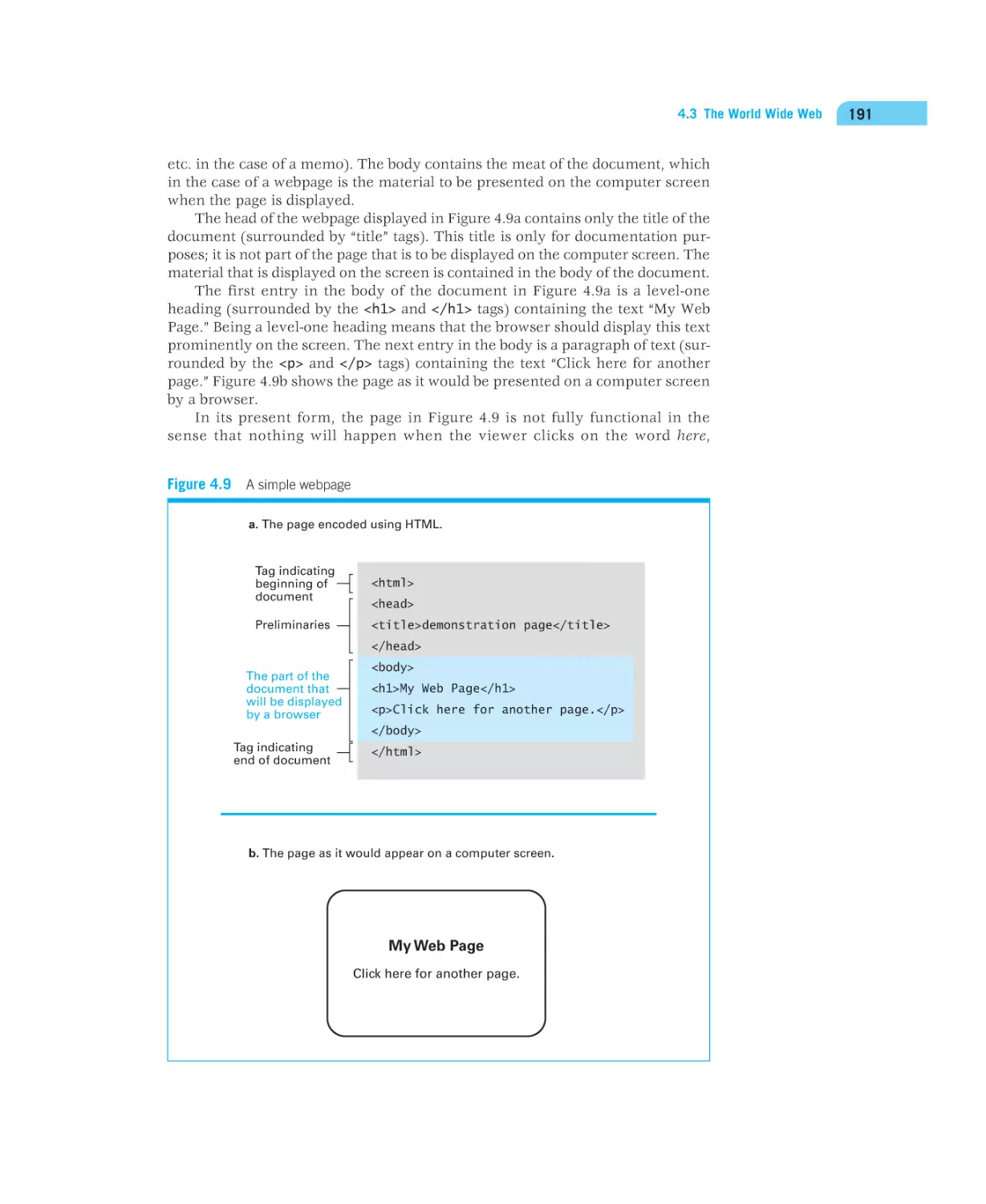


Similar


Text
computer science
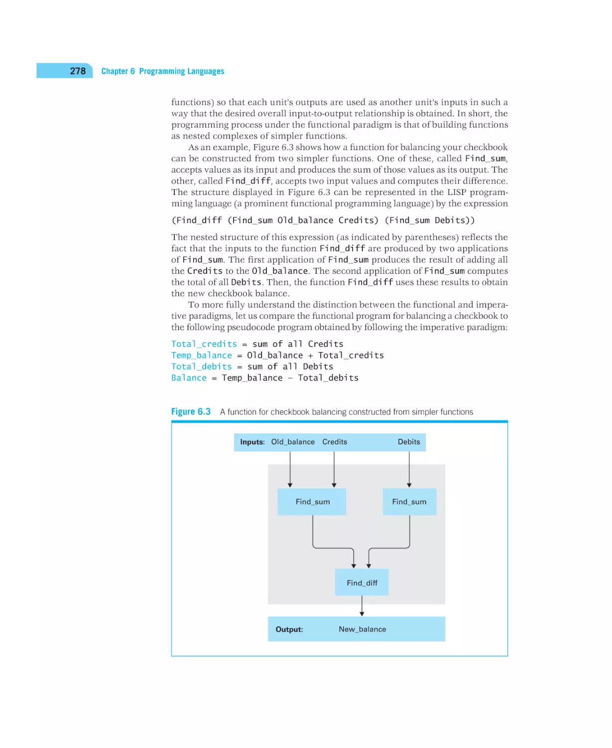
An Overview
12th Edition
Global Edition
J. Glenn Brookshear
and
Dennis Brylow
Global Edition contributions by
Manasa S.
Boston Columbus Indianapolis New York San Francisco Upper Saddle River
Amsterdam Cape Town Dubai London Madrid Milan Munich Paris Montréal Toronto
Delhi Mexico City São Paulo Sydney Hong Kong Seoul Singapore Taipei Tokyo
A01_BROO1160_12_SE_FM.indd 1
01/08/14 9:37 AM
Vice President and Editorial Director, ECS: Marcia Horton
Executive Editor: Tracy Johnson
Program Management Team Lead: Scott Disanno
Program Manager: Carole Snyder
Project Manager: Camille Trentacoste
Head, Learning Asset Acquisitions, Global Edition: Laura Dent
Acquisition Editor, Global Edition: Karthik Subramanian
Project Editor, Global Edition: Anuprova Dey Chowdhuri
Operations Specialist: Linda Sager
Cover Designer: Lumina Datamatics Ltd
Cover Image: Andrea Danti/Shutterstock
Cover Printer/Binder: Courier Kendallville
Pearson Education Limited
Edinburgh Gate
Harlow
Essex CM20 2JE
England
and Associated Companies throughout the world
Visit us on the World Wide Web at:
www.pearsonglobaleditions.com
© Pearson Education Limited 2015
The rights of J. Glenn Brookshear and Dennis Brylow to be identified as the authors of this work have been asserted by them in
accordance with the Copyright, Designs and Patents Act 1988.
Authorized adaptation from the United States edition, entitled computer science: An Overview, 12th edition, ISBN 973-0-13-376006-4, by
J. Glenn Brookshear and Dennis Brylow, published by Pearson Education © 2015.
All rights reserved. No part of this publication may be reproduced, stored in a retrieval system, or transmitted in any form or by any
means, electronic, mechanical, photocopying, recording or otherwise, without either the prior written permission of the publisher or a
license permitting restricted copying in the United Kingdom issued by the Copyright Licensing Agency Ltd, Saffron House, 6–10 Kirby
Street, London EC1N 8TS.
All trademarks used herein are the property of their respective owners.The use of any trademark in this text does not vest in the author
or publisher any trademark ownership rights in such trademarks, nor does the use of such trademarks imply any affiliation with or
endorsement of this book by such owners.
Microsoft and/or its respective suppliers make no representations about the suitability of the information contained in the documents
and related graphics published as part of the services for any purpose. All such documents and related graphics are provided “as is”
without warranty of any kind. Microsoft and/or its respective suppliers hereby disclaim all warranties and conditions with regard to this
information, including all warranties and conditions of merchantability, whether express, implied or statutory, fitness for a particular
purpose, title and non-infringement. In no event shall Microsoft and/or its respective suppliers be liable for any special, indirect or
consequential damages or any damages whatsoever resulting from loss of use, data or profits, whether in an action of contract, negligence
or other tortious action, arising out of or in connection with the use or performance of information available from the services.
The documents and related graphics contained herein could include technical inaccuracies or typographical errors. Changes are periodically
added to the information herein. Microsoft and/or its respective suppliers may make improvements and/or changes in the product(s) and/
or the program(s) described herein at any time. Partial screen shots may be viewed in full within the software version specified.
Microsoft® and Windows® are registered trademarks of the Microsoft Corporation in the U.S.A. and other countries. This book is not
sponsored or endorsed by or affiliated with the Microsoft Corporation.
ISBN 10: 1-292-06116-2
ISBN 13: 978-1-292-06116-0
10 9 8 7 6 5 4 3 2 1
14 13 12 11 10
British Library Cataloguing-in-Publication Data
A catalogue record for this book is available from the British Library
Typeset in 8 VeljovicStd-Books by Laserwords Private, LTD.
Printed and bound by Courier Kendallville.
The publisher’s policy is to use paper manufactured from sustainable forests.
A01_BROO1160_12_SE_FM.indd 2
01/08/14 9:37 AM
Preface
This book presents an introductory survey of computer science. It explores the
breadth of the subject while including enough depth to convey an honest appreciation for the topics involved.
Audience
We wrote this text for students of computer science as well as students from other
disciplines. As for computer science students, most begin their studies with the
illusion that computer science is programming, Web browsing, and Internet file
sharing because that is essentially all they have seen. Yet computer science is
much more than this. Beginning computer science students need exposure to
the breadth of the subject in which they are planning to major. Providing this
exposure is the theme of this book. It gives students an overview of computer
science—a foundation from which they can appreciate the relevance and interrelationships of future courses in the field. This survey approach is, in fact, the
model used for introductory courses in the natural sciences.
This broad background is also what students from other disciplines need if
they are to relate to the technical society in which they live. A computer science
course for this audience should provide a practical, realistic understanding of the
entire field rather than merely an introduction to using the Internet or training
in the use of some popular software packages. There is, of course, a proper place
for that training, but this text is about educating.
While writing previous editions of this text, maintaining accessibility for nontechnical students was a major goal. The result was that the book has been used
successfully in courses for students over a wide range of disciplines and educational levels, ranging from high school to graduate courses. This 12th edition is
designed to continue that tradition.
New in the 12th Edition
The underlying theme during the development of this 12th edition has been incorporating an introduction to the Python programming language into key chapters.
In the earliest chapters, these supplementary sections are labeled optional.
3
A01_BROO1160_12_SE_FM.indd 3
01/08/14 9:37 AM
4
Preface
By Chapter 5, we replace the previous editions’ Pascal-like notation with Python
and Python-flavored pseudocode.
This represents a significant change for a book that has historically striven
to sidestep allegiance to any specific language. We make this change for several
reasons. First, the text already contains quite a bit of code in various languages,
including detailed pseudocode in several chapters. To the extent that readers are
already absorbing a fair amount of syntax, it seems appropriate to retarget that
syntax toward a language they may actually see in a subsequent course. More
importantly, a growing number of instructors who use this text have made the
determination that even in a breadth-first introduction to computing, it is difficult
for students to master many of the topics in the absence of programming tools
for exploration and experimentation.
But why Python? Choosing a language is always a contentious matter, with
any choice bound to upset at least as many as it pleases. Python is an excellent
middle ground, with:
• a clean, easily learned syntax,
• simple I/O primitives,
• data types and control structures that correspond closely to the
pseudocode primitives used in earlier editions, and
• support for multiple programming paradigms.
It is a mature language with a vibrant development community and copious online resources for further study. Python remains one of the top 10 most
commonly used languages in industry by some measures, and has seen a sharp
increase in its usage for introductory computer science courses. It is particularly
popular for introductory courses for non-majors, and has wide acceptance in
other STEM fields such as physics and biology as the language of choice for computational science applications.
Nevertheless, the focus of the text remains on broad computer science
concepts; the Python supplements are intended to give readers a deeper taste
of programming than previous editions, but not to serve as a full-fledged introduction to programming. The Python topics covered are driven by the existing
structure of the text. Thus, Chapter 1 touches on Python syntax for representing
data—integers, floats, ASCII and Unicode strings, etc. Chapter 2 touches on Python
operations that closely mirror the machine primitives discussed throughout the
rest of the chapter. Conditionals, loops, and functions are introduced in Chapter 5,
at the time that those constructs are needed to devise a sufficiently complete
pseudocode for describing algorithms. In short, Python constructs are used to
reinforce computer science concepts rather than to hijack the conversation.
In addition to the Python content, virtually every chapter has seen revisions,
updates, and corrections from the previous editions.
Organization
This text follows a bottom-up arrangement of subjects that progresses from the
concrete to the abstract—an order that results in a sound pedagogical presentation in which each topic leads to the next. It begins with the fundamentals of
information encoding, data storage, and computer architecture (Chapters 1 and 2);
progresses to the study of operating systems (Chapter 3) and computer networks
A01_BROO1160_12_SE_FM.indd 4
01/08/14 9:37 AM
Organization
5
(Chapter 4); investigates the topics of algorithms, programming languages, and
software development (Chapters 5 through 7); explores techniques for enhancing
the accessibility of information (Chapters 8 and 9); considers some major applications of computer technology via graphics (Chapter 10) and artificial intelligence
(Chapter 11); and closes with an introduction to the abstract theory of computation (Chapter 12).
Although the text follows this natural progression, the individual chapters and
sections are surprisingly independent and can usually be read as isolated units or
rearranged to form alternative sequences of study. Indeed, the book is often used
as a text for courses that cover the material in a variety of orders. One of these
alternatives begins with material from Chapters 5 and 6 (Algorithms and Programming Languages) and returns to the earlier chapters as desired. I also know of
one course that starts with the material on computability from Chapter 12. In still
other cases, the text has been used in “senior capstone” courses where it serves as
merely a backbone from which to branch into projects in different areas. Courses
for less technically-oriented audiences may want to concentrate on Chapters 4
(Networking and the Internet), 9 (Database Systems), 10 (Computer Graphics),
and 11 (Artificial Intelligence).
On the opening page of each chapter, we have used asterisks to mark some
sections as optional. These are sections that cover topics of more specific interest
or perhaps explore traditional topics in more depth. Our intention is merely to
provide suggestions for alternative paths through the text. There are, of course,
other shortcuts. In particular, if you are looking for a quick read, we suggest the
following sequence:
Section
Topic
1.1–1.4
Basics of data encoding and storage
2.1–2.3
Machine architecture and machine language
3.1–3.3
Operating systems
4.1–4.3
Networking and the Internet
5.1–5.4
Algorithms and algorithm design
6.1–6.4
Programming languages
7.1–7.2
Software engineering
8.1–8.3
Data abstractions
9.1–9.2
Database systems
10.1–10.2
Computer graphics
11.1–11.3
Artificial intelligence
12.1–12.2
Theory of computation
There are several themes woven throughout the text. One is that computer
science is dynamic. The text repeatedly presents topics in a historical perspective,
discusses the current state of affairs, and indicates directions of research. Another
theme is the role of abstraction and the way in which abstract tools are used to
control complexity. This theme is introduced in Chapter 0 and then echoed in
the context of operating system architecture, networking, algorithm development, programming language design, software engineering, data organization,
and computer graphics.
A01_BROO1160_12_SE_FM.indd 5
01/08/14 9:37 AM
6
Preface
To Instructors
There is more material in this text than students can normally cover in a single
semester so do not hesitate to skip topics that do not fit your course objectives or
to rearrange the order as you see fit. You will find that, although the text follows
a plot, the topics are covered in a largely independent manner that allows you
to pick and choose as you desire. The book is designed to be used as a course
resource—not as a course definition. We suggest encouraging students to read
the material not explicitly included in your course. We underrate students if we
assume that we have to explain everything in class. We should be helping them
learn to learn on their own.
We feel obliged to say a few words about the bottom-up, concrete-to-abstract
organization of the text. As academics, we too often assume that students will
appreciate our perspective of a subject—often one that we have developed over
many years of working in a field. As teachers, we think we do better by presenting material from the student’s perspective. This is why the text starts with data
representation/storage, machine architecture, operating systems, and networking. These are topics to which students readily relate—they have most likely
heard terms such as JPEG and MP3; they have probably recorded data on CDs
and DVDs; they have purchased computer components; they have interacted
with an operating system; and they have used the Internet. By starting the course
with these topics, students discover answers to many of the “why” questions they
have been carrying for years and learn to view the course as practical rather than
theoretical. From this beginning it is natural to move on to the more abstract
issues of algorithms, algorithmic structures, programming languages, software
development methodologies, computability, and complexity that those of us in
the field view as the main topics in the science. As already stated, the topics are
presented in a manner that does not force you to follow this bottom-up sequence,
but we encourage you to give it a try.
We are all aware that students learn a lot more than we teach them directly,
and the lessons they learn implicitly are often better absorbed than those that
are studied explicitly. This is significant when it comes to “teaching” problem
solving. Students do not become problem solvers by studying problem-solving
methodologies. They become problem solvers by solving problems—and not just
carefully posed “textbook problems.” So this text contains numerous problems,
a few of which are intentionally vague—meaning that there is not necessarily a
single correct approach or a single correct answer. We encourage you to use these
and to expand on them.
Other topics in the “implicit learning” category are those of professionalism,
ethics, and social responsibility. We do not believe that this material should be
presented as an isolated subject that is merely tacked on to the course. Instead,
it should be an integral part of the coverage that surfaces when it is relevant.
This is the approach followed in this text. You will find that Sections 3.5, 4.5, 7.9,
9.7, and 11.7 present such topics as security, privacy, liability, and social awareness in the context of operating systems, networking, software engineering,
database systems, and artificial intelligence. You will also find that each chapter
includes a collection of questions called Social Issues that challenge students to
think about the relationship between the material in the text and the society in
which they live.
A01_BROO1160_12_SE_FM.indd 6
01/08/14 9:37 AM
Supplemental Resources
7
Thank you for considering our text for your course. Whether you do or do not
decide that it is right for your situation, I hope that you find it to be a contribution
to the computer science education literature.
Pedagogical Features
This text is the product of many years of teaching. As a result, it is rich in pedagogical aids. Paramount is the abundance of problems to enhance the student’s
participation—over 1,000 in this 12th edition. These are classified as Questions &
Exercises, Chapter Review Problems, and Social Issues. The Questions & Exercises appear at the end of each section (except for the introductory chapter).
They review the material just discussed, extend the previous discussion, or hint
at related topics to be covered later. These questions are answered in Appendix F.
The Chapter Review Problems appear at the end of each chapter (except for
the introductory chapter). They are designed to serve as “homework” problems
in that they cover the material from the entire chapter and are not answered in
the text.
Also at the end of each chapter are the questions in the Social Issues category.
They are designed for thought and discussion. Many of them can be used to
launch research assignments culminating in short written or oral reports.
Each chapter also ends with a list called Additional Reading that contains
references to other material relating to the subject of the chapter. The websites
identified in this preface, in the text, and in the sidebars of the text are also good
places to look for related material.
Supplemental Resources
A variety of supplemental materials for this text are available at the book’s companion website: www.pearsonglobaleditions.com/brookshear. The following
are accessible to all readers:
• Chapter-by-chapter activities that extend topics in the text and provide
opportunities to explore related topics
• Chapter-by-chapter “self-tests” that help readers to rethink the material
covered in the text
• Manuals that teach the basics of Java and C+ in a pedagogical sequence
compatible with the text
In addition, the following supplements are available to qualified
instructors at Pearson Education’s Instructor Resource Center. Please visit
www.pearsonglobaleditions.com/brookshear or contact your Pearson sales
representative for information on how to access them:
• Instructor’s Guide with answers to the Chapter Review Problems
• PowerPoint lecture slides
• Test bank
Errata for this book (should there be any!) will be available at
www.pearsonglobaleditions.com/brookshear.
A01_BROO1160_12_SE_FM.indd 7
01/08/14 9:37 AM
8
Preface
To Students
Glenn Brookshear is a bit of a nonconformist (some of his friends would say more
than a bit) so when he set out to write this text he didn’t always follow the advice
he received. In particular, many argued that certain material was too advanced
for beginning students. But, we believe that if a topic is relevant, then it is relevant even if the academic community considers it to be an “advanced topic.”
You deserve a text that presents a complete picture of computer science—not
a watered-down version containing artificially simplified presentations of only
those topics that have been deemed appropriate for introductory students. Thus,
we have not avoided topics. Instead, we’ve sought better explanations. We’ve
tried to provide enough depth to give you an honest picture of what computer
science is all about. As in the case of spices in a recipe, you may choose to skip
some of the topics in the following pages, but they are there for you to taste if you
wish—and we encourage you to do so.
We should also point out that in any course dealing with technology, the
details you learn today may not be the details you will need to know tomorrow.
The field is dynamic—that’s part of the excitement. This book will give you a current picture of the subject as well as a historical perspective. With this background
you will be prepared to grow along with technology. We encourage you to start
the growing process now by exploring beyond this text. Learn to learn.
Thank you for the trust you have placed in us by choosing to read our book.
As authors we have an obligation to produce a manuscript that is worth your time.
We hope you find that we have lived up to this obligation.
Acknowledgments
First and foremost, I thank Glenn Brookshear, who has shepherded this book, “his
baby,” through eleven previous editions, spanning more than a quarter century of
rapid growth and tumultuous change in the field of computer science. While this
is the first edition in which he has allowed a co-author to oversee all of the revisions, the pages of this 12th edition remain overwhelmingly in Glenn’s voice and,
I hope, guided by his vision. Any new blemishes are mine; the elegant underlying
framework is all his.
I join Glenn in thanking those of you who have supported this book by reading and using it in previous editions. We are honored.
David T. Smith (Indiana University of Pennsylvania) played a significant
role in co-authoring revisions to the 11th edition with me, many of which are
still visible in this 12th edition. David’s close reading of this edition and careful
attention to the supplemental materials have been essential. Andrew Kuemmel
(Madison West), George Corliss (Marquette), and Chris Mayfield (James Madison)
all provided valuable feedback, insight, and/or encouragement on drafts for this
edition, while James E. Ames (Virginia Commonwealth), Stephanie E. August
(Loyola), Yoonsuck Choe (Texas A&M), Melanie Feinberg (UT-Austin), Eric
D. Hanley (Drake), Sudharsan R. Iyengar (Winona State), Ravi Mukkamala
(Old Dominion), and Edward Pryor (Wake Forest) all offered valuable reviews of
the Python-specific revisions.
A01_BROO1160_12_SE_FM.indd 8
01/08/14 9:37 AM
Acknowledgments
9
Others who have contributed in this or previous editions include J. M. Adams,
C. M. Allen, D. C. S. Allison, E. Angel, R. Ashmore, B. Auernheimer, P. Bankston,
M. Barnard, P. Bender, K. Bowyer, P. W. Brashear, C. M. Brown, H. M Brown,
B. Calloni, J. Carpinelli, M. Clancy, R. T. Close, D. H. Cooley, L. D. Cornell, M.
J. Crowley, F. Deek, M. Dickerson, M. J. Duncan, S. Ezekiel, C. Fox, S. Fox,
N. E. Gibbs, J. D. Harris, D. Hascom, L. Heath, P. B. Henderson, L. Hunt, M.
Hutchenreuther, L. A. Jehn, K. K. Kolberg, K. Korb, G. Krenz, J. Kurose, J. Liu,
T. J. Long, C. May, J. J. McConnell, W. McCown, S. J. Merrill, K. Messersmith,
J. C. Moyer, M. Murphy, J. P. Myers, Jr., D. S. Noonan, G. Nutt, W. W. Oblitey,
S. Olariu, G. Riccardi, G. Rice, N. Rickert, C. Riedesel, J. B. Rogers, G. Saito, W.
Savitch, R. Schlafly, J. C. Schlimmer, S. Sells, Z. Shen, G. Sheppard, J. C. Simms,
M. C. Slattery, J. Slimick, J. A. Slomka, J. Solderitsch, R. Steigerwald, L. Steinberg,
C. A. Struble, C. L. Struble, W. J. Taffe, J. Talburt, P. Tonellato, P. Tromovitch,
P. H. Winston, E. D. Winter, E. Wright, M. Ziegler, and one anonymous. To these
individuals we give our sincere thanks.
As already mentioned, you will find Java and C++ manuals at the text’s
Companion Website that teach the basics of these languages in a format compatible with the text. These were written by Diane Christie. Thank you, Diane.
Another thank you goes to Roger Eastman who was the creative force behind the
chapter-by-chapter activities that you will also find at the companion website.
I also thank the good people at Pearson who have supported this project.
Tracy Johnson, Camille Trentacoste, and Carole Snyder in particular have been
a pleasure to work with, and brought their wisdom and many improvements to
the table throughout the process.
Finally, my thanks to my wife, Petra—“the Rock”—to whom this edition is
dedicated. Her patience and fortitude all too frequently exceeded my own, and
this book is better for her steadying influence.
D.W.B.
Pearson wishes to thank Arup Bhattacharjee, Soumen Mukherjee, and Chethan
Venkatesh for reviewing the Global Edition.
A01_BROO1160_12_SE_FM.indd 9
01/08/14 9:37 AM
Contents
Chapter 0
Introduction
0.1
0.2
0.3
0.4
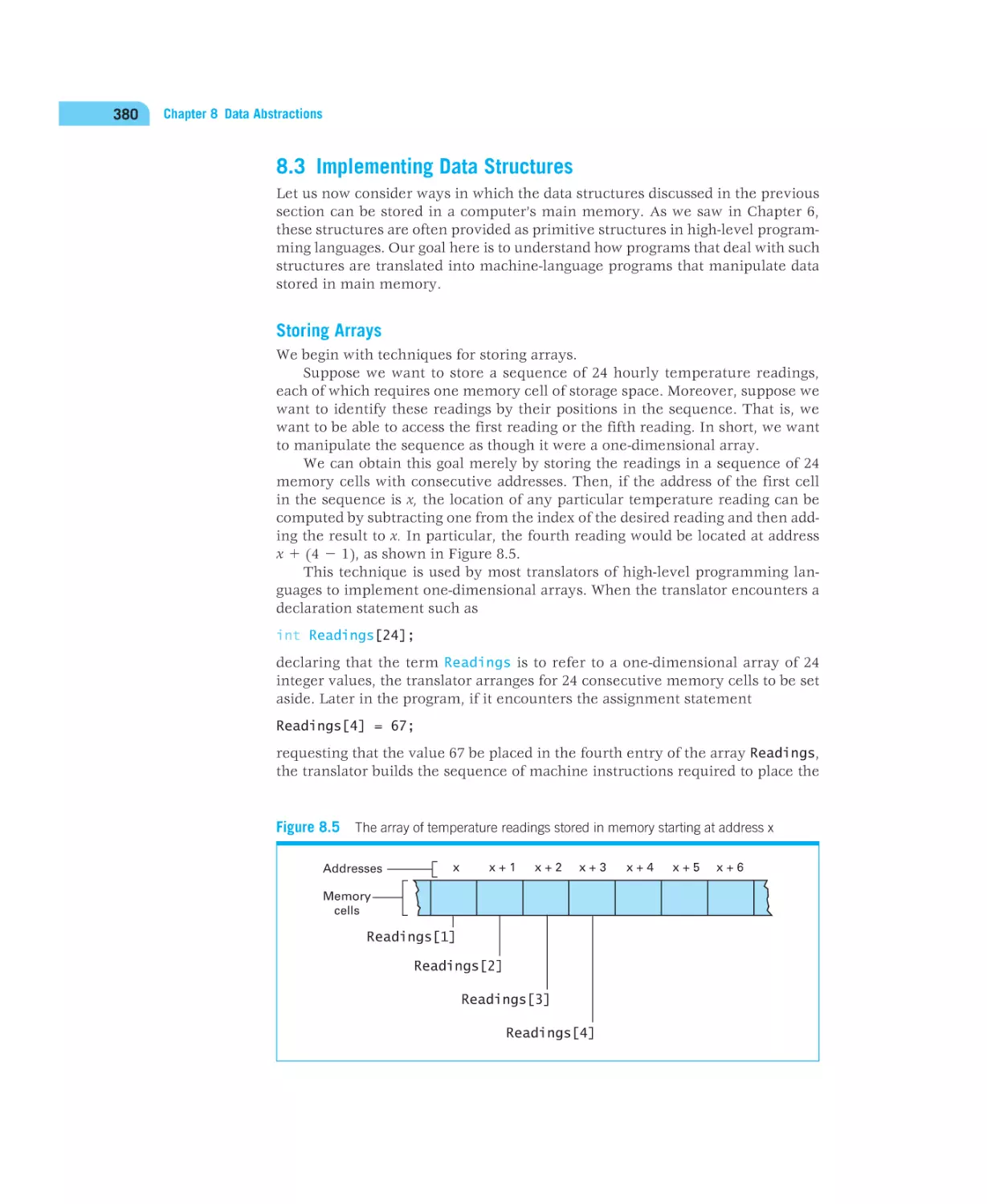
Chapter 1
Chapter 2
23
31
Bits and Their Storage 32
Main Memory 38
Mass Storage 41
Representing Information as Bit Patterns
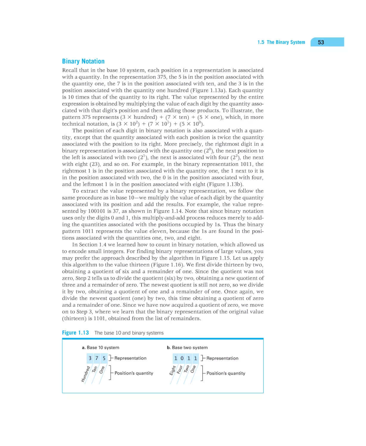
The Binary System 52
Storing Integers 58
Storing Fractions 64
Data and Programming 69
Data Compression 75
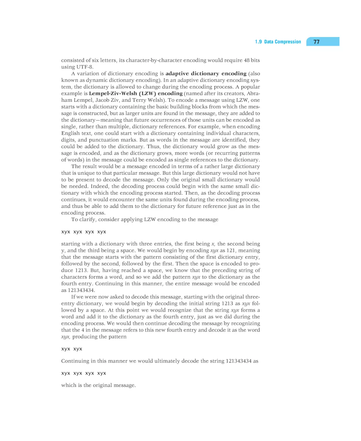
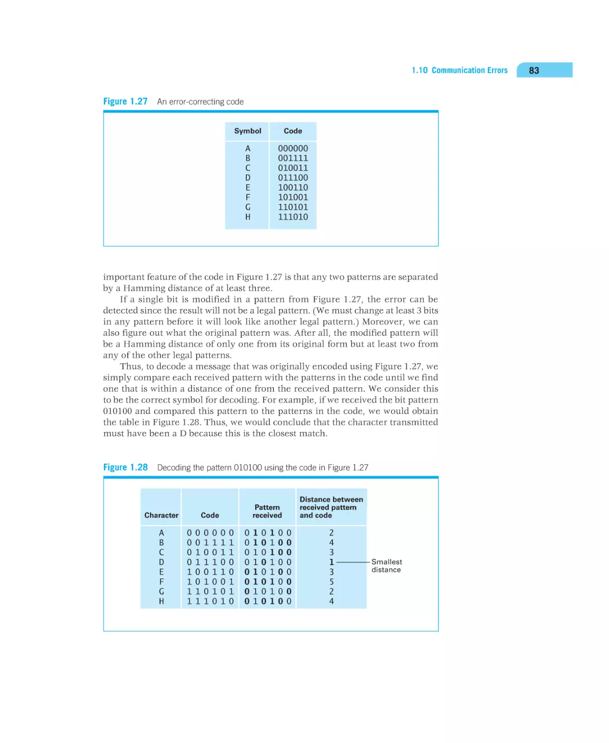
Communication Errors 81
Data Manipulation
2.1
2.2
2.3
*2.4
*2.5
*2.6
*2.7
Chapter 3
The Role of Algorithms 14
The History of Computing 16
An Outline of Our Study 21
The Overarching Themes of Computer Science
Data Storage
1.1
1.2
1.3
1.4
*1.5
*1.6
*1.7
*1.8
*1.9
*1.10
13
46
93
Computer Architecture 94
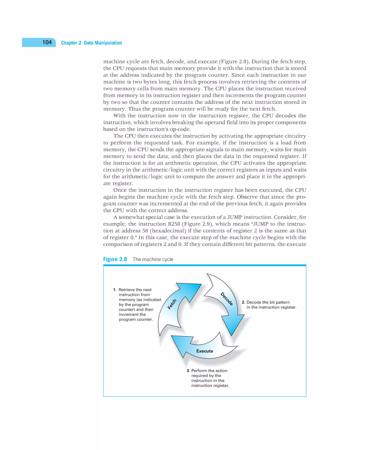
Machine Language 97
Program Execution 103
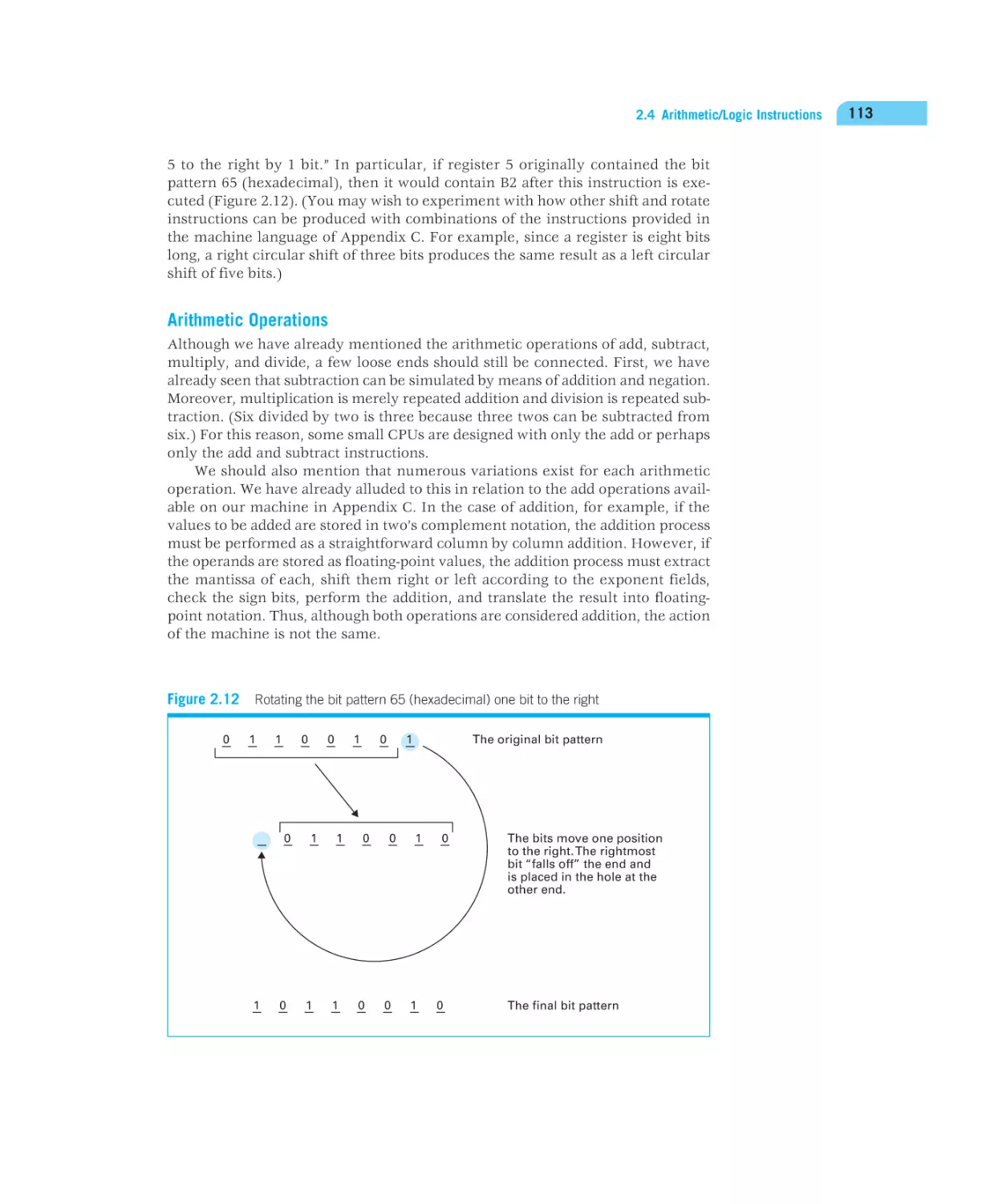
Arithmetic/Logic Instructions 110
Communicating with Other Devices 115
Programming Data Manipulation 120
Other Architectures 129
Operating Systems
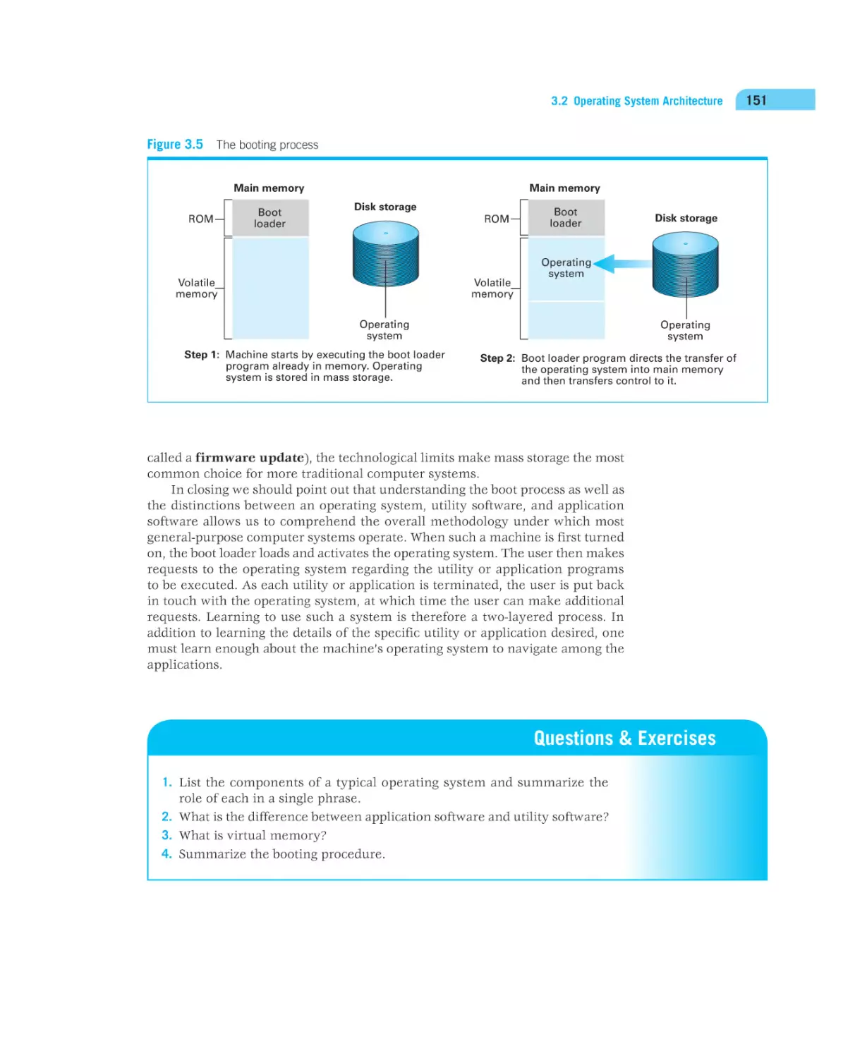
139
3.1 The History of Operating Systems 140
3.2 Operating System Architecture 144
3.3 Coordinating the Machine’s Activities 152
*Asterisks indicate suggestions for optional sections.
10
A01_BROO1160_12_SE_FM.indd 10
01/08/14 9:37 AM
Contents
*3.4 Handling Competition Among Processes
3.5 Security 160
Chapter 4
Networking and the Internet
4.1
4.2
4.3
*4.4
4.5
Chapter 5
Chapter 6
Chapter 7
Chapter 8
271
Historical Perspective 272
Traditional Programming Concepts 280
Procedural Units 292
Language Implementation 300
Object-Oriented Programming 308
Programming Concurrent Activities 315
Declarative Programming 318
331
The Software Engineering Discipline 332
The Software Life Cycle 334
Software Engineering Methodologies 338
Modularity 341
Tools of the Trade 348
Quality Assurance 356
Documentation 360
The Human-Machine Interface 361
Software Ownership and Liability 364
Data Abstractions 373
8.1
8.2
8.3
8.4
8.5
8.6
*8.7
A01_BROO1160_12_SE_FM.indd 11
The Concept of an Algorithm 218
Algorithm Representation 221
Algorithm Discovery 228
Iterative Structures 234
Recursive Structures 245
Efficiency and Correctness 253
Software Engineering
7.1
7.2
7.3
7.4
7.5
7.6
7.7
7.8
7.9
169
217
Programming Languages
6.1
6.2
6.3
6.4
6.5
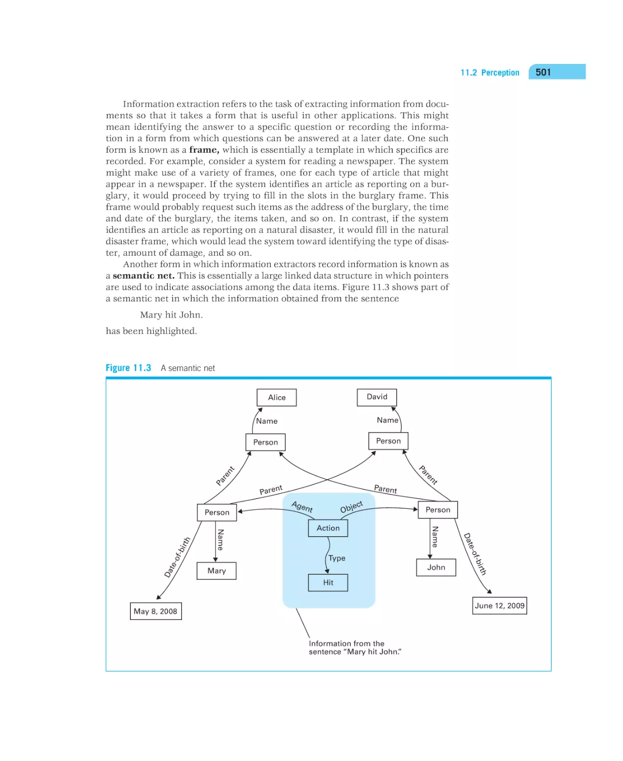
*6.6
*6.7
155
Network Fundamentals 170
The Internet 179
The World Wide Web 188
Internet Protocols 197
Security 203
Algorithms
5.1
5.2
5.3
5.4
5.5
5.6
11
Basic Data Structures 374
Related Concepts 377
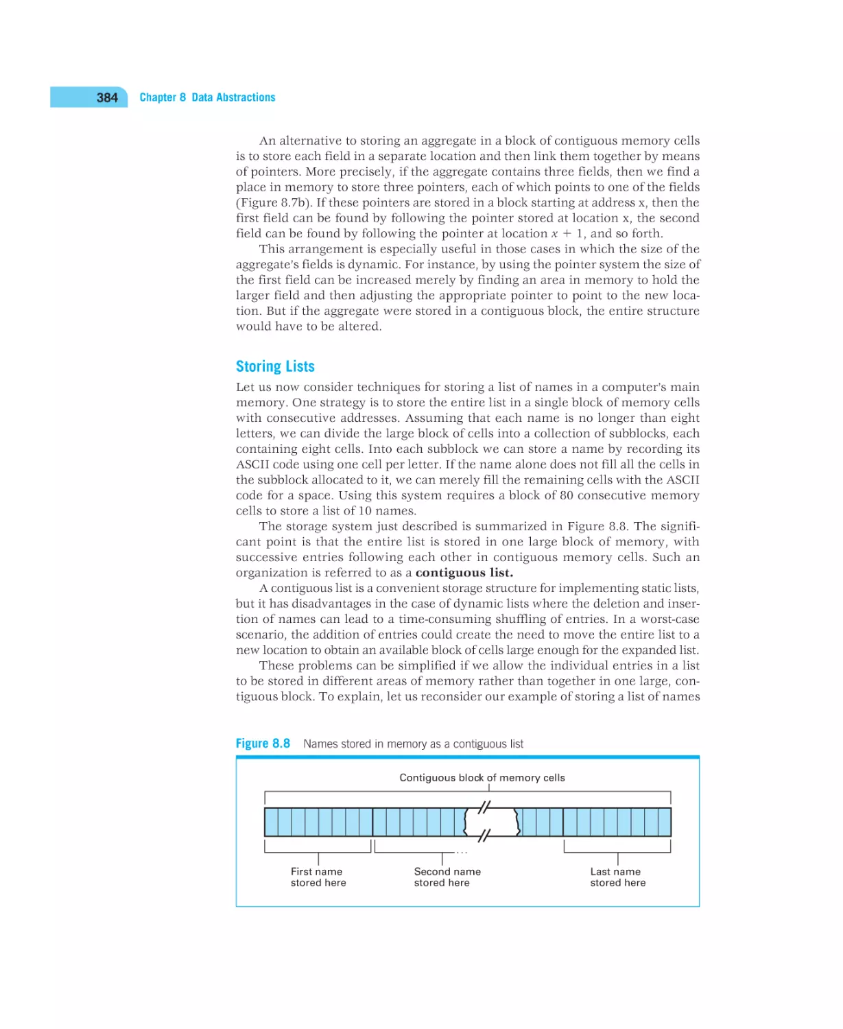
Implementing Data Structures 380
A Short Case Study 394
Customized Data Types 399
Classes and Objects 403
Pointers in Machine Language 405
01/08/14 9:37 AM
12
Contents
Chapter 9
Database Systems
9.1
9.2
*9.3
*9.4
*9.5
9.6
9.7
Chapter 10
415
Database Fundamentals 416
The Relational Model 421
Object-Oriented Databases 432
Maintaining Database Integrity 434
Traditional File Structures 438
Data Mining 446
Social Impact of Database Technology
448
Computer Graphics 457
10.1
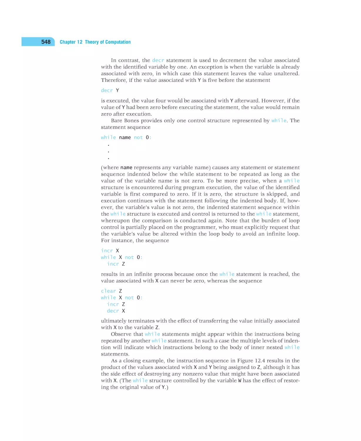
10.2
10.3
10.4
*10.5
10.6
Chapter 11
The Scope of Computer Graphics 458
Overview of 3D Graphics 460
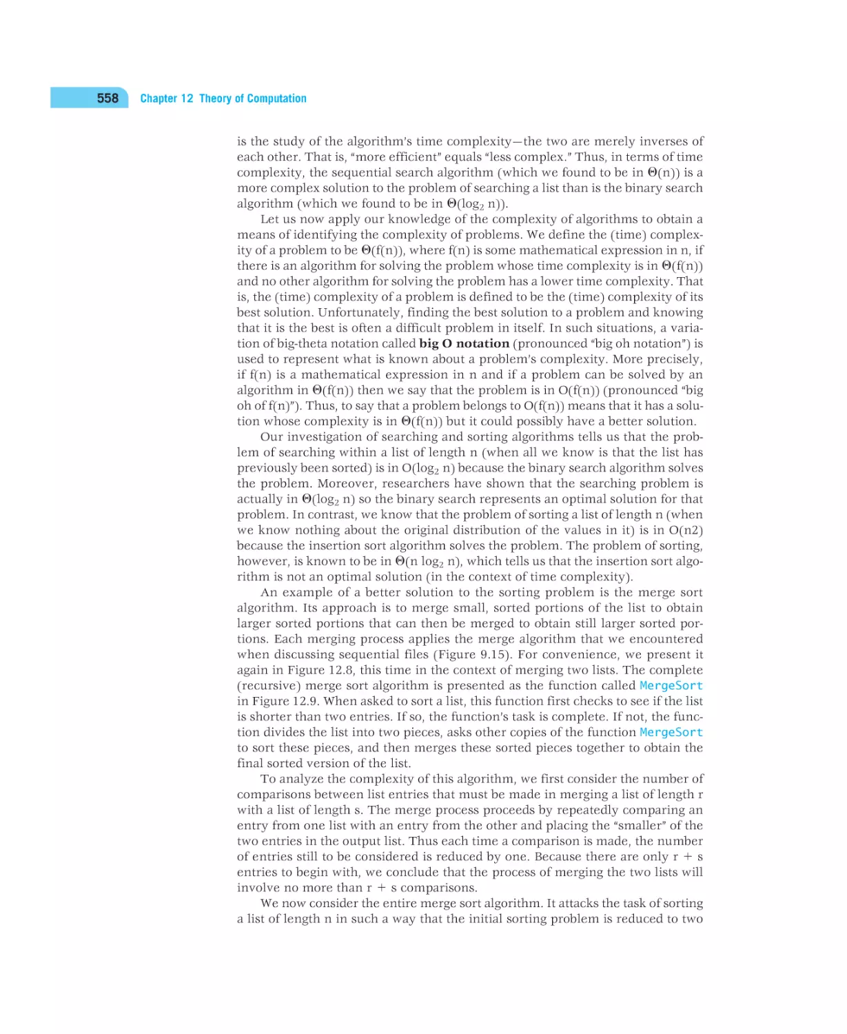
Modeling 461
Rendering 469
Dealing with Global Lighting 480
Animation 483
Artificial Intelligence
11.1
11.2
11.3
11.4
11.5
11.6
11.7
Chapter 12
Theory of Computation
12.1
12.2
12.3
12.4
12.5
*12.6
Appendixes
491
Intelligence and Machines 492
Perception 497
Reasoning 503
Additional Areas of Research 514
Artificial Neural Networks 519
Robotics 526
Considering the Consequences 529
539
Functions and Their Computation 540
Turing Machines 542
Universal Programming Languages 546
A Noncomputable Function 552
Complexity of Problems 556
Public-Key Cryptography 565
575
A ASCII 577
B Circuits to Manipulate Two’s Complement
Representations 578
C A Simple Machine Language 581
D High-Level Programming Languages 583
E The Equivalence of Iterative and Recursive Structures
F Answers to Questions & Exercises 587
Index
A01_BROO1160_12_SE_FM.indd 12
585
629
01/08/14 9:37 AM
0
C H A P T E R
Introduction
In this preliminary chapter we consider the scope of computer
science, develop a historical perspective, and establish a
foundation from which to launch our study.
0.1
The Role of Algorithms
0.2 The History of
Computing
0.3
M00_BROO1160_12_SE_C00.indd 13
An Outline of Our Study
0.4 The Overarching
Themes of Computer Science
Algorithms
Abstraction
Creativity
Data
Programming
Internet
Impact
01/08/14 11:18 AM
14
Chapter 0 Introduction
Computer science is the discipline that seeks to build a scientific foundation for
such topics as computer design, computer programming, information processing,
algorithmic solutions of problems, and the algorithmic process itself. It provides
the underpinnings for today’s computer applications as well as the foundations
for tomorrow’s computing infrastructure.
This book provides a comprehensive introduction to this science. We will
investigate a wide range of topics including most of those that constitute a typical
university computer science curriculum. We want to appreciate the full scope
and dynamics of the field. Thus, in addition to the topics themselves, we will
be interested in their historical development, the current state of research, and
prospects for the future. Our goal is to establish a functional understanding of
computer science—one that will support those who wish to pursue more specialized studies in the science as well as one that will enable those in other fields to
flourish in an increasingly technical society.
0.1 The Role of Algorithms
We begin with the most fundamental concept of computer science—that of an
algorithm. Informally, an algorithm is a set of steps that defines how a task is
performed. (We will be more precise later in Chapter 5.) For example, there are
algorithms for cooking (called recipes), for finding your way through a strange
city (more commonly called directions), for operating washing machines (usually
displayed on the inside of the washer’s lid or perhaps on the wall of a laundromat), for playing music (expressed in the form of sheet music), and for performing magic tricks (Figure 0.1).
Before a machine such as a computer can perform a task, an algorithm for
performing that task must be discovered and represented in a form that is compatible with the machine. A representation of an algorithm is called a program. For
the convenience of humans, computer programs are usually printed on paper or
displayed on computer screens. For the convenience of machines, programs are
encoded in a manner compatible with the technology of the machine. The process
of developing a program, encoding it in machine-compatible form, and inserting
it into a machine is called programming. Programs, and the algorithms they
represent, are collectively referred to as software, in contrast to the machinery
itself, which is known as hardware.
The study of algorithms began as a subject in mathematics. Indeed, the
search for algorithms was a significant activity of mathematicians long before
the d
evelopment of today’s computers. The goal was to find a single set of
directions that described how all problems of a particular type could be solved.
One of the best known examples of this early research is the long division
algorithm for finding the quotient of two multiple-digit numbers. Another
example is the Euclidean algorithm, discovered by the ancient Greek mathematician Euclid, for finding the greatest common divisor of two positive
integers (Figure 0.2).
Once an algorithm for performing a task has been found, the performance
of that task no longer requires an understanding of the principles on which the
algorithm is based. Instead, the performance of the task is reduced to the process
of merely following directions. (We can follow the long division algorithm to find
a quotient or the Euclidean algorithm to find a greatest common divisor without
M00_BROO1160_12_SE_C00.indd 14
01/08/14 11:18 AM
0.1 The Role of Algorithms
15
Figure 0.1 An algorithm for a magic trick
Effect: The performer places some cards from a normal deck of playing cards face
down on a table and mixes them thoroughly while spreading them out on the table.
Then, as the audience requests either red or black cards, the performer turns over cards
of the requested color.
Secret and Patter:
Step 1. From a normal deck of cards, select ten red cards and ten black cards. Deal these cards
face up in two piles on the table according to color.
Step 2. Announce that you have selected some red cards and some black cards.
Step 3. Pick up the red cards. Under the pretense of aligning them into a small deck, hold them
face down in your left hand and, with the thumb and first finger of your right hand, pull
back on each end of the deck so that each card is given a slightly backward curve. Then
place the deck of red cards face down on the table as you say, “Here are the red cards
in this stack.”
Step 4. Pick up the black cards. In a manner similar to that in step 3, give these cards a slight
forward curve. Then return these cards to the table in a face-down deck as you say,
“And here are the black cards in this stack.”
Step 5. Immediately after returning the black cards to the table, use both hands to mix the red
and black cards (still face down) as you spread them out on the tabletop. Explain that
you are thoroughly mixing the cards.
Step 6. As long as there are face-down cards on the table, repeatedly
execute the following steps:
6.1. Ask the audience to request either a red or a black card.
6.2. If the color requested is red and there is a face-down card with a concave
appearance, turn over such a card while saying, “Here is a red card.”
6.3. If the color requested is black and there is a face-down card with a convex
appearance, turn over such a card while saying, “Here is a black card.”
6.4. Otherwise, state that there are no more cards of the requested color and turn over
the remaining cards to prove your claim.
Figure 0.2 The Euclidean algorithm for finding the greatest common divisor of two
positive integers
Description: This algorithm assumes that its input consists of two positive integers and
proceeds to compute the greatest common divisor of these two values.
Procedure:
Step 1. Assign M and N the value of the larger and smaller of the two input values, respectively.
Step 2. Divide M by N, and call the remainder R.
Step 3. If R is not 0, then assign M the value of N, assign N the value of R, and return to step 2;
otherwise, the greatest common divisor is the value currently assigned to N.
M00_BROO1160_12_SE_C00.indd 15
01/08/14 11:18 AM
16
Chapter 0 Introduction
understanding why the algorithm works.) In a sense, the intelligence required to
solve the problem at hand is encoded in the algorithm.
Capturing and conveying intelligence (or at least intelligent behavior) by
means of algorithms allows us to build machines that perform useful tasks.
Consequently, the level of intelligence displayed by machines is limited by
the intelligence that can be conveyed through algorithms. We can construct a
machine to perform a task only if an algorithm exists for performing that task. In
turn, if no algorithm exists for solving a problem, then the solution of that problem lies beyond the capabilities of machines.
Identifying the limitations of algorithmic capabilities solidified as a subject
in mathematics in the 1930s with the publication of Kurt Gödel’s incompleteness theorem. This theorem essentially states that in any mathematical theory
encompassing our traditional arithmetic system, there are statements whose
truth or falseness cannot be established by algorithmic means. In short, any complete study of our arithmetic system lies beyond the capabilities of algorithmic
activities. This realization shook the foundations of mathematics, and the study
of algorithmic capabilities that ensued was the beginning of the field known today
as computer science. Indeed, it is the study of algorithms that forms the core of
computer science.
0.2 The History of Computing
Today’s computers have an extensive genealogy. One of the earlier computing
devices was the abacus. History tells us that it probably had its roots in ancient
China and was used in the early Greek and Roman civilizations. The machine
is quite simple, consisting of beads strung on rods that are in turn mounted in
a rectangular frame (Figure 0.3). As the beads are moved back and forth on the
rods, their positions represent stored values. It is in the positions of the beads that
this “computer” represents and stores data. For control of an algorithm’s execution, the machine relies on the human operator. Thus the abacus alone is merely
a data storage system; it must be combined with a human to create a complete
computational machine.
In the time period after the Middle Ages and before the Modern Era, the
quest for more sophisticated computing machines was seeded. A few inventors
began to experiment with the technology of gears. Among these were Blaise
Pascal (1623–1662) of France, Gottfried Wilhelm Leibniz (1646–1716) of Germany,
and Charles Babbage (1792–1871) of England. These machines represented data
through gear positioning, with data being entered mechanically by establishing
initial gear positions. Output from Pascal’s and Leibniz’s machines was achieved
by observing the final gear positions. Babbage, on the other hand, envisioned
machines that would print results of computations on paper so that the possibility
of transcription errors would be eliminated.
As for the ability to follow an algorithm, we can see a progression of flexibility in these machines. Pascal’s machine was built to perform only addition.
Consequently, the appropriate sequence of steps was embedded into the structure of the machine itself. In a similar manner, Leibniz’s machine had its algorithms firmly embedded in its architecture, although the operator could select
from a variety of arithmetic operations it offered. Babbage’s Difference Engine
M00_BROO1160_12_SE_C00.indd 16
01/08/14 11:18 AM
0.2 The History of Computing
17
Figure 0.3 Chinese wooden abacus (Pink Badger/Fotolia)
(of which only a demonstration model was constructed) could be modified to
perform a variety of calculations, but his Analytical Engine (never funded for construction) was designed to read instructions in the form of holes in paper cards.
Thus Babbage’s Analytical Engine was programmable. In fact, Augusta Ada Byron
(Ada Lovelace), who published a paper in which she demonstrated how Babbage’s
Analytical Engine could be programmed to perform various computations, is
often identified today as the world’s first programmer.
The idea of communicating an algorithm via holes in paper was not originated by Babbage. He got the idea from Joseph Jacquard (1752–1834), who, in
1801, had developed a weaving loom in which the steps to be performed during the weaving process were determined by patterns of holes in large thick
cards made of wood (or cardboard). In this manner, the algorithm followed by
the loom could be changed easily to produce different woven designs. Another
beneficiary of Jacquard’s idea was Herman Hollerith (1860–1929), who applied
the concept of representing information as holes in paper cards to speed up the
tabulation process in the 1890 U.S. census. (It was this work by Hollerith that
led to the creation of IBM.) Such cards ultimately came to be known as punched
cards and survived as a popular means of communicating with computers well
into the 1970s.
Nineteenth-century technology was unable to produce the complex geardriven machines of Pascal, Leibniz, and Babbage cost-effectively. But with the
advances in electronics in the early 1900s, this barrier was overcome. Examples
of this progress include the electromechanical machine of George Stibitz,
completed in 1940 at Bell Laboratories, and the Mark I, completed in 1944 at
Harvard U
niversity by Howard Aiken and a group of IBM engineers. These
machines made heavy use of electronically controlled mechanical relays. In
this sense they were obsolete almost as soon as they were built, because other
researchers were a pplying the technology of vacuum tubes to construct totally
M00_BROO1160_12_SE_C00.indd 17
01/08/14 11:18 AM
18
Chapter 0 Introduction
Figure 0.4 Three women operating the ENIAC’s (Electronic Numerical Integrator And Computer)
main control panel while the machine was at the Moore School. The machine was later moved to
the U.S. Army’s Ballistics Research Laboratory. (Courtesy U.S. Army.)
electronic computers. The first of these vacuum tube machines was apparently
the Atanasoff-Berry machine, constructed during the period from 1937 to 1941
at Iowa State College (now Iowa State University) by John Atanasoff and his
assistant, Clifford Berry. Another was a machine called Colossus, built under
the direction of Tommy F
lowers in England to decode German messages during the latter part of World War II. (Actually, as many as ten of these machines
were apparently built, but military secrecy and issues of national security kept
their existence from becoming part of the “computer family tree.”) Other, more
flexible machines, such as the ENIAC (electronic numerical integrator and calcu
lator) developed by John Mauchly and J. Presper Eckert at the Moore School of
Electrical Engineering, University of Pennsylvania, soon followed (Figure 0.4).
From that point on, the history of computing machines has been closely
linked to advancing technology, including the invention of transistors (for which
physicists William Shockley, John Bardeen, and Walter Brattain were awarded a
Nobel Prize) and the subsequent development of complete circuits constructed
as single units, called integrated circuits (for which Jack Kilby also won a Nobel
Prize in physics). With these developments, the room-sized machines of the 1940s
were reduced over the decades to the size of single cabinets. At the same time,
the processing power of computing machines began to double every two years (a
trend that has continued to this day). As work on integrated circuitry progressed,
many of the components within a computer became readily available on the open
market as integrated circuits encased in toy-sized blocks of plastic called chips.
A major step toward popularizing computing was the development of desktop computers. The origins of these machines can be traced to the computer
hobbyists who built homemade computers from combinations of chips. It was
within this “underground” of hobby activity that Steve Jobs and Stephen Wozniak
M00_BROO1160_12_SE_C00.indd 18
01/08/14 11:18 AM
0.2 The History of Computing
19
Babbage’s Difference Engine
The machines designed by Charles Babbage were truly the forerunners of modern
computer design. If technology had been able to produce his machines in an eco
nomically feasible manner and if the data processing demands of commerce and
government had been on the scale of today’s requirements, Babbage’s ideas could
have led to a computer revolution in the 1800s. As it was, only a demonstration model
of his Difference Engine was constructed in his lifetime. This machine determined
numerical values by computing “successive differences.” We can gain an insight to
this technique by considering the problem of computing the squares of the integers.
We begin with the knowledge that the square of 0 is 0, the square of 1 is 1, the
square of 2 is 4, and the square of 3 is 9. With this, we can determine the square of
4 in the following manner (see the following diagram). We first compute the differ
ences of the squares we already know: 12 - 02 = 1, 22 - 12 = 3, and 32 - 22 = 5.
Then we compute the differences of these results: 3 - 1 = 2, and 5 - 3 = 2. Note
that these differences are both 2. Assuming that this consistency continues (mathe
matics can show that it does), we conclude that the difference between the value
(42 - 32) and the value (32 - 22) must also be 2. Hence (42 - 32) must be 2 greater
than (32 - 22), so 42 - 32 = 7 and thus 42 = 32 + 7 = 16. Now that we know the
square of 4, we could continue our procedure to compute the square of 5 based on
the values of 12, 22, 32, and 42. (Although a more in−depth discussion of successive
differences is beyond the scope of our current study, students of calculus may wish to
observe that the preceding example is based on the fact that the derivative of y = x 2
is a straight line with a slope of 2.)
x
x2
0
0
1
1
2
4
3
9
4
16
First
difference
1
3
5
7
Second
difference
2
2
2
2
5
built a commercially viable home computer and, in 1976, established Apple Computer, Inc. (now Apple Inc.) to manufacture and market their products. Other
companies that marketed similar products were Commodore, Heathkit, and Radio
Shack. Although these products were popular among computer hobbyists, they
were not widely accepted by the business community, which continued to look
to the well-established IBM and its large mainframe computers for the majority
of its computing needs.
In 1981, IBM introduced its first desktop computer, called the personal
computer, or PC, whose underlying software was developed by a newly formed
company known as Microsoft. The PC was an instant success and legitimized
M00_BROO1160_12_SE_C00.indd 19
01/08/14 11:18 AM
20
Chapter 0 Introduction
Augusta Ada Byron
Augusta Ada Byron, Countess of Lovelace, has been the subject of much commentary
in the computing community. She lived a somewhat tragic life of less than 37 years
(1815–1852) that was complicated by poor health and the fact that she was a non
conformist in a society that limited the professional role of women. Although she was
interested in a wide range of science, she concentrated her studies in mathematics.
Her interest in “compute science” began when she became fascinated by the
machines of Charles Babbage at a demonstration of a prototype of his Difference
Engine in 1833. Her contribution to computer science stems from her translation
from French into English of a paper discussing Babbage’s designs for the Analytical
Engine. To this translation, Babbage encouraged her to attach an addendum describ
ing applications of the engine and containing examples of how the engine could be
programmed to perform various tasks. Babbage’s enthusiasm for Ada Byron’s work
was apparently motivated by his hope that its publication would lead to financial
backing for the construction of his Analytical Engine. (As the daughter of Lord Byron,
Ada Byron held celebrity status with potentially significant financial connections.)
This backing never materialized, but Ada Byron’s addendum has survived and is
considered to contain the first examples of computer programs. The degree to which
Babbage influenced Ada Byron’s work is debated by historians. Some argue that
Babbage made major contributions, whereas others contend that he was more of an
obstacle than an aid. Nonetheless, Augusta Ada Byron is recognized today as the
world’s first programmer, a status that was certified by the U.S. Department of Defense
when it named a prominent programming language (Ada) in her honor.
the desktop computer as an established commodity in the minds of the business
community. Today, the term PC is widely used to refer to all those machines
(from various manufacturers) whose design has evolved from IBM’s initial desktop
computer, most of which continue to be marketed with software from Microsoft.
At times, however, the term PC is used interchangeably with the generic terms
desktop or laptop.
As the twentieth century drew to a close, the ability to connect individual
computers in a world-wide system called the Internet was revolutionizing communication. In this context, Tim Berners-Lee (a British scientist) proposed a system by which documents stored on computers throughout the Internet could be
linked together producing a maze of linked information called the World Wide
Web (often shortened to “Web”). To make the information on the Web accessible,
software systems, called search engines, were developed to “sift through” the
Web, “categorize” their findings, and then use the results to assist users researching particular topics. Major players in this field are Google, Yahoo, and Microsoft.
These companies continue to expand their Web-related activities, often in directions that challenge our traditional way of thinking.
At the same time that desktop and laptop computers were being accepted and
used in homes, the miniaturization of computing machines continued. Today,
tiny computers are embedded within a wide variety of electronic appliances and
devices. Automobiles may now contain dozens of small computers running Global
Positioning Systems (GPS), monitoring the function of the engine, and providing
M00_BROO1160_12_SE_C00.indd 20
01/08/14 11:18 AM
0.3 An Outline of Our Study
21
Google
Founded in 1998, Google Inc. has become one of the world’s most recognized tech
nology companies. Its core service, the Google search engine, is used by millions
of people to find documents on the World Wide Web. In addition, Google provides
electronic mail service (called Gmail), an Internet-based video-sharing service (called
YouTube), and a host of other Internet services (including Google Maps, Google
Calendar, Google Earth, Google Books, and Google Translate).
However, in addition to being a prime example of the entrepreneurial spirit,
Google also provides examples of how expanding technology is challenging society.
For example, Google’s search engine has led to questions regarding the extent to which
an international company should comply with the wishes of individual governments;
YouTube has raised questions regarding the extent to which a company should be
liable for information that others distribute through its services as well as the degree
to which the company can claim ownership of that information; Google Books has
generated concerns regarding the scope and limitations of intellectual property rights;
and Google Maps has been accused of violating privacy rights.
voice command services for controlling the car’s audio and phone communication systems.
Perhaps the most revolutionary application of computer miniaturization is
found in the expanding capabilities of smartphones, hand-held general-purpose
computers on which telephony is only one of many applications. More powerful than the supercomputers of prior decades, these pocket-sized devices are
equipped with a rich array of sensors and interfaces including cameras, microphones, compasses, touch screens, accelerometers (to detect the phone’s orientation and motion), and a number of wireless technologies to communicate with
other smartphones and computers. Many argue that the smartphone is having a
greater effect on global society than the PC revolution.
0.3 An Outline of Our Study
This text follows a bottom-up approach to the study of computer science, beginning with such hands-on topics as computer hardware and leading to the more
abstract topics such as algorithm complexity and computability. The result is
that our study follows a pattern of building larger and larger abstract tools as our
understanding of the subject expands.
We begin by considering topics dealing with the design and construction of
machines for executing algorithms. In Chapter 1 (Data Storage), we look at how
information is encoded and stored within modern computers, and in Chapter 2
(Data Manipulation), we investigate the basic internal operation of a simple computer. Although part of this study involves technology, the general theme is technology independent. That is, such topics as digital circuit design, data encoding
and compression systems, and computer architecture are relevant over a wide
range of technology and promise to remain relevant regardless of the direction
of future technology.
M00_BROO1160_12_SE_C00.indd 21
01/08/14 11:18 AM
22
Chapter 0 Introduction
In Chapter 3 (Operating Systems), we study the software that controls the
overall operation of a computer. This software is called an operating system. It is
a computer’s operating system that controls the interface between the machine
and its outside world, protecting the machine and the data stored within from
unauthorized access, allowing a computer user to request the execution of various programs, and coordinating the internal activities required to fulfill the user’s
requests.
In Chapter 4 (Networking and the Internet), we study how computers are
connected to each other to form computer networks and how networks are connected to form internets. This study leads to topics such as network protocols, the
Internet’s structure and internal operation, the World Wide Web, and numerous
issues of security.
Chapter 5 (Algorithms) introduces the study of algorithms from a more formal perspective. We investigate how algorithms are discovered, identify several fundamental algorithmic structures, develop elementary techniques for
representing algorithms, and introduce the subjects of algorithm efficiency and
correctness.
In Chapter 6 (Programming Languages), we consider the subject of algorithm
representation and the program development process. Here we find that the
search for better programming techniques has led to a variety of programming
methodologies or paradigms, each with its own set of programming languages. We
investigate these paradigms and languages as well as consider issues of grammar
and language translation.
Chapter 7 (Software Engineering) introduces the branch of computer science known as software engineering, which deals with the problems encountered when developing large software systems. The underlying theme is that
the design of large software systems is a complex task that embraces problems
beyond those of traditional engineering. Thus, the subject of software engineering
has become an important field of research within computer science, drawing from
such diverse fields as engineering, project management, personnel management,
programming language design, and even architecture.
In the next two chapters we look at ways data can be organized within a
computer system. In Chapter 8 (Data Abstractions), we introduce techniques
traditionally used for organizing data in a computer’s main memory and
then trace the evolution of data abstraction from the concept of primitives
to today’s object-oriented techniques. In Chapter 9 (Database Systems), we
consider methods traditionally used for organizing data in a computer’s mass
storage and investigate how extremely large and complex database systems are
implemented.
In Chapter 10 (Computer Graphics), we explore the subject of graphics and
animation, a field that deals with creating and photographing virtual worlds.
Based on advancements in the more traditional areas of computer science such
as machine architecture, algorithm design, data structures, and software engineering, the discipline of graphics and animation has seen significant progress
and has now blossomed into an exciting, dynamic subject. Moreover, the field
exemplifies how various components of computer science combine with other
disciplines such as physics, art, and photography to produce striking results.
In Chapter 11 (Artificial Intelligence), we learn that to develop more useful machines computer science has turned to the study of human intelligence
for insight. The hope is that by understanding how our own minds reason and
M00_BROO1160_12_SE_C00.indd 22
01/08/14 11:18 AM
0.4 The Overarching Themes of Computer Science
23
perceive, researchers will be able to design algorithms that mimic these p
rocesses
and thus transfer comparable capabilities to machines. The result is the area
of computer science known as artificial intelligence, which leans heavily on
research in such areas as psychology, biology, and linguistics.
We close our study with Chapter 12 (Theory of Computation) by investigating the theoretical foundations of computer science—a subject that allows us to
understand the limitations of algorithms (and thus machines). Here we identify
some problems that cannot be solved algorithmically (and therefore lie beyond
the capabilities of machines) as well as learn that the solutions to many other
problems require such enormous time or space that they are also unsolvable from
a practical perspective. Thus, it is through this study that we are able to grasp the
scope and limitations of algorithmic systems.
In each chapter, our goal is to explore the subject deeply enough to enable
true understanding. We want to develop a working knowledge of computer
science—a knowledge that will allow you to understand the technical society in
which you live and to provide a foundation from which you can learn on your
own as science and technology advance.
0.4 The Overarching Themes of Computer Science
In addition to the main topics of each chapter as listed above, we also hope to
broaden your understanding of computer science by incorporating several overarching themes.
The miniaturization of computers and their expanding capabilities have
brought computer technology to the forefront of today’s society, and computer
technology is so prevalent that familiarity with it is fundamental to being a member of the modern world. Computing technology has altered the ability of governments to exert control; had enormous impact on global economics; led to startling
advances in scientific research; revolutionized the role of data collection, storage,
and applications; provided new means for people to communicate and interact;
and has repeatedly challenged society’s status quo. The result is a proliferation of
subjects surrounding computer science, each of which is now a significant field of
study in its own right. Moreover, as with mechanical engineering and physics, it
is often difficult to draw a line between these fields and computer science itself.
Thus, to gain a proper perspective, our study will not only cover topics central to
the core of computer science but also will explore a variety of disciplines dealing
with both applications and consequences of the science. Indeed, an introduction
to computer science is an interdisciplinary undertaking.
As we set out to explore the breadth of the field of computing, it is helpful to
keep in mind the main themes that unite computer science. While the codification of the “Seven Big Ideas of Computer Science”1 postdates the first ten editions
of this book, they closely parallel the themes of the chapters to come. The “Seven
Big Ideas” are, briefly: Algorithms, Abstraction, Creativity, Data, Programming,
Internet, and Impact. In the chapters that follow, we include a variety of topics,
in each case introducing central ideas of the topic, current areas of research, and
some of the techniques being applied to advance knowledge in that realm. Watch
for the “Big Ideas” as we return to them again and again.
1
www.csprinciples.org
M00_BROO1160_12_SE_C00.indd 23
01/08/14 11:18 AM
24
Chapter 0 Introduction
Algorithms
Limited data storage capabilities and intricate, time-consuming programming procedures restricted the complexity of the algorithms used in the earliest computing machines. However, as these limitations began to disappear, machines were
applied to increasingly larger and more complex tasks. As attempts to express
the composition of these tasks in algorithmic form began to tax the abilities of the
human mind, more and more research efforts were directed toward the study of
algorithms and the programming process.
It was in this context that the theoretical work of mathematicians began to
pay dividends. As a consequence of Gödel’s incompleteness theorem, mathematicians had already been investigating those questions regarding algorithmic processes that advancing technology was now raising. With that, the stage was set
for the emergence of a new discipline known as computer science.
Today, computer science has established itself as the science of algorithms.
The scope of this science is broad, drawing from such diverse subjects as mathematics, engineering, psychology, biology, business administration, and linguistics.
Indeed, researchers in different branches of computer science may have very
distinct definitions of the science. For example, a researcher in the field of computer architecture may focus on the task of miniaturizing circuitry and thus
view computer science as the advancement and application of technology. But, a
researcher in the field of database systems may see computer science as seeking
ways to make information systems more useful. And, a researcher in the field of
artificial intelligence may regard computer science as the study of intelligence
and intelligent behavior.
Nevertheless, all of these researchers are involved in aspects of the science of
algorithms. Given the central role that algorithms play in computer science (see
Figure 0.5), it is instructive to identify some questions that will provide focus for
our study of this big idea.
• Which problems can be solved by algorithmic processes?
• How can the discovery of algorithms be made easier?
Figure 0.5 The central role of algorithms in computer science
Limitations of
Execution of
Application of
Algorithms
Communication of
Analysis of
Discovery of
M00_BROO1160_12_SE_C00.indd 24
Representation of
01/08/14 11:18 AM
0.4 The Overarching Themes of Computer Science
25
• How can the techniques of representing and communicating algorithms
be improved?
• How can the characteristics of different algorithms be analyzed and
compared?
• How can algorithms be used to manipulate information?
• How can algorithms be applied to produce intelligent behavior?
• How does the application of algorithms affect society?
Abstraction
The term abstraction, as we are using it here, refers to the distinction between
the external properties of an entity and the details of the entity’s internal
composition. It is abstraction that allows us to ignore the internal details of a
complex device such as a computer, automobile, or microwave oven and use it as
a single, comprehensible unit. Moreover, it is by means of abstraction that such
complex systems are designed and manufactured in the first place. Computers,
automobiles, and microwave ovens are constructed from components, each of
which represents a level of abstraction at which the use of the component is isolated from the details of the component’s internal composition.
It is by applying abstraction that we are able to construct, analyze, and
manage large, complex computer systems that would be overwhelming if
viewed in their entirety at a detailed level. At each level of abstraction, we
view the system in terms of components, called abstract tools, whose internal
composition we ignore. This allows us to concentrate on how each component
interacts with other components at the same level and how the collection as a
whole forms a higher-level component. Thus we are able to comprehend the
part of the system that is relevant to the task at hand rather than being lost in
a sea of details.
We emphasize that abstraction is not limited to science and technology. It
is an important simplification technique with which our society has created a
lifestyle that would otherwise be impossible. Few of us understand how the various conveniences of daily life are actually implemented. We eat food and wear
clothes that we cannot produce by ourselves. We use electrical devices and communication systems without understanding the underlying technology. We use
the services of others without knowing the details of their professions. With each
new advancement, a small part of society chooses to specialize in its implementation, while the rest of us learn to use the results as abstract tools. In this manner,
society’s warehouse of abstract tools expands, and society’s ability to progress
increases.
Abstraction is a recurring pillar of our study. We will learn that computing
equipment is constructed in levels of abstract tools. We will also see that the
development of large software systems is accomplished in a modular fashion
in which each module is used as an abstract tool in larger modules. Moreover,
abstraction plays an important role in the task of advancing computer science
itself, allowing researchers to focus attention on particular areas within a complex field. In fact, the organization of this text reflects this characteristic of the
science. Each chapter, which focuses on a particular area within the science, is
often surprisingly independent of the others, yet together the chapters form a
comprehensive overview of a vast field of study.
M00_BROO1160_12_SE_C00.indd 25
01/08/14 11:18 AM
26
Chapter 0 Introduction
Creativity
While computers may merely be complex machines mechanically executing rote
algorithmic instructions, we shall see that the field of computer science is an
inherently creative one. Discovering and applying new algorithms is a human
activity that depends on our innate desire to apply our tools to solve problems
in the world around us. Computer science not only extends forms of expression
spanning the visual, language and musical arts, but also enables new modes of
digital expression that pervade the modern world.
Creating large software systems is much less like following a cookbook recipe
than it is like conceiving of a grand new sculpture. Envisioning its form and
function requires careful planning. Fabricating its components requires time,
attention to detail, and practiced skill. The final product embodies the design
aesthetics and sensibilities of its creators.
Data
Computers are capable of representing any information that can be discretized
and digitized. Algorithms can process or transform such digitally represented
information in a dizzying variety of ways. The result of this is not merely the
shuffling of digital data from one part of the computer to another; computer
algorithms enable us to search for patterns, to create simulations, and to correlate connections in ways that generate new knowledge and insight. Massive
storage capacities, high-speed computer networks, and powerful computational
tools are driving discoveries in many other disciplines of science, engineering
and the humanities. Whether predicting the effects of a new drug by simulating
complex protein folding, statistically analyzing the evolution of language across
centuries of digitized books, or rendering 3D images of internal organs from a
noninvasive medical scan, data is driving modern discovery across the breadth
of human endeavors.
Some of the questions about data that we will explore in our study include:
• How do computers store data about common digital artifacts, such as
numbers, text, images, sounds, and video?
• How do computers approximate data about analog artifacts in the real
world?
• How do computers detect and prevent errors in data?
• What are the ramifications of an ever-growing and interconnected digital
universe of data at our disposal?
Programming
Translating human intentions into executable computer algorithms is now
broadly referred to as programming, although the proliferation of languages
and tools available now bear little resemblance to the programmable computers of the 1950s and early 1960s. While computer science consists of much
more than computer programming, the ability to solve problems by devising
executable algorithms (programs) remains a foundational skill for all computer
scientists.
Computer hardware is capable of executing only relatively simple algorithmic
steps, but the abstractions provided by computer programming languages allow
M00_BROO1160_12_SE_C00.indd 26
01/08/14 11:18 AM
0.4 The Overarching Themes of Computer Science
27
humans to reason about and encode solutions for far more complex problems.
Several key questions will frame our discussion of this theme.
•
•
•
•
•
How are programs built?
What kinds of errors can occur in programs?
How are errors in programs found and repaired?
What are the effects of errors in modern programs?
How are programs documented and evaluated?
Internet
The Internet connects computers and electronic devices around the world and has
had a profound impact in the way that our technological society stores, retrieves,
and shares information. Commerce, news, entertainment, and communication
now depend increasingly on this interconnected web of smaller computer networks. Our discussion will not only describe the mechanisms of the Internet as
an artifact, but will also touch on the many aspects of human society that are now
intertwined with the global network.
The reach of the Internet also has profound implications for our privacy
and the security of our personal information. Cyberspace harbors many dangers.
Consequently, cryptography and cybersecurity are of growing importance in our
connected world.
Impact
Computer science not only has profound impacts on the technologies we use to
communicate, work, and play, it also has enormous social repercussions. Progress
in computer science is blurring many distinctions on which our society has based
decisions in the past and is challenging many of society’s long-held principles. In
law, it generates questions regarding the degree to which intellectual property can
be owned and the rights and liabilities that accompany that ownership. In ethics,
it generates numerous options that challenge the traditional principles on which
social behavior is based. In government, it generates debates regarding the extent
to which computer technology and its applications should be regulated. In philosophy, it generates contention between the presence of intelligent behavior and
the presence of intelligence itself. And, throughout society, it generates disputes
concerning whether new applications represent new freedoms or new controls.
Such topics are important for those contemplating careers in computing or
computer-related fields. Revelations within science have sometimes found controversial applications, causing serious discontent for the researchers involved. Moreover, an otherwise successful career can quickly be derailed by an ethical misstep.
The ability to deal with the dilemmas posed by advancing computer technology is also important for those outside its immediate realm. Indeed, technology
is infiltrating society so rapidly that few, if any, are independent of its effects.
This text provides the technical background needed to approach the dilemmas generated by computer science in a rational manner. However, technical
knowledge of the science alone does not provide solutions to all the questions
involved. With this in mind, this text includes several sections that are devoted
to social, ethical, and legal impacts of computer science. These include security
concerns, issues of software ownership and liability, the social impact of database
technology, and the consequences of advances in artificial intelligence.
M00_BROO1160_12_SE_C00.indd 27
01/08/14 11:18 AM
28
Chapter 0 Introduction
Moreover, there is often no definitive correct answer to a problem, and many
valid solutions are compromises between opposing (and perhaps equally valid)
views. Finding solutions in these cases often requires the ability to listen, to recognize other points of view, to carry on a rational debate, and to alter one’s own
opinion as new insights are gained. Thus, each chapter of this text ends with a collection of questions under the heading “Social Issues” that investigate the relationship between computer science and society. These are not necessarily questions
to be answered. Instead, they are questions to be considered. In many cases, an
answer that may appear obvious at first will cease to satisfy you as you explore
alternatives. In short, the purpose of these questions is not to lead you to a “correct” answer, but rather to increase your awareness, including your awareness
of the various stakeholders in an issue, your awareness of alternatives, and your
awareness of both the short- and long-term consequences of those alternatives.
Philosophers have introduced many approaches to ethics in their search for
fundamental theories that lead to principles for guiding decisions and behavior.
Character-based ethics (sometimes called virtue ethics) were promoted by
Plato and Aristotle, who argued that “good behavior” is not the result of applying identifiable rules, but instead is a natural consequence of “good character.”
Whereas other ethical bases, such as consequence-based ethics, duty-based ethics,
and contract-based ethics, propose that a person resolve an ethical dilemma by asking, “What are the consequences?”, “What are my duties?”, or “What contracts do I
have?,” character-based ethics proposes that dilemmas be resolved by asking, “Who
do I want to be?” Thus, good behavior is obtained by building good character, which
is typically the result of sound upbringing and the development of virtuous habits.
It is character-based ethics that underlies the approach normally taken when
“teaching” ethics to professionals in various fields. Rather than presenting specific
ethical theories, the approach is to introduce case studies that expose a variety
of ethical questions in the professionals’ area of expertise. Then, by discussing
the pros and cons in these cases, the professionals become more aware, insightful, and sensitive to the perils lurking in their professional lives and thus grow in
character. This is the spirit in which the questions regarding social issues at the
end of each chapter are presented.
Social Issues
The following questions are intended as a guide to the ethical/social/legal issues
associated with the field of computing. The goal is not merely to answer these
questions. You should also consider why you answered as you did and whether
your justifications are consistent from one question to the next.
1. The premise that our society is different from what it would have been without
the computer revolution is generally accepted. Is our society better than it
would have been without the revolution? Is our society worse? Would your
answer differ if your position within society were different?
2. Is it acceptable to participate in today’s technical society without making an
effort to understand the basics of that technology? For instance, do members
of a democracy, whose votes often determine how technology will be supported and used, have an obligation to try to understand that technology?
M00_BROO1160_12_SE_C00.indd 28
01/08/14 11:18 AM
Social Issues
3.
4.
5.
6.
7.
8.
9.
10.
11.
12.
29
Does your answer depend on which technology is being considered? For
example, is your answer the same when considering nuclear technology as
when considering computer technology?
By using cash in financial transactions, individuals have traditionally had the
option to manage their financial affairs without service charges. However,
as more of our economy is becoming automated, financial institutions are
implementing service charges for access to these automated systems. Is there
a point at which these charges unfairly restrict an individual’s access to the
economy? For example, suppose an employer pays employees only by check,
and all financial institutions were to place a service charge on check cashing and depositing. Would the employees be unfairly treated? What if an
employer insists on paying only via direct deposit?
In the context of interactive television, to what extent should a company be
allowed to retrieve information from children (perhaps via an interactive game
format)? For example, should a company be allowed to obtain a child’s report
on his or her parents’ buying patterns? What about information about the child?
To what extent should a government regulate computer technology and its
applications? Consider, for example, the issues mentioned in questions 3
and 4. What justifies governmental regulation?
To what extent will our decisions regarding technology in general, and computer technology in particular, affect future generations?
As technology advances, our educational system is constantly challenged to
reconsider the level of abstraction at which topics are presented. Many questions take the form of whether a skill is still necessary or whether students
should be allowed to rely on an abstract tool. Students of trigonometry are no
longer taught how to find the values of trigonometric functions using tables.
Instead, they use calculators as abstract tools to find these values. Some argue
that long division should also give way to abstraction. What other subjects are
involved with similar controversies? Do modern word processors eliminate
the need to develop spelling skills? Will the use of video technology someday
remove the need to read?
The concept of public libraries is largely based on the premise that all citizens
in a democracy must have access to information. As more information is
stored and disseminated via computer technology, does access to this technology become a right of every individual? If so, should public libraries be the
channel by which this access is provided?
What ethical concerns arise in a society that relies on the use of abstract tools?
Are there cases in which it is unethical to use a product or service without
understanding how it works? Without knowing how it is produced? Or, without understanding the byproducts of its use?
As our society becomes more automated, it becomes easier for governments
to monitor their citizens’ activities. Is that good or bad?
Which technologies that were imagined by George Orwell (Eric Blair) in his
novel 1984 have become reality? Are they being used in the manner in which
Orwell predicted?
If you had a time machine, in which period of history would you like to live?
Are there current technologies that you would like to take with you? Could
your choice of technologies be taken with you without taking others? To what
M00_BROO1160_12_SE_C00.indd 29
01/08/14 11:18 AM
30
Chapter 0 Introduction
extent can one technology be separated from another? Is it consistent to
protest against global warming yet accept modern medical treatment?
13. Suppose your job requires that you reside in another culture. Should you
continue to practice the ethics of your native culture or adopt the ethics of
your host culture? Does your answer depend on whether the issue involves
dress code or human rights? Which ethical standards should prevail if you
continue to reside in your native culture but conduct business with a foreign
culture on the Internet?
14. Has society become too dependent on computer applications for commerce,
communications, or social interactions? For example, what would be the consequences of a long-term interruption in Internet and/or cellular telephone
service?
15. Most smartphones are able to identify the phone’s location by means of GPS.
This allows applications to provide location-specific information (such as the
local news, local weather, or the presence of businesses in the immediate
area) based on the phone’s current location. However, such GPS capabilities
may also allow other applications to broadcast the phone’s location to other
parties. Is this good? How could knowledge of the phone’s location (thus your
location) be abused?
Additional Reading
Goldstine, J. J. The Computer from Pascal to von Neumann. Princeton, NJ: P
rinceton
University Press, 1972.
Kizza, J. M. Ethical and Social Issues in the Information Age, 3rd ed. London:
Springer-Verlag, 2007.
Mollenhoff, C. R. Atanasoff: Forgotten Father of the Computer. Ames, IA: Iowa State
University Press, 1988.
Neumann, P. G. Computer Related Risks. Boston, MA: Addison-Wesley, 1995.
Ni, L. Smart Phone and Next Generation Mobile Computing. San Francisco, CA:
Morgan Kaufmann, 2006.
Quinn, M. J. Ethics for the Information Age, 5th ed. Boston, MA: AddisonWesley, 2012.
Randell, B. The Origins of Digital Computers, 3rd ed. New York: SpringerVerlag,
1982.
Spinello, R. A., and H. T. Tavani. Readings in CyberEthics, 2nd ed. Sudbury,
MA: Jones and Bartlett, 2004.
Swade, D. The Difference Engine. New York: Viking, 2000.
Tavani, H. T. Ethics and Technology: Ethical Issues in an Age of Information and
Communication Technology, 4th ed. New York: Wiley, 2012.
Woolley, B. The Bride of Science: Romance, Reason, and Byron’s Daughter. New
York: McGraw-Hill, 1999.
M00_BROO1160_12_SE_C00.indd 30
01/08/14 11:18 AM
1
C H A P T E R
Data Storage
In this chapter, we consider topics associated with data represen
tation and the storage of data within a computer. The types of data
we will consider include text, numeric values, images, audio, and
video. Much of the information in this chapter is also relevant to
fields other than traditional computing, such as digital photogra
phy, audio/video recording and reproduction, and long-distance
communication.
1.1
Bits and Their Storage
Boolean Operations
Gates and Flip-Flops
Hexadecimal Notation
1.2
Main Memory
Memory Organization
Measuring Memory Capacity
1.3
Mass Storage
Magnetic Systems
Optical Systems
Flash Drives
1.4 Representing
Information as Bit Patterns
Representing Text
Representing Numeric Values
M01_BROO1160_12_SE_C01.indd 31
Representing Images
Representing Sound
*1.5 The Binary System
Binary Notation
Binary Addition
Fractions in Binary
*1.6 Storing Integers
Two’s Complement Notation
Excess Notation
*1.7 Storing Fractions
Floating-Point Notation
Truncation Errors
*1.8 Data and Programming
Variables
Operators and Expressions
Currency Conversion
Debugging
*1.9 Data Compression
Generic Data Compression
Techniques
Compressing Images
Compressing Audio and Video
*1.10 Communication Errors
Parity Bits
Error-Correcting Codes
*Asterisks indicate suggestions for
optional sections.
Getting Started With Python
Hello Python
01/08/14 11:18 AM
32
Chapter 1 Data Storage
We begin our study of computer science by considering how information is
encoded and stored inside computers. Our first step is to discuss the basics of a
computer’s data storage devices and then to consider how information is encoded
for storage in these systems. We will explore the ramifications of today’s data
storage systems and how such techniques as data compression and error handling
are used to overcome their shortfalls.
1.1 Bits and Their Storage
Inside today’s computers information is encoded as patterns of 0s and 1s. These
digits are called bits (short for binary digits). Although you may be inclined to
associate bits with numeric values, they are really only symbols whose meaning depends on the application at hand. Sometimes patterns of bits are used to
represent numeric values; sometimes they represent characters in an alphabet
and punctuation marks; sometimes they represent images; and sometimes they
represent sounds.
Boolean Operations
To understand how individual bits are stored and manipulated inside a computer,
it is convenient to imagine that the bit 0 represents the value false and the bit 1
represents the value true. Operations that manipulate true/false values are called
Boolean operations, in honor of the mathematician George Boole (1815–1864),
who was a pioneer in the field of mathematics called logic. Three of the basic Boolean operations are AND, OR, and XOR (exclusive or) as summarized in F
igure 1.1.
(We capitalize these Boolean operation names to distinguish them from their English word counterparts.) These operations are similar to the arithmetic operations
TIMES and PLUS because they combine a pair of values (the operation’s input) to
produce a third value (the output). In contrast to arithmetic operations, however,
Boolean operations combine true/false values rather than numeric values.
The Boolean operation AND is designed to reflect the truth or falseness of
a statement formed by combining two smaller, or simpler, statements with the
conjunction and. Such statements have the generic form
P AND Q
where P represents one statement, and Q represents another—for example,
Kermit is a frog AND Miss Piggy is an actress.
The inputs to the AND operation represent the truth or falseness of the compound
statement’s components; the output represents the truth or falseness of the compound statement itself. Since a statement of the form P AND Q is true only when
both of its components are true, we conclude that 1 AND 1 should be 1, whereas
all other cases should produce an output of 0, in agreement with Figure 1.1.
In a similar manner, the OR operation is based on compound statements of
the form
P OR Q
where, again, P represents one statement and Q represents another. Such statements are true when at least one of their components is true, which agrees with
the OR operation depicted in Figure 1.1.
M01_BROO1160_12_SE_C01.indd 32
01/08/14 11:18 AM
1.1 Bits and Their Storage
33
Figure 1.1 The possible input and output values of Boolean operations AND, OR,
and XOR (exclusive or)
The AND operation
0
AND 0
0
0
AND 1
0
1
AND 0
0
1
AND 1
1
The OR operation
OR
0
0
0
OR
0
1
1
OR
1
0
1
OR
1
1
1
The XOR operation
0
XOR 0
0
0
XOR 1
1
1
XOR 0
1
1
XOR 1
0
There is not a single conjunction in the English language that captures the
meaning of the XOR operation. XOR produces an output of 1 (true) when one of
its inputs is 1 (true) and the other is 0 (false). For example, a statement of the
form P XOR Q means “either P or Q but not both.” (In short, the XOR operation
produces an output of 1 when its inputs are different.)
The operation NOT is another Boolean operation. It differs from AND,
OR, and XOR because it has only one input. Its output is the opposite of that
input; if the input of the operation NOT is true, then the output is false, and
vice versa. Thus, if the input of the NOT operation is the truth or falseness of
the statement
Fozzie is a bear.
then the output would represent the truth or falseness of the statement
Fozzie is not a bear.
Gates and Flip-Flops
A device that produces the output of a Boolean operation when given the operation’s input values is called a gate. Gates can be constructed from a variety of
technologies such as gears, relays, and optic devices. Inside today’s computers,
gates are usually implemented as small electronic circuits in which the digits 0
and 1 are represented as voltage levels. We need not concern ourselves with such
details, however. For our purposes, it suffices to represent gates in their symbolic
form, as shown in Figure 1.2. Note that the AND, OR, XOR, and NOT gates are
represented by distinctively shaped symbols, with the input values entering on
one side, and the output exiting on the other.
Gates provide the building blocks from which computers are constructed.
One important step in this direction is depicted in the circuit in Figure 1.3. This is
a particular example from a collection of circuits known as a flip-flop. A flip-flop
M01_BROO1160_12_SE_C01.indd 33
01/08/14 11:18 AM
34
Chapter 1 Data Storage
Figure 1.2 A pictorial representation of AND, OR, XOR, and NOT gates as well as their input
and output values
AND
OR
Inputs
Output
Inputs
0
0
1
1
0
1
0
1
Inputs
Output
Output
Inputs
0
0
0
1
0
0
1
1
XOR
0
1
0
1
Output
0
1
1
1
NOT
Inputs
Output
Inputs
0
0
1
1
0
1
0
1
Inputs
Output
Output
Inputs
Output
0
1
1
0
0
1
1
0
is a fundamental unit of computer memory. It is a circuit that produces an output value of 0 or 1, which remains constant until a pulse (a temporary change
to a 1 that returns to 0) from another circuit causes it to shift to the other value.
In other words, the output can be set to “remember” a zero or a one under control
of external stimuli. As long as both inputs in the circuit in Figure 1.3 remain 0,
the output (whether 0 or 1) will not change. However, temporarily placing a 1
on the upper input will force the output to be 1, whereas temporarily placing a
1 on the lower input will force the output to be 0.
Let us consider this claim in more detail. Without knowing the current output
of the circuit in Figure 1.3, suppose that the upper input is changed to 1 while the
lower input remains 0 (Figure 1.4a). This will cause the output of the OR gate to
be 1, regardless of the other input to this gate. In turn, both inputs to the AND gate
will now be 1, since the other input to this gate is already 1 (the output produced
by the NOT gate whenever the lower input of the flip-flop is at 0). The output of
the AND gate will then become 1, which means that the second input to the OR
gate will now be 1 (Figure 1.4b). This guarantees that the output of the OR gate
will remain 1, even when the upper input to the flip-flop is changed back to 0
(Figure 1.4c). In summary, the flip-flop’s output has become 1, and this output
value will remain after the upper input returns to 0.
M01_BROO1160_12_SE_C01.indd 34
01/08/14 11:18 AM
1.1 Bits and Their Storage
35
Figure 1.3 A simple flip-flop circuit
Input
Output
Input
In a similar manner, temporarily placing the value 1 on the lower input will
force the flip-flop’s output to be 0, and this output will persist after the input value
returns to 0.
Our purpose in introducing the flip-flop circuit in Figures 1.3 and 1.4 is
threefold. First, it demonstrates how devices can be constructed from gates, a
process known as digital circuit design, which is an important topic in computer
Figure 1.4 Setting the output of a flip-flop to 1
a. First, a 1 is placed on the upper
input.
1
b. This causes the output of the OR gate to be 1 and,
in turn, the output of the AND gate to be 1.
1
1
1
1
1
0
0
c. Finally, the 1 from the AND gate keeps the OR gate from
changing after the upper input returns to 0.
0
1
1
1
1
0
M01_BROO1160_12_SE_C01.indd 35
01/08/14 11:18 AM
36
Chapter 1 Data Storage
engineering. Indeed, the flip-flop is only one of many circuits that are basic tools
in computer engineering.
Second, the concept of a flip-flop provides an example of abstraction and
the use of abstract tools. Actually, there are other ways to build a flip-flop. One
alternative is shown in Figure 1.5. If you experiment with this circuit, you will
find that, although it has a different internal structure, its external properties
are the same as those of Figure 1.3. A computer engineer does not need to know
which circuit is actually used within a flip-flop. Instead, only an understanding
of the flip-flop’s external properties is needed to use it as an abstract tool. A flipflop, along with other well-defined circuits, forms a set of building blocks from
which an engineer can construct more complex circuitry. In turn, the design of
computer circuitry takes on a hierarchical structure, each level of which uses the
lower level components as abstract tools.
The third purpose for introducing the flip-flop is that it is one means of storing a bit within a modern computer. More precisely, a flip-flop can be set to
have the output value of either 0 or 1. Other circuits can adjust this value by
sending pulses to the flip-flop’s inputs, and still other circuits can respond to the
stored value by using the flip-flop’s output as their inputs. Thus, many flip-flops,
constructed as very small electrical circuits, can be used inside a computer as a
means of recording information that is encoded as patterns of 0s and 1s. Indeed,
technology known as very large-scale integration (VLSI), which allows millions of electrical components to be constructed on a wafer (called a chip), is
used to create miniature devices containing millions of flip-flops along with their
controlling circuitry. Consequently, these chips are used as abstract tools in the
construction of computer systems. In fact, in some cases VLSI is used to create
an entire computer system on a single chip.
Hexadecimal Notation
When considering the internal activities of a computer, we must deal with patterns of bits, which we will refer to as a string of bits, some of which can be quite
long. A long string of bits is often called a stream. Unfortunately, streams are
difficult for the human mind to comprehend. Merely transcribing the pattern
101101010011 is tedious and error prone. To simplify the representation of such
bit patterns, therefore, we usually use a shorthand notation called hexadecimal
notation, which takes advantage of the fact that bit patterns within a machine
Figure 1.5 Another way of constructing a flip-flop
Input
Input
M01_BROO1160_12_SE_C01.indd 36
Output
01/08/14 11:18 AM
1.1 Bits and Their Storage
37
Figure 1.6 The hexadecimal encoding system
Bit pattern
Hexadecimal
representation
0000
0001
0010
0011
0100
0101
0110
0111
1000
1001
1010
1011
1100
1101
1110
1111
0
1
2
3
4
5
6
7
8
9
A
B
C
D
E
F
tend to have lengths in multiples of four. In particular, hexadecimal notation uses
a single symbol to represent a pattern of four bits. For example, a string of twelve
bits can be represented by three hexadecimal symbols.
Figure 1.6 presents the hexadecimal encoding system. The left column displays all possible bit patterns of length four; the right column shows the symbol
used in hexadecimal notation to represent the bit pattern to its left. Using this
system, the bit pattern 10110101 is represented as B5. This is obtained by dividing
the bit pattern into substrings of length four and then representing each substring
by its hexadecimal equivalent—1011 is represented by B, and 0101 is represented
by 5. In this manner, the 16-bit pattern 1010010011001000 can be reduced to the
more palatable form A4C8.
We will use hexadecimal notation extensively in the next chapter. There you
will come to appreciate its efficiency.
Questions & Exercises
1. What input bit patterns will cause the following circuit to produce an
output of 1?
Inputs
Output
2. In the text, we claimed that placing a 1 on the lower input of the flip-flop
in Figure 1.3 (while holding the upper input at 0) will force the flip-flop’s
output to be 0. Describe the sequence of events that occurs within the
flip-flop in this case.
M01_BROO1160_12_SE_C01.indd 37
01/08/14 11:18 AM
38
Chapter 1 Data Storage
3. Assuming that both inputs to the flip-flop in Figure 1.5 begin as 0, describe
the sequence of events that occurs when the upper input is temporarily
set to 1.
4. a.
If the output of an AND gate is passed through a NOT gate, the com-
bination computes the Boolean operation called NAND, which has an
output of 0 only when both its inputs are 1. The symbol for a NAND
gate is the same as an AND gate except that it has a circle at its output.
The following is a circuit containing a NAND gate. What Boolean operation does the circuit compute?
Input
Input
b. If the output of an OR gate is passed through a NOT gate, the combina-
tion computes the Boolean operation called NOR that has an output
of 1 only when both its inputs are 0. The symbol for a NOR gate is the
same as an OR gate except that it has a circle at its output. The following is a circuit containing an AND gate and two NOR gates. What
Boolean operation does the circuit compute?
Input
Output
Input
5. Use hexadecimal notation to represent the following bit patterns:
a. 0110101011110010
c. 01001000
b. 111010000101010100010111
6. What bit patterns are represented by the following hexadecimal patterns?
a. 5FD97 b. 610A c. ABCD d. 0100
1.2 Main Memory
For the purpose of storing data, a computer contains a large collection of circuits
(such as flip-flops), each capable of storing a single bit. This bit reservoir is known
as the machine’s main memory.
Memory Organization
A computer’s main memory is organized in manageable units called cells, with
a typical cell size being eight bits. (A string of eight bits is called a byte. Thus, a
typical memory cell has a capacity of one byte.) Small computers embedded in
such household devices as microwave ovens may have main memories consisting
M01_BROO1160_12_SE_C01.indd 38
01/08/14 11:18 AM
1.2 Main Memory
39
Figure 1.7 The organization of a byte-size memory cell
0
High-order end
1
0
1
1
0
1
0
Low-order end
Least
significant
bit
Most
significant
bit
of only a few hundred cells, whereas large computers may have billions of cells
in their main memories.
Although there is no left or right within a computer, we normally envision the
bits within a memory cell as being arranged in a row. The left end of this row is
called the high-order end, and the right end is called the low-order end. The leftmost bit is called either the high-order bit or the most significant bit in reference
to the fact that if the contents of the cell were interpreted as representing a numeric
value, this bit would be the most significant digit in the number. Similarly, the
rightmost bit is referred to as the low-order bit or the least significant bit. Thus
we may represent the contents of a byte-size memory cell as shown in Figure 1.7.
To identify individual cells in a computer’s main memory, each cell is
assigned a unique “name,” called its address. The system is analogous to the
technique of identifying houses in a city by addresses. In the case of memory
cells, however, the addresses used are entirely numeric. To be more precise, we
envision all the cells being placed in a single row and numbered in this order
starting with the value zero. Such an addressing system not only gives us a way of
uniquely identifying each cell but also associates an order to the cells (Figure 1.8),
giving us phrases such as “the next cell” or “the previous cell.”
An important consequence of assigning an order to both the cells in main
memory and the bits within each cell is that the entire collection of bits within
a computer’s main memory is essentially ordered in one long row. Pieces of this
long row can therefore be used to store bit patterns that may be longer than the
Figure 1.8 Memory cells arranged by address
101
111
000
10
111
100
001
10
011
10
111
001
01
11
101
01
010
01
10
101
01
l
el
8
7
6
5
l4
l3
ll
2
1
C
110
10
ll
Ce
M01_BROO1160_12_SE_C01.indd 39
01
Ce
011
l
Ce
l
Ce
011
100
ll
11
l
Ce
111
011
ll
Ce
000
ll
Ce
100
l
el
9
ll
Ce
C
101
101
10
Ce
100
ll
Ce
100
0
l1
0
01/08/14 11:18 AM
40
Chapter 1 Data Storage
length of a single cell. In particular, we can still store a string of 16 bits merely
by using two consecutive memory cells.
To complete the main memory of a computer, the circuitry that actually
holds the bits is combined with the circuitry required to allow other circuits to
store and retrieve data from the memory cells. In this way, other circuits can
get data from the memory by electronically asking for the contents of a certain
address (called a read operation), or they can record information in the memory
by requesting that a certain bit pattern be placed in the cell at a particular address
(called a write operation).
Because a computer’s main memory is organized as individual, addressable
cells, the cells can be accessed independently as required. To reflect the ability
to access cells in any order, a computer’s main memory is often called random
access memory (RAM). This random access feature of main memory is in stark
contrast to the mass storage systems that we will discuss in the next section, in
which long strings of bits are manipulated as amalgamated blocks.
Although we have introduced flip-flops as a means of storing bits, the RAM in
most modern computers is constructed using analogous, but more complex technologies that provide greater miniaturization and faster response time. Many of
these technologies store bits as tiny electric charges that dissipate quickly. Thus
these devices require additional circuitry, known as a refresh circuit, that repeatedly replenishes the charges many times a second. In recognition of this volatility,
computer memory constructed from such technology is often called dynamic
memory, leading to the term DRAM (pronounced “DEE–ram”) meaning Dynamic
RAM. Or, at times the term SDRAM (pronounced “ES-DEE-ram”), meaning Synchronous DRAM, is used in reference to DRAM that applies additional techniques
to decrease the time needed to retrieve the contents from its memory cells.
Measuring Memory Capacity
As we will learn in the next chapter, it is convenient to design main memory
systems in which the total number of cells is a power of two. In turn, the size
of the memories in early computers were often measured in 1024 (which is
210) cell units. Since 1024 is close to the value 1000, the computing community
adopted the prefix kilo in reference to this unit. That is, the term kilobyte (abbreviated KB) was used to refer to 1024 bytes. Thus, a machine with 4096 memory
cells was said to have a 4KB memory (4096 = 4 * 1024). As memories became
larger, this terminology grew to include MB (megabyte), GB (gigabyte), and TB
(terabyte). Unfortunately, this application of prefixes kilo-, mega-, and so on, represents a misuse of terminology because these are already used in other fields in
reference to units that are powers of a thousand. For example, when measuring
distance, kilometer refers to 1000 meters, and when measuring radio frequencies,
megahertz refers to 1,000,000 hertz. In the late 1990s, international standards organizations developed specialized terminology for powers of two: kibi-, mebi-, gibi-,
and tebi-bytes denote powers of 1024, rather than powers of a thousand. However,
while this distinction is the law of the land in many parts of the world, both the
general public and many computer scientists have been reluctant to abandon
the more familiar, yet ambiguous “megabyte.” Thus, a word of caution is in order
when using this terminology. As a general rule, terms such as kilo-, mega-, etc.
refer to powers of two when used in the context of computer measurements, but
they refer to powers of a thousand when used in other contexts.
M01_BROO1160_12_SE_C01.indd 40
01/08/14 11:18 AM
1.3 Mass Storage
41
Questions & Exercises
1. If the memory cell whose address is 5 contains the value 8, what is the
difference between writing the value 5 into cell number 6 and moving
the contents of cell number 5 into cell number 6?
2. Suppose you want to interchange the values stored in memory cells 2 and
3. What is wrong with the following sequence of steps:
Step 1. Move the contents of cell number 2 to cell number 3.
Step 2. Move the contents of cell number 3 to cell number 2.
Design a sequence of steps that correctly interchanges the contents of
these cells. If needed, you may use additional cells.
3. How many bits would be in the memory of a computer with 4KB memory?
1.3 Mass Storage
Due to the volatility and limited size of a computer’s main memory, most computers have additional memory devices called mass storage (or secondary storage)
systems, including magnetic disks, CDs, DVDs, magnetic tapes, flash drives, and
solid-state disks (all of which we will discuss shortly). The advantages of mass
storage systems over main memory include less volatility, large storage capacities, low cost, and in many cases, the ability to remove the storage medium from
the machine for archival purposes.
A major disadvantage of magnetic and optical mass storage systems is that
they typically require mechanical motion and therefore require significantly
more time to store and retrieve data than a machine’s main memory, where all
activities are performed electronically. Moreover, storage systems with moving
parts are more prone to mechanical failures than solid state systems.
Magnetic Systems
For years, magnetic technology has dominated the mass storage arena. The
most common example in use today is the magnetic disk or hard disk drive
(HDD), in which a thin spinning disk with magnetic coating is used to hold data
(Figure 1.9). Read/write heads are placed above and/or below the disk so that as
the disk spins, each head traverses a circle, called a track. By repositioning the
read/write heads, different concentric tracks can be accessed. In many cases, a
disk storage system consists of several disks mounted on a common spindle, one
on top of the other, with enough space for the read/write heads to slip between
the platters. In such cases, the read/write heads move in unison. Each time
the read/write heads are repositioned, a new set of tracks—which is called a
cylinder—becomes accessible.
Since a track can contain more information than we would normally want to
manipulate at any one time, each track is divided into small arcs called sectors on
which information is recorded as a continuous string of bits. All sectors on a disk
contain the same number of bits (typical capacities are in the range of 512 bytes to
a few KB), and in the simplest disk storage systems each track contains the same
M01_BROO1160_12_SE_C01.indd 41
01/08/14 11:18 AM
42
Chapter 1 Data Storage
Figure 1.9 A disk storage system
Track divided
into sectors
Disk
Read/write head
Access arm
Arm motion
Disk motion
number of sectors. Thus, the bits within a sector on a track near the outer edge of
the disk are less compactly stored than those on the tracks near the center, since
the outer tracks are longer than the inner ones. In contrast, in high-capacity disk
storage systems, the tracks near the outer edge are capable of containing significantly more sectors than those near the center, and this capability is often used
by applying a technique called zoned-bit recording. Using zoned-bit recording,
several adjacent tracks are collectively known as zones, with a typical disk containing approximately 10 zones. All tracks within a zone have the same number
of sectors, but each zone has more sectors per track than the zone inside of it. In
this manner, efficient use of the entire disk surface is achieved. Regardless of the
details, a disk storage system consists of many individual sectors, each of which
can be accessed as an independent string of bits.
The capacity of a disk storage system depends on the number of platters
used and the density in which the tracks and sectors are placed. Lower-capacity
systems may consist of a single platter. High-capacity disk systems, capable of
holding many gigabytes, or even terabytes, consist of perhaps three to six platters
mounted on a common spindle. Furthermore, data may be stored on both the
upper and lower surfaces of each platter.
Several measurements are used to evaluate a disk system’s performance:
(1) seek time (the time required to move the read/write heads from one track to
another); (2) rotation delay or latency time (half the time required for the disk
to make a complete rotation, which is the average amount of time required for
the desired data to rotate around to the read/write head once the head has been
positioned over the desired track); (3) access time (the sum of seek time and
rotation delay); and (4) transfer rate (the rate at which data can be transferred
to or from the disk). (Note that in the case of zone-bit recording, the amount of
data passing a read/write head in a single disk rotation is greater for tracks in
an outer zone than for an inner zone, and therefore the data transfer rate varies
depending on the portion of the disk being used.)
A factor limiting the access time and transfer rate is the speed at which a
disk system rotates. To facilitate fast rotation speeds, the read/write heads in
these systems do not touch the disk but instead “float” just off the surface. The
spacing is so close that even a single particle of dust could become jammed
M01_BROO1160_12_SE_C01.indd 42
01/08/14 11:18 AM
1.3 Mass Storage
43
between the head and disk surface, destroying both (a phenomenon known as a
head crash). Thus, disk systems are typically housed in cases that are sealed at
the factory. With this construction, disk systems are able to rotate at speeds of
several hundred times per second, achieving transfer rates that are measured in
MB per second.
Since disk systems require physical motion for their operation, these systems
suffer when compared to speeds within electronic circuitry. Delay times within
an electronic circuit are measured in units of nanoseconds (billionths of a second)
or less, whereas seek times, latency times, and access times of disk systems are
measured in milliseconds (thousandths of a second). Thus the time required to
retrieve information from a disk system can seem like an eternity to an electronic
circuit awaiting a result.
Magnetic storage technologies that are now less widely used include m
agnetic
tape, in which information is recorded on the magnetic coating of a thin plastic tape wound on reels, and floppy disk drives, in which single platters with
a magnetic coating are encased in a portable cartridge designed to be readily
removed from the drive. Magnetic tape drives have extremely long seek times,
just as their cousins, audio cassettes, suffer from long rewind and fast-forward
times. Low cost and high data capacities still make magnetic tape suitable for
applications where data is primarily read or written linearly, such as archival data
backups. The removable nature of floppy disk platters came at the cost of much
lower data densities and access speeds than hard disk platters, but their portability was extremely valuable in earlier decades, prior to the arrival of flash drives
with larger capacity and higher durability.
Optical Systems
Another class of mass storage systems applies optical technology. An example is
the compact disk (CD). These disks are 12 centimeters (approximately 5 inches)
in diameter and consist of reflective material covered with a clear protective coating. Information is recorded on them by creating variations in their reflective
surfaces. This information can then be retrieved by means of a laser that detects
irregularities on the reflective surface of the CD as it spins.
CD technology was originally applied to audio recordings using a recording
format known as CD-DA (compact disk-digital audio), and the CDs used today
for computer data storage use essentially the same format. In particular, information on these CDs is stored on a single track that spirals around the CD like
a groove in an old-fashioned phonograph record, however, unlike old-fashioned
phonograph records, the track on a CD spirals from the inside out (Figure 1.10).
This track is divided into units called sectors, each with its own identifying markings and a capacity of 2KB of data, which equates to 1/75 of a second of music in
the case of audio recordings.
Note that the distance around the spiraled track is greater toward the outer
edge of the disk than at the inner portion. To maximize the capacity of a CD,
information is stored at a uniform linear density over the entire spiraled track,
which means that more information is stored in a loop around the outer portion
of the spiral than in a loop around the inner portion. In turn, more sectors will be
read in a single revolution of the disk when the laser is scanning the outer portion of the spiraled track than when the laser is scanning the inner portion of the
track. Thus, to obtain a uniform rate of data transfer, CD-DA players are designed
M01_BROO1160_12_SE_C01.indd 43
01/08/14 11:18 AM
44
Chapter 1 Data Storage
Figure 1.10 CD storage format
Data recorded on a single track,
consisting of individual sectors,
that spirals toward the outer edge
CD
Disk motion
to vary the rotation speed depending on the location of the laser. However, most
CD systems used for computer data storage spin at a faster, constant speed and
thus must accommodate variations in data transfer rates.
As a consequence of such design decisions, CD storage systems perform
best when dealing with long, continuous strings of data, as when reproducing
music. In contrast, when an application requires access to items of data in a
random manner, the approach used in magnetic disk storage (individual, concentric tracks divided into individually accessible sectors) outperforms the spiral
approach used in CDs.
Traditional CDs have capacities in the range of 600 to 700MB. However,
DVDs (Digital Versatile Disks), which are constructed from multiple, semitransparent layers that serve as distinct surfaces when viewed by a precisely
focused laser, provide storage capacities of several GB. Such disks are capable
of storing lengthy multimedia presentations, including entire motion pictures.
Finally, Blu-ray technology, which uses a laser in the blue-violet spectrum of
light (instead of red), is able to focus its laser beam with very fine precision. As
a result, BDs (Blu-ray Disks) provides over five times the capacity of a DVD.
This seemingly vast amount of storage is needed to meet the demands of high
definition video.
Flash Drives
A common property of mass storage systems based on magnetic or optic technology is that physical motion, such as spinning disks, moving read/write heads,
and aiming laser beams, is required to store and retrieve data. This means that
data storage and retrieval is slow compared to the speed of electronic circuitry.
Flash memory technology has the potential of alleviating this drawback. In a
flash memory system, bits are stored by sending electronic signals directly to the
storage medium where they cause electrons to be trapped in tiny chambers of
silicon dioxide, thus altering the characteristics of small electronic circuits. Since
these chambers are able to hold their captive electrons for many years without
external power, this technology is excellent for portable, nonvolatile data storage.
M01_BROO1160_12_SE_C01.indd 44
01/08/14 11:18 AM
1.3 Mass Storage
45
Although data stored in flash memory systems can be accessed in small bytesize units as in RAM applications, current technology dictates that stored data be
erased in large blocks. Moreover, repeated erasing slowly damages the silicon
dioxide chambers, meaning that current flash memory technology is not suitable for general main memory applications where its contents might be altered
many times a second. However, in those applications in which alterations can
be controlled to a reasonable level, such as in digital cameras and smartphones,
flash memory has become the mass storage technology of choice. Indeed, since
flash memory is not sensitive to physical shock (in contrast to magnetic and optic
systems), it is now replacing other mass storage technologies in portable applications such as laptop computers.
Flash memory devices called flash drives, with capacities of hundreds of
GBs, are available for general mass storage applications. These units are packaged
in ever smaller plastic cases with a removable cap on one end to protect the unit’s
electrical connector when the drive is offline. The high capacity of these portable
units as well as the fact that they are easily connected to and disconnected from a
computer make them ideal for portable data storage. However, the vulnerability
of their tiny storage chambers dictates that they are not as reliable as optical disks
for truly long-term applications.
Larger flash memory devices called SSDs (solid-state disks) are explicitly
designed to take the place of magnetic hard disks. SSDs compare favorably to hard
disks in their resilience to vibrations and physical shock, their quiet operation
(due to no moving parts), and their lower access times. SSDs remain more expensive than hard disks of comparable size and thus are still considered a high-end
option when buying a computer. SSD sectors suffer from the more limited lifetime
of all flash memory technologies, but the use of wear-leveling techniques can
reduce the impact of this by relocating frequently altered data blocks to fresh
locations on the drive.
Another application of flash technology is found in SD (Secure Digital)
memory cards (or just SD Card). These provide up to two GBs of storage and are
packaged in a plastic rigged wafer about the size a postage stamp (SD cards are
also available in smaller mini and micro sizes), SDHC (High Capacity) memory
cards can provide up to 32 GBs and the next generation SDXC (Extended Capacity) memory cards may exceed a TB. Given their compact physical size, these
cards conveniently slip into slots of small electronic devices. Thus, they are ideal
for digital cameras, smartphones, music players, car navigation systems, and a
host of other electronic appliances.
Questions & Exercises
1. What is gained by increasing the rotation speed of a disk or CD?
2. When recording data on a multiple-disk storage system, should we fill a
complete disk surface before starting on another surface, or should we
first fill an entire cylinder before starting on another cylinder?
3. Why should the data in a reservation system that is constantly being
updated be stored on a magnetic disk instead of a CD or DVD?
M01_BROO1160_12_SE_C01.indd 45
01/08/14 11:18 AM
46
Chapter 1 Data Storage
4. What factors allow CD, DVD, and Blu-ray disks all to be read by the same
drive?
5. What advantage do flash drives have over the other mass storage systems
introduced in this section?
6. What advantages continue to make magnetic hard disk drives competitive?
1.4 Representing Information as Bit Patterns
Having considered techniques for storing bits, we now consider how information
can be encoded as bit patterns. Our study focuses on popular methods for encoding text, numerical data, images, and sound. Each of these systems has repercussions that are often visible to a typical computer user. Our goal is to understand
enough about these techniques so that we can recognize their consequences for
what they are.
Representing Text
Information in the form of text is normally represented by means of a code in
which each of the different symbols in the text (such as the letters of the alphabet
and punctuation marks) is assigned a unique bit pattern. The text is then represented as a long string of bits in which the successive patterns represent the
successive symbols in the original text.
In the 1940s and 1950s, many such codes were designed and used in connection
with different pieces of equipment, producing a corresponding proliferation of communication problems. To alleviate this situation, the American National Standards Institute (ANSI, pronounced “AN–see”) adopted the American Standard
Code for Information Interchange (ASCII, pronounced “AS–kee”). This code
uses bit patterns of length seven to represent the upper- and lowercase letters of the
English alphabet, punctuation symbols, the digits 0 through 9, and certain control
information such as line feeds, carriage returns, and tabs. ASCII is extended to an
eight-bit-per-symbol format by adding a 0 at the most significant end of each of the
seven-bit patterns. This technique not only produces a code in which each pattern
fits conveniently into a typical byte-size memory cell but also provides 128 additional bit patterns (those obtained by assigning the extra bit the value 1) that can be
used to represent symbols beyond the English alphabet and associated punctuation.
A portion of ASCII in its eight-bit-per-symbol format is shown in Appendix A.
By referring to this appendix, we can decode the bit pattern
01001000 01100101 01101100 01101100 01101111 00101110
as the message “Hello.” as demonstrated in Figure 1.11.
The International Organization for Standardization (also known as ISO,
in reference to the Greek word isos, meaning equal) has developed a number of
extensions to ASCII, each of which was designed to accommodate a major language group. For example, one standard provides the symbols needed to express
the text of most Western European languages. Included in its 128 additional patterns are symbols for the British pound and the German vowels ä, ö, and ü.
M01_BROO1160_12_SE_C01.indd 46
01/08/14 11:18 AM
1.4 Representing Information as Bit Patterns
47
Figure 1.11 The message “Hello.” in ASCII or UTF-8 encoding
01001000
01100101
01101100
01101100
01101111
00101110
H
e
I
I
o
.
The ISO-extended ASCII standards made tremendous headway toward supporting all of the world’s multilingual communication; however, two major obstacles surfaced. First, the number of extra bit patterns available in extended ASCII
is simply insufficient to accommodate the alphabet of many Asian and some Eastern European languages. Second, because a given document was constrained to
using symbols in just the one selected standard, documents containing text of languages from disparate language groups could not be supported. Both proved to be
a significant detriment to international use. To address this deficiency, Unicode
was developed through the cooperation of several of the leading manufacturers of
hardware and software and has rapidly gained the support of the computing community. This code uses a unique pattern of up to 21 bits to represent each symbol.
When the Unicode character set is combined with the Unicode Transformation
Format 8-bit (UTF-8) encoding standard, the original ASCII characters can still
be represented with 8 bits, while the thousands of additional characters from
such languages as Chinese, Japanese, and Hebrew can be represented by 16 bits.
Beyond the characters required for all of the world’s commonly used languages,
UTF-8 uses 24- or 32-bit patterns to represent more obscure Unicode symbols,
leaving ample room for future expansion.
A file consisting of a long sequence of symbols encoded using ASCII or Unicode is often called a text file. It is important to distinguish between simple text
files that are manipulated by utility programs called text editors (or often simply editors) and the more elaborate files produced by word processors such as
Microsoft’s Word. Both consist of textual material. However, a text file contains
only a character-by-character encoding of the text, whereas a file produced by
a word processor contains numerous proprietary codes representing changes in
fonts, alignment information, and other parameters.
Representing Numeric Values
Storing information in terms of encoded characters is inefficient when the information being recorded is purely numeric. To see why, consider the problem of
storing the value 25. If we insist on storing it as encoded symbols in ASCII using
one byte per symbol, we need a total of 16 bits. Moreover, the largest number we
could store using 16 bits is 99. However, as we will shortly see, by using binary
notation we can store any integer in the range from 0 to 65535 in these 16 bits.
Thus, binary notation (or variations of it) is used extensively for encoded numeric
data for computer storage.
Binary notation is a way of representing numeric values using only the digits
0 and 1 rather than the digits 0, 1, 2, 3, 4, 5, 6, 7, 8, and 9 as in the traditional
decimal, or base 10, system. We will study the binary system more thoroughly in
Section 1.5. For now, all we need is an elementary understanding of the system.
For this purpose consider an old-fashioned car odometer whose display wheels
M01_BROO1160_12_SE_C01.indd 47
01/08/14 11:18 AM
48
Chapter 1 Data Storage
The American National Standards Institute
The American National Standards Institute (ANSI) was founded in 1918 by a small
consortium of engineering societies and government agencies as a nonprofit federation to coordinate the development of voluntary standards in the private sector. Today,
ANSI membership includes more than 1300 businesses, professional organizations,
trade associations, and government agencies. ANSI is headquartered in New York
and represents the United States as a member body in the ISO. The website for the
American National Standards Institute is at http://www.ansi.org.
Similar organizations in other countries include Standards Australia (Australia),
Standards Council of Canada (Canada), China State Bureau of Quality and
Technical Supervision (China), Deutsches Institut für Normung (Germany),
Japanese Industrial Standards Committee (Japan), Dirección General de Normas
(Mexico), State C
ommittee of the Russian Federation for Standardization and
Metrology (Russia), Swiss Association for Standardization (Switzerland), and
British Standards Institution (United Kingdom).
contain only the digits 0 and 1 rather than the traditional digits 0 through 9. The
odometer starts with a reading of all 0s, and as the car is driven for the first few
miles, the rightmost wheel rotates from a 0 to a 1. Then, as that 1 rotates back to
a 0, it causes a 1 to appear to its left, producing the pattern 10. The 0 on the right
then rotates to a 1, producing 11. Now the rightmost wheel rotates from 1 back to
0, causing the 1 to its left to rotate to a 0 as well. This in turn causes another 1 to
appear in the third column, producing the pattern 100. In short, as we drive the
car we see the following sequence of odometer readings:
0000
0001
0010
0011
0100
0101
0110
0111
1000
This sequence consists of the binary representations of the integers zero through
eight. Although tedious, we could extend this counting technique to discover
that the bit pattern consisting of 16 1s represents the value 65535, which confirms our claim that any integer in the range from 0 to 65535 can be encoded
using 16 bits.
Due to this efficiency, it is common to store numeric information in a form of
binary notation rather than in encoded symbols. We say “a form of binary notation” because the straightforward binary system just described is only the basis
for several numeric storage techniques used within machines. Some of these
variations of the binary system are discussed later in this chapter. For now, we
merely note that a system called two’s complement notation (see Section 1.6)
is common for storing whole numbers because it provides a convenient method
for representing negative numbers as well as positive. For representing numbers
M01_BROO1160_12_SE_C01.indd 48
01/08/14 11:18 AM
1.4 Representing Information as Bit Patterns
49
with fractional parts such as 4-1/2 or 3/4, another technique, called floatingpoint notation (see Section 1.7), is used.
Representing Images
One means of representing an image is to interpret the image as a collection of
dots, each of which is called a pixel, short for “picture element.” The appearance
of each pixel is then encoded and the entire image is represented as a collection of
these encoded pixels. Such a collection is called a bit map. This approach is popular because many display devices, such as printers and display screens, operate on
the pixel concept. In turn, images in bit map form are easily formatted for display.
The method of encoding the pixels in a bit map varies among applications.
In the case of a simple black-and-white image, each pixel can be represented by
a single bit whose value depends on whether the corresponding pixel is black or
white. This is the approach used by most facsimile machines. For more elaborate
black-and-white photographs, each pixel can be represented by a collection of bits
(usually eight), which allows a variety of shades of grayness to be represented.
In the case of color images, each pixel is encoded by more complex system. Two
approaches are common. In one, which we will call RGB encoding, each pixel is
represented as three color components—a red component, a green component,
and a blue component—corresponding to the three primary colors of light. One
byte is normally used to represent the intensity of each color component. In turn,
three bytes of storage are required to represent a single pixel in the original image.
An alternative to simple RGB encoding is to use a “brightness” component and
two color components. In this case the “brightness” component, which is called
the pixel’s luminance, is essentially the sum of the red, green, and blue components. (Actually, it is considered to be the amount of white light in the pixel, but
these details need not concern us here.) The other two components, called the
blue chrominance and the red chrominance, are determined by computing the
difference between the pixel’s luminance and the amount of blue or red light,
respectively, in the pixel. Together these three components contain the information required to reproduce the pixel.
The popularity of encoding images using luminance and chrominance components originated in the field of color television broadcast because this approach
provided a means of encoding color images that was also compatible with older
black-and-white television receivers. Indeed, a gray-scale version of an image can
be produced by using only the luminance components of the encoded color image.
ISO — The International Organization for Standardization
The International Organization for Standardization (more commonly called ISO) was
established in 1947 as a worldwide federation of standardization bodies, one from
each country. Today, it is headquartered in Geneva, Switzerland, and has more than
100 member bodies as well as numerous correspondent members. (A correspondent
member is usually a standardization body from a country that does not have a
nationally recognized standardization body. Such members cannot participate directly
in the development of standards but are kept informed of ISO activities.) ISO maintains a website at http://www.iso.org.
M01_BROO1160_12_SE_C01.indd 49
01/08/14 11:18 AM
50
Chapter 1 Data Storage
A disadvantage of representing images as bit maps is that an image cannot
be rescaled easily to any arbitrary size. Essentially, the only way to enlarge the
image is to make the pixels bigger, which leads to a grainy appearance. (This is
the technique called “digital zoom” used in digital cameras as opposed to “optical
zoom” that is obtained by adjusting the camera lens.)
An alternate way of representing images that avoids this scaling problem
is to describe the image as a collection of geometric structures, such as lines
and curves, that can be encoded using techniques of analytic geometry. Such a
description allows the device that ultimately displays the image to decide how
the geometric structures should be displayed rather than insisting that the device
reproduce a particular pixel pattern. This is the approach used to produce the
scalable fonts that are available via today’s word processing systems. For example, TrueType (developed by Microsoft and Apple) is a system for geometrically
describing text symbols. Likewise, PostScript (developed by Adobe Systems) provides a means of describing characters as well as more general pictorial data.
This geometric means of representing images is also popular in computer-aided
design (CAD) systems in which drawings of three-dimensional objects are displayed and manipulated on computer display screens.
The distinction between representing an image in the form of geometric
structures as opposed to bit maps is evident to users of many drawing software
systems (such as Microsoft’s Paint utility) that allow the user to draw pictures
consisting of pre-established shapes such as rectangles, ovals, and elementary
curves. The user simply selects the desired geometric shape from a menu and
then directs the drawing of that shape via a mouse. During the drawing process,
the software maintains a geometric description of the shape being drawn. As
directions are given by the mouse, the internal geometric representation is modified, reconverted to bit map form, and displayed. This allows for easy scaling
and shaping of the image. Once the drawing process is complete, however, the
underlying geometric description is discarded and only the bit map is preserved,
meaning that additional alterations require a tedious pixel-by-pixel modification
process. On the other hand, some drawing systems preserve the description as
geometric shapes that can be modified later. With these systems, the shapes can
be easily resized, maintaining a crisp display at any dimension.
Representing Sound
The most generic method of encoding audio information for computer storage
and manipulation is to sample the amplitude of the sound wave at regular intervals and record the series of values obtained. For instance, the series 0, 1.5, 2.0,
1.5, 2.0, 3.0, 4.0, 3.0, 0 would represent a sound wave that rises in amplitude,
falls briefly, rises to a higher level, and then drops back to 0 (Figure 1.12). This
technique, using a sample rate of 8000 samples per second, has been used for
years in long-distance voice telephone communication. The voice at one end of
the communication is encoded as numeric values representing the amplitude
of the voice every eight-thousandth of a second. These numeric values are then
transmitted over the communication line to the receiving end, where they are
used to reproduce the sound of the voice.
Although 8000 samples per second may seem to be a rapid rate, it is not sufficient for high-fidelity music recordings. To obtain the quality sound reproduction obtained by today’s musical CDs, a sample rate of 44,100 samples per second
M01_BROO1160_12_SE_C01.indd 50
01/08/14 11:18 AM
1.4 Representing Information as Bit Patterns
51
Figure 1.12 The sound wave represented by the sequence 0, 1.5, 2.0, 1.5, 2.0, 3.0, 4.0, 3.0, 0
Encoded sound wave
0
1.5
2.0
1.5
2.0
3.0
4.0
3.0
0
Amplitudes
is used. The data obtained from each sample are represented in 16 bits (32 bits
for stereo recordings). Consequently, each second of music recorded in stereo
requires more than a million bits.
An alternative encoding system known as Musical Instrument Digital Interface (MIDI, pronounced “MID–ee”) is widely used in the music synthesizers found
in electronic keyboards, for video game sound, and for sound effects accompanying websites. By encoding directions for producing music on a synthesizer rather
than encoding the sound itself, MIDI avoids the large storage requirements of the
sampling technique. More precisely, MIDI encodes what instrument is to play
which note for what duration of time, which means that a clarinet playing the
note D for two seconds can be encoding in three bytes rather than more than two
million bits when sampled at a rate of 44,100 samples per second.
In short, MIDI can be thought of as a way of encoding the sheet music read
by a performer rather than the performance itself, and in turn, a MIDI “recording” can sound significantly different when performed on different synthesizers.
Questions & Exercises
1. Here is a message encoded in ASCII using 8 bits per symbol. What does
it say? (See Appendix A)
01000011 01101111 01101101 01110000 01110101 01110100 01100101
01110010 00100000 01010011 01100011 01101001 01100101 01101110
01100011 01100101
2. In the ASCII code, what is the relationship between the codes for an
uppercase letter and the same letter in lowercase? (See Appendix A.)
M01_BROO1160_12_SE_C01.indd 51
01/08/14 11:18 AM
52
Chapter 1 Data Storage
3. Encode these sentences in ASCII:
a. “Stop!” Cheryl shouted.
b. Does 2 + 3 = 5?
4. Describe a device from everyday life that can be in either of two states,
such as a flag on a flagpole that is either up or down. Assign the symbol
1 to one of the states and 0 to the other, and show how the ASCII representation for the letter b would appear when stored with such bits.
5. Convert each of the following binary representations to its equivalent
base 10 form:
a. 0101 b. 1001 c. 1011
d. 0110 e. 10000 f. 10010
6. Convert each of the following base 10 representations to its equivalent
binary form:
a. 6
d. 18
b. 13
e. 27
c. 11
f. 4
7. What is the largest numeric value that could be represented with three
bytes if each digit were encoded using one ASCII pattern per byte? What
if binary notation were used?
8. An alternative to hexadecimal notation for representing bit patterns
is dotted decimal notation in which each byte in the pattern is represented by its base 10 equivalent. In turn, these byte representations
are separated by periods. For example, 12.5 represents the pattern
0000110000000101 (the byte 00001100 is represented by 12, and 00000101
is represented by 5), and the pattern 100010000001000000000111 is represented by 136.16.7. Represent each of the following bit patterns in dotted
decimal notation.
a. 0000111100001111
c. 0000101010100000
b. 001100110000000010000000
9. What is an advantage of representing images via geometric structures as
opposed to bit maps? What about bit map techniques as opposed to geometric structures?
10. Suppose a stereo recording of one hour of music is encoded using a sam-
ple rate of 44,100 samples per second as discussed in the text. How does
the size of the encoded version compare to the storage capacity of a CD?
1.5 The Binary System
In Section 1.4 we saw that binary notation is a means of representing numeric
values using only the digits 0 and 1 rather than the 10 digits 0 through 9 that are
used in the more common base 10 notational system. It is time now to look at
binary notation more thoroughly.
M01_BROO1160_12_SE_C01.indd 52
01/08/14 11:18 AM
1.5 The Binary System
53
Binary Notation
Recall that in the base 10 system, each position in a representation is associated
with a quantity. In the representation 375, the 5 is in the position associated with
the quantity one, the 7 is in the position associated with ten, and the 3 is in the
position associated with the quantity one hundred (Figure 1.13a). Each quantity
is 10 times that of the quantity to its right. The value represented by the entire
expression is obtained by multiplying the value of each digit by the quantity associated with that digit’s position and then adding those products. To illustrate, the
pattern 375 represents (3 * hundred) + (7 * ten) + (5 * one), which, in more
technical notation, is (3 * 102) + (7 * 101) + (5 * 100).
The position of each digit in binary notation is also associated with a quantity, except that the quantity associated with each position is twice the quantity
associated with the position to its right. More precisely, the rightmost digit in a
binary representation is associated with the quantity one (20), the next position to
the left is associated with two (21), the next is associated with four (22), the next
with eight (23), and so on. For example, in the binary representation 1011, the
rightmost 1 is in the position associated with the quantity one, the 1 next to it is
in the position associated with two, the 0 is in the position associated with four,
and the leftmost 1 is in the position associated with eight (Figure 1.13b).
To extract the value represented by a binary representation, we follow the
same procedure as in base 10—we multiply the value of each digit by the quantity
associated with its position and add the results. For example, the value represented by 100101 is 37, as shown in Figure 1.14. Note that since binary notation
uses only the digits 0 and 1, this multiply-and-add process reduces merely to adding the quantities associated with the positions occupied by 1s. Thus the binary
pattern 1011 represents the value eleven, because the 1s are found in the positions associated with the quantities one, two, and eight.
In Section 1.4 we learned how to count in binary notation, which allowed us
to encode small integers. For finding binary representations of large values, you
may prefer the approach described by the algorithm in Figure 1.15. Let us apply
this algorithm to the value thirteen (Figure 1.16). We first divide thirteen by two,
obtaining a quotient of six and a remainder of one. Since the quotient was not
zero, Step 2 tells us to divide the quotient (six) by two, obtaining a new quotient of
three and a remainder of zero. The newest quotient is still not zero, so we divide
it by two, obtaining a quotient of one and a remainder of one. Once again, we
divide the newest quotient (one) by two, this time obtaining a quotient of zero
and a remainder of one. Since we have now acquired a quotient of zero, we move
on to Step 3, where we learn that the binary representation of the original value
(thirteen) is 1101, obtained from the list of remainders.
Figure 1.13 The base 10 and binary systems
Two
On
e
Position’s quantity
1 0 1 1
ht
Fou
r
One
Representation
Representation
Position’s quantity
Hu
ndr
ed
Ten
3 7 5
b. Base two system
Eig
a. Base 10 system
M01_BROO1160_12_SE_C01.indd 53
01/08/14 11:18 AM
54
Chapter 1 Data Storage
Figure 1.14 Decoding the binary representation 100101
Binary
pattern
1 0 0 1 0 1
1
0
1
0
0
1
x
x
x
x
x
x
one
two
four
eight
sixteen
thirty-two
Value Position’s
of bit quantity
= 1
= 0
= 4
= 0
= 0
= 32
37 Total
Figure 1.15 An algorithm for finding the binary representation of a positive integer
Step 1.
Divide the value by two and record the remainder.
Step 2.
As long as the quotient obtained is not zero, continue to divide
the newest quotient by two and record the remainder.
Step 3.
Now that a quotient of zero has been obtained, the binary
representation of the original value consists of the remainders
listed from right to left in the order they were recorded.
Figure 1.16 Applying the algorithm in Figure 1.15 to obtain the binary representation
of thirteen
0
2 1
Remainder 1
1
2 3
Remainder 1
3
2 6
Remainder 0
6 Remainder 1
2 13
1 1 0 1
Binary representation
Binary Addition
To understand the process of adding two integers that are represented in binary,
let us first recall the process of adding values that are represented in traditional
base 10 notation. Consider, for example, the following problem:
58
1 27
M01_BROO1160_12_SE_C01.indd 54
01/08/14 11:18 AM
1.5 The Binary System
55
We begin by adding the 8 and the 7 in the rightmost column to obtain the sum 15.
We record the 5 at the bottom of that column and carry the 1 to the next column,
producing
1
58
1 27
5
We now add the 5 and 2 in the next column along with the 1 that was carried to
obtain the sum 8, which we record at the bottom of the column. The result is as
follows:
58
1 27
85
In short, the procedure is to progress from right to left as we add the digits in
each column, write the least significant digit of that sum under the column, and
carry the more significant digit of the sum (if there is one) to the next column.
To add two integers represented in binary notation, we follow the same
procedure except that all sums are computed using the addition facts shown in
Figure 1.17 rather than the traditional base 10 facts that you learned in elementary school. For example, to solve the problem
111010
1 11011
we begin by adding the rightmost 0 and 1; we obtain 1, which we write below the
column. Now we add the 1 and 1 from the next column, obtaining 10. We write
the 0 from this 10 under the column and carry the 1 to the top of the next column.
At this point, our solution looks like this:
1
111010
1 11011
01
We add the 1, 0, and 0 in the next column, obtain 1, and write the 1 under this
column. The 1 and 1 from the next column total 10; we write the 0 under the
column and carry the 1 to the next column. Now our solution looks like this:
1
111010
1 11011
0101
Figure 1.17 The binary addition facts
0
+0
0
1
+0
1
M01_BROO1160_12_SE_C01.indd 55
0
+1
1
1
+1
10
01/08/14 11:18 AM
56
Chapter 1 Data Storage
The 1, 1, and 1 in the next column total 11 (binary notation for the value three);
we write the low-order 1 under the column and carry the other 1 to the top of the
next column. We add that 1 to the 1 already in that column to obtain 10. Again,
we record the low-order 0 and carry the 1 to the next column. We now have
1
111010
1 11011
010101
The only entry in the next column is the 1 that we carried from the previous
column so we record it in the answer. Our final solution is this:
111010
1 11011
1010101
Fractions in Binary
To extend binary notation to accommodate fractional values, we use a radix
point in the same role as the decimal point in decimal notation. That is, the digits
to the left of the point represent the integer part (whole part) of the value and are
interpreted as in the binary system discussed previously. The digits to its right
represent the fractional part of the value and are interpreted in a manner similar
to the other bits, except their positions are assigned fractional quantities. That is,
the first position to the right of the radix is assigned the quantity 1/2 (which is
2-1), the next position the quantity 1/4 (which is 2-2), the next 1/8 (which is 2-3),
and so on. Note that this is merely a continuation of the rule stated previously:
Each position is assigned a quantity twice the size of the one to its right. With
these quantities assigned to the bit positions, decoding a binary representation
containing a radix point requires the same procedure as used without a radix
point. More precisely, we multiply each bit value by the quantity assigned to
that bit’s position in the representation. To illustrate, the binary representation
101.101 decodes to 5-5/8, as shown in Figure 1.18.
For addition, the techniques applied in the base 10 system are also applicable
in binary. That is, to add two binary representations having radix points, we
Figure 1.18 Decoding the binary representation 101.101
Binary
pattern
1 0 1 .1 0 1
1
0
1
1
0
1
x
x
x
x
x
x
one-eighth
one-fourth
one-half
one
two
four
Value Position’s
of bit quantity
M01_BROO1160_12_SE_C01.indd 56
=
=
=
=
=
=
18
0
12
1
0
4
55 8 Total
01/08/14 11:18 AM
1.5 The Binary System
57
Analog versus Digital
Prior to the twenty-first century, many researchers debated the pros and cons of
digital versus analog technology. In a digital system, a value is encoded as a series
of digits and then stored using several devices, each representing one of the digits.
In an analog system, each value is stored in a single device that can represent any
value within a continuous range.
Let us compare the two approaches using buckets of water as the storage devices.
To simulate a digital system, we could agree to let an empty bucket represent the
digit 0 and a full bucket represent the digit 1. Then we could store a numeric value in
a row of buckets using floating-point notation (see Section 1.7). In contrast, we could
simulate an analog system by partially filling a single bucket to the point at which
the water level represented the numeric value being represented. At first glance, the
analog system may appear to be more accurate since it would not suffer from the
truncation errors inherent in the digital system (again see Section 1.7). However,
any movement of the bucket in the analog system could cause errors in detecting
the water level, whereas a significant amount of sloshing would have to occur in the
digital system before the distinction between a full bucket and an empty bucket would
be blurred. Thus the digital system would be less sensitive to error than the analog
system. This robustness is a major reason why many applications that were originally
based on analog technology (such as telephone communication, audio recordings,
and television) are shifting to digital technology.
merely align the radix points and apply the same addition process as before. For
example, 10.011 added to 100.11 produces 111.001, as shown here:
10.011
+ 100.110
111.001
Questions & Exercises
1. Convert each of the following binary representations to its equivalent
base 10 form:
a. 101010 b. 100001 c. 10111 d. 0110 e. 11111
2. Convert each of the following base 10 representations to its equivalent
binary form:
a. 32 b. 64 c. 96
d. 15 e. 27
3. Convert each of the following binary representations to its equivalent
base 10 form:
a. 11.01
b. 101.111
c. 10.1
d. 110.011 e. 0.101
4. Express the following values in binary notation:
a. 41⁄2
M01_BROO1160_12_SE_C01.indd 57
b. 23⁄4
c. 11⁄8
d. 5⁄16
e. 55⁄8
01/08/14 11:18 AM
58
Chapter 1 Data Storage
5. Perform the following additions in binary notation:
a. 11011
11100
b.
1
1010.001
1.101
c.
11111
1 0001
d.
111.11
1 00.01
1.6 Storing Integers
Mathematicians have long been interested in numeric notational systems, and
many of their ideas have turned out to be very compatible with the design of
digital circuitry. In this section we consider two of these notational systems,
two’s complement notation and excess notation, which are used for representing
integer values in computing equipment. These systems are based on the binary
system but have additional properties that make them more compatible with
computer design. With these advantages, however, come disadvantages as well.
Our goal is to understand these properties and how they affect computer usage.
Two’s Complement Notation
The most popular system for representing integers within today’s computers is
two’s complement notation. This system uses a fixed number of bits to represent each of the values in the system. In today’s equipment, it is common to use
a two’s complement system in which each value is represented by a pattern of
32 bits. Such a large system allows a wide range of numbers to be represented
but is awkward for demonstration purposes. Thus, to study the properties of two’s
complement systems, we will concentrate on smaller systems.
Figure 1.19 shows two complete two’s complement systems—one based on
bit patterns of length three, the other based on bit patterns of length four. Such
a system is constructed by starting with a string of 0s of the appropriate length
and then counting in binary until the pattern consisting of a single 0 followed by
1s is reached. These patterns represent the values 0, 1, 2, 3, . . . . The patterns
representing negative values are obtained by starting with a string of 1s of the
appropriate length and then counting backward in binary until the pattern consisting of a single 1 followed by 0s is reached. These patterns represent the values
-1, -2, -3, . . . . (If counting backward in binary is difficult for you, merely start
at the very bottom of the table with the pattern consisting of a single 1 followed
by 0s, and count up to the pattern consisting of all 1s.)
Note that in a two’s complement system, the leftmost bit of a bit pattern indicates the sign of the value represented. Thus, the leftmost bit is often called the
sign bit. In a two’s complement system, negative values are represented by the
patterns whose sign bits are 1; nonnegative values are represented by patterns
whose sign bits are 0.
In a two’s complement system, there is a convenient relationship between the
patterns representing positive and negative values of the same magnitude. They
are identical when read from right to left, up to and including the first 1. From
there on, the patterns are complements of one another. (The complement of a
pattern is the pattern obtained by changing all the 0s to 1s and all the 1s to 0s;
0110 and 1001 are complements.) For example, in the 4-bit system in Figure 1.19
M01_BROO1160_12_SE_C01.indd 58
01/08/14 11:18 AM
1.6 Storing Integers
59
Figure 1.19 Two’s complement notation systems
a. Using patterns of length three
Bit
pattern
011
010
001
000
111
110
101
100
b. Using patterns of length four
Value
represented
Bit
pattern
0111
0110
0101
0100
0011
0010
0001
0000
1111
1110
1101
1100
1011
1010
1001
1000
3
2
1
0
-1
-2
-3
-4
Value
represented
7
6
5
4
3
2
1
0
-1
-2
-3
-4
-5
-6
-7
-8
the patterns representing 2 and -2 both end with 10, but the pattern representing 2 begins with 00, whereas the pattern representing -2 begins with 11.
This observation leads to an algorithm for converting back and forth between bit
patterns representing positive and negative values of the same magnitude. We
merely copy the original pattern from right to left until a 1 has been copied, then
we complement the remaining bits as they are transferred to the final bit pattern
(Figure 1.20).
Understanding these basic properties of two’s complement systems also leads
to an algorithm for decoding two’s complement representations. If the pattern
Figure 1.20 Encoding the value—6 in two’s complement notation using 4 bits
Two’s complement notation
for 6 using four bits
0
1
1
0
Copy the bits from
right to left until a
1 has been copied
Complement the
remaining bits
Two’s complement notation
for –6 using four bits
M01_BROO1160_12_SE_C01.indd 59
1
0
1
0
01/08/14 11:18 AM
60
Chapter 1 Data Storage
to be decoded has a sign bit of 0, we need merely read the value as though the
pattern were a binary representation. For example, 0110 represents the value 6,
because 110 is binary for 6. If the pattern to be decoded has a sign bit of 1, we
know the value represented is negative, and all that remains is to find the magnitude of the value. We do this by applying the “copy and complement” procedure in Figure 1.20 and then decoding the pattern obtained as though it were a
straightforward binary representation. For example, to decode the pattern 1010,
we first recognize that since the sign bit is 1, the value represented is negative.
Hence, we apply the “copy and complement” procedure to obtain the pattern
0110, recognize that this is the binary representation for 6, and conclude that the
original pattern represents -6.
Addition in Two’s Complement Notation To add values represented in two’s comple-
ment notation, we apply the same algorithm that we used for binary addition,
except that all bit patterns, including the answer, are the same length. This means
that when adding in a two’s complement system, any extra bit generated on the
left of the answer by a final carry must be truncated. Thus “adding” 0101 and 0010
produces 0111, and “adding” 0111 and 1011 results in 0010 (0111 + 1011 = 10010,
which is truncated to 0010).
With this understanding, consider the three addition problems in Figure 1.21.
In each case, we have translated the problem into two’s complement notation
(using bit patterns of length four), performed the addition process previously
described, and decoded the result back into our usual base 10 notation.
Observe that the third problem in Figure 1.21 involves the addition of a positive number to a negative number, which demonstrates a major benefit of two’s
complement notation: Addition of any combination of signed numbers can be
accomplished using the same algorithm and thus the same circuitry. This is in
stark contrast to how humans traditionally perform arithmetic computations.
Whereas elementary school children are first taught to add and later taught to subtract, a machine using two’s complement notation needs to know only how to add.
Figure 1.21 Addition problems converted to two’s complement notation
M01_BROO1160_12_SE_C01.indd 60
Problem in
base 10
Problem in
two's complement
3
+ 2
0011
+ 0010
0101
5
-3
+ -2
1101
+ 1110
1011
-5
7
+ -5
0111
+ 1011
0010
2
Answer in
base 10
01/08/14 11:18 AM
1.6 Storing Integers
61
For example, the subtraction problem 7 - 5 is the same as the addition problem 7 + ( -5). Consequently, if a machine were asked to subtract 5 (stored as
0101) from 7 (stored as 0111), it would first change the 5 to -5 (represented as
1011) and then perform the addition process of 0111 + 1011 to obtain 0010, which
represents 2, as follows:
7
0111
0111
–5 → – 0101 → + 1011
0010
→
2
We see, then, that when two’s complement notation is used to represent numeric
values, a circuit for addition combined with a circuit for negating a value is sufficient for solving both addition and subtraction problems. (Such circuits are shown
and explained in Appendix B.)
The Problem of Overflow One problem we have avoided in the preceding examples is
that in any two’s complement system there is a limit to the size of the values that
can be represented. When using two’s complement with patterns of 4 bits, the largest positive integer that can be represented is 7, and the most negative integer is
-8. In particular, the value 9 cannot be represented, which means that we cannot
hope to obtain the correct answer to the problem 5 + 4. In fact, the result would
appear as -7. This phenomenon is called overflow. That is, overflow is the problem that occurs when a computation produces a value that falls outside the range
of values that can be represented. When using two’s complement notation, this
might occur when adding two positive values or when adding two negative values.
In either case, the condition can be detected by checking the sign bit of the answer.
An overflow is indicated if the addition of two positive values results in the pattern
for a negative value or if the sum of two negative values appears to be positive.
Of course, because most computers use two’s complement systems with
longer bit patterns than we have used in our examples, larger values can be
manipulated without causing an overflow. Today, it is common to use patterns
of 32 bits for storing values in two’s complement notation, allowing for positive
values as large as 2,147,483,647 to accumulate before overflow occurs. If still
larger values are needed, longer bit patterns can be used or perhaps the units
of measure can be changed. For instance, finding a solution in terms of miles
instead of inches results in smaller numbers being used and might still provide
the accuracy required.
The point is that computers can make mistakes. So, the person using the
machine must be aware of the dangers involved. One problem is that computer
programmers and users become complacent and ignore the fact that small values
can accumulate to produce large numbers. For example, in the past it was common
to use patterns of 16 bits for representing values in two’s complement notation,
which meant that overflow would occur when values of 215 = 32,768 or larger were
reached. On September 19, 1989, a hospital computer system malfunctioned after
years of reliable service. Close inspection revealed that this date was 32,768 days
after January 1, 1900, and the machine was programmed to compute dates based on
that starting date. Thus, because of overflow, September 19, 1989, produced a negative value—a phenomenon the computer’s program was not designed to handle.
M01_BROO1160_12_SE_C01.indd 61
01/08/14 11:18 AM
62
Chapter 1 Data Storage
Excess Notation
Another method of representing integer values is excess notation. As is the case
with two’s complement notation, each of the values in an excess notation system
is represented by a bit pattern of the same length. To establish an excess system,
we first select the pattern length to be used, then write down all the different
bit patterns of that length in the order they would appear if we were counting in
binary. Next, we observe that the first pattern with a 1 as its most significant bit
appears approximately halfway through the list. We pick this pattern to represent
zero; the patterns following this are used to represent 1, 2, 3, . . .; and the patterns preceding it are used for -1, -2, -3, c. The resulting code, when using
patterns of length four, is shown in Figure 1.22. There we see that the value 5 is
represented by the pattern 1101 and -5 is represented by 0011. (Note that one
difference between an excess system and a two’s complement system is that the
sign bits are reversed.)
The system represented in Figure 1.22 is known as excess eight notation. To
understand why, first interpret each of the patterns in the code using the traditional binary system and then compare these results to the values represented
in the excess notation. In each case, you will find that the binary interpretation
exceeds the excess notation interpretation by the value 8. For example, the pattern 1100 in binary notation represents the value 12, but in our excess system
it represents 4; 0000 in binary notation represents 0, but in the excess system it
represents negative 8. In a similar manner, an excess system based on patterns
of length five would be called excess 16 notation, because the pattern 10000, for
instance, would be used to represent zero rather than representing its usual value
of 16. Likewise, you may want to confirm that the three-bit excess system would
be known as excess four notation (Figure 1.23).
Figure 1.22 An excess eight conversion table
M01_BROO1160_12_SE_C01.indd 62
Bit
pattern
Value
represented
1111
1110
1101
1100
1011
1010
1001
1000
0111
0110
0101
0100
0011
0010
0001
0000
7
6
5
4
3
2
1
0
-1
-2
-3
-4
-5
-6
-7
-8
01/08/14 11:18 AM
1.6 Storing Integers
63
Figure 1.23 An excess notation system using bit patterns of length three
Bit
pattern
Value
represented
111
110
101
100
011
010
001
000
3
2
1
0
-1
-2
-3
-4
Questions & Exercises
1. Convert each of the following two’s complement representations to its
equivalent base 10 form:
a. 00011
d. 11010
b. 01111
e. 00000
c. 11100
f. 10000
2. Convert each of the following base 10 representations to its equivalent
two’s complement form using patterns of 8 bits:
a. 6
d. 13
b. -6
e. -1
c. -17
f. 0
3. Suppose the following bit patterns represent values stored in two’s com-
plement notation. Find the two’s complement representation of the negative of each value:
a. 00000001
d. 11111110
b. 01010101
e. 00000000
c. 11111100
f. 01111111
4. Suppose a machine stores numbers in two’s complement notation. What
are the largest and smallest numbers that can be stored if the machine
uses bit patterns of the following lengths?
a. four
b. six
c. eight
5. In the following problems, each bit pattern represents a value stored in
two’s complement notation. Find the answer to each problem in two’s
complement notation by performing the addition process described in the
text. Then check your work by translating the problem and your answer
into base 10 notation.
a. 0101 + 0010
b. 0011 + 0001 c. 0101 + 1010
d. 1110 + 0011 e. 1010 + 1110
M01_BROO1160_12_SE_C01.indd 63
01/08/14 11:18 AM
64
Chapter 1 Data Storage
6. Solve each of the following problems in two’s complement notation, but
this time watch for overflow and indicate which answers are incorrect
because of this phenomenon.
a. 0100 + 0011 b. 0101 + 0110 c. 1010 + 1010
d. 1010 + 0111 e. 0111 + 0001
7. Translate each of the following problems from base 10 notation into two’s
complement notation using bit patterns of length four, then convert each
problem to an equivalent addition problem (as a machine might do), and
perform the addition. Check your answers by converting them back to
base 10 notation.
a. 6 - ( -1)
d. 2 - ( -4)
b. 3 - ( -2)
e. 1 - 5
c. 4 - 6
8. Can overflow ever occur when values are added in two’s complement
notation with one value positive and the other negative? Explain your
answer.
9. Convert each of the following excess eight representations to its equiva-
lent base 10 form without referring to the table in the text:
a. 1110
d. 0010
b. 0111
e. 0000
c. 1000
f. 1001
10. Convert each of the following base 10 representations to its equivalent
excess eight form without referring to the table in the text:
a. 5
d. 0
b. -5
e. 7
c. 3
f. -8
11. Can the value 9 be represented in excess eight notation? What about rep-
resenting 6 in excess four notation? Explain your answer.
1.7 Storing Fractions
In contrast to the storage of integers, the storage of a value with a fractional part
requires that we store not only the pattern of 0s and 1s representing its binary
representation but also the position of the radix point. A popular way of doing this
is based on scientific notation and is called floating-point notation.
Floating-Point Notation
Let us explain floating-point notation with an example using only one byte of
storage. Although machines normally use much longer patterns, this 8-bit format
is representative of actual systems and serves to demonstrate the important concepts without the clutter of long bit patterns.
We first designate the high-order bit of the byte as the sign bit. Once again, a
0 in the sign bit will mean that the value stored is nonnegative, and a 1 will mean
that the value is negative. Next, we divide the remaining 7 bits of the byte into two
groups, or fields: the exponent field and the mantissa field. Let us designate
M01_BROO1160_12_SE_C01.indd 64
01/08/14 11:18 AM
1.7 Storing Fractions
65
the 3 bits following the sign bit as the exponent field and the remaining 4 bits as
the mantissa field. Figure 1.24 illustrates how the byte is divided.
We can explain the meaning of the fields by considering the following example. Suppose a byte consists of the bit pattern 01101011. Analyzing this pattern
with the preceding format, we see that the sign bit is 0, the exponent is 110, and
the mantissa is 1011. To decode the byte, we first extract the mantissa and place
a radix point on its left side, obtaining
.1011
Next, we extract the contents of the exponent field (110) and interpret it as
an integer stored using the 3-bit excess method (see again Figure 1.24). Thus
the pattern in the exponent field in our example represents a positive 2. This
tells us to move the radix in our solution to the right by 2 bits. (A negative
exponent would mean to move the radix to the left.) Consequently, we obtain
10.11
which is the binary representation for 23⁄4. (Recall the representation of binary
fractions from Figure 1.18.) Next, we note that the sign bit in our example is 0; the
value represented is thus nonnegative. We conclude that the byte 01101011 represents 23⁄4. Had the pattern been 11101011 (which is the same as before except
for the sign bit), the value represented would have been 23⁄4.
As another example, consider the byte 00111100. We extract the mantissa to
obtain
.1100
and move the radix 1 bit to the left, since the exponent field (011) represents the
value -1. We therefore have
.01100
which represents 3/8. Since the sign bit in the original pattern is 0, the value
stored is nonnegative. We conclude that the pattern 00111100 represents 3⁄8.
To store a value using floating-point notation, we reverse the preceding process. For example, to encode 11⁄8, first we express it in binary notation and obtain
1.001. Next, we copy the bit pattern into the mantissa field from left to right,
starting with the leftmost 1 in the binary representation. At this point, the byte
looks like this:
1 0 0 1
Figure 1.24 Floating-point notation components
— ——— ————
Bit positions
Mantissa
Exponent
Sign bit
M01_BROO1160_12_SE_C01.indd 65
01/08/14 11:18 AM
66
Chapter 1 Data Storage
We must now fill in the exponent field. To this end, we imagine the contents
of the mantissa field with a radix point at its left and determine the number of bits
and the direction the radix must be moved to obtain the original binary number.
In our example, we see that the radix in .1001 must be moved 1 bit to the right
to obtain 1.001. The exponent should therefore be a positive one, so we place
101 (which is positive one in excess four notation as shown in Figure 1.23) in the
exponent field. Finally, we fill the sign bit with 0 because the value being stored
is nonnegative. The finished byte looks like this:
0 1 0 1 1 0 0 1
There is a subtle point you may have missed when filling in the mantissa field.
The rule is to copy the bit pattern appearing in the binary representation from
left to right, starting with the leftmost 1. To clarify, consider the process of storing the value 3⁄8, which is .011 in binary notation. In this case the mantissa will be
1 1 0 0
It will not be
0 1 1 0
This is because we fill in the mantissa field starting with the leftmost 1 that
appears in the binary representation. Representations that conform to this rule
are said to be in normalized form.
Using normalized form eliminates the possibility of multiple representations
for the same value. For example, both 00111100 and 01000110 would decode to
the value 3⁄8, but only the first pattern is in normalized form. Complying with
normalized form also means that the representation for all nonzero values will
have a mantissa that starts with 1. The value zero, however, is a special case; its
floating-point representation is a bit pattern of all 0s.
Truncation Errors
Let us consider the annoying problem that occurs if we try to store the value 25⁄8
with our one-byte floating-point system. We first write 25⁄8 in binary, which gives
us 10.101. But when we copy this into the mantissa field, we run out of room, and
the rightmost 1 (which represents the last 1⁄8) is lost (Figure 1.25). If we ignore this
problem for now and continue by filling in the exponent field and the sign bit, we
end up with the bit pattern 01101010, which represents 21⁄2 instead of 25⁄8. What has
occurred is called a truncation error, or round-off error—meaning that part of
the value being stored is lost because the mantissa field is not large enough.
The significance of such errors can be reduced by using a longer mantissa
field. In fact, most computers manufactured today use at least 32 bits for storing
values in floating-point notation instead of the 8 bits we have used here. This
also allows for a longer exponent field at the same time. Even with these longer
formats, however, there are still times when more accuracy is required.
Another source of truncation errors is a phenomenon that you are already
accustomed to in base 10 notation: the problem of nonterminating expansions,
such as those found when trying to express 1⁄3 in decimal form. Some values cannot be accurately expressed regardless of how many digits we use. The difference
between our traditional base 10 notation and binary notation is that more values
have nonterminating representations in binary than in decimal notation. For
example, the value 1/10 is nonterminating when expressed in binary. Imagine
the problems this might cause the unwary person using floating-point notation to
M01_BROO1160_12_SE_C01.indd 66
01/08/14 11:18 AM
1.7 Storing Fractions
67
Figure 1.25 Encoding the value 25⁄8
25/8
Original representation
10.101
Base two representation
1 0 1 01
Raw bit pattern
1 0 1 0
——— ————
Lost bit
Mantissa
Exponent
Sign bit
store and manipulate dollars and cents. In particular, if the dollar is used as the
unit of measure, the value of a dime could not be stored accurately. A solution
in this case is to manipulate the data in units of pennies so that all values are
integers that can be accurately stored using a method such as two’s complement.
Truncation errors and their related problems are an everyday concern for
people working in the area of numerical analysis. This branch of mathematics
deals with the problems involved when doing actual computations that are often
massive and require significant accuracy.
The following is an example that would warm the heart of any numerical
analyst. Suppose we are asked to add the following three values using our onebyte floating-point notation defined previously:
21⁄2 1 1⁄8 1 1⁄8
Single Precision Floating Point
The floating-point notation introduced in this chapter (Section 1.7) is far too simplistic
to be used in an actual computer. After all, with just 8 bits, only 256 numbers out of
the set of all real numbers can be expressed. Our discussion has used 8 bits to keep
the examples simple, yet still cover the important underlying concepts.
Many of today’s computers support a 32-bit form of this notation called Single
Precision Floating Point. This format uses 1 bit for the sign, 8 bits for the exponent
(in an excess notation), and 23 bits for the mantissa. Thus, single precision floating
point is capable of expressing very large numbers (order of 1038) down to very small
numbers (order of 10-37) with the precision of 7 decimal digits. That is to say, the first
7 digits of a given decimal number can be stored with very good accuracy (a small
amount of error may still be present). Any digits passed the first 7 will certainly be lost
by truncation error (although the magnitude of the number is retained).
Another form, called Double Precision Floating Point, uses 64 bits and provides
a precision of 15 decimal digits.
M01_BROO1160_12_SE_C01.indd 67
01/08/14 11:18 AM
68
Chapter 1 Data Storage
If we add the values in the order listed, we first add 21⁄2 to 1⁄8 and obtain 25⁄8, which
in binary is 10.101. Unfortunately, because this value cannot be stored accurately
(as seen previously), the result of our first step ends up being stored as 21⁄2 (which
is the same as one of the values we were adding). The next step is to add this
result to the last 1/8. Here again a truncation error occurs, and our final result
turns out to be the incorrect answer 21⁄2.
Now let us add the values in the opposite order. We first add 1⁄8 to 1⁄8 to obtain
1
⁄4. In binary this is .01; so the result of our first step is stored in a byte as 00111000,
which is accurate. We now add this 1⁄4 to the next value in the list, 21⁄2, and obtain
23⁄4, which we can accurately store in a byte as 01101011. The result this time is
the correct answer.
To summarize, in adding numeric values represented in floating-point notation, the order in which they are added can be important. The problem is that if
a very large number is added to a very small number, the small number may be
truncated. Thus, the general rule for adding multiple values is to add the smaller
values together first, in hopes that they will accumulate to a value that is significant when added to the larger values. This was the phenomenon experienced in
the preceding example.
Designers of today’s commercial software packages do a good job of shielding the uneducated user from problems such as this. In a typical spreadsheet
system, correct answers will be obtained unless the values being added differ
in size by a factor of 1016 or more. Thus, if you found it necessary to add one
to the value
10,000,000,000,000,000
you might get the answer
10,000,000,000,000,000
rather than
10,000,000,000,000,001
Such problems are significant in applications (such as navigational systems) in
which minor errors can be compounded in additional computations and ultimately produce significant consequences, but for the typical PC user the degree
of accuracy offered by most commercial software is sufficient.
Questions & Exercises
1. Decode the following bit patterns using the floating-point format dis-
cussed in the text:
a. 01001010 b. 01101101 c. 00111001 d. 11011100 e. 10101011
2. Encode the following values into the floating-point format discussed in
the text. Indicate the occurrence of truncation errors.
a. 23⁄4 b. 51⁄4 c. 3⁄4 d. 231⁄2 e. 243⁄8
M01_BROO1160_12_SE_C01.indd 68
01/08/14 11:18 AM
1.8 Data and Programming
69
3. In terms of the floating-point format discussed in the text, which of the
patterns 01001001 and 00111101 represents the larger value? Describe a
simple procedure for determining which of two patterns represents the
larger value.
4. When using the floating-point format discussed in the text, what is the
largest value that can be represented? What is the smallest positive value
that can be represented?
1.8 Data and Programming
While humans have devised the data representations and basic operations that
comprise modern computers, few people are very good at working with computers directly at this level. People prefer to reason about computational problems at
a higher level of abstraction, and they rely on the computer to handle the lowest
levels of detail. A programming language is a computer system created to allow
humans to precisely express algorithms to the computer using a higher level of
abstraction.
In the twentieth century, programming computers was considered to be the
province of a few highly trained experts; to be sure, there remain many problems
in computing that require the attention of experienced computer scientists and
software engineers. However, in the twenty-first century, as computers and computing have become increasingly intertwined in every aspect of our modern lives,
it has grown steadily more difficult to identify career fields that do not require at
least some degree of programming skill. Indeed, some have identified programming or coding to be the next foundational pillar of modern literacy, alongside
reading, writing, and arithmetic.
In this section, and in programming supplement sections in subsequent chapters, we look at how a programming language reflects the main ideas of the
chapter and allows humans to more easily solve problems involving computation.
Getting Started with Python
Python is a programming language that was created by Guido van Rossum in the
late 1980s. Today it is one of the top ten most-used languages and remains popular
in developing web applications, in scientific computation, and as an introductory
language for students. Organizations that use Python range from Google to NASA,
DropBox to Industrial Light & Magic, and across the spectrum of casual, scientific,
and artistic computer users. Python emphasizes readability and includes elements of the imperative, object-oriented, and functional programming paradigms,
which will be explored in Chapter 6.
The software for editing and running programs written in Python is freely
available from www.python.org, as are many other resources for getting started.
The Python language has evolved and continues to evolve over time. All of the
examples in this book will use a version of the language called Python 3. Earlier
versions of Python are capable of running very similar programs, but there have
been many minor changes, such as punctuation, since Python 2.
M01_BROO1160_12_SE_C01.indd 69
01/08/14 11:18 AM
70
Chapter 1 Data Storage
Python is an interpreted language, which for beginners means that Python
instructions can be typed into an interactive prompt or can be stored in a plain
text file (called a “script”) and run later. In the examples below, either mode can
be used, but exercise and chapter review problems will generally ask for a Python
script.
Hello Python
By longstanding tradition, the first program described in many programming
language introductions is “Hello, World.” This simple program outputs a nominal
greeting, demonstrating how a particular language produces a result, and also
how a language represents text. In Python1, we write this program as
print('Hello, World!')
Type this statement into Python’s interactive interpreter, or save it as a Python
script and execute it. In either case, the result should be:
Hello, World!
Python parrots the text between the quotation marks back to the user.
There are several aspects to note even in this simple Python script. First,
print is a built-in function, a predefined operation that Python scripts can use to
produce output, a result of the program that will be made visible to the user. The
print is followed by opening and closing parentheses; what comes between those
parentheses is the value to be printed.
Second, Python can denote strings of text using single quotation marks. The
quotation marks in front of the capital H and after the exclamation point denote
the beginning and end of a string of characters that will be treated as a value in
Python.
Programming languages carry out their instructions very precisely. If a user
makes subtle changes to the message between the starting and finishing quotation
marks within the print statement, the resultant printed text will change accordingly. Take a moment to try different capitalizations, punctuation, and even different words within the print statement to see that this is so.
Variables
Python allows the user to name values for later use, an important abstraction
when constructing compact, understandable scripts. These named storage locations are termed variables, analogous to the mathematical variables often seen
in algebra courses. Consider the slightly enhanced version of Hello World below:
message = 'Hello, World!'
print(message)
In this script, the first line is an assignment statement. The use of the = can be
misleading to beginners, who are accustomed to the algebraic usage of the equal
sign. This assignment statement should be read, “variable message is assigned
1
This Python code is for version 3 of the language, which will be referred to only as “Python” for the
remainder of the book. Earlier versions of Python do not always require the opening and closing
parentheses.
M01_BROO1160_12_SE_C01.indd 70
01/08/14 11:18 AM
1.8 Data and Programming
71
the string value 'Hello, World!'”. In general, an assignment statement will
have a variable name on the left side of the equal sign and a value to the right.
Python is a dynamically typed language, which means that our script need not
establish ahead of time that there will be a variable called message, or what type
of value should be stored in message. In the script, it is sufficient to state that our
text string will be assigned to message, and then to refer to that variable message
in the subsequent print statement.
The naming of variables is largely up to the user in Python. Python’s simple
rules are that variable names must begin with an alphabet letter and may consist
of an arbitrary number of letters, digits, and the underscore character, _. While
a variable named m may be sufficient for a two-line example script, experienced
programmers strive to give meaningful, descriptive variable names in their
scripts.
Python variable names are case-sensitive, meaning that capitalization matters. A variable named size is treated as distinct from variables named Size or
SIZE. A small number of keywords, names that are reserved for special meaning
in Python, cannot be used as variable names. You can view this list by accessing
the built-in Python help system.
help('keywords')
Variables can be used to store all of the types of values that Python is able
to represent.
my_integer = 5
my_floating_point = 26.2
my_Boolean = True
my_string = 'characters'
Observe that the types of values we see here correspond directly to the representations covered earlier in this chapter: Boolean trues and falses (Section 1.1), text
(Section 1.4), integers (Section 1.6), and floating point numbers (Section 1.7). With
additional Python code (beyond the scope of our simple introduction in this text)
we could store image and sound data (Section 1.4) with Python variables, as well.
Python expresses hexadecimal values using a 0x prefix, as in
my_integer = 0xFF
print(my_integer)
Specifying a value in hexadecimal does not alter the representation of that value
in the computer’s memory, which stores integer values as a collection of ones
and zeros regardless of the numerical base used in the programmer’s reasoning.
Hexadecimal notation remains a shortcut for humans, used in situations where
that representation may aid in understanding the script. The print statement
above thus prints 255, the base 10 interpretation of hexadecimal 0xFF, because
that is the default behavior for print. More complex adjustments to the print
statement can be used to output values in other representations, but we confine
our discussion here to the more familiar base 10.
Unicode characters, including those beyond the ubiquitous ASCII subset, can
be included directly in strings when the text editor supports them,
print(' 1000')
M01_BROO1160_12_SE_C01.indd 71
# Prints
1000, one thousand Indian Rupees
01/08/14 11:18 AM
72
Chapter 1 Data Storage
or can be specified using four hexadecimal digits following a '\u' prefix.
print('\u00A31000')
#
Prints £1000, one thousand British
# Pounds Sterling
The portion of the string '\u00A3' encodes the Unicode representation of the
British pound symbol. The '1000' follows immediately so that there will be
no space between the currency symbol and the amount in the final output:
£1000.
These example statements introduce another language feature, in addition
to Unicode text strings. The # symbol denotes the beginning of a comment, a
human-readable notation to the Python code that will be ignored by the computer when executed. Experienced programmers use comments in their code
to explain difficult segments of the algorithm, include history or authorship
information, or just to note where a human should pay attention when reading
the code. All of the characters to the right of the # until the end of the line are
ignored by Python.
Operators and Expressions
Python’s built-in operators allow values to be manipulated and combined in a
variety of familiar ways.
print(3 + 4)
print(5 – 6)
print(7 * 8)
print(45 / 4)
print(2 ** 10)
#
#
#
#
#
Prints
Prints
Prints
Prints
Prints
"7", which is 3 plus 4.
"−1", which is 5 minus 6
"56", which is 7 times 8
"11.25", which is 45 divided by 4
"1024", which is 2 to the 10th power
When an operation such as forty-five divided by four produces a non-integer
result, such as 11.25, Python implicitly switches to a floating-point representation. When purely integer answers are desired, a different set of operators can
be used.
print(45 // 4)
print(45 % 4)
# P
rints "11", which is 45 integer divided by 4
# P
rints "1", because 4 * 11 + 1 = 45
The double slash signifies the integer floor division operator, while the percentage
symbol signifies the modulus, or remainder operator. Taken together, we can read
these calculations as, “four goes into forty-five eleven times, with a remainder of
one.” In the earlier example, we used ** to signify exponentiation, which can be
somewhat surprising given that the caret symbol, ^, is often used for this purpose
in typewritten text and even some other programming languages. In Python, the
caret operator belongs to the group of bitwise Boolean operations, which will be
discussed in the next chapter.
String values also can be combined and manipulated in some intuitive ways.
s = 'hello' + 'world'
t = s * 4
print(t)
M01_BROO1160_12_SE_C01.indd 72
# Prints "helloworldhelloworldhelloworldhelloworld"
01/08/14 11:18 AM
1.8 Data and Programming
73
The plus operator concatenates string values, while the multiplication operator
replicates string values.
The multiple meanings of some of the built-in operators can lead to confusion. This script will produce an error:
print('USD$' + 1000)
#
TypeError: Can't convert 'int' to str implicitly
The error indicates that the string concatenation operator doesn’t know what
to do when the second operand is not also a string. Fortunately, Python
provides functions that allow values to be converted from one type of representation to another. The int() function will convert a floating-point value
back to an integer representation, discarding the fractional part. It will also
convert a string of text digits into an integer representation, provided that
the string correctly spells out a valid number. Likewise, the str() function
can be used to convert numeric representations into UTF-8 encoded text
strings. Thus, the following modification to the print statement above corrects the error.
print('USD$' + str(1000))
# Prints "USD$1000"
Currency Conversion
The complete Python script example below demonstrates many of the concepts
introduced in this section. Given a set number of U.S. dollars, the script produces
monetary conversions to four other currencies.
# A converter for international currency exchange.
USD_to_GBP = 0.66
#
Today's rate, US dollars to British Pounds
USD_to_EUR = 0.77
#
Today's rate, US dollars to Euros
USD_to_JPY = 99.18 #
Today's rate, US dollars to Japanese Yen
USD_to_INR = 59.52 #
Today's rate, US dollars to Indian Rupees
GBP_sign
EUR_sign
JPY_sign
INR_sign
=
=
=
=
'\u00A3' #
Unicode values for non-ASCII currency symbols.
'\u20AC'
'\u00A5'
'\u20B9'
dollars
= 1000 # The number of dollars to convert
pounds
euros
yen
rupees
=
=
=
=
dollars
dollars
dollars
dollars
*
*
*
*
USD_to_GBP
USD_to_EUR
USD_to_JPY
USD_to_INR
#
Conversion calculations
print('Today, $' + str(dollars))
#
Printing the results
print('converts to ' + GBP_sign + str(pounds))
M01_BROO1160_12_SE_C01.indd 73
01/08/14 11:18 AM
74
Chapter 1 Data Storage
print('converts to ' + EUR_sign + str(euros))
print('converts to ' + JPY_sign + str(yen))
print('converts to ' + INR_sign + str(rupees))
When executed, this script outputs the following:
Today, $1000
converts to £660.0
converts to €770.0
converts to ¥99180.0
converts to 59520.0
Debugging
Programming languages are not very forgiving for beginners, and a great deal of
time learning to write software can be spent trying to find bugs, or errors in the
code. There are three major classes of bug that we create in software: syntax
errors (mistakes in the symbols that have been typed), semantic errors (mistakes in the meaning of the program), and runtime errors (mistakes that occur
when the program is executed.)
Syntax errors are the most common for novices and include simple errors
such as forgetting one of the quote marks at the beginning or ending of a text
string, failing to close open parentheses, or misspelling the function name print.
The Python interpreter will generally try to point these errors out when it encounters them, displaying an offending line number and a description of the problem.
With some practice, a beginner can quickly learn to recognize and interpret common error cases. As examples:
print(5 + )
SyntaxError: invalid syntax
This expression is missing a value between the addition operator and the closing
parenthesis.
print(5.e)
SyntaxError: invalid token
Python expects digits to follow the decimal point, not a letter.
pront(5)
NameError: name 'pront' is not defined
Like calling someone by the wrong name, misspelling the name of a known function or variable can result in confusion and embarrassment.
Semantic errors are flaws in the algorithm, or flaws in the way the algorithm
is expressed in a language. Examples might include using the wrong variable
name in a calculation or getting the order of arithmetic operations wrong in a
complex expression. Python follows the standard rules for operator precedence,
so in an expression like total_pay = 40 + extra_hours * pay_rate, the multiplication will be performed before the addition, incorrectly calculating the total
pay. (Unless your pay rate happens to be $1/hour.) Use parenthesis to properly
specify the order of operations in complex expressions, thereby avoiding both
semantic errors and code that may be harder to understand (e.g., total_pay =
(40 + extra_hours) * pay_rate).
M01_BROO1160_12_SE_C01.indd 74
01/08/14 11:18 AM
1.9 Data Compression
75
Finally, runtime errors at this level might include unintentionally dividing
by zero or using a variable before you have defined it. Python reads statements
from top to bottom; it and must see an assignment statement to a variable before
that variable is used in an expression.
Testing is an integral part of writing Python scripts—or really any kind of
program—effectively. Run your script frequently as you write it, perhaps as often
as after you complete each line of code. This allows syntax errors to be identified
and fixed early and helps focus the author’s attention on what should be happening at each step of the script.
Questions & Exercises
1. What makes Python an interpreted programming language?
2. Write Python statements that print the following:
a. The words “Computer Science Rocks”, followed by an exclamation
point
b. The number 42
c. An approximation of the value of Pi to 4 decimal places
3. Write Python statements to make the following assignments to variables:
a. The word “programmer” to a variable called, rockstar
b. The number of seconds in an hour to a variable called
seconds_per_hour
c. The average temperature of the human body to a variable called
bodyTemp
4. Write a Python statement that given an existing variable called bodyTemp
in degrees Fahrenheit stores the equivalent temperature in degrees Celsius to a new variable called metricBodyTemp.
1.9 Data Compression
For the purpose of storing or transferring data, it is often helpful (and sometimes
mandatory) to reduce the size of the data involved while retaining the underlying
information. The technique for accomplishing this is called data compression.
We begin this section by considering some generic data compression methods and
then look at some approaches designed for specific applications.
Generic Data Compression Techniques
Data compression schemes fall into two categories. Some are lossless, others are
lossy. Lossless schemes are those that do not lose information in the compression process. Lossy schemes are those that may lead to the loss of information.
Lossy techniques often provide more compression than lossless ones and are
M01_BROO1160_12_SE_C01.indd 75
01/08/14 11:18 AM
76
Chapter 1 Data Storage
therefore popular in settings in which minor errors can be tolerated, as in the
case of images and audio.
In cases where the data being compressed consist of long sequences of the
same value, the compression technique called run-length encoding, which is a
lossless method, is popular. It is the process of replacing sequences of identical
data elements with a code indicating the element that is repeated and the number
of times it occurs in the sequence. For example, less space is required to indicate
that a bit pattern consists of 253 ones, followed by 118 zeros, followed by 87 ones
than to actually list all 458 bits.
Another lossless data compression technique is frequency-dependent
encoding, a system in which the length of the bit pattern used to represent a data
item is inversely related to the frequency of the item’s use. Such codes are examples of variable-length codes, meaning that items are represented by patterns of
different lengths. David Huffman is credited with discovering an algorithm that
is commonly used for developing frequency-dependent codes, and it is common
practice to refer to codes developed in this manner as Huffman codes. In turn,
most frequency-dependent codes in use today are Huffman codes.
As an example of frequency-dependent encoding, consider the task of
encoded English language text. In the English language the letters e, t, a, and i
are used more frequently than the letters z, q, and x. So, when constructing a code
for text in the English language, space can be saved by using short bit patterns to
represent the former letters and longer bit patterns to represent the latter ones.
The result would be a code in which English text would have shorter representations than would be obtained with uniform-length codes.
In some cases, the stream of data to be compressed consists of units, each of
which differs only slightly from the preceding one. An example would be consecutive frames of a motion picture. In these cases, techniques using relative
encoding, also known as differential encoding, are helpful. These techniques
record the differences between consecutive data units rather than entire units;
that is, each unit is encoded in terms of its relationship to the previous unit. Relative encoding can be implemented in either lossless or lossy form depending on
whether the differences between consecutive data units are encoded precisely
or approximated.
Still other popular compression systems are based on dictionary encoding techniques. Here the term dictionary refers to a collection of building blocks
from which the message being compressed is constructed, and the message itself
is encoded as a sequence of references to the dictionary. We normally think of
dictionary encoding systems as lossless systems, but as we will see in our discussion of image compression, there are times when the entries in the dictionary are
only approximations of the correct data elements, resulting in a lossy compression system.
Dictionary encoding can be used by word processors to compress text documents because the dictionaries already contained in these processors for the
purpose of spell checking make excellent compression dictionaries. In particular, an entire word can be encoded as a single reference to this dictionary rather
than as a sequence of individual characters encoded using a system such as
UTF-8. A typical dictionary in a word processor contains approximately 25,000
entries, which means an individual entry can be identified by an integer in the
range of 0 to 24,999. This means that a particular entry in the dictionary can be
identified by a pattern of only 15 bits. In contrast, if the word being referenced
M01_BROO1160_12_SE_C01.indd 76
01/08/14 11:18 AM
1.9 Data Compression
77
consisted of six letters, its character-by-character encoding would require 48 bits
using UTF-8.
A variation of dictionary encoding is adaptive dictionary encoding (also
known as dynamic dictionary encoding). In an adaptive dictionary encoding system, the dictionary is allowed to change during the encoding process. A popular
example is Lempel-Ziv-Welsh (LZW) encoding (named after its creators, Abraham Lempel, Jacob Ziv, and Terry Welsh). To encode a message using LZW, one
starts with a dictionary containing the basic building blocks from which the message is constructed, but as larger units are found in the message, they are added to
the dictionary—meaning that future occurrences of those units can be encoded as
single, rather than multiple, dictionary references. For example, when encoding
English text, one could start with a dictionary containing individual characters,
digits, and punctuation marks. But as words in the message are identified, they
could be added to the dictionary. Thus, the dictionary would grow as the message is encoded, and as the dictionary grows, more words (or recurring patterns
of words) in the message could be encoded as single references to the dictionary.
The result would be a message encoded in terms of a rather large dictionary
that is unique to that particular message. But this large dictionary would not have
to be present to decode the message. Only the original small dictionary would
be needed. Indeed, the decoding process could begin with the same small dictionary with which the encoding process started. Then, as the decoding process
continues, it would encounter the same units found during the encoding process,
and thus be able to add them to the dictionary for future reference just as in the
encoding process.
To clarify, consider applying LZW encoding to the message
xyx xyx xyx xyx
starting with a dictionary with three entries, the first being x, the second being
y, and the third being a space. We would begin by encoding xyx as 121, meaning
that the message starts with the pattern consisting of the first dictionary entry,
followed by the second, followed by the first. Then the space is encoded to produce 1213. But, having reached a space, we know that the preceding string of
characters forms a word, and so we add the pattern xyx to the dictionary as the
fourth entry. Continuing in this manner, the entire message would be encoded
as 121343434.
If we were now asked to decode this message, starting with the original threeentry dictionary, we would begin by decoding the initial string 1213 as xyx followed by a space. At this point we would recognize that the string xyx forms a
word and add it to the dictionary as the fourth entry, just as we did during the
encoding process. We would then continue decoding the message by recognizing
that the 4 in the message refers to this new fourth entry and decode it as the word
xyx, producing the pattern
xyx xyx
Continuing in this manner we would ultimately decode the string 121343434 as
xyx xyx xyx xyx
which is the original message.
M01_BROO1160_12_SE_C01.indd 77
01/08/14 11:18 AM
78
Chapter 1 Data Storage
Compressing Images
In Section 1.4, we saw how images are encoded using bit map techniques. Unfortunately, the bit maps produced are often very large. In turn, numerous compression schemes have been developed specifically for image representations.
One system known as GIF (short for Graphic Interchange Format and
pronounced “Giff” by some and “Jiff” by others) is a dictionary encoding system
that was developed by CompuServe. It approaches the compression problem by
reducing the number of colors that can be assigned to a pixel to only 256. The redgreen-blue combination for each of these colors is encoded using three bytes, and
these 256 encodings are stored in a table (a dictionary) called the palette. Each
pixel in an image can then be represented by a single byte whose value indicates
which of the 256 palette entries represents the pixel’s color. (Recall that a single
byte can contain any one of 256 different bit patterns.) Note that GIF is a lossy
compression system when applied to arbitrary images because the colors in the
palette may not be identical to the colors in the original image.
GIF can obtain additional compression by extending this simple dictionary
system to an adaptive dictionary system using LZW techniques. In particular, as
patterns of pixels are encountered during the encoding process, they are added
to the dictionary so that future occurrences of these patterns can be encoded
more efficiently. Thus, the final dictionary consists of the original palette and a
collection of pixel patterns.
One of the colors in a GIF palette is normally assigned the value “transparent,” which means that the background is allowed to show through each region
assigned that “color.” This option, combined with the relative simplicity of the
GIF system, makes GIF a logical choice in simple animation applications in which
multiple images must move around on a computer screen. On the other hand, its
ability to encode only 256 colors renders it unsuitable for applications in which
higher precision is required, as in the field of photography.
Another popular compression system for images is JPEG (pronounced “JAYpeg”). It is a standard developed by the Joint Photographic Experts Group
(hence the standard’s name) within ISO. JPEG has proved to be an effective standard for compressing color photographs and is widely used in the photography
industry, as witnessed by the fact that most digital cameras use JPEG as their
default compression technique.
The JPEG standard actually encompasses several methods of image compression, each with its own goals. In those situations that require the utmost in
precision, JPEG provides a lossless mode. However, JPEG’s lossless mode does
not produce high levels of compression when compared to other JPEG options.
Moreover, other JPEG options have proven very successful, meaning that JPEG’s
lossless mode is rarely used. Instead, the option known as JPEG’s baseline standard (also known as JPEG’s lossy sequential mode) has become the standard of
choice in many applications.
Image compression using the JPEG baseline standard requires a sequence of
steps, some of which are designed to take advantage of a human eye’s limitations. In
particular, the human eye is more sensitive to changes in brightness than to changes
in color. So, starting from an image that is encoded in terms of luminance and
chrominance components, the first step is to average the chrominance values over
two-by-two pixel squares. This reduces the size of the chrominance information by
a factor of four while preserving all the original brightness information. The result
is a significant degree of compression without a noticeable loss of image quality.
M01_BROO1160_12_SE_C01.indd 78
01/08/14 11:18 AM
1.9 Data Compression
79
The next step is to divide the image into eight-by-eight pixel blocks and to
compress the information in each block as a unit. This is done by applying a mathematical technique known as the discrete cosine transform, whose details need
not concern us here. The important point is that this transformation converts the
original eight-by-eight block into another block whose entries reflect how the pixels
in the original block relate to each other rather than the actual pixel values. Within
this new block, values below a predetermined threshold are then replaced by zeros,
reflecting the fact that the changes represented by these values are too subtle to be
detected by the human eye. For example, if the original block contained a checkerboard pattern, the new block might reflect a uniform average color. (A typical
eight-by-eight pixel block would represent a very small square within the image so
the human eye would not identify the checkerboard appearance anyway.)
At this point, more traditional run-length encoding, relative encoding, and
variable-length encoding techniques are applied to obtain additional compression.
All together, JPEG’s baseline standard normally compresses color images by a
factor of at least 10, and often by as much as 30, without noticeable loss of quality.
Still another data compression system associated with images is TIFF (short
for Tagged Image File Format). However, the most popular use of TIFF is not
as a means of data compression but instead as a standardized format for storing
photographs along with related information such as date, time, and camera settings. In this context, the image itself is normally stored as red, green, and blue
pixel components without compression.
The TIFF collection of standards does include data compression techniques,
most of which are designed for compressing images of text documents in facsimile
applications. These use variations of run-length encoding to take advantage of the
fact that text documents consist of long strings of white pixels. The color image
compression option included in the TIFF standards is based on techniques similar to
those used by GIF and are therefore not widely used in the photography community.
Compressing Audio and Video
The most commonly used standards for encoding and compressing audio and
video were developed by the Motion Picture Experts Group (MPEG) under
the leadership of ISO. In turn, these standards themselves are called MPEG.
MPEG encompasses a variety of standards for different applications. For
example, the demands for high definition television (HDTV) broadcast are distinct from those for video conferencing, in which the broadcast signal must find
its way over a variety of communication paths that may have limited capabilities.
Both of these applications differ from that of storing video in such a manner that
sections can be replayed or skipped over.
The techniques employed by MPEG are well beyond the scope of this text, but
in general, video compression techniques are based on video being constructed as
a sequence of pictures in much the same way that motion pictures are recorded
on film. To compress such sequences, only some of the pictures, called I-frames,
are encoded in their entirety. The pictures between the I-frames are encoded
using relative encoding techniques. That is, rather than encode the entire picture,
only its distinctions from the prior image are recorded. The I-frames themselves
are usually compressed with techniques similar to JPEG.
The best known system for compressing audio is MP3, which was developed within the MPEG standards. In fact, the acronym MP3 is short for
M01_BROO1160_12_SE_C01.indd 79
01/08/14 11:18 AM
80
Chapter 1 Data Storage
MPEG layer 3. Among other compression techniques, MP3 takes advantage of
the properties of the human ear, removing those details that the human ear cannot perceive. One such property, called temporal masking, is that for a short
period after a loud sound, the human ear cannot detect softer sounds that would
otherwise be audible. Another, called frequency masking, is that a sound at one
frequency tends to mask softer sounds at nearby frequencies. By taking advantage of such characteristics, MP3 can be used to obtain significant compression
of audio while maintaining near CD quality sound.
Using MPEG and MP3 compression techniques, video cameras are able to
record as much as an hour’s worth of video within 128MB of storage, and portable music players can store as many as 400 popular songs in a single GB. But,
in contrast to the goals of compression in other settings, the goal of compressing
audio and video is not necessarily to save storage space. Just as important is the
goal of obtaining encodings that allow information to be transmitted over today’s
communication systems fast enough to provide timely presentation. If each video
frame required a MB of storage and the frames had to be transmitted over a communication path that could relay only one KB per second, there would be no hope
of successful video conferencing. Thus, in addition to the quality of reproduction
allowed, audio and video compression systems are often judged by the transmission speeds required for timely data communication. These speeds are normally
measured in bits per second (bps). Common units include Kbps (kilo-bps, equal
to one thousand bps), Mbps (mega-bps, equal to one million bps), and Gbps (gigabps, equal to one billion bps). Using MPEG techniques, video presentations can
be successfully relayed over communication paths that provide transfer rates of
40 Mbps. MP3 recordings generally require transfer rates of no more than 64 Kbps.
Questions & Exercises
1. List four generic compression techniques.
2. What would be the encoded version of the message
xyx yxxxy xyx yxxxy yxxxy
if LZW compression, starting with the dictionary containing x, y, and a
space (as described in the text), were used?
3. Why would GIF be better than JPEG when encoding color cartoons?
4. Suppose you were part of a team designing a spacecraft that will travel to
other planets and send back photographs. Would it be a good idea to compress the photographs using GIF or JPEG’s baseline standard to reduce
the resources required to store and transmit the images?
5. What characteristic of the human eye does JPEG’s baseline standard
exploit?
6. What characteristic of the human ear does MP3 exploit?
7. Identify a troubling phenomenon that is common when encoding numeric
information, images, and sound as bit patterns.
M01_BROO1160_12_SE_C01.indd 80
01/08/14 11:18 AM
1.10 Communication Errors
81
1.10 Communication Errors
When information is transferred back and forth among the various parts of a
computer, or transmitted from the earth to the moon and back, or, for that matter, merely left in storage, a chance exists that the bit pattern ultimately retrieved
may not be identical to the original one. Particles of dirt or grease on a magnetic
recording surface or a malfunctioning circuit may cause data to be incorrectly
recorded or read. Static on a transmission path may corrupt portions of the data.
In the case of some technologies, normal background radiation can alter patterns
stored in a machine’s main memory.
To resolve such problems, a variety of encoding techniques have been developed to allow the detection and even the correction of errors. Today, because
these techniques are largely built into the internal components of a computer
system, they are not apparent to the personnel using the machine. Nonetheless,
their presence is important and represents a significant contribution to scientific
research. It is fitting, therefore, that we investigate some of these techniques that
lie behind the reliability of today’s equipment.
Parity Bits
A simple method of detecting errors is based on the principle that if each bit
pattern being manipulated has an odd number of 1s and a pattern with an even
number of 1s is encountered, an error must have occurred. To use this principle,
we need an encoding system in which each pattern contains an odd number of
1s. This is easily obtained by first adding an additional bit, called a parity bit, to
each pattern in an encoding system already available (perhaps at the high-order
end). In each case, we assign the value 1 or 0 to this new bit so that the entire
resulting pattern has an odd number of 1s. Once our encoding system has been
modified in this way, a pattern with an even number of 1s indicates that an error
has occurred and that the pattern being manipulated is incorrect.
Figure 1.26 demonstrates how parity bits could be added to the ASCII codes
for the letters A and F. Note that the code for A becomes 101000001 (parity bit 1)
and the ASCII for F becomes 001000110 (parity bit 0). Although the original 8-bit
pattern for A has an even number of 1s and the original 8-bit pattern for F has
an odd number of 1s, both the 9-bit patterns have an odd number of 1s. If this
technique were applied to all the 8-bit ASCII patterns, we would obtain a 9-bit
encoding system in which an error would be indicated by any 9-bit pattern with
an even number of 1s.
Figure 1.26 The ASCII codes for the letters A and F adjusted for odd parity
Parity bit
ASCII A containing an even
number of 1s
1 0 1 0 0 0 0 0 1
Total pattern has an odd
number of 1s
M01_BROO1160_12_SE_C01.indd 81
Parity bit
ASCII F containing an odd
number of 1s
0 0 1 0 0 0 1 1 0
Total pattern has an odd
number of 1s
01/08/14 11:18 AM
82
Chapter 1 Data Storage
The parity system just described is called odd parity, because we designed
our system so that each correct pattern contains an odd number of 1s. Another
technique is called even parity. In an even parity system, each pattern is
designed to contain an even number of 1s, and thus an error is signaled by the
occurrence of a pattern with an odd number of 1s.
Today it is not unusual to find parity bits being used in a computer’s main
memory. Although we envision these machines as having memory cells of 8-bit
capacity, in reality each has a capacity of 9 bits, 1 bit of which is used as a parity
bit. Each time an 8-bit pattern is given to the memory circuitry for storage, the
circuitry adds a parity bit and stores the resulting 9-bit pattern. When the pattern
is later retrieved, the circuitry checks the parity of the 9-bit pattern. If this does
not indicate an error, then the memory removes the parity bit and confidently
returns the remaining 8-bit pattern. Otherwise, the memory returns the 8 data
bits with a warning that the pattern being returned may not be the same pattern
that was originally entrusted to memory.
The straightforward use of parity bits is simple, but it has its limitations. If
a pattern originally has an odd number of 1s and suffers two errors, it will still
have an odd number of 1s, and thus the parity system will not detect the errors.
In fact, straightforward applications of parity bits fail to detect any even number
of errors within a pattern.
One means of minimizing this problem is sometimes applied to long bit patterns, such as the string of bits recorded in a sector on a magnetic disk. In this case
the pattern is accompanied by a collection of parity bits making up a checkbyte.
Each bit within the checkbyte is a parity bit associated with a particular collection of bits scattered throughout the pattern. For instance, one parity bit may be
associated with every eighth bit in the pattern starting with the first bit, while
another may be associated with every eighth bit starting with the second bit. In
this manner, a collection of errors concentrated in one area of the original pattern
is more likely to be detected, since it will be in the scope of several parity bits.
Variations of this checkbyte concept lead to error detection schemes known as
checksums and cyclic redundancy checks (CRC).
Error-Correcting Codes
Although the use of a parity bit allows the detection of an error, it does not
provide the information needed to correct the error. Many people are surprised
that error-correcting codes can be designed so that errors can be not only
detected but also corrected. After all, intuition says that we cannot correct
errors in a received message unless we already know the information in the
message. However, a simple code with such a corrective property is presented
in Figure 1.27.
To understand how this code works, we first define the term Hamming
distance, which is named after R. W. Hamming, who pioneered the search for
error-correcting codes after becoming frustrated with the lack of reliability of
the early relay machines of the 1940s. The Hamming distance between two bit
patterns is the number of bits in which the patterns differ. For example, the
Hamming distance between the patterns representing A and B in the code in
Figure 1.27 is four, and the Hamming distance between B and C is three. The
M01_BROO1160_12_SE_C01.indd 82
01/08/14 11:18 AM
1.10 Communication Errors
83
Figure 1.27 An error-correcting code
Symbol
Code
A
B
C
D
E
F
G
H
000000
001111
010011
011100
100110
101001
110101
111010
important feature of the code in Figure 1.27 is that any two patterns are separated
by a Hamming distance of at least three.
If a single bit is modified in a pattern from Figure 1.27, the error can be
detected since the result will not be a legal pattern. (We must change at least 3 bits
in any pattern before it will look like another legal pattern.) Moreover, we can
also figure out what the original pattern was. After all, the modified pattern will
be a Hamming distance of only one from its original form but at least two from
any of the other legal patterns.
Thus, to decode a message that was originally encoded using Figure 1.27, we
simply compare each received pattern with the patterns in the code until we find
one that is within a distance of one from the received pattern. We consider this
to be the correct symbol for decoding. For example, if we received the bit pattern
010100 and compared this pattern to the patterns in the code, we would obtain
the table in Figure 1.28. Thus, we would conclude that the character transmitted
must have been a D because this is the closest match.
Figure 1.28 Decoding the pattern 010100 using the code in Figure 1.27
Character
A
B
C
D
E
F
G
H
M01_BROO1160_12_SE_C01.indd 83
Code
0
0
0
0
1
1
1
1
0
0
1
1
0
0
1
1
0
1
0
1
0
1
0
1
0
1
0
1
1
0
1
0
Distance between
received pattern
and code
Pattern
received
0
1
1
0
1
0
0
1
0
1
1
0
0
1
1
0
0
0
0
0
0
0
0
0
1
1
1
1
1
1
1
1
0
0
0
0
0
0
0
0
1
1
1
1
1
1
1
1
0
0
0
0
0
0
0
0
0
0
0
0
0
0
0
0
2
4
3
1
3
5
2
4
Smallest
distance
01/08/14 11:18 AM
84
Chapter 1 Data Storage
You will observe that using this technique with the code in Figure 1.27 actually allows us to detect up to two errors per pattern and to correct one error. If we
designed the code so that each pattern was a Hamming distance of at least five
from each of the others, we would be able to detect up to four errors per pattern
and correct up to two. Of course, the design of efficient codes associated with
large Hamming distances is not a straightforward task. In fact, it constitutes a part
of the branch of mathematics called algebraic coding theory, which is a subject
within the fields of linear algebra and matrix theory.
Error-correcting techniques are used extensively to increase the reliability
of computing equipment. For example, they are often used in high-capacity
magnetic disk drives to reduce the possibility that flaws in the magnetic surface will corrupt data. Moreover, a major distinction between the original
CD format used for audio disks and the later format used for computer data
storage is in the degree of error correction involved. CD-DA format incorporates error-correcting features that reduce the error rate to only one error for
two CDs. This is quite adequate for audio recordings, but a company using
CDs to supply software to customers would find that flaws in 50 percent of
the disks would be intolerable. Thus, additional error-correcting features are
employed in CDs used for data storage, reducing the probability of error to
one in 20,000 disks.
Questions & Exercises
1. The following bytes were originally encoded using odd parity. In which
of them do you know that an error has occurred?
a. 100101101 b. 100000001 c. 000000000
d. 111000000 e. 011111111
2. Could errors have occurred in a byte from question 1 without your
knowing it? Explain your answer.
3. How would your answers to questions 1 and 2 change if you were told
that even parity had been used instead of odd?
4. Encode these sentences in ASCII using odd parity by adding a parity bit
at the high-order end of each character code:
a. "Stop!" Cheryl shouted.
b. Does 2 + 3 = 5?
5. Using the error-correcting code presented in Figure 1.27, decode the
following messages:
a. 001111 100100 001100
b. 010001 000000 001011
c. 011010 110110 100000 011100
6. Construct a code for the characters A, B, C, and D using bit patterns of
length five so that the Hamming distance between any two patterns is at
least three.
M01_BROO1160_12_SE_C01.indd 84
01/08/14 11:18 AM
85
Chapter Review Problems
Chapter Review Problems
(Asterisked problems are associated with optional sections.)
1. Determine the output of each of the follow-
use this device as an abstract tool in other
circuits. Consider the circuitry using two of
the following flip-flops. If a pulse were sent
on the circuit’s input, the bottom flip-flop
would change state. However, the second
flip-flop would not change, since its input
(received from the output of the NOT gate)
went from a 1 to a 0. As a result, this circuit
would now produce the outputs 0 and 1.
A second pulse would flip the state of both
flip-flops, producing an output of 1 and
0. What would be the output after a third
pulse? After a fourth pulse?
ing circuits, assuming that the upper input is
1 and the lower input is 0. What would be the
output when upper input is 0 and the lower
input is 1?
a.
b.
Output 0
flip
0
1
c.
2. a. What Boolean operation does the circuit
compute?
flip
Input
Output
Input
b. What Boolean operation does the circuit
compute?
Input
Output
Input
*3. a. If we were to purchase a flip-flop circuit
from an electronic component store, we
may find that it has an additional input
called flip. When this input changes from
a 0 to 1, the output flips state (if it was 0 it
is now 1 and vice versa). However, when
the flip input changes from 1 to a 0, nothing happens. Even though we may not
know the details of the circuitry needed
to accomplish this behavior, we could still
Flip-flop
0
0
Input
M01_BROO1160_12_SE_C01.indd 85
Flip-flop
0
b. It is often necessary to coordinate activities
of various components within a computer.
This is accomplished by connecting a pulsating signal (called a clock) to c ircuitry similar
to part a. Additional gates (as shown) send
signals in a coordinated fashion to other connected circuits. On studying this circuit, you
should be able to confirm that on the 1st, 5th,
9th . . . pulses of the clock, a 1 will be sent on
output A. On what pulses of the clock will
a 1 be sent on output B? On what pulses of
the clock will a 1 be sent on output C? On
which output is a 1 sent on the 4th pulse of
the clock?
Output A
flip
Flip-flop
Output B
Clock
flip
Flip-flop
Output C
01/08/14 11:18 AM
86
Chapter 1 Data Storage
4. Assume that both of the inputs in the follow-
ing circuit are 1. Describe what would happen
if the upper input were temporarily changed
to 0. Describe what would happen if the lower
input were temporarily changed to 0. Redraw
the circuit using NAND gates.
9. Express the following bit patterns in hexadeci-
mal notation:
a. 10110100101101001011
b. 000111100001
c. 1111111011011011
10. Suppose a digital camera has a storage capac-
ity of 500MB. How many black-and-white photographs could be stored in the camera if each
consisted of 512 pixels per row and 512 pixels
per column if each pixel required one bit of
storage?
11. Suppose an image is represented on a dis-
5. The following table represents the addresses
and contents (using hexadecimal notation)
of some cells in a machine’s main memory.
Starting with this memory arrangement, follow the sequence of instructions and record
the final contents of each of these memory
cells:
Address
00
01
02
03
Contents
AB
53
D6
02
Step 1. Move the contents of the cell whose
address is 03 to the cell at address 00.
Step 2. Move the value 01 into the cell at
address 02.
Step 3. Move the value stored at address 01
into the cell at address 03.
6. How many cells can be in a computer’s main
memory if each cell’s address can be represented by two hexadecimal digits? What if
four hexadecimal digits are used?
7. What bit patterns are represented by the fol-
lowing hexadecimal notations?
a. 8A9 b. DCB c. EF3
d. A01 e. C99
8. What is the value of the least significant bit in
the bit patterns represented by the following
hexadecimal notations?
a. 9A b. 90
c. 1B d. 6E
M01_BROO1160_12_SE_C01.indd 86
play screen by a square array containing
256 columns and 256 rows of pixels. If for
each pixel, 3 bytes are required to encode the
color and 8 bits to encode the intensity, how
many byte-size memory cells are required to
hold the entire picture?
12. a. What are the advantages, if any, of using
zoned-bit recording?
b. What is the difference between seek time
and access time?
13. Suppose that you want to create a backup of
your entire data which is around 10GB. Would
it be reasonable to use DVDs for the purpose
of creating this backup? What about BDs
(Blu-ray Disks)?
14. If each sector on a magnetic disk can store
512 bytes of data, how many sectors are
required to store two pages of integers (perhaps
10 lines of 100 integers in each page) if every
integer is represented by using four bytes?
15. How many bytes of storage space would be
required to store a 20-page document containing details of employees, in which each page
contains 100 records and every record is of
200 characters, if two byte Unicode characters
were used?
16. In zoned-bit recording, why does the rate of
data transfer vary, depending on the portion
of the disk being used?
17. What is the average access time for a
hard disk which has a rotation delay
of 10 milliseconds and a seek time of 9
milliseconds?
18. Suppose a disk storage system consists of
5 platters with 10 tracks on each side and
01/08/14 11:18 AM
Chapter Review Problems
87
8 sectors in each track. What is the capacity of *29. Convert each of the following base
the system? Assume every sector contains 512
10 representations to its equivalent excess
bytes and data can be stored on both surfaces
sixteen representation:
of each platter.
a. -12 b. 0 c. 10
d. -8 e. 9
19. Here is a message in ASCII. What does it say?
01000011 01101111 01101101 01110000
*30. Convert each of the following two’s comple01110101 01110100 01100101 01110010
ment representations to its equivalent base
00100000 01010011 01100011 01101001
10 representation:
01100101 01101110 01100011 01100101
a. 010101 b. 101010 c. 110110
00100001
d. 011011 e. 111001
20. The following two messages are encoded in
*31. Convert each of the following base
ASCII using one byte per character and then
10 representations to its equivalent two’s comrepresented in hexadecimal notation. Are
plement representation in which each value is
both the messages same?
represented in 8 bits:
436F6D7075746572 436F6D7075736572
a. -27 b. 3 c. 21
d.
8 e. -18
21. Encode the following sentences in ASCII
using one byte per character.
*32. Perform each of the following additions
a. Is 1 byte = 8 bits?
assuming the bit strings represent values in
b. Yes, a byte contains 8 bits!
two’s complement notation. Identify each
22. Combine the two sentences of the previous
problem and express it in hexadecimal notation.
23. List the hexadecimal representations of the
integers from 20 to 27.
24. a. Write the number 100 by representing 1
25.
*26.
*27.
*28.
case in which the answer is incorrect because
of overflow.
a. 00101 1 01000 b. 11111 1 00001
c. 01111 1 00001
d. 10111 1 11010
e. 11111 1 11111
f. 00111 1 01100
*33. Solve each of the following problems by
and 0 in ASCII.
translating the values into two’s complement
b. Write the number 255 in binary representation.
notation (using patterns of 5 bits), convertWhat values have binary representations in
ing any subtraction problem to an equivalent
which only one of the bits is 1? List the binary
addition problem, and performing that addirepresentations for the smallest six values
tion. Check your work by converting your
with this property.
answer to base 10 notation. (Watch out for
Convert each of the following hexadecimal
overflow.)
representations to binary representation and
a. 5 1 1
b. 5 2 1
c. 12 2 5
then to its equivalent base 10 representation:
d. 8 2 7
e. 12 1 5
f. 5 2 11
a. A b. 14 c. 1E
*34. Convert each of the following binary repd. 28 e. 32 f. 3C
resentations into its equivalent base 10
g. 46 h. 65 i. CA
representation:
j. 12F
k. 194 l. 1F9
a. 11.11
b. 100.0101 c. 0.1101
Convert each of the following base 10
d. 1.0
e. 10.01
representations to its equivalent binary
*35. Express each of the following values in binary
representation:
notation:
a. 110
b. 99 c. 72
a. 53⁄4
b. 1515⁄16
c. 53⁄8
d. 81
e. 36
1
5
d. 1 ⁄4
e. 6 ⁄8
Convert each of the following excess 32
representations to its equivalent base 10
*36. Decode the following bit patterns using the
representation:
floating-point format described in Figure 1.24:
a. 011111 b. 100110 c. 111000
a. 01011001
b. 11001000
d. 000101 e. 010101
c. 10101100
d. 00111001
M01_BROO1160_12_SE_C01.indd 87
01/08/14 11:18 AM
88
Chapter 1 Data Storage
*37. Encode the following values using the 8-bit
floating-point format described in Figure 1.24.
Indicate each case in which a truncation error
occurs.
a. 271⁄2
b. 1⁄2
c. 233⁄4
7
31
d. ⁄32
e. ⁄32
*38. Assuming you are not restricted to using nor-
malized form, list all the bit patterns that could
be used to represent the value 3/8 using the
floating-point format described in Figure 1.24.
*39. What is the best approximation to the square
root of 2 that can be expressed in the 8-bit
floating-point format described in Figure 1.24?
What value is actually obtained if this approximation is squared by a machine using this
floating-point format?
*40. What is the best approximation to the value
one-tenth that can be represented using
the 8-bit floating-point format described in
Figure 1.24?
*41. Explain how errors can occur when measure-
ments using the metric system are recorded
in floating-point notation. For example, what
if 110 cm was recorded in units of meters?
*42. One of the bit patterns 01011 and 11011 repre-
*45. If you changed the length of the bit strings
being used to represent integers in binary
from 4 bits to 6 bits, what change would be
made in the value of the largest integer you
could represent? What if you were using two’s
complement notation?
*46. What would be the hexadecimal represen-
tation of the largest memory address in a
memory consisting of 4MB if each cell had a
one-byte capacity?
*47. What would be the encoded version of the
message
xxy yyx xxy xxy yyx
if LZW compression, starting with the dictionary containing x, y, and a space (as described
in Section 1.8), were used?
*48. The following message was compressed using
LZW compression with a dictionary whose
first, second, and third entries are x, y, and
space, respectively. What is the decompressed
message?
22123113431213536
*49. If the message
xxy yyx xxy xxyy
were compressed using LZW with a starting dicsents a value stored in excess 16 notation and
tionary whose first, second, and third entries
the other represents the same value stored in
were x, y, and space, respectively, what would
two’s complement notation.
be the entries in the final dictionary?
a. What can be determined about this common value?
*50. As we will learn in the next chapter, one
b. What is the relationship between a patmeans of transmitting bits over traditional
tern representing a value stored in two’s
telephone systems is to convert the bit patcomplement notation and the pattern repterns into sound, transfer the sound over the
resenting the same value stored in excess
telephone lines, and then convert the sound
notation when both systems use the same
back into bit patterns. Such techniques are
bit pattern length?
limited to transfer rates of 57.6 Kbps. Is this
sufficient for teleconferencing if the video is
*43. The three bit patterns 10000010, 01101000,
compressed using MPEG?
and 00000010 are representations of the
same value in two’s complement, excess, and *51. Encode the following sentences in ASCII
the 8-bit floating-point format presented in
using even parity by adding a parity bit at the
Figure 1.24, but not necessarily in that order.
high-order end of each character code:
What is the common value, and which pattern
a. Does 100/5 = 20?
is in which notation?
b. The total cost is $7.25.
*44. Which of the following values cannot be rep-
resented accurately in the floating-point format introduced in Figure 1.24?
a. 61⁄2
b. 13⁄16
c. 9
17
d. ⁄32
e. 15⁄16
M01_BROO1160_12_SE_C01.indd 88
*52. The following message was originally transmit-
ted with odd parity in each short bit string. In
which strings have errors definitely occurred?
11001 11011 10110 00000 11111 10001
10101 00100 01110
01/08/14 11:18 AM
Social Issues
89
*53. Suppose a 24-bit code is generated by repre-
may get strange symbols in your text editor
senting each symbol by three consecutive copwhen you try to do this.)
ies of its ASCII representation (for example,
*58. The currency converter script of Section 1.8
the symbol A is represented by the bit string
uses the variable dollars to store the amount
010000010100000101000001). What errorof money to be converted before performing
correcting properties does this new code have?
each of the multiplications. This made the
*54. Using the error-correcting code described in
script one line longer than simply typing the
Figure 1.28, decode the following words:
integer quantity 1000 directly into each of
a. 111010 110110
the multiplication calculations. Why is it
b. 101000 100110 001100
advantageous to create this extra variable
c. 011101 000110 000000 010100
ahead of time?
d. 010010 001000 001110 101111
*59. Write and test a Python script that given a
000000 110111 100110
e. 010011 000000 101001 100110
*55. International currency exchange rates change
frequently. Investigate current exchange
rates, and update the currency converter
script from Section 1.8 accordingly.
*56. Find another currency not already included
in the currency converter from Section 1.8.
Acquire its current conversion rate and
find its Unicode currency symbol on the
web. Extend the script to convert this new
currency.
*57. If your web browser and text editor properly
support Unicode and UTF-8, copy/paste the
actual international currency symbols into
the converter script of Section 1.8, in place of
the cumbersome codes like, '\u00A3'. (If your
software has trouble handling Unicode, you
number of bytes outputs the equivalent number of kilobytes, megabytes, gigabytes, and
terabytes. Write and test a complementary
script that given a number of terabytes outputs the equivalent number of GB, MB, KB,
and bytes.
*60. Write and test a Python script that given
a number of minutes and seconds for a
recording calculates the number of bits used to
encode uncompressed, CD-quality stereo
audio data of that length. (Review Section 1.4
for the necessary parameters and equations.)
*61. Identify the error(s) in this Python script.
days_per_week = 7
weeks_per_year = 52
days_per_year = d
ays_per_week **
weeks_per_year
PRINT(days_per_year)
Social Issues
The following questions are intended as a guide to the ethical/social/legal issues
associated with the field of computing. The goal is not merely to answer these
questions. You should also consider why you answered as you did and whether
your justifications are consistent from one question to the next.
1. A truncation error has occurred in a critical situation, causing extensive dam-
age and loss of life. Who is liable, if anyone? The designer of the hardware?
The designer of the software? The programmer who actually wrote that part
of the program? The person who decided to use the software in that particular
application? What if the software had been corrected by the company that
originally developed it, but that update had not been purchased and applied
in the critical application? What if the software had been pirated?
M01_BROO1160_12_SE_C01.indd 89
01/08/14 11:18 AM
90
Chapter 1 Data Storage
2. Is it acceptable for an individual to ignore the possibility of truncation errors
and their consequences when developing his or her own applications?
3. Was it ethical to develop software in the 1970s using only two digits to repre-
sent the year (such as using 76 to represent the year 1976), ignoring the fact
that the software would be flawed as the turn of the century approached? Is
it ethical today to use only three digits to represent the year (such as 982 for
1982 and 015 for 2015)? What about using only four digits?
4. Many argue that encoding information often dilutes or otherwise distorts
the information, since it essentially forces the information to be quantified.
They argue that a questionnaire in which subjects are required to record
their opinions by responding within a scale from one to five is inherently
flawed. To what extent is information quantifiable? Can the pros and cons
of different locations for a waste disposal plant be quantified? Is the debate
over nuclear power and nuclear waste quantifiable? Is it dangerous to base
decisions on averages and other statistical analysis? Is it ethical for news
agencies to report polling results without including the exact wording of the
questions? Is it possible to quantify the value of a human life? Is it acceptable for a company to stop investing in the improvement of a product, even
though additional investment could lower the possibility of a fatality relating
to the product’s use?
5. Should there be a distinction in the rights to collect and disseminate data
depending on the form of the data? That is, should the right to collect and
disseminate photographs, audio, or video be the same as the right to collect
and disseminate text?
6. Whether intentional or not, a report submitted by a journalist usually reflects
that journalist’s bias. Often by changing only a few words, a story can be
given either a positive or negative connotation. (Compare, “The majority of
those surveyed opposed the referendum.” to “A significant portion of those
surveyed supported the referendum.”) Is there a difference between altering
a story (by leaving out certain points or carefully selecting words) and altering a photograph?
7. Suppose that the use of a data compression system results in the loss of subtle
but significant items of information. What liability issues might be raised?
How should they be resolved?
Additional Reading
Drew, M., and Z. Li. Fundamentals of Multimedia. Upper Saddle River, NJ:
Prentice-Hall, 2004.
Halsall, F. Multimedia Communications. Boston, MA: Addison-Wesley, 2001.
Hamacher, V. C., Z. G. Vranesic, and S. G. Zaky. Computer Organization, 5th ed.
New York: McGraw-Hill, 2002.
Knuth, D. E. The Art of Computer Programming, Vol. 2, 3rd ed. Boston, MA:
Addison-Wesley, 1998.
M01_BROO1160_12_SE_C01.indd 90
01/08/14 11:18 AM
Additional Reading
91
Long, B. Complete Digital Photography, 3rd ed. Hingham, MA: Charles River
Media, 2005.
Miano, J. Compressed Image File Formats. New York: ACM Press, 1999.
Petzold, C. CODE: The Hidden Language of Computer Hardware and Software.
edman, WA: Microsoft Press, 2000.
R
Salomon, D. Data Compression: The Complete Reference, 4th ed. New York:
Springer, 2007.
Sayood, K. Introduction to Data Compression, 3rd ed. San Francisco, CA: Morgan
Kaufmann, 2005.
M01_BROO1160_12_SE_C01.indd 91
01/08/14 11:18 AM
M01_BROO1160_12_SE_C01.indd 92
01/08/14 11:18 AM
2
C H A P T E R
Data Manipulation
In this chapter we will learn how a computer manipulates data
and communicates with peripheral devices such as printers and
keyboards. In doing so, we will explore the basics of computer
architecture and learn how computers are programmed by means of
encoded instructions, called machine language instructions.
2.1
Computer Architecture
CPU Basics
The Stored-Program Concept
2.2
Machine Language
The Instruction Repertoire
An Illustrative Machine
Language
2.3
Program Execution
An Example of Program
Execution
Programs Versus Data
M02_BROO1160_12_SE_C02.indd 93
*2.4 Arithmetic/Logic
Instructions
*2.6 Programming Data
Manipulation
Logic Operations
Rotation and Shift Operations
Arithmetic Operations
Logic and Shift Operations
Control Structures
Input and Output
Marathon Training Assistant
*2.5 Communicating with
Other Devices
The Role of Controllers
Direct Memory Access
Handshaking
Popular Communication Media
Communication Rates
*2.7
Other Architectures
Pipelining
Multiprocessor Machines
*Asterisks indicate suggestions for
optional sections.
01/08/14 11:18 AM
94
Chapter 2 Data Manipulation
In Chapter 1 we studied topics relating to the storage of data inside a computer.
In this chapter we will see how a computer manipulates that data. This manipu
lation consists of moving data from one location to another as well as performing
operations such as arithmetic calculations, text editing, and image manipulation.
We begin by extending our understanding of computer architecture beyond that
of data storage systems.
2.1 Computer Architecture
The circuitry in a computer that controls the manipulation of data is called the
central processing unit, or CPU (often referred to as merely the processor). In
the machines of the mid-twentieth century, CPUs were large units comprised of
perhaps several racks of electronic circuitry that reflected the significance of the
unit. However, technology has shrunk these devices drastically. The CPUs found
in today’s desktop computers and notebooks are packaged as small flat squares
(approximately two inches by two inches) whose connecting pins plug into a
socket mounted on the machine’s main circuit board (called the motherboard).
In smartphones, mini-notebooks, and other Mobile Internet Devices (MID),
CPUs are around half the size of a postage stamp. Due to their small size, these
processors are called microprocessors.
CPU Basics
A CPU consists of three parts (Figure 2.1): the arithmetic/logic unit, which
contains the circuitry that performs operations on data (such as addition and
subtraction); the control unit, which contains the circuitry for coordinating the
machine’s activities; and the register unit, which contains data storage cells
(similar to main memory cells), called registers, that are used for temporary
storage of information within the CPU.
Some of the registers within the register unit are considered general-purpose
registers, whereas others are special-purpose registers. We will discuss some
of the special-purpose registers in Section 2.3. For now, we are concerned only
with the general-purpose registers.
Figure 2.1 CPU and main memory connected via a bus
Central processing unit
Main memory
Registers
Arithmetic/logic
unit
.
.
.
Bus
Control
unit
M02_BROO1160_12_SE_C02.indd 94
01/08/14 11:18 AM
2.1 Computer Architecture
95
General-purpose registers serve as temporary holding places for data being
manipulated by the CPU. These registers hold the inputs to the arithmetic/logic
unit’s circuitry and provide storage space for results produced by that unit. To per
form an operation on data stored in main memory, the control unit transfers the
data from memory into the general-purpose registers, informs the arithmetic/
logic unit which registers hold the data, activates the appropriate circuitry within
the arithmetic/logic unit, and tells the arithmetic/logic unit which register should
receive the result.
For the purpose of transferring bit patterns, a machine’s CPU and main mem
ory are connected by a collection of wires called a bus (see again Figure 2.1).
Through this bus, the CPU extracts (reads) data from main memory by supplying
the address of the pertinent memory cell along with an electronic signal telling
the memory circuitry that it is supposed to retrieve the data in the indicated cell.
In a similar manner, the CPU places (writes) data in memory by providing the
address of the destination cell and the data to be stored together with the appro
priate electronic signal telling main memory that it is supposed to store the data
being sent to it.
Based on this design, the task of adding two values stored in main memory
involves more than the mere execution of the addition operation. The data must
be transferred from main memory to registers within the CPU, the values must
be added with the result being placed in a register, and the result must then be
stored in a memory cell. The entire process is summarized by the five steps listed
in Figure 2.2.
The Stored-Program Concept
Early computers were not known for their flexibility—the steps that each device
executed were built into the control unit as a part of the machine. To gain more
flexibility, some of the early electronic computers were designed so that the CPU
could be conveniently rewired. This flexibility was accomplished by means of a
pegboard arrangement similar to old telephone switchboards in which the ends
of jumper wires were plugged into holes.
Figure 2.2 Adding values stored in memory
Step 1. Get one of the values to be
added from memory and
place it in a register.
Step 2. Get the other value to be
added from memory and
place it in another register.
Step 3. Activate the addition circuitry
with the registers used in
Steps 1 and 2 as inputs and
another register designated
to hold the result.
Step 4. Store the result in memory.
Step 5. Stop.
M02_BROO1160_12_SE_C02.indd 95
01/08/14 11:18 AM
96
Chapter 2 Data Manipulation
Cache Memory
It is instructive to compare the memory facilities within a computer in relation to their
functionality. Registers are used to hold the data immediately applicable to the operation at hand; main memory is used to hold data that will be needed in the near future;
and mass storage is used to hold data that will likely not be needed in the immediate
future. Many machines are designed with an additional memory level, called cache
memory. Cache memory is a portion (perhaps several hundred KB) of high-speed
memory located within the CPU itself. In this special memory area, the machine
attempts to keep a copy of that portion of main memory that is of current interest. In
this setting, data transfers that normally would be made between registers and main
memory are made between registers and cache memory. Any changes made to cache
memory are then transferred collectively to main memory at a more opportune time.
The result is a CPU that can execute its machine cycle more rapidly because it is not
delayed by main memory communication.
A breakthrough (credited, apparently incorrectly, to John von Neumann)
came with the realization that a program, just like data, can be encoded and
stored in main memory. If the control unit is designed to extract the program
from memory, decode the instructions, and execute them, the program that the
machine follows can be changed merely by changing the contents of the com
puter’s memory instead of rewiring the CPU.
The idea of storing a computer’s program in its main memory is called
the stored-program concept and has become the standard approach used
today—so standard, in fact, that it seems obvious. What made it difficult origi
nally was that everyone thought of programs and data as different entities:
Data were stored in memory; programs were part of the CPU. The result was
a prime example of not seeing the forest for the trees. It is easy to be caught
in such ruts, and the development of computer science might still be in many
of them today without our knowing it. Indeed, part of the excitement of the
science is that new insights are constantly opening doors to new theories and
applications.
Questions & Exercises
1. What sequence of events do you think would be required to move the
contents of one memory cell in a computer to another memory cell?
2. What information must the CPU supply to the main memory circuitry to
write a value into a memory cell?
3. Mass storage, main memory, and general-purpose registers are all storage
systems. What is the difference in their use?
M02_BROO1160_12_SE_C02.indd 96
01/08/14 11:18 AM
2.2 Machine Language
97
2.2 Machine Language
To apply the stored-program concept, CPUs are designed to recognize instructions
encoded as bit patterns. This collection of instructions along with the encoding
system is called the machine language. An instruction expressed in this lan
guage is called a machine-level instruction or, more commonly, a machine
instruction.
The Instruction Repertoire
The list of machine instructions that a typical CPU must be able to decode and
execute is quite short. In fact, once a machine can perform certain elementary
but well-chosen tasks, adding more features does not increase the machine’s
theoretical capabilities. In other words, beyond a certain point, additional fea
tures may increase such things as convenience but add nothing to the machine’s
fundamental capabilities.
The degree to which machine designs should take advantage of this fact has
led to two philosophies of CPU architecture. One is that a CPU should be designed
to execute a minimal set of machine instructions. This approach leads to what is
called a reduced instruction set computer (RISC). The argument in favor of
RISC architecture is that such a machine is efficient, fast, and less expensive to
manufacture. On the other hand, others argue in favor of CPUs with the ability
to execute a large number of complex instructions, even though many of them
are technically redundant. The result of this approach is known as a complex
instruction set computer (CISC). The argument in favor of CISC architecture is
that the more complex CPU can better cope with the ever-increasing complexities
Who Invented What?
Awarding a single individual credit for an invention is always a dubious u
ndertaking.
Thomas Edison is credited with inventing the incandescent lamp, but other
researchers were developing similar lamps, and in a sense Edison was lucky to
be the one to obtain the patent. The Wright brothers are credited with inventing
the airplane, but they were competing with and benefited from the work of many
contemporaries, all of whom were preempted to some degree by Leonardo da Vinci,
who toyed with the idea of flying machines in the fifteenth century. Even Leonardo’s
designs were apparently based on earlier ideas. Of course, in these cases the designated inventor still has legitimate claims to the credit bestowed. In other cases,
history seems to have awarded credit inappropriately—an example is the storedprogram concept. Without a doubt, John von Neumann was a brilliant scientist
who deserves credit for numerous contributions. But one of the contributions for
which popular history has chosen to credit him, the stored-program concept, was
apparently developed by researchers led by J. P. Eckert at the Moore School of
Electrical Engineering at the University of Pennsylvania. John von Neumann was
merely the first to publish work reporting the idea and thus computing lore has
selected him as the inventor.
M02_BROO1160_12_SE_C02.indd 97
01/08/14 11:18 AM
98
Chapter 2 Data Manipulation
of today’s software. With CISC, programs can exploit a powerful rich set of instruc
tions, many of which would require a multi-instruction sequence in a RISC design.
In the 1990s and into the millennium, commercially available CISC and RISC
processors were actively competing for dominance in desktop computing. Intel
processors, used in PCs, are examples of CISC architecture; PowerPC processors
(developed by an alliance between Apple, IBM, and Motorola) are examples of
RISC architecture and were used in the Apple Macintosh. As time progressed,
the manufacturing cost of CISC was drastically reduced; thus Intel’s processors
(or their equivalent from AMD—Advanced Micro Devices, Inc.) are now found in
virtually all desktop and laptop computers (even Apple is now building computers
based on Intel products).
While CISC secured its place in desktop computers, it has an insatiable thirst
for electrical power. In contrast, the company Advanced RISC Machine (ARM) has
designed a RISC architecture specifically for low power consumption. (Advanced
RISC Machine was originally Acorn Computers and is now ARM Holdings.) Thus,
ARM-based processors, manufactured by a host of vendors including Qualcomm
and Texas Instruments, are readily found in game controllers, digital TVs, naviga
tion systems, automotive modules, cellular telephones, smartphones, and other
consumer electronics.
Regardless of the choice between RISC and CISC, a machine’s instructions
can be categorized into three groupings: (1) the data transfer group, (2) the
arithmetic/logic group, and (3) the control group.
Data Transfer The data transfer group consists of instructions that request the
movement of data from one location to another. Steps 1, 2, and 4 in Figure 2.2
fall into this category. We should note that using terms such as transfer or move
to identify this group of instructions is actually a misnomer. It is rare that the
data being transferred is erased from its original location. The process involved
in a transfer instruction is more like copying the data rather than moving it. Thus
terms such as copy or clone better describe the actions of this group of instructions.
While on the subject of terminology, we should mention that special terms are
used when referring to the transfer of data between the CPU and main m
emory.
A request to fill a general-purpose register with the contents of a memory cell is
Variable-Length Instructions
To simplify explanations in the text, the machine language used for examples in this
chapter (and described in Appendix C) uses a fixed size (two bytes) for all instructions. Thus, to fetch an instruction, the CPU always retrieves the contents of two consecutive memory cells and increments its program counter by two. This consistency
streamlines the task of fetching instructions and is characteristic of RISC machines.
CISC machines, however, have machine languages whose instructions vary in length.
Today’s Intel processors, for example, have instructions that range from single-byte
instructions to multiple-byte instructions whose length depends on the exact use of
the instruction. CPUs with such machine languages determine the length of the
incoming instruction by the instruction’s op-code. That is, the CPU first fetches the
op-code of the instruction and then, based on the bit pattern received, knows how
many more bytes to fetch from memory to obtain the rest of the instruction.
M02_BROO1160_12_SE_C02.indd 98
01/08/14 11:18 AM
2.2 Machine Language
99
commonly referred to as a LOAD instruction; conversely, a request to transfer the
contents of a register to a memory cell is called a STORE instruction. In Figure 2.2,
Steps 1 and 2 are LOAD instructions, and Step 4 is a STORE instruction.
An important group of instructions within the data transfer category con
sists of the commands for communicating with devices outside the CPU-main
memory context (printers, keyboards, display screens, disk drives, etc.). Since
these instructions handle the input/output (I/O) activities of the machine, they
are called I/O instructions and are sometimes considered as a category in their
own right. On the other hand, Section 2.5 describes how these I/O activities can
be handled by the same instructions that request data transfers between the CPU
and main memory. Thus, we shall consider the I/O instructions to be a part of
the data transfer group.
Arithmetic/Logic The arithmetic/logic group consists of the instructions that tell
the control unit to request an activity within the arithmetic/logic unit. Step 3 in
Figure 2.2 falls into this group. As its name suggests, the arithmetic/logic unit is
capable of performing operations other than the basic arithmetic operations. Some
of these additional operations are the Boolean operations AND, OR, and XOR,
introduced in Chapter 1, which we will discuss in more detail later in this chapter.
Another collection of operations available within most arithmetic/logic units
allows the contents of registers to be moved to the right or the left within the
register. These operations are known as either SHIFT or ROTATE operations,
depending on whether the bits that “fall off the end” of the register are merely
discarded (SHIFT) or are used to fill the holes left at the other end (ROTATE).
Control The control group consists of those instructions that direct the execution
of the program rather than the manipulation of data. Step 5 in Figure 2.2 falls into
this category, although it is an extremely elementary example. This group con
tains many of the more interesting instructions in a machine’s repertoire, such as
the family of JUMP (or BRANCH) instructions used to direct the CPU to execute
an instruction other than the next one in the list. These JUMP instructions appear
in two varieties: unconditional jumps and conditional jumps. An example
of the former would be the instruction “Skip to Step 5”; an example of the latter
would be, “If the value obtained is 0, then skip to Step 5.” The distinction is that
a conditional jump results in a “change of venue” only if a certain condition is
satisfied. As an example, the sequence of instructions in Figure 2.3 represents an
algorithm for dividing two values where Step 3 is a conditional jump that protects
against the possibility of division by zero.
An Illustrative Machine Language
Let us now consider how the instructions of a typical computer are encoded. The
machine that we will use for our discussion is described in Appendix C and sum
marized in Figure 2.4. It has 16 general-purpose registers and 256 main memory
cells, each with a capacity of 8 bits. For referencing purposes, we label the regis
ters with the values 0 through 15 and address the memory cells with the values
0 through 255. For convenience we think of these labels and addresses as values
represented in base two and compress the resulting bit patterns using hexadeci
mal notation. Thus, the registers are labeled 0 through F, and the memory cells
are addressed 00 through FF.
M02_BROO1160_12_SE_C02.indd 99
01/08/14 11:18 AM
100
Chapter 2 Data Manipulation
Figure 2.3 Dividing values stored in memory
Step 1. LOAD a register with a value
from memory.
Step 2. LOAD another register with
another value from memory.
Step 3. If this second value is zero,
JUMP to Step 6.
Step 4. Divide the contents of the
first register by the second
register and leave the result
in a third register.
Step 5. STORE the contents of the
third register in memory.
Step 6. STOP.
The encoded version of a machine instruction consists of two parts: the
op-code (short for operation code) field and the operand field. The bit pattern
appearing in the op-code field indicates which of the elementary operations,
such as STORE, SHIFT, XOR, and JUMP, is requested by the instruction. The bit
patterns found in the operand field provide more detailed information about the
operation specified by the op-code. For example, in the case of a STORE opera
tion, the information in the operand field indicates which register contains the
data to be stored and which memory cell is to receive the data.
The entire machine language of our illustrative machine (Appendix C) con
sists of only twelve basic instructions. Each of these instructions is encoded
using a total of 16 bits, represented by four hexadecimal digits (Figure 2.5).
The op-code for each instruction consists of the first 4 bits or, equivalently, the
first hexadecimal digit. Note (Appendix C) that these op-codes are represented
by the hexadecimal digits 1 through C. In particular, the table in Appendix C
Figure 2.4 The architecture of the machine described in Appendix C
Main memory
Central processing unit
Address
Registers
0
2
.
.
.
F
M02_BROO1160_12_SE_C02.indd 100
00
Program counter
Bus
1
Cells
01
02
Instruction register
03
.
.
.
.
.
.
FF
01/08/14 11:18 AM
2.2 Machine Language
101
Figure 2.5 The composition of an instruction for the machine in Appendix C
Op-code
Operand
0011 0101
3
5
1010
0111
A
7
Actual bit pattern (16 bits)
Hexadecimal form (4 digits)
shows us that an instruction beginning with the hexadecimal digit 3 refers to a
STORE instruction, and an instruction beginning with hexadecimal A refers to
a ROTATE instruction.
The operand field of each instruction in our illustrative machine consists
of three hexadecimal digits (12 bits), and in each case (except for the HALT
instruction, which needs no further refinement) clarifies the general instruction
given by the op-code. For example (Figure 2.6), if the first hexadecimal digit of
an instruction were 3 (the op-code for storing the contents of a register), the
next hexadecimal digit of the instruction would indicate which register is to be
stored, and the last two hexadecimal digits would indicate which memory cell
is to receive the data. Thus the instruction 35A7 (hexadecimal) translates to the
statement “STORE the bit pattern found in register 5 in the memory cell whose
address is A7.” (Note how the use of hexadecimal notation simplifies our discus
sion. In reality, the instruction 35A7 is the bit pattern 0011010110100111.)
The instruction 35A7 also provides an explicit example of why main memory
capacities are measured in powers of two. Because 8 bits in the instruction are
reserved for specifying the memory cell utilized by this instruction, it is possible
to reference exactly 28 different memory cells. It behooves us therefore to build
main memory with this many cells—addressed from 0 to 255. If main memory
had more cells, we would not be able to write instructions that distinguished
between them; if main memory had fewer cells, we would be able to write instruc
tions that referenced nonexisting cells.
Figure 2.6 Decoding the instruction 35A7
Instruction
Op-code 3 means
to store the contents
of a register in a
memory cell.
3
5
A
7
This part of the operand identifies
the address of the memory cell
that is to receive data.
This part of the operand identifies
the register whose contents are
to be stored.
M02_BROO1160_12_SE_C02.indd 101
01/08/14 11:18 AM
102
Chapter 2 Data Manipulation
As another example of how the operand field is used to clarify the general
instruction given by an op-code, consider an instruction with the op-code 7 (hexa
decimal), which requests that the contents of two registers be ORed. (We will
see what it means to OR two registers in Section 2.4. For now we are interested
merely in how instructions are encoded.) In this case, the next hexadecimal digit
indicates the register in which the result should be placed, while the last two hexa
decimal digits indicate which two registers are to be ORed. Thus the instruction
70C5 translates to the statement “OR the contents of register C with the contents
of register 5 and leave the result in register 0.”
A subtle distinction exists between our machine’s two LOAD instructions.
Here we see that the op-code 1 (hexadecimal) identifies an instruction that loads a
register with the contents of a memory cell, whereas the op-code 2 (hexadecimal)
identifies an instruction that loads a register with a particular value. The dif
ference is that the operand field in an instruction of the first type contains an
address, whereas in the second type the operand field contains the actual bit
pattern to be loaded.
Note that the machine has two ADD instructions: one for adding two’s com
plement representations and one for adding floating-point representations. This
distinction is a consequence of the fact that adding bit patterns that represent
values encoded in two’s complement notation requires different activities within
the arithmetic/logic unit from adding values encoded in floating-point notation.
We close this section with Figure 2.7, which contains an encoded version of the
instructions in Figure 2.2. We have assumed that the values to be added are stored
in two’s complement notation at memory addresses 6C and 6D and the sum is to
be placed in the memory cell at address 6E.
Figure 2.7 An encoded version of the instructions in Figure 2.2
Encoded
instructions
M02_BROO1160_12_SE_C02.indd 102
Translation
156C
Load register 5 with the bit pattern
found in the memory cell at
address 6C.
166D
Load register 6 with the bit pattern
found in the memory cell at
address 6D.
5056
Add the contents of register 5 and
6 as though they were two’s
complement representation and
leave the result in register 0.
306E
Store the contents of register 0
in the memory cell at address 6E.
C000
Halt.
01/08/14 11:18 AM
2.3 Program Execution
103
Questions & Exercises
1. Why might the term move be considered an incorrect name for the opera
tion of moving data from one location in a machine to another?
2. In the text, JUMP instructions were expressed by identifying the destina
tion explicitly by stating the name (or step number) of the destination
within the JUMP instruction (for example, “Jump to Step 6”). A drawback
of this technique is that if an instruction name (number) is later changed,
we must be sure to find all jumps to that instruction and change that
name also. Describe another way of expressing a JUMP instruction so
that the name of the destination is not explicitly stated.
3. Is the instruction “If 0 equals 0, then jump to Step 7” a conditional or
unconditional jump? Explain your answer.
4. Write the example program in Figure 2.7 in actual bit patterns.
5. The following are instructions written in the machine language described
in Appendix C. Rewrite them in English.
a. 368A b. BADE c. 803C d. 40F4
6. What is the difference between the instructions 15AB and 25AB in the
machine language of Appendix C?
7. Here are some instructions in English. Translate each of them into the
machine language of Appendix C.
a. LOAD register number 3 with the hexadecimal value 56.
b. ROTATE register number 5 three bits to the right.
c. AND the contents of register A with the contents of register 5 and leave
the result in register 0.
2.3 Program Execution
A computer follows a program stored in its memory by copying the instruc
tions from memory into the CPU as needed. Once in the CPU, each instruction
is decoded and obeyed. The order in which the instructions are fetched from
memory corresponds to the order in which the instructions are stored in memory
unless otherwise altered by a JUMP instruction.
To understand how the overall execution process takes place, it is necessary
to consider two of the special purpose registers within the CPU: the instruction
register and the program counter (see again Figure 2.4). The instruction reg
ister is used to hold the instruction being executed. The program counter con
tains the address of the next instruction to be executed, thereby serving as the
machine’s way of keeping track of where it is in the program.
The CPU performs its job by continually repeating an algorithm that guides
it through a three-step process known as the machine cycle. The steps in the
M02_BROO1160_12_SE_C02.indd 103
01/08/14 11:18 AM
104
Chapter 2 Data Manipulation
machine cycle are fetch, decode, and execute (Figure 2.8). During the fetch step,
the CPU requests that main memory provide it with the instruction that is stored
at the address indicated by the program counter. Since each instruction in our
machine is two bytes long, this fetch process involves retrieving the contents of
two memory cells from main memory. The CPU places the instruction received
from memory in its instruction register and then increments the program counter
by two so that the counter contains the address of the next instruction stored in
memory. Thus the program counter will be ready for the next fetch.
With the instruction now in the instruction register, the CPU decodes the
instruction, which involves breaking the operand field into its proper components
based on the instruction’s op-code.
The CPU then executes the instruction by activating the appropriate circuitry
to perform the requested task. For example, if the instruction is a load from
memory, the CPU sends the appropriate signals to main memory, waits for main
memory to send the data, and then places the data in the requested register. If
the instruction is for an arithmetic operation, the CPU activates the appropriate
circuitry in the arithmetic/logic unit with the correct registers as inputs and waits
for the arithmetic/logic unit to compute the answer and place it in the appropri
ate register.
Once the instruction in the instruction register has been executed, the CPU
again begins the machine cycle with the fetch step. Observe that since the pro
gram counter was incremented at the end of the previous fetch, it again provides
the CPU with the correct address.
A somewhat special case is the execution of a JUMP instruction. Consider, for
example, the instruction B258 (Figure 2.9), which means “JUMP to the instruc
tion at address 58 (hexadecimal) if the contents of register 2 is the same as that
of register 0.” In this case, the execute step of the machine cycle begins with the
comparison of registers 2 and 0. If they contain different bit patterns, the execute
Figure 2.8 The machine cycle
De
Fe
t
e
ch
d
co
1. Retrieve the next
instruction from
memory (as indicated
by the program
counter) and then
increment the
program counter.
2. Decode the bit pattern
in the instruction register.
Execute
3. Perform the action
required by the
instruction in the
instruction register.
M02_BROO1160_12_SE_C02.indd 104
01/08/14 11:18 AM
2.3 Program Execution
105
Comparing Computer Power
When shopping for a personal computer, you will find that clock speeds are often
used to compare machines. A computer’s clock is a circuit, called an oscillator, that
generates pulses that are used to coordinate the machine’s activities—the faster this
oscillating circuit generates pulses, the faster the machine performs its machine
cycle. Clock speeds are measured in hertz (abbreviated as Hz) with one Hz equal
to one cycle (or pulse) per second. Typical clock speeds in desktop computers are
in the range of a few hundred MHz (older models) to several GHz. (MHz is short for
megahertz, which is a million Hz. GHz is short for gigahertz, which is 1000 MHz.)
Unfortunately, different CPU designs might perform different amounts of work
in one clock cycle, and thus clock speed alone fails to be relevant in comparing
machines with different CPUs. If you are comparing a machine based on an Intel processor to one based on ARM, it would be more meaningful to compare performance
by means of benchmarking, which is the process of comparing the performance of
different machines when executing the same program, known as a benchmark. By
selecting benchmarks representing different types of applications, you get meaningful
comparisons for various market segments.
step terminates and the next machine cycle begins. If, however, the contents of
these registers are equal, the machine places the value 58 (hexadecimal) in its
program counter during the execute step. In this case, then, the next fetch step
finds 58 in the program counter, so the instruction at that address will be the next
instruction to be fetched and executed.
Note that if the instruction had been B058, then the decision of whether the
program counter should be changed would depend on whether the contents of
register 0 was equal to that of register 0. But these are the same registers and thus
must have equal content. In turn, any instruction of the form B0XY will cause
a jump to be executed to the memory location XY regardless of the contents of
register 0.
Figure 2.9 Decoding the instruction B258
Instruction
Op-code B means to
change the value of
the program counter
if the contents of the
indicated register is
the same as that in
register 0.
B
2
5
8
This part of the operand is the
address to be placed in the
program counter.
This part of the operand identifies
the register to be compared to
register 0.
M02_BROO1160_12_SE_C02.indd 105
01/08/14 11:18 AM
106
Chapter 2 Data Manipulation
An Example of Program Execution
Let us follow the machine cycle applied to the program presented in Figure 2.7,
which retrieves two values from main memory, computes their sum, and stores
that total in a main memory cell. We first need to put the program somewhere
in memory. For our example, suppose the program is stored in consecutive
addresses, starting at address A0 (hexadecimal). With the program stored in this
manner, we can cause the machine to execute it by placing the address (A0) of the
first instruction in the program counter and starting the machine (Figure 2.10).
The CPU begins the fetch step of the machine cycle by extracting the instruc
tion stored in main memory at location A0 and placing this instruction (156C) in
its instruction register (Figure 2.11a). Notice that, in our machine, instructions
are 16 bits (two bytes) long. Thus the entire instruction to be fetched occupies
the memory cells at both address A0 and A1. The CPU is designed to take this
into account so it retrieves the contents of both cells and places the bit patterns
received in the instruction register, which is 16 bits long. The CPU then adds
two to the program counter so that this register contains the address of the next
instruction (Figure 2.11b). At the end of the fetch step of the first machine cycle,
the program counter and instruction register contain the following data:
Program Counter: A2
Instruction Register: 156C
Next, the CPU analyzes the instruction in its instruction register and con
cludes that it is to load register 5 with the contents of the memory cell at address
6C. This load activity is performed during the execution step of the machine
cycle, and the CPU then begins the next cycle.
This cycle begins by fetching the instruction 166D from the two memory cells
starting at address A2. The CPU places this instruction in the instruction register
Figure 2.10 The program from Figure 2.7 stored in main memory ready for execution
Program counter contains
address of first instructions.
CPU
Main memory
Address
Cells
A0
15
A1
6C
A2
16
A3
6D
A4
50
A5
56
A6
30
A7
6E
A8
C0
A9
00
Registers
Program counter
0
A0
1
2
.
.
.
Instruction register
F
M02_BROO1160_12_SE_C02.indd 106
Bus
Program is
stored in
main memory
beginning at
address A0.
01/08/14 11:18 AM
2.3 Program Execution
107
Figure 2.11 Performing the fetch step of the machine cycle
CPU
Main memory
Program counter
A0
Bus
Instruction register
156C
Address
Cells
A0
15
A1
6C
A2
16
A3
6D
a. At the beginning of the fetch step the instruction starting at address A0 is
retrieved from memory and placed in the instruction register.
CPU
Main memory
Program counter
A2
Bus
Instruction register
156C
Address
Cells
A0
15
A1
6C
A2
16
A3
6D
b. Then the program counter is incremented so that it points to the next instruction.
and increments the program counter to A4. The values in the program counter
and instruction register therefore become the following:
Program Counter: A4
Instruction Register: 166D
Now the CPU decodes the instruction 166D and determines that it is to load
register 6 with the contents of memory address 6D. It then executes the instruc
tion. It is at this time that register 6 is actually loaded.
Since the program counter now contains A4, the CPU extracts the next instruc
tion starting at this address. The result is that 5056 is placed in the instruction
register, and the program counter is incremented to A6. The CPU now decodes
the contents of its instruction register and executes it by activating the two’s
complement addition circuitry with inputs being registers 5 and 6.
During this execution step, the arithmetic/logic unit performs the requested
addition, leaves the result in register 0 (as requested by the control unit), and
reports to the control unit that it has finished. The CPU then begins another
machine cycle. Once again, with the aid of the program counter, it fetches the
M02_BROO1160_12_SE_C02.indd 107
01/08/14 11:18 AM
108
Chapter 2 Data Manipulation
next instruction (306E) from the two memory cells starting at memory location
A6 and increments the program counter to A8. This instruction is then decoded
and executed. At this point, the sum is placed in memory location 6E.
The next instruction is fetched starting from memory location A8, and the
program counter is incremented to AA. The contents of the instruction register
(C000) are now decoded as the halt instruction. Consequently, the machine stops
during the execute step of the machine cycle, and the program is completed.
In summary, we see that the execution of a program stored in memory
involves the same process you and I might use if we needed to follow a detailed
list of instructions. Whereas we might keep our place by marking the instructions
as we perform them, the CPU keeps its place by using the program counter. After
determining which instruction to execute next, we would read the instruction
and extract its meaning. Then, we would perform the task requested and return
to the list for the next instruction in the same manner that the CPU executes the
instruction in its instruction register and then continues with another fetch.
Programs Versus Data
Many programs can be stored simultaneously in a computer’s main memory,
as long as they occupy different locations. Which program will be run when the
machine is started can then be determined merely by setting the program counter
appropriately.
One must keep in mind, however, that because data are also contained in
main memory and encoded in terms of 0s and 1s, the machine alone has no
way of knowing what is data and what is program. If the program counter were
assigned the address of data instead of the address of the desired program, the CPU,
not knowing any better, would extract the data bit patterns as though they were
instructions and execute them. The final result would depend on the data involved.
We should not conclude, however, that providing programs and data with a
common appearance in a machine’s memory is bad. In fact, it has proved a useful
attribute because it allows one program to manipulate other programs (or even
itself) the same as it would data. Imagine, for example, a program that modifies
itself in response to its interaction with its environment and thus exhibits the
ability to learn, or perhaps a program that writes and executes other programs in
order to solve problems presented to it.
Questions & Exercises
1. Suppose the memory cells from addresses 00 to 05 in the machine
described in Appendix C contain the (hexadecimal) bit patterns given in
the following table:
Address
00
01
02
03
04
05
M02_BROO1160_12_SE_C02.indd 108
Contents
14
02
34
17
C0
00
01/08/14 11:18 AM
2.3 Program Execution
109
If we start the machine with its program counter containing 00, what bit
pattern is in the memory cell whose address is hexadecimal 17 when the
machine halts?
2. Suppose the memory cells at addresses B0 to B8 in the machine described
in Appendix C contain the (hexadecimal) bit patterns given in the
following table:
Address
B0
B1
B2
B3
B4
B5
B6
B7
B8
Contents
13
B8
A3
02
33
B8
C0
00
0F
a. If the program counter starts at B0, what bit pattern is in register
umber 3 after the first instruction has been executed?
n
b. What bit pattern is in memory cell B8 when the halt instruction is
executed?
3. Suppose the memory cells at addresses A4 to B1 in the machine described
in Appendix C contain the (hexadecimal) bit patterns given in the
following table:
Address
A4
A5
A6
A7
A8
A9
AA
AB
AC
AD
AE
AF
B0
B1
Contents
20
00
21
03
22
01
B1
B0
50
02
B0
AA
C0
00
When answering the following questions, assume that the machine is
started with its program counter containing A4.
a. What is in register 0 the first time the instruction at address AA is
executed?
b. What is in register 0 the second time the instruction at address AA is
executed?
c. How many times is the instruction at address AA executed before the
machine halts?
M02_BROO1160_12_SE_C02.indd 109
01/08/14 11:18 AM
110
Chapter 2 Data Manipulation
4. Suppose the memory cells at addresses F0 to F9 in the machine described
in Appendix C contain the (hexadecimal) bit patterns described in the
following table:
Address
F0
F1
F2
F3
F4
F5
F6
F7
F8
F9
Contents
20
C0
30
F8
20
00
30
F9
FF
FF
If we start the machine with its program counter containing F0, what does
the machine do when it reaches the instruction at address F8?
2.4 Arithmetic/Logic Instructions
As indicated earlier, the arithmetic/logic group of instructions consists of instruc
tions requesting arithmetic, logic, and shift operations. In this section, we look at
these operations more closely.
Logic Operations
We introduced the logic operations AND, OR, and XOR (exclusive or, often pro
nounced, “ex-or”) in Chapter 1 as operations that combine two input bits to pro
duce a single output bit. These operations can be extended to bitwise operations
that combine two strings of bits to produce a single output string by applying the
basic operation to individual columns. For example, the result of ANDing the
patterns 10011010 and 11001001 results in
10011010
AND 11001001
10001000
where we have merely written the result of ANDing the two bits in each column at
the bottom of the column. Likewise, ORing and XORing these patterns would produce
10011010
OR 11001001
11011011
10011010
XOR 11001001
01010011
One of the major uses of the AND operation is for placing 0s in one part of a
bit pattern while not disturbing the other part. There are many applications for
this in practice, such as filtering certain colors out of a digital image represented
in the RGB format, as described in the previous chapter. Consider, for example,
what happens if the byte 00001111 is the first operand of an AND operation.
M02_BROO1160_12_SE_C02.indd 110
01/08/14 11:18 AM
2.4 Arithmetic/Logic Instructions
111
Without knowing the contents of the second operand, we still can conclude that
the four most significant bits of the result will be 0s. Moreover, the four least
significant bits of the result will be a copy of that part of the second operand, as
shown in the following example:
00001111
AND 10101010
00001010
This use of the AND operation is an example of the process called masking.
Here one operand, called a mask, determines which part of the other operand
will affect the result. In the case of the AND operation, masking produces a result
that is a partial replica of one of the operands, with 0s occupying the nondupli
cated positions. One trivial use of the AND operation in this context would be
to mask off all of the bits associated with the red component of the pixels in an
image, leaving only the blue and green components. This transformation is fre
quently available as an option in image manipulation software.
AND operations are useful when manipulating other types of bit map
besides images, whenever a string of bits is used in which each bit represents
the presence or absence of a particular object. As a non-graphical example, a
string of 52 bits, in which each bit is associated with a particular playing card,
can be used to represent a poker hand by assigning 1s to those five bits associ
ated with the cards in the hand and 0s to all the others. Likewise, a bit map of
52 bits, of which thirteen are 1s, can be used to represent a hand of bridge, or a
bit map of 32 bits can be used to represent which of thirty-two ice cream flavors
are available.
Suppose, then, that the eight bits in a memory cell are being used as a bit
map, and we want to find out whether the object associated with the third bit
from the high-order end is present. We merely need to AND the entire byte
with the mask 00100000, which produces a byte of all 0s if and only if the third
bit from the high-order end of the bit map is itself 0. A program can then act
accordingly by following the AND operation with a conditional branch instruc
tion. Moreover, if the third bit from the high-order end of the bit map is a 1,
and we want to change it to a 0 without disturbing the other bits, we can AND
the bit map with the mask 11011111 and then store the result in place of the
original bit map.
Where the AND operation can be used to duplicate a part of a bit string while
placing 0s in the nonduplicated part, the OR operation can be used to duplicate
a part of a string while putting 1s in the nonduplicated part. For this we again
use a mask, but this time we indicate the bit positions to be duplicated with 0s
and use 1s to indicate the nonduplicated positions. For example, ORing any byte
with 11110000 produces a result with 1s in its most significant four bits while its
remaining bits are a copy of the least significant four bits of the other operand,
as demonstrated by the following example:
11110000
OR 10101010
11111010
Consequently, whereas the mask 11011111 can be used with the AND operation
to force a 0 in the third bit from the high-order end of a byte, the mask 00100000
can be used with the OR operation to force a 1 in that position.
M02_BROO1160_12_SE_C02.indd 111
01/08/14 11:18 AM
112
Chapter 2 Data Manipulation
A major use of the XOR operation is in forming the complement of a bit
string. XORing any byte with a mask of all 1s produces the complement of the
byte. For example, note the relationship between the second operand and the
result in the following example:
11111111
XOR 10101010
01010101
The XOR operation can be used to invert all of the bits of an RGB bitmap
image, resulting in an “inverted” color image in which light colors have been
replaced by dark colors, and vice versa.
In the machine language described in Appendix C, op-codes 7, 8, and 9 are
used for the logic operations OR, AND, and XOR, respectively. Each requests
that the corresponding logic operation be performed between the contents of two
designated registers and that the result be placed in another designated register.
For example, the instruction 7ABC requests that the result of ORing the contents
of registers B and C be placed in register A.
Rotation and Shift Operations
The operations in the class of rotation and shift operations provide a means
for moving bits within a register and are often used in solving alignment prob
lems. These operations are classified by the direction of motion (right or left)
and whether the process is circular. Within these classification guidelines are
numerous variations with mixed terminology. Let us take a quick look at the
ideas involved.
Consider a register containing a byte of bits. If we shift its contents one bit to
the right, we imagine the rightmost bit falling off the edge and a hole appearing at
the leftmost end. What happens with this extra bit and the hole is the distinguish
ing feature among the various shift operations. One technique is to place the bit
that fell off the right end in the hole at the left end. The result is a circular shift,
also called a rotation. Thus, if we perform a right circular shift on a byte-size bit
pattern eight times, we obtain the same bit pattern we started with.
Another technique is to discard the bit that falls off the edge and always
fill the hole with a 0. The term logical shift is often used to refer to these
operations. Such shifts to the left can be used for multiplying two’s complement
representations by two. After all, shifting binary digits to the left corresponds
to multiplication by two, just as a similar shift of decimal digits corresponds to
multiplication by ten. Moreover, division by two can be accomplished by shift
ing the binary string to the right. In either shift, care must be taken to preserve
the sign bit when using certain notational systems. Thus, we often find right
shifts that always fill the hole (which occurs at the sign bit position) with its
original value. Shifts that leave the sign bit unchanged are sometimes called
arithmetic shifts.
Among the variety of shift and rotate instructions possible, the machine lan
guage described in Appendix C contains only a right circular shift, designated by
op-code A. In this case the first hexadecimal digit in the operand specifies the
register to be rotated, and the rest of the operand specifies the number of bits
to be rotated. Thus the instruction A501 means “Rotate the contents of register
M02_BROO1160_12_SE_C02.indd 112
01/08/14 11:18 AM
2.4 Arithmetic/Logic Instructions
113
5 to the right by 1 bit.” In particular, if register 5 originally contained the bit
pattern 65 (hexadecimal), then it would contain B2 after this instruction is exe
cuted (Figure 2.12). (You may wish to experiment with how other shift and rotate
instructions can be produced with combinations of the instructions provided in
the machine language of Appendix C. For example, since a register is eight bits
long, a right circular shift of three bits produces the same result as a left circular
shift of five bits.)
Arithmetic Operations
Although we have already mentioned the arithmetic operations of add, subtract,
multiply, and divide, a few loose ends should still be connected. First, we have
already seen that subtraction can be simulated by means of addition and negation.
Moreover, multiplication is merely repeated addition and division is repeated sub
traction. (Six divided by two is three because three twos can be subtracted from
six.) For this reason, some small CPUs are designed with only the add or perhaps
only the add and subtract instructions.
We should also mention that numerous variations exist for each arithmetic
operation. We have already alluded to this in relation to the add operations avail
able on our machine in Appendix C. In the case of addition, for example, if the
values to be added are stored in two’s complement notation, the addition process
must be performed as a straightforward column by column addition. However, if
the operands are stored as floating-point values, the addition process must extract
the mantissa of each, shift them right or left according to the exponent fields,
check the sign bits, perform the addition, and translate the result into floatingpoint notation. Thus, although both operations are considered addition, the action
of the machine is not the same.
Figure 2.12 Rotating the bit pattern 65 (hexadecimal) one bit to the right
0
1
1
0
0
1
M02_BROO1160_12_SE_C02.indd 113
0
0
1
1
1
1
1
0
0
0
1
0
0
The original bit pattern
1
1
0
0
The bits move one position
to the right. The rightmost
bit “falls off” the end and
is placed in the hole at the
other end.
The final bit pattern
01/08/14 11:18 AM
114
Chapter 2 Data Manipulation
Questions & Exercises
1. Perform the indicated operations.
a.
b.
01001011
AND 10101011
d.
e.
01001011
OR
g.
100000011
c.
10000011
OR
10101011
h.
01001011
XOR 10101011
f.
11101100
100000011
XOR 11101100
11111111
AND 00101101
AND 11101100
11111111
OR
i.
00101101
11111111
XOR 00101101
2. Suppose you want to isolate the middle four bits of a byte by placing 0s
in the other four bits without disturbing the middle four bits. What mask
must you use together with what operation?
3. Suppose you want to complement the four middle bits of a byte while
leaving the other four bits undisturbed. What mask must you use together
with what operation?
4. a. Suppose you XOR the first two bits of a string of bits and then continue
down the string by successively XORing each result with the next bit
in the string. How is your result related to the number of 1s appearing
in the string?
b. How does this problem relate to determining what the appropriate
parity bit should be when encoding a message?
5. It is often convenient to use a logical operation in place of a numeric one.
For example, the logical operation AND combines two bits in the same
manner as multiplication. Which logical operation is almost the same as
adding two bits, and what goes wrong in this case?
6. What logical operation together with what mask can you use to change
ASCII codes of lowercase letters to uppercase? What about uppercase to
lowercase?
7. What is the result of performing a three-bit right circular shift on the fol
lowing bit strings:
a. 01101010
b. 00001111
c. 01111111
8. What is the result of performing a one-bit left circular shift on the fol
lowing bytes represented in hexadecimal notation? Give your answer in
hexadecimal form.
a. AB
b. 5C
c. B7
d. 35
9. A right circular shift of three bits on a string of eight bits is equivalent to
a left circular shift of how many bits?
10. What bit pattern represents the sum of 01101010 and 11001100 if the pat
terns represent values stored in two’s complement notation? What if the
M02_BROO1160_12_SE_C02.indd 114
01/08/14 11:18 AM
2.5 Communicating with Other Devices
115
patterns represent values stored in the floating-point format discussed in
Chapter 1?
11. Using the machine language of Appendix C, write a program that places
a 1 in the most significant bit of the memory cell whose address is A7
without modifying the remaining bits in the cell.
12. Using the machine language of Appendix C, write a program that copies
the middle four bits from memory cell E0 into the least significant four
bits of memory cell E1, while placing 0s in the most significant four bits
of the cell at location E1.
2.5 Communicating with Other Devices
Main memory and the CPU form the core of a computer. In this section, we
investigate how this core, which we will refer to as the computer, communicates
with peripheral devices such as mass storage systems, printers, keyboards, mice,
display screens, digital cameras, and even other computers.
The Role of Controllers
Communication between a computer and other devices is normally handled
through an intermediary apparatus known as a controller. In the case of a per
sonal computer, a controller may consist of circuitry permanently mounted on
the computer’s motherboard or, for flexibility, it may take the form of a circuit
board that plugs into a slot on the motherboard. In either case, the controller
connects via cables to peripheral devices within the computer case or perhaps to
a connector, called a port, on the back of the computer where external devices
can be attached. These controllers are sometimes small computers themselves,
each with its own memory circuitry and simple CPU that performs a program
directing the activities of the controller.
A controller translates messages and data back and forth between forms com
patible with the internal characteristics of the computer and those of the periph
eral device to which it is attached. Originally, each controller was designed for a
particular type of device; thus, purchasing a new peripheral device often required
the purchase of a new controller as well.
Recently, steps have been taken within the personal computer arena to
develop standards, such as the universal serial bus (USB) and FireWire, by
which a single controller is able to handle a variety of devices. For example, a
single USB controller can be used as the interface between a computer and any
collection of USB-compatible devices. The list of devices on the market today that
can communicate with a USB controller includes mice, printers, scanners, mass
storage devices, digital cameras, and smartphones.
Each controller communicates with the computer itself by means of con
nections to the same bus that connects the computer’s CPU and main memory
(Figure 2.13). From this position it is able to monitor the signals being sent between
the CPU and main memory as well as to inject its own signals onto the bus.
M02_BROO1160_12_SE_C02.indd 115
01/08/14 11:18 AM
116
Chapter 2 Data Manipulation
Figure 2.13 Controllers attached to a machine’s bus
CD drive
Modem
Controller
Controller
Bus
CPU
Controller
Controller
Monitor
Disk drive
Main
memory
With this arrangement, the CPU is able to communicate with the controllers
attached to the bus in the same manner that it communicates with main memory.
To send a bit pattern to a controller, the bit pattern is first constructed in one
of the CPU’s general-purpose registers. Then an instruction similar to a STORE
instruction is executed by the CPU to “store” the bit pattern in the controller.
Likewise, to receive a bit pattern from a controller, an instruction similar to a
LOAD instruction is used.
In some computer designs the transfer of data to and from controllers is
directed by the same LOAD and STORE op-codes that are already provided for
communication with main memory. In these cases, each controller is designed
to respond to references to a unique set of addresses while main memory is
designed to ignore references to these locations. Thus when the CPU sends a
message on the bus to store a bit pattern at a memory location that is assigned to
a controller, the bit pattern is actually “stored” in the controller rather than main
memory. Likewise, if the CPU tries to read data from such a memory location,
as in a LOAD instruction, it will receive a bit pattern from the controller rather
than from memory. Such a communication system is called memory-mapped
I/O because the computer’s input/output devices appear to be in various memory
locations (Figure 2.14).
An alternative to memory-mapped I/O is to provide special op-codes in
the machine language to direct transfers to and from controllers. Instructions
with these op-codes are called I/O instructions. As an example, if the language
Figure 2.14 A conceptual representation of memory-mapped I/O
Bus
CPU
Main
memory
Controller
M02_BROO1160_12_SE_C02.indd 116
Peripheral device
01/08/14 11:18 AM
2.5 Communicating with Other Devices
117
described in Appendix C followed this approach, it might include an instruction
such as F5A3 to mean “STORE the contents of register 5 in the controller identi
fied by the bit pattern A3.”
Direct Memory Access
Since a controller is attached to a computer’s bus, it can carry on its own com
munication with main memory during those nanoseconds in which the CPU is
not using the bus. This ability of a controller to access main memory is known
as direct memory access (DMA), and it is a significant asset to a computer’s
performance. For instance, to retrieve data from a sector of a disk, the CPU can
send requests encoded as bit patterns to the controller attached to the disk asking
the controller to read the sector and place the data in a specified area of main
memory. The CPU can then continue with other tasks while the controller per
forms the read operation and deposits the data in main memory via DMA. Thus
two activities will be performed at the same time. The CPU will be executing a
program and the controller will be overseeing the transfer of data between the
disk and main memory. In this manner, the computing resources of the CPU are
not wasted during the relatively slow data transfer.
The use of DMA also has the detrimental effect of complicating the commu
nication taking place over a computer’s bus. Bit patterns must move between the
CPU and main memory, between the CPU and each controller, and between each
controller and main memory. Coordination of all this activity on the bus is a major
design issue. Even with excellent designs, the central bus can become an impedi
ment as the CPU and the controllers compete for bus access. This impediment
USB and FireWire
The universal serial bus (USB) and FireWire are standardized serial communication
systems that simplify the process of adding new peripheral devices to a personal computer. USB was developed under the lead of Intel. The development of FireWire was
led by Apple. In both cases the underlying theme is for a single controller to provide
external ports at which a variety of peripheral devices can be attached. In this setting, the controller translates the internal signal characteristics of the computer to the
appropriate USB or FireWire standard signals. In turn, each device connected to the
controller converts its internal idiosyncrasies to the same USB or FireWire standard,
allowing communication with the controller. The result is that attaching a new device
to a PC does not require the insertion of a new controller. Instead, one merely plugs
any USB compatible device into a USB port or a FireWire compatible device into a
FireWire port.
Of the two, FireWire provides a faster transfer rate, but the lower cost of USB 2.0
technology has made it the leader in the lower-cost mass market arena. A new, faster
version of the USB standard, version 3.0, has also begun to appear on the market.
USB-compatible devices on the market today include mice, keyboards, printers, scanners, digital cameras, smartphones, and mass storage systems designed for backup
applications. FireWire applications tend to focus on devices that require higher transfer rates such as video recorders and online mass storage systems.
M02_BROO1160_12_SE_C02.indd 117
01/08/14 11:18 AM
118
Chapter 2 Data Manipulation
is known as the von Neumann bottleneck because it is a consequence of the
underlying von Neumann architecture in which a CPU fetches its instructions
from memory over a central bus.
Handshaking
The transfer of data between two computer components is rarely a one-way
affair. Even though we may think of a printer as a device that receives data, the
truth is that a printer also sends data back to the computer. After all, a computer
can produce and send characters to a printer much faster than the printer can
print them. If a computer blindly sent data to a printer, the printer would quickly
fall behind, resulting in lost data. Thus a process such as printing a document
involves a constant two-way dialogue, known as handshaking, in which the com
puter and the peripheral device exchange information about the device’s status
and coordinate their activities.
Handshaking often involves a status word, which is a bit pattern that is
generated by the peripheral device and sent to the controller. The status word
is a bit map in which the bits reflect the conditions of the device. For example,
in the case of a printer, the value of the least significant bit of the status word
may indicate whether the printer is out of paper, while the next bit may indicate
whether the printer is ready for additional data. Still another bit may be used to
indicate the presence of a paper jam. Depending on the system, the controller
may respond to this status information itself or make it available to the CPU. In
either case, the status word provides the mechanism by which communication
with a peripheral device can be coordinated.
Popular Communication Media
Communication between computing devices is handled over two types of paths:
parallel and serial. These terms refer to the manner in which signals are transferred
with respect to each other. In the case of parallel communication, several signals
are transferred at the same time, each on a separate “line.” Such a technique is capa
ble of transferring data rapidly but requires a relatively complex communication
path. Examples include a computer’s internal bus where multiple wires are used
to allow large blocks of data and other signals to be transferred simultaneously.
In contrast, serial communication is based on transferring signals one after
the other over a single line. Thus serial communication requires a simpler data
path than parallel communication, which is the reason for its popularity. USB and
FireWire, which offer relatively high-speed data transfer over short distances of
only a few meters, are examples of serial communication systems. For slightly
longer distances (within a home or office building), serial communication over
Ethernet connections (Section 4.1), either by wire or radio broadcast, are popular.
For communication over greater distances, traditional voice telephone lines
dominated the personal computer arena for many years. These communication
paths, consisting of a single wire over which tones are transferred one after the
other, are inherently serial systems. The transfer of digital data over these lines
is accomplished by first converting bit patterns into audible tones by means of a
modem (short for modulator-demodulator), transferring these tones serially over
the telephone system, and then converting the tones back into bits by another
modem at the destination.
M02_BROO1160_12_SE_C02.indd 118
01/08/14 11:18 AM
2.5 Communicating with Other Devices
119
For faster long-distance communication over traditional telephone lines, tele
phone companies offer a service known as DSL (Digital Subscriber Line),
which takes advantage of the fact that existing telephone lines are capable of
handling a wider frequency range than that used by traditional voice communi
cation. More precisely, DSL uses frequencies above the audible range to transfer
digital data while leaving the lower-frequency spectrum for voice communica
tion. Although DSL has been highly successful, telephone companies are rapidly
upgrading their systems to fiber-optic lines, which support digital communication
more readily than traditional telephone lines.
Cable modems are a competing technology that modulate and demodulate
bit patterns to be transmitted over cable television systems. Many cable providers
now make use of both fiber-optic lines and traditional coaxial cable to provide
both high definition television signals and computer network access.
Satellite links via high-frequency radio broadcast make computer network
access possible even in some remote locations far from high speed telephone and
cable television networks.
Communication Rates
The rate at which bits are transferred from one computing component to another
is measured in bits per second (bps). Common units include Kbps (kilo-bps,
equal to one thousand bps), Mbps (mega-bps, equal to one million bps), and
Gbps (giga-bps, equal to one billion bps). (Note the distinction between bits and
bytes—that is, 8 Kbps is equal to 1 KB per second. In abbreviations, a lowercase
b usually means bit whereas an uppercase B means byte.)
For short distance communication, USB 2.0 and FireWire provide transfer
rates of several hundred Mbps, which is sufficient for most multimedia applica
tions. This, combined with their convenience and relatively low cost, is why they
are popular for communication between home computers and local peripherals
such as printers, external disk drives, and cameras.
By combining multiplexing (the encoding or interweaving of data so that a
single communication path serves the purpose of multiple paths) and data com
pression techniques, traditional voice telephone systems were able to support
transfer rates of 57.6 Kbps. This falls short of the needs of today’s multimedia
and Internet applications, such as high definition video streaming from sites like
Netflix or YouTube. To play MP3 music recordings requires a transfer rate of
about 64 Kbps, and to play even low quality video clips requires transfer rates
measured in units of Mbps. This is why alternatives such as DSL, cable, and satel
lite links, which provide transfer rates well into the Mbps range, have replaced
traditional audio telephone systems. (For example, DSL offers transfer rates on
the order of 54 Mbps.)
The maximum rate available in a particular setting depends on the type of
the communication path and the technology used in its implementation. This
maximum rate is often loosely equated to the communication path’s bandwidth,
although the term bandwidth also has connotations of capacity rather than trans
fer rate. That is, to say that a communication path has a high bandwidth (or
provides broadband service) means that the communication path has the abil
ity to transfer bits at a high rate as well as the capacity to carry large amounts of
information simultaneously.
M02_BROO1160_12_SE_C02.indd 119
01/08/14 11:18 AM
120
Chapter 2 Data Manipulation
Questions & Exercises
1. Assume that the machine described in Appendix C uses memory-mapped
I/O and that the address B5 is the location within the printer port to
which data to be printed should be sent.
a. If register 7 contains the ASCII code for the letter A, what machine
language instruction should be used to cause that letter to be printed
at the printer?
b. If the machine executes a million instructions per second, how many
times can this character be sent to the printer in one second?
c. If the printer is capable of printing five traditional pages of text per
minute, will it be able to keep up with the characters being sent to it
in (b)?
2. Suppose that the hard disk on your personal computer rotates at 3000
revolutions a minute, that each track contains 16 sectors, and that each
sector contains 1024 bytes. Approximately what communication rate is
required between the disk drive and the disk controller if the controller
is going to receive bits from the disk drive as they are read from the spin
ning disk?
3. Estimate how long it would take to transfer a 300-page novel encoded in
16-bit Unicode characters at a transfer rate of 54 Mbps.
2.6 Programming Data Manipulation
One of the essential features of computer programming languages such as Python
is that they shield users from the tedious details of working with the lowest levels
of the machine. Having just completed much of a chapter on the lowest levels of
data manipulation in computer processors, it is instructive to review some of the
major details that Python scripts shield the programmer from needing to worry
about.
As we will explore in greater detail in Chapter 6, high-level programming
language statements are mapped down to low-level machine instructions in order
to be executed. A single Python statement might map to a single machine instruc
tion, or to many tens or even hundreds of machine instructions, depending on
the complexity of the statement and the efficiency of the machine language. Dif
ferent implementations of the Python language interpreter, in concert with other
elements of the computer’s operating system software, take care of this mapping
process for each particular computer processor. As a result, the Python program
mer does not need to know whether she is executing her Python script on a RISC
processor or a CISC processor.
We can recognize many Python operations that correspond closely to the
basic machine instructions for modern computers or for the simple machine
described in Appendix C. Addition of Python integers and floating-point numbers
clearly resembles the ADD op-codes of our simple machine. Assigning values
M02_BROO1160_12_SE_C02.indd 120
01/08/14 11:18 AM
2.6 Programming Data Manipulation
121
to variables surely involves the LOAD, STORE, and MOVE op-codes in some
arrangement. Python shields us from worrying about which processor registers
are in use, but leverages the op-codes of the machine to carry out our instruc
tions. We cannot see the instruction register, program counter, or memory cell
addresses, but the Python script executes sequentially, one statement after the
other, in the same way as the simple machine language programs.
Logic and Shift Operations
Logic and shift operations can be executed on any kind of numerical data, but
because they often deal with individual bits of data, it is easiest to illustrate these
operations with binary values. Just as Python uses the 0x prefix to specify values
in hexadecimal, the 0b prefix can be used to specify values in binary1.
x
= 0b00110011
mask = 0b00001111
Note that this is effectively no different from assigning x the value 51, (which is
110011 in binary), or 0x33 (which is 51 expressed in hexadecimal), or from assign
ing mask the value 15, (which is 1111 in binary), or 0x0F (15 in hexadecimal).
The representation we use to spell out the integer value in the Python assign
ment statement does not change how it is represented in the computer, only how
human readers understand it.
Built-in Python operators exist for each of the bitwise logical operators
described in Section 2.4.
print(0b00000101 ^ 0b00000100)
print(0b00000101 | 0b00000100)
print(0b00000101 & 0b00000100)
#
Prints 5 XOR 4, which is 1
#
Prints 5 OR 4, which is 5
#
Prints 5 AND 4, which is 4
As a result, we can replicate each of the example problems of Section 2.4 as
Python code.
print(0b10011010 & 0b11001001)
#
#
#
10011010
AND 11001001
10001000
print(0b10011010 | 0b11001001)
#
#
#
OR
print(0b10011010 ^ 0b11001001)
#
#
#
10011010
XOR 11001001
01010011
10011010
11001001
11011011
For all of these examples, Python will print the result in its default output
representation, which is base-10. If the user would also like the output to be
displayed in binary notation, a built-in function exists to convert any integer
value into the string of zero and one characters for the corresponding binary
representation.
1
This syntax is another recent addition to the evolving Python language. Make sure that you are
using at least Python 3 to replicate these examples.
M02_BROO1160_12_SE_C02.indd 121
01/08/14 11:18 AM
122
Chapter 2 Data Manipulation
print(bin(0b10011010 & 0b11001001))
print(bin(0b10011010 | 0b11001001))
print(bin(0b10011010 ^ 0b11001001))
# Prints "0b10001000"
# Prints "0b11011011"
# Prints "0b1010011"
Because newer versions of Python can use an arbitrary number of digits for repre
senting numbers, leading zeros are not printed. Thus, the third line above prints
only seven digits, rather than eight.
Python’s built-in operators for performing logical shift operations consist of
dual greater-than and less-than symbols, visually suggesting the direction of shift.
The operand on the right of the operator indicates the number of bit positions
to shift.
print(0b00111100 >> 2)
print(0b00111100 << 2)
# Prints "15", which is 0b00001111
# Prints "240", which is 0b11110000
In addition to shifting bit masks left or right, bit shift operators are also an effi
cient way to multiply (left shift) or divide (right shift) by powers of 2.
Control Structures
The control group of machine language instructions presented earlier in this chap
ter affords us a mechanism for jumping from one part of a program to another. In
higher-level languages like Python, this enables what are called control structures, syntax patterns that allow us to express algorithms more powerfully. One
example of this is the if-statement, which allows a segment of code to be condi
tionally skipped if a Boolean value in the script is not true.
if (water_temp > 140):
print('Bath water too hot!')
Intuitively, this Python snippet will be mapped to machine instructions that make
the comparison between the water_temp variable and the integer value 140, prob
ably both previously loaded into registers. A conditional jump instruction will skip
over the machine instructions for the print() built-in if the water_temp value
was not 140 or larger.
Another control structure is the looping construct while, which allows
a segment of code to be executed multiple times, often subject to some
condition.
while (n < 10):
print(n)
n = n + 1
Assuming the variable n starts with a value less than 10, this loop will continue
printing and incrementing n until it becomes greater than or equal to 10.
We will spend more time examining these and other control structures in
Chapter 5 and beyond. For now, we focus on a mechanism that allows us to jump
to another part of the program, carry out a desired task, and then return to the
program point we came from.
Functions We have already seen three built-in Python operations that do not f ollow
the same syntactic form as the arithmetic and logic operators. The print(),
M02_BROO1160_12_SE_C02.indd 122
01/08/14 11:18 AM
2.6 Programming Data Manipulation
123
str() and bin() operations are invoked using given names instead of symbols,
and also involve parentheses wrapped around their operands.
Both of these are examples of a Python language feature called functions.
The term function in mathematics is often used to describe algebraic relation
ships, such as “f(x) = x2 + 3x + 4.” Upon seeing such a function definition, we
understand that in subsequent lines the expression “f(5)” is taken to mean that the
value 5 should be plugged in wherever the parameter x occurs in the expression
defining f( ). Thus, f(5) = 52 + 3*5 + 4 = 25 + 15 + 4 = 44. Programming lan
guage functions are quite similar in that they allow us to use a name for a series
of operations that should be performed on the given parameter or parameters.
Due to the way that this language feature is mapped to lower level machine lan
guages, the appearance of a function in an expression or statement is known as
a function call, or sometimes calling a function.
The occurrences of print() and bin() in the examples above are two such
function calls; they indicate that the Python interpreter will go execute the defini
tion of the named function, and then return to continue with its work. The syntax
is to follow the name of the function immediately with an opening parenthesis,
and then to give the function argument value that will be plugged in for the
parameter when the function definition is evaluated, followed by a closing paren
thesis. It is important to match opening and closing parentheses—not doing so
will cause a Python syntax error and is a common mistake for beginners.
From now on, we will follow the convention of including the parentheses
when talking about Python functions, such as print(), so as to clearly denote
them as distinct from variables or other items.
Functions come in many varieties beyond what we have already seen. Some
functions take more than one argument, such as the max() function:
x = 1034
y = 1056
z = 2078
biggest = max(x, y, z)
print(biggest)
# Prints "2078"
Multiple arguments are separated by commas within the parentheses. Some
functions return a value, which is to say that the function call itself can appear
as part of a more complex expression, or as the right-hand side of an assign
ment statement. These are sometimes called fruitful functions. This is the
case for both max() (as above) and bin(), which takes an integer value as an
argument and returns the corresponding string of zeros and ones. Other func
tions do not return a value, and usually are used as standalone statements, as
is the case for print(). Functions that do not return a value are sometimes
called void functions, or procedures, although Python makes no distinction
in its syntax rules. It makes no sense to assign the result of a void function to
a variable, as in
x = print('hello world!')
# x is assigned None
although this is not an error in Python, per se, and is subtly different from not
assigning a value to x at all.
Each of the functions we have seen so far is one of the few dozen built-in
functions that Python knows about, but there are extensive libraries of additional
functions that a more advanced script can refer to. The Python library modules
M02_BROO1160_12_SE_C02.indd 123
01/08/14 11:18 AM
124
Chapter 2 Data Manipulation
contain many useful functions that may not normally be required, but that can
be called upon when needed.
# Calculates the hypotenuse of a right triangle
import math
sideA = 3.0
sideB = 4.0
# Calculate third side via Pythagorean Theorem
hypotenuse = math.sqrt(sideA**2 + sideB**2)
print(hypotenuse)
In this example, the import statement forewarns the Python interpreter that
the script refers to the library called “math,” which happens to be one of the
standard set of library modules that Python comes equipped with. The sqrt()
function defined within the math library module provides the square root of the
argument, which in this case was the expression of sideA squared plus sideB
squared. Note that the library function call includes both the module name
(“math”) and the function name (“sqrt”), joined by a period.
The Python math module includes dozens of useful mathematical functions,
including logorithmic, trigonometric, and hyperbolic functions, as well as some
familiar constant values such as math.pi.
Beyond the built-in and library module functions, Python provides syntax for
a script to define its own functions. We will define a few very simple examples at
the end of this section, and explore more elaborate variations in a later chapter.
Input and Output
The previous example snippets and scripts have used the built-in Python print()
function to output results. Many programming languages provide similar mecha
nisms for achieving input and output, providing programmers with a convenient
abstraction to move data in or out of the computer processor. In fact, these I/O
built-ins communicate with the hardware controllers and peripheral devices dis
cussed in the previous section.
None of our example scripts thus far have required any input from the user.
Simple user input can be accomplished with the built-in Python input() function.
echo = input('Please enter a string to echo: ')
print(echo * 3)
The input() function takes as an optional argument a prompt string to present to
the user when waiting for input. When run, this script will pause after displaying
“Please enter a string to echo: ”, and wait for the user to type something.
When the user hits the enter key, the script assigns the string of characters typed
(not including the enter key,) to the variable echo. The second line of the script
then outputs the string repeated three times. (Recall that the * operator replicates
string operands.)
Armed with the ability to acquire input, let’s rewrite our hypotenuse script
to prompt a user for the side lengths rather than hardcode the values into assign
ment statements.
M02_BROO1160_12_SE_C02.indd 124
01/08/14 11:18 AM
2.6 Programming Data Manipulation
125
# Calculates the hypotenuse of a right triangle
import math
# Inputting the side lengths, first try
sideA = input('Length of side A? ')
sideB = input('Length of side B? ')
# Calculate third side via Pythagorean Theorem
hypotenuse = math.sqrt(sideA**2 + sideB**2)
print(hypotenuse)
When run, this script prompts the user with, “Length of side A? ”, and awaits
input. Let us suppose that the user types “3” and enter. The script prompts the
user with “Length of side B? ”, and awaits input. Let us suppose that the user
types “4” and enter. At this point, the Python interpreter aborts the script, print
ing out:
hypotenuse = math.sqrt(sideA**2 + sideB**2)
TypeError: unsupported operand type(s) for ** or pow(): 'str' and 'int'
This type of error can be easy to create in a dynamically typed language like
Python. Our hypotenuse calculation, which worked in the earlier version of
the script, now causes an error when the values have been read as input from
the user instead. The problem is indeed a “TypeError,” stemming from the
fact that Python no longer knows how to take the square of variable sideA,
because sideA is now a character string in this version of the script, rather than
an integer as before. The problem comes not from the line that calculates the
hypotenuse, but from earlier in the script, when the values of sideA and sideB
are returned from input(). This, too, is common when encountering errors
with programming languages. The Python interpreter attempts to provide the
line of script responsible for the problem, but the real culprit is actually earlier
in the script.
In the string echoing snippet above, it was clear that the value assigned to
echo should be the string of characters typed in by the user. The input() function
behaves in the same way in the hypotenuse program, even though the program
mer’s intent is now to enter integer values. The representation of the ASCII- or
UTF-8-encoded string “4” differs from the two’s complement representation of
the integer 4, and the Python script must explicitly make the conversion from
one representation to the other before proceeding to calculations with integers.
Fortunately, another built-in function provides the capability. The int()
function attempts to convert its argument into an integer representation. If it
cannot, an appropriate error message is produced.
There are at least three places that we can use the int() function to remove
the bug in this script. We can call it before even assigning the result of input() to
the variable. We can add new lines of script that are only for calling the conver
sion function. Or, we can make the conversion just before squaring the variable
within the call to the math.sqrt() function. The revised script below uses the
first option; the other two are left as an exercise for the reader.
# Calculates the hypotenuse of a right triangle
import math
M02_BROO1160_12_SE_C02.indd 125
01/08/14 11:18 AM
126
Chapter 2 Data Manipulation
# Inputting the side lengths, with integer conversion
sideA = int(input('Length of side A? '))
sideB = int(input('Length of side B? '))
# Calculate third side via Pythagorean Theorem
hypotenuse = math.sqrt(sideA**2 + sideB**2)
print(hypotenuse)
The revised script operates as intended and can be used for many right triangles
without having to edit the script, as in the pre-input version.
As a final note, the int() function performs its conversion by carefully exam
ining the string argument and interpreting it as a number. If the input string is a
number, but not an integer, as for example, “3.14,” the int() function discards
the fractional portion and returns only the integer value. This operation is a
truncation and will not “round up” as a human might expect. Similar conversion
functions exist in Python for all of the other standard value types.
Marathon Training Assistant
The complete Python script below demonstrates many of the concepts introduced
in this section. As the popularity of recreational distance running has increased,
many participants find themselves pursuing complex training schedules to pre
pare their bodies for the rigors of running a marathon. This script assists a runner
who wishes to calculate how long her training workout will take, based upon the
distance and pace she wishes to run. Given a pace (number of minutes and sec
onds to run a single mile), and a total mileage, this script calculates the projected
elapsed time to run the workout, as well as a user-friendly speed calculation in
miles per hour. Figure 2.15 gives some example data points; in each row, given
the first three columns as input, the last three columns would be the expected
results. Note that different implementations of Python may print a different num
ber of decimal places from Figure 2.15 for speed values that don’t work out to
round numbers.
Figure 2.15 Example marathon training data
Time Per Mile
M02_BROO1160_12_SE_C02.indd 126
Total Elapsed Time
Minutes
Seconds
Miles
Speed (mph)
Minutes
Seconds
9
14
5
6.49819494584
46
10
8
0
3
7.5
24
0
7
45
6
7.74193548387
46
30
7
25
1
8.08988764044
7
25
01/08/14 11:18 AM
2.6 Programming Data Manipulation
127
# Marathon training assistant.
import math
# This function converts a number of minutes and seconds into just seconds.
def total_seconds(min, sec):
return min * 60 + sec
# This function calculates a speed in miles per hour given
# a time (in seconds) to run a single mile.
def speed(time):
return 3600 / time
# Prompt user for pace and mileage.
pace_minutes = int(input('Minutes per mile? '))
pace_seconds = int(input('Seconds per mile? '))
miles = int(input('Total miles? '))
# Calculate and print speed.
mph = speed(total_seconds(pace_minutes, pace_seconds))
print('Your speed is')
print(mph)
# Calculate elapsed time for planned workout.
total = miles * total_seconds(pace_minutes, pace_seconds)
elapsed_minutes = total // 60
elapsed_seconds = total % 60
print('Your total elapsed time is')
print(elapsed_minutes)
print(elapsed_seconds)
The script above uses both built-in functions— input() , int() , and
print()—as well as user-defined functions—speed() and total_seconds().
The keyword def precedes a user function definition and is followed by the
name for the function and a list of parameters to be provided when the func
tion is called. The indented line that follows is called the body of a function
and expresses the steps that define the function. In a later chapter, we will
see examples of functions with more than one statement in their body. The
keyword return highlights the expression that will be calculated to find the
result of the function.
The user-defined functions are defined at the top of the script, but are not
actually invoked until the script reaches the lines where they are called as part of
a larger expression. Note also the way in which function calls are stacked in this
script. The results of the calls to input() are immediately passed as arguments
to the int() function, and the result of the int() function is then assigned to a
variable. Similarly, the result of total_seconds() is immediately passed as an
argument to the speed() function, whose result is then assigned to the variable
mph. In each of these cases, it would be permissible to make the function calls
one at a time, assign the result to a new variable, and then call the next function
M02_BROO1160_12_SE_C02.indd 127
01/08/14 11:18 AM
128
Chapter 2 Data Manipulation
that relies on the first result. However, this more compact form is more succinct
and does not require a proliferation of temporary variables to hold intermediate
results of the calculation.
Given inputs of 7 minutes and 45 seconds per mile, for 6 miles, this script
outputs:
Your speed is
7.74193548387
Your total elapsed time is
46
30
The format of this output remains quite primitive. It lacks proper units
(7.74193548387 mph, and 46 minutes, 30 seconds), prints an inappropriate
number of decimal places for a simple calculation, and breaks lines in too many
places. Cleaner output is left as an exercise for the reader.
Questions & Exercises
1. The hypotenuse example script truncates the sides to integers, but out
puts a floating-point number. Why? Adapt the script to output an integer.
2. Adapt the hypotenuse script to use floating-point numbers as input, with
out truncating them. Which is more appropriate, the integer version from
the previous question, or the floating-point version?
3. The Python built-in function str() will convert a numerical argument
into a character string representation, and the '+' can be used to concat
enate strings together. Use these to modify the marathon script to produce
cleaner output, for example:
Your speed is 7.74193548387 mph
Your total elapsed time is 46 minutes, 30 seconds
4. Use the Python built-in bin() to write a script that reads a base-10 inte
gers as input and outputs the corresponding binary representation of that
integer in ones and zeros.
5. The XOR operation is often used both for efficiently calculating check
sums (see Section 1.9) and encryption (see Section 4.5). Write a simple
Python script that reads in a number and outputs that number XORed
with a pattern of ones and zeros, such as 0x55555555. The same script will
“encrypt” a number into a seemingly unrelated number, but when run
again and given the encrypted number as input will return the original
number.
6. Explore some of the error conditions that you can create with unexpected
inputs to the example scripts from this section. What happens if you enter
all zeros for the hypotenuse script or the marathon script? What about
negative numbers? Strings of characters instead of numbers?
M02_BROO1160_12_SE_C02.indd 128
01/08/14 11:18 AM
2.7 Other Architectures
129
2.7 Other Architectures
To broaden our perspective, let us consider some alternatives to the traditional
machine architecture we have discussed so far.
Pipelining
Electric pulses travel through a wire no faster than the speed of light. Since
light travels approximately 1 foot in a nanosecond (one billionth of a second), it
requires at least 2 nanoseconds for the CPU to fetch an instruction from a mem
ory cell that is 1 foot away. (The read request must be sent to memory, requiring
at least 1 nanosecond, and the instruction must be sent back to the CPU, requiring
at least another nanosecond.) Consequently, to fetch and execute an instruction
in such a machine requires several nanoseconds—which means that increasing
the execution speed of a machine ultimately becomes a miniaturization problem.
However, increasing execution speed is not the only way to improve a com
puter’s performance. The real goal is to improve the machine’s throughput,
which refers to the total amount of work the machine can accomplish in a given
amount of time.
An example of how a computer’s throughput can be increased without requir
ing an increase in execution speed involves pipelining, which is the technique
of allowing the steps in the machine cycle to overlap. In particular, while one
instruction is being executed, the next instruction can be fetched, which means
that more than one instruction can be in “the pipe” at any one time, each at a
different stage of being processed. In turn, the total throughput of the machine
is increased even though the time required to fetch and execute each individual
instruction remains the same. (Of course, when a JUMP instruction is reached,
any gain that would have been obtained by prefetching is not realized because
the instructions in “the pipe” are not the ones needed after all.)
Modern machine designs push the pipelining concept beyond our simple
example. They are often capable of fetching several instructions at the same time
and actually executing more than one instruction at a time when those instruc
tions do not rely on each other.
The Multi-Core CPU
As technology provides ways of placing more and more circuitry on a silicon chip, the
physical distinction between a computer’s components diminishes. For instance, a
single chip might contain a CPU and main memory. This is an example of the “system-on-a-chip (SoC)” approach in which the goal is to provide a complete apparatus
in a single device that can be used as an abstract tool in higher level designs. In other
cases, multiple copies of the same circuit are provided within a single device. This
latter tactic originally appeared in the form of chips containing several independent
gates or perhaps multiple flip-flops. Today’s state of the art allows for more than one
entire CPU to be placed on a single chip. This is the underlying architecture of devices
known as multi-core CPUs, which consist of two or more CPUs residing on the same
chip along with shared cache memory. (Multi-core CPUs containing two processing
units are typically called dual-core CPUs.) Such devices simplify the construction of
MIMD systems and are readily available for use in home computers.
M02_BROO1160_12_SE_C02.indd 129
01/08/14 11:18 AM
130
Chapter 2 Data Manipulation
Multiprocessor Machines
Pipelining can be viewed as a first step toward parallel processing, which is the
performance of several activities at the same time. However, true parallel pro
cessing requires more than one processing unit, resulting in computers known
as multiprocessor or multi-core machines.
Most computers today are designed with this idea in mind. One strategy is
to attach several processing units, each resembling the CPU in a single-processor
machine, to the same main memory. In this configuration, the processors can
proceed independently yet coordinate their efforts by leaving messages to one
another in the common memory cells. For instance, when one processor is faced
with a large task, it can store a program for part of that task in the common
memory and then request another processor to execute it. The result is a machine
in which different instruction sequences are performed on different sets of data,
which is called a MIMD (multiple-instruction stream, m
ultiple-data stream)
architecture, as opposed to the more traditional SISD (single-instruction
stream, single-data stream) architecture.
A variation of multiple-processor architecture is to link the processors together
so that they execute the same sequence of instructions in unison, each with its
own set of data. This leads to a SIMD (single-instruction stream, m
ultiple-data
stream) architecture. Such machines are useful in applications in which the
same task must be applied to each set of similar items within a large block of
data. Another approach to parallel processing is to construct large computers as
conglomerates of smaller machines, each with its own memory and CPU. Within
such an architecture, each of the small machines is coupled to its neighbors so
that tasks assigned to the whole system can be divided among the individual
machines. Thus if a task assigned to one of the internal machines can be broken
into independent subtasks, that machine can ask its neighbors to perform these
subtasks concurrently. The original task can then be completed in much less time
than would be required by a single-processor machine.
Questions & Exercises
1. Referring back to question 3 of Section 2.3, if the machine used the pipe
line technique discussed in the text, what will be in “the pipe” when
the instruction at address AA is executed? Under what conditions would
pipelining not prove beneficial at this point in the program?
2. What conflicts must be resolved in running the program in question 4 of
Section 2.3 on a pipeline machine?
3. Suppose there were two “central” processing units attached to the same
memory and executing different programs. Furthermore, suppose that
one of these processors needs to add one to the contents of a memory cell
at roughly the same time that the other needs to subtract one from the
same cell. (The net effect should be that the cell ends up with the same
value with which it started.)
a. Describe a sequence in which these activities would result in the cell
ending up with a value one less than its starting value.
b. Describe a sequence in which these activities would result in the cell
ending up with a value one greater than its starting value.
M02_BROO1160_12_SE_C02.indd 130
01/08/14 11:18 AM
131
Chapter Review Problems
Chapter Review Problems
(Asterisked problems are associated with optional sections.)
1. a. In what way are general-purpose registers
and main memory cells similar?
b. In what way do general-purpose registers
and main memory cells differ?
2. Answer the following questions in terms of the
machine language described in Appendix C.
a. Write the instruction 2304 (hexadecimal) as
a string of 16 bits.
b. Write the op-code of the instruction B2A5
(hexadecimal) as a string of 4 bits.
c. Write the operand field of the instruction
B2A5 (hexadecimal) as a string of 12 bits.
3. Suppose a block of data is stored in the mem
ory cells of the machine described in Appen
dix C from address 98 to A2, inclusive. How
many memory cells are in this block? List
their addresses.
4. What is the value of the program counter in
the machine described in Appendix C imme
diately after executing the instruction B0CD?
5. Suppose the memory cells at addresses 00
through 05 in the machine described in
Appendix C contain the following bit patterns:
Address
Contents
00
01
02
03
04
05
22
11
32
02
C0
00
Assuming that the program counter initially
contained 00, record the contents of the pro
gram counter, instruction register, and memory
cell at address 02 at the end of each fetch phase
of the machine cycle until the machine halts.
6. Suppose three values x, y, and z are stored in
a machine’s memory. Describe the sequence
of events (loading registers from memory,
saving values in memory, and so on) that
leads to the computation of x + y + z. How
about (2x) + y?
7. The following are instructions written in the
machine language described in Appendix C.
Translate them into English.
M02_BROO1160_12_SE_C02.indd 131
a. 7123
d. B100
b. 40E1
e. 2BCD
c. A304
8. Suppose a machine language is designed with
an op-code field of 4 bits. How many different
instruction types can the language contain?
What if the op-code field is increased to 6 bits?
9. Translate the following instructions from
nglish into the machine language described
E
in Appendix C.
a.
L OAD register 6 with the hexadecimal
value 77.
b. LOAD register 7 with the contents of mem
ory cell 77.
c. JUMP to the instruction at memory location
24 if the contents of register 0 equals the
value in register A.
d. ROTATE register 4 three bits to the right.
e. AND the contents of registers E and 2 leav
ing the result in register 1.
10. Rewrite the program in Figure 2.7 assuming
that the values to be added are encoded using
floating-point notation rather than two’s com
plement notation.
11. Classify each of the following instructions
(in the machine language of Appendix C) in
terms of whether its execution changes the
contents of the memory cell at location 3B,
retrieves the contents of the memory cell at
location 3C, or is independent of the contents
of the memory cell at location 3C.
a. 353C
b. 253C
c. 153C
d. 3C3C
e. 403C
12. Suppose the memory cells at addresses 00
through 03 in the machine described in
Appendix C contain the following bit patterns:
Address
Contents
00
01
02
03
26
55
C0
00
a. Translate the first instruction into English.
b. If the machine is started with its program
counter containing 00, what bit pattern is in
register 6 when the machine halts?
01/08/14 11:18 AM
132
Chapter 2 Data Manipulation
13. Suppose the memory cells at addresses 00
through 02 in the machine described in
Appendix C contain the following bit patterns:
Address
Contents
00
01
02
12
21
34
a. What would be the first instruction executed
if we started the machine with its program
counter containing 00?
b. What would be the first instruction executed
if we started the machine with its program
counter containing 01?
14. Suppose the memory cells at addresses 00
through 05 in the machine described in
Appendix C contain the following bit patterns:
Address
Contents
00
01
02
03
04
05
12
02
32
42
C0
00
When answering the following questions,
assume that the machine starts with its pro
gram counter equal to 00.
a. Translate the instructions that are executed
into English.
b. What bit pattern is in the memory cell at
address 42 when the machine halts?
c. What bit pattern is in the program counter
when the machine halts?
15. Suppose the memory cells at addresses 00
through 09 in the machine described in
Appendix C contain the following bit patterns:
Address
Contents
00
01
02
03
04
05
06
07
08
09
1C
03
2B
03
5A
BC
3A
00
C0
00
M02_BROO1160_12_SE_C02.indd 132
Assume that the machine starts with its pro
gram counter containing 00.
a. What will be in the memory cell at address
00 when the machine halts?
b. What bit pattern will be in the program coun
ter when the machine halts?
16. Suppose the memory cells at addresses 00
through 07 in the machine described in
Appendix C contain the following bit patterns:
Address
Contents
00
01
02
03
04
05
06
07
2B
07
3B
06
C0
00
00
23
a. List the addresses of the memory cells that
contain the program that will be executed if
we start the machine with its program coun
ter containing 00.
b. List the addresses of the memory cells that
are used to hold data.
17. Suppose the memory cells at addresses 00
through 0D in the machine described in
Appendix C contain the following bit patterns:
Address
Contents
00
01
02
03
04
05
06
07
08
09
0A
0B
0C
0D
20
04
21
01
40
12
51
12
B1
0C
B0
06
C0
00
Assume that the machine starts with its pro
gram counter containing 00.
a. What bit pattern will be in register 0 when
the machine halts?
01/08/14 11:18 AM
133
Chapter Review Problems
b. What bit pattern will be in register 1 when
the machine halts?
c. What bit pattern is in the program counter
when the machine halts?
18. Suppose the memory cells at addresses F0
through FD in the machine described in
Appendix C contain the following (hexadeci
mal) bit patterns:
Address
F0
F1
F2
F3
F4
F5
F6
F7
F8
F9
FA
FB
FC
FD
Contents
20
00
22
02
23
04
B3
FC
50
02
B0
F6
C0
00
If we start the machine with its program coun
ter containing F0, what is the value in register
0 when the machine finally executes the halt
instruction at location FC?
19. If the machine in Appendix C executes an
instruction every microsecond (a millionth of
a second), how long does it take to complete
the program in Problem 18?
20. Suppose the memory cells at addresses
20 through 28 in the machine described
in Appendix C contain the following bit
patterns:
Address
20
21
22
23
24
25
26
27
28
M02_BROO1160_12_SE_C02.indd 133
Contents
12
20
32
30
B0
21
24
C0
00
Assume that the machine starts with its
program counter containing 20.
a. What bit patterns will be in registers 0, 1, and
2 when the machine halts?
b. What bit pattern will be in the memory cell
at address 30 when the machine halts?
c. What bit pattern will be in the memory cell
at address B0 when the machine halts?
21. Suppose the memory cells at addresses AF
through B1 in the machine described in
Appendix C contain the following bit patterns:
Address
Contents
AF
B0
B0
B0
B1
AF
What would happen if we started the machine
with its program counter containing AF?
22. Suppose the memory cells at addresses 00
through 05 in the machine described in
Appendix C contain the following (hexadeci
mal) bit patterns:
Address
Contents
00
25
01
B0
02
35
03
04
04
C0
05
00
If we start the machine with its program coun
ter containing 00, when does the machine
halt?
23. In each of the following cases, write a short
program in the machine language described
in Appendix C to perform the requested activ
ities. Assume that each of your programs is
placed in memory starting at address 00.
a. Move the value at memory location D8 to
memory location B3.
b. Interchange the values stored at memory
locations D8 and B3.
c. If the value stored in memory location 44
is 00, then place the value 01 in memory
location 46; otherwise, put the value FF in
memory location 46.
01/08/14 11:18 AM
134
Chapter 2 Data Manipulation
24. A game that used to be popular among com
puter hobbyists is core wars—a variation of
battleship. (The term core originates from an
early memory technology in which 0s and 1s
were represented as magnetic fields in little
rings of magnetic material. The rings were
called cores.) The game is played between
two opposing programs, each stored in dif
ferent locations of the same computer’s
memory. The computer is assumed to alter
nate between the two programs, executing an
instruction from one followed by an instruc
tion from the other. The goal of each program
is to cause the other to malfunction by writing
extraneous data on top of it; however, neither
program knows the location of the other.
a. Write a program in the machine language
of Appendix C that approaches the game
in a defensive manner by being as small as
possible.
b. Write a program in the language of Appen
dix C that tries to avoid any attacks from the
opposing program by moving to different
locations. More precisely, beginning at loca
tion 00, write a program that will copy itself
to location 70 and then jump to location 70.
c. Extend the program in (b) to continue relo
cating to new memory locations. In particu
lar, make your program move to location 70,
then to E0 (5 70 1 70) then to 60 (5 70 1
70 1 70) etc.
25. Write a program in the machine language of
Appendix C to compute the sum of floatingpoint values stored at memory locations A0,
A1, A2, and A3. Your program should store
the total at memory location A4.
26. Suppose the memory cells at addresses 00
through 05 in the machine described in
Appendix C contain the following (hexadeci
mal) bit patterns:
Address
00
01
02
03
04
05
M02_BROO1160_12_SE_C02.indd 134
Contents
20
C0
30
04
00
00
What happens if we start the machine with its
program counter containing 00?
27. What happens if the memory cells at addresses
08 and 09 of the machine described in Appen
dix C contain the bit patterns B0 and 08,
respectively, and the machine is started with
its program counter containing the value 08?
28. Suppose the following program, written in the
machine language of Appendix C, is stored in
main memory beginning at address 30 (hexa
decimal). What task will the program perform
when executed?
2003
2101
2200
2310
1400
3410
5221
5331
3239
333B
B248
B038
C000
29. Summarize the steps involved when the
machine described in Appendix C performs
an instruction with op-code B. Express your
answer as a set of directions as though you
were telling the CPU what to do.
*30. Summarize the steps involved when the
machine described in Appendix C performs
an instruction with op-code 5. Express your
answer as a set of directions as though you
were telling the CPU what to do.
*31. Summarize the steps involved when the
machine described in Appendix C performs
an instruction with op-code 6. Express your
answer as a set of directions as though you
were telling the CPU what to do.
*32. Suppose the registers 4 and 5 in the machine
described in Appendix C contain the bit
patterns 3A and C8, respectively. What bit
pattern is left in register 0 after executing
each of the following instructions:
a. 5045
b. 6045
c. 7045
d. 8045
e. 9045
01/08/14 11:18 AM
135
Chapter Review Problems
*33. Using the machine language described in
f. Filter out all of the green color component
Appendix C, write programs to perform each
from an RGB bitmap image pixel in which
of the following tasks:
the middle 8 bits of a 24-bit pattern store the
green information.
a.
Copy the bit pattern stored in memory
g. Invert all of the bits in a 24-bit RGB bitmap
location 44 into memory location AA.
pixel.
b. Change the least significant 4 bits in the
h.
Set all the bits in a 24-bit RGB bitmap pixel
memory cell at location 34 to 0s while
to 1, indicating the color “white”.
leaving the other bits unchanged.
c. Copy the least significant 4 bits from memory *36. Write and test short Python scripts to imple
ment each of the parts of the previous
location A5 into the least significant 4 bits of
question.
location A6 while leaving the other bits at
location A6 unchanged.
*37. Identify a logical operation (along with a
d. Copy the least significant 4 bits from memory
corresponding mask) that, when applied to
location A5 into the most significant 4 bits of
an input string of 8 bits, produces an output
A5. (Thus, the first 4 bits in A5 will be the
string of all 0s if and only if the input string is
same as the last 4 bits.)
10000001.
*34. Perform the indicated operations:
*38. Write and test a short Python script to imple
a.
111001
b.
000101
ment the previous question.
AND 101001
c.
AND 101010
001110
AND 010101
d.
111001
101001
f.
OR
000100
010101
h.
OR
e.
g.
111011
AND 110111
OR
010100
101010
OR
101010
110101
i.
111001
XOR 101001
j.
000111
XOR 101010
k.
010000
XOR 010101
l.
111111
XOR 110101
*35. Identify both the mask and the logical opera
*39. Describe a sequence of logical operations
(along with their corresponding masks)
that, when applied to an input string of
8 bits, produces an output byte of all 0s if the
input string both begins and ends with 1s.
Otherwise, the output should contain at least
one 1.
*40. Write and test a short Python script to imple
ment the previous question.
*41. What would be the result of performing a
4-bit left circular shift on the following bit
patterns?
a. 10101
b. 11110000
c. 001
d. 101000
e. 00001
tion needed to accomplish each of the follow
*42. What would be the result of performing a 2-bit
ing objectives:
right circular shift on the following bytes rep
a. Put 1s in the upper 4 bits of an 8-bit pattern
resented in hexadecimal notation (give your
without disturbing the other bits.
answers in hexadecimal notation)?
b. Complement the most significant bit of an
a. 3F
b. 0D
8-bit pattern without changing the other
c. FF
d. 77
bits.
*43. a. What single instruction in the machine
c. Complement a pattern of 8 bits.
language of Appendix C could be used to
d. P ut a 0 in the least significant bit of an
accomplish a 5-bit right circular shift of
8-bit pattern without disturbing the other
register B?
bits.
b. What single instruction in the machine
e. Put 1s in all but the most significant bit of
language of Appendix C could be used
an 8-bit pattern without disturbing the most
to accomplish a 2-bit left circular shift of
significant bit.
register B?
M02_BROO1160_12_SE_C02.indd 135
01/08/14 11:18 AM
136
Chapter 2 Data Manipulation
*44. Write a program in the machine language of
Appendix C that reverses the contents of the
memory cell at address 8C. (That is, the final
bit pattern at address 8C when read from left
to right should agree with the original pattern
when read from right to left.)
*45. Write a program in the machine language of
Appendix C that subtracts the value stored at
A1 from the value stored at address A2 and
places the result at address A0. Assume that
the values are encoded in two’s complement
notation.
*46. High definition video can be delivered at a
character represented by the bit pattern in
register 5 to the printer.
*50. Write a program in the machine language
described in Appendix C that places 0s
in all the memory cells from address A0
through C0 but is small enough to fit in the
memory cells from address 00 through 13
(hexadecimal).
*51. Suppose a machine has 200 GB of
s torage space available on a hard disk
and receives data over a broadband
connection at the rate of 15 Mbps. At this
rate, how long will it take to fill the available
storage space?
rate of 30 frames per second (fps) where each
frame has a resolution of 1920 x 1080 pixels
*52. Suppose a satellite system is being used to
using 24 bits per pixel. Can an uncompressed
receive a serial data stream at 250 Kbps. If
video stream of this format be sent over a USB
a burst of atmospheric interference lasts
1.1 serial port? USB 2.0 serial port? USB 3.0
6.96 seconds, how many data bits will be
serial port? (Note: The maximum speeds of
affected?
USB 1.1, USB 2.0, and USB 3.0 serial ports are
*53. Suppose you are given 32 processors, each
12Mbps, 480Mbps, and 5Gbps respectively.)
capable of finding the sum of two multidigit
*47. Suppose a person is typing forty words per
numbers in a millionth of a second. Describe
minute at a keyboard. (A word is consid
how parallel processing techniques can be
ered to be five characters.) If a machine
applied to find the sum of 64 numbers in only
executes 500 instructions every microsecond
six-millionths of a second. How much time
(millionth of a second), how many instruc
does a single processor require to find this
tions does the machine execute during the
same sum?
time between the typing of two consecutive
*54. Summarize the difference between a CISC
characters?
architecture and a RISC architecture.
*48. How many bits per second must a keyboard
*55. Identify two approaches to increasing
transmit to keep up with a typist typing forty
throughput.
words per minute? (Assume each character is
encoded in ASCII and each word consists of
*56. Describe how the average of a collection
six characters.)
of numbers can be computed more rapidly
with a multiprocessor machine than a single
*49. Suppose the machine described in
processor machine.
Appendix C communicates with a printer
using the technique of memory-mapped
*57. Write and test a Python script that reads in a
I/O. Suppose also that address FF is used to
floating-point radius of a circle and outputs
send characters to the printer, and address
the circumference and area of the circle.
FE is used to receive information about the
*58. Write and test a Python script that reads in a
printer’s status. In particular, suppose the
character string and an integer and outputs
least significant bit at the address FE indi
the character string repeated the number of
cates whether the printer is ready to receive
times given by the integer.
another character (with a 0 indicating “not
*59. Write and test a Python script that reads
ready” and a 1 indicating “ready”). Start
in two floating-point side lengths of a right
ing at address 00, write a machine language
triangle and outputs the hypotenuse length,
routine that waits until the printer is ready
perimeter, and area.
for another character and then sends the
M02_BROO1160_12_SE_C02.indd 136
01/08/14 11:18 AM
Social Issues
137
Social Issues
The following questions are intended as a guide to the ethical/social/legal issues
associated with the field of computing. The goal is not merely to answer these
questions. You should also consider why you answered as you did and whether
your justifications are consistent from one question to the next.
1. Suppose a computer manufacturer develops a new machine architecture. To
2.
3.
4.
5.
6.
7.
8.
what extent should the company be allowed to own that architecture? What
policy would be best for society?
In a sense, the year 1923 marked the birth of what many now call planned
obsolescence. This was the year that General Motors, led by Alfred Sloan,
introduced the automobile industry to the concept of model years. The idea
was to increase sales by changing styling rather than necessarily introducing
a better automobile. Sloan is quoted as saying, “We want to make you dissatis
fied with your current car so you will buy a new one.” To what extent is this
marketing ploy used today in the computer industry?
We often think in terms of how computer technology has changed our society.
Many argue, however, that this technology has often kept changes from occur
ring by allowing old systems to survive and, in some cases, become more
entrenched. For example, would a central government’s role in society have
survived without computer technology? To what extent would centralized
authority be present today had computer technology not been available? To
what extent would we be better or worse off without computer technology?
Is it ethical for an individual to take the attitude that he or she does not need
to know anything about the internal details of a machine because someone
else will build it, maintain it, and fix any problems that arise? Does your
answer depend on whether the machine is a computer, automobile, nuclear
power plant, or toaster?
Suppose a manufacturer produces a computer chip and later discovers a flaw
in its design. Suppose further that the manufacturer corrects the flaw in future
production but decides to keep the original flaw a secret and does not recall
the chips already shipped, reasoning that none of the chips already in use
are being used in an application in which the flaw will have consequences. Is
anyone hurt by the manufacturer’s decision? Is the manufacturer’s decision
justified if no one is hurt and the decision keeps the manufacturer from losing
money and possibly having to lay off employees?
Does advancing technology provide cures for heart disease or is it a source
of a sedentary life style that contributes to heart disease?
It is easy to imagine financial or navigational disasters that may occur as the
result of arithmetic errors due to overflow and truncation problems. What
consequences could result from errors in image storage systems due to loss of
image details (perhaps in fields such as reconnaissance or medical diagnosis)?
ARM Holdings is a small company that designs the processors for a wide
variety of consumer electronic devices. It does not manufacture any of the
processors; instead the designs are licensed to semiconductor vendors (such
as Qualcomm, Samsung, and Texas Instruments) who pay a royalty for each
unit produced. This business model spreads the high cost of research and
M02_BROO1160_12_SE_C02.indd 137
01/08/14 11:18 AM
138
Chapter 2 Data Manipulation
development of computer processors across the entire consumer electronic
market. Today, over 95 percent of all cellular phones (not just smartphones),
over 40 percent of all digital cameras, and 25 percent of digital TVs use an ARM
processor. Furthermore, ARM processors are found in mini-notebooks, MP3
players, game controllers, electronic book readers, navigation systems, and
the list goes on. Given this, do you consider this company to be a monopoly?
Why or why not? Because consumer devices play an ever-increasing role in
today’s society, is the dependency on this little-known company good, or does
it raise concerns?
Additional Reading
Carpinelli, J. D. Computer Systems Organization and Architecture. Boston, MA:
Addison-Wesley, 2001.
Comer, D. E. Essentials of Computer Architecture. Upper Saddle River, NJ:
Prentice-Hall, 2005.
Dandamudi, S P. Guide to RISC Processors for Programmers and Engineers. New
York: Springer, 2005.
Furber, S. ARM System-on-Chip Architecture, 2nd ed. Boston, MA: Addison Wesley,
2000.
Hamacher, V. C., Z. G. Vranesic, and S. G. Zaky. Computer Organization, 5th ed.
New York: McGraw-Hill, 2002.
Knuth, D. E. The Art of Computer Programming, Vol. 1, 3rd ed. Boston, MA:
Addison-Wesley, 1998.
Murdocca, M. J., and V. P. Heuring. Computer Architecture and Organization:
An Integrated Approach. New York: Wiley, 2007.
Stallings, W. Computer Organization and Architecture, 9th ed. Upper Saddle River,
NJ: Prentice-Hall, 2012.
Tanenbaum, A. S. Structured Computer Organization, 6th ed. Upper Saddle River,
NJ: Prentice-Hall, 2012.
M02_BROO1160_12_SE_C02.indd 138
01/08/14 11:18 AM
3
C H A P T E R
Operating
Systems
In this chapter we study operating systems, which are software
packages that coordinate a computer’s internal activities as well as
oversee its communication with the outside world. It is a computer’s
operating system that transforms the computer hardware into a useful tool. Our goal is to understand what operating systems do and
how they do it. Such a background is central to being an enlightened computer user.
3.1 The History of
Operating Systems
3.2 Operating System
Architecture
A Software Survey
Components of an Operating
System
Getting It Started
M03_BROO1160_12_SE_C03.indd 139
3.3 Coordinating the
Machine’s Activities
The Concept of a Process
Process Administration
*3.4 Handling Competition
Among Processes
3.5
Security
Attacks from the Outside
Attacks from Within
*Asterisks indicate suggestions for
optional sections.
Semaphores
Deadlock
23/07/14 8:25 pm
140
Chapter 3 Operating Systems
An operating system is the software that controls the overall operation of a computer. It provides the means by which a user can store and retrieve files, provides
the interface by which a user can request the execution of programs, and provides
the environment necessary to execute the programs requested.
Perhaps the best known example of an operating system is Windows, which
is provided in numerous versions by Microsoft and widely used in the PC arena.
Another well-established example is UNIX, which is a popular choice for larger
computer systems as well as PCs. In fact, UNIX is the core of two other popular
operating systems: Mac OS, which is the operating system provided by Apple
for its range of Mac machines, and Solaris, which was developed by Sun Microsystems (now owned by Oracle). Still another example of an operating system
found on both large and small machines is Linux, which was originally developed
noncommercially by computer enthusiasts and is now available through many
commercial sources, including IBM.
For casual computer users, the differences between operating systems are
largely cosmetic. For computing professionals, different operating systems can
represent major changes in the tools they work with or the philosophy they follow in disseminating and maintaining their work. Nevertheless, at their core all
mainstream operating systems address the same kinds of problems that computing experts have faced for more than half a century.
3.1 The History of Operating Systems
Today’s operating systems are large, complex software packages that have grown
from humble beginnings. The computers of the 1940s and 1950s were not very
flexible or efficient. Machines occupied entire rooms. Program execution required
significant preparation of equipment in terms of mounting magnetic tapes, placing punched cards in card readers, setting switches, and so on. The execution
of each program, called a job, was handled as an isolated activity—the machine
was prepared for executing the program, the program was executed, and then
all the tapes, punched cards, etc. had to be retrieved before the next program
preparation could begin. When several users needed to share a machine, sign-up
sheets were provided so that users could reserve the machine for blocks of time.
During the time period allocated to a user, the machine was totally under that
user’s control. The session usually began with program setup, followed by short
periods of program execution. It was often completed in a hurried effort to do just
one more thing (“It will only take a minute”) while the next user was impatiently
starting to set up.
In such an environment, operating systems began as systems for simplifying program setup and for streamlining the transition between jobs. One early
development was the separation of users and equipment, which eliminated the
physical transition of people in and out of the computer room. For this purpose a
computer operator was hired to operate the machine. Anyone wanting a program
run was required to submit it, along with any required data and special directions
about the program’s requirements, to the operator and return later for the results.
The operator, in turn, loaded these materials into the machine’s mass storage
where a program called the operating system could read and execute them one
at a time. This was the beginning of batch processing—the execution of jobs by
collecting them in a single batch, then executing them without further interaction with the user.
M03_BROO1160_12_SE_C03.indd 140
23/07/14 8:25 pm
3.1 The History of Operating Systems
141
In batch processing systems, the jobs residing in mass storage wait for execution in a job queue (Figure 3.1). A queue is a storage organization in which
objects (in this case, jobs) are ordered in first-in, first-out (abbreviated FIFO and
pronounced “FI-foe”) fashion. That is, the objects are removed from the queue
in the order in which they arrived. In reality, most job queues do not rigorously
follow the FIFO structure, since most operating systems provide for consideration
of job priorities. As a result, a job waiting in the job queue can be bumped by a
higher-priority job.
In early batch-processing systems, each job was accompanied by a set of
instructions explaining the steps required to prepare the machine for that particular job. These instructions were encoded, using a system known as a job
control language (JCL), and stored with the job in the job queue. When the job
was selected for execution, the operating system printed these instructions at a
printer where they could be read and followed by the computer operator. This
communication between the operating system and the computer operator is still
seen today, as witnessed by PC operating systems that report such errors as “network not available” and “printer not responding.”
A major drawback to using a computer operator as an intermediary between
a computer and its users is that the users have no interaction with their jobs
once they are submitted to the operator. This approach is acceptable for some
applications, such as payroll processing, in which the data and all processing
decisions are established in advance. However, it is not acceptable when the user
must interact with a program during its execution. Examples include reservation
systems in which reservations and cancellations must be reported as they occur;
word processing systems in which documents are developed in a dynamic write
and rewrite manner; and computer games in which interaction with the machine
is the central feature of the game.
To accommodate these needs, new operating systems were developed that
allowed a program being executed to carry on a dialogue with the user through
remote terminals—a feature known as interactive processing (Figure 3.2). (A
terminal consisted of little more than an electronic typewriter by which the user
could type input and read the computer’s response that was printed on paper.
Today terminals have evolved into more sophisticated devices called workstations and even into complete PCs that can function as stand-alone computers
when desired.)
Figure 3.1 Batch processing
Jobs: Program, data,
and directions
Results
User domain
Machine
domain
M03_BROO1160_12_SE_C03.indd 141
Job queue
23/07/14 8:25 pm
142
Chapter 3 Operating Systems
Figure 3.2 Interactive processing
Programs, data,
directions, and results
User domain
Machine
domain
Program
execution
Paramount to successful interactive processing is that the actions of the computer be sufficiently fast to coordinate with the needs of the user rather than forcing the user to conform to the machine’s timetable. (The task of processing payroll
can be scheduled to conform to the amount of time required by the computer,
but using a word processor would be frustrating if the machine did not respond
promptly as characters are typed.) In a sense, the computer is forced to execute
tasks under a deadline, a process that became known as real-time processing
in which the actions performed are said to occur in real-time. That is, to say that
a computer performs a task in real time means that the computer performs the
task in accordance with deadlines in its (external real-world) environment.
If interactive systems had been required to serve only one user at a time,
real-time processing would have been no problem. But computers in the 1960s
and 1970s were expensive, so each machine had to serve more than one user.
In turn, it was common for several users, working at remote terminals, to seek
interactive service from a machine at the same time, and real-time considerations
presented obstacles. If the operating system insisted on executing only one job at
a time, only one user would receive satisfactory real-time service.
The solution to this problem was to design operating systems that provided service to multiple users at the same time: a feature called time-sharing.
One means of implementing time-sharing is to apply the technique called
multiprogramming in which time is divided into intervals and then the execution of each job is restricted to only one interval at a time. At the end of each
interval, the current job is temporarily set aside and another is allowed to execute
during the next interval. By rapidly shuffling the jobs back and forth in this manner, the illusion of several jobs executing simultaneously is created. Depending
on the types of jobs being executed, early time-sharing systems were able to
provide acceptable real-time processing to as many as 30 users simultaneously.
Today, multiprogramming techniques are used in single-user as well as multiuser
systems, although in the former the result is usually called multitasking. That
is, time-sharing refers to multiple users sharing access to a common computer,
whereas multitasking refers to one user executing numerous tasks simultaneously.
With the development of multiuser, time-sharing operating systems, a typical computer installation was configured as a large central computer connected
to numerous workstations. From these workstations, users could communicate
directly with the computer from outside the computer room rather than submitting requests to a computer operator. Commonly used programs were stored in
M03_BROO1160_12_SE_C03.indd 142
23/07/14 8:25 pm
3.1 The History of Operating Systems
143
the machine’s mass storage devices, and operating systems were designed to
execute these programs as requested from the workstations. In turn, the role of
a computer operator as an intermediary between the users and the computer
begins to fade.
Today, the existence of a computer operator has essentially disappeared,
especially in the arena of personal computers where the computer user assumes
all of the responsibilities of computer operation. Even most large computer
installations run essentially unattended. Indeed, the job of computer operator
has given way to that of a system administrator who manages the computer
system—obtaining and overseeing the installation of new equipment and software, enforcing local regulations such as the issuing of new accounts and establishing mass storage space limits for the various users, and coordinating efforts
to resolve problems that arise in the system—rather than operating the machines
in a hands-on manner.
In short, operating systems have grown from simple programs that retrieved
and executed programs one at a time into complex systems that coordinate timesharing, maintain programs and data files in the machine’s mass storage devices,
and respond directly to requests from the computer’s users.
But the evolution of operating systems continues. The development of multiprocessor machines has led to operating systems that provide time-sharing/
multitasking capabilities by assigning different tasks to different processors as
well as by sharing the time of each single processor. These operating systems
must wrestle with such problems as load balancing (dynamically allocating tasks
to the various processors so that all processors are used efficiently) as well as
scaling (breaking tasks into a number of subtasks compatible with the number
of processors available).
Moreover, the advent of computer networks in which numerous machines
are connected over great distances has led to the creation of software systems
to coordinate the network’s activities. Thus the field of networking (which we
will study in Chapter 4) is in many ways an extension of the subject of operating systems—the goal being to manage resources across many users on many
machines rather than a single, isolated computer.
What’s in a Smartphone?
As cell phones have become more powerful, it has become possible for them to offer
services well beyond simply processing voice calls. A typical smartphone can now be
used to text message, browse the Web, provide directions, view multimedia content—
in short, it can be used to provide many of the same services as a traditional PC. As
such, smartphones require full-fledged operating systems, not only to manage the
limited resources of the smartphone hardware, but also to provide features that support the rapidly expanding collection of smartphone application software. The battle
for dominance in the smartphone operating system market place promises to be fierce
and will likely be settled on the basis of which system can provide the most imaginative features at the best price. Competitors in the smartphone operating system arena
include Apple’s iPhone OS, Research In Motion’s BlackBerry OS, Microsoft’s Windows
Phone, Nokia’s Symbian OS, and Google’s Android.
M03_BROO1160_12_SE_C03.indd 143
23/07/14 8:25 pm
144
Chapter 3 Operating Systems
Still another direction of research in operating systems focuses on devices
that are dedicated to specific tasks such as medical devices, vehicle electronics, home appliances, cell phones, or other hand-held computers. The computer
systems found in these devices are known as embedded systems. Embedded
operating systems are often expected to conserve battery power, meet demanding
real-time deadlines, or operate continuously with little or no human oversight.
Successes in this endeavor are marked by systems such as VxWORKS, developed
by Wind River Systems and used in the Mars Exploration Rovers named Spirit and
Opportunity; Windows CE (also known as Pocket PC) developed by Microsoft; and
Palm OS developed by PalmSource, Inc., especially for use in hand-held devices.
Questions & Exercises
1. Identify examples of queues. In each case, indicate any situations that
violate the FIFO structure.
2. Which of the following activities require real-time processing?
a.
b.
c.
d.
e.
Printing mailing labels
Playing a computer game
Displaying numbers on a smartphone screen as they are dialed
Executing a program that predicts the state of next year’s economy
Playing an MP3 recording
3. What is the difference between embedded systems and PCs?
4. What is the difference between time-sharing and multitasking?
3.2 Operating System Architecture
To understand the composition of a typical operating system, we first consider
the complete spectrum of software found within a typical computer system. Then
we will concentrate on the operating system itself.
A Software Survey
We approach our survey of the software found on a typical computer system by
presenting a scheme for classifying software. Such classification schemes invariably place similar software units in different classes in the same manner as the
assignment of time zones dictates that nearby communities must set their clocks
an hour apart even though there is no significant difference between the occurrence of sunrise and sunset. Moreover, in the case of software classification, the
dynamics of the subject and the lack of a definitive authority lead to contradictory
terminology. For example, users of Microsoft’s Windows operating systems will find
groups of programs called “Accessories” and “Administrative Tools” that include
software from what we will call the application and utility classes. The following taxonomy should therefore be viewed as a means of gaining a foothold in an
extensive, dynamic subject rather than as a statement of universally accepted fact.
M03_BROO1160_12_SE_C03.indd 144
23/07/14 8:25 pm
3.2 Operating System Architecture
145
Let us begin by dividing a machine’s software into two broad categories:
application software and system software (Figure 3.3). Application software
consists of the programs for performing tasks particular to the machine’s utilization. A machine used to maintain the inventory for a manufacturing company
will contain different application software from that found on a machine used by
an electrical engineer. Examples of application software include spreadsheets,
database systems, desktop publishing systems, accounting systems, program
development software, and games.
In contrast to application software, system software performs those tasks that
are common to computer systems in general. In a sense, the system software
provides the infrastructure that the application software requires, in much the
same manner as a nation’s infrastructure (government, roads, utilities, financial
institutions, etc.) provides the foundation on which its citizens rely for their
individual lifestyles.
Within the class of system software are two categories: One is the operating system itself and the other consists of software units collectively known
as utility software. The majority of an installation’s utility software consists
of programs for performing activities that are fundamental to computer installations but not included in the operating system. In a sense, utility software
consists of software units that extend (or perhaps customize) the capabilities of
the operating system. For example, the ability to format a magnetic disk or to
copy a file from a magnetic disk to a CD is often not implemented within the
operating system itself but instead is provided by means of a utility program.
Other instances of utility software include software to compress and decompress
data, software for playing multimedia presentations, and software for handling
network communication.
Implementing certain activities as utility software allows system software to
be customized to the needs of a particular installation more easily than if they
were included in the operating system. Indeed, it is common to find companies or
Figure 3.3 Software classification
Software
System
Application
Utility
Operating
system
User Interface
M03_BROO1160_12_SE_C03.indd 145
Kernel
23/07/14 8:25 pm
146
Chapter 3 Operating Systems
Linux
For the computer enthusiast who wants to experiment with the internal components of
an operating system, there is Linux. Linux is an operating system originally designed
by Linus Torvalds while a student at the University of Helsinki. It is a nonproprietary
product and available, along with its source code (see Chapter 6) and documentation, without charge. Because it is freely available in source code form, it has become
popular among computer hobbyists, students of operating systems, and programmers
in general. Moreover, Linux is recognized as one of the more reliable operating systems available today. For this reason, several companies now package and market
versions of Linux in an easily usable form, and these products are now challenging the
long-established commercial operating systems on the market. You can learn more
about Linux from the website at www.linux.org.
individuals who have modified, or added to, the utility software that was originally
provided with their machine’s operating system.
Unfortunately, the distinction between application software and utility software can be vague. From our point of view, the difference is whether the package is part of the computer’s “software infrastructure.” Thus a new application
may evolve to the status of a utility if it becomes a fundamental tool. When still a
research project, software for communicating over the Internet was considered
application software; today such tools are fundamental to most PC usage and
would therefore be classified as utility software.
The distinction between utility software and the operating system is equally
vague. In particular, antitrust lawsuits in the United States and Europe have been
founded on questions regarding whether units such as browsers and media players are components of Microsoft’s operating systems or utilities that Microsoft has
included merely to squash competition.
Components of an Operating System
Let us focus now on components that are within the domain of an operating
system. In order to perform the actions requested by the computer’s users, an
operating system must be able to communicate with those users. The portion of
an operating system that handles this communication is often called the user
interface. Older user interfaces, called shells, communicated with users through
textual messages using a keyboard and monitor screen. More modern systems
perform this task by means of a graphical user interface (GUI—pronounced
“GOO–ee”) in which objects to be manipulated, such as files and programs, are
represented pictorially on the display as icons. These systems allow users to issue
commands by using one of several common input devices. For example, a computer mouse, with one or more buttons, can be used to click or drag icons on the
screen. In place of a mouse, special-purpose pointing devices or styluses are often
used by graphic artists or on several types of handheld devices. More recently,
advances in fine-grained touch screens allow users to manipulate icons directly
with their fingers. Whereas today’s GUIs use two-dimensional image projection
systems, three-dimensional interfaces that allow human users to communicate
with computers by means of 3D projection systems, tactile sensory devices, and
surround sound audio reproduction systems are subjects of current research.
M03_BROO1160_12_SE_C03.indd 146
23/07/14 8:25 pm
3.2 Operating System Architecture
147
Although an operating system’s user interface plays an important role in
establishing a machine’s functionality, this framework merely acts as an intermediary between the computer’s user and the real heart of the operating system
(Figure 3.4). This distinction between the user interface and the internal parts of
the operating system is emphasized by the fact that some operating systems allow
a user to select among different interfaces to obtain the most comfortable interaction for that particular user. Users of the UNIX operating system, for example,
can select among a variety of shells including the Bourne shell, the C shell, and
the Korn shell, as well as a GUI called X11. The earliest versions of Microsoft
Windows were a GUI application program that could be loaded from the MS-DOS
operating system’s command shell. The DOS cmd.exe shell can still be found as a
utility program in the latest versions of Windows, although this interface is almost
never required by casual users. Similarly, Apple’s OS X retains a Terminal utility
shell that hearkens back to that system’s UNIX ancestors.
An important component within today’s GUI shells is the window manager,
which allocates blocks of space on the screen, called windows, and keeps track of
which application is associated with each window. When an application wants to
display something on the screen, it notifies the window manager, and the window
manager places the desired image in the window assigned to the application. In
turn, when a mouse button is clicked, it is the window manager that computes
the mouse’s location on the screen and notifies the appropriate application of the
mouse action. Window managers are responsible for what is generally called the
“style” of a GUI, and most managers offer a range of configurable choices. Linux
users even have a range of choices for a window manager, with popular choices
including KDE and Gnome.
In contrast to an operating system’s user interface, the internal part of an
operating system is called the kernel. An operating system’s kernel contains
those software components that perform the very basic functions required by the
computer installation. One such unit is the file manager, whose job is to coordinate the use of the machine’s mass storage facilities. More precisely, the file
manager maintains records of all the files stored in mass storage, including where
Figure 3.4 The user interface acts as an intermediary between users and the operating
system’s kernel
User
User
User
Kernel
User interface
User
M03_BROO1160_12_SE_C03.indd 147
User
23/07/14 8:25 pm
148
Chapter 3 Operating Systems
each file is located, which users are allowed to access the various files, and which
portions of mass storage are available for new files or extensions to existing files.
These records are kept on the individual storage medium containing the related
files so that each time the medium is placed online, the file manager can retrieve
them and thus know what is stored on that particular medium.
For the convenience of the machine’s users, most file managers allow files
to be grouped into a bundle called a directory or folder. This approach allows
a user to organize his or her files according to their purposes by placing related
files in the same directory. Moreover, by allowing directories to contain other
directories, called subdirectories, a hierarchical organization can be constructed.
For example, a user may create a directory called MyRecords that contains subdirectories called FinancialRecords, MedicalRecords, and HouseHoldRecords.
Within each of these subdirectories could be files that fall within that particular
category. (Users of a Windows operating system can ask the file manager to
display the current collection of folders by executing the utility program Windows
Explorer.)
A chain of directories within directories is called a directory path. Paths
are often expressed by listing the directories along the path separated by slashes.
For instance, animals/prehistoric/dinosaurs would represent the path starting at the directory named animals, passing through its subdirectory named
prehistoric, and terminating in the sub-subdirectory dinosaurs. (For Windows users the slashes in such a path expression are reversed as in animals\
prehistoric\dinosaurs.)
Any access to a file by other software units is obtained at the discretion of
the file manager. The procedure begins by requesting that the file manager grant
access to the file through a procedure known as opening the file. If the file manager approves the requested access, it provides the information needed to find
and to manipulate the file.
Another component of the kernel consists of a collection of device drivers,
which are the software units that communicate with the controllers (or at times,
directly with peripheral devices) to carry out operations on the peripheral devices
attached to the machine. Each device driver is uniquely designed for its particular
type of device (such as a printer, disk drive, or monitor) and translates generic
requests into the more technical steps required by the device assigned to that
driver. For example, a device driver for a printer contains the software for reading
and decoding that particular printer’s status word as well as all the other handshaking details. Thus, other software components do not have to deal with those
technicalities in order to print a file. Instead, the other components can merely
rely on the device driver software to print the file, and let the device driver take
care of the details. In this manner, the design of the other software units can be
independent of the unique characteristics of particular devices. The result is a
generic operating system that can be customized for particular peripheral devices
by merely installing the appropriate device drivers.
Still another component of an operating system’s kernel is the memory
manager, which is charged with the task of coordinating the machine’s use of
main memory. Such duties are minimal in an environment in which a computer is
asked to perform only one task at a time. In these cases, the program for performing
the current task is placed at a predetermined location in main memory, executed,
and then replaced by the program for performing the next task. However, in multiuser or multitasking environments in which the computer is asked to address
M03_BROO1160_12_SE_C03.indd 148
23/07/14 8:25 pm
3.2 Operating System Architecture
149
many needs at the same time, the duties of the memory manager are extensive.
In these cases, many programs and blocks of data must reside in main memory
concurrently. Thus, the memory manager must find and assign memory space for
these needs and ensure that the actions of each program are restricted to the program’s allotted space. Moreover, as the needs of different activities come and go,
the memory manager must keep track of those memory areas no longer occupied.
The task of the memory manager is complicated further when the total main
memory space required exceeds the space actually available in the computer.
In this case the memory manager may create the illusion of additional memory
space by rotating programs and data back and forth between main memory and
mass storage (a technique called paging). Suppose, for example, that a main
memory of 8GB is required but the computer only has 4GB. To create the illusion
of the larger memory space, the memory manager reserves 4GB of storage space
on a magnetic disk. There it records the bit patterns that would be stored in main
memory if main memory had an actual capacity of 8GB. This data is divided into
uniform sized units called pages, which are typically a few KB in size. Then the
memory manager shuffles these pages back and forth between main memory
and mass storage so that the pages that are needed at any given time are actually present in the 4GB of main memory. The result is that the computer is able
to function as though it actually had 8GB of main memory. This large “fictional”
memory space created by paging is called virtual memory.
Two additional components within the kernel of an operating system are
the scheduler and dispatcher, which we will study in the next section. For now
we merely note that in a multiprogramming system the scheduler determines
which activities are to be considered for execution, and the dispatcher controls
the allocation of time to these activities.
Getting It Started
We have seen that an operating system provides the software infrastructure
required by other software units, but we have not considered how the operating system gets started. This is accomplished through a procedure known as
Firmware
In addition to the boot loader, a PC’s ROM contains a collection of software routines for
performing fundamental input/output activities such as receiving information from the
keyboard, displaying messages on the computer screen, and reading data from mass
storage. Being stored in nonvolatile memory such as FlashROM, this software is not
immutably etched into the silicon of the machine—the hardware—but is also not as
readily changeable as the rest of the programs in mass storage—the software. The term
firmware was coined to describe this middle ground. Firmware routines can be used
by the boot loader to perform I/O activities before the operating system becomes functional. For example, they are used to communicate with the computer user before the
boot process actually begins and to report errors during booting. Widely used firmware
systems include the BIOS (Basic Input/Output System) long used in PCs, the newer
EFI (Extensible Firmware Interface), Sun’s Open Firmware (now a product of Oracle),
and the CFE (Common Firmware Environment) used in many embedded devices.
M03_BROO1160_12_SE_C03.indd 149
23/07/14 8:25 pm
150
Chapter 3 Operating Systems
boot strapping (often shortened to booting) that is performed by a computer
each time it is turned on. It is this procedure that transfers the operating system
from mass storage (where it is permanently stored) into main memory (which
is essentially empty when the machine is first turned on). To understand the
boot strap process and the reason it is necessary, we begin by considering the
machine’s CPU.
A CPU is designed so that its program counter starts with a particular predetermined address each time the CPU is turned on. It is at this location that the
CPU expects to find the beginning of the program to be executed. Conceptually,
then, all that is needed is to store the operating system at this location. However,
for technical reasons, a computer’s main memory is typically constructed from
volatile technologies—meaning that the memory loses the data stored in it when
the computer is turned off. Thus, the contents of main memory must be replenished each time the computer is restarted.
In short, we need a program (preferably the operating system) to be present
in main memory when the computer is first turned on, but the computer’s volatile
memory is erased each time the machine is turned off. To resolve this dilemma,
a small portion of a computer’s main memory where the CPU expects to find
its initial program is constructed from special nonvolatile memory cells. Such
memory is known as read-only memory (ROM) because its contents can be
read but not altered. As an analogy, you can think of storing bit patterns in ROM
as blowing tiny fuses (some blown open—ones—and some blown closed—zeros),
although the technology used is more advanced. More precisely, most ROM in
today’s PCs is constructed with flash memory technology (which means that it is
not strictly ROM because it can be altered under special circumstances).
In a general-purpose computer, a program called the boot loader is permanently stored in the machine’s ROM. This, then, is the program that is initially
executed when the machine is turned on. The instructions in the boot loader
direct the CPU to transfer the operating system from a predetermined location
into the volatile area of main memory (Figure 3.5). Modern boot loaders can copy
an operating system into main memory from a variety of locations. For example,
in embedded systems, such as smartphones, the operating system is copied from
special flash (nonvolatile) memory; in the case of small workstations at large
companies or universities, the operating system may be copied from a distant
machine over a network. Once the operating system has been placed in main
memory, the boot loader directs the CPU to execute a jump instruction to that
area of memory. At this point, the operating system takes over and begins controlling the machine’s activities. The overall process of executing the boot loader and
thus starting the operating system is called booting the computer.
You may ask why desktop computers are not provided with enough ROM to
hold the entire operating system so that booting from mass storage would not
be necessary. While this is feasible for embedded systems with small operating
systems, devoting large blocks of main memory in general-purpose computers to
nonvolatile storage is not efficient with today’s technology. Moreover, computer
operating systems undergo frequent updates in order to maintain security and
keep abreast of new and improved device drivers for the latest hardware. While
it is possible to update operating systems and boot loaders stored in ROM (often
M03_BROO1160_12_SE_C03.indd 150
23/07/14 8:25 pm
3.2 Operating System Architecture
151
Figure 3.5 The booting process
Main memory
ROM
Boot
loader
Main memory
Disk storage
ROM
Volatile
memory
Volatile
memory
Boot
loader
Operating
system
Operating
system
Step 1: Machine starts by executing the boot loader
program already in memory. Operating
system is stored in mass storage.
Disk storage
Operating
system
Step 2: Boot loader program directs the transfer of
the operating system into main memory
and then transfers control to it.
called a firmware update), the technological limits make mass storage the most
common choice for more traditional computer systems.
In closing we should point out that understanding the boot process as well as
the distinctions between an operating system, utility software, and application
software allows us to comprehend the overall methodology under which most
general-purpose computer systems operate. When such a machine is first turned
on, the boot loader loads and activates the operating system. The user then makes
requests to the operating system regarding the utility or application programs
to be executed. As each utility or application is terminated, the user is put back
in touch with the operating system, at which time the user can make additional
requests. Learning to use such a system is therefore a two-layered process. In
addition to learning the details of the specific utility or application desired, one
must learn enough about the machine’s operating system to navigate among the
applications.
Questions & Exercises
1. List the components of a typical operating system and summarize the
role of each in a single phrase.
2. What is the difference between application software and utility software?
3. What is virtual memory?
4. Summarize the booting procedure.
M03_BROO1160_12_SE_C03.indd 151
23/07/14 8:25 pm
152
Chapter 3 Operating Systems
3.3 Coordinating the Machine’s Activities
In this section we consider how an operating system coordinates the execution
of application software, utility software, and units within the operating system
itself. We begin with the concept of a process.
The Concept of a Process
One of the most fundamental concepts of modern operating systems is the distinction between a program and the activity of executing a program. The former
is a static set of directions, whereas the latter is a dynamic activity whose properties change as time progresses. (This distinction is analogous to a piece of sheet
music, sitting inert in a book on the shelf, versus a musician performing that
piece by taking actions that the sheet music describes.) The activity of executing a program under the control of the operating system is known as a process.
Associated with a process is the current status of the activity, called the process
state. This state includes the current position in the program being executed (the
value of the program counter) as well as the values in the other CPU registers and
the associated memory cells. Roughly speaking, the process state is a snapshot
of the machine at a particular time. At different times during the execution of a
program (at different times in a process) different snapshots (different process
states) will be observed.
Unlike a musician, who normally tries to play only one musical piece at a
time, typical time-sharing/multitasking computers are running many processes,
all competing for the computer’s resources. It is the task of the operating system
to manage these processes so that each process has the resources (peripheral
devices, space in main memory, access to files, and access to a CPU) that it needs,
that independent processes do not interfere with one another, and that processes
that need to exchange information are able to do so.
Process Administration
The tasks associated with coordinating the execution of processes are handled by
the scheduler and dispatcher within the operating system’s kernel. The scheduler
maintains a record of the processes present in the computer system, introduces
new processes to this pool, and removes completed processes from the pool. Thus
when a user requests the execution of an application, it is the scheduler that adds
the execution of that application to the pool of current processes.
To keep track of all the processes, the scheduler maintains a block of information in main memory called the process table. Each time the execution of a
program is requested, the scheduler creates a new entry for that process in the
process table. This entry contains such information as the memory area assigned
to the process (obtained from the memory manager), the priority of the process, and whether the process is ready or waiting. A process is ready if it is in a
state in which its progress can continue; it is waiting if its progress is currently
delayed until some external event occurs, such as the completion of a mass storage operation, the pressing of a key at the keyboard, or the arrival of a message
from another process.
The dispatcher is the component of the kernel that oversees the execution
of the scheduled processes. In a time-sharing/multitasking system this task is
M03_BROO1160_12_SE_C03.indd 152
23/07/14 8:25 pm
3.3 Coordinating the Machine’s Activities
153
accomplished by multiprogramming; that is, dividing time into short segments,
each called a time slice (typically measured in milliseconds or microseconds),
and then switching the CPU’s attention among the processes as each is allowed
to execute for one time slice (Figure 3.6). The procedure of changing from one
process to another is called a process switch (or a context switch).
Each time the dispatcher awards a time slice to a process, it initiates a timer
circuit that will indicate the end of the slice by generating a signal called an
interrupt. The CPU reacts to this interrupt signal in much the same way that
you react when interrupted from a task. You stop what you are doing, record
where you are in the task (so that you will be able to return at a later time), and
take care of the interrupting entity. When the CPU receives an interrupt signal,
it completes its current machine cycle, saves its position in the current process,
and begins executing a program, called an interrupt handler, which is stored
at a predetermined location in main memory. This interrupt handler is a part of
the dispatcher, and it describes how the dispatcher should respond to the interrupt signal.
Thus, the effect of the interrupt signal is to preempt the current process
and transfer control back to the dispatcher. At this point, the dispatcher selects
the process from the process table that has the highest priority among the ready
processes (as determined by the scheduler), restarts the timer circuit, and allows
the selected process to begin its time slice.
Paramount to the success of a multiprogramming system is the ability to stop,
and later restart, a process. If you are interrupted while reading a book, your ability to continue reading at a later time depends on your ability to remember your
location in the book as well as the information that you had accumulated to that
point. In short, you must be able to re-create the environment that was present
immediately prior to the interruption.
In the case of a process, the environment that must be re-created is the
process’s state, which as already mentioned, includes the value of the program
counter as well as the contents of the registers and pertinent memory cells.
CPUs designed for multiprogramming systems incorporate the task of saving
this information as part of the CPU’s reaction to the interrupt signal. These CPUs
Figure 3.6 Multiprogramming between process A and process B
Interrupt
Interrupt
Interrupt
Process B
Process
switch
Advancing
time
M03_BROO1160_12_SE_C03.indd 153
Process
switch
Time slice
Proc
Process
switch
Process A
Time slice
Interrupt
Process B
Process
switch
ss A
Interrupt
Process
switch
Process A
Time slice
Time slice
23/07/14 8:25 pm
154
Chapter 3 Operating Systems
Interrupts
The use of interrupts for terminating time slices, as described in the text, is only one
of many applications of a computer’s interrupt system. There are many situations in
which an interrupt signal is generated, each with its own interrupt routine. Indeed,
interrupts provide an important tool for coordinating a computer’s actions with its
environment. For example, both clicking a mouse and pressing a key on the keyboard
generate interrupt signals that cause the CPU to set aside its current activity and
address the cause of the interrupt.
To manage the task of recognizing and responding to incoming interrupts, the
various interrupt signals are assigned priorities so that the more important tasks can
be taken care of first. The highest priority interrupt is usually associated with a power
failure. Such an interrupt signal is generated if the computer’s power is unexpectedly disrupted. The associated interrupt routine directs the CPU through a series of
“housekeeping” chores during the milliseconds before the voltage level drops below
an operational level.
also tend to have machine-language instructions for reloading a previously saved
state. Such features simplify the task of the dispatcher when performing a process
switch and exemplify how the design of modern CPUs is influenced by the needs
of today’s operating systems.
In closing, we should note that the use of multiprogramming has been found
to increase the overall efficiency of a machine. This is somewhat counterintuitive since the shuffling of processes required by multiprogramming introduces an
overhead. However, without multiprogramming each process runs to completion
before the next process begins, meaning that the time that a process is waiting
for peripheral devices to complete tasks or for a user to make the next request is
wasted. Multiprogramming allows this lost time to be given to another process.
For example, if a process executes an I/O request, such as a request to retrieve
data from a magnetic disk, the scheduler will update the process table to reflect
that the process is waiting for an external event. In turn, the dispatcher will cease
to award time slices to that process. Later (perhaps several hundred milliseconds), when the I/O request has been completed, the scheduler will update the
process table to show that the process is ready, and thus that process will again
compete for time slices. In short, progress on other tasks will be made while the
I/O request is being performed, and thus the entire collection of tasks will be
completed in less time than if executed in a sequential manner.
Questions & Exercises
1. Summarize the difference between a program and a process.
2. Summarize the steps performed by the CPU when an interrupt occurs.
3. In a multiprogramming system, how can high-priority processes be
allowed to run faster than others?
M03_BROO1160_12_SE_C03.indd 154
23/07/14 8:25 pm
3.4 Handling Competition Among Processes
155
4. If each time slice in a multiprogramming system is 50 milliseconds and
each context switch requires at most a microsecond, how many processes
can the machine service in a single second?
5. If each process uses its complete time slice in the machine in question 4,
what fraction of the machine’s time is spent actually performing processes?
What would this fraction be if each process executed an I/O request after
only a microsecond of its time slice?
3.4 Handling Competition Among Processes
An important task of an operating system is the allocation of the machine’s
resources to the processes in the system. Here we are using the term resource in a
broad sense, including the machine’s peripheral devices as well as features within
the machine itself. The file manager allocates access to files as well and allocates
mass storage space for the construction of new files; the memory manager allocates memory space; the scheduler allocates space in the process table; and the
dispatcher allocates time slices. As with many problems in computer systems,
this allocation task may appear simple at first glance. Below the surface, however,
lie several subtleties that can lead to malfunctions in a poorly designed system.
Remember, a machine does not think for itself; it merely follows directions. Thus,
to construct reliable operating systems, we must develop algorithms that cover
every possible contingency, regardless of how minuscule it may appear.
Semaphores
Let us consider a time-sharing/multitasking operating system controlling the
activities of a computer with a single printer. If a process needs to print its results,
it must request that the operating system give it access to the printer’s device
driver. At this point, the operating system must decide whether to grant this
request, depending on whether the printer is already being used by another process. If it is not, the operating system should grant the request and allow the
process to continue; otherwise, the operating system should deny the request and
Microsoft’s Task Manager
You can gain insight to some of the internal activity of a Microsoft Windows operating
system by executing the utility program called Task Manager. (Press the Ctrl, Alt, and
Delete keys simultaneously.) In particular, by selecting the Processes tab in the Task
Manager window, you can view the process table. Here is an experiment you can
perform: Look at the process table before you activate any application program. (You
may be surprised that so many processes are already in the table. These are necessary for the system’s basic operation.) Now activate an application and confirm that
an additional process has entered the table. You will also be able to see how much
memory space was allocated to the process.
M03_BROO1160_12_SE_C03.indd 155
23/07/14 8:25 pm
156
Chapter 3 Operating Systems
perhaps classify the process as a waiting process until the printer becomes available. After all, if two processes were given simultaneous access to the computer’s
printer, the results would be worthless to both.
To control access to the printer, the operating system must keep track of
whether the printer has been allocated. One approach to this task would be to
use a flag, which in this context refers to a bit in memory whose states are often
referred to as set and clear, rather than 1 and 0. A clear flag (value 0) indicates
that the printer is available and a set flag (value 1) indicates that the printer is currently allocated. On the surface, this approach seems well-founded. The operating
system merely checks the flag each time a request for printer access is made. If it
is clear, the request is granted and the operating system sets the flag. If the flag is
set, the operating system makes the requesting process wait. Each time a process
finishes with the printer, the operating system either allocates the printer to a
waiting process or, if no process is waiting, merely clears the flag.
However, this simple flag system has a problem. The task of testing and
possibly setting the flag may require several machine instructions. (The value
of the flag must be retrieved from main memory, manipulated within the CPU,
and finally stored back in memory.) It is therefore possible for a task to be interrupted after a clear flag has been detected but before the flag has been set. In
particular, suppose the printer is currently available, and a process requests use
of it. The flag is retrieved from main memory and found to be clear, indicating
that the printer is available. However, at this point, the process is interrupted and
another process begins its time slice. It too requests the use of the printer. Again,
the flag is retrieved from main memory and found still clear because the previous process was interrupted before the operating system had time to set the flag
in main memory. Consequently, the operating system allows the second process
to begin using the printer. Later, the original process resumes execution where
it left off, which is immediately after the operating system found the flag to be
clear. Thus the operating system continues by setting the flag in main memory
and granting the original process access to the printer. Two processes are now
using the same printer.
The solution to this problem is to insist that the task of testing and possibly
setting the flag be completed without interruption. One approach is to use the
interrupt disable and interrupt enable instructions provided in most machine
languages. When executed, an interrupt disable instruction causes future interrupts to be blocked, whereas an interrupt enable instruction causes the CPU
to resume responding to interrupt signals. Thus, if the operating system starts
the flag-testing routine with a disable interrupt instruction and ends it with an
enable interrupt instruction, no other activity can interrupt the routine once it
starts.
Another approach is to use the test-and-set instruction that is available in
many machine languages. This instruction directs the CPU to retrieve the value of
a flag, note the value received, and then set the flag—all within a single machine
instruction. The advantage here is that because the CPU always completes an
instruction before recognizing an interrupt, the task of testing and setting the flag
cannot be split when it is implemented as a single instruction.
A properly implemented flag, as just described, is called a semaphore, in
reference to the railroad signals used to control access to sections of track. In
fact, semaphores are used in software systems in much the same way as they are
in railway systems. Corresponding to the section of track that can contain only
M03_BROO1160_12_SE_C03.indd 156
23/07/14 8:25 pm
3.4 Handling Competition Among Processes
157
one train at a time is a sequence of instructions that should be executed by only
one process at a time. Such a sequence of instructions is called a critical region.
The requirement that only one process at a time be allowed to execute a critical
region is known as mutual exclusion. In summary, a common way of obtaining
mutual exclusion to a critical region is to guard the critical region with a semaphore. To enter the critical region, a process must find the semaphore clear and
then set the semaphore before entering the critical region; then upon exiting the
critical region, the process must clear the semaphore. If the semaphore is found
in its set state, the process trying to enter the critical region must wait until the
semaphore has been cleared.
Deadlock
Another problem that can arise during resource allocation is deadlock, the condition in which two or more processes are blocked from progressing because each is
waiting for a resource that is allocated to another. For example, one process may
have access to the computer’s printer but be waiting for access to the computer’s
CD player, while another process has access to the CD player but is waiting for the
printer. Another example occurs in systems in which processes are allowed to create new processes (an action called forking in the UNIX vernacular) to perform
subtasks. If the scheduler has no space left in the process table and each process
in the system must create an additional process before it can complete its task,
then no process can continue. Such conditions, as in other settings (Figure 3.7),
can severely degrade a system’s performance.
Analysis of deadlock has revealed that it cannot occur unless all three of the
following conditions are satisfied:
1. There is competition for nonsharable resources.
2. The resources are requested on a partial basis; that is, having received
some resources, a process will return later to request more.
3. Once a resource has been allocated, it cannot be forcibly retrieved.
Figure 3.7 A deadlock resulting from competition for nonsharable railroad intersections
M03_BROO1160_12_SE_C03.indd 157
23/07/14 8:25 pm
158
Chapter 3 Operating Systems
Python and Operating Systems
When a Python script is executed by a user, the operating system launches a new process to run the script. Such scripts are often applications, although they can also be
considered utility software if they extend or customize the capabilities of the system.
Python scripts interact with components of the operating system to accomplish their
work, such as the file manager for reading and writing files, or the GUI or shell for
providing user interactions. The Python module “os” provides a variety of predefined,
system-agnostic functions for accessing common operating system features, such
as forking new Python processes, or executing other utility or application programs.
The point of isolating these conditions is that the deadlock problem can be
removed by attacking any one of the three. Techniques that attack the third condition fall into the category known as deadlock detection and correction schemes.
In these cases, the occurrence of deadlock is considered so remote that no effort
is made to avoid the problem. Instead, the approach is to detect it should it occur
and then correct it by forcibly retrieving some of the allocated resources. Our
example of a full process table might fall in this class. If deadlock should occur
due to a full table, routines within the operating system (or perhaps a human
administrator using his or her powers as “super user”) can remove (the technical
term is kill) some of the processes. This releases space in the process table, breaking the deadlock and allowing the remaining processes to continue their tasks.
Techniques that attack the first two conditions are known as deadlock avoidance schemes. One, for example, attacks the second condition by requiring each
process to request all its resources at one time. Another scheme attacks the first
condition, not by removing the competition directly but by converting nonsharable
resources into sharable ones. For example, suppose the resource in question is a
printer and a variety of processes require its use. Each time a process requests the
printer, the operating system could grant the request. However, instead of connecting the process to the printer’s device driver, the operating system would connect it to a device driver that stores the information to be printed in mass storage
rather than sending it to the printer. Thus each process, thinking it has access to
the printer, could execute in its normal way. Later, when the printer is available,
the operating system could transfer the data from mass storage to the printer. In
this manner, the operating system would make the nonsharable resource appear
sharable by creating the illusion of more than one printer. This technique of holding data for output at a later but more convenient time is called spooling.
We have introduced spooling as a technique for granting several processes
access to a common resource—a theme that has many variations. For example, a
file manager could grant several processes access to the same file if the processes
are merely reading data from the file, but conflicts can occur if more than one
process tries to alter a file at the same time. Thus, a file manager may allocate
file access according to the needs of the processes, allowing several processes to
have read access but allowing only one to have write access. Other systems may
divide the file into pieces so that different processes can alter different parts of the
file concurrently. Each of these techniques, however, has subtleties that must be
resolved to obtain a reliable system. How, for example, should those processes with
only read access to a file be notified when a process with write access alters the file?
M03_BROO1160_12_SE_C03.indd 158
23/07/14 8:25 pm
3.4 Handling Competition Among Processes
159
Multi-Core Operating Systems
Traditional time-sharing/multitasking systems give the illusion of executing many processes at once by switching rapidly between time slices faster than a human can
perceive. Modern systems continue to multitask in this way, but in addition, the latest
multi-core CPUs are genuinely capable of running two, four, or many more processes
simultaneously. Unlike a group of single-core computers working together, a multicore machine contains multiple independent processors (in this case called cores)
that share the computer’s peripherals, memory, and other resources. For a multi-core
operating system, this means that the dispatcher and scheduler must consider which
processes to execute on each core. With different processes running on different
cores, handling competition among processes becomes more challenging because
disabling interrupts on all cores whenever one needs to enter a critical region would
be highly inefficient. Computer science has many active research areas related to
building operating system mechanisms better suited to the new multi-core world.
Questions & Exercises
1. Suppose process A and process B are sharing time on the same machine,
and each needs the same nonsharable resource for short periods of time.
(For example, each process may be printing a series of independent, short
reports.) Each process may then repeatedly acquire the resource, release
it, and later request it again. What is a drawback to controlling access to
the resource in the following manner:
Begin by assigning a flag the value 0. If process A requests the resource and
the flag is 0, grant the request. Otherwise, make process A wait. If process B
requests the resource and the flag is 1, grant the request. Otherwise, make
process B wait. Each time process A finishes with the resource, change the
flag to 1. Each time process B finishes with the resource, change the flag to 0.
2. Suppose a two-lane road converges to one lane to pass through a tunnel.
To coordinate the use of the tunnel, the following signal system has been
installed:
A car entering either end of the tunnel causes red lights above the tunnel
entrances to be turned on. As the car exits the tunnel, the lights are turned
off. If an approaching car finds a red light on, it waits until the light is turned
off before entering the tunnel.
What is the flaw in this system?
3. Suppose the following solutions have been proposed for removing the
deadlock that occurs on a single-lane bridge when two cars meet. Identify which condition for deadlock given in the text is removed by each
solution.
a. Do not let a car onto the bridge until the bridge is empty.
b. If cars meet, make one of them back up.
c. Add a second lane to the bridge.
M03_BROO1160_12_SE_C03.indd 159
23/07/14 8:25 pm
160
Chapter 3 Operating Systems
4. Suppose we represent each process in a multiprogramming system with a
dot and draw an arrow from one dot to another if the process represented
by the first dot is waiting for a (nonsharable) resource being used by the
second. Mathematicians call the resulting picture a directed graph. What
property of the directed graph is equivalent to deadlock in the system?
3.5 Security
Since the operating system oversees the activities in a computer, it is natural for it
to play a vital role in maintaining security as well. In the broad sense, this responsibility manifests itself in multiple forms, one of which is reliability. If a flaw in
the file manager causes the loss of part of a file, then the file was not secure. If
a defect in the dispatcher leads to a system failure (often called a system crash)
causing the loss of an hour’s worth of typing, we would argue that our work was
not secure. Thus the security of a computer system requires a well-designed,
dependable operating system.
The development of reliable software is not a subject that is restricted to
operating systems. It permeates the entire software development spectrum and
constitutes the field of computer science known as software engineering, which
we will study in Chapter 7. In this section, then, we focus on security problems
that are more closely related to the specifics of operating systems.
Attacks from the Outside
An important task performed by operating systems is to protect the computer’s
resources from access by unauthorized personnel. In the case of computers used
by multiple people, this is usually approached by means of establishing “accounts”
for the various authorized users—an account being essentially a record within
the operating system containing such entries as the user’s name, password, and
privileges to be granted to that user. The operating system can then use this
information during each login procedure (a sequence of transactions in which
the user establishes initial contact with a computer’s operating system) to control
access to the system.
Accounts are established by a person known as the super user or the administrator. This person gains highly privileged access to the operating system by
identifying him- or herself as the administrator (usually by name and password)
during the login procedure. Once this contact is established, the administrator
can alter settings within the operating system, modify critical software packages,
adjust the privileges granted to other users, and perform a variety of other maintenance activities that are denied normal users.
From this “lofty perch,” the administrator is also able to monitor activity
within the computer system in an effort to detect destructive behavior, whether
malicious or accidental. To assist in this regard, numerous software utilities,
called auditing software, have been developed that record and then analyze
the activities taking place within the computer system. In particular, auditing
software may expose a flood of attempts to login using incorrect passwords, indicating that an unauthorized user may be trying to gain access to the computer.
M03_BROO1160_12_SE_C03.indd 160
23/07/14 8:25 pm
3.5 Security
161
Auditing software may also identify activities within a user’s account that do not
conform to that user’s past behavior, which may indicate that an unauthorized
user has gained access to that account. (It is unlikely that a user who traditionally
uses only word processing and spreadsheet software will suddenly begin to access
highly technical software applications or try to execute utility packages that lie
outside that user’s privileges.)
Another culprit that auditing systems are designed to detect is the presence
of sniffing software, which is software that, when left running on a computer,
records activities and later reports them to a would-be intruder. An old, wellknown example is a program that simulates the operating system’s login procedure. Such a program can be used to trick authorized users into thinking they are
communicating with the operating system, whereas they are actually supplying
their names and passwords to an impostor.
With all the technical complexities associated with computer security, it is
surprising to many that one of the major obstacles to the security of computer
systems is the carelessness of the users themselves. They select passwords that
are relatively easy to guess (such as names and dates), they share their passwords
with friends, they fail to change their passwords on a timely basis, they subject
offline mass storage devices to potential degradation by transferring them back
and forth between machines, and they import unapproved software into the system that might subvert the system’s security. For problems like these, most institutions with large computer installations adopt and enforce policies that catalog
the requirements and responsibilities of the users.
Attacks from Within
Once an intruder (or perhaps an authorized user with malicious intent) gains
access to a computer system, the next step is usually to explore, looking for information of interest or for places to insert destructive software. This is a straightforward process if the prowler has gained access to the administrator’s account,
which is why the administrator’s password is closely guarded. If, however, access
is through a general user’s account, it becomes necessary to trick the operating system into allowing the intruder to reach beyond the privileges granted to that user.
For example, the intruder may try to trick the memory manager into allowing a
process to access main memory cells outside its allotted area, or the prowler may
try to trick the file manager into retrieving files whose access should be denied.
Today’s CPUs are enhanced with features that are designed to foil such
attempts. As an example, consider the need to restrict a process to the area of
main memory assigned to it by the memory manager. Without such restrictions, a
process could erase the operating system from main memory and take control of
the computer itself. To counter such attempts, CPUs designed for multiprogramming systems typically contain special-purpose registers in which the operating
system can store the upper and lower limits of a process’s allotted memory area.
Then, while performing the process, the CPU compares each memory reference
to these registers to ensure that the reference is within the designated limits.
If the reference is found to be outside the process’s designated area, the CPU
automatically transfers control back to the operating system (by performing an
interrupt sequence) so that the operating system can take appropriate action.
Embedded in this illustration is a subtle but significant problem. Without further security features, a process could still gain access to memory cells outside of
M03_BROO1160_12_SE_C03.indd 161
23/07/14 8:25 pm
162
Chapter 3 Operating Systems
its designated area merely by changing the special-purpose registers that contain
its memory limits. That is, a process that wanted access to additional memory
could merely increase the value in the register containing the upper memory
limit and then proceed to use the additional memory space without approval
from the operating system.
To protect against such actions, CPUs for multiprogramming systems are
designed to operate in one of two privilege levels; we will call one “privileged
mode,” the other we will call “nonprivileged mode.” When in privileged mode,
the CPU is able to execute all the instructions in its machine language. However, when in nonprivileged mode, the list of acceptable instructions is limited.
The instructions that are available only in privileged mode are called privileged
instructions. (Typical examples of privileged instructions include instructions
that change the contents of memory limit registers and instructions that change
the current privilege mode of the CPU.) An attempt to execute a privileged
instruction when the CPU is in nonprivileged mode causes an interrupt. This
interrupt converts the CPU to privileged mode and transfers control to an interrupt handler within the operating system.
When first turned on, the CPU is in privileged mode. Thus, when the operating system starts at the end of the boot process, all instructions are executable.
However, each time the operating system allows a process to start a time slice, it
switches the CPU to nonprivileged mode by executing a “change privilege mode”
instruction. In turn, the operating system will be notified if the process attempts
to execute a privileged instruction, and thus the operating system will be in position to maintain the integrity of the computer system.
Privileged instructions and the control of privilege levels is the major tool
available to operating systems for maintaining security. However, the use of these
tools is a complex component of an operating system’s design, and errors continue
to be found in current systems. A single flaw in privilege level control can open
the door to disaster from malicious programmers or from inadvertent programming errors. If a process is allowed to alter the timer that controls the system’s
multiprogramming system, that process can extend its time slice and dominate
the machine. If a process is allowed to access peripheral devices directly, then
it can read files without supervision by the system’s file manager. If a process is
allowed to access memory cells outside its allotted area, it can read and even alter
data being used by other processes. Thus, maintaining security continues to be an
important task of an administrator as well as a goal in operating system design.
Questions & Exercises
1. Give some examples of poor choices for passwords and explain why they
would be poor choices.
2. Processors in Intel’s Pentium series provide for four privilege levels. Why
would the designers of CPUs decide to provide four levels rather than
three or five?
3. If a process in a multiprogramming system could access memory cells
outside its allotted area, how could it gain control of the machine?
M03_BROO1160_12_SE_C03.indd 162
23/07/14 8:25 pm
Chapter Review Problems
163
Chapter Review Problems
(Asterisked problems are associated with optional sections.)
1. List four activities of a typical operating
system.
2. What led to the development of the interactive
operating system?
3. Suppose three items R, S, and T are placed in a
queue in that order. Then one item is removed
from the queue before a fourth item, X, is
placed in the queue. Then one item is removed
from the queue, the items Y and Z are placed
in the queue, and then the queue is emptied by
removing one item at a time. List all the items
in the order in which they were removed.
4. What is the significance of the window manager
in current GUI shells?
5. What is a real-time operating system?
6. If you have a PC, identify some situations in
which you can take advantage of its multitasking capabilities.
7. On the basis of a computer system with which
you are familiar, identify two units of application
software and two units of utility software. Then
explain why you classified them as you did.
8. a. What is the role of the user interface of an
operating system?
b. What is the role of the kernel of an
operating system?
9. What is the use of the process table in
program execution?
10. Give some examples of functions that are
provided by the Python module “os”.
11. What is the Linux or UNIX command for
creating new processes?
12. What is the difference between a process that
is ready and a process that is waiting?
13. What is the difference between virtual mem-
ory and main memory?
14. Suppose a computer contained 512MB (MiB)
of main memory, and an operating system
needed to create a virtual memory of twice
that size using pages of 2KB (KiB). How many
pages would be required?
M03_BROO1160_12_SE_C03.indd 163
15. What complications could arise in a time-
sharing/multitasking system if two processes
require access to the same file at the same
time? Are there cases in which the file manager
should grant such requests? Are there cases
in which the file manager should deny such
requests?
16. How is firmware different from hardware and
software? What do you mean by a firmware
update?
17. Define load balancing and scaling in the con-
text of multiprocessor architectures.
18. What is a context switch?
19. What are the flaws of privilege level control?
20. If you have a PC, record the sequence activities
that you can observe when you turn it on. Then
determine what messages appear on the computer screen before the booting process actually
begins. What software writes these messages?
21. Suppose a multiprogramming operating system
allocated time slices of 10 milliseconds and the
machine executed an average of five instructions per nanosecond. How many instructions
could be executed in a single time slice?
22. If a typist types 60 words per minute (where
a word is considered five characters), how
much time would pass between typing each
character? If a multiprogramming operating
system allocated time slices in 10 millisecond
units and we ignore the time required for process switches, how many time slices could be
allocated between characters being typed?
23. Suppose a multiprogramming operating sys-
tem is allotting time slices of 50 milliseconds.
If it normally takes 8 milliseconds to position
a disk’s read/write head over the desired track
and another 17 milliseconds for the desired
data to rotate around to the read/write head,
how much of a program’s time slice can be
spent waiting for a read operation from a disk
to take place? If the machine is capable of
executing 10 instructions each nanosecond,
23/07/14 8:25 pm
164
Chapter 3 Operating Systems
how many instructions can be executed during
c. How do you tell the operating system
this waiting period? (This is why when a prothat you do not want other users of the
cess performs an operation with a peripheral
machine to have access to your files?
device, a multiprogramming system terminates *33. Explain an important use for the test-andthat process’s time slice and allows another
set instruction found in many machine lanprocess to run while the first process is waiting
guages. Why is it important for the entire
for the services of the peripheral device.)
test-and-set process to be implemented as a
24. What is the drawback of using the set and clear
single instruction?
flag system while allocating devices?
*34. A banker with only $100,000 loans $50,000 to
25. A process is said to be I/O-bound if it requires
a lot of I/O operations, whereas a process that
consists of mostly computations within the
CPU/memory system is said to be computebound. If both a compute-bound process and
an I/O-bound process are waiting for a time
slice, which should be given priority? Why?
26. Would greater throughput be achieved by
a system running two processes in a multiprogramming environment if both processes
were I/O-bound (refer to problem 25) or
if one were I/O-bound and the other were
compute-bound? Why?
27. Write a set of directions that tells an operating
system’s dispatcher what to do when a process’s time slice is over.
28. What are the various functions of the memory
manager in an operating system?
29. Identify a situation in a multiprogramming
system in which a process does not consume
the entire time slice allocated to it.
30. What is meant by an interrupt handler in
multiprogramming systems and what is its
significance?
31. Answer each of the following in terms of an
operating system that you use:
a. How do you ask the operating system to
copy a file from one location to another?
b. How do you ask the operating system to
show you the directory on a disk?
c. How do you ask the operating system to
execute a program?
32. Answer each of the following in terms of an
operating system that you use:
a. How does the operating system restrict
access to only those who are approved users?
b. How do you ask the operating system to
show you what processes are currently in
the process table?
M03_BROO1160_12_SE_C03.indd 164
each of two customers. Later, both customers return with the story that before they
can repay their loans they must each borrow another $10,000 to complete the business deals in which their previous loans are
involved. The banker resolves this deadlock
by borrowing the additional funds from
another source and passing on this loan (with
an increase in the interest rate) to the two
customers. Which of the three conditions for
deadlock has the banker removed?
*35. Students who want to enroll in Model Railroad-
ing II at the local university are required to
obtain permission from the instructor and pay
a laboratory fee. The two requirements are
fulfilled independently in either order and at
different locations on campus. Enrollment is
limited to 20 students; this limit is maintained
by both the instructor, who will grant permission to only 20 students, and the financial office,
which will allow only 20 students to pay the
laboratory fee. Suppose that this registration system has resulted in 19 students having successfully registered for the course, but with the final
space being claimed by two students—one who
has only obtained permission from the instructor and another who has only paid the fee.
Which requirement for deadlock is removed by
each of the following solutions to the problem?
a. Both students are allowed in the course.
b. The class size is reduced to 19, so neither
of the two students is allowed to register for
the course.
c. The competing students are both denied
entry to the class and a third student is
given the twentieth space.
d. It is decided that the only requirement for
entry into the course is the payment of the
fee. Thus the student who has paid the fee
gets into the course, and entry is denied to
the other student.
23/07/14 8:25 pm
Chapter Review Problems
*36. Since each area on a computer’s display can
be used by only one process at a time (otherwise the image on the screen would be
unreadable), these areas are nonsharable
resources that are allocated by the window
manager. Which of the three conditions necessary for deadlock does the window manager
remove in order to avoid deadlock?
*37. Suppose each nonsharable resource in a com-
165
able to sense the amount of traffic arriving
from each direction and is programmed to
give the green light to the heavier traffic,
the lighter traffic might suffer from starvation. How is starvation avoided?
b. In what sense can a process starve if the dispatcher always assigns time slices according
to a priority system in which the priority
of each process remains fixed? (Hint:
What is the priority of the process that just
completed its time slice in comparison to
the processes that are waiting, and consequently which routine gets the next time
slice?) How, would you guess, do many
operating systems avoid this problem?
puter system is classified as a level 1, level 2,
or level 3 resource. Moreover, suppose each
process in the system is required to request
the resources it needs according to this classification. That is, it must request all the required
level 1 resources at once before requesting any
level 2 resources. Once it receives the level 1
*41. Why can’t special-purpose registers restrict a
resources, it can request all the required
process in its allotted memory area? Explain
level 2 resources, and so on. Can deadlock
your answer.
occur in such a system? Why or why not?
*42. The following is the “dining philosophers”
*38. Each of two robot arms is programmed to lift
problem that was originally proposed by E. W.
assemblies from a conveyor belt, test them
Dijkstra and is now a part of computer science
for tolerances, and place them in one of two
folklore. Five philosophers are sitting at a
bins depending on the results of the test. The
round table. In front of each is a plate of spaassemblies arrive one at a time with a sufghetti. There are five forks on the table, one
ficient interval between them. To keep both
between each plate. Each philosopher wants
arms from trying to grab the same assembly,
to alternate between thinking and eating. To
the computers controlling the arms share a
eat, a philosopher requires possession of both
common memory cell. If an arm is available
the forks that are adjacent to the philosopher’s
as an assembly approaches, its controlling
plate. Identify the possibilities of deadlock
computer reads the value of the common
and starvation (see problem 40) that are prescell. If the value is nonzero, the arm lets
ent in the dining philosophers’ problem.
the assembly pass. Otherwise, the control*43. What problem arises as the lengths of the
ling computer places a nonzero value in the
time slices in a multiprogramming system are
memory cell, directs the arm to pick up the
made shorter and shorter? What about as they
assembly, and places the value 0 back into
become longer and longer?
the memory cell after the action is complete.
*44. When is it preferable to use the deadlock
What sequence of events could lead to a tugprevention scheme, the deadlock avoidance
of-war between the two arms?
scheme, and the deadlock detection and
*39. Why is disabling the interrupts in a multicore
recovery scheme? Can you provide scenarios
operating system not considered to be an
where more than one of these schemes can be
efficient approach?
used?
*40. A process that is waiting for a time slice is
45. Identity two activities that can be performed
said to suffer starvation if it is never given a
by an operating system’s administrator but
time slice.
not by a typical user.
a. The pavement in the middle of an intersec46. How is the read action different from the
tion can be considered as a nonsharable
write action when multiple processes access
resource for which cars approaching the
the same file?
intersection compete. A traffic light rather
than an operating system is used to control
47. Suppose a password consisted of a string of
the allocation of the resource. If the light is
nine characters from the English alphabet
M03_BROO1160_12_SE_C03.indd 165
23/07/14 8:25 pm
166
Chapter 3 Operating Systems
(26 characters). If each possible password
could be tested in a millisecond, how long
would it take to test all possible passwords?
48. Why are CPUs that are designed for multitask-
ing operating systems capable of operating at
different privilege levels?
49. How are privileged instructions handled in
nonprivileged mode?
50. Identify three ways in which a process could
challenge the security of a computer system if
not prevented from doing so by the operating
system.
51. What are the conditions that lead to a
deadlock?
52. What are the policies that a user should follow
to manage login passwords?
53. Give appropriate examples of auditing soft-
ware and sniffing software.
54. How is security relevant in current operating
systems?
55. How is the booting process different in
embedded systems from traditional systems?
Social Issues
The following questions are intended as a guide to the ethical/social/legal issues
associated with the field of computing. The goal is not merely to answer these
questions. You should also consider why you answered as you did and whether
your justifications are consistent from one question to the next.
1. Suppose you are using a multiuser operating system that allows you to view
2.
3.
4.
5.
M03_BROO1160_12_SE_C03.indd 166
the names of the files belonging to other users as well as to view the contents
of those files that are not otherwise protected. Would viewing such information without permission be similar to wandering through someone’s unlocked
home without permission, or would it be more like reading materials placed
in a common lounge such as a physician’s waiting room?
When you have access to a multiuser computer system, what responsibilities
do you have when selecting your password?
If a flaw in an operating system’s security allows a malicious programmer to
gain unauthorized access to sensitive data, to what extent should the developer of the operating system be held responsible?
Is it your responsibility to lock your house in such a way that intruders cannot get in, or is it the public’s responsibility to stay out of your house unless
invited? Is it the responsibility of an operating system to guard access to a
computer and its contents, or is it the responsibility of hackers to leave the
machine alone?
In Walden, Henry David Thoreau argues that we have become tools of our
tools; that is, instead of benefiting from the tools that we have, we spend our
time obtaining and maintaining our tools. To what extent is this true with
regard to computing? For example, if you own a personal computer, how
much time do you spend earning the money to pay for it, learning how to use
its operating system, learning how to use its utility and application software,
maintaining it, and downloading upgrades to its software in comparison to
the amount of time you spend benefiting from it? When you use it, is your
time well spent? Are you more socially active with or without a personal
computer?
23/07/14 8:25 pm
Additional Reading
167
Additional Reading
Bishop, M. Introduction to Computer Security. Boston, MA: Addison-Wesley, 2005.
Craig, B. Cyberlaw: The Law of the Internet and Information Technology. Upper
Saddle River, NJ: Prentice-Hall, 2012.
Davis, W. S., and T. M. Rajkumar. Operating Systems: A Systematic View, 6th ed.
Boston, MA: Addison-Wesley, 2005.
Deitel, H. M., P. J. Deitel, and D. R. Choffnes. Operating Systems, 3rd ed. Upper
Saddle River, NJ: Prentice-Hall, 2005.
Silberschatz, A., P. B. Galvin, and G. Gagne. Operating System Concepts, 9th ed.,
New York: Wiley, 2012.
Stallings, W. Operating Systems, 8th ed. Upper Saddle River, NJ: Prentice-Hall,
2014.
Tanenbaum, A. S. Modern Operating Systems, 3rd ed. Upper Saddle River, NJ:
Prentice-Hall, 2008.
M03_BROO1160_12_SE_C03.indd 167
23/07/14 8:25 pm
M03_BROO1160_12_SE_C03.indd 168
23/07/14 8:25 pm
Networking
and the Internet
In this chapter we discuss the area of computer science known as
4
C H A P T E R
networking, which encompasses the study of how computers can be
linked together to share information and resources. Our study will
include the construction and operation of networks, applications of
networks, and security issues. A prominent topic will be a particular
worldwide network of networks known as the Internet.
4.1
Network Fundamentals
4.3
The World Wide Web
4.5
Security
Network Classifications
Protocols
Combining Networks
Methods of Process
Communication
Distributed Systems
Web Implementation
HTML
XML
Client-Side and Server-Side
Activities
Forms of Attack
Protection and Cures
Encryption
Legal Approaches to Network
Security
4.2
*4.4 Internet Protocols
The Layered Approach to
Internet Software
The TCP/IP Protocol Suite
*Asterisks indicate suggestions for
optional sections.
The Internet
Internet Architecture
Internet Addressing
Internet Applications
M04_BROO1160_12_SE_C04.indd 169
23/07/14 10:24 am
170
Chapter 4 Networking and the Internet
The need to share information and resources among different computers has
led to linked computer systems, called networks, in which computers are connected so that data can be transferred from machine to machine. In these networks, computer users can exchange messages and share resources—such as
printing capabilities, software packages, and data storage facilities—that are scattered throughout the system. The underlying software required to support such
applications has grown from simple utility packages into an expanding system of
network software that provides a sophisticated network-wide infrastructure. In a
sense, network software is evolving into a network-wide operating system. In this
chapter we will explore this expanding field of computer science.
4.1 Network Fundamentals
We begin our study of networks by introducing a variety of basic networking
concepts.
Network Classifications
A computer network is often classified as being either a personal area network (PAN), a local area network (LAN), a metropolitan area network
(MAN), or a wide area network (WAN). A PAN is normally used for shortrange communications—typically less than a few meters—such as between a
wireless headset and a smartphone or between a wireless mouse and its PC. In
contrast, a LAN normally consists of a collection of computers in a single building
or building complex. For example, the computers on a university campus or those
in a manufacturing plant might be connected by a LAN. A MAN is a network of
intermediate size, such as one spanning a local community. Finally, a WAN links
machines over a greater distance—perhaps in neighboring cities or on opposite
sides of the world.
Another means of classifying networks is based on whether the network’s
internal operation is based on designs that are in the public domain or on innovations owned and controlled by a particular entity such as an individual or a
corporation. A network of the former type is called an open network; a network
of the latter type is called a closed, or sometimes a proprietary, network. Open
network designs are freely circulated and often grow in popularity to the point
that they ultimately prevail over proprietary approaches whose applications are
restricted by license fees and contract conditions.
The Internet (a popular worldwide network of networks that we will study
in this chapter) is an open system. In particular, communication throughout the
Internet is governed by an open collection of standards known as the TCP/IP protocol suite, which is the subject of Section 4.4. Anyone is free to use these standards
without paying fees or signing license agreements. In contrast, a company such
as Novell Inc. might develop proprietary systems for which it chooses to maintain
ownership rights, allowing the company to draw income from selling or leasing
these products.
Still another way of classifying networks is based on the topology of the network, which refers to the pattern in which the machines are connected. Two
of the more popular topologies are the bus, in which the machines are all connected to a common communication line called a bus (Figure 4.1a), and the star,
in which one machine serves as a central focal point to which all the others are
M04_BROO1160_12_SE_C04.indd 170
23/07/14 10:24 am
4.1 Network Fundamentals
171
Figure 4.1 Two popular network topologies
a. Bus
b. Star
Computer
Computer
Computer
Computer
Computer
Computer
Computer
Computer
Computer
Computer
Computer
connected (Figure 4.1b). The bus topology was popularized in the 1990s when
it was implemented under a set of standards known as Ethernet, and Ethernet
networks remain one of the most popular networking systems in use today.
The star topology has roots as far back as the 1970s. It evolved from the
paradigm of a large central computer serving many users. As the simple terminals employed by these users grew into small computers themselves, a star
network emerged. Today, the star configuration is popular in wireless networks
where communication is conducted by means of radio broadcast and the central
machine, called the access point (AP), serves as a focal point around which all
communication is coordinated.
The difference between a bus network and a star network is not always obvious by the physical arrangement of equipment. The distinction is whether the
machines in the network envision themselves as communicating directly with
each other over a common bus or indirectly through an intermediary central
machine. For instance, a bus network might not appear as a long bus from which
computers are connected over short links as depicted in Figure 4.1. Instead, it
may have a very short bus with long links to the individual machines, meaning
that the network would look more like a star. Indeed, sometimes a bus network
is created by running links from each computer to a central location where they
are connected to a device called a hub. This hub is little more than a very short
bus. All it does is relay any signal it receives (with perhaps some amplification)
back out to all the machines connected to it. The result is a network that looks
like a star network although it operates like a bus network.
Protocols
For a network to function reliably, it is important to establish rules by which activities are conducted. Such rules are called protocols. By developing and adopting
protocol standards, vendors are able to build products for network applications that
are compatible with products from other vendors. Thus, the development of protocol
standards is an indispensable process in the development of networking technologies.
As an introduction to the protocol concept, let us consider the problem of
coordinating the transmission of messages among computers in a network. Without rules governing this communication, all the computers might insist on transmitting messages at the same time or fail to assist other machines when that
assistance is required.
M04_BROO1160_12_SE_C04.indd 171
23/07/14 10:24 am
172
Chapter 4 Networking and the Internet
In a bus network based on the Ethernet standards, the right to transmit messages is controlled by the protocol known as Carrier Sense, Multiple Access
with Collision Detection (CSMA/CD). This protocol dictates that each message
be broadcast to all the machines on the bus (Figure 4.2). Each machine monitors
all the messages but keeps only those addressed to itself. To transmit a message, a
machine waits until the bus is silent, and at this time it begins transmitting while
continuing to monitor the bus. If another machine also begins transmitting, both
machines detect the clash and pause for a brief, independently random period of
time before trying to transmit again. The result is a system similar to that used
by a small group of people in a conversation. If two people start to talk at once,
they both stop. The difference is that people might go through a series such as,
“I’m sorry, what were you going to say?”, “No, no. You go first,” whereas under
the CSMA/CD protocol each machine merely tries again later.
Note that CSMA/CD is not compatible with wireless star networks in which
all machines communicate through a central AP. This is because a machine may
be unable to detect that its transmissions are colliding with those of another. For
example, the machine may not hear the other because its own signal drowns out
that of the other machine. Another cause might be that the signals from the different machines are blocked from each other by objects or distance even though
they can all communicate with the central AP (a condition known as the hidden
terminal problem, Figure 4.3). The result is that wireless networks adopt the
policy of trying to avoid collisions rather than trying to detect them. Such policies
are classified as Carrier Sense, Multiple Access with Collision Avoidance
(CSMA/CA), many of which are standardized by IEEE (see the sidebar “Institute
of Electrical and Electronics Engineers” in Chapter 7) within the protocols defined
in IEEE 802.11 and commonly referred to as WiFi. We emphasize that collision
avoidance protocols are designed to avoid collisions and may not eliminate them
completely. When collisions do occur, messages must be retransmitted.
The most common approach to collision avoidance is based on giving advantage to machines that have already been waiting for an opportunity to transmit.
The protocol used is similar to Ethernet’s CSMA/CD. The basic difference is that
when a machine first needs to transmit a message and finds the communication
channel silent, it does not start transmitting immediately. Instead, it waits for a
short period of time and then starts transmitting only if the channel has remained
silent throughout that period. If a busy channel is experienced during this process, the machine waits for a randomly determined period before trying again.
Once this period is exhausted, the machine is allowed to claim a silent channel
Figure 4.2 Communication over a bus network
Computer
Computer
Computer
M04_BROO1160_12_SE_C04.indd 172
Computer
Computer
23/07/14 10:24 am
4.1 Network Fundamentals
173
Figure 4.3 The hidden terminal problem
Range of B
Range of C
B
Access point
Building
C
A
Range of A
None of the end systems
can hear each other although
each can communicate
with the AP.
without hesitation. This means that collisions between “newcomers” and those
that have already been waiting are avoided because a “newcomer” is not allowed
to claim a silent channel until any machine that has been waiting is given the
opportunity to start.
This protocol, however, does not solve the hidden terminal problem. After all,
any protocol based on distinguishing between a silent or busy channel requires
that each individual station be able to hear all the others. To solve this problem,
some WiFi networks require that each machine send a short “request” message
to the AP and wait until the AP acknowledges that request before transmitting an
entire message. If the AP is busy because it is dealing with a “hidden terminal,” it
will ignore the request, and the requesting machine will know to wait. Otherwise,
the AP will acknowledge the request, and the machine will know that it is safe
to transmit. Note that all the machines in the network will hear all acknowledgments sent from the AP and thus have a good idea of whether the AP is busy
at any given time, even though they may not be able to hear the transmissions
taking place.
Combining Networks
Sometimes it is necessary to connect existing networks to form an extended communication system. This can be done by connecting the networks to form a larger
version of the same “type” of network. For example, in the case of bus networks
M04_BROO1160_12_SE_C04.indd 173
23/07/14 10:24 am
174
Chapter 4 Networking and the Internet
based on the Ethernet protocols, it is often possible to connect the buses to form
a single long bus. This is done by means of different devices known as repeaters,
bridges, and switches, the distinctions of which are subtle yet informative. The
simplest of these is the repeater, which is little more than a device that passes
signals back and forth between the two original buses (usually with some form
of amplification) without considering the meaning of the signals (Figure 4.4a).
A bridge is similar to, but more complex than, a repeater. Like a repeater,
it connects two buses, but it does not necessarily pass all messages across the
connection. Instead, it looks at the destination address that accompanies each
message and forwards a message across the connection only when that message
is destined for a computer on the other side. Thus, two machines residing on the
same side of a bridge can exchange messages without interfering with communication taking place on the other side. A bridge produces a more efficient system
than that produced by a repeater.
A switch is essentially a bridge with multiple connections, allowing it to connect several buses rather than just two. Thus, a switch produces a network consisting of several buses extending from the switch as spokes on a wheel (Figure 4.4b).
As in the case of a bridge, a switch considers the destination addresses of all
messages and forwards only those messages destined for other spokes. Moreover,
each message that is forwarded is relayed only into the appropriate spoke, thus
minimizing the traffic in each spoke.
It is important to note that when networks are connected via repeaters,
bridges, and switches, the result is a single large network. The entire system
operates in the same manner (using the same protocols) as each of the original
smaller networks.
Sometimes, however, the networks to be connected have incompatible characteristics. For instance, the characteristics of a WiFi network are not readily
compatible with an Ethernet network. In these cases the networks must be connected in a manner that builds a network of networks, known as an internet, in
Figure 4.4 Building a large bus network from smaller ones
Repeater
or
Bridge
a. A repeater or bridge connecting
two buses
M04_BROO1160_12_SE_C04.indd 174
Switch
b. A switch connecting multiple buses
23/07/14 10:24 am
4.1 Network Fundamentals
175
which the original networks maintain their individuality and continue to function
as autonomous networks. (Note that the generic term internet is distinct from the
Internet. The Internet, written with an uppercase I, refers to a particular, worldwide internet that we will study in later sections of this chapter. There are many
other examples of internets. Indeed, traditional telephone communication was
handled by worldwide internet systems well before the Internet was popularized.)
The connection between networks to form an internet is handled by devices
known as routers, which are special purpose computers used for forwarding messages. Note that the task of a router is different from that of repeaters, bridges, and switches in that routers provide links between networks while
allowing each network to maintain its unique internal characteristics. As an
example, Figure 4.5 depicts two WiFi star networks and an Ethernet bus network
connected by routers. When a machine in one of the WiFi networks wants to
send a message to a machine in the Ethernet network, it first sends the message
to the AP in its network. From there, the AP sends the message to its associated
router, and this router forwards the message to the router at the Ethernet. There
the message is given to a machine on the bus, and that machine then forwards
the message to its final destination in the Ethernet.
The reason that routers are so named is that their purpose is to forward messages in their proper directions. This forwarding process is based on an internetwide addressing system in which all the devices in an internet (including the
machines in the original networks and the routers) are assigned unique addresses.
(Thus, each machine in one of the original networks has two addresses: its original “local” address within its own network and its internet address.) A machine
wanting to send a message to a machine in a distant network attaches the internet address of the destination to the message and directs the message to its local
router. From there it is forwarded in the proper direction. For this forwarding
Figure 4.5 Routers connecting two WiFi networks and an Ethernet network
to form an internet
WiFi network
AP
Router
Router
Router
Ethernet network
AP
WiFi network
M04_BROO1160_12_SE_C04.indd 175
23/07/14 10:24 am
176
Chapter 4 Networking and the Internet
purpose, each router maintains a forwarding table that contains the router’s
knowledge about the direction in which messages should be sent depending on
their destination addresses.
The “point” at which one network is linked to an internet is often called a
gateway because it serves as a passageway between the network and the outside
world. Gateways can be found in a variety of forms, and thus the term is used
rather loosely. In many cases a network’s gateway is merely the router through
which it communicates with the rest of the internet. In other cases the term
gateway may be used to refer to more than just a router. For example, in most
residential WiFi networks that are connected to the Internet, the term gateway
refers collectively to both the network’s AP and the router connected to the AP
because these two devices are normally packaged in a single unit.
Methods of Process Communication
The various activities (or processes) executing on the different computers within a
network (or even executing on the same machine via time-sharing/multitasking)
must often communicate with each other to coordinate their actions and to perform their designated tasks. Such communication between processes is called
interprocess communication.
A popular convention used for interprocess communication is the client/
server model. This model defines the basic roles played by the processes as either
a client, which makes requests of other processes, or a server, which satisfies
the requests made by clients.
An early application of the client/server model appeared in networks connecting all the computers in a cluster of offices. In this situation, a single, highquality printer was attached to the network where it was available to all the
machines in the network. In this case the printer played the role of a server (often
called a print server), and the other machines were programmed to play the role
of clients that sent print requests to the print server.
Another early application of the client/server model was used to reduce the
cost of magnetic disk storage while also removing the need for duplicate copies of
records. Here one machine in a network was equipped with a high-capacity mass
storage system (usually a magnetic disk) that contained all of an organization’s
records. Other machines on the network then requested access to the records as
they needed them. Thus the machine that actually contained the records played
the role of a server (called a file server), and the other machines played the role
of clients that requested access to the files that were stored at the file server.
Today the client/server model is used extensively in network applications,
as we will see later in this chapter. However, the client/server model is not the
only means of interprocess communication. Another model is the peer-to-peer
(often abbreviated P2P) model. Whereas the client/server model involves one
process (the server) providing a service to numerous others (clients), the peer-topeer model involves processes that provide service to and receive service from
each other (Figure 4.6). Moreover, whereas a server must execute continuously so
that it is prepared to serve its clients at any time, the peer-to-peer model usually
involves processes that execute on a temporary basis. For example, applications
of the peer-to-peer model include instant messaging in which people carry on a
written conversation over the Internet as well as situations in which people play
competitive interactive games.
M04_BROO1160_12_SE_C04.indd 176
23/07/14 10:24 am
4.1 Network Fundamentals
177
Figure 4.6 The client/server model compared to the peer-to-peer model
Client
Client
Server
Client
Client
a. Server must be prepared to serve multiple clients at any time.
Peer
Peer
b. Peers communicate as equals on a one-to-one basis.
The peer-to-peer model is also a popular means of distributing files such as
music recordings and motion pictures via the Internet. In this case, one peer may
receive a file from another and then provide that file to other peers. The collection of peers participating in such a distribution is sometimes called a swarm.
The swarm approach to file distribution is in contrast to earlier approaches that
applied the client/server model by establishing a central distribution center (the
server) from which clients downloaded files (or at least found sources for those
files).
One reason that the P2P model is replacing the client/server model for file
sharing is that it distributes the service task over many peers rather than concentrating it at one server. This lack of a centralized base of operation leads to
a more efficient system. Unfortunately, another reason for the popularity of file
distribution systems based on the P2P model is that, in cases of questionable
legality, the lack of a central server makes legal efforts to enforce copyright laws
more difficult. There are numerous cases, however, in which individuals have
discovered that “difficult” does not mean “impossible” and have found themselves
faced with significant liabilities due to copyright infringement violations.
You might often read or hear the term peer-to-peer network, which is an example of how misuse of terminology can evolve when technical terms are adopted by
the nontechnical community. The term peer-to-peer refers to a system by which
two processes communicate over a network (or internet). It is not a property of
the network (or internet). A process might use the peer-to-peer model to communicate with another process and later use the client/server model to communicate
with another process over the same network. Thus, it would be more accurate
to speak of communicating by means of the peer-to-peer model rather than communicating over a peer-to-peer network.
M04_BROO1160_12_SE_C04.indd 177
23/07/14 10:24 am
178
Chapter 4 Networking and the Internet
Distributed Systems
With the success of networking technology, interaction between computers via
networks has become common and multifaceted. Many modern software systems, such as global information retrieval systems, company-wide accounting
and inventory systems, computer games, and even the software that controls a
network’s infrastructure itself are designed as distributed systems, meaning that
they consist of software units that execute as processes on different computers.
Early distributed systems were developed independently from scratch. But
today, research is revealing a common infrastructure running throughout these
systems, including such things as communication and security systems. In turn,
efforts have been made to produce prefabricated systems that provide this basic
infrastructure and therefore allow distributed applications to be constructed by
merely developing the part of the system that is unique to the application.
Several types of distributed computing systems are now common. Cluster
computing describes a distributed system in which many independent computers work closely together to provide computation or services comparable to a
much larger machine. The cost of these individual machines, plus the high-speed
network to connect them, can be less than a higher-priced supercomputer, but
with higher reliability and lower maintenance costs. Such distributed systems
are used to provide high-availability—because it is more likely that at least
one member of the cluster will be able to answer a request, even if other cluster members break down or are unavailable—and load-balancing—because the
workload can be shifted automatically from members of the cluster that have too
much to do to those that may have too little. Grid computing refers to distributed
systems that are more loosely coupled than clusters but that still work together
to accomplish large tasks. Grid computing can involve specialized software to
make it easier to distribute data and algorithms to the machines participating in
a grid. Examples include University of Wisconsin’s Condor system, or Berkeley’s
Open Infrastructure for Network Computing (BOINC). Both of these systems
are often installed on computers that are used for other purposes, such as PCs
at work or at home, that can then volunteer computing power to the grid when
the machine is not otherwise being used. Enabled by the growing connectivity of
the Internet, this type of voluntary, distributed grid computing has enabled millions of home PCs to work on enormously complex mathematical and scientific
problems. Cloud computing, whereby huge pools of shared computers on the
network can be allocated for use by clients as needed, is the latest trend in distributed systems. Much as the spread of metropolitan electrical grids in the early
twentieth century eliminated the need for individual factories and businesses to
maintain their own generators, the Internet is making it possible for entities to
entrust their data and computations to “the Cloud,” which in this case refers to the
enormous computing resources already available on the network. Services such
as Amazon’s Elastic Compute Cloud allow clients to rent virtual computers by
the hour, without concern for where the computer hardware is actually located.
Google Drive and Google Apps allow users to collaborate on information or build
Web services without needing to know how many computers are working on the
problem or where the relevant data are stored. Cloud computing services provide
reasonable guarantees of reliability and scalability, but also raise concerns about
privacy and security in a world where we may no longer know who owns and
operates the computers that we use.
M04_BROO1160_12_SE_C04.indd 178
23/07/14 10:24 am
4.2 The Internet
179
Questions & Exercises
1.
2.
3.
4.
What is an open network?
Summarize the distinction between a bridge and a switch.
What is a router?
Identify some relationships in society that conform to the client/server
model.
5. Identify some protocols used in society.
6. Summarize the distinction between cluster computing and grid computing.
4.2 The Internet
The most notable example of an internet is the Internet (note the uppercase I),
which originated from research projects going back to the early 1960s. The
goal was to develop the ability to link a variety of computer networks so that
they could function as a connected system that would not be disrupted by local
disasters. Much of this work was sponsored by the U.S. government through the
Defense Advanced Research Projects Agency (DARPA—pronounced “DAR–pa”).
Over the years, the development of the Internet shifted from a governmentsponsored project to an academic research project, and today it is largely a commercial undertaking that links a worldwide combination of PANs, LANs, MANs,
and WANs involving millions of computers.
Internet Architecture
As we have already mentioned, the Internet is a collection of connected networks. In general, these networks are constructed and maintained by organizations called Internet Service Providers (ISPs). It is also customary to use
the term ISP in reference to the networks themselves. Thus, we will speak of
connecting to an ISP, when what we really mean is connecting to the network
provided by an ISP.
The system of networks operated by the ISPs can be classified in a hierarchy
according to the role they play in the overall Internet structure (Figure 4.7). At
the top of this hierarchy are relatively few tier-1 ISPs that consist of very highspeed, high-capacity, international WANs. These networks are thought of as the
backbone of the Internet. They are typically operated by large companies that are
in the communications business. An example would be a company that originated
as a traditional telephone company and has expanded its scope into providing
other communication services.
Connecting to the tier-1 ISPs are the tier-2 ISPs that tend to be more regional
in scope and less potent in their capabilities. (The distinction between the tier-1
and tier-2 ISPs is often a matter of opinion.) Again, these networks tend to be
operated by companies in the communications business.
Tier-1 and tier-2 ISPs are essentially networks of routers that collectively
provide the Internet’s communication infrastructure. As such, they can be
M04_BROO1160_12_SE_C04.indd 179
23/07/14 10:24 am
180
Chapter 4 Networking and the Internet
Figure 4.7 Internet composition
Tier-1 ISPs
Tier-2 ISPs
Access ISPs
End systems
thought of as the core of the Internet. Access to this core is usually provided
by an intermediary called an access or tier-3 ISP. An access ISP is essentially
an independent internet, sometimes called an intranet, operated by a single
authority that is in the business of supplying Internet access to individual homes
and businesses. Examples include cable and telephone companies that charge
for their service as well as organizations such as universities or corporations that
take it upon themselves to provide Internet access to individuals within their
organizations.
The devices that individual users connect to the access ISPs are known as end
systems or hosts. These end systems may be laptops or PCs, but increasingly
range over a multitude of other devices including telephones, video cameras,
automobiles, and home appliances. After all, the Internet is essentially a communications system, and thus any device that would benefit from communicating
with other devices is a potential end system.
The technology by which end systems connect to larger networks is also varied. Perhaps the fastest growing are wireless connections based on WiFi technology. The strategy is to connect the AP to an access ISP and thus provide Internet
access through that ISP to end systems within the AP’s broadcast range. The
area within the AP or group of APs’ range is often called a hot spot, particularly
when the network access is publicly available or free. Hot spots can be found in
individual residences, hotel and office buildings, small businesses, parks, and in
some cases span entire cities. A similar technology is used by the cellular telephone industry where hot spots are known as cells and the “routers” generating
the cells are coordinated to provide continuous service as an end system moves
from one cell to another.
M04_BROO1160_12_SE_C04.indd 180
23/07/14 10:24 am
4.2 The Internet
181
Internet2
Now that the Internet has shifted from a research project to a household commodity,
the research community has moved on to a project called Internet2. Internet2 is
intended as an academic-only system and involves numerous universities working in
partnership with industry and government. The goal is to conduct research in internet
applications requiring high bandwidth communication, such as remote access and
control of costly state-of-the-art equipment such as telescopes and medical diagnostic
devices. An example of current research involves remote surgery performed by robot
hands that mimic the hands of a distant surgeon who views the patient by video. You
can learn more about Internet2 at http://www.internet2.org.
Other popular techniques for connecting to access ISP’s use telephone lines
or cable/satellite systems. These technologies may be used to provide direct connection to an end system or to a customer’s router to which multiple end systems
are connected. This latter tactic is popular for individual residences where a local
hot spot is created by a router/AP connected to an access ISP by means of existing
cable or telephone lines.
Telephone, cable television, and satellite wide area networks of the twentieth century were designed to carry analog communications, such as the human
voice or pre-digital television signals. Modern networks can be designed to
carry digital data directly between computers, but older, analog network infrastructure still comprises a significant portion of the Internet. Issues arising
from these legacy analog linkages are often referred to collectively as the last
mile problem. The main arteries of WANs, MANs, and many LANs are relatively easy to modernize with high-speed digital technology such as fiber optics,
but it can be far costlier to replace the existing copper telephone lines and
coaxial cables that connect these arteries to each individual home or office.
Thus, information that originated on the Internet continents away from an
end system may spend almost its entire trip on high-speed digital connections,
only to traverse the “last mile” to the end system over a slow, century-old
analog phone line. As alluded to in Chapter 2, several clever schemes have
been developed to extend these legacy analog links to accommodate transmission of digital data. DSL modems, cable modems, satellite uplinks, and even
direct fiber-optic connections to the home are used to bring broadband Internet
access to end users.
Internet Addressing
As we learned in Section 4.1, an internet needs an internet-wide addressing
system that assigns a unique identifying address to each computer in the system. In the Internet these addresses are known as IP addresses. (The term
IP refers to “Internet Protocol,” which is a term we will learn more about in
Section 4.4.) Originally, each IP address was a pattern of 32 bits, but to provide a
larger set of addresses, the process of converting to 128-bit addresses is currently
underway (see the discussion of IPv6 in Section 4.4). Blocks of consecutively
M04_BROO1160_12_SE_C04.indd 181
23/07/14 10:24 am
182
Chapter 4 Networking and the Internet
numbered IP addresses are awarded to ISPs by the Internet Corporation for
Assigned Names and Numbers (ICANN), which is a nonprofit corporation
established to coordinate the Internet’s operation. The ISPs are then allowed
to allocate the addresses within their awarded blocks to machines within their
region of authority. Thus, machines throughout the Internet are assigned unique
IP addresses.
IP addresses are traditionally written in dotted decimal notation in which
the bytes of the address are separated by periods and each byte is expressed as
an integer represented in traditional base 10 notation. For example, using dotted
decimal notation, the pattern 5.2 would represent the two-byte bit pattern
0000010100000010, which consists of the byte 00000101 (represented by 5) followed by the byte 00000010 (represented by 2), and the pattern 17.12.25 would
represent the three-byte bit pattern consisting of the byte 00010001 (which is 17
written in binary notation), followed by the byte 00001100 (12 written in binary),
followed by the byte 00011001 (25 written in binary). In summary, a 32-bit IP
address might appear as 192.207.177.133 when expressed in dotted decimal
notation.
Addresses in bit-pattern form (even when compressed using dotted decimal notation) are rarely conducive to human consumption. For this reason
the Internet has an alternative addressing system in which machines are identified by mnemonic names. This addressing system is based on the concept
of a domain, which can be thought of as a “region” of the Internet operated
by a single authority such as a university, club, company, or government
agency. (The word region is in quotations here because, as we will soon see,
such a region may not correspond to a physical area of the Internet.) Each
domain must be registered with ICANN—a process handled by companies,
called r egistrars, that have been assigned this role by ICANN. As a part of
this registration process, the domain is assigned a mnemonic domain name,
which is unique among all the domain names throughout the Internet. Domain
names are often descriptive of the organization registering the domain, which
enhances their utility for humans.
As an example, the domain name of Marquette University is mu.edu. Note
the suffix following the period. It is used to reflect the domain’s classification,
which in this case is “educational” as indicated by the edu suffix. These suffixes
are called top-level domains (TLDs). Other TLDs include com for commercial
institutions, gov for U.S. government institutions, org for nonprofit organizations, museum for museums, info for unrestricted use, and net, which was originally intended for ISPs but is now used on a much broader scale. In addition to
these general TLDs, there are also two-letter TLDs for specific countries (called
country-code TLDs) such as au for Australia and ca for Canada.
Once a domain’s mnemonic name is registered, the organization that registered the name is free to extend the name to obtain mnemonic identifiers
for individual items within the domain. For example, an individual host within
Marquette University may be identified as eagle.mu.edu. Note that domain
names are extended to the left and separated by a period. In some cases multiple
extensions, called subdomains, are used as a means of organizing the names
within a domain. These subdomains often represent different networks within
the domain’s jurisdiction. For example, if Yoyodyne Corporation was assigned the
domain name yoyodyne.com, then an individual computer at Yoyodyne might
have a name such as overthruster.propulsion.yoyodyne.com, meaning that
M04_BROO1160_12_SE_C04.indd 182
23/07/14 10:24 am
4.2 The Internet
183
the computer overthruster is in the subdomain propulsion within the domain
yoyodyne within the TLD com. (We should emphasize that the dotted notation
used in mnemonic addresses is not related to the dotted decimal notation used
to represent addresses in bit pattern form.)
Although mnemonic addresses are convenient for humans, messages are
always transferred over the Internet by means of IP addresses. Thus, if a human
wants to send a message to a distant machine and identifies the destination by
means of a mnemonic address, the software being used must be able to convert
that address into an IP address before transmitting the message. This conversion
is performed with the aid of numerous servers, called name servers, that are
essentially directories that provide address translation services to clients. Collectively, these name servers are used as an Internet-wide directory system known
as the domain name system (DNS). The process of using DNS to perform a
translation is called a DNS lookup.
Thus, for a machine to be accessible by means of a mnemonic domain
name, that name must be represented in a name server within the DNS. In
those cases in which the entity establishing the domain has the resources,
it can establish and maintain its own name server containing all the names
within that domain. Indeed, this is the model on which the domain system
was originally based. Each registered domain represented a physical region
of the Internet that was operated by a local authority such as a company, university, or government agency. This authority was essentially an access ISP
that provided Internet access to its members by means of its own intranet that
was linked to the Internet. As part of this system, the organization maintained
its own name server that provided translation services for all the names used
within its domain.
This model is still common today. However, many individuals or small organizations want to establish a domain presence on the Internet without committing
the resources necessary to support it. For example, it might be beneficial for a
local chess club to have a presence on the Internet as KingsandQueens.org, but
the club would likely not have the resources to establish its own network, maintain a link from this network to the Internet, and implement its own name server.
In this case, the club can contract with an access ISP to create the appearance
of a registered domain using the resources already established by the ISP. Typically, the club, perhaps with the assistance of the ISP, registers the name chosen
by the club and contracts with the ISP to have that name included in the ISP’s
name server. This means that all DNS lookups regarding the new domain name
will be directed to the ISP’s name server, from which the proper translation will
be obtained. In this way, many registered domains can reside within a single ISP,
each often occupying only a small portion of a single computer.
Internet Applications
In the earlier days of the Internet, most applications were separate, simple programs that each followed a network protocol. A newsreader application contacted
servers using the Network News Transfer Protocol (NNTP), an application
for listing and copying files across the network implemented the File Transfer
Protocol (FTP), or an application for accessing another computer from a great
distance used the Telnet protocol, or later the Secure Shell (SSH) protocol.
As webservers and browsers have become more sophisticated, more and more
M04_BROO1160_12_SE_C04.indd 183
23/07/14 10:24 am
184
Chapter 4 Networking and the Internet
of these traditional network applications have come to be handled by webpages
via the powerful Hyper Text Transfer Protocol (HTTP). Nevertheless, when
examining a network protocol for an Internet application for the first time, it
behooves us to begin with a few simpler examples before moving on to HTTP in
the next section.
Electronic Mail A wide variety of systems now exist for exchanging messages
between end users over the network; instant messaging (IM), browser-based
online chatting, Twitter-based “tweets”, and the Facebook “wall” are but a few.
One of the oldest and most enduring uses of the Internet is the electronic mail
system, or email for short. While many users now rely on their browser or a
sophisticated application like Microsoft’s Outlook, Apple’s Mail, or Mozilla’s Thunderbird to read and compose their email, the actual transmission of email messages from one computer to another on the Internet remains the domain of basic
network protocols like SMTP.
SMTP (Simple Mail Transfer Protocol) defines a way that two computers on the network may interact when transmitting an email message from one
host to the other. Consider the example case of a mail server mail.skaro.gov
sending an email from end user “dalek” to end user “doctor” in the domain
tardis.edu. First, a mail handling process on mail.skaro.gov contacts the
mail server process on mail.tardis.edu. To accomplish this, it uses DNS,
another network protocol, to map the human-readable destination domain name
to the proper mail server name, and then to its IP address. This is not unlike
looking up the phone number of an acquaintance before dialing. Similarly, when
the server process at the other end answers, the protocol states that it must
identify itself to the caller. The transcript of their SMTP exchange might look
something like this:
1
2
3
4
5
6
7
8
9
10
11
12
13
14
15
16
17
220 mail.tardis.edu SMTP Sendmail Gallifrey-1.0; Fri, 23
Aug 2413 14:34:10
HELO mail.skaro.gov
250 mail.tardis.edu Hello mail.skaro.gov, pleased to meet you
MAIL From: dalek@skaro.gov
250 2.1.0 dalek@skaro.gov... Sender ok
RCPT To: doctor@tardis.edu
250 2.1.5 doctor@tardis.edu... Recipient ok
DATA
354 Enter mail, end with "." on a line by itself
Subject: Extermination.
EXTERMINATE!
Regards, Dalek
.
250 2.0.0 r7NJYAEl028071 Message accepted for delivery
QUIT
221 2.0.0 mail.tardis.edu closing connection
In line 1, the remote mail server process answers the caller by announcing
its name, the protocol it speaks, and other optional information, such as the
version of protocol, and the date and time. In line 2, the sending mail server
M04_BROO1160_12_SE_C04.indd 184
23/07/14 10:24 am
4.2 The Internet
185
process introduces itself. In line 3, the remote server acknowledges the name of
the sending server.
Most Internet protocols are not necessarily transmitted in ASCII characters
so easily interpreted by a human. To be sure, the quaint politeness of “pleased
to meet you” in line 3 is neither appreciated by the software on either end of
this connection, nor essential to SMTP’s proper function. However, this is actual
behavior built into one popular SMTP mail server, held over from the early days
of the Internet when human operators frequently needed to review SMTP transcripts to debug incompatibilities between mail servers. Untold millions of these
exchanges occur on the network each day, known only to the software agents
that transport email across the Internet.
In the simplest case, the remote mail server will take mail.skaro.gov at its
word in line 2, accepting that the sending server is the machine named mail from
the domain skaro.gov. SMTP is an example of a protocol originally built on trust
that has subsequently been abused by spammers and other Internet miscreants.
Modern mail servers must use extended versions of SMTP or their equivalent to
help ensure that email is transmitted securely. We discuss concerns about network security in greater detail in the final segment of this chapter.
Returning to the transcript, in line 4 the sending server announces that it has a
mail message to deliver, and identifies the sending user. In line 5, the remote server
acknowledges that it will receive mail from this user at this domain. In line 6, the
sending server announces the recipient on the remote server. In line 7, the remote
server acknowledges that it will receive email destined for that user. In line 8, the
sending server dispenses with the introductions, and announces that it is ready to
send the DATA, the actual body of the e-mail message. In line 8, the remote server
acknowledges (with code 354, in accordance with the SMTP protocol) that it is
ready to receive the body of the message and includes a helpful human-readable
instruction on how to conclude the message transfer.
In lines 10 through 14, the sending server conveys the text of the email message
to be delivered. The remote server acknowledges acceptance in line 15, and in line
17 acknowledges the sending server’s QUIT announcement from line 16.
The technical documents describing SMTP define each of the allowed
steps in a conversation such as the transcript above. The keywords HELO, MAIL,
RCPT, DATA, and QUIT are each precisely defined in terms of how they will be
sent, what options can accompany them, and how they should be interpreted.
Similarly, the remote server’s numeric response codes for acknowledgment
are enumerated and defined. Software designers use a protocol description to
develop algorithms that will correctly implement sending and receiving email
over the network.
Other protocols come into play for other aspects of transporting email.
Because SMTP was initially designed for transferring text messages encoded with
ASCII, additional protocols such as MIME (Multipurpose Internet Mail Extensions) have been developed to convert non-ASCII data to SMTP compatible form.
There are two popular protocols that may be used for accessing email that
has arrived and accumulated at a user’s mail server. These are POP3 (Post
Office Protocol version 3) and IMAP (Internet Mail Access Protocol). POP3
(pronounced “pop-THREE”) is the simpler of the two. Using POP3, a user transfers (downloads) messages to his or her local computer where they can be read,
stored in various folders, edited, and otherwise manipulated as the user desires.
This is done on the user’s local machine using the local machine’s mass storage.
M04_BROO1160_12_SE_C04.indd 185
23/07/14 10:24 am
186
Chapter 4 Networking and the Internet
IMAP (pronounced “EYE-map”) allows a user to store and manipulate messages
and related materials on the same machine as the mail server. In this manner,
a user who must access his or her email from different computers can maintain
records at the mail server that are then accessible from any remote computer to
which the user may have access.
VoIP As an example of a more recent Internet application, consider VoIP (Voice
over Internet Protocol) in which the Internet infrastructure is used to provide
voice communication similar to that of traditional telephone systems. In its simplest form, VoIP consists of two processes on different machines transferring
audio data via the P2P model—a process that in itself presents no significant
problems. However, tasks such as initiating and receiving calls, linking VoIP with
traditional telephone systems, and providing services such as emergency 911
communication are issues that extend beyond traditional Internet applications.
Moreover, governments that own their country’s traditional telephone companies
view VoIP as a threat and have either taxed it heavily or outlawed it completely.
Existing VoIP systems come in four different forms that are competing for
popularity. VoIP soft phones consist of P2P software that allows two or more PCs
to share a call with no more special hardware than a speaker and a microphone.
An example of a VoIP soft phone system is Skype, which also provides its clients
with links to the traditional telephone communication system. One drawback to
Skype is that it is a proprietary system, and thus much of its operational structure
is not publicly known. This means that Skype users must trust the integrity of
the Skype software without third-party verification. For instance, to receive calls,
a Skype user must leave his or her PC connected to the Internet and available
to the Skype system, which means that some of the PC’s resources may be used
to support other Skype communications without the PC owner’s awareness—a
feature that has generated some resistance.
A second form of VoIP consists of analog telephone adapters, which are
devices that allow a user to connect his or her traditional telephone to phone service provided by an access ISP. This choice is frequently bundled with traditional
Internet service and/or digital television service.
The third type of VoIP comes in the form of embedded VoIP phones, which
are devices that replace a traditional telephone with an equivalent handset connected directly to a TCP/IP network. Embedded VoIP phones are becoming
increasingly common for large organizations, many of whom are replacing their
traditional internal copper wire telephone systems with VoIP over Ethernet to
reduce costs and enhance features.
Finally, the current generation of smartphones use wireless VoIP technology.
That is, earlier generations of wireless phones only communicated with the telephone company’s network using that company’s protocols. Access to the Internet
was obtained by gateways between the company’s network and the Internet, at
which point signals were converted to the TCP/IP system. However, the 4G phone
network is an IP-based network throughout, which means a 4G telephone is essentially just another broadband-connected host computer on the global Internet.
Internet Multimedia Streaming An enormous portion of current Internet traffic is
used for transporting audio and video across the Internet in real-time, known
as streaming. Netflix streamed more than 4 billion hours of programming to
end users in the first three months of 2013 alone. Combined with YouTube,
M04_BROO1160_12_SE_C04.indd 186
23/07/14 10:24 am
4.2 The Internet
187
The Generations of Wireless Telephones
Mobile phone technology has evolved rapidly since the first simple, handheld electronic units were introduced in the 1980s. An entirely new wave of phone technology has emerged roughly every 10 years since that time, leading up to our current
complex, multifunction smartphones. The first generation wireless telephone network
transmitted analog voice signals through the air, much like traditional telephones but
without the copper wire running into the wall. In retrospect, we call these early phones
“1G,” or first generation. The second generation used digital signals to encode voice,
providing more effective use of the airwaves, and the transmission of other kinds of
digital data, like text messaging. The third generation (“3G”) phone network provided
higher data rates, allowing for mobile video calls and other bandwidth-intensive activities. The 4G network provides even higher data rates and a fully packet-switched IP
network, which has allowed smartphones to enjoy the connectivity and flexibility previously available only to broadband-enabled PCs.
these two services will consume more than half of the bandwidth of the Internet
in 2014.
On the surface, Internet streaming may not seem to require special consideration. For example, one might guess that an Internet radio station could merely
establish a server that would send program messages to each of the clients who
requested them. This technique is known as N-unicast. (More precisely, unicast
refers to one sender sending messages to one receiver, whereas N-unicast refers
to a single sender involved with multiple unicasts.) The N-unicast approach has
been applied but has the drawback of placing a substantial burden on the station’s
server as well as on the server’s immediate Internet neighbors. Indeed, N-unicast
forces the server to send individual messages to each of its clients on a real-time
basis, and all these messages must be forwarded by the server’s neighbors.
Most alternatives to N-unicast represent attempts to alleviate this problem.
One applies the P2P model in a manner reminiscent of file-sharing systems. That
is, once a peer has received data, it begins to distribute that data to those peers
that are still waiting, meaning that much of the distribution problem is transferred
from the data’s source to the peers.
Another alternative, called multicast, transfers the distribution problem to
the Internet routers. Using multicast, a server transmits a message to multiple
clients by means of a single address and relies on the routers in the Internet to
recognize the significance of that address and to produce and forward copies of
the message to the appropriate destinations. Note then that applications relying
on multicast require that the functionality of the Internet routers be expanded
beyond their original duties. Multicast support has been implemented in small
networks, but has yet to expand to the global Internet.
More importantly, most applications in this category are now on-demand
streaming, in which the end user expects to view or listen to media at an arbitrary time of his or her choosing. This is quite a different problem from the Internet radio station example, because each end user expects to be able to start, pause,
or rewind content at his or her own pace. In this case, N-unicast and multicast
technologies are of little help. Each on-demand stream is effectively unicast from
a media server that stores the content to the end user that wishes to retrieve it.
M04_BROO1160_12_SE_C04.indd 187
23/07/14 10:24 am
188
Chapter 4 Networking and the Internet
In order for this type of streaming to scale to thousands or even millions of
simultaneous users, each with his or her own personal stream, replication of
the content to many distinct servers is essential. Large-scale streaming services
make use of content delivery networks (CDNs), groups of servers distributed
strategically around the Internet that specialize in streaming copies of content to
nearby end users in their network “neighborhood.” In many cases, CDN machines
may reside in an access ISP network, allowing customers of that access ISP to
stream copies of multimedia content at high speed from a nearby server that is
much closer in the network than the streaming service’s central server machines.
A networking technology called anycast, which enables an end user to automatically connect to the closest server out of a defined group of servers, helps to make
CDNs practical.
Internet streaming of high-definition, on-demand video has permeated far
more than traditional PCs. A broad class of embedded devices such as televisions,
DVD/Blu-ray players, smartphones, and game consoles connect directly to the
TCP/IP network to select viewable content from a multitude of both free and
subscription servers.
Questions & Exercises
1. What is the purpose of tier-1 and tier-2 ISPs? What is the purpose of access
2.
3.
4.
5.
6.
7.
8.
ISPs?
What is DNS?
What bit pattern is represented by 3.6.9 in dotted decimal notation?
Express the bit pattern 0001010100011100 using dotted decimal notation.
In what way is the structure of a mnemonic address of a computer on
the Internet (such as overthruster.propulsion.yoyodyne.com) similar to a traditional postal address? Does this same structure occur in IP
addresses?
Name three types of servers found on the Internet and tell what each
does.
What aspects of network communication are described by a protocol?
In what way do the P2P and multicast approaches to Internet radio broadcast differ from N-unicast?
What criteria should one consider when choosing one of the four types
of VoIP?
4.3 The World Wide Web
The World Wide Web had its origins in the work of Tim Berners-Lee who realized the potential of combining internet technology with the concept of linkeddocuments, called hypertext. His first software for implementing the Web was
released in December, 1990. While this early prototype did not yet support multimedia data, it included the key components of what we now recognize as the
World Wide Web: a hypertext document format for embedding hyperlinks to
M04_BROO1160_12_SE_C04.indd 188
23/07/14 10:24 am
4.3 The World Wide Web
189
other documents; a protocol for transferring hypertext across the network, and
a server process that supplied hypertext pages upon request. From this humble
beginning, the Web quickly grew to support images, audio and video, and by the
mid-1990s had become the dominant application powering the growth of the
Internet.
Web Implementation
Software packages that allow users to access hypertext on the Internet fall into
one of two categories: browsers and webservers. A browser resides on the user’s
computer and is charged with the tasks of obtaining materials requested by the
user and presenting these materials to the user in an organized manner. Common
Internet browsers include Firefox, Safari, and Internet Explorer. The webserver
resides on a computer containing hypertext documents to be accessed. Its task
is to provide access to the documents under its control as requested by clients
(browsers). Hypertext documents are normally transferred between browsers and
webservers using a protocol known as the Hypertext Transfer Protocol (HTTP).
In order to locate and retrieve documents on the Web, each document is
given a unique address called a Uniform Resource Locator (URL). Each URL
contains the information needed by a browser to contact the proper server and
request the desired document. Thus to view a webpage, a person first provides
his or her browser with the URL of the desired document and then instructs the
browser to retrieve and display the document.
A typical URL is presented in Figure 4.8. It consists of four segments: the
protocol to use to communicate with the server controlling access to the document, the mnemonic address of the machine containing the server, the directory
path needed for the server to find the directory containing the document, and
the name of the document itself. In short, the URL in Figure 4.8 tells a browser
to contact the webserver on the computer known as eagle.mu.edu using the
protocol HTTP and to retrieve the document named Julius_Caesar.html found
within the subdirectory Shakespeare within the directory called authors.
Sometimes a URL might not explicitly contain all the segments shown in
Figure 4.8. For example, if the server does not need to follow a directory path
Figure 4.8 A typical URL
http://eagle.mu.edu/authors/Shakespeare/Julius_Caesar.html
Mnemonic name of
host holding the
document
Protocol required
to access the
document. In
this case it is
hypertext transfer
protocol (http).
M04_BROO1160_12_SE_C04.indd 189
Document name
Directory path
indicating the
location of the
document within
the host's
file system
23/07/14 10:24 am
190
Chapter 4 Networking and the Internet
to reach the document, no directory path will appear in the URL. Moreover,
sometimes a URL will consist of only a protocol and the mnemonic address of a
computer. In these cases, the webserver at that computer will return a predetermined document, typically called a home page, that usually describes the information available at that website. Such shortened URLs provide a simple means
of contacting organizations. For example, the URL http://www.google.com will
lead to the home page of Google, which contains hyperlinks to the services, products, and documents relating to the company.
To further simplify locating websites, many browsers assume that the HTTP
protocol should be used if no protocol is identified. These browsers correctly
retrieve the Google home page when given the “URL” consisting merely of www
.google.com.
HTML
A traditional hypertext document is similar to a text file because its text is encoded
character by character using a system such as ASCII or Unicode. The distinction
is that a hypertext document also contains special symbols, called tags, that
describe how the document should appear on a display screen, what multimedia
resources (such as images) should accompany the document, and which items
within the document are linked to other documents. This system of tags is known
as Hypertext Markup Language (HTML).
Thus, it is in terms of HTML that an author of a webpage describes the information that a browser needs in order to present the page on the user’s screen
and to find any related documents referenced by the current page. The process
is analogous to adding typesetting directions to a plain typed text (perhaps using
a red pen) so that a typesetter will know how the material should appear in its
final form. In the case of hypertext, the red markings are replaced by HTML tags,
and a browser ultimately plays the role of the typesetter, reading the HTML tags
to learn how the text is to be presented on the computer screen.
The HTML-encoded version (called the source version) of an extremely
simple webpage is shown in Figure 4.9a. Note that the tags are delineated by the
symbols < and >. The HTML source document consists of two sections—a head
(surrounded by the <head> and </head> tags) and a body (surrounded by the
<body> and </body> tags). The distinction between the head and body of a webpage is similar to that of the head and body of an interoffice memo. In both cases,
the head contains preliminary information about the document (date, subject,
The World Wide Web Consortium
The World Wide Web Consortium (W3C) was formed in 1994 to promote the World
Wide Web by developing protocol standards (known as W3C standards). W3C is
headquartered at CERN, the high-energy particle physics laboratory in Geneva, Switzerland. CERN is where the original HTML markup language was developed as well
as the HTTP protocol for transferring HTML documents over the Internet. Today W3C
is the source of many standards (including standards for XML and numerous multimedia applications) that lead to compatibility over a wide range of Internet products.
You can learn more about W3C via its website at http://www.w3c.org.
M04_BROO1160_12_SE_C04.indd 190
23/07/14 10:24 am
4.3 The World Wide Web
191
etc. in the case of a memo). The body contains the meat of the document, which
in the case of a webpage is the material to be presented on the computer screen
when the page is displayed.
The head of the webpage displayed in Figure 4.9a contains only the title of the
document (surrounded by “title” tags). This title is only for documentation purposes; it is not part of the page that is to be displayed on the computer screen. The
material that is displayed on the screen is contained in the body of the document.
The first entry in the body of the document in Figure 4.9a is a level-one
heading (surrounded by the <h1> and </h1> tags) containing the text “My Web
Page.” Being a level-one heading means that the browser should display this text
prominently on the screen. The next entry in the body is a paragraph of text (surrounded by the <p> and </p> tags) containing the text “Click here for another
page.” Figure 4.9b shows the page as it would be presented on a computer screen
by a browser.
In its present form, the page in Figure 4.9 is not fully functional in the
sense that nothing will happen when the viewer clicks on the word here,
Figure 4.9 A simple webpage
a. The page encoded using HTML.
Tag indicating
beginning of
document
<html>
Preliminaries
<title>demonstration page</title>
<head>
</head>
The part of the
document that
will be displayed
by a browser
<body>
<h1>My Web Page</h1>
<p>Click here for another page.</p>
</body>
Tag indicating
end of document
</html>
b. The page as it would appear on a computer screen.
My Web Page
Click here for another page.
M04_BROO1160_12_SE_C04.indd 191
23/07/14 10:24 am
192
Chapter 4 Networking and the Internet
even though the page implies that doing so will cause the browser to display
another page. To cause the appropriate action, we must link the word here to
another document.
Let us suppose that, when the word here is clicked, we want the browser to
retrieve and display the page at the URL http://crafty.com/demo.html. To do
so, we must first surround the word here in the source version of the page with
the tags <a> and </a>, which are called anchor tags. Inside the opening anchor
tag we insert the parameter
href = http://crafty.com/demo.html
(as shown in Figure 4.10a) indicating that the hypertext reference (href) associated
with the tag is the URL following the equal sign (http://crafty.com/demo.html).
Having added the anchor tags, the webpage will now appear on a computer screen
as shown in Figure 4.10b. Note that this is identical to Figure 4.9b except that the
word here is highlighted by color indicating that it is a link to another webpage.
Clicking on such highlighted terms will cause the browser to retrieve and display
the associated webpage. Thus, it is by means of anchor tags that webpages are
linked to each other.
Finally, we should indicate how an image could be included in our
simple webpage. For this purpose, let us suppose that a JPEG encoding of
the image we want to include is stored as the file named OurPic.jpg in
the directory Images at Images.com and is available via the webserver at
that location. Under these conditions, we can tell a browser to display the
image at the top of the webpage by inserting the image tag <img src =
"http://Images.com/Images/OurPic.jpg"> immediately after the <body>
tag in the HTML source document. This tells the browser that the image
named OurPic.jpg should be displayed at the beginning of the document.
(The term src is short for “source,” meaning that the information following
the equal sign indicates the source of the image to be displayed.) When the
browser finds this tag, it will send a message to the HTTP server at Images
.com requesting the image called OurPic.jpg and then display the image
appropriately.
If we moved the image tag to the end of the document just before the </body>
tag, then the browser would display the image at the bottom of the webpage.
There are, of course, more sophisticated techniques for positioning an image on
a webpage, but these need not concern us now.
XML
HTML is essentially a notational system by which a text document along with
the document’s appearance can be encoded as a simple text file. In a similar
manner we can also encode nontextual material as text files—an example being
sheet music. At first glance the pattern of staffs, measure bars, and notes in
which music is traditionally represented does not conform to the character-bycharacter format dictated by text files. However, we can overcome this problem
by developing an alternative notation system. More precisely, we could agree to
represent the start of a staff by <staff clef = "treble">, the end of the staff
by </staff>, a time signature with the form <time> 2/4 </time>, the beginning and ending of a measure by <measure> and </measure>, respectively, a
M04_BROO1160_12_SE_C04.indd 192
23/07/14 10:24 am
4.3 The World Wide Web
193
Figure 4.10 An enhanced simple webpage
a. The page encoded using HTML.
<html>
<head>
<title>demonstration page</title>
</head>
<body>
<h1>My Web Page</h1>
Anchor tag
containing
parameter
Closing
anchor tag
<p>Click
<a href="http://crafty.com/demo.html">
here
</a>
for another page.</p>
</body>
</html>
b. The page as it would appear on a computer screen.
My Web Page
Click here for another page.
note such as an eighth note on C as <notes> egth C </notes>, and so on. Then
the text
<staff clef = "treble"> <key>C minor</key>
<time> 2/4 </time>
<measure> <rest> egth </rest> <notes> egth G,
egth G, egth G </notes></measure>
<measure> <notes> hlf E </notes></measure>
</staff>
could be used to encode the music shown in Figure 4.11. Using such notation, sheet
music could be encoded, modified, stored, and transferred over the Internet as
text files. Moreover, software could be written to present the contents of such files
in the form of traditional sheet music or even to play the music on a synthesizer.
M04_BROO1160_12_SE_C04.indd 193
23/07/14 10:24 am
194
Chapter 4 Networking and the Internet
Figure 4.11 The first two bars of Beethoven’s Fifth Symphony
Note that our sheet music encoding system encompasses the same style used
by HTML. We chose to delineate the tags that identify components by the symbols
< and >. We chose to indicate the beginning and end of structures (such as a
staff, string of notes, or measure) by tags of the same name—the ending tag being
designated by a slash (a <measure> was terminated with the tag </measure>). And
we chose to indicate special attributes within tags by expressions such as clef =
"treble". This same style could also be used to develop systems for representing
other formats such as mathematical expressions and graphics.
The eXtensible Markup Language (XML) is a standardized style (similar
to that of our music example) for designing notational systems for representing
data as text files. (Actually, XML is a simplified derivative of an older set of standards called the Standard Generalized Markup Language, better known as SGML.)
Following the XML standard, notational systems called markup languages have
been developed for representing mathematics, multimedia presentations, and
music. In fact, HTML is the markup language based on the XML standard that was
developed for representing webpages. (Actually, the original version of HTML
was developed before the XML standard was solidified, and therefore some features of HTML do not strictly conform to XML. That is why you might see references to XHTML, which is the version of HTML that rigorously adheres to XML.)
XML provides a good example of how standards are designed to have wideranging applications. Rather than designing individual, unrelated markup languages for encoding various types of documents, the approach represented by
XML is to develop a standard for markup languages in general. With this standard,
markup languages can be developed for various applications. Markup languages
developed in this manner possess a uniformity that allows them to be combined
to obtain markup languages for complex applications such as text documents that
contain segments of sheet music and mathematical expressions.
Finally, we should note that XML allows the development of new markup
languages that differ from HTML in that they emphasize semantics rather than
appearance. For example, with HTML the ingredients in a recipe can be marked so
that they appear as a list in which each ingredient is positioned on a separate line.
But if we used semantic-oriented tags, ingredients in a recipe could be marked
as ingredients (perhaps using the tags <ingredient> and </ingredient>) rather
than merely items in a list. The difference is subtle but important. The semantic approach would allow search engines (websites that assist users in locating
Web material pertaining to a subject of interest) to identify recipes that contain
or do not contain certain ingredients, which would be a substantial improvement
over the current state of the art in which only recipes that do or do not contain
certain words can be isolated. More precisely, if semantic tags are used, a search
engine can identify recipes for lasagna that do not contain spinach, whereas
a similar search based merely on word content would skip over a recipe that
M04_BROO1160_12_SE_C04.indd 194
23/07/14 10:24 am
4.3 The World Wide Web
195
started with the statement “This lasagna does not contain spinach.” In turn, by
using an Internet-wide standard for marking documents according to semantics
rather than appearance, a World Wide Semantic Web, rather than the World Wide
Syntactic Web we have today, would be created.
Client-Side and Server-Side Activities
Consider now the steps that would be required for a browser to retrieve the simple
webpage shown in Figure 4.10 and display it on the browser’s computer screen.
First, playing the role of a client, the browser would use the information in a URL
(perhaps obtained from the person using the browser) to contact the webserver
controlling access to the page and ask that a copy of the page be transferred to it.
The server would respond by sending the text document displayed in Figure 4.10a
to the browser. The browser would then interpret the HTML tags in the document
to determine how the page should be displayed and present the document on its
computer screen accordingly. The user of the browser would see an image like that
depicted in Figure 4.10b. If the user then clicked the mouse over the word here, the
browser would use the URL in the associated anchor tag to contact the appropriate
server to obtain and display another webpage. In summary, the process consists
of the browser merely fetching and displaying webpages as directed by the user.
But what if we wanted a webpage involving animation or one that allows a customer to fill out an order form and submit the order? These needs would require
additional activity by either the browser or the webserver. Such activities are
called client-side activities if they are performed by a client (such as a browser)
or server-side activities if they are performed by a server (such as a webserver).
As an example, suppose a travel agent wanted customers to be able to identify desired destinations and dates of travel, at which time the agent would present the customer with a customized webpage containing only the information
pertinent to that customer’s needs. In this case the travel agent’s website would
first provide a webpage that presents a customer with the available destinations.
On the basis of this information, the customer would specify the destinations of
interest and desired dates of travel (a client-side activity). This information would
then be transferred back to the agent’s server where it would be used to construct
the appropriate customized webpage (a server-side activity), which would then
be sent to the customer’s browser.
Another example occurs when using the services of a search engine. In this
case a user at the client specifies a topic of interest (a client-side activity), which
is then transferred to the search engine where a customized webpage identifying
documents of possible interest is constructed (a server-side activity) and sent back
to the client. Still another example occurs in the case of Web mail—an increasingly popular means by which computer users are able to access their email by
means of Web browsers. In this case, the webserver is an intermediary between
the client and the client’s mail server. Essentially, the webserver builds webpages
that contain information from the mail server (a server-side activity) and sends
those pages to the client where the client’s browser displays them (a client-side
activity). Conversely, the browser allows the user to create messages (a client-side
activity) and sends that information to the webserver, which then forwards the
messages to the mail server (a server-side activity) for mailing.
There are numerous systems for performing client- and server-side activities,
each competing with the others for prominence. An early and still popular means
M04_BROO1160_12_SE_C04.indd 195
23/07/14 10:24 am
196
Chapter 4 Networking and the Internet
of controlling client-side activities is to include programs written in the language
JavaScript (developed by Netscape Communications, Inc.) within the HTML
source document for the webpage. From there a browser can extract the programs
and follow them as needed. Another approach (developed by Sun Microsystems)
is to first transfer a webpage to a browser and then transfer additional program
units called applets (written in the language Java) to the browser as requested
within the HTML source document. Still another approach is the system Flash
(developed by Macromedia) by which extensive multimedia client-side presentations can be implemented.
An early means of controlling server-side activities was to use a set of standards called CGI (Common Gateway Interface) by which clients could request the
execution of programs stored at a server. A variation of this approach (developed
by Sun Microsystems) is to allow clients to cause program units called servlets
to be executed at the server side. A simplified version of the servlet approach is
applicable when the requested server-side activity is the construction of a customized webpage, as in our travel agent example. In this case webpage templates
called JavaServer Pages (JSP) are stored at the webserver and completed using
information received from a client. A similar approach is used by Microsoft, where
the templates from which customized webpages are constructed are called Active
Server Pages (ASP). In contrast to these proprietary systems, PHP (originally standing for Personal Home Page but now considered to mean PHP Hypertext Preprocessor) is an open source system for implementing server-side functionality.
Finally, we would be remiss if we did not recognize the security and ethical
problems that arise from allowing clients and servers to execute programs on the
other’s machine. The fact that webservers routinely transfer programs to clients
where they are executed leads to ethical questions on the server side and security
questions on the client side. If the client blindly executes any program sent to it
by a webserver, it opens itself to malicious activities by the server. Likewise, the
fact that clients can cause programs to be executed at the server leads to ethical questions on the client side and security questions on the server side. If the
server blindly executes any program sent to it by a client, security breaches and
potential damage at the server could result.
Questions & Exercises
1.
2.
3.
4.
What is a URL? What is a browser?
What is a markup language?
What is the difference between HTML and XML?
What is the purpose of each of the following HTML tags?
a.
b.
c.
d.
<html>
<head>
</p>
</a>
5. To what do the terms client side and server side refer?
M04_BROO1160_12_SE_C04.indd 196
23/07/14 10:24 am
4.4 Internet Protocols
197
4.4 Internet Protocols
In this section we investigate how messages are transferred over the Internet.
This transfer process requires the cooperation of all the computers in the system,
and therefore software for controlling this process resides on every computer in
the Internet. We begin by studying the overall structure of this software.
The Layered Approach to Internet Software
A principal task of networking software is to provide the infrastructure required
for transferring messages from one machine to another. In the Internet, this
message-passing activity is accomplished by means of a hierarchy of software
units, which perform tasks analogous to those that would be performed if you
were to send a gift in a package from the West Coast of the United States to a
friend on the East Coast (Figure 4.12). You would first wrap the gift as a package
and write the appropriate address on the outside of the package. Then, you would
take the package to a shipping company such as the U.S. Postal Service. The shipping company might place the package along with others in a large container
and deliver the container to an airline, whose services it has contracted. The
airline would place the container in an aircraft and transfer it to the destination
city, perhaps with intermediate stops along the way. At the final destination, the
airline would remove the container from the aircraft and give it to the shipping
company’s office at the destination. In turn, the shipping company would take
your package out of the container and deliver it to the addressee.
In short, the transportation of the gift would be carried out by a three-level
hierarchy: (1) the user level (consisting of you and your friend), (2) the shipping company, and (3) the airline. Each level uses the next lower level as an
abstract tool. (You are not concerned with the details of the shipping company,
and the shipping company is not concerned with the internal operations of the
airline.) Each level in the hierarchy has representatives at both the origin and the
Figure 4.12 Package-shipping example
Origin
Final destination
You
Friend
Places package
in container
for airline
Shipping
company
Shipping
company
Places container
in airplane
Airline
Prepares package
for shipping
Intermediate stops
Airline
Airline
Airline
Receives and
opens package
Removes package
from container
and delivers it
to addressee
Sends container
to shipping
company
Transfers container
to another airplane
M04_BROO1160_12_SE_C04.indd 197
23/07/14 10:24 am
198
Chapter 4 Networking and the Internet
destination, with the representatives at the destination tending to do the reverse
of their counterparts at the origin.
Such is the case with software for controlling communication over the Internet, except that the Internet software has four layers rather than three, each
consisting of a collection of software routines rather than people and businesses.
The four layers are known as the application layer, the transport layer, the
network layer, and the link layer (Figure 4.13). A message typically originates
in the application layer. From there it is passed down through the transport and
network layers as it is prepared for transmission, and finally it is transmitted by
the link layer. The message is received by the link layer at the destination and
passed back up the hierarchy until it is delivered to the application layer at the
message’s destination.
Let us investigate this process more thoroughly by tracing a message as it
finds its way through the system (Figure 4.14). We begin our journey with the
application layer.
The application layer consists of those software units such as clients and
servers that use Internet communication to carry out their tasks. Although the
names are similar, this layer is not restricted to software in the application classification presented in Section 3.2, but also includes many utility packages. For
example, software for transferring files using FTP or for providing remote login
capabilities using SSH have become so common that they are normally considered utility software.
The application layer uses the transport layer to send and receive messages
over the Internet in much the same way that you would use a shipping company to send and receive packages. Just as it is your responsibility to provide
an address compatible with the specifications of the shipping company, it is the
application layer’s responsibility to provide an address that is compatible with
the Internet infrastructure. To fulfill this need, the application layer may use the
services of the name servers within the Internet to translate mnemonic addresses
used by humans into Internet-compatible IP addresses.
Figure 4.13 The Internet software layers
Application
Transport
Network
Link
M04_BROO1160_12_SE_C04.indd 198
23/07/14 10:24 am
4.4 Internet Protocols
199
Figure 4.14 Following a message through the Internet
At each intermediate stop
the network layer determines
the direction in which the
packet should be forwarded.
Prepares
message
and provides
destination
address
Application
Application
Transport
Transport
Chops message
into packets
Assigns
intermediate
address to
each packet
Transfers
packet
Origin
Network
Network
Network
Network
Link
Link
Link
Link
Intermediate
stops
Receives
message
Collects packets
and reassembles
message
Detects that
packet has
reached its
final destination
Receives
packet
Final
destination
An important task of the transport layer is to accept messages from the application layer and to ensure that the messages are properly formatted for transmission over the Internet. Toward this latter goal, the transport layer divides
long messages into small segments, which are transmitted over the Internet as
individual units. This division is necessary because a single long message can
obstruct the flow of other messages at the Internet routers where numerous messages cross paths. Indeed, small segments of messages can interweave at these
points, whereas a long message forces others to wait while it passes (much like
cars waiting for a long train to pass at a railroad crossing).
The transport layer adds sequence numbers to the small segments it produces
so that the segments can be reassembled at the message’s destination. Then it
hands these segments, known as packets, to the network layer. From this point,
the packets are treated as individual, unrelated messages until they reach the
transport layer at their final destination. It is quite possible for the packets related
to a common message to follow different paths through the Internet.
It is the network layer’s job to decide in which direction a packet should
be sent at each step along the packet’s path through the Internet. In fact, the
M04_BROO1160_12_SE_C04.indd 199
23/07/14 10:24 am
200
Chapter 4 Networking and the Internet
combination of the network layer and the link layer below it constitutes the software residing on the Internet routers. The network layer is in charge of maintaining the router’s forwarding table and using that table to determine the direction
in which to forward packets. The link layer at the router is in charge of receiving
and transmitting the packets.
Thus, when the network layer at a packet’s origin receives the packet from
the transport layer, it uses its forwarding table to determine where the packet
should be sent to get it started on its journey. Having determined the proper direction, the network layer hands the packet to the link layer for actual transmission.
The link layer has the responsibility of transferring the packet. Thus the link
layer must deal with the communication details particular to the individual network in which the computer resides. For instance, if that network is an Ethernet,
the link layer applies CSMA/CD. If the network is a WiFi network, the link layer
applies CSMA/CA.
When a packet is transmitted, it is received by the link layer at the other end
of the connection. There, the link layer hands the packet up to its network layer
where the packet’s final destination is compared to the network layer’s forwarding table to determine the direction of the packet’s next step. With this decision
made, the network layer returns the packet to the link layer to be forwarded along
its way. In this manner each packet hops from machine to machine on its way
to its final destination.
Note that only the link and network layers are involved at the intermediate
stops during this journey (see again Figure 4.14), and thus these are the only layers present on routers, as previously noted. Moreover, to minimize the delay at
each of these intermediate “stops,” the forwarding role of the network layer within
a router is closely integrated with the link layer. In turn, the time required for a
modern router to forward a packet is measured in millionths of a second.
At a packet’s final destination, it is the network layer that recognizes that the
packet’s journey is complete. In that case the network layer hands the packet
to its transport layer rather than forwarding it. As the transport layer receives
packets from the network layer, it extracts the underlying message segments
and reconstructs the original message according to the sequence numbers that
were provided by the transport layer at the message’s origin. Once the message is
assembled, the transport layer hands it to the appropriate unit within the application layer—thus completing the message transmission process.
Determining which unit within the application layer should receive an
incoming message is an important task of the transport layer. This is handled
by assigning unique port numbers (not related to the I/O ports discussed in
Chapter 2) to the various units and requiring that the appropriate port number
be appended to a message’s address before starting the message on its journey.
Then, once the message is received by the transport layer at the destination, the
transport layer merely hands the message to the application layer software at the
designated port number.
Users of the Internet rarely need to be concerned with port numbers because
the common applications have universally accepted port numbers. For example,
if a Web browser is asked to retrieve the document whose URL is http://www
.zoo.org/animals/frog.html, the browser assumes that it should contact the
HTTP server at www.zoo.org via port number 80. Likewise, when sending email,
an SMTP client assumes that it should communicate with the SMTP mail server
through port number 25.
M04_BROO1160_12_SE_C04.indd 200
23/07/14 10:24 am
4.4 Internet Protocols
201
In summary, communication over the Internet involves the interaction of
four layers of software. The application layer deals with messages from the application’s point of view. The transport layer converts these messages into segments
that are compatible with the Internet and reassembles messages that are received
before delivering them to the appropriate application. The network layer deals
with directing the segments through the Internet. The link layer handles the
actual transmission of segments from one machine to another. With all this activity, it is somewhat amazing that the response time of the Internet is measured
in milliseconds, so that many transactions appear to take place instantaneously.
The TCP/IP Protocol Suite
The demand for open networks has generated a need for published standards
by which manufacturers can supply equipment and software that function properly with products from other vendors. One standard that has resulted is the
Open System Interconnection (OSI) reference model, produced by the International Organization for Standardization. This standard is based on a seven-level
hierarchy as opposed to the four-level hierarchy we have just described. It is an
often-quoted model because it carries the authority of an international organization, but it has been slow to replace the four-level point of view, mainly because
it was established after the four-level hierarchy had already become the de facto
standard for the Internet.
The TCP/IP protocol suite is a collection of protocol standards used by the
Internet to implement the four-level communication hierarchy. Actually, the Transmission Control Protocol (TCP) and the Internet Protocol (IP) are the names
of only two of the protocols in this vast collection—so the fact that the entire collection is referred to as the TCP/IP protocol suite is rather misleading. More precisely,
TCP defines a version of the transport layer. We say a version because the TCP/IP
protocol suite provides for more than one way of implementing the transport layer;
one of the other options is defined by the User Datagram Protocol (UDP). This
diversity is analogous to the fact that when shipping a package, you have a choice of
different shipping companies, each of which offers the same basic service but with
its own unique characteristics. Thus, depending on the particular quality of service
required, a unit within the application layer might choose to send data via a TCP or
UDP version of the transport layer (Figure 4.15).
There are several differences between TCP and UDP. One is that before sending a message as requested by the application layer, a transport layer based on
TCP sends its own message to the transport layer at the destination telling it that
a message is about to be sent. It then waits for this message to be acknowledged
before starting to send the application layer’s message. In this manner, a TCP
transport layer is said to establish a connection before sending a message. A transport layer based on UDP does not establish such a connection prior to sending
a message. It merely sends the message to the address it was given and forgets
about it. For all it knows, the destination computer might not even be operational.
For this reason, UDP is called a connectionless protocol.
Another difference between TCP and UDP is that TCP transport layers at the
origin and destination work together by means of acknowledgments and packet
retransmissions to assure that all segments of a message are successfully transferred
to the destination. For this reason TCP is called a reliable protocol, whereas UDP,
which does not offer such retransmission services, is said to be an unreliable protocol.
M04_BROO1160_12_SE_C04.indd 201
23/07/14 10:24 am
202
Chapter 4 Networking and the Internet
Figure 4.15 Choosing between TCP and UDP
Application layer
?
Transport
layer
TCP
UDP
More “reliable”
but less efficient
More efficient
but less “reliable”
Still another distinction between TCP and UDP is that TCP provides for both
flow control, meaning that a TCP transport layer at a message’s origin can
reduce the rate at which it transmits segments to keep from overwhelming its
counterpart at the destination, as well as congestion control, meaning that
a TCP transport layer at a message’s origin can adjust its transmission rate to
alleviate congestion between it and the message’s destination.
All this does not mean that UDP is a poor choice. After all, a transport layer
based on UDP is more streamlined than a layer based on TCP, and thus if an
application is prepared to handle the potential consequences of UDP, that option
might be the better choice. For example, the efficiency of UDP makes it the protocol of choice for DNS lookups and VoIP. However, because email is less time
sensitive, mail servers use TCP to transfer email.
IP is the Internet’s standard for implementing the tasks assigned to the network layer. We have already observed that this task consists of forwarding, which
involves relaying packets through the Internet, and routing, which involves
updating the layer’s forwarding table to reflect changing conditions. For instance,
a router may malfunction, meaning that traffic should no longer be forwarded in
its direction, or a section of the Internet may become congested, meaning that
traffic should be routed around the blockage. Much of the IP standard associated
with routing deals with the protocols used for communication among neighboring
network layers as they interchange routing information.
An interesting feature associated with forwarding is that each time an IP
network layer at a message’s origin prepares a packet, it appends a value called
a hop count, or time to live, to that packet. This value is a limit to the number
of times the packet should be forwarded as it tries to find its way through the
Internet. Each time an IP network layer forwards a packet, it decrements that
packet’s hop count by one. With this information, the network layer can protect
the Internet from packets circling endlessly within the system. Although the
Internet continues to grow on a daily basis, an initial hop count of 64 remains
more than sufficient to allow a packet to find its way through the maze of routers
within today’s ISPs.
For years a version of IP known as IPv4 (IP version four) has been used for
implementing the network layer within the Internet. However, the Internet is
M04_BROO1160_12_SE_C04.indd 202
23/07/14 10:24 am
4.5 Security
203
rapidly outgrowing the 32-bit internet addressing system dictated by IPv4. To
solve this problem as well as to implement other improvements such as multicast,
a new version of IP known as IPv6, which uses internet addresses consisting of
128 bits, has been established. The process of converting from IPv4 to IPv6 is
currently underway—this is the conversion that was alluded to in our introduction of Internet addresses in Section 4.2—and it is expected that the use of 32-bit
addresses within the Internet will be extinct by 2025.
Questions & Exercises
1. What layers of the Internet software hierarchy are not needed at a router?
2. What are some differences between a transport layer based on the TCP
protocol and another based on the UDP protocol?
3. How does the transport layer determine which unit with the application
layer should receive an incoming message?
4. What keeps a computer on the Internet from recording copies of all the
messages passing through it?
4.5 Security
When a computer is connected to a network, it becomes subject to unauthorized
access and vandalism. In this section we address topics associated with these
problems.
Forms of Attack
There are numerous ways that a computer system and its contents can be attacked
via network connections. Many of these incorporate the use of malicious software (collectively called malware). Such software might be transferred to, and
executed on, the computer itself, or it might attack the computer from a distance.
Examples of software that is transferred to, and executed on, the computer under
The Computer Emergency Response Team
In November 1988 a worm released into the Internet caused significant disruption
of service. Consequently, the U.S. Defense Advanced Research Projects Agency
(DARPA—pronounced “DAR–pa”) formed the Computer Emergency Response Team
(CERT—pronounced “SERT”), located at the CERT Coordination Center at CarnegieMellon University. The CERT is the Internet’s security “watchdog.” Among its duties
are the investigation of security problems, the issuance of security alerts, and the
implementation of public awareness campaigns to improve Internet security. The
CERT Coordination Center maintains a website at http://www.cert.org where it posts
notices of its activities.
M04_BROO1160_12_SE_C04.indd 203
23/07/14 10:24 am
204
Chapter 4 Networking and the Internet
attack include viruses, worms, Trojan horses, and spyware, whose names reflect
the primary characteristic of the software.
A virus is software that infects a computer by inserting itself into programs
that already reside in the machine. Then, when the “host” program is executed,
the virus is also executed. When executed, many viruses do little more than try
to transfer themselves to other programs within the computer. Some viruses,
however, perform devastating actions such as degrading portions of the operating
system, erasing large blocks of mass storage, or otherwise corrupting data and
other programs.
A worm is an autonomous program that transfers itself through a network,
taking up residence in computers and forwarding copies of itself to other computers. As in the case of a virus, a worm can be designed merely to replicate itself
or to perform more extreme vandalism. A characteristic consequence of a worm
is an explosion of the worm’s replicated copies that degrades the performance of
legitimate applications and can ultimately overload an entire network or internet.
A Trojan horse is a program that enters a computer system disguised as
a desirable program, such as a game or useful utility package, that is willingly
imported by the victim. Once in the computer, however, the Trojan horse performs additional activities that might have harmful effects. Sometimes these additional activities start immediately. In other instances, the Trojan horse might lie
dormant until triggered by a specific event such as the occurrence of a preselected
date. Trojan horses often arrive in the form of attachments to enticing email messages. When the attachment is opened (that is, when the recipient asks to view
the attachment), the misdeeds of the Trojan horse are activated. Thus, email
attachments from unknown sources should never be opened.
Another form of malicious software is spyware (sometimes called sniffing
software), which is software that collects information about activities at the computer on which it resides and reports that information back to the instigator of the
attack. Some companies use spyware as a means of building customer profiles,
and in this context, it has questionable ethical merit. In other cases, spyware is
used for blatantly malicious purposes such as recording the symbol sequences
typed at the computer’s keyboard in search of passwords or credit card numbers.
As opposed to obtaining information secretly by sniffing via spyware, phishing is a technique of obtaining information explicitly by simply asking for it. The
term phishing is a play on the word fishing because the process involved is to cast
numerous “lines” in hopes that someone will “take the bait.” Phishing is often carried out via email, and in this form, it is little more than an old telephone con. The
perpetrator sends email messages posing as a financial institution, a government
bureau, or perhaps a law enforcement agency. The email asks the potential victim
for information that is supposedly needed for legitimate purposes. However, the
information obtained is used by the perpetrator for hostile purposes.
In contrast to suffering from such internal infections as viruses and spyware,
a computer in a network can also be attacked by software being executed on
other computers in the system. An example is a denial of service (DoS) attack,
which is the process of overloading a computer with messages. Denial of service
attacks have been launched against large commercial webservers on the Internet
to disrupt the company’s business and in some cases have brought the company’s
commercial activity to a halt.
A denial of service attack requires the generation of a large number of messages over a brief period of time. To accomplish this, an attacker usually plants
M04_BROO1160_12_SE_C04.indd 204
23/07/14 10:24 am
4.5 Security
205
software on numerous unsuspecting computers that will generate messages when
a signal is given. Then, when the signal is given, all of these computers (sometimes called a botnet) swamp the target with messages. Inherent, then, in denial
of service attacks is the availability of unsuspecting computers to use as accomplices. This is why all PC users are discouraged from leaving their computers
connected to the Internet when not in use. It has been estimated that once a
PC is connected to the Internet, at least one intruder will attempt to exploit its
existence within 20 minutes. In turn, an unprotected PC represents a significant
threat to the integrity of the Internet.
Another problem associated with an abundance of unwanted messages is the
proliferation of unwanted junk email, called spam. However, unlike a denial of
service attack, the volume of spam is rarely sufficient to overwhelm the computer system. Instead, the effect of spam is to overwhelm the person receiving
the spam. This problem is compounded by the fact that, as we have already seen,
spam is a widely adopted medium for phishing and instigating Trojan horses that
might spread viruses and other detrimental software.
Protection and Cures
The old adage “an ounce of prevention is worth a pound of cure” is certainly true
in the context of controlling vandalism over network connections. A primary prevention technique is to filter traffic passing through a point in the network, usually with a program called a firewall. For instance, a firewall might be installed
at the gateway of an organization’s intranet to filter messages passing in and out
of the region. Such firewalls might be designed to block outgoing messages with
certain destination addresses or to block incoming messages from origins that
are known to be sources of trouble. This latter function is a tool for terminating
a denial of service attack because it provides a means of blocking traffic from the
attacking computers. Another common role of a firewall at a gateway is to block
all incoming messages that have origin addresses within the region accessed
through the gateway because such a message would indicate that an outsider is
pretending to be a member of the inside region. Masquerading as a party other
than one’s self is known as spoofing.
Firewalls are also used to protect individual computers rather than entire networks or domains. For example, if a computer is not being used as a webserver, a
name server, or an email server, then a firewall should be installed at that computer to block all incoming traffic addressed to such applications. Indeed, one way
an intruder might gain entry to a computer is by establishing contact through a
“hole” left by a nonexistent server. In particular, one method for retrieving information gathered by spyware is to establish a clandestine server on the infected
computer by which malicious clients can retrieve the spyware’s findings. A properly installed firewall could block the messages from these malicious clients.
Some variations of firewalls are designed for specific purposes—an example
being spam filters, which are firewalls designed to block unwanted email. Many
spam filters use rather sophisticated techniques to distinguish between desirable
email and spam. Some learn to make this distinction via a training process in
which the user identifies items of spam until the filter acquires enough examples
to make decisions on its own. These filters are examples of how a variety of subject areas (probability theory, artificial intelligence, etc.) can jointly contribute
to developments in other fields.
M04_BROO1160_12_SE_C04.indd 205
23/07/14 10:24 am
206
Chapter 4 Networking and the Internet
Another preventative tool that has filtering connotations is the proxy server.
A proxy server is a software unit that acts as an intermediary between a client and
a server with the goal of shielding the client from adverse actions of the server.
Without a proxy server, a client communicates directly with a server, meaning
that the server has an opportunity to learn a certain amount about the client. Over
time, as many clients within an organization’s intranet deal with a distant server,
that server can collect a multitude of information about the intranet’s internal
structure—information that can later be used for malicious activity. To counter
this, an organization can establish a proxy server for a particular kind of service
(FTP, HTTP, telnet, etc.). Then, each time a client within the intranet tries to
contact a server of that type, the client is actually placed in contact with the proxy
server. In turn, the proxy server, playing the role of a client, contacts the actual
server. From then on the proxy server plays the role of an intermediary between
the actual client and the actual server by relaying messages back and forth. The
first advantage of this arrangement is that the actual server has no way of knowing that the proxy server is not the true client, and in fact, it is never aware of the
actual client’s existence. In turn, the actual server has no way of learning about
the intranet’s internal features. The second advantage is that the proxy server is in
position to filter all the messages sent from the server to the client. For example,
an FTP proxy server could check all incoming files for the presence of known
viruses and block all infected files.
Still another tool for preventing problems in a network environment is auditing software that is similar to the auditing software we learned about in our discussion on operating system security (Section 3.5). Using network auditing software,
a system administrator can detect a sudden increase in message traffic at various
locations within the administrator’s realm, monitor the activities of the system’s
firewalls, and analyze the pattern of requests being made by the individual computers in order to detect irregularities. In effect, auditing software is an administrator’s primary tool for identifying problems before they grow out of control.
Another means of defense against invasions via network connections is software called antivirus software, which is used to detect and remove the presence
of known viruses and other infections. (Actually, antivirus software represents a
broad class of software products, each designed to detect and remove a specific
type of infection. For example, whereas many products specialize in virus control,
others specialize in spyware protection.) It is important for users of these packages to understand that, just as in the case of biological systems, new computer
infections are constantly coming on the scene that require updated vaccines.
Thus, antivirus software must be routinely maintained by downloading updates
from the software’s vendor. Even this, however, does not guarantee the safety of
a computer. After all, a new virus must first infect some computers before it is
discovered and a vaccine is produced. Thus, a wise computer user never opens
email attachments from unfamiliar sources, does not download software without
first confirming its reliability, does not respond to pop-up adds, and does not leave
a PC connected to the Internet when such connection is not necessary.
Encryption
In some cases the purpose of network vandalism is to disrupt the system (as in
denial of service attacks), but in other cases the ultimate goal is to gain access
to information. The traditional means of protecting information is to control its
M04_BROO1160_12_SE_C04.indd 206
23/07/14 10:24 am
4.5 Security
207
access through the use of passwords. However, passwords can be compromised
and are of little value when data are transferred over networks and internets
where messages are relayed by unknown entities. In these cases encryption can
be used so that even if the data fall into unscrupulous hands, the encoded information will remain confidential. Today, many traditional Internet applications
have been altered to incorporate encryption techniques, producing what are
called “secure versions” of the applications.
A prime example is the secure version of HTTP, known as HTTPS, which
is used by most financial institutions to provide customers with secure Internet
access to their accounts. The backbone of HTTPS is the protocol system known as
Secure Sockets Layer (SSL), which was originally developed by Netscape to provide secure communication links between Web clients and servers. Most browsers
indicate the use of SSL by displaying a tiny padlock icon on the computer screen.
(Some use the presence or absence of the icon to indicate whether SSL is being
used; others display the padlock in either the locked or unlocked position.)
One of the more fascinating topics in the field of encryption is publickey encryption, which involves techniques by which encryption systems are
designed so that having knowledge about how messages are encrypted does not
allow one to decrypt messages. This characteristic is somewhat counterintuitive. After all, intuition would suggest that if a person knows how messages are
encrypted, then that person should be able to reverse the encryption process
and thus decrypt messages. But public-key encryption systems defy this intuitive logic.
A public-key encryption system involves the use of two values called keys.
One key, known as the public key, is used to encrypt messages; the other key,
known as the private key, is required to decrypt messages. To use the system,
the public key is first distributed to those who might need to send messages to a
particular destination. The private key is held in confidence at this destination.
Then, the originator of a message can encrypt the message using the public key
and send the message to its destination with assurance that its contents are safe,
even if it is handled by intermediaries who also know the public key. Indeed, the
only party that can decrypt the message is the party at the message’s destination
who holds the private key. Thus if Bob creates a public-key encryption system and
gives both Alice and Carol the public key, then both Alice and Carol can encrypt
messages to Bob, but they cannot spy on the other’s communication. Indeed, if
Carol intercepts a message from Alice, she cannot decrypt it even though she
knows how Alice encrypted it (Figure 4.16).
There are, of course, subtle problems lurking within public-key systems. One
is to ensure that the public key being used is, in fact, the proper key for the destination party. For example, if you are communicating with your bank, you want
to be sure that the public key you are using for encryption is the one for the bank
and not an impostor. If an impostor presents itself as the bank (an example of
spoofing) and gives you its public key, the messages you encrypt and send to the
“bank” would be meaningful to the impostor and not your bank. Thus, the task of
associating public keys with correct parties is significant.
One approach to resolving this problem is to establish trusted Internet sites,
called certificate authorities, whose task is to maintain accurate lists of parties
and their public keys. These authorities, acting as servers, then provide reliable public-key information to their clients in packages known as certificates.
A certificate is a package containing a party’s name and that party’s public key.
M04_BROO1160_12_SE_C04.indd 207
23/07/14 10:24 am
208
Chapter 4 Networking and the Internet
Figure 4.16 Public key encryption
Alice holds
public key
Carol holds
public key
Alice holds
public key
Encryp
ted me
ssages
ssages
ted me
Encryp
Encryp
Bob holds
private key
Both Alice and
Carol can send
encrypted messages
to Bob.
Bob holds
private key
Carol cannot decrypt
Alice’s message even
though she knows how
Alice encrypted it.
ted me
ssage
?
Carol holds
public key
Many commercial certificate authorities are now available on the Internet,
although it is also common for organizations to maintain their own certificate
authorities in order to maintain tighter control over the security of the organization’s communication.
Finally, we should comment on the role public-key encryption systems play
in solving problems of authentication—making sure that the author of a message
is, in fact, the party it claims to be. The critical point here is that, in some publickey encryption systems, the roles of the encryption and decryption keys can be
reversed. That is, text can be encrypted with the private key, and because only
one party has access to that key, any text that is so encrypted must have originated from that party. In this manner, the holder of the private key can produce
a bit pattern, called a digital signature, that only that party knows how to produce. By attaching that signature to a message, the sender can mark the message
as being authentic. A digital signature can be as simple as the encrypted version
of the message itself. All the sender must do is encrypt the message being transmitted using his or her private key (the key typically used for decrypting). When
the message is received, the receiver uses the sender’s public key to decrypt the
signature. The message that is revealed is guaranteed to be authentic because
only the holder of the private key could have produced the encrypted version.
We will return to the topic of public-key encryption at the end of Chapter 12,
as an example of a complex computer algorithm.
Legal Approaches to Network Security
Another way of enhancing the security of computer networking systems is to
apply legal remedies. There are, however, two obstacles to this approach. The
first is that making an action illegal does not preclude the action. All it does is
M04_BROO1160_12_SE_C04.indd 208
23/07/14 10:24 am
4.5 Security
209
provide a legal recourse. The second is that the international nature of networking means that obtaining recourse is often very difficult. What is illegal in one
country might be legal in another. Ultimately, enhancing network security by
legal means is an international project, and thus must be handled by international
legal bodies—a potential player would be the International Court of Justice in
The Hague.
Having made these disclaimers, we must admit that, although less than perfect, legal forces still have a tremendous influence, and thus it behooves us to
explore some of the legal steps that are being taken to resolve conflicts in the
networking arena. For this purpose, we use examples from the federal laws of the
United States. Similar examples could be drawn from other government bodies
such as the European Union.
We begin with the proliferation of malware. In the United States this problem
is addressed by the Computer Fraud and Abuse Act, which was first passed in
1984, although it has been amended several times. It is under this act that most
cases involving the introduction of worms and viruses have been prosecuted. In
short, the act requires proof that the defendant knowingly caused the transmission of a program or data that intentionally caused damage. The Computer Fraud
and Abuse Act also covers cases involving the theft of information. In particular,
the act outlaws obtaining anything of value via the unauthorized access of a computer. Courts have tended to assign a broad interpretation to the phrase “anything
of value,” and thus the Computer Fraud and Abuse Act has been applied to more
than the theft of information. For instance, courts have ruled that the mere use
of a computer might constitute “anything of value.”
The right of privacy is another, and perhaps the most controversial, networking issue facing the legal community. Questions involving an employer’s
right to monitor the communications of employees and the extent to which an
Internet service provider is authorized to access the information being communicated by its clients have been given considerable thought. In the United States,
many of these questions are addressed by the Electronic Communication Privacy
Act (ECPA) of 1986, which has its origins in legislation to control wiretapping.
Although the act is lengthy, its intent is captured in a few short excerpts. In particular, it states that
Except as otherwise specifically provided in this chapter any person who intentionally
intercepts, endeavors to intercept, or procures any other person to intercept or endeavor
to intercept, any wire, oral, or electronic communication . . . shall be punished as provided in subsection (4) or shall be subject to suit as provided in subsection (5).
and
. . . any person or entity providing an electronic communication service to the public
shall not intentionally divulge the contents of any communication . . . on that service
to any person or entity other than an addressee or intended recipient of such communication or an agent of such addressee or intended recipient.
In brief, the ECPA confirms an individual’s right to private communication—it is
illegal for an Internet service provider to release information about the communication of its clients, and it is illegal for unauthorized personnel to eavesdrop on another’s communication. But the ECPA leaves room for debate. For example, the question
regarding the rights of an employer to monitor the communication of employees
becomes a question of authorization, which courts have tended to grant to employers
when the communication is carried out using the employer’s equipment.
M04_BROO1160_12_SE_C04.indd 209
23/07/14 10:24 am
210
Chapter 4 Networking and the Internet
Moreover, the act goes on to give some government agencies authority to
monitor electronic communications under certain restrictions. These provisions
have been the source of much debate. For example, in 2000 the FBI revealed the
existence of its system, called Carnivore, that reports on the communication of
all subscribers of an Internet service provider rather than just a court-designated
target, and in 2001 in response to the terrorist attack on the World Trade Center,
congress passed the controversial USA PATRIOT (Uniting and Strengthening
America by Providing Appropriate Tools Required to Intercept and Obstruct
Terrorism) Act that modified the restrictions under which government agencies
must operate. In 2013, it was subsequently revealed that these laws had been
interpreted to authorize the collection of vast amounts of telephone and Internet
usage data on ordinary Americans indiscriminately.
In addition to the legal and ethical controversies raised by these developments, providing monitoring rights raises some technical problems that are more
pertinent to our study. One is that to provide these capabilities, a communication
system must be constructed and programmed so that communications can be
monitored. To establish such capabilities was the goal of the Communications
Assistance for Law Enforcement Act (CALEA). It requires telecommunication
carriers to modify their equipment to accommodate law enforcement taps—a
requirement that has been complex and expensive to meet.
Another controversial issue involves the clash between the government’s
right to monitor communications and the public’s right to use encryption. If the
messages being monitored are well encrypted, then tapping the communication is
of limited value to law enforcement agencies. Governments in the United States,
Canada, and Europe are considering systems that would require the registration
of ciphering keys, but such demands are being fought by corporations. After all,
due to corporate espionage it is understandable that requiring the registration of
ciphering keys would make many law-abiding corporations, as well as citizens,
uncomfortable. How secure can the registration system be?
Finally, as a means of recognizing the scope of legal issues surrounding the
Internet, we cite the Anticybersquatting Consumer Protection Act of 1999 that is
designed to protect organizations from impostors who might otherwise establish
look-alike domain names (a practice known as cybersquatting). The act prohibits
the use of domain names that are identical or confusingly similar to another’s
trademark or “common law trademark.” One effect is that although the act does
not outlaw domain name speculation (the process of registering potentially desirable domain names and later selling the rights to that name), it limits the practice
to generic domain names. Thus, a domain name speculator might legally register
a generic name such as GreatUsedCars.com but might not be able to claim rights
to the name BigAlUsedCars.com if Big Al is already in the used car business. Such
distinctions are often the subject of debate in lawsuits based on the Anticybersquatting Consumer Protection Act.
Questions & Exercises
1. What is phishing? How are computers secured against it?
2. What distinction is there between the types of firewalls that can be placed
at a domain’s gateway as opposed to an individual host within the domain?
M04_BROO1160_12_SE_C04.indd 210
23/07/14 10:24 am
Chapter Review Problems
211
3. Technically, the term data refers to representations of information,
whereas information refers to the underlying meaning. Does the use of
passwords protect data or information? Does the use of encryption protect
data or information?
4. What advantage does public-key encryption have over more traditional
encryption techniques?
5. What problems are associated with legal attempts to protect against network security problems?
Chapter Review Problems
(Asterisked problems are associated with optional sections.)
1. What is a protocol? Identify three protocols
introduced in this chapter and describe the
purpose of each.
2. What is interprocess communication?
3. What is meant by an intranet?
4. Describe the three types of ISP tiers.
5. What is the difference between a bus network
and a star network?
6. What happens when two nodes using the
CSMA/CD, encounter collision in the
network?
7. Can collisions be completely eliminated by
using the CSMA/CA like collision avoidance
protocols?
8. What is the last mile problem? Describe a
technique for solving it.
9. How does a hub differ from a switch?
10. How does a router differ from such devices as
repeaters, bridges, and switches?
11. State the distinction between the client-server
model and the P2P model.
12. What is the difference between congestion
control and flow control?
13. Using 32-bit Internet addresses was originally
thought to provide ample room for expansion,
but that conjecture is not proving to be accurate.
IPv6 uses 128-bit addressing. Will that prove to
be adequate? Justify your answer. (For example,
you might compare the number of possible
addresses to the population of the world.)
M04_BROO1160_12_SE_C04.indd 211
14. Encode each of the following bit patterns
using dotted decimal notation.
a. 000001010001001000100011
b. 1000000000100000
c. 0011000000011000
15. What bit pattern is represented by each of the
following dotted decimal patterns?
a. 0.0
b. 26.19.1
c. 8.12.20.13
16. Suppose the address of an end system on the
Internet is quoted as 134.48.4.122. What is the
32-bit address in hexadecimal notation?
17. What is on-demand streaming?
18. If a computer’s mnemonic Internet address
is batman.batcave.metropolis.gov what
might you conjecture about the structure of
the domain containing the machine?
19. Explain the components of the email address
kermit@animals.com
20. In the context of VoIP, what is the difference
between an analog telephone adapter and an
embedded phone?
21. What is the role of a name server?
22. What is the distinction between routing and
forwarding?
23. Define each of the following:
a.
b.
c.
d.
Cloud computing
Hot spot
Top-level domains
Secure Shell
23/07/14 10:24 am
212
Chapter 4 Networking and the Internet
24. Define each of the following:
a. Content delivery networks
b. Anycast
c. Markup languages
25. Many “lay users” of the Internet interchange
the terms Internet and World Wide Web. To
what do each of the terms correctly refer?
26. When viewing a simple webpage, ask your
browser to display the source version of the
document. Then identify the basic structure of
the document. In particular, identify the head
and the body of the document and list some of
the statements you find in each.
27. State the difference between sniffing and
phishing.
28. Modify the HTML document below so that the
word “Rover” is linked to the document whose
URL is http://animals.org/pets/dogs
.html.
<html>
<head>
<title>Example</title>
</head>
<body>
<h1> My Pet Dog</h1>
<p>My dog's name is Rover.</p>
</body>
</html>
29. Draw a sketch showing how the following
HTML document would appear when
displayed on a computer screen.
<html>
<head>
<title>Example</title>
</head>
<body>
<h1> My Pet Dog</h1>
<img src = "Rover.jpg">
</body>
</html>
30. Using the informal XML style presented in the
indicate what text should be bold, italic,
underlined, and so on?
32. Using the informal XML style presented in the
text, design a set of tags that could be used to
mark motion picture reviews according to the
way the text items should appear on a printed
page. Then design a set of tags that could be
used to mark the reviews according to the
meaning of the items in the text.
33. Using the informal XML style presented in the
text, design a set of tags that could be used to
mark articles about sporting events according
to the way the text items should appear on a
printed page. Then design a set of tags that
could be used to mark the articles according
to the meaning of the items in the text.
34. Identify the components of the following URL
and describe the meaning of each.
http://lifeforms.com/animals/
moviestars/kermit.html
35. Identify the components of each of the
following abbreviated URLs.
a. http://www.farmtools.org/windmills
.html
b. http://castles.org/
c. www.coolstuff.com
36. How would the action of a browser differ if
you asked it to “find the document” at the
URL http://stargazer.universe.org as
opposed to https://stargazer.universe
.org?
37. Give two examples of client-side activities on
the Web. Give two examples of server-side
activities on the Web.
*38. What is the TCP/IP protocol suite?
*39. In a network based on the bus topology, the
bus is a nonsharable resource for which the
machines must compete in order to transmit
messages. How is deadlock (see the optional
Section 3.4) controlled in this context?
text, design a markup language for representing
*40. List the four layers in the Internet software
simple algebraic expressions as text files.
hierarchy and identify a task performed by
31. Using the informal XML style presented in the
each layer.
text, design a set of tags that a word processor
*41. Why does the transport layer chop large
might use for marking the underlying text.
messages into small packets?
For example, how would a word processor
M04_BROO1160_12_SE_C04.indd 212
23/07/14 10:24 am
Social Issues
*42. When an application asks the transport layer to
use TCP to transmit a message, what additional
messages will be sent by the transport layer in
order to fulfill the application layer’s request?
*43. In what way could TCP be considered a better
protocol for implementing the transport
layer than UDP? In what way could UDP be
considered better than TCP?
*44. What does it mean to say that the TCP is a
connection-oriented protocol?
*45. At what layer in the TCP/IP protocol
hierarchy could a firewall be placed to filter
incoming traffic by means of
a. Message content
b. Source address
c. Type of application
213
46. Suppose you wanted to establish a firewall to
filter out email messages containing certain
terms and phrases. Would this firewall be
placed at your domain’s gateway or at the
domain’s mail server? Explain your answer.
47. What is SSL and what are its benefits?
48. What is the significance of using spam filters?
49. What is the significance of certificate
authorities in public-key encryption?
50. In what sense does the global nature of the
Internet limit legal solutions to Internet
problems?
Social Issues
The following questions are intended as a guide to the ethical/social/legal issues
associated with the field of computing. The goal is not merely to answer these
questions. You should also consider why you answered as you did and whether
your justifications are consistent from one question to the next.
1. The ability to connect computers via networks has popularized the concept
of working at home. What are some pros and cons of this movement? Will it
affect the consumption of natural resources? Will it strengthen families? Will
it reduce “office politics”? Will those who work at home have the same career
advancement opportunities as those who work on site? Will community ties
be weakened? Will reduced personal contact with peers have a positive or
negative effect?
2. Ordering merchandise over the Internet is becoming an alternative to “handson” shopping. What effect will such a shift in shopping habits have on communities? What about shopping malls? What about small shops, such as
bookstores and clothing stores, in which you like to browse without buying?
To what extent is buying at the lowest possible price good or bad? Is there any
moral obligation to pay more for an item in order to support a local business?
Is it ethical to compare products at a local store and then order your selection
at a lower price via the Internet? What are the long-term consequences of
such behavior?
3. To what extent should a government control its citizens’ access to the Internet (or any international network)? What about issues that involve national
security? What are some security issues that might occur?
4. Electronic bulletin boards allow users of networks to post messages (often
anonymously) and read messages posted by others. Should the manager of
such a bulletin board be held responsible for its contents? Should a telephone
company be held responsible for the contents of telephone conversations?
M04_BROO1160_12_SE_C04.indd 213
23/07/14 10:24 am
214
Chapter 4 Networking and the Internet
5.
6.
7.
8.
9.
10.
11.
Should the manager of a grocery store be held responsible for the contents of
a community bulletin board located in the store?
Should the use of the Internet be monitored? Should it be regulated? If so, by
whom and to what extent?
How much time do you spend using the Internet? Is that time well spent?
Has Internet access altered your social activities? Do you find it easier to talk
to people via the Internet than in person?
When you buy a software package for a personal computer, the developer
usually asks you to register with the developer so that you can be notified of
future upgrades. This registration process is increasingly being handled via
the Internet. You are usually asked to give such things as your name, address,
and perhaps how you learned of the product, and then the developer’s software automatically transfers this data to the developer. What ethical issues
would be raised if the developer designed the registration software so that it
sent additional information to the developer during the registration process?
For example, the software might scan the contents of your system and report
the other software packages found.
When you visit a website, that site has the capability of recording data, called
cookies, on your computer indicating that you have visited that site. These
cookies can then be used to identify return visitors and to record their previous activities so that future visits to the site can be handled more efficiently.
The cookies on your computer also provide a record of the sites you have
visited. Should a website have the capability to record cookies on your computer? Should a website be allowed to record cookies on your computer without your knowledge? What are possible benefits of cookies? What problems
could arise from the use of cookies?
If corporations are required to register their encryption keys with a government agency, will they be safe?
In general, etiquette tells us to avoid calling a friend at his or her place of
work for personal or social matters such as making arrangements for a weekend outing. Likewise, most of us would hesitate to call a customer at his or her
home to describe a new product. In a similar manner, we mail wedding invitations to the guests’ residences, whereas we mail announcements of business
conferences to the attendees’ work addresses. Is it proper to send personal
email to a friend via the mail server at the friend’s place of employment?
Suppose a PC owner leaves the PC connected to the Internet where it ultimately is used by another party to implement a denial of service attack. To
what extent should the PC owner be liable? Does your answer depend on
whether the owner installed proper firewalls?
12. Is it ethical for companies that produce candy or toys to provide games on
their company websites that entertain children while promoting the company’s products? What if the game is designed to collect information from
the children? What are the boundaries between entertaining, advertising, and
exploitation?
M04_BROO1160_12_SE_C04.indd 214
23/07/14 10:24 am
Additional Reading
215
Additional Reading
Antoniou, G., P. Groth, F. van Harmelem and R. Hoekstra. A Semantic Web Primer,
3rd ed. Cambridge, MA: MIT Press, 2012.
Bishop, M. Introduction to Computer Security. Boston, MA: Addison-Wesley, 2005.
Comer, D. E. Computer Networks and Internets, 6th ed. Upper Saddle River, NJ:
Prentice-Hall, 2014.
Comer, D. E. Internetworking with TCP/IP, Vol. 1, 6th ed. Upper Saddle River, NJ:
Prentice-Hall, 2013.
Goldfarb, C. F., and P. Prescod. The XML Handbook, 5th ed. Upper Saddle River,
NJ: Prentice-Hall, 2004.
Halsal, F. Computer Networking and the Internet, 5th ed. Boston, MA: AddisonWesley, 2005.
Harrington, J. L. Network Security: A Practical Approach. San Francisco, CA:
Morgan Kaufmann, 2005.
Kurose, J. F., and K. W. Ross. Computer Networking: A Top Down Approach
Featuring the Internet, 6th ed. Boston, MA: Addison-Wesley, 2012.
Peterson, L. L., and B. S. Davie. Computer Networks: A Systems Approach, 5th ed.
San Francisco, CA: Morgan Kaufmann, 2011.
Rosenoer, J. CyberLaw: The Law of the Internet. New York: Springer, 1997.
Spinello, R. A., and H. T. Tavani. Readings in CyberEthics, 2nd ed. Sudbury, MA:
Jones and Bartlett, 2004.
Stallings, W. Cryptography and Network Security, 5th ed. Upper Saddle River, NJ:
Prentice-Hall, 2010.
Stevens, W. R. TCP/IP Illustrated, Vol. 1. Boston, MA: Addison-Wesley, 1994.
M04_BROO1160_12_SE_C04.indd 215
23/07/14 10:24 am
M04_BROO1160_12_SE_C04.indd 216
23/07/14 10:24 am
5
C H A P T E R
Algorithms
In the introductory chapter we learned that the central theme of
computer science is the study of algorithms. It is time now for us to
focus on this core topic. Our goal is to explore enough of this
foundational material so that we can truly understand and
appreciate the science of computing.
5.1
The Concept of an Algorithm
Iterative Structures
The Sequential Search Algorithm
Loop Control
The Insertion Sort Algorithm
5.2
5.5
Algorithm Representation
Recursive Structures
Primitives
Pseudocode
The Binary Search Algorithm
Recursive Control
5.3
5.6
Algorithm Discovery
The Art of Problem Solving
Getting a Foot in the Door
M05_BROO1160_12_SE_C05.indd 217
5.4
An Informal Review
The Formal Definition of an Algorithm
The Abstract Nature of Algorithms
Efficiency and Correctness
Algorithm Efficiency
Software Verification
23/07/14 10:25 am
218
Chapter 5 Algorithms
We have seen that before a computer can perform a task, it must be given an
algorithm telling it precisely what to do; consequently, the study of algorithms is
the cornerstone of computer science. In this chapter we introduce many of the
fundamental concepts of this study, including the issues of algorithm discovery
and representation as well as the major control concepts of iteration and recursion. In so doing we also present a few well-known algorithms for searching and
sorting. We begin by reviewing the concept of an algorithm.
5.1 The Concept of an Algorithm
In the introductory chapter we informally defined an algorithm as a set of steps
that define how a task is performed. In this section we look more closely at this
fundamental concept.
An Informal Review
We have encountered a multitude of algorithms in our study. We have found
algorithms for converting numeric representations from one form to another,
detecting and correcting errors in data, compressing and decompressing data
files, controlling multiprogramming in a multitasking environment, and many
more. Moreover, we have seen that the machine cycle that is followed by a CPU
is nothing more than the simple algorithm
As long as the halt instruction has not been executed continue to
execute the following steps:
a. Fetch an instruction.
b. Decode the instruction.
c. Execute the instruction.
As demonstrated by the algorithm describing a magic trick in Figure 0.1,
algorithms are not restricted to technical activities. Indeed, they underlie even
such mundane activities as shelling peas:
Obtain a basket of unshelled peas and an empty bowl. As long as
there are unshelled peas in the basket c
ontinue to execute the
following steps:
a. Take a pea from the basket.
b. Break open the pea pod.
c. Dump the peas from the pod into the bowl.
d. Discard the pod.
In fact, many researchers believe that every activity of the human mind, i ncluding
imagination, creativity, and decision making, is actually the result of algorithm
execution—a conjecture we will revisit in our study of artificial intelligence
(Chapter 11).
But before we proceed further, let us consider the formal definition of an
algorithm.
The Formal Definition of an Algorithm
Informal, loosely defined concepts are acceptable and common in everyday life,
but a science must be based on well-defined terminology. Consider, then, the
formal definition of an algorithm stated in Figure 5.1.
M05_BROO1160_12_SE_C05.indd 218
23/07/14 10:25 am
5.1 The Concept of an Algorithm
219
Figure 5.1 The definition of an algorithm
An algorithm is an ordered set
of unambiguous, executable steps
that defines a terminating process.
Note that the definition requires that the set of steps in an algorithm be
ordered. This means that the steps in an algorithm must have a well-established
structure in terms of the order of their execution. This does not mean, however,
that the steps must be executed in a sequence consisting of a first step, followed
by a second, and so on. Some algorithms, known as parallel algorithms, contain
more than one sequence of steps, each designed to be executed by different processors in a multiprocessor machine. In such cases the overall algorithm does
not possess a single thread of steps that conforms to the first-step, second-step
scenario. Instead, the algorithm’s structure is that of multiple threads that branch
and reconnect as different processors perform different parts of the overall task.
(We will revisit this concept in Chapter 6.) Other examples include algorithms
executed by circuits such as the flip-flop in Chapter 1, in which each gate performs a single step of the overall algorithm. Here the steps are ordered by cause
and effect, as the action of each gate propagates throughout the circuit.
Next, consider the requirement that an algorithm must consist of executable
steps. To appreciate this condition, consider the instruction
Make a list of all the positive integers
which would be impossible to perform because there are infinitely many positive integers. Thus any set of instructions involving this instruction would not be
an algorithm. Computer scientists use the term effective to capture the concept
of being executable. That is, to say that a step is effective means that it is doable.
Another requirement imposed by the definition in Figure 5.1 is that the steps
in an algorithm be unambiguous. This means that during execution of an algorithm, the information in the state of the process must be sufficient to determine
uniquely and completely the actions required by each step. In other words, the
execution of each step in an algorithm does not require creative skills. Rather,
it requires only the ability to follow directions. (In Chapter 12 we will learn
that “algorithms,” called nondeterministic algorithms, that do not conform to this
restriction are an important topic of research.)
The definition in Figure 5.1 also requires that an algorithm define a terminating process, which means that the execution of an algorithm must lead to an end.
The origin of this requirement is in theoretical computer science, where the goal
is to answer such questions as “What are the ultimate limitations of algorithms
and machines?” Here computer science seeks to distinguish between problems
whose answers can be obtained algorithmically and problems whose answers lie
beyond the capabilities of algorithmic systems. In this context, a line is drawn
between processes that culminate with an answer and those that merely proceed
forever without producing a result.
There are, however, meaningful applications for nonterminating processes,
including monitoring the vital signs of a hospital patient and maintaining
M05_BROO1160_12_SE_C05.indd 219
23/07/14 10:25 am
220
Chapter 5 Algorithms
an aircraft’s altitude in flight. Some would argue that these applications involve
merely the repetition of algorithms, each of which reaches an end and then automatically repeats. Others would counter that such arguments are simply attempts
to cling to an overly restrictive formal definition. In any case, the result is that the
term algorithm is often used in applied, or informal, settings in reference to sets
of steps that do not necessarily define terminating processes. An example is the
long-division “algorithm” that does not define a terminating process for dividing
1 by 3. Technically, such instances represent misuses of the term.
The Abstract Nature of Algorithms
It is important to emphasize the distinction between an algorithm and its
representation—a distinction that is analogous to that between a story and a book.
A story is abstract, or conceptual, in nature; a book is a physical representation of
a story. If a book is translated into another language or republished in a different
format, it is merely the representation of the story that changes—the story itself
remains the same.
In the same manner, an algorithm is abstract and distinct from its representation. A single algorithm can be represented in many ways. As an example,
the algorithm for converting temperature readings from Celsius to Fahrenheit is
traditionally represented as the algebraic formula
F 5 (9⁄5)C 1 32
But it could be represented by the instruction
Multiply the temperature reading in Celsius by 9⁄5
and then add 32 to the product
or even in the form of an electronic circuit. In each case the underlying algorithm
is the same; only the representations differ.
The distinction between an algorithm and its representation presents a problem when we try to communicate algorithms. A common example involves the
level of detail at which an algorithm must be described. Among meteorologists, the
instruction “Convert the Celsius reading to its Fahrenheit equivalent” suffices, but
a layperson, requiring a more detailed description, might argue that the instruction is ambiguous. The problem, however, is not with the underlying algorithm
but that the algorithm is not represented in enough detail for the layperson. In the
next section we will see how the concept of primitives can be used to eliminate
such ambiguity problems in an algorithm’s representation.
Finally, while on the subject of algorithms and their representations, we
should clarify the distinction between two other related concepts—programs and
processes. A program is a representation of an algorithm. (Here we are using the
term algorithm in its less formal sense in that many programs are representations
of nonterminating “algorithms.”) In fact, within the computing community the
term program usually refers to a formal representation of an algorithm designed
for computer application. We defined a process in Chapter 3 to be the activity of
executing a program. Note, however, that to execute a program is to execute the
algorithm represented by the program, so a process could equivalently be defined
as the activity of executing an algorithm. We conclude that programs, algorithms,
and processes are distinct, yet related, entities. A program is the representation
of an algorithm, whereas a process is the activity of executing an algorithm.
M05_BROO1160_12_SE_C05.indd 220
23/07/14 10:25 am
5.2 Algorithm Representation
221
Questions & Exercises
1. Summarize the distinctions between a process, an algorithm, and a
program.
2. Give some examples of algorithms with which you are familiar. Are they
really algorithms in the precise sense?
3. Identify some points of vagueness in our informal definition of an algo-
rithm introduced in Section 0.1 of the introductory chapter.
4. In what sense do the steps described by the following list of instructions
fail to constitute an algorithm?
Step 1. Take a coin out of your pocket and put it on the table.
Step 2. Return to Step 1.
5.2 Algorithm Representation
In this section we consider issues relating to an algorithm’s representation. Our
goal is to introduce the basic concepts of primitives and pseudocode as well as to
establish a representation system for our own use.
Primitives
The representation of an algorithm requires some form of language. In the case
of humans this might be a traditional natural language (English, Spanish, Russian,
Japanese) or perhaps the language of pictures, as demonstrated in Figure 5.2, which
describes an algorithm for folding a bird from a square piece of paper. Often, however, such natural channels of communication lead to misunderstandings, sometimes because the terminology used has more than one meaning. (The sentence,
“Visiting grandchildren can be nerve-racking,” could mean either that the grandchildren cause problems when they come to visit or that going to see them is problematic.) Problems also arise over misunderstandings regarding the level of detail
required. Few readers could successfully fold a bird from the directions given in
Figure 5.2, yet a student of origami would probably have little difficulty. In short,
communication problems arise when the language used for an algorithm’s representation is not precisely defined or when information is not given in adequate detail.
Computer science approaches these problems by establishing a well-defined
set of building blocks from which algorithm representations can be constructed.
Such a building block is called a primitive. Assigning precise definitions to these
primitives removes many problems of ambiguity, and requiring algorithms to be
described in terms of these primitives establishes a uniform level of detail. A collection of primitives along with a collection of rules stating how the primitives can be
combined to represent more complex ideas constitutes a programming language.
Each primitive has its own syntax and semantics. Syntax refers to the primitive’s symbolic representation; semantics refers to the meaning of the primitive.
The syntax of air consists of three symbols, whereas the semantics is a gaseous
substance that surrounds the world. As an example, Figure 5.3 presents some of
the primitives used in origami.
M05_BROO1160_12_SE_C05.indd 221
23/07/14 10:25 am
222
Chapter 5 Algorithms
Figure 5.2 Folding a bird from a square piece of paper
To obtain a collection of primitives to use in representing algorithms for computer execution, we could turn to the individual instructions that the machine
is designed to execute. If an algorithm is expressed at this level of detail, we
will certainly have a program suitable for machine execution. However, expressing algorithms at this level is tedious, and so one normally uses a collection
of “higher-level” primitives, each being an abstract tool constructed from the
lower-level primitives provided in the machine’s language. The result is a formal
programming language in which algorithms can be expressed at a conceptually
higher level than in machine language. We will discuss such programming languages in the next chapter.
Pseudocode
For now, we forgo the introduction of a formal programming language in favor of
a less formal, more intuitive notational system known as pseudocode. In general,
a pseudocode is a notational system in which ideas can be expressed informally
during the algorithm development process.
M05_BROO1160_12_SE_C05.indd 222
23/07/14 10:25 am
5.2 Algorithm Representation
223
Figure 5.3 Origami primitives
Syntax
Semantics
Turn paper over
as in
Shade one side
of paper
Distinguishes between different sides of paper
as in
Represents a valley fold
so that
represents
Represents a mountain fold
so that
represents
Fold over
so that
produces
Push in
so that
produces
One way to obtain a pseudocode is simply to loosen the rules of a formal programming language, borrowing the syntax-semantic structures of the language,
intermixed with less formal constucts. There are many such pseudocode variants, because there are many programming languages in existence. Two particularly popular choices are loose versions of the languages Algol and Pascal, largely
because these were widely used in textbooks and academic papers for decades.
More recently, pseudocode reminiscent of the Java and C languages has proliferated, again because most programmers will have at least a reading knowledge of
these languages. Regardless of where a pseudocode borrows its syntax from, one
essential property is required for it to serve its purpose in expressing algorithms:
A pseudocode must have a consistent, concise notation for representing recurring
semantic structures. For our purposes, we will use a Python-like syntax to express
pseudocode throughout the remainder of the book. Some of our pseudocode semantic structures will borrow from language constructs presented in previous chapters,
while others will look ahead to constructs to be formally covered in future chapters.
One such recurring semantic structure is the saving of a computed value.
For example, if we have computed the sum of our checking and savings account
M05_BROO1160_12_SE_C05.indd 223
23/07/14 10:25 am
224
Chapter 5 Algorithms
Algorithm Representation During Algorithm Design
The task of designing a complex algorithm requires that the designer keep track of
numerous interrelated concepts—a requirement that can exceed the capabilities of
the human mind. Thus the designer of complex algorithms needs a way to record and
recall portions of an evolving algorithm as his or her concentration requires.
During the 1950s and 1960s, flowcharts (by which algorithms are represented
by geometric shapes connected by arrows) were the state-of-the-art design tool. However, flowcharts often became tangled webs of crisscrossing arrows that made understanding the structure of the underlying algorithm difficult. Thus the use of flowcharts
as design tools has given way to other representation techniques. An example is the
pseudocode used in this text, by which algorithms are represented with well-defined
textual structures. Flowcharts are still beneficial when the goal is presentation rather
than design. For example, Figures 5.8 and 5.9 apply flowchart notation to demonstrate the algorithmic structure represented by popular control statements.
The search for better design notations is a continuing process. In Chapter 7 we
will see that the trend is to use graphical techniques to assist in the global design of
large software systems, while pseudocode remains popular for designing the smaller
procedural components within a system.
balances, we may want to save the result so we can refer to it later. In such cases
we will use the form
name = expression
where name is the name by which we will refer to the result and expression
describes the computation whose result is to be saved. This pseudocode structure directly follows the equivalent Python assignment statement, which we
introduced in Chapter 1 for storing a value into a Python variable. For example,
the statement
RemainingFunds = CheckingBalance + SavingsBalance
is an assignment statement that assigns the sum of CheckingBalance and
SavingsBalance to the name RemainingFunds. Thus, the term RemainingFunds
can be used in future statements to refer to that sum.
Another recurring semantic structure is the selection of one of two possible
activities depending on the truth or falseness of some condition. Examples include:
If the gross domestic product has increased, buy common stock; otherwise, sell
common stock.
Buy common stock if the gross domestic product has increased and sell it
otherwise.
Buy or sell common stock depending on whether the gross domestic product has
increased or decreased, respectively.
Each of these statements could be rewritten to conform to the structure
if (condition):
activity
else:
activity
M05_BROO1160_12_SE_C05.indd 224
23/07/14 10:25 am
5.2 Algorithm Representation
225
From Pseudocode to Python
Our pseudocode in this chapter closely mirrors actual Python syntax for the if and
while structures, as well as function definition and calling syntax.
if (condition):
activity
else:
activity
Our pseudocode if and while structures can be converted to Python simply by being
more precise with the condition and activity portions. For example, rather than
the English phrase, “sales have decreased” as a condition, we would need a proper
Python comparison expression, such as
if (sales_current < sales_previous):
where the sales variables had already been assigned in previous lines of the script.
Similarly, informal English sentences or phrases used as the activity in our pseudocode would need to be replaced with Python statements and expressions such as
those we have already seen in earlier chapters.
How can you tell the difference between pseudocode and actual Python code
in this book? As a rule, real Python code uses operators (like “<”, “=”, or “+”) to
string together multiple named variables into more complex expressions, or commas to separate a list of parameters being sent to a function. Articles like “the” and
“a,” or prepositions like “from” appear in pseudocode. We use periods at the end of
sentences in pseudocode; Python statements do not have punctuation at the end.
where we have used the keywords if and else to announce the different substructures within the main structure and have used colons and indentation to
delineate the boundaries of these substructures. The condition and the else
will always be followed immediately by a colon. The corresponding activity will
be indented. If an activity consists of multiple steps, they will all be similarly
indented. By adopting this syntactic structure for our pseudocode, we acquire a
uniform way in which to express this common semantic structure. Thus, whereas
the statement
Depending on whether the year is a leap year, divide the total by 366 or 365,
respectively
might possess a more creative literary style, we will consistently opt for the
straightforward
if (year is leap year):
daily total = total / 366
else:
daily total = total / 365
We also adopt the shorter syntax
if (condition):
Activity
M05_BROO1160_12_SE_C05.indd 225
23/07/14 10:25 am
226
Chapter 5 Algorithms
for those cases not involving an else activity. Using this notation, the
statement
Should it be the case that sales have decreased, lower the price by 5%.
will be reduced to
if (sales have decreased):
lower the price by 5%
Still another common semantic structure is the repeated execution of a statement or sequence of statements as long as some condition remains true. Informal
examples include
As long as there are tickets to sell, continue selling tickets.
and
While there are tickets to sell, keep selling tickets.
For such cases, we adopt the uniform pattern
while (condition):
Activity
for our pseudocode. In short, such a statement means to check the condition and,
if it is true, perform the activity and return to check the condition again. If,
however, the condition is found to be false, move on to the next instruction following the while structure. Thus both of the preceding statements are reduced to
while (tickets remain to be sold):
sell a ticket
In many programming languages, indentation often enhances the readability
of a program. In Python, and thus also in our Python-derived pseudocode, indentation is essential to the notation. For example, in the statement
if (not raining):
if (temperature == hot):
go swimming
else:
play golf
else:
watch television
indentation tells us that the question of whether temperature equals hot will not
even be asked unless it is not raining. Note the use of double equal signs, “==”
to differentiate between assignment (=) and comparison (==). The question about
the temperature is nested inside the if-statement, and is, in effect, the activity to
be performed if the outer if-statement condition holds true. Similarly, indentation
tells us that else: play golf belongs to the inner if-statement, rather than to the
outer if-statement. Thus we will adopt the use of indentation in our pseudocode.
We want to use our pseudocode to describe activities that can be used as
abstract tools in other applications. Computer science has a variety of terms for
such program units, including subprogram, subroutine, procedure, method, and
function, each with its own variation of meaning. We will follow Python convention, using the term function for our pseudocode and using the Python keyword
M05_BROO1160_12_SE_C05.indd 226
23/07/14 10:25 am
5.2 Algorithm Representation
227
def to announce the title by which the pseudocode unit will be known. More
precisely, we will begin a pseudocode unit with a statement of the form
def name():
where name is the particular name of the unit. We will then follow this introductory statement with the statements that define the unit’s action. For example,
Figure 5.4 is a pseudocode representation of a function called Greetings that
prints the message “Hello” three times.
When the task performed by a function is required elsewhere in our pseudocode, we will merely request it by name. For example, if two functions were
named ProcessLoan and RejectApplication, then we could request their services within an if-else structure by writing
if (. . . ):
ProcessLoan()
else:
RejectApplication()
which would result in the execution of the function ProcessLoan if the tested
condition were true or in the execution of RejectApplication if the condition
were false.
If functions are to be used in different situations, they should be designed to
be as generic as possible. A function for sorting lists of names should be designed
to sort any list—not a particular list—so it should be written in such a way that
the list to be sorted is not specified in the function itself. Instead, the list should
be referred to by a generic name within the function’s representation.
In our pseudocode, we will adopt the convention of listing these generic
names (which are called parameters) in parentheses on the same line on which
we identify the function’s name. In particular, a function named Sort, which is
designed to sort any list of names, would begin with the statement
def Sort (List):
Later in the representation where a reference to the list being sorted is required,
the generic name List would be used. In turn, when the services of Sort are
required, we will identify which list is to be substituted for List in the function
Sort. Thus we will write something such as
Sort(the organization's membership list)
and
Sort(the wedding guest list)
depending on our needs.
Figure 5.4 The function Greetings in pseudocode
def Greetings( ):
Count = 3
while (Count > 0):
print('Hello')
Count = Count – 1
M05_BROO1160_12_SE_C05.indd 227
23/07/14 10:25 am
228
Chapter 5 Algorithms
Naming Items in Programs
In a natural language, items often have multiword names such as “cost of producing a
widget” or “estimated arrival time.” Experience has shown that use of such multiword
names in the representation of an algorithm can complicate the algorithm’s description. It is better to have each item identified by a single contiguous block of text. Over
the years many techniques have been used to compress multiple words into a single
lexical unit to obtain descriptive names for items in programs. One is to use underlines
to connect words, producing names such as estimated_arrival_time. Another is
to use uppercase letters to help a reader comprehend a compressed multiword name.
For example, one could start each word with an uppercase letter to obtain names
such as EstimatedArrivalTime. This technique is called Pascal casing, because it
was popularized by users of the Pascal programming language. A variation of Pascal
casing is called camel casing, which is identical to Pascal casing except that the first
letter remains in lowercase as in estimatedArrivalTime. In this text we lean toward
Pascal casing, but the choice is largely a matter of taste.
Questions & Exercises
1. A primitive in one context might turn out to be a composite of p
rimitives
in another. For instance, our while statement is a primitive in our pseudocode, yet it is ultimately implemented as a composite of machine-language
instructions. Give two examples of this phenomenon in a non-computer
setting.
2. In what sense is the construction of functions the construction of
primitives?
3. The Euclidean algorithm finds the greatest common divisor of two posi-
tive integers X and Y by the following process:
As long as the value of neither X nor Y is zero, assign the larger the remainder
of dividing the larger by the smaller. The greatest common divisor, if it exists,
will be the remaining non-zero value.
Express this algorithm in our pseudocode.
4. Describe a collection of primitives that are used in a subject other than
computer programming.
5.3 Algorithm Discovery
The development of a program consists of two activities—discovering the underlying algorithm and representing that algorithm as a program. Up to this point
we have been concerned with the issues of algorithm representation without
considering the question of how algorithms are discovered in the first place. Yet
algorithm discovery is usually the more challenging step in the software development process. After all, discovering an algorithm to solve a problem requires
finding a method of solving that problem. Thus, to understand how algorithms
are discovered is to understand the problem-solving process.
M05_BROO1160_12_SE_C05.indd 228
23/07/14 10:25 am
5.3 Algorithm Discovery
229
The Art of Problem Solving
The techniques of problem solving and the need to learn more about them are
not unique to computer science but rather are topics pertinent to almost any
field. The close association between the process of algorithm discovery and that
of general problem solving has caused computer scientists to join with those of
other disciplines in the search for better problem-solving techniques. Ultimately,
one would like to reduce the process of problem solving to an algorithm in itself,
but this has been shown to be impossible. (This is a result of the material in
Chapter 12, where we will show that there are problems that do not have algorithmic solutions.) Thus the ability to solve problems remains more of an artistic
skill to be developed than a precise science to be learned.
As evidence of the elusive, artistic nature of problem solving, the following
loosely defined problem-solving phases presented by the mathematician G. Polya
in 1945 remain the basic principles on which many attempts to teach problemsolving skills are based today.
Phase 1. Understand the problem.
Phase 2. Devise a plan for solving the problem.
Phase 3. Carry out the plan.
Phase 4. Evaluate the solution for accuracy and for its potential as a tool for
solving other problems.
Translated into the context of program development, these phases become
Phase 1. Understand the problem.
Phase 2. Get an idea of how an algorithmic function might solve the problem.
Phase 3. Formulate the algorithm and represent it as a program.
Phase 4. Evaluate the program for accuracy and for its potential as a tool for
solving other problems.
Having presented Polya’s list, we should emphasize that these phases are not
steps to be followed when trying to solve a problem but rather phases that will be
completed sometime during the solution process. The key word here is followed.
You do not solve problems by following. Rather, to solve a problem, you must
take the initiative and lead. If you approach the task of solving a problem in the
frame of mind depicted by “Now I’ve finished Phase 1, it’s time to move on to
Phase 2,” you are not likely to be successful. However, if you become involved
with the problem and ultimately solve it, you most likely can look back at what
you did and realize that you performed Polya’s phases.
Another important observation is that Polya’s phases are not necessarily
completed in sequence. Successful problem solvers often start formulating strategies for solving a problem (Phase 2) before the problem itself is entirely understood (Phase 1). Then, if these strategies fail (during Phases 3 or 4), the potential
problem solver gains a deeper understanding of the intricacies of the problem
and, with this deeper understanding, can return to form other and hopefully more
successful strategies.
Keep in mind that we are discussing how problems are solved—not how we
would like them to be solved. Ideally, we would like to eliminate the waste inherent in the trial-and-error process just described. In the case of developing large
software systems, discovering a misunderstanding as late as Phase 4 can represent a tremendous loss in resources. Avoiding such catastrophes is a major goal
of software engineers (Chapter 7), who have traditionally insisted on a thorough
M05_BROO1160_12_SE_C05.indd 229
23/07/14 10:25 am
230
Chapter 5 Algorithms
understanding of a problem before proceeding with a solution. One could argue,
however, that a true understanding of a problem is not obtained until a solution
has been found. The mere fact that a problem is unsolved implies a lack of understanding. To insist on a complete understanding of the problem before proposing
any solutions is therefore somewhat idealistic.
As an example, consider the following problem:
Person A is charged with the task of determining the ages of person B’s three
children. B tells A that the product of the children’s ages is 36. After considering
this clue, A replies that another clue is required, so B tells A the sum of the children’s ages. Again, A replies that another clue is needed, so B tells A that the
oldest child plays the piano. After hearing this clue, A tells B the ages of the
three children.
How old are the three children?
At first glance the last clue seems to be totally unrelated to the problem, yet it is
apparently this clue that allows A to finally determine the ages of the children.
How can this be? Let us proceed by formulating a plan of attack and following
this plan, even though we still have many questions about the problem. Our plan
will be to trace the steps described by the problem statement while keeping track
of the information available to person A as the story progresses.
The first clue given A is that the product of the children’s ages is 36. This
means that the triple representing the three ages is one of those listed in
Figure 5.5(a). The next clue is the sum of the desired triple. We are not told what
this sum is, but we are told that this information is not enough for A to isolate the
correct triple; therefore the desired triple must be one whose sum appears at least
twice in the table of Figure 5.5(b). But the only triples appearing in Figure 5.5(b)
with identical sums are (1,6,6) and (2,2,9), both of which produce the sum 13.
This is the information available to A at the time the last clue is given. It is at this
point that we finally understand the significance of the last clue. It has nothing
to do with playing the piano; rather it is the fact that there is an oldest child. This
rules out the triple (1,6,6) and thus allows us to conclude that the children’s ages
are 2, 2, and 9.
In this case, then, it is not until we attempt to implement our plan for solving the problem (Phase 3) that we gain a complete understanding of the problem
(Phase 1). Had we insisted on completing Phase 1 before proceeding, we would
probably never have found the children’s ages. Such irregularities in the problem-solving process are fundamental to the difficulties in developing systematic
approaches to problem solving.
Figure 5.5 Analyzing the possibilities
M05_BROO1160_12_SE_C05.indd 230
a. Triples whose product is 36
b. Sums of triples from part (a)
(1,1,36)
(1,2,18)
(1,3,12)
(1,4,9)
1 + 1 + 36 = 38
1 + 2 + 18 = 21
1 + 3 + 12 = 16
1 + 4 + 9 = 14
(1,6,6)
(2,2,9)
(2,3,6)
(3,3,4)
1 + 6 + 6 = 13
2 + 2 + 9 = 13
2 + 3 + 6 = 11
3 + 3 + 4 = 10
23/07/14 10:25 am
5.3 Algorithm Discovery
231
Another irregularity is the mysterious inspiration that might come to a potential problem solver who, having worked on a problem without apparent success, at
a later time suddenly sees the solution while doing another task. This phenomenon
was identified by H. von Helmholtz as early as 1896 and was discussed by the mathematician Henri Poincaré in a lecture before the Psychological Society in Paris.
There, Poincaré described his experiences of realizing the solution to a problem he
had worked on after he had set it aside and begun other projects. The phenomenon
reflects a process in which a subconscious part of the mind appears to continue
working and, if successful, forces the solution into the conscious mind. Today, the
period between conscious work on a problem and the sudden inspiration is known
as an incubation period, and its understanding remains a goal of current research.
Getting a Foot in the Door
We have been discussing problem solving from a somewhat philosophical point of
view while avoiding a direct confrontation with the question of how we should go
about trying to solve a problem. There are, of course, numerous problem-solving
approaches, each of which can be successful in certain settings. We will identify
some of them shortly. For now, we note that there seems to be a common thread
running through these techniques, which simply stated is “get your foot in the
door.” As an example, let us consider the following simple problem:
Before A, B, C, and D ran a race they made the following predictions:
A predicted that B would win.
B predicted that D would be last.
C predicted that A would be third.
D predicted that A’s prediction would be correct.
Only one of these predictions was true, and this was the prediction made by the
winner. In what order did A, B, C, and D finish the race?
After reading the problem and analyzing the data, it should not take long to realize that since the predictions of A and D were equivalent and only one prediction
was true, the predictions of both A and D must be false. Thus neither A nor D
were winners. At this point we have our foot in the door, and obtaining the complete solution to our problem is merely a matter of extending our knowledge from
here. If A’s prediction was false, then B did not win either. The only remaining
choice for the winner is C. Thus, C won the race, and C’s prediction was true.
Consequently, we know that A came in third. That means that the finishing order
was either CBAD or CDAB. But the former is ruled out because B’s prediction
must be false. Therefore the finishing order was CDAB.
Of course, being told to get our foot in the door is not the same as being told
how to do it. Obtaining this toehold, as well as realizing how to expand this initial
thrust into a complete solution to the problem, requires creative input from the
would-be problem solver. There are, however, several general approaches that have
been proposed by Polya and others for how one might go about getting a foot in the
door. One is to try working the problem backward. For instance, if the problem is
to find a way of producing a particular output from a given input, one might start
with that output and attempt to back up to the given input. This approach is typical of people trying to discover the bird-folding algorithm in the previous section.
They tend to unfold a completed bird in an attempt to see how it is constructed.
M05_BROO1160_12_SE_C05.indd 231
23/07/14 10:25 am
232
Chapter 5 Algorithms
Another general problem-solving approach is to look for a related problem
that is either easier to solve or has been solved before and then try to apply
its solution to the current problem. This technique is of particular value in the
context of program development. Generally, program development is not the
process of solving a particular instance of a problem but rather of finding a
general algorithm that can be used to solve all instances of the problem. More
precisely, if we were faced with the task of developing a program for alphabetizing lists of names, our task would not be to sort a particular list but to find a
general algorithm that could be used to sort any list of names. Thus, although
the instructions
Interchange the names David and Alice.
Move the name Carol to the position between Alice and David.
Move the name Bob to the position between Alice and Carol.
correctly sort the list David, Alice, Carol, and Bob, they do not constitute the
general-purpose algorithm we desire. What we need is an algorithm that can
sort this list as well as other lists we might encounter. This is not to say that our
solution for sorting a particular list is totally worthless in our search for a generalpurpose algorithm. We might, for instance, get our foot in the door by considering
such special cases in an attempt to find general principles that can in turn be used
to develop the desired general-purpose algorithm. In this case, then, our solution
is obtained by the technique of solving a collection of related problems.
Still another approach to getting a foot in the door is to apply stepwise
refinement, which is essentially the technique of not trying to conquer an entire
task (in all its detail) at once. Rather, stepwise refinement proposes that one
first view the problem at hand in terms of several subproblems. The idea is
that by breaking the original problem into subproblems, one is able to approach
the overall solution in terms of steps, each of which is easier to solve than the
entire original problem. In turn, stepwise refinement proposes that these steps
be decomposed into smaller steps and these smaller steps be broken into still
smaller ones until the entire problem has been reduced to a collection of easily
solved subproblems.
In this light, stepwise refinement is a top-down methodology in that it progresses from the general to the specific. In contrast, a bottom-up methodology
progresses from the specific to the general. Although contrasting in theory, the
two approaches often complement each other in creative problem solving. The
decomposition of a problem proposed by the top-down methodology of stepwise
refinement is often guided by the problem solver’s intuition, which might be
working in a bottom-up mode.
The top-down methodology of stepwise refinement is essentially an organizational tool whose problem-solving attributes are consequences of this organization. It has long been an important design methodology in the data processing
community, where the development of large software systems encompasses a
significant organizational component. But, as we will learn in Chapter 7, large
software systems are increasingly being constructed by combining prefabricated
components—an approach that is inherently bottom-up. Thus, both top-down and
bottom-up methodologies remain important tools in computer science.
The importance of maintaining such a broad perspective is exemplified by
the fact that bringing preconceived notions and preselected tools to the problemsolving task can sometimes mask a problem’s simplicity. The ages-of-the-children
M05_BROO1160_12_SE_C05.indd 232
23/07/14 10:25 am
5.3 Algorithm Discovery
233
problem discussed earlier in this section is an excellent example of this phenomenon. Students of algebra invariably approach the problem as a system of
simultaneous equations, an approach that leads to a dead end and often traps the
would-be problem solver into believing that the information given is not sufficient
to solve the problem.
Another example is the following:
As you step from a pier into a boat, your hat falls into the water, unbeknownst to
you. The river is flowing at 2.5 miles per hour so your hat begins to float downstream. In the meantime, you begin traveling upstream in the boat at a speed of
4.75 miles per hour relative to the water. After 10 minutes you realize that your
hat is missing, turn the boat around, and begin to chase your hat down the river.
How long will it take to catch up with your hat?
Most algebra students as well as calculator enthusiasts approach this problem by
first determining how far upstream the boat will have traveled in 10 minutes as
well as how far downstream the hat will have traveled during that same time.
Then, they determine how long it will take for the boat to travel downstream to
this position. But, when the boat reaches this position, the hat will have floated
farther downstream. Thus, the problem solver either begins to apply techniques
of calculus or becomes trapped in a cycle of computing where the hat will be each
time the boat goes to where the hat was.
The problem is much simpler than this, however. The trick is to resist the
urge to begin writing formulas and making calculations. Instead, we need to put
these skills aside and adjust our perspective. The entire problem takes place in
the river. The fact that the water is moving in relation to the shore is irrelevant.
Think of the same problem posed on a large conveyor belt instead of a river. First,
solve the problem with the conveyor belt at rest. If you place your hat at your feet
while standing on the belt and then walk away from your hat for 10 minutes, it
will take 10 minutes to return to your hat. Now turn on the conveyor belt. This
means that the scenery will begin to move past the belt, but, because you are on
the belt, this does not change your relationship to the belt or your hat. It will still
take 10 minutes to return to your hat.
We conclude that algorithm discovery remains a challenging art that must be
developed over a period of time rather than taught as a subject consisting of welldefined methodologies. Indeed, to train a potential problem solver to follow certain
methodologies is to quash those creative skills that should instead be nurtured.
Questions & Exercises
1. a. Find an algorithm for solving the following problem: Given a posi-
tive integer n, find the list of positive integers whose product is the
largest among all the lists of positive integers whose sum is n. For
example, if n is 4, the desired list is 2, 2 because 2 * 2 is larger than
1 * 1 * 1 * 1, 2 * 1 * 1, and 3 * 1. If n is 5, the desired list is 2, 3.
b. What is the desired list if n = 2001?
c. Explain how you got your foot in the door.
M05_BROO1160_12_SE_C05.indd 233
23/07/14 10:25 am
234
Chapter 5 Algorithms
2. a.
Suppose we are given a checkerboard consisting of 2n rows and 2n
columns of squares, for some positive integer n, and a box of L-shaped
tiles, each of which can cover exactly three squares on the board. If
any single square is cut out of the board, can we cover the remaining
board with tiles such that tiles do not overlap or hang off the edge of
the board?
b. Explain how your solution to (a) can be used to show that 22n - 1 is
divisible by 3 for all positive integers n.
c. How are (a) and (b) related to Polya’s phases of problem solving?
3. Decode the following message, then explain how you got your foot in the
door. Pdeo eo pda yknnayp wjosan.
4. Would you be following a top-down methodology if you attempted to solve
a picture puzzle merely by pouring the pieces out on a table and trying
to piece them together? Would your answer change if you looked at the
puzzle box to see what the entire picture was supposed to look like?
5.4 Iterative Structures
Our goal now is to study some of the repetitive structures used in describing
algorithmic processes. In this section we discuss iterative structures in which a
collection of instructions is repeated in a looping manner. In the next section we
will introduce the technique of recursion. As a side effect, we will introduce some
popular algorithms—the sequential search, the binary search, and the insertion
sort. We begin by introducing the sequential search algorithm.
The Sequential Search Algorithm
Consider the problem of searching within a list for the occurrence of a particular
target value. We want to develop an algorithm that determines whether that value
is in the list. If the value is in the list, we consider the search a success; otherwise
we consider it a failure. We assume that the list is sorted according to some rule for
ordering its entries. For example, if the list is a list of names, we assume the names
appear in alphabetical order, or if the list consists of numeric values, we assume
its entries appear in order of increasing magnitude.
To get our foot in the door, we imagine how we might search a guest list of
perhaps 20 entries for a particular name. In this setting we might scan the list
from its beginning, comparing each entry with the target name. If we find the
target name, the search terminates as a success. However, if we reach the end of
the list without finding the target value, our search terminates as a failure. In fact,
if we reach a name greater than (alphabetically) the target name without finding
the target, our search terminates as a failure. (Remember, the list is arranged in
alphabetical order, so reaching a name greater than the target name indicates that
the target does not appear in the list.) In summary, our rough idea is to continue
searching down the list as long as there are more names to be investigated and
the target name is greater than the name currently being considered.
M05_BROO1160_12_SE_C05.indd 234
23/07/14 10:25 am
5.4 Iterative Structures
235
In our pseudocode, this process can be represented as
Select the first entry in the list as TestEntry.
while (TargetValue > TestEntry and entries remain):
Select the next entry in the list as TestEntry.
Upon terminating this while structure, one of two conditions will be true: Either
the target value has been found or the target value is not in the list. In either
case we can detect a successful search by comparing the test entry to the target value. If they are equal, the search has been successful. Thus we add the
statement
if (TargetValue == TestEntry):
Declare the search a success.
else:
Declare the search a failure.
to the end of our pseudocode routine.
Finally, we observe that the first statement in our routine, which selects
the first entry in the list as the test entry, is based on the assumption that the
list in question contains at least one entry. We might reason that this is a safe
guess, but just to be sure, we can position our routine as the else option of the
statement
if (List is empty):
Declare search a failure.
else:
. . .
This produces the function shown in Figure 5.6. Note that this function can be
used from within other functions by using statements such as
Search() the passenger list using Darrel Baker as the target value.
to find out if Darrel Baker is a passenger and
Search() the list of ingredients using nutmeg as the target value.
to find out if nutmeg appears in the list of ingredients.
Figure 5.6 The sequential search algorithm in pseudocode
def Search(List, TargetValue):
if (List is empty):
Declare search a failure.
else:
Select the first entry in List to be TestEntry.
while (TargetValue > TestEntry and
there remain entries to be considered):
Select the next entry in List as TestEntry.
if (TargetValue == TestEntry):
Declare search a success.
else:
Declare search a failure.
M05_BROO1160_12_SE_C05.indd 235
23/07/14 10:25 am
236
Chapter 5 Algorithms
In summary, the algorithm represented by Figure 5.6 considers the entries in
the sequential order in which they occur in the list. For this reason, the algorithm
is called the sequential search algorithm. Because of its simplicity, it is often
used for short lists or when other concerns dictate its use. However, in the case
of long lists, sequential searches are not as efficient as other techniques (as we
shall soon see).
Loop Control
The repetitive use of an instruction or sequence of instructions is an important
algorithmic concept. One method of implementing such repetition is the iterative structure known as the loop, in which a collection of instructions, called
the body of the loop, is executed in a repetitive fashion under the direction of
some control process. A typical example is found in the sequential search algorithm represented in Figure 5.6. Here we use a while statement to control the
repetition of the single statement Select the next entry in List as the
TestEntry. Indeed, the while statement
while (condition):
Body
exemplifies the concept of a loop structure in that its execution traces the cyclic
pattern
check the condition.
execute the body.
check the condition.
execute the body.
.
.
.
check the condition.
until the condition fails.
As a general rule, the use of a loop structure produces a higher degree of
flexibility than would be obtained merely by explicitly writing the body several
times. For example, to execute the statement
Add a drop of sulfuric acid.
three times, we could write:
Add a drop of sulfuric acid.
Add a drop of sulfuric acid.
Add a drop of sulfuric acid.
But we cannot produce a similar sequence that is equivalent to the loop
structure
while (the pH level is greater than 4):
add a drop of sulfuric acid
because we do not know in advance how many drops of acid will be required.
Let us now take a closer look at the composition of loop control. You might be
tempted to view this part of a loop structure as having minor importance. After
M05_BROO1160_12_SE_C05.indd 236
23/07/14 10:25 am
5.4 Iterative Structures
237
all, it is typically the body of the loop that actually performs the task at hand
(for example, adding drops of acid)—the control activities appear merely as the
overhead involved because we chose to execute the body in a repetitive fashion.
However, experience has shown that the control of a loop is the more error-prone
part of the structure and therefore deserves our attention.
The control of a loop consists of the three activities initialize, test, and modify
(Figure 5.7), with the presence of each being required for successful loop control. The test activity has the obligation of causing the termination of the looping
process by watching for a condition that indicates termination should take place.
This condition is known as the termination condition. It is for the purpose of
this test activity that we provide a condition within each while statement of our
pseudocode. In the case of the while statement, however, the condition stated is
the condition under which the body of the loop should be executed—the termination condition is the negation of the condition appearing in the while structure.
Thus, in the statement
while (the pH level is greater than 4):
add a drop of sulfuric acid
the termination condition is “the pH level is not greater than 4,” and in the while
statement of Figure 5.6, the termination condition could be stated as
(TargetValue <= TestEntry) or (there are no more entries to be considered)
The other two activities in the loop control ensure that the termination condition will ultimately occur. The initialization step establishes a starting condition,
and the modification step moves this condition toward the termination condition.
For instance, in Figure 5.6, initialization takes place in the statement preceding
the while statement, where the current test entry is established as the first list
entry. The modification step in this case is actually accomplished within the loop
body, where our position of interest (identified by the test entry) is moved toward
the end of the list. Thus, having executed the initialization step, repeated application of the modification step results in the termination condition being reached.
(Either we will reach a test entry that is greater than or equal to the target value
or we ultimately reach the end of the list.)
We should emphasize that the initialization and modification steps must
lead to the appropriate termination condition. This characteristic is critical
for proper loop control, and thus one should always double-check for its presence when designing a loop structure. Failure to make such an evaluation can
Figure 5.7 Components of repetitive control
M05_BROO1160_12_SE_C05.indd 237
Initialize:
Establish an initial state that will be modified toward the
termination condition
Test:
Compare the current state to the termination condition
and terminate the repetition if equal
Modify:
Change the state in such a way that it moves toward the
termination condition
23/07/14 10:25 am
238
Chapter 5 Algorithms
lead to errors even in the simplest cases. A typical example is found in the
statements
Number = 1
while (Number != 6):
Number = Number + 2
Note the use of the Python “!=” operator, which we read as, “not equal”. Here the
termination condition is “Number == 6.” But the value of Number is initialized at
1 and then incremented by 2 in the modification step. Thus, as the loop cycles,
the values assigned to Number will be 1, 3, 5, 7, 9, and so on, but never the value
6. As a result, this loop will never terminate.
The order in which the components of loop control are executed can have
subtle consequences. In fact, there are two common loop structures that differ
merely in this regard. The first is exemplified by our pseudocode statement
while (condition):
Activity
whose semantics are represented in Figure 5.8 in the form of a flowchart. (Such
charts use various shapes to represent individual steps and use arrows to indicate the order of the steps. The distinction between the shapes indicates the type
of action involved in the associated step. A diamond indicates a decision and a
rectangle indicates an arbitrary statement or sequence of statements.) Note that
the test for termination in the while structure occurs before the loop’s body is
executed.
In contrast, the structure in Figure 5.9 requests that the body of the loop be
executed before the test for termination is performed. In this case, the loop’s
body is always performed at least once, whereas in the while structure, the
body is never executed if the termination condition is satisfied the first time it
is tested.
Python does not have a built-in structure for this second kind of loop, although
it is easy enough to build an equivalent using the existing while structure with
an if-statement and a break at the end of the loop body. For our pseudocode,
Figure 5.8 The while loop structure
Test
condition
Condition
false
Condition
true
Body
M05_BROO1160_12_SE_C05.indd 238
23/07/14 10:25 am
5.4 Iterative Structures
239
Figure 5.9 The repeat loop structure
Body
Condition
false
Test
condition
Condition
true
we will borrow keywords that exists in several other languages, using the syntactic form
repeat:
activity
until (condition)
to represent the structure shown in Figure 5.9. Thus, the statement
repeat:
take a coin from your pocket
until (there are no coins in your pocket)
assumes there is a coin in your pocket at the beginning, but
while (there is a coin in your pocket):
take a coin from your pocket
does not.
Following the terminology of our pseudocode, we will usually refer to these
structures as the while loop structure or the repeat loop structure. In a more
generic context you might hear the while loop structure referred to as a pretest
loop (since the test for termination is performed before the body is executed)
and the repeat loop structure referred to as a posttest loop (since the test for
termination is performed after the body is executed).
While many algorithms require careful consideration of the initialization, test,
and modify activities when controlling loops, others follow some very common
patterns. Particularly when working with lists of data, the most common pattern
is to start with the first element in a list and consider each element in the list
until the end is reached. Returning briefly to our sequential search example, we
saw the pattern similar to
Select the first entry in the list
while (there remain entries to be considered):
. . .
Select the next entry in the list
M05_BROO1160_12_SE_C05.indd 239
23/07/14 10:25 am
240
Chapter 5 Algorithms
Because this structure occurs so frequently in algorithms, we will use the syntactic form
for Item in List:
. . .
to describe a loop that iterates through each element of a list. Notice that this
pseudocode primitive is effectively one level of abstraction higher than the while
structure, because we can accomplish the same effect with separate initialize,
modify, and test structures, but this version more succinctly conveys the meaning of the loop without unnecessary detail.
Each time through the body of this for loop structure, the value Item will
become the next element in List. The termination condition of this loop is
implicitly when the end of List is reached. As an example, to total up the numbers in a list we could use
Sum = 0
for Number in List:
Sum = Sum + Number
This type of loop is often called a for-each loop in languages other than
Python and is a special case of the pretest loop. The for structure is best
suited to situations in which the algorithm will perform the same steps on
each element in a list, and it is not necessary to separately keep track of a
loop counting variable.
The Insertion Sort Algorithm
As an additional example of using iterative structures, let us consider the problem of sorting a list of names into alphabetical order. But before proceeding, we
should identify the constraints under which we will work. Simply stated, our goal
is to sort the list “within itself.” In other words, we want to sort the list by shuffling its entries as opposed to moving the list to another location. Our situation
is analogous to the problem of sorting a list whose entries are recorded on separate index cards spread out on a crowded desktop. We have cleared off enough
space for the cards but are not allowed to push additional materials back to make
more room. This restriction is typical in computer applications, not because the
workspace within the machine is necessarily crowded like our desktop, but simply because we want to use the storage space available in an efficient manner.
Let us get a foot in the door by considering how we might sort the names on
the desktop. Consider the list of names
Fred
Alex
Diana
Byron
Carol
One approach to sorting this list is to note that the sublist consisting of only the
top name, Fred, is sorted but the sublist consisting of the top two names, Fred and
Alex, is not. Thus we might pick up the card containing the name Alex, slide the
name Fred down into the space where Alex was, and then place the name Alex
M05_BROO1160_12_SE_C05.indd 240
23/07/14 10:25 am
5.4 Iterative Structures
241
in the hole at the top of the list, as represented by the first row in Figure 5.10. At
this point our list would be
Alex
Fred
Diana
Byron
Carol
Now the top two names form a sorted sublist, but the top three do not. Thus
we might pick up the third name, Diana, slide the name Fred down into the hole
Figure 5.10 Sorting the list Fred, Alex, Diana, Byron, and Carol alphabetically
Initial list:
Sorted
Sorted
Sorted
Sorted
Fred
Alex
Diana
Byron
Carol
Alex
Fred
Diana
Byron
Carol
Fred
Fred
Alex
Diana
Byron
Carol
Alex
Diana
Byron
Carol
Alex
Fred
Diana
Alex
Diana
Fred
Alex
Byron
Diana
Fred
Carol
Alex
Byron
Diana
Fred
Alex
Alex
Alex
Fred
Diana
Byron
Carol
Diana
Alex
Diana
Fred
Byron
Carol
Byron
Alex
Byron
Diana
Fred
Carol
Carol
Alex
Byron
Carol
Diana
Fred
Fred
Byron
Carol
Byron
Carol
Alex
Diana
Fred
Byron
Carol
Fred
Diana
Byron
Carol
Byron
Alex
Diana
Fred
Carol
Carol
Carol
Alex
Byron
Diana
Fred
Sorted list: Alex
Byron
Carol
Diana
Fred
M05_BROO1160_12_SE_C05.indd 241
23/07/14 10:25 am
242
Chapter 5 Algorithms
where Diana was, and then insert Diana in the hole left by Fred, as summarized
in the second row of Figure 5.10. The top three entries in the list would now be
sorted. Continuing in this fashion, we could obtain a list in which the top four
entries are sorted by picking up the fourth name, Byron, sliding the names Fred
and Diana down, and then inserting Byron in the hole (see the third row of
Figure 5.10). Finally, we can complete the sorting process by picking up Carol,
sliding Fred and Diana down, and then inserting Carol in the remaining hole (see
the fourth row of Figure 5.10).
Having analyzed the process of sorting a particular list, our task now is to
generalize this process to obtain an algorithm for sorting general lists. To this end,
we observe that each row of Figure 5.10 represents the same general process: Pick
up the first name in the unsorted portion of the list, slide the names greater than
the extracted name down, and insert the extracted name back in the list where
the hole appears. If we identify the extracted name as the pivot entry, this process
can be expressed in our pseudocode as
Move the pivot entry to a temporary location leaving a hole in List
while (there is a name above the hole and
that name is greater than the pivot):
move the name above the hole down into the hole
leaving a hole above the name
Move the pivot entry into the hole in List.
Iterative Structures in Music
Musicians were using and programming iterative structures centuries before computer scientists. Indeed, the structure of a song (being composed of multiple verses,
each followed by the chorus) is exemplified by the while statement
while (there is a verse remaining):
sing the next verse
sing the chorus
Moreover, the notation
1
2
Passage
is merely a composer’s way of expressing the structure
N = 1
while (N < 3):
play the passage
play the Nth ending
N = N + 1
M05_BROO1160_12_SE_C05.indd 242
23/07/14 10:25 am
5.4 Iterative Structures
243
Next, we observe that this process should be executed repeatedly. To begin
the sorting process, the pivot should be the second entry in the list and then,
before each additional execution, the pivot selection should be one more entry
down the list until the last entry has been positioned. That is, as the preceding
routine is repeated, the initial position of the pivot entry should advance from the
second entry to the third, then to the fourth, etc., until the routine has positioned
the last entry in the list. Following this lead we can control the required repetition with the statements
N = 2
while (the value of N does not exceed the length of List):
Select the Nth entry in List as the pivot entry
.
.
.
N = N + 1
where N represents the position to use for the pivot entry, the length of List
refers to the number of entries in the list, and the dots indicate the location where
the previous routine should be placed.
Our complete pseudocode program is shown in Figure 5.11. In short, the
program sorts a list by repeatedly removing an entry and inserting it into its
proper place. It is because of this repeated insertion process that the underlying
algorithm is called the insertion sort.
Note that the structure of Figure 5.11 is that of a loop within a loop, the outer
loop being expressed by the first while statement and the inner loop represented
by the second while statement. Each execution of the body of the outer loop
results in the inner loop being initialized and executed until its termination condition is obtained. Thus, a single execution of the outer loop’s body will result in
several executions of the inner loop’s body.
The initialization component of the outer loop’s control consists of establishing the initial value of N with the statement
N = 2
Figure 5.11 The insertion sort algorithm expressed in pseudocode
def Sort (List):
N = 2
while (the value of N does not exceed the length of List):
Select the Nth entry in List as the pivot entry.
Move the pivot entry to a temporary location leaving
a hole in List.
while (there is a name above the hole and that name
is greater than the pivot):
Move the name above the hole down into the hole
leaving a hole above the name.
Move the pivot entry into the hole in List.
N = N + 1
M05_BROO1160_12_SE_C05.indd 243
23/07/14 10:25 am
244
Chapter 5 Algorithms
The modification component is handled by incrementing the value of N at the
end of the loop’s body with the statement
N = N + 1
The termination condition occurs when the value of N exceeds the length of the list.
The inner loop’s control is initialized by removing the pivot entry from the list
and thus creating a hole. The loop’s modification step is accomplished by moving
entries down into the hole, thus causing the hole to move up. The termination
condition consists of the hole being immediately below a name that is not greater
than the pivot or of the hole reaching the top of the list.
Questions & Exercises
1. Modify the sequential search function in Figure 5.6 to allow for lists that
are not sorted.
2. Convert the pseudocode routine
Z = 0
X = 1
while (X < 6):
Z = Z + X
X = X + 1
to an equivalent routine using a repeat statement.
3. Some of the popular programming languages today use the syntax
while (. . . ) do (. . . )
to represent a pretest loop and the syntax
do (. . . ) while (. . . )
to represent a posttest loop. Although elegant in design, what problems
could result from such similarities?
4. Suppose the insertion sort as presented in Figure 5.11 was applied to the
list Gene, Cheryl, Alice, and Brenda. Describe the organization of the list
at the end of each execution of the body of the outer while structure.
5. Why would we not want to change the phrase “greater than” in the while
statement in Figure 5.11 to “greater than or equal to”?
6. A variation of the insertion sort algorithm is the selection sort. It begins
by selecting the smallest entry in the list and moving it to the front. It
then selects the smallest entry from the remaining entries in the list and
moves it to the second position in the list. By repeatedly selecting the
smallest entry from the remaining portion of the list and moving that
entry forward, the sorted version of the list grows from the front of the
list, while the back portion of the list consisting of the remaining unsorted
entries shrinks. Use our pseudocode to express a function similar to that
in Figure 5.11 for sorting a list using the selection sort algorithm.
M05_BROO1160_12_SE_C05.indd 244
23/07/14 10:25 am
5.5 Recursive Structures
245
7. Another well-known sorting algorithm is the bubble sort. It is based on
the process of repeatedly comparing two adjacent names and interchanging them if they are not in the correct order relative to each other. Let
us suppose that the list in question has n entries. The bubble sort would
begin by comparing (and possibly interchanging) the entries in positions
n and n – 1. Then, it would consider the entries in positions n – 1 and
n – 2, and continue moving forward in the list until the first and second entries in the list had been compared (and possibly interchanged).
Observe that this pass through the list will pull the smallest entry to the
front of the list. Likewise, another such pass will ensure that the next to
the smallest entry will be pulled to the second position in the list. Thus,
by making a total of n – 1 passes through the list, the entire list will be
sorted. (If one watches the algorithm at work, one sees the small entries
bubble to the top of the list—an observation from which the algorithm
gets its name.) Use our pseudocode to express a function similar to that
in Figure 5.11 for sorting a list using the bubble sort algorithm.
5.5 Recursive Structures
Recursive structures provide an alternative to the loop paradigm for implementing the repetition of activities. Whereas a loop involves repeating a set of instructions in a manner in which the set is completed and then repeated, recursion
involves repeating the set of instructions as a subtask of itself. As an analogy,
consider the process of conducting telephone conversations with the call waiting
feature. There, an incomplete telephone conversation is set aside while another
incoming call is processed. The result is that two conversations take place. However, they are not performed one-after-the-other as in a loop structure, but instead
one is performed within the other.
The Binary Search Algorithm
As a way of introducing recursion, let us again tackle the problem of searching to
see whether a particular entry is in a sorted list, but this time we get our foot in
the door by considering the procedure we follow when searching a dictionary. In
this case we do not perform a sequential entry-by-entry or even a page-by-page
procedure. Rather, we begin by opening the directory to a page in the area where
we believe the target entry is located. If we are lucky, we will find the target value
there; otherwise, we must continue searching. But at this point we will have narrowed our search considerably.
Of course, in the case of searching a dictionary, we have prior knowledge of
where words are likely to be found. If we are looking for the word somnambulism,
we would start by opening to the latter portion of the dictionary. In the case of
generic lists, however, we do not have this advantage, so let us agree to always
start our search with the “middle” entry in the list. Here we write the word middle
in quotation marks because the list might have an even number of entries and
thus no middle entry in the exact sense. In this case, let us agree that the “middle”
entry refers to the first entry in the second half of the list.
M05_BROO1160_12_SE_C05.indd 245
23/07/14 10:25 am
246
Chapter 5 Algorithms
If the middle entry in the list is the target value, we can declare the search a
success. Otherwise, we can at least restrict the search process to the first or last
half of the list depending on whether the target value is less than or greater than
the entry we have considered. (Remember that the list is sorted.)
To search the remaining portion of the list, we could apply the sequential
search, but instead let us apply the same approach to this portion of the list that
we used for the whole list. That is, we select the middle entry in the remaining
portion of the list as the next entry to consider. As before, if that entry is the target
value, we are finished. Otherwise we can restrict our search to an even smaller
portion of the list.
This approach to the searching process is summarized in Figure 5.12, where
we consider the task of searching the list on the left of the figure for the entry
John. We first consider the middle entry Harry. Since our target belongs after this
entry, the search continues by considering the lower half of the original list. The
middle of this sublist is found to be Larry. Since our target should precede Larry,
we turn our attention to the first half of the current sublist. When we interrogate
the middle of that secondary sublist, we find our target John and declare the
search a success. In short, our strategy is to successively divide the list in question into smaller segments until the target is found or the search is narrowed to
an empty segment.
We need to emphasize this last point. If the target value is not in the original list, our approach to searching the list will proceed by dividing the list into
smaller segments until the segment under consideration is empty. At this point
our algorithm should recognize that the search is a failure.
Figure 5.13 is a first draft of our thoughts using our pseudocode. It directs us
to begin a search by testing to see if the list is empty. If so, we are told to report
that the search is a failure. Otherwise, we are told to consider the middle entry in
the list. If this entry is not the target value, we are told to search either the front
half or the back half of the list. Both of these possibilities require a secondary
search. It would be nice to perform these searches by calling on the services of
Figure 5.12 Applying our strategy to search a list for the entry John
M05_BROO1160_12_SE_C05.indd 246
Original list
First sublist
Second sublist
Alice
Bob
Carol
David
Elaine
Fred
George
Harry
Irene
John
Kelly
Larry
Mary
Nancy
Oliver
Irene
John
Kelly
Larry
Mary
Nancy
Oliver
Irene
John
Kelly
23/07/14 10:25 am
5.5 Recursive Structures
247
Figure 5.13 A first draft of the binary search technique
if (List is empty):
Report that the search failed.
else:
TestEntry = the "middle" entry in the List
if (TargetValue == TestEntry):
Report that the search succeeded.
if (TargetValue < TestEntry):
Search( ) the portion of List preceding TestEntry for TargetValue,
and report the result of that search.
if (TargetValue > TestEntry):
Search( ) the portion of List following TestEntry for TargetValue,
and report the result of that search.
an abstract tool. In particular, our approach is to apply a function named Search
to carry out these secondary searches. To complete our program, therefore, we
must provide such a function.
But this function should perform the same task that is expressed by the
pseudocode we have already written. It should first check to see if the list it is
given is empty, and if it is not, it should proceed by considering the middle entry
of that list. Thus we can supply the function we need merely by identifying the
current routine as being the function named Search and inserting references to
that function where the secondary searches are required. The result is shown in
Figure 5.14.
Note that this function contains a reference to itself. If we were following this
function and came to the instruction
Search(. . . )
we would apply the same function to the smaller list that we were applying to
the original one. If that search succeeded, we would return to declare our original
search successful; if this secondary search failed, we would declare our original
search a failure.
Searching and Sorting
The sequential and binary search algorithms are only two of many algorithms for
performing the search process. Likewise, the insertion sort is only one of many sorting
algorithms. Other classic algorithms for sorting include the merge sort (discussed in
Chapter 12), the selection sort (question 6 in Section 5.4), the bubble sort (question
7 in Section 5.4), the quick sort (which applies a divide-and-conquer approach to
the sorting process), and the heap sort (which uses a clever technique for finding the
entries that should be moved forward in the list). You will find discussions of these
algorithms in the books listed under Additional Reading at the end of this chapter.
M05_BROO1160_12_SE_C05.indd 247
23/07/14 10:25 am
248
Chapter 5 Algorithms
Figure 5.14 The binary search algorithm in pseudocode
def Search(List, TargetValue):
if (List is empty):
Report that the search failed.
else:
TestEntry = the "middle" entry in List
if (TargetValue == TestEntry):
Report that the search succeeded.
if (TargetValue < TestEntry):
Sublist = portion of List preceding
TestEntry
Search(Sublist, TargetValue)
if (TargetValue > TestEntry):
Sublist = portion of List following
TestEntry
Search(Sublist, TargetValue)
To see how the function in Figure 5.14 performs its task, let us follow it as it
searches the list Alice, Bill, Carol, David, Evelyn, Fred, and George, for the target
value Bill. Our search begins by selecting David (the middle entry) as the test
entry under consideration. Since the target value (Bill) is less than this test entry,
we are instructed to apply the function Search to the list of entries preceding
David—that is, the list Alice, Bill, and Carol. In so doing, we create a second copy
of the search function and assign it to this secondary task.
We now have two copies of our search function being executed, as summarized in Figure 5.15. Progress in the original copy is temporarily suspended at
the instruction
Search(Sublist, TargetValue)
while we apply the second copy to the task of searching the list Alice, Bill, and Carol.
When we complete this secondary search, we will discard the second copy of the
function, report its findings to the original copy, and continue progress in the original. In this way, the second copy of the function executes as a subordinate to the original, performing the task requested by the original module and then disappearing.
The secondary search selects Bill as its test entry because that is the middle
entry in the list Alice, Bill, and Carol. Since this is the same as the target value, it
declares its search to be a success and terminates.
At this point, we have completed the secondary search as requested by the
original copy of the function, so we are able to continue the execution of that
original copy. Here we are told that the result of the secondary search should
be reported as the result of the original search. Thus we report that the original
search has succeeded. Our process has correctly determined that Bill is a member
of the list Alice, Bill, Carol, David, Evelyn, Fred, and George.
Let us now consider what happens if we ask the function in Figure 5.14 to
search the list Alice, Carol, Evelyn, Fred, and George for the entry David. This
time the original copy of the function selects Evelyn as its test entry and concludes
that the target value must reside in the preceding portion of the list. It therefore
M05_BROO1160_12_SE_C05.indd 248
23/07/14 10:25 am
5.5 Recursive Structures
249
Figure 5.15 Recursively Searching
We are here.
def Search (List, TargetValue):
if (List is empty):
Report that the search failed.
else:
TestEntry = the "middle" entry in List
if (TargetValue == TestEntry):
Report that the search succeeded.
if (TargetValue < TestEntry):
Sublist = portion of List preceding
TestEntry
Search(Sublist, TargetValue)
if (TargetValue > TestEntry):
Sublist = portion of List following
TestEntry
Search(Sublist, TargetValue)
List
Alice
Bill
Carol
David
Evelyn
Fred
George
(TestEntry)
David
David
Evelyn
Evelyn
Fred
Fred
George
George
requests another copy of the function to search the list of entries appearing in
front of Evelyn—that is, the two-entry list consisting of Alice and Carol. At this
stage our situation is as represented in Figure 5.16.
The second copy of the function selects Carol as its current entry and concludes that the target value must lie in the latter portion of its list. It then requests
a third copy of the function to search the list of names following Carol in the list
Alice and Carol. This sublist is empty, so the third copy of the function has the
task of searching the empty list for the target value David. Our situation at this
point is represented by Figure 5.17. The original copy of the function is charged
with the task of searching the list Alice, Carol, Evelyn, Fred, and George, with the
test entry being Evelyn; the second copy is charged with searching the list Alice
and Carol, with its test entry being Carol; and the third copy is about to begin
searching the empty list.
Of course, the third copy of the function quickly declares its search to be a
failure and terminates. The completion of the third copy’s task allows the second
copy to continue its task. It notes that the search it requested was unsuccessful,
declares its own task to be a failure, and terminates. This report is what the original copy of the function has been waiting for, so it can now proceed. Since the
search it requested failed, it declares its own search to have failed and terminates.
Our routine has correctly concluded that David is not contained in the list Alice,
Carol, Evelyn, Fred, and George.
In summary, if we were to look back at the previous examples, we could
see that the process employed by the algorithm represented in Figure 5.14 is to
M05_BROO1160_12_SE_C05.indd 249
23/07/14 10:25 am
250
Chapter 5 Algorithms
Figure 5.16 Second Recursive Search, First Snapshot
We are here.
def Search (List, TargetValue):
if (List is empty):
Report that the search failed.
else:
TestEntry = the "middle" entry in List
if (TargetValue == TestEntry):
Report that the search succeeded.
if (TargetValue < TestEntry):
Sublist = portion of List preceding
TestEntry
Search(Sublist, TargetValue)
if (TargetValue > TestEntry):
Sublist = portion of List following
TestEntry
Search(Sublist, TargetValue)
List
def Search (List, TargetValue):
if (List is empty):
Report that the search failed.
else:
TestEntry = the "middle" entry in List
if (TargetValue == TestEntry):
Report that the search succeeded.
if (TargetValue < TestEntry):
Sublist = portion of List preceding
TestEntry
Search(Sublist, TargetValue)
if (TargetValue > TestEntry):
Sublist = portion of List following
TestEntry
Search(Sublist, TargetValue)
List
Alice
Carol
Evelyn
Fred
George
(TestEntry)
David
David
Evelyn
Evelyn
Fred
Fred
George
George
repeatedly divide the list in question into two smaller pieces in such a way that
the remaining search can be restricted to only one of these pieces. This divideby-two approach is the reason why the algorithm is known as the binary search.
Recursive Control
The binary search algorithm is similar to the sequential search in that each algorithm requests the execution of a repetitive process. However, the implementation of this repetition is significantly different. Whereas the sequential search
involves a circular form of repetition, the binary search executes each stage of
the repetition as a subtask of the previous stage. This technique is known as
recursion.
As we have seen, the illusion created by the execution of a recursive function is the existence of multiple copies of the function, each of which is called
an activation of the function. These activations are created dynamically in a
telescoping manner and ultimately disappear as the algorithm advances. Of those
activations existing at any given time, only one is actively progressing. The others
are effectively in limbo, each waiting for another activation to terminate before
it can continue.
Being a repetitive process, recursive systems are just as dependent on proper
control as are loop structures. Just as in loop control, recursive systems are
dependent on testing for a termination condition and on a design that ensures
M05_BROO1160_12_SE_C05.indd 250
23/07/14 10:25 am
5.5 Recursive Structures
251
Figure 5.17 Second Recursive Search, Second Snapshot
def Search (List, TargetValue):
if (List is empty):
Report that the search failed.
else:
TestEntry = the "middle" entry in List
if (TargetValue == TestEntry):
Report that the search succeeded.
if (TargetValue < TestEntry):
Sublist = portion of List preceding
TestEntry
Search(Sublist, TargetValue)
if (TargetValue > TestEntry):
Sublist = portion of List following
TestEntry
Search(Sublist, TargetValue)
List
List
Alice
Carol
Evelyn
Fred
George
(TestEntry)
(TestEntry)
We are here.
def Search (List, TargetValue):
if (List is empty):
Report that the search failed.
else:
TestEntry = the "middle" entry in List
if (TargetValue == TestEntry):
Report that the search succeeded.
if (TargetValue < TestEntry):
Sublist = portion of List preceding
TestEntry
Search(Sublist, TargetValue)
if (TargetValue > TestEntry):
Sublist = portion of List following
TestEntry
Search(Sublist, TargetValue)
List
M05_BROO1160_12_SE_C05.indd 251
23/07/14 10:25 am
252
Chapter 5 Algorithms
Recursive Structures in Art
The following recursive function can be applied to a rectangular canvas to produce
drawings of the style of the Dutch painter Piet Mondrian (1872–1944), who produced
paintings in which the rectangular canvas was divided into successively smaller rectangles. Try following the function yourself to produce drawings similar to the one
shown. Begin by applying the function to a rectangle representing the canvas on
which you are working. (If you are wondering whether the algorithm represented by
this function is an algorithm according to the definition in Section 5.1, your suspicions
are well-founded. It is, in fact, an example of a nondeterministic algorithm since there
are places at which the person or machine following the function is asked to make
“creative” decisions. Perhaps this is why Mondrian’s results are considered art while
ours are not.)
def Mondrian (Rectangle):
if (the size of Rectangle is too large for your artistic taste):
divide Rectangle into two smaller rectangles.
apply the function Mondrian to one of the smaller rectangles.
apply the function Mondrian to the other smaller rectangle.
this condition will be reached. In fact, proper recursive control involves the same
three ingredients—initialization, modification, and test for termination—that are
required in loop control.
In general, a recursive function is designed to test for the termination
condition (often called the base case or degenerative case) before requesting further activations. If the termination condition is not met, the routine
creates another activation of the function and assigns it the task of solving a
revised problem that is closer to the termination condition than that assigned
to the current activation. However, if the termination condition is met, a path
is taken that causes the current activation to terminate without creating additional activations.
Let us see how the initialization and modification phases of repetitive control are implemented in our binary search function of Figure 5.14. In this case,
the creation of additional activations is terminated once the target value is
M05_BROO1160_12_SE_C05.indd 252
23/07/14 10:25 am
5.6 Efficiency and Correctness
253
found or the task is reduced to that of searching an empty list. The process is
initialized implicitly by being given an initial list and a target value. From this
initial configuration the function modifies its assigned task to that of searching
a smaller list. Since the original list is of finite length and each modification
step reduces the length of the list in question, we are assured that the target
value ultimately is found or the task is reduced to that of searching the empty
list. We can therefore conclude that the repetitive process is guaranteed to
cease.
Finally, since both loop and recursive control structures are ways to cause
the repetition of a set of instructions, we might ask whether they are equivalent
in power. That is, if an algorithm were designed using a loop structure, could
another algorithm using only recursive techniques be designed that would solve
the same problem and vice versa? Such questions are important in computer science because their answers ultimately tell us what features should be provided
in a programming language in order to obtain the most powerful programming
system possible. We will return to these ideas in Chapter 12 where we consider
some of the more theoretical aspects of computer science and its mathematical
foundations. With this background, we will then be able to prove the equivalence
of iterative and recursive structures in Appendix E.
Questions & Exercises
1. What names are interrogated by the binary search (Figure 5.14) when
searching for the name Joe in the list Alice, Brenda, Carol, Duane, Evelyn,
Fred, George, Henry, Irene, Joe, Karl, Larry, Mary, Nancy, and Oliver?
2. What is the maximum number of entries that must be interrogated when
applying the binary search to a list of 200 entries? What about a list of
100,000 entries?
3. What sequence of numbers would be printed by the following recursive
function if we started it with N assigned the value 1?
def Exercise (N):
print(N)
if (N < 3):
Exercise(N + 1)
print(N)
4. What is the termination condition in the recursive function of question 3?
5.6 Efficiency and Correctness
In this section we introduce two topics that constitute important research areas
within computer science. The first of these is algorithm efficiency, and the second
is algorithm correctness.
M05_BROO1160_12_SE_C05.indd 253
23/07/14 10:25 am
254
Chapter 5 Algorithms
Algorithm Efficiency
Even though today’s machines are capable of executing millions or billions of
instructions each second, efficiency remains a major concern in algorithm design.
Often the choice between efficient and inefficient algorithms can make the difference between a practical solution to a problem and an impractical one.
Let us consider the problem of a university registrar faced with the task of
retrieving and updating student records. Although the university has an actual
enrollment of approximately 10,000 students during any one semester, its “current student” file contains the records of more than 30,000 students who are considered current in the sense that they have registered for at least one course in
the past few years but have not completed a degree. For now, let us assume that
these records are stored in the registrar’s computer as a list ordered by student
identification numbers. To find any student record, the registrar would therefore
search this list for a particular identification number.
We have presented two algorithms for searching such a list: the sequential
search and the binary search. Our question now is whether the choice between
these two algorithms makes any difference in the case of the registrar. We consider the sequential search first.
Given a student identification number, the sequential search algorithm starts
at the beginning of the list and compares the entries found to the identification
number desired. Not knowing anything about the source of the target value, we
cannot conclude how far into the list this search must go. We can say, though, that
after many searches we expect the average depth of the searches to be halfway
through the list; some will be shorter, but others will be longer. Thus, we estimate
that over a period of time, the sequential search will investigate roughly 15,000
records per search. If retrieving and checking each record for its identification
number requires 10 milliseconds (10 one-thousandths of a second), such a search
would require an average of 150 seconds or 2.5 minutes—an unbearably long time
for the registrar to wait for a student’s record to appear on a computer screen.
Even if the time required to retrieve and check each record were reduced to only
1 millisecond, the search would still require an average of 15 seconds, which is
still a long time to wait.
In contrast, the binary search proceeds by comparing the target value to the
middle entry in the list. If this is not the desired entry, then at least the remaining
search is restricted to only half of the original list. Thus, after interrogating the
middle entry in the list of 30,000 student records, the binary search has at most
15,000 records still to consider. After the second inquiry, at most 7,500 remain,
and after the third retrieval, the list in question has dropped to no more than 3,750
entries. Continuing in this fashion, we see that the target record will be found
after retrieving at most 15 entries from the list of 30,000 records. Thus, if each
of these retrievals can be performed in 10 milliseconds, the process of searching
for a particular record requires only 0.15 of a second—meaning that access to any
particular student record will appear to be instantaneous from the registrar’s point
of view. We conclude that the choice between the sequential search algorithm and
the binary search algorithm would have a significant impact in this application.
This example indicates the importance of the area of computer science known
as algorithm analysis that encompasses the study of the resources, such as time
or storage space, that algorithms require. A major application of such studies is
the evaluation of the relative merits of alternative algorithms. Algorithm analysis
M05_BROO1160_12_SE_C05.indd 254
23/07/14 10:25 am
5.6 Efficiency and Correctness
255
often involves best-case, worst-case, and average-case scenarios. In our example,
we performed an average-case analysis of the sequential search algorithm and a
worst-case analysis of the binary search algorithm in order to estimate the time
required to search through a list of 30,000 entries. In general such analysis is
performed in a more generic context. That is, when considering algorithms for
searching lists, we do not focus on a list of a particular length, but instead try to
identify a formula that would indicate the algorithm’s performance for lists of
arbitrary lengths. It is not difficult to generalize our previous reasoning to lists of
arbitrary lengths. In particular, when applied to a list with n entries, the sequential search algorithm will interrogate an average of n⁄2 entries, whereas the binary
search algorithm will interrogate at most log2 n entries in its worst-case scenario.
(log2 n represents the base two logarithm of n. Unless otherwise stated, computer
scientists usually mean base two when talking about logorithms.)
Let us analyze the insertion sort algorithm (summarized in Figure 5.11) in a
similar manner. Recall that this algorithm involves selecting a list entry, called
the pivot entry, comparing this entry to those preceding it until the proper place
for the pivot is found, and then inserting the pivot entry in this place. Since the
activity of comparing two entries dominates the algorithm, our approach will be
to count the number of such comparisons that are performed when sorting a list
whose length is n.
The algorithm begins by selecting the second list entry to be the pivot. It
then progresses by picking successive entries as the pivot until it has reached the
end of the list. In the best possible case, each pivot is already in its proper place,
and thus it needs to be compared to only a single entry before this is discovered.
Thus, in the best case, applying the insertion sort to a list with n entries requires
n - 1 comparisons. (The second entry is compared to one entry, the third entry
to one entry, and so on.)
In contrast, the worst-case scenario is that each pivot must be compared to all
the preceding entries before its proper location can be found. This occurs if the
original list is in reverse order. In this case the first pivot (the second list entry)
is compared to one entry, the second pivot (the third list entry) is compared to
two entries, and so on (Figure 5.18). Thus the total number of comparisons when
sorting a list of n entries is 1 + 2 + 3 + c + (n - 1), which is equivalent to
(1⁄2)(n2 - n). In particular, if the list contained 10 entries, the worst-case scenario
of the insertion sort algorithm would require 45 comparisons.
Figure 5.18 Applying the insertion sort in a worst-case situation.
Comparisons made for each pivot
Initial
list
Elaine
David
Carol
Barbara
Alfred
M05_BROO1160_12_SE_C05.indd 255
1st pivot
1
Elaine
David
Carol
Barbara
Alfred
2nd pivot
3
2
David
Elaine
Carol
Barbara
Alfred
3rd pivot
6
5
4
Carol
David
Elaine
Barbara
Alfred
4th pivot
10
9
8
7
Barbara
Carol
David
Elaine
Alfred
Sorted
list
Alfred
Barbara
Carol
David
Elaine
23/07/14 10:25 am
256
Chapter 5 Algorithms
In the average case of the insertion sort, we would expect each pivot to be
compared to half of the entries preceding it. This results in half as many comparisons as were performed in the worst case, or a total of (1⁄4)(n2 - n) comparisons to sort a list of n entries. If, for example, we use the insertion sort to sort a
variety of lists of length 10, we expect the average number of comparisons per
sort to be 22.5.
The significance of these results is that the number of comparisons made
during the execution of the insertion sort algorithm gives an approximation of
the amount of time required to execute the algorithm. Using this approximation, Figure 5.19 shows a graph indicating how the time required to execute
the insertion sort algorithm increases as the length of the list increases. This
graph is based on our worst-case analysis of the algorithm, where we concluded
that sorting a list of length n would require at most (1⁄2)(n2 - n) comparisons
between list entries. On the graph, we have marked several list lengths and indicated the time required in each case. Notice that as the list lengths increase by
uniform increments, the time required to sort the list increases by increasingly
greater amounts. Thus the algorithm becomes less efficient as the size of the list
increases.
Let us apply a similar analysis to the binary search algorithm. Recall that we
concluded that searching a list with n entries using this algorithm would require
interrogating at most log2 n entries, which again gives an approximation to the
amount of time required to execute the algorithm for various list sizes. Figure 5.20
shows a graph based on this analysis on which we have again marked several
list lengths of uniformly increasing size and identified the time required by the
algorithm in each case. Note that the time required by the algorithm increases
by decreasing increments. That is, the binary search algorithm becomes more
efficient as the size of the list increases.
Figure 5.19 Graph of the worst-case analysis of the insertion sort algorithm
Time required to execute
the algorithm
Time increasing
by increasing
increments
Length increasing by
uniform increments
M05_BROO1160_12_SE_C05.indd 256
Length of list
23/07/14 10:25 am
5.6 Efficiency and Correctness
257
Figure 5.20 Graph of the worst-case analysis of the binary search algorithm
Time required to execute
the algorithm
Time increasing
by decreasing
increments
Length increasing by
uniform increments
Length of list
The distinguishing factor between Figures 5.19 and 5.20 is the general shape
of the graphs involved. This general shape reveals how well an algorithm should
be expected to perform for larger and larger inputs. Moreover, the general shape
of a graph is determined by the type of the expression being represented rather
than the specifics of the expression—all linear expressions produce a straight line;
all quadratic expressions produce a parabolic curve; all logarithmic expressions
produce the logarithmic shape shown in Figure 5.20. It is customary to identify
a shape with the simplest expression that produces that shape. In particular, we
identify the parabolic shape with the expression n2 and the logarithmic shape
with the expression log2 n.
Since the shape of the graph obtained by comparing the time required for an
algorithm to perform its task to the size of the input data reflects the efficiency
characteristics of the algorithm, it is common to classify algorithms according to
the shapes of these graphs—normally based on the algorithm’s worst-case analysis. The notation used to identify these classes is sometimes called big-theta
notation. All algorithms whose graphs have the shape of a parabola, such as
the insertion sort, are put in the class represented by Q(n2) (read “big theta of n
squared”); all algorithms whose graphs have the shape of a logarithmic expression,
such as the binary search, fall in the class represented by Q(log2 n) (read “big theta
of log n”). Knowing the class in which a particular algorithm falls allows us to predict its performance and to compare it against other algorithms that solve the same
problem. Two algorithms in Q(n2) will exhibit similar changes in time requirements as the size of the inputs increases. Moreover, the time requirements of an
algorithm in Q(log2 n) will not expand as rapidly as that of an algorithm in Q(n2).
Software Verification
Recall that the fourth phase in Polya’s analysis of problem solving (Section 5.3)
is to evaluate the solution for accuracy and for its potential as a tool for solving
M05_BROO1160_12_SE_C05.indd 257
23/07/14 10:25 am
258
Chapter 5 Algorithms
other problems. The significance of the first part of this phase is exemplified by
the following example:
A traveler with a gold chain of seven links must stay in an isolated hotel for seven
nights. The rent each night consists of one link from the chain. What is the fewest
number of links that must be cut so that the traveler can pay the hotel one link
of the chain each morning without paying for lodging in advance?
To solve this problem we first realize that not every link in the chain must
be cut. If we cut only the second link, we could free both the first and second
links from the other five. Following this insight, we are led to the solution of cutting only the second, fourth, and sixth links in the chain, a process that releases
each link while cutting only three (Figure 5.21). Furthermore, any fewer cuts
leaves two links connected, so we might conclude that the correct answer to our
problem is three.
Upon reconsidering the problem, however, we might make the observation
that when only the third link in the chain is cut, we obtain three pieces of chain
of lengths one, two, and four (Figure 5.22). With these pieces we can proceed as
follows:
First morning: Give the hotel the single link.
Second morning: Retrieve the single link and give the hotel the two-link
piece.
Third morning: Give the hotel the single link.
Fourth morning: Retrieve the three links held by the hotel and give the hotel
the four-link piece.
Fifth morning: Give the hotel the single link.
Sixth morning: Retrieve the single link and give the hotel the double-link
piece.
Seventh morning: Give the hotel the single link.
Consequently, our first answer, which we thought was correct, is incorrect. How,
then, can we be sure that our new solution is correct? We might argue as follows:
Since a single link must be given to the hotel on the first morning, at least one
link of the chain must be cut, and since our new solution requires only one cut,
it must be optimal.
Translated into the programming environment, this example emphasizes the
distinction between a program that is believed to be correct and a program that is
Figure 5.21 Separating the chain using only three cuts
Cut
M05_BROO1160_12_SE_C05.indd 258
23/07/14 10:25 am
5.6 Efficiency and Correctness
259
Figure 5.22 Solving the problem with only one cut
Cut
correct. The two are not necessarily the same. The data processing community is
rich in horror stories involving software that although “known” to be correct, still
failed at a critical moment because of some unforeseen situation. Verification of
software is therefore an important undertaking, and the search for efficient verification techniques constitutes an active field of research in computer science.
A major line of research in this area attempts to apply the techniques of
formal logic to prove the correctness of a program. That is, the goal is to apply
formal logic to prove that the algorithm represented by a program does what it
is intended to do. The underlying thesis is that by reducing the verification process to a formal procedure, one is protected from the inaccurate conclusions that
might be associated with intuitive arguments, as was the case in the gold chain
problem. Let us consider this approach to program verification in more detail.
Just as a formal mathematical proof is based on axioms (geometric proofs
are often founded on the axioms of Euclidean geometry, whereas other proofs
are based on the axioms of set theory), a formal proof of a program’s correctness is based on the specifications under which the program was designed. To
prove that a program correctly sorts lists of names, we are allowed to begin with
the assumption that the program’s input is a list of names, or if the program is
designed to compute the average of one or more positive numbers, we assume
that the input does, in fact, consist of one or more positive numbers. In short, a
Beyond Verification of Software
Verification problems, as discussed in the text, are not unique to software. Equally
important is the problem of confirming that the hardware that executes a program is
free of flaws. This involves the verification of circuit designs as well as machine construction. Again, the state of the art relies heavily on testing, which, as in the case of
software, means that subtle errors can find their way into finished products. Records
indicate that the Mark I, constructed at Harvard University in the 1940s, contained
wiring errors that were not detected for many years. In the 1990s, a flaw was discovered in the floating- point portion of the early Pentium microprocessors that caused it
to calculate the wrong answer when certain numbers were divided. In both of these
cases, the error was detected before serious consequences developed.
M05_BROO1160_12_SE_C05.indd 259
23/07/14 10:25 am
260
Chapter 5 Algorithms
proof of correctness begins with the assumption that certain conditions, called
preconditions, are satisfied at the beginning of the program’s execution.
The next step in a proof of correctness is to consider how the consequences of
these preconditions propagate through the program. For this purpose, researchers
have analyzed various program structures to determine how a statement, known
to be true before the structure is executed, is affected by executing the structure.
As a simple example, if a certain statement about the value of Y is known to hold
prior to executing the instruction
X = Y
then that same statement can be made about X after the instruction has been
executed. More precisely, if the value of Y is not 0 before the instruction is executed, then we can conclude that the value of X will not be 0 after the instruction
is executed.
A slightly more involved example occurs in the case of an if-else structure
such as
if (condition):
instruction A
else:
instruction B
Here, if some statement is known to hold before execution of the structure, then
immediately before executing instruction A, we know that both that statement
and the condition tested are true, whereas if instruction B is to be executed, we
know the statement and the negation of the condition tested must hold.
Following rules such as these, a proof of correctness proceeds by identifying
statements, called assertions, that can be established at various points in the
program. The result is a collection of assertions, each being a consequence of the
program’s preconditions and the sequence of instructions that lead to the point in
the program at which the assertion is established. If the assertion so established
at the end of the program corresponds to the desired output specifications (which
are called postconditions), we conclude that the program is correct.
As an example, consider the typical while loop structure represented in
Figure 5.23. Suppose, as a consequence of the preconditions given at point A, we
can establish that a particular assertion is true each time the test for termination
is performed (point B) during the repetitive process. (An assertion at a point in a
loop that is true every time that point in the loop is reached is known as a loop
invariant.) Then, if the repetition ever terminates, execution moves to point C,
where we can conclude that both the loop invariant and the termination condition
hold. (The loop invariant still holds because the test for termination does not alter
any values in the program, and the termination condition holds because otherwise the loop does not terminate.) If these combined statements imply the desired
postconditions, our proof of correctness can be completed merely by showing that
the initialization and modification components of the loop ultimately lead to the
termination condition.
You should compare this analysis to our example of the insertion sort shown
in Figure 5.11. The outer loop in that program is based on the loop invariant
Each time the test for termination is performed, the entries in the list from position 1 through position N - 1 are sorted
M05_BROO1160_12_SE_C05.indd 260
23/07/14 10:25 am
5.6 Efficiency and Correctness
261
Figure 5.23 The assertions associated with a typical while structure
A Precondition
Initialize
Loop invariant
B
Test
False
True
C
Body
Loop invariant
and termination condition
Modify
and the termination condition is
The value of N is greater than the length of the list.
Thus, if the loop ever terminates, we know that both conditions must be satisfied,
which implies that the entire list would be sorted.
Progress in the development of program verification techniques continues
to be challenging. However, advancements are being made. One of the more significant is found in the programming language SPARK, which is closely related
to the more popular language Ada. (Ada is one of the languages from which we
will draw examples in the next chapter.) In addition to allowing programs to be
expressed in a high-level form such as our pseudocode, SPARK gives programmers a means of including assertions such as preconditions, postconditions, and
loop invariants within the program. Thus, a program written in SPARK contains
not only the algorithm to be applied but also the information required for the
application of formal proof-of-correctness techniques. To date, SPARK has been
used successfully in numerous software development projects involving critical
software applications, including secure software for the U.S. National Security
Agency, internal control software used in Lockheed Martin’s C130J Hercules
aircraft, and critical rail transportation control systems.
In spite of successes such as SPARK, formal program verification techniques
have not yet found widespread usage, and thus most of today’s software is “verified” by testing—a process that is shaky at best. After all, verification by testing proves nothing more than that the program performs correctly for the cases
under which it was tested. Any additional conclusions are merely projections. The
errors contained in a program are often consequences of subtle oversights that
M05_BROO1160_12_SE_C05.indd 261
23/07/14 10:25 am
262
Chapter 5 Algorithms
are easily overlooked during testing as well as development. Consequently errors
in a program, just as our error in the gold chain problem, can, and often do, go
undetected, even though significant effort may be exerted to avoid it. A dramatic
example occurred at AT&T: An error in the software controlling 114 switching
stations went undetected from the software’s installation in December 1989 until
January 15, 1990, at which time a unique set of circumstances caused approximately five million calls to be unnecessarily blocked over a nine-hour period.
Questions & Exercises
1. Suppose we find that a machine programmed with our insertion sort
algorithm requires an average of one second to sort a list of 100 names.
How long do you estimate it takes to sort a list of 1,000 names? How about
10,000 names?
2. Give an example of an algorithm in each of the following classes:
Q(log2 n), Q(n), and Q(n2).
3. List the classes Q(n2), Q(log2 n), Q(n), and Q(n3) in decreasing order of
efficiency.
4. Consider the following problem and a proposed answer. Is the proposed
answer correct? Why or why not?
Problem:—Suppose a box contains three cards. One of three cards is
painted black on both sides, one is painted red on both sides, and the third
is painted red on one side and black on the other. One of the cards is drawn
from the box, and you are allowed to see one side of it. What is the probability that the other side of the card is the same color as the side you see?
Proposed answer:—One-half. Suppose the side of the card you can see
is red. (The argument would be symmetric with this one if the side were
black.) Only two cards among the three have a red side. Thus the card you
see must be one of these two. One of these two cards is red on the other
side, while the other is black. Thus the card you can see is just as likely
to be red on the other side as it is to be black.
5. The following program segment is an attempt to compute the quotient
(forgetting any remainder) of two positive integers (a dividend and a
divisor) by counting the number of times the divisor can be subtracted
from the dividend before what is left becomes less than the divisor. For
instance, 7/3 should produce 2 because 3 can be subtracted from 7 twice.
Is the program correct? Justify your answer.
Count = 0
Remainder = Dividend
repeat:
Remainder = Remainder – Divisor
Count = Count + 1
until (Remainder < Divisor)
Quotient = Count.
M05_BROO1160_12_SE_C05.indd 262
23/07/14 10:25 am
263
Chapter Review Problems
6. The following program segment is designed to compute the product of
two nonnegative integers X and Y by accumulating the sum of X copies of
Y— that is, 3 times 4 is computed by accumulating the sum of three 4s. Is
the program correct? Justify your answer.
Product = Y
Count = 1
while (Count < X):
Product = Product + Y
Count = Count + 1
7. Assuming the precondition that the value associated with N is a posi-
tive integer, establish a loop invariant that leads to the conclusion that
if the following routine terminates, then Sum is assigned the value
0 + 1 + c + N.
Sum =
K = 0
while
K =
Sum
0
(K < N):
K + 1
= Sum + K
Provide an argument to the effect that the routine does in fact terminate.
8. Suppose that both a program and the hardware that executes it have been
formally verified to be accurate. Does this ensure accuracy?
Chapter Review Problems
(Asterisked problems are associated with optional sections.)
1. Give an example of a set of steps that con-
forms to the informal definition of an algorithm given in the opening paragraph of
Section 5.1 but does not conform to the formal
definition given in Figure 5.1.
2. Explain the distinction between an ambiguity
in a proposed algorithm and an ambiguity in
the representation of an algorithm.
3. Describe how the use of primitives helps
remove ambiguities in an algorithm’s
representation.
4. Select a subject with which you are familiar
and design a pseudocode for giving directions
in that subject. In particular, describe the
primitives you would use and the syntax you
M05_BROO1160_12_SE_C05.indd 263
would use to represent them. (If you are having trouble thinking of a subject, try sports,
arts, or crafts.)
5. Does the following program represent an algo-
rithm in the strict sense? Why or why not?
Count = 0
while (Count != 5):
Count = Count + 2
6. In what sense do the following three steps not
constitute an algorithm?
Step 1: Draw a circle with center coordinates
(2, 5) and radius 3.
Step 2: Draw a circle with center coordinates
(6, 5) and radius 5.
23/07/14 10:25 am
264
Chapter 5 Algorithms
Step 3: Draw a line segment whose endpoints
are at the intersections of the previous two
circles.
7. Rewrite the following program segment using
a repeat structure rather than a while structure. Be sure the new version prints the same
values as the original. Initialization:
num = 0
while (num < 50):
if (num is Odd)
print(num is Odd)
num = num + 1
8. Rewrite the following program segment
using a while structure rather than a repeat
structure. Be sure the new version prints the
same values as the original.
num = 100
repeat:
print(num)
num = num - 1
until (num > 0)
9. What must be done to translate a posttest loop
expressed in the form
repeat:
(. . . )
until (. . . )
into an equivalent posttest loop expressed in
the form
do:
(. . . )
while (. . . )
10. Design an algorithm that, when given an
arrangement of the digits 0, 1, 2, 3, 4, 5, 6,
7, 8, 9, rearranges the digits so that the new
arrangement represents the next larger value
that can be represented by these digits (or
reports that no such rearrangement exists if
no rearrangement produces a larger value).
Thus 5647382901 would produce 5647382910.
11. Design an algorithm for finding all the fac-
tors of a positive integer. For example, in the
case of the integer 12, your algorithm should
report the values 1, 2, 3, 4, 6, and 12.
12. Design an algorithm for determining whether
a particular year is a leap year. For example,
the year 2000 was a leap year.
M05_BROO1160_12_SE_C05.indd 264
13. What is the difference between a formal pro-
gramming language and a pseudocode?
14. What is the difference between syntax and
semantics?
15. The following is an addition problem in tradi-
tional base 10 notation. Each letter represents
a different digit. What digit does each letter
represent? How did you get your foot in the
door?
send
+ more
MONEY
16. The following is a multiplication problem in
traditional base 10 notation. Each letter represents a different digit. What digit does each
letter represent? How did you get your foot in
the door?
XY
× YX
XY
YZ
WVY
17. The following is a multiplication problem
in binary notation. Each letter represents a
unique binary digit. Which letter represents 1
and which represents 0? Design an algorithm
for solving problems like this.
XYYX
× X XY
XYYXY
18. Four prospectors with only one lantern must
walk through a mine shaft. At most, two prospectors can travel together and any prospector in the shaft must be with the lantern. The
prospectors, named Andrews, Blake, Johnson, and Kelly, can walk through the shaft in
one minute, two minutes, four minutes, and
eight minutes, respectively. When two walk
together they travel at the speed of the slower
prospector. How can all four prospectors get
through the mine shaft in only 15 minutes?
After you have solved this problem, explain
how you got your foot in the door.
19. Starting with a large wine glass and a small
wine glass, fill the small glass with wine
and then pour that wine into the large glass.
Next, fill the small glass with water and pour
23/07/14 10:25 am
265
Chapter Review Problems
some of that water into the large glass. Mix
the contents of the large glass, and then pour
the mixture back into the small glass until
the small glass is full. Will there be more
water in the large glass than there is wine in
the small glass? After you have solved this
problem, explain how you got your foot in
the door.
20. Two bees, named Romeo and Juliet, live in
different hives but have met and fallen in
love. On a windless spring morning, they
simultaneously leave their respective hives to
visit each other. Their routes meet at a point
50 meters from the closest hive, but they fail
to see each other and continue on to their
destinations. At their destinations, they spend
the same amount of time to discover that the
other is not home and begin their return trips.
On their return trips, they meet at a point that
is 20 meters from the closest hive. This time
they see each other and have a picnic lunch
before returning home. How far apart are the
two hives? After you have solved this problem,
explain how you got your foot in the door.
21. Design an algorithm that, given two strings of
characters, tests whether the second string is
same as the first string or not.
22. The following algorithm is designed to print
the beginning of what is known as the Fibonacci sequence. Identify the body of the loop.
Where is the initialization step for the loop
control? The modification step? The test step?
What list of numbers is produced?
Last = 0
Current = 1
while (Current < 100):
print(Current)
Temp = Last
Last = Current
Current = Last + Temp
23. What sequence of numbers is printed by the
following algorithm if the input value is 1?
def CodeWrite (num):
While (num < 100):
for (i = 2; i <= num/2; ++i)
if (num % i == 0) flag = 1;
if (flag == 0) print (num);
num ++;
M05_BROO1160_12_SE_C05.indd 265
24. Modify the function CodeWrite in the
preceding problem so that perfect square
values are printed.
25. What letters are interrogated by the binary
search (Figure 5.14) if it is applied to the list
A, B, C, D, E, F, G, H, I, J, K, L, M, N, O when
searching for the value J? What about searching for the value Z?
26. After performing many sequential searches
on a list of 6,000 entries, what would you
expect to be the average number of times that
the target value would have been compared to
a list entry? What if the search algorithm was
the binary search?
27. Identify the termination condition in each of
the following iterative statements.
a.
while (Count < 5):
. . .
b. repeat:
. . .
until (Count == 1)
c. while ((Count < 5) and (Total < 56)):
. . .
28. Identify the body of the following loop struc-
ture and count the number of times it will be
executed. What happens if the test is changed
to read “(Count != 6)”?
Count = 1
while (Count != 7):
print(Count)
Count = Count + 3
29. What problems do you expect to arise if
the following program is implemented on a
computer? (Hint: Remember the problem of
round-off errors associated with floating-point
arithmetic.)
Count = one_tenth
repeat:
print(Count)
Count = Count + one_tenth
until (Count == 1)
30. Design a recursive version of the Euclidean
algorithm (question 3 of Section 5.2).
31. Suppose we apply both Check1 and Check2
(defined next) to the input value 1. What is
the difference in the printed output of the two
routines?
23/07/14 10:25 am
266
Chapter 5 Algorithms
def Check1 (num):
if (num % 2 == 0):
print(num)
Check1(num + 1)
def Check2(num):
if (num % 2 == 1):
print(num)
Check2(num + 1)
32. Identify the important constituents of the
control mechanism in the routines of the previous problem. In particular, what condition
causes the process to terminate? Where is the
state of the process modified toward this termination condition? Where is the state of the
control process initialized?
33. Identify the termination condition in the fol-
lowing recursive function.
def XXX (N):
if (N == 5):
XXX(N + 1)
34. Call the function CodeWrite (defined below)
with the value 100 and record the values that
are printed.
def CodeWrite (N):
if (N > 0):
print(N)
CodeWrite(N / 2)
print(N + 1)
35. Call the function MysteryPrint (defined
below) with the value 2 and record the values
that are printed.
def MysteryPrint (N):
if (N > 0):
print(N)
MysteryPrint(N – 2)
else:
print(N)
if (N > –1):
MysteryPrint(N + 1)
36. Design an algorithm to generate the sequence
of positive integers (in increasing order) whose
only prime divisors are 2 and 3; that is, your
program should produce the sequence 2, 3, 4, 6,
8, 9, 12, 16, 18, 24, 27, . . . . Does your program
represent an algorithm in the strict sense?
37. Answer the following questions in terms of
the list: 19, 37, 53, 71, 96, 137, 289, 374, 559,
797, 979.
M05_BROO1160_12_SE_C05.indd 266
a.
W hich search algorithm (sequential or
binary) will find the number 137 more
quickly?
b.
W hich search algorithm (sequential or
binary) will find the number 19 more
quickly?
c.
W hich search algorithm (sequential or
binary) will detect the absence of the number 99 more quickly?
d.
W hich search algorithm (sequential or
binary) will detect the absence of the number 111 more quickly?
e. How many numbers will be interrogated
when searching for the number 96 when
using the sequential search? How many will
be interrogated when using the binary search?
38. A positive integer is called an Armstrong
number if the sum of the cubes of individual digits of the number is equal to that
number itself. For example, the sum of
cubes of individual digits of the number 153
is 1* 1 * 1 + 5 * 5 * 5 + 3 * 3 * 3 = 153.
Hence, the number 153 is called an Armstrong number. Design an algorithm that
checks whether a given number is an Armstrong number or not.
39. a. Suppose you must sort a list of ten integers
in descending order, and you have already
designed an algorithm that does this for six
integers. Design an algorithm to sort ten
integers by taking advantage of the previously designed algorithm.
b. Design a recursive algorithm to sort arbitrary lists of integers in descending order
based on the technique used in (a).
40. The puzzle called the Towers of Hanoi consists of three pegs, one of which contains
several rings stacked in order of descending
diameter from bottom to top. The problem is
to move the stack of rings to another peg. You
are allowed to move only one ring at a time,
and at no time is a ring to be placed on top
of a smaller one. Observe that if the puzzle
involved only one ring, it would be extremely
easy. Moreover, when faced with the problem
of moving several rings, if you could move
all but the largest ring to another peg, the
largest ring could then be placed on the third
peg, and then the problem would be to move
the remaining rings on top of it. Using this
observation, develop a recursive algorithm
23/07/14 10:25 am
267
Chapter Review Problems
for solving the Towers of Hanoi puzzle for an
arbitrary number of rings.
44. Design an algorithm that lists all possible
4-digit integers made from digits 1 to 5 and are
less than 5000.
45. Design an algorithm that, given a list of
41. Another approach to solving the Towers of
Hanoi puzzle (question 40) is to imagine the
pegs arranged on a circular stand with a peg
mounted at each of the positions of 4, 8, and
12 o’clock. The rings, which begin on one of
the pegs, are numbered 1, 2, 3, and so on,
starting with the smallest ring being 1. Oddnumbered rings, when on top of a stack, are
allowed to move clockwise to the next peg;
likewise, even-numbered rings are allowed to
move counterclockwise (as long as that move
does not place a ring on a smaller one). Under
this restriction, always move the largestnumbered ring that can be moved. Based on
this observation, develop a nonrecursive algorithm for solving the Towers of Hanoi puzzle.
1
46. Design an algorithm that, given a list of nine
or more names, sorts the list in alphabetical
order and finds the name with the minimum
number of characters.
47. Arrange the names Brenda, Doris, Raymond,
Steve, Timothy, and William in an order that
requires the least number of comparisons
when sorted by the insertion sort algorithm
(Figure 5.11).
48. What is the largest number of entries that
are interrogated if the binary search algorithm (Figure 5.14) is applied to a list of 4,000
names? How does this compare to the sequential search (Figure 5.6)?
49. Use big-theta notation to classify the tradi-
2
3
42. Develop two algorithms, one based on a loop
structure and the other on a recursive structure, to print the daily salary of a worker who
each day is paid twice the previous day’s salary (starting with one penny for the first day’s
work) for a 30-day period. What problems
relating to number storage are you likely to
encounter if you implement your solutions on
an actual machine?
43. Design an algorithm to find the square root of
a positive number by starting with the number itself as the first guess and repeatedly producing a new guess from the previous one by
averaging the previous guess with the result
of dividing the original number by the previous guess. Analyze the control of this repetitive process. In particular, what condition
should terminate the repetition?
M05_BROO1160_12_SE_C05.indd 267
names, finds the longest name in the list. Use
the for loop structure. Determine what your
solution does if there are several “longest”
names in the list. In particular, what would
your algorithm do if all the names had the
same length?
tional grade school algorithms for addition
and multiplication. That is, if asked to add
two numbers each having n digits, how many
individual additions must be performed? If
requested to multiply two n-digit numbers,
how many individual multiplications are
required?
50. Sometimes a slight change in a problem can
significantly alter the form of its solution. For
example, find a simple algorithm for solving
the following problem and classify it using
big-theta notation:
Divide a group of people into two disjoint subgroups (of arbitrary size) such that the difference in the total ages of the members of the two
subgroups is as large as possible.
Now change the problem so that the desired
difference is as small as possible and classify
your approach to the problem.
51. From a given a list of 1000 integers from 1 to
1000, extract pairs of numbers whose product
is 2424. How efficient is your approach to the
problem?
23/07/14 10:25 am
268
Chapter 5 Algorithms
52. Explain what will be the values of a and b
if we call the function CodeWrite (defined
below) with inputs 78 and 89.
def CodeWrite (a, b):
if (a > 0 and b > 0):
a = a + b;
a = a + b;
a = a + b;
print(a and b)
53. The following program segment is designed
to compute the product of two nonnegative
integers X and Y by accumulating the sum of
X copies of Y; that is, 3 times 4 is computed by
accumulating the sum of three 4s. Is the program segment correct? Explain your answer.
Product = 0
Count = 0
repeat:
Product = Product + Y
Count = Count + 1
until (Count == X)
54. The following program segment is designed to
report which of the positive integers X and Y is
a divisor of the other. Is the program segment
correct? Explain your answer.
if (X < Y)
if (Y % X == 0):
print('X is Divisor of Y')
else if (X % Y == 0):
print('Y is Divisor of X')
55. The following program segment is designed
to find the smallest entry in a nonempty
list of integers. Is it correct? Explain your
answer.
TestValue = first list entry
CurrentEntry = first list entry
while (CurrentEntry is not the
last entry):
if (CurrentEntry < TestValue):
TestValue = CurrentEntry
CurrentEntry = the next list entry
56. a. Identify the preconditions for the sequential
search as represented in Figure 5.6. Establish a loop invariant for the while structure
in that program that, when combined with
the termination condition, implies that upon
termination of the loop, the algorithm will
report success or failure correctly.
b. Give an argument showing that the while
loop in Figure 5.6 does in fact terminate.
57. The following program segment is designed to
calculate the factorial of a nonnegative number N using recursion. Is the program segment
correct? Explain your answer. Modify this program segment to calculate the factorial without using recursion. Be sure that the output
values do not change.
int fact (int N) {
if (N == 0)
return 1;
return N * fact (N - 1);
}
Social Issues
The following questions are intended as a guide to the ethical/social/legal issues
associated with the field of computing. The goal is not merely to answer these
questions. You should also consider why you answered as you did and whether
your justifications are consistent from one question to the next.
1. Because it is currently impossible to verify completely the accuracy of com-
plex programs, under what circumstances, if any, should the creator of a
program be liable for errors?
2. Suppose you have an idea and develop it into a product that many people can
use. Moreover, it has required a year of work and an investment of $50,000
to develop your idea into a form that is useful to the general public. In its
M05_BROO1160_12_SE_C05.indd 268
23/07/14 10:25 am
Additional Reading
3.
4.
5.
6.
7.
8.
269
final form, however, the product can be used by most people without buying
anything from you. What right do you have for compensation? Is it ethical to
pirate computer software? What about music and motion pictures?
Suppose a software package is so expensive that it is totally out of your price
range. Is it ethical to copy it for your own use? (After all, you are not cheating the supplier out of a sale because you would not have bought the package
anyway.)
Ownership of rivers, forests, oceans, and so on has long been an issue of
debate. In what sense should someone or some institution be given ownership of an algorithm?
Some people feel that new algorithms are discovered, whereas others feel that
new algorithms are created. To which philosophy do you subscribe? Would
the different points of view lead to different conclusions regarding ownership
of algorithms and ownership rights?
Is it ethical to design an algorithm for performing an illegal act? Does it matter
whether the algorithm is ever executed? Should the person who creates such
an algorithm have ownership rights to that algorithm? If so, what should those
rights be? Should algorithm ownership rights be dependent on the purpose of
the algorithm? Is it ethical to advertise and circulate techniques for breaking
security? Does it matter what is being broken into?
An author is paid for the motion picture rights to a novel even though the
story is often altered in the film version. How much of a story has to change
before it becomes a different story? What alterations must be made to an
algorithm for it to become a different algorithm?
Educational software is now being marketed for children in the 18 months or
younger age group. Proponents argue that such software provides sights and
sounds that would otherwise not be available to many children. Opponents
argue that it is a poor substitute for personal parent/child interaction. What
is your opinion? Should you take any action based on your opinion without
knowing more about the software? If so, what action?
Additional Reading
Aho, A. V., J. E. Hopcroft, and J. D. Ullman. The Design and Analysis of Computer
Algorithms. Boston, MA: Addison-Wesley, 1974.
Baase, S., and A. Van Gelder. Computer Algorithms: Introduction to Design and
Analysis, 3rd ed. Boston, MA: Addison-Wesley, 2000.
Barnes, J. High Integrity Software: The SPARK Approach to Safety and Security.
Boston, MA: Addison-Wesley, 2003.
Gries, D. The Science of Programming. New York: Springer-Verlag, 1998.
Harbin, R. Origami—the Art of Paper Folding. London: Hodder Paperbacks, 1973.
Johnsonbaugh, R., and M. Schaefer. Algorithms. Upper Saddle River, NJ: PrenticeHall, 2004.
M05_BROO1160_12_SE_C05.indd 269
23/07/14 10:25 am
270
Chapter 5 Algorithms
Kleinberg, Algorithm Design, 2nd ed. Boston, MA: Addison-Wesley, 2014.
Knuth, D. E. The Art of Computer Programming, Vol. 3, 2nd ed. Boston, MA:
Addison-Wesley, 1998.
Levitin, A. V. Introduction to the Design and Analysis of Algorithms, 3rd ed. Boston,
MA: Addison-Wesley, 2011.
Polya, G. How to Solve It. Princeton, NJ: Princeton University Press, 1973.
Roberts, E. S. Thinking Recursively. New York: Wiley, 1986.
M05_BROO1160_12_SE_C05.indd 270
23/07/14 10:25 am
Programming
Languages
In this chapter we study programming languages. Our purpose is not
6
C H A P T E R
to focus on a particular language, although we will continue to use
examples from Python where appropriate. Rather it is to learn about
programming languages. We want to appreciate the commonality
as well as the diversity among programming languages and their
associated methodologies.
6.1
Historical Perspective
Early Generations
Machine Independence and
Beyond
Programming Paradigms
6.2 Traditional
rogramming Concepts
P
Variables and Data Types
Data Structure
Constants and Literals
Assignment Statements
Control Statements
Comments
M06_BROO1160_12_SE_C06.indd 271
6.3
Procedural Units
Functions
Parameters
Fruitful Functions
6.4 Language
Implementation
The Translation Process
Software Development Packages
6.5 Object-Oriented
Programming
*6.6 Programming
Concurrent Activities
*6.7 Declarative
Programming
Logical Deduction
Prolog
*Asterisks indicate suggestions for
optional sections.
Classes and Objects
Constructors
Additional Features
23/07/14 10:25 am
272
Chapter 6 Programming Languages
The development of complex software systems such as operating systems,
network software, and the vast array of application software available today
would likely be impossible if humans were forced to write programs in machine
language. Dealing with the intricate detail associated with such languages while
trying to organize complex systems would be a taxing experience, to say the least.
Consequently, many programming languages have been developed that allow
algorithms to be expressed in a form that is both palatable to humans and easily
convertible into machine language instructions. Our goal in this chapter is to
explore the sphere of computer science that deals with the design and implementation of these languages.
6.1 Historical Perspective
We begin our study by tracing the historical development of programming
languages.
Early Generations
As we learned in Chapter 2, programs for modern computers consist of sequences
of instructions that are encoded as numeric digits. Such an encoding system is
known as a machine language. Unfortunately, writing programs in a machine
language is a tedious task that often leads to errors that must be located and
corrected (a process known as debugging) before the job is finished.
In the 1940s, researchers simplified the programming process by developing
notational systems by which instructions could be represented in mnemonic
rather than numeric form. For example, the instruction
Move the contents of register 5 to register 6
would be expressed as
4056
using the machine language introduced in Chapter 2, whereas in a mnemonic
system it might appear as
MOV R5, R6
As a more extensive example, the machine language routine
156C
166D
5056
306E
C000
which adds the contents of memory cells 6C and 6D and stores the result at location 6E (Figure 2.7 of Chapter 2) might be expressed as
LD R5,Price
LD R6,ShippingCharge
ADDI R0,R5 R6
ST R0,TotalCost
HLT
M06_BROO1160_12_SE_C06.indd 272
23/07/14 10:25 am
6.1 Historical Perspective
273
using mnemonics. (Here we have used LD, ADDI, ST, and HLT to represent load,
add, store, and halt. Moreover, we have used the descriptive names Price,
ShippingCharge, and TotalCost to refer to the memory cells at locations 6C, 6D,
and 6E, respectively. Such descriptive names are often called program variables
or identifiers.) Note that the mnemonic form, although still lacking, does a better job of representing the meaning of the routine than does the numeric form.
Once such a mnemonic system was established, programs called assemblers
were developed to convert mnemonic expressions into machine language
instructions. Thus, rather than being forced to develop a program directly in
machine language, a human could develop a program in mnemonic form and
then have it converted into machine language by means of an assembler.
A mnemonic system for representing programs is collectively called an
assembly language. At the time assembly languages were first developed, they
represented a giant step forward in the search for better programming techniques.
In fact, assembly languages were so revolutionary that they became known as
second-generation languages, the first generation being the machine languages
themselves.
Although assembly languages have many advantages over their machine
language counterparts, they still fall short of providing the ultimate programming environment. After all, the primitives used in an assembly language are
essentially the same as those found in the corresponding machine language.
The difference is simply in the syntax used to represent them. Thus a program
written in an assembly language is inherently machine dependent—that is, the
instructions within the program are expressed in terms of a particular machine’s
attributes. In turn, a program written in assembly language cannot be easily
transported to another computer design because it must be rewritten to conform
to the new computer’s register configuration and instruction set.
Another disadvantage of an assembly language is that a programmer, although
not required to code instructions in numeric form, is still forced to think in terms
of the small, incremental steps of the machine’s language. The situation is analogous to designing a house in terms of boards, nails, bricks, and so on. It is true
that the actual construction of the house ultimately requires a description based
on these elementary pieces, but the design process is easier if we think in terms
of larger units such as rooms, windows, doors, and so on.
In short, the elementary primitives in which a product must ultimately be
constructed are not necessarily the primitives that should be used during the
product’s design. The design process is better suited to the use of high-level primitives, each representing a concept associated with a major feature of the product.
Once the design is complete, these primitives can be translated to lower-level
concepts relating to the details of implementation.
Following this philosophy, computer scientists began developing programming languages that were more conducive to software development than were
the low-level assembly languages. The result was the emergence of a third generation of programming languages that differed from previous generations in
that their primitives were both higher level (in that they expressed instructions
in larger increments) and machine independent (in that they did not rely on
the characteristics of a particular machine). The best-known early examples are
FORTRAN (FORmula TRANslator), which was developed for scientific and engineering applications, and COBOL (COmmon Business-Oriented Language), which
was developed by the U.S. Navy for business applications.
M06_BROO1160_12_SE_C06.indd 273
23/07/14 10:25 am
274
Chapter 6 Programming Languages
In general, the approach to third-generation programming languages was to
identify a collection of high-level primitives (in essentially the same spirit with
which we developed our pseudocode in Chapter 5) in which software could be
developed. Each of these primitives was designed so that it could be implemented
as a sequence of the low-level primitives available in machine languages. For
example, the statement
assign TotalCost the value Price + ShippingCharge
expresses a high-level activity without reference to how a particular machine
should perform the task, yet it can be implemented by the sequence of machine
instructions discussed earlier. Thus, our pseudocode structure
identifier = expression
is a potential high-level primitive.
Once this collection of high-level primitives had been identified, a p
rogram,
called a translator, was written that translated programs expressed in these
high-level primitives into machine-language programs. Such a translator was
similar to the second-generation assemblers, except that it often had to compile
several machine instructions into short sequences to simulate the activity
requested by a single high-level primitive. Thus, these translation programs were
often called compilers.
An alternative to translators, called interpreters, emerged as another means
of implementing third-generation languages. These programs were similar to
translators except that they executed the instructions as they were translated
instead of recording the translated version for future use. That is, rather than
producing a machine-language copy of a program that would be executed later,
an interpreter actually executed a program from its high-level form.
As a side issue, we should note that the task of promoting third-generation
programming languages was not as easy as might be imagined. The thought of
writing programs in a form similar to a natural language was so r evolutionary
that many in managerial positions fought the notion at first. Grace Hopper,
who is recognized as the developer of the first compiler, often told the story
of d
emonstrating a translator for a third-generation language in which G
erman
terms, rather than English, were used. The point was that the programming language was constructed around a small set of primitives that could be
expressed in a variety of natural languages with only simple modifications to
the translator. But she was surprised to find that many in the audience were
shocked that, in the years surrounding World War II, she would be teaching a
computer to “understand” German. Today we know that understanding a natural
language involves much, much more than responding to a few rigorously defined
primitives. Indeed, natural languages (such as English, German, and Latin) are
distinguished from formal languages (such as programming languages) in that
the latter are precisely defined by grammars (Section 6.4), whereas the former
evolved over time without formal grammatical analysis.
Machine Independence and Beyond
With the development of third-generation languages, the goal of machine independence was largely achieved. Since the statements in a third-generation language did not refer to the attributes of any particular machine, they could be
M06_BROO1160_12_SE_C06.indd 274
23/07/14 10:25 am
6.1 Historical Perspective
275
Cross-Platform Software
A typical application program must rely on the operating system to perform many of
its tasks. It may require the services of the window manager to communicate with
the computer user, or it may use the file manager to retrieve data from mass storage.
Unfortunately, different operating systems dictate that requests for these services be
made in different ways. Thus for programs to be transferred and executed across
networks and internets involving different machine designs and different operating
systems, the programs must be operating-system independent as well as machine
independent. The term cross-platform is used to reflect this additional level of independence. That is, cross-platform software is software that is independent of an
operating system’s design as well as the machine’s hardware design and is therefore
executable throughout a network.
compiled as easily for one machine as for another. A program written in a thirdgeneration language could theoretically be used on any machine simply by applying the appropriate compiler.
Reality, however, has not proven to be this simple. When a compiler is
designed, particular characteristics of the underlying machine are sometimes
reflected as conditions on the language being translated. For example, the different ways in which machines handle I/O operations have historically caused
the “same” language to have different characteristics, or dialects, on different
machines. Consequently, it is often necessary to make at least minor modifications to a program to move it from one machine to another.
Compounding this problem of portability is the lack of agreement in some
cases as to what constitutes the correct definition of a particular language. To aid
in this regard, the American National Standards Institute and the International
Organization for Standardization have adopted and published standards for many
of the popular languages. In other cases, informal standards have evolved because
of the popularity of a certain dialect of a language and the desire of other compiler
writers to produce compatible products. However, even in the case of highly standardized languages, compiler designers often provide features, sometimes called
language extensions, that are not part of the standard version of the language.
If a programmer takes advantage of these features, the program produced will
not be compatible with environments using a compiler from a different vendor.
In the overall history of programming languages, the fact that third-generation
languages fell short of true machine independence is actually of little significance
for two reasons. First, they were close enough to being machine independent that
software could be transported from one machine to another with relative ease.
Second, the goal of machine independence turned out to be only a seed for more
demanding goals. Indeed, the realization that machines could respond to such
high-level statements as
assign TotalCost the value Price + ShippingCharge
led computer scientists to dream of programming environments that would allow
humans to communicate with machines in terms of abstract concepts rather
than forcing them to translate these concepts into machine-compatible form.
M06_BROO1160_12_SE_C06.indd 275
23/07/14 10:25 am
276
Chapter 6 Programming Languages
Moreover, computer scientists wanted machines that could perform much of the
algorithm discovery process rather than just algorithm execution. The result has
been an ever-expanding spectrum of programming languages that challenges a
clear-cut classification in terms of generations.
Programming Paradigms
The generation approach to classifying programming languages is based on a
linear scale (Figure 6.1) on which a language’s position is determined by the
degree to which the user of the language is freed from the world of computer
gibberish and allowed to think in terms associated with the problem being solved.
In reality, the development of programming languages has not progressed in this
manner but has developed along different paths as alternative approaches to the
programming process (called programming paradigms) have surfaced and been
pursued. Consequently, the historical development of programming languages is
better represented by a multiple-track diagram as shown in Figure 6.2, in which
different paths resulting from different paradigms are shown to emerge and progress independently. In particular, the figure presents four paths representing the
functional, object-oriented, imperative, and declarative paradigms, with various
languages associated with each paradigm positioned in a manner that indicates
their births relative to other languages. (It does not imply that one language
necessarily evolved from a previous one.)
We should note that although the paradigms identified in Figure 6.2 are
called programming paradigms, these alternatives have ramifications beyond the
programming process. They represent fundamentally different approaches to
building solutions to problems and therefore affect the entire software development process. In this sense, the term programming paradigm is a misnomer.
A more realistic term would be software development paradigm.
The imperative paradigm, also known as the procedural paradigm, rep
resents the traditional approach to the programming process. It is the paradigm on
which Python and our pseudocode of Chapter 5 are based as well as the machine
language discussed in Chapter 2. As the name suggests, the imperative paradigm
defines the programming process to be the development of a sequence of commands that, when followed, manipulate data to produce the desired result. Thus
the imperative paradigm tells us to approach the programming process by finding
an algorithm to solve the problem at hand and then expressing that algorithm as
a sequence of commands.
Figure 6.1 Generations of programming languages
Problems solved in an environment
in which the machine conforms
to the human’s characteristics
Problems solved in an environment
in which the human must conform
to the machine‘s characteristics
1st
2nd
3rd
4th
Generations
M06_BROO1160_12_SE_C06.indd 276
23/07/14 10:25 am
277
6.1 Historical Perspective
Figure 6.2 The evolution of programming paradigms
LISP
ML
Scheme
Functional
Visual Basic C#
Smalltalk
Machine
Languages
FORTRAN
BASIC
COBOL ALGOL
C
Java
C++
Ada
Python
Imperative
Pascal
APL
Prolog
GPSS
Declarative
SQL
1950
1960
1970
1980
Object-oriented
1990
2000
In contrast to the imperative paradigm is the declarative paradigm, which
asks a programmer to describe the problem to be solved rather than an algorithm
to be followed. More precisely, a declarative programming system applies a
pre-established general-purpose problem-solving algorithm to solve problems
presented to it. In such an environment the task of a programmer becomes that
of developing a precise statement of the problem rather than of describing an
algorithm for solving the problem.
A major obstacle in developing programming systems based on the declarative paradigm is the need for an underlying problem-solving algorithm. For this
reason early declarative programming languages tended to be special-purpose in
nature, designed for use in particular applications. For example, the declarative
approach has been used for many years to simulate a system (political, economic,
environmental, and so on) in order to test hypotheses or to obtain predictions.
In these settings, the underlying algorithm is essentially the process of simulating the passage of time by repeatedly recomputing values of parameters (gross
domestic product, trade deficit, and so on) based on the previously computed
values. Thus, implementing a declarative language for such simulations requires
that one first implement an algorithm that performs this repetitive function.
Then the only task required of a programmer using the system is to describe the
situation to be simulated. In this manner, a weather forecaster does not need to
develop an algorithm for forecasting the weather but merely describes the current
weather status, allowing the underlying simulation algorithm to produce weather
predictions for the near future.
A tremendous boost was given to the declarative paradigm with the discovery
that the subject of formal logic within mathematics provides a simple problemsolving algorithm suitable for use in a general-purpose declarative programming
system. The result has been increased attention to the declarative paradigm and
the emergence of logic programming, a subject discussed in Section 6.7.
Another programming paradigm is the functional paradigm. Under this
paradigm a program is viewed as an entity that accepts inputs and produces
outputs. Mathematicians refer to such entities as functions, which is the reason
this approach is called the functional paradigm. Under this paradigm a program
is constructed by connecting smaller predefined program units (predefined
M06_BROO1160_12_SE_C06.indd 277
23/07/14 10:25 am
278
Chapter 6 Programming Languages
functions) so that each unit’s outputs are used as another unit’s inputs in such a
way that the desired overall input-to-output relationship is obtained. In short, the
programming process under the functional paradigm is that of building functions
as nested complexes of simpler functions.
As an example, Figure 6.3 shows how a function for balancing your checkbook
can be constructed from two simpler functions. One of these, called Find_sum,
accepts values as its input and produces the sum of those values as its output. The
other, called Find_diff, accepts two input values and computes their difference.
The structure displayed in Figure 6.3 can be represented in the LISP programming language (a prominent functional programming language) by the expression
(Find_diff (Find_sum Old_balance Credits) (Find_sum Debits))
The nested structure of this expression (as indicated by parentheses) reflects the
fact that the inputs to the function Find_diff are produced by two applications
of Find_sum. The first application of Find_sum produces the result of adding all
the Credits to the Old_balance. The second application of Find_sum computes
the total of all Debits. Then, the function Find_diff uses these results to obtain
the new checkbook balance.
To more fully understand the distinction between the functional and imperative paradigms, let us compare the functional program for balancing a checkbook to
the following pseudocode program obtained by following the imperative paradigm:
Total_credits = sum of all Credits
Temp_balance = Old_balance + Total_credits
Total_debits = sum of all Debits
Balance = Temp_balance - Total_debits
Figure 6.3 A function for checkbook balancing constructed from simpler functions
Inputs: Old_balance Credits
Find_sum
Debits
Find_sum
Find_diff
Output:
M06_BROO1160_12_SE_C06.indd 278
New_balance
23/07/14 10:25 am
6.1 Historical Perspective
279
Note that this imperative program consists of multiple statements, each of
which requests that a computation be performed and that the result be stored
for later use. In contrast, the functional program consists of a single statement
in which the result of each computation is immediately channeled into the next.
In a sense, the imperative program is analogous to a collection of factories, each
converting its raw materials into products that are stored in warehouses. From
these warehouses, the products are later shipped to other factories as they are
needed. But the functional program is analogous to a collection of factories that
are coordinated so that each produces only those products that are ordered by
other factories and then immediately ships those products to their destinations
without intermediate storage. This efficiency is one of the benefits proclaimed
by proponents of the functional paradigm.
Still another programming paradigm (and the most prominent one in today’s
software development) is the object-oriented paradigm, which is associated
with the programming process called object-oriented programming (OOP).
Following this paradigm, a software system is viewed as a collection of units,
called objects, each of which is capable of performing the actions that are immediately related to itself as well as requesting actions of other objects. Together,
these objects interact to solve the problem at hand.
As an example of the object-oriented approach at work, consider the task of
developing a graphical user interface. In an object-oriented environment, the
icons that appear on the screen would be implemented as objects. Each of these
objects would encompass a collection of functions (called methods in the objectoriented vernacular) describing how that object is to respond to the occurrence
of various events, such as being selected by a click of the mouse button or being
dragged across the screen by the mouse. Thus the entire system would be constructed as a collection of objects, each of which knows how to respond to the
events related to it.
To contrast the object-oriented paradigm with the imperative paradigm,
consider a program involving a list of names. In the traditional imperative
paradigm, this list would be merely a collection of data. Any program unit
accessing the list would have to contain the algorithms for performing the
required manipulations. In the object-oriented approach, however, the list
would be constructed as an object that consisted of the list together with a
collection of methods for manipulating the list. (This might include functions
for inserting a new entry in the list, deleting an entry from the list, detecting
if the list is empty, and sorting the list.) In turn, another program unit that
needed to manipulate the list would not contain algorithms for performing the
pertinent tasks. Instead, it would make use of the functions provided in the
object. In a sense, rather than sorting the list as in the imperative paradigm,
the program unit would ask the list to sort itself. Although we will discuss
the object-oriented paradigm in more detail in Section 6.5, its significance in
today’s software development arena dictates that we include the concept of
a class in this introduction. To this end, recall that an object can consist of
data (such as a list of names) together with a collection of methods for performing activities (such as inserting new names in the list). These features
must be described by statements in the written program. This description of
the object’s properties is called a class. Once a class has been constructed, it
can be applied anytime an object with those characteristics is needed. Thus,
several objects can be based on (that is, built from) the same class. Just like
M06_BROO1160_12_SE_C06.indd 279
23/07/14 10:25 am
280
Chapter 6 Programming Languages
identical twins, these objects would be distinct entities but would have the
same characteristics because they are constructed from the same template
(the same class). (An object that is based on a particular class is said to be an
instance of that class.)
It is because objects are well-defined units whose descriptions are
isolated in reusable classes that the object-oriented paradigm has gained
popularity. Indeed, proponents of object-oriented programming argue that
the object-oriented paradigm provides a natural environment for the “building
block” approach to software development. They envision software libraries of
predefined classes from which new software systems can be constructed in the
same way that many traditional products are constructed from off-the-shelf
components. Building and expanding such libraries is an ongoing process, as
we will learn in Chapter 7.
In closing, we should note that the methods within an object are essentially
small imperative program units. This means that most programming languages
based on the object-oriented paradigm contain many of the features found in
imperative languages. For instance, the popular object-oriented language C++
was developed by adding object-oriented features to the imperative language
known as C. Moreover, since Java and C# are derivatives of C++, they too have
inherited this imperative core. In Sections 6.2 and 6.3 we will explore many of
these imperative features, and in so doing, we will be discussing concepts that
permeate a vast majority of today’s object-oriented software. Then, in Section 6.5,
we will consider features that are unique to the object-oriented paradigm.
Questions & Exercises
1. In what sense is a program in a third-generation language machine inde-
pendent? In what sense is it still machine dependent?
2. What is the difference between an assembler and a compiler?
3. We can summarize the imperative programming paradigm by saying that
it places emphasis on describing a process that leads to the solution of the
problem at hand. Give a similar summary of the declarative, functional,
and object-oriented paradigms.
4. In what sense are the third-generation programming languages at a higher
level than the earlier generations?
6.2 Traditional Programming Concepts
In this section we consider some of the concepts found in imperative as well as
object-oriented programming languages. For this purpose we will draw examples
from the languages Ada, C, C++, C#, FORTRAN, and Java. Our goal is not to
become entangled in the details of any particular language but merely to demonstrate how common language features appear in a variety of actual languages. Our
collection of languages is therefore chosen to be representative of the landscape. C
is a third-generation imperative language. C++ is an object-oriented language that
M06_BROO1160_12_SE_C06.indd 280
23/07/14 10:25 am
6.2 Traditional Programming Concepts
281
was developed as an extension of the language C. Java and C# are object-oriented
languages derived from C++. (Java was developed at Sun Microsystems, which was
later purchased by Oracle, whereas C# is a product of Microsoft.) FORTRAN and
Ada were originally designed as third-generation imperative languages although
their newer versions have expanded to encompass most of the object-oriented
paradigm. Appendix D contains a brief background of each of these languages.
Even though we are including object-oriented languages such as C++, Java,
and C# among our example languages, we will approach this section as though we
were writing a program in the imperative paradigm, because many units within
an object-oriented program (such as the functions describing how an object should
react to an outside stimulus) are essentially short imperative programs. Later, in
Section 6.5, we will focus on features unique to the object-oriented paradigm.
Generally, a program consists of a collection of statements that tend to fall
into three categories: declarative statements, imperative statements, and comments. Declarative statements define customized terminology that is used later
in the program, such as the names used to reference data items; imperative
statements describe steps in the underlying algorithms; and comments enhance
the readability of a program by explaining its esoteric features in a more humancompatible form. Normally, an imperative program (or an imperative program
unit within an object-oriented program) can be thought of as having the structure depicted in Figure 6.4. It begins with a collection of declarative statements
describing the data to be manipulated by the program. This preliminary material
is followed by imperative statements that describe the algorithm to be executed.
Many languages now allow the declarative and imperative statements to be freely
intermingled, but the conceptual distinction remains. Comment statements are
dispersed as needed to clarify the program.
Following this lead, we approach our study of programming concepts by
considering statement categories in the order in which we might encounter them
in a program, beginning with concepts associated with declaration statements.
Variables and Data Types
As we learned in Section 1.8, high-level programming languages allow locations
in main memory to be referenced by descriptive names rather than by numeric
addresses. Such a name is known as a variable, in recognition of the fact that
Figure 6.4 The composition of a typical imperative program or program unit
Program
The first part consists of
declaration statements
describing the data that is
manipulated by the program.
The second part consists
of imperative statements
describing the action to
be performed.
M06_BROO1160_12_SE_C06.indd 281
23/07/14 10:25 am
282
Chapter 6 Programming Languages
Scripting Languages
A subset of the imperative programming languages is the collection of languages
known as scripting languages. These languages are typically used to perform administrative tasks rather than to develop complex programs. The expression of such a
task is known as a script, which explains the term scripting language. For example,
the administrator of a computer system might write a script to describe a sequence
of record-keeping activities that should be performed every evening, or the user of a
PC might write a script to direct the execution of a sequence of programs required to
read pictures from a digital camera, index the pictures by date, and store copies of
them in an archival storage system. The origin of scripting languages can be traced
to the job control languages of the 1960s that were used to direct an o perating
system in the scheduling of batch processing jobs (see Section 3.1). Even today,
many consider scripting languages to be languages for directing the execution of
other programs, which is a rather restrictive view of current scripting languages.
Examples of scripting languages include Perl and PHP, both of which are popular
in controlling server-side Web applications (see Section 4.3), as well as VBScript,
which is a dialect of Visual Basic that was developed by Microsoft and is used in
Windows-specific situations.
by changing the value stored at the location, the value associated with the name
changes as the program executes. Unlike Python, our example languages in this
chapter require that variables be identified via a declarative statement prior to
being used elsewhere in the program. These declarative statements also require
that the programmer describe the type of data that will be stored at the memory
location associated with the variable.
Such a type is known as a data type and encompasses both the manner in
which the data item is encoded and the operations that can be performed on
that data. For example, the type integer refers to numeric data consisting of
whole numbers, probably stored using two’s complement notation. Operations
that can be performed on integer data include the traditional arithmetic operations and comparisons of relative size, such as determining whether one value is
greater than another. The type float (sometimes called real) refers to numeric
data that might contain values other than whole numbers, probably stored in
floating-point notation. Operations performed on data of type float are similar
to those performed on data of type integer. Recall, however, that the activity
required for adding two items of type float differs from that for adding two items
of type integer.
Suppose, then, that we wanted to use the variable WeightLimit in a program
to refer to an area of main memory containing a numeric value encoded in two’s
complement notation. In the languages C, C++, Java, and C# we would declare
our intention by inserting the statement
int WeightLimit;
toward the beginning of the program. This statement means “The name
WeightLimit will be used later in the program to refer to a memory area containing a value stored in two’s complement notation.” Multiple variables of the same
M06_BROO1160_12_SE_C06.indd 282
23/07/14 10:25 am
6.2 Traditional Programming Concepts
283
type can normally be declared in the same declaration statement. For example,
the statement
int Height, Width;
would declare both Height and Width to be variables of type integer. Moreover,
most languages allow a variable to be assigned an initial value when it is declared.
Thus,
int WeightLimit = 100;
would not only declare WeightLimit to be a variable of type integer but also assign
it the starting value 100. In contrast, dynamically typed languages like Python
allow variables to be assigned without first declaring their type; such variables are
checked for correct type later, when operations are performed upon them.
Other common data types include character and Boolean. The type c haracter
refers to data consisting of symbols, probably stored using ASCII or Unicode.
Operations performed on such data include comparisons such as determining
whether one symbol occurs before another in alphabetical order, testing to see
whether one string of symbols appears inside another, and concatenating one
string of symbols at the end of another to form one long string. The statement
char Letter, Digit;
could be used in the languages C, C++, C#, and Java to declare the variables
Letter and Digit to be of type character.
The type Boolean refers to data items that can take on only the values true
or false. Operations on data of type Boolean include inquiries as to whether the
current value is true or false. For example, if the variable LimitExceeded was
declared to be of type Boolean, then a statement of the form
if (LimitExceeded) then (...) else (...)
would be reasonable.
The data types that are included as primitives in a programming language, such
as int for integer and char for character, are called primitive data types. As we
have learned, the types integer, float, character, and Boolean are common primitives.
Other data types that have not yet become widespread primitives include images,
audio, video, and hypertext. However, types such as GIF, JPEG, and HTML might
soon become as common as integer and float. Later (Sections 6.5 and Section 8.4)
we will learn how the object-oriented paradigm enables a programmer to extend the
repertoire of available data types beyond the primitive types provided in a language.
Indeed, this ability is a celebrated trait of the object-oriented paradigm.
In summary, the following program segment, expressed in the language C
and its derivatives C++, C#, and Java, declares the variables Length and Width
to be of type float, the variables Price, Tax, and Total to be of type integer, and
the variable Symbol to be of type character.
float Length, Width;
int
Price, Tax, Total;
char Symbol;
In Section 6.4 we will see how a translator uses the knowledge that it gathers from
such declaration statements to help it translate a program from a high-level language into machine language. For now, we note that such information can be used
M06_BROO1160_12_SE_C06.indd 283
23/07/14 10:25 am
284
Chapter 6 Programming Languages
to identify errors. For example, if a translator found a statement requesting the addition of two variables that had been declared earlier to be of type Boolean, it should
probably consider the statement to be in error and report this finding to the user.
Data Structure
In addition to data type, variables in a program are often associated with data
structure, which is the conceptual shape or arrangement of data. For example,
text is normally viewed as a long string of characters, whereas sales records might
be envisioned as a rectangular table of numeric values, where each row represents the sales made by a particular employee and each column represents the
sales made on a particular day.
One common data structure is the array, which is a block of elements of
the same type such as a one-dimensional list, a two-dimensional table with rows
and columns, or tables with higher dimensions. To establish such an array in a
program, many programming languages require that the declaration statement
declaring the name of the array also specify the length of each dimension of the
array. For example, Figure 6.5 displays the conceptual structure declared by the
statement
int Scores[2][9];
in the language C, which means “The variable Scores will be used in the following
program unit to refer to a two-dimensional array of integers having two rows and
nine columns.” The same statement in FORTRAN would be written as
INTEGER Scores(2,9)
Once an array has been declared, it can be referenced elsewhere in the program
by its name, or an individual element can be identified by means of integer values
called indices that specify the row, column, and so on, desired. However, the
range of these indices varies from language to language. For example, in C (and
its derivatives C++, Java, and C#) indices start at 0, meaning that the entry in
the second row and fourth column of the array called Scores (as declared above)
would be referenced by Scores[1][3], and the entry in the first row and first
column would be Scores[0][0]. In contrast, indices start at 1 in a FORTRAN
program so the entry in the second row and fourth column would be referenced
by Scores(2,4) (see again Figure 6.5).
In contrast to an array in which all data items are the same type, an aggregate
type (also called a structure, a record, or sometimes a heterogeneous array)
Figure 6.5 A two-dimensional array with two rows and nine columns
Scores
Scores (2,4) in
FORTRAN where
indices start at one.
M06_BROO1160_12_SE_C06.indd 284
Scores [1][3] in C
and its derivatives
where indices start
at zero.
23/07/14 10:25 am
6.2 Traditional Programming Concepts
285
is a block of data in which different elements can have different types. For
instance, a block of data referring to an employee might consist of an entry
called Name of type character, an entry called Age of type integer, and an entry
called SkillRating of type float. Such an aggregate type would be declared in C
by the statement
struct { char Name[25];
int Age;
float SkillRating;
} Employee;
which says that the variable Employee is to refer to a structure (abbreviated
struct) consisting of three components called Name (a string of 25 characters),
Age, and SkillRating (Figure 6.6). Once such an aggregate has been declared, a
programmer can use the structure name (Employee) to refer to the entire aggregate or can reference individual fields within the aggregate by means of the
structure name followed by a period and the field name (such as Employee.Age).
In Chapter 8 we will see how conceptual constructs such as arrays are actually implemented inside a computer. In particular, we will learn that the data
contained in an array might be scattered over a wide area of main memory or
mass storage. This is why we refer to data structure as being the conceptual shape
or arrangement of data. Indeed, the actual arrangement within the computer’s
storage system might be quite different from its conceptual arrangement.
Constants and Literals
Sometimes a fixed, predetermined value is used in a program. For example, a
program for controlling air traffic in the vicinity of a particular airport might contain numerous references to that airport’s altitude above sea level. When writing
such a program, one can include this value, say 645 feet, literally each time it is
required. Such an explicit appearance of a value is called a literal. The use of
literals leads to program statements such as
EffectiveAlt = Altimeter + 645
where EffectiveAlt and Altimeter are assumed to be variables and 645 is a
literal. Thus, this statement asks that the variable EffectiveAlt be assigned the
result of adding 645 to the value assigned to the variable Altimeter.
Figure 6.6 The conceptual layout of the structure Employee
Meredith W Linsmeyer
Employee.Name
Employee
23
6.2
M06_BROO1160_12_SE_C06.indd 285
Employee.Age
Employee.SkillRating
23/07/14 10:25 am
286
Chapter 6 Programming Languages
In most programming languages, literals consisting of text are delineated
with single or double quotation marks to distinguish them from other program
components. For instance, the statement
LastName = 'Smith'
might be used to assign the text “Smith” to the variable LastName, whereas the
statement
LastName = Smith
would be used to assign the value of the variable Smith to the variable LastName.
Often, the use of literals is not good programming practice because literals
can mask the meaning of the statements in which they appear. How, for instance,
can a reader of the statement
EffectiveAlt = Altimeter + 645
know what the value 645 represents? Moreover, literals can complicate the task of
modifying the program should it become necessary. If our air traffic p
rogram is
moved to another airport, all references to the airport’s altitude must be changed. If
the literal 645 is used in each reference to that altitude, each such reference throughout the program must be located and changed. The problem is compounded if the
literal 645 also occurs in reference to a quantity other than the airport’s altitude.
How do we know which occurrences of 645 to change and which to leave alone?
To solve these problems, programming languages allow descriptive names to
be assigned to specific, nonchangeable values. Such a name is called a constant.
As an example, in C++ and C#, the declarative statement
const int AirportAlt = 645;
associates the identifier AirportAlt with the fixed value 645 (which is considered
to be of type integer). The similar concept in Java is expressed by
final int AirportAlt = 645;
Following such declarations, the descriptive name AirportAlt can be used in
lieu of the literal 645. Using such a constant in our pseudocode, the statement
EffectiveAlt = Altimeter + 645
could be rewritten as
EffectiveAlt = Altimeter + AirportAlt
which better represents the meaning of the statement. Moreover, if such constants are used in place of literals and the program is moved to another airport
whose altitude is 267 feet, then changing the single declarative statement in
which the constant is defined is all that is needed to convert all references to the
airport’s altitude to the new value.
Assignment Statements
Once the special terminology to be used in a program (such as the variables
and constants) has been declared, a programmer can begin to describe the algorithms involved. This is done by means of imperative statements. The most basic
imperative statement is the assignment statement, which requests that a value
be assigned to a variable (or more precisely, stored in the memory area identified
M06_BROO1160_12_SE_C06.indd 286
23/07/14 10:25 am
6.2 Traditional Programming Concepts
287
by the variable). Such a statement normally takes the syntactic form of a variable,
followed by a symbol representing the assignment operation, and then by an
expression indicating the value to be assigned. The semantics of such a statement
is that the expression is to be evaluated and the result stored as the value of the
variable. For example, the statement
Z = X + Y;
in C, C++, C#, and Java requests that the sum of X and Y be assigned to the variable Z. The semicolon at the end of the line, which is used to separate statements
in many imperative languages, is the only syntactic difference from an equivalent
Python assignment statement. In some other languages (such as Ada) the equivalent statement would appear as
Z := X + Y;
Note that these statements differ only in the syntax of the assignment operator,
which in C, C++, C#, and Java is merely an equal sign but in Ada is a colon followed by an equal sign. Perhaps a better notation for the assignment operator is
found in APL, a language that was designed by Kenneth E. Iverson in 1962. (APL
stands for A Programming Language.) It uses an arrow to represent assignment.
Thus, the preceding assignment would be expressed as
Z ← X + Y
in APL. Unfortunately, the “←” symbol has historically not been available on
most keyboards.
Much of the power of assignment statements comes from the scope of expressions that can appear on the right side of the statement. In general, any algebraic
expression can be used, with the arithmetic operations of addition, subtraction,
multiplication, and division typically represented by the symbols +, -, *, and /,
respectively. In some languages (including Ada and Python, but not including C or
Java), the combination ** is used to represent exponentiation, so the expression
x ** 2
represents x2. Languages differ, however, in the manner in which algebraic expressions are interpreted. For example, the expression 2 * 4 + 6/2 could produce the
value 14 if it is evaluated from right to left, or 7 if evaluated from left to right.
These ambiguities are normally resolved by rules of operator precedence, meaning that certain operations are given precedence over others. The traditional rules
of algebra dictate that multiplication and division have precedence over addition
and subtraction. That is, multiplications and divisions are performed before additions and subtractions. Following this convention, the preceding expression would
produce the value 11. In most languages, parentheses can be used to override the
language’s operator precedence. Thus 2 * (4 + 6)/2 would produce the value 10.
Many programming languages allow the use of one symbol to represent more
than one operation. In these cases the meaning of the symbol is determined by
the data type of the operands. For example, the symbol + traditionally indicates
addition when its operands are numeric, but in some languages, such as Java
and Python, the symbol indicates concatenation when its operands are character
strings. That is, the result of the expression
'abra' + 'cadabra'
is abracadabra. Such multiple use of an operation symbol is called overloading.
While many languages provide built-in overloading of a few common operators,
M06_BROO1160_12_SE_C06.indd 287
23/07/14 10:25 am
288
Chapter 6 Programming Languages
others such as Ada, C++, and C# may allow programmers to define additional
overloaded meanings or even add additional operators.
Control Statements
A control statement alters the execution sequence of the program. Of all the
programming constructs, those from this group have probably received the most
attention and generated the most controversy. The major villain is the simplest
control statement of all, the goto statement. It provides a means of directing the
execution sequence to another location that has been labeled for this purpose by
a name or number. It is therefore nothing more than a direct application of the
machine-level JUMP instruction. The problem with such a feature in a high-level
programming language is that it allows programmers to write a rat’s nest like
20
40
60
70
goto 40
Evade()
goto 70
if (KryptoniteLevel < LethalDose) then goto 60
goto 20
RescueDamsel()
...
when a single statement such as
if (KryptoniteLevel < LethalDose):
RescueDamsel()
else:
Evade()
does the job.
To avoid such complexities, modern languages are designed with control
statements that allow an entire branching pattern to be expressed within a single
lexical structure. The choice of which control statements to incorporate into a language is a design decision. The goal is to provide a language that not only allows
algorithms to be expressed in a readable form but also assists the programmer in
obtaining such readability. This is done by restricting the use of those features that
have historically led to sloppy programming while encouraging the use of betterdesigned features. The result is the practice known as structured programming,
which encompasses an organized design methodology combined with the appropriate use of the language’s control statements. The idea is to produce a program
that can be readily comprehended and shown to meet its specifications.
We have already met two popular branching structures in Chapter 5, represented by the if-else and while statements. These are present in almost all
imperative, functional, or object-oriented languages. More precisely, the Python
statements
if (condition):
statementA
else:
statementB
and
while (condition):
body
M06_BROO1160_12_SE_C06.indd 288
23/07/14 10:25 am
6.2 Traditional Programming Concepts
289
Programming Language Cultures
As with natural languages, users of different programming languages tend to develop
cultural differences and often debate the merits of their perspectives. Sometimes
these differences are significant as, for instance, when different programming
paradigms are involved. In other cases, the distinctions are subtle. For example,
whereas Pascal distinguishes between procedures and functions (Section 6.3), C
and Python p
rogrammers refer to both as functions. This is because a procedure in
a Python program is declared in the same way as a function, but without defining a
returned value. A similar example is that C++ programmers refer to a procedure within
an object as a member function, whereas the generic term for this is method. This
discrepancy can be traced to the fact that C++ was developed as an extension of C.
Another cultural difference is that programs in Ada are normally typeset with reserved
words in either uppercase or bold—a tradition that is not widely practiced by users of
C, C++, C#, FORTRAN, or Java.
Although this book uses Python as an exemplar in most chapters, each specific
example is presented in a form that is compatible with the style of the language involved.
As you encounter these examples, you should keep in mind that they are presented as
examples of how generic ideas appear in actual languages—not as a means of teaching the details of a particular language. Try to look at the forest rather than the trees.
would be written as
if (condition) statementA; else statementB;
and
while (condition) { body }
in C, C++, C#, and Java. Note that the fact that these statements are identical in
all four languages is a consequence of the fact that C++, C#, and Java are objectoriented extensions of the imperative language C. In contrast, the corresponding
statements would be written as
IF condition THEN
statementA;
ELSE
statementB;
END IF;
and
WHILE condition LOOP
body
END LOOP;
in the language Ada.
Another common branching structure is often represented by a switch or
case statement. It provides a means of selecting one statement sequence among
several options, depending on the value assigned to a designated variable. For
example, the statement
M06_BROO1160_12_SE_C06.indd 289
23/07/14 10:25 am
290
Chapter 6 Programming Languages
switch (variable) {
case 'A': statementA; break;
case 'B': statementB; break;
case 'C': statementC; break;
default: statementD;}
in C, C++, C#, and Java requests the execution of statementA, statementB, or
statementC depending on whether the current value of variable is A, B, or C,
respectively or the execution of statementD if the value of variable is something
else. The same structure would be expressed as
CASE variable IS
WHEN 'A'=> statementA;
WHEN 'B'=> statementB;
WHEN 'C'=> statementC;
WHEN OTHERS=> statementD;
END CASE;
in Ada.
Still another common control structure, often called the for loop, is shown in
Figure 6.7 along with its representation in C++, C#, and Java. This structure differs from the Python for structure introduced in Chapter 5. Instead of implicitly
setting up the initialization, modification, and termination components for a loop
that iterates through a list of data, the C family for structure explicitly incorporates initialization, modification, and termination of the loop in a single statement.
Such a statement is convenient when the body of the loop is to be performed once
for each value within a specific range. In particular, the statements in Figure 6.7
direct that the loop body be performed repeatedly—first with the value of Count
being 1, then with the value of Count being 2, and again with the value of Count
Figure 6.7 The for loop structure and its representation in C++, C#, and Java
Assign Count the value 1
False
Count < 4?
True
Body
Assign Count the
value Count + 1
for (int Count = 1; Count < 4; Count++)
body ;
M06_BROO1160_12_SE_C06.indd 290
23/07/14 10:25 am
6.2 Traditional Programming Concepts
291
being 3. Programming languages that incorporate both kinds of for structure may
differentiate between them with syntax, such as foreach or for...in.
The point to be made from the examples we have cited is that common
branching structures appear, with slight variations, throughout the gamut of
imperative and object-oriented programming languages. A somewhat surprising
result from theoretical computer science is that only a few of these structures are
needed to ensure that a programming language provides a means of expressing a
solution to any problem that has an algorithmic solution. We will investigate this
claim in Chapter 12. For now, we merely point out that learning a programming
language is not an endless task of learning different control statements. Most of
the control structures found in today’s programming languages are essentially
variations of those we have identified here.
Comments
No matter how well a programming language is designed and how well the language’s features are applied in a program, additional information is usually helpful or mandatory when a human tries to read and understand the program. For
this reason, programming languages provide ways of inserting explanatory statements, called comments, within a program. These statements are ignored by a
translator, and therefore their presence or absence does not affect the program
from a machine’s point of view. The machine-language version of the program
produced by a translator will be the same with or without comments, but the
information provided by these statements constitutes an important part of the
program from a human’s perspective. Without such documentation, large, complex programs can easily thwart the comprehension of a human programmer.
There are two common ways of inserting comments within a program. One
is to surround the entire comment by special markers, one at the beginning of
the comment and one at the end. The other is to mark only the beginning of the
comment and allow the comment to occupy the remainder of the line to the right
of the marker. We find examples of both these techniques in C++, C#, and Java.
They allow comments to be bracketed by /* and */, but they also allow a comment to begin with // and extend through the remainder of the line.
Thus both
/* This is a comment. */
and
// This is a comment.
are valid comment statements.
A few words are in order about what constitutes a meaningful comment.
Beginning programmers, when told to use comments for internal documentation,
tend to follow a program statement such as
ApproachAngle = SlipAngle + HyperSpaceIncline;
with a comment such as “Calculate ApproachAngle by adding HyperSpaceIncline
and SlipAngle.” Such redundancy adds length rather than clarity to a program.
The purpose of a comment is to explain the program, not to repeat it. A more
appropriate comment in this case might be to explain why ApproachAngle is being
calculated (if that is not obvious). For example, the comment, “ApproachAngle
M06_BROO1160_12_SE_C06.indd 291
23/07/14 10:25 am
292
Chapter 6 Programming Languages
is used later to compute ForceFieldJettisonVelocity and is not needed after
that,” is more helpful than the previous one.
Additionally, comments that are scattered among a program’s statements can
sometimes hamper a human’s ability to follow the program’s flow and thus make
it harder to comprehend the program than if no comments had been included.
A good approach is to collect comments that relate to a single program unit in
one place, perhaps at the beginning of the unit. This provides a central place
where the reader of the program unit can look for explanations. It also provides a
location in which the purpose and general characteristics of the program unit can
be described. If this format is adopted for all program units, the entire program
is given a degree of uniformity in which each unit consists of a block of explanatory statements followed by the formal presentation of the program unit. Such
uniformity in a program enhances its readability.
Questions & Exercises
1. Why is the use of a constant considered better programming style than
the use of a literal?
2. What is the difference between a declarative statement and an imperative
statement?
3. List some common data types.
4. Identify some common control structures found in imperative and object-
oriented programming languages.
5. What is the difference between an array and an aggregate type?
6.3 Procedural Units
In previous chapters we have seen advantages to dividing large programs into
manageable units. In this section we focus on the concept of a function, which
is the major technique for obtaining a modular representation of a program in
an imperative language. As mentioned in Chapter 5, programming languages
through the ages have used many terms for this essential concept: subprogram,
subroutine, procedure, method, function, sometimes with subtle shades of different meaning. Among the strictly imperative languages, the term function has
come to predominate, whereas in object-oriented languages, the term method is
often preferred when programmers specify how objects should respond to various stimuli.
Functions
A function, in its generic sense, is a set of instructions for performing a task that
can be used as an abstract tool by other program units. Control is transferred to
the function at the time its services are required and then returned to the original
M06_BROO1160_12_SE_C06.indd 292
23/07/14 10:25 am
6.3 Procedural Units
293
Figure 6.8 The flow of control involving a function
Calling
program unit
Control is
transferred
to function.
Calling program
unit requests
function.
Function
Function is
executed.
Calling program
unit continues.
Control is returned to
calling environment when
function is completed.
program unit after the function has finished (Figure 6.8). The process of transferring control to a function is often referred to as calling or invoking the function.
We will refer to a program unit that requests the execution of a function as the
calling unit.
As in our Python examples of Chapter 5, functions are usually written as individual program units. The unit begins with a statement, known as the function’s
header, that identifies, among other things, the name of the function. Following
this header are the statements that define the function’s details. These statements
tend to be arranged in the same manner as those in a traditional imperative
program, beginning with declaration statements that describe the variables used
in the function followed by imperative statements that describe the steps to be
performed when the function is executed.
As a general rule, a variable declared within a function is a local variable,
meaning that it can be referenced only within that function. This eliminates any
confusion that might occur if two functions, written independently, happen to
use variables of the same name. (The portion of a program in which a variable
can be referenced is called the scope of the variable. Thus, the scope of a local
variable is the function in which it is declared. Variables whose scopes are not
restricted to a particular part of a program are called global variables. Most
programming languages provide a means of specifying whether a variable is to
be local or global.)
Most modern programming languages allow functions to be called by
merely stating the function’s name. For example, if GetNames, SortNames, and
WriteNames were the names of functions for acquiring, sorting, and printing a
list of names, then a program to get, sort, and print the list could be written as
GetNames()
SortNames()
WriteNames()
M06_BROO1160_12_SE_C06.indd 293
23/07/14 10:25 am
294
Chapter 6 Programming Languages
Note that by assigning each function a name that indicates the action performed by the function, this condensed form appears as a sequence of commands
that reflect the meaning of the program.
Parameters
Functions are often written using generic terms that are made specific when
the function is applied. For example, Figure 5.11 of the preceding chapter is
expressed in terms of a generic list rather than a specific list. In our pseudocode,
we agreed to identify such generic terms within parentheses in the function’s
header. Thus the function in Figure 5.11 begins with the header
def Sort(List):
and then proceeds to describe the sorting process using the term List to refer to
the list being sorted. If we want to apply the function to sort a wedding guest list,
we need merely follow the directions in the function, assuming that the generic
term List refers to the wedding guest list. If, however, we want to sort a membership list, we need merely interpret the generic term List as referring to the
membership list.
Such generic terms within functions are called parameters. More precisely,
the terms used within the function are called formal parameters and the precise
meanings assigned to these formal parameters when the function is applied are
called actual parameters. In a sense, the formal parameters represent slots in the
function into which actual parameters are plugged when the function is requested.
As in Python, many programming languages require that, when defining a
function, the formal parameters be listed in parentheses in the function’s header.
As another example, Figure 6.9 presents the definition of a function named
ProjectPopulation as it might be written in the programming language C. The
function expects to be given a specific yearly growth rate when it is called. Based
on this rate, the function computes the projected population of a species, assuming an initial population of 100, for the next 10 years, and stores these values in
a global array called Population.
Many programming languages also use parenthetical notation to identify the
actual parameters when a function is called. That is, the statement requesting
the execution of a function consists of the function name followed by a list of the
actual parameters enclosed in parentheses. Thus, rather than a statement such as
Call ProjectPopulation() using a growth rate of 0.03
that we might use in pseudocode, the statement
ProjectPopulation(0.03);
would be used in a C program to call the function ProjectPopulation of
igure 6.9 using a growth rate of 0.03. The syntax is the same in Python, but
F
without the trailing semicolon.
When more than one parameter is involved, the actual parameters are associated, entry by entry, with the formal parameters listed in the function’s header—
the first actual parameter is associated with the first formal parameter, and so
on. Then, the values of the actual parameters are effectively transferred to their
corresponding formal parameters, and the function is executed.
To emphasize this point, suppose the function PrintCheck was defined with
a header such as
def PrintCheck(Payee, Amount):
M06_BROO1160_12_SE_C06.indd 294
23/07/14 10:25 am
6.3 Procedural Units
295
Figure 6.9 The function ProjectPopulation written in the programming language C
Starting the header with the term
“void” is the way that a C
programmer specifies that the
program unit returns no value. We will
learn about return values shortly.
void
ProjectPopulation
{ int Year;
}
The formal parameter list. Note
that C, as with many programming
languages, requires that the data
type of each parameter be specified.
(float GrowthRate)
This declares a local variable
named Year.
Population[0] = 100.0;
for (Year = 0; Year =< 10; Year++)
Population[Year+1] = Population[Year] + (Population[Year] * GrowthRate);
These statements describe how the
populations are to be computed and
stored in the global array named
Population.
where Payee and Amount are formal parameters used within the function to refer
to the person to whom the check is to be payable and the amount of the check,
respectively. Then, calling the function with the statement
PrintCheck('John Doe', 150)
would cause the function to be executed with the formal parameter Payee being
associated with the actual parameter John Doe and the formal parameter Amount
being associated with the value 150. However, calling the function with the
statement
PrintCheck(150, 'John Doe')
would cause the value 150 to be assigned to the formal parameter Payee and the
name John Doe to be assigned to the formal parameter Amount, which would lead
to erroneous results.
The task of transferring data between actual and formal parameters is handled in a variety of ways by different programming languages. In some languages
a duplicate of the data represented by the actual parameters is produced and
given to the function. Using this approach, any alterations to the data made by
the function are reflected only in the duplicate—the data in the calling program
unit are never changed. We often say that such parameters are passed by value.
Note that passing parameters by value protects the data in the calling unit from
being mistakenly altered by a poorly designed function. For example, if the calling unit passed an employee’s name to a function, it might not want the function
to change that name.
Unfortunately, passing parameters by value is inefficient when the parameters represent large blocks of data. A more efficient technique is to give the
M06_BROO1160_12_SE_C06.indd 295
23/07/14 10:25 am
296
Chapter 6 Programming Languages
function direct access to the actual parameters by telling it the addresses of the
actual parameters in the calling program unit. In this case we say that the parameters are passed by reference. Note that passing parameters by reference allows
the function to modify the data residing in the calling environment. Such an
approach would be desirable in the case of a function for sorting a list since the
point of calling such a function would be to cause changes in the list.
As an example, let us suppose that the function Demo was defined as
def Demo (Formal):
Formal = Formal + 1
Moreover, suppose that the variable Actual was assigned the value 5 and we
called Demo with the statement
Demo(Actual)
Then, if parameters were passed by value, the change to Formal in the function
would not be reflected in the variable Actual (Figure 6.10). But, if parameters
were passed by reference, the value of Actual would be incremented by one
(Figure 6.11).
Figure 6.10 Executing the function Demo and passing parameters by value
a. When the function is called, a copy of the data is given to
the function
Calling environment
Function‘s environment
Actual
5
Formal
5
b. and the function manipulates its copy.
Calling environment
Actual
5
Function‘s environment
Formal
6
c. Thus, when the function has terminated, the calling
environment has not been changed.
Calling environment
Actual
5
M06_BROO1160_12_SE_C06.indd 296
23/07/14 10:25 am
6.3 Procedural Units
297
Figure 6.11 Executing the function Demo and passing parameters by reference
a. When the function is called, the formal parameter becomes
a reference to the actual parameter.
Calling environment
Actual
Actual
Function’s environment
Formal
5
b. Thus, changes directed by the function are made to the
actual parameter
Calling environment
Actual
Actual
Function’s environment
Formal
6
c. and are, therefore, preserved after the function has
terminated.
Calling environment
Actual
Actual
6
Visual Basic
Visual Basic is an object-oriented programming language that was developed by
Microsoft as a tool by which users of Microsoft’s Windows operating system could
develop their own GUI applications. Actually, Visual Basic is more than a language—it
is an entire software development package that allows a programmer to construct
applications from predefined components (such as buttons, check boxes, text boxes,
scroll bars, etc.) and to customize these components by describing how they should
react to various events. In the case of a button, for example, the programmer would
describe what should happen when that button is clicked. In Chapter 7 we will learn
that this strategy of constructing software from predefined components represents
the current trend in software development techniques.
The growing popularity of the Windows operating system combined with the convenience of the Visual Basic development package made the original Visual Basic a
widely used programming language in the 1990s. Visual Basic successors, such as
VB.NET, remain popular choices of language for rapid prototyping of software with
graphical user interfaces.
M06_BROO1160_12_SE_C06.indd 297
23/07/14 10:25 am
298
Chapter 6 Programming Languages
Different programming languages provide different parameter-passing techniques, but in all cases the use of parameters allows a function to be written in a
generic sense and applied to specific data at the appropriate time.
Fruitful Functions
Let us pause to consider a slight variation of the function concept that is found in
many programming languages. At times the purpose of a function is to produce
a value rather than perform an action. (Consider the subtle distinction between
a function whose purpose is to estimate the number of widgets that will be sold
as opposed to a function for playing a simple game—the emphasis in the former
is to produce a value, the emphasis in the latter is to perform an action.) Indeed,
the term function in computer science is derived from the mathematical concept
of function, which by default is a relationship between a set of inputs and outputs.
In this sense, all of the Python and pseudocode examples of functions we have
defined thus far have been a special case of function, in which there is no output
or returned value to be concerned about. (Technically, all functions in Python do
return a value, and thus are suited to the use of the mathematical term function.
Functions that do not include a return statement return the default value None.)
In the family tree of programming languages, many terms have been used to differentiate these two different types of program unit. In the influential language
Pascal, the term procedure was specifically used to refer to a subprogram that
returned no value. C and Java use the keyword void to label functions or methods
that return no value. Among Python programmers, the term fruitful function is
sometimes used to differentiate functions that do specify a return a value. Regardless of the language-specific terms, most languages have names for the same
idea— a program unit that transfers a value back to the calling program unit as
“the value of the function.” That is, as a consequence of executing the function, a
value will be computed and sent back to the calling program unit. This value can
then be stored in a variable for later reference or used immediately in a computation. For example, a C, C++, Java, or C# programmer might write
ProjectedJanSales = EstimatedSales(January);
to request that the variable ProjectedJanSales be assigned the result of applying
the function EstimatedSales to determine how many widgets are expected to be
sold in January. Or, the programmer might write
if (LastJanSales < EstimatedSales(January)) ...
else ...
to cause different actions to be performed depending on whether this January’s
sales are expected to be better than those of last January. Note that in the second
case, the value computed by the function is used to determine which branch
should be taken, but it is never stored.
Functions that return a value are defined within a program in much the same
way as void functions. The difference is that a function header usually begins by
specifying the data type of the value that is to be returned, and the function definition usually ends with a return statement in which the value to be returned is
specified. Figure 6.12 presents a definition of a function named CylinderVolume
as it might be written in the language C. (Actually, a C programmer would use a
more succinct form, but we will use this somewhat verbose version for pedagogical reasons.) When called, the function receives specific values for the formal
M06_BROO1160_12_SE_C06.indd 298
23/07/14 10:25 am
6.3 Procedural Units
299
Figure 6.12 The fruitful function CylinderVolume written in the programming language C
The function header begins with
the type of the data that will
be returned.
float CylinderVolume (float Radius, float Height)
{ float Volume;
Declare a
local variable
named Volume.
Volume = 3.14 * Radius * Radius * Height;
return Volume;
}
Compute the volume of
the cylinder.
Terminate the function and
return the value of the
variable Volume.
parameters Radius and Height and returns the result of computing the volume
of a cylinder with those dimensions. Thus the function could be used elsewhere
in the program in a statement such as
Cost = CostPerVolUnit * CylinderVolume(3.45, 12.7);
to determine the cost of the contents of a cylinder with radius 3.45 and height 12.7.
We have used several examples of built-in Python functions that return values
in previous chapters, including the input() and math.sqrt() functions, but we
have not defined one of our own. The Python version of the CylinderVolume
function from Figure 6.12 would be
def CylinderVolume(Radius, Height):
Volume = math.pi * Radius * Radius * Height
return Volume
Event-Driven Software Systems
In the text, we have considered cases in which functions are activated as the result
of statements elsewhere in the program that explicitly call the function. There are
cases, however, in which functions are activated implicitly by the occurrence of an
event. Examples are found in GUIs where the function that describes what should
happen when a button is clicked is not activated by a call from another program unit,
but instead is activated as the result of the button being clicked. Software systems
in which functions are activated by events rather than explicit requests are called
event-driven systems. In short, an event-driven software system consists of functions
that describe what should happen as the result of various events. When the system is
executed, these functions lie dormant until their respective event occurs—then they
become active, perform their task, and return to dormancy.
M06_BROO1160_12_SE_C06.indd 299
23/07/14 10:25 am
300
Chapter 6 Programming Languages
Questions & Exercises
1. What is meant by the “scope” of a variable?
2. What is the difference between a function and a fruitful function?
3. Why do many programming languages implement I/O operations as if
they were calls to functions?
4. What is the difference between a formal parameter and an actual parameter?
5. What is the difference between a function that passes parameters using
call by reference and a function that uses call by value?
6.4 Language Implementation
In this section we investigate the process of converting a program written in a
high-level language into a machine-executable form.
The Translation Process
The process of converting a program from one language to another is called
translation. The program in its original form is the source program; the translated version is the object program. The translation process consists of three
activities—lexical analysis, parsing, and code generation—that are performed
by units in the translator known as the lexical analyzer, parser, and code
generator (Figure 6.13).
Lexical analysis is the process of recognizing which strings of symbols from
the source program represent a single entity, or token. For example, the three
symbols 153 should not be interpreted as a 1, a 5, and a 3 but should be recognized as representing a single numeric value. Likewise, a word appearing in the
program, although composed of individual symbols, should be interpreted as a
single unit. Most humans perform lexical analysis with little conscious effort.
When asked to read aloud, we pronounce words rather than individual characters.
Thus the lexical analyzer reads the source program symbol by symbol, identifying which groups of symbols represent tokens, and classifying those tokens
according to whether they are numeric values, words, arithmetic operators,
and so on. The lexical analyzer encodes each token with its classification and
hands them to the parser. During this process, the lexical analyzer skips over all
comment statements.
Figure 6.13 The translation process
Source
program
M06_BROO1160_12_SE_C06.indd 300
Lexical
analyzer
tokens
Parser
parse
trees
Code
generator
Object
program
23/07/14 10:25 am
6.4 Language Implementation
301
Thus the parser views the program in terms of lexical units (tokens) rather
than individual symbols. It is the parser’s job to group these units into statements.
Indeed, parsing is the process of identifying the grammatical structure of the
program and recognizing the role of each component. It is the technicalities of
parsing that cause one to hesitate when reading the sentence
The man the horse that won the race threw was not hurt.
(Try this one: “That that is is. That that is not is not. That that is not is not
that that is.”!)
To simplify the parsing process, early programming languages insisted that
each program statement be positioned in a particular manner on the printed
page. Such languages were known as fixed-format languages. Today, many programming languages are free-format languages, meaning that the positioning
of statements is not critical. The advantage of free-format languages lies in a
programmer’s ability to organize the written program in a way that enhances
readability from a human’s point of view. In these cases it is common to use
indentation to help a reader grasp the structure of a statement. Rather than writing
if Cost < CashOnHand then pay with cash else use credit card
a programmer might write
if Cost < CashOnHand
then pay with cash
else use credit card
For a machine to parse a program written in a free-format language, the
syntax of the language must be designed so that the structure of a program can
be identified regardless of the spacing used in the source program. To this end,
most free-format languages use punctuation marks such as semicolons to mark
the ends of statements, as well as key words such as if, then, and else to mark
the beginning of individual phrases. These key words are often reserved words,
meaning that they cannot be used by the programmer for other purposes within
the program. Python is unusual in this respect, in that it has aspects of free-format
languages, but strictly requires indentation to mark structure, rather than punctuation marks like semicolons and curly braces.
The parsing process is based on a set of rules that define the syntax of the
programming language. Collectively, these rules are called a grammar. One way
of expressing these rules is by means of syntax diagrams, which are pictorial
representations of a language’s grammatical structure. Figure 6.14 shows a syntax
diagram of the if-else statement from Python in Chapter 5. This diagram indicates
that an if-else structure begins with the word if, followed by a Boolean expression,
followed by a colon, followed by Indented Statements. This combination might
Figure 6.14 A syntax diagram of Python's if-else statement
if
M06_BROO1160_12_SE_C06.indd 301
Boolean
expression
:
Indented
Statements
else:
Indented
Statements
23/07/14 10:25 am
302
Chapter 6 Programming Languages
or might not be followed by the word else, a colon, and Indented Statements.
Notice that terms that actually appear in an if-else s tatement are enclosed in
ovals, whereas terms that require further description, such as Boolean expression
and Indented Statements, are enclosed in rectangles. Terms that require further
description (those in rectangles) are called nonterminals; terms that appear in
ovals are called terminals. In a complete description of a language’s syntax the
nonterminals are described by additional diagrams.
As a more complete example, Figure 6.15 presents a set of syntax diagrams
that describes the syntax of a structure called Expression, which is intended to
be the structure of simple arithmetic expressions. The first diagram describes an
Expression as consisting of a Term that might or might not be followed by either
a + or - symbol followed by another Expression. The second diagram describes
a Term as consisting of either a single Factor or a Factor followed by a * or ,
symbol, followed by another Term. Finally, the last diagram describes a Factor as
one of the symbols x, y, or z.
The manner in which a particular string conforms to a set of syntax diagrams can be represented in a pictorial form by a parse tree, as demonstrated in
Figure 6.16, which presents a parse tree for the string
x + y * z
based on the set of diagrams in Figure 6.15. Note that the tree starts at the top
with the nonterminal Expression and at each level shows how the nonterminals
at that level are decomposed until the symbols in the string itself are obtained. In
particular, the figure shows that (according to the first diagram in Figure 6.15) an
Figure 6.15 Syntax diagrams describing the structure of a simple algebraic expression
Expression
Expression
Term
Term
Term
Factor
Factor
x
y
z
M06_BROO1160_12_SE_C06.indd 302
23/07/14 10:25 am
6.4 Language Implementation
303
Figure 6.16 The parse tree for the string x + y * z based on the syntax diagrams in Figure 6.15
Expression
Term
+
Expression
Factor
x
Term
Factor
y
Term
Factor
z
Expression can be decomposed as a Term, followed by the + symbol, followed by
an Expression. In turn, the Term can be decomposed (using the second diagram
in Figure 6.15) as a Factor (which turns out to be the symbol x), and the final
Expression can be decomposed (using the third diagram in Figure 6.15) as a Term
(which turns out to be y * z).
Implementation of Java and C#
In some cases, such as in the control of an animated Web page, software must be
transferred over the Internet and executed on distant machines. If this software is supplied in source program form, additional delays will result at the destination because
the software will have to be translated into the proper machine language before it is
executed. However, supplying the software in machine-language form would mean
that a different version of the software would have to be provided depending on the
machine language used by the distant computer.
Sun Microsystems and Microsoft have resolved this problem by designing “universal machine languages” (called bytecode in the case of Java and .NET Common
Intermediate Language in the case of C#) into which source programs can be translated. Although these languages are not really machine languages, they are designed
to be quickly translatable. Thus if software written in Java or C# is translated into
the appropriate “universal machine language,” then it can be transferred to other
machines in the Internet where it can be executed efficiently. In some cases this
execution is performed by an interpreter. In other cases, it is quickly translated prior
to execution, a process known as just-in-time compilation.
M06_BROO1160_12_SE_C06.indd 303
23/07/14 10:25 am
304
Chapter 6 Programming Languages
The process of parsing a program is essentially that of constructing a parse tree
for the source program. Indeed, a parse tree represents the parser’s interpretation of
the program’s grammatical composition. For this reason the syntax rules describing
a program’s grammatical structure must not allow two distinct parse trees for one
string, since this would lead to ambiguities within the parser. A grammar that does
allow two distinct parse trees for one string is said to be an ambiguous grammar.
Ambiguities in grammars can be quite subtle. In fact, the rule in Figure 6.14 contains such a flaw. It allows both the parse trees in Figure 6.17 for the single statement
if B1: if B2: S1 else: S2
Figure 6.17 Two distinct parse trees for the statement if B1: if B2: S1 else: S2
Statement
if
Boolean
expression
Statement
:
Statement
else:
B1
if
S2
Boolean
expression
:
Statement
B2
S1
Statement
if
Boolean
expression
:
Statement
B1
if
Boolean
expression
B2
M06_BROO1160_12_SE_C06.indd 304
:
Statement
S1
else:
Statement
S2
23/07/14 10:25 am
6.4 Language Implementation
305
Note that these interpretations are significantly different. The first implies
that statement S2 is to execute if B1 is false; the second implies that S2 is to
execute only if B1 is true and B2 is false.
The syntax definitions of formal programming languages are designed to
avoid such ambiguities. In Python we avoid such problems by using indentation.
In particular, we might write
if B1:
if B2:
S1
else:
S2
and
if B1:
if B2:
S1
else:
S2
to distinguish between the two possible interpretations.
As a parser analyzes the grammatical structure of a program, it is able to
identify individual statements and to distinguish between the declarative statements and imperative statements. As it recognizes the declarative statements, it
records the information being declared in a table called the symbol table. Thus
the symbol table contains such information as the names of the variables appearing in the program as well as what data types and data structures are associated
with those variables. The parser then relies on this information when analyzing
imperative statements such as
z = x + y
In particular, to determine the meaning of the symbol +, the parser must know
the data type associated with x and y. If x is of type float and y is of type character,
then adding x and y makes little sense and should be reported as an error. If x
and y are both of type integer, then the parser will request that the code generator build a machine-language instruction using the machine’s integer addition
op-code; if both are of type float, the parser will request that floating-point addition op-code be used; or if both are of type character, the parser might request that
the code generator build the sequence of machine- language instructions needed
to perform the concatenation operation.
A somewhat special case arises if x is of type integer and y is of type float.
Then the concept of addition is applicable but the values are not encoded in compatible forms. In this case the parser might choose to have the code generator
build the instructions to convert one value to the other type and then perform the
addition. Such implicit conversion between types is called coercion.
Coercion is frowned upon by many language designers, because implicit type
conversion can alter the value of a data item, resulting in subtle program bugs. They
argue that the need for coercion usually indicates a flaw in the program’s design
and therefore should not be accommodated by the parser. The result is that most
modern languages are strongly typed, which means that all activities requested
by a program must involve data of agreeable types. Some languages, such as Java,
will allow coercion as long as it is a type promotion, meaning that it involves
M06_BROO1160_12_SE_C06.indd 305
23/07/14 10:25 am
306
Chapter 6 Programming Languages
converting a low precision value to a higher precision value. Implicit coercions
that might alter a value are reported as errors. In most cases a programmer can
still request these type conversions by making an explicit type cast, which notifies
the compiler that the programmer is aware that a type conversion will be applied.
The final activity in the translation process is code generation, which is
the process of constructing the machine-language instructions to implement the
statements recognized by the parser. This process involves numerous issues, one
being that of producing efficient machine-language versions of programs. For
example, consider the task of translating the two-statement sequence
x = y + z
w = x + z
If these statements are translated as individual statements, each would
require that data be transferred from main memory into the CPU before the
indicated addition takes place. However, efficiency can be gained by recognizing
that once the first statement has been executed, the values of x and z will already
be in the CPU’s general-purpose registers and therefore need not be loaded from
memory before performing the second addition. Implementing insights such as
this is called code optimization and is an important task of the code generator.
Finally, we should note that the steps of lexical analysis, parsing, and code
generation are not carried out in a strict sequential order. Instead, these activities are intertwined. The lexical analyzer begins by reading characters from the
source program and identifying the first token. It hands this token to the parser.
Each time the parser receives a token from the lexical analyzer, it analyzes the
grammatical structure being read. At this point it might request another token
from the lexical analyzer or, if the parser recognizes that a complete phrase or
statement has been read, it calls on the code generator to produce the proper
machine instructions. Each such request causes the code generator to build
machine instructions that are added to the object program. In turn, the task of
translating a program from one language to another conforms naturally to the
object-oriented paradigm. The source program, lexical analyzer, parser, code generator, and object program are objects that interact by sending messages back and
forth as each object goes about performing its task (Figure 6.18).
Figure 6.18 An object-oriented approach to the translation process
Source
program
Lexical
analyzer
Code
generator
Parser
Object
program
M06_BROO1160_12_SE_C06.indd 306
23/07/14 10:25 am
6.4 Language Implementation
307
Software Development Packages
The software tools, such as editors and translators, used in the software development process are often grouped into a package that functions as one integrated
software development system. Such a system would be classified as application
software in the classification scheme of Section 3.2. By using this application
package, a programmer gains ready access to an editor for writing programs, a
translator for converting the programs into machine language, and a variety of
debugging tools that allow the programmer to trace the execution of a malfunctioning program to discover where it goes astray.
The advantages of using such an integrated system are numerous. Perhaps the
most obvious is that a programmer can move back and forth between the editor
and debugging tools with ease as changes to the program are made and tested.
Moreover, many software development packages allow related program units that
are under development to be linked in such a way that access to related units is
simplified. Some packages maintain records regarding which program units within
a group of related units have been altered since the last benchmark was made.
Such capabilities are quite advantageous in the development of large software systems in which many interrelated units are developed by different programmers.
On a smaller scale, the editors in software development packages are often
customized to the programming language being used. Such an editor will usually
provide automatic line indentation that is the de facto standard for the target
language and in some cases might recognize and automatically complete key
words after the programmer has typed only the first few characters. Moreover,
the editor might highlight keywords within source programs (perhaps with color)
so that they stand out, making the programs easier to read.
In the next chapter we will learn that software developers are increasingly
searching for ways by which new software systems can be constructed from prefabricated blocks called components—leading to a new software development
model called component architecture. Software development packages based on
the component architecture model often use graphical interfaces in which components can be represented as icons on the display. In this setting a programmer (or
component assembler) selects desired components with a mouse. A selected component can then be customized by means of the package’s editor and then attached
to other components by pointing and clicking with the mouse. Such packages
represent a major step forward in the search for better software development tools.
Questions & Exercises
1. Describe the three major steps in the translation process.
2. What is a symbol table?
3. What is the difference between a terminal and a nonterminal?
4. Draw the parse tree for the expression
x * y + x + z
based on the syntax diagrams in Figure 6.15.
M06_BROO1160_12_SE_C06.indd 307
23/07/14 10:25 am
308
Chapter 6 Programming Languages
5. Describe the strings that conform to the structure Chacha according to
the following syntax diagrams.
Chacha:
Step
Chacha
Turn
Step:
forward
backward
backward
forward
Turn:
cha
cha
cha
cha
cha
cha
right
swing
left
6. Like modern programming language editors, this text uses syntax coloring
in an attempt to make code examples easier to read. How many colors
have you seen? What does each color seem to mean?
6.5 Object-Oriented Programming
In Section 6.1 we learned that the object-oriented paradigm entails the development of active program units called objects, each of which contains functions
describing how that object should respond to various stimuli. The object-oriented
approach to a problem is to identify the objects involved and describe them as
self-contained units. In turn, object-oriented programming languages provide
statements for describing objects and their behavior. In this section we will introduce some of these statements as they appear in the languages C++, Java, and
C#, which are three of the more prominent object-oriented languages used today.
Classes and Objects
Consider the task of developing a simple computer game in which the player
must protect the Earth from falling meteors by shooting them with high-power
lasers. Each laser contains a finite internal power source that is partially consumed each time the laser is fired. Once this source is depleted, the laser becomes
useless. Each laser should be able to respond to the commands to aim farther to
the right, aim farther to the left, and to fire its laser beam.
In the object-oriented paradigm, each laser in the computer game would be
implemented as an object that contains a record of its remaining power as well
as functions for modifying its aim and firing its laser beam. Since all the laser
objects have the same properties, they can be described by means of a common
template. In the object-oriented paradigm a template for a collection of objects
is called a class.
M06_BROO1160_12_SE_C06.indd 308
23/07/14 10:25 am
6.5 Object-Oriented Programming
309
In Chapter 8, we will explore the similarities between classes and data types.
For now we simply note that a class describes the common characteristics of a
collection of objects in much the same way as the concept of the primitive data
type integer encompasses the common characteristics of such numbers as 1, 5,
and 82. Once a programmer has included the description of a class in a program,
that template can be used to construct and to manipulate objects of that “type” in
much the same way that the primitive type integer allows the manipulation of
“objects” of type integer.
In the languages C++, Java, and C# a class is described by a statement of
the form
class Name
{
.
.
.
}
where Name is the name by which the class can be referenced elsewhere in the
program. It is within the braces that the properties of the class are described.
In particular, a class named LaserClass describing the structure of a laser in
our computer game is outlined in Figure 6.19. The class consists of the declaration of a variable named RemainingPower (of type integer) and three functions
named turnRight, turnLeft, and fire. These functions describe the routines
to be performed to accomplish the corresponding action. Thus any object that
is constructed from this template will have these features: a variable called
R
emainingPower and three functions named turnRight, turnLeft, and fire.
A variable that resides within an object, such as RemainingPower, is called
an instance variable and the functions within an object are called methods (or
member functions in the C++ vernacular). Note that in Figure 6.19 the instance
Figure 6.19 The structure of a class describing a laser weapon in a computer game
class LaserClass
{ int RemainingPower = 100;
void turnRight (
)
Description of the data
that will reside inside of
each object of this “type”
{ ... }
void turnLeft (
{ ... }
void fire (
)
Methods describing how an
object of this “type” should
respond to various messages
)
{ ... }
}
M06_BROO1160_12_SE_C06.indd 309
23/07/14 10:25 am
310
Chapter 6 Programming Languages
variable RemainingPower is described using a declaration statement similar to
those discussed in Section 6.2 and the methods are described in a form reminiscent
of functions as discussed in Section 6.3. After all, declarations of instance variables
and descriptions of methods are basically imperative p
rogramming concepts.
Once we have described the class LaserClass in our game program, we can
declare three variables Laser1, Laser2, and Laser3 to be of “type” LaserClass
by a statement of the form
LaserClass Laser1, Laser2, Laser3;
Note that this is the same format as the statement
int x, y, z;
that would be used to declare three variables named x, y, and z of type integer, as
we learned early in Section 6.2. Both consist of the name of a “type” followed by
a list of the variables being declared. The difference is that the latter statement
says that the variables x, y, and z will be used in the program to refer to items
of type integer (which is a primitive type), whereas the former statement says
the variables Laser1, Laser2, and Laser3 will be used in the program to refer to
items of “type” LaserClass (which is a “type” defined within the program).
Once we have declared the variables Laser1, Laser2, and Laser3 to be of
“type” LaserClass, we can assign them values. In this case the values must be
objects that conform to the “type” LaserClass. These assignments can be made
by assignment statements, but it is often convenient to assign starting values to
the variables within the same declaration statements used to declare the variables. Such initial assignments are made automatically in the case of declarations
in the language C++. That is, the statement
LaserClass Laser1, Laser2, Laser3;
not only establishes the variables Laser1, Laser2, and Laser3, but also creates
three objects of “type” LaserClass, one as the value of each variable. In the languages Java and C#, such initial assignments are instigated in much the same way
that initial assignments are made to variables of primitive types. In particular,
whereas the statement
int x = 3;
not only declares x to be a variable of type integer but also assigns the variable
the value 3, the statement
LaserClass Laser1 = new LaserClass();
declares the variable Laser1 to be of “type” LaserClass and also creates a new
object using the LaserClass template and assigns that object as the starting value
of Laser1.
At this point we should pause to emphasize the distinction between a class
and an object. A class is a template from which objects are constructed. One
class can be used to create numerous objects. We often refer to an object as an
instance of the class from which it was constructed. Thus, in our computer game
Laser1, Laser2, and Laser3 are variables whose values are instances of the class
LaserClass.
After using declarative statements to create the variables Laser1, Laser2,
and Laser3 and assign objects to them, we can continue our game program
M06_BROO1160_12_SE_C06.indd 310
23/07/14 10:25 am
6.5 Object-Oriented Programming
311
by writing imperative statements that activate the appropriate methods within
these objects (in object-oriented vernacular, this is called sending messages to the
objects). In particular, we could cause the object assigned to the variable Laser1
to execute its fire method using the statement
Laser1.fire();
Or we could cause the object assigned to Laser2 to execute its turnLeft method
via the statement
Laser2.turnLeft();
These are actually little more than function calls. Indeed, the former statement
is a call to the function (the method) fire inside the object assigned to the variable Laser1, and the latter statement is a call to the function turnLeft inside the
object assigned to the variable Laser2.
At this stage our meteor game example has given us the background to grasp
the overall structure of a typical object-oriented program (Figure 6.20). It will
contain a variety of class descriptions similar to Figure 6.19, each describing the
structure of one or more objects used in the program. In addition, the program
will contain an imperative program segment (usually associated with the name
“main”) containing the sequence of steps to be performed initially when the program is executed. This segment will contain declaration statements similar to our
laser declarations to establish the objects used in the program as well as imperative statements that call for the execution of methods within those objects.
Figure 6.20 The structure of a typical object-oriented program
Program
main ...
{...
}
Procedural unit (often
called main) that directs
the construction of the
objects and makes appropriate
calls to their methods
class ...
{...
}
class ...
{...
Class descriptions
}
class ...
{...
}
M06_BROO1160_12_SE_C06.indd 311
23/07/14 10:25 am
312
Chapter 6 Programming Languages
Constructors
When an object is constructed, often some customizing activities need to be performed. For example, in our meteor computer game we might want the different
lasers to have different initial power settings, which would mean that the instance
variables named RemainingPower within the various objects should be given different starting values. Such initialization needs are handled by defining special
methods, called constructors, within the appropriate class. Constructors are
executed automatically when an object is constructed from the class. A constructor is identified within a class definition by the fact that it is a method with the
same name as the class.
Figure 6.21 presents an extension of the LaserClass definition originally
shown in Figure 6.19. Note that it contains a constructor in the form of a method
named LaserClass. This method assigns the instance variable RemainingPower
the value it receives as its parameter. Thus, when an object is constructed from
this class, this method will be executed, causing RemainingPower to be initialized
at the appropriate setting.
The actual parameters to be used by a constructor are identified in a parameter list in the statement causing the creation of the object. Thus, based on the
class definition in Figure 6.21, a C++, programmer would write
LaserClass Laser1(50), Laser2(100);
to create two objects of type LaserClass—one known as Laser1 with an initial power reserve of 50, and the other known as Laser2 with an initial power
Figure 6.21 A class with a constructor
class
LaserClass
{ int RemainingPower;
Constructor assigns a
value to RemainingPower
when an object is created.
LaserClass (InitialPower)
{ RemainingPower = InitialPower;
}
void turnRight (
)
{ ... }
void turnLeft (
)
{ ... }
void fire (
)
{ ... }
}
M06_BROO1160_12_SE_C06.indd 312
23/07/14 10:25 am
6.5 Object-Oriented Programming
313
reserve of 100. Java and C# programmers would accomplish the same task with
the statements
LaserClass Laser1 = new LaserClass(50);
LaserClass Laser2 = new LaserClass(100);
Additional Features
Let us now suppose we want to enhance our meteor computer game so that a
player who reaches a certain score will be rewarded by recharging some of the
lasers to their original power setting. These lasers will have the same properties
as the other lasers except that they will be rechargeable.
To simplify the description of objects with similar yet different characteristics, object-oriented languages allow one class to encompass the properties of
another through a technique known as inheritance. As an example, suppose
we were using Java to develop our game program. We could first use the class
statement described previously to define a class called LaserClass that described
those properties that are common to all lasers in the program. Then we could
use the statement
class RechargeableLaser extends LaserClass
{
.
.
.
}
to describe another class called RechargeableLaser . (C++ and C# programmers would merely replace the word extends with a colon.) Here the
extends clause indicates that this class is to inherit the features of the class
L aserClass as well as contain those features appearing within the braces.
In our case, these braces would contain a new method (perhaps named
recharge) that would describe the steps required to reset the instance variable RemainingPower to its original value. Once these classes were defined,
we could use the statement
LaserClass Laser1, Laser2;
to declare Laser1 and Laser2 to be variables referring to traditional lasers, and
use the statement
RechargeableLaser Laser3, Laser4;
to declare Laser3 and Laser4 to be variables referring to lasers having the additional properties described in the RechargeableLaser class.
The use of inheritance leads to the existence of a variety of objects with similar yet different characteristics, which in turn leads to a phenomenon reminiscent of overloading, which we met in Section 6.2. (Recall that overloading refers
to the use of a single symbol, such as +, for representing different operations
depending on the type of its operands.) Suppose that an object-oriented graphics package consists of a variety of objects, each representing a shape (circle,
rectangle, triangle, and so on). A particular image might consist of a collection
of these objects. Each object “knows” its size, location, and color as well as how
M06_BROO1160_12_SE_C06.indd 313
23/07/14 10:25 am
314
Chapter 6 Programming Languages
to respond to messages telling it, for example, to move to a new location or to
draw itself on the display. To draw an image, we merely send a “draw yourself”
message to each object in the image. However, the routine used to draw an object
varies according to the shape of the object—drawing a square is not the same process as drawing a circle. This customized interpretation of a message is known as
polymorphism; the message is said to be polymorphic. Another characteristic
associated with object-oriented programming is encapsulation, which refers to
restricting access to an object’s internal properties. To say that certain features of
an object are encapsulated means that only the object itself is able to access them.
Features that are encapsulated are said to be private. Features that are accessible
from outside the object are said to be public.
As an example, let us return to our LaserClass originally outlined in
Figure 6.19. Recall that it described an instance variable RemainingPower
and three methods turnRight, turnLeft, and fire. These methods are to be
accessed by other program units to cause an instance of LaserClass to perform the appropriate action. But the value of RemainingPower should only be
altered by the instance’s internal methods. No other program unit should be able
to access this value directly. To enforce these rules we need merely designate
R
emainingPower as private and turnRight, turnLeft, and fire as public as
shown in F
igure 6.22. With these designations inserted, any attempt to access
the value of RemainingPower from outside the object in which it resides will be
identified as an error when the program is translated—forcing the programmer
to correct the problem before proceeding.
Figure 6.22 Our LaserClass definition using encapsulation as it would appear in a Java or
C# program
class
LaserClass
{private int RemainingPower;
Components in the class
are designated public or
private depending on
whether they should be
accessible from other
program units.
public LaserClass (InitialPower)
{RemainingPower = InitialPower;
}
public void turnRight (
)
{ ... }
public void turnLeft (
)
{ ... }
public void fire (
)
{ ... }
}
M06_BROO1160_12_SE_C06.indd 314
23/07/14 10:25 am
6.6 Programming Concurrent Activities
315
Questions & Exercises
1. What is the difference between an object and a class?
2. What classes of objects other than LaserClass might be found in the
computer game example used in this section? What instance variables in
addition to RemainingPower might be found in the class LaserClass?
3. Suppose the classes PartTimeEmployee and FullTimeEmployee inherited
the properties of the class Employee. What are some features that you
might expect to find in each class?
4. What is a constructor?
5. Why are some items within a class designated as private?
6.6 Programming Concurrent Activities
Suppose we were asked to design a program to produce animation for an action
computer game involving multiple attacking enemy spaceships. One approach
would be to design a single program that would control the entire animation
screen. Such a program would be charged with drawing each of the spaceships,
which (if the animation is to appear realistic) would mean that the program would
have to keep up with the individual characteristics of numerous spacecraft. An
alternate approach would be to design a program to control the animation of a single spaceship whose characteristics are determined by parameters assigned at the
beginning of the program’s execution. Then the animation could be constructed
by creating multiple activations of this program, each with its own set of parameters. By executing these activations simultaneously, we could obtain the illusion
of many individual spaceships streaking across the screen at the same time.
Such simultaneous execution of multiple activations is called parallel
processing or concurrent processing. True parallel processing requires multiple CPU cores, one to execute each activation. When only one CPU is available,
the illusion of parallel processing is obtained by allowing the activations to share
the time of the single processor in a manner similar to that implemented by multiprogramming systems (Chapter 3).
Many modern computer applications are more easily solved in the context
of parallel processing than in the more traditional context involving a single
sequence of instructions. In turn, newer programming languages provide syntax
for expressing the semantic structures involved in parallel computations. The
design of such a language requires the identification of these semantic structures
and the development of a syntax for representing them.
Each programming language tends to approach the parallel processing paradigm from its own point of view, resulting in different terminology. For example,
what we have informally referred to as an activation is called a task in the Ada vernacular and a thread in Java. That is, in an Ada program, simultaneous actions are
performed by creating multiple tasks, whereas in Java one creates multiple threads.
In either case, the result is that multiple activities are generated and executed in
much the same way as processes under the control of a multitasking operating
system. We will adopt the Java terminology and refer to such “processes” as threads.
M06_BROO1160_12_SE_C06.indd 315
23/07/14 10:25 am
316
Chapter 6 Programming Languages
Perhaps the most basic action that must be expressed in a program involving
parallel processing is that of creating new threads. If we want multiple activations of the spaceship program to be executed at the same time, we need a syntax
for saying so. Such spawning of new threads is similar to that of requesting the
execution of a traditional function. The difference is that, in the traditional setting, the program unit that requests the activation of a function does not progress
any further until the requested function terminates (recall Figure 6.8), whereas
in the parallel context the requesting program unit continues execution while the
requested function performs its task (Figure 6.23). Thus to create multiple spaceships streaking across the screen, we would write a main program that simply
generates multiple activations of the spaceship program, each provided with the
parameters describing the distinguishing characteristics of that spaceship.
A more complex issue associated with parallel processing involves handling
communication between threads. For instance, in our spaceship example, the
threads representing the different spaceships might need to communicate their
locations among themselves in order to coordinate their activities. In other cases
one thread might need to wait until another reaches a certain point in its computation, or one thread might need to stop another one until the first has accomplished a particular task.
Such communication needs have long been a topic of study among computer
scientists, and many newer programming languages reflect various approaches
to thread interaction problems. As an example, let us consider the communication problems encountered when two threads manipulate the same data. (This
example is presented in more detail in the optional Section 3.4.) If each of two
threads that are executing concurrently need to add the value three to a common
item of data, a method is needed to ensure that one thread is allowed to complete
its transaction before the other is allowed to perform its task. Otherwise they
could both start their individual computations with the same initial value, which
would mean that the final result would be incremented by only three rather
Figure 6.23 Spawning threads
Calling
program unit
Function
Function is
activated.
Calling program
unit requests
function.
Both units
execute
simultaneously.
M06_BROO1160_12_SE_C06.indd 316
23/07/14 10:25 am
6.6 Programming Concurrent Activities
317
Programming Smartphones
Software for hand-held, mobile, and embedded devices is often developed using
the same general-purpose programming languages that are used in other contexts.
With a larger keyboard and extra patience, some smartphone applications can be
written using the smartphone itself. However, in most cases smartphone software is
developed on desktop computers using special software systems that provide tools for
editing, translating, and testing smartphone software. Simple apps are often written in
Java, C++, and C#. However, writing more complex apps or core system software may
require additional support for concurrent and event-driven programming.
than six. Data that can be accessed by only one thread at a time is said to have
mutually exclusive access.
One way to implement mutually exclusive access is to write the program
units that describe the threads involved so that when a thread is using shared
data, it blocks other threads from accessing that data until such access is safe.
(This is the approach described in the optional Section 3.4, where we identified
the portion of a process that accesses shared data as a critical region.) Experience
has shown that this approach has the drawback of distributing the task of ensuring
mutual exclusion throughout various parts of the program—each program unit
accessing the data must be properly designed to enforce mutual exclusion, and
thus a mistake in a single segment can corrupt the entire system. For this reason
many argue that a better solution is to embody the data item with the ability to
control access to itself. In short, instead of relying on the threads that access
the data to guard against multiple access, the data item itself is assigned this
responsibility. The result is that control of access is concentrated at a single point
in the program rather than dispersed among many program units. A data item
augmented with the ability to control access to itself is often called a monitor.
We conclude that the design of programming languages for parallel processing involves developing ways to express such things as the creation of threads,
the pausing and restarting of threads, the identification of critical regions, and
the composition of monitors.
In closing, we should note that although animation provides an interesting
setting in which to explore the issues of parallel computing, it is only one of many
fields that benefit from parallel processing techniques. Other areas include weather
forecasting, air traffic control, simulation of complex systems (from nuclear reactions to pedestrian traffic), computer networking, and database maintenance.
Questions & Exercises
1. What are some properties that would be found in a programming language
for concurrent processing that would not be found in a more traditional
language?
2. Describe two methods for ensuring mutually exclusive access to data.
3. Identify some settings other than animation in which parallel computing
is beneficial.
M06_BROO1160_12_SE_C06.indd 317
23/07/14 10:25 am
318
Chapter 6 Programming Languages
6.7 Declarative Programming
In Section 6.1 we claimed that formal logic provides a general problem-solving
algorithm around which a declarative programming system can be constructed.
In this section we investigate this claim by first introducing the rudiments of the
algorithm and then taking a brief look at a declarative programming language
based on it.
Logical Deduction
Suppose we know that either Kermit is on stage or Kermit is sick, and we are told
that Kermit is not on stage. We could then conclude that Kermit must be sick. This
is an example of a deductive-reasoning principle called resolution. Resolution
is one of many techniques, called inference rules, for deriving a consequence
from a collection of statements.
To better understand resolution, let us first agree to represent simple
statements by single letters and to indicate the negation of a statement by the
symbol ¬. For instance, we might represent the statement “Kermit is a prince” by
A and “Miss Piggy is an actress” by B. Then, the expression
A OR B
would mean “Kermit is a prince or Miss Piggy is an actress” and
B AND ¬ A
would mean “Miss Piggy is an actress and Kermit is not a prince.” We will use an
arrow to indicate “implies.” For example, the expression
A→B
means “Kermit is a prince implies that Miss Piggy is an actress.”
In its general form, the resolution principle states that from two statements
of the form
P OR Q
and
R OR ¬Q
we can conclude the statement
P OR R
In this case we say that the two original statements resolve to form the third
statement, which we call the resolvent. It is important to observe that the resolvent is a logical consequence of the original statements. That is, if the original
statements are true, the resolvent must also be true. (If Q is true, then R must be
true; but if Q is false, then P must be true. Thus regardless of the truth or falseness
of Q, either P or R must be true.)
We will represent the resolution of two statements pictorially as shown in
Figure 6.24, where we write the original statements with lines projecting down
to their resolvent. Note that resolution can be applied only to pairs of statements
that appear in clause form—that is, statements whose elementary components
are connected by the Boolean operation OR. Thus
P OR Q
M06_BROO1160_12_SE_C06.indd 318
23/07/14 10:25 am
6.7 Declarative Programming
319
Figure 6.24 Resolving the statements (P OR ¬Q) and (R OR Q) to produce (P OR R)
P OR Q
R OR ¬Q
P OR R
is in clause form, whereas
P→Q
is not. The fact that this potential problem poses no serious concern is a consequence of a theorem in mathematical logic that states that any statement
expressed in the first-order predicate logic (a system for representing statements
with extensive expressive powers) can be expressed in clause form. We will not
pursue this important theorem here, but for future reference we observe that
the statement
P→Q
is equivalent to the clause form statement
Q OR ¬P
A collection of statements is said to be inconsistent if it is impossible for all
the statements to be true at the same time. In other words, an inconsistent collection of statements is a collection of statements that are self-contradictory. A
simple example would be a collection containing the statement P as well as the
statement ¬P. Logicians have shown that repeated resolution provides a systematic method of confirming the inconsistency of a set of inconsistent clauses. The
rule is that if repeated application of resolution produces the empty clause (the
result of resolving a clause of the form P with a clause of the form ¬P), then the
original collection of statements must be inconsistent. As an example, Figure 6.25
demonstrates that the collection of statements
P OR Q
R OR ¬Q
¬R
¬P
is inconsistent.
Suppose now that we want to confirm that a collection of statements implies
the statement P. To imply the statement P is the same as contradicting the statement ¬P. Thus, to demonstrate that the original collection of statements implies
P, all we need to do is apply resolution to the original statements together with
the statement ¬P until an empty clause occurs. Upon obtaining an empty clause,
we can conclude that statement ¬P is inconsistent with the original statements,
and thus the original statements must imply P.
M06_BROO1160_12_SE_C06.indd 319
23/07/14 10:25 am
320
Chapter 6 Programming Languages
Figure 6.25 Resolving the statements (P OR Q), (R OR ¬Q), ¬R, and ¬P
R OR ¬Q
P OR Q
¬R
¬P
P OR R
P
empty clause
One final point remains before we are ready to apply resolution in an actual
programming environment. Suppose we have the two statements
(Mary is at X) → (Mary's lamb is at X)
(where X represents any location) and
Mary is at home
In clause form the two statements become
(Mary's lamb is at X) OR ¬(Mary is at X)
and
(Mary is at home)
which at first glance do not have components that can be resolved. On the
other hand, the components (Mary is at home) and ¬(Mary is at X) are
quite close to being opposites of each other. The problem is to recognize that
Mary is at X, being a statement about locations in general, is a statement
about home in particular. Thus a special case of the first statement from above
is
(Mary's lamb is at home) OR ¬(Mary is at home)
which can be resolved with the statement
(Mary is at home)
to produce the statement
(Mary's lamb is at home)
The process of assigning values to variables (such as assigning the value home
to X) so that resolution can be performed is called unification. It is this process
that allows general statements to be applied to specific applications in a deduction system.
M06_BROO1160_12_SE_C06.indd 320
23/07/14 10:25 am
6.7 Declarative Programming
321
Prolog
The programming language Prolog (short for PROgramming in LOGic) is a
declarative programming language whose underlying problem-solving algorithm
is based on repeated resolution. Such languages are called logic programming
languages. A program in Prolog consists of a collection of initial statements to
which the underlying algorithm applies its deductive reasoning. The components
from which these statements are constructed are called predicates. A predicate
consists of a predicate identifier followed by a parenthetical statement listing the
predicate’s arguments. A single predicate represents a fact about its arguments,
and its identifier is usually chosen to reflect this underlying semantics. Thus if we
want to express the fact that Bill is Mary’s parent, we can use the predicate form
parent(bill, mary)
Note that the arguments in this predicate start with lowercase letters, even though
they represent proper nouns. This is because Prolog distinguishes arguments
that are constants from arguments that are variables by insisting that constants
begin with lowercase letters and variables begin with uppercase letters. (Here we
have used the terminology of the Prolog culture where the term constant is used
in place of the more generic term literal. More precisely, the term bill [note the
lowercase] is used in Prolog to represent the literal that might be represented as
"Bill" in a more generic notation. The term Bill [note the uppercase] is used
in Prolog to refer to a variable.)
Statements in a Prolog program are either facts or rules, each of which is terminated by a period. A fact consists of a single predicate. For example, the fact
that a turtle is faster than a snail could be represented by the Prolog statement
faster(turtle, snail).
and the fact that a rabbit is faster than a turtle could be represented by
faster(rabbit, turtle).
A Prolog rule is an “implies” statement. However, instead of writing such a
statement in the form X → Y, a Prolog programmer writes “Y if X,” except that
the symbol :- (a colon followed by a dash) is used in place of the word if. Thus
the rule “X is old implies X is wise” might be expressed by a logician as
old(X) → wise(X)
but would be expressed in Prolog as
wise(X) :- old(X).
As another example, the rule
(faster(X, Y) AND faster(Y, Z)) → faster(X, Z)
would be expressed in Prolog as
faster(X, Z) :- faster(X, Y), faster(Y, Z).
(The comma separating faster(X, Y) and faster(Y, Z) represents the conjunction AND.) Although rules such as these are not in clause form, they are allowed
in Prolog because they can be easily converted into clause form.
Keep in mind that the Prolog system does not know the meaning of the
predicates in a program; it simply manipulates the statements in a totally
M06_BROO1160_12_SE_C06.indd 321
23/07/14 10:25 am
322
Chapter 6 Programming Languages
symbolic manner according to the resolution inference rule. Thus it is up to
the programmer to describe all the pertinent features of a predicate in terms
of facts and rules. In this light, Prolog facts tend to be used to identify specific
instances of a predicate, whereas rules are used to describe general principles.
This is the approach followed by the preceding statements regarding the predicate faster. The two facts describe particular instances of “fasterness” while
the rule describes a general property. Note that the fact that a rabbit is faster
than a snail, although not explicitly stated, is a consequence of the two facts
combined with the rule.
When developing software using Prolog, the task of a programmer is to
develop the collection of facts and rules that describe the information that is
known. These facts and rules constitute the set of initial statements to be used
in the deductive system. Once this collection of statements is established, conjectures (called goals in Prolog terminology) can be proposed to the system—
usually by typing them at a computer’s keyboard. When such a goal is presented
to a Prolog system, the system applies resolution to try to confirm that the goal
is a consequence of the initial statements. Based on our collection of statements
describing the relationship faster, each of the goals
faster(turtle, snail).
faster(rabbit, turtle).
faster(rabbit, snail).
could be so confirmed because each is a logical consequence of the initial
statements. The first two are identical to facts appearing in the initial statements,
whereas the third requires a certain degree of deduction by the system.
More interesting examples are obtained if we provide goals whose arguments
are variables rather than constants. In these cases Prolog tries to derive the goal
from the initial statements while keeping track of the unifications required to do
so. Then, if the goal is obtained, Prolog reports these unifications. For example,
consider the goal
faster(W, snail).
In response to this, Prolog reports
faster(turtle, snail).
Indeed, this is a consequence of the initial statements and agrees with the goal via
unification. Furthermore, if we asked Prolog to tell us more, it finds and reports
the consequence
faster(rabbit, snail).
In contrast, we can ask Prolog to find instances of animals that are slower than a
rabbit by proposing the goal
faster(rabbit, W).
In fact, if we started with the goal
faster(V, W).
Prolog would ultimately seek all the faster relationships that can be derived from
the initial statements. This implies that a single Prolog program could be used to
confirm that a particular animal is faster than another, to find those animals that
M06_BROO1160_12_SE_C06.indd 322
23/07/14 10:25 am
6.7 Declarative Programming
323
are faster than a given animal, to find those animals that are slower than a given
animal, or to find all faster relationships.
This potential versatility is one of the features that has captured the imagination of computer scientists. Unfortunately, when implemented in a Prolog
system, the resolution procedure inherits limitations that are not present in its
theoretical form, and thus Prolog programs can fail to live up to their anticipated
flexibility. To understand what we mean, first note that the diagram in Figure 6.25
displays only those resolutions that are pertinent to the task at hand. There are
other directions that the resolution process could pursue. For example, the leftmost and rightmost clauses could be resolved to produce the resolvent Q. Thus,
in addition to the statements describing the basic facts and rules involved in an
application, a Prolog program often must contain additional statements whose
purpose is to guide the resolution process in the correct direction. For this reason
actual Prolog programs may not capture the multiplicity of purpose suggested by
our previous example.
Questions & Exercises
1. Which of the statements R, S, T, U, and V are logical consequences of the
collection of statements (¬R OR T OR S), (¬S OR V), (¬V OR R), (U OR
¬S), (T OR U), and (S OR V)?
2. Is the following collection of statements consistent? Explain your
answer.
P OR Q OR R ¬R OR Q R OR ¬P ¬Q
3. Complete the two rules at the end of the Prolog program below so that the
predicate mother(X, Y) means “X is the mother of Y” and the predicate
father(X, Y) means “X is the father of Y.”
female(carol).
female(sue).
male(bill).
male(john).
parent(john, carol).
parent(sue, carol).
mother(X,Y) :father(X,Y) :-
4. In the context of the Prolog program in question 3, the following rule is
intended to mean that X is Y’s sibling if X and Y have a common parent.
sibling(X, Y) :- parent(Z, X), parent(Z, Y).
What unexpected conclusion would this definition of the sibling relationship allow Prolog to make?
M06_BROO1160_12_SE_C06.indd 323
23/07/14 10:25 am
324
Chapter 6 Programming Languages
Chapter Review Problems
Asterisked problems are associated with optional sections.
1. What does it mean to say that a programming
language is machine independent?
2. Translate the following Python program into
the machine language described in Appendix C.
x = 0
while (x < 3):
x = x + 1
3. Translate the statement
Halfway = Length + Width
into the machine language of Appendix C,
assuming that Length, Width, and Halfway
are all represented in floating-point notation.
4. Translate the high-level statement
if (X == 0):
Z = Y + W
else:
Z = Y + X
into the machine language of Appendix C,
assuming that W, X, Y, and Z are all values represented in two’s complement notation, each
using one byte of memory.
5. Why was it necessary to identify the type of
data associated with the variables in question
4 in order to translate the statements? Why
do many high-level programming languages
require the programmer to identify the type of
each variable at the beginning of a program?
6. What are the different levels of programming
languages?
7. Suppose the function f expects a string as its
input and returns the same string as its output
by removing the odd-positioned letters from
the string. What is the result returned by
function f(f(“programming”))?
8. Suppose the function f expects two numeric
values as its inputs and returns their addition as
its output value, and g is a function that returns
the subtraction of the two values given as its
input. If a and b represent numeric values,
what is the result returned by f(f(a,b), g(a,b))?
M06_BROO1160_12_SE_C06.indd 324
9. Suppose you are going to write an object-
oriented program for calculating grades of
students. What data should be stored inside
the object representing a student’s grades? To
what messages should that object be able to
respond? What are the different objects that
might be used in the program?
10. Summarize the distinction between a machine
language and an assembly language.
11. Design an assembly language for the machine
described in Appendix C.
12. John Programmer argues that the ability to
declare constants within a program is not necessary because variables can be used instead.
For example, our example of AirportAlt
in Section 6.2 could be handled by declaring
AirportAlt to be a variable and then assigning it the required value at the beginning of
the program. Why is this not as good as using
a constant?
13. Summarize the distinction between the decla-
ration and the definition of a variable.
14. Explain the differences between a local vari-
able and a global variable.
15. a. What is operator precedence?
b. Depending on operator precedence, what
values could be associated with the expression 6 + 2 * 3?
16. Explain the advantages of code reuse.
17. What will be the output of the following C
code? Explain your answer.
#define sqr(X) X * X
main() {
int k = sqr (10 + 20);
printf("%d", k);
}
18. Draw a flowchart representing the structure
expressed by the following for statement.
for (int x = 2; x < 8; ++x)
{ . . . }
23/07/14 10:25 am
Chapter Review Problems
19. Translate the following while statement into
an equivalent program segment using the
Python for statement. Initialization: x = 1
while ( x! = 100)
{ x = x + 1 }
20. If you are familiar with written music, ana-
lyze musical notation as a programming
language. What are the control structures?
What is the syntax for inserting program
comments? What music notation has
semantics similar to the for statement in
Figure 6.7?
21. Rewrite the following program segment using
25. Summarize the distinction between code gen-
eration and code optimization.
26. Suppose the variable P in a program is of type
integer. What will be the output of the following two program statements?
P = 2.5 + 3.5
print(P)
27. What does it mean to say that a programming
language is strongly typed?
28. Can we return more than one value from a
function? Explain your answer.
29. Suppose the Python function Modify is
a while loop instead of a for loop.
defined by
for (i = 0; i<100; i++) {
if (i % 2 == 0)
{
print(i)
}
}
def Modify (Y):
Y = 7
print(Y)
22. Draw a flowchart representing the structure
expressed by the following if and else conditional statements.
if (a > b) {
if (c > a) {
if (d > c) { print(d) }
}
} else if (b > a) {
if (c > b) {
if (d > c) { print(d) }
} }
23. Summarize the following rat’s-nest routine
with a single if-else statement:
80
90
if X > 5 then goto 80
X = X + 1
goto 90
X = X + 2
stop
24. Summarize the basic control structures found
in imperative and object-oriented programming languages for performing each of the following activities:
a. Determining which command should be
executed next
b. Repeating a collection of commands
c. Changing a variable’s value
M06_BROO1160_12_SE_C06.indd 325
325
If parameters are passed by value, what will
be printed when the following program segment is executed? What if parameters are
passed by reference?
X = 5
Modify(X)
print(X)
30. Suppose the Python function Modify is
defined by
def Modify (Y):
Y = 9
print(X)
print(Y)
Also suppose that X is a global variable. If
parameters are passed by value, what will be
printed when the following program segment
is executed? What if parameters are passed by
reference?
X = 5
Modify(X)
print(X)
31. Sometimes an actual parameter is passed to a
function by producing a duplicate to be used
by the function (as when the parameter is
passed by value), but when the function is
completed the value in the function’s copy
is transferred to the actual parameter before
the calling function continues. In such cases
23/07/14 10:25 am
326
Chapter 6 Programming Languages
the parameter is said to be passed by valueresult. What would be printed by the program
segment in question 30 if parameters were
passed by value-result?
32. What is the main difference between passing
parameters to a function by value and passing
parameters to a function by address? Explain
your answer with a proper example for each.
33. What ambiguity exists in the statement
P = 9/4 – 1
34. Suppose a small company has five employees
and is planning to increase the number to
six. Moreover, suppose one of the company’s
programs contained the following assignment
statements.
DailySalary
AvgSalary
DailySales
AvgSales
=
=
=
=
TotalSal/5;
TotalSal/5;
TotalSales/5;
TotalSales/5;
How would the task of updating the program be simplified if the program had originally been written using constants named
NumberOfEmp and WorkWeek (both set to the
value 5) so that the assignment statements
could be expressed as
DailySalary
AvgSalary
DailySales
AvgSales
=
=
=
=
TotalSal/DaysWk;
TotalSal/NumEmpl;
TotalSales/DaysWk;
TotalSales/NumEmpl;
35. a. What is the distinction between an assembly
language and a third-generation programming language?
b. Give an example of each.
such as firstname - middlename - lastname or
the reverse of it.
40. Design a set of syntax diagrams that describes
the grammatical structure of “sentences” that
consist of occurrences of the word yes followed by the same number of the word no.
For example, “yes yes no no” would be such a
sentence, whereas “no yes,” “yes no no,” and
“yes no yes” would not.
41. Give an argument to the effect that a set
of syntax diagrams cannot be designed
that describes the grammatical structure of
“sentences” that consist of occurrences of
the word yes, followed by the same number
of occurrences of the word no, followed by
the same number of occurrences of the word
maybe. For example, “yes no maybe” and “yes
yes no no maybe maybe” would be such sentences, whereas “yes maybe,” “yes no no maybe
maybe,” and “maybe no” would not.
42. Write a sentence describing the structure of
a string as defined by the following syntax
diagram. Then, draw the parse tree for the
string xxyxx.
String
37. Design a set of syntax diagrams to describe
the syntax of telephone numbers in your
locality. For instance, in the United States
telephone numbers consist of an area code,
followed by a regional code, followed by a
four-digit number such as (444) 555–1234.
38. Design a set of syntax diagrams to describe
simple sentences in your native language.
39. Design a set of syntax diagrams to describe
different ways of representing full names
M06_BROO1160_12_SE_C06.indd 326
String
x
y
43. Add syntax diagrams to those in question 5
of Section 6.4 to obtain a set of diagrams that
defines the structure Dance to be either a
Chacha or a Waltz, where a Waltz consists of
one or more copies of the pattern
36. Draw a syntax diagram representing the struc-
ture of the Python nested if-else statement.
x
forward diagonal close
or
backward diagonal close
44. Draw the parse tree for the expression
a , d * b , c + a , d * b , c based on the
syntax diagrams in Figure 6.15.
45. What code optimization could be performed
by a code generator when building the
machine code representing the statement
if (X == 5):
Z = X + 2
23/07/14 8:53 pm
327
Social Issues
else:
Z = X + 4
*55. Draw a diagram (similar to Figure 6.25) rep-
resenting the resolutions needed to show
that the collection of statements (Q OR ¬R),
(T OR R), ¬P, (P OR ¬T), and (P OR ¬Q) are
inconsistent.
46. What will be the output of following code?
if (printf ("Hello")) {
printf("World");
} else {
printf("Hello");
}
47. Simplify the following program segment
*56. Is the collection of statements ¬R, (T OR R),
(P OR ¬Q), (Q OR ¬T), and (R OR ¬P) con-
sistent? Explain your answer.
*57. Extend the Prolog program outlined in ques-
tions 3 and 4 of Section 6.7 to include the
additional family relationships of uncle, aunt,
grandparent, and cousin. Also add a rule that
defines parents (X, Y, Z) to mean that X
and Y are Z’s parents.
while (Z < 10):
Z++;
48. In an object-oriented programming environ-
ment, how are types and classes similar? How
are they different?
*58. Assuming that the first statement in the fol-
49. Describe how inheritance might be used to
develop classes describing various types of
sports.
50. What is the difference between the public and
private parts of a class?
51. a. Give an example of a situation in which an
instance variable should be private.
b. Give an example of a situation in which an
instance variable should be public.
c. Give an example of a situation in which a
method should be private.
d. Give an example of a situation in which a
*59.
method should be public.
52. Describe some objects that might be found in
a program for simulating the pedestrian traffic
in a hotel lobby. Include explanations of the
actions some of the objects should be able to
perform.
*53. What does the term type cast mean in the con-
text of a programming language?
*54. What is the difference between while and
lowing Prolog program is intended to mean
“Alice likes sports,” translate the last two
statements of the program. Then, list all
the things that, based on this program, Prolog would be able conclude that Alice likes.
Explain your list.
likes(alice,
likes(alice,
likes(carol,
likes(david,
likes(alice,
sports).
music).
music).
X) :- likes(X, sports).
X) :- likes(david, X).
What problem would be encountered if the
following program segment was executed on a
computer in which values are represented in
the eight-bit floating-point format described in
Section 1.7?
X = 0.01
while (X != 1.00):
print(X)
X = X + 0.01
do-while loops in the context of a
programming language?
Social Issues
The following questions are intended as a guide to the ethical/social/legal issues
associated with the field of computing. The goal is not merely to answer these
questions. You should also consider why you answered as you did and whether
your justifications are consistent from one question to the next.
M06_BROO1160_12_SE_C06.indd 327
23/07/14 10:26 am
328
Chapter 6 Programming Languages
1. In general, copyright laws support ownership rights associated with the
2.
3.
4.
5.
6.
7.
expression of an idea but not for the idea itself. As a result, a paragraph in a
book is copyrightable but the ideas expressed in the paragraph are not. How
should this right extend to source programs and the algorithms they express?
To what extent should a person who knows the algorithms used in a commercial software package be allowed to write his or her own program expressing
those same algorithms and market this version of the software?
By using a high-level programming language a programmer is able to express
algorithms using words such as if, else, and while. To what extent does the
computer understand the meaning of those words? Does the ability to respond
correctly to the use of words imply an understanding of the words? How do
you know when another person has understood what you said?
Should a person who develops a new and useful programming language have
a right to profit from the use of that language? If so, how can that right be
protected? To what extent can a language be owned? To what extent should
a company have the right to own the creative, intellectual accomplishments
of its employees?
With a deadline approaching, is it acceptable for a programmer to forgo documentation via comment statements to get a program running on time? (Beginning students are often surprised to learn how important documentation is
considered among professional software developers.)
Much of the research in programming languages has been to develop languages
that allow programmers to write programs that can be easily read and understood by humans. To what extent should a programmer be required to use
such capabilities? That is, to what extent is it good enough for the program to
perform correctly even though it is not well written from a human perspective?
Suppose an amateur programmer writes a program for his or her own use and
in doing so is sloppy in the program’s construction. The program does not
use the programming language features that would make it more readable, it
is not efficient, and it contains shortcuts that take advantage of the particular
situation in which the programmer intends to use the program. Over time
the programmer gives copies of the program to friends who want to use it
themselves, and these friends give it to their friends. To what extent is the
programmer liable for problems that might occur?
To what extent should a computer professional be knowledgeable in the various programming paradigms? Some companies insist that all software developed in that company be written in the same, predetermined programming
language. Does your answer to the original question change if the professional works for such a company?
Additional Reading
Aho, A. V., M. S. Lam, R. Sethi, and J. D. Ullman. Compilers: Principles, Techniques,
and Tools, 2nd ed. Boston, MA: Addison-Wesley, 2007.
Barnes, J. Programming in Ada 2005. Boston, MA: Addison-Wesley, 2006.
M06_BROO1160_12_SE_C06.indd 328
23/07/14 10:26 am
Additional Reading
329
Clocksin, W. F., and C. S. Mellish. Programming in Prolog, 5th ed. New York:
Springer-Verlag, 2013.
Friedman, D. P., and M. Felleisen. The Little Schemer, 4th ed. Cambridge, MA:
MIT Press, 1995.
Hamburger, H., and D. Richards. Logic and Language Models for Computer Science.
Upper Saddle River, NJ: Prentice-Hall, 2002.
Kernighan, B.W., and D.M. Ritchie. The C Programming Language, 2nd ed. Englewood Cliffs, NJ: Prentice Hall, 1988.
Metcalf, M., and J. Reid. Fortran 90/95 Explained, 2nd ed. Oxford, England: Oxford
University Press, 1999.
Pratt, T. W., and M. V. Zelkowitz. Programming Languages, Design and Implementation, 4th ed. Upper Saddle River, NJ: Prentice-Hall, 2001.
Savitch, W., and K. Mock. Absolute C++, 5th ed. Boston, MA: Addison-Wesley,
2012.
Savitch, W., and K. Mock. Absolute Java, 5th ed. Boston, MA: Addison-Wesley,
2012.
Savitch, W. Problem Solving with C++, 8th ed. Boston, MA: Addison-Wesley,
2011.
Scott, M. L. Programming Language Pragmatics, 3rd ed. New York: Morgan
Kaufmann, 2009.
Sebesta, R. W. Concepts of Programming Languages, 10th ed. Boston, MA:
Addison Wesley, 2012.
Wu, C. T. An Introduction to Object-Oriented Programming with Java, 5th ed. Burr
Ridge, IL: McGraw-Hill, 2009.
M06_BROO1160_12_SE_C06.indd 329
23/07/14 10:26 am
M06_BROO1160_12_SE_C06.indd 330
23/07/14 10:26 am
7
C H A P T E R
Software
Engineering
In this chapter we explore the problems that are encountered during
the development of large, complex software systems. The subject
is called software engineering because software development
is an engineering process. The goal of researchers in software
engineering is to find principles that guide the software development
process and lead to efficient, reliable software products.
7.1 The Software
Engineering Discipline
7.2 The Software Life
Cycle
The Cycle as a Whole
The Traditional Development
Phase
7.3 Software Engineering
Methodologies
M07_BROO1160_12_SE_C07.indd 331
7.4
Modularity
Modular Implementation
Coupling
Cohesion
Information Hiding
Components
7.5
Tools of the Trade
Some Old Friends
Unified Modeling Language
Design Patterns
7.6
Quality Assurance
The Scope of Quality Assurance
Software Testing
7.7
Documentation
7.8 The Human-Machine
Interface
7.9 Software Ownership
and Liability
01/08/14 11:18 AM
332
Chapter 7 Software Engineering
Software engineering is the branch of computer science that seeks principles to
guide the development of large, complex software systems. The problems faced
when developing such systems are more than enlarged versions of those problems faced when writing small programs. For instance, the development of such
systems requires the efforts of more than one person over an extended period
of time during which the requirements of the proposed system may be altered
and the personnel assigned to the project may change. Consequently, software
engineering includes topics such as personnel and project management that
are more readily associated with business management than computer science.
We, however, will focus on topics readily related to computer science.
7.1 The Software Engineering Discipline
To appreciate the problems involved in software engineering, it is helpful to select
a large complex device (an automobile, a multistory office building, or perhaps a
cathedral) and imagine being asked to design it and then to supervise its construction. How can you estimate the cost in time, money, and other resources to complete the project? How can you divide the project into manageable pieces? How
can you ensure that the pieces produced are compatible? How can those working
on the various pieces communicate? How can you measure progress? How can you
cope with the wide range of detail (the selection of the doorknobs, the design of the
gargoyles, the availability of blue glass for the stained glass windows, the strength
of the pillars, the design of the duct work for the heating system)? Questions of the
same scope must be answered during the development of a large software system.
Because engineering is a well-established field, you might think that there is
a wealth of previously developed engineering techniques that can be useful in
answering such questions. This reasoning is partially true, but it overlooks fundamental differences between the properties of software and those of other fields
of engineering. These distinctions have challenged software engineering projects,
leading to cost overruns, late delivery of products, and dissatisfied customers. In
turn, identifying these distinctions has proven to be the first step in advancing
the software engineering discipline.
One such distinction involves the ability to construct systems from generic
prefabricated components. Traditional fields of engineering have long benefited
from the ability to use “off-the-shelf” components as building blocks when constructing complex devices. The designer of a new automobile does not have to
design a new engine or transmission but instead uses previously designed versions of these components. Software engineering, however, lags in this regard. In
the past, previously designed software components were domain specific—that
is, their internal design was based on a specific application—and thus their use
as generic components was limited. The result is that complex software systems
have historically been built from scratch. As we will see in this chapter, significant
progress is being made in this regard, although more work remains to be done.
Another distinction between software engineering and other engineering disciplines is the lack of quantitative techniques, called metrics, for measuring the
properties of software. For example, to project the cost of developing a software
system, one would like to estimate the complexity of the proposed product, but
methods for measuring the “complexity” of software are evasive. Similarly, evaluating the quality of a software product is challenging. In the case of mechanical
devices, an important measure of quality is the mean time between failures,
M07_BROO1160_12_SE_C07.indd 332
01/08/14 11:18 AM
7.1 The Software Engineering Discipline
333
which is essentially a measurement of how well a device endures wear. Software,
in contrast, does not wear out, so this method of measuring quality is not as applicable in software engineering.
The difficulties involved in measuring software properties in a quantitative
manner is one of the reasons that software engineering has struggled to find a
rigorous footing in the same sense as mechanical and electrical engineering.
Whereas these latter subjects are founded on the established science of physics,
software engineering continues to search for its roots.
Thus research in software engineering is currently progressing on two levels:
Some researchers, sometimes called practitioners, work toward developing techniques for immediate application, whereas others, called theoreticians, search for
underlying principles and theories on which more stable techniques can someday
be constructed. Being based on a subjective foundation, many methodologies
developed and promoted by practitioners in the past have been replaced by other
approaches that may themselves become obsolete with time. Meanwhile, progress
by theoreticians continues to be slow.
The need for progress by both practitioners and theoreticians is enormous.
Our society has become addicted to computer systems and their associated software. Our economy, healthcare, government, law enforcement, transportation,
and defense depend on large software systems. Yet there continue to be major
problems with the reliability of these systems. Software errors have caused such
disasters and near disasters as the rising moon being interpreted as a nuclear
attack, a one-day loss of $5 million by the Bank of New York, the loss of space
probes, radiation overdoses that have killed and paralyzed, and the simultaneous
disruption of telephone communications over large regions.
This is not to say that the situation is all bleak. Much progress is being made
in overcoming such problems as the lack of prefabricated components and metrics. Moreover, the application of computer technology to the software development process, resulting in what is called computer-aided software engineering
(CASE), is continuing to streamline and otherwise simplify the software development process. CASE has led to the development of a variety of computerized
systems, known as CASE tools, which include project planning systems (to assist
in cost estimation, project scheduling, and personnel allocation), project management systems (to assist in monitoring the progress of the development project),
documentation tools (to assist in writing and organizing documentation), prototyping and simulation systems (to assist in the development of prototypes), interface
Association for Computing Machinery
The Association for Computing Machinery (ACM) was founded in 1947 as an international scientific and educational organization dedicated to advancing the arts, sciences, and applications of information technology. It is headquartered in New York and
includes numerous special interest groups (SIGs) focusing on such topics as computer
architecture, artificial intelligence, biomedical computing, computers and society,
computer science education, computer graphics, hypertext/hypermedia, operating
systems, programming languages, simulation and modeling, and software engineering.
The ACM’s website is at http://www.acm.org. Its Code of Ethics and Professional
Conduct can be found at http://www.acm.org/constitution/code.html.
M07_BROO1160_12_SE_C07.indd 333
01/08/14 11:18 AM
334
Chapter 7 Software Engineering
design systems (to assist in the development of GUIs), and programming systems
(to assist in writing and debugging programs). Some of these tools are little more
than the word processors, spreadsheet software, and email communication systems that were originally developed for generic use and adopted by software engineers. Others are quite sophisticated packages designed primarily for the software
engineering environment. Indeed, systems known as integrated development
environments (IDEs) combine tools for developing software (editors, compilers,
debugging tools, and so on) into a single, integrated package. Prime examples of
such systems are those for developing applications for smartphones. These not
only provide the programming tools necessary to write and debug the software
but also provide simulators that, by means of graphical displays, allow a programmer to see how the software being developed would actually perform on a phone.
In addition to the efforts of researchers, professional and standardization
organizations, including the ISO, the Association for Computing Machinery
(ACM), and the Institute of Electrical and Electronics Engineers (IEEE), have
joined the battle for improving the state of software engineering. These efforts
range from adopting codes of professional conduct and ethics that enhance the
professionalism of software developers and counter nonchalant attitudes toward
each individual’s responsibilities to establishing standards for measuring the quality of software development organizations and providing guidelines to help these
organizations improve their standings.
In the remainder of this chapter we discuss some of the fundamental principles of software engineering (such as the software life cycle and modularity),
look at some of the directions in which software engineering is moving (such
as the identification and application of design patterns and the emergence of
reusable software components), and witness the effects that the object-oriented
paradigm has had on the field.
Questions & Exercises
1. Why would the number of lines in a program not be a good measure of
the complexity of the program?
2. Suggest a metric for measuring software quality. What weaknesses does
your metric have?
3. What technique can be used to determine how many errors are in a unit
of software?
4. Identify two contexts in which the field of software engineering has been
or currently is progressing toward improvements.
7.2 The Software Life Cycle
The most fundamental concept in software engineering is the software life cycle.
The Cycle as a Whole
The software life cycle is shown in Figure 7.1. This figure represents the fact that
once software is developed, it enters a cycle of being used and maintained—a
cycle that continues for the rest of the software’s life. Such a pattern is common
M07_BROO1160_12_SE_C07.indd 334
01/08/14 11:18 AM
7.2 The Software Life Cycle
335
Figure 7.1 The software life cycle
Development
Use
Maintenance
for many manufactured products as well. The difference is that, in the case of
other products, the maintenance phase tends to be a repair process, whereas
in the case of software, the maintenance phase tends to consist of correcting or
updating. Indeed, software moves into the maintenance phase because errors are
discovered, changes in the software’s application occur that require corresponding changes in the software, or changes made during a previous modification are
found to induce problems elsewhere in the software.
Regardless of why software enters the maintenance phase, the process
requires that a person (often not the original author) study the underlying program and its documentation until the program, or at least the pertinent part of
the program, is understood. Otherwise, any modification could introduce more
problems than it solves. Acquiring this understanding can be a difficult task, even
when the software is well-designed and documented. In fact, it is often within
this phase that a piece of software is discarded under the pretense (too often true)
that it is easier to develop a new system from scratch than to modify the existing
package successfully.
Experience has shown that a little effort during the development of software
can make a tremendous difference when modifications are required. For example, in our discussion of data description statements in Chapter 6 we saw how the
use of constants rather than literals can greatly simplify future adjustments. In
turn, most of the research in software engineering focuses on the development
stage of the software life cycle, with the goal being to take advantage of this effortversus-benefit leverage.
The Traditional Development Phase
The major steps in the traditional software development life cycle are requirements analysis, design, implementation, and testing (Figure 7.2).
Requirements Analysis The software life cycle begins with requirements analysis—
the goal of which is to specify what services the proposed system will provide, to
identify any conditions (time constraints, security, and so on) on those services,
and to define how the outside world will interact with the system.
Requirements analysis involves significant input from the stakeholders
(future users as well as those with other ties, such as legal or financial interests)
of the proposed system. In fact, in cases where the ultimate user is an entity, such
as a company or government agency, that intends to hire a software developer
for the actual execution of the software project, requirements analysis may start
by a feasibility study conducted solely by the user. In other cases, the software
M07_BROO1160_12_SE_C07.indd 335
01/08/14 11:18 AM
336
Chapter 7 Software Engineering
Figure 7.2 The traditional development phase of the software life cycle
Requirements
Analysis
Design
Implementation
Testing
developer may be in the business of producing commercial off-the-shelf (COTS)
software for the mass market, perhaps to be sold in retail stores or downloaded
via the Internet. In this setting the user is a less precisely defined entity, and
requirements analysis may begin with a market study by the software developer.
In any case, the requirements analysis process consists of compiling and analyzing the needs of the software user; negotiating with the project’s stakeholders
over trade-offs between wants, needs, costs, and feasibility; and finally developing a set of requirements that identify the features and services that the finished
software system must have. These requirements are recorded in a document
called a software requirements specification. In a sense, this document is a
written agreement between all parties concerned, which is intended to guide the
software’s development and provide a means of resolving disputes that may arise
later in the development process. The significance of the software requirements
specification is demonstrated by the fact that professional organizations such as
IEEE and large software clients such as the U.S. Department of Defense have
adopted standards for its composition.
From the software developer’s perspective, the software requirements specification should define a firm objective toward which the software’s development
can proceed. Too often, however, the document fails to provide this stability.
Indeed, most practitioners in the software engineering field argue that poor communication and changing requirements are the major causes of cost overruns
and late product delivery in the software engineering industry. Few customers
would insist on major changes to a building’s floor plan once the foundation has
been constructed, but instances abound of organizations that have expanded,
or otherwise altered, the desired capabilities of a software system well after the
software’s construction was underway. This may have been because a company
decided that the system that was originally being developed for only a subsidiary
should instead apply to the entire corporation or that advances in technology
supplanted the capabilities available during the initial requirements analysis. In
any case, software engineers have found that straightforward and frequent communication with the project’s stakeholders is mandatory.
Design Whereas requirements analysis provides a description of the proposed soft-
ware product, design involves creating a plan for the construction of the proposed
M07_BROO1160_12_SE_C07.indd 336
01/08/14 11:18 AM
7.2 The Software Life Cycle
337
system. In a sense, requirements analysis is about identifying the problem to be
solved, while design is about developing a solution to the problem. From a layperson’s perspective, requirements analysis is often equated with deciding what a
software system is to do, whereas design is equated with deciding how the system
will do it. Although this description is enlightening, many software engineers
argue that it is flawed because, in actuality, there is a lot of how considered during
requirements analysis and a lot of what considered during design.
It is in the design stage that the internal structure of the software system is
established. The result of the design phase is a detailed description of the software
system’s structure that can be converted into programs.
If the project were to construct an office building rather than a software
system, the design stage would consist of developing detailed structural plans
for a building that meets the specified requirements. For example, such plans
would include a collection of blueprints describing the proposed building at various levels of detail. It is from these documents that the actual building would
be constructed. Techniques for developing these plans have evolved over many
years and include standardized notational systems and numerous modeling and
diagramming methodologies.
Likewise, diagramming and modeling play important roles in the design of
software. However, the methodologies and notational systems used by software
engineers are not as stable as they are in the architectural field. When compared
to the well-established discipline of architecture, the practice of software engineering appears very dynamic as researchers struggle to find better approaches
to the software development process. We will explore this shifting terrain in Section 7.3 and investigate some of the current notational systems and their associated diagramming/modeling methodologies in Section 7.5.
Implementation Implementation involves the actual writing of programs, creation
of data files, and development of databases. It is at the implementation stage
that we see the distinction between the tasks of a software analyst (sometimes
Institute of Electrical and Electronics Engineers
The Institute of Electrical and Electronics Engineers (IEEE, pronounced “i-triple-e”)
is an organization of electrical, electronics, and manufacturing engineers that was
formed in 1963 as the result of merging the American Institute of Electrical Engineers
(founded in 1884 by 25 electrical engineers, including Thomas Edison) and the Institute of Radio Engineers (founded in 1912). Today, IEEE’s operation center is located
in Piscataway, New Jersey. The Institute includes numerous technical societies such
as the Aerospace and Electronic Systems Society, the Lasers and Electro-Optics Society, the Robotics and Automation Society, the Vehicular Technology Society, and the
Computer Society. Among its activities, the IEEE is involved in the development of
standards. As an example, IEEE’s efforts led to the single-precision- floating point and
double-precision floating-point standards (introduced in Chapter 1), which are used
in most of today’s computers.
You will find the IEEE’s Web page at http://www.ieee.org, the IEEE Computer
Society’s Web page at http://www.computer.org, and the IEEE’s Code of Ethics at
http://www.ieee.org/about/whatis/code.html.
M07_BROO1160_12_SE_C07.indd 337
01/08/14 11:18 AM
338
Chapter 7 Software Engineering
referred to as a system analyst) and a programmer. The former is a person
involved with the entire development process, perhaps with an emphasis on the
requirements analysis and design steps. The latter is a person involved primarily
with the implementation step. In its narrowest interpretation, a programmer is
charged with writing programs that implement the design produced by a software analyst. Having made this distinction, we should note again that there is no
central authority controlling the use of terminology throughout the computing
community. Many who carry the title of software analyst are essentially programmers, and many with the title programmer (or perhaps senior programmer) are
actually software analysts in the full sense of the term. This blurring of terminology is founded in the fact that today the steps in the software development
process are often intermingled, as we will soon see.
Testing In the traditional development phase of the past, testing was essentially
equated with the process of debugging programs and confirming that the final
software product was compatible with the software requirements specification.
Today, however, this vision of testing is considered far too narrow. Programs are
not the only artifacts that are tested during the software development process.
Indeed, the result of each intermediate step in the entire development process
should be “tested” for accuracy. Moreover, as we will see in Section 7.6, testing is
now recognized as only one segment in the overall struggle for quality assurance,
which is an objective that permeates the entire software life cycle. Thus, many
software engineers argue that testing should no longer be viewed as a separate
step in software development, but instead it, and its many manifestations, should
be incorporated into the other steps, producing a three-step development process
whose components might have names such as “requirements analysis and confirmation,” “design and validation,” and “implementation and testing.”
Unfortunately, even with modern quality assurance techniques, large software systems continue to contain errors, even after significant testing. Many of
these errors may go undetected for the life of the system, but others may cause
major malfunctions. The elimination of such errors is one of the goals of software
engineering. The fact that they are still prevalent indicates that a lot of research
remains to be done.
Questions & Exercises
1. How does the development stage of the software life cycle affect the
maintenance stage?
2. Summarize each of the four stages (requirements analysis, design, implementation, and testing) within the development phase of the software life
cycle.
3. What is the role of a software requirements specification?
7.3 Software Engineering Methodologies
Early approaches to software engineering insisted on performing requirements
analysis, design, implementation, and testing in a strictly sequential manner. The
belief was that too much was at risk during the development of a large software
M07_BROO1160_12_SE_C07.indd 338
01/08/14 11:18 AM
7.3 Software Engineering Methodologies
339
system to allow for variations. As a result, software engineers insisted that the
entire requirements specification of the system be completed before beginning
the design and, likewise, that the design be completed before beginning implementation. The result was a development process now referred to as the waterfall model, an analogy to the fact that the development process was allowed to
flow in only one direction.
In recent years, software engineering techniques have changed to reflect the
contradiction between the highly structured environment dictated by the waterfall model and the “free-wheeling,” trial-and-error process that is often vital to
creative problem solving. This is illustrated by the emergence of the incremental model for software development. Following this model, the desired software
system is constructed in increments—the first being a simplified version of the
final product with limited functionality. Once this version has been tested and
perhaps evaluated by the future user, more features are added and tested in an
incremental manner until the system is complete. For example, if the system
being developed is a patient records system for a hospital, the first increment may
incorporate only the ability to view patient records from a small sample of the
entire record system. Once that version is operational, additional features, such
as the ability to add and update records, would be added in a stepwise manner.
Another model that represents the shift away from strict adherence to the
waterfall model is the iterative model, which is similar to, and in fact sometimes
equated with, the incremental model, although the two are distinct. Whereas the
incremental model carries the notion of extending each preliminary version of
a product into a larger version, the iterative model encompasses the concept of
refining each version. In reality, the incremental model involves an underlying
iterative process, and the iterative model may incrementally add features.
A significant example of iterative techniques is the rational unified process
(RUP, rhymes with “cup”) that was created by the Rational Software Corporation,
which is now a division of IBM. RUP is essentially a software development paradigm that redefines the steps in the development phase of the software life cycle
and provides guidelines for performing those steps. These guidelines, along with
CASE tools to support them, are marketed by IBM. Today, RUP is widely applied
throughout the software industry. In fact, its popularity has led to the development of a nonproprietary version, called the unified process, that is available
on a noncommercial basis.
Incremental and iterative models sometimes make use of the trend in software development toward prototyping in which incomplete versions of the
proposed system, called prototypes, are built and evaluated. In the case of the
incremental model these prototypes evolve into the complete, final system—
a process known as evolutionary prototyping. In a more iterative situation,
the prototypes may be discarded in favor of a fresh implementation of the final
design. This approach is known as throwaway prototyping. An example that
normally falls within this throwaway category is rapid prototyping in which a
simple example of the proposed system is quickly constructed in the early stages
of development. Such a prototype may consist of only a few screen images that
give an indication of how the system will interact with its users and what capabilities it will have. The goal is not to produce a working version of the product but
to obtain a demonstration tool that can be used to clarify communication between
the parties involved in the software development process. For example, rapid
prototypes have proved advantageous in clarifying system requirements during
requirements analysis or as aids during sales presentations to potential clients.
M07_BROO1160_12_SE_C07.indd 339
01/08/14 11:18 AM
340
Chapter 7 Software Engineering
A less formal incarnation of incremental and iterative ideas that has been used
for years by computer enthusiasts/hobbyists is known as open-source development. This is the means by which much of today’s free software is produced.
Perhaps the most prominent example is the Linux operating system whose opensource development was originally led by Linus Torvalds. The open-source development of a software package proceeds as follows: A single author writes an initial
version of the software (usually to fulfill his or her own needs) and posts the source
code and its documentation on the Internet. From there it can be downloaded and
used by others without charge. Because these other users have the source code and
documentation, they are able to modify or enhance the software to fit their own
needs or to correct errors that they find. They report these changes to the original
author, who incorporates them into the posted version of the software, making this
extended version available for further modifications. In practice, it is possible for
a software package to evolve through several extensions in a single week.
Perhaps the most pronounced shift from the waterfall model is represented
by the collection of methodologies known as agile methods, each of which proposes early and quick implementation on an incremental basis, responsiveness
to changing requirements, and a reduced emphasis on rigorous requirements
analysis and design. One example of an agile method is extreme programming
(XP). Following the XP model, software is developed by a team of less than a
dozen individuals working in a communal work space where they freely share
ideas and assist each other in the development project. The software is developed
incrementally by means of repeated daily cycles of informal requirements analysis, designing, implementing, and testing. Thus, new expanded versions of the
software package appear on a regular basis, each of which can be evaluated by the
project’s stakeholders and used to point toward further increments. In summary,
agile methods are characterized by flexibility, which is in stark contrast to the
waterfall model that conjures the image of managers and programmers working
in individual offices while rigidly performing well-defined portions of the overall
software development task.
The contrasts depicted by comparing the waterfall model and XP reveal the
breadth of methodologies that are being applied to the software development
process in the hopes of finding better ways to construct reliable software in an
efficient manner. Research in the field is an ongoing process. Progress is being
made, but much work remains to be done.
Questions & Exercises
1. Summarize the distinction between the traditional waterfall model of soft-
ware development and the newer incremental and iterative paradigms.
2. Identify three development paradigms that represent the move away
from strict adherence to the waterfall model.
3. What is the distinction between traditional evolutionary prototyping and
open-source development?
4. What potential problems do you suspect could arise in terms of ownership
rights of software developed via the open-source methodology?
M07_BROO1160_12_SE_C07.indd 340
01/08/14 11:18 AM
7.4 Modularity
341
7.4 Modularity
A key point in Section 7.2 is that to modify software one must understand the program or at least the pertinent parts of the program. Gaining such an understanding
is often difficult enough in the case of small programs and would be close to impossible when dealing with large software systems if it were not for modularity—that
is, the division of software into manageable units, generically called modules,
each of which deals with only a part of the software’s overall responsibility.
Modular Implementation
Modules come in a variety of forms. We have already seen (Chapters 5 and 6)
that in the context of the imperative paradigm, modules appear as functions. In
contrast, the object-oriented paradigm uses objects as the basic modular constituents. These distinctions are important because they determine the underlying
goal during the initial software design process. Is the goal to represent the overall
task as individual, manageable processes or to identify the objects in the system
and understand how they interact?
To illustrate, let us consider how the process of developing a simple modular program to simulate a tennis game might progress in the imperative and the
object-oriented paradigms. In the imperative paradigm we begin by considering
the actions that must take place. Because each volley begins with a player serving the ball, we might start by considering a function named Serve that (based
on the player’s characteristics and perhaps a bit of probability) would compute
the initial speed and direction of the ball. Next we would need to determine the
path of the ball (Will it hit the net? Where will it bounce?). We might plan on
placing these computations in another function named ComputePath. The next
step might be to determine if the other player is able to return the ball, and if so
we must compute the ball’s new speed and direction. We might plan on placing
these computations in a function named Return.
Continuing in this fashion, we might arrive at the modular structure depicted
by the structure chart shown in Figure 7.3, in which functions are represented
by rectangles and function dependencies (implemented by function calls)
are represented by arrows. In particular, the chart indicates that the entire
game is overseen by a function named ControlGame, and to perform its task,
ControlGame calls on the services of the functions Serve, Return, ComputePath,
and UpdateScore.
Figure 7.3 A simple structure chart
ControlGame
Serve
M07_BROO1160_12_SE_C07.indd 341
Return
ComputePath
UpdateScore
01/08/14 11:18 AM
342
Chapter 7 Software Engineering
Note that the structure chart does not indicate how each function is to p
erform
its task. Rather, it merely identifies the functions and indicates the dependencies
among the functions. In reality, the function ControlGame might perform its
task by first calling the Serve function, then repeatedly calling on the functions
ComputePath and Return until one reports a miss, and finally calling on the
services of UpdateScore before repeating the whole process by again calling on
Serve.
At this stage we have obtained only a very simplistic outline of the desired
program, but our point has already been made. In accordance with the imperative
paradigm, we have been designing the program by considering the activities that
must be performed and are therefore obtaining a design in which the modules
are functions.
Let us now reconsider the program’s design—this time in the context of the
object-oriented paradigm. Our first thought might be that there are two players
that we should represent by two objects: PlayerA and PlayerB. These objects
will have the same functionality but different characteristics. (Both should be
able to serve and return volleys but may do so with different skill and strength.)
Thus, these objects will be instances of the same class. (Recall that in Chapter 6
we introduced the concept of a class: a template that defines the functions (called
methods) and attributes (called instance variables) that are to be associated with
each object.) This class, which we will call PlayerClass, will contain the methods serve and return that simulate the corresponding actions of the player. It
will also contain attributes (such as skill and endurance) whose values reflect
the player’s characteristics. Our design so far is represented by the diagram in
Figure 7.4. There we see that PlayerA and PlayerB are instances of the class
PlayerClass and that this class contains the attributes skill and endurance as
well as the methods serve and returnVolley. (Note that in Figure 7.4 we have
underlined the names of objects to distinguish them from names of classes.)
Next we need an object to play the role of the official who determines whether
the actions performed by the players are legal. For example, did the serve clear
the net and land in the appropriate area of the court? For this purpose we might
establish an object called Judge that contains the methods evaluateServe and
evaluateReturn. If the Judge object determines a serve or return to be acceptable, play continues. Otherwise, the Judge sends a message to another object
named Score to record the results accordingly.
Figure 7.4 The structure of PlayerClass and its instances
Class
Class name
Attributes
PlayerClass
skill
endurance
Objects
instance of
PlayerA
instance o
PlayerB
f
Methods
M07_BROO1160_12_SE_C07.indd 342
serve
returnVolley
01/08/14 11:18 AM
7.4 Modularity
343
At this point the design for our tennis program consists of four objects:
P layerA , PlayerB , Judge , and Score . To clarify our design, consider the
sequences of events that may occur during a volley as depicted in Figure 7.5
where we have represented the objects involved as rectangles. The figure is
intended to present the communication between these objects as the result of calling the serve method within the object PlayerA. Events appear chronologically
as we move down the figure. As depicted by the first horizontal arrow, PlayerA
reports its serve to the object Judge by calling the method evaluateServe. The
Judge then determines that the serve is good and asks PlayerB to return it by
calling PlayerB’s returnVolley method. The volley terminates when the Judge
determines that PlayerA erred and asks the object Score to record the results.
As in the case of our imperative example, our object-oriented program is
very simplistic at this stage. However, we have progressed enough to see how
the object-oriented paradigm leads to a modular design in which fundamental
components are objects.
Coupling
We have introduced modularity as a way of producing manageable software. The
idea is that any future modification will likely apply to only a few of the modules,
allowing the person making the modification to concentrate on that portion of the
system rather than struggling with the entire package. This, of course, depends
on the assumption that changes in one module will not unknowingly affect other
modules in the system. Consequently, a goal when designing a modular system
should be to maximize independence among modules or, in other words, to minimize the linkage between modules (known as intermodule coupling). Indeed,
one metric that has been used to measure the complexity of a software system
(and thus obtain a means of estimating the expense of maintaining the software)
is to measure its intermodule coupling.
Intermodule coupling occurs in several forms. One is control coupling,
which occurs when a module passes control of execution to another, as in a function call. The structure chart in Figure 7.3 represents the control coupling that
exists between functions. In particular, the arrow from the module ControlGame
Figure 7.5 The interaction between objects resulting from PlayerA’s serve
PlayerA
PlayerB
Judge
Score
evaluateServe
PlayerA calls the
method evaluateServe
in Judge.
returnVolley
evaluateReturn
returnVolley
evaluateReturn
updateScore
M07_BROO1160_12_SE_C07.indd 343
01/08/14 11:18 AM
344
Chapter 7 Software Engineering
to Serve indicates that the former passes control to the latter. It is also control
coupling that is represented in Figure 7.5, where the arrows trace the path of
control as it is passed from object to object.
Another form of intermodule coupling is data coupling, which refers to
the sharing of data between modules. If two modules interact with the same
item of data, then modifications made to one module may affect the other, and
modifications to the format of the data itself could have repercussions in both
modules.
Data coupling between functions can occur in two forms. One is by explicitly
passing data from one function to another in the form of parameters. Such coupling is represented in a structure chart by an arrow between the functions that is
labeled to indicate the data being passed. The direction of the arrow indicates the
direction in which the item is transferred. For example, Figure 7.6 is an extended
version of Figure 7.3 in which we have indicated that the function ControlGame
will tell the function Serve which player’s characteristics are to be simulated
when it calls Serve and that the function Serve will report the ball trajectory to
ControlGame when Serve has completed its task.
Similar data coupling occurs between objects in an object-oriented design.
For example, when PlayerA asks the object Judge to evaluate its serve (see
Figure 7.5), it must pass the trajectory information to Judge. On the other hand,
one of the benefits of the object-oriented paradigm is that it inherently tends to
reduce data coupling between objects to a minimum. This is because the methods
within an object tend to include all those functions that manipulate the object’s
internal data. For example, the object PlayerA will contain information regarding
that player’s characteristics as well as all the methods that require that information. In turn, there is no need to pass that information to other objects and thus
interobject data coupling is minimized.
In contrast to passing data explicitly as parameters, data can be shared among
modules implicitly in the form of global data, which are data items that are automatically available to all modules throughout the system, as opposed to local data
items that are accessible only within a particular module unless explicitly passed
to another. Most high-level languages provide ways of implementing both global
and local data, but the use of global data should be employed with caution. The
problem is that a person trying to modify a module that is dependent on global
data may find it difficult to identify how the module in question interacts with
other modules. In short, the use of global data can degrade the module’s usefulness as an abstract tool.
Figure 7.6 A structure chart including data coupling
ControlGame
r Id
ye
Pla
Serve
M07_BROO1160_12_SE_C07.indd 344
y
tor
ec
j
Tra
Return
ComputePath
UpdateScore
01/08/14 11:18 AM
7.4 Modularity
345
Cohesion
Just as important as minimizing the coupling between modules is maximizing the
internal binding within each module. The term cohesion refers to this internal
binding or, in other words, the degree of relatedness of a module’s internal parts.
To appreciate the importance of cohesion, we must look beyond the initial development of a system and consider the entire software life cycle. If it becomes necessary to make changes in a module, the existence of a variety of activities within it
can confuse what would otherwise be a simple process. Thus, in addition to seeking
low intermodule coupling, software designers strive for high intramodule cohesion.
A weak form of cohesion is known as logical cohesion. This is the cohesion
within a module induced by the fact that its internal elements perform activities
logically similar in nature. For example, consider a module that performs all of
a system’s communication with the outside world. The “glue” that holds such a
module together is that all the activities within the module deal with communication. However, the topics of the communication can vary greatly. Some may deal
with obtaining data, whereas others deal with reporting results.
A stronger form of cohesion is known as functional cohesion, which means
that all the parts of the module are focused on the performance of a single activity. In an imperative design, functional cohesion can often be increased by isolating subtasks in other modules and then using these modules as abstract tools. This
is demonstrated in our tennis simulation example (see again Figure 7.3) where
the module ControlGame uses the other modules as abstract tools so that it can
concentrate on overseeing the game rather than being distracted by the details
of serving, returning, and maintaining the score.
In object-oriented designs, entire objects are usually only logically cohesive
because the methods within an object often perform loosely related activities—the
only common bond being that they are activities performed by the same object.
For example, in our tennis simulation example, each player object contains methods for serving as well as returning the ball, which are significantly different
activities. Such an object would therefore be only a logically cohesive module.
However, software designers should strive to make each individual method within
an object functionally cohesive. That is, even though the object in its entirety is
only logically cohesive, each method within an object should perform only one
functionally cohesive task (Figure 7.7).
Information Hiding
One of the cornerstones of good modular design is captured in the concept of
information hiding, which refers to the restriction of information to a specific
portion of a software system. Here the term information should be interpreted in
a broad sense, including any knowledge about the structure and contents of a program unit. As such, it includes data, the type of data structures used, encoding
systems, the internal compositional structure of a module, the logical structure of a
procedural unit, and any other factors regarding the internal properties of a module.
The point of information hiding is to keep the actions of modules from having
unnecessary dependencies or effects on other modules. Otherwise, the validity of
a module may be compromised, perhaps by errors in the development of other
modules or by misguided efforts during software maintenance. If, for example,
a module does not restrict the use of its internal data from other modules, then
that data may become corrupted by other modules. Or, if one module is designed
M07_BROO1160_12_SE_C07.indd 345
01/08/14 11:18 AM
346
Chapter 7 Software Engineering
Figure 7.7 Logical and functional cohesion within an object
Object
Each method
within the object is
functionally cohesive
Perform
action A
Perform
action B
Perform
action C
Each object is only logically cohesive
to take advantage of another’s internal structure, it could malfunction later if that
internal structure is altered.
It is important to note that information hiding has two incarnations—one as a
design goal, the other as an implementation goal. A module should be designed so
that other modules do not need access to its internal information, and a module
should be implemented in a manner that reinforces its boundaries. Examples of
the former are maximizing cohesion and minimizing coupling. Examples of the
latter involve the use of local variables, applying encapsulation, and using welldefined control structures.
Finally we should note that information hiding is central to the theme of
abstraction and the use of abstract tools. Indeed, the concept of an abstract tool
is that of a “black box” whose interior features can be ignored by its user, allowing the user to concentrate on the larger application at hand. In this sense then,
information hiding corresponds to the concept of sealing the abstract tool in much
the same way as a tamperproof enclosure can be used to safeguard complex and
potentially dangerous electronic equipment. Both protect their users from the
dangers inside as well as protect their interiors from intrusion from their users.
Components
We have already mentioned that one obstacle in the field of software engineering is the lack of prefabricated “off-the-shelf” building blocks from which large
software systems can be constructed. The modular approach to software development promises hope in this regard. In particular, the object-oriented programming paradigm is proving especially useful because objects form complete,
self-contained units that have clearly defined interfaces with their environments.
Once an object, or more correctly a class, has been designed to fulfill a certain
role, it can be used to fulfill that role in any program requiring that service. Moreover, inheritance provides a means of refining prefabricated object definitions
M07_BROO1160_12_SE_C07.indd 346
01/08/14 11:18 AM
7.4 Modularity
347
in those cases in which the definitions must be customized to conform to the
needs of a specific application. It is not surprising, then, that the object-oriented
programming languages C++, Java, and C# are accompanied by collections of
prefabricated “templates” from which programmers can easily implement objects
for performing certain roles. In particular, C++ is associated with the C++
Standard Template Library, the Java programming environment is accompanied
by the Java Application Programmer Interface (API), and C# programmers have
access to the .NET Framework Class Library.
The fact that objects and classes have the potential of providing prefabricated building blocks for software design does not mean that they are ideal. One
problem is that they provide relatively small blocks from which to build. Thus,
an object is actually a special case of the more general concept of a component,
which is, by definition, a reusable unit of software. In practice, most components
are based on the object-oriented paradigm and take the form of a collection of one
or more objects that function as a self-contained unit.
Research in the development and use of components has led to the emerging field known as component architecture (also known as component-based
software engineering) in which the traditional role of a programmer is replaced
by a component assembler who constructs software systems from prefabricated
components that, in many development environments, are displayed as icons in
a graphical interface. Rather than be involved with the internal programming of
the components, the methodology of a component assembler is to select pertinent components from collections of predefined components and then connect
them, with minimal customization, to obtain the desired functionality. Indeed, a
property of a well-designed component is that it can be extended to encompass
features of a particular application without internal modifications.
An area where component architectures have found fertile ground is in smartphone systems. Due to the resource constraints of these devices, applications are
actually a set of collaborating components, each of which provides some discrete
Software Engineering in the Real World
The following scenario is typical of the problems encountered by real-world software
engineers. Company XYZ hires a software-engineering firm to develop and install a
company-wide integrated software system to handle the company’s data processing
needs. As a part of the system produced by Company XYZ, a network of PCs is used
to provide employees access to the company-wide system. Thus each employee
finds a PC on his or her desk. Soon these PCs are used not only to access the new
data management system but also as customizable tools with which each employee
increases his or her productivity. For example, one employee may develop a spreadsheet program that streamlines that employee’s tasks. Unfortunately, such customized
applications may not be well designed or thoroughly tested and may involve features
that are not completely understood by the employee. As the years go by, the use of
these ad hoc applications becomes integrated into the company’s internal business
procedures. Moreover, the employees who developed these applications may be promoted, transferred, or quit the company, leaving others behind using a program they
do not understand. The result is that what started out as a well-designed, coherent
system can become dependent on a patchwork of poorly designed, undocumented,
and error-prone applications.
M07_BROO1160_12_SE_C07.indd 347
01/08/14 11:18 AM
348
Chapter 7 Software Engineering
function for the application. For example, each display screen within an application is usually a separate component. Behind the scenes, there may exist other
service components to store and access information on a memory card, perform
some continuous function (such as playing music), or access information over the
Internet. Each of these components is individually started and stopped as needed
to service the user efficiently; however, the application appears as a seamless
series of displays and actions.
Aside from the motivation to limit the use of system resources, the component architecture of smartphones pays dividends in integration between applications. For example, Facebook (a well-known social networking system) when
executed on a smartphone may use the components of the contacts application
to add all Facebook friends as contacts. Furthermore, the telephony application
(the one that handles the functions of the phone), may also access the contacts’
components to lookup the caller of an incoming call. Thus, upon receiving a
call from a Facebook friend, the friend’s picture can be displayed on the phone’s
screen (along with his or her last Facebook post).
Questions & Exercises
1. How does a novel differ from an encyclopedia in terms of the degree of
2.
3.
4.
5.
6.
7.
8.
coupling between its units such as chapters, sections, or entries? What
about cohesion?
A sporting event is often divided into units. For example, a baseball game
is divided into innings and a tennis match is divided into sets. Analyze the
coupling between such “modules.” In what sense are such units cohesive?
Is the goal of maximizing cohesion compatible with minimizing coupling?
That is, as cohesion increases, does coupling naturally tend to decrease?
Define coupling, cohesion, and information hiding.
Extend the structure chart in Figure 7.3 to include the data coupling
between the modules ControlGame and UpdateScore.
Draw a diagram similar to that of Figure 7.5 to represent the sequence
that would occur if PlayerA’s serve is ruled invalid.
What is the difference between a traditional programmer and a component assembler?
Assuming most smartphones have a number of personal organization
applications (calendars, contacts, clocks, social networking, email systems, maps, etc.), what combinations of component functions would you
find useful and interesting?
7.5 Tools of the Trade
In this section we investigate some of the modeling techniques and notational
systems used during the analysis and design stages of software development.
Several of these were developed during the years that the imperative paradigm
dominated the software engineering discipline. Of these, some have found useful
roles in the context of the object-oriented paradigm whereas others, such as the
M07_BROO1160_12_SE_C07.indd 348
01/08/14 11:18 AM
7.5 Tools of the Trade
349
structure chart (see again Figure 7.3), are specific to the imperative paradigm.
We begin by considering some of the techniques that have survived from their
imperative roots and then move on to explore newer object-oriented tools as well
as the expanding role of design patterns.
Some Old Friends
Although the imperative paradigm seeks to build software in terms of procedures
or functions, a way of identifying those functions is to consider the data to be
manipulated rather than the functions themselves. The theory is that by studying
how data moves through a system, one identifies the points at which either data
formats are altered or data paths merge and split. In turn, these are the locations
at which processing occurs, and thus dataflow analysis leads to the identification
of functions. A dataflow diagram is a means of representing the information
gained from such dataflow studies. In a dataflow diagram, arrows represent data
paths, ovals represent points at which data manipulation occurs, and rectangles
represent data sources and stores. As an example, Figure 7.8 displays an elementary dataflow diagram representing a hospital’s patient billing system. Note that
the diagram shows that Payments (flowing from patients) and PatientRecords
(flowing from the hospital’s files) merge at the oval ProcessPayments from which
UpdatedRecords flow back to the hospital’s files.
Dataflow diagrams not only assist in identifying procedures during the design
stage of software development, but they are also useful when trying to gain an
understanding of the proposed system during the analysis stage. Indeed, constructing dataflow diagrams can serve as a means of improving communication
between clients and software engineers (as the software engineer struggles to
understand what the client wants and the client struggles to describe his or her
expectations), and thus these diagrams continue to find applications even though
the imperative paradigm has faded in popularity.
Another tool that has been used for years by software engineers is the data
dictionary, which is a central repository of information about the data items
appearing throughout a software system. This information includes the identifier
used to reference each item, what constitutes valid entries in each item (Will the
item always be numeric or perhaps always alphabetic? What will be the range of
values that might be assigned to this item?), where the item is stored (Will the
item be stored in a file or a database and, if so, which one?), and where the item is
referenced in the software (Which modules will require the item’s information?).
Figure 7.8 A simple dataflow diagram
p
tient records
pa
ay
me
nts
Hospital
Files
Process
Payments
u
pd
a t e d re c o r d
s
ds
Patient
b ill
M07_BROO1160_12_SE_C07.indd 349
s
Process
Bills
t
p a ti e n
re
co
r
01/08/14 11:18 AM
350
Chapter 7 Software Engineering
One goal of constructing a data dictionary is to improve communication
between the stakeholders of a software system and the software engineer charged
with the task of converting all of the stakeholder needs into a requirements specification. In this context the construction of a data dictionary helps ensure that
the fact that part numbers are not really numeric will be revealed during the
analysis stage rather than being discovered late in the design or implementation
stages. Another goal associated with the data dictionary is to establish uniformity
throughout the system. It is usually by means of constructing the dictionary that
redundancies and contradictions surface. For example, the item referred to as
PartNumber in the inventory records may be the same as the PartId in the sales
records. Moreover, the personnel department may use the item Name to refer to
an employee while inventory records may contain the term Name in reference
to a part.
Unified Modeling Language
Dataflow diagrams and data dictionaries were tools in the software engineering arsenal well before the emergence of the object-oriented paradigm and have
continued to find useful roles even though the imperative paradigm, for which
they were originally developed, has faded in popularity. We turn now to the more
modern collection of tools known as Unified Modeling Language (UML) that
has been developed with the object-oriented paradigm in mind. The first tool that
we consider within this collection, however, is useful regardless of the underlying
paradigm because it attempts merely to capture the image of the proposed system
from the user’s point of view. This tool is the use case diagram—an example of
which appears in Figure 7.9.
A use case diagram depicts the proposed system as a large rectangle in which
interactions (called use cases) between the system and its users are represented
as ovals and users of the system (called actors) are represented as stick figures
(even though an actor may not be a person). Thus, the diagram in Figure 7.9
indicates that the proposed Hospital Records System will be used by both
Physicians and Nurses to Retrieve Medical Records.
Whereas use case diagrams view a proposed software system from the outside, UML offers a variety of tools for representing the internal object-oriented
design of a system. One of these is the class diagram, which is a notational system for representing the structure of classes and relationships between classes
(called associations in UML vernacular). As an example, consider the relationships between physicians, patients, and hospital rooms. We assume that objects
representing these entities are constructed from the classes Physician, Patient,
and Room, respectively.
Figure 7.10 shows how the relationships among these classes could be represented in a UML class diagram. Classes are represented by rectangles and associations are represented by lines. Association lines may or may not be labeled.
If they are labeled, a bold arrowhead can be used to indicate the direction in
which the label should be read. For example, in Figure 7.10 the arrowhead following the label cares for indicates that a physician cares for a patient rather
than a patient cares for a physician. Sometimes association lines are given
two labels to provide terminology for reading the association in either direction. This is exemplified in Figure 7.10 in the association between the classes
Patient and Room.
M07_BROO1160_12_SE_C07.indd 350
01/08/14 11:18 AM
7.5 Tools of the Trade
351
Figure 7.9 A simple use case diagram
Hospital Records System
Retrieve Medical
Record
Update Medical
Record
Physician
Nurse
Retrieve Laboratory
Results
Update Laboratory
Results
Laboratory
Technician
Retrieve Financial
Records
Update Financial
Records
Administrator
In addition to indicating associations between classes, a class diagram can also
convey the multiplicities of those associations. That is, it can indicate how many
instances of one class may be associated with instances of another. This information is recorded at the ends of the association lines. In particular, Figure 7.10
indicates that each patient can occupy one room and each room can host zero
or one patient. (We are assuming that each room is a private room.) An asterisk
is used to indicate an arbitrary nonnegative number. Thus, the asterisk in Figure 7.10 indicates that each physician may care for many patients, whereas the
1 at the physician end of the association means that each patient is cared for by
only one physician. (Our design considers only the role of primary physicians.)
For the sake of completeness, we should note that association multiplicities
occur in three basic forms: one-to-one relationships, one-to-many relationships,
Figure 7.10 A simple class diagram
Physician
M07_BROO1160_12_SE_C07.indd 351
1
*
cares for
Patient
0 or 1 occupies
hosts
1
Room
01/08/14 11:18 AM
352
Chapter 7 Software Engineering
and many-to-many relationships as summarized in Figure 7.11. A one-to-one
relationship is exemplified by the association between patients and occupied
private rooms in that each patient is associated with only one room and each
room is associated with only one patient. A one-to-many relationship is exemplified by the association between physicians and patients in that one physician is
associated with many patients and each patient is associated with one (primary)
physician. A many-to-many relationship would occur if we included consulting
physicians in the physician–patient relationship. Then each physician could be
associated with many patients and each patient could be associated with many
physicians.
In an object-oriented design it is often the case that one class represents
a more specific version of another. In those situations we say that the latter
class is a generalization of the former. UML provides a special notation for representing generalizations. An example is given in Figure 7.12, which depicts
the generalizations among the classes MedicalRecord, SurgicalRecord, and
OfficeVisitRecord. There the associations between the classes are represented
by arrows with hollow arrowheads, which is the UML notation for associations
that are generalizations. Note that each class is represented by a rectangle containing the name, attributes, and methods of the class in the format introduced
in Figure 7.4. This is UML’s way of representing the internal characteristics of
a class in a class diagram. The information portrayed in Figure 7.12 is that the
class MedicalRecord is a generalization of the class SurgicalRecord as well as a
generalization of OfficeVisitRecord. That is, the classes SurgicalRecord and
OfficeVisitRecord contain all the features of the class MedicalRecord plus
those features explicitly listed inside their appropriate rectangles. Thus, both the
SurgicalRecord and the OfficeVisitRecord classes contain patient, doctor,
and date of record, but the SurgicalRecord class also contains surgical procedure, hospital, discharge date, and the ability to discharge a patient, whereas
the OfficeVisitRecord class contains symptoms and diagnosis. All three
Figure 7.11 One-to-one, one-to-many, and many-to-many relationships between entities of
types X and Y
One-to-one
Entities of
type x
M07_BROO1160_12_SE_C07.indd 352
Entities of
type y
One-to-many
Entities of
type x
Entities of
type y
Many-to-many
Entities of
type x
Entities of
type y
01/08/14 11:18 AM
7.5 Tools of the Trade
353
Figure 7.12 A class diagram depicting generalizations
MedicalRecord
dateOfRecord
patient
doctor
printRecord
SurgicalRecord
OfficeVisitRecord
surgicalProcedure
hospital
dateOfDischarge
symptoms
diagnosis
dischargePatient
printRecord
printRecord
classes have the ability to print the medical record. The printRecord method in
SurgicalRecord and OfficeVisitRecord are specializations of the printRecord
method in MedicalRecord, each of which will print the information specific to
its class.
Recall from Chapter 6 (Section 6.5) that a natural way of implementing generalizations in an object-oriented programming environment is to use inheritance.
However, many software engineers caution that inheritance is not appropriate
for all cases of generalization. The reason is that inheritance introduces a strong
degree of coupling between the classes—a coupling that may not be desirable
later in the software’s life cycle. For example, because changes within a class are
reflected automatically in all the classes that inherit from it, what may appear
to be minor modifications during software maintenance can lead to unforeseen
consequences. As an example, suppose a company opened a recreation facility for
its employees, meaning that all people with membership in the recreation facility
are employees. To develop a membership list for this facility, a programmer could
use inheritance to construct a RecreationMember class from a previously defined
Employee class. But, if the company later prospers and decides to open the recreation facility to dependents of employees or perhaps company retirees, then
the embedded coupling between the Employee class and the RecreationMember
class would have to be severed. Thus, inheritance should not be used merely for
convenience. Instead, it should be restricted to those cases in which the generalization being implemented is immutable.
Class diagrams represent static features of a program’s design. They do not
represent sequences of events that occur during execution. To express such
dynamic features, UML provides a variety of diagram types that are collectively
known as interaction diagrams. One type of interaction diagram is the sequence
diagram that depicts the communication between the individuals (such as actors,
M07_BROO1160_12_SE_C07.indd 353
01/08/14 11:18 AM
354
Chapter 7 Software Engineering
complete software components, or individual objects) that are involved in performing a task. These diagrams are similar to Figure 7.5 in that they represent
the individuals by rectangles with dashed lines extending downward. Each rectangle together with its dashed line is called a life line. Communication between
the individuals is represented by labeled arrows connecting the appropriate life
line, where the label indicates the action being requested. These arrows appear
chronologically as the diagram is read from top to bottom. The communication
that occurs when an individual completes a requested task and returns control
back to the requesting individual, as in the traditional return from a procedure,
is represented by an unlabeled arrow pointing back to the original life line.
Thus, Figure 7.5 is essentially a sequence diagram. However, the syntax of
Figure 7.5 alone has several shortcomings. One is that it does not allow us to capture the symmetry between the two players. We must draw a separate diagram to
represent a volley starting with a serve from PlayerB, even though the interaction sequence is very similar to that when PlayerA serves. Moreover, whereas
Figure 7.5 depicts only a specific volley, a general volley may extend indefinitely.
Formal sequence diagrams have techniques for capturing these variations in a
single diagram, and although we do not need to study these in detail, we should
still take a brief look at the formal sequence diagram shown in Figure 7.13, which
depicts a general volley based on our tennis game design.
Note also that Figure 7.13 demonstrates that an entire sequence diagram is
enclosed in a rectangle (called a frame). In the upper left-hand corner of the
frame is a pentagon containing the characters sd (meaning “sequence diagram”)
Figure 7.13 A sequence diagram depicting a generic volley
sd serve
self : PlayerClass
Judge
: PlayerClass
Score
evaluateServe
loop
[validPlay == true]
[fromServer == true]
alt
returnVolley
Designates the
interaction fragment
type
Designates the
condition
controlling the
interaction
fragment
evaluateReturn
[fromServer == false]
returnVolley
evaluateReturn
updateScore
M07_BROO1160_12_SE_C07.indd 354
01/08/14 11:18 AM
7.5 Tools of the Trade
355
followed by an identifier. This identifier may be a name identifying the overall
sequence or, as in Figure 7.13, the name of the method that is called to initiate
the sequence. Note that in contrast to Figure 7.5, the rectangles representing the
players in Figure 7.13 do not refer to specific players but merely indicate that
they represent objects of the “type” PlayerClass. One of these is designated
self, meaning that it is the one whose serve method is activated to initiate the
sequence.
The other point to make regarding Figure 7.13 deals with the two inner rectangles. These are interaction fragments, which are used to represent alternative
sequences within one diagram. Figure 7.13 contains two interaction fragments.
One is labeled “loop,” the other is labeled “alt.” These are essentially the while
and if-else structures that we first encountered in Python in Section 5.2. The
“loop” interaction fragment indicates that the events within its boundaries are to
be repeated as long as the Judge object determines that the value of validPlay
is true. The “alt” interaction fragment indicates that one of its alternatives is to
be performed depending on whether the value of fromServer is true or false.
Finally, although they are not a part of UML, it is appropriate at this point to
introduce the role of CRC (class-responsibility-collaboration) cards because
they play an important role in validating object-oriented designs. A CRC card is
simply a card, such as an index card, on which the description of an object is written. The methodology of CRC cards is for the software designer to produce a card
for each object in a proposed system and then to use the cards to represent the
objects in a simulation of the system—perhaps on a desktop or via a “theatrical”
experiment in which each member of the design team holds a card and plays the
role of the object as described by that card. Such simulations (often called structured walkthroughs) have been found useful in identifying flaws in a design
prior to the design’s implementation.
Design Patterns
An increasingly powerful tool for software engineers is the growing collection of
design patterns. A design pattern is a predeveloped model for solving a recurring
problem in software design. For example, the Adapter pattern provides a solution
to a problem that often occurs when constructing software from prefabricated
modules. In particular, a prefabricated module may have the functionality needed
to solve the problem at hand but may not have an interface that is compatible
with the current application. In such cases the Adapter pattern provides a standard approach to “wrapping” that module inside another module that translates
between the original module’s interface and the outside world, thus allowing the
original, prefabricated module to be used in the application.
Another well-established design pattern is the Decorator pattern. It provides
a means of designing a system that performs different combinations of the same
activities depending on the situation at the time. Such systems can lead to an
explosion of options that, without careful design, can result in enormously complex software. However, the Decorator pattern provides a standardized way of
implementing such systems that leads to a manageable solution.
The identification of recurring problems as well as the creation and cataloging
of design patterns for solving them is an ongoing process in software engineering.
The goal, however, is not merely to find solutions to design problems but to find
high-quality solutions that provide flexibility later in the software life cycle. Thus,
M07_BROO1160_12_SE_C07.indd 355
01/08/14 11:18 AM
356
Chapter 7 Software Engineering
considerations of good design principles such as minimizing coupling and maximizing cohesion play an important role in the development of design patterns.
The results of progress in design pattern development are reflected in the
library of tools provided in today’s software development packages such as the
Java programming environments provided by Oracle and the .NET Framework
provided by Microsoft. Indeed, many of the templates found in these tool kits are
essentially design pattern skeletons that lead to ready-made, high-quality solutions to design problems.
In closing, we should mention that the emergence of design patterns in software engineering is an example of how diverse fields can contribute to each
other. The origins of design patterns lie in the research of Christopher Alexander
in traditional architecture. His goal was to identify features that contribute to
high-quality architectural designs for buildings or building complexes and then
to develop design patterns that incorporated those features. Today, many of his
ideas have been incorporated into software design and his work continues to be
an inspiration for many software engineers.
Questions & Exercises
1. Draw a dataflow diagram representing the flow of data that occurs when
2.
3.
4.
5.
6.
a patron checks a book out of a library.
Draw a use case diagram of a library records system.
Draw a class diagram representing the relationship between travelers and
the hotels in which they stay.
Draw a class diagram representing the fact that a person is a generalization of an employee. Include some attributes that might belong to each.
Convert Figure 7.5 into a complete sequence diagram.
What role in the software engineering process do design patterns play?
7.6 Quality Assurance
The proliferation of software malfunctions, cost overruns, and missed deadlines
demands that methods of software quality control be improved. In this section
we consider some of the directions being pursued in this endeavor.
The Scope of Quality Assurance
In the early years of computing, the problem of producing quality software
focused on removing programming errors that occurred during implementation. Later in this section we will discuss the progress that has been made in
this direction. However, today, the scope of software quality control extends
far beyond the debugging process, with branches including the improvement of
software engineering procedures, the development of training programs that in
many cases lead to certification, and the establishment of standards on which
sound software engineering can be based. In this regard, we have already noted
M07_BROO1160_12_SE_C07.indd 356
01/08/14 11:18 AM
7.6 Quality Assurance
357
the role of organizations such as ISO, IEEE, and ACM in improving professionalism and establishing standards for assessing quality control within software
development companies. A specific example is the ISO 9000 series of standards, which address numerous industrial activities such as design, production,
installation, and servicing. Another example is ISO/IEC 15504, which is a set of
standards developed jointly by the ISO and the International Electrotechnical
Commission (IEC).
Many major software contractors now require that the organizations they
hire to develop software meet such standards. As a result, software development
companies are establishing software quality assurance (SQA) groups, which
are charged with overseeing and enforcing the quality control systems adopted
by the organization. Thus, in the case of the traditional waterfall model, the SQA
group would be charged with the task of approving the software requirements
specification before the design stage began or approving the design and its related
documents before implementation was initiated.
Several themes underlie today’s quality control efforts. One is record keeping.
It is paramount that each step in the development process be accurately documented for future reference. However, this goal conflicts with human nature. At
issue is the temptation to make decisions or change decisions without updating
the related documents. The result is the chance that records will be incorrect and
hence their use at future stages will be misleading. Herein lies an important benefit of CASE tools. They make such tasks as redrawing diagrams and updating data
dictionaries much easier than with manual methods. Consequently, updates are
more likely to be made and the final documentation is more likely to be accurate.
(This example is only one of many instances in which software engineering must
cope with the faults of human nature. Others include the inevitable personality
conflicts, jealousies, and ego clashes that arise when people work together.)
Another quality-oriented theme is the use of reviews in which various parties involved in a software development project meet to consider a specific topic.
Reviews occur throughout the software development process, taking the form of
requirements reviews, design reviews, and implementation reviews. They may
appear as a prototype demonstration in the early stages of requirements analysis,
System Design Tragedies
The need for good design disciplines is exemplified by the problems encountered in
the Therac-25, which was a computer-based electron-accelerator radiation-therapy
system used by the medical community in the middle 1980s. Flaws in the machine’s
design contributed to six cases of radiation overdose—three of which resulted in
death. The flaws included (1) a poor design for the machine’s interface that allowed
the operator to begin radiation before the machine had adjusted for the proper dosage, and (2) poor coordination between the design of the hardware and software that
resulted in the absence of certain safety features.
In more recent cases, poor design has led to widespread power outages, severance of telephone service, major errors in financial transactions, loss of space probes,
and disruption of the Internet. You can learn more about such problems through the
Risks Forum at http://catless.ncl.ac.uk/Risks.
M07_BROO1160_12_SE_C07.indd 357
01/08/14 11:18 AM
358
Chapter 7 Software Engineering
as a structured walkthrough among members of the software design team, or as
coordination among programmers who are implementing related portions of the
design. Such reviews, on a recurring basis, provide communication channels
through which misunderstandings can be avoided and errors can be corrected
before they grow into disasters. The significance of reviews is exemplified by
the fact that they are specifically addressed in the IEEE Standard for Software
Reviews, known as IEEE 1028.
Some reviews are pivotal in nature. An example is the review between representatives of a project’s stakeholders and the software development team at
which the final software requirements specification is approved. Indeed, this
approval marks the end of the formal requirements analysis phase and is the
basis on which the remaining development will progress. However, all reviews
are significant, and for the sake of quality control, they should be documented as
part of the ongoing record maintenance process.
Software Testing
Whereas software quality assurance is now recognized as a subject that permeates the entire development process, testing and verification of the programs
themselves continues to be a topic of research. In Section 5.6 we discussed techniques for verifying the correctness of algorithms in a mathematically rigorous
manner but concluded that most software today is “verified” by means of testing.
Unfortunately, such testing is inexact at best. We cannot guarantee that a piece
of software is correct via testing unless we run enough tests to exhaust all possible scenarios. But, even in simple programs, there may be billions of different
paths that could potentially be traversed. Thus, testing all possible paths within
a complex program is an impossible task.
On the other hand, software engineers have developed testing methodologies
that improve the odds of revealing errors in software with a limited number of
tests. One of these is based on the observation that errors in software tend to be
clumped. That is, experience has shown that a small number of modules within
a large software system tend to be more problematic than the rest. Thus, by identifying these modules and testing them more thoroughly, more of the system’s
errors can be discovered than if all modules were tested in a uniform, less-thorough manner. This is an instance of the proposition known as the Pareto principle, in reference to the economist and sociologist Vilfredo Pareto (1848−1923)
who observed that a small part of Italy’s population controlled most of Italy’s
wealth. In the field of software engineering, the Pareto principle states that results
can often be increased most rapidly by applying efforts in a concentrated area.
Another software testing methodology, called basis path testing, is to
develop a set of test data that insures that each instruction in the software is
executed at least once. Techniques using an area of mathematics known as graph
theory have been developed for identifying such sets of test data. Thus, although
it may be impossible to ensure that every path through a software system is
tested, it is possible to ensure that every statement within the system is executed
at least once during the testing process.
Techniques based on the Pareto principle and basis path testing rely on
knowledge of the internal composition of the software being tested. They therefore fall within the category called glass-box testing—meaning that the software
tester is aware of the interior structure of the software and uses this knowledge
M07_BROO1160_12_SE_C07.indd 358
01/08/14 11:18 AM
7.6 Quality Assurance
359
when designing the test. In contrast is the category called black-box testing,
which refers to tests that do not rely on knowledge of the software’s interior composition. In short, black-box testing is performed from the user’s point of view. In
black-box testing, one is not concerned with how the software goes about its task
but merely with whether the software performs correctly in terms of accuracy
and timeliness.
An example of black-box testing is the technique, called boundary value
analysis, that consists of identifying ranges of data, called equivalence classes,
over which the software should perform in a similar manner and then testing the
software on data close to the edge of those ranges. For example, if the software
is supposed to accept input values within a specified range, then the software
would be tested at the lowest and highest values in that range, or if the software
is supposed to coordinate multiple activities, then the software would be tested on
the largest possible collection of activities. The underlying theory is that by identifying equivalence classes, the number of test cases can be minimized because
correct operation for a few examples within an equivalence class tends to validate
the software for the entire class. Moreover, the best chance of identifying an error
within a class is to use data at the class edges.
Another methodology that falls within the black-box category is beta testing in
which a preliminary version of the software is given to a segment of the intended
audience with the goal of learning how the software performs in real-life situations
before the final version of the product is solidified and released to the market.
(Similar testing performed at the developer’s site is called alpha testing.) The
advantages of beta testing extend far beyond the traditional discovery of errors.
General customer feedback (both positive and negative) is obtained that may assist
in refining market strategies. Moreover, early distribution of beta software assists
other software developers in designing compatible products. For example, in the
case of a new operating system for the PC market, the distribution of a beta version
encourages the development of compatible utility software so that the final operating system ultimately appears on store shelves surrounded by companion products.
Moreover, the existence of beta testing can generate a feeling of anticipation within
the marketplace—an atmosphere that increases publicity and sales.
Questions & Exercises
1. What is the role of the SQA group within a software development
organization?
2. In what ways does human nature work against quality assurance?
3. Identify two themes that are applied throughout the development process
to enhance quality.
4. When testing software, is a successful test one that does or does not find
errors?
5. What techniques would you propose using to identify the modules within
a system that should receive more thorough testing than others?
6. What would be a good test to perform on a software package that was
designed to sort a list of no more than 100 entries?
M07_BROO1160_12_SE_C07.indd 359
01/08/14 11:18 AM
360
Chapter 7 Software Engineering
7.7 Documentation
A software system is of little use unless people can learn to use and maintain it.
Hence, documentation is an important part of a final software package, and its
development is, therefore, an important topic in software engineering.
Software documentation serves three purposes, leading to three categories
of documentation: user documentation, system documentation, and technical
documentation. The purpose of user documentation is to explain the features
of the software and describe how to use them. It is intended to be read by the user
of the software and is therefore expressed in the terminology of the application.
Today, user documentation is recognized as an important marketing tool. Good
user documentation combined with a well-designed user interface makes a software package accessible and thus increases its sales. Recognizing this, many software developers hire technical writers to produce this part of their product, or they
provide preliminary versions of their products to independent authors so that howto books are available in book stores when the software is released to the public.
User documentation traditionally takes the form of a physical book or booklet,
but in many cases the same information is included as part of the software itself.
This allows a user to refer to the documentation while using the software. In
this case the information may be broken into small units, sometimes called help
packages, that may appear on the display screen automatically if the user dallies
too long between commands.
The purpose of system documentation is to describe the software’s internal
composition so that the software can be maintained later in its life cycle. A major
component of system documentation is the source version of all the programs in
the system. It is important that these programs be presented in a readable format,
which is why software engineers support the use of well-designed, high-level
programming languages, the use of comment statements for annotating a program, and a modular design that allows each module to be presented as a coherent unit. In fact, most companies that produce software products have adopted
conventions for their employees to follow when writing programs. These include
indentation conventions for organizing a program on the written page; naming conventions that establish a distinction between names of different program
constructs such as variables, constants, objects, and classes; and documentation
conventions to ensure that all programs are sufficiently documented. Such conventions establish uniformity throughout a company’s software, which ultimately
simplifies the software maintenance process.
Another component of system documentation is a record of the design documents including the software requirements specification and records showing
how these specifications were obtained during design. This information is useful
during software maintenance because it indicates why the software was implemented as it was—information that reduces the chance that changes made during
maintenance will disrupt the integrity of the system.
The purpose of technical documentation is to describe how a software
system should be installed and serviced (such as adjusting operating parameters,
installing updates, and reporting problems back to the software’s developer).
Technical documentation of software is analogous to the documentation provided
to mechanics in the automobile industry. This documentation does not discuss
how the car was designed and constructed (analogous to system documentation),
nor does it explain how to drive the car and operate its heating/cooling system
M07_BROO1160_12_SE_C07.indd 360
01/08/14 11:18 AM
7.8 The Human-Machine Interface
361
(analogous to user documentation). Instead, it describes how to service the car’s
components—for example, how to replace the transmission or how to track down
an intermittent electrical problem.
The distinction between technical documentation and user documentation
is blurred in the PC arena because the user is often the person who also installs
and services the software. However, in multiuser environments, the distinction
is sharper. Therefore, technical documentation is intended for the system administrator who is responsible for servicing all the software under his or her jurisdiction, allowing the users to access the software packages as abstract tools.
Questions & Exercises
1. In what forms can software be documented?
2. At what phase (or phases) in the software life cycle is system documenta-
tion prepared?
3. Which is more important, a program or its documentation?
7.8 The Human-Machine Interface
Recall from Section 7.2 that one of the tasks during requirements analysis is to
define how the proposed software system will interact with its environment. In
this section we consider topics associated with this interaction when it involves
communicating with humans—a subject with profound significances. After all,
humans should be allowed to use a software system as an abstract tool. This tool
should be easy to apply and designed to minimize (ideally eliminate) communication errors between the system and its human users. This means that the system’s
interface should be designed for the convenience of humans rather than merely
the expediency of the software system.
The importance of good interface design is further emphasized by the fact that
a system’s interface is likely to make a stronger impression on a user than any
other system characteristic. After all, a human tends to view a system in terms of its
usability, not in terms of how cleverly it performs its internal tasks. From a human’s
perspective, the choice between two competing systems is likely to be based on
the systems’ interfaces. Thus, the design of a system’s interface can ultimately be
the determining factor in the success or failure of a software engineering project.
For these reasons, the human-machine interface has become an important
concern in the requirements stage of software development projects and is a
growing subfield of software engineering. In fact, some would argue that the study
of human-machine interfaces is an entire field in its own right.
A beneficiary of research in this field is the smartphone interface. In order
to attain the goal of a convenient pocket-sized device, elements of the traditional
human-machine interface (full-sized keyboard, mouse, scroll bars, menus) are
being replaced with new approaches; such as gestures performed on a touch
screen, voice commands, and virtual keyboards with advanced autocompletion of
words and phrases. While these represent significant progress, most smartphone
users would argue that there is plenty of room for further innovation.
M07_BROO1160_12_SE_C07.indd 361
01/08/14 11:18 AM
362
Chapter 7 Software Engineering
Research in human-machine interface design draws heavily from the areas
of engineering called ergonomics, which deals with designing systems that harmonize with the physical abilities of humans, and cognetics, which deals with
designing systems that harmonize with the mental abilities of humans. Of the two,
ergonomics is the better understood, largely because humans have been interacting
physically with machines for centuries. Examples are found in ancient tools, weaponry, and transportation systems. Much of this history is self-evident; however, at
times the application of ergonomics has been counterintuitive. An often-cited example is the design of the typewriter keyboard (now reincarnated as the computer
keyboard) in which the keys were intentionally arranged to reduce a typist’s speed
so that the mechanical system of levers used in the early machines would not jam.
Mental interaction with machines, in contrast, is a relatively new phenomenon, and thus, it is cognetics that offers the higher potential for fruitful research
and enlightening insights. Often the findings are interesting in their subtlety. For
example, humans form habits—a trait that, on the surface, is good because it can
increase efficiency. But, habits can also lead to errors, even when the design of an
interface intentionally addresses the problem. Consider the process of a human
asking a typical operating system to delete a file. To avoid unintentional deletions, most interfaces respond to such a request by asking the user to confirm the
request—perhaps via a message such as, “Do you really want to delete this file?”
At first glance, this confirmation requirement would seem to resolve any problem of unintentional deletions. However, after using the system for an extended
period, a human develops the habit of automatically answering the question with
“yes.” Thus, the task of deleting a file ceases to be a two-step process consisting
of a delete command followed by a thoughtful response to a question. Instead,
it becomes a one-step “delete-yes” process, meaning that by the time the human
realizes that an incorrect delete request has been submitted, the request has
already been confirmed and the deletion has occurred.
The formation of habits may also cause problems when a human is required
to use several application software packages. The interfaces of such packages
may be similar yet different. Similar user actions may result in different system
responses or similar system responses may require different user actions. In
these cases habits developed in one application may lead to errors in the other
applications.
Another human characteristic that concerns researchers in human-machine
interface design is the narrowness of a human’s attention, which tends to become
more focused as the level of concentration increases. As a human becomes more
engrossed in the task at hand, breaking that focus becomes more difficult. In
1972, a commercial aircraft crashed because the pilots became so absorbed with
a landing gear problem (actually, with the process of changing the landing gear
indicator light bulb) that they allowed the plane to fly into the ground, even
though warnings were sounding in the cockpit.
Less critical examples appear routinely in PC interfaces. For example, a “Caps
Lock” light is provided on most keyboards to indicate that the keyboard is in “Caps
Lock” mode (i.e., the “Caps Lock” key has been pressed). However, if the key is
accidentally pressed, a human rarely notices the status of the light until strange
characters begin to appear on the display screen. Even then, the user often puzzles over the predicament for a while until realizing the cause of the problem. In
a sense, this is not surprising—the light on the keyboard is not in the user’s field
of view. However, users often fail to notice indicators placed directly in their
M07_BROO1160_12_SE_C07.indd 362
01/08/14 11:18 AM
7.8 The Human-Machine Interface
363
line of sight. For example, users can become so engaged in a task that they fail
to observe changes in the appearance of the cursor on the display screen, even
though their task involves watching the cursor.
Still another human characteristic that must be anticipated during interface
design is the mind’s limited capacity to deal with multiple facts simultaneously. In
an article in Psychological Review in 1956, George A. Miller reported research indicating that the human mind is capable of dealing with only about seven details at
once. Thus, it is important that an interface be designed to present all the relevant
information when a decision is required rather than to rely on the human user’s
memory. In particular, it would be poor design to require that a human remember
precise details from previous screen images. Moreover, if an interface requires
extensive navigation among screen images, a human can get lost in the maze. Thus,
the content and arrangement of screen images becomes an important design issue.
Although applications of ergonomics and cognetics give the field of humanmachine interface design a unique flavor, the field also encompasses many of
the more traditional topics of software engineering. In particular, the search for
metrics is just as important in the field of interface design as it is in the more
traditional areas of software engineering. Interface characteristics that have been
subjected to measurement include the time required to learn an interface, the
time required to perform tasks via the interface, the rate of user-interface errors,
the degree to which a user retains proficiency with the interface after periods
of nonuse, and even such subjective traits as the degree to which users like the
interface.
The GOMS (rhymes with “Toms”) model, originally introduced in 1954, is
representative of the search for metrics in the field of human-machine interface
design. The model’s underlying methodology is to analyze tasks in terms of user
goals (such as delete a word from a text), operators (such as click the mouse button), methods (such as double-click the mouse button and press the delete key),
and selection rules (such as choose between two methods of accomplishing the
same goal). This, in fact, is the origin of the acronym GOMS—goals, operators,
methods, and selection rules. In short, GOMS is a methodology that allows the
actions of a human using an interface to be analyzed as sequences of elementary
steps (press a key, move the mouse, make a decision). The performance of each
elementary step is assigned a precise time period, and thus, by adding the times
assigned to the steps in a task, GOMS provides a means of comparing different
proposed interfaces in terms of the time each would require when performing
similar tasks.
Understanding the technical details of systems such as GOMS is not the purpose of our current study. The point in our case is that GOMS is founded on
features of human behavior (moving hands, making decisions, and so on). In
fact, the development of GOMS was originally considered a topic in psychology.
Thus, GOMS reemphasizes the role that human characteristics play in the field
of human-machine interface design, even in the topics that are carryovers from
traditional software engineering.
The design of human-machine interfaces promises to be an active field
of research in the foreseeable future. Many issues dealing with today’s GUIs
are yet unresolved, and a multitude of additional problems lurk in the use of
three-dimensional interfaces that are now on the horizon. Indeed, because these
interfaces promise to combine audio and tactile communication with threedimensional vision, the scope of potential problems is enormous.
M07_BROO1160_12_SE_C07.indd 363
01/08/14 11:18 AM
364
Chapter 7 Software Engineering
Questions & Exercises
1. a. Identify an application of ergonomics in the field of human-computer
interface design.
b. Identify an application of cognetics in the field of human-computer
interface design.
2. A notable difference in the human-computer interface of a smartphone
from that of a desktop computer are the techniques used to scroll a portion of the display. On a desktop, scroll is typically achieved by dragging
the mouse on scrollbars displayed on the right and bottom sides of the
scrolling region, or by using scroll wheels built into the mouse. On the
other hand, scroll bars are often not used on a smartphone. (If used, they
appear as thin lines to indicate what portion of the underlying display is
currently visible.) Scrolling is thus achieved by the gesture of a sliding
touch across the display screen.
a. Based on ergonomics, what arguments can be made in support of this
difference?
b. Based on cognetics, what arguments can be made in support of this
difference?
3. What distinguishes the field of human-machine interface design from the
more traditional field of software engineering?
4. Identify three human characteristics that should be considered when
designing a human-machine interface.
7.9 Software Ownership and Liability
Most would agree that a company or individual should be allowed to recoup, and
profit from, the investment needed to develop quality software. Otherwise, it is
unlikely that many would be willing to undertake the task of producing the software our society desires. In short, software developers need a level of ownership
over the software they produce.
Legal efforts to provide such ownership fall under the category of intellectual property law, much of which is based on the well-established principles of
copyright and patent law. Indeed, the purpose of a copyright or patent is to allow
the developer of a product to release that product (or portions thereof) to intended
parties while protecting his or her ownership rights. As such, the developer of a
product (whether an individual or a corporation) will assert his or her ownership
by including a copyright statement in all produced works; including requirement
specifications, design documents, source code, test plans, and in some visible place
within the final product. A copyright notice clearly identifies ownership, the personnel authorized to use the work, and other restrictions. Furthermore, the rights
of the developer are formally expressed in legal terms in a software license.
A software license is a legal agreement between the owner and user of a software product that grants the user certain permissions to use the product without
M07_BROO1160_12_SE_C07.indd 364
01/08/14 11:18 AM
7.9 Software Ownership and Liability
365
transferring ownership rights to the intellectual property. These agreements spell
out, to a fine level of detail, the rights and obligations of both parties. Thus, it
is important to carefully read and understand the terms of the software license
before installing and using a software product.
While copyrights and software license agreements provide legal avenues to
inhibit outright copying and unauthorized use of software, they are generally insufficient to prevent another party from independently developing a product with a
nearly identical function. It is sad that over the years there have been many occasions where the developer of a truly revolutionary software product was unable
to capitalize fully on his or her invention (two notable examples are spreadsheets
and web browsers). In most of these cases, another company was successful in
developing a competitive product that secured a dominant share of the market. A
legal path to prevent this intrusion by a competitor is found in patent law.
Patent laws were established to allow an inventor to benefit commercially
from an invention. To obtain a patent, the inventor must disclose the details of
the invention and demonstrate that it is new, useful, and not obvious to others
with similar backgrounds (a requirement that can be quite challenging for software). If a patent is granted, the inventor is given the right to prevent others from
making, using, selling, or importing the invention for a limited period of time,
which is typically 20 years from the date the patent application was filed.
One drawback to the use of patents is that the process to obtain a patent is
expensive and time-consuming, often involving several years. During this time
a software product could become obsolete, and until the patent is granted the
applicant has only questionable authority to exclude others from appropriating
the product.
The importance of recognizing copyrights, software licenses, and patents
is paramount in the software engineering process. When developing a software
product, software engineers often choose to incorporate software from other products, whether it be an entire product, subset of components, or even portions of
source code downloaded over the Internet. However, failure to honor intellectual
property rights during this process may lead to huge liabilities and consequences.
For example, in 2004, a little-known company, NPT Inc., successfully won a
lawsuit against Research In Motion (RIM—the makers of the BlackBerry smartphones) for patent infringement of a few key technologies embedded in RIM’s
email systems. The judgment included an injunction to suspend email services to
all BlackBerry users in the United States! RIM eventually reached an agreement
to pay NPT a total of $612.5 million, thereby averting a shutdown.
Finally, we should address the issue of liability. To protect themselves against
liability, software developers often include disclaimers in the software licenses
that state the limitations of their liability. Such statements as “In no event will
Company X be liable for any damages arising out of the use of this software”
are common. Courts, however, rarely recognize a disclaimer if the plaintiff can
show negligence on the part of the defendant. Thus liability cases tend to focus
on whether the defendant used a level of care compatible with the product being
produced. A level of care that might be deemed acceptable in the case of developing a word processing system may be considered negligent when developing software to control a nuclear reactor. Consequently, one of the best defenses against
software liability claims is to apply sound software engineering principles during
the software’s development, to use a level of care compatible with the software’s
application, and to produce and maintain records that validate these endeavors.
M07_BROO1160_12_SE_C07.indd 365
01/08/14 11:18 AM
366
Chapter 7 Software Engineering
Questions & Exercises
1. What is the significance of a copyright notice in requirement specifica-
tions, design documents, source code, and the final product?
2. In what ways are copyright and patent laws designed to benefit society?
3. To what extent are disclaimers not recognized by the courts?
Chapter Review Problems
(Asterisked problems are associated with optional sections.)
1. Give an example of how efforts in the devel-
opment of software can pay dividends later in
software maintenance.
2. What is throwaway prototyping?
3. Explain how the lack of metrics for measuring
certain software properties affects the software engineering discipline.
4. Would you expect a metric for measuring the
complexity of a software system to be cumulative in the sense that the complexity of a
complete system would be the sum of the
complexities of its parts? Explain your answer.
5. Would you expect a metric for measuring the
complexity of a software system to be commutative in the sense that the complexity of a
complete system would be the same if it were
originally developed with feature X and had
feature Y added later or if it were originally
developed with feature Y and had feature X
added later? Explain your answer.
6. How does software engineering differ from
other, more traditional fields of engineering
such as electrical and mechanical engineering?
7. a. Identify a disadvantage of the traditional
waterfall model for software development.
b. Identify an advantage of the traditional
waterfall model for software development.
8. Is open-source development a top-down or
bottom-up methodology? Explain your answer.
9. Describe how the use of constants rather than
literals can simplify software maintenance.
M07_BROO1160_12_SE_C07.indd 366
10. What is the difference between coupling and
cohesion? Which should be minimized and
which should be maximized? Why?
11. Select an object from everyday life and ana-
lyze its components in terms of functional or
logical cohesion.
12. Contrast the coupling between two program
units obtained by a simple goto statement
with the coupling obtained by a function call.
13. In Chapter 6 we learned that parameters can
be passed to functions by value or by reference. Which provides the more complex form
of data coupling? Explain your answer.
14. What problems could arise during main-
tenance if a large software system were
designed in such a way that all of its data elements were global?
15. In an object-oriented program, what does
declaring an instance variable to be public or
private indicate about data coupling? What
would be the rationale behind a preference
toward declaring instance variables as private?
*16. Identify a problem involving data coupling
that can occur in the context of parallel
processing.
17. Answer the following questions in relation to
the accompanying structure chart:
a. To which module does module Y return
control?
b. To which module does module Z return
control?
01/08/14 11:18 AM
Chapter Review Problems
c. Are modules W and X linked via control
coupling?
d. Are modules W and X linked via data
coupling?
e. What data is shared by both module W and
module Y?
f. In what way are modules W and Z related?
a
V
a
367
27. Give an example of a one-to-many relation-
ship that is not mentioned in this chapter.
Give an example of a many-to-many relationship that is not mentioned in this chapter.
28. Based on the information in Figure 7.10, imag-
ine an interaction sequence that might occur
between a physician and a patient during a
visit with the patient. Draw a sequence diagram representing that sequence.
29. Draw a class diagram representing the rela-
W
X
Y
Z
a
30. Draw a class diagram representing the rela-
18. Using a structure chart, represent the proce-
dural structure of a simple inventory/accounting system for a small store (perhaps a privately
owned curio shop in a resort community).
What modules in your system must be modified
because of changes in sales tax laws? What modules would need to be changed if the decision is
made to maintain a record of past customers so
that advertising can be mailed to them?
19. Using a class diagram, design an object-ori-
ented solution for the previous problem.
20. Draw a simple class diagram representing the
relationships between magazine publishers,
magazines, and subscribers. It is sufficient to
depict only the class name within each box
representing a class.
21. How is the relationship between the system
and the user represented in a use case diagram?
22. Draw a simple use case diagram depicting
the ways in which a traveler uses an airline
reservation system.
23. Draw a sequence diagram representing the
interaction sequence that would ensue when
a utility company sends a bill to a customer.
24. Draw a simple dataflow diagram depicting
the flow of data that occurs in an automated
inventory system when a sale is made.
25. Contrast the information represented in
a class diagram with that represented in a
sequence diagram.
26. Provide at least two examples of a one-to-one
relationship and a many-to-many relationship.
M07_BROO1160_12_SE_C07.indd 367
tionships between the servers and customers
in a restaurant.
tionships between magazines, publishers of
magazines, and subscribers to magazines.
Include a set of instance variables and methods for each class.
31. Extend the sequence diagram in Figure 7.5
to show the interaction sequence that would
occur if PlayerA successfully returns PlayerB’s
volley, but PlayerB fails to return that volley.
32. Answer the following questions based on the
accompanying class diagram that represents
the associations between tools, their users,
and their manufacturers.
X
*
1
uses
used by
*
Y
*
Z
*
1
a. Which classes (X, Y, and Z) represent tools,
users, and manufacturers? Justify your
answer.
b. Can a tool be used by more than one user?
c. Can a tool be manufactured by more than
one manufacturer?
d. Does each user use tools manufactured by
many manufacturers?
33. In each of the following cases, identify
whether the activity relates to a sequence diagram, a use case diagram, or a class diagram.
a. Represents the way in which users will
interact with the system
b. Represents the relationship between
classes in the system
c. Represents the manner in which objects
will interact to accomplish a task
01/08/14 11:18 AM
368
Chapter 7 Software Engineering
34. Answer the following questions based on the
accompanying sequence diagram.
sd ww
self : X
:Y
:Z
b. Each radio station concentrates on a particular format such as hard rock music, classical music, or talk.
c. In an election, candidates are wise to focus
their campaigns on the segment of the
electorate that has voted in the past.
44. Do software engineers expect large software
xx
yy
zz
systems to be homogeneous or heterogeneous
in error content? Explain your answer.
45. What is the difference between black-box test-
ing and glass-box testing?
a. What class contains a method named ww?
b. What class contains a method named xx?
c. During the sequence, does the object of
type Z ever communicate directly with the
object of type Y?
35. Draw a sequence diagram indicating that
object A calls the method bb in object B, B
performs the requested action and returns
control to A, and then A calls the method cc
in object B.
36. Extend your solution to the previous problem
to indicate that A calls the method bb only if
the variable “continue” is true and continues
calling bb as long as “continue” remains true
after B returns control.
37. Draw a class diagram depicting the fact that
the classes Truck and Automobile are generalizations of the class Vehicle.
38. Based on Figure 7.12, what additional
instance variables would be contained in
an object of type SurgicalRecord? Of type
OfficeVisitRecord?
39. Explain why inheritance is not always the
best way to implement class generalizations.
40. What is the significance of using the interac-
tion diagrams provided by UML?
41. Summarize the process of software quality
assurance (SQA).
42. To what extent are the control structures in a
typical high-level programming language (ifelse, while, and so on) small-scale design
patterns?
43. Which of the following involve the Pareto
principle? Explain your answers.
a. One obnoxious person can spoil the party
for everyone.
M07_BROO1160_12_SE_C07.indd 368
46. Give some analogies of black-box and glass-
box testing that occur in fields other than software engineering.
47. How does open-source development differ
from beta testing? (Consider glass-box testing
versus black-box testing.)
48. Suppose that 100 errors were intentionally
placed in a large software system before the
system was subjected to final testing. Moreover, suppose that 200 errors were discovered
and corrected during this final testing, of
which 50 errors were from the group intentionally placed in the system. If the remaining 50 known errors are then corrected, how
many unknown errors would you estimate are
still in the system? Explain why.
49. What is boundary value analysis?
50. What is alpha testing and beta testing?
51. One difference between the human-computer
interface of a smartphone and that of a desktop computer involves the technique used
to alter the scale of an image on the display
screen to obtain more or less detail (a process
called “zooming”). On a desktop, zooming is
typically achieved by dragging a slider that
is separate from the area being displayed, or
by using a menu or toolbar item. On a smartphone, zooming is performed by simultaneously touching the display screen with the
thumb and index finger and then modifying
the space between both touch points (a process called “double touch— spread” to “zoom
in” or “double touch—pinch” to “zoom out”).
a. Based on ergonomics, what arguments can
be made in support of this difference?
b. Based on cognetics, what arguments can be
made in support of this difference?
01/08/14 11:18 AM
Social Issues
52. In what way do traditional copyright laws
fail to safeguard the investments of software
developers?
369
53. In what ways can a software developer be
unsuccessful in obtaining a patent?
Social Issues
The following questions are intended as a guide to the ethical/social/legal issues
associated with the field of computing. The goal is not merely to answer these
questions. You should also consider why you answered as you did and whether
your justifications are consistent from one question to the next.
1. a. Mary Analyst has been assigned the task of implementing a system with
2.
3.
4.
5.
which medical records will be stored on a computer that is connected to a
large network. In her opinion the design for the system’s security is flawed
but her concerns have been overruled for financial reasons. She has been
told to proceed with the project using the security system that she feels is
inadequate. What should she do? Why?
b. Suppose that Mary Analyst implemented the system as she was told, and
now she is aware that the medical records are being observed by unauthorized personnel. What should she do? To what extent is she liable for the
breach of security?
c. Suppose that instead of obeying her employer, Mary Analyst refuses to proceed with the system and blows the whistle by making the flawed design
public, resulting in a financial hardship for the company and the loss of
many innocent employees’ jobs. Were Mary Analyst’s actions correct?
What if it turns out that, being only a part of the overall team, Mary Analyst was unaware that sincere efforts were being made elsewhere within
the company to develop a valid security system that would be applied to
the system on which Mary was working? How does this change your judgment of Mary’s actions? (Remember, Mary’s view of the situation is the
same as before.)
When large software systems are developed by many people, how should liabilities be assigned? Is there a hierarchy of responsibility? Are there degrees
of liability?
We have seen that large, complex software systems are often developed by
many individuals, few of which may have a complete picture of the entire
project. Is it ethically proper for an employee to contribute to a project without full knowledge of its function?
To what extent is someone responsible for how his or her accomplishments
are ultimately applied by others?
In the relationship between a computer professional and a client, is it the
professional’s responsibility to implement the client’s desires or to direct the
client’s desires? What if the professional foresees that a client’s desires could
lead to unethical consequences? For example, the client may wish to cut corners for the sake of efficiency, but the professional may foresee a potential
source of erroneous data or misuse of the system if those shortcuts are taken.
If the client insists, is the professional free of responsibility?
M07_BROO1160_12_SE_C07.indd 369
01/08/14 11:18 AM
370
Chapter 7 Software Engineering
6. What happens if technology begins to advance so rapidly that new inventions
7.
8.
9.
10.
are superseded before the inventor has time to profit from the invention? Is
profit necessary to motivate inventors? How does the success of open-source
development relate to your answer? Is free quality software a sustainable
reality?
Is the computer revolution contributing to, or helping to solve, the world’s
energy problems? What about other large-scale problems such as hunger and
poverty?
Will advances in technology continue indefinitely? What, if anything, would
reverse society’s dependency on technology? What would be the result of a
society that continues to advance technology indefinitely?
If you had a time machine, in which period of history would you like to live?
Are there current technologies that you would like to take with you? Can one
technology be separated from another? Is it realistic to protest against global
warming yet accept modern medical treatment?
Many applications on a smartphone automatically integrate with services provided by other applications. This integration may share information entered
to one application with another. What are the benefits of this integration? Are
there any concerns with “too much” integration?
Additional Reading
Alexander, C., S. Ishikawa, and M. Silverstein. A Pattern Language. New York:
Oxford University Press, 1977.
Beck, K. Extreme Programming Explained: Embrace Change, 2nd ed. Boston, MA:
Addison-Wesley, 2004.
Bowman, D. A., E. Kruijff, J. J. LaViola, Jr., and I. Poupyrev. 3D User Interfaces
Theory and Practice. Boston, MA: Addison-Wesley, 2005.
Braude, E. Software Design: From Programming to Architecture. New York: Wiley,
2004.
Bruegge, B., and A. Dutoit. Object-Oriented Software Engineering Using UML, Patterns, and Java, 3rd ed. Boston, MA: Addison-Wesley, 2010.
Cockburn, A. Agile Software Development: The Cooperative Game, 2nd ed. Boston,
MA: Addison-Wesley, 2006.
Fox, C. Introduction to Software Engineering Design: Processes, Principles and Patterns with UML2. Boston, MA: Addison-Wesley, 2007.
Gamma, E., R. Helm, R. Johnson, and J. Vlissides. Design Patterns: Elements of
Reusable Object-Oriented Software. Boston, MA: Addison-Wesley, 1995.
Maurer, P. M. Component-Level Programming. Upper Saddle River, NJ: Prentice
Hall, 2003.
Pfleeger, S. L., and J. M. Atlee. Software Engineering: Theory and Practice, 4th ed.
Upper Saddle River, NJ: Prentice-Hall, 2010.
M07_BROO1160_12_SE_C07.indd 370
01/08/14 11:18 AM
Additional Reading
371
Pilone, D., and N. Pitman. UML 2.0 in a Nutshell. Cambridge, MA: O’Reilly Media,
2005.
Pressman, R. S., and B. Maxim. Software Engineering: A Practitioner’s Approach,
8th ed. New York: McGraw-Hill, 2014.
Schach, S. R. Classical and Object-Oriented Software Engineering, 8th ed. New York:
McGraw-Hill, 2010.
Shalloway, A., and J. R. Trott. Design Patterns Explained, 2nd ed. Boston, MA:
Addison-Wesley, 2005.
Shneiderman, B., C. Plaisant, M. Cohen, and S. Jacobs. Designing the User Interface:
Strategies for Effective Human-Computer Interaction, 5th ed. Boston, MA: AddisonWesley, 2009.
Sommerville, I. Software Engineering, 9th ed. Boston, MA: Addison-Wesley, 2010.
M07_BROO1160_12_SE_C07.indd 371
01/08/14 11:18 AM
M07_BROO1160_12_SE_C07.indd 372
01/08/14 11:18 AM
8
C H A P T E R
Data Abstractions
In this chapter we investigate how data arrangements other than
the cell-by-cell organization provided by a computer’s main memory
can be simulated—a subject known as data structures. The goal is
to allow the data’s user to access collections of data as abstract
tools rather than force the user to think in terms of the computer’s
main memory organization. Our study will show how the desire to
construct such abstract tools leads to the concept of objects and
object-oriented programming.
8.1
Basic Data Structures
Arrays and Aggregates
Lists, Stacks, and Queues
Trees
8.2
Related Concepts
Abstraction Again
Static Versus Dynamic
Structures
Pointers
M08_BROO1160_12_SE_C08.indd 373
8.3 Implementing Data
Structures
Storing Arrays
Storing Aggregates
Storing Lists
Storing Stacks and Queues
Storing Binary Trees
Manipulating Data Structures
8.4
A Short Case Study
8.5
Customized Data Types
User-Defined Data Types
Abstract Data Types
8.6
Classes and Objects
*8.7 Pointers in Machine
Language
*Asterisks indicate suggestions for
optional sections.
23/07/14 10:26 am
374
Chapter 8 Data Abstractions
We introduced the concept of data structure in Chapter 6, where we learned that
high-level programming languages provide techniques by which p
rogrammers
can express algorithms as though the data being manipulated were stored in
ways other than the cell-by-cell arrangement provided by a computer’s main
memory. We also learned that the data structures supported by a programming
language are known as primitive structures. In this chapter we will explore techniques by which data structures other than a language’s primitive structures can
be constructed and manipulated—a study that will lead us from traditional data
structures to the object-oriented paradigm. An underlying theme throughout this
progression is the construction of abstract tools.
8.1 Basic Data Structures
We begin our study by introducing some basic data structures that will serve as
examples in future sections.
Arrays and Aggregates
In Section 6.2, we learned about the data structures known as arrays and aggregate
types. Recall that an array is a “rectangular” block of data whose entries are of the
same type. The simplest form of array is the one-dimensional array, a single row
of elements with each position identified by an index. A one-dimensional array
with 26 elements could be used to store the number of times each alphabet letter
occurs in a page of text, for example. A two-dimensional array consists of multiple
rows and columns in which positions are identified by pairs of indices—the first
index identifies the row associated with the position, the second index identifies
the column. An example would be a rectangular array of numbers representing
the monthly sales made by members of a sales force—the entries across each
row representing the monthly sales made by a particular member and the entries
down each column representing the sales by each member for a particular month.
Thus, the entry in the third row and first column would represent the sales made
by the third salesperson in January.
In contrast to an array, recall that an aggregate type is a block of data items
that might be of different types and sizes. The items within the block are usually
called fields. An example of an aggregate type would be the block of data relating
to a single employee, the fields of which might be the employee’s name (an array
of type character), age (of type integer), and skill rating (of type float). Fields in
an aggregate type are usually accessed by field name, rather than by a numerical
index number.
Lists, Stacks, and Queues
Another basic data structure is a list, which is a collection whose entries are
arranged sequentially (Figure 8.1a). The beginning of a list is called the head of
the list. The other end of a list is called the tail.
Almost any collection of data can be envisioned as a list. For example, text can
be envisioned as a list of symbols, a two-dimensional array can be envisioned as a
list of rows, and music recorded on a CD can be envisioned as a list of sounds. More
traditional examples include guest lists, shopping lists, class enrollment lists, and
inventory lists. Activities associated with a list vary depending on the situation.
M08_BROO1160_12_SE_C08.indd 374
23/07/14 10:26 am
375
8.1 Basic Data Structures
Figure 8.1 Lists, stacks, and queues
Queue
Jill
List
TICK
ETS
Head
Top
Bob
Stack
Devon
Maurice
a. A list of names
Tail
Bottom
b. A stack of books
Tail
Head
c. A queue of people
In some cases we may need to remove entries from a list, add new entries to a list,
“process” the entries in a list one at a time, change the arrangement of the entries
in a list, or perhaps search to see if a particular item is in a list. We will investigate
such operations later in this chapter.
By restricting the manner in which the entries of a list are accessed, we obtain
two special types of lists known as stacks and queues. A stack is a list in which
entries are inserted and removed only at the head. An example is a stack of books
where physical restrictions dictate that all additions and deletions occur at the top
(Figure 8.1b). Following colloquial terminology, the head of a stack is called the
top of the stack. The tail of a stack is called its bottom or base. Inserting a new
entry at the top of a stack is called pushing an entry. Removing an entry from
the top of a stack is called popping an entry. Note that the last entry placed on a
stack will always be the first entry removed—an observation that leads to a stack
being known as a last-in, first-out, or LIFO (pronounced “LIE-foe”) structure.
This LIFO characteristic means that a stack is ideal for storing items that must
be retrieved in the reverse order from which they were stored, and thus a stack is
often used as the underpinning of backtracking activities. (The term backtracking
refers to the process of backing out of a system in the opposite order from which
the system was entered. A classic example is the process of retracing one’s steps in
order to find one’s way out of a forest.) For instance, consider the underlying structure required to support a recursive process. As each new activation is started, the
previous activation must be set aside. Moreover, as each activation is completed,
the last activation that was set aside must be retrieved. Thus, if the activations are
pushed on a stack as they are set aside, then the proper activation will be on the
top of the stack each time an activation needs to be retrieved.
A queue is a list in which the entries are removed only at the head and new
entries are inserted only at the tail. An example is a line, or queue, of people
waiting to buy tickets at a theater (Figure 8.1c)—the person at the head of the
queue is served while new arrivals step to the rear (or tail) of the queue. We have
already met the queue structure in Chapter 3 where we saw that a batch processing operating system stores the jobs waiting to be executed in a queue called the
job queue. There we also learned that a queue is a first-in, first-out, or FIFO
(pronounced “FIE-foe”) structure, meaning that the entries are removed from a
queue in the order in which they were stored.
Queues are often used as the underlying structure of a buffer, introduced
in Chapter 1,which is a storage area for the temporary placement of data being
M08_BROO1160_12_SE_C08.indd 375
23/07/14 10:26 am
376
Chapter 8 Data Abstractions
transferred from one location to another. As the items of data arrive at the buffer, they are placed at the tail of the queue. Then, when it comes time to forward
items to their final destination, they are forwarded in the order in which they
appear at the head of the queue. Thus, items are forwarded in the same order in
which they arrived.
Trees
A tree is a collection whose entries have a hierarchical organization similar to
that of an organization chart of a typical company (Figure 8.2). The president is
represented at the top, with lines branching down to the vice presidents, who are
followed by regional managers, and so on. To this intuitive definition of a tree
structure we impose one additional constraint, which (in terms of an organization
chart) is that no individual in the company reports to two different superiors. That
is, different branches of the organization do not merge at a lower level. (We have
already seen examples of trees in Chapter 6 where they appeared in the form of
parse trees.)
Each position in a tree is called a node (Figure 8.3). The node at the top is
called the root node (if we turned the drawing upside down, this node would
represent the base or root of the tree). The nodes at the other extreme are called
terminal nodes (or sometimes leaf nodes). We often refer to the number of
nodes in the longest path from the root to a leaf as the depth of the tree. In other
words, the depth of a tree is the number of horizontal layers within it.
At times we refer to tree structures as though each node gives birth to those
nodes immediately below it. In this sense, we often speak of a node’s ancestors
or descendants. We refer to its immediate descendants as its children and its
immediate ancestor as its parent. Moreover, we speak of nodes with the same
parent as being siblings. A tree in which each parent has no more than two children is called a binary tree.
If we select any node in a tree, we find that that node together with the
nodes below it also have the structure of a tree. We call these smaller structures
subtrees. Thus, each child node is the root of a subtree below the child’s parent.
Each such subtree is called a branch from the parent. In a binary tree, we often
speak of a node’s left branch or right branch in reference to the way the tree is
displayed.
Figure 8.2 An example of an organization chart
President
Vice-President
of Sales
Regional
Sales
Manager
M08_BROO1160_12_SE_C08.indd 376
Regional
Sales
Manager
Vice-President
of Finance
Regional
Sales
Manager
Vice-President
of Services
Regional
Service
Manager
Regional
Service
Manager
23/07/14 10:26 am
8.2 Related Concepts
377
Figure 8.3 Tree terminology
Root node
Siblings
Subtree
Terminal (or leaf) nodes
Questions & Exercises
1. Give examples (outside of computer science) of each of the following
structures: list, stack, queue, and tree.
2. Summarize the distinction between lists, stacks, and queues.
3. Suppose the letter A is pushed onto an empty stack, followed by the let-
ters B and C, in that order. Then suppose that a letter is popped off the
stack and the letters D and E are pushed on. List the letters that would
be on the stack in the order they would appear from top to bottom. If a
letter is popped off the stack, which letter will be retrieved?
4. Suppose the letter A is placed in an empty queue, followed by the letters
B and C, in that order. Then suppose that a letter is removed from the
queue and the letters D and E are inserted. List the letters that would be
in the queue in the order they would appear from head to tail. If a letter
is now removed from the queue, which letter will it be?
5. Suppose a tree has four nodes A, B, C, and D. If A and C are siblings and
D’s parent is A, which nodes are leaf nodes? Which node is the root?
8.2 Related Concepts
In this section we isolate three topics that are closely associated with the subject
of data structures: abstraction, the distinction between static and dynamic structures, and the concept of a pointer.
M08_BROO1160_12_SE_C08.indd 377
23/07/14 10:26 am
378
Chapter 8 Data Abstractions
Abstraction Again
The structures presented in the previous section are often associated with data.
However, a computer’s main memory is not organized as arrays, lists, stacks,
queues, and trees but is instead organized as a sequence of addressable m
emory
cells. Thus, all other structures must be simulated. How this simulation is
accomplished is the subject of this chapter. For now we merely point out that
organizations such as arrays, lists, stacks, queues, and trees are abstract tools that
are created so that users of the data can be shielded from the details of actual
data storage and can be allowed to access information as though it were stored in
a more convenient form.
The term user in this context does not necessarily refer to a human. Instead,
the meaning of the word depends on our perspective at the time. If we are thinking in terms of a person using a PC to maintain bowling league records, then the
user is a human. In this case, the application software (perhaps a spreadsheet software package) would be responsible for presenting the data in an abstract form
convenient to the human—most likely as an array. If we are thinking in terms of
a server on the Internet, then the user might be a client. In this case, the server
would be responsible for presenting data in an abstract form convenient to the
client. If we are thinking in terms of the modular structure of a program, then the
user would be any module requiring access to the data. In this case, the module
containing the data would be responsible for presenting the data in an abstract
form convenient to the other modules. In each of these scenarios, the common
thread is that the user has the privilege of accessing data as an abstract tool.
Static Versus Dynamic Structures
An important distinction in constructing abstract data structures is whether the
structure being simulated is static or dynamic, that is, whether the shape or
size of the structure changes over time. For example, if the abstract tool is a list
of names, it is important to consider whether the list will remain a fixed size
throughout its existence or expand and shrink as names are added and deleted.
As a general rule, static structures are more easily managed than dynamic
ones. If a structure is static, we need merely to provide a means of accessing the
various data items in the structure and perhaps a means of changing the values
at designated locations. But, if the structure is dynamic, we must also deal with
the problems of adding and deleting entries as well as finding the memory space
required by a growing data structure. In the case of a poorly designed structure,
adding a single new entry could result in a massive rearrangement of the structure, and excessive growth could dictate that the entire structure be transferred
to another memory area where more space is available.
Pointers
Recall that the various cells in a machine’s main memory are identified by
numeric addresses. Being numeric values, these addresses themselves can be
encoded and stored in memory cells. A pointer is a storage area that contains
such an encoded address. In the case of data structures, pointers are used to
record the location where data items are stored. For example, if we must repeatedly move an item of data from one location to another, we might designate a
fixed location to serve as a pointer. Then, each time we move the item, we can
M08_BROO1160_12_SE_C08.indd 378
23/07/14 10:26 am
8.2 Related Concepts
379
Figure 8.4 Novels arranged by title but linked according to authorship
A Farewell to Arms
by Ernest Hemingway
Pointer
For Whom the Bell Tolls
by Ernest Hemingway
The Sun Also Rises
by Ernest Hemingway
Pointer
Pointer
update the pointer to reflect the new address of the data. Later, when we need to
access the item of data, we can find it by means of the pointer. Indeed, the pointer
will always “point” to the data.
We have already encountered the concept of a pointer in our study of CPUs
in Chapter 2. There we found that a register called a program counter is used
to hold the address of the next instruction to be executed. Thus, the program
counter plays the role of a pointer. In fact, another name for a program counter
is instruction pointer.
As an example of the application of pointers, suppose we have a list of novels
stored in a computer’s memory alphabetically by title. Although convenient in
many applications, this arrangement makes it difficult to find all the novels by a
particular author—they are scattered throughout the list. To solve this problem,
we can reserve an additional memory cell within each block of cells representing
a novel and use this cell as a pointer to another block representing a book by the
same author. In this manner the novels with common authorship can be linked
in a loop (Figure 8.4). Once we find one novel by a given author, we can find all
the others by following the pointers from one book to another.
Many modern programming languages include pointers as a primitive data
type. That is, they allow the declaration, allocation, and manipulation of pointers
in ways reminiscent of integers and character strings. Using such a language, a
programmer can design elaborate networks of data within a machine’s memory
where pointers are used to link related items to each other.
Questions & Exercises
1. In what sense are data structures such as arrays, lists, stacks, queues, and
trees abstractions?
2. Describe an application that you would expect to involve a static data
structure. Then describe an application that you would expect to involve
a dynamic data structure.
3. Describe contexts outside of computer science in which the pointer con-
cept occurs.
M08_BROO1160_12_SE_C08.indd 379
23/07/14 10:26 am
380
Chapter 8 Data Abstractions
8.3 Implementing Data Structures
Let us now consider ways in which the data structures discussed in the previous
section can be stored in a computer’s main memory. As we saw in Chapter 6,
these structures are often provided as primitive structures in high-level programming languages. Our goal here is to understand how programs that deal with such
structures are translated into machine-language programs that manipulate data
stored in main memory.
Storing Arrays
We begin with techniques for storing arrays.
Suppose we want to store a sequence of 24 hourly temperature readings,
each of which requires one memory cell of storage space. Moreover, suppose we
want to identify these readings by their positions in the sequence. That is, we
want to be able to access the first reading or the fifth reading. In short, we want
to manipulate the sequence as though it were a one-dimensional array.
We can obtain this goal merely by storing the readings in a sequence of 24
memory cells with consecutive addresses. Then, if the address of the first cell
in the sequence is x, the location of any particular temperature reading can be
computed by subtracting one from the index of the desired reading and then adding the result to x. In particular, the fourth reading would be located at address
x + (4 - 1), as shown in Figure 8.5.
This technique is used by most translators of high-level programming languages to implement one-dimensional arrays. When the translator encounters a
declaration statement such as
int Readings[24];
declaring that the term Readings is to refer to a one-dimensional array of 24
integer values, the translator arranges for 24 consecutive memory cells to be set
aside. Later in the program, if it encounters the assignment statement
Readings[4] = 67;
requesting that the value 67 be placed in the fourth entry of the array Readings,
the translator builds the sequence of machine instructions required to place the
Figure 8.5 The array of temperature readings stored in memory starting at address x
Addresses
x
x+1
x+2
x+3
x+4
x+5
x+6
Memory
cells
Readings[1]
Readings[2]
Readings[3]
Readings[4]
M08_BROO1160_12_SE_C08.indd 380
23/07/14 10:26 am
8.3 Implementing Data Structures
381
value 67 in the memory cell at address x + (4 - 1), where x is the address of the
first cell in the block associated with the array Readings. In this manner, the
programmer is allowed to write the program as though the temperature readings were actually stored in a one-dimensional array. (Caution: In the languages
Python, C, C++, C#, and Java, array indices start at 0 rather than 1, so the fourth
reading would be referenced by Readings[3]. See question 3 at the end of this
section.)
Now suppose we want to record the sales made by a company’s sales force
during a one-week period. In this case, we might envision the data arranged in a
two-dimensional array, where the values across each row indicate the sales made
by a particular employee, and the values down a column represent all the sales
made during a particular day.
To accommodate this need, we first recognize that the array is static in the
sense that its size does not vary as updates are made. We can therefore calculate
the amount of storage area needed for the entire array and reserve a block of
contiguous memory cells of that size. Next, we store the data in the array row by
row. Starting at the first cell of the reserved block, we store the values from the
first row of the array into consecutive memory locations; following this, we store
the next row, then the next, and so on (Figure 8.6). Such a storage system is said
to use row major order in contrast to column major order in which the array
is stored column by column.
With the data stored in this manner, let us consider how we could find the
value in the third row and fourth column of the array. Envision that we are at the
first location in the reserved block of the machine’s memory. Starting at this location, we find the data in the first row of the array followed by the second, then the
third, and so on. To get to the third row, we must move beyond both the first and
second rows. Since each row contains five entries (one for each day of the week
from Monday through Friday), we must move beyond a total of 10 entries to reach
the first entry of the third row. From there, we must move beyond another three
entries to reach the entry in the fourth column of the row. Altogether, to reach
the entry in the third row and fourth column, we must move beyond 13 entries
from the beginning of the block.
Figure 8.6 A two-dimensional array with four rows and five columns stored in row major order
Conceptual array
Row 1
Row 2
Row 3
Row 4
Machine’s memory
Row 1
Row 2
Row 3
Row 4
Entry from 4th column in Row 3
M08_BROO1160_12_SE_C08.indd 381
23/07/14 10:26 am
382
Chapter 8 Data Abstractions
Implementing Contiguous Lists
The primitives for constructing and manipulating arrays that are provided in most
high-level programming languages are convenient tools for constructing and manipulating contiguous lists. If the entries of the list are all the same primitive data type,
then the list is nothing more than a one-dimensional array. A slightly more involved
example is a list of ten names, each of which is no longer than eight characters, as
discussed in the text. In this case, a programmer could construct the contiguous list
as a two-dimensional array of characters with ten rows and eight columns, which
would produce the structure represented in Figure 8.6 (assuming that the array is
stored in row major order).
Many high-level languages incorporate features that encourage such implementations of lists. For example, suppose the two-dimensional array of characters proposed above was called MemberList. Then in addition to the traditional notation in
which the expression MemberList[3,5] refers to the single character in the third
row and fifth column, some languages adopt the expression MemberList[3] to refer
to the entire third row, which would be the third entry in the list.
The preceding calculation can be generalized to obtain a formula for converting references in terms of row and column positions into actual memory
addresses. In particular, if we let c represent the number of columns in an array
(which is the number of entries in each row), then the address of the entry in the
ith row and jth column will be
x + (c * (i - 1)) + (j - 1)
where x is the address of the cell containing the entry in the first row and first column. That is, we must move beyond i - 1 rows, each of which contains c entries,
to reach the ith row and then j - 1 more entries to reach the jth entry in this row.
In our prior example c = 5, i = 3, and j = 4, so if the array were stored starting
at address x, then the entry in the third row, fourth column would be at address
x + (5 * (3 - 1)) + (4 - 1) = x + 13. The expression (c * (i - 1)) + (j - 1) is
sometimes called the address polynomial.
Once again, this is the technique used by most translators of high-level programming languages. When faced with the declaration statement
int Sales[8, 5];
declaring that the term Sales is to refer to a two-dimensional array of integer
values with 8 rows and 5 columns, the translator arranges for 40 consecutive
memory cells to be set aside. Later, if it encounters the assignment statement
Sales[3, 4] = 5;
requesting that the value 5 be placed in the entry at the third row and fourth column of the array Sales, it builds the sequence of machine instructions required
to place the value 5 in the memory cell whose address is x + 5 * (3 - 1) + (4 - 1),
where x is the address of the first cell in the block associated with the array Sales.
In this manner, the programmer is allowed to write the program as though the
sales were actually stored in a two-dimensional array.
M08_BROO1160_12_SE_C08.indd 382
23/07/14 10:26 am
8.3 Implementing Data Structures
383
Storing Aggregates
Now suppose we want to store an aggregate called Employee consisting of the
three fields: Name of type character array, Age of type integer, and SkillRating of
type float. If the number of memory cells required by each field is fixed, then we
can store the aggregate in a block of contiguous cells. For example, suppose the
field Name required at most 25 cells, Age required only one cell, and SkillRating
required only one cell. Then, we could set aside a block of 27 contiguous cells,
store the name in the first 25 cells, store the age in the 26th cell, and store the
skill rating in the last cell (Figure 8.7a).
With this arrangement, it would be easy to access the different fields within
the aggregate. A reference to a field can be translated to a memory cell by knowing the address where the aggregate begins, and the offset of the desired field
within that aggregate. If the address of the first cell were x, then any reference to
Employee.Name (meaning the Name field within the aggregate Employee) would
translate to the 25 cells starting at address x and a reference to Employee.Age
(the Age field within Employee) would translate to the cell at address x + 25. In
particular, if a translator found a statement such as
Employee.Age = 22;
in a high-level program, then it would merely build the machine language instructions required to place the value 22 in the memory cell whose address is x + 25.
Figure 8.7 Storing the aggregate type Employee
Employee
Employee.Name
Addresses:
Employee.Age
x
Employee.SkillRating
x + 25
x + 26
a. Aggregate stored in a contiguous block
Employee.Name
Pointers
Employee.Age
Employee.SkillRating
b. Aggregate fields stored in separate locations
M08_BROO1160_12_SE_C08.indd 383
23/07/14 10:26 am
384
Chapter 8 Data Abstractions
An alternative to storing an aggregate in a block of contiguous memory cells
is to store each field in a separate location and then link them together by means
of pointers. More precisely, if the aggregate contains three fields, then we find a
place in memory to store three pointers, each of which points to one of the fields
(Figure 8.7b). If these pointers are stored in a block starting at address x, then the
first field can be found by following the pointer stored at location x, the second
field can be found by following the pointer at location x + 1, and so forth.
This arrangement is especially useful in those cases in which the size of the
aggregate’s fields is dynamic. For instance, by using the pointer system the size of
the first field can be increased merely by finding an area in memory to hold the
larger field and then adjusting the appropriate pointer to point to the new location. But if the aggregate were stored in a contiguous block, the entire structure
would have to be altered.
Storing Lists
Let us now consider techniques for storing a list of names in a computer’s main
memory. One strategy is to store the entire list in a single block of memory cells
with consecutive addresses. Assuming that each name is no longer than eight
letters, we can divide the large block of cells into a collection of subblocks, each
containing eight cells. Into each subblock we can store a name by recording its
ASCII code using one cell per letter. If the name alone does not fill all the cells in
the subblock allocated to it, we can merely fill the remaining cells with the ASCII
code for a space. Using this system requires a block of 80 consecutive memory
cells to store a list of 10 names.
The storage system just described is summarized in Figure 8.8. The significant point is that the entire list is stored in one large block of memory, with
successive entries following each other in contiguous memory cells. Such an
organization is referred to as a contiguous list.
A contiguous list is a convenient storage structure for implementing static lists,
but it has disadvantages in the case of dynamic lists where the deletion and insertion of names can lead to a time-consuming shuffling of entries. In a worst-case
scenario, the addition of entries could create the need to move the entire list to a
new location to obtain an available block of cells large enough for the expanded list.
These problems can be simplified if we allow the individual entries in a list
to be stored in different areas of memory rather than together in one large, contiguous block. To explain, let us reconsider our example of storing a list of names
Figure 8.8 Names stored in memory as a contiguous list
Contiguous block of memory cells
...
First name
stored here
M08_BROO1160_12_SE_C08.indd 384
Second name
stored here
Last name
stored here
23/07/14 10:26 am
8.3 Implementing Data Structures
385
(where each name is no more than eight characters long). This time we store each
name in a block of nine contiguous memory cells. The first eight of these cells
are used to hold the name itself, and the last cell is used as a pointer to the next
name in the list. Following this lead, the list can be scattered among several small
nine-cell blocks linked together by pointers. Because of this linkage system, such
an organization is called a linked list.
To keep track of the beginning of a linked list, we set aside another pointer
in which we save the address of the first entry. Since this pointer points to the
beginning, or head, of the list, it is called the head pointer.
To mark the end of a linked list, we use a null pointer (also known as a
NIL pointer in some languages, or the None object in Python), which is merely
a special bit pattern placed in the pointer cell of the last entry to indicate that no
further entries are in the list. For example, if we agree never to store a list entry
at address 0, the value zero will never appear as a legitimate pointer value and
can therefore be used as the null pointer.
The final linked list structure is represented by the diagram in Figure 8.9, in
which we depict the scattered blocks of memory used for the list by individual
rectangles. Each rectangle is labeled to indicate its composition. Each pointer
is represented by an arrow that leads from the pointer itself to the pointer’s
addressee. Traversing the list involves following the head pointer to find the first
entry. From there, we follow the pointers stored with the entries to hop from one
entry to the next until the null pointer is reached.
To appreciate the advantages of a linked list over a contiguous one, consider
the task of deleting an entry. In a contiguous list this would create a hole, meaning that those entries following the deleted one would have to be moved forward
to keep the list contiguous. However, in the case of a linked list, an entry can be
deleted by changing a single pointer. This is done by changing the pointer that
formerly pointed to the deleted entry so that it points to the entry following the
deleted entry (Figure 8.10). From then on, when the list is traversed, the deleted
entry is passed by because it no longer is part of the chain.
Inserting a new entry in a linked list is only a little more involved. We first
find an unused block of memory cells large enough to hold the new entry and a
pointer. Here we store the new entry and fill in the pointer with the address of the
entry in the list that should follow the new entry. Finally, we change the pointer
associated with the entry that should precede the new entry so that it points to
Figure 8.9 The structure of a linked list
Head pointer
Name
Name
Pointer
Name
Pointer
Pointer
null
M08_BROO1160_12_SE_C08.indd 385
23/07/14 10:26 am
386
Chapter 8 Data Abstractions
A Problem with Pointers
Just as the use of flowcharts led to tangled algorithm designs (Chapter 5), and the
haphazard use of goto statements led to poorly designed programs (Chapter 6),
undisciplined use of pointers has been found to produce needlessly complex and
error-prone data structures. To bring order to this chaos, many programming languages restrict the flexibility of pointers. For example, Java does not allow pointers in their general form. Instead, it allows only a restricted form of pointers called
references. One distinction is that a reference cannot be modified by an arithmetic
operation. For example, if a Java programmer wanted to advance the reference Next
to the next entry in a contiguous list, he or she would use a statement equivalent to
redirect Next to the next list entry
whereas a C programmer would use a statement equivalent to
assign Next the value Next + 1
Note that the Java statement better reflects the underlying goal. Moreover, to execute
the Java statement, there must be another list entry, but if Next already pointed to
the last entry in the list, the C statement would result in Next pointing to something
outside the list—a common error for beginning, and even seasoned, C programmers.
the new entry (Figure 8.11). After we make this change, the new entry will be
found in the proper place each time the list is traversed.
Storing Stacks and Queues
For storing stacks and queues, an organization similar to a contiguous list is often
used. In the case of a stack, a block of memory, large enough to accommodate
the stack at its maximum size, is reserved. (Determining the size of this block
can often be a critical design decision. If too little room is reserved, the stack
will ultimately exceed the allotted storage space; however, if too much room is
reserved, memory space will be wasted.) One end of this block is designated as
Figure 8.10 Deleting an entry from a linked list
Head pointer
Deleted entry
Name
Pointer
Old pointer
Name
Pointer
Name
New pointer
M08_BROO1160_12_SE_C08.indd 386
Pointer
null
23/07/14 10:26 am
8.3 Implementing Data Structures
387
Figure 8.11 Inserting an entry into a linked list
Head pointer
New entry
Name
Pointer
New pointer
Name
New pointer
Pointer
Name
Pointer
Name
Pointer
Old pointer
null
the stack’s base. It is here that the first entry to be pushed onto the stack is stored.
Then each additional entry is placed next to its predecessor as the stack grows
toward the other end of the reserved block.
Observe that as entries are pushed and popped, the location of the top of
the stack will move back and forth within the reserved block of memory cells.
To keep track of this location, its address is stored in an additional memory cell
known as the stack pointer. That is, the stack pointer is a pointer to the top of
the stack.
The complete system, as illustrated in Figure 8.12, works as follows: To
push a new entry on the stack, we first adjust the stack pointer to point to the
vacancy just beyond the top of the stack and then place the new entry at this
location. To pop an entry from the stack, we read the data pointed to by the
stack pointer and then adjust the stack pointer to point to the next entry down
on the stack.
The traditional implementation of a queue is similar to that of a stack. Again
we reserve a block of contiguous cells in main memory large enough to hold the
queue at its projected maximum size. However, in the case of a queue we need
to perform operations at both ends of the structure, so we set aside two memory
cells to use as pointers instead of only one as we did for a stack. One of these
Figure 8.12 A stack in memory
Stack’s
base
Reserved block of memory cells
Stack entries
Space for growth
Stack pointer
M08_BROO1160_12_SE_C08.indd 387
23/07/14 10:26 am
388
Chapter 8 Data Abstractions
pointers, called the head pointer, keeps track of the head of the queue; the other,
called the tail pointer, keeps track of the tail. When the queue is empty, both
of these pointers point to the same location (Figure 8.13). Each time an entry is
inserted into the queue, it is placed in the location pointed to by the tail pointer,
and then the tail pointer is adjusted to point to the next unused location. In this
manner, the tail pointer is always pointing to the first vacancy at the tail of the
queue. Removing an entry from the queue involves extracting the entry pointed
to by the head pointer and then adjusting the head pointer to point to the next
entry in the queue.
A problem with the storage system as described thus far is that, as entries are
inserted and removed, the queue crawls through memory like a glacier (see again
Figure 8.13). Thus we need a mechanism for confining the queue to its reserved
block of memory. The solution is simple. We let the queue migrate through the
block. Then, when the tail of the queue reaches the end of the block, we start
inserting additional entries back at the original end of the block, which by this
time is vacant. Likewise, when the last entry in the block finally becomes the
head of the queue and this entry is removed, the head pointer is adjusted back to
the beginning of the block where other entries are, by this time, waiting. In this
manner, the queue chases itself around within the block as though the ends of the
Figure 8.13 A queue implementation with head and tail pointers. Note how the queue
crawls through memory as entries are inserted and removed
A
Head
pointer
Head
pointer
Tail
pointer
Tail
pointer
B
C
b. After inserting entries A, B, and C
a. Empty queue
B
Head
pointer
C
Head
pointer
D
M08_BROO1160_12_SE_C08.indd 388
C
D
Tail
pointer
Tail
pointer
c. After removing A and
inserting D
d. After removing B and
inserting E
E
23/07/14 10:26 am
389
8.3 Implementing Data Structures
Figure 8.14 A circular queue containing the letters P through V
First cell
in block
T
U
First cell
in block
U
V
V
T
Head
pointer
Head
pointer
Tail
pointer
S
Tail
pointer
R
P
Q
Q
P
R
S
Last cell
in block
b. Conceptual storage with last cell “adjacent” to first cell
Last cell
in block
a. Queue as actually stored
block were connected to form a loop (Figure 8.14). The result is an implementation called a circular queue.
Storing Binary Trees
For the purpose of discussing tree storage techniques, we restrict our attention
to binary trees, which we recall are trees in which each node has at most two
children. Such trees normally are stored in memory using a linked structure
similar to that of linked lists. However, rather than each entry consisting of two
components (the data followed by a next-entry pointer), each entry (or node)
of the binary tree contains three components: (1) the data, (2) a pointer to the
node’s first child, and (3) a pointer to the node’s second child. Although there is
no left or right inside a machine, it is helpful to refer to the first pointer as the
left child pointer and the other pointer as the right child pointer in reference to the way we would draw the tree on paper. Thus each node of the tree
is represented by a short, contiguous block of memory cells with the format
shown in Figure 8.15.
Figure 8.15 The structure of a node in a binary tree
Cells containing
the data
M08_BROO1160_12_SE_C08.indd 389
Left child
pointer
Right child
pointer
23/07/14 10:26 am
390
Chapter 8 Data Abstractions
Storing the tree in memory involves finding available blocks of memory cells
to hold the nodes and linking these nodes according to the desired tree structure.
Each pointer must be set to point to the left or right child of the pertinent node
or assigned the null value if there are no more nodes in that direction of the tree.
(This means that a terminal node is characterized by having both of its pointers
assigned null.) Finally, we set aside a special memory location, called a root
pointer, where we store the address of the root node. It is this root pointer that
provides initial access to the tree.
An example of this linked storage system is presented in Figure 8.16, where a
conceptual binary tree structure is exhibited along with a representation of how
that tree might actually appear in a computer’s memory. Note that the actual
arrangement of the nodes within main memory might be quite different from the
conceptual arrangement. However, by following the root pointer, one can find
the root node and then trace any path down the tree by following the appropriate
pointers from node to node.
An alternative to storing a binary tree as a linked structure is to use a single,
contiguous block of memory cells for the entire tree. Using this approach,
we store the tree’s root node in the first cell of the block. (For simplicity, we
assume that each node of the tree requires only one memory cell.) Then we
store the left child of the root in the second cell, store the right child of the root
in the third cell, and in general, continue to store the left and right children of
the node found in cell n in the cells 2n and 2n + 1, respectively. Cells within
the block that represent locations not used by the tree are marked with a unique
bit pattern that indicates the absence of data. Using this technique, the same
tree shown in Figure 8.16 would be stored as shown in Figure 8.17. Note that
the system is essentially that of storing the nodes across successively lower
Figure 8.16 The conceptual and actual organization of a binary tree using a linked storage system
Conceptual tree
A
B
C
D
E
F
Actual storage organization
Root pointer
A
B
M08_BROO1160_12_SE_C08.indd 390
C
D
null
null
E
null
null
null
F
null
null
23/07/14 10:26 am
8.3 Implementing Data Structures
391
Figure 8.17 A tree stored without pointers
Conceptual tree
A
B
D
C
E
F
Actual storage organization
1
2
3
4
5
A
B
C
D
E
6
7
F
Root node
Nodes in 2nd
level of tree
Nodes in 3rd
level of tree
levels of the tree as segments, one after the other. That is, the first entry in the
block is the root node, followed by the root’s children, followed by the root’s
grandchildren, and so on.
In contrast to the linked structure described earlier, this alternative storage
system provides an efficient method for finding the parent or sibling of any node.
The location of a node’s parent can be found by dividing the node’s position in the
block by 2 while discarding any remainder (the parent of the node in position 7
would be the node in position 3). The location of a node’s sibling can be found by
adding 1 to the location of a node in an even-numbered position or subtracting 1
from the location of a node in an odd-numbered position. For example, the sibling
of the node in position 4 is the node in position 5, while the sibling of the node in
position 3 is the node in position 2. Moreover, this storage system makes efficient
use of space when the binary tree is approximately balanced (in the sense that
both subtrees below the root node have the same depth) and full (in the sense
that it does not have long, thin branches). For trees without these characteristics,
though, the system can become quite inefficient, as shown in Figure 8.18.
Manipulating Data Structures
We have seen that the way data structures are actually stored in a computer’s
memory is not the same as the conceptual structure envisioned by the user. A
two-dimensional array is not actually stored as a two-dimensional rectangular
block, and a list or a tree might actually consist of small pieces scattered over a
large area of memory.
Hence, to allow the user to access the structure as an abstract tool, we must
shield the user from the complexities of the actual storage system. This means
that instructions given by the user (and stated in terms of the abstract tool) must
be converted into steps that are appropriate for the actual storage system. In the
M08_BROO1160_12_SE_C08.indd 391
23/07/14 10:26 am
392
Chapter 8 Data Abstractions
Figure 8.18 A sparse, unbalanced tree shown in its conceptual form and as it would be stored without pointers
Conceptual tree
A
B
C
D
E
Actual storage organization
1
2
3
A
B
C
root
2nd level
4
5
6
7
8
9
10
11
D
3rd level
12
13
14
15
E
4th level
case of arrays, we have seen how this can be done by using an address polynomial
to convert row and column indices into memory cell addresses. In particular, we
have seen how the statement
Sales[3, 4] = 5;
written by a programmer who is thinking in terms of an abstract array can be
converted into steps that perform the correct modifications to main memory.
Likewise, we have seen how statements such as
Employee.Age = 22;
referring to an abstract aggregate type can be translated into appropriate actions
depending on how the aggregate is actually stored.
In the case of lists, stacks, queues, and trees, instructions stated in terms
of the abstract structure are usually converted into the appropriate actions by
means of functions that perform the required task while shielding the user from
the details of the underlying storage system. For example, if the function insert
were provided for inserting new entries into a linked list, then J. W. Brown could
be inserted in the list of students enrolled in Physics 208 merely by executing a
function call such as
insert("Brown, J.W.", Physics208)
Note that the function call is stated entirely in terms of the abstract structure—the
manner in which the list is actually implemented is hidden.
As a more detailed example, Figure 8.19 presents a function named printList
for printing a linked list of values. This function assumes that the first entry of
the list is pointed to by a field called Head within the aggregate called List, and
that each entry in the list consists of two pieces: a value (“Value”) and a pointer
M08_BROO1160_12_SE_C08.indd 392
23/07/14 10:26 am
8.3 Implementing Data Structures
393
Figure 8.19 A function for printing a linked list
def PrintList(List):
CurrentPointer = List.Head
while (CurrentPointer != None):
print(CurrentPointer.Value)
CurrentPointer = CurrentPointer.Next
to the next entry (“Next”). In the figure, the special Python value None is used as
the null pointer. Once this function has been developed, it can be used to print
a linked list as an abstract tool without being concerned for the steps actually
required to print the list. For example, to obtain a printed class list for Economics
301, a user need only perform the function call
printList(Economics301ClassList)
to obtain the desired results. Moreover, if we should later decide to change the manner in which the list is actually stored, then only the internal actions of the function
printList must be changed—the user would continue to request the printing of
the list with the same function call as before.
Questions & Exercises
1. Show how the array below would be arranged in main memory when
stored in row major order.
5
3
7
4
2
8
1
9
6
2. Give a formula for finding the entry in the ith row and jth column of a
two-dimensional array if it is stored in column major order rather than
row major order.
3. In the Python, C, C++, Java, and C# programming languages, indices of
arrays start at 0 rather than at 1. Thus the entry in the first row, fourth
column of an array named Array is referenced by Array[0][3]. In this
case, what address polynomial is used by the translator to convert references of the form Array[i][j] into memory addresses?
4. What condition indicates that a linked list is empty?
5. Modify the function in Figure 8.19 so that it stops printing once a particu-
lar name has been printed.
6. Based on the technique of this section for implementing a stack in a con-
tiguous block of cells, what condition indicates that the stack is empty?
M08_BROO1160_12_SE_C08.indd 393
23/07/14 10:26 am
394
Chapter 8 Data Abstractions
7. Describe how a stack can be implemented in a high-level language in
terms of a one-dimensional array.
8. When a queue is implemented in a circular fashion as described in this
section, what is the relationship between the head and tail pointers when
the queue is empty? What about when the queue is full? How can one
detect whether a queue is full or empty?
9. Draw a diagram representing how the tree below appears in memory
when stored using the left and right child pointers, as described in this
section. Then, draw another diagram showing how the tree would appear
in contiguous storage using the alternative storage system described in
this section.
Y
X
Z
W
8.4 A Short Case Study
Let us consider the task of storing a list of names in alphabetical order. We assume
that the operations to be performed on this list are the following:
search for the presence of an entry,
print the list in alphabetical order, and
insert a new entry
Our goal is to develop a storage system along with a collection of functions to
perform these operations—thus producing a complete abstract tool.
We begin by considering options for storing the list. If the list were stored
according to the linked list model, we would need to search the list in a sequential
fashion, a process that, as we discussed in Chapter 5, could be very inefficient
if the list becomes long. We will therefore seek an implementation that allows
us to use the binary search algorithm (Section 5.5) for our search procedure. To
apply this algorithm, our storage system must allow us to find the middle entry
of successively smaller portions of the list. Our solution is to store the list as a
binary tree. We make the middle list entry the root node. Then we make the
middle of the remaining first half of the list the root’s left child, and we make the
middle of the remaining second half the root’s right child. The middle entries of
each remaining fourth of the list become the children of the root’s children and
so forth. For example, the tree in Figure 8.20 represents the list of letters A, B, C,
D, E, F, G, H, I, J, K, L, and M. (We consider the larger of the middle two entries
as the middle when the part of the list in question contains an even number of
entries.)
M08_BROO1160_12_SE_C08.indd 394
23/07/14 10:26 am
8.4 A Short Case Study
395
Figure 8.20 The letters A through M arranged in an ordered tree
G
K
D
F
B
A
C
E
I
H
M
J
L
To search the list stored in this manner, we compare the target value to the
root node. If the two are equal, our search has succeeded. If they are not equal,
we move to the left or right child of the root, depending on whether the target is
less than or greater than the root, respectively. There we find the middle of the
portion of the list that is necessary to continue the search. This process of comparing and moving to a child continues until we find the target value (meaning
that our search was successful) or we reach a null pointer (None) without finding
the target value (meaning that our search was a failure).
Figure 8.21 shows how this search process can be expressed in the case of a
linked tree structure. The Python elif keyword is a shortcut for “else: if ...”.
Note that this function is merely a refinement of the function in Figure 5.14,
which is our original statement of the binary search. The distinction is largely cosmetic. Instead of stating the algorithm in terms of searching successively smaller
segments of the list, we now state the algorithm in terms of searching successively smaller subtrees (Figure 8.22).
Having stored our “list” as a binary tree, you might think that the process of
printing the list in alphabetical order would now be difficult. However, to print
the list in alphabetical order, we merely need to print the left subtree in alphabetical order, print the root node, and then print the right subtree in alphabetical
Figure 8.21 The binary search as it would appear if the list were implemented as a linked
binary tree
def Search(Tree, TargetValue):
if (Tree is None):
return None
# Search failed
elif (TargetValue == Tree.Value):
return Tree
# Search succeeded
elif (TargetValue < Tree.Value):
# Continue search in left subtree.
return Search(Tree.Left, TargetValue)
elif (TargetValue > Tree.Value):
# Continue search in right subtree.
return Search(Tree.Right, TargetValue)
M08_BROO1160_12_SE_C08.indd 395
23/07/14 10:26 am
396
Chapter 8 Data Abstractions
Garbage Collection
As dynamic data structures grow and shrink, storage space is used and released.
The process of reclaiming unused storage space for future use is known as garbage
collection. Garbage collection is required in numerous settings. The memory manager within an operating system must perform garbage collection as it allocates and
retrieves memory space. The file manager performs garbage collection as files are
stored in and deleted from the machine’s mass storage. Moreover, any process running under the control of the dispatcher might need to perform garbage collection
within its own allotted memory space.
Garbage collection involves some subtle problems. In the case of linked structures, each time a pointer to a data item is changed, the garbage collector must
decide whether to reclaim the storage space to which the pointer originally pointed.
The problem becomes especially complex in intertwined data structures involving
multiple paths of pointers. Inaccurate garbage collection routines can lead to loss of
data or to inefficient use of storage space. For example, if garbage collection fails to
reclaim storage space, the available space will slowly dwindle away, a phenomenon
known as a memory leak.
order (Figure 8.23). After all, the left subtree contains all the elements that are
less than the root node, while the right subtree contains all the elements that are
greater than the root. A sketch of our logic so far looks like this:
if (tree not empty):
print the left subtree in alphabetical order
print the root node
print the right subtree in alphabetical order
Figure 8.22 The successively smaller trees considered by the function in Figure 8.21
when searching for the letter J
G
D
B
A
M08_BROO1160_12_SE_C08.indd 396
K
C
M
I
E
H
J
L
23/07/14 10:26 am
8.4 A Short Case Study
397
Figure 8.23 Printing a search tree in alphabetical order
F
D
H
B
E
C
A
I
1. Print the left
branch in
alphabetical
order
A,
J
G
B,
C,
D,
2. Print
the root
node
E,
F,
3. Print the
right branch in
alphabetical order
G,
H,
I,
J
This outline involves the tasks of printing the left subtree and the right subtree in alphabetical order, both of which are essentially smaller versions of our
original task. That is, solving the problem of printing a tree involves the smaller
task of printing subtrees, which suggests a recursive approach to our tree printing problem.
Following this lead, we can expand our initial idea into a complete Python
function for printing our tree as shown in Figure 8.24. We have assigned the
function the name PrintTree and then requested the services of PrintTree for
printing the left and right subtrees. Note that the termination condition of the
recursive process (reaching a null subtree, “None”) is guaranteed to be reached,
because each successive activation of the function operates on a smaller tree than
the one causing the activation.
The task of inserting a new entry in the tree is also easier than it might appear
at first. Your intuition might lead you to believe that insertions might require
cutting the tree open to allow room for new entries, but actually the node being
added can always be attached as a new leaf, regardless of the value involved. To
find the proper place for a new entry, we move down the tree along the path that
we would follow if we were searching for that entry. Since the entry is not in
Figure 8.24 A function for printing the data in a binary tree
def PrintTree(Tree):
if (Tree != None):
PrintTree(Tree.Left)
print(Tree.Value)
PrintTree(Tree.Right)
M08_BROO1160_12_SE_C08.indd 397
23/07/14 10:26 am
398
Chapter 8 Data Abstractions
the tree, our search will lead to a null pointer. At this point we will have found
the proper location for the new node (Figure 8.25). Indeed, this is the location to
which a search for the new entry would lead.
A function expressing this process in the case of a linked tree structure is
shown in Figure 8.26. It searches the tree for the value being inserted (called
NewValue) and then places a new leaf node containing NewValue at the proper
location. Note that if the entry being inserted is actually found in the tree
during the search, no insertion is made. The Python code in Figure 8.26 uses
the function call TreeNode() to create a new aggregate to serve as a fresh
leaf in the linked tree structure. This requires additional code outside of the
figure to identify TreeNode as user-defined type, as we will see in the next
section.
We conclude that a software package consisting of a linked binary tree
structure together with our functions for searching, printing, and inserting
provides a complete package that could be used as an abstract tool by our
hypothetical application. Indeed, when properly implemented, this package
could be used without concern for the actual underlying storage structure. By
using the procedures in the package, the user could envision a list of names
stored in alphabetical order, whereas the reality would be that the “list” entries
are actually scattered among blocks of memory cells that are linked as a
binary tree.
Figure 8.25 Inserting the entry M into the list B, E, G, H, J, K, N, P stored as a tree
a. Search for the new entry until its absence is detected
H
E
N
G
B
P
K
J
?
b. This is the position in which the new entry should be attached
H
E
B
N
G
J
M08_BROO1160_12_SE_C08.indd 398
P
K
M
23/07/14 10:26 am
8.5 Customized Data Types
399
Figure 8.26 A function for inserting a new entry in a list stored as a binary tree
def Insert(Tree, NewValue):
if (Tree is None):
# Create a new leaf with NewValue
Tree = TreeNode()
Tree.Value = NewValue
elif (NewValue < Tree.Value):
# Insert NewValue into the left subtree
Tree.Left = Insert(Tree.Left, NewValue)
elif (NewValue > Tree.Value):
# Insert NewValue into the right subtree
Tree.Right = Insert(Tree.Right, NewValue)
else:
# Make no change.
return Tree
Questions & Exercises
1. Draw a binary tree that you could use to store the list R, S, T, U, V, W, X,
Y, and Z for future searching.
2. Indicate the path traversed by the binary search algorithm in Figure 8.21
when applied to the tree in Figure 8.20 in searching for the entry J. What
about the entry P?
3. Draw a diagram representing the status of activations of the recursive
tree-printing algorithm in Figure 8.24 at the time node K is printed within
the ordered tree in Figure 8.20.
4. Describe how a tree structure in which each node has as many as 26 chil-
dren could be used to encode the correct spelling of words in the English
language.
8.5 Customized Data Types
In Chapter 6 we introduced the concept of a data type and discussed such elementary types as integer, float, character, and Boolean. These data types are provided
in most programming languages as primitive data types. In this section we consider ways in which a programmer can define his or her own data types to fit
more closely the needs of a particular application.
User-Defined Data Types
Expressing an algorithm is often easier if data types other than those provided as
primitives in the programming language are available. For this reason, many modern programming languages allow programmers to define additional data types,
M08_BROO1160_12_SE_C08.indd 399
23/07/14 10:26 am
400
Chapter 8 Data Abstractions
using the primitive types as building blocks. The most elementary examples of
such “home-made” data types are known as user-defined data types, which are
essentially conglomerates of primitive types collected under a single name.
To explain, suppose we wanted to develop a program involving numerous
variables, each with the same aggregate structure consisting of a name, age, and
skill rating. One approach would be to define each variable separately as an
aggregate type (Section 6.2). A better approach, however, would be to define the
aggregate to be a new (user-defined) data type and then to use that new type as
though it were a primitive.
Recalling the example from Section 6.2, in C the statement
struct
{
char Name[25];
int
Age;
float SkillRating;
} Employee;
defines a new aggregate, called Employee, containing fields called Name (of type
character), Age (of type integer), and SkillRating (of type float).
In contrast, the C statement
struct EmployeeType
{
char Name[25];
int
Age;
float SkillRating;
};
does not define a new aggregate variable, but defines a new aggregate type,
EmployeeType. This new data type could then be used to declare variables in the
same way as a primitive data type. That is, in the same way that C allows the
variable x to be declared as an integer using the statement
int x;
the variable Employee1 could be declared to be of the type Employee with the
statement
struct EmployeeType Employee1;
Then, later in the program, the variable Employee1 would refer to an entire
block of memory cells containing the name, age, and skill rating of an employee.
Individual items within the block could be referenced by expressions such as
Employee1.Name and Employee1.Age. Thus, a statement such as
Employee1.Age = 26;
might be used to assign the value 26 to the Age field within the block known as
Employee1. Moreover, the statement
struct EmployeeType DistManager, SalesRep1, SalesRep2;
could be used to declare the three variables DistManager, SalesRep1, and
SalesRep2 to be of type EmployeeType just as a statement of the form
M08_BROO1160_12_SE_C08.indd 400
23/07/14 10:26 am
8.5 Customized Data Types
401
float Sleeve, Waist, Neck;
is normally used to declare the variables Sleeve, Waist, and Neck to be of the
primitive type float.
It is important to distinguish between a user-defined data type and an actual
item of that type. The latter is referred to as an instance of the type. A userdefined data type is essentially a template that is used in constructing instances
of the type. It describes the properties that all instances of that type have but
does not itself constitute an occurrence of that type (just as a cookie-cutter is a
template from which cookies are made but is not itself a cookie). In the preceding
example, the user-defined data type EmployeeType was used to construct three
instances of that type, known as DistManager, SalesRep1, and SalesRep2.
Abstract Data Types
User-defined data types such as C’s structs and Pascal’s records play an important
role in many programming languages, helping the software designer to tailor the
representation of data to the needs for a particular program. Traditional userdefined data types, however, merely allow programmers to define new storage
systems. They do not also provide operations to be performed on data with these
structures.
An abstract data type (ADT) is a user-defined data type that can include
both data (representation) and functions (behavior). Programming languages that
support creation of ADTs generally provide two features: (1) syntax for defining
the ADT as single unit, and (2) a mechanism for hiding the internal structure
of the ADT from other parts of the program that will make use of it. The first
feature is an important organizational tool for keeping the data and functions
of an ADT together, which simplifies maintenance and debugging. The second
feature provides reliability, by preventing other code outside of the ADT from
accessing its data without going through the functions that have been provided
for that purpose.
To clarify, suppose we wanted to create and use several stacks of integer
values within a program. Our approach might be to implement each stack as an
array of 20 integer values. The bottom entry in the stack would be placed (pushed)
into the first array position, and additional stack entries would be placed (pushed)
into successively higher entries in the array (see question 7 in Section 8.3). An
additional integer variable would be used as the stack pointer. It would hold the
index of the array entry into which the next stack entry should be pushed. Thus
each stack would consist of an array containing the stack itself and an integer
playing the role of the stack pointer.
To implement this plan, we could first establish a user-defined type called
StackType with a C statement of the form
struct StackType
{
int StackEntries[20];
int StackPointer = 0;
};
(Recall that in languages such as C, C++, C#, and Java, indices for the array
StackEntries range from 0 to 19, so we have initialized StackPointer to the
M08_BROO1160_12_SE_C08.indd 401
23/07/14 10:26 am
402
Chapter 8 Data Abstractions
value 0.) Having made this declaration, we could then declare stacks called
StackOne, StackTwo, and StackThree via the statement
struct StackType StackOne, StackTwo, StackThree;
At this point, each of the variables StackOne, StackTwo, and StackThree would
reference a unique block of memory cells used to implement an individual stack.
But what if we now want to push the value 25 onto StackOne? We would like to
avoid the details of the array structure underlying the stack’s implementation and
merely use the stack as an abstract tool—perhaps by using a function call similar to
push(25, StackOne);
But such a statement would not be available unless we also defined an appropriate function named push. Other operations we would like to perform on variables
of type StackType would include popping entries off the stack, checking to see
if the stack is empty, and checking to see if the stack is full—all of which would
require definitions of additional functions. In short, our definition of the data type
StackType has not included all the properties we would like to have associated
with the type. Moreover, any function in the program can potentially access the
StackPointer and StackEntries fields of our StackType variables, bypassing
the careful checks we would design into our push and pop functions. A sloppy
assignment statement in another part of the program could overwrite a data element stored in the middle of the stack data structure, or even destroy the LIFO
behavior that is characteristic of all stacks.
What is needed is a mechanism for defining the operations that are allowed
on our StackType, as well as for protecting the internal variables from outside
interference. One such mechanism is the Java language’s interface syntax. For
example, in Java, we could write
interface StackType
{
public int pop(); /* Return the item at top of stack
public void push(int item); /* Add a new item to stack
public boolean isEmpty(); /* Check if stack is emtpy
public boolean isFull(); /* Check if stack is full
*/
*/
*/
*/
}
Alone, this abstract data type does not specify how the stack will be stored, or
what algorithms will be used to execute the push, pop, isEmpty, and isFull functions. Those details (which have been abstracted away in this interface) will be
specified in other Java code elsewhere. However, like our user-defined data type
before, programmers are able to declare variables or function parameters to be
of type StackType.
We could declare StackOne, StackTwo, and StackThree to be stacks with the
statement
StackType StackOne, StackTwo, StackThree;
Later in the program (these three variables start out as null references and must
be instantiated with concrete Java classes before use—but we are not concerned
with those details here), we could push entries onto these stacks with statements
such as
StackOne.push(25);
M08_BROO1160_12_SE_C08.indd 402
23/07/14 10:26 am
8.6 Classes and Objects
403
which means to execute the push function associated with StackOne using the
value 25 as the actual parameter.
As opposed to the more elementary user-defined data types, abstract data
types are complete data types, and their appearance in such languages as Ada in
the 1980s represented a significant step forward in programming language design.
Today, object-oriented languages provide for extended versions of abstract data
types called classes, as we will see in the next section.
Questions & Exercises
1. What is the difference between a data type and an instance of that type?
2. What is the difference between a user-defined data type and an abstract
data type?
3. Describe an abstract data type for implementing a list.
4. Describe an abstract data type for implementing checking accounts.
8.6 Classes and Objects
As we learned in Chapter 6, the object-oriented paradigm leads to systems composed of units called objects that interact with each other to accomplish tasks.
Each object is an entity that responds to messages received from other objects.
Objects are described by templates known as classes.
In many respects, these classes are actually descriptions of abstract data types
(whose instances are called objects). For example, Figure 8.27 shows how a class
known as StackOfIntegers can be defined in the languages Java and C#. (The
equivalent class definition in C++ has the same structure but slightly different
syntax.) Note that this class provides a body for each of the functions declared
in the abstract data type StackType. In addition, this class contains an array of
integers called StackEntries, and an integer used to identify the top of the stack
within the array called StackPointer.
Using this class as a template, an object named StackOne can be created in a
Java or C# program by the statement
StackType StackOne = new StackOfIntegers();
or in a C++ program by the statement
StackOfIntegers StackOne();
Later in the programs, the value 106 can be pushed onto StackOne using the
statement
StackOne.push(106);
or the top entry from StackOne can be retrieved and placed in the variable
OldValue using the statement
OldValue = StackOne.pop();
M08_BROO1160_12_SE_C08.indd 403
23/07/14 10:26 am
404
Chapter 8 Data Abstractions
Figure 8.27 A stack of integers implemented in Java and C#
class StackOfIntegers implements StackType
{
private int[] StackEntries = new int[20];
private int StackPointer = 0;
public void push(int NewEntry)
{ if (StackPointer < 20)
StackEntries[StackPointer++] = NewEntry;
}
public int pop()
{ if (StackPointer > 0) return StackEntries[--StackPointer];
else return 0;
}
public boolean isEmpty()
{
return (StackPointer == 0);
public boolean isFull()
{
return (StackPointer >= MAX);
}
}
}
These features are essentially the same as those associated with abstract
data types. There are, however, distinctions between classes and abstract data
types. The former is an extension of the latter. For instance, as we learned in
Section 6.5, object-oriented languages allow classes to inherit properties from
other classes and to contain special methods called constructors that customize
individual objects when they are created. Moreover, classes can be associated
with varying degrees of encapsulation (Section 6.5), allowing the internal properties of their instances to be protected from misguided shortcuts, while exposing
other fields to be available externally.
We conclude that the concepts of classes and objects represent another step
in the evolution of techniques for representing data abstractions in programs. It
is, in fact, the ability to define and use abstractions in a convenient manner that
has led to the popularity of the object-oriented programming paradigm.
The Standard Template Library
The data structures discussed in this chapter have become standard programming
structures—so standard, in fact, that many programming environments treat them
very much like primitives. One example is found in the C++ programming environment, which is enhanced by the Standard Template Library (STL). The STL contains a
collection of predefined classes that describe popular data structures. Consequently,
by incorporating the STL into a C++ program, the programmer is relieved from the task
of describing these structures in detail. Instead, he or she needs merely to declare
identifiers to be of these types in the same manner that we declared StackOne to be
of type StackOfIntegers in Section 8.6.
M08_BROO1160_12_SE_C08.indd 404
23/07/14 10:26 am
8.7 Pointers in Machine Language
405
Questions & Exercises
1. In what ways are abstract data types and classes similar? In what ways
are they different?
2. What is the difference between a class and an object?
3. Describe a class that would be used as a template for constructing objects
of type queue-of-integers.
8.7 Pointers in Machine Language
In this chapter we have introduced pointers and have shown how they are used in
constructing data structures. In this section we consider how pointers are handled
in machine language.
Suppose that we want to write a program in the machine language described
in Appendix C to pop an entry off the stack as described in Figure 8.12 and place
that entry in a general-purpose register. In other words, we want to load a register
with the contents of the memory cell that contains the entry on top of the stack.
Our machine language provides two instructions for loading registers: one with
op-code 2, the other with op-code 1. Recall that in the case of op-code 2, the operand field contains the data to be loaded, and in the case of op-code 1, the operand
field contains the address of the data to be loaded.
We do not know what the contents will be, so we cannot use op-code 2 to
obtain our goal. Moreover, we cannot use op-code 1, because we do not know
what the address will be. After all, the address of the top of the stack will vary as
the program is executed. However, we do know the address of the stack pointer.
That is, we know the location of the address of the data we want to load. What we
need, then, is a third op-code for loading a register, in which the operand contains
the address of a pointer to the data to be loaded.
To accomplish this goal we could extend the language in Appendix C to
include an op-code D. An instruction with this op-code could have the form
DRXY, which would mean to load register R with the contents of the memory
cell whose address is found at address XY (Figure 8.28). Thus if the stack pointer
is in the memory cell at address AA, then the instruction D5AA would cause the
data at the top of the stack to be loaded into register 5.
This instruction, however, does not complete the pop operation. We must also
subtract one from the stack pointer so that it points to the new top of the stack.
This means that, following the load instruction, our machine language program
would have to load the stack pointer into a register, subtract one from it, and store
the result back in memory.
By using one of the registers as the stack pointer instead of a memory cell,
we could reduce this movement of the stack pointer back and forth between
registers and memory. But this would mean that we must redesign the load
instruction so that it expects the pointer to be in a register rather than in main
memory. Thus, instead of the earlier approach, we might define an instruction
with op-code D to have the form DR0S, which would mean to load register R
M08_BROO1160_12_SE_C08.indd 405
23/07/14 10:26 am
406
Chapter 8 Data Abstractions
Figure 8.28 Our first attempt at expanding the machine language in Appendix C to take
advantage of pointers
CPU
Register 5
Data
Instruction in
instruction
register
Address in
instruction
tells where
pointer is
stored in
memory
Main memory
Pointer stored
at address AA
AA
Bus
D5 AA
Pointer indicates
location of Data
Data
Data transferred
to register during
execute phase of
machine cycle
with the contents of the memory cell pointed to by register S (Figure 8.29).
Then, a complete pop operation could be performed by following this instruction with an instruction (or instructions) to subtract one from the value stored
in register S.
Note that a similar instruction is needed to implement a push operation. We
might therefore extend the language described in Appendix C further by introducing the op-code E so that an instruction of the form ER0S would mean to store
the contents of register R in the memory cell pointed to by register S. Again, to
complete the push operation, this instruction would be followed by an instruction
(or instructions) to add one to the value in register S.
Figure 8.29 Loading a register from a memory cell that is located by means of a pointer
stored in a register
Main memory
CPU
Register 4
Instruction in
instruction
register
D5 04
Register 5
Data
Instruction
indicates
which
register
contains
pointer
Data transferred
to register during
execute phase of
machine cycle
Bus
Data
Pointer indicates
location of Data
M08_BROO1160_12_SE_C08.indd 406
23/07/14 10:26 am
8.7 Pointers in Machine Language
407
These new op-codes D and E that we have proposed not only demonstrate how
machine languages are designed to manipulate pointers, they also d
emonstrate
an addressing technique that was not present in the original machine language.
As presented in Appendix C, the machine language uses two means of identifying the data involved in an instruction. The first of these is demonstrated by an
instruction whose op-code is 2. Here, the operand field contains the data involved
explicitly. This is called immediate addressing. The second means of identifying data is demonstrated by instructions with op-codes 1 and 3. Here the operand
fields contain the address of the data involved. This is called direct addressing.
However, our proposed new op-codes D and E demonstrate yet another form of
identifying data. The operand fields of these instructions contain the address of
the address of the data. This is called indirect addressing. All three are common
in today’s machine languages.
Questions & Exercises
1. Suppose the machine language described in Appendix C has been
extended as suggested at the end of this section. Moreover, suppose register 8 contains the pattern DB, the memory cell at address DB contains
the pattern CA, and the cell at address CA contains the pattern A5. What
bit pattern will be in register 5 immediately after executing each of the
following instructions?
a. 25A5
b. 15CA
c. D508
2. Using the extensions described at the end of this section, write a complete
machine language routine to perform a pop operation. Assume that the
stack is implemented as shown in Figure 8.12, the stack pointer is in register F, and the top of the stack is to be popped into register 5.
3. Using the extensions described at the end of this section, write a program
to copy the contents of five contiguous memory cells starting at address
A0 to the five cells starting at address B0. Assume your program starts at
address 00.
4. In the chapter, we introduced a machine instruction of the form DR0S.
S uppose we extended this form to DRXS, meaning “Load register R with
the data pointed to by the value in register S plus the value X.” Thus the
pointer to the data is obtained by retrieving the value in register S and then
incrementing that value by X. The value in register S is not altered. (If
register F contained 04, then the instruction DE2F would load register E
with the contents of the memory cell at address 06. The value of register F
would remain 04.) What advantages would this instruction have? What about
an instruction of the form DRTS—meaning “Load register R with the data
pointed to by the value in register S incremented by the value in register T”?
M08_BROO1160_12_SE_C08.indd 407
23/07/14 10:26 am
408
Chapter 8 Data Abstractions
Chapter Review Problems
(Asterisked problems are associated with optional sections.)
1. Draw pictures showing how the array below
appears in a machine’s memory when stored
in row major order and in column major
order:
A
B
C
D
E
F
G
H
I
J
K
L
2. Suppose an array with six rows and eight
columns is stored in row major order starting at address −50 (base 10). If each entry in
the array requires two memory cells, what is
the address of the entry in the fifth row and
seventh column? What if each entry requires
three memory cells?
3. Rework question 2 assuming column major
order rather than row major order.
4. Write a function such that if an element in an
M × N matrix is 0, its entire row and column
are set to 0.
5. Why is a contiguous list considered to be a
convenient storage structure for implementing static lists, but not for implementing
dynamic lists? Explain your answer.
6. Suppose you want to insert the number 3 in
the list of numbers 1, 2, 4, 5, 6, 7, 8. What
activities are required to insert the number
3 in the list, assuming that the order of the
list is to be maintained?
7. The following table represents the contents
of some cells in a computer’s main memory
along with the address of each cell represented. Note that some of the cells contain
letters of the alphabet, and each such cell is
followed by an empty cell. Place addresses in
these empty cells so that each cell containing
a letter together with the following cell form
an entry in a linked list in which the letters
appear in alphabetical order. (Use zero for the
null pointer.) What address should the head
pointer contain?
M08_BROO1160_12_SE_C08.indd 408
Address
11
12
13
14
15
16
17
18
19
20
21
22
Contents
C
G
E
B
U
F
8. The following table represents a portion of a
linked list in a computer’s main memory. Each
entry in the list consists of two cells: The first
contains a letter of the alphabet; the second
contains a pointer to the next list entry. Alter
the pointers so that the letter N is no longer
in the list. Then replace the letter N with the
letter G and alter the pointers so that the new
letter appears in the list in its proper place in
alphabetical order.
Address
30
31
32
33
34
35
36
37
38
39
40
41
Contents
J
38
B
30
X
46
N
40
K
36
P
34
9. The following table represents a linked list
using the same format as in the preceding problems. If the head pointer contains
the value 44, what name is represented by
23/07/14 10:26 am
409
Chapter Review Problems
the list? Change the pointers so that the list
contains the name Jean.
Address
40
41
42
43
44
45
46
47
48
49
50
51
Contents
N
46
I
40
J
50
E
00
M
42
A
40
10. Which of the following routines correctly
inserts NewEntry immediately after the entry
called PreviousEntry in a linked list? What is
wrong with the other routine?
Routine 1:
1.
Copy the value in the pointer
field of PreviousEntry into the
pointer field of NewEntry.
2.
Change the value in the pointer
field of PreviousEntry to the
address of NewEntry.
Routine 2:
1.
Change the value in the pointer
field of PreviousEntry to the
address of NewEntry.
2.
Copy the value in the pointer
field of PreviousEntry into the
pointer field of NewEntry.
11. Design a function to find the Kth element in a
single linked list with n elements.
12. Design a function to check whether the ele-
ments of a single linked list with n elements,
form a palindrome.
13. Design a function for counting the nodes of a
linked list.
14. a. Suppose you were given a linked list with
n elements. Design an algorithm to remove
duplicates from an unsorted linked list.
M08_BROO1160_12_SE_C08.indd 409
b. If the use of a temporary buffer is not permitted to solve part (a), how would you
solve the problem?
15. Sometimes a single linked list is given two
different orders by attaching two pointers to
each entry rather than one. Fill in the table
below so that by following the first pointer
after each letter one finds the name Carol, but
by following the second pointer after each letter one finds the letters in alphabetical order.
What values belong in the head pointer of
each of the two lists represented?
Address
60
61
62
63
64
65
66
67
68
69
70
71
72
73
74
Contents
O
C
A
L
R
16. The table below represents a stack stored in
a contiguous block of memory cells, as discussed in the text. If the base of the stack is
at address 10 and the stack pointer contains
the value 12, what value is retrieved by a pop
instruction? What value is in the stack pointer
after the pop operation?
Address
10
11
12
13
14
Contents
F
C
A
B
E
17. Draw a table showing the final contents of the
memory cells if the instruction in question 16
had been to push the letter D on the stack rather
than to pop a letter. What would the value in the
stack pointer be after the push instruction?
23/07/14 10:26 am
410
Chapter 8 Data Abstractions
18. How would you design a stack which, in addi-
tion to the traditional push and pop operations, also supports an operation called min
which returns the element having the minimum value in the stack? push, pop, and min
should all operate in O(1) time.
19. Describe how a single array can be used to
implement three stacks.
20. Suppose you were given a stack and you were
allowed to use one additional stack, without
copying the elements into any other data
structure. Write a program to sort the stack
in ascending order (biggest items on the top).
The stack supports push, pop, peek, and
isEmpty operations.
21. Suppose you were given three stacks and you
were only allowed to move entries one at a
time from one stack to another. Design an
algorithm for reversing two adjacent entries
on one of the stacks.
22. Suppose we want to create a stack of names
that vary in length. Why is it advantageous to
store the names in separate areas of memory
and then build the stack out of pointers to
these names rather than allowing the stack to
contain the names themselves?
ascending order from top to bottom. It has the
following constraints:
a. Only one disk can be moved at a time.
b. A disk is moved from the top of one tower
onto the next tower.
c. A disk can only be placed on top of a larger
disk.
Write a program to move the disks from the
first tower to the last using stacks.
27. Design a method that counts all the possible
ways in which a person can run up the stairs, if
he can jump one, two or three steps at a time.
28. Suppose you were given two queues and you
were only allowed to move one entry at a
time from the head of a queue to the tail of
either. Design an algorithm for reversing two
adjacent entries in one of the queues.
29. The table below represents a tree stored in
a machine’s memory. Each node of the tree
consists of three cells. The first cell contains
the data (a letter), the second contains a
pointer to the node’s left child, and the third
contains a pointer to the node’s right child.
A value of 0 represents a null pointer. If the
value of the root pointer is 55, draw a picture
of the tree.
23. Design a function called TwoStacks which
implements a queue by using two stacks.
24. Suppose a stack consists of boxes of spe-
cific width, height, and depth. Boxes can
be stacked on the top if the underlying box
is larger in all dimensions, but cannot be
rotated. Try to implement the tallest stack,
where the height of a stack is the sum of the
heights of each box.
25. Suppose the entries in a queue require one
memory cell each, the head pointer contains
the value 11, and the tail pointer contains the
value 17. What are the values of these pointers after one entry is inserted and two are
removed?
26. The Towers of Hanoi is a classic puzzle
consisting of 3 towers, and N disks of different sizes which can slide onto any tower.
The puzzle starts with the disks sorted in an
M08_BROO1160_12_SE_C08.indd 410
Address
40
41
42
43
44
45
46
47
48
49
50
51
52
53
54
55
56
57
Contents
G
0
0
X
0
0
J
49
0
M
0
0
F
43
40
W
46
52
23/07/14 10:26 am
411
Chapter Review Problems
30. The table below represents the contents of a
block of cells in a computer’s main memory.
Note that some of the cells contain letters of
the alphabet, and each of those cells is followed by two blank cells. Fill in the blank
cells so that the memory block represents
the tree that follows. Use the first cell following a letter as the pointer to that node’s left
child and the next cell as the pointer to the
33. Apply the recursive tree-printing algorithm of
Figure 8.24. Draw a diagram representing the
nested activations of the algorithm (and the
current position in each) at the time node X is
printed.
34. Implement a function to check if a binary tree
is balanced. A balanced tree is defined to be
a tree in which the heights of two subtrees of
any node never differ by more than one.
35. Draw a diagram showing how the binary
Address
30
31
32
33
34
35
36
37
38
39
40
41
42
43
44
45
46
47
Contents
C
H
Z
T
K
W
R
P
E
H
G
J
36. Suppose each node in a binary tree contains
a value. Design a method that prints all the
paths which sum to a specified value. The
path can start at an arbitrary node.
P
37. Give an example in which you might want
G
C
K
E
H
P
right child. Use 0 for null pointers. What value
should be in the root pointer?
31. Write an algorithm to create a binary search
tree with minimal height, for a given sorted
array of integers.
32. Design a nonrecursive algorithm to replace
the recursive one represented in Figure 8.24.
Use a stack to control any backtracking that
might be necessary.
M08_BROO1160_12_SE_C08.indd 411
tree below appears in memory when
stored without pointers using a block of
contiguous memory cells as described in
Section 8.3.
to implement a list (the conceptual structure) as a tree (the actual underlying structure). Give an example in which you might
want to implement a tree (the conceptual
structure) as a list (the actual underlying
structure).
38. Suppose a binary tree Tl has millions of
nodes, and another tree T2, has hundreds
of nodes. Create an algorithm to decide
whether T2 is a subtree of Tl. T2 would be
a subtree of Tl if there is a node “n” in Tl
whose subtree is identical to T2.
39. Design an algorithm to check whether a
route between two nodes exists in a directed
graph.
23/07/14 10:26 am
412
Chapter 8 Data Abstractions
40. Identify the trees below whose nodes would
be printed in alphabetical order by the algorithm in Figure 8.24.
X
W
Y
Y
Z
W
W
Y
Z
X
X
Z
41. Modify the function in Figure 8.24 to print the
“list” in reverse order.
42. Suppose a call center has three levels of
employees—respondent, manager, and
director. An incoming telephone call must
first be allocated to a respondent who is free.
If the respondent cannot handle the call, the
call must be escalated to a manager. If the
manager is occupied, then the call should be
escalated to a director. Design the classes and
data structures for this problem. Implement a
method dispatchCall() which assigns a call
to the first available employee.
43. Design a procedure for finding and deleting a
given value from a tree stored in the fashion
of Figure 8.20.
44. In the traditional implementation of a tree,
each node is constructed with a separate
pointer for each possible child. The number
of such pointers is a design decision and
represents the maximum number of children any node can have. If a node has fewer
children than pointers, some of its pointers
are simply set to null. But such a node can
never have more children than pointers.
Describe how a tree could be implemented
without limiting the number of children a
node could have.
45. Using pseudocode modeled on the C struct
statement introduced in Section 8.5, define
a user-defined data type representing data
regarding an employee of a company (such as
name, address, job assignment, pay scale, and
so on).
46. Using pseudocode similar to the Java class
syntax of Figure 8.27, sketch a definition of
an abstract data type representing a list of
names. In particular, what structure would
contain the list and what functions would be
provided to manipulate the list? (You do not
M08_BROO1160_12_SE_C08.indd 412
need to include detailed descriptions of the
functions.)
47. Using pseudocode similar to the Java class
syntax of Figure 8.27, sketch a definition of an
abstract data type representing a queue. Then
give pseudocode statements showing how
instances of that type could be created and
how entries could be inserted in and deleted
from those instances.
48. a. What is the difference between a user-
defined data type and a primitive data type?
b. What is the difference between an abstract
data type and a user-defined data type?
49. Identify the data structures and procedures
that might appear in an abstract data type representing an address book.
50. Identify the data structures and procedures
that might appear in an abstract data type
representing a simple spacecraft in a video
game.
51. Modify Figure 8.27 and the StackType inter-
face from Section 8.5 so that the class defines
a queue rather than a stack.
52. In what way is a class more general than a tra-
ditional abstract data type?
*53. Using instructions of the form DR0S and ER0S
as described at the end of Section 8.7, write a
complete machine language routine to push
an entry onto a stack implemented as shown
in Figure 8.12. Assume that the stack pointer
is in register F and that the entry to be pushed
is in register 5.
*54. Suppose a Boolean expression consisting of
the symbols 0, 1, &, |, and A, and a desired
Boolean result value is given. Implement
a function to count the number of ways to
parenthesize the expression, such that it
evaluates to the result. For example, if the
expression is 1 A 01011 and the desired result
is false (0), the output will be 1A( (010) 11)
and 1 A (91 (011)).
*55. What advantages does an instruction of the
form DR0S as described in Section 8.7 have
over an instruction of the form DRXY? What
advantage does the form DRXS as described
in question 4 of Section 8.7 have over the
form DR0S?
23/07/14 10:26 am
Social Issues
413
Social Issues
The following questions are intended as a guide to the ethical/social/legal issues
associated with the field of computing. The goal is not merely to answer these
questions. You should also consider why you answered as you did and whether
your justifications are consistent from one question to the next.
1. Suppose a software analyst designs a data organization that allows for effi-
2.
3.
4.
5.
6.
7.
8.
cient manipulation of data in a particular application. How can the rights to
that data structure be protected? Is a data structure the expression of an idea
(like a poem) and therefore protected by copyright or do data structures fall
through the same legal loopholes as algorithms? What about patent law?
To what extent is incorrect data worse than no data?
In many application programs, the size to which a stack can grow is determined by the amount of memory available. If the available space is consumed, then the software is designed to produce a message such as “stack
overflow” and terminate. In most cases this error never occurs, and the user is
never aware of it. Who is liable if such an error occurs and sensitive information is lost? How could the software developer minimize his or her liability?
In a data structure based on a pointer system, the deletion of an item usually consists of changing a pointer rather than erasing memory cells. Thus
when an entry in a linked list is deleted, the deleted entry actually remains
in memory until its memory space is required by other data. What ethical and
security issues result from this persistence of deleted data?
It is easy to transfer data and programs from one computer to another. Thus it
is easy to transfer the knowledge held by one machine to many machines. In
contrast, it sometimes takes a long time for a human to transfer knowledge to
another human. For example, it takes time for a human to teach another human
a new language. What implications could this contrast in knowledge transfer rate
have if the capabilities of machines begin to challenge the capabilities of humans?
The use of pointers allows related data to be linked in a computer’s memory
in a manner reminiscent of the way many believe information is associated in
the human mind. How are such links in a computer’s memory similar to links
in a brain? How are they different? Is it ethical to attempt to build computers
that more closely mimic the human mind?
Has the popularization of computer technology produced new ethical issues
or simply provided a new context in which previous ethical theories are
applicable?
Suppose the author of an introductory computer science textbook wants to
include program examples to demonstrate concepts in the text. However,
to obtain clarity, many of the examples must be simplified versions of what
would actually be used in professional-quality software. The author knows
that the examples could be used by unsuspecting readers and ultimately
could find their way into significant software applications in which more
robust techniques would be more appropriate. Should the author use the simplified examples, insist that all examples be robust even if doing so decreases
their demonstrative value, or refuse to use such examples unless clarity and
robustness can both be obtained?
M08_BROO1160_12_SE_C08.indd 413
23/07/14 10:26 am
414
Chapter 8 Data Abstractions
Additional Reading
Carrano, F. M., and T. Henry. Data Abstraction and Problem Solving with C11:
Walls and Mirrors, 6th ed. Boston, MA: Addison-Wesley, 2012.
Gray, S. Data Structures in Java: From Abstract Data Types to the Java Collections
Framework. Boston, MA: Addison-Wesley, 2007.
Main, M. Data Structures and Other Objects Using Java, 4th ed. Boston, MA: Addison-Wesley, 2011.
Main, M., and W. Savitch. Data Structures and Other Objects Using C11, 4th ed.
Boston, MA: Addison-Wesley, 2010.
Prichard, J., and F.M. Carrano. Data Abstraction and Problem Solving with Java:
Walls and Mirrors, 3rd ed. Boston, MA: Addison-Wesley, 2010.
Shaffer, C. A. Practical Introduction to Data Structures and Algorithm Analysis,
2nd ed. Upper Saddle River, NJ: Prentice Hall, 2001.
Weiss, M. A. Data Structures and Problem Solving Using Java, 4th ed. Boston, MA:
Addison-Wesley, 2011.
Weiss, M. A. Data Structures and Algorithm Analysis in C11, 4th ed. Boston, MA:
Addison-Wesley, 2013.
Weiss, M. A. Data Structures and Algorithm Analysis in Java, 3rd ed. Boston, MA:
Addison-Wesley, 2011.
M08_BROO1160_12_SE_C08.indd 414
23/07/14 10:26 am
9
C H A P T E R
Database Systems
A database is a system that converts a large collection of data into
an abstract tool, allowing users to search for and extract pertinent
items of information in a manner that is convenient to the user. In
this chapter we explore this subject as well as take side excursions
into the related fields of data mining, which seeks techniques for
uncovering hidden patterns in large data collections, and traditional
file structures, which provide many of the tools underlying today’s
database and data mining systems.
9.1
Database Fundamentals
The Significance of Database
Systems
The Role of Schemas
Database Management Systems
Database Models
9.2
The Relational Model
Issues of Relational Design
Relational Operations
SQL
M09_BROO1160_12_SE_C09.indd 415
*9.3 Object-Oriented
Databases
Indexed Files
Hash Files
*9.4 Maintaining Database
Integrity
9.6
The Commit/Rollback Protocol
Locking
*9.5 Traditional File
Structures
Data Mining
9.7 Social Impact of
atabase Technology
D
*Asterisks indicate suggestions for
optional sections.
Sequential Files
23/07/14 8:26 pm
416
Chapter 9 Database Systems
Today’s technology is capable of storing extremely large amounts of data, but
such data collections are useless unless we are able to extract those particular
items of information that are pertinent to the task at hand. In this chapter we will
study database systems and learn how these systems apply abstraction to convert large data conglomerates into useful information sources. As a related topic,
we will investigate the rapidly expanding field of data mining, whose goal is to
develop techniques for identifying and exploring patterns within data collections.
We will also examine the principles of traditional file structures, which provide
the underpinnings for today’s database and data mining systems.
9.1 Database Fundamentals
The term database refers to a collection of data that is multidimensional in the
sense that internal links between its entries make the information accessible
from a variety of perspectives. This is in contrast to a traditional file system
(Section 9.5), sometimes called a flat file, which is a one-dimensional storage
system, meaning that it presents its information from a single point of view.
Whereas a flat file containing information about composers and their compositions might provide a list of compositions arranged by composer, a database
might present all the works by a single composer, all the composers who wrote
a particular type of music, and perhaps the composers who wrote variations of
another composer’s work.
The Significance of Database Systems
Historically, as computing machinery found broader uses in information management, each application tended to be implemented as a separate system with its
own collection of data. Payroll was processed using the payroll file, the personnel
department maintained its own employee records, and inventory was managed
via an inventory file. This meant that much of the information required by an
organization was duplicated throughout the company, while many different but
related items were stored in separate systems. In this setting, database systems
emerged as a means of integrating the information stored and maintained by
a particular organization (Figure 9.1). With such a system, the same sales data
could be used to produce restocking orders; create reports on market trends,
direct advertisements, and product announcements to customers who are most
likely to respond favorably to such information; and generate bonus checks for
members of the sales force.
Such integrated pools of information provided a valuable resource with
which management decisions could be made, assuming the information could
be accessed in a meaningful way. In turn, database research focused on developing techniques by which the information in a database could be brought to the
decision-making process. Much progress has been made in this regard. Today,
database technology, combined with data mining techniques, is an important
management tool, allowing the management of an organization to extract pertinent information from enormous amounts of data covering all aspects of the
organization and its environment.
Moreover, database systems have become the underlying technology that
supports many of the more popular sites on the World Wide Web. The underlying
theme of sites such as Google, eBay, and Amazon is to provide an interface
M09_BROO1160_12_SE_C09.indd 416
23/07/14 8:26 pm
9.1 Database Fundamentals
417
Figure 9.1 A file versus a database organization
a. File-oriented information system
Customer
records
Payroll
records
Employee
records
Inventory
records
Sales
records
Customer
service
department
Payroll
department
Personnel
department
Purchasing
department
Marketing
department
b. Database-oriented information system
Management
Customer
service
department
Marketing
department
Integrated
database
Payroll
department
Purchasing
department
Personnel
department
between clients and databases. To respond to a client’s request, the server
interrogates a database, organizes the results in the form of a Web page, and
sends that page to the client. Such Web interfaces have popularized a new role
for database technology in which a database is no longer a means of storing a
company’s records but, instead, is the company’s product. Indeed, by combining
database technology with Web interfaces, the Internet has become a major worldwide information source.
The Role of Schemas
Among the disadvantages of the proliferation of database technology is the
potential of sensitive data being accessed by unauthorized personnel. Someone
placing an order at a company’s website should not have access to the company’s
M09_BROO1160_12_SE_C09.indd 417
23/07/14 8:26 pm
418
Chapter 9 Database Systems
financial data; similarly, an employee in a company’s benefits department may
need access to the company’s employee records but should not have access to the
corporation’s inventory or sales records. Thus the ability to control access to the
information in the database is as important as the ability to share it.
To provide different users access to different information within a database,
database systems often rely on schemas and subschemas. A schema is a description of the entire database structure that is used by the database software to
maintain the database. A subschema is a description of only that portion of
the database pertinent to a particular user’s needs. For example, a schema for a
university database would indicate that each student record contains such items
as the current address and phone number of that student in addition to the student’s academic record. Moreover, it would indicate that each student record is
linked to the record of the student’s faculty adviser. In turn, the record for each
faculty member would contain the person’s address, employment history, and so
on. Based on this schema, a linkage system would be maintained that ultimately
connected the information about a student to the employment history of a faculty
member.
To keep the university’s registrar from using this linkage to obtain privileged information about the faculty, the registrar’s access to the database
must be restricted to a subschema whose description of the faculty records
does not include employment history. Under this subschema, the registrar
could find out which faculty member is a particular student’s adviser but
could not obtain access to additional information about that faculty member. In contrast, the subschema for the payroll department would provide
the employment history of each faculty member but would not include the
linkage between students and advisers. Thus the payroll department could
modify a faculty member’s salary but could not obtain the names of the
students advised by that person.
Database Management Systems
A typical database application involves multiple software layers, which we will
group into two major layers—an application layer and a database management
layer (Figure 9.2). The application software handles the communication with the
user of the database and may be quite complex, as exemplified by applications
Figure 9.2 The conceptual layers of a database implementation
User
Application
software
Database seen in
terms of the
application
M09_BROO1160_12_SE_C09.indd 418
Database
management
system
Database seen in
terms of a
database model
Actual
database
Database seen in
its actual
organization
23/07/14 8:26 pm
9.1 Database Fundamentals
419
Distributed Databases
With the advancement of networking capabilities, database systems have grown to
encompass databases, known as distributed databases, that consist of data residing
on different machines. For instance, an international corporation might store and
maintain local employee records at local sites yet link those records via a network to
create a single distributed database.
A distributed database might contain fragmented and/or replicated data. The
first case is exemplified by the previous employee-records example in which different fragments of the database are stored in different locations. In the second case,
duplicates of the same database component are stored at different locations. Such
replication might occur as a means of reducing information retrieval time. Both cases
pose problems not present in more traditional centralized databases—how to disguise
the distributed nature of the database so that it functions as a coherent system or
how to ensure that replicated portions of a database remain duplicates of each other
as updates occur. In turn, the study of distributed databases is a current area of
research.
in which users access a database by means of a website. In that case the entire
application layer consists of clients throughout the Internet and a server that uses
the database to fill the requests from the clients.
Note that the application software does not directly manipulate the database. The actual manipulation of the database is accomplished by the database
management system (DBMS). Once the application software has determined
what action the user is requesting, it uses the DBMS as an abstract tool to obtain
the results. If the request is to add or delete data, it is the DBMS that actually
alters the database. If the request is to retrieve information, it is the DBMS that
performs the required searches.
This dichotomy between the application software and the DBMS has several benefits. One is that it allows for the construction and use of abstract tools,
which we have repeatedly found to be a major simplifying concept in software
design. If the details of how the database is actually stored are isolated within
the DBMS, the design of the application software can be greatly simplified. For
instance, with a well-designed DBMS, the application software does not have
to be concerned with whether the database is stored on a single machine or
scattered among many machines within a network as a distributed database.
Instead, the DBMS would deal with these issues, allowing the application software to access the database without concern for where the data is actually
stored.
A second advantage of separating the application software from the DBMS is
that such an organization provides a means for controlling access to the database.
By dictating that the DBMS performs all access to the database, the DBMS can
enforce the restrictions imposed by the various subschemas. In particular, the
DBMS can use the entire database schema for its internal needs but can require
that the application software employed by each user remain within the bounds
described by that user’s subschema.
M09_BROO1160_12_SE_C09.indd 419
23/07/14 8:26 pm
420
Chapter 9 Database Systems
Still another reason for separating the user interface and actual data manipulation into two different software layers is to achieve data independence—the
ability to change the organization of the database itself without changing the application software. For example, the personnel department might need to add an
additional field to each employee’s record to indicate whether the corresponding
employee chose to participate in the company’s new health insurance program.
If the application software dealt directly with the database, such a change in the
data’s format could require modifications to all application programs dealing with
the database. As a result, the change instigated by the personnel department
might cause changes to the payroll program as well as to the program for printing
mailing labels for the company’s newsletter.
The separation between application software and a DBMS removes the need
for such reprogramming. To implement a change in the database required by a
single user, one needs to change only the overall schema and the subschemas of
those users involved in the change. The subschemas of all the other users remain
the same, so their application software, which is based on the unaltered subschemas, does not need to be modified.
Database Models
We have repeatedly seen how abstraction can be used to hide internal complexities. Database management systems provide yet another example. They hide the
complexities of a database’s internal structure, allowing the user of the database
to imagine that the information stored in the database is arranged in a more
useful format. In particular, a DBMS contains routines that translate commands
stated in terms of a conceptual view of the database into the actions required by
the actual data storage system. This conceptual view of the database is called a
database model.
In the following sections we will consider both the relational database model
and the object-oriented database model. In the case of the relational database
model, the conceptual view of the database is that of a collection of tables consisting of rows and columns. For example, information about a company’s employees
might be viewed as a table containing a row for each employee and columns
labeled name, address, employee identification number, and so on. In turn, the
DBMS would contain routines that would allow the application software to select
certain entries from a particular row of the table or perhaps to report the range of
values found in the salary column—even though the information is not actually
stored in rows and columns.
These routines form the abstract tools used by the application software to
access the database. More precisely, application software is often written in
one of the general-purpose programming languages, such as those discussed in
Chapter 6. These languages provide the basic ingredients for algorithmic expressions but lack instructions for manipulating a database. However, a program
written in one of these languages can use the routines provided by the DBMS as
prewritten subroutines—in effect extending the capabilities of the language in a
manner that supports the conceptual image of the database model.
The search for better database models is an ongoing process. The goal is to
find models that allow complex data systems to be conceptualized easily, lead to
concise ways of expressing requests for information, and produce efficient database management systems.
M09_BROO1160_12_SE_C09.indd 420
23/07/14 8:26 pm
9.2 The Relational Model
421
Questions & Exercises
1. Identify two departments in a manufacturing plant that would have
ifferent uses for the same or similar inventory information. Then,
d
describe how the subschema for the two departments might differ.
2. What is the purpose of a database model?
3. Summarize the roles of the application software and a DBMS.
9.2 The Relational Model
In this section we look more closely at the relational database model. It portrays
data as being stored in rectangular tables, called relations, which are similar
to the format in which information is displayed by spreadsheet programs. For
example, the relational model allows information regarding the employees of a
firm to be represented by a relation such as that shown in Figure 9.3.
A row in a relation is called a tuple (some say “TOO-pul,” others say
“TUH-pul”). In the relation of Figure 9.3, tuples consist of the information about
a particular employee. Columns in a relation are referred to as attributes because
each entry in a column describes some characteristic, or attribute, of the entity
represented by the corresponding tuple.
Issues of Relational Design
A pivotal step in designing a relational database is to design the relations making
up the database. Although this might appear to be a simple task, many subtleties
are waiting to trap the unwary designer.
Suppose that in addition to the information contained in the relation of
Figure 9.3, we want to include information about the jobs held by the employees.
We might want to include a job history associated with each employee that consists of such attributes as job title (secretary, office manager, floor supervisor), a
job identification code (unique to each job), the skill code associated with each job,
the department in which the job exists, and the period during which the employee
held the job in terms of a starting date and termination date. (We use an asterisk
as the termination date if the job represents the employee’s c urrent position.)
Figure 9.3 A relation containing employee information
M09_BROO1160_12_SE_C09.indd 421
Empl ld
Name
Address
SSN
25X15
34Y70
23Y34
•
•
•
Joe E. Baker
Cheryl H. Clark
G. Jerry Smith
•
•
•
33 Nowhere St.
563 Downtown Ave.
1555 Circle Dr.
•
•
•
111223333
999009999
111005555
•
•
•
23/07/14 8:26 pm
422
Chapter 9 Database Systems
One approach to this problem is to extend the relation in Figure 9.3 to
include these attributes as additional columns in the table, as shown in Figure 9.4.
However, close examination of the result reveals several problems. One is a lack
of efficiency due to redundancy. The relation no longer contains one tuple for
each employee but rather one tuple for each assignment of an employee to a
job. If an employee has advanced in the company through a sequence of several
jobs, several tuples in the new relation must contain the same information about
the employee (name, address, identification number, and Social Security number). For example, the personal information about Baker and Smith is repeated
because they have held more than one job. Moreover, when a particular position
has been held by numerous employees, the department associated with that job
along with the appropriate skill code must be repeated in each tuple representing
an assignment of the job. For example, the description of the floor manager job is
duplicated because more than one employee has held this position.
Another, perhaps more serious, problem with our extended relation surfaces
when we consider deleting information from the database. Suppose for example
that Joe E. Baker is the only employee to hold the job identified as D7. If he were
to leave the company and be deleted from the database represented in Figure 9.4,
we would lose the information about job D7. After all, the only tuple containing
the fact that job D7 requires a skill level of K2 is the tuple relating to Joe Baker.
You might argue that the ability to erase only a portion of a tuple could solve
the problem, but this would in turn introduce other complications. For instance,
should the information relating to job F5 also be retained in a partial tuple, or
does this information reside elsewhere in the relation? Moreover, the temptation
to use partial tuples is a strong indication that the design of the database can be
improved.
The cause of all these problems is that we have combined more than one
concept in a single relation. As proposed, the extended relation in Figure 9.4
contains information dealing directly with employees (name, identification number, address, Social Security number), information about the jobs available in the
company (job identification, job title, department, skill code), and information
Figure 9.4 A relation containing redundancy
Empl ld
Name
Address
SSN
Job ld Job Title Skill Code
Dept
Start Date Term Date
25X15
Joe E.
Baker
33 Nowhere
St.
111223333
F5
Floor
manager
FM3
Sales
9-1-2009
9-30-2010
25X15
Joe E.
Baker
33 Nowhere
St.
111223333
D7
Dept.
head
K2
Sales
10-1-2010
*
F5
Floor
manager
FM3
Sales
10-1-2009
*
Personnel
3-1-1999
4-30-2010
34Y70
Cheryl H. 563 Downtown
Clark
Ave.
999009999
23Y34
G. Jerry
Smith
1555 Circle
Dr.
111005555
S25X Secretary
T5
23Y34
G. Jerry
Smith
•
•
•
1555 Circle
Dr.
•
•
•
111005555
S26Z Secretary
T6
•
•
•
M09_BROO1160_12_SE_C09.indd 422
•
•
•
•
•
•
•
•
•
•
•
•
Accounting 5-1-2010
•
•
•
•
•
•
*
•
•
•
23/07/14 8:26 pm
9.2 The Relational Model
423
Database Systems for PCs
Personal computers are used in a variety of applications, ranging from elementary to
sophisticated. In elementary “database” applications, such as storing Christmas card
lists or maintaining bowling league records, spreadsheet systems are often used in
lieu of database software since the application calls for little more than the ability to
store, print, and sort data. There are, however, true database systems available for the
PC market, one of which is Microsoft’s Access. This is a complete relational database
system as described in Section 9.2, as well as chart- and report-generation software.
Access provides an excellent example of how the principles presented in this text form
the backbone of popular products on the market today.
regarding the relationship between employees and jobs (start date, termination
date). On the basis of this observation, we can solve our problems by redesigning
the system using three relations—one for each of the preceding categories. We
can keep the original relation in Figure 9.3 (which we now call the EMPLOYEE relation) and insert the additional information in the form of the two new relations
called JOB and ASSIGNMENT, which produces the database in Figure 9.5.
Figure 9.5 An employee database consisting of three relations
EMPLOYEE relation
Empl ld
Name
Address
SSN
25X15
34Y70
23Y34
•
•
•
Joe E. Baker
Cheryl H. Clark
G. Jerry Smith
•
•
•
33 Nowhere St.
563 Downtown Ave.
1555 Circle Dr.
•
•
•
111223333
999009999
111005555
•
•
•
JOB relation
Job ld
Job Title
Skill Code
Dept
S25X
S26Z
F5
•
•
•
Secretary
Secretary
Floor manager
•
•
•
T5
T6
FM3
•
•
•
Personnel
Accounting
Sales
•
•
•
ASSIGNMENT relation
Empl ld
Job ld
Start Date
Term Date
23Y34
34Y70
23Y34
•
•
•
S25X
F5
S26Z
•
•
•
3-1-1999
10-1-2009
5-1-2010
•
•
•
4-30-2010
*
*
•
•
•
M09_BROO1160_12_SE_C09.indd 423
23/07/14 8:26 pm
424
Chapter 9 Database Systems
A database consisting of these three relations contains the pertinent information about employees in the EMPLOYEE relation, about available jobs in the JOB
relation, and about job history in the ASSIGNMENT relation. Additional information is implicitly available by combining the information from different relations. For instance, if we know an employee’s identification number, we can
find the departments in which that employee has worked by first finding all the
jobs that employee has held using the ASSIGNMENT relation and then finding the
departments associated with those jobs by means of the JOB relation (Figure 9.6).
Through processes such as these, any information that could be obtained from
the single large relation can be obtained from the three smaller relations without
the problems previously cited.
Unfortunately, dividing information into various relations is not always as
trouble-free as in the preceding example. For instance, compare the original relation in Figure 9.7, with attributes EmplId, JobTitle, and Dept, to the proposed
decomposition into two relations. At first glance, the two-relation system might
appear to contain the same information as the single-relation system, but, in
fact, it does not. Consider for example the problem of finding the department in
which a given employee works. This is easily done in the single-relation system
by interrogating the tuple containing the employee identification number of the
target employee and extracting the corresponding department. However, in the
Figure 9.6 Finding the departments in which employee 23Y34 has worked
EMPLOYEE relation
Empl ld
Name
Address
SSN
25X15
34Y70
23Y34
•
•
•
Joe E. Baker
Cheryl H. Clark
G. Jerry Smith
•
•
•
33 Nowhere St.
563 Downtown Ave.
1555 Circle Dr.
•
•
•
111223333
999009999
111005555
•
•
•
JOB relation
Job ld
Job Title
Skill Code
Dept
S25X
S26Z
F5
•
•
•
Secretary
Secretary
Floor manager
•
•
•
T5
T6
FM3
•
•
•
Personnel
Accounting
Sales
•
•
•
are contained
in the personnel
and accounting
departments.
ASSIGNMENT relation
The jobs held
by employee
23Y34
M09_BROO1160_12_SE_C09.indd 424
Empl ld
Job ld
Start Date
Term Date
23Y34
34Y70
23Y34
•
•
•
S25X
F5
S26Z
•
•
•
3-1-1999
10-1-2009
5-1-2010
•
•
•
4-30-2010
*
*
•
•
•
23/07/14 8:26 pm
9.2 The Relational Model
425
Figure 9.7 A relation and a proposed decomposition
Empl ld
Job Title
Dept
Original relation
containing employees,
jobs, and departments.
Empl ld
Job Title
Job Title
Dept
Proposed
decomposition
two-relation system, the desired information is not necessarily available. We can
find the job title of the target employee and a department having such a job but
this does not necessarily mean that the target employee works in that particular
department, because several departments might have jobs with the same title.
We see, then, that sometimes dividing a relation into smaller relations causes
the loss of information, and sometimes it does not. (The latter is called a lossless
decomposition—or sometimes a nonloss decomposition.) Such relational
characteristics are important design considerations. The goal is to identify the
relational characteristics that can lead to problems in database design and find
ways to reorganize those relations to remove these problematic characteristics.
Relational Operations
Now that you have a basic understanding of how data can be organized in terms
of the relational model, it is time to see how information can be extracted from
a database consisting of relations. We begin with a look at some operations that
we might want to perform on relations.
At times we need to select certain tuples from a relation. To retrieve the information about an employee, we must select the tuple with the appropriate identification
attribute value from the EMPLOYEE relation, or to obtain a list of the job titles in a
certain department, we must select the tuples from the JOB relation having that
department as their department attribute. The result of such a process is another
relation consisting of the tuples selected from the parent relation. The outcome of
selecting information about a particular employee results in a relation containing
only one tuple from the EMPLOYEE relation. The outcome of selecting the tuples
associated with a certain department results in a relation that probably contains
several tuples from the JOB relation.
In short, one operation we might want to perform on a relation is to select
tuples possessing certain characteristics and to place these selected tuples in a
new relation. To express this operation, we adopt the syntax
NEW ← SELECT from EMPLOYEE where EmplId = '34Y70'
M09_BROO1160_12_SE_C09.indd 425
23/07/14 8:26 pm
426
Chapter 9 Database Systems
The semantics of this statement is to create a new relation called NEW containing
those tuples (there should be only one in this case) from the relation EMPLOYEE
whose EmplId attribute equals 34Y70 (Figure 9.8).
In contrast to the SELECT operation, which extracts rows from a relation, the
PROJECT operation extracts columns. Suppose, for example, that in searching for
the job titles in a certain department, we had already SELECTed the tuples from
the JOB relation that pertained to the target department and placed these tuples
in a new relation called NEW1. The list we are seeking is the JobTitle column
within this new relation. The PROJECT operation allows us to extract this column
(or columns if required) and place the result in a new relation. We express such
an operation as
NEW2 ← PROJECT JobTitle from NEW1
The result is the creation of another new relation (called NEW2) that contains the
single column of values from the JobTitle column of relation NEW1.
As another example of the PROJECT operation, the statement
MAIL ← PROJECT Name, Address from EMPLOYEE
can be used to obtain a listing of the names and addresses of all employees. This
list is in the newly created (two-column) relation called MAIL (Figure 9.9).
Another operation used in conjunction with relational databases is the JOIN
operation. It is used to combine different relations into one relation. The JOIN of two
relations produces a new relation whose attributes consist of the attributes from the
original relations (Figure 9.10). The names of these attributes are the same as those
in the original relations except that each is prefixed by the relation of its origin. (If
relation A containing attributes V and W is JOINed with relation B containing attributes
X, Y, and Z, then the result has five attributes named A.V, A.W, B.X, B.Y, and B.Z.)
This naming convention ensures that the attributes in the new relation have unique
names, even though the original relations might have attribute names in common.
Figure 9.8 The SELECT operation
EMPLOYEE relation
Empl ld
Name
Address
SSN
25X15
34Y70
23Y34
•
•
•
Joe E. Baker
Cheryl H. Clark
G. Jerry Smith
•
•
•
33 Nowhere St.
563 Downtown Ave.
1555 Circle Dr.
•
•
•
111223333
999009999
111005555
•
•
•
NEW
NEW relation
M09_BROO1160_12_SE_C09.indd 426
SELECT from EMPLOYEE where Emplld = '34Y70'
Empl ld
Name
Address
SSN
34Y70
Cheryl H. Clark
563 Downtown Ave.
999009999
23/07/14 8:26 pm
9.2 The Relational Model
427
Figure 9.9 The PROJECT operation
EMPLOYEE relation
Empl ld
Name
Address
SSN
25X15
24Y70
23Y34
•
•
•
Joe E. Baker
Cheryl H. Clark
G. Jerry Smith
•
•
•
33 Nowhere St.
563 Downtown Ave.
1555 Circle Dr.
•
•
•
111223333
999009999
111005555
•
•
•
MAIL
MAIL relation
PROJECT Name, Address from EMPLOYEE
Name
Address
Joe E. Baker
Cheryl H. Clark
G. Jerry Smith
•
•
•
33 Nowhere St.
563 Downtown Ave.
1555 Circle Dr.
•
•
•
The tuples (rows) of the new relation are produced by concatenating tuples
from the two original relations (see again Figure 9.10). Which tuples are actually
joined to form tuples in the new relation is determined by the condition under
which the JOIN is constructed. One such condition is that designated attributes
Figure 9.10 The JOIN operation
Relation A
X
Y
Z
V
W
5
g
p
r
2
4
d
e
t
4
2
m
q
p
6
4
t
f
C
Relation C
M09_BROO1160_12_SE_C09.indd 427
Relation B
JOIN A and B where A.W = B.X
A.V
A.W
B.X
B.Y
B.Z
r
2
2
m
q
t
4
4
d
e
t
4
4
t
f
23/07/14 8:26 pm
428
Chapter 9 Database Systems
have the same value. This, in fact, is the case represented in Figure 9.10, where
we demonstrate the result of executing the statement
C ← JOIN A and B where A.W = B.X
In this example, a tuple from relation A should be concatenated with a tuple from
relation B in exactly those cases where the attributes W and X in the two tuples are
equal. Thus the concatenation of the tuple (r, 2) from relation A with the tuple
(2, m, q) from relation B appears in the result because the value of attribute W
in the first equals the value of attribute X in the second. On the other hand, the
result of concatenating the tuple (r, 2) from relation A with the tuple (5, g, p) from
relation B does not appear in the final relation because these tuples do not share
common values in attributes W and X.
As another example, Figure 9.11 represents the result of executing the statement
C ← JOIN A and B where A.W < B.X
Note that the tuples in the result are exactly those in which attribute W in relation
A is less than attribute X in relation B.
Let us now see how the JOIN operation can be used with the database of Figure 9.5 to obtain a listing of all employee identification numbers along with the
department in which each employee works. Our first observation is that the information required is distributed over more than one relation, and thus the process
of retrieving the information must entail more than SELECTions and PROJECTions.
In fact, the tool we need is the statement
NEW1 ← JOIN ASSIGNMENT and JOB
where ASSIGNMENT.JobId = JOB.JobId
Figure 9.11 Another example of the JOIN operation
Relation A
Y
Z
V
W
1
g
p
r
2
4
d
e
t
4
2
m
q
p
6
5
t
f
C
Relation B
JOIN A and B where A.W < B.X
A.V A.W
Relation C
M09_BROO1160_12_SE_C09.indd 428
X
B.X
B.Y
B.Z
r
2
4
d
e
r
2
5
t
f
t
4
5
t
f
23/07/14 8:26 pm
9.2 The Relational Model
429
that produces the relation NEW1, as shown in Figure 9.12. From this relation, our
problem can be solved by first SELECTing those tuples in which ASSIGNMENT.
TermDate equals '*' (which indicates “still employed”) and then PROJECTing the
attributes ASSIGNMENT.EmplId and JOB.Dept. In short, the information we need
can be obtained from the database in Figure 9.5 by executing the sequence
NEW1 ←
where
NEW2 ←
LIST ←
JOIN ASSIGNMENT and JOB
ASSIGNMENT.JobId = JOB.JobId
SELECT from NEW1 where ASSIGNMENT.TermDate = '*'
PROJECT ASSIGNMENT.EmplId, JOB.Dept from NEW2
SQL
Now that we have introduced the basic relational operations, let us reconsider
the overall structure of a database system. Remember that a database is actually
stored in a mass storage system. To relieve the application programmer from the
details of such systems, a database management system is provided that allows
the application software to be written in terms of a database model, such as the
relational model. The DBMS accepts commands in terms of the model and converts them into actions relative to the actual storage structure. This conversion is
handled by a collection of routines within the DBMS that are used by the application software as abstract tools. Thus a DBMS based on the relational model would
include routines to perform the SELECT, PROJECT, and JOIN operations, which
Figure 9.12 An application of the JOIN operation
JOB relation
ASSIGNMENT relation
Empl ld
Job Id
Start Date
Term Date
Job ld
Job Title
Skill Code
Dept
23Y34
34Y70
25X15
•
•
•
S25X
F5
S26Z
•
•
•
3-1-1999
10-1-2009
5-1-2010
•
•
•
4-30-2010
*
*
•
•
•
S25X
S26Z
F5
•
•
•
Secretary
Secretary
Floor manager
•
•
•
T5
T6
FM3
•
•
•
Personnel
Accounting
Sales
•
•
•
NEW1
JOIN ASSIGNMENT and JOB where ASSIGNMENT. JobId = JOB.Jobld
NEW1 relation
ASSIGNMENT ASSIGNMENT ASSIGNMENT
Empl ld
Job Id
StartDate
23Y34
34Y70
25X15
•
•
•
M09_BROO1160_12_SE_C09.indd 429
S25X
F5
S26Z
•
•
•
3-1-1999
10-1-2009
5-1-2010
•
•
•
ASSIGNMENT
TermDate
4-30-2010
*
*
•
•
•
JOB
Job ld
JOB
JobTitle
JOB
SkillCode
JOB
Dept
S25X
F5
S26Z
•
•
•
Secretary
Floor manager
Secretary
•
•
•
T5
FM3
T6
•
•
•
Personnel
Sales
Accounting
•
•
•
23/07/14 8:26 pm
430
Chapter 9 Database Systems
could then be called from the application software. In this manner the application
software can be written as though the database were actually stored in the simple
tabular form of the relational model.
Today’s relational database management systems do not necessarily provide
routines to perform the SELECT, PROJECT, and JOIN operations in their raw form.
Instead, they provide routines that might be combinations of these basic steps. An
example is the language SQL (Structured Query Language), which forms the backbone of most relational database query systems. For example, SQL is the underlying language in the relational database system MySQL (pronounced “My–S–Q–L”)
used by many database servers in the Internet.
One reason for SQL’s popularity is that the American National Standards
Institute has standardized it. Another reason is that it was originally developed
and marketed by IBM and has thus benefited from a high level of exposure. In
this section we explain how relational database queries are expressed in SQL.
Although we are about to find that a query stated in SQL is expressed in an
imperative-sounding form, the reality is that it is essentially a declarative statement. You should read an SQL statement as a description of the information
desired rather than a sequence of activities to be performed. The significance of
this is that SQL relieves application programmers from the burden of developing
algorithms for manipulating relations—they need merely to describe the information desired.
For our first example of an SQL statement, let us reconsider our last query in
which we developed a three-step process for obtaining all employee identification
numbers along with their corresponding departments. In SQL this entire query
could be represented by the single statement
SELECT EmplId, Dept
FROM Assignment, Job
WHERE Assignment.JobId = Job.JobId
AND Assignment.TermDate = '*';
As indicated by this example, each SQL query statement can contain three
clauses: a select clause, a from clause, and a where clause. Roughly speaking,
such a statement is a request for the result of forming the JOIN of all the relations
listed in the from clause, SELECTing those tuples that satisfy the conditions in the
where clause, and then PROJECTing those attributes listed in the select clause.
(Note that the terminology is somewhat reversed since the select clause in an
SQL statement identifies the attributes used in the PROJECT operation.) Let us
consider some simple examples.
The statement
SELECT Name, Address
FROM Employee;
produces a listing of all employee names and addresses contained in the relation
Employee. Note that this is merely a PROJECT operation.
The statement
SELECT EmplId, Name, Address, SSNum
FROM Employee
WHERE Name = 'Cheryl H. Clark';
produces all the information from the tuple associated with Cheryl H. Clark in
the Employee relation. This is essentially a SELECT operation.
M09_BROO1160_12_SE_C09.indd 430
23/07/14 8:26 pm
9.2 The Relational Model
431
The statement
SELECT Name, Address
FROM Employee
WHERE Name = 'Cheryl H. Clark';
produces the name and address of Cheryl H. Clark as contained in the Employee
relation. This is a combination of SELECT and PROJECT operations.
The statement
SELECT Employee.Name, Assignment.StartDate
FROM Employee, Assignment
WHERE Employee.EmplId = Assignment.EmplId;
produces a listing of all employee names and their dates of initial employment.
Note that this is the result of JOINing the relations Employee and Assignment and
then SELECTing and PROJECTing the appropriate tuples and attributes as identified
in the where and select clauses.
We close by noting that SQL encompasses statements for defining the structure of relations, creating relations, and modifying the contents of relations
as well as performing queries. For example, the following are examples of the
INSERT INTO, DELETE FROM, and UPDATE statements.
The statement
INSERT INTO Employee
VALUES (
'42Z12', 'Sue A. Burt', '33 Fair St.', '444661111');
adds a tuple to the Employee relation containing the values given;
DELETE FROM Employee
WHERE Name = 'G. Jerry Smith';
removes the tuple relating to G. Jerry Smith from the Employee relation; and
UPDATE Employee
SET Address = '1812 Napoleon Ave.'
WHERE Name = 'Joe E. Baker';
changes the address in the tuple associated with Joe E. Baker in the Employee
relation.
Questions & Exercises
1. Answer the following questions based on the partial information given in
the EMPLOYEE, JOB, and ASSIGNMENT relations in Figure 9.5:
a. Who is the secretary in the accounting department with experience in
the personnel department?
b. Who is the floor manager in the sales department?
c. What job does G. Jerry Smith currently hold?
2. Based on the EMPLOYEE, JOB, and ASSIGNMENT relations presented in
igure 9.5, write a sequence of relational operations to obtain a list of all
F
job titles within the personnel department.
M09_BROO1160_12_SE_C09.indd 431
23/07/14 8:26 pm
432
Chapter 9 Database Systems
3. Based on the EMPLOYEE, JOB, and ASSIGNMENT relations presented in
Figure 9.5, write a sequence of relational operations to obtain a list of
employee names along with the employees’ departments.
4. Convert your answers to questions 2 and 3 into SQL.
5. How does the relational model provide for data independence?
6. How are the different relations in a relational database tied together?
9.3 Object-Oriented Databases
Another database model is based on the object-oriented paradigm. This approach
leads to an object-oriented database consisting of objects that are linked to each
other to reflect their relationships. For example, an object-oriented implementation of the employee database from the previous section could consist of three
classes (types of objects): Employee, Job, and Assignment. An object from the
Employee class could contain such entries as EmplId, Name, Address, and SSNum;
an object from the class Job could contain such entries as JobId, JobTitle,
SkillCode, and Dept; and each object from the class Assignment could contain
entries such as StartDate and TermDate.
A conceptual representation of such a database is shown in Figure 9.13 where
the links between the various objects are represented by lines connecting the
related objects. If we focus on an object of type Employee, we find it linked to a
collection of objects of type Assignment representing the various assignments
that that particular employee has held. In turn, each of these objects of type
Assignment is linked to an object of type Job representing the job associated
Figure 9.13 The associations between objects in an object-oriented database
Assignment
Job
Employee
Assignment
Assignment
Job
Job
M09_BROO1160_12_SE_C09.indd 432
23/07/14 8:26 pm
9.3 Object-Oriented Databases
433
with that assignment. Thus all the assignments of an employee can be found by
following the links from the object representing that employee. Similarly, all the
employees who have held a particular job can be found by following the links
from the object representing that job.
The links between objects in an object-oriented database are normally maintained by the DBMS, so the details of how these links are implemented are not
a concern of the programmer writing application software. Instead, when a new
object is added to the database, the application software merely specifies the other
objects to which it should be linked. The DBMS then creates any linkage system
that might be required to record these associations. In particular, a DBMS might
link the objects representing the assignments of a given employee in a manner
similar to a linked list.
Another task of an object-oriented DBMS is to provide permanent storage for
the objects entrusted to it—a requirement that might seem obvious but is inherently distinct from the manner in which objects are normally treated. Normally,
when an object-oriented program is executed, the objects created during the
program’s execution are discarded when the program terminates. In this sense
the objects are considered transient. But objects that are created and added to
a database must be saved after the program that created them terminates. Such
objects are said to be persistent. Thus creating persistent objects is a significant
departure from the norm.
Proponents of object-oriented databases offer numerous arguments to show
why the object-oriented approach to database design is better than the relational
approach. One is that the object-oriented approach allows the entire software system (application software, DBMS, and the database itself ) to be designed in the
same paradigm. This is in contrast to the historically common practice of using an
imperative programming language to develop application software for interrogating a relational database. Inherent in such a task is the clash between imperative
and relational paradigms. This distinction is subtle at our level of study but the
difference has been the source of many software errors over the years. Even at
our level, we can appreciate that an object-oriented database combined with an
objected-oriented application program produces a homogeneous image of objects
communicating with each other throughout the system. On the other hand, a
relational database combined with an imperative application program conjures an
image of two inherently different organizations trying to find a common interface.
To appreciate another advantage that object-oriented databases have over
their relational counterparts, consider the problem of storing employee names in
a relational database. If an entire name is stored as a single attribute in a relation,
then inquiries regarding only surnames are awkward. However, if the name is
stored as individual attributes, such as first name, middle name, and surname,
then the number of attributes becomes problematic because not all names conform to a specific structure—even when the population is restricted to a single
culture. In an object-oriented database, these issues can be hidden within the
object that holds the employee’s name. An employee’s name can be stored as an
intelligent object that is capable of reporting the related employee’s name in a
variety of formats. Thus, from outside these objects, it would be just as easy to
deal with only surnames as with entire names, maiden names, or nicknames. The
details involved with each perspective would be encapsulated within the objects.
This ability to encapsulate the technicalities of different data formats is advantageous in other cases as well. In a relational database, the attributes in a relation
M09_BROO1160_12_SE_C09.indd 433
23/07/14 8:26 pm
434
Chapter 9 Database Systems
are part of the overall design of the database, and thus the types associated with
these attributes permeate the entire DBMS. (Variables for temporary storage must
be declared to be the appropriate type, and functions for manipulating data of the
various types must be designed.) Thus, extending a relational database to include
attributes of new types (audio and video) can be problematic. In particular, a
variety of functions throughout the database design might need to be expanded
to incorporate these new data types. In an object-oriented design, however, the
same functions used to retrieve an object representing an employee’s name can
be used to retrieve an object representing a motion picture because the distinctions in type can be hidden within the objects involved. Thus the object-oriented
approach appears to be more compatible with the construction of multimedia
databases—a feature that is already proving to be a great advantage.
Still another advantage the object-oriented paradigm offers to database design
is the potential for storing intelligent objects rather than merely data. That is, an
object can contain methods describing how it should respond to messages regarding its contents and relationships. For example, each object of the class Employee
in Figure 9.13 could contain methods for reporting and updating the information
in the object as well as a method for reporting that employee’s job history and
perhaps a method for changing that employee’s job assignment. Likewise, each
object from the Job class could have a method for reporting the specifics of the
job and perhaps a method for reporting those employees who have held that
particular job. Thus to retrieve an employee’s job history, we would not need to
construct an elaborate function. Instead, we could merely ask the appropriate
employee object to report its job history. This ability to construct databases whose
components respond intelligently to inquiries offers an exciting array of possibilities beyond those of more traditional relational databases.
Questions & Exercises
1. What methods would be contained in an instance of an object from the
Assignment class in the employee database discussed in this section?
2. What is a persistent object?
3. Identify some classes, as well as some of their internal characteristics,
that can be used in an object-oriented database dealing with a warehouse
inventory.
4. Identify an advantage that an object-oriented database can have over a
relational database.
9.4 Maintaining Database Integrity
Inexpensive database management systems for personal use are relatively simple
systems. They tend to have a single objective—to shield the user from the technical details of the database implementation. The databases maintained by these
systems are relatively small and generally contain information whose loss or
M09_BROO1160_12_SE_C09.indd 434
23/07/14 8:26 pm
9.4 Maintaining Database Integrity
435
corruption would be inconvenient rather than disastrous. When a problem does
arise, the user can usually correct the erroneous items directly or reload the
database from a backup copy and manually make the modifications required to
bring that copy up to date. This process might be inconvenient, but the cost of
avoiding the inconvenience tends to be greater than the inconvenience itself. In
any case, the inconvenience is restricted to only a few people, and any financial
loss is generally limited.
In the case of large, multiuser, commercial database systems, however, the
stakes are much higher. The cost of incorrect or lost data can be enormous and
can have devastating consequences. In these environments, a major role of the
DBMS is to maintain the database’s integrity by guarding against problems such
as operations that for some reason are only partially completed or different operations that might interact inadvertently to cause inaccurate information in the
database. It is this role of a DBMS that we address in this section.
The Commit/Rollback Protocol
A single transaction, such as the transfer of funds from one bank account to
another, the cancellation of an airline reservation, or the registration of a student
in a university course, might involve multiple steps at the database level. For
example, a transfer of funds between bank accounts requires that the balance
in one account be decremented and the balance in the other be incremented.
Between such steps the information in the database might be inconsistent. Indeed,
funds are missing during the brief period after the first account has been decremented but before the other has been incremented. Likewise, when reassigning
a passenger’s seat on a flight, there might be an instant when the passenger has
no seat or an instant when the passenger list appears to be one passenger greater
than it actually is.
In the case of large databases that are subject to heavy transaction loads, it
is highly likely that a random snapshot will find the database in the middle of
some transaction. A request for the execution of a transaction or an equipment
malfunction will therefore likely occur at a time when the database is in an
inconsistent state.
Let us first consider the problem of a malfunction. The goal of the DBMS
is to ensure that such a problem will not freeze the database in an inconsistent
state. This is often accomplished by maintaining a log containing a record of
each transaction’s activities in a nonvolatile storage system, such as a magnetic
disk. Before a transaction is allowed to alter the database, the alteration to be
performed is first recorded in the log. Thus the log contains a permanent record
of each transaction’s actions.
The point at which all the steps in a transaction have been recorded in the log
is called the commit point. It is at this point that the DBMS has the information
it needs to reconstruct the transaction on its own if that should become necessary.
At this point the DBMS becomes committed to the transaction in the sense that
it accepts the responsibility of guaranteeing that the transaction’s activities will
be reflected in the database. In the case of an equipment malfunction, the DBMS
can use the information in its log to reconstruct the transactions that have been
completed (committed) since the last backup was made.
If problems should arise before a transaction has reached its commit point,
the DBMS might find itself with a partially executed transaction that cannot be
M09_BROO1160_12_SE_C09.indd 435
23/07/14 8:26 pm
436
Chapter 9 Database Systems
completed. In this case the log can be used to roll back (undo) the activities
actually performed by the transaction. In the case of a malfunction, for instance,
the DBMS could recover by rolling back those transactions that were incomplete
(noncommitted) at the time of the malfunction.
Rollbacks of transactions are not restricted, however, to the process of recovering from equipment malfunctions. They are often a part of a DBMS’s normal
operation. For example, a transaction might be terminated before it has completed all its steps because of an attempt to access privileged information, or it
might be involved in a deadlock in which competing transactions find themselves
waiting for data being used by each other. In these cases, the DBMS can use the
log to roll back a transaction and thus avoid an erroneous database due to incomplete transactions.
To emphasize the delicate nature of DBMS design, we should note that there
are subtle problems lurking within the rollback process. The rolling back of one
transaction might affect database entries that have been used by other transactions. For example, the transaction being rolled back might have updated an
account balance, and another transaction might have already based its activities
on this updated value. This might mean that these additional transactions must
also be rolled back, which might adversely affect still other transactions. The
result is the problem known as cascading rollback.
Locking
We now consider the problem of a transaction being executed while the database
is in a state of flux from another transaction, a situation that can lead to inadvertent interaction between the transactions and produce erroneous results. For
instance, the problem known as the incorrect summary problem can arise if
one transaction is in the middle of transferring funds from one account to another
when another transaction tries to compute the total deposits in the bank. This
could result in a total that is either too large or too small depending on the order
in which the transfer steps are performed. Another possibility is known as the
lost update problem, which is exemplified by two transactions, each of which
makes a deduction from the same account. If one transaction reads the account’s
current balance at the point when the other has just read the balance but has not
yet calculated the new balance, then both transactions will base their deductions
on the same initial balance. In turn, the effect of one of the deductions will not
be reflected in the database.
To solve such problems, a DBMS could force transactions to execute in
their entirety on a one-at-a-time basis by holding each new transaction in a
queue until those preceding it have completed. But a transaction often spends
a lot of time waiting for mass storage operations to be performed. By interweaving the execution of transactions, the time during which one transaction
is waiting can be used by another transaction to process data it has already
retrieved. Most large database management systems therefore contain a scheduler to coordinate time-sharing among transactions in much the same way that
a multiprogramming operating system coordinates interweaving of processes
(Section 3.3).
To guard against such anomalies as the incorrect summary problem and the
lost update problem, these schedulers incorporate a locking protocol in which
the items within a database that are currently being used by some transaction
M09_BROO1160_12_SE_C09.indd 436
23/07/14 8:26 pm
9.4 Maintaining Database Integrity
437
are marked as such. These marks are called locks; marked items are said to be
locked. Two types of locks are common—shared locks and exclusive locks.
They correspond to the two types of access to data that a transaction might
require—shared access and exclusive access. If a transaction is not going to alter
a data item, then it requires shared access, meaning that other transactions are
also allowed to view the data. However, if the transaction is going to alter the
item, it must have exclusive access, meaning that it must be the only transaction
with access to that data.
In a locking protocol, each time a transaction requests access to a data
item, it must also tell the DBMS the type of access it requires. If a transaction requests shared access to an item that is either unlocked or locked with a
shared lock, that access is granted and the item is marked with a shared lock.
If, however, the requested item is already marked with an exclusive lock, the
additional access is denied. If a transaction requests exclusive access to an item,
that request is granted only if the item has no lock associated with it. In this
manner, a transaction that is going to alter data protects that data from other
transactions by obtaining exclusive access, whereas several transactions can
share access to an item if none of them are going to change it. Of course, once
a transaction is finished with an item, it notifies the DBMS, and the associated
lock is removed.
Various algorithms are used to handle the case in which a transaction’s access
request is rejected. One algorithm is that the transaction is merely forced to wait
until the requested item becomes available. This approach, however, can lead to
deadlock, since two transactions that require exclusive access to the same two
data items could block each other’s progress if each obtains exclusive access to
one of the items and then insists on waiting for the other. To avoid such deadlocks, some database management systems give priority to older transactions.
That is, if an older transaction requires access to an item that is locked by a
younger transaction, the younger transaction is forced to release all of its data
items, and its activities are rolled back (based on the log). Then, the older transaction is given access to the item it required, and the younger transaction is forced
to start again. If a younger transaction is repeatedly preempted, it will grow older
in the process and ultimately become one of the older transactions with high
priority. This protocol, known as the wound-wait protocol (old transactions
wound young transactions, young transactions wait for old ones), ensures that
every transaction will ultimately be allowed to complete its task.
Questions & Exercises
1. What is the difference between a transaction that has reached its commit
point and one that has not?
2. How could a DBMS guard against extensive cascading rollback?
3. Show how the uncontrolled interweaving of two transactions, one deduct-
ing $100 from an account and the other deducting $200 from the same
account, could produce final balances of $100, $200, and $300, assuming
that the initial balance is $400.
M09_BROO1160_12_SE_C09.indd 437
23/07/14 8:26 pm
438
Chapter 9 Database Systems
4. a. Summarize the possible results of a transaction requesting shared
access to an item in a database.
b. Summarize the possible results of a transaction requesting exclusive
access to an item in a database.
5. Describe a sequence of events that would lead to deadlock among transac-
tions performing operations on a database system.
6. Describe how the deadlock in your answer to question 5 could be broken.
Would your solution require use of the database management system’s
log? Explain your answer.
9.5 Traditional File Structures
In this section we digress from our study of mutidimensional database systems
to consider traditional file structures. These structures represent the historical
beginning of data storage and retrieval systems from which current database
technology has evolved. Many of the techniques developed for these structures
(such as indexing and hashing) are important tools in the construction of today’s
massive, complex databases.
Sequential Files
A sequential file is a file that is accessed in a serial manner from its beginning
to its end as though the information in the file were arranged in one long row.
Examples include audio files, video files, files containing programs, and files containing textual documents. In fact, most of the files created by a typical personal
computer user are sequential files. For instance, when a spreadsheet is saved, its
information is encoded and stored as a sequential file from which the spreadsheet
application software can reconstruct the spreadsheet.
Text files, which are sequential files in which each logical record is a single
symbol encoded using ASCII or Unicode, often serve as a basic tool for constructing
more elaborate sequential files such as an employee records file. One only needs to
establish a uniform format for representing the information about each employee as
a string of text, encode the information according to that format, and then record the
resulting employee records one after another as one single string of text. For example, one could construct a simple employee file by agreeing to enter each employee
record as a string of 31 characters, consisting of a field of 25 characters containing the employee’s name (filled with enough blanks to complete the 25-character
field), followed by a field of 6 characters representing the employee’s identification
number. The final file would be a long string of encoded characters in which each
31-character block represents the information about a single employee (Figure 9.14).
Information would be retrieved from the file in terms of logical records consisting of
31-character blocks. Within each of these blocks, individual fields would be identified according to the uniform format with which the blocks were constructed.
M09_BROO1160_12_SE_C09.indd 438
23/07/14 8:26 pm
439
9.5 Traditional File Structures
Figure 9.14 The structure of a simple employee file implemented as a text file
File consists of a sequence of blocks each
containing 31 characters.
File
Each block consists of a 25 character
field containing an employee’s name followed by
a six character field containing the employee’s
identification number.
Logical
record
K
I M B E R L Y
A N N
D A W S O N
Employee’s name
3
8
5
1
7
2
Employee’s
identification
number
The data in a sequential file must be recorded in mass storage in such a way
that the sequential nature of the file is preserved. If the mass storage system is
itself sequential (as in the case of a magnetic tape or CD), this is a straightforward
undertaking. We need merely record the file on the storage medium according
to the sequential properties of the medium. Then processing the file is the task
of merely reading and processing the file’s contents in the order in which they
are found. This is exactly the process followed in playing audio CDs, where the
music is stored as a sequential file sector by sector along one continuous spiraling track.
In the case of magnetic disk storage, however, the file would be scattered over
different sectors that could be retrieved in a variety of orders. To preserve the
proper order, most operating systems (more precisely, the file manager) maintain a list of the sectors on which the file is stored. This list is recorded as part
of the disk’s directory system on the same disk as the file. By means of this list,
the operating system can retrieve the sectors in the proper sequence as though
the file were stored sequentially, even though the file is actually distributed over
various portions of the disk.
Inherent in processing a sequential file is the need to detect when the end
of the file is reached. Generically, we refer to the end of a sequential file as the
end-of-file (EOF). There are a variety of ways of identifying the EOF. One is to
place a special record, called a sentinel, at the end of the file. Another is to use
the information in the operating system’s directory system to identify a file’s EOF.
That is, since the operating system knows which sectors contain the file, it also
knows where the file terminates. A classic example involving sequential files is
payroll processing in a small company. Here we imagine a sequential file consisting of a series of logical records, each of which contains the information about an
employee’s pay (name, employee identification number, pay scale, and so on)
from which checks must be printed on a routine basis. As each employee record is
M09_BROO1160_12_SE_C09.indd 439
23/07/14 8:26 pm
440
Chapter 9 Database Systems
retrieved, that employee’s pay is calculated, and the appropriate check produced.
The activity of processing such a sequential file is exemplified by the statement
while (the EOF has not been reached):
retrieve the next record from the file and process it
When the logical records within a sequential file are identified by key field values, the file is usually arranged so that the records appear in the order determined
by the keys (perhaps alphabetical or numerical). Such an arrangement simplifies
the task of processing the information in the file. For example, suppose that processing payroll requires that each employee record be updated to reflect the information
on that employee’s time sheet. If both the file containing the time sheet records
and the file containing the employee records are in the same order according to
the same keys, then this updating process can be handled by accessing both files
sequentially—using the time sheet retrieved from one file to update the corresponding record from the other file. This is a significant improvement over the repeated
searching process that would be required if the files were not in corresponding
order. Thus updating classic sequential files is typically handled in multiple steps.
First, the new information (such as the collection of time sheets) is recorded in a
sequential file known as a transaction file, and this transaction file is sorted to match
the order of the file to be updated, which is called the master file. Then, the records
in the master file are updated by retrieving the records from both files sequentially.
A slight variation of this updating process is the process of merging two
sequential files to form a new file containing the records from the two originals.
The records in the input files are assumed to be arranged in ascending order
according to a common key field, and it is also assumed that the files are to be
merged in a manner that produces an output file whose keys are also in ascending
order. The classic merge algorithm is summarized in Figure 9.15. The underlying
theme is to build the output file as the two input files are scanned sequentially
(Figure 9.16).
Figure 9.15 A function for merging two sequential files
def MergeFiles (InputFileA, InputFileB, OutputFile):
if (both input files at EOF):
Stop, with OutputFile empty.
if (InputFileA not at EOF):
Declare its first record to be its current record.
if (InputFileB not at EOF):
Declare its first record to be its current record.
while (neither input file at EOF):
Put the current record with the "smaller" key field
value in OutputFile.
if (that current record is the
last record in its corresponding input file):
Declare that input file to be at EOF.
else:
Declare the next record in that input file
to be the file’s current record.
Starting with the current record in the input file that is not at
EOF, copy the remaining records to OutputFile.
M09_BROO1160_12_SE_C09.indd 440
23/07/14 8:26 pm
9.5 Traditional File Structures
441
Figure 9.16 Applying the merge algorithm. (Letters are used to represent entire records. The
particular letter indicates the value of the record’s key field)
Output file
Input files
B
D
A
C
B
D
A
C
B
D
A
C
B
D
A
C
B
D
A
C
B
D
A
C
A
A
A
A
A
A
B
B
C
B
C
D
B
C
D
E
E
F
E
F
E
F
E
F
E
F
E
F
B
C
D
E
F
Indexed Files
Sequential files are ideal for storing data that will be processed in the order in
which the file’s entries are stored. However, such files are inefficient when
records within the file must be retrieved in an unpredictable order. In such situations what is needed is a way to identify the location of the desired logical record
quickly. A popular solution is to use an index for the file in much the same way
that an index in a book is used to locate topics within the book. Such a file system
is called an indexed file.
An index for a file contains a list of the keys stored in the file along with
entries indicating where the record containing each key is stored. Thus to find a
particular record, one finds the identifying key in the index and then retrieves
the block of information stored at the location associated with that key.
M09_BROO1160_12_SE_C09.indd 441
23/07/14 8:26 pm
442
Chapter 9 Database Systems
A file’s index is normally stored as a separate file on the same mass storage
device as the indexed file. The index is usually transferred to main memory
before file processing begins so that it is easily accessible when access to records
in the file is required (Figure 9.17).
A classic example of an indexed file occurs in the context of maintaining
employee records. Here an index can be used to avoid lengthy searches when you
are retrieving an individual record. In particular, if the file of employee records is
indexed by employee identification numbers, then an employee’s record can be
retrieved quickly when the employee’s identification number is known. Another
example is found on audio CDs where an index is used to allow relatively quick
access to individual recordings.
Over the years numerous variations of the basic index concept have been used.
One variation constructs an index in a hierarchical manner so that the index takes
on a layered or tree structure. A prominent example is the hierarchical directory
system used by most operating systems for organizing file storage. In such a case,
the directories, or folders, play the role of indexes, each containing links to its subindexes. From this perspective, the entire file system is merely one large indexed file.
Hash Files
Although indexing provides relatively quick access to entries within a data storage
structure, it does so at the expense of index maintenance. Hashing is a technique
that provides similar access without such overhead. As in the case of an indexed
system, hashing allows a record to be located by means of a key value. But, rather
than looking up the key in an index, hashing identifies the location of the record
directly from the key.
A hash system can be summarized as follows: The data storage space is
divided into several sections, called buckets, each of which is capable of holding
several records. The records are dispersed among the buckets according to an
algorithm that converts key values into bucket numbers. (This conversion from
key values to bucket numbers is called a hash function.) Each record is stored
in the bucket identified by this process. Therefore, a record that has been placed
in the storage structure can be retrieved by first applying the hash function to the
Figure 9.17 Opening an indexed file
Main memory
Index is transferred
to main memory
when the indexed
file is opened
Mass storage
Index
Indexed
file
Index is stored in
mass storage as
a separate file
M09_BROO1160_12_SE_C09.indd 442
23/07/14 8:26 pm
9.5 Traditional File Structures
443
Authentication via Hashing
Hashing is much more than a means of constructing efficient data storage systems.
For example, hashing can be used as a means of authenticating messages transferred
over the Internet. The underlying theme is to hash the message in a secret way. This
value is then transferred with the message. To authenticate the message, the receiver
hashes the message received (in the same secret way) and confirms that the value
produced agrees with the original value. (The odds of an altered message hashing to
the same value are assumed to be very small.) If the value obtained does not agree
with the original value, the message is exposed as being corrupted. Those who are
interested might wish to search the Internet for information about MD5, which is a
hash function used extensively in authentication applications.
It is enlightening to consider error detection techniques as an application of
hashing for authentication. For example, the use of parity bits is essentially a hashing
system in which a bit pattern is hashed to produce either a 0 or a 1. This value is then
transferred along with the original pattern. If the pattern ultimately received does not
hash to that same value, the pattern is considered corrupted.
record’s identifying key to determine the appropriate bucket, then retrieving the
contents of that bucket, and finally searching through the data retrieved for the
desired record.
Hashing is not only used as a means of retrieving data from mass storage but
also as a means of retrieving items from large blocks of data stored in main memory. When hashing is applied to a storage structure in mass storage, the result is
called a hash file. When applied to a storage structure within main memory, the
result is usually called a hash table.
Let us apply the hashing technique to the classic employee file in which each
record contains information about a single employee in a company. First, we
establish several available areas of mass storage that will play the role of buckets.
The number of buckets and the size of each bucket are design decisions that we
will consider later. For now, let us assume that we have created 41 buckets, which
we refer to as bucket number 0, bucket number 1, through bucket number 40. (The
reason we selected 41 buckets rather than an even 40 will be explained shortly.)
Let us assume that an employee’s identification number will be used as the
key for identifying the employee’s record. Our next task, then, is to develop
a hash function for converting these keys into bucket numbers. Although the
employee identification “numbers” might have the form 25X3Z or J2X35 and are
therefore not numeric, they are stored as bit patterns, and we can interpret the
bit patterns as numbers. Using this numeric interpretation, we can divide any
key by the number of buckets available and record the remainder, which in our
case will be an integer in the range from 0 to 40. Thus we can use the remainder
of this division process to identify one of the 41 buckets (Figure 9.18).
Using this as our hash function, we proceed to construct the file by considering each record individually, applying our divide-by-41 hash function to its key to
obtain a bucket number, and then storing the record in that bucket (Figure 9.19).
Later, if we need to retrieve a record, we need merely apply our hash function to
the record’s key to identify the appropriate bucket and then search that bucket
for the record in question.
M09_BROO1160_12_SE_C09.indd 443
23/07/14 8:26 pm
444
Chapter 9 Database Systems
Figure 9.18 Hashing the key field value 25X3Z to one of 41 buckets
25X3Z
Key field value:
ASCII representation:
0011001000110101010110000011001101011010
Equivalent base 10 value:
215,643,337,562
Remainder after division by 41:
3
Bucket number:
3
At this point let us reconsider our decision to divide the storage area into
41 buckets. First, note that to obtain an efficient hash system, the records being
stored should be distributed evenly among the buckets. If a disproportionate number of keys happen to hash to the same bucket (a phenomenon called clustering),
then a disproportionate number of records will be stored in a single bucket. In
turn, retrieving a record from that bucket could require a time-consuming search,
causing the loss of any benefits gained by hashing.
Now observe that if we had chosen to divide the storage area into 40 buckets
rather than 41, our hash function would have involved dividing the keys by the
value 40 rather than 41. But, if a dividend and a divisor both have a common
Figure 9.19 The rudiments of a hashing system
1
41 55
41
14
2
41 96
82
14
0
41 14
0
14
Remainders
When divided by 41, the key field values of 14, 55, and 96
each produce a remainder of 14. Thus these records are stored
in bucket 14.
95 136
#13
M09_BROO1160_12_SE_C09.indd 444
96 14 55
#14
343
#15
Buckets in
mass storage
#16
23/07/14 8:26 pm
9.5 Traditional File Structures
445
factor, that factor will be present in the remainder as well. In particular, if the
keys to the entries stored in our hash file happened to be multiples of 5 (which
is also a divisor of 40), then the factor of 5 would appear in the remainders when
divided by 40, and the entries would cluster in those buckets associated with the
remainders 0, 5, 10, 15, 20, 25, 30, and 35. Similar situations would occur in the
case of keys that are multiples of 2, 4, 8, 10, and 20, because they are all also factors of 40. Consequently, we choose to divide the storage area into 41 buckets
because the choice of 41, being a prime number, eliminated the possibility of
common factors and therefore reduced the chance of clustering.
Unfortunately, the possibility of clustering can never be completely eliminated. Even with a well-designed hash function, it is highly likely that two keys
will hash to the same value, a phenomenon called a collision, early in the file
construction process. To understand why, consider the following scenario.
Suppose that we have found a hash function that arbitrarily distributes
records among 41 buckets, that our storage system is empty, and that we are
going to insert new records one at a time. When we insert the first record, it will
be placed in an empty bucket. However, when we insert the next record, only
40 of the 41 buckets are still empty, so the probability that the second record will
be placed in an empty bucket is only 40/41. Assuming that the second record is
placed in an empty bucket, the third record finds only 39 empty buckets, and
thus the probability of it being placed in one of them is 39/41. Continuing this
process, we find that if the first seven records are placed in empty buckets, the
eighth record has only a 34/41 probability of being placed in one of the remaining empty buckets.
This analysis allows us to compute the probability that all the first eight
records will be placed in empty buckets—it is the product of the probabilities of
each record being placed in an empty bucket, assuming that the preceding entries
were so placed. This probability is
(41/41)(40/41)(39/41)(38/41) . . . (34/41) = .482
The point is that the result is less than one-half. That is, it is more likely than not
that in distributing records among 41 buckets a collision will have occurred by
the time the eighth record is stored.
The high probability of collisions indicates that, regardless of how well-chosen
a hash function might be, any hash system must be designed with clustering in
mind. In particular, it is possible that a bucket might fill up and overflow. One
approach to this problem would be to allow the buckets to expand in size. Another
approach is to allow buckets to spill into an overflow area that has been reserved
for that purpose. In any case the occurrence of clustering and overflowing buckets
can significantly degrade the performance of a hash file.
Research has shown that, as a general rule, hash files perform well as long as
the ratio of the number of records to the total record capacity of the file (a ratio
known as the load factor) remains below 50 percent. However, if the load factor
begins to creep above 75 percent, the system’s performance generally degrades
(clustering raises its ugly head, causing some buckets to fill and possibly overflow). For this reason, a hash storage system is usually reconstructed with a larger
capacity if its load factor approaches the 75 percent value. We conclude that the
efficiency of record retrieval obtained by implementing a hash system is not
gained without cost.
M09_BROO1160_12_SE_C09.indd 445
23/07/14 8:26 pm
446
Chapter 9 Database Systems
Questions & Exercises
1. Follow the merge algorithm presented in Figure 9.15, assuming that one
input file contains records with key field values equal to B and E while
the other contains A, C, D, and F.
2. The merge algorithm is the heart of a popular sort algorithm called the
merge sort. Can you discover this algorithm? (Hint: Any nonempty file
can be considered to be a collection of one-entry files.)
3. Is being sequential a physical or conceptual property of a file?
4. What are the steps required when retrieving a record from an indexed
file?
5. Explain how a poorly chosen hash function can result in a hash storage
system becoming little more than a sequential file.
6. Suppose a hash storage system is constructed using the division hash
function as presented in the text but with six storage buckets. For each
of the following key values, identify the bucket in which the record with
that key is placed. What goes wrong and why?
a. 24
f. 21
b. 30
g. 9
c. 3
d. 18
h. 39 i. 27
e. 15
j. 0
7. How many people must be gathered together before the odds are that two
members of the group will have birthdays on the same day of the year?
How does this problem relate to the material in this section?
9.6 Data Mining
A rapidly expanding subject that is closely associated with database technology is
data mining, which consists of techniques for discovering patterns in collections
of data. Data mining has become an important tool in numerous areas including marketing, inventory management, quality control, loan risk management,
fraud detection, and investment analysis. Data mining techniques even have
applications in what might seem unlikely settings as exemplified by their use
in identifying the functions of particular genes encoded in DNA molecules and
characterizing properties of organisms.
Data mining activities differ from traditional database interrogation in that
data mining seeks to identify previously unknown patterns as opposed to traditional database inquiries that merely ask for the retrieval of stored facts. Moreover, data mining is practiced on static data collections, called data warehouses,
rather than “online” operational databases that are subject to frequent updates.
These warehouses are often “snapshots” of databases or collections of databases.
They are used in lieu of the actual operational databases because finding patterns
in a static system is easier than in a dynamic one.
We should also note that the subject of data mining is not restricted to the
domain of computing but has tentacles that extend far into statistics. In fact, many
M09_BROO1160_12_SE_C09.indd 446
23/07/14 8:26 pm
9.6 Data Mining
447
would argue that since data mining had its origins in attempts to perform statistical analysis on large, diverse data collections, it is an application of statistics
rather than a field of computer science.
Two common forms of data mining are class description and class
discrimination. Class description deals with identifying properties that characterize a given group of data items, whereas class discrimination deals with identifying properties that divide two groups. For example, class description techniques
would be used to identify characteristics of people who buy small economical
vehicles, whereas class discrimination techniques would be used to find properties that distinguish customers who shop for used cars from those who shop for
new ones.
Another form of data mining is cluster analysis, which seeks to discover
classes. Note that this differs from class description, which seeks to discover
properties of members within classes that are already identified. More precisely,
cluster analysis tries to find properties of data items that lead to the discovery of
groupings. For example, in analyzing information about people’s ages who have
viewed a particular motion picture, cluster analysis might find that the customer
base breaks down into two age groups—a 4-to-0 age group and a 25-to-40 age
group. (Perhaps the motion picture attracted children and their parents?)
Still another form of data mining is association analysis, which involves
looking for links between data groups. It is association analysis that might reveal
that customers who buy potato chips also buy beer and soda or that people who
shop during the traditional weekday work hours also draw retirement benefits.
Outlier analysis is another form of data mining. It tries to identify data
entries that do not comply with the norm. Outlier analysis can be used to identify errors in data collections, to identify credit card theft by detecting sudden
deviations from a customer’s normal purchase patterns, and perhaps to identify
potential terrorists by recognizing unusual behavior.
Finally, the form of data mining called sequential pattern analysis tries to
identify patterns of behavior over time. For example, sequential pattern analysis
might reveal trends in economic systems such as equity markets or in environmental systems such as climate conditions.
As indicated by our last example, results from data mining can be used to
predict future behavior. If an entity possesses the properties that characterize a
class, then the entity will probably behave like members of that class. However,
many data mining projects are aimed at merely gaining a better understanding
Bioinformatics
Advances in database technology and data mining techniques are expanding the
repertoire of tools available to biologists in research areas involving the identification of
patterns and the classification of organic compounds. The result is a new field within
biology called bioinformatics. Having originated in endeavors to decode DNA, bioinformatics now encompasses such tasks as cataloguing proteins and understanding
sequences of protein interactions (called biochemical pathways). Although normally
considered to be a part of biology, bioinformatics is an example of how computer science is influencing and even becoming ingrained in other fields.
M09_BROO1160_12_SE_C09.indd 447
23/07/14 8:26 pm
448
Chapter 9 Database Systems
of the data, as witnessed by the use of data mining in unraveling the mysteries of
DNA. In any case, the scope of data mining applications is potentially enormous,
and thus data mining promises to be an active area of research for years to come.
Note that database technology and data mining are close cousins, and thus
research in one will have repercussions in the other. Database techniques are
used extensively to give data warehouses the capability of presenting data in the
form of data cubes (data viewed from multiple perspectives—the term cube is
used to conjecture the image of multiple dimensions) that make data mining possible. In turn, as researchers in data mining improve techniques for implementing
data cubes, these results will pay dividends in the field of database design.
In closing, we should recognize that successful data mining encompasses
much more than the identification of patterns within a collection of data. Intelligent judgment must be applied to determine whether those patterns are significant or merely coincidences. The fact that a particular convenience store has
sold a high number of winning lottery tickets should probably not be considered
significant to someone planning to buy a lottery ticket, but the discovery that
customers who buy snack food also tend to buy frozen dinners might constitute meaningful information to a grocery store manager. Likewise, data mining
encompasses a vast number of ethical issues involving the rights of individuals represented in the data warehouse, the accuracy and use of the conclusions
drawn, and even the appropriateness of data mining in the first place.
Questions & Exercises
1. Why is data mining not conducted on “online” databases?
2. Give an additional example of a pattern that might be found by each of
the types of data mining identified in the text.
3. Identify some different perspectives that a data cube might allow when
mining sales data.
4. How does data mining differ from traditional database inquiries?
9.7 Social Impact of Database Technology
With the development of database technology, information that was once buried in arcane records has become accessible. In many cases, automated library
systems place a patron’s reading habits within easy reach, retailers maintain
records of their customers’ purchases, and Internet search engines keep records
of their clients’ requests. In turn this information is potentially available to marketing firms, law enforcement agencies, political parties, employers, and private
individuals.
This is representative of the potential problems that permeate the entire spectrum of database applications. Technology has made it easy to collect enormous
amounts of data and to merge or compare different data collections to obtain
M09_BROO1160_12_SE_C09.indd 448
23/07/14 8:26 pm
9.7 Social Impact of Database Technology
449
relationships that would otherwise remain buried in the heap. The ramifications,
both positive and negative, are enormous. These ramifications are not merely
subjects for academic debate—they are realities.
In some cases the data collection process is readily apparent; in others it is
subtle. Examples of the first case occur when one is explicitly asked to provide
information. This may be done in a voluntary manner, as in surveys or contest
registration forms, or it may be done in an involuntary manner, such as when
imposed by government regulations. Sometimes whether it is voluntary depends
on one’s point of view. Is providing personal information when applying for a
loan voluntary or involuntary? The distinction depends on whether receiving
the loan is a convenience or a necessity. To use a credit card at some retailers
now requires that you allow your signature to be recorded in a digitized format.
Again, providing the information is either voluntary or involuntary depending
on your situation.
More subtle cases of data collection avoid direct communication with the
subject. Examples include a credit company that records the purchasing practices
of the holders of its credit cards, websites that record the identities of those who
visit the site, and social activists who record the license plate numbers on the cars
parked in a targeted institution’s parking lot. In these cases the subject of the data
collection might not be aware that information is being collected and less likely
to be aware of the existence of the databases being constructed.
Sometimes the underlying data-collection activities are self-evident if one
merely stops to think. For example, a grocery store might offer discounts to its
regular customers who register in advance with the store. The registration process might involve the issuance of identification cards that must be presented at
the time of purchase to obtain the discount. The result is that the store is able to
compile a record of the customers’ purchases—a record whose value far exceeds
the value of the discounts awarded.
Of course, the force driving this boom in data collection is the value of the
data, which is amplified by advances in database technology that allow data to
be linked in ways that reveal information that would otherwise remain obscure.
For example, the purchasing patterns of credit card holders can be classified and
cross-listed to obtain customer profiles of immense marketing value. Subscription forms for body-building magazines can be mailed to those who have recently
purchased exercise equipment, whereas subscription forms for dog obedience
magazines can be targeted toward those who have recently purchased dog food.
Alternative ways of combining information are sometimes very imaginative.
Welfare records have been compared to criminal records to find and apprehend
parole violators, and in 1984 the Selective Service in the United States used old
birthday registration lists from a popular ice cream retailer to identify citizens
who had failed to register for the military draft.
There are several approaches to protecting society from abusive use of databases. One is to apply legal remedies. Unfortunately, passing a law against an
action does not stop the action from occurring but merely makes the action illegal. A prime example in the United States is the Privacy Act of 1974 whose purpose was to protect citizens from abusive use of government databases. One
provision of this act required government agencies to publish notice of their
databases in the Federal Register to allow citizens to access and correct their
personal information. However, government agencies were slow to comply with
M09_BROO1160_12_SE_C09.indd 449
23/07/14 8:26 pm
450
Chapter 9 Database Systems
this provision. This does not necessarily imply malicious intent. In many cases
the problem was one of bureaucracy. But, the fact that a bureaucracy might be
constructing personnel databases that it is unable to identify is not reassuring.
Another, and perhaps more powerful, approach to controlling database abuse
is public opinion. Databases will not be abused if the penalties outweigh the benefits; and the penalty businesses fear the most is adverse public opinion—this goes
right to the bottom line. In the early 1990s it was public opinion that ultimately
stopped major credit bureaus from selling mailing lists for marketing purposes.
More recently, Google discontinued its Google Buzz social networking tool in 2011
after its automatic sharing of contact information from the popular Gmail tool
was greeted with harsh public criticism. Even government agencies have bowed
to public opinion. In 1997 the Social Security Administration in the United States
modified its plan to make Social Security records available via the Internet when
public opinion questioned the security of the information. In some of these cases
results were obtained in days—a stark contrast to the extended time periods associated with legal processes.
Of course, in many cases database applications are beneficial to both the
holder and the subject of the data, but in all cases there is a loss of privacy
that should not be taken lightly. Such privacy issues are serious when the
information is accurate, but they become gigantic when the information is
erroneous. Imagine the feeling of hopelessness if you realized that your credit
rating was adversely affected by erroneous information. Imagine how your
problems would be amplified in an environment in which this misinformation
was readily shared with other institutions. Privacy problems are, and will be, a
major side effect of advancing technology in general and database techniques
in particular. The solutions to these problems will require an educated, alert,
and active citizenry.
Questions & Exercises
1. Should law enforcement agencies be given access to databases for the
purpose of identifying individuals with criminal tendencies, even though
the individuals might not have committed a crime?
2. Should insurance companies be given access to databases for the purpose
of identifying individuals with potential medical problems, even though
the individuals have not shown any symptoms?
3. Suppose you were financially comfortable. What benefits could you derive
if this information were shared among a variety of institutions? What
penalties could you suffer from the distribution of this same information?
What if you were financially uncomfortable?
4. What role does a free press have in controlling database abuse? (For example,
to what extent does the press affect public opinion or expose abuse?)
M09_BROO1160_12_SE_C09.indd 450
23/07/14 8:26 pm
451
Chapter Review Problems
Chapter Review Problems
(Asterisked problems are associated with optional sections.)
1. What is the significance of database manage-
ment systems?
2. What is a database model?
3. What is a lossless decomposition or a nonloss
decomposition?
4. What is the difference between a tuple and an
attribute?
5. Identify two benefits of separating application
software from the DBMS.
6. Describe the similarities between an abstract
data type (Chapter 8) and a database model.
7. Identify the level within a database system
(user, programmer of application software,
designer of the DBMS software) at which each
of the following concerns or activities occur:
a. How should data be stored on a disk to
maximize efficiency?
b. Is there a vacancy on flight 243?
c. How should a relation be organized in mass
storage?
d. How many times should a user be allowed
to mistype a password before the conversation is terminated?
e. How can the PROJECT operation be
implemented?
8. Which of the following tasks are handled by a
DBMS?
Trains: Rolar, Omni, and Holiday
Trains for Rolar: R221, R567, and R234
Holiday special Trains: H897 and H008
Trains for Omni: O999 and O815
John has reservations on R221 (seat 34U),
R567 (seat 23U), and R234 (seat 43L).
Henry has reservations on O999 (seat 15L)
and H008 (seat 18L).
Duke has reservations on H897 (seat 7U) and
O815 (seat 2L).
10. To what extent is the order in which SELECT
and PROJECT operations are applied to a relation significant? That is, under what conditions will SELECTing and then PROJECTing
produce the same results as first PROJECTing
and then SELECTing?
11. Give an argument showing that the “where”
clause in the JOIN operation as described in
Section 9.2 is not necessary. (That is, show
that any query that uses a “where” clause
could be restated using a JOIN operation that
concatenated every tuple in one relation with
every tuple in the other.)
12. In terms of the relations shown below, what
is the appearance of the relation FINAL after
executing each of these instructions:
a. Ensure that a user’s access to the database
is restricted to the appropriate subschema.
b. Translate commands stated in terms of the
database model into actions compatible
with the actual data storage system.
c. Disguise the fact that the data in the database is actually scattered among many
computers in a network.
9. Describe how the following information about
railways, trains (for a particular day), and passengers would be represented in a relational
database:
M09_BROO1160_12_SE_C09.indd 451
A relation
a.
b.
c.
d.
B relation
L
M
N
X
Y
X
P
1
9
7
Y
Q
7
4
3
Z
R
6
FINAL
FINAL
FINAL
FINAL
←
←
←
←
SELECT from B where X = 9
PROJECT L from A
SELECT from A where L = Z
JOIN A and B where A.N = B.Y
23/07/14 8:26 pm
452
Chapter 9 Database Systems
13. Using the commands SELECT, PROJECT,
and JOIN, write a sequence of instructions to
answer each of the following questions about
branches and their courses in terms of the following database:
ID
Networks
DataBase
VLSI
IT655
CS543
EC653
19. Design a relational database containing infor-
mation about employees of different companies and their salaries. (Avoid redundancies
similar to those in Figure 9.4.)
20. Design a relational database containing infor-
Course relation
CName
disciplines. (Avoid redundancies similar to
those in Figure 9.4.)
mation about fruits, colors, and the season of
their availability. (Avoid redundancies similar
to those in Figure 9.4.)
21. Design a relational database containing infor-
Branch relation
BName
ID
Credits
Computer Science
Computer Science
Electronics & Communication
Electronics & Communication
Information Technology
Information Technology
CS543
EC653
IT655
EC653
CS543
IT655
4
5
4
5
4
4
mation about parts, suppliers, and customers.
Each part might be supplied by several suppliers and ordered by many customers. Each
supplier might supply many parts and have
many customers. Each customer might order
many parts from many suppliers; in fact, the
same part might be ordered from more than
one supplier. (Avoid redundancies similar to
those in Figure 9.4.)
22. Write a sequence of instructions (using the
a. Which branches offer IT665?
b.
List all the branches present in Branch
relation.
c. Which branches offer 4-credit courses?
operations SELECT, PROJECT and JOIN) to
retrieve the JobId, StartDate, and TermDate
for each job in the accounting department
from the relational database described in
Figure 9.5.
14. Answer question 13 using SQL.
23. Answer the previous problem using SQL.
15. Using the commands SELECT, PROJECT, and
24. Write a sequence of instructions (using the
JOIN, write sequences to answer the follow-
ing questions about the information in the
EMPLOYEE, JOB, and ASSIGNMENT relations in
Figure 9.5:
a. Obtain the name of an employee whose Job
ID is S25X.
b. Obtain a list of the department, skill code
and job title of the employee named G. Jerry
Smith.
c. Obtain a list of the name and address of the
employee whose start date is 5-1-2010.
16. Answer question 14 using SQL.
17. Design a relational database containing infor-
mation about authors, their titles, and their
publishers. (Avoid redundancies similar to
those in Figure 9.4.)
18. Design a relational database containing
information about students, their courses,
and their current semester along with their
M09_BROO1160_12_SE_C09.indd 452
operations SELECT, PROJECT and JOIN) to
retrieve the Name, Address, JobTitle, and
Dept of every current employee from the relational database described in Figure 9.5.
25. Answer the previous problem using SQL.
26. Write a sequence of instructions (using the
operations SELECT, PROJECT and JOIN) to
retrieve the Name and JobTitle of each current employee from the relational database
described in Figure 9.5.
27. Answer the previous problem using SQL.
28. What is the difference in the information sup-
plied by the single relation
Name
Department
TelephoneNumber
Jones
Smith
Baker
Sales
Sales
Personnel
555-2222
555-3333
555-4444
23/07/14 8:26 pm
Chapter Review Problems
36. Translate the query in the previous problem
and the two relations
Name
Jones
Smith
Baker
Department
Sales
Sales
Personnel
Department
TelephoneNumber
Sales
Sales
Personnel
555-2222
555-3333
555-4444
29. Design a relational database containing informa-
tion about novels, its authors and the number of
pages in the novels. Be sure to allow for the fact
that a novel may contain less number of pages
in one version and at the same it may contain
more number of pages in a new version.
30. Pick a popular website such as www.google.com,
www.amazon.com, or www.ebay.com and
design a relational database that you would propose to serve as the site’s supporting database.
31. On the basis of the database represented in
Figure 9.5, state the question that is answered
by the following program segment:
TEMP ← SELECT from JOB
where JobTitle = 'Secretary'
RESULT ← PROJECT SkillCode, Department
from TEMP
32. Answer question 31 using SQL.
33. On the basis of the database represented in
Figure 9.5, state the question that is answered
by the following program segment:
INTER1 ← JOIN JOB and ASSIGNMENT
where JOB.JobId =
ASSIGNMENT.JobId
INTER2 ← SELECT from INTER1 where
EmplId = '23Y34'
FINAL ← PROJECT TermDate, StartDate
from INTER2
34. Answer question 33 using SQL.
35. On the basis of the database represented in
Figure 9.5, state the question that is answered
by the following program segment:
TEMP1 ← JOIN EMPLOYEE and JOB
where EMPLOYEE.EmplId = JOB.EmplId
M09_BROO1160_12_SE_C09.indd 453
453
into SQL.
37. Translate the SQL statement
SELECT Job.JobTitle
FROM Assignment, Job
WHERE Assignment.JoblId = Job.JobId
AND Assignment.EmplId = '34Y70';
into a sequence of SELECT, PROJECT, and JOIN
operations.
38. Translate the SQL statement
SELECT Assignment.StartDate
FROM Assignment, Employee
WHERE Assignment.EmplId =
Employee.EmplId
AND Employee.Name = 'Joe E.
Baker';
into a sequence of SELECT, PROJECT, and JOIN
operations.
39. Describe the effect that the following SQL
statement would have on the database in
Problem 13.
INSERT INTO Course
VALUES ('Computer Concepts', 'CS342');
40. Describe the effect that the following SQL
statement would have on the database in
question 13.
UPDATE Branch
SET ID = 'CS555'
WHERE BName = 'Computer Science'
AND Credits = 5;
*41. Identify some of the objects that you would
expect to find in an object-oriented database
used to maintain a grocery store’s inventory. What methods would you expect to find
within each of these objects?
*42. Identify some of the objects that you would
expect to find in an object-oriented database
used to maintain records of a library’s holdings. What methods would you expect to find
within each of these objects?
*43. What incorrect information is generated by
the following schedule of transactions T1
and T2?
23/07/14 8:26 pm
454
*44.
*45.
*46.
*47.
*48.
*49.
*50.
*51.
*52.
Chapter 9 Database Systems
T1 is designed to compute the sum of
accounts A and B; T2 is designed to transfer
$100 from account A to account B. T1 begins
by retrieving the balance of account A; then,
T2 performs its transfer; and finally, T1
retrieves the balance of account B and reports
the sum of the values it has retrieved.
What is the difference between incorrect
summary problem and lost update problem?
Explain your answer with examples.
What effect would the wound-wait protocol
have on the sequence of events in question 43
if T1 was the younger transaction? If T2 was
the younger transaction?
Suppose one transaction tries to add $100 to an
account whose balance is $200 while another
tries to withdraw $100 from the same account.
Describe an interweaving of these transactions that would lead to a final balance of $100.
Describe an interweaving of these transactions
that would lead to a final balance of $300.
What is the difference between a transaction
having exclusive access or shared access to an
item in a database and why is the distinction
important?
The problems discussed in Section 9.4 involving concurrent transactions are not limited to
database environments. What similar problems would arise when accessing a document
with word processors? (If you have a PC with
a word processor, try to access the same document with two activations of the word processor and see what happens.)
Suppose a sequential file contains 50,000
records and 5 milliseconds is required to
interrogate an entry. How long should we
expect to wait when retrieving a record from
the middle of the file?
List the steps that are executed in the merge
algorithm in Figure 9.15 if one of the input
files is empty at the start.
Modify the algorithm in Figure 9.15 to handle
the case in which both input files contain a
record with the same key field value. Assume
that these records are identical and that only
one should appear in the output file.
Design a system by which a file stored on a
disk can be processed as a sequential file with
either of two different orderings.
M09_BROO1160_12_SE_C09.indd 454
*53. Describe how a sequential file containing
information about a magazine’s subscribers
could be constructed using a text file as the
underlying structure.
*54. Design a technique by which a sequential
file whose logical records are not a consistent
size could be implemented as a text file. For
example, suppose you wanted to construct a
sequential file in which each logical record
contained information about a novelist as well
as a list of that author’s works.
*55. Explain the terms cluster analysis, association
analysis, outlier analysis, and sequential pattern analysis in brief.
*56. The chapter drew parallels between a tradi-
tional file index and the file directory system
maintained by an operating system. In what
ways does an operating system’s file directory
differ from a traditional index?
*57. If a hash file is partitioned into 10 buckets,
what is the probability of at least two of three
arbitrary records hashing to the same bucket?
(Assume the hash function gives no bucket
priority over the others.) How many records
must be stored in the file until it is more
likely for collisions to occur than not?
*58. Solve the previous problem, assuming that
the file is partitioned into 100 buckets instead
of 10.
*59. If we are using the division technique dis-
cussed in this chapter as a hash function and
the file storage area is divided into 23 buckets, which section should we search to find
the record whose key, when interpreted as a
binary value, is the integer 124?
*60. Compare the implementation of a hash file to
that of a homogeneous two-dimensional array.
How are the roles of the hash function and
the address polynomial similar?
*61. Give one advantage that
a.
b.
c.
d.
e.
f.
a sequential file has over an indexed file.
a sequential file has over a hash file.
an indexed file has over a sequential file.
an indexed file has over a hash file.
a hash file has over a sequential file.
a hash file has over an indexed file.
*62. Explain the technique of hashing. How is it
related to a hash function and a hash table?
23/07/14 8:26 pm
Social Issues
455
Social Issues
The following questions are intended as a guide to the ethical/social/legal issues
associated with the field of computing. The goal is not merely to answer these
questions. You should also consider why you answered as you did and whether
your justifications are consistent from one question to the next.
1. In the United States, DNA records of all federal prisoners are now stored in a
2.
3.
4.
5.
6.
7.
8.
database for use in criminal investigations. Would it be ethical to release this
information for other purposes—for example, for medical research? If so, for
what purposes? If not, why not? What are the pros and cons in each case?
To what extent should a university be allowed to release information about its
students? What about their names and addresses? What about grade distributions without identifying the students? Is your answer consistent with your
answer to question 1?
What restrictions are appropriate regarding the construction of databases
about individuals? What information does a government have a right to hold
regarding its citizens? What information does an insurance company have a
right to hold regarding its clients? What information does a company have
a right to hold regarding its employees? Should controls in these settings be
implemented and, if so, how?
Is it proper for a credit card company to sell the purchasing patterns of its
clients to marketing firms? Is it acceptable for a sports car mail order business
to sell its mailing list to a sports car magazine? Is it acceptable for the Internal Revenue Service in the United States to sell the names and addresses of
those taxpayers with significant capital gains to stockbrokers? If you cannot
answer with an unqualified yes or no, what would you propose as an acceptable policy?
To what extent is the designer of a database responsible for how the information in that database is used?
Suppose a database mistakenly allows unapproved access to information in
the database. If that information is obtained and used adversely, to what
degree do the database designers share responsibility for the misuse of the
information? Does your answer depend on the amount of effort required by
the perpetrator to discover the flaw in the database design and obtain the
unauthorized information?
The prevalence of data mining raises numerous issues of ethics and privacy. Is your privacy infringed if data mining reveals certain characteristics about the overall population of your community? Does the use of
data mining promote good business practice or bigotry? To what extent is
it proper to force citizens to participate in a census, knowing that more
information will be extracted from the data than is explicitly requested by
the individual questionnaires? Does data mining give marketing firms an
unfair advantage over unsuspecting audiences? To what extent is profiling
good or bad?
To what extent should a person or corporation be allowed to collect and hold
information about individuals? What if the information collected is already
publicly available although scattered among several sources? To what extent
should a person or company be expected to protect such information?
M09_BROO1160_12_SE_C09.indd 455
23/07/14 8:26 pm
456
Chapter 9 Database Systems
9. Many libraries offer a reference service so that patrons can enlist the assis-
tance of a librarian when searching for information. Will the existence of the
Internet and database technology render this service obsolete? If so, would
that be a step forward or backward? If not, why not? How will the existence of the Internet and database technology affect the existence of libraries
themselves?
10. To what extent are you exposed to the possibility of identity theft? What steps
can you take to minimize that exposure? How could you be damaged if you
were the victim of identity theft? Should you be liable when identity theft
occurs?
Additional Reading
Berstein, A., M. Kifer, and P. M. Lewis. Database Systems, 2nd ed. Boston, MA:
Addison-Wesley, 2006.
Connolly, T., and C.E. Beg. Database Systems: A Practical Approach to Design,
Implementation and Management, 5th ed. Boston, MA: Addison-Wesley, 2009.
Date, C. J. An Introduction to Database Systems, 8th ed. Boston, MA: AddisonWesley, 2004.
Date, C. J. Databases, Types and the Relational Model, 3rd ed. Boston, MA: AddisonWesley, 2007.
Elmasri, R., and S. Navathe. Fundamentals of Database Systems, 6th ed. Boston,
MA: Addison-Wesley, 2011.
Patrick, J. J. SQL Fundamentals, 3rd ed. Upper Saddle River, NJ: Prentice-Hall,
2009.
Silberschatz, A., H. Korth, and S. Sudarshan. Database Systems Concepts, 6th ed.
New York: McGraw-Hill, 2009.
Ullman, J. D., and J. D. Widom. A First Course in Database Systems, 3rd ed. Upper
Saddle River, NJ: Prentice-Hall, 2008.
M09_BROO1160_12_SE_C09.indd 456
23/07/14 8:26 pm
10
C H A P T E R
Computer
Graphics
In this chapter we explore the field of computer graphics—a field
that is having a major impact in the production of motion pictures
and interactive video games. Indeed, advances in computer g raphics
are freeing the visual media from restrictions of reality, and many
argue that computer-generated animation may soon replace the
need for traditional actors, sets, and photography throughout the
motion picture and television industries.
10.1 The Scope of
Computer Graphics
10.2 Overview of 3D
Graphics
10.3
Modeling
Modeling Individual Objects
Modeling Entire Scenes
10.4
Rendering
Light-Surface Interaction
Clipping, Scan Conversion, and
Hidden-Surface Removal
Shading
Rendering-Pipeline Hardware
10.6
Animation
Animation Basics
Dynamics and Kinematics
The Animation Process
*Asterisks indicate suggestions for
optional sections.
*10.5 Dealing with Global
Lighting
Ray Tracing
Radiosity
M10_BROO1160_12_SE_C10.indd 457
01/08/14 11:19 AM
458
Chapter 10 Computer Graphics
Computer graphics is the branch of computer science that applies computer
technology to the production and manipulation of visual representations. It is
associated with a wide assortment of topics including the presentation of text,
the construction of graphs and charts, the development of graphical user interfaces, the manipulation of photographs, the production of video games, and the
creation of animated motion pictures. However, the term computer graphics is
increasingly being used in reference to the specific field called 3D graphics,
and most of this chapter concentrates on this topic. We begin by defining 3D
graphics and clarifying its role within the broader interpretation of computer
graphics.
10.1 The Scope of Computer Graphics
With the emergence of digital cameras, the popularity of software for manipulating digitally encoded images has rapidly expanded. This software allows one to
touch up photographs by removing blemishes and the dreaded “red eye,” as well
as cutting and pasting portions from different photographs to create images that
do not necessarily reflect reality.
Similar techniques are often applied to create special effects in the motion
picture and television industries. In fact, such applications were major motivating factors for these industries shifting from analog systems such as film
to digitally encoded images. Applications include removing the appearance of
support wires, overlaying multiple images, or producing short sequences of
new images that are used to alter the action that was originally captured by a
camera.
In addition to software for manipulating digital photographs and motion picture frames, there is now a wide variety of utility/application software packages
that assist in producing two-dimensional images ranging from simple line drawings to sophisticated art. (A well-known elementary example is Microsoft’s application called Paint.) At a minimum, these programs allow the user to draw dots
and lines, insert simple geometric shapes such as ovals and rectangles, fill regions
with color, and cut and paste designated portions of a drawing.
Note that all the preceding applications deal with the manipulation of flat
two-dimensional shapes and images. They are, therefore, examples of two related
fields of research: One is 2D graphics, the other is image processing. The distinction is that 2D graphics focuses on the task of converting two-dimensional
shapes (circles, rectangles, letters, etc.) into patterns of pixels to produce an
image, whereas image processing, which we will meet later in our study of arti
ficial intelligence, focuses on analyzing the pixels in an image in order to identify patterns that can be used to enhance or perhaps “understand” the image. In
short, 2D graphics deals with producing images while image processing deals
with analyzing images.
In contrast to converting two-dimensional shapes into images as in 2D
graphics, the field of 3D graphics deals with converting three-dimensional
shapes into images. The process is to construct digitally encoded versions of
three-dimensional scenes and then to simulate the photographic process to
produce images of those scenes. The theme is analogous to that of traditional
photography, except that the scene that is “photographed” using 3D graphics
techniques does not exist as a physical reality but instead “exists” merely as a
collection of data and algorithms. Thus, 3D graphics involves “photographing”
M10_BROO1160_12_SE_C10.indd 458
01/08/14 11:19 AM
10.1 The Scope of Computer Graphics
459
virtual worlds, whereas traditional photography involves photographing the
real world.
It is important to note that the creation of an image using 3D graphics
encompasses two distinct steps. One is the creation, encoding, storage, and
manipulation of the scene to be photographed. The other is the process of
producing the image. The former is a creative, artistic process; the latter is a
computationally intense process. These are topics that we will explore in the
next four sections.
The fact that 3D graphics produces “photographs” of virtual scenes makes it
ideal for use in interactive video games and animated motion picture productions
where the shackles of reality would otherwise limit the action. An interactive
video game consists of an encoded three-dimensional virtual environment with
which the game player interacts. The images that the player sees are produced
by means of 3D graphics technology. Animated motion pictures are created in
a similar manner, except that it is the human animator who interacts with the
virtual environment rather than the ultimate viewer. The product ultimately
distributed to the public is a sequence of two-dimensional images as determined
by the production’s director/producer.
We will investigate the use of 3D graphics in animation more thoroughly in
Section 10.6. For now, let us close this section by imagining where these applications may lead as 3D graphics technology advances. Today, motion pictures are
distributed as sequences of two-dimensional images. Although the projectors that
display this information have progressed from analog devices with reels of film to
digital technology using DVD players and flat panel displays, they still deal only
with two-dimensional representations.
Imagine, however, how this may change as our ability to create and manipulate realistic three-dimensional virtual worlds improves. Rather than “photographing” these virtual worlds and distributing a motion picture in the form of
two-dimensional images, we could distribute the virtual worlds. A potential
viewer would receive access to the motion picture set rather than just the
motion picture. This three-dimensional set would then be viewed by means of a
“3D graphics projector” in much the same way that video games are viewed by
special-purpose “game boxes.” One might first watch a “suggested plot” that would
result in v
iewing the motion picture as the director/producer envisioned. But,
the viewer could also interact with the virtual set in a manner reminiscent of a
video game to produce other scenarios. The possibilities are extensive, especially
when we also consider the potentials of the three-dimensional human-machine
interfaces that are being developed.
Questions & Exercises
1. Summarize the distinction between image processing, 2D graphics, and
3D graphics.
2. How does 3D graphics differ from traditional photography?
3. What are the two major steps in producing a “photograph” using 3D
graphics?
M10_BROO1160_12_SE_C10.indd 459
01/08/14 11:19 AM
460
Chapter 10 Computer Graphics
10.2 Overview of 3D Graphics
Let us begin our study of 3D graphics by considering the entire process of creat
ing and displaying images—a process that consists of three steps: modeling, rendering, and displaying. The modeling step (which we will explore in detail in
Section 10.3) is analogous to designing and constructing a set in the traditional
motion picture industry, except that the 3D graphics scene is “constructed” from
digitally encoded data and algorithms. Thus, the scene produced in the context
of computer graphics may never exist in reality.
The next step is to produce a two-dimensional image of the scene by computing how the objects in the scene would appear in a photograph made by a camera
at a specified position. This step is called rendering—the subject of Sections 10.4
and 10.5. Rendering involves applying the mathematics of analytic geometry to
compute the projection of the objects in the scene onto a flat surface known as
the projection plane in a manner analogous to a camera projecting a scene onto
film (Figure 10.1). The type of projection applied is a perspective projection,
which means that all objects are projected along straight lines, called projectors,
that extend from a common point called the center of projection, or the view
point. (This is in contrast to a parallel projection in which the projectors are
parallel. A perspective projection produces a projection similar to that seen by the
human eye, whereas a parallel projection produces a “true” profile of an object,
which is often useful in the context of engineering drawings.)
The restricted portion of the projection plane that defines the boundaries of
the final image is known as the image window. It corresponds to the rectangle
that is displayed in the viewfinder of most cameras to indicate the boundaries of
the potential picture. Indeed, the viewfinder of most cameras allows you to view
more of the camera’s projection plane than merely its image window. (You may
see the top of Aunt Martha’s head in the viewfinder, but unless the top of her head
is within the image window, it will not appear in the final picture.)
Once the portion of the scene that projects into the image window is identified, the appearance of each pixel in the final image is computed. This
Figure 10.1 The 3D graphics paradigm
Projection
plane
Image window
Projectors
Object in
scene
Image of object
on projection plane
Center of
projection
M10_BROO1160_12_SE_C10.indd 460
01/08/14 11:19 AM
10.3 Modeling
461
pixel-by-pixel process can be computationally complex because it requires determining how the objects in the scene interact with light—a hard, shiny surface in
bright light should be rendered differently than a soft, transparent surface in indirect light. In turn, the rendering process borrows heavily from numerous fields
including material science and physics. Moreover, determining the appearance of
one object often requires knowledge about other objects in the scene. The object
may be in the shadow of another object, or the object may be a mirror whose
appearance is essentially that of another object.
As the appearance of each pixel is determined, the results are stored collectively as a bit map representation of the image in a storage area called the frame
buffer. This buffer may be an area of main memory or, in the case of hardware
designed specifically for graphics applications, it may be a block of special purpose memory circuitry.
Finally, the image stored in the frame buffer is either displayed for viewing
or transferred to more permanent storage for later display. If the image is being
produced for use in a motion picture, it may be stored and perhaps even modified before final presentation. However, in an interactive video game or flight
simulator, images must be displayed as they are produced on a real-time basis, a
requirement that often limits the quality of the images created. This is why the
graphics quality of full-feature animated productions distributed by the motion
picture industry exceeds that of today’s interactive video games.
We close our introduction to 3D graphics by analyzing a typical video game
system. The game itself is essentially an encoded virtual world together with
software that allows that world to be manipulated by the game player. As the
player manipulates that world, the game system repeatedly renders the scene
and stores the image in the image buffer. To overcome real-world time constraints, much of this rendering process is handled by special-purpose hardware.
Indeed, the presence of this hardware is a distinguishing feature between a game
system and a generic personal computer. Finally, the display device in the game
system displays the contents of the frame buffer, giving the player the illusion
of a changing scene.
Questions & Exercises
1. Summarize the three steps involved in producing an image using 3D
graphics.
2. What is the difference between the projection plane and the image
window?
3. What is a frame buffer?
10.3 Modeling
A 3D computer graphics project begins in much the same way as a theatrical stage
production—a set must be designed and the required props must be collected or
constructed. In computer graphics terminology, the set is called a scene and the
props are called objects. Keep in mind that a 3D graphics scene is virtual because
M10_BROO1160_12_SE_C10.indd 461
01/08/14 11:19 AM
462
Chapter 10 Computer Graphics
it consists of objects that are “constructed” as digitally encoded models rather than
tangible, physical structures.
In this section we will explore topics related to “constructing” objects and
scenes. We begin with issues of modeling individual objects and conclude by
considering the task of collecting those objects to form a scene.
Modeling Individual Objects
In a stage production, the extent to which a prop conforms to reality depends
on how it will be used in the scene. We may not need an entire automobile, the
telephone does not have to be functional, and the background scenery may be
painted on a flat backdrop. Likewise, in the case of computer graphics, the degree
to which the software model of an object accurately reflects the true properties of
the object depends on the requirements of the situation. More detail is necessary
to model objects in the foreground than objects in the background. Moreover,
more detail can be produced in those cases that are not under stringent, real-time
constraints.
Thus, some object models may be relatively simple whereas others may be
extremely complex. As a general rule, more precise models lead to higher-quality
images but longer rendering times. In turn, much of the ongoing research in
computer graphics seeks the development of techniques for constructing highly
detailed, yet efficient, object models. Some of this research deals with developing models that can provide different levels of detail depending on the object’s
ultimate role in the scene, the result being a single object model that can be used
in a changing environment.
The information required to describe an object includes the object’s shape
as well as additional properties, such as surface characteristics that determine
how the object interacts with light. For now, let us consider the task of modeling
shape.
Shape The shape of an object in 3D graphics is usually described as a collection
of small flat surfaces called planar patches, each of which is the shape of a polygon. Collectively, these polygons form a polygonal mesh that approximates the
shape of the object being described (Figure 10.2). By using small planar patches,
the approximation can be made as precise as needed.
The planar patches in a polygonal mesh are often chosen to be triangles
because each triangle can be represented by its three vertices, which is the minimum number of points required to identify a flat surface in three-dimensional
space. In any case a polygonal mesh is represented as the collection of the vertices of its planar patches.
A polygonal mesh representation of an object can be obtained in a variety of
ways. One is to begin with a precise geometric description of the desired shape,
and then use that description to construct a polygonal mesh. For example, analytic geometry tells us that a sphere (centered at the origin) with radius r is
described by the equation
r 2 = x 2 + y2 + z 2
Based on this formula, we can establish equations for lines of latitude and longitude on the sphere, identify the points where these lines intersect, and then
use these points as the vertices of a polygonal mesh. Similar techniques can
be applied to other traditional geometric shapes, and this is why characters in
M10_BROO1160_12_SE_C10.indd 462
01/08/14 11:19 AM
10.3 Modeling
463
Figure 10.2 A polygonal mesh for a sphere
less-expensive computer-generated animations often appear to be pieced together
from such structures as spheres, cylinders, and cones.
More general shapes can be described by more sophisticated analytical
means. One is based on the use of Bezier curves (named after Pierre Bezier
who developed the concept in the early 1970s as an engineer for the Renault car
company), which allow a curved line segment in three-dimensional space to be
defined by only a few points called control points—two of which represent the
ends of the curve segment while the others indicate how the curve is distorted.
As an example, Figure 10.3 displays a curve defined by four control points. Note
how the curve appears to be pulled toward the two control points that do not
identify the segment ends. By moving these points, the curve can be twisted into
Figure 10.3 A Bezier curve
Control points
marking the ends
of the curve
Curve
Control points
used to distort
the curve
M10_BROO1160_12_SE_C10.indd 463
01/08/14 11:19 AM
464
Chapter 10 Computer Graphics
different shapes. (You may have experienced such techniques when constructing
curved lines using drawing software packages such as Microsoft’s Paint.) Although
we will not pursue the topic here, Bezier’s techniques for describing curves can
be extended to describe three-dimensional surfaces, known as Bezier surfaces.
In turn, Bezier surfaces have proven to be an efficient first step in the process of
obtaining polygonal meshes for complex surfaces.
You may ask why it is necessary to convert a precise description of a shape,
such as the concise formula of a sphere or the formulas describing a Bezier surface,
into an approximation of the shape using a polygonal mesh. The answer is that
representing the shape of all objects by polygonal meshes establishes a uniform
approach to the rendering process—a trait that allows entire scenes to be rendered
more efficiently. Thus, although geometric formulas provide precise descriptions
of shapes, they serve merely as tools for constructing polygonal meshes.
Another way of obtaining a polygonal mesh is to construct the mesh in a
brute force manner. This approach is popular in cases where a shape defies
representation by elegant mathematical techniques. The procedure is to build
a physical model of the object and then to record the location of points on the
surface of the model by touching the surface with a pen device that records its
position in three-dimensional space—a process known as digitizing. The collection of points obtained can then be used as vertices to obtain a polygonal mesh
describing the shape.
Unfortunately, some shapes are so complex that obtaining realistic models
by geometric modeling or manual digitizing is unfeasible. Examples include intricate plant structures such as trees, complex terrain such as mountain ranges,
and gaseous substances such as clouds, smoke, or the flames of a fire. In these
cases, polygonal meshes can be obtained by writing programs that construct the
desired shape automatically. Such programs are collectively known as procedural models. In other words, a procedural model is a program unit that applies
an algorithm to generate a desired structure.
As an example, procedural models have been used to generate mountain
ranges by executing the following steps: Starting with a single triangle, i dentify the
midpoints of the triangle’s edges (Figure 10.4a). Then, connect these midpoints
to form a total of four smaller triangles (Figure 10.4b). Now, while holding the
original triangle’s vertices fixed, move the midpoints in three-dimensional space
(allowing the triangle’s edge lines to stretch or contract), thus distorting the
triangular shapes (Figure 10.4c). Repeat this process with each of the smaller triangles (Figure 10.4d), and continue repeating the process until the desired detail
is obtained.
Procedural models provide an efficient means of producing multiple complex
objects that are similar yet unique. For instance, a procedural model can be used
to construct a variety of realistic tree objects—each with its own, yet similar,
branching structure. One approach to such tree models is to apply branching
rules to “grow” tree objects in much the same way that a parser (Section 6.4) constructs a parse tree from grammar rules. In fact, the collection of branching rules
used in these cases is often called a grammar. One grammar may be designed for
“growing” pine trees whereas another may be designed for “growing” oaks.
Another method of constructing procedural models is to simulate the underlying structure of an object as a large collection of particles. Such models are called
particle systems. Usually particle systems apply certain predefined rules to
move the particles in the system, perhaps in a manner reminiscent of molecular
M10_BROO1160_12_SE_C10.indd 464
01/08/14 11:19 AM
10.3 Modeling
465
Figure 10.4 Growing a polygonal mesh for a mountain range
a. Identify the midpoints
Midpoint
Midpoint
Midpoint
b. Connect the midpoints
Midpoint
Midpoint
Midpoint
c. Move the midpoints
Midpoint
Midpoint
Midpoint
d. Repeat the process on the smaller triangles
interactions, to produce the desired shape. As an example, particle systems have
been used to produce an animation of sloshing water as we will see later in our
discussion of animation. (Imagine a bucket of water modeled as a bucket of marbles. As the bucket rocks, the marbles tumble around, simulating the movement
of water.) Other examples of particle system applications include flickering fire
flames, clouds, and crowd scenes.
The output of a procedural model is usually a polygonal mesh that approximates the shape of the desired object. In some cases, such as generating a mountain range from triangles, the mesh is a natural consequence of the generating
process. In other cases, such as growing a tree from branching rules, the mesh
may be constructed as an additional, final step. For example, in the case of particle systems, the particles on the outer edge of the system are natural candidates
for the vertices of the final polygonal mesh.
How precise the mesh generated by a procedural model may be depends on
the situation. A procedural model for a tree in a scene’s background may produce
a course mesh that reflects only the basic shape of the tree, whereas a procedural
model for a tree in the foreground may produce a mesh that distinguishes individual branches and leaves.
M10_BROO1160_12_SE_C10.indd 465
01/08/14 11:19 AM
466
Chapter 10 Computer Graphics
Fractals
The construction of a mountain range by means of a procedural model as described
in the text (see Figure 10.4) is an example of the role that fractals play in 3D graphics.
Technically speaking, a fractal is a geometric object whose “Hausdorff dimension is
greater than its topological dimension.” What this means intuitively is that the object
is formed by “packing together” copies of an object of a lower dimension. (Think of
the illusion of width created by “packing together” multiple parallel line segments.)
A fractal is usually formed by means of a recursive process, where each activation
in the recursion “packs together” additional (yet smaller) copies of the pattern being
used to build the fractal. The fractal that results is self-similar in that each portion,
when magnified, appears as a copy of itself.
A traditional example of a fractal is the von Koch snowflake that is formed by
repeatedly replacing the straight-line segments in the structure
with smaller versions of the same structure. This leads to a sequence of refinements
that proceeds as follows:
Fractals are often the backbone of procedural models in the field of 3D graphics.
Indeed, they have been used to produce realistic images of mountain ranges, vegetation, clouds, and smoke.
Surface Characteristics A model consisting merely of a polygonal mesh captures
only the shape of an object. Most rendering systems are capable of enriching such
models during the rendering process to simulate various surface characteristics
as requested by the user. For example, by applying different shading techniques
(which we will introduce in Section 10.4) a user may specify that a polygonal
mesh for a ball be rendered as a red smooth ball or a green rough ball. In some
cases, such flexibility is desirable. But in situations requiring faithful rendering of
an original object, more specific information about the object must be included in
the model so that the rendering system will know what it should do.
There are a variety of techniques for encoding information about an object in
addition to its shape. For instance, along with each vertex in a polygonal mesh,
one might encode the color of the original object at that point on the object. This
information could then be used during rendering to recreate the appearance of
the original object.
In other instances, color patterns can be associated with an object’s surface
by means of a process known as texture mapping. Texture mapping is similar
to the process of applying wallpaper in that it associates a predefined image with
M10_BROO1160_12_SE_C10.indd 466
01/08/14 11:19 AM
10.3 Modeling
467
the surface of an object. This image might be a digital photograph, an artist’s
rendering, or perhaps a computer-generated image. Traditional texture images
include brick walls, wood grained surfaces, and marble facades.
Suppose, for example, that we wanted to model a stone wall. We could represent the shape of the wall with a simple polygonal mesh depicting a long rectangular solid. Then, with this mesh we could supply a two-dimensional image of
stone masonry. Later, during the rendering process, this image could be applied
to the rectangular solid to produce the appearance of a stone wall. More precisely,
each time the rendering process needed to determine the appearance of a point
on the wall it would simply use the appearance of the corresponding point in the
masonry image.
Texture mapping works best when applied to relatively flat surfaces. The
result can look artificial if the texture image must be distorted significantly to
cover a curved surface (imagine the problems of trying to wallpaper a beach ball)
or if the texture image wraps completely around an object causing a seam where
the texture pattern may not blend with itself. Nonetheless, texture mapping has
proven to be an efficient means of simulating texture and is widely used in situations that are real-time sensitive—a prime example being interactive video games.
The Search for Realism Building object models that lead to realistic images is a topic
of ongoing research. Of special interest are materials associated with living characters such as skin, hair, fur, and feathers. Much of this research is specific to a
particular substance and encompasses both modeling and rendering techniques.
For instance, to obtain realistic models of human skin, some researchers have
incorporated the degree to which light penetrates the epidermal and dermal skin
layers and how the contents of those layers affect the skin’s appearance.
Another example involves the modeling of human hair. If hair is to be seen
from a distance, then more traditional modeling techniques may suffice. But,
for close-up views, realistic-appearing hair can be challenging. Problems include
translucent properties, textural depth, draping characteristics, and the manner
in which hair responds to external forces such as wind. To overcome these hurtles, some applications have resorted to modeling individual strands of hair—a
daunting task because the number of hairs on a human head can be on the order
of 100,000. More astounding, however, is that some researchers have constructed
hair models that address the scaled texture, color variation, and mechanical
dynamics of each individual strand.
Still another example in which considerable detail has been pursued is in
modeling cloth. In this case the intricacies of weaving patterns have been used
to produce proper textural distinctions between fabric types such as twill versus
satin, and detailed properties of yarn have been combined with knitting p
attern
data to create models of knit fabric that lead to extremely realistic close-up
images. In addition, knowledge of physics and mechanical engineering has been
applied to individual threads to compute images of draped material that account
for such aspects as stretching of threads and shearing of the weave.
The production of realistic images is an active area of research that, as we
have said, incorporates techniques in both the modeling and rendering processes. Typically, as progress is made, the new techniques are first incorporated
in applications that are not subject to real-time constraints, such as the graphics software of motion picture production studios where there is a significant
delay between the modeling/rendering process and the ultimate presentation
M10_BROO1160_12_SE_C10.indd 467
01/08/14 11:19 AM
468
Chapter 10 Computer Graphics
of images. As these new techniques are refined and streamlined, they find their
way into real-time applications, and the quality of the graphics in these environments improves as well. Truly realistic real-time interaction with virtual worlds
may not be too far in the future.
Modeling Entire Scenes
Once the objects in a scene have been adequately described and digitally encoded,
they are each assigned a location, size, and an orientation within the scene. This
collection of information is then linked to form a data structure called a scene
graph. In addition, the scene graph contains links to special objects representing
light sources as well as a particular object representing the camera. It is here that
the location, orientation, and focal properties of the camera are recorded.
Thus, a scene graph is analogous to a studio set-up in traditional photography.
It contains the camera, lights, props, and background scenery—everything that
will contribute to the appearance of the photograph when the shutter is snapped—
all in their proper places. The difference is that a traditional photography setup
contains physical objects whereas a scene graph contains digitally encoded representations of objects. In short, the scene graph describes a virtual world.
The positioning of the camera within a scene has many repercussions. As
we mentioned earlier, the detail with which objects are modeled depends on the
object’s location in the scene. Foreground objects require more detail than background objects, and the distinction between foreground and background depends
on the camera position. If the scene is to be used in a context analogous to a
theatrical stage setting, then the roles of foreground and background are well
established and the object models can be constructed accordingly. If, however,
the context requires that the camera’s position be altered for different images, the
detail provided by the object models might need to be adjusted between “photographs.” This is an area of current research. One envisions a scene consisting of
“intelligent” models that refine their polygonal meshes and other features as the
camera moves within the scene.
An interesting example of a moving camera scenario occurs in virtual reality systems with which a human user is allowed to experience the sensation of
3D Television
Several technologies exist to produce 3D imagery in the context of television, but all
rely on the same stereoscopic visual effect—two slightly different images arriving at the
left and right eyes are interpreted by the brain as depth. The most inexpensive mechanisms for this require special glasses with filter lenses. Older colored lenses (used in
cinema in the 1950s) or the more modern polarized lenses filter out different aspects
of a single image from the screen, resulting in different images reaching different eyes.
More costly technology involves “active” glasses that alternately s hutter left and right
lenses in synchronization with a 3D television that switches quickly between the left
and right images. Finally, 3D televisions are being developed that do not require special
glasses or head gear. They use elaborate arrays of filters or magnifying lens on the surface of the screen to project the left and right images toward a viewer’s head at slightly
different angles, meaning that the left and right eyes of the viewer see different images.
M10_BROO1160_12_SE_C10.indd 468
01/08/14 11:19 AM
10.4 Rendering
469
moving around within an imaginary three-dimensional world. The imaginary
world is represented by a scene graph, and the human views this environment
by means of a camera that moves within the scene as dictated by the movements
of the human. Actually, to provide the depth perception of three dimensions, two
cameras are used: one representing the human’s right eye, the other representing the human’s left eye. By displaying the image obtained by each camera in
front of the appropriate eye, the human gets the illusion of residing inside the
three-dimensional scene, and when audio and tactile sensations are added to the
experience, the illusion can become quite realistic.
In closing, we should note that the construction of a scene graph resides at a
pivotal position in the 3D graphics process. Because it contains all the information
required to produce the final image, its completion marks the end of the artistic
modeling process and the beginning of the computationally intensive process of
rendering the image. Indeed, once the scene graph is constructed, the graphics
task becomes that of computing projections, determining surface details at specific points, and simulating the effects of light—a collection of tasks that is largely
independent of the particular application.
Questions & Exercises
1. The following are four points (encoded using the traditional rectangular
coordinate system) that represent the vertices of a planar patch. Describe
the shape of the patch. (For those without a background in analytic geometry, each triple tells you how to reach the point in question beginning at
the corner of a room. The first number tells you how far to walk along the
seam between the floor and the wall on your right. The second number
tells you how far to walk out into the room in a direction parallel to the
wall on your left. The third number tells you how far to climb up from
the floor. If a number is negative, you will have to pretend that you are a
ghost and can walk backward through walls and floors.)
(0, 0, 0)
(0, 1, 1)
(0, 2, 1)
(0, 1, 0)
2. What is a procedural model?
3. List some of the objects that might be present in a scene graph used to
produce an image in a park.
4. Why are shapes represented by polygonal meshes even though they could
be represented more precisely by geometric equations?
5. What is texture mapping?
10.4 Rendering
It is time now to consider the process of rendering, which involves determining
how the objects in a scene graph would appear when projected onto the projection plane. There are several ways to accomplish the rendering task. This s ection
focuses on the traditional approach that is used by most of the more popular
M10_BROO1160_12_SE_C10.indd 469
01/08/14 11:19 AM
470
Chapter 10 Computer Graphics
graphics systems (video games, home computers, etc.) on the “consumer market”
today. The following section investigates two alternatives to this approach.
We begin with some background information on the interaction between
light and objects. After all, the appearance of an object is determined by the light
emitted from that object, and thus determining an object’s appearance ultimately
becomes the task of simulating the behavior of light.
Light-Surface Interaction
Depending on the material properties of an object, light striking its surface may
be absorbed, bounce off the surface as reflected light, or pass through the surface
(and be bent) as refracted light.
Reflection Let us consider a ray of light that is reflected off a flat opaque surface.
The ray arrives traveling in a straight line and strikes the surface at an angle
called the incidence angle. The angle at which the ray is reflected is identical to
the incidence angle. As shown in Figure 10.5, these angles are measured relative
to a line perpendicular (or normal) to the surface. (A line normal to a surface is
often referred to as simply “the normal” as in “The incidence angle is measured
relative to the normal.”) The incoming ray, the reflected ray, and the normal all
lie in the same plane.
If a surface is smooth, parallel light rays (such as those arriving from the
same light source) that strike the surface in the same area will be reflected
in essentially the same direction and travel away from the object as parallel
rays. Such reflected light is called specular light. Note that specular light
can be observed only when the orientation of the surface and the light source
causes the light to be reflected in the viewer’s direction. Thus, it normally
appears as bright highlights on a surface. Moreover, because specular light has
minimal contact with the surface, it tends to portray the color of the original
light source.
Surfaces, however, are rarely perfectly smooth, and therefore many light
rays may strike the surface at points whose orientations differ from that of the
prevailing surface. Moreover, light rays often penetrate the immediate boundary
of a surface and ricochet among the surface particles before finally departing
as reflected light. The result is that many rays will be scattered in different
directions. This scattered light is called diffuse light. Unlike specular light,
Figure 10.5 Reflected light
Light
source
M10_BROO1160_12_SE_C10.indd 470
Normal
Incoming ray
Reflected ray
Incidence angle
Angle of reflection
01/08/14 11:19 AM
10.4 Rendering
471
diffuse light is visible within a wide range of directions. And, because it tends to
have prolonged contact with the surface, diffuse light is more susceptible to the
absorption properties of the material and therefore tends to portray the color of
the object.
Figure 10.6 presents a ball that is illuminated by a single light source. The
bright highlight on the ball is produced by specular light. The rest of the hemisphere facing the light source is seen by means of diffuse light. Note that the
hemisphere facing away from the primary light source is not visible by means of
light being reflected directly from that source. The ability to see this portion of the
ball is due to ambient light, which is “stray” or scattered light that is not associated with any particular source or direction. Portions of surfaces illuminated by
ambient light often appear as a uniform dark color.
Most surfaces reflect both specular and diffuse light. The characteristics of the
surface determine the proportion of each. Smooth surfaces appear shiny because
they reflect more specular light than diffuse light. Rough surfaces appear dull
because they reflect more diffuse light than specular light. Moreover, due to
minute properties of some surfaces, the ratio of specular to diffuse light varies
depending on the direction of the incoming light. Light striking such a surface
from one direction may be reflected primarily as specular light, whereas light
striking the surface from another direction may be reflected primarily as diffuse
light. Thus, the appearance of the surface will shift from shiny to dull as it is
rotated. Such surfaces are called anisotropic surfaces, as opposed to isotropic
surfaces whose reflection patterns are symmetric. Examples of anisotropic surfaces are found in fabric such as satin, where the nap of the cloth alters the material’s appearance depending on its orientation. Another example is the grassy
surface of an athletic field, where the lie of the grass (usually determined by the
manner in which the grass is cut) produces anisotropic visual effects such as light
and dark striped patterns.
Figure 10.6 Specular versus diffuse light
Specular light
Diffuse light
M10_BROO1160_12_SE_C10.indd 471
01/08/14 11:19 AM
472
Chapter 10 Computer Graphics
Refraction Now consider light striking an object that is transparent rather than
opaque. In this case light rays pass through the object rather than bounce off its
surface. As the rays penetrate the surface, their direction is altered—a phenomenon called refraction (Figure 10.7). The degree of refraction is determined by
the refractive index of the materials involved. The refractive index is related
to the density of the material. Dense materials tend to have a higher refractive
index than less dense materials. As a light ray passes into a material with a higher
reflective index (such as passing from air into water), it bends toward the normal
at the point of entry. If it passes into a material with a lower refractive index, it
bends away from the normal.
To render transparent objects properly, rendering software must know the
refractive indexes of the materials involved. But this is not the whole story. The
rendering software must also know which side of an object’s surface represents
the inside of an object as opposed to the outside. Is the light entering the object
or exiting the object? Techniques for obtaining this information are sometimes
quite subtle. For example, if we agree to always list the vertices of each polygon
in a polygonal mesh in a counter-clockwise order as seen from outside the object,
then the list cleverly encodes which side of the patch represents the outside of
the object.
Clipping, Scan Conversion, and Hidden-Surface Removal
Let us now focus on the process of producing an image from a scene graph.
Our approach for now is to follow the techniques used in most interactive video
game systems. Collectively, these techniques form a well-established paradigm
known as the rendering pipeline. We will consider some of the pros and cons
of this approach at the end of this section and explore two alternatives in the
following section. For now it is helpful to note that the rendering pipeline deals
with opaque objects and thus refraction is not an issue. Moreover, it ignores interactions between objects so that, for now, we will not be concerned with mirrors
and shadows.
Figure 10.7 Refracted light
Light
source
Normal
Incoming ray
Incidence angle
Boundary
between
materials
Material with
higher fractive
index
Angle of
refraction
M10_BROO1160_12_SE_C10.indd 472
Refracted ray
01/08/14 11:19 AM
10.4 Rendering
473
The rendering pipeline begins by identifying the region in a three-dimensional
scene that contains the objects (or parts of objects) that can be “seen” by the camera. This region, called the view volume, is the space within the pyramid defined
by straight lines extending from the center of projection through the corners of
the image window (Figure 10.8).
Once the view volume is identified, the task is to discard from consideration those objects or parts of objects that do not intersect the view volume.
After all, the projection of that portion of the scene will fall outside the image
window and therefore not appear in the final image. The first step is to discard
all those objects that are totally outside the view volume. To streamline this
process, a scene graph may be organized in a tree structure in which objects
in different regions of the scene are stored in different branches. In turn,
large sections of the scene graph can be discarded merely by ignoring entire
branches in the tree.
After identifying and discarding the objects that do not intersect the view
volume, the remaining objects are trimmed by a process known as clipping,
which essentially slices off the portion of each object that lies outside the view
volume. More precisely, clipping is the process of comparing each individual
planar patch to the boundaries of the view volume and trimming off those portions of the patch that fall outside. The results are polygonal meshes (of possibly
trimmed planar patches) that lie entirely within the view volume.
The next step in the rendering pipeline is to identify the points on the
remaining planar patches that are to be associated with pixel positions in the final
image. It is important to realize that only these points will contribute to the final
Figure 10.8 Identifying the region of the scene that lies inside the view volume
View volume
Image window
Center of
projection
M10_BROO1160_12_SE_C10.indd 473
Only the portion of an object inside
the view volume will appear inside
the image window
01/08/14 11:19 AM
474
Chapter 10 Computer Graphics
Aliasing
Have you ever noticed the weird “glittery” appearance that striped shirts and ties
have on television screens? This is the result of the phenomenon called aliasing,
which occurs when a pattern in the desired image meshes inappropriately with the
density of the pixels comprising the image. As an example, suppose a portion of
the desired image consists of alternating black and white stripes but the center of
all the pixels happens to fall only on the black stripes. The object would then be
rendered as being completely black. But, if the object moves slightly, the center of
all the pixels may fall on the white stripes, meaning that the object would suddenly
change to white. There are a variety of ways to compensate for this annoying effect.
One is to render each pixel as the average of a small area in the image rather than
as the appearance of a precise single point.
picture. If a detail on an object falls between the pixel positions, it will not be
represented by a pixel and therefore not be visible in the final image. This is why
pixel counts are heavily advertised in the digital camera market. The more pixels
there are, the more likely that small details will be captured in a photograph.
The process of associating pixel positions with points in the scene is called
scan conversion (because it involves converting the patches into horizontal
rows of pixels called scan lines) or rasterization (because an array of pixels
is known as a raster). Scan conversion is accomplished by extending straight
lines (projectors) from the center of projection through each pixel position in the
image window and then identifying the points at which these projectors intersect the planar patches. These, then, are the points on the patches at which we
must determine an object’s appearance. Indeed, these are the points that will be
represented by the pixels in the final image.
Figure 10.9 depicts the scan conversion of a single triangular patch. Part a of
the figure shows how a projector is used to associate a pixel position with a point
on the patch. Part b shows the pixel image of the patch as determined by the scan
conversion. The entire array of pixels (the raster) is represented by a grid, and
the pixels associated with the triangle have been shaded. Note that the figure also
demonstrates the distortion that can occur when scan converting a shape whose
features are small relative to the size of the pixels. Such jagged edges are familiar
to users of most personal computer display screens.
Unfortunately, scan conversion of an entire scene (or even a single object)
is not as straightforward as scan converting a single patch. This is because when
multiple patches are involved, one patch may block the view of another. Thus,
even though a projector intersects a planar patch, that point on the patch may not
be visible in the final image. Identifying and discarding points in a scene that are
blocked from view is the process called hidden-surface removal.
A specific version of hidden-surface removal is back face elimination,
which involves discarding from consideration those patches in a polygonal mesh
that represent the “back side” of an object. Note that back face elimination is
relatively straightforward because the patches on the back side of an object can
be identified as those whose orientation faces away from the camera.
Solving the complete hidden-surface removal problem, however, requires
much more than back face elimination. Imagine, for example, a scene of an
M10_BROO1160_12_SE_C10.indd 474
01/08/14 11:19 AM
10.4 Rendering
475
Figure 10.9 The scan conversion of a triangular patch
Image window
divided into
pixel positions
Pixel position
Triangular
patch
Projector
Center of projection
a. The scan conversion process
Pixels associated
with triangular patch
Raster
b. Raster showing the “projected shape” of the triangular patch
automobile in front of a building. Planar patches from both the automobile and
the building will project into the same area of the image window. Where overlaps occur, the pixel data ultimately stored in the frame buffer should indicate
the appearance of the object in the foreground (the automobile) rather than the
object in the background (the building). In short, if a projector intersects more
than one planar patch, it is the point on the patch nearest the image window that
should be rendered.
A simplistic approach to solving this “foreground/background” problem,
known as the painter’s algorithm, is to arrange the objects in the scene according to their distances from the camera and then to scan convert the more distant
objects first, allowing the results of scan converting closer objects to override any
previous results. Unfortunately, the painter’s algorithm fails to handle cases in
M10_BROO1160_12_SE_C10.indd 475
01/08/14 11:19 AM
476
Chapter 10 Computer Graphics
which objects are intertwined. Part of a tree may be behind another object while
another part of the tree may be in front of that object.
More encompassing solutions to the “foreground/background” problem are
obtained by focusing on individual pixels rather than entire objects. A popular
technique uses an extra storage area, called a z-buffer (also a depth buffer),
which contains an entry for each pixel in the image (or, equivalently, each pixel
entry in the frame buffer). Each position in the z-buffer is used to store the distance along the appropriate projector from the camera to the object currently
represented by the corresponding entry in the frame buffer. Thus, with the aid of
a z-buffer, the “foreground/background” problem can be resolved by computing
and storing the appearance of a pixel only if data for that pixel has not yet been
placed in the frame buffer or if the point on the object currently being considered
is closer than that of the previously rendered object as determined by the distance
information recorded in the z-buffer.
More precisely, when using a z-buffer, the rendering process can proceed as
follows: Set all entries in the z-buffer to a value representing the maximum distance from the camera that an object will be considered for rendering. Then, each
time a new point on a planar patch is considered for rendering, first compare its
distance from the camera to the value in the z-buffer associated with the current
pixel position. If that distance is less than the value found in the z-buffer, compute
the appearance of the point, record the results in the frame buffer, and replace the
old entry in the z-buffer with the distance to the point just rendered. (Note that if
the distance to the point is greater than the value found in the z-buffer, no action
needs to be taken because the point on the patch is too far away to be considered
or it is blocked from view by a closer point that has already been rendered.)
Shading
Once scan conversion has identified a point on a planar patch that is to appear in
the final image, the rendering task becomes that of determining the appearance of
the patch at that point. This process is called shading. Note that shading involves
computing the characteristics of the light projected toward the camera from the
point in question, which, in turn, depends on the orientation of the surface at that
point. After all, it is the orientation of the surface at the point that determines the
degree of specular, diffuse, and ambient light witnessed by the camera.
A straightforward solution to the shading problem, called flat shading, is
to use the orientation of a planar patch as the orientation of each point on the
patch—that is, to assume the surface over each patch is flat. The result, however,
is that the final image will appear faceted as depicted in Figure 10.10 rather than
rounded as shown in Figure 10.6. In a sense, flat shading produces an image of
the polygonal mesh itself rather than the object being modeled by the mesh.
To produce a more realistic image, the rendering process must blend the
appearance of individual planar patches into a smoothly curved appearing surface. This is accomplished by estimating the true orientation of the original surface at each individual point being rendered.
Such estimation schemes normally begin with data indicating the surface
orientation at the vertices of the polygonal mesh. There are several ways to obtain
this data. One is to encode the orientation of the original surface at each vertex
and attach this data to the polygonal mesh as part of the modeling process. This
produces a polygonal mesh with arrows, called normal vectors, attached to each
M10_BROO1160_12_SE_C10.indd 476
01/08/14 11:19 AM
10.4 Rendering
477
Figure 10.10 A sphere as it might appear when rendered by flat shading
vertex. Each normal vector points outward in the direction perpendicular to the
original surface. The result is a polygonal mesh that can be envisioned as shown
in Figure 10.11. (Another approach is to compute the orientation of each patch
adjacent to a vertex and then use an “average” of those orientations as an estimate
of the surface’s orientation at the vertex.)
Regardless of how the orientation of the original surface at a polygonal mesh’s
vertices is obtained, several strategies are available for shading a planar patch
based on this data. These include Gouraud shading and Phong shading, the
distinction between which is subtle. Both begin by using the information about
the surface orientation at a patch’s vertices to approximate the surface orientation
along the boundaries of the patch. Gouraud shading then applies that information to determine the appearance of the surface along the patch boundaries and,
finally, interpolates that boundary appearance to estimate the appearance of the
surface at points in the interior of the patch. In contrast, Phong shading interpolates the orientation of the surface along the patch’s boundaries to estimate the
surface orientation at points within the patch’s interior and only then considers
questions of appearance. (In short, Gouraud shading converts orientation information into color information and then interpolates the color information. Phong
Figure 10.11 A conceptual view of a polygonal mesh with normal vectors at its vertices
Vectors indicate the
orientation of the
original surface.
M10_BROO1160_12_SE_C10.indd 477
01/08/14 11:19 AM
478
Chapter 10 Computer Graphics
shading interpolates orientation information until the orientation of the point in
question is estimated, and then converts that orientation information into color
information.) The result is that Phong shading is more likely to detect specular
light within a patch’s interior because it is more responsive to changes in surface
orientation. (See question 3 at the end of this section.)
Finally, we should note that basic shading techniques can be augmented to
add the appearance of texture to a surface. An example, called bump mapping,
is essentially a way of generating small variations in the apparent orientation of
a surface so that the surface appears to be rough. More precisely, bump mapping
adds a degree of randomness to the interpolation process applied by traditional
shading algorithms so that the overall surface appears to have texture, as demonstrated in Figure 10.12.
Rendering-Pipeline Hardware
As we have already said, the processes of clipping, scan conversion, hidden- surface removal, and shading are viewed collectively as a sequence known as the
rendering pipeline. Moreover, efficient algorithms for performing these tasks are
well-known and have been implemented directly in electronic circuitry, which
has been miniaturized by VLSI technology to produce chips that perform the
entire rendering pipeline automatically. Today, even inexpensive examples are
capable of rendering millions of planar patches per second.
Most computer systems that are designed for graphics applications, including video game machines, incorporate these devices in their design. In the case
of more general-purpose computer systems, this technology can be added in the
form of a graphics card, or graphics adapter, which is attached to the computer’s bus as a specialized controller (see Chapter 2). Such hardware substantially
reduces the time required to perform the rendering process.
Figure 10.12 A sphere as it might appear when rendered using bump mapping
M10_BROO1160_12_SE_C10.indd 478
01/08/14 11:19 AM
10.4 Rendering
479
Rendering-pipeline hardware also reduces the complexity of graphics application software. Essentially, all the software needs to do is provide the graphics
hardware with the scene graph. The hardware then performs the pipeline steps
and places the results in the frame buffer. Thus, from the software’s perspective,
the entire rendering pipeline is reduced to a single step using the hardware as
an abstract tool.
As an example, let us again consider an interactive video game. To initialize the game, the game software transfers the scene graph to the graphics
hardware. The hardware then renders the scene and places the image in the
frame buffer from where it is automatically displayed on the monitor screen.
As the game progresses, the game software merely updates the scene graph
in the graphics hardware to reflect the changing game situation, and the hardware repeatedly renders the scene, each time placing the updated image in
the frame buffer.
We should note, however, that the capabilities and communication properties
of different graphics hardware vary substantially. Thus, if an application such as
a video game were developed for a specific graphics platform, it would have to be
modified if transferred to another environment. To reduce this dependence on
the specifics of graphics systems, standard software interfaces have been developed to play an intermediary role between graphics hardware and application
software. These interfaces consist of software routines that convert standardized
commands into the specific instructions required by a particular graphics hardware system. Examples include OpenGL (short for Open Graphics Library),
which is a nonproprietary system developed by Silicon Graphics and widely used
in the video game industry, and Direct3D, which was developed by Microsoft for
use in Microsoft Windows environments.
In closing we should note that, with all the advantages associated with the
rendering pipeline, there are disadvantages as well—the most significant of
which is the fact that the pipeline implements only a local lighting model,
meaning that the pipeline renders each object independently of other objects.
That is, under a local lighting model, each object is rendered in relation to the
light sources as though it were the only object in the scene. The result is that
light interactions between objects, such as shadows and reflections, are not captured. This is in contrast to a global lighting model in which interactions
among objects are considered. We will discuss two techniques for implementing
a global lighting model in the next section. For now we merely note that these
techniques lie outside the real-time capabilities of current technology.
This does not mean, however, that systems using rendering-pipeline hardware
are not able to produce some global lighting effects. Indeed, clever techniques
have been developed to overcome some of the restrictions imposed by a local
lighting model. In particular, the appearance of drop shadows, which are shadows cast on the ground, can be simulated within the context of a local lighting
model by making a copy of the polygonal mesh of the object casting the shadow,
squashing the duplicate mesh flat, placing it on the ground, and coloring it dark.
In other words, the shadow is modeled as though it were another object, which
can then be rendered by traditional rendering-pipeline hardware to produce the
illusion of a shadow. Such techniques are popular in both “consumer level” applications such as interactive video games and “professional level” applications such
as flight simulators.
M10_BROO1160_12_SE_C10.indd 479
01/08/14 11:19 AM
480
Chapter 10 Computer Graphics
Questions & Exercises
1. Summarize the distinction between specular light, diffuse light, and
ambient light.
2. Define the terms clipping and scan conversion.
3. Gouraud shading and Phong shading can be summarized as follows:
Gouraud shading uses the orientation of an object’s surface along the
boundaries of a patch to determine the appearance of the surface along
the boundaries and then interpolates these appearances over the interior
of the patch to determine the appearance of the particular points in
question. Phong shading interpolates the boundary orientations to compute the orientations of points interior to the patch and then uses those
orientations to determine the appearance of the particular points in
question. How would the appearance of an object possibly differ?
4. What is the significance of the rendering pipeline?
5. Describe how reflections in a mirror might be simulated using a local
lighting model.
10.5 Dealing with Global Lighting
Researchers are currently investigating two alternatives to the rendering pipeline,
both of which implement a global lighting model and thus provide the potential
of overcoming the local lighting model restrictions inherent in the traditional
pipeline. One of these alternatives is ray tracing, the other is radiosity. Both are
meticulous, time-consuming processes, as we are about to see.
Ray Tracing
Ray tracing is essentially the process of following a ray of light backward to find
its source. The process starts by selecting a pixel to be rendered, identifying the
straight line passing through that pixel and the center of projection, and then
tracing the light ray that strikes the image window along that line. This tracing
process involves following the line into the scene until it contacts an object. If
that object is a light source, the ray tracing process terminates and the pixel is
rendered as a point on the light source. Otherwise, the properties of the object’s
surface are evaluated to determine the direction of the incoming ray of light that
was reflected to produce the ray the process is backtracking. The process then
follows that incoming ray backward to find its source, at which point yet another
ray may be identified and traced.
An example of ray tracing is depicted in Figure 10.13 where we see a ray
traced backward through the image window to the surface of a mirror. From
there the ray is traced to a shiny ball, from there back to the mirror, and from
the mirror to the light source. Based on the information gained from this tracing
process, the pixel in the image should appear as a point on the ball illuminated
by the light source reflected in the mirror.
M10_BROO1160_12_SE_C10.indd 480
01/08/14 11:19 AM
10.5 Dealing with Global Lighting
481
Figure 10.13 Ray tracing
Light source
Mirror
Ball
Light ray
Pixel location
This point on the mirror
should be rendered as
the back of the ball
illuminated by light
reflected from
the mirror
Image window
Center of
projection
One drawback to ray tracing is that it traces only specular reflections. Thus,
all the objects rendered by this method tend to have a shiny appearance. To
counter this effect, a variation of ray tracing, called distributed ray tracing, can
be applied. The difference is that rather than tracing a single ray backward from
a point of reflection, distributed ray tracing traces multiple rays from that point,
each extending in a slightly different direction.
Another variation to basic ray tracing is applicable when transparent objects
are involved. In this case, two effects must be considered each time a ray is traced
back to a surface. One is reflection, the other is refraction. In this case, the task
of tracing the original ray splits into two tasks: tracing the reflection backwards
and tracing the refraction backwards.
Ray tracing is normally implemented recursively, with each activation being
asked to trace a ray to its source. The first activation may trace its ray to a shiny
opaque surface. At that point it would recognize that its ray is the reflection of
an incoming ray, compute the direction of that incoming ray, and call another
activation to trace that incoming ray. This second activation would perform a
similar task to find the source of its ray—a process that may result in calling still
other activations.
A variety of conditions can be used to terminate recursive ray tracing. The
ray being traced may reach a light source, the ray being traced may exit the scene
without striking an object, or the number of activations may reach a predetermined limit. Still another termination condition can be based on the absorption
properties of the surfaces encountered. If a surface is highly absorptive, such as
a dark matte surface, then any incoming ray will have little effect on the surface’s appearance and ray tracing can cease. Accumulative absorption can have a
M10_BROO1160_12_SE_C10.indd 481
01/08/14 11:19 AM
482
Chapter 10 Computer Graphics
similar effect. That is, ray tracing can terminate after visiting several moderately
absorptive surfaces.
Being based on a global lighting model, ray tracing avoids many of the restrictions inherent in the traditional rendering pipeline. For example, the problems
of hidden-surface removal and detecting shadows are naturally solved in the
ray tracing process. Unfortunately, ray tracing has the major drawback of being
time consuming. As each reflection is traced back to its source, the number of
computations required grows immensely—a problem that is compounded when
allowing for refractions or applying distributed ray tracing. Hence, ray tracing is
not implemented in consumer-level real-time systems such as interactive video
games but instead may be found in professional-level applications that are not
real-time sensitive such as the graphics software used by motion picture studios.
Radiosity
Another alternative to the traditional rendering pipeline is radiosity. Whereas ray
tracing takes a point-by-point approach by tracing individual rays of light, radiosity takes a more regional approach by considering the total light energy radiated
between pairs of planar patches. This radiated light energy is essentially diffuse light.
The light energy that is radiated from an object is either generated by the object (as
in the case of a light source) or reflected off the object. The appearance of each object
is then determined by considering the light energy it receives from other objects.
The degree to which light radiated from one object affects the appearance of
another is determined by parameters called form factors. A unique form factor is
associated with each pair of patches in the scene to be rendered. These form factors take into account the geometric relationships between the patches involved
such as separation distance and relative orientations. To determine the appearance of a patch in the scene, the amount of light energy received from all the
other patches in the scene is computed using the appropriate form factor for each
computation. The results are combined to produce a single color and intensity
for each patch. These values are then interpolated among adjacent patches using
techniques similar to Gouraud shading to obtain a smoothly contoured appearing
surface rather than a faceted one.
Because there are numerous patches to be considered, radiosity is very computationally intense. In turn, like ray tracing, its application falls outside the capabilities of real-time graphics systems currently available in the consumer market.
Another problem with radiosity is that because it deals with units consisting of entire
patches rather than individual points, it fails to capture the details of specular light,
meaning that all the surfaces rendered by radiosity tend to have a dull appearance.
Radiosity does, however, have its merits. One is that determining the appearance of objects using radiosity is independent of the camera. Thus, once the
radiosity computations for a scene have been performed, the rendering of the
scene can be completed quickly for various camera positions. Another is that
radiosity captures many of the subtle characteristics of light such as color
bleeding where the color of one object affects the hue of other objects around it.
In turn, radiosity has its niches. One is in graphics software used in architectural
design settings. Indeed, the light within a proposed building consists mainly of
diffuse and ambient light so that specular effects are not significant, and the fact
that new camera positions can be handled efficiently means that an architect can
quickly view different rooms from different perspectives.
M10_BROO1160_12_SE_C10.indd 482
01/08/14 11:19 AM
10.6 Animation
483
Questions & Exercises
1. Why does ray tracing follow rays backward from the image window to
the light source rather than forward from the light source to the image
window?
2. What is the difference between straightforward ray tracing and distributed
ray tracing?
3. What are two disadvantages of radiosity?
4. In what ways are ray tracing and radiosity similar? In what ways are they
different?
10.6 Animation
We turn now to the subject of computer animation, which is the use of computer
technology to produce and display images that exhibit motion.
Animation Basics
We begin by introducing some basic animation concepts.
Frames Animation is achieved by displaying a sequence of images, called frames,
in rapid succession. These frames capture the appearance of a changing scene at
regular time intervals, and thus their sequential presentation creates the illusion
of observing the scene continuously over time. The standard rate of display in
the motion picture industry is twenty-four frames per second. The standard in
broadcast video is sixty frames per second (although because every other video
frame is designed to be interwoven with the preceding frame to produce a complete detailed image, video can also be classified as a thirty-frames-per- second
system).
Kineographs
A kineograph is a book of animation frames that simulate motion when the pages are
flipped rapidly. You can make your own kineograph out of this text (assuming that you
have not already filled the margins with doodles). Simply place a dot in the margin
of the first page and then, based on the position of the impression made on the third
page, place another dot on the third page in a slightly different position than the dot
on the first. Repeat this process on each consecutive odd page until you reach the
end of the book. Now flip through the pages and watch the dot dance around. Presto!
You have made your own kineograph and perhaps taken the first step toward a career
in animation! As an experiment in kinematics, try drawing a stick figure instead of a
simple dot and make the stick figure appear to walk. Now, experiment with dynamics
by producing the image of a drop of water hitting the ground.
M10_BROO1160_12_SE_C10.indd 483
01/08/14 11:19 AM
484
Chapter 10 Computer Graphics
Frames can be produced by traditional photography or generated artificially
by means of computer graphics. Moreover, the two techniques can be combined.
For example, 2D graphics software is often used to modify images obtained via
photography to remove the appearance of support wires, to superimpose images,
and to create the illusion of morphing, which is the process of one object appearing to change into another.
A closer look at morphing provides interesting insights into the animation
process. Constructing a morphing effect begins by identifying a pair of key frames
that bracket the morphing sequence. One is the last image before the morph is
to occur; the other is the first image after the morph has occurred. (In traditional
motion picture production, this requires “filming” two sequences of action: one
leading up to the occurrence of the morph, the other proceeding after the morph.)
Features such as points and lines, called control points, in the frame preceding
the morph are then associated with similar features in the postmorph frame, and
the morph is constructed by applying mathematical techniques that incrementally distort one image into the other while using the control points as guides. By
recording the images produced during this distortion process, a short sequence
of artificially generated images is obtained that fills the gap between the original
key frames and creates the morphing illusion.
The Storyboard A typical animation project begins with the creation of a storyboard,
which is a sequence of two-dimensional images that tell the complete story in the
form of sketches of scenes at key points in the presentation. The ultimate role of
the storyboard depends on whether the animation project is implemented using
2D or 3D techniques. In a project using 2D graphics, the storyboard typically
evolves into the final set of frames in much the same way that it did back in the
Disney studios of the 1920s. In those days, artists, called master animators, would
refine the storyboard into detailed frames, called key frames, that established
the appearance of the characters and scenery at regular intervals of the animation. Assistant animators would then draw additional frames that would fill the
gaps between the key frames so that the animation would appear continuous and
smooth. This fill-in-the-gap process was called in-betweening.
The major distinction between this process and that used today is that animators now use image processing and 2D graphics software to draw key frames
Blurring
In the field of traditional photography, much effort has been expended toward the
goal of producing sharp images of fast-moving objects. In the field of animation, the
opposite problem arises. If each frame in a sequence depicting a moving object portrays the object as a sharp image, then the motion may appear jerky. However, sharp
images are a natural byproduct of creating frames as individual images of stationary
objects in a scene graph. Thus, animators often artificially distort the image of a
moving object in a computer-generated frame. One technique, called supersampling,
is to produce multiple images in which the moving object is only slightly displaced
and then to overlay these images to produce a single frame. Another technique is to
alter the shape of the moving object so that it appears elongated along the direction
of motion.
M10_BROO1160_12_SE_C10.indd 484
01/08/14 11:19 AM
10.6 Animation
485
and much of the in-betweening process has been automated so that the role of
assistant animators has essentially disappeared.
3D Animation Most video game animation and full-feature animated productions
are now created using 3D graphics. In these cases the project still begins with the
creation of a storyboard consisting of two-dimensional images. However, rather
than evolving into the final product as with 2D graphics projects, the storyboard
is used as a guide in the construction of a three-dimensional virtual world. This
virtual world is then repeatedly “photographed” as the objects within it are moved
according to the script or the progression of the video game.
Perhaps we should pause here and clarify what it means for an object to move
within a computer-generated scene. Keep in mind that the “object” is actually a
collection of data stored in the scene graph. Among the data in this collection are
values that indicate the location and orientation of the object. Thus, “moving” an
object is accomplished merely by changing these values. Once these changes have
been made, the new values will be used in the rendering process. Consequently,
the object will appear to have moved in the final two-dimensional image.
Dynamics and Kinematics
The degree to which motion within a 3D graphics scene is automated or controlled by a human animator varies among applications. The goal, of course, is to
automate the entire process. To this end, much research has been directed toward
finding ways to identify and simulate the motion of naturally occurring phenomena. Two areas of mechanics have proven particularly useful in this regard.
One is dynamics, which deals with describing the motion of an object by
applying the laws of physics to determine the effects of the forces acting on
the object. For example, in addition to a location, an object in a scene might be
assigned a direction of motion, speed, and mass. These items could then be used
to determine the effects that gravity or collisions with other objects would have
on the object, which would allow software to calculate the proper location of the
object for the next frame.
As an example, consider the task of constructing an animated sequence
depicting water sloshing in a container. We could use a particle system in the
scene graph to represent the water, where each particle represents a small unit
of water. (Think of the water consisting of large “molecules” the size of marbles.)
Then, we could apply the laws of physics to compute the effects of gravity on
the particles as well as the interaction among the particles themselves as the
container rocks side to side. This would allow us to compute the location of each
particle at regular time intervals, and by using the location of the outer particles
as vertices of a polygonal mesh, we could obtain a mesh depicting the surface of
the water. Our animation could then be obtained by repeatedly “photographing”
this mesh as the simulation progresses.
The other branch of mechanics used to simulate motion is kinematics, which
deals with describing an object’s motion in terms of how parts of an object move
with respect to each other. Applications of kinematics are prominent when animating articulated figures, where it is necessary to move appendages such as
arms and legs. These motions are more easily modeled by simulating joint movement patterns than by computing the effects of the individual forces exerted by
muscles and gravity. Thus, whereas dynamics might be the technique of choice
M10_BROO1160_12_SE_C10.indd 485
01/08/14 11:19 AM
486
Chapter 10 Computer Graphics
when determining the path of a bouncing ball, the motion of an animated character’s arm would be determined by applying kinematics to compute the proper
shoulder, elbow, and wrist rotations. In turn, much research in animating living
characters focuses on issues of anatomy and how joint and appendage structure
influence motion.
A typical method of applying kinematics is to begin by representing a character by a stick figure that simulates the skeletal structure of the character being
portrayed. Each section of the figure is then covered with a polygonal mesh representing the character’s surface surrounding that section, and rules are established
to determine how adjacent meshes should connect with each other. The figure
can then be manipulated (either by software or a human animator) by repositioning the joints in the skeletal structure in the same manner that one manipulates
a string puppet. The points at which the “strings” attach to the model are called
avars, short for “articulation variables” (or more recently “animation variables”).
Much research in the application of kinematics has been directed toward
developing algorithms for automatically computing sequences of appendage positions that mimic natural occurring motion. Along these lines, algorithms are now
available that generate realistic walking sequences.
However, much of the animation based on kinematics is still produced by
directing a character through a preset sequence of joint-appendage positions.
These positions may be established by the creativity of an animator or obtained
by motion capture, which involves recording the positions of a living model as
the model performs the desired action. More precisely, after applying reflective
tape to strategic points on a human’s body, the human can be photographed from
multiple angles while throwing a baseball. Then, by observing the locations of the
tape in the various photographs, the precise orientations of the human’s arms and
legs can be identified as the throwing action progresses, and these orientations
can then be transferred to a character in an animation.
The Animation Process
The ultimate goal of research in animation is to automate the entire animation
process. One imagines software that, given the proper parameters, would automatically produce the desired animated sequence. Progress in this direction is demonstrated by the fact that the motion picture industry now produces images of crowds,
battle scenes, and stampeding animals by means of individual virtual “robots” that
automatically move within a scene graph, each performing its allotted task.
An interesting case in point occurred when filming the fantasy armies of Orcs
and humans for the Lord of the Rings trilogy. Each onscreen warrior was modeled as
a distinct “intelligent” object with its own physical characteristics and a randomly
assigned personality that gave it tendencies to attack or flee. In test simulations for
the battle of Helms Deep in the second film, the Orcs had their tendency to flee
set too high, and they simply ran away when confronted with the human warriors.
(This was perhaps the first case of virtual extras considering a job too dangerous.)
Of course, much animation today is still created by human animators. However, rather than drawing two-dimensional frames by hand as in the 1920s, these
animators use software to manipulate three-dimensional virtual objects in a scene
graph in a manner reminiscent of controlling string puppets, as explained in our
earlier discussion of kinematics. In this way, an animator is able to create a series
of virtual scenes that are “photographed” to produce the animation. In some cases
M10_BROO1160_12_SE_C10.indd 486
01/08/14 11:19 AM
Chapter Review Problems
487
this technique is used to produce only the scenes for key frames, and then software is used to produce the in-between frames by automatically rendering the
scene as the software applies dynamics and kinematics to move the objects in the
scene graph from one key-frame scene position to the next.
As research in computer graphics progresses and technology continues
to improve, more of the animation process will certainly become automated.
Whether the role of human animators as well as human actors and physical sets
will someday become obsolete remains to be seen, but many believe that day is not
too far in the future. Indeed, 3D graphics has the potential of affecting the motion
picture industry far more than the transition from silent movies to “talkies.”
Questions & Exercises
1. Images seen by a human tend to linger in the human’s perception for
approximately 200 milliseconds. Based on this approximation, how many
images per second must be presented to the human to create animation?
How does this approximation compare to the number of frames per second used in the motion picture industry?
2. What is a storyboard?
3. What is in-betweening?
4. Define the terms kinematics and dynamics.
Chapter Review Problems
1. Which of the following are applications of 2D
graphics and which are applications of 3D
graphics?
a. Designing the layout of magazine pages
b. Drawing an image using Microsoft Paint
c. Producing images from a virtual world for a
video game
2. In the context of 3D graphics, what cor-
responds to each of the following items
from traditional photography? Explain your
answers.
a. Film
b. Rectangle in viewfinder
c. Scene being photographed
3. When using a perspective projection, under
what conditions will a sphere in the scene not
produce a circle on the projection plane?
M10_BROO1160_12_SE_C10.indd 487
4. When using a perspective projection, can the
image of a straight line segment ever be a
curved line segment on the projection plane?
Justify your answer.
5. Suppose one end of an eight-foot straight pole
is four feet from the center of projection.
Moreover, suppose that a straight line from
the center of projection to one end of the
pole intersects the projection plane at a point
that is one foot from the center of projection.
If the pole is parallel to the projection plane,
how long is the image of the pole in the projection plane?
6. Explain the concepts of kinematics and
dynamics as used in 3D animation.
7. How is blurring in animation different from
image blurring?
01/08/14 11:19 AM
488
Chapter 10 Computer Graphics
8. What is a significant difference between
applying 3D graphics to produce a motion
picture and applying 3D graphics to produce
the animation for an interactive video game?
Explain your answer.
9. Identify some properties of an object that
might be incorporated in a model of that object
for use in a 3D graphics scene. Identify some
properties that would probably not be represented in the model. Explain your answer.
10. Identify some physical properties of an object
that are not captured by a model containing
only a polygonal mesh. (Thus, a polygonal
mesh alone does not constitute a complete
model of the object.) Explain how one of
those properties could be added to the object’s
model.
11. A triangle is displayed with approximate
shading in Figure 10.9(b). Suggest a way to
improve the accuracy of the shape.
12. Each collection that follows represents the
vertices (using the traditional rectangular
coordinate system) of a patch in a polygonal
mesh. Describe the shape of the mesh.
Patch 1: (0,
(2,
Patch 2: (0,
(2,
Patch 3: (2,
(2,
Patch 4: (2,
(0,
Patch 5: (0,
(0,
0,
2,
0,
0,
0,
2,
2,
2,
2,
0,
0)
0)
0)
0)
0)
0)
0)
0)
0)
0)
(0, 2, 0)
(2, 0, 0)
(1, 1, 1)
(1, 1, 1)
(1, 1, 1)
(1, 1, 1)
13. Each collection that follows represents the
14. Design a polygonal mesh representing
a rectangular solid. Use the traditional
rectangular coordinate system to encode
the vertices and draw a sketch representing
your solution.
15. Using no more than eight triangular patches,
design a polygonal mesh to approximate the
shape of a sphere with radius one. (With only
eight patches, your mesh will be a very rough
approximation of a sphere, but the goal is for
you to display an understanding of what a
polygonal mesh is rather than to produce a
precise representation of a sphere.) Represent
the vertices of your patches using the traditional rectangular coordinate system and draw
a sketch of your mesh.
16. Why would the following four points not be
the vertices of a planar patch?
(0, 0, 0) (1, 0, 0)
(0, 1, 0) (0, 0, 1)
17. Suppose the points (1, 0, 0), (1, 1, 1), and
(1, 0, 2) are the vertices of a planar patch.
Which of the following line segments is/are
normal to the surface of the patch?
a. The line segment from (1, 0, 0) to (1, 1, 0)
b. The line segment from (1, 1, 1) to (2, 1, 1)
c. The line segment from (1, 0, 2) to (0, 0, 2)
d. The line segment from (1, 0, 0) to (1, 1, 1)
18. What is meant by flat shading?
19. What procedures can be adopted to obtain
polygonal meshes for the following cases?
a. A mob at a rock concert
b. A building
c. A sphere
d. A painted canvas
vertices (using the traditional rectangular
coordinate system) of a patch in a polygonal
mesh. Describe the shape of the mesh.
20. Explain the following terms with the help of a
Patch 1: (0,
(2,
Patch 2: (0,
(1,
Patch 3: (2,
(1,
Patch 4: (0,
(2,
Patch 5: (2,
(0,
21. Explain the terms hidden-surface removal,
M10_BROO1160_12_SE_C10.indd 488
0,
4,
0,
4,
0,
4,
0,
0,
4,
4,
0)
0)
0)
1)
0)
1)
0)
0)
0)
0)
(0,
(2,
(0,
(1,
(1,
(2,
(1,
4,
0,
4,
0,
0,
4,
0,
0)
0)
0)
1)
1)
0)
1)
labelled diagram:
a. Projection plane
b. Center of projection
c. View volume
d. Image window
back face elimination, and z-buffer in brief.
22. What is meant by aliasing? Suggest one of the
(1, 4, 1)
possible ways to overcome the problem of
aliasing.
01/08/14 11:19 AM
489
Chapter Review Problems
23. Suppose the surface of the planar patch with
vertices (0, 0, 0), (0, 2, 0), (2, 2, 0), and (2, 0, 0)
is smooth and shiny. If a light ray originates
at the point (0, 0, 1) and strikes the surface at
(1, 1, 0), through which of the following points
will the reflected ray pass?
a. (0, 0, 1)
b. (1, 1, 1)
c. (2, 2, 1)
d. (3, 3, 1)
24. Suppose a buoy supports a light ten feet above
the surface of still water. At what point on the
water’s surface will an observer see the reflection
of the light if the observer is fifteen feet from the
buoy and five feet above the water’s surface?
25. If a fish is swimming below the surface of still
water and an observer is viewing the fish from
above the water, where will the fish appear to
be from the observer’s position?
a. Above and toward the background of its true
position
b. At the true position
c. Below and toward the foreground of its true
position
26. Suppose the points (1, 0, 0), (1, 1, 1), and (1, 0, 2)
are the vertices of a planar patch and the vertices are listed in a counter-clockwise order as
seen from outside the object. In each case that
follows, indicate whether a ray of light originating at the given point would strike the surface of
the patch from outside or inside the object.
a. (0, 0, 0)
b. (2, 0, 0)
c. (2, 1, 1)
d. (3, 2, 1)
27. In what way is the process of hidden-surface
removal more complex than back face elimination? Explain your answer.
28. How is movement produced on screen in
animation?
29. In our discussion of hidden-surface removal,
we described the procedure for solving the
“foreground/background” problem with the
aid of a z-buffer. Express that procedure using
the pseudocode introduced in Chapter 5.
30. Suppose the surface of an object is covered by
alternating orange and blue vertical stripes,
each of which is one centimeter wide. If the
M10_BROO1160_12_SE_C10.indd 489
object is positioned in a scene so that the
pixel positions are associated with points on
the object spaced at two-centimeter intervals,
what would be the possible appearances of the
object in the final image? Explain your answer.
31. Although texture mapping and bump mapping
are means of associating “texture” with a surface, they are considerably different techniques.
Write a short paragraph comparing the two.
32. Give an example scenario where the painter’s
algorithm fails to solve the foreground/background problem.
33. You have two images of resolution 1024 × 1024
and 640 × 480. Which image would be more
detailed?
34. In what way does the hardware in a computer
designed for interactive video games differ
from that of a general-purpose PC?
35. What are the various advantages and disad-
vantages of radiosity?
36. What is the distinction between anisotropic
surfaces and isotropic surfaces?
37. What advantage does ray tracing have over
the traditional rendering pipeline? What
disadvantage does it have?
38. What advantage does distributed ray tracing
have over traditional ray tracing? What disadvantage does it have?
39. What is the significance of graphics software
interfaces in graphics processing? Explain
your answer.
40. Write a pseudocode to draw a triangle with
vertices at (0, 0), (2, 2) and (2, 0). Use the
brute force approach to choose every pixel to
be printed on screen.
41. How many frames would be required to pro-
duce a ninety-minute animated production to
be shown in a motion picture theater?
42. What is the distinction between Bezier curves
and Bezier surfaces? Explain your answer.
43. Explain how the use of a z-buffer could assist
when creating an animation sequence depicting a single object moving within a scene.
44. Dynamics and kinematics have proven to
be useful in simulating motion. Give a brief
distinction between the two.
01/08/14 11:19 AM
490
Chapter 10 Computer Graphics
Social Issues
The following questions are intended as a guide to the ethical/social/legal issues
associated with the field of computing. The goal is not merely to answer these
questions. You should also consider why you answered as you did and whether
your justifications are consistent from one question to the next.
1. Suppose computer animation reaches the point that real actors are no longer
needed in the motion picture and television industries. What would the consequences be? What would be the ripple effect of no longer having “movie stars”?
2. With the development of digital cameras and related software, the ability to
alter or fabricate photographs has been placed within the capabilities of the
general public. What changes will this bring to society? What ethical and legal
issues could arise?
3. To what extent should photographs be owned? Suppose a person places his or
her photograph on a website and someone else downloads that photograph,
alters it so that the subject is in a compromising situation, and circulates the
altered version. What recourse should the subject of the photograph have?
4. To what extent is a programmer who helps develop a violent video game
responsible for any consequences of that game? Should children’s access to
video games be restricted? If so, how and by whom? What about other groups
in society, such as convicted criminals?
Additional Reading
Angel, E. and D. Shreiner. Interactive Computer Graphics, A Top-Down Approach
with Shader-Based OpenGL, 6th ed. Boston, MA: Addison-Wesley, 2011.
Bowman, D. A., E. Kruijff, J. J. LaViola, Jr., and I. Poupyrev. 3D User Interfaces
Theory and Practice. Boston, MA: Addison-Wesley, 2005.
Hill, Jr., F. L., and S. Kelley. Computer Graphics Using OpenGL. 3rd ed. Upper
Saddle River, NJ: Prentice-Hall, 2007.
McConnell, J. J. Computer Graphics, Theory into Practice. Sudbury, MA: Jones and
Bartlett, 2006.
Parent, R. Computer Animation, Algorithms and Techniques, 3rd ed. San Francisco,
CA: Morgan Kaufmann, 2012.
M10_BROO1160_12_SE_C10.indd 490
01/08/14 11:19 AM
11
C H A P T E R
Artificial
Intelligence
In this chapter we explore the branch of computer science known
as artificial intelligence. Although this field is relatively young, it
has produced some astonishing results such as electronic game
show contestants, computers that appear to learn and reason, and
machines that coordinate their activities to achieve a common goal
such as winning a soccer game. In artificial intelligence, today’s
science fiction might well be tomorrow’s reality.
11.1 Intelligence and
Machines
Intelligent Agents
Research Methodologies
The Turing Test
11.2
Perception
Understanding Images
Language Processing
M11_BROO1160_12_SE_C11.indd 491
11.3
Reasoning
Production Systems
Search Trees
Heuristics
11.4 Additional Areas of
Research
Representing and Manipulating
Knowledge
Learning
Genetic Algorithms
11.5 Artificial Neural
Networks
Basic Properties
Training Artificial Neural
Networks
Associative Memory
11.6
Robotics
11.7 Considering the
Consequences
01/08/14 11:19 AM
492
Chapter 11 Artificial Intelligence
Artificial intelligence is the field of computer science that seeks to build
autonomous machines—machines that can carry out complex tasks without
human intervention. This goal requires that machines be able to perceive and
reason. Such capabilities fall within the category of common sense activities
that, although natural for the human mind, have historically proven difficult for
machines. The result is that work in the field continues to be challenging. In this
chapter we explore some of the topics in this vast area of research.
11.1 Intelligence and Machines
The field of artificial intelligence is quite large and merges with other subjects
such as psychology, neurology, mathematics, linguistics, and electrical and
mechanical engineering. To focus our thoughts, then, we begin by considering
the concept of an agent and the types of intelligent behavior that an agent might
exhibit. Indeed, much of the research in artificial intelligence can be categorized
in terms of an agent’s behavior.
Intelligent Agents
An agent is a “device” that responds to stimuli from its environment. It is natural to envision an agent as an individual machine such as a robot, although an
agent may take other forms such as an autonomous airplane, a character in an
interactive video game, or a process communicating with other processes over
the Internet (perhaps as a client, a server, or a peer). Most agents have sensors by
which they receive data from their environments and actuators by which they can
affect their environments. Examples of sensors include microphones, cameras,
range sensors, and air or soil sampling devices. Examples of actuators include
wheels, legs, wings, grippers, and speech synthesizers.
Much of the research in artificial intelligence can be characterized in the
context of building agents that behave intelligently, meaning that the actions of
the agent’s actuators must be rational responses to the data received though its
sensors. In turn, we can classify this research by considering different levels of
these responses.
The simplest response is a reflex action, which is merely a predetermined
response to the input data. Higher levels of response are required to obtain more
“intelligent” behavior. For example, we might empower an agent with knowledge
of its environment and require that the agent adjust its actions accordingly. The
process of throwing a baseball is largely a reflex action but determining how and
where to throw the ball requires knowledge of the current environment. (There is
one out with runners on first and third.) How such real-world knowledge can be
stored, updated, accessed, and ultimately applied in the decision-making process
continues to be a challenging problem in artificial intelligence.
Another level of response is required if we want the agent to seek a goal such
as winning a game of chess or maneuvering through a crowded passageway.
Such goal-directed behavior requires that the agent’s response, or sequence of
responses, be the result of deliberately forming a plan of action or selecting the
best action among the current options.
In some cases an agent’s responses improve over time as the agent learns.
This could take the form of developing procedural knowledge (learning “how”)
or storing declarative knowledge (learning “what”). Learning procedural
M11_BROO1160_12_SE_C11.indd 492
01/08/14 11:19 AM
11.1 Intelligence and Machines
493
knowledge usually involves a trial-and-error process by which an agent learns
appropriate actions by being punished for poor actions and rewarded for good
ones. Following this approach, agents have been developed that, over time,
improve their abilities in competitive games such as checkers and chess. Learning
declarative knowledge usually takes the form of expanding or altering the “facts”
in an agent’s store of knowledge. For example, a baseball player must repeatedly
adjust his or her database of knowledge (there is still just one out, but now runners are on first and second) from which rational responses to future events are
determined.
To produce rational responses to stimuli, an agent must “understand” the
stimuli received by its sensors. That is, an agent must be able to extract information from the data produced by its sensors, or in other words, an agent must be
able to perceive. In some cases this is a straightforward process. Signals obtained
from a gyroscope are easily encoded in forms compatible with calculations for
determining responses. But in other cases extracting information from input data
is difficult. Examples include understanding speech and images. Likewise, agents
must be able to formulate their responses in terms compatible with their actuators. This might be a straightforward process or it might require an agent to formulate responses as complete spoken sentences—meaning that the agent must
generate speech. In turn, such topics as image processing and analysis, natural
language understanding, and speech generation are important areas of research.
The agent attributes that we have identified here represent past as well as current areas of research. Of course, they are not totally independent of each other.
We would like to develop agents that possess all of them, producing agents that
understand the data received from their environments and develop new response
patterns through a learning process whose goal is to maximize the agent’s abilities. However, by isolating various types of rational behavior and pursuing them
independently, researchers gain a toehold that can later be combined with progress in other areas to produce more intelligent agents.
We close this subsection by introducing an agent that will provide a context
for our discussion in Sections 11.2 and 11.3. The agent is designed to solve the
eight-puzzle, which consists of eight square tiles labeled 1 through 8 mounted in
a frame capable of holding a total of nine such tiles in three rows and three columns (Figure 11.1). Among the tiles in the frame is a vacancy into which any of
the adjacent tiles can be pushed, allowing the tiles in the frame to be scrambled.
The problem posed is to move the tiles in a scrambled puzzle back to their initial
positions (Figure 11.1).
Our agent takes the form of a box equipped with a gripper, a video camera,
and a finger with a rubber end so that it does not slip when pushing something
Figure 11.1 The eight-puzzle in its solved configuration
2
1
5
4
7
M11_BROO1160_12_SE_C11.indd 493
3
6
8
01/08/14 11:19 AM
494
Chapter 11 Artificial Intelligence
(Figure 11.2). When the agent is first turned on, its gripper begins to open and
close as if asking for the puzzle. When we place a scrambled eight-puzzle in the
gripper, the gripper closes on the puzzle. After a short time the machine’s finger
lowers and begins pushing the tiles around in the frame until they are back in
their original positions. At this point the machine releases the puzzle and turns
itself off.
This puzzle-solving machine exhibits two of the agent attributes that we have
identified. First, it must be able to perceive in the sense that it must extract the
current puzzle state from the image it receives from its camera. We will address
issues of understanding images in Section 11.2. Second, it must develop and implement a plan for obtaining a goal. We will address these issues in Section 11.3.
Research Methodologies
To appreciate the field of artificial intelligence, it is helpful to understand that it is
being pursued along two paths. One is the engineering track in which researchers
are trying to develop systems that exhibit intelligent behavior. The other is a theoretical track in which researchers are trying to develop a computational understanding of animal—especially human—intelligence. This dichotomy is clarified
by considering the manner in which the two tracks are pursued. The engineering
approach leads to a performance-oriented methodology because the underlying
goal is to produce a product that meets certain performance goals. The theoretical approach leads to a simulation-oriented methodology because the underlying
goal is to expand our understanding of intelligence and thus the emphasis is on
the underlying process rather than the exterior performance.
As an example, consider the fields of natural language processing and
linguistics. These fields are closely related and benefit from research in each
other, yet the underlying goals are different. Linguists are interested in learning how humans process language and thus tend toward more theoretical
Figure 11.2 Our puzzle-solving machine
M11_BROO1160_12_SE_C11.indd 494
01/08/14 11:19 AM
11.1 Intelligence and Machines
495
pursuits. Researchers in the field of natural language processing are interested
in developing machines that can manipulate natural language and therefore lean
in the engineering direction. Thus, linguists operate in simulation-oriented mode-
building systems whose goals are to test theories. In contrast, researchers in
natural language processing operate in performance-oriented mode-building systems to perform tasks. Systems produced in this latter mode (such as document
translators and systems by which machines respond to verbal commands) rely
heavily on knowledge gained by linguists but often apply “shortcuts” that happen
to work in the restricted environment of the particular system.
As an elementary example, consider the task of developing a shell for an
operating system that receives instructions from the outside world through verbal English commands. In this case, the shell (an agent) does not need to worry
about the entire English language. More precisely, the shell does not need to
distinguish between the various meanings of the word copy. (Is it a noun or a
verb? Should it carry the connotation of plagiarism?) Instead, the shell needs
merely to distinguish the word copy from other commands such as rename and
delete. Thus the shell could perform its task just by matching its inputs to predetermined audio patterns. The performance of such a system may be satisfactory
to an engineer, but the way it is obtained would not be aesthetically pleasing
to a theoretician.
The Turing Test
In the past the Turing test (proposed by Alan Turing in 1950) has served as a
benchmark in measuring progress in the field of artificial intelligence. Today the
significance of the Turing test has faded although it remains an important part
of the artificial intelligence folklore. Turing’s proposal was to allow a human,
whom we call the interrogator, to communicate with a test subject by means of
a typewriter system without being told whether the test subject was a human or
a machine. In this environment, a machine would be declared to behave intelligently if the interrogator was not able to distinguish it from a human. Turing
predicted that by the year 2000 machines would have a 30 percent chance of
passing a five-minute Turing test—a conjecture that turned out to be surprisingly
accurate.
The Origins of Artificial Intelligence
The quest to build machines that mimic human behavior has a long history, but many
would agree that the modern field of artificial intelligence had its origins in 1950.
This was the year that Alan Turing published the article “Computing Machinery and
Intelligence” in which he proposed that machines could be programmed to exhibit
intelligent behavior. The name of the field—artificial intelligence—was coined a few
years later in the now legendary proposal written by John McCarthy who suggested
that a “study of artificial intelligence be carried out during the summer of 1956 at
Dartmouth College” to explore “the conjecture that every aspect of learning or any
other feature of intelligence can in principle be so precisely described that a machine
can be made to simulate it.”
M11_BROO1160_12_SE_C11.indd 495
01/08/14 11:19 AM
496
Chapter 11 Artificial Intelligence
One reason that the Turing test is no longer considered to be a m
eaningful
measure of intelligence is that an eerie appearance of intelligence can be
produced with relative ease. A well-known example arose as a result of the program DOCTOR (a version of the more general system called ELIZA) developed
by Joseph Weizenbaum in the mid-1960s. This interactive program was designed
to project the image of a Rogerian analyst conducting a psychological interview;
the computer played the role of the analyst while the user played the patient.
Internally, all that DOCTOR did was restructure the statements made by the
patient according to some well-defined rules and direct them back to the patient.
For example, in response to the statement “I am tired today,” DOCTOR might
have replied with “Why do you think you’re tired today?” If DOCTOR was unable
to recognize the sentence structure, it merely responded with something like “Go
on” or “That’s very interesting.”
Weizenbaum’s purpose in developing DOCTOR dealt with the study of natural language communication. The subject of psychotherapy merely provided
an environment in which the program could “communicate.” To Weizenbaum’s
dismay, however, several psychologists proposed using the program for actual
psychotherapy. (The Rogerian thesis is that the patient, not the analyst, should
lead the discussion during the therapeutic session, and thus, they argued, a computer could possibly conduct a discussion as well as a therapist could.) Moreover,
DOCTOR projected the image of comprehension so strongly that many who “communicated” with it became subservient to the machine’s question-and- answer
dialogue. In a sense, DOCTOR passed the Turing test. The result was that ethical,
as well as technical, issues were raised, and Weizenbaum became an advocate for
maintaining human dignity in a world of advancing technology.
More recent examples of Turing test “successes” include Internet viruses that
carry on “intelligent” dialogs with a human victim in order to trick the human into
dropping his or her malware guard. Moreover, phenomena similar to Turing tests
occur in the context of computer games such as chess-playing programs. Although
these programs select moves merely by applying brute-force techniques (similar
to those we will discuss in Section 11.3), humans competing against the computer
often experience the sensation that the machine possesses creativity and even a
personality. Similar sensations occur in robotics where machines have been built
with physical attributes that project intelligent characteristics. Examples include
toy robot dogs that project adorable personalities merely by tilting their heads or
lifting their ears in response to a sound.
Questions & Exercises
1. Identify several types of “intelligent” actions that might be made by an agent.
2. A plant placed in a dark room with a single light source grows toward the
light. Is this an intelligent response? Does the plant possess intelligence?
What, then, is your definition of intelligence?
3. Suppose a vending machine is designed to dispense various products
depending on which button is pressed. Would you say that such a machine
is “aware” of which button is pressed? What, then, is your definition of
awareness?
M11_BROO1160_12_SE_C11.indd 496
01/08/14 11:19 AM
11.2 Perception
497
4. If a machine passes the Turing test, would you agree that it is intelligent?
If not, would you agree that it appears to be intelligent?
5. Suppose you used a chat room to chat with someone over the Internet (or
used Instant Messenger) and carried on a meaningful coherent conversation for ten minutes. If later you found out that you had conversed with
a machine, would you conclude that the machine was intelligent? Why
or why not?
11.2 Perception
To respond intelligently to the input from its sensors, an agent must be able to
understand that input. That is, the agent must be able to perceive. In this section
we explore two areas of research in perception that have proven to be especially
challenging—understanding images and language.
Understanding Images
Let us consider the problems posed by the puzzle-solving machine introduced
in the previous section. The opening and closing of the gripper on the machine
presents no serious obstacle, and the ability to detect the presence of the puzzle in
the gripper during this process is straightforward because our application requires
very little precision. Even the problem of focusing the camera on the puzzle can
be handled simply by designing the gripper to position the puzzle at a particular
predetermined position for viewing. Consequently, the first intelligent behavior
required by the machine is the extraction of information through a visual medium.
It is important to realize that the problem faced by our machine when looking
at the puzzle is not that of merely producing and storing an image. Technology has
been able to do this for years as in the case of traditional photography and television
systems. Instead, the problem is to understand the image in order to extract the current status of the puzzle (and perhaps later to monitor the movement of the tiles).
In the case of our puzzle-solving machine, the possible interpretations of the
puzzle image are relatively limited. We can assume that what appears is always an
image containing the digits 1 through 8 in a well-organized pattern. The problem
is merely to extract the arrangement of these digits. For this, we imagine that the
picture of the puzzle has been encoded in terms of bits in the computer’s memory,
with each bit representing the brightness level of a particular pixel. Assuming a
uniform size of the image (the machine holds the puzzle at a predetermined location in front of the camera), our machine can detect which tile is in which position by comparing the different sections of the picture to prerecorded templates
consisting of the bit patterns produced by the individual digits used in the puzzle.
As matches are found, the condition of the puzzle is revealed.
This technique of recognizing images is one method used in optical character
readers. It has the drawback, however, of requiring a certain degree of uniformity
for the style, size, and orientation of the symbols being read. In particular, the
bit pattern produced by a physically large character does not match the template
for a smaller version of the same symbol, even though the shapes are the same.
Moreover, you can imagine how the problems increase in difficulty when trying
to process handwritten material.
M11_BROO1160_12_SE_C11.indd 497
01/08/14 11:19 AM
498
Chapter 11 Artificial Intelligence
Another approach to the problem of character recognition is based on matching
the geometric characteristics rather than the exact appearance of the symbols. In
such cases the digit 1 might be characterized as a single vertical line, 2 might be an
opened curved line joined with a horizontal straight line across the bottom, and so
on. This method of recognizing symbols involves two steps: The first is to extract
the features from the image being processed, and the second is to compare the
features to those of known symbols. As with the template-matching approach, this
technique for recognizing characters is not foolproof. For instance, minor errors in
the image can produce a set of entirely different geometric features, as in the case of
distinguishing between an O and a C or, in the case of the eight-puzzle, a 3 and an 8.
We are fortunate in our puzzle application because we do not need to understand images of general three-dimensional scenes. Consider, for example, the
advantage we have by being assured that the shapes to be recognized (the digits
1 through 8) are isolated in different parts of the picture rather than appearing
as overlapping images, as is common in more general settings. In a general photograph, for instance, one is faced not only with the problem of recognizing an
object from different angles but also with the fact that some portions of the object
might be hidden from view.
The task of understanding general images is usually approached as a two-step
process: (1) image processing, which refers to identifying characteristics of the
image, and (2) image analysis, which refers to the process of understanding
what these characteristics mean. We have already observed this dichotomy in
the context of recognizing symbols by means of their geometric features. In that
situation, we found image processing represented by the process of identifying
the geometric features found in the image and image analysis represented by the
process of identifying the meaning of those features.
Image processing entails numerous topics. One is edge enhancement, which is
the process of applying mathematical techniques to clarify the boundaries between
regions in an image. In a sense, edge enhancement is an attempt to convert a
photograph into a line drawing. Another activity in image analysis is known as
Strong AI versus Weak AI
The conjecture that machines can be programmed to exhibit intelligent behavior is
known as weak AI and is accepted, to varying degrees, by a wide audience today.
However, the conjecture that machines can be programmed to possess intelligence
and, in fact, consciousness, which is known as strong AI, is widely debated. Opponents
of strong AI argue that a machine is inherently different from a human and thus can
never feel love, tell right from wrong, and think about itself in the same way that
a human does. However, proponents of strong AI argue that the human mind is
constructed from small components that individually are not human and are not
conscious but, when combined, are. Why, they argue, would the same phenomenon
not be possible with machines?
The problem in resolving the strong AI debate is that such attributes as intelligence and consciousness are internal characteristics that cannot be identified directly.
As Alan Turing pointed out, we credit other humans with intelligence because they
behave intelligently—even though we cannot observe their internal mental states. Are
we, then, prepared to grant the same latitude to a machine if it exhibits the external
characteristics of consciousness? Why or why not?
M11_BROO1160_12_SE_C11.indd 498
01/08/14 11:19 AM
11.2 Perception
499
region finding. This is the process of identifying those areas in an image that have
common properties such as brightness, color, or texture. Such a region probably
represents a section of the image that belongs to a single object. (It is the ability to
recognize regions that allows computers to add color to old-fashioned black-andwhite motion pictures.) Still another activity within the scope of image processing
is smoothing, which is the process of removing flaws in the image. Smoothing
keeps errors in the image from confusing the other image-processing steps, but
too much smoothing can cause the loss of important information as well.
Smoothing, edge enhancement, and region finding are all steps toward identifying the various components in an image. Image analysis is the process of
determining what these components represent and ultimately what the image
means. Here one faces such problems as recognizing partially obstructed objects
from different perspectives. One approach to image analysis is to start with an
assumption about what the image might be and then try to associate the components in the image with the objects whose presence is conjectured. This appears
to be an approach applied by humans. For instance, we sometimes find it hard
to recognize an unexpected object in a setting in which our vision is blurred, but
once we have a clue to what the object might be, we can easily identify it.
The problems associated with general image analysis are enormous, and
much research in the area remains to be done. Indeed, image analysis is one of
the fields that demonstrates how tasks that are performed quickly and apparently
easily by the human mind continue to challenge the capabilities of machines.
Language Processing
Another perception problem that has proven challenging is that of understanding language. The success obtained in translating formal high-level programming
languages into machine language (Section 6.4) led early researchers to believe
that the ability to program computers to understand natural language was only a
few years away. Indeed, the ability to translate programs gives the illusion that
the machine actually understands the language being translated. (Recall from
Section 6.1 the story told by Grace Hopper about managers who thought she was
teaching computers to understand German.)
What these researchers failed to understand was the depth to which formal
programming languages differ from natural languages such as English, German,
and Latin. Programming languages are constructed from well-designed primitives
so that each statement has only one grammatical structure and only one meaning. In contrast, a statement in a natural language can have multiple meanings
depending on its context or even the manner in which it is communicated. Thus,
to understand natural language, humans rely heavily on additional knowledge.
For example, the sentences
Norman Rockwell painted people.
and
Cinderella had a ball.
have multiple meanings that cannot be distinguished by parsing or translating each
word independently. Instead, to understand these sentences requires the ability to
comprehend the context in which the statement is made. In other instances the
true meaning of a sentence is not the same as its literal translation. For example,
Do you know what time it is?
M11_BROO1160_12_SE_C11.indd 499
01/08/14 11:19 AM
500
Chapter 11 Artificial Intelligence
often means “Please tell me what time it is,” or if the speaker has been waiting
for a long time, it might mean “You are very late.”
To unravel the meaning of a statement in a natural language therefore
requires several levels of analysis. The first of these is syntactic analysis, whose
major component is parsing. It is here that the subject of the sentence
Mary gave John a birthday card.
is recognized as Mary, while the subject of
John got a birthday card from Mary.
is found to be John.
Another level of analysis is called semantic analysis. In contrast to the parsing process, which merely identifies the grammatical role of each word, semantic
analysis is charged with the task of identifying the semantic role of each word
in the statement. Semantic analysis seeks to identify such things as the action
described, the agent of that action (which might or might not be the subject of the
sentence), and the object of the action. It is through semantic analysis that the
sentences “Mary gave John a birthday card” and “John got a birthday card from
Mary” would be recognized as saying the same thing.
A third level of analysis is contextual analysis. It is at this level that the
context of the sentence is brought into the understanding process. For example,
it is easy to identify the grammatical role of each word in the sentence
The bat fell to the ground.
We can even perform semantic analysis by identifying the action involved as falling, the agent as bat, and so on. But it is not until we consider the context of the
statement that the meaning of the statement becomes clear. In particular, it has
a different meaning in the context of a baseball game than it does in the context
of cave exploration. Moreover, it is at the contextual level that the true meaning
of the question “Do you know what time it is?” would finally be revealed.
We should note that the various levels of analysis—syntactic, semantic, and
contextual—are not necessarily independent. The subject of the sentence
Stampeding cattle can be dangerous.
is the noun cattle (modified by the adjective stampeding) if we envision the cattle
stampeding on their own. But the subject is the gerund stampeding (with object
cattle) in the context of a troublemaker whose entertainment consists of starting
stampedes. Thus the sentence has more than one grammatical structure—which
one is correct depends on the context.
Another area of research in natural language processing concerns an entire
document rather than individual sentences. Here the problems of concern
fall into two categories: information retrieval and information extraction.
Information retrieval refers to the task of identifying documents that relate to the
topic at hand. An example is the problem faced by users of the World Wide Web
as they try to find the sites that relate to a particular topic. The current state of
the art is to search sites for key words, but this often produces an avalanche of
false leads and can overlook an important site because it deals with “automobiles”
instead of “cars.” What is needed is a search mechanism that understands the
contents of the sites being considered. The difficulty of obtaining such understanding is the reason many are turning to techniques such as XML to produce a
semantic Web, as introduced in Section 4.3.
M11_BROO1160_12_SE_C11.indd 500
01/08/14 11:19 AM
11.2 Perception
501
Information extraction refers to the task of extracting information from documents so that it takes a form that is useful in other applications. This might
mean identifying the answer to a specific question or recording the information in a form from which questions can be answered at a later date. One such
form is known as a frame, which is essentially a template in which specifics are
recorded. For example, consider a system for reading a newspaper. The system
might make use of a variety of frames, one for each type of article that might
appear in a newspaper. If the system identifies an article as reporting on a burglary, it would proceed by trying to fill in the slots in the burglary frame. This
frame would probably request such items as the address of the burglary, the time
and date of the burglary, the items taken, and so on. In contrast, if the system
identifies an article as reporting on a natural disaster, it would fill in the natural
disaster frame, which would lead the system toward identifying the type of disaster, amount of damage, and so on.
Another form in which information extractors record information is known as
a semantic net. This is essentially a large linked data structure in which pointers
are used to indicate associations among the data items. Figure 11.3 shows part of
a semantic net in which the information obtained from the sentence
Mary hit John.
has been highlighted.
Figure 11.3 A semantic net
David
Alice
Name
Name
Person
Person
t
en
Pa
r
rth
-of
John
th
bir
of-
te-
Type
Mary
Da
-bi
Action
Person
Name
Name
Da
te
ect
Obj
nt
t
Age
en
r
Pa
Person
Parent
t
Paren
Hit
June 12, 2009
May 8, 2008
Information from the
sentence “Mary hit John.”
M11_BROO1160_12_SE_C11.indd 501
01/08/14 11:19 AM
502
Chapter 11 Artificial Intelligence
Artificial Intelligence in the Palm of Your Hand
Artificial intelligence techniques are increasingly showing up in smartphone applications. For example, Google has developed Google Goggles, a smartphone application
providing a visual search engine. Just take a picture of a book, landmark, or sign using
a smartphone’s camera and Goggles will perform image processing, image analysis,
and text recognition, and then initiate a Web search to identify the object. If you are an
English speaker visiting in France, you can take a picture of a sign, menu, or other text
and have it translated to English. Beyond Goggles, Google is actively working on voiceto-voice language translation. Soon you will be able to speak English into your phone
and have your words spoken in Spanish, Chinese, or another language. Smartphones
will undoubtedly get smarter as AI continues to be utilized in innovative ways.
Questions & Exercises
1. How do the requirements of a video system on a robot differ if the robot
itself uses them to control its activities rather than relaying them to a
human who controls the robot remotely?
2. What tells you that the following drawing is nonsense? How can this
insight be programmed into a machine?
3. How many blocks are in the stack represented next? How could a machine
be programmed to answer such questions accurately?
4. How do you know that the two statements “Nothing is better than com-
plete happiness” and “A bowl of cold soup is better than nothing” do not
imply that “A bowl of cold soup is better than complete happiness”? How
can your ability to make this differentiation be transferred to a machine?
5. Identify the ambiguities involved in translating the sentence “They are
racing horses.”
6. Compare the results of parsing the following two sentences. Then, explain
how the sentences differ semantically.
The farmer built the fence in the field.
The farmer built the fence in the winter.
7. Based on the semantic net in Figure 11.3, what is the family relationship
between Mary and John?
M11_BROO1160_12_SE_C11.indd 502
01/08/14 11:19 AM
11.3 Reasoning
503
11.3 Reasoning
Let us now use the puzzle-solving machine introduced in Section 11.1 to explore
techniques for developing agents with elementary reasoning abilities.
Production Systems
Once our puzzle-solving machine has deciphered the positions of the tiles from
the visual image, its task becomes that of figuring out what moves are required
to solve the puzzle. An approach to this problem that might come to mind
is to preprogram the machine with solutions to all possible arrangements of
the tiles. Then the machine’s task would merely be to select and execute the
proper program. However, the eight-puzzle has over 100,000 configurations, so
the idea of providing an explicit solution for each is not inviting. Thus, our goal
is to program the machine so that it can construct solutions to the eight-puzzle
on its own. That is, the machine must be programmed to perform elementary
reasoning activities.
The development of reasoning abilities within a machine has been a topic of
research for many years. One of the results of this research is the recognition that
there is a large class of reasoning problems with common characteristics. These
common characteristics are isolated in an abstract entity known as a production
system, which consists of three main components:
1. A collection of states. Each state is a situation that might occur in the appli-
cation environment. The beginning state is called the start (or initial)
state; the desired state (or states) is called the goal state. (In our case, a
state is a configuration of the eight-puzzle; the start state is the configuration of the puzzle when it is handed to the machine; the goal state is the
configuration of the solved puzzle as shown in Figure 11.1.)
2. A collection of productions (rules or moves). A production is an operation
that can be performed in the application environment to move from one
state to another. Each production might be associated with preconditions;
that is, conditions might exist that must be present in the environment
before a production can be applied. (Productions in our case are the movements of tiles. Each movement of a tile has the precondition that the
vacancy must be next to the tile in question.)
3. A control system. The control system consists of the logic that solves the
problem of moving from the start state to the goal state. At each step in the
process the control system must decide which of those productions whose
preconditions are satisfied should be applied next. (Given a particular
state in our eight-puzzle example, there would be several tiles next to the
vacancy and therefore several applicable productions. The control system
must decide which tile to move.)
Note that the task assigned to our puzzle-solving machine can be formulated
in the context of a production system. In this setting the control system takes the
form of a program. This program inspects the current state of the eight-puzzle,
identifies a sequence of productions that leads to the goal state, and executes
this sequence. It is therefore our task to design a control system for solving the
eight-puzzle.
An important concept in the development of a control system is that of a
problem space, which is the collection of all the states, productions, and preconditions in a production system. A problem space is often conceptualized
M11_BROO1160_12_SE_C11.indd 503
01/08/14 11:19 AM
504
Chapter 11 Artificial Intelligence
in the form of a state graph. Here the term graph refers to a structure that
mathematicians would call a directed graph, meaning a collection of locations
called nodes connected by arrows. A state graph consists of a collection of nodes
representing the states in the system connected by arrows representing the
productions that shift the system from one state to another. Two nodes are connected by an arrow in the state graph if and only if there is a production that
transforms the system from the state at the origin of the arrow to the state at the
destination of the arrow.
We should emphasize that just as the number of possible states prevented
us from explicitly providing preprogrammed solutions to the eight-puzzle, the
problem of magnitude prevents us from explicitly representing the entire state
graph. A state graph is therefore a way of conceptualizing the problem at hand
but not something that we would consider drawing in its entirety. Nonetheless,
you might find it helpful to consider (and possibly extend) the portion of the state
graph for the eight-puzzle displayed in Figure 11.4.
When viewed in terms of the state graph, the problem faced by the control
system becomes that of finding a sequence of arrows that leads from the start
state to the goal state. After all, this sequence of arrows represents a sequence of
productions that solves the original problem. Thus, regardless of the application,
the task of the control system can be viewed as that of finding a path through a
state graph. This universal view of control systems is the prize that we obtain
by analyzing problems requiring reasoning in terms of production systems. If a
problem can be characterized in terms of a production system, then its solution
can be formulated in terms of searching for a path.
To emphasize this point, let us consider how other tasks can be framed in
terms of production systems and thus performed in the context of control systems
Figure 11.4 A small portion of the eight-puzzle’s state graph
...
...
...
...
...
2
4
7
5
...
1
3
1
2
6
4
5
3
8
7
8
6
1
2
3
...
2
3
1
2
3
1
2
4
5
6
4
5
6
4
5
8
7
8
7
8
6
4
7
1
2
3
4
5
6
7
8
...
...
5
8
6
...
...
...
Goal
M11_BROO1160_12_SE_C11.indd 504
3
...
7
...
...
...
1
01/08/14 11:19 AM
11.3 Reasoning
505
finding paths through state graphs. One of the classic problems in a rtificial
intelligence is playing games such as chess. These games involve moderate complexity in a well-defined context and hence provide an ideal environment for
testing theories. In chess the states of the underlying production system are the
possible board configurations, the productions are the moves of the pieces, and
the control system is embodied in the players (human or otherwise). The start
node of the state graph represents the board with the pieces in their initial positions. Branching from this node are arrows leading to those board configurations
that can be reached after the first move in a game; branching from each of those
configurations are arrows to those configurations that are reachable by the next
move; and so on. With this formulation, we can imagine a game of chess as consisting of two players, each trying to find a path through a large state graph to a
goal node of his or her own choosing.
Perhaps a less obvious example of a production system is the problem of
drawing logical conclusions from given facts. The productions in this context
are the rules of logic, called inference rules, that allow new statements to be
formed from old ones. For example, the statements “All super heroes are noble”
and “Superman is a super hero” can be combined to produce “Superman is noble.”
States in such a system consist of collections of statements known to be true at
particular points in the deduction process: The start state is the collection of basic
statements (often called axioms) from which conclusions are to be drawn, and a
goal state is any collection of statements that contain the proposed conclusion.
As an example, Figure 11.5 shows the portion of a state graph that might be
traversed when the conclusion “Socrates is mortal” is drawn from the collection
Figure 11.5 Deductive reasoning in the context of a production system
Start state
Socrates is a man.
All men are humans.
All humans are mortal.
Socrates is a man.
All men are humans.
Socrates is a man.
All men are humans.
All humans are mortal.
Socrates is a human.
Socrates is a man.
All men are humans.
All humans are mortal.
Socrates is a human.
Socrates is mortal.
=> Socrates is a human.
Intermediate state
All humans are mortal.
Socrates is a human.
=> Socrates is mortal.
Goal state
M11_BROO1160_12_SE_C11.indd 505
01/08/14 11:19 AM
506
Chapter 11 Artificial Intelligence
of statements “Socrates is a man,” “All men are humans,” and “All humans are
mortal.”
There we see the body of knowledge shifting from one state to another as
the reasoning process applies appropriate productions to generate additional statements. Today, such reasoning systems, often implemented in logic programming
languages (Section 6.7), are the backbone of most expert systems, which are
software packages designed to simulate the cause-and-effect reasoning that human
experts would follow if confronted with the same situations. Medical expert systems,
for example, are used to assist in diagnosing ailments or developing treatments.
Search Trees
We have seen that, in the context of a production system, a control system’s job
involves searching the state graph to find a path from the start node to a goal. A
simple method of performing this search is to traverse each of the arrows leading
from the start state and in each case record the destination state, then traverse
the arrows leaving these new states and again record the results, and so on. The
search for a goal spreads out from the start state like a drop of dye in water. This
process continues until one of the new states is a goal, at which point a solution
has been found, and the control system needs merely to apply the productions
along the discovered path from the start state to the goal.
The effect of this strategy is to build a tree, called a search tree, that consists
of the part of the state graph that has been investigated by the control system.
The root node of the search tree is the start state, and the children of each node
are those states reachable from the parent by applying one production. Each arc
between nodes in a search tree represents the application of a single production,
and each path from the root to a leaf represents a path between the corresponding states in the state graph.
The search tree that would be produced in solving the eight-puzzle from the
configuration shown in Figure 11.6 is illustrated in Figure 11.7. The leftmost
branch of this tree represents an attempt to solve the problem by first moving the
6 tile up, the center branch represents the approach of moving the 2 tile to the
right, and the rightmost branch represents moving the 5 tile down. Furthermore,
the search tree shows that if we do begin by moving the 6 tile up, then the only
production allowable next is to move the 8 tile to the right. (Actually, at that point
we could also move the 6 tile down but that would merely reverse the previous
production and thus be an extraneous move.)
The goal state occurs in the last level of the search tree of Figure 11.7. Since
this indicates that a solution has been found, the control system can terminate
its search procedure and begin constructing the instruction sequence that will
be used to solve the puzzle in the external environment. This turns out to be the
simple process of walking up the search tree from the location of the goal node
Figure 11.6 An unsolved eight-puzzle
M11_BROO1160_12_SE_C11.indd 506
1
3
4
2
7
8
5
6
01/08/14 11:19 AM
507
11.3 Reasoning
Figure 11.7 A sample search tree
135
42
786
135
4 2
786
135
426
78
135
426
7 8
135
426
78
135
26
478
1 5
432
786
135
4 6
728
135
46
728
1 5
436
728
135
46
728
13
425
786
135
42
786
135
482
7 6
1 3
425
786
15
432
786
15
432
786
135
742
86
35
142
786
135
482
76
135
482
76
415
32
786
152
43
786
135
742
8 6
3 5
142
786
135
82
476
135
48
762
123
4 5
786
123
45
786
123
485
7 6
13
425
786
123
45
786
413
25
786
35 135 35 135 15 15 13 135 415 415 152 152 135 135 345 35 135 35 135 13 123 23 123 123 123 12 413 413
126 2 6 146 746 436 436 465 468 3 2 732 4 3 436 7 2 742 1 2 142 8 2 182 4 8 485 745 145 485 485 456 453 725 2 5
478 478 728 28 728 728 728 72 786 86 786 78 846 86 786 786 476 476 762 762 86 786 76
76 78 786 86 786
Goal
while pushing the productions represented by the tree arcs on a stack as they are
encountered. Applying this technique to the search tree in Figure 11.7 produces
the stack of productions in Figure 11.8. The control system can now solve the
puzzle in the outside world by executing the instructions as they are popped from
this stack.
There is one more observation that we should make. Recall that the trees we
discussed in Chapter 8 use a pointer system that points down the tree, thereby
allowing us to move from a parent node to its children. In the case of a search
Figure 11.8 Productions stacked for later execution
Top of stack
Move the 5 tile down.
Move the 3 tile right.
Move the 2 tile up.
Move the 5 tile left.
Move the 6 tile up.
M11_BROO1160_12_SE_C11.indd 507
01/08/14 11:19 AM
508
Chapter 11 Artificial Intelligence
tree, however, the control system must be able to move from a child to its parent
as it moves up the tree from the goal state to the start state. Such trees are constructed with their pointer systems pointing up rather than down. That is, each
child node contains a pointer to its parent rather than the parent nodes containing
pointers to their children. (In some applications, both sets of pointers are used to
allow movement within the tree in both directions).
Heuristics
For our example in Figure 11.7, we chose a starting configuration that produces
a manageable search tree. In contrast, the search tree generated in an attempt to
solve a more complex problem could grow much larger. In a game of chess, there
are twenty possible first moves so the root node of the search tree in such a case
would have twenty children rather than the three in the case of our example.
Moreover, a game of chess can easily consist of thirty to thirty-five pairs of moves.
Even in the case of the eight-puzzle, the search tree can become quite large if the
goal is not quickly reached. As a result, developing a full search tree can become
as impractical as representing the entire state graph.
One strategy for countering this problem is to change the order in which the
search tree is constructed. Rather than building it in a breadth-first manner
(meaning that the tree is constructed layer by layer), we can pursue the more
promising paths to greater depths and consider the other options only if these
original choices turn out to be false leads. This results in a depth-first construction of the search tree, meaning that the tree is constructed by building vertical
paths rather than horizontal layers. More precisely, this approach is often called
a best-first construction in recognition of the fact that the vertical path chosen
for pursuit is the one that appears to offer the best potential.
The best-first approach is similar to the strategy that we as humans would
apply when faced with the eight-puzzle. We would rarely pursue several options
at the same time, as modeled by the breadth-first approach. Instead, we probably
would select the option that appeared most promising and follow it first. Note
that we said appeared most promising. We rarely know for sure which option is
best at a particular point. We merely follow our intuition, which may, of course,
lead us astray. Nonetheless, the use of such intuitive information seems to give
humans an advantage over the brute-force methods in which each option was
given equal attention, and it would therefore seem prudent to apply intuitive
methods in automated control systems.
To this end, we need a way of identifying which of several states appears to
be the most promising. Our approach is to use a heuristic, which in our case is
a quantitative value associated with each state that attempts to measure the “distance” from that state to the nearest goal. In a sense, our heuristic is a measure
of projected cost. Given a choice between two states, the one with the smaller
heuristic value is the one from which a goal can apparently be reached with the
least cost. This state, therefore, would represent the direction we should pursue.
A heuristic should have two characteristics. First, it should constitute a reasonable estimate of the amount of work remaining in the solution if the associated
state were reached. This means that it can provide meaningful information when
selecting among options—the better the estimate provided by the heuristic, the
better will be the decisions that are based on the information. Second, the heuristic should be easy to compute. This means that its use has a chance of benefiting
the search process rather than of becoming a burden. If computing the heuristic
M11_BROO1160_12_SE_C11.indd 508
01/08/14 11:19 AM
11.3 Reasoning
509
Behavior-Based Intelligence
Early work in artificial intelligence approached the subject in the context of explicitly
writing programs to simulate intelligence. However, many argue today that human
intelligence is not based on the execution of complex programs but instead by simple
stimulus-response functions that have evolved over generations. This theory of
“intelligence” is known as behavior-based intelligence because “intelligent” stimulus
response functions appear to be the result of behaviors that caused certain individuals
to survive and reproduce while others did not.
Behavior-based intelligence seems to answer several questions in the artificial
intelligence community such as why machines based on the von Neumann architec
ture easily outperform humans in computational skills but struggle to exhibit common sense. Thus behavior-based intelligence promises to be a major influence in
artificial intelligence research. As described in the text, behavior-based techniques
have been applied in the field of artificial neural networks to teach neurons to behave
in desired ways, in the field of genetic algorithms to provide an alternative to the
more traditional programming process, and in robotics to improve the performance
of machines through reactive strategies.
is extremely complicated, then we might as well spend our time conducting a
breadth-first search.
A simple heuristic in the case of the eight-puzzle would be to estimate the
“distance” to the goal by counting the number of tiles that are out of place—the
conjecture being that a state in which four tiles are out of place is farther from the
goal (and therefore less appealing) than a state in which only two tiles are out of
place. However, this heuristic does not take into account how far out of position
the tiles are. If the two tiles are far from their proper positions, many productions
could be required to move them across the puzzle.
A slightly better heuristic, then, is to measure the distance each tile is from
its destination and add these values to obtain a single quantity. A tile immediately adjacent to its final destination would be associated with a distance of one,
whereas a tile whose corner touches the square of its final destination would
be associated with a distance of two (because it must move at least one position
vertically and another position horizontally). This heuristic is easy to compute
and produces a rough estimate of the number of moves required to transform the
puzzle from its current state to the goal. For instance, the heuristic value associated with the configuration in Figure 11.9 is seven (because tiles 2, 5, and 8 are
Figure 11.9 An unsolved eight-puzzle
1
5
4
8
7
6
2
These tiles are at least one
move from their original positions.
3
These tiles are at least two
moves from their original positions.
M11_BROO1160_12_SE_C11.indd 509
01/08/14 11:19 AM
510
Chapter 11 Artificial Intelligence
Figure 11.10 An algorithm for a control system using heuristics
Establish the start node of the state graph as the root of the
search tree and record its heuristic value.
while (the goal node has not been reached):
Select the leftmost leaf node with the smallest heuristic
value of all leaf nodes.
To this selected node attach as children those nodes that
can be reached by a single production.
Record the heuristic of each of these new nodes next to the
node in the search tree
Traverse the search tree from the goal node up to the root, pushing
the production associated with each arc traversed onto a stack.
Solve the original problem by executing the productions as they
are popped off the stack.
each a distance of one from their final destinations while tiles 3 and 6 are each a
distance of two from home). In fact, it actually takes seven moves to return this
puzzle configuration to the solved configuration.
Now that we have a heuristic for the eight-puzzle, the next step is to incorporate it into our decision-making process. Recall that a human faced with a decision tends to select the option that appears closest to the goal. Thus our search
procedure should consider the heuristic of each leaf node in the search tree and
pursue the search from a leaf node associated with the smallest value. This is the
strategy adopted in Figure 11.10, which presents an algorithm for developing a
search tree and executing the solution obtained.
Let us apply this algorithm to the eight-puzzle, starting from the initial configuration in Figure 11.6. First, we establish this initial state as the root node and
record its heuristic value, which is five. Then, the first pass through the body
of the while statement instructs us to add the three nodes that can be reached
from the initial state, as shown in Figure 11.11. Note that we have recorded the
heuristic value of each leaf node in parentheses beneath the node.
The goal node has not been reached, so we again pass through the body of
the while statement, this time extending our search from the leftmost node (“the
Figure 11.11 The beginnings of our heuristic search
1
3
4
2
7
8
6
3
5
1
3
2
4
2
5
6
7
8
6
1
3
5
1
4
2
6
4
7
8
(4)
7
8
5
(6)
(4)
Heuristic values
M11_BROO1160_12_SE_C11.indd 510
01/08/14 11:19 AM
11.3 Reasoning
511
Figure 11.12 The search tree after two passes
1
3
4
2
7
8
6
3
5
1
3
2
4
2
5
6
7
8
6
1
3
5
1
4
2
6
4
7
8
7
5
8
(6)
1
3
4
2
7
(4)
5
6
Heuristic values
8
(5)
leftmost leaf node with the smallest heuristic value”). After this, the search tree
has the form displayed in Figure 11.12.
The heuristic value of the leftmost leaf node is now five, indicating that this
branch is perhaps not a good choice to pursue after all. The algorithm picks up
on this and in the next pass through the while statement instructs us to expand
the tree from the rightmost node (which now is the “leftmost leaf node with the
smallest heuristic value”). Having been expanded in this fashion, the search tree
appears as in Figure 11.13.
At this point the algorithm seems to be on the right track. Because the heuris
tic value of this last node is only three, the while statement instructs us to continue
Figure 11.13 The search tree after three passes
1
3
4
2
7
8
6
3
5
1
3
2
4
2
5
6
7
8
6
1
3
5
1
4
2
6
4
7
8
7
8
5
(6)
1
3
5
1
4
2
6
4
2
5
7
8
6
7
8
(5)
M11_BROO1160_12_SE_C11.indd 511
Heuristic values
3
(3)
01/08/14 11:19 AM
512
Chapter 11 Artificial Intelligence
pursuing this path, and the search focuses toward the goal, producing the search
tree appearing in Figure 11.14. Comparing this with the tree in Figure 11.7 shows
that, even with the temporary wrong turn taken early on by the new algorithm,
the use of heuristic information has greatly decreased the size of the search tree
and produced a much more efficient process.
After reaching the goal state, the while statement terminates, and we move
on to traverse the tree from the goal node up to the root, pushing the productions encountered onto a stack as we go. The resultant stack appears as depicted
earlier in Figure 11.8.
Finally, we are instructed to execute these productions as they are popped
from the stack. At this point, we would observe the puzzle-solving machine lower
its finger and begin to move the tiles.
One final comment regarding heuristic searching is in order. The algorithm
we have proposed in this section, which is often called the best-fit algorithm,
is not guaranteed to find be the best solution in all applications. For example,
when searching for a path to a city using a Global Positioning System (GPS) in an
automobile, one would like to find the shortest path rather than just any path.
The A* algorithm (pronounced “A star algorithm”) is a modified version of our
Figure 11.14 The complete search tree formed by our heuristic system
(4)
135
426
78
(5)
135
426
7 8
(5)
135
42
786
(6)
135
4 2
786
(3)
123
45
786
(4)
13
425
786
(3)
1 3
425
786
(2)
123
4 5
786
(4)
13
425
786
(3)
123
485
7 6
(1)
123
45
786
(0)
123
456
78
(2)
12
453
786
Goal
M11_BROO1160_12_SE_C11.indd 512
01/08/14 11:19 AM
11.3 Reasoning
513
best-fit algorithm that finds an optimal solution. The major difference between
the two algorithms is that, in addition to a heuristic value, the A* algorithm takes
into account the “accumulated cost” incurred to reach each leaf node when selecting the next node to expand. (In the case of an automobile’s GPS, this cost is the
distance traveled that the GPS obtains from its internal database.) Thus, the A*
algorithm bases its decisions on estimates of the cost of complete potential paths
rather than merely on projections of remaining costs.
Questions & Exercises
1. What is the significance of production systems in artificial intelligence?
2. Draw a portion of the state graph for the eight-puzzle surrounding the
node representing the following state:
4
7
1
3
2
6
5
8
3. Using a breadth-first approach, draw the search tree that is constructed
by a control system when solving the eight-puzzle from the following
start state:
1
2
3
4
8
5
7
6
4. Use pencil, paper, and the breadth-first approach to try to construct the
search tree that is produced in solving the eight-puzzle from the following
start state. (You do not have to finish.) What problems do you encounter?
4
3
2
1
8
7
6
5
5. What analogy can be drawn between our heuristic system for solving the
eight-puzzle and a mountain climber who attempts to reach the peak by
considering only the local terrain and always proceeding in the direction
of steepest ascent?
6. Using the heuristic presented in this section, apply the best-fit algorithm
of Figure 11.10 to the problem of solving the following eight-puzzle:
1
2
4
7
M11_BROO1160_12_SE_C11.indd 513
3
8
6
5
01/08/14 11:19 AM
514
Chapter 11 Artificial Intelligence
7. Refine our method of computing the heuristic value for a state of the
eight-puzzle so that the search algorithm of Figure 11.10 does not make
the wrong choice, as it did in the example in this section. Can you find
an example in which your heuristic still causes the search to go astray?
8. Draw to the search tree produced by the best-fit algorithm (Figure 11.10)
in finding the route from Leesburg to Bedford. Each node in the search
tree will be a city on the map. Begin with a node for Leesburg. When
expanding a node, add only the cities that are directly connected to the
city being expanded. Record in each node the straight-line distance to
Bedford and use this as the heuristic value. What is the solution found by
the best-fit algorithm? Is the found solution the shortest route?
Leesburg
Straight-line distance to Bedford from
16
37
Stone
19
Dayton
Leesburg
Stone
28
16
34
19
16
Bedford
Dayton
9. The A* algorithm modifies the best-fit algorithm in two significant ways.
First, it records the actual cost to reach a state. In the case of a route on
a map, the actual cost is the distance traveled. Second, when selecting a
node to expand, it chooses the node whose sum of the actual cost plus
heuristic value is the smallest. Draw the search tree of question 8 that
would result from these two modifications. Record in each node the distance traveled to the city, the heuristic value to reach the goal, and their
sum. What is the found solution? Is the found solution the shortest route?
11.4 Additional Areas of Research
In this section we explore issues of handling knowledge, learning, and dealing
with very complex problems, which continue to challenge researchers in the field
of artificial intelligence. These activities involve capabilities that appear to be easy
for human minds but apparently tax the capabilities of machines. For now, much
of the progress in developing “intelligent” agents has been achieved essentially
by avoiding direct confrontation with these issues—perhaps by applying clever
shortcuts or limiting the scope in which a problem arises.
Representing and Manipulating Knowledge
In our discussion of perception we saw that understanding images requires a significant amount of knowledge about the items in the image and that the meaning
of a sentence might depend on its context. These are examples of the role played
by the warehouse of knowledge, often called real-world knowledge, maintained
M11_BROO1160_12_SE_C11.indd 514
01/08/14 11:19 AM
11.4 Additional Areas of Research
515
by human minds. Somehow, humans store massive amounts of information and
draw from that information with remarkable efficiency. Giving machines this
capability is a major challenge in artificial intelligence.
The underlying goal is to find ways to represent and store knowledge. This is
complicated by the fact that, as we have already seen, knowledge occurs in both
declarative and procedural forms. Thus, representing knowledge is not merely
the representation of facts, but instead encompasses a much broader spectrum.
Whether a single scheme for representing all forms of knowledge will ultimately
be found is therefore questionable.
The problem, however, is not just to represent and store knowledge. The
knowledge must also be readily accessible, and achieving this accessibility is a
challenge. Semantic nets, as introduced in Section 11.2, are often used as a means
of knowledge representation and storage, but extracting information from them
can be problematic. For example, the significance of the statement “Mary hit
John” depends on the relative ages of Mary and John. (Are the ages 2 and 30 or
vice versa?) This information would be stored in the complete semantic net suggested by Figure 11.3, but extracting such information during contextual analysis
could require a significant amount of searching through the net.
Yet another problem dealing with accessing knowledge is identifying knowledge that is implicitly, instead of explicitly, related to the task at hand. Rather
than answering the question “Did Arthur win the race?” with a blunt “No,” we
want a system that might answer with “No, he came down with the flu and was
not able to compete.” In the next section we will explore the concept of associative memory, which is one area of research that is attempting to solve this
related information problem. However, the task is not merely to retrieve related
information. We need systems that can distinguish between related information
and relevant information. For example, an answer such as “No, he was born
in January and his sister’s name is Lisa” would not be considered a worthy
response to the previous question, even though the information reported is in
some way related.
Another approach to developing better knowledge extraction systems has
been to insert various forms of reasoning into the extraction process, resulting in
what is called meta-reasoning—meaning reasoning about reasoning. An example,
originally used in the context of database searches, is to apply the c
losed-world
assumption, which is the assumption that a statement is false unless it can be
explicitly derived from the information available. For example, it is the closedworld assumption that allows a database to conclude that Nicole Smith does not
subscribe to a particular magazine even though the database does not contain any
information at all about Nicole. The process is to observe that Nicole Smith is not
on the subscription list and then apply the closed-world assumption to conclude
that Nicole Smith does not subscribe.
On the surface the closed-world assumption appears trivial, but it has consequences that demonstrate how apparently innocent meta-reasoning techniques
can have subtle, undesirable effects. Suppose, for example, that the only knowledge we have is the single statement
Mickey is a mouse OR Donald is a duck.
From this statement alone we cannot conclude that Mickey is in fact a mouse.
Thus the closed-world assumption forces us to conclude that the statement
Mickey is a mouse.
M11_BROO1160_12_SE_C11.indd 515
01/08/14 11:19 AM
516
Chapter 11 Artificial Intelligence
is false. In a similar manner, the closed-world assumption forces us to conclude
that the statement
Donald is a duck.
is false. Thus, the closed-world assumption has led us to the contradictory conclusion that although at least one of the statements must be true, both are false.
Understanding the consequences of such innocent-looking meta-reasoning techniques is a goal of research in the fields of both artificial intelligence and database,
and it also underlines the complexities involved in the development of intelligent
systems.
Finally, there is the problem, known as the frame problem, of keeping
stored knowledge up to date in a changing environment. If an intelligent agent is
going to use its knowledge to determine its behavior, then that knowledge must
be current. But the amount of knowledge required to support intelligent behavior
can be enormous, and maintaining that knowledge in a changing environment
can be a massive undertaking. A complicating factor is that changes in an environment often alter other items of information indirectly and accounting for such
indirect consequences is difficult. For example, if a flower vase is knocked over
and broken, your knowledge of the situation no longer contains the fact that water
is in the vase, even though spilling the water was only indirectly involved with
breaking the vase. Thus, to solve the frame problem not only requires the ability
to store and retrieve massive amounts of information in an efficient manner, but
it also demands that the storage system properly react to indirect consequences.
Learning
In addition to representing and manipulating knowledge, we would like to give
intelligent agents the ability to acquire new knowledge. We can always “teach” a
computer-based agent by writing and installing a new program or explicitly adding to
its stored data, but we would like intelligent agents to be able to learn on their own.
We want agents to adapt to changing environments and to perform tasks for which
we cannot easily write programs in advance. A robot designed for household chores
will be faced with new furniture, new appliances, new pets, and even new owners.
An autonomous, self-driving car must adapt to variations in the boundary lines on
roads. Game-playing agents should be able to develop and apply new strategies.
One way of classifying approaches to computer learning is by the level of
human intervention required. At the first level is learning by imitation, in
which a person directly demonstrates the steps in a task (perhaps by carrying
out a sequence of computer operations or by physically moving a robot through
a sequence of motions) and the computer simply records the steps. This form of
learning has been used for years in application programs such as spreadsheets
and word processors, where frequently occurring sequences of commands are
recorded and later replayed by a single request. Note that learning by imitation
places little responsibility on the agent.
At the next level is learning by supervised training. In supervised training a
person identifies the correct response for a series of examples and then the agent
generalizes from those examples to develop an algorithm that applies to new
cases. The series of examples is called the training set. Typical applications of
supervised training include learning to recognize a person’s handwriting or voice,
learning to distinguish between junk and welcome email, and learning how to
identify a disease from a set of symptoms.
M11_BROO1160_12_SE_C11.indd 516
01/08/14 11:19 AM
11.4 Additional Areas of Research
517
A third level is learning by reinforcement. In learning by reinforcement, the
agent is given a general rule to judge for itself when it has succeeded or failed at
a task during trial and error. Learning by reinforcement is good for learning how
to play a game like chess or checkers, because success or failure is easy to define.
In contrast to supervised training, learning by reinforcement allows the agent to
act autonomously as it learns to improve its behavior over time.
Learning remains a challenging field of research since no general, universal
principle has been found that covers all possible learning activities. However,
there are numerous examples of progress. One is ALVINN (Autonomous Land
Vehicle in a Neural Net), a system developed at Carnegie Mellon University to
learn to steer a van with an on-board computer using a video camera for input.
The approach used was supervised training. ALVINN collected data from a human
driver and used that data to adjust its own steering decisions. As it learned, it
would predict where to steer, check its prediction against the human driver’s data,
and then modify its parameters to come closer to the human’s steering choice.
ALVINN succeeded well enough that it could steer the van at 70 miles an hour,
leading to additional research that has produced control systems that have successfully driven at highway speeds in traffic.
Finally, we should recognize a phenomenon that is closely related to learning:
discovery. The distinction is that learning is “target based” whereas discovery is
not. The term discovery has a connotation of the unexpected that is not present
in learning. We might set out to learn a foreign language or how to drive a car,
but we might discover that those tasks are more difficult than we expected. An
explorer might discover a large lake, whereas the goal was merely to learn what
was there. Developing agents with the ability to discover efficiently requires
that the agent be able to identify potentially fruitful “trains of thought.” Here,
discovery relies heavily on the ability to reason and the use of heuristics. Moreover, many potential applications of discovery require that an agent be able to
distinguish meaningful results from insignificant ones. A data mining agent, for
example, should not report every trivial relationship it finds.
Knowledge in Logic Programming
An important concern in representing and storing knowledge is that it be done in a
way that is compatible with the system that must access the knowledge. It is in this
context that logic programming (see Section 6.7) often proves beneficial. In such
systems knowledge is represented by “logic” statements such as
Dumbo is an elephant.
and
X is an elephant implies X is gray.
Such statements can be represented using notational systems that are readily
accessible to the application of inference rules. In turn, sequences of deductive reasoning, such as we saw in Figure 11.5, can be implemented in a straightforward
manner. Thus, in logic programming the representation and storage of knowledge
are well integrated with the knowledge extraction and application process. One might
say that logic programming systems provide a “seamless” boundary between stored
knowledge and its application.
M11_BROO1160_12_SE_C11.indd 517
01/08/14 11:19 AM
518
Chapter 11 Artificial Intelligence
Examples of success in computer discovery systems include Bacon, named
after the philosopher Sir Francis Bacon, that has discovered (or maybe we should
say “rediscovered”) Ohm’s law of electricity, Kepler’s third law of planetary
motion, and the conservation of momentum. Perhaps more persuasive is the
system AUTOCLASS that, using infrared spectral data, has discovered new classes
of stars that were previously unknown in astronomy—a true scientific discovery
by a computer.
Genetic Algorithms
The A* algorithm (introduced in the previous section) will find the optimal solution to many search problems; however, there are some problems that are too
complex to be solved (execution exceeds available memory or cannot be completed within a reasonable amount of time) by such search techniques. For these
problems, a solution can sometimes be discovered through an evolutionary process involving many generations of trial solutions. This strategy is the foundation
for what is called genetic algorithms. In essence, genetic algorithms will discover a solution by random behavior combined with a simulation of reproductive
theory and the evolutionary process of natural selection.
A genetic algorithm begins by generating a random pool of trial solutions.
Each solution is just a guess. (In the case of the eight-puzzle, a trial solution
can be a random sequence of tile movements.) Each trial solution is called a
chromosome and each component of the chromosome is a called a gene (a single
tile movement in the case of the eight-puzzle).
Since each initial chromosome is a random guess, it is very unlikely that it
will represent a solution to the problem at hand. Thus, the genetic algorithm proceeds to generate a new pool of chromosomes whereby each chromosome is an
offspring (child) of two chromosomes (parents) of the previous pool. The parents
are randomly selected from the pool giving a probabilistic preference to those
chromosomes that appear to provide the best chance of leading to a solution,
thereby emulating the evolutionary principle of survival of the fittest. (Determining which chromosomes are the best candidates for parenthood is perhaps
the most problematic step in the generic algorithm process.) Each offspring is a
random combination of genes from the parents. In addition, a resulting offspring
may occasionally be mutated in some random way (switch two moves). Hopefully, by repeating this process over and over, better and better trial solutions
will evolve until a very good one, if not the best, is discovered. Unfortunately,
there is no assurance that the genetic algorithm will ultimately find a solution,
yet research has demonstrated that genetic algorithms can be effective in solving
a surprisingly wide range of complex problems.
When applied to the task of program development, the genetic algorithm
approach is known as evolutionary programming. Here the goal is to develop
programs by allowing them to evolve rather than by explicitly writing them.
Researchers have applied evolutionary programming techniques to the program
development process using functional programming languages. The approach has
been to start with a collection of programs that contain a rich variety of functions.
The functions in this starting collection form the “gene pool” from which future
generations of programs will be constructed. One then allows the evolutionary
process to run for many generations, hoping that by producing each generation
from the best performers in the previous generation, a solution to the target
problem will evolve.
M11_BROO1160_12_SE_C11.indd 518
01/08/14 11:19 AM
11.5 Artificial Neural Networks
519
Questions & Exercises
1. What is meant by the term real-world knowledge, and what is its signifi2.
3.
4.
5.
cance in artificial intelligence?
A database about magazine subscribers typically contains a list of subscribers to each magazine but does not contain a list of those who do not
subscribe. How, then, does such a database determine that a person does
not subscribe to a particular magazine?
Summarize the frame problem.
Identify three ways of training a computer. Which one does not involve
direct human intervention?
How do evolutionary techniques differ from more traditional problemsolving techniques?
11.5 Artificial Neural Networks
With all the progress that has been made in artificial intelligence, many problems
in the field continue to tax the abilities of computers using traditional algorithmic approaches. Sequences of instructions do not seem capable of perceiving
and reasoning at levels comparable to those of the human mind. For this reason,
many researchers are turning to approaches that leverage phenomena observed
in nature. One such approach is genetic algorithms presented in the previous
section. Another approach is the artificial neural network.
Basic Properties
Artificial neural networks provide a computer processing model that mimics
networks of neurons in living biological systems. A biological neuron is a single
cell with input tentacles called dendrites and an output tentacle called the axon
(Figure 11.15). The signals transmitted via a cell’s axon reflect whether the cell
is in an inhibited or excited state. This state is determined by the combination of
signals received by the cell’s dendrites. These dendrites pick up signals from the
Figure 11.15 A neuron in a living biological system
Axons from
other neurons
Dendrites
Axon
Cell body
Synapses
M11_BROO1160_12_SE_C11.indd 519
01/08/14 11:19 AM
520
Chapter 11 Artificial Intelligence
axons of other cells across small gaps known as synapses. Research suggests that
the conductivity across a single synapse is controlled by the chemical composition
of the synapse. That is, whether the particular input signal will have an exciting
or inhibiting effect on the neuron is determined by the chemical composition of
the synapse. Thus it is believed that a biological neural network learns by adjusting these chemical connections between neurons.
A neuron in an artificial neural network is a software unit that mimics this basic
understanding of a biological neuron. It produces an output of 1 or 0, depending
on whether its effective input exceeds a given value, which is called the neuron’s
threshold value. This effective input is a weighted sum of the actual inputs, as
represented in Figure 11.16. In this figure, a neuron is represented with an oval and
connections between neurons are represented with arrows. The values obtained
from the axons of other neurons (denoted by v1, v2, and v3) are used as inputs to the
depicted neuron. In addition to these values, each connection is associated with a
weight (denoted by w1, w2, and w3). The neuron receiving these input values multiplies each by the associated weight for the connection and then adds these products
to form the effective input (v1w1 1 v2w2 1 v3w3). If this sum exceeds the neuron’s
threshold value, the neuron produces an output of 1 (simulating an excited state);
otherwise, the neuron produces a 0 as its output (simulating an inhibited state).
Following the lead of Figure 11.16, we adopt the convention of representing
neurons as circles. Where each input connects to a neuron, we record the weight
associated with that input. Finally, we write the neuron’s threshold value in the
middle of the circle. As an example, Figure 11.17 represents a neuron with a
threshold value of 1.5 and weights of -2, 3, and -1 associated with each of its input
connections. Therefore, if the neuron receives the inputs 1, 1, and 0, its effective input is (1)( -2) + (1)(3) + (0)( -1) = 1, and thus its output is 0. But, if the
neuron receives 0, 1, and 1, its effective input is (0)( -2) + (1)(3) + (1)( -1) = 2,
which exceeds the threshold value. The neuron’s output will thus be 1.
The fact that a weight can be positive or negative means that the corresponding input can have either an inhibiting or exciting effect on the receiving neuron.
(If the weight is negative, then a 1 at that input position reduces the weighted
sum and thus tends to hold the effective input below the threshold value. In contrast, a positive weight causes the associated input to have an increasing effect
on the weighted sum and thus increase the chances of that sum exceeding the
threshold value.) Moreover, the actual size of the weight controls the degree to
which the corresponding input is allowed to inhibit or excite the receiving neuron. Consequently, by adjusting the values of the weights throughout an artificial
Figure 11.16 The activities within a neuron
v1
Neuron
w1
w2
v2
w3
Compute
effective input:
v1w 1 + v2w 2 + v3w 3
Compare effective
input to threshold
value
Produce output
of 0 or 1
v3
M11_BROO1160_12_SE_C11.indd 520
01/08/14 11:19 AM
11.5 Artificial Neural Networks
521
Figure 11.17 Representation of a neuron
–2
3
1.5
–1
neural network, we can program the network to respond to different inputs in a
predetermined manner.
Artificial neural networks are typically arranged in a topology of several layers. The input neurons are in the first layer and the output neurons are in the last.
Additional layers of neurons (called hidden layers) may be included between the
input and output layers. Each neuron of one layer is interconnected with every
neuron in the subsequent layer. As an example, the simple network presented
in Figure 11.18a is programmed to produce an output of 1 if its two inputs differ
and an output of 0 otherwise. If, however, we change the weights to those shown
in Figure 11.18b, we obtain a network that responds with a 1 if both of its inputs
are 1s and with a 0 otherwise.
We should note that the network configuration in Figure 11.18 is far more
simplistic than an actual biological network. A human brain contains approximately 1011 neurons with about 104 synapses per neuron. Indeed, the dendrites
of a biological neuron are so numerous that they appear more like a fibrous mesh
than the individual tentacles represented in Figure 11.15.
Training Artificial Neural Networks
An important feature of artificial neural networks is that they are not programmed
in the traditional sense but instead are trained. That is, a programmer does not
determine the values of the weights needed to solve a particular problem and
Figure 11.18 A neural network with two different programs
a.
b.
Input
Hidden
Output
Input
1
1
Hidden
0
1
1.5
1
–2
.5
1.5
0
1
1
0
.5
.35
1
0
.35
0
1
1
M11_BROO1160_12_SE_C11.indd 521
1
1
1
1
1
1
0
Output
0
1
01/08/14 11:19 AM
522
Chapter 11 Artificial Intelligence
then “plug” those values into the network. Instead, an artificial neural network
learns the proper weight values via supervised training (Section 11.4) involving
a repetitive process in which inputs from the training set are applied to the network and then the weights are adjusted by small increments so that the network’s
performance approaches the desired behavior.
It is interesting to note how genetic algorithm techniques have been applied
to the task of training artificial neural networks. In particular, to train a neural
network, a number of sets of weights for the network can be randomly generated—
each set of which will serve as a chromosome for the genetic algorithm. Then, in
a step-by-step process, the network can be assigned the weights represented by
each chromosome and tested over a variety of inputs. The chromosomes producing fewest errors during this testing process can then be given a greater probability of being selected as parents for the next generation. In numerous experiments
this approach has ultimately led to a successful set of weights.
Let us consider an example in which training an artificial neural network to
solve a problem has been successful and perhaps more productive than trying to
provide a solution by means of traditional programming techniques. The problem
is one that might be faced by a robot when trying to understand its environment
via the information it receives from its video camera. Suppose, for example, that
the robot must distinguish between the walls of a room, which are white, and
the floor, which is black. At first glance, this would appear to be an easy task:
Simply classify the white pixels as part of a wall and the black pixels at part of the
floor. However, as the robot looks in different directions or moves around in the
room, various lighting conditions can cause the wall to appear gray in some cases
whereas in other cases the floor may appear gray. Thus, the robot needs to learn
to distinguish between walls and floor under a wide variety of lighting conditions.
To accomplish this, we could build an artificial neural network whose inputs
consist of values indicating the color characteristics of an individual pixel in the
image as well as a value indicating the overall brightness of the entire image. We
could then train the network by providing it with numerous examples of pixels
representing parts of walls and floors under various lighting conditions.
Beyond simple learning problems (such as the classification of pixels), artificial neural networks have been used to learn sophisticated intelligent behavior, as testified by the ALVINN project cited in the previous section. Indeed,
ALVINN was an artificial neural network whose composition was surprisingly
simple (Figure 11.19). Its input was obtained from a 30 by 32 array of sensors,
each of which observed a unique portion of the video image of the road ahead
and reported its findings to each of four neurons on a hidden layer. (Thus, each
of these four neurons had 960 inputs.) The output of each of these four neurons
was connected to each of thirty output neurons, whose outputs indicated the
direction to steer. Excited neurons at one end of the thirty-neuron row indicated
a sharp turn to the left, while excited neurons at the other end indicated a sharp
turn to the right.
ALVINN was trained by “watching” a human drive while it made its own
steering decisions, comparing its decisions to those of the human, and making
slight modifications to its weights to bring its decisions closer to those of the
human. There was, however, an interesting side issue. Although ALVINN learned
to steer following this simple technique, ALVINN did not learn how to recover
from mistakes. Thus, the data collected from the human was artificially enriched
to include recovery situations as well. (One approach to this recovery training
M11_BROO1160_12_SE_C11.indd 522
01/08/14 11:19 AM
11.5 Artificial Neural Networks
523
Figure 11.19 The structure of ALVINN (Autonomous Land Vehicle in a Neural Net)
Sharp turn
to the right
•
•
•
•
•
•
Straight
•
•
•
Sharp turn
to the left
30 by 32
image of
road
that was initially considered was to have the human swerve the vehicle so that
ALVINN could watch the human recover and thus learn how to recover on its
own. But unless ALVINN was disabled while the human performed the initial
swerve procedure, ALVINN learned to swerve as well as to recover—an obviously
undesirable trait.)
Associative Memory
The human mind has the amazing ability to retrieve information that is associated with a current topic of consideration. When we experience certain smells,
we might readily recall memories of our childhood. The sound of a friend’s voice
might conjure an image of the person or perhaps memories of good times. Certain
music might generate thoughts of particular holiday seasons. These are examples
of associative memory—the retrieval of information that is associated with, or
related to, the information at hand.
To construct machines with associative memory has been a goal of research
for many years. One approach is to apply techniques of artificial neural networks.
For instance, consider a network consisting of many neurons that are interconnected to form a web with no inputs or outputs. (In some designs, called Hopfield
networks, the output of each neuron is connected as inputs to each of the other
M11_BROO1160_12_SE_C11.indd 523
01/08/14 11:19 AM
524
Chapter 11 Artificial Intelligence
neurons; in other cases, the output of a neuron may be connected only to its
immediate neighbors.) In such a system, the excited neurons will tend to excite
other neurons, whereas the inhibited neurons will tend to inhibit others. In turn,
the entire system may be in a constant state of change, or it may be that the system will find its way to a stable configuration where the excited neurons remain
excited and the inhibited neurons remain inhibited. If we start the network in a
nonstable configuration that is close to a stable one, we would expect it to wander
to that stable configuration. In a sense, when given a part of a stable configuration,
the network might be able to complete the configuration.
Now suppose that we represent an excited state by 1 and an inhibited state
by 0 so that the condition of the entire network at any time can be envisioned as
a configuration of 0s and 1s. Then, if we set the network to a bit pattern that is
close to a stable pattern, we could expect the network to shift to the stable pattern. In other words, the network might find the stable bit pattern that is close to
the pattern it was given. Thus if some of the bits are used to encode smells and
others are used to encode childhood memories, then initializing the smell bits
according to a certain stable configuration could cause the remaining bits to find
their way to the associated childhood memory.
Now consider the artificial neural network shown in Figure 11.20. Following the conventions used to depict artificial neural networks, each circle in the
figure represents a neuron whose threshold value is recorded inside the circle.
Instead of arrows, the lines connecting the circles represent two-way connections
between the corresponding neurons. That is, a line connecting two neurons indicates that the output of each neuron is connected as an input to the other. Thus
the output of the center neuron is connected as an input to each of the neurons
around the perimeter, and the output of each of the neurons around the perimeter is connected as an input to the center neuron as well as an input to each
of its immediate neighbors on the perimeter. Two connected neurons associate
the same weight with each other’s output. This common weight is recorded next
to the line connecting the neurons. Thus the neuron at the top of the diagram
associates a weight of -1 with the input it receives from the center neuron and
a weight of 1 with the inputs it receives from its two neighbors on the perimeter.
Figure 11.20 An artificial neural network implementing an associative memory
1
.5
1
–1
.5
–1
.5
–1
–1.5
1
–1
.5
1
–1
.5
–1
1
1
.5
M11_BROO1160_12_SE_C11.indd 524
01/08/14 11:19 AM
11.5 Artificial Neural Networks
525
Likewise, the center neuron associates a weight of -1 with each of the values it
receives from the neurons around the perimeter.
The network operates in discrete steps in which all neurons respond to their
inputs in a synchronized manner. To determine the next configuration of the network from its current configuration, we determine the effective inputs of each
neuron throughout the network and then allow all the neurons to respond to their
inputs at the same time. The effect is that the entire network follows a coordinated
sequence of compute effective inputs, respond to inputs, compute effective inputs,
respond to inputs, etc. Consider the sequence of events that would occur if we initialized the network with its two rightmost neurons inhibited and the other neurons
excited (Figure 11.21a). The two leftmost neurons would have effective inputs of
1, so they would remain excited. But, their neighbors on the perimeter would have
effective inputs of 0, so they would become inhibited. Likewise, the center neuron
would have an effective input of -4, so it would become inhibited. Thus the entire
network would shift to the configuration shown in Figure 11.21b in which only the
two leftmost neurons are excited. Since the center neuron would now be inhibited,
the excited conditions of the leftmost neurons would cause the top and bottom
neurons to become excited again. Meanwhile, the center neuron would remain
inhibited since it would have an effective input of -2. Thus the network would shift
to the configuration in Figure 11.21c, which would then lead to the configuration
in Figure 11.21d. (You might wish to confirm that a blinking phenomenon would
Figure 11.21 The steps leading to a stable configuration
M11_BROO1160_12_SE_C11.indd 525
a.
b.
Start: All but the rightmost
units are excited
Step1: Only the leftmost
units remain excited
c.
d.
Step 2: The top and bottom
units become excited
Final: All the units on the
perimeter are excited
01/08/14 11:19 AM
526
Chapter 11 Artificial Intelligence
occur if the network were initialized with only the upper four neurons excited. The
top neuron would remain excited while its two neighbors on the perimeter and the
center neuron would alternate between being excited and inhibited.)
Finally, observe that the network has two stable configurations: one in which
the center neuron is excited and the others are inhibited, and another configuration in which the center neuron is inhibited and the others are excited. If we
initialize the network with the center neuron excited and no more than two of the
other neurons excited, the network will wander to the former stable configuration. If we initialize the network with at least four adjacent neurons on the perimeter in their excited states, the network will wander to the latter configuration.
Thus we could say that the network associates the former stable configuration
with initial patterns in which its center neuron and fewer than three of its perimeter neurons are excited and associates the latter stable configuration with initial
patterns in which four or more of its perimeter neurons are excited. In short, the
network represents an elementary associative memory.
Questions & Exercises
1. What is the output of the following neuron when both its inputs are 1s?
What about the input patterns 0, 0; 0, 1; and 1, 0?
1
.5
–1
2. Adjust the weights and threshold value of the following neuron so that its
output is 1 if and only if at least two of its inputs are 1s.
___
___
___
___
3. Identify a problem that might occur in training an artificial neural
network.
4. To which stable configuration will the network in Figure 11.21 wander if
it is initialized with all its neurons inhibited?
11.6 Robotics
Robotics is the study of physical, autonomous agents that behave intelligently.
As with all agents, robots must be able to perceive, reason, and act in their environment. Research in robotics thereby encompasses all areas of artificial intelligence as well as drawing heavily from mechanical and electrical engineering.
M11_BROO1160_12_SE_C11.indd 526
01/08/14 11:19 AM
11.6 Robotics
527
To interact with the world, robots need mechanisms to manipulate objects and
to move about. In the early days of robotics, the field was closely allied with the
development of manipulators, most often mechanical arms with elbows, wrists,
and hands or tools. Research dealt not only with how such devices could be maneuvered but also with how knowledge of their location and orientation could be maintained and applied. (You are able to close your eyes and still touch your nose with
your finger because your brain maintains a record of where your nose and finger
are.) Over time robots’ arms have become more dexterous to where, with a sense of
touch based on force feedback, they can handle eggs and paper cups successfully.
Recently, the development of faster, lighter weight computers has led to
greater research in mobile robots that can move about. Achieving this mobility
has led to an abundance of creative designs. Researchers in robot locomotion have
developed robots that swim like fish, fly like dragonflies, hop like grasshoppers,
and crawl like snakes.
Wheeled robots are very popular since they are relatively easy to design and
build, but they are limited in the type of terrain they can traverse. Overcoming
this restriction, using combinations of wheels or tracks to climb stairs or roll over
rocks, is the goal of current research. As an example, the NASA Mars rovers used
specially designed wheels to move on rocky soil.
Legged robots offer greater mobility but are significantly more complex.
For instance, two-legged robots, designed to walk as humans, must constantly
Robots Making History
a. Two teams of robots play against each other in soccer at the 2013 RoboCup German
Open tournament on April 26, 2013 in Magdeburg, Germany. (Jens Schlueter/
Stringer/GettyImages). b. Tartan Racing’s “Boss”—winner of the Urban Challenge,
a contest sponsored by DARPA to have vehicles drive themselves through an urban
environment (© DARPA). c. One of NASA’s Rovers—a robot geologist exploring the
surface of Mars (Courtesy NASA/JPL-Caltech).
c.
a.
b.
M11_BROO1160_12_SE_C11.indd 527
01/08/14 11:19 AM
528
Chapter 11 Artificial Intelligence
monitor and adjust their stance or they will fall. However, such difficulties can
be overcome, as exemplified by the two-legged humanoid robot named Asimo,
developed by Honda, that can walk up stairs and even run.
Despite great advances in manipulators and locomotion, most robots are still
not very autonomous. Industrial robot arms are typically rigidly programmed
for each task and work without sensors, assuming parts will be given to them in
exact positions. Other mobile robots such as the NASA Mars rovers and military
unmanned aerial vehicles (UAVs) rely on human operators for their intelligence.
Overcoming this dependency on humans is a major goal of current research.
One question deals with what an autonomous robot needs to know about its environment and to what degree it needs to plan its actions in advance. One approach
is to build robots that maintain detailed records of their environments, containing
an inventory of objects and their locations with which they develop precise plans
of action. Research in this direction depends heavily on progress in knowledge
representation and storage as well as improved reasoning and plan-development
techniques.
An alternative approach is to develop reactive robots that, rather than maintaining complex records and expending great efforts in constructing detailed
plans of action, merely apply simple rules for interacting with the world to guide
their behavior moment by moment. Proponents of reactive robotics argue that
when planning a long trip by car, humans do not make all-encompassing, detailed
plans in advance. Instead, they merely select the major roads, leaving such details
as where to eat, what exits to take, and how to handle detours for later consideration. Likewise, a reactive robot that needs to navigate a crowded hallway or to go
from one building to another does not develop a highly detailed plan in advance,
but instead applies simple rules to avoid each obstacle as it is encountered. This
is the approach taken by the best-selling robot in history, the iRobot Roomba
vacuum cleaner, which moves about a floor in a reactive mode without bothering
to remember the details of furniture and other obstacles. After all, the family pet
will probably not be in the same place next time.
Of course, no single approach will likely prove the best for all situations.
Truly autonomous robots will most likely use multiple levels of reasoning and
planning, applying high-level techniques to set and achieve major goals and lowerlevel reactive systems to achieve minor sub-goals. An example of such multilevel
reasoning is found in the Robocup competition—an international competition of
robot soccer teams—that serves as a forum for research toward developing a team
of robots that can beat world-class human soccer teams by the year 2050. Here
the emphasis is not just to build mobile robots that can “kick” a ball but to design
a team of robots that cooperate with each other to obtain a common goal. These
robots not only have to move and to reason about their actions, but they have to
reason about the actions of their teammates and their opponents.
Another example of research in robotics is the field known as evolutionary
robotics in which theories of evolution are applied to develop schemes for both
low-level reactive rules and high-level reasoning. Here we find the survival-ofthe-fittest theory being used to develop devices that over multiple generations
acquire their own means of balance or mobility. Much of the research in this area
distinguishes between a robot’s internal control system (largely software) and the
physical structure of its body. For example, the control system for a swimming
tadpole robot was transferred to a similar robot with legs. Then evolutionary techniques were applied within the control system to obtain a robot that crawled. In
M11_BROO1160_12_SE_C11.indd 528
01/08/14 11:19 AM
11.7 Considering the Consequences
529
other instances, evolutionary techniques have been applied to a robot’s physical
body to discover positions for sensors that are optimal for performing a particular
task. More challenging research seeks ways to evolve software control systems
simultaneously with physical body structures.
To list all the impressive results from research in robotics would be an overwhelming task. Our current robots are far from the powerful robots in fictional movies and novels, but they have achieved impressive successes on specific tasks. We
have robots that can drive in traffic, behave like pet dogs, and guide weapons to their
targets. However, while relishing in these successes, we should note that the affection we feel for an artificial pet dog and the awesome power of smart weapons raise
social and ethical questions that challenge society. Our future is what we make it.
Questions & Exercises
1. In what way does the reactive approach to robot behavior differ from the
more traditional “plan-based” behavior?
2. What are some current topics of research in the field of robotics?
3. What are two levels at which evolutionary theories are being applied to
robot development?
11.7 Considering the Consequences
Without a doubt, advances being made in artificial intelligence have the potential
of benefiting humankind, and it is easy to become caught up in the enthusiasm
generated by the potential benefits. However, there are also potential perils lurking in the future whose ramifications could be as devastating as their counterparts
are beneficial. The distinction is often merely one’s point of view or perhaps
one’s position in society—one person’s gain might be another’s loss. It is fitting
then that we take a moment to look at advancing technology from alternative
perspectives.
Some view the advancement of technology as a gift to humanity—a means
of freeing humans from boring, mundane tasks and opening the door to more
enjoyable lifestyles. But others see this same phenomenon as a curse that robs
citizens of employment and channels wealth toward those with power. This, in
fact, was a message of the devoted humanitarian Mahatma Gandhi of India. He
repeatedly argued that India would be better served by replacing large textile
mills with spinning wheels placed in the homes of the peasants. In this way, he
claimed, centralized mass production that employed only a few would be replaced
by a distributed mass production system that would benefit multitudes.
History is full of revolutions with roots in the disproportionate distribution of
wealth and privilege. If today’s advancing technology is allowed to entrench such
discrepancies, catastrophic consequences could result.
But the consequences of building increasingly intelligent machines is more
subtle—more fundamental—than those dealing with power struggles between
different segments of society. The issues strike at the very heart of humanity’s
M11_BROO1160_12_SE_C11.indd 529
01/08/14 11:19 AM
530
Chapter 11 Artificial Intelligence
self-image. In the nineteenth century, society was appalled by Charles Darwin’s
theory of evolution and the thought that humans might have evolved from lesser
life forms. How then will society react if faced with the onslaught of machines
whose mental capabilities challenge those of humans?
In the past, technology has developed slowly, allowing time for our self-image
to be preserved by readjusting our concept of intelligence. Our ancient ancestors
would have interpreted the mechanical devices of the nineteenth century as
having supernatural intelligence, but today we do not credit these machines with
any intelligence at all. But how will humanity react if machines truly challenge
the intelligence of humans, or, more likely, if the capabilities of machines begin
to advance faster than our ability to adapt?
We might get a clue to humanity’s potential reaction to machines that challenge our intellect by considering society’s response to IQ tests in the middle of
the twentieth century. These tests were considered to identify a child’s level of
intelligence. Children in the United States were often classified by their performances on these tests and channeled into educational programs accordingly. In
turn, educational opportunities were opened to those children who performed
well on these tests, whereas children who performed poorly were directed toward
remedial programs of study. In short, when given a scale on which to measure
an individual’s intelligence, society tended to disregard the capabilities of those
who found themselves on the lower end of the scale. How then would society
handle the situation if the “intellectual” capabilities of machines became comparable, or even appeared to be comparable, with those of humans? Would society
discard those whose abilities were seen as “inferior” to those of machines? If so,
what would be the consequences for those members of society? Should a person’s
dignity be subject to how he or she compares to a machine?
We have already begun to see the intellectual powers of humans challenged
by machines in specific fields. Machines are now capable of beating experts in
chess; computerized expert systems are capable of giving medical advice; and
simple programs managing investment portfolios often outperform investment
professionals. How do such systems affect the self-image of the individuals
involved? How will an individual’s self-esteem be affected as that individual is
outperformed by machines in more and more areas?
Many argue that the intelligence possessed by machines will always be inherently different from that of humans since humans are biological and machines are
not. Thus, they argue, machines will never reproduce a human’s decision-making
process. Machines might reach the same decisions as humans but those decisions
would not be made on the same basis as those made by humans. To what extent,
then, are there different kinds of intelligence, and would it be ethical for society
to follow paths proposed by nonhuman intelligence?
In his book, Computer Power and Human Reason, Joseph Weizenbaum argues
against the unchecked application of artificial intelligence as follows:
Computers can make judicial decisions, computers can make psychiatric judgments.
They can flip coins in much more sophisticated ways than can the most patient human
being. The point is that they ought not be given such tasks. They might even be able
to arrive at “correct” decisions in some cases—but always and necessarily on bases no
human being should be willing to accept.
There have been many debates on “Computers and Mind.” What I conclude here is
that the relevant issues are neither technological nor even mathematical; they are
M11_BROO1160_12_SE_C11.indd 530
01/08/14 11:19 AM
531
Chapter Review Problems
ethical. They cannot be settled by asking questions beginning with “can.” The limits
of the applicability of computers are ultimately statable only in terms of oughts.
What emerges as the most elementary insight is that, since we do not now have
any ways of making computers wise, we ought not now to give computers tasks that
demand wisdom.
You might argue that much of this section borders on science fiction rather
than computer science. It was not too long ago, however, that many dismissed
the question “What will happen if computers take over society?” with the same
it-will-never-happen attitude. But in many respects, that day has now arrived. If
a computerized database erroneously reports that you have a bad credit rating, a
criminal record, or an overdrawn checking account, is it the computer’s statement
or your claim of innocence that will prevail? If a malfunctioning navigational
system indicates that a fog-covered runway is in the wrong place, where will the
aircraft land? If a machine is used to predict the public’s reaction to various political decisions, which decision does a politician make? How many times has a clerk
been unable to help you because “the computer is down”? Who (or what), then, is
in charge? Have we not already surrendered society to machines?
Questions & Exercises
1. How much of today’s population would survive if the machines developed
over the last 100 years were removed? What about the last fifty years?
What about twenty years? Where would the survivors be located?
2. To what extent is your life controlled by machines? Who controls the
machines that affect your life?
3. Where do you get the information on which you base your daily decisions? What about your major decisions? What confidence do you have
in the accuracy of that information? Why?
Chapter Review Problems
(Asterisked problems are associated with optional sections.)
1. As demonstrated in Section 11.2, humans
might use a question for a purpose other than
asking. Another example is “Do you know
that your tire is flat?” which is used to inform
rather than to ask. Give examples of questions
used to reassure, to warn, and to criticize.
2. Analyze a soda dispensing machine as an
agent. What are its sensors? What are its
actuators? What level of response (reflex,
knowledge-based, goal-based) does it exhibit?
M11_BROO1160_12_SE_C11.indd 531
3. Identify each of the following responses as
being reflex, knowledge based, or goal based.
Justify your answers.
a. A computer program translating text from
German to English
b. A thermostat turning on the furnace when
the temperature in a house drops below the
current setting
c. A pilot landing a plane safely on a
runway
01/08/14 11:19 AM
532
Chapter 11 Artificial Intelligence
4. If a researcher uses computer models for
studying the memorization capabilities of the
human mind, do the programs developed for
the machine necessarily memorize to the best
of the machine’s abilities? Explain.
5. Give some examples of declarative knowl-
edge. Give some examples of procedural
knowledge.
*6. In the context of object-oriented program-
ming, what parts of an object are used to store
declarative knowledge? What parts are used to
store procedural knowledge?
7. Which of the following activities do you
expect to be performance oriented and which
are simulation oriented?
a. The design of an automated shuttle system
(often used at airports between terminals)
b. The design of a model predicting the path
of a hurricane
c. The design of a Web search database used
to derive and maintain indices for documents stored on the World Wide Web
d. The design of a model of a nation’s economy for testing theories
e. The design of a program for monitoring a
patient’s vital signs
8. Today, some telephone calls to businesses are
handled by automated answering systems that
use speech and voice recognition to converse
with the caller. Do these systems pass the
Turing test? Explain your answer.
9. Identify a small set of geometric properties
that can be used to distinguish between the
symbols F, E, L, and T.
*10. Describe the similarities between the tech-
nique of identifying characteristics by
comparing them to templates and the errorcorrecting codes discussed in Chapter 1.
11. Describe two interpretations of the following
line drawing based on whether the “corner”
marked A is convex or concave:
A
M11_BROO1160_12_SE_C11.indd 532
12. Compare the roles of the prepositional
phrases in the following two sentences
(which differ by only one word). How could
a machine be programmed to make such
distinctions?
The pigpen was built by the barn.
The pigpen was built by the farmer.
13. How do the results of parsing the following
two sentences differ? How do the results of
semantic analysis differ?
An awesome sunset was seen by Andrea.
Andrea saw an awesome sunset.
14. How do the results of parsing the following
two sentences differ? How do the results of
semantic analysis differ?
If X < 10 then subtract 1 from X else add 1
from X.
If X > 10 then add 1 to X else subtract 1
from X.
15. In the text we briefly discussed the problems
of understanding natural languages as
opposed to formal programming languages.
As an example of the complexities involved
in the case of natural languages, identify situations in which the question “Do you know
what time it is?” has different meanings.
16. Changes in the context of a sentence can
change the significance of the sentence
as well as its meaning. In the context of
Figure 11.3, how would the significance of the
sentence “Mary hit John” change if the birth
dates were in the late 2000s? What if one were
in the 1980s and the other in the late 2000s?
17. Draw a semantic net representing the infor-
mation in the following paragraph.
Donna threw the ball to Jack, who hit it into
center field. The center fielder tried to catch
it, but it bounced off the wall instead.
18. Sometimes the ability to answer a question
depends as much on knowing the limits of
knowledge as it does on the facts themselves.
For example, suppose databases A and B both
contain a complete list of employees who
belong to the company’s health insurance program, but only database A is aware that the
01/08/14 11:19 AM
Chapter Review Problems
list is complete. What could database A conclude about a member who was not on its list
that database B could not?
19. Give an example in which the closed-world
assumption leads to a contradiction.
20. Give two examples where the closed-world
assumption is commonly used.
the last move of the game. The leaf nodes of
the tree are labeled W, L, or T, depending on
whether that ending represents a win, loss,
or tie for player X. Should player X select
move A or move B? Why? How does selecting a “production” in a competitive atmosphere differ from a o
ne-person game such
as the eight-puzzle?
21. In the context of a production system, what
is the difference between a state graph and a
search tree?
533
A
Player Y’s
choices
B
Player X’s
choices
22. Analyze the task of solving the Rubik’s cube in
terms of a production system. (What are the
states, the productions, and so on?)
23. a. Suppose a search tree is a binary tree and
reaching the goal requires eight productions. What is the largest number of nodes
that could be in the tree when the goal
state is reached if the tree is constructed
with a breadth-first manner?
b. Explain how the total number of nodes considered during the search could be reduced
by conducting two searches at the same
time—one beginning at the initial state
while the other searches backward from
the goal—until the two meet. (Assume that
the search tree recording the states found
in the backward search is also a binary
tree and that both searches progress at the
same rate.)
24. In the text we mentioned that a p
roduction
system is often used as a technique for
drawing conclusions from known facts. The
states of the system are the facts known to be
true at each stage of the reasoning process,
and the productions are the rules of logic
for manipulating the known facts. Identify
some rules of logic that allow the conclusion
“John is tall” to be obtained from the facts
that “John is a basketball player,” “Basketball
players are not short,” and “John is either
short or tall.”
25. The following tree represents possible
moves in a competitive game, showing that
player X currently has a choice between
move A and move B. Following the move
of player X, player Y is allowed to select a
move, and then player X is allowed to select
M11_BROO1160_12_SE_C11.indd 533
W
W
L
L W
W
T
L
T
L
26. Analyze the game of checkers as a
roduction system and describe a heuristic
p
that could be used to determine which of
two states is closer to the goal. How would
the control system in this setting differ
from that of a one-person game such as the
eight-puzzle?
27. By considering the manipulation rules of alge-
bra as productions, problems involving the
simplification of algebraic expressions can be
solved in the context of a production system.
Identify a set of algebraic productions that
allow the equation 3/(2x - 1) = 6/(3x + 1)
to be reduced to the form x = 3. What are
some general rules (that is, heuristic rules)
used when performing such algebraic
simplifications?
28. Draw the search tree that is generated by a
breadth-first search in an attempt to solve
the eight-puzzle from the following start state
without using the assistance of any heuristic
information.
1
3
4
2
5
7
8
6
29. Draw the search tree that is generated by
the best-fit algorithm of Figure 11.10 in an
attempt to solve the eight-puzzle from the
start state in problem 28 if the number of tiles
out of place is used as a heuristic.
01/08/14 11:19 AM
534
Chapter 11 Artificial Intelligence
30. Draw the search tree that is generated by
the best-fit algorithm of Figure 11.10 in an
attempt to solve the eight-puzzle from the
following start state, assuming the heuristic used is the same as that developed in
Section 11.3.
1
2
3
5
7
6
4
8
value. Does the best-fit algorithm have a
defect in its processing? If so, what correction
is needed?
Trent
Seaport
9
7
Bath
Straight line distance
to Wildwood from
8
6
14
Avon
Avon
Bath
Trent
Seaport
10
8
15
13
Wildwood
31. When solving the eight-puzzle, why would the
number of tiles out of place not be as good a
heuristic as the one used in Section 11.3?
32. What is the distinction between the technique
of deciding which half of the list to consider
when performing a binary search (Section 5.5)
and deciding which branch to pursue when
performing a heuristic search?
33. Note that if a state in the state graph of a
production system has an extremely low heuristic value in comparison to the other states
and if there is a production from that state to
itself, the algorithm in Figure 11.10 can get
caught in the loop of considering that state
over and over again. Show that if the cost of
executing any production in the system is at
least one, then by computing the projected
cost to be the sum of the heuristic value plus
the cost of reaching the state along the path
being traversed, this endless looping process
will be avoided.
34. What heuristic do you use when searching
for a route between two cities on a large road
map?
35. Draw to four levels the search tree produced
by the best-fit algorithm of Figure 11.10 in
finding the route from Trent to Wildwood.
Each node in the search tree will be a city on
the map. Begin with a node for Trent. When
expanding a node, add only the cities that are
directly connected to the city being expanded.
Record in each node the straight-line distance
to Wildwood and use this as the heuristic
M11_BROO1160_12_SE_C11.indd 534
36. The A* algorithm modifies the best-fit algo-
rithm in two significant ways. First, it records
the actual cost to reach a state. In the case of a
route on a map, the actual cost is the distance
traveled. Second, when selecting a node to
expand, it chooses the node whose sum of the
actual cost plus heuristic value is the smallest. Draw the search tree of problem 35 that
would result from these two modifications.
Record in each node the distance traveled to
the city, the heuristic value to reach the goal,
and their sum. What is the found path from
Dearborn to Wildwood?
37. List two properties that a heuristic should
have if it is to be useful in a production
system.
38. Suppose you have two buckets. One has a
capacity of exactly three liters; the other has
a capacity of five liters. You can pour water
from one bucket to another, empty a bucket,
or fill a bucket at any time. Your problem is
to place exactly four liters of water in the fiveliter bucket. Describe how this problem could
be framed as a production system.
39. Suppose your job is to supervise the loading
of two trucks, each of which can carry at
most fourteen tons. The cargo is a variety
of crates whose total weight is twenty-eight
tons but whose individual weights vary from
crate to crate. The weight of each crate is
marked on its side. What heuristic would you
use for dividing the crates between the two
trucks?
01/08/14 11:19 AM
Chapter Review Problems
40. Which of the following are examples of
meta-reasoning?
a. He has been gone long so he must have
gone far.
b. Since I usually make the wrong decision
and the last two decisions I made were correct, I will reverse my next decision.
c. I am getting tired so I am probably not
thinking clearly.
d. I am getting tired so I think I will take a
nap.
41. Describe how a human’s ability to solve the
frame problem helps the human find lost
articles.
42. a. In what sense is learning by imitation simi-
lar to learning by supervised training?
b. In what sense is learning by imitation
different from learning by supervised
training?
43. The following diagram represents an artificial
neural network for an associative memory as
discussed in Section 11.5. What pattern does
it associate with any pattern in which only
two neurons that are separated by a single
neuron are excited? What will happen if the
network is initialized with all its neurons
inhibited?
–1
–.5
–1
–.5
–.5
–1
–1
–.5
–.5
–1
–.5
–1
44. The following diagram represents an artificial
neural network for an associative memory as
discussed in Section 11.5. What stable configuration does it associate with any initial pattern
in which at least three of the neurons on the
perimeter are excited and the center neuron
is inhibited? What would happen if it were
given an initial pattern in which only two
neurons that are opposite each other on the
perimeter were excited?
M11_BROO1160_12_SE_C11.indd 535
535
.5
1
.5
–1
1
–1
–2.5
–1
1
–1
.5
1
.5
45. Design an artificial neural network for
an associative memory (as discussed in
Section 11.5) consisting of a rectangular array
of neurons that tries to move toward stable
patterns in which a single vertical column of
neurons is excited.
46. Adjust the weights and threshold values in
the artificial neural network in Figure 11.18
so that its output is 1 when both inputs are
the same (both 0 or both 1) and 0 when the
inputs are different (one being 0 while the
other is 1).
47. Draw a diagram similar to Figure 11.5
r epresenting the process of simplifying the
algebraic expression 7x + 3 = 3x - 5 to the
expression x = -2.
48. Expand your answer to the previous problem
to show other paths that a control system
might pursue when attempting to solve the
problem.
49. Draw a diagram similar to Figure 11.5
r epresenting the reasoning process involved
when concluding that “Polly can fly” from the
initial facts “Polly is a parrot,” “A parrot is a
bird,” and “All birds can fly.”
50. In contrast to the statement in the preceding
problem, some birds, such as an ostrich or a
robin with a broken wing, cannot fly. However, it would not seem reasonable to construct a deductive reasoning system in which
all the exceptions to the statement “All birds
can fly” are explicitly listed. How then do we
as humans decide whether a particular bird
can or cannot fly?
01/08/14 11:19 AM
536
Chapter 11 Artificial Intelligence
51. Explain how the meaning of the sentence
“I read the new tax law” depends on the
context.
52. Describe how the problem of traveling from
one city to another could be framed as a production system. What are the states? What are
the productions?
53. Suppose you must perform three tasks, A, B,
and C, that can be performed in any order
(but not simultaneously). Describe how
this problem can be framed as a production
system and draw its state graph.
54. How does the state graph in the previous
problem change if task C must be performed
before task B?
55. a. If the notation (i, j), where i and j are posi-
tive integers, is used to mean “if the entry
in the ith position in the list is greater than
the entry in the jth position, interchange
the two entries,” which of the following two
sequences does a better job of sorting a list
of length three?
(1, 3) (3, 2)
(1, 2) (2, 3) (1, 2)
b. Note that by representing sequences
of interchanges in this manner,
sequences can be broken into
sub-sequences that can then be
reconnected to form new sequences.
Use this approach to describe a genetic
algorithm for developing a program that
sorts lists of length ten.
56. Suppose each member in a group of robots
is to be equipped with a pair of sensors.
Each sensor can detect an object directly
in front of it within a range of two meters.
Each robot is shaped like a round trash can
and can move in any direction. Design a
sequence of experiments to determine where
the sensors should be placed to produce a
robot that successfully pushes a basketball
in a straight line. How does your sequence
of experiments compare to an evolutionary
system?
57. Do you tend to make decisions in a reactive
or plan-based mode? Does your answer
depend on whether you are deciding on
what to have for lunch or making a career
decision?
Social Issues
The following questions are intended as a guide to the ethical/social/legal issues
associated with the field of computing. The goal is not merely to answer these
questions. You should also consider why you answered as you did and whether
your justifications are consistent from one question to the next.
1. To what extent should researchers in nuclear power, genetic engineering, and
artificial intelligence be held responsible for the way the results of their work
are used? Is a scientist responsible for the knowledge revealed by his or her
research? What if the resulting knowledge was an unexpected consequence?
2. How would you distinguish between intelligence and simulated intelligence?
Do you believe there is a difference?
3. Suppose a computerized medical expert system gains a reputation within the
medical community for giving sound advice. To what extent should a physician allow that system to alter his or her decisions regarding the treatment
of patients? If the physician applies a treatment contrary to that proposed by
the expert system and the system turns out to be right, is the physician guilty
of malpractice? In general, if an expert system becomes well-known within
a field, to what degree could it hamper, rather than enhance, the ability of
human experts when making their own judgments?
M11_BROO1160_12_SE_C11.indd 536
01/08/14 11:19 AM
Social Issues
537
4. Many would argue that a computer’s actions are merely consequences of how
it was programmed, and thus a computer cannot possess free will. In turn, a
computer should not be held responsible for its actions. Is a human’s mind a
computer? Are humans preprogrammed at birth? Are humans programmed
by their environments? Are humans responsible for their actions?
5. Are there avenues that science should not pursue even though it might
be capable of doing so? For instance, if it becomes possible to construct a
machine with perception and reasoning skills comparable to those of humans,
would the construction of such a machine be appropriate? What issues could
the existence of such a machine raise? What are some of the issues being
raised today by advancements in other scientific fields?
6. History abounds with instances in which the work of scientists and artists was
affected by the political, religious, or other social influences of their times.
In what ways are such issues affecting current scientific efforts? What about
computer science in particular?
7. Many cultures today take at least some responsibility toward helping to
retrain those whose jobs have been made redundant by advancing technology. What should/can society do as technology makes more and more of our
capabilities redundant?
8. Suppose you receive a computer-generated bill for $0.00. What should you
do? Suppose you do nothing and 30 days later you receive a second notice of
$0.00 due in your account. What should you do? Suppose you do nothing and
30 days later you receive another notice of $0.00 due in your account along
with a note stating that, unless the bill is paid promptly, legal action will be
taken. Who is in charge?
9. Are there times when you associate personalities with your personal com-
puter? Are there times when it seems vindictive or stubborn? Do you ever
get mad at your computer? What is the difference between being mad at your
computer and being mad as a result of your computer? Does your computer
ever get mad at you? Do you have similar relationships with other objects
such as cars, televisions, and ballpoint pens?
10. On the basis of your answers to question 9, to what extent are humans willing
to associate an entity’s behavior with the presence of intelligence and awareness? To what extent should humans make such associations? Is it possible
for an intelligent entity to reveal its intelligence in some way other than its
behavior?
11. Many feel that the ability to pass the Turing test does not imply that a machine
is intelligent. One argument is that intelligent behavior does not, in itself,
imply intelligence. Yet the theory of evolution is based on the survival of
the fittest, which is a behavior-based test. Does the theory of evolution imply
that intelligent behavior is a predecessor to intelligence? Would the ability
to pass the Turing test imply that machines were on their way to becoming
intelligent?
12. Medical treatment has advanced to the point that numerous parts of the
human body can now be replaced with artificial parts or parts from human
donors. It is conceivable that this might someday include parts of the brain.
What ethical problems would such capabilities raise? If a patient’s neurons
were replaced one at a time with artificial neurons, would the patient remain
M11_BROO1160_12_SE_C11.indd 537
01/08/14 11:19 AM
538
Chapter 11 Artificial Intelligence
the same person? Would the patient ever notice a difference? Would the
patient remain human?
13. A GPS in an automobile provides a friendly voice notifying the driver of
upcoming turns and other actions. In the event the driver makes a mistake,
it will automatically make adjustments and provide directions to get back on
route without undue emotion. Do you feel that a GPS reduces a driver’s stress
when driving to a new destination? In what ways does a GPS contribute to
stress?
14. Suppose your smartphone provided voice-to-voice language translation,
would you feel comfortable using this feature? Would you trust it to convey
the correct meaning? Would you have any concerns?
Additional Reading
Banzhaf, W., P. Nordin, R. E. Deller, and F. D. Francone. Genetic Programming:
An Introduction. San Francisco, CA: Morgan Kaufmann, 1998.
Lu, J., and J. Wu. Multi-Agent Robotic Systems. Boca Raton, FL: CRC Press, 2001.
Luger, G. F. Artificial Intelligence: Structures and Strategies for Complex Problem
Solving, 6th ed. Boston, MA: Addison-Wesley, 2008.
Mitchell, M. An Introduction to Genetic Algorithms. Cambridge, MA: MIT Press,
1998.
Negnevitsky, M. Artificial Intelligence: A Guide to Intelligent Systems, 2nd ed. Boston,
MA: Addison-Wesley, 2005.
Nilsson, N. Artificial Intelligence: A New Synthesis. San Francisco, CA: Morgan
Kaufmann, 1998.
Nolfi, S., and D. Floreano. Evolutionary Robotics. Cambridge, MA: MIT Press, 2000.
Rumelhart, D. E., and J. L. McClelland. Parallel Distributed Processing. Cambridge,
MA: MIT Press, 1986.
Russell, S., and P. Norvig. Artificial Intelligence: A Modern Approach, 3rd ed. Upper
Saddle River, NJ: Prentice-Hall, 2009.
Shapiro, L. G., and G. C. Stockman. Computer Vision. Englewood Cliffs, NJ:
Prentice-Hall, 2001.
Shieber, S. The Turing Test. Cambridge, MA: MIT Press, 2004.
Weizenbaum, J. Computer Power and Human Reason. New York: W. H. Freeman,
1979.
M11_BROO1160_12_SE_C11.indd 538
01/08/14 11:19 AM
Theory of
Computation
In this chapter we will consider the theoretical foundations of
12
C H A P T E R
computer science. In a sense, it is the material in this chapter
that gives computer science the status of a true science. Although
somewhat abstract in nature, this body of knowledge has many very
practical applications. In particular, we will explore its implications
regarding the power of programming languages and see how it
leads to a public-key encryption system that is widely used in
communication over the Internet.
12.1 Functions and Their
Computation
12.2
Turing Machines
Turing Machine Fundamentals
The Church–Turing Thesis
12.3 Universal
Programming Languages
The Bare Bones Language
Programming in Bare Bones
The Universality of Bare Bones
M12_BROO1160_12_SE_C12.indd 539
12.4 A Noncomputable
Function
*12.6 Public-Key
Cryptography
The Halting Problem
The Unsolvability of the Halting
Problem
Modular Notation
RSA Public-Key Cryptography
12.5
Complexity of Problems
*Asterisks indicate suggestions for
optional sections.
Measuring a Problem’s
Complexity
Polynomial Versus
Nonpolynomial Problems
NP Problems
23/07/14 8:27 pm
540
Chapter 12 Theory of Computation
In this chapter we consider questions regarding what computers can and cannot
do. We will see how simple machines, known as Turing machines, are used
to identify the boundary between problems that are solvable by machines and
problems that are not. We will identify a particular problem, known as the halting problem, whose solution falls beyond the powers of algorithmic systems and
therefore beyond the capabilities of today’s as well as tomorrow’s computers.
Moreover, we will find that even among the machine-solvable problems, there
are problems whose solutions are so complex that they are unsolvable from any
practical point of view. We close by considering how knowledge in the field of
complexity can be used to construct a public-key encryption system.
12.1 Functions and Their Computation
Our goal in this chapter is to investigate the capabilities of computers. We want to
understand what machines can and cannot do and what features are required for
machines to reach their full potential. We have seen many examples of Python
functions in previous chapters, but here we begin with the more general concept
of computing mathematical functions.
A function in its mathematical sense is a correspondence between a collection of possible input values and a collection of output values so that each possible
input is assigned a single output. An example is the function that converts measurements in yards into meters. With each measurement in yards, it assigns the
value that would result if the same distance were measured in meters. Another
example, which we could call the sort function, assigns each input list of numeric
values to an output list whose entries are the same as those in the input list but
are arranged in the order of increasing value. Still another example is the addition
function whose inputs are pairs of values and whose outputs are values representing the sum of each input pair.
The process of determining the particular output value that a function assigns
to a given input is called computing the function. The ability to compute functions
is important because it is by means of computing functions that we are able to
solve problems. To solve an addition problem we must compute the addition
function; to sort a list we must compute the sort function. In turn, a fundamental
task of computer science is to find techniques for computing the functions that
lie beneath the problems we want to solve.
Consider, for example, a system in which a function’s inputs and outputs can
be predetermined and recorded in a table. Each time the output of the function
Recursive Function Theory
Nothing tantalizes human nature more than to be told something cannot be done.
Once researchers began to identify problems that are unsolvable in the sense that
they have no algorithmic solutions, others began to study these problems to try to
understand their complexity. Today, this field of research is a major part of the subject known as recursive function theory, and much has been learned about these
super-difficult problems. Indeed, just as mathematicians have developed number
systems that reveal “quantitative” levels beyond infinity, recursive function theorists
have uncovered multiple levels of complexity within problems that exist well beyond
the capabilities of algorithms.
M12_BROO1160_12_SE_C12.indd 540
23/07/14 8:27 pm
12.1 Functions and Their Computation
541
is required, we merely look for the given input in the table where we find the
required output. Thus the computation of the function is reduced to the process
of searching the table. Such systems are convenient but limited in power because
many functions cannot be represented completely in tabular form. An example is
shown in Figure 12.1, which is an attempt to display the function that converts measurements in yards into equivalent measurements in meters. Because there is no
limit to the list of possible input/output pairs, the table is destined to be incomplete.
A more powerful approach to computing functions is to follow directions
provided by an algebraic formula rather than trying to display all possible input/
output combinations in a table. We could, for example, use the algebraic formula
V = P(1 + r)n
to describe how to compute the value of an investment of P after earning an annually compounded interest rate of r for n years.
But the expressive power of algebraic formulas has its limitations as well.
There are functions whose input/output relationships are too complex to be
described by algebraic manipulations. Examples include the trigonometric functions such as sine and cosine. If pressed to calculate the sine of 38 degrees, you
might draw the appropriate triangle, measure its sides, and calculate the desired
ratio—a process that cannot be expressed in terms of algebraic manipulations of
the value 38. Your pocket calculator also struggles with the task of computing the
sine of 38 degrees. In reality, it is forced to apply rather sophisticated mathematical techniques to obtain a very good approximation to the sine of 38 degrees,
which it reports to you as the answer.
We see, then, that as we consider functions with increasing complexity, we are
forced to apply more powerful techniques for computing them. Our question is
whether we can always find a system for computing functions, regardless of their
complexity. The answer is no. A striking result from mathematics is that there are
functions that are so complex that there is no well-defined, step-by-step process for
determining their outputs based on their input values. In turn, the computation of
these functions lies beyond the abilities of any algorithmic system. These functions
are said to be noncomputable, whereas the functions whose output values can be
determined algorithmically from their input values are said to be computable.
The distinction between computable and noncomputable functions is important in computer science. Because machines can only perform tasks described
Figure 12.1 An attempt to display the function that converts measurements in yards into meters
Yards
(input)
Meters
(output)
1
2
3
4
5
0.9144
1.8288
2.7432
3.6576
4.5720
.
.
.
M12_BROO1160_12_SE_C12.indd 541
.
.
.
23/07/14 8:27 pm
542
Chapter 12 Theory of Computation
by algorithms, the study of computable functions is the study of the ultimate
capabilities of machines. If we can identify capabilities that allow a machine to
compute the entire set of computable functions and then build machines with
these capabilities, we will be assured that the machines we build are as powerful
as we can make them. Likewise, if we discover that the solution to a problem
requires the computation of a noncomputable function, we can conclude that the
solution to that problem lies beyond the capabilities of machines.
Questions & Exercises
1. Identify some functions that can be represented completely in tabular
form.
2. Identify some functions whose outputs can be described as an algebraic
expression involving their inputs.
3. Identify a function that cannot be described in terms of an algebraic formula. Is your function nonetheless computable?
4. Ancient Greek mathematicians used a straight-edge and compass to draw
shapes. They developed techniques for finding the midpoint on a straight
line, constructing a right angle, and drawing an equilateral triangle.
However, what were some “computations” that their “computational system” could not perform?
12.2 Turing Machines
In an effort to understand capabilities and limitations of machines, many researchers have proposed and studied various computational devices. One of these is the
Turing machine, which was proposed by Alan M. Turing in 1936 and is still used
today as a tool for studying the power of algorithmic processes.
Turing Machine Fundamentals
A Turing machine consists of a control unit that can read and write symbols on
a tape by means of a read/write head (Figure 12.2). The tape extends indefinitely
at both ends and is divided into cells, each of which can contain any one of a finite
set of symbols. This set is called the machine’s alphabet.
Figure 12.2 The components of a Turing machine
Control
unit
Tape
M12_BROO1160_12_SE_C12.indd 542
Read/write head
23/07/14 8:27 pm
12.2 Turing Machines
543
The Origins of Turing Machines
Alan Turing developed the concept of a Turing machine in the 1930s, well before
technology was capable of providing the machines we know today. In fact, Turing’s
vision was that of a human performing computations with pencil and paper. Turing’s
goal was to provide a model by which the limits of “computational processes” could
be studied. This was shortly after the publication in 1931 of Gödel’s famous paper
exposing the limitations of computational systems, and a major research effort was
being directed toward understanding these limitations. In the same year that Turing
presented his model (1936), Emil Post presented another model (now known as Post
production systems) that has been shown to have the same capabilities as Turing’s.
As a testimony to the insights of these early researchers, their models of computational systems (such as Turing machines and Post production systems) still serve as
valuable tools in computer science research.
At any time during a Turing machine’s computation, the machine must be in
one of a finite number of conditions, called states. A Turing machine’s computation begins in a special state called the start state and ceases when the machine
reaches another special state known as the halt state.
A Turing machine’s computation consists of a sequence of steps that are
executed by the machine’s control unit. Each step consists of observing the symbol in the current tape cell (the one viewed by the read-write head), writing a
symbol in that cell, possibly moving the read-write head one cell to the left or
right, and then changing states. The exact action to be performed is determined
by a program that tells the control unit what to do based on the machine’s state
and the contents of the current tape cell.
Let us consider an example of a specific Turing machine. For this purpose, we
represent the machine’s tape as a horizontal strip divided into cells in which we
can record symbols from the machine’s alphabet. We indicate the current position
of the machine’s read/write head by placing a label under the current tape cell.
The alphabet for our example consists of the symbols 0, 1, and *. The tape of our
machine might appear as follows:
*
1
0
1
*
Current
position
By interpreting a string of symbols on the tape as representing binary numbers separated by asterisks, we recognize that this particular tape contains the
value 5. Our Turing machine is designed to increment such a value on the tape
by 1. More precisely, it assumes that the starting position is at an asterisk marking the right end of a string of 0s and 1s, and it proceeds to alter the bit pattern
to the left so that it represents the next larger integer.
M12_BROO1160_12_SE_C12.indd 543
23/07/14 8:27 pm
544
Chapter 12 Theory of Computation
The states for our machine are START, ADD, CARRY, OVERFLOW, RETURN, and
HALT. The actions corresponding to each of these states and the content of the
current cell are described in the table in Figure 12.3. We assume that the machine
always begins in the START state.
Let us apply this machine to the tape pictured earlier, which contains the
value 5. Observe that when in the START state with the current cell containing *
(as is our case), we are instructed by the table to rewrite the *, move the read/
write head one cell to the left, and enter the ADD state. Having done this, the
machine can be described as follows:
1
*
0
Machine State = ADD
1
*
Current
position
To proceed, we look at the table to see what to do when in the ADD state with
the current cell containing 1. The table tells us to replace the 1 in the current cell
with 0, move the read/write head one cell to the left, and enter the CARRY state.
Thus the configuration of the machine becomes:
1
*
Machine State = CARRY
0
0
*
Current
position
We again refer to the table to see what to do next and find that when in the
CARRY state with the current cell containing 0, we should replace the 0 with 1,
Figure 12.3 A Turing machine for incrementing a value
M12_BROO1160_12_SE_C12.indd 544
Current state
Current cell
content
Value
to write
Direction to move
New state
to enter
START
ADD
ADD
ADD
CARRY
CARRY
CARRY
OVERFLOW
RETURN
RETURN
RETURN
*
0
1
*
0
1
*
(Ignored)
0
1
*
*
1
0
*
1
0
1
*
0
1
*
Left
Right
Left
Right
Right
Left
Left
Right
Right
Right
No move
ADD
RETURN
CARRY
HALT
RETURN
CARRY
OVERFLOW
RETURN
RETURN
RETURN
HALT
23/07/14 8:27 pm
12.2 Turing Machines
545
move the read/write head one cell to the right, and enter the RETURN state. After
we do this, the machine’s configuration is as follows:
1
*
1
Machine State = RETURN
0
*
Current
position
From this situation, the table instructs us to proceed by replacing the 0 in the current cell with another 0, move the read/write head one cell to the right, and remain
in the RETURN state. Consequently, we find our machine in the following condition:
1
*
1
0
Machine State = RETURN
*
Current
position
At this point, we see that the table instructs us to rewrite the asterisk in the
current cell and HALT. The machine thus stops in the following configuration (the
symbols on the tape now represent the value 6 as desired):
*
Machine State = HALT
1
1
0
*
Current
position
The Church-Turing Thesis
The Turing machine in the preceding example can be used to compute the function known as the successor function, which assigns each nonnegative integer
input value n to the output value n + 1. We need merely place the input value
in its binary form on the machine’s tape, run the machine until it halts, and then
read the output value from the tape. A function that can be computed in this
manner by a Turing machine is said to be Turing computable.
Turing’s conjecture was that the Turing-computable functions were the same
as the computable functions. In other words, he conjectured that the computational power of Turing machines encompasses that of any algorithmic system or,
equivalently, that (in contrast to such approaches as tables and algebraic formulas) the Turing machine concept provides a context in which solutions to all the
computable functions can be expressed. Today, this conjecture is often referred
to as the Church–Turing thesis, in reference to the contributions made by
both Alan Turing and Alonzo Church. Since Turing’s initial work, much evidence
has been collected to support this thesis, and today the Church–Turing thesis is
widely accepted. That is, the computable functions and the Turing-computable
functions are considered the same.
The significance of this conjecture is that it gives insight to the capabilities and limitations of computing machinery. More precisely, it establishes the
capabilities of Turing machines as a standard to which the powers of other computational systems can be compared. If a computational system is capable of
computing all the Turing-computable functions, it is considered to be as powerful
as any computational system can be.
M12_BROO1160_12_SE_C12.indd 545
23/07/14 8:27 pm
546
Chapter 12 Theory of Computation
Questions & Exercises
1. Apply the Turing machine described in this section (Figure 12.3), starting
with the following initial status:
*
1
1
0
Machine State = START
*
Current
position
2. Describe a Turing machine that replaces a string of 0s and 1s with a single 0.
3. Describe a Turing machine that decrements the value on the tape if it is
greater than zero or leaves the value unaltered if it is zero.
4. Identify an everyday situation in which calculating takes place. How is
that situation analogous to a Turing machine?
5. Describe a Turing machine that ultimately halts for some inputs but
never halts for others.
12.3 Universal Programming Languages
In Chapter 6 we studied a variety of features found in high-level programming
languages. In this section we apply our knowledge of computability to determine
which of these features are actually necessary. We will find that most features in
today’s high-level languages merely enhance convenience rather than contribute
to the fundamental power of the language.
Our approach is to describe a simple imperative programming language that
is rich enough to allow us to express programs for computing all the Turingcomputable functions (and thus all the computable functions). Hence, if a future
programmer finds that a problem cannot be solved using this language, the reason
will not be a fault of the language. Instead, it will be that there is no algorithm
for solving the problem. A programming language with this property is called a
universal programming language.
You might find it surprising that a universal language need not be complex.
Indeed, the language we are about to present is quite simple. We will call it Bare
Bones because it isolates the minimal set of requirements of a universal programming language.
The Bare Bones Language
Let us begin our presentation of Bare Bones by considering the variables
found in other programming languages. Variables allow programmers the
luxury of thinking in terms of data structures and data types (such as lists
of numbers and strings of alphabetic characters) even though the machine
itself merely manipulates bit patterns without any knowledge of what the
patterns represent. Before being presented to a machine for execution, a
M12_BROO1160_12_SE_C12.indd 546
23/07/14 8:27 pm
12.3 Universal Programming Languages
547
high-level instruction dealing with elaborate data types and structures must
be translated into machine-level instructions that manipulate bit patterns to
simulate the actions requested.
For convenience, we can interpret these patterns as numeric values represented in binary notation. Thus, all computations performed by a computer could
be expressed as numeric computations involving nonnegative integers—it is all in
the eye of the beholder. Moreover, programming languages could be simplified
by requiring programmers to express algorithms in these terms (although this
would place a larger burden on the programmer).
Because our goal in developing Bare Bones is to develop the simplest language
possible, we will follow this lead. All variables in Bare Bones will be considered to
represent bit patterns that, for convenience, we interpret as nonnegative integers
in binary notation. Thus a variable currently assigned the pattern 10 will be said
to contain the value two, whereas a variable assigned the pattern 101 will be said
to contain five.
Using this convention, all variables in a Bare Bones program are of the same
type so the language does not need operations for converting between value types
or declarative statements by which variable names and their associated properties
are described. When using Bare Bones, as in Python, a programmer can simply
begin using a new variable name when it is needed, with the understanding that
it refers to a bit pattern interpreted as a nonnegative integer.
Of course, a translator for our Bare Bones language must be able to distinguish variable names from the other terms. This is done by designing the syntax
of Bare Bones so that the role of any term can be identified by syntax alone. For
this purpose, we specify that variable names must begin with a letter from the
English alphabet, which can be followed by any combination of letters and digits
(0 through 9). Thus the strings XYZ, B747, abcdefghi, and X5Y can be used as
variable names, whereas 2G5, %o, and x.y cannot.
Let us now consider the procedural statements in Bare Bones. There are three
assignment statements and one control structure representing a loop. Following
Python-inspired syntax, we adopt the policy of writing only one statement per
line, and use indentation to mark the body of a loop structure.
Each of the three assignment statements requests that the contents of the
variable identified in the statement be modified. The first allows us to associate
the value zero with a variable. Its syntax is
clear name
where name can be any variable name.
The other assignment statements are essentially opposites of each other:
incr name
and
decr name
Again, name represents any variable name. The first of these statements causes
the value associated with the identified variable to be incremented by one. Thus,
if the variable Y were assigned the value five before the statement
incr Y
is executed, then the value assigned to Y afterward would be six.
M12_BROO1160_12_SE_C12.indd 547
23/07/14 8:27 pm
548
Chapter 12 Theory of Computation
In contrast, the decr statement is used to decrement the value associated
with the identified variable by one. An exception is when the variable is already
associated with zero, in which case this statement leaves the value unaltered.
Therefore, if the value associated with Y is five before the statement
decr Y
is executed, the value four would be associated with Y afterward. However, if the
value of Y had been zero before executing the statement, the value would remain
zero after execution.
Bare Bones provides only one control structure represented by while. The
statement sequence
while name not 0:
.
.
.
(where name represents any variable name) causes any statement or statement
sequence indented below the while statement to be repeated as long as the
value of the variable name is not zero. To be more precise, when a while
structure is encountered during program execution, the value of the identified
variable is first compared to zero. If it is zero, the structure is skipped, and
execution continues with the statement following the indented body. If, however, the variable’s value is not zero, the indented statement sequence within
the while structure is executed and control is returned to the while statement,
whereupon the comparison is conducted again. Note that the burden of loop
control is partially placed on the programmer, who must explicitly request that
the variable’s value be altered within the loop body to avoid an infinite loop.
For instance, the sequence
incr X
while X not 0:
incr Z
results in an infinite process because once the while statement is reached, the
value associated with X can never be zero, whereas the sequence
clear Z
while X not 0:
incr Z
decr X
ultimately terminates with the effect of transferring the value initially associated
with X to the variable Z.
Observe that while statements might appear within the instructions being
repeated by another while statement. In such a case the multiple levels of indention will indicate which instructions belong to the body of inner nested while
statements.
As a closing example, the instruction sequence in Figure 12.4 results in the
product of the values associated with X and Y being assigned to Z, although it has
the side effect of destroying any nonzero value that might have been associated
with X. (The while structure controlled by the variable W has the effect of restoring the original value of Y.)
M12_BROO1160_12_SE_C12.indd 548
23/07/14 8:27 pm
12.3 Universal Programming Languages
549
Figure 12.4 A Bare Bones program for computing X × Y
clear Z
while X not 0:
clear W
while Y not 0:
incr Z
incr W
decr Y
while W not 0:
incr Y
decr W
decr X
Programming in Bare Bones
Keep in mind that our goal in presenting the language Bare Bones is to investigate
what is possible, not what is practical. Bare Bones would prove to be awkward if
used in an applied setting. On the other hand, we will soon see that this simple
language fulfills our goal of providing a no-frills universal programming language.
For now, we will merely demonstrate how Bare Bones can be used to express
some elementary operations.
We first note that with a combination of the assignment statements, any value
(any nonnegative integer) can be associated with a given variable. For example,
the following sequence assigns the value three to the variable X by first assigning
it the value zero and then incrementing its value three times:
clear X
incr X
incr X
incr X
Another common activity in programs is to copy data from one location to
another. In terms of Bare Bones, this means that we need to be able to assign the
value of one variable to another variable. This can be accomplished by first clearing the destination and then incrementing it an appropriate number of times. In
fact, we have already observed that the sequence
clear Z
while X not 0:
incr Z
decr X
transfers the value associated with X to Z. However, this sequence has the side
effect of destroying the original value of X. To correct for this, we can introduce
an auxiliary variable to which we first transfer the subject value from its initial
location. We then use this auxiliary variable as the data source from which we
restore the original variable while placing the subject value in the desired destination. In this manner, the movement of Today to Yesterday can be accomplished
by the sequence shown in Figure 12.5.
We adopt the syntax
copy name1 to name2
M12_BROO1160_12_SE_C12.indd 549
23/07/14 8:27 pm
550
Chapter 12 Theory of Computation
Figure 12.5 A Bare Bones implementation of the instruction “copy Today to Tomorrow”
clear Aux
clear Tomorrow
while Today not 0:
incr Aux
decr Today
while Aux not 0:
incr Today
incr Tomorrow
decr Aux
(where name1 and name2 represent variable names) as a shorthand notation for a
statement structure of the form in Figure 12.5. Thus, although Bare Bones itself
does not have an explicit copy instruction, we often write programs as though
it did, with the understanding that to convert such informal programs into real
Bare Bones programs, we must replace the copy statements with their equivalent
while structures using an auxiliary variable whose name does not clash with a
name already used elsewhere in the program.
The Universality of Bare Bones
Let us now apply the Church-Turing thesis to confirm our claim that Bare Bones
is a universal programming language. First, we observe that any program written
in Bare Bones can be thought of as directing the computation of a function. The
function’s input consists of values assigned to variables prior to executing the
program, and the function’s output consists of the values of variables when the
program terminates. To compute the function, we merely execute the program,
starting with proper variable assignments, and then observe the variables’ values
when the program terminates.
Under these conditions the program
incr X
directs the computation of the same function (the successor function) that is
computed by the Turing machine example of Section 12.2. Indeed, it increases
the value associated with X by one. Likewise, if we interpret the variables X and
Y as inputs and the variable Z as the output, the program
copy Y to Z
while X not 0:
incr Z
decr X
directs the computation of the addition function.
Researchers have shown that the Bare Bones programming language can be
used to express algorithms for computing all the Turing-computable functions.
Combining this with the Church-Turing thesis implies that any computable function can be computed by a program written in Bare Bones. Thus Bare Bones is
a universal programming language in the sense that, if an algorithm exists for
M12_BROO1160_12_SE_C12.indd 550
23/07/14 8:27 pm
12.3 Universal Programming Languages
551
solving a problem, then that problem can be solved by some Bare Bones program.
In turn, Bare Bones could theoretically serve as a general-purpose programming
language.
We say theoretically because such a language is certainly not as convenient
as Python or the high-level languages introduced in Chapter 6. However, each of
those languages essentially contains the features of Bare Bones as its core. It is,
in fact, this core that ensures the universality of each of those languages; all the
other features in the various languages are included for convenience.
Although not practical in an application programming environment,
l anguages such as Bare Bones find use within theoretical computer science.
For example, in Appendix E we use Bare Bones as a tool to settle the question regarding the equivalence of iterative and recursive structures raised
in Chapter 5. There we find that our suspicion of equivalence was, in fact,
justified.
Questions & Exercises
1. Show that the statement invert X (whose action is to convert the value
of X to zero if its initial value is nonzero and to 1 if its initial value is zero)
can be simulated by a Bare Bones program segment.
2. Show that even our simple Bare Bones language contains more statements
than necessary by showing that the clear statement can be replaced with
combinations of other statements in the language.
3. Show that the if-else structure can be simulated using Bare Bones. That
is, write a program sequence in Bare Bones that simulates the action of
the statement
if X not 0:
S1
else:
S2
where S1 and S2 represent arbitrary statement sequences.
4. Show that each of the Bare Bones statements can be expressed in terms
of the machine language of Appendix C. (Thus Bare Bones can be used
as a programming language for such a machine.)
5. How can negative numbers be dealt with in Bare Bones?
6. Describe the function computed by the following Bare Bones program,
assuming the function’s input is represented by X and its output by Z:
clear Z
while X not 0:
incr Z
incr Z
decr X
M12_BROO1160_12_SE_C12.indd 551
23/07/14 8:27 pm
552
Chapter 12 Theory of Computation
12.4 A Noncomputable Function
We now identify a function that is not Turing computable and so, by the ChurchTuring thesis, is widely believed to be noncomputable in the general sense. Thus
it is a function whose computation lies beyond the capabilities of computers.
The Halting Problem
The noncomputable function we are about to reveal is associated with a
problem known as the halting problem, which (in an informal sense) is the
problem of trying to predict in advance whether a program will terminate (or
halt) if started under certain conditions. For example, consider the simple Bare
Bones program
while X not 0:
incr X
If we execute this program with the initial value of X being zero, the loop will not
be executed and the program’s execution will quickly terminate. However, if we
execute the program with any other initial value of X, the loop will be executed
forever, leading to a nonterminating process.
In this case, then, it is easy to conclude that the program’s execution will halt
only when it is started with X assigned the value zero. However, as we move to
more complex examples, the task of predicting a program’s behavior becomes
more complicated. In fact, in some cases the task is impossible, as we shall see.
But first we need to formalize our terminology and focus our thoughts more
precisely.
Our example has shown that whether a program ultimately halts can depend
on the initial values of its variables. Thus if we hope to predict whether a program’s execution will halt, we must be precise in regard to these initial values.
The choice we are about to make for these values might seem strange to you
at first, but do not despair. Our goal is to take advantage of a technique called
self-reference—the idea of an object referring to itself. This ploy has repeatedly
led to amazing results in mathematics from such informal curiosities as the sentence “This statement is false” to the more serious paradox represented by the
question “Does the set of all sets contain itself?” What we are about to do, then,
is set the stage for a line of reasoning similar to “If it does, then it doesn’t; but, if
it doesn’t, then it does.”
In our case self-reference will be achieved by assigning the variables in a
program an initial value that represents the program itself. To this end, observe
that each Bare Bones program can be encoded as a single long bit pattern in a
one-character-per-byte format using ASCII, which can then be interpreted as the
binary representation for a (rather large) nonnegative integer. It is this integer
value that we assign as the initial value for the variables in the program.
Let us consider what would happen if we did this in the case of the simple
program
while X not 0:
incr X
We want to know what would happen if we started this program with X assigned
the integer value representing the program itself (Figure 12.6). In this case the
answer is readily apparent. Because X would have a nonzero value, the program
M12_BROO1160_12_SE_C12.indd 552
23/07/14 8:27 pm
12.4 A Noncomputable Function
553
Figure 12.6 Testing a program for self-termination
While X not 0:
incr X
Encode the
program as
one long bit
pattern using
ASCII.
0111011101101000...0010000001011000
Assign this pattern to X
and execute the program.
would become caught in the loop and never terminate. On the other hand, if we
performed a similar experiment with the program
clear X
while X not 0:
incr X
the program would terminate because the variable X would have the value zero
by the time the while structure is reached regardless of its initial value.
Let us, then, make the following definition: A Bare Bones program is selfterminating if executing the program with all its variables initialized to the program’s own encoded representation leads to a terminating process. Informally, a
program is self-terminating if its execution terminates when started with itself as
its input. Here, then, is the self-reference that we promised.
Note that whether a program is self-terminating probably has nothing to do
with the purpose for which the program was written. It is merely a property that
each Bare Bones program either possesses or does not possess. That is, each Bare
Bones program is either self-terminating or not.
We can now describe the halting problem in a precise manner. It is the problem of determining whether Bare Bones programs are or are not self-terminating.
We are about to see that there is no algorithm for answering this question in general. That is, there is no single algorithm that, when given any Bare Bones program, is capable of determining whether that program is or is not self-terminating.
Thus the solution to the halting problem lies beyond the capabilities of computers.
The fact that we have apparently solved the halting problem in our previous examples and now claim that the halting problem is unsolvable might sound
contradictory, so let us pause for clarification. The observations we used in our
examples were unique to those particular cases and would not be applicable in
all situations. What the halting problem requests is a single, generic algorithm
that can be applied to any Bare Bones program to determine whether it is selfterminating. Our ability to apply certain isolated insights to determine whether a
particular program is self-terminating in no way implies the existence of a single,
generic approach that can be applied in all cases. In short, we might be able to
build a machine that can solve a particular halting problem, but we cannot build
a single machine that we could use to solve any halting problem that arises.
M12_BROO1160_12_SE_C12.indd 553
23/07/14 8:27 pm
554
Chapter 12 Theory of Computation
The Unsolvability of the Halting Problem
We now want to show that solving the halting problem lies beyond the capabilities
of machines. Our approach is to show that to solve the problem would require an
algorithm for computing a noncomputable function. The inputs of the function
in question are encoded versions of Bare Bones programs; its outputs are limited
to the values 0 and 1. More precisely, we define the function so that an input representing a self-terminating program produces the output value 1 while an input
representing a program that is not self-terminating produces the output value 0.
For the sake of conciseness, we will refer to this function as the halting function.
Our task is to show that the halting function is not computable. Our approach
is the technique known as “proof by contradiction.” In short, we prove that a
statement is false by showing that it cannot be true. Let us, then, show that the
statement “the halting function is computable” cannot be true. Our entire argument is summarized in Figure 12.7.
If the halting function is computable, then (because Bare Bones is a universal
programming language) there must be a Bare Bones program that computes it.
In other words, there is a Bare Bones program that terminates with its output
equal to 1 if its input is the encoded version of a self-terminating program and
terminates with its output equal to 0 otherwise.
To apply this program we do not need to identify which variable is the input
variable but instead merely to initialize all the program’s variables to the encoded
representation of the program to be tested. This is because a variable that is not
an input variable is inherently a variable whose initial value does not affect the
ultimate output value. We conclude that if the halting function is computable,
then there is a Bare Bones program that terminates with its output equal to 1 if all
its variables are initialized to the encoded version of a self-terminating program
and terminates with its output equal to 0 otherwise.
Assuming that the program’s output variable is named X (if it is not we could
simply rename the variables), we could modify the program by attaching the
statement
while X not 0:
at its end, producing a new program. This new program must be either selfterminating or not. However, we are about to see that it can be neither.
In particular, if this new program were self-terminating and we ran it with
its variables initialized to the program’s own encoded representation, then when
its execution reached the while statement that we added, the variable X would
contain a 1. (To this point the new program is identical to the original program that produced a 1 if its input was the representation of a self-terminating
program.) At this point, the program’s execution would be caught forever in
the while structure because we made no provisions for X to be decremented
within the loop. But this contradicts our assumption that the new program
is self-terminating. Therefore we must conclude that the new program is not
self-terminating.
If, however, the new program were not self-terminating and we executed
it with its variables initialized to the program’s own encoded representation, it
would reach the added while statement with X being assigned the value 0. (This
occurs because the statements preceding the while statement constitute the
original program that produces an output of 0 when its input represents a program
M12_BROO1160_12_SE_C12.indd 554
23/07/14 8:27 pm
12.4 A Noncomputable Function
555
Figure 12.7 Proving the unsolvability of the halting program
First: Propose the existence
of a program that,
Then: If such a program exists,
we could modify it by
Now: If this new program were
self-terminating and
we started it with
its own encoding
as its input
given any encoded
version of a program
adding a
while
structure
to produce
a new
program.
while X
not 0:
will halt with variable
X equal to 1 if the
input represents a
self-terminating
program, or with X
equal to 0 otherwise.
execution would
reach this point
with X equal to 1,
while X
not 0:
so execution
would become
trapped in this
loop forever;
i.e., if the new program is
self-terminating, then it
is not self-terminating.
However: If this new program were
not self-terminating and
we started it with
its own encoding
as its input,
Consequently:
the existence of
a new program
The existence of
the proposed
program
execution would
reach this point
with X equal to 0,
would
lead to
while X
not 0:
so this loop
would be skipped
and execution
would halt;
while X
not 0:
that is neither
self-terminating
nor not selfterminating
so the existence of the proposed
program is impossible.
i.e., if the new program
is not self-terminating,
then it is self-terminating.
that is not self-terminating.) In this case, the loop in the while structure would be
avoided and the program would halt. But this is the property of a self-terminating
program, so we are forced to conclude that the new program is self-terminating,
just as we were forced to conclude earlier that it is not self-terminating.
In summary, we see that we have the impossible situation of a program
that on the one hand must be either self-terminating or not and on the other
hand can be neither. Consequently, the assumption that led to this dilemma
must be false.
M12_BROO1160_12_SE_C12.indd 555
23/07/14 8:27 pm
556
Chapter 12 Theory of Computation
We conclude that the halting function is not computable, and because the
solution to the halting problem relies on the computation of that function we
must conclude that solving the halting problem lies beyond the capabilities of any
algorithmic system. Such problems are called unsolvable problems.
In closing, we should relate what we have just discussed to the ideas in
Chapter 11. There, a major underlying question was whether the powers of
computing machines include those required for intelligence itself. Recall that
machines can solve only problems with algorithmic solutions, and we have now
found that there are problems without algorithmic solutions. The question, then,
is whether the human mind embodies more than the execution of algorithmic
processes. If it does not, then the limits we have identified here are also limits
of human thought. Needless to say, this is a highly debatable and sometimes
emotional issue. If, for example, human minds are no more than programmed
machines, then one would conclude that humans do not possess free will.
Questions & Exercises
1. Is the following Bare Bones program self-terminating? Explain your answer.
incr X
decr Y
2. Is the following Bare Bones program self-terminating? Explain your answer.
copy X to Y
incr Y
incr Y
while X not 0:
decr X
decr X
decr Y
decr Y
decr Y
while Y not 0:
3. What is wrong with the following scenario?
In a certain community, everyone owns his or her own house. The house
painter of the community claims to paint all those and only those houses
that are not painted by their owners.
(Hint: Who paints the house painter’s house?)
12.5 Complexity of Problems
In Section 12.4 we investigated the solvability of problems. In this section we are
interested in the question of whether a solvable problem has a practical solution.
We will find that some problems that are theoretically solvable are so complex
that they are unsolvable from a practical point of view.
M12_BROO1160_12_SE_C12.indd 556
23/07/14 8:27 pm
12.5 Complexity of Problems
557
Measuring a Problem’s Complexity
We begin by returning to our study of algorithm efficiency that we started in
Section 5.6. There we used big-theta notation to classify algorithms according to
the time required to execute them. We found that the insertion sort algorithm
is in the class Q(n2), The sequential search algorithm is in Q(n), and the binary
search algorithm is in Q(log2 n). We now use this classification system to help us
identify the complexity of problems. Our goal is to develop a classification system
that tells us which problems are more complex than others and ultimately which
problems are so complex that their solutions lie beyond practicality.
The reason that our present study is based on our knowledge of algorithm
efficiency is that we wish to measure the complexity of a problem in terms of the
complexity of its solutions. We consider a simple problem to be one that has a
simple solution; a complex problem is one that does not have a simple solution.
Note that the fact that a problem has a difficult solution does not necessarily mean
that the problem itself is complex. After all, a problem has many solutions, one of
which is bound to be complex. Thus to conclude that a problem itself is complex
requires that we show that none of its solutions are simple.
In computer science, the problems of interest are those that are solvable by
machines. The solutions to these problems are formulated as algorithms. Thus
the complexity of a problem is determined by the properties of the algorithms
that solve that problem. More precisely, the complexity of the simplest algorithm
for solving a problem is considered to be the complexity of the problem itself.
But how do we measure the complexity of an algorithm? Unfortunately, the
term complexity has different interpretations. One deals with the amount of decision making and branching involved in the algorithm. In this light, a complex
algorithm would be one that involves a twisted, entwined set of directions. This
interpretation might be compatible with the point of view of a software engineer
who is interested in issues relating to algorithm discovery and representation, but
it does not capture the concept of complexity from a machine’s point of view. A
machine does not really make decisions when selecting the next instruction for
execution but merely follows its machine cycle over and over, each time executing the instruction that is indicated by the program counter. Consequently, a
machine can execute a set of tangled instructions as easily as it can execute a list
of instructions in a simple sequential order. This interpretation of complexity,
therefore, tends to measure the difficulty encountered in an algorithm’s representation rather than the complexity of the algorithm itself.
An interpretation that more accurately reflects the complexity of an algorithm from a machine’s point of view is to measure the number of steps that must
be performed when executing the algorithm. Note that this is not the same as
the number of instructions appearing in the written program. A loop whose body
consists of a single statement but whose control requests the body’s execution 100
times is equivalent to 100 statements when executed. Such a routine is therefore
considered more complex than a list of 50 individually written statements, even
though the latter appears longer in written form. The point is that this meaning
of complexity is ultimately concerned with the time it takes a machine to execute
a solution and not with the size of the program representing the solution.
We therefore consider a problem to be complex if all its solutions require a
lot of time. This definition of complexity is referred to as time complexity. We
have already met the concept of time complexity indirectly through our study of
algorithm efficiency in Section 5.6. After all, the study of an algorithm’s efficiency
M12_BROO1160_12_SE_C12.indd 557
23/07/14 8:27 pm
558
Chapter 12 Theory of Computation
is the study of the algorithm’s time complexity—the two are merely inverses of
each other. That is, “more efficient” equals “less complex.” Thus, in terms of time
complexity, the sequential search algorithm (which we found to be in Q(n)) is a
more complex solution to the problem of searching a list than is the binary search
algorithm (which we found to be in Q(log2 n)).
Let us now apply our knowledge of the complexity of algorithms to obtain a
means of identifying the complexity of problems. We define the (time) complexity of a problem to be Q(f(n)), where f(n) is some mathematical expression in n, if
there is an algorithm for solving the problem whose time complexity is in Q(f(n))
and no other algorithm for solving the problem has a lower time complexity. That
is, the (time) complexity of a problem is defined to be the (time) complexity of its
best solution. Unfortunately, finding the best solution to a problem and knowing
that it is the best is often a difficult problem in itself. In such situations, a variation of big-theta notation called big O notation (pronounced “big oh notation”) is
used to represent what is known about a problem’s complexity. More precisely,
if f(n) is a mathematical expression in n and if a problem can be solved by an
algorithm in Q(f(n)) then we say that the problem is in O(f(n)) (pronounced “big
oh of f(n)”). Thus, to say that a problem belongs to O(f(n)) means that it has a solution whose complexity is in Q(f(n)) but it could possibly have a better solution.
Our investigation of searching and sorting algorithms tells us that the problem of searching within a list of length n (when all we know is that the list has
previously been sorted) is in O(log2 n) because the binary search algorithm solves
the problem. Moreover, researchers have shown that the searching problem is
actually in Q(log2 n) so the binary search represents an optimal solution for that
problem. In contrast, we know that the problem of sorting a list of length n (when
we know nothing about the original distribution of the values in it) is in O(n2)
because the insertion sort algorithm solves the problem. The problem of sorting,
however, is known to be in Q(n log2 n), which tells us that the insertion sort algorithm is not an optimal solution (in the context of time complexity).
An example of a better solution to the sorting problem is the merge sort
algorithm. Its approach is to merge small, sorted portions of the list to obtain
larger sorted portions that can then be merged to obtain still larger sorted portions. Each merging process applies the merge algorithm that we encountered
when discussing sequential files (Figure 9.15). For convenience, we present it
again in Figure 12.8, this time in the context of merging two lists. The complete
(recursive) merge sort algorithm is presented as the function called MergeSort
in Figure 12.9. When asked to sort a list, this function first checks to see if the list
is shorter than two entries. If so, the function’s task is complete. If not, the function divides the list into two pieces, asks other copies of the function MergeSort
to sort these pieces, and then merges these sorted pieces together to obtain the
final sorted version of the list.
To analyze the complexity of this algorithm, we first consider the number of
comparisons between list entries that must be made in merging a list of length r
with a list of length s. The merge process proceeds by repeatedly comparing an
entry from one list with an entry from the other and placing the “smaller” of the
two entries in the output list. Thus each time a comparison is made, the number
of entries still to be considered is reduced by one. Because there are only r + s
entries to begin with, we conclude that the process of merging the two lists will
involve no more than r + s comparisons.
We now consider the entire merge sort algorithm. It attacks the task of sorting
a list of length n in such a way that the initial sorting problem is reduced to two
M12_BROO1160_12_SE_C12.indd 558
23/07/14 8:27 pm
12.5 Complexity of Problems
559
Figure 12.8 A MergeLists function for merging two lists
def MergeLists(InputListA, InputListB, OutputList):
if (both input lists are empty):
Stop, with OutputList empty.
if (InputListA is empty):
Declare it to be exhausted.
else:
Declare its first entry to be its current entry.
if (InputListB is empty):
Declare it to be exhausted.
else:
Declare its first entry to be its current entry.
while (neither input list is exhausted):
Put the "smaller" current entry in OutputList.
if (that current entry is the last entry in its corresponding input list):
Declare that input list to be exhausted.
else:
Declare the next entry in that input list to be the list’s current entry.
Starting with the current entry in the input list that is not exhausted,
copy the remaining entries to OutputList.
smaller problems, each of which is asked to sort a list of length approximately
n/2. These two problems are in turn reduced to a total of four problems of sorting
lists of length approximately n/4. This division process can be summarized by
the tree structure in Figure 12.10, where each node of the tree represents a single
problem in the recursive process and the branches below a node represent the
smaller problems derived from the parent. Hence, we can find the total number
of comparisons that occur in the entire sorting process by adding together the
number of comparisons that occur at the nodes in the tree.
Let us first determine the number of comparisons made across each level
of the tree. Observe that each node appearing across any level of the tree has
the task of sorting a unique segment of the original list. This is accomplished by
the merge process and therefore requires no more comparisons than there are
entries in the list segment, as we have already argued. Hence, each level of the
tree requires no more comparisons than the total number of entries in the list
segments, and because the segments across a given level of the tree represent
disjoint portions of the original list, this total is no greater than the length of the
Figure 12.9 The merge sort algorithm implemented as a function MergeSort
def MergeSort(List):
if (List has more than one entry):
MergeSort(the first half of List)
MergeSort(the second half of List)
MergeLists(the first and second halves of List) to produce
a sorted version of List.
M12_BROO1160_12_SE_C12.indd 559
23/07/14 8:27 pm
560
Chapter 12 Theory of Computation
Figure 12.10 The hierarchy of problems generated by the merge sort algorithm
Sort list of
n names
Sort first half
of list
Sort first
quarter
of list
Sort second
quarter
of list
Sort second half
of list
Sort third
quarter
of list
Sort last
quarter
of list
original list. Consequently, each level of the tree involves no more than n comparisons. (Of course the lowest level involves sorting lists of length less than two,
which involves no comparisons at all.)
Now we determine the number of levels in the tree. For this, observe that the
process of dividing problems into smaller problems continues until lists of length
less than two are obtained. Thus the number of levels in the tree is determined by
the number of times that, starting with the value n, we can repeatedly divide by
two until the result is no larger than one, which is log2 n. More precisely, there
z
are no more than log2 n levels of the tree that involve comparisons, where the
z
notation log2 n represents the value of log2 n rounded up to the next integer.
Finally, the total number of comparisons made by the merge sort algorithm
when sorting a list of length n is obtained by multiplying the number of comparisons made at each level of the tree by the number of levels in which comparisons
z
are made. We conclude that this is no larger than n log2 n . Because the graph of
z
n log2 n has the same general shape as the graph of n log2 n, we conclude that
the merge sort algorithm belongs to O(n log2 n). Combining this with the fact that
researchers tell us that the sorting problem has complexity Q(n log2 n) implies that
the merge sort algorithm represents an optimal solution to the sorting problem.
z
z
z
z
Space Complexity
An alternative to measuring complexity in terms of time is to measure storage space
requirements instead—resulting in a measure known as space complexity. That is, the
space complexity of a problem is determined by the amount of storage space required
to solve the problem. In the text we have seen that the time complexity of sorting a
list with n entries is O(n lg n). The space complexity of the same problem is no more
than O(n + 1) = O(n). After all, sorting a list with n entries using the insertion sort
requires space for the list itself plus space to store a single entry on a temporary basis.
Thus, if we were asked to sort longer and longer lists, we would find that the time
required for each task would increase more rapidly than the space required. This is in
fact a common phenomenon. Because it takes time to use space, a problem’s space
complexity never grows more rapidly than its time complexity.
M12_BROO1160_12_SE_C12.indd 560
23/07/14 8:27 pm
12.5 Complexity of Problems
561
There are often tradeoffs made between time and space complexity. In some
applications it might be advantageous to perform certain computations in advance
and store the results in a table from which they can be retrieved quickly when needed.
Such a “table lookup” technique decreases the time required to obtain a result once
it is actually needed, at the expense of the additional space required by the table. On
the other hand, data compression is often used to reduce storage requirements at
the expense of the additional time required to compress and decompress the data.
Polynomial versus Nonpolynomial Problems
Suppose f(n) and g(n) are mathematical expressions. To say that g(n) is bounded
by f(n) means that as we apply these expressions to larger and larger values of
n, the value of f(n) will ultimately become greater than that of g(n) and remain
greater than g(n) for all larger values of n. In other words, that g(n) is bounded
by f(n) means that the graph of f(n) will be above the graph of g(n) for “large”
values of n. For instance, the expression log2 n is bounded by the expression n
(Figure 12.11a), and n log2 n is bounded by n2 (Figure 12.11b).
We say that a problem is a polynomial problem if the problem is in O(f(n)),
where the expression f(n) is either a polynomial itself or bounded by a polynomial. The collection of all polynomial problems is represented by P. Note that
our previous investigations tell us that the problems of searching a list and of
sorting a list belong to P.
To say that a problem is a polynomial problem is a statement about the time
required to solve the problem. We often say that a problem in P can be solved in
polynomial time or that the problem has a polynomial time solution. Identifying
the problems that belong to P is of major importance in computer science because
it is closely related to questions regarding whether problems have practical solutions. Indeed, problems that are outside the class P are characterized as having
extremely long execution times, even for inputs of moderate size. Consider, for
example, a problem whose solution requires 2n steps. The exponential expression
2n is not bounded by any polynomial—if f(n) is a polynomial, then as we increase
Figure 12.11 Graphs of the mathematical expressions n, log2 n, n log2 n, and n2
y = n2
y
y=n
y = log2 n
n
a. n versus log2 n
M12_BROO1160_12_SE_C12.indd 561
y
y = n log2 n
n
b. n2 versus n log2 n
23/07/14 8:27 pm
562
Chapter 12 Theory of Computation
the value of n, we will find that the values of 2n will ultimately be larger than
those of f(n). This means that an algorithm with complexity Q(2n) will generally
be less efficient, and thus require more time, than an algorithm with complexity
Q(f(n)). An algorithm whose complexity is identified by an exponential expression is said to require exponential time.
As a particular example, consider the problem of listing all possible subcommittees that can be formed from a group of n people. Because there are 2n - 1
such subcommittees (we allow a subcommittee to consist of the entire group but
do not consider the empty set to be a subcommittee), any algorithm that solves
this problem must have at least 2n - 1 steps and thus a complexity at least that
large. But, the expression 2n - 1, being an exponential expression, is not bounded
by any polynomial. Hence any solution to this problem becomes enormously
time-consuming as the size of the group from which the committees are selected
increases.
In contrast to our subcommittee problem, whose complexity is large merely
because of the size of its output, problems exist whose complexities are large even
though their ultimate output is merely a simple yes or no answer. An example
involves the ability to answer questions about the truth of statements involving the addition of real numbers. For instance, we can easily recognize that the
answer to the question “Is it true that there is a real number that when added to
itself produces the value 6?” is yes, whereas the answer to “Is it true that there
is a nonzero real number which when added to itself is 0?” is no. However, as
such questions become more involved, our ability to answer them begins to fade.
If we found ourselves faced with many such questions, we might be tempted to
turn to a computer program for assistance. Unfortunately, the ability to answer
these questions has been shown to require exponential time, so even a computer
ultimately fails to produce answers in a timely manner as the questions become
more involved.
The fact that the problems that are theoretically solvable but are not in P
have such enormous time complexities leads us to conclude that these problems
are essentially unsolvable from a practical point of view. Computer scientists call
these problems intractable. In turn, the class P has come to represent an important boundary that distinguishes intractable problems from those that might have
practical solutions. Thus an understanding of the class P has become an important
pursuit within computer science.
NP Problems
Let us now consider the traveling salesperson problem, which involves a traveling
salesperson who must visit each of her clients in different cities without exceeding her travel budget. His problem, then, is to find a path (starting from her home,
connecting the cities involved, and returning to her home) whose total length
does not exceed her allowed mileage.
The traditional solution to this problem is to consider the potential paths in a
systematic manner, comparing the length of each path to the mileage limit until
either an acceptable path is found or all possibilities have been considered. This
approach, however, does not produce a polynomial time solution. As the number
of cities increases, the number of paths to be tested grows more rapidly than any
polynomial. Thus, solving the traveling salesperson problem in this manner is
impractical for cases involving large numbers of cities.
M12_BROO1160_12_SE_C12.indd 562
23/07/14 8:27 pm
12.5 Complexity of Problems
563
We conclude that to solve the traveling salesperson problem in a reasonable amount of time, we must find a faster algorithm. Our appetite is whetted
by the observation that if a satisfactory path exists and we happen to select
it first, our present algorithm terminates quickly. In particular, the following
list of instructions can be executed quickly and has the potential of solving the
problem:
Pick one of the possible paths, and compute its total distance.
if (this distance is not greater than the allowable mileage):
Declare a success.
else:
Declare nothing.
However, this set of instructions is not an algorithm in the technical sense.
Its first instruction is ambiguous in that it does not specify which path is to be
selected nor does it specify how the decision is to be made. Instead it relies on
the creativity of the mechanism executing the program to make the decision on
its own. We say that such instructions are nondeterministic, and we call an “algorithm” containing such statements a nondeterministic algorithm.
Note that as the number of cities increases, the time required to execute
the preceding nondeterministic algorithm grows relatively slowly. The process
of selecting a path is merely that of producing a list of the cities, which can be
done in a time proportional to the number of cities involved. Moreover, the time
required to compute the total distance along the chosen path is also proportional
to the number of cities to be visited, and the time required to compare this total
to the mileage limit is independent of the number of cities. In turn, the time
required to execute the nondeterministic algorithm is bounded by a polynomial.
Thus it is possible to solve the traveling salesperson problem by a nondeterministic algorithm in polynomial time.
Of course, our nondeterministic solution is not totally satisfactory. It relies
on a lucky guess. But its existence is enough to suggest that perhaps there is a
deterministic solution to the traveling salesperson problem that runs in polynomial time. Whether this is true remains an open question. In fact, the traveling
salesperson problem is one of many problems that are known to have nondeterministic solutions that execute in polynomial time but for which no deterministic
polynomial time solution has yet been found. The tantalizing efficiency of the
nondeterministic solutions to these problems causes some to hope that efficient
deterministic solutions will be found someday, yet most believe that these problems are just complex enough to escape the capabilities of efficient deterministic
algorithms.
A problem that can be solved in polynomial time by a nondeterministic algorithm is called a nondeterministic polynomial problem, or an NP problem
for short. It is customary to denote the class of NP problems by NP. Note that
all the problems in P are also in NP, because any (deterministic) algorithm can
have a nondeterministic instruction added to it without affecting its performance.
Whether all of the NP problems are also in P, however, is an open question,
as demonstrated by the traveling salesperson problem. This is perhaps the most
widely known unsolved problem in computer science today. Its solution could
have significant consequences. For example, in the next section we will learn that
encryption systems have been designed whose integrity relies on the enormous
M12_BROO1160_12_SE_C12.indd 563
23/07/14 8:27 pm
564
Chapter 12 Theory of Computation
time required to solve problems similar to the traveling salesperson problem. If it
turns out that efficient solutions to such problems exist, these encryption systems
will be compromised.
Efforts to resolve the question of whether the class NP is, in fact, the same
as the class P have led to the discovery of a class of problems within the class
NP known as the NP-complete problems. These problems have the property that a polynomial time solution for any one of them would provide a
polynomial time solution for all the other problems in NP as well. That is, if
a (deterministic) algorithm can be found that solves one of the NP-complete
problems in polynomial time, then that algorithm can be extended to solve
any other problem in NP in polynomial time. In turn, the class NP would be
the same as the class P. The traveling salesperson problem is an example of
an NP-complete problem.
In summary, we have found that problems can be classified as either solvable (having an algorithmic solution) or unsolvable (not having an algorithmic
solution), as depicted in Figure 12.12. Moreover, within the class of solvable
problems are two subclasses. One is the collection of polynomial problems that
contains those problems with practical solutions. The second is the collection of
nonpolynomial problems whose solutions are practical for only relatively small
or carefully selected inputs. Finally, there are the mysterious NP problems that
thus far have evaded precise classification.
Deterministic versus Nondeterministic
In many cases, there is a fine line between a deterministic and a nondeterministic
“algorithm.” However, the distinction is quite clear and significant. A deterministic
algorithm does not rely on the creative capabilities of the mechanism executing the
algorithm, whereas a nondeterministic “algorithm” might. For instance, compare the
instruction
Go to the next intersection and turn either right or left.
and the instruction
Go to the next intersection and turn right or left depending on
what the person standing on the corner tells you to do.
In either case the action taken by the person following the directions is not determined
prior to actually executing the instruction. However, the first instruction requires the
person following the directions to make a decision based on his or her own judgment
and is therefore nondeterministic. The second instruction makes no such requirements of the person following the directions—the person is told what to do at each
stage. If several different people follow the first instruction, some might turn right,
while others might turn left. If several people follow the second instruction and receive
the same information, they will all turn in the same direction. Herein lies an important
distinction between deterministic and nondeterministic “algorithms.” If a deterministic
algorithm is executed repeatedly with the same input data, the same actions will be
performed each time. However, a nondeterministic “algorithm” might produce different actions when repeated under identical conditions.
M12_BROO1160_12_SE_C12.indd 564
23/07/14 8:27 pm
12.6 Public-Key Cryptography
565
Figure 12.12 A graphic summation of the problem classification
Solvable problems
Unsolvable problems
NP problems
?
Polynomial
problems
Nonpolynomial
problems
Questions & Exercises
1. Suppose a problem can be solved by an algorithm in Q(2n). What can we
conclude about the complexity of the problem?
2. Suppose a problem can be solved by an algorithm in Q(n2) as well as
another algorithm in Q(2n). Will one algorithm always outperform the
other?
3. List all of the subcommittees that can be formed from a committee consisting of the two members Alice and Bill. List all the subcommittees that
can be formed from the committee consisting of Alice, Bill, and Carol.
What about the subcommittees from Alice, Bill, Carol, and David?
4. Give an example of a polynomial problem. Give an example of a nonpolynomial problem. Give an example of an NP problem that as yet has not
been shown to be a polynomial problem.
5. If the complexity of algorithm X is greater than that of algorithm Y, is
algorithm X necessarily harder to understand than algorithm Y? Explain
your answer.
12.6 Public-Key Cryptography
In some cases the fact that a problem is difficult to solve has been turned into an
asset rather than a liability. Of particular interest is the problem of finding the
factors of a given integer—a problem for which an efficient solution has yet to be
found, if one even exists. For example, armed with only paper and pencil, you
might find the task of finding the factors of relatively small values such as 2,173
to be time consuming, and if the number involved was so large that its representation required several hundred digits, the task would be intractable even if modern
technology were applied using the best factoring techniques currently known.
The failure to find an efficient way of determining the factors of large integers has long been a thorn in the side of many mathematicians, but in the field
of cryptography it has been applied to produce a popular method of encrypting
M12_BROO1160_12_SE_C12.indd 565
23/07/14 8:27 pm
566
Chapter 12 Theory of Computation
and decrypting messages. This method is known as the RSA algorithm—a name
chosen to honor its inventors Ron Rivest, Adi Shamir, and Len Adleman. It is a
means of encrypting messages using one set of values known as the encrypting
keys and decrypting those messages using another set of values known as the
decrypting keys. People who know the encrypting keys can encrypt messages,
but they cannot decrypt messages. The only person who can decrypt messages
is the one holding the decrypting keys. Thus the encrypting keys can be widely
distributed without violating the security of the system.
Such cryptography systems are called public-key encryption systems, a
term that reflects the fact that the keys used to encrypt messages can be public
knowledge without degrading the system’s security. Indeed, the encrypting keys
are often called the public keys, whereas the decrypting keys are called the
private keys (Figure 12.13).
Modular Notation
To describe the RSA public-key encryption system, it is convenient to use the
notation x % m, which is read “x modulo m” or usually just “x mod m,” to represent the remainder obtained when the value x is divided by m. Thus, 9 % 7 is 2
because 9 , 7 produces a remainder of 2. Similarly, 24 % 7 is 3 because 24 , 7
produces a remainder of 3, and 14 % 7 is 0 because 14 , 7 produces a remainder
of 0. Note that x % m is x itself if x is an integer in the range 0 to m - 1. For
example, 4 % 9 is 4.
Mathematics tells us that if p and q are prime numbers and m is an integer
between 0 and pq (the product of p and q) then
1 = mk(p - 1)(q - 1)%pq
for any positive integer k. Although we will not justify this claim here, it is advantageous to consider an example to clarify the statement. Suppose, then, that p and
Figure 12.13 Public key cryptography
Public domain
Private domain
Messages in the form of
bit patterns are encrypted
using public keys.
Messages are decrypted
using the private keys.
Messages cannot be
decrypted because the
private keys are not known.
M12_BROO1160_12_SE_C12.indd 566
23/07/14 8:27 pm
12.6 Public-Key Cryptography
567
q are the prime numbers 3 and 5, respectively, and m is the integer 4. Then the
statement claims that for any positive integer k, the value mk(p - 1)(q - 1) divided by
15 (the product of 3 and 5) will produce the remainder 1. In particular, if k = 1,
then
mk(p - 1)(q - 1) = 41(3 - 1)(5 - 1) = 48 = 65,536
which when divided by 15 produces the remainder 1 as claimed. Moreover, if
k = 2, then
mk(p - 1)(q - 1) = 42(3 - 1)(5 - 1) = 416 = 4,294,967,296
which when divided by 15 again produces the remainder 1. Indeed, we would
obtain the remainder 1 regardless of the positive integer chosen for k.
RSA Public-Key Cryptography
We are now prepared to construct and analyze a public-key encryption system
based on the RSA algorithm. First we pick two distinct prime numbers p and q,
whose product we will represent by n. Then we pick two other positive integers
e and d such that e * d = k(p - 1)(q - 1) + 1, for some positive integer k. We
are calling these values e and d because they will be part of the encryption and
decryption process, respectively. (The fact that values e and d can be chosen to
satisfy the preceding equation is another fact from mathematics that we will not
pursue here.)
Thus we have selected five values: p, q, n, e, and d. The values e and n are the
encrypting keys. The values d and n are decrypting keys. The values p and q are
only used for constructing the encryption system.
Let us consider a specific example for clarification. Suppose we choose 7 and 13 as the
values for p and q. Then n = 7 * 13 = 91. Moreover, the values 5 and 29 could be used
for e and d because 5 * 29 = 145 = 144 + 1 = 2(7 - 1)(13 - 1) + 1 = 2(p - 1)(q - 1) + 1
as required. Thus, the encrypting keys are n = 91 and e = 5, and the decrypting
keys are n = 91 and d = 29. We distribute the encrypting keys to anyone who might
want to send us messages, but we keep the decrypting keys (as well as the values of
p and q) to ourselves.
We now consider how messages are encrypted. To this end, suppose a message is currently encoded as a bit pattern (perhaps using ASCII or Unicode) and
the value of the pattern, when interpreted as a binary representation, is less than
n. (If it is not less than n, we would chop the message into smaller segments and
encrypt each segment individually.)
Let us assume that our message, when interpreted as a binary representation, represents the value m. Then, the encrypted version of the message is the
binary representation of the value c = me % n. That is, the encrypted message is
the binary representation of the remainder obtained by dividing me by n.
In particular, if someone wanted to encrypt the message 10111 using the encrypting keys n = 91 and e = 5 as developed in the previous example, he or she
would first recognize that 10111 is the binary representation for 23, then compute
23e = 235 = 6,436,343, and finally divide this value by n = 91 to obtain the remainder
4. The encrypted version of the message would therefore be 100, which is the binary
representation of 4.
M12_BROO1160_12_SE_C12.indd 567
23/07/14 8:27 pm
568
Chapter 12 Theory of Computation
To decrypt a message that represents the value c in binary notation, we
compute the value cd % n. That is, we compute the value cd, divide the result by
n, and retain the remainder. Indeed, this remainder will be the value m of the
original message because
cd % n =
=
=
=
=
me * d % n
mk(p - 1)(q - 1) + 1 % n
m * mk(p - 1)(q - 1) %n
m% n
m
Here we have used the facts that mk(p - 1)(q - 1) % n = mk(p - 1)(q - 1) % pq = 1 and
that m%n = m (because m 6 n), as previously claimed.
Continuing with the preceding example, if we received the message 100, we would recognize this as the value 4, compute the value 4d = 429 = 288, 230, 376, 151, 711, 744,
and divide this value by n = 91 to obtain the remainder 23, which produces the original message 10111 when expressed in binary notation.
In summary, an RSA public-key encryption system is generated by selecting
two prime integers, p and q, from which the values n, e, and d are generated.
The values n and e are used to encrypt messages and are therefore the public
keys. The values n and d are used to decrypt messages and are the private keys
(Figure 12.14). The beauty of the system is that knowing how to encrypt messages
does not allow one to decrypt messages. Thus the encrypting keys n and e can be
widely distributed. If your adversaries were to obtain these keys, they would still
not be able to decrypt the messages they intercept. Only a person who knows the
decrypting keys can decrypt messages.
Figure 12.14 Establishing an RSA public key encryption system
Public domain
Private domain
Based on the choice of
two large prime numbers
p and q, determine the
keys n, e, and d.
The keys n and e are
provided to anyone who
may want to encrypt
a message.
The values of p, q, and d
are kept private.
M12_BROO1160_12_SE_C12.indd 568
23/07/14 8:27 pm
Chapter Review Problems
569
The security of this system is based on the assumption that knowing the
encrypting keys n and e does not allow one to compute the decrypting keys n and
d. However, there are algorithms for doing exactly that! One approach would be
to factor the value n to discover the values p and q, and then to determine d by
finding a value k such that k(p - 1)(q - 1) + 1 is evenly divided by e (the quotient would then be d ). On the other hand, the first step in this process can be
time-consuming—especially if the values of p and q were chosen to be large. In
fact, if p and q are so large that their binary representations require hundreds of
digits, then the best known factoring algorithms would require years before the
identities of p and q could be revealed from n. In turn, the content of an encrypted
message would remain secure long after its significance had deteriorated.
To this date, no one has found an efficient way of decrypting messages based
on RSA cryptography without knowing the decrypting keys, and thus public-key
encryption based on the RSA algorithm is widely used to obtain privacy when
communicating over the Internet.
Questions & Exercises
1. Find the factors of 66,043. (Don’t waste too much time on this one. The
point is that it can be time-consuming.)
2. Using the public keys n = 91 and e = 5, encrypt the message 101.
3. Using the private keys n = 91 and d = 29, decrypt the message 10.
4. Find the appropriate value for the decrypting keys n and d in an RSA
public-key cryptography system based on the primes p = 7 and q = 19
and the encryption key e = 5.
Chapter Review Problems
1. Show how a structure of the form
while X equals 0:
.
.
.
can be simulated with Bare Bones.
2. Write a Bare Bones program that places a 1 in
the variable Z if the variable X is less than or
equal to the variable Y, and places a 0 in the
variable Z otherwise.
3. Write a Bare Bones program that places the
Xth power of 2 in the variable Z.
M12_BROO1160_12_SE_C12.indd 569
4. In each of the following cases write a program
sequence in Bare Bones that performs the
indicated activity:
a. Assign 0 to Z if the value of X is even;
otherwise assign 1 to Z.
b. Calculate the sum of the integers from 0
to X.
5. Write a Bare Bones routine that divides the
value of X by the value of Y. Disregard any
remainder; that is, 1 divided by 2 produces 0,
and 5 divided by 3 produces 1.
6. Describe the function computed by the following Bare Bones program, assuming the
23/07/14 8:27 pm
570
Chapter 12 Theory of Computation
function’s inputs are represented by X and Y
and its output by Z:
statement were replaced with a posttest loop
expressed in the form
copy X to Z
copy Y to Aux
while Aux not 0:
decr Z
decr Aux
repeat:
...
until (name equals 0)
7. Describe the function computed by the follow-
ing Bare Bones program, assuming the function’s inputs are represented by X and Y and
its output by Z:
clear Z
copy X to Aux1
copy Y to Aux2
while Aux1 not 0:
while Aux2 not 0:
decr Z
decr Aux2
decr Aux1
8. Write a Bare Bones program that computes
the exclusive-OR of the variables X and Y,
leaving the result in the variable Z. You might
assume that X and Y start only with integer
values of 0 and 1.
9. Show that if we allow instructions in a Bare
Bones program to be labeled with integer values and replace the while loop structure with
the conditional branch represented by the form
if name not 0:
goto label
where name is any variable and label is an
integer value used elsewhere to label an
instruction, then the new language will still be
a universal programming language.
10. In this chapter we saw how the statement
copy name1 to name2
could be simulated in Bare Bones. Show how
that statement could still be simulated if the
while loop structure in Bare Bones were
replaced with a posttest loop expressed in the
form
repeat:...
until (name equals 0)
11. Show that the Bare Bones language would
remain a universal language if the while
M12_BROO1160_12_SE_C12.indd 570
12. Give an example of a language that is not
deterministic.
13. Design a Turing machine that recognizes the
set of palindromes in {a, b}* such that the
number of as is a multiple of three.
14. Suppose a pattern of 0s and 1s on the tape of
a Turing machine is delimited by asterisks
at either end. Design a Turing machine that
rotates this pattern one cell to the left, assuming that the machine starts with the current
cell being the asterisk at the right end of the
pattern.
15. Design a Turing machine that places 0s and
1s in all the cells to the right of the current
cell until it reaches a cell containing a plus
symbol.
16. Summarize the Church–Turing thesis.
17. Is the following Bare Bones program self-
terminating? Explain your answer.
copy X to Y
incr Y
incr Y
while X not 0:
decr X
decr X
decr Y
decr Y
decr Y
while Y not 0:
incr X
decr Y
while X not 0:
18. Is the following Bare Bones program self-
terminating? Explain your answer.
while X not 0:
19. Is the following Bare Bones program self-
terminating? Explain your answer.
while X not 0:
decr X
23/07/14 8:27 pm
571
Chapter Review Problems
20. Analyze the validity of the following pair of
statements:
The next statement is true.
The previous statement is false.
21. Analyze the validity of the statement “The
cook on a ship cooks for all those and only
those who do not cook for themselves.” (Who
cooks for the cook?)
22. Suppose you were in a country where each
person was either a truth teller or a liar. (A
truth teller always tells the truth, a liar always
lies.) What single question could you ask a
person that would allow you to detect whether
that person was a truth teller or a liar?
23. When is a function said to be Turing comput-
able? Explain your answer.
24. What is meant by a halting problem? Explain
how a halting problem is undecidable.
25. Suppose you needed to find out if anyone
in a group of people had a birthday on a
particular date. One approach would be to
ask the members one at a time. If you took
this approach, the occurrence of what event
would tell you that there was such a person?
What event would tell you that there was no
such person? Now suppose that you wanted
to find out if at least one of the positive integers has a particular property and you applied
the same approach of systematically testing
the integers one at a time. If, in fact, some
integer has the property, how would you find
out? If, however, no integer has the property,
how would you find out? Is the task of testing
to see if a conjecture is true necessarily symmetric with the task of testing to see if it is
false?
26. Is the problem of searching through a binary
tree for a particular value a polynomial problem? Justify your answer.
27. Design an algorithm for calculating the Fibo-
nacci series of a given number. Is your solution efficient? Is your solution a polynomial or
nonpolynomial one?
28. Give an example of a scenario in which there
is a fine line of distinction between deterministic and nondeterministic algorithms.
M12_BROO1160_12_SE_C12.indd 571
29. Design a Turing machine for a palindrome
detector. The program should check a string
of symbols on the tape and return a true(1)
if it is a palindrome, else false(0).
30. Charlie Programmer is given the problem
of dividing a group (of an even number of
people) into two disjoint subgroups of equal
size so that the difference between the total
ages of each subgroup is as large as possible.
He proposes the solution of forming all possible subgroup pairs, computing the difference between the age totals of each pair, and
selecting the pair with the largest difference.
Mary Programmer, on the other hand, proposes that the original group first be sorted
by age and then divided into two subgroups
by forming one subgroup from the younger
half of the sorted group and the other from
the older half. What is the complexity of
each of these solutions? Is the problem
itself of polynomial, NP, or nonpolynomial
complexity?
31. Prove that if L is recognized by a Turing
machine with a two-way infinite tape, it can
be recognized by a Turing machine with a
one-way infinite tape.
32. Suppose a lottery is based on correctly
icking four integer values, each in the
p
range from 1 to 50. Moreover, suppose that
the jackpot grows so large that it becomes
profitable to buy a separate lottery ticket for
each possible combination. If it takes one
second to buy a single ticket, how long would
it take to buy one ticket for each combination?
How would the time requirement change if
the lottery required picking five numbers
instead of four? What does this problem
have to do with the material from this
chapter?
33. Is the following algorithm deterministic?
Explain your answer.
def mystery(Number):
if (Number > 5):
answer "yes"
else:
pick a value less than 5 and give
this number as the answer
23/07/14 8:27 pm
572
Chapter 12 Theory of Computation
34. Is the following algorithm deterministic?
Explain your answer.
Drive straight ahead.
At the third intersection, ask the
person standing on the corner if you
should turn right or left.
Turn according to that person's
directions.
Drive two more blocks and stop
there.
35. Identify the points of nondeterminism in the
following algorithm:
Select three numbers between 1 and 100.
if (the sum of the selected
numbers is greater than 150):
answer "yes"
else:
s
elect one of the chosen n
umbers
and give that number as the
answer
36. Does the following algorithm have a poly-
nomial or nonpolynomial time complexity?
Explain your answer.
def mystery(ListOfNumbers):
Pick a collection of numbers from
ListOfNumbers.
if (the numbers in that collection
add to 125):
answer "yes"
else:
do not give an answer
37. Which of the following problems are in the
class P?
a. For a given set S of n integers, sort S.
b. The traveling salesperson problem.
c. The Hamilton Path problem.
d. The Node Cover problem.
38. Summarize the distinction between stating
that a problem is a polynomial problem and
stating that it is a nondeterministic polynomial problem.
39. Explain how a Turing machine can be used to
determine whether a given number is prime.
40. Suppose you are given two algorithms for
solving the same problem. One algorithm has
time complexity n4 and the other has time
M12_BROO1160_12_SE_C12.indd 572
complexity 4n. For what size inputs is the former more efficient than the latter?
41. Suppose we were faced with solving the
traveling salesperson problem in a context
involving 15 cities in which any two cities
were connected by a unique road. How many
different paths through the cities would there
be? How long would it take to compute the
length of all of these paths assuming that
the length of a path can be computed in one
microsecond?
42. How many comparisons between names are
made if the merge sort algorithm (Figures 12.9
and 12.8) is applied to the list Alice, Bob,
Carol, and David? How many are required if
the list is Alice, Bob, Carol, David, and Elaine?
43. How does a universal Turing machine func-
tion? Explain with an example.
44. Design an algorithm for finding integer solu-
tions for equations of the form x 2 + y2 = n,
where n is some given positive integer. Determine the time complexity of your algorithm.
45. Another problem that falls in the NP-complete
category is the knapsack problem, which is
the problem of finding which numbers from
a list are the ones whose sum is a particular
value. For example, the numbers 257, 388,
and 782 are the entries in the list
642 257 771 388 391 782 304
whose sum is 1427. Find the entries whose
sum is 1723. What algorithm did you apply?
What is the complexity of that algorithm?
46. Identify similarities between the traveling
salesperson problem and the knapsack problem (see question 45).
47. The following algorithm for sorting a list is
called the bubble sort. How many comparisons between list entries does the bubble sort
require when applied to a list of n entries?
def BubbleSort(List):
Counter = 1
while (Counter < number of entries
in List):
N = the number of entries in List
while (N > 1):
23/07/14 8:27 pm
Social Issues
if (the Nth List entry is less
than the entry preceding it):
interchange the Nth entry with
the preceding entry
N = N – 1
48. Use RSA public-key encryption to encrypt the
message 1111 using the public keys n = 119
and e = 5.
49. Use RSA public-key encryption to decrypt the
message 1101 using the private keys n = 911
and d = 5.
573
RSA algorithm are n = 3233 and e = 17.
What are the private keys? Can you solve this
problem in a reasonable amount of time?
51. Find the factors of 211,397. How does this
problem relate to this chapter?
52. What can be concluded if the positive integer
n has no integer factors in the range from 2 to
the square root of n? What does this tell you
about the task of finding the factors of a positive integer?
50. Suppose you know that the public keys to a
public-key encryption system based on the
Social Issues
The following questions are intended as a guide to the ethical/social/legal issues
associated with the field of computing. The goal is not merely to answer these
questions. You should also consider why you answered as you did and whether
your justifications are consistent from one question to the next.
1. Suppose the best algorithm for solving a problem would require 100 years to
execute. Would you consider the problem to be tractable? Why?
2. Should citizens have the right to encrypt messages in such a manner that
precludes monitoring from government agencies? Does your answer provide
for “proper” law enforcement? Who should decide what “proper” law enforcement is?
3. If the human mind is an algorithmic device, what consequences does Turing’s
thesis have in regard to humanity? To what extent do you believe that Turing
machines encompass the computational abilities of the human mind?
4. We have seen that there are different computational models (finite tables,
algebraic formulae, Turing machines, and so on) having different computational abilities. Are there differences in the computational capabilities of
different organisms? Are there differences in the computational capabilities
of different humans? If so, should humans with higher abilities be able to use
those abilities to obtain higher lifestyles?
5. Today there are websites that provide road maps of most cities. These sites
assist in finding particular addresses and provide zooming capabilities for
viewing the layout of small neighborhoods. Starting with this reality, consider
the following fictitious sequence. Suppose these map sites were enhanced
with satellite photographs with similar zooming capabilities. Suppose these
zooming capabilities were increased to give a more detailed image of individual buildings and the surrounding landscape. Suppose these images were
enhanced to include real-time video. Suppose these video images were
enhanced with infrared technology. At this point others could watch you
inside your own home 24 hours a day. At what point in this progression were
M12_BROO1160_12_SE_C12.indd 573
23/07/14 8:27 pm
574
Chapter 12 Theory of Computation
your privacy rights first violated? At what point in this progression do you
think we moved beyond the capabilities of current spy-satellite technology?
To what degree is this scenario fictitious?
6. Suppose a company develops and patents an encryption system. Should the
national government of the company have the right to use the system as it
sees fit in the name of national security? Should the national government of
the company have the right to restrict the company’s commercial use of the
system in the name of national security? What if the company is a multinational organization?
7. Suppose you buy a product whose internal structure is encrypted. Do you
have the right to decrypt the underlying structure? If so, do you have the
right to use that information in a commercial manner? What about a noncommercial manner? What if the encryption was done using a secret encryption
system, and you discover the secret. Do you have the right to share that
secret?
8. Some years ago the philosopher John Dewey (1859–1952) introduced the
term “responsible technology.” Give some examples of what you would consider to be “responsible technology.” Based on your examples, formulate your
own definition of “responsible technology.” Has society practiced “responsible
technology” over the last 100 years? Should actions be taken to ensure that it
does? If so, what actions? If not, why?
Additional Reading
Garey, M. R., and D. S. Johnson. Computers and Intractability. New York: W. H.
Freeman, 1979.
Hamburger, H., and D. Richards. Logic and Language Models for Computer Science.
Englewood Cliffs, NJ: Prentice-Hall, 2002.
Hofstadter, D. R. Gödel, Escher, Bach: An Eternal Golden Braid. St. Paul, MN: Vintage, 1980.
Hopcroft, J. E., R. Motwani, and J. D. Ullman. Introduction to Automata Theory,
Languages, and Computation, 3rd ed. Boston, MA: Addison-Wesley, 2007.
Lewis, H. R., and C. H. Papadimitriou. Elements of the Theory of Computation, 2nd
ed. Englewood Cliffs, NJ: Prentice-Hall, 1998.
Rich, E. Automata. Computability, and Complexity: Theory and Application. Upper
Saddle River, NJ: Prentice-Hall, 2008.
Sipser, M. Introduction to the Theory of Computation, 3rd ed. Boston, MA: Cengage
Learning, 2012.
Smith, C., and E. Kinber. Theory of Computing: A Gentle Introduction. Englewood
Cliffs, NJ: Prentice-Hall, 2001.
Sudkamp, T. A. Languages and Machines: An Introduction to the Theory of Computer
Science, 3rd ed. Boston, MA: Addison-Wesley, 2006.
M12_BROO1160_12_SE_C12.indd 574
23/07/14 8:27 pm
Appendixes
A ASCII
B C
ircuits to Manipulate Two’s
Complement Representations
C A Simple Machine Language
E T he Equivalence of Iterative and
Recursive Structures
F A
nswers to Questions &
Exercises
D High-Level Programming
Languages
Z01_BROO1160_12_SE_APP1.indd 575
01/08/14 10:43 AM
Z01_BROO1160_12_SE_APP1.indd 576
01/08/14 10:43 AM
A
appendix
ASCII
The following is a partial listing of ASCII code, in which each bit pattern has been
extended with a 0 on its left to produce the 8-bit pattern commonly used today.
The hexadecimal value of each 8-bit pattern is given in the third column.
Symbol
ASCII
Hex
Symbol
ASCII
Hex
Symbol
ASCII
Hex
line feed
carriage return
space
!
”
#
$
%
&
’
(
)
*
+
’
.
/
0
1
2
3
4
5
6
7
8
9
:
;
<
=
00001010
00001011
00100000
00100001
00100010
00100011
00100100
00100101
00100110
00100111
00101000
00101001
00101010
00101011
00101100
00101101
00101110
00101111
00110000
00110001
00110010
00110011
00110100
00110101
00110110
00110111
00111000
00111001
00111010
00111011
00111100
00111101
0A
0B
20
21
22
23
24
25
26
27
28
29
2A
2B
2C
2D
2E
2F
30
31
32
33
34
35
36
37
38
39
3A
3B
3C
3D
>
?
@
A
B
C
D
E
F
G
H
I
J
K
L
M
N
O
P
Q
R
S
T
U
V
W
X
Y
Z
[
\
]
00111110
00111111
01000000
01000001
01000010
01000011
01000100
01000101
01000110
01000111
01001000
01001001
01001010
01001011
01001100
01001101
01001110
01001111
01010000
01010001
01010010
01010011
01010100
01010101
01010110
01010111
01011000
01011001
01011010
01011011
01011100
01011101
3E
3F
40
41
42
43
44
45
46
47
48
49
4A
4B
4C
4D
4E
4F
50
51
52
53
54
55
56
57
58
59
5A
5B
5C
5D
^
_
`
a
b
c
d
e
f
g
h
i
j
k
l
m
n
o
p
q
r
s
t
u
v
w
x
y
z
{
|
}
01011110
01011111
01100000
01100001
01100010
01100011
01100100
01100101
01100110
01100111
01101000
01101001
01101010
01101011
01101100
01101101
01101110
01101111
01110000
01110001
01110010
01110011
01110100
01110101
01110110
01110111
01111000
01111001
01111010
01111011
01111100
01111101
5E
5F
60
61
62
63
64
65
66
67
68
69
6A
6B
6C
6D
6E
6F
70
71
72
73
74
75
76
77
78
79
7A
7B
7C
7D
577
Z01_BROO1160_12_SE_APP1.indd 577
01/08/14 10:43 AM
B
appendix
Circuits to Manipulate Two’s
Complement Representations
This appendix presents circuits for negating and adding values represented in
two’s complement notation. We begin with the circuit in Figure B.1 that converts
a four-bit two’s complement representation to the representation for the negative of that value. For example, given the two’s complement representation of 3,
the circuit produces the representation for -3. It does this by following the same
algorithm as presented in the text. That is, it copies the pattern from right to left
until a 1 has been copied and then complements each remaining bit as it is moved
from the input to the output. Because one input of the rightmost XOR gate is fixed
at 0, this gate will merely pass its other input to the output. However, this output
is also passed to the left as one of the inputs to the next XOR gate. If this output
is 1, the next XOR gate will complement its input bit as it passes to the output.
Moreover, this 1 will also be passed to the left through the OR gate to affect the
next gate as well. In this manner, the first 1 that is copied to the output will also be
passed to the left, where it will cause all the remaining bits to be complemented
as they are moved to the output.
Figure B.1 A circuit that negates a two’s complement pattern
Input
0
Output
578
Z02_BROO1160_12_SE_APP2.indd 578
01/08/14 10:44 AM
Appendix B
579
Next, let us consider the process of adding two values represented in two’s
complement notation. In particular, when solving the problem
+ 0110
+ 1011
we proceed from right to left in a column-by-column manner, executing the same
algorithm for each column. Thus once we obtain a circuit for adding one column
of such a problem, we can construct a circuit for adding many columns merely
by repeating the single-column circuit.
The algorithm for adding a single column in a multiple-column addition problem is to add the two values in the current column, add that sum
to any carry from the previous column, write the least significant bit of this
sum in the answer, and transfer any carry to the next column. The circuit
in Figure B.2 follows this same algorithm. The upper XOR gate determines
the sum of the two input bits. The lower XOR gate adds this sum to the value
carried from the previous column. The two AND gates together with the OR
gate pass any carry to the left. In particular, a carry of 1 will be produced if
the original two input bits in this column were 1 or if the sum of these bits
and the carry were both 1.
Figure B.2 A circuit to add a single column in a multiple-column addition problem
Upper bit
from column
Lower bit
from column
Carry to
next column
Carry from
previous column
Sum
Z02_BROO1160_12_SE_APP2.indd 579
01/08/14 10:44 AM
580
Appendixes
Figure B.3 shows how copies of this single-column circuit can be used to
produce a circuit that computes the sum of two values represented in a four-bit
two’s complement system. Each rectangle represents a copy of the single-column
addition circuit. Note that the carry value given to the rightmost rectangle is
always 0 because there is no carry from a previous column. In a similar manner,
the carry produced from the leftmost rectangle is ignored.
The circuit in Figure B.3 is known as a ripple adder because the carry information must propagate, or ripple, from the rightmost to the leftmost column.
Although simple in composition, such circuits are slower to perform their
functions than more clever versions, such as the lookahead carry adder, which
minimize this column-to-column propagation. Thus the circuit in F
igure B.3,
although sufficient for our purposes, is not the circuit that is used in today’s
machines.
Figure B.3 A circuit for adding two values in a two’s complement notation using four copies
of the circuit in Figure B.2
Upper input
Carry
out
Carry
in
Lower input
Carry
out
Carry
in
Carry
out
Carry
in
Carry
out
Carry
in
0
Sum
Z02_BROO1160_12_SE_APP2.indd 580
01/08/14 10:44 AM
C
appendix
A Simple Machine Language
In this appendix we present a simple but representative machine language. We
begin by explaining the architecture of the machine itself.
The Machine’s Architecture
The machine has 16 general-purpose registers numbered 0 through F (in hexadecimal). Each register is one byte (eight bits) long. For identifying registers within
instructions, each register is assigned the unique four-bit pattern that represents
its register number. Thus register 0 is identified by 0000 (hexadecimal 0), and
register 4 is identified by 0100 (hexadecimal 4).
There are 256 cells in the machine’s main memory. Each cell is assigned a
unique address consisting of an integer in the range of 0 to 255. An address can
therefore be represented by a pattern of eight bits ranging from 00000000 to
11111111 (or a hexadecimal value in the range of 00 to FF).
Floating-point values are assumed to be stored in an eight-bit format discussed
in Section 1.7 and summarized in Figure 1.24.
The Machine’s Language
Each machine instruction is two bytes long. The first 4 bits provide the op-code;
the last 12 bits make up the operand field. The table that follows lists the instructions in hexadecimal notation together with a short description of each. The letters R, S, and T are used in place of hexadecimal digits in those fields representing
a register identifier that varies depending on the particular application of the
instruction. The letters X and Y are used in lieu of hexadecimal digits in variable
fields not representing a register.
Op-code
Operand
Description
1
RXY
LOAD the register R with the bit pattern found in the memory
cell whose address is XY.
Example: 14A3 would cause the contents of the memory cell
located at address A3 to be placed in register 4.
2
RXY
LOAD the register R with the bit pattern XY.
Example: 20A3 would cause the value A3 to be placed in
register 0.
581
Z03_BROO1160_12_SE_APP3.indd 581
01/08/14 11:14 AM
582
Appendixes
Z03_BROO1160_12_SE_APP3.indd 582
Op-code
Operand
3
RXY
STORE the bit pattern found in register R in the memory cell
whose address is XY.
Example: 35B1 would cause the contents of register 5 to be
placed in the memory cell whose address is B1.
Description
4
0RS
MOVE the bit pattern found in register R to register S.
Example: 40A4 would cause the contents of register A to be
copied into register 4.
5
RST
ADD the bit patterns in registers S and T as though they were
two’s complement representations and leave the result in
register R.
Example: 5726 would cause the binary values in registers 2 and
6 to be added and the sum placed in register 7.
6
RST
ADD the bit patterns in registers S and T as though they
represented values in floating-point notation and leave the
floating-point result in register R.
Example: 634E would cause the values in registers 4 and E to
be added as floating-point values and the result to be placed in
register 3.
7
RST
OR the bit patterns in registers S and T and place the result in
register R.
Example: 7CB4 would cause the result of ORing the contents of
registers B and 4 to be placed in register C.
8
RST
AND the bit patterns in registers S and T and place the result in
register R.
Example: 8045 would cause the result of ANDing the contents of
registers 4 and 5 to be placed in register 0.
9
RST
EXCLUSIVE OR the bit patterns in registers S and T and place
the result in register R.
Example: 95F3 would cause the result of EXCLUSIVE ORing the
contents of registers F and 3 to be placed in register 5.
A
R0X
ROTATE the bit pattern in register R one bit to the right X times.
Each time place the bit that started at the low-order end at the
high-order end.
Example: A403 would cause the contents of register 4 to be
rotated 3 bits to the right in a circular fashion.
B
RXY
JUMP to the instruction located in the memory cell at address
XY if the bit pattern in register R is equal to the bit pattern
in register number 0. Otherwise, continue with the normal
sequence of execution. (The jump is implemented by copying
XY into the program counter during the execute phase.)
Example: B43C would first compare the contents of register 4
with the contents of register 0. If the two were equal, the pattern
3C would be placed in the program counter so that the next
instruction executed would be the one located at that memory
address. Otherwise, nothing would be done and program
execution would continue in its normal sequence.
C
000
HALT execution.
Example: C000 would cause program execution to stop.
01/08/14 11:14 AM
D
appendix
High-Level Programming Languages
This appendix contains a brief background of each of the languages used as
examples in Chapter 6.
Ada
The language Ada, named after Augusta Ada Byron (1815–1851), who was an
advocate of Charles Babbage and the daughter of poet Lord Byron, was developed at the initiative of the U.S. Department of Defense in an attempt to obtain a
single, general-purpose language for all its software development needs. A major
emphasis during Ada’s design was to incorporate features for programming realtime computer systems used as a part of larger machines such as missile guidance
systems, environmental control systems within buildings, and control systems in
automobiles and small home appliances. Ada thus contains features for expressing
activities in parallel processing environments as well as convenient techniques
for handling special cases (called exceptions) that might arise in the application
environment. Although originally designed as an imperative language, newer
versions of Ada have embraced the object-oriented paradigm.
The design of the Ada language has consistently emphasized features that
lead to the efficient development of reliable software, a characteristic exemplified
by the fact that all of the internal control software in the Boeing 777 aircraft was
written in Ada. This is also a major reason that Ada was used as a starting point
in the development of the language SPARK, as indicated in Chapter 5.
C
The language C was developed by Dennis Ritchie at Bell Laboratories in the early
1970s. Although originally designed as a language for developing system software,
C has achieved popularity throughout the programming community and has been
standardized by the American National Standards Institute.
C was originally envisioned as merely a step up from machine language.
Consequently, its syntax is terse compared with other high-level languages that
use complete English words to express some primitives that are represented
by special symbols in C. This terseness allows for efficient representations of
complex algorithms, which is a major reason for C’s popularity. (Often a concise
representation is more readable than a lengthy one.)
Z04_BROO1160_12_SE_APP4.indd 583
583
01/08/14 11:15 AM
584
Appendixes
C++
The language C++ was developed by Bjarne Stroustrup at Bell Laboratories as
an enhanced version of the language C. The goal was to produce a language compatible with the object-oriented paradigm. Today, C++ is not only a prominent
object-oriented language in its own right but it has served as a starting point for
the development of two other leading object-oriented languages: Java and C#.
C#
The language C# was developed by Microsoft to be a tool in the .NET Framework, which is a comprehensive system for developing application software for
machines running Microsoft system software. The C# language is very similar to
C++ and Java. Indeed, the reason Microsoft introduced C# as a different language
was not that it is truly new in the language sense, but that, as a different language,
Microsoft could customize specific features of the language without concern for
standards that were already associated with other languages or for proprietary
rights of other corporations. Thus the novelty of C# is in its role as a prominent
language for developing software utilizing the .NET Framework. With Microsoft’s
backing, C# and the .NET Framework promise to be prominent players in the
world of software development for years to come.
FORTRAN
FORTRAN is an acronym for FORmula TRANslator. This language was one of the
first high-level languages developed (it was announced in 1957) and one of the
first to gain wide acceptance within the computing community. Over the years
its official description has undergone numerous extensions, meaning that today’s
FORTRAN language is much different from the original. Indeed, by studying the
evolution of FORTRAN, one would witness the effects of research in programming language design. Although originally designed as an imperative language,
newer versions of FORTRAN now encompass many object-oriented features.
FORTRAN continues to be a popular language within the scientific community.
In particular, many numerical analysis and statistical packages are, and will probably continue to be, written in FORTRAN.
Java
Java is an object-oriented language developed by Sun Microsystems in the early
1990s. Its designers borrowed heavily from C and C++. The excitement over Java
is due, not to the language itself, but to the language’s universal implementation
and the vast number of predesigned templates that are available in the Java programming environment. The universal implementation means that a program
written in Java can be executed efficiently over a wide range of machines; and
the availability of templates means that complex software can be developed with
relative ease. For example, templates such as applet and servlet streamline the
development of software for the World Wide Web.
Z04_BROO1160_12_SE_APP4.indd 584
01/08/14 11:15 AM
E
appendix
The Equivalence of Iterative and Recursive Structures
In this appendix, we use our Bare Bones language of Chapter 12 as a tool to
answer the question posed in Chapter 5 regarding the relative power of iterative
and recursive structures. Recall that Bare Bones contains only three assignment
statements (clear, incr, and decr) and one control structure (constructed from
a while statement). This simple language has the same computing power as a
Turing machine; thus, if we accept the Church-Turing thesis, we might conclude
that any problem with an algorithmic solution has a solution expressible in Bare
Bones.
The first step in the comparison of iterative and recursive structures is to
replace the iterative structure of Bare Bones with a recursive structure. We do this
by removing the while statement from the language and in its place providing the
ability to divide a Bare Bones program into units along with the ability to call one
of these units from another location in the program. More precisely, we propose
that each program in the modified language consist of a number of syntactically
disjoint program units. We suppose that each program must contain exactly one
unit called MAIN having the syntactic structure of
def MAIN():
.
.
.
(where the dots represent other indented Bare Bones statements) and perhaps
other units (semantically subordinate to MAIN) that have the structure
def unit():
.
.
.
(where unit represents the unit’s name that has the same syntax as variable
names). The semantics of this partitioned structure is that the program always
begins execution at the beginning of the unit MAIN and halts when that unit’s
indented body is completed. Program units other than MAIN can be called as functions by means of the conditional statement
if name not 0:
unit()
Z05_BROO1160_12_SE_APP5.indd 585
585
01/08/14 11:16 AM
586
Appendixes
(where name represents any variable name and unit represents any of the program unit names other than MAIN). Moreover, we allow the units other than MAIN
to call themselves recursively.
With these added features, we can simulate the while structure found in the
original Bare Bones. For example, a Bare Bones program of the form
while X not 0:
S
(where S represents any sequence of Bare Bones statements) can be replaced by
the unit structure
def MAIN():
if X not 0:
unitA()
def unitA():
S
if X not 0:
unitA()
Consequently, we conclude that the modified language has all the capabilities of
the original Bare Bones.
It can also be shown that any problem that can be solved using the modified
language can be solved using Bare Bones. One method of doing this is to show
how any algorithm expressed in the modified language could be written in the
original Bare Bones. However, this involves an explicit description of how recursive structures can be simulated with the while structure of Bare Bones.
For our purpose, it is simpler to rely on the Church-Turing thesis as presented
in Chapter 12. In particular, the Church-Turing thesis, combined with the fact that
Bare Bones has the same power as Turing machines, dictates that no language can
be more powerful than our original Bare Bones. Therefore, any problem solvable
in our modified language can also be solved using Bare Bones.
We conclude that the power of the modified language is the same as that of
the original Bare Bones. The only distinction between the two languages is that
one provides an iterative control structure and the other provides recursion. Thus
the two control structures are in fact equivalent in terms of computing power.
Z05_BROO1160_12_SE_APP5.indd 586
01/08/14 11:16 AM
F
appendix
Answers to Questions & Exercises
Chapter 1
Section 1.1
1. One and only one of the upper two inputs must be 1, and the lowest input
must be 1.
2. The 1 on the lower input is negated to 0 by the NOT gate, causing the out-
put of the AND gate to become 0. Thus both inputs to the OR gate are 0
(remember that the upper input to the flip-flop is held at 0) so the output
of the OR gate becomes 0. This means that the output of the AND gate will
remain 0 after the lower input to the flip-flop returns to 0.
3. The output of the upper OR gate will become 1, causing the upper NOT
gate to produce an output of 0. This will cause the lower OR gate to produce a 0, causing the lower NOT gate to produce a 1. This 1 is seen as the
output of the flip-flop as well as being fed back to the upper OR gate, where
it holds the output of that gate at 1, even after the flip-flop’s input has
returned to 0.
4. a. The entire circuit is equivalent to a single OR gate.
b. This entire circuit is also equivalent to a single XOR gate.
5. a. 6AF2 b. E85517 c. 48
6. a.
b.
c.
d.
01011111110110010111
0110000100001010
101010 1111001101
0000000100000000
Section 1.2
1. In the first case, memory cell number 6 ends up containing the value 5. In
the second case, it ends up with the value 8.
2. Step 1 erases the original value in cell number 3 when the new value is
written there. Consequently, Step 2 does not place the original value from
cell number 3 in cell number 2. The result is that both cells end up with
587
Z06_BROO1160_12_SE_APP6.indd 587
01/08/14 11:21 AM
588
Appendixes
the value that was originally in cell number 2. A correct procedure is the
following:
Step 1. Move the contents of cell number 2 to cell number 1.
Step 2. Move the contents of cell number 3 to cell number 2.
Step 3. Move the contents of cell number 1 to cell number 3.
3. 32768 bits
Section 1.3
1. Faster retrieval of data and higher transfer rates
2. The point to remember here is that the slowness of mechanical motion
compared with the speed of the internal functioning of the computer
dictates that we minimize the number of times we must move the read/
write heads. If we fill a complete surface before starting the next, we must
move the read/write head each time we finish with a track. The number of
moves therefore is approximately the same as the total number of tracks on
the two surfaces. If, however, we alternate between surfaces by electronically switching between the read/write heads, we must move the read/
write heads only after each cylinder has been filled.
3. In this application, information must be retrieved from mass storage in
a random manner, which would be time consuming in the context of the
spiral system used on CDs and DVDs. (Moreover, current technology does
not allow individual portions of data to be updated on a CD or DVD.)
4. CD, DVD, and Blu-ray disks are all the same physical size and use the same
spiral track layout for placing data on the platter. A player equipped with
multiple lasers is able to read all three types of optical disk.
5. Flash drives do not require physical motion so they have shorter response
times and do not suffer from physical wear.
6. Magnetic hard disks are faster and have higher capacities than other
forms of magnetic media, such as floppy disks and magnetic tape. Speed,
capacity, and rewriting ability compare favorably to optical media. Price
per units of storage on magnetic disks continues to be lower than solid-state
disks, although this advantage has steadily eroded in recent years.
Section 1.4
1. Computer Science
2. The two patterns are the same, except that the sixth bit from the low-order
end is always 0 for uppercase and 1 for lowercase.
Z06_BROO1160_12_SE_APP6.indd 588
3. a. 00100010
01010011
01110100
01101111
01110000
00100001
00100010
00100000
01000011
01101000
01100101
01110010
01111001
01101100
00100000
01110011
01101000
01101111
01110101
01110100
01100101
01110100
00101110
01/08/14 11:21 AM
Appendix F
01100101
00100000
00100000
00111111
A
A
01110011
00101011
00111101
A
A
A
A
A
A
A
A
A
A
A
4.
01101111
00110010
00110011
00110101
A
b. 01000100
00100000
00100000
00100000
589
A
A
5. a. 5
b. 9
c. 11
d. 6
e. 16
f. 18
6. a. 110
b. 1101
c. 1011
d. 10010
e. 11011
f. 100
7. In 24 bits, we can store three symbols using ASCII. Thus we can store
alues as large as 999. However, if we use the bits as binary digits, we can
v
store values up to 16,777,215.
8. a. 15.15 b. 51.0.128 c. 10.160
9. Geometric representations are more conducive to changes in scale than
images encoded as bit maps. However, geometric representations do not
typically provide the same photographic quality that bit maps produce.
Indeed, as discussed in Section 1.9, JPEG representations of bit maps are
very popular in photography.
10. With a sample rate of 44,100 samples per second, one hour of stereo music
would require 635,040,000 bytes of storage. Thus, it would just about fill a
CD whose capacity is slightly more than 600MB.
Section 1.5
1. a. 42
b. 33
c. 23
d. 6
e. 31
2. a. 100000
b. 1000000
c. 1100000
d. 1111
e. 11011
3. a. 3 ⁄4
b. 5 ⁄8
c. 2 ⁄2
d. 6 ⁄8
e. 5⁄8
4. a. 100.1
b. 10.11
c. 1.001
d. 0.0101
e. 101.101
5. a. 100111
b. 1011.110
c. 100000
d. 1000.00
1
7
1
3
Section 1.6
1. a. 3 b. 15 c. -4 d. -6 e. 0 f. -16
2. a. 00000110
d. 00001101
3. a. 11111111
d. 00000010
b. 11111010
e. 11111111
c. 11101111
f. 00000000
b. 10101011
e. 00000000
c. 00000100
f. 10000001
4. a. With 4 bits the largest value is 7 and the smallest is -8.
b. With 6 bits the largest value is 31 and the smallest is -32.
c. With 8 bits the largest value is 127 and the smallest is -128.
5. a. 0111 (5 + 2 = 7) b. 0100 (3 + 1 = 4) c. 1111 (5 + ( -6) = -1)
d. 0001 ( -2 + 3 = 1) e. 1000 ( -6 + ( -2) = -8)
Z06_BROO1160_12_SE_APP6.indd 589
01/08/14 11:21 AM
590
Appendixes
6. a. 0111
d. 0001
7. a. 0110
+ 0001
0111
b. 1011 (overflow)
e. 1000 (overflow)
b. 0011
+ 1110
0001
c. 0100
+ 1010
1110
c. 0100 (overflow)
d. 0010
+ 0100
0110
e. 0001
+1011
1100
8. No. Overflow occurs when an attempt is made to store a number that is too
large for the system being used. When adding a positive value to a negative
value, the result must be between the values being added. Therefore the
result will be small enough to be stored without error.
9. a. 6 because 1110 → 14 - 8
b. -1 because 0111 → 7 - 8
c. 0 because 1000 → 8 - 8
d. -6 because 0010 → 2 - 8
e. -8 because 0000 → 0 - 8
f. 1 because 1001 → 9 - 8
10. a. 1101 because 5 + 8 = 13 → 1101
b. 0011 because -5 + 8 = 3 → 0011
c. 1011 because 3 + 8 = 11 → 1011
d. 1000 because 0 + 8 = 8 → 1000
e. 1111 because 7 + 8 = 15 → 1111
f. 0000 because -8 + 8 = 0 → 0000
11. No. The largest value that can be stored in excess eight notation is 7,
represented by 1111. To represent a larger value, at least excess 16 (which
uses patterns of 5 bits) must be used. Similarly, 6 cannot be represented in
excess four notation. (The largest value that can be represented in excess
four notation is 3.)
Section 1.7
1. a. 5⁄8 b. 31⁄4 c. 9⁄32 d. -11⁄2 e. - (11⁄64)
2. a. 01101011 b. 01111010 (truncation error)
c. 01001100 d. 11101110 e. 11111000 (truncation error)
3. 01001001 (9⁄16) is larger than 00111101 (13⁄32). The following is a simple way
of determining which of two patterns represents the larger value:
Case 1. If the sign bits are different, the larger is the one with 0 sign bit.
Case 2. If the sign bits are both 0, scan the remaining portions of the
patterns from left to right until a bit position is found where the
two patterns differ. The pattern containing the 1 in this position
represents the larger value.
Case 3. If the sign bits are both 1, scan the remaining portions of the
patterns from left to right until a bit position is found where the
two patterns differ. The pattern containing the 0 in this position
represents the larger value. The simplicity of this comparison
process is one of the reasons for representing the exponent in
floating-point systems with an excess notation rather than with
two’s complement.
Z06_BROO1160_12_SE_APP6.indd 590
01/08/14 11:21 AM
Appendix F
591
4. The largest value would be 71⁄2, which is represented by the pattern
01111111. As for the smallest positive value, you could argue that there are
two “correct” answers. First, if you stick to the coding process described
in the text, which requires the most significant bit of the mantissa to be 1
(called normalized form), the answer is 1⁄32, which is represented by the pattern 00001000. However, most machines do not impose this restriction for
values close to 0. For such a machine, the correct answer is 1⁄256 represented
by 00000001.
Section 1.8
1. Python is considered an interpreted language because users can type
rogram fragments interactively at a prompt, rather than having to save the
p
script, invoke a compiler, and then execute the program.
2. a. print('Computer Science Rocks' + '!')
b. print(42)
c. print(3.1416)
3. a. rockstar = 'programmer'
b. seconds_per_hour = 60 * 60
or
seconds_per_hour = 3600
c. bodyTemp = 98.6
4. metricBodyTemp = (bodyTemp - 32)/1.8
Section 1.9
1. Run-length encoding, frequency-dependent encoding, relative encoding,
and dictionary encoding
2. 121321112343535
3. Color cartoons consist of blocks of solid color with sharp edges. Moreover,
the number of colors involved is limited.
4. No. Both GIF and JPEG are lossy compression systems, meaning that
details in the image will be lost.
5. JPEG’s baseline standard takes advantage of the fact that the human eye is
not as sensitive to changes in color as it is to changes in brightness. Thus
it reduces the number of bits used to represent color information without
noticeable loss in image quality.
6. Temporal masking and frequency masking
7. When encoding information, approximations are made. In the case of
numeric data, these approximations are compounded when computations are performed, which can lead to erroneous results. Approximations
are not as critical in the cases of images and sound because the encoded
data are normally only stored, transferred, and reproduced. If, however,
images or sound were repeatedly reproduced, rerecorded, and then reencoded, these approximations could compound and ultimately lead to
worthless data.
Z06_BROO1160_12_SE_APP6.indd 591
01/08/14 11:21 AM
592
Appendixes
Section 1.10
1. b, c, and e
2. Yes. If an even number of errors occurs in one byte, the parity technique
does not detect them.
3. In this case, errors occur in bytes a and d of Question 1. The answer to
Question 2 remains the same.
4. a. 100100010
101010011
001110000
000100000
101100101
101101100
001101000
101110100
100101110
101101111
100100000
100101011
000100000
100110101
b. CAB
c. HEAD
101101111
100100010
001101000
001111001
001110011
001110101
001100100
b. 101000100
001110011
000100000
100110011
000100000
5. a. BED
101110100
100100001
001000011
101110010
000100000
101101111
101100101
101100101
000110010
000100000
000111101
100111111
6. One solution is the following:
A
B
C
D
00000
11100
01111
10011
Chapter 2
Section 2.1
1. On some machines this is a two-step process consisting of first reading the
contents from the first cell into a register and then writing it from the register into the destination cell. On most machines, this is accomplished as one
activity without using an intermediate register.
2. The value to be written, the address of the cell in which to write, and the
command to write
3. General-purpose registers are used to hold the data immediately applicable
to the operation at hand; main memory is used to hold data that will be
needed in the near future; and mass storage is used to hold data that will
likely not be needed in the near future.
Section 2.2
1. The term move often carries the connotation of removing from one location
and placing in another, thus leaving a hole behind. In most cases within a
machine, this removal does not take place. Rather, the object being moved
is most often copied (or cloned) into the new location.
Z06_BROO1160_12_SE_APP6.indd 592
01/08/14 11:21 AM
Appendix F
593
2. A common technique, called relative addressing, is to state how far rather
than where to jump. For example, an instruction might be to jump forward
three instructions or jump backward two instructions. You should note,
however, that such statements must be altered if additional instructions are
later inserted between the origin and the destination of the jump.
3. This could be argued either way. The instruction is stated in the form of a
conditional jump. However, because the condition that 0 be equal to 0 is
always satisfied, the jump will always be made as if there were no condition stated at all. You will often find machines with such instructions in
their repertoires because they provide an efficient design. For example, if
a machine is designed to execute an instruction with a structure such as
“If . . . jump to. . . ” this instruction form can be used to express both conditional and unconditional jumps.
4. 156C = 0001010101101100
166D = 0001011001101101
5056 = 0101000001010110
306E = 0011000001101110
C000 = 1100000000000000
5. a. STORE the contents of register 6 in memory cell number 8A.
b. JUMP to location DE if the contents of register A equals that of register 0.
c. AND the contents of registers 3 and C, leaving the result in register 0.
d. MOVE the contents of register F to register 4.
6. The instruction 15AB requires that the CPU query the memory circuitry for
the contents of the memory cell at address AB. This value, when obtained
from memory, is then placed in register 5. The instruction 25AB does
not require such a request of memory. Rather, the value AB is placed in
register 5.
7. a. 2356
b. A503
c. 80A5
Section 2.3
1. Hexadecimal 34
2. a. 0F
b. C3
3. a. 00
b. 01
c. four times
4. It halts. This is an example of what is often called self-modifying code. That
is, the program modifies itself. Note that the first two instructions place
hexadecimal C0 at memory location F8, and the next two instructions place
00 at location F9. Thus, by the time the machine reaches the instruction at
F8, the halt instruction (C000) has been placed there.
Section 2.4
1. a. 00001011
d. 11101011
g. 11100000
b. 10000000
e. 11101111
h. 01101111
c. 00101101
f. 11111111
i. 11010010
2. 00111100 with the AND operation
3. 00111100 with the XOR operation
Z06_BROO1160_12_SE_APP6.indd 593
01/08/14 11:21 AM
594
Appendixes
4. a. The final result is 0 if the string contained an even number of 1s.
Otherwise it is 1.
b. The result is the value of the parity bit for even parity.
5. The logical XOR operation mirrors addition except for the case where both
operands are 1, in which case the XOR produces a 0, whereas the sum is 10.
(Thus the XOR operation can be considered an addition operation with no
carry.)
6. Use AND with the mask 11011111 to change lowercase to uppercase. Use
OR with 00100000 to change uppercase to lowercase.
7. a. 01001101
b. 11100001
c. 11101111
8. a. 57
b. B8
c. 6F
d. 6A
9. 5
10. 00110110 in two’s complement; 01011110 in floating-point. The point here
is that the procedure used to add the values is different depending on the
interpretation given the bit patterns.
11. One solution is as follows:
12A7 (LOAD register 2 with the contents of memory cell A7.)
2380 (LOAD register 3 with the value 80.)
7023 (OR registers 2 and 3 leaving the result in register 0.)
30A7 (STORE contents of register 0 in memory cell A7.)
C000 (HALT.)
12. One solution is as follows:
15E0 (LOAD register 5 with the contents of memory cell E0.)
A502 (ROTATE the contents of register 5 to the left by 2 bits.)
260F (LOAD register 6 with the value 0F.)
8056 (AND registers 5 and 6, leaving the result in register 0.)
30E1 (STORE the contents of register 0 in memory cell E1.)
C000 (HALT.)
Section 2.5
1. a. 37B5
b. One million times
c. No. A typical page of text contains less than 4000 characters. Thus the
ability to print five pages in a minute indicates a printing rate of no more
than 20,000 characters per minute, which is much less than one million
characters per second. (The point is that a computer can send characters
to a printer much faster than the printer can print them; thus the printer
needs a way of telling the computer to wait.)
2. The disk will make 50 revolutions in one second, meaning that 800 sectors
will pass under the read/write head in a second. Because each sector contains 1024 bytes, bits will pass under the read/write head at approximately
6.5 Mbps. Thus communication between the controller and the disk drive
will have to be at least this fast if the controller is going to keep up with the
data being read from the disk.
Z06_BROO1160_12_SE_APP6.indd 594
01/08/14 11:21 AM
Appendix F
595
3. A 300-page novel represented in Unicode consists of about 2MB or
16,000,000 bits. Thus approximately 0.3 seconds would be required to transfer the entire novel at 54 Mbps.
Section 2.6
1. The int() function calls used when inputting the side lengths will trun-
cate any floating-point values entered to integer values. However, the
math.sqrt() function returns a floating-point value, regardless of whether
its parameters were integers or floats. To output an integer instead, the
final line of the script can be replaced with
print(int(hypotenuse))
or the assignment statement for hypotenuse can be replaced with
hypotenuse = int(math.sqrt(sideA**2 + sideB**2))
2. Replacing both int() calls in the original script with float() produces a
script that works with floating-point values.
3. One example of Python code that would produce cleaner output is:
print('Your speed is ' + str(mph) + ' mph')
. . .
print(
'Your total elapsed time is ' + str(elapsed_minutes) +
' minutes, ' + str(elapsed_seconds) + ' seconds')
4. One example would be:
number = int(input('Enter a base-10 number: '))
print('Binary representation is: ' + str(bin(number)))
5. One example would be:
number = int(input('Enter a number to encrypt or decrypt: '))
number = number ˆ 0x55555555
print('Result is: ' + str(number))
6. Unexpected inputs in simple scripts such as these will generally cause
errors or unexpected behavior. More complex scripts would check the input
for suitability before trying to convert it to an integer, or would include
conditionals to check for negative side lengths, etc.
Section 2.7
1. The pipe would contain the instructions B1B0 (being executed), 5002, and
perhaps even B0AA. If the value in register 1 is equal to the value in register
0, the jump to location B0 is executed, and the effort already expended on
the instructions in the pipe is wasted. On the other hand, no time is wasted
because the effort expended on these instructions did not require extra time.
2. If no precautions are taken, the information at memory locations F8 and F9
is fetched as an instruction before the previous part of the program has had
a chance to modify these cells.
Z06_BROO1160_12_SE_APP6.indd 595
01/08/14 11:21 AM
596
Appendixes
3. a. The CPU that is trying to add 1 to the cell can first read the value in the
cell. Following this the other CPU reads the cell’s value. (Note that at
this point both CPUs have retrieved the same value.) If the first CPU
now finishes its addition and writes its result back in the cell before the
second finishes its subtraction and writes its result, the final value in the
cell reflects only the activity of the second CPU.
b. The CPUs might read the data from the cell as before, but this time the
second CPU might write its result before the first. Thus only the activity
of the first CPU is reflected in the cell’s final value.
Chapter 3
Section 3.1
1. A traditional example is the line of people waiting to buy tickets to an
event. In this case there might be someone who tries to “break in line,”
which would violate the FIFO structure.
2. Options (b), (c), and (e)
3. Embedded systems often focus on dedicated tasks, whereas PCs are
g eneral-purpose computers. Embedded systems frequently have more
limited resources than PCs of comparable age, but may face strict deadlines
with minimal human intervention.
4. Time-sharing refers to more than one user accessing a machine at the same
time. Multitasking refers to a user performing more than one task at the
same time.
Section 3.2
1. Shell: Communicates with the machine’s environment.
File manager: Coordinates the use of the machine’s mass storage.
Device drivers: Handle communication with the machine’s peripheral devices.
Memory manager: Coordinates the use of the machine’s main memory.
Scheduler: Coordinates the processes in the system.
Dispatcher: Controls the assignment of processes to CPU time.
2. The line is vague, and the distinction is often in the eye of the beholder.
Roughly speaking, utility software performs basic, universal tasks, whereas
application software performs tasks unique to the machine’s application.
3. Virtual memory is the imaginary memory space whose apparent presence
is created by the process of swapping data and programs back and forth
between main memory and mass storage.
4. When the machine is turned on, the CPU begins executing the bootstrap,
which resides in ROM. This bootstrap directs the CPU through the process
of transferring the operating system from mass storage into the volatile
area of main memory. When this transfer is complete, the bootstrap directs
the CPU to jump to the operating system.
Z06_BROO1160_12_SE_APP6.indd 596
01/08/14 11:21 AM
Appendix F
597
Section 3.3
1. A program is a set of directions. A process is the action of following those
directions.
2. The CPU completes its current machine cycle, saves the state of the
c urrent process, and sets its program counter to a predetermined value
(which is the location of the interrupt handler). Thus the next instruction
executed will be the first instruction within the interrupt handler.
3. They could be given higher priorities so that they would be given prefer-
ence by the dispatcher. Another option would be to give the higher-priority
processes longer time slices.
4. If each process consumed its entire time slice, the machine could provide
a complete slice to almost 20 processes in one second. If processes did not
consume their entire time slices, this value could be much higher, but then
the time required to perform a context switch might become more significant (see Question 5).
5. A total of 5000/5001 of the machine’s time would be spent actually performing
processes. However, when a process requests an I/O activity, its time slice
is terminated while the controller performs the request. Thus if each p
rocess
made such a request after only one microsecond of its time slice, the efficiency of the machine would drop to 1/2. That is, the machine would spend
as much time performing context switches as it would e
xecuting processes.
Section 3.4
1. This system guarantees that the resource is not used by more than one
process at a time; however, it dictates that the resource be allocated in a
strictly alternating fashion. Once a process has used and relinquished the
resource, it must wait for the other process to use the resource before the
original process can access it again. This is true even if the first process
needs the resource right away and the other process will not need it for
some time.
2. If two cars enter opposite ends of the tunnel at the same time, they will not
be aware of the other’s presence. The process of entering and turning on
the lights is another example of a critical region, or in this case we might
call it a critical process. In this terminology, we could summarize the flaw
by saying that cars at opposite ends of the tunnel could execute the critical
process at the same time.
3. a. This guarantees that the nonsharable resource is not required and allo-
cated on a partial basis; that is, a car is given the whole bridge or nothing
at all.
b. This means that the nonsharable resource can be forcibly retrieved.
c. This makes the nonsharable resource shareable, which removes the
competition.
4. A sequence of arrows that forms a closed loop in the directed graph. It is
on this observation that techniques have been developed that allow some
operating systems to recognize the existence of deadlock and consequently
to take appropriate corrective action.
Z06_BROO1160_12_SE_APP6.indd 597
01/08/14 11:21 AM
598
Appendixes
Section 3.5
1. Names and dates are considered poor candidates because they are common
choices and therefore represent easy targets for password guessers. The use
of complete words is also considered poor because password guessers can
easily write a program to try the words found in a dictionary. Moreover,
passwords containing only characters are discouraged because they are
formed from a limited character set.
2. Four is the number of different bit patterns that can be formed using 2 bits.
If more privilege levels were required, the designers would need at least
3 bits to represent the different levels and would therefore probably choose
to use a total of 8 levels. In the same manner, the natural choice for fewer
than 4 privilege levels would be 2, which is the number of patterns that can
be represented with 1 bit.
3. The process could alter the operating system program so that the dis-
patcher gave every time slice to that process.
Chapter 4
Section 4.1
1. An open network is one whose specifications and protocols are public,
allowing different vendors to produce compatible products.
2. Both connect two buses to form a larger bus network. However, a bridge
forwards only those messages destined for the other side of the bridge,
whereas a switch has multiple connections that each may act as a bridge.
3. A router is a device that directs messages between networks in an internet.
4. How about a mail-order business and its clients, a bank teller and the
bank’s customers, or a pharmacist and his or her customers?
5. There are numerous protocols involved in traffic flow, verbal telephone
communication, and etiquette.
6. Cluster computing typically involves multiple, dedicated computers to pro-
vide high-availability or load-balanced distributed computing. Grid computing
is more loosely coupled than cluster computing, and could involve machines
that join the distributed computation when they are otherwise idle.
Section 4.2
1. Tier-1 and tier-2 ISPs provide the Internet’s communication “core,” whereas
access ISPs provide access to that core to their customers.
2. The DNS (Domain Name System) is the Internet-wide collection of name
servers that allow translation from mnemonic addresses to IP addresses
(and in the other direction as well).
3. The expression 3.6.9 represents the three-byte pattern
000000110000011000001001. The bit pattern 0001010100011100 would be
represented as 21.28 in dotted decimal notation.
Z06_BROO1160_12_SE_APP6.indd 598
01/08/14 11:21 AM
Appendix F
599
4. There could be several answers to this. One is that both progress from the
specific to the general. Internet addresses in mnemonic form begin with
the name of a particular machine and progress to the name of the TLD.
Postal addresses begin with the name of an individual and progress to
increasingly larger regions such as city, state, and country. This order is
reversed in IP addresses, which start with the bit pattern identifying the
domain.
5. Name servers help translate mnemonic addresses into IP addresses. Mail
servers send, receive, and store email messages. FTP servers provide file
transfer service.
6. Protocols can describe the format of messages that are exchanged, the
proper ordering of messages in an exchange, and the meaning of messages.
7. They relieve the initial server from the burden of sending individual
essages to each client. The P2P approach shifts this burden to the clients
m
(peers) themselves, whereas multicast shifts this burden to the Internet
routers.
8. Criteria to consider may include cost, portability, the practicality of using
your computer as your phone, the need to preserve any existing analog
phones, emergency 911 service, and the reliability and service areas of the
various providers involved.
Section 4.3
1. A URL is essentially the address of a document in the World Wide Web.
A browser is a program that assists a user in accessing hypertext.
2. A markup language is a system for inserting explanatory information in a
document.
3. HTML is a particular markup language. XML is a standard for producing
markup languages.
4. a. <html> marks the beginning of an HTML document.
b. <head> marks the beginning of a document’s head.
c. </p> marks the end of a paragraph.
d. </a> marks the end of an item that is linked to another document.
5. Client side and server side are terms used to identify whether an activity is
performed at the client’s computer or the server’s computer.
Section 4.4
1. The link layer receives the message and hands it to the network layer. The
network layer determines the direction in which the message should be
forwarded and gives the message back to the link layer to be forwarded.
The higher layers are not required for routing, although advanced routers
may use the transport or application layers to provide additional services
such as selective filtering or tiered quality of service.
2. Unlike TCP, UDP is a connectionless protocol that does not confirm that
the message was received at the destination.
Z06_BROO1160_12_SE_APP6.indd 599
01/08/14 11:21 AM
600
Appendixes
3. The transport layer uses transport protocol port numbers to determine
which unit within the application layer should receive an incoming
message.
4. Nothing really. A programmer at any host could modify the software
at that host to keep such records. This is why sensitive data should be
encrypted.
Section 4.5
1. Phishing is a technique for obtaining sensitive information by asking
users for their passwords, credit card numbers, etc., through email while
masquerading as a legitimate entity such as the user’s bank or the campus
IT department. Computers are not secured against phishing; users must
rely on sound judgment when revealing sensitive data to others without
proper verification.
2. A region’s gateway is a router that merely forwards packets (parts of
essages) as they pass through. Thus a firewall at the gateway cannot filter
m
traffic by its content but merely by its address information.
3. The use of passwords protects data (and therefore information as well). The
use of encryption protects information.
4. In the case of a public-key encryption system, knowing how messages are
encrypted does not allow messages to be decrypted.
5. The problems are international in nature and therefore not subject to the
laws of a single government. Moreover, legal remedies merely provide
recourse to injured parties rather than preventing the injuries.
Chapter 5
Section 5.1
1. A process is the activity of executing an algorithm. A program is a represen-
tation of an algorithm.
2. In the introductory chapter we cited algorithms for playing music, operat-
ing washing machines, constructing models, and performing magic tricks,
as well as the Euclidean algorithm. Many of the “algorithms” you meet in
everyday life fail to be algorithms according to our formal definition. The
example of the long-division algorithm was cited in the text. Another is the
algorithm executed by a clock that continues to advance its hands and ring
its chimes day after day.
3. The informal definition fails to require that the steps be ordered and unam-
biguous. It merely hints at the requirements that the steps be executable
and lead to an end.
4. There are two points here. The first is that the instructions define a nonter-
minating process. In reality, however, the process will ultimately reach the
state in which there are no coins in your pocket. In fact, this might be the
starting state. At this point the problem is that of ambiguity. The algorithm,
as represented, does not tell us what to do in this situation.
Z06_BROO1160_12_SE_APP6.indd 600
01/08/14 11:21 AM
Appendix F
601
Section 5.2
1. One example is found in the composition of matter. At one level, the primi-
tives are considered molecules, yet these particles are actually composites
made up of atoms, which in turn are composed of electrons, protons, and
neutrons. Today, we know that even these “primitives” are composites.
2. Once a function is correctly constructed, it can be used as a building block
for larger program structures without reconsidering the function’s internal
composition.
3. X = the larger input
Y = the smaller input
while (Y not zero):
Remainder = remainder after dividing X by Y
X = Y
Y = Remainder
GCD = X
4. All other colors of light can be produced by combining red, blue, and green.
Thus a television picture tube is designed to produce these three basic
colors.
Section 5.3
1. a. if (n == 1 or n == 2):
the answer is the list containing the single value n
else:
Divide n by 3, obtaining a quotient q and a remainder r
if (r == 0):
the answer is the list containing q 3s
if (r == 1):
the answer is the list containing (q - 1) 3s and two 2s
if (r == 2):
the answer is the list containing q 3s and one 2
b. The result would be the list containing 667 threes.
c. You probably experimented with small input values until you began to
see a pattern.
2. a. Yes. Hint: Place the first tile in the center so that it avoids the quadrant
containing the hole while covering one square from each of the other
quadrants. Each quadrant then represents a smaller version of the
original problem.
b. The board with a single hole contains 22n - 1 squares, and each tile
covers exactly three squares.
c. Parts (a) and ( b) of this question provide an excellent example of how
knowing a solution to one problem helps solve another. See Polya’s
fourth phase.
3. It says, “This is the correct answer.”
4. Simply trying to assemble the pieces would be a bottom-up approach. How-
ever, by looking at the puzzle box to see what the picture is supposed to
look like adds a top-down component to your approach.
Z06_BROO1160_12_SE_APP6.indd 601
01/08/14 11:21 AM
602
Appendixes
Section 5.4
1. Change the test in the while statement to read “target value != current
entry and there remain entries to be considered.”
2. Z = 0
X = 1
repeat:
Z = Z + X
X = X + 1
until (X == 6)
3. This has proven to be a problem with the C language. When the do and
while key words are separated by several lines, readers of a program
often stumble over the proper interpretation of a while clause. In particular, the while at the end of a do statement is often interpreted as the
beginning of a while statement. Thus experience would say that it is
better to use d
ifferent key words to represent pretest and posttest loop
structures.
4. Cheryl
Gene
Alice
Brenda
Alice
Cheryl
Gene
Brenda
Alice
Brenda
Cheryl
Gene
5. It is a waste of time to insist on placing the pivot above an identical entry in
the list. For instance, make the proposed change and then try the new program on a list in which all entries are the same.
6. def sort (List):
N = 1
while (N is less than the length of List):
J = N + 1
while (J is not greater than length of List):
if (the entry in position J is less than the entry in
position N):
interchange the two entries
J = J + 1
N = N + 1
7. The following is an inefficient solution. Can you make it more
efficient?
def sort (List):
N = the length of List
while (N > 1):
J = the length of List
while (J > 1):
if (the entry in position J < the entry in
position J – 1):
interchange the two entries
J = J - 1
N = N - 1
Z06_BROO1160_12_SE_APP6.indd 602
01/08/14 11:21 AM
Appendix F
603
Section 5.5
1. The first name considered would be Henry, the next would be Larry, and
the last would be Joe.
2. 8, 17
3. 1, 2, 3, 3, 2, 1
4. The termination condition is “N is bigger than or equal to 3” (or “N is not
less than 3”). This is the condition under which no additional activations
are created.
Section 5.6
1. If the machine can sort 100 names in one second, it can perform
⁄4 (10,000 - 100) comparisons in one second. This means that each
c omparison takes approximately 0.0004 second. Consequently, sorting 1000
names [which requires an average of 1⁄4 (1,000,000 - 1000) comparisons]
requires roughly 100 seconds or 12⁄3 minutes.
1
2. The binary search belongs to Q(log2 n), the sequential search belongs to
Q(n), and the insertion sort belongs to Q(n2).
3. The class Q(log2 n) is most efficient, followed by Q(n), Q(n2), and Q(n3).
4. No. The answer is not correct, although it might sound right. The truth is
that two of the three cards are the same on both sides. Thus the probability
of picking such a card is two-thirds.
5. No. If the dividend is less than the divisor, such as in 3⁄7, the answer given
is 1, although it should be 0.
6. No. If the value of X is zero and the value of Y is nonzero, the answer given
will not be correct.
7. Each time the test for termination is conducted, the statement
“Sum = 1 + 2 + c + K and K less than or equal to N” is true.
ombining this with the termination condition “K greater than or equal to
C
N” produces the desired conclusion “Sum = 1 + 2 + c + N.” Because K
is initialized at zero and incremented by one each time through the loop, its
value must ultimately reach that of N.
8. Unfortunately, no. Problems beyond the control of hardware and software
design, such as mechanical malfunctions and electrical problems, can affect
computations.
Chapter 6
Section 6.1
1. A program in a third-generation language is machine independent in the
sense that its steps are not stated in terms of the machine’s attributes such
as registers and memory cell addresses. On the other hand, it is machine
dependent in the sense that arithmetic overflow and truncation errors will
still occur.
Z06_BROO1160_12_SE_APP6.indd 603
01/08/14 11:21 AM
604
Appendixes
2. The major distinction is that an assembler translates each instruction in the
source program into a single machine instruction, whereas a compiler often
produces many machine-language instructions to obtain the equivalent of a
single source program instruction.
3. The declarative paradigm is based on developing a description of the
problem to be solved. The functional paradigm forces the programmer to
describe the problem’s solution in terms of solutions to smaller problems.
The object-oriented paradigm places emphasis on describing the components in the problem’s environment.
4. The third-generation languages allow the program to be expressed more in
terms of the problem’s environment and less in terms of computer gibberish than do the earlier-generation languages.
Section 6.2
1. Using a descriptive constant can improve the accessibility of the program.
2. A declarative statement describes terminology; an imperative statement
describes steps in an algorithm.
3. Integer, float, character, and Boolean
4. The if-else and while loop structures are very common.
5. All components of an array have the same type.
Section 6.3
1. The scope of a variable is the range of the program in which that variable is
accessible.
2. A fruitful function is a function that returns a value associated with the
function’s name.
3. Because that is what they are. I/O operations are actually calls to routines
within the machine’s operating system.
4. A formal parameter is an identifier within a function. It serves as a place
holder for the value, the actual parameter, that is passed to the function
when the function is called.
5. A function that passes parameters call-by-reference can potentially make
changes to the parameters that will be visible to the caller; call-by-value
parameters are copies, and changes made to them within the function will
not be visible from outside.
Section 6.4
1. Lexical analysis: the process of identifying tokens.
Parsing: the process of recognizing the grammatical structure of the program.
Code generation: the process of producing the instructions in the object
program.
2. A symbol table is the record of information the parser has obtained from
the program’s declarative statements.
Z06_BROO1160_12_SE_APP6.indd 604
01/08/14 11:21 AM
Appendix F
605
3. In the syntax diagrams, terms that appear in ovals are terminals.
Terms that require further description are in rectangles, and are called
“nonterminals.”
4.
Expression
Term
Factor
x
x
Expression
+
Term
Term
Factor
Factor
y
x
+
Expression
Term
Factor
z
5. The strings that conform to the structure Chacha consist of one or more of
the following substrings:
forward backward cha cha cha
backward forward cha cha cha
swing right cha cha cha
swing left cha cha cha
6. Python keywords appear in this color. Module names, f
unctions
and classes appear in this color, as do first time v
ariable
assignments. String constants and comments appear in this color.
All other Python code appears in this color.
Section 6.5
1. A class is the description of an object.
2. One would probably be MeteorClass from which the various meteors
would be constructed. Within the class LaserClass one might find an
instance variable named AimDirection indicating the direction in which
the laser is aimed. This variable would probably be used by the fire,
turnRight, and turnLeft methods.
3. The Employee class might contain features relating to an employee’s
name, address, years in service, etc. The FullTimeEmployee class might
contain features relating to retirement benefits. The PartTimeEmployee
class might contain features relating to hours worked per week, hourly
wage, etc.
Z06_BROO1160_12_SE_APP6.indd 605
01/08/14 11:21 AM
606
Appendixes
4. A constructor is a special method in a class that is executed when an
instance of the class is created.
5. Some items in a class are designated as private to keep other program units
from gaining direct access to those items. If an item is private, then the
repercussions of modifying that item should be restricted to the interior of
the class.
Section 6.6
1. The list would include techniques for initiating the execution of concurrent
processes and techniques for implementing interprocess communication.
2. One is to place the burden on the processes, another is to place the burden
on the data. The latter has the advantage of concentrating the task at a single point in the program.
3. These include weather forecasting, air traffic control, simulation of com-
plex systems (from nuclear reactions to pedestrian traffic), computer networking, and database maintenance.
Section 6.7
1. R, T, and V. For instance, we can show that R is a consequence by adding
its negation to the collection and showing that resolution can lead to the
empty statement, as shown here:
¬R
¬V OR R
S OR V
¬V
¬S OR V
S
¬S
empty
2. No. The collection is inconsistent, because resolution can lead to the empty
statement, as shown here:
¬R OR Q
R OR ¬P
¬Q
¬R
¬P
P OR Q OR R
P OR R
P
empty
3. mother(X, Y) :- parent(X, Y), female(X).
father(X, Y) :- parent(X, Y), male(X).
Z06_BROO1160_12_SE_APP6.indd 606
01/08/14 11:21 AM
Appendix F
607
4. Prolog will conclude that carol is her own sibling. To solve this p
roblem,
the rule needs to include the fact that X cannot be equal to Y, which
in P
rolog is written X \ = Y. Thus an improved version of the rule
would be
sibling (X, Y) :-X \= Y, parent(Z, X), parent(Z, Y).
which says that X is Y’s sibling if X and Y are not equal and have a common
parent. The following version would insist that X and Y are siblings only if
they have both parents in common:
sibling (X, Y) :− X \= Y, Z \= W
parent (Z, X), parent (Z, Y),
parent (W, X), parent (W, Y).
Chapter 7
Section 7.1
1. A long sequence of assignment statements is not as complex in the context
of program design as a few nested if statements.
2. How about the number of errors found after a fixed period of use? One
problem here is that this value cannot be measured in advance.
3. The point here is to think about how software properties can be measured.
One approach for estimating the number of errors in a piece of software
is to intentionally place some errors in the software when it is designed.
Then, after the software has supposedly been debugged, check to see how
many of the original errors are still present. For example, if you intentionally place seven errors in the software and find that five have been
removed after debugging, then you might conjecture that only 5⁄7 of the
total errors in the software have been removed.
4. Possible answers include the discovery of metrics, the development of
refabricated components, the development of CASE tools, the move
p
toward standards. Another, which is covered later in Section 7.5, is the
development of modeling and notational systems such as UML.
Section 7.2
1. Small efforts made during development can pay enormous dividends
during maintenance.
2. The requirements analysis phase concentrates on what the proposed sys-
tem must accomplish. The design phase concentrates on how the system
accomplishes its goals. The implementation phase concentrates on the
actual construction of the system. The testing phase concentrates on making sure that the system does what it is intended to do.
3. A software requirements specification is a written agreement between a
c lient and a software engineering firm stating the requirements and specifications of the software to be developed.
Z06_BROO1160_12_SE_APP6.indd 607
01/08/14 11:21 AM
608
Appendixes
Section 7.3
1. The traditional waterfall approach dictates that the requirements analysis,
design, implementation, and testing phases be performed in a linear
manner. The newer models allow for a more relaxed trial-and-error
approach.
2. How about the incremental model, the iterative model, and XP?
3. Traditional evolutionary prototyping is performed within the organization
developing the software, whereas open-source development is not
restricted to an organization. In the case of open-source development the
person overseeing the development does not necessarily determine what
enhancements will be reported, whereas in the case of traditional evolutionary prototyping the person managing the software development assigns
personnel to specific enhancement tasks.
4. This is one for you to think about. If you were an administrator in a soft-
ware development company, would you be able to adopt the open-source
methodology for the development of software to be sold by your company?
Section 7.4
1. The chapters of a novel build on one another, whereas the sections in an
encyclopedia are largely independent. Hence, a novel has more coupling
between its chapters than an encyclopedia has between its sections.
However, the sections within an encyclopedia probably have a higher level
of cohesion than the chapters in a novel.
2. The accumulated score would be an example of data coupling. Other
“couplings” that might exist would include fatigue, momentum, knowledge
gained about an opponent’s strategy, and perhaps self-confidence. In many
sports the cohesion of the units is increased by terminating the action and
restarting the next unit from a fresh beginning. For example, in baseball
each inning starts without any base runners, even though the team might
have finished the previous inning with the bases loaded. In other cases the
units are scored separately as in tennis where each set is won or lost without regard for the other sets.
3. This is a tough one. From one point of view, we could start by placing
everything in a single module. This would result in little cohesion and no
coupling at all. If we then begin to divide this single module into smaller
ones, the result would be an increase in coupling. We might therefore conclude that increasing cohesion tends to increase coupling. On the other
hand, suppose the problem at hand naturally divides into three very cohesive modules, which we will call A, B, and C. If our original design did not
observe this natural division (for example, half of task A might be placed
with half of task B, and so on), we would expect the cohesion to be low and
the coupling high. In this case, redesigning the system by isolating tasks
A, B, and C into separate modules would most likely decrease intermodule
coupling as intramodule cohesion increases.
4. Coupling is linking between modules. Cohesion is the connectedness within
a module. Information hiding is the restriction of information sharing.
Z06_BROO1160_12_SE_APP6.indd 608
01/08/14 11:21 AM
Appendix F
609
5. You should probably add an arrow indicating that ControlGame must
tell UpdateScore who won the volley and another arrow in the other
irection indicating that UpdateScore will report the current status
d
(such as “set over” or “match over”) when it returns control to
ControlGame.
6. Delete all the horizontal arrows in Figure 7.5 except for the first and last.
That is, the judge should evaluate Player A’s serve and directly send the
updateScore message to Score. (This, of course, ignores the chance for
a second serve. How could you modify the program design to allow for
double faults?)
7. A traditional programmer writes programs in terms of statements such as
those introduced in Chapter 6. A component assembler builds programs by
linking prefabricated blocks called components.
8. There are many answers to this question. One combination is to have
the calendar automatically set an alarm in a clock to notifying the user of
an upcoming appointment. Furthermore, the calendar application could
use the components of a map application to provide the directions to the
address of the appointment.
Section 7.5
1. Make sure that your diagram deals with the flow of data (not the movement
of books). The following diagram indicates that book identifications (from
patrons) and patron records (from the library files) are combined to form
loan records that are stored in the library files.
pa
Patron
book id.
Library
Files
Process
Loan
lo
2.
tr o n re c o r d
a n recor d
Library System
Borrow
book
Patron
Return
book
Update library
holdings
Librarian
Z06_BROO1160_12_SE_APP6.indd 609
01/08/14 11:21 AM
610
Appendixes
3.
Guest
*
stays in
*
Hotel
hosts
4.
PersonClass
EmployeeClass
name
employee ID
address
seniorityLevel
5. Simply draw a rectangle around the figure and add a “sd” label in the upper
left-hand corner as in Figure 7.13.
6. Design patterns provide standardized, well-developed approaches for imple-
menting recurring software themes.
Section 7.6
1. The SQA (software quality assurance) group oversees and enforces the
quality control systems adopted by the organization.
2. Humans have a tendency not to record the steps (decisions, actions, etc.)
that they take during a project. (There are also issues of personality
conflicts, jealousies, and ego clashes.)
3. Record keeping and reviewing.
4. The purpose of testing software is to find errors. In a sense, then, a test that
does not reveal an error is a failure.
5. One would be to consider the amount of branching in the modules. For
instance, a procedural module containing numerous loops and if-else
statements would probably be more prone to errors than a module with a
simple logical structure.
6. Boundary value analysis would suggest that you test the software on a list
with 100 entries as well as a list with no entries. You might also perform a
test with a list that is already in the correct order.
Section 7.7
1. Documentation takes the form of user documentation, system documentation,
and technical documentation. It might appear in accompanying manuals,
within the source program in the form of comments and well-written code,
through interactive messages that the program itself writes at a terminal,
through data dictionaries, and in the form of design documents such as structure charts, class diagrams, dataflow diagrams, and entity-relationship diagrams.
2. In both the development and modification phases. The point is that modi-
fications must be documented as thoroughly as the original program. (It is
also true that software is documented while in its use phase. For example,
a user of the system might discover problems, which, rather than being
fixed, are merely reported in future editions of the system user’s manual.
Z06_BROO1160_12_SE_APP6.indd 610
01/08/14 11:21 AM
Appendix F
611
Moreover, “how to” books are often produced after the software has been in
use for an extended period.)
3. Different people will have different opinions on this one. Some will argue
that the program is the point of the whole project and thus is naturally the
more important. Others will argue that a program is worth nothing if it is
not documented, because if you cannot understand a program, you cannot
use it or modify it. Moreover, with good documentation, the task of creating
the program can be “easily” re-created.
Section 7.8
1. a. How about the ability to adjust the tilt of a display or the shape of a
mouse? On smartphones, how about the use of touch screens instead of
a mouse, or tilting the phone to provide input?
b. How about the layout of a window on the display including the design of
toolbars, scroll elevators, and pull-down menus? On a smartphone, isn’t
titling the camera to point at the items of interest in line with the way
humans think?
2. a. It would be impractical and inconvenient to use a mouse (or even a
stylus) on a smartphone. Furthermore, the reduced size of the display
screen requires that nonessential elements of the display be constrained
to limited space. For this reason, scrollbars are often omitted. If present,
scrollbars are shown as thin lines.
b. A sliding touch on the display screen is a natural gesture to the way we
think. We may move papers or other items by sliding them around on
a desk. An augment can be made that this is more natural than the use
of scrollbars on a desktop computer. While indeed the scrollbar moves
as expected, the area being scrolled moves in the opposite direction.
For a user who has never used a computer, this behavior may seem
counterintuitive.
3. You could answer “the role of human characteristics.” Another good answer
would be that interface design focuses on the external, rather than the
internal, characteristics of a software system.
4. The three that are discussed in the text are the formation of habits, the
narrowness of attention, and limited multiprocessing capabilities. Can you
imagine others? How about the tendency to make assumptions?
Section 7.9
1. The copyright notice asserts ownership of the work and identifies person-
nel authorized to use the work. All works including requirements specifications, design documents, source code, and the final product usually involve
a considerable investment to produce. An individual or corporation should
take the steps to insure that their ownership rights are reserved and that all
intellectual property is not used by undesired parties.
2. Copyright and patent laws benefit society because they encourage creators
of new products to make them available to the public. Without such protection, companies would hesitate to make major investments in new products.
3. A disclaimer does not protect a company against negligence.
Z06_BROO1160_12_SE_APP6.indd 611
01/08/14 11:21 AM
612
Appendixes
Chapter 8
Section 8.1
1. List: A listing of the members of a sports team.
Stack: The stack of trays in a cafeteria.
Queue: The line at a cafeteria.
Tree: The organization chart of many governments.
2. Stacks and queues can be thought of as special types of lists. In the case of
a general list, entries can be inserted and removed at any location. In the
case of a stack, entries can be inserted and removed only at the head. In
the case of a queue, entries can be inserted only at the tail, and entries can
be removed only at the head.
3. The letters on the stack from top to bottom would be E, D, B, and A. If a
letter were popped off the stack, it would be the letter E.
4. The letters in the queue from head to tail would be B, C, D, and E. If a
letter were removed from the queue, it would be the letter B.
5. The leaf (or terminal) nodes are D and C. B must be the root node because
all the other nodes have parents.
Section 8.2
1. Data within a computer’s main memory is actually stored in individually
addressable memory cells. Structures such as arrays, lists, and trees are
simulated to make the data more accessible to the data’s users.
2. If you were to write a program for playing a game of checkers, the data
structure representing the checkerboard would probably be a static
structure because the size of the board does not change during the game.
However, if you were to write a program for playing a game of dominoes,
the data structure representing the pattern of dominoes constructed on the
table would probably be a dynamic structure because this pattern varies in
size and cannot be predetermined.
3. A telephone directory is essentially a collection of pointers (telephone
numbers) to people. The clues left at the scene of a crime are (perhaps
encrypted) pointers to the perpetrator.
Section 8.3
1. 5 3 7 4 2 8 1 9 6
2. If R is the number of rows in the matrix, the formula is R(J - 1) + (I - 1).
3. (c - i) + j
4. The head pointer contains the NIL value.
5. def PrintList (List):
Last = the last name to be printed
Finished = False
CurrentPointer = List.Head
Z06_BROO1160_12_SE_APP6.indd 612
01/08/14 11:21 AM
Appendix F
613
while ((CurrentPointer != None) and (Finished != False)):
print(CurrentPointer.Value)
if (name just printed == Last):
Finished = True
CurrentPointer = CurrentPointer.Next
6. The stack pointer points to the cell immediately below the base of the
stack.
7. Represent the stack as a one-dimensional array and the stack pointer as a
variable of integer type. Then use this stack pointer to maintain a record
of the position of the stack’s top within the array rather than of the exact
memory address.
8. Both empty and full conditions are indicated by the equal head and tail
pointers. Thus additional information is required to distinguish between
the two conditions.
9.
Root pointer
Y
X
Y
Z
NIL
X
Z
W
NIL
NIL
NIL
NIL
W
Section 8.4
1.
V
T
Y
S
U
R
X
Z
W
2. When searching for J:
G
D
K
B
A
Z06_BROO1160_12_SE_APP6.indd 613
F
C
E
I
H
M
J
L
01/08/14 11:21 AM
614
Appendixes
When searching for P:
G
D
K
B
A
F
C
E
I
H
M
J
L
3.
def PrintTree (Tree):
if (Tree is not None):
PrintTree(Tree.Left)
print(Tree.Value)
PrintTree(Tree.Right)
def PrintTree (Tree):
if (Tree is not None):
PrintTree(Tree.Left)
print(Tree.Value)
PrintTree(Tree.Right)
Here, when K
is printed
4. At each node, each child pointer could be used to represent a unique letter
in the alphabet. A word could be represented by a path down the tree along
the sequence of pointers representing the spelling of the word. A node
could be marked in a special way if it represented the end of a correctly
spelled word.
Section 8.5
1. A type is a template; an instance of that type is an actual entity built from
that template. As an analogy, dog is a type of animal, whereas Lassie and
Rex are instances of that type.
2. A user-defined data type is a description of data organization, whereas an
abstract data type includes operations for manipulating the data.
3. A point to be made here is that you have a choice between implementing
the list as a contiguous list or a linked list. The choice you make will affect
the structure of the functions for inserting new entries, deleting old ones,
and finding entries of interest. However, this choice should not be visible to
a user of an instance of the abstract data type.
4. The abstract data type would at least contain a description of a data struc-
ture for storing the account balance and functions for making a deposit and
making a withdrawal via a check.
Section 8.6
1. Both abstract data types and classes are templates for constructing
instances of a type. Classes, however, are more general in that they
are associated with inheritance and might describe a collection of only
functions.
Z06_BROO1160_12_SE_APP6.indd 614
01/08/14 11:21 AM
Appendix F
615
2. A class is a template from which objects are constructed.
3. The class might contain a circular queue along with functions for adding
entries, removing entries, testing to see if the queue is full, and testing to
see if the queue is empty.
Section 8.7
1. a. A5
b. A5
c. CA
2. D50F, 2EFF, 5FFE
3. 2EA0, 2FB0, 2101, 20B5, D50E, E50F, 5EE1, 5FF1, BF14, B008, C000
4. When traversing a linked list in which each entry consists of two memory
cells (a data cell followed by a pointer to the next entry), an instruction of
the form DR0S could be used to retrieve the data and DR1S could be used
to retrieve the pointer to the next entry. If the form DRTS were used, then
the exact memory cell being referenced could be adjusted by modifying the
value in register T.
Chapter 9
Section 9.1
1. The purchasing department would be interested in inventory records to
place orders for more raw goods, whereas the accounting department
would need the information to balance the books.
2. A database model provides an organizational perspective of a database that
is more compatible with applications than the actual organization. Thus
defining a database model is the first step toward allowing the database to
be used as an abstract tool.
3. The application software translates the user’s requests from the terminol-
ogy of the application into terminology compatible with the database model
that is supported by the database management system. The database management system in turn converts these requests into actions on the actual
database.
Section 9.2
1. a. Jerry Smith
b. Cheryl H. Clark
c. S26Z
2. One solution is
TEMP d SELECT from JOB
where Dept = "PERSONNEL"
LIST d PROJECT JobTitle from TEMP
In some systems this results in a list with a job title repeated, depending on
how many times it occurred in the personnel department. That is, our list
might contain numerous occurrences of the title secretary. It is more common, however, to design the PROJECT operation so that it removes duplicate tuples from the resulting relation.
Z06_BROO1160_12_SE_APP6.indd 615
01/08/14 11:21 AM
616
Appendixes
3. One solution is
TEMP1 d JOIN JOB and ASSIGNMENT
where JOB.JobId = ASSIGNMENT.JobId
TEMP2 d SELECT from TEMP1
where TermDate = '*'
TEMP3 d JOIN EMPLOYEE and TEMP2
where EMPLOYEE.EmplId = TEMP2.EmplId
RESULT d PROJECT Name, Dept from TEMP3
4. SELECT JobTitle
FROM Job
WHERE Dept = 'PERSONNEL';
SELECT Employee.Name, Job.Dept
FROM Job, Assignment, and Employee
WHERE (Job.Job = Assignment.JobId) and
(Assignment.EmplId = Employee.EmplID)
and (Assignment.TermDate = '*');
5. The model itself does not provide data independence. This is a property of
the data management system. Data independence is achieved by providing
the data management system the ability to present a consistent relational
organization to the application software even though the actual organization might change.
6. Through common attributes. For instance, the EMPLOYEE relation in this
section is tied to the ASSIGNMENT relation via the attribute EmplId, and the
ASSIGNMENT relation is tied to the JOB relation by the attribute JobId. Attributes used to connect relations like this are sometimes called connection
attributes.
Section 9.3
1. There might be methods for assigning and retrieving the StartDate as well
as the TermDate. Another method might be provided for reporting the total
time in service.
2. A persistent object is an object that is stored indefinitely.
3. One approach is to establish an object for each type of product in inven-
tory. Each of these objects could maintain the total inventory of its product,
the cost of the product, and links to the outstanding orders for the product.
4. As indicated at the beginning of this section, object-oriented databases
appear to handle composite data types more easily than relational databases.
Moreover, the fact that objects can contain methods that take an active role
in answering questions promises to give object-oriented databases an advantage over relational databases whose relations merely hold the data.
Section 9.4
1. Once a transaction has reached its commit point, the database management
system accepts the responsibility of seeing that the complete transaction is
performed on the database. A transaction that has not reached its commit
Z06_BROO1160_12_SE_APP6.indd 616
01/08/14 11:21 AM
Appendix F
617
point does not have such assurance. If problems arise, it might have to be
resubmitted.
2. One approach would be to stop interweaving transactions for an instant so
that all current transactions can be completed in full. This would establish
a point at which a future cascading rollback would terminate.
3. A balance of $100 would result if the transactions were executed one at a
time. A balance of $200 would result if the first transaction were executed
after the second transaction retrieved the original balance and before that
second transaction stored its new balance. A balance of $300 would result
if the second transaction were executed after the first retrieved the original
balance and before the first transaction stored its new balance.
4. a. If no other transaction has exclusive access, the shared access will be
granted.
b. If another transaction already has some form of access, the database management system will normally make the new transaction wait, or it could
roll back the other transactions and give access to the new transaction.
5. Deadlock would occur if each of two transactions acquired exclusive access
to different items and then required access to the other.
6. The preceding deadlock could be removed by rolling back one of the trans-
actions (using the log) and giving the other transaction access to the data
item previously held by the first.
Section 9.5
1. You should be led through these initial stages:
Output file
Input files
A
A
A
B
B
C
A
C
B
E
C
D
B
E
C
D
D
F
F
F
E
2. The idea is to first divide the file to be stored into many separate files con-
taining one record each. Next, group the one-record files into pairs, and
apply the merge algorithm to each pair. This results in half as many files,
each with two records. Furthermore, each of these two-record files is sorted.
We can group them into pairs and again apply the merge algorithm to the
pairs. Again we find ourselves with fewer but larger files, each of which
is sorted. Continuing in this fashion, we are ultimately left with only one
file that consists of all the original records but in sorted order. (If an odd
Z06_BROO1160_12_SE_APP6.indd 617
01/08/14 11:21 AM
618
Appendixes
number of files occurs at any stage of this process, we need merely to set
the odd one aside and pair it with one of the larger files in the next stage.)
3. If the file is stored on tape or CD, its physical organization is most likely
sequential. However, if the file is stored on magnetic disk, then it is most
likely scattered over various sectors on the disk and the sequential nature of
the file is a conceptual property that is supported by a pointer system or some
form of a list in which the sectors on which the file is stored are recorded.
4. First find the target key in the file’s index. From there, obtain the location
of the target record. Then retrieve the record at that location.
5. A poorly chosen hash algorithm results in more clustering than normal and
thus in more overflow. Because the overflow from each section of mass
storage is organized as a linked list, searching through the overflow records
is essentially searching a sequential file.
6. The section assignments are as follows:
a. 0
f. 3
b. 0
g. 3
c. 3
h. 3
d. 0
i. 3
e. 3
j. 0
Thus all the records hash into buckets 0 and 3, leaving buckets 1, 2, 4, and
5 empty. The problem here is that the number of buckets being used (6)
and the key values have the common factor of 3. (You might try rehashing
these key values using 7 buckets and see what improvement you find.)
7. The point here is that we are essentially applying a hash algorithm to place
the people in the group into one of 365 categories. The hash algorithm,
of course, is the calculation of one’s birthday. The amazing thing is that
only twenty-three people are required before the probability is in favor of
at least two of the birthdays being the same. In terms of a hashed file, this
indicates that when hashing records into 365 available buckets of mass storage, clustering is likely to be present after only twenty-three records have
been entered.
Section 9.6
1. Searching for patterns in dynamic data is problematic.
2. Class description—Identify characteristics of subscribers to a certain
magazine.
Class discrimination—Identify features that distinguish between subscribers
of two magazines.
Cluster analysis—Identify magazines that tend to attract similar subscribers.
Association analysis—Identify links between subscribers to various magazines and different purchasing habits.
Outlier analysis—Identify subscribers to a magazine who do not conform to
the profile of normal subscribers.
Sequential pattern analysis—Identify trends in magazine subscription.
3. The data cube might allow sales data to be viewed as sales by month, sales
by geographic region, sales by product class, etc.
4. Traditional database inquiries retrieve facts stored in the database. Data
mining looks for patterns among the facts.
Z06_BROO1160_12_SE_APP6.indd 618
01/08/14 11:21 AM
Appendix F
619
Section 9.7
1. The point here is to compare your answer to this question with that of the
next. The two raise essentially the same question but in different contexts.
2. See previous problem.
3. You might receive announcements or advertisements for opportunities that
you would not have otherwise received, but you might also become the
subject of solicitation or the target of crime.
4. The point here is that a free press can alert the public to abuses or potential
abuses and thus bring public opinion into play. In most of the cases cited
in the text, it was a free press that initiated corrective action by alerting the
public.
Chapter 10
Section 10.1
1. Image processing deals with analyzing two-dimensional images, 2D
graphics deals with converting two-dimensional shapes into images, and
3D graphics deals with converting three-dimensional scenes into images.
2. Traditional photography produces images of actual scenes, whereas 3D
graphics produces images of virtual scenes.
3. The first is “building” the virtual scene. The second is capturing the image.
Section 10.2
1. The steps are modeling (building the scene), rendering (producing a
picture), and displaying (displaying the picture).
2. The image window is the portion of the projection plane that constitutes
the image.
3. A frame buffer is a memory area that contains an encoded version of an
image.
Section 10.3
1. It is a rhombus (a squashed square).
2. A procedural model is a program segment that directs the construction of
an object.
3. The list could include the grass-covered ground, a stone walkway, a gazebo,
trees, shrubbery, clouds, sun, and actors. The point here is to emphasize
the scope of a scene graph—it can contain a lot of detail.
4. Representing all objects by polygonal meshes provides a uniform approach
to the rendering process. (In most cases, rendering is approached as the
task of rendering planar patches rather than rendering objects.)
5. Texture mapping is a means of associating a two-dimensional image with
the surface of an object.
Z06_BROO1160_12_SE_APP6.indd 619
01/08/14 11:21 AM
620
Appendixes
Section 10.4
1. Specular light is light that is “directly” reflected off a surface. Diffuse light
is light that is “scattered” off a surface. Ambient light is light that does not
have a precise source.
2. Clipping is the process of discarding those objects (and parts of objects) that
do not lie within the view volume.
3. Suppose a highlight should appear in the middle of a patch. That highlight
is caused by a specific surface orientation at that point of the patch. Because
Gouraud shading considers only the surface orientations along the boundaries of the patch, it will miss the highlight. But, because Phong shading
attempts to determine the surface orientations within the patch interior, it
may detect the highlight.
4. The rendering pipeline provides a standardized approach to rendering,
which ultimately leads to more efficient rendering systems. In particular,
the rendering pipeline can be implemented in firmware, meaning that the
rendering process can be performed more quickly than if the task were
implemented via traditional software.
5. The purpose of this question is to get you to think about the distinctions
between local and global lighting models rather than to produce a specific
predetermined answer. Potential solutions that you might propose include
placing appropriately modified copies of the objects to be reflected behind
the mirror while considering the mirror transparent or trying to handle
images in the mirror as a form of drop shadows.
Section 10.5
1. We are interested only in the rays that ultimately reach the image window.
If we started at the light source, we would not know which rays to follow.
2. Distributed ray tracing tries to avoid the inherent shiny appearance pro-
duced by traditional ray tracing by tracing multiple rays.
3. Radiosity is time consuming and fails to capture specular affects.
4. Both ray tracing and radiosity implement a global lighting model, and both
are computationally intense. However, ray tracing tends to produce shiny
appearing surfaces, whereas radiosity leads to dull-appearing surfaces.
Section 10.6
1. There is not an exact answer. If an image lingers for 200 milliseconds and
we projected five frames per second, each frame would have just faded
away by the time the next frame was projected. This would probably result
in a pulsating image that would be uncomfortable to watch for an extended
time but still produce an animated effect. (In fact, slower rates can produce
rough animation.) Note that the rate of five frames per second is well below
the motion picture standard of twenty-four frames per second.
2. A storyboard is a “pictorial outline” of the desired animation sequence.
3. In-betweening is the process of creating frames that fill in the gaps between
key frames.
Z06_BROO1160_12_SE_APP6.indd 620
01/08/14 11:21 AM
Appendix F
621
4. Dynamics is the branch of mechanics that analyzes motion as the con-
sequence of forces. Kinematics is the branch of mechanics that analyzes
motion without regard for the forces that cause the motion.
Chapter 11
Section 11.1
1. Those introduced in the chapter include reflex actions, actions based on
2.
3.
4.
5.
real-world knowledge, goal seeking actions, learning, and perception.
Our purpose here is not to give a decisive answer to this issue but to use it to
show how delicate the argument over the existence of intelligence really is.
Although most of us would probably say no, we would probably claim that if
a human dispensed the same products in a similar atmosphere, awareness
would be present even though we might not be able to explain the distinction.
There is not a right or wrong answer. Most would agree that the machine at
least appears to be intelligent.
There is not a right or wrong answer. It should be noted that chat bots, programs designed to emulate a person chatting, have difficulty carrying on a
meaningful conversation for even a short period of time. Chat bots are easily identified as machines.
Section 11.2
1. In the remote control case, the system needs only to relay the picture,
whereas to use the picture for maneuvering, the robot must be able to
“understand” the meaning of the picture.
2. The possible interpretations for one section of the drawing do not match
any of those of another section. To embed this insight into a program, you
might isolate the interpretations allowable for various line junctions and
then write a program that tries to find a set of compatible interpretations
(one for each junction). In fact, if you stop and think about it, this is probably what your own senses did in trying to evaluate the drawing. Did you
detect your eyes scanning back and forth between the two ends of the
drawing as your senses tried to piece possible interpretations together? (If
this subject interests you, you will want to read about the work of people
such as D. A. Huffman, M. B. Clowes, and D. Waltz.)
3. There are four blocks in the stack but only three are visible. The point is
that understanding this apparently simple concept requires a significant
amount of “intelligence.”
4. Interesting, isn’t it? Such subtle distinctions in meaning present significant
problems in the field of natural language understanding.
5. Is the sentence describing what kind of horses they are, or is it telling what
some people are doing?
6. The parsing process produces identical structures, but the semantic analy-
sis recognizes that the prepositional phrase in the first sentence tells where
the fence was built, whereas the phrase in the second sentence tells when
the fence was built.
7. They are brother and sister.
Z06_BROO1160_12_SE_APP6.indd 621
01/08/14 11:21 AM
622
Appendixes
Section 11.3
1. Production systems provide a uniform approach to a variety of problems.
That is, although apparently different in their original form, all problems
reformulated into terms of production systems become the problem of finding a path through a state graph.
•••
13
426
758
•••
2.
413
26
758
413
726
58
•••
•••
•••
413
2 6
758
3. The tree is four moves deep. The upper portion appears as follows:
123
485
76
123
485
7 6
123
48
765
12
483
765
123
4 8
765
123
485
76
123
4 5
786
4. The task requires too much paper as well as too much time.
5. Our heuristic system for solving the eight-puzzle is based on an analysis of
the immediate situation, just as that of the mountain climber. This shortsightedness is what allowed our algorithm to proceed initially along the
wrong path in the example of this section just as a mountain climber can be
led into trouble by always plotting a course based only on the local terrain.
(This analogy often causes heuristic systems based on local or immediate
information to be called hill-climbing systems.)
6. The system rotates the 5, 6, and 8 tiles either clockwise or counterclock-
wise until the goal state is reached.
7. The problem here is that our heuristic scheme ignores the value of keeping
the hole adjacent to the tiles that are out of place. If the hole is surrounded
by tiles in their correct position, some of these tiles must be moved before
those tiles still seeking their correct place can be moved. Thus it is incorrect to consider all those tiles surrounding the hole as actually being correct. To fix this flaw, we might first observe that a tile in its correct position
but blocking the hole from incorrectly positioned tiles must be moved
away from its correct position and later moved back. Thus each correctly
positioned tile on a path between the hole and the nearest incorrectly
Z06_BROO1160_12_SE_APP6.indd 622
01/08/14 11:21 AM
Appendix F
623
positioned tile accounts for at least two moves in the remaining solution.
We can therefore modify our projected cost calculation as follows:
First, calculate the projected cost as before. However, if the hole is totally
isolated from the incorrectly positioned tiles, find a shortest path between
the hole and an incorrectly positioned tile, multiply the number of tiles on
this path by two, and add the resulting value to the previous projected cost.
With this system, the leaf nodes in Figure 11.10 have projected costs of 6, 6,
and 4 (from left to right), and thus the correct branch is pursued initially.
Our new system is not foolproof. For example, consider the following configuration. The solution is to slide the 5 tile down, rotate the top two rows
clockwise until those tiles are correct, move the 5 tile back up, and finally
move the 8 tile to its correct position. However, our new heuristic system
wants us to start by moving the 8 tile, because the state obtained by this
initial move has a projected cost of only 6 compared with the other options
that have costs of 8.
236
154
7 8
236
154
78
236
1 4
758
236
154
78
(6)
(8)
(8)
8. The solution found by the best fit algorithm is the path from Leesburg to
Dayton and then to Bedford. This path is not the shortest route.
Leesburg
34
Stone
19
Stone
19
Dayton
16
Bedford
0
9. The solution found is the path from Leesburg to Stone, and then to Bedford.
This path is the shortest route.
Leesburg
0 + 34 = 34
Stone
16 + 19 = 35
Bedford
35 + 0 = 35
Dayton
37 +16 = 53
Dayton
44 + 16 = 60
Section 11.4
1. Real-world knowledge is the information about the environment that a
human uses to understand and reason. Developing methods for representing, storing, and recalling this information is a major goal of research in
artificial intelligence.
Z06_BROO1160_12_SE_APP6.indd 623
01/08/14 11:21 AM
624
Appendixes
2. It uses the closed-world assumption.
3. The frame problem is the problem of correctly updating a machine’s store
of knowledge as events occur. The task is complicated by the fact that
many events have indirect consequences.
4. Imitation, supervised training, and reinforcement. Reinforcement does not
involve direct human intervention.
5. Traditional techniques derive a single computer system. Evolutionary techniques involve multiple generations of trial systems from which a “good”
system may be discovered.
Section 11.5
1. All patterns produce an output of 0 except for the pattern 1, 0, which pro-
duces an output of 1.
2. Assign a weight of 1 to each input, and assign the unit a threshold value
of 1.5.
3. A major problem identified in the text is that the training process might
oscillate, repeating the same adjustments over and over.
4. The network will wander to the configuration in which the center neuron is
excited and all others are inhibited.
Section 11.6
1. Rather than developing a complete plan of action, the reactive approach is
to wait and make decisions as options arise.
2. The point here is for you to think about how broad the field of robotics is. It
encompasses the entire scope of artificial intelligence as well as numerous
topics in other fields. The goal is to develop truly autonomous machines
that can move about and react intelligently with their environments.
3. Internal control and physical structure.
Section 11.7
1. There is no right or wrong answer.
2. There is no right or wrong answer.
3. There is no right or wrong answer.
Chapter 12
Section 12.1
1. How about the boolean operations AND, OR, and XOR. In fact, we used
tables in Chapter 1 when introducing these functions.
2. The computation of a loan payment, the area of a circle, or a car’s mileage.
3. Mathematicians call such functions transcendental functions. Examples
include the logarithmic and trigonometric functions. These particular
Z06_BROO1160_12_SE_APP6.indd 624
01/08/14 11:21 AM
Appendix F
625
examples can still be computed but not by algebraic means. For example,
the trigonometric functions can be calculated by actually drawing the triangle involved, measuring its sides, and only then turning to the algebraic
operation of dividing.
4. One example is the problem of trisecting an angle. That is, they were
unable to construct an angle that was one-third the size of a given angle.
The point is that the Greeks’ straight-edge and compass computational system is another example of a system with limitations.
Section 12.2
1. The result is the following diagram:
*
1
1
1
Machine State = HALT
2.
Current
position
Current
state
Current
cell
content
Value
to
write
Direction
to
move
START
STATE 1
STATE 1
STATE 1
STATE 2
STATE 2
STATE 2
STATE 3
STATE 3
*
0
1
*
0
1
*
0
1
*
0
0
0
*
*
*
0
0
left
left
left
left
right
right
right
right
right
Current
state
Current
cell
content
Value
to
write
Direction
to
move
*
0
1
0
1
*
0
1
*
0
1
*
0
1
*
*
1
0
1
0
*
0
1
*
0
0
*
0
1
*
3.
START
SUBTRACT
SUBTRACT
BORROW
BORROW
BORROW
NO BORROW
NO BORROW
NO BORROW
ZERO
ZERO
ZERO
RETURN
RETURN
RETURN
Z06_BROO1160_12_SE_APP6.indd 625
*
left
left
left
left
left
right
left
left
right
right
right
no move
right
right
no move
New state
to enter
STATE 1
STATE 2
STATE 2
STATE 2
STATE 3
STATE 3
STATE 3
HALT
HALT
New state
to enter
SUBTRACT
BORROW
NO BORROW
BORROW
NO BORROW
ZERO
NO BORROW
NO BORROW
RETURN
ZERO
ZERO
HALT
RETURN
RETURN
HALT
01/08/14 11:21 AM
626
Appendixes
4. The point here is that the concept of a Turing machine is supposed to cap-
ture the meaning of “to compute.” That is, any time a situation occurs in
which computing is taking place, the components and activities of a Turing
machine should be present. For example, a person figuring income tax is
doing a certain degree of computing. The computing machine is the person
and the tape is represented by the paper on which values are recorded.
5. The machine described by the following table halts if started with an even
input but never halts if started with an odd input:
Current
state
Cell
content
Value
to
write
Direction
to
move
New state
to enter
START
STATE 1
STATE 1
STATE 1
*
0
1
*
*
0
1
*
left
right
no move
no move
STATE 1
HALT
STATE 1
STATE 1
Section 12.3
1. clear AUX
incr AUX
while X not 0:
clear X
clear AUX
while AUX not 0:
incr X
clear AUX
2. while X not 0:
decr X
3. copy X to AUX
while AUX not 0:
S1
clear AUX
copy X to AUX
invert AUX (See Question #1)
while AUX not 0:
S2
clear AUX
while X not 0:
clear AUX
clear X
4. If we assume that X refers to the memory cell at address 40 and that each pro-
gram segment starts at location 00, we have the following conversion table:
clear X
incr X
decr X
Z06_BROO1160_12_SE_APP6.indd 626
01/08/14 11:21 AM
Appendix F
627
while X not 0:
.
.
.
5. Just as in a real machine, negative numbers could be dealt with via a cod-
ing system. For example, the rightmost bit in each string can be used as
a sign but with the remaining bits used to represent the magnitude of the
value.
6. The function is multiplication by 2.
Section 12.4
1. Yes. In fact, this program halts regardless of the initial values of its vari-
ables, and therefore it must halt if its variables are initialized to the program’s encoded representation.
2. The program halts only if the initial value of X ends in a 1. Because
the ASCII representation of a semicolon is 00111011, the encoded
version of the program must end in a 1. Therefore the program is
self-terminating.
3. The point here is that the logic is the same as in our argument that the
alting problem does not have an algorithmic solution. If the house
h
painter paints his or her own house, then he or she does not and vice
versa.
Section 12.5
1. We could conclude only that the problem has complexity Q(2n). If we could
show that the “best algorithm” for solving the problem belongs to Q(2n), we
could conclude that the problem belongs to Q(2n).
2. No. As a general rule, the algorithm in Q(n2) will outperform the one in
Q(2n), but for small input values an exponential algorithm often outperforms a polynomial algorithm. In fact, it is true that exponential algorithms
are sometimes preferred to polynomial ones when the application involves
only small inputs.
3. The point is that the number of subcommittees is growing exponentially,
and from this point on, the job of listing all the possibilities becomes a laborious task.
4. Within the class of polynomial problems is the sorting problem, which
can be solved by polynomial algorithms such as the insertion sort.
Within the class of nonpolynomial problems is the task of listing all the
subcommittees that could be formed from a given parent committee. Any
polynomial p
roblem is an NP problem. The Traveling Salesman problem is
an example of an NP problem that has not been shown to be a polynomial
problem.
5. No. Our use of the term complexity refers to the time required to execute an
algorithm—not to how hard the algorithm might be to understand.
Z06_BROO1160_12_SE_APP6.indd 627
01/08/14 11:21 AM
628
Appendixes
Section 12.6
1. 211 - 313 = 66043
2. The message 101 is the binary representation for 5. 5e = 55 = 15625. 15625
(mod 91) = 64, which is 1000000 in binary notation. Thus, 1000000 is the
encrypted version of the message.
3. The message 10 is the binary representation for 2. 2d = 229 = 536870912.
536870912 (mod 91) = 32, which is 100000 in binary notation. Thus, 100000
is the decrypted version of the message.
4. n = p - q = 7 - 19 = 133. To find d we need a positive integer value k
such that k(p - 1)(q - 1) + 1 = k(6 - 18) + 1 = 108k + 1 is evenly divisible by e = 5. The values k = 1 and k = 2 are not satisfactory, but k = 3
produces 108k + 1 = 325, which is divisible by 5. The quotient 65 is the
value of d.
Z06_BROO1160_12_SE_APP6.indd 628
01/08/14 11:21 AM
index
:– (Prolog if symbol), 321
* (multiplication), 72, 287
* (string replication), 73
# (Python comment), 72
/* (Java comment), 291
** (exponentiation), 72, 287
// (Java comment), 291
// (Python integer division), 72
+ (concatenation), 73, 287
= (Python assignment
operator), 70
% (modulus), 72
:= (Ada assignment operator), 287
/ (division), 72, 287
− (subtraction), 72, 287
== (comparison), 226
^ (bitwise XOR), 121
| (bitwise OR), 121
& (bitwise AND), 121
2D graphics, 458
3D animation, 485
3D graphics, 458–459
animation, 483–487
modeling, 461–469
overview, 460–461
paradigm, 460
rendering, 471–481
3D television, 468
3G phone network, 187
4G phone network, 186
A* algorithm, 512–513
Abacus, 16
Abstract data types, 401–403
Abstract tool, 25, 36, 346
Abstraction, 25, 36, 346, 378
Access, Microsoft database system,
423
Access ISP, 180
Access point (AP), 171
Access time, 42
ACM. See Association for
Computing Machinery (ACM)
Active Server Pages (ASP), 196
Actors, 350
Actual parameter, 294, 295
Ada language, 261, 288, 315
Adapter pattern, 355
Adaptive dictionary encoding, 77
ADD instructions, 102
Addition
binary, 54–56
in two’s complement notation,
58–61
Address, of memory cell, 39
Address polynomial, 382
Administrator, 160
Advanced RISC Machines (ARM),
98
Agents, 492–494
Aggregate types, 284–285, 374,
383–384
Agile methods, 340
Aiken, Howard, 18
Alexander, Christopher, 356
Algorithm analysis, 254–255
Algorithms, 17
A*, 512–513
abstract nature of, 220
binary search, 245–250, 256–257
complexity of, 556–565
concept of, 218–221
designing, 224
deterministic, 564
discovery process, 228–234
efficiency, 254–262, 557
formal definition of, 218–220
genetic, 518, 520
insertion sort, 240–244, 255–257
iterative structures, 234–245
merge sort, 558–560
nondeterministic, 563, 564
representation, 221–228
role of, 14–16, 24
RSA, 566
sequential search, 234–236
verification of, 257–262
Aliasing, 474
Alpha testing, 359
ALVINN (Autonomous Land
Vehicle in a Neural Net), 517,
522–523
Amazon, 416
Ambient light, 471
Ambiguous grammar, 304–305
American Institute of Electrical
Engineers, 337
American National Standards
Institute (ANSI), 46, 48, 275
American Online, 450
American Standard Code for
Information Interchange
(ASCII), 46–47
Analog telephone adapter, 186
Analog vs. Digital, 57
Analytical Engine, 17
AND, 32, 33, 34, 110–112, 121
Animation, 483–487
Anisotropic surface, 471
ANSI. See American National
Standards Institute (ANSI)
Anticybersquatting Consumer
Protection Act, 210
Antivirus software, 206
Apple Computer, 19
629
Z07_BROO1160_12_SE_IDX.indd 629
01/08/14 11:31 am
630
Index
Application layer, 198, 199, 200
Application software, 145, 146,
419–420
Architecture
alternative, 129–130
component, 346–348
computer, 94–96
Internet, 179–181
operating system, 144–151
von Neumann, 117–118
Argument value, 123
Aristotle, 28
Arithmetic operations, 72,
113, 287
Arithmetic shifts, 112, 122
Arithmetic/logic instructions, 72,
110–115, 121
Arithmetic/logic unit, 94, 99, 107
ARM. See Advanced RISC
Machines (ARM)
ARM holdings, 98, 137
ARM-based processor, 98, 105, 137
Arrays, 284, 285
aggregate, 383–384
heterogeneous, 284–285
one-dimensional, 374
storing, 380–382
two-dimensional, 374
Artificial intelligence
behavior-based, 509
consequences of, 529–531
intelligent agents, 492–494
language processing, 499–501
neural networks, 519–526
origins of, 495
perception, 497–503
reasoning, 503–514
research methodologies,
494–495
research on, 514–519
robotics, 526–529
in smartphones, 502
strong versus weak, 498
Turing test, 495–496
Artificial neural networks,
519–526
Assemblers, 273
Assembly language, 273
Assertions, 260
Assignment statements, 70, 224,
286–288, 310
Association analysis, 447
Z07_BROO1160_12_SE_IDX.indd 630
Association for Computing
Machinery (ACM), 333, 334,
357
Associations, 350, 351–352
Associative memory, 523–526
Atanasoff, John, 18
Atanasoff-Berry machine, 18
AT&T, 262
Attributes, 421
Audio compression, 79–80
Audio encoding, 50
Auditing software, 160
Authentication, 208, 443
Avars, 486
Average-case analysis, 255
Axiom, 259
Babbage, Charles, 16–17, 18, 20
Back face elimination, 474
Backtracking, 375
Bandwidth, 119
Bardeen, John, 19
Base, of stack, 375
Base case, 252
Base ten system, 53
Base two system, 53
Basis path testing, 358
Batch processing, 141
BDs (Blu-ray disks), 44
Behavior-based intelligence,
509
Benchmarking, 105
Berkeley’s Open Infrastructure for
Network Computing (BOINC),
178
Berners-Lee, Tim, 20, 188
Berry, Clifford, 18
Best-first search, 508
Beta testing, 359
Bezier curves, 463–464
Bezier surfaces, 464
Big O notation, 558
Big-theta notation, 257
bin (Python built-in), 122
Binary addition, 54–56
Binary notation, 47–48, 53–54
Binary search algorithm, 245–250,
256–257
Binary system, 52–58
Binary trees, 376, 389–391,
396–399
Bioinformatics, 447
BIOS (Basic Input/Output
System), 149
Bit map, 49–50, 111
Bits, 32, 36, 121
representing information as,
46–51
Bits per second (bps), 80, 119
Black box, 346
Black-box testing, 359
Blu-ray disks, 44
Blurring, 484
Body, of a function, 124
Body, of a loop, 236
Boole, George, 32
Boolean data type, 283
Boolean expression, 71, 301
Boolean operations, 32–33, 122
Boot loader, 150
Boot strapping, 150–151
Booting, 150–151
Bottom, of stack, 375
Bottom-up methodology, 232
Boundary value analysis,
359
Bourne shell, 147
Branch, 376
Brattain, Walter, 19
Breadth-first search, 508
Bridge, 174
Brightness component, 49
Broadband, 119
Browser, 189
Bucket, hashing, 442
Buffer, 375–376
Bugs, 74
Bump mapping, 478
Bus, 94
Bus topology, 170, 171, 172
Byron, Augusta Ada (Ada
Lovelace), 17, 20
Byte, 38–39
Bytecode, 303
C language, 280, 287, 289, 290,
294, 298
C shell, 147
C# language, 280, 281, 287, 288,
289, 290, 303
C++ language, 280–281, 287, 288,
289, 290, 347
C++ Standard Template Library,
347
01/08/14 11:31 am
Index
Cache memory, 96
CAD. See Computer-aided design
(CAD)
Call, function, 123, 293
Camel casing, 228
Carnivore, 210
Carrier Sense, Multiple Access
with Collision Avoidance
(CSMA/CA), 172–173
Carrier Sense, Multiple Access
with Collision Detection
(CSMA/CD), 172
Cascading rollback, 436
Case statement, 289–290
CASE. See Computer-aided
software engineering (CASE)
CASE tools, 333–334
CD-DA (Compact Disk-Digital
Audio), 43, 84
Cell, memory, 38–39
Center of projection, 460
Central processing unit (CPU),
94–95, 104, 105, 150
dual-core, 129
multi-core, 129
CERN, 190
CERT. See Computer Emergency
Response Team (CERT)
Certificate, 207
Certificate authorities (CAs),
207
CFE (Common Firmware
Environment), 149
CGI (Common Gateway
Interface), 196
Character data type, 283
Character recognition, 497–498
Character-based ethics, 28
Checkbyte, 82
Checksums, 82
Children, in a tree, 376
Chips, 19, 36
Chrominance, 49
Chromosome, 518
Church, Alonzo, 545
Church-Turing thesis, 545,
550–551
Circuits
flip-flop, 33–36
refresh, 40
Circular queue, 389–390
Circular shift, 112
Z07_BROO1160_12_SE_IDX.indd 631
CISC. See Complex instruction set
computer (CISC)
Class, 279–280, 308–311,
403–404
associations between, 351
with constructor, 312
Class description, 447
Class diagram, 350, 351, 353
Class discrimination, 447
Clause form, 318–319
Client, 176
Client/server model, 176
Client-side activities, 195–196
Clipping, 473
Clock, 105
Clock speeds, 105
Closed network, 170
Closed-world assumption,
515–516
Cloud computing, 178
Cluster analysis, 447
Cluster computing, 178
Clustering, 444
COBOL, 273
Code generation, 306
Code generator, 300
Code optimization, 306
Coercion, 305
Cognetics, 362, 363
Cohesion, 345
Collision, 445
Collision avoidance protocols,
172–173
Color bleeding, 482
Colossus, 18–19
Column major order, 381
Command shell, 147
Comments, 72, 281, 291–292
Commercial off-the-shelf (COTS)
software, 336
Commit point, 435
Commit/rollback protocol,
435–436
Commodore, 19
Communication
between devices, 115–120
interprocess, 176–177
parallel, 118
serial, 118
Communication errors, 81–84
Communication media, 118–119
Communication rates, 119
631
Communications Assistance
for Law Enforcement Act
(CALEA), 210
Compact disk (CD), 43, 84
Compilation, just-in-time, 303
Compilers, 274
Complement, 58
Complex instruction set computer
(CISC), 98–99
Complexity, problem, 556–565
Component architecture, 347–348
Component assembler, 347
Components, 346–348
Computable functions, 541–542
Computation, of functions, 540–542
Computer architecture, 94–96
Computer Emergency Response
Team (CERT), 203
Computer Fraud and Abuse Act,
209
Computer graphics
3D graphics, 460–461
animation, 483–487
global lighting and, 480–482
modeling, 461–469
rendering, 471–481
scope of, 458–459
Computer networks, 143
Computer power, 105
Computer science, 14
abstraction, 25
creativity, 26
data, 26
internet, 27
programming, 26–27
role of algorithms, 24
social repercussions, 27–28
Computer-aided design (CAD), 50
Computer-aided software
engineering (CASE), 333
Computing, history of, 16–21
Concurrent processing, 315–317
Conditional jumps, 99
Congestion control, 202
Consequence-based ethics, 28
Constants, 285–286
Constructors, 312–313
Context switch, 153
Contextual analysis, 500
Contiguous lists, 382, 384–385
Contract-based ethics, 28
Control coupling, 343
01/08/14 11:31 am
632
Index
Control points, 463, 484
Control statements, 288–291
Control structures, 122–124
Control system, 503
Control unit, 94, 99
Controller, 115–117
Copyright, 365
Country-code TLDs, 182
Coupling, intermodule, 343–344
CPU. See Central processing unit
(CPU)
CRC (Class-ResponsibilityCollaboration) cards, 355
Critical region, 157
Cross-platform software, 275
Cryptography, 565–569
CSMA/CA. See Carrier Sense,
Multiple Access with Collision
Avoidance (CSMA/CA)
CSMA/CD. See Carrier Sense,
Multiple Access with Collision
Detection (CSMA/CD)
Cybersquatting, 210
Cyclic redundancy checks (CRC),
82
Cylinder, 41
Darwin, Charles, 530
Data, 26, 69–75
global, 344
versus programs, 108
Data collection, 448–449
Data compression, 75–80
Data coupling, 344
Data cubes, 448
Data dictionary, 349–350
Data independence, 420
Data mining, 446–448
Data structures, 284–285
arrays, 374
implementing, 380–393
lists, stacks, and queues,
374–376
manipulation of, 391–393
static versus dynamic, 378
trees, 376–377
Data transfer, 90–91, 98–99
Data transfer rates, 119
Data types, 281–284
abstract, 401–403
customized, 399–403
user-defined, 399–401
Z07_BROO1160_12_SE_IDX.indd 632
Data warehouse, 446
Database
conceptual layers, 418
definition of, 416
distributed, 419
versus file, 417
fundamentals, 416–421
integrity, maintaining,
434–437
object-oriented, 432–434
relational design, 421–425
schemas, 417–418
social impact of database
technology, 448–450
Database distributed, 419
Database independence, 420
Database management system
(DBMS), 418–420, 429, 434
Database models, 420
relational, 421–431
Database systems, 416–417, 423
Dataflow diagram, 349
DBMS. See Database management
system (DBMS)
Deadlock, 157–159
Debugging, 272
Declarative knowledge, 492
Declarative paradigm, 277
Declarative programming, 318–323
Declarative statements, 281, 305,
310–311
Decorator pattern, 355
Decrypting keys, 566
Define type statement, 401, 403
def (Python keyword), 123
Degenerative case, 252
Denial of service (DoS)
attacks, 204
Depth, of a tree, 376
Depth-first search, 508
Design patterns, 355–356
Design stage, of software life
cycle, 337–338
Desktop computers, 19–20
Deterministic algorithm, 564
Device driver, 148
Dictionary, 76
Dictionary encoding, 76–77
Difference Engine, 16, 18
Differential encoding, 76
Diffuse light, 470
Digital cameras, 458
Digital signatures, 208
Digital technology, 57
Digitizing, 464
Dijkstra, E. W., 165
Direct addressing, 407
Direct memory access (DMA),
117–118
Direct3D, 479
Directed graph, 504
Directory, 148
Directory path, 148
Disclaimer, 365
Disk storage system, 41–43
Dispatcher, 149, 152–153
Distributed ray tracing, 481
Distributed systems, 178
DMA. See Direct memory access
(DMA)
DNS. See Domain name system
(DNS)
DNS lookup, 183
DOCTOR, 496
Documentation, 360–361
Domain, 182
Domain name, 182–183
Domain name system (DNS), 183
Dotted decimal notation, 182
Double precision floating point, 67
DRAM, 40
Drawing software, 50, 464
Drop shadows, 479
DSL (Digital Subscriber Line), 119,
181
Dual-core CPUs, 129
Duty-based ethics, 28
DVDs (Digital Versatile Disks), 44
Dynamic data structures, 378
Dynamic dictionary encoding, 77
Dynamic memory, 40
Dynamic typing, 71
Dynamics, 485–486
eBay, 416
Eckert, J. Presper, 19, 97
Edge enhancement, 499
Edison, Thomas, 97, 337
Effective input, of a neuron, 520
Efficiency, algorithm, 254–262
EFI (Extensible Firmware
Interface), 149
Eight-puzzle, 493–494, 497–498,
503–504, 506–510
01/08/14 11:31 am
Index
Electromechanical machine, 17
Electronic circuits, 43
Electronic Communication
Privacy Act (ECPA), 209
ELIZA, 496
Email (electronic mail), 184–186
Embedded systems, 144
Encapsulation, 314
Encrypting keys, 566
Encryption, 206–208, 565–569
End systems, 180
End-of-file (EOF), 439
ENIAC, 19
Equivalence class, 359
Ergonomics, 362, 363
Erroneous information, 450
Error-correcting codes, 82–84
Ethernet, 171, 172, 174
Ethics, 27–28
Euclid, 14
Euclidean algorithm, 14–15
Even parity, 82
Event-driven software systems,
299
Evolutionary programming, 518
Evolutionary prototyping, 339
Evolutionary robotics, 528
Excess 28 notation, 62
Excess eight notation, 62
Excess notation, 62–63
Exclusive lock, 437
Expert systems, 506
Exponent field, 64
eXtensible Markup Language
(XML), 192–195
Extreme programming (XP), 340
Federal Register, 449
Fields, 285, 374
FIFO. See First-in, first-out (FIFO)
File manager, 147–148, 158
File server, 176
File structures, 438–446
File transfer protocol (FTP), 183
Files
versus databases, 417
hash, 442–445
indexed, 441–442
sequential, 438–440
Firewall, 205–206
FireWire, 115, 117, 119
Firmware, 149
Z07_BROO1160_12_SE_IDX.indd 633
Firmware update, 151
First-in, first-out (FIFO), 141, 375
Fixed-format languages, 301
Flash drives, 45
Flash memory, 45
FlashROM, 149
Flat file, 416
Flat shading, 476
Flip-flop, 33–36
Float, 282
Floating-point notation, 49, 64–66
Flow control, 202
Flowcharts, 224, 238
Flowers, Tommy, 18
Folder, 148
For loop structure, 240, 290
For-each loop, 240
Forking, 157
Form factors, 482
Formal Language, 274
Formal Logic, 277
Formal parameters, 294, 295
FORTRAN, 273, 281
Forwarding, 202
Forwarding table, 176
Fractals, 466
Fractions
in binary, 56–57
storing, 64–68
Frame, 354
Frame buffer, 461
Frame problem, 516
Frames, 483–484, 501
Free-format languages, 301
Frequency masking, 80
Frequency-dependent encoding,
76
Fruitful functions, 123, 298–299
FTP. See File Transfer Protocol
(FTP)
Function call, 123
Functional cohesion, 345
Functional paradigm, 277–279
Functions, 292–294, 540–542
computable, 541–542
noncomputable, 552–556
Function’s header, 293
Gandhi, Mahatma, 529
Garbage collection, 396
Gates, 33–36
Gateway, 176
633
GB (gigabyte), 40
Gbps, 80, 119
Gene, 518
Generalization, 352–353
General-purpose registers, 94
Generations, of programming
languages, 272–274
Genetic algorithms, 518, 522
GIF (Graphic Interchange
Format), 78
Glass-box testing, 358–359
Global data, 344
Global lighting model, 479–482
Global Positioning System (GPS), 20
Global variables, 293
Goal state, 503
Gödel, Kurt, 16, 24
GOMS model, 363
Google, 20, 21, 416
Google Goggles, 502
Goto statements, 288, 386
Gouraud shading, 477–478
Grammar, 301
Graphical user interface (GUI),
146, 147, 363
Graphics. See Computer graphics
Graphics adapter, 478
Graphics card, 478
Grid computing, 178
GUI. See Graphical user interface
(GUI)
Halting problem, 552–556
Hamming distance, 82–83
Handshaking, 118
Hardware, 14
Hash files, 442–445
Hash function, 442
Hash table, 443
Hashing, 442, 443
Head, of list, 374
Head pointer, 385, 387–388
Header, functions, 293
Heathkit, 19
help (Python), 71
Heterogeneous arrays, 284–285
Heuristics, 508–513
Hexadecimal notation, 36–38, 71
Hidden terminal problem, 172,
173
Hidden-surface removal, 474
High-availability systems, 178
01/08/14 11:31 am
634
Index
High-order end, 39
Hollerith, Herman, 17
Hop count, 202
Hopper, Grace, 274, 499
Hosts, 180
Hot spots, 180
HTML. See Hypertext Markup
Language (HTML)
HTTP. See Hypertext Transfer
Protocol (HTTP)
HTTPS, 207
Hub, 171
Huffman codes, 76
Huffman, David, 76
Human-machine interface,
361–364
Hyperlinks, 188
Hypertext, 188
Hypertext Markup Language
(HTML), 190–191
Hypertext Transfer Protocol
(HTTP), 189
IBM, 17, 19–20
Identifiers, 273
IDEs. See Integrated development
environments (IDEs)
IEEE. See Institute of Electrical
and Electronics Engineers
(IEEE)
IEEE Standard for Software
Reviews (IEEE 1,028), 358
If-else statement, 122, 288–289,
301–302
Image analysis, 498
Image processing, 458, 498–499
Image window, 460
Images
compression of, 78–79
recognition of, 497–499
representation of, 49–50
in Web pages, 192
IMAP (Internet Mail Access
Protocol), 185
Imitation, 516
Immediate addressing, 407
Imperative paradigm, 276,
278–279, 349
Imperative statements, 281, 305
Implementation stage, of software
life cycle, 337–338
In-betweening, 484
Z07_BROO1160_12_SE_IDX.indd 634
Incidence angle, 470
Incompleteness theorem, 16, 24
Inconsistent statements, 319
Incorrect summary problem, 436
Incremental model, 339
Indentation, 301
Indexed files, 441–442
Indices, 284
Indirect addressing, 407
Inference rules, 318, 505–506
Information extraction, 500–501
Information hiding, 345–346
Information representation,
46–52
Information retrieval, 500
Inheritance, 313–314, 353
input (Python built-in), 124
Input/Output (I/O), 99, 124
Input/output instructions, 99, 116
Insertion sort algorithm, 240–244,
255–257
Instance, of a class, 280, 310
Instance, of a data type, 401
Instance variable, 309
Institute of Electrical and
Electronics Engineers (IEEE),
334, 337, 357
Institute of Radio Engineers, 337
Instruction pointer, 379
Instruction register, 103
int (Python built-in), 73
Integers, 282
storage of, 58–64
Integrated circuit, 19
Integrated development
environments (IDEs), 334
Intel, 98, 117
Intel processors, 98, 105
Intellectual property, 27, 364
Intelligent agents, 492–494
Interaction diagrams, 353–355
Interaction fragments, 355
Interactive processing, 141
Interface design, 361–364
Intermodule coupling, 343–344
International Court of Justice, 209
International Electrotechnical
Commission (IEC), 357
International Organization for
Standardization (ISO), 46, 49,
275, 334, 357
Internet, generic term, 175
Internet, the, 20, 27, 170, 174,
179–188
addressing, 181–183
applications, 183–188
architecture, 179–181
Internet Corporation for Assigned
Names and Numbers
(ICANN), 182
Internet Mail Access Protocol
(IMAP), 185
Internet Protocols (IPs), 197–203
Internet radio, 187
Internet Service Provider (ISP),
179–180
Internet software, 197–201
Internet2, 181
Interpreted language, 70
Interpreter, 274
Interprocess communication,
176–177
Interrupt handler, 153
Interrupts, 153, 154
Intractable problems, 562
Intranet, 180
I/O instructions, 99
I/O requests, 154
IP address, 181
IPv4, 202
IPv6, 203
IQ tests, 530
ISO. See International
Organization for
Standardization (ISO)
ISO 9,000-series, 357
ISO/OEC 15,504, 357
Isotropic surface, 471
ISP. See Internet Service Provider
(ISP)
Iterative model, 339
Iterative structures, 234–245
Jacquard, Joseph, 17
Jacquard loom, 17
Java, 280, 281, 287, 289, 290, 315,
347
implementation of, 303
pointers in, 386
Java Application Programmer
Interface (API), 347
JavaServer Pages (JSP), 196
JCL. See Job Control Language
(JCL)
01/08/14 11:31 am
Index
Job, 140
Job control language (JCL), 141
Job queue, 141
Jobs, Steve, 19
JOIN operation, 426–431
Joint Photographic Experts Group,
78
JPEG, 78
JSP. See JavaServer Pages (JSP)
JUMP instructions, 99, 104–105
Just-in-time compilation, 303
KB (kilobyte), 40
Kbps, 80, 119
Kernel, 147
Key frame, 484–485
Keyword, 71, 301
Kilby, Jack, 19
Kill, a process, 158
Kilobyte, 40
Kinematics, 485–486
Kineograph, 483
Knapsack problem, 572
Knowledge
declarative, 492
procedural, 492–493
real-world, 514–515
representing and manipulating,
514–516
Korn shell, 147
Language implementation,
300–307
Language processing, 499–501
Last-in, first-out (LIFO), 375
Latency time, 42
Leaf node, 376
Learning, 516–518
Least significant bit, 39
Left child pointer, 389
Legal remedies
for data collection, 449
for network security, 208–210
Leibniz, Gottfried Wilhelm, 16
Lempel, Abraham, 77
Lempel-Ziv-Welsh (LZW)
encoding, 77
Leonardo da Vinci, 97
Lexical analyzer, 300, 306
Liability, 365
Library module (Python), 124
License agreements, 364–365
Z07_BROO1160_12_SE_IDX.indd 635
Life line, 354
LIFO. See Last-in, first-out (LIFO)
Light
ambient, 471
diffuse, 470
reflected, 470–471
refracted, 472
specular, 470
Lighting models, 479–482
Light-surface interaction, 470–472
Line normal, 470
Linguistics, 494–495
Link layer, 198, 199, 200
Linked list, 385–387, 392
Linux, 140, 146, 340
List, 374–375
contiguous, 382, 384–385
linked, 385–387, 392
searching, 245–250
sorting, 240–244
storing, 384–387, 394–399
Literal, 285–286
Load balancing, 143, 178
Load factor, 445
LOAD instruction, 98–99, 102, 116
LOAD op-codes, 120–121
Local area network (LAN), 170
Local lighting model, 479
Local variable, 293
Locking, 436–437
Logic operations, 110–112
Logic programming, 277, 321–323,
517
Logical cohesion, 345
Logical deduction, 318–320
Logical shift, 112
Login procedure, 160
Long division algorithm, 14
Loop, 122, 236–240
Loop invariant, 260
Lossless compression, 75
Lossless decomposition, 425
Lossy compression, 75–76
Lost update problem, 436
Low-order end, 39
Luminance, 49
Mac OS, 140
Machine cycle, 103–108
Machine independence, 274–276
Machine independent, 273
Machine instruction, 97–99
635
Machine language, 97–103,
272–273
pointers in, 405–407
universal, 303
Magnetic disk, 41, 439
Magnetic tape, 43
Mail server, 184
Main memory, 38–41
Malware, 203
MAN. See Metropolitan Area
Network (MAN)
Mantissa field, 64
Many-to-many relationship, 352
Marathon training assistant,
126–128
Mark I, 17–18, 19, 259
Markup language, 194
Mars Exploration Rovers, 144
Mask, 111
Masking, 111
Mass storage, 41–46
Mauchly, John, 19
MB (megabyte), 40
Mbps, 80, 119
Memory, 95
associative, 523–526
cache, 96
capacity, 40
dividing values stored in, 100
DRAM, 40
dynamic, 40
flash, 45
main, 38–41
organization, 38–39
RAM, 40
ROM, 150
SDRAM, 40
virtual, 149
Memory cells, 38–40
Memory leak, 396
Memory manager, 148–149
Memory-mapped I/O, 116
Merge sort algorithm, 558–560
Meta-reasoning, 515
Methods, 279, 309
Metrics, 332
Metropolitan area network
(MAN), 170
Microprocessors, 94
Microsoft, 19–20, 140, 144, 146,
297, 303
Microsoft Access, 423
01/08/14 11:31 am
636
Index
Microsoft Windows, 140, 144, 147,
155, 297
MIDI. See Musical Instrument
Digital Interface (MIDI)
Miller, George A., 363
MIMD architecture, 130
MIME (Multipurpose Internet
Mail Extensions), 185
Miniaturization, 20, 21
Mobile Internet Devices (MID), 94
Modeling, 461–469
Modem, 118, 181
Modular notation, 566–567
Modular programming, 341–343
Modularity, 341–346
cohesion, 345
components, 346–348
coupling, 343–344
information hiding, 345–346
Module, 341
Mondrian, Piet, 252
Monitor, 317
Morphing, 484
Most significant bit, 39
Motherboard, 94
Motion, in 3D graphics, 485–486
Motion capture, 486
Motion Pictures Experts Group
(MPEG), 79
MOVE op-codes, 120–121
MP3, 79–80
MPEG. See Motion Pictures Expert
Group (MPEG)
MS-DOS, 147
Multicast, 187
Multi-core CPU, 129
Multi-core operating systems, 159
Multiplexing, 119
Multiprocessor machines, 130
Multiprogramming, 142, 153, 154
Multipurpose Internet Mail
Extensions (MIME), 185
Multitasking, 142
Musical Instrument Digital
Interface (MIDI), 51
Mutual exclusion, 157
Name servers, 183
NASA Mars rovers, 527
Natural language processing,
494–495
Natural languages, 274
Z07_BROO1160_12_SE_IDX.indd 636
.NET Common Intermediate
Language, 303
.NET Framework, 356
.Net Framework Class Library, 347
Network layer, 198, 199, 200
Networking software, 197–201
Networks/networking, 143
classifications, 170–171
combining, 173–176
communication, 176–177
fundamentals, 170–178
protocols, 171–173
security, 203–210
topology, 170–171
Neural networks, 519–526
Neuron, 509, 519–521, 523–526
NIL pointer, 385
Node, 376, 504
Noncomputable function,
552–556
Nondeterministic algorithms, 563
Nondeterministic polynomial (NP)
problem, 562–564
None (Python value), 385
Nonloss decomposition, 425
Nonpolynomial problems, 561–562
Nonterminal, 302
Nonterminating expansions, 66
Normal vector, 476
Normalized form, 66
NOT, 33, 34
Novell Inc., 170
NP problems, 562–564
NP-complete problems, 564
NPT Inc., 365
NULL pointer, 385
Numeric values, 47–49
N-unicast, 187
Object, 279–280, 308–311, 403–404
modeling, 461–468
persistent, 433
rendering, 469–479
Object persistent, 433
Object program, 300
Object-oriented database, 432–434
Object-oriented languages, 292
Object-oriented paradigm, 279,
341
Object-oriented programming
(OOP), 279–280, 308–315
classes, 308–311
constructors, 312–313
encapsulation, 314
inheritance, 313–314, 353
objects, 308–311
polymorphism, 314
program structure, 311
Odd parity, 82
One-to-many relationships,
351–352
One-to-one relationships,
351–352
OOP. See Object-oriented
programming (OOP)
Op-code, 100, 102, 116, 405
Open Firmware, 149
Open network, 170
Open System Interconnection
(OSI), 201
OpenGL (Open Graphics Library),
479
Open-source development, 340
Operand field, 100–102
Operating system, 139–167
architecture, 144–151
components of, 146–149
coordination by, 152–154
definition of, 140
history of, 140–144
multi-core, 159
resource allocation by, 155–159
security, 160–162
starting, 149–151
Operator precedence, 287
Optical character reader, 497
Optical systems, 43–44
OR, 32–34, 110–112, 121
Oracle, 281, 356
OSI. See Open System
Interconnection (OSI)
Outlier analysis, 447
Overflow, 61
Overloading, 287–288
Packets, 199
Page, memory, 149
Paging, 149
Paint, Microsoft, 458
Painter’s algorithm, 475
Palm OS, 144
Parallel communication, 118
Parallel processing, 130, 315–317
Parallel projection, 460
01/08/14 11:31 am
637
Index
Parameters, 123, 227, 294–298
actual, 294, 295
formal, 294, 295
passed by reference, 296, 297
passed by value, 295, 296
Parentheses, 287
Parenthetical notation, 294
Pareto, Vilfredo, 358
Pareto principle, 358
Parity bits, 81–82
Parse tree, 302–303, 304
Parser, 300, 301, 305
Particle system, 464
Pascal, Blaise, 16
Pascal casing, 228
Passed by reference, 296, 297
Passed by value, 295, 296
Password, 161
Patents, 365
Peer-to-peer (P2P) model, 177
Pentium microprocessor, 259
Perception, 497–503
Perl, 282
Personal computer (PC), 19–20, 423
Perspective projection, 460
Phishing, 204
Phong shading, 477–478
PHP, 196, 282
Pipelining, 129
Pixel, 49
Planar patch, 462
Plato, 28
Pocket PC, 144
Pointer, 378–379, 386, 390–391,
405–407
Polya, G., 229
Polygonal mesh, 462–465
Polymorphism, 314
Polynomial problem, 561–562
Pop, stack operation, 375
POP3 (Post Office Protocol
version 15), 185
Port, 115
Port numbers, 200
Post, Emil, 543
Post production system, 543
Postconditions, 260
PostScript, 50
Posttest loop, 239
Precedence, of operators, 287
Preconditions, in proof of
correctness, 259–260
Z07_BROO1160_12_SE_IDX.indd 637
Predicates, 321
Pretest loop, 239
Primitive data types, 283
Primitives, 221–222, 223
print (Python built-in), 70
Print server, 176
Privacy Act, 449
Privacy rights, 209
Private keys, 207, 566
Privilege levels, 162
Privileged instruction, 162
Problem complexity, 556–565
Problem solving, 229–231
Problem space, 503
Procedural knowledge, 492–493
Procedural model, 464–465
Procedural paradigm, 276
Procedural units, 292–300
Procedures, 349
Process, 152
Process state, 152
Process switch, 153
Process table, 152
Processes, 152
handling competition among,
155–159
killing, 158
starting/stopping, 153–154
Production, 503
Production system, 503–506
Program, 14
Program counter, 103
Program execution, 103–110
Programmer, 338
Programming, 14, 26–27
Programming concepts, 280–292
assignment statements,
286–288
comments, 291–292
constants, 285–286
control statements, 288–291
data structure, 284–285
data types, 281–284
literals, 285–286
variables, 281–284
Programming data manipulation,
120–128
Programming languages, 69–75,
221
concurrent processing and,
315–317
cultures, 289
declarative programming and,
318–323
early generations of, 272–274
history of, 272–280
implementation, 300–307
scripting languages, 282
syntax, 301–302
universal, 546–551
Programming paradigms, 276–280
Programs, 220
versus data, 108
verification of, 257–262
PROJECT operation, 426, 427,
430–431
Projection plane, 460
Projectors, 460
Prolog, 321–323
Proprietary network, 170
Protocols, 171–173
Internet, 197–203
Prototyping, 339
Proxy server, 206
Pseudocode, 222–228
Public keys, 207, 566
Public-key encryption, 207–208,
565–569
Punched cards, 17
Push, stack operation, 375
Python, 225, 298
bugs, 74–75
currency conversion, 73–74
help, 71
operators and expressions,
72–73
script, 70
variables, 70–72
Quality assurance, 356–359
Queues, 141, 375–376, 386–389
Radio Shack, 19
Radiosity, 482
Radix point, 56
RAM. See Random access memory
(RAM)
Random access memory (RAM),
40
Rapid prototyping, 339
Rasterization, 474
Rational unified process (RUP),
339
Ray tracing, 480–482
01/08/14 11:31 am
638
Index
Read-only memory (ROM), 150
Read/write heads, 41–42
Ready, process, 152
Real data type, 282
Realism, 467–468
Real-time processing, 142
Real-world knowledge, 514–515
Reasoning, 503–514
Record, 284–285
Recursion, 250
Recursive function theory, 540
Recursive ray tracing, 481–482
Recursive structures, 245–253
Reduced instruction set computer
(RISC), 97–98
Reflection, 470–471
Refraction, 472
Refresh circuit, 40
Region finding, 499
Register unit, 94
Registers, 94
Registrars, 182
Reinforcement, 517
Relation, in a database, 322
Relational database models,
421–431
Relational design, 421–425
Relational operations, 425–429
Relations, 421
Relative encoding, 76
Rendering, 460, 469–479
Rendering pipeline, 472–474,
478–479
Repeat loop, 239
Repeater, 174
Requirements analysis, 336–337
Research in Motion (RIM), 365
Reserved words, 301
Resolution, 318–320
Resolvent, 318
Resource allocation, 157–159
Reviews, in software development,
357–358
RGB encoding, 49
Right child pointer, 389
RISC. See Reduced instruction set
computer (RISC)
Risks Forum, 357
Ritchie, Dennis, 583
Rivest, Ron, 566
Robocup, 527
Robotics, 526–529
Z07_BROO1160_12_SE_IDX.indd 638
Roll back, 436
ROM (read-only memory), 150
Root node, 376
Root pointer, 390
Rossum, Guido van, 69
Rotation, 112
Rotation delay, 42
Round-off error, 66
Router, 175–176
Routing, 202
Row major order, 381
RSA algorithm, 565–569
Run-length encoding, 76
Runtime errors, 74
RUP. See Rational Unified Process
(RUP)
Scaling, 143
Scan conversion, 474–476
Scene, 461
Scene graph, 468–469, 472, 479
Scheduler, 149
Schema, 417–418
Scope, of a variable, 293
Script, 282
Scripting languages, 282
SD (Secure Digital)
memory cards, 45
SDHC (High Capacity) memory
cards, 45
SDRAM, 40
SDXC (Extended Capacity)
memory cards, 45
Search engine, 20, 194
Search process, 245–250
Search trees, 506–508
Sector, 41
Secure Shell (SSH), 183
Secure Sockets Layer (SSL), 207
Security
network, 203–210
operating system, 160–162
Seek time, 42
SELECT operation, 425–426,
430–431
Self-reference, 552
Self-terminating, 553, 555
Semantic analysis, 500
Semantic errors, 74
Semantic net, 501
Semantic Web, 195
Semantics, 221
Semaphore, 155–157
Sentinel, 439
Sequence diagram, 353–355
Sequential files, 438–440
Sequential pattern analysis, 447
Sequential search algorithm,
234–236
Serial communication, 118
Server, 176
Server-side activities, 195–196
Shading, 476–478
Shamir, Adi, 566
Shape, modeling, 462–464
Shared lock, 437
Shells, 146, 147
Shift operations, 112–113
Shockley, William, 19
Siblings, 376
Sign bit, 58
SIMD architecture, 130
Single Precision Floating Point, 67
SISD architecture, 130
Smartphone, 21, 143, 186, 317,
334, 361, 502
Smoothing, 499
SMTP (Simple Mail Transfer
Protocol), 184
Sniffing software, 161
Social Security records, 450
Soft phones, 186
Software, 14
application, 145, 146
classification of, 144–145
cross-platform, 275
event-driven, 299
smartphone, 317
system, 145
testing, 358–359
utility, 145–146
verification of, 257–262
Software analyst, 337–338
Software development packages,
307
Software engineering, 331–334
computer-aided, 333
documentation, 360–361
methodologies, 338–340
modularity and, 341–346
quality assurance, 356–359
real world, 347
standards, 334
tools, 348–356
01/08/14 11:31 am
Index
Software license, 364–365
Software life cycle, 334–338
design, 336–337
implementation, 337–338
requirements analysis,
335–336
testing, 338
Software quality assurance (SQA)
groups, 357
Software requirements
specification, 336
Software verification, 257–262
Sound, representation of, 50–51
Source program, 300
Source version of web page, 190
Space complexity, 560–561
Spam, 205
Spam filters, 205
SPARK, 261
Special-purpose registers, 94
Specular light, 470
Spoofing, 205
Spooling, 158–159
Spyware, 204
SQL, 429–431
sqrt (Python built-in), 124
SSH. See Secure Shell (SSH)
SSL. See Secure
Sockets Layer (SSL)
Stack, 375, 386–389
Stack pointer, 387–388
Stakeholders, 335
Standard Template Library (STL),
404
Star topology, 171
Start state, 503
State, 503
State graph, 504
Static data structures, 378
Status word, 118
Stepwise refinement, 232
Stibitz, George, 17
Storage
of binary trees, 389–391
of bit, 36
of fractions, 64–68
of integers, 58–64
of lists, 384–387, 394–399
of stack and queues, 386–389
STORE op-code, 116, 120–121
Stored-program concept, 95–96, 97
Storyboard, 484–485
Z07_BROO1160_12_SE_IDX.indd 639
str (Python built-in), 73
Stream, 36
Streaming audio, 186
Strong AI, 498
Strongly typed languages, 305
Structure, 284–285
Structure chart, 341
Structured programming, 288
Structured Query Language (SQL),
429–431
Structured walkthroughs, 355
Subdomain, 182
Subprogram, 226
Subroutine, 226
Subschema, 418
Subtrees, 376
Sun Microsystems, 281, 303
Super user, 160
Supervised training, 516
Surface modeling, 466–467
Switch, 174, 175
Switch statement, 289–290
Symbol table, 305
Syntactic analysis, 500
Syntax, 221, 301–302
Syntax diagrams, 301
Syntax errors, 74
System administrator, 143
System analyst, 338
System documentation, 360
System software, 145
System-on-a-chip approach, 129
Tag, in a markup language, 190
Tail, of list, 374
Tail pointer, 387–388
Task Manager, 155
TB (terabyte), 40
TCP. See Transmission Control
Protocol (TCP)
TCP/IP protocol, 170, 201–203
Technical documentation, 360–361
Technological advancement, 529
Telnet, 183
Template, 347, 356
Temporal masking, 80
Terminal, in a syntax diagram, 302
Terminal node, 376
Termination condition, 237, 243
Test-and-set instruction, 156
Testing, 75
Testing, software, 358–359
639
Testing stage, of software life
cycle, 338
Text, representation of, 46–47
Text editor, 47
Text file, 47, 438–439
Texture mapping, 466
Therac-25, 357
Third-generation programming
languages, 273–276
Thread, 315–316
Three-bit excess system, 62
Threshold value, 520
Throughput, 129
Throwaway prototyping, 339
Tier-1 ISPs, 179
Tier-2 ISPs, 179
TIFF (Tagged Image File Format),
79
Time complexity, 557
Time-sharing, 142
Time slice, 153
Token, 300, 301
Top, of stack, 375
Top-down methodology, 232
Top-level domains (TLDs), 182
Torvalds, Linus, 146, 340
Track, 41
Traditional development phase, of
software life cycle, 335–338
Training set, 516
Transfer rate, 42
Transistor, 19
Translation process, 300–306
Translator, 274
Transmission Control Protocol
(TCP), 201–203
Transparent object, 481
Transport layer, 198–201
Traveling salesman problem, 562
Tree, 376–377
binary, 389–391, 396–399
search, 506–508
Trojan horse, 204
TrueType, 50
Truncation error, 66–68
Tuple, in a relation, 421
Turing, Alan, 495, 543, 545
Turing computable, 545
Turing machines, 542–546
Turing test, 495–496
Two’s complement notation, 48,
58–61
01/08/14 11:31 am
640
Index
Type cast, 306
Type error, 125
Type promotion, 305–306
UDP. See User Datagram Protocol
(UDP)
UML. See Unified Modeling
Language (UML)
Unconditional jumps, 99
Unicode, 47, 72
Unification, 320
Unified Modeling Language
(UML), 350–356
Unified process, 339
Uniform Resource Locator (URL),
189–190
Universal machine languages,
303
Universal programming
languages, 546–551
Universal serial bus (USB), 115,
117, 119
UNIX, 140, 147
Unmanned aerial vehicles (UAVs),
528
Unsolvable problems, 556
Urban Challenge, 527
URL. See Universal Resource
Locator (URL)
USA PATRIOT Act, 210
USB. See Universal serial bus
(USB)
Use case diagram, 350, 351
Use cases, 350
User Datagram Protocol (UDP),
201–202
User documentation, 360, 361
User interface, 146–147, 361–364
User-defined data type, 399–401
Utility software, 145–146
Z07_BROO1160_12_SE_IDX.indd 640
Vacuum tube, 18
Variable-length instructions, 98
Variable
assigning, 70, 310
global, 293
instance, 309
local, 293
scope of, 293
VBScript, 282
Vectors, normal, 476
Very large-scale integration
(VLSI), 36
Video compression, 79–80
Video games, 461, 478, 485
View point, 460
View volume, 473
Virtual memory, 149
Virtue ethics, 28
Virus, 204
Visual Basic, 282, 297
Void functions, 123
VoIP (Voice over Internet
Protocol), 186
Von Koch snowflake, 466
Von Neumann architecture,
117–118
Von Neumann bottleneck,
117–118
Von Neumann, John, 97
VxWORKS, 144
W3. See World Wide Web
W3C. See World Wide Web
Consortium (W3C)
Waiting, process, 152
WAN. See Wide area network
(WAN)
Waterfall model, 339
Weak AI, 498
Weaving loom, 17
Web. See World Wide Web
Web mail, 195
Webpages, 190–192, 193
Webserver, 189, 190, 196
Websites, 190
Weight, in an artificial neuron, 520
Weizenbaum, Joseph, 530
Welsh, Terry, 77
While loop, 122, 238, 239, 260
While statement, 237, 238, 243,
288–289
Wide area network (WAN), 170
WiFi, 172, 173
Window manager, 147
Windows, 140, 144, 147, 155, 297
Windows CE, 144
Wireless telephone, 187
Word processor, 47
World Wide Web, 20, 188–196
World Wide Web Consortium
(W3C), 190
Worm, 204
Worst-case analysis, 255–257
Wound-wait protocol, 437
Wozniak, Stephen, 19
WWW. See World Wide Web
X11, 147
XML. See eXtensible Markup
Language (XML)
XOR (exclusive or), 32, 33, 34,
110–112, 121
XP. See Extreme programming
(XP)
Yahoo, 20
Z-buffer, 476
Ziv, Jacob, 77
Zoned-bit recording, 42
01/08/14 11:31 am