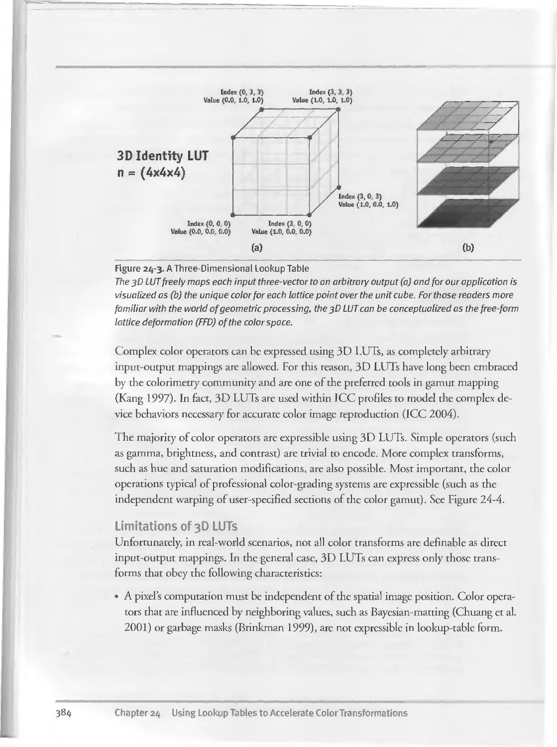
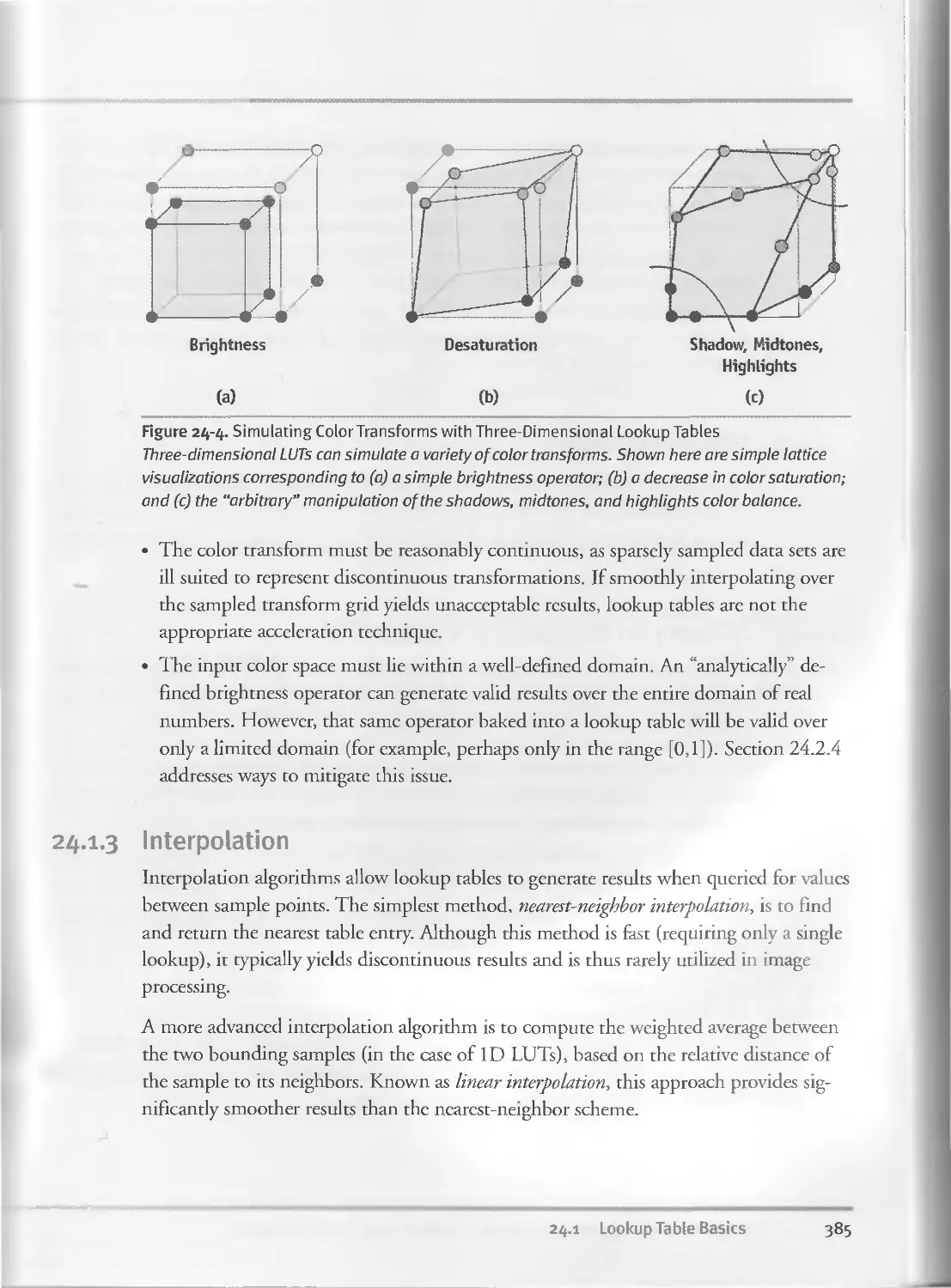
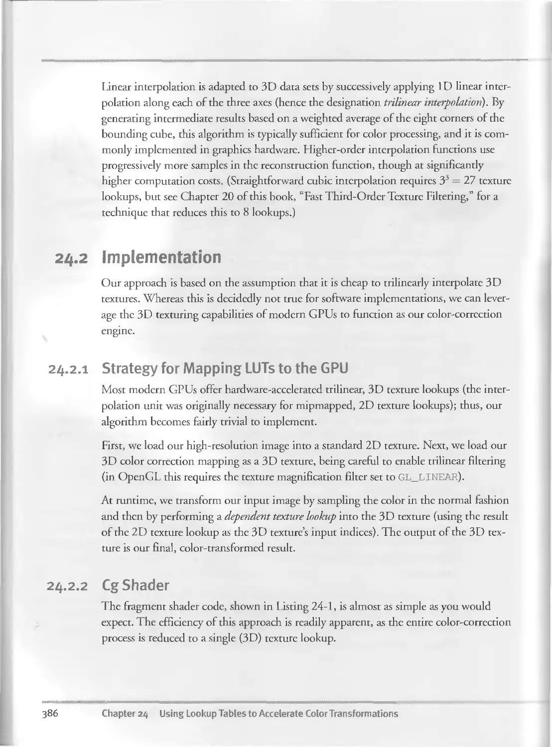
/


Text
Programming Techniques for
High-Performance Granhics and
IMAGE-ORIENTED COMPUTING SHADING. LIGHTING, AND SHADOWS G* OMETRIC COMPLEXITY
Terrain Rendering Using
GPU-Based Geometry Chpmaps
And Asirvatham and Hugues Hoppe
(Microsoft Reseorch)
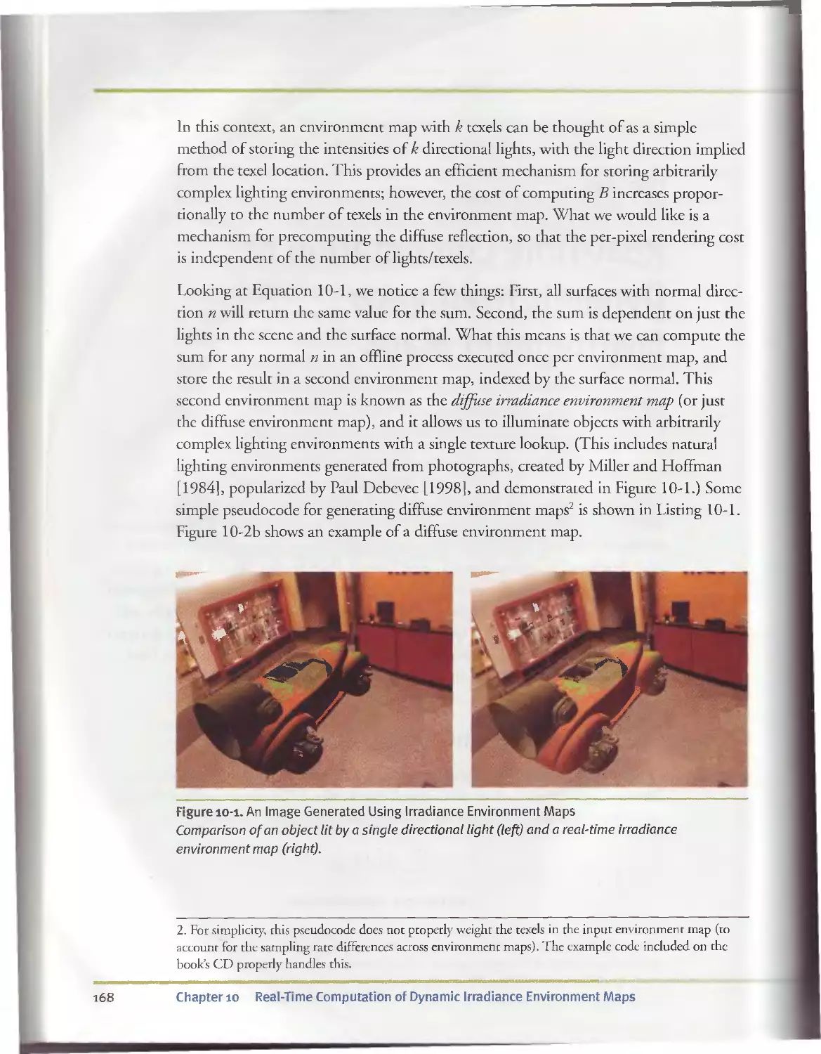
feal-Time lompuiaiMMi of Dye amir
liWkHv e La-Hionmerrt Haps
Gary King
(NVIDIA)
Efficient Seh Ldged Shadows
Using Pixel Shader Branching
Yury Uralsky
(NVIDIA)
GPU Image Р&хъампу
in Apple's Motion
Pete Warden
(Apple Computer)
••the G«>
Sylvain Lefebvre, Samuel Hornus,
and Fabrice Neyret
(GRAVIR/IMAG - INRIA)
l/etevved Filtering Rendering
from Dlffki'd D rta hrnnafc
Joe Kphj, (Univ. Aaron Lefobn,
and Nathaniel Fout (UC Davis)
Using Wrtex b>xtwe Displacement
for Realistic. Wa ter Renden , g
Yuri Kryachko
(1C: Maddox Games)
Implementing Improved
Pertin Noise
Simon Green
(NVIDIA)
High-Qu hty bit,. •( flluminatiou
Rendering Using Rasterisation
Toshiya Hachisuka
(The University of Tokyo)
CjMMOntTVf Rasterization
Jon Hasselgren, Tomas
Akenine-Moller, and Lennart
Ohlsson (Lund University)
Inside Instancing
Francesco Carucd
(Lionhead Studios)
A, j Xinu - М^чЬ.,» !
Texture Functions
Jan Kautz
(MIT)
Generic Refraction
Simulation
Tiago Sousa
(Crytek)
Advanced High-Quality
Filtering
Justin Novosad
(discreet)
w
I 9
Global Iilunrirwrion Using
Progressive Ref nement i.
Greg Coombe (UNC at Chapel Hill)
and Mark Hams (NVIDIA)
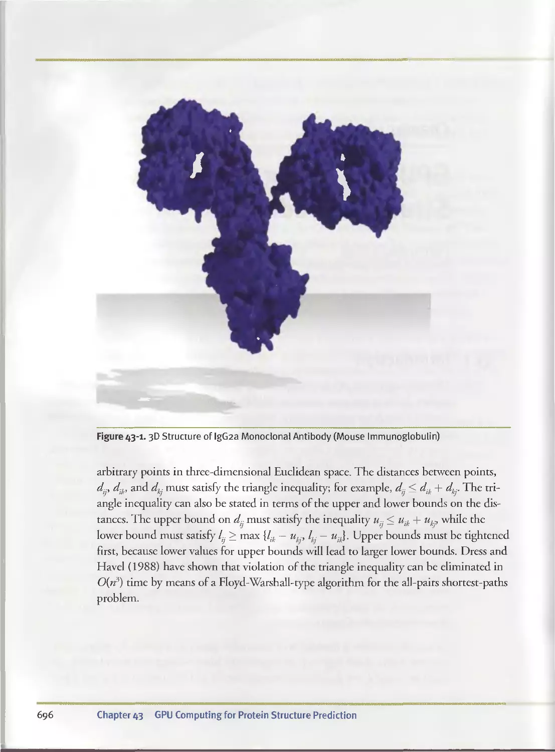
GPU Computing for Protem
Structure PredictUH
Paulins Micikevicius
(Armstrong Atlantic State University)
Segment Bufferin
Ion Otick
(2015)
Tile-Based
Texture Mapping
U-Yi Wei
(NVIDIA)
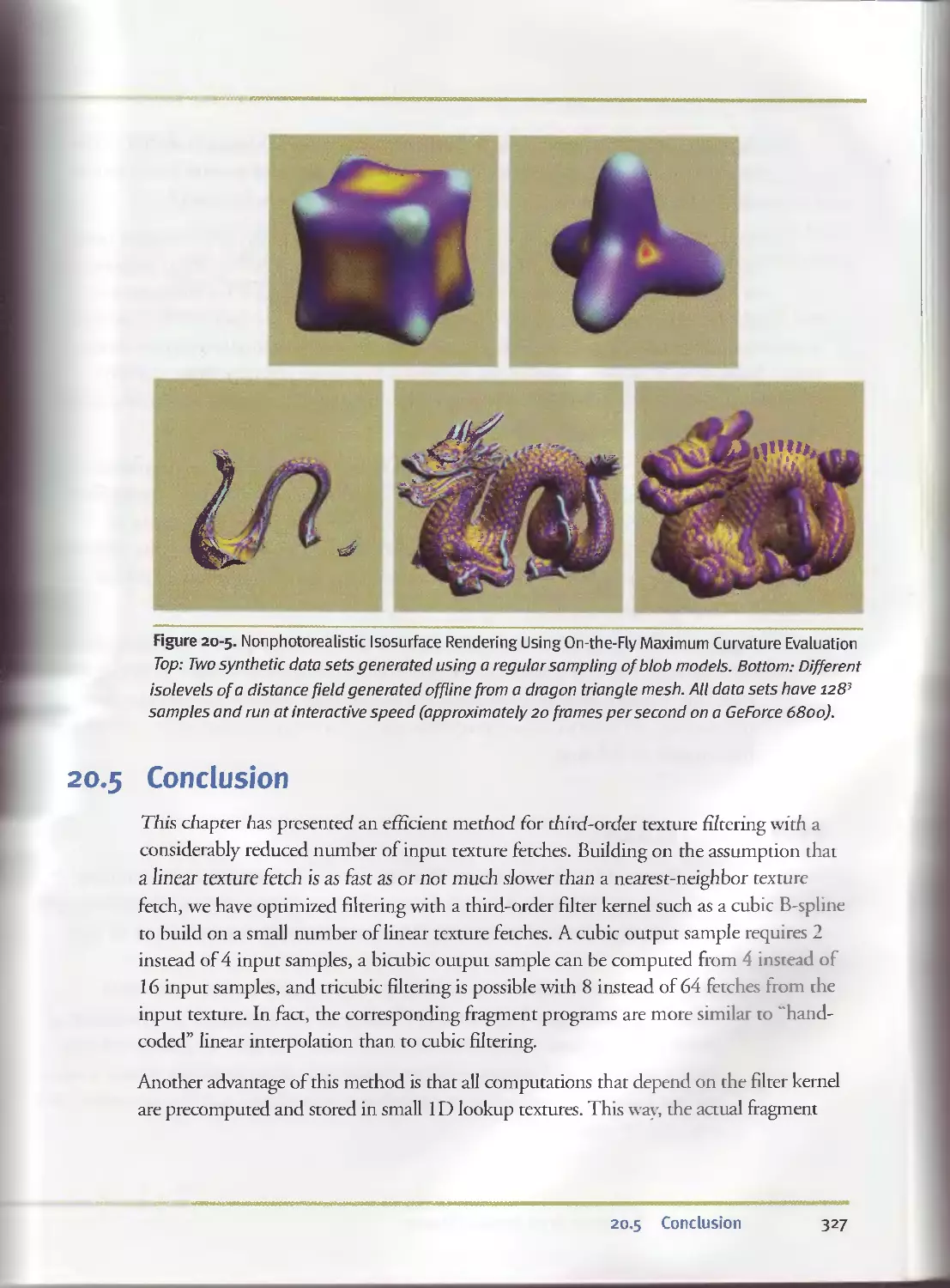
Fast Third-Order Texture Filtering
Christian Sigg (ETH Zurich)
and Markus Hadwiger
(VRVis Research Center)
Mipmap-Level
Measurement
lam Cantlay
(Climax Entertainment)
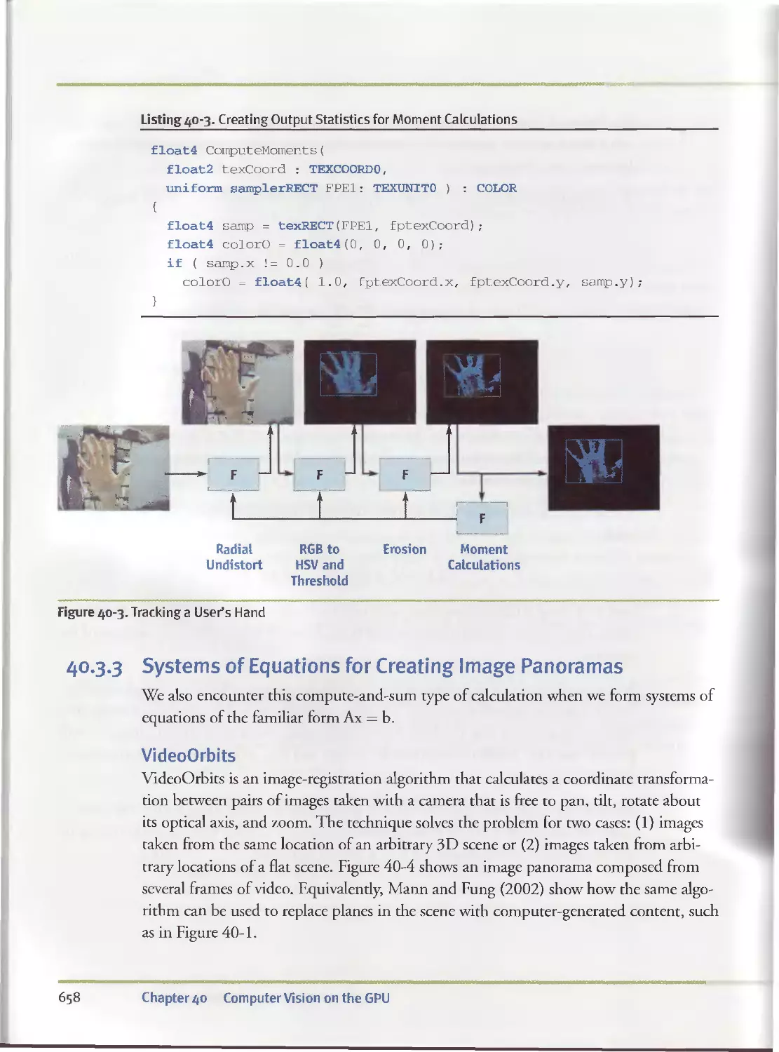
Computer Vision on the GPU
James Fung
(University of Toronto)
A GPU framework for Solving
Systems at Снгеаг Equations
Jens Kruger and Rudiger Westermann
(Technische Universitat Munchen)
*
Optimizing Resource Management
with Multistreaming
Oliver Hoeller and Kurt Pelzer
(Piranha Bytes)
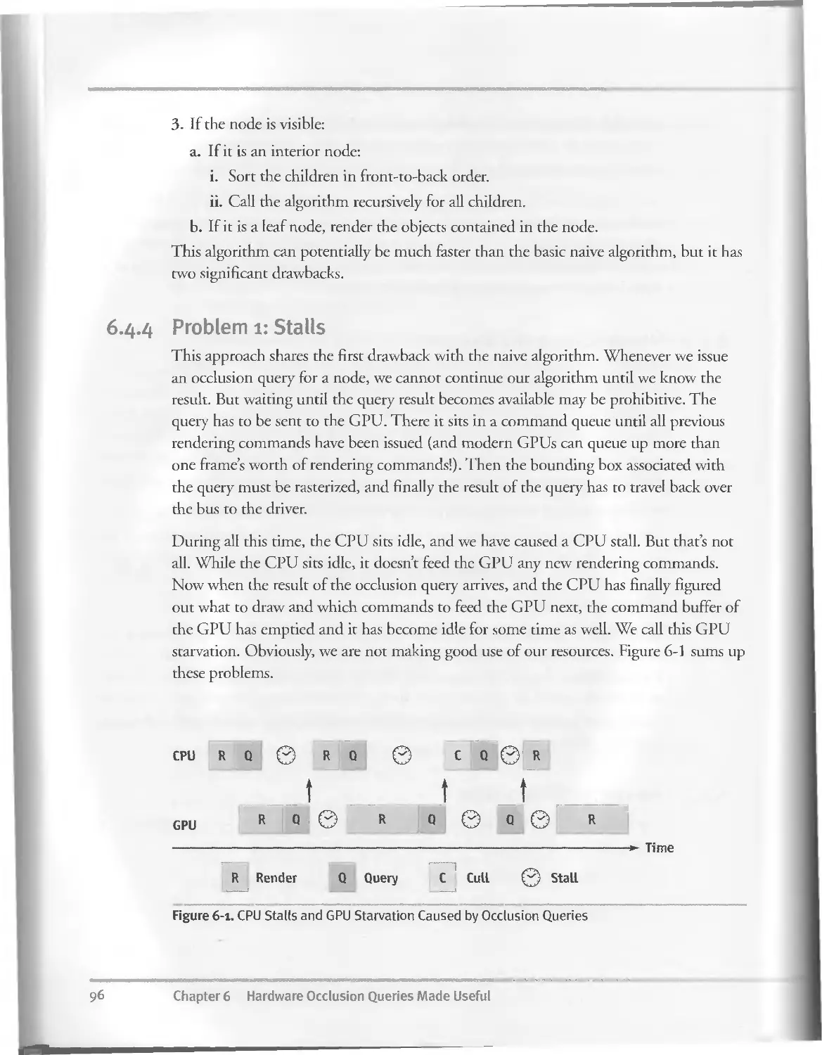
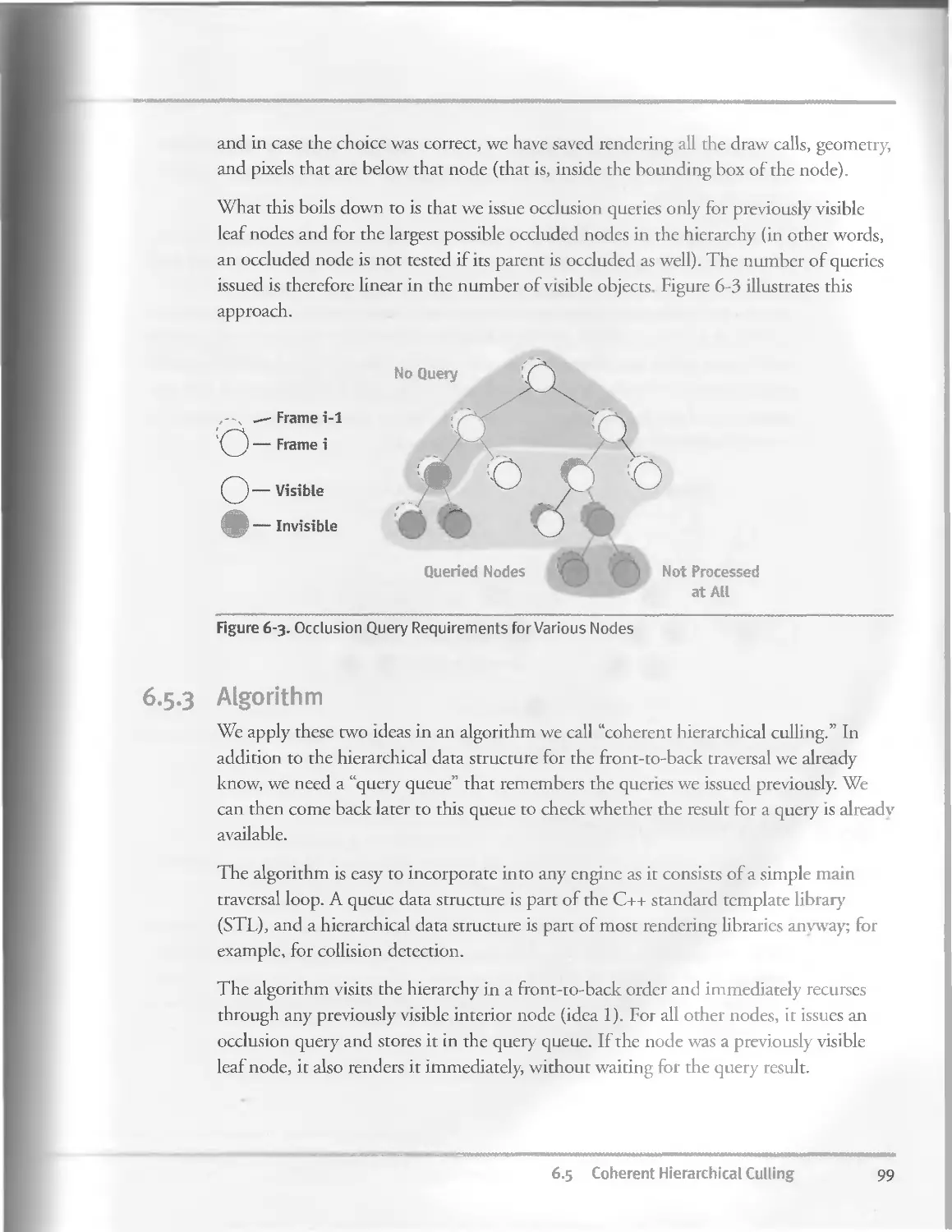
Hardware Occlusion Queries
Made Useful
Michael Wimmer and Jiri Bittner
(Vienna University of Technology)
Adaptive Tessellation of Sahd«v«stv •
Surfaces with Displacement Mapping
Michael Bunnell
(NVIDIA)
Pe«-f»rel Dnplacement Mapping
with Di ялпсе Functions
William Donnelly
(University af Waterloo)
Implementing the mental wages
Phenomena Renderer on the GPU
Martin-Kart Lefran^ois
(mental images)
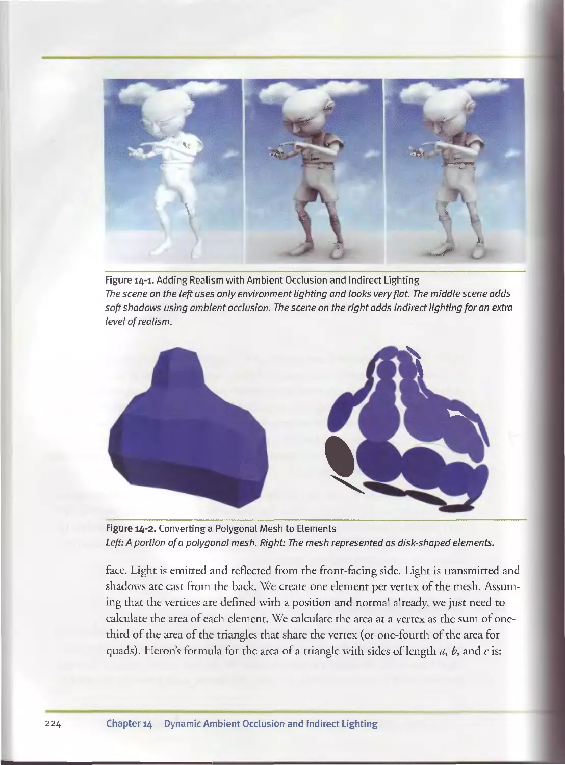
Dynamic Ambient Occlusion
and Indirect Lighting
Michael Bunnell
(NVIDIA)
Blueprint Rendering and
"Sketchy Drawings'1
Marc Nien hairs and Jurgen Dollner
(University of Potsdam)
Accurate Atmosph he
Scattering
Sean O'Neil
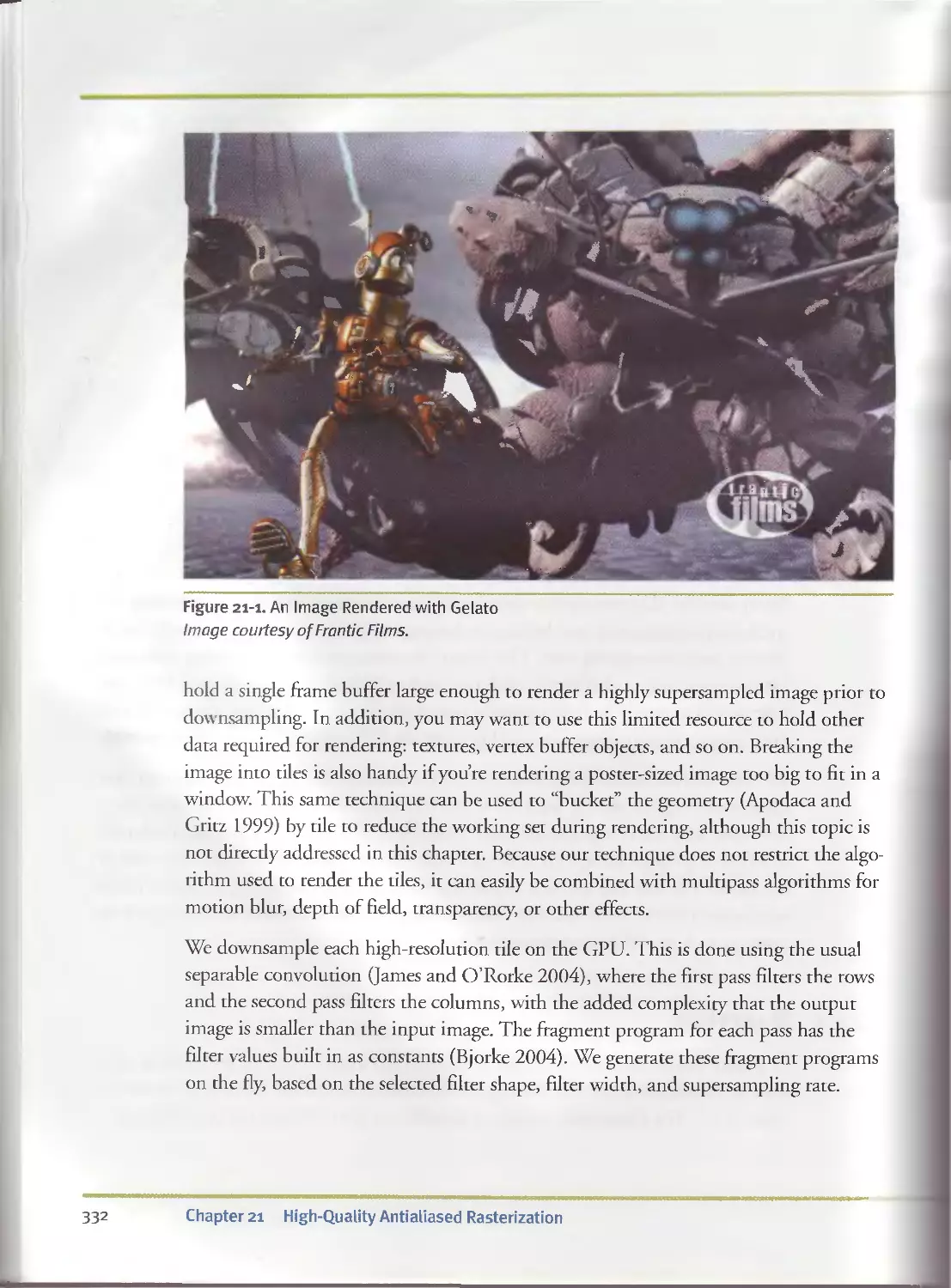
High-Quality Antialiased
Rasterization
Dan Wexler and Eric Enderton
(NVIDIA)
Fast PrefMtered Lines
Eric Chan and Fredo Durand
(MTT)
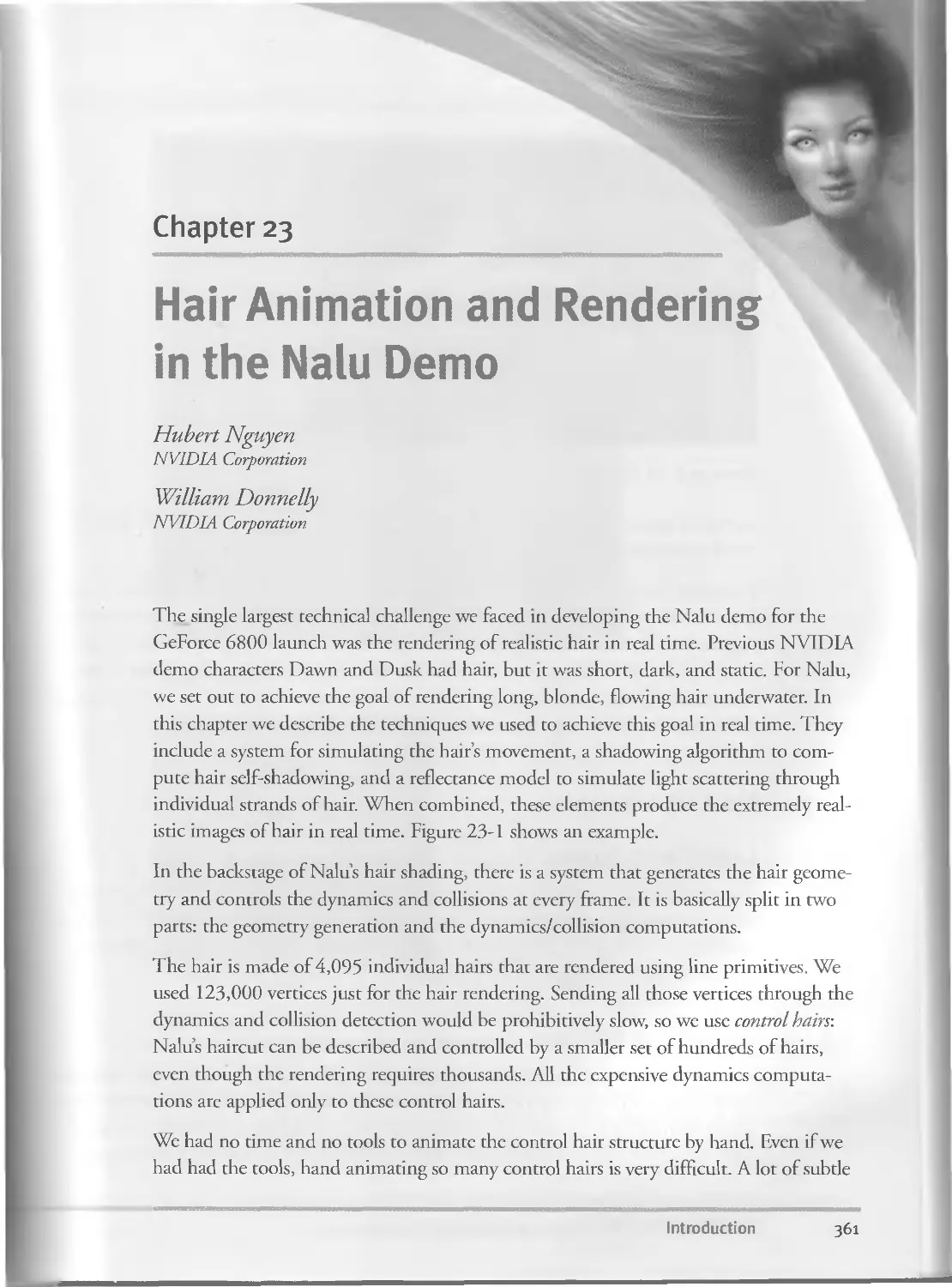
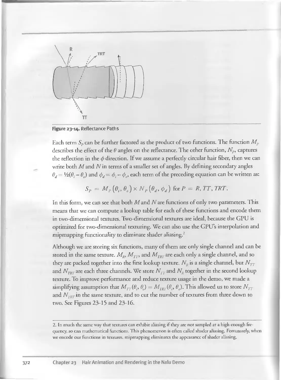
Hair Animation and Rendering
in the Nalu Вето
Hubert Nguyen and William Donnelly
(NVIDIA)
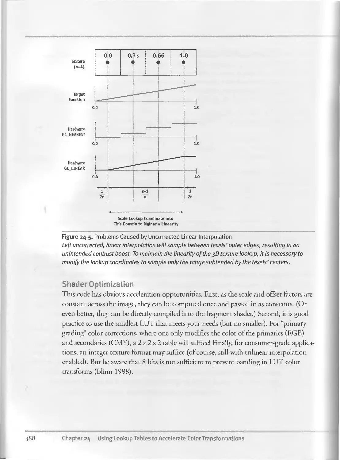
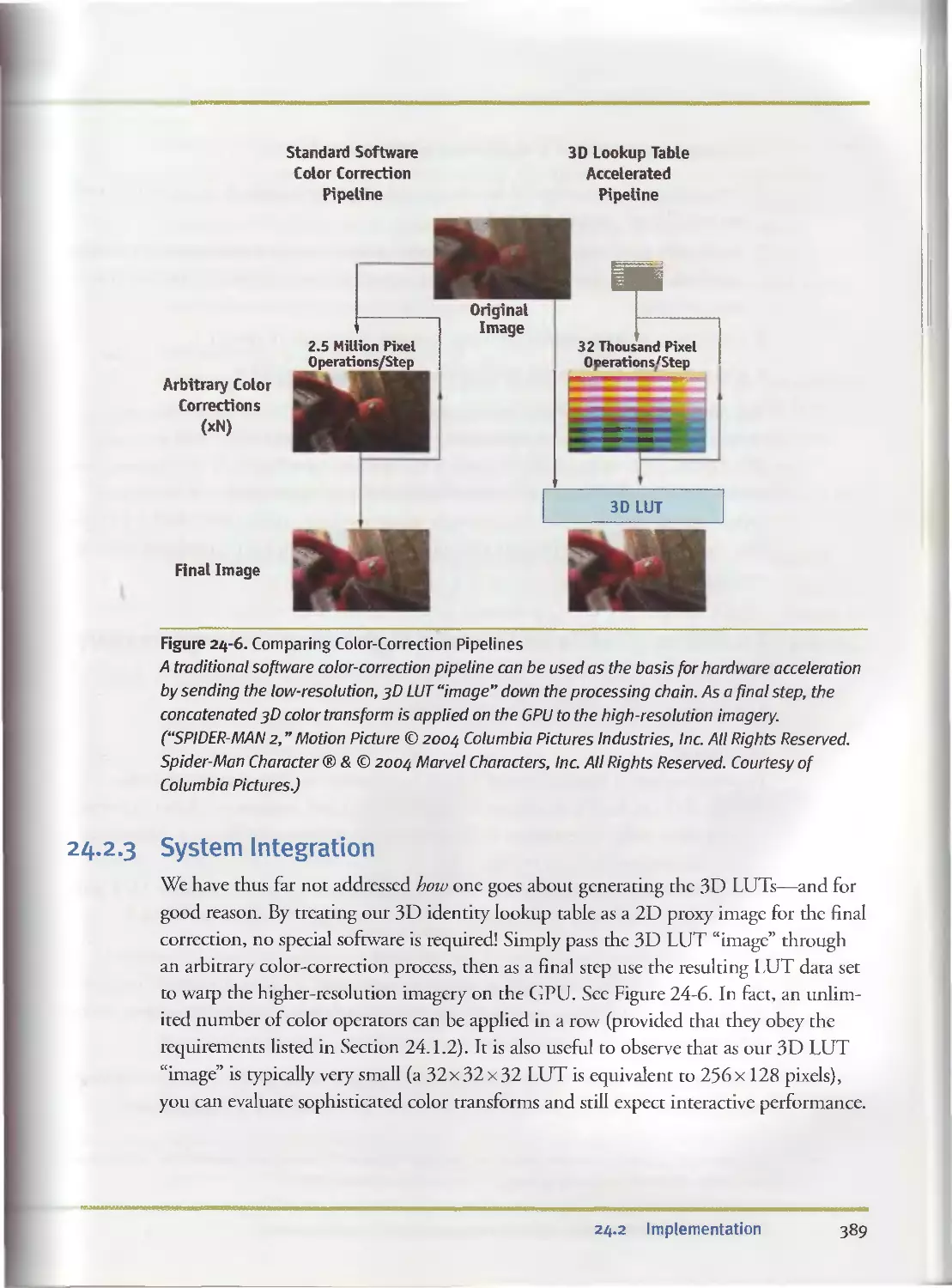
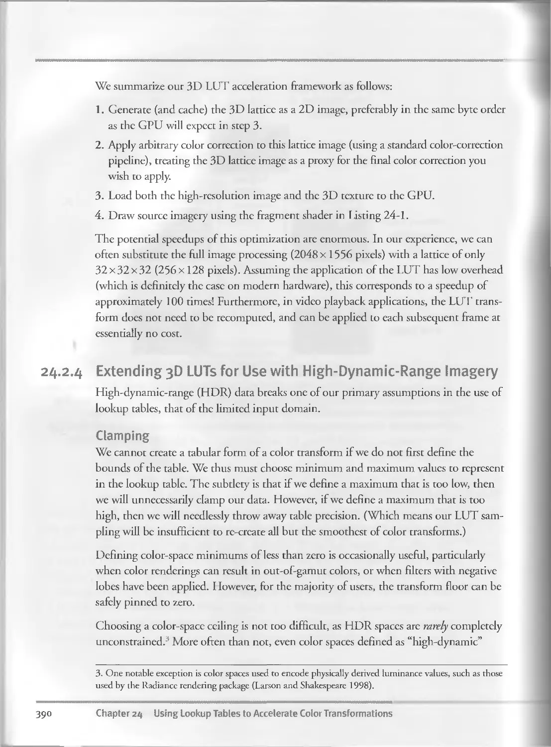
Using Lookup ТаИе$ to Accelerate
Color Transformations
Jeremy Setan
(Sony Pictures Imugewciia)
X
О
Streaming Architectures
and Technology Trends
John Owens
(UC Davis)
The GeForce 6 Senes
GPU Architecture
Emmett Kilgariff and
Randi ma Fernando
(NVIDIA)
Mapping Computational
Concepts to GPUs
Mark Harris
(NVIDIA)
Taking the Plunge frfo
GPU Computing
Ian Bnck
(Stanford University)
Implementing Efficient Parallel
Data Structures on GPUs
Aaron Lefohn (UC Davis), Joe Kniss
(Univ. of Utah), John Owens (UC Davis)
GPU Rew-Cwrtrol Idfoms
Mark Harris (NVIDIA) and
Ian Buck (Stanford University)
GPU Program oj t»m jtfem
Cliff Woolley
(University of Virginia)
'rtream taw™. Of пл bon-.
Daniel Horn
(Stanford University)
Options Pricing en the GPU
Craig Kolb and Matt Pharr
(NVIDIA)
Improved t PU Sortnig
Peter Kipfer and Rudiger Westermann
(Technische Universitat Munchen)
RowSfoftrtatiwH with Lwmplex Bounder*-?
Wei Li (Siemens Corporate Research),
Zhe Fan, Xiaoming Wei, and Arie
Kaufman (Stony Brook University)
win* the FH
Thilaka Jumanaweera and Donald Liu
(Siemens Medical Solutions USA)
GPU Gems 2
GPU Gems 2
Programming Techniques for
High-Performance Graphics and
General-Purpose Computation
Edited by Matt Pharr
Randima Fernando, Series Editor
A Addison-Wesley
Upper Saddle River, NJ • Boston • Indianapolis • San Francisco
New York • Toronto • Montreal • London • Munich • Paris • Madrid
Capetown • Sydney • Tokyo • Singapore • Mexico City
About the Cover: The Nalu character was created by the NVIDIA Demo Team to showcase the rendering power of the
GeForce 6800 GPU. The demo shows off advanced hair shading and shadowing algorithms, as well as iridescence and
bioluminescence. Soft shafts of light from the water surface are blocked by her body, and her skin is ht by the light
refracted through the waters surface, with her body and hair casting soft shadows on her as she swims.
Many of the designations used by manufacturers and sellers to distinguish their products are claimed as trade-
marks. Where those designations appear in this book, and Addison-Wesley was aware of a trademark claim, the
designations have been printed with initial capital letters or in all capitals.
The authors and publisher have taken care in the preparation of this book, but make no expressed or implied war-
ranty of any kind and assume no responsibility for errors or omissions. No liability is assumed for incidental or
consequential damages in connection with or arising out of the use of the information or programs contained herein.
NVIDIA makes no warranty or representation that the techniques described herein are free from any Intellectual
Property claims. The reader assumes all risk of any such claims based on his or her use of these techniques.
The publisher offers excellent discounts on this book when ordered in quantity for bulk purchases or special
sales, which may include electronic versions and/or custom covers and content particular to your business, train-
ing goals, marketing focus, and branding interests. For more information, please contact:
U.S. Corporate and Government Sales
(800) 382-3419
corpsales@pearsontechgroup.com
For sales outside of the U.S., please contact:
International Sales
international@pearsoned.com
Visit Addison-Wesley on the Web: www.awprofessional.com
Library of Congress Cataloging-in-Publication Data
GPU gems 2 : programming techniques for high-performance graphics and general-purpose
computation I edited by Matt Pharr ; Randima Fernando, series editor.
p. cm.
Includes bibliographical references and index.
ISBN 0-321-33559-7 (hardcover : alk. paper)
1. Computer graphics. 2. Real-time programming. I. Pharr, Matt. II. Fernando, Randima.
T385-G688 2005
006.66—dc22
2004030181
GeForce™ and NVIDIA Quadro® are trademarks or registered trademarks of NVIDIA Corporation.
Nalu, Timbury, and Clear Sailing images © 2004 NVIDIA Corporation.
mental images and mental ray are trademarks or registered trademarks of mental images, GmbH.
Copyright © 2005 by NVIDIA Corporation.
All rights reserved. No part of this publication may be reproduced, stored in a retrieval system, or transmitted, in
any form, or by any means, electronic, mechanical, photocopying, recording, or otherwise, without the prior con-
sent of the publisher. Primed in the United States of America. Published simultaneously in Canada.
For information on obtaining permission for use of material from this work, please submit a written request to:
Pearson Education, Inc.
Rights and Contracts Department
One Lake Street
Upper Saddle River, NJ 07458
ISBN 0-321-33559-7
Text printed in the United States on recycled paper at Quebecor World Taunton in Taunton, Massachusetts.
First printing, March 2005
To everyone striving to make
todays best computer graphics
look primitive tomorrow
Contents
Foreword..........................................................xxix
Preface...........................................................xxxi
Contributors......................................................xxxv
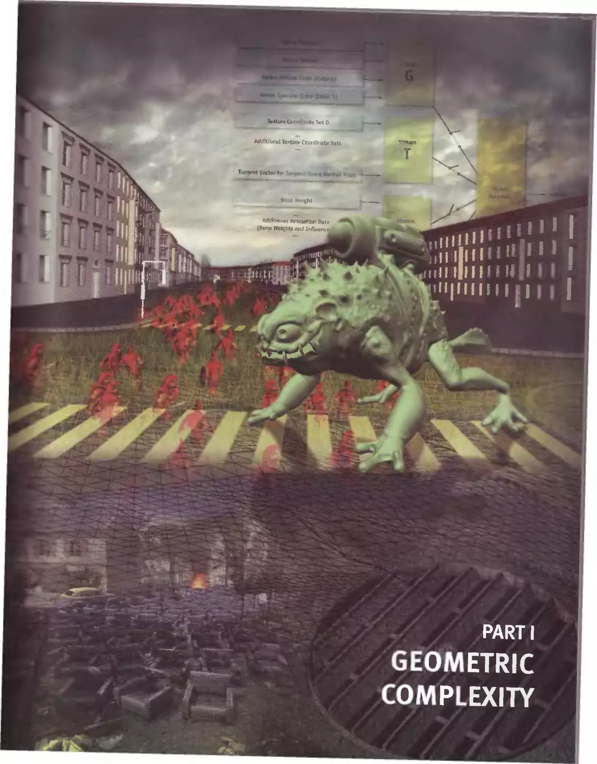
PARTI GEOMETRIC COMPLEXITY 1
Chapter i
Toward Photorealism in Virtual Botany........................................7
David Whatley, Simutronics Corporation
1.1 Scene Management............................................7
1.1.1 The Planting Grid. . . .............................8
1.1.2 Planting Strategy...................................9
1.1.3 Real-Time Optimization.............................10
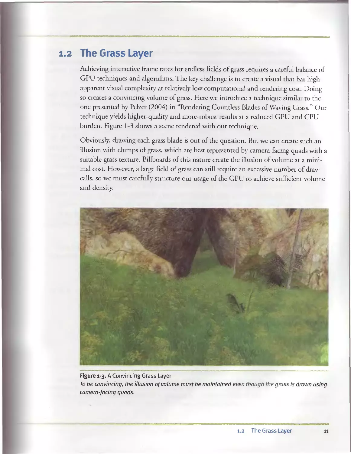
1.2 The Grass Layer............................................11
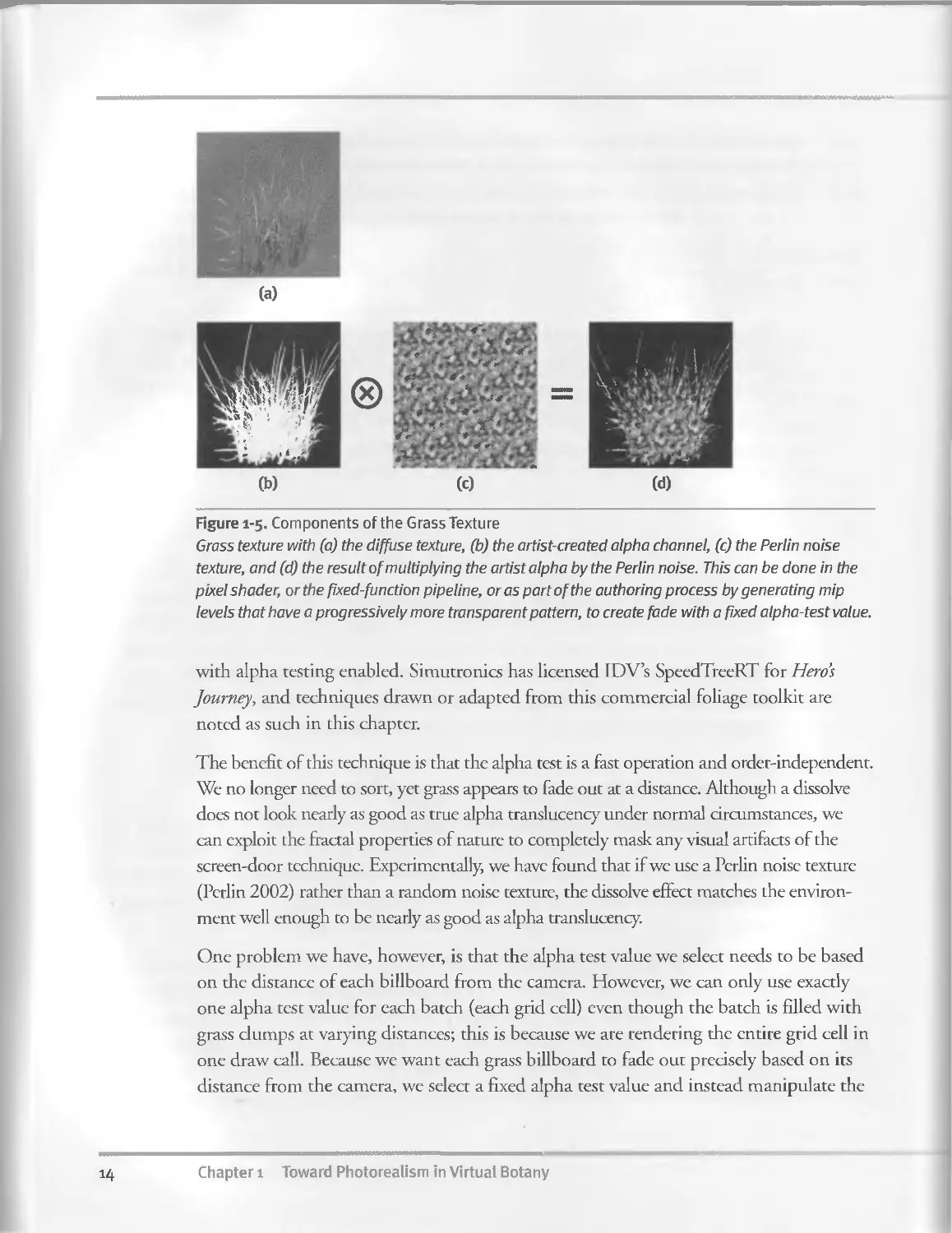
1.2.1 Simulating Alpha Transparency via Dissolve.........13
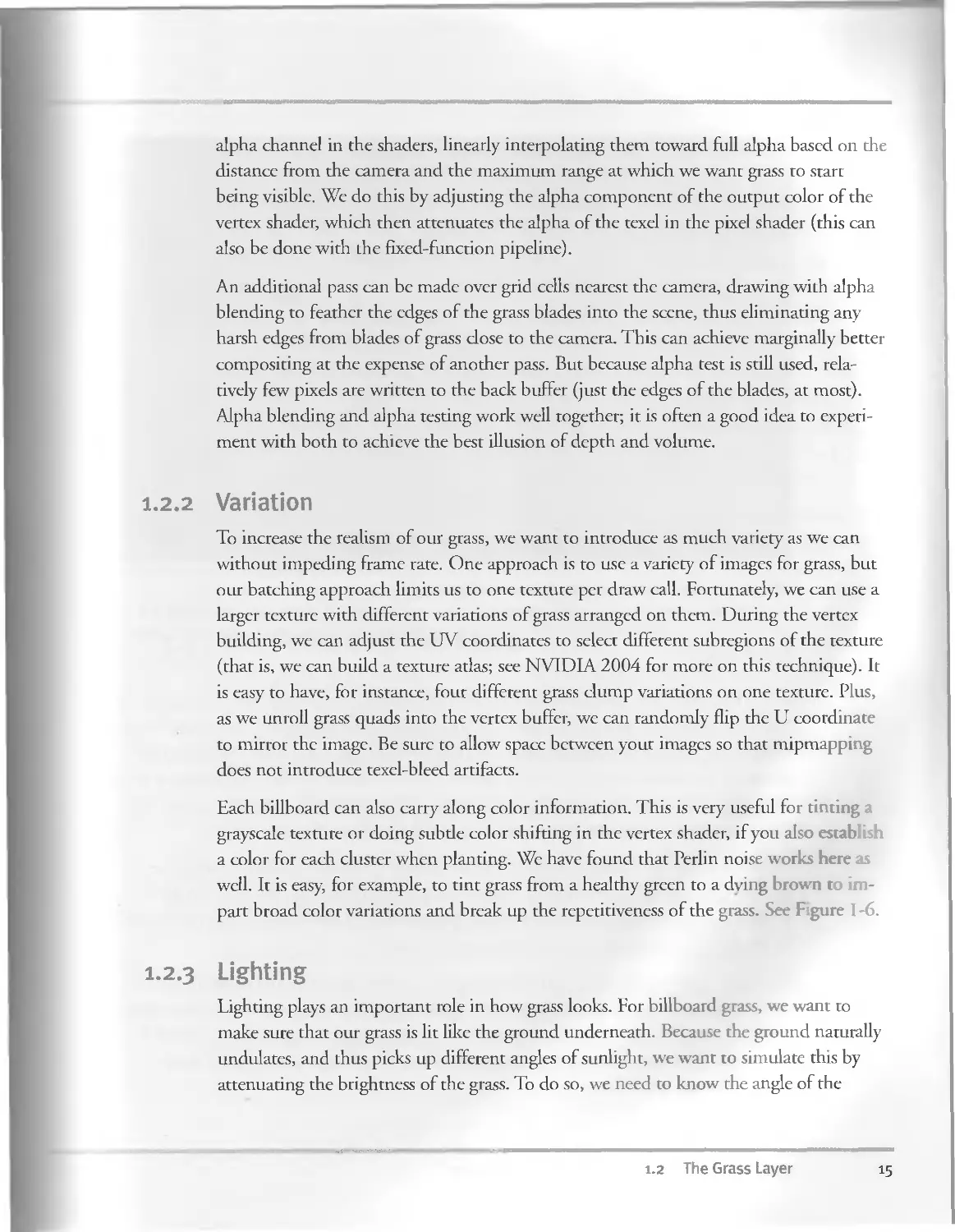
1.2.2 Variation..........................................15
I.2.3 Lighting...........................................15
I.2.4 Wind...............................................17
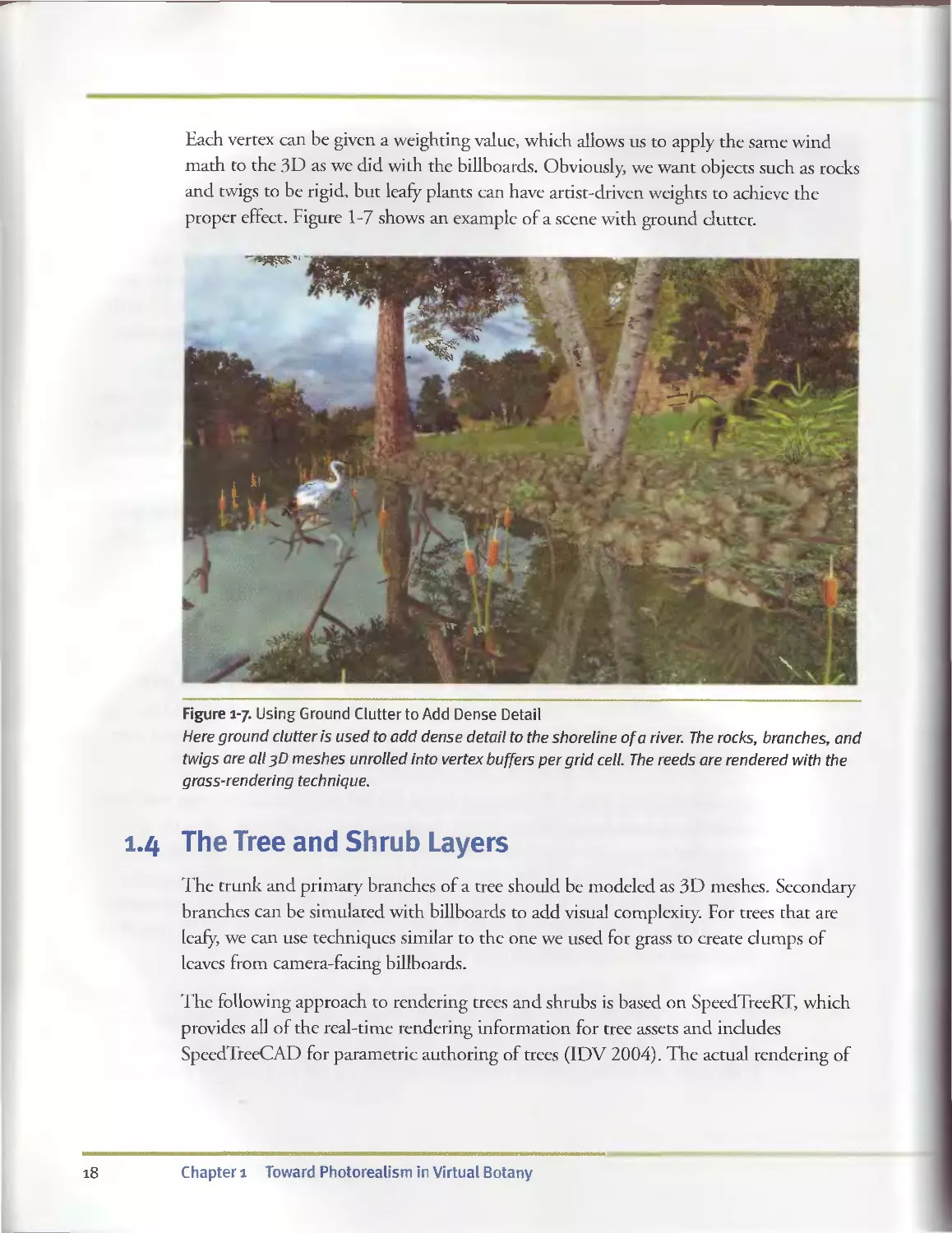
1.3 The Ground Clutter Layer...................................17
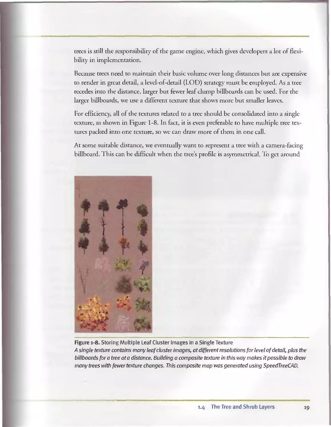
1.4 The Tree and Shrub Layers..................................18
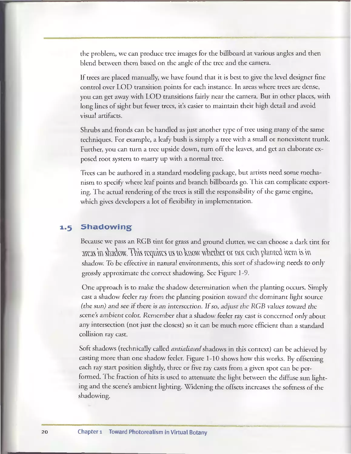
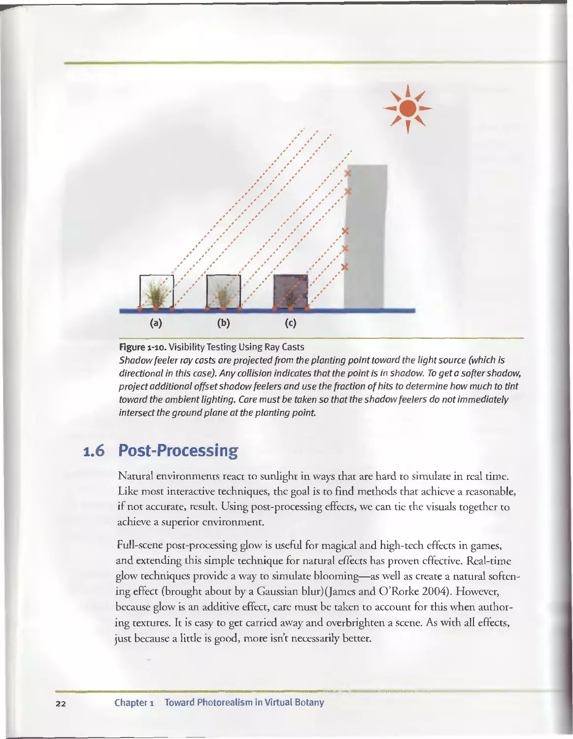
1.5 Shadowing................................................ . 20
1.6 Post-Processing.......................................... 22
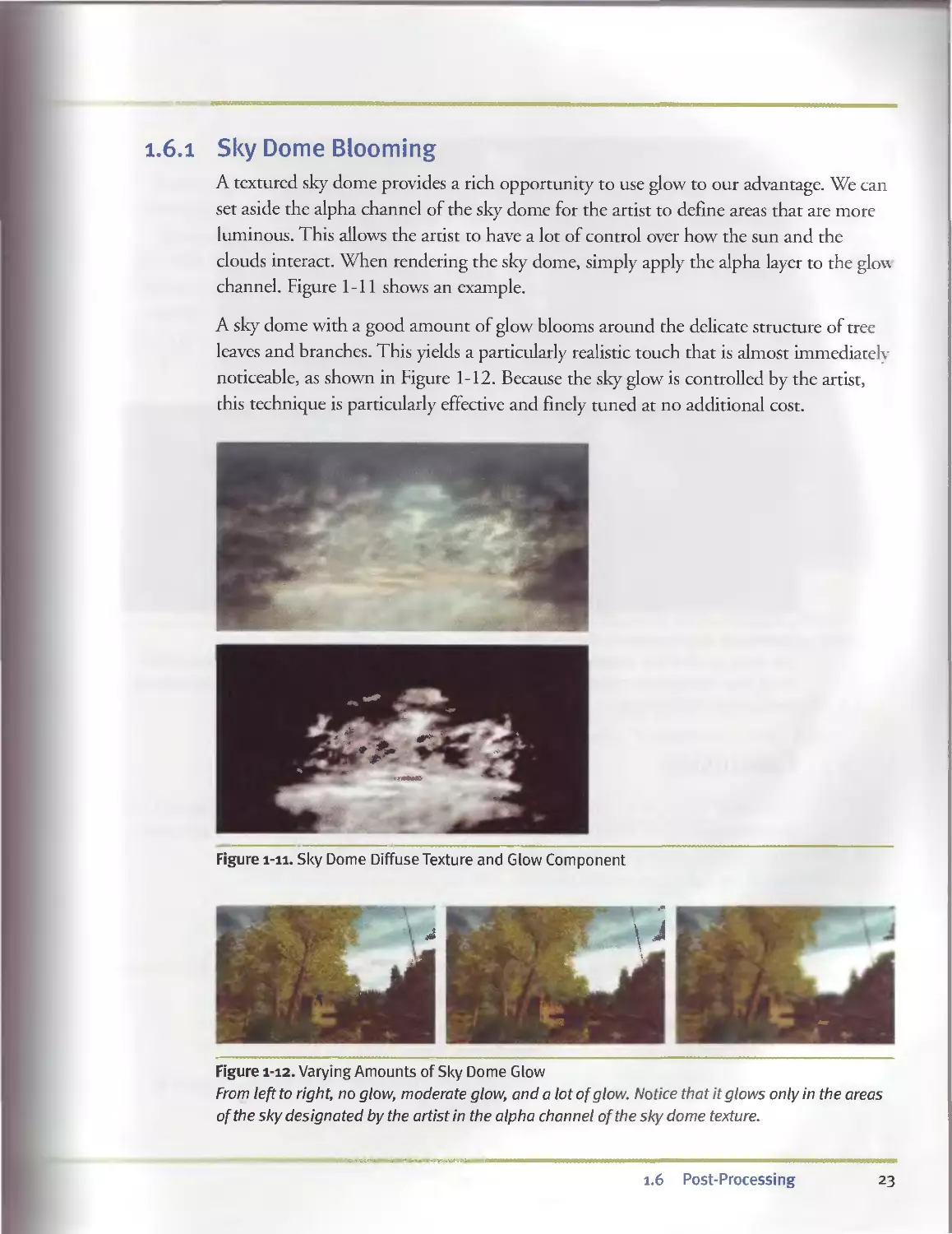
1.6.1 Sky Dome Blooming................................ .23
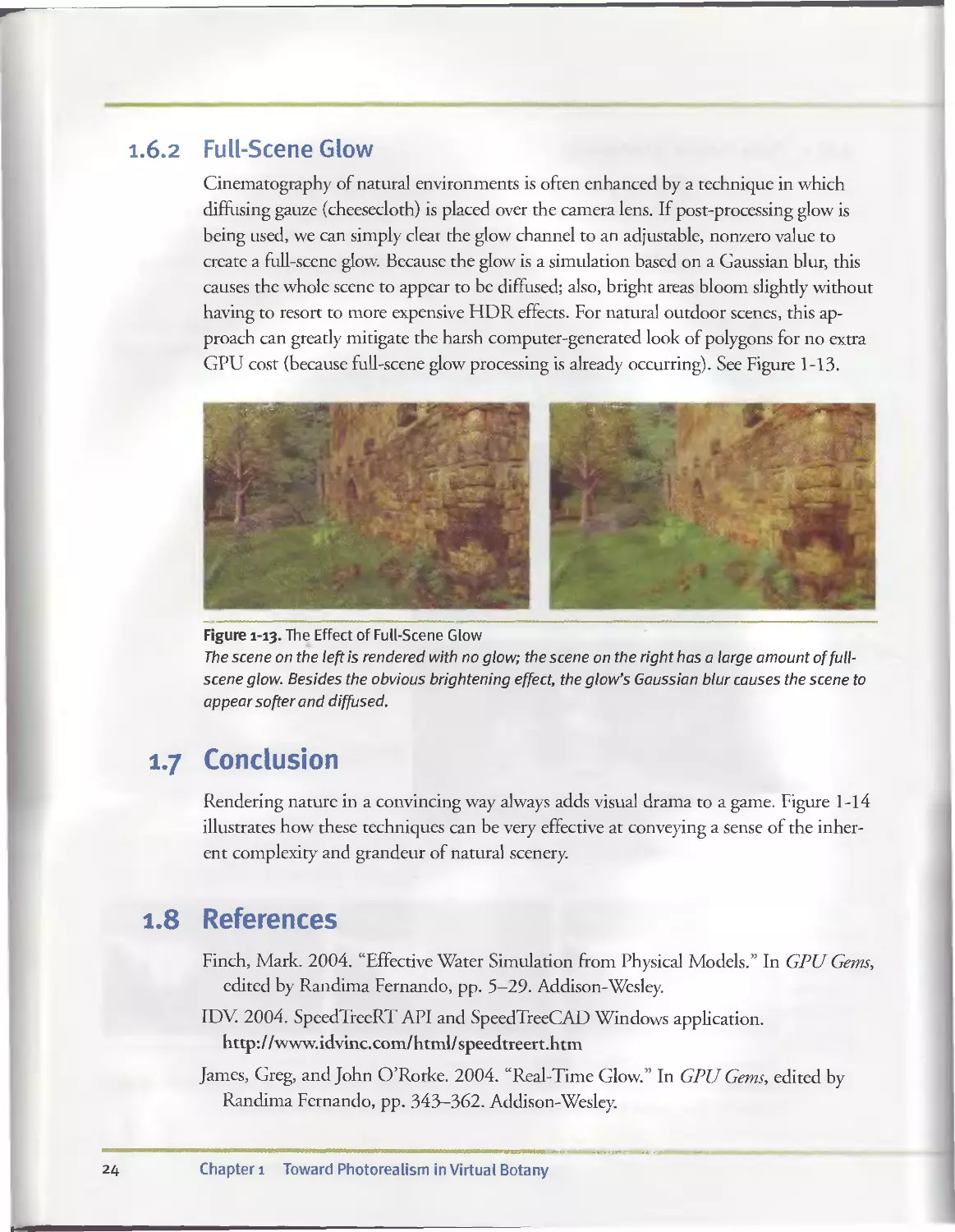
1.6.2 Full-Scene Glow............................... .... 24
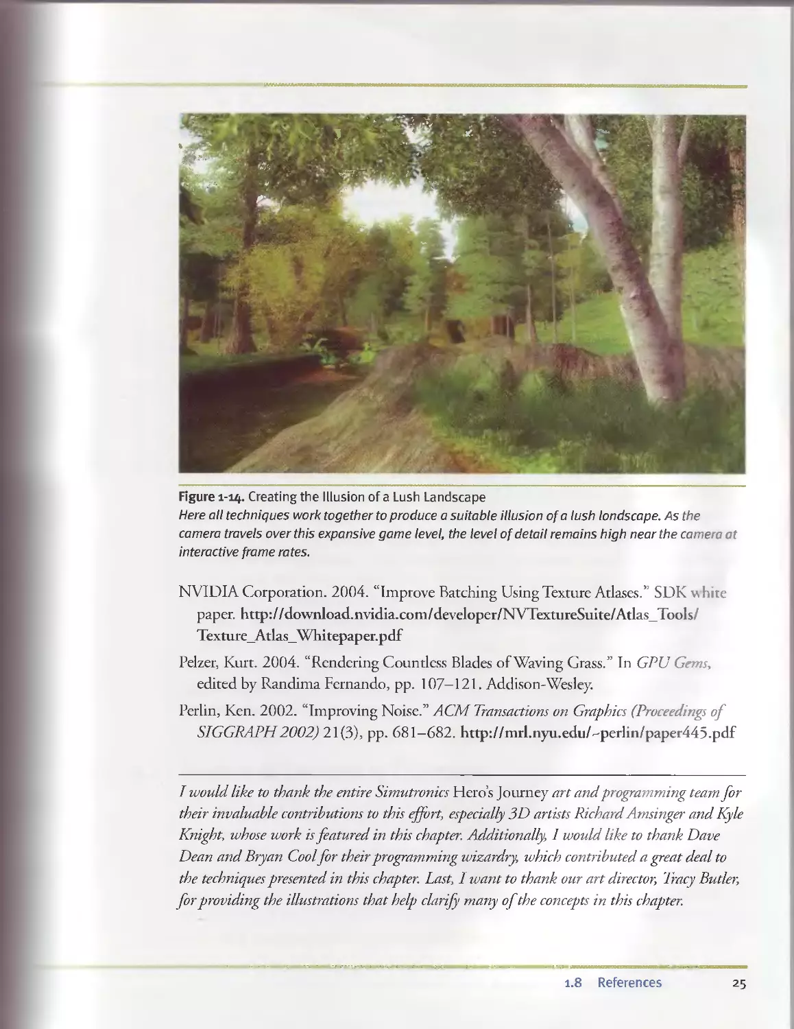
1.7 Conclusion............................................... . . 24
1.8 References................................................ 24
Contents vii
Chapter 2
Terrain Rendering Using GPU-Based Geometry Clipmaps........................27
Aral Asirvatham, Microsoft Research
Hugues Hoppe, Microsoft Research
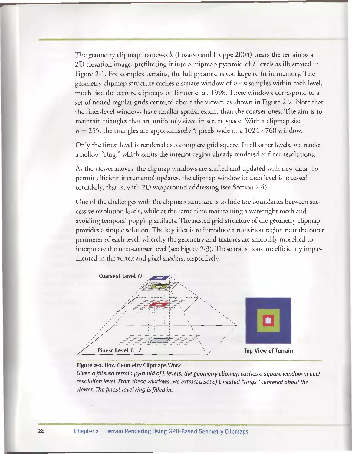
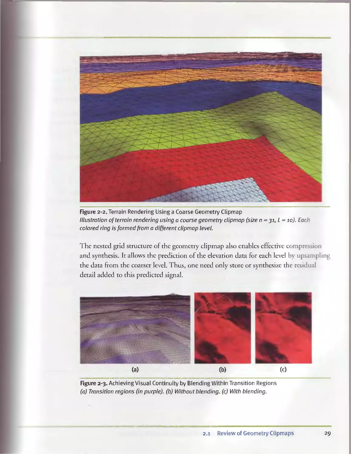
2.1 Review of Geometry Clipmaps.................................27
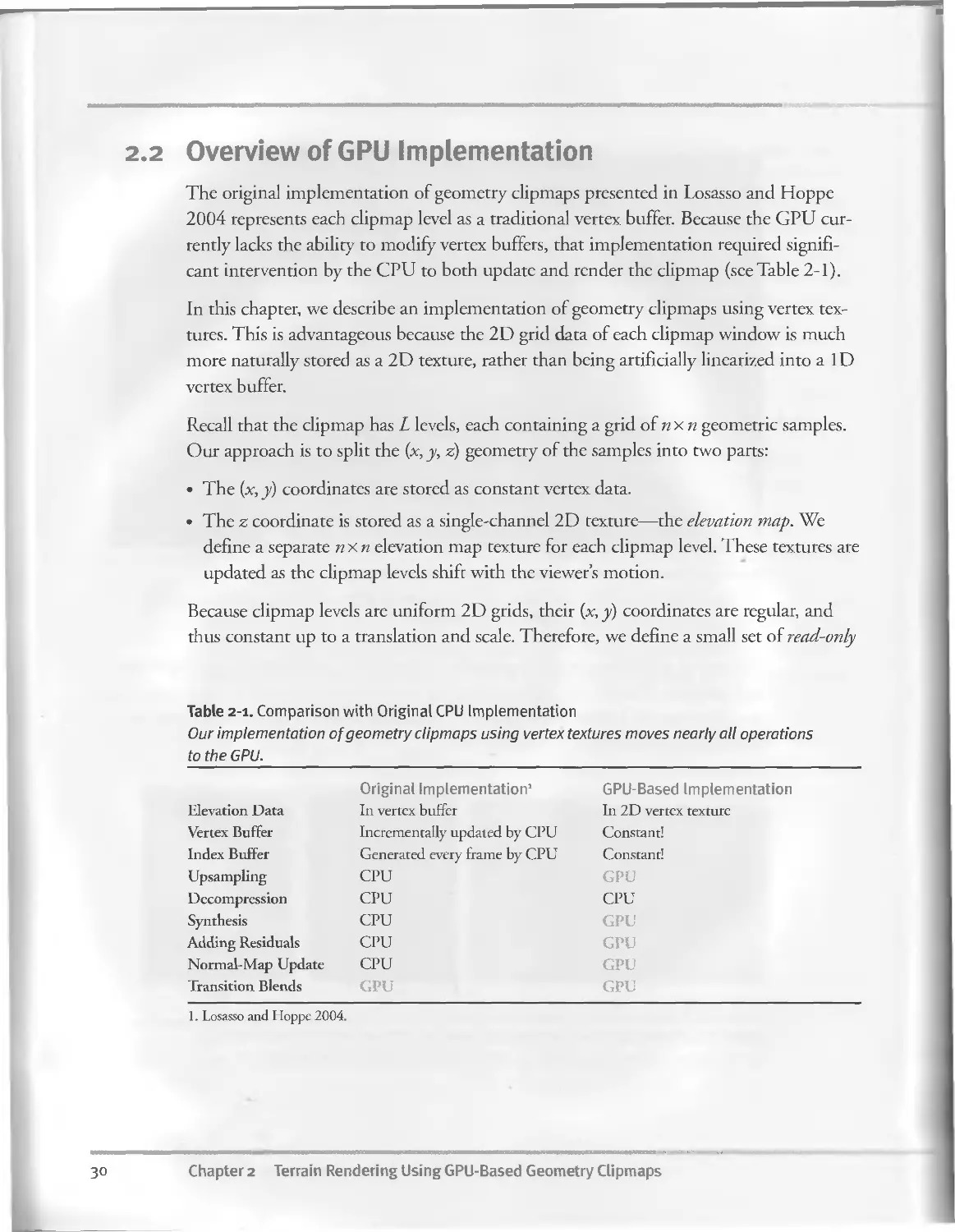
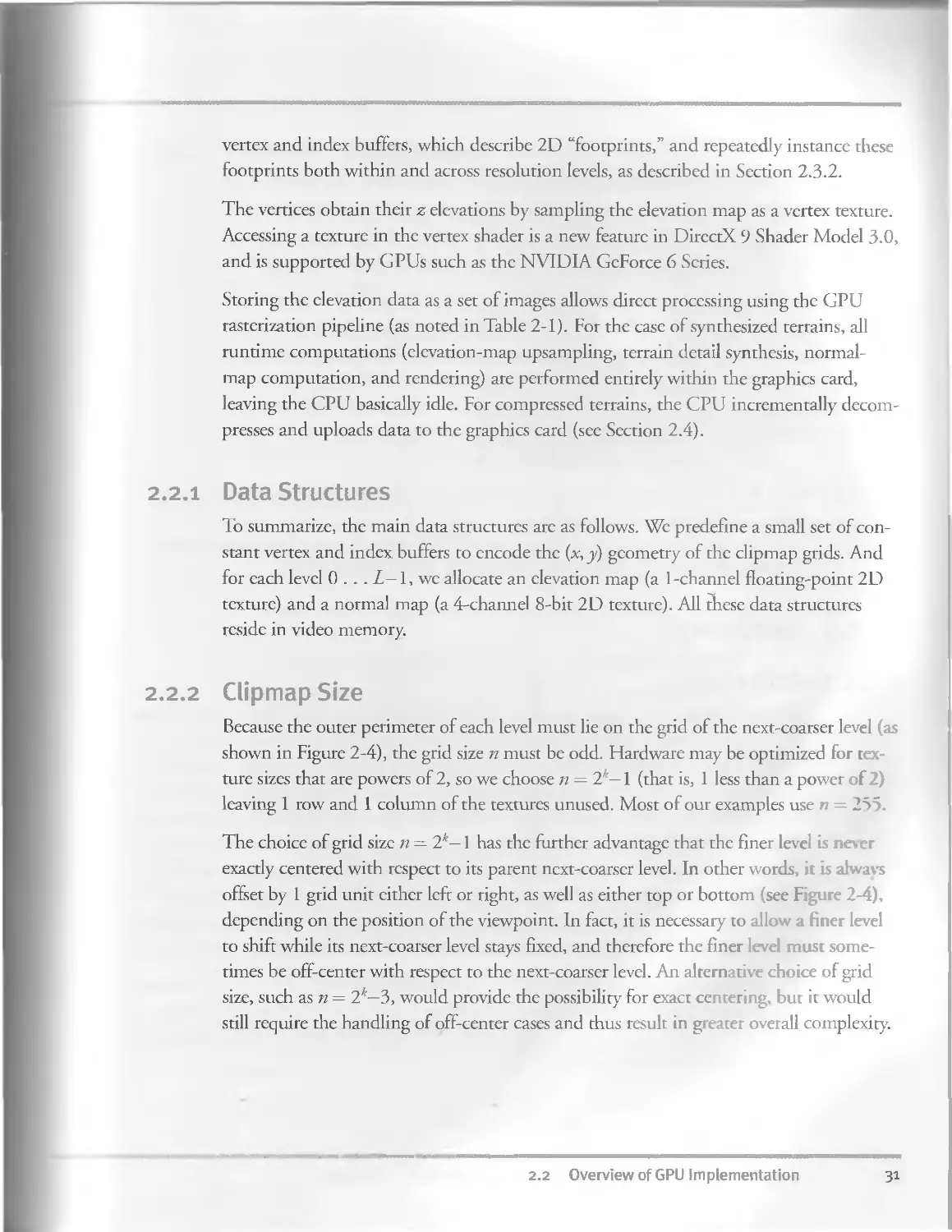
2.2 Overview of GPU Implementation.............................30
2.2.1 Data Structures.....................................31
2.2.2 Clipmap Size...................................... 31
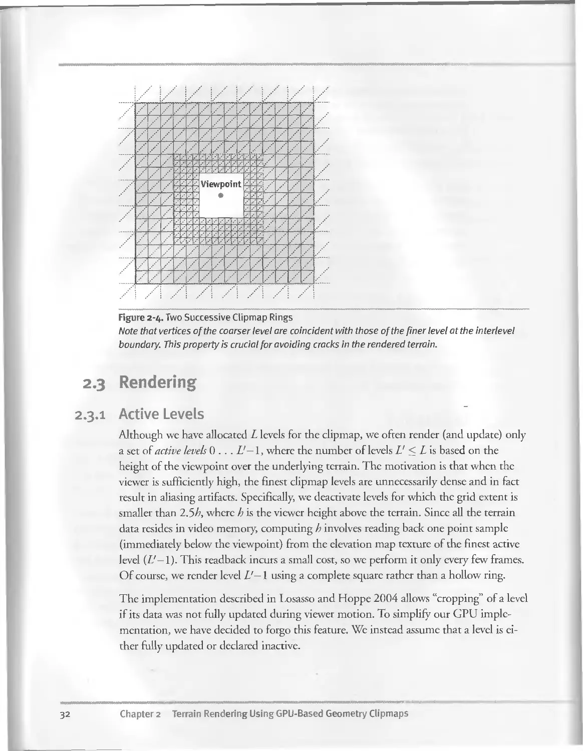
2.3 Rendering..................................................32
2.3 .I Active Levels.....................................32
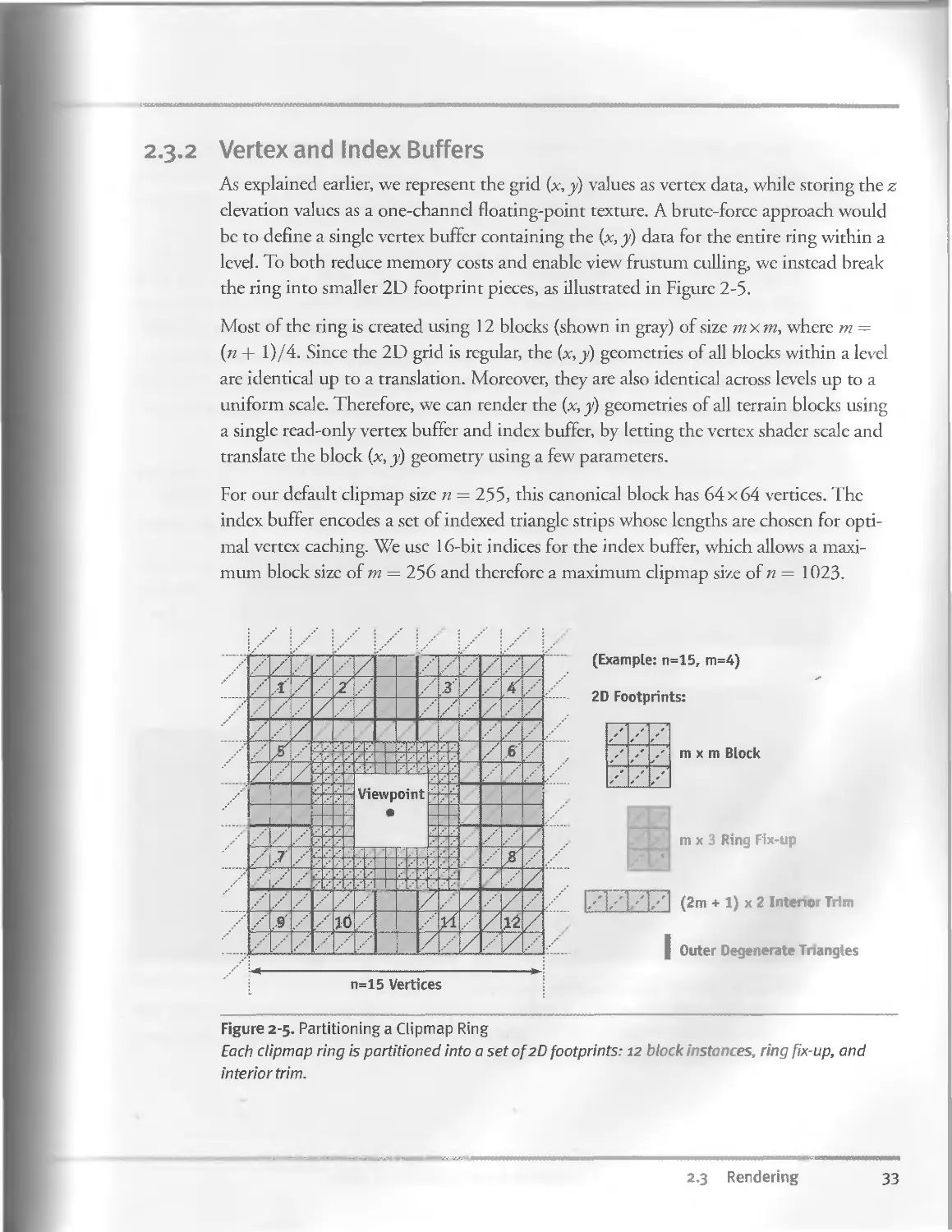
2-3-2 Vertex and Index Buffers............................33
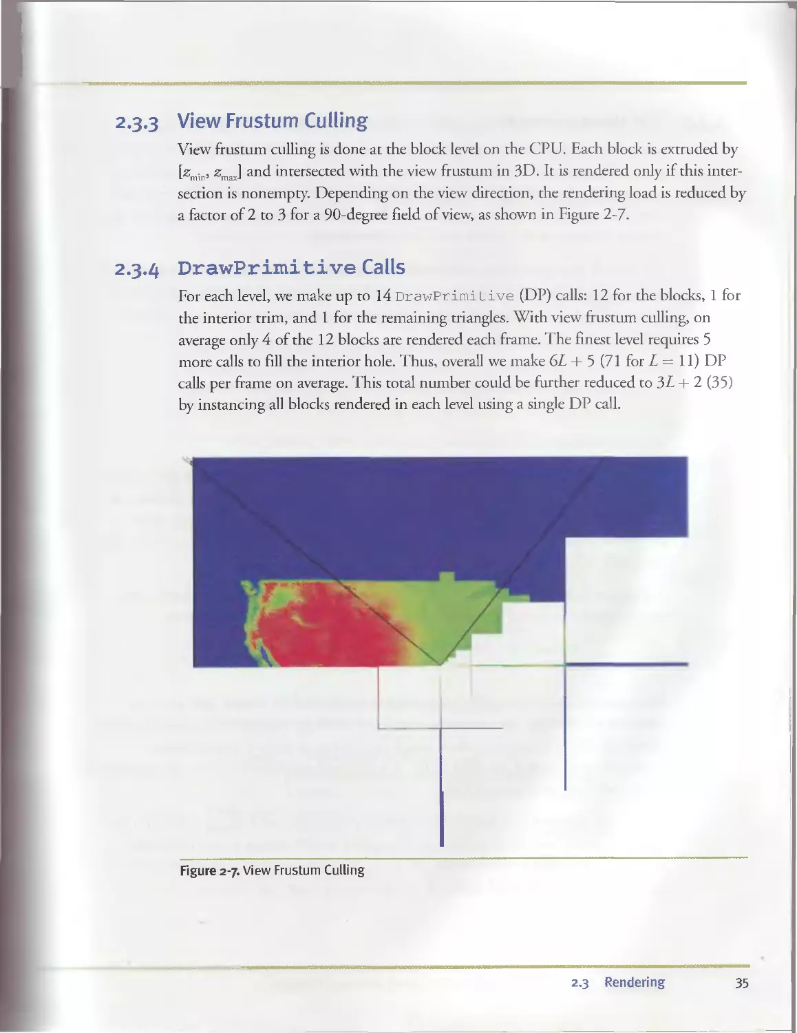
2.3 -3 View Frustum Culling..............................35
2.3-4 DrawPrimitive Calls.................................35
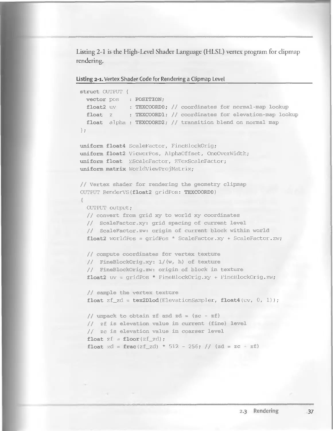
2.3.5 The Vertex Shader...................................36
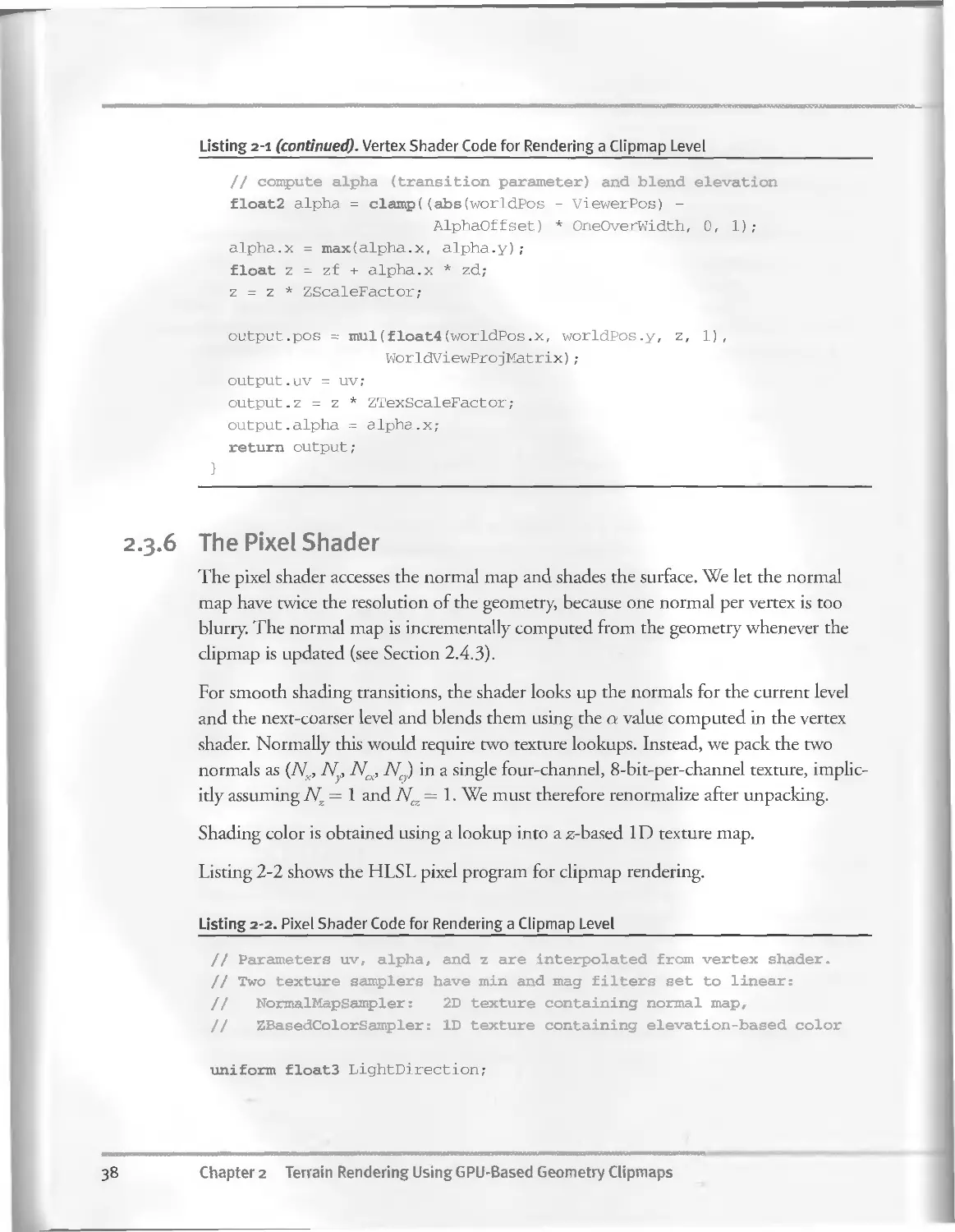
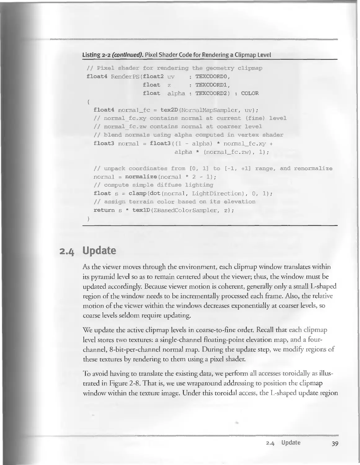
2.3.6 The Pixel Shader . . ...............................38
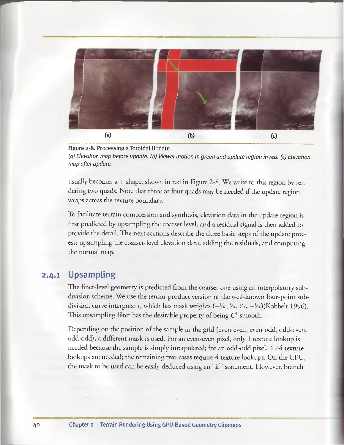
2.4 Update.....................................................39
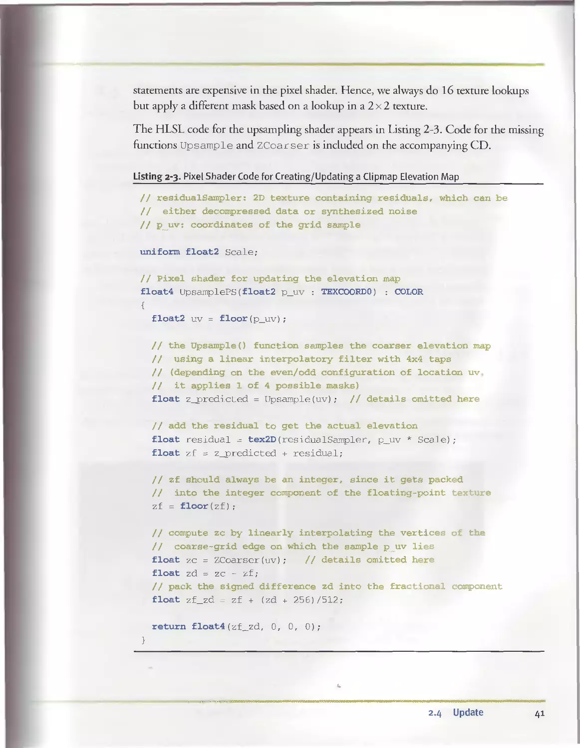
2.4.1 Upsampling..........................................40
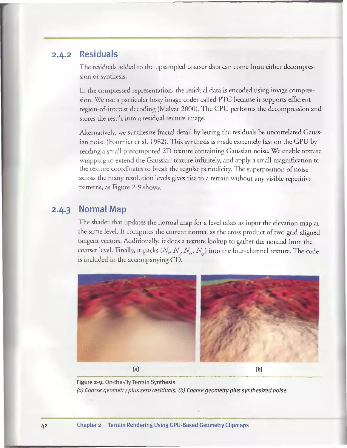
2.4-2 Residuals...........................................42
2.4.3 Normal Map..........................................42
2.5 Results and Discussion.................................... 43
2.6 Summary and Improvements...................................43
2.6.1 Vertex Textures.....................................44
2.6.2 Eliminating Normal Maps.............................44
2.6.3 Memory-Free Terrain Synthesis.......................44
2.7 References.................................................44
Chapter 3
Inside Geometry Instancing..................................................47
Francesco Carucci, Lionhead Studios
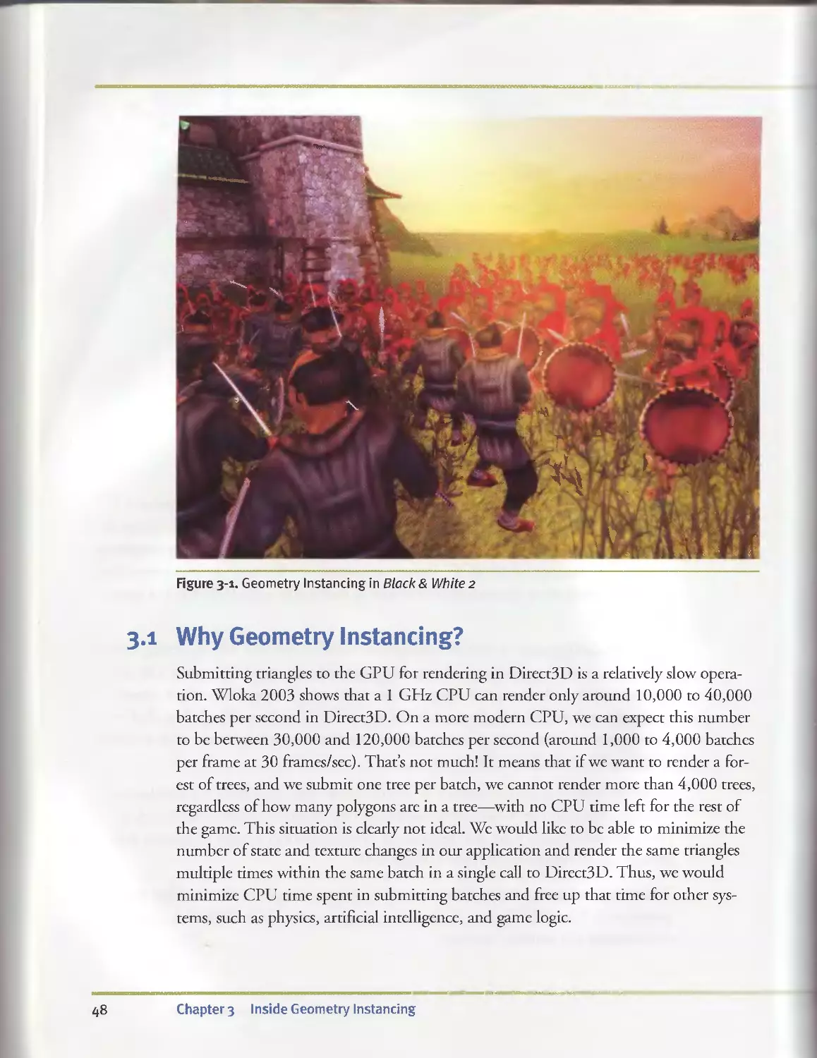
3.1 Why Geometry Instancing?....................................48
3.2 Definitions................................................49
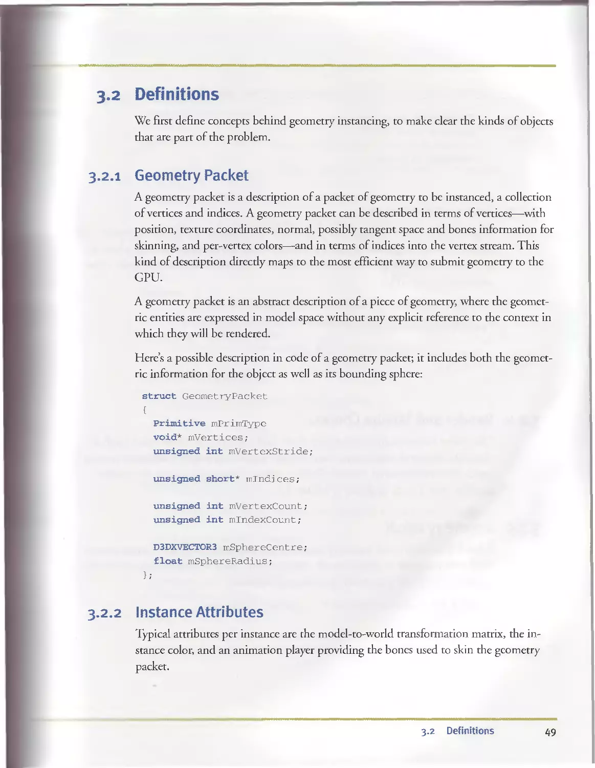
3.2.1 Geometry Packet.....................................49
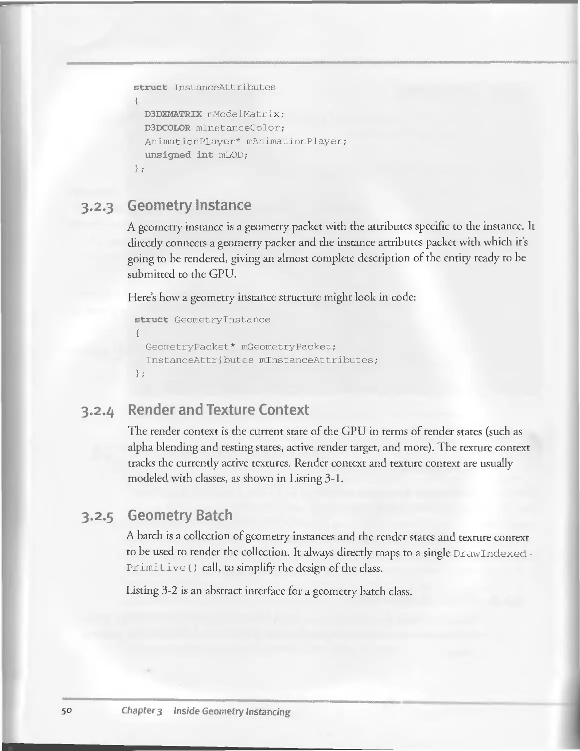
3.2.2 Instance Attributes.................................49
3.2.3 Geometry Instance...................................50
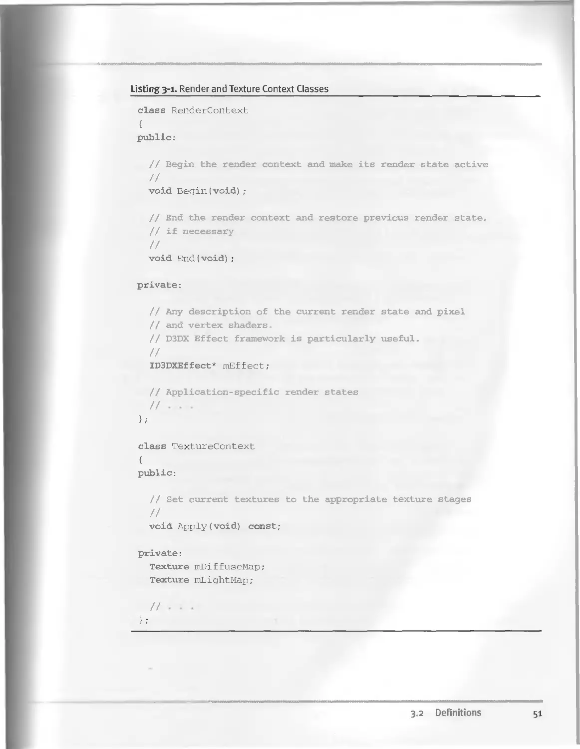
3.2.4 Render and Texture Context..........................50
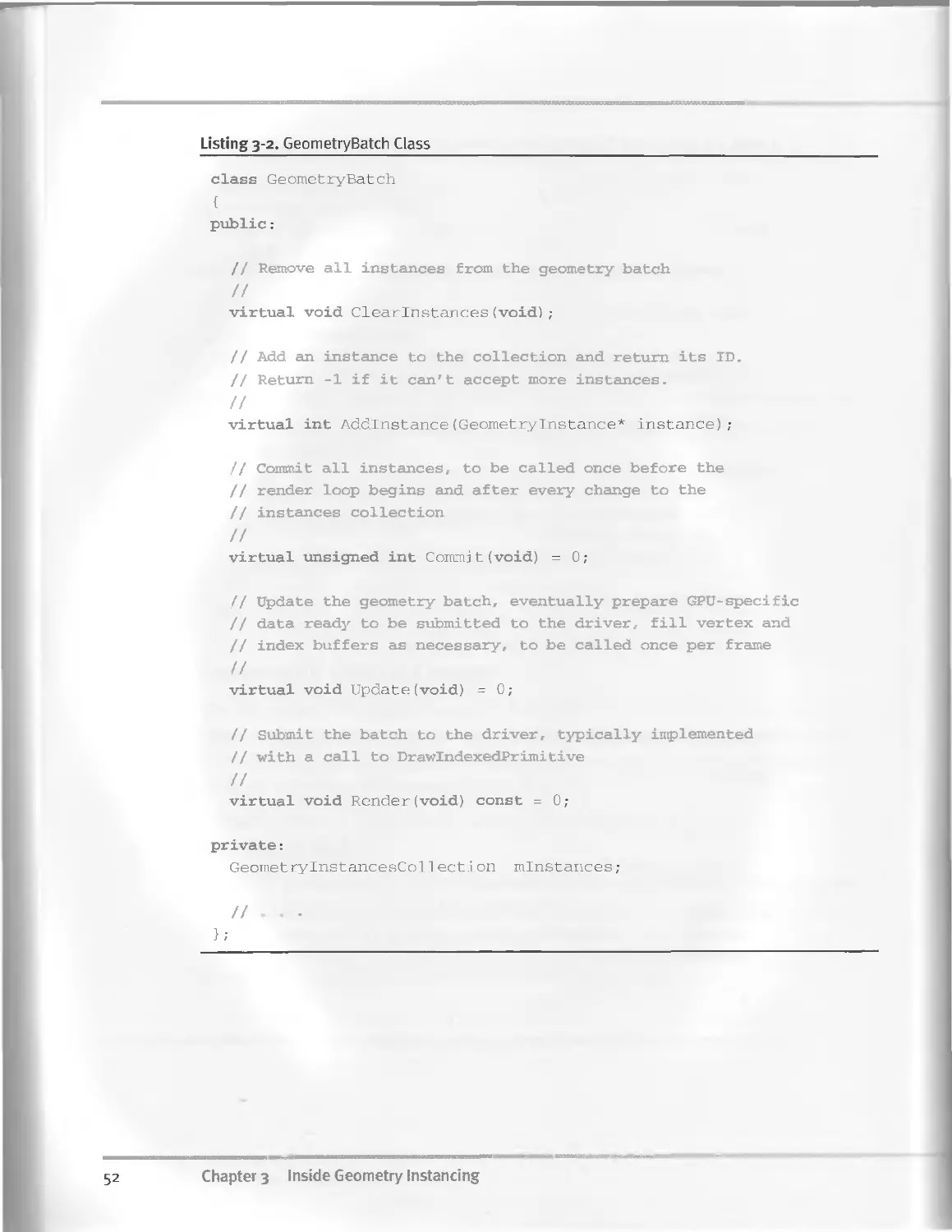
3.2.5 Geometry Batch......................................5О
viii Contents
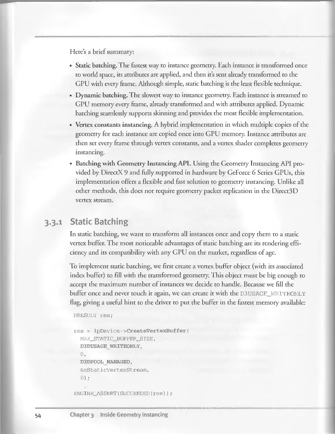
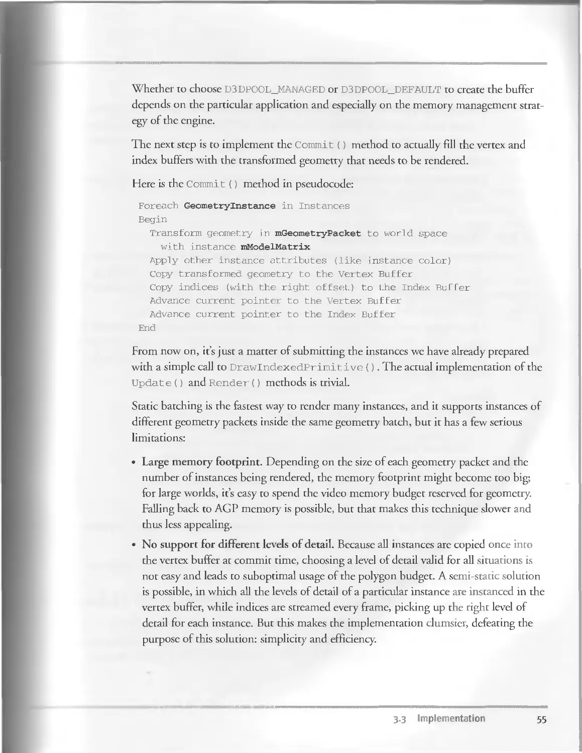
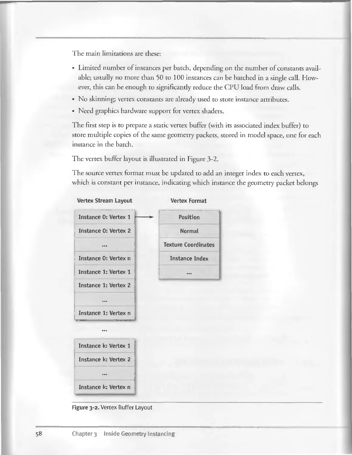
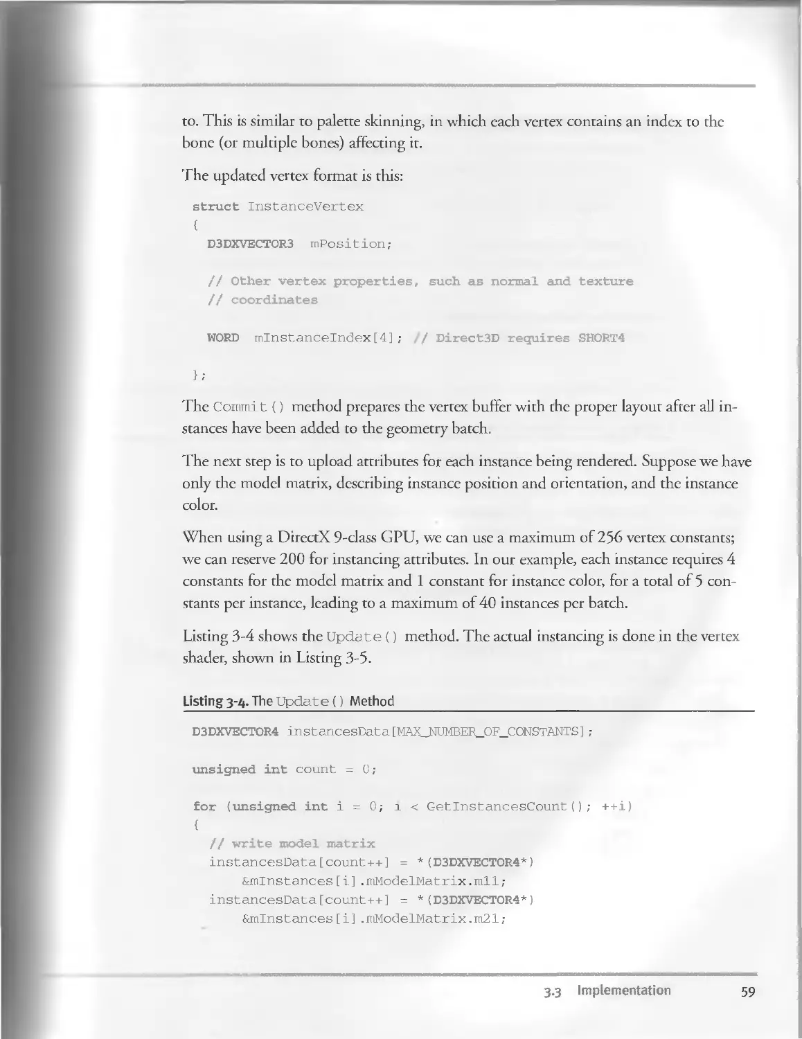
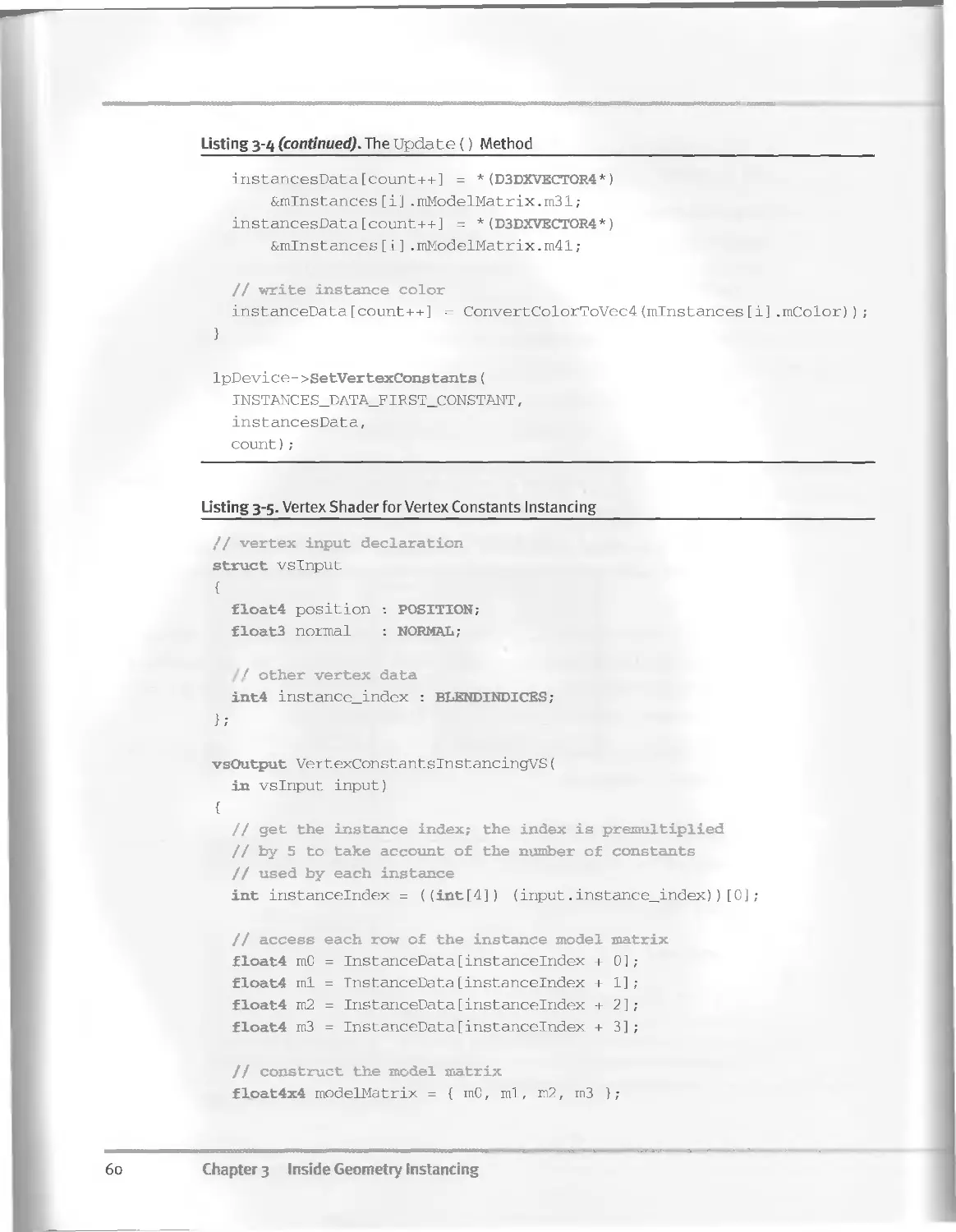
3-3 Implementation................................................53
3.3.I Static Batching.................................. 54
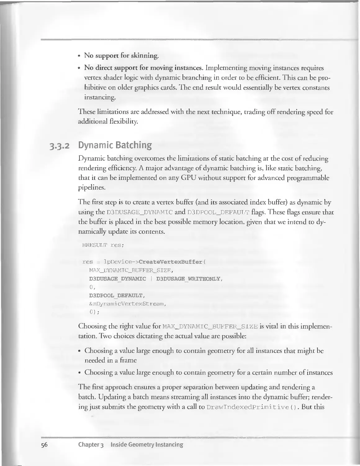
3-3-2 Dynamic Batching.....................................56
3-3-3 Vertex Constants Instancing..........................57
3-3-4 Batching with the Geometry Instancing API............61
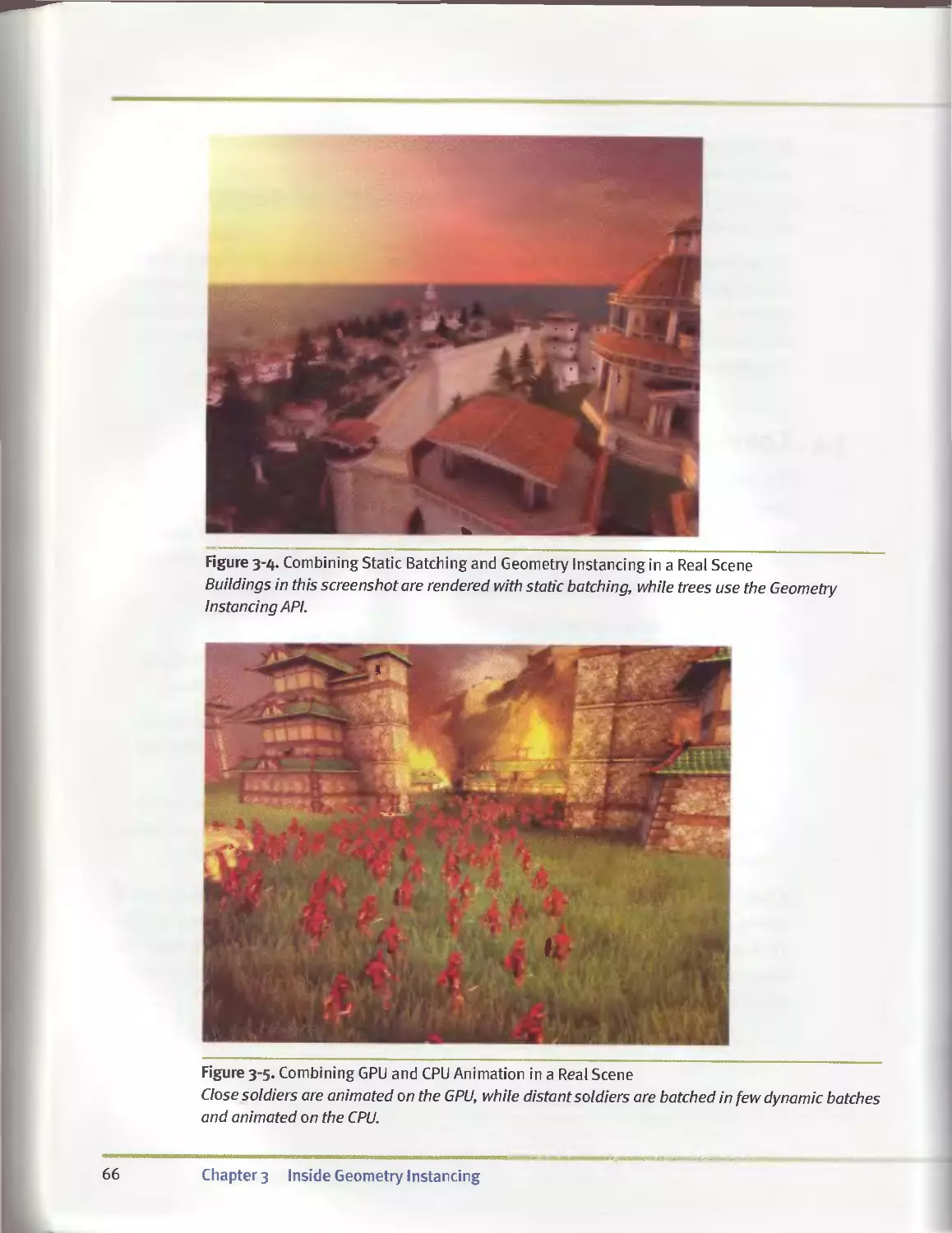
3.4 Conclusion....................................................65
3-5 References....................................................67
Chapter 4
Segment Buffering.......................................................... 69
Jon Olick, 2015
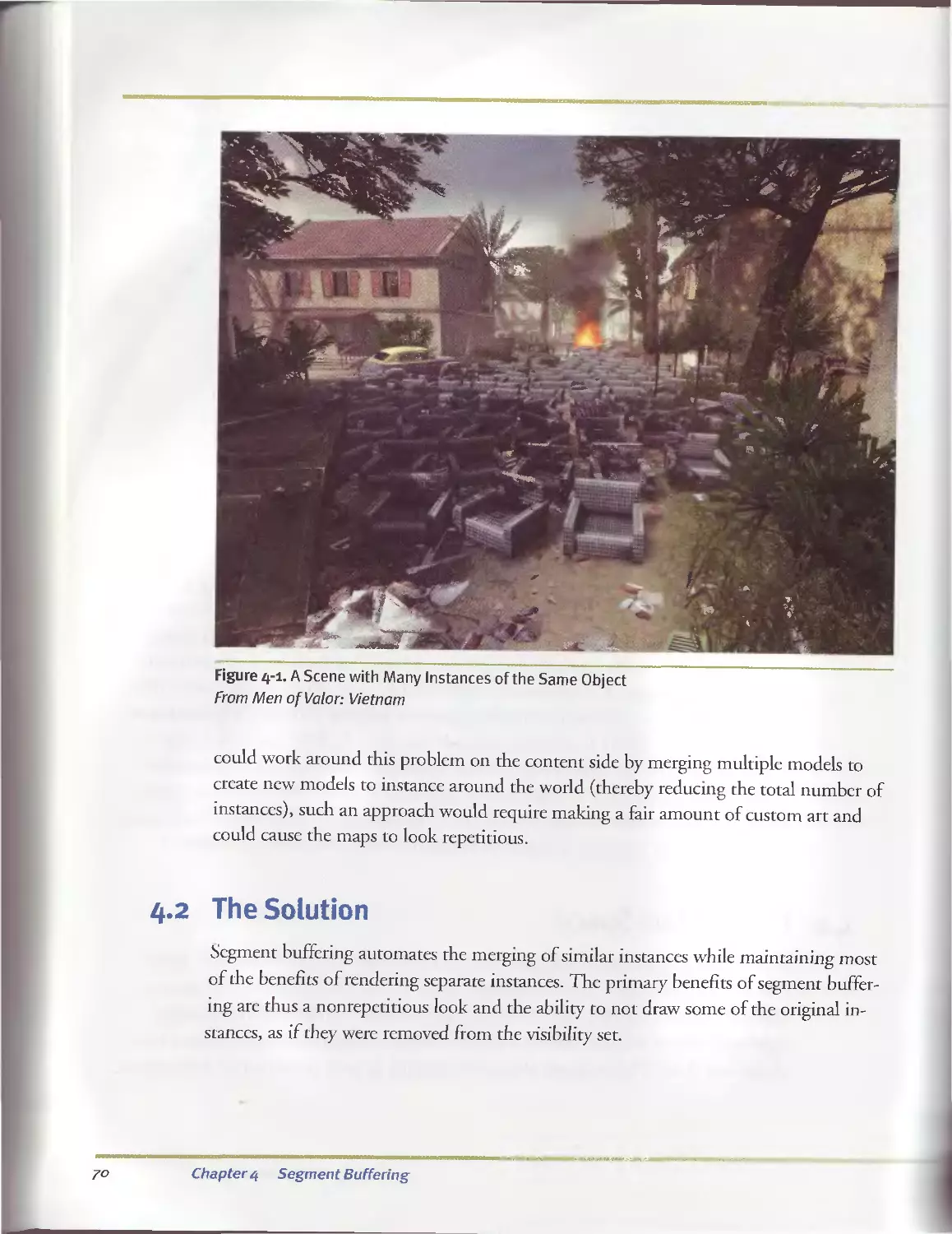
4.1 The Problem Space............................................69
4.2 The Solution.................................................70
4.3 The Method...................................................71
4.3.1 Segment Buffering, Step 1............................71
4.3.2 Segment Buffering, Step 2............................71
4.3.3 Segment Buffering, Step 3............................72
4.4 Improving the Technique.................................... 72
4.5 Conclusion...................................................72
4.6 References...................................................73
Chapter 5
Optimizing Resource Management with Multistreaming...........................75
Oliver Hoeller, Piranha Bytes
Kurt Pelzer, Piranha Bytes
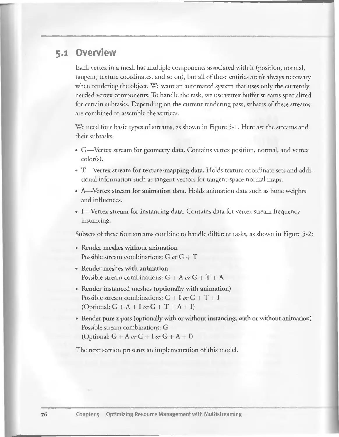
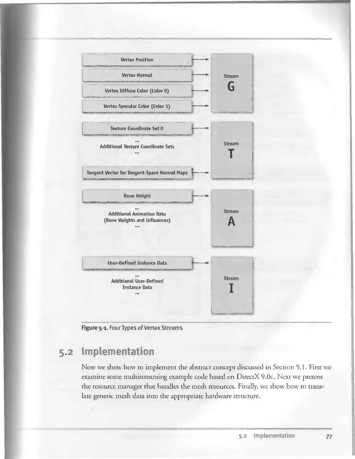
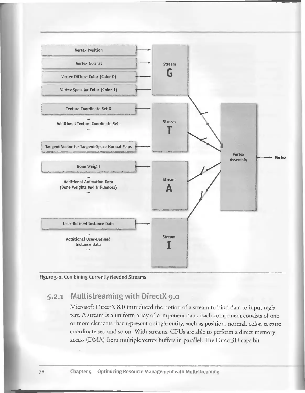
5-1 Overview......................................................76
5.2 Implementation...............................................77
5.2.1 Multistreaming with DirectX 9.0......................78
5.2.2 Resource Management..................................81
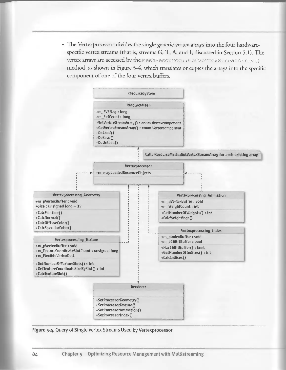
5.2.3 Processing Vertices.......... ............. .. 83
5.3 Conclusion...................................................89
5.4 References...................................................90
Chapter 6
Hardware Occlusion Queries Made Useful.......................................91
Michael Wimmer, Vienna University of Technology
Jiri Bittner, Vienna University of Technology
6.1 Introduction..................................................91
6.2 For Which Scenes Are Occlusion Queries Effective?............92
Contents ix
6-3 What Is Occlusion Culling?.......................................93
6.4 Hierarchical Stop-and-Wait Method..............................94
6.4.I The Naive Algorithm, or Why Use Hierarchies at All?.....94
6.4.2 Hierarchies to the Rescue!..............................95
6.4.3 Hierarchical Algorithm..................................95
6.4.4 Problem 1: Stalls.......................................96
6.4-5 Problem 2: Query Overhead...............................97
6.5 Coherent Hierarchical Culling...................................97
6.5.1 Idea 1: Being Smart and Guessing........................97
6.5.2 Idea 2: Pull Up, Pull Up................................98
6-5-3 Algorithm...............................................99
6.5.4 Implementation Details.................................100
6.5.5 Why Are There Fewer Stalls?............................103
6.5.6 Why Are There Fewer Queries?...........................104
6.5-7 How to Traverse the Hierarchy..........................104
6.6 Optimizations.................................................105
6.6.1 Querying with Actual Geometry..........................105
6.6.2 Z-Only Rendering Pass......... . . . ..................105
6.6.3 Approximate Visibility.................................105
6.6.4 Conservative Visibility Testing........................106
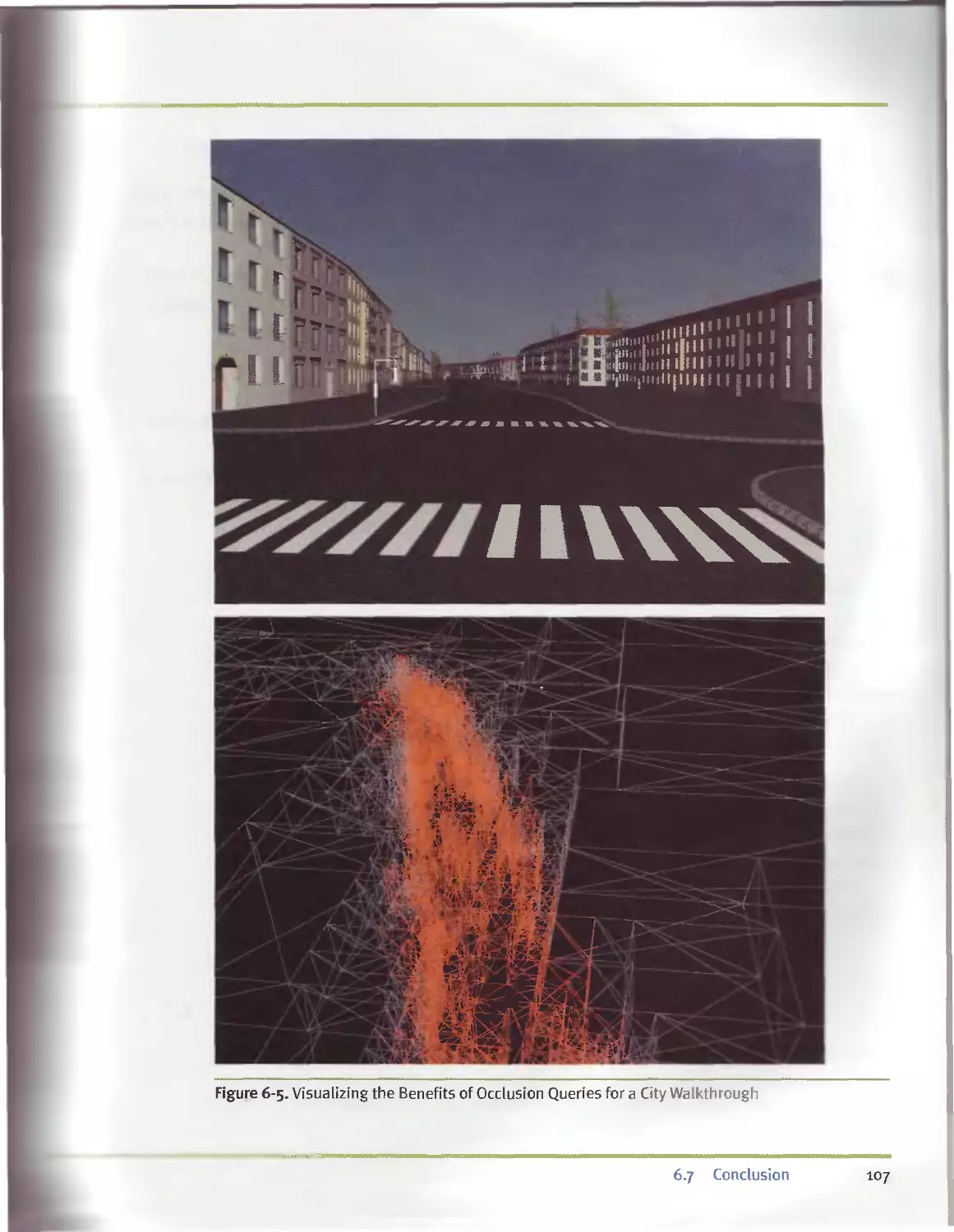
6.7 Conclusion.....................................................106
6.8 References....................................................108
Chapter 7
Adaptive Tessellation of Subdivision Surfaces with
Displacement Mapping............................................................109
Michael Bunnell, NVIDIA Corporation
7.1 Subdivision Surfaces...........................................109
7.1.1 Some Definitions......................................110
7.1.2 Catmull-Clark Subdivision.............................110
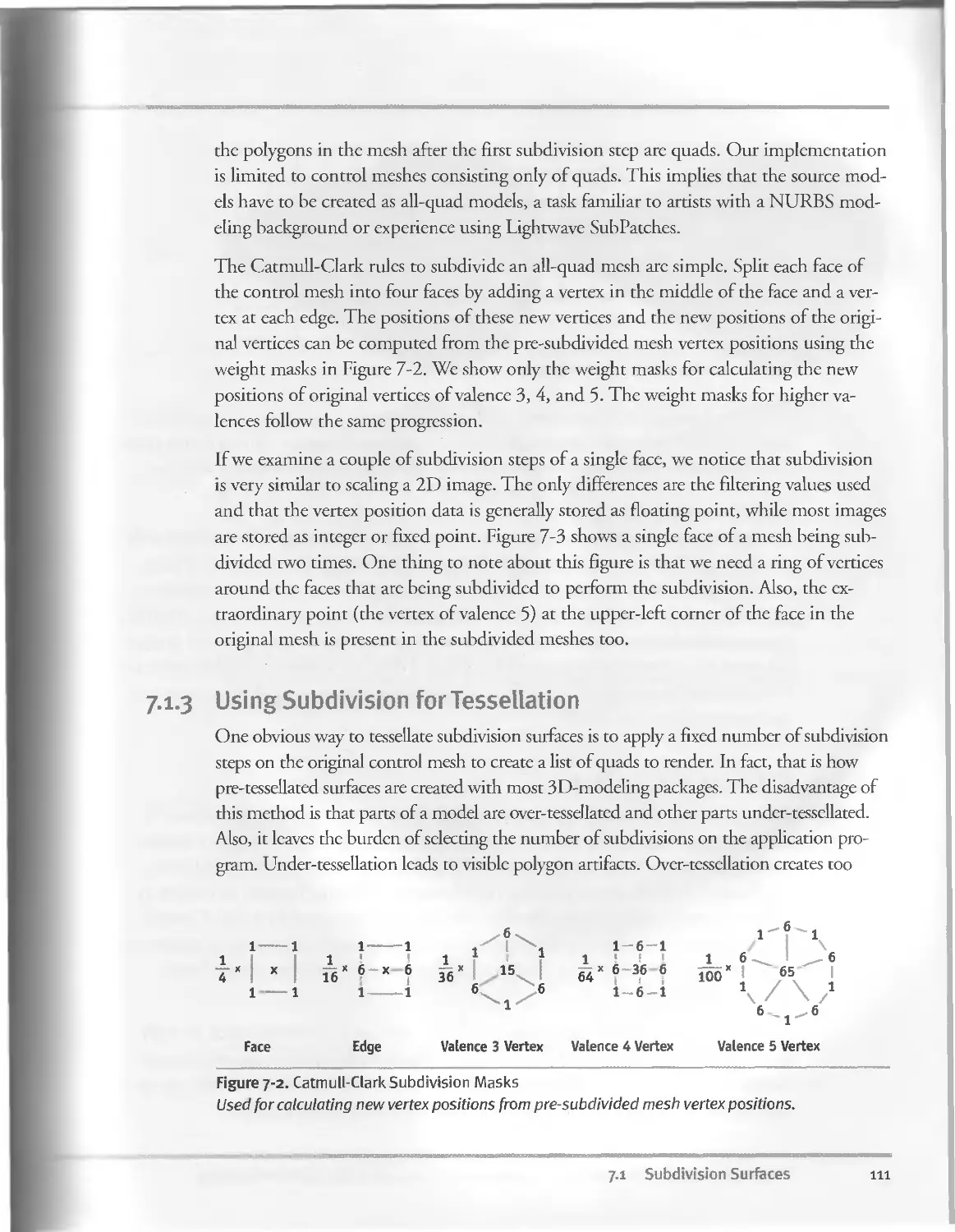
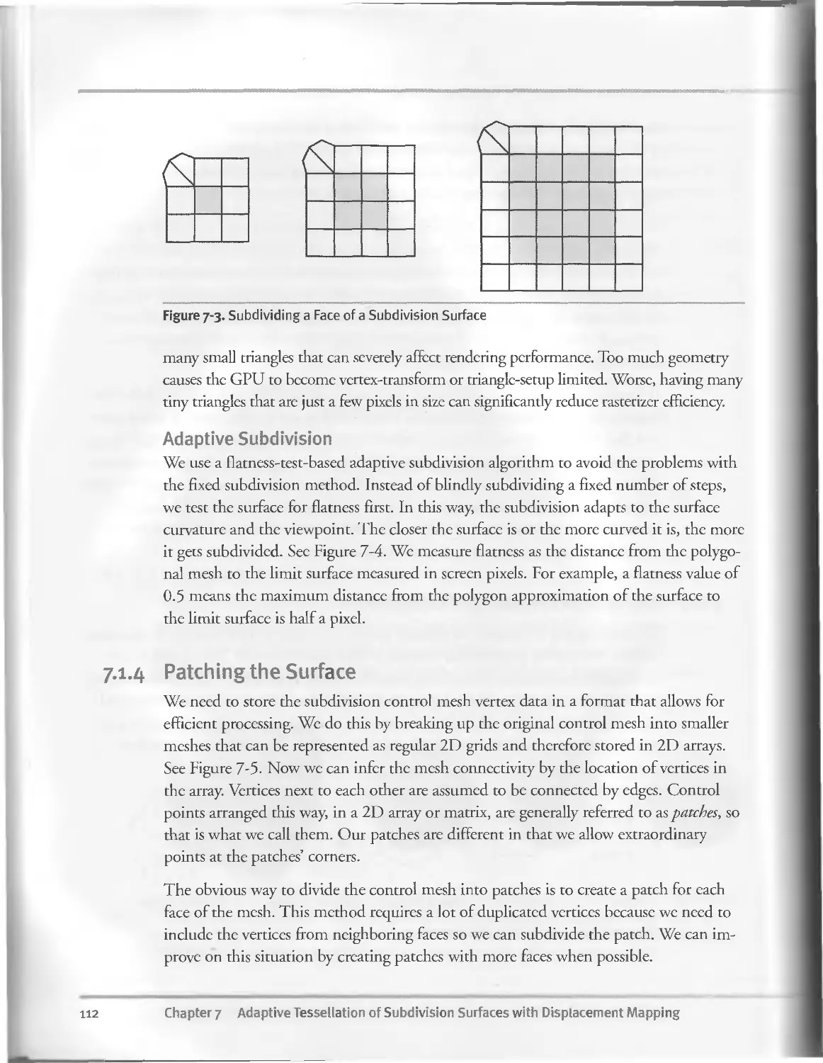
7.I.3 Using Subdivision for Tessellation....................Ill
7.I.4 Patching the Surface..................................112
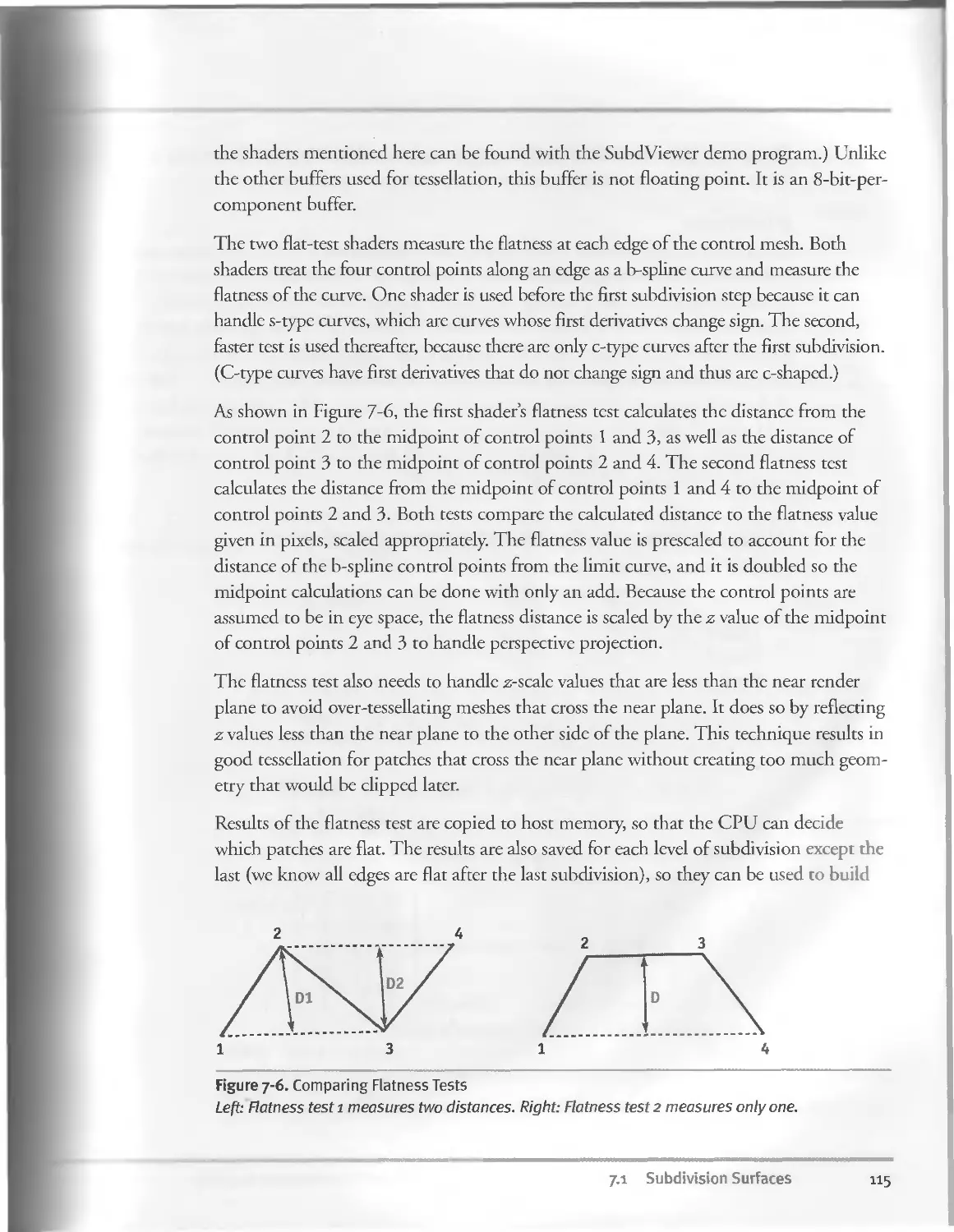
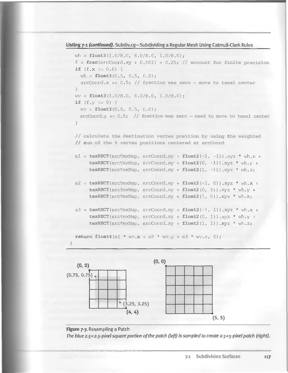
7.I.5 The GPU Tessellation Algorithm........................114
7.1.6 Watertight Tessellation...............................118
7.2 Displacement Mapping...........................................119
7.2.1 Changing the Flatness Test............................120
7.2.2 Shading Using Normal Mapping..........................120
7.3 Conclusion.....................................................122
7.4 References.....................................................122
x
Contents
£ян еажй^^^пэиювмияпймимймйвк^^^жпмаяеапемйтмяпаа^вмпммямм^^^мчпмкжаяажмам^пваматмамймаминаажмммаммйаммжшаям
Chapter 8
Per-Pixel Displacement Mapping with Distance Functions...........................123
William Donnelly, University of Waterloo
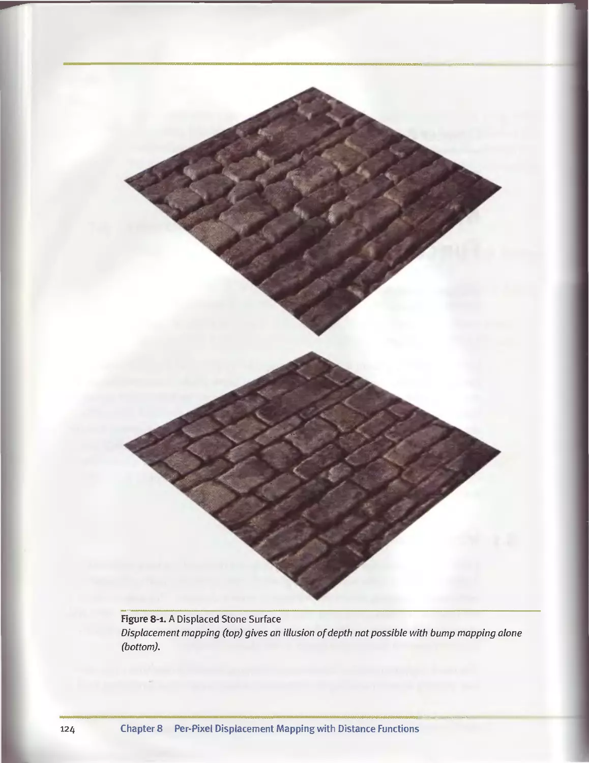
8.1 Introduction.....................................................123
8.2 Previous Work....................................................125
8.3 The Distance-Mapping Algorithm...................................126
8.3.I Arbitrary Meshes.........................................129
8.4 Computing the Distance Map.......................................130
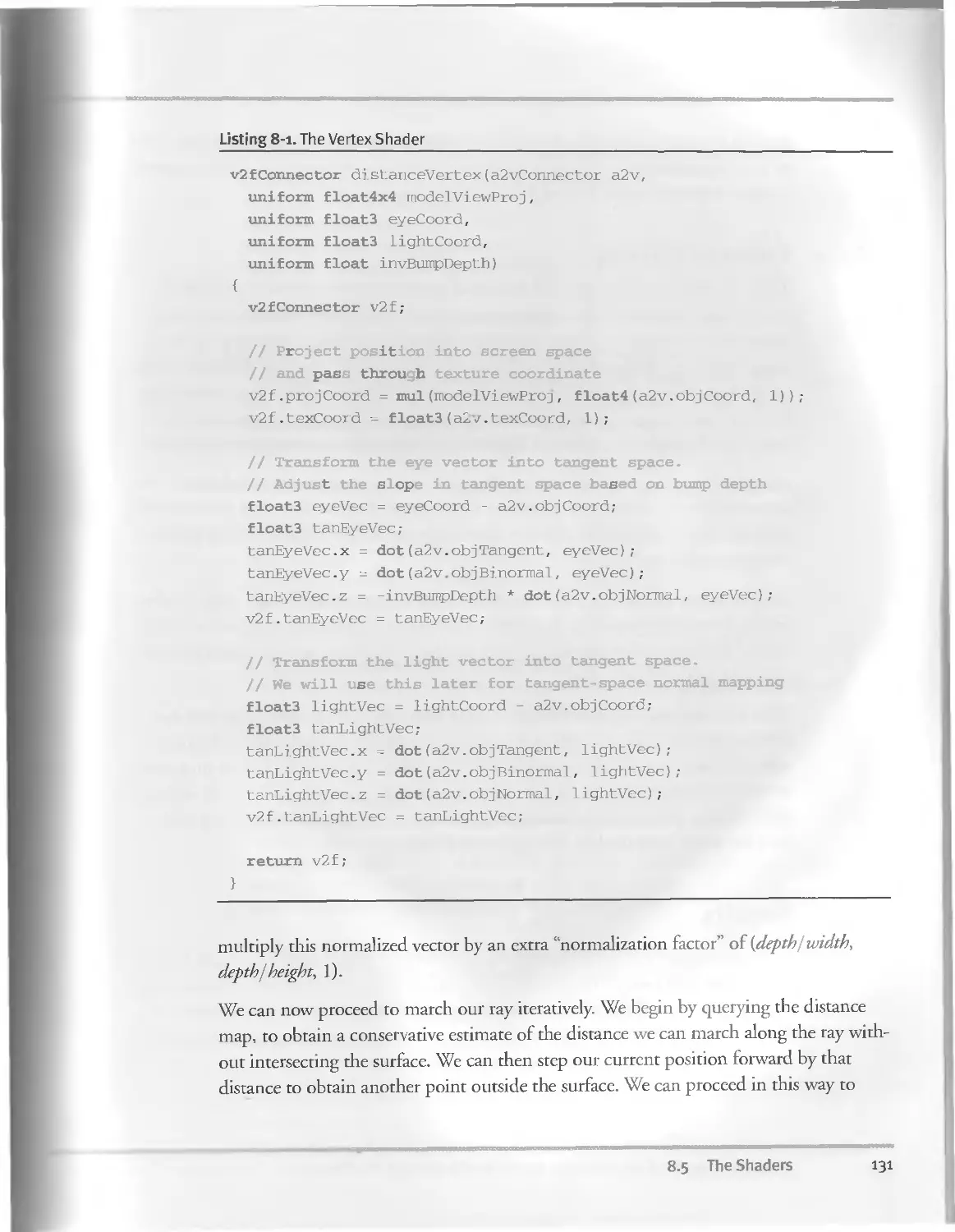
8.5 The Shaders......................................................130
8.5.1 The Vertex Shader........................................130
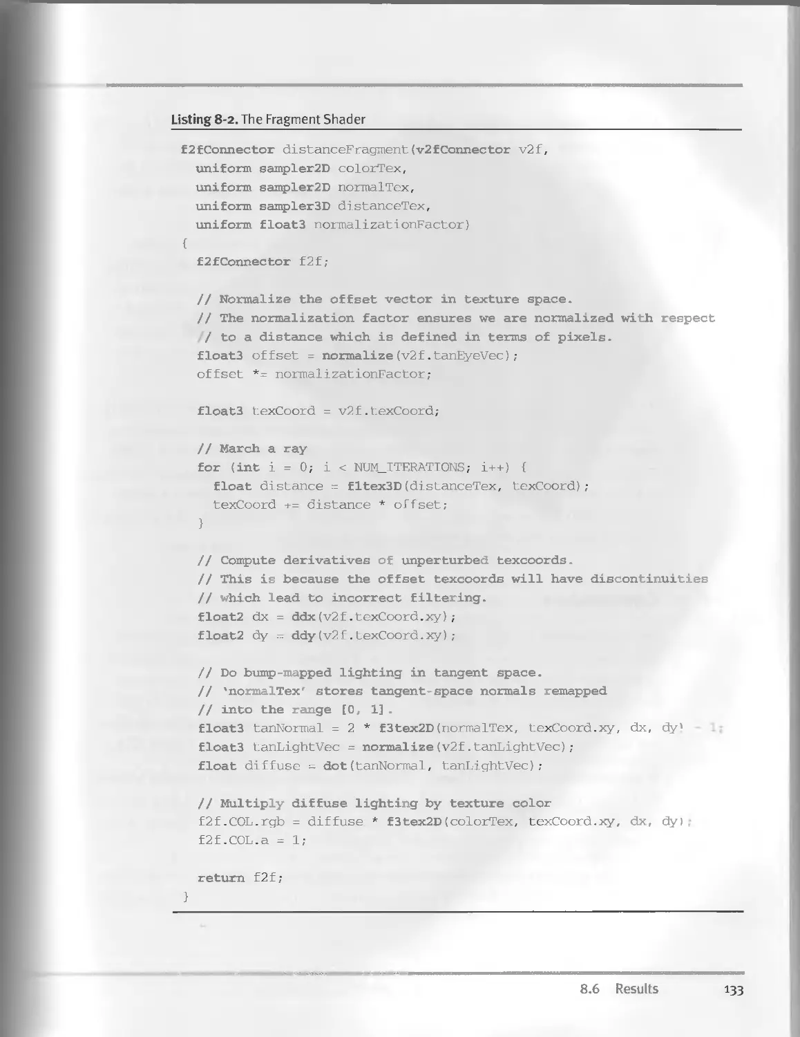
8.5.2 The Fragment Shader......................................130
8-5-3 A Note on Filtering......................................132
8.6 Results..........................................................132
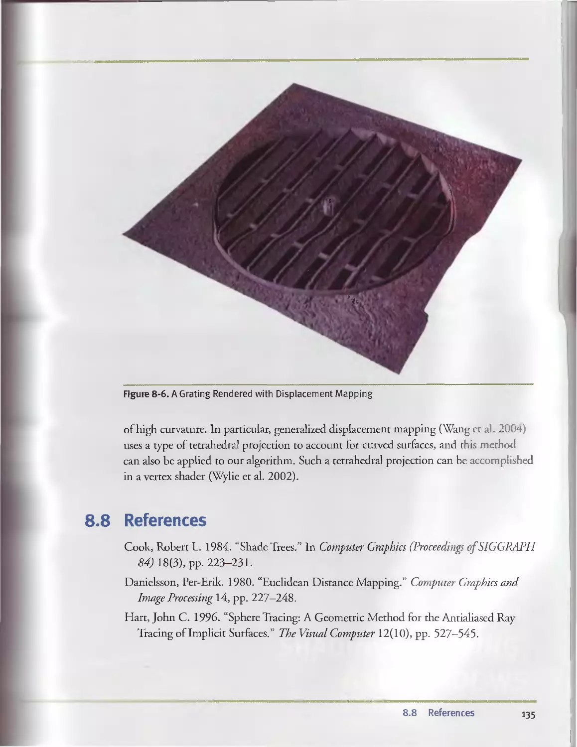
8.7 Conclusion.......................................................134
8.8 References...................................................... 135
PART II SHADING, LIGHTING, AND SHADOWS 137
Chapter 9
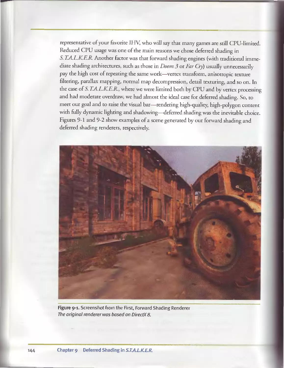
Deferred Shading in S.T.A.L.K.E.R.................................................143
Oles Shishkovtsov, GSC Game World
9.1 Introduction.....................................................143
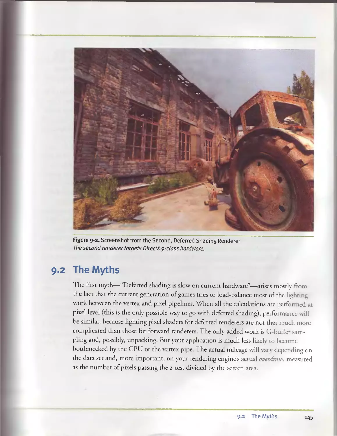
9.2 The Myths........................................................145
9.3 Optimizations....................................................147
9.3.I What to Optimize........................................147
9.3.2 Lighting Optimizations..................................148
9-3-3 G-Buffer-Creation Optimizations.........................151
9-3-4 Shadowing Optimizations................................153
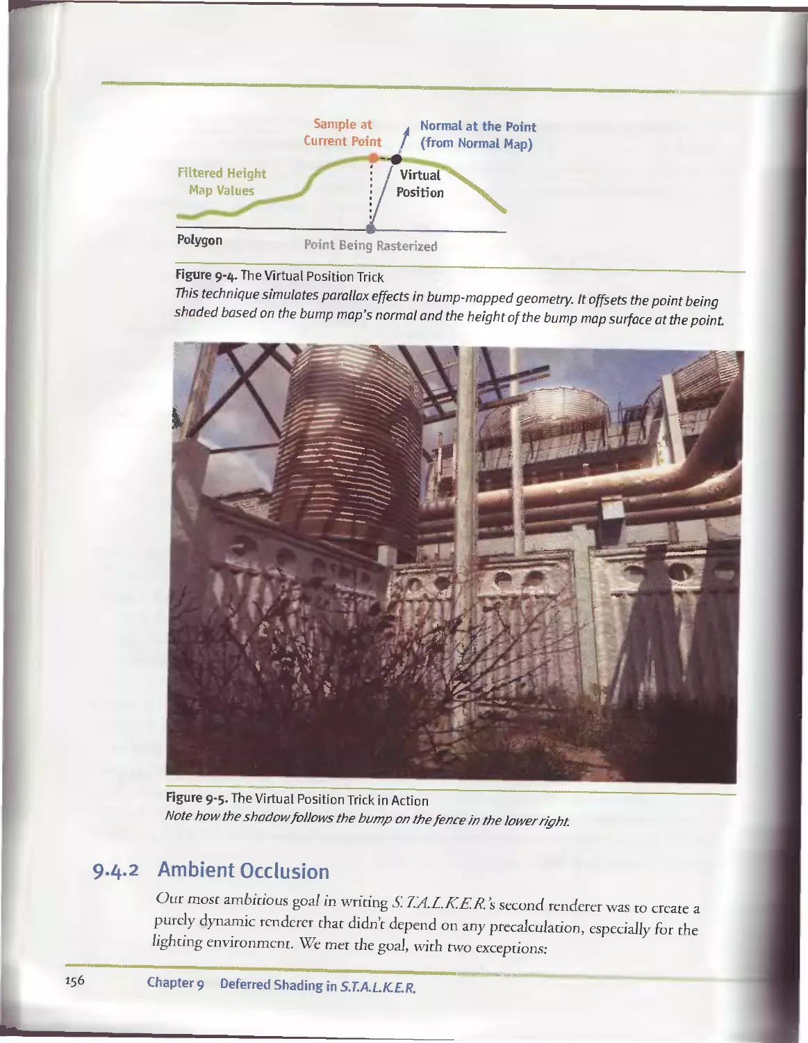
9.4 Improving Quality................................................154
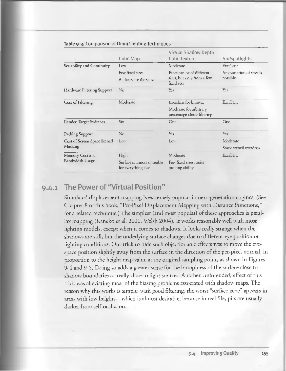
9.4.I The Power of “Virtual Position”.........................155
9.4.2 Ambient Occlusion.......................................I56
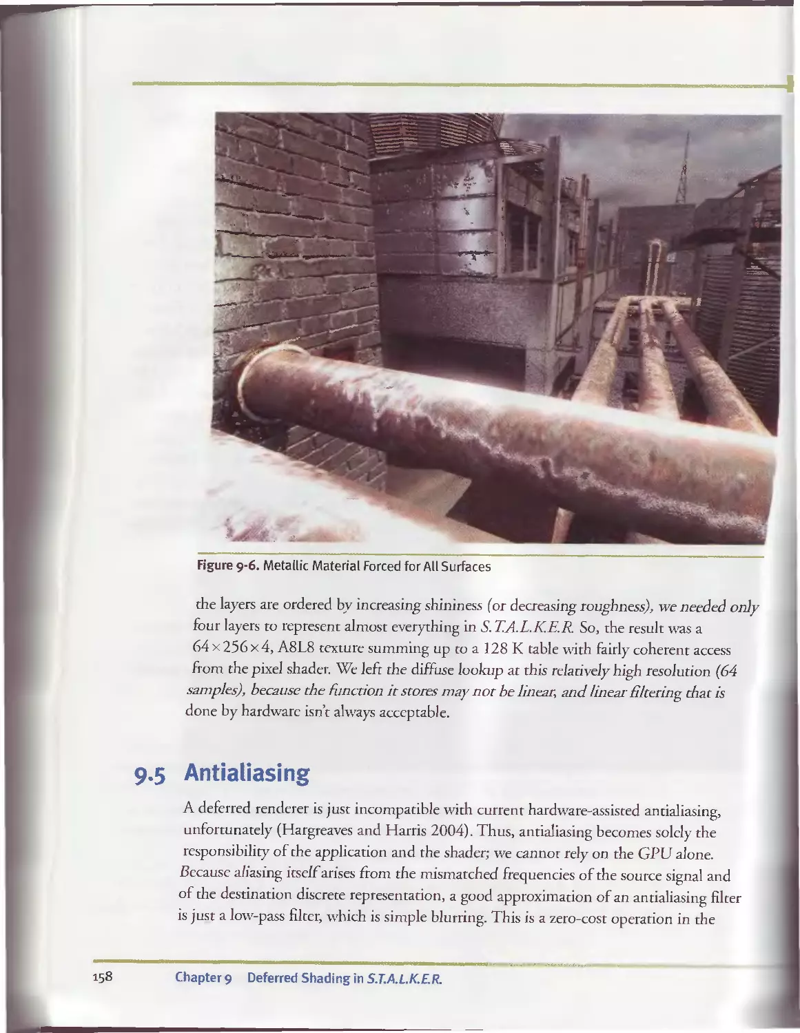
9-4-3 Materials and Surface-Light Interaction.............. ... 157
9.5 Antialiasing................. ...................... .. 158
9.5.I Efficient Tone Mapping............................. .... 161
9.5.2 Dealing with Transparency...................... . . . 162
9.6 Things We Tried but Did Not Include in the Final Code . . . 162
9.6.I Elevation Maps......................................... 163
9-6.2 Real-Time Global Illumination . . ... ... 163
9.7 Conclusion.......................................................164
9.8 References.......................................................165
Contents xi
и—wmwHiHi и > m »i 14а——ши——и——адямваа«е»м1жячав1 i н ыии naw iimi 1 там»» и—чиж мпдсагтцареявт—двчаа — нши-^ит ч -
Chapter ю
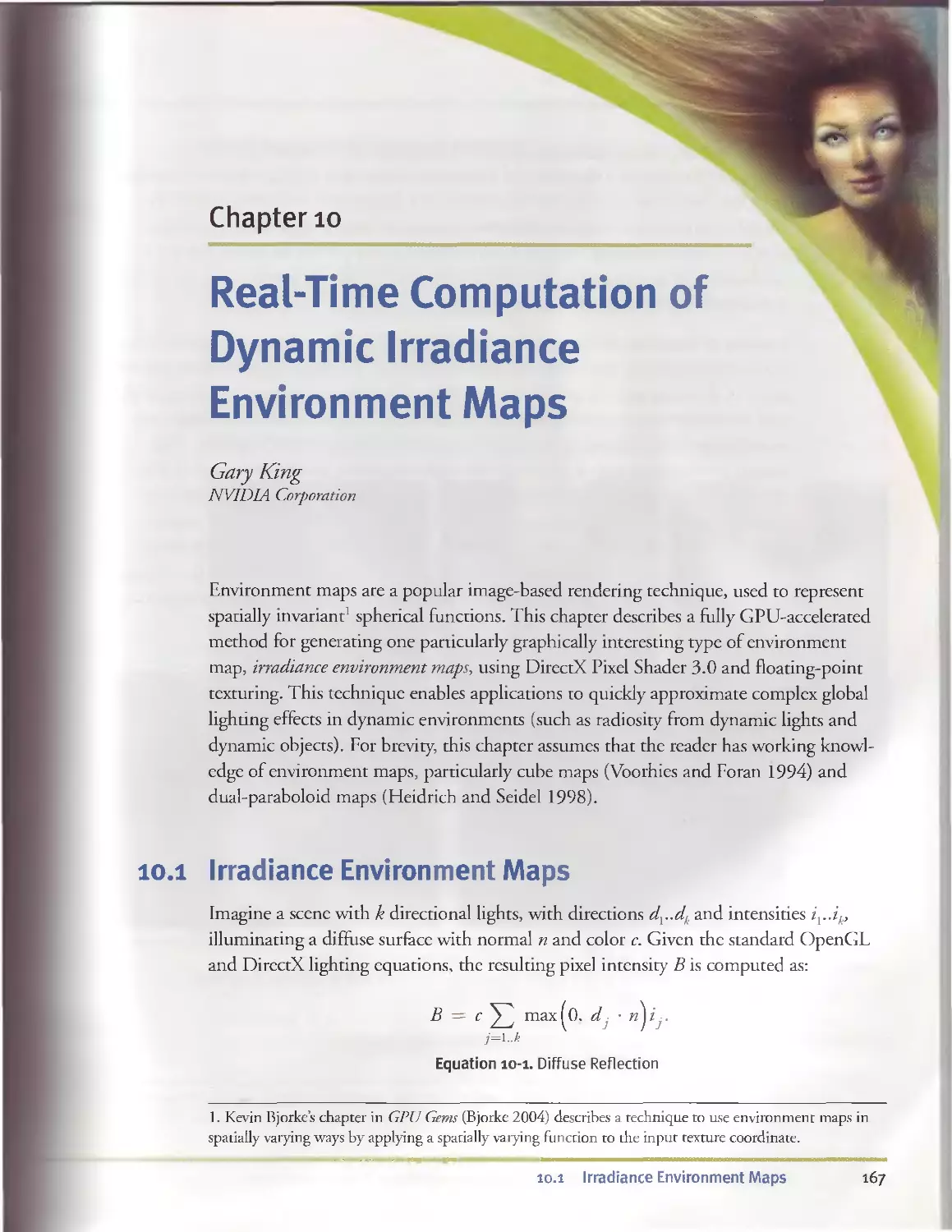
Real-Time Computation of Dynamic Irradiance
Environment Maps......................................................... 167
Gary King, NVIDIA Corporation
10. 1 Irradiance Environment Maps...............................167
10. 2 Spherical Harmonic Convolution............................170
IO. 3 Mapping to the GPU.......................................172
Ю.3.1 Spatial to Frequency Domain...... 172
IO.3.2 Convolution and Back Again.........................173
10. 4 Further Work..............................................175
IO. 5 Conclusion................................................176
10. 6 References................................................176
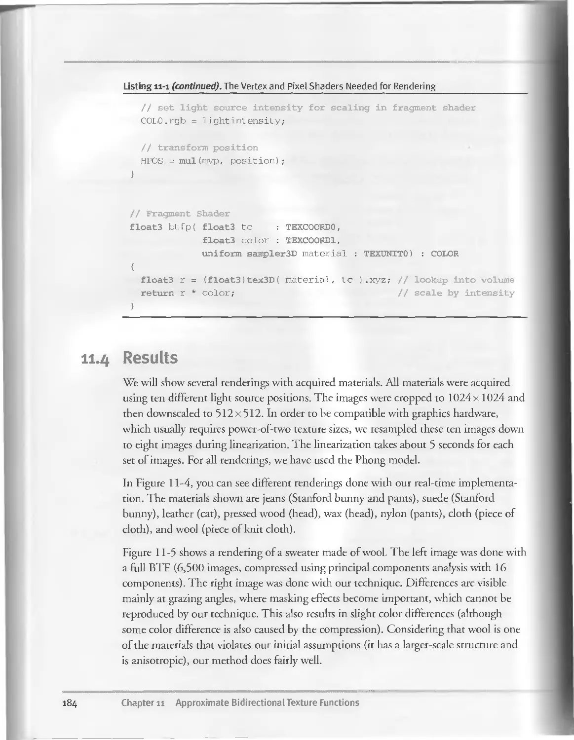
Chapter и
Approximate Bidirectional Texture Functions................................177
Jan Kautz, Massachusetts Institute ofTechnology
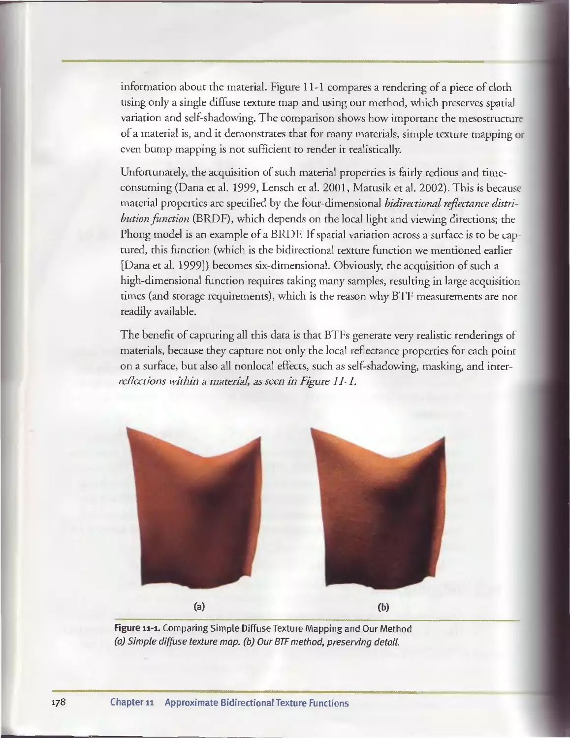
11. 1 Introduction..............................................177
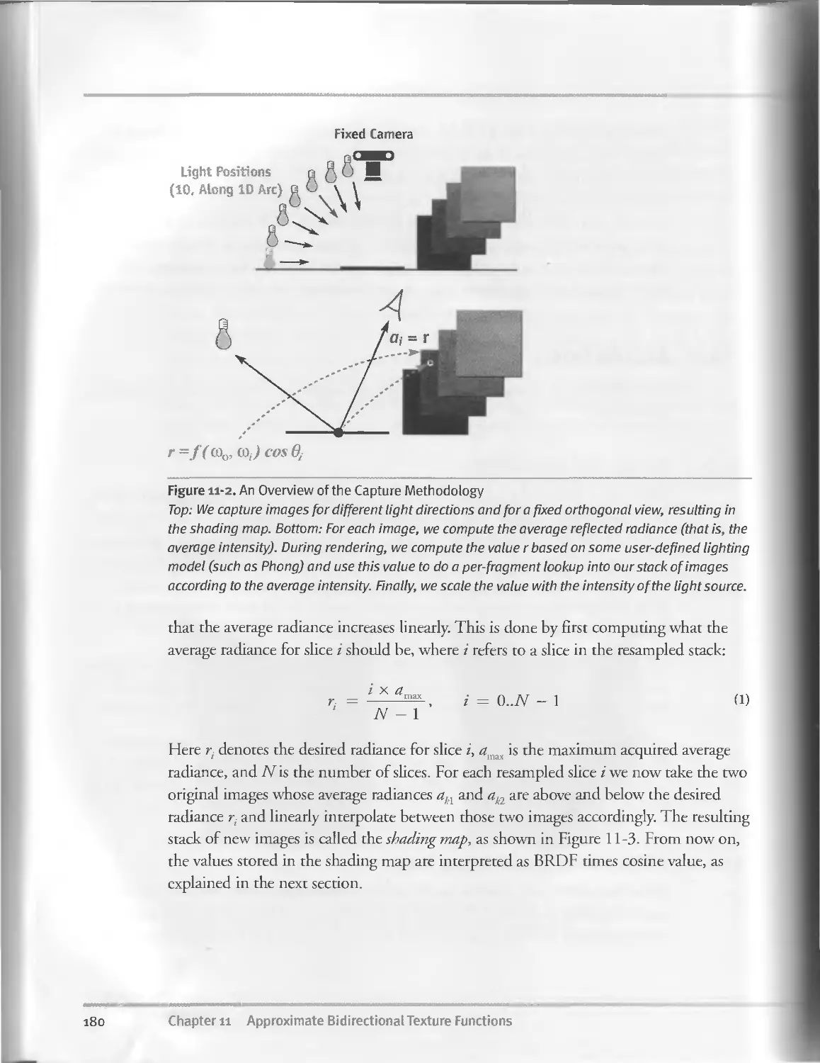
11. 2 Acquisition...............................................179
11.2.1 Setup and Acquisition.............................179
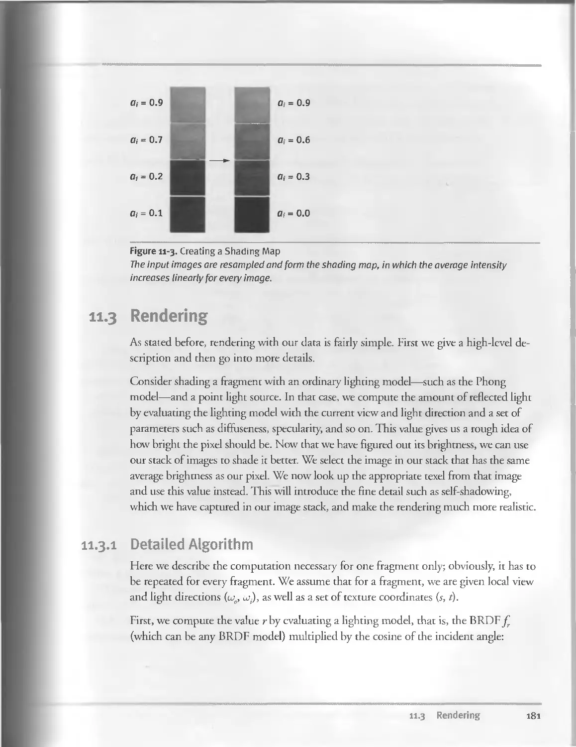
11.2.2 Assembling the Shading Map........................179
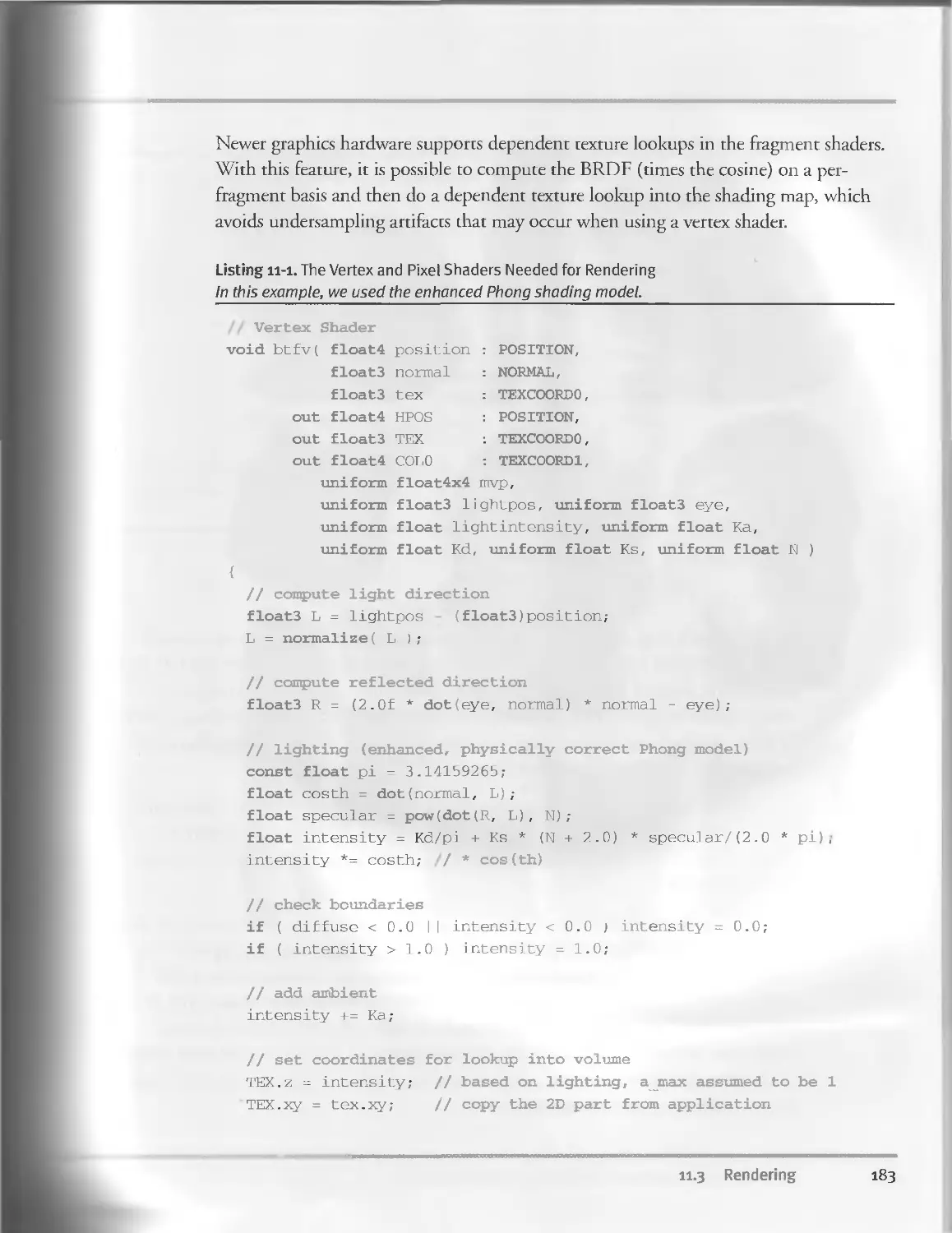
11. 3 Rendering.................................................181
H.3.1 Detailed Algorithm................................181
II.3.2 Real-Time Rendering...............................182
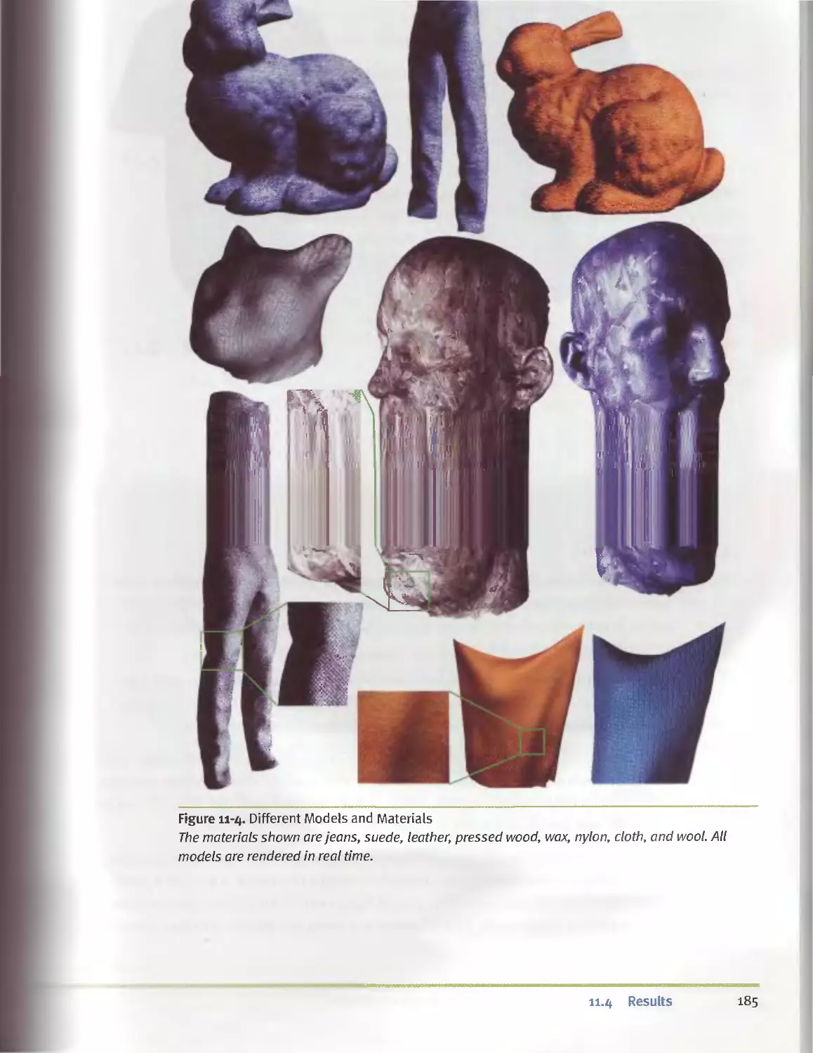
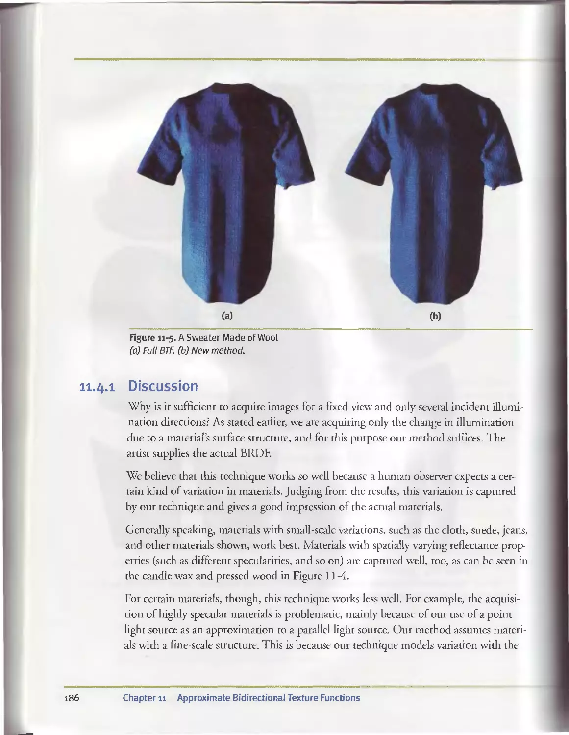
11.4 Results....................................................184
11-4-1 Discussion........................................186
11-5 Conclusion.................................................187
11.6 References.............................................. 187
Chapter 12
Tile-Based Texture Mapping.................................................189
Li-Yi Wei, NVIDIA Corporation
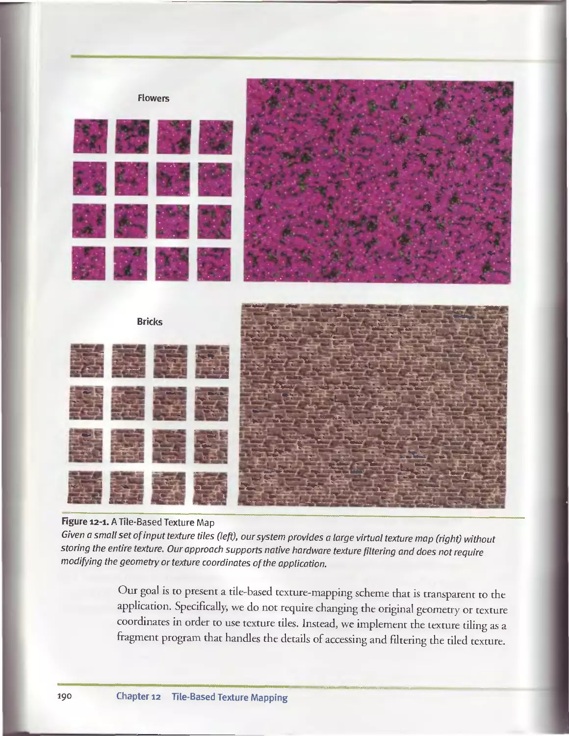
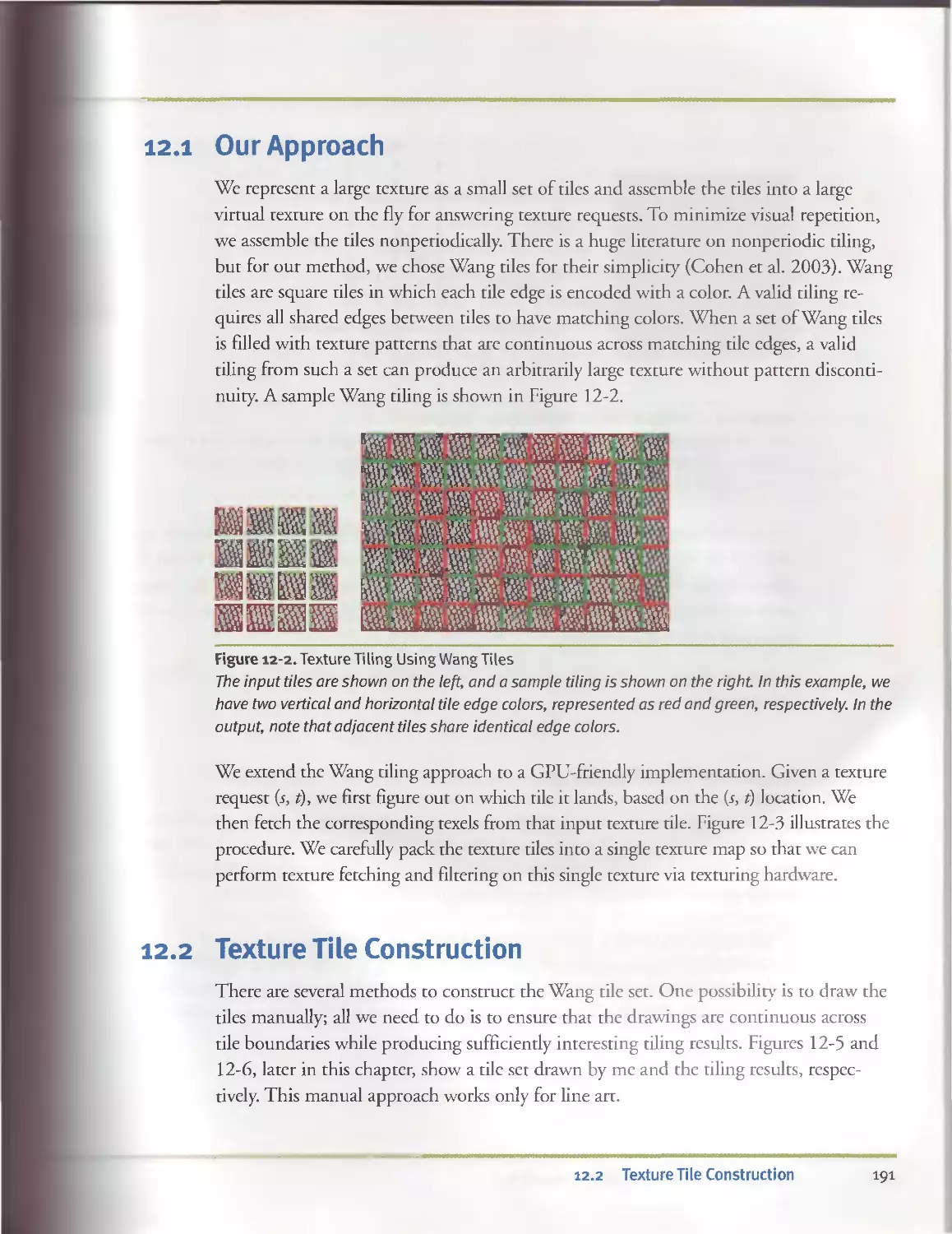
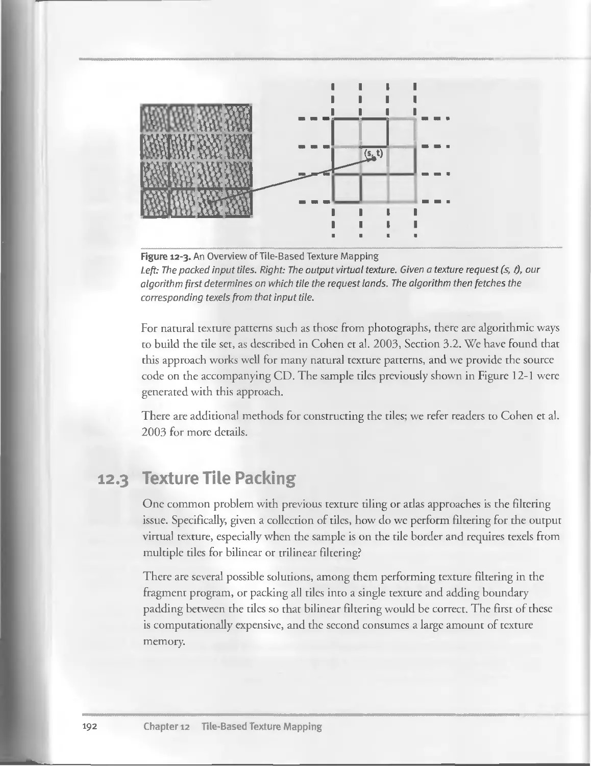
12.1 Our Approach...............................................191
12.2 Texture Tile Construction.................................191
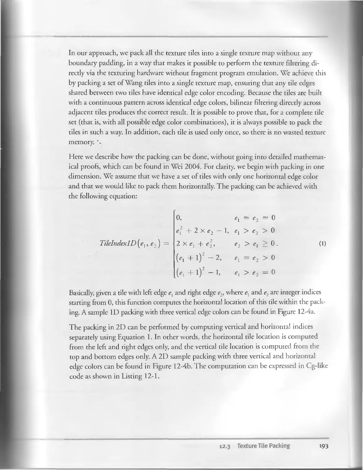
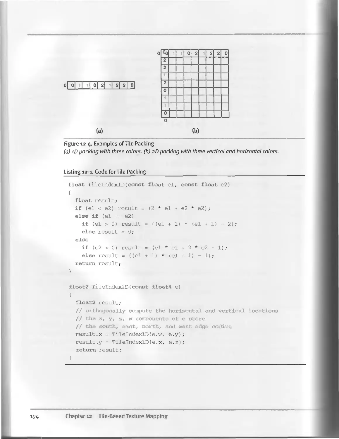
12.3 Texture Tile Packing......................................192
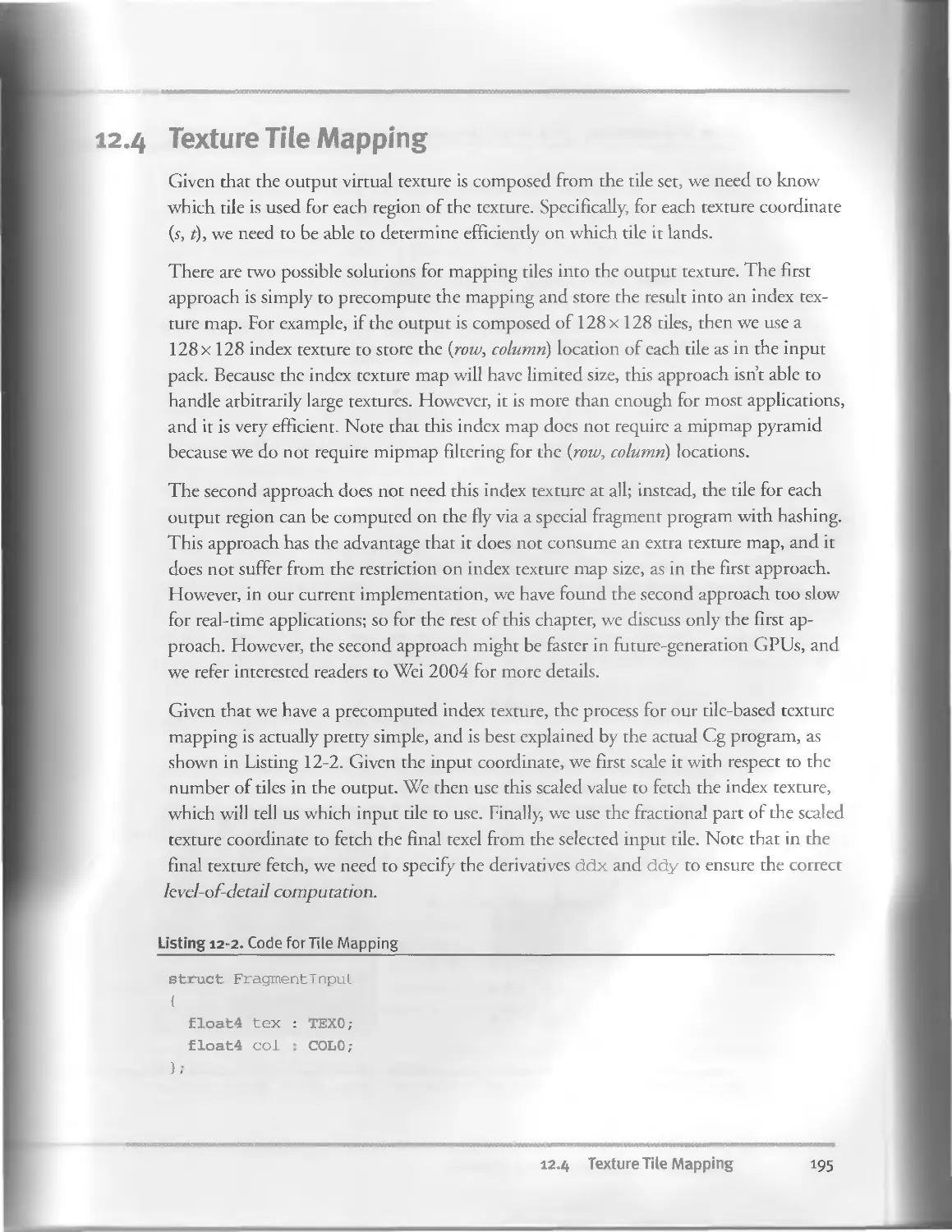
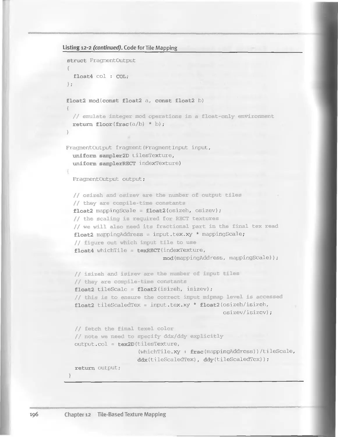
12.4 Texture Tile Mapping......................................195
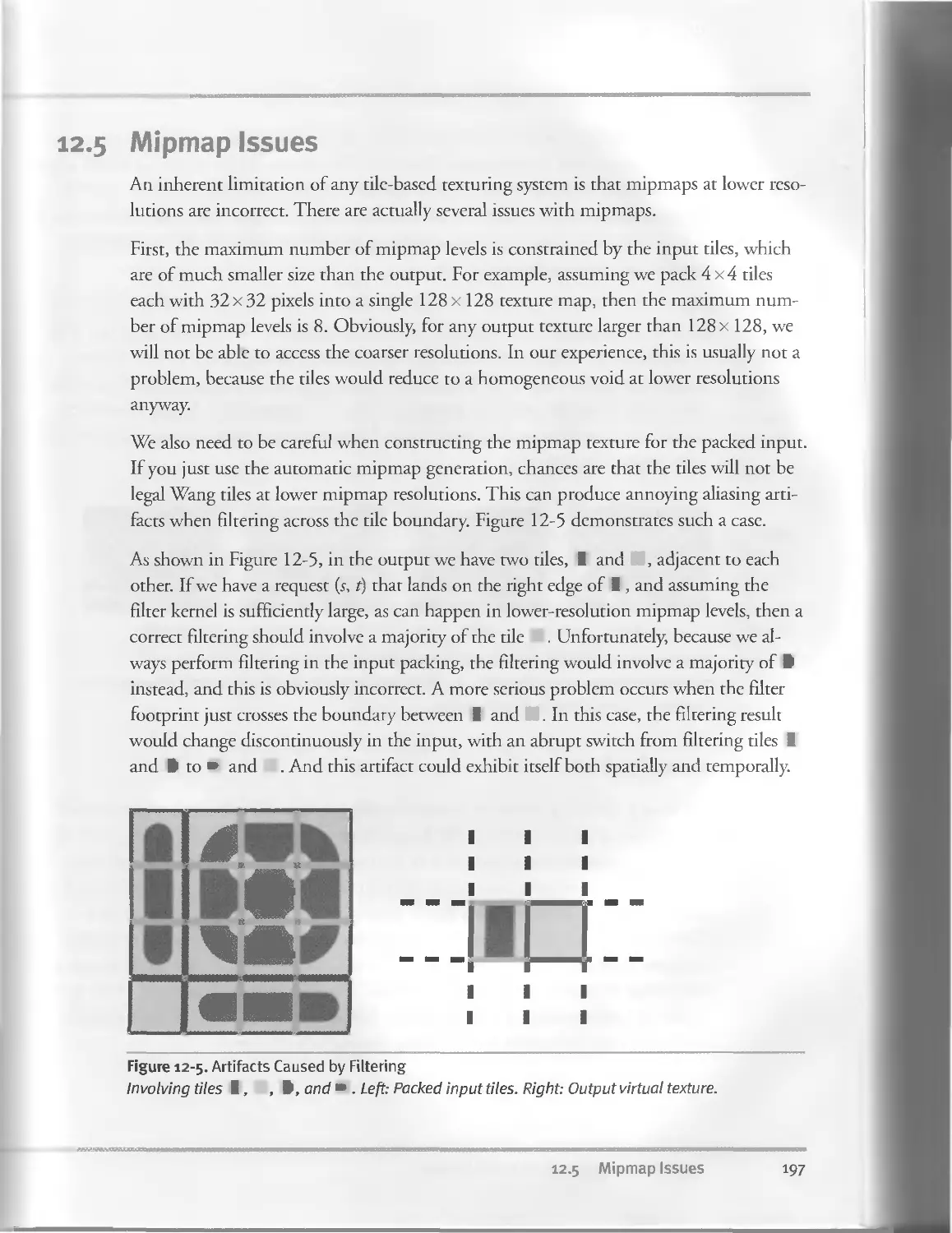
12.5 Mipmap Issues..............................................197
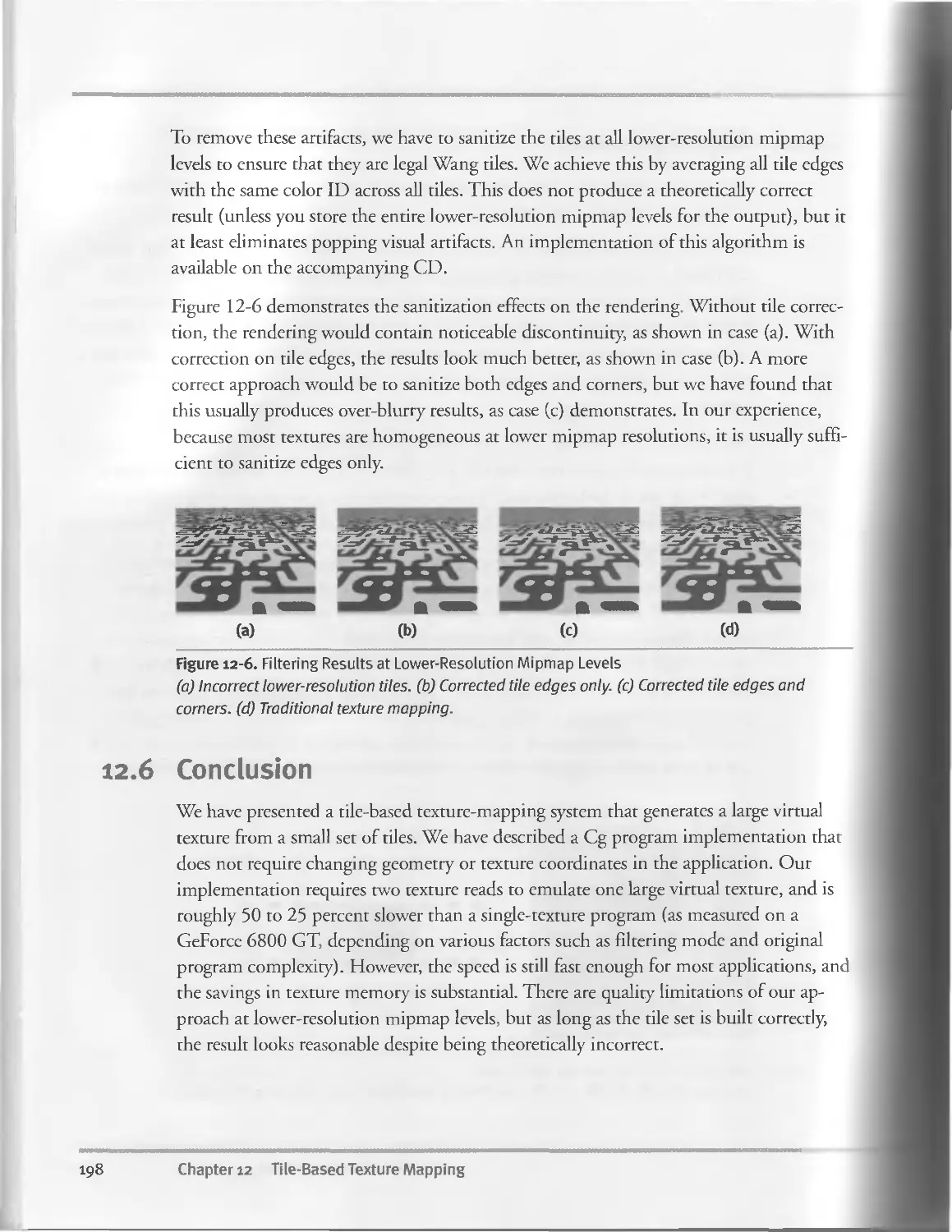
12.6 Conclusion................................................198
12.7 References................................................199
xii Contents
Chapter 13
Implementing the mental images Phenomena Renderer
on the GPU.................................................................201
Martin-Karl Lefrangois, mental images
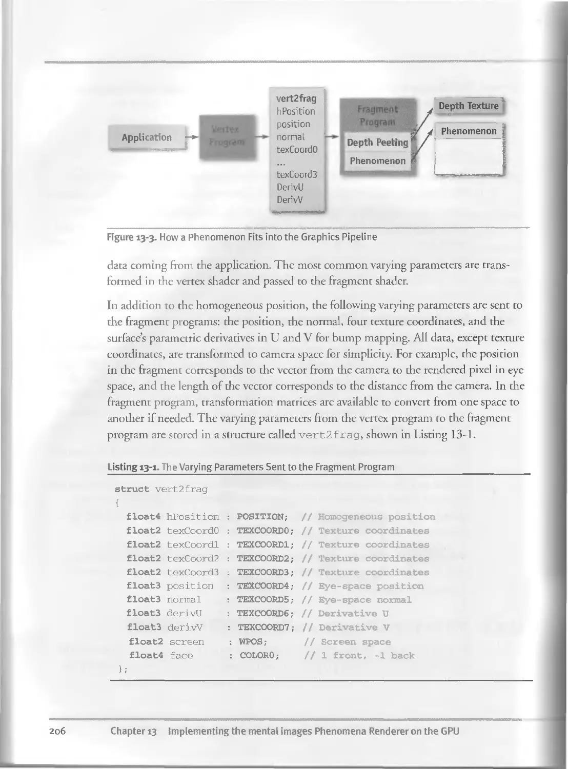
13.I Introduction................................................201
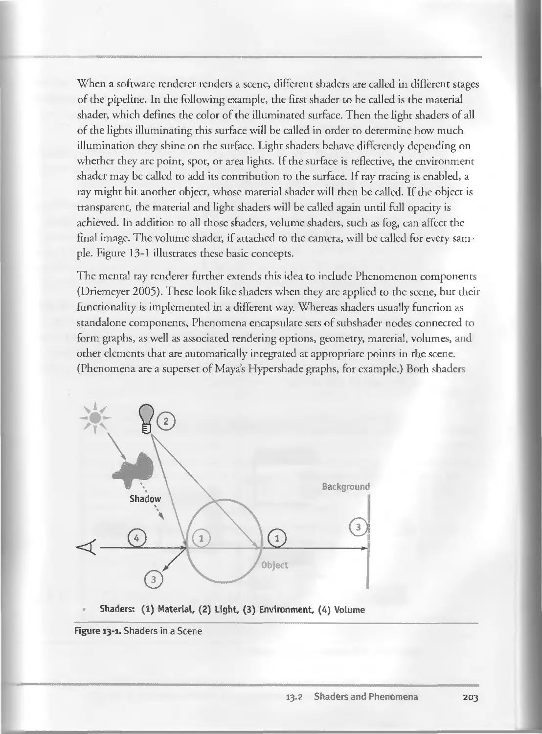
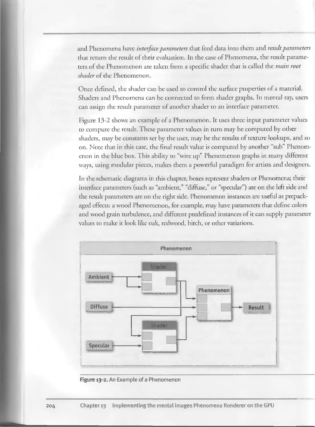
13.2 Shaders and Phenomena......................................202
13.3 Implementing Phenomena Using Cg............................205
13.3.I The Cg Vertex Program and the Varying Parameters.....205
13.3.2 The main () Entry Point for Fragment Shaders.......207
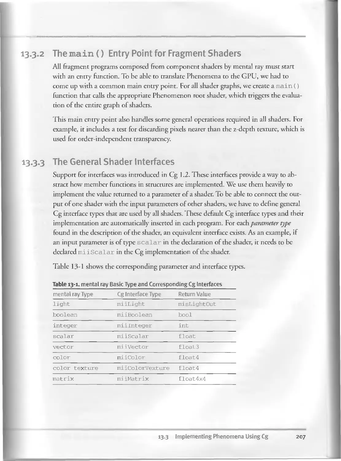
13.3.3 The General Shader Interfaces......................207
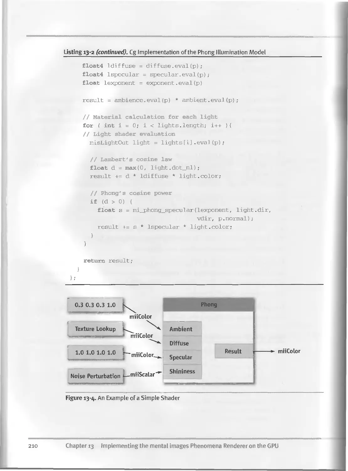
13.3.4 Example of a Simple Shader.........................208
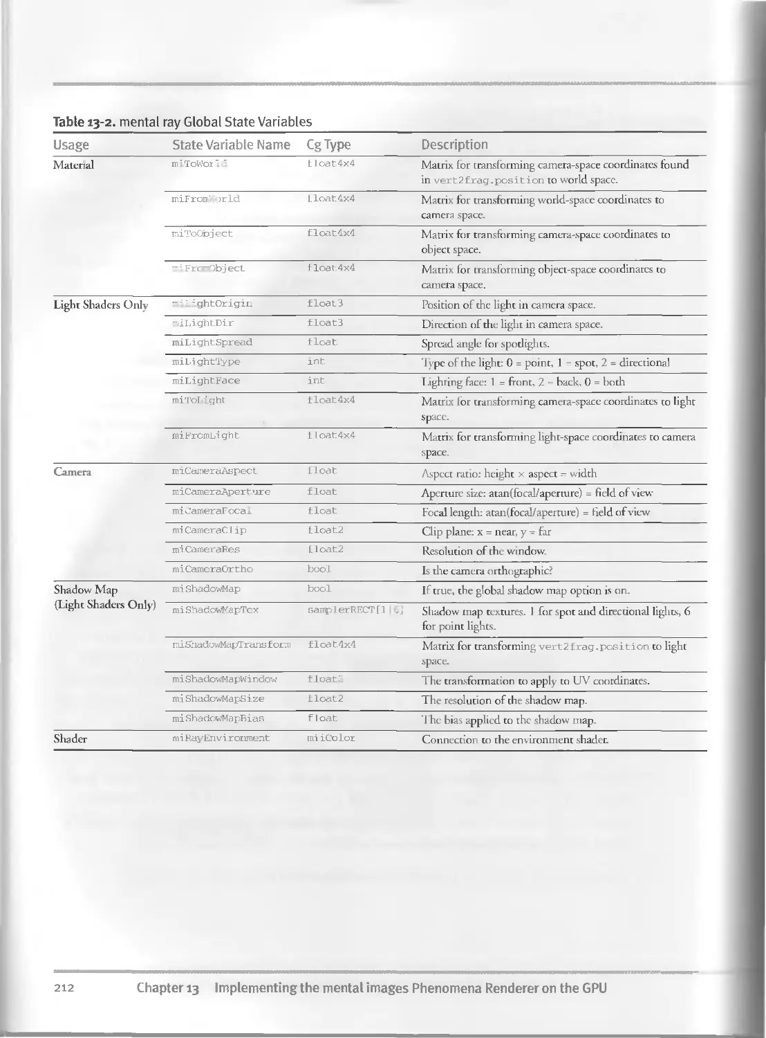
13.3.5 Global State Variables........................ ... 211
13.3.6 Light Shaders......................................211
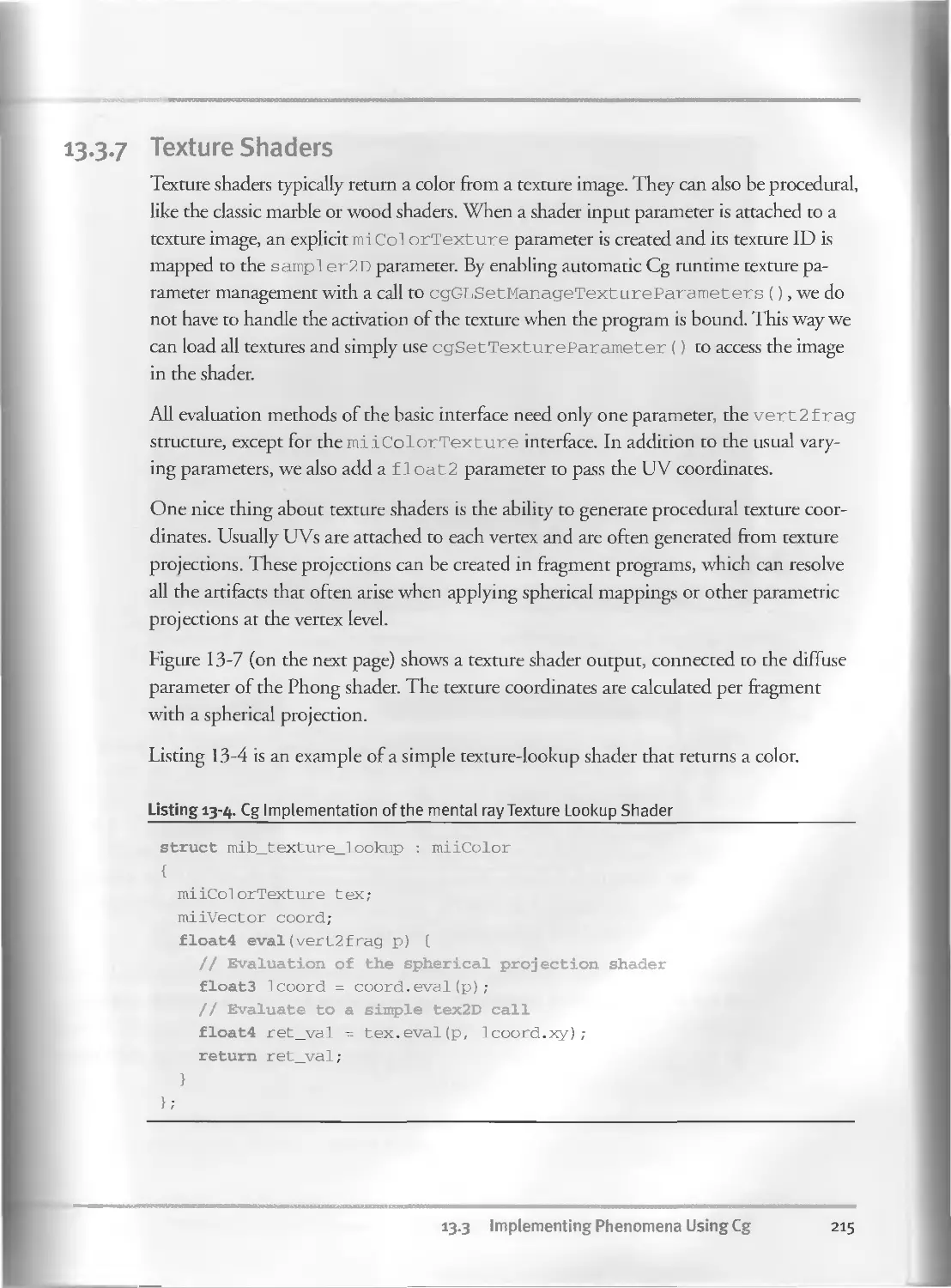
13.3.7 Texture Shaders....................................215
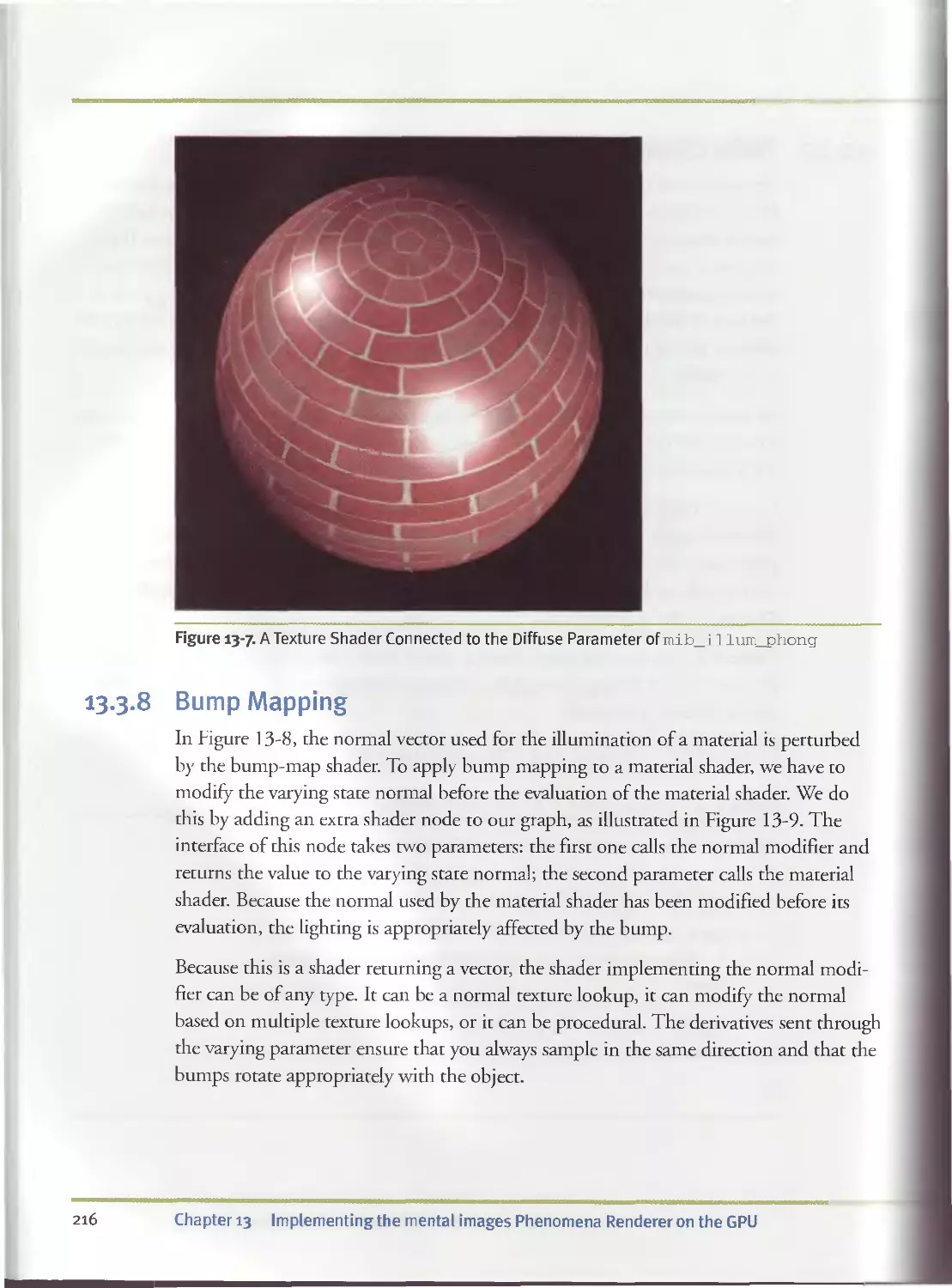
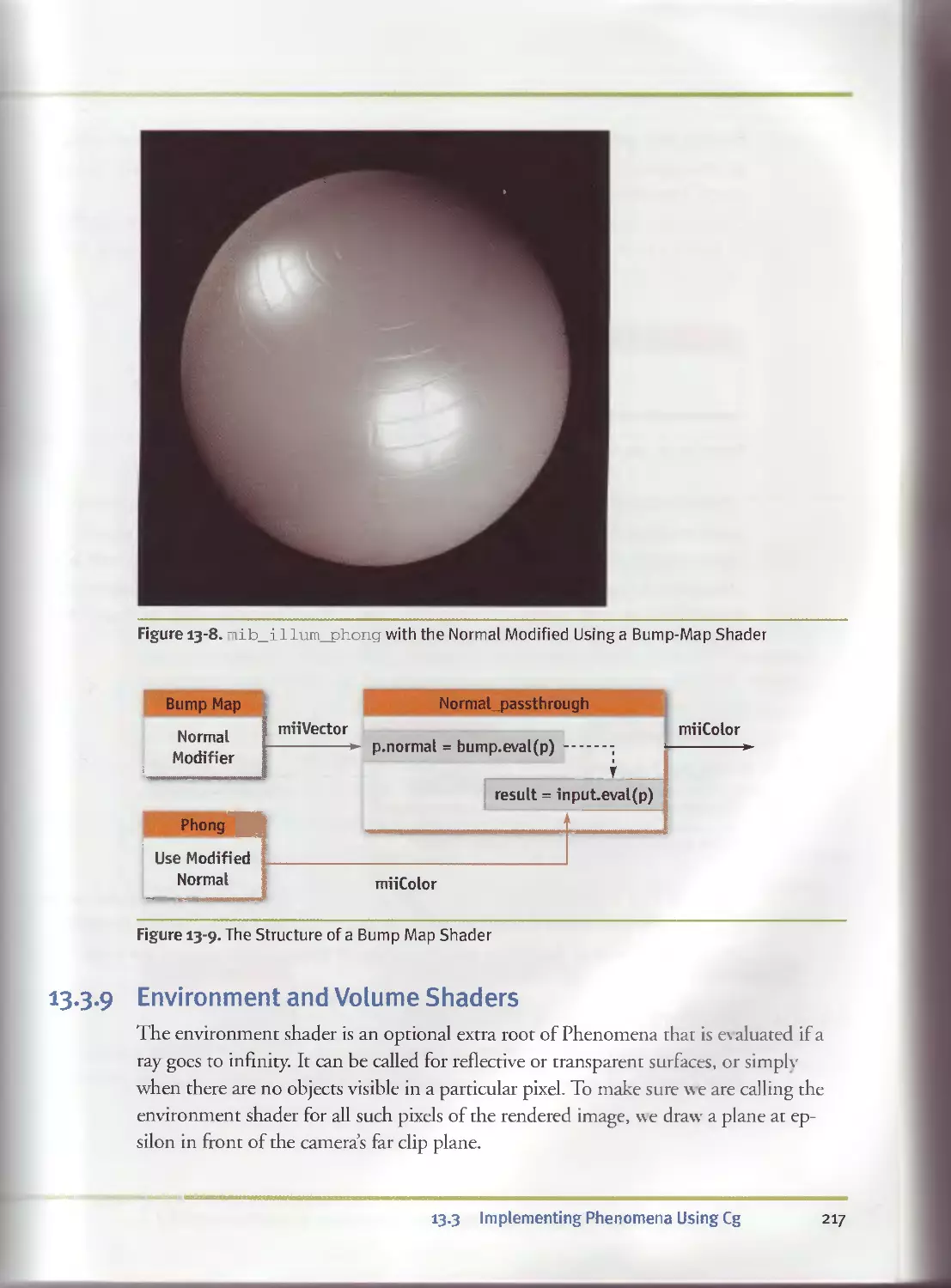
13.3.8 Bump Mapping.......................................216
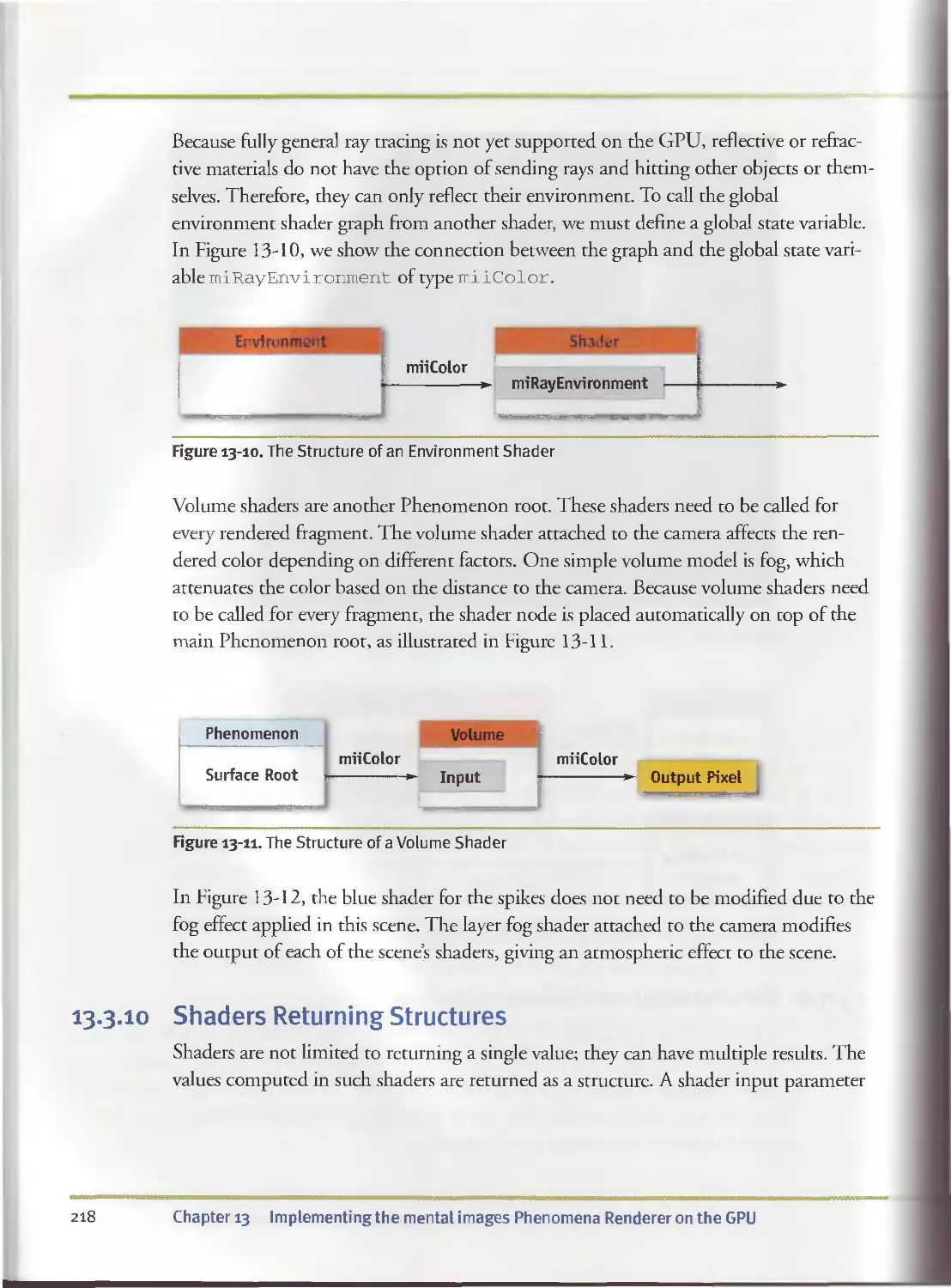
13.3.9 Environment and Volume Shaders ....................217
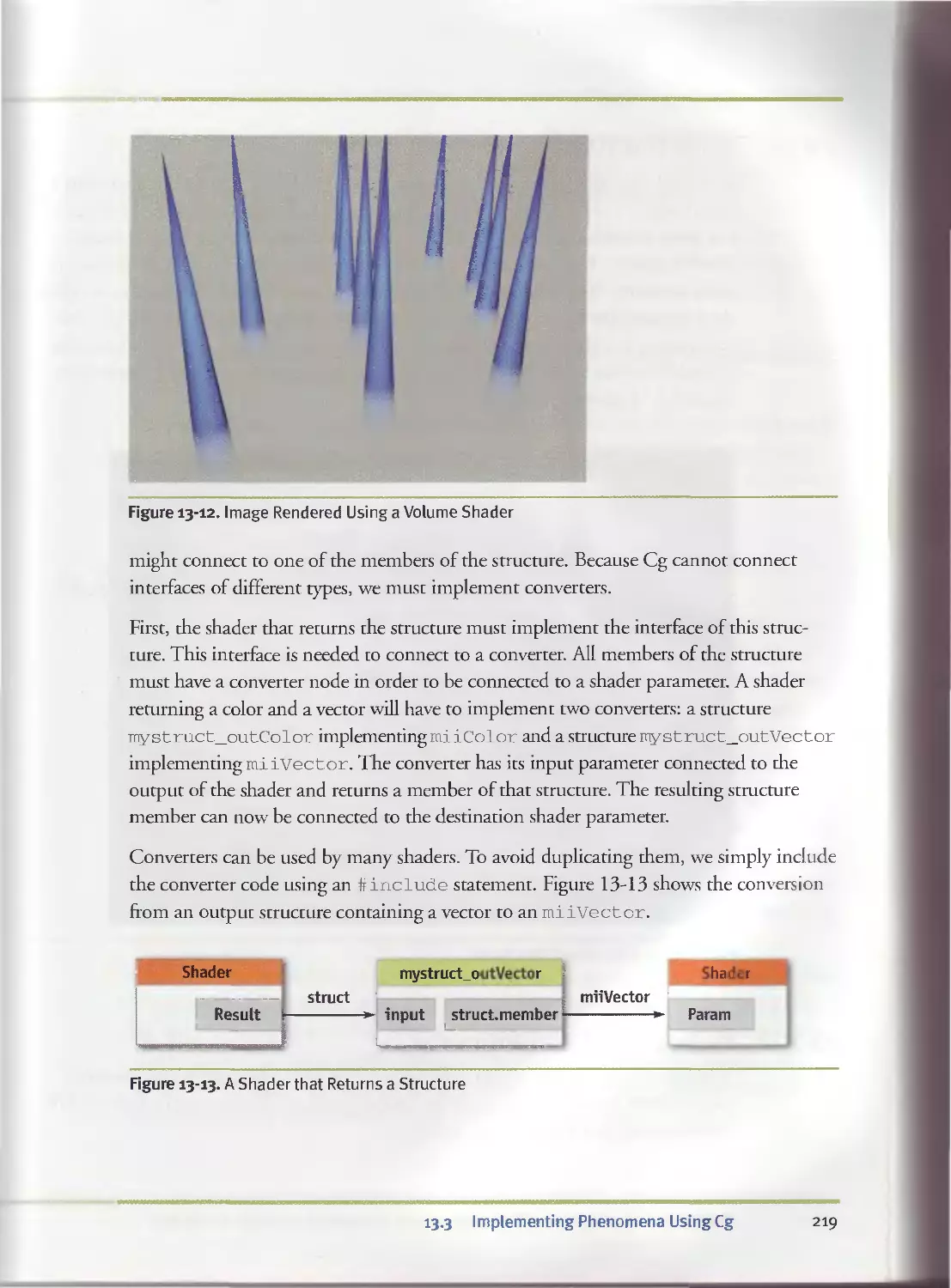
I3.3.IO Shaders Returning Structures.......................218
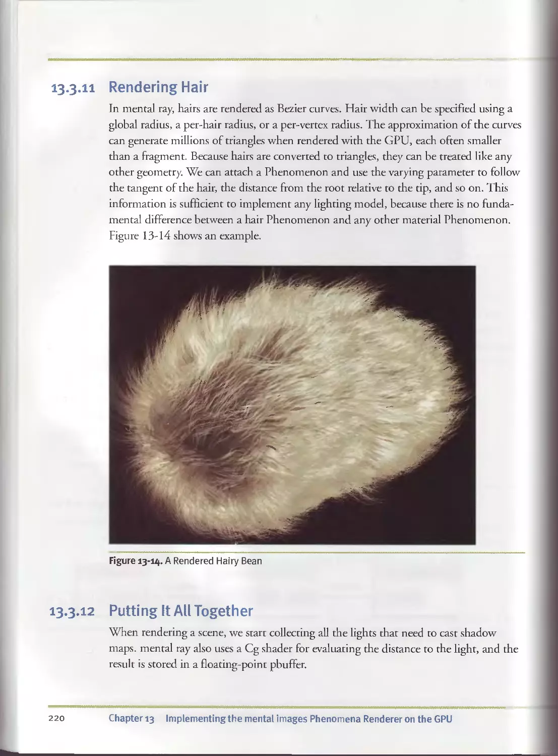
13.3.II Rendering Hair.....................................220
13.3.12 Putting It All Together............................220
13.4 Conclusion.................................................221
13.5 References..................................................222
Chapter 14
Dynamic Ambient Occlusion and Indirect Lighting............................223
Michael Bunnell, NVIDIA Corporation
14.I Surface Elements...........................................223
14.2 Ambient Occlusion..........................................225
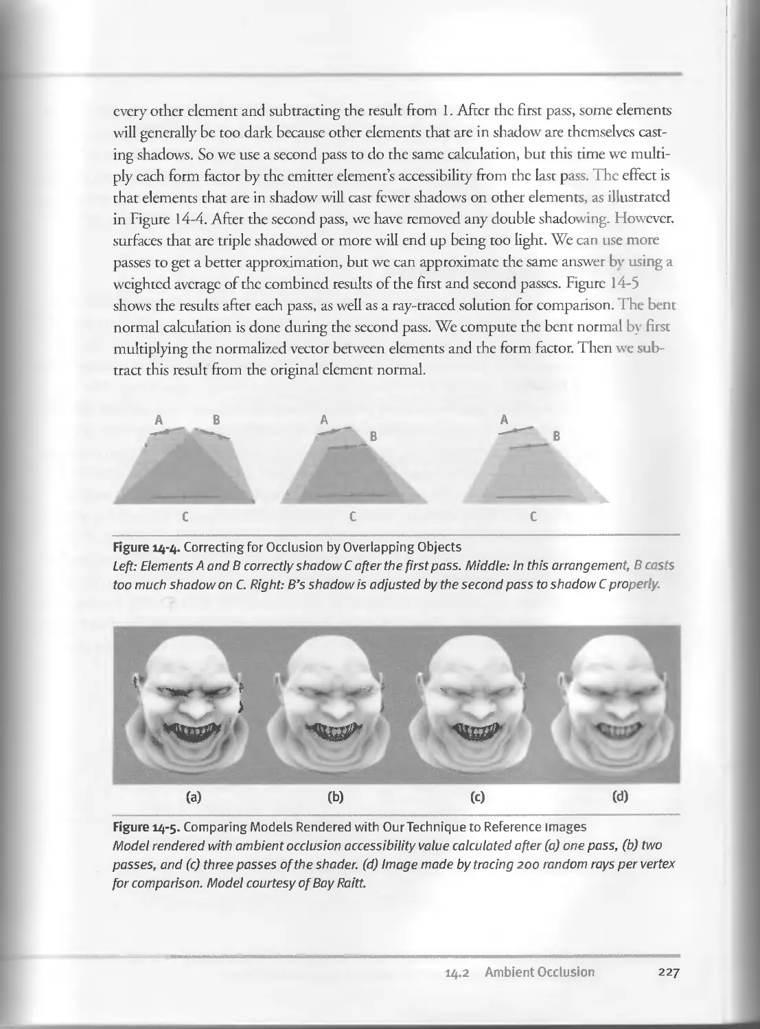
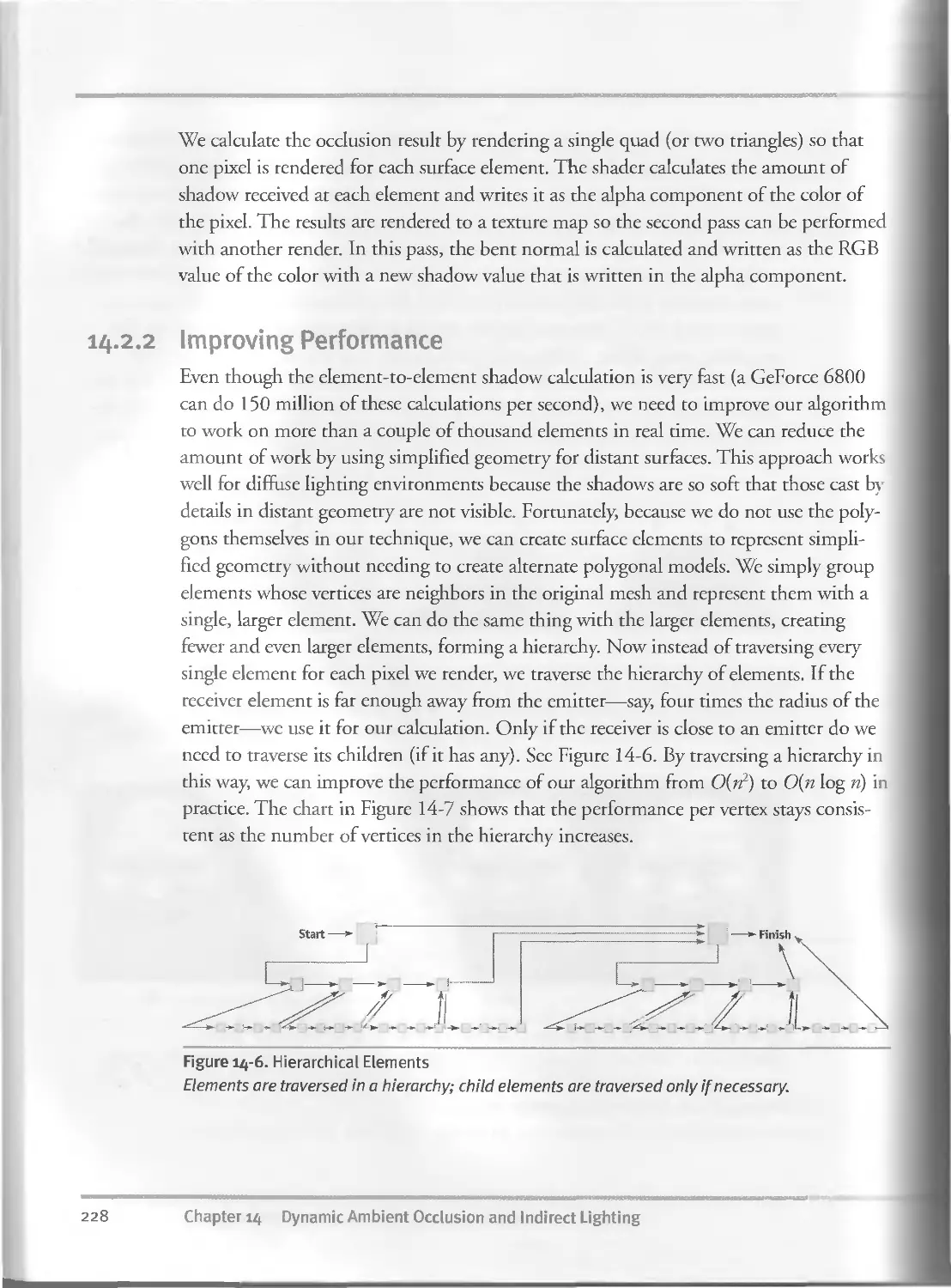
14.2.I The Multipass Shadowing Algorithm..................226
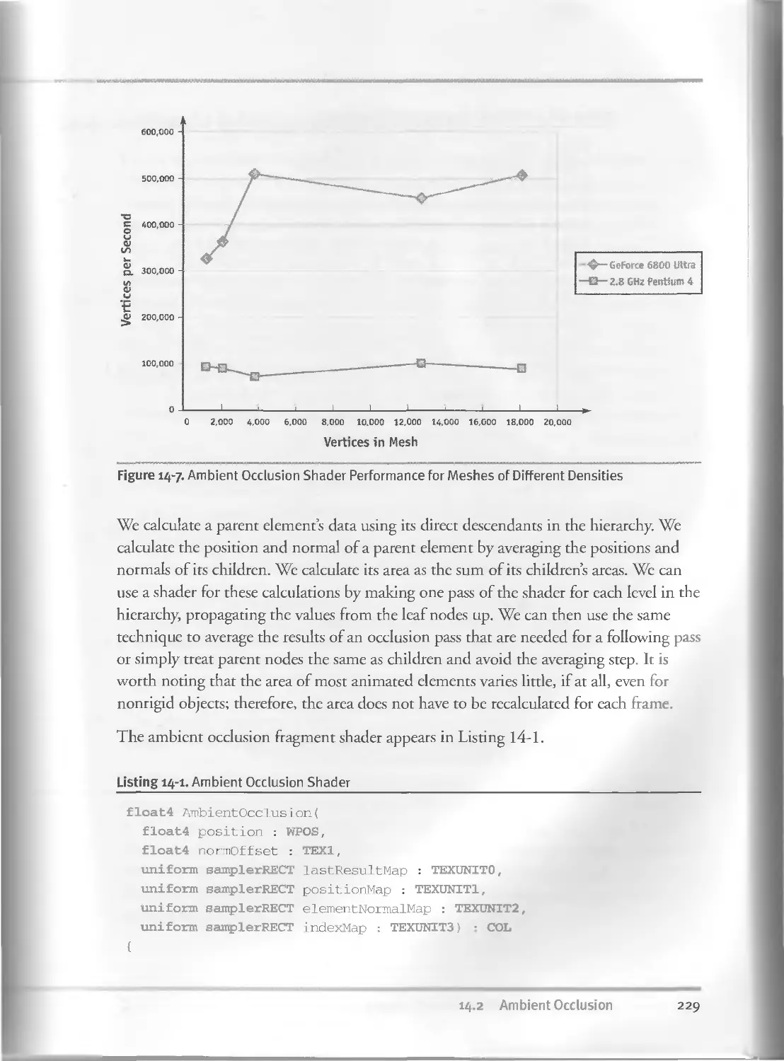
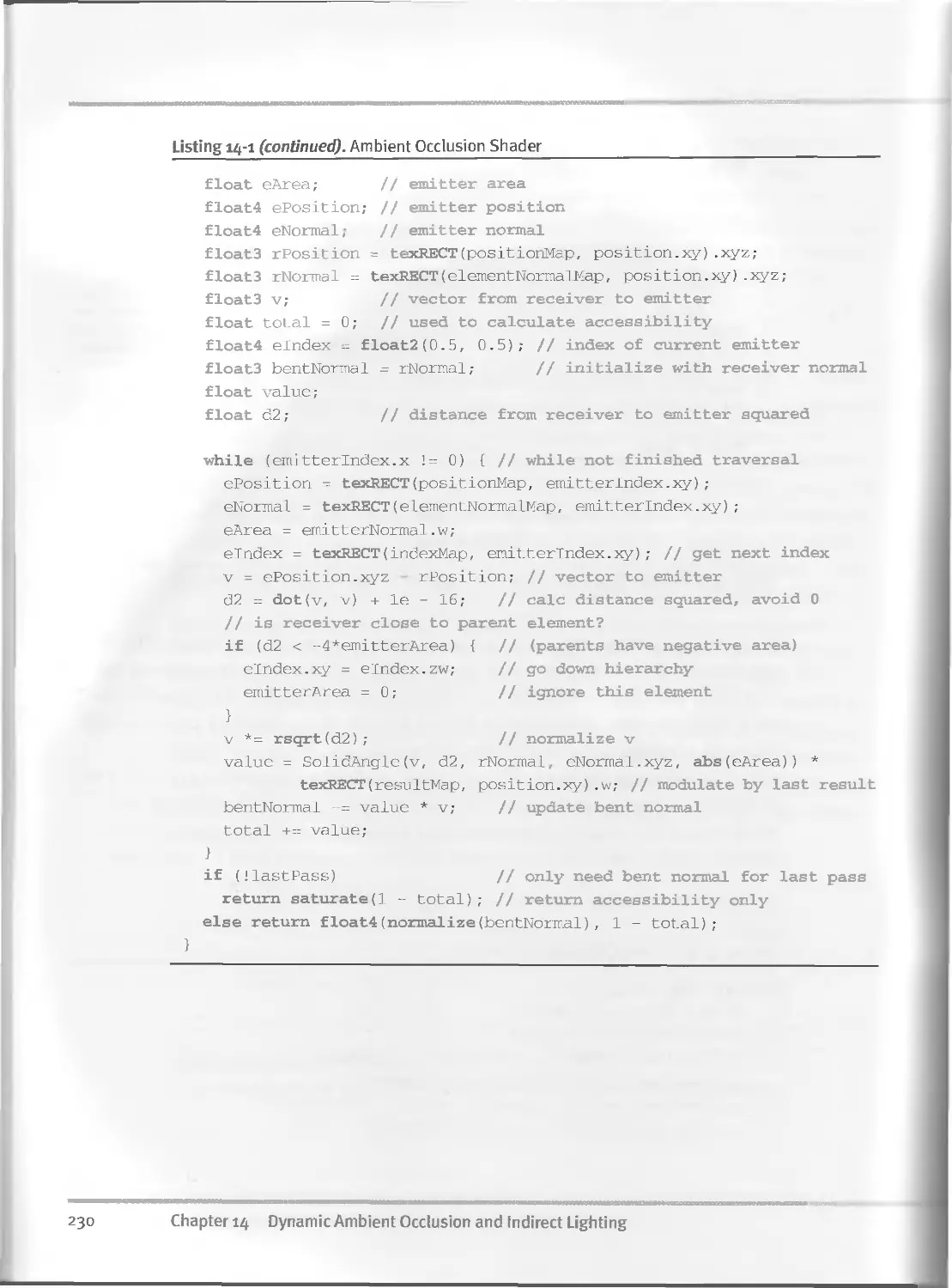
14.2.2 Improving Performance. . . .............. . 228
14.3 Indirect Lighting and Area Lights......................... 231
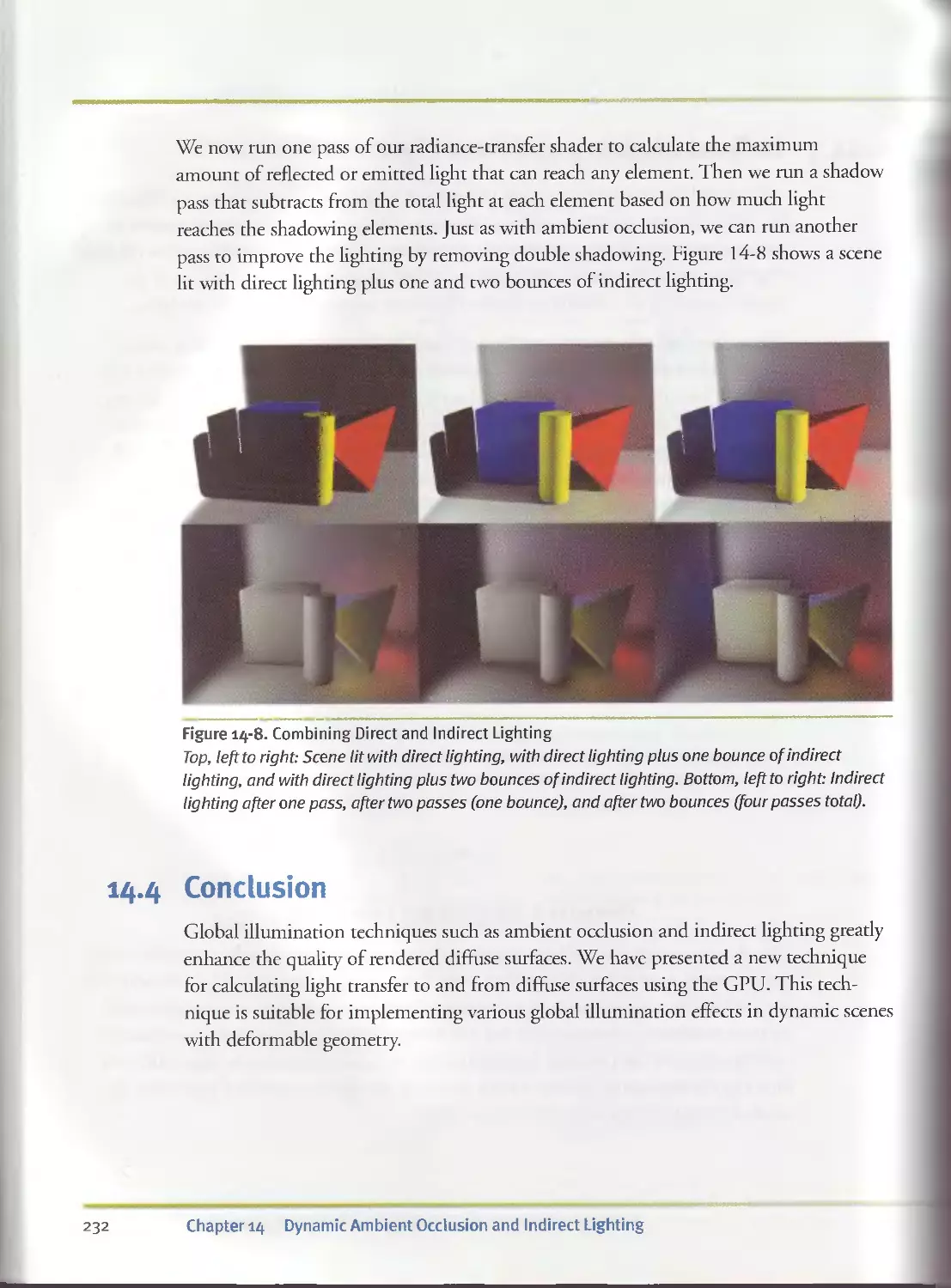
14.4 Conclusion................................................ 232
14.5 References............................................... . 233
Contents xiii
ма—пм»ммя№дшиMWtHwwiamnnniif rn'i,rr—»iniiH4wnrin«TrwinHtBi'nMinmwjmaiBwtaiamH . ыяа жмн
Chapter 15
Blueprint Rendering and “Sketchy Drawings”....................................... 235
Marc Nienhaus, University of Potsdam, Hasso-Plattner-lnstitute
Jurgen Dollner, University of Potsdam, Hasso-Plattner-lnstitute
15.1 Basic Principles..................................................236
15.I.I Intermediate Rendering Results............................236
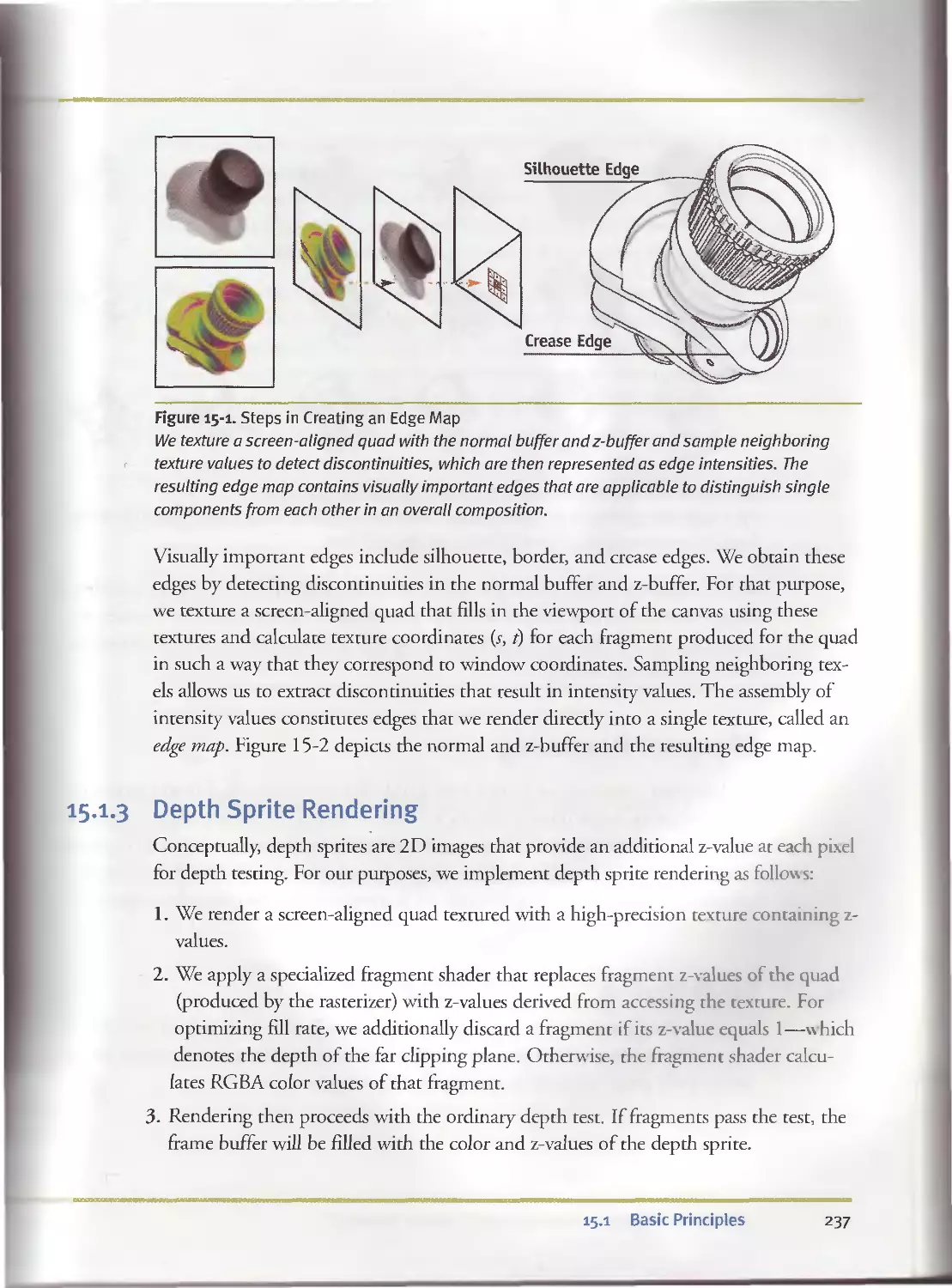
15.I.2 Edge Enhancement..........................................236
15.I.3 Depth Sprite Rendering....................................237
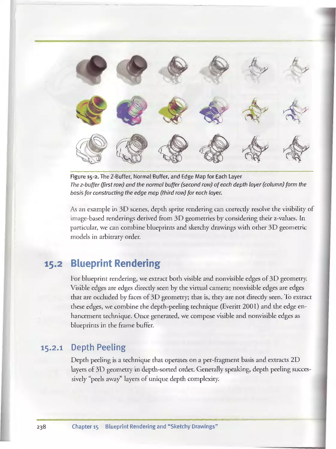
15.2 Blueprint Rendering...............................................238
I5.2.I Depth Peeling.............................................238
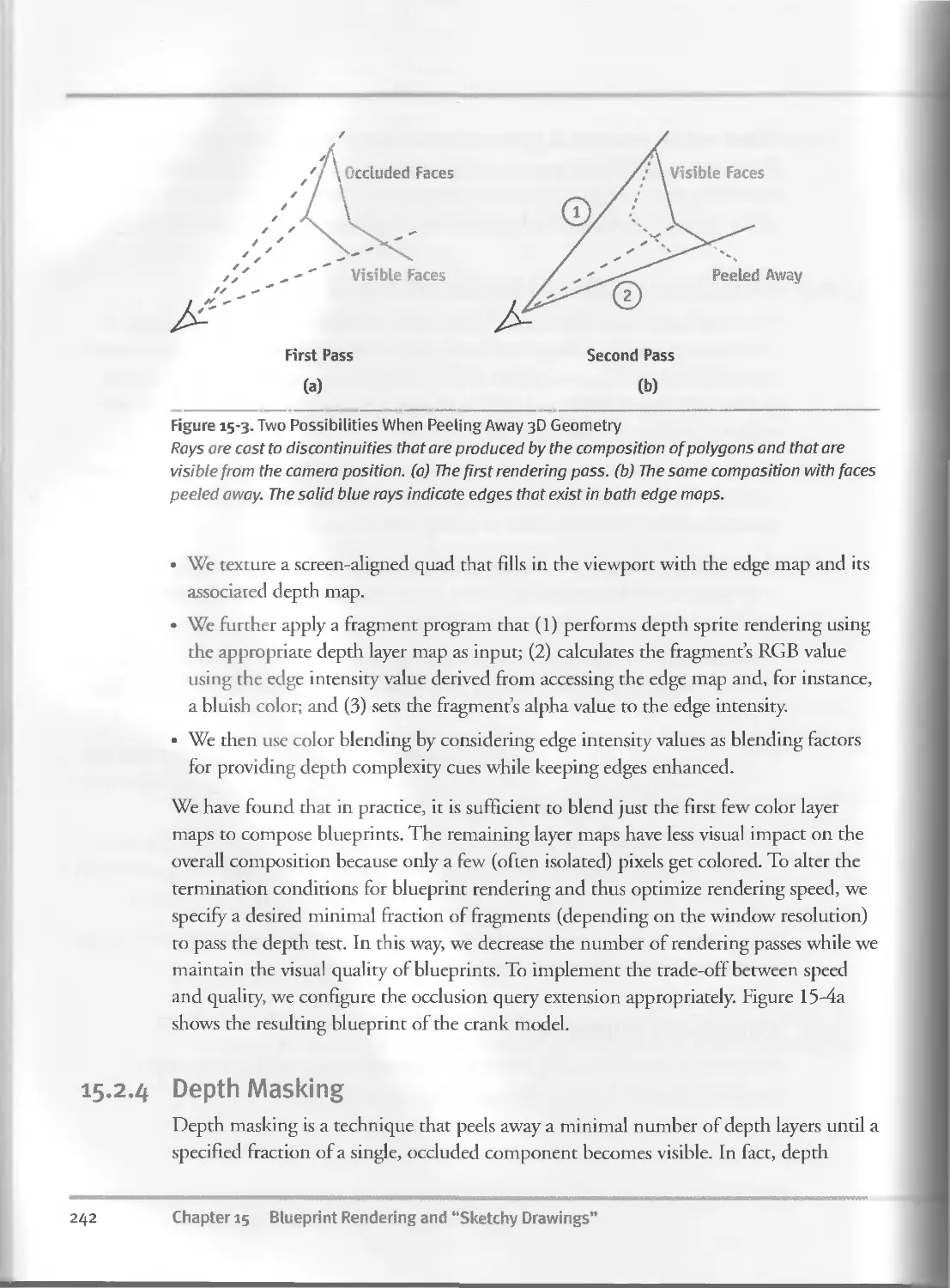
I5.2.2 Extracting Visible and Nonvisible Edges...................241
15.2.3 Composing Blueprints......................................241
15.2.4 Depth Masking.............................................242
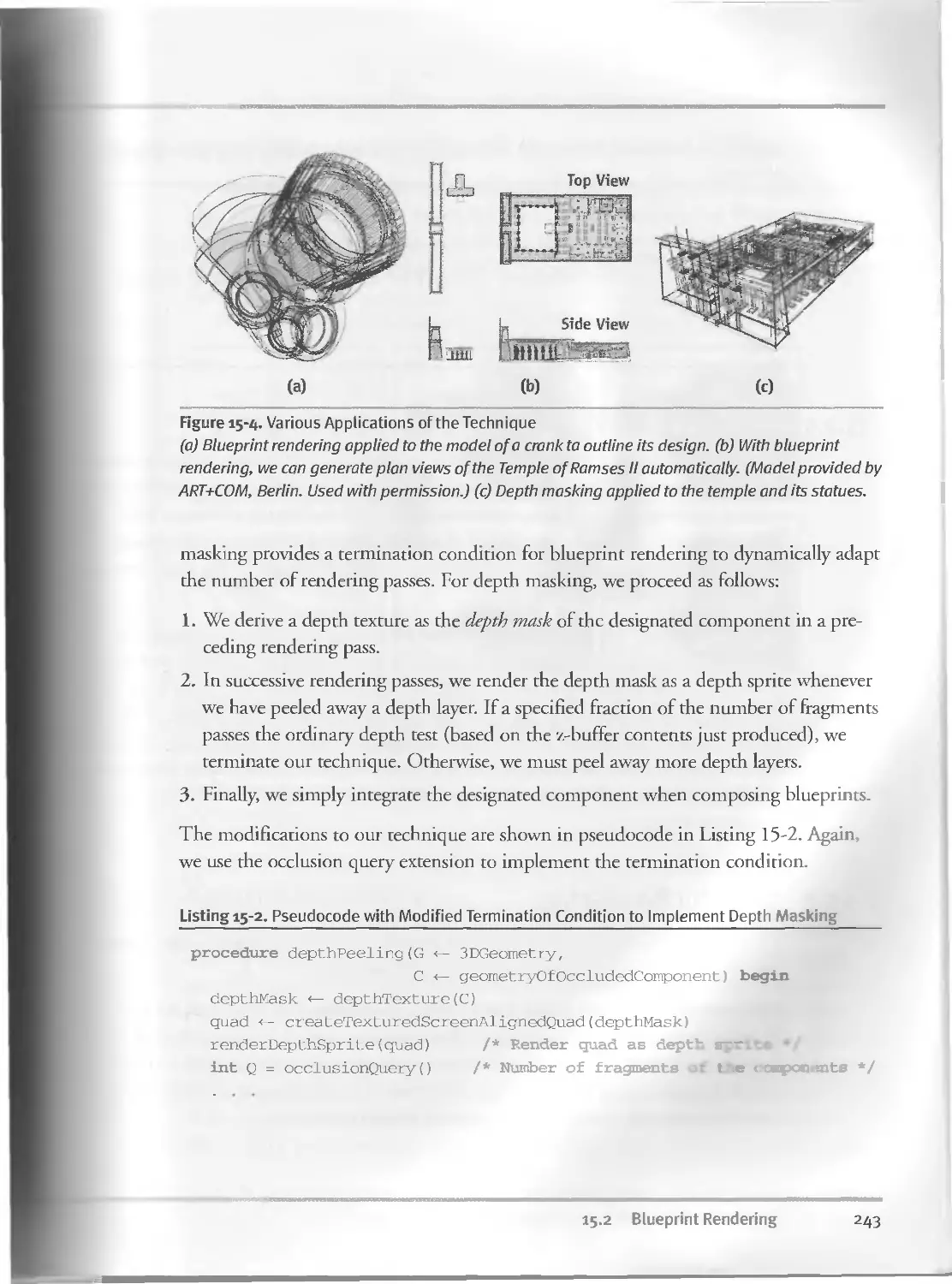
15.2.5 Visualizing Architecture Using Blueprint Rendering........244
15.3 Sketchy Rendering.................................................244
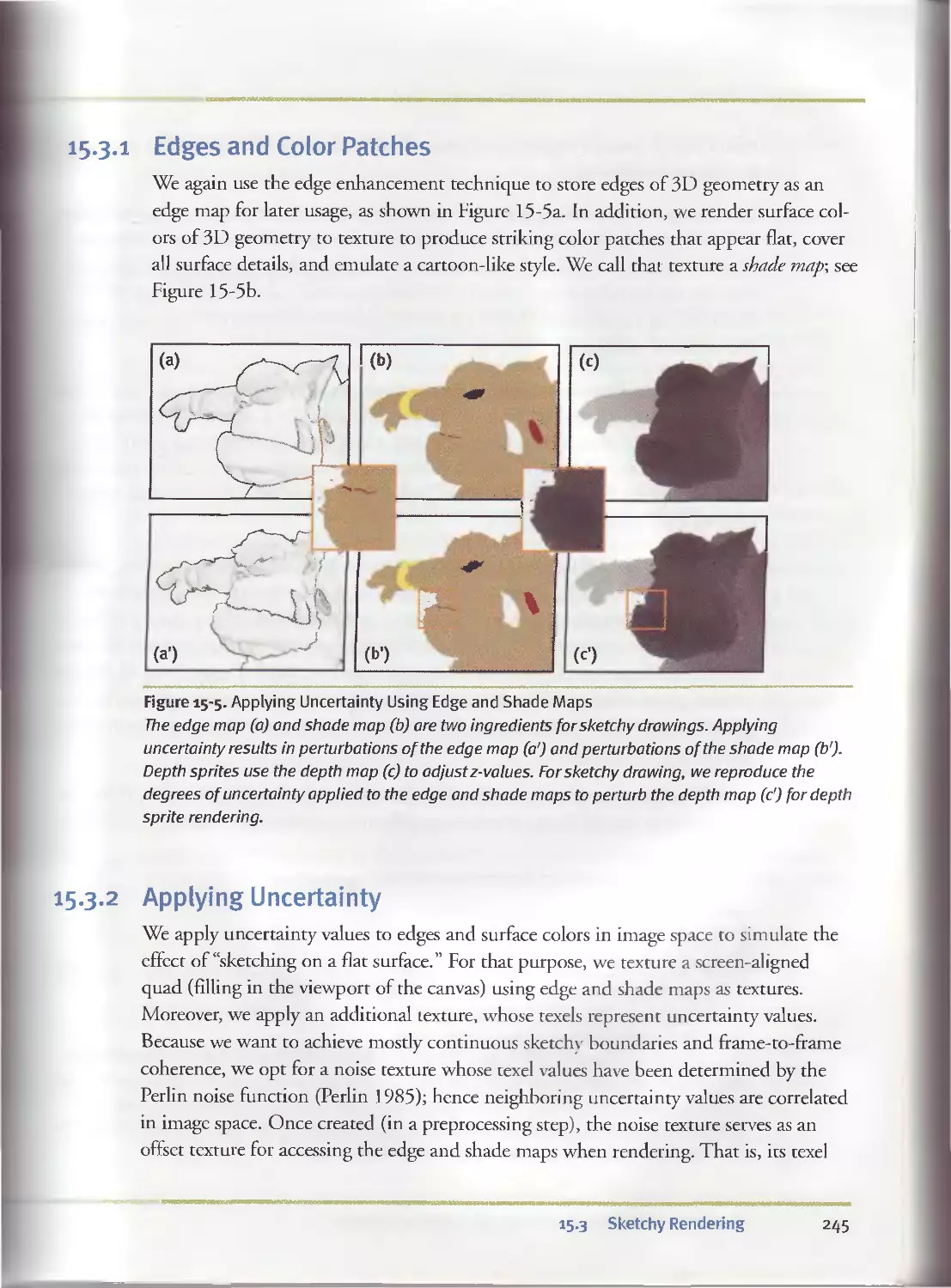
I5.3.I Edges and Color Patches...................................245
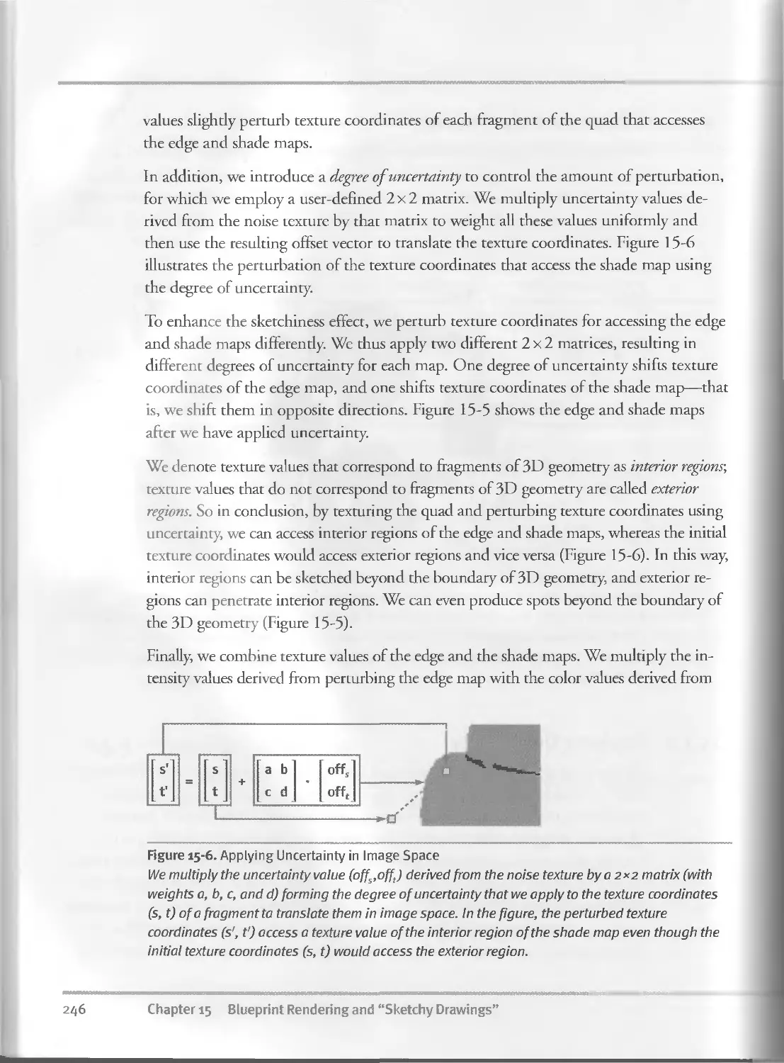
15.3.2 Applying Uncertainty......................................245
15.3.3 Adjusting Depth..........................................Iiyj
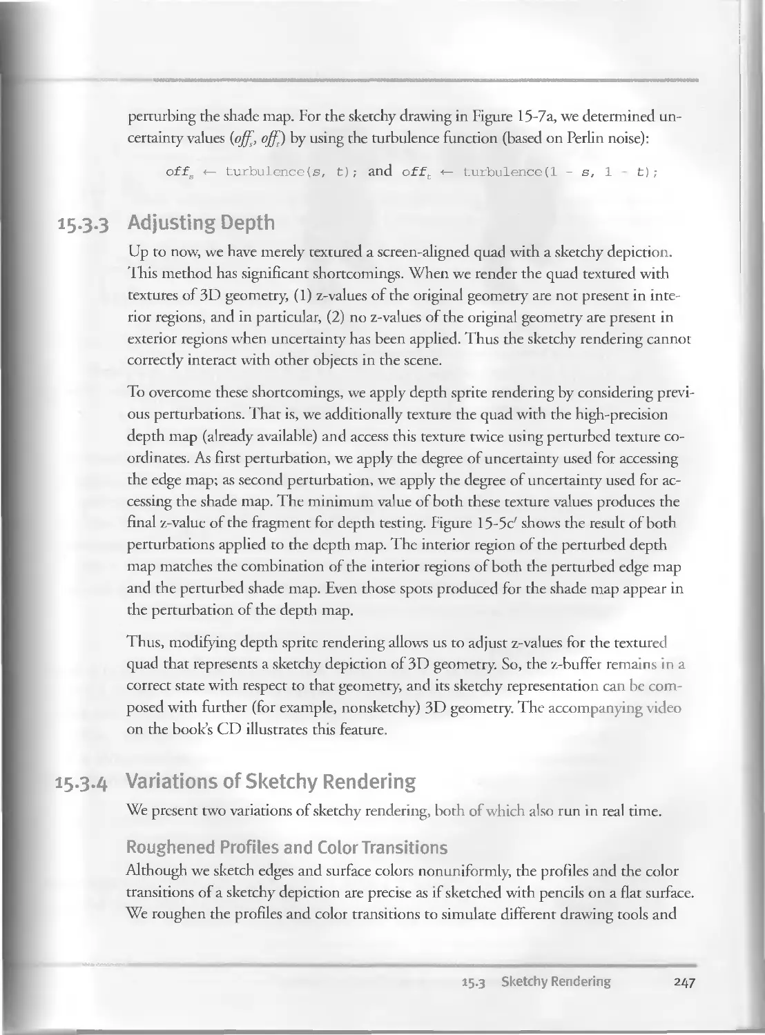
15.3.4 Variations of Sketchy Drawing.............................247
15.3.5 Controlling Uncertainty...................................248
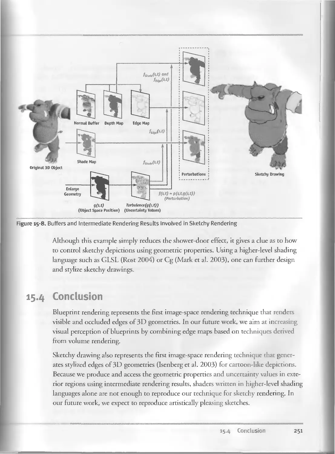
15.3.6 Reducing the Shower-Door Effect...........................250
15.4 Conclusion........................................................251
15.5 References........................................................252
Chapter 16
Accurate Atmospheric Scattering ...................................................253
Sean O’Neil
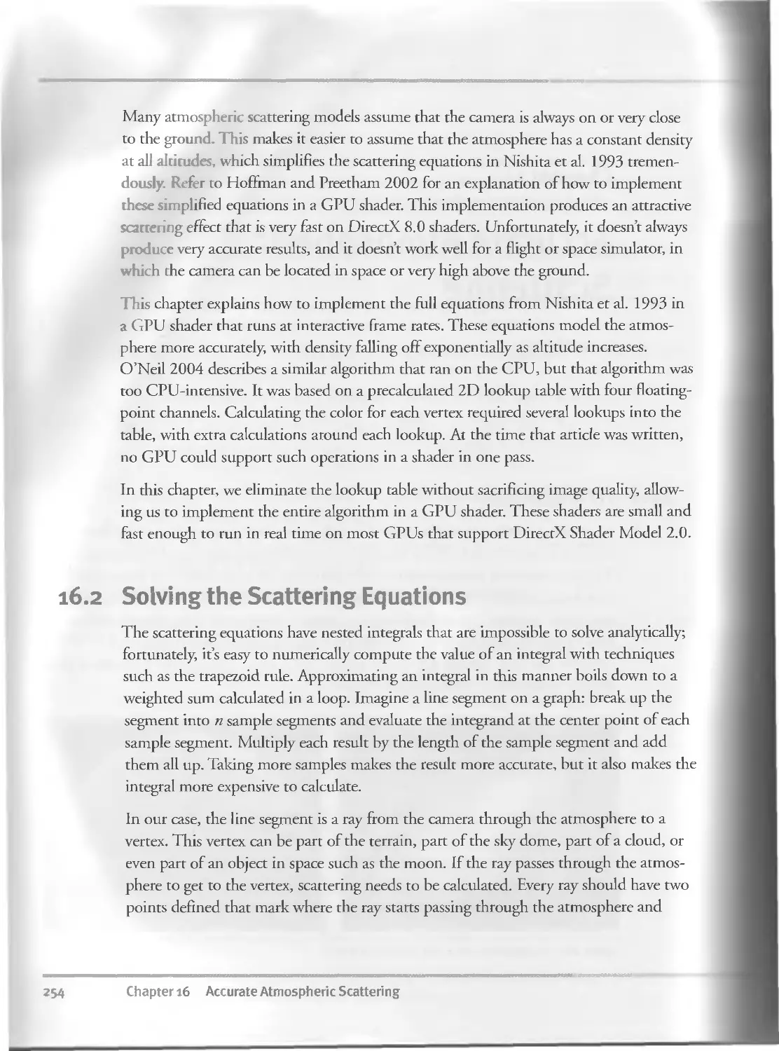
16.1 Introduction......................................................253
16.2 Solving the Scattering Equations..................................254
16.2.1 Rayleigh Scattering vs. Mie Scattering....................255
16.2.2 The Phase Function........................................256
16.2.3 The Out-Scattering Equation...............................256
16.2.4 The In-Scattering Equation................................257
16.2.5 The Surface-Scattering Equation...........................257
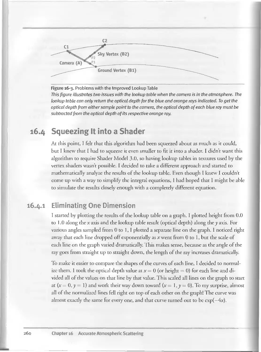
16.3 Making It Real-Time...............................................258
16.4 Squeezing It into a Shader........................................260
16.4-1 Eliminating One Dimension.................................260
16.4.2 Eliminating the Other Dimension...........................261
xiv Contents
16. 5 Implementing the Scattering Shaders......................262
16.5. I The Vertex Shader................................262
16.5. 2 The Fragment Shader..............................264
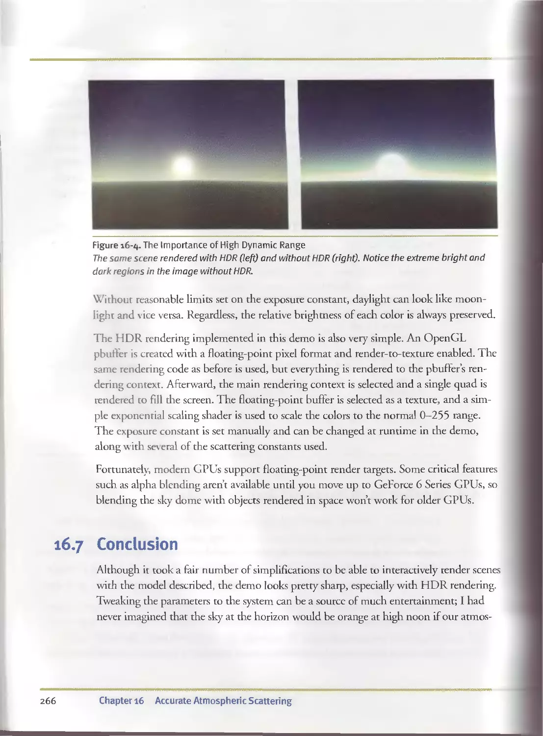
16. 6 Adding High-Dynamic-Range Rendering......................265
16. 7 Conclusion...............................................266
16. 8 References....................................... 'iCrj
Chapter 17
Efficient Soft-Edged Shadows Using Pixel Shader Branching...............269
Yury Uralsky, NVIDIA Corporation
17.1 Current Shadowing Techniques............................ 270
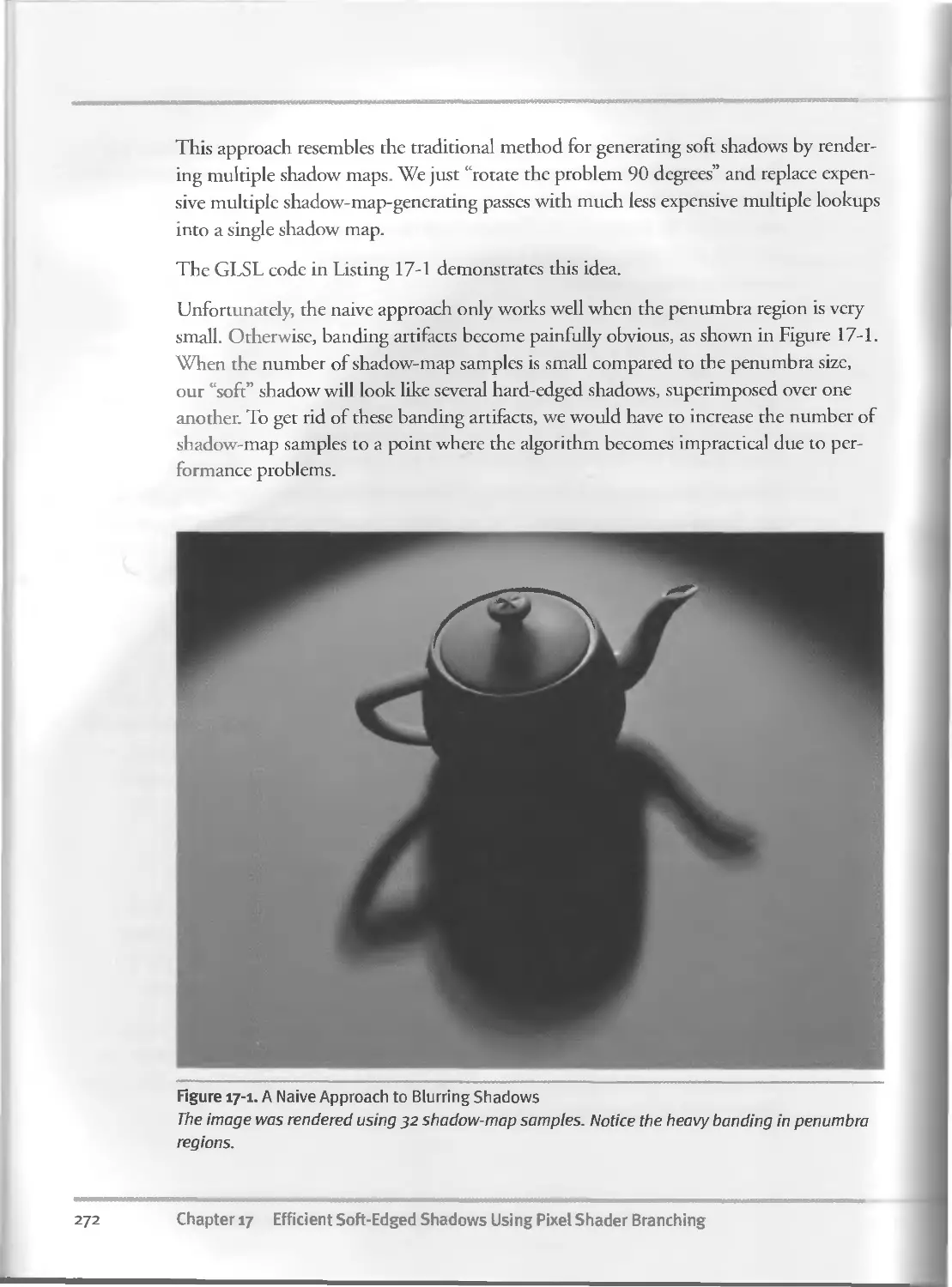
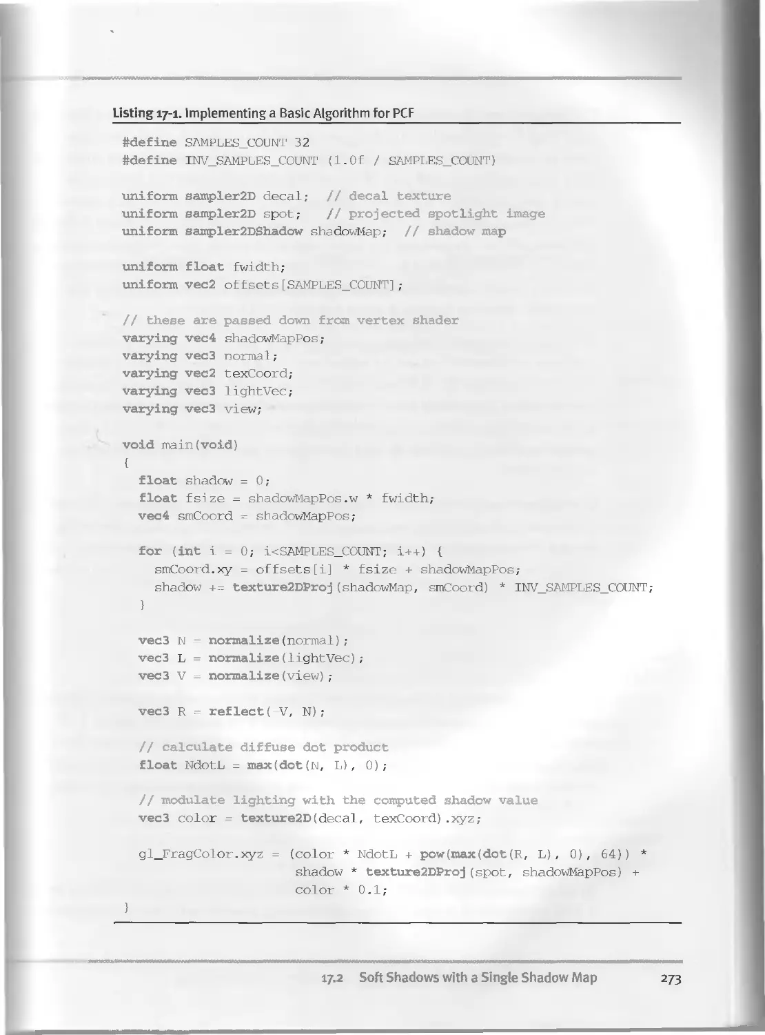
17.2 Soft Shadows with a Single Shadow Map.....................271
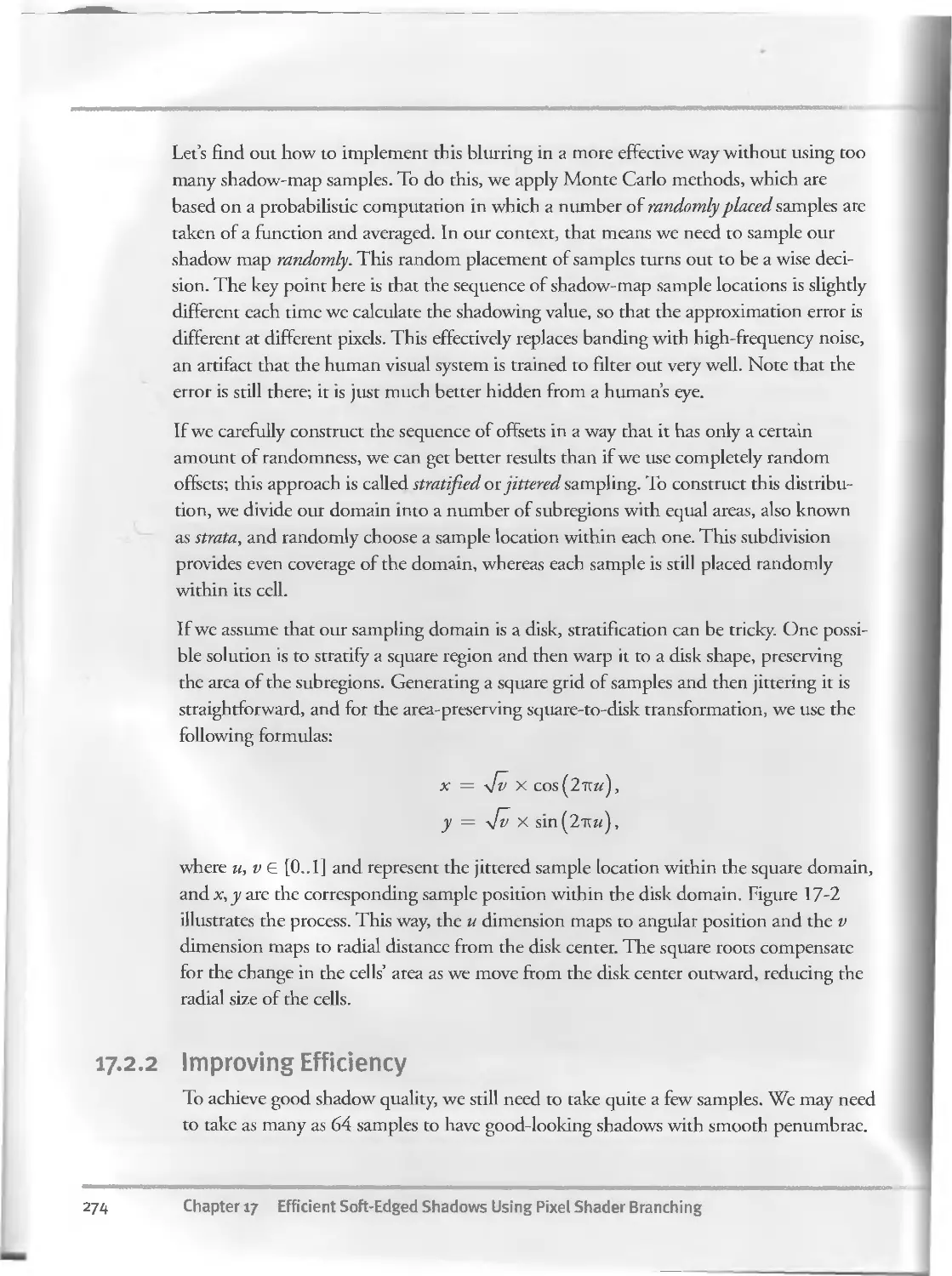
17.2.I Blurring Hard-Edged Shadows. . ...... .... 271
17.2.2 Improving Efficiency..............................274
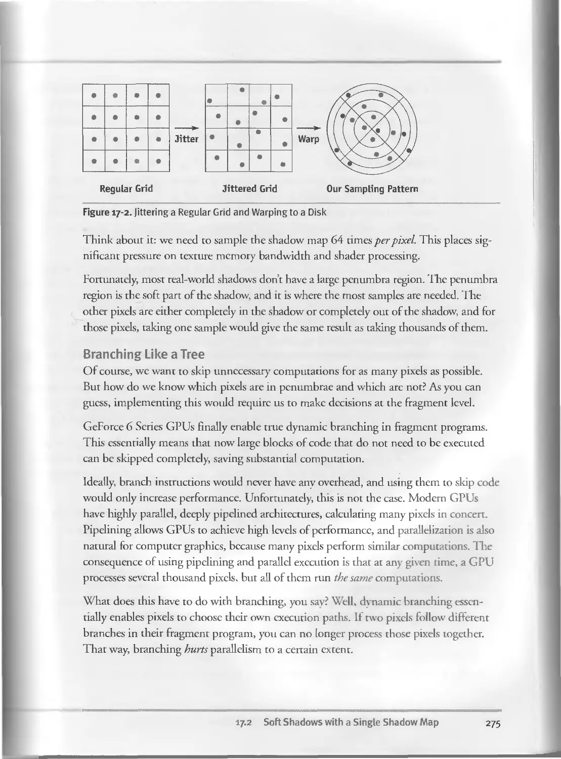
17.2.3 Implementation Details............................277
17.3 Conclusion................................................281
I7.4 References................................................282
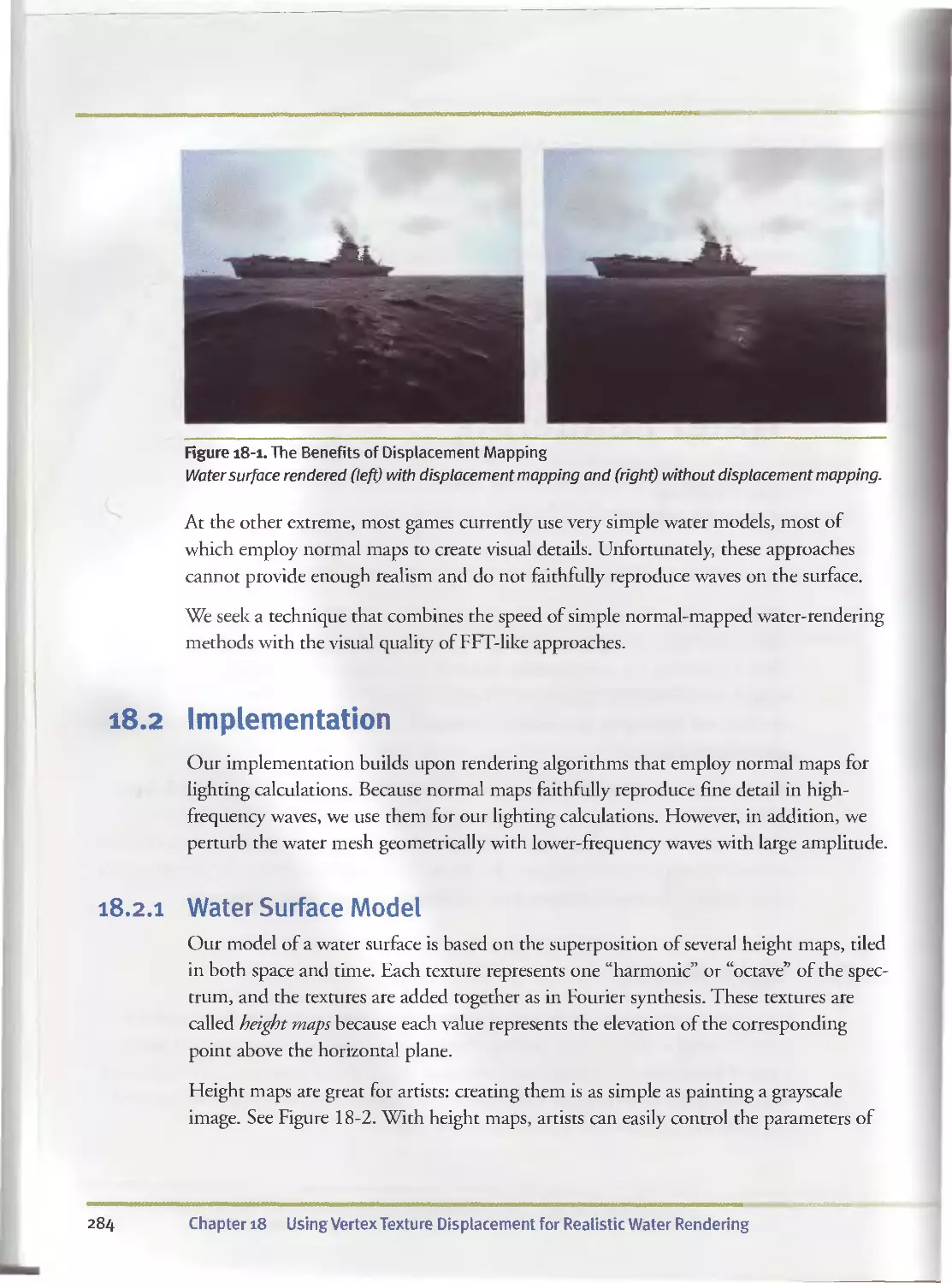
Chapter 18
Using Vertex Texture Displacement for Realistic
Water Rendering...........................................................283
Yuri Kryachko, iCMaddox Games
18.1 Water Models.............................................283
18.2 Implementation...........................................284
18.2.1 Water Surface Model............................. 284
18.2.2 Implementation Details......................... 285
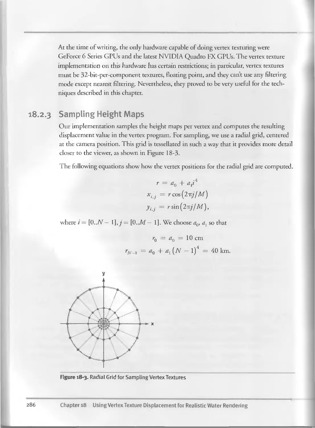
18.2.3 Sampling Height Maps.............................286
18.2.4 Quality Improvements and Optimizations...... . 288
18.2.5 Rendering Local Perturbations....................292
18.3 Conclusion................................................294
18.4 References...... ...................................... 294
Chapter 19
Generic Refraction Simulation.............................................295
Tiago Sousa, Crytek
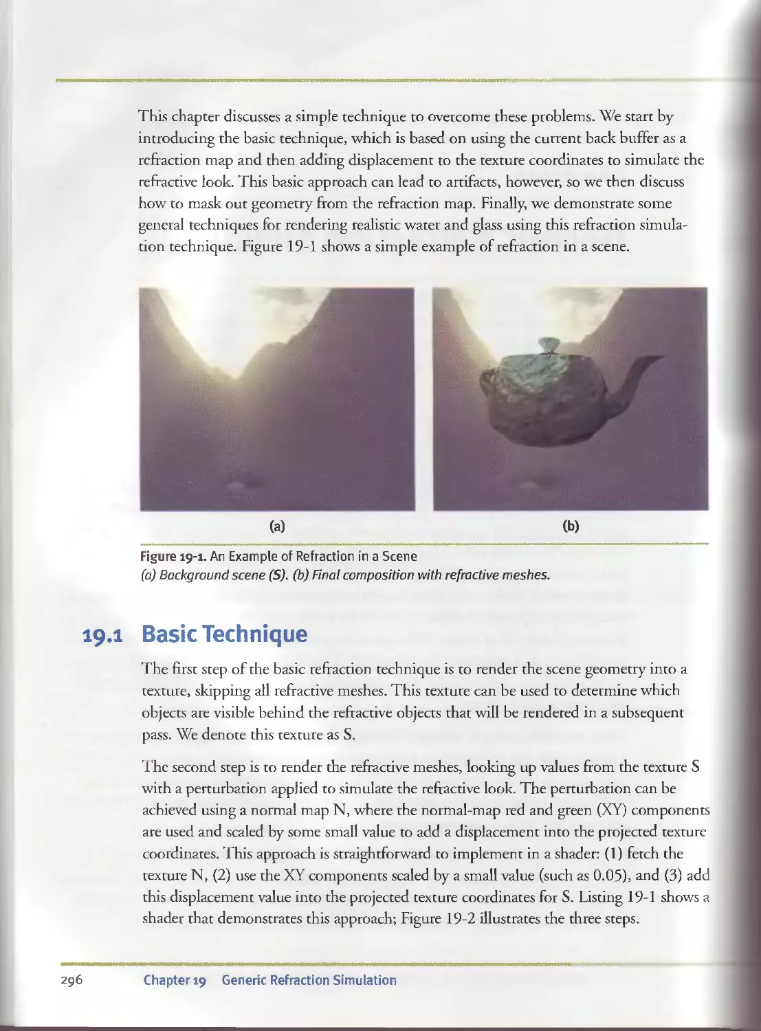
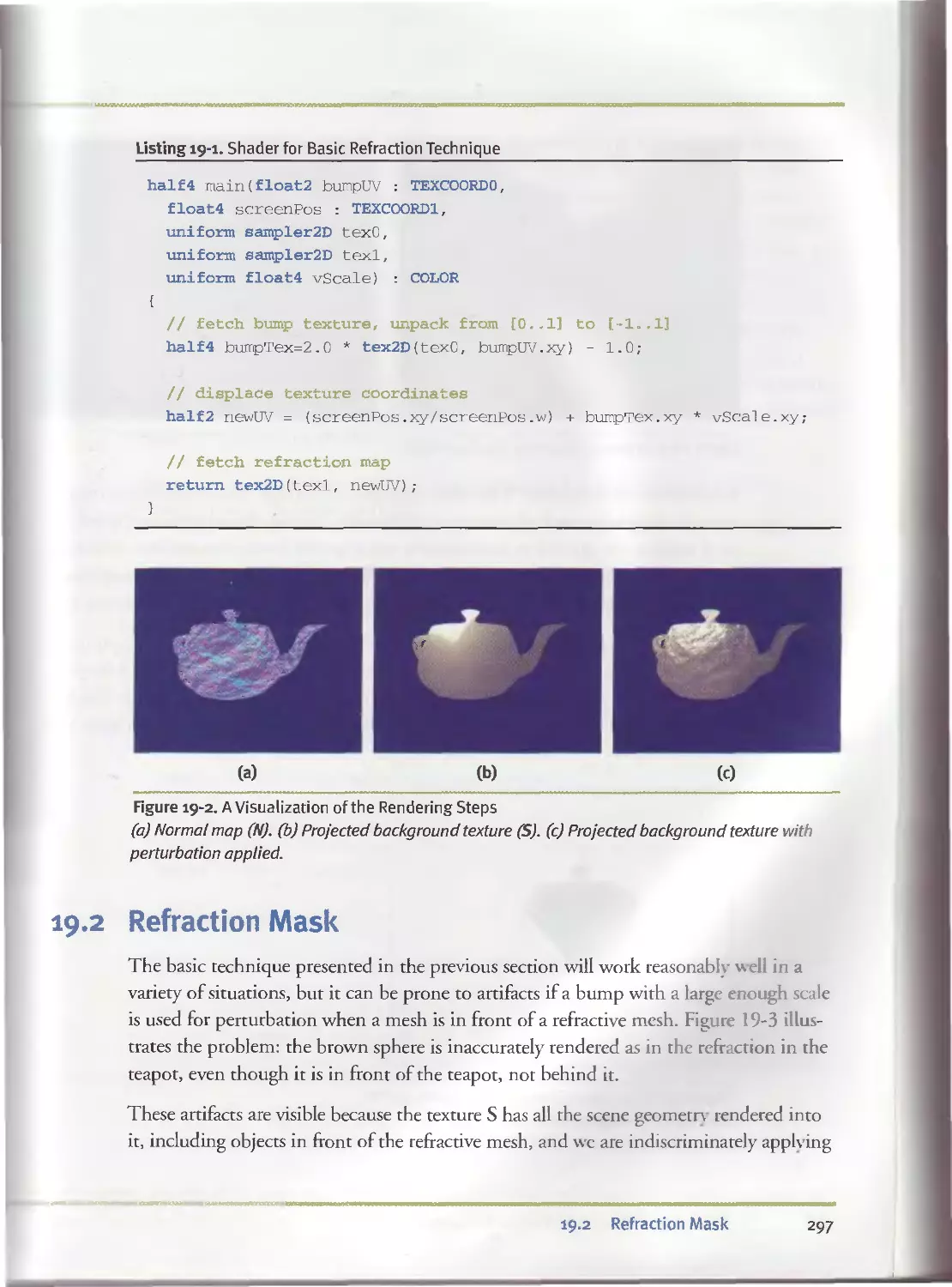
19.1 Basic Technique......................................... 296
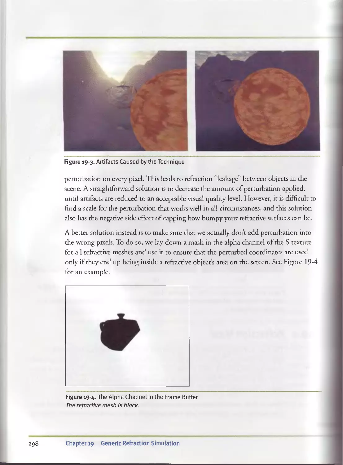
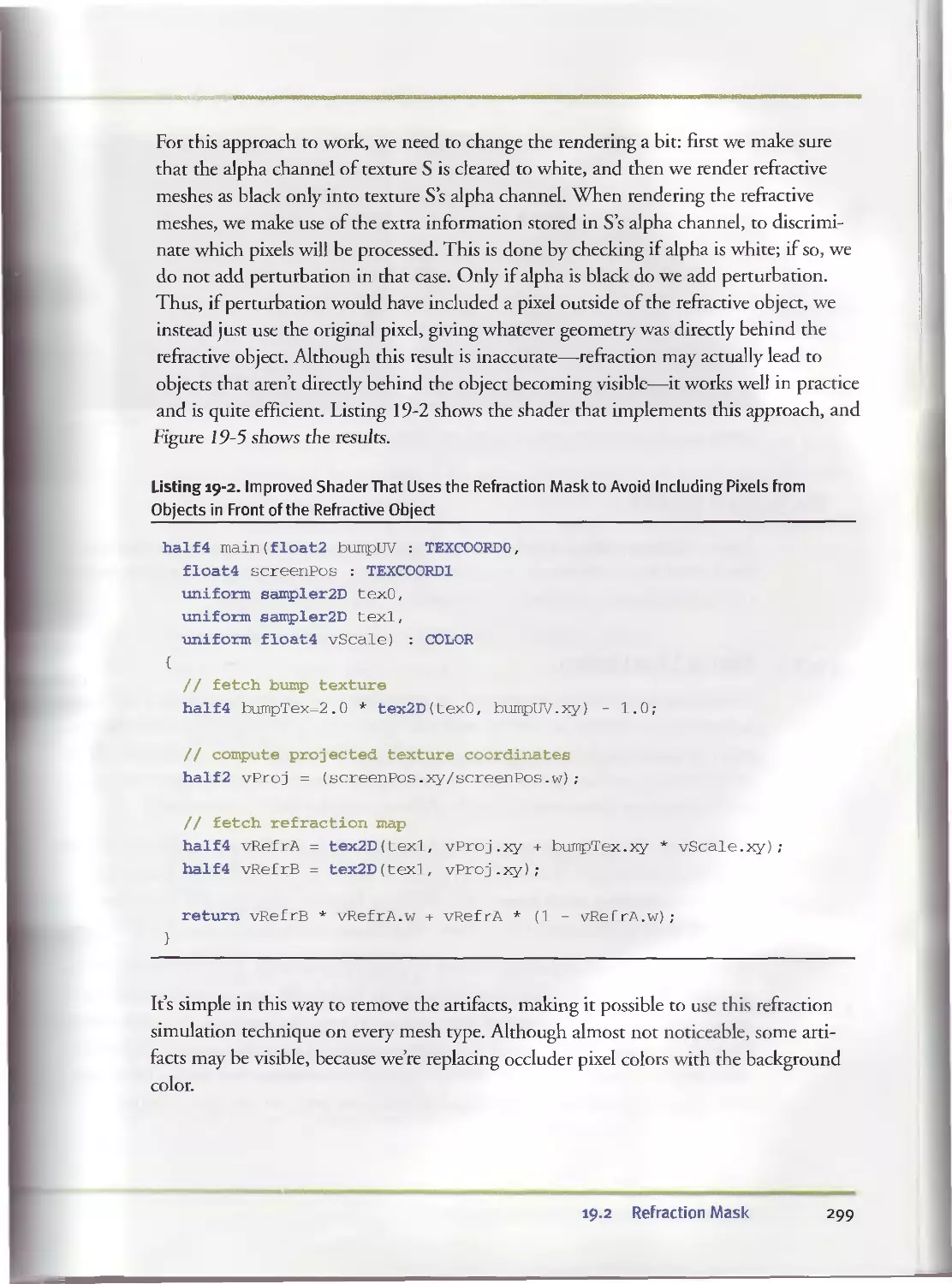
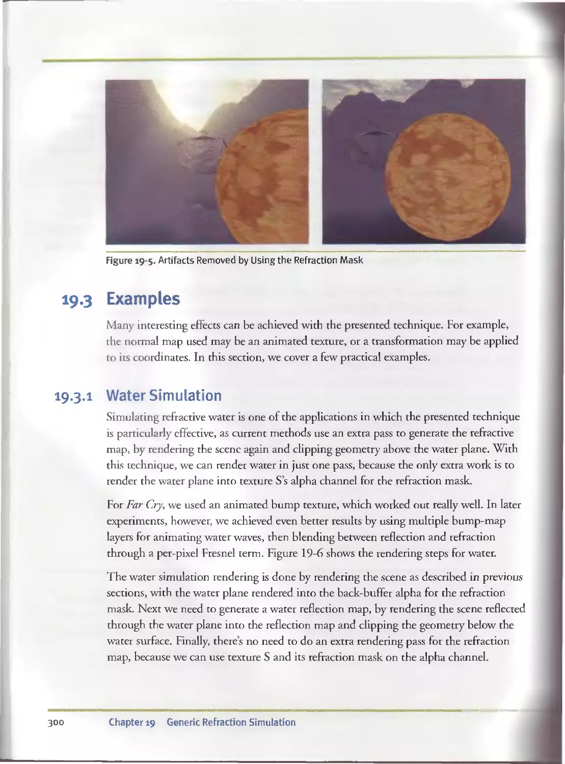
19.2 Refraction Mask...........................................297
Contents
XV
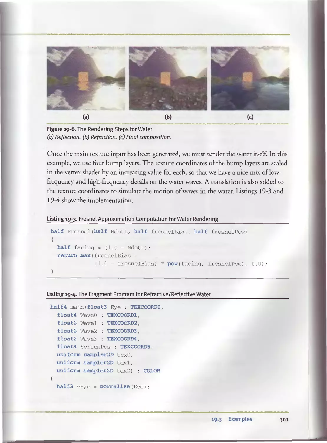
19.3 Examples.................................................300
I9.3.I Water Simulation.................................300
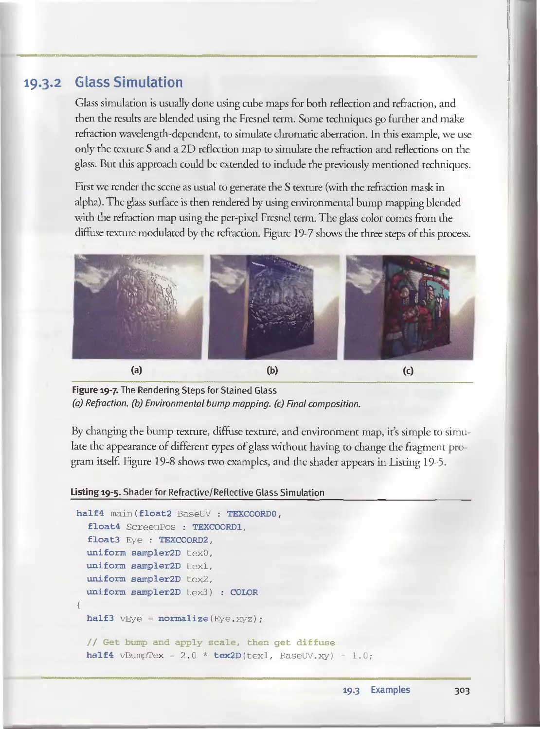
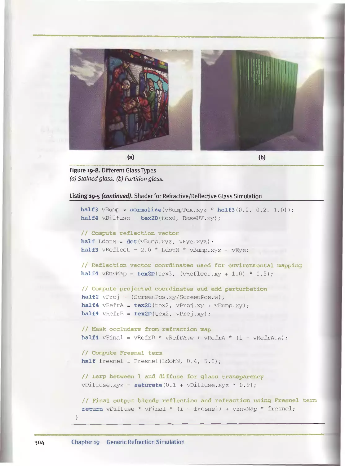
19.3.2 Glass Simulation................................303
19.4 Conclusion...............................................305
19.5 References...............................................305
PART III HIGH-QUALITY RENDERING 307
Chapter 20
Fast Third-Order Texture Filtering......................................313
Christian Sigg, ETH Zurich
Markus Hadwiger, VRVis Research Center
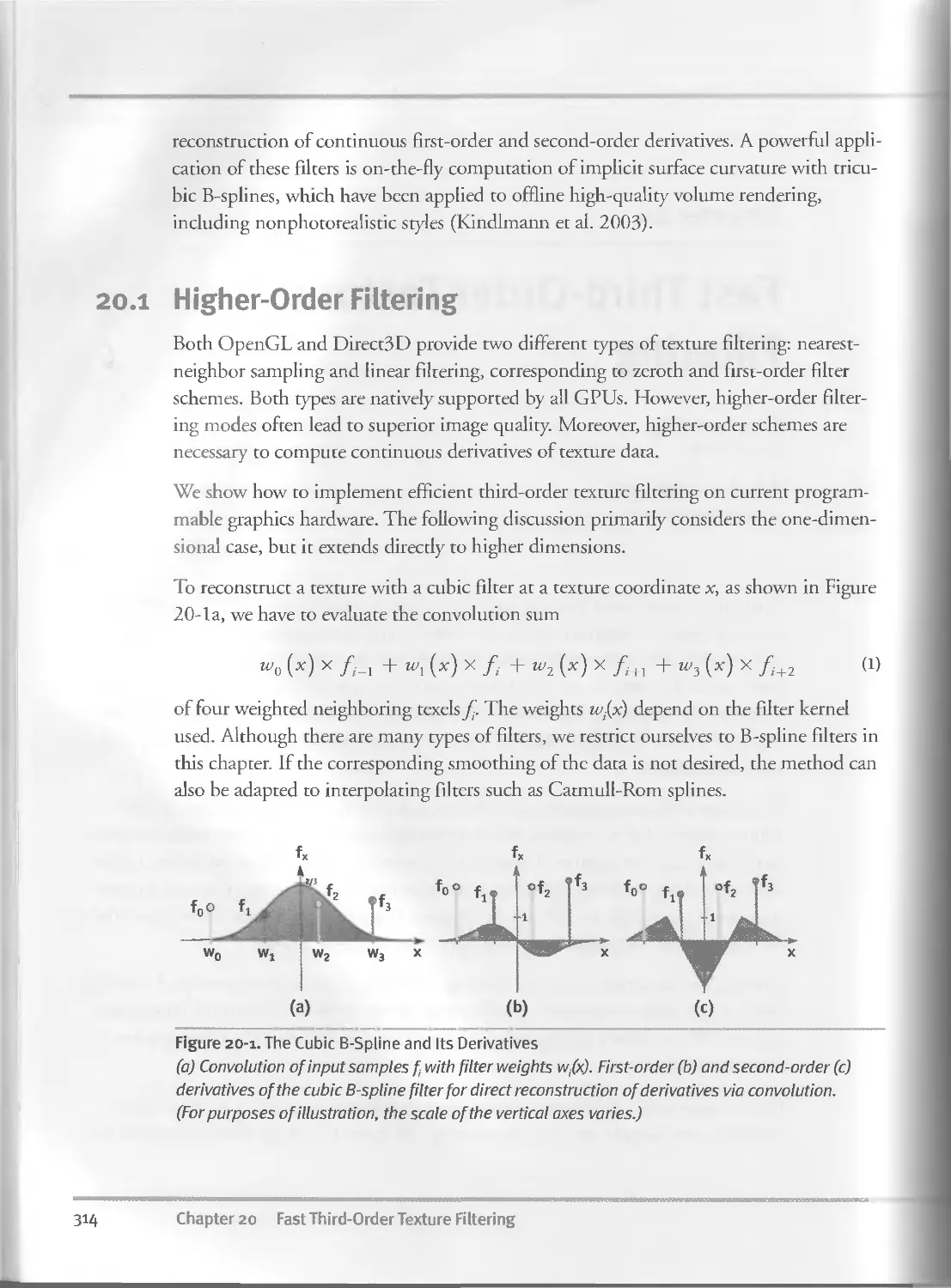
20.1 Higher-Order Filtering....................................314
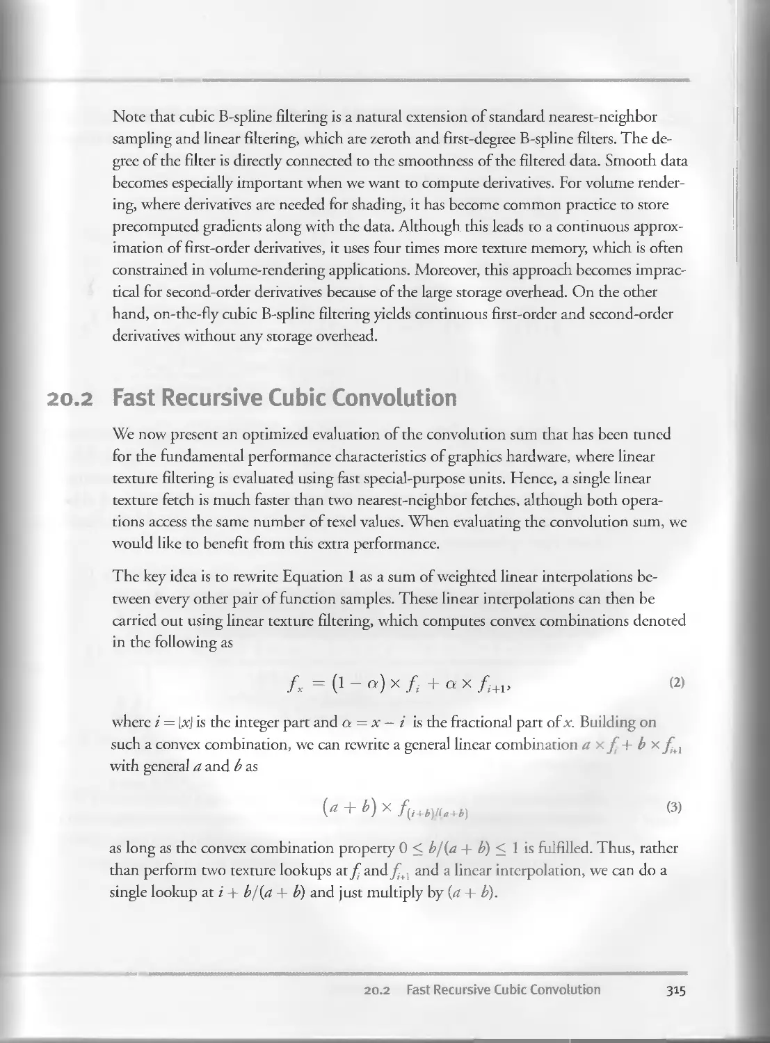
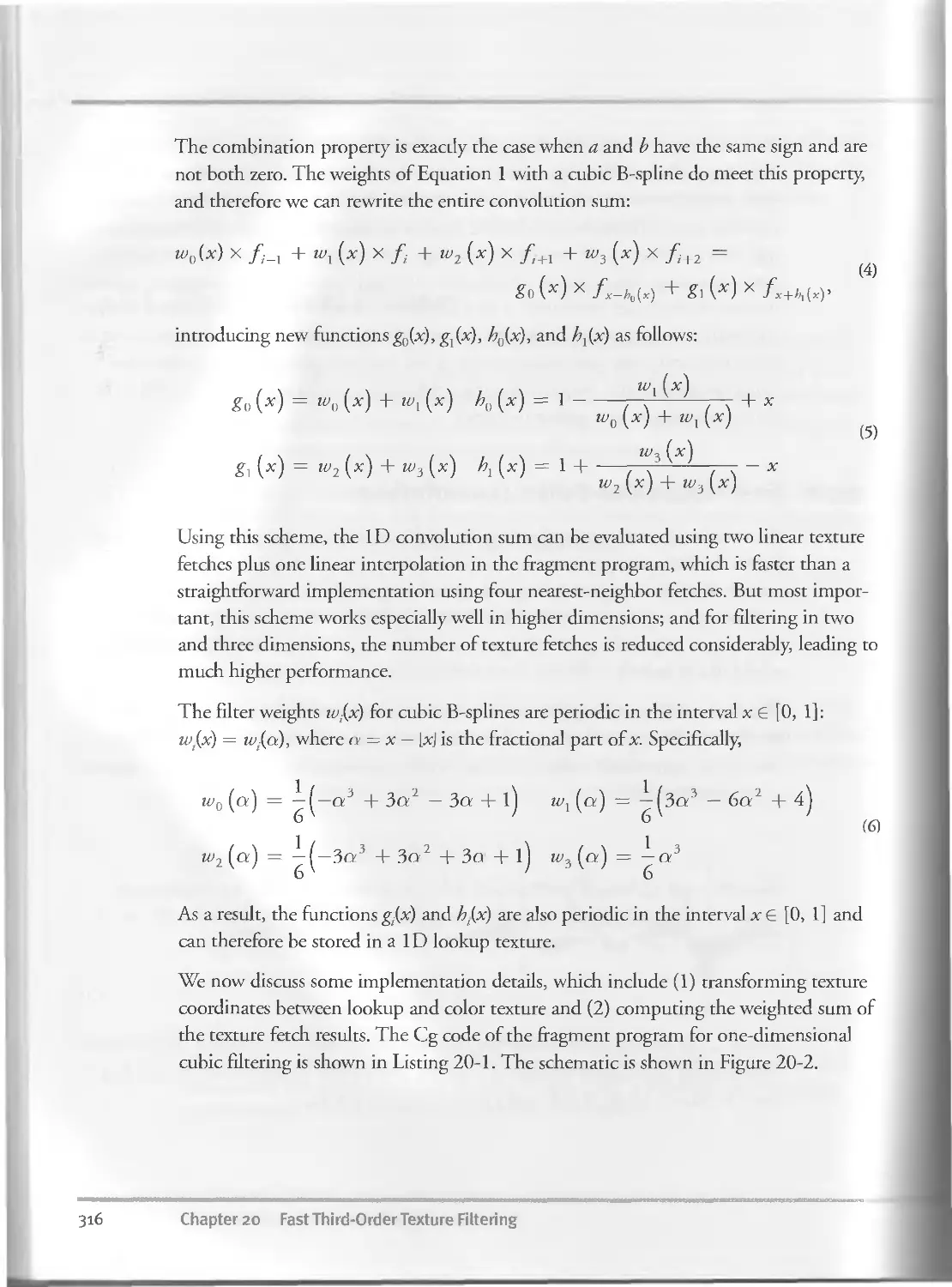
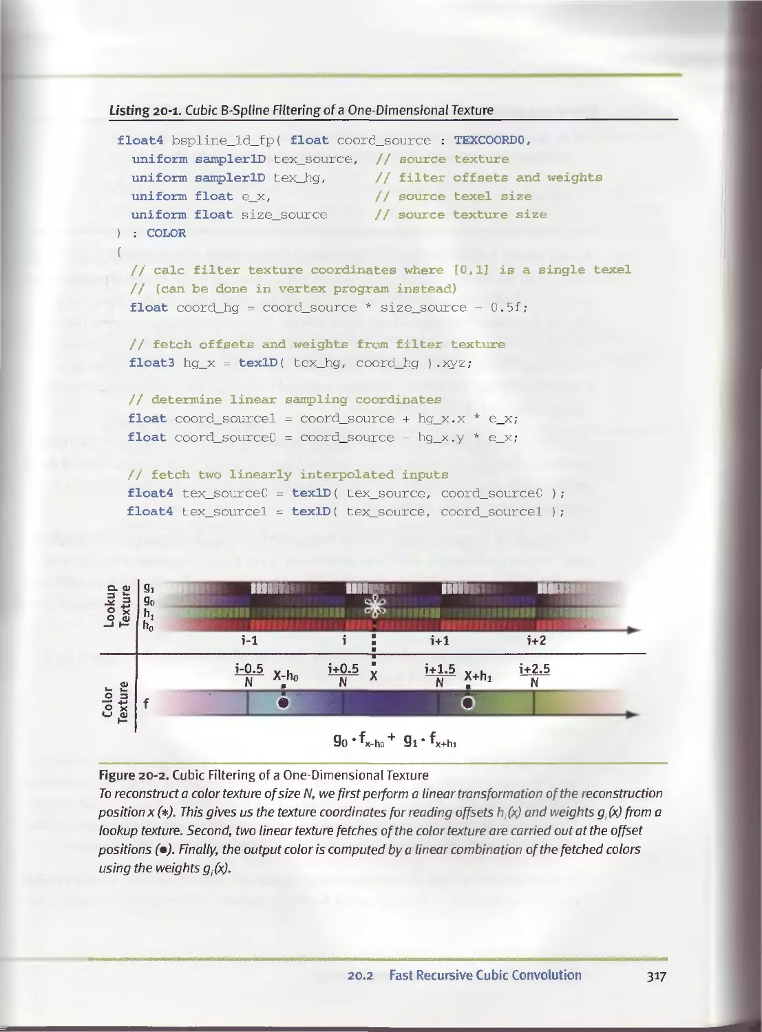
20.2 Fast Recursive Cubic Convolution.........................315
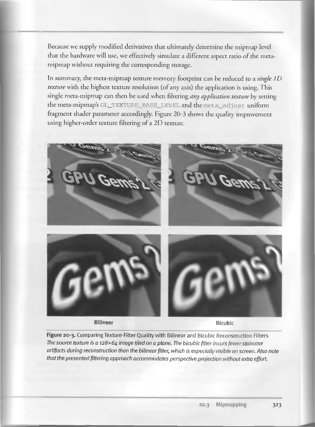
20.3 Mipmapping............................................ . . 320
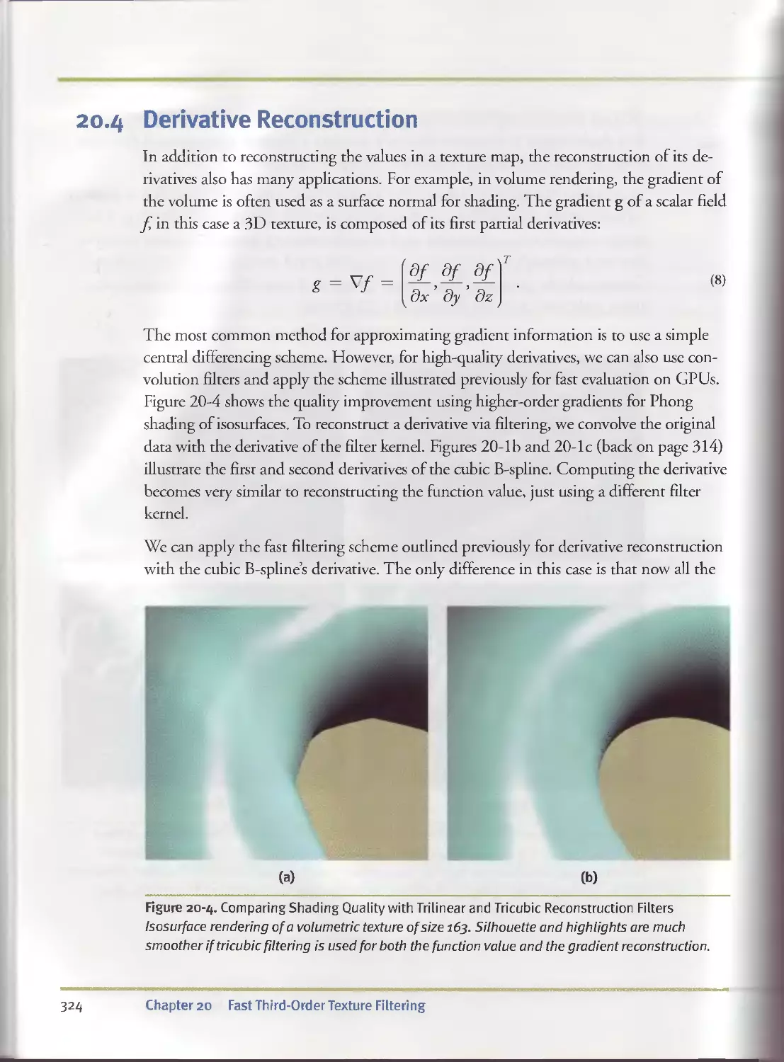
20.4 Derivative Reconstruction................................324
20.5 Conclusion...............................................327
20.6 References..............................................328
Chapter 21
High-Quality Antialiased Rasterization..................................331
Dan Wexler, NVIDIA Corporation
Eric Enderton, NVIDIA Corporation
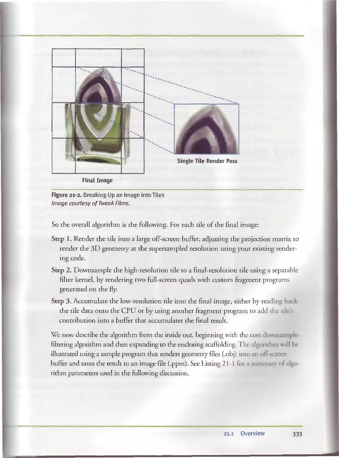
21.1 Overview.................................................331
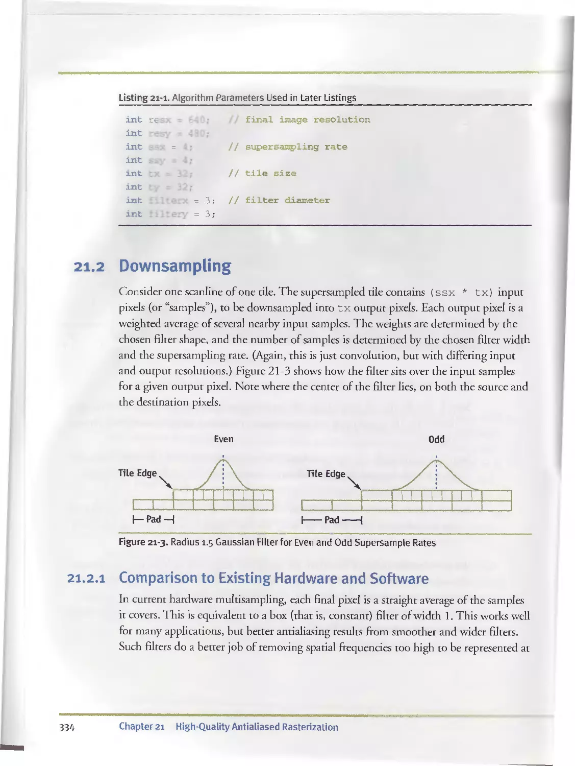
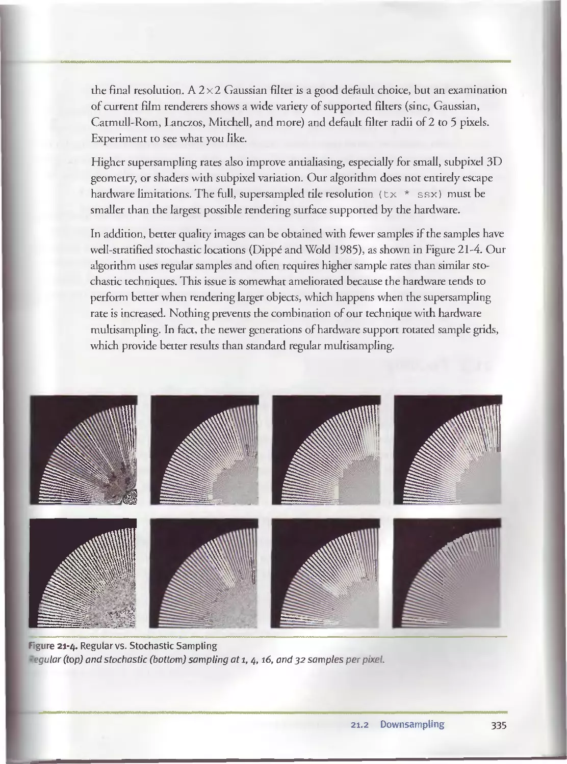
21.2 Downsampling.............................................334
21.2.1 Comparison to Existing Hardware and Software.....334
21.2.2 Downsampling on the GPU..........................336
21.3 Padding..................................................336
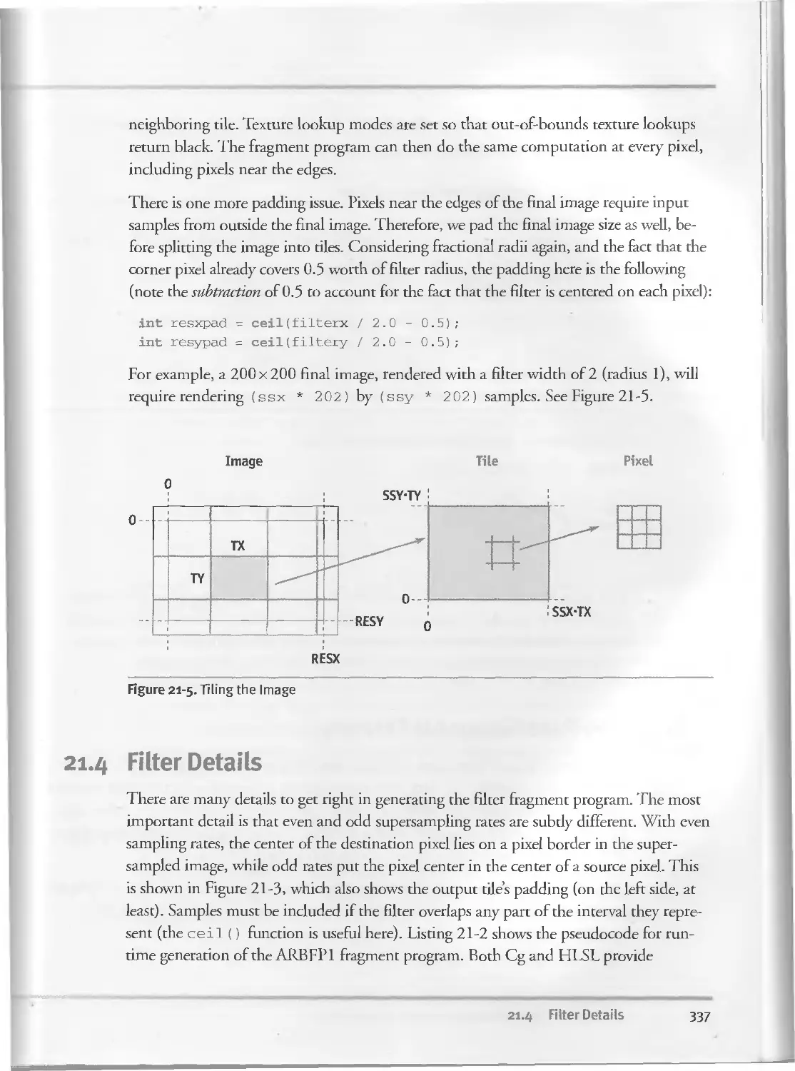
21.4 Filter Details...........................................337
21.5 Two-Pass Separable Filtering.............................338
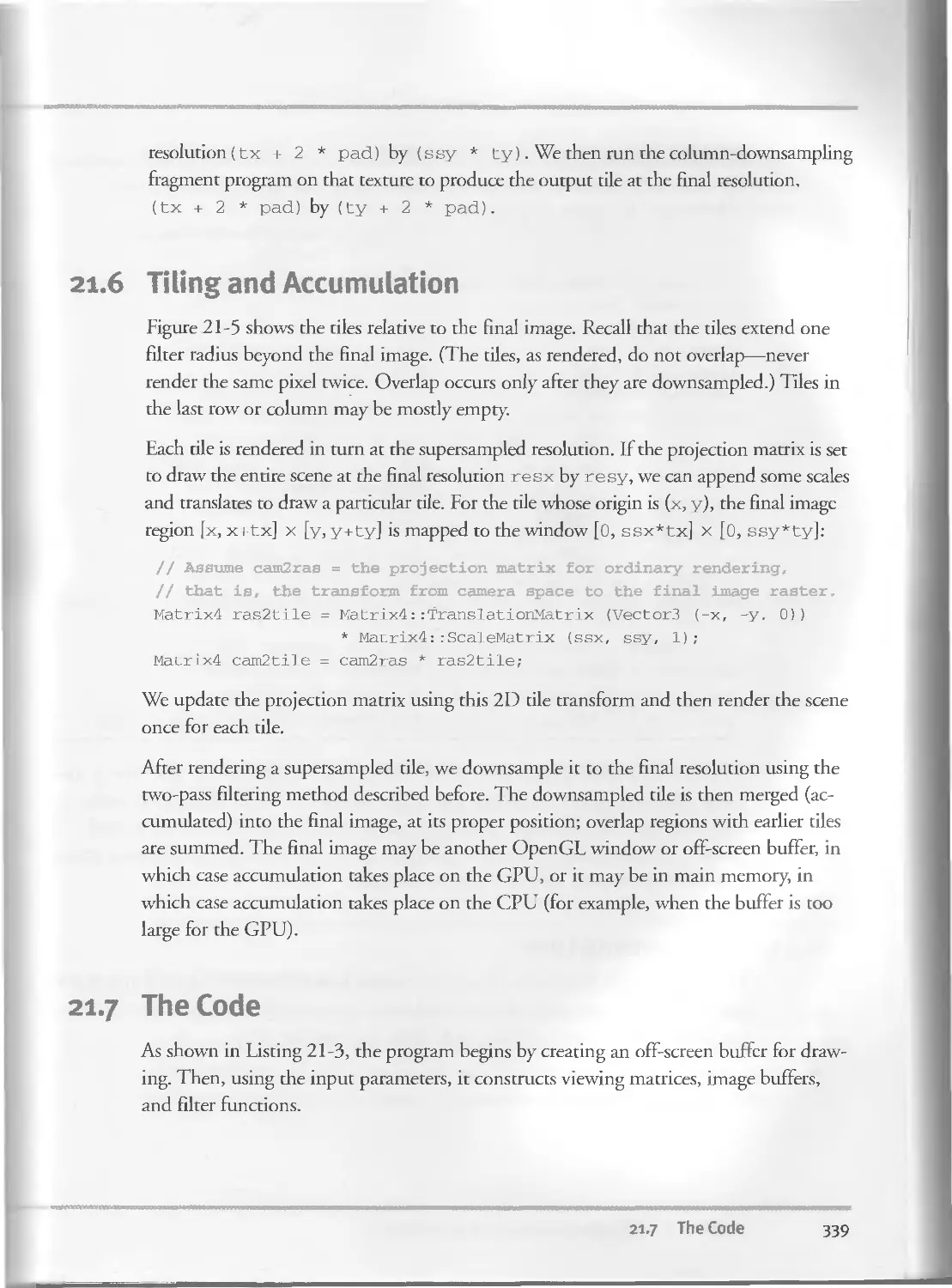
21.6 Tiling and Accumulation..................................339
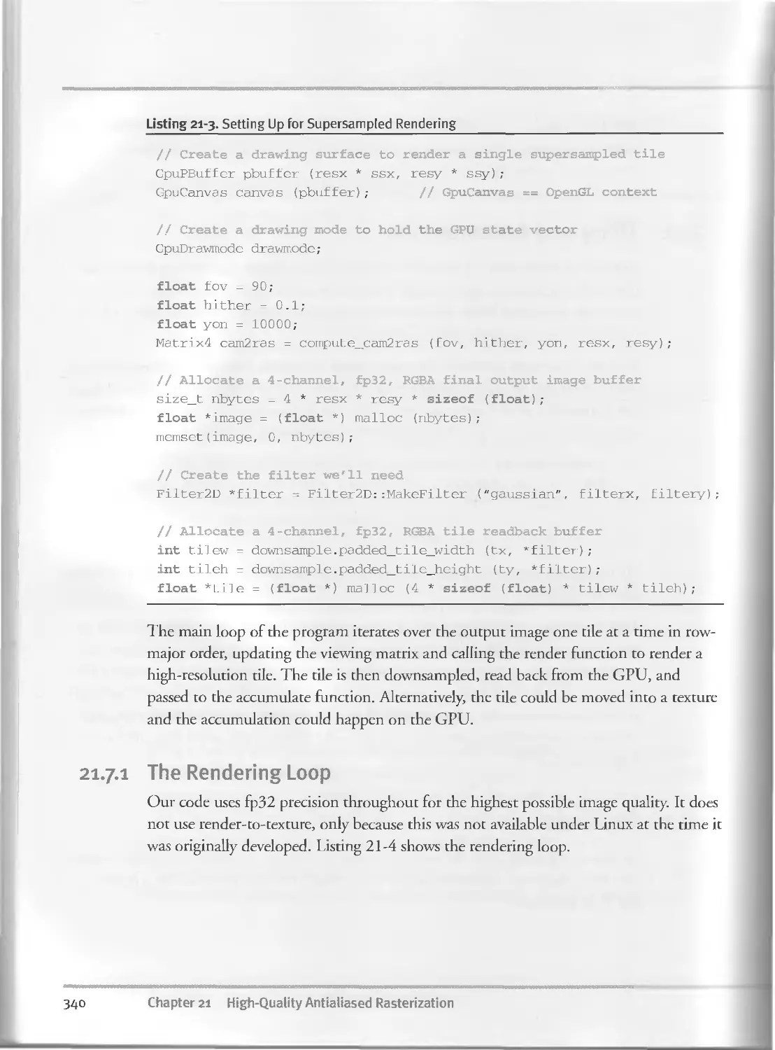
21.7 The Code.................................................339
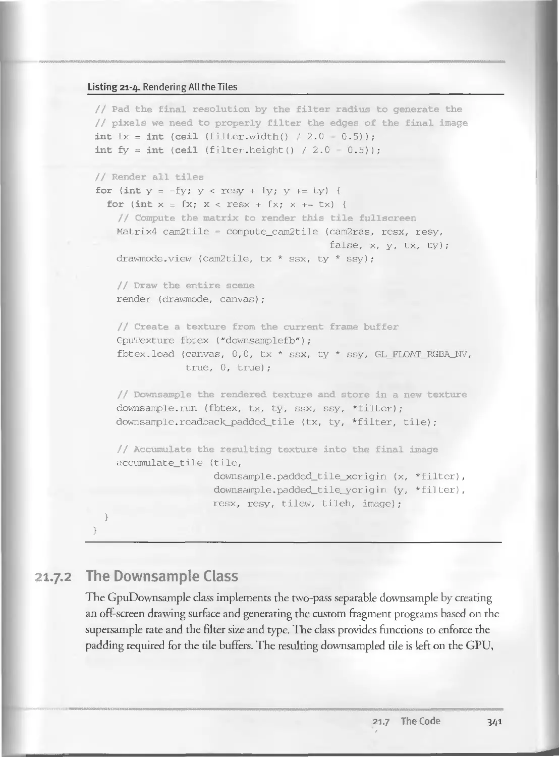
2I.7.I The Rendering Loop...............................340
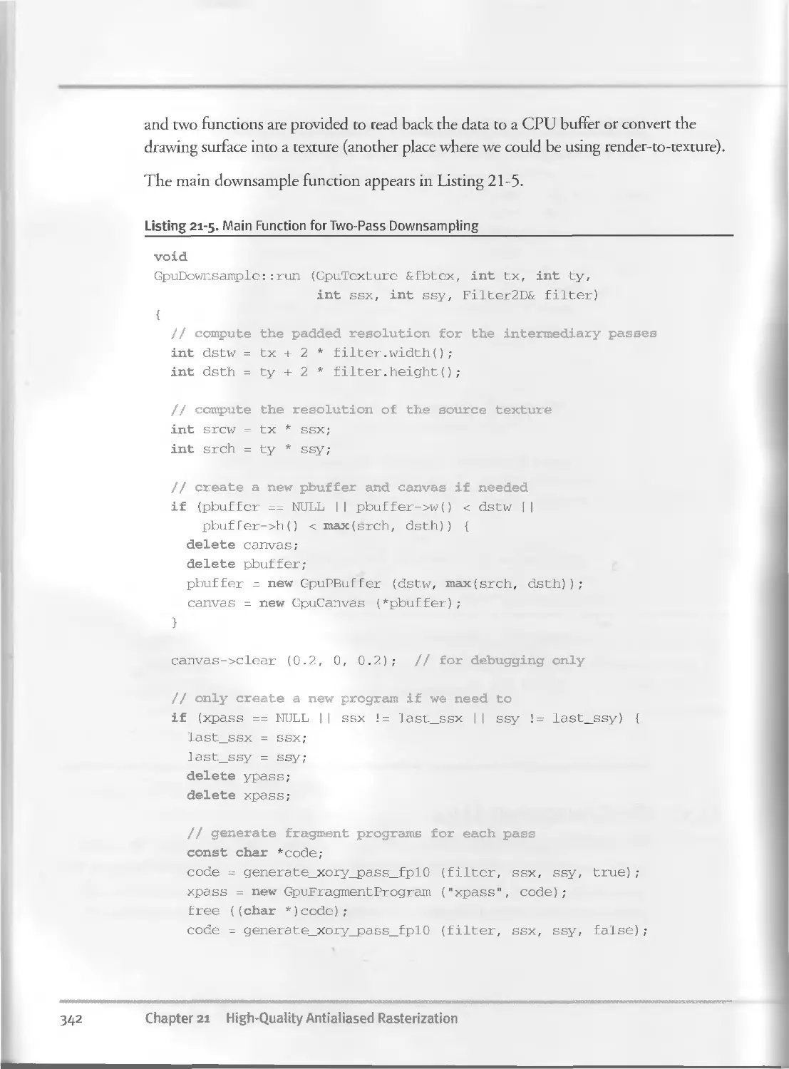
21.7.2 The Downsample Class.............................341
21.7.3 Implementation Details...........................343
21.8 Conclusion...............................................344
21.9 References...............................................344
xvi Contents
Chapter 22
Fast Prefiltered Lines.......................................................345
Eric Chan, Massachusetts Institute of Technology
Fredo Durand, Massachusetts Institute of Technology
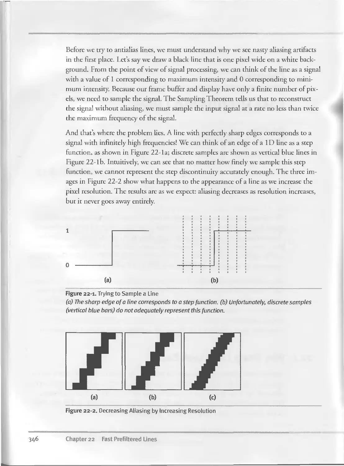
22.1 Why Sharp Lines Look Bad....................................345
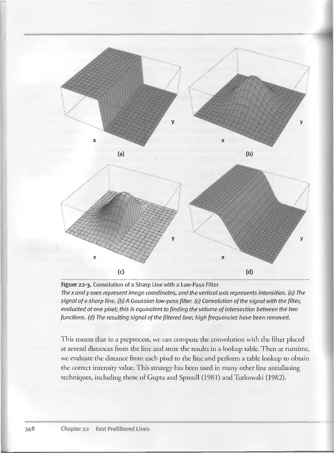
22.2 Bandlimiting the Signal................................... 347
22.2.1 Prefiltering.........................................347
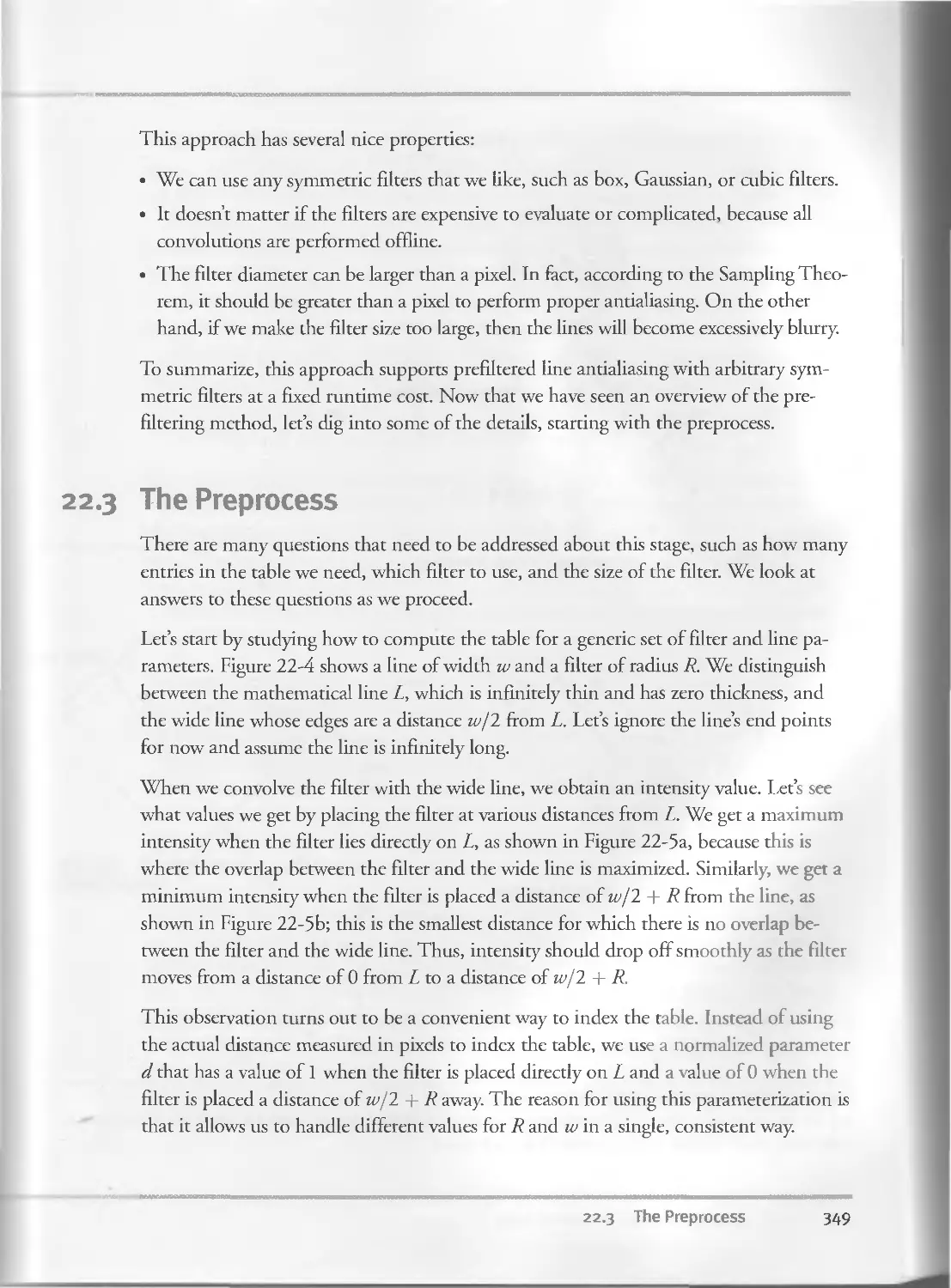
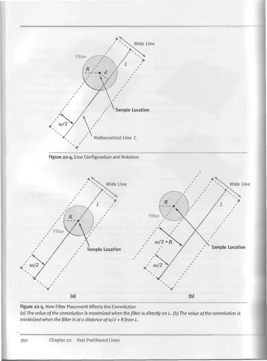
22.3 The Preprocess..............................................349
22.4 Runtime.....................................................351
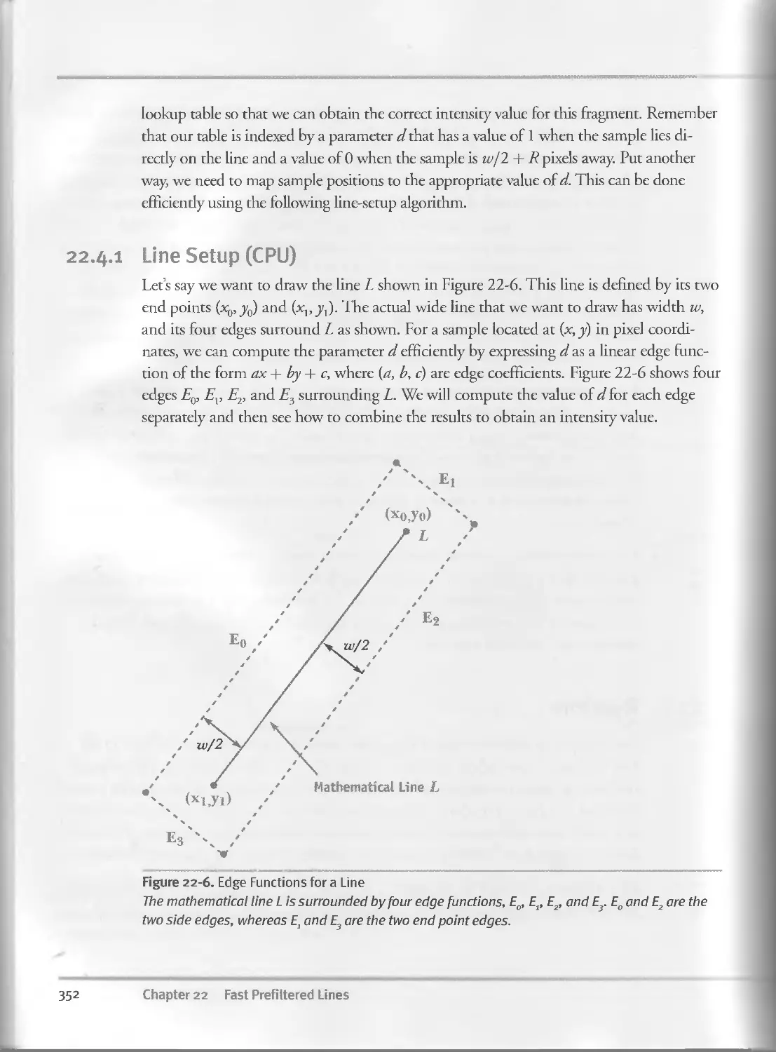
22.4.I Line Setup (CPU)....................................352
22.4.2 Table Lookups (GPU)................................353
22.5 Implementation Issues.......................................355
22.5.I Drawing Fat Lines.......... ... ................355
22.5.2 Compositing Multiple Lines..........................355
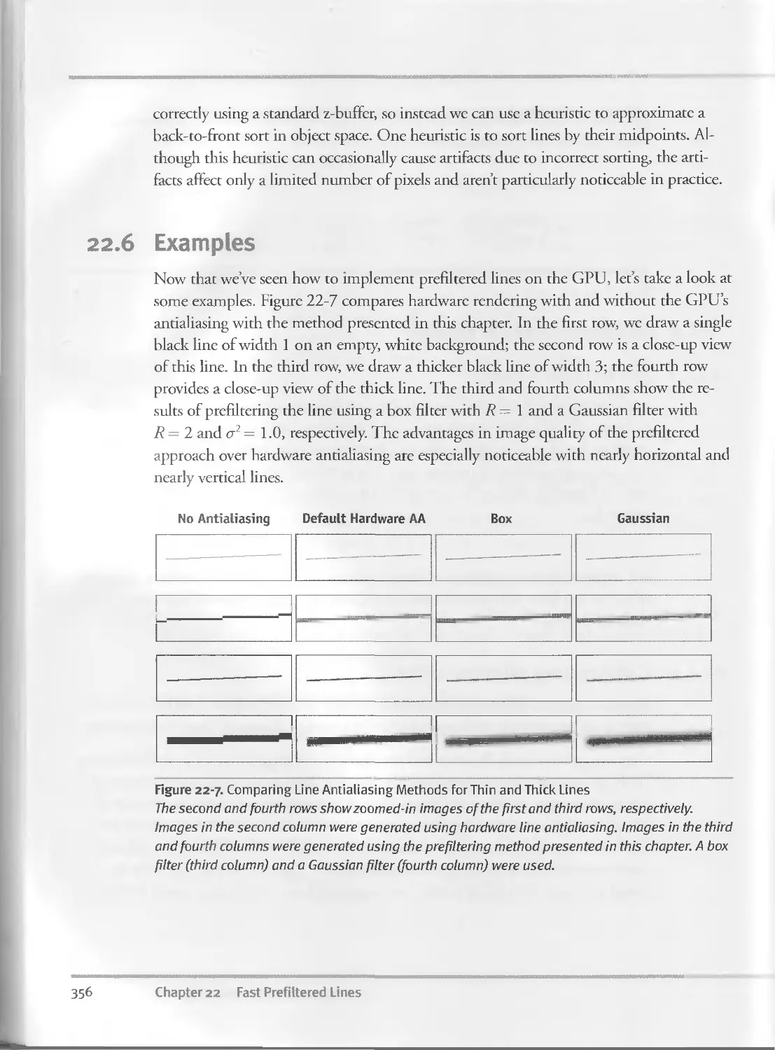
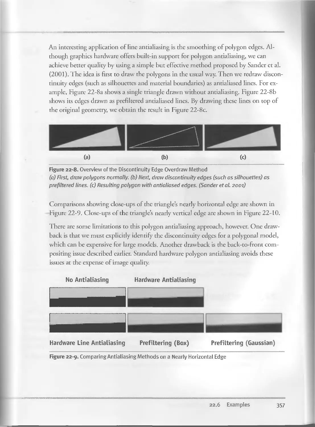
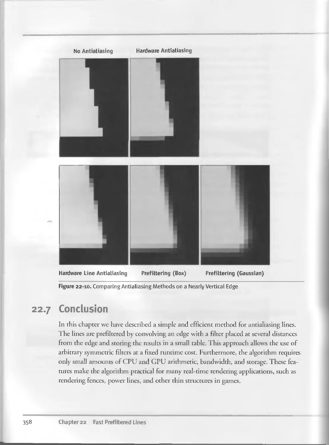
22.6 Examples....................................................356
22.7 Conclusion................................................ 358
22.8 References..................................................359
Chapter 23
Hair Animation and Rendering in the Nalu Demo................................361
Hubert Nguyen, NVIDIA Corporation
William Donnelly, NVIDIA Corporation
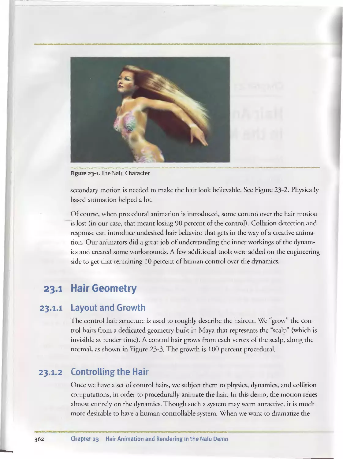
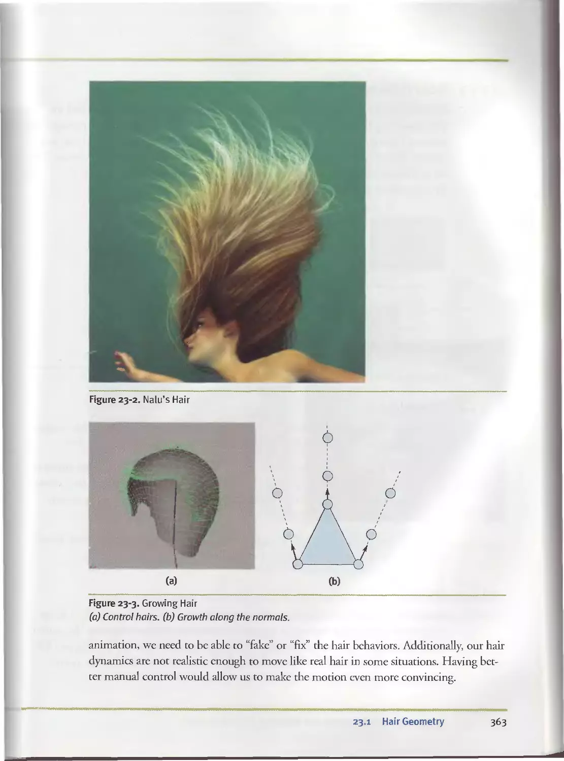
23.I Hair Geometry................................................362
23.I.I Layout and Growth...................................3^2
23.I.2 Controlling the Hair................................362
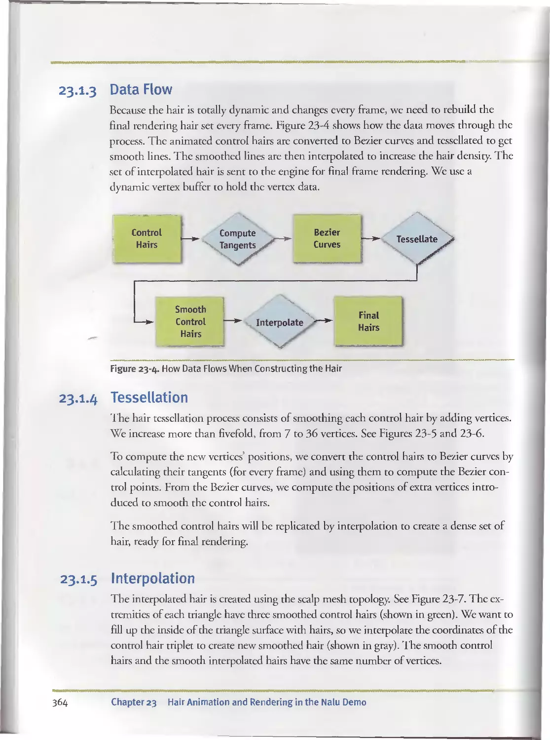
23.I.3 Data Flow....................................... . 364
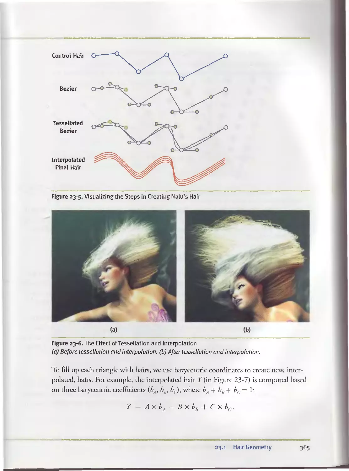
23.I.4 Tessellation...................................... 364
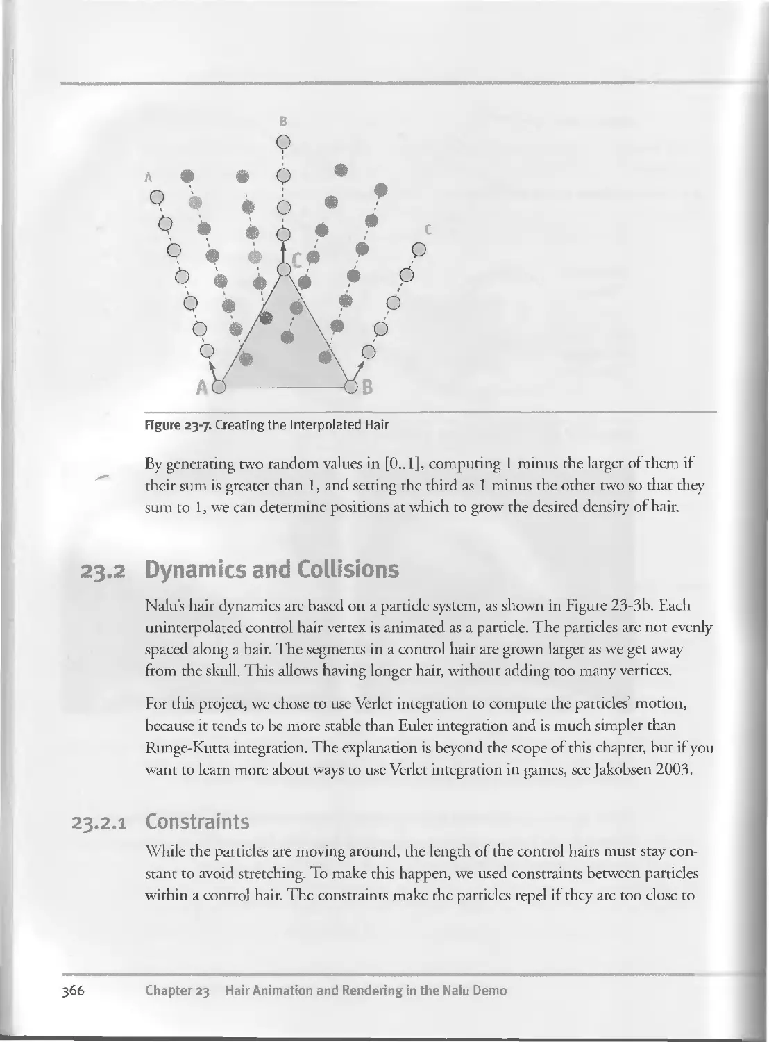
23.I.5 Interpolation................................... . 364
23.2 Dynamics and Collisions................................ . 366
23.2.I Constraints........................................ 366
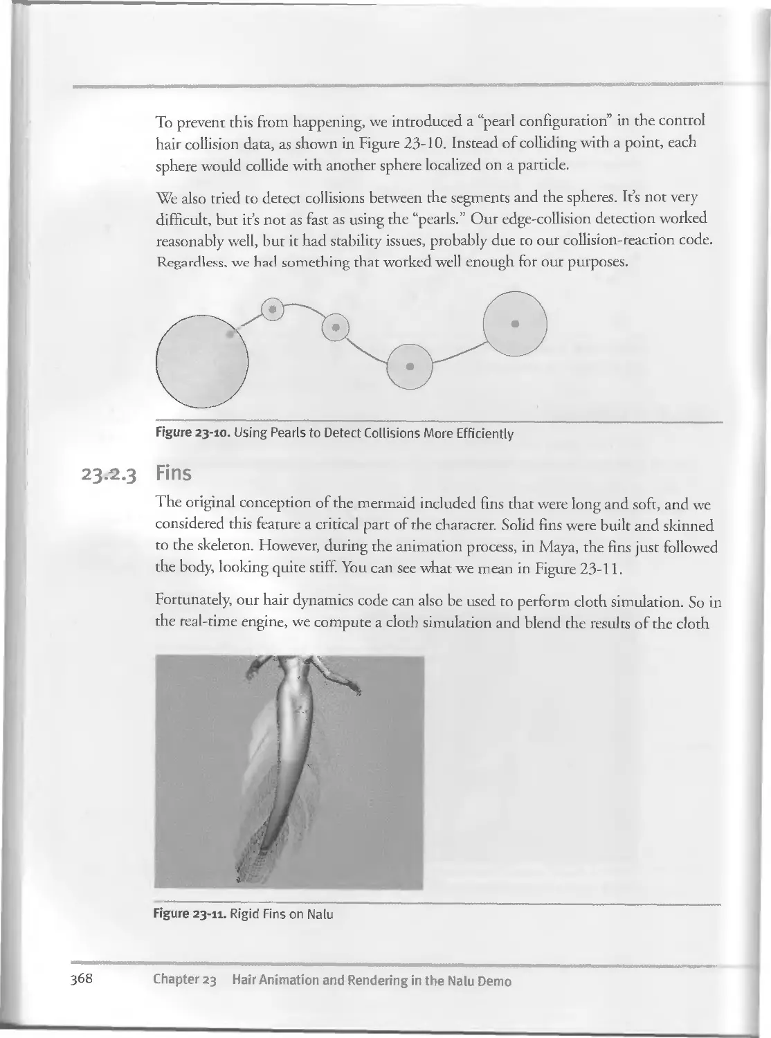
23.2.2 Collisions....................................... 367
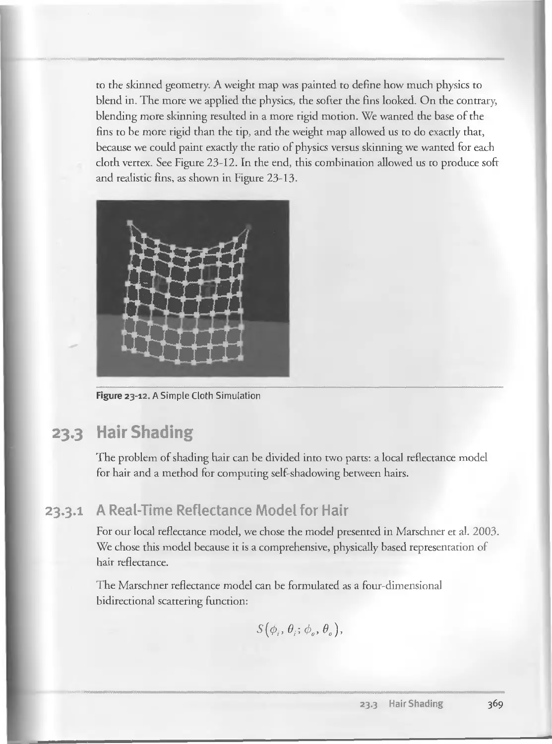
23.2.3 Fins............................................... 368
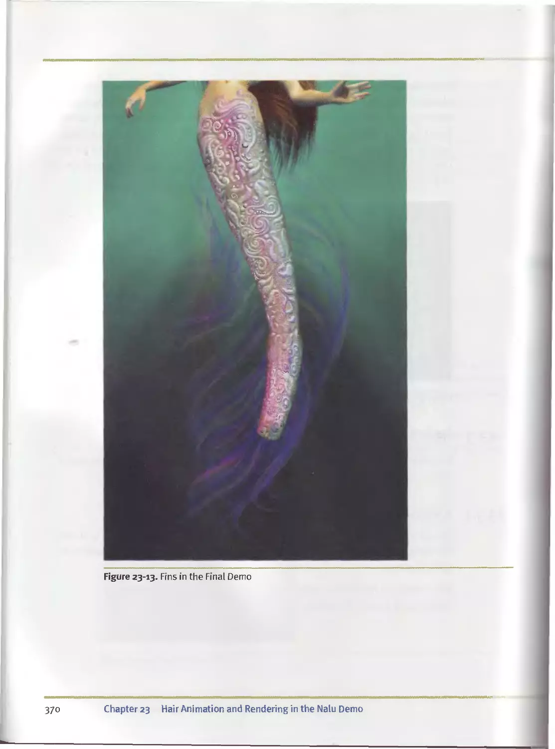
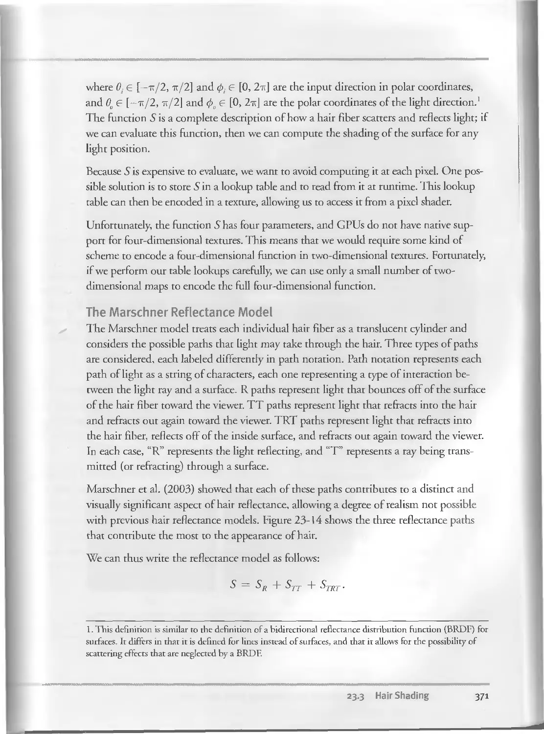
23.3 Hair Shading.................................. . . . . 369
23.3.I A Real-Time Reflectance Model for Hair. . . . . 369
23.3.2 Real-Time Volumetric Shadows in Hair. 375
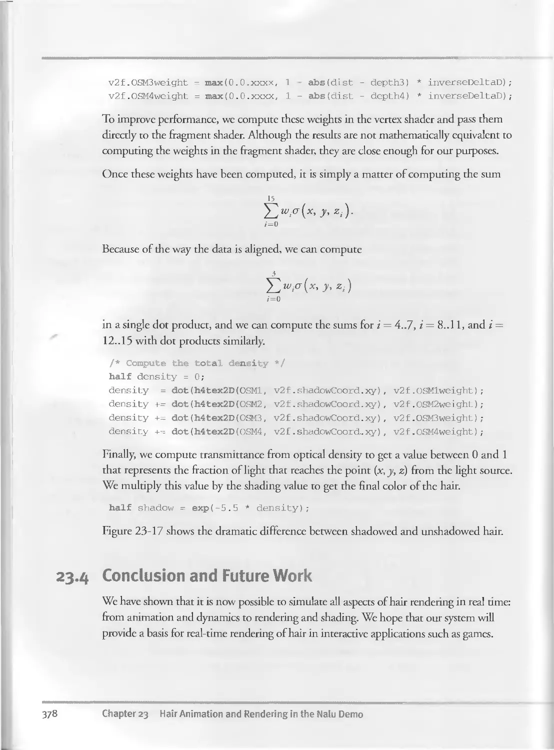
23.4 Conclusion and Future Work................... . . 378
23.5 References. .......................... . 380
Contents
xvii
Chapter 24
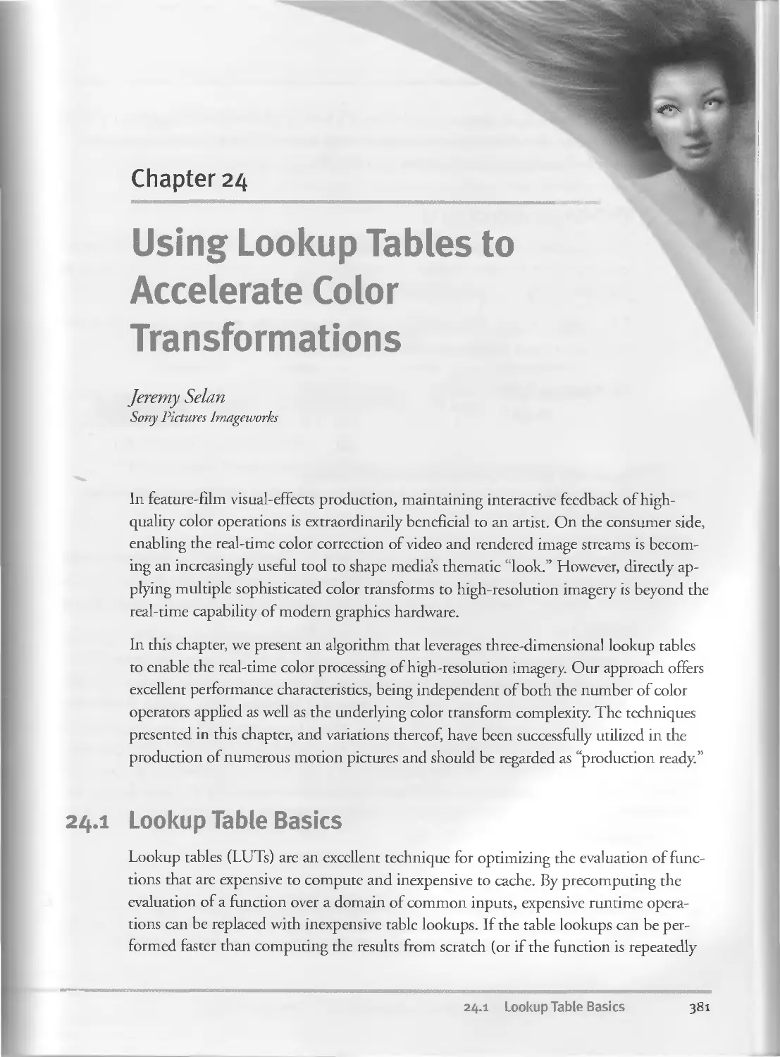
Using Lookup Tables to Accelerate Color Transformations.................381
Jeremy Selan, Sony Pictures Imageworks
24-1 Lookup Table Basics.......................................381
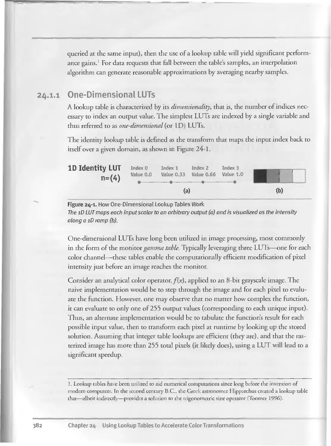
24.1.1 One-Dimensional LUTs.............................382
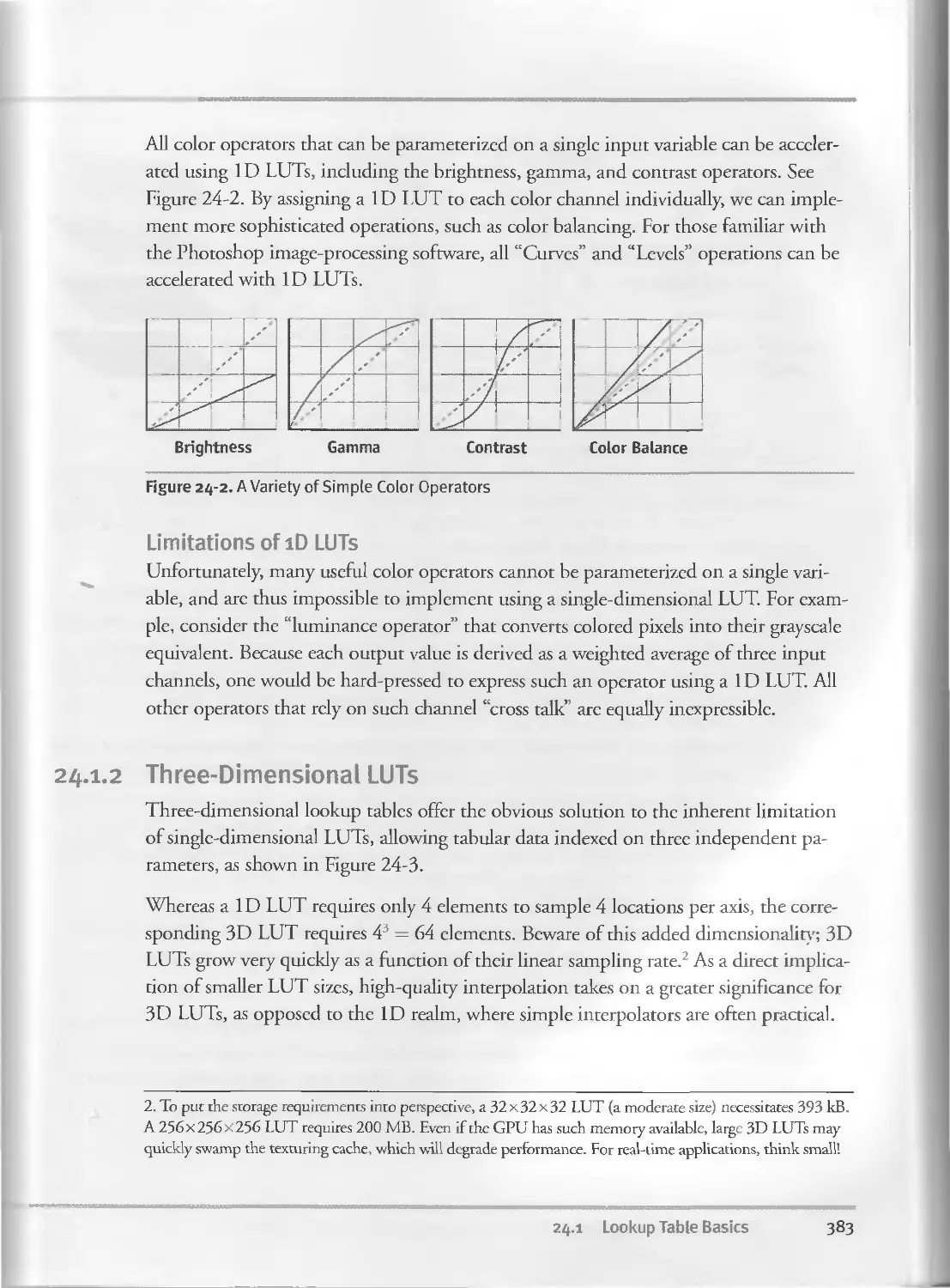
24.1.2 Three-Dimensional LUTs...........................383
24.I.3 Interpolation....................................385
24. 2 Implementation..........................................386
24.2.I Strategy for Mapping LUTs to the GPU.............386
24.2.2 Cg Shader........................................386
24.2.3 System Integration...............................389
24.2.4 Extending 3D LUTs for Use with High-Dynamic-Range
Imagery.................................................390
24. 3 Conclusion...............................................392
24. 4 References...............................................392
Chapter 25
GPU Image Processing in Apple’s Motion..................................393
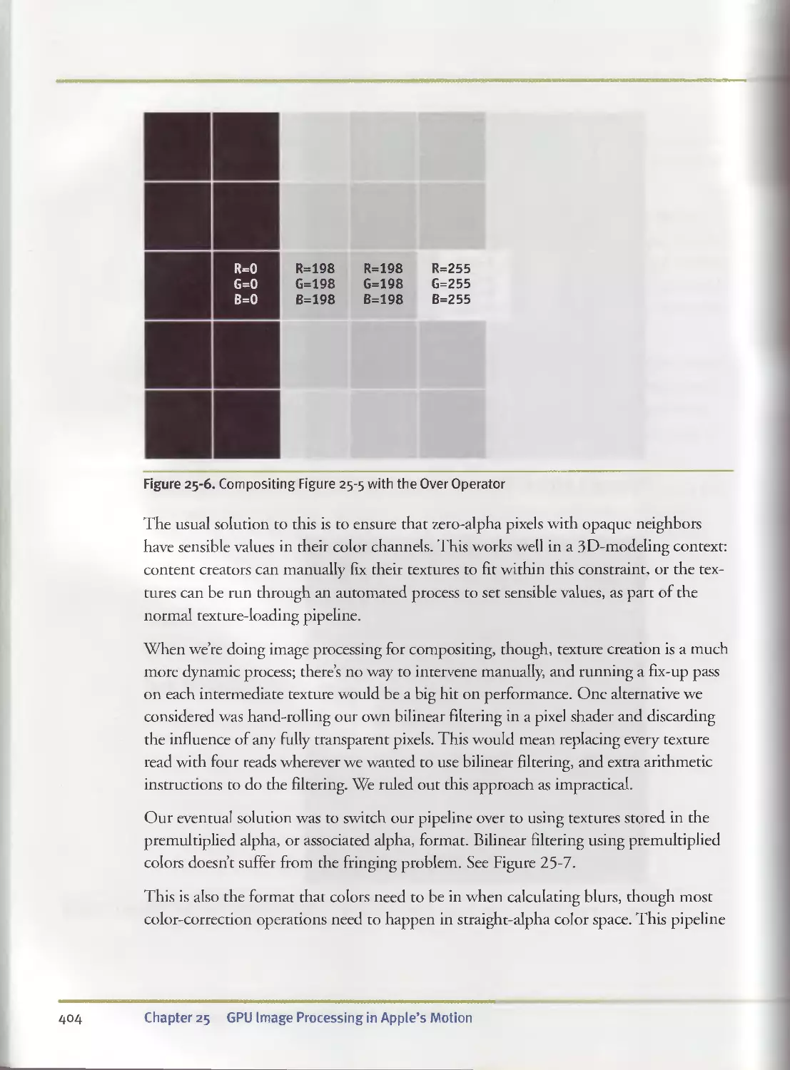
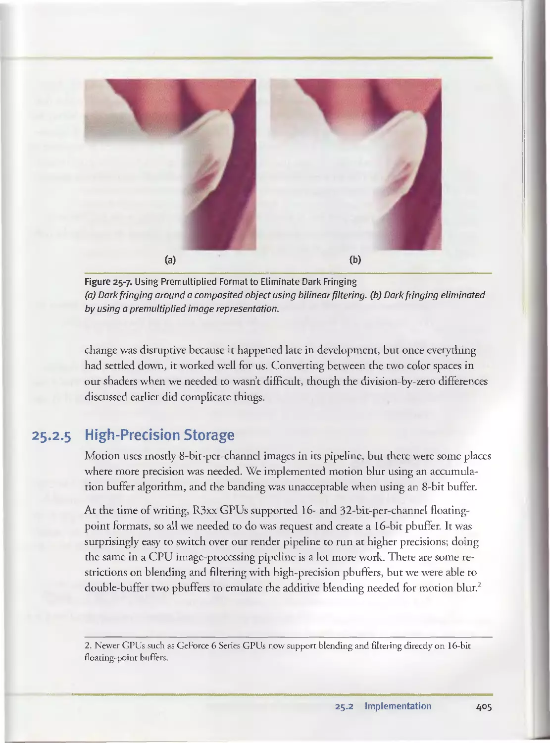
Pete Warden, Apple Computer
25.1 Design. ............................................... . 393
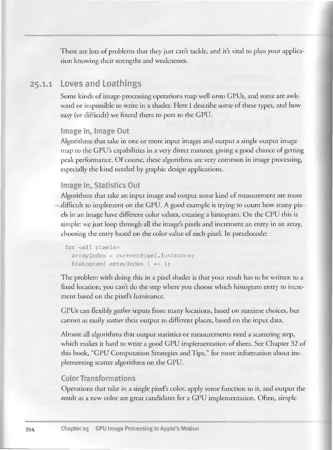
25.I.I Loves and Loathings..............................394
25.I.2 Pick a Language..................................396
25.1.3 CPU Fallback.....................................396
25.2 Implementation...........................................397
25.2.I GPU Resource Limits..............................397
25.2.2 Division by Zero.................................399
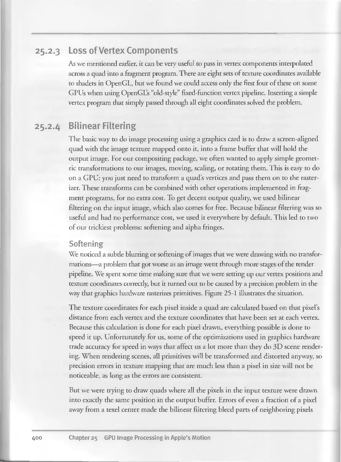
25.2.3 Loss of Vertex Components........................4°°
25.2.4 Bilinear Filtering...............................400
25.2.5 High-Precision Storage...........................405
25.3 Debugging................................................4°6
25.4 Conclusion..............................................407
25.5 References...............................................4°S
Chapter 26
Implementing improved Perlin Noise......................................409
Simon Green, NVIDIA Corporation
26.I Random but Smooth.........................................4°9
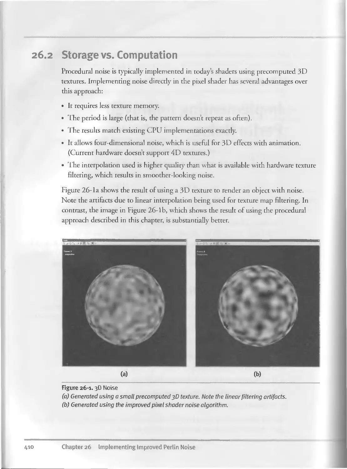
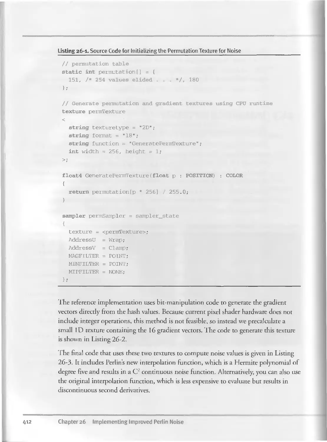
26.2 Storage vs. Computation..................................41°
xviii
Contents
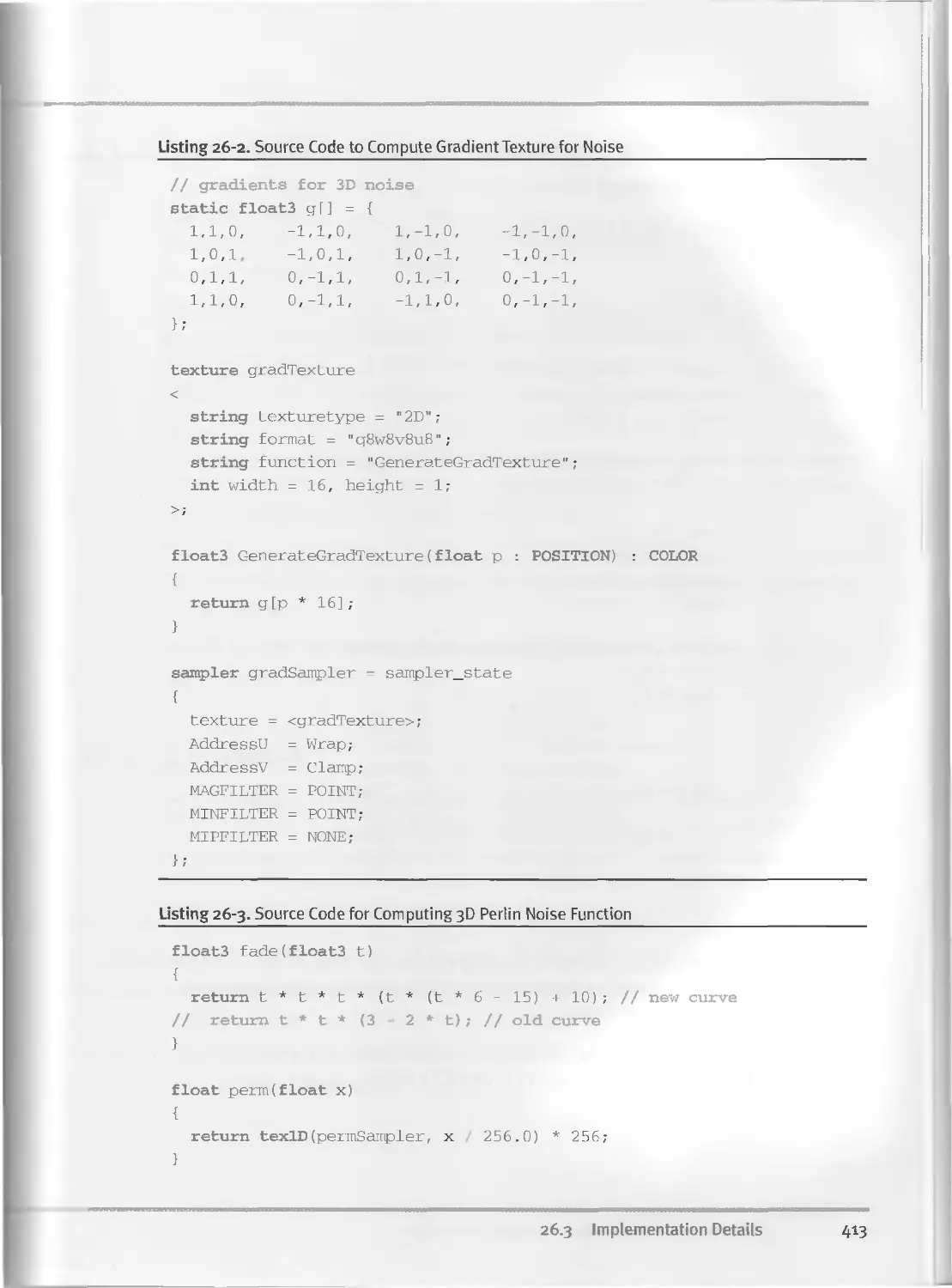
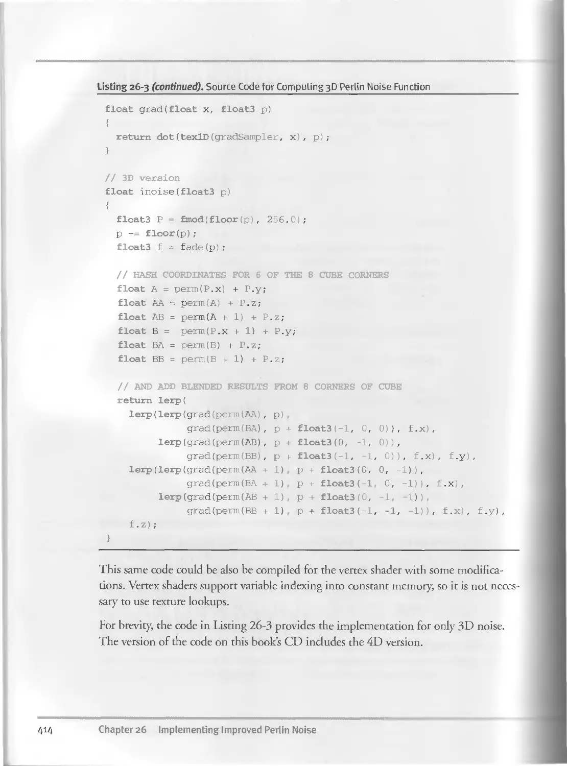
26.3 Implementation Details......................................411
26.3.I Optimization........................................415
26.4 Conclusion..................................................415
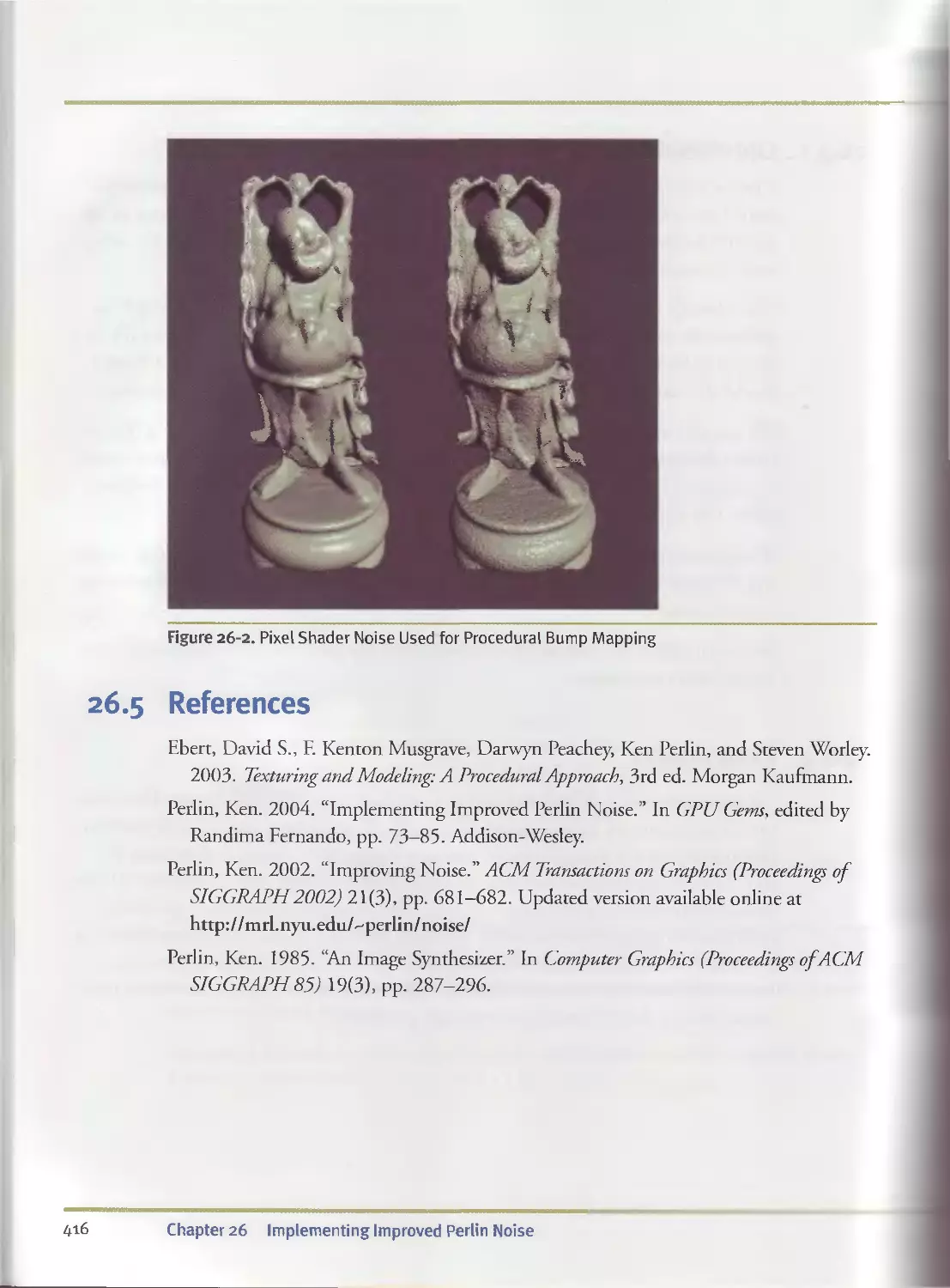
26.5 References..................................................416
Chapter 27
Advanced High-Quality Filtering.............................................417
Justin Novosad, discreet
27.1 Implementing Filters on GPUs.................................417
27.I.I Accessing Image Samples.............................418
27.I.2 Convolution Filters.................................419
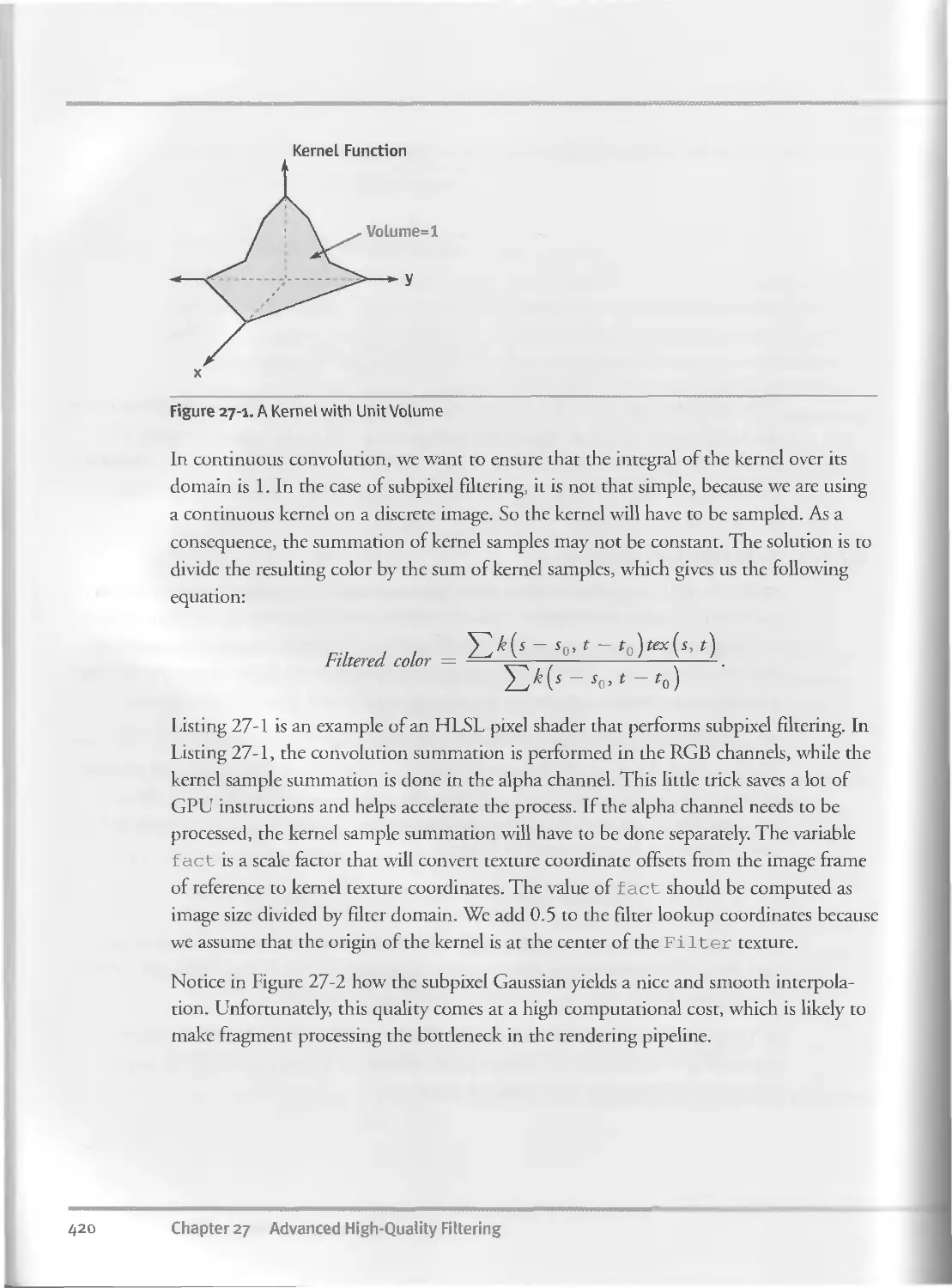
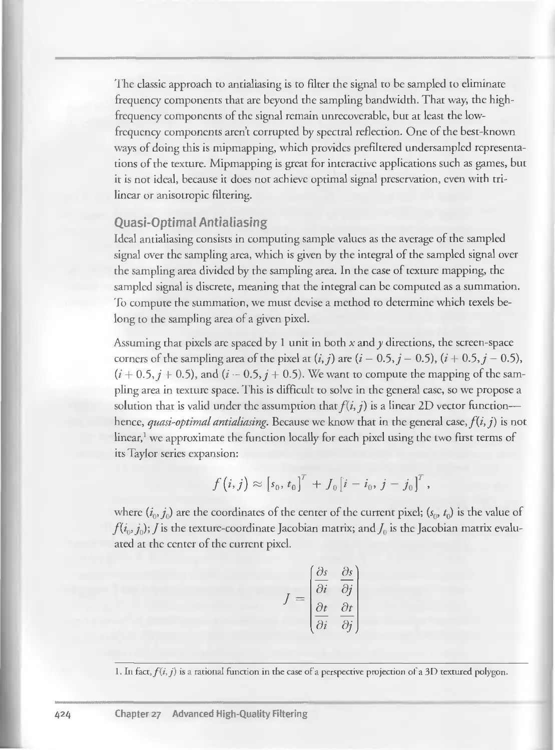
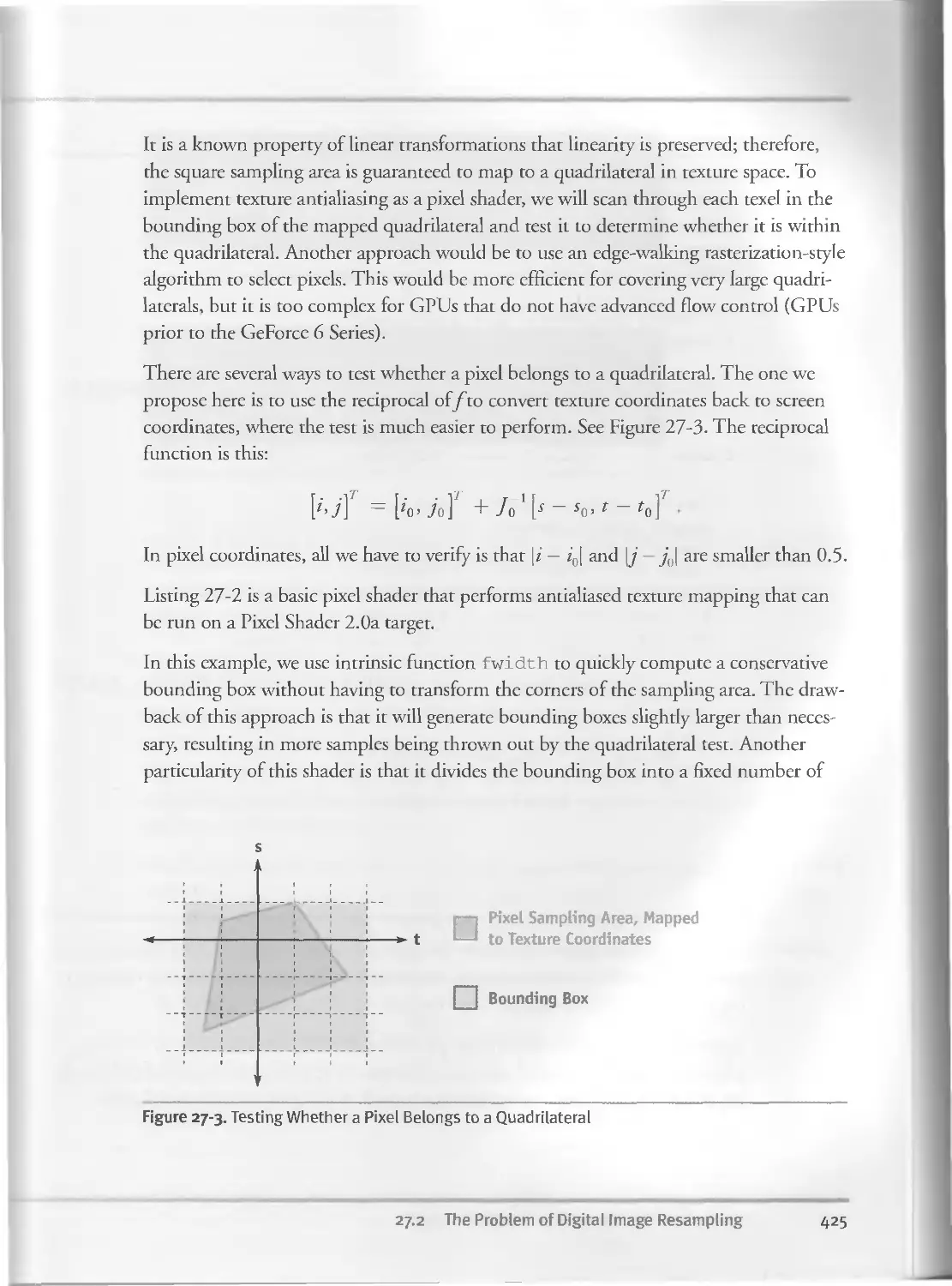
27.2 The Problem of Digital Image Resampling. . ..422
27.2.I Background..........................................423
Tj.'l.l Antialiasing.......................................423
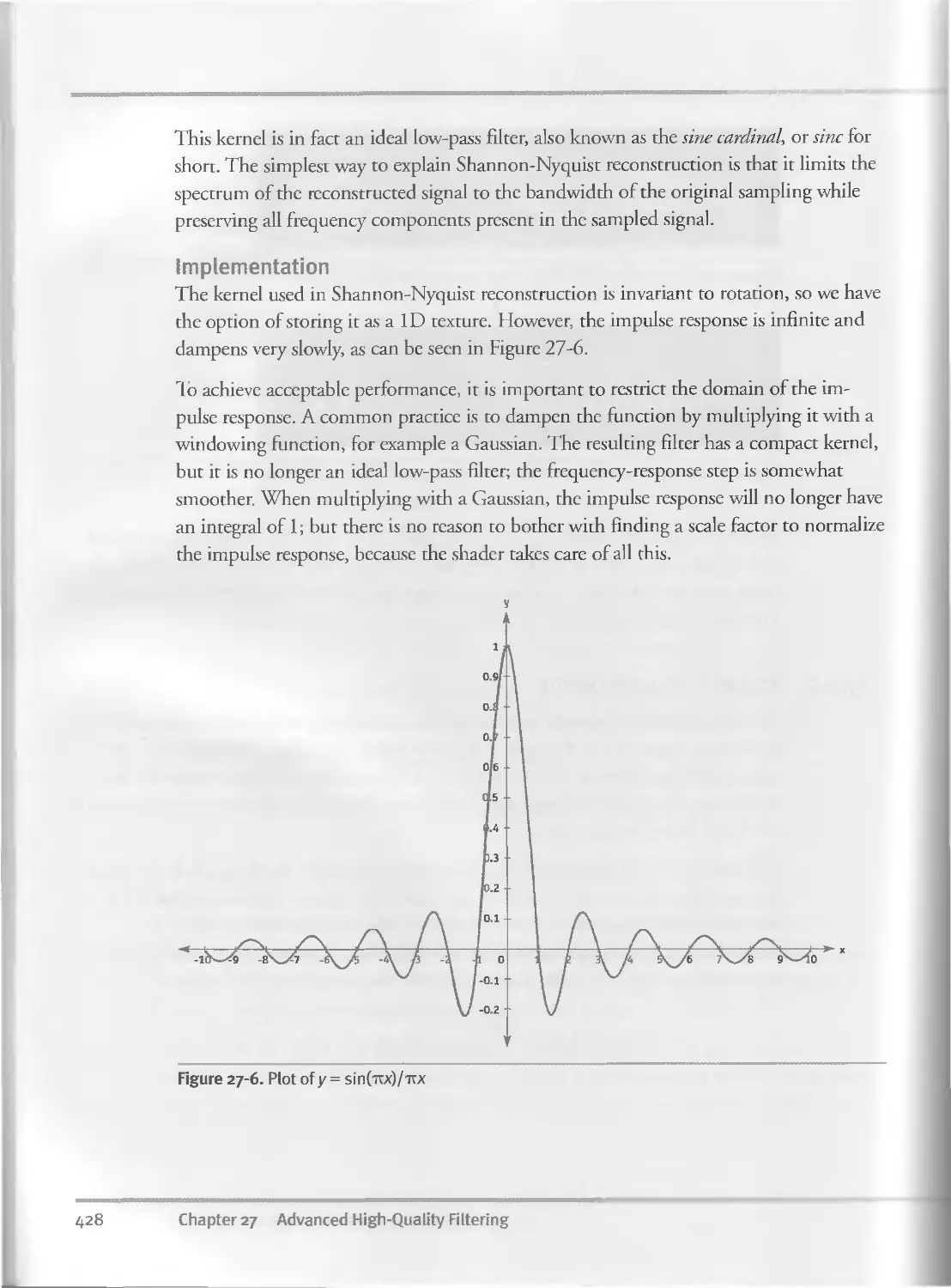
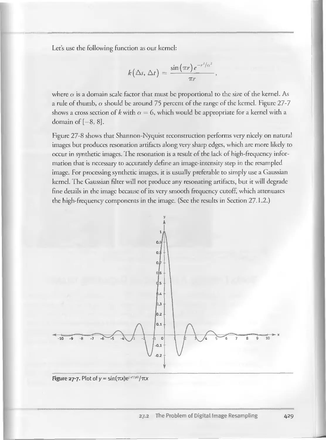
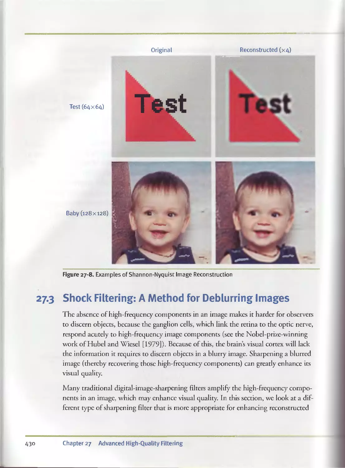
27.2.3 Image Reconstruction................................427
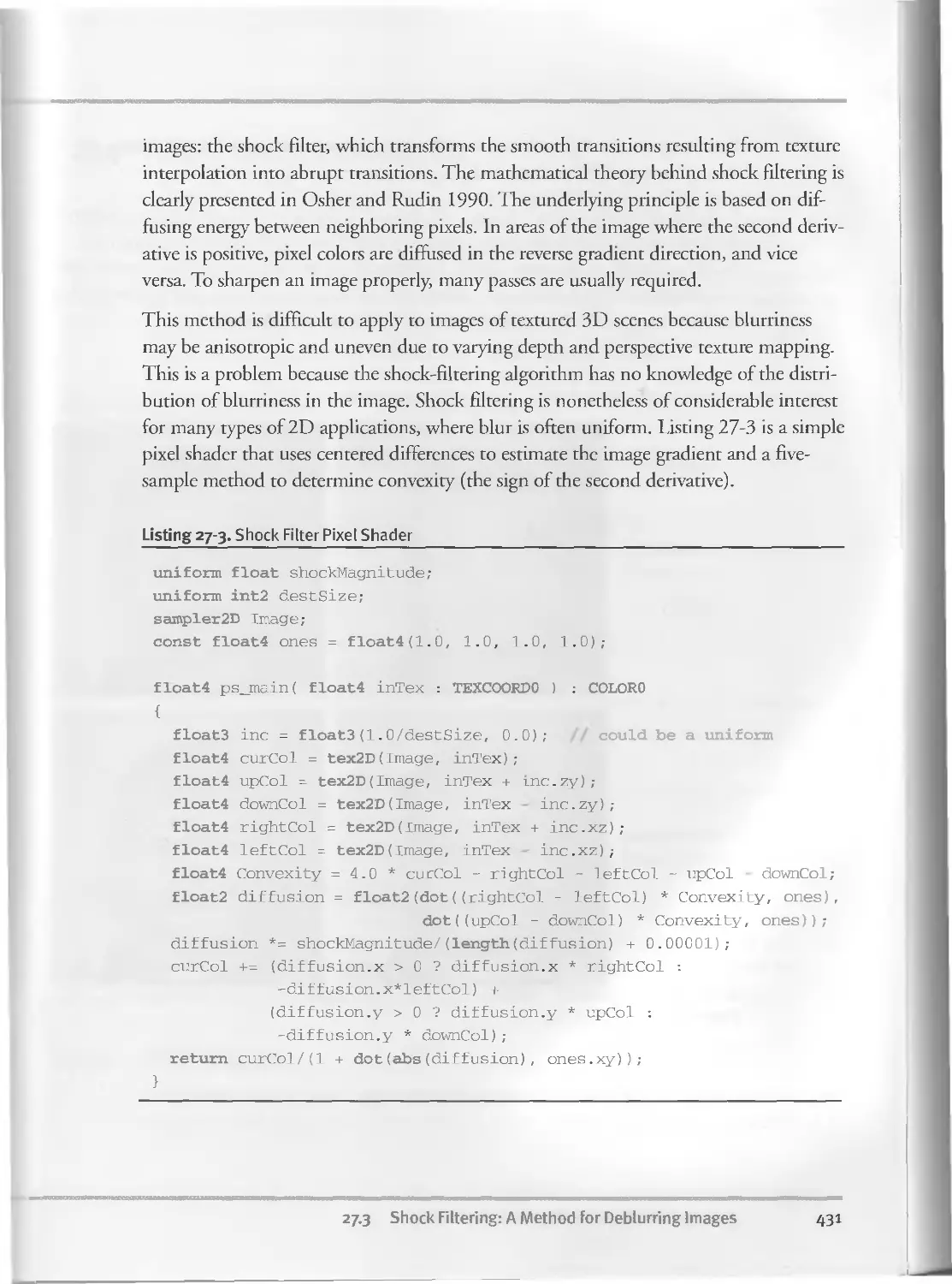
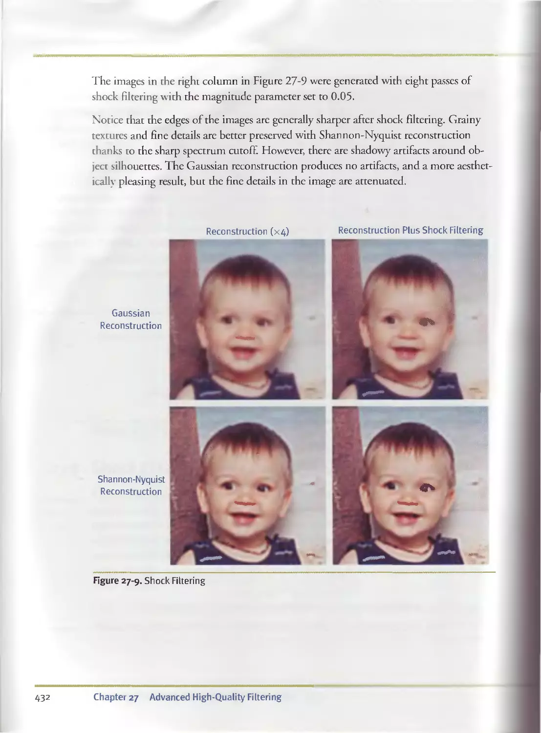
27.3 Shock Filtering: A Method for Deblurring Images..............430
27.4 Filter Implementation Tips................................. 433
27.5 Advanced Applications........................................433
27.5.I Time Warping........................................433
27.5.2 Motion Blur Removal.................................434
27.5.3 Adaptive Texture Filtering..........................434
27.6 Conclusion............................................. ... 434
27.7 References..................................................435
Chapter 28
Mipmap-Level Measurement....................................................437
lain Cantlay, Climax Entertainment
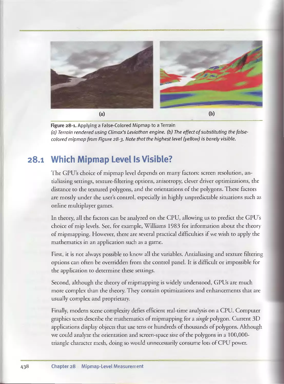
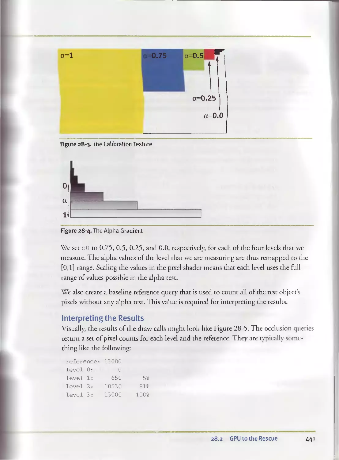
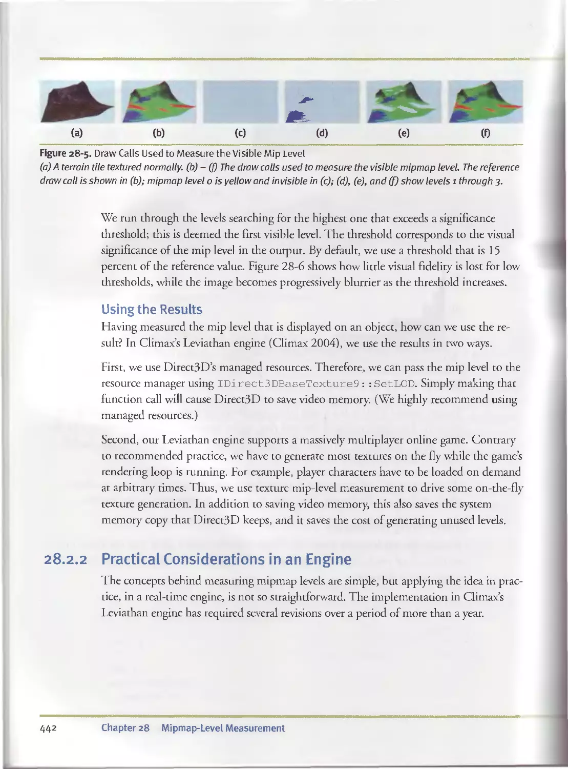
28.I Which Mipmap Level Is Visible?................................43 8
28.2 GPU to the Rescue.................................... . 439
28.2.1 Counting Pixels.....................................439
28.2.2 Practical Considerations in an Engine ........... . . 442
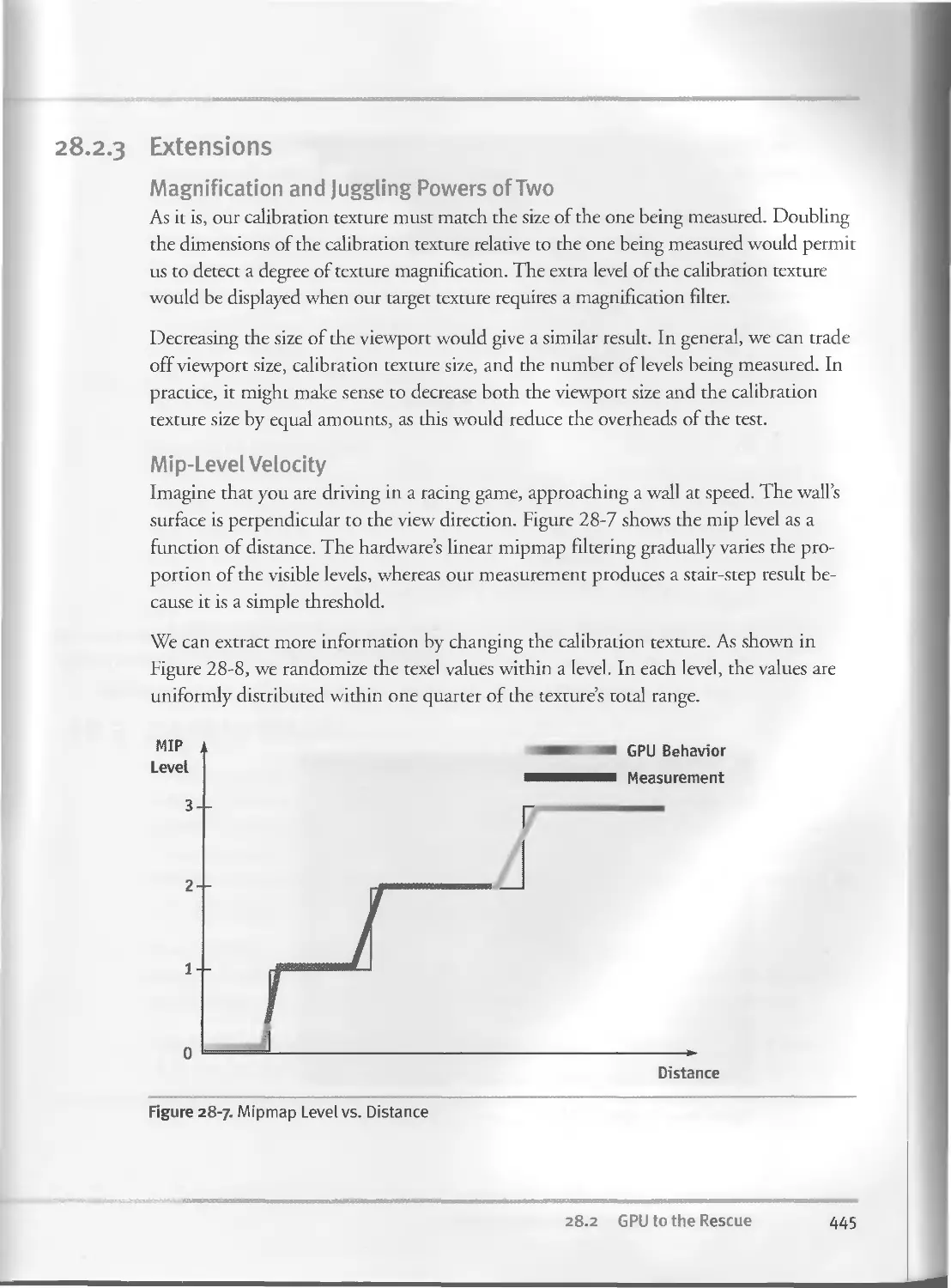
28.2.3 Extensions...................................... .. 445
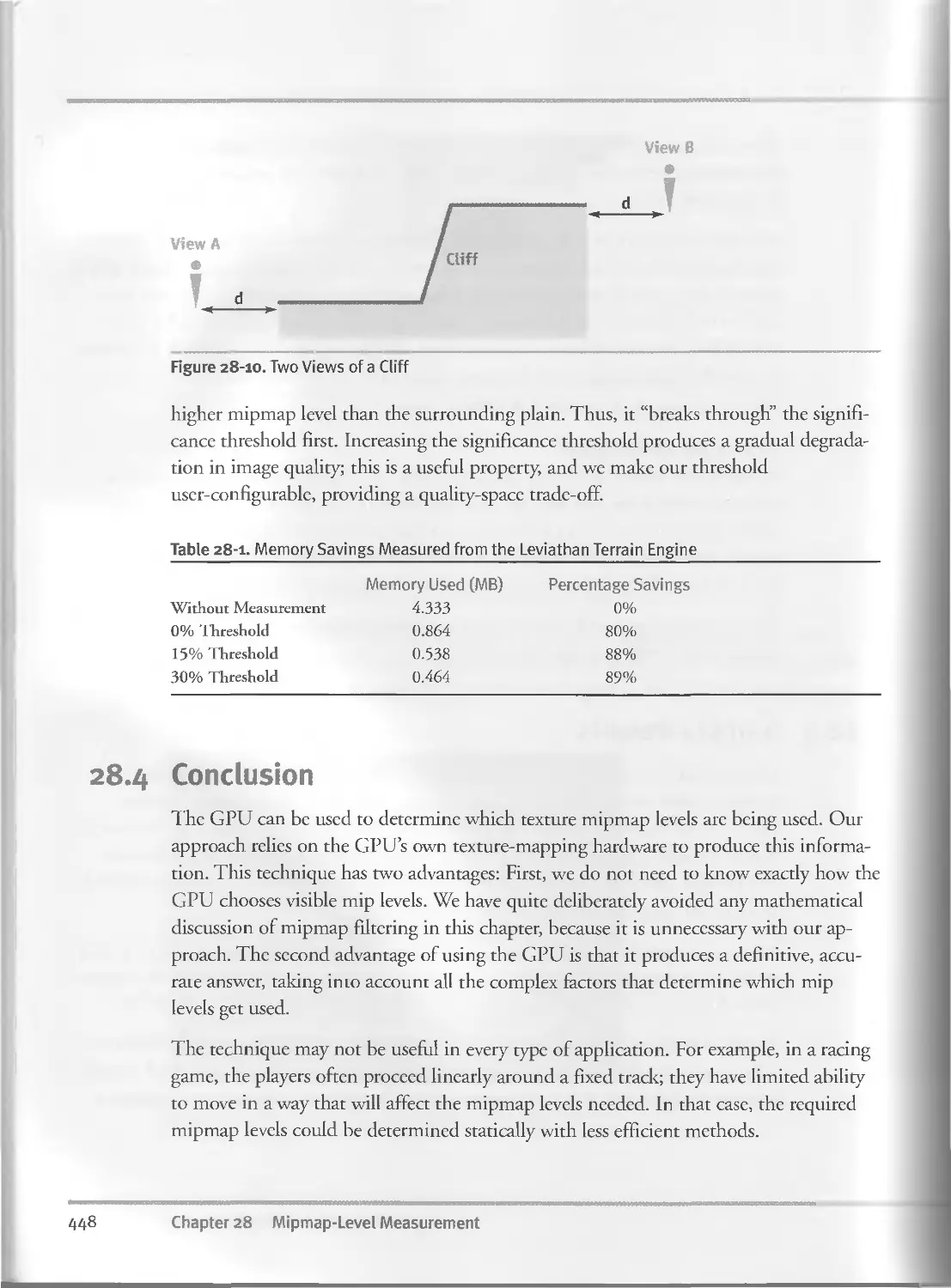
28.3 Sample Results..................................... . ... 447
28.4 Conclusion............................................... . 448
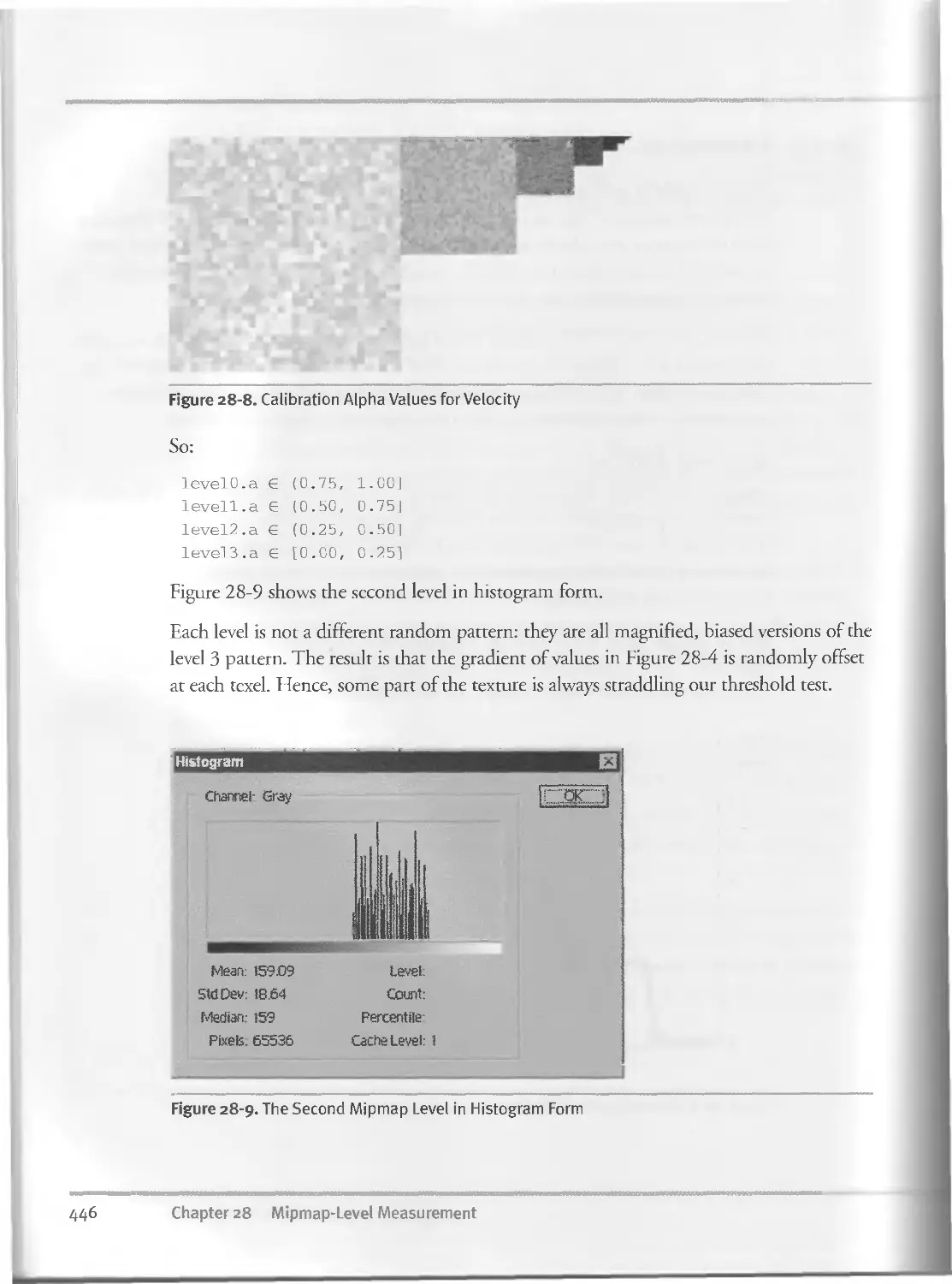
28.5 References............................................... . . 449
Contents xix
PART IV GENERAL-PURPOSE COMPUTATION ON GPUS: A PRIMER 451
Chapter 29
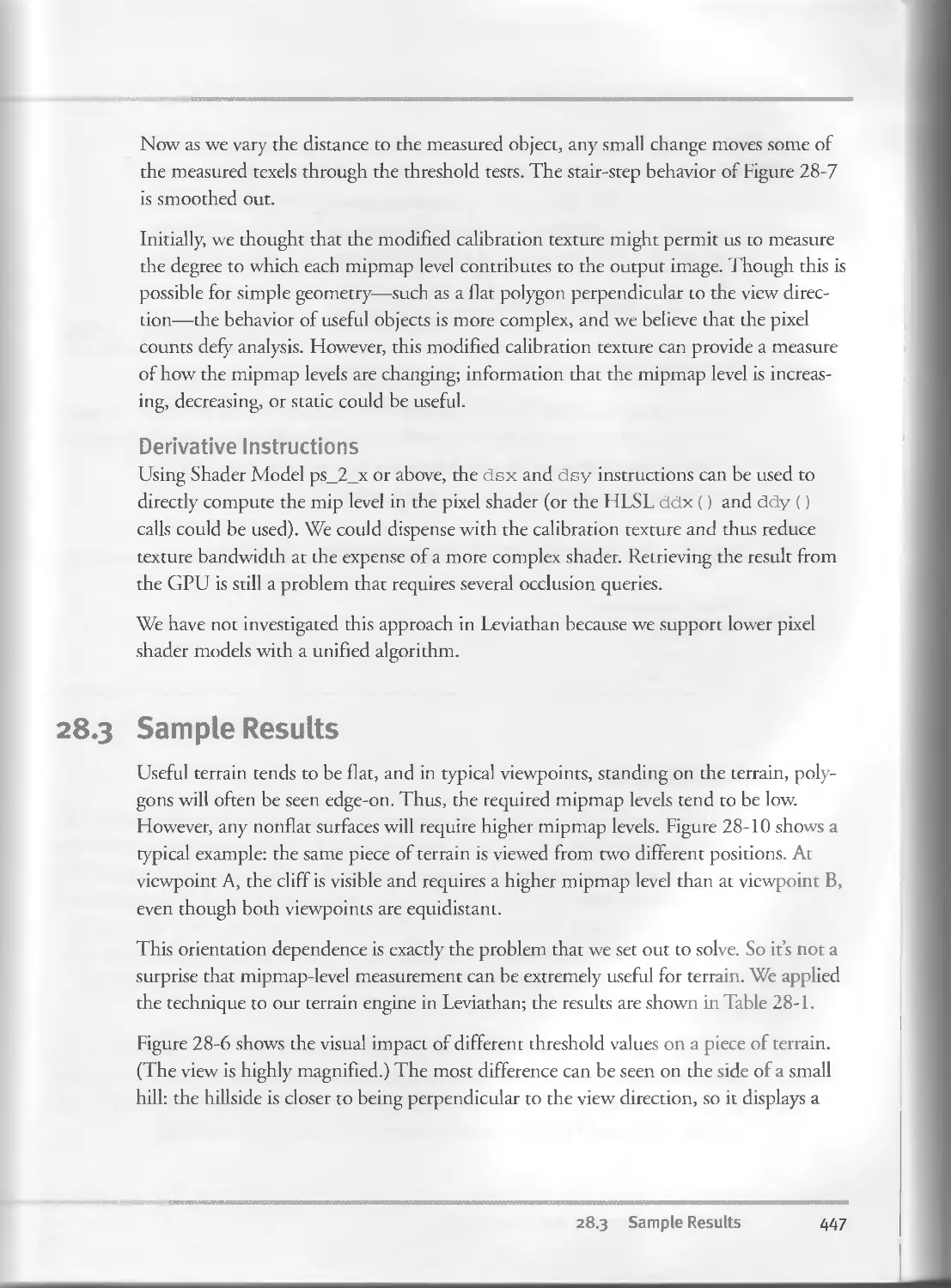
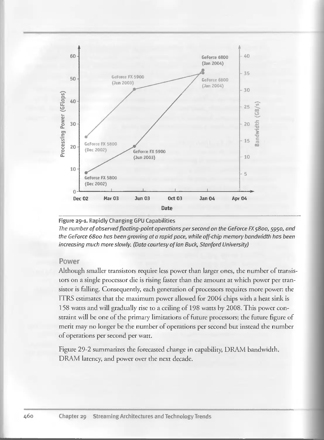
Streaming Architectures and Technology Trends..............................457
John Owens, University of California, Davis
29.1 Technology Trends..........................................457
29.I.I Core Technology Trends.............................458
29.1.2 Consequences.......................................458
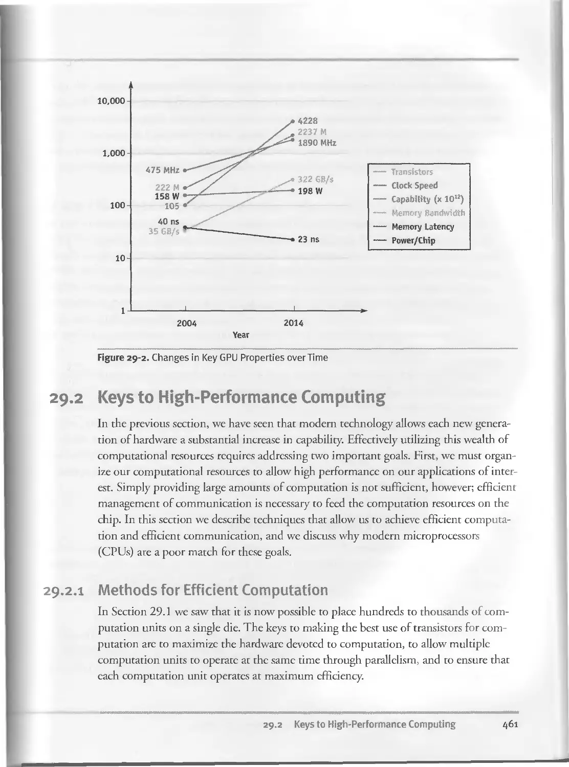
29.2 Keys to High-Performance Computing ........................461
29.2.I Methods for Efficient Computation..................461
29.2.2 Methods for Efficient Communication.............. . 462
29.2.3 Contrast to CPUs....................................463
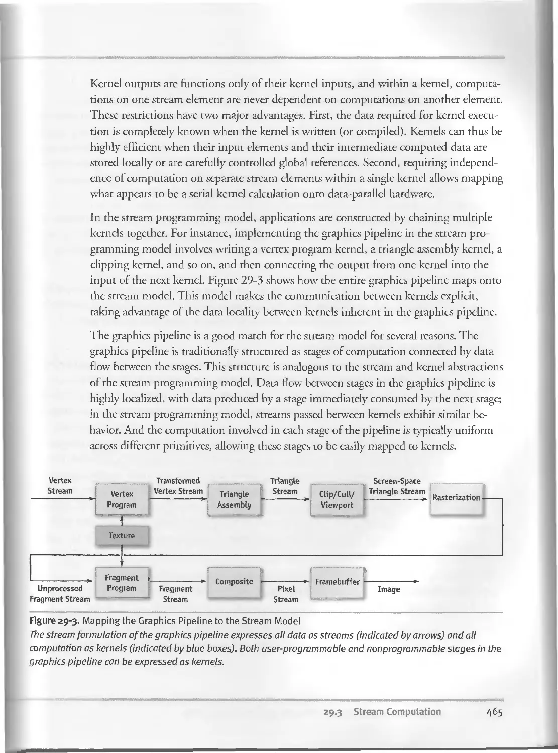
29.3 Stream Computation.........................................464
29.3.I The Stream Programming Model.......................464
29.3.2 Building a Stream Processor........................466
29.4 The Future and Challenges................................ 468
29.4.I Challenge: Technology Trends .......................468
29.4.2 Challenge: Power Management ........................468
29.4.3 Challenge: Supporting More Programmability and
Functionality ............................................469
29.4.4 Challenge: GPU Functionality Subsumed by CPU
(or Vice Versa)?..........................................470
29.5 References.................................................470
Chapter 30
The GeForce 6 Series GPU Architecture......................................471
Emmett Kilgariff, NVIDIA Corporation
Randima Fernando, NVIDIA Corporation
30.1 How the GPU Fits into the Overall Computer System..........471
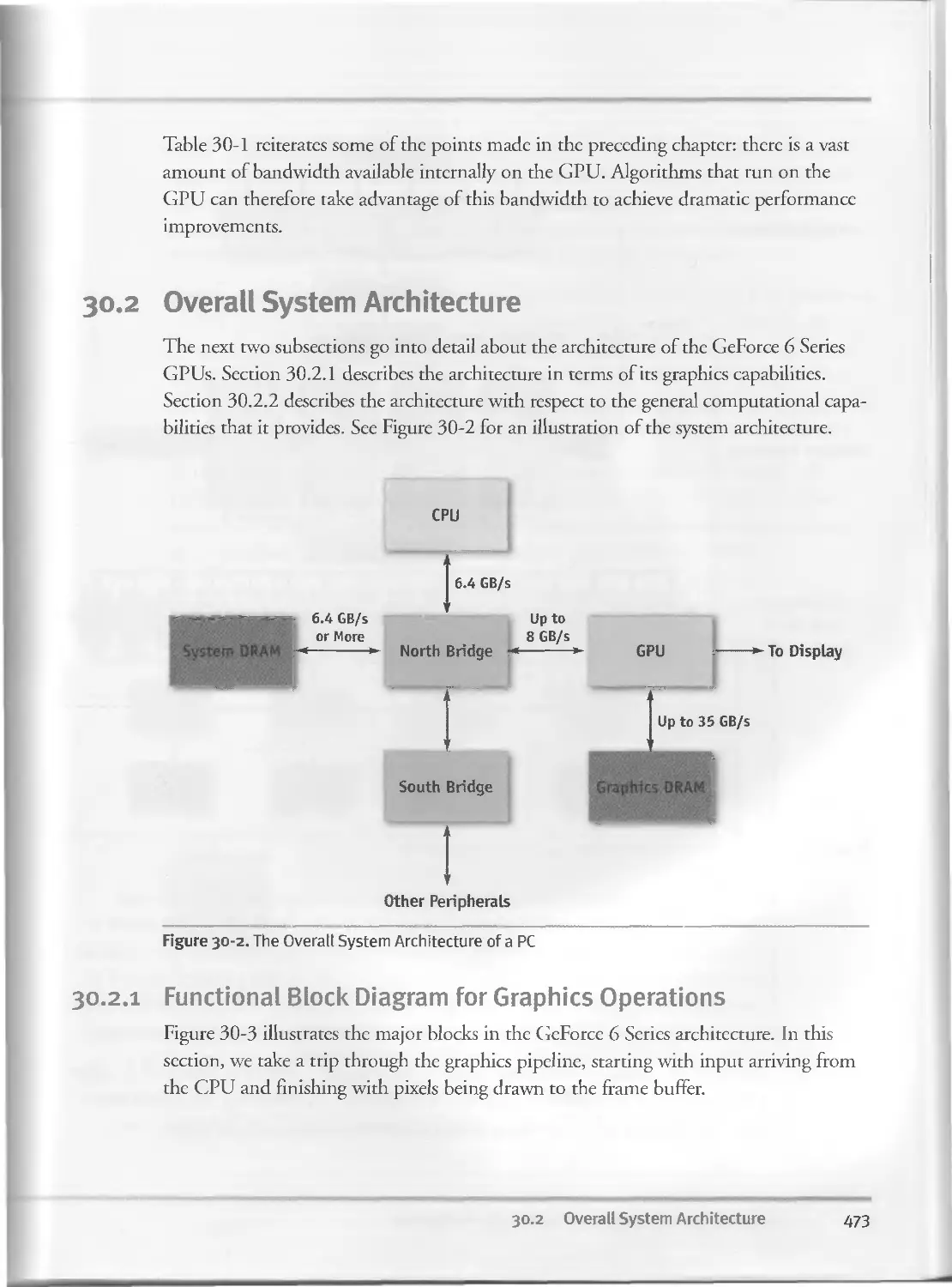
30.2 Overall System Architecture................................473
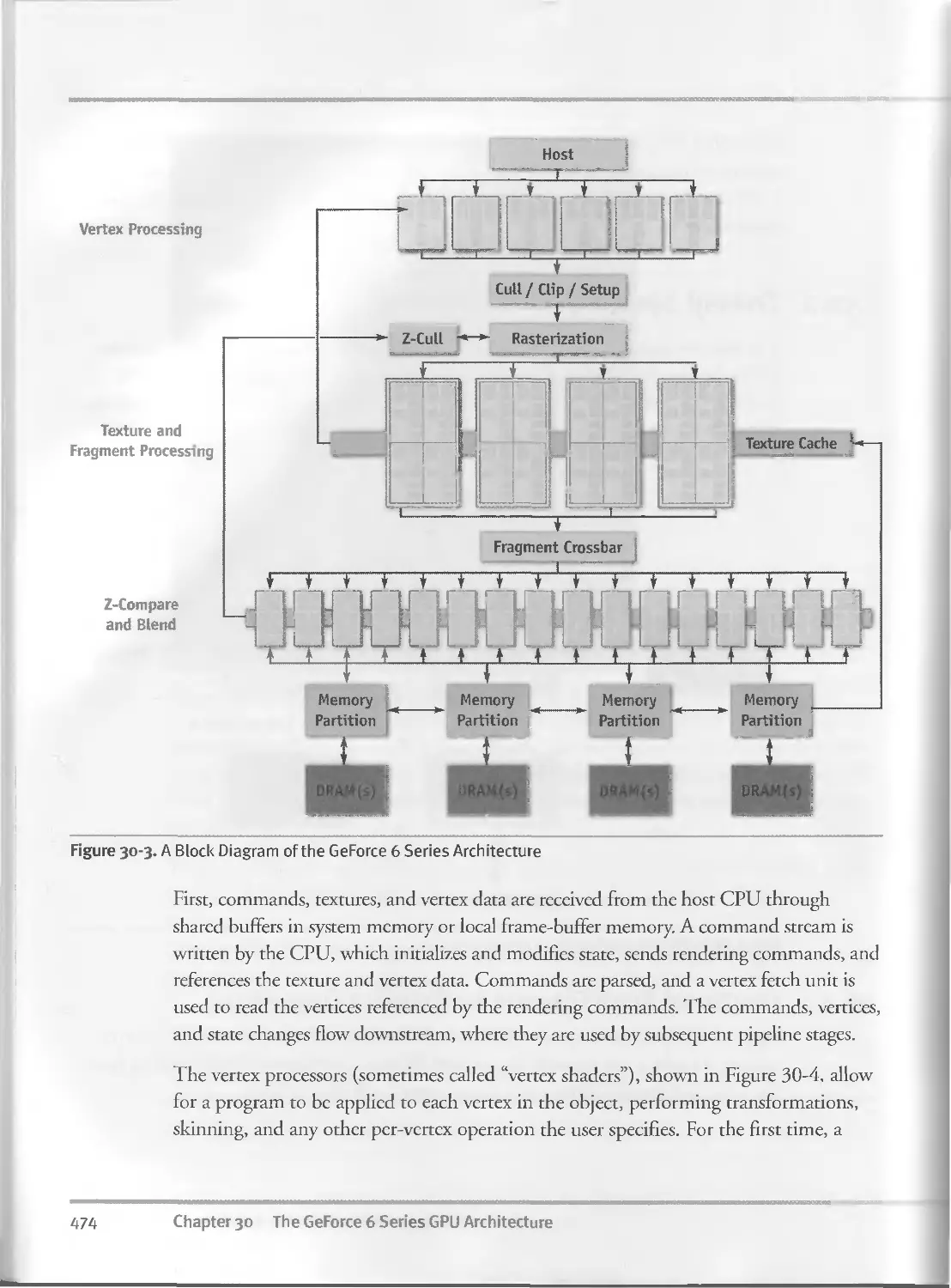
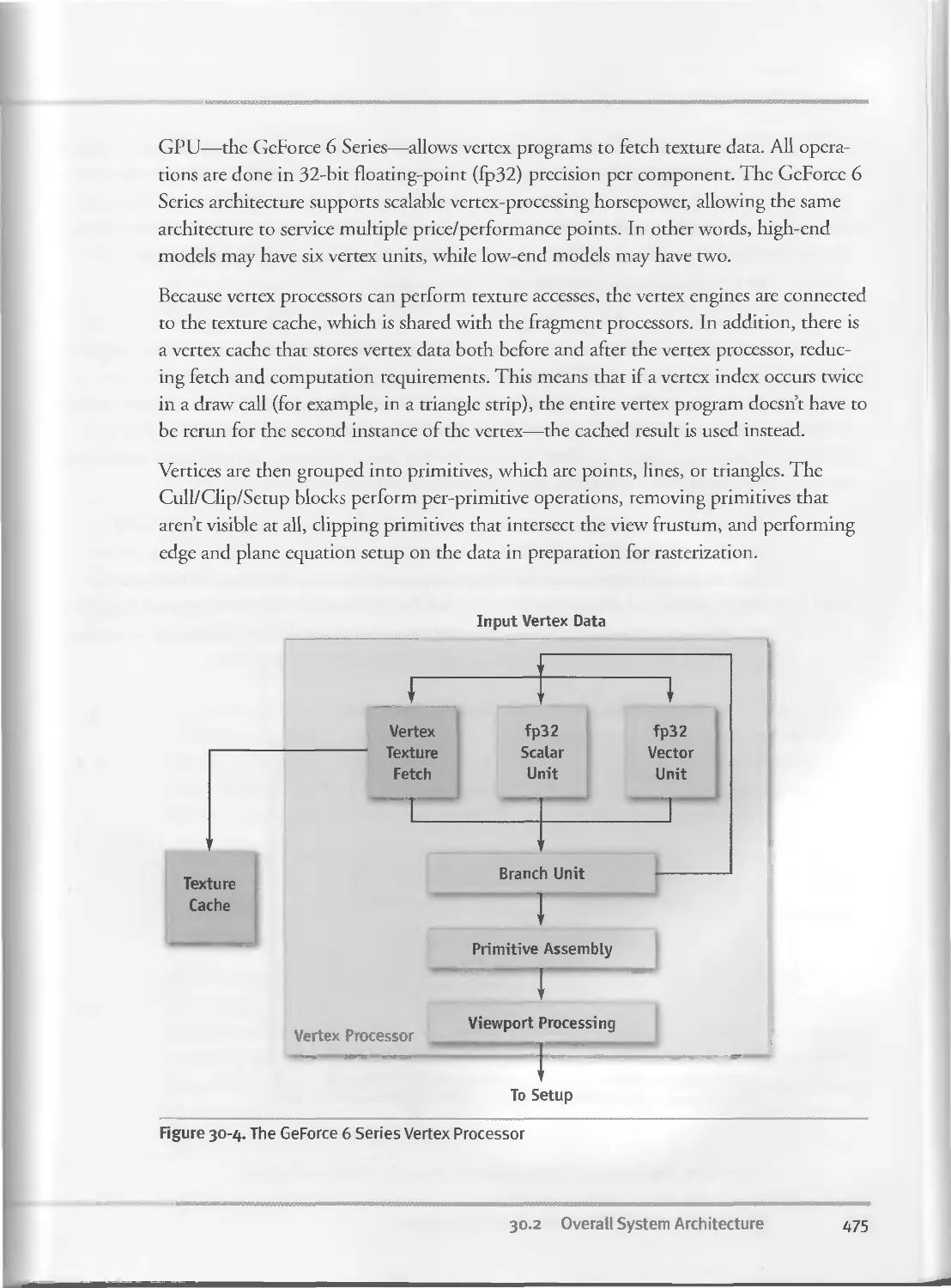
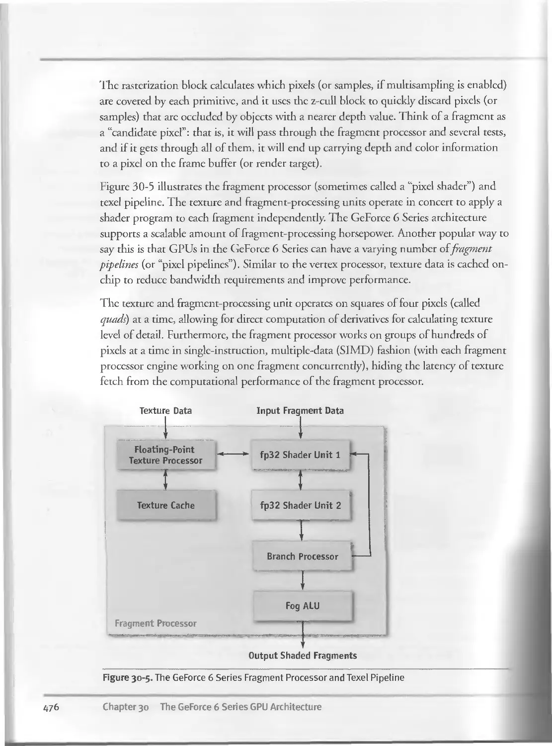
3O.2.I Functional Block Diagram for Graphics Operations...473
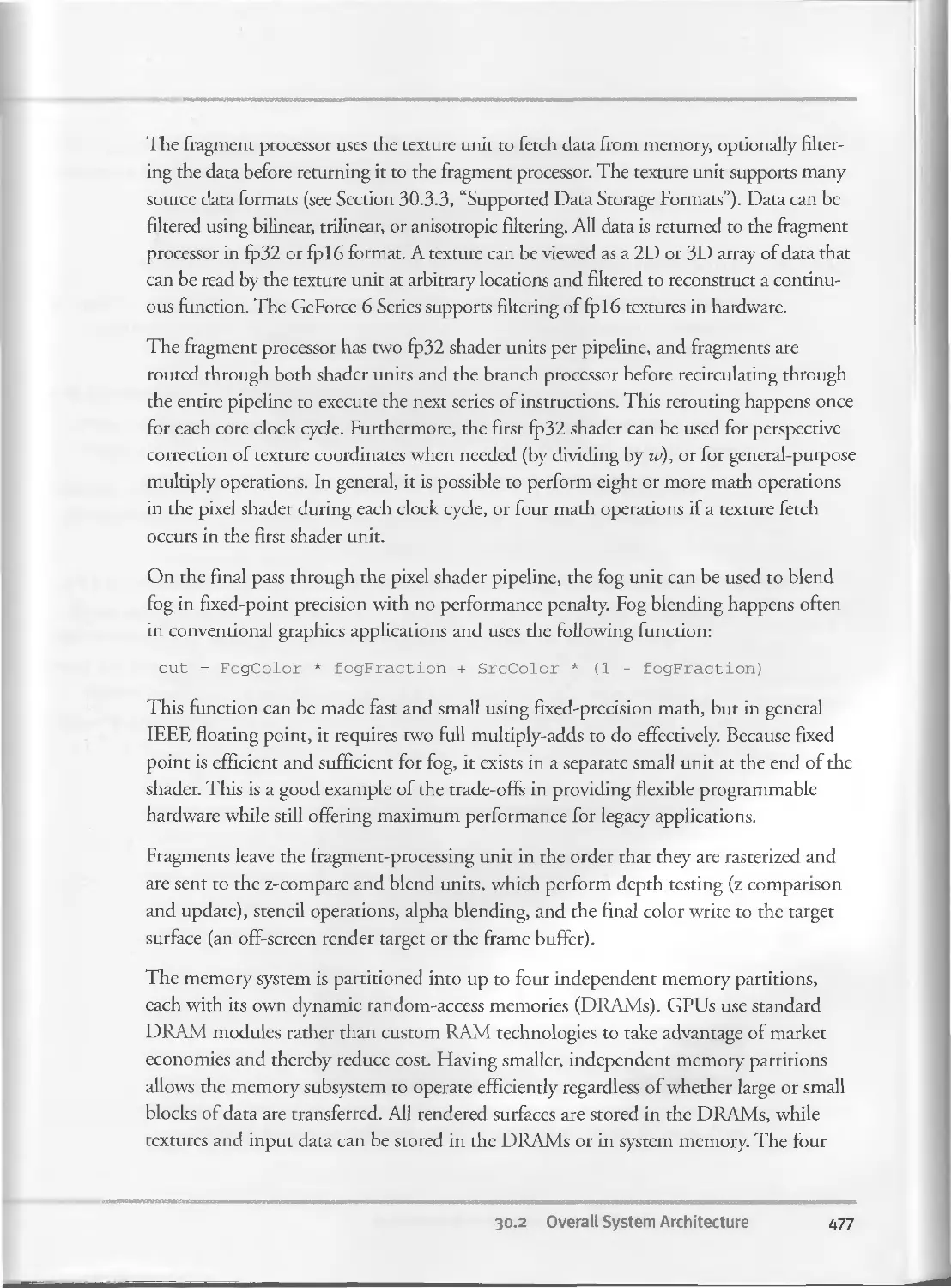
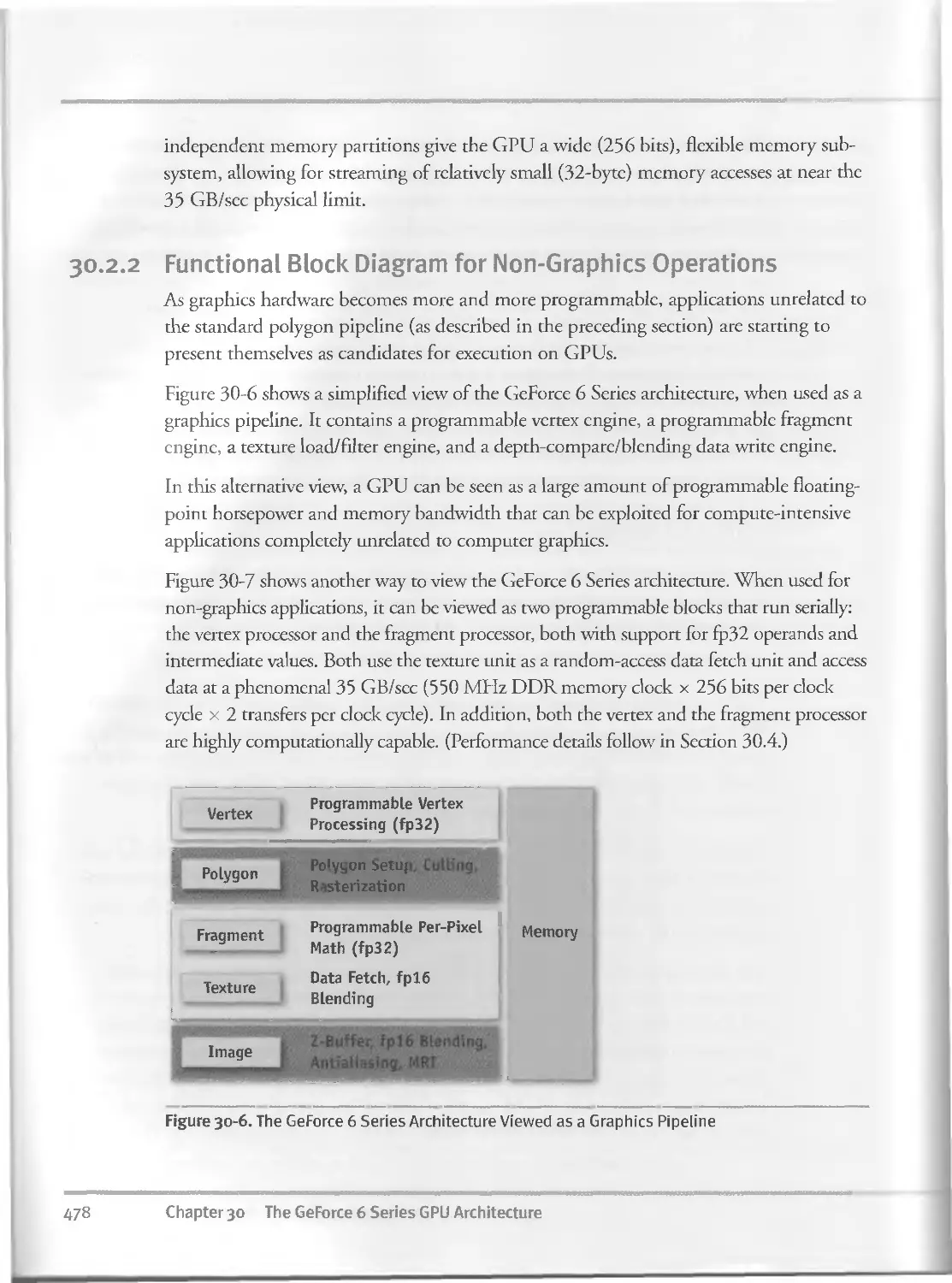
30.2.2 Functional Block Diagram for Non-Graphics Operations . . 478
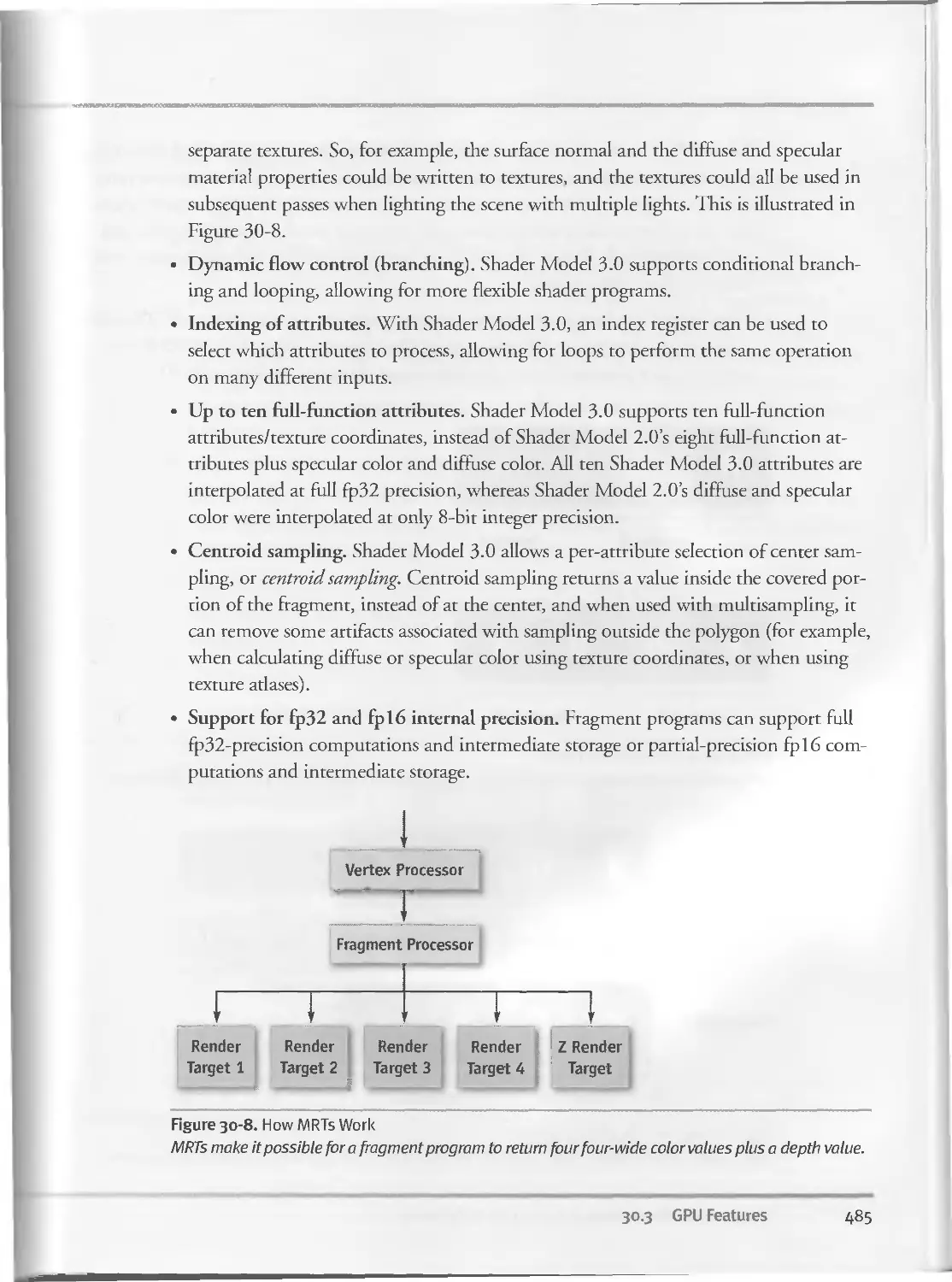
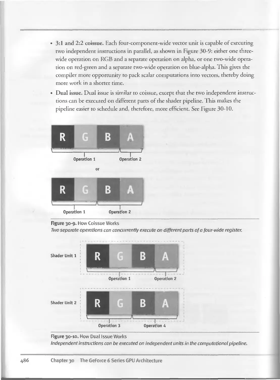
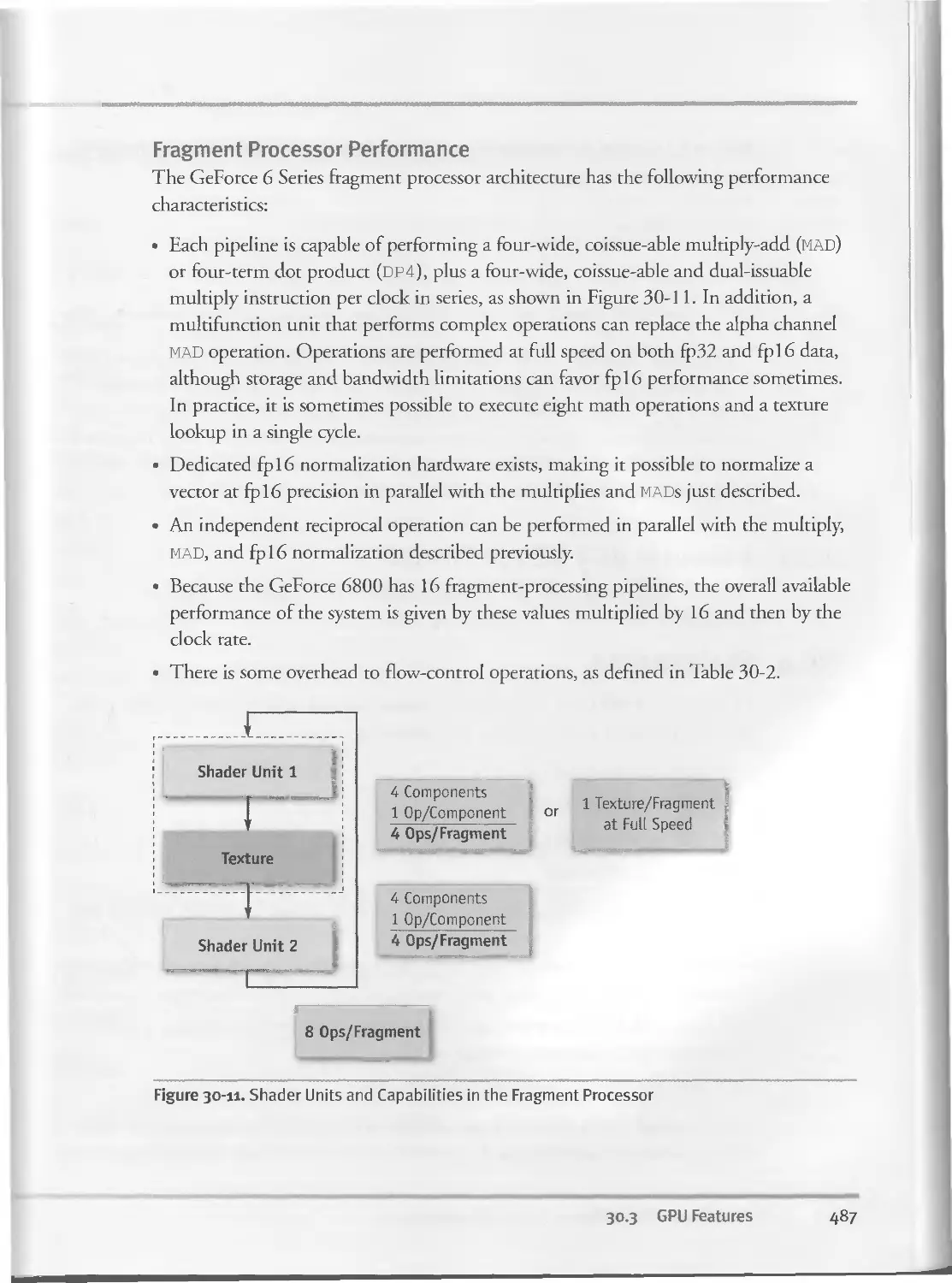
30.3 GPU Features...............................................481
3O.3.I Fixed-Function Features............................481
3O.3.2 Shader Model 3.0 Programming Model.................483
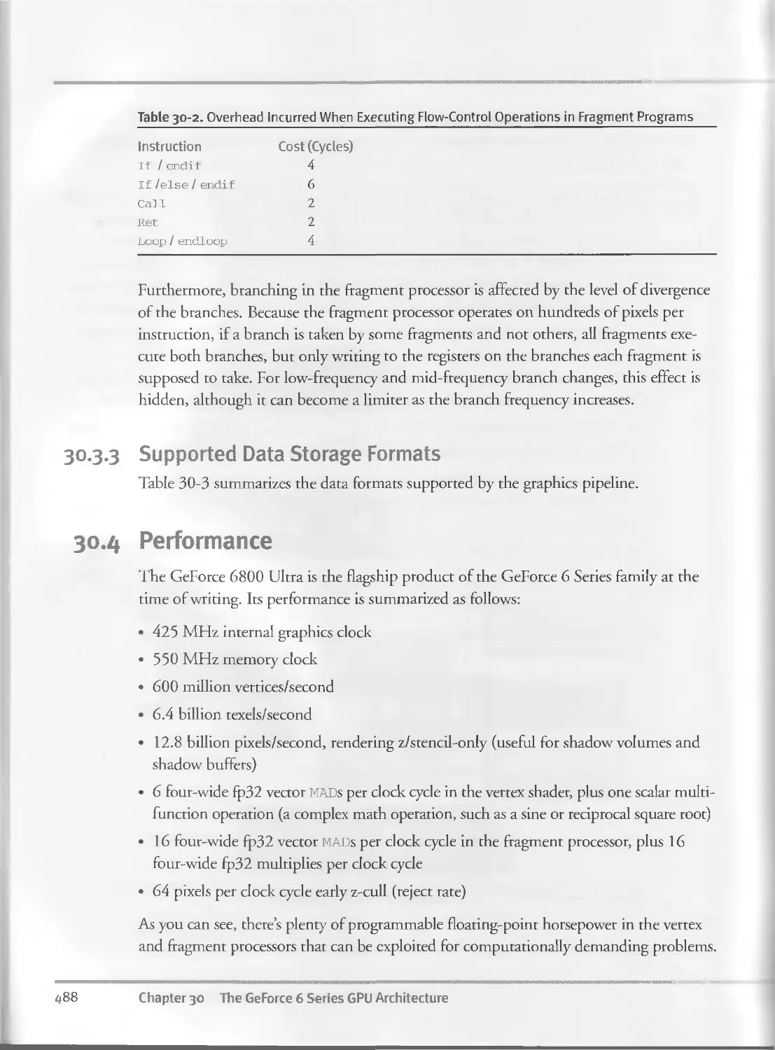
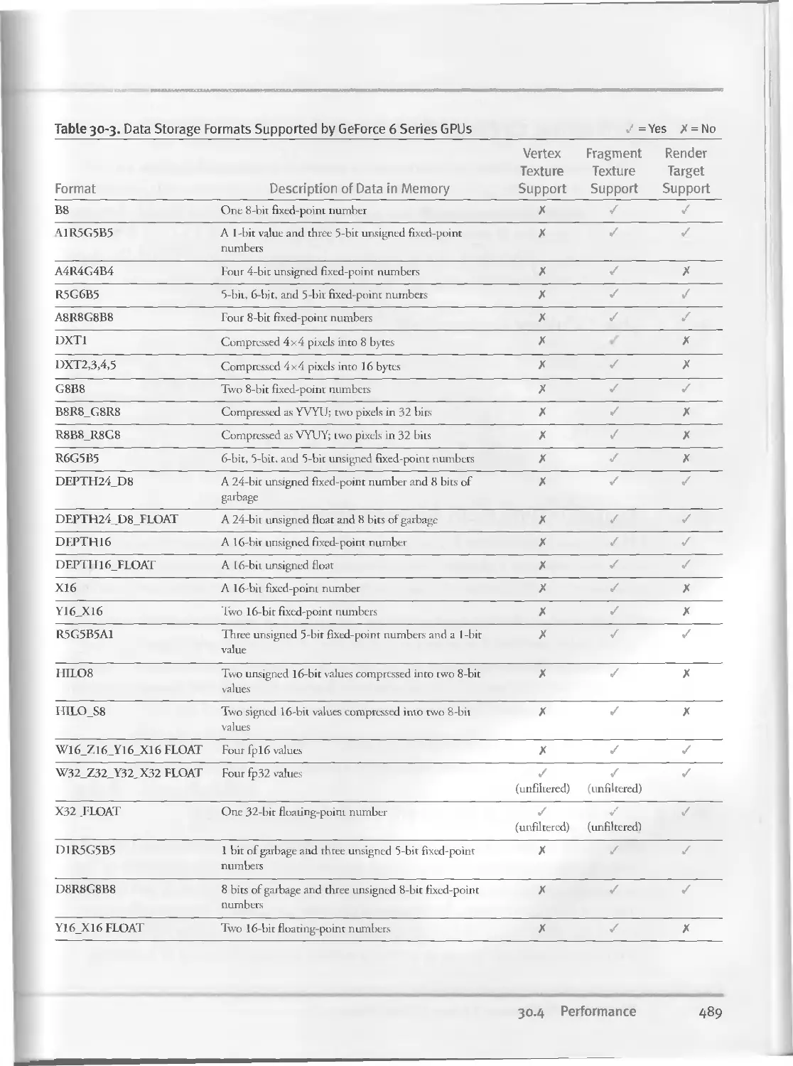
30.3.3 Supported Data Storage Formats.....................488
30.4 Performance............................................ 488
xx
Contents
30-5 Achieving Optimal Performance................................490
30.5.I Use Z-Culling Aggressively...........................490
30.5.2 Exploit Texture Math When Loading Data . ............490
30.5.3 Use Branching in Fragment Programs Judiciously.......490
30.5.4 Use fpl6 Intermediate Values Wherever Possible.......491
30.6 Conclusion...................................................491
Chapter 31
Mapping Computational Concepts to GPUs.......................................493
Mark Harris, NVIDIA Corporation
31.1 The Importance of Data Parallelism...........................493
31.I.I What Kinds of Computation Map Well to GPUs?..........494
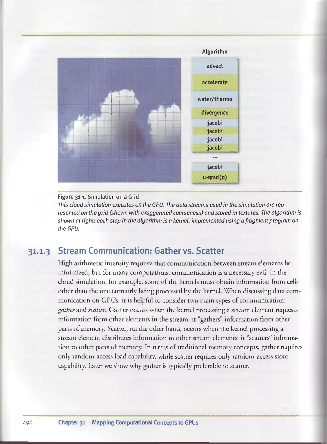
31.I.2 Example: Simulation on a Grid........................495
31.I.3 Stream Communication: Gather vs. Scatter.............496
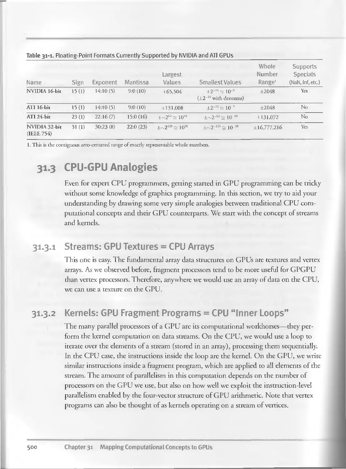
31.2 An Inventory of GPU Computational Resources..... ......497
31.2.1 Programmable Parallel Processors.....................497
31.3 CPU-GPU Analogies......................................... 500
3I.3.I Streams: GPU Textures = CPU Arrays...................500
31.3.2 Kernels: GPU Fragment Programs = CPU “Inner Loops”. . 500
31.3.3 Render-to-Texture = Feedback.........................501
31.3.4 Geometry Rasterization = Computation Invocation......501
31.3.5 Texture Coordinates = Computational Domain...........501
31.3.6 Vertex Coordinates = Computational Range.............502
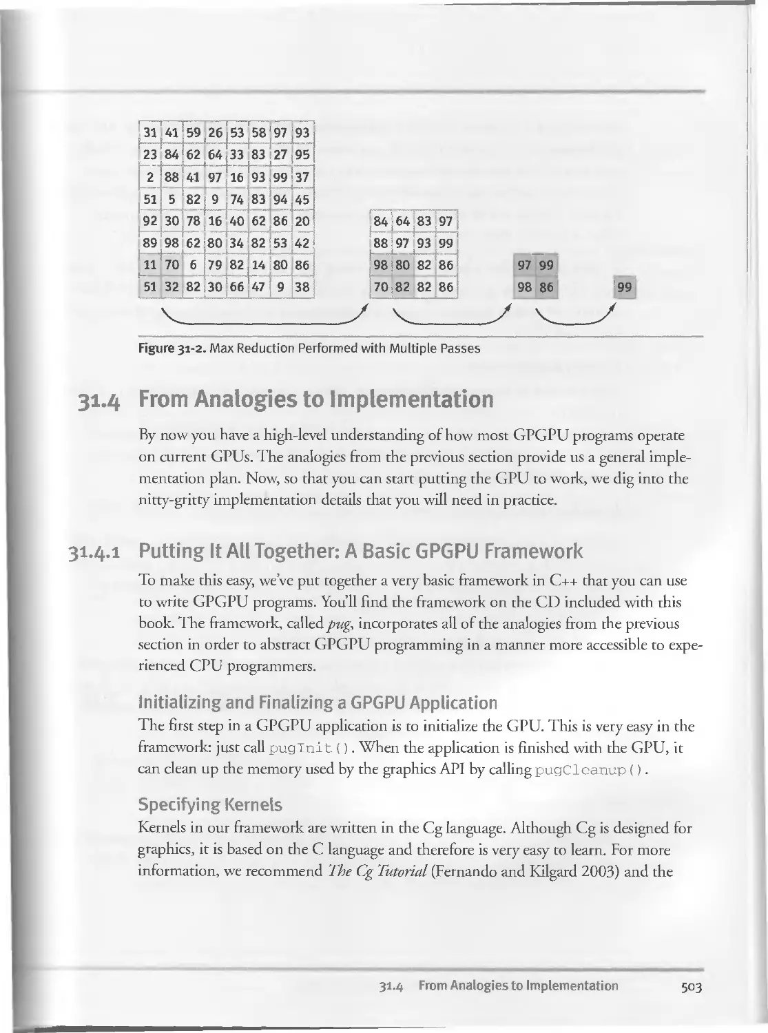
31.3.7 Reductions...........................................502
31.4 From Analogies to Implementation............................503
31.4.I Putting It All Together: A Basic GPGPU Framework.....503
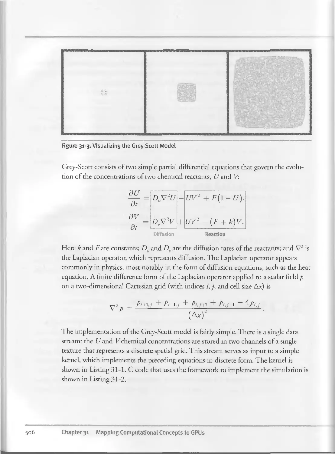
31.5 A Simple Example. . .................................... ... 505
31.6 Conclusion..................................................5°8
31.7 References..................................................508
Chapter 32
Taking the Plunge into GPU Computing.........................................509
Ian Buck, Stanford University
32.1 Choosing a Fast Algorithm................................. • 5°9
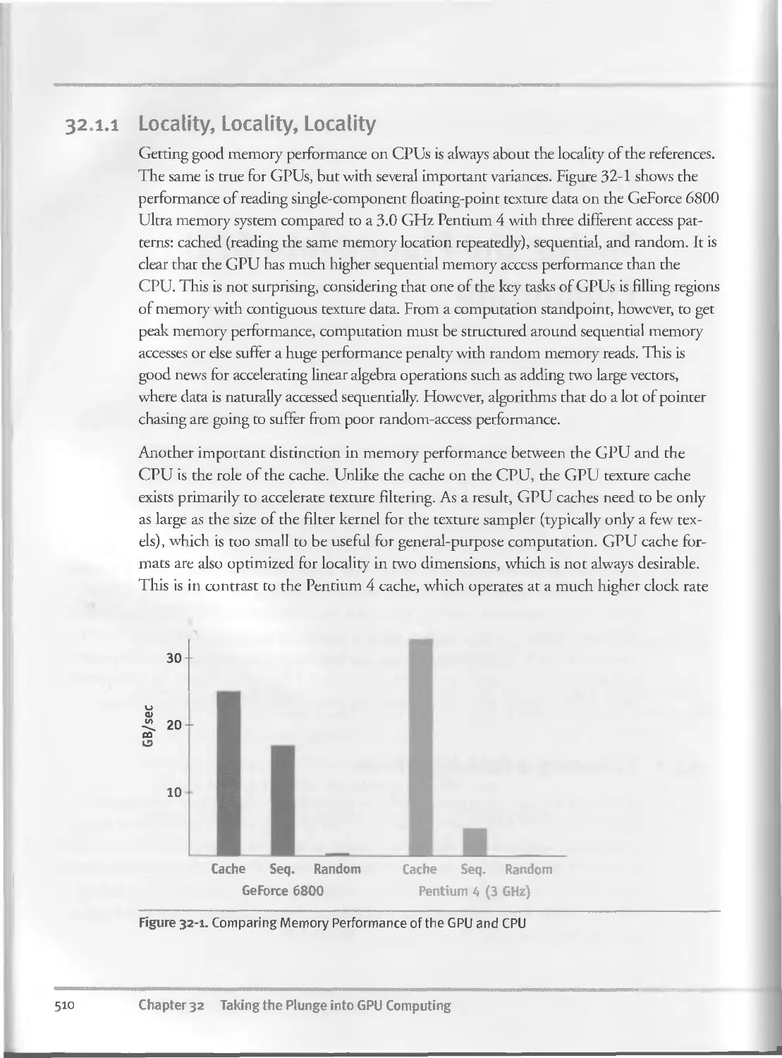
32.I.I Locality, Locality, Locality........................ 510
32.I.2 Letting Computation Rule......... . 511
32.1.3 Considering Download and Readback. . . . 512
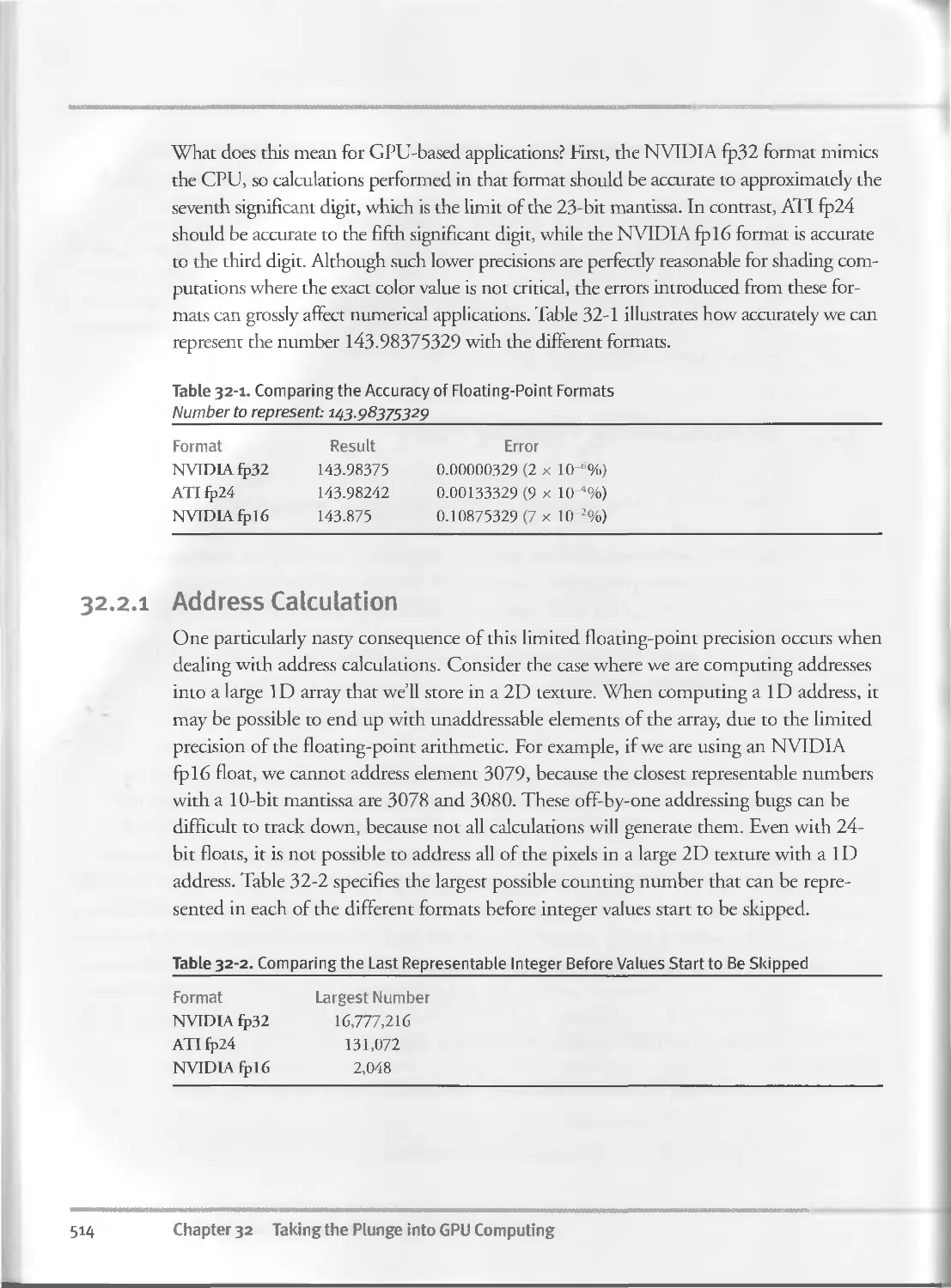
32.2 Understanding Floating Point.............................. . 513
32.2.I Address Calculation . . 514
V.TJWI
Contents
xxi
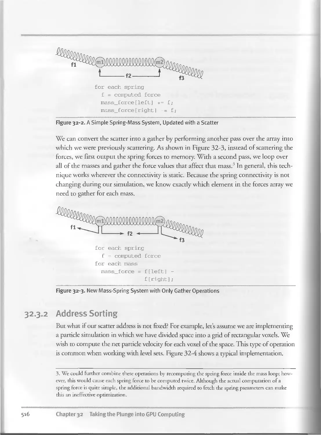
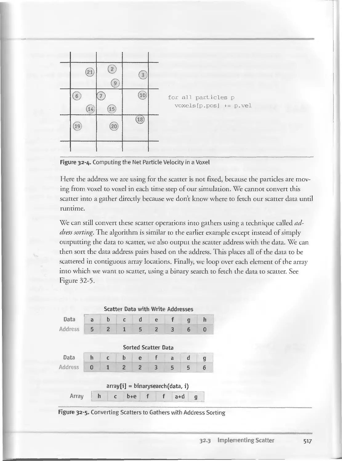
32.3 Implementing Scatter........................................515
32.3.I Converting to Gather.................................515
32.3.2 Address Sorting ... ......... ............. .... 516
32.3.3 Rendering Points.....................................518
32.4 Conclusion..................................................518
32.5 References..................................................519
Chapter 33
Implementing Efficient Parallel Data Structures on GPUs....................521
Aaron Lefohn, University of California, Davis
Joe Kniss, University of Utah
John Owens, University of California, Davis
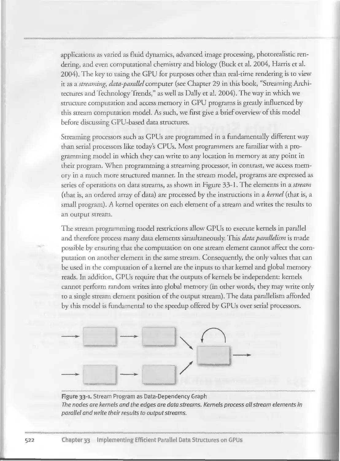
33.I Programming with Streams.....................................521
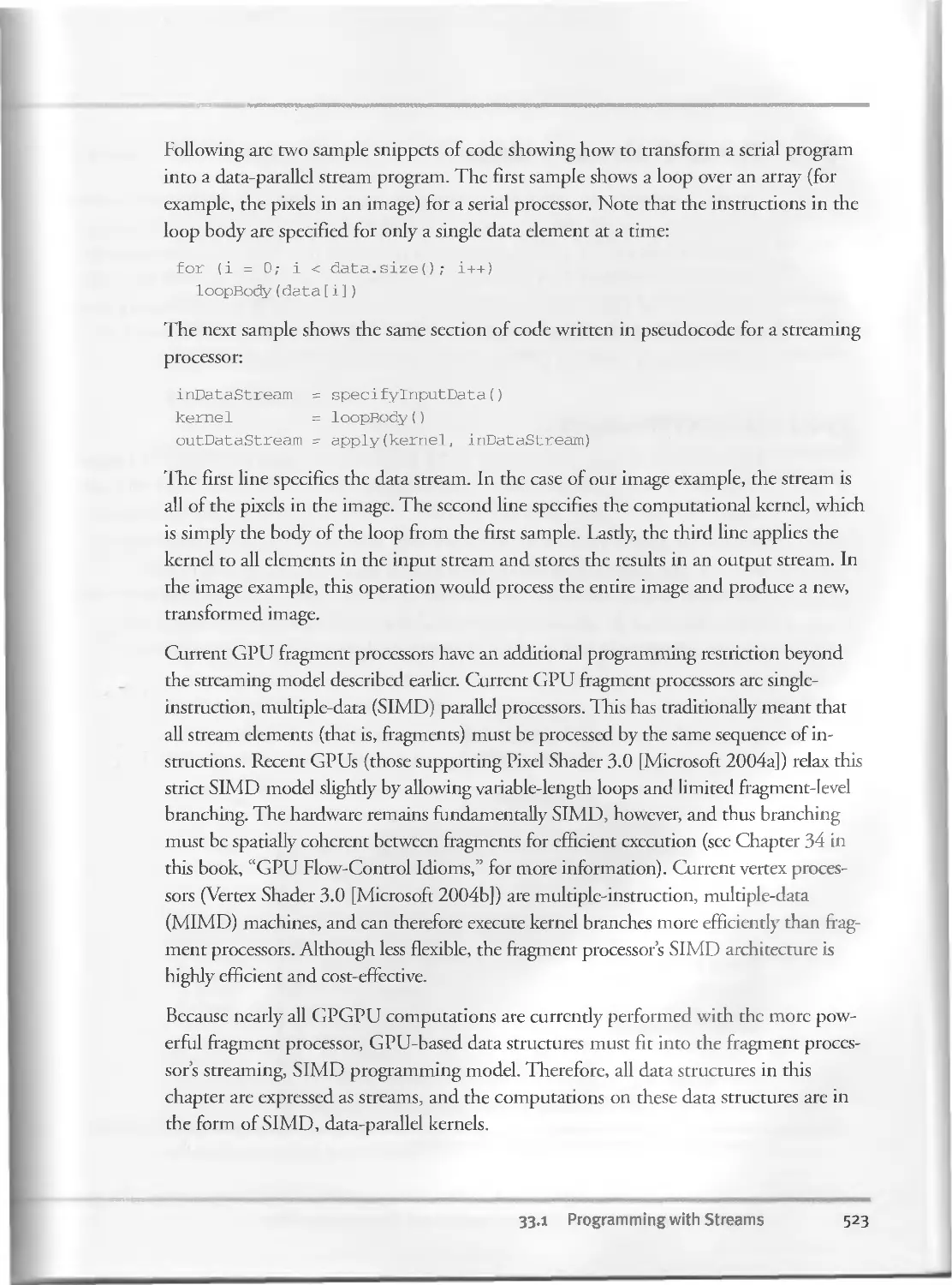
33.2 The GPU Memory Model........................................524
33-2.1 Memory Hierarchy.....................................524
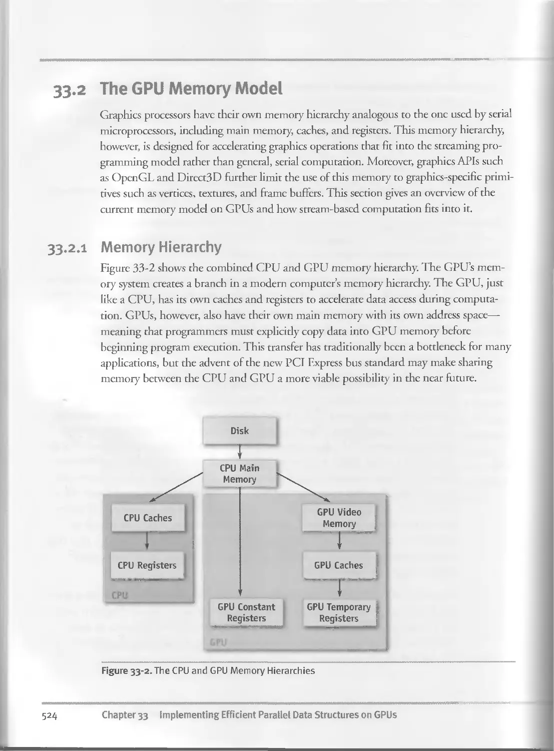
33-2.2 GPU Stream Types.....................................525
33.2.3 GPU Kernel Memory Access.............................527
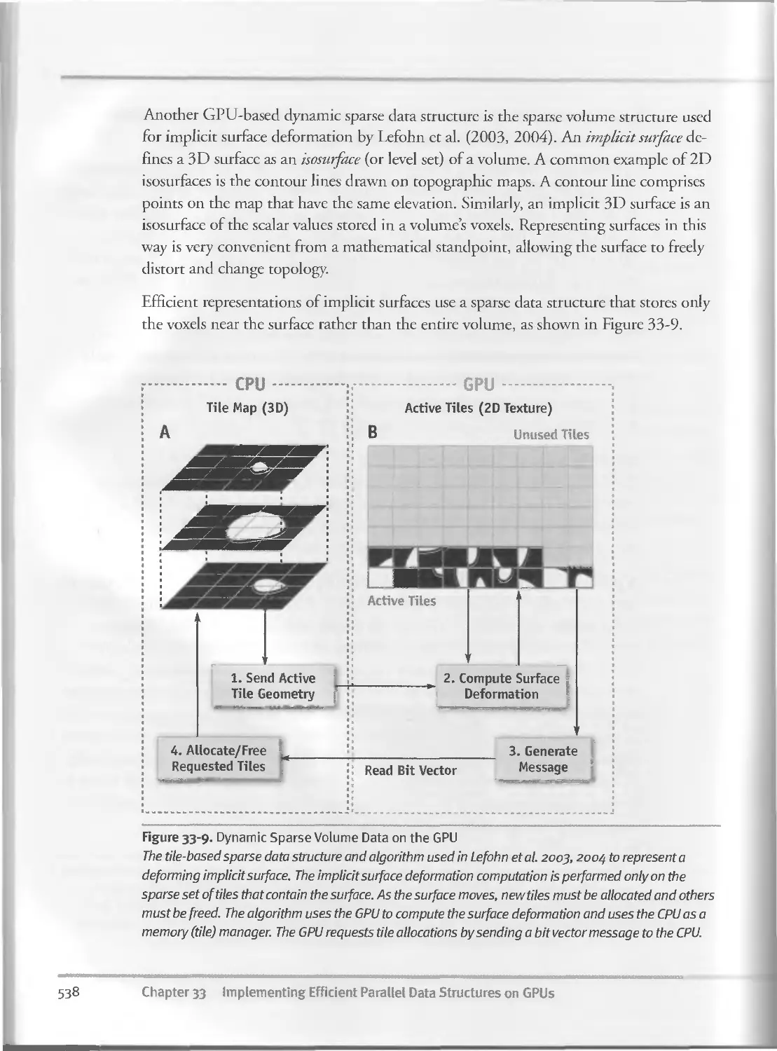
33-3 GPU-Based Data Structures.....................................528
33.3.1 Multidimensional Arrays..............................528
33.3.2 Structures...........................................534
33-3-3 Sparse Data Structures...............................535
33-4 Performance Considerations....... .............. ... 540
33-4-1 Dependent Texture Reads..............................540
33.4.2 Computational Frequency..............................541
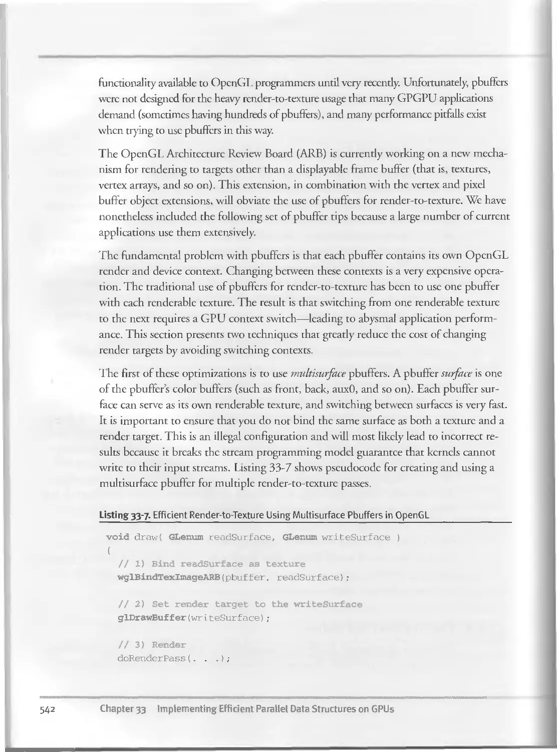
33.4.3 Pbuffer Survival Guide...............................541
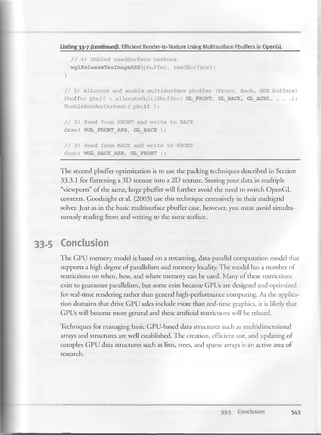
33-5 Conclusion....................................................543
33-6 References....................................................544
Chapter 34
GPU Flow-Control Idioms.....................................................547
Mark Harris, NVIDIA Corporation
lan Buck, Stanford University
34.1 Flow-Control Challenges......................................547
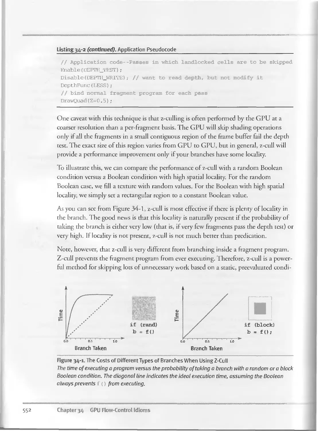
34.2 Basic Flow-Control Strategies...............................549
34.2.1 Predication..........................................549
34.2.2 Moving Branching up the Pipeline.....................549
34.2.3 Z-Cull.............................................. 550
34.2.4 Branching Instructions...............................553
34.2.5 Choosing a Branching Mechanism.......................553
34.3 Data-Dependent Looping with Occlusion Queries...............554
34.4 Conclusion..................................................555
xxii Contents
Chapter 35
GPU Program Optimization..................................................557
Cliff Woolley, University of Virginia
35.1 Data-Parallel Computing...................................557
35.I.I Instruction-Level Parallelism.....................558
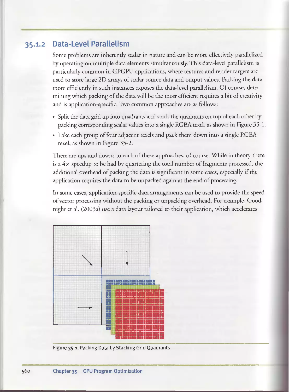
35-1-2 Data-Level Parallelism............................560
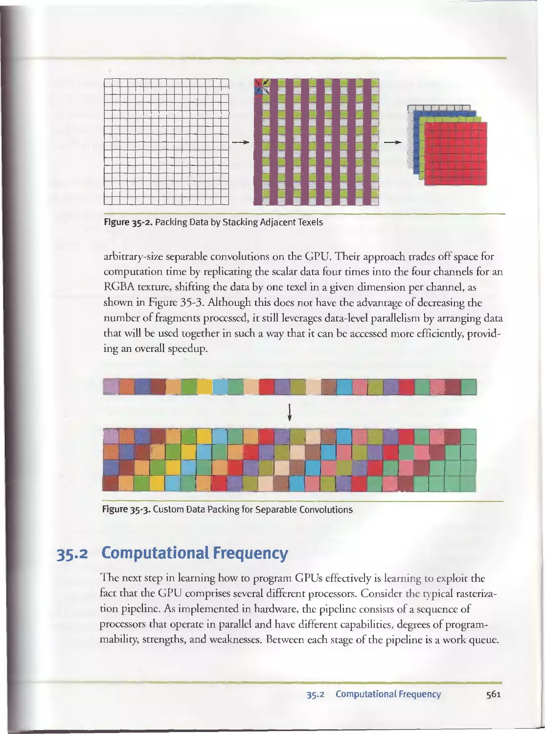
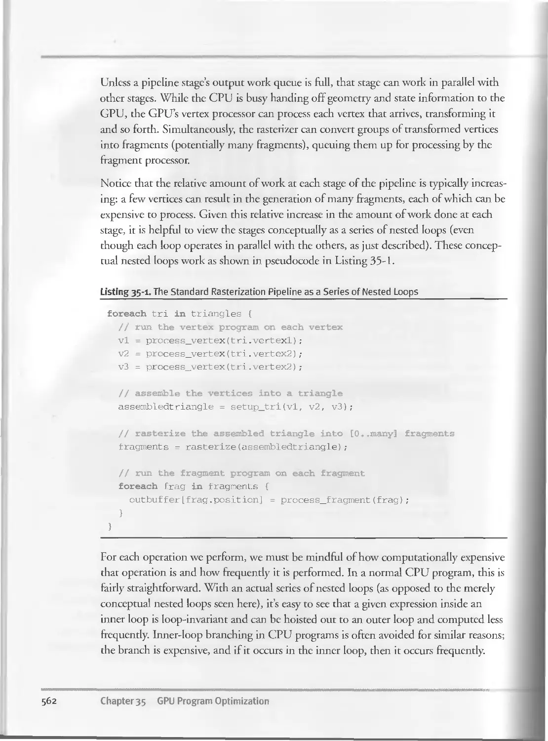
35-2 Computational Frequency...................................561
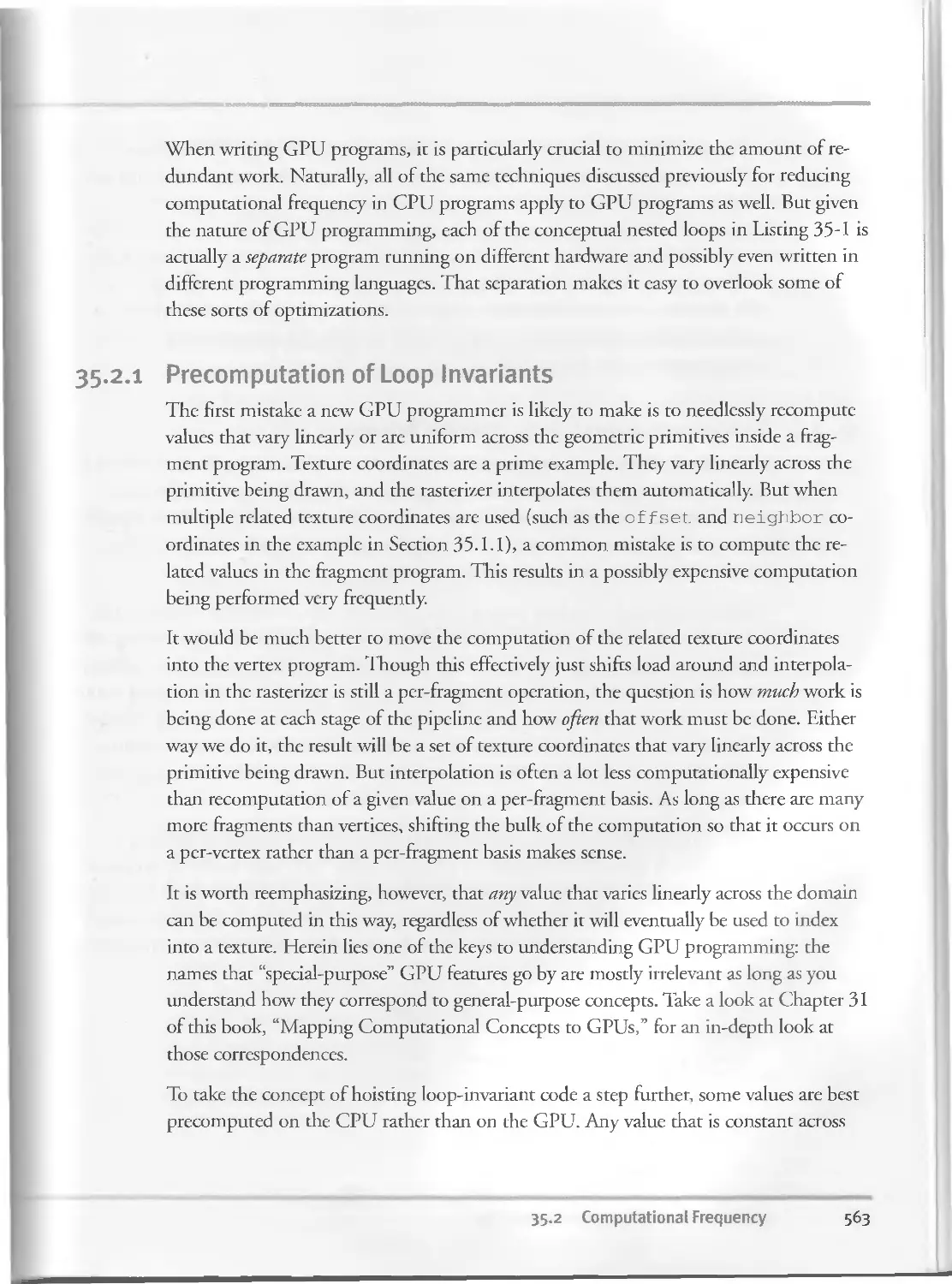
35-2.1 Precomputation of Loop Invariants.................563
35.2.2 Precomputation Using Lookup Tables................564
35.2.3 Avoid Inner-Loop Branching........................566
35.2.4 The Swizzle Operator..............................566
35-3 Profiling and Load Balancing ........................... 568
35-4 Conclusion................................................570
35-5 References................................................570
Chapter 36
Stream Reduction Operations for GPGPU Applications........................573
Daniel Horn, Stanford University
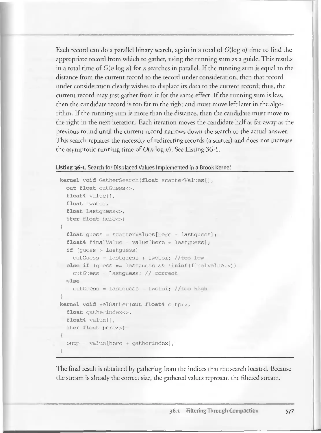
36.1 Filtering Through Compaction..............................574
36.I.I Running Sum Scan..................................574
36.1.2 Scatter Through Search/Gather.....................575
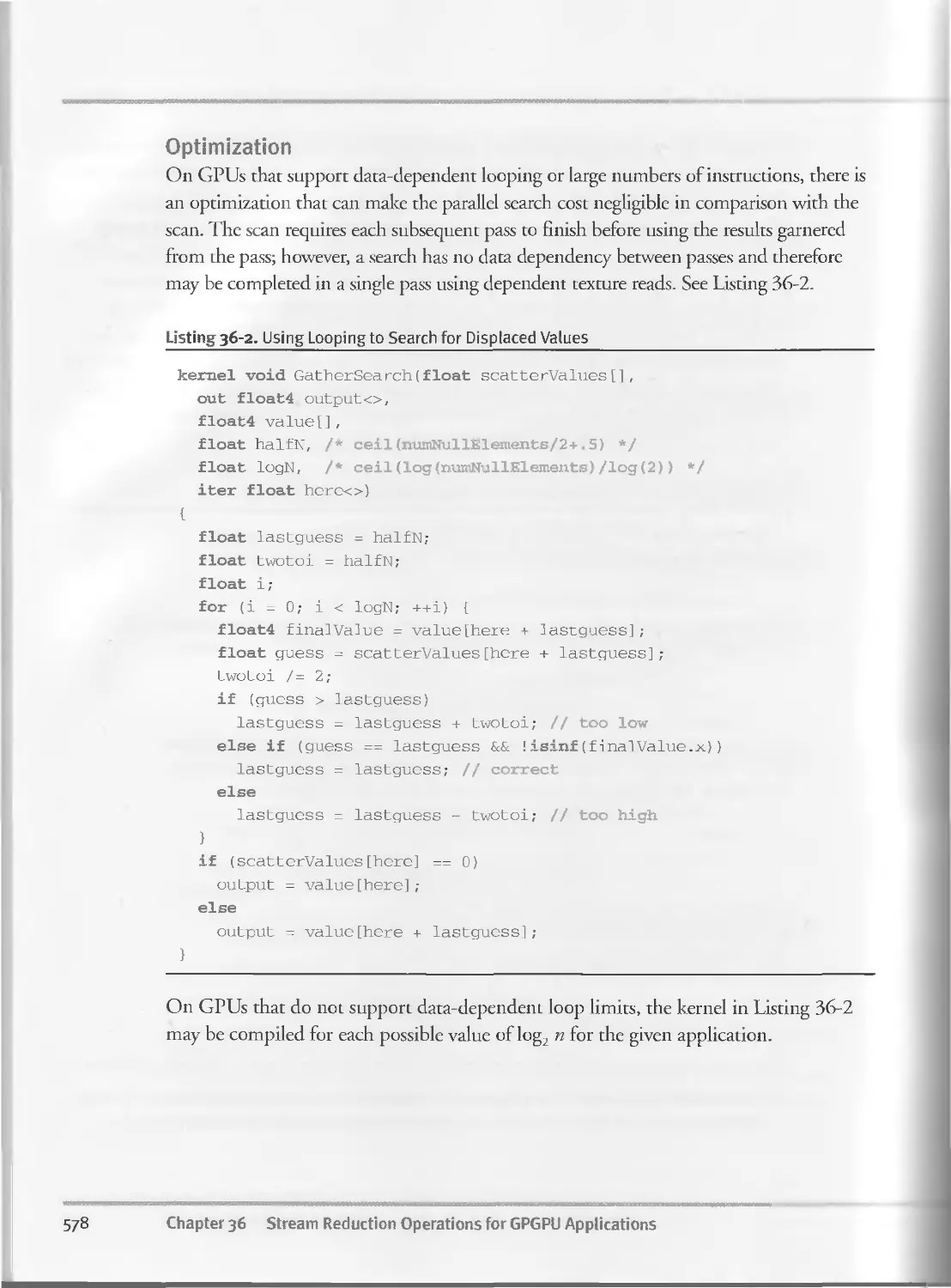
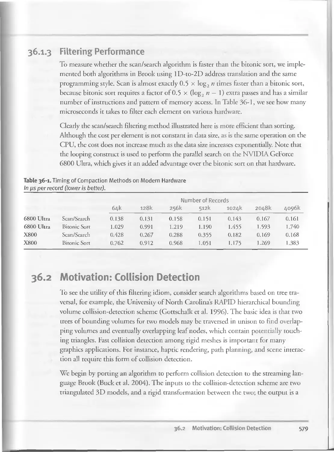
36.I.3 Filtering Performance.............................579
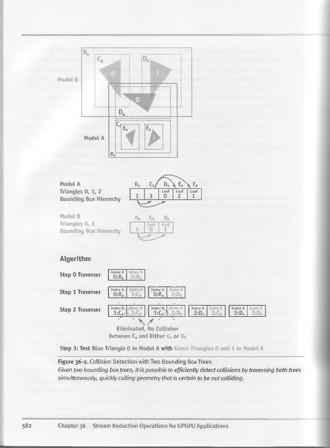
36.2 Motivation: Collision Detection...........................579
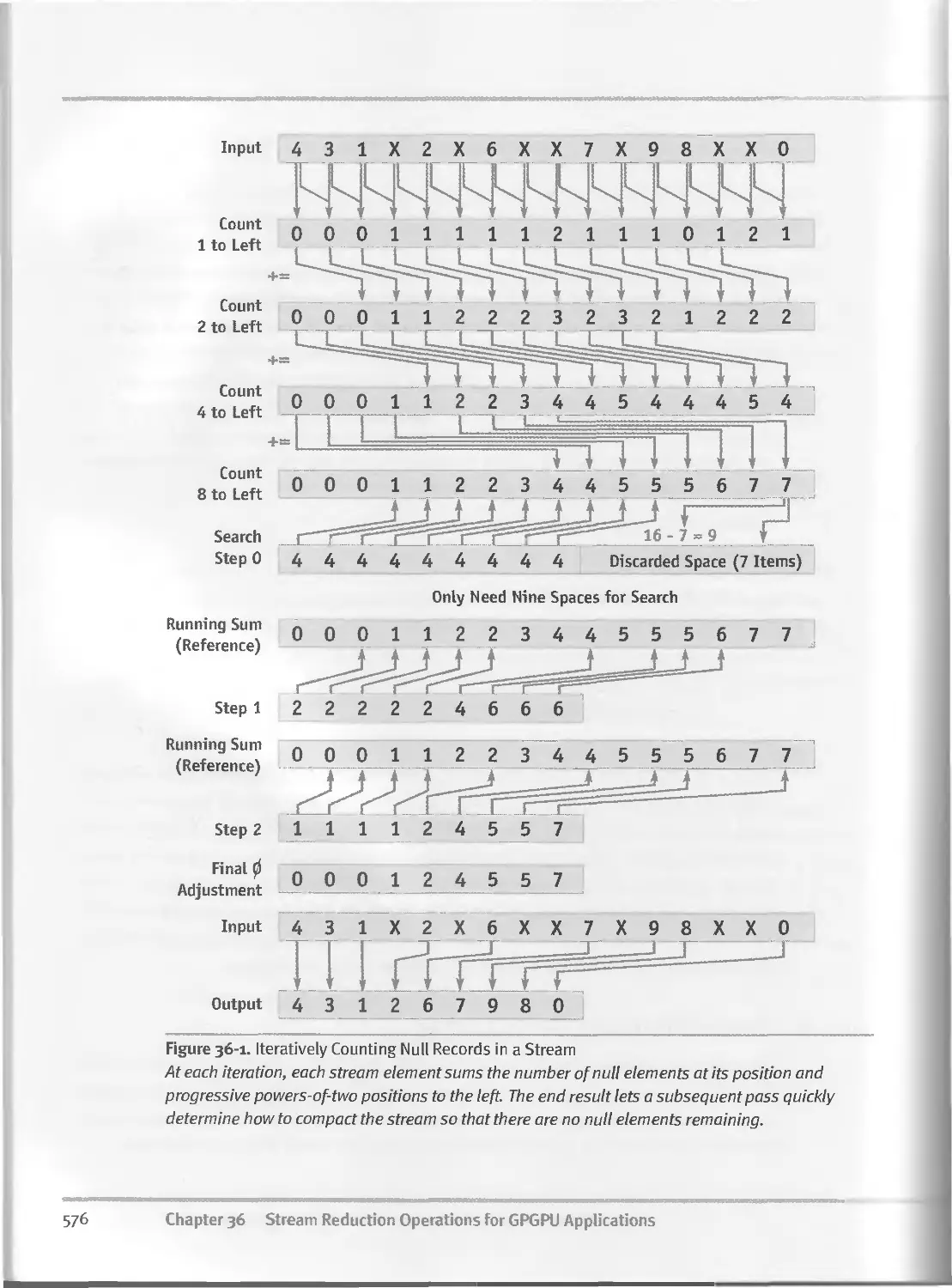
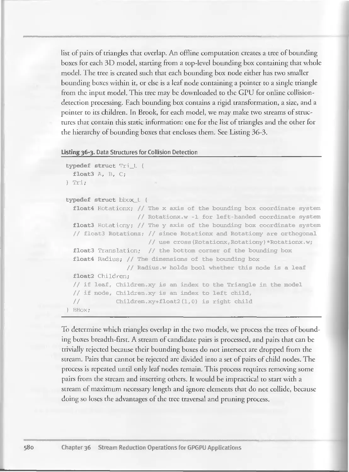
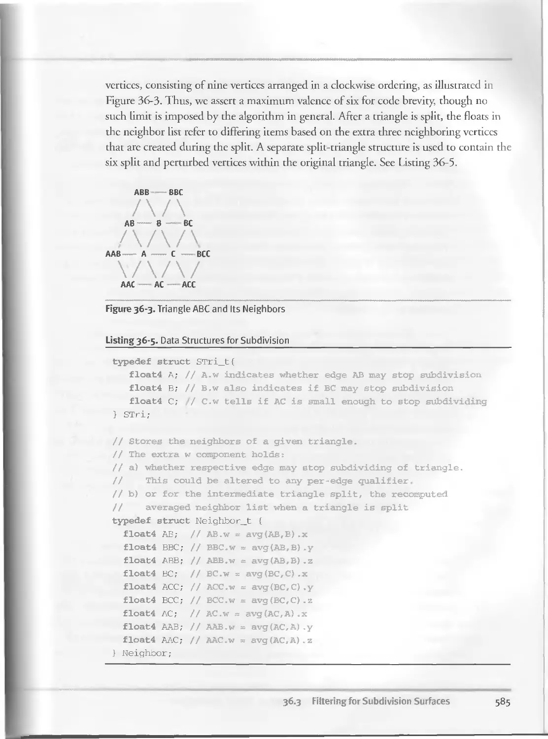
36.3 Filtering for Subdivision Surfaces........................583
36.3.I Subdivision on Streaming Architectures. ........ 584
36.4 Conclusion.............................................. 587
36.5 References............................................... 587
PARTV IMAGE-ORIENTED COMPUTING 591
Chapter 37
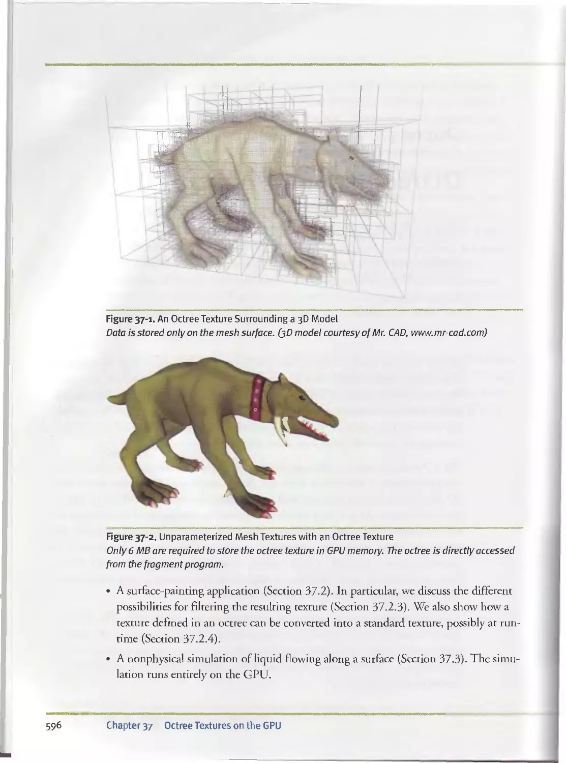
Octree Textures on the GPU...............................................595
Sylvain Lefebvre, GRAVIR/IMAG - INRIA
Samuel Hornus, GRAVIR/IMAG - INRIA
Fabrice Neyret, GRAVIR/IMAG - INRIA
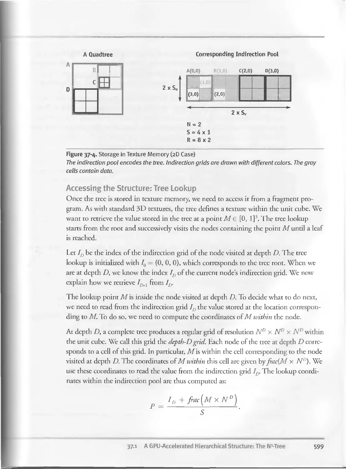
37.1 A GPU-Accelerated Hierarchical Structure: The N3-Tree. ...597
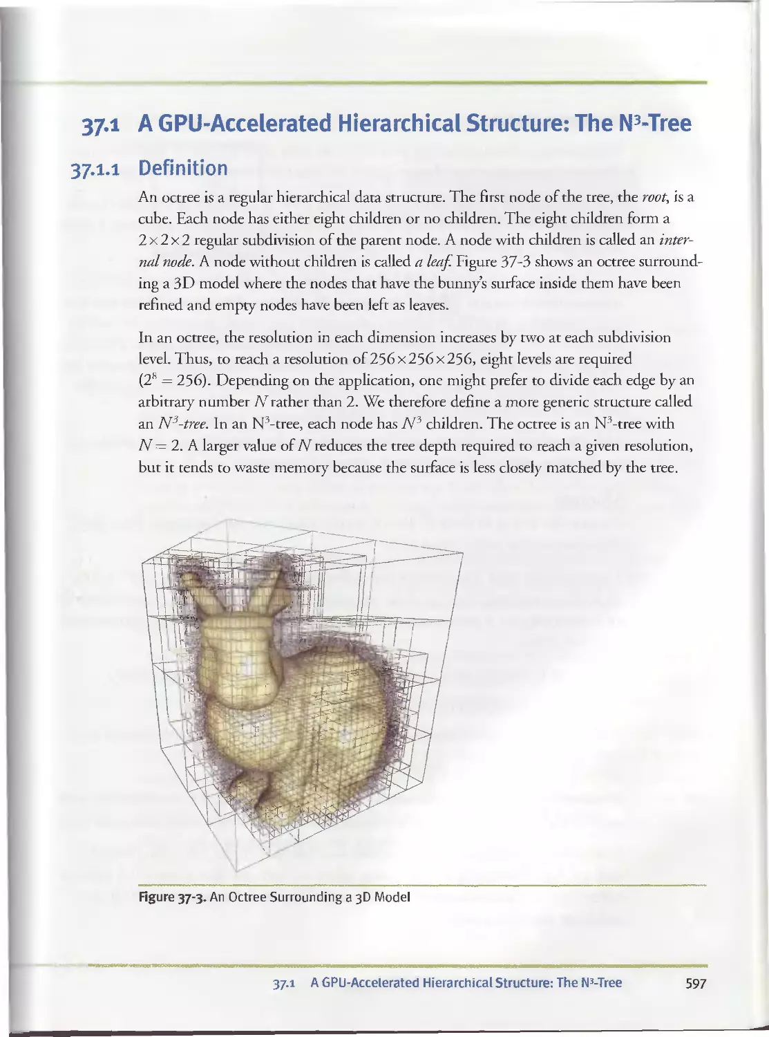
37.1.1 Definition........................................597
37.1.2 Implementation....................................598
maw
Contents
xxiii
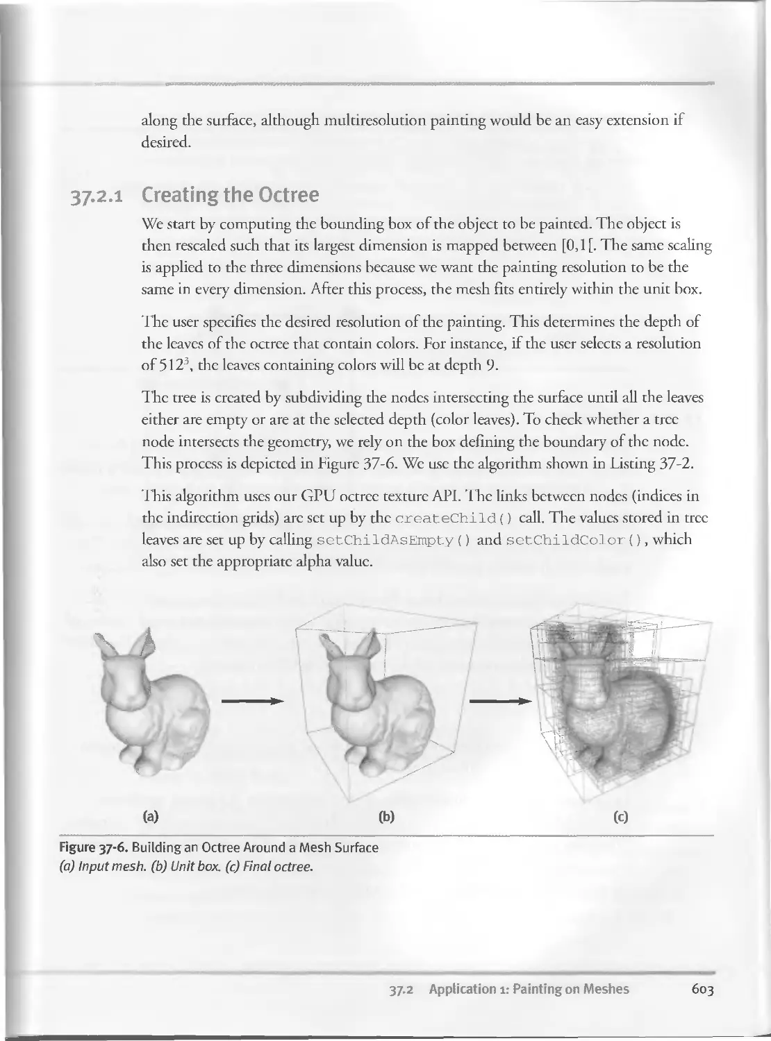
37-2 Application 1: Painting on Meshes..............................602
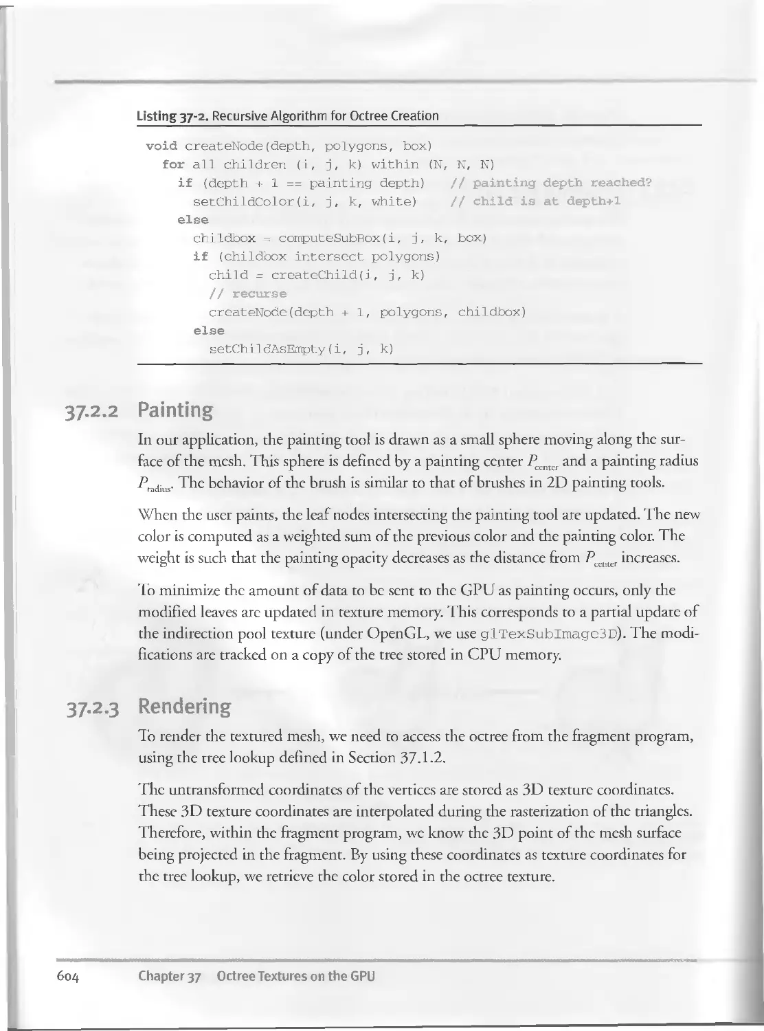
37.2.I Creating the Octree............................ . . 603
37.2.2 Painting..............................................604
37.2.3 Rendering.............................................604
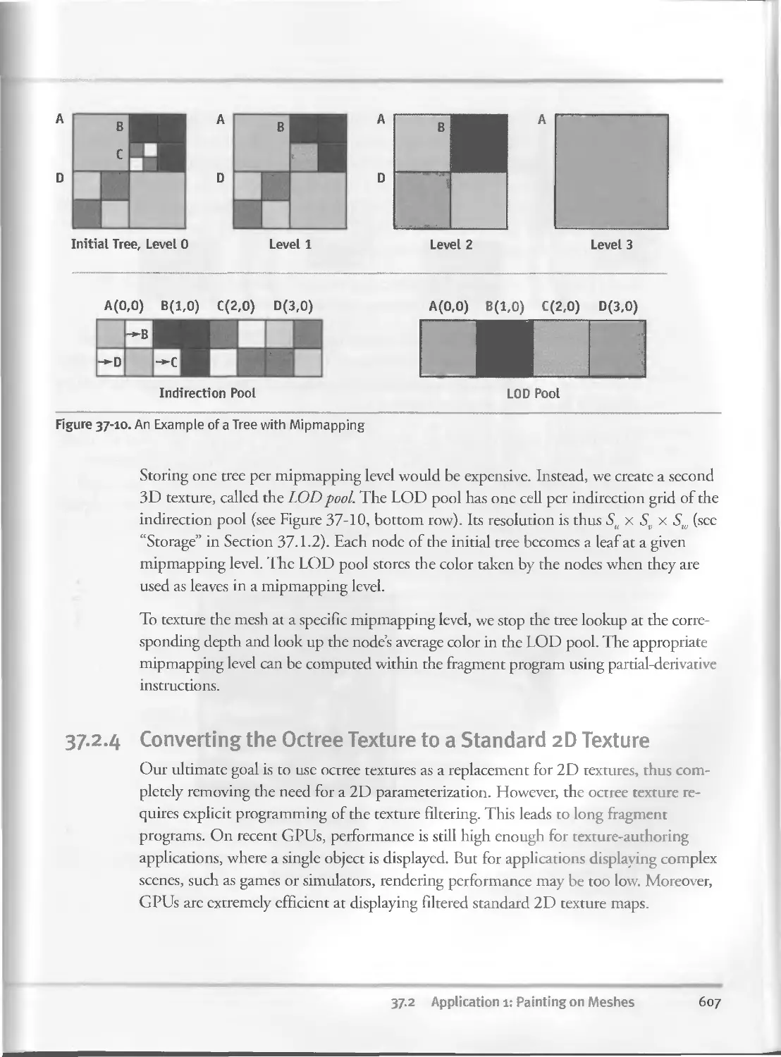
37.2.4 Converting the Octree Texture to a Standard 2D Texture . . 607
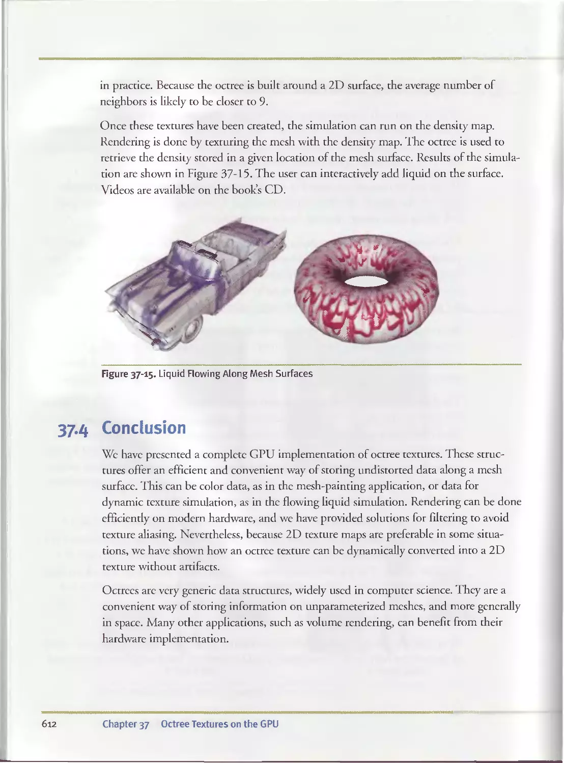
37. 3 Application 2: Surface Simulation............................611
37. 4 Conclusion...................................................612
37-5 References...................................................613
Chapter 38
High-Quality Global Illumination Rendering Using
Rasterization................................................................615
Toshiya Hachisuka, The University of Tokyo
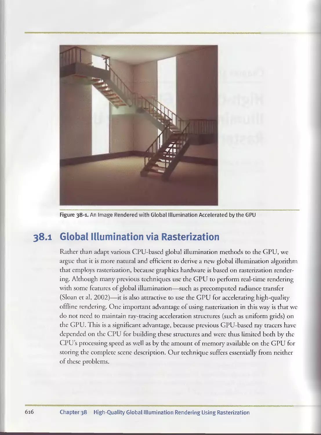
38.1 Global Illumination via Rasterization.........................616
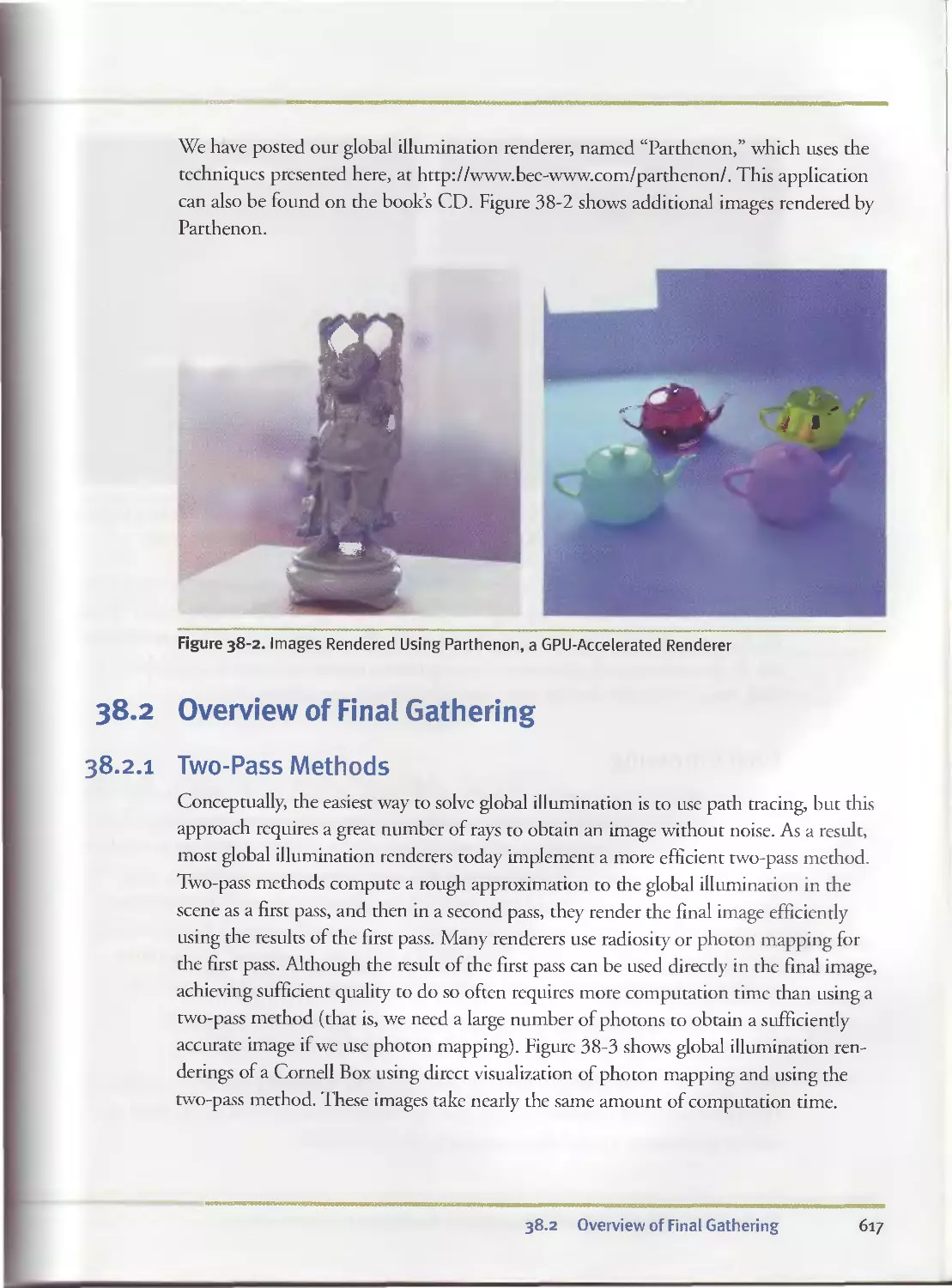
38.2 Overview of Final Gathering................................. 617
38.2.1 Two-Pass Methods.....................................617
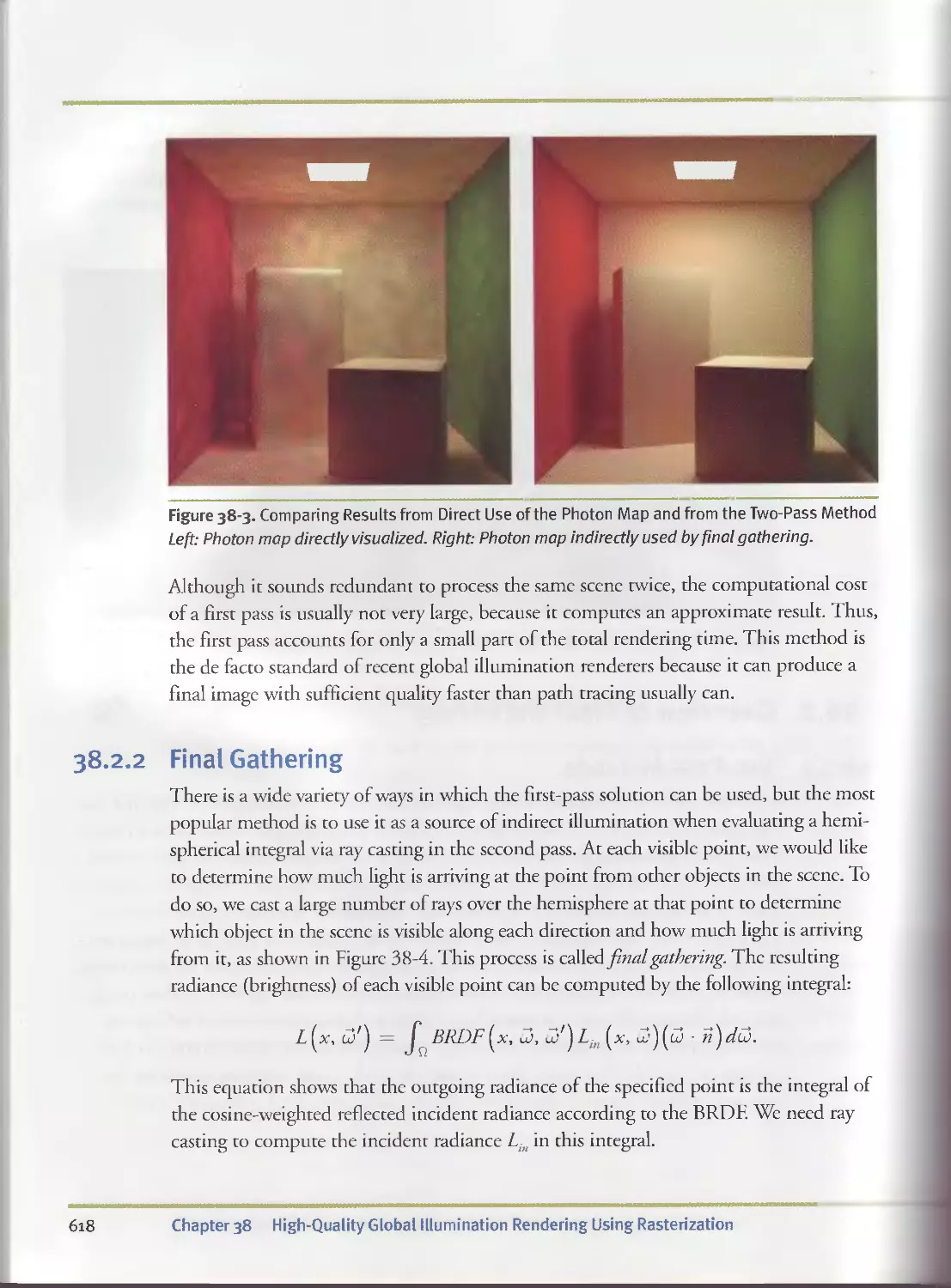
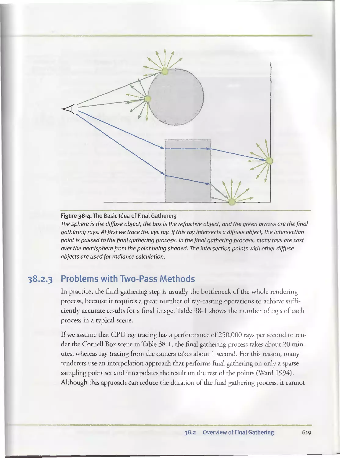
38.2.2 Final Gathering......................................618
38.2.3 Problems with Two-Pass Methods.......................619
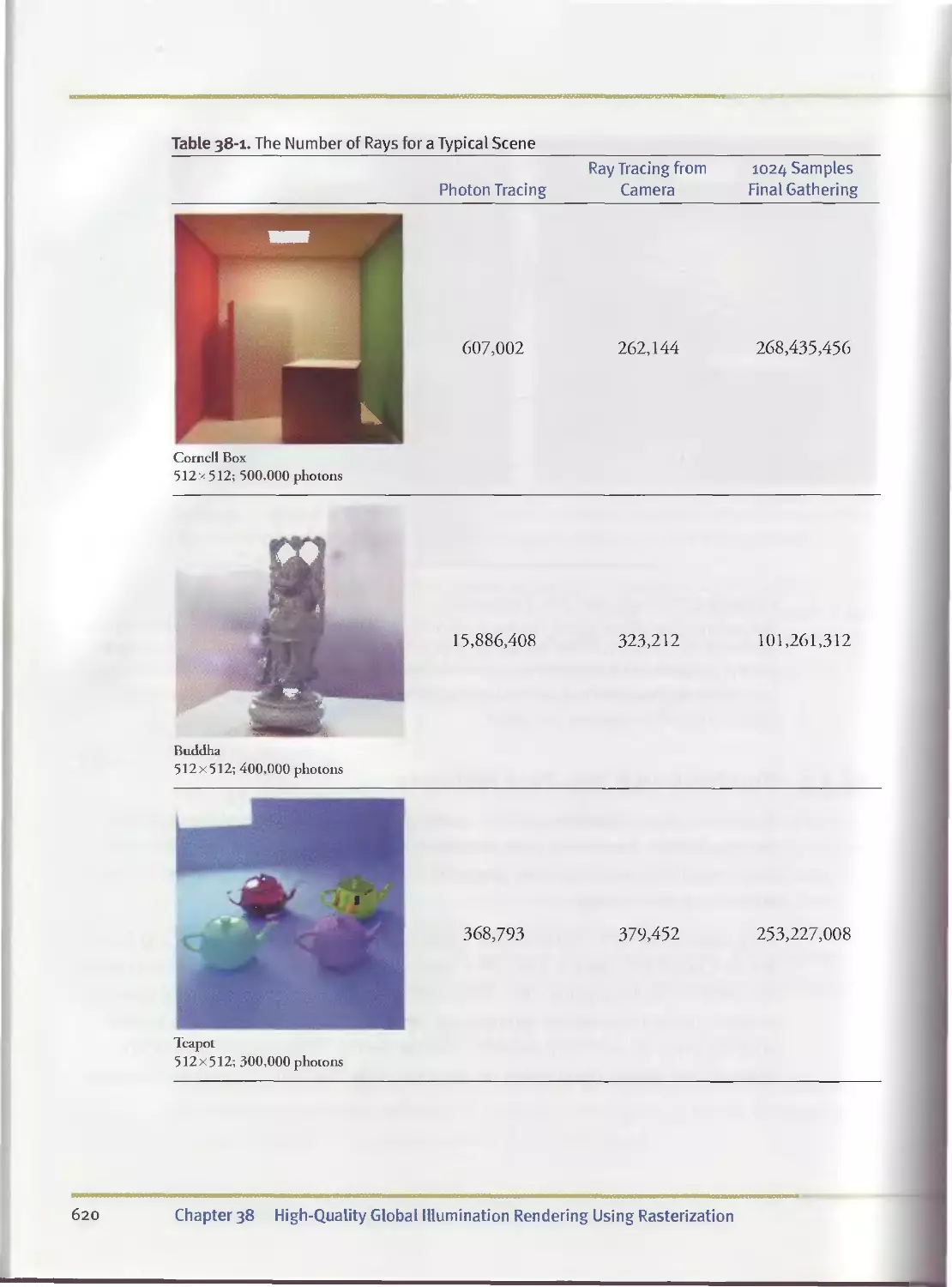
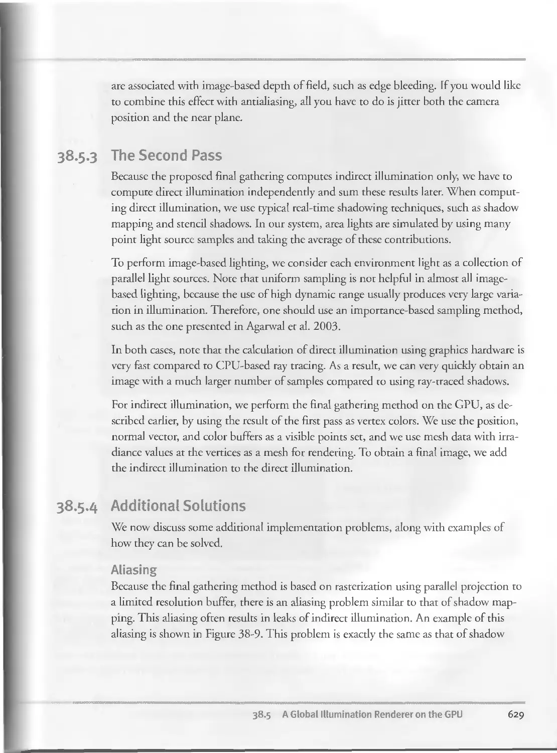
38.3 Final Gathering via Rasterization.............................621
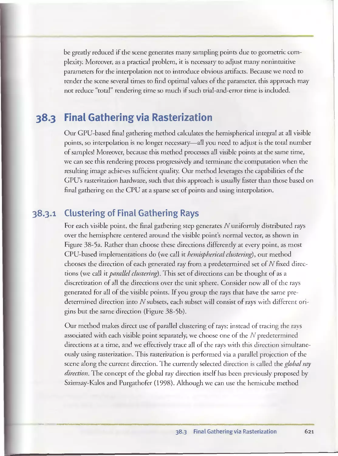
38.3.1 Clustering of Final Gathering Rays....................621
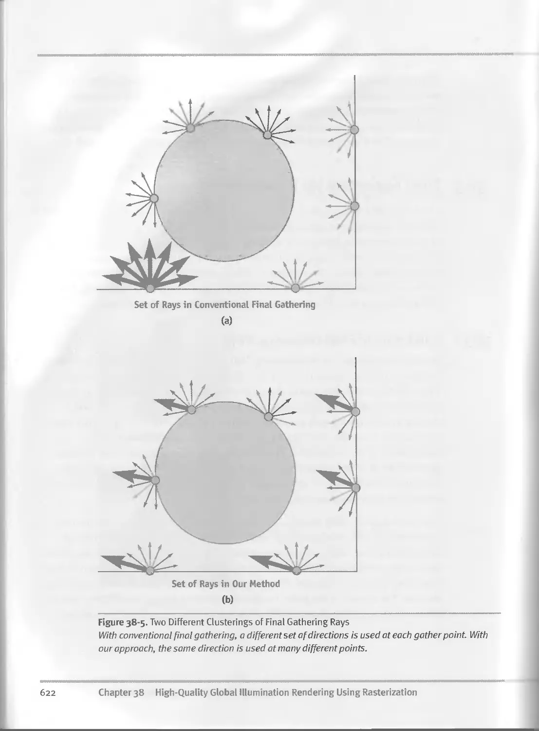
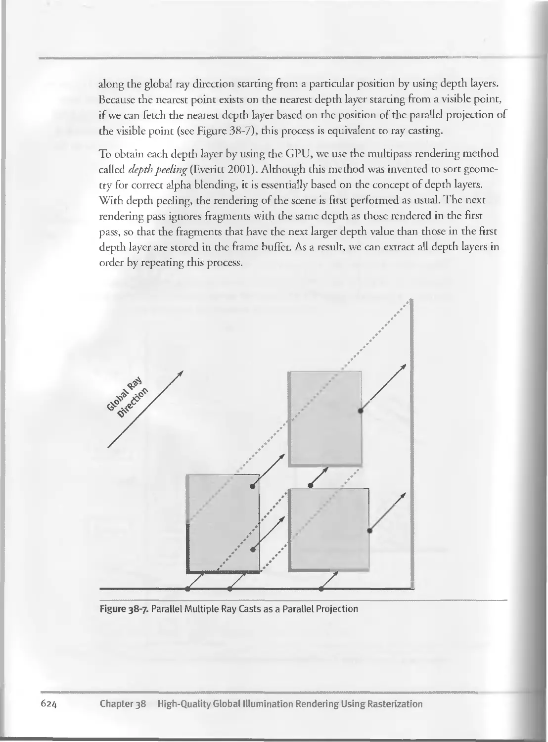
38.3.2 Ray Casting as Multiple Parallel Projection...........623
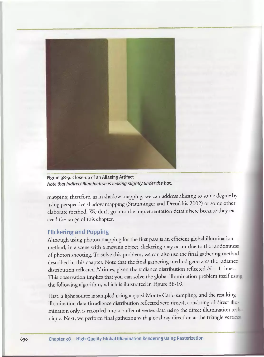
38.4 Implementation Details.......................................625
38.4.1 Initialization........................................625
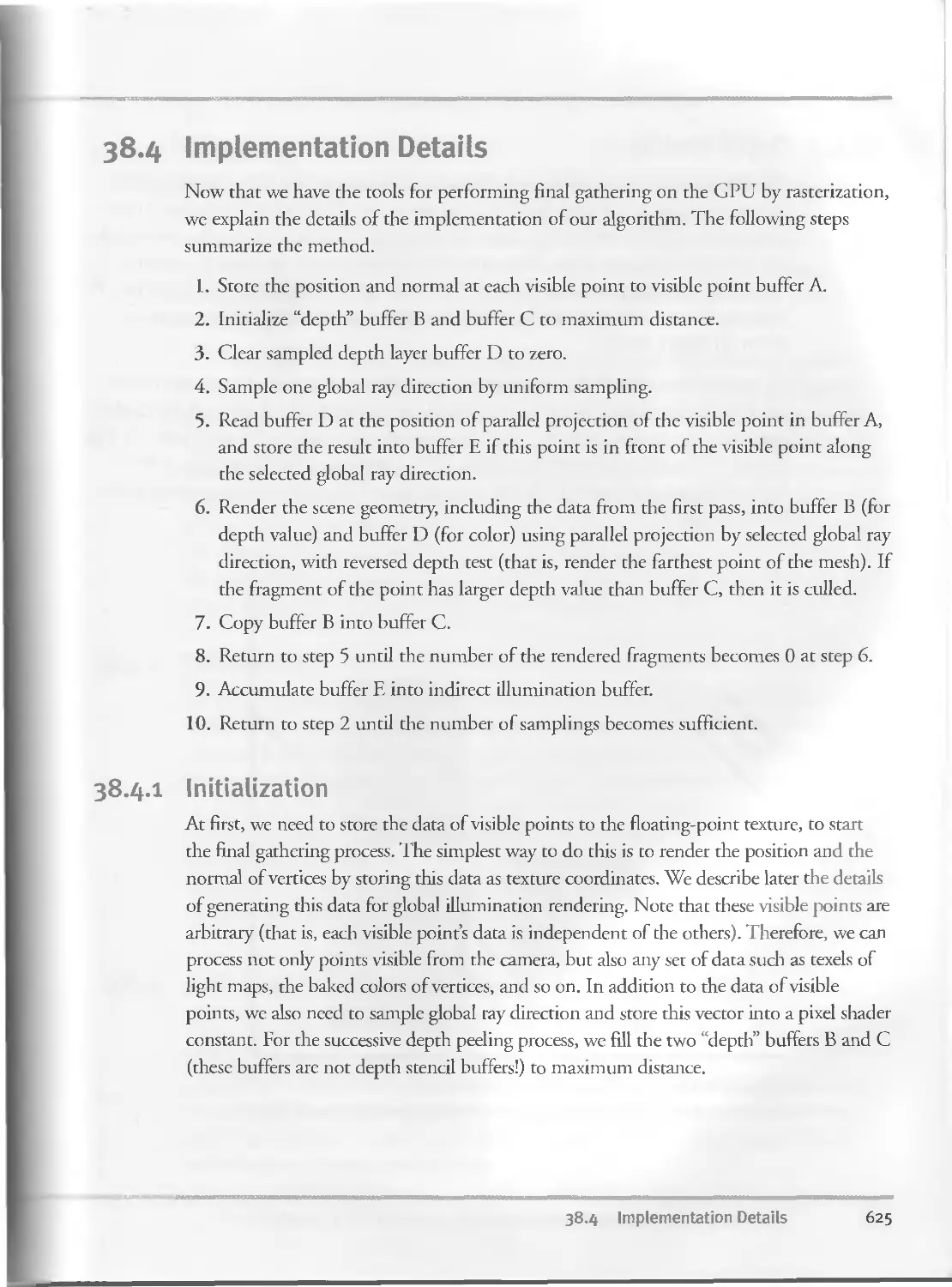
38.4.2 Depth Peeling.......,,................................626
38.4.3 Sampling..............................................627
38.4.4 Performance...........................................627
38.5 A Global Illumination Renderer on the GPU....................627
38.5.1 The First Pass........................................628
38.5.2 Generating Visible Points Data........................628
38.5.3 The Second Pass.......................................629
38.5.4 Additional Solutions..................................629
38.6 Conclusion. ......................... ...............632
38.7 References....................................................632
Chapter 39
Global Illumination Using Progressive Refinement Radiosity..................635
Greg Coombe, University of North Carolina at Chapel Hill
Mark Harris, NVIDIA Corporation
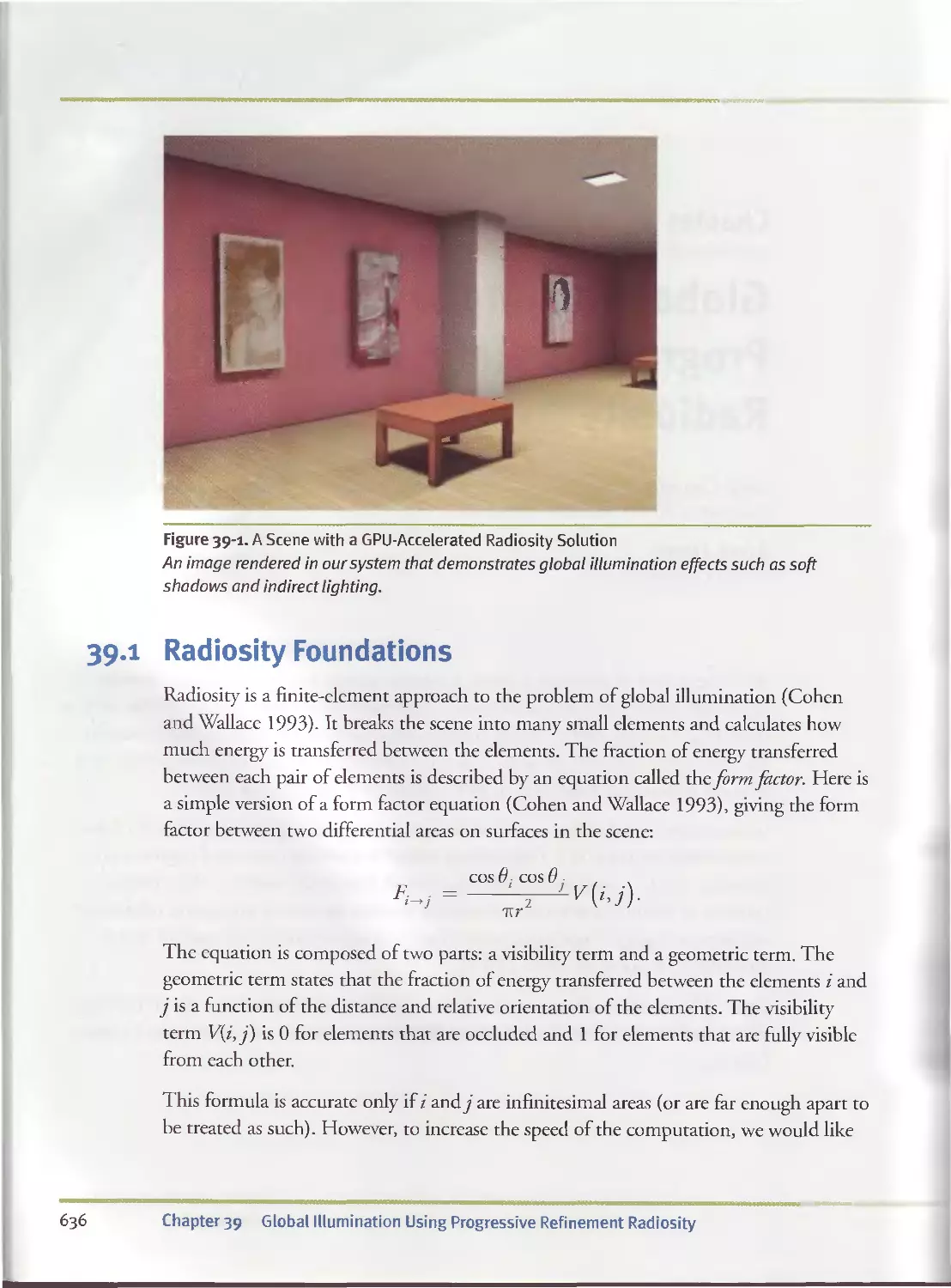
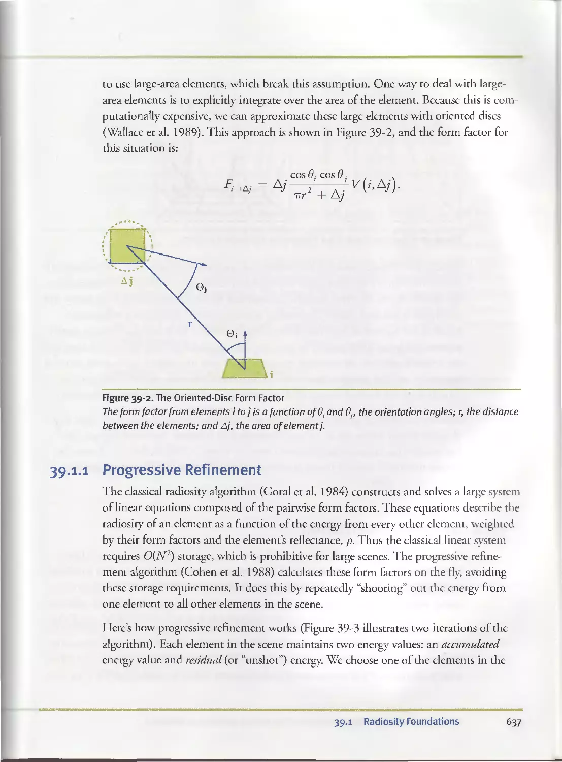
39.1 Radiosity Foundations..........................................636
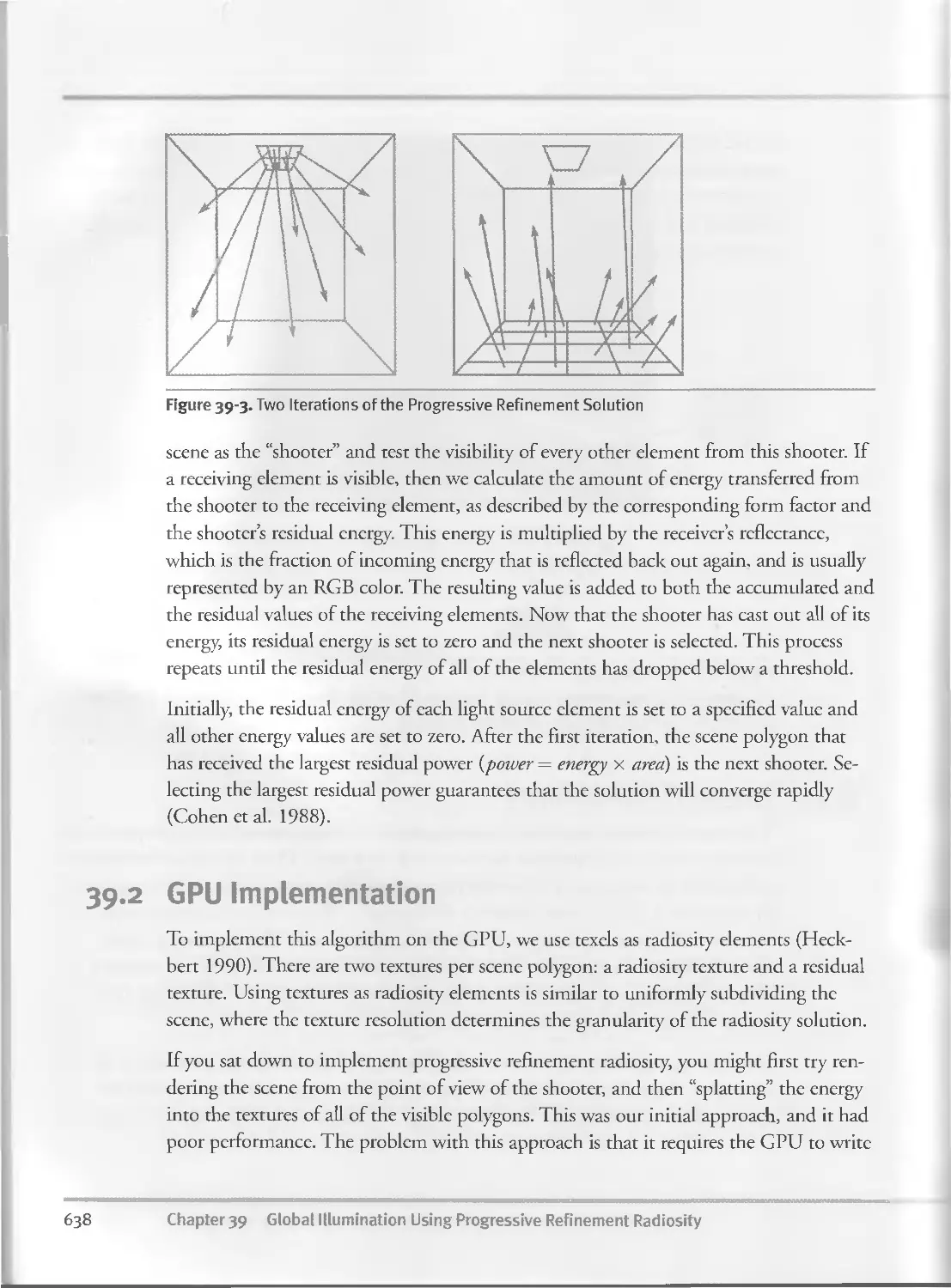
39.1.1 Progressive Refinement................................637
xxiv Contents
39-2 GPU Implementation............................................638
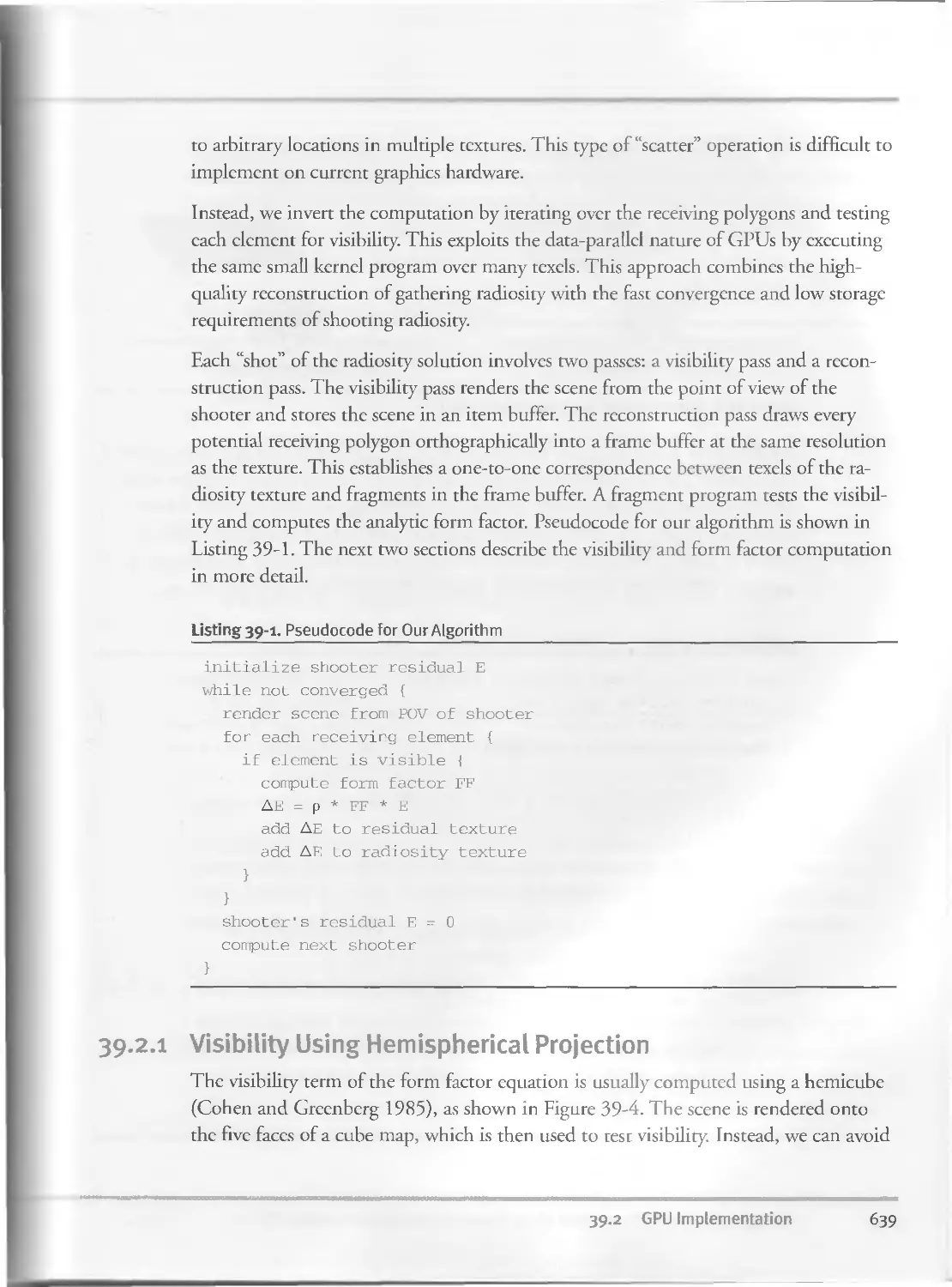
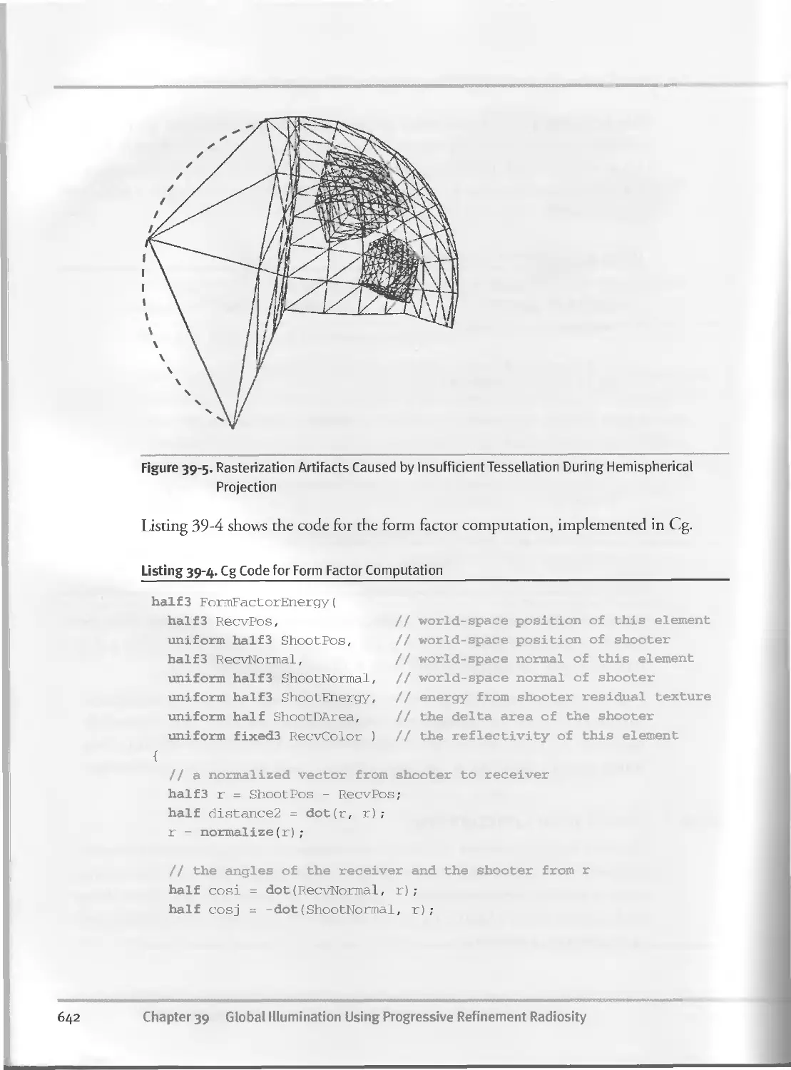
39.2.1 Visibility Using Hemispherical Projection............639
39.2.2 Form Factor Computation..............................641
39-2-3 Choosing the Next Shooter............................643
39-3 Adaptive Subdivision..........................................643
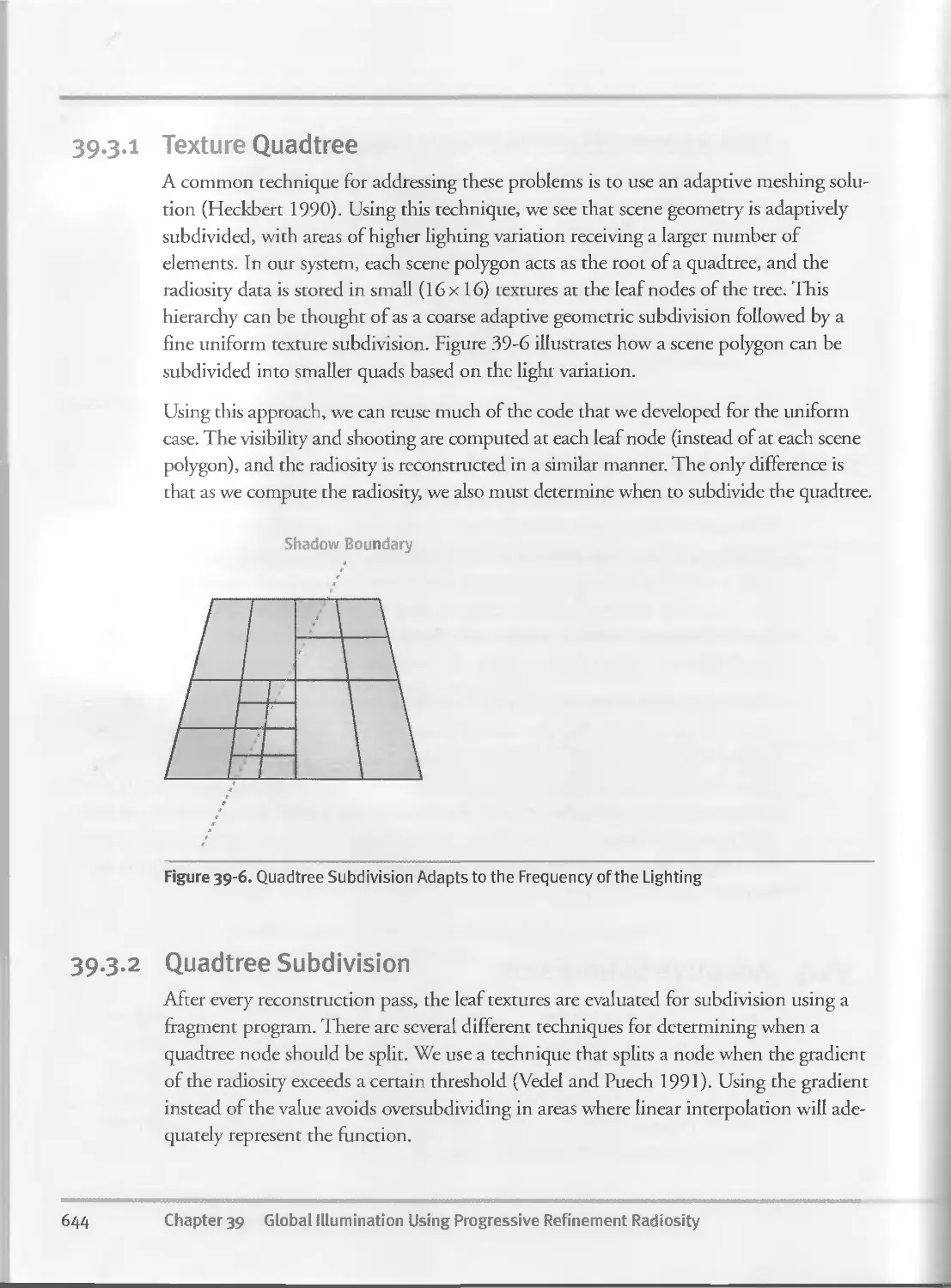
39.3.1 Texture Quadtree.....................................644
39.3.2 Quadtree Subdivision.................................644
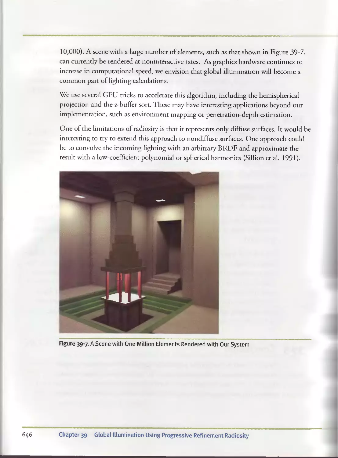
39-4 Performance...................................................645
39. 5 Conclusion..................................................645
39. 6 References................................................ 647
Chapter 40
Computer Vision on the GPU....................................................649
James Fung, University of Toronto
40.I Introduction.................................................649
40.2 Implementation Framework.....................................650
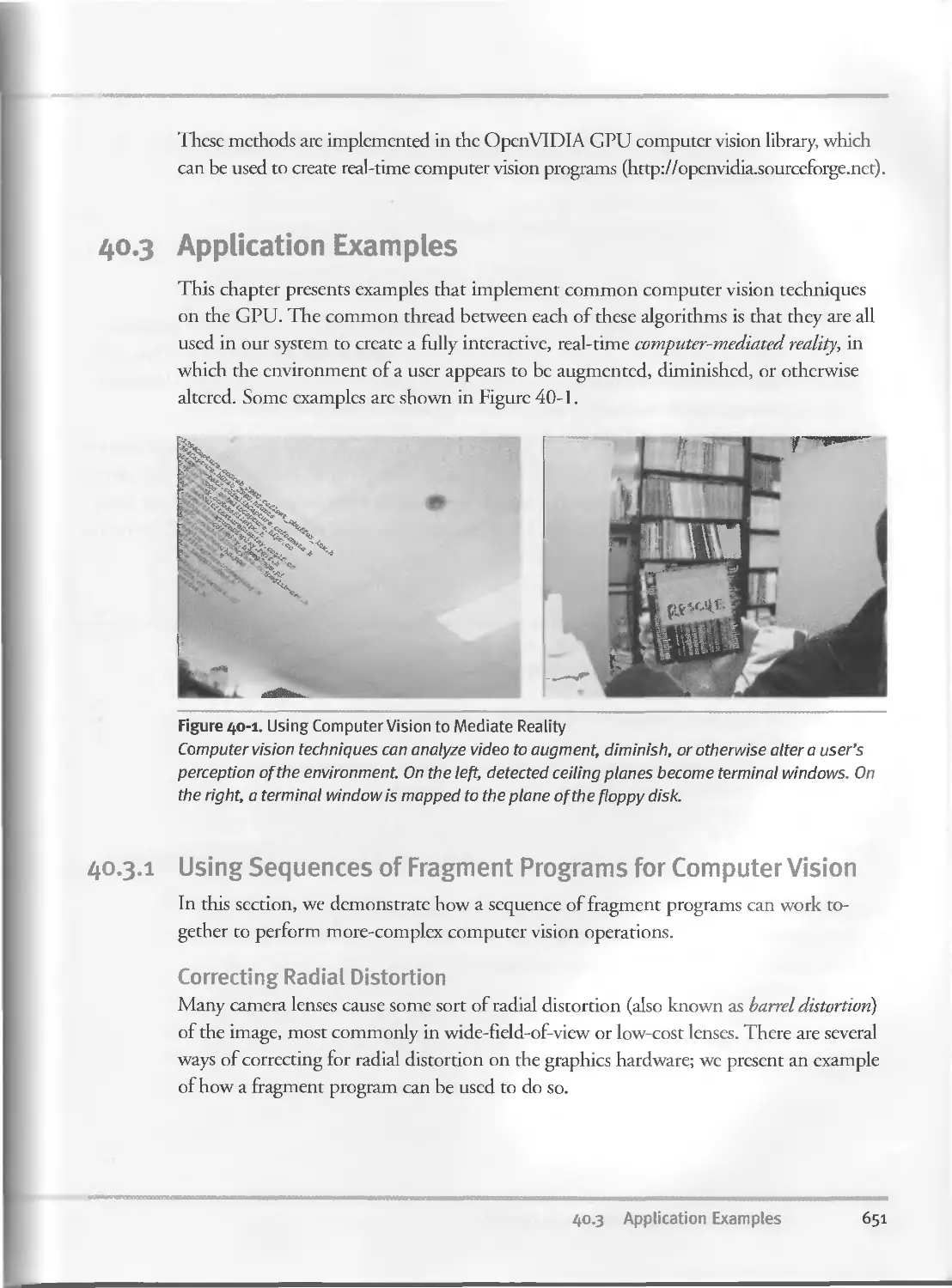
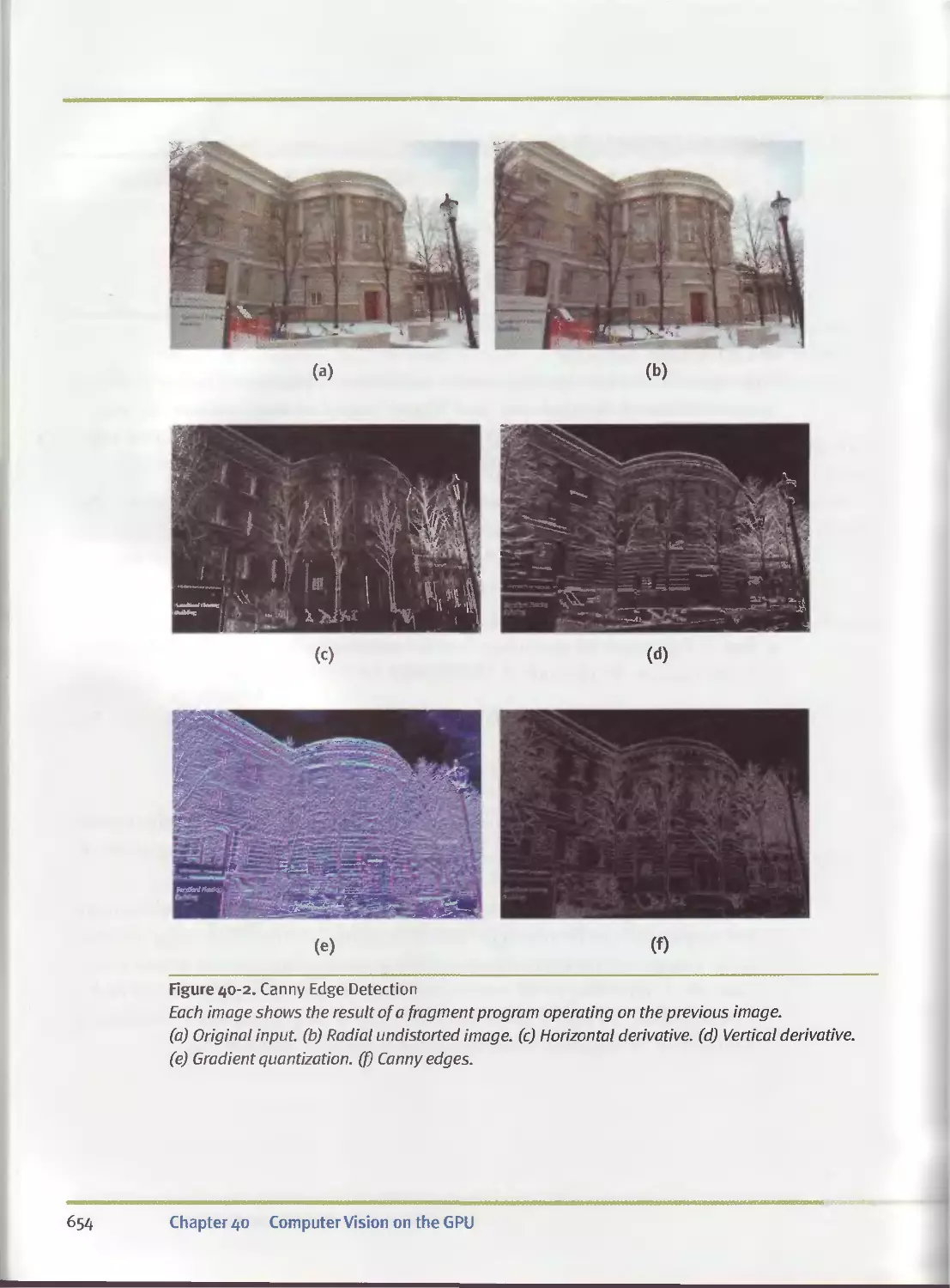
4O.3 Application Examples.........................................651
40.3.I Using Sequences of Fragment Programs for
Computer Vision..............................................651
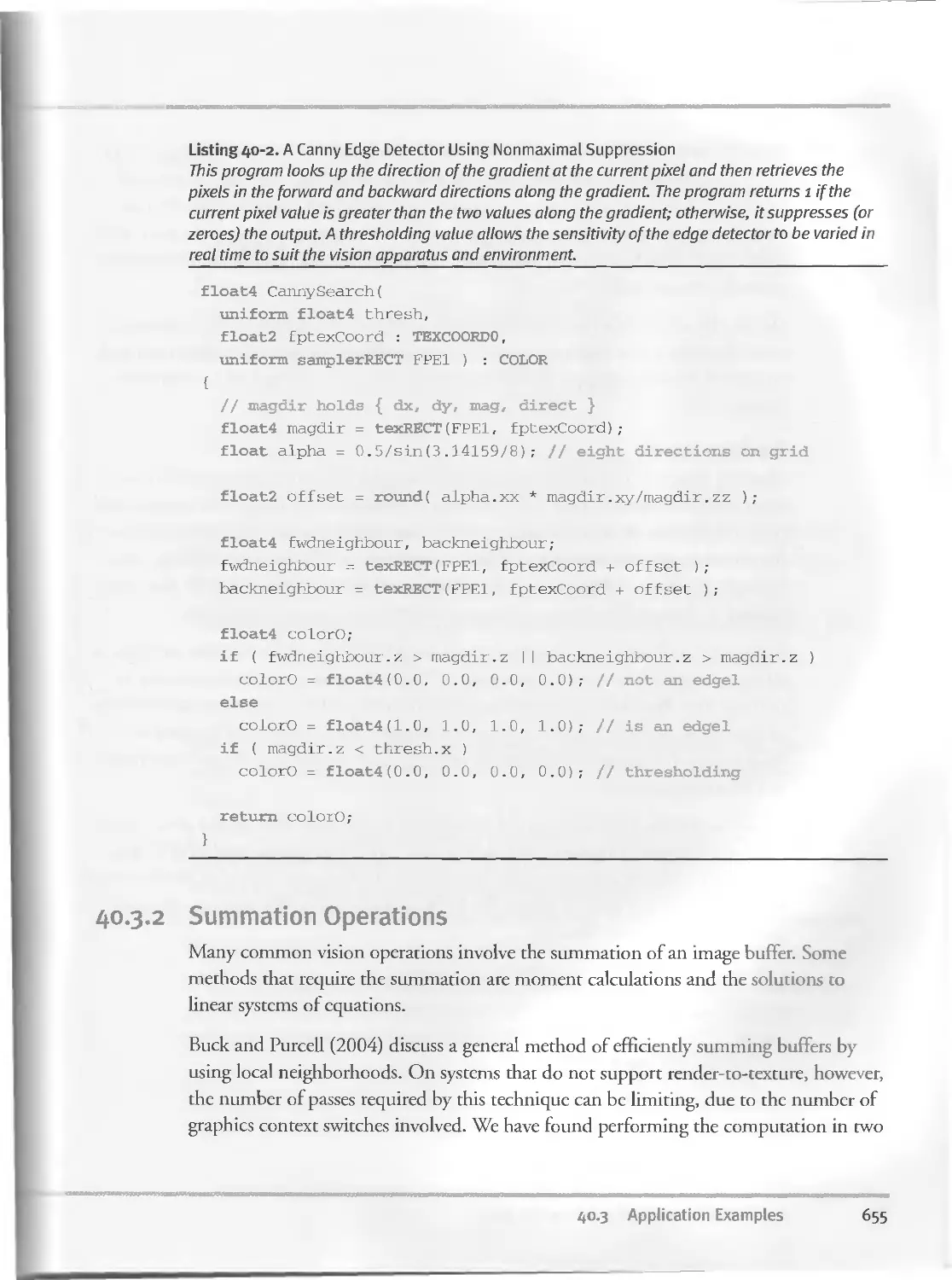
40.3.2 Summation Operations................................ 655
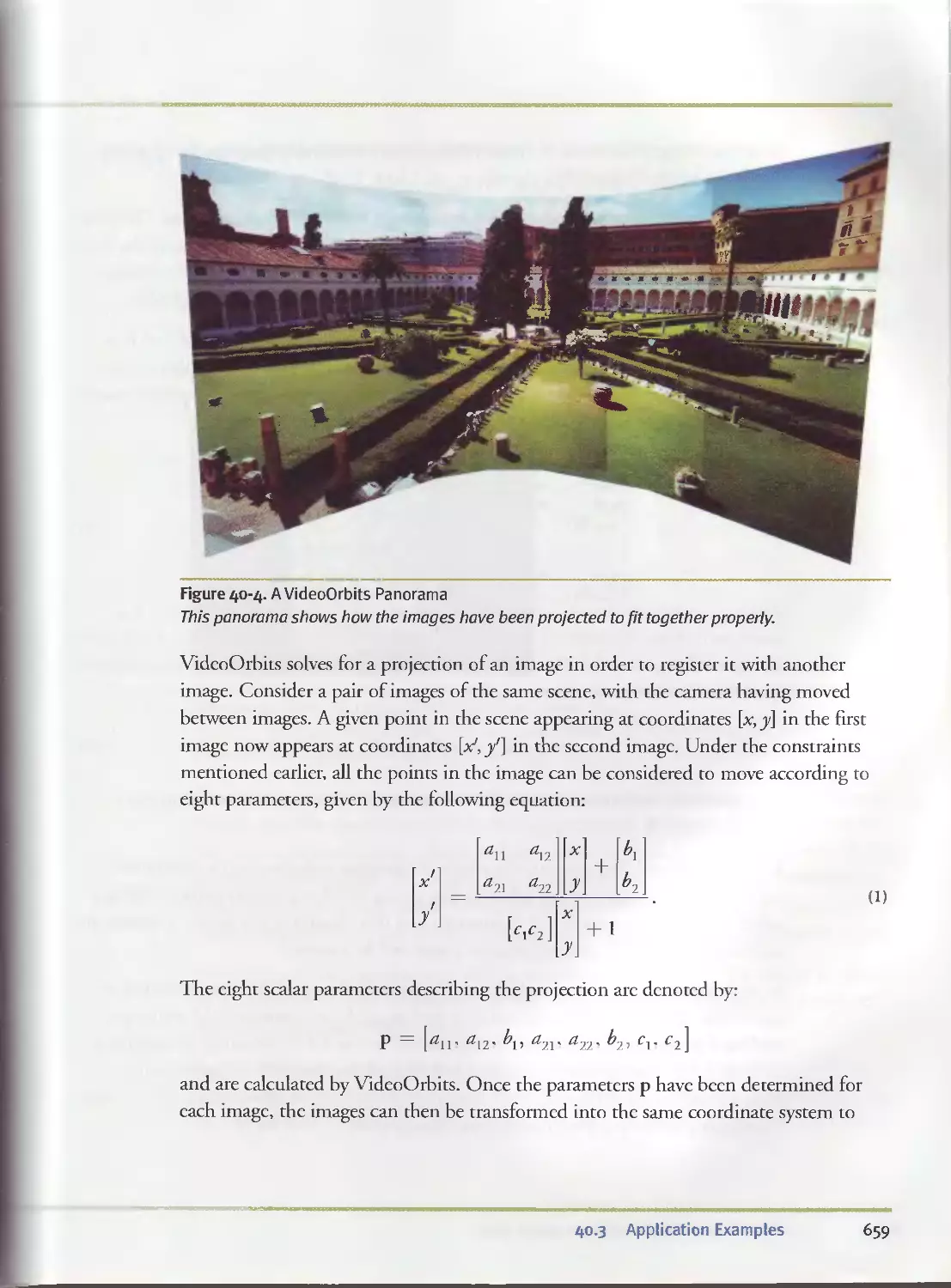
40.33 Systems of Equations for Creating Image Panoramas.....658
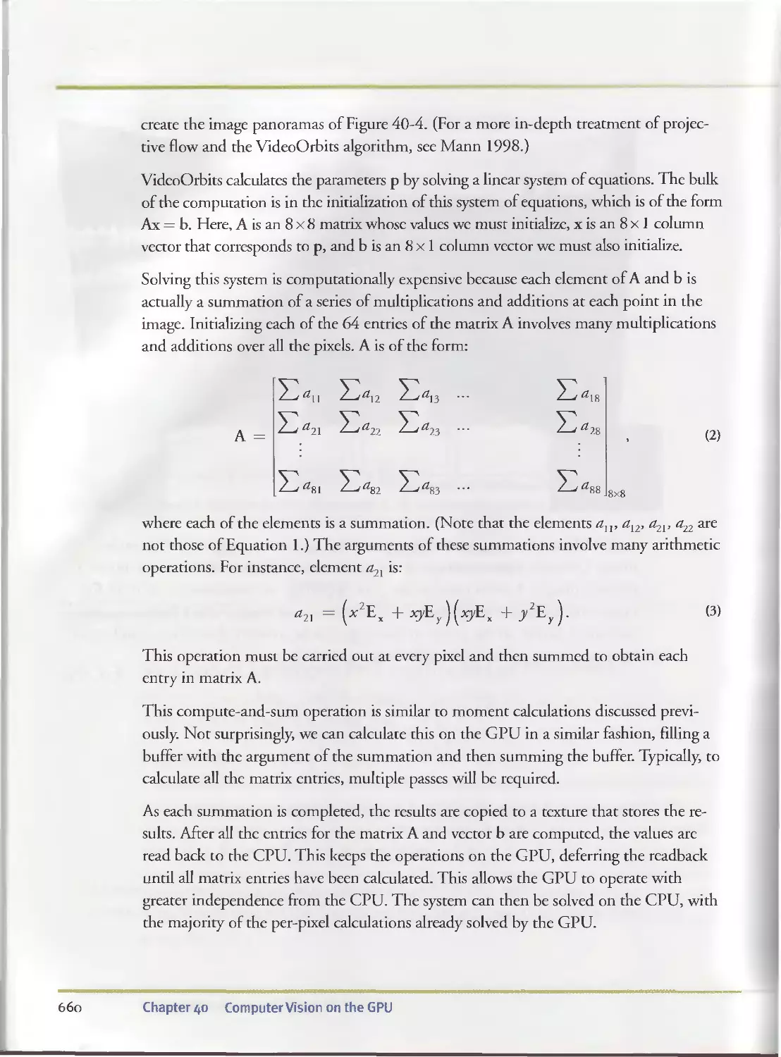
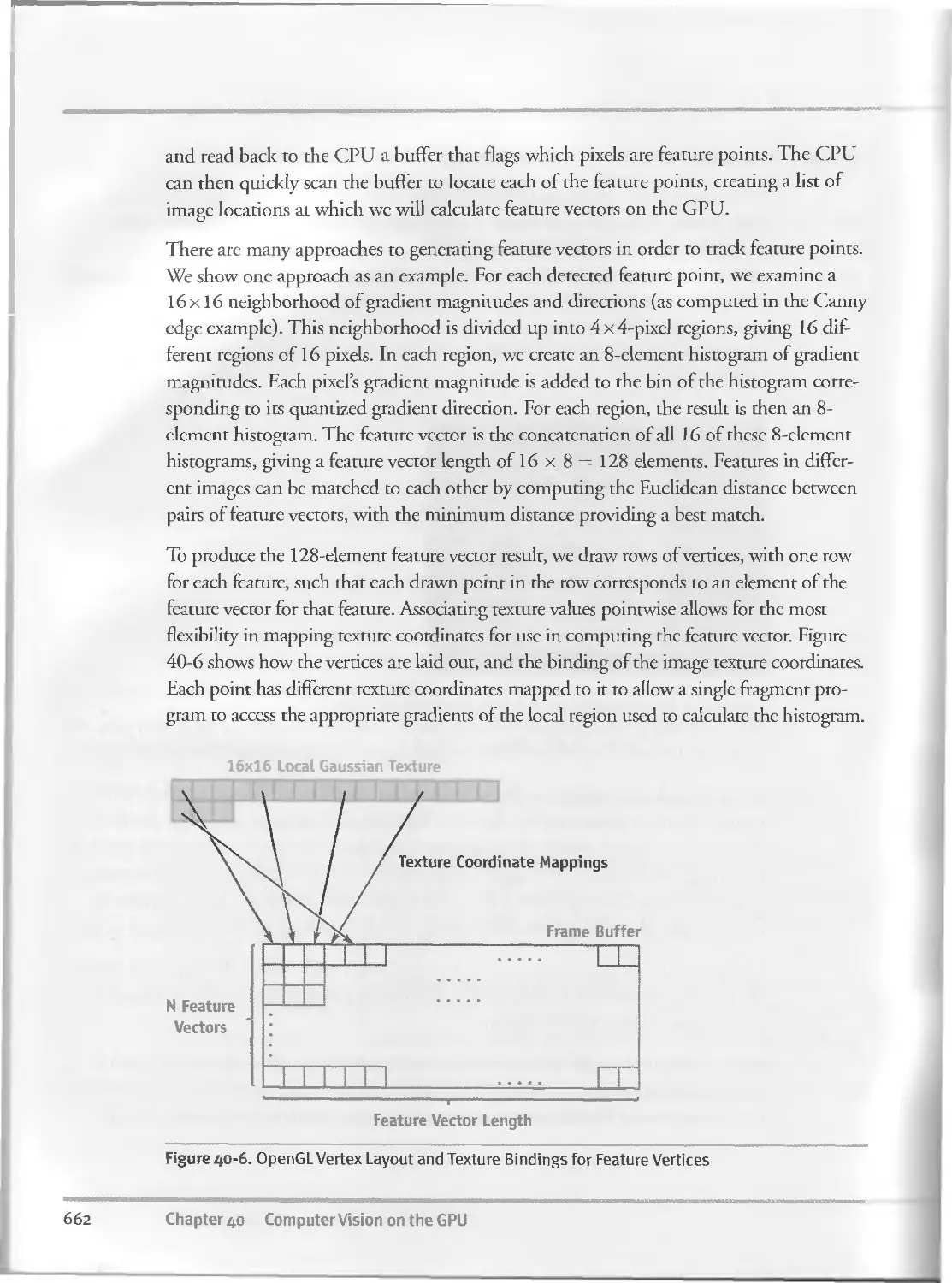
40.3.4 Feature Vector Computations..........................661
40.4 Parallel Computer Vision Processing..........................664
4O.5 Conclusion ..................................................664
40.6 References...................................................665
Chapter 41
Deferred Filtering: Rendering from Difficult Data Formats...................667
Joe Kniss, University of Utah
Aaron Lefohn, University of California, Davis
Nathaniel Fout, University of California, Davis
41.1 Introduction................................................ 667
41.2 Why Defer?............................................... . 668
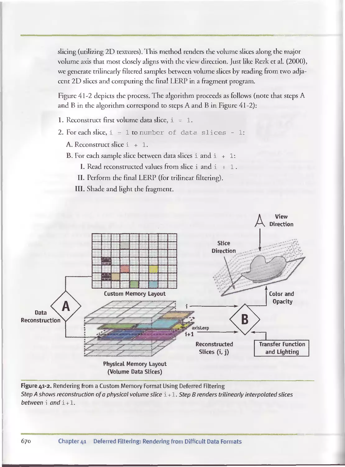
41.3 Deferred Filtering Algorithm............................... .669
41.4 Why It Works................................................ 673
41.5 Conclusions: When to Defer................................ . . 67З
41.6 References................................................ . . 674
Contents
XXV
Chapter 42
Conservative Rasterization.................................................677
Jon Hasselgren, Lund University
Tomas Akenine-Moller, Lund University
Lennart Ohlsson, Lund University
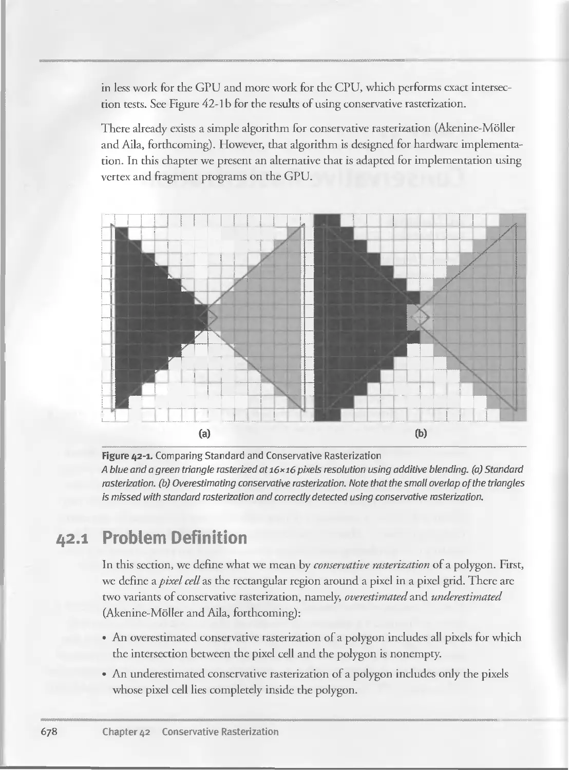
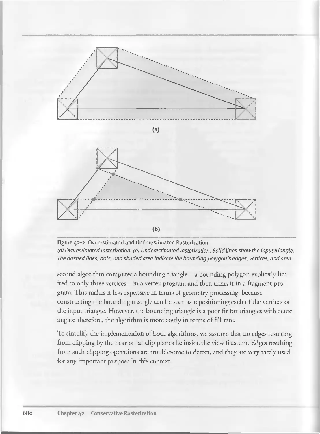
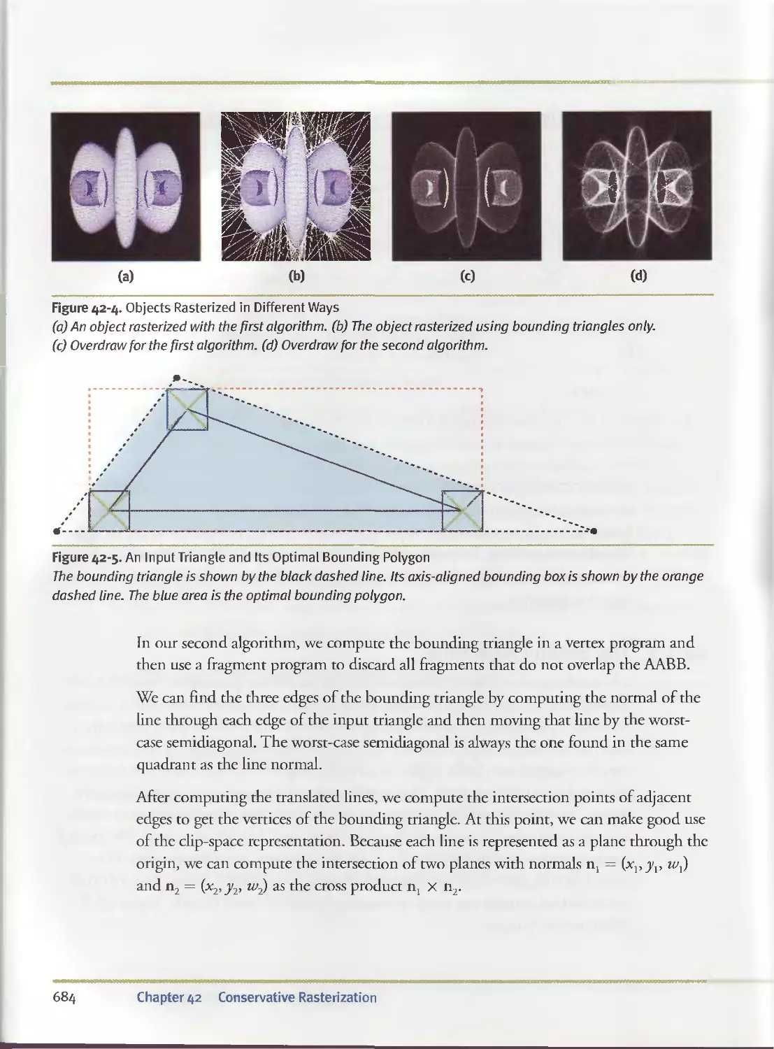
42.1 Problem Definition.........................................678
42.2 Two Conservative Algorithms................................679
42.2.I Clip Space.........................................681
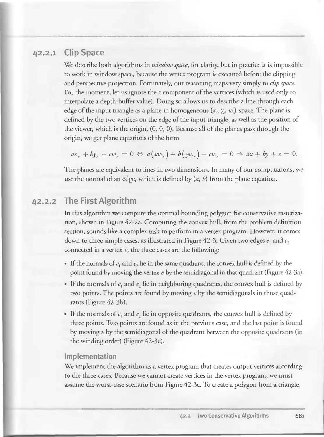
42.2.2 The First Algorithm................................681
42.2.3 The Second Algorithm...............................683
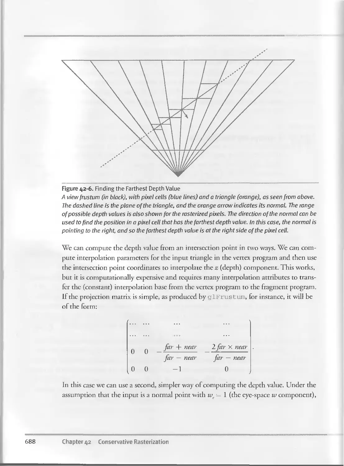
42.3 Robustness Issues..........................................686
42.4 Conservative Depth....................................... 687
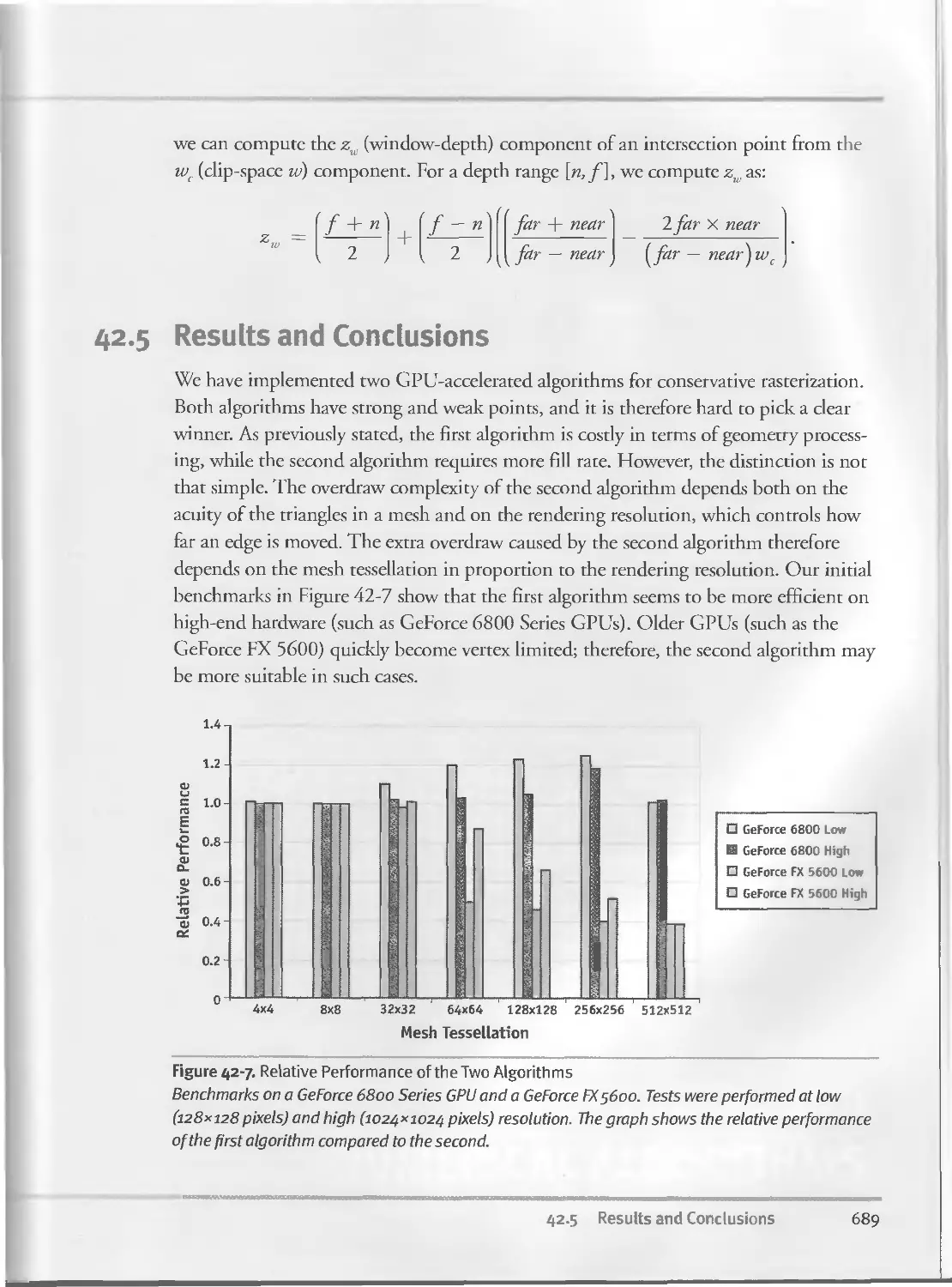
42.5 Results and Conclusions....................................689
42.6 References.................................................690
PART VI SIMULATION AND NUMERICAL ALGORITHMS 691
Chapter 43
GPU Computing for Protein Structure Prediction.............................695
Paulius Micikevicius, Armstrong Atlantic State University
43.1 Introduction...............................................695
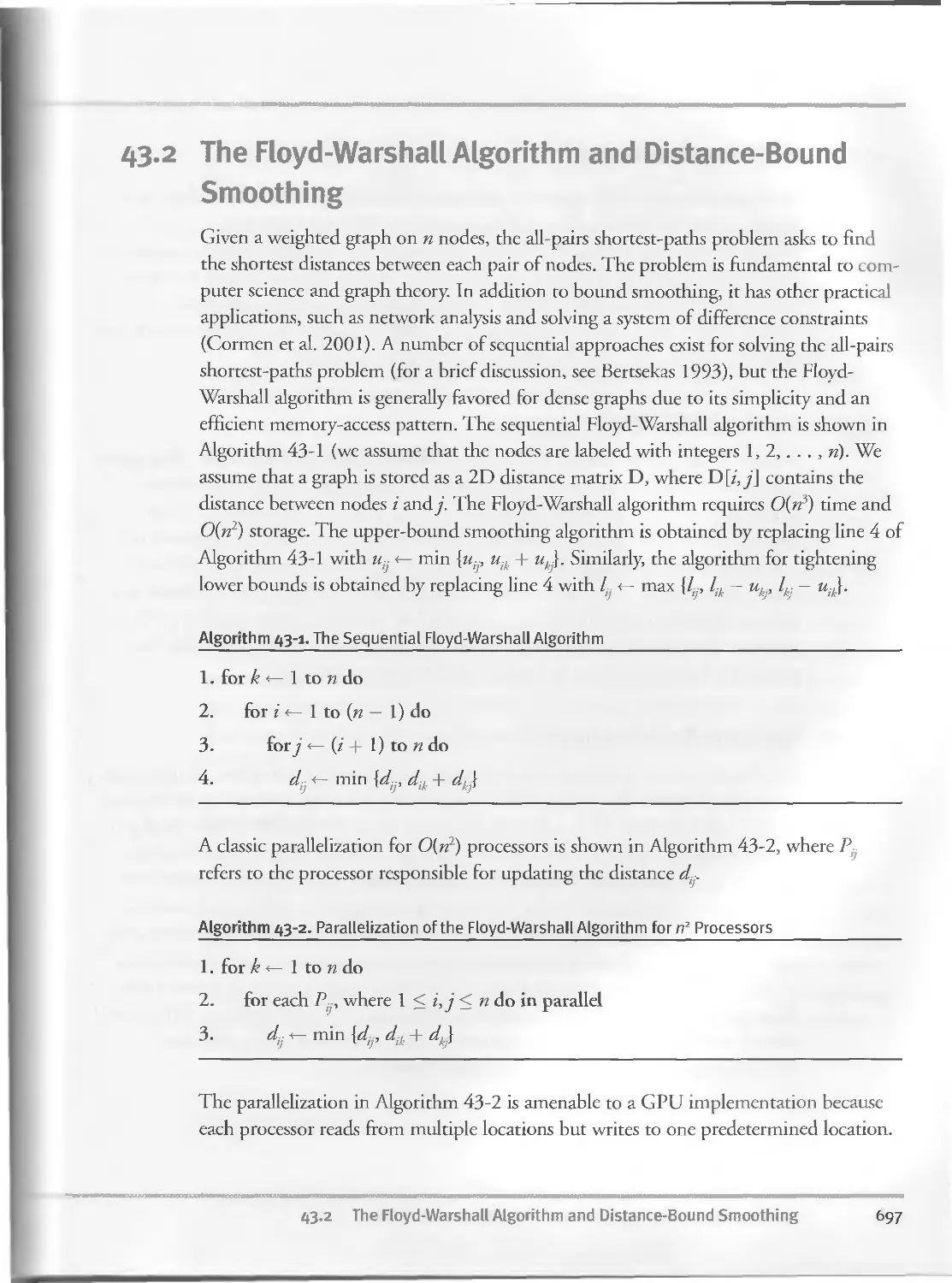
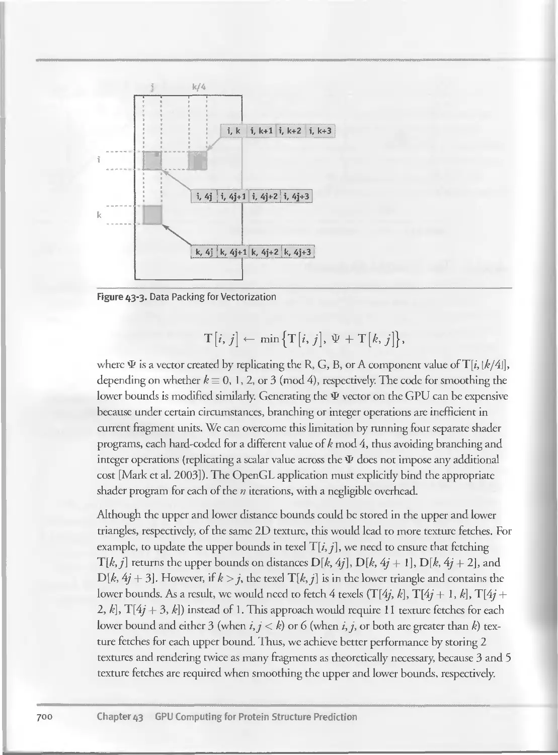
43-2 The Floyd-Warshall Algorithm and Distance-Bound Smoothing...697
43.3 GPU Implementation.........................................698
43.3.I Dynamic Updates....................................698
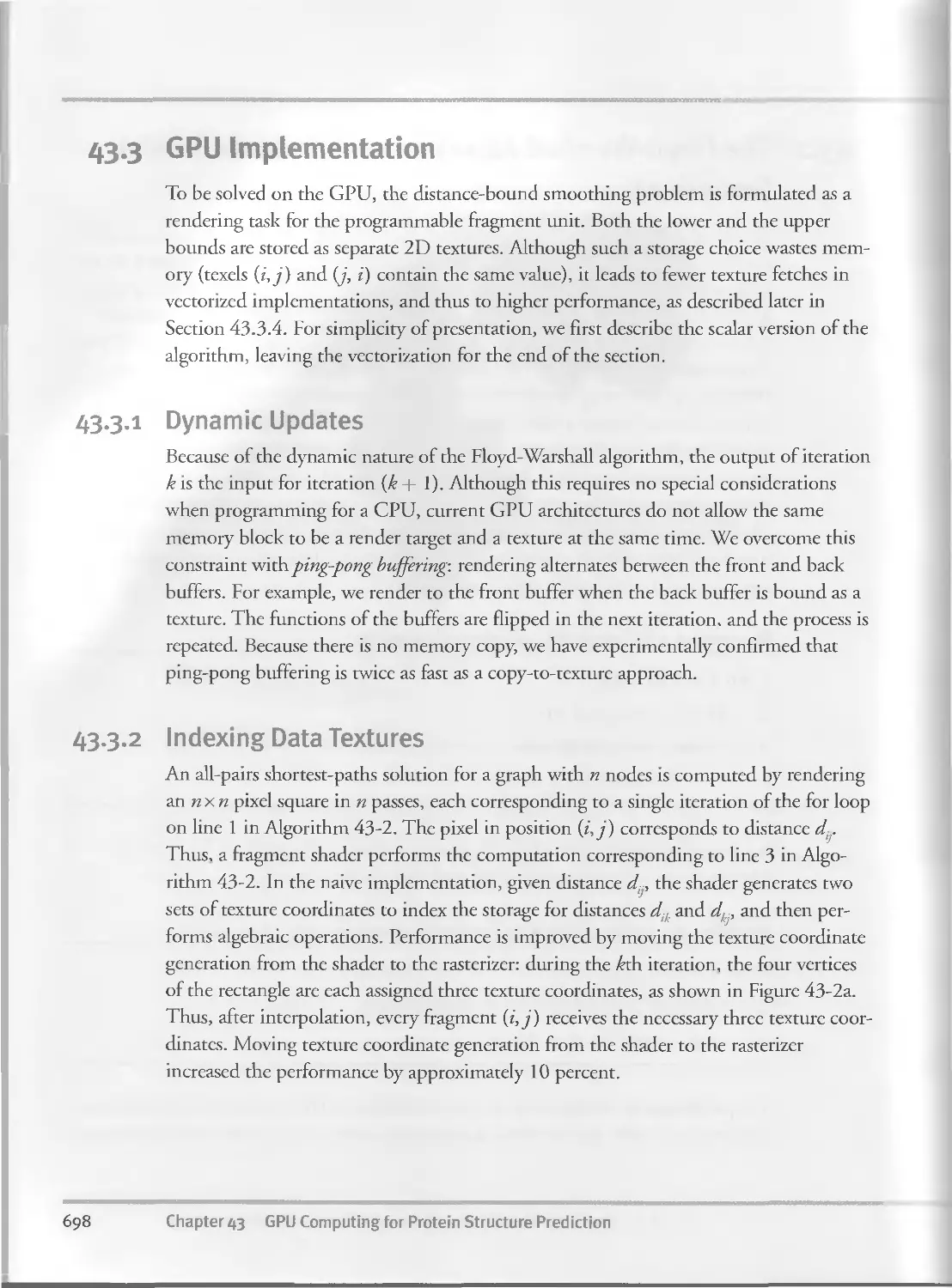
43.3.2 Indexing Data Textures.............................698
43.3.3 The Triangle Approach..............................699
43.3.4 Vectorization......................................699
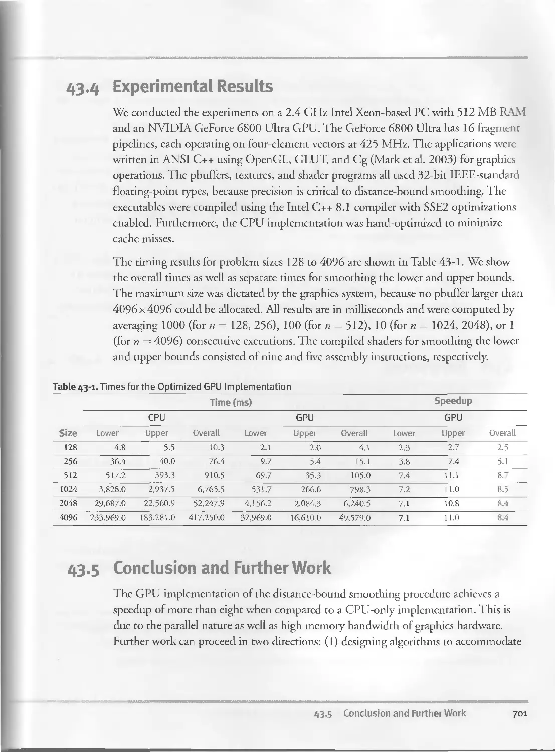
43.4 Experimental Results.......................................701
43.5 Conclusions and Further Work...............................701
43.6 References.................................................702
Chapter 44
A GPU Framework for Solving Systems of Linear Equations....................703
Jens Kruger, Technische Universitat Munchen
Rudiger Westermann, Technische Universitat Munchen
44.1 Overview...................................................703
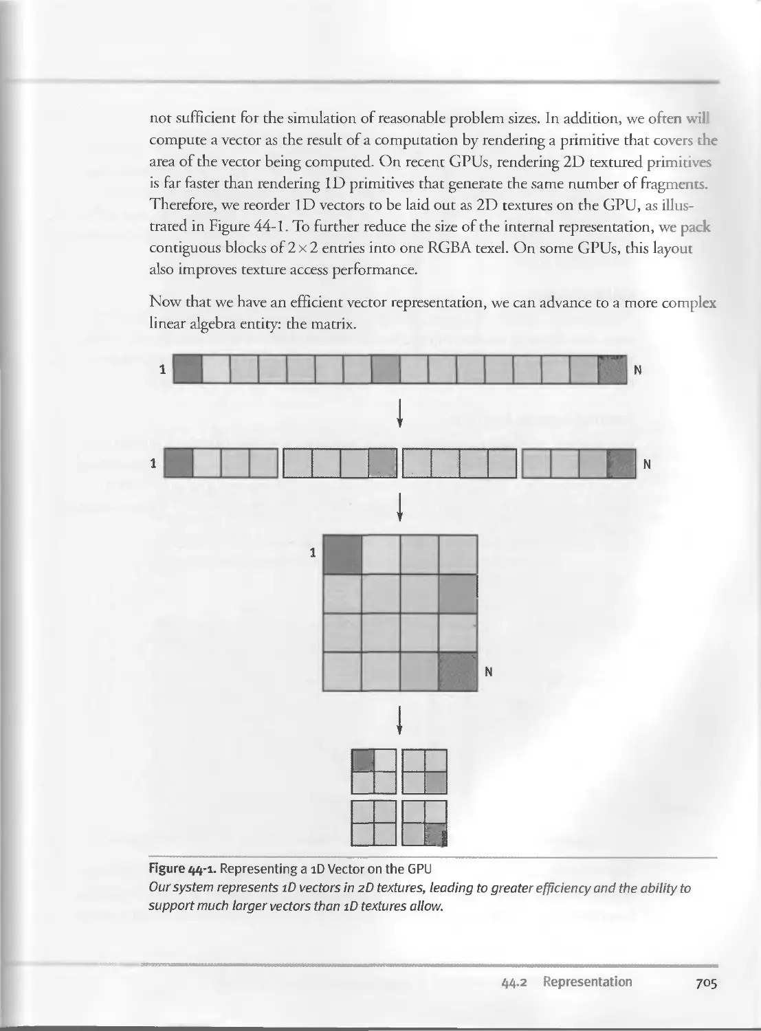
44.2 Representation.............................................704
44.2.1 The “Single Float” Representation..................704
44.2.2 Vectors......................................... . 704
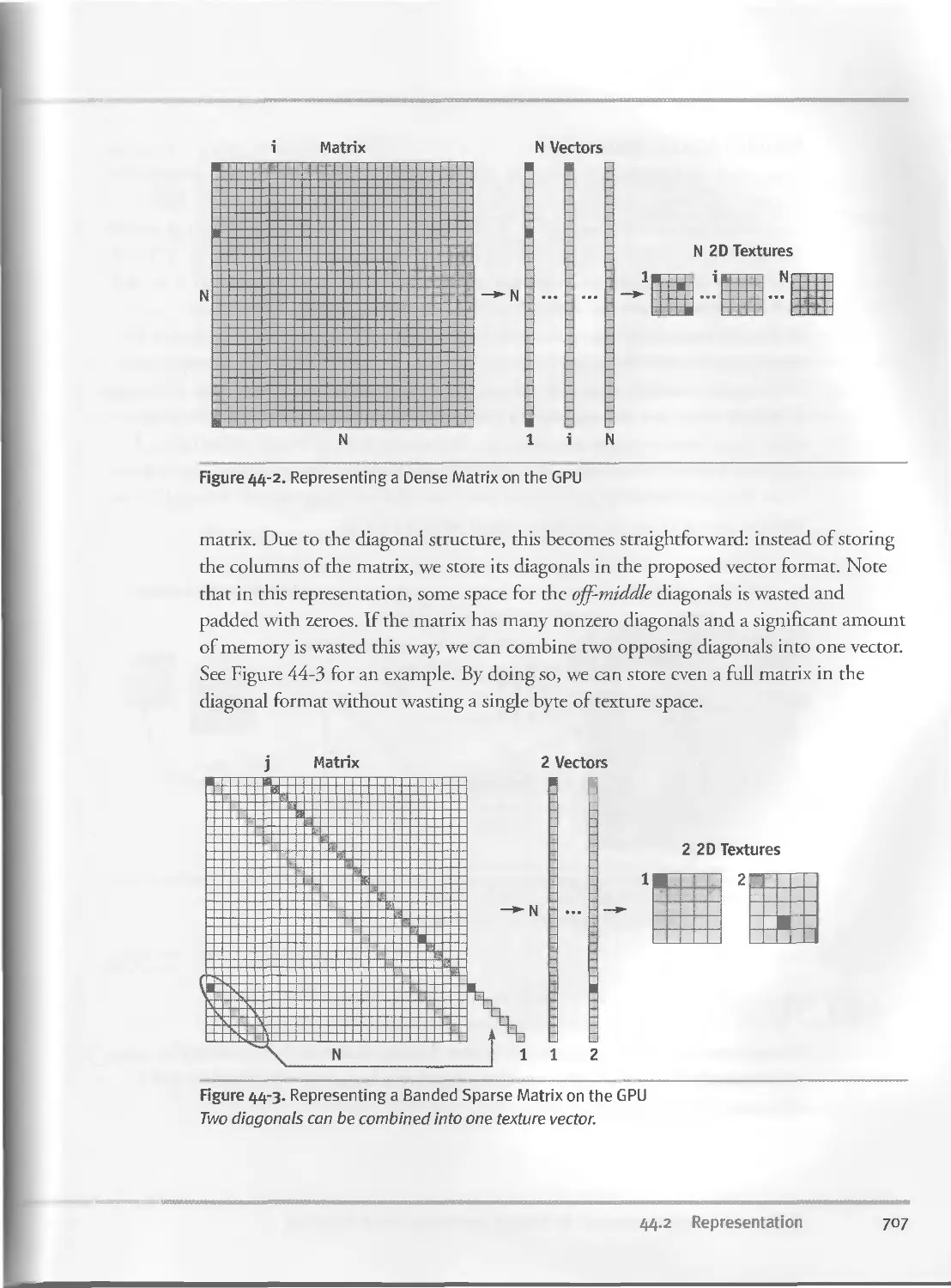
44.2.3 Matrices...........................................706
xxvi Contents
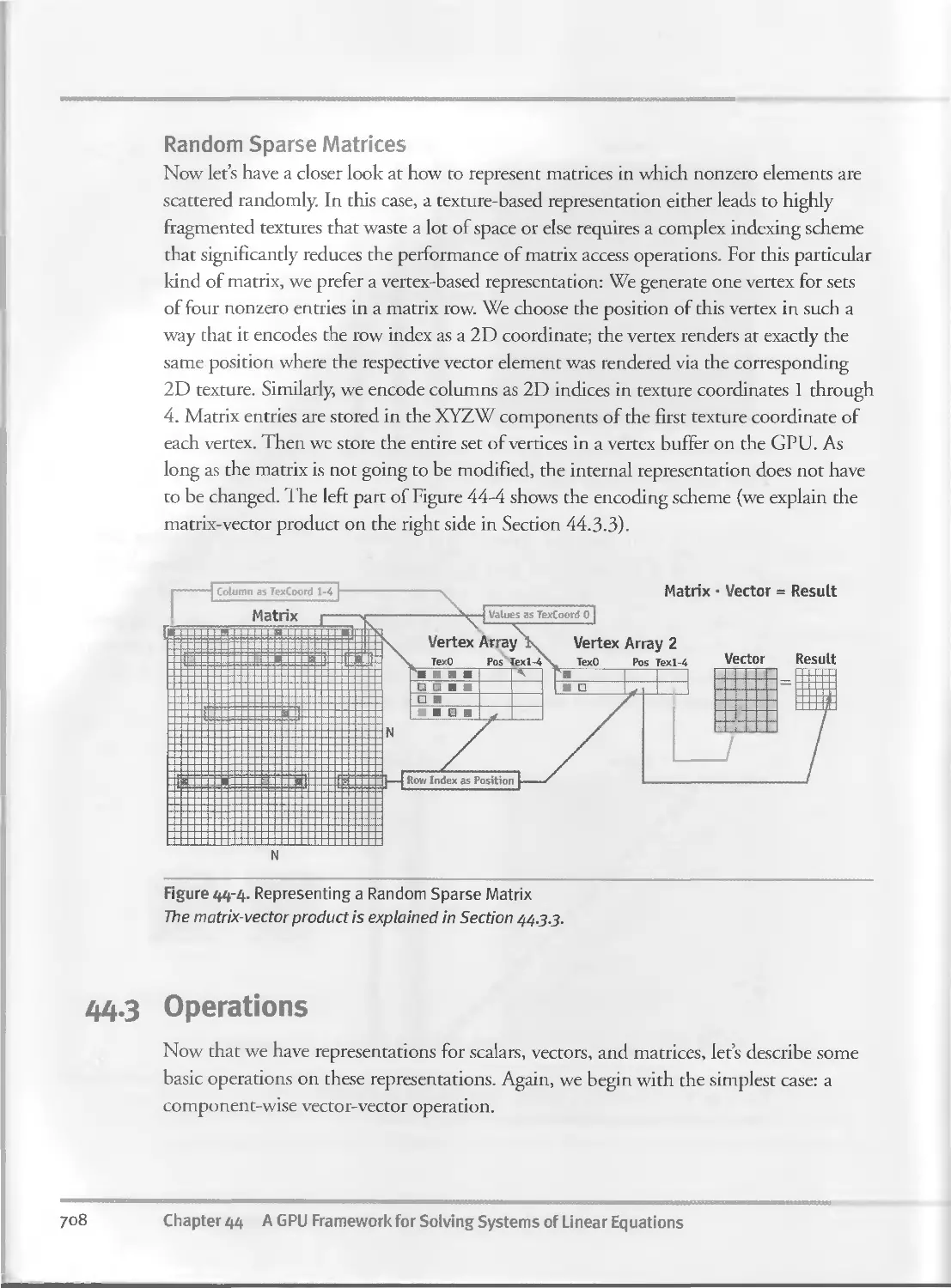
44-3 Operations...................................................708
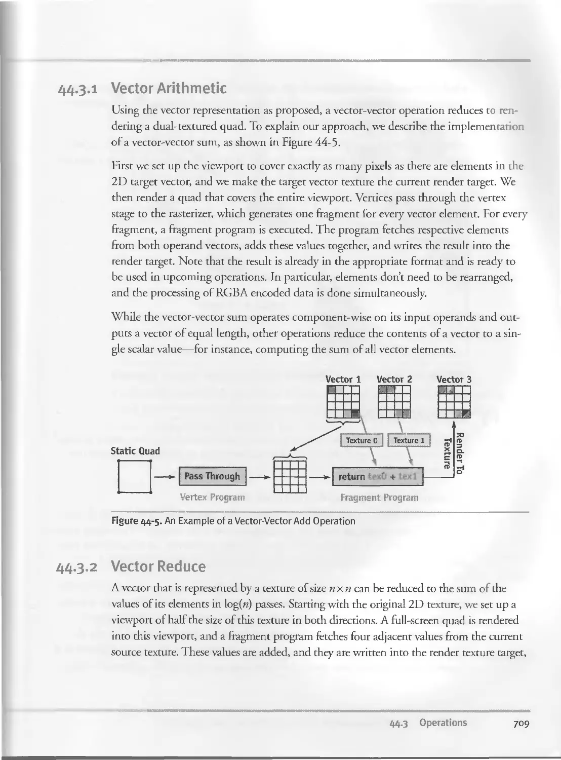
44.3.I Vector Arithmetic..................................709
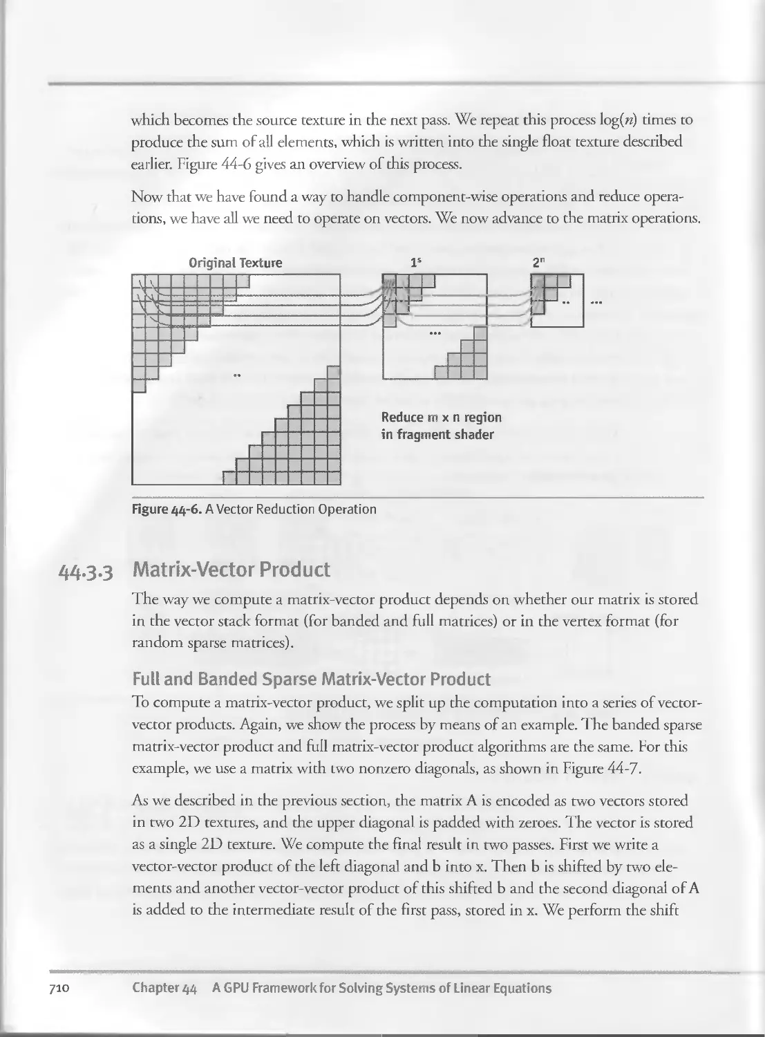
44-3-2 Vector Reduce.......................................709
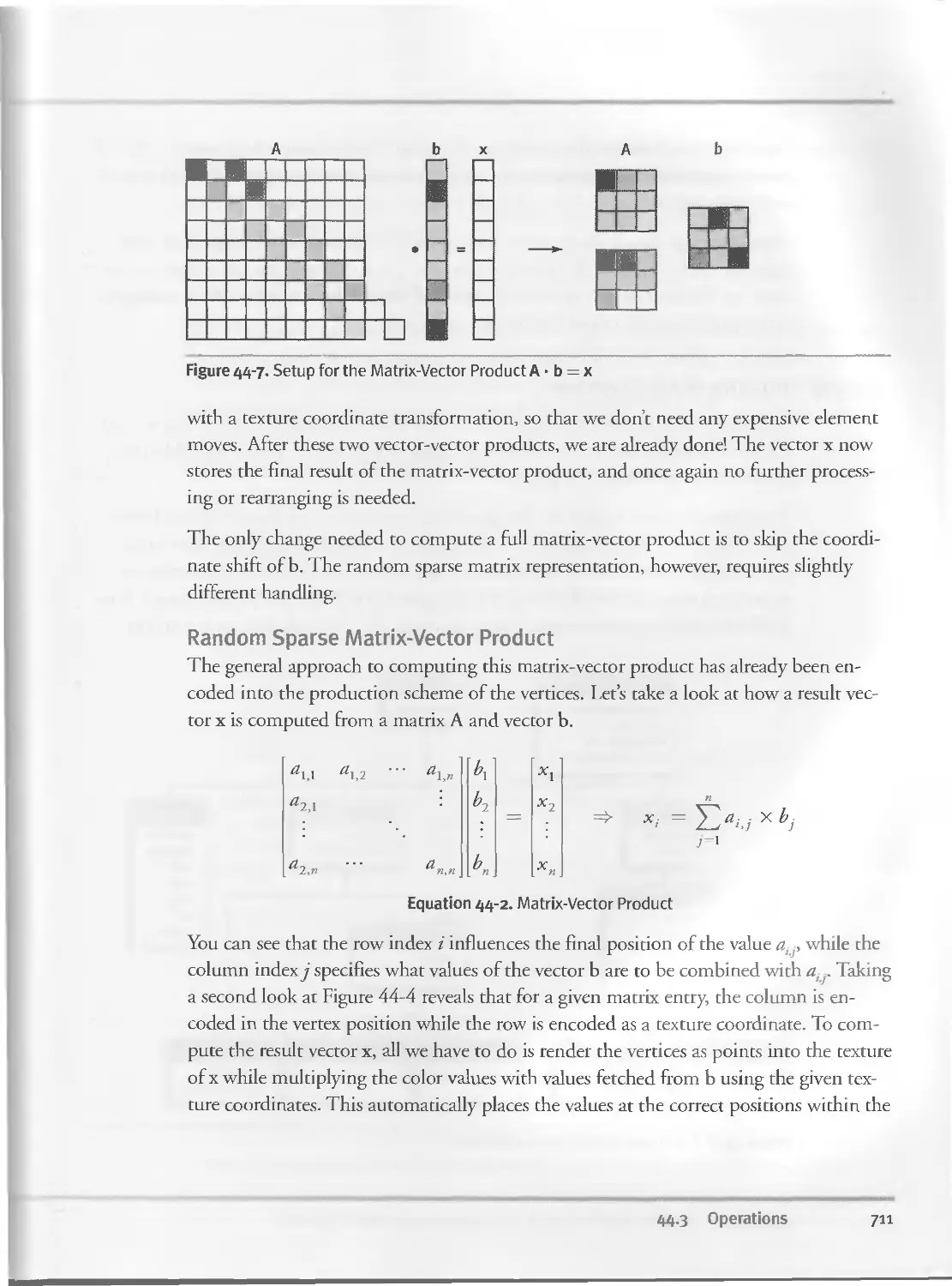
44-3-3 Matrix-Vector Product...............................710
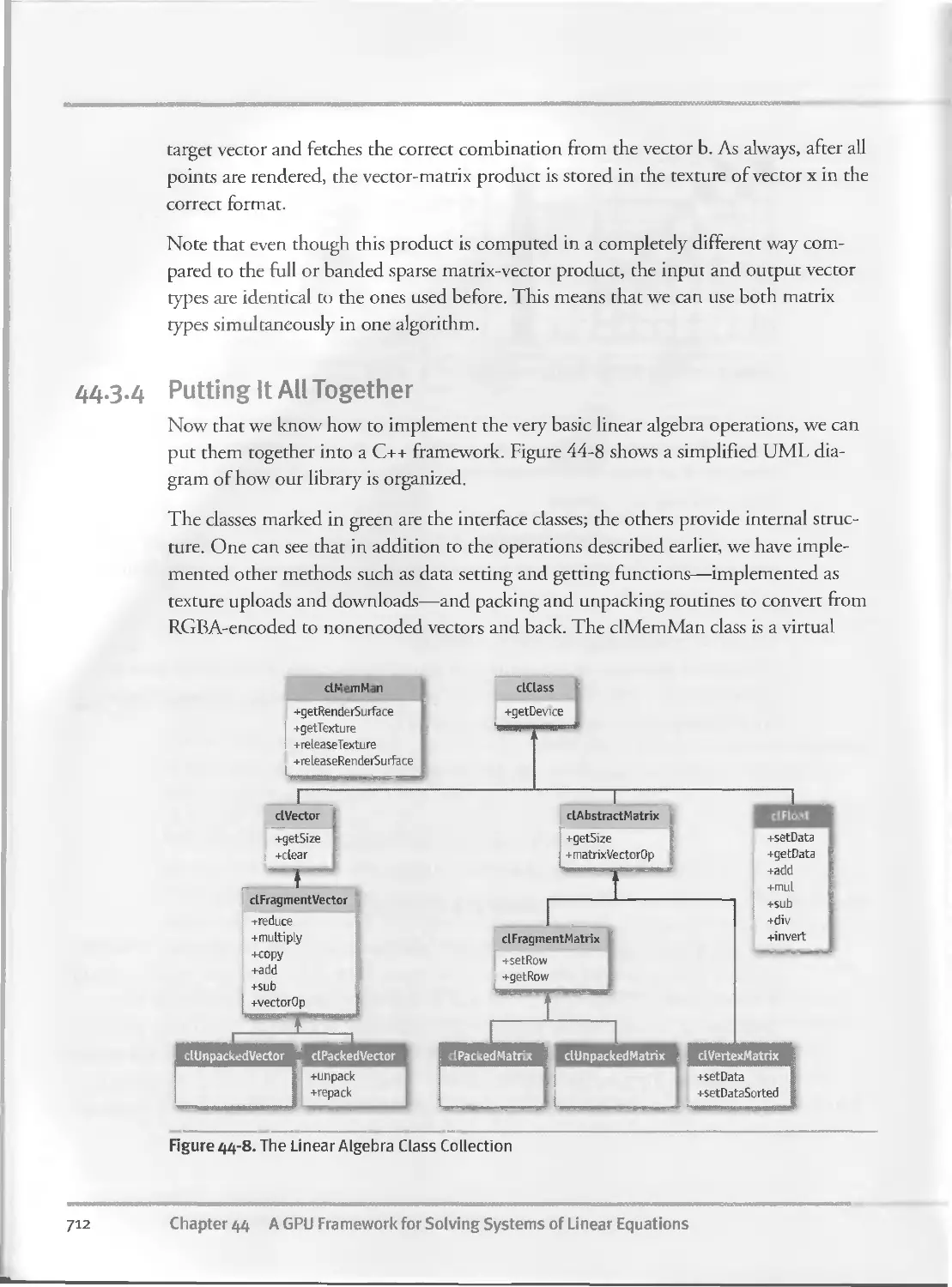
44.3.4 Putting It All Together............................712
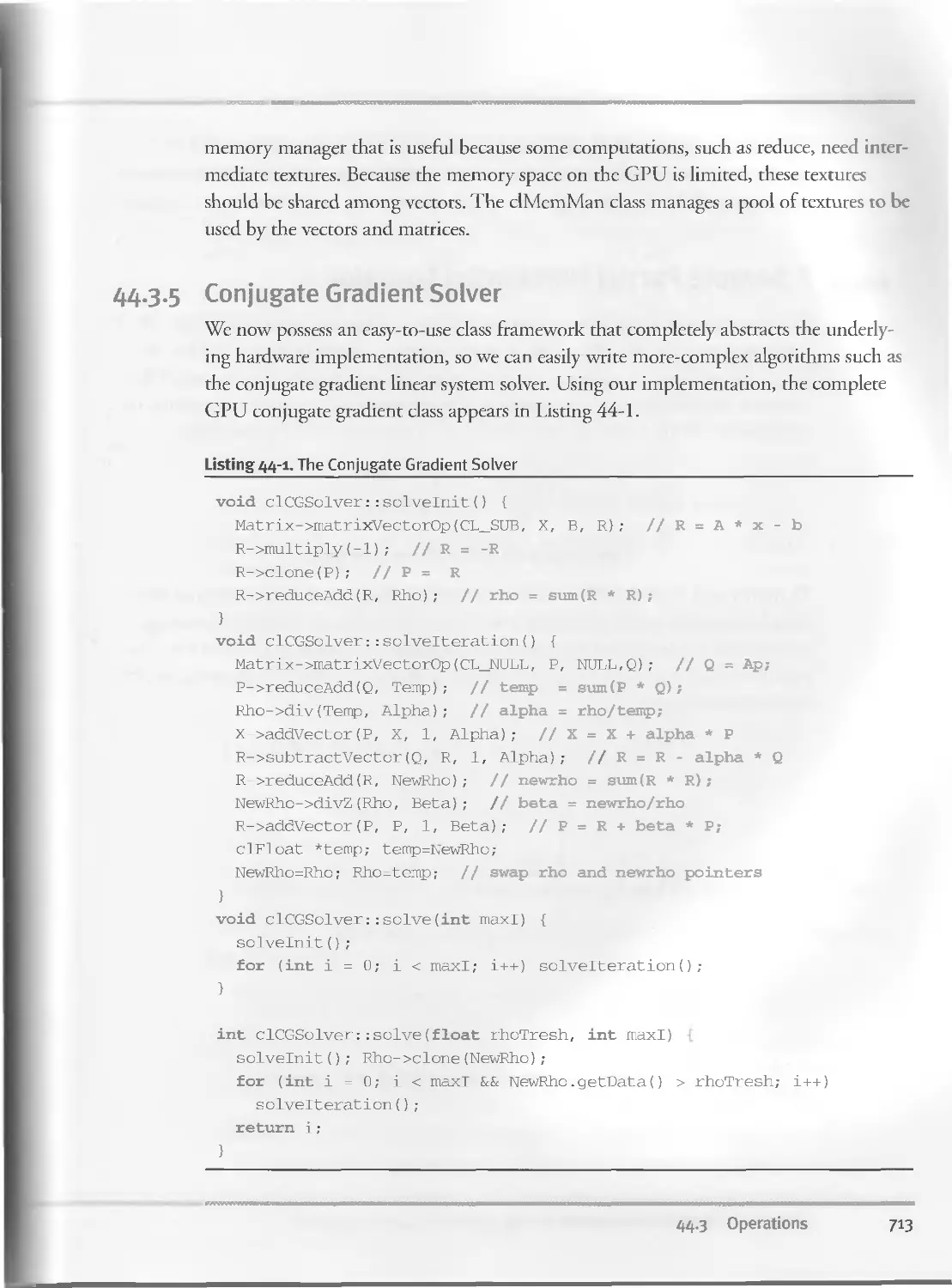
44-3-5 Conjugate Gradient Solver...........................713
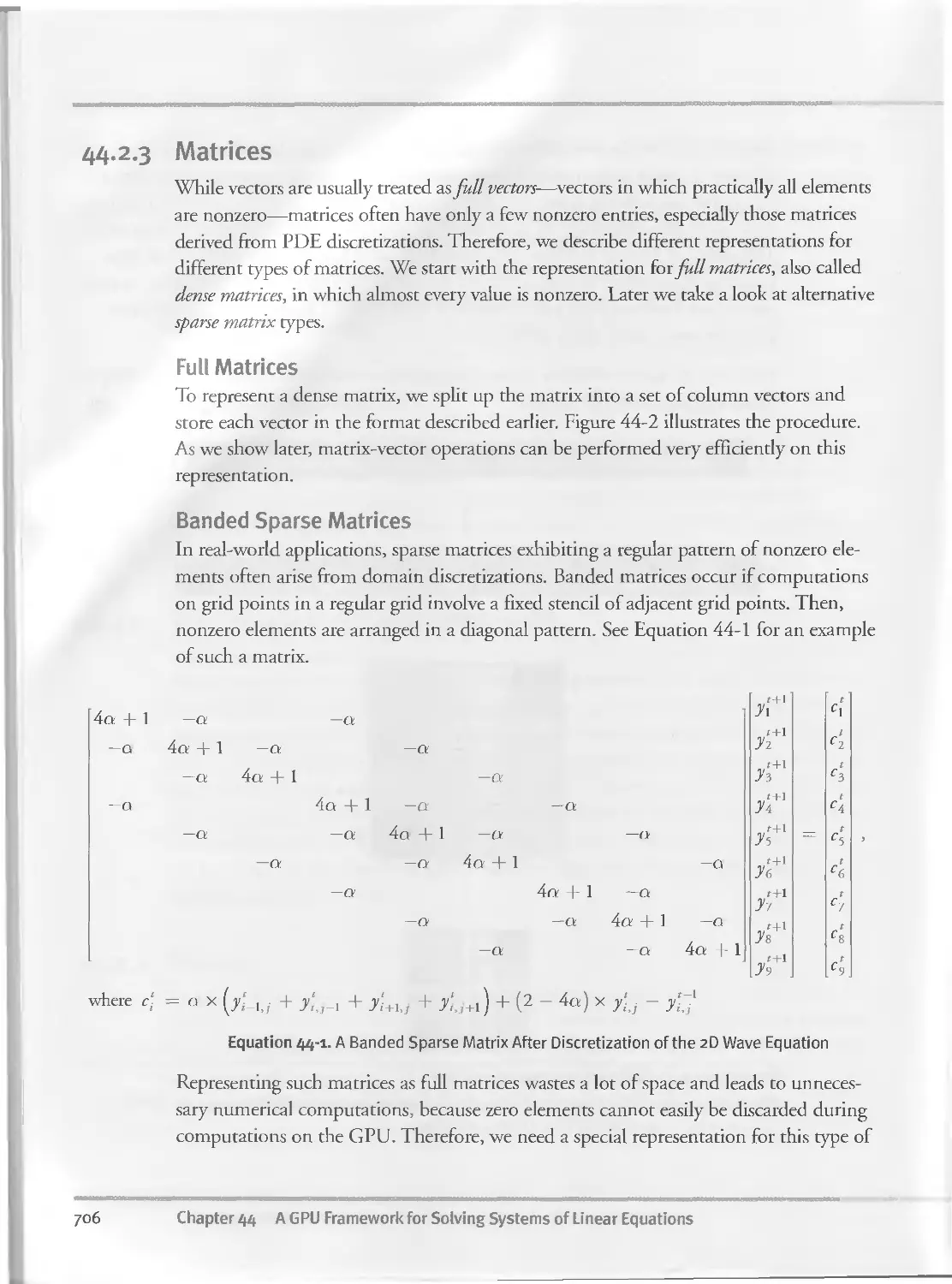
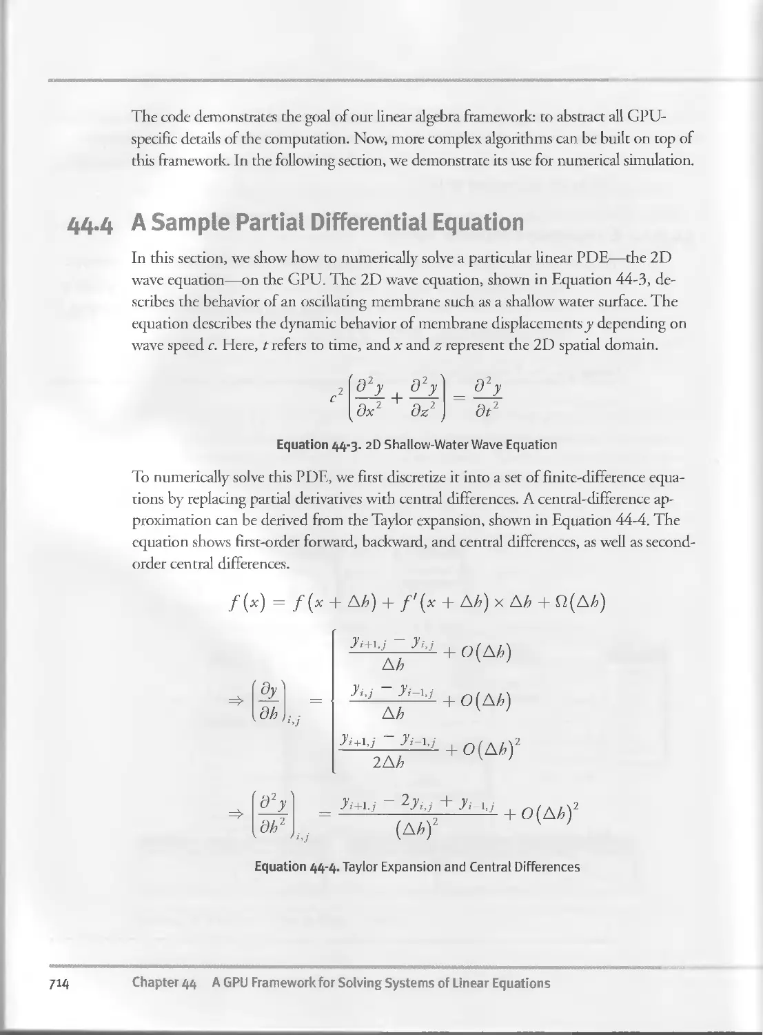
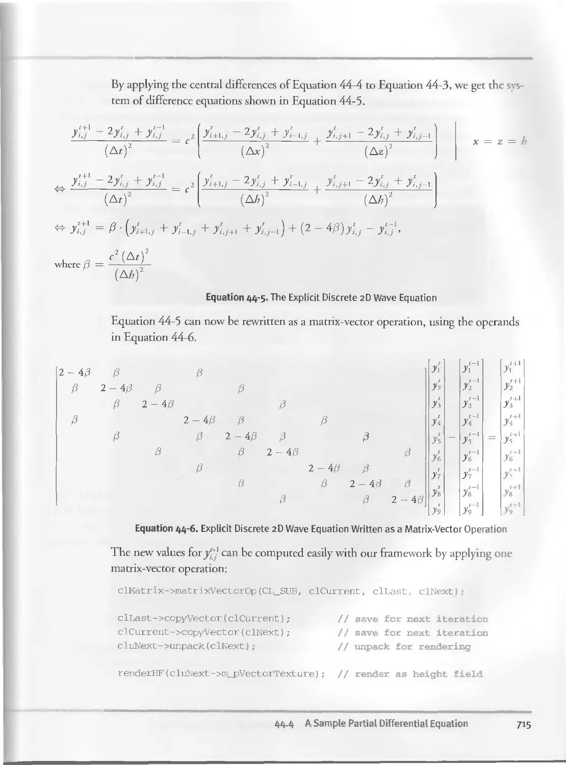
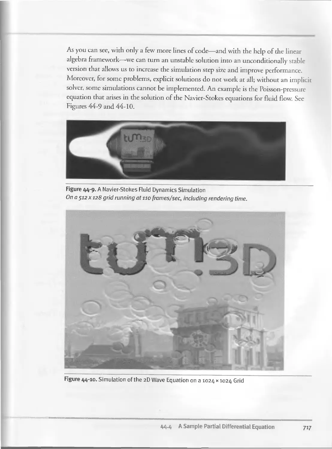
44.4 A Sample Partial Differential Equation ......... ............714
44-4-1 The Crank-Nicholson Scheme..........................716
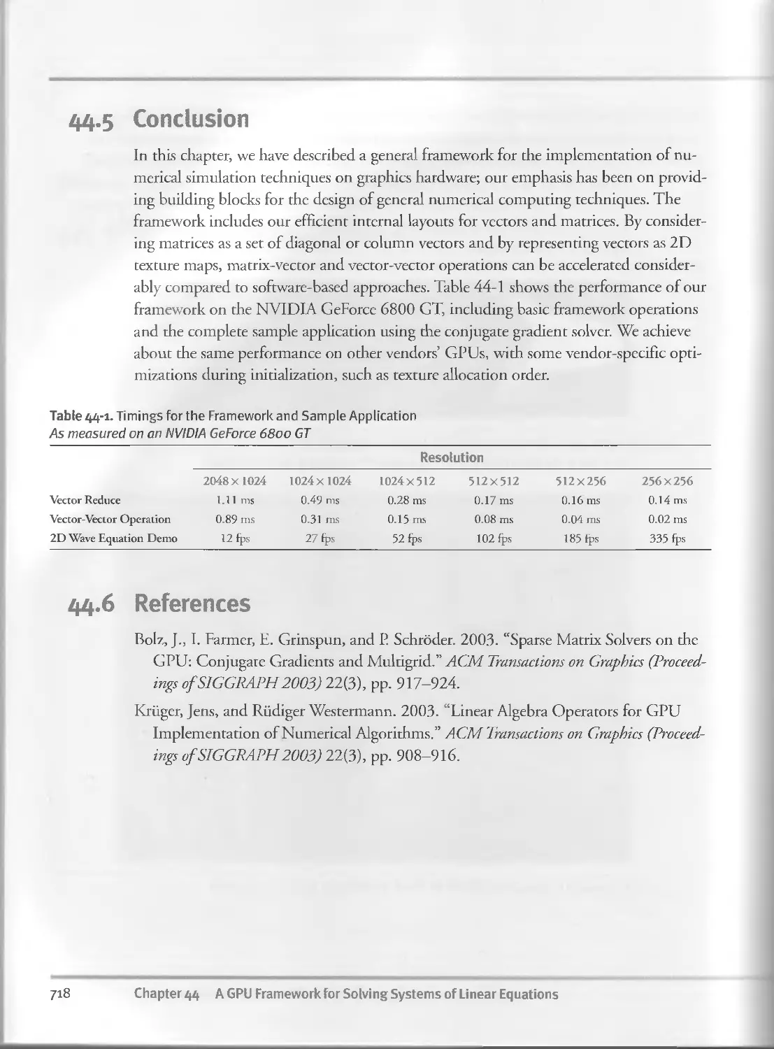
44-5 Conclusion...................................................718
44-6 References ..................................................718
Chapter 45
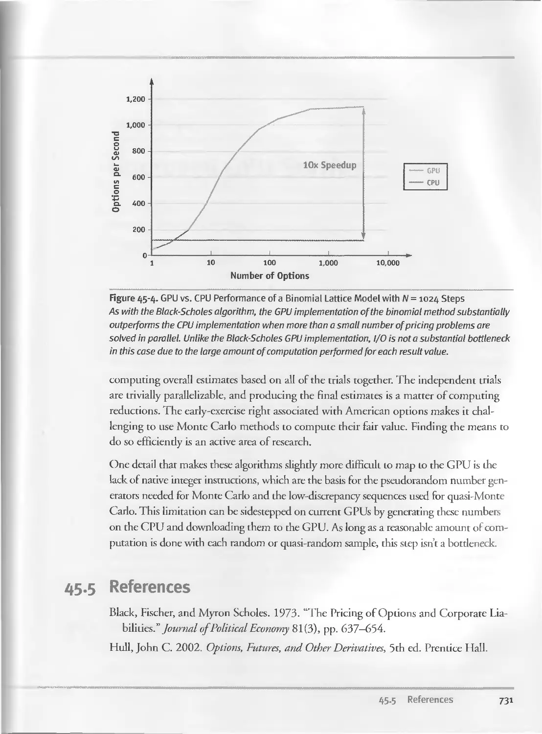
Options Pricing on the GPU..................................................719
Craig Kolb, NVIDIA Corporation
Matt Pharr, NVIDIA Corporation
45.1 What Are Options?...........................................719
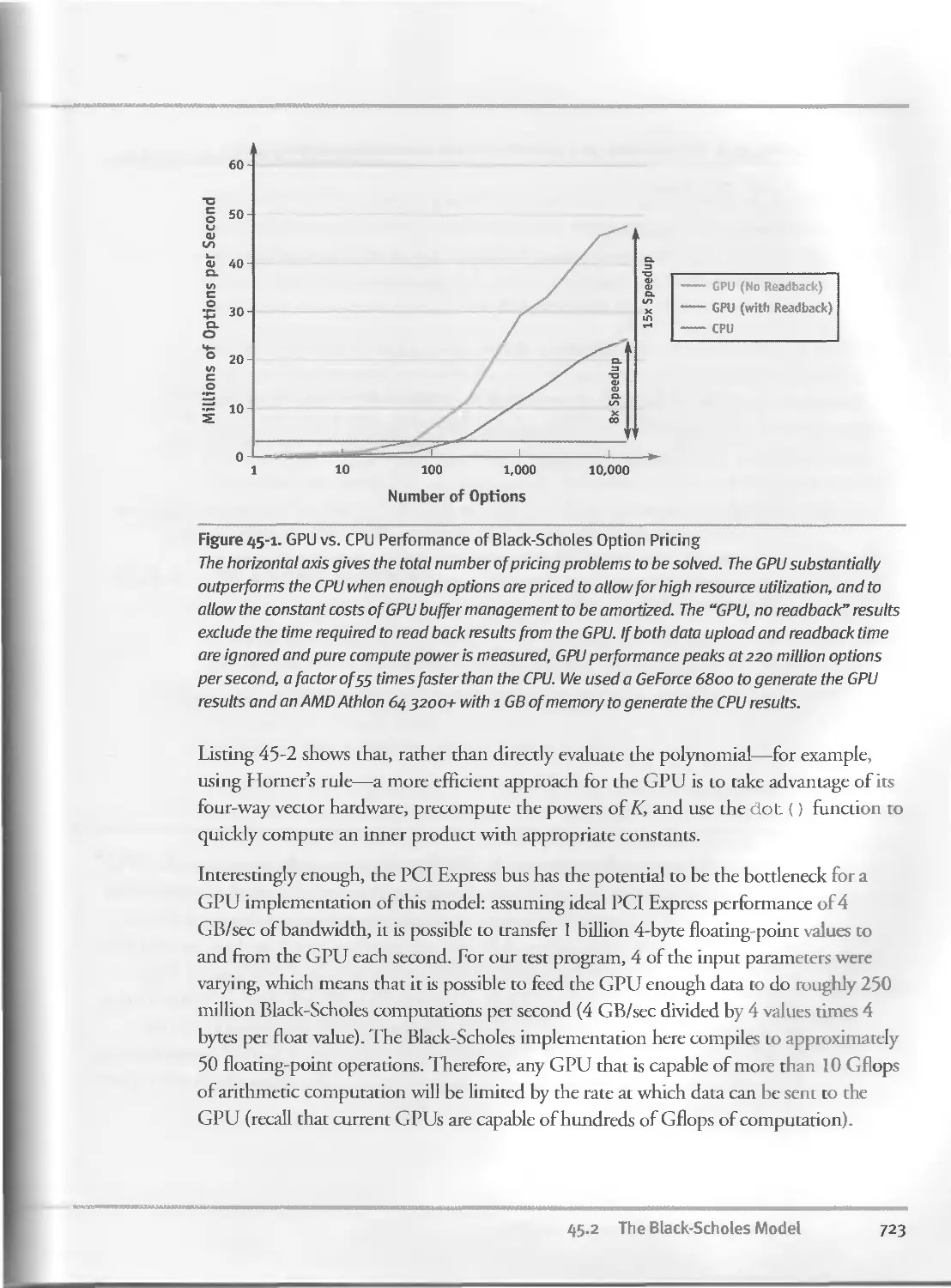
45.2 The Black-Scholes Model....................................721
45.3 Lattice Models.............................................725
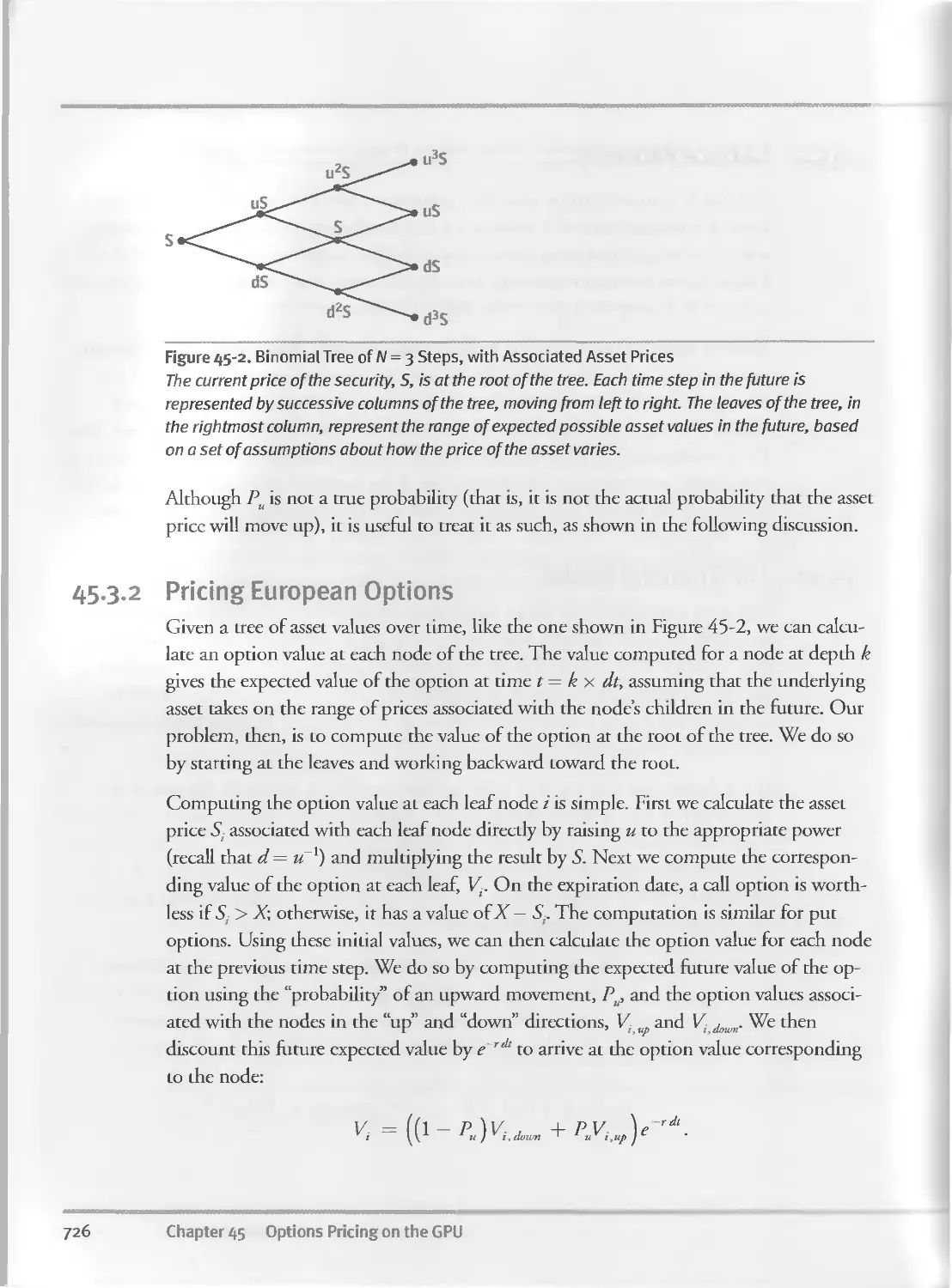
45-3-1 The Binomial Model..................................725
45.3.2 Pricing European Options............................726
45.4 Conclusion.................................................73°
45.5 References..................................................731
Chapter 46
Improved GPU Sorting........................................................733
Peter Kipfer, Technische Universitat Munchen
Rudiger Westermann, Technische Universitat Munchen
46.1 Sorting Algorithms.........................................733
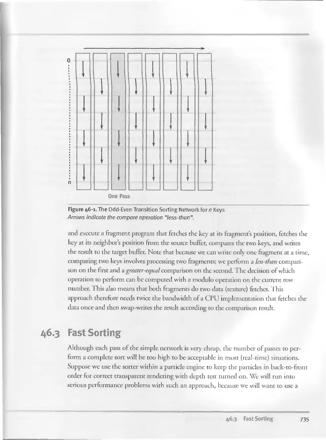
46.2 A Simple First Approach....................................734
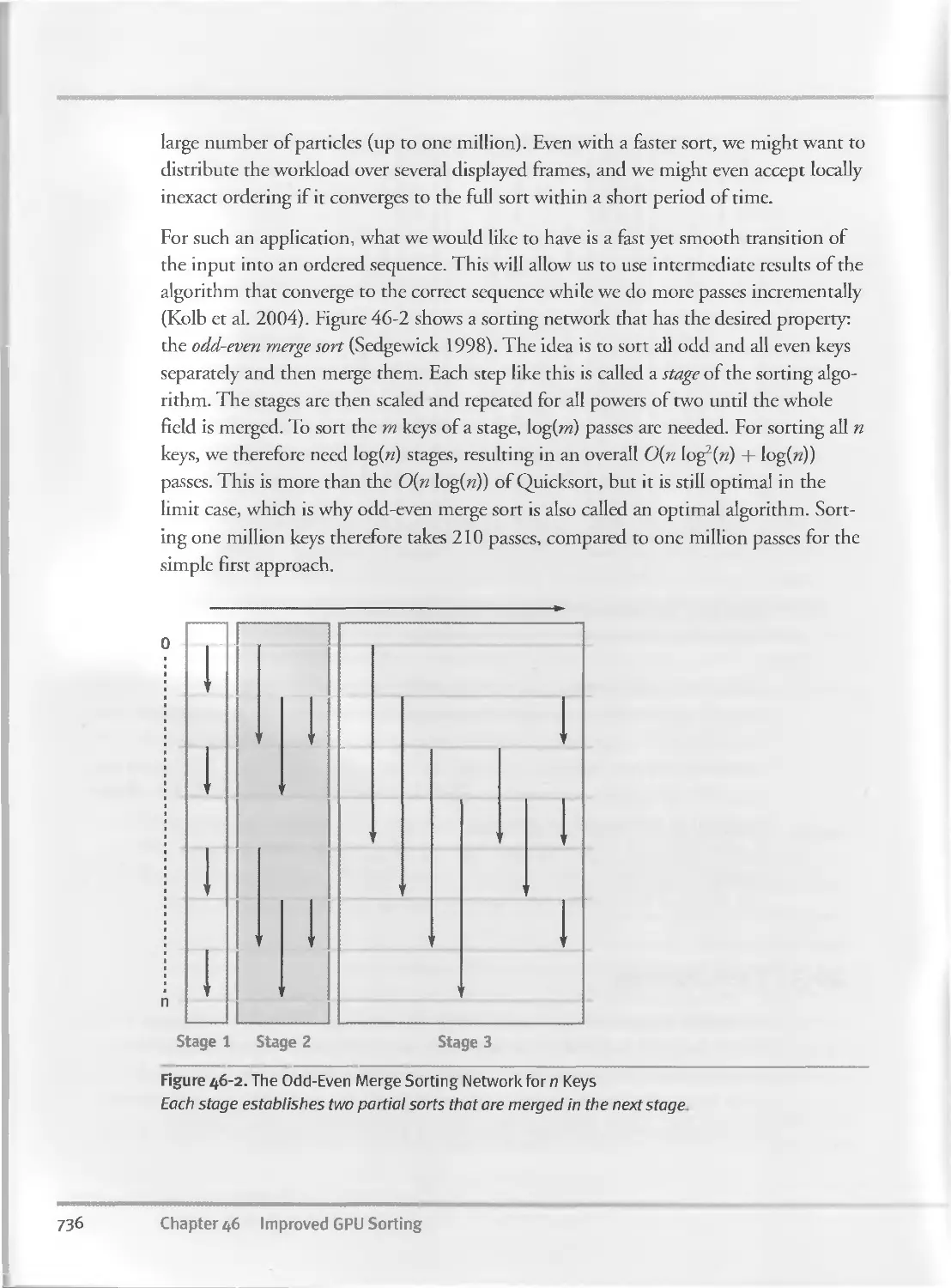
46.3 Fast Sorting...............................................735
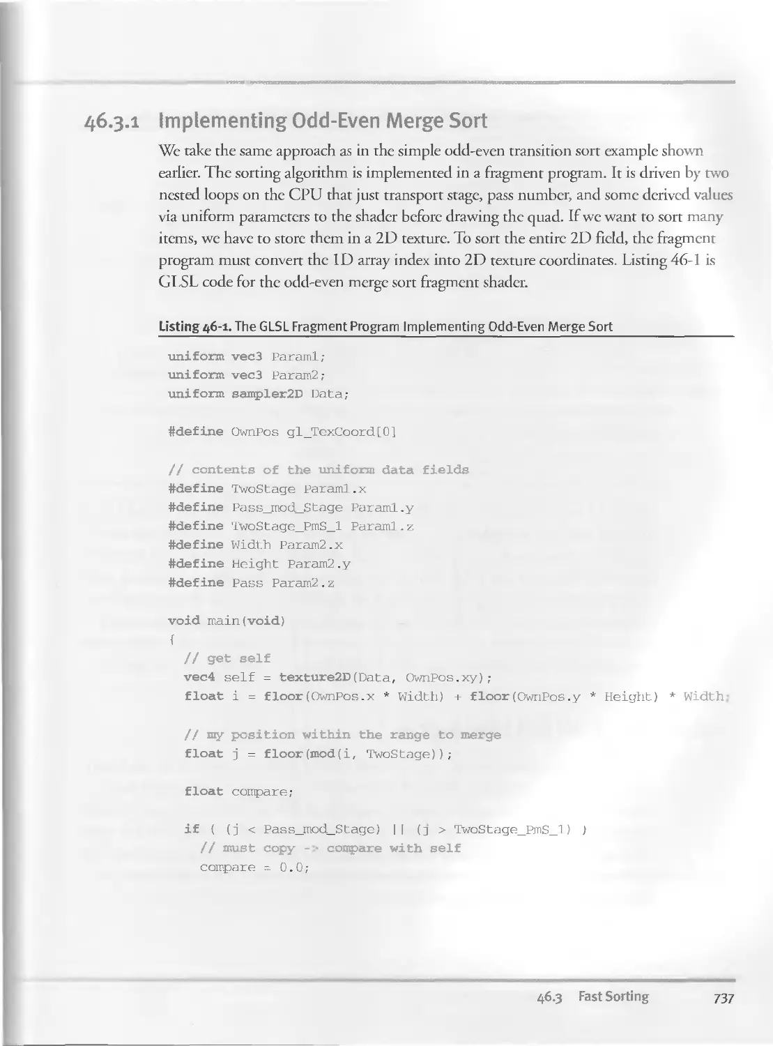
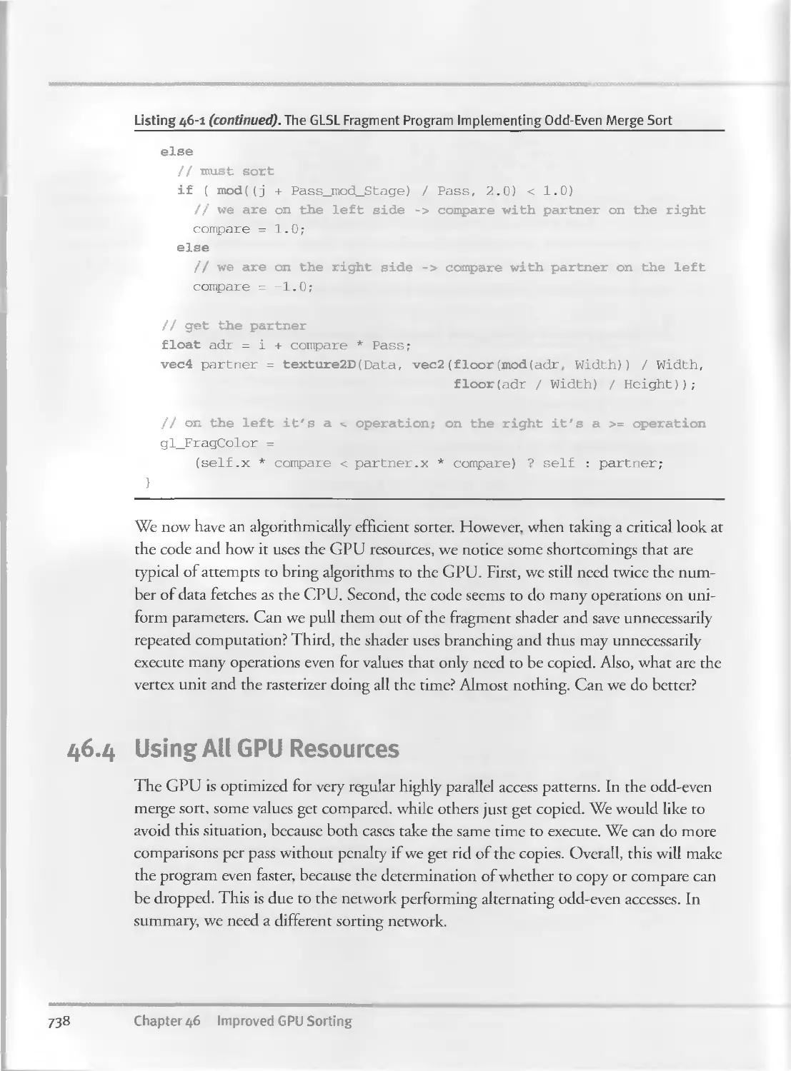
46.3.I Implementing Odd-Even Merge Sort....................737
46.4 Using All GPU Resources............................... --738
46.4.I Implementing Bitonic Merge Sort.................. ... 743
46.5 Conclusion................................................ 745
46.6 References.................................................746
Contents
xxvii
Chapter 47
Flow Simulation with Complex Boundaries....................................747
Wei Li, Siemens Corporate Research
Zhe Fan, Stony Brook University
Xiaoming Wei, Stony Brook University
Arie Kaufman, Stony Brook University
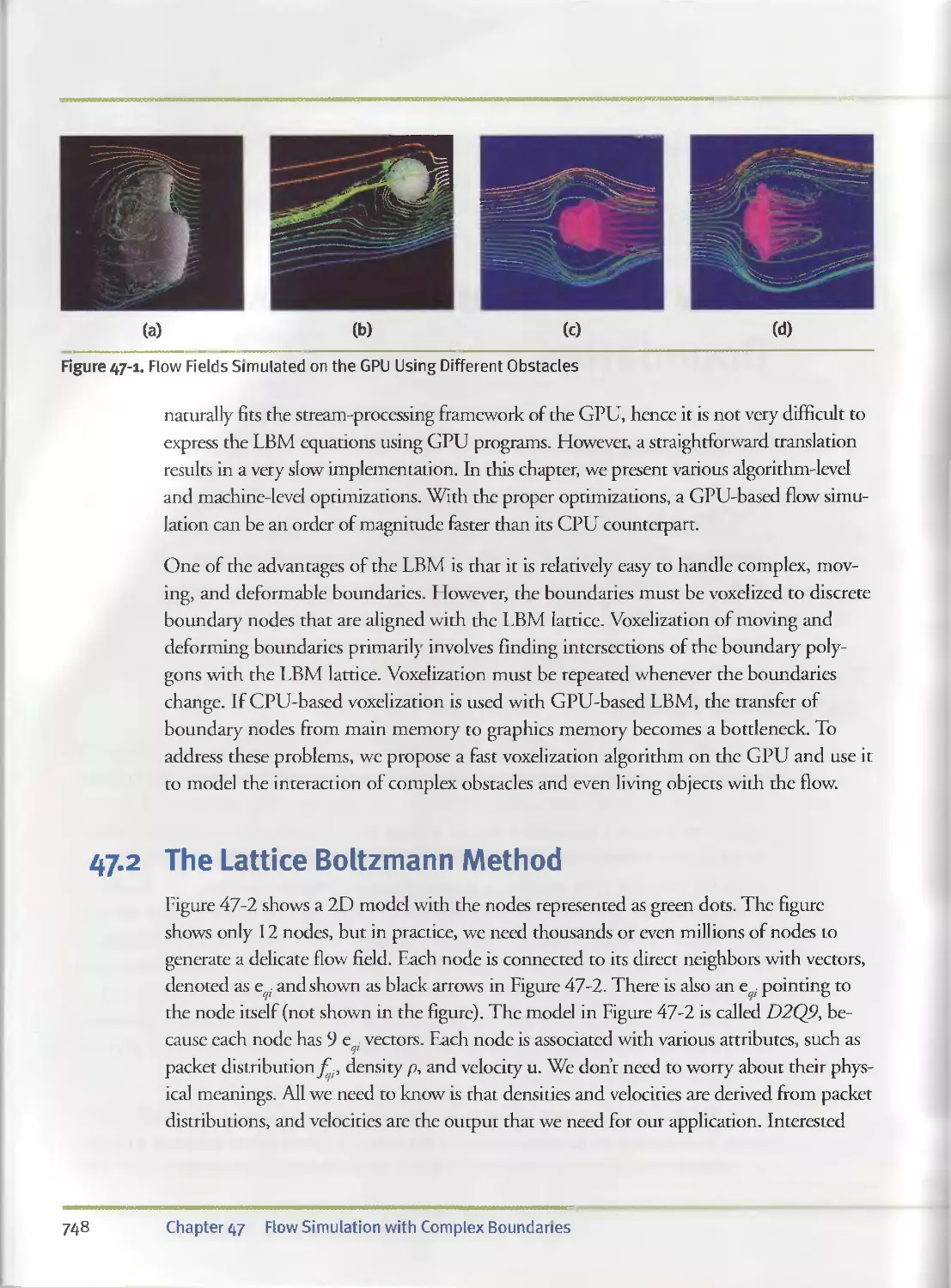
ltf.1 Introduction................................................747
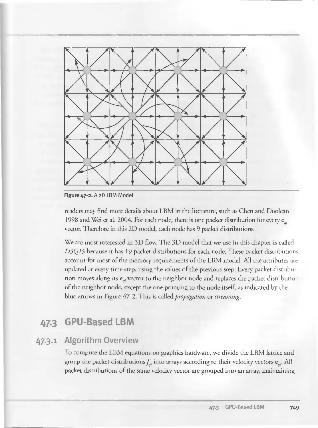
47.2 The Lattice Boltzmann Method................................748
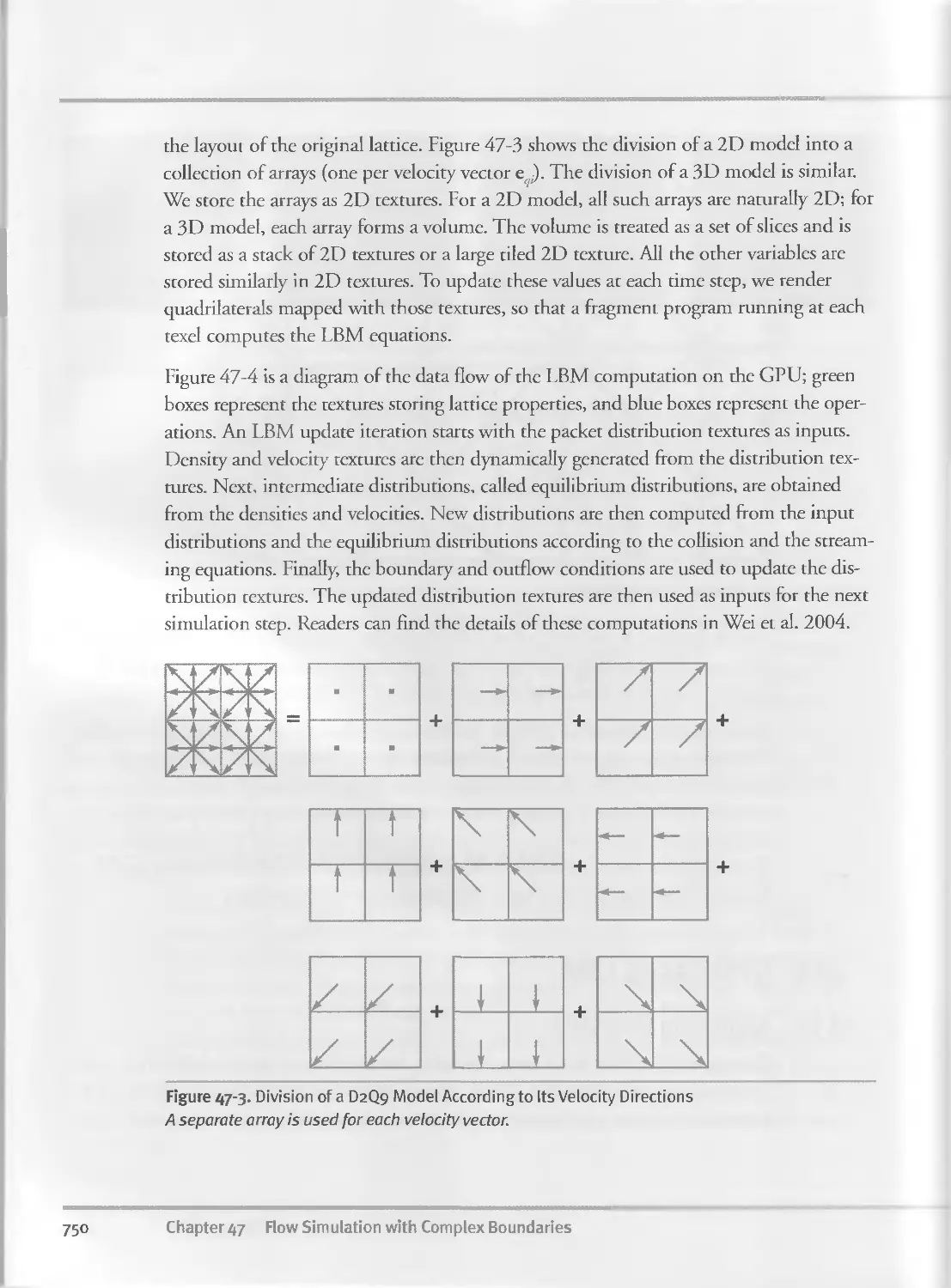
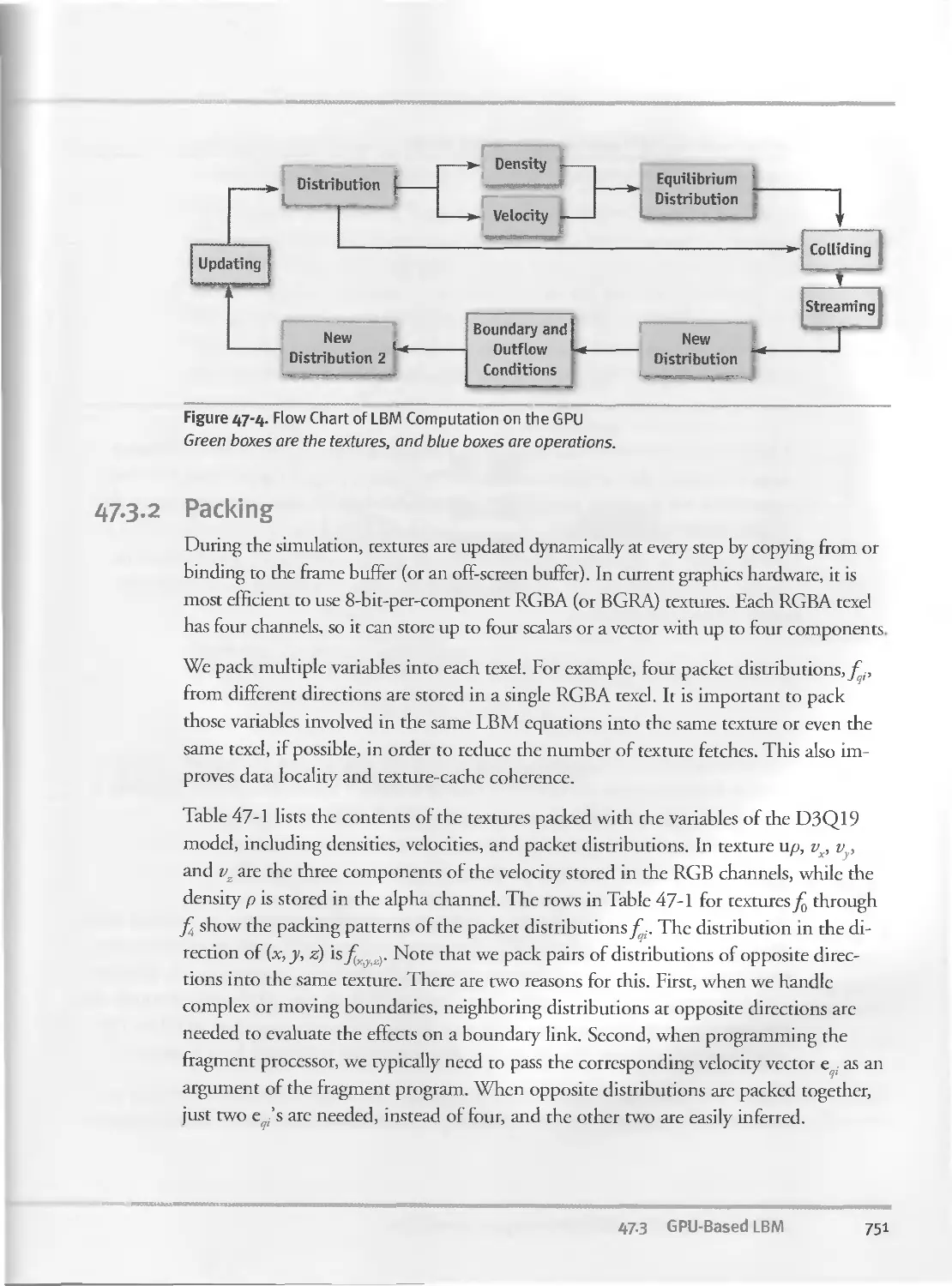
47.3 GPU-Based LBM...............................................749
47.3.I Algorithm Overview.................................749
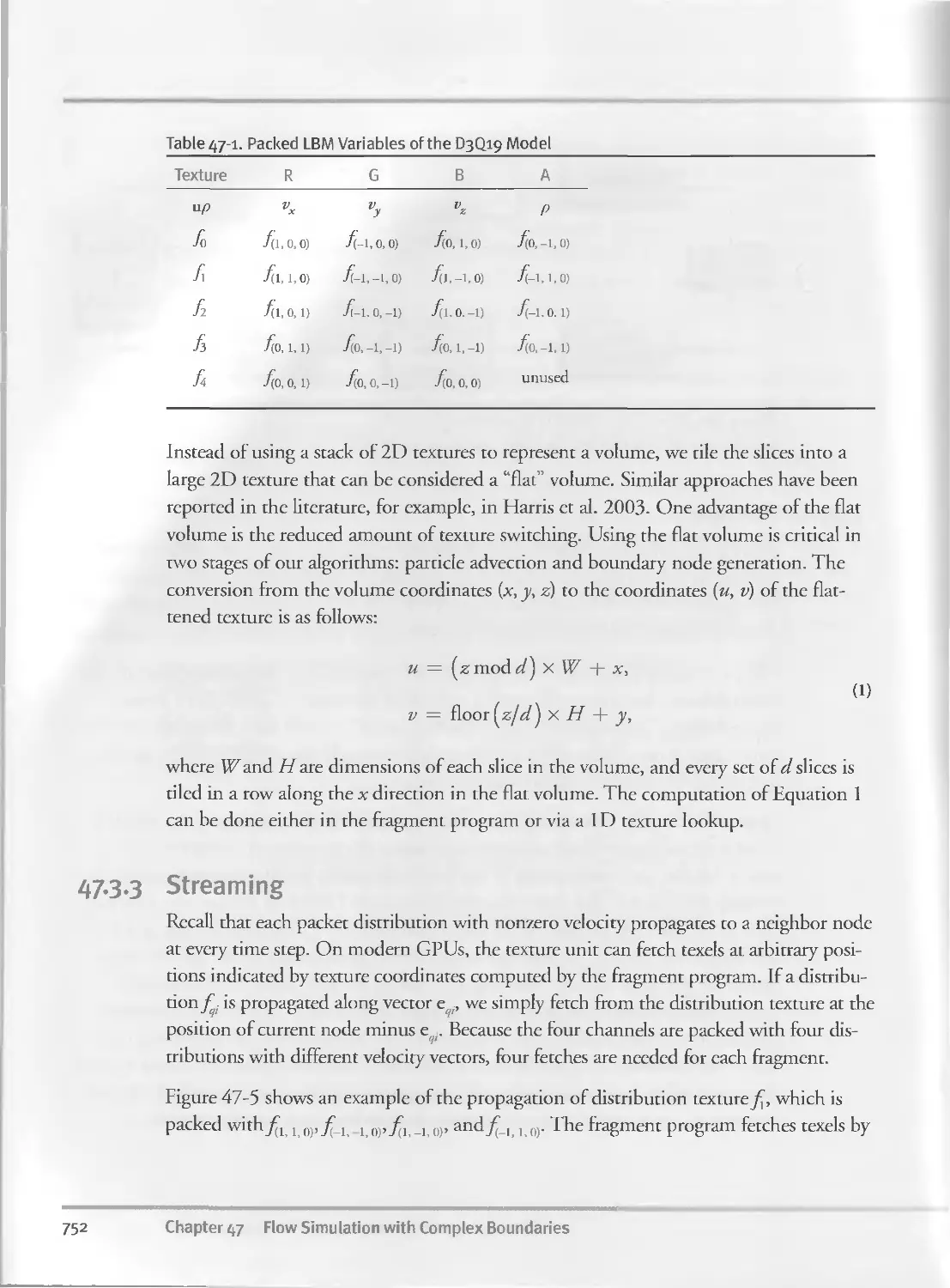
47.3.2 Packing............................................751
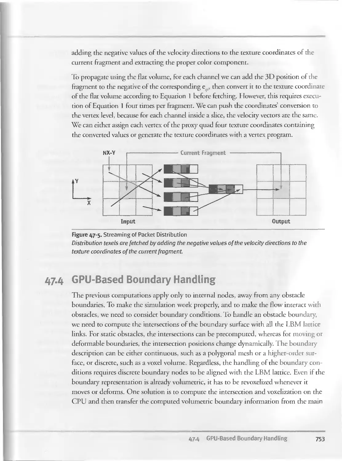
47.3.3 Streaming........................................-jtyi
Itf.li GPU-Based Boundary Handling ... ...........................753
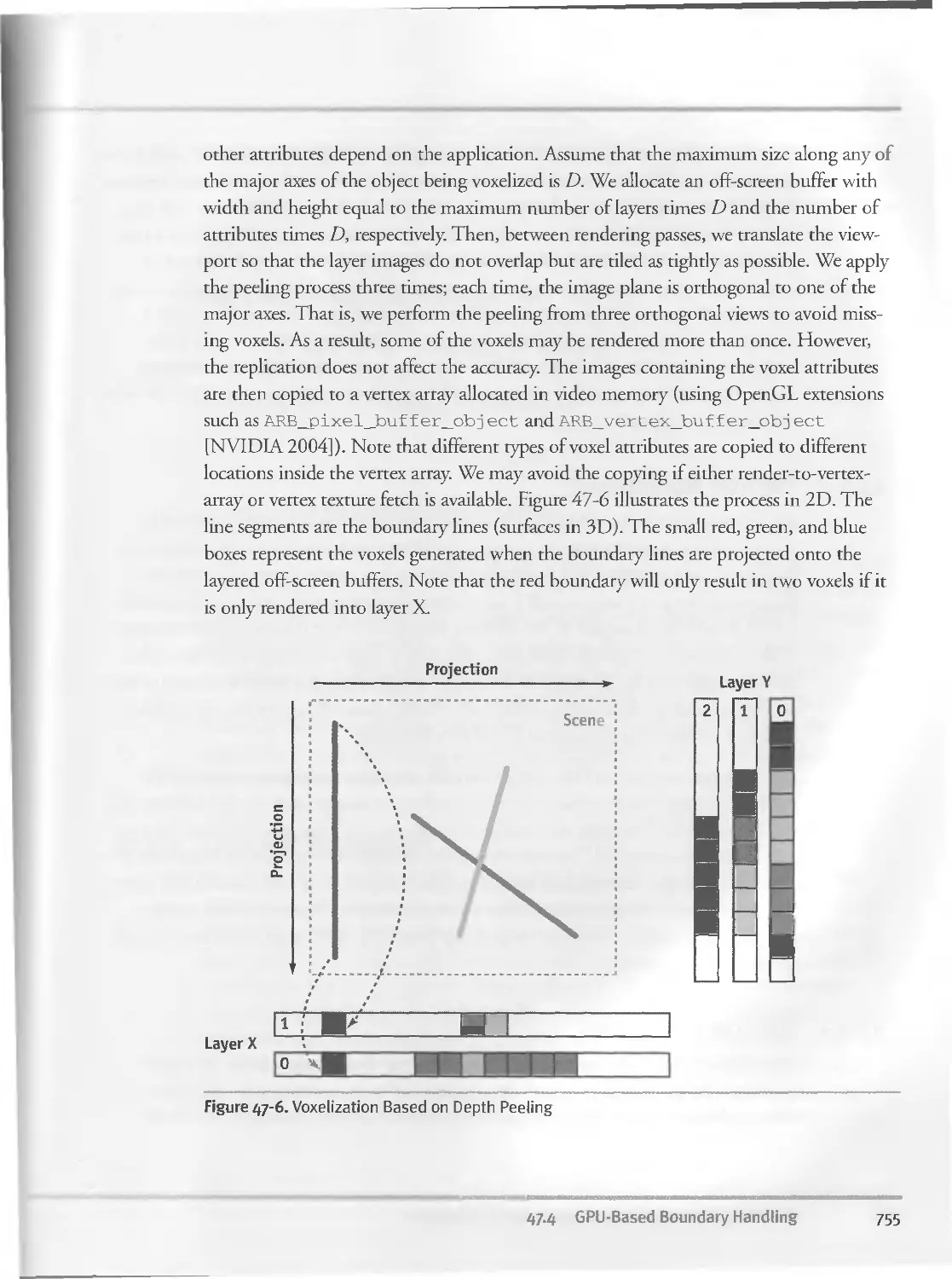
47-4-1 GPU-Based Voxelization.............................754
Periodic Boundaries................................756
47-4-3 Outflow Boundaries.................................756
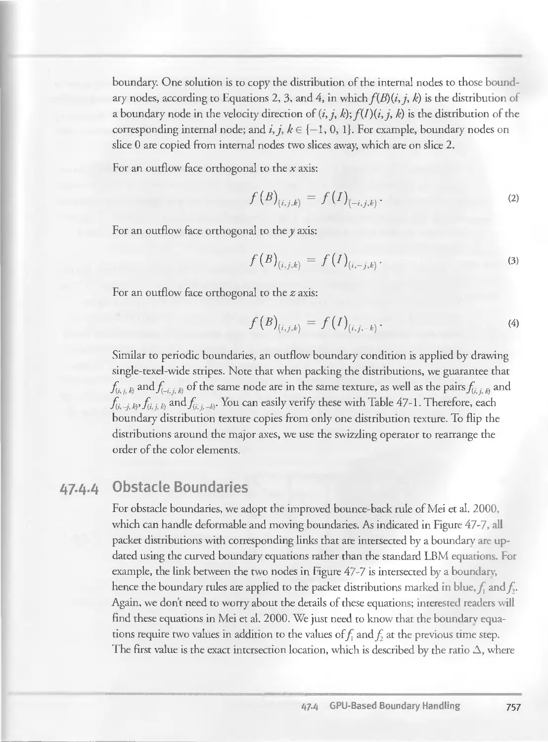
47.4.4 Obstacle Boundaries................................757
47.5 Visualization...............................................759
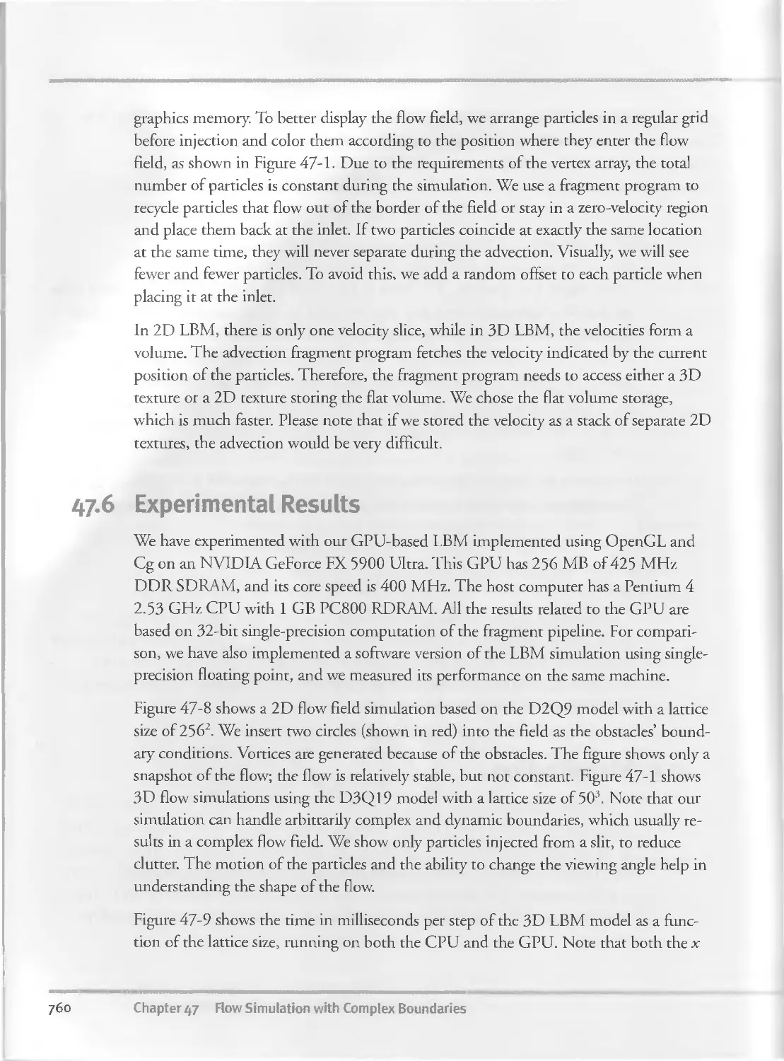
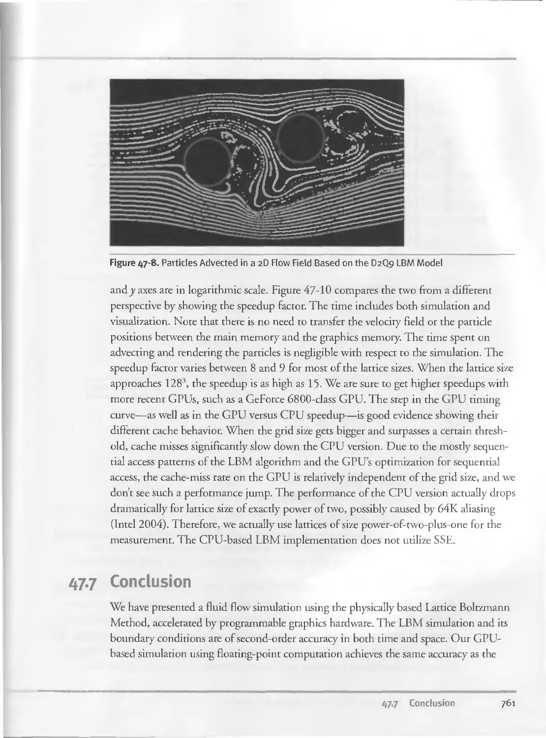
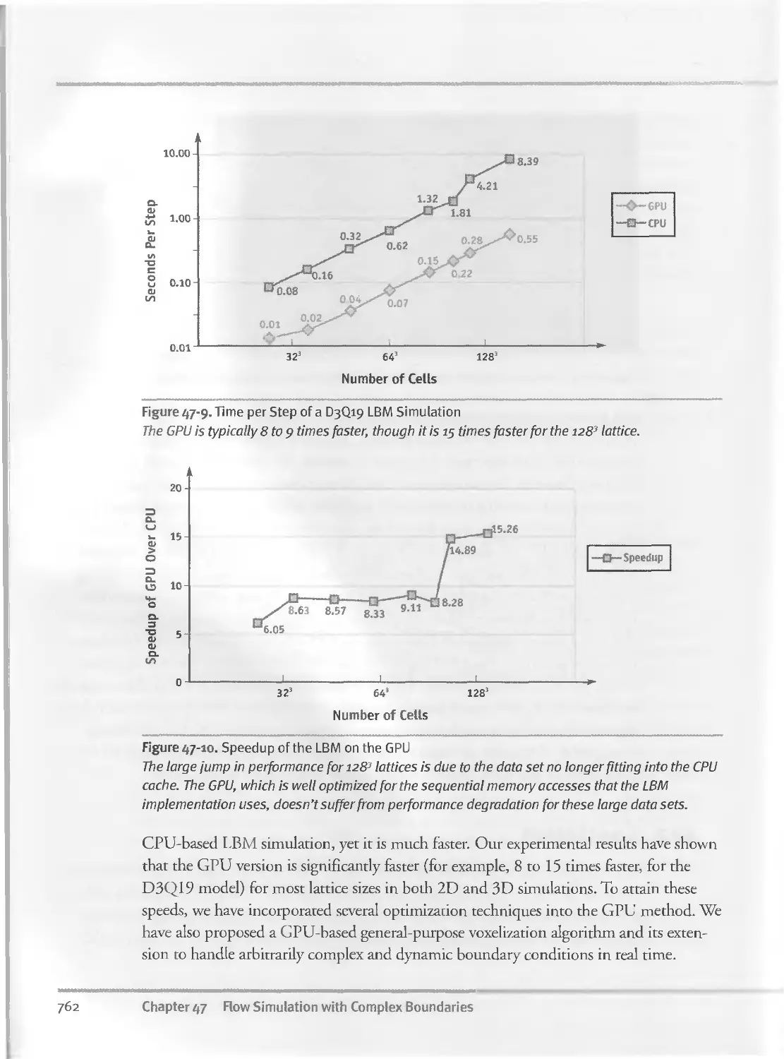
47.6 Experimental Results.......................................76 О
47.7 Conclusion................................................ 761
47-8 References................................................. 763
Chapter 48
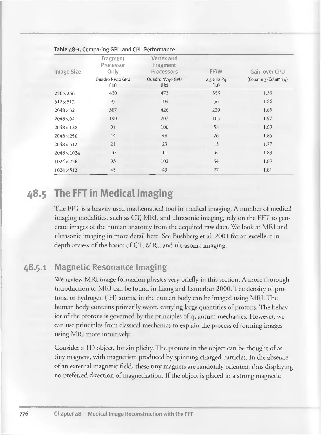
Medical Image Reconstruction with the FFT..................................765
Thilaka Sumanaweera, Siemens Medical Solutions USA
Donald Liu, Siemens Medical Solutions USA
48.1 Background...................................................765
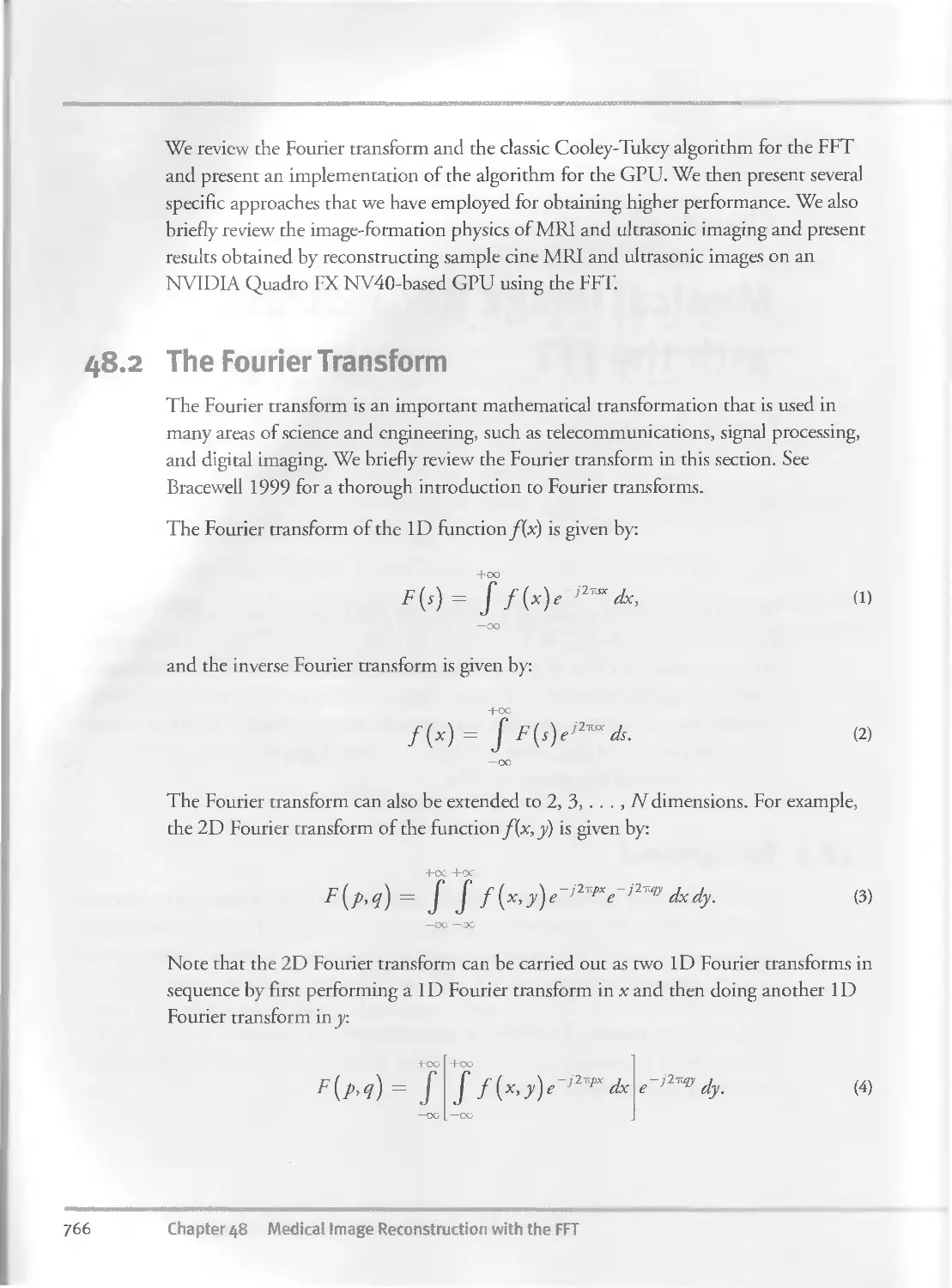
48.2 The Fourier Transform......................................766
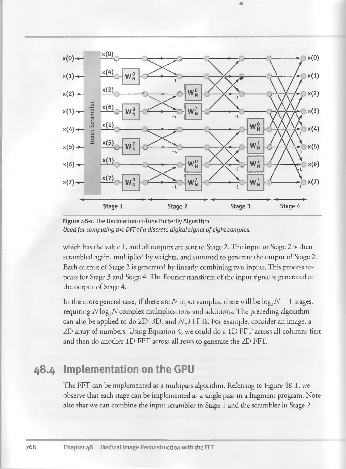
48.3 The FFT Algorithm..........................................7^7
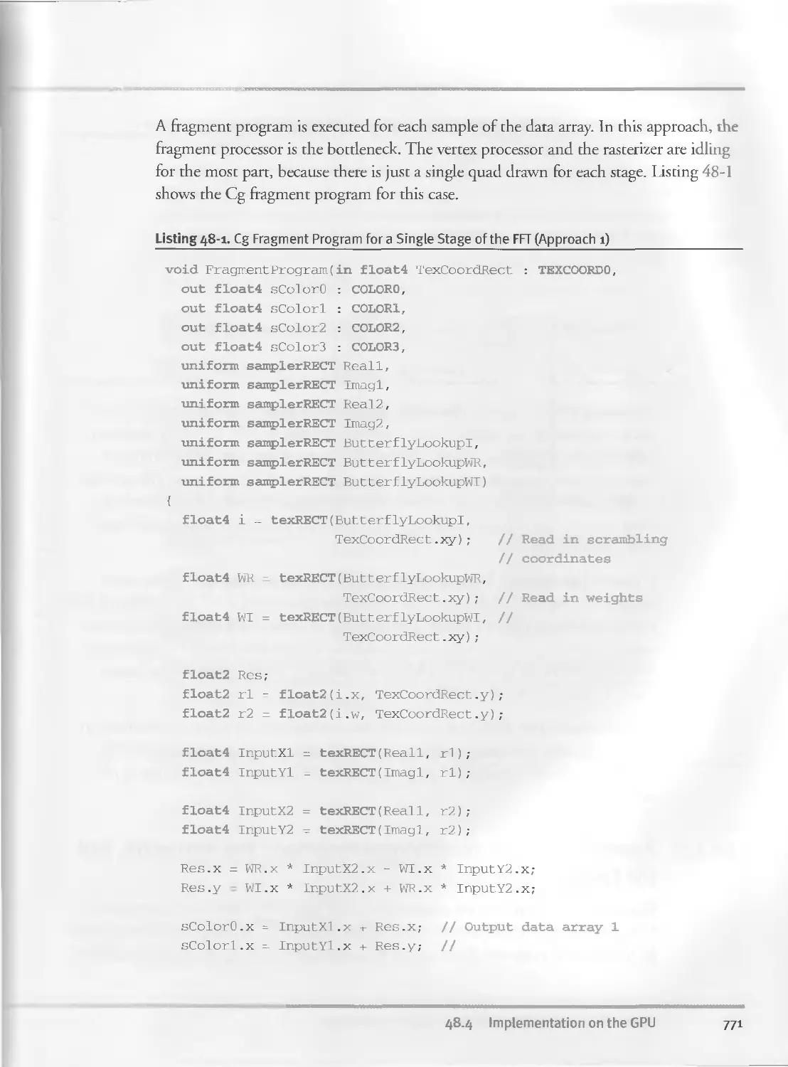
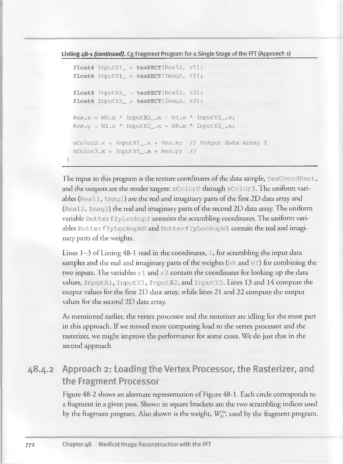
48.4 Implementation on the GPU..................................768
48.4.1 Approach 1: Mostly Loading the Fragment Processor...770
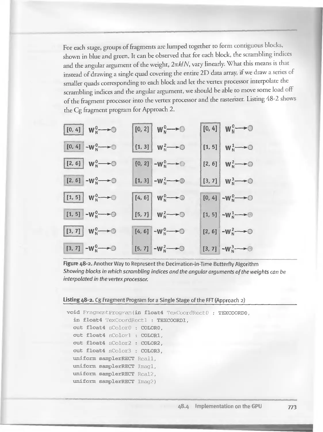
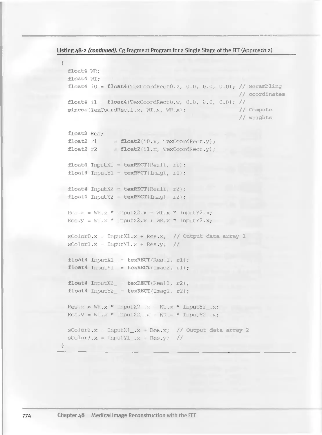
48.4.2 Approach 2: Loading the Vertex Processor, the Rasterizer,
and the Fragment Processor................................772
48.4.3 Load Balancing......................................775
48.4.4 Benchmarking Results................................775
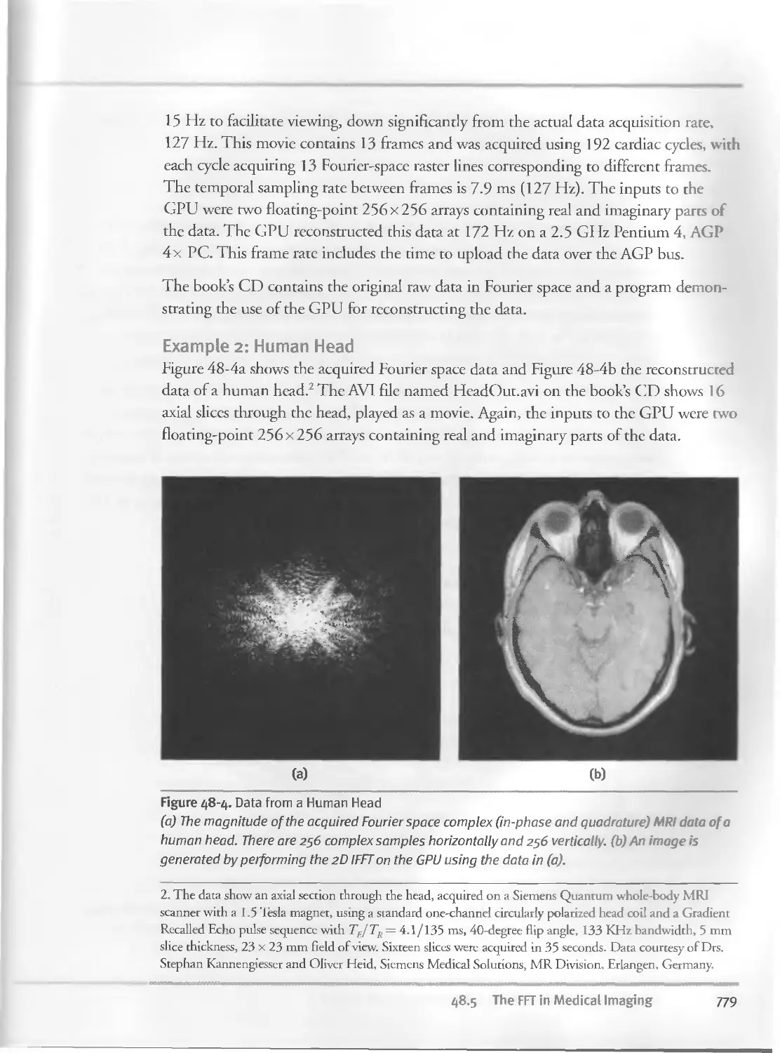
48.5 The FFT in Medical Imaging.................................776
48.5.1 Magnetic Resonance Imaging..........................
48.5.2 Results in MRI......................................778
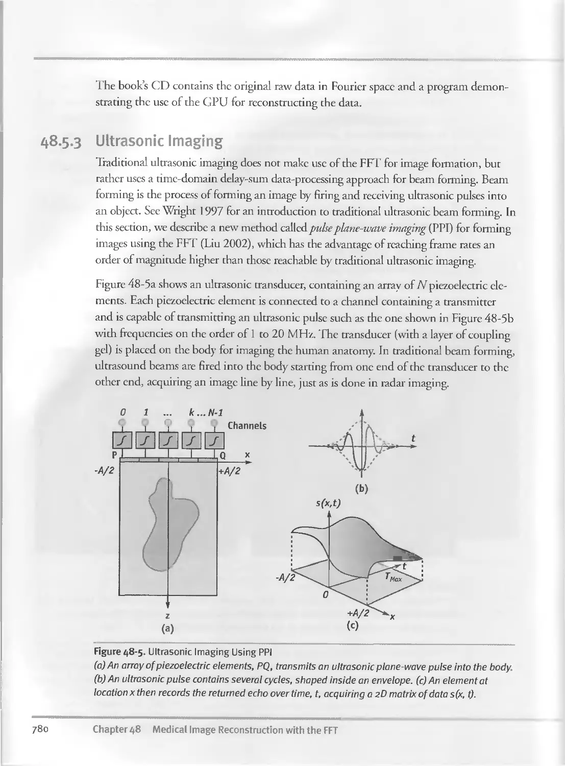
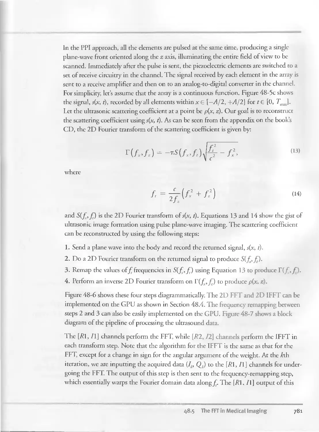
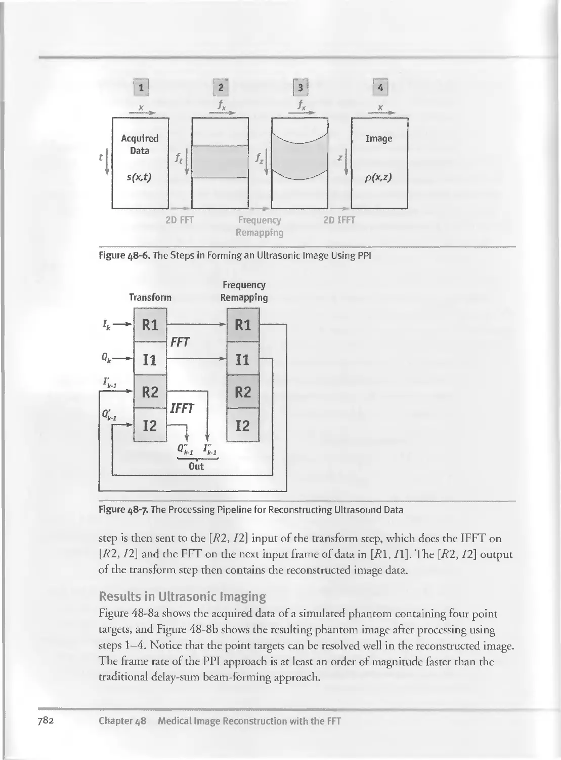
48.5.3 Ultrasonic Imaging..................................780
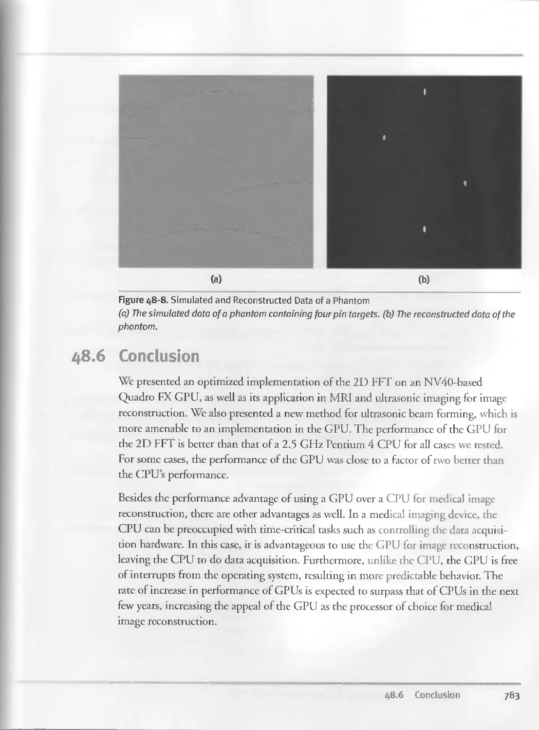
48.6 Conclusion............................................. 783
48.7 References............................................... 784
Index.......................................................................785
xxviii
Contents
Foreword
iiimimii—w miii win iiiirmiiii
Before the advent of dedicated PC graphics hardware, the industry’s first 3D games used
CPU-based software rendering. I wrote the first Unreal Engine in that era, inspired by
John Carmack’s pioneering programming work on Doom and Quake. Despite slow
CPUs and low resolutions, the mid-1990s became a watershed time for graphics and
gaming. New visual effects appeared almost monthly, marked by milestones like Quakes
light mapping and shadowing and Unreal’s colored lighting and volumetric fog. That era
faded away as fixed-function 3D accelerators appeared. Deprived of the programmabil-
ity that drove innovation and differentiation, 3D games grew indistinct.
Today, a new Renaissance in 3D graphics is under way, driven by fully programmable
GPUs—graphics processing units—that deliver thousands of times the graphics power avail-
able just ten years ago. Combining incredible parallel computing power with modern,
high-level programming languages, today’s GPUs have unleashed a Cambrian Explosion
of innovation and creativity. Real-time soft shadowing, accurate lighting models, and real-
istic material interactions are readily achievable. But the most important gain of program-
mability is that you can do anything with a GPU so long as you can find an algorithm to
express your idea. GPU Gems 2 demonstrates many such ideas-turned-algorithms.
Let us take a moment to review the set of resources available to today’s graphics pro-
grammer. First, you have access to a GPU that can perform tens of billions of floating-
point calculations per second in programmable shading algorithms. It’s your workhorse;
if you can move your problem into the realm of pixels and vertices, then you can har-
ness the GPU’s immense power. Second, you have a CPU, the system’s general-purpose
computing engine. The CPU sends commands to the graphics processing unit, man-
ages resources, and interacts with the outside world. Finally, you have access to artistic
content—texture maps, meshes, and other multimedia data that the GPU can com-
bine, filter, and procedurally modify during rendering.
The Gems in this book employ these resources in novel ways to render realistic scenes,
process images, and produce special effects. In doing so, many of the previous era’s
Foreword xxix
graphics rules may be broken. GPUs are fast and flexi-
ble enough that you may render a given object many
times, decomposing a scene into its components—
lighting, shadowing, reflections, post-processing ef-
fects, and so on. You can employ the GPU for
decidedly non-graphics tasks like collision detection,
physics, and numerical computation; and within tex-
ture maps you can encode arbitrary data, such as vec-
tors, positions, or lookup tables used by shader
programs. And while visual realism is now achievable
on GPUs, it is not your only option: nonphotorealistic rendering techniques are avail-
able, such as cel shading, exaggerated motion blur and light blooms, and other effects
seen frequently in Hollywood productions.
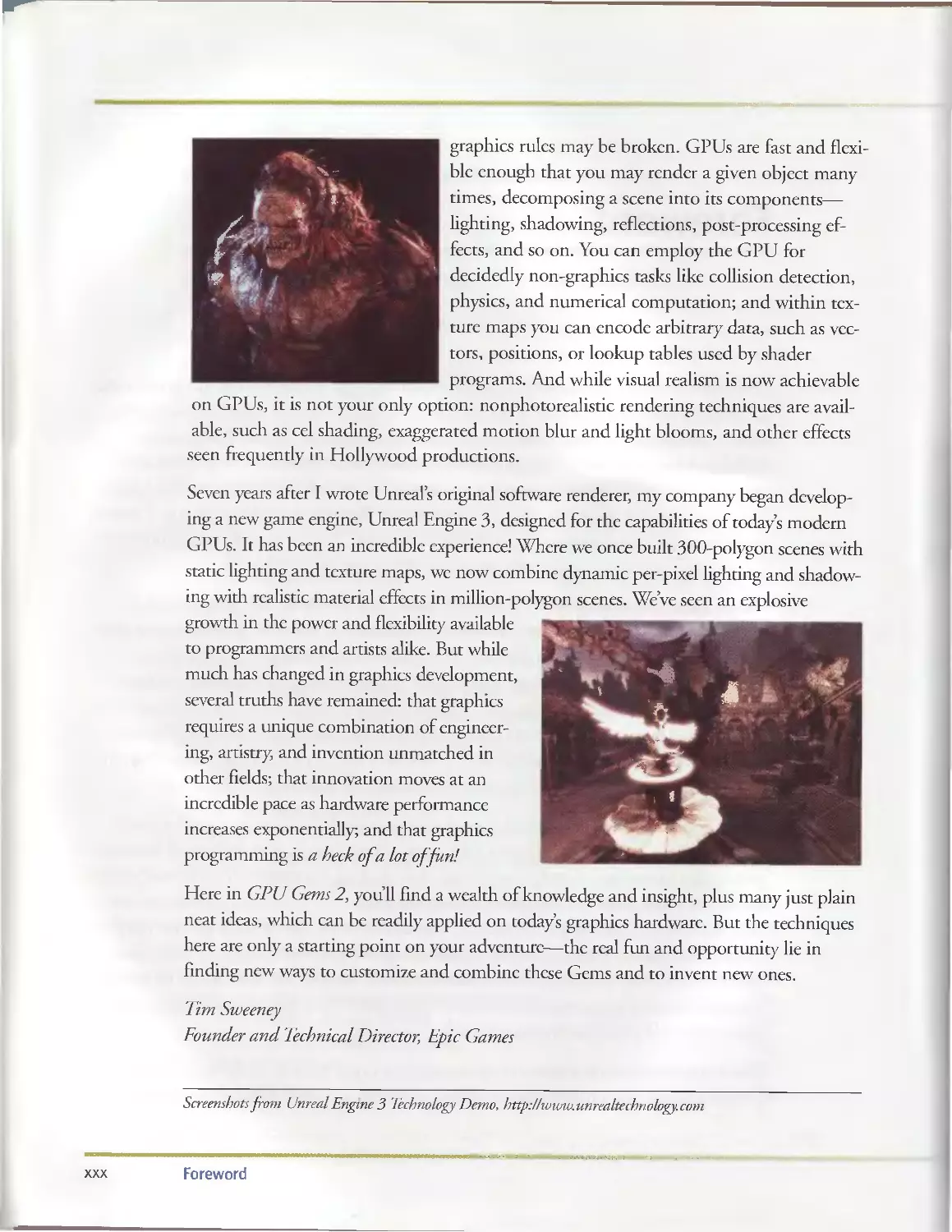
Seven years after I wrote Unreal’s original software tenderer, my company began develop-
ing a new game engine, Unreal Engine 3, designed for the capabilities of today’s modern
GPUs. It has been an incredible experience! Where we once built 300-polygon scenes with
static lighting and texture maps, we now combine dynamic per-pixel lighting and shadow-
ing with realistic material effects in million-polygon scenes. We’ve seen an explosive
growth in the power and flexibility available
to programmers and artists alike. But while
much has changed in graphics development,
several truths have remained: that graphics
requires a unique combination of engineer-
ing, artistry, and invention unmatched in
other fields; that innovation moves at an
incredible pace as hardware performance
increases exponentially, and that graphics
programming is a heck of a lot of fun!
Here in GPU Gems 2, you’ll find a wealth of knowledge and insight, plus many just plain
neat ideas, which can be readily applied on today’s graphics hardware. But the techniques
here are only a starting point on your adventure—the real fun and opportunity lie in
finding new ways to customize and combine these Gems and to invent new ones.
Tim Sweeney
Founder and Technical Director, Epic Games
Screenshots from Unreal Engine 3 Technology Demo, http://www.unrealtechnology.com
XXX
Foreword
Preface
The first volume of GPU Gems was conceived in the spring of 2003, soon after the arrival
of the first generation of fully programmable GPUs. The resulting book was released less
than a year later and quickly became a best seller, providing a snapshot of the best ideas
for making the most of the capabilities of the latest programmable graphics hardware.
GPU programming is a rapidly changing field, and the time is already ripe for a sequel. In
the handful of years since programmable graphics processors first became available, they
have become faster and more flexible at an incredible pace. Early programmable GPUs
supported programmability only at the vertex level, while today complex per-pixel pro-
grams are common. A year ago, real-time GPU programs were typically tens of instruc-
tions long, while this year’s GPUs handle complex programs hundreds of instructions
long and still render at interactive rates. Programmable graphics has even transcended the
PC and is rapidly spreading to consoles, handheld gaming devices, and mobile phones.
Until recently, performance-conscious developers might have considered writing their
GPU programs in assembly language. These days, however, high-level GPU program-
ming languages are ubiquitous. It is extremely rare for developers to bother writing
assembly for GPUs anymore, thanks both to improvements in compilers and to the
rapidly increasing capabilities of GPUs. (In contrast, it took many more years before
game developers switched from writing their games in CPU assembly language to using
higher-level languages.)
This sort of rapid change makes a “gems”-style book a natural fit for assembling the
state of the art and disseminating it to the developer community. Featuring chapters
written by acknowledged experts, GPU Gems 2 provides broad coverage of the most
exciting new ideas in the field.
Innovations in graphics hardware and programming environments have inspired fur-
ther innovations in how to use programmability. While programmable shading has long
been a staple of offline software rendering, the advent of programmability on GPUs has
Preface
xxxi
led to the invention of a wide variety of new techniques for programmable shading.
Going far beyond procedural pattern generation and texture composition, the state of
the art of using shaders on GPUs is rapidly breaking completely new ground, leading to
novel techniques for animation, lighting, particle systems, and much more.
Indeed, the flexibility and speed of GPUs have fostered considerable interest in doing
computations on GPUs that go beyond computer graphics: general-purpose computa-
tion on GPUs, or “GPGPU.” This volume of the GPU Gems series devotes a significant
number of chapters to this new topic, including an overview of GPGPU programming
techniques as well as in-depth discussions of a number of representative applications
and key algorithms. As GPUs continue to increase in performance more quickly than
CPUs, these topics will gain in importance for more and more programmers because
GPUs will provide superior results for many computationally intensive applications.
With this background, we sent out a public call for participation in GPU Gems 2. The
response was overwhelming: more than 150 chapters were proposed in the short time
that submissions were open, covering a variety of topics related to GPU programming.
We were able to include only about a third of them in this volume; many excellent
submissions could not be included purely because of constraints on the physical size of
the book. It was difficult for the editors to whittle down the chapters to the 48
included here, and we would like to thank everyone who submitted proposals.
The accepted chapters went through a rigorous review process in which the book’s edi-
tors, the authors of other chapters in the same part of the book, and in some cases addi-
tional reviewers from NVIDIA carefully read them and suggested improvements or
changes. In almost every case, this step noticeably improved the final chapter, due to
the high-quality feedback provided by the reviewers. We thank all of the reviewers for
the time and effort they put into this important part of the production process.
Intended Audience
We expect readers to be familiar with the fundamentals of computer graphics and GPU
programming, including graphics APIs such as Direct3D and OpenGL, as well as GPU
languages such as HLSL, GLSL, and Cg. Readers interested in GPGPU programming
may find it helpful to have some basic familiarity with parallel programming concepts.
Developers of games, visualization applications, and other interactive applications, as
well as researchers in computer graphics, will find GPU Gems 2 an invaluable daily
resource. In particular, those developing for next-generation consoles will find a wealth
of timely and applicable content.
xxxii
Preface
Trying the Examples
GPU Gems 2 comes with a CD-ROM that includes code samples, movies, and other
demonstrations of the techniques described in the book. This CD is a valuable supple-
ment to the ideas explained in the book. In many cases, the working examples provided
by the authors will provide additional enlightenment. You can find sample chapters,
updated CD content, supplementary materials, and more at the book’s Web site,
http://developer.nvidia.com/GPUGems2/.
Acknowledgments
An enormous amount of work by many different people went into this book. First, the
contributors wrote a great collection of chapters on a tight schedule. Their efforts have
made this collection as valuable, timely, and thought provoking as it is.
The section editors—Kevin Bjorke, Cem Cebenoyan, Simon Green, Mark Harris,
Craig Kolb, and Matthias Wloka—put in many hours of hard work on this project,
working with authors to polish their chapters and their results until they shone, con-
sulting with them about best practices for GPU programming, and gently reminding
them of deadlines. Without their focus and dedication, we’d still be working through
the queue of submissions. Chris Seitz also kindly took care of many legal, logistical, and
business issues related to the book’s production.
Many others at NVIDIA also contributed to GPU Gems 2. We thank Spender Yuen once
again for his patience while doing a wonderful job on the book’s diagrams, as well as on
the cover. Helen Ho also helped with the illustrations as their number grew to more than
150. We are grateful to Caroline Lie and her team for their continual support of our proj-
ects. Similarly, Teresa Saffaie and Catherine Kilkenny have always been ready and willing
to provide help with copyediting as our projects develop. Jim Black coordinated commu-
nication with a number of developers and contributors, including Tim Sweeney, to whom
we are grateful for writing a wonderfully focused and astute Foreword.
At Addison-Wesley Professional, Peter Gordon, Julie Nahil, and Kim Boedigheimer
oversaw this project and helped to expedite the production pipeline so we could release
this book in as timely a manner as possible. Christopher Keane’s copyediting skills and
Jules Keane’s assistance improved the content immeasurably, and Curt Johnson helped
to market the book when it was finally complete.
The support of several members of NVIDIA’s management team was instrumental to
this project’s success. Mark Daly and Dan Vivoli saw the value of putting together a
Preface
xxxiii
second volume in the GPU Gems series and supported this book throughout. Nick
Triantos allowed Matt the time to work on this project and gave feedback on a number
of the GPGPU chapters. Jonah Alben and Tony Tamasi provided insightful perspectives
and valuable feedback about the chapter on the GeForce 6 Series architecture. We give
sincere thanks to Jen-Hsun Huang for commissioning this project and fostering the
innovative, challenging, and forward-thinking environment that makes NVIDIA such
an exhilarating place to work.
Finally, we thank all of our colleagues at NVIDIA for continuing to push the envelope
of computer graphics day by day; their efforts make projects like this possible.
Matt Pharr
NVIDIA Corporation
Randima (Randy) Fernando
NVIDIA Corporation
xxxiv
Preface
Contributors
Tomas Akenine-Moller, Lund University
Tomas Akenine-Moller is an associate professor tn rhe department of computer science at
Lund University in Sweden. His main interests lie in real-time rendering, graphics on
mobile devices, and shadows.
Aral Asirvatham, Microsoft Research
Arul Asirvatham is a Ph.D student in the School of Computing, University of Ut He
received a B.Tech. in computer science and engineering in 2002 from die Indian Institute of
Information Technology in India. His primary research interest is digital geometry p g;
he has been working on mesh parameterization techniques. He is also interested in real-time
computer graphics. Currently he is focusing on rendering huge terrain data sets interactively.
Jiri Bittner, Vienna University of Technology
Jiri Bittner is currently affiliated with the Institute of Computer Graphics and Algo-
rithms of rhe Vienna University of Technology. He received his Ph.D. in 2003 from the
department of computer science and engineering of rhe Czech Technical University in
Prague. His research interests include visibility computations, efficient real-time render-
ing techniques, global illumination, and computational geometry.
Kevin Bjorke, NVIDIA Corporation
Kevin Bjorke is a member of the Developer Technology group at NVIDIA. He was a
section editor and authored several chapters for GPU Gems. He has an extensive and
award-winning production background in live-action and computer-animated films,
television, advertising, theme park rides, and, of course, games. Kevin has been a regular
speaker at events such as Game Developers Conference (GDC) and ACM SIGGRAPH
since the mid-1980s. His current work at NVIDIA involves exploring and harnessing the power of program-
mable shading for high-quality real-world applications.
Contributors
XXXV
1 Ian Buck, Stanford University
Ian Buck is completing his Ph.D. in computer science at the Stanford Computer Graph-
ics Lab, researching general-purpose computing models for GPUs. He received a B.S.E.
in computer science from Princeton University in 1999 and received fellowships from
the Stanford School of Engineering and NVIDIA. His research focuses on programming
language design for graphics hardware as well as general-computing applications that
map to graphics hardware architectures.
Michael Bunnell, NVIDIA Corporation
Michael Bunnell graduated from Southern Methodist University with degrees in computer
science and electrical engineering. He wrote the Megamax C compiler for the Macintosh,
Atari ST, and Apple IIGS before cofounding what is now LynuxWorks. After working on
real-time operating systems for nine years, he moved to Silicon Graphics, focusing on image-
processing, video, and graphics software. Next, he worked at Gigapixel, then at 3dfx, and
now at NVIDIA, where, interestingly enough, he is working on compilers again—this time, shader compilers.
lain Cantlay, Climax Entertainment
Iain Cantlay is currently a senior engineer at Climax, where he was responsible for the
graphical aspects of the Leviathan MMO engine and Warhammer Online. His current
projects include MotoGP 3 (to be published for Xbox and PC by THQ in 2005). Iain is
passionate about exploiting rhe best visuals from rhe latest technology, but natural phe-
nomena interest him most: terrain, skies, clouds, vegetation, and water.
Francesco Carucci, Lionhead Studios
Francesco Carucci graduated from the Polirecnico di Torino in Italy with a degree in soft-
ware engineering. When he was eight, rather than make pizza (like every good Italian), he
decided to make video games, and he tried to animate a running character in BASIC on an
Inrellivision. He is now writing code to animate running characters ar Lionhead, working
on the latest rendering technology for Black & White 2. He contributed to various Italian
technical 3D sires and to ShaderX2. His main interests include lighting and shadowing algorithms, 3D software
construction, and the latest 3D hardware architectures. And when he needs help, he writes shaders for food.
Cem Cebenoyan, NVIDIA Corporation
Cem Cebenoyan is a software engineer working in the Developer Technology group at
NVIDIA. He was an author and section editor for GPU Gems. He spends his days research-
ing graphics techniques and helping game developers ger the most out of graphics hardware.
He has spoken ar past Game Developer Conferences on character animation, graphics per-
formance, and nonphororealistic rendering. Before joining NVIDIA, he was a student and
research assistant in the Graphics, Visualization, and Usability Lab at the Georgia Institute of Technology.
xxxvi
Contributors
Eric Chan, Massachusetts Institute of Technology
Eric Chan is a Ph.D. student in the Computer Science and Artificial Intelligence Labora-
tory at M.I.T. He fiddles with graphics architectures, shading languages, and real-time
rendering algorithms. He has recently developed efficient methods for rendering hard
and soft shadows. Before attending graduate school, Eric was a research staff member in
the Stanford Computer Graphics Laboratory. As part of rhe Real-Time Programmable
Shading team, he wrote compiler back ends for rhe NV30 and R300 fragment architectures and developed a
pass-decomposition algorithm for virtualizing hardware resources. Eric enjoys photography and spends an
unreasonable amount of his free rime behind rhe camera.
Greg Coombe, The University of North Carolina at Chapel Hill
Greg Coombe is a graduate student at the University of North Carolina at Chapel Hill.
He received a B.S. in mathematics and a B.S. in computer science from rhe University of
Utah in 2000. Greg’s research interests include global illumination, graphics hardware,
nonphororealisric rendering, virtual environments, and 3D modeling. During the course
of his graduate studies, he has worked briefly at Intel, NVIDIA, and Vicious Cycle Soft-
ware. Greg was the recipient of the NVIDIA Graduate Fellowship in 2003 and 2004.
Jurgen Dollner, University of Potsdam, Hasso-Plattner-lnstitute
Jiirgen Dollner, a professor at the Hasso-Plattner-lnstitute of the University of Potsdam,
directs rhe computer graphics and visualization division. He has studied mathematics
and computer science and received a Ph.D. in computer science. He researches and
teaches in real-time computer graphics and spatial visualization.
William Donnelly, NVIDIA Corporation and University of Waterloo
William Donnelly is a fourth-year undergraduate in computer science and mathema
the University of Waterloo in Ontario. He interned with Okino Computer Graphi
he worked on global illumination and volumetric rendering; and with NVIDIA
Team, where he worked on the “Last Chance Gas” and “Nalu” demos. He has d
for greatness in computer graphics since mastering the art of the Bezier spline
Fwdo Durand, Massachusetts Institute of Technology
Fredo Durand received a Ph.D. from Grenoble University in France in 1 worked
on both theoretical and practical aspects of 3D visibility. From 1999 until 2002,1 was a
postdoc in the M.I.T Computer Graphics Group, where he is now an assistant professor. His
research interests span most aspects of picture generation and creation, including realistic
graphics, real-time rendering, nonphororealisric rendering, and computational photography.
He received a Eurographics Young Researcher Award in 2004. (Digital drawing courtesy of Victor Ostromoukhov)
Contributors
xxxvii
yij Eric Enderton, NVIDIA Corporation
Eric Enderron is a senior engineer at NVIDIA, where he is working on the Gelato film
tenderer. After studying computer science at rhe University of California, Berkeley, Eric
spent a decade developing rendering and animation software at Industrial Light &
Magic, and he larer consulted ar other studios. His film credits include Terminator 2-,
Jurassic Park-, and Star Wars, Episode I: The Phantom Menace.
Zhe Fan, Stony Brook University
Zhe Fan is a Ph.D. candidate in rhe computer science department ar Stony Brook Univer-
sity. He received a B.S. in computer science from the University of Science and Technology
of China in 1998 and an M.S. in computer science from the Chinese Academy of Sciences
in 2001. His current research interests include GPU clusters for general-purpose computa-
tion, parallel graphics and visualization, and modeling of amorphous phenomena.
Randima Fernando, NVIDIA Corporation
Randima (Randy) Fernando has loved computer graphics since age eight. Working in
NVIDIA’s Developer Technology group, he helps reach developers how to rake advantage
of the latest GPU technology. Randy has a B.S. in computer science and an M.S. in com-
puter graphics, both from Cornell University. He has published research in SIGGRAPH
and is coauthor, with Mark Kilgard, of The Cg Tutorial: The Definitive Guide to Program-
mable Real-Time Graphics. He edited GPU Gems: Programming Techniques, Tips, and Tricks for Real-Time Graphics
and is the GPU Gems series editor.
Nathaniel Fout, University of California, Davis
Nathaniel Fout received a B.S. in chemical engineering and an M.S. in computer science
from the University of Tennessee in 2002 and 2003, respectively. He is a Ph.D. student in
computer science ar the University of California, Davis, where he is a member of the Insti-
tute for Dara Analysis and Visualization. His research interests include volumetric compres-
sion for rendering, multivariate and comparative visualization, and tensor visualization.
James Fung, University of Toronto
James Fung is completing his Ph.D. in engineering. He received a B.A.Sc. in engineering
science and an M.S. in electrical engineering from the University of Toronto. His re-
search interests include wearable computing, mediated reality, and exploring new types
of musical instrument interfaces based on EEG brain-wave signal processing. His most
recent work has been rhe development of the GPU-based computer vision and mediated
reality library called OpenVIDIA.
xxxviii
Contributors
Simon Green, NVIDIA Corporation
Simon Green is a senior software engineer in the Developer Technology group ar
NVIDIA. He started graphics programming on the Sinclair ZX-81, which had 1 кВ of
RAM and a screen resolution of 64 x 48 pixels. He received a B.S. in computer science
from the University of Reading, in the United Kingdom, in 1994. Since 1999 Simon has
found a stable home ar NVIDIA, where he develops new rendering techniques and helps
application developers rake maximum advantage of GPU hardware. He is a frequent presenter ar GDC, has
written for Amiga Shopper and Wired magazines, and was a section editor for GPU Gems. His research interests
include cellular automata, general-purpose computation on GPUs, and analog synthesizers.
Toshiya Hachisuka, University of Tokyo
Toshiya Hachisuka is an undergraduate in the Department of Systems Innovation at the
University of Tokyo. He also works as a programmer for MagicPictures, integrating cutting-
edge research results into current computer graphics software. He has studied computer
graphics since age ten. His current research interests are physically based rendering, physically
based modeling, real-time rendering techniques, and general-purpose computation on GPUs.
Markus Hadwiger, VRVis Research Center
Markus Hadwiger received his Ph.D. in computer science from the Vienna University of
Technology in 2004, where he concentrated on high-quality real-time volume rendering and
texture filtering with graphics hardware, in cooperation with the VRVis Research Center. He
has been a researcher ar VRVis since 2000, working in the Basic Research on Visualization
group and the Medical Visualization group (since 2004). From 1996 to 2001, he was also
the lead programmer of the cross-platform 3D space-shooter game Parsec, which is now an open source project.
Mark Harris, NVIDIA Corporation
Mark Harris received a B.S. from the University of Notre Dame in 1998 and a Ph.D. in
computer science from the University of North Carolina ar Chapel Hill (UNC) in 2003.
At UNC, Mark’s research covered a wide variety of computer graphics topics, including
real-time cloud simulation and rendering, general-purpose computation on GPUs, global
illumination, nonphotorealistic rendering, and virtual environments. Mark is now a
member of NVIDIA’s Developer Technology team based in the United Kingdom.
Jon Hasselgren, Lund University
Jon Hasselgren received an M.Sc. from Lund University. He now pursues graduate stud-
ies in the computer science department, where he researches graphics for mobile phones.
Contributors
xxxix
Oliver Hoeller, Piranha Bytes
Oliver Hoeller is a senior software engineer at Piranha Bytes, which developed the RPGs
Gothic I and Gothic II. Previously he was director of development at H2Labs/Codecult,
where he was responsible for development and architecture design of the Codecreatures
game system. He was an active member of the German demo scene in the 1980s and
early 1990s. After exploring different areas—developing music software, creating a secu-
rity program, and working as a Web services consultant—Oliver returned to his roots and now guarantees a
high level of visual quality for Piranha Bytes’ forthcoming Gothic III.
Hugues Hoppe, Microsoft Research
Hugues Hoppe is a senior researcher in the Computer Graphics Group at Microsoft
Research. His primary interests lie in the acquisition, representation, and rendering of
geometric models. He received the 2004 ACM SIGGRAPH Achievement Award for his
pioneering work on surface reconstruction, progressive meshes, geometry texturing, and
geometry images. His publications include twenty papers at ACM SIGGRAPH, and he
is associate editor of ACM Transactions on Graphics. He received a B.S. in electrical engineering in 1989 and a
Ph.D. in computer science in 1994 from the University of Washington.
Daniel Horn, Stanford University
Daniel Horn is a Ph.D. candidate at the Stanford Computer Graphics Lab; he received
his B.S. from the University of California, Berkeley. While Daniel focuses on program-
ming graphics hardware and real-time graphics, theory and compilers have always inter-
ested him deeply, and he tries to incorporate knowledge from those fields into his
graphics research. In his spare time, Daniel enjoys hacking with his brother, Patrick, on
their open source space sim, Vega Strike. He also enjoys roaming with friends in the Bay Area’s many natural
parks, from Palo Alto’s Foothills Park to Berkeley’s Tilden Park.
Samuel Hornus, GRAVIR/IMAG-INRIA
Samuel Hornus is a Ph.D. candidate at INRIA in Grenoble, France. He is a former
student of the Ecole Normale Superieure de Cachan. His research focuses on 3D visibil-
ity problems, as well as other aspects of computer graphics, such as texture authoring,
interactive walkthroughs, real-time shadows, realistic rendering, implicit surfaces, and
image-based modeling.
xl
Contributors
Arie Kaufman, Stony Brook University
Arie Kaufman is the director of the Center for Visual Computing, a distinguished profes-
sor and chair of the Computer Science Department, and distinguished professor of radi-
ology at Stony Brook University. He received a B.S. in mathematics and physics from the
Hebrew University of Jerusalem in 1969; an M.S. in computer science from the Weiz-
mann Institute of Science, Rehovot, Israel, in 1973; and a Ph.D. in computer science
from the Ben-Gurion University, Israel, in 1977. Kaufman has conducted research and consulted for more
than thirty years, with numerous publications in volume visualization; graphics architectures, algorithms, and
languages; virtual reality; user interfaces; and multimedia.
Jan Kautz, Massachusetts Institute of Technology
Jan Kautz is a postdoctoral researcher at M.I.T. He is particularly interested in realistic shad-
ing and lighting, hardware-accelerated rendering, textures and reflection properties, and
interactive computer graphics. He received his Ph.D. in computer science from the Max-
Planck-Institut fur Informatik in Germany; a diploma in computer science from the Univer-
sity of Erlangen in Germany, and an M.Math. from the University of Waterloo in Ontario.
Emmett Kilgariff NVIDIA Corporation
Emmett Kilgariff is a director of architecture in the GPU group at NVIDIA, where he
has contributed to the design of many GeForce chips, including the GeForce 6 and
GeForce 7 Series. He has more than twenty years of experience designing graphics hard-
ware, at Sun Microsystems, Silicon Graphics, 3dfx, and many small companies whose
memories have faded over time.
Gary King, NVIDIA Corporation
Unscrupulous. Unconventional. Uncouth. Unkempt. All are accurate adjectives for the
worst thing to happen to the graphics industry since Execute Buffers. A master of GPL
arcana, lore, and the occult, he spends his days at NVIDIA crafting increasingly ingen-
iously nefarious rendering techniques, imbuing next-generation architectures with un-
holy energies, worshipping the Dark Lord, and kicking puppies.
Peter Kipfer, Technische Universitiit MDnchen
Peter Kipfer is a postdoctoral researcher in the Computer Graphics and Visualization
Group at the Technische Universitat Munchen. He received his Ph.D. from the Univer-
sity of Erlangen-Niirnberg in 2003 for his work on parallel and distributed visualization
and rendering within the KONWIHR supercomputing project. His current research
focuses on general-purpose computing and geometry processing on the GPU.
Contributors
xli
JoeKniss, University of Utah
Joe Kniss is a Ph.D. student in computer science at the University of Utah, where he is a
member of the Scientific Computing and Imaging Institute. His research interests include
nonpolygonal rendering, light transport in participating media, user-interface design, and
all things GPU. He is a Department of Energy High-Performance Computer Science
graduate fellow.
Craig Kolb, NVIDIA Corporation
Craig Kolb has been interested in computer graphics since he began writing games on his high
school’s sub-megaflop PDP-11. He received a B.A. and an M.Sc. from Princeton, where he
wrote the first version of rayshade, a popular ray tracer, as part of his senior thesis. He spent the
1990s waiting for frames to render: first as a research assistant to Benoit Mandelbrot at Yale,
then as a Ph.D. candidate researching camera and rendering systems at Princeton and Stanford,
and later as head of rendering development at Pixar Animation Studios. In 2000 he cofounded Exluna and now
works in the Software Architecture group at NVIDIA finding novel ways to push multi-gigaflop GPUs to their limits.
Jens Kruger, Technische Universitat Munchen
Jens Kruger is a Ph.D. student in the Computer Graphics and Visualization Group at the
Technische Universitat Munchen. Jens’s current research focuses on GPU solutions to nu-
merical problems, often arising in physically based simulations. He has published papers on
GPU programming at conferences such as ACM SIGGRAPH and IEEE Visualization. In
2004 he received an ATI Fellowship, which honors outstanding graduate students in areas
related to computer grapliics and graphics systems.
Yuri Kryachko, iQMaddox Games
Yuri Kryachko is the 3D graphics and effects programmer on IL-2 Sturmovik, WW2, IL-2
Sturmovik: Forgotten Battles, AEP, and Pacific Fighters. He has been at Maddox Games since
1996, and he’s been playing and creating PC games since writing his first 2D game in
1987. He received an M.S. from the department of applied mathematics of the Moscow
State Engineering Physics Institute (Technical University). Previous game projects include
Gty3D—Drive Simulator (ELF) in 1995 and Helicopter Simulator from 1995 to 1996.
Sylvain Lefebvre, GRAVIR/IMAG-INRIA
Sylvain Lefebvre is a final-year Ph.D. student at INRIA in Grenoble, France. He received
an M.S. in computer science from the INPG University, Grenoble, in 2001. His research
focuses on developing new texturing methods for creating, storing, and rendering highly
detailed textures for real-time applications. Recently he has worked on landscape textur-
ing, direct painting on meshes, and the progressive loading of texture maps. He is also
interested in many aspects of game programming.
xlii
Contributors
Aaron Lefohn, University of California, Davis
Aaron Lefohn is a Ph.D. student in the computer science department at the University
of California, Davis, and a graphics software engineer at Pixar Animation Studios. His
current research focuses on data-parallel data structures and programming models and
their application to high-quality interactive rendering. Aaron completed his M.S. in
computer science at the University of Utah in 2003; he received an M.S. in theoretical
chemistry from the University of Utah in 2001 and a B.A. in chemistry from Whitman College in 1997.
Aaron is a National Science Foundation graduate fellow in computer science.
Martin-Karl Lefran^ois, mental images
Martin-Karl Lefrangois is senior graphics software engineer at mental images in Berlin,
maker of the mental ray tenderer and other graphics software products. Under his lead,
his team at mental images delivered automatic GPU support in mental ray 3.3 and is
responsible for GPU acceleration support in all mental images products. After graduating
with a degree in computer science and mathematics from the University of Sherbrooke in
Quebec, he worked as a graphics developer for nearly ten years at Softimage in Montreal and Tokyo before
leading the core game engine team at A2M.
Wei Li, Siemens Corporate Research
* Wei Li is a research scientist at Siemens Corporate Research in Princeton, New Jersey. Hi
» _ . current research focuses on texture-based volume rendering and general-purpose computa-
tion on the GPU. He received an M.S. and a Ph.D. in computer science from Stony Brook
' тВИ University in 2001 and 2004, respectively. He also received a B.S. and an M.S. in electrical
engineering from Xi’an Jiaotong University in China in 1992 and 1995, respectively.
ИМ Donald Liu, Siemens Medical Solutions USA
- I Donald Liu received a B.Eng. from Qinghua University in Beijing in 1984; he received
4 I an M.Eng. and a D.Eng. from the University ofTokyo in 1988 and 1991, respectively.
i He was an assistant professor at Sophia University in Tokyo for a year before joining the
* faculty of the electrical engineering department at the University of Rochester in New
"_____.. York. Since 1997 he has been with the Siemens Medical Solutions Ultrasound Group in
Issaquah, Washington, where he is currently a senior staff systems engineer. He is a senior member of IEEE
and a recipient of the National Institutes of Health FIRST award. His research interests include analysis and
correction of ultrasonic wavefront distortion, efficient image formation, and digital signal processing.
Contributors
xliii
Paulius Micikevicius, Armstrong Atlantic State University
Paulius Micikevicius received a B.S. in computer science from Midwestern State Univer-
sity in 1998 and a Ph.D. in computer science from the University of Central Florida
(UCF) in 2002. He is an assistant professor at Armstrong Atlantic State University in
Savannah, Georgia, as well as a research associate at the Media Convergence Laboratory
at UCF. His research interests include real-time graphics, graphics processing for
mixed/augmented reality experiences, and parallel computing and graph theory.
Fabrice Neyret, GRAVIR/IMAG-INRIA
Fabrice Neyret has worked on the R&D teams of several companies, including TDI in
Paris and Alias|Wavefront in Toronto. He received a master’s degree in applied mathemat-
ics, an engineering degree from Telecom Paris (ENST), and a Ph.D. in computer science.
He did his postdoctoral work at the University of Toronto. He is currently a full-time
CNRS researcher at GRAVIR lab in Grenoble, France. His research interests include natu-
ral phenomena (especially water and clouds), highly complex scenes (such as landscapes covered by forest), tex-
tures, local illumination and shaders, alternate representations (such as volumetric textures), phenomenological
approaches, and, of course, getting the most out of GPUs. He is also involved in pedagogic software (such as
MobiNet), scientific popularization, and writing short stories.
Hubert Nguyen, NVIDIA Corporation
Hubert Nguyen is a software engineer on the NVIDIA Demo Team. He spends his time
searching for novel effects that show off the features of NVIDIA’s latest GPUs. He most
recently worked on “Nalu,” NVIDIA’s mermaid. Before joining NVIDIA, Hubert was at
3dfx interactive, the creators of Voodoo Graphics. Prior to 3dfx, Hubert was part of the
R&D department of Cryo Interactive in Paris. Hubert started to develop 3D graphics
programs when he was involved in the European demo scene. He holds a degree in computer science.
Marc Nienhaus, University of Potsdam, Hasso-Plattner-lnstitute
Marc Nienhaus is a Ph.D. candidate at the Hasso-Plattner-lnstitute of the University of
Potsdam. He studied mathematics and computer science and has worked as a software
engineer focusing on computer graphics. His research interests include real-time render-
ing, nonphotorealistic rendering, and depiction strategies for symbolizing dynamics.
xliv
Contributors
Justin Novosad, discreet
Justin Novosad is a software developer for discreet (a division of Autodesk). He received a
bachelors degree in computer engineering and a masters degree in medical imaging, both
from Ecole Polytechnique de Montreal, in 2001 and 2003, respectively. Justin is a member
of the “effects” team at discreet, working on the Inferno, Flame, and Flint visual effects and
digital compositing products. Before joining discreet in 2004, he was a research engineer at
Sainte-Justine Hospital in Montreal, where he developed computer vision algorithms for the study of spinal defor-
mities from X-ray data. His fields of interest include computer graphics, computer vision, machine learning, image
processing, and applied mathematics. He is a cofounder of the ACM SIGGRAPH Montreal Professional Chapter.
Lennart Ohlsson, Lund University
Lennart Ohlsson is an assistant professor in the computer science department at Lund
University. His primary research interest is software architecture for computer graphics.
Jon Click, 2015
Jon Olick has been creating games since age 11. He is a senior software engineer special-
izing in graphics technology and engine design at 2015, where he has worked on titles
such as Medal of Honor: Allied Assault and Men of Valor: Vietnam. He is now developing
engine technology for future products.
Sean O’Neil
Sean O’Neil graduated from Georgia Tech in 1995 with a B.S. in computer science. He
lives in Atlanta with his wife and two wonderful children. All of his full-time positions
have been in the telecommunications industry, so for now graphics programming is just
a hobby.
John Owens, University of California, Davis
John Owens is an assistant professor of electrical and computer engineering at the Univer-
sity of California, Davis, where he leads research projects in graphics hardware/software
and wireless sensor networks. Prior to his appointment at Davis, he earned an M.S. and a
Ph.D. in electrical engineering from Stanford University in 1997 and 2002, respectively.
At Stanford he was an architect of the Imagine Stream Processor and a member of the
Concurrent VLSI Architecture Group and the Computer Graphics Laboratory. He received a B.S. in electrical
engineering and computer science from the University of California, Berkeley, in 1995.
Contributors
xlv
Kurt Pelzer, Piranha Bytes
Kurt Pelzer is a senior software engineer at Piranha Bytes, where he worked on the PC
game Gothic, the top-selling Gothic II (awarded RPG of the Year in Germany during
2001 and 2002, respectively), and the add-on Gothic II: The Night of the Raven. Previ-
ously he was a senior programmer at Codecult and developed several real-time simula-
tions and technology demos built on Codecults 3D engine. Kurt has published in GPU
Gems, ShaderX2, and Game Programming Gems 4.
Matt Pharr, NVIDIA Corporation
Matt Pharr is a senior software developer in the Software Architecture group at NVIDIA,
where he works on Cg and interactive rendering techniques. He is coauthor, with Greg
Humphreys, of Physically Based Rendering: From Theory to Implementation. Previously he
was a cofounder of Exluna and a Ph.D. student in the Stanford Computer Graphics Lab,
where he researched systems issues for rendering and theoretical foundations of rendering;
he published a series of SIGGRAPH papers on these topics.
Jeremy Selan, Sony Pictures Imageworks
Jeremy Selan currently pioneers color and lighting tools at Sony Pictures Imageworks. His
work has been utilized on numerous motion pictures, most recently on Spider-Man 2.
Professionally, he maintains an active interest in colorimetry and digital cinema. He is a
graduate of the Program of Computer Graphics and the School of Electrical and Com-
puter Engineering at Cornell University. In his free time—drawn by a climate markedly
superior to that of his hometown, Skokie, Illinois—Jeremy is an aspiring Santa Monica beach bum.
Oles Shishkovtsov, GSC Game World
Oles Shishkovtsov became interested in programming and graphics at age 13; by age 17
he had won two national competitions in programming and enrolled at the Junior Acad-
emy of Science in Ukraine. At 19 he started working for White Lynx as a software devel-
oper/graphics programmer, where he successfully completed three projects. Since 2000 he
has worked for GSC Game World as an engine architect/team leader and has continued
doing R&D in his free time. He has spent the last three years working on <S. T.A.L.K.E.R.: Shadows of Chernobyl.
Christian Sigg, ETH Zurich
Christian Sigg received his degree in computational science and engineering from the
Swiss Federal Institute of Technology Zurich. He became interested in computer graph-
ics during a semester abroad at the University of Texas at Austin, where he worked on
parallel volume rendering at the Computational Visualization Center. He is working on
his Ph.D. at the ETH Zurich Computer Graphics Laboratory. His research interests lie
in the area of algorithms for implicit surface representations using graphics hardware.
xlvi
Contributors
Tiago Sousa, Crytek
Tiago Sousa is a self-taught game and graphics programmer who has worked at Crytek as
an R&D software engineer for the last two years. He has contributed to most of the
special effects in Crytek’s games. In 1999, before joining Crytek, he cofounded a pio-
neering game development team in Portugal and studied computer science at a local
university. He spends most of his time researching real-time and non-real-time graphics
and reading all kinds of technical books.
Thilaka Sumanaweera, Siemens Medical Solutions USA
Thilaka Sumanaweera has been having fun with first GL and then OpenGL since the late
1980s, creating 2, 3, and 4D applications in computer vision, image processing, and med-
ical imaging. He received his Ph.D. in electrical engineering from Stanford University in
1992. He then joined the Radiological Sciences Laboratory at Stanfords Radiology Depart-
ment as a postdoc and a research associate developing CT/MRI image fusion and image-
guided neurosurgery. Currently he is a Fellow in the Siemens Medical Solutions Ultrasound Division, working in
the areas of volume rendering, motion detection and compensation, and image segmentation. He holds 24 patents
for techniques related to medical imaging and visualization, and he has published extensively in medical journals.
Yury Uralsky, NVIDIA Corporation
Yury Uralsky became interested in games and computer graphics when the ZX Spectrum
48K was a dream machine and writing software rasterizers in assembly language was fun.
He received an M.S. in computer science from the Moscow State Technical University in
2001. He worked as a graphics engine programmer for Eagle Dynamics, creating graphics
for the flight simulator LockOn: Modem Air Combat. He joined the NVIDIA Developer
Technology group in March 2004 and enjoys pushing 3D graphics forward in the NVIDIA Moscow office
j Pete Warden, Apple Computer
В Pete Warden has worked as a graphics engine programmer on PC, PSX, PS2, GameCube.
br and Xbox titles, specializing in low-level assembler and vector unit programming on the
PS2. He has also published 45 open source video filters that run in a variety of real-time
video applications on Windows, Linux, and OS X, including After Effects, and helped to
create the Freeframe open plug-in standard. Pete is now part of the team working on
Apples Motion video effects package, a fully GPU-based image-processing application. He has written many of
its original video filters and also works on the rendering engine.
Contributors
xlvii
Li-Yi Wei, NVIDIA Corporation
Li-Yi Wei is a 3D graphics architect at NVIDIA Corporation. He received a B.S. in electri-
cal engineering from the National Taiwan University in 1993 and a Ph.D. in electrical
engineering from Stanford University in 2001. He spends 1 percent of his time designing
next-generation graphics hardware and the remaining 99 percent verifying that the design
actually works. When not wreaking havoc on NVIDIA’s chips, he enjoys researching vari-
ous fields of computer graphics. He is a frequent contributor to SIGGRAPH and other academic conferences.
МИНПИМ Xiaoming Wei, Stony Brook University
. i Xiaoming Wei is an assistant professor of computer science at Iona College in New
' * I Rochelle, New York. She received her Ph.D. in computer science from Stony Brook
I University in 2004. She received a B.Sc. from the Beijing University of Aeronautics and
I Astronautics in 1995 and an M.Sc. in computer science fromTsinghua University in
______________ И Beijing in 1998. Her research interests include physically based modeling, natural phe-
nomena modeling, and computer animation.
RiidigerWestermann, Technische Universitat Munchen
Rudiger Westermann studied computer science at the Technical University Darmstadt,
Germany. He received a Ph.D. in computer science from the University of Dortmund,
Germany. In 2002 he was appointed the chair of Computer Graphics and Visualization
at the Technische Universitat Munchen. His research interests include general-purpose
computing on GPUs, hardware-accelerated visualization and image synthesis, hierarchi-
cal methods in scientific visualization, volume rendering, flow visualization, and parallel graphics algorithms.
Daniel Wexler, NVIDIA Corporation
Daniel Wexler attended the University of California, Berkeley, where he studied with the
graphics research group before leaving school to work at Sun Microsystems. He worked
at Xaos Tools before joining the R&D team at Pacific Data Images (PDI) in 1995. After
spending six years writing a new tenderer and shading system for PDI, which was used
on a variety of feature film projects including Antz and Shrek, he joined NVIDIA to
work on hardware-based rendering systems with Larry Gritz and the rest of the NVIDIA architecture team.
David Whatley, Simutronics Corporation
David Whatley is president and CEO of Simutronics Corporation and a developer and
publisher of online games. His passion for online gaming led him to found Simutronics
in 1987, when he was 20 years old. David—chief designer and technology architect of
most of the company’s games—has won numerous awards, including Computer Gaming
World’s first Online Game of the Year award for CyberStrike. His current focus is on
alternate techniques for more photorealistic rendering of 3D environments in games.
xlviii
Contributors
Michael Wimmer, Vienna University of Technology
Michael Wimmer is an assistant professor at the Institute of Computer Graphics and
Algorithms of the Vienna University of Technology, where he received an M.Sc. in 1997
and a Ph.D. in 2001. His current research interests are real-time rendering, virtual and
augmented reality, computer games, and real-time visualization of urban environments;
he has coauthored several scientific papers in these fields. He also teaches courses on 3D
computer games and real-time rendering.
Matthias Wloka, NVIDIA Corporation
Matthias Wloka is a software engineer in the Developer Technology group at NVIDIA.
His primary responsibility is to collaborate with game developers to enhance image qual-
ity and graphics performance of their games; he is also a regular contributor at game
developer conferences, such as GDC. Matthias’s passion for computer gaming started at
age 15 when he discovered that his schools Commodore PET 2001 computers could
also play Black Jack. He started writing his own games soon thereafter and continues to use the latest graphics
hardware to explore the limits of interactive real-time rendering. Before joining NVIDIA, Matthias was a
game developer at GameFX/THQ. He received an M.Sc. in computer science from Brown University in 1990
and a B.Sc from Christian-Albrechts-University in Kiel, Germany, in 1987.
Cliff Woolley, University of Virginia
Cliff Woolley is a Ph.D. student in computer science at the University of Virginia. His
research interests include interactive rendering techniques, sparse sample reconstruction,
and general-purpose computation using programmable graphics hardware. He received
an M.C.S. in computer graphics from the University of Virginia in 2003 and a B.A. in
computer science and theater at Washington and Lee University in 1999.
Contributors
xlix
7c£tar« Ci. • -te Set 0
PARTI
GEOMETRIC
COMPLEXITY
‘IL ” f g * J £
Today’s games are visually more interesting and complex than ever before. Geo-
metric complexity—how many objects are visible and how detailed each looks—
is one of the dimensions in which games are making leaps and bounds.
Advances in technology are partly responsible for these leaps and bounds:
CPUs, memory, and buses all have become faster, but specifically GPUs are un-
dergoing significant change and are becoming ever more powerful—at a rate
faster than Moore’s Law.
These GPU changes include incorporating fixed-function processing for the ver-
tex- and pixel-shading units, then generalizing those to be fully programmable.
GPUs also have gained more units to process pixels and vertices in parallel: the
GeForce 6800 Ultra, for example, incorporates 6 vertex shader units and 16
pixel pipelines.
Despite these performance advances, rendering complex scenes is still more
difficult than simply dumping all geometry onto the GPU and forgetting about it.
The simple approach tends to fail either because the generated GPU workload
turns out to be excessive, or because the associated CPU overhead is prohibi-
tive. This part of the book discusses the challenges today’s games face in ren-
dering complex geometric scenes.
Chapter 1, “Toward Photorealism in Virtual Botany” by David Whatley of
Simutronics Corporation, provides a holistic view on how to render nature
scenes. It explains the multitude of different techniques, from scene manage-
ment and rendering various plant layers to post-processing effects, that
Simutronics’ Hero’s Journey employs to generate complex and stunning visuals.
Rendering terrain is a good example of why simply dumping all available data to
the GPU cannot work: the horizon represents a near-infinite amount of vertex
data and thus workload. Arul Asirvatham and Hugues Hoppe of Microsoft Re-
search use vertex texture fetches for a new highly efficient terrain-rendering
algorithm. Their technique avoids overloading the GPU even as it shifts most
work onto the GPU and away from the CPU, which too often is the bottleneck in
modern games. Chapter 2, “Terrain Rendering Using GPU-Based Geometry
Clipmaps,” provides all the implementation details.
PARTI GEOMETRIC COMPLEXITY
3
As already mentioned, another way to increase geometric complexity is to increase
the number of visible objects in a scene. The straightforward solution of drawing
each object independently of the others, however, quickly bogs down even a high-
end system. It is much easier to efficiently draw ten objects that are one million
triangles each, than it is to draw one million objects that are ten triangles each.
Francesco Carucci of Lionhead Studios faces this very problem while developing
Block & White 2, the sequel to Lionhead’s critically acclaimed Block & White.
Chapter 3, “Inside Geometry Instancing,” describes his solution: a framework of
instancing techniques that applies to legacy GPUs as well as to GPUs supporting
DirectX 9’s instancing API. Jon Click of 2015 provides further optimizations to the
instancing technique that prove beneficial for 2015’s title Men ofVolor: Vietnam.
Jon describes his findings in Chapter 4, “Segment Buffering.”
Also, as games incorporate more and more data—more complex scenes of more
complex meshes rendered in multiple, disparate passes supporting the gamut of
differing functionality from legacy to current high-end GPUs—managing this glut
of data efficiently becomes paramount. Oliver Hoeller and Kurt Pelzer of Piranha
Bytes are currently working on Piranha Bytes’ Gothic III engine. They share their
solutions in Chapter 5, “Optimizing Resource Management with Multistreaming ”
The best way to render lots of geometry to create geometric complexity is to avoid
rendering the occluded parts. Michael Wimmer and Jiri Bittner of the Vienna Uni-
versity of Technology explore how best to apply that idea in Chapter 6, “Hardware
Occlusion Queries Made Useful.” Occlusion queries are a GPU feature that pro-
vides high-latency feedback on whether an object is visible or not after it is ren-
dered. Unlike earlier occlusion-query culling techniques, Michael and Jiri's
algorithm is pixel-perfect. That is, it introduces no rendering artifacts, generates a
near-optimal set of visible objects to render, does not put unnecessary load on the
GPU, and has minimal CPU overhead.
Similarly, increasing geometric detail only where visible and simplifying it when
and where it isn’t visible is a good way to avoid excessive GPU loads. View-
dependent and adaptive subdivision schemes are an appealing solution that the
4
PARTI GEOMETRIC COMPLEXITY
offline-rendering world already employs to render their highly detailed models to
subpixel geometric accuracy. Subdivision surfaces have not yet found a place in
today’s real-time applications, partly because they are not directly supported in
graphics hardware. Rendering subdivision surfaces thus seems out of reach for
real-time applications. Not so, says Michael Bunnell of NVIDIA Corporation. In
Chapter 7, Michael shows how his implementation of "Adaptive Tessellation of
Subdivision Surfaces with Displacement Mapping” is already feasible on modern
GPUs and results in movie-quality geometric detail at real-time rates.
Finally, faking geometric complexity with methods that are cheaper than actually
rendering geometry allow for higher apparent complexity at faster speeds. Re-
placing geometry with textures that merely depict it used to be an acceptable
trade-off—and in the case of grates and wire-mesh fences, often still is. Normal
mapping is a more sophisticated fake that properly accounts for lighting informa-
tion. Parallax mapping is the latest craze that attempts to also account for intra-
object occlusions. William Donnelly of the University of Waterloo one-ups
parallax mapping: he describes “Per-Pixel Displacement Mapping with Distance
Functions” in Chapters. Displacement mapping provides correct intra-object
occlusion information, yet minimally increases computation cost. His technique
gives excellent results while taking full advantage of the latest programmable
pixel-shading hardware. Even better, it is practical for applications today.
Matthias Wloka, NVIDIA Corporation
PARTI GEOMETRIC COMPLEXITY
5
Toward Photorealism in
Virtual Botany
David Whatley
Simutronics Corporation
Rendering natural scenes in real time, while leaving enough CPU and GPU resources
for other game-engine requirements, is a difficult proposition. Images of botanv require
a great deal of visual depth and detail to be convincing. This chapter describes strategies
for rendering more photorealistic natural scenes in a manner that is friendly to real-
time game engines. The methods presented here work together to create a convincing
illusion of grassy fields teeming with plants and trees, while not overwhelming either
the CPU or the GPU. These techniques are used in Simutronics’ Hero’s Journey, as
shown in Figure 1-1.
We begin by describing the foundation for managing scene data in large outdoor envi-
ronments. Next, we provide details on how to maximize throughput of the GPU to
achieve the required visual density in grass. Then we expand on these techniques to add
ground clutter and larger-scale botany, such as trees. Finally, we tie the visuals together
with shadowing and environmental effects.
i.i Scene Management
Game engines must manage their rendering techniques to match the scope of the envi-
ronment they hope to visualize. Game levels that feature nature scenes, made up of thou-
sands of trees and bushes and perhaps millions of blades of grass, present significant data
management problems that must be solved to allow rendering at interactive frame rates.
1.1 Scene Management
7
Figure 1-1. Babbling Brook: A Nature Scene from Hero’s Journey
Rendering a virtual nature scene convincingly is both an artistic and a technical chal-
lenge. We can approach the rendering of nature much like a painter: break down the
elements into layers and treat each layer independently to ultimately create a unified
whole. For example, a layer of grass, a layer of ground clutter, a layer of trees, and so
on. All these layers share some common properties, which we can leverage to compress
our data representation.
Our goal is to travel the game camera over long distances of convincing outdoor scenes
without having to dedicate excessive memory resources to managing the task. With
guided deterministic random-number generation, we have an algorithm that can
“plant” all of the elements of nature in a reasonable manner while achieving the same
visual results each time we revisit the same spot on the map. In an online game, every-
one would see the same thing right down to the placement of a blade of grass without
this placement being permanently stored in memory.
i.i.i The Planting Grid
We establish a world-space fixed grid around the camera to manage the planting data
for each layer of plants and other natural objects. Each grid cell contains all of the data
8
Chapter i Toward Photorealism in Virtual Botany
to render its layer in the physical space it occupies. In particular, the cell data structure
stores the corresponding vertex and index buffers, along with material information to
represent what is drawn.
For each layer of botany, we establish a distance from the camera that the layer needs to
generate visuals; this determines the size of our virtual grid. As the camera moves, the virtual
grids travel with it. When a grid cell is no longer in the virtual grid, we discard it and add
new cells where needed to maintain our full grid structure. As each cell is added, a planting
algorithm is used to fill in the layer with the appropriate data for rendering. See Figure 1-2.
1.1.2 Planting Strategy
For each cell that is filled with natural objects, we need to pick suitable spots on the
ground where those objects are placed. The heuristic used to choose these spots
depends on the type of object being placed. Generally, we would like to pick random
spots, at some desired density, and then see if the corresponding points on the ground
are acceptable for what we are planting. In our implementation, a ground polygons
material determines what layers are applicable.
The obvious approach is to randomly cast rays straight down at the ground within the
volume of the cell. Each time we hit a polygon, we check to see if it is suitable (Can
grass be planted here? Is the slope too severe?). If we succeed, then we have a planted
point. We continue until we reach the proper density.
Figure 1-2. The Virtual Grid
Each layer consists of a fixed-size grid that is world-space aligned. The dark green cells represent
active cells. The camera is moving forward, and the cells marked with an X are being discarded as
new cells (shown in light green) are added to maintain our virtual grid size. A useful improvement
in the implementation is to pool the grid cells and simply recycle them, because a new cell is
always added when an old one is discarded.
i.i Scene Management
9
This approach yields good results but has significant problems. First, in grid cells where
there are few suitable places to plant (for example, just the top of a polygon that is
marked for grass), we can burn inordinate amounts of CPU time trying to randomly
achieve our density requirement. So in the worst case, we must abandon our search if
we reach some maximum limit of planting attempts. Second, we cannot handle over-
lapping terrain (such as a land bridge) with this approach.
A better approach is to collect all of the polygons that intersect the cell, discard all poly-
gons inappropriate for planting, and then scan-convert them to find suitable spots for
planting. This is similar to rasterizing a polygon for rendering, but instead each “pixel”
of our traversal is a world-space potential planting point. We must be careful to keep
the scan conversion rate appropriate to the density, while not exceeding the boundaries
of the triangle. Further, at each planting point we select, it is important to offset along
the plane of the polygon by some suitable random distance to eliminate repeating pat-
terns. All of these values are adjustable coefficients that should be determined during
design time. In our implementation, the designer can interactively tweak these values to
achieve the desired result for the layer.
Finally, when scan-converting we also must take care to clip to the polygon edges
(when offsetting) as well as to the cell’s border, because the polygon may extend beyond
it (and another cell is managing the planting there).
Planting in this manner can take place in real time or as part of offline level preprocess-
ing. In the latter case, the grass planting spots should be stored in a highly compressed
form; the data should be uncompressed at run time as each cell is added to the set of
potentially visible cells by the moving camera.
1.1.3 Real-Time Optimization
If this planting operation is done in real time, care must be taken to ensure that plant-
ing is a fast operation. Collecting polygons in a grid cell can be done quickly by using
an AABB tree or a similar data structure. Because many cells may need to be planted
suddenly due to continuous camera movement, it is also effective to queue up this task
so that we spend only a relatively fixed amount of CPU on the task for each frame. By
extending the size of the grid, we can be reasonably sure that all the appropriate plant-
ing will take place before the contents of the cell come into view.
10
Chapter 1 Toward Photorealism in Virtual Botany
1.2 The Grass Layer
Achieving interactive frame rates for endless fields of grass requires a careful balance of
GPU techniques and algorithms. The key challenge is to create a visual that has high
apparent visual complexity at relatively low computational and rendering cost. Doing
so creates a convincing volume of grass. Here we introduce a technique similar to the
one presented by Pelzer (2004) in “Rendering Countless Blades of Waving Grass.” Our
technique yields higher-quality and more-robust results at a reduced GPU and CPU
burden. Figure 1-3 shows a scene rendered with our technique.
Obviously, drawing each grass blade is out of the question. But we can create such an
illusion with clumps of grass, which are best represented by camera-facing quads with a
suitable grass texture. Billboards of this nature create the illusion of volume at a mini-
mal cost. However, a large field of grass can still require an excessive number of draw
calls, so we must carefully structure our usage of the GPU to achieve sufficient volume
and density.
Figure 1-3. A Convincing Grass Layer
To be convincing, the illusion of volume must be maintained even though the grass is drawn using
camera-facing quads.
1.2 The Grass Layer
11
GPUs work best when they are presented with large batch sizes to draw at once. There-
fore, our goal is to figure out how to draw fields of grass with a relatively small number
of draw calls to the APT. The naive approach is to draw one billboard at a time. Instead,
what we want is to draw as many as is practical in one draw call.
To achieve this, we use a technique whereby we create a vertex and an index buffer and
fill it with a large number of grass billboards. We then draw all these billboards in one
call. This algorithm is similar to speeding up a CPU loop by unrolling it.
For our purposes, each layer of grass—that is, all grass that uses the same texture and
other parameters—is represented by a vertex and an index buffer pair per grid cell, as
shown in Figure 1-4. For each clump of grass (or billboard) we plant, we write its posi-
tions into the vertex buffer and update the index buffer accordingly. We need four ver-
tices and six indices per billboard. For each vertex, we set the position to the point
where we have planted the grass clump. This means that all four vertices of a billboard
have an identical position, but we offset this position in the vertex shader to create the
proper camera-facing quad shape. Alternatively, if the grass texture fits within a triangu-
lar shape, we can save processing one vertex each. Even better, at this point, indices
become unnecessary and can be skipped altogether without loss of performance; no
vertex is ever reused out of the post-transformation-and-lighting cache when rendering
this sort of triangle soup.
Once the vertex buffer is created and sent to video memory, we can draw each grid
cell’s worth of botany with a single draw call. On the GPU, we use a vertex shader to
Figure 1-4. Structures for Drawing Each Grid Cell
Each grid cell contains a vertex and an index buffer into which we unroll our grass quads. The
position of each of the quad’s four vertices is set to the planting point (where the grass roots enter
the ground) and the vertex shader moves the vertices into proper position. The entire grid cell’s
worth of grass can now be drawn in one call.
12
Chapter 1 Toward Photorealism in Virtual Botany
offset each of the vertices so that they form a screen-aligned, quad. Since each vertex
moves in a different direction, we have to identify which vertex forms what corner of
the quad. To do this, we augment our vertex data with two additional floats that con-
tain — 1, 0, or 1. The first float is for the x direction on the screen, and the second is for
the j. We multiply this factor by our scale in x and у to offset as necessary. Additionally,
we can randomly set all — 1 and 1 values to slightly different values (such as 0.98 or
—1.2) to add size variety to each grass clump.
Though we intend to move the vertex in screen space, we do all our work in world
space so that we get the perspective effect for free. To do this, we provide our vertex
shader with a vector that points to the right of the camera and another that points up
from the camera. Simple math moves the vertex into the correct position:
// For each vertex, we pass a -1, 0, 1 value for x, y, which determines
// how it is moved by the right and up vectors of the camera. This
// we pass in as a texture coordinate (inTexCoord2).
Out.Pos = Input.inPos + (Input.inTexCoord2.x * Rightvector) +
(Input.inTexCoord2,y * UpVector);
Our approach differs from Pelzer’s because we use camera-facing billboards instead of
having three quads per clump and doing no screen alignment. The screen-facing bill-
boards create a constant depth at all view angles (even when looking down), whereas
the three-quad clump approach progressively breaks down as the camera looks more
directly down at the grassy field. In a third-person camera view, typical of manv types
of games and simulations, this is not an uncommon camera angle.
i.2.i Simulating Alpha Transparency via Dissolve
When rendering grass, we want to use transparency to improve the visual blending and
fade out at a distance near the boundary of our virtual grid. However, alpha-based
transparency is far from ideal because it requires sorting, which is slow. Although there
are techniques that take advantage of the chaotic nature of grass to minimize some of
the sorting (Pelzer 2004), we can actually eliminate it altogether.
To do this, we adopt a dissolve effect (also called the screen-door effect) instead of alpha
blending to simulate translucency. We accomplish this by modulating the alpha chan-
nel of our grass texture with a noise texture. Then we use alpha test to eliminate pixels
from rendering. By sliding the alpha test value from 0 to 1, the texture appears to dis-
solve. The process is shown in Figure 1-5. SpeedTreeRT, a commercial package for real-
time foliage creation, was the first to use this technique to blend between levels of detail
i.2 The Grass Layer
13
(b)
(d)
Figure 1-5. Components of the Grass Texture
Grass texture with (a) the diffuse texture, (b) the artist-created alpha channel, (c) the Perlin noise
texture, and (d) the result of multiplying the artist alpha by the Perlin noise. This can be done in the
pixel shader, or the fixed-function pipeline, or as part of the authoring process by generating mip
levels that have a progressively more transparent pattern, to create fade with a fixed alpha-test value.
with alpha testing enabled. Simutronics has licensed IDV’s SpeedTreeRT for Hero’s
Journey, and techniques drawn or adapted from this commercial foliage toolkit are
noted as such in this chapter.
The benefit of this technique is that the alpha test is a fast operation and order-independent.
We no longer need to sort, yet grass appears to fade out at a distance. Although a dissolve
does not look nearly as good as true alpha translucency under normal circumstances, we
can exploit the fractal properties of nature to completely mask any visual artifacts of the
screen-door technique. Experimentally, we have found that if we use a Perlin noise texture
(Perlin 2002) rather than a random noise texture, the dissolve effect matches the environ-
ment well enough to be nearly as good as alpha translucency.
One problem we have, however, is that the alpha test value we select needs to be based
on the distance of each billboard from the camera. However, we can only use exactly
one alpha test value for each batch (each grid cell) even though the batch is filled with
grass clumps at varying distances; this is because we are rendering the entire grid cell in
one draw call. Because we want each grass billboard to fade out precisely based on its
distance from the camera, we select a fixed alpha test value and instead manipulate the
14
Chapter 1 Toward Photorealism in Virtual Botany
alpha channel in the shaders, linearly interpolating them toward full alpha based on the
distance from the camera and the maximum range at which we want grass to start
being visible. We do this by adjusting the alpha component of the output color of the
vertex shader, which then attenuates the alpha of the texel in the pixel shader (this can
also be done with the fixed-function pipeline).
An additional pass can be made over grid cells nearest the camera, drawing with alpha
blending to feather the edges of the grass blades into the scene, thus eliminating any
harsh edges from blades of grass close to the camera. This can achieve marginally better
compositing at the expense of another pass. But because alpha test is still used, rela-
tively few pixels are written to the back buffer (just the edges of the blades, at most).
Alpha blending and alpha testing work well together; it is often a good idea to experi-
ment with both to achieve the best illusion of depth and volume.
1.2.2 Variation
To increase the realism of our grass, we want to introduce as much variety as we can
without impeding frame rate. One approach is to use a variety of images for grass, but
our batching approach limits us to one texture per draw call. Fortunately, we can use a
larger texture with different variations of grass arranged on them. During the vertex
building, we can adjust the UV coordinates to select different subregions of the texture
(that is, we can build a texture atlas; see NVIDIA 2004 for more on this technique). It
is easy to have, for instance, four different grass clump variations on one texture. Plus,
as we unroll grass quads into the vertex buffer, we can randomly flip the U coordinate
to mirror the image. Be sure to allow space between your images so that mipmapping
does not introduce texel-bleed artifacts.
Each billboard can also carry along color information. This is very useful for tinting a
grayscale texture or doing subtle color shifting in the vertex shader, if you also estab sh
a color for each cluster when planting. We have found that Perlin noise works here as
well. It is easy, for example, to tint grass from a healthy green to a dving brown to im-
part broad color variations and break up the repetitiveness of the grass. See Figure 1-6.
1.2.3 Lighting
Lighting plays an important role in how grass looks. For billboard grass, we want to
make sure that our grass is lit like the ground underneath. Because the ground naturally
undulates, and thus picks up different angles of sunlight, we want to simulate this by
attenuating the brightness of the grass. To do so, we need to know the angle of the
1.2 The Grass Layer
15
Figure 1-6. Using RGB Information to Increase Realism
Each planting of grass carries RGB information in the vertices. In this scene, the colorvalues are
derived from a Perlin noise function to simulate grass that is greener and patches that are a less-
healthy brown.
ground on which the grass is sitting. An easy solution is to pass along this information in
the vertex definition as another vector. During planting, we determine the normal of the
polygon on which we are planting grass and carry this along in our grass billboard defi-
nition. With this approach, the vertex shader can do the same lighting calculation as for
the polygon underneath the grass and attenuate its color to match. On hilly terrain, this
causes the grass to have the subde angle-to-the-light cues that the ground has.
Unfortunately, this approach leads to a faceted shading of the grass even though the
ground polygons are likely smooth shaded (such as with Gouraud shading). To get
around this discrepancy, the normal that is passed through the vertex shader must itself
be smoothly interpolated during the planting process.
If the sun angle is dynamic, a simplification is to assume that the ground normal is
roughly straight up and then carry out the lighting based on this normal and the light
angle. In this way, we do not have to compute or carry the ground polygon normal in
the vertex definition. There is a quality trade-off here, but this approach was good
enough for our application.
16
Chapter i Toward Photorealism in Virtual Botany
1.2.4 Wind
Grass comes alive when wind affects it. Offsetting the top two vertices of the grass quad
each frame causes the quad to wave in the wind. We compute this offset by using a sum
of sines approximation, similar to computing surface undulation for water (Finch 2004).
The trick to this is to carry a blend weight in the vertex definition, where the top two
vertices of the grass quad are set to 1 and the bottom two to 0. Then we multiply our
wind scale factor by this value, so that the bottom vertices remain firmly planted in the
ground. For additional variation, we can randomize the top two vertex weights some-
what during planting. This simulates some grass being more or less rigid.
Grass blades often change their orientation to the light as they wave in the wind, caus-
ing them to brighten and darken. We can use the wind term to augment the lighting to
simulate this effect. This greatly improves the visual effect of the wind, even for grass
clumps at a distance where the physical waving deformation becomes subpixel in size.
Note, however, that the wind factors should not be allowed to deform the grass quads
too much. If they do, the resulting deformation will appear comical rather than realis-
tic. Subtlety is the key.
1.3 The Ground Clutter Layer
Ground cover consists of more than just waving fields of grass. Twigs, small plants,
rocks, and other debris complete the illusion of natural complexity. Some of these can
be represented as billboards just as grass is, but the richness of the environment is en-
hanced when we mix in an assortment of geometric objects, as well.
Just as we did with grass billboards, we unroll our 3D mesh data into vertex and index
buffers for each grid cell, which can then be drawn with a single call. We must group
our ground clutter into layers that use the same textures and shaders. We can apply
random transforms to vary their size and orientation as we pick our planting points,
but the transforms must vary depending on the nature of the mesh: an upside-down
rock is okay, but an upside-down bush is not. For additional variety’, w e can pass RGB
information to tint the objects just as we did with the grass polygons.
The dissolve technique for handling order-independent transparency effects works exactly
the same for 3D meshes as it does for billboards. We modulate the alpha channel of the
texture by our Perlin noise texture and use our distance from the camera to attenuate.
Then alpha test dissolves the 3D meshes the same way it did with the grass billboards.
1.3 The Ground Clutter Layer
17
Each vertex can be given a weighting value, which allows us to apply the same wind
math to the 3D as we did with the billboards. Obviously, we want objects such as rocks
and twigs to be rigid, but leafy plants can have artist-driven weights to achieve the
proper effect. Figure 1-7 shows an example of a scene with ground clutter.
Figure 1-7. Using Ground Clutter to Add Dense Detail
Here ground clutter is used to add dense detail to the shoreline of a river. The rocks, branches, and
twigs are all 3D meshes unrolled into vertex buffers per grid cell. The reeds are rendered with the
grass-rendering technique.
1.4 The Tree and Shrub Layers
The trunk and primary branches of a tree should be modeled as 3D meshes. Secondary
branches can be simulated with billboards to add visual complexity. For trees that are
leafy', we can use techniques similar to the one we used for grass to create clumps of
leaves from camera-facing billboards.
The following approach to rendering trees and shrubs is based on SpeedTreeRT, which
provides all of the real-time rendering information for tree assets and includes
SpeedTreeCAD for parametric authoring of trees (IDV 2004). The actual rendering of
18
Chapter 1 Toward Photorealism in Virtual Botany
trees is still the responsibility of the game engine, which gives developers a lot of flexi-
bility in implementation.
Because trees need to maintain their basic volume over long distances but are expensive
to render in great detail, a level-of-detail (LOD) strategy must be employed. As a tree
recedes into the distance, larger but fewer leaf clump billboards can be used. For the
larger billboards, we use a different texture that shows more but smaller leaves.
For efficiency, all of the textures related to a tree should be consolidated into a single
texture, as shown in Figure 1-8. In fact, it is even preferable to have multiple tree tex-
tures packed into one texture, so we can draw more of them in one call.
At some suitable distance, we eventually want to represent a tree with a camera-facing
billboard. This can be difficult when the tree’s profile is asymmetrical. To get around
Figure 1-8. Storing Multiple Leaf Cluster Images in a Single Texture
A single texture contains many leaf cluster images, at different resolutions for level of detail, plus the
billboards for a tree at a distance. Building a composite texture in this way makes it possible to draw
many trees with fewer texture changes. This composite map was generated using SpeedTreeCAD.
1.4 The Tree and Shrub Layers
19
the problem, we can produce tree images for the billboard at various angles and then
blend between them based on the angle of the tree and the camera.
If trees are placed manually, we have found that it is best to give the level designer fine
control over LOD transition points for each instance. In areas where trees are dense,
you can get away with LOD transitions fairly near the camera. But in other places, with
long lines of sight but fewer trees, it’s easier to maintain their high detail and avoid
visual artifacts.
Shrubs and fronds can be handled as just another type of tree using many of the same
techniques. For example, a leafy bush is simply a tree with a small or nonexistent trunk.
Further, you can turn a tree upside down, turn off the leaves, and get an elaborate ex-
posed root system to marry up with a normal tree.
Trees can be authored in a standard modeling package, but artists need some mecha-
nism to specify where leaf points and branch billboards go. This can complicate export-
ing. The actual rendering of the trees is still the responsibility of the game engine,
which gives developers a lot of flexibility in implementation.
1.5 Shadowing
Because we pass an RGB tint for grass and ground clutter, we can choose a dark tint for
ffi ibAowTtift rcqvrn us vokucw whahtt 01 row rack pWtd kcm is ki
shadow. To be effective in natural environments, this sort of shadowing needs to only
grossly approximate the correct shadowing. See Figure 1 -9.
One approach is to make the shadow determination when the planting occurs. Simply
cast a shadow feeler ray from the planting position toward the dominant light source
(the sun) and see if there is an intersection. If so, adjust the RGB values toward the
scenes ambient color. Remember that a shadow feeler ray cast is concerned only about
any intersection (not just the closest) so it can be much more efficient than a standard
collision ray cast.
Soft shadows (technically called antialiased shadows in this context) can be achieved by
casting more than one shadow feeler. Figure 1-10 shows how this works. By offsetting
each ray start position slighdy, three or five ray casts from a given spot can be per-
formed. The fraction of hits is used to attenuate the light between the diffuse sun light-
ing and the scene’s ambient lighting. Widening the offsets increases the softness of the
shadowing.
20
Chapter i Toward Photorealism in Virtual Botany
Figure 1-9. Grass Shadowed by a Tree Root
In this scene, grass is shadowed by an object (an oversized tree root). Having multiple shadow
feelers per grass clump helps soften the transitions between shadowed and illuminated areas.
These sorts of shadows are not dynamic, but they can be recomputed fairly quickly at
intervals for slow-moving light sources (such as the traveling sun). In general, thev pro-
vide sufficient visual cues to cause the scenery to seem more lifelike.
Special approximation techniques can be used to cause shadow feeler hits when casting
through the bulk of a tree. Instead of looking for intersections with individual leaves,
simply collide with the spherical volume of the leafy part of the tree or the cv linder of
the trunk. For the leafy part, use a random function to determine if rays intersect based
on the density of the leaves. Although this shadowing technique is crude, accurate solu-
tions are not visually distinct.
If planting is precomputed as an offline process, then shadow fidelin can be greatly
enhanced. One possibility beyond shadow feelers is to look at the texel of a light map
to determine shadowing. This can be difficult in real rime if the light map is not in
system memory.
1.5 Shadowing
21
Figure 1-10. Visibility Testing Using Ray Casts
Shadow feeler ray casts are projected from the planting point toward the light source (which is
directional in this case). Any collision indicates that the point is in shadow. To get a softer shadow,
project additional offset shadow feelers and use the fraction of hits to determine how much to tint
toward the ambient lighting. Care must be taken so that the shadow feelers do not immediately
intersect the ground plane at the planting point.
1.6 Post-Processing
Natural environments react to sunlight in ways that are hard to simulate in real time.
Like most interactive techniques, the goal is to find methods that achieve a reasonable,
if not accurate, result. Using post-processing effects, we can tie the visuals together to
achieve a superior environment.
Full-scene post-processing glow is useful for magical and high-tech effects in games,
and extending this simple technique for natural effects has proven effective. Real-time
glow techniques provide a way to simulate blooming—as well as create a natural soften-
ing effect (brought about by a Gaussian blur)(James and O’Rorke 2004). However,
because glow is an additive effect, care must be taken to account for this when author-
ing textures. It is easy to get carried away and overbrighten a scene. As with all effects,
just because a little is good, more isn’t necessarily better.
22
Chapter i Toward Photorealism in Virtual Botany
1.6.1 Sky Dome Blooming
A textured sky dome provides a rich opportunity to use glow to our advantage. We can
set aside the alpha channel of the sky dome for the artist to define areas that are more
luminous. This allows the artist to have a lot of control over how the sun and the
clouds interact. When rendering the sky dome, simply apply the alpha layer to the glow
channel. Figure 1-11 shows an example.
A sky dome with a good amount of glow blooms around the delicate structure of tree
leaves and branches. This yields a particularly realistic touch that is almost immediately
noticeable, as shown in Figure 1-12. Because the sky glow is controlled by the artist,
this technique is particularly effective and finely tuned at no additional cost.
Figure i-ii. Sky Dome Diffuse Texture and Glow Component
Figure i-i2. Varying Amounts of Sky Dome Glow
From left to right, no glow, moderate glow, and a lot of glow. Notice that it glows only in the areas
of the sky designated by the artist in the alpha channel of the sky dome texture.
1.6 Post-Processing
23
1.6.2 Full-Scene Glow
Cinematography of natural environments is often enhanced by a technique in which
diffusing gauze (cheesecloth) is placed over the camera lens. If post-processing glow is
being used, we can simply clear the glow channel to an adjustable, nonzero value to
create a full-scene glow. Because the glow is a simulation based on a Gaussian blur, this
causes the whole scene to appear to be diffused; also, bright areas bloom slighdy without
having to resort to more expensive HDR effects. For natural outdoor scenes, this ap-
proach can greatly mitigate the harsh computer-generated look of polygons for no extra
GPU cost (because full-scene glow processing is already occurring). See Figure 1-13.
Figure 1-13. The Effect of Full-Scene Glow
The scene on the left is rendered with no glow; the scene on the right has a large amount of full-
scene glow. Besides the obvious brightening effect, the glow’s Gaussian blur causes the scene to
appear softer and diffused.
1.7 Conclusion
Rendering nature in a convincing way always adds visual drama to a game. Figure 1-14
illustrates how these techniques can be very effective at conveying a sense of the inher-
ent complexity and grandeur of natural scenery.
1.8 References
Finch, Mark. 2004. “Effective Water Simulation from Physical Models.” In GPU Gems,
edited by Randima Fernando, pp. 5—29. Addison-Wesley.
IDV. 2004. SpeedTreeRT API and SpeedTreeCAD Windows application.
http: //www.idvinc.com/html/ speedtreert.htm
James, Greg, and John O’Rorke. 2004. “Real-Time Glow.” In GPU Gems, edited by
Randima Fernando, pp. 343-362. Addison-Wesley.
24
Chapter 1 Toward Photorealism in Virtual Botany
Figure 1-14. Creating the Illusion of a Lush Landscape
Here all techniques work together to produce a suitable illusion of a lush landscape. As the
camera travels over this expansive game level, the level of detail remains high near the camera at
interactive frame rates.
NVIDIA Corporation. 2004. “Improve Batching Using Texture Atlases.” SDK white
paper, http://download.nvidia.com/developer/NVTextureSuite/Atlas_Tools/
Texture_Atlas_Whitepaper.pdf
Pelzer, Kurt. 2004. “Rendering Countless Blades of Waving Grass.” In GPU Gems,
edited by Randima Fernando, pp. 107-121. Addison-Wesley.
Perlin, Ken. 2002. “Improving Noise.” ACM Transactions on Graphics (Proceedings of
SIGGRAPH2002) 21(3), pp. 681—682. Fttp://mrl.nyu.eduApcrlin/paper445.pdf
I would like to thank the entire Simutronics Hero’s Journey art and programming team for
their invaluable contributions to this effort, especially 3D artists Richard Amsinger and Kyle
Knight, whose work is featured in this chapter. Additionally, 1 would like to thank Dave
Dean and Bryan Coolfor their programming wizardry, which contributed a great deal to
the techniques presented in this chapter. Last, I want to thank our art director, Tracy Butler,
for providing the illustrations that help clarify many of the concepts in this chapter.
1.8 References
25
Chapter 2
Terrain Rendering Using
GPU-Based Geometry Clipmaps
Arul Asirvatham
Microsoft Research
Hugues Hoppe
Microsoft Research
The geometry clipmap introduced in Losasso and Hoppe 2004 is a new level-of-detail
structure for rendering terrains. It caches terrain geometry in a set of nested regular
grids, which are incrementally shifted as the viewer moves. The grid structure provides
a number of benefits over previous irregular-mesh techniques: simplicity of data struc-
tures, smooth visual transitions, steady rendering rate, graceful degradation, efficient
compression, and runtime detail synthesis. In this chapter, we describe a GPU-based
implementation of geometry clipmaps, enabled by vertex textures. By processing terrain
geometry as a set of images, we can perform nearly all computations on the GPU itself,
thereby reducing CPU load. The technique is easy to implement, and allows interactive
flight over a 20-billion-sample grid of the United States stored in just 355 Л1В of mem-
ory, at around 90 frames per second.
2.i Review of Geometry Clipmaps
In large outdoor environments, the geometry of terrain landscapes can require signifi-
cant storage and rendering bandwidth. Numerous level-of-detail techniques have been
developed to adapt the triangulation of the terrain mesh as a function of the view.
However, most such techniques involve runtime creation and modification of mesh
structures (vertex and index buffers), which can prove expensive on current graphics
architectures. Moreover, use of irregular meshes generally requires processing by the
CPU, and many applications such as games are already CPU-limited.
2.i Review of Geometry Clipmaps
27
The geometry clipmap framework (Losasso and Hoppe 2004) treats the terrain as a
2D elevation image, prefiltering it into a mipmap pyramid of L levels as illustrated in
Figure 2-1. For complex terrains, the full pyramid is too large to fit in memory. The
geometry clipmap structure caches a square window of n X n samples within each level,
much like the texture clipmaps of Tanner et al. 1998. These windows correspond to a
set of nested regular grids centered about the viewer, as shown in Figure 2-2. Note that
the finer-level windows have smaller spatial extent than the coarser ones. The aim is to
maintain triangles that are uniformly sized in screen space. With a clipmap size
n = 255, the triangles are approximately 5 pixels wide in a 1024x768 window.
Only the finest level is rendered as a complete grid square. In all other levels, we render
a hollow “ring,” which omits the interior region already rendered at finer resolutions.
As the viewer moves, the clipmap windows are shifted and updated with new data. To
permit efficient incremental updates, the clipmap window in each level is accessed
toroidally, that is, with 2D wraparound addressing (see Section 2.4).
One of the challenges with the clipmap structure is to hide the boundaries between suc-
cessive resolution levels, while at the same time maintaining a watertight mesh and
avoiding temporal popping artifacts. The nested grid structure of the geometry clipmap
provides a simple solution. The key idea is to introduce a transition region near the outer
perimeter of each level, whereby the geometry and textures are smoothly morphed to
interpolate the next-coarser level (see Figure 2-3). These transitions are efficiently imple-
mented in the vertex and pixel shaders, respectively.
Figure 2-i. How Geometry Clipmaps Work
Given a filtered terrain pyramid ofL levels, the geometry clipmap caches a square window at each
resolution level. From these windows, we extract a set ofL nested “rings” centered about the
viewer. The finest-level ring is filled in.
Top View of Terrain
28
Chapter 2 Terrain Rendering Using GPU-Based Geometry Clipmaps
Figure 2-2. Terrain Rendering Using a Coarse Geometry Clipmap
Illustration of terrain rendering using a coarse geometry clipmap (size n =31, L = 10). Each
colored ring is formed from a different clipmap level.
The nested grid structure of the geometry clipmap also enables effective compression
and synthesis. It allows the prediction of the elevation data for each level hr upsampling
the data from the coarser level. Thus, one need only store or synthesize the residual
detail added to this predicted signal.
Figure 2-3. Achieving Visual Continuity by Blending Within Transition Regions
(a) Transition regions (in purple), (b) Without blending, (c) With blending.
2.1 Review of Geometry Clipmaps
29
2.2 Overview of GPU Implementation
The original implementation of geometry clipmaps presented in Losasso and Hoppe
2004 represents each clipmap level as a traditional vertex buffer. Because the GPU cur-
rently lacks the ability to modify vertex buffers, that implementation required signifi-
cant intervention by the CPU to both update and render the clipmap (see Table 2-1).
In this chapter, we describe an implementation of geometry clipmaps using vertex tex-
tures. This is advantageous because the 2D grid data of each clipmap window is much
more naturally stored as a 2D texture, rather than being artificially linearized into a ID
vertex buffer.
Recall that the clipmap has L levels, each containing a grid of n x n geometric samples.
Our approach is to split the (x, y, z) geometry of the samples into two parts:
• The (x, y) coordinates are stored as constant vertex data.
• The z coordinate is stored as a single-channel 2D texture—the elevation map. We
define a separate n x n elevation map texture for each clipmap level. These textures are
updated as the clipmap levels shift with the viewer’s motion.
Because clipmap levels are uniform 2D grids, their (x, y) coordinates are regular, and
thus constant up to a translation and scale. Therefore, we define a small set of read-only
Table 2-i. Comparison with Original CPU Implementation
Our implementation of geometry clipmaps using vertex textures moves nearly all operations
to the GPU.
Original Implementation1 GPU-Based Implementation
Elevation Data In vertex buffer In 2D vertex texture
Vertex Buffer Incrementally updated by CPU Constant!
Index Buffer Generated every frame by CPU Constant!
Upsampling CPU GPU
Decompression CPU CPU
Synthesis CPU GPU
Adding Residuals CPU GPU
Normal-Map Update CPU GPU
Transition Blends GPU GPU
1. Losasso and Hoppe 2004.
30
Chapter 2 Terrain Rendering Using GPU-Based Geometry Clipmaps
vertex and index buffers, which describe 2D “footprints,” and repeatedly instance these
footprints both within and across resolution levels, as described in Section 2.3.2.
The vertices obtain their z elevations by sampling the elevation map as a vertex texture.
Accessing a texture in the vertex shader is a new feature in DirectX 9 Shader Model 3.0,
and is supported by GPUs such as the NVIDIA GeForce 6 Series.
Storing the elevation data as a set of images allows direct processing using the GPU
rasterization pipeline (as noted in Table 2-1). For the case of synthesized terrains, all
runtime computations (elevation-map upsampling, terrain detail synthesis, normal-
map computation, and rendering) are performed entirely within the graphics card,
leaving the CPU basically idle. For compressed terrains, the CPU incrementally decom-
presses and uploads data to the graphics card (see Section 2.4).
2.2.1 Data Structures
To summarize, the main data structures are as follows. We predefine a small set of con-
stant vertex and index buffers to encode the (x, y) geometry of the clipmap grids. And
for each level 0 . . . L— 1, we allocate an elevation map (a 1-channel floating-point 2D
texture) and a normal map (a 4-channel 8-bit 2D texture). All these data structures
reside in video memory.
2.2.2 Clipmap Size
Because the outer perimeter of each level must lie on the grid of the next-coarser level (as
shown in Figure 2-4), the grid size n must be odd. Hardware may be optimized for tex-
ture sizes that are powers of 2, so we choose n = 2k— 1 (that is, 1 less than a power of 2)
leaving 1 row and 1 column of the textures unused. Most of our examples use n = 255.
The choice of grid size n — 2k— 1 has the further advantage that the finer level is never
exactly centered with respect to its parent next-coarser level. In other words, it is always
offset by 1 grid unit either left or right, as well as either top or bottom (see Figure 2-4),
depending on the position of the viewpoint. In fact, it is necessary to allow a finer level
to shift while its next-coarser level stays fixed, and therefore the finer level must some-
times be off-center with respect to the next-coarser level. An alternative choice of grid
size, such as n = 2Л—3, would provide the possibility for exact centering, but it would
still require the handling of off-center cases and thus result in greater overall complexity.
2.2 Overview of GPU Implementation
3i
Figure 2-4. Two Successive Clipmap Rings
Note that vertices of the coarser level are coincident with those of the finer level at the interlevel
boundary. This property is crucial for avoiding cracks in the rendered terrain.
2.3 Rendering
2.3.1 Active Levels
Although we have allocated L levels for the clipmap, we often render (and update) only
a set of active levels 0 . . . L'— 1, where the number of levels L' < L is based on the
height of the viewpoint over the underlying terrain. The motivation is that when the
viewer is sufficiently high, the finest clipmap levels are unnecessarily dense and in fact
result in aliasing artifacts. Specifically, we deactivate levels for which the grid extent is
smaller than 2.5/', where h is the viewer height above the terrain. Since all the terrain
data resides in video memory, computing h involves reading back one point sample
(immediately below the viewpoint) from the elevation map texture of the finest active
level {L'~ 1). This readback incurs a small cost, so we perform it only every few frames.
Of course, we render level L'~ 1 using a complete square rather than a hollow ring.
The implementation described in Losasso and Hoppe 2004 allows “cropping” of a level
if its data was not fully updated during viewer motion. To simplify our GPU imple-
mentation, we have decided to forgo this feature. We instead assume that a level is ei-
ther fully updated or declared inactive.
32
Chapter 2 Terrain Rendering Using GPU-Based Geometry Clipmaps
23-2
Vertex and Index Buffers
As explained earlier, we represent the grid (x, y) values as vertex data, while storing the z
elevation values as a one-channel floating-point texture. A brute-force approach would
be to define a single vertex buffer containing the (x, y) data for the entire ring within a
level. To both reduce memory costs and enable view frustum culling, we instead break
the ring into smaller 2D footprint pieces, as illustrated in Figure 2-5.
Most of the ring is created using 12 blocks (shown in gray) of size mxm, where m —
(n + l)/4. Since the 2D grid is regular, the (,x,y) geometries of all blocks within a level
are identical up to a translation. Moreover, they are also identical across levels up to a
uniform scale. Therefore, we can render the (x, y) geometries of all terrain blocks using
a single read-only vertex buffer and index buffer, by letting the vertex shader scale and
translate the block (x, y) geometry using a few parameters.
For our default clipmap size n = 255, this canonical block has 64x64 vertices. The
index buffer encodes a set of indexed triangle strips whose lengths are chosen for opti-
mal vertex caching. We use 16-bit indices for the index buffer, which allows a maxi-
mum block size of m = 256 and therefore a maximum clipmap size of n = 1023.
n=15 Vertices
(Example: n=15, m=4)
x m Block
x 3 Ring Fix-up
+ 1) x 2 Intenor Trim
| Outer Degenerate Triangles
Figure 2-5. Partitioning a Clipmap Ring
Each clipmap ring is partitioned into a set of 2D footprints: 12 block instances, ring fix-up, and
interior trim.
2.3 Rendering
33
However, the union of the 12 blocks does not completely cover the ring. We fill the
small remaining gaps using a few additional 2D footprints, as explained next. Note that
in practice, these additional regions have a very small area compared to the regular m x m
blocks, as revealed in Figure 2-6. First, there is a gap of (n - 1) — ((m — 1) x 4) = 2
quads at the middle of each ring side. We patch these gaps using four mx 3 fix-up re-
gions (shown in green in Figures 2-5 and 2-6). We encode these regions using one vertex
and index buffer, and we reuse these buffers across all levels. Second, there is a gap of one
quad on two sides of the interior ring perimeter, to accommodate the off-center finer
level. This L-shaped strip (shown in blue) can lie at any of four possible locations (top-
left, top-right, bottom-left, bottom-right), depending on the relative position of the fine
level inside the coarse level. We define four vertex and one index buffer for this interior
trim, and we reuse these across all levels.
Also, we render a string of degenerate triangles (shown in orange) on the outer perimeter.
These zero-area triangles are necessary to avoid mesh T-junctions. Finally, for the finest
level, we fill the ring interior with four additional blocks and one more L-shaped region.
Because the footprint (x, y) coordinates are local, these do not require 32-bit precision,
so we pack them into a D3DDECLTYPE_SHORT2, requiring only 4 bytes per vertex. In
the future, it may be possible to compute the (x, y) coordinates within the m x m block
from the vertex index i itself as (fmod(i, m) , floor (i/m)).
Figure 2-6. Visualizing the Nested Grid Structure
For practical clipmap sizes, most of the terrain is rendered using instances of the mxm block. Left:
top view of terrain, showing each nested grid composed of 12 blocks. Right: forward view, showing
nested grid structure and final shaded terrain.
34
Chapter 2 Terrain Rendering Using GPU-Based Geometry Clipmaps
2.3.3 View Frustum Culling
View frustum culling is done at the block level on the CPU. Each block is extruded by
\z • , z 1 and intersected with the view frustum in 3D. It is rendered only if this inter-
L min-’ maxJ J
section is nonempty. Depending on the view direction, the rendering load is reduced by
a factor of 2 to 3 for a 90-degree field of view, as shown in Figure 2-7.
2.3.4 DrawPrimitive Calls
For each level, we make up to 14 DrawPrimitive (DP) calls: 12 for the blocks, 1 for
the interior trim, and 1 for the remaining triangles. With view frustum culling, on
average only 4 of the 12 blocks are rendered each frame. The finest level requires 5
more calls to fill the interior hole. Thus, overall we make 6L + 5 (71 for L = 11) DP
calls per frame on average. This total number could be further reduced to 3Z + 2 (35)
by instancing all blocks rendered in each level using a single DP call.
Figure 2-7. View Frustum Culling
2.3 Rendering
35
2.3.5 The Vertex Shader
The same vertex shader is applied to the rendering of all 2D footprints described previ-
ously. First, given the footprint (x, y) coordinates, the shader computes the world (x, y)
coordinates using a simple scaling and translation. Next, it reads the z value from the
elevation map stored in the vertex texture. No texture filtering is necessary because the
vertices correspond one-to-one with the texture samples.
For smooth transitions, the vertex shader blends the geometry near the outer boundary
of each level with that of the next-coarser level. It computes the blending parameter a
based on the (x,y) location relative to the continuous viewer position (zy, vy). Specifi-
cally, a = maxfay, of), with
and similarly for a
Here, all coordinates are expressed in the [0 . . . n— 1] range of the clipmap grid, and w
is the transition width (chosen to be n/10). The desired property is that a evaluates to
0 except in the transition region, where it ramps up linearly to reach 1 at the outer
perimeter. Figure 2-3a (on page 29) shows the evaluation of the parameter a within the
transition regions in purple.
For geometric blending, we linearly interpolate between the current (fine-level) eleva-
tion Zy and the elevation zc at the same (x, y) location in the next-coarser level:
z = (1 — a) Zy + a zc
In the general case, the sample location lies on an edge of the coarser grid, and zc is
obtained by averaging the two coarse samples on the edge endpoints. We could perform
this computation at runtime, but it would require a total of three vertex-texture
lookups (one for z? and two for zc = (zfl + z2)/2) and vertex-texture reads are currently
expensive (Gerasimov et al. 2004).
Instead, we compute zr as part of the clipmap update, and pack both z^ and zf into the
same 1-channel floating-point texture. We achieve this by storing Zy into the integer
part of the float, and the difference zd — zr — Zj (scaled) into the fractional part. The
packing is done in the pixel shader of the upsampling stage (see Section 2.4.1).
Chapter 2 Terrain Rendering Using GPU-Based Geometry Clipmaps
Listing 2-1 is the High-Level Shader Language (HLSL) vertex program for clipmap
rendering.
Listing 2-1. Vertex Shader Code for Rendering a Clipmap Level
struct OUTPUT {
vector pos : POSITION;
float2 uv : TEXCOORDO; // coordinates for normal-map lookup
float z ; TEXC00RD1; // coordinates for elevation-map lookup
float alpha : TEXCOORD2; // transition blend on normal map
};
uniform float4 ScaleFactor, FineBlockOrig;
uniform float2 ViewerPos, AlphaOffset, OneOverWidth;
uniform float ZScaleFactor, ZTexScaleFactor;
uniform matrix WorldViewProjMatrix;
// Vertex shader for rendering the geometry clipmap
OUTPUT RenderVS(float2 gridPos: TEXCOORDO)
{
OUTPUT output;
// convert from grid xy to world xy coordinates
// ScaleFactor.xy: grid spacing of current level
// ScaleFactor.zw: origin of current block within world
float2 worldPos = gridPos * ScaleFactor.xy + ScaleFactor.zw;
// compute coordinates for vertex texture
// FineBlockOrig.xy: l/(w, h) of texture
// FineBlockOrig.zw: origin of block in texture
float2 uv = gridPos * FineBlockOrig.xy + FineBlockOrig.zw;
// sample the vertex texture
float zf_zd = tex2Dlod(Elevationsampler, float4(uv.
0, 1));
// unpack to obtain zf and zd = (zc - zf)
// zf is elevation value in current (fine) level
If zc is elevation value in coarser level
float zf = floor (zf_zd) ,-
float zd = frac(zf_zd) * 512 - 256; If (zd = zc - zf)
2.3 Rendering
37
Listing 2-1 (continued). Vertex Shader Code for Rendering a Clipmap Level
// compute alpha (transition parameter) and blend elevation
float2 alpha = clamp((abs(worldPos - ViewerPos) -
AlphaOffset) * OneOverWidth, 0, 1);
alpha.x = max(alpha.x, alpha.у);
float z = zf + alpha.x * zd;
z = z * ZScaleFactor;
output.pos = mul(float4(worldPos.x, worldPos.y, z, 1),
WorldViewProjMatrix);
output.uv = uv;
output.z = z * ZTexScaleFactor;
output.alpha = alpha.x;
return output;
}
2.3.6 The Pixel Shader
The pixel shader accesses the normal map and shades the surface. We let the normal
map have twice the resolution of the geometry, because one normal per vertex is too
blurry. The normal map is incrementally computed from the geometry whenever the
clipmap is updated (see Section 2.4.3).
For smooth shading transitions, the shader looks up the normals for the current level
and the next-coarser level and blends them using the a value computed in the vertex
shader. Normally this would require two texture lookups. Instead, we pack the two
normals as (Nx, N, Ncx, N^) in a single four-channel, 8-bit-per-channel texture, implic-
itly assuming N7 = 1 and Na = 1. We must therefore renormalize after unpacking.
Shading color is obtained using a lookup into a z-based ID texture map.
Listing 2-2 shows the HLSL pixel program for clipmap rendering.
Listing 2-2. Pixel Shader Code for Rendering a Clipmap Level
// Parameters uv, alpha, and z are interpolated from vertex shader.
// Two texture samplers have min and mag filters set to linear:
// NormalMapSampler: 2D texture containing normal map,
// ZBasedColorSampler: ID texture containing elevation-based color
uniform floats LightDirection;
38
Chapter 2 Terrain Rendering Using GPU-Based Geometry Clipmaps
Listing 2-2 (continued). Pixel Shader Code for Rendering a Clipmap Level
// Pixel shader for rendering the geometry clipmap
float4 RenderPS(float2 uv : TEXCOORDO,
float z : TEXC00RD1,
float alpha : TEXCOORD2) : COLOR
{
float4 normal_fc = tex2D(NormalMapSampler, uv);
I/ normalfc.xy contains normal at current (fine) level
// normal_fc.zw contains normal at coarser level
// blend normals using alpha computed in vertex shader
floats normal = floats((1 - alpha) * normal_fc.xy +
alpha * (normal_fc.zw), 1);
// unpack coordinates from [0, 1] to [-1, +1] range, and renormalize
normal = normalize(normal * 2 - 1);
// compute simple diffuse lighting
float s = clamp(dot(normal, LightDirection), 0, 1);
// assign terrain color based on its elevation
return s * texlD(ZBasedColorSampler, z);
}
2.4 Update
As the viewer moves through the environment, each clipmap window translates within
its pyramid level so as to remain centered about the viewer; thus, the window must be
updated accordingly. Because viewer motion is coherent, generally only a small L-shaped
region of the window needs to be incrementally processed each frame. Also, the relative
motion of the viewer within the windows decreases exponentially at coarser levels, so
coarse levels seldom require updating.
We update the active clipmap levels in coarse-to-fine order. Recall that each clipmap
level stores two textures: a single-channel floating-point elevation map, and a four-
channel, 8-bit-per-channel normal map. During the update step, we modify regions of
these textures by rendering to them using a pixel shader.
To avoid having to translate the existing data, we perform all accesses toroidally as illus-
trated in Figure 2-8. That is, we use wraparound addressing to position the clipmap
window within the texture image. Under this toroidal access, the L-shaped update region
2.4 Update
39
Figure 2-8. Processing a Toroidal Update
(a) Elevation map before update, (b) Viewer motion in green and update region in red. (c) Elevation
map after update.
usually becomes a + shape, shown in red in Figure 2-8. We write to this region by ren-
dering two quads. Note that three or four quads may be needed if the update region
wraps across the texture boundary.
To facilitate terrain compression and synthesis, elevation data in the update region is
first predicted by upsampling the coarser level, and a residual signal is then added to
provide the detail. The next sections describe the three basic steps of the update proc-
ess: upsampling the coarser-level elevation data, adding the residuals, and computing
the normal map.
2.4.1 Upsampling
The finer-level geometry is predicted from the coarser one using an interpolatory sub-
division scheme. We use the tensor-product version of the well-known four-point sub-
division curve interpolant, which has mask weights (—%, 716, — 2ir)(Kobbelt 1996).
This upsampling filter has the desirable property of being C1 smooth.
Depending on the position of the sample in the grid (even-even, even-odd, odd-even,
odd-odd), a different mask is used. For an even-even pixel, only 1 texture lookup is
needed because the sample is simply interpolated; for an odd-odd pixel, 4x4 texture
lookups are needed; the remaining two cases require 4 texture lookups. On the CPU,
the mask to be used can be easily deduced using an “if ” statement. However, branch
40
Chapter 2 Terrain Rendering Using GPU-Based Geometry Clipmaps
statements are expensive in the pixel shader. Hence, we always do 16 texture lookups
but apply a different mask based on a lookup in a 2 x 2 texture.
The HLSL code for the upsampling shader appears in Listing 2-3. Code for the missing
functions Upsample and ZCoarser is included on the accompanying CD.
Listing 2-3. Pixel Shader Code for Creating/Updating a Clipmap Elevation Map
// residualsampler: 2D texture containing residuals, which can be
// either decompressed data or synthesised noise
// puv: coordinates of the grid sample
uniform float2 Scale;
// Pixel shader for updating the elevation map
float4 UpsamplePS(float2 p_uv : TEXCOORDO) : COLOR
{
float2 uv = floor(p_uv);
// the Upsample() function samples the coarser elevation map
// using a linear interpolatory filter with 4x4 taps
// (depending on the even/odd configuration of location uv.
// it applies 1 of 4 possible masks)
float z_predicted = Upsample(uv); // details omitted here
// add the residual to get the actual elevation
float residual = tex2D(residualSampler, p__uv * Scale);
float zf = z_predicted + residual;
// zf should always be an integer, since it gets packed
// into the integer component of the floating-point texture
zf = floor(zf);
// compute zc by linearly interpolating the vertices of the
// coarse-grid edge on which the sample puv lies
float zc = ZCoarser(uv); // details omitted here
float zd = zc - zf;
// pack the signed difference zd into the fractional component
float zf_zd = zf + (zd + 256)/512;
return float4(zf_zd, 0, 0, 0);
2.4 Update
41
2.4.2 Residuals
The residuals added to the upsampled coarser data can come from either decompres-
sion or synthesis.
In the compressed representation, the residual data is encoded using image compres-
sion. We use a particular lossy image coder called PTC because it supports efficient
region-of-interest decoding (Malvar 2000). The CPU performs the decompression and
stores the result into a residual texture image.
Alternatively, we synthesize fractal detail by letting the residuals be uncorrelated Gauss-
ian noise (Fournier et al. 1982). This synthesis is made extremely fast on the GPU by
reading a small precomputed 2D texture containing Gaussian noise. We enable texture
wrapping to extend the Gaussian texture infinitely, and apply a small magnification to
the texture coordinates to break the regular periodicity. The superposition of noise
across the many resolution levels gives rise to a terrain without any visible repetitive
patterns, as Figure 2-9 shows.
2.4.3 Normal Map
The shader that updates the normal map for a level takes as input the elevation map at
the same level. It computes the current normal as the cross product of two grid-aligned
tangent vectors. Additionally, it does a texture lookup to gather the normal from the
coarser level. Finally, it packs (Nx, Ny, Ncx, into the four-channel texture. The code
is included in the accompanying CD.
Figure 2-9. On-the-Fly Terrain Synthesis
(a) Coarse geometry plus zero residuals, (b) Coarse geometry plus synthesized noise.
42 Chapter 2 Terrain Rendering Using GPU-Based Geometry Clipmaps
2.5 Results and Discussion
Our main data set is a 216,000 x 93,600 height map of the conterminous United States
at 30-meter spacing and 1.0-meter vertical resolution. It compresses by a factor of more
than 100 and therefore fits in only 355 MB of system memory. We render this terrain
into a 1024 x 768 window on a PC with a 2.4 GHz Pentium 4, 1 GB system memory,
and an NVIDIA GeForce 6800 GT.
Rendering rate: For L = 11 levels of size n = 255, we obtain 130 frames/sec with view
frustum culling, at a rendering rate of 60 million triangles/sec. The use of a vertex-
texture lookup is a bottleneck, since removing the lookup increases rendering rate to
185 frames/sec. (For n — 127, the rate with vertex textures is 298 frames/sec.)
Update rate: Table 2-2 shows the processing times for the various steps of the update
process, for the extreme case of updating a whole level at once. Decompression on the
CPU is clearly the bottleneck of the update process.
Final frame rate: For decompressed terrains, the system maintains a rate of around 87
frames/sec during viewer motion, and for synthesized terrains, the frame rate is about
120 frames/sec.
Table 2-2. Update Times for Processing an Entire 255x255 Level
These are worst-case numbers because, in general, during smooth viewer motions, only small
fractions of a full level need be updated per frame.
Previous Implementation* GPU-Based Implementation
Upsampling 3 ms 1.0 ms
Decompression 8 ms 8 ms**
Synthesis 3 ms •0 ms
Normal-Map Computation 11 ms 0.6 ms
* Losasso and Hoppe 2004. **Still on the CPU.
2.6 Summary and Improvements
We have presented a GPU implementation of the geometry clipmap framework. The
representation of geometry using regular grids allows nearly all computation to proceed
on the graphics card, thereby offloading work from the CPU. The system supports
interactive flight over a 20-billion-sample grid of the U.S. data set stored in just 355
MB of memory at around 90 frames/sec.
2.6 Summary and Improvements
43
2.6.1 Vertex Textures
Geometry clipmaps use vertex textures in a very special, limited way: the texels are ac-
cessed essentially in raster-scan order, and in one-to-one correspondence with vertices.
Thus, we can hope for future mechanisms that would allow increased rendering
efficiency.
2.6.2 Eliminating Normal Maps
It should be possible to directly compute normals in the pixel shader by accessing four
filtered samples of the elevation map. At present, vertex texture lookups require that the
elevation maps be stored in 32-bit floating-point images, which do not support efficient
bilinear filtering.
2.6.3 Memory-Free Terrain Synthesis
Fractal terrain synthesis is so fast on the GPU that we can consider regenerating the
clipmap levels during every frame, thereby saving video memory. We allocate two tex-
tures, 7\ and T2, and toggle between them as follows. Let f initially contain the coarse
geometry used to seed the synthesis process. First, we use 7\ as a source texture in the
update pixel shader to upsample and synthesize the next-finer level into the destination
texture T2. Second, we use f as a vertex texture to render its clipmap ring. Then, we
swap the roles of the two textures and iterate the process until all levels are synthesized
and rendered. Initial experiments are extremely promising, with frame rates of about
59 frames/sec using L = 9 levels.
2.7 References
Fournier, Alain, Don Fussell, and Loren Carpenter. 1982. “Computer Rendering of
Stochastic Models.” Communications of the ACM 25(6), June 1982, pp. 371—384.
Gerasimov, Philip, Randima Fernando, and Simon Green. 2004. “Shader Model 3.0:
Using Vertex Textures.” NVIDIA white paper DA-01373-001_v00, June 2004.
Available online at http://developer.nvidia.com/object/using_vertex_textures.html.
Kobbelt, Leif. 1996. “Interpolatory Subdivision on Open Quadrilateral Nets with Arbi-
trary Topology.” In Eurographics 1996, pp. 409—420.
44
Chapter 2 Terrain Rendering Using GPU-Based Geometry Clipmaps
Losasso, Frank, and Hugues Hoppe. 2004. “Geometry Clipmaps: Terrain Rendering
Using Nested Regular Grids.” ACM Transactions on Graphics (Proceedings of
SIGGRAPH 2004) 23(3), pp. 769-776.
Malvar, Henrique. 2000. “Fast Progressive Image Coding without Wavelets.” In Data
Compression Conference (DCC ’00), pp. 243—252.
Tanner, Christopher, Christopher Migdal, and Michael Jones. 1998. “The Clipmap: A
Virtual Mipmap.” In Computer Graphics (Proceedings of SIGGRAPH 98), pp. 151-158.
2.7 References
45
Chapter з
Inside Geometry Instancing
Francesco Carucci
Lionhead Studios
A great way to enrich the user experience in an interactive application is to present a
credible world, full of small, interesting features and objects. From countless blades of
grass, to trees, to generic clutter: it all improves the final perception and helps maintain
the user’s “suspension of disbelief.” If the user can believe the world he is immersed in,
he is more likely to be emotionally connected to that world—the Holy Grail of game
development.
From a rendering point of view, achieving this richness translates into rendering many
small objects, often each one similar to the next, with only small differences such as
color, position, and orientation. For example, every tree in a big forest might be geo-
metrically very similar, but all may be different in terms of their color or height. The
user perceives a forest made of many unique trees and believes the world to be credible,
enriching his or her game experience.
However, rendering a large number of small objects, each made from a few poh gons,
imposes a big strain on todays GPUs and rendering libraries. Graphics APIs such as
Direct3D and OpenGL are not designed to efficiently render a small number of poly-
gons thousands of times per frame (Wloka 2003).
This chapter addresses the problem of rendering many unique instances of the same
geometry in Direct3D. Figure 3-1 shows an example from Black & White 2, a game in
development at Lionhead Studios.
Introduction
47
Figure 3-1. Geometry Instancing in Black & White 2
3.1 Why Geometry Instancing?
Submitting triangles to the GPU for rendering in Direct3D is a relatively slow opera-
tion. Wloka 2003 shows that a 1 GHz CPU can render only around 10,000 to 40,000
batches per second in Direct3D. On a more modern CPU, we can expect this number
to be between 30,000 and 120,000 batches per second (around 1,000 to 4,000 batches
per frame at 30 frames/sec). That’s not much! It means that if we want to render a for-
est of trees, and we submit one tree per batch, we cannot render more than 4,000 trees,
regardless of how many polygons are in a tree—with no CPU time left for the rest of
the game. This situation is clearly not ideal. We would like to be able to minimize the
number of state and texture changes in our application and render the same triangles
multiple times within the same batch in a single call to Direct3D. Thus, we would
minimize CPU time spent in submitting batches and free up that time for other sys-
tems, such as physics, artificial intelligence, and game logic.
48
Chapter 3 Inside Geometry Instancing
3.2 Definitions
We first define concepts behind geometry instancing, to make clear the kinds of objects
that are part of the problem.
3.2.1 Geometry Packet
A geometry packet is a description of a packet of geometry to be instanced, a collection
of vertices and indices. A geometry packet can be described in terms of vertices—with
position, texture coordinates, normal, possibly tangent space and bones information for
skinning, and per-vertex colors—and in terms of indices into the vertex stream. This
kind of description directly maps to the most efficient way to submit geometry to the
GPU.
A geometry packet is an abstract description of a piece of geometry, where the geomet-
ric entities are expressed in model space without any explicit reference to the context in
which they will be rendered.
Here’s a possible description in code of a geometry packet; it includes both the geomet-
ric information for the object as well as its bounding sphere:
struct GeometryPacket
{
Primitive mPrimType
void* mVertices;
unsigned int mVertexStride;
unsigned short* mindices;
unsigned int mVertexCount;
unsigned int mlndexCount;
D3DXVECTOR3 mSphereCentre;
float mSphereRadius;
};
3.2.2 Instance Attributes
Typical attributes per instance are the model-to-world transformation matrix, the in-
stance color, and an animation player providing the bones used to skin the geometry
packet.
3.2 Definitions
49
struct InstanceAttributes
<
D3DXMATRIX mModelMatrix;
D3DCOLOR mlnstanceColor;
AnimationPlayer* mAnimationPlayer;
unsigned int mLOD;
};
3.2.3 Geometry Instance
A geometry instance is a geometry packet with the attributes specific to the instance. It
directly connects a geometry packet and the instance attributes packet with which it’s
going to be rendered, giving an almost complete description of the entity ready to be
submitted to the GPU.
Here’s how a geometry instance structure might look in code:
struct Geometry Instance
{
GeometryPacket* mGeometryPacket;
InstanceAttributes mlnstanceAttributes;
};
3.2.4 Render and Texture Context
The render context is the current state of the GPU in terms of render states (such as
alpha blending and testing states, active render target, and more). The texture context
tracks the currently active textures. Render context and texture context are usually
modeled with classes, as shown in Listing 3-1.
3.2.5 Geometry Batch
A batch is a collection of geometry instances and the render states and texture context
to be used to render the collection. It always directly maps to a single Drawlndexed-
Primitive () call, to simplify the design of the class.
Listing 3-2 is an abstract interface for a geometry batch class.
50
Chapter 3 Inside Geometry Instancing
Listing 3-1. Render and Texture Context Classes
class RenderContext
{
public:
// Begin the render context and make its render state active
//
void Begin(void) ;
// End the render context and restore previous render state,
// if necessary
//
void End(void);
private:
// Any description of the current render state and pixel
// and vertex shaders.
// D3DX Effect framework is particularly useful.
//
ID3DXEffect* mEffect;
// Application-specific render states
// . . .
};
class TextureContext
{
public:
// Set current textures to the appropriate texture stages
//
void Apply(void) const;
private:
Texture mDiffuseMap;
Texture mLightMap;
// . . .
};
3.2 Definitions
51
Listing з-2. GeometryBatch Class
class GeometryBatch
{
public:
// Remove all Instances from the geometry batch
II
virtual void Clearinstances(void) ;
// Add an instance to the collection and return its ID.
// Return -1 if it can't accept more instances.
//
virtual int Addinstance(GeometryInstance* instance);
// Commit all instances, to be called once before the
// render loop begins and after every change to the
// instances collection
//
virtual unsigned int Commit (void) = 0;
// Update the geometry batch, eventually prepare GPU-specific
// data ready to be submitted to the driver, fill vertex and
// index buffers as necessary, to be called once per frame
H
virtual void Update(void) = 0;
// Submit the batch to the driver, typically implemented
// with a call to DrawIndexedPrimitive
//
virtual void Render(void) const = 0;
private:
GeometrylnstancesCollection mlnstances;
};
52
Chapter 3 Inside Geometry Instancing
33 Implementation
The engine’s Tenderer can see geometry instancing only in terms of the abstract inter-
face of a GeometryBatch, which hides the specifics of the instancing implementation
and provides services for managing instances, updating, and rendering a batch. This
way, the engine can concentrate on sorting batches to minimize render state and texture
changes, while the GeometryBatch takes care of the actual implementation and com-
munication protocol with Direct3D.
Listing 3-3 shows a simple implementation of a render loop in pseudocode, sorting
GeometryBatches first by render context and then by texture context, thus minimizing
the number of render-state changes.
Listing 3-3. Render Loop in Pseudocode
// Update phase
Foreach GeometryBatch in ActiveBatchesList
GeometryBatch.Update() ;
// Render phase
Foreach Rendercontext
Begin
Rendercontext.BeginRendering() ;
RenderContext.CommitStates() ;
Foreach TextureContext
Begin
TextureContext.Apply();
Foreach GeometryBatch in the texture context
GeometryBatch.Render();
End
End
The update and render phases can be kept separate in case we want to update all
batches once and render several times: this idea is extremely useful when implementing
shadow mapping or water reflection and refraction, for example.
In this chapter, we discuss four implementations of GeometryBatch and analyze their
performance characteristics, with a particular interest in the memory footprint and
flexibility of each technique.
3.3 Implementation
53
Here’s a brief summary:
• Static batching. The fastest way to instance geometry. Each instance is transformed once
to world space, its attributes are applied, and then it’s sent already transformed to the
GPU with every frame. Although simple, static batching is the least flexible technique.
• Dynamic batching. The slowest way to instance geometry. Each instance is streamed to
GPU memory every frame, already transformed and with attributes applied. Dynamic
batching seamlessly supports skinning and provides the most flexible implementation.
• Vertex constants instancing. A hybrid implementation in which multiple copies of the
geometry for each instance are copied once into GPU memory. Instance attributes are
then set every frame through vertex constants, and a vertex shader completes geometry
instancing.
• Batching with Geometry Instancing API. Using the Geometry Instancing API pro-
vided by DirectX 9 and fully supported in hardware by GeForce 6 Series GPUs, this
implementation offers a flexible and fast solution to geometry instancing. Unlike all
other methods, this does not require geometry packet replication in the Direct3D
vertex stream.
3.3.1 Static Batching
In static batching, we want to transform all instances once and copy them to a static
vertex buffer. The most noticeable advantages of static batching are its rendering effi-
ciency and its compatibility with any GPU on the market, regardless of age.
To implement static batching, we first create a vertex buffer object (with its associated
index buffer) to fill with the transformed geometry. This object must be big enough to
accept the maximum number of instances we decide to handle. Because we fill the
buffer once and never touch it again, we can create it with the D3USAGE_WRITE0NLY
flag, giving a useful hint to the driver to put the buffer in the fastest memory available:
HRESULT res;
res = XpDevice->CreateVertexBuffer(
MAX_STATIC_BUFFER_SIZE,
D3DUSAGEWRITE0NLY,
0,
D3DPOOLMANAGED,
&mStaticVertexStream,
0) ;
ENGINE_ASSERT(SUCCEEDED(res));
54
Chapter 3 Inside Geometry Instancing
Whether to choose D3DPOOL_MANAGED or D3DP00L_DEFAULT to create the buffer
depends on the particular application and especially on the memory management strat-
egy of the engine.
The next step is to implement the Commit () method to actually fill the vertex and
index buffers with the transformed geometry that needs to be rendered.
Here is the Commit () method in pseudocode:
Foreach Geometryinstance in Instances
Begin
Transform geometry in mGeometryPacket to world space
with instance itiModelMatrix
Apply other instance attributes (like instance color)
Copy transformed geometry to the Vertex Buffer
Copy indices (with the right offset) to the Index Buffer
Advance current pointer to the Vertex Buffer
Advance current pointer to the Index Buffer
End
From now on, it’s just a matter of submitting the instances we have already prepared
with a simple call to DrawIndexedPrimitive (). The actual implementation of the
Update () and Render () methods is trivial.
Static batching is the fastest way to render many instances, and it supports instances of
different geometry packets inside the same geometry batch, but it has a few serious
limitations:
• Large memory footprint. Depending on the size of each geometry packet and the
number of instances being rendered, the memory footprint might become too big;
for large worlds, it’s easy to spend the video memory budget reserved for geometry.
Falling back to AGP memory is possible, but that makes this technique slower and
thus less appealing.
• No support for different levels of detail. Because all instances are copied once into
the vertex buffer at commit time, choosing a level of detail valid for all situations is
not easy and leads to suboptimal usage of the polygon budget. A semi-static solution
is possible, in which all the levels of detail of a particular instance are instanced in the
vertex buffer, while indices are streamed every frame, picking up the right level of
detail for each instance. But this makes the implementation clumsier, defeating the
purpose of this solution: simplicity and efficiency.
3.3 Implementation
55
• No support for skinning.
• No direct support for moving instances. Implementing moving instances requires
vertex shader logic with dynamic branching in order to be efficient. This can be pro-
hibitive on older graphics cards. The end result would essentially be vertex constants
instancing.
These limitations are addressed with the next technique, trading off rendering speed for
additional flexibility.
3.3.2 Dynamic Batching
Dynamic batching overcomes the limitations of static batching at the cost of reducing
rendering efficiency. A major advantage of dynamic batching is, like static batching,
that it can be implemented on any GPU without support for advanced programmable
pipelines.
The first step is to create a vertex buffer (and its associated index buffer) as dynamic by
using the D3DUSAGE_DYNAMIC and D3DP00L_DEFAULT flags. These flags ensure that
the buffer is placed in the best possible memory location, given that we intend to dy-
namically update its contents.
HRESULT res;
res = lpDevice->CreateVertexBuffer(
MAX_DYNAMIC_BUFFER_SIZE,
D3DUSAGEDYNAMIC i D3DUSAGEWRITE0NLY,
0,
D3DPOOLDEFAULT,
&mpynami cVert exSt ream,
0) ;
Choosing the right value for MAX_DYNAMIC—BUFFER_SIZE is vital in this implemen-
tation. Two choices dictating the actual value are possible:
• Choosing a value large enough to contain geometry for all instances that might be
needed in a frame
• Choosing a value large enough to contain geometry for a certain number of instances
The first approach ensures a proper separation between updating and rendering a
batch. Updating a batch means streaming all instances into the dynamic buffer; render-
ing just submits the geometry with a call to DrawIndexedPrimitive (). But this
56
Chapter 3 Inside Geometry Instancing
approach typically requires a large amount of graphics memory (that is, either video or
AGP memory) and is less reliable in the worst case if we can’t ensure that the buffer is
always big enough during the life of the application.
The second solution requires interleaving between streaming geometry and rendering
it: when the dynamic buffer is full, its geometry is submitted for rendering and the
content of the buffer is discarded, ready for more instances to be streamed. For optimal
performance, it is important to use the proper protocol, that is, locking the dynamic
buffer with D3DL0CK_DISCARD at the beginning of a new batch of instances and with
D3DL0CK_WRITE0NLY for each new instance to be streamed. The drawback of this
solution is that it requires locking the buffer and streaming geometry again each time
the batch needs to be rendered, for example, when implementing shadow mapping.
The choice depends on the particular application and its requirements. In this chapter,
we choose the first solution, for its simplicity and clarity, but we add a slight complica-
tion: dynamic batching naturally supports skinning, and we address this in our imple-
mentation.
The Update () method is very similar to the Commit () method we have already de-
scribed in Section 3.3.1, but it is executed every frame. Here it is in pseudocode:
Foreach Geometry Instance in Instances
Begin
Transform geometry in mGeometryPacket to world space with
instance mModelMatrix
If instance needs skinning, request a set of bones from
mAnimationPlayer and skin geometry
Apply other instance attributes (like instance color)
Copy transformed geometry to the Vertex Buffer
Copy indices (with the right offset) to the Index Buffer
Advance current pointer to the Vertex Buffer
Advance current pointer to the Index Buffer
End
In this case, the Render () method is a trivial call to DrawIndexedPrimitive (j.
3.3.3 Vertex Constants Instancing
In vertex constants instancing, we take advantage of vertex constants to store instancing
attributes. Vertex constants batching is very fast in terms of rendering performance, and it
supports instances moving from frame to frame, but it pays in terms of flexibility.
3.3 Implementation
57
The main limitations are these:
• Limited number of instances per batch, depending on the number of constants avail-
able; usually no more than 50 to 100 instances can be batched in a single call. How-
ever, this can be enough to significantly reduce the CPU load from draw calls.
• No skinning; vertex constants are already used to store instance attributes.
• Need graphics hardware support for vertex shaders.
The first step is to prepare a static vertex buffer (with its associated index buffer) to
store multiple copies of the same geometry packets, stored in model space, one for each
instance in the batch.
The vertex buffer layout is illustrated in Figure 3-2.
The source vertex format must be updated to add an integer index to each vertex,
which is constant per instance, indicating which instance the geometry packet belongs
Vertex Stream Layout Vertex Format
Figure 3-2. Vertex Buffer Layout
58
Chapter 3 Inside Geometry Instancing
to. This is similar to palette skinning, in which each vertex contains an index to the
bone (or multiple bones) affecting it.
The updated vertex format is this:
struct Instancevertex
{
D3DXVECTOR3 mPosition;
// Other vertex properties, such as normal and texture
// coordinates
WORD mlnstancelndex[4] ; // Direct3D requires SH0RT4
};
The Commi t () method prepares the vertex buffer with the proper layout after all in-
stances have been added to the geometry batch.
The next step is to upload attributes for each instance being rendered. Suppose we have
only the model matrix, describing instance position and orientation, and the instance
color.
When using a DirectX 9-class GPU, we can use a maximum of 256 vertex constants;
we can reserve 200 for instancing attributes. In our example, each instance requires 4
constants for the model matrix and 1 constant for instance color, for a total of 5 con-
stants per instance, leading to a maximum of 40 instances per batch.
Listing 3-4 shows the Update () method. The actual instancing is done in the vertex
shader, shown in Listing 3-5.
Listing 3-4. The Update () Method
D3DXVECTOR4 instancesData[MAX_NUMBER_OF_CONSTANTS];
unsigned int count = 0;
for (unsigned int i = 0; 1 < GetlnstancesCount () ; ++i)
{
// write model matrix
instancesData [count++] = * (D3DXVECTOR4*)
Smlnstances[i].mModelMatrix.mil;
instancesData[count++] = * (D3DXVECT0R4*)
Smlnstances[i].mModelMatrix.m21;
3.3 Implementation
59
Listing 3-4 (continued). The Update () Method
instancesData [count++] = * (D3DXVECTOR4*)
^Instances[i].mModelMatrix.m31;
instancesData [count++] = * (D3DXVECTOR4*)
kmlnstances[i].mModelMatrix.m41;
// write instance color
instanceData[count++] = ConvertColorToVec4(mlnstances[i].mColor));
}
lpDevice->SetVertexConstants (
INSTANCES_DATA_FIRST_CONSTANT,
instancesData,
count);
Listing 3-5. Vertex Shader for Vertex Constants Instancing
// vertex input declaration
struct vslnput
{
float4 position POSITION;
float3 normal : NORMAL;
// other vertex data
int4 instance_index : BLENDINDICES;
vsOutput VertexConstantsInstancingVS(
in vslnput input)
{
// get the instance index; the index is premultiplied
II by 5 to take account of the number of constants
// used by each instance
int instanceindex = ((int[4]) (input.instance__index) ) [0] ;
// access each row of the instance model matrix
float4 mO = InstanceData[instanceindex + 0] ;
float4 ml = InstanceData[instanceindex + 1];
float4 m2 = InstanceData[instanceindex + 2];
float4 m3 = InstanceData[instanceindex + 3];
// construct the model matrix
fIoat4x4 modelMatrix = { mO, ml, m2, m3 };
60
Chapter 3 Inside Geometry Instancing
Listing 3-5 (continued). Vertex Shader for Vertex Constants Instancing
// get the instance color
float4 instancecolor = InstanceData[instanceindex + 4];
// transform input position and normal to world space with
// the instance model matrix
float4 worldposition = mul(input.position, modelMatrix);
float3 worldNormal = mul(input.normal, modelMatrix);
// output position, normal, and color
output.position = mul(worldPosition, ViewProjectioriMatrix);
output.normal = mul(worldNormal, ViewProjectionMatrix);
output.color = instancecolor;
// output other vertex data
}
The Render () sets the view projection matrix and submits all instances with a
DrawIndexedPrimitive() call.
A possible optimization in production code is to store the rotational part of the model
matrix as a quaternion, saving two vertex constants and increasing the maximum num-
ber of instances to around 70. A uniform scaling value can be stored in the w compo-
nent of the translation vector. The model matrix is then reconstructed in the vertex
shader, increasing its complexity and execution time.
3.3.4 Batching with the Geometry instancing API
The last technique we present in this chapter is batching with the Geometry Instancing
API exposed by DirectX 9 and fully implemented in hardware on GeForce 6 Series
GPUs. As more hardware starts supporting the Geometry Instancing API, this tech-
nique will become more interesting, because it elegantly solves limitations imposed by
vertex constants instancing, has a very limited memory footprint, and requires little
intervention by the CPU. The only drawback of this technique is that it can only han-
dle instances of the same geometry packet.
DirectX 9 provides the following call to access the Geometry Instancing API:
HRESULT SetStreamSourceFreqf
UINT StreamNumber,
UINT Frequencyparameter) ;
3.3 Implementation
61
StreamNumber is the index of the source stream and Frequencyparameter indi-
cates the number of instances each vertex contains.
We first create two vertex buffers: a static one to store geometry for the single geometry
packet we want to instance multiple times, and a dynamic one to store instance data.
The two vertex streams are shown in Figure 3-3.
The Commit () method ensures that all instances are using only one geometry packet
and copies its geometry to the static buffer.
The Update () method simply copies all instance attributes into the second stream. Even
though this method looks very similar to the Update () method of a dynamic batch,
CPU intervention and graphics bus (AGP or PCI Express) bandwidth are minimal.
Moreover, we can choose to allocate a vertex buffer big enough to accept attributes for all
instances without worrying about graphics memory consumption, because each instance
attribute uses only a fraction of the memory consumed by a whole geometry packet.
Vertex Stream 0 Layout
Instance Vertex
Instance Vertex 2
Instance Vertex n
Geometry Data
Position
Normal
Texture Coordinates
Instance Data
Vertex Stream 1 Layout
Model Matrix Row 0
г -------------------
Model Matrix Row 1
Model Matrix Row 2
Model Matrix Row 3
Instance Color
Figure 3-3. Vertex Streams for Instancing with the Geometry Instancing API
62
Chapter 3 Inside Geometry Instancing
The Render () method sets up two streams with the correct stream frequency and
issues a DrawIndexedPrimitive () call to render all instances in one batch, as
shown in Listing 3-6.
The GPU takes care of virtually duplicating vertices of the first stream and packing them
together with the second stream. The vertex shader sees as input a vertex with its position
in model space and an additional instance attribute giving the model matrix to transform it
to world space.
Listing 3-6. Setting Up Two Streams for Batching with the Geometry Instancing API
unsigned int instancesCount = GetInstancesCount();
// set up stream source frequency for the first stream
// to render instancesCount instances
// D3DSTREAMS0URCEINDEXEDDATA tells Direct3D we'll use
// indexed geometry for instancing
IpDevice->SetStreamSourceFreq(
0,
D3DSTREAMSOURCEINDEXEDDATA I instancesCount);
// set up first stream source with the vertex buffer
ff containing geometry for the geometry packet
lpDevice->SetStreamSource(
0,
mGeometrylnstancingVB[0],
0,
mGeometryPacketDecl);
// set up stream source frequency for the second stream;
// each set of instance attributes describes one instance
// to be rendered
lpDevice~>SetStreamSourceFreq(
1,
D3DSTREAMSOURCE_INSTANCEDATA I 1) ;
// set up second stream source with the vertex buffer
// containing all instances' attributes
pd3dDevice->SetStreamSource(
1,
mGeometrylnstancingVB[0],
0,
mlnstancesDataVertexDecl);
3.3 Implementation
63
The vertex shader code appears in Listing 3-7.
Listing 3-7. Vertex Shader for Batching with the Geometry Instancing API
// vertex input declaration
struct vslnput
{
// stream 0
float4 position : POSITION;
float3 normal : NORMAL;
// stream 1
float4 model_matrixO : TEXCOORDO;
float4 model_matrixl : TEXCOORD1;
float4 model_matrix2 : TEXCOORD2;
float4 model_matrix3 : TEXCOORD3;
float4 instance_color : D3DCOLOR;
};
vsOutput Geometry InstancingVS(
in vslnput input)
{
// construct the model matrix
float4x4 modelMatrix =
{
input,model_matrixO,
input.model_matrixl,
input.model_matrix2,
input.model_matrix3
};
// transform input position and normal to world space
// with the instance model matrix
float4 worldposition = mul(input.position, modelMatrix);
float3 worldNormal = mul(input.normal, modelMatrix);
// output position, normal, and color
output.position = mul(worldposition, ViewProjectionMatrix);
output.normal = mul(worldNormal, ViewProjectionMatrix);
output.color = input.instance__color;
// output other vertex data
64 Chapters Inside Geometry Instancing
With minimal CPU overhead and memory footprint, this technique can efficiently
render many copies of the same geometry and is therefore the ideal solution in many
scenarios. The only drawback is that it requires special hardware capabilities and doesn’t
easily support skinning.
To implement skinning, it would be possible to store all bones for all instances into a
texture and fetch the right bones of the right instance with the texture fetch available in
Shader Model 3.0 (which is required by the Geometry Instancing API). If this solution
seems attractive, the performance impact of using texture fetches with this kind of ac-
cess pattern is uncertain and should be tested.
3.4 Conclusion
This chapter defined the concepts behind geometry instancing and described four dif-
ferent techniques to achieve the goal of efficiently rendering the same geometry multi-
ple times. Each technique has pros and cons, and no single technique clearly represents
the ideal choice for every scenario. The best choice depends mainly on the application
and on the type of objects being rendered.
Some scenarios and proposed solutions:
• An indoor scene with many static instances of the same geometry, which rarely or
never move (such as walls or furniture). This is an ideal case for static batching.
• An outdoor scene with many instances of animated objects, as in a strategy game
with big battles involving hundreds of soldiers. In this scenario, dynamic batching is
probably the best solution.
• An outdoor scene with lots of vegetation and trees, many of which tend to modify
their attributes (for example, trees and grass swaying in the wind), and lots of particle
systems. This is probably the best scenario for the Geometry Instancing API.
Often the same application needs to rely on two or more techniques. Figures 3-4 and 3-5
show two examples. In such cases, hiding the implementation behind an abstract geome-
try batch concept makes the engine more modular and easier to maintain. As a result, the
costs of implementing all the geometry-instancing techniques are greatly reduced for the
entire application.
3.4 Conclusion
65
Figure 3-4- Combining Static Batching and Geometry Instancing in a Real Scene
Buildings in this screenshot are rendered with static batching, while trees use the Geometry
Instancing API.
Figure 3-5. Combining GPU and CPU Animation in a Real Scene
Close soldiers are animated on the GPU, while distant soldiers are batched in few dynamic batches
and animated on the CPU.
66
Chapter 3 Inside Geometry Instancing
3-5 References
Cebenoyan, Cem. 2004. “Graphics Pipeline Performance.” In GPU Gems, edited by
Randima Fernando, pp. 473—486. Addison-Wesley. Available online at
http://developer.nvidia.com/object/GPU_Gems_Samples.html
O’Rorke, John. 2004. “Managing Visibility for Per-Pixel Lighting.” In GPU Gems,
edited by Randima Fernando, pp. 245—257. Addison-Wesley.
Wloka, Matthias. 2003. “Batch, Batch, Batch: What Does It Really Mean?” Presenta-
tion at Game Developers Conference 2003.
http://developer.nvidia.com/docs/IO/8230/BatchBatchBatch.pdf
3.5 References
67
Chapter 4
Segment Buffering
Jon Olick
2015
As graphical requirements evolve to include more polygons, more clutter, and better
lighting to create more realistic-looking scenes, we are forced to produce more art to
meet those requirements. One technique that helps to conserve development time is an
instancing approach. For example, a single chair is modeled and placed all around the
game world (see Figure 4-1). Instancing helps immensely to shrink development time.
It is, however, all too common for modern games to become limited by the number of
draw calls (Wloka 2003). If each instance used in a scene leads to one more batch, it
may not be possible to realize the benefits of instancing: batches become the bottle-
neck. Segment buffering is a technique that collects multiple instances that are close to
each other in the scene and merges them into “uber-instances,” thus reducing the num-
ber of batches and providing a simple and elegant solution to the batch bottleneck.
4.1 The Problem Space
Figure 4-1 shows a scene containing many static objects of the same material. Most
GPUs cannot efficiently render scenes like this for more than a thousand instances;
each instance potentially requires a render-state change, such as transform changes,
light map texture changes, or vertex stream changes. These render-state changes cause
driver and thus CPU overhead, ultimately resulting in poor performance. Although we
4.1 The Problem Space
69
Figure 4-1. A Scene with Many Instances of the Same Object
From Men of Valor: Vietnam
could work around this problem on the content side by merging multiple models to
create new models to instance around the world (thereby reducing the total number of
instances), such an approach would require making a fair amount of custom art and
could cause the maps to look repetitious.
4.2 The Solution
Segment buffering automates the merging of similar instances while maintaining most
of the benefits of rendering separate instances. The primary benefits of segment buffer-
ing are thus a nonrepetitious look and the ability to not draw some of the original in-
stances, as if they were removed from the visibility set.
70
Chapter 4 Segment Buffering
4.3 The Method
Let’s assume that we have a list of instances of a specific model. The next step is to spa-
tially organize the instances such that in a ID array, objects that are near each other
spatially are also near each other in the array With this new, organized list, the final
step is to stitch all of the individual instances together as if they were one big instance,
recording which parts in the new vertex/index buffers belong to the individual
instances. We call each record in this list a segment. To render objects inside the seg-
ment buffer, simply generate a list of segments to be rendered while merging sequential
segments in the list. This procedure thus generates a new list of optimally merged sec-
tions of the vertex/index buffer to render. Segments are rendered as static batches (see
Chapter 3 of this book, “Inside Geometry Instancing”).
4.3.1 Segment Buffering, Step 1
The key to making segment buffering work and work well is in the spatial organization
of the segments inside the segment buffer. For this, we can use any spatial organization
structure. К-d trees (Samet 1989, 1990), where k is 3, perform well for 2015’s game
Men of Valor: Vietnam. Octrees (Suter 1999) or any other spatial data structures would
probably work just as well.
The tree is generated from a list of points that represent the locations of the instances
for which we are creating a segment buffer. Once we have this tree, we do a depth-first
traversal, always branching left first at every interior tree node. When we hit a leaf, we
add all the points contained in the leaf to the new ordered list. When the traversal is
complete, we have a spatially ordered list of instances.
The segment buffers and the spatially ordered list of instances need to be generated
only when a new list of instances is introduced. In the majority of cases, then, the seg-
ment buffers and ordered list of instances need to be created only at load time.
4.3.2 Segment Buffering, Step 2
Given a spatially ordered list of instances, we iterate through the list and construct a
single vertex/index buffer containing all of the instances. We make sure to transform
each instances vertex buffer components into world space before the instance is written
into the big vertex buffer. Also, we need to record what parts of the big vertex/index
4.3 The Method
71
buffer belong to each instance, for later reference during rendering. Again, this big
vertex/index buffer needs to be created only in the event a new list of instances is intro-
duced, typically at load time.
4.3.3 Segment Buffering, Step 3
When rendering, instead of immediately drawing an instance that is segmented, we
generate a list of all these instances that need to be rendered. Instances outside the view
frustum, for example, need not be rendered and should be omitted. Then we translate
this list of instances into the parts of the big vertex/index buffer we previously gener-
ated for segment buffering. While doing this, we can merge segments adjacent to one
another in the big vertex/index buffer to achieve an optimal list of the pieces of those
buffers to be rendered. The result is the exact same output as if the instance list was
rendered individually without segment buffering.
4.4 Improving the Technique
To make segment buffering a viable technique for a game that uses light mapping ex-
tensively, we need to implement automatic texture-atlas generation (NVIDIA 2004).
This is because we cannot segment instances together that require render-state changes
in between the rendering of each instance. In scenes where every instance has its own
light map, a texture change is required between the rendering of each instance. Auto-
matic texture-atlas generation is fairly easy to implement in the context of segment
buffering because every instance inside the big vertex buffer has a unique section. Thus,
the texture coordinates can be directly modified without affecting any other instance.
This is in contrast to the traditional method of modifying the texture coordinates in-
side a vertex or pixel shader.
4.5 Conclusion
In this chapter, we have described a technique to significantly reduce the number of
batches rendered in a single displayed frame. In doing so, the technique enables us to
create a much richer and more realistic-looking environment. In addition to segment
buffering, we described enhancements that make it applicable in situations where it
normally would not be appropriate.
72
Chapter 4 Segment Buffering
4.6 References
NVIDIA Corporation. 2004. “Improve Batching Using Texture Atlases.” SDK white
paper, http://download.nvidia.com/developer/NVTextureSuite/Atlas_Tools/
Texture_Atlas_Whitepaper.pdf
Samet, Hanan. 1989. Applications of Spatial Data Structures. Addison-Wesley.
Samet, Hanan. 1990. The Design and Analysis ofSpatial Data Structures. Addison-Wesley.
Suter, Jaap. 1999. “Introduction to Octrees.” Flipcode Web site.
http://www.flipcode.com/tutorials/tut_octrees.shtml
Wloka, Matthias. 2003. “Batch, Batch, Batch: What Does It Really Mean?” Presenta-
tion at Game Developers Conference 2003.
http://developer.nvidia.com/docs/Ю/8230/BatchBatchBatch.pdf
4.6 References
73
Management with
Multistreaming
Oliver Hoeller
Piranha Bytes
Kurt Pelzer
Piranha Bytes
One of the most difficult problems in modern real-time graphics applications is the
massive amount of data that must be managed. Complex scenes with complex meshes
combined with multiple render passes—as are needed for high-quality shadows and
additional reflection and refraction effects, for example—are expensive to render. Find-
ing ways to feed the GPU with optimally formatted data is crucial for successfully ren-
dering complex scenes.
This chapter addresses this issue and focuses on a flexible model to resolve the problem
of handling the gamut of graphics hardware found in current PCs. A PC game must be
able to run and run well on the latest high-end GPU all the way down to last year’s
“value” GPU—and on everything in between. We introduce a solution that handles the
massive amount of data and is careful to transmit only the currently needed vertex
components for each pass. This system, which has been implemented in the Gothic III
engine, combines two powerful techniques: several vertex buffers are combined via
multistreaming (a feature introduced with Microsoft DirectX 8.0), and each vertex
buffer is controlled by an optimized resource manager. We present both the abstract
concept as well as its implementation based on DirectX 9.0c.
Introduction
75
5.1 Overview
Each vertex in a mesh has multiple components associated with it (position, normal,
tangent, texture coordinates, and so on), but all of these entities aren’t always necessary
when rendering the object. We want an automated system that uses only the currently
needed vertex components. To handle the task, we use vertex buffer streams specialized
for certain subtasks. Depending on the current rendering pass, subsets of these streams
are combined to assemble the vertices.
We need four basic types of streams, as shown in Figure 5-1. Here are the streams and
their subtasks:
• G—Vertex stream for geometry data. Contains vertex position, normal, and vertex
color(s).
• T—Vertex stream for texture-mapping data. Holds texture coordinate sets and addi-
tional information such as tangent vectors for tangent-space normal maps.
• A—Vertex stream for animation data. Holds animation data such as bone weights
and influences.
• I—Vertex stream for instancing data. Contains data for vertex stream frequency
instancing.
Subsets of these four streams combine to handle different tasks, as shown in Figure 5-2:
• Render meshes without animation
Possible stream combinations: G or G + T
• Render meshes with animation
Possible stream combinations: G + A or G + T + A
• Render instanced meshes (optionally with animation)
Possible stream combinations: G + I or G + T + I
(Optional: G+A + IorG + T + A+I)
• Render pure z-pass (optionally with or without instancing, with or without animation)
Possible stream combinations: G
(Optional: G+AorG + IorG + A+I)
The next section presents an implementation of this model.
76
Chapter 5 Optimizing Resource Management with Multistreaming
Vertex Diffuse Color (Color 0)
Texture Coordinate Set 0
Stream
Additional Texture Coordinate Sets
L
Bone Weight
Vertex Specular Color (Color 1)
Stream
Stream
User-Defined Instance Data
Stream
Additional User-Defined
Instance Data
prangent Victor for Tangent-Space Normal Maps
L
—I
Additional Animation Data
(Bone Weights and Influences)
Figure 5-1. Four Types of Vertex Streams
5.2 Implementation
Now we show how to implement the abstract concept discussed in Section 5.1. First we
examine some multistreaming example code based on DirectX 9.0c. Next we present
the resource manager that handles the mesh resources. Finally, we show how to trans-
late generic mesh data into the appropriate hardware structure.
5.2 Implementation
71
Vertex Position
Vertex Specular Color (Color 1)
Texture Coordinate Set 0
Additional Texture Coordinate Sets
j Tangent Vector for Tangent-Space Normal Maps |-
Additional Animation Data
(Bone Weights and Influences)
User-Defined Instance Data
Additional User-Defined
Instance Data
Vertex
Figure 5-2. Combining Currently Needed Streams
5.2.1 Multistreaming with DirectX 9.0
Microsoft DirectX 8.0 introduced the notion of a stream to bind data to input regis-
ters. A stream is a uniform array of component data. Each component consists of one
or more elements that represent a single entity, such as position, normal, color, texture
coordinate set, and so on. With streams, GPUs are able to perform a direct memory
access (DMA) from multiple vertex buffers in parallel. The Direct3D caps bit
78
Chapter 5 Optimizing Resource Management with Multistreaming
D3DCAPS9 .Maxstreams defines how many streams a GPU supports; modern hard-
ware supports up to 16 streams, while older, DirectX 8.0-compliant GPUs are limited
to 8 streams. Because multistreaming has some minor performance implications, it’s
advisable to minimize the number of active streams. Because our implementation uses
only 1 to 4 streams, all GPUs with multistreaming support can be targeted, with mini-
mal loss of performance.
Listing 5-1 shows our multistreaming example code. Using DirectX 9.0 for this task,
we need only three simple components:
• A correct vertex declaration (an array of D3DVERTEXELEMENT9) and the
IDirect3DDevice9 : : CreateVertexDeclaration () method to create a
vertex declaration object.
• The IDirect3DDevice9 : : SetVertexDeclaration () method to set the ver-
tex declaration object.
• The IDirect3DDevice9 : : SetStreamSource () method to bind a vertex
buffer to a device data stream, creating an association between the vertex data and
one of several data stream ports that feed the primitive processing functions.
Listing 5-1. A Set of Vertex Definitions and a Vertex Declaration
//
// Initializations:
//
// Here is a set of vertex definitions to support two streams.
// Vertex format:
// stream 0 -> position + normal + color 0 + color 1
// stream 1 -> 4 texture coordinate pairs
Struct VTXSTREAM-0
{
float fPosX, fPosY, fPosZ;
float fNormX, fNormY, fNormZ;
DWORD dwColorO, dwColorl;
1;
struct VTXSTREAM-1
{
float fTexUO, fTexVO;
float fTexUl, fTexVl;
float fTexU2, fTexV2;
float fTexU3, fTexV3;
J;
5.2 Implementation
79
Listing 5-1 (continued). A Set of Vertex Definitions and a Vertex Declaration
// Vertex declaration
D3DVERTEXELEMENT9 m_VtxDcl[] =
{
{0, 0, D3DDECLTYPEFLOAT3, D3DDECLMETHODDEFAULT,
D3DDECLUSAGE_POSITION, 0}, // stream 0, position
[0, 12, D3DDECLTYPEFLOAT3, D3DDECLMETHODDEFAULT,
D3DDECLUSAGENORMAL, 0}, // stream 0, normal
{0, 24, D3DDECLTYPED3DCOLOR, D3DDECLMETHODDEFAULT,
D3DDECLUSAGECOLOR, 0}, // stream 0, color 0
{0, 28, D3DDECLTYPED3DCOLOR, D3DDECLMETHODDEFAULT,
D3DCECLUSAGECOLOR, 1}, // stream 0, color 1
{1, 0, D3DDECLUSAGEFLOAT2, D3DDECLMETHODDEFAULT,
D3DDECLUSAGE_TEXCOORD, 0}, // stream 1, tex coord set 0
{1, 8, D3DDECLUSAGEFLOAT2, D3DDECLMETHODDEFAULT,
D3DDECLUSAGETEXCOORD, 1}, // stream 1, tex coord set 1
{1, 16, D3DDECLUSAGEFLOAT2, D3DDECLMETHODDEFAULT,
D3DDECLUSAGETEXCOORD, 2}, // stream 1, tex coord set 2
{1, 24, D3DDECLUSAGEFLOAT2, D3DDECLMETHODDEFAULT,
D3DDECLUSAGETEXCOORD, 3} // stream 1, tex coord set 3
// Create a vertex declaration object
LPDIRECT3DVERTEXDECLARATION9 m_pVtxDeclObject;
m_pd3dDevice->CreateVertexI)eclaration(m_VtxDcl,&m_pVtxDclObj);
In Listing 5-1, we present a set of vertex definitions and create a vertex declaration
object m_pVtxDeclOb j ect that describes the following vertex data layout:
• Vertex position data are found in stream 0 with a 0-byte offset. The data type is
three-component float that expands to (float, float, float, 1).
• Vertex normal data are found in stream 0 with a 12-byte offset. The data type is
three-component float that expands to (float, float, float, 1).
• Diffuse and specular color are found in stream 0 with offsets of 24 bytes (diffuse) and
28 bytes (specular). The data type is four-component, packed, unsigned bytes
mapped to a range of 0 to 1.
• Texture coordinate data (sets 0 to 3) are found in stream 1 with offsets of 0 bytes (set 0),
8 bytes (set 1), 16 bytes (set 2), and 24 bytes (set 3). The data type is two-component
float that expands to (float, float, 0, 1).
80
Chapter 5 Optimizing Resource Management with Multistreaming
Before calling a draw method, we must set this vertex declaration object together with
the vertex buffers bound to the correct device data streams, as shown in Listing 5-2.
Listing 5-2. Binding Vertex Buffers to Streams
//
// Each time we want to render primitives:
//
// Set the vertex declaration object
m_pd3dDevice->SetVertexDeclaration(ni__pVtxDcl0bj) ;
// Bind vertex buffers to device data streams
m_pd3dDevice~>SetStreamSource(0, m__pVtxBufO, 0, sizeof(VTXSTREAM_0));
m_pd3dDevice->SetStreamSource(1, m_pVtxBufl, 0, sizeof(VTXSTREAM_1));
// Render ..
m_pd3dDevice->Draw!ndexedPrimitive( .. );
The actual references to the stream data do not occur until a drawing method, such as
IDirect3DDevice9 : : DrawlndexedPrimitive (), is called.
5.2.2 Resource Management
In the Gothic ///engine, we employ the concept of resource management to handle the
administration of all data-intensive elements, such as vertex data (mesh information),
textures, animation data (key frames and skinning data), sounds, and music. All these
data structures use a uniform framework. It provides a simple interface so that other
systems of the engine can access it.
All resources are packed into abstract data objects. We address these data objects t fi
name or by a globally unique identifier (GUID). The access of data containers is s
larly organized like a database access. If you call a query, you get a referenceable data
container with all necessary structures of the specified data.
The resource management system ensures the immediate and simultaneous availability
of the data. It is also responsible for converting this proprietan data into the graphics
hardware’s preferred format.
As we mentioned, the resource management system makes it possible to store mesh
data in specified file locations and to load these mesh objects only as needed. These
5.2 Implementation
81
structures must be stored in an efficient and flexible way, but vertex data layout can
vary substantially from mesh to mesh.
The loaded resources should provide a reference counter, so that the same mesh can be
used repeatedly in a scene. Geometry instancing is used to speed up rendering this type
of mesh. (See Chapter 3 of this book, “Inside Geometry Instancing.”)
The mesh information is generated by tools such as 3ds max or Maya. For this opera-
tion, a suitable importer has to be developed, as shown in Figure 5-3.
The Mesh Resource
One of the database containers provided by the resource management system is a mesh
resource, which has all relevant structures, all vertex and index data arrays, and a link to
an abstract material object (which is also a referenceable resource).
Note that the vertex structure wrapped into a resource class (as shown in Figure 5-3)
isn’t adapted to any specific graphics API (such as DirectX or OpenGL). We can there-
fore implement the whole resource system independent of the graphics API used.
3D Modeller (for example, 3ds max or Maya)
ResourceAdmin _____________________________
+m_ArrayOfResources: ResourceMesh ------------ Importer (to Import Vertex
+CreateMesh() : ResourceMesh _________________ Data into Proprietary Format)
l+LoadMesh() : ResourceMesh —
+SaveMesh() : ResourceMesh
+UnloadMesh()
Figure 5-3, Structure of the Resource Framework
82
Chapter 5 Optimizing Resource Management with Multistreaming
These structures consist of simple vertex streams (arrays) containing a single vertex com-
ponent, such as position (an array of 3D vectors), normals (an array of 3D vectors), color
(an array of DWORD values), or up to 16 texture coordinates (an array of ID, 2D, 3D, or
4D vectors) and other customized data arrays such as weights for hardware skinning.
To complete this groundwork, we have developed a hardware-independent resource
framework with a mesh class and its administrative interface. Furthermore, we have
written a specified importer for the corresponding modeling tool.
5.2.3 Processing Vertices
The tenderer takes over the task of changing the hardware-independent data into a
format that is optimal for the graphics hardware.
First, the mesh resources are loaded into main memory at the start of the application.
Alternatively, we use an on-demand approach to load the data into memory when
needed, using a separate thread.
For the tenderer, the mesh object is only a temporary container to build up the correct
format. The generated hardware-dependent format is used by the application to draw
the scene. The reason for this strict separation is the ability to tailor the data optimally
for the GPU found in the PC on which the application is currently running. We use
only the vertex data that are actually needed.
This separation becomes useful in the adaptation of needed texture coordinates: On less
powerful hardware, many visual effects are turned off because the hardware is incapable
of running them, or because the overall rendering load needs to be reduced. Because
these effects are not rendered, the texture coordinates used by these effects need not be
passed to the graphics hardware. They can simply be removed. So we reduce memory
consumption and save processor power and bandwidth.
For this task, we provide a submodule, which we have named Vertexprocessor, that
translates the generic mesh data into the specified hardware structure. The following
steps are necessary for the data to be prepared for multistreaming:
• When a mesh resource is requested, Vertexprocessor loads this data into memory if
the object isn’t already available, or increments the reference counter of the mesh
object if it is already loaded.
• The stored vertex format of the mesh object is determined. This can happen via the
embedded FVF flag or with the implementation used in the resource class (hardware
independent).
5.2 Implementation
83
• The Vertexprocessor divides the single generic vertex arrays into the four hardware-
specific vertex streams (that is, streams G, T, A, and I, discussed in Section 5.1). The
vertex arrays are accessed by the MeshResource: : GetVertexStreamArray ()
method, as shown in Figure 5-4, which translates or copies the arrays into the specific
component of one of the four vertex buffers.
Resourcesystem
ResourceMesh
+m FVFFlag : long
+m RefCount: long
+SetVertexStreamArray() : enum Vertexcomponent
+GetVertexStreamArray() : enum Vertexcomponent
+DoLoad()
+DoSave()
+DoUnload()
Calls ResourceMesh::GetVertex5treamArray for each existing array
Vertexprocessor
*• +m mapLoadedResourceObjects
Vertexprocessing Geometry
ч-m pVertexBuffer: void
+Size : unsigned long = 32
+CalcPosition()
+CalcNormal()
+CalcDiffuseColor()
+CalcSpecularColor()
Vertexprocessing Animation
+m pVertexBuffer: void
+m WeightCount: int
+GetNumberOfWeights() : int
+CalcWeightings()
Vertexprocessing Texture
+m .pVertexBuffer: void
+m_TextureCoordinateSlotCount: unsigned long
+m_FlexibleVertexDecl
+GetNumberOfTextureSlots() : int
+GetTextureCoordinateSizeBySlot() : int
+CalcTextureSlotQ
Vertexprocessing Index
+m plndexBuffer: void
+m b!6BitBuffer -. bool
+Hasl6BitBuffer() : bool
+GetNumberOfIndices() : int
+Calclndices()
Renderer
+SetProcessorGeometry()
+SetProcessorTexture()
+SetProcessorAni mation ()
+SetProcessorIndex()
Figure 5-4. Query of Single Vertex Streams Used by Vertexprocessor
84
Chapter 5 Optimizing Resource Management with Multistreaming
Geometry Data
The Vertexprocessor unit for geometry data seeks position, normals, and the two colors
(if available) from a mesh object.
For illustration purposes, Listing 5-3 creates a vertex buffer that contains all this infor-
mation and uses this specific vertex layout. The buffer should have a cache-friendly size
of 32 bytes per entry, so the layout is fixed for this buffer type.
Listing 5-3. Creating a Vertex Buffer
D3DVERTEXELEMENT9 m_VtxDcl[] =
{
{0, 0, D3DDECLTYPEFLOAT3, D3DDECLMETHOD_DEFAULT,
D3DDECLUSAGEPOSITION, 0}, // stream 0, position
{0, 12, D3DDECLTYPEFLOAT3, D3DDECLMETHODDEFAULT,
D3DDECLUSAGENORMAL, 0}, // stream 0, normal
{0, 24, D3DDECLTYPED3DCOLOR, D3DDECLMETHODDEFAULT,
D3DDECLUSAGECOLOR, 0}, // stream 0, color 0
{0, 28, D3DDECLTYPED3DCOLOR, D3DDECLMETHODDEFAULT,
D3DDECLUSAGECOLOR, 0}, // stream 0, color 1
};
// Here comes the vertex definition.
// Vertex format:
// stream 0 -> position + normal + color 0 + color 1
struct sVTXStreamGeometry
{
float vecPos[ 3 ] ;
float vecNormE 3 ]
DWORD dwColorO, dwColorl;
};
// Data container Resourcemesh supports GetVertexStreamArray here.
// (See API methods above.)
cResourceMesh* m_pResourceMesh;
// Create the vertex declaration and create a specific vertex buffer.
// For clarity, we calculate the size of the buffer in the number of
// elements and the corresponding FVF flags. In our engine implementation,
// the geometry stream has a size of 32 bytes (cache-friendly), so we
// can easily create the sufficient memory size of the vertex buffer.
CreateVertexDeclaration ( m_VtxDcl ) ,-
m_pVtxBuf0 _ CreateVertexBuffer (NumVertices,
FVFXYZ | FVF_NORMAL | FVFDIFFUSE , FVF_SPECULAR);
5.2 Implementation
85
Listing 5-3 (continued). Creating a Vertex Buffer
sVTXStreamGeometry* pBuffer = LockBuffer(m_pVtxBufO);
for each vertexindex in m_pResourceMesh
{
pBuffer->m_vecPos =
m_pResourceMesh->GetVertexStreamArray(enum_Position, vertexindex);
pBuffer->m_vecNorm =
m_pResourceMesh->GetVertexStreamArray(enum_Normal, vertexindex);
pBuffer->m_dwColorO =
m_pResourceMesh->GetVertexStreamArray(enum_Diffuse, vertexindex);
pBuffer->m_dwColorl =
m_pResourceMesh->GetVertexStreamArray(enum_Specular, vertexindex);
pBuffer++;
}
Texture Data
The Vertexprocessor unit for texture data fetches the available texture coordinate slots
from the mesh object and builds up a flexible vertex buffer with all necessary texture
coordinates. At most, eight texture coordinate groups (with a ID, 2D, 3D, or 4D vec-
tor per texture coordinate) are possible.
In addition, one of the slots can be encoded as tangent vectors for tangent-space nor-
mal maps; otherwise, it would be necessary to use a separate vertex buffer stream for
this information. We omit this in Listing 5-4 for clarity. It is, however, straightforward
to add this feature.
If light maps are available, we should use a separate Vertexprocessor unit (that is, a sepa-
rate vertex buffer per mesh instance), because every instance must have unique UV
pairs for light map textures. Light maps must be individually mapped, and their map-
ping coordinates depend on their world-space position, and so they can’t be instanti-
ated. This can be a big problem for the memory footprint and performance of your
application. Consequently, light maps are useful for big meshes, such as terrain in out-
door scenarios or irregular wall meshes in dungeons, but not for small meshes or multi-
instantiated objects.
Listing 5-4. A Vertex Buffer Stream for Texture Data
// Data container Resourcemesh supports GetVertexStreamArray here.
// (See API methods above.)
cResourceMesh* m_pResourceMesh;
86
Chapter 5 Optimizing Resource Management with Multistreaming
Listing 5-4 (continued). A Vertex Buffer Stream for Texture Data
// This is a template array structure to allocate a flexible amount
ll of vtxDcl structures in one block
Array<D3DVERTEXELEMENT9> arrDeclVtx;
//We create a specific vertex buffer for textures. We use the FVF flag
// from Resourcemesh and filter the specific texture flags to create
// the specific buffer.
// For clarity, we use here a function that calculates the size of the
// buffer and the corresponding FVF flags. You can use an alternative
// implementation to calculate the correct size of the vertex buffer.
sVTXStreamTexture* pVtxBufl =
CreateVertexBuf f er (NumTextureEntries,
m_pResourceMesh->m_FVFFlag & TextureFlags);
// Lock buffer with unspecific byte pointer
char* pBuffer - LockBufferf pVtxBufl );
// Current buffer position (in bytes) in locked data of vertex buffer
DWORD dwGlobalBufferPosition = 0;
for each textureindex in m_pResourceMesh
{
DWORD dwCurrentOffset =0; // Current offset position for vtxDecl
for (int i = 0; i<m_pResourceMesh->GetNumberOfTextureSlots(); i++)
{
// Array template allocates us a new structure at the end of the
// structure block and returns a nonconstant reference of the block.
I/ All structures allocated before remain unchanged (by realloc).
D3DVERTEXELEMENT9& flexibleElement = arrDeclVtx.InsertNewEnd();
flexibleElement.Stream =1; // Is at 2nd position after Geometry
flexibleElement.Usage = D3DDECLUSAGETEXCOORD;
I/ Current size in bytes of texture slots (u,v = 8 bytes)
// r,s,t = 12 bytes, r,s,t,w = 16 bytes
DWORD dwCurrentTextureSlotSize =
m_pResourceMesh->GetTextureCoordinateSizeBySlot( 1;
// For specified slot, we look for what size (in bytes) we need
// and add it to our global offset counter dwCurrentOffset
flexibleElement.Offset = dwCurrentOffset;
5.2 Implementation
87
Listing 5-4 (continued). A Vertex Buffer Stream for Texture Data
/I Calculate stream position in Resourcemesh for specified
// texture slot
int enumStreamArraySlot =
m_pResourceMesh->GetTextureSlotEnum( i );
// Now copy out the vertex information from the Resourcemesh
/I stream into locked buffer
memcpy(&pBuffer[ dwGlobalBufferPosition + dwCurrentOffset ],
_pResourceMesh->GetVertexStreamArray(enumStreamArraySlot,
textureindex), dwCurrentTextureSlotSize);
dwCurrentOffset += dwCurrentTextureSlotSize;
// Calculate types of vtxDecl (D3DDECLTYPEFLOAT2 = 8 bytes,
// D3DDECLTYPEFLOAT3 = 12 bytes, D3DDECLTYPEFLOAT4 = 16 bytes)
flexibleElement.Type =
CalculateDataSizeType (dwCurrentTextureSlotSize) ;
1
// Add new position offset to global position in buffer
dwGlobalBufferPosition += dwCurrentOffset;
1
Animation Data
The Vertexprocessor unit for animation data builds up weights for animation skinning
with bones in hardware. A varying number of weights per bone can be used, so it is not
necessary to waste more memory than is really needed. In Gothic III, we use up to six
weights per bone for our animation system.
Index Data
An index buffer corresponding to the above vertex buffers is also built up. Indices are
stored into a mesh object as a separate stream of information. The bit size of index
entries (whether 16 or 32 bit) depends on the number of vertices. Having more than
65,535 entries necessitates using DWORDs as index entries. Otherwise, WORD (16-bit)
indices suffice. Choosing the smallest possible data type helps reduce an application’s
memory footprint.
88
Chapter 5 Optimizing Resource Management with Multistreaming
The Vertexprocessor has the responsibility to create all the previously described vertex
buffers in an optimal manner for hardware (typically they are created as Pool_Managed
and WriteOnly)(Ashida 2004).
Rendering the Streams
Once all the streams are built up properly, they are available for rendering and drawing.
As an example of using streams separately, we execute the G-stream (that is, the geome-
try stream) as a separate z-pass, to achieve fast z-rejects in hardware and to use this
buffer in conjunction with an occlusion query system implemented in the render sys-
tem. (See Chapter 6 of this book, “Hardware Occlusion Queries Made Useful,” for an
example of such a system.)
It is possible to add the А-stream (the animation stream) in the calculation, but the
effort isn’t worthwhile in most cases. The number of pixels that differ because of the
animation is typically small and thus out of proportion to the additional rendering cost
of adding animation.
Individual streams are activated depending on the view (whether solid rendering or
z-pass) by the tenderer.
5.3 Conclusion
In this chapter, we have shown how current applications can overcome problems caused
by the growing amount of geometry data in scenes. We’ve discussed a flexible model
that gives the application more control over the data and drives the detected hardware
optimally by combining two powerful techniques:
• Several vertex buffers are combined via multistreaming.
• Each vertex buffer is controlled by an optimized resource manager.
A nice side benefit: we efficiently handle the bandwidth for data, which sometimes can
be limited because of data duplication/redundant data transmission across the bus from
system memory to the GPU.
5.3 Conclusion
89
5.4 References
Ashida, Koji. 2004. “Optimising the Graphics Pipeline.” NVIDIA presentation.
http://developer.nvidia.com/docs/IO/10878/
ChinaJoy2004_OptimizationAndTools.pdf
Cebenoyan, Cem. 2004. “Graphics Pipeline Performance.” In GPU Gems, edited by
Randima Fernando, pp. 473—486. Addison-Wesley. Available online at
http://developer.nvidia.com/object/GPU_Gems_Samples.html
For additional information about programming one or more streams in DirectX, see the
Microsoft Web site:
http://msdn.microsoft.com/directx
90
Chapter 5 Optimizing Resource Management with Multistreaming
Chapter 6
Hardware Occlusion Queries
Made Useful
Michael Wimmer
Vienna University of Technology
Jiri Bittner
Vienna University of Technology
6.1 Introduction
Hardware occlusion queries were one of the most eagerly awaited graphics hardware
features in a long time. This feature makes it possible for an application to ask the 3D
API (OpenGL or Direct3D) whether or not any pixels would be drawn if a particular
object were rendered. With this feature, applications can check whether or not the
bounding boxes of complex objects are visible; if the bounds are occluded, the applica-
tion can skip drawing those objects. Hardware occlusion queries are appealing to
todays games because they work in completely dynamic scenes.
However, although this feature has been available for more than two years (via the
NV/ARB_occlusion_query OpenGL extension and by the IDirect3DQuery9
interface in Direct3D), there is not yet widespread adoption of this feature for solving
visibility culling in rendering engines. This is due to two main problems related to
naive usage of the occlusion query feature: the overhead caused by issuing the occlusion
queries themselves (since each query adds an additional draw call), and the latency
caused by waiting for the query results.
In this chapter, we present a simple but powerful algorithm that solves these problems
(Bittner et al. 2004): it minimizes the number of issued queries and reduces the impact
of delays due to the latency of query results.
6.1 Introduction
91
To achieve this, the algorithm exploits the spatial and temporal coherence of visibility
by reusing the results of occlusion queries from the previous frame in order to initiate
and schedule the queries in the current frame. This is done by storing the scene in a
hierarchical data structure (such as a к-d tree or octree [Cohen-Or et al. 2003]), pro-
cessing nodes of the hierarchy in a front-to-back order, and interleaving occlusion
queries with the rendering of certain previously visible nodes.
The algorithm is smart about the queries it actually needs to issue: most visible interior
nodes of the spatial hierarchy and many small invisible nodes are not tested at all. Further-
more, previously visible nodes are rendered immediately without waiting for their query
result, which allows filling the time needed to wait for query results with useful work.
6.2 For Which Scenes Are Occlusion Queries Effective?
Let’s recap briefly for which scenes and situations the algorithm presented in this chap-
ter is useful.
Occlusion queries work best for large scenes where only a small portion of the scene is
visible each frame—for example, a walkthrough in a city. More generally, the algorithm
presented here works if in each frame there are large occluded interior nodes in the
hierarchy. These nodes should contain many objects, so that skipping them if they are
occluded saves geometry, overdraw, and draw calls (which are a typical bottleneck in
today’s rendering systems [Wloka 2003]). An important advantage the algorithm has
over most other techniques used nowadays in games (such as portal culling) is that it
allows completely dynamic environments.
Some games—for example, shader-heavy ones—use a separate initial rendering pass
that writes only to the depth buffer. Subsequent passes test against this depth buffer,
and thus expensive shading is done only for visible pixels. If the scenes are complex, our
occlusion-culling algorithm can be used to accelerate establishing the initial depth
buffer and at the same time to obtain a complete visibility classification of the hierar-
chy. For the subsequent passes, we skip over objects or whole groups of objects that are
completely invisible ar virtually no cost.
Finally, if there is little or no occlusion in a scene—for example, a flyover of a city—
there is no benefit to occlusion culling. Indeed, occlusion queries potentially introduce
an overhead in these scenes and make rendering slower, no matter how the occlusion
queries are used. If an application uses several modes of navigation, it will pay to switch
off occlusion culling for modes in which there is no or only very little occlusion.
92
Chapter 6 Hardware Occlusion Queries Made Useful
б.з What Is Occlusion Culling?
The term occlusion culling refers to a method that tries to reduce the rendering load on the
graphics system by eliminating (that is, culling) objects from the rendering pipeline if they
are hidden (that is, occluded) by other objects. There are several methods for doing this.
One way to do occlusion culling is as a preprocess: for any viewpoint (or regions of
viewpoints), compute ahead of time what is and is not visible. This technique relies on
most of the scene to be static (so visibility relationships do not change) and is thus not
applicable for many interactive and dynamic applications (Cohen-Or et al. 2003).
Portal culling is a special case of occlusion culling; a scene is divided into cells (typically
rooms) connected via portals (typically door and window openings). This structure is
used to find which cells (and objects) are visible from which viewpoint—either in a
preprocess or on the fly (Cohen-Or et al. 2003). Like general preprocess occlusion
culling, it relies on a largely static scene description, and the room metaphor restricts it
to mostly indoor environments.
Online occlusion culling is more general in that it works for fully dynamic scenes. Typi-
cal online occlusion-culling techniques work in image space to reduce computation
overhead. Even then, however, CPUs are less efficient than, say, GPUs for performing
rasterization, and thus CPU-based online occlusion techniques are typically expensive
(Cohen-Or et al. 2003).
Fortunately, graphics hardware is very good at rasterization. Recently, an OpenGL exten-
sion called NV_occlusion_query, or now ARB_occlusion_query, and Direct3D’s
occlusion query (d3DQUERYTYPE_OCCLUSION) allow us to query the number of raster-
ized fragments for any sequence of rendering commands. Testing a single complex object
for occlusion works like this (see also Sekulic 2004):
1. Initiate an occlusion query.
2. Turn off writing to the frame and depth buffer, and disable any superfluous state. Mod-
ern graphics hardware is thus able to rasterize at a much higher speed (NVIDIA 2004).
3. Render a simple but conservative approximation of the complex object—usually a
bounding box: the GPU counts the number of fragments that would actually have
passed the depth test.
4. Terminate the occlusion query.
6.3 What Is Occlusion Culling?
93
5. Ask for the result of the query (that is, the number of visible pixels of the approxi-
mate geometry).
6. If the number of pixels drawn is greater than some threshold (typically zero), render
the complex object.
The approximation used in step 3 should be simple so as to speed up the rendering
process, but it must cover at least as much screen-space area as the original object, so
that the occlusion query does not erroneously classify an object as invisible when it
actually is visible. The approximation should thus be much faster to render, and does
not modify the frame buffer in any way.
This method works well if the tested object is really complex, but step 5 involves wait-
ing until the result of the query actually becomes available. Since, for example,
Direct3D allows a graphics driver to buffer up to three frames of rendering commands,
waiting for a query results in potentially large delays. In the rest of this chapter, we refer
to steps I through 4 as “issuing an occlusion query for an object.”
If correctness of the rendered images is not important, a simple way to avoid the delays is to
check for the results of the queries only in the following frame (Sekulic 2004). This obvi-
ously leads to visible objects being omitted from rendering, which we avoid in this chapter.
6.4 Hierarchical Stop-and-Wait Method
As a first attempt to use occlusion queries, we show a naive occlusion-culling algorithm
and extend it to use a hierarchy. In the following section, we show our coherent hierar-
chical culling algorithm, which makes use of coherence and other tricks to be much
more effective than the naive approach.
6.4.1 The Naive Algorithm, or Why Use Hierarchies at All?
To understand why we want to use a hierarchical algorithm, let’s take a look at the
naive occlusion query algorithm first:
1. Sort objects front to back.
2. For each object
a. Issue occlusion query for the object (steps 1—4 from previous section).
b. Stop and wait for result of query.
c. If number of visible pixels is greater than 0, render the object.
94
Chapter 6 Hardware Occlusion Queries Made Useful
Although this algorithm calculates correct occlusion information for all of our objects,
it is most likely slower than just rendering all the objects directly. The reason is that we
have to issue a query and wait for its result for every object in the scene!
Now imagine, for example, a walkthrough of a city scene: We typically see a few hun-
dred objects on screen (buildings, streetlights, cars, and more). But there might be tens
of thousands of objects in the scene, most of which are hidden by nearby buildings. If
each of these objects is not very complex, then issuing and waiting for queries for all of
them is more expensive than just rendering them.
6.4.2 Hierarchies to the Rescue!
We need a mechanism to group objects close to one another so we can treat them as a
single object for the occlusion query. That’s just what a spatial hierarchy does. Examples
of spatial hierarchies are к-d trees, BSP trees, and even standard bounding-volume hierar-
chies. They all have in common that they partition the scene recursively until the cells of
the partition are “small” enough according to some criterion. The result is a tree structure
with interior nodes that group other nodes, and leaf nodes that contain actual geometry.
The big advantage of using hierarchies for occlusion queries is that we can now test
interior nodes, which contain much more geometry than the individual objects. In our
city example, hundreds or even thousands of objects might be grouped into one indi-
vidual node. If we issue an occlusion query for this node, we save the tests of all of these
objects—a potentially huge gain!
If geometry is not the main rendering bottleneck, but rather the number of draw calls
issued (Wloka 2003), then making additional draw calls to issue the occlusion queries
is a performance loss. With hierarchies, though, interior nodes group a larger number
of draw calls, which are all saved if the node is occluded using a single query. So we see
that in some cases, a hierarchy is what makes it possible to gain anything at all by using
occlusion queries.
6.4.3 Hierarchical Algorithm
The naive hierarchical occlusion-culling algorithm works like this—it is specified for a
node within the hierarchy and initially called for the root node:
1. Issue occlusion query for the node.
2. Stop and wait for the result of the query.
6.4 Hierarchical Stop-and-Wait Method
95
3- If the node is visible:
a. If it is an interior node:
i. Sort the children in front-to-back order.
ii. Call the algorithm recursively for all children.
b. If it is a leaf node, render the objects contained in the node.
This algorithm can potentially be much faster than the basic naive algorithm, but it has
two significant drawbacks.
6.4.4 Problem 1: Stalls
This approach shares the first drawback with the naive algorithm. Whenever we issue
an occlusion query for a node, we cannot continue our algorithm until we know the
result. But waiting until the query result becomes available may be prohibitive. The
query has to be sent to the GPU. There it sits in a command queue until all previous
rendering commands have been issued (and modern GPUs can queue up more than
one frame’s worth of rendering commands!). Then the bounding box associated with
the query must be rasterized, and finally the result of the query has to travel back over
the bus to the driver.
During all this time, the CPU sits idle, and we have caused a CPU stall. But that’s not
all. While the CPU sits idle, it doesn’t feed the GPU any new rendering commands.
Now when the result of the occlusion query arrives, and the CPU has finally figured
out what to draw and which commands to feed the GPU next, the command buffer of
the GPU has emptied and it has become idle for some time as well. We call this GPU
starvation. Obviously, we are not making good use of our resources. Figure 6-1 sums up
these problems.
CPU R Q © R Q © C 0 © R
I t 1
GPU H Q Civ Q Civ Q Civ
-----------------------------------------------------------------------► yi me
R Render Q Query C Cull © Stall
Figure 6-1. CPU Stalls and GPU Starvation Caused by Occlusion Queries
96
Chapter 6 Hardware Occlusion Queries Made Useful
6.4.5 Problem 2: Query Overhead
The second drawback of this algorithm runs contrary to the original intent of the hier-
archical method. We wanted to reduce the overhead for the occlusion queries by group-
ing objects together. Unfortunately, this approach increases the number of queries
(especially if many objects are visible): in addition to the queries for the original ob-
jects, we have to add queries for their groupings. So we have improved the good case
(many objects are occluded), but the bad case (many objects are visible) is even slower
than before.
The number of queries is not the only problem. The new queries are for interior nodes
of the hierarchy, many of which, especially the root node and its children, will have
bounding boxes covering almost the entire screen. In all likelihood, they are also visible.
In the worst case, we might end up filling the entire screen tens of times just for raster-
izing the bounding geometry of interior nodes.
6.5 Coherent Hierarchical Culling
As we have seen, the hierarchical stop-and-wait method does not make good use of
occlusion queries. Let us try to improve on this algorithm now.
6.5.1 Idea 1: Being Smart and Guessing
To solve problem 1, we have to find a way to avoid the latency of the occlusion queries.
Let’s assume that we could “guess” the outcome of a query. We could then react to our
guess instead of the actual result, meaning we don’t have to wait for the result, eliminat-
ing CPU stalls and GPU starvations.
Now where does our guess come from? The answer lies, as it so often does in computer
graphics, in temporal coherence. This is just another way of expressing the fact that in
real-time graphics, things don’t move around too much from one frame to the next. For
our occlusion-culling algorithm, this means that if we know what’s visible and what’s
occluded in one frame, it is very likely that the same classification will be correct for
most objects in the following frame as well. So our “guess” is simply the classification
from the previous frame.
But wait—there are two ways in which our guess can go wrong: If we assume the node
to be visible and it’s actually occluded, we will have processed the node needlessly. This
6.5 Coherent Hierarchical Culling
97
can cost some time, but the image will be correct. However, if we guess that a node is
occluded and in reality it isn’t, we won’t process it and some objects will be missing
from the image—something we need to avoid!
So if we want to have correct images, we need to verify our guess and rectify our choice
in case it was wrong. In the first case (the node was actually occluded), we update the
classification for the next frame. In the second case (the node was actually visible), we
just process (that is, traverse or render) the node normally. The good news is that we
can do all of this later, whenever the query result arrives. Note also that the accuracy of
our guess is not critical, because we are going to verify it anyway. Figure 6-2 shows the
different cases.
Frame i-1
(22 — Frame i
(22 — Visible
— Invisible
Immediately
Processed Nodes
Not Processed
at All
Processing Waits
for Query Result
Figure 6-2. Processing Requirements for Various Nodes
6.5.2 Idea 2: Pull Up, Pull Up
To address problem 2, we need a way to reduce overhead caused by the occlusion
queries for interior nodes.
Luckily, this is easy to solve. Using idea 1, we are already processing previously visible
interior nodes without waiting for their query results anyway. It turns out that we don’t
even need to issue a query for these nodes, because at the end of the frame, this infor-
mation can be easily deduced from the classification of its children, effectively “pulling
up” visibility information in the tree. Therefore, we save a number of occlusion queries
and a huge amount of fill rate.
On the other hand, occlusion queries for interior nodes that were occluded in the pre-
vious frame are essential. They are required to verify our choice not to process the node,
98
Chapter 6 Hardware Occlusion Queries Made Useful
and in case the choice was correct, we have saved rendering all the draw calls, geometry,
and pixels that are below that node (that is, inside the bounding box of the node).
What this boils down to is that we issue occlusion queries only for previously visible
leaf nodes and for the largest possible occluded nodes in the hierarchy (in other words,
an occluded node is not tested if its parent is occluded as well). The number of queries
issued is therefore linear in the number of visible objects. Figure 6-3 illustrates this
approach.
Frame i-1
'(^2) — Frame i
(22 — Visible
— Invisible
No Query
Queried Nodes
Not Processed
at All
Figure 6-3. Occlusion Query Requirements for Various Nodes
6.5.3 Algorithm
We apply these two ideas in an algorithm we call “coherent hierarchical culling.” In
addition to the hierarchical data structure for the front-to-back traversal we already
know, we need a “query queue” that remembers the queries we issued previously. We
can then come back later to this queue to check whether the result for a query is already
available.
The algorithm is easy to incorporate into any engine as it consists of a simple main
traversal loop. A queue data structure is part of the C++ standard template library
(STL), and a hierarchical data structure is part of most rendering libraries anvway; for
example, for collision detection.
The algorithm visits the hierarchy in a front-to-back order and immediately recurses
through any previously visible interior node (idea 1). For all other nodes, it issues an
occlusion query and stores it in the query queue. If the node was a previously visible
leaf node, it also renders it immediately, without waiting for the query result.
6.5 Coherent Hierarchical Culling
99
During the traversal of the hierarchy, we want to make sure that we incorporate the
query results as soon as possible, so that we can issue further queries if we encounter a
change in visibility.
Therefore, after each visited node, we check the query queue to see if a result has al-
ready arrived. Any available query result is processed immediately. Queries that verify
our guess to be correct are simply discarded and do not generate additional work.
Queries that contradict our guess are handled as follows: Nodes that were previously
visible and became occluded are marked as such. Nodes that were previously occluded
and became visible are traversed recursively (interior nodes) or rendered (leaf nodes).
Both of these cases cause visibility information to be pulled up through the tree. See
Figure 6-4, which also depicts a “pull-down” situation: a previously occluded node has
become visible and its children need to be traversed.
Figure 6-4. Visibility of Hierarchy Nodes in Two Consecutive Frames
Frame i+1
6.5.4 Implementation Details
The algorithm is easy to follow using the pseudocode, which we show in Listing 6-1.
Let’s discuss some of the details in the code.
To maintain the visibility classification for all nodes over consecutive frames, we use a
visible flag and a f ramelD, which increments every frame. Nodes visible in the
previous frame are easily identified through lastVisited = framelD - land
visible = true; all other nodes are assumed invisible. This way, we don’t have to
reset the visibility classification for each frame.
100
Chapter 6 Hardware Occlusion Queries Made Useful
Listing 6-1. Algorithm Pseudocode
TraversalStack.Push(hierarchy.Root);
while ( not TraversalStack.Empty() or
not QueryQueue.Empty() )
{
//— PART 1: process finished occlusion queries
while ( not QueryQueue.Empty() and
(ResultAvailable(QueryQueue.Front()) or
TraversalStack.Empty()) )
{
node = QueryQueue.Dequeue();
// wait if result not available
visiblePixels = GetOcclusionQueryResult(node);
if ( visiblePixels > VisibilityThreshold )
{
PullUpVisibility(node);
TraverseNode(node);
}
}
//— PART 2: hierarchical traversal
if ( not TraversalStack.Empty() )
{
node = TraversalStack.Pop();
if ( InsideViewFrustum(node) )
{
// identify previously visible nodes
wasVisible = node.visible and
(node.lastVisited == framelD - 1) ;
// identify nodes that we cannot skip queries for
leafOrWasInvisible = not wasVisible or IsLeaf(node);
// reset node's visibility classification
node.visible = false;
// update node's visited flag
node.lastVisited = framelD;
// skip testing previously visible interior nodes
if ( leafOrWasInvisible )
{
Is sueOc clus ionQuery(node);
QueryQueue.Enqueue(node);
}
6.5 Coherent Hierarchical Culling
101
Listing 6-1 (continued). Algorithm Pseudocode
// always traverse a node if it was visible
if ( wasVisible )
Traver se’ ,ode (node) ;
}
}
}
TraverseNode(node)
{
if ( IsLeaf(node)
Render(node);
else
Traversalstack.Pushchildren(node);
PullUpVisibility(node)
{
while (not node.visible)
{
node.visible = true;
node = node.parent;
)
}
To establish the new visibility classification for the current frame, we set all nodes we
encounter during the traversal to invisible by default. Later, when a query identifies a
node as visible, we “pull up” visibility; that is, we set all its ancestors to visible as well.
Interior nodes that were visible in the previous frame (that is, not leafOrWasInvisible)
are nodes for which we skip occlusion queries altogether.
Traversing a node means rendering the node for leaf nodes or pushing its children onto
the traversal stack so that they get rendered front to back.
We also assume that the Render () call renders an object only if it hasn’t been ren-
dered before (this can be checked using the frame ID). This facilitates the code for
previously visible objects: when we finally get the result of their visibility query, we can
just process them again without introducing a special case or rendering them twice
(since they have already been rendered immediately after their query was issued).
102
Chapter 6 Hardware Occlusion Queries Made Useful
Another advantage is that we can reference objects in several nodes of the hierarchy,
and they still get rendered only once if several of these nodes are visible.
Furthermore, we have to be careful with occlusion tests for nodes near the viewpoint. If the
front faces of a bounding box get clipped by the near plane, no fragments are generated for
the bounding box. Thus the node would be classified as occluded by the test, even though
the node is most likely visible. To avoid this error for each bounding box that passes the
view-frustum test, we should check whether any of its vertices is closer than the near plane.
In such a case, the associated node should be set visible without issuing an occlusion query.
Finally, note that for the occlusion queries, the actual node bounding boxes can be used
instead of the (usually less tight) nodes of the spatial hierarchy.
6.5.5 Why Are There Fewer Stalls?
Let’s take a step back and see what we have achieved with our algorithm and why.
The coherent hierarchical culling algorithm does away with most of the inefficient
waiting found in the hierarchical stop-and-wait method. It does so by interleaving the
occlusion queries with normal rendering, and avoiding the need to wait for a query to
finish in most cases.
If the viewpoint does not move, then the only point where we actually might have to wait
for a query result is at the end of the frame, when all the visible geometry is already ren-
dered. Previously visible nodes are rendered right away without waiting for the results.
If the viewpoint does move, the only dependency occurs if a previously invisible node
becomes visible. We obviously need to wait for this to be known in order to decide
whether to traverse the children of the node. However, this does not bother us too
much: most likely, we have some other work to do during the traversal. The query
queue allows us to check regularly whether the result is available while we are doing
useful work in between.
Note that in this situation, we might also not detect some occlusion situations and
unnecessarily draw some objects. For example, if child A occludes child В of a previ-
ously occluded interior node, but the query for В is issued before A is rendered, then В
is still classified as visible for the current frame. This happens when there is not enough
work to do between issuing the queries for A and B. (See also Section 6.5.7, where we
show how a priority queue can be used to increase the chance that there is work to do
between the queries for A and B.)
6.5 Coherent Hierarchical Culling
103
6.5 -6 Why Are There Fewer Queries?
We have already seen that a hierarchical occlusion-culling algorithm can save a lot of
occlusion queries if large parts of the scene are occluded. However, this is paid for by
large costs for testing interior nodes.
The coherent hierarchical culling algorithm goes a step further by obviating the need
for testing most interior nodes. The number of queries that need to be issued is only
proportional to the number of visible objects, not to the total number of objects in the
scene. In essence, the algorithm always tests the largest possible nodes for occluded
regions.
Neither does the number of queries depend on the depth of the hierarchy, as in the
hierarchical stop-and-wait method. This is a huge win, because the rasterization of large
interior nodes can cost more than occlusion culling buys.
6.5.7 How to Traverse the Hierarchy
We haven’t talked a lot about traversing the hierarchy up to now. In principle, the tra-
versal depends on which hierarchy we use, and is usually implemented with a traversal
stack, where we push child nodes in front-to-back order when a node is traversed. This
basically boils down to a depth-first traversal of the hierarchy.
However, we can gain something by not adhering to a strict depth-first approach. When
we find nodes that have become visible, we can insert these nodes into the traversal, which
should be compatible with the already established front-to-back order in the hierarchy.
The solution is not to use a traversal stack, but a priority queue based on the distance
to the observer. A priority queue makes the front-to-back traversal very simple. When-
ever the children of a node should be traversed, they are simply inserted into the prior-
ity queue. The main loop of the algorithm now just checks the priority queue, instead
of the stack, for the next node to be processed.
This approach makes it simple to work with arbitrary hierarchies. The hierarchy only
needs to provide a method to extract its children from a node, and to compute the
bounding box for any node. This way, it is easy to use a sophisticated hierarchy such as
a к-d tree (Cohen-Or et al. 2003), or just the bounding volume hierarchy of the scene
graph for the traversal, and it is easy to handle dynamic scenes.
Note also that an occlusion-culling algorithm can be only as accurate as the objects on
which it operates. We cannot expect to get accurate results for individual triangles if we
104
Chapter 6 Hardware Occlusion Queries Made Useful
only test nodes of a coarse hierarchy for occlusion. Therefore, the choice of a hierarchy
plays a critical role in occlusion culling.
6.6 Optimizations
We briefly cover a few optimizations that are beneficial in some (but not all) scenes.
6.6.1 Querying with Actual Geometry
First of all, a very simple optimization that is always useful concerns previously visible
leaf nodes (Sekulic 2004). Because these will be rendered regardless of the outcome of
the query, it doesn’t make sense to use an approximation (that is, a bounding box) for
the occlusion query. Instead, when issuing the query as described in Section 6.3, we
omit step 2 and replace step 3 by rendering the actual geometry of the object. This saves
rasterization costs and draw calls as well as state changes for previously visible leaf nodes.
6.6.2 Z-Only Rendering Pass
For some scenes, using a z-only rendering pass can be advantageous for our algorithm.
Although this entails twice the transformation cost and (up to) twice the draw calls for
visible geometry, it provides a good separation between occlusion culling and rendering
passes as far as rendering states are concerned. For the occlusion pass, the only state that
needs to be changed between an occlusion query and the rendering of an actual object
is depth writing. For the full-color pass, visibility information is already available,
which means that the rendering engine can use any existing mechanism for optimizing
state change overhead (such as ordering objects by rendering state).
6.6.3 Approximate Visibility
We might be willing to accept certain image errors in exchange for better performance.
This can be achieved by setting the VisibilityThreshold in the algorithm to a
value greater than zero. This means that nodes where no more than, say, 10 or 20 pixels
are visible are still considered occluded. Don’t set this too high, though: otherwise the
algorithm culls potential occluders and obtains the reverse effect.
This optimization works best for scenes with complex visible geometrv, where each
additional culled object means a big savings.
6.6 Optimizations
105
6.6.4 Conservative Visibility Testing
Another optimization makes even more use of temporal coherence. When an object is
visible, the current algorithm assumes it will also be visible for the next frame. We can
even go a step further and assume that it will be visible for a number of frames. If we
do that, we save the occlusion queries for these frames (we assume it’s visible anyway).
For example, if we assume an object remains visible for three frames, we can cut the
number of required occlusion queries by almost a factor of three! Note, however, that
temporal coherence does not always hold, and we almost certainly render more objects
than necessary.
This optimization works best for deep hierarchies with simple leaf geometry, where the
number of occlusion queries is significant and represents significant overhead that can
be reduced using this optimization.
6.7 Conclusion
Occlusion culling is an essential part of any rendering system that strives to display
complex scenes. Although hardware occlusion queries seem to be the long-sought-after
solution to occlusion culling, they need to be used carefully, because they can introduce
stalls into the rendering pipeline.
We have shown an algorithm that practically eliminates any waiting time for occlusion
query results on both the CPU and the GPU. This is achieved by exploiting temporal
coherence, assuming that objects that have been visible in the previous frame remain
visible in the current frame. The algorithm also reduces the number of costly occlusion
queries by using a hierarchy to cull large occluded regions using a single test. At the
same time, occlusion tests for most other interior nodes are avoided.
This algorithm should make hardware occlusion queries useful for any application that
features a good amount of occlusion, and where accurate images are important. For
example, Figure 6-5 shows the application of the algorithm to the walkthrough of a city
model, with the visibility classification of hierarchy nodes below. The orange nodes
were found visible; all the other depicted nodes are invisible. Note the increasing size of
the occluded nodes with increasing distance from the visible set. For the viewpoint
shown, the algorithm presented in this chapter provided a speedup of about 4 com-
pared to rendering with view-frustum culling alone, and a speedup of 2.6 compared to
the hierarchical stop-and-wait method.
106
Chapter 6 Hardware Occlusion Queries Made Useful
Figure 6-5. Visualizing the Benefits of Occlusion Queries for a City Walkthrough
6.7 Conclusion
107
6.8 References
Bittner, J., M. Wimmer, H. Piringer, and W Purgathofer. 2004. “Coherent Hierarchi-
cal Culling: Hardware Occlusion Queries Made Useful.” Computer Graphics Forum
(Proceedings of Eurographics 2004) 23(3), pp. 615—624.
Cohen-Or, D., Y. Chrysanthou, C. Silva, and E Durand. 2003. “A Survey of Visibility
for Walkthrough Applications.” IEEE Transactions on Visualization and Computer
Graphics 9(3), pp. 412—431.
NVIDIA Corporation. 2004. NVIDIA GPU Programming Guide.
http://developer.nvidia.com/object/gpu_programming_guide.html
Sekulic, D. 2004. “Efficient Occlusion Culling.” In GPU Gems, edited by Randima
Fernando, pp. 487—503. Addison-Wesley.
Wloka, M. 2003. “Batch, Batch, Batch: What Does It Really Mean?” Presentation at
Game Developers Conference 2003.
http://developer.nvidia.com/ docs/Ю/8230/BatchBatchBatch.pdf
108
Chapter 6 Hardware Occlusion Queries Made Useful
Chapter 7
Adaptive Tessellation of
Subdivision Surfaces with
Displacement Mapping
Michael Bunnell
NVIDIA Corporation
In this chapter we describe how to perform view-dependent, adaptive tessellation of
Catmull-Clark subdivision surfaces with optional displacement mapping. We use the
GPU to do the tessellation calculations, which saves graphics bus bandwidth and is many
times faster than using the CPU. The first part of this chapter explains how to tessellate
subdivision surfaces to polygons for rendering high-quality curved surfaces without visible
polygon artifacts. The second part of this chapter describes how to add displacement-
mapping support for rendering highly detailed models that can be animated in real time
This chapter takes a repeated subdivision approach to tessellation, implemented by
rendering into 2D textures. The subdivision, flatness test, and final vertex attribute
calculations are done using fragment programs (pixel shaders). This method assumes
that the vertex data of the subdivision surface control mesh are stored in a texture map.
Intermediate results are also rendered to and read from texture maps, and the final
tessellation results (position, normal, and so on) are rendered to a vertex array ready to
be used by a render-primitives call such as glDrawElements ().
7.1 Subdivision Surfaces
Subdivision surfaces are arguably the most popular curved-surface representation used
in computer graphics today. Specifically, Catmull-Clark subdivision surfaces are sup-
ported in practically every 3D modeling and animation application. Introduced to the
7.1 Subdivision Surfaces
109
big screen by Pixar with A Bugs Life, they have been used in all of Pixar’s movies since,
including Finding Nemo and The Incredibles. Subdivision surfaces are often combined
with displacement mapping to add extra detail for computer-generated characters in
live-action movies. The most striking example of a displacement-mapped subdivision
surface model is probably the creature Gollum from the recent Lord of the Rings movies.
Subdivision surfaces are curved surfaces (or higher-order surfaces) described by a simple
polygon control mesh and some subdivision rules. The subdivision rules define how to
perform one subdivision step on the surface. Each subdivision step creates a new mesh
with more geometry and a smoother appearance than the previous mesh. Figure 7-1
illustrates such rules applied to a cube.
7.1.1 Some Definitions
• Limit surface—the hypothetical surface created after an infinite number of sub-
division steps
• Valence (of a vertex)—the number of edges connected to a vertex
• Extraordinary point—a vertex with a valence other than 4 (for a quad-based sub-
division scheme, such as Catmull-Clark)
7.1.2 Catmull-Clark Subdivision
We use Catmull-Clark subdivision surfaces in this chapter, and so we use the Catmull-
Clark subdivision rules (Catmull and Clark 1978). Catmull-Clark subdivision works
on meshes of arbitrary manifold topology. However, it is considered a quad-based sub-
division scheme because it works best on four-sided polygons (quads) and because all
Figure 7-1. Catmull-Clark Subdivision of a Cube
From left to right: Original control mesh, mesh after one subdivision step, mesh after two steps,
and the limit surface.
no
Chapter 7 Adaptive Tessellation of Subdivision Surfaces with Displacement Mapping
the polygons in the mesh after the first subdivision step are quads. Our implementation
is limited to control meshes consisting only of quads. This implies that the source mod-
els have to be created as all-quad models, a task familiar to artists with a NURBS mod-
eling background or experience using Lightwave SubPatches.
The Catmull-Clark rules to subdivide an all-quad mesh are simple. Split each face of
the control mesh into four faces by adding a vertex in the middle of the face and a ver-
tex at each edge. The positions of these new vertices and the new positions of the origi-
nal vertices can be computed from the pre-subdivided mesh vertex positions using the
weight masks in Figure 7-2. We show only the weight masks for calculating the new
positions of original vertices of valence 3, 4, and 5. The weight masks for higher va-
lences follow the same progression.
If we examine a couple of subdivision steps of a single face, we notice that subdivision
is very similar to scaling a 2D image. The only differences are the filtering values used
and that the vertex position data is generally stored as floating point, while most images
are stored as integer or fixed point. Figure 7-3 shows a single face of a mesh being sub-
divided two times. One thing to note about this figure is that we need a ring of vertices
around the faces that are being subdivided to perform the subdivision. Also, the ex-
traordinary point (the vertex of valence 5) at the upper-left corner of the face in the
original mesh is present in the subdivided meshes too.
7.1.3 Using Subdivision for Tessellation
One obvious way to tessellate subdivision surfaces is to apply a fixed number of subdivision
steps on the original control mesh to create a list of quads to render. In fact, that is how
pre-tessellated surfaces are created with most 3D-modeling packages. The disadvantage of
this method is that parts of a model are over-tessellated and other parts under-tessellated.
Also, it leaves the burden of selecting the number of subdivisions on the application pro-
gram. Under-tessellation leads to visible polygon artifacts. Over-tessellation creates too
1-----1
x
1-----1
1------1
1
16 х ? x 6
1 -----1
1-6-1
1
^«6 36 6
64
1 6-1
100 х
Face Edge
Valence 3 Vertex Valence 4 Vertex Valence 5 Vertex
Figure 7-2. Catmull-ClarkSubdivision Masks
Used for calculating new vertex positions from pre-subdivided mesh vertex positions.
7.1 Subdivision Surfaces
111
Figure 7-3. Subdividing a Face of a Subdivision Surface
many small triangles that can severely affect rendering performance. Too much geometry
causes the GPU to become vertex-transform or triangle-setup limited. Worse, having many
tiny triangles that are just a few pixels in size can significantly reduce rasterizer efficiency.
Adaptive Subdivision
We use a flatness-test-based adaptive subdivision algorithm to avoid the problems with
the fixed subdivision method. Instead of blindly subdividing a fixed number of steps,
we test the surface for flatness first. In this way, the subdivision adapts to the surface
curvature and the viewpoint. The closer the surface is or the more curved it is, the more
it gets subdivided. See Figure 7-4. We measure flatness as the distance from the polygo-
nal mesh to the limit surface measured in screen pixels. For example, a flatness value of
0.5 means the maximum distance from the polygon approximation of the surface to
the limit surface is half a pixel.
7.1.4 Patching the Surface
We need to store the subdivision control mesh vertex data in a format that allows for
efficient processing. We do this by breaking up the original control mesh into smaller
meshes that can be represented as regular 2D grids and therefore stored in 2D arrays.
See Figure 7-5. Now we can infer the mesh connectivity by the location of vertices in
the array. Vertices next to each other are assumed to be connected by edges. Control
points arranged this way, in a 2D array or matrix, are generally referred to as patches, so
that is what we call them. Our patches are different in that we allow extraordinary
points at the patches’ corners.
The obvious way to divide the control mesh into patches is to create a patch for each
face of the mesh. This method requires a lot of duplicated vertices because we need to
include the vertices from neighboring faces so we can subdivide the patch. We can im-
prove on this situation by creating patches with more faces when possible.
112
Chapter 7 Adaptive Tessellation of Subdivision Surfaces with Displacement Mapping
Figure 7-4. Adaptive vs. Uniform Tessellation
The long, cylindrical object on the left is adaptively tessellated and consists of about one-third as
many polygons as the uniformly tessellated one on the right.
Figure 7-5. Patching a Surface
Top: A mesh is broken up into meshes 1,2, and 3. Bottom: Mesh 1 is converted to a patch.
7.1 Subdivision Surfaces
113
Patching a surface is not a trivial process, but fortunately it can be done in a preprocess-
ing step. Even animated meshes generally do not change topology, so the vertex loca-
tions in each patch can be precalculated and stored in a 2D texture. The texture can be
passed to the tessellation code along with the list of patch information, which includes
the size of the patch and the valences of any extraordinary vertices. The demo program
available on the book’s Web site shows one possible implementation of patching an
arbitrary quad model.
7.1.5 The GPU Tessellation Algorithm
The tessellation algorithm works as follows. First, we copy the vertex data of the control
mesh (positions) into the patch buffer texture. The flatness test assumes the vertex co-
ordinates are in eye space. If they are not in eye space, they can be transformed before
or during this copy. Next, we check each patch for flatness (see “The Flatness Test,”
later in this section). Then we compute vertex attribute data, such as positions and
normals, for the patches that are flat and write them to the vertex array, writing the
index information to a primitive index buffer. Patches that are not flat are subdivided
into another patch buffer. Then we swap patch-buffer pointers and go back to the flat-
ness test step. This section describes each step in the tessellation process in more detail.
CPU Processing
We use the CPU to do buffer management and to create the list of vertex indices that
form part of the tessellation result. The CPU does not have to touch the vertex data,
but it does read the flatness test results (using glReadPixels) and decides which
patches need further tessellation. It assigns patch locations in the buffers, and it uses a
simple recursive procedure to build the primitive index list based on the edge flatness
results computed by the shaders.
Creating the Patches
Patches are created by rendering a quad per patch at the appropriate location in the
patch buffer, to copy the control mesh vertex position data from a texture. The pro-
gram executed at the quad’s fragments uses a precomputed texture to index the control
mesh vertices discussed in Section 7.1.4. If there are more vertex attributes to sub-
divide, such as texture coordinates, they are copied into a different location in the patch
buffer. Vertex attributes other than position are bilinearly interpolated for performance.
The Flatness Test
The flatness of each edge in the patch is calculated by rendering a quad of appropriate
size into the flatness buffer using the FlatTestl.cg or the FlatTest2.cg shaders. (All of
114
Chapter 7 Adaptive Tessellation of Subdivision Surfaces with Displacement Mapping
the shaders mentioned here can be found with the SubdViewer demo program.) Unlike
the other buffers used for tessellation, this buffer is not floating point. It is an 8-bit-per-
component buffer.
The two flat-test shaders measure the flatness at each edge of the control mesh. Both
shaders treat the four control points along an edge as a b-spline curve and measure the
flatness of the curve. One shader is used before the first subdivision step because it can
handle s-type curves, which are curves whose first derivatives change sign. The second,
faster test is used thereafter, because there are only c-type curves after the first subdivision.
(C-type curves have first derivatives that do not change sign and thus are c-shaped.)
As shown in Figure 7-6, the first shader’s flatness test calculates the distance from the
control point 2 to the midpoint of control points 1 and 3, as well as the distance of
control point 3 to the midpoint of control points 2 and 4. The second flatness test
calculates the distance from the midpoint of control points 1 and 4 to the midpoint of
control points 2 and 3. Both tests compare the calculated distance to the flatness value
given in pixels, scaled appropriately. The flatness value is prescaled to account for the
distance of the b-spline control points from the limit curve, and it is doubled so the
midpoint calculations can be done with only an add. Because the control points are
assumed to be in eye space, the flatness distance is scaled by the z value of the midpoint
of control points 2 and 3 to handle perspective projection.
The flatness test also needs to handle z-scale values that are less than the near render
plane to avoid over-tessellating meshes that cross the near plane. It does so by reflecting
z values less than the near plane to the other side of the plane. This technique results in
good tessellation for patches that cross the near plane without creating too much geom-
etry that would be clipped later.
Results of the flatness test are copied to host memory, so that the CPU can decide
which patches are flat. The results are also saved for each level of subdivision except the
last (we know all edges are flat after the last subdivision), so they can be used to build
Figure 7-6. Comparing Flatness Tests
Left: Flatness test t measures two distances. Right: Flatness test 2 measures only one.
7.1 Subdivision Surfaces
115
the array of primitive indices. This data is packed to save bandwidth and averages about
200 times fewer bytes of data than the description of the patch itself.
Subdivision
Subdivision is performed by rendering a quad for each patch into the destination patch
buffer using the Subdiv.cg shader shown in Listing 7-1. The render works similar to a
2x scaled image blit, but it uses the weights for Catmull-Clark subdivision, as dis-
cussed in Section 7 1.2. The source coordinate for rendering is offset from the patch’s
origin by (0.75, 0.75), to account for the ring of extra vertices around the faces that are
being subdivided and to create a similar ring in the destination. See Figure 7-7. The size
of the result patch is twice that of the source patch, minus 3. The Subdiv.cg shader uses
the fractional part of the source coordinates to determine which subdivision mask to
use: the face mask, the edge mask, or the valence-4 vertex mask. Attributes other than
position are interpolated bilinearly in Normal.cg.
Listing 7-1. Subdiv.cg—Subdividing a Regular Mesh Using Catmull-Clark Rules
float4 main(float4 srcCoord,
uniform samplerRECT srcTexMap : TEXUNITO) : COLOR
{
floats wh, wv; // weight values
floats si, s2, s3;
float2 f;
// calculate weights based on fractional part of
// source texture coordinate
//
// x == 0.0, у == 0.0 use face weights (1/4, 1/4, 0)
// (1/4, 1.4, 0)
// ( 0, 0, 0)
// x == 0.5, у == 0.0 use edge weights (horizontal)
// (1/16, 6/16, 1/16)
// (1/16, 6/16, 1/16)
// ( 0, 0, 0)
// x == 0.0, у == 0.5 use edge weights (vertical)
// (1/16, 1/16, 0)
// (6/16, 6/16, 0)
// (1/16, 1/16, 0)
// x == 0.5, у == 0.5 use valence 4 vertex weights
// (1/64, 6/64, 1/64)
// (6/64, 36/64, 6/64)
// (1/64, 6/64, 1/64)
116
Chapter 7 Adaptive Tessellation of Subdivision Surfaces with Displacement Mapping
Listing 7-1 (continued). Subdiv.cg—Subdividing a Regular Mesh Using Catmull-Clark Rules
wh = floats(1.0/8.0, 6.0/8.0, 1.0/8.0);
f = frac(srcCoord.xy + 0.001) < 0.25; // account for finite precision
if (f.x != 0.0) {
wh = float3(0.5, 0.5, 0.0);
srcCoord.x += 0.5; // fraction was zero — move to texel center
}
wv = floats(1.0/8.0, 6.0/8.0, 1.0/8.0);
if (f.y != 0) {
wv = float3(0.5, 0.5, 0.0);
srcCoord.y += 0.5; // fraction was zero — need to move to texel center
}
// calculate the destination vertex position by using the weighted
// sum of the 9 vertex positions centered at srcCoord
si = texRECT(srcTexMap, srcCoord.xy + float2(-l, -1)).xyz * wh.x +
texRECT(srcTexMap, srcCoord.xy + float2(0, -1)).xyz * wh.y +
texRECT(srcTexMap, srcCoord.xy + float2(l, -1)).xyz * wh.z;
s2 = texRECT(srcTexMap, srcCoord.xy + float2(-l, 0)).xyz * wh.x +
texRECT(srcTexMap, srcCoord.xy + float2(0, 0)).xyz * wh.y +
texRECT(srcTexMap, srcCoord.xy + float2(l, 0)).xyz * wh.z;
s3 = texRECT(srcTexMap, srcCoord.xy + float2(-l, 1)).xyz * wh.x +
texRECT(srcTexMap, srcCoord.xy + float2(0, 1)).xyz * wh.y +
texRECT(srcTexMap, srcCoord.xy + float2(l, 1)).xyz * wh.z;
return float4(sl * wv.x + s2 * wv.y + s3 * wv.z, 0) ;
}
Figure 7-7. Resampling a Patch
The blue 2.5><2.5-pixel square portion of the patch (left) is sampled to create a s^s-pixel patch (right).
7.1 Subdivision Surfaces
117
If there are any extraordinary points at the corners of the patch, they are copied and
adjusted using the extraordinary-point subdivision shader, EPSubdiv.cg. This shader
does not really subdivide per se, because no more data is created. It only adjusts the
positions based on the subdivision rules, using a table lookup to get the appropriate
filter weights. It calculates the coordinates of the weights in the lookup table based on
the valence of the extraordinary point and the relative position of the control point that
it is calculating. This shader is much slower than the regular subdivision shader, but it
runs at many fewer pixels. Each corner of the patch (that has an extraordinary point) is
handled by rendering a separate, small quad. The extraordinary-point shader is run
after the regular subdivision shader and overwrites the control points in the destination
that were calculated incorrectly.
Limit Positions and Normals
We use the limit shaders and normal shaders to create the vertex attributes that are
written to the vertex array for rendering, including the attributes that are bilinearly
interpolated, which are copied in the normal shader. The limit shader calculates the
position on the limit surface corresponding to the vertices of the patch. It uses a
weighted average of each vertex and its eight neighbors (Halstead et al. 1993). The
control points themselves are often not close enough to the limit surface to be substi-
tuted for the limit surface points, especially for neighboring patches that are subdivided
to different depths. The EPLimit.cg shader is used to calculate the limit position for
extraordinary points.
The normal shader calculates two tangents for each control point and then uses their
cross product to calculate the surface normal of the limit surface at that point. The
EPNormal.cg shader does the same for extraordinary points. Both shaders calculate the
tangents using a weighted average of the control vertex’s neighbors. Because the normal
shaders use the same control points as the limit shaders, it is a good idea to combine
them in a single shader and use multiple render targets to write out the position and
normal at the same time.
7.1.6 Watertight Tessellation
Watertight tessellation means that there are no gaps between polygons in the tessella-
tion output. Even tiny gaps can lead to missing pixels when rendering the surface. One
source of these gaps is the fact that floating-point operations performed in different
orders do not always give the exact same result. Ordering shader calculations so that
they are identical for neighboring patches costs a lot of performance. Therefore, we do
118
Chapter 7 Adaptive Tessellation of Subdivision Surfaces with Displacement Mapping
not rely on positions or flatness data at the edge of a patch to match its neighbor s. The
index list-building code ensures watertightness by using only one patch’s data for shared
corners and edges.
Another watertight tessellation problem that must be avoided is T-junctions. T-junctions
often crop up with adaptive tessellation schemes. They occur if a patch is split even
though one or more of its edges is flat. If the patch sharing the flat edges is not also split,
then a T-junction is created. There are different methods for avoiding T-junctions during
tessellation, some of which are quite complicated. Our tessellator has the advantage that
index values of all the vertices of a patch are known when building the index list. The
tessellator simply replaces the index of the vertex at the junction with one that is farther
from the edge and fills the gap with a triangle, as illustrated in Figure 7-8. Moving the
vertex at the T-junction avoids zero-area triangles, which can cause artifacts when ren-
dering alpha-blended surfaces.
Figure 7-8. Handling T-Junctions
Left: A T-junction causes a crack in the mesh. Middle: The vertex at the T-junction is replaced with
one away from the edge. Right: The crack is filled with a triangle.
Displacement Mapping
Displacement mapping is a method for adding geometric complexity to a simple, light-
weight model. A displacement map is a texture map containing a scalar value per texel
that describes how much the surface to which it is applied should be displaced in the
direction of its normal. Unlike bump or normal maps, displacement maps change the
actual geometry of the surface, not just the surface normal.
There are several reasons to add displacement mapping to subdivision surfaces. First,
subdivision surfaces provide a nice, smooth surface from which to displace, even when
animated. Second, they are very compact. The control mesh does not need any normal
and tangent data, like polygon models, because they are derived during tessellation.
Third, it is easy to modify our subdivision surface shaders to support adaptive displace-
ment mapping.
7.2 Displacement Mapping
119
у.2л Changing the Flatness Test
The trick to efficient displacement mapping is adding geometry where it is really
needed. We can modify our flatness test so that more geometry is added if the maxi-
mum displacement is greater than the flatness threshold. Because the flatness is tested
per edge, we create a table using the displacement map containing the maximum dis-
placement on either side of each edge. Figure 7-9 shows a 2D representation of how the
maximum distance is calculated for each level of subdivision. Note that all the low-
resolution mesh points are located on the displaced surface, because that is where the
tessellated vertices are positioned. In the flatness-test shaders, we add the edge’s maxi-
mum displacement value to the error distance before comparing it to the flatness
threshold. All that is left to do geometry-wise is to add the displacement from the dis-
placement map to the vertex position in the limit shaders.
7.2.2 Shading Using Normal Mapping
We use normal mapping to take the displacement into account when shading the sur-
face, instead of adjusting the vertex normals. See Figure 7-10 for an example. This tech-
nique has a couple of advantages. First, normal mapping is done per pixel, so it
120
Chapter 7 Adaptive Tessellation of Subdivision Surfaces with Displacement Mapping
generally allows more detailed shading than is possible with vertex normals. More im-
portant, the surface does not appear to pop when animated, as the amount of geometry
changes due to adaptive tessellation. Normal mapping requires some extra attributes
from the tessehator: a tangent, and normal map texture coordinates.
Figure 7-10. An Example of Displacement Mapping
The displacement and normal maps (top) were used to change the appearance of the low-
resolution model from smooth (left) to detailed (right). Creature model courtesy of Bay Raitt,
Boxrocket Entertainment.
ул Displacement Mapping
121
73 Conclusion
We have described a method to tessellate subdivision surfaces on the GPU using subdi-
vision with a breadth-first recursion algorithm. We described the shaders necessary to
perform flatness testing, to carry out the subdivision, and to compute the limit surface
attributes. We also explained how to modify the shaders to add displacement-mapping
support for increasing the geometric detail of subdivision surface models.
7.4 References
Catmull, E„ and J. Clark. 1978. “Recursively Generated В-Spline Surfaces on Arbitrary
Topology Meshes.” Computer Aided Design 10(6), pp. 350—355.
DeRose, T., M. Kass, andT. Truong. 1998. “Subdivision Surfaces in Character Anima-
tion.” In Computer Graphics (Proceedings of SIGGRAPH 98), pp. 85—94.
Halstead, M., M. Kass, andT. DeRose. 1993. “Efficient, Fair Interpolation Using
Catmull-Clark Surfaces.” In Computer Graphics (Proceedings of SIGGRAPH 93),
pp. 35-44.
122
Chapter 7 Adaptive Tessellation of Subdivision Surfaces with Displacement Mapping
Chapters
Per-Pixel Displacement
Mapping with Distance
Functions
William Donnelly
University of Waterloo
*
In this chapter, we present distance mapping, a technique for adding small-scale dis-
placement mapping to objects in a pixel shader. We treat displacement mapping as a
ray-tracing problem, beginning with texture coordinates on the base surface and calcu-
lating texture coordinates where the viewing ray intersects the displaced surface. For
this purpose, we precompute a three-dimensional distance map, which gives a measure
of the distance between points in space and the displaced surface. This distance map
gives us all the information necessary to quickly intersect a ray with the surface. Our
algorithm significantly increases the perceived geometric complexity of a scene while
maintaining real-time performance.
8.1 Introduction
Cook (1984) introduced displacement mapping as a method for adding small-scale
detail to surfaces. Unlike bump mapping, which affects only the shading of surfaces,
displacement mapping adjusts the positions of surface elements. This leads to effects
not possible with bump mapping, such as surface features that occlude each other and
nonpolygonal silhouettes. Figure 8-1 shows a rendering of a stone surface in which
occlusion between features contributes to the illusion of depth.
The usual implementation of displacement mapping iteratively tessellates a base sur-
face, pushing vertices out along the normal of the base surface, and continuing until
8.1 Introduction
123
Figure 8-1. A Displaced Stone Surface
Displacement mapping (top) gives an illusion of depth nat possible with bump mapping alone
(bottom).
124
Chapter 8 Per-Pixel Displacement Mapping with Distance Functions
the polygons generated are close to the size of a single pixel. Michael Bunnell presents
this approach in Chapter 7 of this book, “Adaptive Tessellation of Subdivision Surfaces
with Displacement Mapping.”
Although it seems most logical to implement displacement mapping in the vertex shad-
ing stage of the pipeline, this is not possible because of the vertex shaders inability to
generate new vertices. This leads us to consider techniques that rely on the pixel shader.
Using a pixel shader is a good idea for several reasons:
• Current GPUs have more pixel-processing power than they have vertex-processing
power. For example, the GeForce 6800 Ultra has 16 pixel-shading pipelines to its 6
vertex-shading pipelines. In addition, a single pixel pipeline is often able to perform
more operations per clock cycle than a single vertex pipeline.
• Pixel shaders are better equipped to access textures. Many GPUs do not allow tex-
ture access within a vertex shader; and for those that do, the access modes are limited,
and they come with a performance cost.
• The amount of pixel processing scales with distance. The vertex shader always exe-
cutes once for each vertex in the model, but the pixel shader executes only once per
pixel on the screen. This means work is concentrated on nearby objects, where it is
needed most.
A disadvantage of using the pixel shader is that we cannot alter a pixel’s screen coordi-
nate within the shader. This means that unlike an approach based on tessellation, an
approach that uses the pixel shader cannot be used for arbitrarily large displacements.
This is not a severe limitation, however, because displacements are almost always
bounded in practice.
8.2 Previous Work
Parallax mapping is a simple way to augment bump mapping to include parallax effects
(Kaneko et al. 2001). Parallax mapping uses the information about the height of a sur-
face at a single point to offset the texture coordinates either toward or away from the
viewer. Although this is a crude approximation valid only for smoothlv varying height
fields, it gives surprisingly good results, particularly given that it can be implemented
with only three extra shader instructions. Unfortunately, because of the inherent as-
sumptions of the technique, it cannot handle large displacements, high-frequency fea-
tures, or occlusion between features.
8.2 Previous Work
125
Relief mapping as presented by Policarpo (2004) uses a root-finding approach on a
height map. It begins by transforming the viewing ray into texture space. It then per-
forms a linear search to locate an intersection with the surface, followed by a binary
search to find a precise intersection point. Unfortunately, linear search requires a fixed
step size. This means that in order to resolve small details, it is necessary to increase the
number of steps, forcing the user to trade accuracy for performance. Our algorithm does
not have this trade-off: it automatically adjusts the step size as necessary to provide fine
detail near the surface, while skipping large areas of empty space away from the surface.
View-dependent displacement mapping (Wang et al. 2003) and its extension, general-
ized displacement mapping (Wang et al. 2004), treat displacement mapping as a ray-
tracing problem. They store the result of all possible ray intersection queries within a
three-dimensional volume in a five-dimensional map indexed by three position coordi-
nates and two angular coordinates. This map is then compressed by singular value de-
composition, and decompressed in a pixel shader at runtime. Because the data is
five-dimensional, it requires a significant amount of preprocessing and storage.
The algorithm for displacement rendering we present here is based on sphere tracing
(Hart 1996), a technique developed to accelerate ray tracing of implicit surfaces. The
concept is the same, but instead of applying the algorithm to ray tracing of implicit
surfaces, we apply it to the rendering of displacement maps on the GPU.
8.3 The Distance-Mapping Algorithm
Suppose we want to apply a displacement map to a plane. We can think of the surface
as being bounded by an axis-aligned box. The conventional displacement algorithm
would render the bottom face of the box and push vertices upward. Our algorithm
instead renders the top plane of the box. Then within the shader, we find which point
on the displaced surface the viewer would have really seen.
In a sense, we are computing the inverse problem to conventional displacement map-
ping. Displacement mapping asks, “For this piece of geometry, what pixel in the image
does it map to?” Our algorithm asks, “For this pixel in the image, what piece of geome-
try do we see?” While the first approach is the one used by rasterization algorithms, the
second approach is the one used by ray-tracing algorithms. So we approach distance
mapping as a ray-tracing problem.
A common ray-tracing approach is to sample the height map at uniformly spaced loca-
tions to test whether the viewing ray has intersected the surface. Unfortunately, we
126
Chapter 8 Per-Pixel Displacement Mapping with Distance Functions
encounter the following problem: as long as our samples are spaced farther apart than a
single texel, we cannot guarantee that we have not missed an intersection that lies be-
tween our samples. This problem is illustrated in Figure 8-2. These “overshoots” can
cause gaps in the rendered geometry and can result in severe aliasing. Thus we have two
options: either we accept artifacts from undersampling, or we must take a sample for
each texel along the viewing ray. Figure 8-3 shows that our algorithm can render objects
with fine detail without any aliasing or gaps in geometry.
Figure 8-2. A Difficult Case for Displacement Algorithms
An algorithm that takes fixed-size steps misses an important piece of geometry.
Figure 8-3. Rendering Displaced Text
Because of the fine detail, text is a difficult case for some per-pixel displacement algorithms,
particularly those based on uniformly spaced sampling. Note that our algorithm correctly captures
occlusion between letters without aliasing.
8.3 The Distance-Mapping Algorithm
127
We can draw two conclusions from the preceding example:
1. We cannot simply query the height map at fixed intervals. It either leads to under-
sampling artifacts or results in an intractable algorithm.
2. We need more information at our disposal than just a height field; we need to know
how far apart we can take our samples in any given region without overshooting the
surface.
To solve these problems, we define the distance map of the surface. For any point p in
texture space and a surface S, we define a function distfp, S) = min{d(p, q): q in 5]. In
other words, dist(/>, S) is the shortest distance from p to the closest point on the surface
S. The distance map for S' is then simply a 3D texture that stores, for each point p, the
value of distfp, 5). Figure 8-4 shows a sample one-dimensional height map and its cor-
responding distance map.
This distance map gives us exactly the information we need to choose our sampling
positions. Suppose we have a ray with origin p0 and direction vector d, where d is nor-
malized to unit length. We define a new point px= p0 + dist( />(,, S) X d. This point has
the important property that ifp0 is outside the surface, then/?! is also outside the sur-
face. We then apply the same operation again by defining p2 = px-\- dist(/>p S') x d, and
so on. Each consecutive point is a little bit closer to the surface. Thus, if we take
enough samples, our points converge toward the closest intersection of the ray with the
surface. Figure 8-5 illustrates the effectiveness of this algorithm.
Figure 8-4. A Sample Distance Map in Two Dimensions
Left, top: A one-dimensional height map as an array. Left, bottom: The height map visualized in two dimensions.
Right: The corresponding two-dimensional distance map.
128
Chapter 8 Per-Pixel Displacement Mapping with Distance Functions
Figure 8-5. Sphere Tracing
A ray begins at point po. We then determine the distance to the closest point on the surface.
Geometrically we can imagine expanding a sphere So around pD until it intersects the surface.
Point p> is then the intersection between the ray and the sphere. We repeat this process,
generating points p2..p4. We can see from the diagram that point p4 is effectively the intersection
point with the surface, and so in this case the algorithm has converged in four iterations.
It is worth noting that distance functions do not apply only to height fields. In fact, a
distance map can represent arbitrary voxelized data. This means that it would be possi-
ble to render small-scale detail with complex topology. For example, chain mail could
be rendered in this manner.
8.3.1 Arbitrary Meshes
Up to this point, we have discussed applying distance mapping only to planes. We
would like to apply distance mapping to general meshes. We do so by assuming the
surface is locally planar. Based on this assumption, we can perform the same calcula-
tions as in the planar case, using the local tangent frame of the surface. We use the local
surface tangents to transform the view vector into tangent space, just as we would
transform the light vector for tangent space normal mapping. Once we have trans-
formed the viewing ray into tangent space, the algorithm proceeds exactly as in the
planar case.
Now that we know how to use a distance map for ray tracing, we need to know how to
efficiently compute a distance map for an arbitrary height field.
8.3 The Distance-Mapping Algorithm
129
8.4 Computing the Distance Map
Computing a distance transform is a well-studied problem. Danielsson (1980) has pre-
sented an algorithm that runs in O(n) time, where n is the number of pixels in the map.
The idea is to create a 3D map where each pixel stores a 3D displacement vector to the
nearest point on the surface. The algorithm then performs a small number of sequential
sweeps over the 3D domain, updating each pixel’s displacement vector based on neigh-
boring displacement vectors. Once the displacements have been calculated, the distance
for each pixel is computed as the magnitude of the displacement. An implementation
of this algorithm is on the book’s CD.
When the distance transform algorithm is finished, we have computed the distance
from each pixel in the distance map to the closest point on the surface, measured in
pixels. To make these distances lie in the range [0, 1], we divide each distance by the
depth of the 3D texture in pixels.
8.5 The Shaders
8.5.1 The Vertex Shader
The vertex shader for distance mapping, shown in Listing 8-1, is remarkably similar to
a vertex shader for tangent-space normal mapping, with two notable differences. The
first is that in addition to transforming the light vector into tangent space, we also
transform the viewing direction into tangent space. This tangent-space eye vector is
used in the vertex shader as the direction of the ray to be traced in texture space. The
second difference is that we incorporate an additional factor inversely proportional to
the perceived depth. This allows us to adjust the scale of the displacements interactively.
8.5.2 The Fragment Shader
We now have all we need to begin our ray marching: we have a starting point (the base
texture coordinate passed down by the vertex shader) and a direction (the tangent-space
view vector).
The first thing the fragment shader has to do is to normalize the direction vector. Note
that distances stored in the distance map are measured in units proportional to pixels;
the direction vector is measured in units of texture coordinates. Generally, the distance
map is much higher and wider than it is deep, and so these two measures of distance
are quite different. To ensure that our vector is normalized with respect to the measure
of distance used by the distance map, we first normalize the direction vector, and then
130
Chapter 8 Per-Pixel Displacement Mapping with Distance Functions
Listing 8-1. The Vertex Shader
v2fConnector distancevertex(a2vConnector a2v,
uniform float4x4 modelViewProj,
uniform float3 eyeCoord,
uniform float3 LightCoord,
uniform float invBumpDepth)
{
v2fConnector v2f;
// Project position into screen space
// and pass through texture coordinate
v2f.projCoord = mul(modelViewProj, float4(a2v.objCoord, 1));
v2f.texCoord - floats(a2v.texCoord, 1) ;
// Transform the eye vector into tangent space.
// Adjust the slope in tangent space based on bump depth
float3 eyeVec = eyeCoord - a2v.objCoord;
floats tanEyeVec;
tanEyeVec.x = dot(a2v.objTangent, eyeVec);
tanEyeVec.у = dot(a2v.objBinormal, eyeVec);
tanEyeVec.z = -invBumpDepth * dot(a2v.objNormal, eyeVec);
v2f.tanEyeVec = tanEyeVec;
// Transform the light vector into tangent space.
// We will use this later for tangent-space normal mapping
float3 lightVec = lightCoord - a2v.objCoord;
floats tanLightVec;
tanLightVec.x = dot(a2v.obj Tangent, lightVec);
tanLightVec.у = dot(a2v.objBinormal, lightVec);
tanLightVec.z = dot(a2v.objNormal, lightVec);
v2f.tanLightVec = tanLightVec;
return v2f;
multiply this normalized vector by an extra “normalization factor” of {depth/ width,
depth / height, 1).
We can now proceed to march our ray iteratively. We begin by querying the distance
map, to obtain a conservative estimate of the distance we can march along the ray with-
out intersecting the surface. We can then step our current position forward by that
distance to obtain another point outside the surface. We can proceed in this way to
8.5 The Shaders
131
generate a sequence of points that converges toward the displaced surface. Finally, once
we have the texture coordinates of the intersection point, we compute normal-mapped
lighting in tangent space. Listing 8-2 shows the fragment shader.
8.5.3 A Note on Filtering
When sampling textures, we must be careful about how to specify derivatives for tex-
ture lookups. In general, the displaced texture coordinates have discontinuities (for
example, due to sections of the texture that are occluded). When mipmapping or
anisotropic filtering is enabled, the GPU needs information about the derivatives of the
texture coordinates. Because the GPU approximates derivatives with finite differences,
these derivatives have incorrect values at discontinuities. This leads to an incorrect
choice of mipmap levels, which in turn leads to visible seams around discontinuities.
Instead of using the derivatives of the displaced texture coordinates, we substitute the
derivatives of the base texture coordinates. This works because displaced texture coordi-
nates are always continuous, and they vary at approximately the same rate as the base
texture coordinates.
Because we do not use the GPU’s mechanism for determining mipmap levels, it is pos-
sible to have texture aliasing. In practice, this is not a big problem, because the deriva-
tives of the base texture coordinates are a good approximation of the derivatives of the
displaced texture coordinates.
Note that the same argument about mipmap levels also applies to lookups into the
distance map. Because the texture coordinates can be discontinuous around feature
edges, the texture unit will access a mipmap level that is too coarse. This in turn results
in incorrect distance values. Our solution is to filter the distance map linearly without
any mipmaps. Because the distance map values are never visualized directly, aliasing
does not result from the lack of mipmapping here.
8.6 Results
We implemented the distance-mapping algorithm in OpenGL and Cg as well as in Sh
(http://www.libsh.org). The images in this chapter were created with the Sh implemen-
tation, which is available on the accompanying CD. Because of the large number of
dependent texture reads and the use of derivative instructions, the implementation
works only on GeForce FX and GeForce 6 Series GPUs.
132
Chapter 8 Pet-Pixel Displacement Mapping with Distance Functions
Listing 8-2. The Fragment Shader
f2fConnector distanceFragment(v2fConnector v2f,
uniform sampler2D colorTex,
uniform sampler2D normalTex,
uniform sampler3D distanceTex,
uniform float3 normalizationFactor)
{
f2fConnector f2f;
// Normalize the offset vector in texture space.
// The normalization factor ensures we are normalized with respect
/ to a distance which is defined in terms of pixels.
float3 offset = normalize(v2f.tanEyeVec);
offset *= normalizationFactor;
floats texCoord = v2f.texCoord;
// March a ray
for (int i = 0; i < NUM_ITERATIONS; i++) {
float distance = fltexSD(distanceTex, texCoord);
texCoord += distance * offset;
}
// Compute derivatives of unperturbed texcoords.
// This is because the offset texcoords will have discontinuities
// which lead to incorrect filtering.
float2 dx = ddx(v2f.texCoord.xy) ;
float2 dy = ddy(v2f.texCoord.xy);
// Do bump-mapped lighting in tangent space.
// 'normalTex' stores tangent-space normals remapped
// into the range [0, 1].
floats tanNormal = 2 * f3tex2D(normalTex, texCoord.xy, dx, dy'
float3 tanLightVec = normalize(v2f.tanLightVec);
float diffuse = dot(tanNormal, tanLightVec);
// Multiply diffuse lighting by texture color
f2f.COL.rgb = diffuse * f3tex2D(colorTex, texCoord.xy, dx, dy>
f2f.COL.a = 1;
return f2f;
8.6 Results
133
In all examples in this chapter, we have used a 3D texture size of 256 x 256 x 16, but
this choice may be highly data-dependent. We also experimented with maps up to
512 x 512x32 for complex data sets. We set the value of NUM_ITERATIONS to 16
iterations for our examples. In most cases, this was more than sufficient, with 8 itera-
tions sufficing for smoother data sets.
Our fragment shader, assuming 16 iterations, compiles to 48 instructions for the
GeForce FX. Each iteration of the loop takes 2 instructions: a texture lookup followed
by a multiply-add. GeForce FX and GeForce 6 Series GPUs can execute this pair of
operations in a single clock cycle, meaning that each iteration takes only one clock
cycle. It should be noted that each texture lookup depends on the previous one; on
GPUs that limit the number of indirect texture operations, this shader needs to be
broken up into multiple passes.
We tested our distance-mapping implementation on a GeForce FX 5950 Ultra and on
a GeForce 6800 GT with several different data sets. One such data set is pictured in
Figure 8-6. On the GeForce FX 5950 Ultra, we can shade every pixel at 1024x768
resolution at approximately 30 frames per second. If we reduce the number of iterations
to 8, we obtain approximately 75 frames per second at the same resolution. On the
GeForce 6800 GT, we were able to run at a consistent 70 frames per second, even shad-
ing every pixel at 1280 x 1024 resolution with 16 iterations.
8.7 Conclusion
We have presented distance mapping, a fast iterative technique for displacement map-
ping based on ray tracing of implicit surfaces. We show that the information contained
in a distance function allows us to take larger steps when rays are farther from the sur-
face, while ensuring that we never take a step so large that we create gaps in the rendered
geometry. The resulting implementation is very efficient; it converges in a few iterations,
and each iteration costs only a single cycle on GeForce FX and GeForce 6 Series GPUs.
In the future we would like to use the dynamic branching capabilities of Shader Model 3
GPUs to improve the performance of our technique by taking “early outs” for pixels that
converge quickly. This would allow us to increase the quality of the technique by devot-
ing more computing power to pixels that converge more slowly.
We would also like to adapt our technique to curved surfaces. Although our algorithm
can be used on any model with appropriate tangents, it results in distortion in regions
134
Chapter 8 Per-Pixel Displacement Mapping with Distance Functions
Figure 8-6. A Grating Rendered with Displacement Mapping
of high curvature. In particular, generalized displacement mapping (Wang et al. 2004)
uses a type of tetrahedral projection to account for curved surfaces, and this method
can also be applied to our algorithm. Such a tetrahedral projection can be accomplished
in a vertex shader (Wylie et al. 2002).
8.8 References
Cook, Robert L. 1984. “Shade Trees.” In Computer Graphics (Proceedings of SIGGRAPH
84) 18(3), pp. 223-231.
Danielsson, Per-Erik. 1980. “Euclidean Distance Mapping.” Computer Graphics and
Image Processing 14, pp. 227—248.
Hart, John C. 1996. “Sphere Tracing: A Geometric Method for the Antialiased Ray
Tracing of Implicit Surfaces.” The Visual Computer 12(10), pp. 527-545.
8.8 References
135
Kaneko, Tomomichi, Toshiyuki Takahei, Masahiko Inami, Naoki Kawakami, Yasuyuki
Yanagida, Taro Maeda, and Susumu Tachi. 2001. “Detailed Shape Representation with
Parallax Mapping.” In Proceedings of the ICAT2001 (The 11th International Conference
on Artificial Reality and Telexistence), Tokyo, December 2001, pp. 205—208.
Policarpo, Fabio. 2004. “Relief Mapping in a Pixel Shader Using Binary Search.”
http://www.paralelo.com.br/arquivos/ReliefMapping.pdf
Wang, Lifeng, Xi Wang, Xin Tong, Stephen Lin, Shimin Hu, Baining Guo, and
Heung-Yeung Shum. 2003. “View-Dependent Displacement Mapping.” ACM
Transactions on Graphics (Proceedings of SIGGRAPH2003) 22(3), pp. 334-339.
Wang, Xi, Xin Tong, Stephen Lin, Shimin Hu, Baining Guo, and Heung-Yeung Shum.
2004. “Generalized Displacement Maps.” In Eurographics Symposium on Rendering
2004, pp. 227-234.
Wylie, Brian, Kenneth Moreland, Lee Ann Fisk, and Patricia Crossno. 2002. “Tetra-
hedral Projection Using Vertex Shaders.” In Proceedings of IEEE Volume Visualization
and Graphics Symposium 2002, October 2002, pp. 7—12.
Special thanks to Stefanus Du Toitfor his help implementing the distance tranform and
writing the Sh implementation.
136
Chapter 8 Per-Pixel Displacement Mapping with Distance Functions
PART II
SHADING, LIGHTING,
AND SHADOWS
The subject of shading, lighting, and shadows is a broad one, which touches
many areas of real-time 3D applications, from the low-level instructions that
determine how a pixel is colored or a vertex is positioned, to the higher-level
ideas that govern the content creation and art pipeline.
Each year, GPUs with more and more features and higher performance become
available; much of that extra power and flexibility is poured into “solving” the
problem of creating realistic shading, lighting, and shadows. But we are decid-
edly not there yet, and we may never be. Every current algorithm for real-time
shadows, for example, has artifacts in certain cases, or performance problems
in others, or most likely both. Similarly with lighting: you often have to trade
interactivity or scene complexity for quality. This part of the book is all about
making good choices among these trade-offs and creating great-looking and
fast real-time renderings.
In Chapter 9, “Deferred Shading in S.T.A.LK.E.R.” Oles Shishkovtsov of GSC
Game World details the deferred shading architecture developed for the game
S.T.A.L.K.E.R. Deferred shading has gained popularity lately, but there are a
number of nonobvious pitfalls when one goes to implement this approach. This
chapter covers solutions to these problems and explains how to create a robust,
flexible, and fast deferred renderer.
Irradiance environment maps enable fast, high-quality diffuse and specular
lighting, with one significant caveat: the lighting environment must be static.
Gary King of NVIDIA shows how to avoid this limitation in Chapter 10, “Real-
Time Computation of Dynamic Irradiance Environment Maps” by using newer
GPU features to dramatically accelerate irradiance map creation, making it feasi-
ble in real time for use with dynamic scenes.
Accurately rendering complex materials such as denim and wool is a tricky busi-
ness; the usual texture-mapping approaches don’t give realistic results for such
materials. In Chapter 11, “Approximate Bidirectional Texture Functions,” Jan
Kautz of the Massachusetts Institute of Technology presents a method for ap-
proximating BTFs (which are a very general description of a material’s proper-
ties) using precomputation combined with a runtime calculation that is just a
fairly simple pixel shader looking up into a volume texture.
PART II SHADING, LIGHTING, AND SHADOWS
139
The amount of texture detail possible in a scene often has the single greatest
impact on the overall visual quality; however, texture detail is often fundamen-
tally limited by hardware texture-size constraints and texture memory space
issues. In Chapter 12, “Tile-Based Texture Mapping,” Li-Yi Wei of NVIDIA works
around these restrictions by synthesizing larger virtual textures at runtime from
a smaller set of texture tiles using pixel shaders.
The increased flexibility of modern GPUs is rapidly narrowing the gap between
renderings that traditionally could only be done using software algorithms and
those that are fully hardware-accelerated. In Chapter 13, “Implementing the
mental images Phenomena Renderer on the GPU,” Martin-Karl Lefran^ois of
mental images introduces the architecture of the mental ray renderer, used in
the production of numerous feature films, and describes the implementation of
its GPU-accelerated components.
The algorithms usually employed for ambient occlusion and indirect lighting are
confined to limited environments that cannot be animated, thus limiting their
usefulness. In Chapter 14, “Dynamic Ambient Occlusion and Indirect Lighting,”
Michael Bunnell of NVIDIA describes a technique for accelerating the computa-
tion of ambient occlusion and indirect lighting using the GPU, turning the algo-
rithms into real-time solutions.
When visualizing complex objects and architectures, perfect photorealism is
often not ideal for understanding structures and object relationships, and non-
photorealistic techniques are necessary to aid comprehension. Marc Nienhaus
and Jurgen Dollner of the University of Potsdam explain some techniques that
make good use of the latest features of modern GPUs for achieving this goal in
real time in Chapter 15, “Blueprint Rendering and ‘Sketchy Drawings.’”
In Chapter 16, “Accurate Atmospheric Scattering,” Sean O’Neil presents a flexi-
ble real-time hardware-accelerated technique for simulating atmospheric scat-
tering that works as well on the ground as it does from space, producing some
truly gorgeous visuals.
140
PART II SHADING, LIGHTING, AND SHADOWS
In GPU Gems (Addison-Wesley, 2004), efficient, high-quality soft shadows were
the focus of a number of chapters. Yury Uralsky of NVIDIA shows there’s still a
lot of life left in the topic in Chapter 17, “Efficient Soft-Edged Shadows Using
Pixel Shader Branching.” Yury covers techniques for rendering high-quality soft
shadow edges as well as optimization techniques based on using pixel shader
early-outs to minimize shadow computation cost.
Yuri Kryachko of iC:Maddox Games presents an overview of the water effect
from the game Pacific Fighters in Chapter 18, “Using Vertex Texture Displace-
ment for Realistic Water Rendering.” The technique uses the ability of newer
GPUs to perform texture fetches at the vertices of a mesh to do true displace-
ment mapping on the water surface, resulting in very high quality and efficient
animated water that looks incredibly realistic.
Finally, Tiago Sousa of Crytek introduces a technique for simulating refractive
surfaces such as water or glass in Chapter 19, “Generic Refraction Simulation.”
This technique is a generalization of an effect used in the popular game Far Cry.
Looking back on the year since writing my introduction to the Lighting and
Shadows section of the original GPU Gems, it’s clear that the pace of innovation
has not slowed. Indeed, many of the techniques in this section were simply
impossible to achieve a year ago, and many others were impractical. I, for one,
can’t wait to see what new techniques people come up with in the year ahead!
Cem Cebenoyan, NVIDIA
PART II SHADING, LIGHTING, AND SHADOWS
141
Chapter 9
Deferred Shading in
S.T.A.LK.E.R.
Oles Shishkovtsov
GSC Game World
This chapter is a post-mortem of almost two years of research and development on a
tenderer that is based solely on deferred shading and 100 percent dynamic lighting,
targeted at high-end GPUs. Because no single solution can suit all needs, this chapter
should not be considered a comprehensive guide to performing deferred shading.
9.1 Introduction
For those who are not familiar with the concepts of deferred shading, we recommend
Hargreaves and Harris 2004. This presentation is a good introduction to the basics, and
it briefly showcases a number of techniques originally developed for and used in the
game S. T.A.L.K.E.R. With deferred shading, during scene-geometry rendering, we don’t
have to bother with any lighting; instead, we just output lighting properties such as the
position and normal of each pixel. Later we apply lighting as a 2D post-process using
this intermediate buffer—usually called a G-buffer (Saito and Takahashi 1990)—as
input to the lighting shader.
When most people first think about deferred shading, they envision nice algorithmic
properties such as perfect depth complexity for lighting, predictable performance pro-
portional to the lights’ screen-space areas, simplified scene management, and more. One
additional crucial fact is usually missed: the ability to cut down on large numbers of
batches, which are inevitable when dynamic shadows come into the game. Ask a
9.1 Introduction
143
representative of your favorite IHV, who will say that many games are still CPU-limited.
Reduced CPU usage was one of the main reasons we chose deferred shading in
5. T.A.L.K.E.R. Another factor was that forward shading engines (with traditional imme-
diate shading architectures, such as those in Doom 3 or Far Cry) usually unnecessarily
pay the high cost of repeating the same work—vertex transform, anisotropic texture
filtering, parallax mapping, normal map decompression, detail texturing, and so on. In
the case of S. T.A.L.K.E.R., where we were limited both by CPU and by vertex processing
and had moderate overdraw, we had almost the ideal case for deferred shading. So, to
meet our goal and to raise the visual bar—rendering high-quality, high-polygon content
with fully dynamic lighting and shadowing—deferred shading was the inevitable choice.
Figures 9-1 and 9-2 show examples of a scene generated by our forward shading and
deferred shading tenderers, respectively.
Figure 9-1. Screenshot from the First, Forward Shading Renderer
The original renderer was based on DirectX 8.
144
Chapter 9 Deferred Shading in S.T.A.L.K.E.R.
Figure 9-2. Screenshot from the Second, Deferred Shading Renderer
The second renderer targets DirectX9-class hardware.
9.2 The Myths
The first myth—“Deferred shading is slow on current hardware”—arises mostly from
the fact that the current generation of games tries to load-balance most of the lighting
work between the vertex and pixel pipelines. When all the calculations are performed at
pixel level (this is the only possible way to go with deferred shading), performance will
be similar, because lighting pixel shaders for deferred tenderers are not that much more
complicated than those for forward tenderers. The only added work is G-buffer sam-
pling and, possibly, unpacking. But your application is much less likely to become
bottlenecked by the CPU or the vertex pipe. The actual mileage will \ary depending on
the data set and, more important, on your rendering engine’s actual overdraw, measured
as the number of pixels passing the z-test divided by the screen area.
9.2 The Myths
145
Another myth is that deferred shading is useless for rendering directional lights. In
S. T.A.L.KE.R’s case, this is true for scenes with a few unshadowed directional lights; but
it’s false even for a single, shadow-casting directional light (such as the sun). A more
detailed explanation appears in Section 9.3.2, on the optimization of the lighting phase.
Because deferred tenderers process each object only once, conventional techniques for
handling multiple material types (such as changing shaders per-object) do not trans-
late well. However, by using DirectX 9 multiple render targets (MRT), we can render
up to 16 material attributes during the G-buffer creation phase (four render targets of
four floating-point numbers each). Ten are used to perform basic diffuse and specular
lighting (three each for albedo, normal, and position, plus one for gloss), but this
leaves six components for controlling the lighting functions. In S. T.A.L.K.E.R., we
stored material and object IDs in the spare components and defined functions in each
light shader (accelerated using 2D and 3D texture lookup tables) that depended on
these values. This freed us from a specific material reflection model, while also allow-
ing us to define a huge number of light shader primitives without the combinatorial
increase in the number of shaders that affects forward tenderers. In addition to the
traditional point, spot, and directional light primitives, we also had special light
sources such as wrapped hemispherical sources and volumetric fog. This approach can
be considered an inversion of the shaders in forward tenderers: instead of using light
properties to modify material shaders, we used material properties to modify light
shaders. By adapting our material system to take advantage of the benefits of deferred
shading and using textures to efficiently avoid some of the limitations, we created a
deferred rendering engine in which the only limits on the types of materials were the
artists’ and programmers’ imaginations.
During the writing of this chapter, S. T.A.L.K.E.R. was in the process of synchronizing
the material look between two tenderers: the first one targeted at DirectX 8-class hard-
ware, and a second one targeted at high-end DirectX 9-class hardware. An interesting
discovery was that more than 90 percent of materials used in the first tenderer were just
simple modifiers to the base albedo and emissive terms, plus a few that affected the
position and surface normal. Examples are the waving of trees or grass under the wind,
or different sorts of detail texturing. These modifications were performed identically in
every rendering pass, so there was almost a direct mapping to the forward phase of the
second tenderer, the G-buffer creation phase.
146
Chapter 9 Deferred Shading in S.T.A.L.K.E.R.
93 Optimizations
Delivering a product that pushes the newest graphics hardware to its limits while still
offering a playable game requires a great deal of planning. Both technical and artistic
decisions must consider the target audience and the target hardware. Failing to do so
may result in significant wasted effort. This happened to us when we changed the target
for S. T.A.L.KE.RLs first renderer from fixed-function T&L (DirectX 7-class) GPUs to
first-generation pixel shading (DirectX 8-class) GPUs; we had to rewrite much of our
tool set and engine to accommodate the change. Our goals for S. T.A.L.K.E.R.L second
(deferred) renderer were for it to be a drop-in replacement for the first renderer (so it
would work on the same data set and content, except for the lighting environment),
and for it to run with “maximal eye candy” at 30 frames per second on a GeForce 6800
Ultra at 1024 x768 resolution. We encouraged our designers to complicate the second
tenderer’s lighting environment whenever the performance exceeded this target.
9.3.1 What to Optimize
Given the structure of a deferred renderer, the obvious places that are likely to be per-
formance bottlenecks are deferring, lighting, and post-processing. Our 5. T.A.L.KE.R.
performance testing confirmed this:
• Average number of lights per frame in closed spaces: 50
• Average number of lights per pixel in closed spaces: 5
• Average number of lights per pixel in open spaces: less than 1
• Average geometric depth complexity: 2.5
Because one of the primary features of the second renderer is real-time shadowing,
shadow creation was a significant bottleneck; in fact, in some scenes it turned out to be
the largest individual bottleneck. Given this, our optimization goals were obvious:
• Limit the number of lights drawn to just those that affect the rendered image.
• Convert shadow-casting lights to unshadowed lights where possible.
• Simplify the lighting shaders as much as possible.
• Optimize post-processing and deferring passes, but not at the expense of quality.
We decided to favor quality over performance for the G-buffer creation and post-
processing (G-buffer shading) passes because these have tightly bounded costs, whereas
9.3 Optimizations
147
a game player is free to drop multiple torches in the same place, making lighting arbi-
trarily expensive. Also, most artists are comfortable optimizing for forward tenderers
(by reducing the number of polygons or the resolution of textures, adding good occlud-
ers, and so on), and these optimizations also benefit the deferring pass.
9.3.2 Lighting Optimizations
The most important optimization for the lighting pass is to render only those lights
that actually affect the final image, and for those lights, render only the affected pixels.
For S. T.A.L.K.E.R., we used a hierarchical occlusion-culling system that utilized both
the CPU and the GPU. Our coarsest test was sector-portal culling followed by CPU-
based occlusion culling (similar to the hierarchical z-buffer [Greene et al. 1993]). In a
typical closed-space frame, this reduced the number of lights by up to 30 to 50 percent.
Then we used DirectX 9’s occlusion query to eliminate the completely occluded lights.
Finally, we used a stencil mask to tag affected pixels for each light. All together, these
culling optimizations resulted in a twofold or even larger performance increase.
Even with perfect culling, though, lighting is still the most expensive aspect of a de-
ferred renderer. Therefore, it is important to make sure that the shaders and artistic
properties of the light sources are optimized as much as possible. About half of the time
we spent creating S. T.A.LK.E.R’s. deferred renderer was devoted to searching for ways
to squeeze additional cycles out of our lighting shaders. The primary artistic decisions
we made were these:
• Does the light need to cast shadows?
— Many lights are needed only to mimic a global illumination-style look, and shad-
ows just ruin the illusion.
• Does the light need a projective image?
— If so, maybe the projection is the same as the shadow-map projection (which saves
a few dp4s)?
• Does the light need to cast shadows from translucent surfaces? See Figure 9-3.
— If so, are there any translucent surfaces that exist in the lights frustum?
— If both projective image and translucent color-modifier are required, maybe we
can combine them into one image?
• Does the light need to contribute to glossy specular reflection?
— Many lights in S. TA.EK.E.R. were added to mimic global illumination. For these
lights, we used very simple diffuse-only lighting.
148
Chapter 9 Deferred Shading in S.T.A.LK.E.R.
Figure 9-3. Cast Shadows from Translucent Objects
• Does the light move?
- If it doesn’t, we precomputed shadow-caster visibility to make shadow generation
more efficient, by incrementally testing visibility for primitives that are found to
be static to each other in a particular 1 ghr configuration, thus forming a conserva-
tive potentially visible set (PVS) with a set of rules that can invalidate parts of it.
Additionally, we made some special optimizations for directional lights (such as the sun).
Optimizing the Sun
Although large-scale shadow mapping from directional light sources is a quite interest-
ing and difficult problem, it is beyond the scope of this chapter. We used a single
2048 x 2048-pixel shadow map for most of the sun lighting, using a perspective shadow
map-style projection transform to maximize area near the viewer. A demo showcasing a
variety of related techniques can be found in King 2004. Sun shadows need very careful
9.3 Optimizations
149
filtering and therefore have a relatively high per-pixel cost, so we want to skip as much
work as possible; this is where deferred shading comes in. The first optimization comes
from the fact that the sky box doesn’t need to be shaded, and it occupies a significant
part of the screen (30 to 40 percent is common in a typical outdoor environment). Also,
in average configurations of the viewer and sun direction, approximately 50 percent of
pixels face away from the sun and don’t need to have complex shading applied. Finally,
the pixels that have an ambient occlusion term of zero cannot be reached by sun rays, so
they can also be excluded from processing. We use a shader to quickly determine these
conditions per-pixel, and store the results in a stencil mask so that the GPU’s hierarchi-
cal culling hardware can avoid applying complex shading on these pixels.
The final algorithm for sunlight accumulation is shown in Listing 9-1.
Note: There is an option to use a single-sample shadow term in pass 0 to avoid the
lighting and shadow filtering cost for points in shadow. This doesn’t work in practice^
because (1) the performance was lower, and (2) a single sample is insufficient, because
the percentage-closer filtering (PCF) kernel in pass 1 is quite large.
This idea is more useful for Pixel Shader 3.0 dynamic branching, because it has high
screen-space coherence and because these shadow samples can be utilized in the final
computation. This is left as an exercise for the reader.
We can compute the theoretical performance increase due to this stencil mask: assum-
ing that 15 percent of pixels have an ambient occlusion of zero, and 30 percent of the
frame is occupied by the sky, the expected percentage of pixels that will be shaded is
(1 - 0.3) x 0.5 x (1 — 0.15) ~ 30 percent, or about a 3x increase in frames per sec-
ond. The actual performance increase measured in S. T.A.L.K.E.R. was close to 2x.
Listing 9-1. Pseudocode for Sunlight Accumulation
Pass 0: Render full-screen quad only where 0x03==stencil count
(where attributes are stored)
If ((N dot L) * ambient_occlusion_term > 0)
discard fragment
Else
color =r 0, stencil = 0x01
Pass 1: Render full-screen quad only where 0x03==stencil count
Perform light accumulation ' shading
150
Chapter 9 Deferred Shading in S.T.A.LK.E.R.
9-3-3 G-Buffer-Creation Optimizations
The biggest individual step you can take to improve the performance of creating the
G-buffer is selecting the appropriate format for the buffer itself.
Contrary to a common misconception, you don’t need a feature-rich GPU to do de-
ferred shading. All you need is DirectX 9 Pixel Shader 2.0 support; no fancy surface
formats or even MRT are strictly required. All of these extras can be considered opti-
mizations for performance and quality7. Implementations exist for other platforms as
well, such as the Microsoft Xbox and the Sony Playstation 2 (Geldreich et al. 2004).
First we have to define the space in which we work. Due to the limited range of com-
ponents, we are forced to work in a tight, restricted space. The obvious candidates are
view space and post-projection space. Then comes the question: How much perform-
ance can we dedicate to unpacking?
The drawback of any fat-format encoding (that is, having buffers larger than 32 bits
per texel) is the reading speed. For example, a 64-bit texel can take twice as much time
to load as a 32-bit one, even when the entire surface fits inside the texture cache (and
128-bit texels are even slower).
So let’s start with the assumption (which is not the case, in fact) that we are limited by
MRT surface count.We outline the major features of the most practical solutions first
for position encoding and then for normal encoding. See Table 9-1.
Depth encoding is usually done in one of two ways:
1. Storing zlw of the visible surface at each pixel. Along with the (x, y} pixel coordi-
nates and information from the perspective projection, this is enough information to
reconstruct the 3D eye-space position.
2. Storing distance from the near plane, thus avoiding the division in the G-buffer-
creation phase. Along with interpolated ray direction (from the eye position to the cen-
ter of the pixel on the near plane), this is enough to find the exact point of intersection.
There is no row labeled “Precision of the Method” in Table 9-1 because the methods are
all similar in this respect. There may be differences due to hardware precision, but as-
suming fp32-capable hardware, we can build the following list, from best to worst:
• Depth, encoded as R32F (single-component, 32-bit floating point)
• Post-projection space, integer encoding, all three components (x, y, z) stored
• Depth, encoded in 24-bit R8G8B8
• Eye-space, fpl6 encoding, all three components (x,y, z) stored
9.3 Optimizations
151
Table 9-1. Storage Options for the Position Buffer
Depth Only (3 г bits per pixel) Full (x,y,z) Positio n (64 bits per pixel)
R32F A8R8G8B8 Post-Projection Space Eye Space
Hardware Support GeForce FX or better Radeon 9500 or better All GeForce FX or better Radeon 9500 or better GeForce FX or better Radeon 9500 or better
G-Buffer Creation Cost Single mov Low bandwidth Three texs Three muls One mov One rep One mul One mov Single mov
Decoding Cost One mov Four dp4s One rep One mul for screen- space reconstruction Similar cost for ray- based reconstruction Same as the R32F, plus one dp3 Four dp4s One rep One mul None
Sampling and Storage 32 bits 32 bits 64 bits 64 bits
Virtual Position Support Limited Limited Arbitrary but expensive Arbitrary
Free Components 0 1 1 1
This ordering depends, of course, on rhe application, but the differences are not signifi-
cant enough to worry about in a typical open-space, first-person shooter view.
The options for storing the normals (stored in eye space, which has obvious benefits for
lighting calculations) are shown in Table 9-2.
Interestingly enough, S. T.A.L.K.E.R was actually working using each of the encodings
shown in Table 9-2 at different times during development, and on quite different hard-
ware, with combinations limited only by the fact that rendering targets must have the same
bit depth on current hardware when using MRT. The only interesting exception was the
NVIDIA GeForce FX line of GPUs, where deferring was performed via DirectX 9 multi-
element textures (MET), instead of multiple render targets, but was then decompressed
into ordinary surfaces, mostly because of sampling performance and latency issues.
We can make quality and performance trade-offs using the options enumerated in these
tables and some basic tenderer statistics. Because many lights affect every pixel in
5. T.A.L.KE.R., sampling and decoding affects performance more than any other prop-
erties. On the other hand, the quality of the stored normals, and the ability to support
virtual position (more about this later) greatly influence the resulting image quality.
Free components can be used to improve performance, too, but only in limited cases.
152
Chapter 9 Deferred Shading in S.T.A.LK.E.R.
We implemented only the basic types of shadowed light sources, because highly special-
ized implementations allowed us to optimize them greatly. The next section briefly
touches on spotlights, but our main focus is on omnidirectional lights, which are the
most difficult light sources from which to cast shadows, especially if you’re concerned
about performance.
Efficient Omni Lights
There are three major options for omnidirectional shadow mapping in deferred tenderers:
• Using a cube map for storing distance from the light center, R32F or A8R8G8B8
packed.
• Using a 2D surface with “unrolled” cube-map faces, with reindexing done through a
small cube map (called virtual shadow depth cube texture [King and Newhall 2004]).
• Treating the point light as six spotlights and rendering each separately.
There is another technique, called “dual-paraboloid shadow maps,” but it is not gener-
ally applicable to deferred shading, because a nonlinear projection applied first at the
vertex level and then at the pixel level can lead to major artifacts.
Let’s outline the major benefits and drawbacks, as shown in Table 9-3. Here, by scala-
bility we mean using different sizes for different faces, which can enable packing
shadow maps for many lights on one surface. Continuity means we are able to change
the resolution smoothly from, say 1024 x 1024 to 16 x 16 in one-pixel decrements.
Treating point lights like six spotlights is difficult for forward shading engines due to
the amount of retransformed geometry for every face, but for deferred shading, it is
probably the best choice. S. T.A.L.K.E.R. was doing a lot of shadow-filtering work, so
that was the option we chose. One nuance to keep in mind: leave a small border
around each spotlight (small, but larger than the filter-kernel radius) to avoid filtering
glitches at frustum edges.
9.4 Improving Quality
The architecture of a deferred renderer can greatly affect the final image quality7, as can the
decisions made on what to store in the G-buffer. This section briefly outlines a few deci-
sions and tricks we used in S. TALKER. to achieve the level of visual quality we needed.
154
Chapter 9 Deferred Shading in S.T.A.L.K.E.R.
Table 9-3. Comparison of Omni LightingTechniques
Cube Map Virtual Shadow Depth Cube Texture Six Spotlights
Scalability and Continuity Low Few fixed sizes All faces are die same Moderate Faces can be of different sizes, but only from a few fixed sets Excellent Any variation of sizes is possible
Hardware Filtering Support No Yes Yes
Cost of Filtering Moderate Excellent for bilinear Moderate for arbitrary percentage-closer filtering Excellent
Render Target Switches Six One One
Packing Support No Yes Yes
Cost of Screen Space Stencil Masking Low Low Moderate Some stencil overdraw
Memory Cost and Bandwidth Usage High Surface is almost unusable for everything else Moderate Few fixed sizes limits packing ability Excellent
9.4.1 The Power of “Virtual Position”
Simulated displacement mapping is extremely popular in next-generation engines. (See
Chapter 8 of this book, “Pet-Pixel Displacement Mapping with Distance Functions,”
for a related technique.) The simplest (and most popular) of these approaches is paral-
lax mapping (Kaneko et al. 2001, Welsh 2004). It works reasonably well with most
lighting models, except when it comes to shadows. It looks really strange when the
shadows are still, but the underlying surface changes due to different eye position or
lighting conditions. Our trick to hide such objectionable effects was to move the eye-
space position slightly away from the surface in the direction of the per-pixel normal, in
proportion to the height map value at the original sampling point, as shown in Figures
9-4 and 9-5. Doing so adds a greater sense for the bumpiness of the surface close to
shadow boundaries or really close to light sources. Another, unintended, effect of this
trick was alleviating most of the biasing problems associated with shadow maps. The
reason why this works is simple: with good filtering, the worst “surface acne” appears in
areas with low heights—which is almost desirable, because in real life, pits are usually
darker from self-occlusion.
9.4 Improving Quality
155
Filtered Height
Map Values
Sample at . Normal at the Point
Current Point / (from Normal Map)
Polygon
Point Being Rasterized
Virtual
Position
Figure 9-4. The Virtual Position Trick
This technique simulates parallax effects in bump-mapped geometry. It offsets the point being
shaded based on the bump map’s normal and the height of the bump map surface at the point.
Figure 9-5. The Virtual Position Trick in Action
Note how the shadowfollows the bump on the fence in the lower right.
9.4.2 Ambient Occlusion
Our most ambitious goal in writing ,S’. T.A.L.K.E.R.’s second renderer was to create a
purely dynamic renderer that didn’t depend on any precalculation, especially for the
lighting environment. We met the goal, with two exceptions:
156 Chapter 9 Deferred Shading in S.T.A.LK.E.R.
1. The sector-portal structure and low-polygonal geometry used for occlusion culling
was already available from the data set created for the first tenderer.
2. The ambient occlusion term was available too, but it was stored mostly in light
maps, used by the first tenderer.
Using visibility data may seem like a compromise, but this data doesn’t require much
preprocessing (we don’t use any sort of PVS and mostly rely on occlusion culling). On
the other hand, using light maps for the ambient occlusion term seemed to be a big
waste of both memory and designer time. Instead, we stored the occlusion term in an
unused per-vertex component, and this worked well enough for S. T.A.L.K.E.R. The
way we handle it: tessellating original geometry up to a constant edge length (0.5 me-
ters in our case), then applying adaptive tessellation, estimating both edge error and the
triangle-middle-point error up to a minimum edge length (0.1 meters in our case). The
next step was simplification based on the Quadric Error Metric algorithm (see Garland
and Heckbert 1998 and Hoppe 1999) with intermediate errors recomputed at each
iteration with a simple placement policy of three variants: edge middle, first, or second
vertex. We allow no more than a 10 percent increase in vertex count and use a fixed
maximal error limit, but in practice we did not reach this limit on vertices in any of our
levels. Although we still allowed the usage of light maps to store the ambient occlusion
term, we encouraged our artists to shift to a vertex-based solution. The result: our first
tenderer was changed to use the vertex-based ambient occlusion, too.
9.4.3 Materials and Surface-Light Interaction
The generic way of doing materials in a deferred tenderer—store all the information
the light-shader needs—is the right way to go in the future, because “Hey! The real
world is shaded by the same shader.” The alternative is to use something like material
index and to apply different fragment programs to different materials branching on this
index—this is fairly questionable on today’s hardware though.
To maintain the target frame rate, we limited ourselves to a material index into a light-
response lookup table. After many experiments to find an optimal re-parameterization
for this texture, we settled on the simplest and most intuitive way: indexing the volume
texture by (N L, N H, material). This allows a fairly large range of materials to be
simulated, from dimmed surfaces to glossy reflecting ones, and even a faux-anisotropic
reflection model. Figure 9-6 shows an example.
The beauty of this solution is that materials that come from adjacent layers in the tex-
ture can be blended by the texture-sampling unit for free. We also discovered that when
9.4 Improving Quality
157
Figure 9-6. Metallic Material Forced for All Surfaces
rhe layers are ordered by increasing shininess for decreasing roughness), we needed only
four layers to represent almost everything in S. T.A.L.K.E.R. So, the result was a
64x256x4, A8L8 texture summing up to a 128 К table with fairly coherent access
from the pixel shader. We left the diffuse lookup at this relatively high resolution (64
samples), because the function it stores may not be linear, and linear filtering that is
done by hardware isn’t always acceptable.
9.5 Antialiasing
A deferred renderer is just incompatible with current hardware-assisted antialiasing,
unfortunately (Hargreaves and Harris 2004). Thus, antialiasing becomes solely the
responsibility of the application and the shader; we cannot rely on the GPU alone.
Because aliasing itself arises from the mismatched frequencies of the source signal and
of the destination discrete representation, a good approximation of an antialiasing filter
is just a low-pass filter, which is simple blurring. This is a zero-cost operation in the
158
Chapter 9 Deferred Shading in S.T.A.L.K.E.R.
console world, where any TV display works like a low-pass filter anyway. In the PC
world, we need an alternative. Our solution was to trade some signal frequency at the
discontinuities for smoothness, and to leave other parts of the image intact. This was
performed in a way similar to the edge-detection filters used in nonphotorealistic appli-
cations: We detect discontinuities in both depth and normal direction by taking 8+1
samples of depth and finding how depth at the current pixel differs from the ideal line
passed through opposite corner points. The normals were used to fix issues such as a
wall perpendicular to the floor, where the depth forms a perfect line (or will be similar
at all samples) but an aliased edge exists. The normals were processed in a similar cross-
filter manner, and the dot product between normals was used to determine the pres-
ence of an edge. Listing 9-2 shows the code.
The two detectors were then multiplied to produce a single value indicating how much
the current pixel “looks like an edge.” This value was used to offset four bilinear texture
lookups into the composited (near-final) back buffer. The result was automatic weight-
ing of samples with a very strong edge-detection policy that seamlessly handles edge
and alpha-test/texkill aliasing without blurring other parts of the image. See Figure 9-7
for a sample result.
Listing 9-2. Edge-Detection Shader Used for Antialiasing
struct v2p
{
float4 tcO: TEXCOORDO; // Center
float4 tel: TEXCOORD1; // Left Top
float4 tc2: TEXC00RD2; // Right Bottom
float4 tc3: TEXC00RD3; // Right Top
float4 tc4: TEXC00RD4; // Left Bottom
float4 tc5: TEXC00RD5; // Left I Right
float4 tc6: TEXC00RD6; // Top / Bottom
///////////////////////////////////////////7///////////////// - '
uniform sampler2D s_distort;
uniform half4 e_barrier; // x=norm(-.8f) , y=depth(~.5f
uniform half4 e_weights; // x=norm, y=depth
uniform half4 e_kernel; // x=norm, y=depth
//////////77/7////7/////////////////7/////////////Z/7 HUnilllllllll
half4 main(v2p I) : COLOR
{
9.5 Antialiasing
159
Listing p-2 (continued). Edge-Detection Shader Used for Antialiasing
// Normal discontinuity filter
half3 nc = tex2D(s_normal, I.tcO);
half4 nd;
nd.x = dot(nc, (half3)tex2D(s_normal, I.tcl));
nd.у = dot(nc, (half3)tex2D(s_normal, I.tc2));
nd.z = dot(nc, (half3)tex2D(s_normal, I.tc3));
nd.w = dot(nc, (half3)tex2D(s_normal, I.tc4));
nd -= e_barrier.x;
nd = step(0, nd);
half ne = saturate(dot(nd, e_weights.x));
// Opposite coords
float4 tc5r - I.tc5.wzyx;
float4 tc6r = I.tc6.wzyx;
// Depth filter : compute gradiental difference:
// (c-sarnplel)+(c-samplel_opposite)
half4 de = tex2D(s_position, I.tcO);
half4 dd;
dd.x = (half)tex2D(s_position, I.tcl).z +
(half)tex2D(s_position, I.tc2). z;
dd.y = (half)tex2D(s_position, I.tc3).z +
(half)tex2D(s_position, I.tc4).z;
dd.z = (half)tex2D(exposition, I.tc5).z +
(half)tex2D(s_position, tc5r).z;
dd.w = (half)tex2D(s_position, I.tc6).z +
(half)tex2D(s_position, tc6r).z;
dd = abs(2 * dc.z - dd)- e_barrier.y;
dd = stepfdd, 0);
half de = saturate(dot(dd, e_weights.y));
// Weight
half w = (1 - de * ne) * e_kernel.x; // 0 - no aa, l=full aa
// Smoothed color
// (a-c)*w + c = a*w + c(l-w)
float2 offset = I.tcO * (1-w);
half4 sO = tex2D(s_image, offset + I.tcl * w) ,-
half4 si = tex2D(s_image, offset + I.tc2 * w) ,-
half4 s2 = tex2D(s_image, offset + I.tc3 * w) ;
half4 s3 = tex2D(s_image, offset + I.tc4 * w) ;
return (sO + si + s2 + s3)/4.h;
160
Chapter 9 Deferred Shading in S.T.A.LK.E.R.
Figure 9-7. Weight Computed by the Edge-Detection Shader
There is one side note to this approach: the parameters/delimiters tweaked for one
resolution do not necessarily work well for another; even worse, they often do not work
at all. That is because the lower the resolution, the more source signal is lost during
discretization, and blurring becomes a worse approximation of an antialiasing filter.
Visually, you get more and more false positives, and the picture becomes more blurred
than necessary. However, lowering the blur radius according to resolution works fine.
9.5.1 Efficient Tone Mapping
Both high-dynamic-range lighting and automatic exposure control are natural, easy,
and relatively cheap extensions to deferred renderers. But the wav S. T.A.L.K.E.R. han-
dles this is somewhat different.
The main difference is that we estimate scene luminance based only on the luminance
of a blurred bloom surface. So the desired luminance should be set really low, to some-
thing like 0.01.
9.5 Antialiasing
161
When building the bloom target, we blend information from the current frame into
the previous frame’s bloom target. This gives sharper highlights near the really bright
parts and allows use of a smaller filter kernel; we used a simple 2x2 cross filter. The
side effect of this approach is the appearance of a slight motion blur, but this was even
desired by our artists.
After the final average luminance was determined, we blended it into a 1 x 1 R32F
render target to perform adaptation (as in the DirectX 9 SDK sample); however, the
blend speed needed to be significantly lower than the bloom’s blend speed to avoid
resonance effects.
Our initial implementation used the classical tone-map operator similar to the log-
average one described in the DirectX SDK. We changed this to a simple linear scale and
linear average luminance estimation, because our artists complained that the original
one reduced contrast. This works better for us because our data set was designed
around the low-dynamic-range rendering used in the first renderer.
The result is spectacular and extremely efficient: enabling tone mapping with automatic
exposure control has less than a 1 percent impact on frame rate.
9.5.2 Dealing with Transparency
Unfortunately, deferred tenderers are incompatible with any sort of alpha blending.
Depth peeling (Everitt 2001) is not an option, given current GPU performance levels.1
We handled transparency with a straightforward hack; we used forward rendering for
transparent primitives with lighting but without shadows. This was done by copying-
and-pasting from the first tenderer’s source tree.
9.6 Things We Tried but Did Not Include in the Final Code
Because of our goal to raise the visual bar higher than any game ever written, even
without deep content modification (content was almost fixed at the time of writing,
except for constant small changes required by gameplay flow), we tried a few ideas that
didn’t make it into the actual commercial game.
1. There is another option, usually called “screen-door transparency,” but its use is fairly questionable as a
generic solution. See Foley et al. 1990.
162
Chapter 9 Deferred Shading in S.T.A.LK.E.R.
9-6.1 Elevation Maps
The concept of elevation maps can be found in Dietrich 2000. The first assumption
was that because the layers are drawn only in the first (attribute-deferring) phase, they
should not greatly affect performance. Another assumption was that with little position
modification (perhaps 1 cm total), we should be able to hide layering with a relatively
small number of layers, something like three to five layers.
After implementation of this scheme, we found the following:
• To make 1 cm of displacement, we need at least 32 layers at 1024x768 resolution, so
that layering becomes invisible, but even then, the algorithm fails around the sharp
edges, where it produces something like “fur.”
• Deferring even 4 layers costs an incredible amount of fill and shading power (espe-
cially including texkill, which can work against early-z), dropping the frame rate
by up to 30 percent.
• The antialiasing method described earlier proved to be quite good at masking out
artifacts between layers.
Although we decided to drop the scheme altogether, it was fun to see adaptive displace-
ment mapping in almost real time, approximately 3 frames per second with 64 layers.
The idea can still be useful for an application with a cheaper G-buffer creation phase.
9.6.2 Real-Time Global Illumination
An old dream for the author of this chapter was to see global illumination in an interac-
tive application, which doesn’t depend on any precomputation and works with 100
percent dynamic lighting conditions and a similarly dynamic environment. The algo-
rithm we chose is similar to photon mapping (Jensen 2001), but without any sort of
“final gathering.” (Although not strictly related, one may want to read a paper of Ingo
Wald’s, such as Wald 2003.) All the lights were modified to track the changes in their
local environment by casting hundreds of rays (on the CPU) in random directions;
selecting the fixed amount of the brightest secondary, indirect lights; adding them to
the database; and then repeating the same process on them until the minimal threshold
was reached or the fixed number of iterations ended. Then everything continued as
usual, up to the end of render-frame, where all the secondary lights were just destroyed
(cached, in fact).
The first results were at least strange from a visual standpoint: lots of bright spots every-
where, crossed by weird shadows. Then the secondary light was modified to be more
9.6 Things We Tried but Did Not Include in the Final Code
163
like a hemispherical spot, with the major contribution along the primary axis (parent
reflection vector) and gradually lowering power to the sides. The shadows were disabled
altogether, but CPU-based rays were increased several times to provide some sense of
occlusion. For the sake of optimization, the specular contribution from the secondary
lights was dropped; also the lights used no material information at all—they were pure
Blinn-style. The result really looks like a global illumination and was obtained almost
in real time: up to 10 frames per second with up to 500 indirect lights, where direct-
only lighting runs at around 50 to 60 frames per second on our target hardware.
Although this frame rate is unacceptable for a real-time game application, one can ex-
trapolate the performance growth curve of current GPUs—approximately doubling in
performance every year—to hope that in two years, this approach could be practical.
9.7 Conclusion
Deferred shading, although not appropriate for every game, proved to be a great ren-
dering architecture for accomplishing our goals in S. T.A.L.K.E.R. It gave us a rendering
engine that leverages modern GPUs and has lower geometry-processing requirements,
lower pixel-processing requirements, and lower CPU overhead than a traditional for-
ward shading architecture. And it has cleaner and simpler scene management to boot.
Once we worked around the deficiencies inherent in a deferred shader, such as a poten-
tially restricted material system and the lack of antialiasing, the resulting architecture
was both flexible and fast, allowing for a wide range of effects. See Figure 9-8 for an
example. Of course, the proof is in the implementation. In S. T.A.L.K.E.R., our original
forward shading system, despite using significantly less complex and interesting
shaders, actually ran slower than our final deferred shading system in complex scenes
with a large number of dynamic lights. Such scenes are, of course, exactly the kind in
which you need the most performance!
9.8 References
Dietrich, Sim. 2000. “Elevation Maps.”
http://www.nvidia.com/object/Elevation_Maps_Paper.html
Everitt, C. 2001. “Interactive Order-Independent Transparency.” NVIDIA technical
report. http://deveioper.nvidia.com/object/Interactive_Order_Transparency.html
164
Chapter 9 Deferred Shading in S.T.A.LK.E.R.
Figure 9-8. S.T.A.L.K.E.R. in Action
Foley, James D., Andries van Dam, Steven K. Feiner, and John F. Hughes. 1990. Com-
puter Graphics: Principles and Practice. Addison-Wesley.
Garland, M„ and P. Heckbert. 1998. “Simplifying Surfaces with Color and Texture Using
Quadric Error Metrics.” In IEEE Visualization 98, October 1998, pp. 263—269.
Geldreich, Rich, Matt Pritchard, and John Brooks. 2004. “Deferred Light ng and
Shading.” Presentation at Game Developers Conference 2004.
http://www.gdconf.com/archives/2004/pritchard_matt.ppt
Greene, Ned, Michael Kass, and Gavin Miller. 1993. “Hierarchical Z-Buffer Visibility.’
In Computer Graphics (Proceedings of SIGGRAPH 93), pp. 231—238.
Hargreaves, Shawn, and Mark Harris. 2004. “Deferred Shading.” Presentation.
http://download.nvidia.com/developer/presentations/2004/6800_Leagues/
6800_Leagues_Deferred_Shading.pdf
9.8 References 165
Hoppe, H. 1999. “New Quadric Metric for Simplifying Meshes with Appearance At-
tributes.” In IEEE Visualization 99, October 1999, pp. 59—66.
Jensen, Henrik Wann. 2001. Realistic Image Synthesis Using Photon Mapping. AK Peters.
Kaneko, Tomomichi, Toshiyuki Takahei, Masahiko Inami, Naoki Kawakami, Yasuyuki
Yanagida, Taro Maeda, and SusumuTachi. 2001. “Detailed Shape Representation with
Parallax Mapping.” In Proceedings ofthelCAT2001 (The 11th International Conference
on Artificial Reality and Telexistence), Tokyo, December 2001, pp. 205—208.
King, Gary. 2004. Practical Perspective Shadow Mapping demo.
http://download.nvidia.com/developer/SDK/Individual_Samples/DEMOS/
Direct3D9/PracticalPSM.zip
King, Gary, and William Newhall. 2004. “Efficient Omnidirectional Shadow Maps.”
In ShaderX 3, edited by Wolfgang Engel. Charles River Media.
Saito, T, and T. Takahashi. 1990. “Comprehensible Rendering of 3-D Shapes.” In Com-
puter Graphics (Proceedings of SIGGRAPH 90) 24(4), August 1990, pp. 197—206.
Wald, Ingo. 2003. Instant Global Illumination, Version II.
http://www.openrt.de/Gallery/IGI2/
Welsh, Terry. 2004. “Parallax Mapping with Offset Limiting: A Per-Pixel Approxima-
tion of Uneven Surfaces.”
http://www.infiscape.com/doc/ parallax_mapping.pdf
166
Chapter 9 Deferred Shading in S.T.A.LK.E.R.
Chapter ю
Real-Time Computation of
Dynamic Irradiance
Environment Maps
1
NVIDIA Corporation
Environment maps are a popular image-based rendering technique, used to represent
spatially invariant1 spherical functions. This chapter describes a fully GPU-accelerated
method for generating one particularly graphically interesting type of environment
map, irradiance environment maps, using DirectX Pixel Shader 3.0 and floating-point
texturing. This technique enables applications to quickly approximate complex global
lighting effects in dynamic environments (such as radiosity from dynamic lights and
dynamic objects). For brevity, this chapter assumes that the reader has working knowl-
edge of environment maps, particularly cube maps (Voorhies and Foran 1994) and
dual-paraboloid maps (Heidrich and Seidel 1998).
io.i Irradiance Environment Maps
Imagine a scene with k directional lights, with directions dv.dk and intensities i}..ik,
illuminating a diffuse surface with normal n and color c. Given the standard OpenGL
and DirectX lighting equations, the resulting pixel intensity В is computed as:
Equation ю-i. Diffuse Reflection
1. Kevin Bjorke’s chapter in GPU Gems (Bjorke 2004) describes a technique to use environment maps in
spatially varying ways by applying a spatially varying function to the input texture coordinate.
io.i Irradiance Environment Maps
167
In this context, an environment map with k texels can be thought of as a simple
method of storing the intensities of k directional lights, with the light direction implied
from the texel location. This provides an efficient mechanism for storing arbitrarily
complex lighting environments; however, the cost of computing В increases propor-
tionally to the number of texels in the environment map. What we would like is a
mechanism for precomputing the diffuse reflection, so that the per-pixel rendering cost
is independent of the number of lights/texels.
Looking at Equation 10-1, we notice a few things: First, all surfaces with normal direc-
tion n will return the same value for the sum. Second, the sum is dependent on just the
lights in the scene and the surface normal. What this means is that we can compute the
sum for any normal n in an offline process executed once per environment map, and
store the result in a second environment map, indexed by the surface normal. This
second environment map is known as the diffuse irradiance environment map (or just
the diffuse environment map), and it allows us to illuminate objects with arbitrarily
complex lighting environments with a single texture lookup. (This includes natural
lighting environments generated from photographs, created by Miller and Hoffman
[1984], popularized by Paul Debevec [1998], and demonstrated in Figure 10-1.) Some
simple pseudocode for generating diffuse environment maps2 is shown in Listing 10-1.
Figure 10-2b shows an example of a diffuse environment map.
Figure ю-l. An Image Generated Using Irradiance Environment Maps
Comparison of an object lit by a single directional light (left) and a real-time irradiance
environment map (right).
2. For simplicity, this pseudocode does not properly weight the texels in the input environment map (to
account for the sampling rate differences across environment maps). The example code included on the
book’s CD properly handles this.
168
Chapter io Real-Time Computation of Dynamic Irradiance Environment Maps
Listing ю-i. Diffuse Convolution Pseudocode
diffuseconvolution(outputEnvironmentMap. inputEnvironmentMap)
{
for_all {T : outputEnvironmentMap}
sum = 0
N = envMap_direction(“ )
for_all {T : inputEnvironmentMap}
L = envMap_direction(Tj)
I = inputEnvironmentMap[T ]
sum += max(0, dot(L, N) ) * I
T„ = sum
return outputEnvironmentMap
}
Figure 10-2. Comparing Irradiance Environment Maps
(a) A cube environment map of St. Peter’s Basilica. The resulting (b) diffuse and (c) specular maps.
St. Peter’s light probe © 1999 Paul Debevec, http://www.debevec.org/Probes/.
This concept can be trivially extended to handle popular symmetric specular functions,
such as the Phong reflection model. Instead of creating an irradiance environment map
indexed by the surface normal, we create one indexed by the view-reflection vector R;
and instead of computing max (0, dot (L, N) ) for each input texel, we compute
pow(max(0, dot(R, L) ) , s). These are known as specular irradiance environment
maps.
10.1 Irradiance Environment Maps
169
10.
Spherical Harmonic Convolution
Although rendering with irradiance environment maps is extremely efficient (just one
lookup for a diffuse reflection or two for diffuse and specular), generating them using
the algorithm in Listing 10-1 is not. For AL input texels and N output texels, generating
a single irradiance map is an 0(MN) operation. In more concrete terms, if we want to
generate a diffuse cube map with an edge length of just 32 texels, from an input cube
map with an edge length of 64 texels, the cost is 32 x 32 x 6 x 64 x 64 x 6 л 151 million
operations. Even with CPU speeds approaching 4 GHz, real-time generation of irradi-
ance environment maps cannot be achieved using such a brute-force algorithm.
At SIGGRAPH 2001, a technique was presented that reduced the cost of computing
irradiance environment maps from 0(MN) to 0(MK), with N » Af (Ramamoorthi
and Hanrahan 2001b). The key insight was that diffuse irradiance maps vary extremely
slowly with respect to the surface normal, so they could be generated and stored more
efficiently by using the frequency-space representation of the environment map. To
convert a spherical function (such as an environment map) into its frequency-space
representation, we use the real spherical harmonic transform'-.
L™ = JL{6,<p)y™ [6,cp^sinO d6 dtp.
s
Equation 10-2. Spherical Harmonic Transform
For Ndiscrete samples (such as an environment map), Equation 10-2 becomes:
»=0
Equation 10-3. Discrete Spherical Harmonic Transform
where
Л'-l
ddJ (f) — 4ft
j=0
is the solid angle subtended by each sample,3 4 and definitions for y™ (the spherical har-
monic basis functions) can be found in Ramamoorthi and Hanrahan 2001b, Green
2003, or any spherical harmonics reference.
3. For those with signal-processing backgrounds, the spherical harmonic transform is analogous to the
Fourier transform in Cartesian coordinate systems.
4. The definition of rL; will depend on the type of environment map used, because the different projections
170
Chapter 10 Real-Time Computation of Dynamic Irradiance Environment Maps
While a detailed discussion of spherical harmonics is outside the scope of this chapter,
the References section lists a number of excellent articles that provide in-depth explana-
tions (and other applications) of spherical harmonics. In order to use spherical harmon-
ics for computing irradiance maps, all we need to know are some basic properties:
>
• Any band I has 21 + 1 coefficients m, defined from Therefore, an Zth-order
projection has (Z + I)2 total coefficients.
• The basis functions are linear and orthonormal.
• Convolving two functions in the spatial domain is equivalent to multiplying them in
the frequency domain.
The last property (known as the convolution theorem in signal-processing parlance) is an
extremely powerful one, and the reason why we can use spherical harmonics to effi-
ciently generate irradiance maps: Given two functions that we want to convolve (the
Lambertian BRDF and a sampled lighting environment, for example), we can compute
the convolved result by separately projecting each function into an /th-order spherical
harmonic representation, and then multiplying and summing the resulting (Z + I)2
coefficients. This is more efficient than brute-force convolution because for diffuse
lighting (and low-exponent specular), the Lm coefficients (Equation 10-3) rapidly ap-
proach 0 as Z increases, so we can generate very accurate approximations to the true
diffuse convolution with a very small number of terms. In fact, Ramamoorthi and
Hanrahan (2001a) demonstrate that I = 2 (9 coefficients) is all that is required for dif-
fuse lighting, and Z = л/r is sufficient for specular lighting (where r is the Phong expo-
nent). This reduces the runtime complexity of the example convolution to just
9x64x64x6 rs 221 thousand operations per function (442 thousand total, 1 for the
lighting environment, and 1 for the reflection function), compared to the 151 million
operations using the brute-force technique.
We can further improve the spherical harmonic convolution performance by noticing
that the reflection function coefficients are constant for each function (Lambert,
Phong, and so on). Therefore, each functions coefficients can be computed once (in a
preprocess step) and be reused by all convolutions. This optimization reduces the run-
time complexity of the example convolution to just 221 thousand operations.
used by different environment map types (such as spherical, cubic, and azimuth-angle) will cause the
relative sampling densities to vary uniquely across the unit sphere. Therefore, to generate a correct result,
we need to use the correct solid angle subtended by each texel. The included demo has functions that
calculate dw for both dual-paraboloid and cubic environment maps.
io.2 Spherical Harmonic Convolution
171
The only remaining detail is that our diffuse environment map is now stored in a
spherical harmonic representation. To convert it back into its spatial representation,5 we
generate a new environment map by using the inverse spherical harmonic transform
(the tilde indicates that the reconstructed function is an approximation):
1=0
Equation 10-4. Inverse Spherical Harmonic Transform
Application of this formula is trivial: for every texel in the output environment map,
multiply the spherical harmonic basis function by the coefficients. This is an O{KN)
process, so the total runtime complexity for generating irradiance environment maps is
O(KN+ KM).
10.3 Mapping to the GPU
With Pixel Shader 3.0 and floating-point textures (features supported on GeForce 6
Series GPUs), mapping spherical harmonic convolution to the GPU becomes a trivial
two-pass operation6: one pass to transform the lighting environment into its spherical
harmonic representation, and one to convolve it with the reflection function and trans-
form it back into the spatial domain.
10.3.1 Spatial to Frequency Domain
To transform a lighting environment into its spherical harmonic representation, we
need to write a shader that computes Equation 10-3. This equation has some interest-
ing properties that can be exploited to make writing a shader a very straightforward
process:
• The output is (Z + I)2 three-vector floats (one for each of red, green, and blue).
• The input is N three-vector floats, TV scalar du values, and TV scalar y™ values.
• For any input texel i from any environment map L, yi' (i) du(i) is a scalar constant.
The last point is the important one: it means that we can generate one texture per
(Z, m) pair as an offline process. This can then be mapped onto the GPU using (Z + I)2
5- Ramamoorthi and Hanrahan (2001b) also demonstrate how to apply the spherical harmonic coefficients
directly, without generating an output environment map.
6. For a sufficiently motivated programmer, the convolution could be performed in multiple Pixel Shader
2.0 passes; however, this distinction does not apply to the author of this chapter.
172
Chapter 10 Real-Time Computation of Dynamic Irradiance Environment Maps
rendering passes, where each pass generates a three-vector of spherical harmonic coeffi-
cients by looping over all N texels in the input environment map, and multiplying each
by the corresponding texel in the appropriate lookup table. We can reduce this to a
single pass by tiling the lookup tables, and rendering all of the (Z + I)2 three-vector
coefficients at once, as separate pixels in an output texture. Using Pixel Shader 3.0 s
VPOS input register, we can trivially map the output pixel location to a tile in the
lookup table, allowing each of the output pixels to project the input environment map
onto the appropriate spherical harmonic basis function (scaled by /ZL). This is shown in
HLSL pseudocode in Listing 10-2 and demonstrated in Figure 10-3.
Listing io-2. Spherical Harmonic Projection Pseudocode
float2 map_to_tile_an _offset( tile, offsetTexCoord )
{
return (tile numTiles) +
(offsetTexCoord (numTiles * numSamples))
1
float3 SH_Projection( inputEnvironmentMap,
dwY ,
currently : VPOS ) : COLOR
{
sum = 0
for_all {T : inputEnvironmentMap}
Tx = map_to_tile_and_offset (currentLlp, Tn)
weighted_SHbasis = dujYlm[T, ]
radiance_Sample = inputEnvironmentMap[T ]
sum += radiance_Sample * weighted_SHbasis
return sum
}
Note that for simplicity, you may want a separate lookup table for each face in the envi-
ronment map. The included demo uses dual-paraboloid environment maps for input,
so two weight lookup tables are generated.
10.3.2 Convolution and Back Again
As described in Section 10.2, the convolution operator in frequency space is just multiply-
ing the L’i coefficients generated in Section 10.3.1 with a set of precomputed coefficients
for the desired reflection function (for clarity, we refer to these as the AT coefficients), and
then evaluating Equation 10-4 for each texel in the output environment map. This is very
10.3 Mapping to the GPU
173
9 Output
Coefficients
9 Tiled 64x64 Lookup Tables (Plus Padding)
64x64 Input Face
Figure 10-3. Mapping Output Coefficients to Input Lookup Table Tiles for One Face
similar to the process we used with Equation 10-3, and we can use tiling to execute this
operation in a single shader pass, too. Because Afy\" is a scalar constant for any given (/, m)
pair and texel location, we can precompute (Z + I)2 environment maps that store these
values. If the desired output environment map is a cube map, we can instead precompute
six weighting textures (one for each cube-map face), tile the (/, m} coefficients inside each
face, and generate the final cube map by iteratively setting each face as the active render
target, binding the appropriate weight texture, and executing the pixel shader.
The pixel shader used to perform the convolution plus inverse transformation is very
similar to the one used in Section 10.3.1; however, instead of executing an A -element
loop over К output values, we execute a АГ-element loop over M output values.
Pseudocode is provided in Listing 10-3.
Listing 10-3. Convolution and Evaluation Pseudocode
float3 SH_Evaluation( Lh ,
Ml .
thetaPhi : VPOS ) : COLOR
Г
I
sum = 0
forall {T„: Llr,}
Tx = map_to_tile_and_of fset (Т7, thetaPhi)
weighted_BRDF =
light_environment = inputEnvironmentMap[T0]
sum += light_environment * weighted_BRDF
return sum
174
Chapter 10 Real-Time Computation of Dynamic Irradiance Environment Maps
As mentioned in footnote 5, Ramamoorthi and Hanrahan (2001b) demonstrate an
alternative method for performing diffuse convolution by generating a 4 x 4 matrix from
the first nine L\" terms and using this to transform the normal vector. When per-vertex
lighting is sufficient, this approach may be more efficient than the one described in this
chapter; however, because the convolved cube-map resolution is generally much lower
than the screen resolution, the approach described here offers significant performance
advantages when per-pixel lighting is desired, or in scenes with high polygon counts.
10.4 Further Work
So far, we’ve managed to show how to use GPUs to accelerate what is traditionally an
offline process. However, because this operation executes in milliseconds on modern
GPUs, by using render-to-texture functionality to generate the input environment
maps, applications can practically generate diffuse and specular cube maps for dynamic
environments. The accompanying demo generates irradiance maps in excess of 300
frames per second on a GeForce 6800 GT. Flat ambient lighting can be replaced with a
cube-map lookup that varies as the sun moves through the sky, or as flares are tossed
into a small room.
One of the deficiencies of using irradiance environment maps for scene lighting is that
correct shadowing is extremely difficult, if not impossible. One technique that offline
tenderers use to compensate for this is computing a global shadowing term (called am-
bient occlusion) that is used to attenuate the illumination from the environment map
(Landis 2002). For static objects, the ambient occlusion value can be precomputed and
stored; however, for dynamic objects, this is not possible. In Chapter 14 of this book.
“Dynamic Ambient Occlusion and Indirect Lighting,” Mike Bunnell provides a
method for efficiently approximating ambient occlusion values, so that this same tech-
nique can be applied to dynamic characters.
Also, spherical harmonics have a number of valuable properties not explored in this
chapter. For example, component-wise linear interpolation between two sets of spheri-
cal harmonic coefficients is equivalent to linear interpolation of the spatial representa-
tions. Component-wise addition of two sets of coefficients is equivalent to addition of
the spatial representations. These two properties (combined with the convolution theo-
rem) provide a powerful set of primitives for approximating numerous complex, global
lighting effects. This concept is described in detail in Nijasure 2003.
10.4 Further Work
175
Ю.5 Conclusion
Rendering dynamic, complex lighting environments is an important step for interactive
applications to take in the quest for visual realism. This chapter has demonstrated how
one method used in offline rendering, irradiance maps, can be efficiently implemented
on modern GPUs. By cleverly applying and extending the techniques presented here,
real-time applications no longer need to choose between complex static lighting and
simple dynamic lighting; they can have the best of both.
10.6 References
Bjorke, K. 2004. “Image-Based Lighting.” In GPU Gems, edited by Randima
Fernando, pp. 307—321. Addison-Wesley. This chapter describes a technique to use
environment maps to represent spatially variant reflections.
Debevec, P. 1998. “Rendering Synthetic Objects into Real Scenes: Bridging Traditional
and Image-Based Graphics with Global Illumination and High Dynamic Range
Photography.” In Computer Graphics (Proceedings of SIGGRAPH 98), pp. 189—198.
Green, R. 2003. “Spherical Harmonic Lighting: The Gritty Details.”
http://www.research.scea.com/gdc2003/spherical-harmonic-lighting.pdf
Heidrich, W., and H.-P Seidel. “View-Independent Environment Maps.” Eurographics
Workshop on Graphics Hardware 1998, pp. 39—45.
Kautz, J., et al. 2000. “A Unified Approach to Prefiltered Environment Maps.” Euro-
graphics Rendering Workshop 2000, pp. 185—196.
Landis, H. 2002. “Production-Ready Global Illumination.” Course 16 notes,
SIGGRAPH 2002.
Miller, G., and C. Hoffman. 1984. “Illumination and Reflection Maps: Simulated
Objects in Simulated and Real Environments.”
http:/1 athens.ict.usc.edu/ReflectionMapping/illumap.pdf
Nijasure, M. 2003. “Interactive Global Illumination on the GPU.”
http://www.cs.ucf.edu/graphics/GPUassistedGI/GPUGIThesis.pdf
Ramamoorthi, R., and R Hanrahan. 2001a. “A Signal-Processing Framework for In-
verse Rendering.” In Proceedings of SIGGRAPH2001, pp. 117—128.
Ramamoorthi, R., and P. Hanrahan. 2001b. “An Efficient Representation for Irradiance
Environment Maps.” In Proceedings of SIGGRAPH2001, pp. 497—500.
Voorhies, D., and J. Foran. 1994. “Reflection Vector Shading Hardware.” In Proceed-
ings of SIGGRAPH 94, pp. 163—166.
176
Chapter 10 Real-Time Computation of Dynamic Irradiance Environment Maps
Chapter 11
Approximate Bidirectional
Texture Functions
Jan Kautz
Massachusetts Institute of Technology
In this chapter we present a technique for the easy acquisition and rendering of realistic
materials, such as cloth, wool, and leather. These materials are difficult to render with
previous techniques, which mostly rely on simple texture maps. The goal is to spend
little effort on acquisition and little computation on rendering but still achieve realistic
appearances.
Our method, which is based on recent work by Kautz et al. (2004), arises from the
observation that under certain circumstances, the material of a surface can be acquired
with very few images, yielding results similar to those achieved with full bidirectional
texture functions (or BTFs—we give a full definition in the first section). Rendering
with this approximate BTF amounts to evaluating a simple shading model and per-
forming a lookup into a volume texture. Rendering is easily possible using graphics
hardware, where it achieves real-time frame rates. Compelling results are achieved for a
wide variety of materials.
ii.i Introduction
One of the long-sought goals in computer graphics is to create photorealistic images. To
this end, realistic material properties are a necessity. It is especially important to capture
the fine spatial variation and mesostructure of materials, because they convey a lot of
11.1 Introduction
177
information about the material. Figure 11-1 compares a rendering of a piece of cloth
using only a single diffuse texture map and using our method, which preserves spatial
variation and self-shadowing. The comparison shows how important the mesostructure
of a material is, and it demonstrates that for many materials, simple texture mapping or
even bump mapping is not sufficient to render it realistically.
Unfortunately, the acquisition of such material properties is fairly tedious and time-
consuming (Dana et al. 1999, Lensch et al. 2001, Matusik et al. 2002). This is because
material properties are specified by the four-dimensional bidirectional reflectance distri-
bution function (BRDF), which depends on the local light and viewing directions; the
Phong model is an example of a BRDF. If spatial variation across a surface is to be cap-
tured, this function (which is the bidirectional texture function we mentioned earlier
[Dana et al. 1999]) becomes six-dimensional. Obviously, the acquisition of such a
high-dimensional function requires taking many samples, resulting in large acquisition
times (and storage requirements), which is the reason why BTF measurements are not
readily available.
The benefit of capturing all this data is that BTFs generate very realistic renderings of
materials, because they capture not only the local reflectance properties for each point
on a surface, but also all nonlocal effects, such as self-shadowing, masking, and inter-
reflections within a material, as seen in Figure 11-1.
(a)
(b)
Figure ii-i. Comparing Simple Diffuse Texture Mapping and Our Method
(a) Simple diffuse texture map. (b) Our BTFmethod, preserving detail.
178
Chapter 11 Approximate Bidirectional Texture Functions
Instead of acquiring a full BTF and rendering with that, we show that it is sufficient to
acquire only some slices of the BTF. This allows for a simple acquisition setup (which can
be done manually) and an even simpler rendering method, which runs in real time on
GPUs even a few years old. An artist can also easily manipulate an acquired material, for
example, making it more or less specular by manipulating a few parameters. To make this
work, we assume that the captured material patch is isotropic (that is, its appearance does
not depend on its orientation) and has only small-scale features (that is, no large self-
shadowing and masking effects). Later on, we discuss in more detail why this is necessary.
11.2 Acquisition
The acquisition and preprocessing steps are very simple, resulting in a fast acquisition
procedure.
11.2.1 Setup and Acquisition
The setup is illustrated in the top of Figure 11-2. A camera is looking orthographically at
the material to be acquired. The material is assumed to be planar, so it is best to place the
material patch on a flat surface. We then illuminate the surface with a parallel light source
(a distant point light source works fine) at different incident elevation angles. The light
source is moved only along an arc; that is, it is not rotated around the surface normal.
With the light source moving along an arc, the material reveals small self-shadowing ef-
fects, which are very characteristic of many materials.
The light source elevation angles are (roughly) spaced in 10-degree steps; that is, we acquire
ten images for every material. For real-time rendering, low-dynamic-range images work
fine, as shown in Section 11.4; however, high-dynamic-range images can also be acquired.
In Figure 11-2, you can see the acquired images for a few different light source angles.
We acquire all images manually, but even then the acquisition of a material takes only a
few minutes, a big advantage over other methods (Dana et al. 1999, Matusik et al. 2002,
Sattler et al. 2003).
u.2.2 Assembling the Shading Map
We now assemble our acquired images as a stack of images. To this end, we first com-
pute the average radiance (or intensity) ak of each acquired image k. Because we want to
index efficiently into this stack of images later on, it is useful to resample the stack so
n.2 Acquisition
179
Fixed Camera
Figure 11-2. An Overview of the Capture Methodology
Top: We capture images for different light directions and for a fixed orthogonal view, resulting in
the shading map. Bottom: For each image, we compute the average reflected radiance (that is, the
average intensity). During rendering, we compute the value r based on some user-defined lighting
model (such as Phong) and use this value to do a per-fragment lookup into our stack of images
according to the average intensity. Finally, we scale the value with the intensity of the light source.
that the average radiance increases linearly. This is done by first computing what the
average radiance for slice i should be, where i refers to a slice in the resampled stack:
N - 1 ’
i = 0..N - 1
(1)
Here rz denotes the desired radiance for slice i, atxt.. is the maximum acquired average
radiance, and is the number of slices. For each resampled slice i we now take the two
original images whose average radiances akl and ak2 are above and below the desired
radiance r- and linearly interpolate between those two images accordingly. The resulting
stack of new images is called the shading map, as shown in Figure 11-3- From now on,
the values stored in the shading map are interpreted as BRDF times cosine value, as
explained in the next section.
180
Chapter n Approximate Bidirectional Texture Functions
Figure 11-3. Creating a Shading Map
The input images are resampled and form the shading map, in which the average intensity
increases linearly for every image.
11.3 Rendering
As stated before, rendering with our data is fairly simple. First we give a high-level de-
scription and then go into more details.
Consider shading a fragment with an ordinary lighting model—such as the Phong
model—and a point light source. In that case, we compute the amount of reflected light
by evaluating the lighting model with the current view and light direction and a set of
parameters such as diffuseness, specularity, and so on. This value gives us a rough idea of
how bright the pixel should be. Now that we have figured out its brightness, we can use
our stack of images to shade it better. We select the image in our stack that has the same
average brightness as our pixel. We now look up the appropriate texel from that image
and use this value instead. This will introduce the fine detail such as self-shadowing,
which we have captured in our image stack, and make the rendering much more realistic.
11.3.1 Detailed Algorithm
Here we describe the computation necessary for one fragment only; obviously, it has to
be repeated for every fragment. We assume that for a fragment, we are given local view
and light directions (cy, cj-), as well as a set of texture coordinates (s, t).
First, we compute the value r by evaluating a lighting model, that is, the BRDF^
(which can be any BRDF model) multiplied by the cosine of the incident angle:
11.3 Rendering
181
The value cr is used to fine-tune the shade of the material. It is needed if the acquisition
is not done with a unit light source or if only low-dynamic-range images are captured.
For example, for the simple Phong model, this computation boils down to the follow-
ing formula:
/ \ I ( \E
= eykd COsSi + ks\^o X reflected )
where kd and ks are the diffuse and specular coefficients, respectively, and E is the specu-
lar exponent.
Now we compute the amount of reflected light by multiplying the intensity of the inci-
dent light with the value <S’(r) from our shading map:
where f(w ) is the intensity of the light source (coming from ц-)- Using the value
r(cq,, Lb';), we do a lookup into our shading map using the operator <S’(). It performs the
lookup with the coordinates (r, t, rfa^ X (N — 1)), where fi, t) signifies the position
in the map, and rfa^ x (N— 1) is the layer to be chosen (as before, лтах is the maxi-
mum acquired value and TV is the number of slices). Trilinear filtering of the shading
map samples should be used to avoid blockiness and contouring artifacts.
One special case needs to be treated. If the required value r is higher than the maxi-
mum average value zzniax in our shading map, we can either clamp the result at zzm;lx or
scale the brightest image in our shading map to the desired level r. The smallest average
radiance r0 is always zero (see Equation I), and no special treatment is required.
11.3.2 Real-Time Rendering
The algorithm for real-time rendering using graphics hardware is straightforward. We
load the shading map as a 3D (volume) texture onto the graphics hardware. In a vertex
shader, we compute lE-) (for a single-point light source). The result of the vertex
shader is a set of texture coordinates (r, t, г/лтах), which is then used to look up into the
shading map. A fragment shader performs the multiplication with the intensity of the
light source. See Listing 11-1 for a vertex and fragment shader performing this operation.
182
Chapter 11 Approximate Bidirectional Texture Functions
Newer graphics hardware supports dependent texture lookups in the fragment shaders.
W ith this feature, it is possible to compute the BRDF (times the cosine) on a per-
fragment basis and then do a dependent texture lookup into the shading map, which
avoids undersampling artifacts that may occur when using a vertex shader.
Listing 11-1. The Vertex and Pixel Shaders Needed for Rendering
In this example, we used the enhanced Phong shading model.
Il Vertex Shader
void btfv( float4 position : POSITION,
floats normal : NORMAL,
floats tex : TEXCOORDO,
out float4 HPOS : POSITION,
out floats TEX : TEXCOORDO,
out float4 COLO : TEXCOORD1,
uniform float4x4 mvp.
uniform floats lightpos, uniform floats eye.
uniform float lightintensity, uniform float Ka,
uniform float Kd, uniform float Ks, uniform float N
{
// compute light direction
floats L = lightpos (floats)position;
L = normalize( L );
// compute reflected direction
floats R = (2.Of * dot(eye, normal) * normal - eye) ;
// lighting (enhanced, physically correct Phong model)
const float pi = 3.14159265;
float costh = dot(normal, L ;
float specular = pow(dot(R, L) , N) ;
float intensity = Kd/pi + Ks * (N + 2.0) * specular/(2.0 * pi);
intensity *= costh; / * cos(th)
// check boundaries
if ( diffuse <0.0 II intensity <0.0 ) intensity = 0.0;
if ( intensity >1.0 ) intensity = 1.0;
// add ambient
intensity += Ka;
// set coordinates for lookup into volume
TEX.z = intensity; // based on lighting, ajnax assumed to be 1
TEX.xy = tex.xy; // copy the 2D part from application
11.3 Rendering
183
Listing n-i (continued). The Vertex and Pixel Shaders Needed for Rendering
// set light source intensity for scaling in fragment shader
COL 0.rgb = 1ight intensity;
// transform position
HPOS = mul(mvp, position);
}
// Fragment Shader
float3 btfp( float3 to : TEXCOORDO,
floats color : TEXCOORD1,
uniform samplerSD material : TEXUNITO) : COLOR
{
floats r = (floats)tex3D( material, tc ).xyz; // lookup into volume
return r * color; // scale by intensity
}
11.4 Results
We will show several renderings with acquired materials. All materials were acquired
using ten different light source positions. The images were cropped to 1024 x 1024 and
then downscaled to 512 x 512. In order to be compatible with graphics hardware,
which usually requires power-of-two texture sizes, we resampled these ten images down
to eight images during linearization. The linearization takes about 5 seconds for each
set of images. For all renderings, we have used the Phong model.
In Figure 11-4, you can see different renderings done with our real-time implementa-
tion. The materials shown are jeans (Stanford bunny and pants), suede (Stanford
bunny), leather (cat), pressed wood (head), wax (head), nylon (pants), cloth (piece of
cloth), and wool (piece of knit cloth).
Figure 11-5 shows a rendering of a sweater made of wool. The left image was done with
a full BTF (6,500 images, compressed using principal components analysis with 16
components). The right image was done with our technique. Differences are visible
mainly at grazing angles, where masking effects become important, which cannot be
reproduced by our technique. This also results in slight color differences (although
some color difference is also caused by the compression). Considering that wool is one
of the materials that violates our initial assumptions (it has a larger-scale structure and
is anisotropic), our method does fairly well.
184 Chapter 11 Approximate Bidirectional Texture Functions
Figure 11-4. Different Models and Materials
The materials shown are jeans, suede, leather, pressed wood, wax, nylon, cloth, and wool. All
models are rendered in real time.
11.4 Results
185
Figure 11-5. A Sweater Made of Wool
(a) Full BTF. (b) New method.
11.4.1 Discussion
Why is it sufficient to acquire images for a fixed view and only several incident illumi-
nation directions? As stated earlier, we are acquiring only the change in illumination
due to a material s surface structure, and for this purpose our method suffices. The
artist supplies the actual BRDF.
We believe that this technique works so well because a human observer expects a cer-
tain kind of variation in materials. Judging from the results, this variation is captured
by our technique and gives a good impression of the actual materials.
Generally speaking, materials with small-scale variations, such as the cloth, suede, jeans,
and other materials shown, work best. Materials with spatially varying reflectance prop-
erties (such as different specularities, and so on) are captured well, too, as can be seen in
the candle wax and pressed wood in Figure 11-4.
For certain materials, though, this technique works less well. For example, the acquisi-
tion of highly specular materials is problematic, mainly because of our use of a point
light source as an approximation to a parallel light source. Our method assumes materi-
als with a fine-scale structure. This is because our technique models variation with the
186
Chapter 11 Approximate Bidirectional Texture Functions
incidence angle only, not with the azimuth. Therefore, shadows from larger structures
cannot be captured or represented well, because they always appear in the same direc-
tion. Furthermore, the materials are assumed to be isotropic.
Even for materials violating these assumptions, our technique might still be suitable for
a fast preview, because it is much better than regular texturing, as Figure 11-1 shows.
11.5 Conclusion
We have presented a method that enables acquisition and rendering of complex spa-
tially varying materials using only a few images. This empirical method does not cap-
ture the actual BRDF but only how illumination changes due to fine surface structure;
the BRDF can be adapted later. Real-time rendering using the technique can be easily
implemented.
11.6 References
Dana, К., B. van Ginneken, S. Nayar, and J. Koenderink. 1999. “Reflectance and Tex-
ture of Real-World Surfaces.” ACM Transactions on Graphics 18(1), January 1999
pp. 1-34.
Kautz, J„ M. Sattler, R. Sarlette, R. Klein, and H.-P. Seidel. 2004. “Decoupling BRDFs
from Surface Mesostructures.” In Proceedings of Graphics Interface 2004, May 2 ,
pp. 177-184.
Lensch, H., J. Kautz, M. Goesele, W. Heidrich, and H.-P. Seidel. 2001. “Image-Based
Reconstruction of Spatially Varying Materials.” In 12th Eurographics Workshop m
Rendering, June 2001, pp. 103—114.
Matusik, W., H. Pfister, A. Ngan, P. Beardsley, and L. McMillan. 2002. ‘Image-Based
3D Photography Using Opacity Hulls.” ACM Transactions on Graphics (Proceedings
of SIGGRAPH2002), July 2002, pp. 427-437.
Sattler, M., R. Sarlette, and R. Klein. 2003. “Efficient and Realistic Visualization of
Cloth.” In Eurographics Symposium on Rendering2003, June 2003, pp. 167—178.
11.6 References
187
Chapter 12
Tile-Based Texture Mapping
Li-Yi Wei
NVIDIA Corporation
Many graphics applications such as games and simulations frequently use large textures
for walls, floors, or terrain. There are several issues with large textures. First, the r can
consume significant storage, in either disk space, system memory, or graphics memory.
Second, they can consume significant bandwidth, during either initial texture loading
or rendering. Third, most graphics cards impose an upper limit on individual texture
sizes. For example, the GeForce 6800 has an upper resolution limit of 4,096x4,096 for
RGBA8 textures, and many other GPUs have stricter limitations.
One possible solution to address these problems is texture compression. However, exist-
ing GPU texture-compression techniques such as DXT have a limited compression
ratio. In addition, texture compression cannot handle the problem of texture size limit.
An alternative approach is texture tiling, as shown in Figure 12-1. For example, if we
have a large wall or floor consisting of repeating tiles, then obviousl we don’t have to
store all the tiles. Instead, we could have just one tile and repeat it on the wall. For
more complex patterns, we can dice up the wall or floor into smaller polygons and
apply different texture tiles or texture coordinate transformations for each polygon. The
advantage of this approach is that we can achieve infinite compression ratio in theory,
because we can produce an arbitrarily large output from a few tiles. The disadvantage,
however, lies in the complication of application code and data.
Introduction
189
Flowers
Bricks
Figure 12-1. A Tile-Based Texture Map
Given a small set of input texture tiles (left), our system provides a large virtual texture map (right) without
storing the entire texture. Our approach supports native hardware texture filtering and does not reguire
modifying the geometry or texture coordinates of the application.
Our goal is to present a tile-based texture-mapping scheme that is transparent to the
application. Specifically, we do not require changing the original geometry or texture
coordinates in order to use texture tiles. Instead, we implement the texture tiling as a
fragment program that handles the details of accessing and filtering the tiled texture.
190 Chapter 12 Tile-Based Texture Mapping
12.1
Our Approach
We represent a large texture as a small set of tiles and assemble the tiles into a large
virtual texture on the fly for answering texture requests. To minimize visual repetition,
we assemble the tiles nonperiodically. There is a huge literature on nonperiodic tiling,
but for our method, we chose Wang tiles for their simplicity (Cohen et al. 2003). Wang
tiles are square tiles in which each tile edge is encoded with a color. A valid tiling re-
quires all shared edges between tiles to have matching colors. When a set of Wang tiles
is filled with texture patterns that are continuous across matching tile edges, a valid
tiling from such a set can produce an arbitrarily large texture without pattern disconti-
nuity. A sample Wang tiling is shown in Figure 12-2.
Figure 12-2. Texture Tiling Using Wang Tiles
The input tiles are shown on the left, and a sample tiling is shown on the right In this example, we
have two vertical and horizontal tile edge colors, represented as red and green, respectively. In the
output, note that adjacent tiles share identical edge colors.
We extend the Wang tiling approach to a GPU-friendly implementation. Given a texture
request (s, t), we first figure out on which tile it lands, based on the fs, t) location. We
then fetch the corresponding texels from that input texture tile. Figure 12-3 illustrates the
procedure. We carefully pack the texture tiles into a single texture map so that we can
perform texture fetching and filtering on this single texture via texturing hardware.
12.2
Texture Tile Construction
There are several methods to construct the Wang tile set. One possibility' is to draw the
tiles manually; all we need to do is to ensure that the drawings are continuous across
tile boundaries while producing sufficiently interesting tiling results. Figures 12-5 and
12-6, later in this chapter, show a tile set drawn by me and the tiling results, respec-
tively. This manual approach works only for line art.
12.2 Texture Tile Construction
191
Figure 12-3. An Overview of Tile-Based Texture Mapping
Left: The packed input tiles. Right: The output virtual texture. Given a texture request (s, t), our
algorithm first determines on which tile the request lands. The algorithm then fetches the
corresponding texels from that input tile.
For natural texture patterns such as those from photographs, there are algorithmic ways
to build the tile set, as described in Cohen et al. 2003, Section 3.2. We have found that
this approach works well for many natural texture patterns, and we provide the source
code on the accompanying CD. The sample tiles previously shown in Figure 12-1 were
generated with this approach.
There are additional methods for constructing the tiles; we refer readers to Cohen et al.
2003 for more details.
12.3 Texture Tile Packing
One common problem with previous texture tiling or atlas approaches is the filtering
issue. Specifically, given a collection of tiles, how do we perform filtering for the output
virtual texture, especially when the sample is on the tile border and requires texels from
multiple tiles for bilinear or trilinear filtering?
There are several possible solutions, among them performing texture filtering in the
fragment program, or packing all tiles into a single texture and adding boundary
padding between the tiles so that bilinear filtering would be correct. The first of these
is computationally expensive, and the second consumes a large amount of texture
memory.
192
Chapter 12 Tile-Based Texture Mapping
In our approach, we pack all the texture tiles into a single texture map without any
boundary padding, in a way that makes it possible to perform the texture filtering di-
rectly via the texturing hardware without fragment program emulation. We achieve this
by packing a set of Wang tiles into a single texture map, ensuring that any tile edges
shared between two tiles have identical edge color encoding. Because the tiles are built
with a continuous pattern across identical edge colors, bilinear filtering directly across
adjacent tiles produces the correct result. It is possible to prove that, for a complete tile
set (that is, with all possible edge color combinations), it is always possible to pack the
tiles in such a way. In addition, each tile is used only once, so there is no wasted texture
memory.
Here we describe how the packing can be done, without going into detailed mathemat-
ical proofs, which can be found in Wei 2004. For clarity, we begin with packing in one
dimension. We assume that we have a set of tiles with only one horizontal edge color
and that we would like to pack them horizontally. The packing can be achieved with
the following equation:
TilelndexlD (f,, e2) =
0, ei = D = 0
q + 2x - 1, ei > D > 0
2 x ex + e 2, e2 > e\ > 0
(*1 + l)2 - 2, ei = S2 > 0
+ I)2 - 1, ei > e2 = 0
(1)
Basically, given a tile with left edge and right edge e2, where eY and ег are integer indices
starting from 0, this function computes the horizontal location of this tile within the pack-
ing. A sample ID packing with three vertical edge colors can be found in Figure 12-4a.
The packing in 2D can be performed by computing vertical and horizontal indices
separately using Equation 1. In other words, the horizontal tile location is computed
from the left and right edges only, and the vertical tile location is computed from the
top and bottom edges only. A 2D sample packing with three vertical and horizontal
edge colors can be found in Figure 12-4b. The computation can be expressed in Cg-like
code as shown in Listing 12-1.
12.3 Texture Tile Packing
193
о| о| 1| 1» о| 2| 1| 2| 2| о|
(а)
(Ь)
Figure 12-4. Examples of Tile Packing
(a) iD packing with three colors, (b) 2D packing with three vertical and horizontal colors.
Listing 12-1. Code for Tile Packing
float TileIndexlD(const float el, const float e2)
{
float result;
if (el < e2) result = (2 * el + e2 * e2) ;
else if (el == e2)
if (el > 0) result = ((el + 1) * (el + 1) - 2);
else result = 0;
else
if (e2 > 0) result = (el * el + 2 * e2 - 1) ;
else result = ((el + 1) * (el + 1) - 1);
return result;
}
float2 TileTndex2D(const float4 e)
{
float2 result;
// orthogonally compute the horizontal and vertical locations
// the x, y, z, w components of e store
// the south, east, north, and west edge coding
result.x = TilelndexlDfe.w, e.y);
result.у = TilelndexlD(e.x, e.z);
return result;
194
Chapter 12 Tile-Based Texture Mapping
12.4 Texture Tile Mapping
Given that the output virtual texture is composed from the tile set, we need to know
which tile is used for each region of the texture. Specifically, for each texture coordinate
(s, r), we need to be able to determine efficiently on which tile it lands.
There are two possible solutions for mapping tiles into the output texture. The first
approach is simply to precompute the mapping and store the result into an index tex-
ture map. For example, if the output is composed of 128 x128 tiles, then we use a
128 x 128 index texture to store the (row, column) location of each tile as in the input
pack. Because the index texture map will have limited size, this approach isn’t able to
handle arbitrarily large textures. However, it is more than enough for most applications,
and it is very efficient. Note that this index map does not require a mipmap pyramid
because we do not require mipmap filtering for the (row, column) locations.
The second approach does not need this index texture at all; instead, the tile for each
output region can be computed on the fly via a special fragment program with hashing.
This approach has the advantage that it does not consume an extra texture map, and it
does not suffer from the restriction on index texture map size, as in the first approach.
However, in our current implementation, we have found the second approach too slow
for real-time applications; so for the rest of this chapter, we discuss only the first ap-
proach. However, the second approach might be faster in future-generation GPUs, and
we refer interested readers to Wei 2004 for more details.
Given that we have a precomputed index texture, the process for our tile-based texture
mapping is actually pretty simple, and is best explained by the actual Cg program, as
shown in Listing 12-2. Given the input coordinate, we first scale it with respect to the
number of tiles in the output. We then use this scaled value to fetch the index texture,
which will tell us which input tile to use. Finally, we use the fractional part of the scaled
texture coordinate to fetch the final texel from the selected input tile. Note that in the
final texture fetch, we need to specify the derivatives ddx and ddy to ensure the correct
level-of-detail computation.
Listing 12-2. Code for Tile Mapping
struct FragmentInput
{
float4 tex : TEXO;
float4 col : COLO;
1;
12.4 Texture Tile Mapping
195
Listing 12-2 (continued). Code for Tile Mapping
struct Fragmentoutput
{
float4 col : COL;
float2 mod(const float2 a, const float2 b)
{
// emulate integer mod operations in a float-only environment
return floor(frac(a/b) * b);
}
Fragmentoutput fragment(Fragmentinput input,
uniform sampler2D tilesTexture,
uniform samplerRECT indexTexture)
Fragmentoutput output;
// osizeh and osizev are the number of output tiles
// they are compile-time constants
float2 mappingscale = float2(osizeh, osizev);
// the scaling is required for RECT textures
// we will also need its fractional part in the final tex read
float2 mappingAddress = input.tex.xy * mappingscale;
// figure out which input tile to use
float4 whichTile = texRECT(indexTexture,
mod(mappingAddress, mappingscale));
// isizeh and isizev are the number of input tiles
// they are compile-time constants
float2 tileScale = float2(isizeh, isizev);
// this is to ensure the correct input mipmap level is accessed
float2 tileScaledTex = input.tex.xy * float2(osizeh/isizeh,
osizev/isizev);
// fetch the final texel color
// note we need to specify ddx/ddy explicitly
output.col = tex2D(tilesTexture,
(whichTile.xy + frac(mappingAddress))/tileScale,
ddx(tileScaledTex), ddy(tileScaledTex));
return output;
196
Chapter 12 Tile-Based Texture Mapping
12.5 Mipmap Issues
An inherent limitation of any tile-based texturing system is that mipmaps at lower reso-
lutions are incorrect. There are actually several issues with mipmaps.
First, the maximum number of mipmap levels is constrained by the input tiles, which
are of much smaller size than the output. For example, assuming we pack 4x4 tiles
each with 32 x 32 pixels into a single 128 x 128 texture map, then the maximum num-
ber of mipmap levels is 8. Obviously, for any output texture larger than 128 x 128, we
will not be able to access the coarser resolutions. In our experience, this is usually not a
problem, because the tiles would reduce to a homogeneous void at lower resolutions
anyway.
We also need to be careful when constructing the mipmap texture for the packed input.
If you just use the automatic mipmap generation, chances are that the tiles will not be
legal Wang tiles at lower mipmap resolutions. This can produce annoying aliasing arti-
facts when filtering across the tile boundary. Figure 12-5 demonstrates such a case.
As shown in Figure 12-5, in the output we have two tiles, I and , adjacent to each
other. If we have a request (s, t) that lands on the right edge of I, and assuming the
filter kernel is sufficiently large, as can happen in lower-resolution mipmap levels, then a
correct filtering should involve a majority of the tile . Unfortunately, because we al-
ways perform filtering in the input packing, the filtering would involve a majority of В
instead, and this is obviously incorrect. A more serious problem occurs when the filter
footprint just crosses the boundary between I and . In this case, the filtering result
would change discontinuously in the input, with an abrupt switch from filtering tiles I
and • to » and . And this artifact could exhibit itself both spatially and temporally.
Figure 12-5. Artifacts Caused by Filtering
Involving tiles I, , and . Left: Packed input tiles. Right: Output virtual texture.
12.5 Mipmap Issues 197
To remove these artifacts, we have to sanitize the tiles at all lower-resolution mipmap
levels to ensure that they are legal Wang tiles. We achieve this by averaging all tile edges
with the same color ID across all tiles. This does not produce a theoretically correct
result (unless you store the entire lower-resolution mipmap levels for the output), but it
at least eliminates popping visual artifacts. An implementation of this algorithm is
available on the accompanying CD.
Figure 12-6 demonstrates the sanitization effects on the rendering. Without tile correc-
tion, the rendering would contain noticeable discontinuity, as shown in case (a). With
correction on tile edges, the results look much better, as shown in case (b). A more
correct approach would be to sanitize both edges and corners, but we have found that
this usually produces over-blurry results, as case (c) demonstrates. In our experience,
because most textures are homogeneous at lower mipmap resolutions, it is usually suffi-
cient to sanitize edges only.
Figure 12-6. Filtering Results at Lower-Resolution Mipmap Levels
(a) Incorrect lower-resolution tiles, (b) Corrected tile edges only, (c) Corrected tile edges and
corners, (d) Traditional texture mapping.
12.6 Conclusion
We have presented a tile-based texture-mapping system that generates a large virtual
texture from a small set of tiles. We have described a Cg program implementation that
does not require changing geometry or texture coordinates in the application. Our
implementation requires two texture reads to emulate one large virtual texture, and is
roughly 50 to 25 percent slower than a single-texture program (as measured on a
GeForce 6800 GT, depending on various factors such as filtering mode and original
program complexity). However, the speed is still fast enough for most applications, and
the savings in texture memory is substantial. There are quality limitations of our ap-
proach at lower-resolution mipmap levels, but as long as the tile set is built correctly,
the result looks reasonable despite being theoretically incorrect.
198
Chapter 12 Tile-Based Texture Mapping
izj References
Cohen, Michael E, Jonathan Shade, Stefan Hiller, and Oliver Deussen. 2003. “Wang
Tiles for Image and Texture Generation.” ACM Transactions on Graphics (Proceedings
of SIGGRAPH2003) 22(3), pp. 287-294.
Glanville, R. Steven. 2004. “Texture Bombing.” In GPU Gems, edited by Randima
Fernando, pp. 323—338. Addison-Wesley.
Lefebvre, Sylvain, and Fabrice Neyret. 2003. “Pattern Based Procedural Textures.” In
Proceedings of SIGGRAPH2003 Symposium on Interactive 3D Graphics, pp. 203—212.
Losasso, Frank, and Hugues Hoppe. 2004. “Geometry Clipmaps: Terrain Rendering
Using Nested Regular Grids.” ACM Transactions on Graphics (Proceedings of ACM
SIGGRAPH 2004) 23(3), pp. 769-776.
Tanner, Christopher, Christopher Migdal, and Michael Jones. 1998. “The Clipmap: A
Virtual Mipmap.” In Proceedings of SIGGRAPH 98, pp. 151-158.
Wei, Li-Yi. 2004. “Tile-Based Texture Mapping on Graphics Hardware.” In Proceedings
of Graphics Hardware 2004, pp. 55—63.
I would like to thank the people who helped me in my original paper (Wei 2004), Hugues
Hoppe for pointing out the mipmap issue, Shaun Ho for recommending the submission of
this technique for this book, and my NVIDIA colleagues for their help and support.
12.7 References
199
Chapter 13
в—MtHaetwaamraHSissHasH—вив—aa^—n—a^wMwww—iwnw^ma— n I'ui! . । imwiiiiii i irmririnifi—hiiiml»
Implementing the mental
images Phenomena Renderer
on the GPU
Martin-Karl Lefran^ois
mental images
13.1 Introduction
mental images’ rendering software mental ray is the rendering component of many
leading 3D content-creation tools, including industrial CAD, product design, and
architectural design software packages, mental ray is widely used for the creation of
visual effects and feature animation films, as well as for high-quality visualization and
lighting simulation in industrial and architectural design. Now that modern GPUs can
execute complex programs to compute the color of each shaded pixel, there is an op-
portunity to apply this power to rendering complex scenes that previously could be
handled only by a CPU-based renderer. Given the substantial floating-point computa-
tional power available on GPUs, doing these computations on the GPU can be much
faster than on the CPU. This chapter describes some of the work that mental images
has done to add support for GPU-based rendering to mental ray.
Because the per-fragment mathematical computation done by a GPU can now be identi-
cal to the computation done by a software renderer, it is possible to use the GPU to accel-
erate rendering of the final image. Although some techniques, such as software ray
tracing, cannot yet be replaced with an efficient GPU-based solution due to the limita-
tions of current hardware, there are many scenes that do not require these techniques.
Such scenes can be entirely rendered by the GPU. In some cases, we still have to combine
13.1 Introduction
201
software and hardware rendering to achieve the final image, but hardware technology
evolves so fast that we will see more and more of the work shifting to the GPU.
One of the main difficulties with rendering high-quality imagery on the GPU is mak-
ing it possible to use the same shaders on the GPU as on the CPU. Production compa-
nies use a carefully developed set of shaders that they combine to create the final effect
they want. With most GPU programming languages, it is difficult to efficiendy com-
bine shaders, because the languages are designed for monolithic programs that imple-
ment a complete effect. However, the release of Cg 1.2 was a breakthrough for the
creation of complex shaders on die GPU: with the addition of shader interfaces and
unsized arrays to the language, it became possible to combine shaders at runtime to
generate GPU programs that render the desired final effect.
In this chapter, we briefly review mental rays 3.3/3.4 shading architecture and describe
how we convert combinations of mental ray shaders to GPU programs. The techniques
we use provide a powerful and flexible means of creating complex visual effects. We are
now able to accelerate rendering of final images with the GPU without sacrificing qual-
ity or visual richness.
13.2 Shaders and Phenomena
For high-quality offline rendering, the concept of a “shader” is a slightly different one
than for interactive rendering on GPUs. On the GPU, vertex shaders and fragment
shaders operate on the input geometry to compute the color of each pixel. In mental
ray, shaders are plug-in modules that are used in materials, light sources, cameras, and
other elements to control a wide range of effects, from surface material, volume, and
camera lens properties to compositing. High-end visual effects and feature animation
production companies keep separate effect components in separate shaders that are
combined automatically at runtime; it often makes more sense to divide particular
visual effects into smaller elements that separately represent the environment and what
interacts with it. As an example, objects carry surface shaders that define the response
of the surface to incident light (that is, the BRDF). Lights are separate scene elements
that carry light shaders that define the light emission characteristics. Both need to be
combined at runtime to perform shading. Additionally, there are volume shaders; lens
shaders attached to cameras; texture, environment, and other shaders that all contribute
to shading and must be collected to create the fragment program.
202
Chapter 13 Implementing the mental images Phenomena Renderer on the GPU
When a software renderer renders a scene, different shaders are called in different stages
of the pipeline. In the following example, the first shader to be called is the material
shader, which defines the color of the illuminated surface. Then the light shaders of all
of the lights illuminating this surface will be called in order to determine how much
illumination they shine on the surface. Light shaders behave differently depending on
whether they are point, spot, or area lights. If the surface is reflective, the environment
shader may be called to add its contribution to the surface. If ray tracing is enabled, a
ray might hit another object, whose material shader will then be called. If the object is
transparent, the material and light shaders will be called again until full opacity is
achieved. In addition to all those shaders, volume shaders, such as fog, can affect the
final image. The volume shader, if attached to the camera, will be called for every sam-
ple. Figure 13-1 illustrates these basic concepts.
The mental ray renderer further extends this idea to include Phenomenon components
(Driemeyer 2005). These look like shaders when they are applied to the scene, but their
functionality is implemented in a different way. Whereas shaders usually function as
standalone components, Phenomena encapsulate sets of subshader nodes connected to
form graphs, as well as associated rendering options, geometry, material, volumes, and
other elements that are automatically integrated at appropriate points in the scene.
(Phenomena are a superset of Maya’s Hypershade graphs, for example.) Both shaders
Shaders: (1) Material, (2) Light, (3) Environment, (4) Volume
Figure 13-1. Shaders in a Scene
Background
13.2 Shaders and Phenomena
203
and Phenomena have interface parameters that feed data into them and result parameters
that return the result of their evaluation. In the case of Phenomena, the result parame-
ters of the Phenomenon are taken from a specific shader that is called the main root
shader of the Phenomenon.
Once defined, the shader can be used to control the surface properties of a material.
Shaders and Phenomena can be connected to form shader graphs. In mental ray, users
can assign the result parameter of another shader to an interface parameter.
Figure 13-2 shows an example of a Phenomenon. It uses three input parameter values
to compute the result. These parameter values in turn may be computed by other
shaders, may be constants set by the user, may be the results of texture lookups, and so
on. Note that in this case, the final result value is computed by another “sub” Phenom-
enon in the blue box. This ability to “wire up” Phenomenon graphs in many different
ways, using modular pieces, makes them a powerful paradigm for artists and designers.
In the schematic diagrams in this chapter, boxes represent shaders or Phenomena; their
interface parameters (such as “ambient,” “diffuse,” or “specular”) are on the left side and
the result parameters are on the right side. Phenomenon instances are useful as prepack-
aged effects: a wood Phenomenon, for example, may have parameters that define colors
and wood grain turbulence, and different predefined instances of it can supply parameter
values to make it look like oak, redwood, birch, or other variations.
Phenomenon
Result
Figure 13-2. An Example of a Phenomenon
204
Chapter 13 Implementing the mental images Phenomena Renderer on the GPU
When using shaders or Phenomena in a scene, you need to know three properties:
• The name of the shader or Phenomenon
• Its interface parameters
• Its result parameter
The shader name is identical to the name of the Cg structure type that implements it.
The interface parameters are a set of named values passed to the shader or Phenomenon
when it runs. For example, a shader implementing Phong shading could have three
interface parameters of type color named ambient, diffuse, and specular and
one of type scalar named exponent. Finally, the result parameters of a shader repre-
sent the values returned by the shaders. Most of the time, this is a single value of type
color, but other types and structures of multiple values are also possible.
13.3 Implementing Phenomena Using Cg
Because GPUs do not support loading multiple shaders and then having one shader call
another shader at runtime, mental ray must collect the Phenomenon—including all sub-
shaders that feed its input parameters, root shaders, and assigned shaders (such as light
shaders that illuminate the surface)—into a single fragment program that can be down-
loaded to the GPU. The shader interfaces feature introduced in Cg 1.2 (Pharr 2004)
facilitates this process.
In our system, we have predefined an abstract Cg interface type for each of the parame-
ter types that may be passed as input, or computed as output, by a shader component.
Shaders and Phenomena are written to use these abstract interface types when declaring
input and output parameters. At runtime, concrete instances of each subshader are
created using the Cg runtime library, and the outputs of each internal subshader are
connected to the proper inputs, as shown in Figure 13-3.
The rest of this section provides details on the GPU programs we use, the interface
types we define, and how output parameters are connected to the inputs of other
shaders to form graphs.
13.3.1 The Cg Vertex Program and the Varying Parameters
We have found that for the majority of effects we want to achieve, we can use the same
vertex program. This vertex program primarily serves as a simple pass-through for the
13.3 Implementing Phenomena Using Cg
205
Application
vert2frag
hPosition
position
normal
texCoordO
texCoord3
DerivU
DerivV
Depth Peeling f
Phenomenon
Fragment
Program
Depth Texture
Phenomenon Г
Figure 13-3. How a Phenomenon Fits into the Graphics Pipeline
data coming from the application. The most common varying parameters are trans-
formed in the vertex shader and passed to the fragment shader.
In addition to the homogeneous position, the following varying parameters are sent to
the fragment programs: the position, the normal, four texture coordinates, and the
surface’s parametric derivatives in U and V for bump mapping. All data, except texture
coordinates, are transformed to camera space for simplicity. For example, the position
in the fragment corresponds to the vector from the camera to the rendered pixel in eye
space, and the length of the vector corresponds to the distance from the camera. In the
fragment program, transformation matrices are available to convert from one space to
another if needed. The varying parameters from the vertex program to the fragment
program are stored in a structure called vert2frag, shown in Listing 13-1.
Listing 13-1. The Varying Parameters Sent to the Fragment Program
struct vert2frag
{
float4 hPosition float2 texCoordO : POSITION; // Homogeneous position : TEXCOORDO; // Texture coordinates
fl oat 2 texCoordl : TEXC00RD1; // Texture coordinates
float2 texCoordO : TEXC00RD2; // Texture coordinates
float2 texCoord3 : TEXC00RD3; // Texture coordinates
float3 position : TEXC00RD4; // Eye-space position
floats normal : TEXC00RD5; // Eye-space normal
floats derivU : TEXC00RD6; // Derivative U
floats derivV : TEXC00RD7; // Derivative V
float2 screen : WPOS; // Screen space
float4 face : COLORO; // 1 front, -1 back
1;
206
Chapter 13 Implementing the mental images Phenomena Renderer on the GPU
13.3*2 The main () Entry Point for Fragment Shaders
All fragment programs composed from component shaders by mental ray must start
with an entry function. To be able to translate Phenomena to the GPU, we had to
come up with a common main entry point. For all shader graphs, we create a main ()
function that calls the appropriate Phenomenon root shader, which triggers the evalua-
tion of the entire graph of shaders.
This main entry point also handles some general operations required in all shaders. For
example, it includes a test for discarding pixels nearer than the z-depth texture, which is
used for order-independent transparency.
13.3.3 The General Shader Interfaces
Support for interfaces was introduced in Cg 1.2. These interfaces provide a way to ab-
stract how member functions in structures are implemented. We use them heavily to
implement the value returned to a parameter of a shader. To be able to connect the out-
put of one shader with the input parameters of other shaders, we have to define general
Cg interface types that are used by all shaders. These default Cg interface types and their
implementation are automatically inserted in each program. For each parameter type
found in the description of the shader, an equivalent interface exists. As an example, if
an input parameter is of type scalar in the declaration of the shader, it needs to be
declared miiScalar in the Cg implementation of the shader.
Table 13-1 shows the corresponding parameter and interface types.
Table 13-1. mental ray Basic Type and Corresponding Cg Interfaces
mental ray Type Cg Interface Type Return Value
light miiLight misLightOut
boolean miiBoolean bool
integer miilnteger int
scalar miiScalar float
vector miiVector floats
color miiColor float4
color texture miiColorTexture float4
matrix miiMatrix float4x4
13.3 Implementing Phenomena Using Cg
207
Each Cg interface type defines a single evaluation method, named eval (), that re-
turns a value of the corresponding concrete type. For example:
// integer
interface milInteger (
int eval( rert2frag params);
) ;
// vector
interface miiVector (
float3 eval (vert2 frag params);
To write a shader that serves as a concrete implementation of an interface type, we sim-
ply define a struct that implements the appropriate eval () method. This allows us to
“plug in” the struct wherever the corresponding interface type is called for.
As an example, the following case shows the implementation ofmiiScalar, in which
we want a simple constant value to be assigned to an interface parameter. We create and
connect a simple implementation of the interface, which causes a constant value to be
returned by the eval () method:
// base scalar implementation
struct miScalar : miiScalar {
float s;
float eval(vert2frag params) {
return s;
}
};
13.3.4 Example of a Simple Shader
mental ray needs to know how shaders are defined to properly call them and assign
values to the shader’s parameter. Here is an example of a shader declaration as it can be
found when parsing a mental ray scene:
declare shader
color "mib_illum_phong" (
color "ambience",
color "ambient",
color "diffuse",
color "specular",
208
Chapter 13 Implementing the mental images Phenomena Renderer on the GPU
scalar "exponent", # phong exponent
Integer "mode", # light selection mode 0..2
array light "lights"
)
end declare
When writing fragment shaders, we follow a simple rule: in the Cg file implementing
the shader, we define a structure that implements the interface corresponding to the
return value of the shader as required by the declaration of the shader. The structure
should also have the input parameters of the shader and an eval () method for the
return interface.
The name of the structure is the same name found in the declaration of the shader. It
must implement the return type interface also found in the shader declaration. All of
the shaders required input parameters must be defined using their equivalent type
interfaces. They also must have the same name as found in the shader declaration.
For a single shader, an instance of the shader will be created and connected to the main
root of the Phenomenon. And when no shaders are attached to the input parameters, a
simple interface that evaluates to a constant is connected, the variability of which is set
to CG_LITERAL using the Cg runtime. Setting the variability to CG_LITERAL allows
the Cg compiler to optimize the resulting fragment shader (by using constant folding)
to a greater degree than if a uniform value were used.
As shown in Listing 13-2, the name of the structure is the same as the shader declara-
tion. The structure implements the interface miiColor, which corresponds to the
output parameter. Not all input parameters are needed; for example, the parameter
mode is ignored in the Cg shader.
The graph in Figure 13-4 shows an example of the connection of values in the shader.
Some parameters are omitted for clarity.
Listing 13-2. Cg Implementation of the Phong Illumination Model
struct mib_illum_phong : miiColor
1
miiColor ambience, ambient, diffuse, specular;
miiScalar exponent;
miiLight lights[];
// Implementation of miiColor
float4 eval(vert2frag p) {
float4 result;
13.3 Implementing Phenomena Using Cg
209
Listing 13-2 (continued). Cg Implementation of the Phong Illumination Model
float4 Idiffuse = diffuse.eval(p);
float4 Ispecular = specular.eval(p);
float lexponent = exponent.eval(p)
result = ambience.eval(p) * ambient.eval(p);
// Material calculation for each light
for ( int i = 0; i < lights.length; i++ ){
// Light shader evaluation
misLightOut light = lights[i].eval(p);
// Lambert's cosine law
float d = max(0, light,dot_nl);
result += d * Idiffuse * light.color;
// Phong's cosine power
if (d > 0) {
float s = mi_phong_specular(lexponent, light.dir,
vdir, p.normal);
result += s * Ispecular * light.color;
}
}
return result;
miiColor
Figure 13-4. An Example of a Simple Shader
210
Chapter 13 Implementing the mental images Phenomena Renderer on the GPU
13-3-5 Global State Variables
Shaders may need additional information that is not passed to them via interface pa-
rameters. For example, it might be important to know the current object being ren-
dered or the resolution of the final image. Also, many shaders need to convert from one
coordinate space to another, which requires access to various transformation matrices.
Our system uses specific global state variables to provide these values. For example,
when creating a program, our system iterates through its global parameters looking for
any named “miToWorld”. If the program contains this parameter name and if the type
corresponds to fIoat4x4, it is initialized with the appropriate transformation matrix.
Table 13-2 shows the variables that can be used.
These state variables are created as shared parameters using the Cg runtime. When we
find a known state parameter as a programs global parameter, we just connect it to the
corresponding global uniform parameter. When the value changes during a frame, we
only have to update the value of the shared parameter to have the value updated in each
shader that has a parameter bound to it. This use of uniform values is illustrated in
Figure 13-5.
13.3.6 Light Shaders
Light shaders implement the characteristics of a light source. For example, a spotlight
shader would use the illumination direction to attenuate the amount of light emitted
within a cone. A light shader is called whenever a material shader uses the light inter-
face to evaluate a light. In production scenes, we often find a lot of different lights illu-
minating a model. In our implementation, all light shaders must return a structure
containing the amount of contributed color from the light, the direction to the light,
and the dot product of the light direction and the normal. Because surface shaders are
written to call out to the abstract light interface to get these values back, it is easy to use
any type of light that implements this interface with any type of surface shader.
Light shaders are also responsible for shadow casting, as illustrated in Figure 13-6. In
the light shader, we can compute whether or not the fragment is currently visible to the
light source, using a shadow map rendered in a previous pass or a software-generated
one. If the fragment is not visible, the light will typically return a black color, meaning
there will be no light contribution to the illumination of the material.
Listing 13-3 is a sample implementation of a spotlight.
13.3 Implementing Phenomena Using Cg
211
Table 13-2. mental ray Global State Variables
Usage State Variable Name CgType Description
Material in i.ToWoi 12 float4x4 Matrix for transforming camera-space coordinates found in vert2frag.position to world space.
miFron.Xorld float4x4 Matrix for transforming world-space coordinates to camera space.
miToObject float4x4 Matrix for transforming camera-space coordinates to object space.
FrcBObject float4x4 Matrix for transforming object-space coordinates to camera space.
Light Shaders Only - 21' ghtOrigin float! Position of the light in camera space.
niLightDir float! Direction of the light in camera space.
miLightSpread float Spread angle for spotlights.
miLightType int Type of the light: 0 = point, 1 = spot, 2 = directional
miLightFace int Lighting face: 1 = front, 2 = back, 0 = both
miToL.ight float4x4 Matrix for transforming camera-space coordinates to light space.
miFromLight float4x4 Matrix for transforming light-space coordinates to camera space.
Camera miCameraAspect float Aspect ratio: height x aspect = width
miCameraAperture float Aperture size: atan(focal/aperture) = field of view
mi earner aFocal float Focal length: atan(focal/aperture) = field of view
mi CameraClip float2 Clip plane: x = near, у = far
miCameraRes float2 Resolution of the window.
miCameraOrtho bool Is the camera orthographic?
Shadow Map (Light Shaders Only) miShadowMap bool If true, the global shadow map option is on.
mi ShadowMapTex samplerRECT[1 Cj Shadow map textures. 1 for spot and directional lights, 6 for point lights.
mi ShadowMapTrans form float4x4 Matrix for transforming vert2frag.position to light space.
mi ShadowMapW i ndow floats The transformation to apply to UV coordinates.
mi ShadowMapS i ze float2 The resolution of the shadow map.
mi ShadowMapBias float The bias applied to the shadow map.
Shader m iRayEnv i ronment mi iColor Connection to the environment shader.
212
Chapter 13 Implementing the mental images Phenomena Renderer on the GPU
Figure 13-5. How Global Uniforms Are Shared
Figure 13-6. Directional, Point, and Spotlight Illumination and Shadow Map
Listing 13-3. Partial Cg Implementation of the mental ray Base Spotlight
struct mib_light_spot : miiLight [
' / parameters of the shader
miiColor color;
miiBoolean shadow;
miiScalar factor;
miiBoolean atten;
miiScalar start;
miiScalar stop;
miiScalar cone;
// Information from the light instance
/7 position of the light
float3 miLightOrigin;
13.3 Implementing Phenomena Using Cg
213
Listing 13-3 (continued). Partial Cg Implementation of the mental ray Base Spotlight
// direction of the light
float3 miLightDir;
// cos angle of the spread
float miLightSpread;
bool miShadowMap; //
samplerRECT miShadowMapTex[1]; //
float4x4 miShadowMapTransfo; //
floats miShadowMapWindow;
floats miShadowMapSize;
float miShadowMapBias;
// Evaluation of the light
misLightOut eval(vert2frag p) {
misLightOut ret_val;
float4 Icolor = color.eval(p);
Shadow active or not?
light shadow map
From camera to light space
size of the window
size of the shadow map
// vector to light
ret_val.dir = normalize(miLightOrigin - p.position);
ret_val.dot_nl = dot(p.normal, ret_val.dir);
// shadow
if (shadow.eval(p) && miShadowMap) (
float Ifactor = factor.eval(p);
Icolor.rgb *= lerp(lfactor, 1, map_z/4);
// cone
// dist attenuation
ret_val.color = Icolor;
return ret_val;
214
Chapter 13 Implementing the mental images Phenomena Renderer on the GPU
13-3-7 Texture Shaders
Texture shaders typically return a color from a texture image. They can also be procedural,
like the classic marble or wood shaders. When a shader input parameter is attached to a
texture image, an explicit miColorTexture parameter is created and its texture ID is
mapped to the sampler2D parameter. By enabling automatic Cg runtime texture pa-
rameter management with a call to cgGLSetManageTextureParameters (), we do
not have to handle the activation of the texture when the program is bound. This way we
can load all textures and simply use cgSetTextureParameter () to access the image
in the shader.
All evaluation methods of the basic interface need only one parameter, the vert2 f rag
structure, except for the miiColorTexture interface. In addition to the usual vary-
ing parameters, we also add a float2 parameter to pass the UV coordinates.
One nice thing about texture shaders is the ability to generate procedural texture coor-
dinates. Usually UVs are attached to each vertex and are often generated from texture
projections. These projections can be created in fragment programs, which can resolve
all the artifacts that often arise when applying spherical mappings or other parametric
projections at the vertex level.
Figure 13-7 (on the next page) shows a texture shader output, connected to the diffuse
parameter of the Phong shader. The texture coordinates are calculated per fragment
with a spherical projection.
Listing 13-4 is an example of a simple texture-lookup shader that returns a color.
Listing 13-4. Cg Implementation of the mental ray Texture Lookup Shader
struct mib_texture_lookup : miiColor
{
miiColorTexture tex;
miiVector coord;
float4 eval(vert2frag p) [
// Evaluation of the spherical projection shader
float3 Icoord = coord.eval(p);
// Evaluate to a simple tex2D call
float4 ret_val = tex.eval(p, Icoord.xy);
return ret_val;
}
};
13.3 Implementing Phenomena Using Cg
215
Figure 13-7. ATexture Shader Connected to the Diffuse Parameter ofmib_illum_phong
13.3.8 Bump Mapping
In Figure 13-8, the normal vector used for the illumination of a material is perturbed
by the bump-map shader. To apply bump mapping to a material shader, we have to
modify the varying state normal before the evaluation of the material shader. We do
this by adding an extra shader node to our graph, as illustrated in Figure 13-9. The
interface of this node takes two parameters: the first one calls the normal modifier and
returns the value to the varying state normal; the second parameter calls the material
shader. Because the normal used by the material shader has been modified before its
evaluation, the lighting is appropriately affected by the bump.
Because this is a shader returning a vector, the shader implementing the normal modi-
fier can be of any type. It can be a normal texture lookup, it can modify the normal
based on multiple texture lookups, or it can be procedural. The derivatives sent through
the varying parameter ensure that you always sample in the same direction and that the
bumps rotate appropriately with the object.
216
Chapter 13 Implementing the mental images Phenomena Renderer on the GPU
Figure 13-8. ~iib_illum_phong with the Normal Modified Using a Bump-Map Shader
Bump Map NormaLpassthrough
Normal I miiVector miiColor
„ I---—-------► p.normal = bump.eval(p) .....- ---------
Modifier I !
I _______________у______I
result = input.eval(p)
Phong
Use Modified _______________________________________I
Normal I miiColor
Figure 13-9. The Structure of a Bump Map Shader
133-9
Environment and Volume Shaders
The environment shader is an optional extra root of Phenomena that is evaluated if a
ray goes to infinity. It can be called for reflective or transparent surfaces, or simplv
when there are no objects visible in a particular pixel. To make sure we are calling the
environment shader for all such pixels of the rendered image, we draw a plane at ep-
silon in front of the camera’s far clip plane.
13.3 Implementing Phenomena Using Cg
217
Because fully general ray tracing is not yet supported on the GPU, reflective or refrac-
tive materials do not have the option of sending rays and hitting other objects or them-
selves. Therefore, they can only reflect their environment. To call the global
environment shader graph from another shader, we must define a global state variable.
In Figure 13-10, we show the connection between the graph and the global state vari-
able miRay Environment of type miiColor.
Figure 13-10. The Structure of an Environment Shader
Volume shaders are another Phenomenon root. These shaders need to be called for
every rendered fragment. The volume shader attached to the camera affects the ren-
dered color depending on different factors. One simple volume model is fog, which
attenuates the color based on the distance to the camera. Because volume shaders need
to be called for every fragment, the shader node is placed automatically on top of the
main Phenomenon root, as illustrated in Figure 13-11.
Figure 13-11. The Structure of a Volume Shader
In Figure 13-12, the blue shader for the spikes does not need to be modified due to the
fog effect applied in this scene. The layer fog shader attached to the camera modifies
the output of each of the scenes shaders, giving an atmospheric effect to the scene.
13-3-Ю
Shaders Returning Structures
Shaders are not limited to returning a single value; they can have multiple results. The
values computed in such shaders are returned as a structure. A shader input parameter
218
Chapter 13 Implementing the mental images Phenomena Renderer on the GPU
Figure 13-12. Image Rendered Using a Volume Shader
might connect to one of the members of the structure. Because Cg cannot connect
interfaces of different types, we must implement converters.
First, the shader that returns the structure must implement the interface of this struc-
ture. This interface is needed to connect to a converter. All members of the structure
must have a converter node in order to be connected to a shader parameter. A shader
returning a color and a vector will have to implement two converters: a structure
mystruct_outColor implementing mi icolor and a structure mystruct_outVcctor
implementing mi iVector. The converter has its input parameter connected to the
output of the shader and returns a member of that structure. The resulting structure
member can now be connected to the destination shader parameter.
Converters can be used by many shaders. To avoid duplicating them, we simply include
the converter code using an # include statement. Figure 13-13 shows the conversion
from an output structure containing a vector to an mi iVector.
Shader mystruct_o«jtVector | ha r
struct I miiVector
Result I-----------*- input struct.membt ri--------------► Param
Figure 13-13. A Shader that Returns a Structure
13.3 Implementing Phenomena Using Cg
219
13.3.11 Rendering Hair
In mental ray, hairs are rendered as Bezier curves. Hair width can be specified using a
global radius, a per-hair radius, or a per-vertex radius. The approximation of the curves
can generate millions of triangles when rendered with the GPU, each often smaller
than a fragment. Because hairs are converted to triangles, they can be treated like any
other geometry. We can attach a Phenomenon and use the varying parameter to follow
the tangent of the hair, the distance from the root relative to the tip, and so on. This
information is sufficient to implement any lighting model, because there is no funda-
mental difference between a hair Phenomenon and any other material Phenomenon.
Figure 13-14 shows an example.
Figure 13-14. A Rendered Hairy Bean
13.3.12 Putting It All Together
When rendering a scene, we start collecting all the lights that need to cast shadow
maps, mental ray also uses a Cg shader for evaluating the distance to the light, and the
result is stored in a floating-point pbuffer.
220
Chapter 13 Implementing the mental images Phenomena Renderer on the GPU
We then convert all Phenomena to Cg and construct a unique tree from the different
roots. If the resulting shader tree compiles successfully for the profile of the graphics
card, the object is drawn by the GPU; otherwise, software renders it.
Because some materials are transparent, we draw the entire scene using an order-
independent-transparency technique, also known as depth peeling (Everitt 2001). The
shaders know the distance between each level and adjust the color contribution to the
frame buffer. This is, for example, how we render hair primitives.
When all render passes are completed in hardware, the frame buffer is merged using the
z-depth value and alpha to blend with the software pass.
During this process, a number of things can go wrong. For example, there might not be
enough video or texture memory, or the Cg shader may not compile because of hard-
ware limitations. In any of these cases, the objects in which errors occurred are rendered
with software.
13.4 Conclusion
Phenomena converted to Cg and Phenomena evaluated by software produce the same
result, and in the end, the hardware-rendered image is not noticeably different from the
software-rendered version, which was our original goal. With hardware multisampling
and supersampling, we can achieve comparable image quality as with software, and
rendering on the GPU takes just a small fraction of the time needed for software to
render a frame.
In complex production scenes, compiling the numerous shaders takes some time during
preprocessing of the scene. Sometimes the Cg compiler overhead can reduce the overall
gain from high-speed hardware rendering. But when shaders are compiled and all tex-
tures reside in video memory, there is no doubt that using the GPU to render the scene
is far faster than using the CPU. With numerous test scenes, we have found that GPUs
consistently render an order of magnitude or more faster than CPUs.
GPUs are now so fast that we can push the limit on the numbers of triangles in a scene.
Because all triangles do not need to be resident in memory, we can render scenes that
are very expensive to render in software. On the other hand, mental ray’s software ren-
derer provides functionality that cannot yet be achieved by hardware. Knowing the
limitations of the hardware, we can create scenes to exploit its strengths and reduce
rendering time by one or two orders of magnitude.
13.4 Conclusion
221
At the time this chapter was written, we noticed that the time to render a frame was
being cut by more than a factor of two per year. Each new generation of GPUs provides
more power and more memory, and overcomes more limitations. In the near future,
current hardware limitations will disappear and will make the usage of GPUs even
more common. We think that by 2010, almost all rendering will be GPU based.
13.5 References
Driemeyer, Thomas, ed. 2005. Rendering with Mental Ray, 3rd ed. Springer.
Everitt, Cass. 2001. “Order-Independent Transparency.” Technical report. NVIDIA
Corporation. Available online at
http-.//developer.nvidia.com/view.asp?IO=order_independent_transparency
Pharr, Matt. 2004. “An Introduction to Shader Interfaces.” In GPU Gems, edited by
Randima Fernando, pp. 537-550. Addison-Wesley.
222
Chapter 13 Implementing the mental images Phenomena Renderer on the GPU
Chapter 14
Dynamic Ambient Occlusion
and Indirect Lighting
Michael Bunnell
NVIDIA Corporation
In this chapter we describe a new technique for computing diffuse light transfer and
show how it can be used to compute global illumination for animated scenes. Our
technique is efficient enough when implemented on a fast GPU to calculate ambient
occlusion and indirect lighting data on the fly for each rendered frame. It does not have
the limitations of precomputed radiance transfer (PRT) or precomputed ambient oc-
clusion techniques, which are limited to rigid objects that do not move relative to one
another (Sloan 2002). Figure 14-1 illustrates how ambient occlusion and indirect light-
ing enhance environment lighting.
Our technique works by treating polygon meshes as a set of surface elements that can
emit, transmit, or reflect light and that can shadow each other. This method is so effi-
cient because it works without calculating the visibility of one element to another. In-
stead, it uses a much simpler and faster technique based on approximate shadow ing to
account for occluding (blocking) geometry.
14.1 Surface Elements
The first step in our algorithm is to convert the polygonal data to surface elements to
make it easy to calculate how much one part of a surface shadows or illuminates an-
other. Figure 14-2 illustrates the basic concept. We define a surface element as an ori-
ented disk with a position, normal, and area. An element has a front face and a back
14.1 Surface Elements
223
Figure 14-1. Adding Realism with Ambient Occlusion and Indirect Lighting
The scene on the left uses only environment lighting and looks very flat. The middle scene adds
soft shadows using ambient occlusion. The scene on the right adds indirect lighting for an extra
level of realism.
Figure 14-2. Converting a Polygonal Mesh to Elements
Left: A portion of a polygonal mesh. Right: The mesh represented as disk-shaped elements.
face. Light is emitted and reflected from the front-facing side. Light is transmitted and
shadows are cast from the back. We create one element per vertex of the mesh. Assum-
ing that the vertices are defined with a position and normal already, we just need to
calculate the area of each element. We calculate the area at a vertex as the sum of one-
third of the area of the triangles that share the vertex (or one-fourth of the area for
quads). Herons formula for the area of a triangle with sides of length a, b, and c is:
224
Chapter 14 Dynamic Ambient Occlusion and Indirect Lighting
where s is half the perimeter of the triangle: (д + b + c)/2.
We store element data (position, normal, and area) in texture maps because we will be
using a fragment program (that is, a pixel shader) to do all the ambient occlusion calcu-
lations. Assuming that vertex positions and normals will change for each frame, we
need to be able to change the values in the texture map quickly. One option is to keep
vertex data in a texture map from the start and to do all the animation and transforma-
tion from object space to eye (or world) space with fragment programs instead of vertex
programs. We can use render-to-vertex-array to create the array of vertices to be sent
down the regular pipeline, and then use a simple pass-through vertex shader. Another,
less efficient option is to do the animation and transformation on the CPU and load a
texture with the vertex data each frame.
14.2 Ambient Occlusion
Ambient occlusion is a useful technique for adding shadowing to diffuse objects lit with
environment lighting. Without shadows, diffuse objects lit from many directions look flat
and unrealistic. Ambient occlusion provides soft shadows by darkening surfaces that are
partially visible to the environment. It involves calculating the accessibility value, which is
the percentage of the hemisphere above each surface point not occluded by geometry
(Landis 2002). In addition to accessibility, it is also useful to calculate the direction of
least occlusion, commonly known as the bent normal. The bent normal is used in place of
the regular normal when shading the surface for more accurate environment lighting.
We can calculate the accessibility value at each element as 1 minus the amount by
which all the other elements shadow the element. We refer to the element that is shad-
owed as the receiver and to the element that casts the shadow as the emitter. We use an
approximation based on the solid angle of an oriented disk to calculate the amount by
which an emitter element shadows a receiver element. Given that A is the area of the
emitter, the amount of shadow can be approximated by:
r cos 6 p max
1 - E
Equation 14-1. Shadow Approximation
14.2 Ambient Occlusion
225
As illustrated in Figure 14-3, 0E is the angle between the emitter’s normal and the vector
from the emitter to the receiver. 6R is the corresponding angle for the receiver element.
The max(l, 4 x cos 0R) term is added to the disk solid angle formula to ignore emitters
that do not lie in the hemisphere above the receiver without causing rendering artifacts
for elements that lie near the horizon.
Here is the fragment program function to approximate the element-to-element occlusion:
float Elementshadow(float3 v, float rSquared, floats receiverNormal,
floats emitterNormal, float emitterArea)
{
// we assume that emitterArea has already been divided by PI
return (1 rsqrt(emitterArea/rSquared +1)) *
saturate(dot(emitterNormal, v)) *
saturate(4 * dot(receiverNormal, v));
}
Figure 14-3. The Relationship Between Receiver and Emitter Elements
Receiver element R receives light or shadow from emitter E with ras the distance between the
centers of the two elements.
14.2.1 The Multipass Shadowing Algorithm
We calculate the accessibility values in two passes. In the first pass, we approximate the
accessibility for each element by summing the fraction of the hemisphere subtended by
226
Chapter 14 Dynamic Ambient Occlusion and Indirect Lighting
every other element and subtracting the result from 1. After the first pass, some elements
will generally be too dark because other elements that are in shadow are themselves cast-
ing shadows. So we use a second pass to do the same calculation, but this time we multi-
ply each form factor by the emitter element s accessibility from the last pass. The effect is
that elements that are in shadow will cast fewer shadows on other elements, as illustrated
in Figure 14-4. After the second pass, we have removed any double shadowing. However,
surfaces that are triple shadowed or more will end up being too light. We can use more
passes to get a better approximation, but we can approximate the same answer by using a
weighted average of the combined results of the first and second passes. Figure 14-5
shows the results after each pass, as well as a ray-traced solution for comparison. The bent
normal calculation is done during the second pass. We compute the bent normal by first
multiplying the normalized vector between elements and the form factor. Then we sub-
tract this result from the original element normal.
Figure 14-4. Correcting for Occlusion by Overlapping Objects
Left: Elements A and В correctly shadow C after the first pass. Middle: In this arrangement, В casts
too much shadow on C. Right: B’s shadow is adjusted by the second pass to shadow C properly.
(a) (b) (c) (d)
Figure 14-5. Comparing Models Rendered with OurTechnique to Reference Images
Model rendered with ambient occlusion accessibility value calculated after (a) one pass, (b) two
passes, and (c) three passes of the shader, (d) Image made by tracing 200 random rays per vertex
for comparison. Model courtesy of Bay Raitt.
14.2 Ambient Occlusion
227
We calculate the occlusion result by rendering a single quad (or two triangles) so that
one pixel is rendered for each surface element. The shader calculates the amount of
shadow received at each element and writes it as the alpha component of the color of
the pixel. The results are rendered to a texture map so the second pass can be performed
with another render. In this pass, the bent normal is calculated and written as the RGB
value of the color with a new shadow value that is written in the alpha component.
14.2.2 Improving Performance
Even though the element-to-element shadow calculation is very fast (a GeForce 6800
can do 150 million of these calculations per second), we need to improve our algorithm
to work on more than a couple of thousand elements in real time. We can reduce the
amount of work by using simplified geometry for distant surfaces. This approach works
well for diffuse lighting environments because the shadows are so soft that those cast bj
details in distant geometry are not visible. Fortunately, because we do not use the poly-
gons themselves in our technique, we can create surface elements to represent simpli-
fied geometry without needing to create alternate polygonal models. We simply group
elements whose vertices are neighbors in the original mesh and represent them with a
single, larger element. We can do the same thing with the larger elements, creating
fewer and even larger elements, forming a hierarchy. Now instead of traversing every
single element for each pixel we render, we traverse the hierarchy of elements. If the
receiver element is far enough away from the emitter—say, four times the radius of the
emitter—we use it for our calculation. Only if the receiver is close to an emitter do we
need to traverse its children (if it has any). See Figure 14-6. By traversing a hierarchy in
this way, we can improve the performance of our algorithm from O(t/2) to O(n log n) in
practice. The chart in Figure 14-7 shows that the performance per vertex stays consis-
tent as the number of vertices in the hierarchy increases.
Figure 14-6. Hierarchical Elements
Elements are traversed in a hierarchy; child elements are traversed only if necessary.
228
Chapter 14 Dynamic Ambient Occlusion and Indirect Lighting
Vertices in Mesh
Figure 14-7. Ambient Occlusion Shader Performance for Meshes of Different Densities
We calculate a parent element’s data using its direct descendants in the hierarchy. We
calculate the position and normal of a parent element by averaging the positions and
normals of its children. We calculate its area as the sum of its childrens areas. We can
use a shader for these calculations by making one pass of the shader for each level in the
hierarchy, propagating the values from the leaf nodes up. We can then use the same
technique to average the results of an occlusion pass that are needed for a following pass
or simply treat parent nodes the same as children and avoid the averaging step. It is
worth noting that the area of most animated elements varies little, if at all, even for
nonrigid objects; therefore, the area does not have to be recalculated for each frame.
The ambient occlusion fragment shader appears in Listing 14-1.
Listing 14-1. Ambient Occlusion Shader
float4 ArrtbientOcclusion (
float4 position : WPOS,
float4 normoffset : TEX1,
uniform samplerRECT lastResultMap : TEXUNITO,
uniform samplerRECT positionMap : TEXUNIT1,
uniform samplerRECT elementNormalMap : TEXUNIT2,
uniform samplerRECT indexMap : TEXUNIT3) : COL
14.2 Ambient Occlusion
229
Listing 14-1 (continued). Ambient Occlusion Shader
float eArea; // emitter area
float4 ePosition; // emitter position
float4 eNormal; // emitter normal
float3 rPosition = texRECT(positionMap, position.xy).xyz;
float3 rNormal = texRECT(elementNormalMap, position.xy).xyz;
floats v; // vector from receiver to emitter
float total =0; // used to calculate accessibility
float4 eindex t float2(0.5, 0.5); // index of current emitter
float3 bentNormal = rNormal; // initialize with receiver normal
float value;
float <52; // distance from receiver to emitter squared
while (emitterindex.x != 0) { // while not finished traversal
ePosition = texRECT(positionMap, emitterindex.xy);
eNormal = texRECT(elementNormalMap, emitterindex.xy);
eArea = emitterNormal.w;
eindex = texRECT(indexMap, emitterindex.xy); // get next index
v = ePosition.xyz rPosition; // vector to emitter
d2 = dot(v, v) + le - 16; // calc distance squared, avoid 0
// is receiver close to parent element?
if (d2 < -4*emitterArea) { // (parents have negative area)
elndex.xy = elndex.zw; // go down hierarchy
emitterArea = 0; // ignore this element
}
v *= rsqrt(d2); // normalize v
value = SolidAngle(v, d2, rNormal, eNormal.xyz, abs(eArea)) *
texRECT(resultMap, position.xy).w; // modulate by last result
bentNormal -= value * v; // update bent normal
total +== value;
}
if (JlastPass) // only need bent normal for last pass
return saturate(1 - total); // return accessibility only
else return float4(normalize(bentNormal), 1 - total);
230
Chapter 14 Dynamic Ambient Occlusion and Indirect Lighting
143 Indirect Lighting and Area Lights
We can add an extra level of realism to rendered images by adding indirect lighting caused
by light reflecting off diffuse surfaces (Tabellion 2004). We can add a single bounce of
indirect light using a slight variation of the ambient occlusion shader. We replace the solid
angle function with a disk-to-disk radiance transfer function. We use one pass of the
shader to transfer the reflected or emitted light and two passes to shadow the light.
For indirect lighting, first we need to calculate the amount of light to reflect off the
front face of each surface element. If the reflected light comes from environment light-
ing, then we compute the ambient occlusion data first and use it to compute the envi-
ronment light that reaches each vertex. If we are using direct lighting from point or
directional lights, we compute the light at each element just as if we are shading the
surface, including shadow mapping. We can also do both environment lighting and
direct lighting and sum the two results. We then multiply the light values by the color
of the surface element, so that red surfaces reflect red, yellow surfaces reflect yellow, and
so on. Area lights are handled just like light-reflective diffuse surfaces except that they
are initialized with a light value to emit.
Here is the fragment program function to calculate element-to-element radiance transfer:
float FormFactor(float3 v, float d2, float3 receiverNormal,
float3 emitterNormal, float emitterArea)
{
// assume that emitterArea has been divided by ₽I
return emitterArea * saturate(dot(emitterNormal, v)) *
saturate(dot(receiverNormal, v)) / (d2 + emitterArea);
}
A cos6E cos6R
Ttr2 + A
Equation 14-2. Disk-to-Disk Form Factor Approximation
We calculate the amount of light transferred from one surface element to another using
the geometric term of the disk-to-disk form factor given in Equation 14-2. We leave off
the visibility factor, which takes into account blocking (occluding) geometry. Instead
we use a shadowing technique like the one we used for calculating ambient occlusion—
only this time we use the same form factor that we used to transfer the light. Also, we
multiply the shadowing element s form factor by the three-component light value in-
stead of a single-component accessibility value.
14.3 Indirect Lighting and Area Lights
231
We now run one pass of our radiance-transfer shader to calculate the maximum
amount of reflected or emitted light that can reach any element. Then we run a shadow
pass that subtracts from the total light at each element based on how much light
reaches the shadowing elements. Just as with ambient occlusion, we can run another
pass to improve the lighting by removing double shadowing. Figure 14-8 shows a scene
lit with direct lighting plus one and two bounces of indirect lighting.
Figure 14-8. Combining Direct and Indirect Lighting
Top, left to right: Scene lit with direct lighting, with direct lighting plus one bounce of indirect
lighting, and with direct lighting plus two bounces of indirect lighting. Bottom, left to right: Indirect
lighting after one pass, after two passes (one bounce), and after two bounces (four passes total).
14.4 Conclusion
Global illumination techniques such as ambient occlusion and indirect lighting greatly
enhance the quality of rendered diffuse surfaces. We have presented a new technique
for calculating light transfer to and from diffuse surfaces using the GPU. This tech-
nique is suitable for implementing various global illumination effects in dynamic scenes
with deformable geometry.
232
Chapter 14 Dynamic Ambient Occlusion and Indirect Lighting
14.5 References
Landis, Hayden. 2002. “Production-Ready Global Illumination.” Course 16 notes,
SIGGRAPH 2002.
Pharr, Matt, and Simon Green. 2004. “Ambient Occlusion.” In GPU Gems, edited by
Randima Fernando, pp. 279—292. Addison-Wesley.
Sloan, Peter-Pike, Jan Kautz, and John Snyder. 2002. “Precomputed Radiance Transfer
for Real-Time Rendering in Dynamic, Low-Frequency Lighting Environments.”
ACM Transactions on Graphics (Proceedings of SIGGRAPH2002) 21(3), pp. 527—536.
Tabellion, Eric, and Arnauld Lamorlette. 2004. “An Approximate Global Illumination
System for Computer Generated Films.” ACM Transactions on Graphics (Proceedings
of SIGGRAPH2004) 23(3), pp. 469-476.
14.5 References
233
Chapter 15
Blueprint Rendering and
“Sketchy Drawings”
Marc Nienhaus
University of Potsdam, Hasso-Plattner-lnstitute
Jurgen Dollner
University of Potsdam, Hasso-Plattner-lnstitute
In this chapter, we present two techniques for hardware-accelerated, image-space non-
photorealistic rendering: blueprint rendering and sketchy drawing.
Outlining and enhancing visible and occluded features in drafts of architecture and tech-
nical parts are essential techniques for visualizing complex aggregate objects and for illus-
trating the position, layout, and relation of their components. Blueprint rendering is a
novel multipass rendering technique that outlines visible and nonvisible visually impor-
tant edges of 3D objects. The word blueprint in its original sense is defined by Merriam-
Webster as “a photographic print in white on a bright blue ground or blue on a white
ground used especially for copying maps, mechanical drawings, and architects’ plans.”
Blueprints consist of transparently rendered features, represented by their outlines. Thus,
blueprints make it easy to understand the structure of complex, hierarchical object assem-
blies such as those found in architectural drafts, technical illustrations, and designs.
In this sense, blueprint rendering can become an effective tool for interactively explor-
ing, visualizing, and communicating spatial relations. For instance, they can help guide
players through dungeon-like environments and highlight hidden chambers and com-
ponents in a computer game, or they can make it easier for artists to visualize and de-
sign game levels in a custom level editor.
In contrast, rendering in a “sketchy” manner can be used to communicate visual ideas
and to illustrate drafts and concepts, especially in application areas such as architectural
Introduction
235
and product designs. In particular, sketchy drawings encourage the exchange of ideas
when people are reconsidering drafts.
Sketchy drawing is a real-time rendering technique for sketching visually important
edges as well as inner color patches of arbitrary 3D geometries even beyond their geo-
metrical boundary. Generally speaking, with sketchy drawing we sketch the outline of
3D geometries to imply vagueness and “crayon in” inner color patches exceeding the
sketchy outline as though they have been painted roughly. Combining both produces
sketchy, cartoon-like depictions that can be applied to enhance the visual attraction of
characters and 3D scenery.
Because of the way they’re implemented (with depth sprite rendering) and the fact that
they work on a per-object basis, both blueprint and sketchy rendering can easily be
integrated into any real-time graphics application.
15.1 Basic Principles
Blueprint and sketchy renderings are both built on three basic principles: (1) to pre-
serve images of intermediate renderings of the scenes geometry, (2) to implement an
edge enhancement technique, and (3) to apply depth sprite rendering. We briefly de-
scribe these concepts in the following sections.
15.1.1 Intermediate Rendering Results
We denote 2D data derived from 3D geometry and rendered into textures as intermedi-
ate rendering results. In doing so, we implement G-buffers (Saito and Takahashi 1990)
that store geometric properties of 3D geometry. (See also Chapter 9 of this book, “De-
ferred Shading in S. TA.L.KE.R.” for application of this idea to realistic rendering.) In
particular, we generate a normal buffer and a z-buffer by rendering encoded normal
and z-values of 3D geometry directly into 2D textures, as shown in Figure 15-1. In a
multipass rendering technique, we generate intermediate rendering results once and can
reuse them in subsequent rendering passes. Technically, we use render-to-texture capa-
bilities of graphics hardware. Doing so also allows us to render high-precision (color)
values to high-precision buffers (such as textures).
15.1.2 Edge Enhancement
To extract visually important edges from 3D geometry on a per-object basis, we imple-
ment an image-space edge enhancement technique (Nienhaus and Dollner 2003).
236
Chapter 15 Blueprint Rendering and “Sketchy Drawings'
Figure 15-1. Steps in Creating an Edge Map
H/e texture a screen-aligned quad with the normal buffer and z-buffer and sample neighboring
texture values to detect discontinuities, which are then represented as edge intensities. The
resulting edge map contains visually important edges that are applicable to distinguish single
components from each other in an overall composition.
Visually important edges include silhouette, border, and crease edges. We obtain these
edges by detecting discontinuities in the normal buffer and z-buffer. For that purpose,
we texture a screen-aligned quad that fills in the viewport of the canvas using these
textures and calculate texture coordinates (s, t) for each fragment produced for the quad
in such a way that they correspond to window coordinates. Sampling neighboring tex-
els allows us to extract discontinuities that result in intensity values. The assembly of
intensity values constitutes edges that we render directly into a single texture, called an
edge map. Figure 15-2 depicts the normal and z-buffer and the resulting edge map.
15.1.3 Depth Sprite Rendering
Conceptually, depth sprites are 2D images that provide an additional z-value at each pixel
for depth testing. For our purposes, we implement depth sprite rendering as follows:
1. We render a screen-aligned quad textured with a high-precision texture containing z-
values.
2. We apply a specialized fragment shader that replaces fragment z-values of the quad
(produced by the rasterizer) with z-values derived from accessing the texture. For
optimizing fill rate, we additionally discard a fragment if its z-value equals 1—which
denotes the depth of the far clipping plane. Otherwise, the fragment shader calcu-
lates RGBA color values of that fragment.
3- Rendering then proceeds with the ordinary depth test. If fragments pass the test, the
frame buffer will be filled with the color and z-values of the depth sprite.
15.1 Basic Principles
237
Figure 15-2. The Z-Buffer, Normal Buffer, and Edge Map for Each Layer
The z-buffer (first row) and the normal buffer (second row) of each depth layer (column) form the
basis for constructing the edge map (third row) for each layer.
As an example in 3D scenes, depth sprite rendering can correctly resolve the visibility of
image-based renderings derived from 3D geometries by considering their z-values. In
particular, we can combine blueprints and sketchy drawings with other 3D geometric
models in arbitrary order.
15.2 Blueprint Rendering
For blueprint rendering, we extract both visible and nonvisible edges of 3D geometry.
Visible edges are edges directly seen by the virtual camera; nonvisible edges are edges
that are occluded by faces of 3D geometry; that is, they are not direcdy seen. To extract
these edges, we combine the depth-peeling technique (Everitt 2001) and the edge en-
hancement technique. Once generated, we compose visible and nonvisible edges as
blueprints in the frame buffer.
15.2.1 Depth Peeling
Depth peeling is a technique that operates on a per-fragment basis and extracts 2D
layers of 3D geometry in depth-sorted order. Generally speaking, depth peeling succes-
sively “peels away” layers of unique depth complexity.
238 Chapter 15 Blueprint Rendering and “Sketchy Drawings”
In general, fragments passing an ordinary depth test define the minimal z-value at each
pixel. But we cannot determine the fragment that comes second (or third, and so on) with
respect to its depth complexity. Thus, we need an additional depth test to extract those
fragments that form a layer of a given ordinal number (with respect to depth complexity)
(Diefenbach 1996). We thus can extract the first и layers using и rendering passes.
We refer to a layer of unique depth complexity as a depth layer and a high-precision
texture received from capturing the associated z-buffer contents as a depth layer map.
Accordingly, we call the contents of the associated color buffer captured in an addi-
tional texture a color layer map. In particular, color layer maps can later be used in
depth-sorted order to compose the final rendering, for example, for order-independent
transparency (Everitt 2001).
The pseudocode in Listing 15-1 outlines our implementation of depth peeling. It oper-
ates on a set G of 3D geometries. We render G multiple times, whereby the rasterizer
produces a set F of fragments. The loop terminates if no fragment gets rendered (termi-
nation condition)-, otherwise, we continue with the next depth layer. That is, if the num-
ber of rendering passes has reached the maximum depth complexity, the condition is
satisfied.
Listing 15-1. Pseudocode for Combining Depth Peeling and Edge Enhancement for Blueprint
Rendering
procedure depthPeeling(G «— 3DGeometry) begin
i=0
do
F «— rasterize(G)
/* Perforin single depth test in the first rendering pass */
if(i==0) begin
for all fragment € F begin
bool test «— performDepthTest(fragment)
if(test) begin
fragment.depth —> z-buffer
fragment.color —> color buffer
end
else reject fragment
end
end
else begin
/* Perform two depth test */
for all fragment e F begin
if (fragment. depth > fragment .valuea( rKat begin
15.2 Blueprint Rendering
239
Listing 15-1 (continued). Pseudocode for Combining Depth Peeling and Edge Enhancement for
Blueprint Rendering
/* First test */
bool test <— performDepthTest (fragment)
if(test) begin
/* Second test */
fragment.depth —> z-buffer
fragment.color —> color buffer
end
else reject fragment
end
else reject fragment
end
end
depthLayerMap,, <— capture(z-buffer)
colorLayerMap(1/ <— capture (color buffer)
/* Edge intensities */
edgeMap(1] <— edges (depthLayerMap( ,, colorLayerMapy.j)
while (occlusionQuery () / 1 /* Termination condition */
end
Performing Two Depth Tests
In the first rendering pass (i = 0), we perform an ordinary depth test on each frag-
ment. We capture the contents of the z-buffer and the color buffer in a depth layer map
and a color layer map for further processing.
In consecutive rendering passes (i > 0), we perform an additional depth test on each
fragment. For this test, we use a texture with the depth layer map of the previous ren-
dering pass (1 - 1). We then determine the texture coordinates of a fragment in such
a way that they correspond to canvas coordinates of the targeted pixel position. In this
way, a texture access can provide a fragment with the z-value stored at that pixel posi-
tion in the z-buffer of the previous rendering pass.
Now, the two depth tests work as follows:
• If the current z-value of a fragment is greater than the texture value that results from
accessing the depth layer map, the fragment proceeds and the second ordinary depth
test is performed.
• Otherwise, if the test fails, the fragment is rejected.
240
Chapter 15 Blueprint Rendering and “Sketchy Drawings”
When we have processed all fragments, the contents of the z-buffer and the color buffer
form the new depth layer map and color layer map. We can efficiently implement the
additional depth test using a fragment program. Furthermore, we utilize the occlusion
query extension (Kilgard 2004) to efficiently implement the termination condition.
15.2.2 Extracting Visible and Nonvisible Edges
We complement depth peeling with edge map construction for each depth layer. Be-
cause discontinuities in the normal buffer and z-buffer constitute visible edges, we must
construct both for a rendering pass. We encode fragment normals as color values to
generate the normal buffer as a color layer map. Then we can directly construct the
edge map because the depth map already exists.
Furthermore, nonvisible edges become visible when depth layers are peeled away suc-
cessively. Consequently, we can also extract nonvisible edges using the modified depth
peeling technique (already shown in Listing 15-1).
As a result, our blueprint rendering technique preserves visible and nonvisible edges as
edge maps for further processing. Figure 15-2 shows z-buffers, normal buffers, and
resulting edge maps of successive depth layers.
Note that edges in edge maps of consecutive depth layers appear repeatedly because
local discontinuities remain if we peel away faces of 3D geometry. Consider the follow-
ing cases:
1. Two connected polygons share the same edge. One polygon occludes the other one.
The discontinuity in the z-buffer that is produced along the shared edge will remain
if we peel away the occluding polygon.
2. A polygon that partially occludes another polygon produces discontinuities in the z-
buffer at the transition. If we peel away the occluding polygon and the nonoccluded
portions, a discontinuity in the z-buffer will be produced at the same location.
Figure 15-3 illustrates both cases. However, the performance of edge map construction
is virtually independent of the number of discontinuities.
15.2.3 Composing Blueprints
We compose blueprints using visible and nonvisible edges stored in edge maps in
depth-sorted order. For each edge map, we proceed as follows:
15.2 Blueprint Rendering
241
Figure 15-3. Two Possibilities When Peeling Away 3D Geometry
Rays are cast to discontinuities that are produced by the composition of polygons and that are
visible from the camera position, (a) The first rendering pass, (b) The same composition with faces
peeled away. The solid blue rays indicate edges that exist in bath edge maps.
• We texture a screen-aligned quad that fills in the viewport with the edge map and its
associated depth map.
• We further apply a fragment program that (1) performs depth sprite rendering using
the appropriate depth layer map as input; (2) calculates the fragment’s RGB value
using the edge intensity value derived from accessing the edge map and, for instance,
a bluish color; and (3) sets the fragment’s alpha value to the edge intensity.
• We then use color blending by considering edge intensity values as blending factors
for providing depth complexity cues while keeping edges enhanced.
We have found that in practice, it is sufficient to blend just the first few color layer
maps to compose blueprints. The remaining layer maps have less visual impact on the
overall composition because only a few (often isolated) pixels get colored. To alter the
termination conditions for blueprint rendering and thus optimize rendering speed, we
specify a desired minimal fraction of fragments (depending on the window resolution)
to pass the depth test. In this way, we decrease the number of rendering passes while we
maintain the visual quality of blueprints. To implement the trade-off between speed
and quality, we configure the occlusion query extension appropriately. Figure 15-4a
shows the resulting blueprint of the crank model.
15.2.4 Depth Masking
Depth masking is a technique that peels away a minimal number of depth layers until a
specified fraction of a single, occluded component becomes visible. In fact, depth
242
Chapter 15 Blueprint Rendering and “Sketchy Drawings”
Figure 15-4. Various Applications of the Technique
(a) Blueprint rendering applied to the model of a crank ta outline its design, (b) With blueprint
rendering, we can generate plan views of the Temple of Ramses II automatically. (Model provided by
ART+COM, Berlin. Used with permission.) (c) Depth masking applied to the temple and its statues.
masking provides a termination condition for blueprint rendering to dynamically adapt
the number of rendering passes. For depth masking, we proceed as follows:
1. We derive a depth texture as the depth mask of the designated component in a pre-
ceding rendering pass.
2. In successive rendering passes, we render the depth mask as a depth sprite whenever
we have peeled away a depth layer. If a specified fraction of the number of fragments
passes the ordinary depth test (based on the z-buffer contents just produced), we
terminate our technique. Otherwise, we must peel away more depth layers.
3. Finally, we simply integrate the designated component when composing blueprints.
The modifications to our technique are shown in pseudocode in Listing 15-2. Again,
we use the occlusion query extension to implement the termination condition.
Listing 15-2. Pseudocode with Modified Termination Condition to Implement Depth Masking
procedure depthPeeling(G <- 3DGeometry,
C <- geonretryOfOccludedComponent) begin
depthMask <— depthTexture(C)
quad <— createTexturedScreenAlignedQuad(depthMask)
renderDepthSprite(quad) /* Render quad as depth sprite •/
int Q = occlusionQuery() /* Number of fragments t t e < oepourmts */
15.2 Blueprint Rendering
243
Listing 15-2 (continued). Pseudocode with Modified Termination Condition to Implement Depth
Masking
do
renderDepthSprite(quad)
int R = occlusionQuery()
while(R<Traction(Q))
end
/* Number of visible fragments of the
component */
/* Termination condition */
15.2.5 Visualizing Architecture Using Blueprint Rendering
Blueprints can be used to outline the design of architecture. We apply blueprint render-
ing to generate plan views of architecture. Composing plan views using an orthographic
camera is a straightforward task. In the visualization of the Temple of Ramses II in
Abydos (Figure 15-4b), we can identify chambers, pillars, and statues systematically.
Thus, blueprints increase the visual perception in these illustrations. The plan views are
produced automatically.
A perspective view still provides better spatial orientation and conceptual insight in
blueprints of architecture. Figure 15-4c visualizes the design of the entrance and the
inner yard of the temple with its surrounding walls and statues. These are in front of
the highlighted statues that guard the doorway to the rear part of the temple. With
depth masking, we determine the number of depth layers that occlude the guarding
statues and, therefore, must be peeled away. In this way, we can reduce the visual com-
plexity of a blueprint if the structural complexity of the model is more than can be
reasonably displayed.
15.3 Sketchy Rendering
Our sketchy drawing technique considers visually important edges and surface colors
for sketching 3D geometry nonuniformly using uncertainty.
Our rendering technique proceeds as follows: As with blueprint rendering, we first
generate intermediate rendering results that represent edges and surface colors of 3D
geometry. Then we apply uncertainty values in image space to sketch these textures
nonuniformly. Finally, we adjust depth information in such a way that the resulting
sketchy drawing can be merged with general 3D scene contents.
244 Chapter 15 Blueprint Rendering and “Sketchy Drawings”
15-3-1 Edges and Color Patches
We again use the edge enhancement technique to store edges of 3D geometry as an
edge map for later usage, as shown in Figure 15-5a. In addition, we render surface col-
ors of 3D geometry to texture to produce striking color patches that appear flat, cover
all surface details, and emulate a cartoon-like style. We call that texture a shade map-, see
Figure 15-5b.
Figure 15-5. Applying Uncertainty Using Edge and Shade Maps
rhe edge map (a) and shade map (b) are two ingredients for sketchy drawings. Applying
uncertainty results in perturbations of the edge map (o') and perturbations of the shade map (b').
Depth sprites use the depth map (c) to adjust z-values. For sketchy drawing, we reproduce the
degrees of uncertainty applied to the edge and shade maps to perturb the depth map (c') for depth
sprite rendering.
15.3.2 Applying Uncertainty
We apply uncertainty values to edges and surface colors in image space to simulate the
effect of “sketching on a flat surface.” For that purpose, we texture a screen-aligned
quad (filling in the viewport of the canvas) using edge and shade maps as textures.
Moreover, we apply an additional texture, whose texels represent uncertainty values.
Because we want to achieve mostly continuous sketchv boundaries and frame-to-frame
coherence, we opt for a noise texture whose texel values have been determined by the
Perlin noise function (Perlin 1985); hence neighboring uncertainty values are correlated
in image space. Once created (in a preprocessing step), the noise texture serves as an
offset texture for accessing the edge and shade maps when rendering. That is, its texel
15.3 Sketchy Rendering
245
values slightly perturb texture coordinates of each fragment of the quad that accesses
the edge and shade maps.
In addition, we introduce a degree of uncertainty to control the amount of perturbation,
for which we employ a user-defined 2x2 matrix. We multiply uncertainty values de-
rived from the noise texture by that matrix to weight all these values uniformly and
then use the resulting offset vector to translate the texture coordinates. Figure 15-6
illustrates the perturbation of the texture coordinates that access the shade map using
the degree of uncertainty.
To enhance the sketchiness effect, we perturb texture coordinates for accessing the edge
and shade maps differently. We thus apply two different 2x2 matrices, resulting in
different degrees of uncertainty for each map. One degree of uncertainty shifts texture
coordinates of the edge map, and one shifts texture coordinates of the shade map—that
is, we shift them in opposite directions. Figure 15-5 shows the edge and shade maps
after we have applied uncertainty.
We denote texture values that correspond to fragments of 3D geometry as interior regions',
texture values that do not correspond to fragments of 3D geometry are called exterior
regions. So in conclusion, by texturing the quad and perturbing texture coordinates using
uncertainty, we can access interior regions of the edge and shade maps, whereas the initial
texture coordinates would access exterior regions and vice versa (Figure 15-6). In this way,
interior regions can be sketched beyond the boundary of 3D geometry, and exterior re-
gions can penetrate interior regions. We can even produce spots beyond the boundary of
the 3D geometry (Figure 15-5).
Finally, we combine texture values of the edge and the shade maps. We multiply the in-
tensity values derived from perturbing the edge map with the color values derived from
Figure 15-6. Applying Uncertainty in Image Space
H/e multiply the uncertainty value (off,off) derived from the noise texture by a 2x2 matrix (with
weights a, b, c, and d) forming the degree of uncertainty that we apply to the texture coordinates
(s, t) of a fragment ta translate them in image space. In the figure, the perturbed texture
coordinates (s', t') access a texture value of the interior region of the shade map even though the
initial texture coordinates (s, t) would access the exterior region.
246
Chapter 15 Blueprint Rendering and “Sketchy Drawings”
perturbing the shade map. For the sketchy drawing in Figure 15-7a, we determined un-
certaintyvalues (offs, offt) by using the turbulence function (based on Perlin noise):
offB <— turbulence(s, t); and offt <— turbulence(l - s, 1 - t) ;
15.3.3 Adjusting Depth
Up to now, we have merely textured a screen-aligned quad with a sketchy depiction.
This method has significant shortcomings. When we render the quad textured with
textures of 3D geometry, (1) z-values of the original geometry are not present in inte-
rior regions, and in particular, (2) no z-values of the original geometry are present in
exterior regions when uncertainty has been applied. Thus the sketchy rendering cannot
correctly interact with other objects in the scene.
To overcome these shortcomings, we apply depth sprite rendering by considering previ-
ous perturbations. That is, we additionally texture the quad with the high-precision
depth map (already available) and access this texture twice using perturbed texture co-
ordinates. As first perturbation, we apply the degree of uncertainty used for accessing
the edge map; as second perturbation, we apply the degree of uncertainty used for ac-
cessing the shade map. The minimum value of both these texture values produces the
final z-value of the fragment for depth testing. Figure 15-5c' shows the result of both
perturbations applied to the depth map. The interior region of the perturbed depth
map matches the combination of the interior regions of both the perturbed edge map
and the perturbed shade map. Even those spots produced for the shade map appear in
the perturbation of the depth map.
Thus, modifying depth sprite rendering allows us to adjust z-values for the textured
quad that represents a sketchy depiction of 3D geometry. So, the z-buffer remains in a
correct state with respect to that geometry, and its sketchy representation can be com-
posed with further (for example, nonsketchy) 3D geometry. The accompanying video
on the book’s CD illustrates this feature.
15.3.4 Variations of Sketchy Rendering
We present two variations of sketchy rendering, both of which also run in real time.
Roughened Profiles and Color Transitions
Although we sketch edges and surface colors nonuniformly, the profiles and the color
transitions of a sketchy depiction are precise as if sketched with pencils on a flat surface.
We roughen the profiles and color transitions to simulate different drawing tools and
15.3 Sketchy Rendering
247
Figure 15-7. Different Styles of Sketchy Rendering
The combination of the perturbed edge, shade, and depth maps generates the final sketchy
drawing in (a). Additionally, sketchy rendering can generate different styles of depiction, including
(b) roughened profiles and color transitions and (c) repeated edge rendering.
media, such as chalk applied on a rough surface. We apply randomly chosen noise val-
ues; hence, adjacent texture values of the noise texture are uncorrelated. Consequently,
the degrees of uncertainty that we apply to the texture coordinates of adjacent frag-
ments are also uncorrelated. In this way, we produce sketchy depictions with softened
and frayed edges and color transitions, as shown in Figure 15-7b. The roughness and
granularity, in particular for edges, vary as though the pressure had varied as it does
when drawing with chalk. This effect depends on the amount of uncertainty that we
apply in image space.
Repeated Edges
A fundamental technique in hand drawings is to repeatedly draw edges to draft a layout
or design. We sketch visually important edges only to simulate this technique. For that
purpose, we exclude the shade map but apply the edge map multiple times using differ-
ent degrees of uncertainty and possibly different edge colors. Edges will then overlap
nonuniformly as if the edges of the 3D geometry have been sketched repeatedly, as in
Figure 15-7c. We also have to adjust the depth information by accessing the depth map
multiple times, using the corresponding degrees of uncertainty.
15.3.5 Controlling Uncertainty
Controlling uncertainty values, in general, enables us to configure the visual appearance
of sketchy renderings. By providing uncertainty values based on a Perlin noise function
248
Chapter 15 Blueprint Rendering and “Sketchy Drawings”
for each pixel in image space, (1) we achieve frame-to-frame coherence, for instance,
when interacting with the scene (because neighboring uncertainty values are
correlated), and (2) we can access interior regions from beyond exterior regions and,
vice versa, sketch beyond the boundary of 3D geometries. However, uncertainty values
remain unchanged in image space and have no obvious correspondence with geometric
properties of the original 3D geometry. Consequently, sketchy drawings tend to “swim”
in image space (known as the shower-door effect) and we cannot predetermine their
visual appearance.
To overcome these limitations, we seek to accomplish the following:
• Preserve geometric properties such as surface positions, normals, or curvature infor-
mation to determine uncertainty values.
• Continue to provide uncertainty values in exterior regions, at least close to the 3D
geometry.
Preserving Geometric Properties
To preserve geometric properties of 3D geometry to control uncertainty, we proceed as
follows:
1. We render these geometric properties directly into a texture to generate an additional
G-buffer.
2. Next we texture the screen-aligned quad with that additional texture, and then ac-
cess geometric properties using texture coordinates (s, t).
3. Finally, we calculate uncertainty values based on a noise function, using the geomet-
ric properties as parameters.
Then we can use these uncertainty values to determine different degrees of uncertainty
for perturbing texture coordinates resulting in (s', t'). Mathematically, we use the fol-
lowing function to determine the perturbed texture coordinates (s', t'):
f : (., - (Z Z)
/(», <) = p(s,t,
where (s, t) represent texture coordinates of a fragment produced when rasterizing the
screen-aligned quad, £'() provides the geometric properties available in the additional
texture, and p() determines the perturbation applied to (s, t) using ff) as input.
For sketchy rendering, we apply two functions f(s, t) to handle perturbations for the
edge (fEdge(s, t)) and the shade (fshaik(s, t)) maps differently.
15.3 Sketchy Rendering
249
Enlarging the Geometry
We enlarge the original 3D geometry to generate geometric properties in its surround-
ings in image space. We do this by slightly shifting each vertex of the mesh along its
vertex normal in object space. For this technique to work as expected, the surface must
at least form a connected component and each of its shared vertices must have an inter-
polated normal.
By enlarging the 3D geometry in this way, we can render the geometric properties into
a texture for calculating uncertainty values in interior regions as well as in the exterior
regions (nearby the original 3D geometry). That way, interior regions can be sketched
beyond the boundary of the 3D geometry and exterior regions can penetrate interior
regions. We can then apply perturbations based on uncertainty values that do have an
obvious correspondence to the underlying 3D geometry.
15.3.6 Reducing the Shower-Door Effect
We now illustrate, by way of example, how to control sketchiness to reduce the shower-
door effect for sketchy rendering.
We render enlarged 3D geometry with its object-space positions as color values into a
texture. To do so, we determine the object-space positions for each of the displaced
vertices and provide them as texture coordinates to the rasterization process. Then the
rasterizer produces interpolated object-space positions for each fragment. A specialized
fragment shader then outputs them as high-precision color values to a high-precision
texture. Thus, g(s, t) preserves object-space positions.
Based on^(s, t), we can determine texture coordinates/!^, z) using/>()• In our example,
the function p() calculates the perturbation by a user-defined 2x2 matrix and by a
Perlin noise function encoded into a 3D texture. Then we access the 3D texture using
g(s, i) as texture coordinates. We multiply the resulting texture value by the 2x2 matrix
to obtain a degree of uncertainty. The function f(s, t) then applies the degree of uncer-
tainty to perturb (5, z), resulting in (s', t').
Calculaiing/^.b, z) and fshalle(s, t) using different matrices results in the sketchy depic-
tion in Figure 15-8. The accompanying video on the book’s CD illustrates that the
shower-door effect has been significantly reduced. The overview in Figure 15-8 illus-
trates the process flow of sketchy rendering by considering the underlying geometric
properties.
250
Chapter 15 Blueprint Rendering and “Sketchy Drawings”
g(s,t) Turbuience(g(s, t) )
(Object Space Position) (Uncertainty Values)
Figure 15-8. Buffers and Intermediate Rendering Results Involved in Sketchy Rendering
Although this example simply reduces the shower-door effect, it gives a clue as to how
to control sketchy depictions using geometric properties. Using a higher-level shading
language such as GLSL (Rost 2004) or Cg (Mark et al. 2003), one can further design
and stylize sketchy drawings.
15.4 Conclusion
Blueprint rendering represents the first image-space rendering technique that renders
visible and occluded edges of 3D geometries. In our future work, we aim at increasing
visual perception of blueprints by combining edge maps based on techniques derived
from volume rendering.
Sketchy drawing also represents the first image-space rendering technique that gener-
ates stylized edges of 3D geometries (Isenberg et al. 2003) for cartoon-like depictions.
Because we produce and access the geometric properties and uncertainty values in exte-
rior regions using intermediate rendering results, shaders written in higher-level shading
languages alone are not enough to reproduce our technique for sketchy rendering. In
our future work, we expect to reproduce artistically pleasing sketches.
15.4 Conclusion
251
15.5 References
Diefenbach, P. J. 1996. “Pipeline Rendering: Interaction and Realism Through
Hardware-Based Multi-Pass Rendering.” Ph.D. thesis. University of Pennsylvania.
Everitt, C. 2001. “Interactive Order-Independent Transparency.” NVIDIA technical
report. Available online at
http:/1 developer.nvidia.com/object/Interactive_Order_Transparency.html
Isenberg, T, B. Freudenberg, N. Halper, S. Schlechtweg, and T. Strothotte. 2003. “A
Developer’s Guide to Silhouette Algorithms for Polygonal Models.” IEEE Computer
Graphics and Applications 23(4), pp. 28—37.
Kilgard, M„ ed. 2004. “NVIDIA OpenGL Extension Specifications.” NVIDIA Corpo-
ration. Available online at
http://www.nvidia.com/dev_content/nvopenglspecs/nvOpenGLspecs.pdf
Mark, W. R., R. S. Glanville, K. Akeley, and M. J. Kilgard. 2003. "Cg: A System for
Programming Graphics Hardware in a C-like Language.” ACM Transactions on
Graphics (Proceedings of ACM SIGGRAPH2003) 22(3), pp. 896—907.
Nienhaus, M., and J. Dollner. 2003. “Edge-Enhancement: An Algorithm for Real-
Time Non-Photorealistic Rendering.” Journal ofWSCG ’03, pp- 346—353.
Perlin, K. 1985. “An Image Synthesizer.” In Computer Graphics (Proceedings of
SIGGRAPH 85) 19(3), pp. 287-296.
Rost, R. J. 2004. OpenGL Shading Language. Addison-Wesley.
Saito, T, andT. Takahashi. 1990. “Comprehensible Rendering of 3-D Shapes.” In Com-
puter Graphics (Proceedings ofSLGGRAPH90) 24(4), August 1990, pp. 197—206.
The authors want to thank ART+ COM, Berlin, for providing the model of the Temple of
Ramses LL; Amy and Bruce Gooch for the crank model; and Konstantin Baumann, Johannes
Bohnet, Henrik Buchholz, Oliver Kersting, Florian Kirsch, and Stefan Maass for their con-
tributions to the Virtual Rendering System.
252
Chapter 15 Blueprint Rendering and “Sketchy Drawings”
Chapter 16
Accurate Atmospheric
Scattering
Sean O’Neil
16.1 Introduction
Generating realistic atmospheric scattering for computer graphics has always been a
difficult problem, but it is very important for rendering realistic outdoor environments.
The equations that describe atmospheric scattering are so complex that entire books
have been dedicated to the subject. Computer graphics models generally use simplified
equations, and very few of them run at interactive frame rates. This chapter explains
how to implement a real-time atmospheric scattering algorithm entirely on the GPU
using the methods described in Nishita et al. 1993. Figure 16-1 shows screenshots from
the scattering demo included on this book’s CD.
Figure 16-1. Screenshots from the Scattering Demo
16.1 Introduction
253
Many atmospheric scattering models assume that the camera is always on or very close
to the ground. This makes it easier to assume that the atmosphere has a constant density
at all altitudes, which simplifies the scattering equations in Nishita et al. 1993 tremen-
dously. Refer to Hoffman and Preetham 2002 for an explanation of how to implement
these simplified equations in a GPU shader. This implementation produces an attractive
scattering effect that is very fast on DirectX 8.0 shaders. Unfortunately, it doesn’t always
produce very accurate results, and it doesn’t work well for a flight or space simulator, in
which the camera can be located in space or very high above the ground.
This chapter explains how to implement the full equations from Nishita et al. 1993 in
a GPU shader that runs at interactive frame rates. These equations model the atmos-
phere more accurately, with density falling off exponentially as altitude increases.
O’Neil 2004 describes a similar algorithm that ran on the CPU, but that algorithm was
too CPU-intensive. It was based on a precalculated 2D lookup table with four floating-
point channels. Calculating the color for each vertex required several lookups into the
table, with extra calculations around each lookup. At the time that article was written,
no GPU could support such operations in a shader in one pass.
In this chapter, we eliminate the lookup table without sacrificing image quality, allow-
ing us to implement the entire algorithm in a GPU shader. These shaders are small and
fast enough to run in real time on most GPUs that support DirectX Shader Model 2.0.
16.2 Solving the Scattering Equations
The scattering equations have nested integrals that are impossible to solve analytically;
fortunately, it’s easy to numerically compute the value of an integral with techniques
such as the trapezoid rule. Approximating an integral in this manner boils down to a
weighted sum calculated in a loop. Imagine a line segment on a graph: break up the
segment into n sample segments and evaluate the integrand at the center point of each
sample segment. Multiply each result by the length of the sample segment and add
them all up. Taking more samples makes the result more accurate, but it also makes the
integral more expensive to calculate.
In our case, the line segment is a ray from the camera through the atmosphere to a
vertex. This vertex can be part of the terrain, part of the sky dome, part of a cloud, or
even part of an object in space such as the moon. If the ray passes through the atmos-
phere to get to the vertex, scattering needs to be calculated. Every ray should have two
points defined that mark where the ray starts passing through the atmosphere and
254
Chapter 16 Accurate Atmospheric Scattering
where it stops passing through the atmosphere. We’ll call these points A and B, and
they are shown in Figure 16-2. When the camera is inside the atmosphere, A is the
camera’s position. When the vertex is inside the atmosphere, В is the vertex’s position.
When either point is in space, we perform a sphere-intersection check to find out
where the ray intersects the outer atmosphere, and then we make the intersection point
A or B.
Now we have a line segment defined from point A to point B, and we want to approxi-
mate the integral that describes the atmospheric scattering across its length. For now
let’s take five sample positions and name their points Px through Py Each point P{
through P5 represents a point in the atmosphere at which light scatters; light comes into
the atmosphere from the sun, scatters at that point, and is reflected toward the camera.
Consider the point P5, for example. Sunlight goes directly from the sun to P5 in a
straight fine. Along that line the atmosphere scatters some of the light away from Py At
Pv some of this light is scattered directly toward the camera. As the light from P5 trav-
els to rhe camera, some of it gets scattered away again.
Figure 16-2. The Geometry of Atmospheric Scattering
The blue line represents the ray from the camera to the vertex. The green lines represent the rays
from P5 to the sun and to the camera.
16.2.1 Rayleigh Scattering vs. Mie Scattering
Another important detail is related to how the light scattering at the point P is mod-
eled. Different particles in the atmosphere scatter light in different ways. The two most
common forms of scattering in the atmosphere are Rayleigh scattering and Mie
scattering. Rayleigh scattering is caused by small molecules in the air, and it scatters
light more heavily at the shorter wavelengths (blue first, then green, and then red). The
sky is blue because the blue light bounces all over the place, and ultimately reaches your
eyes from every direction. The sun’s light turns yellow/orange/red at sunset because as
light travels far through the atmosphere, almost all of the blue and much of the green
light is scattered away before it reaches you, leaving just the reddish colors.
16.2 Solving the Scattering Equations
255
Mie scattering is caused by larger particles in the air called aerosols (such as dust and
pollution), and it tends to scatter all wavelengths of light equally. On a hazy day, Mie
scattering causes the sky to look a bit gray and causes the sun to have a large white halo
around it. Mie scattering can also be used to simulate light scattered from small parti-
cles of water and ice in the air, to produce effects like rainbows, but that is beyond the
scope of this chapter. (Refer to Brewer 2004 for more information.)
16.2.2 The Phase Function
3 X (1 ) 1 + cos2 0
2 x ^2 + g ) (i-|_ £2 _ 2 x £ x cos#)2
The phase function describes how much light is scattered toward the direction of the
camera based on the angle в (the angle between the two green rays in Figure 16-2) and
a constant g that affects the symmetry of the scattering. There are many different ver-
sions of the phase function. This one is an adaptation of the Henyey-Greenstein func-
tion used in Nishita et al. 1993.
Rayleigh scattering can be approximated by setting g to 0, which greatly simplifies the
equation and makes it symmetrical for positive and negative angles. Negative values of g
scatter more light in a forward direction, and positive values of g scatter more light back
toward the light source. For Mie aerosol scattering, g is usually set between —0.75 and
—0.999. Never set g to 1 or —1, as it makes the equation reduce to 0.
16.2.3 The Out-Scattering Equation
pt
t(PaPb, X) = 4TV x 76(X) X f exp
ds
Ho.
The out-scattering equation is the inner integral mentioned earlier. The integral part
determines the “optical depth,” or the average atmospheric density across the ray from
point Pa to point Pb multiplied by the length of the ray. This is also called the “optical
length” or “optical thickness.” Think of it as a weighting factor based on how many air
particles are in the path of the light along the ray. The rest of the equation is made up
of constants, and they determine how much of the light those particles scatter away
from the ray.
256
Chapter 16 Accurate Atmospheric Scattering
To compute the value of this integral, the ray from Pa to Ph will be broken up into seg-
ments and the exponential term will be evaluated at each sample point. The variable h
is the height of the sample point. In my implementation, the height is scaled so that 0
represents sea level and 1 is at the top of the atmosphere. In theory, the atmosphere has
no fixed top, but for practical purposes, we have to choose some height at which to
render the sky dome. Ho is the scale height, which is the height at which the atmos-
phere’s average density is found. My implementation uses 0.25, so the average density is
found 25 percent of the way up from the ground to the sky dome.
The constant X is the wavelength (or color) of fight and K(X) is the scattering constant,
which is dependent on the density of the atmosphere at sea level. Rayleigh and Mie
scattering each have their own scattering constants, including the scale height (Ho).
Rayleigh and Mie scattering also differ in how they depend on wavelength. The Rayleigh
scattering constant is usually divided by X4. In most computer graphics models, the Mie
scattering constant is not dependent on wavelength, but at least one implementation
divides it by X0 84. Wherever this equation depends on wavelength, it must be solved
separately for each of the three color channels and separately for each type of scattering.
16.2.4 The In-Scattering Equation
UX) = /,(X)xT(X)xf(0, £)x
x cxp(—/ (PPC> X) — t(PPa, X)) ds
The in-scattering equation describes how much light is added to a ray through the at-
mosphere due to light scattering from the sun. For each point P along the ray from Pa to
P^PP. is the ray from the point to the sun and PPa is the ray from the sample point to
the camera. The out-scattering function determines how much light is scattered away
along the two green rays in Figure 16-2. The remaining light is scaled by the phase func-
tion, the scattering constant, and the intensity of the sunlight, Z(X). The sunlight inten-
sity does not have to be dependent on wavelength, but this is where you would apply the
color if you wanted to create an alien world revolving around a purple star.
16.2.5 The Surface-Scattering Equation
К (X) = I. (X) + I. (X) X «хр(-,(р.р„ X))
To scatter light reflected from a surface, such as the surface of a planet, you must take
into account the fact that some of the reflected light will be scattered away on its way to
16.2 Solving the Scattering Equations
257
the camera. In addition, extra light is scattered in from the atmosphere. Z(X) is the
amount of light emitted or reflected from a surface, and it is attenuated by an out-
scattering factor. The sky is not a surface that can reflect or emit light, so only Z1;(X) is
needed to render the sky. Determining how much light is reflected or emitted by a
surface is application-specific, but for reflected sunlight, you need to account for the
out-scattering that takes place before the sunlight strikes the surface (that is,
Z(X) x exp(—t(PcPb, X))), and use that as the color of the light when determining how
much light the surface reflects.
16.3 Making It Real-Time
Let’s find out how poorly these equations will perform if they’re implemented as ex-
plained in the preceding section, with five sample points for the in-scattering equation
and five sample points for each of the integrals to compute the out-scattering equa-
tions. This gives 5 x (5 + 5) samples at which to evaluate the functions for each vertex.
We also have two types of scattering, Rayleigh and Mie, and we have to calculate each
one for the different wavelengths of each of the three color channels (RGB). So now
we’re up to approximately 2 x 3 x 5 x (5 + 5), or 300 computations per vertex. To
make matters worse, the visual quality suffers noticeably when using only five samples
for each integral. O’Neil 2004 used 50 samples for the inner integrals and five for the
outer integral, which pushes the number of calculations up to 3,000 per vertex!
We don’t need to go any further to know that this will not run very fast. Nishita et al.
1993 used a precalculated 2D lookup table to cut the number of calculations in half,
but it still won’t run in real time. Their lookup table took advantage of the fact that the
sun is so far away that its rays can be considered parallel. (This idea is reflected in the
in-scattering equation, in Section 16.2.4.) This makes it possible to calculate a lookup
table that contains the amount of out-scattering for rays going from the sun to any
point in the atmosphere. This table replaces one of the out-scattering integrals with a
lookup table whose variables are altitude and angle to the sun. Because the rays to the
camera are not parallel, the out-scattering integral for camera rays still had to be solved
at runtime.
In O’Neil 2004, I proposed a better 2D lookup table that allows us to avoid both out-
scattering integrals. The first dimension, x, takes a sample point at a specific altitude
above the planet, with 0.0 being on the ground and 1.0 being at the top of the atmos-
phere. The second dimension, y, represents a vertical angle, with 0.0 being straight up
and 1.0 being straight down. At each (x, y) pair in the table, a ray is fired from a point at
258
Chapter 16 Accurate Atmospheric Scattering
altitude x to the top of the atmosphere along angle y. The lookup table had four chan-
nels, two reserved for Rayleigh scattering and two reserved for Mie scattering. One chan-
nel for each simply contained the atmospheric density at that altitude, or exp(—h/Hf).
The other channel contained the optical depth of the ray just described. Because the
lookup table was precomputed, I chose to use 50 samples to approximate the optical
depth integral, resulting in very good accuracy.
As with the lookup table proposed in Nishita et al. 1993, we can get the optical depth
for the ray to the sun from any sample point in the atmosphere. All we need is the
height of the sample point (x) and the angle from vertical to the sun (y), and we look
up (x, y) in the table. This eliminates the need to calculate one of the out-scattering
integrals. In addition, the optical depth for the ray to the camera can be figured out in
the same way, right? Well, almost. It works the same way when the camera is in space,
but not when the camera is in the atmosphere. That’s because the sample rays used in
the lookup table go from some point at height x all the way to the top of the atmos-
phere. They don’t stop at some point in the middle of the atmosphere, as they would
need to when the camera is inside the atmosphere.
Fortunately, the solution to this is very simple. First we do a lookup from sample point
P to the camera to get the optical depth of the ray passing through the camera to the
top of the atmosphere. Then we do a second lookup for the same ray, but starting at
the camera instead of starting at P. This will give us the optical depth for the part of the
ray that we don’t want, and we can subtract it from the result of the first lookup. Exam-
ine the rays starting from the ground vertex (Д) in Figure 16-3 for a graphical repre-
sentation of this.
There’s only one problem left. When a vertex is above the camera in the atmosphere,
the ray from sample point P through the camera can pass through the planet itself. The
height variable is not expected to go so far negative, and it can cause the numbers in the
lookup table to go extremely high, losing precision and sometimes even encountering a
floating-point overflow. The way to avoid this problem is to reverse the direction of the
rays when the vertex is above the camera. Examine the rays passing through the sky
vertex fB2) in Figure 16-3 for a graphical representation of this.
So now we’ve reduced 3,000 calculations per vertex to something closer to 2 x 3 x 5 x
(1 + 1), or 60 (assuming five samples for the out-scattering integral for the eye ray).
Implemented in software on an Athlon 2500+ with an inefficient brute-force rendering
method, I was able to get this method to run between 50 and 100 frames per second.
16.3 Making It Real-Time
259
Sky Vertex (B2)
Camera
Ground Vertex (Bl)
Figure 16-3. Problems with the Improved Lookup Table
This figure illustrates two issues with the lookup table when the camera is in the atmosphere. The
lookup table can only return the optical depth for the blue and orange rays indicated. To get the
optical depth from either sample point to the camera, the optical depth of each blue ray must be
subtracted from the optical depth of its respective orange ray.
16.4 Squeezing It into a Shader
At this point, I felt that this algorithm had been squeezed about as much as it could,
but I knew that I had to squeeze it even smaller to fit it into a shader. I didn’t want this
algorithm to require Shader Model 3.0, so having lookup tables in textures used by the
vertex shaders wasn’t possible. I decided to take a different approach and started to
mathematically analyze the results of the lookup table. Even though I knew I couldn’t
come up with a way to simplify the integral equations, I had hoped that 1 might be able
to simulate the results closely enough with a completely different equation.
16.4.1 Eliminating One Dimension
I started by plotting the results of the lookup table on a graph. I plotted height from 0.0
to 1.0 along the x axis and the lookup table result (optical depth) along they axis. For
various angles sampled from 0 to 1,1 plotted a separate line on the graph. I noticed right
away that each line dropped off exponentially as x went from 0 to 1, but the scale of
each line on the graph varied dramatically. This makes sense, because as the angle of the
ray goes from straight up to straight down, the length of the ray increases dramatically.
To make it easier to compare the shapes of the curves of each line, I decided to normal-
ize them. I took the optical depth value at x = 0 (or height = 0) for each line and di-
vided all of the values on that line by that value. This scaled all lines on the graph to start
at (x = 0, у = 1) and work their way down toward (x = 1, у = 0). To my surprise, almost
all of the normalized lines fell right on top of each other on the graph! The curve was
almost exactly the same for every one, and that curve turned out to be exp(—4x).
260
Chapter 16 Accurate Atmospheric Scattering
This makes some sense, because the optical depth equation is the integral of exp(—h/H^.
I chose Ho to be 0.25, so exp(—4/z) is a common factor. It is still a bit puzzling, how-
ever, as the h inside the integral is not the same as the height x outside the integral,
which is only the height at the start of the ray. The h value inside the integral does not
vary linearly, and it has more to do with how it passes through a spherical space than
with the starting height. There is some variation in the lines, and the variation increases
as the angle increases. The variation gets worse exponentially as the angle increases over
90 degrees. Because we don’t care about angles that are much larger than 90 degrees
(because the ray passes through the planet), exp(—4x) works very well for eliminating
the x axis of the lookup table.
16.4.2 Eliminating the Other Dimension
Now that the x dimension (height) of the lookup table is being handled by exp(—4x),
we need to eliminate they dimension (angle). The only part of the optical depth that is
not handled by exp(—4x) is the scale used to normalize the lines on the graph explained
previously, which is the value of the optical depth at x = 0. So now we create a new
graph by plotting the angle from 0 to 1 on the x axis and the scale of each angle on the
у axis. For lack of a better name, I call this the scale function.
The first time I looked at the scale function, I noticed that it started at 0.25 (the scale
height) and increased on some sort of accelerating curve. Thinking that it might be
exponential, I divided the scales by the scale height (to make the graph start at 1) and
took the natural logarithm of the result. The result was another accelerating curve that I
didn’t recognize. I tried a number of curves, but nothing fit well on all parts of the
curve. I ended up using graphical analysis software to find a “best fit” equation for the
curve, and it came back with a polynomial equation that was not pretty but fit the
values well.
One significant drawback to this implementation is that the scale function is depend-
ent on the scale height and the ratio between the atmosphere’s thickness and the
planet’s radius. If either value changes, you need to calculate a new scale function. In
the demo included on this book’s CD, the atmosphere’s thickness (the distance from
the ground to the top of the atmosphere) is 2.5 percent of the planets radiu> and the
scale height is 25 percent of the atmosphere’s thickness. The radius of the planet doesn t
matter as long as those two values stay the same.
16.4 Squeezing It into a Shader
261
16.5 Implementing the Scattering Shaders
that the problem has been solved mathematically, let’s look at how the demo was
implemented. The C++ code for the demo is fairly simple. The gluSphere () func-
tion n ..ailed to render both the ground and the sky dome. The front faces are reversed
far Йк iky dome so that the inside of its sphere is rendered. It uses a simple rectangular
Earth tenure to make it possible to see how the ground scattering affects colors on the
gpour d and it uses a simple glow texture billboard to render the moon. No distinct sun
i nr lercd. but the Mie scattering creates a glow in the sky dome that looks like the
sun f,only when seen through the atmosphere).
I hB . provided shader implementations in both Cg and GLSL on the book’s CD. The
ground the sky, and objects in space each have two scattering shaders, one for when
can. a is in space and one for when the camera is in the atmosphere (this avoids
atodfafanal branching in the shaders). The ground shaders can be used for the terrain,
J1 as for objects that are beneath the camera. The sky shaders can be used for the
у <kie, as well as for objects that are above the camera. The space shaders can be
fur any objects outside the atmosphere, such as the moon.
The naming convention for the shaders is “render_objectYrom.camera_position So the
Skv FromSpace shader is used to render the sky dome when the camera is in space.
There is also a common shader that contains some common constants and helper func-
tions used throughout the shaders. Let’s use SkyFromSpace as an example.
16.5.1 The Vertex Shader
As you can see in Listing 16-1, SkyFromSpace.vert is a fairly complex vertex shader, but
hopefully it’s easy enough to follow with the comments in the code and the explana-
tions provided here. Kr is the Rayleigh scattering constant, Km is the Mie scattering
constant, and ESun is the brightness of the sun. Rayleigh scatters different wavelengths
of light at different rates, and the ratio is 1/pow (wavelength, 4). Referring back
to Figure 16-2, v3Start is point A from the previous examples and v3Start +
fFar * v3Ray is point B. The variable v3SamplePoint goes from PY to Pn with
each iteration of the loop.
The variable f StartOff set is actually the value of the lookup table from point A going
toward the camera. Why would we need to calculate this when it’s at the outer edge of the
atmosphere? Because the density is not truly zero at the outer edge. The density falls off
exponentially and it is close to zero, but if we do not calculate this value and use it as an
offset, there may be a visible “jump” in color when the camera enters the atmosphere.
262
Chapter 16 Accurate Atmospheric Scattering
You may have noticed that the phase function is missing from this shader. The phase
function depends on the angle toward the light source, and it suffers from tessellation
artifacts if it is calculated per vertex. To avoid these artifacts, the phase function is im-
plemented in the fragment shader.
Listing 16-1. SkyFromSpace.vert, Which Renders the Sky Dome When the Camera Is in Space
ftinclude "Common.eg"
vertout main(float4 gl_Vertex : POSITION,
uniform float4x4 gl_ModelViewProjectionMatrix,
uniform float3 v3CameraPos,
uniform floats v3LightDir,
uniform floats v3InvWavelength,
uniform float fCameraHeight,
uniform float fCameraHeight2,
uniform float fOuterRadius,
uniform float f0uterRadius2,
uniform float flnnerRadius,
uniform float fInnerRadius2,
uniform float fKrESun,
uniform float fKmESun,
uniform float fKr4PI,
uniform float fKm4PI,
uniform float fScale,
// The camera's current position
// Direction vector to the light source
// 1 / pow(wavelength, 4) for RG3
// The camera's current height
// fCameraHeightл2
/7 The outer (atmosphere) radius
/7 fOuterRadius'2
// The inner (planetary) radius
// fInnerRadius A2
// Kr * ESun
// Km * ESun
// Kr * 4 * PI
// Km * 4 * PI
/7 1/ (fOut r ladius - fl в)
uniform float fScaleOverScaleDepth) // fScale / fScaleDepth
// Get the ray from the camera to the vertex and its length (which
// is the far point of the ray passing through the atmosphere)
floats v3Pos = gl_Vertex.xyz;
floats v3Ray = v3Pos - v3CameraPos;
float fFar = length(v3Ray);
v3Ray /= fFar;
// Calculate the closest intersection of the ray with
// the outer atmosphere (point A in Figure 16-3)
float fNear = getNearlntersection(v3CameraPos, v3Ray, KaetraHeightJ,
f0uterRadius2);
// Calculate the ray's start and end positions in the atmosphere,
/7 then calculate its scattering offset
floats v3Start = v3CameraPos + v3Ray * fNear;
fFar -= fNear;
16.5 Implementing the Scattering Shaders
263
Listing 16-1 (continued). SkyFromSpace.vert, Which Renders the Sky Dome When the Camera Is in
Space
float fStartAngle = dot(v3Ray, v3Start) / fOuterRadius;
float fStartDepth = exp(-flnvScaleDepth);
float fStartOffset = fStartDepth * scale(fStartAngle);
// Initialize the scattering loop variables
float fSampleLength = fFar / fSamples;
float fScaledLength = fSampleLength * fScale;
float3 v3SampleRay = v3Ray * fSampleLength;
floats v3SamplePoint = v3Start + v3SampleRay * 0.5;
// Now loop through the sample points
floats v3FrontColor = floats(0.0, 0.0, 0.0);
for(int i=0; i<nSamples; i++) {
float fHeight = length(v3SamplePoint);
float fDepth = exp(fScaleOverScaleDepth * (fInnerRadius fHeight));
float fLightAngle = dot(v3LightDir, v3SamplePoint) / fHeight;
float fCameraAngle = dot(v3Ray, v3SamplePoint) / fHeight;
float fScatter = (fStartOffset + fDepth * (scale(fLightAngle) -
scale(fCameraAngle)));
floats v3Attenuate = exp(~fScatter *
(v3InvWavelength * fKr4PL + fKm4PI));
v3FrontColor += v3Attenuate * (fDepth * fScaledLength);
v3SamplePoint += v3SampleRay;
// Finally, scale the Mie and Rayleigh colors
vertout OUT;
OUT.pos = mul(gl_ModelViewProjectionMatrix, gl_Vertex);
OUT.cO.rgb = v3FrontColor * (v3LnvWavelength * fKrESun);
OUT.cl.rgb = v3FrontColor * fKmESun;
OUT.tO = v3CameraPos - v3Pos;
return OUT;
16.5.2 The Fragment Shader
This shader should be fairly self-explanatory. One thing that is not shown in Listing
16-2 is that I commented out the math in the getRayleighPhase () function. The
Rayleigh phase function causes the blue sky to be the brightest at 0 degrees and 180
degrees and the darkest at 90 degrees. However, I feel it makes the sky look too dark
264
Chapter 16 Accurate Atmospheric Scattering
around 90 degrees. In theory, this problem arises because we are not implementing
multiple scattering. Single scattering only calculates how much light is scattered coming
directly from the sun. Light that is scattered out of the path of a ray just vanishes. Mul-
tiple scattering attempts to figure out where that light went, and often it is redirected
back toward the camera from another angle. It is a lot like radiosity lighting, and it is
not considered feasible to calculate in real time. Nishita et al. 1993 uses an ambient
factor to brighten up the darker areas. I feel that it looks better to just leave out the
Rayleigh phase function entirely. Feel free to play with it and see what you like best.
Listing 16-2. SkyFromSpace.frag, Which Renders the Sky Dome When the Camera Is in Space
#include "Common.eg“
float4 main(float4 cO : COLORO,
float4 cl : COLORI,
float3 v3Direction : TEXCOORDO,
uniform floats v3LightDirection,
uniform float g,
uniform float g2) : COLOR
{
float fCos = dot(v3LightDirection, v3Direction) / length(v3Direction);
float fCos2 = fCos * fCos;
float4 color = getRayleighPhase(fCos2) * cO +
getMiePhase(fCos, fCos2, g, g2) * cl;
color.a = color.b;
retum color;
16.6 Adding High-Dynamic-Range Rendering
Atmospheric scattering doesn’t look very good without high-dynamic-range (HDR)
rendering. This is because these equations can very easily generate images that are too
bright or too dark. See Figure 16-4. It looks much better when vou render the image to
a floating-point buffer and scale the colors to fall within the range 0..1 using an expo-
nential curve with an adjustable exposure constant.
The exposure equation used in this demo is very simple: 1.0 — exp(—{Exposure x color).
The exposure constant works like the aperture of a camera or the pupils of your eyes.
When there is too much light, the exposure constant is reduced to let in less light.
When there is not enough light, the exposure constant is increased to let in more light.
16.6 Adding High-Dynamic-Range Rendering 265
Figure 16-4. The Importance of High Dynamic Range
The same scene rendered with HDR (left) and without HDR (right). Notice the extreme bright and
dark regions in the image without HDR.
Without reasonable limits set on the exposure constant, daylight can look like moon-
light and vice versa. Regardless, the relative brightness of each color is always preserved.
The HDR rendering implemented in this demo is also very simple. An OpenGL
pbuffer is created with a floating-point pixel format and render-to-texture enabled. The
same rendering code as before is used, but everything is rendered to the pbuffer’s ren-
dering contexi Afterward, the main rendering context is selected and a single quad is
rendered to fill the screen. The floating-point buffer is selected as a texture, and a sim-
ple exponential scaling shader is used to scale the colors to the normal 0—255 range.
The exposure constant is set manually and can be changed at runtime in the demo,
along with several of the scattering constants used.
Fortunately, modern GPUs support floating-point render targets. Some critical features
such as alpha blending aren’t available until you move up to GeForce 6 Series GPUs, so
blending the sky dome with objects rendered in space wont work for older GPUs.
16.7 Conclusion
Although it took a fair number of simplifications to be able to interactively render scenes
with the model described, the demo looks pretty sharp, especially with HDR rendering.
Tweaking the parameters to the system can be a source of much entertainment; I had
never imagined that the sky at the horizon would be orange at high noon if our atmos-
266
Chapter 16 Accurate Atmospheric Scattering
phere were a little thicker, or that sunsets would look that much more incredible. Red
and orange skies produce sunsets of different shades of blue, and purple skies produce
green sunsets. Once I even managed to find settings that produced a rainbow sunset.
In any case, the work is not done here. There are a number of improvements that could
be made to this algorithm:
• Create an atmospheric-density scale function that is not hard-coded to a specific scale
height and the ratio between the atmosphere thickness and the planetary radius.
• Split up the Rayleigh and Mie scattering so that they can have different scale depths.
• Provide a better way to simulate multiple scattering and start using the Rayleigh
phase function again.
• Allow light from other sources, such as the moon, to be scattered, as well as sunlight.
This would be necessary to create a moonlight effect with a halo surrounding the
moon.
• Atmospheric scattering also makes distant objects look larger and blurrier than they
are. The moon would look much smaller to us if it were not viewed through an at-
mosphere. It may be possible to achieve this in the HDR pass with some sort of blur-
ring filter that is based on optical depth.
• Change the sample points taken along the ray from linear to exponential based on
altitude. Nishita et al. 1993 explains why this is beneficial.
• Add other atmospheric effects, such as clouds, precipitation, lightning, and rainbows.
See Harris 2001, Brewer 2004, and Dobashi et al. 2001.
16.8 References
Brewer, Clint. 2004. “Rainbows and Fogbows: Adding Natural Phenomena.” NVIDIA
Corporation. SDK white paper.
http://download, nvidia.com/ developer/SDK/Individual_Samples/DEMOS/
Direct3D9/src/HLSL_RainbowFogbow/docs/RainbowFogbow.pdf
Dobashi, Y., T. Yamamoto, andT. Nishita. 2001. “Efficient Rendering of Lightning
Taking into Account Scattering Effects due to Clouds and Atmospheric Particles.”
http://nis-lab.is-s.u-tokyo.ac.jp/-nis/cdrom/pg/pg01_lightning.pdf
16.8 References
267
Harris, Mark J., and Anselmo Lastra. 2001. “Real-Time Cloud Rendering.” Eurographics
2001 20(3), pp. 76-84.
http://www.markmark.net/PDFs/RTClouds_HarrisEG2001.pdf
Hoffman, N., and A. J. Preetham. 2002. “Rendering Outdoor Scattering in Real
Time.” ATI Corporation.
http://www.ati.com/ developer/dx9/ATI-LightScattering.pdf
Nishita, T, T. Sirai, K. Tadamura, and E. Nakamae. 1993. “Display of the Earth
Taking into Account Atmospheric Scattering.” In Proceedings of SIGGRAPH 93,
pp. 175-182.
http.7/nis-lab. is. s. u-tokyo.ac.jp/-nis/cdrom/sig93_nis.pdf
O’Neil, Sean. 2004. “Real-Time Atmospheric Scattering.” GameDev.net.
http://www.gamedev.net/columns/hardcore/ atmscattering/
268
Chapter 16 Accurate Atmospheric Scattering
Chapter 17
Efficient Soft-Edged Shadows
Using Pixel Shader Branching
Yury Uralsky
NVIDIA Corporation
Rendering realistic shadows has always been a hard problem in computer graphics. Soft
shadows present an even greater challenge to developers, even when real-time perform-
ance is not required. Yet shadows are important visual clues that help us to establish
spatial relationships between objects in a scene. In the past, artists understood the im-
portance of shadows and used them to their advantage to emphasize certain objects and
add depth to their pictures.
Real-world shadows always appear to have a certain amount of blurriness across their
edges, and never appear strictly hard. Even on a bright, sunny day, when shadows are
the sharpest, this is a noticeable effect. Even the sun, being a huge distance away from
the Earth, cant be considered a point light source. Additionally, atmospheric scattering
diffuses incoming light, blurring shadows from sunlight even more.
Recent advances in graphics hardware functionality and performance finally enable us
to achieve real-time speeds when rendering soft shadows. This chapter discusses a
method for rendering a high-quality approximation to real soft shadows at interactive
frame rates. The method is based on adaptively taking multiple shadow-map samples in
the fragment shader using a technique called percentage-closer filtering (PCF). With the
branching capabilities of fragment shaders, this adaptive sampling approach provides
increased visual quality while still maintaining high performance, compared to always
taking a fixed number of samples.
Introduction
269
17.1 Current Shadowing Techniques
The most well-known and robust techniques for rendering shadows are stencil shadow
volumes and shadow maps. Both methods have their advantages and disadvantages.
Stencil shadow volumes work by classifying points on the scene surfaces with respect to
frusta that encompass space where lighting is blocked by occluders. Sides of these frusta
are formed by planes containing light-source position and edges in an object silhouette,
as observed from the light source’s point of view. The sides of the shadow volumes are
rendered into a special off-screen buffer, “tagging” pixels in shadow. After that, normal
scene rendering can color each pixel according to its tag value.
This method is simple and elegant, and it requires only minimal hardware support. It
works well with both directional and point light sources, and it can be integrated pretty
easily into any polygon-based rendering system such that every surface will be shad-
owed properly.
On the other hand, stencil shadow volumes depend heavily on how complex the geom-
etry of a shadowing object is, and they burn a lot of fill rate. Most current implementa-
tions of the stencil shadow volumes algorithm require quite a bit of work on the CPU
side, though that situation is likely to change in the future. Another downside of stencil
shadow volumes is that the method is inherently multipass, which further restricts the
polygon count of scenes with which it can be used.
Shadow maps are essentially z-buffers rendered as viewed from the light source’s per-
spective. The entire scene is rendered into the shadow map in a separate pass. When the
scene itself is rendered, the position of each pixel is transformed to light space, and then
its z-value is compared to the value stored in the shadow map. The result of this com-
parison is then used to decide whether the current pixel is in shadow or not. Shadow
mapping is an image-space algorithm, and it suffers from aliasing problems due to fi-
nite shadow-map resolution and resampling issues. Imagine we are looking at a large
triangle positioned edge-on with respect to a light source such that the shadow stretches
over it. As you can guess, its projection will cover only a handful of texels in the shadow
map, failing to reproduce the shadow boundary with decent resolution. Another disad-
vantage of shadow maps is that they do not work very well for omnidirectional light
sources, requiring multiple rendering passes to generate several shadow maps and cover
the entire sphere of directions.
270
Chapter 17 Efficient Soft-Edged Shadows Using Pixel Shader Branching
When their disadvantages can be avoided or minimized, shadow maps are great.
Shadow maps are fully orthogonal to the rest of the rendering pipeline: everything that
can be rendered and that can produce a z-value can be shadowed. Shadow maps scale
very well as the triangle count increases, and they can even work with objects that have
partially transparent textures. These properties have made this algorithm the method of
choice for offline rendering.
Neither of these algorithms is able to produce shadows with soft edges “out of the box.”
Extensions to these algorithms exist that allow rendering of soft-edged shadows, but
they rely on sampling the surface of the area light source and performing multiple
shadow-resolution passes for each sample position, accumulating the results. This in-
creases the cost of the shadows dramatically, and it produces visible color bands in the
penumbrae of the shadows if the number of passes is not high enough.
However, it is possible to efficiently approximate soft shadows by modifying the origi-
nal shadow-mapping algorithm. The percentage-closer filtering technique described by
Reeves et al. (1987) takes a large number of shadow-map samples around the current
point being shaded and filters their results to produce convincing soft shadows.
17.2 Soft Shadows with a Single Shadow Map
With PCF, instead of sampling the light source and rendering shadow maps at each
sample position, we can get away with a single shadow map, sampling it several times in
the area around the projected point in the shadow map, and then combining the re-
sults. This method does not produce physically correct soft shadows, but the visual
effect is similar to what we see in reality.
17.2.1 Blurring Hard-Edged Shadows
Effectively, we are going to blur our hard-edged shadow so that it appears to have a
softer edge. The straightforward way to implement this is to perform shadow-map
comparisons several times using offset texture coordinates and then average the results.
Intuitively, the amount of this offset determines how blurry the final shadow is.
Note that we cannot blur the actual contents of the shadow map, because it contains
depth values. Instead, we have to blur the results of the shadow-map lookup when ren-
dering a scene, which requires us to perform several lookups, each with a position offset
slightly from the pixel’s true position.
17.2 Soft Shadows with a Single Shadow Map
271
This approach resembles the traditional method for generating soft shadows by render-
ing multiple shadow maps. We just “rotate the problem 90 degrees” and replace expen-
sive multiple shadow-map-generating passes with much less expensive multiple lookups
into a single shadow map.
The GLSL code in Listing 17-1 demonstrates this idea.
Unfortunately, the naive approach only works well when the penumbra region is very
small. Otherwise, banding artifacts become painfully obvious, as shown in Figure 17-1.
When the number of shadow-map samples is small compared to the penumbra size,
our “soft” shadow will look like several hard-edged shadows, superimposed over one
another. To get rid of these banding artifacts, we would have to increase the number of
shadow-map samples to a point where the algorithm becomes impractical due to per-
formance problems.
Figure 17-1. A Naive Approach to Blurring Shadows
The image was rendered using 32 shadow-map samples. Notice the heavy banding in penumbra
regions.
272
Chapter 17 Efficient Soft-Edged Shadows Using Pixel Shader Branching
Listing 17-1. Implementing a Basic Algorithm for PCF
Sdefine samples_count 32
Sdefine INV_SAMPLES_COUNT
(l.Of / SAMPLES_COUNT)
uniform sampler2D decal; // decal texture
uniform sampler2D spot; // projected spotlight image
uniform sampler2DShadow shadowMap; // shadow map
uniform float fwidth;
uniform vec2 offsets[SAMPLES_COUNT];
// these are passed down from vertex shader
varying vec4 shadowMapPos,-
varying vec3 normal;
varying vec2 texCoord;
varying vec3 lightVec;
varying vec3 view;
void main(void)
{
float shadow = 0;
float fsize = shadowMapPos.w * fwidth;
vec4 smCoord = shadowMapPos;
for (int i = 0; i<SAMPLES_COUNT; i++) {
smCoord.xy = offsets[i] * fsize + shadowMapPos;
shadow += texture2DProj(shadowMap, smCoord) * INV_SAMPLES_COUNT;
vec3 N = normalize(normal);
vec3 L = normalize(lightVec);
vec3 V = normalize(view);
vec3 R = reflect(-V, N) ;
// calculate diffuse dot product
float NdotL = max (dot (N, L), 0);
// modulate lighting with the computed shadow value
vec3 color = texture2D(decal, texCoord).xyz;
gl_FragColor.xyz = (color * NdotL + pow(max(dot(R, L), 0), 64)) *
shadow * texture2DProj(spot, shadowMapPos) +
color * 0.1;
17.2 Soft Shadows with a Single Shadow Map
273
Let’s find out how to implement this blurring in a more effective way without using too
many shadow-map samples. To do this, we apply Monte Carlo methods, which are
based on a probabilistic computation in which a number of randomly placed samples are
taken of a function and averaged. In our context, that means we need to sample our
shadow map randomly. This random placement of samples turns out to be a wise deci-
sion. The key point here is that the sequence of shadow-map sample locations is slightly
different each time we calculate the shadowing value, so that the approximation error is
different at different pixels. This effectively replaces banding with high-frequency noise,
an artifact that the human visual system is trained to filter out very well. Note that the
error is still there; it is just much better hidden from a humans eye.
If we carefully construct the sequence of offsets in a way that it has only a certain
amount of randomness, we can get better results than if we use completely random
offsets; this approach is called stratified or jittered sampling. To construct this distribu-
tion, we divide our domain into a number of subregions with equal areas, also known
as strata, and randomly choose a sample location within each one. This subdivision
provides even coverage of the domain, whereas each sample is still placed randomly
within its cell.
If we assume that our sampling domain is a disk, stratification can be tricky. One possi-
ble solution is to stratify a square region and then warp it to a disk shape, preserving
the area of the subregions. Generating a square grid of samples and then jittering it is
straightforward, and for the area-preserving sqtiare-to-disk transformation, we use the
following formulas:
x = fiv x cos(2to),
у = \[v X sin(2itw),
where u, v G [0..1] and represent the jittered sample location within the square domain,
and x, у are the corresponding sample position within the disk domain. Figure 17-2
illustrates the process. This way, the w dimension maps to angular position and the v
dimension maps to radial distance from the disk center. The square roots compensate
for the change in the cells’ area as we move from the disk center outward, reducing the
radial size of the cells.
17.2.2 Improving Efficiency
To achieve good shadow quality, we still need to take quite a few samples. We may need
to take as many as 64 samples to have good-looking shadows with smooth penumbrae.
274
Chapter 17 Efficient Soft-Edged Shadows Using Pixel Shader Branching
Figure 17-2. Jittering a Regular Grid and Warping to a Disk
Think about it: we need to sample the shadow map 64 times per pixel. This places sig-
nificant pressure on texture memory bandwidth and shader processing.
Fortunately, most real-world shadows don’t have a large penumbra region. The penumbra
region is the soft part of the shadow, and it is where the most samples are needed. The
other pixels are either completely in the shadow or completely out of the shadow, and for
those pixels, taking one sample would give the same result as taking thousands of them.
Branching Like a Tree
Of course, we want to skip unnecessary computations for as many pixels as possible.
But how do we know which pixels are in penumbrae and which are not? As you can
guess, implementing this would require us to make decisions at the fragment level.
GeForce 6 Series GPUs finally enable true dynamic branching in fragment programs.
This essentially means that now large blocks of code that do not need to be executed
can be skipped completely, saving substantial computation.
Ideally, branch instructions would never have anv overhead, and using them to skip code
would only increase performance. Unfortunately, this is not the case. Modern GPUs
have highly parallel, deeply pipelined architectures, calculating many pixels in concert.
Pipelining allows GPUs to achieve high levels of performance, and parallelization is also
natural for computer graphics, because many pixels perform similar computations. The
consequence of using pipelining and parallel execution is that at any given time, a GPU
processes several thousand pixels, but all of them run the same computations.
What does this have to do with branching, you sav? Well, dvnamic branching essen-
tially enables pixels to choose their own execution paths. If two pixels follow different
branches in their fragment program, you can no longer process those pixels together.
That way, branching hurts parallelism to a certain extent.
17.2 Soft Shadows with a Single Shadow Map
275
For this reason, you want to make sure your branching is as coherent as possible. Coher-
ence in this context means that pixels in some local neighborhood should always follow
the same branch—that way, all of them can be processed together. The less coherent
branching is, the less benefit you’ll get from skipping code with branching.
Predict and Forecast
Now let’s try to predict how much benefit we can expect from branching. Basically, we
need to detect whether a pixel is in the penumbra and decide how many shadow-map
samples it needs. If we could come up with an inexpensive “estimator” function that
would tell us whether we need more samples for the current pixel, we could use it as
our branch condition.
It is impossible to find out something about the shadow map at a given pixel without
actually sampling the shadow map. It also seems obvious that one sample is not enough
to determine if the current pixel is only partly in shadow. So, we need a way to deter-
mine that with a small number of samples.
Therefore, we take a small number of shadow-map samples and compare them. If they
all happen to have the same value (that is, all of them are either ones or zeroes), then it is
very likely that the rest of the samples within the same region will have the same value.
This works because most shadows are “well behaved”: changes between lit and shadowed
areas are pretty infrequent compared to penumbra size. The smaller the number of sam-
ples we take to try to figure this out, the bigger the benefit we gain from branching.
The next question is how to place our estimation samples to make the penumbra pre-
diction as precise as possible. If these samples have fixed locations within the sampling
domain, once again we will suffer from banding. But we know how to deal with band-
ing: jitter the samples again!
As it turns out, the best we can do is distribute the jittered samples in a circle near the
edge of the disk, where they are most likely to catch the transition from light to
shadow, as shown in Figure 17-3.
Of course, this placement of samples will fail to catch penumbrae for some pixels. But
thanks to jittering, the next pixel will have a slightly different placement of estimation
samples and will probably get it correct. That way, we again dissipate prediction error
in high-frequency noise across adjacent pixels.
276
Chapter 17 Efficient Soft-Edged Shadows Using Pixel Shader Branching
Figure 17-3. Estimation Samples (Shown in Green)
17.2.3 Implementation Details
For the shadow map itself, we use a depth texture and a “compare” texture application
mode that are standard in OpenGL 1.4. Note that using floating-point formats for
shadow maps is usually overkill and adds the unnecessary burden of having to manually
perform comparisons in the fragment shader. As an additional benefit, NVIDIA hard-
ware supports free four-sample bilinear percentage-closer filtering of depth textures,
which helps to smooth out the penumbrae even more.
The bulk of our algorithm deals with jittered sampling. Because generating jittered
offsets is a nontrivial task, it is best to precompute them and store them in a texture
(jitter map).
To avoid the color-banding issue, pixels that are near each other need to use different
sets of jittering offsets. It is not a problem if the offsets repeat due to tiling of the jitter
map, as long as the noise frequency is high enough to keep the effect from being no-
ticeable.
The most natural way to implement this is to use a 3D texture to store the jittered
offsets. We store unique sequences of jittered offsets in “columns” of texels along the r
texture dimension, and we tile the texture in screen space along the r and t dimensions.
The texture extent in the t and t dimensions determines the size of the region where
sequences are different, and its size in the r dimension depends on the maximum num-
ber of samples we intend to take. Conveniently for us, GLSL provides a built-in vari-
able, gl_FragCoord, that contains current pixel position in screen space. This is
exactly what we need to address this 3D texture in the t and t dimensions.
Because our offsets are two-dimensional and texels can have up to four channels, we
can employ another optimization to reduce storage requirements for this 3D texture.
17.2 Soft Shadows with a Single Shadow Map
277
We store a pair of offsets per texel, with the first offset occupying the r and g compo-
nents and the second one sitting in the b and a components of the texel. This way, the
“depth” of our texture in texels is half the number of shadow-map samples we take per
pixel. As an additional bonus, we save some amount of texture memory bandwidth,
because we have to look up the texture only once for every two shadow-map samples.
Our offsets are stored in normalized form: if we distribute our samples within a disk
with a radius of 1, then the center-relative offsets are always in the range [—1..1]. In a
fragment program, we scale each offset by a blurriness factor to control how soft our
shadows appear. Offsets don’t need to be high precision, so we can get away with the
signed four-component, 8-bit-per-component format for this texture.
Because our estimation samples need to be jittered too, we can use some of the offsets
stored in the 3D texture for them. These should be located on the outer rings of the
sampling disk. We fill our 3D texture in such a way that estimation sample offsets start
at r = 0 within each column, with the rest of the offsets following. This simplifies ad-
dressing in the fragment program a bit.
To better understand the construction process for the jitter map, look at the function
create_j itter_lookup () in the source code included on the accompanying CD.
Performance Notes
Shadow maps have another well-known problem related to sampling and precision. This
problem is commonly called “shadow acne” and appears as shadow “leakage” on the lit
side of the object, similar to z-fighting. It is usually avoided by rendering the objects
back faces to the shadow map instead of its front faces. This moves the problem to the
triangles facing away from the light source, which is not noticeable because those trian-
gles are not lit by that light source and have the same intensity as shadowed surfaces.
This trick has certain performance implications with our soft shadow algorithm.
Though not visible, the “acne” will have a significant impact on the branching coher-
ence. To remedy this, we modulate our penumbra estimation result with the function
(dot(N, L) <= 0 ? 0 : 1). That is, if a pixel happens to belong to the shadowed
side of the object, the function will resolve to 0, effectively invalidating potentially incor-
rect penumbra estimation and forcing it to return a “completely in shadow” result.
Another possible improvement is to use midpoint shadow maps instead of regular
shadow maps. Midpoint shadow maps work by storing an averaged depth between
front faces and back faces, as viewed from the light source. When shadowing objects are
closed and have reasonable thickness, this reduces shadow-aliasing artifacts as well, at
the expense of more complex shadow-map construction.
278
Chapter 17 Efficient Soft-Edged Shadows Using Pixel Shader Branching
The GLSL fragment shader code in Listing 17-2 illustrates the adaptive sampling ap-
proach described in this chapter.
Listing 17-2. Implementing Adaptive Sampling for PCF of Shadow Maps
Sdefine SAMPLES_COUNT 64
#define SAMPLES_C0UNT_DIV_2 32
Sdefine IW_SAMPLES_COUNT (l.Of / SAMPLES_COUNT)
uniform sampler2D decal; 11 decal texture
uniform sampler3D jitter; // jitter map
uniform sampler2D spot; // projected spotlight image
uniform sampler2DShadow shadowMap; // shadow map
uniform float fwidth;
uniform vec2 jxyscale;
// these are passed down from vertex shader
varying vec4 shadowMapPos;
varying vea3 normal;
varying vec2 texCoord;
varying vea3 lightVec,-
varying vec3 view;
void main(void)
{
float shadow = 0;
float fsize = shadowMapPos.w * fwidth;
vec3 jcoord = vec3(gl_FragCoord.xy * jxyscale, 0);
vea4 smCoord = shadowMapPos;
// take cheap "test" samples first
for (int i = 0; i<4; i++) {
vec4 offset = texture3D(jitter, jcoord);
jcoord. z += l.Of / SAMPLES_COUNT_DIV_2 ;
smCoord.xy = offset.xy * fsize + shadowMapPos;
shadow += texture2DProj(shadowMap, smCoord) 8;
smCoord.xy = offset.zw * fsize + shadowMapPos;
shadow += texture2DProj(shadowMap, smCoord) 8;
17.2 Soft Shadows with a Single Shadow Map
279
Listing 17-2 (continued). Implementing Adaptive Sampling for PCF of Shadow Maps
vec3 N = normalize(normal);
vec3 L = normalize (lightVec) ,-
vec3 V = normalize(view);
vec3 R = reflect (-V, N),-
// calculate diffuse dot product
float NdotL = max(dot(N, L), 0);
// if all the test samples are either zeroes or ones, or diffuse dot
// product is zero, we skip expensive shadow-map filtering
if ((shadow - 1) * shadow * NdotL != 0) (
// most likely, we are in the penumbra
shadow *= l.Of / 8; // adjust running total
// refine our shadow estimate
for (int i = 0; i<SAMPLES_COUNT_DIV_2 - 4; i++) {
vec4 offset = texture3D(jitter, jcoord) ,-
jcoord.z += l.Of / SAMPLES_COUNT_DIV_2;
smCoord.xy = offset.xy * fsize + shadowMapPos;
shadow += texture2DProj(shadowMap, smCoord)* INV_SAMPLES_COUNT;
smCoord.xy = offset.zw * fsize + shadowMapPos;
shadow += texture2DProj(shadowMap, smCoord)* INV_SAMPLES_COUNT;
}
}
// all done - modulate lighting with the computed shadow value
vec3 color = texture2D(decal, texCoord).xyz;
gl_FragColor.xyz = (color * NdotL + pow(max(dot(R, L), 0), 64)) *
shadow * texture2DProj(spot, shadowMapPos) +
color * 0.1;
280
Chapter 17 Efficient Soft-Edged Shadows Using Pixel Shader Branching
173 Conclusion
We have described an efficient method for rendering soft-edged shadows in real time
based on percentage-closer filtering in a fragment shader. Figure 17-4 shows sample
results. This method is fully orthogonal with respect to other rendering techniques; for
example, the stencil buffer can still be used for additional effects. Because most of the
work is performed on the GPU, this method will demonstrate higher performance as
new, more powerful GPU architectures become available.
Note that the approach described here may not work very well with unusual shadow-
map projections such as perspective shadow maps. In such cases, more work is neces-
sary to adjust the size of the penumbra on a per-pixel basis.
If used carefully, branching can provide significant performance benefits by allowing
the GPU to skip unnecessary computations on a per-fragment basis. On a GeForce
Figure 17-4. Realistic Soft-Edged Shadows in Real Time
17.3 Conclusion
281
6800 GT GPU, our test implementation of adaptive shadow-map sampling showed
more than twice the improvement in frame rate compared to the regular shadow-map
sampling. The key point for achieving high performance with branching is to keep it as
coherent as possible. This will become even more important for future hardware archi-
tectures, from which we can expect even more parallelism and deeper pipelining.
17.4 References
Akenine-Moller, Tomas, and Ulf Assarsson. 2002. “Approximate Soft Shadows on Arbi-
trary Surfaces Using Penumbra Wedges.” In Thirteenth Eurographics Workshop on
Rendering, pp. 297—306.
Assarsson, Ulf, Michael Dougherty, Michael Mounier, and Tomas Akenine-Moller.
2003- “An Optimized Soft Shadow Volume Algorithm with Real-Time
Performance.” In Proceedings of the SIGGRAPH/Eurographics Workshop on Graphics
Ehardware 2003, pp. 33—40.
Brabec, Stefan, and Hans-Peter Seidel. 2002. “Single Sample Soft Shadows Using
Depth Maps.” In Proceedings of Graphics Interface 2002, pp. 219—228.
Cook, Robert L. 1986. “Stochastic Sampling in Computer Graphics.” ACM Transac-
tions on Graphics 5(1), pp. 51—72.
Kirsch, Florian, and Jurgen Dollner. 2003. “Real-Time Soft Shadows Using a Single
Light Sample.” WSCG 11(1), pp. 255—262.
Reeves, William T, David H. Salesin, and Robert L. Cook. 1987. “Rendering
Antialiased Shadows with Depth Maps.” Comptiter Graphics 21(4), pp. 283—291.
282
Chapter 17 Efficient Soft-Edged Shadows Using Pixel Shader Branching
Chapter 18
Using Vertex Texture
Displacement for Realistic
Water Rendering
Yuri Kryachko
lC:Maddox Games
Water surfaces are common in computer graphics, especially in games. They are a criti-
cal element that can significantly improve the level of realism in a scene. But depicting
them realistically is a hard problem, because of the high visual complexity present in
the motion of water surfaces, as well as in the way light interacts with water. This chap-
ter describes techniques developed for rendering realistic depictions of the ocean for the
game Pacific Fighters.
Modern graphics hardware provides a number of useful features with DirectX Shader
Model 3.0 that can be used to aid the rendering of water surfaces. This chapter will
discuss how one of these features, vertex texturing, can be used to increase the realism
of rendered water surfaces. Figure 18-1 shows some sample results. In addition, we also
use branching in order to improve the performance of our vertex programs.
18.1 Water Models
For water animation and rendering, a number of methods have been developed. The
most remarkable and realistic-looking ones are those based on fluid d namics and Fast
Fourier Transforms (FFTs)(such as Tessendorf 2001). These methods provide very real-
istic results, but unfortunately they require substantial amounts of computation, mak-
ing them inappropriate for interactive applications.
i8.i Water Models
283
Figure 18-1. The Benefits of Displacement Mapping
Water surface rendered (left) with displacement mapping and (right) without displacement mapping.
At the other extreme, most games currently use very simple water models, most of
which employ normal maps to create visual details. Unfortunately, these approaches
cannot provide enough realism and do not faithfully reproduce waves on the surface.
We seek a technique that combines the speed of simple normal-mapped water-rendering
methods with the visual quality of FFT-like approaches.
18.2 Implementation
Our implementation builds upon rendering algorithms that employ normal maps for
lighting calculations. Because normal maps faithfully reproduce fine detail in high-
frequency waves, we use them for our lighting calculations. However, in addition, we
perturb the water mesh geometrically with lower-frequency waves with large amplitude.
18.2.1 Water Surface Model
Our model of a water surface is based on the superposition of several height maps, tiled
in both space and time. Each texture represents one “harmonic” or “octave” of the spec-
trum, and the textures are added together as in Fourier synthesis. These textures are
called height maps because each value represents the elevation of the corresponding
point above the horizontal plane.
Height maps are great for artists: creating them is as simple as painting a grayscale
image. See Figure 18-2. With height maps, artists can easily control the parameters of
284
Chapter 18 Using Vertex Texture Displacement for Realistic Water Rendering
Figure 18-2. A Height Map Used for Water Displacement
water animation down to individual waves by just painting their shapes. Height maps also
work well as vertex textures: using them to displace vertex positions vertically is trivial.
By combining several height maps with different spatial and time scales, we can achieve
complex and visually intricate animations:
N
H(x, y, t) = ^h^A-x + B-, Aly + Bl, A\t + £').
;=o
The coefficients A and В and the number of terms under the sum are chosen heuristi-
cally to achieve the most aesthetically pleasing results while minimizing repeating-
pattern artifacts. In Pacific Fighters, we sum four height maps for lighting calculations,
and two of them with the largest scale are used for displacement mapping. This is suffi-
cient for simulating moving ocean surfaces at scales from 10 cm up to 40 km.
18.2.2 Implementation Details
All of the computations we need to perform can be classified into two groups: geometric
displacement computations and lighting computations. Because our water surface is
finely tessellated, it is reasonable to perform lighting calculations at the fragment program
level, offloading the displacement mapping to the vertex stage. Also, performing lighting
calculations at the vertex stage can create visual artifacts, especially in the distance.
18.2 Implementation
285
At the time of writing, the only hardware capable of doing vertex texturing were
GeForce 6 Series GPUs and the latest NVIDIA Quadro FX GPUs. The vertex texture
implementation on this hardware has certain restrictions; in particular, vertex textures
must be 32-bit-per-component textures, floating point, and they cant use any filtering
mode except nearest filtering. Nevertheless, they proved to be very useful for the tech-
niques described in this chapter.
18.2.3 Sampling Height Maps
Our implementation samples the height maps per vertex and computes the resulting
displacement value in the vertex program. For sampling, we use a radial grid, centered
at the camera position. This grid is tessellated in such a way that it provides more detail
closer to the viewer, as shown in Figure 18-3.
The following equations show how the vertex positions for the radial grid are computed.
r = aQ + a}i''
x^j = rcos(2Tty/7U)
Л; = rsin(2Tt//Af),
where i = [0. JV— 1], j = [O.JU — 1]. We choose aQ, ax so that
r0 = zz0 = 10 cm
rN_x = + zq \N — 1J =40 km.
Figure 18-3. Radial Grid for Sampling Vertex Textures
286
Chapter 18 UsingVertex Texture Displacement for Realistic Water Rendering
With this approach, we naturally get distance-based tessellation, which provides a sim-
ple level-of-detail (LOD) scheme. Other approaches, such as the ROAM or SOAR
terrain-rendering algorithms, could be used here, but they require a significant amount
of work on the CPU side, which would eliminate all the benefits of using vertex tex-
tures. See Chapter 2 of this book, “Terrain Rendering Using GPU-Based Geometry
Clipmaps,” for another approach to rendering height fields on the GPU with adaptive
tessellation.
Listing 18-1 shows the simple vertex shader that implements sampling from a single
height map with a radial grid.
Listing 18-1. Vertex Shader for Sampling from a Height Map Using the Radial Grid Geometry
float4 main(float4 position : POSITION,
uniform sampler2D texO,
uniform fIoat4x4 ModelViewProj,
uniform float4 DMParameters, // displacement map parameters
uniform float4 VOfs) : POSITION
{
// Read vertex packed as (cost), sin(), j)
float4 INP = position;
// Transform to radial grid vertex
INP.xy = INP.xy * (pow(INP.z, 4) * VOfs.z);
// Find displacement map texture coordinates
// VOfs.xy, DMParameters.x - Height texture offset and scale
float2 t = (INP.xy + VOfs.xy) * DMParameters.x;
// Fetch displacement value from texture (lod 0)
float vDisp = tex2D(texO, t).x;
// Scale fetched value from 0..1:
II DMParameters.у - water level
II DMParameters.z - wavy amplitude
INP.z = DMParameters .y + (vDisp - 0.5) * DMParameters.z ;
II Displace current position with water height
II and project it
return mul(ModelViewProj , INP) ;
18.2 Implementation
287
18.2.Д Quality Improvements and Optimizations
Packing Heights for Bilinear Filtering
Vertex texture fetch can be quite expensive. On GeForce 6 Series hardware, a single
vertex texture fetch can introduce noticeable latency in the vertex program. So we want
to minimize the number of texture fetches inside the vertex program. On the other
hand, it is very desirable to perform some kind of filtering on the texture values; other-
wise, visual quality will be significantly degraded.
Traditional well-known filtering methods are bilinear and trilinear filtering. Bilinear
filtering computes the weighted average of four texels closest to the coordinates of the
texture fetch. Trilinear filtering averages the results of bilinear lookups in adjacent mip
levels, weighting each by the corresponding LOD fraction.
Because the current generation of graphics hardware doesn’t support any form of filter-
ing of vertex texture values, we have to emulate filtering in the shader with explicit
math instructions. When implemented naively, even the simplest bilinear filter would
require four texture lookups to calculate a single filtered value. A trilinear filter would
require twice as many texture lookups.
To reduce the number of texture fetches necessary for filtering, we build our texture in a
special way, so that each texel contains all the data necessary for a single bilinear texture
lookup. This is possible because our height maps are essentially one-component textures,
and we can pack four height values into a single texel of a four-component texture:
A’*1 = H‘-J,
Ai,j =
A'z’j =
A filtered —
where i = 0../V — 1, j = 0..M — 1. His our height map value, A is a filtering function,
and A is the packed output texture.
Listing 18-2 implements bilinear texture lookup into vertex texture, packed as shown
previously.
288
Chapter 18 Using Vertex Texture Displacement for Realistic Water Rendering
Listing 18-2. Efficient Bilinear Texture Interpolation in Vertex Shaders
Based on fetching the appropriate four height components with a single texture fetch.
float tex2D_bilinear4x(uniform sampler2D tex,
float4 t,
float2 Scales)
{
float size = Scales.x;
float scale = Scales.y;
float4 tABO = tex2Dbias(tex, t);
float2 f = fracft.xy * size) ,-
float2 tAB = lerp(tABO.xz, tABO,yw, f.x);
return lerpftAB.x, tAB.y, f.y);
We can extend this approach for trilinear filtering. Because trilinear filtering requires a
fractional LOD value, we can use the distance from the camera as a good approxima-
tion of LOD. The code in Listing 18-3 implements trilinear texture lookup into the
packed vertex texture.
Listing 18-3. Extending the Bilinear Filtering Technique to Trilinear Filtering
float tex2D_trilinear(uniform sampler2D tex,
float4 t,
float2 Scales)
{
float fr = frac(t.z);
t.z -= fr; II floor(t.zw);
float Res;
if (fr < 0.30)
Res = tex2D_bilinear4x(tex, t.xyzz. Scales);
else if (fr > 0.70)
Res = tex2D_bilinear4x(tex, t.xyzz + float4(0, 0, 1, 1),
Scales * f loat2 (0.5, 2) ) ,-
else {
Res = tex2D_bilinear4x(tex, t.xyzz. Scales);
float Resl = tex2D_bilinear4x(tex, t.xyzz + float4(0, 0, 1, 1),
Scales * float2(0.5, 2));
fr = saturate((fr - 0.30) * (1 / (0.70 - 0.30))),-
Res = Resl * fr + Res * (1 fr) ;
}
return Res;
18.2 Implementation
289
Note that we’ve further optimized trilinear texture fetch by performing two texture lookups
only in the region where the influence of both mip levels is significant. In other regions, we
“snap” the LOD value to the closest mip level, thus saving on texture bandwidth.
Avoiding Unnecessary Work with Branching
Even with optimized texture filtering, the number of texture fetches during water ren-
dering can still be high, which significantly affects performance. We could reduce the
total number of rendered vertices, but that would lower overall visual detail and in-
crease aliasing.
Because we render our water with large batches of geometry, some of the triangles end up
being completely off-screen. Note that even for such triangles, the vertex program is still
executed, wasting precious computational resources. We can save a significant amount of
per-vertex work if we skip computation for triangles falling outside the camera frustum.
The vertex program operates at one vertex at a time and has no access to topological
information, so we can make decisions only on the per-vertex level, but not on the per-
triangle level. This can create artifacts if some of the vertices within a triangle skip ver-
tex texturing and others don’t. We have found that in practice our triangles and our
vertex texture displacements are small enough for this artifact not to be detectable.
The following pseudocode illustrates this idea:
float4 ClipPos = mul(ModelViewProj, INP);
float3 bO = abs(ClipPos.xyz) < (ClipPos.www * CO + Cl);
if (all(bO)) {
// Vertex belongs to visible triangle,
// Perform texture sampling and displace vertex accordingly
}
In the preceding code, we use the clip-space vertex position to determine if the current
vertex lies within the frustum, and then we perform the expensive computations only
when necessary.
The values CO and Cl are special “fudge” constants that control how much triangles
need to extend beyond the camera frustum to trigger clipping. That way, we avoid arti-
facts caused by skipping texturing for out-of-frustum vertices whose triangles are still
visible. Effectively, we are making our “clipping” frustum slightly wider, allowing for a
certain amount of “guard-band” space along screen edges. Because our water plane is
tessellated finely enough and the vertex texture displacements are reasonable, this sim-
ple method works well in practice.
290
Chapter 18 Using Vertex Texture Displacement for Realistic Water Rendering
Using Render-to-Texture
We can also improve the speed of our approach by first combining our height map
textures into a single floating-point texture in a separate pass. It then becomes unneces-
sary to perform multiple expensive filtering operations in the vertex shader. Addition-
ally, we can now use a more compact texture format, 16-bit floating point, for storage
of the original height maps. We could also store a sequence of animated height maps as
slices of a 3D texture, which would make animation smoother.
With this optimization, our rendering loop becomes two passes:
1. Combine the height maps using a special pixel shader by rendering a single quadrilat-
eral into an fp32-texture. Texels in this texture map to the vertices of the radial mesh.
2. Use the generated height map as a vertex texture to displace the radial mesh vertices,
as described previously.
Back Sides of Waves
Because our lighting computations are performed in the pixel shader under the assumption
that the water surface is flat, this approximation can cause visual artifacts in certain cases.
In the case depicted in Figure 18-4, we see the back side of the wave, even though it is
directed outward from the viewer due to geometrical displacement and shouldn’t be
visible in reality. This results in disturbing bright areas at the tops of the waves.
To minimize these artifacts, we adjust our normal vectors used for the lighting calculation
by “tilting” them toward the viewer a bit, so that they correspond to the front faces of the
wave more closely. You can find source code for this technique on the accompanying CD.
Figure 18-5 shows a scene produced using the methods described in this chapter.
Figure 18-4. A Source of Rendering Artifacts
The back side of a wave (green) may be shaded even though it shouldn’t be visible. Adjusting the
normal vector used in the lighting calculation can significantly reduce this error.
18.2 Implementation
291
Figure 18-5. Extremely Realistic Water Rendered with Techniques Presented Here
18.2.5 Rendering Local Perturbations
Sometimes it is desirable to render local choppiness caused by buoyant objects or by
objects falling into the water. This is especially important for games, where it is neces-
sary to generate explosions, ship trails, or the like. Because it is hard to integrate physi-
cally correct methods in our height-map-based model of the water surface, we discuss
simpler methods, based on heuristics.
Analytical Deformation Model
The simplest way to achieve local choppiness is to disturb displaced vertex positions
analytically, by combining them with the computed vertex position in the vertex
shader. For explosions, we can use the following formula:
Io sm.(kr + иЛ^е ht
292
Chapter 18 Using Vertex Texture Displacement for Realistic Water Rendering
where r is the distance from the explosion center in the water plane and b is a decima-
tion constant. The values of Io, oj, and k are chosen according to a given explosion and
its parameters.
For rendering, we can use the same radial grid as the one used for regular water render-
ing, but centered at the explosion location.
Dynamic Displacement Mapping
Another option is to render all of the locally generated displacements directly into the
vertex texture, essentially implementing a general-purpose programming on the GPU
(GPGPU) type of approach. That way, we generate a vertex texture in the first pass and
then use it in a subsequent pass for the actual water rendering. As an additional benefit,
we can offload some work from the vertex shaders by filtering the base height map and
summing “octaves” in the pixel shader.
To calculate displacements, we can either employ the above-mentioned analytical
model or try using a cellular-automata approach, by evolving local displacements from
frame to frame. Wind effects can also be taken into account by blurring the texture
along the appropriate direction.
However, to cover 1 km of water surface with 50 cm resolution, it would be necessary
to use a texture about 2048 x 2048 in size, which would create additional pressure on
texture memory and shader execution speed. Also, quick transitions of the viewpoint
would be problematic.
Nevertheless, we encourage the reader to experiment with these approaches.
Foam Generation
When choppiness is strong enough, we can generate foam to further increase realism.
The simplest way to do this is to blend in a precreated foam texture at vertices
displaced above a certain height Ho. Transparency of the foam texture is calculated ac-
cording to the following formula:
Foam.a = saturate
' H-H.
Hm3X-H0
where Hmax is the height at which the foam is at maximum, Ho is the base height, and
H is the current height.
18.2 Implementation
293
The foam texture can be animated to show the evolution of foam creation and dissipa-
tion. The animation sequence can be either created manually by artists or generated
programmatically.
18.3 Conclusion
By combining the flexibility of vertex texture fetch and the performance-saving features of
dynamic branching, we were able to develop a practical method for rendering realistic-
looking water surfaces at interactive speeds. The approach described here was successfully
applied in the title Pacific Fighters, and it allowed us to create a realistic water surface
across a significant range of distances—from 10 cm up to 40 km. This is acceptable for
modern flight simulators. We were able to eliminate tiling artifacts across the whole visi-
ble region of the water surface.
Future hardware is likely to enable even more robust implementations of the technique,
in particular eliminating the need to manually perform filtering of the texture values, as
well as providing even more vertex shader performance.
The quality of our approach can be increased even further by employing advanced
shading techniques, such as parallax mapping, to provide fine-grained details and
bumps on the water surface. See Chapter 8, “Per-Pixel Displacement Mapping with
Distance Functions,” for one approach like this.
Finally, lighting calculations could greatly benefit from high-dynamic-range techniques,
because highly reflective water surfaces can exhibit huge brightness variations.
18.4 References
Fournier, Alain, and William T. Reeves. 1986. “A Simple Model of Ocean Waves.” In
Computer Graphics (Proceedings of SIGGRAPH 86), pp. 75-84.
Kryachko, Yuri. 2004. “Modelling Sea and River Water with Pixel Shader 2.0.”
Presentation. Available online at
http://www.kriconf.ru/2004/rec/KRI-2004.Programming_20.ppt
Tessendorf, Jerry. 2001. “Simulating Ocean Water.” In “Simulating Nature: Realistic
and Interactive Techniques,” SIGGRAPH2001 course notes, course 47.
294 Chapter 18 Using Vertex Texture Displacement for Realistic Water Rendering
Cha pter 19
Generic Refraction Simulation
Tiago Sousa
Crytek
Refraction, the bending of light as it passes from a medium with one index of refraction
to another (for example, from air to water, from air to glass, and so on), is challenging
to achieve efficiently in real-time computer graphics. There are many well-known tech-
niques for simulating light reflection (such as planar reflection maps and cubic environ-
ment maps), and these techniques work well in most situations. However, there aren’t
as many widely known and effective techniques for simulating refraction. This chapter
describes an approach to refraction based on perturbing the texture coordinates used in
a texture lookup of an image of the nonrefractive objects in the scene. This technique is
very efficient and works well in many cases. The method presented here is an expansion
of the techniques used in Far Cry for rendering water, heat haze, and the sniper-scope
lens, among other effects.
There are several ways to simulate refraction: some are based on precomputing an envi-
ronment map and then using it at runtime; others are based on computing the environ-
ment map on the fly. Drawbacks of these techniques are high texture memory usage
and the performance penalty, especially if there are many refractive surfaces in the scene
requiring different environment maps.
Another problem with current water refraction simulation techniques is that they re-
quire two rendering passes: one to generate the refraction map with geometry above the
water plane clipped, and then another pass to render the water surface. This approach
can also have poor performance, especially in complex rendering situations.
Introduction
295
This chapter discusses a simple technique to overcome these problems. We start by
introducing the basic technique, which is based on using the current back buffer as a
refraction map and then adding displacement to the texture coordinates to simulate the
refractive look. This basic approach can lead to artifacts, however, so we then discuss
how to mask out geometry from the refraction map. Finally, we demonstrate some
general techniques for rendering realistic water and glass using this refraction simula-
tion technique. Figure 19-1 shows a simple example of refraction in a scene.
(a) (b)
Figure 19-1. An Example of Refraction in a Scene
(a) Background scene (S). (b) Final composition with refractive meshes.
19.1 Basic Technique
The first step of the basic refraction technique is to render the scene geometry into a
texture, skipping all refractive meshes. This texture can be used to determine which
objects are visible behind the refractive objects that will be rendered in a subsequent
pass. We denote this texture as S.
The second step is to render the refractive meshes, looking up values from the texture S
with a perturbation applied to simulate the refractive look. The perturbation can be
achieved using a normal map N, where the normal-map red and green (XY) components
are used and scaled by some small value to add a displacement into the projected texture
coordinates. This approach is straightforward to implement in a shader: (1) fetch the
texture N, (2) use the XY components scaled by a small value (such as 0.05), and (3) add
this displacement value into the projected texture coordinates for S. Listing 19-1 shows a
shader that demonstrates this approach; Figure 19-2 illustrates the three steps.
296 Chapter 19 Generic Refraction Simulation
Listing 19-1. Shader for Basic Refraction Technique
half4 main(float2 bumpUV : TEXCOORDO,
float4 screenPos : TEXCOORD1,
uniform sampler2D texO,
uniform sampler2D texl,
uniform float4 vScale) : COLOR
{
// fetch bump texture, unpack from [0..1] to [-1..1]
half4 bumpTex=2.0 * tex2D(texO, bumpUV.xy) - 1.0;
// displace texture coordinates
half2 newUV = (screenPos.xy/screenPos .w) + bumpTex.xy * vScale.xy;
// fetch refraction map
return tex2D(texl, newUV);
(a) (b) (c)
Figure 19-2. A Visualization of the Rendering Steps
(a) Normal map (N). (b) Projected background texture (S). (c) Projected background texture with
perturbation applied.
19.2 Refraction Mask
The basic technique presented in the previous section will work reasonably well in a
variety of situations, but it can be prone to artifacts if a bump with a large enough scale
is used for perturbation when a mesh is in front of a refractive mesh. Figure 19-3 illus-
trates the problem: the brown sphere is inaccurately rendered as in the refraction in the
teapot, even though it is in front of the teapot, not behind it.
These artifacts are visible because the texture S has all the scene geometry rendered into
it, including objects in front of the refractive mesh, and we are indiscriminately applying
19.2 Refraction Mask
297
Figure 19-3. Artifacts Caused by the Technique
perturbation on every pixel. This leads to refraction “leakage” between objects in the
scene. A straightforward solution is to decrease the amount of perturbation applied,
until artifacts are reduced to an acceptable visual quality level. However, it is difficult to
find a scale for the perturbation that works well in all circumstances, and this solution
also has the negative side effect of capping how bumpy your refractive surfaces can be.
A better solution instead is to make sure that we actually don’t add perturbation into
the wrong pixels. To do so, we lay down a mask in the alpha channel of the S texture
for all refractive meshes and use it to ensure that the perturbed coordinates are used
only if they end up being inside a refractive object’s area on the screen. See Figure 19-4
for an example.
Figure 19-4. The Alpha Channel in the Frame Buffer
The refractive mesh is black.
298
Chapter 19 Generic Refraction Simulation
«.wwauwmwii
For this approach to work, we need to change the rendering a bit: first we make sure
that the alpha channel of texture S is cleared to white, and then we render refractive
meshes as black only into texture S’s alpha channel. When rendering the refractive
meshes, we make use of the extra information stored in S’s alpha channel, to discrimi-
nate which pixels will be processed. This is done by checking if alpha is white; if so, we
do not add perturbation in that case. Only if alpha is black do we add perturbation.
Thus, if perturbation would have included a pixel outside of the refractive object, we
instead just use the original pixel, giving whatever geometry was directly behind the
refractive object. Although this result is inaccurate—refraction may actually lead to
objects that aren’t directly behind the object becoming visible—it works well in practice
and is quite efficient. Listing 19-2 shows the shader that implements this approach, and
figure 19-5 shows the results.
Listing 19-2. Improved Shader That Uses the Refraction Mask to Avoid Including Pixels from
Objects in Front of the Refractive Object
half4 main(float2 bumpUV : TEXCOORDO,
float4 screenPos : TEXC00RD1
uniform sampler2D texO,
uniform sampler2D texl,
uniform float4 vScale) : COLOR
{
// fetch bump texture
half4 burnpTex=2.0 * tex2D(texO, bumpUV.xy) - 1.0;
// compute projected texture coordinates
half2 vProj = (screenPos.xy/screenPos.w);
// fetch refraction map
half4 vRefrA = tex2D(texl, vProj.xy + bumpTex.xy * vScale.xy);
half4 vRefrB = tex2D(texl, vProj.xy);
return vRefrB * vRefrA.w + vRefrA * (1 - vRefrA.w);
}
It’s simple in this way to remove the artifacts, making it possible to use this refraction
simulation technique on every mesh type. Although almost not noticeable, some arti-
facts may be visible, because we’re replacing occluder pixel colors with the background
color.
19.2 Refraction Mask
299
1
Figure 19-5. Artifacts Removed by Using the Refraction Mask
19.3 Examples
Many interesting effects can be achieved with the presented technique. For example,
the normal map used may be an animated texture, or a transformation may be applied
to its coordinates. In this section, we cover a few practical examples.
19.3.1 Water Simulation
Simulating refractive water is one of the applications in which the presented technique
is particularly effective, as current methods use an extra pass to generate the refractive
map, by rendering the scene again and clipping geometry above the water plane. With
this technique, we can render water in just one pass, because the only extra work is to
render the water plane into texture S’s alpha channel for the refraction mask.
For Far Cry, we used an animated bump texture, which worked out really well. In later
experiments, however, we achieved even better results by using multiple bump-map
layers for animating water waves, then blending between reflection and refraction
through a per-pixel Fresnel term. Figure 19-6 shows the rendering steps for water.
The water simulation rendering is done by rendering the scene as described in previous
sections, with the water plane rendered into the back-buffer alpha for the refraction
mask. Next we need to generate a water reflection map, by rendering the scene reflected
through the water plane into the reflection map and clipping the geometry below the
water surface. Finally, there’s no need to do an extra rendering pass for the refraction
map, because we can use texture S and its refraction mask on the alpha channel.
300
Chapter 19 Generic Refraction Simulation
Figure 19-6. The Rendering Steps for Water
(a) Reflection, (b) Refraction, (c) Final composition.
Once the main texture input has been generated, we must render the water itself. In this
example, we use four bump layers. The texture coordinates of the bump layers are scaled
in the vertex shader by an increasing value for each, so that we have a nice mix of low-
frequency and high-frequency details on the water waves. A translation is also added to
the texture coordinates to simulate the motion of waves in the water. Listings 19-3 and
19-4 show the implementation.
Listing 19-3. Fresnel Approximation Computation for Water Rendering
half Fresnel(half NdotL, half fresnelBias, half fresnelPow)
{
half facing = (1.0 - NdotL);
return max(fresnelBias +
(1.0 - fresnelBias) * pow(facing, fresnelPow), 0.0);
Listing 19-4. The Fragment Program for Refractive/Reflective Water
half4 main(float3 Eye : TEXCOORDO,
float4 WaveO : TEXC00RD1,
float2 Wavel : TEXCOORD2,
floats Wave2 : TEXCOORD3,
float2 Wave3 : TEXC00RD4,
float4 ScreenPos : TEXCOORD5,
uniform samplerSD texO,
uniform samplerSD texl,
uniform sampler2D tex2) : COLOR
{
half3 vEye = normalize (Eye),-
19.3 Examples
301
Listing 19-4 (continued). The Fragment Program for Refractive/Reflective Water
// Get bump layers
half3 vBumpTexA = tex2D(texO, WaveO.xy) .xyz
half3 vBumpTexB = tex2D(tex0, Wavel.xy) .xyz
half3 vBumpTexC = tex2D(texO, Wave2.xy).xyz
half3 vBumpTexD = tex2D(texO, Wave3.xy).xyz
// Average bump layers
half3 vBumpTex=normalize(2.0 * (vBumpTexA.xyz + vBumpTexB.xyz +
vBumpTexC.xyz + vBumpTexD.xyz) - 4.0);
// Apply individual bump scale for refraction and reflection
half3 vRefrBump = vBumpTex.xyz * half3(0.075, 0.075, 1.0);
half3 vReflBump = vBumpTex.xyz * half3(0.02, 0.02, 1.0);
// Compute projected coordinates
half2 vProj = (ScreenPos.xy/ScreenPos,w);
half4 vReflection = tex2D(tex2, vProj.xy + vReflBump.xy);
half4 vRefrA = tex2D(texl, vProj.xy + vRefrBump.xy);
half4 vRefrB = tex2D(texl, vProj.xy);
// Mask occluders from refraction map
half4 vRefraction = vRefrB * vRefrA.w + vRefrA * (1 - vRefrA.w);
// Compute Fresnel term
half NdotL = max(dot(vEye, vReflBump), 0);
half facing = (1.0 - NdotL);
half fresnel = Fresnel(NdotL, 0.2, 5.0);
// Use distance to lerp between refraction and deep water color
half fDistScale = saturate(10.0/Wave0.w);
half3 WaterDeepColor = (vRefraction.xyz * fDistScale +
(1 - fDistScale) * half3(0, 0.15, 0.115));
// Lerp between water color and deep water color
half3 WaterColor = half3(0, 0.15, 0.115);
half3 waterColor = (WaterColor * facing +
WaterDeepColor * (1.0 - facing));
half3 cReflect = fresnel * vReflection;
// final water = reflectioncolor * fresnel + watercolor
return half4(cReflect + waterColor, 1);
302
Chapter 19 Generic Refraction Simulation
19-3-2 Glass Simulation
Glass simulation is usually done using cube maps for both reflection and refraction, and
then the results are blended using the Fresnel term. Some techniques go further and make
refraction wavelength-dependent, to simulate chromatic aberration. In this example, we use
only the texture S and a 2D reflection map to simulate the refraction and reflections on the
glass. But this approach could be extended to include the previously mentioned techniques.
First we render the scene as usual to generate the S texture (with the refraction mask in
alpha). The glass surface is then rendered by using environmental bump mapping blended
with the refraction map using the per-pixel Fresnel term. The glass color comes from the
diffuse texture modulated by the refraction. Figure 19-7 shows the three steps of this process.
(a) (b) (c)
Figure 19-7. The Rendering Steps for Stained Glass
(a) Refraction, (b) Environmental bump mapping, (c) Final composition.
By changing the bump texture, diffuse texture, and environment map, it’s simple to simu-
late the appearance of different types of glass without having to change the fragment pro-
gram itself. Figure 19-8 shows two examples, and the shader appears in Listing 19-5.
Listing 19-5. Shader for Refractive/Reflective Glass Simulation
half4 main(floats BaseUV : TEXCOORDO,
float4 ScreenPos : TEXC00RD1,
float3 Eye : TEXC00RD2,
uniform samplerSD texO,
uniform samplerSD texl,
uniform samplerSD tex2,
uniform samplerSD tex3) : COLOR
{
half3 vEye = normalize(Eye.xyz);
// Get bump and apply scale, then get diffuse
half4 vBumpTex = 2.0 * tex2D(texl, BaseUV.xy) - 1.0;
19.3 Examples
303
(a) (b)
Figure 19-8. Different Glass Types
(a) Stained glass, (b) Partition glass.
Listing 19-5 (continued). Shader for Refractive/Reflective Glass Simulation
half3 vBump = normalize(vBumpTex.xyz * half3(0.2, 0.2, 1.0));
half4 vDiffuse = tex2D(texO, BaseUV.xy);
// Compute reflection vector
half LdotN = dot(vBump.xyz, vEye.xyz);
half3 vReflect -2.0 * LdotN * vBump.xyz - vEye;
// Reflection vector coordinates used for environmental mapping
half4 vEnvMap = tex2D(tex3, (vReflect.xy + 1.0) * 0.5);
// Compute projected coordinates and add perturbation
half2 vProj = (ScreenPos.xy/ScreenPos.w);
half4 vRefrA = tex2D(tex2, vProj.xy + vBump.xy);
half4 vRefrB = tex2D(tex2, vProj.xy);
// Mask occluders from refraction map
half4 vFinal = vRefrB * vRefrA.w + vRefrA * (1 - vRefrA.w);
// Compute Fresnel term
half fresnel = Fresnel(LdotN, 0.4, 5.0);
// Lerp between 1 and diffuse for glass transparency
vDiffuse.xyz = saturate(0.1 + vDiffuse.xyz * 0.9);
// Final output blends reflection and refraction using Fresnel term
return vDiffuse * vFinal * (1 - fresnel) + vEnvMap * fresnel;
304
Chapter 19 Generic Refraction Simulation
19.4 Conclusion
In this chapter we have presented a technique to simulate refraction. The technique,
though not physically based, produces results with good visual quality and is extremely
efficient. The examples presented are just a few of the diverse effects that can be achieved.
One limitation of this technique is that, when applied to different-colored refractive
surfaces, it will yield incorrect results where the surfaces overlap. As long as the refractive
surfaces have a similar color, the visuals will look correct. One possible solution would
be to sort refractive meshes from back to front and update the refraction map every time
a refractive mesh is rendered. Alternatively, a less accurate solution would be to sort the
refractive meshes from back to front and use alpha blending while rendering them.
The technique is also applicable to a range of target hardware: even though it’s not
demonstrated in this chapter, the technique can easily be expanded so that it works on
lower-end hardware using pixel shader versions 1.1 to 1.4.
19.5 References
Akenine-Moller, Tomas, and Eric Haines. 2002. “Planar Reflections.” In Real-Time
Rendering, 2nd ed., pp. 239—243. A К Peters.
Everitt, Cass. 2001.“Projective Texture Mapping.” NVIDIA Corporation. Available
online at http://developer.nvidia.com/object/Projective_Texture_Mapping.html
Kilgard, Mark J. 2001.“Chromatic Aberration.” NVIDIA Corporation. Available on-
line at http://developer.nvidia.com/object/chromatic_aberration.html
Oliveira, Gustavo. 2000. “Refractive Texture Mapping, Part One.” On Gamasutra Web
site. Available online at
http://www.gamasutra.com/features/20001110/oliveira_01 .htm
Vlachos, Alex, John Isidoro, and Chris Oat. 2002. “Rippling Reflective and Refractive
Water.” In ShaderX, edited by Wolfgang Engel. Wordware.
Wloka, Matthias. 2002. “Fresnel Reflection Technical Report.” NVIDIA Corporation.
A special thanks to Martin Mittring and Carsten Wenzel for ideas and discussion about arti-
fact minimization and to Mdrcio Martins for his model loader used in the chapter demos.
19.5 References
305
{j»hsy of Frantic Films
Somjie Location
Mathen at Lii
« *>
R. I'f
G»7
Rad
a=G
PART III
— HIGH-QUALITY
RENDERING
Every author of an interactive application is faced with a scale that must be bal-
anced: deliver high-quality images, but deliver them at interactive speeds. While
Moore’s Law and the cleverness of GPU architects provide graphics programmers
more raw horsepower with each generation of devices, fresh new techniques are
also invented to get the most from the chips we have available today.
“High quality” is a slippery term, and one whose definition can change abruptly
from year to year, with last year’s innovative techniques being considered mun-
dane by the next generation. What sorts of images could we achieve with the
GPU’s power if we were not constrained by real-time considerations?
Horsepower never goes out of style—today’s slow algorithm will eventually be-
come tomorrow’s fast one. Even in today’s real-time applications, new GPUs are
already capable of delivering image quality that would have been inaccessible
only a year or two ago.
In Chapter 20, “Fast Third-Order Texture Filtering,” authors Christian Sigg of
ETH Zurich and Markus Hadwiger of VRVis Research Center attack one of the
fundamental challenges for all GPU-accelerated imaging: image filtering. They
offer an efficient GPU-centric solution to complex filtering by leveraging the
linear filtering already provided by GPUs. Their method delivers valid deriva-
tives as well, with applications beyond simple 2D filtering into volume rendering
and reconstruction of implicit surfaces.
Dan Wexler and Eric Enderton of NVIDIA, two of the authors of NVIDIA’s GPU-
accelerated final-film renderer Gelato, also confront both 2D image filtering and
3D imaging. In Chapter 21, “High-Quality Antialiased Rasterization,” they de-
scribe their method for filtering large, tiled images. Their method, as used in
Gelato, is well suited to highly complex rendering that is performed in a large
number of tiled pieces—and at resolutions that may be far higher than the ren-
dering capacity of a single GPU pass.
PART III HIGH-QUALITY RENDERING
309
In Chapter 22, “Fast Prefiltered Lines,” Eric Chan and Fredo Durand of the
Massachusetts Institute of Technology present an accelerated method for im-
proving the quality of an ubiquitous graphics entity that many users don’t think
about: simple lines. Chan and Durand draw lines using a CPU-prefiltered convo-
lution that permits smooth line drawing from lookup table textures in the GPU,
performed at interactive speeds. High-quality line drawing has application for
game, CAD, and medical imaging, not just for 2D drawing but also for rendering
such infamously problematic narrow 3D objects as telephone and power lines.
Hair-thin primitives come to the fore again with Chapter 23, “Hair Animation
and Rendering in the Nalu Demo,” by Hubert Nguyen and William Donnelly of
NVIDIA. They describe the breakthrough methods they employed for the anima-
tion and GPU rendering of “Nalu,” a real-time demo whose innovative use of
lighting and shadow techniques challenges the look of some of the best non-
real-time character rendering from films and TV.
Rendering 3D images isn’t the only application of GPUs in motion-picture produc-
tion. In Chapter 24, “Using Lookup Tables to Accelerate Color Transformations,”
Jeremy Selan of Sony Pictures Imageworks describes how complex color manipu-
lations of 2D images—sourced from 3D renderings or live-action plates—can be
performed in real time by GPUs for the purposes of compositing and real-time
preview on a variety of output media.
In a similar vein, Pete Warden of Apple Computer describes in Chapter 25, “GPU
Image Processing in Apple’s Motion,” a program that faced many of the same
challenges and provided powerful real-time solutions on the desktops of profes-
sional and amateur video users. Warden’s experience with GPUs in a heteroge-
neous, media-rich environment may help lead the way to a graphics-intensive
rethinking of the computer usage experience as a whole.
Simon Green of NVIDIA revisits and expands upon a topic from GPU Gems, re-
vealing his methods in Chapter 26, “Implementing Improved Perlin Noise.” This
GPU-friendly algorithm has application in both 2D and 3D imaging and delivers
higher quality than the simple texture noise currently in vogue among game
programmers.
310
PART III HIGH-QUALITY RENDERING
Justin Novosad of discreet takes yet another view of image filtering in Chapter 27,
“Advanced High-Quality Filtering.” He lays out a broad overview of the general
problems of image reconstruction, and then he adds innovative ideas about
image deblurring and even howto reduce live-action motion blur.
Finally, Climax Entertainment’s lain Cantlay brings high-quality issues to en-
lightened game programmers in Chapter 28, “Mipmap-Level Measurement,”
providing ideas and tools to help programmers manage the complex balances
between image quality, memory consumption, and rendering speed—not just
for individual still images but also how they play out dynamically in an active,
in-game environment.
Today’s audiences—whether they are game players, movie watchers, or com-
puter users—demand ever more rich, high-quality imagery, a trend that has
been accelerating since at least the mid-i8oos. It’s in the interests of every GPU
programmer to stay aware of these soon-to-be-standard methods for ensuring
the best experiences in all media for today and tomorrow.
Kevin Bjorke, NVIDIA
PART III HIGH-QUALITY RENDERING
311
Chapter 20
Fast Third-Order Texture
Filtering
Christian Sigg
ETH Zurich
Markus Hadwiger
VRVis Research Center
Current programmable graphics hardware makes it possible to implement general con-
volution filters in fragment shaders for high-quality texture filtering, such as cubic fil-
ters (Bjorke 2004). However, several shortcomings are usually associated with these
approaches: the need to perform many texture lookups and the inability to antialias
lookups with mipmaps, in particular. We address these issues in this chapter for filter-
ing with a cubic B-spline kernel and its first and second derivatives in one, two, and
three dimensions.
The major performance bottleneck of higher-order filters is the large number of input
texture samples that are required, which are usually obtained via repeated nearest-neighbor
sampling of the input texture. To reduce the number of input samples, we perform cubic
filtering building on linear texture fetches, which reduces the number of texture accesses
considerably, especially for 2D and 3D filtering. Specifically, we are able to evaluate a tricu-
bic filter with 64 summands using just eight trilinear texture fetches.
Approaches that perform custom filtering in the fragment shader depend on knov. ledge
of the input texture resolution, which usually prevents correct filtering of mipmapped
textures. We describe a general approach for adapting a higher-order filtering scheme to
mipmapped textures.
Often, high-quality derivative reconstruction is required in addition to value recon-
struction, for example, in volume rendering. We extend our basic filtering method to
Introduction
313
reconstruction of continuous first-order and second-order derivatives. A powerful appli-
cation of these filters is on-the-fly computation of implicit surface curvature with tricu-
bic B-splines, which have been applied to offline high-quality volume rendering,
including nonphotorealistic styles (Kindlmann et al. 2003).
20.1 Higher-Order Filtering
Both OpenGL and Direct3D provide two different types of texture filtering: nearest-
neighbor sampling and linear filtering, corresponding to zeroth and first-order filter
schemes. Both types are natively supported by all GPUs. However, higher-order filter-
ing modes often lead to superior image quality. Moreover, higher-order schemes are
necessary to compute continuous derivatives of texture data.
We show how to implement efficient third-order texture filtering on current program-
mable graphics hardware. The following discussion primarily considers the one-dimen-
sional case, but it extends directly to higher dimensions.
To reconstruct a texture with a cubic filter at a texture coordinate x, as shown in Figure
20-la, we have to evaluate the convolution sum
W X fi-X + WX (*) X fi + W1 (*) X Z+l + W1 W X fi+2 W
of four weighted neighboring texels f. The weights wt(x) depend on the filter kernel
used. Although there are many types of filters, we restrict ourselves to B-spline filters in
this chapter. If the corresponding smoothing of the data is not desired, the method can
also be adapted to interpolating filters such as Catmull-Rom splines.
Figure 20-i. The Cubic В-Spline and Its Derivatives
(a) Convolution of input samples f with filter weights w(x). First-order (b) and second-order (c)
derivatives of the cubic B-spline filter for direct reconstruction of derivatives via convolution.
(For purposes of illustration, the scale of the vertical axes varies.)
314
Chapter 20 Fast Third-Order Texture Filtering
Note that cubic B-spline filtering is a natural extension of standard nearest-neighbor
sampling and linear filtering, which are zeroth and first-degree B-spline filters. The de-
gree of the filter is directly connected to the smoothness of the filtered data. Smooth data
becomes especially important when we want to compute derivatives. For volume render-
ing, where derivatives are needed for shading, it has become common practice to store
precomputed gradients along with the data. Although this leads to a continuous approx-
imation of first-order derivatives, it uses four times more texture memory, which is often
constrained in volume-rendering applications. Moreover, this approach becomes imprac-
tical for second-order derivatives because of the large storage overhead. On the other
hand, on-the-fly cubic B-spline filtering yields continuous first-order and second-order
derivatives without any storage overhead.
20.2 Fast Recursive Cubic Convolution
We now present an optimized evaluation of the convolution sum that has been tuned
for the fundamental performance characteristics of graphics hardware, where linear
texture filtering is evaluated using fast special-purpose units. Hence, a single linear
texture fetch is much faster than two nearest-neighbor fetches, although both opera-
tions access the same number of texel values. When evaluating the convolution sum, we
would like to benefit from this extra performance.
The key idea is to rewrite Equation 1 as a sum of weighted linear interpolations be-
tween every other pair of function samples. These linear interpolations can then be
carried out using linear texture filtering, which computes convex combinations denoted
in the following as
fx = (1 - Ct) X /; + Ct X fi+l, (2)
where i = [xj is the integer part and a = x — i is the fractional part of x. Building on
such a convex combination, we can rewrite a general linear combination axf+bx fM
with general a and b as
(zZ + b) X f(i+by(a+b) (3)
as long as the convex combination property 0 < b/(a + b) < 1 is fulfilled. Thus, rather
than perform two texture lookups at f and fM and a linear interpolation, we can do a
single lookup at i + b/(a + b) and just multiply by (л + b).
20.2 Fast Recursive Cubic Convolution
315
The combination property is exactly the case when a and b have the same sign and are
not both zero. The weights of Equation 1 with a cubic B-spline do meet this property,
and therefore we can rewrite the entire convolution sum:
«'oW X + wx (x) X fi + w2 (x) X fi+x + w, (x) x fi+2 =
go (*) x + gi Wx А+л(.)’
introducing new functions g0(x), gx(x), h0(x), and hx(x) as follows:
f \ f \ ( \ l ( \ W\ W
g0 W = ^o И + w\ N "o И =1--------------—T\ + x
Wo (xj + wx (xj
, , , , f \ г f \ (X)
gi(x) = w2 (x) + (x) Z>j(x) = l +------------r^-x
W1 + U>3 (x)
Using this scheme, the ID convolution sum can be evaluated using two linear texture
fetches plus one linear interpolation in the fragment program, which is faster than a
straightforward implementation using four nearest-neighbor fetches. But most impor-
tant, this scheme works especially well in higher dimensions; and for filtering in two
and three dimensions, the number of texture fetches is reduced considerably, leading to
much higher performance.
The filter weights w^x} for cubic B-splines are periodic in the interval x £ [0, 1]:
w,;(x) = w^a), where <y = x — 1x1 is the fractional part of x. Specifically,
w
о (ct) — —(—+ 3ct — 3ct +
6 ' '
(®) = —(—3ct3 + 3(y + 3o + ij
6' '
(6)
As a result, the functions g/x) and h[x) are also periodic in the interval x £ [0, 1] and
can therefore be stored in a ID lookup texture.
We now discuss some implementation details, which include (1) transforming texture
coordinates between lookup and color texture and (2) computing the weighted sum of
the texture fetch results. The Cg code of the fragment program for one-dimensional
cubic filtering is shown in Listing 20-1. The schematic is shown in Figure 20-2.
316
Chapter 20 Fast Third-Order Texture Filtering
Listing 20-1. Cubic В-Spline Fiiteringof a One-Dimensional Texture
float4 bspline_ld_fp( float coord_source : TEXCOORDO,
uniform samplerlD tex_source, // source texture
uniform samplerlD tex_hg, // filter offsets and weights
uniform float e_x, // source texel size
uniform float size_source // source texture size
) : COLOR
{
// calc filter texture coordinates where [0,1] is a single texel
// (can be done in vertex program instead)
float coord_hg = coord_source * size_source - 0.5f;
// fetch offsets and weights
from filter texture
float3 hg_x = texlD( tex_hg, coord_hg ).xyz;
// determine linear sampling coordinates
float coord_sourcel = coord_source + hg_x.x * e_x;
float coord_sourceO = coord_source - hg_x.y * e_x;
// fetch two linearly interpolated inputs
float4 tex_sourceO = texlD( tex_source, coord_sourceO );
float4 tex_sourcel = texlD( tex_source, coord_sourcel );
Figure 20-2. Cubic Filtering of a One-Dimensional Texture
To reconstruct a color texture of size N, we first perform a linear transformation of the reconstruction
position x (*). This gives us the texture coordinates for reading offsets h (x) and weights g,(x) from a
lookup texture. Second, two linear texture fetches of the color texture are carried out at the offset
positions (•). Finally, the output color is computed by a linear combination of the fetched colors
using the weights g^x).
20.2 Fast Recursive Cubic Convolution 317
Listing 20-1 (continued). Cubic В-Spline Filtering of a One-Dimensional Texture
// weight linear samples
tex_sourceO = lerp( tex_sourceO, tex_sourcel, tex_hg_x.z );
return tex_sourceO;
}
As mentioned before, the functions g;(x) and h^x) are stored in a lookup texture (called
tex_hg in the listing) to reduce the amount of operations in the fragment program. In
practice, a 16-bit texture of 128 samples is sufficient. Note that the functions are peri-
odic in the sample positions of the input texture. Therefore, we apply a linear transfor-
mation to the texture coordinate and use a texture wrap parameter of GL_REPEAT for
the lookup texture. In Listing 20-1, this linear transformation is incorporated into the
fragment program for clarity. However, we would normally use a separate texture coor-
dinate computed in the vertex shader.
After fetching the offsets and weights from the lookup texture, we compute the texture
coordinate for the two linear texture fetches from the source color texture. Note that we
need to scale the offset by the inverse of the texture resolution, which is stored in a
constant-register shader parameter.
The rest of the program carries out the two color fetches and computes their weighted
sum. Note that B-splines fulfill the partition of unity Ezg(x) = 1, and so do the two
weights g0(x) + у, (л) = 1. Therefore, we do not need to actually store gx (x) in addition
to g0(x) in this case, and the final weighting is again a convex combination carried out
with a single lerp () instruction.
The fragment shader parameters of Listing 20-1 would be initialized as follows for a
ID source texture with 256 texels:
e_x = float( 1/256.Of I;
size_source = float( 256.Of );
The e_x parameter corresponds to the size of a single source texel in texture coordinates,
which is needed to scale the offsets fetched from the filter texture to match the resolution
of the source texture. The size_source parameter simply stores the size of the source
texture, which is needed to compute filter texture from source texture coordinates so that
the size of the entire filter texture corresponds to a single texel of the source texture.
We now extend this cubic filtering method to higher dimensions, which is straightforward
due to the separability of tensor-product B-splines. Actually, our optimization works even
318
Chapter 20 Fast Third-Order Texture Filtering
better in higher dimensions. Using bilinear or trilinear texture lookups, we can combine 4
or 8 summands into one weighted convex combination. Therefore, we are able to evaluate
a tricubic filter with 64 summands using just eight trilinear texture fetches.
The offset and weight functions for multidimensional filtering can be computed inde-
pendently for each dimension using Equation 5. In our implementation, this leads to
multiple fetches from the same one-dimensional lookup texture. The final weights and
offsets are then computed in the fragment program using
&(*) = IIsU**) = (7)
where the index k denotes the axis and ek are the basis vectors. Listing 20-2 shows an
implementation that minimizes the number of dependent texture reads by computing
all texture coordinates at once.
Listing 20-2. Bicubic В-Spline Filtering
float4 bspline_2d_fp( float2 coord_source : TEXCOORDO,
uniform sampler2D tex_source, // source texture
uniform samplerlD tex_hg, // filter offsets and weights
uniform float2 e_x, // texel size in x direction
uniform float2 e__y, // texel size in у direction
uniform float2 size_source // source texture size
) : COLOR
{
11 calc filter texture coordinates where [0,1] is a single texel
// (can be done in vertex program instead)
float2 coord_hg = coord_source * size_source - float2(0.5f, 0.5f);
ft fetch offsets and weights from filter texture
float3 hg_x = texlD( tex_hg, coord_hg.x ).xyz;
float3 hg__y = texlD( tex_hg, coord_hg.y ).xyz;
// determine linear sampling coordinates
float2 coord_sourcelO = coord_source + hg_x.x * e_x;
float2 coord_sourceOO = coord_source - hg_x.y * e_x;
float2 coord_sourcell = coord_sourcelO + hg_y.x * e_y;
float2 coord_source01 = coord_sourceOO * hg_y.x * e_y;
coord_sourcelO = coord_sourcelO - hg_y.y * e__y;
coord_sourceOO = coord_sourceOO - hg_y.y * e_y;
20.2 Fast Recursive Cubic Convolution
319
Listing 20-2 (continued). Bicubic В-Spline Filtering
// Eetch four linearly interpolated inputs
float4 tex_sourceOO = tex2D( tex_source. coord_sourceOO )
float4 t ex_s ourc e10 = tex2D( tex_source, coord_sourcelO )
float4 tex__sourceOl = tex2D( tex_source, coord_source01 )
float4 tex_sourcell = tex2D( tex_source. coord_sourcell )
// weight along у direction
tex_sourceOO = lerp( tex_sourceOO, tex_source01, hg_y.z );
tex_sourcelO = lerp( tex_sourcelO, tex_sourcell, hg_y.z );
// weight along x direction
tex_sourceOO = lerp( tex_sourceOO, tex_sourcelO, hg_x.z );
re turn t ex_s rc 0 0;
}
The fragment shader parameters of Listing 20-2 would be initialized as follows for a
2D source texture with 256 x 128 texels:
e_x = float2( 1/256.Of, O.Of ) ;
c_y = float2( O.Of, 1/128.Of );
size_source = float2l 256.Of, 128.Of );
The particular way the source texel size is stored in the e_x and e_y parameters allows
us to compute the coordinates of all four source samples with a minimal number of
instructions, because in this way we can avoid applying offsets along the x axis for all
four samples, as shown in Listing 20-2. In three dimensions, the same approach makes it
possible to compute all eight source coordinates with only 14 multiply-add instructions.
Filtering in three dimensions is a straightforward extension of Listing 20-2.
20.3 Mipmapping
For mipmapped textures, we run into the problem that the offset and scale operations
of texture coordinates that correspond to the input texture resolution cannot be done
with uniform fragment shader constants as shown in Listings 20-1 and 20-2. When a
texture is mipmapped, the appropriate texture resolution changes on a per-fragment
basis (for GL_*_MIPMAP_NEAREST filtering) or is even a linear interpolation between
two adjacent texture resolutions (for GL_*_MIPMAP_LINEAR filtering).
320
Chapter 20 Fast Third-Order Texture Filtering
In this chapter, we describe only the case of GL_*_MIPMAP_NEAREST filtering in de-
tail. However, GL_*_MIPMAP_LINEAR filtering can also be handled with a slightly
extended approach that filters both contributing mipmap levels with a bicubic filter
and interpolates linearly between the two in the fragment shader.
For our filtering approach, we need to know the actual mipmap level and correspon-
ding texture resolution used for a given fragment in order to obtain correct offsets
(e_x, e_y, e_z) and scale factors (size_source). However, on current architectures,
it is not possible to query the mipmap level in the fragment shader. We therefore use a
workaround that stores mipmap information in what we call a meta-mipmap. The
meta-mipmap is an additional mipmap that in each level stores the same information
in all texels, such as the resolution of this level. A similar approach can be used to simu-
late derivative instructions in the fragment shader (Pharr 2004).
We use a floating-point RGB texture for the meta-mipmap, as follows:
// RGB meta-mipmap information for each texel of a given mipmaplevel
metatexel = float3( l/level_width, l/level_height, mipmap_level ';
The following code fragment shows how the size_source and e_x, e_y scales and
offsets in Listings 20-1 and 20-2 (where they were uniform parameters) can then be
substituted by a correct per-fragment adaptation to the actual mipmap level used by the
hardware for the current fragment:
It fetch meta-mipmap information
float3 meta = tex2D( tex_meta, coord_source .xyz;
// compute scales from offsets so we do not need to store them
float2 size_source = float2l 1.Of/meta.x, l.Of/meta.y );
// filter texture coordinates
// where [0,1] is a single texel of the source texture
// (cannot be done in the vertex program anymore)
float2 coord_hg = coord_source * size_source - 0.5f;
// adjust neighbor sample offsets
e_x *= meta.x;
e_y *= meta.у;
Now e_x and e_y are initialized to unit vectors instead of being premultiplied with
the texture dimensions:
e_x = float2i l.Of, O.Of );
e_y = float2( O.Of, l.Of );
20.3 Mipmapping
321
For GL_*_MIPMAP_NEAREST filtering, we do not need the third component of the
meta-mipmap (meta. z), which stores the mipmap level itself. However, to implement
GL_*_MIPMAP_LINEAR filtering, we also need the interpolation weight between the
two contributing mipmap levels. This weight can then be obtained as frac (meta. z)
from the third meta-mipmap component as interpolated by the hardware.
An important consideration when using a meta-mipmap is its texture memory foot-
print, which can be quite high when used in a straightforward manner. Theoretically,
we would need a meta-mipmap for each texture size and aspect ratio that an application
is using in order to ger the corresponding mipmap information. However, this memory
overhead can be reduced considerably.
First, we use only a single meta-mipmap that matches the highest texture resolution
used in the application (called meta_baselevel_size). To get correct mipmapping
information for any resolution, we strip higher resolutions of the meta-mipmap on the
fly by setting the GL_TEXTURE_BASE_LEVEL texture parameter to match the resolu-
tion of the current texture (called tarqet_size):
glTexParameter( GL_TEXTURE_2D, GL_TEXTURE_BASE_LEVEL,
log2 ( meta_baselevel_size / target_size ) l;
Second, a meta-mipmap of height 1 can indeed be used for all aspect ratios and dimen-
sions if the fragment shader profile supports the ddx () and ddy () functions for ob-
taining partial derivatives of texture coordinates with respect to screen coordinates.
These functions, together with the variant of tex2D (), which accepts user-supplied
derivatives, allow us to simulate all aspect ratios with respect to mipmap level selection
even without knowing the actual mipmap level.
The texture fetch from the meta-mipmap is then performed with modified derivatives:
// fetch and modify derivatives
// requires uniform float2 meta_adjust; see below
float2 meta_ddx = ddx( coord_soirce ) * neta_adjust;
float2 meta_ddy = ddy( coor _source ) * meta_adjust;
// sample meta-mipmap with modified derivatives
float3 meta = tex2D( tex_meta, coord_src, meta_ddx, meta_ddy l.xyz;
The uniform parameter meta_adjust must be set in order to adapt the actual aspect
ratio of the meta-mipmap to the aspect ratio of the target texture, where cur_base_size
is the actual size of the current GL_TEXTURE_BASE_LEVEL of the meta-mipmap:
meta_adjust = float2( target_size_x/cur_base_size, target_size_y );
322
Chapter 20 Fast Third-Order Texture Filtering
Because we supply modified derivatives that ultimately determine the mipmap level
that the hardware will use, we effectively simulate a different aspect ratio of the meta-
mipmap without requiring the corresponding storage.
In summary, the meta-mipmap texture memory footprint can be reduced to a single ID
texture with the highest texture resolution (of any axis) the application is using. This
single meta-mipmap can then be used when filtering any application texture by setting
the meta-mipmap’s GL_TEXTURE_BASE_LEVEL and the meta_adjust uniform
fragment shader parameter accordingly. Figure 20-3 shows the quality improvement
using higher-order texture filtering of a 2D texture.
Bilinear
Bicubic
Figure 20-3. Comparing Texture-Filter Quality with Bilinear and Bicubic Reconstruction Filters
The source texture is a 128x64 image tiled on a plane. The bicubic filter incurs fewer staircase
artifacts during reconstruction than the bilinear filter, which is especially visible on screen. Also note
that the presented filtering approach accommodates perspective projection without extra effort.
20.3 Mipmapping
323
20.4
Derivative Reconstruction
In addition to reconstructing the values in a texture map, the reconstruction of its de-
rivatives also has many applications. For example, in volume rendering, the gradient of
the volume is often used as a surface normal for shading. The gradient g of a scalar field
f, in this case a 3D texture, is composed of its first partial derivatives:
g = v/ =
[df df art
dx’ dy’ dz
(8)
The most common method for approximating gradient information is to use a simple
central differencing scheme. However, for high-quality derivatives, we can also use con-
volution filters and apply the scheme illustrated previously for fast evaluation on GPUs.
Figure 20-4 shows the quality improvement using higher-order gradients for Phong
shading of isosurfaces. To reconstruct a derivative via filtering, we convolve the original
data with the derivative of the filter kernel. Figures 20-lb and 20-lc (back on page 314)
illustrate the first and second derivatives of the cubic B-spline. Computing the derivative
becomes very similar to reconstructing the function value, just using a different filter
kernel.
We can apply the fast filtering scheme outlined previously for derivative reconstruction
with the cubic B-spline’s derivative. The only difference in this case is that now all the
(a) (b)
Figure 20-4. Comparing Shading Quality with Trilinear and Tricubic Reconstruction Filters
Isosurface rendering of a volumetric texture of size 163. Silhouette and highlights are much
smoother if tricubic filtering is used for both the function value and the gradient reconstruction.
324
Chapter 20 Fast Third-Order Texture Filtering
filter kernel weights sum up to zero instead of one: Ly(x) = 0. Now, in comparison to
Listing 20-1, where the two linear input samples were weighted using a single lerp (),
we obtain the second weight as the negative of the first one; that is, gj(x) = —g0(x),
which can be written as a single subtraction and subsequent multiplication, as shown in
Listing 20-3.
Listing 20-3. First-Derivative Cubic В-Spline Filteringof a One-Dimensional Texture
// . . . unchanged from Listing 20-1
// weight linear samples
tex_sourceO = ( tex_sourceO tex_sourcel ) * hg_x.z;
return tex_sourceO;
)
To compute the gradient in higher dimensions, we obtain the corresponding filter ker-
nels via the tensor product of a 1D derived cubic B-spline for the axis of derivation,
and 1D (nonderived) cubic B-splines for the other axes.
In addition to first partial derivatives, second partial derivatives can also be computed
very quickly on GPUs. All these second derivatives taken together make up the Hessian
matrix H, shown here for the 3D case:
a2/ d2f d2f
dx2 dxdy dxdz
d2f d2f d2f
H = Vg =
дудх dy1 dydz
d2f d2f d2f
dzdx dzdy dz2
(9)
The mixed derivatives in H (the off-diagonal elements) can be computed using the fast
filtering approach for first derivatives that we have just described, because the ID filter
kernels are derived only once in this case.
For the diagonal elements of H, however, the derivative of the filter kernel itself has to
be taken two times. Figure 20-1c shows the second derivative of the cubic B-spline,
which is a piecewise linear function. The convolution sum with this filter is very simple
to evaluate. Listing 20-4 shows how to do this using three linearly interpolated input
20.4 Derivative Reconstruction
325
samples. In this case, no filter texture is needed, due to the simple shape of the filter.
The three input samples are simply fetched at unit intervals and weighted with a vector
of (1, -2, 1).
Listing 20-4. Second-Derivative Cubic В-Spline Filtering of a One-Dimensional Texture
float4 bspline_dd_ld_fp( float coord_source : TEXCOORDO,
uniform samplerlD tex_source, // source texture
uniform float e_x,
) : COLOR
{
// determine additional linear sampling coordinates
float coord_sourcel = coord_source + e_x;
float coord_sourceO = coord_source e_x;
// fetch three linearly interpolated inputs
float4 tex_sourceO = texlD( tex_source, coord_sourceO );
float4 tex_sourcex = texlD( tex_source, coord_source );
float4 tex_sourcel = texlD( tex_source, coord_sourcel );
// weight linear samples
tex_sourceO = tex_sourceO - 2 * tex_sourcex + tex_sourcel;
return tex_sourceO;
t
A very useful application of high-quality first and second derivative information is
computing implicit surface curvature from volume data stored in a 3D texture. Implicit
surface curvature in this case is the curvature of isosurfaces, which can easily be ren-
dered on graphics hardware (Westermann and Ertl 1998).
Implicit curvature information can be computed directly from the gradient g and the
Hessian matrix H (Kindlmann et al. 2003), for which tricubic B-spline filters yield
high-quality results. Each of the required nine components (three for g and six for H,
due to symmetry), requires the evaluation of a separate tricubic convolution filter,
which has traditionally been extremely expensive. However, using the fast filtering
scheme described in this chapter, it can actually be done in real time on current GPUs.
Figure 20-5 shows images that have been generated in real time with the isosurface
volume rendering demo applications that are included on the book’s CD.
326
Chapter 20 Fast Third-Order Texture Filtering
Figure 20-5. Nonphotorealistic Isosurface Rendering Using Оп-the-Fly Maximum Curvature Evaluation
Top: Two synthetic data sets generated using a regular sampling of blob models. Bottom: Different
isolevels of a distance field generated offline from a dragon triangle mesh. All data sets have 12&
samples and run at interactive speed (approximately 20 frames per second on a GeForce 6800).
20.5 Conclusion
This chapter has presented an efficient method for third-order texture fi/tcring with a
considerably reduced number of input texture fetches. Building on the assumption that
a linear texture fetch is as fast as or not much slower than a nearest-neighbor texture
fetch, we have optimized filtering with a third-order filter kernel such as a cubic B-spline
to build on a small number of linear texture fetches. A cubic output sample requires 2
instead of 4 input samples, a bicubic output sample can be computed from 4 instead of
16 input samples, and tricubic filtering is possible with 8 instead of 64 fetches from the
input texture. In fact, the corresponding fragment programs are more similar to “hand-
coded” linear interpolation than to cubic filtering.
Another advantage of this method is that all computations that depend on the filter kernel
are precomputed and stored in small ID lookup textures. This way, the actual fragment
20.5 Conclusion
327
shader can be kept independent from the filter kernel in use (Hadwiger et al. 2001). The
fragment shaders for value and first-derivative reconstruction that we have shown can be
used without change with a Gaussian filter of appropriate width, for example.
A disadvantage of building on linear input samples is that it may require higher preci-
sion of the input texture for high-quality results. On current GPUs, linear interpolation
of 8-bit textures is also performed at a similar precision, which is not sufficient for
tricubic filtering, where a single trilinearly interpolated sample contains the contribu-
tion of 8 input samples. We have used 16-bit textures in our implementation, which
provides sufficient precision of the underlying linear interpolation. Many current-
generation GPUs also support filtering of floating-point textures, which would provide
even higher precision.
In another vein, we have used our filters for function (or derivative) reconstruction,
which in OpenGL terminology is called magnification filtering. For higher-order filters
to also work with texture minification, we have shown how to extend their use to
mipmapped textures. An important component of this introduced here is the reduction
of the memory footprint of the required additional texture information (which we call
a meta-mipmap).
Finally, we have shown how our method can be used for high-quality reconstruction of
first and second partial derivatives, which is especially useful for volume rendering or
rendering implicit surfaces represented by a signed distance field, for example. With
this method, differential surface properties such as curvature can also be computed with
high quality in real time.
20.6 References
Bjorke, Kevin. 2004. “High-Quality Filtering.” In GPU Gems, edited by Randima
Fernando, pp. 391—415. Addison-Wesley. Gives a very nice overview of different appli-
cations for high-quality filtering with filter kernels evaluated procedurally in the frag-
ment shader.
Hadwiger, Markus, Thomas TheuKl, Helwig Hauser, and Eduard Groller. 2001.
Hardware-Accelerated High-Quality Filtering on PC Hardware.” In Proceedings of
Vision, Modeling, and Visualization 2001, pp. 105—112. Stores all filter kernel infor-
mation in textures and evaluates arbitrary convolution sums in multiple rendering passes
without procedural computations or dependent texture lookups. Can be implemented in a
single pass on todays GPUs.
328
Chapter 20 Fast Third-Order Texture Filtering
Kindlmann, Gordon, Ross Whitaker, Tolga Tasdizen, and Torsten Moller. 2003.
“Curvature-Based Transfer Functions for Direct Volume Rendering: Methods and
Applications.” In Proceedings of IEEE Visualization 2003, pp. 513—520. Shows how
implicit surface curvature can be computed directly from first and second partial deriva-
tives obtained via tricubic B-spline filtering, along with very nice applications, including
nonphotorealistic rendering.
Pharr, Matt. 2004. “Fast Filter-Width Estimates with Texture Maps.” In GPU Gems,
edited by Randima Fernando, pp. 417—424. Addison-Wesley. Uses the concept of
mipmaps that store information about the mipmap level itself in all pixels of a given
mipmap level for approximating the ddx () and ddy () fiagment shader instructions.
Westermann, Rudiger, and Thomas Ertl. 1998. “Efficiently Using Graphics Hardware
in Volume Rendering Applications.” In Proceedings of SIGGRAPH 98, pp. 169—177.
Shows how to render isosurfaces of volume data by using the hardware alpha test and
back-to-front rendering. On current GPUs, using the discard. () instruction and
fiont-to-back rendering provides better performance in combination with early-z testing.
The authors would like to thank Markus Gross and Katja Buhler for their valuable contri-
butions and Henning Scharsach for his implementation of a GPU ray caster. The first au-
thor has been supported by Schlumberger Cambridge Research, and the second author has
been supported by the Kplus program of the Austrian government.
20.6 References
329
Chapter 21
—mhwhbmm—м—ним»—bmmhbmhiwww ! —w—hmw—iihmctmwmww* m jujanajwuj u— »»ii m и
High-Quality Antialiased
Rasterization
Dan Wexler
NVIDIA Corporation
Eric Enderton
NVIDIA Corporation
Finely detailed 3D geometry can show significant aliasing artifacts if rendered using na-
tive hardware multisampling, because multisampling is currently limited to one-pixel box
filtering and low sampling rates. This chapter describes a tiled supersampling technique
for rendering images of arbitrary resolution with arbitrarily wide user-defined filters and
high sampling rates. The code presented here is used in the Gelato film tenderer to pro-
duce images of uncompromising quality using the GPU. Figure 21-1 shows an example.
We describe how to break the image into tiles, render each tile at high resolution, then
downsample (that is, shrink) each tile to its final resolution, using two-pass separable
downsampling with fragment programs constructed on the fly. We present the details
involved in proper overlap and padding of the tiles and filters, and we provide code on
this book’s CD that can be easily incorporated into existing rendering systems without
significant modification. The code also includes a number of useful utility libraries for
working with the GPU and separable filters.
21.1 Overview
To support large supersampling rates and large final images, we start by breaking the
final image into constant-size rectangular tiles (sometimes called buckets), as shown in
Figure 21-2. The frame-buffer memory available on the GPU is often insufficient to
2i.i Overview
331
Figure 21-1. An Image Rendered with Gelato
Image courtesy of Frantic Films.
hold a single frame buffer large enough to render a highly supersampled image prior to
dow nsampling. In addition, you may want to use this limited resource to hold other
data required for rendering: textures, vertex buffer objects, and so on. Breaking the
image into tiles is also handy if you re rendering a poster-sized image too big to fit in a
window. This same technique can be used to “bucket” the geometry (Apodaca and
Gritz 1999) by tile to reduce the working set during rendering, although this topic is
not directly addressed in this chapter. Because our technique does not restrict the algo-
rithm used to render the tiles, it can easily be combined with multipass algorithms for
motion blur, depth of field, transparency, or other effects.
We downsample each high-resolution tile on the GPU. This is done using the usual
separable convolution (James and O’Rorke 2004), where the first pass filters the rows
and the second pass filters the columns, with the added complexity that the output
image is smaller than the input image. The fragment program for each pass has the
filter values built in as constants (Bjorke 2004). We generate these fragment programs
on the fly, based on the selected filter shape, filter width, and supersampling rate.
332
Chapter 21 High-Quality Antialiased Rasterization
Final Image
Figure 21-2. Breaking Up an Image into Tiles
Image courtesy of Tweak Films.
So the overall algorithm is the following. For each tile of the final image:
Step 1. Render the tile into a large off-screen buffer, adjusting the projection matrix to
render the 3D geometry at the supersampled resolution using your existing render-
ing code.
Step 2. Downsample the high-resolution tile to a final-resolution tile using a separable
filter kernel, by rendering two full-screen quads with custom fragment programs
generated on the fly.
Step 3. Accumulate the low-resolution tile into the final image, either by reading back
the tile data onto the CPU or by using another fragment program to add the tile
contribution into a buffer that accumulates the final result.
We now describe the algorithm from the inside out, beginning with the core downjampie-
filtering algorithm and then expanding to the enclosing scaffolding. The algorithm will be
illustrated using a sample program that renders geometry files (.obj) into an off-screen
buffer and saves the result to an image file (.ppm). See Listing 21-1 for a summan of algo-
rithm parameters used in the following discussion.
2i.i Overview
333
Listing 21-1. Algorithm Parameters Used in Later Listings
int re s - - ; final image resolution
int res V - 4 -< 0:
int ssx = .; // supersampling rate
int
int // tile size
int
int =3; // filter diameter
int : 1; = 3;
21.2 Downsampling
Consider one scanline of one tile. The supersampled tile contains (ssx * tx) input
pixels (or “samples”), to be downsampled into tx output pixels. Each output pixel is a
weighted average of several nearby input samples. The weights are determined by the
chosen filter shape, and the number of samples is determined by the chosen filter width
and the supersampling rate. (Again, this is just convolution, but with differing input
and output resolutions.) Figure 21-3 shows how the filter sits over the input samples
for a given output pixel. Note where the center of the filter lies, on both the source and
the destination pixels.
Figure 21-3. Radius 1.5 Gaussian Filter for Even and Odd Supersample Rates
21.2.1 Comparison to Existing Hardware and Software
In current hardware multisampling, each final pixel is a straight average of the samples
it covers. This is equivalent to a box (that is, constant) filter of width 1. This works well
for many applications, but better antialiasing results from smoother and wider filters.
Such filters do a better job of removing spatial frequencies too high to be represented at
334
Chapter 21 High-Quality Antialiased Rasterization
the final resolution. A 2 x 2 Gaussian filter is a good default choice, but an examination
of current film tenderers shows a wide variety of supported filters (sine, Gaussian,
Catmull-Rom, Lanczos, Mitchell, and more) and default filter radii of 2 to 5 pixels.
Experiment to see what you like.
Higher supersampling rates also improve antialiasing, especially for small, subpixel 3D
geometry, or shaders with subpixel variation. Our algorithm does not entirely escape
hardware limitations. The full, supersampled tile resolution (tx * ssx) must be
smaller than the largest possible rendering surface supported by the hardware.
In addition, better quality images can be obtained with fewer samples if the samples have
well-stratified stochastic locations (Dippe and Wold 1985), as shown in Figure 21-4. Our
algorithm uses regular samples and often requires higher sample rates than similar sto-
chastic techniques. This issue is somewhat ameliorated because the hardware tends to
perform better when rendering larger objects, which happens when the supersampling
rate is increased. Nothing prevents the combination of our technique with hardware
multisampling. In fact, the newer generations of hardware support rotated sample grids,
which provide better results than standard regular multisampling.
Figure 21-4. Regular vs. Stochastic Sampling
•egular (top) and stochastic (bottom) sampling at 1,4,16, and 32 samples per pixel.
21.2 Downsampling
335
21.2.2 Downsampling on the GPU
To downsample on the GPU, we place the input samples in a row of a texture and ren-
der the output pixels as a row of an offscreen buffer. Recall that drawing a rectang/e
that covers the output pixels will cause the current fragment program to be run for each
output pixel (rectangles are like for loops in x and y). We supply a fragment program
that computes a weighted sum of some texels, where the weights are based on the filter,
and the texel indices depend on the x position of the current output pixel.
Our approach is to automatically generate the fragment program from the filter param-
eters. The fragment program is straight-line code that includes all filter weights and
pixel offsets as numerical constants. This avoids per-pixel evaluation, or even per-pixel
texture lookup, of the filter values, and it avoids loop overhead. Although the current
generation of fragment program languages supports looping, we have found that un-
rolling the loop and inlining the constants results in better performance for this case.
Before diving into the detailed formulas, we need to discuss padding.
21.3 Padding
Consider an output pixel within one filter radius of the edge of a tile. Some of the con-
tributing samples for this pixel are in the neighboring tile. To be correct, the final pixel
must combine samples from both tiles (four tiles, in the corner regions). To handle this,
we pad the size of the downsampling output buffer: the output tile covers not just the
pixels covering the input samples, but all pixels to which the input samples contribute.
This expands the tile by one filter radius in each direction. (Note: It can be helpful to
think of the filter radius as the maximum distance that a sample can “travel” to partici-
pate in an output pixel.) The accumulate_tile () function is responsible for sum-
ming pixels in the overlap regions to produce the final image.
Considering fractional filter radii, and the fact that some samples fall near the edge of a
pixel, the actual padding amount is the following (note the addition of 0.5 to account
for the maximal distance that the filter may cover from the edge of a pixel):
int txpad = ceil(filterx / 2.0 + 0.5);
int typad = ceil(filtery / 2.0 + 0.5);
The total size of a downsampled tile is (tx + 2 * txpad) by (ty + 2 * typad).
While downsampling any one tile, “missing” input samples (that is, input samples from
outside the tile) are treated as black, because those samples will be accounted for by the
336 Chapter 21 High-Quality Antialiased Rasterization
neighboring tile. Texture lookup modes are set so that out-of-bounds texture lookups
return black. The fragment program can then do the same computation at every pixel,
including pixels near the edges.
There is one more padding issue. Pixels near the edges of the final image require input
samples from outside the final image. Therefore, we pad the final image size as well, be-
fore splitting the image into tiles. Considering fractional radii again, and the fact that the
corner pixel already covers 0.5 worth of filter radius, the padding here is the following
(note the subtraction of 0.5 to account for the fact that the filter is centered on each pixel):
int resxpad = ceil(filterx / 2.0 - 0.5);
int resypad = ceil(filtery / 2.0 - 0.5);
For example, a 200x200 final image, rendered with a filter width of 2 (radius 1), will
require rendering (ssx * 202) by (ssy * 2 02) samples. See Figure 21-5.
Figure 21-5. Tiling the Image
21.4 Filter Details
There are many details to get right in generating the filter fragment program. The most
important detail is that even and odd supersampling rates are subtly different. With even
sampling rates, the center of the destination pixel lies on a pixel border in the super-
sampled image, while odd rates put the pixel center in the center of a source pixel. This
is shown in Figure 21-3, which also shows the output tile’s padding (on the left side, at
least). Samples must be included if the filter overlaps any part of the interval they repre-
sent (the ceil () function is useful here). Listing 21-2 shows the pseudocode for run-
time generation of the ARBFP1 fragment program. Both Cg and HLSL provide
21.4 Filter Details
337
program literalization features that obviate the need for the type of direct assembly-
language generation shown here.
Listing 21-2. Generating a Downsampling Shader
ssx = supersampling rate in x
r = ceil(ssx * filterradius)
evenoffset = ssx is even ? 0.5 : 0
pad = ceil(filterradius + 0.5)
for each pixel x in range (-r, r):
weight = normalized!ilter((x + evenoffset) ssx)
offset = x + evenoffset - pad * ssx
print "MAD coord.xy fragment.position, {$ssx, 1}, {$offset, 1};"
print "TEX sample, coord, texture-EO] , RECT;"
print "MAD accum, sample, {$weight}, accum;"
Here’s a piece of the resulting fragment program.
TEMP coord, sample, accum;
MAD coord.xy, fragment.position, {4, 1}, {-6.5, 1};
TEX sample, coord, texture[0], RECT;
MAD accum, sample, {0.04509}, accum;
This fragment program, run for each pixel in a row of a final-resolution tile, samples
pixels from the original image stored as a texture to produce a filtered and shrunken
version of the row. Note that the number of samples is the product of the supersam-
pling rate and the filter diameter (which is measured in final image pixels).
21.5 Two-Pass Separable Filtering
With a few x’s and y’s swapped, the same algorithm produces a fragment program for
downsampling columns. We use these two fragment programs to do the usual two-pass
separable convolution method: first filter the rows, then take the result as a new input
and filter the columns. (Separable filters are a special case of general convolution filters
that can be expressed as the product of one-dimensional filters in x and y.)
We start with a supersampled tile of dimensions (ssx * tx) by (ssy * ty).Werun
the row-downsampling fragment program to produce an intermediate texture that is
338
Chapter 21 High-Quality Antialiased Rasterization
resolution (tx + 2 * pad) by (ssy * ty). We then run the column-downsampling
fragment program on that texture to produce the output tile at the final resolution,
(tx + 2 * pad) by (ty + 2 * pad).
21.6 Tiling and Accumulation
Figure 21-5 shows the tiles relative to the final image. Recall that the tiles extend one
filter radius beyond the final image. (The tiles, as rendered, do not overlap—never
render the same pixel twice. Overlap occurs only after they are downsampled.) Tiles in
the last row or column may be mostly empty.
Each tile is rendered in turn at the supersampled resolution. If the projection matrix is set
to draw the entire scene at the final resolution resx by resy, we can append some scales
and translates to draw a particular tile. For the tile whose origin is (x, y), the final image
region [x, x+tx] x [y, y+ty] is mapped to the window [0, ssx*tx] x [0, ssy*ty]:
// Assume cam2ras = the projection matrix for ordinary rendering,
// that is, the transform from camera space to the final image raster.
Matrix4 ras2tile = Matrix4::TranslationMatrix (Vector3 (-x, -y. 0))
* Matrix4::ScaleMatrix (ssx, ssy, 1);
Matrix4 cam2tile = cam2ras * ras2tile;
We update the projection matrix using this 2D tile transform and then render the scene
once for each tile.
After rendering a supersampled tile, we downsample it to the final resolution using the
two-pass filtering method described before. The downsampled tile is then merged (ac-
cumulated) into the final image, at its proper position; overlap regions with earlier tiles
are summed. The final image may be another OpenGL window or off-screen buffer, in
which case accumulation takes place on the GPU, or it may be in main memory, in
which case accumulation takes place on the CPU (for example, when the buffer is too
large for the GPU).
21.7 The Code
As shown in Listing 21-3, the program begins by creating an off-screen buffer for draw-
ing. Then, using the input parameters, it constructs viewing matrices, image buffers,
and filter functions.
21.7 The Code
339
Listing 21-3. Setting Up for Supersampled Rendering
// Create a drawing surface to render a single supersampled tile
GpuPBuffer pbuffer (resx * ssx, resy * ssy),-
GpuCanvas canvas (pbuffer); // GpuCanvas == OpenGL context
// Create a drawing mode to hold the GPU state vector
GpuDrawmode drawmode;
float fov = 90;
float hither = 0.1;
float yon = 10000;
Matrix4 cam2ras = compute_cam2ras (fov, hither, yon, resx, resy);
// Allocate a 4-channel, fp32, RGBA final output image buffer
size_t nbytes = 4 * resx * resy * sizeof (float);
float ’image = (float *) malloc (nbytes);
memset(image, 0, nbytes);
// Create the filter we'll need
Filter2D ’filter = Filter2D::MakeFilter ("gaussian", filterx, filtery);
// Allocate a 4-channel, fp32, RGBA tile readback buffer
int tilew = downsample.padded_tile_width (tx, ’filter);
int tileh = downsample.padded_tile_height (ty, ’filter);
float ’tile = (float *) malloc (4 * sizeof (float) * tilew * tileh);
The main loop of the program iterates over the output image one tile at a time in row-
major order, updating the viewing matrix and calling the render function to render a
high-resolution tile. The tile is then downsampled, read back from the GPU, and
passed to the accumulate function. Alternatively, the tile could be moved into a texture
and the accumulation could happen on the GPU.
21.7.1 The Rendering Loop
Our code uses fp32 precision throughout for the highest possible image quality. It does
not use render-to-texture, only because this was not available under Linux at the time it
was originally developed. Listing 21-4 shows the rendering loop.
340
Chapter 21 High-Quality Antialiased Rasterization
Listing 21-4. Rendering All the Tiles
// Pad the final resolution by the filter radius to generate the
// pixels we need to properly filter the edges of the final image
int fx = int (ceil (filter.width() 2.0 0.5));
int fy = int (ceil (filter.height() / 2.0 0.5));
// Render all tiles
for (int у = -fy; у < resy + fy; у += ty) {
for (int x = fx; x < resx + fx; x += tx) {
// Compute the matrix to render this tile fullscreen
Matrix4 cam2tile = compute_cam2tile (cam2ras, resx, resy,
false, x, у, tx, ty);
drawmode.view (cam2tile, tx * ssx, ty * ssy);
// Draw the entire scene
render (drawmode, canvas);
// Create a texture from the current frame buffer
GpuTexture fbtex ("downsamplefb");
fbtex.load (canvas, 0,0, tx * ssx, ty * ssy, GL_FLOAT_RGBA_NV,
true, 0, true),-
// Downsample the rendered texture and store in a new texture
downsample.run (fbtex, tx, ty, ssx, ssy, *filter);
downsample.readback_padded_tile (tx, ty, *filter, tile);
// Accumulate the resulting texture into the final image
accumulate_tile (tile,
downsample.padded_tile_xorigin (x, *fliter),
downsample.padded_tile_yorigin (y, *filter),
resx, resy, tilew, tileh, image);
}
}
21.7.2 The Downsample Class
The GpuDownsample class implements the two-pass separable downsample by creating
an off-screen drawing surface and generating the custom fragment programs based on the
supersample rate and the filter size and type. The class provides functions to enforce the
padding required for the tile buffers. The resulting downsampled tile is left on the GPU,
21.7 The Code 341
and two functions are provided to read back the data to a CPU buffer or convert the
drawing surface into a texture (another place where we could be using render-to-texture).
The main downsample function appears in Listing 21-5.
Listing 21-5. Main Function for Two-Pass Downsampling
void
GpuDownsample::run (GpuTexture Sfbtex, int tx, int ty,
int ssx, int ssy, Filter2D& filter)
{
II compute the padded resolution for the intermediary passes
int dstw = tx + 2 * filter.width() ,-
int dsth = ty + 2 * filter.height();
// compute the resolution of the source texture
int srcw = tx * ssx;
int srch = ty * ssy;
// create a new pbuffer and canvas if needed
if (pbuffer == NULL I I pbuffer->w() < dstw I I
pbuffer->h() < max(srch, dsth)) {
delete canvas;
delete pbuffer;
pbuffer = new GpuPBuffer (dstw, max(srch, dsth));
canvas = new GpuCanvas (*pbuffer);
}
canvas->clear (0.2, 0, 0.2); // for debugging only
// only create a new program if we need to
if (xpass == NULL I I ssx != last_ssx | | ssy != last_ssy) {
last_ssx = ssx;
last_ssy = ssy;
delete ypass;
delete xpass;
// generate fragment programs for each pass
const char *code;
code = generate_xory_pass_fplO (filter, ssx, ssy, true);
xpass = nevr GpuFragmentProgram ("xpass", code);
free ((char *)code);
code = generate_xory_pass_fplO (filter, ssx, ssy, false);
342
Chapter 21 High-Quality Antialiased Rasterization
Listing 21-5 (continued). Main Function for Two-Pass Downsampling
ypass = new GpuFragmentProgram ("ypass", code);
free ( (char *) code) ,-
}
// distensions of destination image in each pass
int pw = dstw;
int ph = srch;
GpuDrawmode drawmode;
drawmode.texture (0, fbtex); drawmode.fragment_program (xpass); // set src in texO // set fragment prog
drawmode.view (pw, ph); // set 2D pixel view
GpuPrimitive recto (0, pw, 0, ph); recto.render (drawmode, ‘canvas); // fullscreen rect // compute first pass
fbtex.load (‘canvas, 0,0, pw,ph, GL_FLOAT_RGBA_NV, true,0,true);
ph = dsth; // second pass height
drawmode.view (pw, ph); drawmode.fragment_program (ypass); // dest 2D view // set fragment prog
GpuPrimitive recti (0, pw, 0, ph); recti.render (drawmode, ‘canvas); } // fullscreen rect // second pass
21.7.3 Implementation Details
Our code uses a number of utilities libraries that are included in the sample code on
this book’s CD. The GPU library is a high-level interface to OpenGL that provides
routines for constructing windows, off-screen buffers, textures, and vertex and fragment
programs. It also provides optimized vertex buffer object (VBO) primitive drawing
routines that work under both Windows and Linux. Its drawmode objects encapsulate
OpenGL states, minimizing state changes and making debugging much easier. The
library is fully thread-safe and supports drawing to multiple buffers.
The code included on the CD also contains low-level vector and matrix functions (on
the CPU), along with a platform-independent thread-management library. The Filter
library provides a set of commonly used sampling filters.
21.7 The Code
343
21.8 Conclusion
Film, video, and print often require better antialiasing than what current hardware
natively provides. The GPU-based technique described here achieves the same image
quality as software tenderers, while placing almost no limitations on the basic scene
rendering method used. The sample code provided is easy to graft onto your existing
rendering program (we hope), letting you render beautifully antialiased frames.
This technique works around filter-quality limitations by using fragment programs,
and it works around buffer-size limitations by using tiling. The filtering step makes
quite effective use of the GPU’s parallel floating-point power.
21.9 References
Apodaca, Anthony A., and Larry Gritz, eds. 1999. Advanced RenderMan: Creating CGI
for Motion Pictures. Morgan Kaufmann.
Bjorke, Kevin. 2004. “High-Quality Filtering.” In GPU Gems, edited by Randima
Fernando, pp. 391—415. Addison-Wesley.
Dippe, Mark A. Z„ and Erling H. Wold. 1985. “Antialiasing through Stochastic
Sampling.” In Computer Graphics (Proceedings of SIGGRAPH 85) 19(3), pp. 69—78.
James, Greg, and John O’Rorke. 2004. “Real-Time Glow.” In GPU Gems, edited by
Randima Fernando, pp. 343—362. Addison-Wesley.
344
Chapter 21 High-Quality Antialiased Rasterization
Chapter 22
Fast Prefiltered Lines
Eric Chan
Massachusetts Institute of Technology
Fredo Durand
Massachusetts Institute of Technology
This chapter presents an antialiasing technique for lines. Aliased lines appear to have
jagged edges, and these “jaggies” are especially noticeable when the lines are animated.
Although line antialiasing is supported in graphics hardware, its quality is limited by
many factors, including a small number of samples per pixel, a narrow filter support,
and the use of a simple box filter. Furthermore, different hardware vendors use different
algorithms, so antialiasing results can vary from GPU to GPU.
The prefiltering method proposed in this chapter was originally developed by McNamara,
McCormack, and Jouppi (2000) and offers several advantages. First, it supports arbitrary
symmetric filters at a fixed runtime cost. Second, unlike common hardware antialiasing
schemes that consider only those samples that lie within a pixel, the proposed method
supports larger filters. Results are hardware-independent, which ensures consistent line
antialiasing across different GPUs. Finally, the algorithm is fast and easy to implement.
22.1 Why Sharp Lines Look Bad
Mathematically speaking, a line segment is defined by its two end points, but it has no
thickness or area. In order to see a line on the display, however, we need to give it some
thickness. So, a line in our case is defined by two end points plus a width parameter.
For computer graphics, we usually specify this width in screen pixels. A thin line might
be one pixel wide, and a thick line might be three pixels wide.
22.1
Lines Look Bad
345
Before we try to antialias lines, we must understand why we see nasty aliasing artifacts
in the first place. Let’s say we draw a black line that is one pixel wide on a white back-
ground. From the point of view of signal processing, we can think of the line as a signal
with a value of 1 corresponding to maximum intensity and 0 corresponding to mini
mum intensity. Because our frame buffer and display have only a finite number of pix-
els, we need to sample the signal. The Sampling Theorem tells us that to reconstruct
the signal without aliasing, we must sample the input signal at a rate no less than twice
the maximum frequency of the signal.
And that’s where the problem lies. A line with perfectly sharp edges corresponds to a
signal with infinitely high frequencies! We can think of an edge of a 1D line as a step
function, as shown in Figure 22-la; discrete samples are shown as vertical blue lines in
Figure 22-lb. Intuitively, we can see that no matter how finely we sample this step
function, we cannot represent the step discontinuity accurately enough. The three im-
ages in Figure 22-2 show what happens to the appearance of a line as we increase the
pixel resolution. The results are as we expect: aliasing decreases as resolution increases,
but it never goes away entirely.
i ----------- : : : : r*—i—i—i-
o ------------- -4—,—,—4-J : : : :
(a) (b)
Figure 22-1. Trying to Sample a Line
(a) The sharp edge of a line corresponds to a step function, (b) Unfortunately, discrete samples
(vertical blue bars) do not adequately represent this function.
(a) (b) (c)
Figure 22-2. Decreasing Aliasing by Increasing Resolution
346
Chapter 22 Fast Prefiltered Lines
What have we learned? The only way to reconstruct a line with perfectly sharp edges is
to use a frame buffer with infinite resolution—which means it would take an infinite
amount of time, memory, and money. Obviously this is not a very practical solution!
22.2 Bandlimiting the Signal
A more practical solution, and the one that we describe in this chapter, is to bandlimit the
signal. In other words, because we cannot represent the original signal by increasing the
screen resolution, we can instead remove the irreproducible high frequencies. The visual
result of this operation is that our lines will no longer appear to have sharp edges. Instead,
the line’s edges will appear blurry. This is what we normally think of when we hear the
term “antialiased”: a polygon or line with soft, smooth edges and no visible jaggies.
We can remove high frequencies from the original signal by convolving the signal with a
low-pass filter. Figure 22-3 illustrates this process with a two-dimensional signal. Figure
22-3a shows the sharp edge of a line. The x and у axes represent the 2D image coordi-
nates, and the vertical z axis represents intensity values. The left half (z — 1) corresponds
to the interior of the line, and the right half {z = 0) lies outside of the line. Notice the
sharp discontinuity at the boundary between z = 0 and z = 1. Figure 22-3b shows a
low-pass filter, centered at a pixel; the filter is normalized to have unit volume. To evalu-
ate the convolution of the signal in Figure 22-3a with the filter shown in Figure 22-3b at
a pixel, we place the filter at that pixel and compute the volume of intersection between
the filter and the signal. An example of such a volume is shown in Figure 22-3c. Repeat-
ing this process at every image pixel yields the smooth edge shown in Figure 22-3d.
Although the idea of convolving the signal with a low-pass filter is straightforward, the
calculations need to be performed at every image pixel. This makes the overall approach
quite expensive! Fortunately, as we see in the next section, all of the expensive calcula-
tions can be done in a preprocess.
22.2.1 Prefiltering
McNamara et al. (2000) developed an efficient prefiltering method originally designed
for the Neon graphics accelerator. We describe their method here and show how it can
be implemented using a pixel shader on modern programmable GPUs.
The key observation is that if we assume that our two-dimensional low-pass filter is
symmetric, then the convolution depends only on the distance from the filter to the line.
22.2 Bandlimiting the Signal
347
Figure 22-3. Convolution of a Sharp Line with a Low-Pass Filter
The x and у axes represent image coordinates, and the vertical axis represents intensities, (a) The
signal of a sharp line, (b) A Gaussian low-pass filter, (c) Convolution of the signal with the filter,
evaluated at one pixel; this is equivalent to finding the volume of intersection between the two
functions, (d) The resulting signal of the filtered line; high frequencies have been removed.
This means that in a preprocess, we can compute the convolution with the filter placed
at several distances from the line and store the results in a lookup table. Then at runtime,
we evaluate the distance from each pixel to the line and perform a table lookup to obtain
the correct intensity value. This strategy has been used in many other line antialiasing
techniques, including those of Gupta and Sproull (1981) andTurkowski (1982).
348
Chapter 22 Fast Prefiltered Lines
This approach has several nice properties:
• We can use any symmetric filters that we like, such as box, Gaussian, or cubic filters.
• It doesn’t matter if the filters are expensive to evaluate or complicated, because all
convolutions are performed offline.
• The filter diameter can be larger than a pixel. In fact, according to the Sampling Theo-
rem, it should be greater than a pixel to perform proper antialiasing. On the other
hand, if we make the filter size too large, then the lines will become excessively blurry.
To summarize, this approach supports prefiltered line antialiasing with arbitrary sym-
metric filters at a fixed runtime cost. Now that we have seen an overview of the pre-
filtering method, let’s dig into some of the details, starting with the preprocess.
22.3 The Preprocess
There are many questions that need to be addressed about this stage, such as how many
entries in the table we need, which filter to use, and the size of the filter. We look at
answers to these questions as we proceed.
Let’s start by studying how to compute the table for a generic set of filter and line pa-
rameters. Figure 22-4 shows a line of width w and a filter of radius R. We distinguish
between the mathematical line L, which is infinitely thin and has zero thickness, and
the wide line whose edges are a distance w/2 from L. Let’s ignore the line’s end points
for now and assume the line is infinitely long.
When we convolve the filter with the wide line, we obtain an intensity value. Let’s see
what values we get by placing the filter at various distances from L. We get a maximum
intensity when the filter lies directly on L, as shown in Figure 22-5a, because this is
where the overlap between the filter and the wide line is maximized. Similarly, we get a
minimum intensity when the filter is placed a distance of w/2 + R from the line, as
shown in Figure 22-5b; this is the smallest distance for which there is no overlap be-
tween the filter and the wide line. Thus, intensity should drop off smoothly as the filter
moves from a distance of 0 from L to a distance of w/2 + R.
This observation turns out to be a convenient way to index the table. Instead of using
the actual distance measured in pixels to index the table, we use a normalized parameter
d that has a value of 1 when the filter is placed directly on L and a value of 0 when the
filter is placed a distance of w/2 + R away. The reason for using this parameterization is
that it allows us to handle different values for R and w in a single, consistent way.
22.3 The Preprocess
349
Figure 22-4. Line Configuration and Notation
Figure 22-5. How Filter Placement Affects the Convolution
(a) The value of the convolution is maximized when the filter is directly on L. (b) The value of the convolution is
minimized when the filter is at a distance ofw/2 + R from L.
35°
Chapter 22 Fast Prefiltered Lines
Let’s get back to some of the questions we raised earlier about prefiltering the lines. For
instance, which filter should we use, and how big should it be? Signal processing theory
tells us that to eliminate aliasing in the reconstructed signal, we should use the sine filter.
Unfortunately, this filter is not practical, because it has an infinite support, meaning that
R would be unbounded. The good news is that we can achieve good results using sim-
pler filters with a compact support. In practice, for thick lines (that is, with higher values
of w), we prefer to use a Gaussian with a two-pixel radius and a variance of ст2 = 1.0. For
thinner lines, however, the results can be a bit soft and blurry, so in those cases, we use a
box filter with a one-pixel radius. Blinn 1998 examines these issues in more detail. Re-
member, everything computed in this stage is part of a preprocess, and runtime perform-
ance is independent of our choice of filter. Therefore, feel free to precompute tables for
different filters and pick one that gives results that you like.
Here’s another question about our precomputation: How big do our tables need to be? Or
in other words, at how many distances from L should we perform the convolution? We
have found that a 32-entry table is more than enough. The natural way to feed this table to
the GPU at runtime is as a one-dimensional luminance texture. A one-dimensional,
32-entry luminance texture is tiny, so if for some reason you find that 32 entries is insuffi-
cient, you can step up to a 64-entry texture and the memory consumption will still be very
reasonable.
One more question before we move on to the runtime part of the algorithm: What
about the line’s end points? We’ve completely ignored them in the preceding discussion
and in Figure 22-4, pretending that the line L is infinitely long. The answer is that for
convenience’s sake, we can ignore the end points during the preprocess and instead
handle them entirely at runtime.
22.4 Runtime
The previous section covered the preprocess, which can be completed entirely on the
host processor once and for all. Now let’s talk about the other half of the algorithm. At
runtime, we perform two types of computations. First, we compute line-specific param-
eters and feed them to the GPU. Second, we draw each line on the GPU conservatively
as a “wide” line, and for each fragment generated by the hardware rasterizer, we use the
GPU’s pixel shader to perform antialiasing via table lookups. Let’s dig into the details.
Each fragment produced by the rasterizer for a given line corresponds to a sample position.
We need to figure out how to use this sample position to index into our precomputed
22.4 Runtime
351
lookup table so that we can obtain the correct intensity value for this fragment. Remember
that our table is indexed by a parameter d that has a value of 1 when the sample lies di-
rectly on the line and a value of 0 when the sample is w/2 + R pixels away. Put another
way, we need to map sample positions to the appropriate value of d. This can be done
efficiently using the following line-setup algorithm.
22.4.1 Line Setup (CPU)
Let’s say we want to draw the line L shown in Figure 22-6. This line is defined by its two
end points (x0, j/0) and (x,, _y,). The actual wide line that we want to draw has width w,
and its four edges surround L as shown. For a sample located at (x, y) in pixel coordi-
nates, we can compute the parameter d efficiently by expressing d as a linear edge func-
tion of the form ax + by + c, where (a, b, c) are edge coefficients. Figure 22-6 shows four
edges To, Ev Ev and T3 surrounding L. We will compute the value of d for each edge
separately and then see how to combine the results to obtain an intensity value.
Figure 22-6. Edge Functions for a Line
The mathematical line L is surrounded by four edge functions, EB, E2, and E3. EB and E2 are the
two side edges, whereas E, and E3 are the two end point edges.
352
Chapter 22 Fast Prefiltered Lines
First, we transform the line’s end points from object space to window space (that is, pixel
coordinates). This means we transform the object-space vertices by the modelview projec-
tion matrix to obtain clip-space coordinates, apply perspective division to project the
coordinates to the screen, and then remap these normalized device coordinates to window
space. Let (x0, y0) and (xp y,) be the coordinates of the line’s end points in window space.
Next, we compute the coefficients of the four linear edge functions. Each set of coeffi-
cients is expressed as a three-vector:
C = ~ Jh)> ~ xo)> 1 + ^(xoJ'i - *iJo))
C = - xo), k(y} - J/o), 1 + k(x* + J/02 - X0X! - J/OJ!
?2 = (^(ji - 7o)> k(xo - t)’ 1 + - Wi))
?3 = (k(xv - xj, £(y0 - yj, 1 + k(xf + y2 - xQx} - уоУ1
where
_________________2_________________
(2r + w)y/(x0 - Xj)2 - (y0 - yj2
These calculations are performed once per line on the CPU.
Table Lookups (GPU)
The four sets of coefficients are passed to a pixel shader as uniform (that is, constant)
parameters. The shader itself is responsible for performing the following calculations. If
(x,y) are the pixel coordinates (in window space) of the incoming fragment, then we
evaluate the four linear edge functions using simple dot products:
a'o = (x, y, 1) • e0
afj = (x, y, 1) • ?[
^2 = У’ 0 • C
= (x, y, 1) • e3
If any of the four results is less than zero, it means that (x, y) is more than w/2 + R
pixels away from the line and therefore this fragment should be discarded.
22.4 Runtime
353
How do we use the results of the four edge functions? We need a method that
antialiases both the sides of the wide line and the end points. McNamara et al. (2000)
propose the following algorithm:
intensity = lookup(min(dd, d2)) * lookup(min(dl, d3))
Let’s see how this method works. It finds the minimum of d0 and d2, the two functions
corresponding to the two side edges Eo and E2. Similarly, it finds the minimum of dy
and dy the two functions corresponding to the two end point edges Ex and E3 (see
Figure 22-6). Two table lookups using these minimum values are performed. The
lookup associated with min(</0, </2) returns an intensity value that varies in the direction
perpendicular to Z; as expected, pixels near L will have high intensity, and those near
edges Eo or E2 will have near-zero intensity. If L was infinitely long, this would be the
only lookup required.
Because we need to handle Es end points, however, the method performs a second
lookup (with min(</j, d3)) that returns an intensity value that varies in the direction
parallel to Z; pixels near the end points of L will have maximum intensity, whereas
those near edges E} and E3 will have near-zero intensity. Multiplying the results of the
two lookups yields a very close approximation to the true convolution between a filter
and a finite wide line segment. The resulting line has both smooth edges and smooth
end points.
Notice that only a few inexpensive operations need to be performed per pixel. This
makes line antialiasing very efficient.
Cg pixel shader source code is shown in Listing 22-1. A hand-optimized assembly ver-
sion requires only about ten instructions.
Listing 22-1. Cg Pixel Shader Source Code for Antialiasing Lines
void main (out float4 color : COLOR,
float4 position : WPOS,
uniform float3 edged,
uniform floats edgel,
uniform floats edge2,
uniform floats edge3,
uniform samplerlD table)
{
floats pos = floats(position.x, position.y, 1);
float4 d = float4(dot(edged, pos), dot(edgel, pos),
dot(edge2, pos), dot(edge3, pos));
354
Chapter 22 Fast Prefiltered Lines
Listing 22-1 (continued). Cg Pixel Shader Source Code for Antialiasing Lines
if (any(d < 0)) discard;
// . . . compute color . . .
color.w = texlD(table, min(d.x, d.z)).x
texlD(table, min(d.y, d.w)).x;
}
22.5 Implementation Issues
22.5.1 Drawing Fat Lines
For the pixel shader in Listing 22-1 to work, we have to make sure the hardware rasterizer
generates all the fragments associated with a wide line. After all, our pixel shader won’t do
anything useful without any fragments! Therefore, we must perform conservative rasteriza-
tion and make sure that all the fragments that lie within a distance of w/2 + R are gener-
ated. In OpenGL, this can be accomplished by calling glLineWidth with a sufficiently
large value:
glLineWidth(ceil((2.Of * R + w) * sqrt(2.Of)));
For example, if R — 1 and w — 2, then we should call glLineWidth with a parameter
of 6. We also have to extend the line by w/2 + R in each direction to make it
sufficiently long.
22.5.2 Compositing Multiple Lines
Up until now, we have only considered drawing a single line. What happens when we
have multiple (possibly overlapping) lines? We need to composite these lines properly.
One way to accomplish this task is to use frame-buffer blending, such as alpha blending.
In the pixel shader, we write the resulting intensity value into the alpha component of
the RGBA output, as shown in Listing 22-1. In the special case where the lines are all
the same color, alpha blending is a commutative operation, so the order in which we
draw the lines does not matter. For the more general case of using lines with different
colors, however, alpha blending is noncommutative. This means that lines must be
sorted and drawn from back to front on a per-pixel basis. This cannot always be done
22.5 Implementation Issues
355
correctly using a standard z-buffer, so instead we can use a heuristic to approximate a
back-to-front sort in object space. One heuristic is to sort lines by their midpoints. Al-
though this heuristic can occasionally cause artifacts due to incorrect sorting, the arti-
facts affect only a limited number of pixels and aren’t particularly noticeable in practice.
22.6 Examples
Now that we’ve seen how to implement prefiltered lines on the GPU, let’s take a look at
some examples. Figure Tl-1 compares hardware rendering with and without the GPU’s
antialiasing with the method presented in this chapter. In the first row, we draw a single
black line of width 1 on an empty, white background; the second row is a close-up view
of this line. In the third row, we draw a thicker black line of width 3; the fourth row
provides a close-up view of the thick line. The third and fourth columns show the re-
sults of prefiltering the line using a box filter with R — 1 and a Gaussian filter with
R = 2 and cr2 = 1.0, respectively. The advantages in image quality of the prefiltered
approach over hardware antialiasing are especially noticeable with nearly horizontal and
nearly vertical lines.
Figure 22-7. Comparing Line Antialiasing Methods for Thin and Thick Lines
The second and fourth rows show zoomed-in images of the firstand third rows, respectively.
Images in the second column were generated using hardware line antialiasing. Images in the third
and fourth columns were generated using the prefiltering method presented in this chapter. A box
filter (third column) and a Gaussian filter (fourth column) were used.
356
Chapter 22 Fast Prefiltered Lines
An interesting application of line antialiasing is the smoothing of polygon edges. Al-
though graphics hardware offers built-in support for polygon antialiasing, we can
achieve better quality by using a simple but effective method proposed by Sander et al.
(2001). The idea is first to draw the polygons in the usual way. Then we redraw discon-
tinuity edges (such as silhouettes and material boundaries) as antialiased lines. For ex-
ample, Figure 22-8a shows a single triangle drawn without antialiasing. Figure 22-8b
shows its edges drawn as prefiltered antialiased lines. By drawing these lines on top of
the original geometry, we obtain the result in Figure 22-8c.
(c)
Figure 22-8. Overview of the Discontinuity Edge Overdraw Method
(a) First, draw polygons normally, (b) Next, draw discontinuity edges (such as silhouettes) as
pre filtered lines, (c) Resulting polygon with antialiased edges. (Sander et al. 2001)
Comparisons showing close-ups of the triangle s nearly horizontal edge are shown in
Figure 22-9. Close-ups of the triangles nearly vertical edge are shown in Figure 22-10.
There are some limitations to this polygon antialiasing approach, however. One draw-
back is that we must explicitly identify the discontinuity edges for a polygonal model,
which can be expensive for large models. Another drawback is the back-to-front com-
positing issue described earlier. Standard hardware polygon antialiasing avoids these
issues at the expense of image quality.
Figure 22-9. Comparing Antialiasing Methods on a Nearly Horizontal Edge
22.6 Examples
357
No Antialiasing
Hardware Antialiasing
Hardware Line Antialiasing Prefiltering (Box) Prefiltering (Gaussian)
Figure 22-10. Comparing Antialiasing Methods on a Nearly Vertical Edge
22.7 Conclusion
In this chapter we have described a simple and efficient method for antialiasing lines.
The lines are prefiltered by convolving an edge with a filter placed at several distances
from the edge and storing the results in a small table. This approach allows the use of
arbitrary symmetric filters at a fixed runtime cost. Furthermore, the algorithm requires
only small amounts of CPU and GPU arithmetic, bandwidth, and storage. These fea-
tures make the algorithm practical for many real-time rendering applications, such as
rendering fences, power lines, and other thin structures in games.
358
Chapter 22 Fast Prefiltered Lines
22.8 References
Blinn, Jim. 1998. “Return of the Jaggy.” In Jim Blinns Corner: Dirty Pixels, pp. 23—34.
Morgan Kaufmann.
Gupta, Satish, and Robert E Sproull. 1981. “Filtering Edges for Gray-Scale Devices.”
In Proceedings of ACM SIGGRAPH 81, pp. 1—5.
McNamara, Robert, Joel McCormack, and Norman P. Jouppi. 2000. “Prefiltered Anti-
aliased Lines Using Half-Plane Distance Functions.” In Proceedings of the ACM
SIGGRAPH/Eurographics Workshop on Graphics Hardware, pp. 77—85.
Sander, Pedro V., Hugues Hoppe, John Snyder, and Steven J. Gortler. 2001. “Disconti-
nuity Edge Overdraw.” In Proceedings of the 2001 Symposium on Interactive 3D
Graphics, pp. 167—174.
Turkowski, Kenneth. 1982. “Anti-Aliasing Through the Use of Coordinate Transforma-
tions.” ACM Transactions on Graphics 1(3), pp. 215—234.
22.8 References
359
Chapter 23
e*1**'! < —пмммяямшимтмя мммнимопп icоптпгашалдошдоявкнз
Hair Animation and Rendering д
in the Nalu Demo
Hubert Nguyen
NVIDIA Corporation
William Donnelly
NVIDIA Corporation
The single largest technical challenge we faced in developing the Nalu demo for the
GeForce 6800 launch was the rendering of realistic hair in real time. Previous NVIDIA
demo characters Dawn and Dusk had hair, but it was short, dark, and static. For Nalu,
we set out to achieve the goal of rendering long, blonde, flowing hair underwater. In
this chapter we describe the techniques we used to achieve this goal in real time. They
include a system for simulating the hair’s movement, a shadowing algorithm to com-
pute hair self-shadowing, and a reflectance model to simulate light scattering through
individual strands of hair. When combined, these elements produce the extremely real-
istic images of hair in real time. Figure 23-1 shows an example.
In the backstage of Nalu s hair shading, there is a system that generates the hair geome-
try and controls the dynamics and collisions at every frame. It is basically split in two
parts: the geometry generation and the dynamics/collision computations.
The hair is made of 4,095 individual hairs that are rendered using line primitives. We
used 123,000 vertices just for the hair rendering. Sending all those vertices through the
dynamics and collision detection would be prohibitively slow, so we use control hairs-.
Nalus haircut can be described and controlled by a smaller set of hundreds of hairs,
even though the rendering requires thousands. All the expensive dynamics computa-
tions are applied only to these control hairs.
We had no time and no tools to animate the control hair structure by hand. Even if we
had had the tools, hand animating so many control hairs is very difficult. A lot of subtle
Introduction
361
Figure 23-1. The Nalu Character
secondary motion is needed to make the hair look believable. See Figure 23-2. Physically
based animation helped a lot.
Of course, when procedural animation is introduced, some control over the hair motion
is lost (in our case, that meant losing 90 percent of the control). Collision detection and
response can introduce undesired hair behavior that gets in the way of a creative anima-
tion. Our animators did a great job of understanding the inner workings of the dynam-
ics and created some workarounds. A few additional tools were added on the engineering
side to get that remaining 10 percent of human control over the dynamics.
23.1 Hair Geometry
23.1.1 Layout and Growth
The control hair structure is used to roughly describe the haircut. We “grow” the con-
trol hairs from a dedicated geometry built in Maya that represents the “scalp” (which is
invisible at render time). A control hair grows from each vertex of the scalp, along the
normal, as shown in Figure 23-3. The growth is 100 percent procedural.
23.1.2 Controlling the Hair
Once we have a set of control hairs, we subject them to physics, dynamics, and collision
computations, in order to procedurally animate the hair. In this demo, the motion relies
almost entirely on the dynamics. Though such a system may seem attractive, it is much
more desirable to have a human-controllable system. Wben we want to dramatize the
362
Chapter 23 Hair Animation and Rendering in the Nalu Demo
Figure 23-2. Nalu’s Hair
(a) (b)
Figure 23-3. Growing Hair
(a) Control hairs, (b) Growth along the normals.
animation, we need to be able to “fake” or “fix” the hair behaviors. Additionally, our hair
dynamics are not realistic enough to move like real hair in some situations. Having bet-
ter manual control would allow us to make the motion even more convincing.
23.1 Hair Geometry
363
23.1.3 Data Flow
Because the hair is totally dynamic and changes every frame, we need to rebuild the
final rendering hair set every frame. Figure 23-4 shows how the data moves through the
process. The animated control hairs are converted to Bezier curves and tessellated to get
smooth lines. The smoothed lines are then interpolated to increase the hair density. The
set of interpolated hair is sent to the engine for final frame rendering. We use a
dynamic vertex buffer to hold the vertex data.
Figure 23-4. How Data Flows When Constructing the Hair
23.1.4 Tessellation
The hair tessellation process consists of smoothing each control hair by adding vertices.
We increase more than fivefold, from 7 to 36 vertices. See Figures 23-5 and 23-6.
To compute the new vertices’ positions, we convert the control hairs to Bezier curves by
calculating their tangents (for every frame) and using them to compute the Bezier con-
trol points. From the Bezier curves, we compute the positions of extra vertices intro-
duced to smooth the control hairs.
The smoothed control hairs will be replicated by interpolation to create a dense set of
hair, ready for final rendering.
23.1.5 Interpolation
The interpolated hair is created using the scalp mesh topology. See Figure 23-7. The ex-
tremities of each triangle have three smoothed control hairs (shown in green). We want to
fill up the inside of the triangle surface with hairs, so we interpolate the coordinates of the
control hair triplet to create new smoothed hair (shown in gray). The smooth control
hairs and the smooth interpolated hairs have the same number of vertices.
364
Chapter 23 Hair Animation and Rendering in the Nalu Demo
Control Hair
Bezier
Tessellated
Bezier
Interpolated
Final Hair
Figure 23-5. Visualizing the Steps in Creating Nalu’s Hair
Figure 23-6. The Effect of Tessellation and Interpolation
(a) Before tessellation and interpolation, (b) After tessellation and interpolation.
To fill up each triangle with hairs, we use barycentric coordinates to create new, inter-
polated, hairs. For example, the interpolated hair Y (in Figure 23-7) is computed based
on three barycentric coefficients (bA, bB, bc), where bA + bB + bc= 1:
Y = A x bA + В x bB + C x bc.
23.1 Hair Geometry
Figure 23-7. Creating the Interpolated Hair
By generating two random values in [0..1], computing 1 minus the larger of them if
their sum is greater than 1, and setting the third as 1 minus the other two so that they
sum to 1, we can determine positions at which to grow the desired density of hair.
23.2 Dynamics and Collisions
Nalu’s hair dynamics are based on a particle system, as shown in Figure 23-3b. Each
uninterpolated control hair vertex is animated as a particle. The particles are not evenly
spaced along a hair. The segments in a control hair are grown larger as we get away
from the skull. This allows having longer hair, without adding too many vertices.
For this project, we chose to use Verlet integration to compute the particles’ motion,
because it tends to be more stable than Euler integration and is much simpler than
Runge-Kutta integration. The explanation is beyond the scope of this chapter, but if you
want to learn more about ways to use Verlet integration in games, see Jakobsen 2003.
23.2.1 Constraints
While the particles are moving around, the length of the control hairs must stay con-
stant to avoid stretching. To make this happen, we used constraints between particles
within a control hair. The constraints make the particles repel if they are too close to
366
Chapter 23 Hair Animation and Rendering in the Nalu Demo
each other, or they contract the segment if the particles are too far apart. Of course,
when we pull one particle, the length of the neighboring segment becomes invalid, so
the modifications need to be applied iteratively. After several iterations, the system con-
verges toward the desired result. See Figure 23-8.
Figure 23-8. How Constraints Work to Make the Length of Hairs Stay Constant
(a) Too close, (b) Ideol length, (c) Too far apart.
23.2.2 Collisions
We tried many collision-detection techniques. We needed to keep the process simple
and fast. For this demo, a rig of spheres turned out to work well, and it was the easiest
to implement. See Figure 23-9.
At first, the solution did not work as planned, because some hair segments were larger
than the collision spheres. Because we are colliding “a point against spheres,” nothing
prevents the two extremities of a hair from intersecting a sphere.
Figure 23-9. Collision Detection with Spheres
23.2 Dynamics and Collisions
367
To prevent this from happening, we introduced a “pearl configuration” in the control
hair collision data, as shown in Figure 23-10. Instead of colliding with a point, each
sphere would collide with another sphere localized on a particle.
We also tried to detect collisions between the segments and the spheres. It’s not very
difficult, but it’s not as fast as using the “pearls.” Our edge-collision detection worked
reasonably well, but it had stability issues, probably due to our collision-reaction code.
Regardless, we had something that worked well enough for our purposes.
Figure 23-10. Using Pearls to Detect Collisions More Efficiently
23.2.3 Fins
The original conception of the mermaid included fins that were long and soft, and we
considered this feature a critical part of the character. Solid fins were built and skinned
to the skeleton. However, during the animation process, in Maya, the fins just followed
the body, looking quite stiff. You can see what we mean in Figure 23-11.
Fortunately, our hair dynamics code can also be used to perform cloth simulation. So in
the real-time engine, we compute a cloth simulation and blend the results of the cloth
Figure 23-11. Rigid Fins on Nalu
368
Chapter 23 Hair Animation and Rendering in the Nalu Demo
to the skinned geometry. A weight map was painted to define how much physics to
blend in. The more we applied the physics, the softer the fins looked. On the contrary,
blending more skinning resulted in a more rigid motion. We wanted the base of the
fins to be more rigid than the tip, and the weight map allowed us to do exactly that,
because we could paint exactly the ratio of physics versus skinning we wanted for each
cloth vertex. See Figure 23-12. In the end, this combination allowed us to produce soft
and realistic fins, as shown in Figure 23-13.
Figure 23-12. A Simple Cloth Simulation
23.3 Hair Shading
The problem of shading hair can be divided into two parts: a local reflectance model
for hair and a method for computing self-shadowing between hairs.
23.3.1 A Real-Time Reflectance Model for Hair
For our local reflectance model, we chose the model presented in Marschner et al. 2003.
We chose this model because it is a comprehensive, physically based representation of
hair reflectance.
The Marschner reflectance model can be formulated as a four-dimensional
bidirectional scattering function:
23.3 Hair Shading
369
Figure 23-13. Fins in the Final Demo
370
Chapter 23 Hair Animation and Rendering in the Nalu Demo
where R G [—ir/2, tt/2J and ф; G [0, 2 tv] are the input direction in polar coordinates,
and 60 G [—it/2, tt/2 | and фе G [0, 2tt] are the polar coordinates of the light direction.1
The function S is a complete description of how a hair fiber scatters and reflects light; if
we can evaluate this function, then we can compute the shading of the surface for any
light position.
Because S is expensive to evaluate, we want to avoid computing it at each pixel. One pos-
sible solution is to store S in a lookup table and to read from it at runtime. This lookup
table can then be encoded in a texture, allowing us to access it from a pixel shader.
Unfortunately, the function S has four parameters, and GPUs do not have native sup-
port for four-dimensional textures. This means that we would require some kind of
scheme to encode a four-dimensional function in two-dimensional textures. Fortunately,
if we perform our table lookups carefully, we can use only a small number of two-
dimensional maps to encode the full four-dimensional function.
The Marschner Reflectance Model
The Marschner model treats each individual hair fiber as a translucent cylinder and
considers the possible paths that light may take through the hair. Three types of paths
are considered, each labeled differently in path notation. Path notation represents each
path of light as a string of characters, each one representing a type of interaction be-
tween the light ray and a surface. R paths represent light that bounces off of the surface
of the hair fiber toward the viewer. TT paths represent light that refracts into the hair
and refracts out again toward the viewer. TRT paths represent light that refracts into
the hair fiber, reflects off of the inside surface, and refracts out again toward the viewer.
In each case, “R” represents the light reflecting, and “T” represents a ray being trans-
mitted (or refracting) through a surface.
Marschner et al. (2003) showed that each of these paths contributes to a distinct and
visually significant aspect of hair reflectance, allowing a degree of realism not possible
with previous hair reflectance models. Figure 23-14 shows the three reflectance paths
that contribute the most to the appearance of hair.
We can thus write the reflectance model as follows:
'TT \Г ^TRT *
1. This definition is similar to the definition of a bidirectional reflectance distribution function (BRDF) for
surfaces. It differs in that it is defined for lines instead of surfaces, and that it allows for the possibility of
scattering effects that are neglected by a BRDF.
23.3 Hair Shading
371
Figure 23-14. Reflectance Paths
Each term Sp can be further factored as the product of two functions. The function Mp
describes the effect of the 0 angles on the reflectance. The other function, NP, captures
the reflection in the ф direction. If we assume a perfectly circular hair fiber, then we can
write both M and N in terms of a smaller set of angles. By defining secondary angles
0d = Yi{0i — ()t) and = <bi — фо, each term of the preceding equation can be written as:
SP = Mp {6^ 6C) x Np (6d, (pd) for P = R, TT, TRT.
In this form, we can see that both M and N are functions of only two parameters. This
means that we can compute a lookup table for each of these functions and encode them
in two-dimensional textures. Two-dimensional textures are ideal, because the GPU is
optimized for two-dimensional texturing. We can also use the GPU’s interpolation and
mipmapping functionality to eliminate shader aliasing.2
Although we are storing six functions, many of them are only single channel and can be
stored in the same texture. MR, MTT, and MTRT are each only a single channel, and so
they are packed together into the first lookup texture. Np is a single channel, but NTT
and Ntrt are each three channels. We store NTT and NR together in the second lookup
texture. To improve performance and reduce texture usage in the demo, we made a
simplifying assumption that МТТ(0Р 0°) = Мтнт{0^ 0O). This allowed us to store NrT
and NTKr in the same texture, and to cut the number of textures from three down to
two. See Figures 23-15 and 23-16.
2. In much the same way that textures can exhibit aliasing if they are not sampled at a high enough fre-
quency, so can mathematical functions. This phenomenon is often called shader aliasing. Fortunately, when
we encode our functions in textures, mipmapping eliminates the appearance of shader aliasing.
372 Chapter 23 Hair Animation and Rendering in the Nalu Demo
Figure 23-15. Reflectance
Top: The TT term produces a bright halo when the hair is backlit. Bottom: The R and TRT terms
produce two overlapping specular highlights.
(a) (b)
Figure 23-16. Lookup Textures for the Marschner Hair Reflectance Model
(a) The table that stores the M terms: MR in red, MTrin green, and MTRTin blue, (b) The table that
stores NTTin the red, green, and blue channels, and NK in the alpha channel.
23.3 Hair Shading
373
Although the model is expressed in terms of angles, computing these angles from vec-
tors would require inverse trigonometric functions. These are expensive, and we would
like to avoid them if possible. Instead of passing down 6i and ()/: into the first lookup,
we compute the sines:
sin A = (light tangent},
sin0o = (eye tangent}.
We can then express M as a function of sin t). and sin 60, saving some math in the shader.
With a little more work, we can also compute cos фи. We first project the eye and light
vectors perpendicular to the hair as follows:
lightPerp = light — (light tangent} X tangent,
eyePerp = eye — (eye tangent'} X tangent.
Then from the formula
(lightPerp eyePerp} = \ lightPerp \ X ^eyePefp^ X cos<^,
we can compute cos cpd as follows:
cos<^ = (eyePerp lightPerp} x
([eyePerp eyePerp} X (lightPerp lightPerp}}
The only angle left to calculate is t)d. To do so, we note that f)d is a function of and в0.
Because we are already using a lookup table indexed by 0 and 6o, we can add an extra
channel to the lookup table that stores ()d.
Listing 23-1 is a brief summary of our shader in pseudocode.
In our implementation, the lookup tables were computed on the CPU. We used
128 x 128 textures with an 8-bit-per-component format. The 8-bit format required us
to scale the values to be in the range [0.. 1]. As a result, we had to add an extra scale
factor in the shader to balance out the relative intensities of the terms. If more accuracy
were desired, we could skip this step and use 16-bit floating-point textures to store the
lookup tables. We found this unnecessary for our purposes.
To actually compute one of these lookup tables, we had to write a program to evaluate
the functions Aland N. These functions are too complicated to present here;
Marschner et al. 2003 provides a complete description as well as a derivation.
374
Chapter 23 Hair Animation and Rendering in the Nalu Demo
Listing 23-1. Pseudocode Summarizing the Shaders
// In the Vertex Shader:
SinThetal = dot(light, tangent)
SinThetaO = dot(eye, tangent)
LightPerp = light - SinThetal * tangent
eyePerp = eye - SinThetaO * tangent;
CosPhiD = dot(eyePerp, lightPerp) * (dot(eyePerp, eyePerp) *
dot(lightPerp, lightPerp))л-0.5
//In the Fragment Shader:
(MR, MTT, MTRT, cosThetaD) = lookupl(cosThetal, cosThetaO)
(NTT, NR) = lookup2(CosPhiD, cosThetaD)
NTRT = lookup!(CosPhiD, cosThetaD)
S = MR * NR + MTT * NTT + MTRT * NTRT
Note that there are many other parameters to the reflectance model that are encoded in
the lookup tables. These include the width and strength of highlights and the color and
index of refraction of the hair, among others. In our implementation, we allowed these
parameters to be altered at runtime, and we recomputed the lookup tables on the fly.
Solid Geometry
Though we used this hair reflectance model for rendering hair represented as line strips,
it is possible to extend it to hair that is represented as solid geometry. Instead of using
the tangent of a line strip, we could use one of the primary tangents of the surface. Fi-
nally, we must take into account self-occlusion by the surface. This is done by multiply-
ing by an extra term (wrap + dot(N, L) ) I (1 + wrap) where dot (N, L) is
the dot product between the normal light vector and wrap is a value between zero and
one that controls how far the lighting is allowed to wrap around the model. This is a
simple approximation used to simulate light bleeding through the hair (Green 2004).
23.3.2 Real-Time Volumetric Shadows in Hair
Shadows in real-time applications are usually computed with one of two methods: sten-
cil shadow volumes or shadow maps. Unfortunately, neither of these techniques works
well for computing shadows on hair. The sheer amount of geometry used in the hair
23.3 Hair Shading
375
would make stencil shadow volumes intractable, and shadow maps exhibit severe alias-
ing on highly detailed geometry such as hair.
Instead, we used an approach to shadow rendering specifically designed for rendering
shadows in hair. Opacity shadow maps extend shadow mapping to handle volumetric
objects and antialiasing (Kim and Neumann 2001). Opacity shadow maps were originally
implemented on GeForce 2-class hardware, where the flexibility in terms of programma-
bility was much more limited than what is available on current GPUs. The original im-
plementation did not achieve real-time performance on large data sets, and it required a
large portion of the algorithm to be run on the CPU. GeForce 6 Series hardware has
sufficient programmability that we can execute the majority of the algorithm on the
GPU. In doing so, we achieve real-time performance even for a large hair data set.
Opacity Shadow Maps
Rather than use a discrete test such as traditional shadow maps, we use opacity shadow
maps, which allow fractional shadow values. This means that rather than a simple bi-
nary test for occlusion, we need a measure of the percentage of light that penetrates to
depth z (in light space) over a given pixel. This is given by the following formula:
T(x, y, z) =
(x, y,
T(x, y, z) is the fraction of light penetrating to depth z at pixel location (x, у), <7 is called
the opacity thickness, and r(x, y, z) is the extinction coefficient, which describes the
percentage of light that is absorbed per unit distance at the point (x, y, z). The value k is
a constant chosen such that when a = 1, 7 is approximately 0 (within numerical preci-
sion). This allows us to ignore cr values outside of the range [0..1].
The idea of opacity shadow maps is to compute о at a discrete set of z values z0 . . . znA.
Then we determine in-between values for a by interpolation between the two nearest
values as follows:
where z < z < z-+1.
This is a reasonable approximation, because sigma is a strictly increasing function of z.
We take n to be 16, with z0 being the near plane of the hair in light space, and z15 being
376
Chapter 23 Hair Animation and Rendering in the Nalu Demo
the far plane of the hair in light space. The other planes were distributed uniformly
apart, so that z- = z0 + i dz, where dz — (z15 — z(1)/16. Note that because r is 0 outside
of the hair volume, cr(x, y, z0) = 0 for all x and y, and so we only have to store a at
Z — Z-y . . • Z^,
Kim and Neumann (2001) noted that the integral sigma could be computed using
additive blending on graphics hardware. Our implementation also uses hardware blend-
ing, but it also uses shaders to reduce the amount of work done by the CPU.
An Updated Implementation
The naive approach would be to store <r(x, y, Z-) in 16 textures. This would require that
we render 16 times to generate the full opacity shadow map. Our first observation is
that storing a requires only 1 channel, so we can pack up to 4 sigma values into a single
4-channel texture and render to all of them simultaneously. Using this scheme, we can
reduce the number of render passes from 16 to 4.
We can do better than 4 render passes, however, if we use multiple render targets
(MRT). MRT is a feature that allows us to render to up to 4 different textures simulta-
neously. If we use MRT, we can render to 4 separate 4-channel textures simultaneously,
allowing us to render to all 16 channels in just a single render pass.
Now if we simply blend additively to every channel, then we will get every strand of
hair contributing to every layer. What we really want is for each layer i to be affected by
only those parts of the hair with zhair < zt. With a shader, we can simply output 0 if
Zhair > U
Performing a Lookup
Given an opacity shadow map, we must evaluate T at the point (x,y, z), given the slices of
the opacity shadow map. We do this by linearly interpolating the values of sigma from the
two nearest slices. The value at a(x, y, z) is a linear combination of a(x,y, z0) ... cr(x, y, zn).
In particular,
Я- 1
y, z) = ) X max(o> 1 — |jz —
I 0
We can compute wt = |z — z\/dz in the vertex shader for all 16 values.
// depthl contains z0..z3, inverseDeltaD - 1/dz.
v2f.OSMlweight = max(0.0.xxxx, 1 - absfdist - depthl) * inverseDeltaD);
v2f.0SM2weight = max(0.0.xxxx, 1 - absfdist - depth2) * inverseDeltaD);
23.3 Hair Shading
377
v2f.0SM3weight = maxfO.0.xxxx, 1 - absfdist - depth3) * inverseDeltaD);
v2f,0SM4weight = maxfO.0.xxxx, 1 - absfdist - depth4) * inverseDeltaD);
To improve performance, we compute these weights in the vertex shader and pass them
directly to the fragment shader. Although the results are not mathematically equivalent to
computing the weights in the fragment shader, they are close enough for our purposes.
Once these weights have been computed, it is simply a matter of computing the sum
15
y, z,.).
i=0
Because of the way the data is aligned, we can compute
3
^2 wt(7 (x, y, zi)
i=0
in a single dot product, and we can compute the sums for i = 4..7, i = 8..11, and z =
12..15 with dot products similarly.
/* Compute the total density */
half density = 0;
density = dot(h4tex2D(OSMl, v2f.shadowCoord.xy), v2f.OSMlweight);
density += dot(h4tex2D(OSM2, v2f.shadowCoord.xy), v2f,OSM2weight);
density += dot(h4tex2D(OSM3, v2f.shadowCoord.xy), v2f.OSM3weight);
density += dot(h4tex2D(OSM4, v2f.shadowCoord..xy), v2f.OSM4weight);
Finally, we compute transmittance from optical density to get a value between 0 and 1
that represents the fraction of light that reaches the point (x, y, z) from the light source.
We multiply this value by the shading value to get the final color of the hair.
half shadow = exp(-5.5 * density);
Figure 23-17 shows the dramatic difference between shadowed and unshadowed hair.
23.4 Conclusion and Future Work
We have shown that it is now possible to simulate all aspects of hair rendering in real time:
from animation and dynamics to rendering and shading. We hope that our system will
provide a basis for real-time rendering of hair in interactive applications such as games.
378
Chapter 23 Hair Animation and Rendering in the Nalu Demo
Figure 23-17. Comparing Shadowed and Unshadowed Hair
Left: Without shadows, the hair has an overly bright appearance, and it looks flat. Right: Shadows
give the appearance of depth and significantly increase realism.
Although the ideas here have been applied to the animation and rendering of hair, this
is not their only application. The Marschner reflectance model has a natural factoriza-
tion that we used to decompose it into texture lookups. This approach can be extended
to any reflectance model by using approximate factorizations (McCool et al. 2001).
These numerical factorizations have all the advantages of analytical factorizations, with
the exception of a small amount of error.
Opacity shadow maps, in addition to being extremely useful for rendering hair, can also
be used for cases where depth maps fail. For example, they could be applied to volu-
metric representations such as clouds and smoke, or to highly detailed objects such as
dense foliage.
As GPUs become more flexible, it is worthwhile to look for ways to transfer more work
to them. This includes not only obviously parallel tasks such as tessellation and interpo-
lation, but also domains more traditionally given to CPUs, such as collision detection
and physics.
Performance is not our only focus; we are also looking at making the hair more control-
lable by the developers, so that it becomes easy to style and animate. Manv challenges
are ahead, but we hope to see more realistic hair in next-generation applications.
23.4 Conclusion and Future Work
379
23.5 References
Gree n, Simon. 2004. “Real-Time Approximations to Subsurface Scattering.” In GPU
Gems, edited by Randima Fernando, pp. 263—278. Addison-Wesley.
Jakobsen, Thomas. 2003. “Advanced Character Physics.” IO Interactive.
Kim, T.-Y, and U. Neumann. 2001. “Opacity Shadow Maps.” In Proceedings of
SIGGRAPH 2001, pp. 177-182.
Marschner, S. R., H. W. Jensen, M. Cammarano, S. Worley, and P. Hanrahan. 2003.
“Light Scattering from Human Hair Fibers.” ACM Transactions on Graphics (Proceed-
ings of SIGGRAPH 2003) 22(3), pp. 780-791.
McCool, Michael D., Jason Ang, and Anis Ahmad. 2001. “Homomorphic Factoriza-
tions of BRDFs for High-Performance Rendering.” In Proceedings of SIGGRAPH
2001, pp. 171-178.
380
Chapter 23 Hair Animation and Rendering in the Nalu Demo
Chapter 24
шм* eaw- ооа
Using Lookup Tables to
Accelerate Color
Transformations
Jeremy Selan
Sony Pictures Imageworks
In feature-film visual-effects production, maintaining interactive feedback of high-
quality color operations is extraordinarily beneficial to an artist. On the consumer side,
enabling the real-time color correction of video and rendered image streams is becom-
ing an increasingly useful tool to shape media’s thematic “look.” However, directly ap-
plying multiple sophisticated color transforms to high-resolution imagery is beyond the
real-time capability of modern graphics hardware.
In this chapter, we present an algorithm that leverages three-dimensional lookup tables
to enable the real-time color processing of high-resolution imagery. Our approach offers
excellent performance characteristics, being independent of both the number of color
operators applied as well as the underlying color transform complexity. The techniques
presented in this chapter, and variations thereof, have been successfully utilized in the
production of numerous motion pictures and should be regarded as “production ready.”
Lookup Table Basics
Lookup tables (LUTs) are an excellent technique for optimizing the evaluation of func-
tions that are expensive to compute and inexpensive to cache. By precomputing the
evaluation of a function over a domain of common inputs, expensive runtime opera-
tions can be replaced with inexpensive table lookups. If the table lookups can be per-
formed faster than computing the results from scratch (or if the function is repeatedly
24.1 Lookup Table Basics
381
queried at the same input), then the use of a lookup table will yield significant perform-
ance gains.1 For data requests that fall between the table’s samples, an interpolation
algorithm can generate reasonable approximations by averaging nearby samples.
24.1.1 One-Dimensional LUTs
A lookup table is characterized by its dimensionality, that is, the number of indices nec-
essary to index an output value. The simplest LUTs are indexed by a single variable and
thus referred to as one-dimensional (or ID) LUTs.
The identity lookup table is defined as the transform that maps the input index back to
itself over a given domain, as shown in Figure 24-1.
ID Identity LUT Index 0 Index 1 Index 2 Index 3 __
„ //4 Value 0.0 Value 0.33 Value 0.66 Value 1.0
n=(4)
(a)
(b)
Figure 24-1. How One-Dimensional Lookup Tables Work
The 1D LUT maps each input scalar to an arbitrary output (a) and is visualized as the intensity
along a 1D ramp (b).
One-dimensional LUTs have long been utilized in image processing, most commonly
in the form of the monitor gamma table. Typically leveraging three LUTs—one for each
color channel—these tables enable the computationally efficient modification of pixel
intensity just before an image reaches the monitor.
Consider an analytical color operator, f(x), applied to an 8-bit grayscale image. The
naive implementation would be to step through the image and for each pixel to evalu-
ate the function. However, one may observe that no matter how complex the function,
it can evaluate to only one of 255 output values (corresponding to each unique input).
Thus, an alternate implementation would be to tabulate the functions result for each
possible input value, then to transform each pixel at runtime by looking up the stored
solution. Assuming that integer table lookups are efficient (they are), and that the ras-
terized image has more than 255 total pixels (it likely does), using a LUT will lead to a
significant speedup.
1. Lookup tables have been utilized to aid numerical computations since long before the invention of
modern computers. In the second century B.C., the Greek astronomer Hipparchus created a lookup table
that—albeit indirectlv—provides a solution to the trigonometric sine operator (Toomer 1996).
382
Chapter 24 Using Lookup Tables to Accelerate Color Transformations
All color operators that can be parameterized on a single input variable can be acceler-
ated using ID LUTs, including the brightness, gamma, and contrast operators. See
Figure 24-2. By assigning a ID LUT to each color channel individually, we can imple-
ment more sophisticated operations, such as color balancing. For those familiar with
the Photoshop image-processing software, all “Curves” and “Levels” operations can be
accelerated with ID LUTs.
Brightness Gamma Contrast Color Balance
Figure 24-2. A Variety of Simple Color Operators
Limitations of 1D LUTs
Unfortunately, many useful color operators cannot be parameterized on a single vari-
able, and are thus impossible to implement using a single-dimensional LUT. For exam-
ple, consider the “luminance operator” that converts colored pixels into their grayscale
equivalent. Because each output value is derived as a weighted average of three input
channels, one would be hard-pressed to express such an operator using a 1D LUT. All
other operators that rely on such channel “cross talk” are equally inexpressible.
24.1.2 Three-Dimensional LUTs
Three-dimensional lookup tables offer the obvious solution to the inherent limitation
of single-dimensional LUTs, allowing tabular data indexed on three independent pa-
rameters, as shown in Figure 24-3.
Whereas a ID LUT requires only 4 elements to sample 4 locations per axis, the corre-
sponding 3D LUT requires 43 = 64 elements. Beware of this added dimensionality'; 3D
LUTs grow very quickly as a function of their linear sampling rate.2 As a direct implica-
tion of smaller LUT sizes, high-quality interpolation takes on a greater significance for
3D LUTs, as opposed to the ID realm, where simple interpolators are often practical.
2. To put the storage requirements into perspective, a 32x32x32 LUT (a moderate size) necessitates 393 кВ.
A 256x256x256 LUT requires 200 MB. Even if the GPU has such memory available, large 3D LUTs may
quickly swamp the texturing cache, which will degrade performance. For real-time applications, think small!
24.1 Lookup Table Basics
383
Index (0, 3, 3) Index (3, 3, 3)
Value (0.0,1.0,1.0) Value (1.0,1.0,1.0)
Value (0.0, 0.0, 0.0) Value (1.0, 0.0, 0.0)
(a)
(b)
Figure 24-3. A Three-Dimensional Lookup Table
The 3D LUTfreely maps each input three-vector to an arbitrary output (a) and for our application is
visualized as (b) the unique color for each lattice point over the unit cube. Forthose readers more
familiar with the world of geometric processing, the 3D LUT can be conceptualized as the free-form
lattice deformation (FFD) of the color space.
Complex color operators can be expressed using 3D LUTs, as completely arbitrary
input-output mappings are allowed. For this reason, 3D LUTs have long been embraced
by the colorimetry community and are one of the preferred tools in gamut mapping
(Kang 1997). In fact, 3D LUTs are used within ICC profiles to model the complex de-
vice behaviors necessary for accurate color image reproduction (ICC 2004).
The majority of color operators are expressible using 3D LUTs. Simple operators (such
as gamma, brightness, and contrast) are trivial to encode. More complex transforms,
such as hue and saturation modifications, are also possible. Most important, the color
operations typical of professional color-grading systems are expressible (such as the
independent warping of user-specified sections of the color gamut). See Figure 24-4.
Limitations of 3D LUTs
Unfortunately, in real-world scenarios, not all color transforms are definable as direct
input-output mappings. In the general case, 3D LUTs can express only those trans-
forms that obey the following characteristics:
• A pixel’s computation must be independent of the spatial image position. Color opera-
tors that are influenced by neighboring values, such as Bayesian-matting (Chuang et al.
2001) or garbage masks (Brinkman 1999), are not expressible in lookup-table form.
384
Chapter 24 Using Lookup Tables to Accelerate Color Transformations
(b)
Shadow, Midtones,
Highlights
(c)
Figure 24-4. Simulating Color Transforms with Three-Dimensional Lookup Tables
Three-dimensional LUTs can simulate a variety of color transforms. Shown here are simple lattice
visualizations corresponding to (a) a simple brightness operator; (b) a decrease in color saturation;
and (c) the “arbitrary” manipulation of the shadows, midtones, and highlights color balance.
• The color transform must be reasonably continuous, as sparsely sampled data sets are
ill suited to represent discontinuous transformations. If smoothly interpolating over
the sampled transform grid yields unacceptable results, lookup tables are not the
appropriate acceleration technique.
• The input color space must lie within a well-defined domain. An “analytically” de-
fined brightness operator can generate valid results over the entire domain of real
numbers. However, that same operator baked into a lookup table will be valid over
only a limited domain (for example, perhaps only in the range [0,1]). Section 24.2.4
addresses ways to mitigate this issue.
24.1.3 Interpolation
Interpolation algorithms allow lookup tables to generate results when queried for values
between sample points. The simplest method, nearest-neighbor interpolation, is to find
and return the nearest table entry. Although this method is fast (requiring only a single
lookup), it typically yields discontinuous results and is thus rarely utilized in image
processing.
A more advanced interpolation algorithm is to compute the weighted average between
the two bounding samples (in the case of ID LUTs), based on the relative distance of
the sample to its neighbors. Known as linear interpolation, this approach provides sig-
nificantly smoother results than the nearest-neighbor scheme.
24.1 Lookup Table Basics
385
Linear interpolation is adapted to 3D data sets by successively applying ID linear inter-
polation along each of the three axes (hence the designation trilinear interpolation}. By
generating intermediate results based on a weighted average of the eight corners of the
bounding cube, this algorithm is typically sufficient for color processing, and it is com-
monly implemented in graphics hardware. Higher-order interpolation functions use
progressively more samples in the reconstruction function, though at significantly
higher computation costs. (Straightforward cubic interpolation requires 33 = 27 texture
lookups, but see Chapter 20 of this book, “Fast Third-Order Texture Filtering,” for a
technique that reduces this to 8 lookups.)
24.2 Implementation
Our approach is based on the assumption that it is cheap to trilinearly interpolate 3D
textures. Whereas this is decidedly not true for software implementations, we can lever-
age the 3D texturing capabilities of modern GPUs to function as our color-correction
engine.
24.2.1 Strategy for Mapping LUTs to the GPU
Most modern GPUs offer hardware-accelerated trilinear, 3D texture lookups (the inter-
polation unit was originally necessary for mipmapped, 2D texture lookups); thus, our
algorithm becomes fairly trivial to implement.
First, we load our high-resolution image into a standard 2D texture. Next, we load our
3D color correction mapping as a 3D texture, being careful to enable trilinear filtering
(in OpenGL this requires the texture magnification filter set to GL_LINEAR).
At runtime, we transform our input image by sampling the color in the normal fashion
and then by performing a dependent texture lookup into the 3D texture (using the result
of the 2D texture lookup as the 3D texture’s input indices). The output of the 3D tex-
ture is our final, color-transformed result.
24.2.2 Cg Shader
The fragment shader code, shown in Listing 24-1, is almost as simple as you would
expect. The efficiency of this approach is readily apparent, as the entire color-correction
process is reduced to a single (3D) texture lookup.
386
Chapter 24 Using Lookup Tables to Accelerate Color Transformations
Listing 24-1. Fragment Shader to Perform the 3D Texture Lookup
void main(in float2 sUV : TEXCOORDO,
out half4 cOut : COLORO,
const uniform samplerRECT imagePlane,
const uniform samplerSD lut,
const uniform float3 lutSize)
{
// Get the image color
half3 rawColor = texRECT(imagePlane, sUV). rgb;
// Compute the 3D LUT lookup scale/offset factor
half3 scale = (lutSize - 1.0) / lutSize;
half3 offset = 1.0 / (2.0 * lutSize);
// ****** Apply 3D LUT color transform! **************
II This is our dependent texture read; The 3D texture's
// lookup coordinates are dependent on the
// previous texture read's result
cOut.rgb = tex3D(lut, scale * rawColor + offset);
}
Shader Analysis
The most common question is probably “Why are the scale and offset factors neces-
sary?” The answer relates to the coordinate system that the texture-mapping hardware
uses to sample from our LUT. Specifically, the hardware texture-sampling algorithms
sample (by default) from one extreme of the data set to the other. Though this is en-
tirely reasonable when texturing image data, it is not appropriate for sampling numeri-
cal data sets, because it introduces nonlinearities near the texture’s edges, as shown in
Figure 24-5. Thus, to properly interpolate our “data” image, we must query only the
region between the outer sample’s centers, according to the following equation:
Adjusted sample coordinate - {lutSize — 1.0)/lutSize x oldCoord+ 1.0Д2.0 x lutSize}
Observe that as the size of the LUT grows large, the correction factor becomes negligi-
ble. For example, with a 4.096-entry lookup table (a common ID LUT size), the scal-
ing factor can be safely ignored, as the error is smaller than the precision of the hal f
pixel format. However, for the small lattice sizes common to 3D LUTs, the effect is
visually significant and cannot be ignored; uncorrected 8-bit scaling errors on a
32x32x32 LUT are equivalent to clamping all data outside of [4..251]!
24.2 Implementation
387
Scale Lookup Coordinate into
This Domain to Maintain Linearity
Figure 24-5. Problems Caused by Uncorrected Linear Interpolation
Left uncorrected, linear interpolation will sample between texels’ outer edges, resulting in an
unintended contrast boost. To maintain the linearity of the 3D texture lookup, it is necessary to
modify the lookup coordinates to sample only the range subtended by the texels’ centers.
Shader Optimization
This code has obvious acceleration opportunities. First, as the scale and offset factors are
constant across the image, they can be computed once and passed in as constants. (Or
even better, they can be directly compiled into the fragment shader.) Second, it is good
practice to use the smallest LUT that meets your needs (but no smaller). For “primary
grading” color corrections, where one only modifies the color of the primaries (RGB)
and secondaries (CMY), a 2x2x2 table will suffice! Finally, for consumer-grade applica-
tions, an integer texture format may suffice (of course, still with trilinear interpolation
enabled). But be aware that 8 bits is not sufficient to prevent banding in LUT color
transforms (Blinn 1998).
388
Chapter 24 Using Lookup Tables to Accelerate Color Transformations
Standard Software
Color Correction
Pipeline
3D Lookup Table
Accelerated
Pipeline
Arbitrary Color
Corrections
(xN)
2.5 Million Pixel
Operations/Step
Final Image
32 Thousand Pixel
Operations/Step
Figure 24-6. Comparing Color-Correction Pipelines
A traditional software color-correction pipeline can be used as the basis for hardware acceleration
by sending the low-resolution, 3D LUT “image” down the processing chain. As a final step, the
concatenated 3D color transform is applied on the GPU to the high-resolution imagery.
(“SPIDER-MAN 2, ” Motion Picture © 2004 Columbia Pictures Industries, Inc. All Rights Reserved.
Spider-Man Character ® & © 2004 Marvel Characters, Inc. All Rights Reserved. Courtesy of
Columbia Pictures.)
24.2.3 System Integration
We have thus far not addressed how one goes about generating the 3D LUTs—and for
good reason. By treating our 3D identity lookup table as a 2D proxy image for the final
correction, no special software is required! Simply pass the 3D LUT “image” through
an arbitrary color-correction process, then as a final step use the resulting LUT data set
to warp the higher-resolution imagery on the GPU. See Figure 24-6. In fact, an unlim-
ited number of color operators can be applied in a row (provided that they obey the
requirements listed in Section 24.1.2). It is also useful to observe that as our 3D LUT
“image” is typically very small (a 32 x 32 x 32 LUT is equivalent to 256 x 128 pixels),
you can evaluate sophisticated color transforms and still expect interactive performance.
24.2 Implementation
389
mmr
We summarize our 3D LUT acceleration framework as follows:
1. Generate (and cache) the 3D lattice as a 2D image, preferably in the same byte order
as the GPU will expect in step 3.
2. Apply arbitrary color correction to this lattice image (using a standard color-correction
pipeline), treating the 3D lattice image as a proxy for the final color correction you
wish to apply.
3. Load both the high-resolution image and the 3D texture to the GPU.
4. Draw source imagery using the fragment shader in Listing 24-1.
The potential speedups of this optimization are enormous. In our experience, we can
often substitute the full image processing (2048 x 1556 pixels) with a lattice of only
32 x 32 x 32 (256 x 128 pixels). Assuming the application of the LUT has low overhead
(which is definitely the case on modern hardware), this corresponds to a speedup of
approximately 100 times! Furthermore, in video playback applications, the LUT trans-
form does not need to be recomputed, and can be applied to each subsequent frame at
essentially no cost.
24.2.4 Extending 3D LUTs for Use with High-Dynamic-Range Imagery
High-dynamic-range (HDR) data breaks one of our primary assumptions in the use of
lookup tables, that of the limited input domain.
Clamping
We cannot create a tabular form of a color transform if we do not first define the
bounds of the table. We thus must choose minimum and maximum values to represent
in the lookup table. The subtlety is that if we define a maximum that is too low, then
we will unnecessarily clamp our data. However, if we define a maximum that is too
high, then we will needlessly throw away table precision. (Which means our LUT sam-
pling will be insufficient to re-create all but the smoothest of color transforms.)
Defining color-space minimums of less than zero is occasionally useful, particularly
when color renderings can result in out-of-gamut colors, or when fdters with negative
lobes have been applied. However, for the majority of users, the transform floor can be
safely pinned to zero.
Choosing a color-space ceiling is not too difficult, as HDR spaces are rarely completely
unconstrained.3 More often than not, even color spaces defined as “high-dynamic”
3. One notable exception is color spaces used to encode physically derived luminance values, such as those
used by the Radiance rendering package (Larson and Shakespeare 1998).
39°
Chapter 24 Using Lookup Tables to Accelerate Color Transformations
(having pixel values greater than one) often have enforceable ceilings dictated for other
reasons. For example, in linear color spaces directly derived from the Cineon (log) neg-
ative specification (Kennel and Snider 1993), the maximum defined value is approxi-
mately 13.5.4 Even in color space not tied directly to film densities, allowing for
completely unconstrained highlights wreaks havoc with filter kernel sizes. In the major-
ity of practical compositing situations, a reasonable maximum does exist—just know
your data sets and use your best judgment.
Nonuniformly Sampled Lattices
Once we have picked a ceiling and a floor for the range we wish to sample, we still have
the issue of sample distribution. Say we have set our ceiling at a pixel value of 100.0.
Dividing this into equally sampled regions for a 32 x 32 x 32 LUT yields a cell size of
about 3. Assuming a reasonable exposure transform, almost all perceptually significant
results are going to be compressed into the few lowest cells, wasting the majority of our
data set.
We thus want to place our samples in the most visually significant locations, which
typically occur closer to the dark end of the gamut. We achieve this effect by wrapping
our 3D lookup-table transform with a matched pair of ID “shaper” LUTs, as shown in
Figure 24-7. The ideal shaper LUT maps the input HDR color space to a normalized,
perceptually uniform color space.5 The 3D LUT is then applied normally (though dur-
ing its computation, this ID transform must be accounted for). Finally, the image is
mapped through the inverse of the original ID LUT, “unwrapping” the pixel data back
into their original dynamic range.
Sampling
Figure 24-7. Creating a Nonuniform Lattice Sampling
A nonuniform sampling lattice is often desirable when working with high-dynamic-range color
spaces, providing more samples in perceptually relevant regions of the gamut.
Nonuniform Lattice
Sampling
4. When one assumes a linear light response across the entire negatives dynamic range, the maximum
linear value is 2(|,и1 M5l/’“.
5- In a perceptually uniform color space, code values are directly proportional ro the perceived color. In our
experience, it is often sufficient to independently map each channel of the HDR color space to values
approximating the L* component of the CIE 1976 L*a*b* color space (Wyszecki and Stiles 1982).
24.2 Implementation
391
24.3 Conclusion
We have presented a production-ready algorithm that allows the real-time color process-
ing of high-resolution imagery, offering speedup of greater than 100 times on common
applications. This technique is independent of both the number of color operators ap-
plied and the underlying color transform complexity. It is our hope that these ideas will
enable real-time, sophisticated color corrections to become more commonplace, both in
the visual effects industry as well as in consumer applications.
24.4 References
Bjorke, Kevin. 2004. “Color Controls.” In GPU Gems, edited by Randima Fernando,
pp. 363—373. Addison-Wesley. This chapter presents a general overview of color correc-
tion on the GPU. Also outlines the use of ID LUTs in color correction.
Blinn, Jim. 1998. Jim Blinris Corner: Dirty Pixels. Morgan Kaufmann. Contains an
excellent discussion of quantization errors inherent in integer color spaces.
Brinkman, Ron. 1999. The Art and Science of Digital Compositing. Morgan Kaufmann.
A primer on basic compositing and image processing.
Chuang, Yung-Yu, Brian Curless, David H. Salesin, and Richard Szeliski. 2001. “A
Bayesian Approach to Digital Matting.” In Proceedings of IEEE Computer Vision and
Pattern Recognition (CVPR 2001) 2, pp. 264—271.
ICC. 2004. International Color Consortium Specification ICC. 1:2004-04. Available
online at http://www.color.org. ICC profiles leverage 3D LUTs to encode acquisition
and display device performance characteristics.
Kang, Henry. 1997. Color Technology for Electronic Imaging Devices. SPIE. Chapter!
contains information on 3D LUTs in color applications, including additional interpola-
tion types.
Kennel, Glenn, and David Snider. 1993. “Gray-Scale Transformations of Digital Film
Data for Display, Conversion, and Film Recording.” SMPTEJournal 103, pp.
1109-1119.
Larson, GregW, and Rob A. Shakespeare. 1998. Rendering with Radiance: The Art and
Science of Lighting Visualization. Morgan Kaufmann.
Toomer, G. J. 1996. “Trigonometry.” In Oxford Classical Dictionary, 3rd ed. Oxford.
Wyszecki, G., and W. S. Stiles. 1982. Color Science: Concepts and Methods, Quantitative
Data and Formulae, 2nd ed. Wiley.
392
Chapter 24 Using Lookup Tables to Accelerate Color Transformations
Chapter 25
GPU Image Processing in
Apple’s Motion
Pete Warden
Apple Computer
In this chapter I cover some of the challenges we faced, the solutions we found, and the
lessons we learned while writing Motion. In here is everything we wish we had known
when we started! The speed improvement over CPU-based rendering provided by pixel
shaders was amazing, often ten to twenty times faster, but being on the frontier meant
facing a steep hill to climb.
We needed to implement complex image-processing operations, so we needed GPUs
that were able to run flexible and general-purpose pixel shaders. At the time we wrote
Motion, in 2003 and early 2004, there were two families of graphics cards able to do
this on the Mac: the ATI R3xx series and the NVIDIA NV34. Today newer GPUs
like the NVIDIA GeForce 6 Series are available for the Apple platform. I concentrate
on the R3xx and NV34 when I’m discussing implementation details, but most points
may still apply to more recent hardware. The biggest differences in new hardware are
much-increased resource limits, the advent of floating-point pixel support, and higher
performance.
25.1 Design
GPUs are able to solve some problems much faster than CPUs can because they’re
highly specialized, can do many operations in parallel, and have very high speed parallel
memory access. These capabilities come at a cost: GPUs trade off flexibility for speed.
25.1 Design
393
There are lots of problems that they just can’t tackle, and it’s vital to plan your applica-
tion knowing their strengths and weaknesses.
25.1.1 Loves and Loathings
Some kinds of image-processing operations map well onto GPUs, and some are awk-
ward or impossible to write in a shader. Here I describe some of these types, and how
easy (or difficult) we found them to port to the GPU.
Image In, Image Out
Algorithms that take in one or more input images and output a single output image
map to the GPU’s capabilities in a very direct manner, giving a good chance of getting
peak performance. Of course, these algorithms are very common in image processing,
especially the kind needed by graphic design applications.
Image In, Statistics Out
Algorithms that take an input image and output some kind of measurement are more
difficult to implement on the GPU. A good example is trying to count how many pix-
els in an image have different color values, creating a histogram. On the CPU this is
simple: we just loop through all the image’s pixels and increment an entry in an array,
choosing the entry based on the color value of each pixel. In pseudocode:
for <all pixels>
arrayindex = currentpixel.luminance;
histogram[ arrayindex ] += 1;
The problem with doing this in a pixel shader is that your result has to be written to a
fixed location; you can’t do the step where you choose which histogram entry to incre-
ment based on the pixel’s luminance.
GPUs can flexibly gather inputs from many locations, based on runtime choices, but
cannot as easily scatter their output to different places, based on the input data.
Almost all algorithms that output statistics or measurements need a scattering step,
which makes it hard to write a good GPU implementation of them. See Chapter 32 of
this book, “GPU Computation Strategies and Tips,” for more information about im-
plementing scatter algorithms on the GPU.
Color Transformations
Operations that take in a single pixel’s color, apply some function to it, and output the
result as a new color are great candidates for a GPU implementation. Often, simple
394
Chapter 25 GPU Image Processing in Apple’s Motion
transformations such as gamma correction or brightness adjustments can be calculated
directly using a few arithmetic instructions in a pixel shader. More-involved transfor-
mations can be precalculated on the CPU and passed in as lookup tables. (See also
Chapter 24, “Using Lookup Tables to Accelerate Color Transformations.”)
Independent Neighborhood Operations
GPUs are well suited to reading in multiple pixels around a base position and combin-
ing them to get an output value. There may be limits on how many pixels can be com-
bined in a single shader, but we can work around this by splitting the operation into
several shaders and running multiple passes, with the intermediate results written out to
OpenGL pixel buffers (pbuffers) and passed in as textures to following passes. We’ve
had a lot of success implementing convolution filters such as edge detection and Gauss-
ian blurring using this approach.
Sequential Neighborhood Operations
Any algorithm that needs to visit the pixels in an image in a particular order, using
results from previous pixels in the same pass, won’t work on a GPU. The results must
be written to a texture. There’s no way to tell in what order the pixels will be processed,
and no way to access the result from any other pixel within the same pass. GPUs get
some of their speed from doing many operations in parallel; to be able to do this, the
programming model doesn’t allow shaders that depend on this sort of ordering.
One example of an algorithm that doesn’t translate well to the GPU is the sliding boxcar
method for doing a box filter. It relies on traveling across rows and down columns, adding
or subtracting from a running total to get its result at each pixel. There’s no way to keep
such a total in a shader, nor to ensure the rows and columns are visited in the right order.
Less obviously, per-pixel random-number generators can be tricky to implement, be-
cause they usually rely on storing a seed value that is updated every time a random
value is fetched, and that seed value cannot be stored between pixels in a shader.
Conditional Execution
Any operation that contained more than a few branches had trouble fitting on a lot of
the hardware we were developing on.1 Shader support did not include any branch or
jump instructions, and the only support at all for anything conditional was instructions
that allowed a comparison value to decide which of two inputs gets placed into a result.
This means calculating both possible results before doing the comparison, which soon
requires a very long program for even a mildly complex decision tree.
1. Hardware introduced since rhe original GPU Gems, such as GeForce 6 Series/NV4X-class GPUs, now
permits far more flexible branching in the pixel and vertex shading units.
25.1 Design
395
25.1.2 Pick a Language
After evaluating a number of high-level GPU programming languages—including Cg,
GLSL, HLSL, Direct3D’s pixel shaders, and vendor-specific assembly languages—we
chose to use OpenGL’s low-level ARB_fragment_program extension for Motion.
The advantages of a C-like high-level language are clear: the learning curve is less steep,
programs are easier to maintain, the compiler is able to apply high-level optimizations,
and programs can be ported easily to different hardware.
It was still early in the evolution of the technology, however, and early versions of high-
level compilers were not as mature as modern CPU compilers. Some were available on
only a limited range of platforms at the time. These issues are easing as the language
technology matures, but at the time of writing Motion, they were still unresolved.
The flaws of writing in an assembler-like language are equally well known: they’re tough
to learn, fiddly to build programs in, and tricky to debug and maintain. They do have
some hidden strengths, though. Importantly for us, it was a lot easier to understand and
work around the limits of specific GPUs when dealing with our shaders’ low-level in-
structions than it would have been in a high-level language hiding those sorts of imple-
mentation details. Understanding the strengths and weaknesses of the GPUs through the
instruction set also helped us to change our algorithms to improve performance.
ARBfragmentprogram
We were happy with our choice of ARB_f ragment program for our shaders. We had
solid support from both ATI and NVIDIA, we didn’t suffer any big delays due to im-
plementation bugs, and we learned a lot about how the GPUs worked. As expected,
debugging was painful, but there were some other pleasant surprises.
The instruction set is quite elegant and orthogonal, and it mapped very well to many of
the image-processing operations we were tackling. In quite a few cases, the GPU ver-
sion was even easier to write than the C version! The functional style forced on us by
the lack of conditional execution instructions in ARB fragment program also led to
some unusual and fruitful approaches to porting over our CPU algorithms. Of course,
more recent GPUs such as the GeForce 6 Series do support conditional execution.
25.1.3 CPU Fallback
There are going to be systems around for some time that lack GPUs capable of running
the kind of shaders you need to do image processing. If you’re adding GPU processing
to an existing CPU-based program, then you can just disable the shaders and use the
396
Chapter 25 GPU Image Processing in Apple’s Motion
existing code on those systems. For an application built primarily for shader-capable
hardware that chooses to support computers without GPUs, you need to decide how to
handle running on these legacy systems.
There are two approaches to building a CPU fallback: you can write separate CPU
versions of all your algorithms, or you can write a GPU emulator that will run shaders
on the CPU.
Having independent CPU versions of your algorithms is extremely useful when imple-
menting and debugging the GPU versions. We strongly recommend that you start off
with this sort of reference implementation as a development aid; it’s invaluable when
you need to tell if a bug is a flaw in the basic algorithm or a problem in the shader im-
plementation. The biggest drawback with this approach is the time needed to imple-
ment and maintain parallel versions of all your operations.
Writing a GPU emulator is beyond the scope of this chapter, but it’s worth noting that
image processing generally needs only a small subset of a GPU’s features emulated, and
that low-level shader languages use vector instructions that map well to the AltiVec and
x SSE instruction sets.
For Motion, we chose to support only GPU-capable hardware, because that included
the majority of our target market of video professionals, and doing so let us concentrate
our development time on expanding the application’s capabilities.
25.2 Implementation
As we built Motion, we ran into a number of practical issues implementing our image-
processing algorithms as shaders.
25.2.1 GPU Resource Limits
On ATI R3xx cards, the biggest difficulties were caused by the restrictions under which
ARB_f raqment program shaders could actually be run. The GPU programs could
have no more than 64 arithmetic and 32 texture-access instructions. The NVIDIA
NV34 had a much higher limit of 1,024 total instructions. In practice, we found that
ATI’s instruction limits were not much of a problem for most of the operations we
needed, though we had to spend time reducing the instruction count on a few of our
more complex shaders.
25.2 Implementation
397
Things were slightly complicated by instructions that mapped to multiple native assem-
bly instructions on the GPU. For example, the SIN instruction on ATI cards executed
a multiple-instruction Taylor series, rather than a single-instruction operation, as the
NV34 does (which actually produces a higher-precision result than the Taylor series).
Far more serious for us was the limit of four levels of texture indirection on ATI GPUs.
The ARB_f ragment_prograrr specification explains in detail what defines a level of
texture indirection, but for practical purposes it limits you to a chain four-deep of de-
pendent texture reads. A dependent texture read uses the results of a previous texture
read or arithmetic instruction for its coordinates. Here’s a simple example:
IJARBfpl.O
TEMP inputcolor, tableResult;
# Read the input pixel; first level of indirection
TEX inputcolor, fragment.texcoord[0], texturefO], 2D;
# Look up a result from a table; second level of indirection
TEX tableResult, inputcolor, texture[1], 3D;
# Look up the output in a palette texture; third level of indirection
TEX result.color, tableResult, texture[2], ID;
END
This is an example of a typical operation we’d want to do, and it’s already just one level
away from the limit.
Avoiding texture indirections became a major headache as we wrote our shaders. One
useful approach was moving as many calculations as possible to the vertex level, because
reads using interpolated vertex components or program constants do not trigger an
indirection. Because we hit the indirection limit more often than we ran out of instruc-
tions, we got into the habit of burning up arithmetic instructions to do calculations on
the fly rather than reading them from precalculated tables stored in textures. As a last
resort, we also broke up algorithms into multiple passes, passing intermediate results
between the shader stages in pbuffers. We preferred to avoid this, though, as the
pbuffers available on our platform were normally 8-bit-per-channel rather than the
internal shader precision of an IEEE 32-bit float on NVIDIA GPUs, or 24-bit floating
point on AT GPUs. Running multiple passes also meant a performance loss.
398
Chapter 25 GPU Image Processing in Apple’s Motion
25.2.2 Division by Zero
The NV34 has generous instruction limits, and no cap on levels of texture indirection,
but its handling of divisions by zero forced us to rewrite some of our shaders.
When an R3xx hits an RCP or RSQ instruction with an input of zero, it sets the result
to be a very large number. The NV34 correctly follows the IEEE floating-point stan-
dard in these situations and outputs a “not a number” (NaN) value, representing either
positive or negative infinity, depending on the sign of the numerator. The big differ-
ence between this NaN and ATI’s big number is that the NaN causes the result of any
math instruction it’s used in to also become a NaN.
In our specific shaders, we could actually capitalize on the non-IEEE-compliant behavior,
because where we had divisions by zero, they were followed by later multiplications by
zero. A common example was taking a premultiplied color input, dividing the color chan-
nels by alpha to do some calculations in straight color space, and then multiplying by that
same input alpha to put the result back in premultiplied space. On an R3xx, when the
alpha value was zero, the output red, green, and blue channels would also be zero, which
is what we desired. A NaN, however, would propagate to the output, where it would be
stored as pure white in the frame buffer, which was undesirable to say the least.
Our solution was to ensure that those instructions never get passed a denominator of
zero, at the cost of a few extra instructions. The general idea was to nudge the denomi-
nator a very small amount away from zero, by adding a small epsilon value if it was
positive:
CMP epsilonFudge, denominator.x, 0, 0.00001;
ADD denominator.x, denominator.x, epsilonFudge;
RCP reciprocal.x, denominator.x;
This adds two extra instructions per division, but if you know the denominator will
never be negative—for example, when it’s been read from an 8-bit texture—you can
skip the comparison like this:
ADD denominator.x, denominator.x, 0.00001;
RCP reciprocal.x, denominator.x;
Though this may look as if it sacrifices precision, the epsilon value is so small that in
practice it gets lost in the underflow when added to anything but numbers very close to
zero.
25.2 Implementation
399
25.2.3 Loss of Vertex Components
As we mentioned earlier, it can be very useful to pass in vertex components interpolated
across a quad into a fragment program. There are eight sets of texture coordinates available
to shaders in OpenGL, but we found we could access only the first four of these on some
GPUs when using OpenGL’s “old-style” fixed-function vertex pipeline. Inserting a simple
vertex program that simply passed through all eight coordinates solved the problem.
25.2.4 Bilinear Filtering
The basic way to do image processing using a graphics card is to draw a screen-aligned
quad with the image texture mapped onto it, into a frame buffer that will hold the
output image. For our compositing package, we often wanted to apply simple geomet-
ric transformations to our images, moving, scaling, or rotating them. This is easy to do
on a GPU: you just need to transform a quad’s vertices and pass them on to the raster-
izer. These transforms can be combined with other operations implemented in frag-
ment programs, for no extra cost. To get decent output quality, we used bilinear
filtering on the input image, which also comes for free. Because bilinear filtering was so
useful and had no performance cost, we used it everywhere by default. This led to two
of our trickiest problems: softening and alpha fringes.
Softening
We noticed a subtle blurring or softening of images that we were drawing with no transfor-
mations—a problem that got worse as an image went through more stages of the render
pipeline. We spent some time making sure that we were setting up our vertex positions and
texture coordinates correctly, but it turned out to be caused by a precision problem in the
way that graphics hardware rasterizes primitives. Figure 25-1 illustrates the situation.
The texture coordinates for each pixel inside a quad are calculated based on that pixel’s
distance from each vertex and the texture coordinates that have been set at each vertex.
Because this calculation is done for each pixel drawn, everything possible is done to
speed it up. Unfortunately for us, some of the optimizations used in graphics hardware
trade accuracy for speed in ways that affect us a lot more than they do 3D scene render-
ing. When rendering scenes, all primitives will be transformed and distorted anyway, so
precision errors in texture mapping that are much less than a pixel in size will not be
noticeable, as long as the errors are consistent.
But we were trying to draw quads where all the pixels in the input texture were drawn
into exactly the same position in the output buffer. Errors of even a fraction of a pixel
away from a texel center made the bilinear filtering bleed parts of neighboring pixels
400
Chapter 25 GPU Image Processing in Apple’s Motion
•0 oe
e ot
О Correct Texture Sample Position
Ф Actual Texture Sample Position
Figure 25-1. Texture Sample Position
There are small discrepancies between the expected texture sample position and the texture
sample position generated by the graphics hardware.
into the result, causing the softening we were seeing. The amount of error depended on
the way that a specific GPU implemented its texture coordinate calculations (for exam-
ple, we saw much smaller errors on the NV34 than on ATI GPUs, because the NV34
has many more bits of subpixel precision). See Figure 25-2.
We solved this problem in most cases by switching to nearest-neighborhood filtering where
we knew we wanted one-to-one mapping. Because the errors were much less than 1 pixel
wide, this produced the result we were after. The errors seemed to grow with the size of the
quad, so one method we worked on was splitting a large quad into a grid of much smaller
quads, doing the texture coordinate interpolation precisely on the CPU, and then storing
the values into the vertices of this grid. This approach greatly reduced the error.
(a) (b) (c)
Figure 25-2. A 2x 2-Pixel Checkerboard Pattern
(a) Base pattern, (b) Part of the same pattern as shown on the R300. (c) Amplified difference image
showing subpixel filtering error.
25.2 Implementation
401
Alpha Fringes
The other bilinear filtering problem we hit was the dark fringes we were seeing around
the alpha edges of our rendered objects, wherever any transformation caused the filter-
ing to kick in. See Figure 25-3 for an example.
Our pipeline was based on rendering to and from pbuffer textures stored in the non-
premultiplied alpha format, and this turned out to be the root of our problem. To see
what was happening, look at the white, fully opaque pixel surrounded by a sea of com-
pletely transparent pixels in Figure 25-4. (Because the transparent pixels have zero alpha
values and this is a straight alpha texture, it shouldn’t matter what we put in their color
channels, so I’ve set them up as black.)
Bilinear filtering works by taking the four closest pixels and calculating a result by mixing
them together in different proportions. Figure 25-5 shows the values you get when you
draw this texture scaled up by a factor of three using bilinear filtering, and Figure 25-6
shows what happens when you composite Figure 25-5 on top of another image using the
Over operator.
Bilinear interpolation deals with all channels separately and mixes in the color of a fully
transparent pixel anywhere there’s a fully or partially opaque pixel with a zero-alpha
neighbor. In our case, this resulted in a gray fringe when it was blended, because the
black was mixed in from the fully transparent pixels.
Figure 25-3. Fringing Using Bilinear Filtering
A scaled-up straight alpha image.
402
Chapter 25 GPU Image Processing in Apple's Motion
Figure 25-4. A White, Fully Opaque Pixel Surrounded by Transparent Pixels
Figure 25-5. A Portion of the Result After Scaling Up the Texture Three Times with Bilinear Filtering
25.2 Implementation
403
R=198 R=255
G=198 G=255
8=198 8=255
Figure 25-6. Compositing Figure 25-5 with the Over Operator
The usual solution to this is to ensure that zero-alpha pixels with opaque neighbors
have sensible values in their color channels. This works well in a 3D-modeling context:
content creators can manually fix their textures to fit within this constraint, or the tex-
tures can be run through an automated process to set sensible values, as part of the
normal texture-loading pipeline.
When we’re doing image processing for compositing, though, texture creation is a much
more dynamic process; there’s no way to intervene manually, and running a fix-up pass
on each intermediate texture would be a big hit on performance. One alternative we
considered was hand-rolling our own bilinear filtering in a pixel shader and discarding
the influence of any fully transparent pixels. This would mean replacing every texture
read with four reads wherever we wanted to use bilinear filtering, and extra arithmetic
instructions to do the filtering. We ruled out this approach as impractical.
Our eventual solution was to switch our pipeline over to using textures stored in the
premultiplied alpha, or associated alpha, format. Bilinear filtering using premultiplied
colors doesn’t suffer from the fringing problem. See Figure 25-7.
This is also the format that colors need to be in when calculating blurs, though most
color-correction operations need to happen in straight-alpha color space. This pipeline
404
Chapter 25 GPU Image Processing in Apple’s Motion
(a)
(b)
Figure 25-7. Using Premultiplied Format to Eliminate Dark Fringing
(a) Dark fringing around a composited object using bilinear filtering, (b) Dark fringing eliminated
by using a premultiplied image representation.
change was disruptive because it happened late in development, but once everything
had settled down, it worked well for us. Converting between the two color spaces in
our shaders when we needed to wasn’t difficult, though the division-by-zero differences
discussed earlier did complicate things.
25.2.5 High-Precision Storage
Motion uses mostly 8-bit-per-channel images in its pipeline, but there were some places
where more precision was needed. We implemented motion blur using an accumula-
tion buffer algorithm, and the banding was unacceptable when using an 8-bit buffer.
At the time of writing, R3xx GPUs supported 16- and 32-bit-per-channel floating-
point formats, so all we needed to do was request and create a 16-bit pbuffer. It was
surprisingly easy to switch over our render pipeline to run at higher precisions; doing
the same in a CPU image-processing pipeline is a lot more work. There are some re-
strictions on blending and filtering with high-precision pbuffers, but we were able to
double-buffer two pbuffers to emulate the additive blending needed for motion blur.2
2. Newer GPUs such as GeForce 6 Series GPUs now support blending and filtering direcdy on 16-bit
floating-point buffers.
25.2 Implementation
405
At the time we wrote Motion, the NV34 Mac drivers exposed support for only 8-bit-
per-channel textures, so we needed an alternative implementation of motion blur that
didn’t use the floating-point formats. The flexibility of pixel shaders came in handy, as
it enabled us to emulate a 16-bit-per-channel fixed-point pbuffer using two 8-bit tex-
tures. The accumulation buffer needed to sum up to 256 8-bit samples, so we chose to
use an 8.8 fixed-point format, packing the whole number and fractional parts of each
color channel into an 8-bit channel in the pbuffer, so that each color channel needed
two channels in the stored texture.
Packing the value into two channels meant dividing the original value by 256, to get
the whole-number part into a range where it wouldn’t get clipped, and taking the mod-
ulo of the value with 1, to get the fractional part to store:
MUL output.x, value.x, reciprocalOf256;
FRC output.у, value.x;
Reconstructing the packed value meant multiplying the whole-number part stored in
one channel by 256 and adding it to the fractional part to get the original value.
MAD value.x, input.x, 256, input.y;
Implementing the accumulation buffer algorithm took two shader passes: one dealing
with the red and green channels, the other with the blue and alpha, because a shader then
could output its results to only one buffer at a time, and each buffer could hold only two
channels.
25.3 Debugging
We spent a lot of time trying to figure out why our shaders weren’t working. There are
some debugging tools that work with ARB_fragment_program shaders—notably
Apple’s Shader Builder and the open source ShaderSmith project—but there was noth-
ing available that would let us debug our GPU programs as they ran within our appli-
cation. We had to fall back to some old-fashioned techniques to pry open the black box
of the GPU.
Syntax errors were easiest to track down: invalid programs give a white output when
they’re used, just like using invalid textures. When you first load a program, calling
glGetString (GL_PROGRAM_ERROR_STRING) will return a message describing any
syntax error that was found.
406
Chapter 25 GPU Image Processing in Apple’s Motion
In theory, detecting when a program has too many instructions or levels of texture indi-
rection should just need the following call:
glGetProgramivARB(GL_fragment_program_ARB,
GL_PROGRAM_UNDER_NATIVE_LIMITS_ARB,
&isUnderNativeLimits)
In practice, this didn’t always detect when such a limit was hit, and we learned to recog-
nize the completely black output we’d get when we went over limits on ATI GPUs. We
found that the best way to confirm we had a limit problem and not a calculation error
was to put a MOV result. color, { 1, 1, 0, 1 } instruction at the end of the
shader. If the output became yellow, then the shader was actually executing, but if it re-
mained black, then the program was not executing because it was over the GPU’s limits.
To understand what limit we were hitting, we could comment out instructions and run
the program again. Eventually, after we cut enough instructions, we’d see yellow. The
type of instructions that were cut last would tell us which limit we had hit.
The nastiest errors to track down were mistakes in our logic or math, because we really
needed to see the inner workings of the shader while it was running to understand what
was going wrong. We found that the best way to start debugging this sort of problem
was to have a simple CPU version of the algorithm that we knew was working; then we
would step through the shader instruction by instruction, comparing by eye each in-
struction with that of the equivalent stage in the CPU implementation.
When this sort of inspection doesn’t work, there’s only one way to get information out
of a shader: by writing it to the frame buffer. First you need to comment out the final
output instruction and, instead, store some intermediate value you’re interested in. You
may need to scale this value so that it’s in the 0—1 range storable in a normal buffer. You
can then use glReadPixels () to retrieve the exact values, but often the rough color
shown on screen is enough to help figure out what’s happening.
If something’s really baffling, try it on different GPUs, to make sure that the problem
isn’t caused by differences in the vendors’ implementations.
25.4 Conclusion
Trying to use hardware designed for games to do high-quality image processing was both
frustrating and rewarding for us. The speed of the GPU didn’t just help us to convert
existing algorithms; it also inspired us to experiment with new ideas. The ability to see
25.4 Conclusion
407
our results instantly, combined with the convenience of reloading shaders while the ap-
plication was running, gave us a fantastic laboratory in which to play with images.
25.5 References
ARB_f ragment_program Specification. Not light reading, but Table X.5 has a good sum-
mary ofall instructions, and Section 3-11.5 has full explanations ofhow each one works.
http:/1 oss.sgi.com/projects/ogl-sample/registry/ARB/fragment_pr ograrn.txt
Apple’s OpenGL Web Site. Lots of developer information and some great tools.
http: //developer, apple .com/graphicsimaging/ opengl/
GPGPU Web Site. News and links to current research and tools.
http://www.gpgpu.org/
My thanks to the Apple OpenGL and Core Imaging teams; to ATI and NVIDIA for making
all this possible; to all the Motion team; and in particular to Tim Connolly and Richard
Salvador, who generously shared their expertise.
408
Chapter 25 GPU Image Processing in Apple’s Motion
Chapter 26
Implementing Improved
Perlin Noise
Simon Green
NVIDIA Corporation
This chapter follows up on Ken Perlin’s chapter in GPU Gems, “Implementing Improved
Perlin Noise” (Perlin 2004). Whereas Ken’s chapter discussed how to implement fest
approximations to procedural noise using 3D textures, here we describe a working GPU
implementation of the improved noise algorithm in both Microsoft Direct 3D Effects
(FX) and CgFX syntax that exactly matches the reference CPU implementation.
26.1 Random but Smooth
Noise is an important building block for adding natural-looking variety to procedural
textures. In the real world, nothing is perfectly uniform, and noise provides a controlled
way of adding this randomness to your shaders.
The noise function has several important characteristics:
• It produces a repeatable pseudorandom value for each input position.
• It has a known range (usually [—1, 1]).
• It has band-limited spatial frequency (that is, it is smooth).
• It doesn’t show obvious repeating patterns.
• Its spatial frequency is invariant under translation.
Perlin’s improved noise algorithm meets all these requirements (Perlin 2002). We now
go on to explain how it can be implemented on the GPU.
26.1 Random but Smooth 409
26.2 Storage vs. Computation
Procedural noise is typically implemented in todays shaders using precomputed 3D
textures. Implementing noise directly in the pixel shader has several advantages over
this approach:
• It requires less texture memory.
• The period is large (that is, the pattern doesn’t repeat as often).
• The results match existing CPU implementations exactly.
• It allows four-dimensional noise, which is useful for 3D effects with animation.
(Current hardware doesn’t support 4D textures.)
• The interpolation used is higher quality than what is available with hardware texture
filtering, which results in smoother-looking noise.
Figure 26-la shows the result of using a 3D texture to render an object with noise.
Note the artifacts due to linear interpolation being used for texture map filtering. In
contrast, the image in Figure 26-lb, which shows the result of using the procedural
approach described in this chapter, is substantially better.
(b)
Figure 26-1.3D Noise
(a) Generated using a small precomputed 3D texture. Note the linear filtering artifacts.
(b) Generated using the improved pixel shader noise algorithm.
410
Chapter 26 Implementing Improved Perlin Noise
The obvious disadvantage of this approach is that it is more computationally expensive.
This is largely because we have to perform the interpolation in the shader, and are not
taking advantage of the texture-filtering hardware present in the GPU. The optimized
implementation of 3D noise compiles to around 50 Pixel Shader 2.0 instructions using the
latest compilers; fortunately, this doesn’t pose a challenge for current high-end GPUs.
26.3 Implementation Details
Perlin’s noise algorithm consists of two main stages.
The first stage generates a repeatable pseudorandom value for every integer (x, y, z) posi-
tion in 3D space. This can be achieved in several ways, but Perlin’s algorithm uses a hash
function. The hash function is based on a permutation table that contains the integers
from 0 to 255 in random order. (This table can be standardized between implementations
so that they produce the same results.) First the table is indexed based on the x coordinate
of the position. Then they/ coordinate is added to the value at this position in the table,
and the result is used to look up in the table again. After this process is repeated for the z
coordinate, the result is a pseudorandom integer for every possible (x, y, z) position.
In the second stage of the algorithm, this pseudorandom integer is used to index into a
table of 3D gradient vectors. In the “improved” algorithm, only eight different gradi-
ents are used. A scalar value is calculated by taking the dot product between the gradi-
ent and the fractional position within the noise space. The final value is obtained by
interpolating between the noise values for each of the neighboring eight points in space.
The CPU implementation of Perlins improved noise algorithm stores the permutation and
gradient tables in arrays. Pixel shaders do not currently support indexing into constant
memory, so instead we store these tables in textures and use texture lookups to access them.
The texture addressing is set to wrap (or repeat) mode, so we don’t have to worry about
extending the tables to avoid indexing past the end of the array, as is done in the CPU
implementation. Listing 26-1 shows how these textures can be initialized in an FX file.
One of the most useful features of the Microsoft Direct 3D Effects and CgFX runtimes
is a virtual machine that can be used to procedurally generate textures from functions.
We use this feature to build the permutation and gradient textures from the same data
given in the reference implementation. If you are using another shading language, such
as the OpenGL Shading Language, it should be trivial to include this code in your
application instead.
26.3 Implementation Details
411
Listing 26-i. Source Code for Initializing the Permutation Texture for Noise
// permutation table
static int permutation[] = {
151, /* 254 values elided
};
*/, 180
// Generate permutation and gradient textures using CPU runtime
texture permTexture
string texturetype = "2D";
string format = "18";
string function = "GeneratePermTexture”;
int width = 256, height = 1;
float4 GeneratePermTexture(float p : POSITION) : COLOR
{
return permutation[p * 256] 255.0;
}
sampler permSampler = sampler_state
{
texture = <permTexture>;
AddressU = Wrap;
AddressV = Clamp;
MAGFILTER = POINT;
MINFILTER = POINT;
MIPFILTER = NONE;
};
The reference implementation uses bit-manipulation code to generate the gradient
vectors directly from the hash values. Because current pixel shader hardware does not
include integer operations, this method is not feasible, so instead we precalculate a
small 1D texture containing the 16 gradient vectors. The code to generate this texture
is shown in Listing 26-2.
The final code that uses these two textures to compute noise values is given in Listing
26-3. It includes Berlin’s new interpolation function, which is a Hermite polynomial of
degree five and results in a C2 continuous noise function. Alternatively, you can also use
the original interpolation function, which is less expensive to evaluate but results in
discontinuous second derivatives.
412
Chapter 26 Implementing Improved Perlin Noise
Listing 26-2. Source Code to Compute Gradient Texture for Noise
// gradients for 3D noise
static float3 g[] = {
1.1,0, -1,1,0, l,-l,o. -l,-l,0
1,0,1, -1,0,1, l,o,-l. -l,o,-l
0,1,1, o,-l,l. 0,l,-l, o,-l,-l
1,1,0, 0,-l,l, -1,1,0, o,-l,-l
texture gradTexture
string texturetype = "2D";
string format = ''q8w8v8u8" ;
string function = "GenerateGradTexture";
int width = 16, height = 1;
float3 GenerateGradTexture(float p : POSITION) : COLOR
{
return g[p * 16];
}
sampler gradSampler = sampler_state
{
texture = <gradTexture>;
AddressU = Wrap;
AddressV = Clamp;
MAGFILTER = POINT;
MINFILTER = POINT;
MIPFILTER = NONE;
};
Listing 26-3. Source Code for Computing 3D Perlin Noise Function
float3 fade(float3 t)
{
return t * t * t * (t * (t * 6 - 15) + 10); // new curve
// return t * t * (3 - 2 * t); // old curve
}
float perm(float x)
{
return texlD(permSampler, x 256.0) * 256;
}
26.3 Implementation Details 413
Listing 26-3 (continued). Source Code for Computing 3D Perlin Noise Function
float grad(float x, floats p)
{
return dot(texlD(gradSampler, x , p) ;
}
// 3D version
float inoise(float3 p)
{
floats P = fmodffloor(p), 256.0 ;
p -= floor(p);
floats f = fade(p ;
// HASH COORDINATES FOR 6 OF THE 8 CUBE CORNERS
float A = perm(P.x + P.y;
float AA = perm(A) + P.z;
float AB = perm(A + 1) + P.z;
float В = perm(P.x + 1) + P.y;
float BA = perm(B) + P.z;
float BB = perm(B + 1) + P.z;
// AND ADD BLENDED RESULTS FROM 8 CORNERS OF CUBE
return lerp(
lerp(lerp(grad perm(AA), p)
grad(perm(BA), p + floats(-1, 0, 0)), f.x),
lerp(grad(perm(AB), p i floats(0, -1, 0)),
grad(perm(BB) , p + floats(-1, , 0)), f.x), f.y ,
lerp(lerp(grad(perm(AA +1), p + floats(0, 0, -1)),
grad(perm(BA +1), p + floats(-1, 0, -1)), f.x ,
lerp(grad(perm(AB +1), p + floats(0, -1, -1)),
grad(perm(BB +1) p + floats(- , -1, -1)), f.x), f.y),
f. z) ;
This same code could be also be compiled for the vertex shader with some modifica-
tions. Vertex shaders support variable indexing into constant memory, so it is not neces-
sary to use texture lookups.
For brevity, the code in Listing 26-3 provides the implementation for only 3D noise.
The version of the code on this book’s CD includes the 4D version.
414
Chapter 26 Implementing Improved Perlin Noise
26.3.1 Optimization
The code in Listing 26-3 is a straightforward port of the reference CPU implementa-
tion. There are several ways this code can be optimized to take better advantage of the
graphics hardware. (The optimized code is included on the accompanying CD, along
with the implementation for 4D noise.)
The reference implementation uses six recursive lookups into the permutation table to
generate the initial four hash values. The obvious way to implement this on the GPU is as
six texture lookups into a 1D texture, but instead we can precalculate a 256 x 256-pixel
RGBA 2D texture that contains four values in each texel, and use a single 2D lookup.
We can also remove the final lookup into the permutation table by expanding the gra-
dient table and permuting the gradients. So instead of using a 16-pixel gradient texture,
we create a 256-pixel texture with the gradients rearranged based on the permutation
table. This eliminates eight 1D texture lookups.
The unoptimized implementation compiles to 81 Pixel Shader 2.0 instructions, includ-
ing 22 texture lookups. After optimization, it is 53 instructions, only nine of which are
texture lookups.
Because much of the code is scalar, there may also be potential for taking more advan-
tage of vector operations.
26.4 Conclusion
We have described an implementation of procedural noise for pixel shaders. Procedural
noise is an important building block for visually rich rendering, and it can be used for
bump mapping and other effects, as shown in Figure 26-2. Although developers of
most real-time applications running on today’s GPUs will not want to dedicate 50 pixel
shader instructions to a single noise lookup, this technique is useful for high-quality,
offline-rendering applications, where matching existing CPU noise implementations is
important. As the computational capabilities of GPUs increase and memory access
becomes relatively more expensive due to continued hardware trends, procedural tech-
niques such as this will become increasingly attractive.
26.4 Conclusion
415
Figure 26-2. Pixel Shader Noise Used for Procedural Bump Mapping
26.5 References
Ebert, David S., E Kenton Musgrave, Darwyn Peachey, Ken Perlin, and Steven Worley.
2003. Texturing and Modeling: A Procedural Approach, 3rd ed. Morgan Kaufmann.
Perlin, Ken. 2004. “Implementing Improved Perlin Noise.” In GPU Gems, edited by
Randima Fernando, pp. 73—85. Addison-Wesley.
Perlin, Ken. 2002. “Improving Noise.” ACM Transactions on Graphics (Proceedings of
SIGGRAPH2002) 21(3), pp. 681—682. Updated version available online at
http://mrl.nyu.edu/-perlin/noise/
Perlin, Ken. 1985. “An Image Synthesizer.” In Computer Graphics (Proceedings of ACM
SIGGRAPH 85) 19(3), pp. 287-296.
416
Chapter 26 Implementing Improved Perlin Noise
Chapter 27
Advanced High-Quality
Filtering
Justin Novosad
discreet
Advanced filtering methods have been around for a long time. They were developed
primarily for scientific applications such as analyzing MRIs and satellite images. Thanks
to recent advances in GPU technology, these methods can be made available to PC
users who simply want their computer graphics to look as nice as possible.
This chapter provides a general overview of GPU-based texture-filter implementation
issues and solutions, with an emphasis on texture interpolation and antialiasing prob-
lems. We explore a series of high-quality texture-filtering methods for rendering tex-
tured surfaces. These techniques can be used to perform several common imaging tasks
such as resizing, warping, and deblurring, or for simply rendering textured 3D scenes
better than with the standard filters available from graphics hardware.
Readers should be familiar with the following topics: fundamental computer graphics
techniques such as mipmapping, antialiasing, and texture filtering; basic frequency-
domain image analysis and image processing; and calculus.
27.1 Implementing Filters on GPUs
The most practical and straightforward way to implement digital image filters on GPUs
is to use pixel shaders on textured polygons. For an introduction to this approach, see
Bjorke 2004. For most image-filtering applications, in which image dimensions need to
27.1 Implementing Filters on GPUs
417
be preserved, one should simply use a screen-aligned textured quad of the same dimen-
sions as the input image.
27.1.1 Accessing Image Samples
Common digital-image-filtering methods require access to multiple arbitrary pixels
from the input image. Typically, texture filters need to sample data at discrete texel
locations corresponding to samples of the input image. Unfortunately, current pixel
shader languages do not natively provide direct integer-addressed access to texels (ex-
cept for samplerRECT in Cg). Instead, texture lookups use real coordinates in the
interval 0 to 1, making lookups independent of texture resolution, which is optimal for
most texture-mapping operations but not for filters. So the first step in writing a filter
shader is to understand how to compute the integer sample coordinate corresponding
to the current texture coordinate and how to convert sample coordinates back into
conventional texture coordinates. The following equations comply with Direct3D’s
texture-mapping specifications:
sampleCoord = floor(textureCoord * texSize);
textureCoord = (sampleCoord + 0.5) texSize;
We add 0.5 to the sample coordinates to get the coordinate of the center of the corre-
sponding texel. Although the coordinates of texel corners could be used, it is always
safer to use centers to guard against round-off errors. Variable texSize is a uniform
value containing the dimensions of the texture excluding border texels.
In many situations, filters need to access only those pixels in their immediate neighbor-
hood, in which case coordinate conversions may not be necessary. The following
macros can be used to compute the texture coordinates of adjacent pixels in a single
arithmetic operation:
#define TC_XMINUS_YMINUS(coord) (coord - texincrement.xy)
#define TC_XPLUS_YPLUS(coord) (coord + texincrement.xy)
#define TC_XCENTER_YMINUS(coord) (coord - texincrement.zy)
#define TC_XCENTER_YPLUS(coord) (coord + texincrement.zy)
#define TC_XMINUS_YCENTER(coord) (coord - texincrement.xz)
#define TC_XPLUS_YCENTER(coord) (coord t- texincrement.xz)
#define TC_XMINUS_YPLUS(coord) (coord - texincrement.xw)
#define TC_XPLUS_YMINUS(coord) (coord + texincrement.xw)
Here, texincrement is a uniform variable whose components are initialized as follows:
418
Chapter 27 Advanced High-Quality Filtering
1
л -- ,
texture width
1
У ~ ’
texture height
z = 0,
1
w =----------------.
texture height
One additional tip is that it is not necessary to snap texture coordinates to the center of
the nearest texel as long as texture lookups do not perform any type of filtering. This
means setting filtering to GL_NEAREST in OpenGL or D3DTEXF_P0INT in Direct3D.
This way, coordinate snapping is performed automatically during texture lookups.
27.1.2 Convolution Filters
In Bjorke 2004, as well as in Rost 2004, there are some interesting techniques for im-
plementing convolution filters in shaders. In most situations, storing the convolution
coefficients in constants or uniforms works well and is very efficient for conventional
discrete convolution. However, we would like to promote the usage of textures for rep-
resenting continuous convolution kernels that are required for subpixel filtering.
Subpixel filtering is an important tool for achieving high-quality filtered texture magni-
fication. The idea is simple: we want to apply the convolution kernel centered precisely
at the current texture coordinates, which is not necessarily at the center of a texel. In
this case, the kernel must be viewed as a continuous function k(As, At). Hence, the
convolution can be represented as follows:
Filtered color = ~ so> f —
where the summation is over the neighborhood of the current texel coordinate (s0, r0),
and tex is the texture lookup function. In this chapter, we use (z,y) to designate screen
coordinates and (s, i) to designate image and texture coordinates.
In image processing, it is often desirable to work with filters that have a steady-state
response of 1, to preserve the image’s mean intensity. Therefore, we want the sum of
kernel coefficients to be 1, as shown in Figure 27-1.
27.1 Implementing Filters on GPUs
419
Kernel Function
Figure 27-1. A Kernel with Unit Volume
In continuous convolution, we want to ensure that the integral of the kernel over its
domain is 1. In the case of subpixel filtering, it is not that simple, because we are using
a continuous kernel on a discrete image. So the kernel will have to be sampled. As a
consequence, the summation of kernel samples may not be constant. The solution is to
divide the resulting color by the sum of kernel samples, which gives us the following
equation:
> k(s — t — ] texts,
Filtered color = °------------J---U
2^k\s - sQ,t - t0)
Listing 27-1 is an example of an HLSL pixel shader that performs subpixel filtering. In
Listing 27-1, the convolution summation is performed in the RGB channels, while the
kernel sample summation is done in the alpha channel. This little trick saves a lot of
GPU instructions and helps accelerate the process. If the alpha channel needs to be
processed, the kernel sample summation will have to be done separately. The variable
fact is a scale factor that will convert texture coordinate offsets from the image frame
of reference to kernel texture coordinates. The value of fact should be computed as
image size divided by filter domain. We add 0.5 to the fdter lookup coordinates because
we assume that the origin of the kernel is at the center of the Filter texture.
Notice in Figure 27-2 how the subpixel Gaussian yields a nice and smooth interpola-
tion. Unfortunately, this quality comes at a high computational cost, which is likely to
make fragment processing the bottleneck in the rendering pipeline.
420
Chapter 27 Advanced High-Quality Filtering
Listing 27-1. Discrete Convolution with a Continuous Kernel
int2 texSize;
half2 fact;
sampler2D Filter;
sampler2D image;
const half pi = 3.141592654;
half4 ps_main( half4 inTex: TEXCOORDO ) : COLORO
{
half4 color = half4(0, 0, 0, 0);
half2 base = floor(inTex * texSize);
half2 pos;
half2 curCoord;
for (pos.x = -3; pos.x <= 3; pos.x++)
for (pos.у = -3; pos.у <= 3; pos.y++)
{
curCoord = (base + pos + 0.5) texSize;
color += half4(tex2D(Image, curCoord).rgb, 1)*
tex2D(Filter, (inTex - curCoord) * fact + 0.5).r;
}
return color color.a;
(a)
(b)
Figure 27-2. The Result of Using a Subpixel Gaussian Filter for Image Magnification
(a) Original image 0164^64. (b) Blown up to 512x512 using a subpixel Gaussian filter.
27.1 Implementing Filters on GPUs
421
Using iD Textures for Rotationally Invariant Kernels
Representing in 2D a kernel that is invariant to rotation is highly redundant. All the nec-
essary information could be encoded into a ID texture by simply storing a cross section
of the kernel. To apply this technique, replace the color summation line in Listing 27-1
with the following:
color += half4(tex2D( Image, curCoord).rgb,1) *
texlD(Filter, length(inTex - curCoord) * fact). r;
This method requires us to add an expensive length () function call to the inner
loop, which will likely hinder the performance of the shader, although it saves texture
memory. Trading performance for texture memory is not so relevant with recent
GPUs—which are typically equipped with 128 MB or more memory—unless we are
dealing with very large kernels. We discuss that situation briefly in the next section.
Another, more efficient method is to take advantage of the separability of convolution
kernels. A 2D convolution filter is said to be separable when it is equivalent to applying
a ID filter on the rows of the image, followed by a ID filter on the columns of the
image. The Gaussian blur and the box filter are examples of separable kernels. The
downside is that the filter has to be applied in two passes, which may be slower than
regular 2D convolution when the kernel is small.
Applying Very Large Kernels
Because some GPUs can execute only a relatively limited number of instructions in a
shader, it may not be possible to apply large kernels in a single pass. The solution is to
subdivide the kernel into tiles and to apply one tile per pass. The ranges of the two loops
in Listing 27-1 must be adjusted to cover the current tile. The results of all the passes
must be added together by accumulating them in the render target, which should be a
floating-point renderable texture (a pbuffer in OpenGL), or an accumulation buffer.
The convolution shader must no longer perform the final division by the kernel sample
sum (the alpha channel), because the division can only be done once all the samples have
been accumulated. The division has to be performed in a final post-processing step.
27.2 The Problem of Digital Image Resampling
In this section we look at methods for improving the visual quality of rendered textures
using interpolation filters and antialiasing. We also present a method for restoring sharp
edges in interpolated textures.
422
Chapter 27 Advanced High-Quality Filtering
tj.Q-л Background
A digital image is a two-dimensional array of color samples. To display a digital image
on a computer screen, often the image must be resampled to match the resolution of
the screen. Image resampling is expressed by the following equation:
where P{i,j} is the color of the physical pixel at viewport coordinates I(u, v) is the
image color at coordinates (u, v); and function/maps screen coordinates to image coor-
dinates (or texture coordinates) such that (zz, v) =f(i,j). The topic we want to address
is how to evaluate I(u, v) using pixel shaders to obtain high-quality visual results.
The function f{i,j) is an abstraction of the operations that go on in the software, the
operating system, the graphics driver, and the graphics hardware that result in texture
coordinates (u, v) being assigned to a fragment at screen coordinates These com-
putations are performed upstream of the fragment-processing stage, which is where
I(u, v) is typically evaluated by performing a texture lookup.
OpenGL and Direct3D have several built-in features for reducing the artifacts caused
by undersampling and oversampling. Undersampling occurs when the image is reduced
by/ which may cause aliasing artifacts. Oversampling occurs when the image is en-
larged byf, which requires sample values to be interpolated. Texture-aliasing artifacts
can be eliminated through texture mipmapping, and sample interpolation can be per-
formed using hardware bilinear filtering. Most GPUs also provide more advanced tech-
niques, such as trilinear filtering and anisotropic filtering, which efficiently combine
sample interpolation with mipmapping.
27.2.2 Antialiasing
Aliasing is a phenomenon that occurs when the Sampling Theorem, also known as
Nyquist’s rule, is not respected. The Sampling Theorem states that a continuous signal
must be sampled at a frequency greater than twice the upper bound of the signal spec-
trum, or else the signal cannot be fully reconstructed from the samples (that is, infor-
mation is lost). When aliasing occurs, the part of the signal spectrum that is beyond the
sampling bandwidth gets reflected, which causes undesirable artifacts in the recon-
structed signal (by bandwidth, we mean the frequency range allowed by Nyquist’s rule).
The theory behind the phenomenon of spectral aliasing is beyond the scope of this
chapter; more on the topic can be found in any good signal-processing textbook.
27.2 The Problem of Digital Image Resampling
423
The classic approach to antialiasing is to filter the signal to be sampled to eliminate
frequency components that are beyond the sampling bandwidth. That way, the high-
frequency components of the signal remain unrecoverable, but at least the low-
frequency components aren’t corrupted by spectral reflection. One of the best-known
ways of doing this is mipmapping, which provides prefiltered undersampled representa-
tions of the texture. Mipmapping is great for interactive applications such as games, but
it is not ideal, because it does not achieve optimal signal preservation, even with tri-
linear or anisotropic filtering.
Quasi-Optimal Antialiasing
Ideal antialiasing consists in computing sample values as the average of the sampled
signal over the sampling area, which is given by the integral of the sampled signal over
the sampling area divided by the sampling area. In the case of texture mapping, the
sampled signal is discrete, meaning that the integral can be computed as a summation.
To compute the summation, we must devise a method to determine which texels be-
long to the sampling area of a given pixel.
Assuming that pixels are spaced by 1 unit in both x and у directions, the screen-space
corners of the sampling area of the pixel at (z’,7) are (z — 0.5, j — 0.5), (j + 0.5, j — 0.5),
(z + 0.5,7 + 0.5), ant' (г ~ 0.5,7 + 0-5). We want to compute the mapping of the sam-
pling area in texture space. This is difficult to solve in the general case, so we propose a
solution that is valid under the assumption that/(/,7) is a linear 2D vector function—
hence, quasi-optimal antialiasing. Because we know that in the general case, f(i, j) is not
linear,1 we approximate the function locally for each pixel using the two first terms of
its Taylor series expansion:
~ [*o> + Jo V ~ fo> j ~ jo f >
where (z'0,70) are the coordinates of the center of the current pixel; (s0, /0) is the value of
Д4’7о); Jls Г'1С texture-coordinate Jacobian matrix; and JG is the Jacobian matrix evalu-
ated at the center of the current pixel.
ds ds
di dj
dt dt
di dj
1. In is a rational function in the case of a perspective projection of a 3D textured polygon.
424
Chapter 27 Advanced High-Quality Filtering
It is a known property of linear transformations that linearity is preserved; therefore,
the square sampling area is guaranteed to map to a quadrilateral in texture space. To
implement texture antialiasing as a pixel shader, we will scan through each texel in the
bounding box of the mapped quadrilateral and test it to determine whether it is within
the quadrilateral. Another approach would be to use an edge-walking rasterization-style
algorithm to select pixels. This would be more efficient for covering very large quadri-
laterals, but it is too complex for GPUs that do not have advanced flow control (GPUs
prior to the GeForce 6 Series).
There are several ways to test whether a pixel belongs to a quadrilateral. The one we
propose here is to use the reciprocal of/to convert texture coordinates back to screen
coordinates, where the test is much easier to perform. See Figure TJ-Ъ- The reciprocal
function is this:
[м'Г = [*o> jo f + /о 1 [* - W - h>]
In pixel coordinates, all we have to verify is that |z — z0| and \j — y0| are smaller than 0.5.
Listing 27-2 is a basic pixel shader that performs antialiased texture mapping that can
be run on a Pixel Shader 2.0a target.
In this example, we use intrinsic function fwidth to quickly compute a conservative
bounding box without having to transform the corners of the sampling area. The draw-
back of this approach is that it will generate bounding boxes slightly larger than neces-
sary, resulting in more samples being thrown out by the quadrilateral test. Another
particularity of this shader is that it divides the bounding box into a fixed number of
Pixel Sampling Area, Mapped
to Texture Coordinates
| | Bounding Box
Figure 27-3. Testing Whether a Pixel Belongs to a Quadrilateral
27.2 The Problem of Digital Image Resampling
425
Listing 27-2. A Quasi-Optimal Antialiasing Pixel Shader
bool doTest;
int2 texSize;
sampler2D Image;
const int SAMPLES =5; // should be an odd number
const int Si'AIiLSAMPLE = -2; // = - (SAMPLES-1)/2
// Compute the inverse of a 2-by-2 matrix
float2x2 inverse (float2x2 M)
{
return float2x2<M[1][1], -M[0][1], -M[l][0], M[0][0]) / determinant(M);
}
float4 ps_main( float2 inTex: TEXCOORDO ) : COLORO
{
float2 texWidth = fwidth(inTex);
float4 color = float4(0, 0, 0, 0);
float2 texStep = texWidth / SAMPLES;
float2 pos = START_SAMPLE * texStep;
float2x2 J = transpose(float2x2(ddx(inTex), ddy(inTex)));
float2x2 Jinv = inverse(J);
for (int i = 0; i < SAMPLES; i++, pos.x += texStep.x)
{
pos.у = START_SAMPLE * texStep.у;
for (int j = 0; j < SAMPLES; j++, pos.у += texStep.у)
{
float2 test = abs(mul(Jinv, pos));
if (test.x < 0.5h && test.у < 0.5h)
color += float4(tex2D(Image, inTex + pos).rgb, 1) ;
}
}
return color / (color.a);
}
rectangular subdivisions, which are not likely to have one-to-one correspondence with
texels. Using advanced flow control, it is possible to improve the shader by making it
use a variable-size texel-aligned sampling grid. See Figures 27-4 and 27-5.
Figure 27-5 is the result of sampling the texture over the window given by fwidth,
which is a primitive form of anisotropic filtering. The difference is subtle, but by look-
ing at the images closely, we see that the benefit of the quasi-optimal antialiasing
426
Chapter 27 Advanced High-Quality Filtering
Figure 27-4. Checkerboard Texture Using Quasi-Optimal Antialiasing
Figure 27-5. Antialiased Checkerboard Texture Without Quadrilateral Test
method is a sharper perspective texture mapping. Also note that antialiasing is applied
only to the texture, not to the polygon, which explains why the outer edges of the tex-
tured quad are still jaggy. To smooth polygon edges, hardware multisampling (that is,
full-scene antialiasing) should be used.
27.2.3 Image Reconstruction
When oversampling (enlarging) an image, the strategy is to reconstruct the original
continuous signal and to resample it in a new, higher resolution. Bilinear texture filter-
ing is a very quick way to do this, but it results in poor-quality, fuzzy images. In this
subsection, we see how to implement some more-advanced image-reconstruction meth-
ods based on information theory.
First let’s look at the Shannon-Nyquist signal reconstruction method, which can yield a
theoretically perfect reconstruction of any signal that respects the Nyquist limit. The
theoretical foundation of the method can be found in Jahne 2002. To apply the
method in a shader, simply use the following equation to generate a subpixel convolu-
tion kernel and apply it to the texture using the shader presented in Listing 27-1.
, / . л \ sin (ivr) 1—z-------~
k(/\s, = --------, where r = y/As2 + A/2
ivr
27.2 The Problem of Digital Image Resampling
427
This kernel is in fact an ideal low-pass filter, also known as the sine cardinal, or sine for
short. The simplest way to explain Shannon-Nyquist reconstruction is that it limits the
spectrum of the reconstructed signal to the bandwidth of the original sampling while
preserving all frequency components present in the sampled signal.
Implementation
The kernel used in Shannon-Nyquist reconstruction is invariant to rotation, so we have
the option of storing it as a ID texture. However, the impulse response is infinite and
dampens very slowly, as can be seen in Figure 27-6.
To achieve acceptable performance, it is important to restrict the domain of the im-
pulse response. A common practice is to dampen the function by multiplying it with a
windowing function, for example a Gaussian. The resulting filter has a compact kernel,
but it is no longer an ideal low-pass filter; the frequency-response step is somewhat
smoother. When multiplying with a Gaussian, the impulse response will no longer have
an integral of 1; but there is no reason to bother with finding a scale factor to normalize
the impulse response, because the shader takes care of all this.
Figure 27-6. Plot of у = sinCra)/™
428
Chapter 27 Advanced High-Quality Filtering
Let’s use the following function as our kernel:
A/-) =
sin (тгг) e
where a is a domain scale factor that must be proportional to the size of the kernel. As
a rule of thumb, a should be around 75 percent of the range of the kernel. Figure 27-7
shows a cross section of k with a = 6, which would be appropriate for a kernel with a
domain of [—8, 8].
Figure 27-8 shows that Shannon-Nyquist reconstruction performs very nicely on natural
images but produces resonation artifacts along very sharp edges, which are more likely to
occur in synthetic images. The resonation is a result of the lack of high-frequency infor-
mation that is necessary to accurately define an image-intensity step in the resampled
image. For processing synthetic images, it is usually preferable to simply use a Gaussian
kernel. The Gaussian filter will not produce any resonating artifacts, but it will degrade
fine details in the image because of its very smooth frequency cutoff, which attenuates
the high-frequency components in the image. (See the results in Section 27.1-2.)
Figure 27-7. Plot of у = 51п(тофе' л'/зв/то(
27.2 The Problem of Digital Image Resampling
429
Test (64x64)
Original
Baby (128x128)
Reconstructed (x/j)
Figure 27-8. Examples of Shannon-Nyquist Image Reconstruction
27.3 Shock Filtering: A Method for Deblurring Images
The absence of high-frequency components in an image makes it harder for observers
to discern objects, because the ganglion cells, which link the retina to the optic nerve,
respond acutely to high-frequency image components (see the Nobel-prize-winning
work of Hubei and Wiesel [1979]). Because of this, the brains visual cortex will lack
the information it requires to discern objects in a blurry image. Sharpening a blurred
image (thereby recovering those high-frequency components) can greatly enhance its
visual quality.
Many traditional digital-image-sharpening filters amplify the high-frequency compo-
nents in an image, which may enhance visual quality. In this section, we look at a dif-
ferent type of sharpening filter that is more appropriate for enhancing reconstructed
430
Chapter 27 Advanced High-Quality Filtering
images: the shock filter, which transforms the smooth transitions resulting from texture
interpolation into abrupt transitions. The mathematical theory behind shock filtering is
clearly presented in Osher and Rudin 1990. The underlying principle is based on dif-
fusing energy between neighboring pixels. In areas of the image where the second deriv-
ative is positive, pixel colors are diffused in the reverse gradient direction, and vice
versa. To sharpen an image properly, many passes are usually required.
This method is difficult to apply to images of textured 3D scenes because blurriness
may be anisotropic and uneven due to varying depth and perspective texture mapping.
This is a problem because the shock-filtering algorithm has no knowledge of the distri-
bution of blurriness in the image. Shock filtering is nonetheless of considerable interest
for many types of 2D applications, where blur is often uniform. Listing 27-3 is a simple
pixel shader that uses centered differences to estimate the image gradient and a five-
sample method to determine convexity (the sign of the second derivative).
Listing 27-3. Shock Filter Pixel Shader
uniform float shockMagnitude;
uniform int2 destSize;
sampler2D Image;
const float4 ones = float4(1.0, 1.0, 1.0, 1.0);
float4 ps_main( float4 inTex : TEXCOORDO ) : COLORO
{
float3 inc = floats(1.0/destSize, 0.0); could be a uniform
float4 curCol = tex2D(Image, inTex);
float4 upCol - tex2D(Image, inTex + inc.zy);
float4 downCol = tex2D(Image, inTex inc.zy);
float4 rightCol = tex2D(Image, inTex + inc.xz);
float4 leftCol = tex2D(Image, inTex inc.xz);
float4 Convexity =4.0 * curCol - rightCol - leftCol - upCol downCol;
float2 diffusion = float2(dot((rightCol - leftCol) * Convexity, ones),
dot((upCol - downCol) * Convexity, ones));
diffusion *= shockMagnitude/(length(diffusion) + 0.00001);
curCol += (diffusion.x > 0 ? diffusion.x * rightCol :
-diffusion.x*leftCol) +
(diffusion.у > 0 ? diffusion.у * upCol :
-diffusion.у * downCol);
return curCol/(l + dot(abs(diffusion), ones.xy));
27.3 Shock Filtering: A Method for Deblurring Images
431
The images in the right column in Figure 27-9 were generated with eight passes of
shock filtering v ith the magnitude parameter set to 0.05.
Notice that the edges of the images are generally sharper after shock filtering. Grainy
textures and fine details are better preserved with Shannon-Nyquist reconstruction
thanks to the sharp spectrum cutoff. However, there are shadowy artifacts around ob-
ject silhouettes. The Gaussian reconstruction produces no artifacts, and a more aesthet-
ically pleasing result, but the fine details in the image are attenuated.
Gaussian
Reconstruction
Shannon-Nyquist
Reconstruction
Reconstruction (xzj)
Reconstruction Plus Shock Filtering
Figure 27-9. Shock Filtering
432
Chapter 27 Advanced High-Quality Filtering
27.4 Filter Implementation Tips
In many situations, shaders need to evaluate complex functions. Performance of a
shader is generally closely related to the number of operations that are performed, so it
is important to precompute everything that can be precomputed. Shader developers
often encounter this limitation and try to use uniform variables and constants wherever
possible to pass precomputed data. One particular strategy that is often overlooked is to
use textures as lookup tables in order to evaluate functions quickly by performing a
simple texture read instead of evaluating a complicated expression.
Here is a list of tips to consider when designing a shader that uses textures as function
lookup tables:
• Choose your texture format carefully, according to the desired precision and range of
your function.
• Scale your function properly, so that useful parts fit into the bounds of the texture.
For periodic functions, use texture-coordinate wrapping. For functions with horizon-
tal asymptotes, use texture-coordinate clamping.
• Use linear texture filtering to get better precision through interpolation.
• Set the resolution of your texture carefully, to make a reasonable compromise
between precision and texture-memory consumption.
• Not all GPUs allow linear texture filtering with floating-point textures. When filter-
ing is not available, a higher-resolution texture may be necessary to achieve the re-
quired precision.
• Whenever possible, use the different color components of the texture to evaluate
several functions simultaneously.
27.5 Advanced Applications
In this section, we expose some ideas on how to use the techniques presented earlier in
the chapter. These suggestions are intended for readers who wish to extend the func-
tionality of the presented shaders to perform advanced image-processing tasks.
27.5.1 Time Warping
We have seen how subpixel convolution filtering can be used for image reconstruction, but
it is also possible to generalize the method to higher-dimensional signals. By representing a
27.5 Advanced Applications
433
sequence of images as a 3D array, the third dimension being time, it is possible to interpo-
late frames to yield fluid slow-motion effects. The frames of the original image sequence
can be passed to the shader either as a 3D texture or as multiple 2D textures. For superior
interpolation of sequences with fast-moving objects, be sure to use Shannon-Nyquist re-
construction with a very large kernel.
This technique may be considered an interesting compromise between the simple but
low-quality frame-blending method and the high-quality but complex motion-estimation
approach.
27.5.2 Motion Blur Removal
A slow-motion time warp by means of signal reconstruction may yield motion blur that
corresponds to shutter speeds slower than the interpolated frame intervals. In such
cases, one may use an adapted shock filter that diffuses only along the time dimension
to attenuate motion blur.
27.5.3 Adaptive Texture Filtering
A smart and versatile shader for high-quality rendering of textured 3D scenes would
combine the antialiasing and reconstruction filters presented in this chapter into one
shader, which would choose between the two using a ramification/magnification test. A
good example of how to perform this test is given in the OpenGL specifications at
http://www.opengl.org.
27.6 Conclusion
The techniques presented in this chapter are designed to produce optimal-quality ren-
derings of 2D textures. Despite the simplicity of these techniques, their computational
cost is generally too high to use them at render time in full-screen computer games and
interactive applications that require high frame rates. They are more likely to be useful
for applications that prioritize render quality over speed, such as medical and scientific
imaging, photo and film editing, image compositing, video format conversions, profes-
sional 3D rendering, and so on. They could also be used for resolution-dependent tex-
ture preparation (preprocessing) in games.
434
Chapter 27 Advanced High-Quality Filtering
These techniques are feasible in multimedia applications today thanks to the recent
availability of highly programmable GPUs. Before, most image-processing tasks had to
be performed by the CPU or by highly specialized hardware, which made advanced
image-filtering methods prohibitively slow or expensive.
27.7 References
Aubert, Gilles, and Pierre Kornprobst. 2002. Mathematical Problems in Image Processing.
Springer.
Bjorke, Kevin. 2004. “High-Quality Filtering.” In GPU Gems, edited by Randima
Fernando, pp. 391—415. Addison-Wesley.
Hubei, D. H., andT. N. Wiesel. 1979. “Brain Mechanisms of Vision.” Scientific American
241(3), pp. 150-162.
Jahne, Bernd. 2002. Digital Image Processing. Springer.
Osher, S„ and L. Rudin. 1990. “Feature-Oriented Image Enhancement Using Shock
Filters.” SIAMJournal on Numerical Analysis 27(4), pp. 919—940.
Rost, R. 2004. OpenGL Shading Language. Chapter 16. Addison-Wesley.
27.7 References
435
Chapter 28
Mipmap-Level Measurement
Iain Cantlay
Climax Entertainment
In the original GPU Gems, Cem Cebenoyan asks the question, “Do your users ever get
to see your highest mip level?” (Cebenoyan 2004). If the answer is no, performance can
be enhanced and memory can be saved by swapping those unused mipmap levels out of
video memory.
One approach to answering this question is to substitute a “false-colored” mipmap and
then render the scene. Such a mipmap is one in which each mip level has a different,
contrasting color. Figure 28-la shows a view of some textured terrain; Figure 28-lb
shows the same view substituting a false-colored mipmap. Although the viewpoint is
that of a character standing on the terrain, it is easy to see that the highest-detail yellow
mip level is hardly visible.
The false-coloring technique is useful for authoring art assets, but it requires a person in
the loop. This chapter shows how we can use the GPU to automate the process. The tech-
nique can then be extended to the more general question: Which mip levels are visible?
Our GPU-based approach is efficient enough to be used in a game engine. Thus, the
visible mip level can be dynamically fed back into the engines texture management rou-
tines to reduce memory consumption. The memory that is saved can be used to increase
texture resolution elsewhere, improving the richness of the scene. We recently applied the
technique to terrain in Climax’s Leviathan engine, producing texture-memory savings of
80 percent, with no detectable loss of visual quality.
Introduction
437
(a) (b)
Figure 28-1. Applying a False-Colored Mipmap to a Terrain
(a) Terrain rendered using Climax’s Leviathan engine, (b) The effect of substituting the false-
colored mipmap from Figure 28-3. Note that the highest level (yellow) is barely visible.
28.1 Which Mipmap Level Is Visible?
The GPU’s choice of mipmap level depends on many factors: screen resolution, an-
tialiasing settings, texture-filtering options, anisotropy, clever driver optimizations, the
distance to the textured polygons, and the orientations of the polygons. These factors
are mostly under the user’s control, especially in highly unpredictable situations such as
online multiplayer games.
In theory, all the factors can be analyzed on the CPU, allowing us to predict the GPU’s
choice of mip levels. See, for example, Williams 1983 for information about the theory
of mipmapping. However, there are several practical difficulties if we wish to apply the
mathematics in an application such as a game.
First, it is not always possible to know all the variables. Antialiasing and texture filtering
options can often be overridden from the control panel. It is difficult or impossible for
the application to determine these settings.
Second, although the theory of mipmapping is widely understood, GPUs are much
more complex than the theory. They contain optimizations and enhancements that are
usually complex and proprietary.
Finally, modern scene complexity defies efficient real-time analysis on a CPU. Computer
graphics texts describe the mathematics of mipmapping for a single polygon. Current 3D
applications display objects that use tens or hundreds of thousands of polygons. Although
we could analyze the orientation and screen-space size of the polygons in a 100,000-
triangle character mesh, doing so would unnecessarily consume lots of CPU power.
438
Chapter 28 Mipmap-Level Measurement
28.2 GPU to the Rescue
Fortunately, the GPU excels at analyzing a 100,000-triangle mesh. It does not have an
explicit function that reports which mip levels will be used to draw a mesh, but it does
implicitly perform this analysis every time that it draws an object.1 The result is not
explicitly available in the form that we need, but it is implicitly there in the pixels that
appear in the frame buffer. The trick is to somehow analyze those pixels and convert
them into a result of the form “mipmap levels 0 and 1 are not required.”
28.2.1 Counting Pixels
Consider the false-coloring example cited in the introduction. Our approach is loosely
based on automating this process.
We could false-color a texture, render the object, and copy the frame buffer to system
memory. The various colored pixels could then be counted to give an analysis of the
visible mip levels. Though this is possible, it is not fast. Copying from video memory to
system memory is currently prohibitively slow. Note the “currently”: PCI Express
changes the speed of video-to-system memory transfers. Even so, using the CPU to
count frame-buffer pixels is likely to be inefficient.
The GPU, however, can efficiently count pixels using occlusion queries. (Strictly speak-
ing, it counts visible fragments, but the distinction makes no difference to our approach.)
An occlusion query indicates how many pixels of a draw call passed the z-buffer test. That
test cannot be used to directly analyze our color frame buffer, but it can be made to work
if we rephrase the problem.
Is the First Mip Level Visible?
First, return to the simpler initial question: Is the highest mip level visible? How can we
answer this with an occlusion query?
Fortunately, occlusion queries take into account all of the render state in the pipeline; that
includes the alpha test. Our approach exploits this: we create a special calibration texture
with opaque alpha (1) in the highest level and translucent alpha (0) in the other levels; we
enable alpha testing with a reference value of 0; we render the target object, substituting the
calibration texture; and we create an occlusion query for the draw call. The alpha test rejects
any entirely transparent pixels and passes any with alpha greater than 0. So only those pixels
that have sampled the highest mipmap level are counted by the occlusion query.
1. We can, however, wish for an explicit function that would determine the mipmap levels used as a by-
product of rendering a mesh.
28.2 GPU to the Rescue
439
Figure 28-2 illustrates the result on a piece of terrain. Figure 28-2a shows the original
terrain; Figure 28-2b shows a version rendered with false coloring and opaque alpha in
all mipmap levels; Figure 28-2c shows the same object with opaque alpha in only the
top, yellow mipmap level. The more distant parts of the terrain (and the flatter parts)
do not sample the highest mipmap level; therefore, the output alpha values are entirely
transparent (0) and the pixels are not rendered.
(a) (b) (c)
Figure 28-2. Applying the Test to a Piece of Terrain
Extending to Multiple Mipmap Levels
We can use an occlusion query to determine if any given level of a mipmap is visible. To
determine which level is visible, we simply repeat the process for each mipmap level that
we care to measure. Our goal is to save texture memory, so it is not necessary to measure
all the levels in a mipmap. Significant savings will result if we can avoid the highest few
mipmap levels. For example, in an uncompressed 512x512x4-byte texture, the highest
four levels consume 1 MB, 256 кВ, 64 кВ, and 16 кВ of memory (or 100 percent, 25
percent, 6.3 percent, and 1.6 percent). The third and subsequent levels are insignificant.
Rather than create a calibration texture corresponding to each measured level, we use a
single texture and fill successive levels with decreasing alpha values. Figure 28-3 shows a
sample calibration texture. Linear mipmap filtering will thus produce a continuous
gradient of alpha values through the top four levels, as shown in Figure 28-4.
Only the alpha values are important to the algorithm; the different RGB colors in each
level are useful for illustration and debugging.
We could test each mip level against a different: alpha reference value. However, we
instead choose to keep the alpha test constant and use a pixel shader to offset and scale
the alpha value differently for each level:
ps.1.1
tex tO
mov rO.rgb, tO
+sub_x4 rO.a, tO, cO
440
Chapter 28 Mipmap-Level Measurement
Figure 28-3. The Calibration Texture
Figure 28-4. The Alpha Gradient
We set cO to 0.75, 0.5, 0.25, and 0.0, respectively, for each of the four levels that we
measure. The alpha values of the level that we are measuring are thus remapped to the
[0,1] range. Scaling the values in the pixel shader means that each level uses the full
range of values possible in the alpha test.
We also create a baseline reference query that is used to count all of the test objects
pixels without any alpha test. This value is required for interpreting the results.
Interpreting the Results
Visually, the results of the draw calls might look like Figure 28-5. The occlusion queries
return a set of pixel counts for each level and the reference. They are typically some-
thing like the following:
reference: 13000
level 0: 0
level 1: 650 5%
level 2: 10530 81%
level 3: 13000 100%
28.2 GPU to the Rescue 441
(a) (b) (c)
(D
Figure 28-5. Draw Calls Used to Measure the Visible Mip Level
(a) A terrain tile textured normally, (b) - (fj The draw calls used to measure the visible mipmap level. The reference
draw call is shown in (b); mipmap level о is yellow and invisible in (c); (d), (e), and (f) show levels 1 through 3.
We run through the levels searching for the highest one that exceeds a significance
threshold; this is deemed the first visible level. The threshold corresponds to the visual
significance of the mip level in the output. By default, we use a threshold that is 15
percent of the reference value. Figure 28-6 shows how little visual fidelity is lost for low
thresholds, while the image becomes progressively blurrier as the threshold increases.
Using the Results
Having measured the mip level that is displayed on an object, how can we use the re-
sult? In Climax’s Leviathan engine (Climax 2004), we use the results in two ways.
First, we use DirectdD’s managed resources. Therefore, we can pass the mip level to the
resource manager using IDirect3DBaseTexture9 : : SetLOD. Simply making that
function call will cause DirectdD to save video memory. (We highly recommend using
managed resources.)
Second, our Leviathan engine supports a massively multiplayer online game. Contrary
to recommended practice, we have to generate most textures on the fly while the game’s
rendering loop is running. For example, player characters have to be loaded on demand
at arbitrary times. Thus, we use texture mip-level measurement to drive some on-the-fly
texture generation. In addition to saving video memory, this also saves the system
memory copy that DirectdD keeps, and it saves the cost of generating unused levels.
28.2.2 Practical Considerations in an Engine
The concepts behind measuring mipmap levels are simple, but applying the idea in prac-
tice, in a real-time engine, is not so straightforward. The implementation in Climax’s
Leviathan engine has required several revisions over a period of more than a year.
442
Chapter 28 Mipmap-Level Measurement
Unmeasured
4.333 MB
Threshold 15%
0.538 MB
Threshold 25%
0.526 MB
Threshold 45%
0.464 MB
Figure 28-6. The Effects of Varying the Threshold
As the threshold increases, less texture memory is needed, as fewer mipmap levels are stored on
the GPU. However, the result becomes progressively blurrier. The arrows indicate a part of the
image where the differences are particularly evident.
Emitting Modified Draw Calls
To measure the mip level of an object, we must redraw it with altered render states. We
must override the following:
1. The pixel shader
2. The alpha-test render states (D3DRS_ALPHATESTENABLE, D3DRS_ALPHAFUNC,
and D3DRS_ALPHAREF)
3. The texture
Additionally, D3DRS_C0L0RWRITEENABLE is used to ensure that the calibration ob-
jects do not appear in the frame buffer. Fortunately, disabling color writes does not
affect the results of the occlusion queries.
The design of the Leviathan engine naturally supports overriding states in this manner.
Each draw call is buffered and stored as a vector of abstract state. Thus, any draw call
can be re-emitted with a slightly altered list of render states.
28.2 GPU to the Rescue 443
We might also wish to modify one other render state: the view transform. As ir stands,
objects will not be measured if they are outside the view frustum. It would be possible
to center the view transform on each object, measuring them even if they are outside
the view frustum.
Amortizing the Overheads
Measuring the mip level of an object is not a cheap operation: you must redraw the
target object several times. It is highly unlikely that we can afford to multiply a game’s
draw call count by four or five times.
Fortunately, it is not necessary to measure every object in every frame; texture mip
levels tend to vary slowly and predictably as the relative positions of objects change. For
our game, we have found that it suffices to put all the measured objects in a round-
robin queue and measure one per frame. We measure four mip levels, so our overhead
is only five draw calls per frame. We have been unable to measure a performance im-
pact in typical game conditions.
The round-robin queue can result in some latency: moving objects sometimes visibly
pop texture resolution. A more sophisticated management algorithm would probably
solve this; for example, we could use a priority queue and measure objects that were
moving quickly more often. However, we have not done this in our game, as we find
that the latency is seldom visible.
RGB Calibration Data
Only the alpha channel of the calibration texture is used by our algorithm. That does
not mean, however, that we leave the RGB values blank. They can serve two purposes.
First, RGB data is useful for visual debugging; we have illustrated many figures with
colored mipmap levels, and in practice, false color is equally useful when developing an
application.
Second, it has been known for drivers to analyze textures in order to adapt their filter-
ing to the characteristics of a particular texture. If that occurs, it would be best for the
calibration texture to be representative of the actual textures that we wish to measure.
In practice, we fill it with the RGB values of a representative image, rather than leave it
blank.
Chapter 28 Mipmap-Level Measurement
28.2.3 Extensions
Magnification and Juggling Powers of Two
As it is, our calibration texture must match the size of the one being measured. Doubling
the dimensions of the calibration texture relative to the one being measured would permit
us to detect a degree of texture magnification. The extra level of the calibration texture
would be displayed when our target texture requires a magnification filter.
Decreasing the size of the viewport would give a similar result. In general, we can trade
off viewport size, calibration texture size, and the number of levels being measured. In
practice, it might make sense to decrease both the viewport size and the calibration
texture size by equal amounts, as this would reduce the overheads of the test.
Mip-Level Velocity
Imagine that you are driving in a racing game, approaching a wall at speed. The wall’s
surface is perpendicular to the view direction. Figure 28-7 shows the mip level as a
function of distance. The hardware’s linear mipmap filtering gradually varies the pro-
portion of the visible levels, whereas our measurement produces a stair-step result be-
cause it is a simple threshold.
We can extract more information by changing the calibration texture. As shown in
Figure 28-8, we randomize the texel values within a level. In each level, the values are
uniformly distributed within one quarter of the texture’s total range.
Figure 28-7. Mipmap Level vs. Distance
28.2 GPU to the Rescue
445
Figure 28-8. Calibration Alpha Values for Velocity
So:
levelO.a £ (0.75, 1.00]
levell.a £ (0.50, 0.75]
level2.a £ (0.25, 0.50]
level3.a £ [0.00, 0.25]
Figure 28-9 shows the second level in histogram form.
Each level is not a different random pattern: they are all magnified, biased versions of the
level 3 pattern. The result is that the gradient of values in Figure 28-4 is randomly offset
at each texel. Hence, some part of the texture is always straddling our threshold test.
Figure 28-9. The Second Mipmap Level in Histogram Form
446 Chapter 28 Mipmap-Level Measurement
Now as we vary the distance to the measured object, any small change moves some of
the measured texels through the threshold tests. The stair-step behavior of Figure 28-7
is smoothed out.
Initially, we thought that the modified calibration texture might permit us to measure
the degree to which each mipmap level contributes to the output image. Though this is
possible for simple geometry—such as a flat polygon perpendicular to the view direc-
tion—the behavior of useful objects is more complex, and we believe that the pixel
counts defy analysis. However, this modified calibration texture can provide a measure
of how the mipmap levels are changing; information that the mipmap level is increas-
ing, decreasing, or static could be useful.
Derivative Instructions
Using Shader Model ps_2_x or above, the dsx and dsy instructions can be used to
directly compute the mip level in the pixel shader (or the HLSL ddx () and ddy ()
calls could be used). We could dispense with the calibration texture and thus reduce
texture bandwidth at the expense of a more complex shader. Retrieving the result from
the GPU is still a problem that requires several occlusion queries.
We have not investigated this approach in Leviathan because we support lower pixel
shader models with a unified algorithm.
28.3 Sample Results
Useful terrain tends to be flat, and in typical viewpoints, standing on the terrain, poly-
gons will often be seen edge-on. Thus, the required mipmap levels tend to be low.
However, any nonflat surfaces will require higher mipmap levels. Figure 28-10 shows a
typical example: the same piece of terrain is viewed from two different positions. At
viewpoint A, the cliff is visible and requires a higher mipmap level than at viewpoint B,
even though both viewpoints are equidistant.
This orientation dependence is exactly the problem that we set out to solve. So it’s not a
surprise that mipmap-level measurement can be extremely useful for terrain. We applied
the technique to our terrain engine in Leviathan; the results are shown in Table 28-1.
Figure 28-6 shows the visual impact of different threshold values on a piece of terrain.
(The view is highly magnified.) The most difference can be seen on the side of a small
hill: the hillside is closer to being perpendicular to the view direction, so it displays a
28.3 Sample Results
447
View В
Figure 28-10. Two Views of a Cliff
higher mipmap level than the surrounding plain. Thus, it “breaks through” the signifi-
cance threshold first. Increasing the significance threshold produces a gradual degrada-
tion in image quality; this is a useful property, and we make our threshold
user-configurable, providing a quality-space trade-off.
Table 28-1. Memory Savings Measured from the Leviathan Terrain Engine
Without Measurement 0% Threshold 15% Threshold 30% Threshold Memory Used (MB) Percentage Savings 4.333 0% 0.864 80% 0.538 88% 0.464 89%
28.4 Conclusion
The GPU can be used to determine which texture mipmap levels are being used. Our
approach relies on the GPU’s own texture-mapping hardware to produce this informa-
tion. This technique has two advantages: First, we do not need to know exactly how the
GPU chooses visible mip levels. We have quite deliberately avoided any mathematical
discussion of mipmap filtering in this chapter, because it is unnecessary with our ap-
proach. The second advantage of using the GPU is that it produces a definitive, accu-
rate answer, taking into account all the complex factors that determine which mip
levels get used.
The technique may not be useful in every type of application. For example, in a racing
game, the players often proceed linearly around a fixed track; they have limited ability
to move in a way that will affect the mipmap levels needed. In that case, the required
mipmap levels could be determined statically with less efficient methods.
448
Chapter 28 Mipmap-Level Measurement
However, as a developer of massively multiplayer online games, we face novel challenges.
Our players have much more control than in many other games, and the result is an
environment where texture sizes cannot be predicted in advance. We have successfully
applied the technique described in this chapter to produce significant reductions in
memory consumption without detectable degradation of the resulting images.
28.5 References
Cebenoyan, Cem. 2004. “Graphics Pipeline Performance.” In GPU Gems, edited by
Randima Fernando, pp. 473—486. Addison-Wesley.
Climax. 2004. Climax Entertainment Web site.
http://www.climaxgroup.com/technology/technology.aspx?ArticleID=152
Williams, Lance. 1983. “Pyramidal Parametrics.” Computer Graphics (Proceedings of
SIGGRAPH83) 17(3), pp. 1-11.
28.5 References
449
This part of the book aims to provide a gentle introduction to the world of general-
purpose computation on graphics processing units, or “GPGPU,” as it has come to
be known. The text is intended to be understandable to programmers with no
graphics experience, as well as to those who have been programming graphics for
years but have little knowledge of parallel computing for other applications.
Since the publication of GPU Gems, GPGPU has grown from something of a cu-
riosity to a well-respected active new area of graphics and systems research.
Why would you want to go to the trouble of converting your computational prob-
lems to run on the GPU? There are two reasons: price and performance. Eco-
nomics and the rise of video games as mass-market entertainment have driven
down prices to the point where you can now buy a graphics processor capable
of several hundred billion floating-point operations per second for just a few
hundred dollars.
The GPU is not well suited to all types of problems, but there are many examples
of applications that have achieved significant speedups from using graphics
hardware. The applications that achieve the best performance are typically those
with high “arithmetic intensity”; that is, those with a large ratio of mathematical
operations to memory accesses. These applications range all the way from audio
processing and physics simulation to bioinformatics and computational finance.
Anybody with any exposure to modern computing cannot fail to notice the rapid
pace of technological change in our industry. The first chapter in this part,
Chapter 29, “Streaming Architectures and Technology Trends,” by John Owens of
the University of California, Davis, sets the stage for the chapters to come by
describing the trends in semiconductor design and manufacturing that are driv-
ing the evolution of both the CPU and the GPU. One of the important factors driv-
ing these changes is the memory “gap”—the fact that computation speeds are
increasing at a much faster rate than memory access speeds. This chapter also
introduces the “streaming” computational model, which is a reasonably close
match to the characteristics of modern GPU hardware. By using this style of pro-
gramming, application programmers can take advantage of the GPU’s massive
computation and memory bandwidth resources, and the resulting programs can
achieve large performance gains over equivalent CPU implementations.
PART IV GENERAL-PURPOSE COMPUTATION ON GPUS: A PRIMER
453
Chapter 30, “The GeForce 6 Series GPU Architecture,” by Emmett Kilgariff and
Randima Fernando of NVIDIA, describes in detail the design of a current state-
of-the-art graphics processor, the GeForce 6800. Cowritten by one of the lead
architects of the chip, this chapter includes many low-level details of the hard-
ware that are not available anywhere else. This information is invaluable for
anyone writing high-performance GPU applications.
The remainder of this part of the book then moves on to several tutorial-style
chapters that explain the details of how to solve general-purpose problems
using the GPU.
Chapter 31, “Mapping Computational Concepts to GPUs,” by Mark Harris of
NVIDIA, discusses the issues involved with converting computational problems
to run efficiently on the parallel hardware of the GPU. The GPU is actually made
up of several programmable processors plus a selection of fixed-function hard-
ware, and this chapter describes how to make the best use of these resources.
Chapter 32, “Taking the Plunge into GPU Computing,” by Ian Buck of Stanford
University, provides more details on the differences between the CPU and the
GPU in terms of memory bandwidth, floating-point number representation, and
memory access models. As Ian mentions in his introduction, the GPU was not
really designed for general-purpose computation, and getting it to operate effi-
ciently requires some care.
One of the most difficult areas of GPU programming is general-purpose data
structures. Data structures such as lists and trees that are routinely used by
CPU programmers are not trivial to implement on the GPU. The GPU doesn’t
allow arbitrary memory access and mainly operates on four-vectors designed to
represent positions and colors. Particularly difficult are sparse data structures
that do not have a regular layout in memory and where the size of the structure
may vary from element to element.
Chapter 33, “Implementing Efficient Parallel Data Structures on GPUs,” by
Aaron Lefohn of the University of California, Davis; Joe Knissof the University of
Utah; and John Owens gives an overview of the stream programming model and
goes on to explain the details of implementing data structures such as multi-
dimensional arrays and sparse data structures on the GPU.
454
PART IV GENERAL-PURPOSE COMPUTATION ON GPUS: A PRIMER
Traditionally, GPUs have not been very good at executing code with branches.
Because they are parallel machines, they achieve best performance when the
the same operation can be applied to every data element. Chapter 34, “GPU
Flow-Control Idioms,” by Mark Harris and Ian Buck, explains different ways in
which flow-control structures such as loops and if statements can be efficiently
implemented on the GPU. This includes using the depth-test and z-culling capa-
bilities of modern GPUs, as well as the branching instructions available in the
latest versions of the pixel shader hardware.
Cliff Woolley of the University of Virginia has spent many hours writing GPGPU ap-
plications, and (like many of our other authors) he has published several papers
based on his research. In Chapter 35, “GPU Program Optimization,” he passes on
his experience on the best ways to optimize GPU code, and how to avoid the com-
mon mistakes made by novice GPU programmers. It is often said that premature
optimization is the root of all evil, but it has to be done at some point.
On the CPU, it is easy to write programs that have variable amounts of output
per input data element. Unfortunately, this is much more difficult on a parallel
machine like the GPU. Chapter 36, “Stream Reduction Operations for GPGPU
Applications,” by Daniel Horn of Stanford University, illustrates several ways in
which the GPU can be programmed to perform filtering operations that remove
elements from a data stream in order to generate variable amounts of output.
He demonstrates how this technique can be used to efficiently implement colli-
sion detection and subdivision surfaces.
Only time will tell what the final division of labor between the CPU, the GPU, and
other processors in the PC ecosystem will be. One thing is sure: the realities of
semiconductor design and the memory gap mean that data-parallel program-
ming is here to stay. By learning how to express your problems in this style
today, you can ensure that your code will continue to execute at the maximum
possible speed on all future hardware.
Simon Green, NVIDIA Corporation
PART IV GENERAL-PURPOSE COMPUTATION ON GPUS: A PRIMER
455
Chapter 29
«I iurfMHIbWHUM I Mtl H‘ri*tT4BlfTf1lt»!liWHH1WI — яииввВЛ t— . . .
Streaming Architectures and
Technology Trends
John Owens
University of California, Davis
Modern technology allows the designers of today’s processors to incorporate enormous
computation resources into their latest chips. The challenge for these architects is to
translate the increase in capability to an increase in performance. The last decade of
graphics processor development shows that GPU designers have succeeded spectacu-
larly at this task. In this chapter, we analyze the technology and architectural trends that
motivate the way GPUs are built today and what we might expect in the future.
29.1 Technology Trends
As computer users, we have become accustomed to each new generation of computer
hardware running faster, with more capabilities—and often a lower price—than the
last. This remarkable pace of development is made possible by continued advances in
the underlying technologies, allowing more processing power to be placed on each
chip. Each year in the International Technology Roadmap for Semiconductors (ITRS), the
semiconductor industry forecasts how a number of chip metrics of interest, such as
the size of transistors, the number of transistors per chip, and overall power consump-
tion, will change in the coming years (ITRS 2003). These projections have an enor-
mous impact on the companies that make chips and chip-making equipment, as well as
the designers of next-generation chips. In this section we explain some of the trends we
can expect in the future, as well as what they will mean for the development of next-
generation graphics processors.
29.1 Technology Trends 457
29-1.1 Core Technology Trends
Today’s processors are constructed from millions of connected switching devices called
transistors. As process technologies advance, these transistors, and the connections be-
tween them, can be fabricated in a smaller area. In 1965, Gordon Moore noted that the
number of transistors that could be economically fabricated on a single processor die
was doubling every year (Moore 1965). Moore projected that such an increase was
likely to continue in the future. This oft-quoted prediction, termed “Moores Law,”
today means that each year, approximately 50 percent more components can be placed
on a single die.1 In the forty years since Moore made his prediction, the number of
transistors per die has gone from fifty (in 1965) to hundreds of millions (in 2005), and
we can expect this rate of growth to continue for at least the next decade.
New chip generations not only increase the number of transistors, they also decrease tran-
sistor size. Because of their smaller size, these transistors can operate faster than their pred-
ecessors, allowing the chip to run faster overall. Historically, transistor speeds have
increased by 15 percent per year (Dally and Poulton 1998). In modern processors, a
global signal called a clock synchronizes computation that occurs throughout the proces-
sor, and so processor users see the increase in transistor speed reflected in a faster clock.
Together, the increase in transistor count and clock speed combine to increase the capabil-
ity of a processor at 71 percent per year. This yearly increase in capability means that each
year, we can expect 71 percent more computation on a chip compared to the year before.
Semiconductor computer memory, which uses slightly different fabrication methods
than processor logic, also benefits from similar advances in fabrication technology. The
ITRS forecasts that commodity dynamic random-access memory (DRAM) will con-
tinue to double in capacity every three years. DRAM performance can be measured in
two ways: by bandwidth, which measures the amount of data it can transfer each sec-
ond, and by latency, which measures the length of time between the time data is re-
quested and the time it is returned. DRAM performance does not increase as quickly as
processor capability. DRAM bandwidth increases by 25 percent each year (ITRS 2003,
Tables 4c, 4d), and DRAM latency improves by only 5 percent per year.
29.1.2 Consequences
In general, most of the trends just described are positive ones: with each new generation
of fabrication technology, processor capability, memory bandwidth, and memory latency
1. Though references to “Moore s Law” in the popular press often refer to performance increases, Moore s
actual prediction referred only to the number of devices that could fit on a single die.
458
Chapter 29 Streaming Architectures and Technology Trends
all improve. For example, the yearly capability increase has led to an enormous degree of
integration on a single die. Fifteen years ago, designers were only just beginning to inte-
grate floating-point arithmetic units onto a processor die; today, such a unit occupies less
than a square millimeter of die area, and hundreds can be placed onto the same die.
However, the most important consequences of these technology trends are the differ-
ences between them. When one metric changes at a different rate than another, it re-
quires rethinking the assumptions behind processor and system design. We can identify
three major issues that will help drive GPU architectures of the future: compute versus
communicate, latency versus bandwidth, and power.
Compute vs. Communicate
As both clock speeds and chip sizes increase, the amount of time it takes for a signal to
travel across an entire chip, measured in clock cycles, is also increasing. On today’s
fastest processors, sending a signal from one side of a chip to another typically requires
multiple clock cycles, and this amount of time increases with each new process genera-
tion. We can characterize this trend as an increase in the cost of communication when
compared to the cost of computation. As a consequence, designers of the future will
increasingly use computation via cheap transistors to replace the need for expensive
communication. Another likely impact will be an increase in the amount of computa-
tion available per word of memory bandwidth. As an example, let us compare
NVIDIA’s last three flagship GPUs (2002’s GeForce FX 5800, 2003’s GeForce FX
5950, and 2004’s GeForce 6800) in measured peak programmable floating-point per-
formance against peak off-chip bandwidth ro memory. The GeForce FX 5800 could
sustain 2 floating-point operations for every word of off-chip bandwidth, while the
GeForce FX 5950 could sustain 2.66 operations, and the GeForce 6800 could sustain
nearly 6. We expect this trend to continue in future chip generations. Figure 29-1
shows historical data for observed floating-point operations per second and available
memory bandwidth for a series of GPU architectures.
Latency vs. Bandwidth
The gap between the trends of bandwidth and latency will also be an important driver
of future architectures. Because latency will continue to improve more slowly than
bandwidth (Patterson 2004), designers must implement solutions that can tolerate
larger and larger amounts of latency by continuing to do useful work while waiting for
data to return from operations that take a long time.
29.1 Technology Trends
459
Figure 29-1. Rapidly Changing GPU Capabilities
The number of observed floating-point operations per second on the GeForce FX5800,5950, and
the GeForce 6800 has been growing at a rapid pace, while off-chip memory bandwidth has been
increasing much more slowly. (Data courtesy of Ian Buck, Stanford University)
Power
Although smaller transistors require less power than larger ones, the number of transis-
tors on a single processor die is rising faster than the amount at which power per tran-
sistor is falling. Consequently, each generation of processors requires more power: the
ITRS estimates that the maximum power allowed for 2004 chips with a heat sink is
158 watts and will gradually rise to a ceiling of 198 watts by 2008. This power con-
straint will be one of the primary limitations of future processors; the future figure of
merit may no longer be the number of operations per second but instead the number
of operations per second per watt.
Figure 29-2 summarizes the forecasted change in capability, DRAM bandwidth,
DRAM latency, and power over the next decade.
460
Chapter 29 Streaming Architectures and Technology Trends
— Transistors
— Clock Speed
— Capability (x 1012)
— Memory Bandwidth
— Memory Latency
— Power/Chip
2004
2014
Year
Figure 29-2. Changes in Key GPU Properties over Time
29.2 Keys to High-Performance Computing
In the previous section, we have seen that modern technology allows each new genera-
tion of hardware a substantial increase in capability. Effectively utilizing this wealth of
computational resources requires addressing two important goals. First, we must organ-
ize our computational resources to allow high performance on our applications of inter-
est. Simply providing large amounts of computation is not sufficient, however; efficient
management of communication is necessary to feed the computation resources on the
chip. In this section we describe techniques that allow us to achieve efficient computa-
tion and efficient communication, and we discuss why modern microprocessors
(CPUs) are a poor match for these goals.
29.2.1 Methods for Efficient Computation
In Section 29.1 we saw that it is now possible to place hundreds to thousands of com-
putation units on a single die. The keys to making the best use of transistors for com-
putation are to maximize the hardware devoted to computation, to allow multiple
computation units to operate at the same time through parallelism, and to ensure that
each computation unit operates at maximum efficiency.
29.2 Keys to High-Performance Computing
461
Though modern technologies allow us a large number of transistors on each die, our
resources are not infinite. Our use of transistors can be broadly divided into three cate-
gories: control, the hardware used to direct the computation; datapath, the hardware
used to perform the computation; and storage, the hardware used to store data. If our
goal is to maximize performance, we must make hardware and software decisions that
allow us to maximize the transistors in the datapath that are devoted to performing
computation.
Within the datapath, we can allow simultaneous operations at the same time. This
technique is termed parallelism. We can envision several ways to exploit parallelism and
permit simultaneous execution. Complex tasks such as graphics processing are typically
composed of several sequential tasks. When running these applications, we may be able
to run several of these tasks on different data at the same time {taskparallelism). Within
a stage, if we are running a task on several data elements, we may be able to exploit data
parallelism in evaluating them at the same time. And within the complex evaluation of
a single data element, we may be able to evaluate several simple operations at the same
time {instruction parallelism). To effectively use hundreds of computation units, we may
take advantage of any or all of these types of parallelism.
Within each of the tasks, we could make each of our arithmetic units fully programma-
ble and thus able to perform any task. However, we can gain more efficiency from our
transistors by taking advantage of specialization. If a specific arithmetic unit performs
only one kind of computation, that unit can be specialized to that computation with a
considerable gain in efficiency. For example, triangle rasterization, in which a screen-
space triangle is transformed into the fragments that cover that triangle, realizes an enor-
mous efficiency benefit when the rasterization task is implemented in special-purpose
hardware instead of programmable hardware.
29.2.2 Methods for Efficient Communication
As we saw in Section 29.1.2, off-chip bandwidth is growing more slowly than on-chip
arithmetic capability, so high-performance processors must minimize off-chip commu-
nication. The easiest way to reduce this cost is to eliminate it: modern processors at-
tempt to keep as much required data communication on-chip as possible, requiring
off-chip communication only to fetch or store truly global data.
Another common way to mitigate the increasing cost of communication is through
caching: a copy of recently used data memory is stored on-chip, removing the need for
a fetch from off-chip if that data is needed again. Such data caching will be more com-
462
Chapter 29 Streaming Architectures and Technology Trends
mon in future architectures, extending to local caches or user-controlled memories that
relieve the need for on-chip communication. These caches effectively trade transistors
in the form of cache memory for bandwidth. Another powerful technique is compres-
sion; only the compressed form of data is transmitted and stored off-chip. Compression
also trades transistors (compression and decompression hardware) and computation
(the compression/decompression operation) for off-chip bandwidth.
29.2.3 Contrast to CPUs
Today’s high-performance microprocessors target general-purpose applications with
different goals from a computer graphics pipeline. In general, these general-purpose
programs have less parallelism, more complex control requirements, and lower perform-
ance goals than the rendering pipeline. Consequently, the design goals we enumerated
previously are not those addressed by CPUs, and CPUs have made different design
choices that result in a poor mapping to the graphics pipeline and many other applica-
tions with similar attributes.
CPU programming models are generally serial ones that do not adequately expose data
parallelism in their applications. CPU hardware reflects this programming model: in
the common case, CPUs process one piece of data at a time and do not exploit data
parallelism. They do an admirable job of taking advantage of instruction parallelism,
and recent CPU additions to the instruction set such as Intel’s SSE and the PowerPC’s
AltiVec allow some data parallel execution, but the degree of parallelism exploited by a
CPU is much less than that of a GPU.
One reason parallel hardware is less prevalent in CPU datapaths is the designers’ deci-
sion to devote more transistors to control hardware. CPU programs have more complex
control requirements than GPU programs, so a large fraction of a CPU’s transistors and
wires implements complex control functionality such as branch prediction and out-of-
order execution. Consequently, only a modest fraction of a CPU’s die is devoted to
computation.
Because CPUs target general-purpose programs, they do not contain specialized hard-
ware for particular functions. GPUs, however, can implement special-purpose hardware
for particular tasks, which is far more efficient than a general-purpose programmable
solution could ever provide.
Finally, CPU memory systems are optimized for minimum latency rather than the
maximum throughput targeted by GPU memory systems. Lacking parallelism, CPU
programs must return memory references as quickly as possible to continue to make
29.2 Keys to High-Performance Computing
463
progress. Consequently, CPU memory systems contain several levels of cache memory
(making up a substantial fraction of the chip’s transistors) to minimize this latency
However, caches are ineffective for many types of data, including graphics inputs and
data that is accessed only once. For the graphics pipeline, maximizing throughput for
all elements rather than minimizing latency for each element results in better utilization
of the memory system and a higher-performance implementation overall.
29.3 Stream Computation
In the previous section, we have seen that building high-performance processors today
requires both efficient computation and efficient communication. Part of the reason
that CPUs are poorly suited to many of these high-performance applications is their
serial programming model, which does not expose the parallelism and communication
patterns in the application. In this section, we describe the stream programming model,
which structures programs in a way that allows high efficiency in computation and
communication (Kapasi et al. 2003). This programming model is the basis for pro-
gramming GPUs today.
29.3.1 The Stream Programming Model
In the stream programming model, all data is represented as a stream, which we define
as an ordered set of data of the same data type. That data type can be simple (a stream
of integers or floating-point numbers) or complex (a stream of points or triangles or
transformation matrices). While a stream can be any length, we will see that operations
on streams are most efficient if streams are long (hundreds or more elements in a
stream). Allowed operations on streams include copying them, deriving substreams
from them, indexing into them with a separate index stream, and performing computa-
tion on them with kernels.
A kernel operates on entire streams, taking one or more streams as inputs and produc-
ing one or more streams as outputs. The defining characteristic of a kernel is that it
operates on entire streams of elements as opposed to individual elements. The most
typical use of a kernel is to evaluate a function on each element of an input stream (a
“map” operation); for example, a transformation kernel may project each element of a
stream of points into a different coordinate system. Other desirable kernel operations
include expansions (in which more than one output element is produced for each input
element), reductions (in which more than one element is combined into a single output
element), or filters (in which a subset of input elements are output).
464
Chapter 29 Streaming Architectures and Technology Trends
Kernel outputs are functions only of their kernel inputs, and within a kernel, computa-
tions on one stream element are never dependent on computations on another element.
These restrictions have two major advantages. First, the data required for kernel execu-
tion is completely known when the kernel is written (or compiled). Kernels can thus be
highly efficient when their input elements and their intermediate computed data are
stored locally or are carefully controlled global references. Second, requiring independ-
ence of computation on separate stream elements within a single kernel allows mapping
what appears to be a serial kernel calculation onto data-parallel hardware.
In the stream programming model, applications are constructed by chaining multiple
kernels together. For instance, implementing the graphics pipeline in the stream pro-
gramming model involves writing a vertex program kernel, a triangle assembly kernel, a
clipping kernel, and so on, and then connecting the output from one kernel into the
input of the next kernel. Figure 29-3 shows how the entire graphics pipeline maps onto
the stream model. This model makes the communication between kernels explicit,
taking advantage of the data locality between kernels inherent in the graphics pipeline.
The graphics pipeline is a good match for the stream model for several reasons. The
graphics pipeline is traditionally structured as stages of computation connected by data
flow between the stages. This structure is analogous to the stream and kernel abstractions
of the stream programming model. Data flow between stages in the graphics pipeline is
highly localized, with data produced by a stage immediately consumed by the next stage;
in the stream programming model, streams passed between kernels exhibit similar be-
havior. And the computation involved in each stage of the pipeline is typically uniform
across different primitives, allowing these stages to be easily mapped to kernels.
Figure 29-3. Mapping the Graphics Pipeline to the Stream Model
The stream formulation of the graphics pipeline expresses all data as streams (indicated by arrows) and all
computation as kernels (indicated by blue boxes). Both user-programmable and nonprogrammable stages in the
graphics pipeline can be expressed as kernels.
29.3 Stream Computation 465
Efficient Computation
The stream model enables efficient computation in several ways. Most important,
streams expose parallelism in the application. Because kernels operate on entire streams,
stream elements can be processed in parallel using data-parallel hardware. Long streams
with many elements allow this data-level parallelism to be highly efficient. Within the
processing of a single element, we can exploit instruction-level parallelism. And because
applications are constructed from multiple kernels, multiple kernels can be deeply
pipelined and processed in parallel, using task-level parallelism.
Dividing the application of interest into kernels allows a hardware implementation to
specialize hardware for one or more kernels’ execution. Special-purpose hardware, with
its superior efficiency over programmable hardware, can thus be used appropriately in
this programming model.
Finally, allowing only simple control flow in kernel execution (such as the data-parallel
evaluation of a function on each input element) permits hardware implementations to
devote most of their transistors to datapath hardware rather than control hardware.
Efficient Communication
Efficient communication is also one of the primary goals of the stream programming
model. First, off-chip (global) communication is more efficient when entire streams,
rather than individual elements, are transferred to or from memory, because the fixed
cost of initiating a transfer can be amortized over an entire stream rather than a single
element. Next, structuring applications as chains of kernels allows the intermediate
results between kernels to be kept on-chip and not transferred to and from memory.
Efficient kernels attempt to keep their inputs and their intermediate computed data
local within kernel execution units; therefore, data references within kernel execution
do not go off-chip or across a chip to a data cache, as would typically happen in a CPU.
And finally, deep pipelining of execution allows hardware implementations to continue
to do useful work while waiting for data to return from global memories. This high
degree of latency tolerance allows hardware implementations to optimize for through-
put rather than latency.
29.3.2 Building a Stream Processor
The stream programming model structures programs in a way that both exposes paral-
lelism and permits efficient communication. Expressing programs in the stream model
is only half the solution, however. High-performance graphics hardware must effec-
466
Chapter 29 Streaming Architectures and Technology Trends
tively exploit the high arithmetic performance and the efficient computation exposed
by the stream model. How do we structure a hardware implementation of a GPU to
ensure the highest overall performance?
The first step to building a high-performance GPU is to map kernels in the graphics
pipeline to independent functional units on a single chip. Each kernel is thus imple-
mented on a separate area of the chip in an organization known as task parallel, which
permits not only task-level parallelism (because all kernels can be run simultaneously)
but also hardware specialization of each functional unit to the given kernel. The task-
parallel organization also allows efficient communication between kernels: because the
functional units implementing neighboring kernels in the graphics pipeline are adjacent
on the chip, they can communicate effectively without requiring global memory access.
Within each stage of the graphics pipeline that maps to a processing unit on the chip,
GPUs exploit the independence of each stream element by processing multiple data
elements in parallel. The combination of task-level and data-level parallelism allows
GPUs to profitably use dozens of functional units simultaneously.
Inputs to the graphics pipeline must be processed by each kernel in sequence. Conse-
quently, it may take thousands of cycles to complete the processing of a single element.
If a high-latency memory reference is required in processing any given element, the
processing unit can simply work on other elements while the data is being fetched. The
deep pipelines of modern GPUs, then, effectively tolerate high-latency operations.
For many years, the kernels that make up the graphics pipeline were implemented in
graphics hardware as fixed-function units that offered little to no user programmability.
In 2000, for the first time, GPUs allowed users the opportunity to program individual
kernels in the graphics pipeline. Todays GPUs feature high-performance data-parallel
processors that implement two kernels in the graphics pipeline: a vertex program that
allows users to run a program on each vertex that passes through the pipeline, and a
fragment program that allows users to run a program on each fragment. Both of these
stages permit single-precision floating-point computation. Although these additions
were primarily intended to provide users with more flexible shading and lighting calcu-
lations, their ability to sustain high computation rates on user-specified programs with
sufficient precision to address general-purpose computing problems has effectively
made them programmable stream processors—that is, processors that are attractive for a
much wider variety of applications than simply the graphics pipeline.
29.3 Stream Computation
467
29.4 The Future and Challenges
The migration of GPUs into programmable stream processors reflects the culmination
of several historical trends. The first trend is the ability to concentrate large amounts of
computation on a single processor die. Equally important has been the ability and tal-
ent of GPU designers in effectively using these computation resources. The economies
of scale that are associated with building tens of millions of processors per year have
allowed the cost of a GPU to fall enough to make a GPU a standard part of today’s
desktop computer. And the addition of reasonably high-precision programmability to
the pipeline has completed the transition from a hard-wired, special-purpose processor
to a powerful programmable processor that can address a wide variety of tasks.
What, then, can we expect from future GPU development?
29.4.1 Challenge: Technology Trends
Each new generation of hardware will present a challenge to GPU vendors: How can
they effectively use additional hardware resources to increase performance and func-
tionality? New transistors will be devoted to increased performance, in large part
through greater amounts of parallelism, and to new functionality in the pipeline. We
will also see these architectures evolve with changes in technology.
As we described in Section 29.1.2, future architectures will increasingly use transistors to
replace the need for communication. We can expect more aggressive caching techniques
that not only alleviate off-chip communication but also mitigate the need for some on-
chip communication. We will also see computation increasingly replace communication
when appropriate. For example, the use of texture memory as a lookup table may be
replaced by calculating the values in that lookup table dynamically. And instead of send-
ing data to a distant on-chip computation resource and then sending the result back, we
may simply replicate the resource and compute our result locally. In the trade-off be-
tween communicate and recompute!'cache, we will increasingly choose the latter.
The increasing cost of communication will also influence the microarchitecture of fu-
ture chips. Designers must now explicitly plan for the time required to send data across
a chip; even local communication times are becoming significant in a timing budget.
29.4.2 Challenge: Power Management
Ideas for how to use future GPU transistors must be tempered by the realities of their
costs. Power management has become a critical piece of todays GPU designs as each
468
Chapter 29 Streaming Architectures and Technology Trends
generation of hardware has increased its power demand. The future may hold more
aggressive dynamic power management targeted at individual stages; increasing
amounts of custom or power-aware design for power-hungry parts of the GPU; and
more sophisticated cooling management for high-end GPUs. Technology trends indi-
cate that the power demand will only continue to rise with future chip generations, so
continued work in this area will remain an important challenge.
29.4.3 Challenge: Supporting More Programmability and
Functionality
While the current generation of graphics hardware features substantially more program-
mability than previous generations, the general programmability of GPUs is still far from
ideal. One step toward addressing this trend is to improve the functionality and flexibil-
ity within the two current programmable units (vertex and fragment). It is likely that we
will see their instruction sets converge and add functionality, and that their control flow
capabilities will become more general as well. We may even see programmable hardware
shared between these two stages in an effort to better utilize these resources. GPU archi-
tects will have to be mindful, however, that such improvements not affect the GPUs
performance on its core tasks. Another option will be expanding programmability to
different units. Geometric primitives particularly benefit from programmability, so we
may soon see programmable processing on surfaces, triangles, and pixels.
As GPU vendors support more general pipelines and more complex and varied shader
computation, many researchers have used the GPU to address tasks outside the bounds
of the graphics pipeline. This book contains examples of many of these efforts; the
general-purpose computation on GPUs (GPGPU) community has successfully
addressed problems in visual simulation, image processing, numerical methods, and
databases with graphics hardware. We can expect that these efforts will grow in the
future as GPUs continue to increase in performance and functionality.
Historically, we have seen GPUs subsume functionality previously belonging to the
CPU. Early consumer-level graphics hardware could not perform geometry processing
on the graphics processor; it was only five years ago that rhe entire graphics pipeline
could be fabricated on a single chip. Though since that time the primary increase in
GPU functionality has been directed toward programmability within the graphics
pipeline, we should not expect that GPU vendors have halted their efforts to identify
more functions to integrate onto the GPU. In particular, todays games often require
large amounts of computation in physics and artificial intelligence computations. Such
computation may be attractive for future GPUs.
29.4 The Future and Challenges
469
29-4-4 Challenge: GPU Functionality Subsumed by CPU
(or Vice Versa)?
We can be confident that CPU vendors will not stand still as GPUs incorporate more
processing power and more capability onto their future chips. The ever-increasing
number of transistors with each process generation may eventually lead to conflict be-
tween CPU and GPU manufacturers. Is the core of future computer systems the CPU,
one that may eventually incorporate GPU or stream functionality on the CPU itself?
Or will future systems contain a GPU at their heart with CPU functionality incorpo-
rated into the GPU? Such weighty questions will challenge the next generation of
processor architects as we look toward an exciting future.
29.5 References
Dally, William J., and John W. Poulton. 1998. Digital Systems Engineering. Cambridge
University Press.
ITRS. 2003. International Technology Roadmap for Semiconductors.
http://public.itrs.net
Kapasi, Ujval J., Scott Rixner, William J. Dally, Brucek Khailany, Jung Ho Ahn, Peter
Mattson, and John D. Owens. 2003. “Programmable Stream Processors.” IEEE
Computer, pp. 54—62.
Moore, Gordon. 1965. “Cramming More Components onto Integrated Circuits.” Elec-
tronics 38(8). More information is available at
http://www.intel.com/ research/silicon/mooreslaw.htm
Owens, John D. 2002. “Computer Graphics on a Stream Architecture.” Ph.D. Thesis,
Stanford University, November 2002.
Patterson, David A. 2004. “Latency Lags Bandwidth.” Communications of the ACM
47(10), pp. 71-75.
470
Chapter 29 Streaming Architectures and Technology Trends
Chapter зо
The GeForce 6 Series GPU
Architecture
Emmett Kilgariff
NVIDIA Corporation
Randima Fernando
NVIDIA Corporation
The previous chapter described how GPU architecture has changed as a result of compu-
tational and communications trends in microprocessing. This chapter describes the archi-
tecture of the GeForce 6 Series GPUs from NVIDIA, which owe their formidable
computational power to their ability to take advantage of these trends. Most notably, we
focus on the GeForce 6800 (NVIDIA’s flagship GPU at the time of writing, shown in
Figure 30-1), which delivers hundreds of gigaflops of single-precision floating-point com-
putation, as compared to approximately 12 gigaflops for current high-end CPUs. In this
chapter—and throughout the book—references to GeForce 6 Series GPUs should be read
to include the latest Quadro FX GPUs supporting Shader Model 3.0, which provide a
superset of the functionality offered by the GeForce 6 Series. We start with a general
overview of where the GPU fits into the overall computer system, and then we describe
the architecture along with details of specific features and performance characteristics.
30.1 How the GPU Fits into the Overall Computer System
The CPU in a modern computer system communicates with the GPU through a graph-
ics connector such as a PCI Express or AGP slot on the motherboard. Because the
graphics connector is responsible for transferring all command, texture, and vertex data
from the CPU to the GPU, the bus technology has evolved alongside GPUs over the
past few years. The original AGP slot ran at 66 MHz and was 32 bits wide, giving a
transfer rate of 264 МВ/sec. AGP 2x, 4x, and 8x followed, each doubling the available
30.1 How the GPU Fits into the Overall Computer System
471
Figure 30-1. The GeForce 6800 Microprocessor
bandwidth, until finally the PCI Express standard was introduced in 2004, with a maxi-
mum theoretical bandwidth of 4 GB/sec simultaneously available to and from the GPU.
(Your mileage may vary; currently available motherboard chipsets fall somewhat below
this limit—around 3.2 GB/sec or less.)
It is important to note the vast differences between the GPU’s memory interface band-
width and bandwidth in other parts of the system, as shown in Table 30-1.
Table 30-1. Available Memory Bandwidth in Different Parts of the Computer System
Component
GPU Memory Interface
PCI Express Bus (x 16)
CPU Memory Interface
(800 MHz Front-Side Bus)
Bandwidth
35 GB/sec
8 GB/sec
6.4 GB/sec
472
Chapter 30 The GeForce 6 Series GPU Architecture
30.2
Table 30-1 reiterates some of the points made in the preceding chapter: there is a vast
amount of bandwidth available internally on the GPU. Algorithms that run on the
GPU can therefore take advantage of this bandwidth to achieve dramatic performance
improvements.
Overall System Architecture
The next two subsections go into detail about the architecture of the GeForce 6 Series
GPUs. Section 30.2.1 describes the architecture in terms of its graphics capabilities.
Section 30.2.2 describes the architecture with respect to the general computational capa-
bilities that it provides. See Figure 30-2 for an illustration of the system architecture.
CPU
Other Peripherals
Figure 30-2. The Overall System Architecture of a PC
30.2.1
Functional Block Diagram for Graphics Operations
Figure 30-3 illustrates the major blocks in the GeForce 6 Series architecture. In this
section, we take a trip through the graphics pipeline, starting with input arriving from
the CPU and finishing with pixels being drawn to the frame buffer.
30.2 Overall System Architecture
473
Z-Compare
and Blend
Vertex Processing
Texture and
Fragment Processing
Host
Memory
Partition
_ —-л
Г
Cull / Clip / Setup
Rasterization
Memory
Partition
Memory
Partition
Memory
Partition
DRAM(s)
Figure 30-3. A Block Diagram of the GeForce 6 Series Architecture
First, commands, textures, and vertex data are received from the host CPU through
shared buffers in system memory or local frame-buffer memory. A command stream is
written by the CPU, which initializes and modifies state, sends rendering commands, and
references the texture and vertex data. Commands are parsed, and a vertex fetch unit is
used to read the vertices referenced by the rendering commands. The commands, vertices,
and state changes flow downstream, where they are used by subsequent pipeline stages.
The vertex processors (sometimes called “vertex shaders”), shown in Figure 30-4, allow
for a program to be applied to each vertex in the object, performing transformations,
skinning, and any other per-vertex operation the user specifies. For the first time, a
474
Chapter 30 The GeForce 6 Series GPU Architecture
GPU—the GeForce 6 Series—allows vertex programs to fetch texture data. All opera-
tions are done in 32-bit floating-point (fp32) precision per component. The GeForce 6
Series architecture supports scalable vertex-processing horsepower, allowing the same
architecture to service multiple price/performance points. In other words, high-end
models may have six vertex units, while low-end models may have two.
Because vertex processors can perform texture accesses, the vertex engines are connected
to the texture cache, which is shared with the fragment processors. In addition, there is
a vertex cache that stores vertex data both before and after the vertex processor, reduc-
ing fetch and computation requirements. This means that if a vertex index occurs twice
in a draw call (for example, in a triangle strip), the entire vertex program doesn’t have to
be rerun for the second instance of the vertex—the cached result is used instead.
Vertices are then grouped into primitives, which are points, lines, or triangles. The
Cull/Clip/Setup blocks perform per-primitive operations, removing primitives that
aren’t visible at all, clipping primitives that intersect the view frustum, and performing
edge and plane equation setup on the data in preparation for rasterization.
Input Vertex Data
Vertex
Texture
Fetch
fp32
Vector
Unit
fp32
Scalar
Unit
Branch Unit
Primitive Assembly
Vertex Processor
Viewport Processing
To Setup
Figure 30-4. The GeForce 6 Series Vertex Processor
30.2 Overall System Architecture
475
The rasterization block calculates which pixels (or samples, if multisampling is enabled)
are covered by each primitive, and it uses the z-cull block to quickly discard pixels (or
samples) that are occluded by objects with a nearer depth value. Think of a fragment as
a “candidate pixel”: that is, it will pass through the fragment processor and several tests,
and if it gets through all of them, it will end up carrying depth and color information
to a pixel on the frame buffer (or render target).
Figure 30-5 illustrates the fragment processor (sometimes called a “pixel shader”) and
texel pipeline. The texture and fragment-processing units operate in concert to apply a
shader program to each fragment independently. The GeForce 6 Series architecture
supports a scalable amount of fragment-processing horsepower. Another popular way to
say this is that GPUs in the GeForce 6 Series can have a varying number offragment
pipelines (or “pixel pipelines”). Similar to the vertex processor, texture data is cached on-
chip to reduce bandwidth requirements and improve performance.
The texture and fragment-processing unit operates on squares of four pixels (called
quads) at a time, allowing for direct computation of derivatives for calculating texture
level of detail. Furthermore, the fragment processor works on groups of hundreds of
pixels at a time in single-instruction, multiple-data (SIMD) fashion (with each fragment
processor engine working on one fragment concurrently), hiding the latency of texture
fetch from the computational performance of the fragment processor.
Ii7b
Chapter 30 The GeForce 6 Series GPU Architecture
The fragment processor uses the texture unit to fetch data from memory, optionally filter-
ing the data before returning it to the fragment processor. The texture unit supports many
source data formats (see Section 30.3.3, “Supported Data Storage Formats”). Data can be
filtered using bilinear, trilinear, or anisotropic filtering. All data is returned to the fragment
processor in fp32 or fp!6 format. A texture can be viewed as a 2D or 3D array of data that
can be read by the texture unit at arbitrary locations and filtered to reconstruct a continu-
ous function. The GeForce 6 Series supports filtering of fpl6 textures in hardware.
The fragment processor has two fp32 shader units per pipeline, and fragments are
routed through both shader units and the branch processor before recirculating through
the entire pipeline to execute the next series of instructions. This rerouting happens once
for each core clock cycle. Furthermore, the first fp32 shader can be used for perspective
correction of texture coordinates when needed (by dividing by w), or for general-purpose
multiply operations. In general, it is possible to perform eight or more math operations
in the pixel shader during each clock cycle, or four math operations if a texture fetch
occurs in the first shader unit.
On the final pass through the pixel shader pipeline, the fog unit can be used to blend
fog in fixed-point precision with no performance penalty. Fog blending happens often
in conventional graphics applications and uses the following function:
out = FogColor * fogFraction + SrcColor * (1 - fogFraction)
This function can be made fast and small using fixed-precision math, but in general
IEEE floating point, it requires two full multiply-adds to do effectively. Because fixed
point is efficient and sufficient for fog, it exists in a separate small unit at the end of the
shader. This is a good example of the trade-offs in providing flexible programmable
hardware while still offering maximum performance for legacy applications.
Fragments leave the fragment-processing unit in the order that they are rasterized and
are sent to the z-compare and blend units, which perform depth testing (z comparison
and update), stencil operations, alpha blending, and the final color write to the target
surface (an off-screen render target or the frame buffer).
The memory system is partitioned into up to four independent memory partitions,
each with its own dynamic random-access memories (DRAMs). GPUs use standard
DRAM modules rather than custom RAM technologies to take advantage of market
economies and thereby reduce cost. Having smaller, independent memory partitions
allows the memory subsystem to operate efficiently regardless of whether large or small
blocks of data are transferred. All rendered surfaces are stored in the DRAMs, while
textures and input data can be stored in the DRAMs or in system memory. The four
30.2 Overall System Architecture
477
independent memory partitions give the GPU a wide (256 bits), flexible memory sub-
system, allowing for streaming of relatively small (32-byte) memory accesses at near the
35 GB/sec physical limit.
30.2.2 Functional Block Diagram for Non-Graphics Operations
As graphics hardware becomes more and more programmable, applications unrelated to
the standard polygon pipeline (as described in the preceding section) are starting to
present themselves as candidates for execution on GPUs.
Figure 30-6 shows a simplified view of the GeForce 6 Series architecture, when used as a
graphics pipeline. It contains a programmable vertex engine, a programmable fragment
engine, a texture load/filter engine, and a depth-compare/blending data write engine.
In this alternative view, a GPU can be seen as a large amount of programmable floating-
point horsepower and memory bandwidth that can be exploited for compute-intensive
applications completely unrelated to computer graphics.
Figure 30-7 shows another way to view the GeForce 6 Series architecture. When used for
non-graphics applications, it can be viewed as two programmable blocks that run serially:
the vertex processor and the fragment processor, both with support for fp32 operands and
intermediate values. Both use the texture unit as a random-access data fetch unit and access
data at a phenomenal 35 GB/sec (550 MHz DDR memory clock x 256 bits per clock
cycle x 2 transfers per clock cycle). In addition, both the vertex and the fragment processor
are highly computationally capable. (Performance details follow in Section 30.4.)
Programmable Vertex
Processing (fp32)
Vertex
йнмаяман
Polygon
Fragment
Texture
J
Image
Polygon Setup, Culling,
Rasterization
Programmable Per-Pixel Memory
Math (fp32)
Data Fetch, fpl6
Blending
Z-Buffer, fp!6 Blending.
Antialiasing, MR!
Figure 30-6. The GeForce 6 Series Architecture Viewed as a Graphics Pipeline
478
Chapter 30 The GeForce 6 Series GPU Architecture
Data । Programmable MIMD ' Processing (fp32)
Lists Data Data । Programmable SIMD 1 Processing (fp32) | Data Fetch, fp!6 Blending Memory
Figure 30-7. The GeForce 6 Series Architecture for Non-Graphics Applications
The vertex processor operates on data, passing it directly to the fragment processor, or
by using the rasterizer to expand the data into interpolated values. At this point, each
triangle (or point) from the vertex processor has become one or more fragments.
Before a fragment reaches the fragment processor, the z-cull unit compares the pixel’s
depth with the values that already exist in the depth buffer. If the pixel’s depth is
greater, the pixel will not be visible, and there is no point shading that fragment, so the
fragment processor isn’t even executed. (This optimization happens only if it’s clear that
the fragment processor isn’t going to modify the fragment’s depth.) Thinking in a
general-purpose sense, this early culling feature makes it possible to quickly decide to
skip work on specific fragments based on a scalar test. Chapter 34 of this book, “GPU
Flow-Control Idioms,” explains how to take advantage of this feature to efficiently
predicate work for general-purpose computations.
After the fragment processor runs on a potential pixel (still a “fragment” because it has
not yet reached the frame buffer), the fragment must pass a number of tests in order to
move farther down the pipeline. (There may also be more than one fragment that
comes out of the fragment processor if multiple render targets [MRTs] are being used.
Up to four MRTs can be used to write out large amounts of data—up to 16 scalar
floating-point values at a time, for example—plus depth.)
First, the scissor test rejects the fragment if it lies outside a specified subrectangle of the
frame buffer. Although the popular graphics APIs define scissoring at this location in the
pipeline, it is more efficient to perform the scissor test in the rasterizer. Scissoring in x and
у actually happens in the rasterizer, before fragment processing, and z scissoring happens
30.2 Overall System Architecture
479
during z-cull. This avoids all fragment processor work on scissored (rejected) pixels. Scis-
soring is rarely useful for general-purpose computation because general-purpose program-
mers typically draw rectangles to perform computations in the first place.
Next, the fragments depth is compared with the depth in the frame buffer. If the depth
test passes, the fragment moves on in the pipeline. Optionally, the depth value in the
frame buffer can be replaced at this stage.
After this, the fragment can optionally test and modify what is known as the stencil
buffer, which stores an integer value per pixel. The stencil buffer was originally
intended to allow programmers to mask off certain pixels (for example, to restrict draw-
ing to a cockpit’s windshield), but it has found other uses as a way to count values by
incrementing or decrementing the existing value. This feature is used for stencil shadow
volumes, for example.
If the fragment passes the depth and stencil tests, it can then optionally modify the
contents of the frame buffer using the blend function. A blend function can be
described as
out = src * srcOp + dst * dstOp
where source is the fragment color flowing down the pipeline; dst is the color value
in the frame buffer; and srcOp and dstOp can be specified to be constants, source
color components, or destination color components. Full blend functionality is sup-
ported for all pixel formats up to fpl6x4. However, fp32 frame buffers don’t support
blending—only updating the buffer is allowed.
Finally, a feature called occlusion query makes it possible to quickly determine if any of
the fragments that would be rendered in a particular computation would cause results
to be written to the frame buffer. (Recall that fragments that do not pass the z-test don’t
have any effect on the values in the frame buffer.) Traditionally, the occlusion query test
is used to allow graphics applications to avoid making draw calls for occluded objects,
but it is useful for GPGPU applications as well. For instance, if the depth test is used to
determine which outputs need to be updated in a sparse array, updating depth can be
used to indicate when a given output has converged and no further work is needed. In
this case, occlusion query can be used to tell when all output calculations are done. See
Chapter 34 of this book, “GPU Flow-Control Idioms,” for further information about
this idea.
480
Chapter 30 The GeForce 6 Series GPU Architecture
зо.з GPU Features
This section covers both fixed-function features and Shader Model 3.0 support (de-
scribed in detail later) in GeForce 6 Series GPUs. As we describe the various pieces, we
focus on the many new features that are meant to make applications shine (in terms of
both visual quality and performance) on GeForce 6 Series GPUs.
30.3.1 Fixed-Function Features
Geometry Instancing
With Shader Model 3.0, the capability for sending multiple batches of geometry with
one Direct3D call has been added, greatly reducing driver overhead in these cases. The
hardware feature that enables instancing is vertex stream frequency—the ability to read
vertex attributes at a frequency less than once every output vertex, or to loop over a
subset of vertices multiple times. Instancing is most useful when the same object is
drawn multiple times with different positions, for example, when rendering an army of
soldiers or a field of grass.
Early Culling/Clipping
GeForce 6 Series GPUs are able to cull nonvisible primitives before shading at a high
rate and clip partially visible primitives at full speed. Previous NVIDIA products would
cull nonvisible primitives at primitive-setup rates, and clip all partially visible primitives
at full speed.
Rasterization
Like previous NVIDIA products, GeForce 6 Series GPUs are capable of rendering the
following objects:
• Point sprites
• Aliased and antialiased lines
• Aliased and antialiased triangles
Multisample antialiasing is also supported, allowing accurate antialiased polygon ren-
dering. Multisample antialiasing supports all rasterization primitives. Multisampling is
supported in previous NVIDIA products, though the 4x multisample pattern was
improved for GeForce 6 Series GPUs.
30.3 GPU Features
481
Z-Cull
NVIDIA GPUs since GeForce3 have technology, called z-cull, that allows hidden sur-
face removal at speeds much faster than conventional rendering. The GeForce 6 Series
z-cull unit is the third generation of this technology, which has increased efficiency for
a wider range of cases. Also, in cases where stencil is not being updated, early stencil
reject can be employed to remove rendering early when stencil test (based on equals
comparison) fails.
Occlusion Query
Occlusion query is the ability to collect statistics on how many fragments passed or
failed the depth test and to report the result back to the host CPU. Occlusion query
can be used either while rendering objects or with color and z-write masks turned off,
returning depth test status for the objects that would have been rendered, without
modifying the contents of the frame buffer. This feature has been available since the
GeForceS was introduced.
Texturing
Like previous GPUs, GeForce 6 Series GPUs support bilinear, trilinear, and anisotropic
filtering on 2D and cube-map textures of various formats. Three-dimensional textures
support bilinear, trilinear, and quad-linear filtering, with and without mipmapping.
Here are the new texturing features on GeForce 6 Series GPUs:
• Support for all texture types (2D, cube map, 3D) with fpl6x2, fpl6x4, fp32 x 1,
fp32 x 2, and fp32 x 4 formats
• Support for all filtering modes on fpl6x2 and fpl6x4 texture formats
• Extended support for non-power-of-two textures to match support for power-of-two
textures, specifically:
— Mipmapping
- Wrapping and clamping
- Cube map and 3D textures
Shadow Buffer Support
NVIDIA GPUs support shadow buffering directly. The application first renders the
scene from the light source into a separate z-buffer. Then during the lighting phase, it
fetches the shadow buffer as a projective texture and performs z-compares of the
shadow buffer data against a value corresponding to the distance from the light. If the
482
Chapter 30 The GeForce 6 Series GPU Architecture
distance passes the test, it’s in light; if not, it’s in shadow. NVIDIA GPUs have dedi-
cated transistors to perform four z-compares per pixel (on four neighboring z-values)
per clock, and to perform bilinear filtering of the pass/fail data. This more advanced
variation of percentage-closer filtering saves many shader instructions compared to
GPUs that don’t have direct shadow buffer support.
High-Dynamic-Range Blending Using fpi6 Surfaces, Texture Filtering,
and Blending
GeForce 6 Series GPUs allow for fpl6x4 (four components, each represented by a
16-bit float) filtered textures in the pixel shaders; they also allow performing all alpha-
blending operations on fpl6x4 filtered surfaces. This permits intermediate rendered
buffers at a much higher precision and range, enabling high-dynamic-range rendering,
motion blur, and many other effects. In addition, it is possible to specify a separate
blending function for color and alpha values. (The lowest-end member of the GeForce
6 Series family, the GeForce 6200 TC, does not support floating-point blending or
floating-point texture filtering because of its lower memory bandwidth, as well as to
save area on the chip.)
30.3.2 Shader Model 3.0 Programming Model
Along with the fixed-function features listed previously, the capabilities of the vertex
and the fragment processors have been enhanced in GeForce 6 Series GPUs. With
Shader Model 3.0, the programming models for vertex and fragment processors are
converging: both support fp32 precision, texture lookups, and the same instruction set.
Specifically, here are the new features that have been added.
Vertex Processor
• Increased instruction count. The total instruction count is now 512 static instructions
and 65,536 dynamic instructions. The static instruction count represents the number
of instructions in a program as it is compiled. The dynamic instruction count repre-
sents the number of instructions actually executed. In practice, the dynamic count can
be much higher than the static count due to looping and subroutine calls.
• More temporary registers. Up to 32 four-wide temporary registers can be used in a
vertex program.
• Support for instancing. This enhancement was described earlier.
30.3 GPU Features
483
• Dynamic flow control. Branching and looping are now part of the shader model. On
the GeForce 6 Series vertex engine, branching and looping have minimal overhead of
just two cycles. Also, each vertex can take its own branches without being grouped in
the way pixel shader branches are. So as branches diverge, the GeForce 6 Series vertex
processor still operates efficiently.
• Vertex texturing. Textures can now be fetched in a vertex program, although only
nearest-neighbor filtering is supported in hardware. More advanced filters can of
course be implemented in the vertex program. Up to four unique textures can be
accessed in a vertex program, although each texture can be accessed multiple times.
Vertex textures generate latency for fetching data, unlike true constant reads. There-
fore, the best way to use vertex textures is to do a texture fetch and follow it with
arithmetic operations to hide the latency before using the result of the texture fetch.
Each vertex engine is capable of simultaneously performing a four-wide SIMD MAD
(multiply-add) instruction and a scalar special function per clock cycle. Special function
instructions include:
• Exponential functions: EXP, EXPP, LIT, LOG, LOGP
• Reciprocal instructions: RCP, RSQ
• Trigonometric functions: SIN, COS
Fragment Processor
• Increased instruction count. The total instruction count is now 65,535 static in-
structions and 65,535 dynamic instructions. There are limitations on how long the
operating system will wait while the shader finishes working, so a long shader pro-
gram working on a full screen of pixels may time-out. This makes it important to
carefully consider the shader length and number of fragments rendered in one draw
call. In practice, the number of instructions exposed by the driver tends to be smaller,
because the number of instructions can expand as code is translated from Direct3 D
pixel shaders or OpenGL fragment programs to native hardware instructions.
• Multiple render targets. The fragment processor can output to up to four separate
color buffers, along with a depth value. All four separate color buffers must be the
same format and size. MRTs can be particularly useful when operating on scalar data,
because up to 16 scalar values can be written out in a single pass by the fragment
processor. Sample uses of MRTs include particle physics, where positions and veloci-
ties are computed simultaneously, and similar GPGPU algorithms. Deferred shading
is another technique that computes and stores multiple four-component floating-
point values simultaneously: it computes all material properties and stores them in
484
Chapter 30 The GeForce 6 Series GPU Architecture
separate textures. So, for example, the surface normal and the diffuse and specular
material properties could be written to textures, and the textures could all be used in
subsequent passes when lighting the scene with multiple lights. This is illustrated in
Figure 30-8.
• Dynamic flow control (branching). Shader Model 3.0 supports conditional branch-
ing and looping, allowing for more flexible shader programs.
• Indexing of attributes. With Shader Model 3.0, an index register can be used to
select which attributes to process, allowing for loops to perform the same operation
on many different inputs.
• Up to ten full-function attributes. Shader Model 3.0 supports ten full-function
attributes/texture coordinates, instead of Shader Model 2.0’s eight full-function at-
tributes plus specular color and diffuse color. All ten Shader Model 3.0 attributes are
interpolated at full fp32 precision, whereas Shader Model 2.0’s diffuse and specular
color were interpolated at only 8-bit integer precision.
• Centroid sampling. Shader Model 3.0 allows a per-attribute selection of center sam-
pling, or centroid sampling. Centroid sampling returns a value inside the covered por-
tion of the fragment, instead of at the center, and when used with multisampling, it
can remove some artifacts associated with sampling outside the polygon (for example,
when calculating diffuse or specular color using texture coordinates, or when using
texture atlases).
• Support for fp32 and fpl6 internal precision. Fragment programs can support full
fp32-precision computations and intermediate storage or partial-precision fpl6 com-
putations and intermediate storage.
Figure 30-8. How MRTs Work
MRTs make it possible for a fragment program to return four four-wide color values plus a depth value.
30.3 GPU Features
485
• 3:1 and 2:2 coissue. Each four-component-wide vector unit is capable of executing
two independent instructions in parallel, as shown in Figure 30-9: either one three-
wide operation on RGB and a separate operation on alpha, or one two-wide opera-
tion on red-green and a separate two-wide operation on blue-alpha. This gives the
compiler more opportunity to pack scalar computations into vectors, thereby doing
more work in a shorter time.
• Dual issue. Dual issue is similar to coissue, except that the two independent instruc-
tions can be executed on different parts of the shader pipeline. This makes the
pipeline easier to schedule and, therefore, more efficient. See Figure 30-10.
R G В A
Operation 1 Operation 2
or
R G В A
Operation 1 Operation 2
Figure 30-9. How Coissue Works
Two separate operations can concurrently execute on different parts of a four-wide register.
Shader Unit 1
Operation 1 Operation 2
I I
Operation 3 Operation 4
Figure 30-10. How Dual Issue Works
Independent instructions con be executed on independent units in the computational pipeline.
486
Chapter 30 The GeForce 6 Series GPU Architecture
Fragment Processor Performance
The GeForce 6 Series fragment processor architecture has the following performance
characteristics:
• Each pipeline is capable of performing a four-wide, coissue-able multiply-add (MAD)
or four-term dot product (DP4), plus a four-wide, coissue-able and dual-issuable
multiply instruction per clock in series, as shown in Figure 30-11. In addition, a
multifunction unit that performs complex operations can replace the alpha channel
MAD operation. Operations are performed at full speed on both fp32 and fpl6 data,
although storage and bandwidth limitations can favor fpl6 performance sometimes.
In practice, it is sometimes possible to execute eight math operations and a texture
lookup in a single cycle.
• Dedicated fpl6 normalization hardware exists, making it possible to normalize a
vector at fjp 16 precision in parallel with the multiplies and MADs just described.
• An independent reciprocal operation can be performed in parallel with the multiply,
MAD, and fp 16 normalization described previously.
• Because the GeForce 6800 has 16 fragment-processing pipelines, the overall available
performance of the system is given by these values multiplied by 16 and then by the
clock rate.
• There is some overhead to flow-control operations, as defined in Table 30-2.
4 Components
1 Op/Component
4 Ops/Fragment
4 Components
1 Op/Component
4 Ops/Fragment I
1 Texture/Fragment
at Full Speed
8 Ops/Fragment
Figure 30-11. Shader Units and Capabilities in the Fragment Processor
30.3 GPU Features 487
Table 30-2. Overhead Incurred When Executing Flow-Control Operations in Fragment Programs
Instruction Cost (Cycles)
If I endif 4
If/else / endif 6
Call 2
Ret 2
Loop / endloop 4
Furthermore, branching in the fragment processor is affected by the level of divergence
of the branches. Because the fragment processor operates on hundreds of pixels per
instruction, if a branch is taken by some fragments and not others, all fragments exe-
cute both branches, but only writing to the registers on the branches each fragment is
supposed to take. For low-frequency and mid-frequency branch changes, this effect is
hidden, although it can become a limiter as the branch frequency increases.
30.3.3 Supported Data Storage Formats
Table 30-3 summarizes the data formats supported by the graphics pipeline.
30.4 Performance
The GeForce 6800 Ultra is the flagship product of the GeForce 6 Series family at the
time of writing. Its performance is summarized as follows:
• 425 MHz internal graphics clock
• 550 MHz memory clock
• 600 million vertices/second
• 6.4 billion texels/second
• 12.8 billion pixels/second, rendering z/stencil-only (useful for shadow volumes and
shadow buffers)
• 6 four-wide fp32 vector MADs per clock cycle in the vertex shader, plus one scalar multi-
function operation (a complex math operation, such as a sine or reciprocal square root)
• 16 four-wide fp32 vector MADs per clock cycle in the fragment processor, plus 16
four-wide fp32 multiplies per clock cycle
• 64 pixels per clock cycle early z-cull (reject rate)
As you can see, there’s plenty of programmable floating-point horsepower in the vertex
and fragment processors that can be exploited for computationally demanding problems.
488
Chapter 30 The GeForce 6 Series GPU Architecture
Table 30-3. Data Storage Formats Supported by GeForce 6 Series GPUs
J =Yes X = No
Format Description of Data in Memory Vertex Texture Support Fragment Texture Support Render Target Support
B8 One 8-bit fixed-point number X / /
41R5G5B5 A l-bit value and three 5-bit unsigned fixed-point numbers X ✓ ✓
A4R4G4B4 Four 4-bit unsigned fixed-point numbers X ✓ X
R5G6B5 5-bit, 6-bit, and 5-bit fixed-point numbers X ✓ ✓
A8R8G8B8 Four 8-bit fixed-point numbers X ✓ /
DXT1 Compressed 4x4 pixels into 8 bytes X X
DXT2,3,4.5 Compressed 4x4 pixels into 16 bytes X ✓ X
G8B8 Two 8-bit fixed-point numbers X ✓ ✓
B8R8_G8R8 Compressed as YVYU; two pixels in 32 bits X ✓ X
R8B8R8G8 Compressed as VYUY; two pixels in 32 bits X ✓ X
R6G5B5 6-bit, 5-bit, and 5-bit unsigned fixed-point numbers X X
DEPTH24_D8 A 24-bic unsigned fixed-point number and 8 bits of garbage X J ✓
DFPTH24 D8 FLOAT A 24-bit unsigned float and 8 bits of garbage X J ✓
DEPTH16 A 16-bit unsigned fixed-point number X J
DEPTH 16 FLOAT A 16-bit unsigned float X J ✓
X16 A 16-bit fixed-point number X J X
Y16_X16 Two 16-bit fixed-point numbers X J X
R5G5B5A1 Three unsigned 5-bit fixed-point numbers and a 1-bit value X J ✓
HILO8 Two unsigned 16-bit values compressed into two 8-bit values X J X
HILO S8 Two signed 16-bit values compressed into two 8-bit values X J X
W16_Z16_Y16_X16 FLOAT Four fpl6 values X J ✓
W32_Z32_Y32_X32 FLOAT Four fp32 values / (unfiltered) J (unfiltered) ✓
X32FLOAT One 32-bit floating-point number / (unfiltered) (unfiltered) ✓
D1R5G5B5 1 bit of garbage and three unsigned 5-bit fixed-point numbers X
D8R8G8B8 8 bits of garbage and three unsigned 8-bit fixed-point numbers X ✓ ✓
Y16 X16 FLOAT Two 16-bit floating-point numbers X ✓ X
30.4 Performance 489
30.5 Achieving Optimal Performance
While graphics hardware is becoming more and more programmable, there are still
some tricks to ensuring that you exploit the hardware fully to get the most perform-
ance. This section lists some common techniques that you may find helpful. A more
detailed discussion of performance advice is available in the NVIDIA GPU Program-
ming Guide, which is freely available in several languages from the NVIDIA Developer
Web site (http: //developer.nvidia.com/object/gpu_programming_guide.html).
30.5.1 Use Z-Culling Aggressively
Z-cull avoids work that won’t contribute to the final result. It’s better to determine early
on that a computation doesn’t matter and save doing the work. In graphics, this can be
done by rendering the z-values for all objects first, before shading. For general-purpose
computation, the z-cull unit can be used to select which parts of the computation are
still active, culling computational threads that have already resolved. See Section 34.2.3
of Chapter 34, “GPU Flow-Control Idioms,” for more details on this idea.
30.5.2 Exploit Texture Math When Loading Data
The texture unit filters data before returning it to the fragment processor, thus reducing the
total data needed by the shader. The texture unit’s bilinear filtering can frequently be used
to reduce the total work done by the shader if it’s performing more sophisticated shading.
Often, large filter kernels can be dissected into groups of bilinear footprints, which are
scaled and accumulated to build the large kernel. A few caveats apply here, most no-
tably that all filter coefficients must be positive for bilinear footprint assembly to work
properly. (See Chapter 20, “Fast Third-Order Texture Filtering,” for more information
about this technique.)
Similarly, the filtering support given by shadow buffering can be used to offload the
work from the processor when performing compares, then filtering the results.
30.5.3 Use Branching in Fragment Programs Judiciously
Because the fragment processor is a SIMD machine operating on many fragments at a
time, if some fragments in a given group take one branch and other fragments in that
group take another branch, the fragment processor needs to take both branches. Also,
there is a six-cycle overhead for if-else-endif control structures. These two effects can
reduce the performance of branching programs if not considered carefully. Branching
can be very beneficial, as long as the work avoided outweighs the cost of branching.
490
Chapter 30 The GeForce 6 Series GPU Architecture
Alternatively, conditional writes (that is, write if a condition code is set) can be used
when branching is not performance-effective. In practice, the compiler will use the
method that delivers higher performance when possible.
30.5.4 Use fpi6 Intermediate Values Wherever Possible
Because GeForce 6 Series GPUs support a full-speed fp!6 normalize instruction in parallel
with the multiplies and adds, and because fpl6 intermediate values reduce internal storage
and datapath requirements, using fpl6 intermediate values wherever possible can be a
performance win, saving fp32 intermediate values for cases where the precision is needed.
Excessive internal storage requirements can adversely affect performance in the follow-
ing way: The shader pipeline is optimized to keep hundreds of fragments in flight given
a fixed amount of register space per fragment (four fp32 x 4 registers or eight fpl6 x 4
registers). If the register space is exceeded, then fewer fragments can remain in flight,
reducing the latency tolerance for texture fetches, and adversely affecting performance.
The GeForce 6 Series fragment processor will have the maximum number of fragments
in flight when shader programs use up to four fp32 x 4 temporary registers (or eight
fpl6x4 registers). That is, at any one time, a maximum of four temporary fp32x4 (or
eight fpl6x4) registers are in use. This decision was based on the fact that for the over-
whelming majority of analyzed shaders, four or fewer simultaneously active fp32x4
registers proved to be the sweet spot during the shaders’ execution. In addition, the
architecture is designed so that performance degrades slowly if more registers are used.
Similarly, the register file has enough read and write bandwidth to keep all the units
busy if reading fpl6 x4 values, but it may run out of bandwidth to feed all units if
using fp32 x 4 values exclusively. NVIDIA’s compiler technology' is smart enough to
reduce this effect’s impact substantially, but fpl6 intermediate values are never slower
than fp32 values; because of the resource restrictions and the fpl 6 normalize hardware,
they can often be much faster.
30.6 Conclusion
GeForce 6 Series GPUs provide the GPU programmer with unparalleled flexibility and
performance in a product line that spans the entire PC market. After reading this chap-
ter, you should have a better understanding of what GeForce 6 Series GPUs are capable
of, and you should be able to use this knowledge to develop applications—either
graphical or general purpose—in a more efficient way.
30.6 Conclusion
491
Chapter 31
Mapping Computational
Concepts to GPUs
Mark Harris
NVIDIA Corporation
Recently, graphics processors have emerged as a powerful computational platform. A
variety of encouraging results, mostly from researchers using GPUs to accelerate scien-
tific computing and visualization applications, have shown that significant speedups
can be achieved by applying GPUs to data-parallel computational problems. However,
attaining these speedups requires knowledge of GPU programming and architecture.
The preceding chapters have described the architecture of modern GPUs and the trends
that govern their performance and design. Continuing from the concepts introduced in
those chapters, in this chapter we present intuitive mappings of standard computational
concepts onto the special-purpose features of GPUs. After presenting the basics, we
introduce a simple GPU programming framework and demonstrate the use of the
framework in a short sample program.
31.1 The Importance of Data Parallelism
As with any computer, attaining maximum performance from a GPU requires some
understanding of its architecture. The previous two chapters provide a good overview of
GPU architecture and the trends that govern its evolution. As those chapters showed,
GPUs are designed for computer graphics, which has a highly parallel style of computa-
tion that computes output streams of colored pixels from input streams of independent
31.1 The Importance of Data Parallelism
493
data elements in the form of vertices and texels. To do this, modern GPUs have many
programmable processors that apply kernel computations to stream elements in parallel.
The design of GPUs is essential to keep in mind when programming them—whether
for graphics or for general-purpose computation. In this chapter, we apply the stream
processing concepts introduced in Chapter 29, “Streaming Architectures and Technol-
ogy Trends,” to general-purpose computation on GPUs (GPGPU). The biggest diffi-
culty in applying GPUs to general computational problems is that they have a very
specialized design. As a result, GPU programming is entrenched in computer graphics
APIs and programming languages. Our goal is to abstract from those APIs by drawing
analogies between computer graphics concepts and general computational concepts. In
so doing, we hope to get you into the data-parallel frame of mind that is necessary to
make the most of the parallel architecture of GPUs.
31.1.1 What Kinds of Computation Map Well to GPUs?
Before we get started, let’s get an idea of what GPUs are really good at. Clearly they are
good at computer graphics. Two key attributes of computer graphics computation are
data parallelism and independence: not only is the same or similar computation applied
to streams of many vertices and fragments, but also the computation on each element
has little or no dependence on other elements.
Arithmetic Intensity
These two attributes can be combined into a single concept known as arithmetic inten-
sity, which is the ratio of computation to bandwidth, or more formally:
arithmetic intensity = operations I words transferred.
As discussed in Chapter 29, the cost of computation on microprocessors is decreasing
at a faster rate than the cost of communication. This is especially true of parallel proces-
sors such as GPUs, because as technology improvements make more transistors avail-
able, more of these transistors are applied to functional units (such as arithmetic logic
units) that increase computational throughput, than are applied to memory hierarchy
(caches) that decrease memory latency. Therefore, GPUs demand high arithmetic in-
tensity for peak performance.
As such, the computations that benefit most from GPU processing have high arith-
metic intensity. A good example of this is the solution of systems of linear equations.
494
Chapter 31 Mapping Computational Concepts to GPUs
Chapter 44, “A GPU Framework for Solving Systems of Linear Equations,” discusses
the efficient representation of vectors and matrices and how to use this representation
to rapidly solve linear partial differential equations. These computations perform well
on GPUs because they are highly data-parallel: they consist of large streams of data
elements (in the form of matrices and vectors), to which identical computational ker-
nels are applied. The data communication required to compute each element of the
output is small and coherent. As a result, the number of data words transferred from
main memory is kept low and the arithmetic intensity is high.
Other examples of computation that works well on GPUs include physically based
simulation on lattices, as discussed in Chapter 47, “Flow Simulation with Complex
Boundaries,” and all-pairs shortest-path algorithms, as described in Chapter 43, “GPU
Computing for Protein Structure Prediction.”
31.1.2 Example: Simulation on a Grid
For the rest of this chapter, we employ a simple but effective example: simulating natu-
ral phenomena on a grid. The Cartesian grid shown in Figure 31-1 is a discrete repre-
sentation of the 2D spatial domain on which our phenomenon evolves. The example in
this case is a physically based cloud simulation. We won’t go into the physical and
mathematical detail of this simulation, except to illustrate some basic GPGPU con-
cepts. For more information on cloud simulation, see Harris et al. 2003.
Computation on a grid is common in GPGPU, because grids have a natural representa-
tion on GPUs: textures. Also, GPUs contain small texture caches that are optimized for
2D data locality, unlike the 1D data caches employed in CPUs. Many computations
map naturally to grids, including matrix algebra; image and volume processing; physi-
cally based simulation; and global illumination algorithms such as ray tracing, photon
mapping, and radiosity (see Chapter 39, “Global Illumination Using Progressive Re-
finement Radiosity”). Computations that aren’t naturally performed on grids can also
be mapped to grid computation by converting ID addresses into 2D addresses.
The cloud simulation algorithm consists of a number of steps, as shown in Figure 31-1.
The important detail about the algorithm steps is that each step updates the entire grid,
and each step must complete before the next proceeds. In stream processing terms, the
data stored in the grid cells make up our streams, and the algorithm steps are our com-
putational kernels. Each kernel is applied to each stream element, generating a new
stream that becomes the input to the next step.
31.1 The Importance of Data Parallelism
495
Algorithm
advert
accelerate
water/thermo
I_______________
divergence
jacobi
jacobi
jacobi
jacobi
jacobi
u-grad(p)
Figure 31-1. Simulation on a Grid
This cloud simulation executes on the GPU. The data streams used in the simulation are rep-
resented on the grid (shown with exaggerated coarseness) and stored in textures. The algorithm is
shown at right; each step in the algorithm is a kernel, implemented using a fragment program on
the GPU.
31.1.3 Stream Communication: Gather vs. Scatter
High arithmetic intensity requires that communication between stream elements be
minimized, but for many computations, communication is a necessary evil. In the
cloud simulation, for example, some of the kernels must obtain information from cells
other than the one currently being processed by the kernel. When discussing data com-
munication on GPUs, it is helpful to consider two main types of communication:
gather and scatter. Gather occurs when the kernel processing a stream element requests
information from other elements in the stream: it “gathers” information from other
parts of memory. Scatter, on the other hand, occurs when the kernel processing a
stream element distributes information to other stream elements: it “scatters” informa-
tion to other parts of memory. In terms of traditional memory concepts, gather requires
only random-access load capability, while scatter requires only random-access store
capability. Later we show why gather is typically preferable to scatter.
496
Chapter 31 Mapping Computational Concepts to GPUs
31.2 An Inventory of GPU Computational Resources
To start mapping general computation onto the specialized hardware of a GPU, we
should first survey the computational resources that GPUs provide. We start with the
computational workhorses: the processors.
31.2.1 Programmable Parallel Processors
GPUs have two types of programmable processors: vertex processors and fragment proces-
sors. Vertex processors process streams of vertices (made up of positions, colors, normal
vectors, and other attributes), which are the elements that compose polygonal geomet-
ric models. Computer graphics typically represents 3D objects with triangular meshes.
The vertex processors apply a vertex program (sometimes called a vertex shader} to trans-
form each vertex based on its position relative to the camera, and then each set of three
vertices is used to compute a triangle, from which streams offragments are generated. A
fragment can be considered a “proto-pixel.” It contains all information needed to gen-
erate a shaded pixel in the final image, including color, depth, and destination in the
frame buffer. The fragment processors apply a fragment program (sometimes called a
pixel shader) to each fragment in the stream to compute the final color of each pixel.
Vertex Processors
Modern GPUs have multiple vertex processors (the NVIDIA GeForce 6800 Ultra and
the ATI Radeon X800 XT both have six). These processors are fully programmable and
operate in either SIMD- or MIMD-parallel fashion on the input vertices (see Chapter
34 for more information on these terms). The basic primitives of 3D computer graph-
ics are 3D vertices in projected space, represented by an (x, y, z, w) vector, and four-
component colors stored as (red, green, blue, alpha) vectors (often abbreviated RGBA),
where alpha typically represents an opacity percentage. Because of this, vertex proces-
sors have hardware to process four-component vectors. This allows them to produce
transformed vertex positions in fewer cycles.
Vertex processors are capable of changing the position of input vertices. If you think
about this, the position of these vertices ultimately affects where in the image pixels will
be drawn. An image is nothing but an array of memory; thus, because vertex processors
can control where in memory data will be written, they are thus capable of scatter.
However, most current vertex processors cannot directly read information from vertex
elements in the input stream other than the one currently being processed. Therefore,
31.2 An Inventory of GPU Computational Resources
497
they are incapable of gather. The NVIDIA GeForce 6 Series GPUs have a new feature
called vertex texture fetch (VTF). This means that GeForce 6 vertex processors are capa-
ble of random-access memory reads. So, we can store part or all of our input stream
data in a vertex texture and use VTF to implement a gather operation.
Fragment Processors
Modern GPUs also have multiple fragment processors (the NVIDIA GeForce 6800
Ultra and the ATI X800 XT both have 16). Like vertex processors, these are fully pro-
grammable. Fragment processors operate in SIMD-parallel fashion on input elements,
processing four-element vectors in parallel. Fragment processors have the ability to
fetch data from textures, so they are capable of gather. However, the output address of a
fragment is always determined before the fragment is processed: the processor cannot
change the output location of a pixel. Fragment processors are thus not natively capable
of scatter. However, see Section 31.3 for further discussion and techniques for working
around this limitation.
For GPGPU applications, the fragment processors are typically used more heavily than
the vertex processors. There are two main reasons for this. First, there are more frag-
ment processors than vertex processors on a typical programmable GPU. Second, the
output of the fragment processors goes more or less directly into memory, which can be
fed straight back in as a new stream of texture data. Vertex processor output, on the
other hand, must pass through the rasterizer and fragment processors before reaching
memory. This makes direct output from vertex processors less straightforward.
Rasterizer
As mentioned earlier, after the vertex processors transform vertices, each group of three
vertices is used to compute a triangle (in the form of edge equations), and from this
triangle a stream of fragments is generated. This work of generating fragments is done
by the rasterizer. We can think of the rasterizer as an address interpolator. Later we
show how memory addresses are represented as texture coordinates. The rasterizer inter-
polates these addresses and other per-vertex values based on the fragment position.
Because it generates many data elements from only a few input elements, we can also
think of the rasterizer as a data amplifier. These functions of the rasterizer are very spe-
cialized to rendering triangles and are not user-programmable.
Texture Unit
Fragment processors (and vertex processors on the latest GPUs) can access memory in
the form of textures. We can think of the texture unit as a read-only memory interface.
498
Chapter 31 Mapping Computational Concepts to GPUs
Render-to-Texture
When an image is generated by the GPU, it can be written to frame-buffer memory
that can be displayed, or it can be written to texture memory. This render-to-texture
functionality is essential for GPGPU, because it is the only current mechanism with
which to implement direct feedback of GPU output to input without going back to the
host processor. (Indirect feedback is also available via copy-to-texture, which requires a
copy from one location in the GPU’s memory to another.) We can think of render-to-
texture as a write-only memory interface.
You may be wondering why we don’t consider the texture unit and render-to-texture
together as a read-write memory interface. The reason is that the fragment processor
can read memory as many times as it wants inside a kernel, but it can write data only at
the end of the kernel program (this is stream out). Thus, memory reads and writes are
fundamentally separate on GPUs, so it helps to think about them that way.
Data Types
When programming CPUs, we are used to dealing with multiple data types, such as
integers, floats, and Booleans. Current GPUs are more limited in this regard. Although
some of the high-level shading languages used by GPUs expose integer and Boolean
data types, current GPUs process only real numbers in the form of fixed- or floating-
point values. Also, there are multiple floating-point formats supported by current
GPUs. For example, NVIDIA GeForce FX and GeForce 6 Series GPUs support both
16-bit (a sign bit, 10 mantissa bits, and 5 exponent bits) and 32-bit (a sign bit, 23
mantissa bits, and 8 exponent bits: identical to the IEEE-754 standard) floating-point
formats. All current ATI products, including the Radeon 9800 and X800, support a
24-bit floating-point format, with a sign bit, 16 mantissa bits, and 7 exponent bits. The
lack of integer data types on GPUs is a current limitation. This can typically be worked
around using floating-point numbers, but, for example, not all 32-bit integers can be
represented in 32-bit floating-point format (because there are only 23 bits in the man-
tissa). One must be careful because floating-point numbers cannot exactly represent the
same range of whole numbers that their same-size integer counterparts can represent.
Table 31-1 shows the bit fields of each floating-point format and a description of the
values they can represent.
31.2 An Inventory of GPU Computational Resources
499
Table 31-1. Floating-Point Formats Currently Supported by NVIDIA and ATI GPUs
Name Sign Exponent Mantissa Largest Values Smallest Values Whole Number Range1 Supports Specials (NaN, Inf, etc.)
NVIDIA 16-bit 15(1) 14:10(5) 9:0 (10) ±65,504 ±2-14 10-5 (±2 24 with denorms) ±2048 Yes
ATI 16-bit 15(1) 14:10 (5) 9:0 (10) ±131,008 ±2 15 = IO-3 ±2048 No
ATI 24-bit 23 (1) 22:16 (7) 15:0(16) ±~264 10” ±^2-“^ 10-” ±131,072 No
NVIDIA 32-bit (IEEE 754) 31 (1) 30:23 (8) 22:0 (23) ±-2l2S 1038 ±~2-126 ± 10 38 ±16,777,216 Yes
1. This is the contiguous zero-centered range of exactly representable whole numbers.
31.3 CPU-GPU Analogies
Even for expert CPU programmers, getting started in GPU programming can be tricky
without some knowledge of graphics programming. In this section, we try to aid your
understanding by drawing some very simple analogies between traditional CPU com-
putational concepts and their GPU counterparts. We start with the concept of streams
and kernels.
31.3.1 Streams: GPU Textures = CPU Arrays
This one is easy. The fundamental array data structures on GPUs are textures and vertex
arrays. As we observed before, fragment processors tend to be more useful for GPGPU
than vertex processors. Therefore, anywhere we would use an array of data on the CPU,
we can use a texture on the GPU.
31.3.2 Kernels: GPU Fragment Programs = CPU “Inner Loops”
The many parallel processors of a GPU are its computational workhorses—they per-
form the kernel computation on data streams. On the CPU, we would use a loop to
iterate over the elements of a stream (stored in an array), processing them sequentially.
In the CPU case, the instructions inside the loop are the kernel. On the GPU, we write
similar instructions inside a fragment program, which are applied to all elements of the
stream. The amount of parallelism in this computation depends on the number of
processors on the GPU we use, but also on how well we exploit the instruction-level
parallelism enabled by the four-vector structure of GPU arithmetic. Note that vertex
programs can also be thought of as kernels operating on a stream of vertices.
500
Chapter 31 Mapping Computational Concepts to GPUs
31-3-3 Render-to-Texture = Feedback
As mentioned before, most computations are broken into steps. Each step depends on
the output of previous steps. In terms of streams, typically a kernel must process an
entire stream before the next kernel can proceed, due to dependencies between stream
elements. Also, in the case of physically based simulation, each time step of the simula-
tion depends on the results of the previous time step.
All of this feedback is trivial to implement on the CPU because of its unified memory
model, in which memory can be read or written anywhere in a program. Things aren’t
so easy on the GPU, as we discussed before. To achieve feedback, we must use render-
to-texture to write the results of a fragment program to memory so they can then be
used as input to future programs.
31.3.4 Geometry Rasterization = Computation Invocation
Now we have analogies for data representation, computation, and feedback. To run a
program, though, we need to know how to invoke computation. Our kernels are frag-
ment programs, so all we need to know is how to generate streams of fragments. This
should be clear from the previous section; to invoke computation, we just draw geome-
try. The vertex processors will transform the geometry, and the rasterizer will determine
which pixels in the output buffer it covers and generate a fragment for each one.
In GPGPU, we are typically processing every element of a rectangular stream of frag-
ments representing a grid. Therefore, the most common invocation in GPGPU pro-
gramming is a single quadrilateral.
31.3.5 Texture Coordinates = Computational Domain
Each kernel (fragment program) that executes on the GPU takes a number of streams as
input and typically generates one stream of output. Newer GPUs that support multiple
render targets can generate multiple output streams (currently limited to four RGBA
streams). Any computation has an input domain and an output range. In many cases,
the domain of a computation on the GPU may have different dimensions than the
input streams.
GPUs provide a simple way to deal with this, in the form of texture coordinates. These
coordinates are stored at vertices, and the rasterizer linearly interpolates the coordinates
at each vertex to generate a set of coordinates for each fragment. The interpolated
31.3 CPU-GPU Analogies
501
coordinates are passed as input to the fragment processor. In computer graphics, these
coordinates are used as indices for texture fetches. For GPGPU, we can think of them
as array indices, and we can use them to control the domain of the computation. The
domain and range may be the same size, or the domain can be smaller than the range
(data amplification/magnification), or the domain can be larger than the range (data
minification). The rasterizer makes it easy to correctly sample the input stream at the
correct intervals for each of these cases.
31.3.6 Vertex Coordinates = Computational Range
As discussed before, fragments are generated from input geometry by the rasterizer, and
these fragments become output pixels after fragment processing. Because the fragment
processors are not directly capable of scatter, the input vertices and the vertex program
determine which pixels are generated. Typically, we specify four vertices of a quad in
output pixel coordinates and apply a vertex program that simply passes the vertices
through untransformed. Thus, vertex coordinates directly control the output range of
the computation.
31.3.7 Reductions
Everything we’ve discussed up to this point has assumed purely parallel computation:
each element is computed largely independently of the rest of the stream. However,
there are times when we need to reduce a large vector of values to a smaller vector, or
even to a single value. For example, we might need to compute the sum or the maxi-
mum of all values in an array. This sort of computation is called a parallel reduction.
On GPUs, reductions can be performed by alternately rendering to and reading from a
pair of buffers. On each pass, the size of the output (the computational range) is reduced
by some fraction. To produce each element of the output, a fragment program reads two
or more values and computes a new one using the reduction operator, such as addition
or maximum. These passes continue until the output is a single-element buffer, at which
point we have our reduced result. In general, this process takes O(log n) passes, where n
is the number of elements to reduce. For example, for a 2D reduction, the fragment
program might read four elements from four quadrants of the input buffer, such that the
output size is halved in both dimensions at each step. Figure 31-2 demonstrates a max
reduction on a 2D buffer.
502
Chapter 31 Mapping Computational Concepts to GPUs
31 41 59 26 53 58 97 93
'23 84 62 64 33 83 V 95
h 88 41 97 16'93 99 r-i 94 37
5 82 9 74 83 45
92 30 73 16 40 62 86 20
89 98 62 80 __ 34 82 53 42
11 70 6 79 82 14 80 86
51 32 82 30 66' 47 9 38
84'64 83 97
I— ! —|—I—।
88197 93 99
fr—}--1—-j- —i
98180 82 86
70;82 82 86
97 99
98 86
Figure 31-2. Max Reduction Performed with Multiple Passes
31.4 From Analogies to Implementation
By now you have a high-level understanding of how most GPGPU programs operate
on current GPUs. The analogies from the previous section provide us a general imple-
mentation plan. Now, so that you can start putting the GPU to work, we dig into the
nitty-gritty implementation details that you will need in practice.
31.4.1 Putting It All Together: A Basic GPGPU Framework
To make this easy, we’ve put together a very basic framework in C++ that you can use
to write GPGPU programs. You’ll find the framework on the CD included with this
book. The framework, called pug, incorporates all of the analogies from the previous
section in order to abstract GPGPU programming in a manner more accessible to expe-
rienced CPU programmers.
Initializing and Finalizing a GPGPU Application
The first step in a GPGPU application is to initialize the GPU. This is very easy in the
framework: just call puglnit (). When the application is finished with the GPU, it
can clean up the memory used by the graphics API by calling pugCleanup ().
Specifying Kernels
Kernels in our framework are written in the Cg language. Although Cg is designed for
graphics, it is based on the C language and therefore is very easy to learn. For more
information, we recommend The Cg Tutorial (Fernando and Kilgard 2003) and the
31.4 From Analogies to Implementation
503
documentation included with the Cg distribution (NVIDIA 2004). There are very few
graphics-specific keywords in Cg. We provide a Cg file, pug.cg, that you can include in
your kernel files. This file defines a structure called Stream that abstracts the most
graphics-centric concept: texture fetching. Stream is a wrapper for the texture sampler
Cg type. Calling one of the value () functions of the Stream structure gives the
value of a stream element.
To load and initialize a kernel program from a file, use the pugLoadProgram () func-
tion. The function returns a pointer to a PUGProgram structure, which you will need
to store and pass to the other framework functions to bind constants and streams to the
kernel and to run it.
Stream Management
Arrays of data in the framework are called buffers. The pugAllocateBuf f er () func-
tion creates a new buffer. Buffers can be read-only, write-only, or read-write, and this
can be specified using the mode parameter of this function. This function returns a
pointer to a PUGBuf fer structure, which can be passed to a number of functions in
the framework, including the following two.
To load initial data into a buffer, pass the data to the puglnitBuffer () function.
To bind an input stream for a kernel to a buffer, call pugBindStream (), which takes
as arguments a pointer to the PUGProgram to bind to, the PUGBuf fer pointer, and a
string containing the name of the Stream parameter in the Cg kernel program to
which this PUGBuf fer should be bound.
Specifying Computational Domain and Range
To specify the domain and range of a computation, define a PUGRect structure with
the coordinates of the corners of the rectangle that should be used as either the domain
or range. Multiple domains can be specified. These will generate additional texture
coordinates that the kernel program can use as needed.
To bind a domain, call pugBindDomain (), passing it the PUGProgram, a string
parameter name for this domain defined in the kernel Cg program, and the PUGRect
for the domain.
There can be only one range for a kernel, due to the inability of fragment programs to
scatter. To specify the range, simply pass a PUGRect to the range parameter of the
pugRunProgram () function.
504
Chapter 31 Mapping Computational Concepts to GPUs
вавмааео
Specifying Constant Parameters
Constant one-, two-, three-, or four-component floating-point parameters can be speci-
fied using pugBindFloat (), which takes as arguments a pointer to the PUGProgram,
a string parameter name, and up to four floating-point values.
Invoking a Kernel
Once the preceding steps have been done, executing the computation is simple: just call
the function pugRunProgram (). Pass it a pointer to the PUGProgram, the output
PUGBuf fer (which must be writable), and an optional PUGRect to specify the range.
The entire buffer will be written if the range is not specified.
Note that a stream cannot be bound to a buffer if that buffer is currently being used for
the output of a kernel. The framework will automatically release all streams bound to
any buffer that is specified as the output buffer in pugRunProgram ().
Getting Data Back to the CPU
To bring results on the GPU back to the CPU, call the pugGetBufferData () func-
tion, passing it a pointer to the PUGBuf fer. This function returns a pointer to a C
array of type float. Reading data back from the GPU can cause the GPU pipeline to
flush, so use this function sparingly to avoid hurting application performance.
Parallel Reductions
The framework provides support for three types of simple parallel reduction. Buffers
can be reduced along rows (to a single column vector), along columns (to a single row
vector), or both (to a single value). The framework functions for these operations are
pugReducelD() and pugReduce2D().
31.5 A Simple Example
As a basic but nontrivial GPGPU example, we use a simulation of a phenomenon
known as chemical reaction-diffusion. Reaction-diffusion is a model of how the con-
centrations of two or more reactants in a solution evolve in space and time as they un-
dergo the processes of chemical reaction and diffusion. The reaction-diffusion model
we use is called the Grey-Scott model (Pearson 1993) and involves just two chemical
reactants. This phenomenological model does not represent a particular real chemical
reaction; it serves as a simple model for studying the general reaction-diffusion phe-
nomenon. Figure 31-3 shows the results of many iterations of the Grey-Scott model.
31.5 A Simple Example
505
Figure 31-3. Visualizing the Grey-Scott Model
Grey-Scott consists of two simple partial differential equations that govern the evolu-
tion of the concentrations of two chemical reactants, U and V:
dU
Bt
dV
dt
DriV2£7 UV2 + A(1 - U),
+ UV2 - (A + k)V.
Diffusion Reaction
Here k and F are constants; Du and Dv are the diffusion rates of the reactants; and V2 is
the Laplacian operator, which represents diffusion. The Laplacian operator appears
commonly in physics, most notably in the form of diffusion equations, such as the heat
equation. A finite difference form of the Laplacian operator applied to a scalar field p
on a two-dimensional Cartesian grid (with indices i,j, and cell size Ax) is
Pi+\,j + + Pi,j+i + Pi, j-i ~ ^Pi,j
(Ax)2
The implementation of the Grey-Scott model is fairly simple. There is a single data
stream: the U and Vchemical concentrations are stored in two channels of a single
texture that represents a discrete spatial grid. This stream serves as input to a simple
kernel, which implements the preceding equations in discrete form. The kernel is
shown in Listing 31-1. C code that uses the framework to implement the simulation is
shown in Listing 31-2.
506
Chapter 31 Mapping Computational Concepts to GPUs
Listing 3i-i. The Reaction-Diffusion Kernel Program
float4 rd(float2 coords : DOMAIN,
uniform stream concentration,
uniform float2 DuDv, uniform float F, uniform float k) : RANGE
{
float2 center = concentration.value2(coords).xy;
float2 diffusion = concentration.value2(coords + half2(l, 0) ) ;
diffusion += concentration.value2(coords + half2(-l, 0));
diffusion += concentration.value2(coords + half2(0, 1));
diffusion += concentration.value2(coords + half2(0, -1) ) ;
// Average and scale by diffusion coeffs
diffusion *= 0.25f * DuDv;
float2 reaction = center.xx * center.yy * center.yy;
reaction.x = -1;
reaction.x += (1 - DuDv.x) * center.x + F * (1 - center.x);
reaction.у += (-F - к + (1 - DuDv.у)) * center.у;
// Now add the diffusion to the reaction to get the result,
return float4(diffusion + reaction, 0, 0) ;
Listing 31-2. C++ Code to Set Up and Run a Reaction-Diffusion Simulation on the GPU
See the source code on the accompanying CD for more details.
PUGBuffer *rdBuffer; PUGProgram *rdProgram;
void init_rd(){ // Call this once.
puglnit(); // Start up the GPU framework
// Create a "double-buffered" PUGBuffer. Two buffers allow the
// simulation to alternate using one as input, one as output
PUGBuffer *rdBuffer = pugAllocateBuffer(width, height,
PUG_READWRITE, 4, true);
PUGProgram *rdProgram = pugLoadProgram("rd.cg", "rd");
pugBindFloat(rdProgram, "DuDv", du, dv); // bind parameters
pugBindFloat(rdProgram, "F", F);
pugBindFloat(rdProgram, "k", k) ;
31.5 A Simple Example
507
Listing 31-2 (continued). C++ Code to Set Up and Run a Reaction-Diffusion Simulation on the GPU
// Initialize the state
puglnitBuffer(rdBuffer,
of the simulation with values in array-
array) ;
void update_rd(){ // Call this every iteration
pugBindStreamfrdProgram, "concentration", rdBuffer, currentsource);
PUGRect range(0, width, 0, height);
pugRunProgram(rdProgram, rdBuffer, range, currentTarget);
std::swap(currentsource, currentTarget);
31.6 Conclusion
You should now have a good understanding of how to map general-purpose computa-
tions onto GPUs. With this basic knowledge, you can begin writing your own GPGPU
applications and learn more advanced concepts. The simple GPU framework intro-
duced in the previous section is included on this book’s CD. We hope that it provides a
useful starting point for your own programs.
31.7 References
Fernando, Randima, and Mark J. Kilgard. 2003. The Cg Tutorial: The Definitive Guide
to Programmable Real-Time Graphics. Addison-Wesley.
Harris, Mark J., William V. Baxter III, Thorsten Scheuermann, and Anselmo Lastra.
2003. “Simulation of Cloud Dynamics on Graphics Hardware.” In Proceedings of the
SIGGRAPH/Eurographics Workshop on Graphics Hardware 2003, pp. 92—101.
NVIDIA Corporation. 2004. The Cg Toolkit. Available online at
http://developer.nvidia.com/object/cg_toolkit.html
Pearson, John E. 1993. “Complex Patterns in a Simple System.” Science 261, p. 189.
508
Chapter 31 Mapping Computational Concepts to GPUs
ж
Chapter 32
1 num i ! »iMjuuwiuMHWMinMfMiiHnMiwwiwwiMuiJwuw ji .ihuihii j 'wauMMMiitwMwwMHBMMiM'jiM лнджнымдяадяжиждиоваЕстйаа»—
Taking the Plunge into GPU
Computing
Ian Buck
Stanford University
This and many other chapters in this book demonstrate how we can use GPUs as gen-
eral computing engines, but it is important to remember that GPUs are primarily de-
signed for interactive rendering, not computation. As a result, you can run into some
stumbling blocks when trying to use the GPU as a computing engine. There are signifi-
cant differences between the GPU and the CPU regarding both capabilities and per-
formance, ranging from memory bandwidth and floating-point number representation
to indirect memory access. Because our goal in porting applications to the GPU is to
outperform the CPU implementations, it is important to understand these differences
and structure our computation optimally for the GPU. In this chapter, we cover some of
these differences and show how to write fast and efficient GPU-based applications.
32.1 Choosing a Fast Algorithm
Given that the GPU is primarily designed for rendering, the memory and compute
units are optimized for shading rather than general-purpose computing such as signal
processing, complex linear algebra, ray tracing, or whatever we might want to cram into
the shader pipeline. In this section, we examine some of the performance characteristics
of GPUs, contrasting them with CPUs. Understanding these characteristics can help us
decide whether a given algorithm can capitalize on the capabilities of the GPU and, if
so, how best to structure the computation for the GPU.
32.1 Choosing a Fast Algorithm
509
32.1.1 Locality, Locality, Locality
Getting good memory performance on CPUs is always about the locality of the references.
The same is true for GPUs, but with several important variances. Figure 32-1 shows the
performance of reading single-component floating-point texture data on the GeForce 6800
Ultra memory system compared to a 3.0 GHz Pentium 4 with three different access pat-
terns: cached (reading the same memory location repeatedly), sequential, and random. It is
clear that the GPU has much higher sequential memory access performance than the
CPU. This is not surprising, considering that one of the key tasks of GPUs is filling regions
of memory with contiguous texture data. From a computation standpoint, however, to get
peak memory performance, computation must be structured around sequential memory
accesses or else suffer a huge performance penalty with random memory reads. This is
good news for accelerating linear algebra operations such as adding two large vectors,
where data is naturally accessed sequentially. However, algorithms that do a lot of pointer
chasing are going to suffer from poor random-access performance.
Another important distinction in memory performance between the GPU and the
CPU is the role of the cache. Unlike the cache on the CPU, the GPU texture cache
exists primarily to accelerate texture filtering. As a result, GPU caches need to be only
as large as the size of the filter kernel for the texture sampler (typically only a few tex-
els), which is too small to be useful for general-purpose computation. GPU cache for-
mats are also optimized for locality in two dimensions, which is not always desirable.
This is in contrast to the Pentium 4 cache, which operates at a much higher clock rate
Figure 32-1. Comparing Memory Performance of the GPU and CPU
510
Chapter 32 Taking the Plunge into GPU Computing
and contains megabytes of data. In addition, the Pentium 4 is able to cache both read
and write memory operations, while the GPU cache is designed for read-only texture
data. Any data written to memory (that is, the frame buffer) is not cached but written
out to memory.
What does this mean for general-purpose computation on GPUs? The read-write CPU
cache permits programmers to optimize algorithms to operate primarily out of the
cache. For example, if your application data set is relatively small, it may fit entirely in-
side the Pentium 4 cache. Even with larger data sets, an application writer can “block”
the computation to ensure that most reads and writes occur in the cache. In contrast, the
limited size and read-only nature of the GPU cache puts it at a significant disadvantage.
Therefore, an application that is more limited by sequential or random read bandwidth,
such as adding two large vectors, will see much more significant performance improve-
ments when ported to the GPU. The vector addition example sequentially reads and
writes large vectors with no reuse of the data—an optimal access pattern on the GPU.
32.1.2 Letting Computation Rule
Memory access patterns are not the only determining characteristic in establishing
whether an algorithm will run faster on a GPU versus a CPU. Certainly, if an applica-
tion is dominated by computation, it does not matter much how we access memory. The
rate of computation is where GPUs clearly outperform CPUs. Today’s GPUs offer more
than 60 gigaflops (billions of floating-point operations per second, or Gflops) of com-
puting power in the fragment program hardware alone. Compare this to the Pentium 4
processor, which is limited to only 12 Gflops.1 Therefore, with enough computation in
GPU programs, any differences in memory performance should be unnoticeable.
But how much computation is necessary to avoid becoming limited by memory per-
formance? To answer that question, we need to first review how memory accesses be-
have on the GPU. When we issue a texture fetch instruction, the memory read is
serviced by the texture subsystem, which will likely have to fetch the texel from off-chip
memory. To hide the time, or latency, of the texture fetch, the GPU begins work on the
next fragment to be shaded after issuing the texel read request. When the texture data
returns, the GPU suspends work on the next fragment and returns to continue shading
the original fragment. Therefore, if we want to be limited by the computing perform-
ance of the GPU and not by the memory, our programs need to contain enough arith-
metic instructions to cover the latency of any texture fetches we perform.
1. Comparing the observed performance of a fragment program’s MAD instruction with the theoretical SSE
MAD instruction rate on a 3.0 GHz Pentium 4.
32.1 Choosing a Fast Algorithm
511
As explained in Section 29.1.2 of Chapter 29, “Streaming Architectures and Technol-
ogy Trends,” the number of floating-point operations that GPUs can perform per value
read from memory has increased over the past few years and is currently at a factor of
seven to ten. From this discrepancy, we can make some conclusions regarding the kinds
of GPU-based applications that are likely to outperform their CPU counterparts. To
avoid being limited by the memory system, we must examine the ratio of arithmetic
and memory operations for a given algorithm. This ratio is called the arithmetic inten-
sity of the algorithm. If an algorithm has high arithmetic intensity, it performs many
more arithmetic operations than memory operations. Because today’s GPUs have five
or more times more computing performance than CPUs, applications with high arith-
metic intensity are likely to perform well on GPUs. Furthermore, we are more likely to
be able to hide the costs of any memory fetch operations with arithmetic instructions.
32.1.3 Considering Download and Readback
One final performance consideration when using the GPU as a computing platform is
the issue of download and readback. Before we even start computing on the GPU, we
need to transfer our initial data down to the graphics card. Likewise, if the results of the
computation are needed by the CPU, we need to read the data back from the GPU.
Performing the computation on the CPU does not require these extra operations.
When comparing against the CPU, we must consider the performance impact of
downloading and reading back data.
Consider the example of adding two large vectors on the GPU. Executing a fragment
program that simply fetches two floating-point values, adds them, and writes the result
will certainly run faster than a CPU implementation, for reasons explained earlier.
However, if we add the cost of downloading the vector data and reading back the re-
sults to the CPU, we are much better off simply performing the vector add on the
CPU. Peak texture download and readback rates for today’s PCI Express graphics cards
max out around 3.2 GB/sec. A 3.0 GHz Pentium 4 can add two large vectors at a rate
of approximately 700 megaflops (millions of floating-point operations per second, or
Mflops).2 So before we could even download both of the vectors to the GPU, the CPU
could have completed the vector addition.
To avoid this penalty, we need to amortize the cost of the download and readback of our
data. For simulation applications, this is less of a problem, because most such algorithms
iterate over the data many times before returning. However, if you plan to use the GPU
2. Based on observed results running SSE-optimized code.
512
Chapter 32 Taking the Plunge into GPU Computing
to speed up linear algebra operators (such as vector add), make sure you are doing
enough operations on the data to cover the additional cost of download and readback.
One further consideration is the different pixel formats. Not all texture and frame-
buffer formats operate at the same speed. In some cases, the graphics driver may have to
use the CPU to convert from user data provided as RGBA to the native GPU format,
which might be BGRA. This can significantly affect download and readback perform-
ance. Native formats varv between vendors and different GPUs. It is best to experiment
with a variety of formats to find the one that is fastest.
32.2 Understanding Floating Point
Today’s GPUs perform all their computation using floating-point arithmetic. While
desktop CPUs generally support a single floating-point standard, GPU vendors have
implemented a variety of floating-point formats. Understanding the differences
between these formats can help you both understand whether your application can
produce accurate results and avoid some of the more common floating-point arithmetic
mistakes, which can be more treacherous when using GPUs compared to CPUs.
First, let’s review floating-point representation. A floating-point number is represented
by the following expression:
• , 1 /-* (exponent -bias}
sign x v.matissa x 2'
Consider representing the number 143.5, which corresponds to 1.435 x 10² in scien-
tific notation. The scientific binary representation is 1.00011111 x 2111. Thus the
mantissa is set to 00011111 (the leading 1 is implied), and the exponent is stored bi-
ased by 127 (set by the particular floating-point format standard), which corresponds
to 10000110. Different floating-point formats have differing numbers of bits dedicated
to the mantissa and the exponent. For example, in the IEEE 754 standard used by most
CPUs, a 32-bit float value consists of 1 sign bit, an 8-bit exponent, and a 23-bit man-
tissa. The number of bits available in the mantissa and exponent determines how accu-
rately we can represent numbers. For IEEE 754, 143.5 is represented exactly; however
143.98375329 is rounded to 143.98375, because there are only 23 bits available for the
mantissa. The GPU floating-point formats available today are the following:
• NVIDIA fp32: 23-bit mantissa, 8-bit exponent
• ATI fp24: 16-bit mantissa, 7-bit exponent
• NVIDIA fpl6: 10-bit mantissa, 5-bit exponent
32.2 Understanding Floating Point
513
What does this mean for GPU-based applications? First, the NVIDIA fp32 format mimics
the CPU, so calculations performed in that format should be accurate to approximately the
seventh significant digit, which is the limit of the 23-bit mantissa. In contrast, ATI fp24
should be accurate to the fifth significant digit, while the NVIDIA fpl6 format is accurate
to the third digit. Although such lower precisions are perfectly reasonable for shading com-
putations where the exact color value is not critical, the errors introduced from these for-
mats can grossly affect numerical applications. Table 32-1 illustrates how accurately we can
represent the number 143.98375329 with the different formats.
Table 32-1. Comparing the Accuracy of Floating-Point Formats
Number to represent: 143.98375329
Format Result Error
NVIDIA fp32 143.98375 0.00000329 (2 x 10-°%)
ATI fp24 143.98242 0.00133329 (9 x 10 4%)
NVIDIA fp 16 143.875 0.10875329 (7 x 10 2%)
32.2.1 Address Calculation
One particularly nasty consequence of this limited floating-point precision occurs when
dealing with address calculations. Consider the case where we are computing addresses
into a large ID array that we’ll store in a 2D texture. When computing a ID address, it
may be possible to end up with unaddressable elements of the array, due to the limited
precision of the floating-point arithmetic. For example, if we are using an NVIDIA
fpl6 float, we cannot address element 3079, because the closest representable numbers
with a 10-bit mantissa are 3078 and 3080. These off-by-one addressing bugs can be
difficult to track down, because not all calculations will generate them. Even with 24-
bit floats, it is not possible to address all of the pixels in a large 2D texture with a ID
address. Table 32-2 specifies the largest possible counting number that can be repre-
sented in each of the different formats before integer values start to be skipped.
Table 32-2. Comparing the Last Representable Integer Before Values Start to Be Skipped
Format NVIDIA fP32 ATIfp24 NVIDIA fpl6 Largest Number 16,777,216 131,072 2,048
514
Chapter 32 Taking the Plunge into GPU Computing
As future GPUs begin to provide integer arithmetic, address calculation should become less
of a problem. Until then, be aware of the floating-point precision you are using in your
application, particularly when relying on floating-point values for memory addressing.
32.3 Implementing Scatter
One of the first things GPU programmers discover when using rhe GPU for general-
purpose computation is the GPU’s inability to perform a scatter operation in the frag-
ment program. A scatter operation, also called an indirect write, is any memory write
operation from a computed address. For example, the C code a [ i ] = x is a scatter
operation in which we are “scattering” the value x into the array a from a computed
address i. Scatter operations are extremely common in even the most basic algorithms.
Examples include quicksort, hashing, histograms, or any algorithm that must write to
memory from a computed address.
To see why scatters are hard to implement in a fragment program, let’s look at the opposite
of a scatter operation: gather. A gather is an indirect read operation, such as x = a [ i ].
Implementing gather inside a fragment program is straightforward, because it corresponds
to a dependent texture read. For example, a is a texture, i is any computed value, and
a [ i ] is a simple texture fetch instruction. Implementing scatter (a [ i ] = x) in a frag-
ment program is not so simple, because there is no texture write instruction. In fact, the
only memory writes we can perform in the GPU are at the precomputed fragment address,
which cannot be changed by a fragment program. Each fragment writes to a fixed position
in the frame buffer. In this section, we discuss some ways to get around this limitation of
GPUs for applications that need to scatter data.
32.3.1 Converting to Gather
In some cases, it is possible to convert a scatter operation into a gather operation. To
illustrate this, let’s consider the example of simulating a spring-mass system on the GPU.
Figure 32-2 illustrates a simple mass-spring system in which we loop over each spring,
compute the force exerted by the spring, and add the force contribution to the masses
connected to the spring. The problem with implementing this algorithm on the GPU
is that the spring force is scattered to the mass_force array. This scatter cannot be
performed inside the fragment program.
32.3 Implementing Scatter
515
fl
for each spring
f = computed force
mass_force[left] += f;
mass_force[right] -= f;
Figure 32-2. A Simple Spring-Mass System, Updated with a Scatter
We can convert the scatter into a gather by performing another pass over the array into
which we were previously scarrering. As shown in Figure 32-3, instead of scattering the
forces, we first output the spring forces to memory. With a second pass, we loop over
all of the masses and gather the force values that affect that mass.3 In general, this tech-
nique works wherever the connectivity is static. Because the spring connectivity is not
changing during our simulation, we know exactly which element in the forces array we
need to gather for each mass.
for each spring
f = computed force
for each mass
mass_force = f[left] -
f[right];
Figure 32-3. New Mass-Spring System with Only Gather Operations
32.3.2 Address Sorting
But what if our scatter address is not fixed? For example, let’s assume we are implementing
a particle simulation in which we have divided space into a grid of rectangular voxels. We
wish to compute the net particle velocity for each voxel of the space. This type of operation
is common when working with level sets. Figure 32-4 shows a typical implementation.
3. We could further combine these operations by recomputing the spring force inside the mass loop; how-
ever, this would cause each spring force to be computed twice. Although the actual computation of a
spring force is quite simple, the additional bandwidth required to fetch the spring parameters can make
this an ineffective optimization.
516
Chapter 32 Taking the Plunge into GPU Computing
Figure 32-4. Computing the Net Particle Velocity in a Voxel
Here the address we are using for the scatter is not fixed, because the particles are mov-
ing from voxel to voxel in each time step of our simulation. We cannot convert this
scatter into a gather directly because we don’t know where to fetch our scatter data until
runtime.
We can still convert these scatter operations into gathers using a technique called ad-
dress sorting. The algorithm is similar to the earlier example except instead of simply
ourputting the data to scatter, we also output the scatter address with the data. We can
then sort the data address pairs based on the address. This places all of the data to be
scattered in contiguous array locations. Finally, we loop over each element of the array
into which we want to scatter, using a binary search to fetch the data to scatter. See
Figure 32-5.
Scatter Data with Write Addresses
Data abcdefgh
Address 52152360 Sorted Scatter Data
Data hcbefadg
Address ~0~"! 1 i 2 ] 2 3 5 5 6 array[i] = binarysearch(data, i)
Array 1 h c b+e f f a+tH g
Figure 32-5. Converting Scatters to Gathers with Address Sorting
32.3 Implementing Scatter
517
Using address sorting to convert scatters to gathers is a fairly extensive multipass solu-
tion, but it may be the only option if your scatter addresses are not fixed in advance.
Exacdy how to implement sorting and searching on the GPU is explained in Buck and
Purcell 2004, as well as in Chapter 46 of this book, “Improved GPU Sorting.”
32.3.3 Rendering Points
Although fragment programs cannot change the address to which they are writing,
vertex programs can by their very nature specify where to render in the output image.
We can therefore use a vertex program to perform our scatter operation. This technique
is fairly straightforward. The application simply issues points to render and the vertex
program fetches from texture the scatter address and assigns it to the point’s destination
address with the appropriate scatter data. If the GPU does not support vertex textures,
we can use the vertex and pixel buffer object extensions to remap texture data into a
vertex array. The downside to this approach is that rendering points does not make very
efficient use of the rasterization hardware. Also, you will have to be conscious of colli-
sions in the scatter addresses (that is, when two points end up in the same position).
Some simple ways to resolve collisions are either to use the z-buffer to prioritize them
or to use blending operations to combine the values.
In summary, if you need to perform a scatter operation, you should convert the scatter
into gather operations wherever you have fixed scatter addresses. If your scatter
addresses are not fixed, you can use either address sorting or point rendering. Deciding
which will be faster may differ from GPU to GPU; however, in general, if you are
going to do very few scatters into a large region of memory, consider rendering points.
The time it takes to scatter data with point rendering is a function of only the number
of values to scatter. If you are scattering lots of data, it may be better to use the address
sorting method to avoid reading data back to the CPU or being limited by the rate at
which the GPU can render points.
32.4 Conclusion
In this chapter, we have touched on some of the challenges programmers discover when
transitioning from CPU-based to GPU-based computing. To outperform the CPU, we
need to understand GPU performance strengths, specifically favoring algorithms with
sequential memory access and a good ratio of computation to memory operations. In
addition, we have discussed some of the different types of floating-point formats avail-
able on GPUs and how they can affect the correctness of a program. Finally, we’ve
518
Chapter 32 Taking the Plunge into GPU Computing
shown how to work around the GPU’s limited support for scatter operations. As you
discover how the GPU can be used to accelerate your own algorithms, we hope the
strategies described in this chapter will help you improve your application through
efficient GPU-based computing.
32.5 References
Buck, Ian, and Purcell, Tim. 2004. “A Toolkit for Computation on GPUs.” In GPU
Gems, edited by Randima Fernando, pp. 621—636. Addison-Wesley.
Fatahalian, Kayvon, Jeremy Sugerman, and Pat Hanrahan. 2004. “Understanding the
Efficiency of GPU Algorithms for Matrix-Matrix Multiplication.” Proceedings of
Graphics Hardware.
Goldberg, David. 1991. “What Every Computer Scientist Should Know About Float-
ing Point Arithmetic. ACM Computing Surveys 23(1), pp. 5—48.
IEEE Standards Committee 754. 1987. “IEEE Standard for Binary Floating-Point
Arithmetic, ANSI/IEEE Standard 754-1985.” Reprinted in SIGPLAN Notices 22(2),
pp. 9-25.
NVIDIA fpl6 specification. Available online at
http://www.nvidia.com/dev_content/nvopenglspecs/GL_NV_half_float.txt
32.5 References
519
Chapter 33
nn—n——n—nno—aaa——»»nwiw—an——тияитмшаамяиштшиппп «м»^«мппдоол«диьяатпп»дг<мтггм1Л—^*»ьа»-»
Implementing Efficient Parallel
Data Structures on GPUs
Aaron Lefohn
University of California, Davis
Joe Kniss
University of Utah
John Owens
University of California, Davis
Modern GPUs, for the first time in computing history, put a data-parallel, streaming
computing platform in nearly every desktop and notebook computer. A number of
recent academic research papers—as well as other chapters in this book—demonstrate
that these streaming processors are capable of accelerating a much broader scope of
applications than the real-time rendering applications for which they were originally
designed. Leveraging this computational power, however, requires using a fundamen-
tally different programming model that is foreign to many programmers. This chapter
seeks to demystify one of the most fundamental differences between CPU and GPU
programming: the memory model. Unlike traditional CPU-based programs, GPU-
based programs have a number of limitations on when, where, and how memory can be
accessed. This chapter gives an overview of the GPU memory model and explains how
fundamental data structures such as multidimensional arrays, structures, lists, and
sparse arrays are expressed in this data-parallel programming model.
33.1 Programming with Streams
Modern graphics processors are now capable of accelerating much more than real-time
computer graphics. Recent work in the emerging field of general-purpose computation
on graphics processing units (GPGPU) has shown that GPUs are capable of accelerating
33.1 Programming with Streams
521
applications as varied as fluid dynamics, advanced image processing, photorealistic ren-
dering, and even computational chemistry and biology (Buck et al. 2004, Harris et al.
2004). The key to using the GPU for purposes other than real-time rendering is to view
it as a streaming, data-parallel computer (see Chapter 29 in this book, “Streaming Archi-
tectures and Technology Trends,” as well as Dally et al. 2004). The way in which we
structure computation and access memory in GPU programs is greatly influenced by
this stream computation model. As such, we first give a brief overview of this model
before discussing GPU-based data structures.
Streaming processors such as GPUs are programmed in a fundamentally different way
than serial processors like today’s CPUs. Most programmers are familiar with a pro-
gramming model in which they can write to any location in memory at any point in
their program. When programming a streaming processor, in contrast, we access mem-
ory in a much more structured manner. In the stream model, programs are expressed as
series of operations on data streams, as shown in Figure 33-1. The elements in a stream
(that is, an ordered array of data) are processed by the instructions in a kernel (that is, a
small program). A kernel operates on each element of a stream and writes the results to
an output stream.
The stream programming model restrictions allow GPUs to execute kernels in parallel
and therefore process many data elements simultaneously. This data parallelism is made
possible by ensuring that the computation on one stream element cannot affect the com-
putation on another element in the same stream. Consequently, the only values that can
be used in the computation of a kernel are the inputs to that kernel and global memory
reads. In addition, GPUs require that the outputs of kernels be independent: kernels
cannot perform random writes into global memory (in other words, they may write only
to a single stream element position of the output stream). The data parallelism afforded
by this model is fundamental to the speedup offered by GPUs over serial processors.
Figure 33-1. Stream Program as Data-Dependency Graph
The nodes are kernels and the edges are data streams. Kernels process all stream elements in
parallel and write their results to output streams.
522
Chapter 33 Implementing Efficient Parallel Data Structures on GPUs
Following are two sample snippets of code showing how to transform a serial program
into a data-parallel stream program. The first sample shows a loop over an array (for
example, the pixels in an image) for a serial processor. Note that the instructions in the
loop body are specified for only a single data element at a time:
for (i = 0,- i < data, size () ; i++)
loopBody(data[i] )
The next sample shows the same section of code written in pseudocode for a streaming
processor:
inDataStream = specifylnputData()
kernel = loopBody()
outDataStream = apply(kernel, inDataStream)
The first line specifies the data stream. In the case of our image example, the stream is
all of the pixels in the image. The second line specifies the computational kernel, which
is simply the body of the loop from the first sample. Lastly, the third line applies the
kernel to all elements in the input stream and stores the results in an output stream. In
the image example, this operation would process the entire image and produce a new,
transformed image.
Current GPU fragment processors have an additional programming restriction beyond
the streaming model described earlier. Current GPU fragment processors are single-
instruction, multiple-data (SIMD) parallel processors. This has traditionally meant that
all stream elements (that is, fragments) must be processed by the same sequence of in-
structions. Recent GPUs (those supporting Pixel Shader 3.0 [Microsoft 2004a]) relax this
strict SIMD model slightly by allowing variable-length loops and limited fragment-level
branching. The hardware remains fundamentally SIMD, however, and thus branching
must be spatially coherent between fragments for efficient execution (see Chapter 34 in
this book, “GPU Flow-Control Idioms,” for more information). Current vertex proces-
sors (Vertex Shader 3.0 [Microsoft 2004b]) are multiple-instruction, multiple-data
(MIMD) machines, and can therefore execute kernel branches more efficiently than frag-
ment processors. Although less flexible, the fragment processors SIMD architecture is
highly efficient and cost-effective.
Because nearly all GPGPU computations are currently performed with the more pow-
erful fragment processor, GPU-based data structures must fit into the fragment proces-
sor’s streaming, SIMD programming model. Therefore, all data structures in this
chapter are expressed as streams, and the computations on these data structures are in
the form of SIMD, data-parallel kernels.
33.1 Programming with Streams
523
33*2 The GPU Memory Model
Graphics processors have their own memory hierarchy analogous to the one used by serial
microprocessors, including main memory, caches, and registers. This memory hierarchy,
however, is designed for accelerating graphics operations that fit into the streaming pro-
gramming model rather than general, serial computation. Moreover, graphics APIs such
as OpenGL and Direct3D further limit the use of this memory to graphics-specific primi-
tives such as vertices, textures, and frame buffers. This section gives an overview of the
current memory model on GPUs and how stream-based computation fits into it.
33.2.1 Memory Hierarchy
Figure 33-2 shows the combined CPU and GPU memory hierarchy. The GPU’s mem-
ory system creates a branch in a modern computer’s memory hierarchy. The GPU, just
like a CPU, has its own caches and registers to accelerate data access during computa-
tion. GPUs, however, also have their own main memory with its own address space—
meaning that programmers must explicitly copy data into GPU memory before
beginning program execution. This transfer has traditionally been a bottleneck for many
applications, but the advent of the new PCI Express bus standard may make sharing
memory between the CPU and GPU a more viable possibility in the near future.
Disk
Figure 33-2. The CPU and GPU Memory Hierarchies
524
Chapter 33 Implementing Efficient Parallel Data Structures on GPUs
33-2.2 GPU Stream Types
Unlike CPU memory, GPU memory has a number of usage restrictions and is accessible
only via the abstractions of a graphics programming interface. Each of these abstractions
can be thought of as a different stream type with its own set of access rules. The three
types of streams visible to the GPU programmer are vertex streams, frame-buffer
streams, and texture streams. A fourth stream type, fragment streams, is produced and
consumed entirely within the GPU. Figure 33-3 shows the pipeline for a modern GPU,
the three user-accessible streams, and the points in the pipeline where each can be used.
Vertex Streams
Vertex streams are specified as vertex buffers via the graphics API. These streams hold
vertex positions and a variety of per-vertex attributes. These attributes have traditionally
been used for texture coordinates, colors, normals, and so on, but they can be used for
arbitrary input stream data for vertex programs.
Vertex programs are not allowed to randomly index into their input vertices. Until re-
cently, vertex streams could be updated only by transferring data from the CPU to the
GPU. The GPU was not allowed to write to vertex streams. Recent API enhancements,
however, have made it possible for the GPU to write to vertex streams. This is accom-
plished by either “copy-to-vertex-buffer” or “render-to-vertex-buffer.” In the former
technique, rendering results are copied from a frame buffer to a vertex buffer; in the
latter technique, the rendering results are written directly to a vertex buffer. The recent
addition of GPU-writable vertex streams enables GPUs, for the first time, to loop stream
results from the end to the beginning of the pipeline.
I
Vertex
! Data
Textures
Vertex Rasterizer Fragment Frame
Processor Processor Buffer(s)
Figure 33-3. Streams in Modern GPUs
The GPU programmer can directly access vertices, frame buffers, and textures. Fragment streams
are generated by the rasterizer and consumed by the fragment processor. They are the input
streams to fragment programs but are created and consumed entirely within the GPU and so are
not directly accessible to the programmer.
33.2 The GPU Memory Model
525
Fragment Streams
Fragment streams are generated by the rasterizer and consumed by the fragment proces-
sor. They are the stream inputs to fragment programs, but they are not directly accessible
to programmers because they are created and consumed entirely within the graphics
processor. Fragment stream values include all of the interpolated outputs from the vertex
processor: position, color, texture coordinates, and so on. As with per-vertex stream at-
tributes, the per-fragment values that have traditionally been used for texture coordinates
may now be used for any stream value required by the fragment program.
Fragment streams cannot be randomly accessed by fragment programs. Permitting ran-
dom access to the fragment stream would create a dependency between fragment
stream elements, thus breaking the data-parallel guarantee of the programming model.
If random access to fragment streams is needed by algorithms, the stream must first be
saved to memory and converted to a texture stream.
Frame-Buffer Streams
Frame-buffer streams are written by the fragment processor. They have traditionally
been used to hold pixels for display to the screen. Streaming GPU computation, how-
ever, uses frame buffers to hold the results of intermediate computation stages. In addi-
tion, modern GPUs are able to write to multiple frame-buffer surfaces (that is, multiple
RGBA buffers) simultaneously. Current GPUs can write up to 16 floating-point scalar
values per render pass (this value is expected to increase in future hardware).
Frame-buffer streams cannot be randomly accessed by either fragment or vertex pro-
grams. They can, however, be directly read from or written to by the CPU via the
graphics API. Lastly, recent API enhancements have begun to blur the distinction be-
tween frame buffers, vertex buffers, and textures by allowing a render pass to be directly
written to any of these stream types.
Texture Streams
Textures are the only GPU memory that is randomly accessible by fragment programs
and, for Vertex Shader 3.0 GPUs, vertex programs. If programmers need to randomly
index into a vertex, fragment, or frame-buffer stream, they must first convert it to a
texture. Textures can be read from and written to by either the CPU or the GPU. The
GPU writes to textures either by rendering directly to them instead of to a frame buffer
or by copying data from a frame buffer to texture memory.
Textures are declared as ID, 2D, or 3D streams and addressed with a ID, 2D, or 3D
address, respectively. A texture can also be declared as a cube map, which can be treated
as an array of six 2D textures.
526
Chapter 33 Implementing Efficient Parallel Data Structures on GPUs
33«2.3 GPU Kernel Memory Access
Vertex and fragment programs (kernels) are the workhorses of modern GPUs. Vertex
programs operate on vertex stream elements and send output to the rasterizer. Frag-
ment programs operate on fragment streams and write output to frame buffers. The
capabilities of these programs are defined by the arithmetic operations they can per-
form and the memory they are permitted to access. The variety of available arithmetic
operations permitted in GPU kernels is approaching those available on CPUs, yet there
are numerous memory access restrictions. As described previously, many of these re-
strictions are in place to preserve the parallelism required for GPUs to maintain their
speed advantage. Other restrictions, however, are artifacts of the evolving GPU archi-
tecture and will almost certainly be relaxed in future generations.
The following is a list of memory access rules for vertex and fragment kernels on GPUs
that support Pixel Shader 3.0 and Vertex Shader 3.0 functionality (Microsoft 2004a, b):
• No CPU main memory access; no disk access.
• No GPU stack or heap.
• Random reads from global texture memory.
• Reads from constant registers.
— Vertex programs can use relative indexing of constant registers.
• Reads/writes to temporary registers.
— Registers are local to the stream element being processed.
— No relative indexing of registers.
• Streaming reads from stream input registers.
— Vertex kernels read from vertex streams.
— Fragment kernels read from fragment streams (rasterizer results).
• Streaming writes (at end of kernel only).
— Write location is fixed by the position of the element in the stream.
Cannot write to computed address (that is, no scatter).
— Vertex kernels write to vertex output streams.
Can write up to 12 four-component floating-point values.
— Fragment kernels write to frame-buffer streams.
Can write up to 4 four-component floating-point values.
An additional access pattern emerges from the preceding set of rules and the stream
types described in Section 33-2.2: pointer streams (Purcell et al. 2002). Pointer streams
33.2 The GPU Memory Model
527
arise out of the ability to use any input stream as the address for a texture read. Figure
33-4 shows that pointer streams are simply streams whose values are memory addresses.
If the pointer stream is read from a texture, this capability is called dependent texturing.
Figure 33-4. Implementing Pointer Streams with Textures
33.3 GPU-Based Data Structures
While the previous sections have described the GPU and its programming model with
elegant abstractions, we now delve into the details of real-world data structures on cur-
rent GPUs. The abstractions from Sections 33.1 and 33.2 continue to apply to the data
structures herein, but the architectural restrictions of current GPUs make the real-world
implementations slightly more complicated.
We first describe implementations of basic structures: multidimensional arrays and
structures. We then move on to more advanced structures in Sections 33.3.3 and
33.3.4: static and dynamic sparse structures.
33.3.1 Multidimensional Arrays
Why include a section about multidimensional arrays if the GPU already provides ID,
2D, and 3D textures? There are two reasons. First, current GPUs provide only 2D ras-
terization and 2D frame buffers. This means the only kind of texture that can be easily
updated is a 2D texture, because it is a natural replacement for a 2D frame buffer.1
Second, textures currently have restrictions on their size in each dimension. For exam-
ple, current GPUs do not support ID textures with more than 4,096 elements. If
GPUs could write to an N-D frame buffer (where N= 1, 2, 3,. . .) with no size restric-
tions, this section would be trivial.
1. Upcoming extensions to OpenGL allow rendering to a slice of a 3D texture.
528
Chapter 33 Implementing Efficient Parallel Data Structures on GPUs
Given these restrictions, 2D textures with nearest-neighbor filtering are the substrate on
which nearly all GPGPU-based data structures are built.2 Note that until recently, the
size of each texture dimension was required to be a power of two, but this restriction is
thankfully no longer in place.
All of the following examples use address translation to convert an N-D array address
into a 2D texture address. Although it is important to minimize the cost of this address
translation, remember that CPU-based multidimensional arrays must also perform
address translation to look up values in the underlying 1D array. In fact, the GPU’s
texture-addressing hardware actually helps make these translations very efficient. Cur-
rent GPUs do, however, suffer from one problem related to these address translations:
the limitations of floating-point addressing. Chapter 32 of this book discusses impor-
tant limitations and errors associated with using floating-point rather than integer ad-
dresses, and those problems apply to the techniques presented in this section.
1D Arrays
One-dimensional arrays are represented by packing the data into a 2D texture, as shown in
Figure 33-5. Current GPUs can therefore represent ID arrays containing up to
16,777,216 (4,096 x 4,096) elements.3 Each time this packed array is accessed from a frag-
ment or vertex program, the ID address must be converted to a 2D texture coordinate.
Two versions of this address translation are shown in Cg syntax in Listings 33-1 and 33-2.
Listing 33-1 (Buck et al. 2004) shows code for using rectangle textures, which use integer
Figure 33-5.1D Arrays Packed into 2D Arrays
Doing so avoids the size restrictions that current GPUs place on 1D textures.
2. if a data structure will remain static throughout an entire computation (for example, traditional texture
uses), then ID and 3D textures can and should be used.
3. Note that a 4096 x 4096 texture containing floating-point RGBA texels consumes 256 MB of RAM—as
of January 2005, only the NVIDIA Quadro FX 4400 with unified frame buffer provides adequate contigu-
ous memory.
33.3 GPU-Based Data Structures
529
addresses and do not support repeat-tiling address modes. Note that CONV_CONST is a
constant based on the texture size and should be precomputed rather than recomputed
for each stream element. Section 33.4 describes an elegant technique for computing val-
ues such as CONV_CONST with a feature of the Cg compiler called program specialization.
With this optimization. Listing 33-1 compiles to three assembly instructions.
Listing 33-1.1D to 2D Address Translation for Integer-Addressed Textures
float2 addrTranslation_lDtoRECT( float addresslD, float2 texSize )
{
// Parameter explanation:
// - "addresslD" is a ID array index into an array of size N
// - "texSize" is size of RECT texture that stores the ID array
// Step 1) Convert ID address from [0,N] to [0,texSize.y]
float CONV_CONST = 1.0 / texSize.x;
float normAddrlD = addresslD * CONV_CONST;
// Step 2) Convert the [0,texSize.y] ID address to 2D.
// Performing Step 1 first allows us to efficiently compute the
// 2D address with “frac" and "floor" instead of modulus
// and divide. Note that the "floor" of the у-component is
// performed by the texture system.
float2 address2D = float2( frac(normAddrlD) * texSize.x, normAddrlD );
return address2D;
1
Listing 33-2 shows an address translation routine that can be used with traditional 2D
textures, which use normalized [0,1] addressing. If CONV_CONST is precomputed, this
address translation takes two fragment assembly instructions. It may also be possible to
eliminate the frac instruction from Listing 33-2 by using the repeating-tiled address-
ing mode (such as GL_REPEAT). This reduces the conversion to a single assembly in-
struction. This optimization may be problematic on some hardware and texture
configurations, however, so it should be carefully tested on your target architecture.
2D Arrays
Two-dimensional arrays are represented simply as 2D textures. Their maximum size is
limited by the GPU driver. That limit for current GPUs ranges from 2048 x 2048 to
4096 x 4096 depending on the display driver and the GPU. These limits can be queried
via the graphics API.
530
Chapter 33 Implementing Efficient Parallel Data Structures on GPUs
Listing 33-2.1D to 2D Address Translation for Normalized-Addressed Textures
float2 addrTranslation_lDto2D( float addresslD, float2 texSize )
{
// Parameter explanation:
// - "addresslD" is a ID array index into an array of size N
// - "texSize" is size of 2D texture that stores the ID array
// NOTE: Precompute CONVCONST before running the kernel.
float2 CONV_CONST = float2( 1.0 I texSize.x,
1.0 / (texSize.x * texSize.у );
// Return a normalized 2D address (with values in [0,1])
float2 normAddr2D = addresslD * CONV_CONST;
float2 address2D = float21 frac(normAddr2D.x), normAddr2D.y );
return address2D;
3D Arrays
Three-dimensional arrays may be stored in one of three ways: in a 3D texture, with each
slice stored in a separate 2D texture, or packed into a single 2D texture (Harris et al. 2003,
Lefohn et al. 2003, Goodnight et al. 2003). Each of these techniques has pros and cons
that affect the best representation for an application.
The simplest approach, using a 3D texture, has two distinct advantages. The first is that
no address translation computation is required to access the memory. The second ad-
vantage is that the GPU’s native trilinear filtering may be used to easily create high-
quality volume renderings of the data. A disadvantage is that GPUs can update at most
only four slices of the volume per render pass—thus requiring many passes to write to
the entire array.
The second solution is to store each slice of the 3D texture in a separate 2D texture, as
shown in Figure 33-6. The advantages are that, like a native 3D representation, no
address translation is required for data access, and yet each slice can be easily updated
without requiring render-to-slice-of-3D-texture API support. The disadvantage is that
the volume can no longer be truly randomly accessed, because each slice is a separate
texture. The programmer must know which slice numbers will be accessed before the
kernel executes, because fragment and vertex programs cannot dynamically compute
which texture to access at runtime.
33.3 GPU-Based Data Structures
531
Single 3D Texture
Four 2D Slices
Figure 33-6. Storing a 3D Texture with Separate 2D Slices
Three-dimensional textures can be stored with each slice in a separate 2D texture. The advantage is that
no address translation is required to access the data and 2D slices are easily updated in separate render
passes. The disadvantages are that each slice must be updated in separate render passes and the slice
number to be accessed must be known before a kernel may access the data.
The third option is to pack the 3D array into a single 2D texture, as shown in Figure 33-7.
This solution requires an address translation for each data access, but the entire 3D array
can be updated in a single render pass and no render-to-s!ice-of-3D-texture functionality is
required. The ability to update the entire volume in a single render pass may have signifi-
cant performance benefits, because the GPU’s parallelism is better utilized when processing
large streams. Additionally, unlike the 2D slice layout, the entire 3D array can be randomly
accessed from within a kernel.
A disadvantage of both the second and third schemes is that the GPU’s native trilinear
filtering cannot be used for high-quality volume rendering of the data. Fortunately,
3D Volume
Flattened Volume
Figure 33-7. 3D Arrays Flattened into a Single 2D Texture
Three-dimensional arrays can be flattened into a single 2D texture (or pbuffer) so that the entire
volume can be updated in a single render pass and the entire 3D array may be randomly accessed.
The data maybe laid out in slices (as shown here) or in a linear packing, as described in Listing 33-3.
532
Chapter 33 Implementing Efficient Parallel Data Structures on GPUs
alternate volume rendering algorithms can efficiently render high-quality, filtered im-
ages from these complex 3D texture formats (see Chapter 41 of this book, “Deferred
Filtering: Rendering from Difficult Data Formats”).
The Cg code in Listing 33-3 shows one form of address translation to convert a 3D
address into a 2D address for a packed representation. This packing is identical to the
one used for the ID arrays in Listings 33-1 and 33-2. It simply converts the 3D address
to a large ID address space before packing the ID space into a 2D texture. This pack-
ing scheme was presented in Buck et al. 2004. Note that this scheme can use either of
the conversions shown in Listing 33-1 and 33-2, depending on the type of the data
texture (2D or rectangle).
Listing 33-3. Converting a 3D Address into a 2D Address
float2 addrTranslation_3Dto2D(float3 address3D,
floats sizeTex3D,
float2 sizeTex2D)
{
// Parameter explanation:
// - "address3D" is 3D array index into a 3D array of "sizeTex3D"
// - "sizeTex2D" is size of 2D texture that stores the 3D array
// Step 1) Texture size constant (This should be precomputed!)
floats SIZE_CONST = float3(1.0, sizeTex3D.x,
sizeTex3D.y * sizeTex3D.x);
// Step 2) Convert 3D address to ID address in [0, sizeTex2D.y]
float addresslD - dot( address3D, SIZE_CONST );
// Step 3) Convert [0, texSize.y] ID address to 2D using the
// lD-to-2D translation function defined in Listing 33-1.
return addrTranslation_lDto2D( addresslD, sizeTex2D );
The Cg code for a slice-based, alternate packing scheme is shown in Listing 33-4. This
scheme packs slices of the 3D texture into the 2D texture. One difficulty in this scheme
is that the width of the 2D texture must be evenly divisible by the width of a slice of
the 3D array. The advantage is that native bilinear filtering may be used within each
slice. Note that the entire address translation reduces to two instructions (a ID texture
lookup and a multiply-add) if the sliceAddr computation is stored in a ID lookup
table texture indexed by address3D. z and nSlicesPerRow is precomputed.
33.3 GPU-Based Data Structures
533
Listing 33-4. Source Code for Packing Slices of 3D Texture in a 2D Texture
float2 addrTranslation_slice_3Dto2D( float3 address3D,
float3 sizeTex3D,
float2 sizeTex2D)
{
// NOTE: This should be precomputed
float nSlicesPerRow = sizeTex2D.x ' sizeTex3D.x;
// Compute (x,y) for slice in address space of the slices
float2 sliceAddr = float2( fmod(address3D.z, nSlicesPerRow),
floor(address3D.z / nSlicesPerRow) );
// Convert sliceSpace address to 2D texture address
float2 sliceSize = float2(address3D.x, address3D.y );
float2 offset = sliceSize * sliceAddr;
return addr3D.xy + offset;
}
Note that there would be no reason to store 3D arrays in 2D textures if GPUs supported
either 3D rasterization with 3D frame buffers or the ability to “cast” textures from 2D to
3D. In the latter case, the GPU would rasterize the 2D, flattened form of the array but
allow the programmer to read from it using 3D addresses.
Higher-Dimensional Arrays
Higher-dimensional arrays can be packed into 2D textures using a generalized form of
the packing scheme shown in Listing 33-3 (Buck et al. 2004).
33.3.2 Structures
A “stream of structures” such as the one shown in Listing 33-5 must be defined instead
as a “structure of streams,” as shown in Listing 33-6. In this construct, a separate stream
is created for each structure member. In addition, the structures may not contain more
data than can be output per fragment by the GPU.4 These restrictions are due to the
inability of fragment programs to specify the address to which their frame-buffer result
is written (that is, they cannot perform a scatter operation). By specifying structures as a
“structure of streams,” each structure member has the same stream index, and all mem-
bers can therefore be updated by a single fragment program.
4. Current GPUs as of January 2005 (NVIDIA GeForce 6 Series and ATI Radeon 9800 and X800) can
output up to 16 floating-point values per fragment.
534
Chapter 33 Implementing Efficient Parallel Data Structures on GPUs
Listing 33-5. Stream of Structures
// WARNING: "Streams of structures" like the one shown
// in this example cannot be easily updated on current GPUs,
struct Foo {
float4 a;
float4 b;
};
// This "stream of structures" is problematic
Foo foo[N];
Listing 33-6. Structure of Streams
// This "structure of streams" can be easily updated on
// current GPUs if the number of data members in each structure
// is <= the number of fragment outputs supported by the GPU.
struct Foo {
float4 a[N];
f loat4 b [N]
};
// Define a separate stream for each member
float4 Foo_a[N];
float4 Foo_b[N];
33-3-3 Sparse Data Structures
The arrays and structures we’ve discussed thus far are dense structures. In other words,
all elements in the address space of the arrays contain valid data. There are many prob-
lems, however, whose efficient solution requires sparse data structures (such as lists,
trees, or sparse matrices). Sparse data structures are an important part of many opti-
mized CPU-based algorithms; brute-force GPU-based implementations that use dense
data structures in their place are often slower than their optimized CPU counterparts.
In addition, sparse data structures can reduce an algorithms memory requirement—an
important consideration given the limited amount of available GPU memory.
Despite their importance, GPU implementations of sparse data structures are problem-
atic. The first reason is that updating sparse structures usually involves writing to a
computed memory address (that is, scattering). The second difficulty is that traversing a
sparse structure often involves a nonuniform number of pointer dereferences to access
33.3 GPU-Based Data Structures
535
the data. This is problematic because, as discussed in Section 33.1, current fragment
processors are SIMD machines that must process coarse batches of stream elements
with exactly the same instructions. Researchers have nonetheless recently shown that a
number of sparse structures can be implemented with current GPUs.
Static Sparse Structures
We begin by describing static GPU-based sparse data structures whose structure does not
change during GPU computation. Examples of such data structures include the list of
triangles in Purcell’s ray acceleration grid (Purcell et al. 2002) and the sparse matrices in
Bolz et al. 2003 and Kruger and Westermann 2003. In these structures, the location and
number of sparse elements are fixed throughout the GPU computation. For example,
the location and number of triangles in the ray-traced scene do not change. Because the
structures are static, they do not have to write to computed memory addresses.
All of these structures use one or more levels of indirection to represent the sparse struc-
tures in memory. Purcell’s ray acceleration structure, for example, begins with a regular
3D grid of triangle list pointers, as shown in Figure 33-8. The 3D grid texture contains
a pointer to the start of the triangle list (stored in a second texture) for that grid cell.
Each entry in the triangle list, in turn, contains a pointer to vertex data stored in a third
texture. Similarly, the sparse matrix structures use a fixed number of levels of indirec-
tion to find nonzero matrix elements.
These structures solve the problem of irregular access patterns with one of two different
methods. The first method is to break the structure into blocks, where all elements in
the block have an identical access pattern and can therefore be processed together. The
second method is to have each stream element process one item from its list per render
Figure 33-8. Purcell’s Sparse Ray-Tracing Data Structure
Rays traverse a 3D grid, accessing the 3D texture to get the location of the start of the triangle list
forthat cell in the triangle list texture. The triangle list entries index into a third texture that stores
vertex positions and texture coordinates for all triangles in the scene.
536
Chapter 33 Implementing Efficient Parallel Data Structures on GPUs
pass. Those elements with more items to process will continue to compute results,
while those that have reached the end of their list will be disabled?
An example of the blocking strategy is found in Bolz et al. 2003. They split sparse ma-
trices into blocks that have the same number of nonzero elements and pad similar rows
so that they have identical layouts. The algorithm for traversing the triangle lists found
in Purcell et al. 2002 is an example of nonuniform traversal via conditional execution.
All active rays (stream elements) process one element from their respective lists in each
render pass. Rays become inactive when they reach the end of their triangle list, while
rays that have more triangles to process continue to execute.
Note that the constraint of uniform access patterns for all stream elements is a restric-
tion of the SIMD execution model of current GPUs. If future GPUs support MIMD
stream processing, accessing irregular sparse data structures may become much easier.
For example, the limited branching offered in Pixel Shader 3.0 GPUs already offers
more options for data structure traversal than previous GPU generations.
Dynamic Sparse Structures
GPU-based sparse data structures that are updated during a GPU computation are an
active area of research. Two noteworthy examples are the photon map in Purcell et al. 2003
and the deformable implicit surface representation in Lefohn et al. 2003, 2004. This sec-
tion gives a brief overview of these data structures and the techniques used to update them.
A photon map is a sparse, adaptive data structure used to estimate the irradiance (that is,
the light reaching a surface) in a scene. Purcell et al. (2003) describe an entirely GPU-
based photon map tenderer. To create the photon map on the GPU, they devise two
schemes for writing data to computed memory addresses (that is, scatter) on current
GPUs. The first technique computes the memory addresses and the data to be stored at
those addresses. It then performs the scatter by performing a data-parallel sort operation
on these buffers. The second technique, stencil routing, uses the vertex processor to draw
large points at positions defined by the computed memory addresses. It resolves conflicts
(when two data elements are written to the same address) via an ingenious stencil-buffer
trick that routes data values to unique bins (pixel locations) even when they are drawn at
the same fragment position. The nonuniform data are accessed in a manner similar to
the triangle list traversal described in the previous subsection.
5. Disabling computation on a sparse subset of stream elements is itself a difficult problem. Researchers have
used the depth buffer, stencil buffer, substreams (drawing smaller sets of geometry), and other tricks to
prevent stream elements from being processed. NVIDIA GeForce 6 Series GPUs have full support for
branching in the vertex processor and a limited form of branching in the fragment processor. Combining
conditional execution with data-parallel computation is an active area of research.
33.3 GPU-Based Data Structures
537
Another GPU-based dynamic sparse data structure is the sparse volume structure used
for implicit surface deformation by Lefohn et al. (2003, 2004). An implicit surface de-
fines a 3D surface as an isosurface (or level set) of a volume. A common example of 2D
isosurfaces is the contour lines drawn on topographic maps. A contour line comprises
points on the map that have the same elevation. Similarly, an implicit 3D surface is an
isosurface of the scalar values stored in a volume s voxels. Representing surfaces in this
way is very convenient from a mathematical standpoint, allowing the surface to freely
distort and change topology.
Efficient representations of implicit surfaces use a sparse data structure that stores only
the voxels near the surface rather than the entire volume, as shown in Figure 33-9.
GPU...............
Active Tiles (2D Texture)
В Unused Tiles
.........CPU -
Tile Map (3D)
A
4. Allocate/Free ,
Requested Tiles
____________________ 3. Generate
Read Bit Vector Message •
Figure 33-9. Dynamic Sparse Volume Data on the GPU
The tile-based sparse data structure and algorithm used in Lefohn et al. 2003,2004 to represent a
deforming implicit surface. The implicit surface deformation computation is performed only on the
sparse set of tiles that contain the surface. As the surface moves, new tiles must be allocated and others
must be freed. The algorithm uses the GPU to compute the surface deformation and uses the CPU as a
memory (tile) manager. The GPU requests tile allocations by sending a bit vector message to the CPU.
538
Chapter 33 Implementing Efficient Parallel Data Structures on GPUs
Lefohn et al. (2003, 2004) describe a GPU-based technique for deforming implicit
surfaces from one shape into another. As the surface evolves, the sparse data structure
representing it must also evolve (because the size of the data structure is proportional to
the surface area of the implicit surface). For example, if the initial surface is a small
sphere and the final form is a large square, the final form will require significantly more
memory than was required for the initial sphere. The remainder of this section
describes this sparse volume structure and how it evolves with the moving surface.
The sparse structure is created by subdividing the 3D volume into small 2D tiles (see the
section marked “A” in Figure 33-9). The CPU stores tiles that contain the surface (that
is, active tiles) in GPU texture memory (see the section marked “B” in Figure 33-9). The
GPU performs the surface deformation computation on only the active tiles (see step 2
in Figure 33-9). The CPU keeps a map of the active tiles and allocates/frees tiles as nec-
essary for the GPU computation. This scheme solves the dynamic update problem by
employing the CPU as a memory management coprocessor for the GPU.
A key component of the system is the way in which the GPU requests that the CPU
allocate or free tiles. The CPU receives the communication by reading a small encoded
message (image) from the GPU (see steps 3 and 4 in Figure 33-9). This image contains
one pixel per active tile, and the value of each pixel is a bit code. The 7-bit code has 1
bit for the active tile and 6 bits for each of the tiles neighboring it in the 3D volume.
The value of each bit instructs the CPU to allocate or free the associated tile. The CPU,
in fact, interprets the entire image as a single bit vector. The GPU creates the bit vector
image by computing a memory request at each active pixel, then reducing the requests
to one per tile by using either automatic mipmap generation or the reduction tech-
niques described in Buck et al. 2004. Once the CPU decodes the memory request mes-
sage, it allocates/frees the requested tiles and sends a new set of vertices and texture
coordinates to the GPU (see step 1 in Figure 33-9). These vertex data represent the new
active set of tiles on which the GPU computes the surface deformation.
In summary, this dynamic sparse data structure solves the problem of requiring scatter
functionality by sending small messages to the CPU when the GPU data structure
needs to be updated. The structure uses the blocking strategy, discussed at the begin-
ning of this section, to unify computation on a sparse domain. The scheme is effective
for several reasons. First, the amount of GPU-CPU communication is minimized by
using the compressed bit vector message format. Second, the CPU serves only as a
memory manager and lets the GPU perform all of the “heavy” computation. Note that
the implicit surface data resides only on the GPU throughout the deformation. Lastly,
the dynamic sparse representation enables the computation and memory requirements
33.3 GPU-Based Data Structures
539
to scale with the surface area of the implicit surface rather than the volume of its
bounding box. This is an important optimization, which if ignored would allow CPU-
based implementations to easily outpace the GPU version.
The two dynamic sparse data structures described in this section both adhere to the
rules of data-parallel data structures in that their data elements can be accessed inde-
pendently in parallel. Purcell et al.’s structure is updated in a data-parallel fashion,
whereas Lefohn et al. s structure is updated partially in parallel (the GPU generates a
memory allocation request using data-parallel computation) and partially with a serial
program (the CPU services the array of memory requests one at a time using stacks and
queues). Complex GPU-compatible data structures will remain an active area of re-
search due to their importance in creating scalable, optimized algorithms. Whether
or not these data structures are contained entirely within the GPU or use a hybrid
CPU/GPU model will depend largely on how the GPU evolves and at what speed/la-
tency the CPU and GPU can communicate.
33.4 Performance Considerations
This last section describes low-level details that can have a large impact on the overall
performance of GPU-based data structures.
33.4.1 Dependent Texture Reads
One of the GPU’s advantages over a CPU is its ability to hide the cost of reading out-
of-cache values from memory. It accomplishes this by issuing asynchronous memory
read requests and performing other, nondependent operations to fill the time taken by
the memory request. Performing multiple dependent memory accesses (that is, using
the result of a memory access as the address for the next) reduces the amount of avail-
able nondependent work and thus gives the GPU less opportunity to hide memory
access latency. As such, certain types of dependent texture reads can cause severe slow-
downs in your program if not used with discretion.
Not all dependent texture reads will slow down your program. The publicly available
benchmarking tool GPUBench (Fatahalian et al. 2004) reports that the cost of dependent
texture reads is entirely based on the cache coherency of the memory accesses. The dan-
ger, then, with dependent texture reads is their ability to easily create cache-incoherent
memory accesses. Strive to make dependent texture reads in your data structures as cache-
coherent as possible. Techniques for maintaining cache coherency include grouping simi-
540
Chapter 33 Implementing Efficient Parallel Data Structures on GPUs
lar computations into coherent blocks, using the smallest possible lookup tables, and
minimizing the number of levels of texture dependencies (thereby reducing the risk of
incoherent accesses).
33.4.2 Computational Frequency and Program Specialization
The data streams described in Section 33.2.2 are computed at different computational
frequencies. Vertex streams, for example, are a lower-frequency stream than fragment
streams. This means that vertex streams contain fewer elements than fragment streams.
The available computational frequencies for GPU computation are these: constant,
uniform, vertex, and fragment. Constant values are known at compile time, and uni-
form arguments are runtime values computed only once per kernel execution. We can
take advantage of the different computational frequencies in GPUs by computing val-
ues at the lowest possible frequency. For example, if a fragment program accesses multi-
ple neighboring texels, it is generally more efficient to compute the memory addresses
for those texels in a vertex program rather than a fragment program if there are fewer
vertices than fragments.
Another example of computational frequency optimizations is kernel code that com-
putes the same value at each data element. This computation should be precomputed
on the CPU at uniform frequency before the GPU kernel executes. Such code is com-
mon in the address translation code shown earlier (Listings 33-1, 33-2, and 33-3). One
way to avoid such redundant computation is to precompute the uniform results by
hand and change the kernel code accordingly (including the kernel’s parameters). An-
other, more elegant, option is to use the Cg compiler’s program specialization function-
ality to perform the computation automatically. Program specialization (Jones et al.
1993) recompiles a program at runtime after “runtime constant” uniform parameters
have been set. All code paths that depend only on these known values are executed, and
the constant-folded values are stored in the compiled code. Program specialization is
available in Cg via the cgSetParameterVariability API call (NVIDIA 2004).
Note that this technique requires recompiling the kernel and is thus applicable only
when the specialized kernel is used many times between changes to the uniform param-
eters. The technique often applies to only a subset of uniform parameters that are set
only once (that is, “runtime constants”).
33.4.3 Pbuffer Survival Guide
Pbuffers, or pixel buffers, are off-screen frame buffers in OpenGL. In addition to providing
floating-point frame buffers, these special frame buffers offer the only render-to-texture
33.4 Performance Considerations
541
functionality available to OpenGL programmers until very recently. Unfortunately, pbuffers
were not designed for the heavy render-to-texture usage that many GPGPU applications
demand (sometimes having hundreds of pbuffers), and many performance pitfalls exist
when trying to use pbuffers in this way.
The OpenGL Architecture Review Board (ARB) is currently working on a new mecha-
nism for rendering to targets other than a displayable frame buffer (that is, textures,
vertex arrays, and so on). This extension, in combination with the vertex and pixel
buffer object extensions, will obviate the use of pbuffers for render-to-texture. We have
nonetheless included the following set of pbuffer tips because a large number of current
applications use them extensively.
The fundamental problem with pbuffers is that each pbuffer contains its own OpenGL
render and device context. Changing between these contexts is a very expensive opera-
tion. The traditional use of pbuffers for render-to-texture has been to use one pbuffer
with each renderable texture. The result is that switching from one renderable texture
to the next requires a GPU context switch—leading to abysmal application perform-
ance. This section presents two techniques that greatly reduce the cost of changing
render targets by avoiding switching contexts.
The first of these optimizations is to use multisurface pbuffers. A pbuffer surface is one
of the pbuffers color buffers (such as front, back, auxO, and so on). Each pbuffer sur-
face can serve as its own renderable texture, and switching between surfaces is very fast.
It is important to ensure that you do not bind the same surface as both a texture and a
render target. This is an illegal configuration and will most likely lead to incorrect re-
sults because it breaks the stream programming model guarantee that kernels cannot
write to their input streams. Listing 33-7 shows pseudocode for creating and using a
multisurface pbuffer for multiple render-to-texture passes.
Listing 33-7. Efficient Render-to-Texture Using Multisurface Pbuffers in OpenGL
void drawl GLenum readsurface, GLenum writeSurface )
{
// 1) Bind readsurface as texture
wglBindTexImageARB(pbuffer, readsurface);
// 2) Set render target to the writeSurface
glDrawBuffer(writeSurface);
// 3) Render
doRenderPass(. . .);
542
Chapter 33 Implementing Efficient Parallel Data Structures on GPUs
Listing 33-7 (continued). Efficient Render-to-Texture Using Multisurface Pbuffers in OpenGL
// 4) Unbind readSurface texture
wglReleaseTexImageARB(pbuffer, readSurface);
}
// 1) Allocate and enable multisurface pbuffer (Front, Back, AUX buffers)
Pbuffer pbuff = allocateMultiPbuffer( GL_FRONT, GLBACK, GLAUXO, . . .);
EnableRenderContext( pbuff );
Il 2) Read from FRONT and write to BACK
draw( WGL_FRONT_ARB, GL_BACK );
// 3) Read from BACK and write to FRONT
draw( WGL_BACK_ARB, GL_FRONT I;
The second pbuffer optimization is to use the packing techniques described in Section
33.3.1 for flattening a 3D texture into a 2D texture. Storing your data in multiple
“viewports” of the same, large pbuffer will further avoid the need to switch OpenGL
contexts. Goodnight et al. (2003) use this technique extensively in their multigrid
solver. Just as in the basic multisurface pbuffer case, however, you must avoid simulta-
neously reading from and writing to the same surface.
33.5 Conclusion
The GPU memory model is based on a streaming, data-parallel computation model that
supports a high degree of parallelism and memory locality. The model has a number of
restrictions on when, how, and where memory can be used. Many of these restrictions
exist to guarantee parallelism, but some exist because GPUs are designed and optimized
for real-time rendering rather than general high-performance computing. As the applica-
tion domains that drive GPU sales include more than real-time graphics, it is likely that
GPUs will become more general and these artificial restrictions will be relaxed.
Techniques for managing basic GPU-based data structures such as multidimensional
arrays and structures are well established. The creation, efficient use, and updating of
complex GPU data structures such as lists, trees, and sparse arrays is an active area of
research.
33.5 Conclusion
543
33-6 References
Bolz, J., I. Farmer, E. Grinspun, and P. Schroder. 2003. “Spare Matrix Solvers on the
GPU: Conjugate Gradients and Multigrid.” ACM Transactions on Graphics (Proceed-
ings of SIGGRAPH2003) 22(3), pp. 917-924.
Buck, I., T. Foley, D. Horn, J. Sugerman, and P. Hanrahan. 2004. “Brook for GPUs:
Stream Computing on Graphics Hardware.” ACM Transactions on Graphics (Proceed-
ings of SIGGRAPH 2004) 23(3), pp. 777-786.
Dally, W. J., U. J. Kapasi, B. Khailany, J. Ahn, and A. Das. 2004. “Stream Processors:
Programmability with Efficiency.” ACM Queue 2(1), pp. 52—62.
Fatahalian, К., I. Buck, and P. Hanrahan. 2004. “GPUBench: Evaluating GPU Perfor-
mance for Numerical and Scientific Applications.” GP2 Workshop. Available online
at http://graphics.stanford.edu/projects/gpubench/
Goodnight, N., C. Woolley, G. Lewin, D. Luebke, and G. Humphreys. 2003. “A Multi-
grid Solver for Boundary Value Problems Using Programmable Graphics Hardware.”
In Proceedings of the SIGGRAPH/Eurographics Workshop on Graphics Hardware 2003,
pp. 102-111.
Harris, M. J. 2004. “GPGPU: General Purpose Computing on Graphics Processing
Units.” Available online at http://www.gpgpu.org
Harris, M. J., W. V. Baxter, T. Scheuermann, and A. Lastra. 2003. “Simulation of Cloud
Dynamics on Graphics Hardware.” In Proceedings of the SIGGRAPH/Eurographics
Workshop on Graphics Hardware 2003, pp. 92—101.
Jones, N. D„ С. K. Gomard, and P. Sestoft. 1993. Partial Evaluation and Automatic
Program Generation. Prentice Hall.
Kruger, J., and R. Westermann. 2003. “Linear Algebra Operators for GPU Implemen-
tation of Numerical Algorithms.” ACM Transactions on Graphics (Proceedings of
SIGGRAPH2003) 22(3), pp. 908-916.
Lefohn, A. E., J. M. Kniss, C. D. Hansen, and R. T. Whitaker. 2003. “Interactive De-
formation and Visualization of Level Set Surfaces Using Graphics Hardware.” IEEE
Visualization, pp. 75—82.
Lefohn, A. E., J. M. Kniss, C. D. Hansen, and R. T. Whitaker. 2004. “A Streaming
Narrow-Band Algorithm: Interactive Deformation and Visualization of Level Sets.”
IEEE Transactions on Visualization and Computer Graphics 10(2), pp. 422—433.
544
Chapter 33 Implementing Efficient Parallel Data Structures on GPUs
Microsoft Corporation. 2004a. “Pixel Shader 3.0 Spec.“
Available online at http://msdn.microsoft.com/library/default.asp?
url=/library/ en-us/directx9_c/directx/graphics/reference/assemblylanguageshaders/
pixelshaders/ps_3_0.asp
Microsoft Corporation. 2004b. “Vertex Shader 3.0 Spec.”
Available online at http://msdn.microsoft.com/library/default.asp?
url=/library/ еп-us/directx9_c/ directx/graphics/reference/assemblylanguageshaders/
vertexshaders/vs_3_0.asp
NVIDIA Corporation. 2004. “Cg Language Reference.” Available online at
http://developer.nvidia.com/
OpenGL Extension Registry. 2004. Available online at
http:/1 oss.sgi.com/ projects/ogl-sample/ registry/
Purcell, T. J., I. Buck, W. R. Mark, and P. Hanrahan. 2002. “Ray Tracing on Program-
mable Graphics Hardware.” ACM Transactions on Graphics (Proceedings of
SIGGRAPH2002) 21(3), pp. 703-712.
Purcell, T. J., C. Donner, M. Cammarano, H. W. Jensen, and P. Hanrahan. 2003.
“Photon Mapping on Programmable Graphics Hardware.” In Proceedings of the
SIGGRAPH/Eurographics Workshop on Graphics Hardware 2003, pp. 41—50.
33.6 References
545
Chapter 34
GPU Flow-Control Idioms
Mark Harris
NVIDIA Corporation
Ian Buck
Stanford University
Flow control is one of the most fundamental concepts taught to beginning program-
mers. Branching and looping are such basic concepts that it can be daunting to write
software for a platform that supports them in a limited manner. The latest GPUs sup-
port vertex and fragment program branching in multiple forms, but their highly paral-
lel nature requires care in how they are used. This chapter surveys some of the
limitations of branching on current GPUs and describes a variety of techniques for
iteration and decision making in GPGPU programs.
34.1 Flow-Control Challenges
Let’s start by discussing the most obvious form of flow control on GPUs. All current
high-level shading languages for GPUs support traditional C-style explicit flow-control
constructs, such as if-then-else, for, and while. The underlying implementations of
these, however, are much different from their implementations on CPUs.
For example, consider the following code:
if (a)
b = f () ;
else
b g () ;
34.1 Flow-Control Challenges
547
CPUs can easily branch based on the Boolean a and evaluate either the f () or g ()
functions. The performance characteristics of this branch are relatively easily under-
stood: CPUs generally have long instruction pipelines, so it is important that the CPU
be able to accurately predict whether a particular branch will be taken. If this predic-
tion is done successfully, branching generally incurs a small penalty. If the branch is not
correctly predicted, the CPU may stall for a number of cycles as the pipeline is flushed
and must be refilled from the correct target address. As long as the functions f () and
g () have a reasonable number of instructions, these costs aren’t too high.
The latest GPUs, such as the NVIDIA GeForce 6 Series, have similar branch instruc-
tions, though their performance characteristics are slightly different. Older GPUs do
not have native branching of this form, so other strategies are necessary to emulate
these operations.
The two most common control mechanisms in parallel architectures are single instruc-
tion, multiple data (SIMD) and multiple instruction, multiple data (MIMD). All
processors in a SIMD-parallel architecture execute the same instruction at the same
time; in a MIMD-parallel architecture, different processors may simultaneously execute
different instructions. There are three current methods used by GPUs to implement
branching: MIMD branching, SIMD branching, and condition codes.
MIMD branching is the ideal case, in which different processors can take different
data-dependent branches without penalty, much like a CPU. The NVIDIA GeForce 6
Series supports MIMD branching in its vertex processors.
SIMD branching allows branching and looping inside a program, but because all proces-
sors must execute identical instructions, divergent branching can result in reduced per-
formance. For example, imagine a fragment program that decides the output value of
each fragment by branching using conditions based on random input numbers. The
fragments will randomly take different branches, which can cause processors that are
running threads for fragments that do not take the branch to stall until other processors
are finished running threads for fragments that do take the branch. The end result is that
many fragments will take as long as both branches together, plus the overhead of the
branch instruction. SIMD branching is very useful in cases where the branch conditions
are fairly “spatially” coherent, but lots of incoherent branching can be expensive.
NVIDIA GeForce FX GPUs support SIMD branching in their vertex processors, and
NVIDIA GeForce 6 Series GPUs support it in their fragment processors.
Condition codes (predication) are used in older architectures to emulate true branching.
If-then statements compiled to these architectures must evaluate both taken and not
548
Chapter 34 GPU Flow-Control Idioms
taken branch instructions on all fragments. The branch condition is evaluated and a
condition code is set. The instructions in each part of the branch must check the value
of the condition code before writing their results to registers. As a result, only instruc-
tions in taken branches write their output. Thus, in these architectures all branches cost
as much as both parts of the branch, plus the cost of evaluating the branch condition.
Branching should be used sparingly on such architectures. NVIDIA GeForce FX Series
GPUs use condition-code branch emulation in their fragment processors.
34.2 Basic Flow-Control Strategies
34.2.1 Predication
The simplest approach to implementing branching on the GPU is predication, as dis-
cussed earlier. With predication, the GPU effectively evaluates both sides of the branch
and then discards one of the results, based on the value of the Boolean branch condi-
tion. The disadvantage of this approach is that evaluating both sides of the branch can
be costly if f () and g () are large functions. While predication may be effective for
small branches, alternative strategies are necessary for more complex branching.
34.3.2 Moving Branching up the Pipeline
Because explicit branching can be tricky on GPUs, it’s handy to have a number of tech-
niques in your repertoire. A useful strategy is to move flow-control decisions up the
pipeline to an earlier stage, where they can be more efficiently evaluated.
Static Branch Resolution
When performing computations on streams or arrays of data on the CPU, most pro-
grammers know that they should strive to avoid branching inside the inner loops of the
computation. Doing so can cause the pipeline to stall due to incorrect branch predic-
tion. For example, consider evaluating a partial differential equation (PDE) on a dis-
crete spatial grid. Correct evaluation of the PDE on a finite domain requires boundary
conditions. A naive CPU implementation might iterate over the entire grid, deciding at
each cell if it is a boundary cell and applying the appropriate computation based on the
result of the decision. A better implementation divides the processing into multiple
loops: one over the interior of the grid, excluding boundary cells, and one or more over
the boundary edges. This static branch resolution results in loops that contain efficient
code without branches.
34.2 Basic Flow-Control Strategies 549
The same optimization is even more important on most GPUs. In this case, the com-
putation is divided into two fragment programs: one for interior cells and one for
boundary cells. The interior program is applied to the fragments of a quad drawn over
all but the outer single-cell-wide edge of the output buffer. The boundary program is
applied to fragments of lines drawn over the edge pixels.
Precomputation
In the preceding example, the result of a branch was constant over a large domain of
input (or range of output) values. Similarly, sometimes the result of a branch is con-
stant for a period of time or a number of iterations of a computation. In this case, we
can evaluate the branches only when the results change, and store the results for use
over many subsequent iterations. This can result in a large performance boost.
The “gpgpu_fltiid” example in the NVIDIA SDK uses this technique to avoid branch-
ing when computing boundary conditions at the edges of arbitrary obstacles in the flow
field. In this case, fluid cells with no neighboring obstacles can be processed normally,
but cells with neighboring obstacles require more work. These cells must check their
neighbors to figure out in which direction the obstacle lies, and they use this direction to
look up more data to be used in the computation. In the example, the obstacles change
only when the user “paints” them. Therefore, we can precompute the offset direction
and store it in an offset texture to be reused until the user changes the obstacles again.
34.2.3 Z-Cull
We can take precomputed branch results a step further and use another GPU feature to
entirely skip unnecessary work. Modern GPUs have a number of features designed to
avoid shading pixels that will not be seen. One of these is z-cull. Z-cull is a technique
for comparing the depth (z) of incoming fragments with the depth of the correspon-
ding fragments in the z-buffer such that if the incoming fragments fail the depth test,
they are discarded before their pixel colors are calculated in the fragment processor.
Thus, only fragments that pass the depth test are processed, work is saved, and the
application runs faster.
We can use this technique for general-purpose computation, too. In the example of ob-
stacles in fluid flow given earlier, there are some cells that are completely “landlocked”:
all of their neighbors are obstacle cells. We don’t need to do any computation on these
cells. To skip these cells, we do a bit of setup work whenever the user paints new obsta-
cles. We run a fragment program that examines the neighbors of each fragment. The
program draws only fragments that are landlocked and discards all others using the
550
Chapter 34 GPU Flow-Control Idioms
discard keyword. (The discard keyword is available in Cg and GLSL. The HLSL
equivalent is clip ()). The Cg code for this program is shown in Listing 34-1. The
pseudocode that follows in Listing 34-2 demonstrates how z-cull is set up and then used
to skip processing of landlocked cells.
What happens in the code in these two listings is that the preprocessing pass sets up a
“mask” in the z-buffer where landlocked cells have a depth of 0.0 and all other cells
have a depth of 1.0. Therefore, when we draw a quad at z = 0.5, the landlocked cells
will be “blocked” by the values of 0.0 in the z-buffer and will be automatically culled by
the GPU. If the obstacles are fairly large, then we will save a lot of work by not process-
ing these cells.
Listing 34-1. Cg Code to Set Z-Depth Values for Z-Culling in Subsequent Passes
half obstacles(half2 coords : WPOS,
uniform samplerRECT obstacleGrid) : COLOR
// get neighboring boundary values (on or off)
half4 bounds; bounds.x = texRECT(obstacleGrid, coords - half2(l. 0)).x;
bounds.у = texRECT(obstacleGrid, coords + half2(l. 0)).x;
bounds.z = texRECT(obstacleGrid, coords - half2(0. D) -x;
bounds.w = texRECT(obstacleGrid, coords + half2(0. D) -x;
bounds.x = dot(bounds, (1).xxxx); // add them up
// discard cells that are not landlocked
if (bounds.x < 4)
discard;
return 0;
}
Listing 34-2. Application Pseudocode
H/e setz values in the first pass. In the second pass, we execute a fragment program at pixels
where the z test passes.
I/ Application Code--Preprocess pass
ClearZBuffer(1.0);
Enable(DEPTH_TEST);
DepthFunc(LESS);
BindFragmentProgram("obstacles");
DrawQuad(Z=0.0);
34.2 Basic Flow-Control Strategies
551
Listing 34-2 (continued). Application Pseudocode
// Application code--Passes in which landlocked cells are to be skipped
Enable(DEPTH_TEST);
Disable (DEPTH_WRITE) // want to read depth, but not modify it
DepthFunc(LESS);
// bind normal fragment program for each pass
DrawQuad(Z= 0.5);
One caveat with this technique is that z-culling is often performed by the GPU at a
coarser resolution than a per-fragment basis. The GPU will skip shading operations
only if all the fragments in a small contiguous region of the frame buffer fail the depth
test. The exact size of this region varies from GPU to GPU, but in general, z-cull will
provide a performance improvement only if your branches have some locality.
To illustrate this, we can compare the performance of z-cull with a random Boolean
condition versus a Boolean condition with high spatial locality. For the random
Boolean case, we fill a texture with random values. For the Boolean with high spatial
locality, we simply set a rectangular region to a constant Boolean value.
As you can see from Figure 34-1, z-cull is most effective if there is plenty of locality in
the branch. The good news is that this locality is naturally present if the probability of
taking the branch is either very low (that is, if very few fragments pass the depth test) or
very high. If locality is not present, z-cull is not much better than predication.
Note, however, that z-cull is very different from branching inside a fragment program.
Z-cull prevents the fragment program from ever executing. Therefore, z-cull is a power-
ful method for skipping lots of unnecessary work based on a static, preevaluated condi-
Branch Taken
Branch Taken
Figure 34-1. The Costs of Different Types of Branches When Using Z-Cull
The time of executing a program versus the probability of taking a branch with a random or a block
Boolean condition. The diagonal line indicates the ideal execution time, assuming the Boolean
always prevents f () from executing.
552
Chapter 34 GPU Flow-Control Idioms
tion. To do the same with fragment program branching would require the program to
be executed, the condition to be evaluated, and the program to exit early. All of this
requires more processor cycles than skipping the fragment program altogether.
34.2.4 Branching Instructions
The first GPUs to support fragment branching instructions are the NVIDIA GeForce 6
Series. These instructions are available with both the Microsoft DirectX Pixel Shader
3.0 instruction set and the OpenGL NV fragment program2 extension. As more
GPUs support branch instructions, using predication for branching should no longer
be necessary. Note, however, that the locality issues that affect early z-cull also apply to
these branch instructions. GPUs execute fragment programs on groups of fragments in
parallel, where each group can execute only one branch. Where this is not possible, the
GPU will effectively fall back to predication. Figure 34-2 shows the time versus proba-
bility test implemented using branch instructions.
As you can see, the same spatial locality caveat applies to branching efficiency. How-
ever, as with z-cull, if the branch has either a very low or a ver}7 high probability,
branching instructions are quite effective.
if (block)
b = f();
Figure 34-2. The Costs of Different Types of Branches with Pixel Shader 3.0
The time to execute a program using the branch instructions with a high-locality Boolean branch
condition.
34.2.5 Choosing a Branching Mechanism
Choosing an effective branching mechanism for your program depends primarily on the
amount of code inside a branch and the amount of state present. For short branches—
two to four operations—predication is preferred, because the overhead for either z-cull
or the branching instructions can negate any benefits. For branches that are embedded
in larger programs, consider using the branching instructions rather than z-cull. Even
34.2 Basic Flow-Control Strategies
553
though the branching instructions are more sensitive to locality issues, using z-cull re-
quires you to save all program state, execute the branch in a separate pass, and restore the
state of the program to continue. For large programs, these saves and restores can make
z-culling inefficient. However, if we can effectively isolate the branch component of our
program, z-cull can provide the best performance.
34.3 Data-Dependent Looping with Occlusion Queries
Another GPU feature designed to avoid drawing what is not visible is the hardware occlu-
sion query. This feature enables you to query the number of pixels updated by a rendering
call. Such queries are pipelined, which means that they provide a way to get a limited
amount of data (an integer count) back from the GPU without stalling the pipeline, as
occurs when we read back actual pixels. Because in GPGPU we are almost always drawing
quads with known pixel coverage, we can use occlusion query with the discard keyword
discussed in Section 34.2.3 to get a count of fragments updated and discarded. This allows
us to implement global decisions controlled by the CPU based on GPU processing.
Suppose we have a computation that needs to proceed iteratively on elements of a
stream until all elements satisfy a termination criterion. To implement this on the
GPU, we write a fragment program that implements the computation and one that
tests the termination criterion. The latter program discards fragments that satisfy the
termination criterion. We then write a loop on the CPU like the following pseudocode,
which will execute until all stream elements satisfy the termination criteria.
int numberNotTerminated = streamsize;
while ( numberNotTerminated > 0 ) {
gpuRunProgram(computationprogram);
gpuBeginQuery(ryQuery);
gpuRunProgram(terminationprogram);
gpuEndQuery(myQuery);
numberNotTerminated = gpuGetQueryResults(myQuery);
}
This technique can also be used for subdivision algorithms, such as the adaptive radios-
ity solution in Chapter 39 of this book, “Global Illumination Using Progressive Refine-
ment Radiosity.”
554
Chapter 34 GPU Row-Control Idioms
34-4 Conclusion
With their support for branching at the fragment processor level, the latest generation
of GPUs makes branching much easier to use in GPGPU programs. Higher-level lan-
guage constructs such as if, for, and while compile directly to GPU assembly in-
structions, freeing the developer from having to use more complex strategies such as
z-cull and occlusion queries, as is necessary on earlier GPUs.
Nevertheless, there is still a penalty for incoherent branching on GPUs. Employing tech-
niques based on precomputation and moving computation higher up the pipeline—
either to the vertex processing unit or to the CPU, as described in Section 34.2.2—will
continue to be a useful GPGPU strategy.
34.4 Conclusion
555
Chapter 35
GPU Program Optimization
Cliff Woolley
University of Virginia
As GPU programmability has become more pervasive and GPU performance has be-
come almost irresistibly appealing, increasing numbers of programmers have begun to
recast applications of all sorts to make use of GPUs. But an interesting trend has
appeared along the way: it seems that many programmers make the same performance
mistakes in their GPU programs regardless of how much experience they have program-
ming CPUs. The goal of this chapter is to help CPU programmers who are new to GPU
programming avoid some of these common mistakes so that they gain the benefits of
GPU performance without all the headaches of the GPU programmers learning curve.
35.1 Data-Parallel Computing
One of the biggest hurdles you’ll face when first programming a GPU is learning how
to get the most out of a data-parallel computing environment. This parallelism exists at
several levels on the GPU, as described in Chapter 29 of this book, “Streaming Archi-
tectures and Technology Trends.” First, parallel execution on multiple data elements is a
key design feature of modern GPUs. Vertex and fragment processors operate on four-
vectors, performing four-component instructions such as additions, multiplications,
multiply-accumulates, or dot products in a single cycle. They can schedule more than
one of these instructions per cycle per pipeline. This provides ample opportunities for
the extraction of instruction-level parallelism within a GPU program. For example, a
35.1 Data-Parallel Computing
557
series of sequential but independent scalar multiplications might be combined into a
single four-component vector multiplication. Furthermore, parallelism can often be
extracted by rearranging the data itself. For example, operations on a large array of
scalar data will be inherently scalar. Packing the data in such a way that multiple identi-
cal scalar operations can occur simultaneously provides another means of exploiting the
inherent parallelism of the GPU. (See Chapter 44 of this book, “A GPU Framework for
Solving Systems of Linear Equations,” for examples of this idea in practice.)
35.1.1 Instruction-Level Parallelism
While modern CPUs do have SIMD processing extensions such as MMX or SSE, most
CPU programmers never attempt to use these capabilities themselves. Some count on
the compiler to make use of SIMD extensions when possible; some ignore the exten-
sions entirely. As a result, it’s not uncommon to see new GPU programmers writing
code that ineffectively utilizes vector arithmetic.
Let’s take an example from a real-world application written by a first-time GPU pro-
grammer. In the following code snippet, we have a texture coordinate center and a
uniform value called params. From them, a new coordinate offset is computed that
will be used to look up values from the texture Operator:
float2 offset = float2(params.x * center.x - 0.5f * (params.x - l.Of),
params.x * center.у 0.5f * (params.x - l.Of));
float4 О = f4texRECT(Operator. offset);
While the second line of this snippet (the actual texture lookup) is already as concise as
possible, the first line leaves a lot to be desired. Each multiplication, addition, or sub-
traction is operating on a scalar value instead of a four-vector, wasting computational
resources. Compilers for GPU programs are constantly getting better at detecting situa-
tions like this, but it’s best to express arithmetic operations in vector form up front
whenever possible. This helps the compiler do its job, and more important, it helps the
programmer get into the habit of thinking in terms of vector arithmetic.
The importance of that habit becomes clearer when we look ar the next snippet of code
from that same fragment program. Here we take the center texture coordinate and
use it to compute the coordinates of the four texels adjacent to center.
float4 neighbor = float4(center.x - l.Of, center.x + l.Of,
center.у - l.Of, center.у + l.Of);
558
Chapter 35 GPU Program Optimization
float output =
(-O.x * fltexRECT(Source, float2(neighbor.x, center.y)) +
- O.x * fltexRECT(Source, float2(neighbor.y, center.y)) +
- O.y * fltexRECT(Source, float2(center.x, neighbor.z)) +
- O.z * fltexRECT(Source, floats(center.x, neighbor.w))) / O.w;
Now not only have we made the mistake of expressing our additions and subtractions in
scalar form, but we’ve also constructed from the four separate scalar results a four-vector
neighbor that isn’t even exactly what we need. To get the four texture coordinates we
actually want, we have to assemble them one by one. That requires a number of move
instructions. It would have been better to let the four-vector addition operation assemble
the texture coordinates for us. The swizzle operator, discussed later in Section 35-2.4,
helps here by letting us creatively rearrange the four-vector produced by the addition
into multiple two-vector texture coordinates.
Performing the necessary manipulations to improve vectorization, here is an improved
version of the preceding program:
float2 offset = center.xy - 0.5f;
offset = offset * params.xx + 0.5f; // multiply-and-accumulate
float4 X—neighbor = center.xyxy + float4(-1.Of, O.Of, l.Of, O.Of);
float4 y_neighbor = center.xyxy + float4(0.0f, -l.Of, O.Of, l.Of);
float4 О = f4texRECT(Operator, offset);
float output = (-O.x * fltexRECT(Source, x_neighbor.xy) +
-O.x * fltexRECT(Source, x_neighbor.zw) +
-O.y * fltexRECT(Source, y_neighbor.xy) +
-O.z * fltexRECT(Source, y_neighbor.zw) ) / O.w;
An additional point of interest here is that the expression offset * params . xx +
0.5f, a multiply-and-accumulate operation, can be expressed as a single GPU assem-
bly instruction and thus can execute in a single cycle. This allows us to achieve twice as
many floating-point operations in the same amount of time.
Finally, notice that the output value could have been computed using a four-vector
dot product. Unfortunately, while one of the two input vectors, 0, is already on hand,
the second one must be assembled from the results of four separate scalar texture
lookups. Fortunately, the multiply-and-accumulate operation comes to the rescue once
again in this instance. But in general, it seems wasteful to assemble four-vectors from
scalar values just to get the benefit of a single vector operation. That’s where data-level
parallelism comes into play.
35.1 Data-Parallel Computing
559
35-1.2 Data-Level Parallelism
Some problems are inherently scalar in nature and can be more effectively parallelized
by operating on multiple data elements simultaneously. This data-level parallelism is
particularly common in GPGPU applications, where textures and render targets are
used to store large 2D arrays of scalar source data and output values. Packing the data
more efficiently in such instances exposes the data-level parallelism. Of course, deter-
mining which packing of the data will be the most efficient requires a bit of creativity
and is application-specific. Two common approaches are as follows:
• Split the data grid up into quadrants and stack the quadrants on top of each other by
packing corresponding scalar values into a single RGBA texel, as shown in Figure 35-1-
• Take each group of four adjacent texels and pack them down into a single RGBA
texel, as shown in Figure 35-2.
There are ups and downs to each of these approaches, of course. While in theory there
is a 4x speedup to be had by quartering the total number of fragments processed, the
additional overhead of packing the data is significant in some cases, especially if the
application requires the data to be unpacked again at the end of processing.
In some cases, application-specific data arrangements can be used to provide the speed
of vector processing without the packing or unpacking overhead. For example, Good-
night et al. (2003a) use a data layout tailored to their application, which accelerates
Figure 35-1. Packing Data by Stacking Grid Quadrants
560
Chapter 35 GPU Program Optimization
Figure 35-2. Packing Data by Stacking Adjacent Texels
arbitrary-size separable convolutions on the GPU. Their approach trades off space for
computation time by replicating the scalar data four times into the four channels for an
RGBA texture, shifting the data by one texel in a given dimension per channel, as
shown in Figure 35-3. Although this does not have the advantage of decreasing the
number of fragments processed, it still leverages data-level parallelism by arranging data
that will be used together in such a way that it can be accessed more efficiendy, provid-
ing an overall speedup.
Figure 35-3. Custom Data Packing for Separable Convolutions
35.2 Computational Frequency
The next step in learning how to program GPUs effectively is learning to exploit the
fact that the GPU comprises several different processors. Consider the typical rasteriza-
tion pipeline. As implemented in hardware, the pipeline consists of a sequence of
processors that operate in parallel and have different capabilities, degrees of program-
mability, strengths, and weaknesses. Between each stage of the pipeline is a work queue.
35.2 Computational Frequency
561
Unless a pipeline stage’s output work queue is full, that stage can work in parallel with
other stages. While the CPU is busy handing off geometry and state information to the
GPU, the GPU’s vertex processor can process each vertex that arrives, transforming it
and so forth. Simultaneously, the rasterizer can convert groups of transformed vertices
into fragments (potentially many fragments), queuing them up for processing by the
fragment processor.
Notice that the relative amount of work at each stage of the pipeline is typically increas-
ing: a few vertices can result in the generation of many fragments, each of which can be
expensive to process. Given this relative increase in the amount of work done at each
stage, it is helpful to view the stages conceptually as a series of nested loops (even
though each loop operates in parallel with the others, as just described). These concep-
tual nested loops work as shown in pseudocode in Listing 35-1.
Listing 35-1. The Standard Rasterization Pipeline as a Series of Nested Loops
foreach tri in triangles {
// run the vertex program on each vertex
vl = process_vertex(tri.vertexl);
v2 = process_vertex(tri.vertex2);
v3 = process_vertex(tri.vertex2);
// assemble the vertices into a triangle
assembledtriangle = setup_tri(vl, v2, v3);
// rasterize the assembled triangle into [O..many] fragments
fragments = rasterize(assembledtriangle);
// run the fragment program on each fragment
foreach frag in fragments {
outbuffer[frag.position] = process_fragment(frag);
}
}
For each operation we perform, we must be mindful of how computationally expensive
that operation is and how frequently it is performed. In a normal CPU program, this is
fairly straightforward. With an actual series of nested loops (as opposed to the merely
conceptual nested loops seen here), it’s easy to see that a given expression inside an
inner loop is loop-invariant and can be hoisted out to an outer loop and computed less
frequently. Inner-loop branching in CPU programs is often avoided for similar reasons;
the branch is expensive, and if it occurs in the inner loop, then it occurs frequently.
562
Chapter 35 GPU Program Optimization
When writing GPU programs, it is particularly crucial to minimize the amount of re-
dundant work. Naturally, all of the same techniques discussed previously for reducing
computational frequency in CPU programs apply to GPU programs as well. But given
the nature of GPU programming, each of the conceptual nested loops in Listing 35-1 is
actually a separate program running on different hardware and possibly even written in
different programming languages. That separation makes it easy to overlook some of
these sorts of optimizations.
35.2.1 Precomputation of Loop Invariants
The first mistake a new GPU programmer is likely to make is to needlessly recompute
values that vary linearly or are uniform across the geometric primitives inside a frag-
ment program. Texture coordinates are a prime example. They vary linearly across the
primitive being drawn, and the rasterizer interpolates them automatically. But when
multiple related texture coordinates are used (such as the offset and neighbor co-
ordinates in the example in Section 35.1.1), a common mistake is to compute the re-
lated values in the fragment program. This results in a possibly expensive computation
being performed very frequently.
It would be much better to move the computation of the related texture coordinates
into the vertex program. Though this effectively just shifts load around and interpola-
tion in the rasterizer is still a per-fragment operation, the question is how much work is
being done at each stage of the pipeline and how often that work must be done. Either
way we do it, the result will be a set of texture coordinates that vary linearly across the
primitive being drawn. But interpolation is often a lot less computationally expensive
than recomputation of a given value on a per-fragment basis. As long as there are many
more fragments than vertices, shifting the bulk of the computation so that it occurs on
a per-vertex rather than a per-fragment basis makes sense.
It is worth reemphasizing, however, that any value that varies linearly across the domain
can be computed in this way, regardless of whether it will eventually be used to index
into a texture. Herein lies one of the keys to understanding GPU programming: the
names that “special-purpose” GPU features go by are mostly irrelevant as long as you
understand how they correspond to general-purpose concepts. Take a look at Chapter 31
of this book, “Mapping Computational Concepts to GPUs,” for an in-depth look at
those correspondences.
To take the concept of hoisting loop-invariant code a step further, some values are best
precomputed on the CPU rather than on the GPU. Any value that is constant across
35.2 Computational Frequency
563
the geometry being drawn can be factored all the way out to the CPU and passed to the
GPU program as a uniform parameter. This sometimes results in parameters that are
less than semantically elegant; for example, suppose we pass a uniform parameter size
to a vertex or fragment program, but the program only uses the value size * size
* 100. Although size and even size squared have semantic meaning, size squared times
100 has little. But again, if the GPU programs are equated to a series of nested loops
and the goal is to remove redundant loop-invariant computations, it is likely still
preferable to compute size * size * 100 on the CPU and pass that as the uni-
form parameter value to the GPU.
35.2.2 Precomputation Using Lookup Tables
In the more classic sense, “precomputation” means computation that is done offline in
advance—the classic storage versus computation trade-off. This concept also maps
readily onto GPUs: functions with a constant-size domain and range that are constant
across runs of an algorithm—even if they vary in complex ways based on their input—
can be precomputed and stored in texture maps.
Texture maps can be used for storing functions of one, two, or three variables over a
finite domain as ID, 2D, or 3D textures. Textures are usually indexed by floating-point
texture coordinates between 0 and 1. The range is determined by the texture format
used; 8-bit texture formats can only store values in the range [0, 1], but floating-point
textures provide a much larger range of possible values. Textures can store up to four
channels, so you can encode as many as four separate functions in the same texture.
Texture lookups also provide filtering (interpolation), which you can use to get piece-
wise linear approximations to values in between the table entries.
As an example, suppose we had a fragment program that we wanted to apply to a
checkerboard: half of the fragments of a big quad, the “red” ones, would be processed
in one pass, while the other half, the “black” fragments, would be processed in a second
pass. But how would the fragment program determine whether the fragment it was
currently processing was red or black? One way would be to use modulo arithmetic on
the fragment’s position:
// Calculate red-Ыаск (odd-even) masks
float2 intpart;
float2 place = floor(1.0f - modf(round(position + 0.5f) / 2.Of,
intpart));
564
Chapter 35 GPU Program Optimization
float2 mask = float2((1.0f place.x) * (l.Of - place.y),
place.x * place.y);
if (((mask.x + mask.y) && do_red) I I
(!(mask.x + mask.y) && !do_red))
{
}
Here, roughly speaking, place is the location of the fragment modulo 2 and mask. x
and mask.y are Boolean values that together tell us whether the fragment is red or
black. The uniform parameter do_red is set to 0 if we want to process the black frag-
ments and 1 if we want the red fragments.
But clearly this is all a ridiculous amount of work for a seemingly simple task. It’s much
easier to precompute a checkerboard texture that stores a 0 in black texels and a 1 in
red texels. Then we can skip all of the preceding arithmetic, replacing it with a single
texture lookup, providing a substantial speedup. What we’re left with is the following:
half4 mask = f4texRECT(RedBlack, IN.redblack);
/*
* mask.x and mask.w tell whether IN.position.x and IN.position.у
* are both odd or both even, respectively. Either of these two
* conditions indicates that the fragment is red. params.x==l
* selects red; params.y==l selects black.
*/
if (dot(mask, params.xyyx)) {
}
However, although table lookups in this case were a win in terms of performance, that’s
not always going to be the case. Many GPU applications—particularly those that use a
large number of four-component floating-point texture lookups—are memory-bandwidth-
limited, so the introduction of an additional texture read in order to save a small amount
of computation might in fact be a loss rather than a win. Furthermore, texture cache co-
herence is critical; a lookup table that is accessed incoherently will thrash the cache and
hurt performance rather than help it. But if enough computation can be “pre-baked” or if
the GPU programs in question are compute-limited already, and if the baked results are
read from the texture in a spatially coherent way, table lookups can improve performance
substantially. See Section 35.3 later in this chapter for more on benchmarking and GPU
application profiling.
35.2 Computational Frequency
565
35-2.3 Avoid Inner-Loop Branching
In CPU programming, it is often desirable to avoid branching inside inner loops. This
usually involves making several copies of the loop, with each copy acting on a subset of
the data and following the execution path specific to that subset. This technique is
sometimes called static branch resolution or substreaming.
The same concept applies to GPUs. Because a fragment program conceptually repre-
sents an inner loop, applying this technique requires a fragment program containing a
branch to be divided into multiple fragment programs without the branch. The result-
ing programs each account for one code execution path through the original, mono-
lithic program. This technique also requires the application to subdivide the data,
which for the GPU means rasterization of multiple primitives instead of one. See
Chapter 34 of this book, “GPU Flow-Control Idioms,” for details.
A typical example is a 2D grid where data elements on the boundary of the grid require
special handling that does not apply to interior elements. In this case, it is preferable to
create two separate fragment programs—a short one that does not account for bound-
ary conditions and a longer one that does—and draw a filled-in quad over the interior
elements and an outline quad over the boundary elements.
35.2.4 The Swizzle Operator
An easily overlooked or underutilized feature of GPU programming is the swizzle oper-
ator. Because all registers on the GPU are four-vectors but not all instructions take
four-vectors as arguments, some mechanism for creating other-sized vectors out of these
four-vector registers is necessary. The swizzle operator provides this functionality. It is
syntactically similar to the C concept of a structure member access but has the addi-
tional interesting property that data members can be rearranged, duplicated, or omitted
in arbitrary combinations, as shown in the following example:
float4 f = float4(1.0f, 2.Of, 3.0f, 4.Of);
float4 g = float4(5.0f, 6.Of, 7.Of, 8.Of);
float4 h = float4(0.1f, 0.2f, 0.3f, 0.4f);
// note that h.w is syntactically equivalent to h.wwww
float4 out = f.xyyz * g.wyxz + h.w; // this is one instruction!
// multiply-and-accumulate again.
// result: out is (8.4f, 12.4f, 10.4f, 21.4f)
566
Chapter 35 GPU Program Optimization
The swizzle operator has applications in the computational frequency realm. For exam-
ple, consider the common case of a fragment program that reads from three adjacent
texels: (x,у), (x — 1, y), and (x + 1,у). Computing the second and third texture coordi-
nates from the first is a job best left to the vertex program and rasterizer, as has already
been discussed. But the rasterizer can interpolate four-vectors as easily as it can two-
vectors, so there is no reason that these three texture coordinates should have to occupy
three separate interpolants. In fact, there are only four distinct values being used: x,
x — 1, x + 1, and y. So all three texture coordinates can actually be packed into and
interpolated as a single four-vector. The three distinct two-vector texture coordinates
are simply extracted (for free) from the single four-vector interpolant in the fragment
program by using swizzle operators, as shown here:
struct vertdata {
float4 position : POSITION;
float4 texcoord : TEXCOORDO;
}
vertdata vertexprog(vertdata IN)
{
vertdata OUT;
OUT.position = IN.position;
OUT.texcoord = float4(IN.texcoord.x, IN.texcoord.у,
IN.texcoord.x - 1, IN.texcoord.x + 1);
return vertdata;
}
frag2frame fragmentprog(vertdata IN, uniform samplerRECT texmap)
{
float4 center = f4texRECT(texmap, IN.texcoord.xy);
float4 left = f4texRECT(texmap, IN.texcoord.zy);
float4 right = f4texRECT(texmap, IN.texcoord.wy) ;
}
Not only does this save on arithmetic in the vertex processor, but it saves interpolants as
well. Further, it avoids the construction of vectors in the fragment program: swizzles are
free (on NVIDIA GeForce FX and GeForce 6 Series GPUs), but the move instructions
required to construct vectors one channel at a time are not. We saw this same issue in
Section 35.1.1.
Also worth mentioning is a syntactic cousin of the swizzle operator: the write mask
operator. The write mask specifies a subset of the destination variable’s components that
35.2 Computational Frequency
567
should be modified by the current instruction. This can be used as a hint to the com-
piler that unnecessary work can be avoided. For example, if a write mask is applied to a
texture lookup, memory bandwidth could be saved because texture data in channels
that will never be used need not be read from texture memory. Note that although the
syntax of a write mask is similar to that of a swizzle, the concepts of rearranging or
duplicating channels do not apply to a write mask.
float4 out;
out float4(1.0f, 2.Of, 3.0f, 4.Of) ;
out.xz = float4(5.0f, 6.Of, 7.Of, 8.Of);
// result: out is (5.Of, 2.Of, 7.Of, 4.Of)
35.3 Profiling and Load Balancing
As with CPU programming, the best way to write efficient GPU code is to write some-
thing straightforward that works and then optimize it iteratively as necessary. Unfortu-
nately, this process currently isn’t quite as easy with GPU code, because fewer tools exist
to help with it. But a bit of extra diligence on the part of the programmer allows opti-
mization to be done effectively even in the absence of special tools.
Frequent timing measurements are the key. In fact, every optimization that gets applied
should be independently verified by timing it. Even optimizations that seem obvious
and certain to result in a speedup can in fact provide no gain at all or, worse, cause a
slowdown. When this happens, it might indicate a load imbalance in the graphics
pipeline, but such problems can also arise because the final optimization step occurs
inside the graphics driver, making it difficult for the programmer to know exactly what
code is really being executed. A transformation made on the source code that seems
beneficial might in fact disable some other optimization being done by the driver, caus-
ing a net loss in performance. These sorts of problems are much more easily detected by
benchmarking after each optimization; backtracking to isolate problematic optimiza-
tions after the fact is a waste of time and energy.
Once the obvious optimizations have been applied, a low-level understanding of the
capabilities of the hardware, particularly in terms of superscalar instruction issues, be-
comes useful. The more detailed your knowledge of what kinds of instructions can be
executed simultaneously, the more likely you will be to recognize additional opportuni-
568
Chapter 35 GPU Program Optimization
ties for code transformation and improvement. The NVShaderPerf tool helps with this
by showing you exactly how your fragment programs schedule onto the arithmetic units
of the GPU, taking much of the guesswork out of fragment program optimization. (For
more information on NVShaderPerf, see “References” at the end of the chapter.)
Even with the most highly tuned fragment programs imaginable, there’s still a chance
that a GPU application can be made to run faster. At this point it becomes a matter of
finding the main bottleneck in the application and shifting load away from it as much
as possible. The first step is to use a CPU-application profiling tool, such as Rational
Quantify, Intel VTune, or AMD CodeAnalyst. This can help pinpoint problems like
driver overhead (such as in context switching). Not all of the information that such a
profiler provides will be reliable; many graphics API calls are nonblocking so that the
CPU and GPU can operate in parallel. At some point, the GPU’s work queue will fill
up and an arbitrary API call on the CPU side will block to wait for the GPU to catch
up. The blocked call will be counted by the CPU profiler as having taken a long time
to execute, even if the work done during that time would be more fairly attributed to
an earlier API call that did not block. As long as this caveat is kept in mind, however,
CPU profilers can still provide valuable insights.
Once CPU overhead is minimized, the only remaining issue is determining where the
GPU bottlenecks lie. Specialized tools for monitoring GPU performance are beginning
to appear on the market for this purpose; NVPerfHUD is a good example (see “Refer-
ences” for more on NVPerfHUD). To the extent that these tools do not yet provide
detailed information or are inapplicable to a particular application (NVPerfHUD, for
example, is currently Direct3D-only and is not well suited to GPGPU applications),
other techniques can be utilized to fill in the gaps. Each involves a series of experiments.
One approach is to test whether the addition of work to a given part of the GPU
pipeline increases the total execution time or the reduction of work decreases execution
time. If so, it’s likely that that is where the main bottleneck lies. For example, if a frag-
ment program is compute-limited, then inserting additional computation instructions
will increase the time it takes the program to execute; but if the program is memory-
bandwidth-limited, the extra computation can probably be done for free. An alternate
approach is to underclock either the compute core or the memory system of the graphics
card. If the memory system can be underclocked without decreasing performance, then
memory bandwidth is not the limiting factor. These techniques and many more are
detailed in the NVIDIA GPU Programming Guide (NVIDIA 2004).
35.3 Profiling and Load Balancing
569
Ultimately, understanding the bottlenecks is the key to knowing how to get them to go
away. A combination of the preceding techniques and a bit of experience will aid in
that understanding.
35.4 Conclusion
As we’ve seen, GPU program optimization shares many common themes with CPU pro-
gram optimization. High-level languages for GPGPU that provide a unified stream pro-
gramming model (and thus, hopefully, more opportunities for global GPU application
optimization) are emerging (McCool et al. 2002, Buck et al. 2004), and automatic opti-
mization of GPU code is constantly improving. But until those technologies have ma-
tured, GPU programmers will continue to have to take responsibility for high-level
optimizations and understand the details of the hardware they’re working with to get the
most out of low-level optimizations. Hopefully this chapter has given you the tools you
need to learn how best to extract from your GPU application all of the performance that
the GPU has to offer.
35.5 References
Buck, Ian, Tim Foley, Daniel Horn, Jeremy Sugerman, Kayvon Fatahalian, Mike Hous-
ton, and Pat Hanrahan. 2004. “Brook for GPUs: Stream Computing on Graphics
Hardware.” ACM Transactions on Graphics (Proceedings of SIGGRAPH2004) 23(3),
pp. 777—786. Available online at http://graphics.stanford.edu/projects/brookgpu/
Goodnight, Nolan, Rui Wang, Cliff Woolley, and Greg Humphreys. 2003a. “Interactive
Time-Dependent Tone Mapping Using Programmable Graphics Hardware.” In Euro-
graphics Symposium on Rendering: 14th Eurographics Workshop on Rendering, pp. 26—37.
Goodnight, Nolan, Cliff Woolley, Gregory Lewin, David Luebke, and Greg Humphreys.
2003b. “A Multigrid Solver for Boundary Value Problems Using Programmable
Graphics Hardware.” In Proceedings of the SIGGRAPH/Eurographics Workshop on
Graphics Hardware 2003, pp. 102—111.
McCool, Michael D., Zheng Qin, andTiberiu S. Popa. 2002. “Shader Metaprogram-
ming.” In Proceedings of the SIGGRAPH/Eurographics Workshop on Graphics Hard-
ware 2002, pp. 57—68. Revised article available online at
http://www.cgl.uwaterloo.ca/Projects/rendering/Papers/index.html#metaprog
570
Chapter 35 GPU Program Optimization
NVIDIA. 2004. NVIDIA GPU Programming Guide. Available online at
http://developer.nvidia.com/object/gpu_programming_guide.html
NVPerfHUD. Available online at
http://developer.nvidia.com/ object/nvperfhud_home.html
NVShaderPerf. Available online at
http://developer.nvidia.com/ object/nvshaderperf_home.html
35.5 References
571
Chapter 36
««.чп hiii। и>и— nni»nit«»iч mi» in ni»u.. 11 imTiiirni ii iii it «uMiinmirjinirr/ru-'T ruciii.Tiii-LULi
Stream Reduction Operations
for GPGPU Applications
Daniel Horn
Stanford University
Many GPGPU-based applications rely on the fragment processor, which operates
across a large set of output memory locations, consuming a fixed number of input ele-
ments per location and operating a small program on those elements to produce a sin-
gle output element in that location. Because the fragment program must write its
results to a preordained memory location, it is not able to vary the amount of data that
it outputs according to the input data it processes. (See Chapter 30 in this book, “The
GeForce 6 Series GPU Architecture,” for more details on the capabilities and limits of
the fragment processor.)
Many algorithms are difficult to implement under these limitations—specifically, algo-
rithms that reduce many data elements to few data elements. The reduction of data by
a fixed factor has been carefully studied on GPUs (Buck et al. 2004); such operations
require an amount of time linear in the size of the data to be reduced. However,
nonuniform reductions—that is, reductions that filter out data based on its content on
a per-element basis—have been less thoroughly studied, yet they are required for a
number of interesting applications. We refer to such a technique of nonuniform reduc-
tion as a method of data filtering.
This chapter presents a data filtering algorithm that makes it possible to write GPU
programs that efficiently generate varying amounts of output data.
Introduction
573
36.1 Filtering Through Compaction
Assume we have a data set with arbitrary values and we wish to extract all positive val-
ues. On current GPUs, a fragment program that filters streams must produce null
records for each output that should not be retained in the final output stream. Null
records are represented with some value that the program will never generate when it
does want to output a value. (In the examples that follow, we use floating-point infinity
for this purpose. Floating-point infinity can be generated by computing 1.0/0.0, and it
can be detected with the is inf () standard library function.) The following example
uses the Brook programming language:
kernel void positive(float inputo, out float output», float info) {
if (input > 0)
output = input;
else
output = inf; //inf 1./0 must be passed in as a stream on ATI GPUs
}
The output must then be compacted, moving null records to the end. The most obvi-
ous method for compaction utilizes a stable sort to eliminate the null records; however,
using bitonic sort to do this will result in a running time of O(n (log и)2) (Buck and
Purcell 2004). Instead, we present a technique here that uses a scan (Hillis and Steele
1986) to obtain a running count of the number of null records, and then a search and
gather to compact them, for a final running time of O(n log n).
36.1.1 Running Sum Scan
Given a list of data peppered with null records, to decide where a particular non-null
record should redirect itself, it is sufficient to count the number of null records to the left
of the non-null record, then move the record that many records to the left. On a parallel
system, the cost of finding a running count of null records is actually O(w log n). The
multipass technique to perform a running sum is called a scan. It starts by counting the
number of nulls in the current record and the adjacent record exactly one index to the
left, resulting in a number between 0 and 2 per record. This number is saved to a stream
for further processing.
kernel void StartScan(float4 value[],
out float count»,
iter float here»,
iter float left_l<>)
574
Chapter 36 Stream Reduction Operations for GPGPU Applications
{
count = isinf(value[here].x) ? 1 : 0;
if (here >= 1)
count += isinf(value[left_l].x) ? 1 : 0;
}
Now each record in the stream holds the number of null records at its location and to
the left of its location. This can be used to the algorithm’s advantage in another pass,
where the stream sums itself with records indexed two values to the left and saves the
result to a new stream. Now each record in the new stream effectively has added the
number of null records at zero, one, two, and three records to its left, because the
record two items to the left in the previous stream already added the third item in the
first pass. The subsequent steps add their values to values indexed at records of increas-
ing powers of two to their left, until the power of two exceeds the length of the input
array. This process is illustrated in Figure 36-1.
kernel void Scan (float input[],
out float counto,
iter float hereo,
iter float left_2toi<>,
float twotoi)
{
count = input[here];
if (here > twotoi)
count += input[left_2toi];
}
After performing this multipass counting kernel log n times, each record knows how
many nodes to the left to send its item. The value at the very right of the stream indi-
cates how many null records there are in the entire stream, and hence the length of the
compacted output, which is the total length minus the last value in the running sum
stream. However, current fragment processors provide no way to send records, or scat-
ter them, only to receive them with a texture fetch, or gather operation. Although ver-
tex processors can scatter by rendering a stream of input points to various locations on
the frame buffer, this does not make efficient use of the rasterizer.
36.1.2 Scatter Through Search/Gather
To overcome the lack of scatter on the fragment processor, we can use a parallel search
algorithm to complete the filtering process. Luckily, a running sum is always monotoni-
cally increasing, so the result of the running sum scan step is a sorted, increasing set of
numbers, which we can search to find the correct place from which to gather data.
36.1 Filtering Through Compaction
575
Input
Count
1 to Left
431X2X6XX7X98XX0
0001111121110121
Count
2 to Left
0001122232321222
Count
4 to Left
Count
8 to Left
Search
Step 0
Only Need Nine Spaces for Search
Running Sum
(Reference)
Step 1
Running Sum
(Reference)
Step 2
Final 0
Adjustment
Input
Output
0001122344555677
1 1 1 12 4 5 5 7
0 0 0 1 2 4 5 5 7
43 1X 2 X6XX7 X98XX0
Г T _ J j -i г —Г
I „
4 3__1 2 6 7 9 8 0
Figure 36-1. Iteratively Counting Null Records in a Stream
At each iteration, each stream element sums the number of null elements at its position and
progressive powers-of-two positions to the left. The end result lets a subsequent pass quickly
determine how to compact the stream so that there are no null elements remaining.
Chapter 36 Stream Reduction Operations for GPGPU Applications
Each record can do a parallel binary search, again in a total of O(log и) time to find the
appropriate record from which to gather, using the running sum as a guide. This results
in a total time of O(n log n) for n searches in parallel. If the running sum is equal to the
distance from the current record to the record under consideration, then that record
under consideration clearly wishes to displace its data to the current record; thus, the
current record may just gather from it for the same effect. If the running sum is less,
then the candidate record is too far to the right and must move left later in the algo-
rithm. If the running sum is more than the distance, then the candidate must move to
the right in the next iteration. Each iteration moves the candidate half as far away as the
previous round until the current record narrows down the search to the actual answer.
This search replaces the necessity of redirecting records (a scatter) and does not increase
the asymptotic running time of О(и log и). See Listing 36-1.
Listing 36-1. Search for Displaced Values Implemented in a Brook Kernel
kernel void GatherSearch(float scatterValues[],
out float outGuesso,
float4 value!],
float twotoi,
float lastguesso,
iter float hereo)
{
float guess = scatterValues [here + lastguess]
float4 finalValue = value[here + lastguess];
if (guess > lastguess)
outGuess = lastguess + twotoi; //too low
else if (guess == lastguess && !isinf(finalvalue.x))
outGuess = lastguess; // correct
else
outGuess = lastguess - twotoi; //too high
}
kernel void RelGather (out float4 outpo,
float gather indexo,
float4 value[],
iter float hereo)
{
outp = value[here + gatherindex];
}
The final result is obtained by gathering from the indices that the search located. Because
the stream is already the correct size, the gathered values represent the filtered stream.
36.1 Filtering Through Compaction
571
Optimization
On GPUs that support data-dependent looping or large numbers of instructions, there is
an optimization that can make the parallel search cost negligible in comparison with the
scan. The scan requires each subsequent pass to finish before using the results garnered
from the pass; however, a search has no data dependency between passes and therefore
may be completed in a single pass using dependent texture reads. See Listing 36-2.
Listing 36-2. Using Looping to Search for Displaced Values
kernel void GatherSearch(float scatterValues[],
out float4 outputo,
float4 value[],
float halfN, /* ceil(nurriNullElements/2+.5) */
float logN, /* ceil(log(numNullElements)/log{2)) */
iter float hereo)
{
float lastguess = halfN;
float twotoi = halfN;
float i;
for (i = 0; i < logN; ++i) {
float4 finalValue = value[here + lastguess];
float guess = scatterValues[here + lastguess];
twotoi /= 2;
if (guess > lastguess)
lastguess = lastguess + twotoi; // too low
else if (guess == lastguess && !isinf(finalValue.x))
lastguess = lastguess; // correct
else
lastguess = lastguess - twotoi; // too high
}
if (scatterValues[here] == 0)
output = value[here];
else
output = value[here + lastguess];
}
On GPUs that do not support data-dependent loop limits, the kernel in Listing 36-2
may be compiled for each possible value of log2 n for the given application.
578
Chapter 36 Stream Reduction Operations for GPGPU Applications
36.1.3 Filtering Performance
To measure whether the scan/search algorithm is faster than the bitonic sort, we imple-
mented both algorithms in Brook using lD-to-2D address translation and the same
programming style. Scan is almost exactly 0.5 x log2 n times faster than a bitonic sort,
because bitonic sort requires a factor of 0.5 x (log2 n — 1) extra passes and has a similar
number of instructions and pattern of memory access. In Table 36-1, we see how many
microseconds it takes to filter each element on various hardware.
Clearly the scan/search filtering method illustrated here is more efficient than sorting.
Although the cost per element is not constant in data size, as is the same operation on the
CPU, the cost does not increase much as the data size increases exponentially. Note that
the looping construct is used to perform the parallel search on the NVIDIA GeForce
6800 Ultra, which gives it an added advantage over the bitonic sort on that hardware.
Table 36-1. Timing of Compaction Methods on Modern Hardware
In ps per record (lower is better).
64k Number of Records 4096k
128k 256k 512k 1024k 2048k
6800 Ultra Scan/Search 0.138 0.131 0.158 0.151 0.143 0.167 0.161
6800 Ultra Bitonic Sort 1.029 0.991 1.219 1.190 1.455 1.593 1.740
X800 Scan/Search 0.428 0.267 0.288 0.355 0.182 0.169 0.168
X800 Bitonic Sort 0.762 0.912 0.968 1.051 1.175 1.269 1.383
36.2 Motivation: Collision Detection
To see the utility of this filtering idiom, consider search algorithms based on tree tra-
versal, for example, the University of North Carolina’s RAPID hierarchical bounding
volume collision-detection scheme (Gottschalk et al. 1996). The basic idea is that two
trees of bounding volumes for two models may be traversed in unison to find overlap-
ping volumes and eventually overlapping leaf nodes, which contain potentially touch-
ing triangles. Fast collision detection among rigid meshes is important for many
graphics applications. For instance, haptic rendering, path planning, and scene interac-
tion all require this form of collision detection.
We begin by porting an algorithm to perform collision detection to the streaming lan-
guage Brook (Buck et al. 2004). The inputs to the collision-detection scheme are two
triangulated 3D models, and a rigid transformation between the two; the output is a
36.2 Motivation: Collision Detection
579
list of pairs of triangles that overlap. An offline computation creates a tree of bounding
boxes for each 3D model, starting from a top-level bounding box containing that whole
model. The tree is created such that each bounding box node either has two smaller
bounding boxes within it, or else is a leaf node containing a pointer to a single triangle
from the input model. This tree may be downloaded to the GPU for online collision-
detection processing. Each bounding box contains a rigid transformation, a size, and a
pointer to its children. In Brook, for each model, we may make two streams of struc-
tures that contain this static information: one for the list of triangles and the other for
the hierarchy of bounding boxes that encloses them. See Listing 36-3.
Listing 36-3. Data Structures for Collision Detection
typeclef struct Tri_t {
floats А, В, C;
} Tri ;
typeclef struct bbox_t {
float4 Rotationx; // The x axis of the bounding box coordinate system
// Rotationx.w -1 for left-handed coordinate system
float3 Rotationy; // The у axis of the bounding box coordinate system
// float3 Rotationz; // since Rotationx and Rotationy are orthogonal
// use cross(Rotationx,Rotationy)‘Rotationx.w;
float3 Translation; // the bottom corner of the bounding box
float4 Radius; // The dimensions of the bounding box
// Radius.w holds bool whether this node is a leaf
float2 Children;
// if leaf. Children.xy is an index to the Triangle in the model
// if node. Children.xy is an index to left child,
// Children.xy+floats(1,0) is right child
} BBox;
To determine which triangles overlap in the two models, we process the trees of bound-
ing boxes breadth-first. A stream of candidate pairs is processed, and pairs that can be
trivially rejected because their bounding boxes do not intersect are dropped from the
stream. Pairs that cannot be rejected are divided into a set of pairs of child nodes. The
process is repeated until only leaf nodes remain. This process requires removing some
pairs from the stream and inserting others. It would be impractical to start with a
stream of maximum necessary length and ignore elements that do not collide, because
doing so loses the advantages of the tree traversal and pruning process.
580
Chapter 36 Stream Reduction Operations for GPGPU Applications
For example, to determine which triangles overlap in the two models A and B, we begin
with the largest bounding boxes that form the root of each of the two trees in the input
models. Suppose model A is a small model that has bounding box root Ra and model В
is a larger model with bounding box root Rb. We will first check if Ra overlaps with Rb,
and if not, then there must be no collision, because the entire models are contained in
Ra and Rb, respectively. Assuming that Ri; and Rb overlap, we take the two children of
the larger bounding box Cb and Db and compare each in turn with Ra to check for over-
lap. We can repeat this procedure, checking RJs children Ca and with the potential
colliders from Cb and Db, splitting each bounding box into its two components at each
phase until we reach leaf nodes that point to actual triangles. Finally, we compare the
pairs of triangles contained in each overlapping leaf node with each other, checking for
collisions. See Figure 36-2. On average, far fewer leaf nodes are processed with this
approach than there are pairs of triangles, bur it is easily conceivable that a pair of de-
generate models could be designed such that each triangle must be checked with each
other triangle in the two models.
A data structure to contain the dynamic state needed for the traversal of the node hier-
archies could thus be contained in the following:
typeclef struct traverser_t {
float4 index; // index.xy is index into the first model
// index.zw is index into the second model
floats Translation;
floats Rotationx;
floats Rotationy;
floats Rotationz;
} Traverser;
In Listing 36-4, we examine some CPU pseudocode to check collisions on two given
models, with the preceding data structures.
Porting Collision Detection to the GPU
Now that we have established a systematic method for searching the pair of trees for
triangle intersections, the question remains how to best implement this algorithm as a
fragment program on the graphics hardware. To do so, a breadth-first search on a tree
may be represented as follows: At any given stage of the algorithm, a stream of candi-
date pairs of bounding box nodes for a collision may be checked in parallel. Pairs of
candidates that clearly do not collide must be filtered, and overlapping pairs of bound-
ing boxes must be split, one for each child node of the larger bounding box. Another
pass may be made on the filtered and split candidate pairs until only leaf nodes remain.
Those leaf nodes may be checked for actual geometry collisions.
36.2 Motivation: Collision Detection
581
Ra- ""
Model A
Triangles О, 1, 2
Bounding Box Hierarchy
Model В
Triangles 0,1
Bounding Box Hierarchy
Rs Сь Ob
Algorithm
Step 0 Traverser
Index A 0:Ra index E 0:Rtl
Step 1 Traverser
Step 2 Traverser
Index A 0:Ra 1:0, index A 0:Ra Inaex c 2:1?,,
index К 1:C,(< Дпйех A
index 1:C5' 2:3b
Index A 2:Da 1 idex В 1
Index A 2:Da inaex 1 2:3ь
Eliminated, No Collision
Between Ca and Either Сь or Оь
Step 3: Test Blue Triangle 0 in Model A with Green Triangles 0 and 1 in Model В
Figure 36-2. Collision Detection with Two Bounding Box Trees
Given two bounding box trees, it is possible to efficiently detect collisions by traversing both trees
simultaneously, guickly culling geometry that is certain to be not colliding.
582
Chapter 36 Stream Reduction Operations for GPGPU Applications
Listing 36-4. Collision Pseudocode
bool collide (BBox mA[] , BBox mB[], Triangle tri[], Traverser state){
BBox A = mA[state.index.xy]
BBox В = roB[state.index.zw]
if (bb_overlap(state, A.Radius, B.Radius)){
if (isLeaf(A) && isLeaf(B)){
return tri_overlap(tri[A.Children], tri[B.Children])
} else {
if (AisBigger(A, B)) { // bigger or nonleaf
state = Compose(state, A.Translation, A.Rotationx, A.Rotationy);
state.index.xy = Leftchild(A);
bool ret = collide(mA, mB, tri, state);
state.index.xy = Rightchild(A);
return ret II collide(mA, mB, tri, state);
} else { // В is bigger than A or A is a leaf node
state = invCompose(state, B.Translation, B.Rotationx, B.Rotationy);
state.index.zw = LeftChild(B);
bool ret = collide(mA, mB, tri, state);
state.index.zw = RightChild(B);
return ret I I collide(mA, mB, tri, state);
}
}
}
return false;
}
Thus, given a filtering operator primitive, the overall collision-detection algorithm itself
runs as follows, depicted in Figure 36-2. Starting from a single pair of top-level bound-
ing boxes for the models in question, each active bounding box pair is checked for colli-
sion. Next, bounding box pairs that do not collide are filtered out using the filtering
primitive described in Section 36.1. The short list of remaining pairs of leaf bounding
boxes that point to triangles in the respective models are checked for physical collision.
The remaining list of nonleaf pairs is doubled in length, one for each child of the larger
of the two bounding boxes. The algorithm is then repeated for this doubled list, until it
has been filtered to length zero.
36.3 Filtering for Subdivision Surfaces
The filtering idiom we presented is useful not only in tree searches such as collision
detection, but also in conjunction with imbalanced trees, graphs, and other sparse data
sets such as meshes. A hardware-accelerated adaptive subdivision surface tessellation
36.3 Filtering for Subdivision Surfaces 583
algorithm offers an interesting possibility as the computational capabilities of fragment
programs continue to improve. Subdivision surfaces operate as follows: Given an input
mesh with connectivity information, an output mesh of four times the number of tri-
angles is produced. Each triangle is then split into four smaller triangles, and those
triangles’ vertex positions are updated based on neighboring vertex positions. The result
is a smoother mesh. Repetition of this algorithm causes the mesh to converge to a
smooth limit surface.
Adaptive subdivision surfaces operate similarly, but with the caveat that some triangles
may be frozen based on image-space size, curvature, or any per-edge constraint, and
hence not divided. In this case, we examine Loop’s subdivision scheme (Loop 1987),
which uses neighbor information from the adjacent polygons to compute a smoothed
vertex position. This process may be repeated until the desired polygon count is
reached. In the limiting case, Loop subdivision guarantees C2 continuity at vertices that
have six neighbors and hence a valence of six; it guarantees C1 continuity at the vertices
that have a valence other than six. A surface with C1 continuity has no sharp corners,
and a surface with C2 continuity has no drastic changes in curvature along that surface.
Loop subdivision never creates new vertices with higher valence than the original
model, so the original model dictates the highest possible valence.
36.3.1 Subdivision on Streaming Architectures
We implement adaptive subdivision surfaces in Brook using the filtering process pre-
sented in Section 36.1. An adaptive subdivision scheme requires filtering completed
triangles at each stage of the algorithm, and it requires communication to determine
which neighbors are filtered.
In a streaming application that operates on a stream of triangles of increasing sparse-
ness, it is prudent to have each triangle be self-contained, tracking the coordinates of its
neighboring vertices, instead of saving and updating indices to neighbors. The texture
indirection from its neighbor list, and the as-yet-unsolved problem of tracking updates
to the neighbor list as subdivision continues, make tracking pointers to neighbors a
difficult proposition. However, tracking the coordinates of neighbors directly uses only
a quarter more storage and results in far fewer dependent texture lookups and thus
faster performance.
The algorithm operates on a stream of triangles, consisting of three coordinates per
vertex, and a Boolean value indicating if any edge that the vertex touches has
completed its subdivision. Alongside this stream of triangles is a stream of neighboring
584
Chapter 36 Stream Reduction Operations for GPGPU Applications
vertices, consisting of nine vertices arranged in a clockwise ordering, as illustrated in
Figure 36-3. Thus, we assert a maximum valence of six for code brevity, though no
such limit is imposed by the algorithm in general. After a triangle is split, the floats in
the neighbor list refer to differing items based on the extra three neighboring vertices
that are created during the split. A separate split-triangle structure is used to contain the
six split and perturbed vertices within the original triangle. See Listing 36-5.
ABB BBC
/\/\
AB — В-----ВС
/\/\/\
AAB--- A — С -----BCC
\/\/\/
AAC — AC ACC
Figure 36-3. Triangle ABC and Its Neighbors
Listing 36-5. Data Structures for Subdivision
typedef struct STri_t{
float4 A; // A.w indicates whether edge AB may stop subdivision
float4 B; // E.w also indicates if BC may stop subdivision
float4 C; // C.w tells if AC is small enough to stop subdividing
} STri;
// Stores the neighbors of a given triangle.
// The extra w component holds:
//a) whether respective edge may stop subdividing of triangle.
// This could be altered to any per-edge qualifier.
// b) or for the intermediate triangle split, the recomputed
// averaged neighbor list when a triangle is split
typedef struct Neighbor—t {
float4 AB; // AB.w = avg(AB,B).x
float4 BBC; // BBC.w = avg(AB,B).y
float4 ABB; // ABB.w = avg(AB,B). z
float4 BC; // BC.w = avg(BC,C).x
float4 ACC; // ACC.w = avg(BC,C).y
float4 BCC; // BCC.w = avg(BC,C).z
float4 AC; // AC.w = avg(AC,A).x
float4 AAB; // AAB.w = avg(AC,A).y
float4 AAC; // AAC.w = avg(AC,A).z
} Neighbor;
36.3 Filtering for Subdivision Surfaces
585
The initial data is given as two streams: a stream of triangles forming a closed mesh and a
stream of neighbors to the triangles that make up the first stream. Triangle edges are each
checked in turn for completion, and the stream is filtered for completed triangles. These
triangles are saved for rendering, and the inverse filter is applied to the list to determine
which triangles are in need of further subdivision. For nonadaptive subdivision, the filter
stage can be replaced with a polygon count check to terminate subdivision altogether.
When a triangle is completed but its neighbors are not, a T-junction can appear where
the edge of one triangle abuts a vertex of another. These need to be patched so as to
preserve the mesh’s state of being closed. At each stage, T-junctions can be detected by
measuring whether two edges of a vertex have reached the exit condition, even if the
triangle in question is still subdividing. When a T-junction is detected, our implemen-
tation has opted to place a sliver triangle there, filling in the potential rasterization gap
between the polygons that have a T-junction. Other techniques, such as Red-Green
triangulation (Seeger et al. 2001), may make more pleasing transitions, but this choice
was made for its simplicity.
Finally, the subdivision calculation stage occurs. Each vertex in the triangle stream is
weighted by its neighbors and split according to Loop’s subdivision rule, resulting in six
vertices per triangle: three near the original triangle corners and three new ones near the
midpoints of the original triangle edges. The neighbors are likewise split, and the resulting
12 vertices are spread over the nine float 4 values. To recurse on this data, new streams
are made that are four times as long as the split triangle and split neighbor streams. The
new values are ordered into the appropriate original Neighbor and Triangle struc-
tures, depending on the arithmetic remainder of the output index divided by four. At this
point, Boolean values declaring whether the edges of the triangle in question meet the
per-edge constraint are computed, giving a hint to the filtering stage in the next round.
The algorithm is repeated until a maximum depth is reached, or until all triangles have
been filtered out as complete.
Details Specific to Streaming on the GPU
There are a few caveats that should be noted: Each of the triangles surrounding a given
vertex must make the same decision about where the vertex ends up. This requires a few
cautionary practices. First, vertices that are currently in the mesh must be weighted inde-
pendently by all neighbors. Because floating-point addition is not associative, the sur-
rounding values must be sorted from smallest to largest before being added together. This
results in each of the triangles containing a vertex making the same decision about the final
location of that vertex. Second, some optimizing compilers do not always respect IEEE
floating-point standards in their optimizations and may reorder floating-point operations
586
Chapter 36 Stream Reduction Operations for GPGPU Applications
in ways that break the commutativity of floating-point addition. Others, like the Cg com-
piler, provide a command-line switch to control this behavior.
36.4 Conclusion
In this chapter we have demonstrated the utility of a filtering idiom for graphics hard-
ware. The filtering paradigm enables a number of new applications that operate by
filtering a data set at the price of a scan and search. Searching is becoming faster due to
the recent addition of branching and looping to vertex programs, yet improvement of
the scanning phase of the algorithm is largely predicated on having new hardware.
Specifically, a central running sum register that can quickly produce unique, increasing
values for fragments to use, and the ability to send fragments to other locations in the
frame buffer would allow for a linear-time scan phase, and then would result in a direct
output of the appropriate values. However, using a running sum register would destroy
any order of the filtered fragments. The order has, however, been largely unnecessary in
the algorithms presented here.
Future hardware has the distinct possibility of supporting order-preserving filtering
natively and offers an exciting possibility for improving performance of general-purpose
programmability.
There are plenty of other applications that can benefit from this idiom. For example,
Monte Carlo ray tracing produces zero, one, or more rays per intersection with a surface.
The scene may be traversed using the filtering idiom described in this chapter to propa-
gate rays, terminating them when necessary, and producing more after an intersection.
Marching Cubes takes a large 3D data set and culls it down into a 2D surface of interest,
weighting the triangle vertices by the measured density values. An example of the
Marching Cubes algorithm utilizing filtering is included with the Brook implementation
available online at the Brook Web site (Buck et al. 2004). Furthermore, as shown by our
collision-detection application, filtering permits GPUs to traverse tree data structures.
This same approach could be used with other applications that operate on trees.
36.5 References
To learn more about collisions on the GPU, see the published papers on how to do
collision detection on GPUs. A majority of the algorithms operate in image space, se-
lecting views from which to render two objects such that colliding objects overlap.
These algorithms, although fast in practice, often rely heavily on fine sampling to cull
36.5 References
587
enough work away initially. They require O(n) time, where n is the sum total of poly-
gons in their objects (Govindaraju et al. 2003).
Hierarchical schemes are on average asymptotically faster. Gress and Zachmann (2003)
also devised an object-space scheme for hierarchical collision detection, instead of a
balanced tree of axis-aligned bounding boxes. They perform a breadth-first search into
the respective collision trees, but at each level they use occlusion query to count the
number of overlapping bounding boxes at that level. They allocate a texture of the ap-
propriate size and search for the sequential filtered list of bounding boxes using a pro-
gressively built balanced tree structure. This technique, requiring O(log n) extra passes
over the data to perform filtering effectively, emulates the technique presented in this
chapter, but it is limited in scope to collision detection on balanced trees, instead of a
more generic filtering technique.
Likewise, for more information on tessellation of subdivision surfaces, Owens et al.
(2002) presented adaptive Catmull-Clark quadrilateral subdivision on the Imagine
processor using a technique similar to the one presented in this chapter, but that algo-
rithm utilized the conditional move operation present in the Imagine processor archi-
tecture (Khailany et al. 2001), which provides data filtering in hardware.
Buck, I., T. Foley, D. Horn, J. Sugarman, and P. Hanrahan. 2004. “Brook for GPUs:
Stream Computing on Graphics Hardware.” ACM Transactions on Graphics (Proceed-
ings of SIGGRAPH2004) 23(3). Available online at
http://graphics.stanford.edu/projects/brookgpu/
Buck, I., and T. Purcell. 2004. “A Toolkit for Computation on GPUs.” In GPU Gems,
edited by Randima Fernando, pp. 621—636.
Gottschalk, S., M. C. Lin, and D. Manocha. 1996. “OBB-Tree: A Hierarchical Structure
for Rapid Interference Detection.” In Proceedings of SIGGRAPH 96, pp. 171—180.
Govindaraju, N. K., S. Redon, M. C. Lin, and D. Manocha. 2003. “CULLIDE: Inter-
active Collision Detection Between Complex Models in Large Environments Using
Graphics Hardware.” In Proceedings of the SIGGRAPH/Eurographics Workshop on
Graphics Hardware 2003, pp. 25—32.
Gress, A., and G. Zachmann. 2003. “Object-Space Interference Detection on Program-
mable Graphics Hardware.” In Proceedings of the SIAM Conference on Geometric De-
sign and Computing, pp. 13—17-
588
Chapter 36 Stream Reduction Operations for GPGPU Applications
Hillis, W. D., and G. L. Steele, Jr. 1986. “Data Parallel Algorithms.” Communications of
the ЛС7И 29(12), p. 139.
Khailany, B., W. J. Dally, et al. 2001. “Imagine: Media Processing with Streams.” IEEE
Micro, March/April 2001.
Loop, C. 1987. “Smooth Subdivision Surfaces Based on Triangles.” Master’s thesis,
Department of Mathematics, University of Utah.
Owens, J. D., B. Khailany, B. Towles, and W. J. Dally. 2002. “Comparing Reyes and
OpenGL on a Stream Architecture.” In Proceedings of the SIGGRAPH/Eurographics
Workshop on Graphics Hardware, pp. 47—56.
Seeger, S., K. Hormann, G. Hausler, and G. Greiner. 2001. “A Sub-Atomic Subdivision
Approach.” In Proceedings of the Vision, Modeling, and Visualization Conference.
36.5 References
589
Programmable vertex and fragment shaders have proven to be powerful addi-
tions to the OpenGL and DirectsD rendering pipelines. Beyond its expected uses
in traditional graphics applications, this programmability has also enabled en-
tirely new classes of GPU-based algorithms for image creation and analysis. This
part of the book focuses on these kinds of image-oriented GPGPU techniques.
Hardware-assisted texture mapping is a key part of the modern graphics pipeline.
Texture mapping on the GPU normally requires that objects be parameterized with
texture coordinates, which can be difficult with certain types of models. Octree
textures provide the usual benefits of texture mapping but do not require the use
of texture coordinates. In Chapter 37, “Octree Textures on the GPU,” Sylvain
Lefebvre, Samuel Hornus, and Fabrice Neyret of GRAVIR/IMAG-INRIA show how
octree textures can be implemented on GPUs and demonstrate their use in two
interactive applications.
Images produced by GPUs typically only account for direct illumination from
tight sources and ignore diffuse and glossy reflection between objects. Toshiya
Hachisuka of the University of Tokyo describes how the GPU’s high-performance
rasterization capabilities can be leveraged to implement a global illumination
rendering system in Chapter 38, “High-Quality Global Illumination Rendering
Using Rasterization.” By using rasterization to effectively cast many rays in the
same direction at once, it is possible to efficiently include a wide variety of non-
local illumination effects.
Next, in Chapter 39, “Global Illumination Using Progressive Refinement Radiosity,”
Greg Coombe of the University of North Carolina at Chapel Hill and Mark Harris
of NVIDIA describe a different kind of GPU-based global illumination renderer.
By inverting the usual roles of “shooters” and “receivers” in progressive refine-
ment radiosity, they are able to use the GPU to efficiently produce images that
account for diffuse interreflection between large numbers of scene elements.
Computer vision is often referred to as the inverse of computer graphics: graphics
generates images from models; vision does the opposite. James Fung of the Univer-
sity of Toronto turns the traditional graphics pipeline on its head in Chapter 40,
“Computer Vision on the GPU.” James shows how a GPU—or multiple GPUs—can
be leveraged to form the backbone of a tow-cost, high-performance computer vi-
sion system capable of running sophisticated vision algorithms at interactive rates.
PARTV IMAGE-ORIENTED COMPUTING
593
Rendering images of data that is in a format not directly supported by graphics
hardware is a common problem in GPGPU applications. In Chapter 41, “Deferred
Filtering: Rendering from Difficult Data Formats,” joe Kniss of the University of
Utah, Aaron Lefohn, and Nathaniel Fout, both of the University of California, Davis,
demonstrate how these “difficult” data formats can be tamed through a two-pass
rendering approach that takes advantage of the GPU’s native texturing capabilities.
In the final chapter of this part, Chapter 42, “Conservative Rasterization,” Jon
Hasselgren, Tomas Akenine-Moller, and Lennart Ohlsson of Lund University
make a valuable contribution to the GPGPU toolbox. They show how an applica-
tion can control when and how fragments for partially covered pixels are gener-
ated, which is extremely useful when running a GPGPU calculation over a
discretized domain. This capability allows applications to make conservative
assumptions about which pixels are rasterized, resulting in more accurate GPU-
based algorithms for applications ranging from collision detection to occlusion
culling.
By their very nature, GPUs will continue to excel at image-oriented computation
as their capabilities evolve. The techniques presented in this part offer a broad
look at what is possible today, and they provide foundations upon which tomor-
row’s cutting-edge applications can be built. I trust you will find them to be as
useful and thought provoking as I have.
Craig Kolb, NVIDIA
594
PARTV IMAGE-ORIENTED COMPUTING
Chapter 37
Sylvain Lefebvre
GRAVIRJIMAG- INRIA
Samuel Hornus
GRAVIRJIMAG - INRIA
Fabrice Neyret
GRAVIRJIMAG - INRIA
Octree Textures on the GPU
Texture mapping is a very effective and efficient technique for enriching the appearance
of polygonal models with details. Textures store not only color information, but also
normals for bump mapping and various shading attributes to create appealing surface
effects. However, texture mapping usually requires parameterizing a mesh by assoc at-
ing a 2D texture coordinate with every mesh vertex. Distortions and seams are often
introduced by this difficult process, especially on complex meshes.
The 2D parameterization can be avoided by defining the texture inside a volume en-
closing the object. Debry et al. (2002) and Benson and Davis (2002) have shown how
3D hierarchical data structures, named octree textures, can be used to efficiently store
color information along a mesh surface without texture coordinates. This approach has
two advantages. First, color is stored only where the surface intersects the volume, thus
reducing memory requirements. Figures 37-1 and 37-2 illustrate this idea. Second, the
surface is regularly sampled, and the resulting texture does not suffer from any distor-
tions. In addition to mesh painting, any application that requires storing information
on a complex surface can benefit from this approach.
This chapter details how to implement octree textures on todays GPUs. The octree is
directly stored in texture memory and accessed from a fragment program. We discuss
the trade-offs between performance, storage efficiency, and rendering quality. After
explaining our implementation in Section 37-1, we demonstrate it on two different
interactive applications:
Introduction
595
Figure 37-1. An Octree Texture Surrounding a 3D Model
Data is stored only on the mesh surface. (3D model courtesy of Mr. CAD, www.mr-cad.com)
Figure 37-2. Unparameterized Mesh Textures with an Octree Texture
Only 6 MB are required to store the octree texture in GPU memory. The octree is directly accessed
from the fragment program.
• A surface-painting application (Section 37.2). In particular, we discuss the different
possibilities for filtering the resulting texture (Section 37.2.3). We also show how a
texture defined in an octree can be converted into a standard texture, possibly at run-
time (Section 37.2.4).
• A nonphysical simulation of liquid flowing along a surface (Section 37.3). The simu-
lation runs entirely on the GPU.
596
Chapter 37 Octree Textures on the GPU
37*i A GPU-Accelerated Hierarchical Structure: The N3-Tree
37.1.1 Definition
An octree is a regular hierarchical data structure. The first node of the tree, the root, is a
cube. Each node has either eight children or no children. The eight children form a
2x2x2 regular subdivision of the parent node. A node with children is called an inter-
nal node. A node without children is called a leaf. Figure 37-3 shows an octree surround-
ing a 3D model where the nodes that have the bunny’s surface inside them have been
refined and empty nodes have been left as leaves.
In an octree, the resolution in each dimension increases by two at each subdivision
level. Thus, to reach a resolution of 256x256x256, eight levels are required
(28 = 256). Depending on the application, one might prefer to divide each edge by an
arbitrary number TV rather than 2. We therefore define a more generic structure called
an N3-tree. In an N3-tree, each node has N3 children. The octree is an N3-tree with
N = 2. A larger value of N reduces the tree depth required to reach a given resolution,
but it tends to waste memory because the surface is less closely matched by the tree.
Figure 37-3. An Octree Surrounding a 3D Model
37.1 A GPU-Accelerated Hierarchical Structure: The N3-Tree
597
37-1-2 Implementation
To implement a hierarchical tree on a GPU, we need to define how to store the struc-
ture in texture memory and how to access the structure from a fragment program.
A simple approach to implement an octree on a CPU is to use pointers to link the tree
nodes together. Each internal node contains an array of pointers to its children. A child
can be another internal node or a leaf. A leaf contains only a data field.
Our implementation on the GPU follows a similar approach. Pointers simply become
indices within a texture. They are encoded as RGB values. The content of the leaves is
directly stored as an RGB value within the parent node’s array of pointers. We use the
alpha channel to distinguish between a pointer to a child and the content of a leaf. Our
approach relies on dependent texture lookups (or texture indirections). This requires the
hardware to support an arbitrary number of dependent texture lookups, which is the
case for GeForce FX and GeForce 6 Series GPUs.
The following sections detail our GPU implementation of the N3-tree. For clarity, the
figures illustrate the 2D equivalent of an octree (a quadtree).
Storage
We store the tree in an 8-bir RGBA 3D texture called the indirection pool. Each “pixel”
of the indirection pool is called a cell.
The indirection pool is subdivided into indirection grids. An indirection grid is a cube
of NxNx AT cl Is (a 2x2x2 grid for an octree). Each node of the tree is represented by
an indirection grid. It corresponds to the array of pointers in the CPU implementation
described earlier.
A cell of an indirection grid can be empty or can contain one of the following:
• Data, if the corresponding child is a leaf
• The index of an indirection grid, if the corresponding child is another internal node
Figure 37-4 illustrates our tree storage representation.
We note S = Su x Sv x Sw as the number of indirection grids stored in the indirection pool
and R = (N x Su) x (N x St) x (N x SJ) as the resolution in cells of the indirection pool.
Data values and indices of children are both stored as RGB triples. The alpha channel is
used as a flag to determine the cell content (alpha = 1 indicates data; alpha =0.5 indicates
index; alpha = 0 indicates empty cell). The root of the tree is always stored at (0, 0, 0)
within the indirection pool.
598
Chapter 37 Octree Textures on the GPU
A Quadtree
Corresponding Indirection Pool
N = 2
S = 4xl
R = 8x2
Figure 37-4. Storage in Texture Memory (2D Case)
The indirection pool encodes the tree. Indirection grids are drawn with different colors. The gray
cells contain data.
Accessing the Structure: Tree Lookup
Once the tree is stored in texture memory, we need to access ir from a fragment pro-
gram. As with standard 3D textures, the tree defines a texture within the unit cube. We
want to retrieve the value stored in the tree at a point M e [0, l]3. The tree lookup
starts from the root and successively visits the nodes containing the point M until a leaf
is reached.
Let ID be the index of the indirection grid of the node visited at depth D. The tree
lookup is initialized with 70 = (0, 0, 0), which corresponds to the tree root. When we
are at depth D, we know the index ID of the current node’s indirection grid. We now
explain how we retrieve from ID.
The lookup point M is inside the node visited at depth D. To decide what to do next,
we need to read from the indirection grid ID the value stored at the location correspon-
ding to M. To do so. we need to compute the coordinates of M within the node.
At depth D, a complete tree produces a regular grid of resolution № x ND x ND within
the unit cube. We call this grid the depth-D grid. Each node of the tree at depth D corre-
sponds to a cell of this grid. In particular, M is within the cell corresponding to the node
visited at depth D. The coordinates of M within this cell are given by frac(M x №). We
use these coordinates to read the value from the indirection grid /л. The lookup coordi-
nates within the indirection pool are thus computed as:
ID + frac^M X Nd^
~ S '
37.1 A GPU-Accelerated Hierarchical Structure: The N3-Tree
599
We then retrieve the RGBA value stored at P in the indirection pool. Depending on the
alpha value, either we will return the RGB color if the child is a leaf, or we will interpret
the RGB values as the index of the child’s indirection grid (Zo+1) and continue to the
next tree depth. Figure 37-5 summarizes this entire process for the 2D case (quadtree).
The lookup ends when a leaf is reached. In practice, our fragment program also stops
after a fixed number of texture lookups: on most hardware, it is only possible to imple-
ment loop statements with a fixed number of iterations (however, early exit is possible
on GeForce 6 Series GPUs). The application is in charge of limiting the tree depth with
respect to the maximum number of texture lookups done within the fragment
program. The complete tree lookup code is shown in Listing 37-1.
Listing 37-1. The Tree Lookup Cg Code
float4 tree_lookup(uniform sampler3D IndirPool, // Indirection Pool
uniform float3 invS, // 1 / S
uniform float N,
floats M) // Lookup coordinates
{
float4 I = float4(0.0, 0.0, 0.0, 0.0);
floats MND = M;
for (float i=0; i<HRDWTREE_MAX_DEPTH; i++) { // fixed # of iterations
floats P;
// compute lookup coords, within current node
P = (MND + floor(0.5 + I.xyz * 255.0)) * invS;
// access indirection pool
if (I.w < 0.9) // already in a leaf?
I = (float4) tex3D (IndirPool, P) ,- // no, continue to next depth
#ifdef DYN_BRANCHING // early exit if hardware supports dynamic branching
if (I .w > 0.9) //a leaf has been reached
break;
#endif
if (l.w < 0.1) // empty cell
discard;
// confute pos within next depth grid
MND = MND * N;
}
return (I);
6oo
Chapter 37 Octree Textures on the GPU
S = 4xl
R = 8x2
Lookup at Point M:
Figure 37-5. Example of a Tree Lookup
At each step, the value stored within the current node’s indirection grid is retrieved. If this value
encodes an index, the lookup continues to the next level. Otherwise, the value is returned.
37.1 A GPU-Accelerated Hierarchical Structure: The N3-Tree
601
Further Optimizations
In our tree lookup algorithm, as we explained earlier, the computation of P requires a
frac instruction. In our implementation, however, as shown Listing 37-1, we actually
avoid computing the frac by relying on the cyclic behavior of the texture units (repeat
mode). We leave the detailed explanations as an appendix, located on the book’s CD.
We compute P as
p = + Дд
5
where Ao is an integer within the range [0, 5[.
We store Ал instead of directly storing the ID values. Please refer to the appendix on the
CD for the code to compute Ao.
Encoding Indices
The indirection pool is an 8-bit 3D RGBA texture. This means that we can encode only
256 different values per channel. This gives us an addressing space of 24 bits (3 indices
of 8 bits), which makes it possible to encode octrees large enough for most applications.
Within a fragment program, a texture lookup into an 8-bit texture returns a value mapped
between [0,1]. However, we need to encode integers. Using a floating-point texture to do
so would require more memory and would reduce performance. Instead, we map values
between [0,1] with a fixed precision of 1/255 and simply multiply the floating-point value
by 255 to obtain an integer. Note that on hardware without fixed-precision registers, we
need to compute floor (0.5 + 255 * v)to avoid rounding errors.
37.2 Application i: Painting on Meshes
In this section we use the GPU-accelerated octree structure presented in the previous
section to create a surface-painting application. Thanks to the octree, the mesh does
not need to be parameterized. This is especially useful with complex meshes such as
trees, hairy monsters, or characters.
The user will be able to paint on the mesh using a 3D brush, similar to the brush used
in 2D painting applications. In this example, the painting resolution is homogeneous
602
Chapter 37 Octree Textures on the GPU
along the surface, although multiresolution painting would be an easy extension if
desired.
37.2.1 Creating the Octree
We start by computing the bounding box of the object to be painted. The object is
then rescaled such that its largest dimension is mapped between [0,1 [. The same scaling
is applied to the three dimensions because we want the painting resolution to be the
same in every dimension. After this process, the mesh fits entirely within the unit box.
The user specifies the desired resolution of the painting. This determines the depth of
the leaves of the octree that contain colors. For instance, if the user selects a resolution
of 5123, the leaves containing colors will be at depth 9.
The tree is created by subdividing the nodes intersecting the surface until all the leaves
either are empty or are at the selected depth (color leaves). To check whether a tree
node intersects the geometry, we rely on the box defining the boundary of the node.
This process is depicted in Figure 37-6. We use the algorithm shown in Listing 37-2.
This algorithm uses our GPU octree texture API. The links between nodes (indices in
the indirection grids) are set up by the createChild () call. The values stored in tree
leaves are set up by calling setChiIdAsEmpty () and setChiIdColor (), which
also set the appropriate alpha value.
Figure 37-6. Building an Octree Around a Mesh Surface
(a) Input mesh, (b) Unit box. (c) Final octree.
37.2 Application 1: Painting on Meshes 603
Listing 37-2. Recursive Algorithm for Octree Creation
void createNode(depth, polygons, box)
for all children (i, j, k) within (N, N, N)
if (depth + 1 == painting depth) Il painting depth reached?
setChiIdColor(i, j, k, white) // child is at depth+1
else
childbox = computeSubBox(i, j, k, box)
if (childbox intersect polygons)
child = createChild(i, j, k)
// recurse
createNode(depth + 1, polygons, childbox)
else
setChildAsEmpty(i, j, k)
37.2.2 Painting
In our application, the painting tool is drawn as a small sphere moving along the sur-
face of the mesh. This sphere is defined by a painting center Tcntcr and a painting radius
^radius- The behavior of the brush is similar to that of brushes in 2D painting tools.
When the user paints, the leaf nodes intersecting the painting tool are updated. The new
color is computed as a weighted sum of the previous color and the painting color. The
weight is such that the painting opacity decreases as the distance from Tccnter increases.
To minimize the amount of data to be sent to the GPU as painting occurs, only the
modified leaves are updated in texture memory. This corresponds to a partial update of
the indirection pool texture (under OpenGL, we use glTexSubImage3D). The modi-
fications are tracked on a copy of the tree stored in CPU memory.
37.2.3 Rendering
To render the textured mesh, we need to access the octree from the fragment program,
using the tree lookup defined in Section 37.1.2.
The untransformed coordinates of the vertices are stored as 3D texture coordinates.
These 3D texture coordinates are interpolated during the rasterization of the triangles.
Therefore, within the fragment program, we know the 3D point of the mesh surface
being projected in the fragment. By using these coordinates as texture coordinates for
the tree lookup, we retrieve the color stored in the octree texture.
604
Chapter 37 Octree Textures on the GPU
However, this produces the equivalent of a standard texture lookup in “nearest” mode.
Linear interpolation and mipmapping are often mandatory for high-quality results. In
the following section, we discuss how to implement these techniques for octree textures.
Linear Interpolation
Linear interpolation of the texture can be obtained by extending the standard 2D linear
interpolation. Because the octree texture is a volume texture, eight samples are required
for linear interpolation, as shown in Figure 37-7.
Figure 37-7. Linear Interpolation Using Eight Samples
However, we store information only where the surface intersects the volume. Some of
the samples involved in the 3D linear interpolation are not on the surface and have no
associated color information. Consider a sample at coordinates (i, j, k) within the maxi-
mum depth grid (recall that the depth D grid is the regular grid produced by a complete
octree at depth D). The seven other samples involved in the 3D linear interpolation are
at coordinates (z + l,y, k), k), (i,j, £+1), (z,y + l, £+1), (z'+l,y, £+1), (z-t-1,
7+I, k), and (z'+Ly + l, £+1). However, some of these samples may not be included in
the tree, because they are too far from the surface. This leads to rendering artifacts, as
shown in Figure 37-8.
We remove these artifacts by modifying the tree creation process. We make sure that all
of the samples necessary for linear interpolation are included in the tree. This can be
done easily by enlarging the box used to check whether a tree node intersects the geom-
etry. The box is built in such a way that it includes the previous samples in each dimen-
sion. Indeed, the sample at (z’,y, k) must be added if one of the previous samples (for
example, the one at (z — 1, j—1, ^1)) is in the tree. This is illustrated in Figure 37-9.
37.2 Application 1: Painting on Meshes
605
Figure 37-9. Modifying the Tree Creation to Remove Linear Interpolation Artifacts
(a) Top samples are not stored in the tree, which leads to false interpolation, (b) The enlarged box
shown forthe upper-left sample (orange) nowintersects with the surface. The sample will be included
in the octree, (c) All the samples required for correct linear interpolation are now stored in the octree.
In our demo, we use the same depth for all color leaves. Of course, the octree structure
makes it possible to store color information at different depths. However, doing so
complicates linear interpolation. For more details, refer to Benson and Davis 2002.
Mipmapping
When a textured mesh becomes small on the screen, multiple samples of the texture fall
into the same pixel. Without a proper filtering algorithm, this leads to aliasing. Most
GPUs implement the mipmapping algorithm on standard 2D textures. We extend this
algorithm to our GPU octree textures.
We define the mipmap levels as follows. The finest level (level 0) corresponds to the
leaves of the initial octree. A coarser level is built from the previous one by merging the
leaves in their parent node. The node color is set to the average color of its leaves, and
the leaves are suppressed, as shown in Figure 37-10. The octree depth is therefore re-
duced by one at each mipmapping level. The coarsest level has only one root node,
containing the average color of all the leaves of the initial tree.
606
Chapter 37 Octree Textures on the GPU
А(0,0) В(1,0) С(2,0) D(3,0)
Indirection Pool
Figure 37-10. An Example of a Tree with Mipmapping
A(0,0) B(l,0) C(2,0) D(3,0)
LOD Pool
Storing one tree per mipmapping level would be expensive. Instead, we create a second
3D texture, called the LODpool. The LOD pool has one cell per indirection grid of the
indirection pool (see Figure 37-10, bottom row). Its resolution is thus Su x Sv x Sw (see
“Storage” in Section 37.1.2). Each node of the initial tree becomes a leaf at a given
mipmapping level. The LOD pool stores the color taken by the nodes when they are
used as leaves in a mipmapping level.
To texture the mesh ar a specific mipmapping level, we stop the tree lookup at the corre-
sponding depth and look up the node’s average color in the LOD pool. The appropriate
mipmapping level can be computed within the fragment program using partial-derivative
instructions.
37.2.4 Converting the Octree Texture to a Standard 2D Texture
Our ultimate goal is to use octree textures as a replacement for 2D textures, thus com-
pletely removing the need for a 2D parameterization. However, the octree texture re-
quires explicit programming of the texture filtering. This leads to long fragment
programs. On recent GPUs, performance is still high enough for texture-authoring
applications, where a single object is displayed. But for applications displaying complex
scenes, such as games or simulators, rendering performance may be too low. Moreover,
GPUs are extremely efficient at displaying filtered standard 2D texture maps.
37.2 Application i: Painting on Meshes
607
Being able to convert an octree texture into a standard 2D texture is therefore impor-
tant. We would like to perform this conversion dynamically: this makes it possible to
select the best representation at runtime. For example, an object near the viewpoint
would use the linearly interpolated octree texture and switch to the corresponding fil-
tered standard 2D texture when it moves farther away. The advantage is that filtering of
the 2D texture is natively handled by the GPU. Thus, the extra cost of the octree tex-
ture is incurred only when details are visible.
In the following discussion, we assume that the mesh is already parameterized. We
describe how we create a 2D texture map from an octree texture.
To produce the 2D texture map, we render the triangles using their 2D («, v) coordi-
nates instead of their 3D (x, y, z) coordinates. The triangles are textured with the octree
texture, using the 3D coordinates of the mesh vertices as texture coordinates for the tree
lookup. The result is shown in Figure 37-11.
However, this approach produces artifacts. When the 2D texture is applied to the mesh
with filtering, the background color bleeds inside the texture. This happens because
samples outside of the 2D triangles are used by the linear interpolation for texture fil-
tering. It is not sufficient to add only a few border pixels: more and more pixels outside
of the triangles are used by coarser mipmapping levels. These artifacts are shown in
Figure 37-12.
Figure 37-11. Converting the Octree into a Standard 2D Texture
3D model courtesy of Philippe Chaubaroux
608
Chapter 37 Octree Textures on the GPU
Figure 37-12. Artifacts Resulting from Straightforward Conversion
To suppress these artifacts, we compute a new texture in which the colors are extrapo-
lated outside of the 2D triangles. To do so, we use a simplified GPU variant of the
extrapolation method known as push-pull. This method has been used for the same
purpose in Sander et al. 2001.
We first render the 2D texture map as described previously. The background is set with
an alpha value of 0. The triangles are rendered using an alpha value of 1. We then ask
the GPU to automatically generate the mipmapping levels of the texture. Then we
collapse all the mipmapping levels into one texture, interpreting the alpha value as a
transparency coefficient. This is done with the Cg code shown in Listing 37-3.
Finally, new mipmapping levels are generated by the GPU from this new texture.
Figures 37-13 and 37-14 show the result of this process.
Listing 37-3. Color Extrapolation Cg Code
PixelOut main(V2FI IN,
uniform sampler2D Tex) // texture with mipmapping levels
{
PixelOut OUT;
float4 res = float4(0.0, 0.0, 0.0, 0.0);
float alpha = 0.0;
// start with coarsest level
float sz = TEX_SIZE;
37.2 Application 1: Painting on Meshes
609
Listing 37-3 (continued). Color Extrapolation Cg Code
// for all mipmapping levels
for (float i=0.0; i<=TEX_SIZE_LOG2; i+=1.0)
{
// texture lookup at this level
float2 MIP = float2(sz/TEX_SIZE, 0.0);
float4 c = (float4)tex2D(Tex, IN.TCoordO, MIP.xy, MIP.yx);
// blend with previous
res = c + res * (1.0 - c.w);
// go to finer level
sz /= 2.0;
}
// done - return normalized color (alpha == 1)
OUT.COL = float4(res.xyz/res.w,1);
return OUT;
Figure 37-13. Color Extrapolation
Finest Level
Figure 37-14. Artifacts Removed Due to Color Extrapolation
610
Chapter 37 Octree Textures on the GPU
373 Application 2: Surface Simulation
We have seen with the previous application that octree structures are useful for storing
color information along a mesh surface. But octree structures on GPUs are also useful
for simulation purposes. In this section, we present how we use an octree structure on
the GPU to simulate liquid flowing along a mesh.
We do not go through the details of the simulation itself, because that is beyond the
scope of this chapter. We concentrate instead on how we use the octree to make avail-
able all the information required by the simulation.
The simulation is done by a cellular automaton residing on the surface of the object. To
perform the simulation, we need to attach a 2D density map to the mesh surface. The
next simulation step is computed by updating the value of each pixel with respect to
the density of its neighbors. This is done by rendering into the next density map using
the previous density map and neighboring information as input.
Because physical simulation is very sensitive to distortions, using a standard 2D parame-
terization to associate the mesh surface to the density map would not produce good re-
sults in general. Moreover, computation power could be wasted if some parts of the 2D
density map were not used. Therefore, we use an octree to avoid the parameterization.
The first step is to create an octree around the mesh surface (see Section 37.2.1). We do
not directly store density within the octree: the density needs to be updated using a
render-to-texture operation during the simulation and should therefore be stored in a
2D texture map. Instead of density, each leaf of the octree contains the index of a pixel
within the 2D density map. Recall that the leaves of the octree store three 8-bit values
(in RGB channels). To be able to use a density map larger than 256x256, we combine
the values of the blue and green channels to form a 16-bit index.
During simulation, we also need to access the density of the neighbors. A set of 2D
RGB textures, called neighbor textures, is used to encode neighboring information. Let I
be an index stored within a leaf L of the octree. Let Dmap be the density map and N a
neighbor texture. The Cg call tex2D(Dmap, I) returns the density associated with leaf
L. The call tex2D (N, I) gives the index within the density map corresponding to a
neighbor (in 3D space) of the leaf L. Therefore, tex2D(Dmap, texZD (N, 11 ) gives
us the density of the neighbor of L.
To encode the full 3D neighborhood information, 26 textures would be required (a leaf
of the tree can have up to 26 neighbors in 3D). However, fewer neighbors are required
37-3 Application 2: Surface Simulation
611
in practice. Because the octree is built around a 2D surface, the average number of
neighbors is likely to be closer to 9.
Once these textures have been created, the simulation can run on the density map.
Rendering is done by texturing the mesh with the density map. The octree is used to
retrieve the density stored in a given location of the mesh surface. Results of the simula-
tion are shown in Figure 37-15. The user can interactively add liquid on the surface.
Videos are available on the book’s CD.
Figure 37-15. Liquid Flowing Along Mesh Surfaces
37.4 Conclusion
We have presented a complete GPU implementation of octree textures. These struc-
tures offer an efficient and convenient way of storing undistorted data along a mesh
surface. This can be color data, as in the mesh-painting application, or data for
dynamic texture simulation, as in the flowing liquid simulation. Rendering can be done
efficiently on modern hardware, and we have provided solutions for filtering to avoid
texture aliasing. Nevertheless, because 2D texture maps are preferable in some situa-
tions, we have shown how an octree texture can be dynamically converted into a 2D
texture without artifacts.
Octrees are very generic data structures, widely used in computer science. They are a
convenient way of storing information on unparameterized meshes, and more generally
in space. Many other applications, such as volume rendering, can benefit from their
hardware implementation.
612
Chapter 37 Octree Textures on the GPU
We hope that you will discover many further uses for and improvements to the tech-
niques presented in this chapter! Please see http://www.aracknea.net/octreetextures for
updates of the source code and additional information.
37.5 References
Benson, D., and J. Davis. 2002. “Octree Textures.” ACM Transactions on Graphics
(Proceedings of SIGGRAPH2002) 21(3), pp. 785—790.
Debry, D., J. Gibbs, D. Petty, and N. Robins. 2002. “Painting and Rendering Textures on
Unparameterized Models.” ACM Transactions on Graphics (Proceedings of SIGGRAPH
2002) 21(3), pp. 763-768.
Sander, P, J. Snyder, S. Gortler, and H. Hoppe. 2001. “Texture Mapping Progressive
Meshes.” In Proceedings of SIGGRAPH2001, pp. 409—416.
37.5 References
613
Chapter 38
High-Quality Global
Illumination Rendering Using
Rasterization
Toshiya Hachisuka
The University of Tokyo
While the visual richness of images that current GPUs can render interactively contin-
ues to increase quickly, there are many important lighting effects that are not easily
handled with current techniques. One important lighting effect that is difficult for
GPUs is high-quality global illumination, where light that reflects off of objects in the
scene that are not themselves light emitters is included in the final image. Incorporating
this indirect illumination in rendered images greatly improves their visual quality; Fig-
ure 38-1 shows an indoor scene with indirect lighting and large area light sources. Like
all images in this chapter, it was rendered with a GPU-based global illumination algo-
rithm that uses rasterization hardware for efficient ray casting.
Techniques for including these effects usually require ray tracing for high-quality' re-
sults. At each pixel, a “final gather” computation is done, in which a large number of
rays are cast over the hemisphere around the point, in order to sample the light arriv ing
from many different directions. This chapter describes an approach for using the GPU’s
rasterization hardware to do fast ray casting for final gathering for high-quality' offline
rendering. In contrast to previous techniques for GPU ray tracing (for example, Purcell
et al. 2002 and Carr et al. 2002), this approach is based on using the rasterization hard-
ware in an innovative way to perform ray-object intersections, rather than on mapping
classic ray-tracing algorithms to the GPU’s programmable fragment processing unit.
Even though our target is images of the highest quality, rather than images rendered at
interactive frame rates, the enormous amounts of computational capability and band-
width available on the GPU make it worthwhile to use for offline rendering.
Introduction
615
Figure 38-1. An Image Rendered with Global Illumination Accelerated by the GPU
38.1 Global Illumination via Rasterization
Rather than adapt various CPU-based global illumination methods to the GPU, we
argue that it is more natural and efficient to derive a new global illumination algorithm
that employs rasterization, because graphics hardware is based on rasterization render-
ing. Although many previous techniques use the GPU to perform real-time rendering
with some features of global illumination—such as precomputed radiance transfer
(Sloan et al. 2002)—it is also attractive to use the GPU for accelerating high-quality
offline rendering. One important advantage of using rasterization in this way is that we
do not need to maintain ray-tracing acceleration structures (such as uniform grids) on
the GPU. This is a significant advantage, because previous GPU-based ray tracers have
depended on the CPU for building these structures and were thus limited both by the
CPU’s processing speed as well as by the amount of memory available on the GPU for
storing the complete scene description. Our technique suffers essentially from neither
of these problems.
616
Chapter 38 High-Quality Global Illumination Rendering Using Rasterization
We have posted our global illumination tenderer, named “Parthenon,” which uses the
techniques presented here, at http://www.bee-www.com/parthenon/. This application
can also be found on the book’s CD. Figure 38-2 shows additional images rendered by
Parthenon.
Figure 38-2. Images Rendered Using Parthenon, a GPU-Accelerated Renderer
38.2 Overview of Final Gathering
38.2.1 Two-Pass Methods
Conceptually, the easiest way to solve global illumination is to use path tracing, but this
approach requires a great number of rays to obtain an image without noise. As a result,
most global illumination tenderers today implement a more efficient two-pass method.
Two-pass methods compute a rough approximation to the global illumination in the
scene as a first pass, and then in a second pass, they render the final image efficiently
using the results of the first pass. Many tenderers use radiosity or photon mapping for
the first pass. Although the result of the first pass can be used directly in the final image,
achieving sufficient quality to do so often requires more computation time than using a
two-pass method (that is, we need a large number of photons to obtain a sufficiently
accurate image if we use photon mapping). Figure 38-3 shows global illumination ren-
derings of a Cornell Box using direct visualization of photon mapping and using the
two-pass method. These images take nearly the same amount of computation time.
38.2 Overview of Final Gathering
617
Figure 38-3. Comparing Results from Direct Use of the Photon Map and from the Two-Pass Method
Left: Photon map directly visualized. Right: Photon map indirectly used by final gathering.
Although it sounds redundant to process the same scene twice, the computational cost
of a first pass is usually not very large, because it computes an approximate result. Thus,
the first pass accounts for only a small part of the total rendering time. This method is
the de facto standard of recent global illumination tenderers because it can produce a
final image with sufficient quality faster than path tracing usually can.
38.2.2 Final Gathering
There is a wide variety of ways in which the first-pass solution can be used, but the most
popular method is to use it as a source of indirect illumination when evaluating a hemi-
spherical integral via ray casting in the second pass. At each visible point, we would like
to determine how much light is arriving at the point from other objects in the scene. To
do so, we cast a large number of rays over the hemisphere at that point to determine
which object in the scene is visible along each direction and how much light is arriving
from it, as shown in Figure 38-4. This process is called final gathering. The resulting
radiance (brightness) of each visible point can be computed by the following integral:
L(x, u/) = j BRDF [x, D, (x, n^du).
This equation shows that the outgoing radiance of the specified point is the integral of
the cosine-weighted reflected incident radiance according to the BRDF. We need ray
casting to compute the incident radiance Lin in this integral.
618
Chapter 38 High-Quality Global Illumination Rendering Using Rasterization
Figure 38-4. The Basic Idea of Final Gathering
The sphere is the diffuse object, the box is the refractive object, and the green arrows are the final
gathering rays. At first we trace the eye ray. If this ray intersects a diffuse object, the intersection
point is passed to the final gathering process. In the final gathering process, many rays are cast
over the hemisphere from the point being shaded. The intersection points with other diffuse
objects are used for radiance calculation.
38.2.3 Problems with Two-Pass Methods
In practice, the final gathering step is usually the bottleneck of the whole rendering
process, because it requires a great number of ray-casting operations to achieve suffi-
ciently accurate results for a final image. Table 38-1 shows the number of rays of each
process in a typical scene.
If we assume that CPU ray tracing has a performance of250,000 rays per second to ren-
der the Cornell Box scene in Table 38-1, the final gathering process takes about 20 min-
utes, whereas ray tracing from the camera takes about 1 second. For this reason, many
tenderers use an interpolation approach that performs final gathering on only a sparse
sampling point set and interpolates the result on the rest of the points (Ward 1994).
Although this approach can reduce the duration of the final gathering process, it cannot
38.2 Overview of Final Gathering
619
Table 38-1. The Number of Rays for a Typical Scene
Ray Tracing from 1024 Samples
Photon Tracing Camera Final Gathering
Cornell Box
512'512; 500,000 photons
607,002
262,144 268,435,456
Buddha
512x512; 400,000 photons
15,886,408
323,212 101,261,312
Teapot
512x512; 300,000 photons
368,793 379,452 253,227,008
620
Chapter 38 High-Quality Global Illumination Rendering Using Rasterization
be greatly reduced if the scene generates many sampling points due to geometric com-
plexity. Moreover, as a practical problem, it is necessary to adjust many nonintuitive
parameters for the interpolation not to introduce obvious artifacts. Because we need to
render the scene several times to find optimal values of the parameter, this approach may
not reduce “total” rendering time so much if such trial-and-error time is included.
38.3 Final Gathering via Rasterization
Our GPU-based final gathering method calculates the hemispherical integral at all visible
points, so interpolation is no longer necessary—all you need to adjust is the total number
of samples! Moreover, because this method processes all visible points at the same time,
we can see this rendering process progressively and terminate the computation when the
resulting image achieves sufficient quality. Our method leverages the capabilities of the
GPU’s rasterization hardware, such that this approach is usually faster than those based on
final gathering on the CPU at a sparse set of points and using interpolation.
38.3.1 Clustering of Final Gathering Rays
For each visible point, the final gathering step generates N uniformly distributed rays
over the hemisphere centered around the visible point’s normal vector, as shown in
Figure 38-5a. Rather than choose these directions differently at every point, as most
CPU-based implementations do (we call it hemispherical clustering), our method
chooses the direction of each generated ray from a predetermined set of N fixed direc-
tions (we call it parallel clustering). This set of directions can be thought of as a
discretization of all the directions over the unit sphere. Consider now all of the rays
generated for all of the visible points. If you group the rays that have the same pre-
determined direction into N subsets, each subset will consist of rays with different ori-
gins but the same direction (Figure 38-5b).
Our method makes direct use of parallel clustering of rays: instead of tracing the rays
associated with each visible point separately, we choose one of the N predetermined
directions at a time, and we effectively trace all of the rays with this direction simultane-
ously using rasterization. This rasterization is performed via a parallel projection of the
scene along the current direction. The currently selected direction is called the global ray
direction. The concept of the global ray direction itself has been previously proposed by
Szirmay-Kalos and Purgathofer (1998). Although we can use the hemicube method
38.3 Final Gathering via Rasterization
621
Set of Rays in Conventional Final Gathering
(a)
Figure 38-5. Two Different Clusterings of Final Gathering Rays
With conventional final gathering, a different set af directions is used at each gather point. With
our approach, the same direction is used at many different points.
622
Chapter 38 High-Quality Global Illumination Rendering Using Rasterization
(Cohen et al. 1993) with hemispherical clustering of rays, this is a very time-consuming
approach, because we need to rasterize the scene on the order of the number of pixels.
Note that our method only requires rasterization on the order of the number of global
ray directions (that is, the number of final gathering samples). Usually, the number of
pixels is orders of magnitude larger than the number of final gathering samples, so the
proposed method is very efficient.
38.3.2 Ray Casting as Multiple Parallel Projection
The key to considering final gathering as multiple parallel projections is the concept of
a depth layer. Depth layers are subsets of the geometry in a scene, based on the number
of intersections along a certain direction, starting from outside the scene, as shown in
Figure 38-6. For example, a ray arrives at the second depth layer for rays shot in the
opposite of the global ray direction after intersecting the first depth layer. Thus, after
choosing a particular global ray direction, all we have to do is obtain the nearest point
Layer 0
Layer 1
Layer 2
Layer 3
Figure 38-6. Depth Layers of a Simple Scene Along a Particular Direction
38.3 Final Gathering via Rasterization
623
along the global ray direction starting from a particular position by using depth layers.
Because the nearest point exists on the nearest depth layer starting from a visible point,
if we can fetch the nearest depth layer based on the position of the parallel projection of
the visible point (see Figure 38-7), this process is equivalent to ray casting.
To obtain each depth layer by using the GPU, we use the multipass rendering method
called depth peeling (Everitt 2001). Although this method was invented to sort geome-
try for correct alpha blending, it is essentially based on the concept of depth layers.
With depth peeling, the rendering of the scene is first performed as usual. The next
rendering pass ignores fragments with the same depth as those rendered in the first
pass, so that the fragments that have the next larger depth value than those in the first
depth layer are stored in the frame buffer. As a result, we can extract all depth layers in
order by repeating this process.
624
Chapter 38 High-Quality Global Illumination Rendering Using Rasterization
38.4 Implementation Details
Now that we have the tools for performing final gathering on the GPU by rasterization,
we explain the details of the implementation of our algorithm. The following steps
summarize the method.
1. Store the position and normal at each visible point to visible point buffer A.
2. Initialize “depth” buffer В and buffer C to maximum distance.
3. Clear sampled depth layer buffer D to zero.
4. Sample one global ray direction by uniform sampling.
5. Read buffer D at the position of parallel projection of the visible point in buffer A,
and store the result into buffer E if this point is in front of the visible point along
the selected global ray direction.
6. Render the scene geometry, including the data from the first pass, into buffer В (for
depth value) and buffer D (for color) using parallel projection by selected global ray
direction, with reversed depth test (that is, render the farthest point of the mesh). If
the fragment of the point has larger depth value than buffer C, then it is culled.
7. Copy buffer В into buffer C.
8. Return to step 5 until the number of the rendered fragments becomes 0 at step 6.
9. Accumulate buffer E into indirect illumination buffer.
10. Return to step 2 until the number of samplings becomes sufficient.
38.4.1 Initialization
At first, we need to store the data of visible points to the floating-point texture, to start
the final gathering process. The simplest way to do this is to render the position and the
normal of vertices by storing this data as texture coordinates. We describe later the details
of generating this data for global illumination rendering. Note that these visible points are
arbitrary (that is, each visible point’s data is independent of the others). Therefore, we can
process not only points visible from the camera, but also any set of data such as texels of
light maps, the baked colors of vertices, and so on. In addition to the data of visible
points, we also need to sample global ray direction and store this vector into a pixel shader
constant. For the successive depth peeling process, we fill the two “depth” buffers В and C
(these buffers are not depth stencil buffers!) to maximum distance.
38.4 Implementation Details
625
38.4.2 Depth Peeling
Because depth peeling needs two depth buffers, we use two textures as depth buffers.
We extract depth layers from farthest to nearest along the global ray direction. There-
fore, at first, each visible point samples the farthest intersection point, whereas we need
the nearest intersection point. We extract depth layers in turn and sample the depth
layer if the sampled point is in front of the visible point along the selected direction. By
iterating this process, each visible point finally gets its nearest intersection point, as
shown in Figure 38-8.
To extract each depth layer, we render the scene depth value with the reversed depth
test (that is, the farthest fragment is rendered) to “depth" buffer В and cull the resulting
fragment if its distance is farther than the corresponding value in “depth” buffer C. The
data of this fragment is stored into buffer D for sampling of the depth layer. Then
buffer В is copied to buffer C for the next iteration. This iteration extracts each depth
layer to buffer D.
Figure 38-8. Obtaining the Nearest Intersection Point
The nearest intersection point is found by sampling the nearest depth layer.
626
Chapter 38 High-Quality Global Illumination Rendering Using Rasterization
38.4.3 Sampling
We can sample the nearest intersection points by depth peeling, as just described. For
each iteration, we project visible points by parallel projection and read the buffer D if
the point is in front of the projected visible point. The resulting sampled point is stored
into buffer E. Note that buffer E will be overwritten if the sampled point is nearer than
the stored point in buffer E. Finally, buffer E stores the nearest intersection point from
the visible point position with the global ray direction.
If we clear buffer D to the corresponding color from the environment map at step 3,
we can simultaneously sample direct illumination by image-based lighting. (However,
this sampling method is limited to uniform sampling because the distribution of indi-
rect illumination for each point is different. Therefore, we usually use a separate direct
illumination step with a more elaborate sampling method, as described later.) Note that
the number of fragments does not need to be completely zero at the conditional branch
of step 8 of our algorithm. If you are willing to allow some rendering errors, the num-
ber of fragments used as the ending condition can be some value (such as 2 percent of
the total number of fragments) rather than zero; setting this value larger than zero can
reduce the number of iterations and improve performance.
38.4.4 Performance
Because the presented algorithm is completely different from ray-traced final gathering
on the CPU, comparing the two is difficult. However, current performance is nearly
the same as an interpolation method (such as irradiance gradients) on the CPU. Note
that our method does final gathering on all pixels. Compared to doing final gathering
on all pixels using the CPU, our GPU-rasterization-based method is much faster. Its
performance typically approaches several million rays cast per second. That matches or
beats the best performance of highly optimized CPU ray tracing (Wald et al. 2003).
Note that this high CPU performance depends on all rays being coherent, which is not
the case when final gathering is used.
38.5 A Global Illumination Renderer on the GPU
Given the ability to do final gathering quickly with the GPU, we now discuss the prac-
tical implementation of a global illumination renderer on the GPU using our tech-
nique. The actual implementation of any global illumination renderer is quite complex,
so to simplify the explanation here, we limit the discussion to Lambertian materials,
and to such renderer features as soft shadows, interreflection, antialiasing, depth-of-
field effects, and image-based lighting.
38.5 A Global Illumination Renderer on the GPU
627
38.5.1 The First Pass
As already explained, a rough global illumination calculation is performed in the first
pass. Here we use grid photon mapping on the CPU because this method is somewhat
faster than ordinary photon mapping. Grid photon mapping accumulates photons into
a grid data structure and uses a constant-time, nearest-neighbor query (that is, a query
of the grid) at the cost of precision. After constructing this grid representation of the
photon map, we compute the irradiance values as vertex colors in a finely tessellated
mesh. Note that you can also use any data structure to store irradiance, such as light
maps or volume textures (for example, Greger et al. 1998). We don’t explain the imple-
mentation details here because you can use any kind of global illumination technique
on the CPU or the GPU. The important thing is to generate the irradiance distribution
quickly, and the resulting data should be accessed easily and instantly by the GPU’s
rasterization in the successive GPU final gathering step. Therefore, for example, it may
not be efficient to use photon mapping on the GPU (Purcell et al. 2003), because im-
plementations of this approach so far have all estimated the irradiance on the fly. Note
that, as mentioned in Section 38.2, we can get a rough global illumination result by
rendering this mesh with irradiance data.
38.5.2 Generating Visible Points Data
Before beginning the illumination process, we have to prepare the position, normal
vector, and color of visible points. To do so, we simply render the scene from the cam-
era and write out this data to floating-point buffers using a fragment shader. Using
multiple render target functionality for this process is useful, if it is available.
These buffers can be used directly during the illumination process, or you can use accu-
mulation buffer techniques to increase the quality of the final image. For example,
antialiasing can be performed by jittering the near plane of the view frustum on a sub-
pixel basis when generating the visible point set (Haeberli and Akeley 1990). It is better
to use quasi-Monte Carlo methods or stratified sampling for jittering. In rasterization
rendering, we can use a great number of samples to perform antialiasing, because it is
done simply by changing the perspective projection matrix.
Similarly, to achieve depth-of-field effects, the position of the camera can also be jit-
tered. The amount of jittering in this case is varied with the aperture/form of the lens
or the position of the focal plane. Because the image resulting from this technique is
equivalent to a ray-traced depth-of-field effect, we don’t have any of the problems that
628
Chapter 38 High-Quality Global Illumination Rendering Using Rasterization
are associated with image-based depth of field, such as edge bleeding. If you would like
to combine this effect with antialiasing, all you have to do is jitter both the camera
position and the near plane.
38.5.3 The Second Pass
Because the proposed final gathering computes indirect illumination only, we have to
compute direct illumination independently and sum these results later. When comput-
ing direct illumination, we use typical real-time shadowing techniques, such as shadow
mapping and stencil shadows. In our system, area lights are simulated by using many
point light source samples and taking the average of these contributions.
To perform image-based lighting, we consider each environment light as a collection of
parallel light sources. Note that uniform sampling is not helpful in almost all image-
based lighting, because the use of high dynamic range usually produces very large varia-
tion in illumination. Therefore, one should use an importance-based sampling method,
such as the one presented in Agarwal er al. 2003.
In both cases, note that the calculation of direct illumination using graphics hardware is
very fast compared to CPU-based ray tracing. As a result, we can very quickly obtain an
image with a much larger number of samples compared to using ray-traced shadows.
For indirect illumination, we perform the final gathering method on the GPU, as de-
scribed earlier, by using the result of the first pass as vertex colors. We use the position,
normal vector, and color buffers as a visible points set, and we use mesh data with irra-
diance values at the vertices as a mesh for rendering. To obtain a final image, we add
the indirect illumination to the direct illumination.
38.5.4 Additional Solutions
We now discuss some additional implementation problems, along with examples of
how they can be solved.
Aliasing
Because the final gathering method is based on rasterization using parallel projection to
a limited resolution buffer, there is an aliasing problem similar to that of shadow map-
ping. This aliasing often results in leaks of indirect illumination. An example of this
aliasing is shown in Figure 38-9. This problem is exactly the same as that of shadow
38.5 A Global Illumination (tenderer on the GPU
629
Figure 38-9. Close-up of an Aliasing Artifact
Note that indirect illumination is leaking slightly under the box.
mapping; therefore, as in shadow mapping, we can address aliasing to some degree by
using perspective shadow mapping (Stamminger and Dretakkis 2002) or some other
elaborate method. We don’t go into the implementation details here because they ex-
ceed the range of this chapter.
Flickering and Popping
Although using photon mapping for the first pass is an efficient global illumination
method, in a scene with a moving object, flickering may occur due to the randomness
of photon shooting. To solve this problem, we can also use the final gathering method
described in this chapter. Note that the final gathering method generates the radiance
distribution reflected TV times, given the radiance distribution reflected TV— 1 times.
This observation implies that you can solve the global illumination problem itself using
the following algorithm, which is illustrated in Figure 38-10.
First, a light source is sampled using a quasi-Monte Carlo sampling, and the resulting
illumination data (irradiance distribution reflected zero times), consisting of direct illu-
mination only, is recorded into a buffer of vertex data using the direct illumination tech
nique. Next, we perform final gathering with global ray direction at the triangle vertices
630
Chapter 38 High-Quality Global Illumination Rendering Using Rasterization
Figure 38-10. Computing Global Illumination Using Final Gathering
(a) Direct illumination is computed at the triangle vertices by quasi-Monte Carlo sampling of lights, and the
resulting data is copied to another buffer, (b) One-time reflected illumination is computed at the vertices by final
gathering using direct illumination, and the resulting data is accumulated to another buffer, (c) Global illumination
is computed by iterating the process.
38.5 A Global Illumination (tenderer on the GPU
631
using the quasi-Monte Carlo method and this illumination data, and we accumulate the
results into another buffer of vertex data. As a result, we get reflected “0 +1” time global
illumination data (that is, direct illumination and indirect illumination data after reflect-
ing one time) using the GPU-based final gathering method. To compute all of the indi-
rect illumination, we simply iterate this process, generating illumination data reflected
n + 1 times, one after another, and then accumulate this data into a buffer. Note that
each step doesn’t need a large number of samples, as final rendering does. By using this
precomputation method, flickering and popping are suppressed, because the sampling
direction (that is, the global ray direction) does not change in time when we use a quasi-
Monte Carlo method.
38.6 Conclusion
In this chapter we have demonstrated how to perform global illumination rendering
using rasterization on the GPU. The resulting algorithm can render high-quality images
efficiently. Moreover, because the proposed final gathering method is performed on all
points, any set of points (such as texels of light maps or baked colors of vertices) can be
easily processed. The final gather step itself is simply a hemispherical integral calcula-
tion by ray casting, so you can also use the proposed method to perform any calcula-
tion that needs this integral value (such as form factor calculation or precomputation of
radiance transfer). Our method does not currently run at interactive rates on modern
GPUs, but it greatly accelerates offline rendering compared to a CPU implementation
of equivalent algorithms.
38.7 References
Agarwal, S., R. Ramamoorthi, S. Belongie, and H. W. Jensen. 2003. “Structured Im-
portance Sampling of Environment Maps.” ACM Transactions on Graphics 22(3),
pp. 605-612.
Carr, N. A., J. D. Hall, and J. C. Hart. 2002. “The Ray Engine.” In Proceedings of the
SIGGRAPH/Eurographics Workshop on Graphics Hardware 2002, pp. 37—46.
Cohen, M„ and J. Wallace. 1993. Radiosity and Realistic Image Synthesis. Morgan
Kaufmann.
Everitt, C. 2001. “Interactive Order-Independent Transparency.” NVIDIA technical
report. Available online at
http://developer.nvidia.com/object/In teractive_Order_Transparency.html
632
Chapter 38 High-Quality Global Illumination Rendering Using Rasterization
Greger, G., P. Shirley, P. M. Hubbard, and D. P. Greenberg. 1998. “The Irradiance
Volume.” IEEE Computer Graphics and Applications (18)2, pp. 32—43.
Haeberli, P., and K. Akeley. 1990. “The Accumulation Buffer. Hardware Support for
High-Quality Rendering.” In Computer Graphics (Proceedings of SIGGRAPH90) 24(4),
pp. 309-318.
Purcell, T. J., I. Buck, W R. Mark, and P. Hanrahan. 2002. “Ray Tracing on Programma-
ble Graphics Hardware.” ACM Transactions on Graphics (Proceedings of SIGGRAPH
2002) 21(3), pp. 703-712.
Purcell, T. J., C. Donner, M. Cammarano, H.-W. Jensen, and P. Hanrahan. 2003.
“Photon Mapping on Programmable Graphics Hardware.” In Proceedings of the
SIGGRAPH/Eurographics Workshop on Graphics Hardware 2003, pp. 41—50.
Sloan, P-P, J. Kautz, and J. Snyder. 2002. “Precomputed Radiance Transfer for Real-
Time Rendering in Dynamic, Low-Frequency Lighting Environments.” ACM Trans-
actions on Graphics (Proceedings of SIGGRAPH2002) 21(3), pp. 527—536.
Stamminger, M., and G. Drettakis. 2002. “Perspective Shadow Maps.” ACM Transac-
tions on Graphics (Proceedings of SIGGRAPH 2002) 21(3), pp. 557—562.
Szirmay-Kalos, L„ and W. Purgathofer. 1998. “Global Ray-Bundle Tracing with Hard-
ware Acceleration.” In Proceedings of the 9th Eurographics Workshop on Rendering,
Vienna.
Wald, L, T. J. Purcell, J. Schmittler, C. Benthin, and P. Slusallek. 2003. “Realtime Ray
Tracing and Its Use for Interactive Global Illumination.” In Eurographics State of the
Art Reports 2003.
Ward, G. 1994. “The RADIANCE Lighting Simulation and Rendering System.”
Computer Graphics, pp. 459—472.
38.7 References
633
Chapter 39
Global Illumination Using
Progressive Refinement
Radiosity
Greg Coombe
University of North Carolina at Chapel Hill
Mark Harris
NVIDIA Corporation
With the advent of powerful graphics hardware, people have begun to look beyond
local illumination models toward more complicated global illumination models, such as
those made possible by ray tracing and radiosity. Global illumination, which incorpo-
rates interobject effects such as shadows and interreflections, attains a compelling level
of visual realism that is difficult to achieve with local illumination models.
In this chapter we describe a method for computing radiosity that performs all of the
computation on the GPU. The radiosity energy is stored in texels, and fragment pro-
grams are used to compute the form factors and interobject visibility. We avoid the
problem of writing to arbitrary locations in memory by casting progressive refinement
radiosity as a “gather” operation, which has a regular memory access pattern that is
amenable to running on current GPUs.
Figure 39-1 shows an image rendered in our system that demonstrates the compelling
effects that can be obtained with global illumination, such as soft shadows and indirect
lighting.
Introduction
635
Figure 39-1. A Scene with a GPU-Accelerated Radiosity Solution
An image rendered in our system that demonstrates global illumination effects such as soft
shadows and indirect lighting.
39.1 Radiosity Foundations
Radiosity is a finite-element approach to the problem of global illumination (Cohen
and Wallace 1993). It breaks the scene into many small elements and calculates how
much energy is transferred between the elements. The fraction of energy transferred
between each pair of elements is described by an equation called the form factor. Here is
a simple version of a form factor equation (Cohen and Wallace 1993), giving the form
factor between two differential areas on surfaces in the scene:
cos в- cos 0
The equation is composed of two parts: a visibility term and a geometric term. The
geometric term states that the fraction of energy transferred between the elements i and
j is a function of the distance and relative orientation of the elements. The visibility
term V(i, j) is 0 for elements that are occluded and 1 for elements that are fully visible
from each other.
This formula is accurate only if i andy are infinitesimal areas (or are far enough apart to
be treated as such). However, to increase the speed of the computation, we would like
636
Chapter 39 Global Illumination Using Progressive Refinement Radiosity
to use large-area elements, which break this assumption. One way to deal with large-
area elements is to explicitly integrate over the area of the element. Because this is com-
putationally expensive, we can approximate these large elements with oriented discs
(Wallace et al. 1989). This approach is shown in Figure 39-2, and the form factor for
this situation is:
COS в; COS в ,
Psj--------------
Ttr2 + Ду
у(/,ду).
Figure 39-2. The Oriented-Disc Form Factor
The form factor from elements i to j is a function of(f and 0^ the orientation angles; r, the distance
between the elements; and Aj, the area of element).
39.1.1 Progressive Refinement
The classical radiosity algorithm (Goral et al. 1984) constructs and solves a large system
of linear equations composed of the pairwise form factors. These equations describe the
radiosity of an element as a function of the energy from every other element, weighted
by their form factors and the elements reflectance, p. Thus the classical linear system
requires O(N2) storage, which is prohibitive for large scenes. The progressive refine-
ment algorithm (Cohen et al. 1988) calculates these form factors on the fly, avoiding
these storage requirements. It does this by repeatedly “shooting” out the energy from
one element to all other elements in the scene.
Here’s how progressive refinement works (Figure 39-3 illustrates two iterations of the
algorithm). Each element in the scene maintains two energy values: an accumulated
energy value and residual (or “unshof’) energy. We choose one of the elements in the
39.1 Radiosity Foundations
637
scene as the “shooter” and test the visibility of every other element from this shooter. If
a receiving element is visible, then we calculate the amount of energy transferred from
the shooter to the receiving element, as described by the corresponding form factor and
the shooter’s residual energy. This energy is multiplied by the receiver’s reflectance,
which is the fraction of incoming energy that is reflected back out again, and is usually
represented by an RGB color. The resulting value is added to both the accumulated and
the residual values of the receiving elements. Now that the shooter has cast out all of its
energy, its residual energy is set to zero and the next shooter is selected. This process
repeats until the residual energy of all of the elements has dropped below a threshold.
Initially, the residual energy of each light source element is set to a specified value and
all other energy values are set to zero. After the first iteration, the scene polygon that
has received the largest residual power {power = energy x area) is the next shooter. Se-
lecting the largest residual power guarantees that the solution will converge rapidly
(Cohen et al. 1988).
39.2 GPU Implementation
To implement this algorithm on the GPU, we use texels as radiosity elements (Heck-
bert 1990). There are two textures per scene polygon: a radiosity texture and a residual
texture. Using textures as radiosity elements is similar to uniformly subdividing the
scene, where the texture resolution determines the granularity of the radiosity solution.
If you sat down to implement progressive refinement radiosity, you might first try ren-
dering the scene from the point of view of the shooter, and then “splatting” the energy
into the textures of all of the visible polygons. This was our initial approach, and it had
poor performance. The problem with this approach is that it requires the GPU to write
638
Chapter 39 Global Illumination Using Progressive Refinement Radiosity
to arbitrary locations in multiple textures. This type of “scatter” operation is difficult to
implement on current graphics hardware.
Instead, we invert the computation by iterating over the receiving polygons and testing
each element for visibility. This exploits the data-parallel nature of GPUs by executing
the same small kernel program over many texels. This approach combines the high-
quality reconstruction of gathering radiosity with the fast convergence and low storage
requirements of shooting radiosity.
Each “shot” of the radiosity solution involves two passes: a visibility pass and a recon-
struction pass. The visibility pass renders the scene from the point of view of the
shooter and stores the scene in an item buffer. The reconstruction pass draws every
potential receiving polygon orthographically into a frame buffer at the same resolution
as the texture. This establishes a one-to-one correspondence between texels of the ra-
diosity texture and fragments in the frame buffer. A fragment program tests the visibil-
ity and computes the analytic form factor. Pseudocode for our algorithm is shown in
Listing 39-1. The next two sections describe the visibility and form factor computation
in more detail.
Listing 39-1. Pseudocode for Our Algorithm
initialize shooter residual E
while not converged {
render scene from POV of shooter
for each receiving element {
if element is visible I
compute form factor FF
ДЕ = p * FF * E
add ДЕ to residual texture
add ДЕ to radiosity texture
1
}
shooter's residual E = 0
compute next shooter
39.2.1 Visibility Using Hemispherical Projection
The visibility term of the form factor equation is usually computed using a hemicube
(Cohen and Greenberg 1985), as shown in Figure 39-4. The scene is rendered onto
the five faces of a cube map, which is then used to test visibility. Instead, we can avoid
39.2 GPU Implementation
639
Hemispherical Projection
Figure 39-4. Hemicube and Hemispherical Projection
rendering the scene five times by using a vertex program to project the vertices onto a
hemisphere. The hemispherical projection, also known as a stereographic projection, al-
lows us to compute the visibility in only one rendering pass. The Cg code for this
technique, which is similar to parabolic projection (Heidrich and Seidel 1998), is
shown in Listing 39-2. Note that the z value is projected separately from the (x, y)
position, which maintains the correct depth ordering and avoids precision issues.
Listing 39-2. Cg Code for Hemispherical Projection
void hemiwarp(float4 Position: POSITION, // pos in world space
uniform half4x4 Modelview, // modelview matrix
uniform half2 NearFar, // near and far planes
out float4 ProjPos: POSITION) // projected position
// transform the geometry to camera space
half4 mpos = mul(Modelview, Position);
// project to a point on a unit hemisphere
half3 hemi_pt = normalize( mpos.xyz );
// Compute (f-n), but let the hardware divide z by this
// in the w component (so premultiply x and y)
half £__minus_n = NearFar.у - NearFar.x;
ProjPos.xy = hemi_pt.xy * f_minus_n;
// compute depth proj. independently, using OpenGL orthographic
ProjPos.z = (-2.0 * mpos.z - NearFar.у - NearFar.x);
ProjPos.w = f_minus_n;
640
Chapter 39 Global Illumination Using Progressive Refinement Radiosity
The hemispherical projection vertex program calculates the positions of the projected
elements, and the fragment program renders the unique ID of each element as color.
Later, when we need to determine visibility, we use a fragment program to compare the
ID of the receiver with the ID at the projected location in the item buffer. The Cg code
for this lookup is shown in Listing 39-3.
Listing 39-3. Cg Code for the Visibility Test
bool Visible(half3 ProjPos, // camera-space pos of element
uniform flxed3 RecvID, // ID of receiver, for item buffer
sampler2D HemiltemBuffer )
{
// Project the texel element onto the hemisphere
half3 proj = normalize(ProjPos);
// Vector is in [-1,1], scale to [0..1] for texture lookup
proj.xy = proj.xy * 0.5 + 0.5;
// Look up projected point in hemisphere item buffer
fixed3 xtex = tex2D(HemiltemBuffer, proj.xy);
// Compare the value in item buffer to the ID of the fragment
return all(xtex == RecvID);
}
This process is a lot like shadow mapping, except using polygon IDs rather than depth.
Using the IDs avoids problems with depth precision, but it loses the advantages of the
built-in shadow mapping hardware (such as percentage-closer filtering).
One drawback of hemispherical projection is that although polygon edges project to
curves on a hemisphere, rasterization produces only straight edges. This is shown in
Figure 39-5. To deal with this limitation, the scene polygons must be tessellated at a
higher level of subdivision so that they can more closely approximate a curved edge.
39.2.2 Form Factor Computation
Once the visibility has been determined, we compute the energy transferred from the
shooter to the receiver using the shooter-receiver form factor. This form factor compu-
tation is typically the most time-consuming part of the radiosity computation. We’ve
implemented this in a fragment program in order to exploit the computational power
of the fragment processor.
39.2 GPU Implementation
641
Figure 39-5. Rasterization Artifacts Caused by Insufficient Tessellation During Hemispherical
Projection
Listing 39-4 shows the code for the form factor computation, implemented in Cg.
Listing 39-4. Cg Code for Form Factor Computation
half3 FormFactorEnergy(
half3 RecvPos,
uniform hal£3 ShootPos,
half3 RecvNormal,
uniform hal£3 ShootNormal,
uniform half3 ShootEnergy,
uniform half ShootDArea,
uniform fixed3 RecvColor )
{
// a
hal£3 r = ShootPos - RecvPos;
half distance2 = dot(r, r);
r = normalize(r);
normalized vector from
// world-space position of this element
// world-space position of shooter
// world-space normal of this element
// world-space normal of shooter
// energy from shooter residual texture
// the delta area of the shooter
// the reflectivity of this element
shooter to receiver
// the angles of the receiver and the shooter from r
half cosi = dot(RecvNormal, r);
half cosj = -dot(ShootNormal, r);
642
Chapter 39 Global Illumination Using Progressive Refinement Radiosity
Listing39*4 (continued). Cg Code for Form Factor Computation
// compute the disc approximation form factor
const half pi = 3.1415926535;
half Fij = max(cosi * cosj, 0) (pi * distance2 + ShootDArea);
Fij *= VisibleO; // returns visibility as 0 or 1
// Modulate shooter's energy by the receiver's reflectivity
// and the area of the shooter.
half3 delta = ShooterEnergy * RecvColor * ShootDArea * Fij;
return delta;
39.2.3 Choosing the Next Shooter
Progressive refinement techniques achieve fast convergence by shooting from the scene
element with the highest residual power. To find the next shooter, we use a simple т.-
buffer sort. A mipmap pyramid is created from the residual texture of each element.
The top level of this mipmap pyramid, which represents the average energy of the en-
tire texture, is multiplied by the texture resolution to get the sum of the energy in the
texture. Reductions of this sort are described in more detail in Buck and Purcell 2004
and Chapter 31 of this book, “Mapping Computational Concepts to GPUs.”
This scalar value is multiplied by the area of the polygon, which gives us the total
power of the polygon. We then draw a screen-aligned quadrilateral into a 1 x 1 frame
buffer with the reciprocal of power as the depth and the unique polygon ID as the
color. Each residual texture is rendered in this way, and z-buffering automatically selects
the polygon with the highest power. We read back the 1-pixel frame buffer to get the
ID of the next shooter. This technique also allows us to test convergence by setting the
far clipping plane to the reciprocal of the convergence threshold. If no fragments are
written, then the solution has converged.
39.3 Adaptive Subdivision
Until this point, we have been assuming that the radiosity textures are mapped one-to-
one onto the scene geometry. This means that the scene is uniformly and statically
tessellated (based on the texture resolution). However, uniform tessellation cannot
adapt to the variable spatial frequency of the lighting. We would like to have more
elements in areas of high-frequency lighting, such as shadow boundaries, and fewer
elements in areas of low frequency, such as flat walls.
39.3 Adaptive Subdivision
643
39-3-1 Texture Quadtree
A common technique for addressing these problems is to use an adaptive meshing solu-
tion (Heckbert 1990). Using this technique, we see that scene geometry is adaptively
subdivided, with areas of higher lighting variation receiving a larger number of
elements. In our system, each scene polygon acts as the root of a quadtree, and the
radiosity data is stored in small (16x16) textures at the leaf nodes of the tree. This
hierarchy can be thought of as a coarse adaptive geometric subdivision followed by a
fine uniform texture subdivision. Figure 39-6 illustrates how a scene polygon can be
subdivided into smaller quads based on the light variation.
Using this approach, we can reuse much of the code that we developed for the uniform
case. The visibility and shooting are computed at each leaf node (instead of at each scene
polygon), and the radiosity is reconstructed in a similar manner. The only difference is
that as we compute the radiosity, we also must determine when to subdivide the quadtree.
Shadow Boundary
Figure 39-6. Quadtree Subdivision Adapts to the Frequency of the Lighting
39.3.2 Quadtree Subdivision
After every reconstruction pass, the leaf textures are evaluated for subdivision using a
fragment program. There are several different techniques for determining when a
quadtree node should be split. We use a technique that splits a node when the gradient
of the radiosity exceeds a certain threshold (Vedel and Puech 1991). Using the gradient
instead of the value avoids oversubdividing in areas where linear interpolation will ade-
quately represent the function.
644
Chapter 39 Global Illumination Using Progressive Refinement Radiosity
The gradient of the radiosity is evaluated in a fragment program, and fragmen ts with
gradient discontinuities are discarded. A hardware occlusion query is used to count these
discarded fragments. If the number of discarded fragments exceeds our threshold, the
current node is subdivided, and the process is repeated recursively. The recursion termi-
nates when the radiosity is found to be smooth, or when a maximum depth is reached.
39.4 Performance
There are several optimization techniques for achieving interactive rates on small mod-
els. We use occlusion queries in the visibility pass to avoid reconstructing radiosity on
surfaces that are not visible. We also shoot at a lower resolution than the texture resolu-
tion, which is called substructuring (Cohen et al. 1986). This can be done using the
mipmaps that were created for the next-shooter selection.
If a polygon is selected as the next shooter, then all of the polygons elements shoot
their radiosity in turn. This amortizes the cost of mipmapping and sorting over multi-
ple shots. We also batch together multiple shooters to reduce context switching.
Using these techniques, we’ve been able to compute a radiosity solution of a 10,000-
element version of the Cornell Box scene to 90 percent convergence at about 2 frames
per second.
For real-time applications, this technique can be combined with standard rendering tech-
niques for higher performance. We can split the lighting into indirect and direct illumina-
tion by assuming that the indirect lighting is low frequency. This allows us to drastically
reduce the texture resolution, which speeds up the calculation. The radiosity is calculated
using the low-resolution textures, and the direct illumination is removed by setting the
accumulated radiosity to zero after first iteration. The direct illumination is computed
separately using lighting techniques such as per-pixel lighting and shadow volumes. The
indirect illumination is added to this direct illumination to get the final image.
39.5 Conclusion
We’ve presented a method for implementing global illumination on graphics hardware
by using progressive refinement radiosity. By exploiting the computational power of the
fragment processor and rasterization hardware to compute the form factors, we can
achieve interactive rates for scenes with a small number of elements (approximately
39.5 Conclusion
645
10,000). A scene with a large number of elements, such as that shown in Figure 39-7,
can currently be rendered at noninteractive rates. As graphics hardware continues to
increase in computational speed, we envision that global illumination will become a
common part of lighting calculations.
We use several GPU tricks to accelerate this algorithm, including the hemispherical
projection and the z-buffer sort. These may have interesting applications beyond our
implementation, such as environment mapping or penetration-depth estimation.
One of the limitations of radiosity is that it represents only diffuse surfaces. It would be
interesting to try to extend this approach to nondiffuse surfaces. One approach could
be to convolve the incoming lighting with an arbitrary BRDF and approximate the
result with a low-coefficient polynomial or spherical harmonics (Sillion et al. 1991).
Figure 39-7. A Scene with One Million Elements Rendered with Our System
646
Chapter 39 Global Illumination Using Progressive Refinement Radiosity
39*6 References
Buck, I., and T. Purcell. 2004. “A Toolkit for Computation on GPUs.” In GPU Gems,
edited by Randima Fernando, pp. 621—636. Addison-Wesley.
Cohen, M., S. E. Chen, J. R. Wallace, and D. P. Greenberg. 1988. “A Progressive Re-
finement Approach to Fast Radiosity Image Generation.” In Computer Graphics
(Proceedings of SIGGRAPH 88) 22(4), pp. 75-84.
Cohen, M., and D. P Greenberg. 1985. “The Hemi-Cube: A Radiosity Solution for
Complex Environments.” In Computer Graphics (Proceedings of SIGGRAPH 85) 19(3),
pp. 31-40.
Cohen, M., D. P. Greenberg, D. S. Immel, and P. J. Brock. 1986. “An Efficient Radios-
ity Approach for Realistic Image Synthesis.” IEEE Computer Graphics and Applica-
tions 6(3), pp. 26-35.
Cohen, M., and J. Wallace. 1993. Radiosity and Realistic Image Synthesis. Morgan
Kaufmann.
Goral, С. M., К. E. Torrance, D. P. Greenberg, and B. Battaile. 1984. “Modelling the
Interaction of Light Between Diffuse Surfaces.” In Computer Graphics (Proceedings of
SIGGRAPH84) 18(3), pp. 213-222.
Heckbert, P. 1990. “Adaptive Radiosity Textures for Bidirectional Ray Tracing.” In
Computer Graphics (Proceedings of SIGGRAPH 90) 24(4), pp. 145—154.
Heidrich, W, and H.-P. Seidel. 1998. “View-Independent Environment Maps.” In
Eurographics Workshop on Graphics Hardware 1998, pp. 39M5-
Sillion, F. X., J. R. Arvo, S. H. Westin, and D. P. Greenberg. 1991. “A Global Illumina-
tion Solution for General Reflectance Distributions.” In Computer Graphics (Proceed-
ings of SIGGRAPH 91) 25(4), pp. 187-196.
Vedel, C., and C. Puech. 1991. “ATestbed for Adaptive Subdivision in Progressive
Radiosity.” In Second Eurographics Workshop on Rendering.
Wallace, J. R., K. A. Elmquist, and E. A. Haines. 1989. “A Ray Tracing Algorithm for
Progressive Radiosity.” In Computer Graphics (Proceedings of SIGGRAPH 89) 23(4),
pp. 315-324.
39.6 References
647
Computer Vision on the GPU
James Fung
University of Toronto
Computer vision tasks are computationally intensive and repetitive, and they often
exceed the real-time capabilities of the CPU, leaving little time for higher-level tasks.
However, many computer vision operations map efficiently onto the modern GPU,
whose programmability allows a wide variety of computer vision algorithms to be im-
plemented. This chapter presents methods of efficiently mapping common mathemati-
cal operations of computer vision onto modern computer graphics architecture.
40.1 Introduction
In some sense, computer graphics and computer vision are the opposites of one an-
other. Computer graphics takes a numerical description of a scene and renders an
image, whereas computer vision analyzes images to create numerical representations of
the scene. Thus, carrying out computer vision tasks in graphics hardware uses the
graphics hardware in an “inverse” fashion.
The GPU provides a streaming, data-parallel arithmetic architecture. This type of ar-
chitecture carries out a similar set of calculations on an array of image data. The single-
instruction, multiple-data (SIMD) capability of the GPU makes it suitable for running
computer vision tasks, which often involve similar calculations operating on an entire
image.
40.1 Introduction
649
Special-purpose computer vision hardware is rarely found in typical mass-produced
personal computers. Instead, the CPU is usually used for computer vision tasks. Opti-
mized computer vision libraries for the CPU often consume many of the CPU cycles to
achieve real-time performance, leaving little time for other, nonvision tasks.
GPUs, on the other hand, are found on most personal computers and often exceed the
capabilities of the CPU. Thus, we can use the GPU to accelerate computer vision com-
putation and free up the CPU for other tasks. Furthermore, multiple GPUs can be used
on the same machine, creating an architecture capable of running multiple computer
vision algorithms in parallel.
40.2 Implementation Framework
Many computer vision operations can be considered sequences of filtering operations,
with each sequential filtering stage acting upon the output of the previous filtering
stage. On the GPU, these filtering operations are carried out by fragment programs. To
apply these fragment programs to input images, the input images are initialized as tex-
tures and then mapped onto quadrilaterals. By displaying these quadrilaterals in appro-
priately sized windows, we can ensure that there is a one-to-one correspondence of
image pixels to output fragments.
When the textured quadrilateral is displayed, the fragment program then runs, operat-
ing identically on each pixel of the image. The fragment program is analogous to the
body of a common for-loop program statement, but each iteration of the body can be
thought of as executing in parallel. The resulting output is not the original image, but
rather the filtered image. Modern GPUs allow input and results in full 32-bit IEEE
floating-point precision, providing sufficient accuracy for many algorithms.
A complete computer vision algorithm can be created by implementing sequences of
these filtering operations. After the texture has been filtered by the fragment program,
the resulting image is placed into texture memory, either by using render-to-texture
extensions or by copying the frame buffer into texture memory. In this way, the output
image becomes the input texture to the next fragment program. This creates a pipeline
that runs the entire computer vision algorithm.
However, often a complete vision algorithm will require operations beyond filtering.
For example, summations are common operations; we present examples of how they
can be implemented and used. Furthermore, more-generalized calculations, such as
feature tracking, can also be mapped effectively onto graphics hardware.
650
Chapter 40 Computer Vision on the GPU
These methods are implemented in the OpenVIDIA GPU computer vision library, which
can be used to create real-time computer vision programs (http://openvidia.sourceforge.net).
40.3 Application Examples
This chapter presents examples that implement common computer vision techniques
on the GPU. The common thread between each of these algorithms is that they are all
used in our system to create a fully interactive, real-time computer-mediated reality, in
which the environment of a user appears to be augmented, diminished, or otherwise
altered. Some examples are shown in Figure 40-1.
Figure 40-1. Using Computer Vision to Mediate Reality
Computer vision techniques can analyze video to augment, diminish, or otherwise alter a user’s
perception of the environment. On the left, detected ceiling planes become terminal windows. On
the right, a terminal window is mapped to the plane of the floppy disk.
40.3.1 Using Sequences of Fragment Programs for Computer Vision
In this section, we demonstrate how a sequence of fragment programs can work to-
gether to perform more-complex computer vision operations.
Correcting Radial Distortion
Many camera lenses cause some sort of radial distortion (also known as barrel distortion)
of the image, most commonly in wide-field-of-view or low-cost lenses. There are several
ways of correcting for radial distortion on the graphics hardware; we present an example
of how a fragment program can be used to do so.
40.3 Application Examples 651
We begin by assuming that the displacement of a pixel due to radial distortion is Ax,
Ay and is commonly modeled by:
Ax = x^ttjr2 + tt2r4 + . ..j,
Ay = Дк/ + к2г4 + ...j,
where x, у are the image coordinates, r is the distance of the pixel from the principal
point of the camera, and the coefficients k12_3 are camera parameters determined by
some known calibration method. Given a particular camera, the required calibration
parameters can be found using the tools provided at Bouguet 2004.
The fragment program shown in Listing 40-1 applies this correction by using the cur-
rent texture coordinates to calculate an offset. The program then adds this offset to the
current pixel’s coordinates and uses the result to look up the texture value at the cor-
rected coordinate. This texture value is then output, and the image’s radial distortion is
thereby corrected.
Listing40-1. Radial Undistortion
float4 CorrectBarrelDistortion(
float2 fptexCoord : TEXCOORDO,
float4 wpos : WPOS,
uniform samplerRECT FPE1 ) : COLOR
{
// known constants for the particular lens and sensor
float f = 368.28488; // focal length
float ox = 147.54834; // principal point, x axis
float oy = 126.01673; // principal point, у axis
float kl = 0.4142; // constant for radial distortion correction
float k2 = 0.40348;
float2 xy = (fptexCoord - float2(ox, oy))/float2 (f, f) ,-
r = sqrt( dot(xy, xy) );
float r2 = r * r;
float r4 = r2 * r2;
float coeff = (kl * r2 + k2 * r4);
652
Chapter 40 Computer Vision on the GPU
Listing40-1 (continued). Radial Undistortion
// add the calculated offsets to the current texture coordinates
xy = ((xy + xy * coeff.xx) * E.xx) + float2(ox, oy);
// look up the texture at the corrected coordinates
// and output the color
return texRECT(FPE1, xy);
A Canny Edge Detector
Edge detection is a key algorithm used in many vision applications. Here we present an
implementation of the commonly used “Canny” edge-detection algorithm that runs
entirely on the GPU. See Figure 40-2 for an example. We implement the Canny edge
detector as a series of fragment programs, each performing a step of the algorithm:
• Step 1. Filter the image using a separable Gaussian edge filter (Jargstorff 2004). The
filter footprint is typically around 15x15 elements wide, and separable. A separable
filter is one whose 2D mask can be calculated by applying two 1D filters in the x and
у directions. The separability saves us a large number of texture lookups, at the cost of
an additional pass.
• Step 2. Determine the magnitude, I, of the derivatives at each pixel computed in step
1, and quantize the direction d. The values of d and / are given by:
d = arctan2^dy, dx^,
I = T dy ,
where d is the direction of the gradient vector, quantized to one of the eight possible
directions one may traverse a 3 x 3 region of pixels. The length / is the magnitude of
the vector.
• Step 3. Perform a nonmaximal suppression, as shown in Listing 40-2. The nonmaxi-
mal suppression uses the direction of the local gradient to determine which pixels are
in the forward and backward direction of the gradient. This direction is used to cal-
culate the x and j offset of the texture coordinates to look up the forward and back-
ward neighbors. An edge is considered found only if the gradient is at a maximum as
compared to its neighbors, ensuring a thin line along the detected edge.
40.3 Application Examples
653
(C) (d)
(е) (П
Figure 40-2. Canny Edge Detection
Each image shows the result of a fragment program operating on the previous image.
(a) Original input, (b) Radial undistorted image, (c) Horizontal derivative, (d) Vertical derivative.
(e) Gradient quantization, (f) Canny edges.
654
Chapter 40 Computer Vision on the GPU
Listing40-2. A Canny Edge Detector Using Nonmaximal Suppression
This program looks up the direction of the gradient at the current pixel and then retrieves the
pixels in the forward and backward directions along the gradient. The program returns 1 if the
current pixel value is greater than the two values along the gradient; otherwise, it suppresses (or
zeroes) the output. A thresholding value allows the sensitivity of the edge detector to be varied in
real time to suit the vision apparatus and environment.
float4 CannySearch(
uniform float4 thresh,
float2 fptexCoord : TEXCOORDO,
uniform samplerRECT FPE1 ) : COLOR
{
// magdir holds { dx, dy, mag, direct }
float4 magdir = texRECT(FPEl, fptexCoord);
float alpha = 0.5/sin (3.14159/8) ,- // eight directions on grid
float2 offset = roundt alpha.xx * magdir.xy/magdir.zz );
float4 fwdneighbour, backneighbour;
fwdneighbour = texRECT(FPEl, fptexCoord + offset );
backneighbour = texRECT(FPE1, fptexCoord + offset );
float4 colorO;
if ( fwdneighbour.z > magdir.z I I backneighbour.z > magdir.z )
colorO = float4(0.0, 0.0, 0.0, 0.0); // not an edgel
else
colorO = float4(1.0, 1.0, 1.0, 1.0); // is an edgel
if ( magdir.z < thresh.x )
colorO = float4(0.0, 0.0, 0.0, 0.0); // thresholding
return colorO ,-
}
40.3.2 Summation Operations
Many common vision operations involve the summation of an image buffer. Some
methods that require the summation are moment calculations and the solutions to
linear systems of equations.
Buck and Purcell (2004) discuss a general method of efficiently summing buffers by
using local neighborhoods. On systems that do not support render-to-texture, however,
the number of passes required by this technique can be limiting, due to the number of
graphics context switches involved. We have found performing the computation in two
40.3 Application Examples
655
passes to be more efficient on such systems. In our approach, we create a fragment pro-
gram that sums each row of pixels, resulting in a single column holding the sums of
each row. Then, in a second pass, we draw a single pixel and execute a program that
sums down the column. The result is a single pixel that has as its “color” the sum of the
entire buffer. The Cg code for computing the sum in this way is given in this chapter’s
appendix on the book’s CD.
We use the summation operation within the context of two different, but commonly
used, algorithms that require summation over a buffer: a hand-tracking algorithm and
an algorithm for creating panoramas from images by determining how to stitch them
together.
Tracking Hands
Tracking a user’s hands or face is a useful vision tool for creating interactive systems,
and it can be achieved on the GPU by using a combination of image filtering and mo-
ment calculations. A common way to track a user’s hand is to use color segmentation to
find areas that are skin-colored, and then continually track the location of those areas
through the image. Additionally, it is useful to track the average color of the skin tone,
because it changes from frame to frame, typically due to changes in lighting.
It is common to carry out the segmentation in an HSV color space, because skin tone of
all hues tends to cluster in HSV color space. The HSV color space describes colors in
terms of their hue (the type of color, such as red, green, or blue); saturation (the vibrancy
of that color); and value (the brightness of the color). Cameras typically produce an
RGB image, so a fragment program can be used to perform a fast color space conversion
as a filtering operation.
Assuming that we have some sort of initial guess for the HSV color of the skin, we can
also use a fragment program to threshold pixels. Given a particular pixel’s HSV value,
we can determine its difference from the mean HSV skin color and either output to 0 if
the difference is too great or output the HSV value otherwise. For instance, the com-
parison might be easily done as:
if ( distance( hsv, meanhsv ) < thresh ) {
colorO = hsv;
}
else
colorO = float4(0.0, 0.0, 0.0, 0.0);
656
Chapter 40 Computer Vision on the GPU
Finally, we determine the centroid of the skin-colored region and update the mean skin
value based on what is currently being seen. For both of these steps, we need to calcu-
late sums over the image.
To compute centroids, we can first compute the first three moments of the image:
x=W y—H
= 52 52£(xu)’
x=0 y—0
x=W y=H
Mw = 52 52х£(х’^)’
x—0
M
01
x=W y=n
= 52 52>,/7(x’>')’
x=0 >-0
where Wand H are the sizes of the image in each axis, and E(x, y) is the pixel value at
location (x, y). The x coordinate of the centroid is then computed as ^io/^oo’ an<^
AF01/JW00 is the centroid’s у coordinate.
These summations can be done by first running a fragment program that fills a buffer
with:
E(x, j), xE(x, j), yE(x, j)
and then using a GPU summation method to sum the entire buffer. The result will be a
single pixel whose value can then be read back to the CPU to update the location of the
centroid.
In our case—tracking the centroid of a thresholded skin-tone blob—we might simply
let the fragment program output 1.0 in skin-colored areas and 0 elsewhere. Listing 40-3
shows a Cg program that produces four output components that, after summation, will
provide the sums needed to calculate the zeroth and first-order moments. Figure 40-3
depicts this process.
Should we require more statistics like the preceding, we could either reduce the preci-
sion and output eight 16-bit floating-point results to a 128-bit floating-point texture or
use the multiple render targets (MRTs) OpenGL extension.
40.3 Application Examples
657
Listing 40-3. Creating Output Statistics for Moment Calculations
float4 ComputeMoments(
float2 texCoord : TEXCOORDO,
uniform samplerRECT FPE1: TEXUNITO ) : COLOR
{
float4 samp = texRECT(FPE1, fptexCoord);
float4 colorO = float4(0, 0, 0, 0) ;
if ( samp.x != 0.0 )
colorO = float4 ( 1.0, fptexCoord.x, fptexCoord.y, samp.y) ,-
Radial RGB to Erosion Moment
Undistort HSV and Calculations
Threshold
Figure 40-3. Tracking a User’s Hand
40.3.3 Systems of Equations for Creating Image Panoramas
We also encounter this compute-and-sum type of calculation when we form systems of
equations of the familiar form Ax = b.
VideoOrbits
VideoOrbits is an image-registration algorithm that calculates a coordinate transforma-
tion between pairs of images taken with a camera that is free to pan, tilt, rotate about
its optical axis, and zoom. The technique solves the problem for two cases: (1) images
taken from the same location of an arbitrary 3D scene or (2) images taken from arbi-
trary locations of a flat scene. Figure 40-4 shows an image panorama composed from
several frames of video. Equivalently, Mann and Fung (2002) show how the same algo-
rithm can be used to replace planes in the scene with computer-generated content, such
as in Figure 40-1.
658
Chapter 40 Computer Vision on the GPU
Figure 40-4. A VideoOrbits Panorama
This panorama shows how the images have been projected to pt together properly.
VideoOrbits solves for a projection of an image in order to register it with another
image. Consider a pair of images of the same scene, with the camera having moved
between images. A given point in the scene appearing at coordinates [%, y] in the first
image now appears at coordinates [V, y'J in the second image. Under the constraints
mentioned earlier, all the points in the image can be considered to move according to
eight parameters, given by the following equation:
(1)
The eight scalar parameters describing the projection are denoted by:
p — [ ^114 ^12' 5 ^21' ^22 ' ^2 ? . ^"2
and are calculated by VideoOrbits. Once the parameters p have been determined for
each image, the images can then be transformed into the same coordinate system to
40.3 Application Examples
659
create the image panoramas of Figure 40-4. (For a more in-depth treatment of projec-
tive flow and the VideoOrbits algorithm, see Mann 1998.)
VideoOrbits calculates the parameters p by solving a linear system of equations. The bulk
of the computation is in the initialization of this system of equations, which is of the form
Ax = b. Here, A is an 8 x 8 matrix whose values we must initialize, x is an 8 x 1 column
vector that corresponds to p, and b is an 8 x 1 column vector we must also initialize.
Solving this system is computationally expensive because each element of A and b is
actually a summation of a series of multiplications and additions at each point in the
image. Initializing each of the 64 entries of the matrix A involves many multiplications
and additions over all the pixels. A is of the form:
where each of the elements is a summation. (Note that the elements au, al2, a2l, a22 are
not those of Equation 1.) The arguments of these summations involve many arithmetic
operations. For instance, element <z21 is:
*21 = (*4 + V'Ey)(x>Ex + /Ey). (3)
This operation must be carried out at every pixel and then summed to obtain each
entry in matrix A.
This compute-and-sum operation is similar to moment calculations discussed previ-
ously. Not surprisingly, we can calculate this on the GPU in a similar fashion, filling a
buffer with the argument of the summation and then summing the buffer. Typically, to
calculate all the matrix entries, multiple passes will be required.
As each summation is completed, the results are copied to a texture that stores the re-
sults. After all the entries for the matrix A and vector b are computed, the values are
read back to the CPU. This keeps the operations on the GPU, deferring the readback
until all matrix entries have been calculated. This allows the GPU to operate with
greater independence from the CPU. The system can then be solved on the CPU, with
the majority of the per-pixel calculations already solved by the GPU.
66o
Chapter 40 Computer vision on the GPU
40.3.4 Feature Vector Computations
Calculate ng /az/wtt’ vectors at detected feature points is a common operation in com-
puter vision. A feature in an image is a local area around a point with some higher-
than-average amount of “uniqueness.” This makes the point easier to recognize in
subsequent frames of video. The uniqueness of the point is characterized by computing
a feature vector for each feature point. Feature vectors can be used to recognize the
same point in different images and can be extended to more generalized object recogni-
tion techniques. Figure 40-5 shows the motion of the features between frames as the
camera moves.
Figure 40-5. Detecting Distinctive Points as the Camera Pans
The GPU is used to detect and track distinctive points (features) in real time as the camera pans. The
green lines connect the same point in the previous image to its new location in the current image.
Computing feature vectors on the GPU requires handling the image data in a different
manner than the operations we have thus far presented. Because only a few points in
the image are feature points, this calculation does not need to be done at every point in
the image. Additionally, for a single feature point, a large feature vector (100 elements
or more) is typically calculated. Thus, each single point produces a larger number of
results, rather than the one-to-one or many-to-one mappings we have discussed so far.
These types of computations can still be carried out on the GPU. We take as an exam-
ple a feature vector that is composed of the filtered gradient magnitudes in a local re-
gion around a located feature point.
Feature detection can be achieved using methods similar to the Canny edge detector
that instead search for corners rather than lines. If the feature points are being detected
using sequences of filtering, as is common, we can perform the filtering on the GPU
40.3 Application Examples
661
and read back to the CPU a buffer that flags which pixels are feature points. The CPU
can then quickly scan the buffer to locate each of the feature points, creating a list of
image locations at which we will calculate feature vectors on the GPU.
There are many approaches to generating feature vectors in order to track feature points.
We show one approach as an example. For each detected feature point, we examine a
16x16 neighborhood of gradient magnitudes and directions (as computed in the Canny
edge example). This neighborhood is divided up into 4x4-pixel regions, giving 16 dif-
ferent regions of 16 pixels. In each region, we create an 8-element histogram of gradient
magnitudes. Each pixel’s gradient magnitude is added to the bin of the histogram corre-
sponding to its quantized gradient direction. For each region, the result is then an 8-
element histogram. The feature vector is the concatenation of all 16 of these 8-element
histograms, giving a feature vector length of 16 x 8 = 128 elements. Features in differ-
ent images can be matched to each other by computing the Euclidean distance between
pairs of feature vectors, with the minimum distance providing a best match.
To produce the 128-element feature vector result, we draw rows of vertices, with one row
for each feature, such that each drawn point in the row corresponds to an element of the
feature vector for that feature. Associating texture values pointwise allows for the most
flexibility in mapping texture coordinates for use in computing the feature vector. Figure
40-6 shows how the vertices are laid out, and the binding of the image texture coordinates.
Each point has different texture coordinates mapped to it to allow a single fragment pro-
gram to access the appropriate gradients of the local region used to calculate the histogram.
Figure 40-6. OpenGL Vertex Layout and Texture Bindings for Feature Vertices
662
Chapter 40 Computer Vision on the GPU
By associating the correct texture coordinates for each point vertex, the single fragment
program shown in Listing 40-4 calculates the feature vectors. To produce 8 elements
per region, we have packed the results into 16-bit half-precision floating-point values;
alternatively, we could use MRTs to output multiple 32-bit values. After completion,
we read back the frame buffer, containing one feature vector per row, to the CPU.
Listing 40-4. Fragment Program for Calculating Feature Vectors
float4 Featurevector(
float2 fptexCoord : TEXCOORDO,
float2 tapsCoord : TEXCOORD1,
float4 colorZero : COLORO,
float4 wpos : WPOS,
uniform samplerRECT FPE1,
uniform samplerRECT FPE2 ) : COLOR
{
const float4x4 LclGauss = { 0.3536, 0.3536, 0.3536, 0.3536,
0.3536, 0.7071, 0.7071, 0.3536,
0.3536, 0.7071, 0.7071, 0.3536,
0.3536, 0.3536, 0.3536, 0.3536 };
const float eps = 0.001;
float4 input;
int xoffset = 1, yoffset = 1;
float4 bins_0 = float4( 0.0, 0.0, 0.0, 0.0 );
float4 bins_l = float4( 0.0, 0.0, 0.0, 0.0 );
for ( xoffset = 0 ; xoffset < 4 ; xoffset++ ) {
for ( yoffset = 0 ,- yoffset < 4 ; yoffset++ ) {
input = texRECT( FPE1, fptexCoord + float2(xoffset, yoffset));
float dir = input.у;
input *= IclGauss[xoffset,yoffset].xxxx *
texRECT( FPE2, tapsCoord + float2(xoffset, yoffset)).xxxx;
if ( dir <= (1.0 + eps)/8.0 )
bins_0.x += input.z;
/* . . . for each bin . . . */
else if ( dir <= (7.0 + eps)/8.0 )
bins_l.z += input.z;
else bins_l.w += input.z;
}
}
return float4( pack_2half(bins_0.xy), pack_2half(bins_0.zw),
pack_2half(bins_l.xy), pack_2half(bins_l.zw) )
40.3 Application Examples
663
40.4 Parallel Computer Vision Processing
When multiple computer vision algorithms are needed for an application, parallel GPU
processing can be achieved by placing multiple graphics cards in the PCI bus slots of a
motherboard. Figure 40-7 shows a machine built to explore the benefits of parallel
computations by using multiple graphics cards. Running each computer vision pro-
gram on a different GPU allows the cards to process in parallel; conventional shared
memorv can be used to allow the programs to interact.
Although creating multi-GPU systems using PCI cards will soon no longer be possible
due to the obsolescence of the PCI bus, the advent of PCI Express has made new
multi-GPU approaches possible. One such approach is NVIDIA’s SLI, which makes
the presence of multiple GPUs transparent to the developer by automatically distribut-
ing work between them.
Figure 40-7. Multiple GPUs Used for a Computer Vision Application
Left: A computer vision application (Fung and Mann 2002) using graphics hardware to display six
video streams in a hexagonal form. Right: A computer vision machine that runs computer vision
tasks in parallel using six PCI graphics cards and one AGP graphics card. Each PCI card is a
GeForce FX5200 GPU, resulting in an inexpensive, powerful, and easily constructible parallel
architecture well suited for pattern recognition and computer vision.
40.5 Conclusion
This chapter has presented techniques for mapping computer vision algorithms onto
modern GPUs. We hope that this chapter has provided an understanding of how to
write computer vision algorithms for fast processing on the GPU. Although other
664
Chapter 40 ComputerVisionontheGPU
special-purpose hardware systems could be used to provide hardware acceleration of
computer vision algorithms, the low cost and widespread availability of GPUs will
make hardware-accelerated computer vision algorithms more accessible.
40.6 References
The methods presented here are implemented in the OpenVIDIA project. OpenVIDIA is
an open-source project that includes library functions and sample programs that run com-
puter vision applications on the GPU. For more information, visit OpenVidia’s Web site:
http:/1 openvidia.sourceforge.net.
Bouguet, J.-Y. 2004. Camera Calibration Toolbox for Matlab. Available online at
http://www.vision.caltech.edu/bouguetj/calib_doc/index.html
Bradski, G. 1998. “Computer Vision Face Tracking for Use in a Perceptual User Inter-
face.” Intel Technology Journal.
Buck, I., andT. Purcell. 2004. “AToolkit for Computation on GPUs.” In GPU Gems,
edited by Randima Fernando, pp. 621—636. Addison-Wesley.
Canny, J. F. 1986. “A Computational Approach to Edge Detection.” IEEEPAM 18(G),
pp. 679-698.
Fung, J., and S. Mann. 2004a. “Computer Vision Signal Processing on Graphics Process-
ing Units.” In Proceedings of the IEEE International Conference on Acoustics, Speech, and
Signal Processing (ICASSP 2004), Montreal, Quebec, Canada, pp. 83—89.
Fung, J., and S. Mann. 2004b. “Using Multiple Graphics Cards as a General Purpose
Parallel Computer: Applications to Computer Vision.” In Proceedings of the 17th
International Conference on Pattern Recognition (ICPR2004), Cambridge, United
Kingdom, pp. 805—808.
Fung, J., F. Tang, and S. Mann. 2002. “Mediated Reality Using Computer Graphics
Hardware for Computer Vision.” In Proceedings of the International Symposium on
Wearable Computing 2002 (ISWC2002), Seattle, Washington, pp. 83—89-
Horn, B., and B. Schunk. 1981. “Determining Optical Flow.” Artificial Intelligence 17,
pp. 185-203.
Jargstorff, F. 2004. “A Framework for Image Processing.” In GPU Gems, edited by
Randima Fernando, pp. 445—467. Addison-Wesley.
Lowe, D. 2004. “Distinctive Image Features from Scale-Invariant Keypoints.” Interna-
tional Journal of Computer Vision 60(2), pp. 91—110.
40.6 References
665
Mann, S. 1998. “Humanistic Intelligence/Humanistic Computing: ‘Wearcomp’ as a
New Framework for Intelligent Signal Processing.” Proceedings of the IEEE 86(11),
pp. 2123—2151. Available online at http://wearcam.org/procieee.htm
Mann, S., and J. Fung. 2002. “Eye Tap Devices for Augmented, Deliberately Dimin-
ished or Otherwise Altered Visual Perception of Rigid Planar Patches of Real World
Scenes.” Presence 11(2), pp. 158—175.
Tsai, R. 1986. “An Efficient and Accurate Camera Calibration Technique for 3D Ma-
chine Vision.” In Proceedings of IEEE Conference on Computer Vision and Pattern
Recognition, Miami Beach, Florida, pp. 364—374.
666
Chapter 40 Computer Vision on the GPU
Chapter 41
Deferred Filtering: Rendering
from Difficult Data Formats
Joe Kniss
University of Utah
Aaron Lefohn
University of California, Davis
Nathaniel Font
University of California, Davis
In this chapter, we describe a toolkit of tricks for interactively rendering 2D and 3D
data sets that are stored in difficult formats. These data formats are common in
GPGPU computations and when volume rendering from compressed data. GPGPU
examples include the “flat 3D textures” used for cloud and fire simulations and the
sparse formats used for implicit surface deformations. These applications use complex
data formats to optimize for efficient GPU computation rather than for efficient ren-
dering. However, such nonstandard and difficult data formats do not easily fit into
standard rendering pipelines, especially those that require texture filtering. This chapter
introduces deferred filtering and other tips and tricks required to efficiently render
high-quality images from these complex custom data formats.
41.1 Introduction
The key concept for achieving filtered, interactive rendering from difficult data formats
is deferredfiltering. Deferred filtering is a two-pass rendering approach that first recon-
structs a subset of the data into conventional 2D textures. A second pass uses the hard-
ware’s native interpolation to create high-quality, filtered renderings of 2D or 3D data.
41.1 Introduction
667
The algorithm is incremental, such that rendering 3D data sets requires approximately
the same amount of memory as rendering 2D data.
The deferred filtering approach is relevant to GPGPU computations that simulate or
compress 2D and 3D effects using a difficult or nonstandard memory layout, as well as
volume tenderers that use compressed data formats. Relevant GPGPU applications
include sparse computations and flat 3D textures (see Chapter 33, “Implementing
Efficient Parallel Data Structures on GPUs”). Traditionally, high-quality rendering of
these data sets requires that interpolation be done “by hand” in a fragment program,
which in turn requires the reconstruction of multiple neighboring data samples. This
approach leads to an enormous amount of redundant work.
Deferred filtering was first described in Lefohn et al. 2004. The paper presents algo-
rithms for interactively computing and rendering deformable implicit surfaces. The
data are represented in a sparse tiled format, and deferred filtering is a key component
of the interactive volume rendering pipeline described in the paper. In this chapter we
expand and generalize their description of the technique.
41.2 Why Defer?
Let’s examine a simple scenario: imagine that you are rendering a volumetric effect such
as a cloud or an explosion, and the 3D data have been compressed using vector quanti-
zation (see Schneider and Westermann 2003). This scheme compresses blocks of data
by using a single value, called the key. The key value is used as an index into a code
book, which allows blocks of data with similar characteristics to share the same memory.
Reconstructing these data requires you first to read from the key texture, and then to
read from the corresponding texel in the code book texture. Let’s imagine that it takes
four fragment program instructions to reconstruct a single texel.
One problem with this approach is that you cannot simply enable linear texture inter-
polation on the GPU and expect a smoothly filtered texture. Instead, linear interpola-
tion must be implemented “by hand” as part of your fragment program. In practice,
this is so expensive that tenderers often resort to nearest-neighbor sampling only and
forgo filtering completely. See Figure 41-1, top right. To perform “by-hand” filtering
means we must reconstruct the 8 nearest texels and then perform 7 linear interpolations
(LERPs) to get just a single trilinearly filtered value for each rendered fragment. Let’s
say that the original data size is 1283 voxels, the rendering fills a viewport of size 2562
(that is, the rendering magnifies the data by 2x), and we are sampling the data twice
668
Chapter 41 Deferred Filtering: Rendering from Difficult Data Formats
Original
Compressed (Deferred Filtering)
Compressed (No Filtering)
"Key" Data Slice "Codebook" Data
Figure 41-1. Vector Quantization Compressed 3D Data
Top left: The original (uncompressed) data. Top center: The compressed data rendered using deferred filtering.
Top right: The compressed data rendered without filtering (nearest neighbor). Bottom left: A slice of the “key”
value data volume. Bottom center: The entire 256x64 code book. Bottom right: The decoded slice of data.
Decoded Slice
per voxel. The number of fragments rendered would be 256 x 256 x 128 x 2, which
totals approximately 16 million fragments. Now let’s look at the number of fragment
program instructions per fragment: 8 x 4 (8 texels times 4 instructions for each recon-
struction) + 8 (texture reads) + 14 (for trilinear interpolation; LERP and add), which
equals 54 instructions per filtered texture read. This brings us to a grand total of one
billion fragment instructions for this simple rendering. As you can imagine, this might
put a damper on your applications interactivity.
41.3 Deferred Filtering Algorithm
To combat the explosion of fragment instructions required for texture filtering in the
previous example, we advocate a two-pass rendering approach. This two-pass approach
avoids redundant work (texture reads and math) and leverages the hardware’s native
filtering capabilities. The first pass reconstructs a local subset of the data at its native
resolution, and the second pass renders the reconstructed data using the GPU’s hard-
ware filtering capabilities.
In the previous example, we described naive slice-based volume rendering (see Ikits et al.
2004) of 3D data stored in a custom, compressed memory format. Deferring the filtering
to another pass has huge advantages, but it requires us to solve the problem slightly differ-
ently. Instead of rendering the volume by using arbitrary slice planes, we use axis-aligned
41.3 Deferred Filtering Algorithm
669
slicing (utilizing 2D textures). This method renders the volume slices along the major
volume axis that most closely aligns with the view direction. Just like Rezk et al. (2000),
we generate trilinearly filtered samples between volume slices by reading from two adja-
cent 2D slices and computing the final LERP in a fragment program.
Figure 41-2 depicts the process. The algorithm proceeds as follows (note that steps A
and В in the algorithm correspond to steps A and В in Figure 41-2):
1. Reconstruct first volume data slice, i = 1.
2. For each slice, 1 = 1 to number of data slices - 1:
A. Reconstruct slice i + 1.
B. For each sample slice between data slices i and i + 1:
I. Read reconstructed values from slice i and i + 1.
II. Perform the final LERP (for trilinear filtering).
III. Shade and light the fragment.
Physical Memory Layout
(Volume Data Slices)
Figure 41-2. Rendering from a Custom Memory Format Using Deferred Filtering
Step A shows reconstruction of a physical volume slice i +1. Step В renders trilinearly interpolated slices
between i and i + 1.
670
Chapter 41 Deferred Filtering: Rendering from Difficult Data Formats
Now, instead of reconstructing and filtering the data for each fragment rendered, we
reconstruct the data at its native resolution and let the GPU’s texture engine do the bulk
of the filtering. The savings are dramatic: 3 fragment instructions (2 texture reads and 1
LERP) compared to 54 fragment instructions for single-pass reconstruction and render-
ing. Naturally, there is some overhead for the additional pass, which must include the
reconstruction cost (but only once per texel). Be sure to avoid unnecessary texture copies
by using render-to-texture (such as pbuffers) for slice textures i and i + 1.
The function in Listing 41-1 shows the three instructions needed to read a trilinearly
filtered 3D texture by using deferred filtering. Notice that the axisLerp variable is a
constant. Because we are using axis-aligned slicing, we know that every fragment ren-
dered for the current slice will have the exact same texture coordinate along the slice
axis; that is, the axisLerp represents the slices position within the current voxel and
is constant across the entire slice (see Figure 41-2).
Listing 41-1. A Cg Function for a Trilinearly Filtered 3D Texture Read Using Deferred Filtering
This code would be used in step В of Figure 41-2.
float4 deferredTex3D(float2 texCoord2D, // slice texcoord
const uniform float axisLerp, // major axis pos
uniform saa$>ler2D texture!, // tex slice "i"
uniform saa$>ler2D textured) // tex slice ”j"
{
float4 texVall = tex2D(texture!, texCoord);
float4 texValJ = tex2D(textureJ, texCoord);
return lerp(texVall, texValJ, axisLerp);
1
When the data set is stored as 2D slices of a 3D domain, we can easily volume-render it
if the preferred slice axis corresponds to the axis along which the data was sliced for
storage, as shown in part A of Figure 41-3. When the slice axis is perpendicular to the
storage slice axis, the data are reconstructed from lines of the 2D storage layout, as
shown in part В of Figure 41-3.
Although there is some overhead for the separate reconstruction and filtering passes, in
general we observed speedups from 2x to 10 x in practice. In Figure 41-4, we show the
timings for an implementation using deferred filtering to render from a compressed
volume format. We can see that in some cases, deferred filtering is even faster than
nearest-neighbor filtering. This is because when sampling more than once per voxel,
nearest-neighbor filtering will perform redundant reconstruction.
41.3 Deferred Filtering Algorithm 671
Figure 41-3. Reconstructing 3D Data from a Custom 2D Memory Layout
A A data slice reconstructed when the preferred rendering axis is the same as the memory layout.
B: A slice reconstructed perpendicular to the memory layout using lines.
Figure 41-4. A Comparison of Various Filtering Methods
Comparing deferred filtering (DF), direct decompression (DD, which is reconstruction and filtering in a
fragment program), ond nearest-neighborfiltering (NN, or no filtering). Colored bars represent different
data set sizes. Notice that deferred filtering is at worst half as fast as nearest-neighbor and at least twice
as fast as nearest-neighbor when the volume size is large. Tested on on NVIDIA GeForce 6800 Series GPU.
672
Chapter 41 Deferred Filtering: Rendering from Difficult Data Formats
41.4 Why It Works
The major problem with reconstructing and filtering custom data formats without
deferred filtering is that, for a given rendered fragment, there are often many neighbor-
ing fragments that reconstruct identical values. The burden of this obvious inefficiency
increases greatly as the cost of reconstruction goes up.
For the foreseeable future, the hard-wired efficiency of the GPU texturing and filtering
engine will greatly exceed that of “hand-coded” fragment program trilinear filtering.
Lifting computation from the fragment program to the appropriate built-in functional
units will nearly always be a performance win. In the examples and algorithm, we as-
sume the use of trilinear interpolation. However, even when we implement a higher-
order filtering scheme, deferred filtering is still a big win (see Hadwiger et al. 2001). As
the filter support grows (that is, as the number of data samples required for filtering
increases), so does the redundancy (and therefore cost) of reconstruction. Deferred fil-
teringguarantees that the cost of reconstruction is incurred only once per texel.
Depending on your memory layout, other, more subtle issues come into play. Multi-
dimensional cache coherence is an important mechanism that GPUs utilize to achieve
their stellar performance. Reading multiple texels from disparate memory locations can
cause significant cache-miss latency, thus increasing render times. Deferred filtering
may not be able to entirely prevent this effect, but it ensures that such problems happen
only once per texel rather than eight times per fragment.
41.5 Conclusions: When to Defer
The need to represent volume data in difficult formats arises in two scenarios. The first
case is when the data are stored on the GPU in a compressed format, as in our example
earlier. The second case arises when the 3D data are generated by the GPU (that is, dy-
namic volumes). Dynamic volumes arise when performing GPGPU techniques for sim-
ulation, image processing, or segmentation/morphing. Current GPU memory models
require us to store dynamic volume data either in a collection of 2D textures or as a “flat
3D texture” (see Chapter 33 of this book, “Implementing Efficient Parallel Data Struc-
tures on GPUs,” for more details). Rendering the collection of 2D textures requires a
new variant of 2D-texture-based volume rendering that uses only' a single set of 2D slices
described earlier. Deferred filtering frees you from worrying about whether or not vour
GPGPU computational data structure is suitable for interactive rendering. Deferred
filtering makes it possible to interactively render images from any' of these data formats.
iwwmiMimwi
41.5 Conclusions: When to Defer
67З
Deferred filtering is efficient in both time and space because it nearly eliminates recon-
struction costs (because they are incurred only once per texel) and is incremental (re-
quiring only two slices at a time). Even if the reconstruction cost is negligible, it is still
more efficient to add the deferred reconstruction pass than to filter the data in a frag-
ment program for each fragment.
One disadvantage of deferred filtering is the fact that it requires us to “split” our frag-
ment programs. In general, this isn’t a problem, because texture reads often occur up
front before other computation. When the texture read is dependent on other compu-
tation, however, using deferred filtering may require sophisticated multipass partition-
ing schemes (Chan et al. 2002, Foley et al. 2004, Riffel et al. 2004).
41.6 References
Chan, Eric, Ren Ng, Pradeep Sen, Kekoa Proudfoot, and Pat Hanrahan. 2002. “Effi-
cient Partitioning of Fragment Shaders for Multipass Rendering on Programmable
Graphics Hardware.” In Proceedings of Graphics Hardware 2002, pp. 69—78. This
paper, along with Foley et al. 2004 and Rijfel et al. 2004, demonstrates automatic meth-
ods for multipass partitioning of fragment programs.
Foley, Tim, Mike Houston, and Pat Hanrahan. 2004. “Efficient Partitioning of Fragment
Shaders for Multiple-Output Hardware.” In Proceedings of Graphics Hardware2004.
Hadwiger, Markus, Thomas TheuEl, Helwig Hauser, and Eduard Groller. 2001.
“Hardware-Accelerated High-Quality Filtering on PC Hardware.” In Proceedings of
Vision, Modeling, and Visualization 2001, pp. 105—112.
Harris, Mark J. 2004. “Fast Fluid Dynamics Simulation on the GPU.” In GPU Gems,
edited by Randima Fernando, pp. 637—665. Addison-Wesley.
Ikits, Milan, Joe Kniss, Aaron Lefohn, and Charles Hansen. 2004. “Volume Rendering
Techniques.” In GPU Gems, edited by Randima Fernando, pp. 667—692. Addison-
Wesley.
Lefohn, A. E„ J. M. Kniss, C. D. Hansen, and R. T. Whitaker. 2004. “A Streaming
Narrow-Band Algorithm: Interactive Deformation and Visualization of Level Sets.”
IEEE Transactions on Visualization and Computer Graphics 10(2).
Available online at http://graphics.idav.ucdavis.edu/-lefohn/work/pubs/
This paper describes an efficient GPGPU algorithm for sparse, nonlinear partial differen-
tial equations that permit real-time morphing and animation. This algorithm dynami-
cally remaps data blocks to ensure that only the necessary, active data blocks receive
computation. The authors describe how deferredfiltering works in their rendering pipeline.
674
Chapter 41 Deferred Filtering: Rendering from Difficult Data Formats
Rezk-Salama, С., К. Engel, М. Bauer, G. Greiner, andT. Ertl. 2000. “Interactive Vol-
ume Rendering on Standard PC Graphics Elardware Using Multi-Textures and
Multi-Stage Rasterization.” In Proceedings of the SIGGRAPH/Eurographics Workshop
on Graphics Hardware 2000, pp. 109—118. These authors were among the first to lever-
age the capabilities of programmable graphics hardware for volume rendering. They were
also the first to demonstrate trilinear interpolation of 3D textures stored as 2D slices.
Riffel, Andrew T., Aaron E. Lefohn, Kiril Vidimce, Mark Leone, and John D. Owens.
2004. “Mio: Fast Multipass Partitioning via Priority-Based Instruction Scheduling.”
In Proceedings of Graphics Hardware 2004.
Schneider, J., and R. Westermann. 2003. “Compression Domain Volume Rendering.”
In Proceedings of IEEE Visualization 2003, pp. 293—300. This article presents an ap-
proach for volume data (3D) compression using vector quantization that allows decom-
pression during rendering using programmable graphics hardware.
41.6 References
675
Chapter 42
Conservative Rasterization
Jon Hasselgren
Lund University
Tomas Akenine-Moller
Lund University
Lennart Ohlsson
Lund University
Over the past few years, general-purpose computation using GPUs has received much
attention in the research community. The stream-based rasterization architecture pro-
vides for much faster performance growth than that of CPUs, and therein lies the at-
traction in implementing an algorithm on the GPU: if not now, then at some point in
time, your algorithm is likely to run faster on the GPU than on a CPU.
However, some algorithms that discretize their continuous problem domain do not
return exact results when the GPU’s standard rasterization is used. Examples include
algorithms for collision detection (Myzskowski et al. 1995, Govindaraju et al. 2003),
occlusion culling (Koltun et al. 2001), and visibility testing for shadow acceleration
(Lloyd et al. 2004). The accuracy of these algorithms can be improved by increasing
rendering resolution. However, one can never guarantee a fully correct result. This is
similar to the antialiasing problem: you can never avoid sampling artifacts by just in-
creasing the number of samples; you can only reduce the problems at the cost of
performance.
A simple example of when standard rasterization does not compute the desired result is
shown in Figure 42-la, where one green and one blue triangle have been rasterized.
These triangles overlap geometrically, but the standard rasterization process does not
detect this fact. With conservative rasterization, the overlap is always properly detected,
no matter what resolution is used. This property can enable load balancing between the
CPU and the GPU. For example, for collision detection, a lower resolution would result
Introduction
677
in less work for the GPU and more work for the CPU, which performs exact intersec-
tion tests. See Figure 42-lb for the results of using conservative rasterization.
There already exists a simple algorithm for conservative rasterization (Akenine-Moller
and Aila, forthcoming). However, that algorithm is designed for hardware implementa-
tion. In this chapter we present an alternative that is adapted for implementation using
vertex and fragment programs on the GPU.
(a)
(b)
Figure 42-1. Comparing Standard and Conservative Rasterization
A blue and a green triangle rasterized at 16x16 pixels resolution using additive blending, (a) Standard
rasterization, (b) Overestimating conservative rasterization. Note that the small ovedap of the triangles
is missed with standard rasterization and correctly detected using conservative rasterization.
42.1 Problem Definition
In this section, we define what we mean by conservative rasterization of a polygon. First,
we define a pixel cell as the rectangular region around a pixel in a pixel grid. There are
two variants of conservative rasterization, namely, overestimated and underestimated
(Akenine-Moller and Aila, forthcoming):
• An overestimated conservative rasterization of a polygon includes all pixels for which
the intersection between the pixel cell and the polygon is nonempty.
• An underestimated conservative rasterization of a polygon includes only the pixels
whose pixel cell lies completely inside the polygon.
678
Chapter 42 Conservative Rasterization
Here, we are mainly concerned with the overestimated variant, because that one is usu-
ally the most useful. If not specified further, we mean the overestimated variant when
writing “conservative rasterization.”
As can be seen, the definitions are based only on the pixel cell and are therefore inde-
pendent of the number of sample points for a pixel. To that end, we choose not to con-
sider render targets that use multisampling, because this would be just a waste of
resources. It would also further complicate our implementation.
The solution to both of these problems can be seen as a modification of the polygon
before the rasterization process. Overestimated conservative rasterization can be seen as
the image-processing operation dilation of the polygon by the pixel cell. Similarly, un-
derestimated conservative rasterization is the erosion of the polygon by the pixel cell.
Therefore, we transform the rectangle-polygon overlap test of conservative rasterization
into a point-in-region test.
The dilation is obtained by locking the center of a pixel-cell-size rectangle to the poly-
gon edges and sweeping it along them while adding all the pixel cells it touches to the
dilated triangle. Alternatively, for a convex polygon, the dilation can be computed as
the convex hull of a set of pixel cells positioned at each of the vertices of the polygon.
This is the equivalent of moving the vertices of the polygon in each of the four possible
directions from the center of a pixel cell to its corners and then computing the convex
hull. Because the four vectors from the center of a pixel cell to each corner are impor-
tant in any algorithm for conservative rasterization, we call them the semidiagonals. This
type of vertex movement is shown by the green lines in Figure 42-2a, which also shows
the bounding polygon for a triangle.
The erosion is obtained by sweeping the pixel-cell-size rectangle in the same manner as
for dilation, but instead we erase all the pixel cells it touches. We note that for a general
convex polygon, the number of vertices may be decreased due to this operation. In the
case of a triangle, the result will always be a smaller triangle or an “empty” polygon.
The erosion of a triangle is illustrated in Figure 42-2b.
42.2 Two Conservative Algorithms
We present two algorithms for conservative rasterization that have different perform-
ance characteristics. The first algorithm computes the optimal bounding polygon in a
vertex program. It is therefore optimal in terms of fill rate, but it is also costly in terms
of geometry processing and data setup, because every vertex must be replicated. The
42.2 Two Conservative Algorithms
679
Figure 42-2. Overestimated and Underestimated Rasterization
(a) Overestimated rasterization. (b) Underestimated rasterization. Solid lines show the input triangle.
The dashed lines, dots, and shaded area indicate the bounding polygon’s edges, vertices, and area.
second algorithm computes a bounding triangle—a bounding polygon explicitly lim-
ited to only three vertices—in a vertex program and then trims it in a fragment pro-
gram. This makes it less expensive in terms of geometry processing, because
constructing the bounding triangle can be seen as repositioning each of the vertices of
the input triangle. However, the bounding triangle is a poor fir for triangles with acute
angles; therefore, the algorithm is more costly in terms of fill rate.
To simplify the implementation of both algorithms, we assume that no edges resulting
from clipping by the near or far clip planes lie inside the view frustum. Edges resulting
from such clipping operations are troublesome to detect, and they are very rarely used
for any important purpose in this context.
680
Chapter 42 Conservative Rasterization
42.2.1 Clip Space
We describe both algorithms in window space, for clarity, but in practice it is impossible
to work in window space, because the vertex program is executed before the clipping
and perspective projection. Fortunately, our reasoning maps very simply to clip space.
For the moment, let us ignore the z component of the vertices (which is used only to
interpolate a depth-buffer value). Doing so allows us to describe a line through each
edge of the input triangle as a plane in homogeneous (xt, yc, w)-space. The plane is
defined by the two vertices on the edge of the input triangle, as well as the position of
the viewer, which is the origin, (0, 0, 0). Because all of the planes pass through the
origin, we get plane equations of the form
+ byc + cwc = 0 <=> a(xwc} + b^ywj] + cwc = 0 => ax + by + c = 0.
The planes are equivalent to lines in two dimensions. In many of our computations, we
use the normal of an edge, which is defined by (a, b) from the plane equation.
42.2.2 The First Algorithm
In this algorithm we compute the optimal bounding polygon for conservative rasteriza-
tion, shown in Figure 42-2a. Computing the convex hull, from the problem definition
section, sounds like a complex task to perform in a vertex program. However, it comes
down to three simple cases, as illustrated in Figure 42-3. Given two edges and e2
connected in a vertex v, the three cases are the following:
• If the normals of ex and e2 lie in the same quadrant, the convex hull is defined by the
point found by moving the vertex v by the semidiagonal in that quadrant (Figure 42-3a).
• If the normals of e, and e2 lie in neighboring quadrants, the convex hull is defined by
two points. The points are found by moving v by the semidiagonals in those quad-
rants (Figure 42-3b).
• If the normals of ey and e2 lie in opposite quadrants, the convex hull is defined by
three points. Two points are found as in the previous case, and the last point is found
by moving v by the semidiagonal of the quadrant between the opposite quadrants (in
the winding order) (Figure 42-3c).
Implementation
We implement the algorithm as a vertex program that creates output vertices according
to the three cases. Because we cannot create vertices in the vertex program, we must
assume the worst-case scenario from Figure 42-3c. To create a polygon from a triangle,
42.2 Two Conservative Algorithms
681
Figure 42-3. Computing an Optimal Bounding Polygon
we must send three instances of each vertex of the input triangle to the hardware and
then draw the bounding polygon as a triangle fan with a total of nine vertices. The
simpler cases from Figure 42-3, resulting in only one or two vertices, are handled by
collapsing two or three instances of a vertex to the same position and thereby generat-
ing degenerate triangles. For each instance of every vertex, we must also send the posi-
tions of the previous and next vertices in the input triangle, as well as a local index in
the range [0,2]. The positions and indices are needed to compute which case and which
semidiagonal to use when computing the new vertex position.
The core of the vertex program consists of code that selects one of the three cases and
creates an appropriate output vertex, as shown in Listing 42-1.
Listing 42-1. Vertex Program Implementing the First Algorithm
// semiDiagonal[0,13 = Normalized semidiagonals in the same
// quadrants as the edge's normals.
Il vtxPos = The position of the current vertex.
// hPixel = dimensions of half a pixel cell
float dp = dot(semiDiagonal[0], semiDiagonal[1]);
float2 diag;
if (dp > 0) {
// The normals are in the same quadrant -> One vertex
diag = semiDiagonal[0];
682
Chapter 42 Conservative Rasterization
Listing 42-1 (continued). Vertex Program Implementing the First Algorithm
else if (dp < 0) {
// The normals are in neighboring quadrants -> Two vertices
diag = (In.index == 0 ? semiDiagonal[0] : semiDiagonal[1]);
}
else {
// The normals are in opposite quadrants -> Three vertices
if (In.index == 1) {
// Special "quadrant between two quadrants case"
diag = float2(semiDiagonal[0].x * semiDiagonal[0].y *
semiDiagonal[1].x,
semiDiagonal[0].y * semiDiagonal[1].x *
semiDiagonal[1].y) ;
}
else
diag = (In.index == 0 ? semiDiagonal[0] : semiDiagonal[1]);
vtxPos.xy += hPixel.xy * diag * vtxPos.w;
In cases with input triangles that have vertices behind the eye, we can get projection
problems that force tessellation edges out of the bounding polygon in its visible regions.
To solve this problem, we perform basic near-plane clipping of the current edge. If
orthographic projection is used, or if no polygon will intersect the near clip plane, we
skip this operation.
42.2.3 The Second Algorithm
The weakness of the first algorithm is that it requires multiple output vertices for each
input vertex. An approach that avoids this problem is to compute a bounding triangle
for every input triangle, instead of computing the optimal bounding polygon, which
may have as many as nine vertices. However, the bounding triangle is a bad approxima-
tion for triangles with acute angles. As a result, we get an overly conservative rasteriza-
tion, as shown in Figure 42-4. The poor fit makes the bounding triangles practically
useless. To work around this problem, we use an alternative interpretation of a simple
test for conservative rasterization (Akenine-Moller and Aila, forthcoming). The bound-
ing polygon (as used in Section 42.2.2) can be computed as the intersection of the
bounding triangle and the axis-aligned bounding box (AABB) of itself. The AABB of
the bounding polygon can easily be computed from the input triangle. Figure 42-5
illustrates this process.
42.2 Two Conservative Algorithms 683
Figure 42-4. Objects Rasterized in Different Ways
(a) An object rasterized with the first algorithm, (b) The object rasterized using bounding triangles only.
(c) Overdraw for the first algorithm, (d) Overdraw for the second algorithm.
Figure 42-5. An Input Triangle and Its Optimal Bounding Polygon
The bounding triangle is shown by the black dashed line. Its axis-aligned bounding box is shown by the orange
dashed line. The blue area is the optimal bounding polygon.
In our second algorithm, we compute the bounding triangle in a vertex program and
then use a fragment program to discard all fragments that do not overlap the AABB.
We can find the three edges of the bounding triangle by computing the normal of the
line through each edge of the input triangle and then moving that line by the worst-
case semidiagonal. The worst-case semidiagonal is always the one found in the same
quadrant as the line normal.
After computing the translated lines, we compute the intersection points of adjacent
edges to get the vertices of the bounding triangle. At this point, we can make good use
of the clip-space representation. Because each line is represented as a plane through the
origin, we can compute the intersection of two planes with normals = (xp jp
and n2 = (x2, y2, w2) as the cross product П] x n2.
684
Chapter 42 Conservative Rasterization
Note that the result is a direction rather than a point, but all points in the given direc-
tion will project to the same point in window space. This also ensures that the w com-
ponent of the computed vertex receives the correct sign.
Implementation
Because the bounding triangle moves every vertex of the input triangle to a new posi-
tion, we need to send only three vertices for every input triangle. However, along with
each vertex, we also send the positions of the previous and next vertices, as texture coor-
dinates, so we can compute the edges. For the edges, we use planes rather than lines. A
parametric representation of the lines, in the form of a point and a direction, would
simplify the operation of moving the line at the cost of more problems when comput-
ing intersection. Because we represent our lines as equations of the form:
(л, b'j • x + c = 0,
we must derive how to modify the line equation to represent a movement by a vector v.
It can be done by modifying the c component of the line equation as:
cmm.ed = c-v(a,b).
If we further note that the problem of finding a semidiagonal is symmetric with respect
to 90-degree rotations, we can use a fixed semidiagonal in the first quadrant along with
the component-wise absolute values of the line normal to move the line. The code in
Listing 42-2 shows the core of the bounding triangle computation.
Listing 42-2. Cg Code for Computing the Bounding Triangle
// hPixel = dimensions of half a pixel cell
// Compute equations of the planes through the two edges
float3 plane[2];
plane[0] = cross(currentPos.xyw - prevPos.xyw, prevPos.xyw);
plane[1] = cross(nextPos.xyw - currentPos.xyw, currentPos.xyw);
// Move the planes by the appropriate semidiagonal
plane[0].z -= dot(hPixel.xy, abs(plane[0].xy));
plane[l].z -= dot(hPixel.xy, abs(plane[1].xy));
// Compute the intersection point of the planes.
float4 finalPos;
finalPos.xyw = cross(plane[0], plane[1]);
42.2 Two Conservative Algorithms
685
We compute the screen-space AABB for the optimal bounding polygon in our vertex
program. We iterate over the edges of the input triangle and modify the current AABB
candidate to include that edge. The result is an AABB for the input triangle. Extending
its size by a pixel cell gives us the AABB for the optimal bounding polygon. To guaran-
tee the correct result, we must clip the input triangle by the near clip plane to avoid
back projection. The clipping can be removed under the same circumstances as for the
previous algorithm.
We send the AABB of the bounding polygon and the clip-space position to a fragment
program, where we perform perspective division on the clip-space position and discard
the fragment if it lies outside the AABB. The fragment program is implemented by the
following code snippet:
// Compute the device coordinates of the current pixel
float2 pos - In.clipSpace.xy / In.clipSpace.w;
// Discard fragment if outside the AABB. In.AABB contains min values
// in the xy components and max values in the zw components
discard(pos.xy < In.AABB.xy || pos.xy > In.AABB.zw);
Underestimated Conservative Rasterization
So far, we have covered algorithms only for overestimated conservative rasterization.
However, we have briefly implied that the optimal bounding polygon for underestimated
rasterization is a triangle or an “empty” polygon. The bounding triangle for under-
estimated rasterization can be computed just like the bounding triangle for overestimated
rasterization: simply swap the minus for a plus when computing a new c component for
the lines. The case of the empty polygon is automatically addressed because the bounding
triangle will change winding order and be culled by the graphics hardware.
42.3 Robustness Issues
Both our algorithms have issues that, although not equivalent, suggest the same type of
solution. The first algorithm is robust in terms of floating-point errors but may gener-
ate front-facing triangles when the bounding polygon is tessellated, even though the
input primitive was back-facing. The second algorithm generates bounding triangles
with the correct orientation, but it suffers from precision issues in the intersection com-
putations when near-degenerate input triangles are used. Note that degenerate triangles
may be the result of projection (with a very large angle between view direction and
polygon), rather than a bad input.
686
Chapter 42 Conservative Rasterization
To solve these problems, we first assume that the input data contains no degenerate
triangles. We introduce a value, e, small enough that we consider all errors caused by s
to fall in the same category as other floating-point precision errors. If the signed dis-
tance from the plane of the triangle to the viewpoint is less than e, we consider the
input triangle to be back-facing and output the vertices expected for standard rasteriza-
tion. This hides the problems because it allows the GPU’s culling unit to remove the
back-facing polygons.
42.4 Conservative Depth
When performing conservative rasterization, you often want to compute conservative
depth values as well. By conservative depth, we mean either the maximum or the mini-
mum depth values, zmax and zmin, in each pixel cell. For example, consider a simple
collision-detection scenario (Govindaraju et al. 2003) with two objects A and B. If any
part of object A is occluded by object В and any part of object В is occluded by object
A, we say that the objects potentially collide. To perform the first half of this test using
our overestimating conservative rasterizer, we would first render object В to the depth
buffer using a computed z^ as the depth. We would then render object A with depth
writes disabled and occlusion queries enabled, and using a computed zmax as depth. If
any fragments of object A were discarded during rasterization, the objects potentially
collide. This result could be used to initiate an exact intersection point computation on
the CPU.
When an attribute is interpolated over a plane covering an entire pixel cell, the extreme
values will always be in one of the corners of the cell. We therefore compute zr:.. and
zmin based on the plane of the triangle, rather than the exact triangle representation.
Although this is just an approximation, it is conservatively correct. It will always com-
pute a гглг greater than or equal to the exact solution and a z^ less than or equal to it.
This is illustrated in Figure 42-6.
The depth computation is implemented in our fragment program. A ray is sent from
the eye through one of the corners of the current pixel cell. If zmax is desired, we send
the ray through the corner found in the direction of the triangle normal; the zmin depth
value can be found in the opposite corner. We compute the intersection point between
the ray and the plane of the triangle and use its coordinates to get the depth value. In
some cases, the ray may not intersect the plane (or have an intersection point behind
the viewer). When this happens, we simply return the maximum depth value.
42.4 Conservative Depth
687
Figure 42-6. Finding the Farthest Depth Value
A view frustum (in black), with pixel cells (blue lines) and a triangle (orange), as seen from above.
The dashed line is the plane of the triangle, and the orange arrow indicates its normal. The range
of possible depth values is also shown for the rasterized pixels. The direction of the normal can be
used to find the position in a pixel cell that has the farthest depth value. In this case, the normal is
pointing to the right, and so the farthest depth value is at the right side of the pixel cell.
We can compute the depth value from an intersection point in two ways. We can com-
pute interpolation parameters for the input triangle in the vertex program and then use
the intersection point coordinates to interpolate the z (depth) component. This works,
but it is computationally expensive and requires many interpolation attributes to trans-
fer the (constant) interpolation base from the vertex program to the fragment program.
If the projection matrix is simple, as produced by glFrustum, for instance, it will be
of the form:
0 „ far + near 2 far X near 0 — far — near far — near
0 0-1 0
In this case we can use a second, simpler way of computing the depth value. Under the
assumption that the input is a normal point with we = 1 (the eye-space w component),
688
Chapter 42 Conservative Rasterization
we can compute the zw (window-depth) component of an intersection point from the
wc (clip-space w) component. For a depth range [n, f], we compute zu. as:
' f + n
< 2 .
w
f — n far + near
2 J far — near
2 far X near
(far — near}wc
42.5 Results and Conclusions
We have implemented two GPU-accelerated algorithms for conservative rasterization.
Both algorithms have strong and weak points, and it is therefore hard to pick a clear
winner. As previously stated, the first algorithm is costly in terms of geometry process-
ing, while the second algorithm requires more fill rare. However, the distinction is not
that simple. The overdraw complexity of the second algorithm depends both on the
acuity of the triangles in a mesh and on the rendering resolution, which controls how
far an edge is moved. The extra overdraw caused by the second algorithm therefore
depends on the mesh tessellation in proportion to the rendering resolution. Our initial
benchmarks in Figure 42-7 show that the first algorithm seems to be more efficient on
high-end hardware (such as GeForce 6800 Series GPUs). Older GPUs (such as the
GeForce FX 5600) quickly become vertex limited; therefore, the second algorithm may
be more suitable in such cases.
□ GeForce 6800 Low
Я GeForce 6800 High
□ GeForce FX 5600 Low
□ GeForce FX 5600 High
Figure 42-7. Relative Performance of the Two Algorithms
Benchmarks on a GeForce 6800 Series GPU and a GeForce FX5600. Tests were performed at low
(128x128 pixels) and high (1024x1024 pixels) resolution. The graph shows the relative performance
of the first algorithm compared to the second.
42.5 Results and Conclusions
689
It is likely that the first algorithm will be the better choice in the future. The vertex-
processing power of graphics hardware is currently growing faster than the fragment
processing power. And with potential future features such as “geometry shaders,” we
could make a better implementation of the first algorithm.
We can probably enhance the performance of both of our algorithms by doing silhou-
ette edge detection on the CPU and computing bounding polygons only for silhouette
edges, or for triangles with at least one silhouette edge. This would benefit the GPU
load of both of our algorithms, at the expense of more CPU work.
Our algorithms will always come with a performance penalty when compared to stan-
dard rasterization. However, because we can always guarantee that the result is conserv-
atively correct, it is possible that the working resolution can be significantly lowered. In
contrast, standard rasterization will sometimes generate incorrect results, which for
many applications is completely undesirable.
42.6 References
Akenine-Moller, Tomas, and Timo Aila. Forthcoming. “Conservative and Tiled Rasteri-
zation Using a Modified Triangle Setup.” Journal of Graphics Tools.
Govindaraju, Naga K., Stephane Redon, Ming C. Lin, and Dinesh Manocha. 2003.
“CULLIDE: Interactive Collision Detection Between Complex Models in Large Envi-
ronments Using Graphics Hardware.” In Proceedings of the SIGGRAPH/Eurographics
Workshop on Graphics Hardware 2003, pp. 25—32.
Koltun, Vladlen, Daniel Cohen-Or, and Yiorgos Chrysanthou. 2001. “Hardware-
Accelerated From-Region Visibility Using a Dual Ray Space.” In 12th Eurographics
Workshop on Rendering, pp. 204—214.
Lloyd, Brandon, Jeremy Wendt, Naga Govindaraju, and Dinesh Manocha. 2004.
“CG Shadow Volumes.” In Eurographics Symposium on Rendering2004, pp. 197—205.
McCormack, Joel, and Robert McNamara. 2000. “Tiled Polygon Traversal Using Half-
Plane Edge Functions.” In Proceedings of the SIGGRAPH/Eurographics Workshop on
Graphics Hardware 2000, pp. 15—21.
Myzskowski, Karol, Oleg G. Okunev, and Tosiyasu L. Kunii. 1995. “Fast Collision
Detection Between Complex Solids Using Rasterizing Graphics Hardware.” The
Visual Computer 11(9), pp. 497—512.
Seitz, Chris. 2004. “Evolution of NV40.” Presentation at NVIDIA GPU BBQ 2004.
Available online at
http://developer.nvidia.com/object/gpu_bbq_2004_presentations.html
690
Chapter 42 Conservative Rasterization
PART VI
SIMULATION AND
ICAL ALGORITHMS
Real-world computational problems have a variety of needs. Some computa-
tions, such as everyday office tasks like word processing, are inherently
sequential in nature; others, such as computer graphics, physics simulation,
and image processing, exhibit a large amount of data parallelism. Most applica-
tions require a mix of sequential and data-parallel computation, and modern
computer systems are evolving to support these needs. The wide availability
and relatively low cost of GPUs make them uniquely suited to serving the data-
parallel needs of modern computing. This part of the book focuses on several
examples of data-parallel computations that perform well on GPUs.
Bioinformatics and computational biology and chemistry are fast-growing areas
in scientific computing. Chapter 43, “GPU Computing for Protein Structure
Prediction,” by Paulius Micikevicius of Armstrong Atlantic State University, pre-
sents a GPU implementation of a simple but important problem in the study of
protein structure. The algorithm is highly data-parallel and is based on the well-
known Floyd-Warshall all-pairs shortest-paths algorithm.
Systems of linear equations are very common in many types of problems.
Chapter 44, “A GPU Framework for Solving Systems of Linear Equations,” by
Jens Kruger and Rudiger Westermann of Technische Universitat Munchen, shows
how to efficiently represent a variety of matrix and vector types on the GPU. Their
framework provides basic operations that can be used to build up more compli-
cated linear system solvers. As an example, they use the framework to build a
conjugate gradient solver used in the simulation of the 2D wave equation.
Another growing area in parallel computing is computational finance. Investment
firms currently use large clusters of processors to crunch huge amounts of data
for purposes such as pricing stock options and credit derivatives. In Chapter 45,
“Options Pricing on the GPU,” Craig Kolb and Matt Pharr of NVIDIA describe an
efficient GPU implementation of two widely used algorithms for options pricing.
Sorting is a fundamental algorithm in computer science. GPU implementation of
sorting is important because when using the GPU for other parts of a computa-
tional system, even in cases where the CPU outperforms GPU-based sorting, it
is more efficient to keep the data on the GPU and avoid unnecessary transfers
PART VI SIMULATION AND NUMERICAL ALGORITHMS
693
back and forth to the CPU. In Chapter 46, “Improved GPU Sorting,” Peter Kipfer
and Rudiger Westermann of Technische Universitat Munchen improve on the
current state of the art in GPU-based sorting, showing how to bring as many
GPU resources to bear on the problem as possible. The result is a useful and
essential component for many applications.
Simulating fluid flow is important in many industries, from automotive and aero-
space engineering to medicine. GPU simulation of fluids has been a popular topic
for the past couple of years, because physically based simulation is a naturally
data-parallel problem that maps well to the GPU architecture. Chapter 47, “Flow
Simulation with Complex Boundaries,” by Wei Li of Siemens Corporate Research
and Zhe Fan, Xiaoming Wei, and Arie Kaufman of Stony Brook University, describes
fluid simulation on the GPU using the Lattice-Boltzman technique, which models
the transfer of “packets” of fluid between cells in a lattice. They also describe a
novel technique for simulating the flow around arbitrary dynamic obstacles.
Electronic imaging has revolutionized how physicians diagnose and treat pa-
tients. Medical image processing is a growing field that involves large amounts
of parallel computation. An essential algorithmic tool used in medical imaging
(and any other type of signal processing) is the Fast Fourier Transform (FFT).
Chapter 48, “Medical Image Reconstruction with the FFT,” by Thilaka
Sumanaweera and Donald Liu of Siemens Medical Solutions USA, presents an
efficient implementation of the FFT on the GPU, including a number of insightful
optimizations. Sumanaweera and Liu also describe how the FFT is used to re-
construct MRI and ultrasonic images on the GPU.
This part of the book demonstrates that GPUs are a powerful computational plat-
form for solving a variety of data-parallel problems. The chapters included here are
just a sample: many other types of computation have been implemented on GPUs,
and I expect to see a wider variety, with even better performance, in the future. To
keep up to date with developments in this exciting field, visit www.GPGPU.org.
Mark Harris, NVIDIA Corporation
694 PARTVI SIMULATION AND NUMERICAL ALGORITHMS
Chapter 43
GPU Computing for Protein
Structure Prediction
Paulius Micikevicius
Armstrong Atlantic State University
43.1 Introduction
Determining protein 3D structure is one of the greatest challenges in computational
biology. Nuclear magnetic resonance (NMR) spectroscopy is the second most popular
method (after X-ray crystallography) for structure prediction. Given a molecule, NMR
experiments provide upper and lower bounds on the interatomic distances. If all dis-
tances are known exactly, Cartesian coordinates for each atom can be easily computed.
However, only a fraction (often fewer than 10 percent) of all distance bounds are ob-
tained by NMR experiments (unknown upper and lower bounds are set to the mole-
cule’s diameter and the diameter of a hydrogen atom, respectively). Thus, a number of
heuristics are used in practice to generate 3D structures from NMR data. Because the
quality of the computed structures and the time required to obtain them depend on the
bound tightness, it is necessary to use efficient procedures for bound smoothing (that is,
increasing lower bounds or decreasing upper bounds). The most widely used procedure
is based on the triangle inequality and is included in popular molecular dynamics soft-
ware packages, such as X-PLOR and DYANA. In this chapter we describe a GPU imple-
mentation of the triangle inequality distance-bound smoothing procedure. Figure 43-1
shows one example of results obtained.
An и-atom molecule is modeled with a complete graph on n nodes, Kn, where nodes
represent atoms. Each edge (z,/) is assigned two labels—upper and lower bounds, de-
noted by uf-and on the distance between the zth andyth atoms. Let i, j, and k be
43.1 Introduction
695
Figure 43-1.3D Structure of lgG2a Monoclonal Antibody (Mouse Immunoglobulin)
arbitrary points in three-dimensional Euclidean space. The distances between points,
йЕ, djk, and dkj must satisfy the triangle inequality; for example, d- < dik + dkj. The tri-
angle inequality can also be stated in terms of the upper and lower bounds on the dis-
tances. The upper bound on d~ must satisfy the inequality ut- < uik + uk-, while the
lower bound must satisfy lf- > max {ljk — u^, — u^. Upper bounds must be tightened
first, because lower values for upper bounds will lead to larger lower bounds. Dress and
Havel (1988) have shown that violation of the triangle inequality can be eliminated in
О(и’) time by means of a Floyd-Warshall-type algorithm for the all-pairs shortest-paths
problem.
696
Chapter 43 GPU Computing for Protein Structure Prediction
43*2 The Floyd-Warshall Algorithm and Distance-Bound
Smoothing
Given a weighted graph on n nodes, the all-pairs shortest-paths problem asks to find
the shortest distances between each pair of nodes. The problem is fundamental to com-
puter science and graph theory. In addition to bound smoothing, it has other practical
applications, such as network analysis and solving a system of difference constraints
(Cormen et al. 2001). A number of sequential approaches exist for solving the all-pairs
shortest-paths problem (for a brief discussion, see Bertsekas 1993), but the Floyd-
Warshall algorithm is generally favored for dense graphs due to its simplicity and an
efficient memory-access pattern. The sequential Floyd-Warshall algorithm is shown in
Algorithm 43-1 (we assume that the nodes are labeled with integers 1, 2, . . . , n}. We
assume that a graph is stored as a 2D distance matrix D, where D[z,y] contains the
distance between nodes i and /. The Floyd-Warshall algorithm requires O(U’) time and
O(n2) storage. The upper-bound smoothing algorithm is obtained by replacing line 4 of
Algorithm 43-1 with u_. <— min \u:_, ujk + uk^. Similarly, the algorithm for tightening
lower bounds is obtained by replacing line 4 with l;. <— max {1-, lik — ukj, — w-J.
Algorithm 43-1. The Sequential Floyd-Warshall Algorithm
1. for k <— 1 to n do
2. for i «— 1 to (n — 1) do
3- fory <—(z + 1) to n do
4. й(- min Ц, dik + d$
A classic parallelization for О(и2) processors is shown in Algorithm 43-2, where P
refers to the processor responsible for updating the distance d?
Algorithm 43-2. Parallelization of the Floyd-Warshall Algorithm for n2 Processors
1. for k <— 1 to и do
2. for each P-, where 1 < i,j' < n do in parallel
3. 4 <- min {dtj, dik + dk)
The parallelization in Algorithm 43-2 is amenable to a GPU implementation because
each processor reads from multiple locations but writes to one predetermined location.
43.2 The Floyd-Warshall Algorithm and Distance-Bound Smoothing
697
433 GPU Implementation
To be solved on the GPU, the distance-bound smoothing problem is formulated as a
rendering task for the programmable fragment unit. Both the lower and the upper
bounds are stored as separate 2D textures. Although such a storage choice wastes mem-
ory (texels (z, j) and (y, i) contain the same value), it leads to fewer texture fetches in
vectorized implementations, and thus to higher performance, as described later in
Section 43.3.4. For simplicity of presentation, we first describe the scalar version of the
algorithm, leaving the vectorization for the end of the section.
43.3.1 Dynamic Updates
Because of the dynamic nature of the Floyd-Warshall algorithm, the output of iteration
k is the input for iteration (k + 1). Although this requires no special considerations
when programming for a CPU, current GPU architectures do not allow the same
memory block to be a render target and a texture at the same time. We overcome this
constraint with ping-pong buffering-, rendering alternates between the front and back
buffers. For example, we render to the front buffer when the back buffer is bound as a
texture. The functions of the buffers are flipped in the next iteration, and the process is
repeated. Because there is no memory copy, we have experimentally confirmed that
ping-pong buffering is twice as fast as a copy-to-texture approach.
43.3.2 Indexing Data Textures
An all-pairs shortest-paths solution for a graph with n nodes is computed by rendering
an n x n pixel square in n passes, each corresponding to a single iteration of the for loop
on line 1 in Algorithm 43-2. The pixel in position (z',y) corresponds to distance di}.
Thus, a fragment shader performs the computation corresponding to line 3 in Algo-
rithm 43-2. In the naive implementation, given distance zsf, the shader generates two
sets of texture coordinates to index the storage for distances dik and dk-, and then per-
forms algebraic operations. Performance is improved by moving the texture coordinate
generation from the shader to the rasterizer: during the Uh iteration, the four vertices
of the rectangle are each assigned three texture coordinates, as shown in Figure 43-2a.
Thus, after interpolation, every fragment (z, j) receives the necessary three texture coor-
dinates. Moving texture coordinate generation from the shader to the rasterizer
increased the performance by approximately 10 percent.
698
Chapter 43 GPU Computing for Protein Structure Prediction
(a)
Figure 43-2. Texture Coordinates for the /<th Iteration
43.3.3 The Triangle Approach
The upper and lower distance bounds can be stored respectively in the upper and lower
triangles of a texture. Under this assumption, it is necessary to ensure that the shader
for smoothing the upper bounds fetches only the upper-triangle texels. This is achieved
when texture coordinate (и, v) satisfies и < v. during the A’th iteration, the upper trian-
gle is partitioned into three regions determined by the relation between i,j, and k, as
shown in Figure 43-2b. Thus, three geometric primitives are rendered with texture
coordinates adjusted according to the region. For example, texture coordinates for the
bottom triangle are shown in Figure 43-2c. If a single primitive is rendered instead of
three as described, the GPU has to execute additional instructions for each fragment to
determine to which region the fragment belongs. A similar approach can be used to
smooth the lower bounds.
43.3.4 Vectorization
We can improve performance by vectorizing the algorithm, because each of the GPU
pipelines operates on four-component vectors. We can do so by packing the distances of
four consecutive edges into RGBA components of a single texel. As shown in Figure 43-3,
texel T[z’,y] contains the following entries of the distance matrix: D[z, 4/], D[z', 4/ + 1],
D[z, 4/ + 2], D[z, 4/ + 3]. Thus, only an ихи/4 rectangle needs to be rendered. Note
that rendering pixels in the z'th row during the Ah iteration requires fetching the distance
value D[z, k], so we need to modify the computation for the upper-bound smoothing,
D[z, 7] min|D[z, j], D[z, k] + D[A
for vector operations:
43.3 GPU Implementation
699
щи
Figure 43-3. Data Packing for Vectorization
T[z', j] min{Tp, j], Ф + T[£, ;]},
where Ф is a vector created by replicating the R, G, B, or A component value of T[z, 1^/41],
depending on whether k = 0, 1, 2, or 3 (mod 4), respectively The code for smoothing the
lower bounds is modified similarly. Generating the Ф vector on the GPU can be expensive
because under certain circumstances, branching or integer operations are inefficient in
current fragment units. We can overcome this limitation by running four separate shader
programs, each hard-coded for a different value of k mod 4, thus avoiding branching and
integer operations (replicating a scalar value across the Ф does not impose any additional
cost [Mark et al. 2003]). The OpenGL application must explicitly bind the appropriate
shader program for each of the n iterations, with a negligible overhead.
Although the upper and lower distance bounds could be stored in the upper and lower
triangles, respectively, of the same 2D texture, this would lead to more texture fetches. For
example, to update the upper bounds in texel T[z,j], we need to ensure that fetching
T[A/] returns the upper bounds on distances D[/;, 4/], D[/;, 4j + 1], D[A 4/ + 2], and
D[/;, 4/ + 3]. However, if k >j, the texel Т[/г,у] is in the lower triangle and contains the
lower bounds. As a result, we would need to fetch 4 texels (T[4/, k\, T[4; + 1, k\, T[4; +
2, k\, T[4y + 3, £]) instead of 1. This approach would require 11 texture fetches for each
lower bound and either 3 (when i,j < k) or 6 (when i,j, or both are greater than k) tex-
ture fetches for each upper bound. Thus, we achieve better performance by storing 2
textures and rendering twice as many fragments as theoretically necessary, because 3 and 5
texture fetches are required when smoothing the upper and lower bounds, respectively.
700
Chapter 43 GPU Computing for Protein Structure Prediction
43*4 Experimental Results
We conducted the experiments on a 2.4 GHz Intel Xeon-based PC with 512 MB RAM
and an NVIDIA GeForce 6800 Ultra GPU. The GeForce 6800 Ultra has 16 fragment
pipelines, each operating on four-element vectors at 425 MHz. The applications were
written in ANSI C++ using OpenGL, GLUT, and Cg (Mark et al. 2003) for graphics
operations. The pbuffers, textures, and shader programs all used 32-bit IEEE-standard
floating-point types, because precision is critical to distance-bound smoothing. The
executables were compiled using the Intel C++ 8.1 compiler with SSE2 optimizations
enabled. Furthermore, the CPU implementation was hand-optimized to minimize
cache misses.
The timing results for problem sizes 128 to 4096 are shown in Table 43-1. We show
the overall times as well as separate times for smoothing the lower and upper bounds.
The maximum size was dictated by the graphics system, because no pbuffer larger than
4096 x 4096 could be allocated. AU results are in milliseconds and were computed by
averaging 1000 (for n = 128, 256), 100 (for n = 512), 10 (for n = 1024, 2048), or 1
(for n = 4096) consecutive executions. The compiled shaders for smoothing the lower
and upper bounds consisted of nine and five assembly instructions, respectively.
Table 43-1. Times for the Optimized GPU Implementation
Size Time (ms) Speedup
CPU GPU GPU
Lower Upper Overall Lower Upper Overall Lower Upper Overall
128 4.8 5.5 10.3 2.1 2.0 4.1 2.3 2.7 2.5
256 36.4 40.0 76.4 9.7 5.4 15.1 3.8 7.4 5.1
512 517.2 393.3 910.5 69.7 35.3 105.0 7.4 11.1 8."
1024 3,828.0 2,937.5 6,765.5 531.7 266.6 798.3 7.2 11.0 8.5
2048 29,687.0 22,560.9 52,247.9 4,156.2 2,084.3 6,240.5 7.1 10.8
4096 233,969.0 183,281.0 417,250.0 32,969.0 16,610.0 49,579.0 7.1 11.0 8.4
43.5 Conclusion and Further Work
The GPU implementation of the distance-bound smoothing procedure achieves a
speedup of more than eight when compared to a CPU-only implementation. This is
due to the parallel nature as well as high memory bandwidth of graphics hardware.
Further work can proceed in two directions: (1) designing algorithms to accommodate
43.5 Conclusion and Further Work
701
GPU memory limitations in order to increase the solvable problem size (4096 atoms is
a modest size for a protein molecule) and (2) overlapping the computation between the
CPU and the GPU.
To overcome the 4096 x 4096 pbuffer size restriction, the algorithm should be designed
so that segments (stripes or blocks) of the adjacency matrix can be updated one at a
time. Thus, the adjacency matrix would be distributed among several pixel buffers. An
application-specific method for explicitly caching data in the GPU memory should also
be developed to overcome the physical restriction on GPU memory. Alternatively, a
recursive approach similar to the one in Park et al. 2002 could be adopted, with the
GPU executing the base cases.
Sharing the computation load between the CPU and the GPU will require data transfer
between the GPU and CPU memories n times for a graph on n nodes. However, the
overhead may be acceptable because for each of n iterations, only one row and one
column need to be communicated. Thus, communication cost is O(zz2) while computa-
tion complexity is О(и3)-
43.6 References
Bertsekas, D. P. 1993. “A Simple and Fast Label Correcting Algorithm for Shortest
Paths.” Networks 23, pp. 703—709.
Cormen, T. H., С. E. Leiserson, R. L. Rivest, and C. Stein. 2001. Introduction to Algo-
rithms. MIT Press.
Dress, W M., andT. E Havel. 1988. “Shortest-Path Problems and Molecular Confor-
mation.” Discrete Applied Mathematics 19, pp. 129—144.
Mark, W. R., R. S. Glanville, K. Akeley, and M. J. Kilgard. 2003. “Cg: A System for
Programming Graphics Hardware in a C-like Language.” ACM Transactions on
Graphics (Proceedings of SIGGRAPH2003) 22(3), pp. 896—907.
Park, J.-S., M. Penner, and V. K. Prasanna. 2002. “Optimizing Graph Algorithms for
Improved Cache Performance.” IEEE Transactions on Parallel and Distributed Systems
15(9), pp. 769-782.
The author would like to thank Mark Harris and Rayann Kovacik for helpful suggestions.
702 Chapter 43 GPU Computing for Protein Structure Prediction
Chapter 44
Jens Kruger
Technische Universitat Munchen
Riidiger Westermann
Technische Universitat Munchen
A GPU Framework for Solving
Systems of Linear Equations
44.1
Overview
The development of numerical techniques for solving partial differential equations
(PDEs) is a traditional subject in applied mathematics. These techniques have a variety
of applications in physics-based simulation and modeling, geometry processing, and
image filtering, and they have been frequently employed in computer graphics to pro-
vide realistic simulation of real-world phenomena.
One of the basic methods to solve a PDE is to transform it into a large linear system of
equations via discretization. This system can then be solved using linear algebra operations.
In this chapter, we present a general framework for the computation of linear algebra
operations on programmable graphics hardware. Built upon efficient representations of
vectors and matrices on the GPU, vector-vector and matrix-vector operations are im-
plemented using fragment programs on DirectX 9-class hardware. By means of these
operations, implicit solvers for systems of algebraic equations can be implemented, thus
enabling stable numerical simulation on programmable graphics hardware.
We describe a C++ class hierarchy that allows easy and efficient use of the proposed
operations. The library provides routines for solving systems of linear equations, least-
squares solutions of linear systems of equations, and standard operations on vector and
matrix elements. Our system handles dense, banded, and general sparse matrices. The
ямя
44.1 Overview
703
complete library, together with the “implicit water surface” demo (see Figure 44-9, later
in the chapter), can be found on this book’s CD.
We demonstrate the efficiency of our GPU solver using a particular PDE: the Poisson
equation. Poisson’s equation is of particular importance in physics, and its solution is
frequently employed in computer graphics for the simulation of fluids and flow (as
shown in Figure 44-10, later in the chapter). Throughout this chapter, we show a vari-
ety of graphics effects that involve the solution of this PDE.
44.2 Representation
To solve linear PDEs on the GPU, we need a linear algebra package. Built upon effi-
cient GPU representations of scalar values, vectors, and matrices, such a package can
implement high-performance linear algebra operations such as vector-vector and
matrix-vector operations. In this section, we describe in more detail the internal repre-
sentation of linear algebra operators in our GPU linear algebra library.
44.2.1 The “Single Float” Representation
In addition to representing vectors and matrices, the library needs to represent individ-
ual scalar floating-point values. At first glance, a representation of single floating-point
values on the GPU might seem needless; the values could just be given via uniform
program parameters. However, because many operations generate and work with single
scalar values, we need to carefully choose how to represent such values on the GPU. A
reasonable representation (and one that fits well with the representations of other types)
is to use single-element textures. Because GPUs provide an efficient memory interface
to texture data, in our system, single floating-point values are stored in textures of size
1x1. No matter the actual size of the GPU texture cache, we can safely assume that
one float value will fit into it.
44.2.2 Vectors
Because a vector is a ID data structure, we could simply represent a vector as a ID
texture on the GPU. The drawbacks of such a representation quickly become apparent
after investigating the constraints that are imposed on textures by the GPU. All textures
on current generations of GPUs are limited in size; this limit is currently 4096 for ID
textures. Thus we can represent only vectors of length 4096 using ID textures, which is
704
Chapter 44 A GPU Framework for Solving Systems of Linear Equations
not sufficient for the simulation of reasonable problem sizes. In addition, we often will
compute a vector as the result of a computation by rendering a primitive that covers the
area of the vector being computed. On recent GPUs, rendering 2D textured primitives
is far faster than rendering ID primitives that generate the same number of fragments.
Therefore, we reorder ID vectors to be laid out as 2D textures on the GPU, as illus-
trated in Figure 44-1. To further reduce the size of the internal representation, we pack
contiguous blocks of 2 x 2 entries into one RGBA texel. On some GPUs, this layout
also improves texture access performance.
Now that we have an efficient vector representation, we can advance to a more complex
linear algebra entity: the matrix.
Figure 44-1. Representing a 1D Vector on the GPU
Our system represents 1D vectors in 2D textures, leading to greater efficiency and the ability to
support much larger vectors than 1D textures allow.
44.2 Representation
705
44.2.3 Matrices
While vectors are usually treated as full vectors—vectors in which practically all elements
are nonzero—matrices often have only a few nonzero entries, especially those matrices
derived from PDE discretizations. Therefore, we describe different representations for
different types of matrices. We start with the representation for full matrices, also called
dense matrices, in which almost every value is nonzero. Later we take a look at alternative
sparse matrix types.
Full Matrices
To represent a dense matrix, we split up the matrix into a set of column vectors and
store each vector in the format described earlier. Figure 44-2 illustrates the procedure.
As we show later, matrix-vector operations can be performed very efficiently on this
representation.
Banded Sparse Matrices
In real-world applications, sparse matrices exhibiting a regular pattern of nonzero ele-
ments often arise from domain discretizations. Banded matrices occur if computations
on grid points in a regular grid involve a fixed stencil of adjacent grid points. Then,
nonzero elements are arranged in a diagonal pattern. See Equation 44-1 for an example
of such a matrix.
r+1
4a -h 1 —a —a 71
—a 4a + 1 —a —a r+1 У2
—a where c\ ~a —a = a x | 4a + 1 —a 4a + 1 —a -a —a 4a +1 —a —a —a —a 4a + 1 —0 —a 4a + 1 —a —a —a 4a + 1 —a —a —a 4a +1 f-i,j + + f+i,j + Xj+i) + (2 - 4a) x yU - r+1 7з t+i J4 r+1 Уь r+1 Уб r+1 У1 r+1 JT r+1
ci
t
c6
C1
Equation 44-1. A Banded Sparse Matrix After Discretization of the 2D Wave Equation
Representing such matrices as full matrices wastes a lot of space and leads to unneces-
sary numerical computations, because zero elements cannot easily be discarded during
computations on the GPU. Therefore, we need a special representation for this type of
706
Chapter 44 A GPU Framework for Solving Systems of Linear Equations
Figure 44-2. Representing a Dense Matrix on the GPU
N 2D Textures
matrix. Due to the diagonal structure, this becomes straightforward: instead of storing
the columns of the matrix, we store its diagonals in the proposed vector format. Note
that in this representation, some space for the off-middle diagonals is wasted and
padded with zeroes. If the matrix has many nonzero diagonals and a significant amount
of memory is wasted this way, we can combine two opposing diagonals into one vector.
See Figure 44-3 for an example. By doing so, we can store even a full matrix in the
diagonal format without wasting a single byte of texture space.
Figure 44-3. Representing a Banded Sparse Matrix on the GPU
Two diagonals can be combined into one texture vector.
44.2 Representation
707
Random Sparse Matrices
Now let’s have a closer look at how to represent matrices in which nonzero elements are
scattered randomly. In this case, a texture-based representation either leads to highly
fragmented textures that waste a lot of space or else requires a complex indexing scheme
that significantly reduces the performance of matrix access operations. For this particular
kind of matrix, we prefer a vertex-based representation: We generate one vertex for sets
of four nonzero entries in a matrix row. We choose the position of this vertex in such a
way that it encodes the row index as a 2D coordinate; the vertex renders at exactly the
same position where the respective vector element was rendered via the corresponding
2D texture. Similarly, we encode columns as 2D indices in texture coordinates 1 through
4. Matrix entries are stored in the XYZW components of the first texture coordinate of
each vertex. Then we store the entire set of vertices in a vertex buffer on the GPU. As
long as the matrix is not going to be modified, the internal representation does not have
to be changed. The left part of Figure 44-4 shows the encoding scheme (we explain the
matrix-vector product on the right side in Section 44.3.3).
Figure 44-4. Representing a Random Sparse Matrix
The matrix-vector product is explained in Section 44.3.3.
44.3 Operations
Now that we have representations for scalars, vectors, and matrices, let’s describe some
basic operations on these representations. Again, we begin with the simplest case: a
component-wise vector-vector operation.
708
Chapter 44 A GPU Framework for Solving Systems of Linear Equations
44-3-1 Vector Arithmetic
Using the vector representation as proposed, a vector-vector operation reduces to ren-
dering a dual-textured quad. To explain our approach, we describe the implementation
of a vector-vector sum, as shown in Figure 44-5.
First we set up the viewport to cover exactly as many pixels as there are elements in the
2D target vector, and we make the target vector texture the current render target. We
then render a quad that covers the entire viewport. Vertices pass through the vertex
stage to the rasterizer, which generates one fragment for every vector element. For every
fragment, a fragment program is executed. The program fetches respective elements
from both operand vectors, adds these values together, and writes the result into the
render target. Note that the result is already in the appropriate format and is ready to
be used in upcoming operations. In particular, elements don’t need to be rearranged,
and the processing of RGBA encoded data is done simultaneously.
While the vector-vector sum operates component-wise on its input operands and out-
puts a vector of equal length, other operations reduce the contents of a vector to a sin-
gle scalar value—for instance, computing the sum of all vector elements.
Static Quad
Figure 44-5. An Example of a Vector-Vector Add Operation
44.3.2 Vector Reduce
A vector that is represented by a texture of size n x n can be reduced to the sum of the
values of its elements in log(t?) passes. Starting with the original 2D texture, we set up a
viewport of half the size of this texture in both directions. A full-screen quad is rendered
into this viewport, and a fragment program fetches four adjacent values from the current
source texture. These values are added, and they are written into the render texture target,
44.3 Operations
709
which becomes the source texture in the next pass. We repeat this process log(t?) times to
produce the sum of all elements, which is written into the single float texture described
earlier. Figure 44-6 gives an overview of this process.
Now that we have found a way to handle component-wise operations and reduce opera-
tions, we have all we need to operate on vectors. We now advance to the matrix operations.
Figure 44-6. A Vector Reduction Operation
44.3.3 Matrix-Vector Product
The way we compute a matrix-vector product depends on whether our matrix is stored
in the vector stack format (for banded and full matrices) or in the vertex format (for
random sparse matrices).
Full and Banded Sparse Matrix-Vector Product
To compute a matrix-vector product, we split up the computation into a series of vector-
vector products. Again, we show the process by means of an example. The banded sparse
matrix-vector product and full matrix-vector product algorithms are the same. For this
example, we use a matrix with two nonzero diagonals, as shown in Figure 44-7.
As we described in the previous section, the matrix A is encoded as two vectors stored
in two 2D textures, and the upper diagonal is padded with zeroes. The vector is stored
as a single 2D texture. We compute the final result in two passes. First we write a
vector-vector product of the left diagonal and b into x. Then b is shifted by two ele-
ments and another vector-vector product of this shifted b and the second diagonal of A
is added to the intermediate result of the first pass, stored in x. We perform the shift
710
Chapter 44 A GPU Framework for Solving Systems of Linear Equations
Figure 44-7. Setup for the Matrix-Vector Product A • b = x
with a texture coordinate transformation, so that we don’t need any expensive element
moves. After these two vector-vector products, we are already done! The vector x now
stores the final result of the matrix-vector product, and once again no further process-
ing or rearranging is needed.
The only change needed to compute a full matrix-vector product is to skip the coordi-
nate shift of b. The random sparse matrix representation, however, requires slightly
different handling.
Random Sparse Matrix-Vector Product
The general approach to computing this matrix-vector product has already been en-
coded into the production scheme of the vertices. Let’s take a look at how a result vec-
tor x is computed from a matrix A and vector b.
^11 ^1 2
Й2,1
* * *
2,n
xi = x bi
7 = 1
Equation 44-2. Matrix-Vector Product
You can see that the row index i influences the final position of the value a ,, while the
column index j specifies what values of the vector b are to be combined with a .. Taking
a second look at Figure 44-4 reveals that for a given matrix entry, the column is en-
coded in the vertex position while the row is encoded as a texture coordinate. To com-
pute the result vector x, all we have to do is render the vertices as points into the texture
of x while multiplying the color values with values fetched from b using the given tex-
ture coordinates. This automatically places the values at the correct positions within the
44.3 Operations
711
target vector and fetches the correct combination from the vector b. As always, after all
points are rendered, the vector-matrix product is stored in the texture of vector x in the
correct format.
Note that even though this product is computed in a completely different way com-
pared to the full or banded sparse matrix-vector product, the input and output vector
types are identical to the ones used before. This means that we can use both matrix
types simultaneously in one algorithm.
44.3.4 Putting It All Together
Now that we know how to implement the very basic linear algebra operations, we can
put them together into a C++ framework. Figure 44-8 shows a simplified UML dia-
gram of how our library is organized.
The classes marked in green are the interface classes; the others provide internal struc-
ture. One can see that in addition to the operations described earlier, we have imple-
mented other methods such as data setting and getting functions—implemented as
texture uploads and downloads—and packing and unpacking routines to convert from
RGBA-encoded to nonencoded vectors and back. The clMemMan class is a virtual
clMemMan
+getRenderSurface
+gettexture
I +releasetexture
+releaseRenderSurface
cltlass
+getDevice
clVector
+getSize
+clear
clFragmentVertor
-t-reduce
multiply
+setData
+geWata
+add
+ftiliL
4-sub
+div
^invert
+copy
+add
+sub
+vectorOp
Figure 44-8. The Linear Algebra Class Collection
clFragtnentMatrix
+setRow
+getRow
712
Chapter 44 A GPU Framework for Solving Systems of Linear Equations
anmwimw-вмм -aeesee
memory manager that is useful because some computations, such as reduce, need inter-
mediate textures. Because the memory space on the GPU is limited, these textures
should be shared among vectors. The clMemMan class manages a pool of textures to be
used by the vectors and matrices.
443-5
Conjugate Gradient Solver
We now possess an easy-to-use class framework that completely abstracts the underly-
ing hardware implementation, so we can easily write more-complex algorithms such as
the conjugate gradient linear system solver. Using our implementation, the complete
GPU conjugate gradient class appears in Listing 44-1.
Listing44-1. The Conjugate Gradient Solver
void clCGSolver::solvelnit() {
Matrix->matrixVectorOp(CL_SUB, X, B, R); //R=A*x-b
R->multiply(-1); // R = -R
R->clone(P); // P = R
R->reduceAdd(R, Rho); // rho = sum(R * R);
}
void clCGSolver::solvelteration() {
Matrix->matrixVectorOp(CL_NULL, P, NULL,Q); // Q = Ap;
P->reduceAdd(Q, Temp); // temp = sum(P * Q);
Rho->div(Temp, Alpha); // alpha = rho/temp;
X->addVector(P, X, 1, Alpha); // X = X + alpha * P
R->subtractVector(Q, R, 1, Alpha); // R = R - alpha * Q
R->reduceAdd(R, NewRho); // newrho = sum(R * R);
NewRho->divZ(Rho, Beta); // beta = newrho/rho
R->addVector(P, P, 1, Beta); // P = R + beta * P;
clFloat *temp; temp=NewRho;
NewRho=Rho; Rho=temp; // swap rho and newrho pointers
}
void clCGSolver::solve(int maxi) {
solvelnit();
for (int i = 0; i < maxi; i++) solvelteration();
}
int clCGSolver::solve(float rhoTresh, int maxi) {
solvelnit(); Rho->clone(NewRho);
for (int i = 0; i < maxi && NewRho.getData() > rhoTresh; i++)
solvelteration();
return i;
44.3 Operations
713
The code demonstrates the goal of our linear algebra framework: to abstract all GPU-
specific details of the computation. Now, more complex algorithms can be built on top of
this framework. In the following section, we demonstrate its use for numerical simulation.
44.4 A Sample Partial Differential Equation
In this section, we show how to numerically solve a particular linear PDE—the 2D
wave equation—on the GPU. The 2D wave equation, shown in Equation 44-3, de-
scribes the behavior of an oscillating membrane such as a shallow water surface. The
equation describes the dynamic behavior of membrane displacements у depending on
wave speed c. Here, t refers to time, and x and z represent the 2D spatial domain.
2
' д2у dM _ &y_
dx2 dz2 dt2
Equation 44-3. 2D Shallow-Water Wave Equation
To numerically solve this PDE, we first discretize it into a set of finite-difference equa-
tions by replacing partial derivatives with central differences. A central-difference ap-
proximation can be derived from the Taylor expansion, shown in Equation 44-4. The
equation shows first-order forward, backward, and central differences, as well as second-
order central differences.
/(x) = + f'kx + A/') x AZ? + Q(AZ?)
У i+\,j У
... 2l\h
Equation 44-4. Taylor Expansion and Central Differences
714
Chapter 44 A GPU Framework for Solving Systems of Linear Equations
By applying the central differences of Equation 44-4 to Equation 44-3, we get the sys-
tem of difference equations shown in Equation 44-5.
y-j - 2X7 + y’c- 2 - C yi+i,j - 2y',j + yLl.j , y‘,j+i - 2yi,j + Л.7-1
(M2 (Ax)2 1 3 (M2
- 2УЧ + у,0- 2 t t yi+i.j - 2y,-,j + y’i-A.j y‘-,j+i - 2y\,j + Xj-1
(Ar)2 (AZ,)2 (AZ,)2
<=> Л;1 = 0 • (л+1,7 + y\-vj + X;+1 + У/.j-i) + (2 - 4^)yi,j - У.,/’
where /3
с2 Ы
(A/,)2
Equation 44-5. The Explicit Discrete 2D Wave Equation
Equation 44-5 can now be rewritten as a matrix-vector operation, using the operands
in Equation 44-6.
2 - 40 (3 0
0 2-40 0
0 2 — 40
0 2-40
0 0
0
0
0
0
2-40
0
0
3
0
0 0
2 — 40
2 — 40 0
0 2-43
3 3
<11
J's
Уб
у”'
уГ'
»-l
У9
Equation 44-6. Explicit Discrete 2D Wave Equation Written as a Matrix-Vector Operation
The new values for jT1 can be computed easily with our framework by applying one
matrix-vector operation:
clMatrix->matrixVectorOp(CL_SUB,
clCurrent, clLast clNext);
clLast->copyVector(clCurrent);
clCurrent->copyVector(clNext);
cluNext->unpack(ciNext);
// save for next iteration
// save for next iteration
// unpack for rendering
renderHF(cluNext->m_pVectorTexture);
// render as height field
44.4 A Sample Partial Differential Equation
715
Although this method is very fast, it is only conditionally stable. If the integration time
step becomes too large, the system will become unstable—a well-known drawback of
explicit approaches. Therefore, we will employ an implicit scheme to numerically solve
the wave equation.
44-4-1
The Crank-Nicholson Scheme
To turn this unstable discretization of the wave equation into an unconditionally stable
version, we use the Crank-Nicholson scheme. In this scheme, the average of the current
and the next time steps is used for the special discretization. This yields the formula
shown in Equation 44-7.
where
27/,y + 7л/ _ 1с2 X+1J ~ * 2 *7л; + 7r-ij + 7,'j+i ~ 27лу + /j-i
(Ar)2 “ (АЛ)2 (АЛ)2
+ lc2 7,41,7 - 27л/ + 7,-M ! 7/.;+i ~ 27л; + 7,,>-i
2 (АЛ)2 (АЛ)2
(1 + 4«)^ - « x (7^,7 + 7r-ij + 7'/li + 7,'/-i)
= a x (7'+i,j + 7/-1,j + 7лУ+1 + 7лу-1) + (2 - 4ft )>',/ “ 7,'/>
с2 (Ar)2
а = —ь—т
2(АЛ)
Equation 44-7. Implicit Discrete 2D Wave Equation
If we write this as a matrix-vector product, we get the matrix from the beginning of this
chapter in Equation 44-1. However, finding a solution for jT1 now requires a solver for a
system of linear equations. Fortunately, we have developed a solver for such matrices
already: the conjugate gradient solver. The program to implicitly solve the wave equation
now looks like this:
cluRHS->computeRHS(cluLast, cluCurrent);
// generate c(i, j, t)
clRHS->repack(cluRHS);
// encode into RGBA
iSteps = pCGSolver->solve(iMaxSteps); // solve using CG
cluLast->copyVector(cluCurrent);
ciNext->unpack(cluCurrent);
renderHF(cluCurrent->m_pVectorTexture);
// save for next iteration
// unpack for rendering
716
Chapter 44 A GPU Framework for Solving Systems of Linear Equations
As you can see, with only a few more lines of code—and with the help of the linear
algebra framework—-we can turn an unstable solution into an unconditionally stable
version that allows us to increase the simulation step size and improve performance.
Moreover, for some problems, explicit solutions do not work at all; without an implicit
solver, some simulations cannot be implemented. An example is the Poisson-pressure
equation that arises in the solution of the Navier-Stokes equations for fluid flow. See
Figures 44-9 and 44-10.
Figure 44-9. A Navier-Stokes Fluid Dynamics Simulation
On a 512 x 128 grid running at 110 frames/sec, including rendering time.
Figure 44-10. Simulation of the 2D Wave Equation on a 1024x1024 Grid
44.4 A Sample Partial Differential Equation
7V
44*5 Conclusion
In this chapter, we have described a general framework for the implementation of nu-
merical simulation techniques on graphics hardware; our emphasis has been on provid-
ing building blocks for the design of general numerical computing techniques. The
framework includes our efficient internal layouts for vectors and matrices. By consider-
ing matrices as a set of diagonal or column vectors and by representing vectors as 2D
texture maps, matrix-vector and vector-vector operations can be accelerated consider-
ably compared to software-based approaches. Table 44-1 shows the performance of our
framework on the NVIDIA GeForce 6800 GT, including basic framework operations
and the complete sample application using the conjugate gradient solver. We achieve
about the same performance on other vendors’ GPUs, with some vendor-specific opti-
mizations during initialization, such as texture allocation order.
Table 44-1. Timings for the Framework and Sample Application
As measured on an NVIDIA GeForce 68oo GT
Resolution
2048x1024 1024x1024 1024x512 512x512 512x256 256x256
Vector Reduce 1.11 ms 0.49 ms 0.28 ms 0.17 ms 0.16 ms 0.14 ms
Vector-Vector Operation 0.89 ms 0.31 ms 0.15 ms 0.08 ms 0.04 ms 0.02 ms
2D Wave Equation Demo 12 fps 27 fps 52 fps 102 fps 185 fps 335 fps
44.6 References
Bolz, J., I. Farmer, E. Grinspun, and P. Schroder. 2003. “Sparse Matrix Solvers on the
GPU: Conjugate Gradients and Multigrid.” ACM Transactions on Graphics (Proceed-
ings of SIGGRAPH2003) 22(3), pp. 917-924.
Kruger, Jens, and Rudiger Westermann. 2003. “Linear Algebra Operators for GPU
Implementation of Numerical Algorithms.” ACM Transactions on Graphics (Proceed-
ings of SIGGRAPH2003) 22(3), pp. 908-916.
718
Chapter 44 A GPU Framework for Solving Systems of Linear Equations
Chapter 45
Options Pricing on the GPU
Craig Kolb
NVIDIA Corporation
Matt Pharr
NVIDIA Corporation
In the past three decades, options and other derivatives have become increasingly impor-
tant financial tools. Options are commonly used to hedge the risk associated with invest-
ing in securities, and to take advantage of pricing anomalies in the market via arbitrage.
A key requirement for utilizing options is calculating their fair value. Finding ways of
efficiently solving this pricing problem has been an active field of research for more
than thirty years, and it continues to be a focus of modern financial engineering. As
more computation has been applied to finance-related problems, finding efficient ways
to implement these algorithms on modern architectures has become more important.
This chapter describes how options can be priced efficiently using the GPU. We per-
form our evaluations using two different pricing models: the Black-Scholes model and
lattice models. Both of these approaches map well to the GPU, and both are substan-
tially faster on the GPU than on modern CPUs. Although both also have straight-
forward mappings to the GPU, implementing lattice models requires additional work
because of interdependencies in the calculations.
45.1 What Are Options?
Options belong to the family of investment tools known as derivatives. Traditional in-
vestment instruments, such as real estate or stocks, have inherent value. Options, on
45.1 What Are Options?
719
the other hand, derive their value from another investment instrument, known as the
underlying asset. The underlying asset is typically stock or another form of security.
Options come in several varieties. A call option contract gives the purchaser (or holder)
the right, but not the obligation, to buy the underlying asset for a particular, predeter-
mined price ar some future date. The predetermined price is known as the strike price,
and the future date is termed the expiration date. Similarly, a put gives the holder the
option of selling the underlying asset for a predetermined price on the expiration date.
For example, consider a call option written on the stock of the XYZ Corporation.
Imagine that this contract guaranteed that you could buy 100 shares of XYZ’s stock at a
price of $100 six months from today. If the stock were trading for less than $100 on
the date of expiration, it would make little sense to exercise the option—you could buy
the stock for less money on the open market, after all. In this case, you would simply
let the option expire, worthless. On the other hand, if XYZ were trading for, say, $120
per share on the expiration date, you would exercise the option to buy the shares at
$100 each. If you then sold the shares immediately, you would profit $20 a share,
minus whatever you had paid for the option.
As just illustrated, both the strike price, X, and the price of the underlying asset ar the
expiration date strongly influence the future value of the option, and thus how much
you should pay for it today. Under certain simplifying assumptions, we can statistically
model the asset’s future price fluctuations using its current price, S, and its volatility, v,
which describes how widely the price changes over time.
A number of additional factors influence how much you’d likely be willing to pay for
an option:
• The time to the expiration date, T. Longer terms imply a wider range of possible
values for the underlying asset on the expiration date, and thus more uncertainty
about the value of the option when it expires.
• The riskless rate of return, r. Even if the option made you a profit of P dollars six
months from now, the value of those P dollars to you today is less than P. If a bond
or other “riskless” investment paid interest at a continually compounded annual rate
of r, you could simply invest P x f-r(6/12) dollars in the bond today, and you would be
guaranteed the same P dollars six months from now. As such, the value of an asset at
some future time 0 < t < T must be discounted by multiplying it by e~rt in order to
determine its effective value today.
720
Chapter 45 Options Pricing on the GPU
• Exercise restrictions. So far, we have discussed only so-called European options,
which may be exercised only on the day the option expires. Other types of options
with different exercise restrictions also exist. In particular, American options may be
exercised at any time up to and including the expiration date. This added flexibility
means that an American option will be priced at least as high as the corresponding
European option.
Other factors, such as dividend payouts, can also enter into the picture. For this chap-
ter, however, we will limit ourselves to the preceding considerations.
The rest of this chapter describes two standard methods of pricing options and how
they are traditionally implemented on the CPU. We show how these methods can be
implemented on the GPU with greater throughput, as measured by the number of
options priced per second.
We omit the majority of the mathematical details in the discussion that follows. See
Hull 2002 for extensive background material, including supporting theory, derivations,
and assumptions used in these pricing models.
45.2 The Black-Scholes Model
In 1973, Fischer Black and Myron Scholes famously derived an analytical means of
computing the price of European options (Black and Scholes 1973). For this work,
Scholes was awarded the Nobel Prize for economics in 1997. (Black had passed away
before the prize was awarded.)
The Black-Scholes equation is a differential equation that describes how, under a certain
set of assumptions, the value of an option changes as the price of the underlying asset
changes. More precisely, it is a stochastic differential equation; it includes a random-walk
term—which models the random fluctuation of the price of the underlying asset over
time—in addition to a deterministic term. This random term necessitates using slightly
different mathematical tools than you’d normally use to solve differential equations; see
the references for details.
The Black-Scholes equation implies that the value of a European call option, V, may be
computed as:
V = S x CND(d^ - Xe rT x CND(d2),
45.2 The Black-Scholes Model
721
where
(The formula for a put option is similar.) The cumulative normal distribution function,
CND(x), gives the probability that a normally distributed random variable will have a
value less than x. There is no closed-form expression for this function, and as such it
must be evaluated numerically. It is typically approximated using a polynomial func-
tion, as we do here.
We use the GPGPU framework described in Chapter 31 of this book, “Mapping Com-
putational Concepts to GPUs,” together with the Cg code in Listing 45-1, to price
options in parallel on the GPU. We first initialize four 2D arrays of data with the exer-
cise price, asset price, time to expiration, and asset volatility corresponding to each
option, with the input data for a particular option residing at the same location in each
array. It is then a simple matter to price all of the options in parallel by running the
fragment program at every pixel. For our tests, we assumed that the riskless rate of re-
turn for all options was constant and thus could be given via a uniform parameter to
the Cg program. For some applications, it may also be useful to vary this value, a
straightforward change to the program. The implementation of the cumulative normal
distribution function, CND (), is shown later in Listing 45-2.
Listing 45-1. Implementing the Black-Scholes Model in Cg
float BlackScholesCall(float S, float X, float T, float r, float v) {
float dl = (log(S/X) + (r + v * v * .5f) * T) / (v * sqrt(T));
float d2 = dl - v * sqrt(T);
return S * CND(dl) - X * exp(-r * T) * CND(d2);
}
Pricing a given option using this method thus depends on five input parameters, re-
quires a relatively large amount of floating-point calculation, and produces a single
float-point value. The result is a computation with very high arithmetic intensity, mak-
ing it extremely well suited for running on the GPU, as can be seen in Figure 45-1.
722
Chapter 45 Options Pricing on the GPU
----GPU (No Readback)
----GPU (with Readback)
----CPU
Figure 45-1. GPU vs. CPU Performance of Black-Scholes Option Pricing
The horizontal axis gives the total number of pricing problems to be solved. The GPU substantially
outperforms the CPU when enough options are priced to allow for high resource utilization, and to
allow the constant costs of GPU buffer management to be amortized. The “GPU, no readback” results
exclude the time required to read back results from the GPU. If both data upload and readback time
are ignored and pure compute power is measured, GPU performance peaks at 220 million options
per second, a factor of 55 times faster than the CPU. We used a GeForce 6800 to generate the GPU
results and an AMD Athlon 64 3200+ with 1 GB of memory to generate the CPU results.
Listing 45-2 shows that, rather than directly evaluate the polynomial—for example,
using Horner s rule—a more efficient approach for the GPU is to take advantage of its
four-way vector hardware, precompute the powers of K, and use the dot () function to
quickly compute an inner product with appropriate constants.
Interestingly enough, the PCI Express bus has the potential to be the bottleneck for a
GPU implementation of this model: assuming ideal PCI Express performance of 4
GB/sec of bandwidth, it is possible to transfer 1 billion 4-byte floating-point values to
and from the GPU each second. For our test program, 4 of the input parameters were
varying, which means that it is possible to feed the GPU enough data to do roughly 250
million Black-Scholes computations per second (4 GB/sec divided by 4 values times 4
bytes per float value). The Black-Scholes implementation here compiles to approximately
50 floating-point operations. Therefore, any GPU that is capable of more than 10 Gflops
of arithmetic computation will be limited by the rate at which data can be sent to the
GPU (recall that current GPUs are capable of hundreds of Gflops of computation).
45.2 The Black-Scholes Model
723
Listing 45-2. Implementing the Cumulative Normal Distribution Function
float CND(float X)
{
float L = abs(X);
// Set up float4 so that K.x = K, K.y = K*2, K.z = K*3, K.w = K*4
float4 K;
K.x = 1.0 / (1.0 + 0.2316419 * L);
K.y = K.x * K.x;
K.zw = K.xy * K.yy;
// compute K, KA2, KA3, and K*4 terms, reordered for efficient
// vectorization. Above, we precomputed the К powers; here we111
// multiply each one by its corresponding scale and sum up the
// terms efficiently with the dot() routine.
//
// dot(float4(a, b, c, d), float4(e, f, g, h)) efficiently computes
// the inner product a*e + b*f + c*g + d*h, making much better
// use of the 4-way vector floating-point hardware than a
// straightforward implementation would.
float w = dot(float4(0.31938153f, -0.356563782f,
1.781477937f, -1.821255978f). K);
// and add in the KA5 term on its own
w += 1.330274429f * K.w * K.x;
w *= rsqrt(2.f * PI) * exp(-L * L * .5f); // rsqrt() == l/sqrt()
if (X > 0)
w = 1.0 - w;
return w;
}
In spite of this potential bottleneck, the GPU is still substantially faster than the CPU
for our implementation: it is effectively able to run at its peak potential computational
rate, subject to PCI Express limitations. For complete applications that need to com-
pute option prices, it is likely that additional computation would be done on the GPU
with the Black-Scholes results, which also reduces the impact of PCI Express band-
width. (In general, the GPU works best as more computation is done on it and there is
less communication with the CPU. The PCI Express bandwidth limitation is just a
manifestation of the fact that the GPU particularly excels as the ratio of computation to
bandwidth increases, as discussed in Chapter 29 of this book, “Streaming Architectures
and Technology Trends.”)
724
Chapter 45 Options Pricing on the GPU
453 Lattice Models
The Black-Scholes equation provides a convenient analytical method of computing the
price of European options. However, it is not suitable for pricing American options,
which can be exercised at any time prior to the date of expiration. In fact, there is no
known closed-form expression that gives the fair price of an American option under the
same set of assumptions used by the Black-Scholes equation.
Another family of option pricing models is lattice models. These models use a dynamic
programming approach to derive the value of an option at time 0 (that is, now) by
starting at time T (that is, the expiration date) and iteratively stepping “backward”
toward t = 0 in a discrete number of time steps, TV. This approach is versatile and sim-
ple to implement, but it can be computationally expensive due to its iterative nature. In
this section, we discuss the implementation of the binomial lattice model on the GPU
and how it can be used to compute prices of both European and American options.
45.3.1 The Binomial Model
The most commonly used lattice model is the binomial model. The binomial model is
so named because it assumes that if the underlying asset has a price Sk at time step k, its
price at step k + 1 can take on only two possible values, uSk and dSk, corresponding to
an “up” or “down” movement in the price of the stock. Typically, и is calculated by
assuming that during a small time duration dt, the change of the asset value is normally
distributed, with a standard deviation equal to Spiy/dt.
If d is chosen such that и x d = 1, the possible asset prices during the lifetime of the
option form a tree, as shown in Figure 45-2. Each path from the root node of the tree to
a leaf corresponds to a “walk” of the underlying asset s price over time. The set of nodes
at depth k from the root represent the range of possible asset prices at time t = k x dt,
where dt = T/N. The leaf nodes, at depth k = TV, represent the range of prices the asset
might have at the time the option expires.
To price the option using the binomial tree, we also compute the pseudo-probability Ры
that the asset price will move “up” at any given time. The pseudo-probability of a down
movement is simply 1 — Pu. To compute the value of Pu, we assume a risk-neutral
world, which implies that the expected return on the underlying asset is equal to r.
rdt 1
(Upu + d(\ - Pu)]Sk = erd‘Sk Pu = e—^-.
и — d
45.3 Lattice Models
725
Figure 45-2. Binomial Tree of N = 3 Steps, with Associated Asset Prices
The current price of the security, S, is at the root of the tree. Each time step in the future is
represented by successive columns of the tree, moving from left to right. The leaves of the tree, in
the rightmost column, represent the range of expected possible asset values in the future, based
on a set of assumptions about how the price of the asset varies.
Although Pu is not a true probability (that is, it is nor the actual probability that the asset
price will move up), it is useful to treat it as such, as shown in the following discussion.
45.3.2 Pricing European Options
Given a tree of asset values over time, like the one shown in Figure 45-2, we can calcu-
late an option value at each node of the tree. The value computed for a node at depth k
gives the expected value of the option at time t= k x dt, assuming that the underlying
asset takes on the range of prices associated with the node’s children in the future. Our
problem, then, is to compute the value of the option at the root of the tree. We do so
by starting at the leaves and working backward toward the root.
Computing the option value at each leaf node i is simple. First we calculate the asset
price St associated with each leaf node directly by raising и to the appropriate power
(recall that d= u~l) and multiplying the result by 5. Next we compute the correspon-
ding value of the option at each leaf, I/ . On the expiration date, a call option is worth-
less if 5; > X; otherwise, it has a value of X — S . The computation is similar for put
options. Using these initial values, we can then calculate the option value for each node
at the previous time step. We do so by computing the expected future value of rhe op-
tion using the “probability” of an upward movement, P, and the option values associ-
ated with the nodes in the “up” and “down” directions, I/ and I/ We then
discount this future expected value by e~rdt to arrive at the option value corresponding
to the node:
726
Chapter 45 Options Pricing on the GPU
We perform this computation for all nodes at a given level of the tree, and then itera-
tively repeat for the next-highest level, and so on until reaching the root of the tree. The
value at the root gives us the value of the option at t = 0: “now”. Pseudocode for this
algorithm (assuming a European call option) is shown in Listing 45-3. AID array, V, is
used to iteratively compute option values. At termination, V [ 0 ] holds the value of the
option at the present time.
Listing 45-3. Pseudocode for Pricing a European Put Option Using the Binomial Method
dt = T/N
u = exp(v * sqrt(dt))
d = 1/u
disc = exp(r * dt)
Pu = (disc - d) / (u - d)
// initialize option value array with values at expiry
for i = 0 to N
Si = S * pow(u, 2 * i - N)
V[i] = max(0, X - Si)
// for each time step
for j = N-l to 0
// for each node at the current time
for i = 0 to j
// compute the discounted expected
V[i] = ((1 - Pu) * V[i] + Pu * V[i
step
value of the option
+ 1])/disc
To adapt the binomial model to run on the GPU, we need to deal with the fact that,
unlike Black-Scholes, this calculation is iterative and requires the use of intermediate
computed values—the various values of V [ i ]. One way to parallelize this task for the
GPU is to work on a single time step (column) of the binomial tree at a time: one
thread is launched for each node of a column of the tree, and it computes the option
value for that node. Starting with the rightmost column, the option value at expiry is
computed. For the column associated with each previous time step, in turn, option
values are computed using the previously computed values for the two child nodes in
the manner described earlier. This strategy is illustrated in Figure 45-3. After each
thread computes its result, those values are used as input to a new set of threads
launched to compute values for the next column to the left. (The general ideas behind
this process are related to how reductions are computed on the GPU, as described in
Chapter 31 of this book.)
45.3 Lattice Models
727
Figure 45-3. Computation Strategy and Data Layout
Each iteration computes the option values for a single time step in parallel. Data is arranged such
that each column represents a single pricing problem, with the rows in the column holding the I/
array for that problem. Multiple pricing problems (that is, multiple columns) are run at the same
time, further increasing parallelism and thus overall throughput. The algorithm will use a
maximum buffer size of(N+i) times the number of options priced in parallel.
To increase the parallelism available to rhe GPU, our implementation simultaneously
runs this algorithm for a thousand or so independent options to price at the same time.
Thus, the total number of threads running on the GPU at any time is equal to the num-
ber of options being priced times the number of tree nodes in the column currendy being
processed. This additional parallelism is easy to incorporate, and it gives better GPU per-
formance than just parallelizing over a single option-pricing calculation at a time.
We use two fragment programs to price the set of options. The first program computes
the initial N + 1 leaf option values (v [ 0 ] . . . V [ N ]) and corresponds to the first for
loop in Listing 45-3. The second program is run multiple times to iteratively compute
the V [ i ] s for the interior nodes. The application invokes this program N times, one
for each time step (corresponding to the second for loop in Listing 45-3), with each
728
Chapter 45 Options Pricing on the GPU
iteration using the previously computed V [ i ] s to compute the values for the current
time step. Each invocation of the program corresponds to the innermost for loop in
Listing 45-3; as shown there, at each iteration, the number of computed nodes is re-
duced by one, leaving us with a single result value corresponding to V [ 0 ].
Running the second program involves using the output of one iteration as the input to
the next. To do so efficiently, we use a double-buffered pbuffer, which avoids context
switching and texture copying overhead. The Cg code for these programs is shown in
Listing 45-4, and the pseudocode for driving them is given in Listing 45-5.
Listing45-4. Computing Lattice Model Option Pricing
void init(Stream stockPrice,
Stream strikePrice,
Stream yearsToMaturity,
Stream volatility,
uniform float riskFreeRate,
uniform float numSteps,
float2 offset : DOMAINO,
out float4 result : RANGED)
{
float deltaT = yearsToMaturity.value(offset.x)/numSteps;
float u = exp(volatility.value(offset.x) * sqrt(deltaT));
float price = stockPrice.value(offset.x) *
pow(u, 2 * (offset.у - 0.5) - numSteps);
float value = max(strikePrice.value(offset.x) - price, 0);
result = value;
void iterate(Stream Pu,
Stream Pd,
Stream optval,
float2 offset : DOMAINO,
float2 offsetplusl : D0MAIN1,
out float4 result : RANGED)
{
float val = (Pu.value(offset.x) * optval.value(offsetplusl) +
Pd.value(offset.x) * optval.value(offset));
result = val;
45.3 Lattice Models
729
Listing 45-5. Lattice Model Application Pseudocode
domain = [0, nproblems, 0, N + 1]
Varray[N % 2] = init(Range, S, X, T, v, r, N, domain)
for j = N 1 to 0
offset = [0, nproblems, 0, j + 1]
offsetplusl = [0, nproblems, 1, j + 2]
Varray[(j % 2) ] = iterate(Pu, Pd, Varray[((j +1) % 2)], offset,
offsetplusl)
As we increase the number of time steps N, the value computed using the binomial
method converges to that computed by the Black-Scholes method. The binomial
method is far more computationally expensive than the Black-Scholes method; its
asymptotic time complexity is O(N2), for example, versus Black-Scholes’s 0(1). How-
ever, this computational expense does come with an advantage: unlike Black-Scholes,
lattice methods can be adapted for use on a wide variety of options-pricing problems.
For example, we can modify the previous algorithm to price American options. When
calculating the expected value of holding the option at each node, we can also compute
the value of exercising it immediately. If exercising is more valuable than holding, we
set the value of the option at that node to the exercise value, rather than the expected
value of holding. In the case of a call option, the value of exercising is % — S:, where S
is the computed price of the asset at node i. A full implementation may be found on
the CD that accompanies this book.
As with Black-Scholes, the GPU outperforms rhe CPU when pricing American options
with the binomial approach, as shown in Figure 45-4. As in Figure 45-1, a GeForce 6800
was used for rhe GPU tests, and an AMD Athlon 64 3200+ was used for the CPU tests.
45.4 Conclusion
Both the Black-Scholes model and the lattice model for option pricing are basic build-
ing blocks of computational finance. In this chapter, we have shown how the GPU can
be used to price options using these models much more efficiently than the CPU. As
GPUs continue to become faster more quickly than CPUs, the gap between the two is
likely to grow for this application.
Another widely used approach for pricing options is to implement algorithms based on
Monte Carlo or quasi-Monte Carlo simulation. These algorithms are also well suited to
the GPU, because they rely on running a large number of independent trials and then
730
Chapter 45 Options Pricing on the GPU
Figure 45-4. GPU vs. CPU Performance of a Binomial Lattice Model with N = 1024 Steps
/Is with the Black-Scholes algorithm, the GPU implementation of the binomial method substantially
outperforms the CPU implementation when more than a small number of pricing problems are
solved in parallel. Unlike the Black-Scholes GPU implementation, I/O is not a substantial bottleneck
in this case due to the large amount of computation performed for each result value.
computing overall estimates based on all of the trials together. The independent trials
are trivially parallelizable, and producing the final estimates is a matter of computing
reductions. The early-exercise right associated with American options makes it chal-
lenging to use Monte Carlo methods to compute their fair value. Finding the means to
do so efficiently is an active area of research.
One detail that makes these algorithms slightly more difficult to map to the GPU is the
lack of native integer instructions, which are the basis for the pseudorandom number gen-
erators needed for Monte Carlo and the low-discrepancy sequences used for quasi-Monte
Carlo. This limitation can be sidestepped on current GPUs by generating these numbers
on the CPU and downloading them to the GPU. As long as a reasonable amount of com-
putation is done with each random or quasi-random sample, this step isn’t a bottleneck.
45.5 References
Black, Fischer, and Myron Scholes. 1973. “The Pricing of Options and Corporate Lia-
bilities.” Journal of Political Economy 81(3), pp. 637—654.
Hull, John C. 2002. Options, Futures, and Other Derivatives, 5th ed. Prentice Hall.
45.5 References
731
Chapter 46
Improved GPU Sorting
Peter Kipfer
Technische Universitat Munchen
Rildiger Westermann
Technische Universitat Munchen
Sorting is one of the most important algorithmic building blocks in computer science.
Being able to efficiently sort large amounts of data is a critical operation. Although imple-
menting sorting algorithms on the CPU is relatively straightforward—mostly a matter of
choosing a particular sorting algorithm to use—sorting on the GPU is less easily imple-
mented because the GPU is effectively a highly parallel single-instruction, multiple-data
(SIMD) architecture. Given that the GPU can outperform the CPU both for memory-
bound and compute-bound algorithms, finding ways to sort efficiently on the GPU is
important. Furthermore, because reading back data from rhe GPU to the CPU to per-
form operations such as sorting is inefficient, sorting the data on the GPU is preferable.
Buck and Purcell 2004 showed how the parallel bitonic merge sort algorithm could be
used to sort data on the GPU. In this chapter, we show how to improve the efficiency of
sorting on the GPU by making full use of the GPU’s computational resources. We also
demonstrate a sorting algorithm that does not destroy the ordering of nearly sorted arrays
at intermediate steps of the algorithm. This can be useful for effects such as particle sys-
tems, where geometric objects need to be sorted according to viewer distance but small
sorting errors can be tolerable temporarily in exchange for improved application response.
46.1 Sorting Algorithms
Sorting algorithms are among the most important building blocks of virtually every pro-
gram. Computer graphics applications require visibility sorting for correctly rendering
46.1 Sorting Algorithms
733
transparent objects and efficiently exploiting acceleration features such as the early-z test.
In physics simulation, sorting is necessary for inserting the participating objects into spa-
tial structures for collision detection.
Sorting algorithms can be divided into two categories: data-driven ones and data-
independent ones. In practice, the fastest algorithms are data-driven, which means that
the step the algorithm takes depends on the value of the key currently under considera-
tion. This may result in unexpected bad performance if the sequence to sort is already
in order. The well-known Quicksort algorithm is one example. When sorting n items,
it has 0(n log(zz)) complexity on average, which is provably optimal. But in the worst
case, Quicksort has O(n2) complexity, which is not acceptable. There are other sorting
algorithms such as Heapsort that do not have this problem, but they exhibit more diffi-
cult data access patterns or require more comparison operations. Heapsort is most use-
ful when you need only partially ordered lists (such as in a priority queue).
The second category of algorithms, the data-independent ones, does not exhibit this
discrepancy. As the algorithms do not change their processing according to the current
key value, they always take the same processing path. This makes their operation se-
quence completely rigid, a fact that we can exploit to implement them on multiple
processors, because the points at which communication must occur are known in ad-
vance. This feature is key when considering an implementation of sorting on the GPU,
because the sorting program will run on the fragment processors, which cannot change
their output location in memory based on input data values.
46.2 A Simple First Approach
Data-independent sorting algorithms can be represented as a sorting network, as shown
in Figure 46-1. To study the general approach, let’s look at a simple example. For sim-
plicity, we assume that we are sorting a ID array of keys. In the sorting network, each
column is a series of compare operations that execute in parallel. We call this one pass of
the sorting network. The input keys get sorted as they travel from left to right through
the network. In this simple example, called odd-even transition sort, if the compare opera-
tion is less-than, as indicated by the direction of the arrows, small keys will move one row
upward with each iteration, while large keys move downward. In the worst case, if the
smallest key starts in position n, it will take n iterations to bring it all the way up to posi-
tion 0. This sorting algorithm therefore has a complexity of O(rr), which is not optimal.
Implementation of this algorithm is easy, and it is easily parallelizable in nature. We ren-
der to two texture buffers in double-buffer mode. For each pass, we draw a full-size quad
734
Chapter 46 Improved GPU Sorting
о
One Pass
Figure 46-1. The Odd-Even Transition Sorting Network for n Keys
Arrows indicate the compare operation “less-than”.
and execute a fragment program that fetches the key at its fragment’s position, fetches the
key at its neighbors position from the source buffer, compares the two keys, and writes
the result to the target buffer. Note that because we can write only one fragment at a time,
comparing two keys involves processing two fragments; we perform a less-than compari-
son on the first and 3. greater-equal comparison on the second. The decision of which
operation to perform can be computed with a modulo operation on the current row
number. This also means that both fragments do two data (texture) fetches. This
approach therefore needs twice the bandwidth of a CPU implementation that fetches the
data once and then swap-writes the result according to the comparison result.
46.3 Fast Sorting
Although each pass of the simple network is very cheap, the number of passes to per-
form a complete sort will be too high to be acceptable in most (real-time) situations.
Suppose we use the sorter within a particle engine to keep the particles in back-to-front
order for correct transparent rendering with depth test turned on. We will run into
serious performance problems with such an approach, because we will want to use a
46.3 Fast Sorting
735
large number of particles (up to one million). Even with a faster sort, we might want to
distribute the workload over several displayed frames, and we might even accept locally
inexact ordering if it converges to the full sort within a short period of time.
For such an application, what we would like to have is a fast yet smooth transition of
the input into an ordered sequence. This will allow us to use intermediate results of the
algorithm that converge to the correct sequence while we do more passes incrementally
(Kolb et al. 2004). Figure 46-2 shows a sorting network that has the desired property:
the odd-even merge sort (Sedgewick 1998). The idea is to sort all odd and all even keys
separately and then merge them. Each step like this is called a stage of the sorting algo-
rithm. The stages are then scaled and repeated for all powers of two until the whole
field is merged. To sort the m keys of a stage, log(w) passes are needed. For sorting all n
keys, we therefore need log(«) stages, resulting in an overall O(n log’(w) + log(«))
passes. This is more than the O(n log(«)) of Quicksort, but it is still optimal in the
limit case, which is why odd-even merge sort is also called an optimal algorithm. Sort-
ing one million keys therefore takes 210 passes, compared to one million passes for the
simple first approach.
Stage 1 Stage 2
Stage 3
Figure 46-2. The Odd-Even Merge Sorting Network for n Keys
Each stage establishes two partial sorts that are merged in the next stage.
736
Chapter 46 Improved GPU Sorting
46.3.1 Implementing Odd-Even Merge Sort
We take the same approach as in the simple odd-even transition sort example shown
earlier. The sorting algorithm is implemented in a fragment program. It is driven by two
nested loops on the CPU that just transport stage, pass number, and some derived values
via uniform parameters to the shader before drawing the quad. If we want to sort many
items, we have to store them in a 2D texture. To sort the entire 2D field, the fragment
program must convert the ID array index into 2D texture coordinates. Listing 46-1 is
GLSL code for the odd-even merge sort fragment shader.
Listing 46-1. The GLSL Fragment Program Implementing Odd-Even Merge Sort
uniform vec3 Paraml;
uniform vec3 Param2;
uniform sampler2D Data;
ftdefine OwnPos gl_TexCoord[0]
// contents of the uniform data fields
#define TWoStage Paraml.x
#define Pass_mod_Stage Paraml.у
#define TwoStage_PmS_l Paraml.z
#define Width Param2.x
ttdefine Height Param2.y
#define Pass Param2.z
void main(void)
{
// get self
vec4 self = texture2D(Data, OwnPos.xy);
float i = floor(OwnPos.x * Width) + floor(OwnPos.у * Height) * Width;
// my position within the range to merge
float j = floor(mod(i, TwoStage));
float compare;
if ( (j < Pass_mod_Stage) II (j > TwoStage_PmS_l) )
// must copy compare with self
compare = 0.0;
46.3 Fast Sorting
737
Listing 46-1 (continued). The GLSL Fragment Program Implementing Odd-Even Merge Sort
else
// must sort
if ( mod((j + Pass_mod_Stage) / Pass, 2.0) < 1.0)
// we are on the left side -> compare with partner on the right
compare = 1.0;
else
//we are on the right side -> compare with partner on the left
compare = -1.0;
// get the partner
float adr = i + compare * Pass;
vec4 partner = texture2D(Data, vec2(floor(mod(adr, Width)) / Width,
floor(adr / Width) / Height));
//on the left it's a operation; on the right it's a >= operation
gl_FragColor =
(self.x * compare < partner.x * compare) ? self : partner;
}
We now have an algorithmically efficient sorter. However, when taking a critical look at
the code and how it uses the GPU resources, we notice some shortcomings that are
typical of attempts to bring algorithms to the GPU. First, we still need twice the num-
ber of data fetches as the CPU. Second, the code seems to do many operations on uni-
form parameters. Can we pull them out of the fragment shader and save unnecessarily
repeated computation? Third, the shader uses branching and thus may unnecessarily
execute many operations even for values that only need to be copied. Also, what are the
vertex unit and the rasterizer doing all the time? Almost nothing. Can we do better?
46.4 Using All GPU Resources
The GPU is optimized for very regular highly parallel access patterns. In the odd-even
merge sort, some values get compared, while others just get copied. We would like to
avoid this situation, because both cases take the same time to execute. We can do more
comparisons per pass without penalty if we ger rid of the copies. Overall, this will make
the program even faster, because the determination of whether to copy or compare can
be dropped. This is due to the network performing alternating odd-even accesses. In
summary, we need a different sorting network.
738
Chapter 46 Improved GPU Sorting
Figure 46-3 shows the sorting network for the bitonic merge sort algorithm (Batcher
1968), which builds both an ascending and a descending subsequence of keys (that is, a
bitonic sequence) and then merges the two subsequences. Starting with n/2 two-item
sequences, this continues until one fully sorted ascending sequence is left. This means
we have to build log(zz) bitonic sequences and merge them. The sorting network reflects
this pattern, showing Iog(«) sorting stages, where the zth stage has to perform i passes.
This results in a total complexity of O(n log’(w) + log(zz)), which is the same as the
odd-even merge sort. This is still not as fast as Quicksort, but remember that we do not
have a bad worst-case complexity here.
The straightforward implementation would be to simply encode the stage and pass
numbers in texture coordinates and have the fragment shader execute the “inner loop”
of the sorting procedure (that is, one column of the network), as other work has shown
(Purcell et al. 2003). However, from Figure 46-3, we note that this incurs only integer
operations for computing the compare distance and change of compare operation.
Moreover, these changes occur always at positions that are powers of two and do not
Figure 46-3. The Bitonic Merge Sorting Network for n Keys
Each stage merges a bitonic sequence of the previous stage, consisting of one ascending and one
descending sorted sequence.
46.4 Using AU GPU Resources
739
straddle certain power-of-two boundaries. Unfortunately, integer operations that could
efficiently detect these cases are not supported on current GPUs. They therefore have to
be emulated by appropriate floating-point operations. Specifically, the operations that
we need for the sorting procedure, such as modulo and bitwise operations, are possible
only with floating-point arithmetic on the GPU. The straightforward implementation
of this algorithm in a fragment shader will therefore not be as efficient as possible.
We need a smarter solution, one that reduces the amount of work done in the fragment
units and makes use of the vertex processors and the rasterizer (Kipfer et al. 2004). By
rotating Figure 46-3 90 degrees to the right, we obtain Figure 46-4, for sorting a ID
array of n keys. Observe that in each pass, there are always groups of items that are
treated alike (yellow or green boxes). This means that their sorting parameters are the
same. Moreover, there is a strong relationship between neighboring groups: they some-
times have parameters with opposite values. These changes depend on the stage and
pass and can be expressed as a simple modulo relationship. In sorting passes where there
is more than one group, instead of drawing one single, big quad and computing the
appropriate parameters in the fragment shader, we now draw several quads per sorting
pass that exactly fit pairs of groups (one yellow and one green box) and together cover
the entire buffer. On the right side of each quad, we perform the operation opposite
that of the left side. To compute this flip, we observe that texture parameters specified
in the vertex program are linearly interpolated by the rasterizer over the fragments. If
we simply specify a flag value of +1 on the left side of the quad and a flag value of — 1
on the right side, the fragment program can determine the current fragment’s position
within the quad by simply looking at the sign of the flag.
The remaining two actions that have to be computed are to decide which compare
operation to use and to locate the partner item to compare. Both can also be expressed
using the interpolation technique. We first fix the compare operation to be a less-than
operation. Multiplying the two key values with the interpolated flag value from the
vertex shader now makes the operation implicitly flip to greater-equal halfway across the
quad, which is exactly what we want. The same is done for the compare distance. Its
absolute value is constant for the quad. We extract the sign of another interpolated flag
value and multiply it with the absolute value in order to not scale the distance. The
numeric precision of the interpolator on all current GPUs is high enough to prevent
subpixel rounding problems.
If we want to sort many items, we have to store them in a 2D texture. To sort an entire
2D field, we understand each row of the field to be one bitonic sequence of the whole
field. We therefore perform the same sorting operations for every row. The quads we have
740
Chapter 46 Improved GPU Sorting
Stage 3 -----------------------
Figure 46-4. Grouping Keys for the Bitonic Merge Sort
introduced previously need simply to be extended vertically to cover all rows. Figure 46-5
shows the compare operation performed and the underlying quads that are rendered. If
we now introduce another modulation to the compare operation according to the row
number, we easily get rows completely sorted in alternating ascending/descending order.
All that’s left is to merge them in pairs, groups of 4, groups of 8, groups of 16, until the
whole field is processed. Note that this uses the same sorting procedure along the columns
that we used along the rows. We take the same approach for the columns as for the rows,
using vertical compare distances (instead of horizontal) by simply transposing the quads
that form each pass.
The final optimization we make is to generalize the sorter to work on key/index pairs.
Because the GPU processes four-vectors, we can pack two key/index pairs into one frag-
ment. Because the last pass of each sorting stage only compares neighboring items (see
Figure 46-3), this will happen inside the fragment, saving the second texture fetch. Pack-
ing two consecutive items also cuts the row width in half and consequendy the overall
number of fragments to process. We now do the same number of data fetches as a CPU
implementation. Note that the concept of packing can also be used for the odd-even
transition sort shader, but there it obviously helps only every other pass avoid the second
data fetch.
46.4 Using AU GPU Resources
741
Stage 1
Pass 1
First Pass
Stage 2
Stage 3
Figure 46-5. Bitonic Merge Sort of Rows of a 2D Field
In one row, equal colors indicate elements to be compared. For each element, the compare operation
is also shown. The underlying quad shading represents the interpolated decision value for the
compare operation.
742
Chapter 46 Improved GPU Sorting
46.4.1 Implementing Bitonic Merge Sort
For the sample application of sorting particles according to camera distance, we imple-
ment a small fragment program that computes the sorting keys (distance) and indices
(particle numbers) and packs two of them into one RGBA texture value. Because we
must touch every item to sort anyway, we take the opportunity and also perform the
very first sorting pass while writing the packed representation. The first pass simply has
to produce alternating ascending/descending pairs of keys—an operation that is inter-
nal to each fragment (see Figure 46-3).
All quads for one sorting pass are recorded in a display list. To sort the entire field, we
just call the next list and swap the buffers until we’re done. The display list records the
vertices of the quads and two texture coordinates. The first texture coordinate holds all
data that varies per quad (that is, the fragment position, the search direction, and the
compare operation flag that is to be interpolated). The second texture coordinate holds
data that is constant for the quad. Because we pack two consecutive items into one
fragment, in the last pass of each stage, the fragment shader accesses the same items as
the previous pass (compare Figure 46-4). We account for this by folding both passes
into one, using a special shader for this case. Note that the fragment program does not
need to perform a conversion from 1D indices to 2D texture coordinates, because this
is done implicitly by the texture coordinates of the quads. Listing 46-2 shows the GLSL
code for the special program.
The program for passes greater than 1 along the rows skips the last compare operation
in Listing 46-2 and returns the result variable. The program for passes along the
columns differs just in building the adr variable: here x is 0 and у is computed accord-
ing to the search direction.
In summary, we need four programs to perform the sorting: The first one computes the
key/index pairs and does the first sorting pass. The second performs row sorting for
passes 0 and 1 of each stage simultaneously. The third does row sorting for all passes
greater than 1 of each stage, and the fourth performs the column sort.
When the sort is done, we have a permutation of the key/index pairs. The application
can now reorder any data buffer according to the sorting criterion by simple indexed
lookup.
46.4 Using All GPU Resources
743
Listing 46-2. GLSL Fragment Program Implementing the Combined Passes 1 and о for Row-wise
Sorting of the Bitonic Merge Sort
uniform sampler2D PackedData;
// contents of the texcoord data
# define OwnPos gl_TexCoord[0].xy
# define SearchDir gl_TexCoord[0].z
# define CompOp gl_TexCoord[0].w
# define Distance gl_TexCoord[1].x
#define Stride gl_TexCoord[l].y
#define Height gl_TexCoord[l]. z
# define HalfStrideMHalf gl_TexCoord[1].w
void main (void)
{
// get self
vec4 self = texture2D(PackedData, OwnPos);
// restore sign of search direction and assemble vector to partner
vec2 adr = vec2( (SearchDir < 0.0) ? -Distance : Distance , 0.0);
// get the partner
vec4 partner = texture2D(PackedData, OwnPos + adr) ;
// switch ascending/descending sort for every other row
// by modifying comparison flag
float compare = CompOp * -(mod(floor(gl_TexCoord[0].y * Height),
Stride) - HalfStrideMHalf);
// x and у are the keys of the two items
// multiply with comparison flag
vec4 keys = compare * vec4( self.x, self.y, partner.x, partner.y);
// compare the keys and store accordingly
// z and w are the indices
// just copy them accordingly
vec4 result;
result.xz = (keys.x < keys.z) ? self.xz : partner.xz;
result.yw = (keys.у < keys.w) ? self.yw : partner.yw;
// do pass 0
compare *= adr.x;
gl_FragColor =
(result.x * compare < result.у * compare) ? result : result.yxwz;
744 Chapter 46 Improved GPU Sorting
Conclusion
We have implemented the bitonic merge sort very efficiently on the GPU. Table 46-1
lists the number of passes required to sort various field sizes and the sorting performance
obtained on a 425 MHz NVIDIA GeForce 6800 Ultra GPU. The CPU and the GPU
sorted 16-bit кеу/16-bit index pairs.1 Additional performance information can be found
in Kipfer et al. 2004. Note that the CPU timings do not include the time that would be
necessary for upload. A limitation of the bitonic merge sort is that we cannot distribute
sorting passes over multiple displayed frames in order to make the system more respon-
sive, because the intermediate st ages of the sort do not maintain a globally ordered se-
quence. Because they always produce a bitonic pair (one ascending and one descending
partial sequence), at least half of the field gets completely reordered in each stage.
Table 46-1. Performance of the CPU and GPU Sorting Algorithms
std: : sort: 16-Bit Data, Pentium 4 3.0 GHz
N Full Sorts/Sec Sorted Keys/Sec
2562 82.5 5.4 M
5122 20.6 5.4 M
10242 4.7 5.0 M
Odd-Even Merge Sort: 16-Bit Data, NVIDIA GeForce 6800 Ultra
N Passes Full Sorts/Sec Sorted Keys/Sec
2562 136 36.0 2.4 M
5122 171 7.8 2.0 M
10242 210 1.25 1.3 M
Bitonic Merge Sort: 16-Bit Float Data, NVIDIA GeForce 6800 Ultra
N Passes Full Sorts/Sec Sorted Keys/Sec
2562 120 90.07 6.1 M
5122 153 18.3 4.8 M
10242 190 3.6 3.8 M
The odd-even merge sort maintains the sort-while-drawing property, but the last pass
of each stage performs a merge of the odd and the even items. This is not a good access
pattern for the packing we have done. For this sorting algorithm, it thus does not make
sense to combine the last two passes of each stage into a special program, as we did with
the bitonic merge sort. The implementation therefore performs log(w) more passes than
the bitonic merge sort. Although this results in inferior overall performance, the work-
load can be spread over several displayed frames.
1. Note that there is no 16-bit floating-point format on the CPU, so the CPU sorted 16-bit short data.
Comparisons of signed floating-point values are slightly more expensive than integer comparisons.
46.5 Conclusion
745
You now have two optimal sorting algorithms, each with its own advantages and draw-
backs. Both, however, execute very efficiently on the GPU. So if your shiny new GPU
algorithm requires sorting, there is no longer a need to return to the CPU. On the
book’s CD, you will find a small demo program implemented in C++, OpenGL, and
GLSL that performs the GPU sorting techniques discussed in this chapter.
46.6 References
Batcher, Kenneth E. 1968. “Sorting Networks and Their Applications.” Proceedings of
AFIPS Springjoint Computer Conference 32, pp. 307—314.
Buck, Ian, and Tim Purcell. 2004. “A Toolkit for Computation on GPUs.” In GPU
Gems, edited by Randima Fernando, pp. 621—636. Addison-Wesley.
Kipfer, Peter, Mark Segal, and Rudiger Westermann. 2004. “UberFlow: A GPU-Based
Particle Engine.” In Proceedings of the SIGGRAPH/Eurographics Workshop on Graphics
Hardware 2004, pp. 115-122.
Kolb, A., L. Latta, and C. Rezk-Salama. 2004. “Hardware-Based Simulation and Colli-
sion Detection for Large Particle Systems.” In Proceedings of the SIGGRAPH/Euro-
graphics Workshop on Graphics Hardware 2004, pp. 123—131.
Purcell, Tim, Craig Donner, Mike Cammarano, Henrik Wann Jensen, and Pat Hanrahan.
2003. “Photon Mapping on Programmable Graphics Hardware.” In Proceedings of the
SIGGRAPH/Eurographics Workshop on Graphics Hardware2003, pp. 41—50.
Sedgewick, Robert. 1998. Algorithms in C++, 3rd ed., Parts 1—4. Addison-Wesley.
746
Chapter 46 Improved GPU Sorting
Chapter 47
Flow Simulation with Complex
Boundaries
Wei Li
Siemens Corporate Research
Zhe Fan
Stony Brook University
Xiaoming Wei
Stony Brook University
Arie Kaufman
Stony Brook University
ttfa Introduction
Physically based fluid flow simulation is commonplace in many prediction and scientific
computation problems. It also greatly improves the visual fidelity in computer graphics
applications. However, an accurate simulation is computationally expensive. In this
chapter, we present a physically plausible yet fast fluid flow simulation approach based
on the Lattice Boltzmann Method (LBM) (Chen and Doolean 1998). Figure 47-1
shows the results of fluid simulation around different obstacles. In Figure 47-la, the
obstacle is a static vase, while in Figure 47-lb, it is a sphere that moves toward the top
right. Figure 47-lc and Figure 47-ld are two snapshots showing a jellyfish swimming
from right to left. Note that when the jellyfish deforms its body, the liquid-solid bound-
ary also deforms. To visualize the flow field, we inject a slice of colored particles and
advect them according to the velocity field of the flow. All the computations, the simula-
tion, the generation of the boundaries, the advection, and the rendering of the particles
are executed on the GPU in real time.
The LBM model is composed of many nodes arranged on Cartesian grids, usually called a
lattice. Each node is associated with several attributes. At discrete time steps, the attributes
are updated to determine the dynamics of a flow field. The basic computation of the LBM
47.1 Introduction
747
(a) (b) (c) (d)
Figure 47-1. Flow Fields Simulated on the GPU Using Different Obstacles
naturally fits the stream-processing framework of the GPU, hence it is not very difficult to
express the LBM equations using GPU programs. However, a straightforward translation
results in a very slow implementation. In this chapter, we present various algorithm-level
and machine-level optimizations. With the proper optimizations, a GPU-based flow simu-
lation can be an order of magnitude faster than its CPU counterpart.
One of the advantages of the LBM is that it is relatively easy to handle complex, mov-
ing, and deformable boundaries. However, the boundaries must be voxelized to discrete
boundary nodes that are aligned with the LBM lattice. Voxelization of moving and
deforming boundaries primarily involves finding intersections of the boundary poly-
gons with the LBM lattice. Voxelization must be repeated whenever the boundaries
change. If CPU-based voxelization is used with GPU-based LBM, the transfer of
boundary nodes from main memory to graphics memory becomes a bottleneck. To
address these problems, we propose a fast voxelization algorithm on the GPU and use it
to model the interaction of complex obstacles and even living objects with the flow.
47.2 The Lattice Boltzmann Method
Figure 47-2 shows a 2D model with the nodes represented as green dots. The figure
shows only 12 nodes, but in practice, we need thousands or even millions of nodes to
generate a delicate flow field. Each node is connected to its direct neighbors with vectors,
denoted as e,/; and shown as black arrows in Figure 47-2. There is also an e • pointing to
the node itself (not shown in the figure). The model in Figure 47-2 is called D2Q9, be-
cause each node has 9 e?/ vectors. Each node is associated with various attributes, such as
packet distribution^,, density p, and velocity u. We don’t need to worry about their phys-
ical meanings. All we need to know is that densities and velocities are derived from packet
distributions, and velocities are the output that we need for our application. Interested
748
Chapter 47 Flow Simulation with Complex Boundaries
Figure 47-2. A 2D LBM Model
readers may find more details about LBM in the literature, such as Chen and Doolean
1998 and Wei et al. 2004. For each node, there is one packet distribution for every e?;
vector. Therefore in this 2D model, each node has 9 packet distributions.
We are most interested in 3D flow. The 3D model that we use in this chapter is called
D3Q19 because it has 19 packet distributions for each node. These packet distributions
account for most of the memory requirements of the LBM model. All the attributes are
updated at every time step, using the values of the previous step. Every packet distribu-
tion moves along its e . vector to the neighbor node and replaces the packet distribution
of the neighbor node, except the one pointing to the node itself, as indicated by the
blue arrows in Figure 47-2. This is called propagation or streaming.
47.3 GPU-Based LBM
47.3.1 Algorithm Overview
To compute the LBM equations on graphics hardware, we divide the LBM lattice and
group the packet distributions yL into arrays according to their velocity vectors All
packet distributions of the same velocity vector are grouped into an array, maintaining
47.3 GPU-Based LBM
749
the layout of the original lattice. Figure 47-3 shows the division of a 2D model into a
collection of arrays (one per velocity vector e?;). The division of a 3D model is similar.
We store the arrays as 2D textures. For a 2D model, all such arrays are naturally 2D; for
a 3D model, each array forms a volume. The volume is treated as a set of slices and is
stored as a stack of 2D textures or a large tiled 2D texture. All the other variables are
stored similarly in 2D textures. To update these values at each time step, we render
quadrilaterals mapped with those textures, so that a fragment program running at each
texel computes the LBM equations.
Figure 47-4 is a diagram of the data flow of the LBM computation on the GPU; green
boxes represent the textures storing lattice properties, and blue boxes represent the oper-
ations. An LBM update iteration starts with the packet distribution textures as inputs.
Density and velocity textures are then dynamically generated from the distribution tex-
tures. Next, intermediate distributions, called equilibrium distributions, are obtained
from the densities and velocities. New distributions are then computed from the input
distributions and the equilibrium distributions according to the collision and the stream-
ing equations. Finally, the boundary and outflow conditions are used to update the dis-
tribution textures. The updated distribution textures are then used as inputs for the next
750
Chapter 47 Flow Simulation with Complex Boundaries
Figure 47-4. Flow Chart of LBM Computation on the GPU
Green boxes are the textures, and blue boxes are operations.
47.3.2 Packing
During rhe simulation, textures are updated dynamically at every step by copying from or
binding to the frame buffer (or an off-screen buffer). In current graphics hardware, it is
most efficient to use 8-bit-per-component RGBA (or BGRA) textures. Each RGBA texel
has four channels, so it can store up to four scalars or a vector with up to four components.
We pack multiple variables into each texel. For example, four packet distributions,^,,
from different directions are stored in a single RGBA texel. It is important to pack
those variables involved in the same LBM equations into the same texture or even the
same texel, if possible, in order to reduce the number of texture fetches. This also im
proves data locality and texture-cache coherence.
Table 47-1 lists the contents of the textures packed with the variables of the D3Q19
model, including densities, velocities, and packet distributions. In texture up, vx, v ,
and vz are the three components of the velocity stored in the RGB channels, while the
density p is stored in the alpha channel. The rows in Table 47-1 for textures/j through
f4 show the packing patterns of the packet distributions/^. The distribution in the di-
rection of (x, y, z) is/ Note that we pack pairs of distributions of opposite direc-
tions into the same texture. There are two reasons for this. First, when we handle
complex or moving boundaries, neighboring distributions at opposite directions are
needed to evaluate the effects on a boundary link. Second, when programming the
fragment processor, we typically need to pass the corresponding velocity vector e as an
argument of the fragment program. When opposite distributions are packed together,
just two e ’s are needed, instead of four, and the other two are easily inferred.
47.3 GPU-Based LBM
751
Table 47-1- Packed LBM Variables of the D3Q19 Model
Texture R G в A
up Vx vy Vz p
/0 f 1,0,0) f-l, 0, 0) fo, 1, 0) fo, -1. 0)
/1 fl, 1.0) Л-1,-1,0) Л1.-1.0) f-l, 1, 0)
fl fi, 0, i) f-l. 0, -1) Л1.0.-1) f-l. 0. 1)
f fo, 1, 1) fo,—l,—l) fo, 1,-1) f.0,-1, 1)
f fo, 0, 1) fo, 0, -1) fo, 0, 0) unused
Instead of using a stack of 2D textures to represent a volume, we tile the slices into a
large 2D texture that can be considered a “flat” volume. Similar approaches have been
reported in the literature, for example, in Harris et al. 2003. One advantage of the flat
volume is the reduced amount of texture switching. Using the flat volume is critical in
two stages of our algorithms: particle advection and boundary node generation. The
conversion from the volume coordinates (x, y, z) to the coordinates (u, v) of the flat-
tened texture is as follows:
и = (zmodf^) X W + x,
v = floor (z/d^ x H + у,
(1)
where W and H are dimensions of each slice in the volume, and every set of d slices is
tiled in a row along the x direction in the flat volume. The computation of Equation 1
can be done either in the fragment program or via a ID texture lookup.
47-3-3 Streaming
Recall that each packet distribution with nonzero velocity propagates to a neighbor node
at every time step. On modern GPUs, the texture unit can fetch texels at arbitrary posi-
tions indicated by texture coordinates computed by the fragment program. If a distribu-
tion^. is propagated along vector e , we simply fetch from the distribution texture at the
position of current node minus e . Because the four channels are packed with four dis-
tributions with different velocity vectors, four fetches are needed for each fragment.
Figure 47-5 shows an example of the propagation of distribution textureУр which is
packed with f{l ti.op/i.-i.o)’ and f-i, i.o)- ^he fragment program fetches texels by
752
Chapter 47 Flow Simulation with Complex Boundaries
adding the negative values of the velocity directions to the texture coordinates of the
current fragment and extracting the proper color component.
To propagate using the flat volume, for each channel we can add the 3D position of the
fragment to the negative of the corresponding e , then convert it to the texture coordinate
of the flat volume according to Equation 1 before fetching. However, this requires execu-
tion of Equation 1 four times per fragment. We can push the coordinates’ conversion to
the vertex level, because for each channel inside a slice, the velocity vectors are the same.
We can either assign each vertex of the proxy quad four texture coordinates containing
the converted values or generate the texture coordinates with a vertex program.
Figure 47-5. Streaming of Packet Distribution
Distribution texels are fetched by adding the negative values of the velocity directions to the
texture coordinates of the current fragment.
GPU-Based Boundary Handling
The previous computations apply only to internal nodes, away from any obstacle
boundaries. To make the simulation work properly, and to make the flow interact with
obstacles, we need to consider boundary conditions. To handle an obstacle boundary,
we need to compute the intersections of the boundary surface with all the LBM lattice
links. For static obstacles, the intersections can be precomputed, whereas for moving or
deformable boundaries, the intersection positions change dynamically. The boundary
description can be either continuous, such as a polygonal mesh or a higher-order sur-
face, or discrete, such as a voxel volume. Regardless, the handling of the boundary con-
ditions requires discrete boundary nodes to be aligned with the LBM lattice. Even if the
boundary representation is already volumetric, it has to be revoxelized whenever it
moves or deforms. One solution is to compute the intersection and voxelization on the
CPU and then transfer the computed volumetric boundary information from the main
47.4 GPU-Based Boundary Handling
753
memory to the graphics memory. Unfortunately, both the computation and the data
transfer are too time-consuming for interactive applications.
In the following sections, we first propose a general-purpose GPU-based voxelization
algorithm that converts an arbitrary model into a Cartesian grid volume. Then we discuss
the handling of three different boundary conditions, while focusing on arbitrary complex
boundaries that can move and deform. The generation of the boundary nodes of arbitrary
boundaries is performed by extending our general-purpose GPU-based voxelization.
47.4.1 GPU-Based Voxelization
An intuitive voxelization approach is the slicing method, which sets the near and far clip
planes so that for each rendering pass, only the geometry falling into the slab between
the two clip planes is rendered (Fang and Chen 2000). This creates one slice of the re-
sulting volume. The clip planes are shifted to generate subsequent slices. Obviously, for
this slicing method, the number of rendering passes is the same as the number of slices
in the volume. In most cases, the boundaries are sparse in a volume. In other words, only
a small percentage of voxels are intersected by the boundary surfaces. There is no need to
voxelize the “empty” space that corresponds to nonboundary voxels.
Our GPU-based voxelization avoids this slicing. Instead, we adapt the idea of depth
peeling (Everitt 2001) used for order-independent transparency, in which the depth
layers in the scene are stripped away with successive rendering passes. In the first pass,
the scene is rendered normally, and we obtain the layer of nearest fragments—or equiv-
alently, voxels. From the second rendering pass, each fragment is compared with a
depth texture obtained from the depth buffer of the previous pass. A fragmen t reaches
the frame buffer only if its depth value is greater than that of the corresponding pixel in
the depth texture, while the ordinary depth test is still enabled. Therefore, the second
pass generates the second-nearest layer, and so on. The process continues until no frag-
ment is farther away than the corresponding pixel in the depth texture. This condition
is best determined by using a hardware occlusion query, which returns the number of
pixels written to the frame buffer. The number of rendering passes of the depth-peeling
algorithm is the number of layers plus one, which typically is significantly smaller than
the number of slices.
When rendering order-independent transparent objects, all the layer images are blended
in depth order. In contrast, for voxelization, we want the layers to be separated, which is
similar to a layered depth image (Shade et al. 1998). The pixels of the layered images are
the attributes of the corresponding voxels. The first attribute is the 3D position, and the
754
Chapter 47 Flow Simulation with Complex Boundaries
other attributes depend on the application. Assume that the maximum size along any of
the major axes of the object being voxelized is D. We allocate an off-screen buffer with
width and height equal to the maximum number of layers times D and the number of
attributes times D, respectively. Then, between rendering passes, we translate the view-
port so that the layer images do not overlap but are tiled as tightly as possible. We apply
the peeling process three times; each time, the image plane is orthogonal to one of the
major axes. That is, we perform the peeling from three orthogonal views to avoid miss-
ing voxels. As a result, some of the voxels may be rendered more than once. However,
the replication does not affect the accuracy. The images containing the voxel attributes
are then copied to a vertex array allocated in video memory (using OpenGL extensions
such as ARB_pixel_buffer_object and ARB_vertex_buf fer_object
[NVIDIA 2004]). Note that different types of voxel attributes are copied to different
locations inside the vertex array. We may avoid the copying if either render-to-vertex-
array or vertex texture fetch is available. Figure 47-6 illustrates the process in 2D. The
line segments are the boundary lines (surfaces in 3D). The small red, green, and blue
boxes represent the voxels generated when the boundary lines are projected onto the
layered off-screen buffers. Note that the red boundary will only result in two voxels if it
is only rendered into layer X.
Figure 47-6. Voxelization Based on Depth Peeling
47.4 GPU-Based Boundary Handling
755
The vertex array is essentially an array of voxel positions and other attributes, which can
generate all the boundary voxels for further processing. We use the vertex array because
current GPU fragment programs cannot scatter (that is, the output location of a frag-
ment is fixed). Therefore, we must rely on the transformation capability of vertex pro-
grams. We convert the vertex array into a flat volume by rendering each vertex as a
point of size 1, so that each voxel has a footprint of 1 pixel. All the vertices of the array
pass through a vertex program that translates each voxel properly according to its z
coordinate, using equations similar to Equation 1. The frame buffers for the depth
peeling are initialized with large numbers. If a pixel is not covered by any boundary
voxels, then the corresponding vertex created from the pixel falls far away from the view
frustum and is clipped.
47.4.2 Periodic Boundaries
For periodic boundaries, outgoing packet distributions wrap around and reenter the
lattice from the opposite side. In practice, periodic boundaries are actually computed
during the propagation of the packet distributions. If a periodic boundary face is or-
thogonal to the x or у axis, we call it an in-slice periodic boundary face, because a distri-
bution on the face is copied to the opposite side of the lattice but stays inside the same
xy slice. For in-slice periodic boundaries, we simply apply a modulo operation to the
texture coordinates by the width or the height of each slice. If a periodic boundary face
is perpendicular to the z axis, we call it an out-slice periodic boundary face, for which we
need to copy distribution textures of one slice to another.
A naive implementation of the in-slice periodic boundary condition is to apply the
modulo operation to the texture coordinates of all the distribution texels. However, this
can be very slow. Therefore, one optimization we use first propagates without the peri-
odic boundary condition. Then we draw strips of single-texel width that only cover the
boundary and apply the modulo operation. (See Chapter 34 of this book, “GPU Flow-
Control Idioms,” for more information on this technique.) In this way, the cost for
computing is negligible, because the periodic boundary nodes account for only a small
percentage of the lattice.
47.4.3 Outflow Boundaries
For outflow conditions, some packet distributions of the boundary nodes propagate
outside of the lattice and can simply be discarded. However, these nodes also expect
some packet distributions to propagate inward from fictitious nodes just outside the
756
Chapter 47 Row Simulation with Complex Boundaries
boundary. One solution is to copy the distribution of the internal nodes to those bound-
ary nodes, according to Equations 2, 3, and 4, in which /г) is the distribution of
a boundary node in the velocity direction of (z,y, k);j, /г) is the distribution of the
corresponding internal node; and i,j, k G {—1, 0, 1}. For example, boundary nodes on
slice 0 are copied from internal nodes two slices away, which are on slice 2.
For an outflow face orthogonal to the x axis:
For an outflow face orthogonal to the у axis:
For an outflow face orthogonal to the z axis:
Similar to periodic boundaries, an outflow boundary condition is applied by drawing
single-texel-wide stripes. Note that when packing the distributions, we guarantee that
and^_- y of the same node are in the same texture, as well as the pairs and
апс^Л’.у-®‘ Y°u can easily verify these with Table 47-1. Therefore, each
boundary distribution texture copies from only one distribution texture. To flip the
distributions around the major axes, we use the swizzling operator to rearrange the
order of the color elements.
47.4.4 Obstacle Boundaries
For obstacle boundaries, we adopt the improved bounce-back rule of Mei et al. 2000,
which can handle deformable and moving boundaries. As indicated in Figure 47-7, all
packet distributions with corresponding links that are intersected by a boundary are up-
dated using the curved boundary equations rather than the standard LBM equations. For
example, the link between the two nodes in Figure 47-7 is intersected by a boundary,
hence the boundary rules are applied to the packet distributions marked in blue.yj and f,.
Again, we don’t need to worry about the details of these equations; interested readers will
find these equations in Mei et al. 2000. We just need to know that the boundary equa-
tions require two values in addition to the values of/j and /j at the previous time step.
The first value is the exact intersection location, which is described by the ratio A, where
47.4 GPU-Based Boundary Handling
757
Д = tx/(tx + ?2) for у,, and Л = t2/(tx + /2) foi^. The second value is the moving speed at
the intersection, иш, which is useful for moving and deformable boundaries. Note that for
each boundary link, the boundary condition affects two distributions, one on each side of
the boundary. The two distributions are in opposite directions, but they are colinear with
the link. We refer to them as boundary distributions.
To generate the boundary information, we first create a voxelization of the boundaries
using the method described in the previous section. Besides the position of the voxels,
we also need the wall velocity uw, as well as the coefficients of polygon plane equations,
which will be used to compute Д. That is, we need three attributes in total. To preserve
accuracy, we treat these attributes as texture coordinates when rendering the vertex
array in the next step.
In practice, we don’t explicitly generate the flat volume of the boundary voxels. Rather,
we combine the generation with the computation of the boundary conditions, by ren-
dering the boundary vertex array directly into the off-screen buffer containing the
propagated new distributions and then applying the fragment program for complex
boundary conditions. Note that in most cases only one node of each boundary link is
covered by a voxel from the generated voxel array. However, we need each boundary
node to receive a fragment so that the boundary distributions are updated. Therefore,
for each packed distribution texture, we render the voxel array three times. In the first
pass, they are rendered normally, covering those voxels in the generated voxel array. In
the second pass, we first set the color mask so that only the R and G channels can be
: tl t2
Figure 47-7. Curved-Wall Boundary in LBM Lattice
758
Chapter 47 Flow Simulation with Complex Boundaries
modified. Then we apply a translation to all the voxels using a vertex program. The
translated offset is computed according to the following rule:
• eqi x flag2 > °;
- eqi '^fagi x fag2 < °;
• 0 = if^i x flag2 = 0;
where flagY = (posx,posy,posx, 1) • (А, В, C, V>),flag2 = (А, В, C) • e , and • represents a dot
product. The coordinates (posx, posy, posj represent the 3D position of the voxel without
translation. The boundary surface inside the voxel is defined by Ax + By + Cz + D = 0,
where (А, В, C) is a normalized plane normal pointing from the solid region to the liquid
region. The value e - is the velocity vector associated with the distribution in the red chan-
nel. The third pass is similar to the second pass, except that this time the blue and alpha
channels are modified, and is the velocity vector corresponding to the blue channel
distribution.
In this way, all the boundary nodes are covered by the voxels. We then compute A at the
beginning of the boundary condition fragment program with the following equations:
A' =
A = 1 - A'.
The meanings offlagY and flag2 are the same as before. Note that each channel com-
putes its flagvflag2, and A independently, with its own e .. A distribution is a boundary
distribution only if, for the corresponding color channel, 1 > A > 0. If it is not a
boundary distribution, the fragment program prevents modifying the corresponding
color channel by assigning it the old value.
47.5 Visualization
To visualize the simulation, we inject particles into the flow field. The positions of the
particles are stored in a texture and are updated every time step by a fragment program
using the current velocity field. Similar to the generation of boundary voxels, the up-
dated particle positions are then copied to a vertex array residing in the graphics mem-
ory for rendering. The whole simulation and rendering cycle is inside the GPU, hence
there is no need to transfer large chunks of data between the main memory and the
47.5 Visualization
759
graphics memory. To better display the flow field, we arrange particles in a regular grid
before injection and color them according to the position where they enter the flow
field, as shown in Figure 47-1- Due to the requirements of the vertex array, the total
number of particles is constant during the simulation. We use a fragment program to
recycle particles that flow out of the border of the field or stay in a zero-velocity region
and place them back at the inlet. If two particles coincide at exactly the same location
at the same time, they will never separate during the advection. Visually, we will see
fewer and fewer particles. To avoid this, we add a random offset to each particle when
placing it at the inlet.
In 2D LBM, there is only one velocity slice, while in 3D LBM, the velocities form a
volume. The advection fragment program fetches the velocity indicated by the current
position of the particles. Therefore, the fragment program needs to access either a 3D
texture or a 2D texture storing the flat volume. We chose the flat volume storage,
which is much faster. Please note that if we stored the velocity as a stack of separate 2D
textures, the advection would be very difficult.
47.6 Experimental Results
We have experimented with our GPU-based LBM implemented using OpenGL and
Cg on an NVIDIA GeForce FX 5900 Ultra. This GPU has 256 MB of 425 MHz
DDR SDRAM, and its core speed is 400 MHz. The host computer has a Pentium 4
2.53 GHz CPU with 1 GB PC800 RDRAM. All the results related to the GPU are
based on 32-bit single-precision computation of the fragment pipeline. For compari-
son, we have also implemented a software version of the LBM simulation using single-
precision floating point, and we measured its performance on the same machine.
Figure 47-8 shows a 2D flow field simulation based on the D2Q9 model with a lattice
size of 2562. We insert two circles (shown in red) into the field as the obstacles’ bound-
ary conditions. Vortices are generated because of the obstacles. The figure shows only a
snapshot of the flow; the flow is relatively stable, but not constant. Figure 47-1 shows
3D flow simulations using the D3Q19 model with a lattice size of 503. Note that our
simulation can handle arbitrarily complex and dynamic boundaries, which usually re-
sults in a complex flow field. We show only particles injected from a slit, to reduce
clutter. The motion of the particles and the ability to change the viewing angle help in
understanding the shape of the flow.
Figure 47-9 shows the time in milliseconds per step of the 3D LBM model as a func-
tion of the lattice size, running on both the CPU and the GPU. Note that both the x
760
Chapter 47 Flow Simulation with Complex Boundaries
Figure 47-8. Particles Adverted in a 2D Row Field Based on the D2Q9 LBM Model
and j axes are in logarithmic scale. Figure 47-10 compares the two from a different
perspective by showing the speedup factor. The time includes both simulation and
visualization. Note that there is no need to transfer the velocity field or the particle
positions between the main memory and the graphics memory. The time spent on
advecting and rendering the particles is negligible with respect to the simulation. The
speedup factor varies between 8 and 9 for most of the lattice sizes. When the lattice size
approaches 1283, the speedup is as high as 15. We are sure to get higher speedups with
more recent GPUs, such as a GeForce 6800-class GPU. The step in the GPU timing
curve—as well as in the GPU versus CPU speedup—is good evidence showing their
different cache behavior. When the grid size gets bigger and surpasses a certain thresh-
old, cache misses significantly slow down the CPU version. Due to the mostly sequen-
tial access patterns of the LBM algorithm and the GPU’s optimization for sequential
access, the cache-miss rate on the GPU is relatively independent of the grid size, and we
don’t see such a performance jump. The performance of the CPU version actually drops
dramatically for lattice size of exactly power of two, possibly caused by 64K aliasing
(Intel 2004). Therefore, we actually use lattices of size power-of-two-plus-one for the
measurement. The CPU-based LBM implementation does not utilize SSE.
47.7 Conclusion
We have presented a fluid flow simulation using the physically based Lattice Boltzmann
Method, accelerated by programmable graphics hardware. The LBM simulation and its
boundary conditions are of second-order accuracy in both time and space. Our GPU-
based simulation using floating-point computation achieves the same accuracy as the
47.7 Conclusion
761
Figure 47-9. Time per Step of a D3Q19 LBM Simulation
The GPU is typically 8 to 9 times faster, though it is 15 times faster for the 1283 lattice.
Figure 47-10. Speedup of the LBM on the GPU
The large jump in performance for 1283 lattices is due to the data set no longer fitting into the CPU
cache. The GPU, which is well optimized for the sequential memory accesses that the LBM
implementation uses, doesn’t suffer from performance degradation for these large datasets.
CPU-based LBM simulation, yet it is much faster. Our experimental results have shown
that the GPU version is significantly faster (for example, 8 to 15 times faster, for the
D3Q19 model) for most lattice sizes in both 2D and 3D simulations. To attain these
speeds, we have incorporated several optimization techniques into the GPU method. We
have also proposed a GPU-based general-purpose voxelization algorithm and its exten-
sion to handle arbitrarily complex and dynamic boundary conditions in real time.
762
Chapter 47 Flow Simulation with Complex Boundaries
47-8 References
Other graphics researchers have explored the approach of solving the Navier-Stokes
(NS) equations to simulate amorphous phenomena, such as gases and fluid: Foster
and Metaxas 1997, Stam 1999, and Fedkiw et al. 2001. Readers may find a compari-
son of direct NS solvers with the LBM in Wei et al. 2004. Researchers have also devel-
oped GPU-accelerated conjugate gradient solvers that can be used for NS equations:
Bolz et al. 2003, Kruger and Westermann 2003. There are also other works on using
GPUs to compute fluid dynamics: Harris et al. 2003, Goodnight et al. 2003, and
Harris 2004. More details of the GPU-accelerated LBM can be found in Li 2004.
Bolz, J., I. Farmer, E. Grinspun, and P. Schroder. 2003.“Sparse Matrix Solvers on the
GPU: Conjugate Gradients and Multigrid.” ACM Transactions on Graphics (Proceed-
ings of SIGGRAPH2003) 22(3), pp. 917-924.
Chen, S., and G. D. Doolean. 1998. “Lattice Boltzmann Method for Fluid Flows.”
Annual Review of Fluid Mechanics 30, pp. 329—364.
Everitt, C. 2001. “Interactive Order-Independent Transparency.” NVIDIA technical
report. Available online at
http://developer.nvidia.com/object/Interactive_Order_Transparency.html
Fang, S., and H. Chen. 2000. “Hardware Accelerated Voxelization.” Computers and
Graphics 24(3), pp. 433—442.
Fedkiw, R., J. Stam, and H. W. Jensen. 2001. “Visual Simulation of Smoke.” In Pro-
ceedings of SIGGRAPH2001, pp. 15—22.
Foster, N., and D. Metaxas. 1997. “Modeling the Motion of a Hot, Turbulent Gas.” In
Proceedings of SIGGRAPH97, pp. 181—188.
Goodnight, N„ C. Woolley, G. Lewin, D. Luebke, and G. Humphreys. 2003. “A
Multigrid Solver for Boundary Value Problems Using Programmable Graphics Hard-
ware.” In Proceedings of the SIGGRAPH/Eurographics Workshop on Graphics Hard-
ware 2003, pp. 102—111.
Harris, M. 2004. “Fast Fluid Dynamics Simulation on the GPU.” In GPU Gems, ed-
ited by Randima Fernando, pp. 637—665- Addison-Wesley.
Harris, M., W. V. Baxter, T. Scheuermann, and A. Lastra. 2003. “Simulation of Cloud
Dynamics on Graphics Hardware.” In Proceedings of the SIGGRAPH/Eurographics
Workshop on Graphics Hardware 2003, pp. 92—101.
47.8 References
Intel. 2004. “Capacity Limits and Aliasing in Caches.” In Chapter 2 of IA-32 Intel
Architecture Optimization Reference Manual, pp. 41—43. Available online at
http://www.intel.com/design/pentium4/manuals/index_new.htm
Kruger, J., and R. Westermann. 2003. “Linear Algebra Operators for GPU Implemen-
tation of Numerical Algorithms.” ACM Transactions on Graphics (Proceedings of
SIGGRAPH2003) 22(3), pp. 908-916.
Li, W. 2004. “Accelerating Simulation and Visualization on Graphics Hardware.”
Ph.D. dissertation, Computer Science Department, Stony Brook University.
Mei, R., W. Shyy, D. Yu, and L.-S. Luo. 2000. “Lattice Boltzmann Method for 3-D
Flows with Curved Boundary.” Journal of Computational Physics 161, pp. 680—699.
NVIDIA Corporation. 2004. OpenGL Extension Specifications. Available online at
http://developer.nvidia.com/object/nvidia_opengl_specs.html
Shade, J., S. J. Gortler, L. He, and R. Szelisk. 1998. “Layered Depth Images.” In Pro-
ceedings of SIGGRAPH 98, pp. 231—242.
Stam, J. 1999. “Stable Fluids.” In Proceedings of SIGGRAPH 99, pp. 121—128.
Wei, X., W. Li, K. Mueller, and A. Kaufman. 2004. “The Lattice-Boltzmann Method
for Gaseous Phenomena.” IEEE Transactions on Visualization and Computer Graphics
10(2), pp. 164-176.
764
Chapter 47 Flow Simulation with Complex Boundaries
Chapter 48
Medical Image Reconstruction
with the FFT
г
Thilaka Sumanaweera
Siemens Medical Solutions USA
Donald Liu
Siemens Medical Solutions USA
In a number of medical imaging modalities, the Fast Fourier Transform (FFT) is being
used for the reconstruction of images from acquired raw data. In this chapter, we present
an implementation of the FFT in a GPU performing image reconstruction in magnetic
resonance imaging (MRI) and ultrasonic imaging. Our implementation automatically
balances the load between the vertex processor, the rasterizer, and the fragment proces-
sor; it also uses several other novel techniques to obtain high performance on the
NVIDIA Quadro NV4x family of GPUs.
48.1 Background
The FFT has been implemented in GPUs before (Ansari 2003, Spitzer 2003, Moreland
and Angel 2003). The improvements presented in this chapter, however, obtain higher
performance from GPUs through numerous optimizations. In medical imaging devices
used in computed tomography (CT), MRI, and ultrasonic scanning, among others,
specialized hardware or CPUs are used to reconstruct images from acquired raw data.
GPUs have the potential for providing better performance compared to the CPUs in
medical image reconstruction at a cheaper cost, thanks to economic forces resulting
from the large consumer PC market.
48.1 Background 765
We review the Fourier transform and the classic Cooley-Tukey algorithm for the FFT
and present an implementation of the algorithm for the GPU. We then present several
specific approaches that we have employed for obtaining higher performance. We also
briefly review the image-formation physics of MRI and ultrasonic imaging and present
results obtained by reconstructing sample cine MRI and ultrasonic images on an
NVIDIA Quadro FX NV40-based GPU using the FFT.
48.2 The Fourier Transform
The Fourier transform is an important mathematical transformation that is used in
many areas of science and engineering, such as telecommunications, signal processing,
and digital imaging. We briefly review the Fourier transform in this section. See
Bracewell 1999 for a thorough introduction to Fourier transforms.
The Fourier transform of the ID function f(x) is given by:
+00
F(s) = J е A, (1)
and the inverse Fourier transform is given by:
+00
f(x)= f F(s)e]1T'sx ds. (2)
The Fourier transform can also be extended to 2, 3, ... , N dimensions. For example,
the 2D Fourier transform of the function j\x,y) is given by:
4-oc 4-oc
T(y>, = У У f (x, y^e у1~г'хdx dy. (3)
Note that the 2D Fourier transform can be carried out as two ID Fourier transforms in
sequence by first performing a ID Fourier transform in x and then doing another ID
Fourier transform in y:
e~Fv
dx e dy.
(4)
766
Chapter 48 Medical Image Reconstruction with the FFT
When processing digital signals, it is necessary to convert Equation 1 into a discrete
form, turning the Fourier transform into a Discrete Fourier Transform (DFT):
w-i
F(£) = £/»<', (5)
и=0
where
,2nkn
Wfl' = . у(и), „ = о,..., TV - 1,
is a set of discrete samples of a continuous signal and F(fl), k = 0, . . . , N— 1, are the
coefficients of its DFT. The inverse DFT is given by:
i 7V-1
(«)
k=0
Note that both f{n) and Wfl are complex numbers. When performing the DFT, F(k) is
to be evaluated as shown in Equation 5 for all k, requiring N2 complex multiplications
and additions. However, the most widely used algorithm for computing the DFT is the
FFT algorithm, which can perform the DFT using only TV log2TV complex multiplica-
tions and additions, making it substantially faster, although it requires that TV be a
power of two. This algorithm is known as the Cooley-Tukey algorithm (Cooley and
Tukey 1965), although it was also known to Carl Friedrich Gauss in 1805 (Gauss
1805, Heideman et al. 1984). We review this FFT algorithm in the next section.
48.3 The FFT Algorithm
For simplicity, let us consider a discrete digital signal of eight samples: x(0), . . . , x(7).
Figure 48-1 shows a flow chart of the FFT algorithm (the so-called decimation-in-time
butterfly algorithm) for computing the DFT.
On the left side of the figure, in Stage 1, the input samples are first sent through an
input scrambler stage. If n is the index of the sample, that sample is sent to the £th out-
put of the input scrambler, where
к = BIT_REVERSE(n)
For example, sample index 3 (that is, Oil in binary) is sent to the output index (110
binary), which is 6. Every other output of the input scrambler is then multiplied by Wfl
48.3 The FFT Algorithm 767
Stage 1
Stage 2 Stage 3 Stage 4
Figure 48-1. The Decimation-in-Time Butterfly Algorithm
Used for computing the DFT of a discrete digital signal of eight samples.
which has the value 1, and all outputs are sent to Stage 2. The input to Stage 2 is then
scrambled again, multiplied by weights, and summed to generate the output of Stage 2.
Each output of Stage 2 is generated by linearly combining two inputs. This process re-
peats for Stage 3 and Stage 4. The Fourier transform of the input signal is generated at
the output of Stage 4.
In the more general case, if there are N input samples, there will be log, TV + 1 stages,
requiring A''log. A'' complex multiplications and additions. The preceding algorithm
can also be applied to do 2D, 3D, and ND FFTs. For example, consider an image, a
2D array of numbers. Using Equation 4, we could do a ID FFT across all columns first
and then do another ID FFT across all rows to generate the 2D FFT.
48.4 Implementation on the GPU
The FFT can be implemented as a multipass algorithm. Referring to Figure 48-1, we
observe that each stage can be implemented as a single pass in a fragment program. Note
also that we can combine the input scrambler in Stage 1 and the scrambler in Stage 2
768
Chapter 48 Medical Image Reconstruction with the FFT
into a single stage (because is 1), an improvement over Ansari 2003 and Spitzer
2003. For our implementation, we make use of the following OpenGL extensions:
• WGL_ARB_pbuffer: We use a single pbuffer, with multiple draw buffers, as both
the inputs and the outputs to each stage. Alternatively, we could have used one
pbuffer as the input and another as the output to each stage. We chose the former
method because it is slightly faster: using two pbuffers involves switching the render-
ing contexts, as in Ansari 2003.
• WGL_ARB_render_texture: The output of each stage is written to 2D textures
for use as the input for the next stage.
• NV_f loat_buf f er, NV_texture_rectangle: Used to create floating-point
pbuffers and to input and output IEEE 32-bit floating-point numbers to and from
each stage. The FFT operates on complex numbers. Furthermore, in applications such
as MRI and ultrasonic imaging, it is important to use 32-bit floating-point numbers
to obtain good numerical stability. Because of memory bandwidth limitations, looking
up 32-bit floating-point scalars four times on a Quadro FX NV40-based GPU is faster
than looking up a 32-bit floating-point four-vector once. Thus, it is advantageous to
use GL_FLOAT—R32_NV texture internal format, instead of GL_FLOAT_RGBA3 2_NV
format.
• ATI—texture_f loat: For certain texture lookups that do not require high preci-
sion (see the discussion later), two 16-bit floating-point numbers can be packed into
a single 32-bit memory location using the GL_LUMINANCE_ALPHA_FLOAT16_ATI
texture internal format.
• ATI_draw_buf f ers: Many modern GPUs support up to four render targets. Fur-
thermore, on the Quadro FX NV4x family of GPUs, it is possible to create a pbuffer
with eight draw buffers: GL_FRONT_LEFT, GL_BACK_LEFT, GLFRQijT—Й IGitt,
GL_BACK_RIGHT, GL_AUX0, GL_AUX1, GL_AUX2, and GL_AUX3, using the Stereo
mode. Using these two aspects, we can compute two FFTs in parallel bv outputting
two complex numbers to four render targets, and then use those four render targets
as input to the next stage—without having to switch contexts, as is the case when
using two separate pbuffers.
• ARB_fragment_program: The weights, W^n, can be computed inside the fragment
program using a single SCS instruction, as discussed in Section 48.4.2.
The application first creates a single GL_FLOAT_R32_NV floating-point stereo pbuffer.
Note that the stereo mode must be enabled from the control panel for this to be effec-
tive. The pbuffer comes with eight 32-bit scalar draw buffers:
48.4 Implementation on the GPU
769
II IfWll'WII Mifc
• GL_FRONT_LEFT
• GL_BACK_LEFT
• GL_FRONT_RIGHT
• GL_BACK_RIGHT
• GL_AUXO
• GL_AUX1
• GL_AUX2
• GL_AUX3
In the first pass, GL_FRONT_LEFT, GL_BACK_LEFT, GL_FRONT_RIGHT, and
GL_BACK_RIGHT are the source draw buffers, and GL_AUX0, GL_AUX1, GL_AUX2,
and GL_AUX3 are the destination draw buffers. GL_FRONT_LEFT and GL_AUX0 con-
tain the real part of the first FFT, while GL_BACK_LEFT and GL_AUX1 contain the
imaginary part of the first FFT. GL_FRONT_RIGHT and GL_AUX2 contain the real part
of the second FFT, while GL_BACK__RIGHT and GL_AUX3 contain the imaginary part
of the second FFT. In subsequent passes, the source and destination draw buffers are
swapped and the process continues. After all the stages are complete, what are remain-
ing in the destination draw buffers are the FFTs of the two input 2D data arrays. The
application then displays the magnitude of the FFT for one of the data arrays.
We employ two approaches: (1) mostly loading the fragment processor and (2) loading
the vertex processor, the rasterizer, and the fragment processor. We present the advan-
tages and limitations of the two approaches and discuss a way to use a combination of
the two to obtain the best performance from a Quadro NV40 GPU.
48.4.1 Approach i: Mostly Loading the Fragment Processor
In this approach, the application renders a series of quads covering the entire 2D data
array, parallel to the pbuffer for each stage of the algorithm. The application also creates
a series of ID textures, called butterfly lookups, required for each stage for scrambling
the input data and for looking up Wfl1. Naturally, the scrambling indices are integers.
The largest possible index when pbuffers are used is 2048, the size of the largest texture
that can be created in an NV40-based Quadro FX. This means we can use 16-bit
precision to store these indices. Because there are two indices to look up, we can pack
two 16-bit indices into a single 32-bit memory location of a texture with the
GL_LUMINANCE_ALPHA_FLOAT16_ATI internal format. This way, a single texture
lookup can generate both scrambling indices. As for the weights, Wfl, we use two sepa-
rate GL_FLOAT_R3 2_NV textures to store the real and imaginary parts of them.
770
Chapter 48 Medical Image Reconstruction with the FFT
A fragment program is executed for each sample of the data array. In this approach, the
fragment processor is the bottleneck. The vertex processor and the rasterizer are idling
for the most part, because there is just a single quad drawn for each stage. Listing 48-1
shows the Cg fragment program for this case.
Listing 48-1. Cg Fragment Program for a Single Stage of the FFT (Approach 1)
void FragmentProgram(in float4 TexCoordRect : TEXCOORDO,
out float4 sColorO : COLORO,
out float4 sColorl : COLORI,
out float4 sColor2 : COLOR2,
out float4 sColor3 : COLOR3,
uniform samplerRECT Reall,
uniform samplerRECT Imagl,
uniform samplerRECT Real2,
uniform samplerRECT Imag2,
uniform samplerRECT ButterflyLookupI,
uniform samplerRECT ButterflyLookupWR,
uniform samplerRECT ButterflyLookupWI)
{
float4 i = texRECT(ButterflyLookupI,
TexCoordRect.xy); // Read in scrambling
11 coordinates
float4 WR - texRECT(ButterflyLookupWR,
TexCoordRect.xy); // Read in weights
float4 WI = texRECT(ButterflyLookupWI, //
TexCoordRect.xy);
float2 Res;
float2 rl = float2(i.x, TexCoordRect.y);
float2 r2 = float2(i.w, TexCoordRect.y);
float4 InputXl = texRECT(Reall, rl);
float4 InputY1 = texRECT(Imagl, rl);
float4 InputX2 = texRECT(Reall, r2);
float4 InputY2 = texRECT(Imagl, r2);
Res.x = WR.x * InputX2.x - WI.x * InputY2.x;
Res.у - WI.x * InputX2.x + WR.x * InputY2.x;
sColorO.x = InputXl.x т Res.x; // Output data array 1
sColorl.x = Input Yl.x + Res.y,- //
48.4 Implementation on the GPU
771
Listing 48-1 (continued). Cg Fragment Program for a Single Stage of the FFT (Approach 1)
float4 InputXl_ = texRECT(Real2, rl);
float4 InputYl_ = texRECT(Imag2, rl);
float4 InputX2_ = texRECT (Real2, r2);
float4 InputY2_ = texRECT(Imag2, r2);
Res.x = WR.x * InputX2_.x WI.x * InputY2_.x;
Res.y = WI.x * InputX2_.x + WR.x * InputY2_.x;
sColor2.x = InputXl_.x + Res.x; // Output data array 2
sColor3.x = InputYl_.x + Res.y; //
The input to this program is the texture coordinates of the data sample, TexCoordRect,
and the outputs are the render targets: sColorO through sColor3. The uniform vari-
ables (Reall, Imagl) are the real and imaginary parts of the first 2D data array and
(Real 2, Imag2) the real and imaginary parts of the second 2D data array. The uniform
variable ButterflyLookupI contains the scrambling coordinates. The uniform vari-
ables Butterf lyLookupWR and Butterf lyLookupWI contain the real and imagi-
nary parts of the weights.
Lines 1—3 of Listing 48-1 read in the coordinates, i, for scrambling the input data
samples and the real and imaginary parts of the weights (WR and Wl) for combining the
two inputs. The variables rl and r2 contain the coordinates for looking up the data
values, InputXl, InputYl, InputX2, and InputY2. Lines 13 and 14 compute the
output values for the first 2D data array, while lines 21 and 22 compute the output
values for the second 2D data array.
As mentioned earlier, the vertex processor and the rasterizer are idling for the most parr
in this approach. If we moved more computing load to the vertex processor and the
rasterizer, we might improve the performance for some cases. We do just that in the
second approach.
48.4.2 Approach 2: Loading the Vertex Processor, the Rasterizer, and
the Fragment Processor
Figure 48-2 shows an alternate representation of Figure 48-1. Each circle corresponds to
a fragment in a given pass. Shown in square brackets are the two scrambling indices used
by the fragment program. Also shown is the weight, used by the fragment program.
772
Chapter 48 Medical Image Reconstruction with the FFT
For each stage, groups of fragments are lumped together to form contiguous blocks,
shown in blue and green. It can be observed that for each block, the scrambling indices
and the angular argument of the weight, Ir klN, vary linearly. What this means is that
instead of drawing a single quad covering the entire 2D data array, if we draw a series of
smaller quads corresponding to each block and let the vertex processor interpolate the
scrambling indices and the angular argument, we should be able to move some load off
of the fragment processor into the vertex processor and the rasterizer. Listing 48-2 shows
the Cg fragment program for Approach 2.
[0, 4] [0, 4] О oz 0 z £ 5 1 [0, 2] [1, 3] w°—>0 Wj;—*O [0,4] [C 5] О О 0 z: z
[2, 6] r, ,1 [2,6] W°—*0 -w°—*O [0, 2] [1- 3] -wg—*O -\N2—*0 [2. 6] [3, 7] < £ Z w Z 0 0
[L 5] [C 5] w°—*0 -wg—*£> [4, 6] [5, 7] —*0 Wjj— [0, 4] IL 5] О 0 о z «-< z 1 1
[3, 7] [3, 7] £ £ z о z 0 0 0 [4, 6] [5, 7] О О О z cm z £ 5 1 1 [2, 6] [3, 7] -wg— -w’—нэ
Figure 48-2. Another Way to Represent the Decimation-in-Time Butterfly Algorithm
Showing blocks in which scrambling indices and the angular arguments of the weights can be
interpolated in the vertex processor.
Listing 48-2. Cg Fragment Program for a Single Stage of the FFT (Approach 2)
void FragmentProgram(in float4 TexCoordRectO : TEXCOORDO,
in float4 TexCoordRectl : TEXC00RD1,
out float4 sColorO -. COLORO,
out float4 sColorl : COLORI,
out float4 sColor2 : COLOR2,
out float4 sColor3 : COLOR3,
uniform samplerRECT Reall,
uniform samplerRECT Imagl,
uniform samplerRECT Real2,
uniform samplerRECT Imag2)
48.4 Implementation on the GPU
773
Listing 48-2 (continued). Cg Fragment Program fora Single Stage of the FFT (Approach 2)
float4 WR;
float4 WI;
float4 iO = float4(TexCoordRectO.z, 0.0, 0.0, 0.0); // Scrambling
// coordinates
float4 il = float4(TexCoordRectO .w, 0.0, 0.0, 0.0); //
sincos(TexCoordRectl.x, WI.x, WR.x); // Compute
// weights
float2 Res;
float2 rl = float2(i0.x, TexCoordRect.y);
float2 r2 float2(il.x, TexCoordRect.y) ;
float4 InputXl = texRECT(Real1, rl) ;
float4 InputYl = texRECT(Imagl, rl);
float4 InputX2 texRECT(Real 1, r2);
float4 InputY2 = texRECT(Imagl, r2);
Res.x = WR.x * InputX2.x - WI.x * LnputY2.x;
Res.у = WI.x * InputX2.x + WR.x * InputY2.x;
sColorO.x = InputXl.x + Res.x; // Output data array 1
sColorl.x = InputYl.x + Res.y; //
float4 InputXl_ = texRECT(Real2, rl) ;
float4 InputYl_ = texRECT(Imag2, rl) ;
float4 InputX2_ = texRECT(Real2, r2);
float4 InputY2_ = texRECT(Imag2, r2);
Res.x = WR.x * InputX2_.x - WI.x * InputY2_.x;
Res.y = WI.x * InputX2_.x + WR.x * InputY2_.x;
sColor2.x = InputXl_.x - Res.x; // Output data array 2
sColor3.x = InputYl_.x -* Res.y; //
774
Chapter 48 Medical Image Reconstruction with the FFT
Notice that compared to Listing 48-1, the butterfly lookup texture uniform variables
are now missing. The inputs to this program are the texture coordinates of the data
sample, TexCoordRectO and TexCoordRectl. The values of TexCoordRectO . z
and TexCoordRectO . w contain the scrambling coordinates, and the value of Tex-
CoordRectl . x contains the angular argument, all interpolated by the rasterizer. Note
also that in line 5 of the body of the program, the weights WR and WI are computed by
calling the sincos instruction.
48.4.3 Load Balancing
Notice also that for later stages of Approach 2, the number of quads we have to draw is
only a handful. For the early stages, the number of quads we have to draw is quite large.
For example, for Stage 1, we need to draw one quad for each fragment. This means that
the vertex processor and the rasterizer can become the bottleneck for early stages, result-
ing in performance degradation worse than that of Approach 1.
However, it is possible to use Approach 1 for the early stages and Approach 2 for the
later stages and reach an overall performance better than using Approaches 1 or 2
alone. The accompanying software automatically chooses the transition point by trying
out all possible transition points and picking the one with the best performance.
48.4.4 Benchmarking Results
Table 48-1 compares the performance of our 2D FFT implementation with optimized
2D FFT implementations available in the FFTW library (http://www.fftw.org). For the
NV40-based Quadro FX, two 2D images were uploaded once into the GPU’s video
memory and then Fourier-transformed continuously. All inputs and outputs were
32-bit IEEE numbers. The FFTW_PATIENT mode of the FFTW library was used; this
mode spends some time when the library is initialized choosing the fastest CPU imple-
mentation. The second column lists the frame rates reached using Approach 1 alone,
while the third column lists the frame rates reached using load balancing. The fourth
column lists the frame rates for using the CPU, and the fifth column shows the frame
rate gain of using load balancing on the GPU over using the CPU. All results were
acquired on an NVIDIA Quadro FX 4000 using driver 7.0.4.1 (beta), released on
October 9, 2004. Notice that in all cases, the GPU outperformed the CPU. We saw the
largest gain over the CPU for a 2048 x 64 2D image, reaching a factor of 1.97.
48.4 Implementation on the GPU
775
Table 48-1. Comparing GPU and CPU Performance
Image Size Fragment Processor Only Quadro NV40 GPU (Hz) Vertex and Fragment Processors Quadro NV40 GPU (Hz) FFTW 2.5 GHz P4 (Hz) Gain over CPU (Column 3/Column 4)
256x256 430 473 355 1.33
512x512 95 104 56 1.86
2048x32 387 426 230 1.85
2048x64 190 207 105 1.97
2048 x 128 91 100 53 1.89
2048x256 44 48 26 1.85
2048x512 21 23 13 1.77
2048 x1024 10 11 6 1.83
1024x256 93 102 54 1.89
1024x512 45 49 27 1.81
48.5 The FFT in Medical Imaging
The FFT is a heavily used mathematical tool in medical imaging. A number of medical
imaging modalities, such as CT, MRI, and ultrasonic imaging, rely on the FFT to gen-
erate images of the human anatomy from the acquired raw data. We look at MRI and
ultrasonic imaging in more detail here. See Bushberg et al. 2001 for an excellent in-
depth review of the basics of CT, MRI, and ultrasonic imaging.
48.5.1 Magnetic Resonance Imaging
We review MRI image formation physics very briefly in this section. A more thorough
introduction to MRI can be found in Liang and Lauterbur 2000. The density of pro-
tons, or hydrogen f'H) atoms, in the human body can be imaged using MRI. The
human body contains primarily water, carrying large quantities of protons. The behav-
ior of the protons is governed by the principles of quantum mechanics. However, we
can use principles from classical mechanics to explain the process of forming images
using MRI more intuitively.
Consider a ID object, for simplicity. The protons in the object can be thought of as
tiny magnets, with magnetism produced by spinning charged particles. In the absence
of an external magnetic field, these tiny magnets are randomly oriented, thus displaying
no preferred direction of magnetization. If the object is placed in a strong magnetic
776
Chapter 48 Medical Image Reconstruction with the FFT
field, Bo, on the order of 1 Tesla, the majority of these tiny magnets will align along the
magnetic field and will spin at a rate given by:
= 7^o>
(7)
where 7 is the gyromagnetic ratio for 'II and w0 is called the Larmor frequency. An MR]
scanner contains a strong constant magnetic field, superimposed on linear magnetic
gradients. If the magnetic field В varies linearly across the field of view as:
В — Bo + Gxx,
(8)
then the Larmor frequency varies linearly as:
uj — uJq + yG Xx.
(9)
Without going into more detail, it is possible to collect a signal from the object sitting
in this magnetic field by exciting the tissue with a radio frequency (RF) pulse and lis-
tening to the echo, using an antenna or a coil. The received RF signal is given by:
Sr (Ю =
Д/2
f p(x)e-J^xt dx,
Д/2
(10)
where, p(x) is the proton density, A is the extent of our ID object, s.(t) is the received
signal from the tissue, and t is time, which corresponds to the Fourier spatial-frequency
dimension of the object. Equation 10 shows an amplitude-modulated signal on a carrier
tone with an angular frequency, w0. After amplitude demodulation, the received signal is:
(ID
Equation 11 shows that the collected data is the Fourier transform of the proton den-
sity of the object. Hence the proton density, p(x), of the object can be reconstructed by
performing an inverse Fourier transform on the acquired signal.
Equation 11 can be thought of as “traversing” the Fourier spatial-frequency space as
time changes. When time is zero, we are at the origin of the Fourier domain. As time
increases, we are at high frequencies. Equation 11 shows only 1D MR] imaging, but it
can be extended to do 2D and 3D MRI imaging as well. Briefly, in 2D MR] imaging, a
slice through the object is imaged by first selectively exciting the desired slice of tissue
and then traversing the Fourier spatial-frequency space in 2D, line by line:
48.5 The FFT in Medical Imaging
777
= J'J' p[x,y}e i~*GxXt e ,1Gyyty dxdy,
A
(12)
where the spatial-frequency space is given by (t, £), G is they gradient of the magnetic
field, and p(x, y) is the 2D proton density of the object. Once again, p(x,y) can be re-
constructed from the acquired data by doing a 2D inverse Fourier transform.
48.5.2 Results in MRI
In this section, we present some examples of MRI images reconstructed using the GPU.
Example 1: Mouse Heart
Figure 48-3a shows the acquired Fourier space data and Figure 48-3b the reconstructed
data of a mouse heart.1 The AVI file named MouseOut.avi on the book’s CD shows the
beating heart of the mouse, although the playback speed of the movie is slowed to
(a)
Figure 48-3. Images Generated from MRI Data
(a) The magnitude of the acquired Fourier space complex (in-phase and quadrature) MRI data of a
mouse heart. There are 256 complex samples horizontally and 192 vertically. The vertical dimension
is zero-padded to generate 256 samples, (b) An image is generated by performing the 2D IFFTon a
Quadro NV40 GPU using the data in (a).
(b)
1. The data shows a short-axis view of a mouse heart with normal cardiac function, acquired on a 7 Tesla
magnet using TE/ TR = 2.8/7.9 ms, 1 mm slice thickness, 32 X 32 mm field of view, using an ECG and
respiratory-gated FLASH MRI pulse sequence. The time between two successive frames is 7.9 ms. Data
courtesy of Dr. Janaka Wansapura, Assistant Professor, Imaging Research Center, Cincinnati Childrens
Hospital Medical Center.
778
Chapter 48 Medical Image Reconstruction with the FFT
15 Hz to facilitate viewing, down significantly from the actual data acquisition rate,
127 Hz. This movie contains 13 frames and was acquired using 192 cardiac cycles, with
each cycle acquiring 13 Fourier-space raster lines corresponding to different frames.
The temporal sampling rate between frames is 7.9 ms (127 Hz). The inputs to the
GPU were two floating-point 256 x 256 arrays containing real and imaginary parts of
the data. The GPU reconstructed this data at 172 Hz on a 2.5 GHz Pentium 4, AGP
4x PC. This frame rate includes the time to upload the data over the AGP bus.
The book’s CD contains the original raw data in Fourier space and a program demon-
strating the use of the GPU for reconstructing the data.
Example 2: Human Head
Figure 48-4a shows the acquired Fourier space data and Figure 48-4b the reconstructed
data of a human head.2 The AVI file named HeadOut.avi on the book’s CD shows 16
axial slices through the head, played as a movie. Again, the inputs to the GPU were two
floating-point 256 x 256 arrays containing real and imaginary parts of the data.
(b)
Figure 48-4. Data from a Human Head
(a) The magnitude of the acquired Fourier space complex (in-phase and quadrature) MRI data of a
human head. There are 256 complex samples horizontally and 256 vertically, (b) An image is
generated by performing the 2D IFFT on the GPU using the data in (a).
2. The data show an axial section through the head, acquired on a Siemens Quantum whole-body MRI
scanner with a 1.5 Tesla magnet, using a standard one-channel circularly polarized head coil and a Gradient
Recalled Echo pulse sequence with TE/TR = 4.1/135 ms, 40-degree flip angle, 133 KHz bandwidth, 5 mm
slice thickness, 23 X 23 mm field of view. Sixteen slices were acquired in 35 seconds. Data courtesy of Drs.
Stephan Kannengiesser and Oliver Heid, Siemens Medical Solutions, MR Division, Erlangen, Germany.
48.5 The FFT in Medical Imaging
779
The book’s CD contains the original raw data in Fourier space and a program demon-
strating the use of the GPU for reconstructing the data.
48.5.3 Ultrasonic Imaging
Traditional ultrasonic imaging does not make use of the FFT for image formation, but
rather uses a time-domain delay-sum data-processing approach for beam forming. Beam
forming is the process of forming an image by firing and receiving ultrasonic pulses into
an object. See Wright 1997 for an introduction to traditional ultrasonic beam forming. In
this section, we describe a new method called pulse plane-wave imaging (PPI) for forming
images using the FFT (Liu 2002), which has the advantage of reaching frame rates an
order of magnitude higher than those reachable by traditional ultrasonic imaging.
Figure 48-5a shows an ultrasonic transducer, containing an array of N piezoelectric ele-
ments. Each piezoelectric element is connected to a channel containing a transmitter
and is capable of transmitting an ultrasonic pulse such as the one shown in Figure 48-5b
with frequencies on the order of 1 to 20 MHz. The transducer (with a layer of coupling
gel) is placed on the body for imaging the human anatomy. In traditional beam forming,
ultrasound beams are fired into the body starting from one end of the transducer to the
other end, acquiring an image line by line, just as is done in radar imaging.
Figure 48-5. Ultrasonic Imaging Using PPI
(a) An array of piezoelectric elements, PQ, transmits an ultrasonic plane-wave pulse into the body
(b) An ultrasonic pulse contains several cycles, shaped inside an envelope, (c) An element at
location x then records the returned echo over time, t, acquiring a 2D matrix of data s(x, t).
780 Chapter 48 Medical Image Reconstruction with the FFT
In the PPI approach, all the elements are pulsed at the same time, producing a single
plane-wave front oriented along the z axis, illuminating the entire field of view to he
scanned. Immediately after the pulse is sent, the piezoelectric elements are switched to a
set of receive circuitry in the channel. The signal received by each element in the array is
sent to a receive amplifier and then on to an analog-to-digital converter in the channel.
For simplicity, let’s assume that the array is a continuous function. Figure 48-5c shows
the signal, s(x, i), recorded by all elements within x G [—A/2, +Л/2] for t G [0, Tmax].
Let the ultrasonic scattering coefficient at a point be p(x, z). Our goal is to reconstruct
the scattering coefficient using s(x, t). As can be seen from the appendix on the book’s
CD, the 2D Fourier transform of the scattering coefficient is given by:
(13)
where
f. = + T) <1«
and S(fx,fy is the 2D Fourier transform of s(x, t). Equations 13 and 14 show the gist of
ultrasonic image formation using pulse plane-wave imaging. The scattering coefficient
can be reconstructed by using the following steps:
1. Send a plane wave into the body and record the returned signal, s(x, t).
2. Do a 2D Fourier transform on the returned signal to produce
3. Remap the values offt frequencies in S(fx,f) using Equation 13 to produce
4. Perform an inverse 2D Fourier transform on r(fx,fz) to produce p(x, z).
Figure 48-6 shows these four steps diagrammatically. The 2D FFT and 2D IFFT can be
implemented on the GPU as shown in Section 48.4. The frequency remapping between
steps 2 and 3 can also be easily implemented on the GPU. Figure 48-7 shows a block
diagram of the pipeline of processing the ultrasound data.
The [7?1, /1J channels perform the FFT, while [7?2, 72] channels perform the IFFT in
each transform step. Note that the algorithm for the IFFT is the same as that for the
FFT, except for a change in sign for the angular argument of the weight. At the Ah
iteration, we are inputting the acquired data (/л, Qz) to the [7?1, /1J channels for under-
going the FFT. The output of this step is then sent to the frequency-remapping step,
which essentially warps the Fourier domain data along ft. The [7?1, /1] output of this
48.5 The FFT in Medical Imaging
781
2D FFT
Frequency
Remapping
2D IFFT
Figure 48-6. The Steps in Forming an Ultrasonic Image Using PPI
Transform
Frequency
Remapping
Figure 48-7. The Processing Pipeline for Reconstructing Ultrasound Data
step is then sent to the [7?2, /2] input of the transform step, which does the IFFT on
[7?2, /2] and the FFT on the next input frame of data in [7?1, /1]. The [7?2, /2] output
of the transform step then contains the reconstructed image data.
Results in Ultrasonic Imaging
Figure 48-8a shows the acquired data of a simulated phantom containing four point
targets, and Figure 48-8b shows the resulting phantom image after processing using
steps 1—4. Notice that the point targets can be resolved well in the reconstructed image.
The frame rate of the PPI approach is at least an order of magnitude faster than the
traditional delay-sum beam-forming approach.
782
Chapter 48 Medical Image Reconstruction with the FFT
(a)
Figure 48-8. Simulated and Reconstructed Data of a Phantom
(a) The simulated data of a phantom containing four pin targets, (b) The reconstructed data of the
phantom.
(b)
48.6 Conclusion
We presented an optimized implementation of the 2D FFT on an NV40-based
Quadro FX GPU, as well as its application in MRI and ultrasonic imaging for image
reconstruction. We also presented a new method for ultrasonic beam forming, which is
more amenable to an implementation in the GPU. The performance of the GPU for
the 2D FFT is better than that of a 2.5 GHz Pentium 4 CPU for all cases we tested.
For some cases, the performance of the GPU was close to a factor of two better than
the CPU’s performance.
Besides the performance advantage of using a GPU over a CPU for medical image
reconstruction, there are other advantages as well. In a medical imaging device, the
CPU can be preoccupied with time-critical tasks such as controlling the data acquisi-
tion hardware. In this case, it is advantageous to use the GPU for image reconstruction,
leaving the CPU to do data acquisition. Furthermore, unlike the CPU, the GPU is free
of interrupts from the operating system, resulting in more predictable behavior. The
rate of increase in performance of GPUs is expected to surpass that of CPUs in the next
few years, increasing the appeal of the GPU as the processor of choice for medical
image reconstruction.
48.6 Conclusion
783
48.7 References
Ansari, Marwan. 2003. “Video Image Processing Using Shaders.” Presentation at Game
Developers Conference 2003.
Bracewell, Ronald N. 1999. The Fourier Transform and Its Applications. McGraw-Hill.
Bushberg, Jerrold T., J. Anthony Seibert, Edwin M. Leidholdt, Jr., and John M. Boone.
2001. The Essential Physics of Medical Imaging, 2nd ed. Lippincott Williams &
Wilkins.
Cooley, James W, and John Tukey. 1965- “An Algorithm for the Machine Calculation
of Complex Fourier Series.” Mathematics of Computation 19, pp. 297-301.
Gauss, Carl E 1805. “Nachlass: Theoria Interpolationis Methodo Nova Tractata.”
Werke 3, pp. 265—327, Konigliche Gesellschaft der Wissenschaften, Gottingen,
1866.
Heideman, M. T., D. H. Johnson, and C. S. Burrus. 1984. “Gauss and the History of
the Fast Fourier Transform.” IEEEASSP Magazine 1(4), pp. 14—21.
Liang, Z. P., and P. Lauterbur. 2000. Principles of Magnetic Resonance Imaging: A Signal
Processing Perspective. IEEE Press.
Liu, Donald. 2002. Pulse Wave Scanning Reception and Receiver. U.S. Patent
6,685,641, filed Feb. 1, 2002, and issued Feb. 3, 2004.
Moreland, Kenneth, and Edward Angel. 2003. “The FFT on a GPU.” In Proceedings of
the SIGGRAPH/Eurographics Workshop on Graphics Hardware 2003, pp. 112—120.
Spitzer, John. 2003. “Implementing a GPU-Efficient FFT.” NVIDIA course presenta-
tion, SIGGRAPH 2003.
Wright, J. Nelson. 1997. “Image Formation in Diagnostic Ultrasound.” Course notes,
IEEE International Ultrasonic Symposium.
The authors thank Mark Harris at NVIDIA Corporation for helpful discussions and feed-
back during the development of the FFT algorithm presented in this chapter.
7^
Chapter 48 Medical Image Reconstruction with the FFT
Index
A
A streams in multistreaming, 76-78, 84, 89
access to GPU memory, 527—528
accessing octrees, 599—601
accumulated energy values in progressive refine-
ment, 637—638
accumulation in antialiased rasterization, 339
acquisition of materials, 179—181
active levels for geometry clipmaps, 32
active tiles, 539
adaptive sampling, 279-280
adaptive subdivision, 112
in global illumination. 643-645
surfaces in, 584
texture quadtrees in 644
adaptive tessellation, 109
algorithm for, 114—119
subdivision for, 111—113
watertight, 118—119
adaptive texture filtering, 434
addresses
floating-point operations for, 514
sorting, 516-518
translating, 530-534
aerosols, atmospheric scattering from, 256
AGP slots, 471
aliasing. See also antialiasing
in global illumination, 629-630
in lines, 346
in Marschner reflectance models, 372
in soft-edged shadows, 278
alpha blending for multiple lines, 355
alpha channels in refraction simulation, 298—299
alpha fringes in Motion, 402—405
alpha gradients in mipmap filtering, 440—441
alpha tests in mipmap-level measurement, 439. 443
alpha transparency, 13—15
alpha values in mipmap-level measurements, 446
ambient occlusion
in deferred shading, 150, 156-157
dynamic, 223
computations for, 225-226
multipass shadow algorithm for, 226-228
performance of, 228—230
surface elements in, 223—225
in dynamic irradiance environment maps, 175
in G-buffer optimization, 153
AMD CodeAnalyst tool, 569
American options
exercising, 721
pricing, 725—726
analytical deformation models, 292—293
angles in atmospheric scattering, 259
animation
hair. See hair animation and rendering
in multistreaming, 76
anisotropy for mipmap levels, 438
antialiased rasterization, 331—334
code for, 339—343
downsampling in, 331—336, 341—343
filters in, 337—339
implementing, 343
padding in, 336-337
rendering loop in, 340-341
tiling and accumulation in, 339
antialiased shadows, 21
antialiasing
in deferred shading, 158—162
in filters, 423—427
in GeForce 6 Series GPU, 481
in hair generation, 376
Index
785
antialiasing (continued)
in lines. See prefiltered lines
for mipmap levels, 438
quasi-optimal, 424—427
approximate bidirectional texture functions,
177-179
rendering in, 181-184
results of, 184—187
setup and acquisition for, 179
shading maps for, 179—181
approximate visibility in occlusion, 105
ARB (Architecture Review Board), 542
ARB_f ragment^program extension, 396-398,
406, 769
ARB_occlusion__query extension, 91, 93
ARB_pixel_buffer_object extension, 755
ARB_vertex_buffer_object extension, 755
arbitrary meshes in distance-mapping algorithm,
129
architecture drafts. See blueprints
Architecture Review Board (ARB), 542
area lights, 231—232
arithmetic intensity
of algorithms 512
data parallelism for, 494-495
arithmetic operations in kernels, 527
arithmetic units in computation efficiency, 462
arrays, multidimensional, 528—529
ID, 529-530
2D, 530-531
3D, 531-534
higher, 534
artifacts
in distance-mapping algorithm, 127
in Gaussian reconstruction, 432
in lines, 346
from octrees, 605-606, 608—609
from refraction, 296-300
from sampling, 346, 423
from shadows, 272, 274
in soft-edged shadows, 278
in tile-based texture mapping, 198
in water rendering, 290-291
assembler-like languages for Motion, 396
ATI_draw_buf f ers extension, 769
ATI__texture_flcat extension, 769
atmospheric scattering, 253
equations for, 254-255
in-scart< ring, 257
out-scattering, 256-257
surface-scattering, 257—258
high-dynamic-range rendering in, 265—266
phase function in, 256
Rayleigh scattering vs. Mie scattering, 255—256
real-time, 258-260
shaders in, 260—265
attributes
instancing, 49-50
in Shader Model 3.0 programming, 485
automatic texture-atlas generation, 72
В
B-spline filters
bicubic, 319—320
in cubic convolution, 315-316
in higher-order filtering, 314—315
back buffers for refraction, 296, 300
banded sparse matrices
characteristics of, 706-707
in linear equations, 710-711
banding artifacts, 272
bandlimiting signals, 347—349
bandwidth
in antialiasing, 423
in arithmetic intensity, 494
of computer system components, 472
in deferred shading, 155
in DRAM performance, 458
for lookups, 565
trends in, 459
barrel distortion, 651-653
basis functions in spherical harmonic convolution,
171
batches and batching
in geometry instancing, 50, 52-53
API for, 61-65
dynamic, 56-57
static, 54-56. 66
in tessellation, 122
Bayesian-matting, 384
786
Index
benchmarking
in FFT, 775-776
in optimizations, 568
bending light. See refraction simulation
bent normals in ambient occlusion computations,
225, 227
Bezier curves for hair generation, 220, 364-365
BGRA texels in LBM, 751
biasing problems in deferred shading, 155
bicubic filtering
B-spline, 319—320
reconstruction, 323
bidirectional reflectance distribution functions
(BRDFs)
for material properties, 178
in material rendering, 181—183
for Phenomena, 202
for shading maps, 180
bidirectional texture functions (BTFs). See approxi-
mate bidirectional texture functions
bilinear filtering
for depth textures, 277
in GeForce 6 Series GPU, 482
in Motion, 400-405
packing heights for, 288-290
reconstruction, 323
for texture tiles, 192
bilinear interpolation, 404
bilinear texture
in cubic convolution, 317
in water rendering, 289
billboards for grass layer, 11-13
binding
domains, 504
vertex buffers to streams, 81
binomial lattice models, TLS-ITJ
bitonic sort, 579, 742
algorithm for, 739
grouping keys in, 740-741
implementing, 743—744
Black, Fischer, 721
Black & White 2 game, 47—48
Black-Scholes model, 721-724
blending
in blueprints, 242
in compositing lines, 355
in GeForce 6 Series GPU, 477, 480, 483
for geometry clipmaps, 28—29
block diagram of GeForce 6 Series GPU architec-
ture
graphics operations, 473—477
non-graphics operations, 478—480
blocking strategy for static sparse structures, 537
bloom targets in deferred shading, 162
blueprints
composing, 241—242
depth masking for, 242—244
depth peeling for, 238-241
edge extraction for, 241
rendering, 235—236
for architecture, 244
depth sprites, 237—238
edge enhancement in, 236-237
intermediate results, 236
blurring
in deferred shading, 158-159, 162
hard-edged shadows, 271—274
in Motion, 395, 400—402
for soft-edged shadows. See soft-edged shadows
in virtual botany, 22
Boolean conditions with z-culls, 552
botany. See virtual botany
bottlenecks
in deferred shading, 147
memory, 524
in optimization, 569
boundaries
complex. See complex boundaries
for geometry clipmaps, 28
for prefiltered lines, 357
boundary distributions, 758
bounding boxes, 581-583
in hierarchical stop-and-wait function, 96
for painting on meshes, 603
bounding polygons, 679-686
bounding triangles, 684-685
branching
in deferred shading, 150
in flow control, 548—550, 553—554
in GeForce 6 Series GPU, 490-491
inner-loop, 566
instructions for, 553-554
Index
787
branching (continued)
in pipelines, 275, 549-550
pixel shader. See pixel shaders
in Shader Model 3.0 programming, 485, 487—488
in water rendering, 290
BRDFs (bidirectional reflectance distribution
functions)
for material properties, 178
in material rendering, 181-183
for Phenomena, 202
for shading maps, 180
brightness, lookup tables for, 384-385
Brook language, 579-580
BSP trees in hierarchical stop-and-wait function, 95
BTFs (bidirectional texture functions). See approxi-
mate bidirectional texture functions
buckets
in antialiased rasterization, 331—333, 339
in sparse data structures, 538—539
buffers
in antialiased rasterization, 333, 336, 339
binding to streams, 81
in computer vision, 655—656
in deferred shading, 143, 145-146
in GeForce 6 Series GPU, 474, 479^480, 482^183
for geometry clipmaps, 30—31, 33—34
in geometry instancing, 58, 62
for grass layer, 12—13
for hardware occlusion queries, 92
in multistreaming, 85—88
optimizing, 151—153
pixel, 541-543
in protein structure prediction, 698
for refraction, 296, 300
segment buffering. See segment buffering
for stream management, 504
for visible points data, 628
for voxelization. 755
bump mapping, 206, 216—217
bump texture in glass simulation, 303
butterfly lookups, 770, 773
c
caches
challenges in, 468
in communication efficiency, 462—463
in CPU performance, 464
in GeForce 6 Series GPU, 475
GPU vs. CPU, 510-511
calibration data in mipmap-level measurements,
444-446
call options, 720
cameras
in material acquisition, 179
variables for, 212
for virtual botany, 9
candidate pixels, 479
Canny edge-detection algorithm, 653—655
capability, trends in, 458
Cartesian grid simulation, 495—496
Catmull-Clark subdivision surfaces, 109-111
cells in indirection pools, 598
central differencing schemes
for gradient information, 324
in partial differential equations, 714-715
centroids
computing, 657
sampling, 485
Cg language for kernels, 503-504
Cg shaders
for lookup tables, 386-388
for prefiltered lines, 354-355
Cg structures and Phenomena, 205
Cg vertex program
bump mapping in, 216—217
global state variables in, 211—212
hair rendering in, 220
parameters in, 205—206
shaders in
environment and volume, 217-218
example, 208-210
fragment, 207
general interfaces for, 207-208
light, 211, 213-214
returning structures, 218—219
texture, 215-216
CgFX for Perlin noise, 411
chaining operations, 465—466
children in octrees, 597-598
chip generations, trends in, 458
choppiness in water rendering, 293
clamping with lookup tables, 390
clip( i function, 551
clip planes for voxelization, 754
788
Index
clip space in conservative rasterization, 681
clipmaps, geometry. See geometry clipmaps
clipping, 481
clocks
in GeForce 6 Series GPU, 488
speed trends in, 458
cloth
material, 184
simulating, 369
cloud simulation, 496
clustering of final gathering rays, 621—623
code books for compression, 668
coherence for dynamic branching, 276
coherent hierarchical culling
algorithm for, 99—100
guessing in, 97—98
implementation details for, 100—103
pull up in, 98-99
queries in, 104
stalls in, 103
traversals in, 104-105
coissue in Shader Model 3.0 programming,
485-486
collisions
detecting, 579-583
in hair generation, 367—368
color
in blueprints, 239, 242
extrapolating, 609—610
in geometry clipmaps, 38—39
in glass simulation. 303
in grass layer, 15
HSV color space, 656
layer maps for, 239
in multistreaming, 80
in octree texture conversions, 609-610
in sketchy rendering, 245, 247—248
color banding in soft-edged shadows, 277
color-space ceiling, 390
color transformations
lookup tables for. See lookup tables (LUTs)
in Motion, 394-395
commands in GeForce 6 Series GPU, 474
communication
in arithmetic intensity, 494
challenges in, 468
efficiency in, 462—463
in stream programming model, 466-467, 496
trends in, 459—460
compaction, filtering through, 574-579
complex boundaries, 753-754
obstacle, 757—759
outflow, 756-757
periodic, 756
results, 760—761
visualization in, 759-760
voxelization in, 754-756
composing blueprints, 241—242
compositing multiple lines, 355—356
compression
in communication efficiency, 463
for geometry clipmaps, 29, 31, 40
keys for, 668-669
texture, 189
computation
in arithmetic intensity, 494
challenges in, 468
efficiency in, 461—462
in fast algorithms, 511—512
in global illumination, 641-643
for noise, 410—411
in stream programming model, 464, 466-467
trends in, 458—460
computational domains, 504
computational frequency, 561—563
inner-loop branching, 566
lookup table precomputation, 564-565
loop-invariant precomputation, 563—564
in performance, 541
swizzle operator, 566-568
computational resources, 497—500
compute-and-sum operations, 660
computed tomography (CT), 765
computer-mediated reality, 651
computer vision, 649-650
Canny edge-detection algorithm for, 653—655
feature vectors for, 661 —663
fragment program sequences for, 651-655
hand tracking in, 656—658
image panorama equation for, 658-660
implementation framework for, 650—651
parallel computer vision processing, 664
radial distortion in, 651-653
summation operations in, 655—658
computing, 509
data parallel, 557—561
Index
789
computing (continued)
fast algorithms for, 509-513
floating-point operations, 513-515
(iiglt-pertormance,
communication efficiency in, 462—463
computation efficiency iii, 461—462
CPUs, 463-464
scatter operations, 515-518
condition codes for branching, 549
conditional execution in Motion, 395
conjugate gradient solver, 713-714
conservative rasterization, 677—678
algorithms for, 679-681
clip space, 681
first attempt, 681—683
second attempt, 683—686
conservative depth in, 687-689
implementation, 681—683
problem definition in, 678-679
results and conclusions, 689—690
robustness issues in, 686-687
constant parameters and values
computational frequency of, 541
in GPGPU framework, 505
constraints in hair generation, 366-367
contexts
in geometry instancing, 50-51
for pbuffers, 542
continuity in deferred shading, 154-155
control
in computation efficiency, 462
flow. See flow control
control hairs, 361, 364—365
converters for shaders, 219
converting
addresses for packed representation, 533
octree textures into standard 2D textures,
607-610
polygonal data to surface elements, 223—225
scattering to gather, 515—516
convex hulls, 681
convolution
in dynamic irradiance environment maps,
173-175
recursive cubic, 315—320
convolution filters, 395, 419—422
convolution sums, 325
convolution theorem, 171
Cooley-Tukey algorithm, 767
coordinate-space conversions, 211
coordinates
texture. See textures
transforming, 658-659
copy-to-vertex-buffer operation, 525
core technology trends, 458
CPU-based occlusion culling, 148
CPU data in GPGPU framework, 505
CPU fallback, 396-397
CPU stalls, 96
CPUs
in deferred shading, 144
GPU analogies for, 500-503
performance of, 463—464
in tessellation algorithm, 114
Crank-Nicholson scheme, 716-717
CT (computed tomography), 765
cube maps
in deferred shading, 154
in dynamic irradiance environment maps. 175
in glass simulation, 303
cubic convolution, 315—320
cubic filters, 314-317
culling
coherent. See coherent hierarchical culling
in GeForce 6 Series GPU, 481—482, 490
occlusion, 93-94, 157
view frustum, 35
z-culls, 550-553
curvature information in derivative reconstruction,
326
curved-surface subdivisions, 109
D
D2Q9 model, 748, 750, 760-76]
D3Q19 model, 749, 751-752, 760
data caches. See caches
data-dependent looping, 554-555
data-driven sorting algorithms, 734
data filtering. See filters and filtering
data flow
in hair generation, 364
in stream programming model, 465
data-independent sorting algorithms, 734
data packing for vectorization, 699—700
790
Index
data parallelism, 522—523
for arithmetic intensity, 494-495
in computation efficiency, 462
for grid simulation, 495—496
importance of, 493—494
in optimization, 557—561
for stream communication, 496
data storage formats, 488-489
data structures, 534-535
for geometry clipmaps, 31
sparse, 535-536
dynamic, 537—540
static, 536-537
streams of, 534-535
data textures, indexing, 698-699
data types, 499
datapaths in computation efficiency, 462
deblurring images, shock filtering for, 430—432
debugging in Motion, 406—407
decimation-in-time butterfly algorithm, 767—768,
773
decoding costs in G-buffer optimization,
152-153
deferred filtering, 667—668
algorithm, 669-672
operation of, 672
purpose of, 668—669
deferred shading, 143—145
ambient occlusion in, 150, 156-157
antialiasing in, 158-162
efficient tone mapping in, 162
elevation maps in, 163
materials in, 146, 157—158
myths about, 145—146
optimizations for. 147-154
quality in, 154-158
real-time global illumination in, 163—164
surface-light interaction in, 157—158
transparency in, 162
virtual positions in, 155—156
deforming implicit surfaces, 539
degree of uncertainty in sketchy rendering, 246
dense matrices, 706
dense structures, 535
dependencies in coherent hierarchical culling, 103
dependent textures, 528
lookups, 386
reads, 540—541
depth
in conservative rasterization, 687-689
in G-buffer optimization, 151—152
in GeForce 6 Series GPU, 480
in sketchy rendering, 247
depth buffers
in GeForce 6 Series GPU, 479
for hardware occlusion queries, 92
depth-compare/blending data write engine, 478
depth-D grids for octrees, 599
depth-first approaches in hierarchical traversals,
104
depth layer maps, 239
depth layers
for blueprints, 239
in final gathering, 623—624
depth maps in hair generation, 379
depth masking for blueprints, 242—244
depth-of-field effects in global illumination, 628
depth peeling
in blueprints, 238—241
in deferred shading, 162
in global illumination, 624, 626
in voxelization, 754-755
depth sprite rendering
implementing, 237—238
in sketchy rendering, 247
depth tests
for blueprints, 240-241
in GeForce 6 Series GPU, 477
derivatives, 719—720
in mipmap-level measurements, 447
in third-order texture filtering, 324—32"”
in vertex program, 206
detecting
collisions, 579-583
infinity, 574
device contexts for pbuffers, 542
DFT (Discrete Fourier Transform), 767
diffuse color in multistreaming, 80
diffuse irradiance environment maps, 168—169
diffuse surfaces, indirect lighting off, 231
diffuse texture in glass simulation, 303
diffusion in reaction-diffusion model. 505—508
digital image resampling, 422-423
antialiasing in, 423—427
image reconstruction in, 427—430
dilation in conservative rasterization, 679
Index
dimensions
in atmospheric scattering, 260—261
of lookup tables, 382
in octrees, 597
direct illumination. 629
direct memory access (DMA) in mulristreaming,
78-79
directional illumination, light shaders for, 213
directional lights, deferred shading for, 146
DirectX 9
for geometry instancing, 61-62
multistreaming with, 78—81
J_ can keyword, 551, 554
discontinuity edges for prefiltered lines, 357
discounted option values, 720
Discrete Fourier Transform (DFT), 767
displaced values, searching for, 577—578
displacement mapping, 109—110
with distance functions. See distance functions
for subdivision surfaces, 119—121
in water rendering, 283—284, 293
dissolves for alpha transparency, 13—15
distance-bound smoothing, 697
distance functions, 123—125
distance map computations, 129
distance-mapping algorithm, 126-129
previous work, 125—126
results with, 132-134
shaders for, 130—132
distances in scaling, 125
distortion in computer vision, 651-653
distributions, boundary, 758
division by zero, 399
DMA (direct memory access) in multistreaming,
78-79
domains
binding, 504
for lookup tables, 385
download in fast algorithms, 512—513
downsampling in antialiased rasterization,
331-336, 341-343
DRAM (dynamic random-access memory)
in GeForce 6 Series GPU, 477
trends in, 458
driver optimizations, 438
dsx instruction, 447
dsy instruction, 447
dual issue in Shader Model 3.0 programming, 486
dual-paraboloid shadow masks, 154
dust, atmospheric scattering from, 256
DYANA package, 695
dynamic ambient occlusion, 223
computations for, 225—226
multipass shadow algorithm for, 226-228
performance of, 228—230
surface elements in, 223—225
dynamic batching, 56—57
dynamic branching
in deferred shading, 150
in fragment programs, 275
dynamic displacement mapping, 293
dynamic flow control, 483, 485
dynamic irradiance environment maps, 167-169
further work for, 175
GPU mapping in, 172—175
spherical harmonic convolution in, 170—172
dynamic random-access memory (DRAM)
in GeForce 6 Series GPU, 477
trends in, 458
dynamic scenes in occlusion culling, 93
dynamic sparse structures, 537-540
dynamic updates in protein structure prediction,
698
dynamics/collision computations in hair genera-
tion, 361
E
early culling, in GeForce 6 Series GPU, 479, 481
edge detection
for computer vision, 653—655
in deferred shading, 159-161
in Motion, 395
edge filters for computer vision, 653
edge maps, 237
edges
in conservative rasterization, 680
enhancement of, 236-237
extracting, 241
with hemispherical projection, 641
for prefiltered lines, 357
in sketchy rendering, 245, 248
efficiency
in communication, 462—463, 466
in computation, 461—462, 466
792
Index
efficiency (continued)
in soft-edged shadows, 274—277
in stream programming model, 466
efficient tone mapping, 162
elevation angles in material acquisition, 179
elevation data for geometry clipmaps, 40
elevation maps
in deferred shading, 163
for geometry clipmaps, 30
emitters in ambient occlusion computations, 225-226
emitting modified draw calls, 443—444
emulators, 397
encoding indices for octrees, 602
environment maps
dynamic irradiance. See dynamic irradiance
environment maps
in glass simulation, 303
environment shaders
in Cg vertex program, 217—218
and Phenomena, 202
equations
for image panoramas, 658-660
linear. See linear equations
erosion in conservative rasterization, 679
estimation for soft-edged shadows, 276-278
European options
Black-Scholes model, 721 —724
exercising, 721
lattice models, 726—730
exercise restrictions on options, 721
expansion operations in stream programming
model, 464
expiration date of options, 720
exponential functions, 484
exponents in floating-point representation, 513-514
exterior regions in sketchy rendering, 246
extracting edges, 241
extraordinary points
for surfaces, 110
in tessellation performance, 122
extrapolation in octree texture conversions, 609—610
eye space in G-buffer optimization, 152—153
F
false-colored mipmaps, 437—439
Far Cry game, 295, 300
fast algorithms, 509
computation emphasis in, 511—512
download and readback in, 512—513
memory performance in, 510-511
fast filtering schemes, 326
Fast Fourier Transform. See FFT (Fast Fourier
Transform)
fast sorting, 735
fat-format encoding, 151
fat lines, drawing, 355
feature vectors for computer vision, 661—663
fetch instructions, latency of, 511
fetching data in GeForce 6 Series GPU, 475—476
FFT (Fast Fourier Transform), 765—767
algorithm, 767-768
benchmarking in, 775-776
fragment processors for, 770-772
implementing, 768—770
load balancing in, 775
in medical imaging, 776—780
in ultrasonic imaging, 780-783
vertex processors, rasterizers, and fragment
processors for, 772—775
in water rendering, 283
filters and filtering
antialiasing in, 337—339, 423-427
bicubic
B-spline, 319-320
reconstruction, 323
bilinear. See bilinear filtering
compaction for, 574-579
for computer vision, 650, 653
convolution, 395, 419—422
cubic, 314-317
deferred. See deferred filtering
in deferred shading, 150, 155, 158-159
digital image resampling for, 422—423
antialiasing in, 423—427
image reconstruction in, 42’’—430
with distance functions, 132
in GeForce 6 Series GPU, 4“r‘7—478 482, 90
image samples for, 418—419
implementing, 417—418, 433
for lines, 351
motion blur removal, 434
performance of, 579
shock, 430-432
in stream programming model, 464
Index
793
filters and filtering (continued)
for subdivision surfaces, 583—587
for textures, 192
adaptive, 434
in loading, 490
for mipmap levels, 438
third-order. See third-order texture filtering
types of, 314-315
time warping, 433-434
tricubic, 317, 324
final gathering in global illumination, 618-624
finalizing applications, 503
fins, hair generation for, 368—370
first-order linear filtering, 314—315
first pass in global illumination, 628
fixed-function features, 481-483
fixed-function units, limitations of, 467
fixed-precision math, 477
flat ambient lighting, 175
flatness tests
in displacement mapping, 120
in tessellation algorithm, 114—115
flickering in global illumination, 630-632
floating-point formats, 499
floating-point infinity, 574
floating-point operations
in GeForce 6 Series GPU, 477
working with, 513—515
flow control, 547
branching in, 548-550, 553-554
challenges in, 547-549
data-dependent looping, 554-555
predication for, 549
in Shader Model 3.0 programming, 483, 485
z-culls, 550-553
flow simulation
with complex boundaries, 753—754
obstacle, 757-759
outflow, ТЬСз-ЧЫ
periodic, 756
results, 760-761
visualization in, 759—760
voxelization in, 754-756
with Lattice Boltzmann Method, 747—749
algorithm overview, 749-751
packing in, 751-752
streaming in, 752-753
Floyd-Warshall algorithm, 697
fluid dynamics, 283
foam generation, 293
fog
in deferred shading, 146
and Phenomena, 203
volume shaders for, 218
fog blending, 477
fog units, 477
forecasts in soft-edged shadows, UG-ТП
form factors
in global illumination, 641—643
for radiosity, 636
forward rendering in deferred shading, 162
forward shading engines, 144
four-point subdivision curve interpolants, 40
four-sample bilinear percentage-closer filtering, 277
fpl6 surfaces, 483
frac instruction for octrees, 602
fractal details for geometry clipmaps, 42
fractional filter radii, 336-337
fractional shadow values, 376
fragment () function, 196
fragment processors
characteristics of, 497-498
for FFT, 770-775
in GeForce 6 Series GPU, 475-478, 490—491
in Shader Model 3.0 programming, 484-488
fragment programs
for computer vision, 651-655
CPU-GPU analogies, 500
in options pricing, 728—729
in stream programming, 467
fragment shaders
in atmospheric scattering, 264—265
for distance functions, 130-131
main entry point for, 207
fragment streams
characteristics of, 526
computational frequency of, 541
fragments
in GeForce 6 Series GPU, 478-480
vertices for, 497
in voxelization, 754
frame-buffer blending, 355
frame-buffer memory, 474
frame-buffer streams, 526
frame rate for geometry clipmaps, 43
free components in G-bufFer optimization, 152—153
794
Index
free four-sample bilinear percentage-closer filtering,
277
free tiles, 539
Fresnel terms in refraction simulation, 300—303
fringes, alpha, 402-405
front-to-back order in hierarchical traversals, 104
full-function attributes, 485
full matrices, 706
full matrix-vector products, 710—711
full-scene glow, 23—24
full vectors, 706
functional block diagrams of GeForce 6 Series
GPU architecture
graphics operations, 473—477
non-graphics operations, 478-480
functionality, challenges in, 468-469
future technology trends, 468
G
G-buffers
in deferred shading, 143, 145-146
optimizing, 151—153
G streams in mukistreaming, 76-78, 84, 89
gamma tables, 382
gathering
in global illumination
final, 618—619
rasterization in, 621—624
two-pass methods in, 617—621
scatter converted to, 515—516
in stream communication, 496
Gaussian blur
in Motion, 395
in virtual botany, 22
Gaussian filters
in antialiased rasterization, 334—335
for computer vision, 653
for prefiltered lines, 348, 351, 356, 358
Gaussian noise for geometry clipmaps, 42
Gaussian reconstruction, 428—429, 432
Gaussian subpixels, 420-421
GeForce 6 Series GPU
architecture, 471
in computer systems, 471-473
fixed-function features in, 481-483
graphics operations, 473-477
non-graphics operations, 478-480
data storage formats for, 488—489
performance of, 489, 491
Shader Model 3.0 programming model in,
483-488
GeForce FX performance trends, 459
Gelato film tenderer, 331—332
general-purpose applications, CPUs for, 463
general-purpose programming on GPUs, 293. See
also GPGPU (general-purpose program-
ming on GPUs)
general shader interfaces, 207—208
geometric term for radiosity form factor, 636
geometry
in hair generation, 361
in hardware occlusion query optimizations, 105
in multistreaming, 76, 85, 89
in sketchy rendering, 249—250
geometry clipmaps, 27—29
active levels for, 32
buffers for, 30-31, 33-34
data structures for, 31
DrawIndexedPrimitive calls for, 50, 55—56,
63
DrawPrimitive calls for, 35
GPU implementation for, 30-32
normal maps for, 42, 44
pixel shaders for, 28, 38-39, 41
rendering, 32-39, 43
residuals for, 42
results and discussion, 43
size of, 31—32
summary, 43—44
updates for, 39—42
upsampling for, 40-41
view frustum culling for, 35
geometry instancing, 47-48
attributes for, 49-50
batching in, 50, 52-53
API for, 61—65
dynamic, 56-57
static, 54—56, 66
in GeForce 6 Series GPU, 481
geometry packets in, 49
implementing, 53-54
purpose of, 48
render and texture contexts in 50-51
vertex constants instancing in, 57-61
Index
795
geometry rasterization, 501
GL_ extensions, 769-770
glass simulation, 303-305
global communication, 466
global illumination, 615—616
aliasing in, 629—630
depth peeling in, 626
first pass in, 628
flickering and popping in, 630-632
gathering in
implementation details, 625—627
rasterization in, 621-624
two-pass methods in, 617-621
initialization in, 625-626
performance of, 627, 645
progressive refinement radiosity for, 635-637
adaptive subdivision in, 643—645
form factor computation in, 641—643
foundations of, 636-638
GPU implementation, 638—639
next shooters in, 643
progressive refinement in, 637—638
quadtree subdivision in, 644-645
visibility using hemispherical projection,
639-641
sampling in, 627
second pass in, 629
visible points data in, 628
global radii for hair rendering, 220
global ray direction in final gathering rays,
621
global shadowing terms, 175
global state variables, 211—212
globally unique identifiers (GUIDs), 81
gloss masks, 153
glossy specular reflections, 148
Gothic III, 75, 81, 88
GPGPU (general-purpose programming on
GPUs), 293
computational domains and ranges in, 504
constant parameters in, 505
CPU data in, 505
example, 505—508
initializing and finalizing applications, 503
kernel invocation in, 505
kernel specifications in, 503-504
parallel reductions in, 505
stream management in, 504
GPUs
CPU analogies for, 500-503
in dynamic irradiance environment maps,
172-175
functionality assumption by CPU, 470
GeForce. See GeForce 6 Series GPU
pixel-processing power of, 125
sorting. See sorting
in tessellation performance, 122
gradients
conjugate gradient solver, 713—714
in mipmap filtering, 440 441
for Perlin noise, 411-413
in volume rendering, 324
graphics clocks, 488
graphics connectors, 471
graphics pipelines, 465, 467
grass layer, 11—13
alpha transparency simulations for, 13—15
lighting for, 15-16
variation in, 15
wind for, 17
greater-equal comparisons in sorts, 735, 740
Grey-Scott model, 505—508
grids
data parallelism for, 495—496
for geometry clipmaps, 28, 31, 33—34
for virtual botany, 17—18
ground cover, 17—18
grouping keys in bironic merge sorts, 740—741
guard-band spaces in water rendering, 290
GUIDs (globally unique identifiers), 81
gyromagnetic ratio, 777
H
hair animation and rendering, 361
collisions in, 367—368
constraints in, 366—367
controlling, 362—363
data flow in, 364
for fins, 368-370
interpolation in, 364-366
layout and growth of, 362
reflectance models for, 369-375
rendering, 220
shading in, 369—378
796
Index
hair animation and rendering (continued)
tessellation in, 364-365
volumetric shadows in, 375—378
hand tracking in computer vision, 656-658
hard-edged shadows, blurring, 271—274
hardware
in CPU performance, 463
in deferred shading, 155
in optimization, 152—153, 568
hardware occlusion queries, 91—92
coherent hierarchical culling in. See coherent
hierarchical culling
hierarchical stop-and-wait function, 94-97
occlusion culling in, 93—94
optimizations in, 105-106
scenes for, 92
harmonics in water surface models. 284
hashing
for Perlin noise, 411
for texture tile mapping, 195
haze
atmospheric scattering from, 256
refraction for, 295
HDR (high-dynamic-range) data
in atmospheric scattering, 265—266
blending, 483
lookup tables for, 390-391
head, MRI for, 779-780
Heapsort algorithm, 734
heat haze, refraction for, 295
height maps for water
in rendering, 286-287
surface models, 284-285
hemispherical clustering of final gathering rays, 621
hemispherical projection for visibility, 639-641
Hermite polynomials, 412
Hero’s Journey, 7—8, 14
hidden objects in occlusion culling, 93
hierarchical culling. See coherent hierarchical
culling
hierarchical occlusion-culling systems, 148
benefits of, 95
naive algorithm for, 94-95
stalls in, 96
hierarchy, memory, 524
high-dynamic-range (HDR) data
in atmospheric scattering, 265—266
blending, 483
lookup tables for, 390-391
high-frequency components, shock filtering for,
430-432
high-frequency limiting for prefiltered lines, 347
high-latency operations, 467
High-Level Shader Language (HLSL) vertex pro-
gram, 37-38, 41
high-performance computing, 461
communication efficiency in, 462-463
computation efficiency in, 461—462
CPUs, 463-464
high-precision storage, 405-406
higher-dimensional arrays, 534
higher-order filtering. See third-order texture
filtering
highlights, lookup tables for, 384—385
HLSL (High-Level Shader Language) vertex pro-
gram, 37—38, 41
holders of options, 720
Horners rule, 723
HSV color space, 656
hue in HSV color space, 656
human head, MRI for, 779-780
I streams in multistreaming, 76-78, 84
IDirect3DQuery9 interface, 91
illumination, global. See global illumination
image-based lighting, 629
image buffers in computer vision, 655-656
image panoramas, 658—660
image reconstruction, 427-430
images in Motion, 394
implicit surfaces, 538-539
in-scattering equation, 257
in-slice periodic boundary faces, 756
independent neighborhood operations, 395
index buffers
for geometry clipmaps, 31, 33—34
for grass layer, 12
index data and indices
for attributes in Shader Model 3.0 programming,
485
in geometry packets, 49
in multistreaming, 88—89
for octrees, 602
Index
797
index data and indices (continued)
for Perlin noise, 411
for textures, 698-699
index of refraction. See refraction simulation
index texture maps, 195
indirect lighting, 223
area lights in, 231—232
dynamic ambient occlusion for, 225—230
in global illumination, 629
surface elements in, 223—225
indirect writes. See scatter and scattering
indirection grids for octrees, 598
indirection levels in structures. 536
indirection pools for octrees, 598-600
infinity detection, 574
inner-loop branching, 566
input scrambler stage for FFT, 767
input tiles in texture mapping, 197
inputs in Motion, 394
instances in segment buffering, 72
instancing
in GeForce 6 Series GPU, 481
geometry. See geometry instancing
in multistreaming, 76
in Shader Model 3.0 programming, 483
instruction counts in Shader Model 3.0 program-
ming, 483-484
instruction parallelism
in computation efficiency, 462
in CPU performance, 463
in optimization, 558—559
instruction pipelines, flow control in, 548
integer data types, 499
Intel VTune tool, 569
interface classes for linear equations, 712—713
interface parameters and Phenomena, 204
interior nodes
in coherent hierarchical culling, 102
in hierarchical stop-and-wait function, 95—96
interior regions in sketchy rendering, 246
intermediate results
in GeForce 6 Series GPU, 491
in stream programming model, 466
internal nodes of octrees, 597-598
internal precision in Shader Model 3.0 program-
ming, 485
International Technology Roadmap for Semi-
conductors (ITRS), 457
interpolation
cost of, 563
for geometry clipmaps, 36
in hair generation, 364-366
for lookup tables, 384-386
in Motion, 404
in painting on meshes, 605—606
invariant kernels, ID textures for, 422
inverse Fourier transform, 766
inverse spherical harmonic transforms, 172
invoking kernels, 505
irradiance environment maps, dynamic. See dy-
namic irradiance environment maps
isosurfaces, 538
ITRS (International Technology Roadmap for
Semiconductors), 457
J
jaggies, 345
jeans, rendering of, 184
jittered samples for soft-edged shadows, 274-278
К
к-d trees
in hierarchical stop-and-wait function, 95
in segment buffering, 71
kernels
CPU-GPU analogies, 500
invariant, 422
invoking, 505
memory access by, 527—528
specifying, 503—504
in stream programming, 464-467, 522
keys
in compression, 668—669
in sorts, 740-741, 743
languages in Morion, 396
Laplacian operator, 506
large kernels, 422
large textures, 191
798
Index
largest numbers allowed, 514
Larmor frequency, 777
latency
in CPU performance, 464
in DRAM performance, 458
in fetch instructions, 511
in GeForce 6 Series GPU, 476
in mipmap-level measurements, 444
trends in, 459
Lattice Boltzmann Method (LBM), 747—749
algorithm overview, 749—751
packing in, 751—752
streaming in, 752-753
lattices, 725
binomial model,
for European options, 726-730
in LBM model. See Lattice Boltzmann Method
(LBM)
for lookup tables, 389—391
layering in deferred shading, 163
LBM (Lattice Boltzmann Method), 747-749
algorithm overview, 749—751
packing in, 751—752
streaming in, 752-753
leaf cluster images, 19
leakage, shadow, 278
leather material, 184
leaves and leaf nodes
in hierarchical stop-and-wait function, 96
in octrees, 597-598
lens shaders, 202
less-than comparisons in sorts, 734-735, 740
level-of-detail (LOD)
in geometry instancing, 55
for tree and shrub layers, 18-19
in water rendering, 287, 289-290
levels of indirection in structures, 536
levels of mipmapping in painting on meshes,
606-607
Leviathan engine, mipmap levels with,
442-444
light
bending. See refraction simulation
in Marschner reflectance models, 371—372
scattering. See atmospheric scattering
light maps
in deferred shading, 157
in multistreaming, 86
light shaders
in Cg vertex program, 211,213—214
and Phenomena, 203
variables for, 212
lighting and light sources
in Cg vertex program, 220
in deferred shading, 146-150, 154
environment maps for. See dynamic irradiance
environment maps
global. See global illumination
for grass layer, 15-16
indirect. See indirect lighting
in material acquisition and rendering, 179,
181
for soft-edged shadows, 278
limit positions in subdivision tessellation algorithm,
118
limit surfaces, 110
linear equations, 703—704
operations in, 708
conjugate gradient solver, 713—714
matrix-vector products, 710-712
vector arithmetic, 709
vector reduce, 709-710
partial differential equations, 714—717
representation for, 704
matrices, 706—708
single float, 704
vectors, 704-705
linear filtering, 314-315
linear interpolation
in lookup tables, 385
in painting on meshes, 605—606
linear mipmap filtering, 440
linear searches in relief mapping, 126
linear transformations
in antialiasing, 425
in recursive cubic convolution, 317
lines
in GeForce 6 Series GPU, 475
prefiltered. See prefiltered lines
liquid flowing simulation, 611-612
load balancing
in FFT, 775
in optimization, 568—570
loading
fragment processor, TJQ-TTi.
kernel programs, 504
Index
799
loading (continued)
vertex processors, rasterizers, and fragment
processors, 'lll-HTb
local frame-buffer memory, 474
local perturbations in water rendering 292—293
LOD pools in painting on meshes, 607
LOD (level-of-detail) schemes
in geometry instancing, 55
for tree and shrub layers, 18-19
in water rendering, 287, 289-290
lookup for octrees, 599-601
lookup tables (LUTs)
basics, 381—382
Cg shaders for, 386-388
for color transformation. 381
high-dynamic-range imagery with, 390—391
interpolation for, 384-386
mapping, 386
in Marschner reflectance models, 373-375
one-dimensional, 382-383
optimization for, 387—388
for precomputation, 564—565
for prefiltered lines, 353-355
system integration for, 388—390
three-dimensional, 383-385
lookup textures, 317, 327-328
loop invariants, precomputation of, 563—564
loops
data-dependent, 554-555
for displaced values searches, 578
in flow control, 548
for rasterization, 562
low-pass filters
in deferred shading, 158-159
for prefiltered lines, 347-348, 351
in Shannon-Nyquist signal reconstruction func-
tion, 428
low-polygonal geometry in deferred shading, 157
LUTs. See lookup tables (LUTs)
M
magnetic resonance imaging (MRI), 765—766
for human head, 779-780
for mouse heart, 778—779
operation of, 776-778
magnification filtering, 328
magnification in mipmap-level measurements, 445
main root shaders, 204
mantissas in floating-point representation,
513-514
many-to-one mappings for feature vectors, 661
maps and mapping
bump, 206, 216-217
in deferred shading, 154, 157, 162-163
depth, 379
displacement, 109-110
per-ptxel with distance functions. See distance
functions
for subdivision surfaces, 119—121
in water rendering, 283—284, 293
dynamic irradiance. See dynamic irradiance
environment maps
for feature vectors, 661
for geometry clipmaps, 30
in glass simulation, 303
height, 284-287
lookup tables, 386
in multistreaming, 86
shadow. See shadow maps
in stream programming, 464-465, 467
texture
lookup tables for, 564-565
in multistreaming, 76
tile-based. See tile-based texture mapping
tone, 162
Marschner reflectance models, 369—375
masks and masking
in deferred shading, 150, 154-155
depth, 242—244
in G-buffer optimization, 153
for geometry clipmaps, 40
in refraction simulation, 297-300
material shaders
in Cg vertex program, 211
and Phenomena, 203
materials
acquisition of, 179-181
in deferred shading, 146, 157—158
discussion, 186-187
in G-buffer optimization, 153
in realistic images, 177
rendering process, 181—184
rendering results, 184-186
variables for, 212
8oo
Index
matrices in linear equations, 706
full, 706
sparse, 706-708
matrix-vector products, 710-712
medical image reconstruction
MRI, 765-766
for human head, 779—780
for mouse heart, ~ПЬ-7'1Э
operation of, 776-778
ultrasonic imaging, 780-783
memory
in CPU performance, 463-464
in deferred shading, 155
in GeForce 6 Series GPU, 474, 477
hierarchy of, 524
kernel access to, 527-528
for lookups, 565
in mipmap-level measurements, 448
performance of, 510-511
stream types, 525—526
trends in, 458
memory clocks, 488
memory footprints
in geometry instancing, 55
texture, 322
memory-free terrain synthesis, 44
memory interface for GPUs, 472
mental images Phenomena tenderer
implementing. See Cg vertex program
and shaders, 202—205
meshes
in distance-mapping algorithm, 129
in multistreaming, 76, 82—83
painting on. See painting on meshes
in refraction simulation, 299
mesostructure of materials, 177
meta-mipmaps, 321-323
METs (multi-element textures), 152
microprocessor performance, 463-464
midpoint shadow maps, 278
midtones, lookup tables for, 384-385
Mie scattering, 255-259
MIMD (multiple-insrruction, multiple-data)
processors, 523, 548
mipmap-level measurements, 437-438
derivative instructions in, 447
emitting modified draw calls in, 443-444
magnification in, 445
mip-level velocity, 445-447
multiple, 440-441
overhead in, 444
pixel counting in, 439-443
results of, 441-443
samples, 447-448
mipmap pyramids for geometry clipmaps, 28
mipmapping
in antialiasing, 424
in painting on meshes, 606-607
in third-order texture filtering, 320-323
in tile-based texture mapping, 197—198
mixed derivatives, 325
Monte Carlo methods
for light sources, 630—632
for soft-edged shadows, 274
Moore, Gordon, 458
Moores Law, 458
Motion, 393
alpha fringes in, 402-405
bilinear filtering in, 400-405
color transformations in, 394-395
conditional execution in, 395
CPU fallback in, 396-397
debugging in, 406—407
design for, 393-394
high-precision storage in, 405 406
independent neighborhood operations in, 395
languages in, 396
resource limits in, 397-399
sequential neighborhood operations in, 395
softening in, 400-402
vertex components in, 400
motion blur removal, 434
mouse heart, MRI for, Tftr-TI*)
moving instances in geometry instancing, 56
moving light in deferred shading, 149
MRI (magnetic resonance imaging), 765—766
for human head, 779—780
for mouse heart, 778-779
operation of, 776-778
MRTs (multiple render targets)
for deferred shading, 146, 153
in hair generation, 377
multi-element textures (METs), 152
multidimensional arrays, 528—529
ID, 529-530
2D, 530-531
Index
8oi
multidimensional arrays (continued)
3D, 531-534
higher dimensions, 534
multipass shadow algorithm, 226-228
multiple-instruction, multiple-data (MIMD)
processors, 523, 548
multiple lines compositing, 355—356
multiple parallel projection, 623—624
multiple render targets (MRTs)
for deferred shading, 146, 153
in hair generation, 377
multisample antialiasing, 481
multistreaming, 75—77
with DirectX 9.0, 78-81
implementing, 77—78
rendering in, 89
for resource management, 81—83
vertices in, 76, 83-89
multisurface pbuffers, 542
N
№-trees. See octrees
Nalu demo. See hair animation and rendering
NaN value, 399
nature. See virtual botany
Navier-Stokes equations, 717
nearest-neighbor interpolation for lookup tables,
385
nearest-neighbor sampling in texture filtering,
314-315
nearest-neighborhood filtering in Motion. 401
neighbor textures in octrees, 611
neighborhood operations in Motion, 395
nested loops for rasterization, 562
next shooters in global illumination, 643
NMR (nuclear magnetic resonance) spectroscopy,
695-696
nodes
in coherent hierarchical culling, 102
in hierarchical stop-and-wait() function, 95—96
in octrees, 597-598
noise
for alpha transparency, 14
for geometry clipmaps, 42
for grass layer, 17
Perlin. See Perlin noise
in shadows, 274
in sketchy rendering, 246, 248—249
nonuniformly sampled lattices, 391
nonvisible edges, extracting, 241
normal buffers in G-buffer optimization, 152-153
normal maps
for geometry clipmaps, 42, 44
in refraction simulation, 296
shading with, 120—121
normal shaders in tessellation algorithm, 118
normalization hardware, 487
normals
in ambient occlusion computations, 225, 227
in Cg vertex program, 206
nuclear magnetic resonance (NMR) spectroscopy,
695-696
null records
in filtering, 574
in sum scans, 575—576
NV_f 1 oaL bu Г f er extension, 769
NV_fragment_program2 extension, 553
NV_occlusion_query extension, 91, 93
NV_texture_rectangle extension, 769
NVPerfHUD tool, 569
NVShaderPerf tool, 569
nylon material, 184
Nyquist s rule, 423
0
object IDs in deferred shading, 146
obstacle boundaries, 757-759
occlusion, ambient. See ambient occlusion
occlusion culling, 93-94, 157
occlusion queries
data-dependent looping with, 554-555
in GeForce 6 Series GPU, 480, 482
hardware. See hardware occlusion queries
oceans. See water rendering
octaves in water surface models, 284
octrees, 595-596
accessing, 599—601
converting into standard 2D textures, 607—610
creating, 603-604
definition, 597
implementing, 598
indices for, 602
802
Index
octrees (continued)
optimizations, 602
painting on meshes. See painting on meshes
in segment buffering, 71
storage of, 598-599
for surface simulation, 611-612
odd-even sorts
merge, 736-738
transition, 734
ofF-chip communication in stream programming,
466
off-middle diagonals in banded sparse matrices,
707
off-screen buffers, 333, 336, 339
offsets
for lookup tables, 387
for multidimensional filtering, 318
for soft-edged shadows, 278
omni lights in deferred shading, 154
omnidirectional shadow mapping, 154
one-dimensional lookup tables, 382—383
one-dimensional packing, 193
one-dimensional textures
cubic filtering of, 318—319
for rotationally invariant kernels, 422
one pass of sorting networks, 734
one-to-one mappings for feature vectors, 661
opacity shadow maps, 376-377, 379
OpenGL Architecture Review Board, 542
optical depth in out-scattering equation, 256
optimization, 557
computational frequency, 561—563
inner-loop branching, 566
lookup table precomputation, 564-565
loop invariant precomputation, 563—564
in performance, 541
swizzle operator, 566-568
data-parallel computing, 557-561
for deferred shading, 147-154
GeForce 6 Series GPU, 490-491
in hardware occlusion queries, 105—106
for lookup tables, 387-388
for mipmap levels, 438
for octrees, 602
for Perlin noise, 415
profiling and load balancing for, 568—570
resource management, multistreaming for,
75-77, 81-83
with DirectX 9.0, 78-81
implementing, 77—78
rendering in, 89
vertices in, 76, 83-89
for virtual botany, 10
in water rendering, 288—292
options pricing, 719
Black-Scholes model, 721-724
lattice models in, 725—730
option types in, 719-721
orientation for mipmap levels, 438, 447-448
oriented-disc form factor, 637
out-scattering equations, 256-257
out-slice periodic boundary faces, 756
outdoor environments
atmospheric scattering. See atmospheric scattering
nature scenes. See virtual botany
outflow boundaries, I'fa-TSl
outputs in Motion, 394
over-tessellation, 111—112
overdraw in deferred shading, 145
overestimated conservative rasterization, 678-680
overhead
in hierarchical stop-and-wait function, 97
in mipmap-level measurements, 444
overlapping objects
in ambient occlusion computations, 227
in collision detection, 580—581
oversampling, artifacts from, 423
overshoots in distance-mapping algorithm, 127
P
Pacific Fighters game, 283-285
packing
in bilinear filtering, 288-290
in data-level parallelism, 560-561
in deferred shading, 155
in LBM, 751-752
in Motion, 406
for pbuffers, 543
texture tiles, 192-194
for vectorization, 699-700
padding in antialiased rasterization, 336-337
painting on meshes, 602—603
linear interpolation in, 605-606
mipmapping in, 606-607
Index
803
1Ы1з 1ИКЯИЕ
painting on meshes (continued)
octrees in
converting, 607-610
creating, 603-604
painting process, 604
rendering, 604—607
panoramas, image, 658—660
parallax mapping
in bump mapping, 125
in deferred shading, 155
parallel clustering, 621
parallel computer vision processing, 664
parallel data structures
memory models, 524-528
multidimensional arrays, 528-534
performance considerations, 540—543
sparse, 535-536
dynamic, 537-540
static, 536-537
streams, 521 523
structures, 534-535
parallel hardware, 463
parallel reductions, 502, 505
parallelism
for arithmetic intensity, 494-495
challenges in, 468
in computation efficiency, 462
for Floyd-Warshall algorithm, 697
for grids, 495-496
importance of, 493—494
in optimization, 557-561
in options pricing, 728
for stream communication, 496
parameters
in Cg vertex program, 205—206
constant, 505
parametric derivatives, 206
parsing command, 474
Parthenon tenderer, 616-617, 631
partial derivatives, 325
partial differential equations (PDFs), 703
Crank-Nicholson scheme for, 716-717
sample, 714—716
for spatial grids, 549-550
partition glass, 303-304
partitioning clipmap rings, 33-34
pass-through vertex shaders, 225
parches
resampling, 117
in sketchy rendering, 245
in subdivision surfaces, 112—114
in tessellation algorithm, 114
path tracing, 617
pbuffers (pixel buffers), 541—543
PCF (percentage-closer filtering), 269, 273,
279-280
PCI Express slots, 471-472
PDEs (partial differential equations), 703
Crank-Nicholson scheme for, 716—717
sample, 714—716
for spatial grids, 549—550
pearl configuration, 368
per-hair radii, 220
per-pixel displacement mapping. See distance
functions
per-pixel random-number generators, 395
pet-vertex radii, 220
percentage-closer filtering (PCF), 269, 273,
279-280
performance
of ambient occlusion computations, 228—230
challenges in, 468
computational frequency in, 541
in deferred shading, 145, 150
dependent texture reads in, 540-541
of filtering, 579
of GeForce 6 Series GPU, 489, 491
of global illumination, 627, 645
high-performance computing, 461—464
of memory, 510-511
optimization. See optimization
of pbuffers, 541-543
of Shader Model 3.0 487-488
of Shannon-Nyquist signal reconstruction func-
tion, 428
of soft-edged shadows, 278-280
of tessellation, 122
periodic boundaries, 756
Perlin noise, 409
for alpha transparency, 14
for grass layer, 17
implementing, 411—415
804 Index
Perlin noise (continued)
optimizing, 415
in sketchy rendering, 246, 248—249
storage vs. computation for, 410-411
perturbations
in refraction simulation, 296—298
in sketchy rendering, 246-247
in water rendering, 292—293
phase function in atmospheric scattering, 256
Phenomena renderer, 201—202
implementing. See Cg vertex program
and shaders, 202—205
Phong models
diffuse environment maps for, 169
in material rendering, 181—182
photon maps
in deferred shading, 163
in global illumination, 617—618
as sparse structures, 537
photorealistic images, 177
piezoelectric elements, 780
ping-pong buffering, 698
pipelines
branching in, 275, 549-550
challenges in, 469
in dynamic branching, 275
flow control in, 548
in GeForce 6 Series GPU, 476-477, 491
in Motion, 404-405
for rasterization, 562
in Shader Model 3.0 programming, 487
in stream programming, 465—467
pixel buffers (pbuffers), 541—543
pixel cells in conservative rasterization, 678—679
pixel counting in mipmap-level measurement,
439-443
pixel engines, 478
pixel pipelines, 476
pixel-processing power, 125
pixel shaders, 497
branching in, 269, 275-276
implementation details, 277—280
performance of, 278-280
prediction and forecasts in, 276-277
in dynamic irradiance environment maps, 174-175
for geometry clipmaps, 28, 38—39, 41
in material rendering, 183-184
for texture access, 125
plan views for architecture, 244
plants. See also virtual botany
grids for, 8-9
strategy for, 9—10
point illumination
light shaders for, 213
in material rendering, 181
pointers for octrees, 598
points
in GeForce 6 Series GPU, 475
rendering, 518
Poisson-pressure equation, 717
pollution, atmospheric scattering from, 256
polygon edges with hemispherical projection,
641
polygons
antialiasing, 357
bounding, 679-686
converting to surface elements, 223—225
texture, 417, 438
popping in global illumination, 630—632
portal culling, 93
porting collision detection, 581-583
position encoding, 151—152
position parameters in Cg vertex program, 206
post-processing
in deferred shading, 147
in virtual botany, 22—24
post-projection space, 151-152
potentially visible sets (PVSs), 149
power, trends in, 460—461
power management challenges, 468—469
PPI (pulse plane-wave imaging), 780-781
precision in Shader Model 3.0 programming,
485
precomputation
forbranching, 550
lookup tables for, 564—565
of loop invariants, 563-564
predication for flow control, 549
prediction in soft-edged shadows, 276-277
prefiltered lines, 345
bandlimiting signals for, 347—349
compositing, 355—356
Index
805
prefiltered lines (continued)
examples, 356-358
fat lines, 355
preprocessing for, 349-351
runtime, 351-355
setup for, 352-353
sharp lines, 345—348
table lookups for, 353—355
pressed wood material, 184
pricing, options, 719
Black-Scholes model, 721—724
lattice models in, 725—730
option types in, 719-721
priority queues, 104
procedural texture coordinates, 215
processors
fragment, 497-498, 770-775
for stream computation, 466^167
trends in, 458
vertex, 497-498, 526, 772-775
profiling, 568-570
program specialization feature, 530, 541
programmability, challenges in, 469
programmable parallel processors, 497—500
programmable stream processors, 467
programmable vertex engines, 478
programming models, 463
progressive refinement radiosity. See global illumi-
nation
projective images, 148
propagation in flow simulation, 749
protein structure prediction, 695—696
data texture indexing in, 698—699
dynamic updates in, 698
experimental results in, 701
Floyd-Warshall algorithm and distance-bound
smoothing, 697
GPU implementation, 698—700
triangle approach in, 699
vectorization in, 699-700
pseudo-probability for option pricing, 725
pseudorandom values for Perlin noise, 411
PTC code for geometry clipmaps, 42
pull up in coherent hierarchical culling, 98—99
pulse plane-wave imaging (PPI), 780-781
Purcell’s ray acceleration structure, 536-537
pure-z passes in multistreaming, 76
PVSs (potentially visible sets), 149
Q
quad-linear filters, 482
Quadric Error Metric algorithm, 157
quads
for computer vision, 650
in GeForce 6 Series GPU, 476
for subdivision, 111
quadtrees, 598
in adaptive subdivision, 644
in global illumination, 644-645
quality
in deferred shading, 154-158
in G-buffer optimization, 153
in water rendering, 288—292
quasi-Monte Carlo sampling, 630-632
quasi-optimal antialiasing, 424-427
queries, hardware occlusion. See hardware occlusion
queries
queues
in mipmap-level measurements, 444
priority, 104
Quicksort algorithm, 734, 736
R
radial distortion in computer vision, 651—653
radio frequency (RF) in MRI, 777
radiosity in global illumination, 617, 635-637
adaptive subdivision in, 643—645
form factor computation in, 641—643
foundations of, 636-638
GPU implementation, 638-639
next shooters in, 643
progressive refinement in, 637-638
quadtree subdivision in, 644-645
visibility using hemispherical projection,
639-641
random-number generators, 395
random sparse matrices, 708
random sparse matrix-vector product, 711—712
randomly placed samples for soft-edged shadows,
274
randomness, noise for, 409
RAPID collision-detection scheme, 579
rasterization, 616-617
antialiased. See antialiased rasterization
8o6
Index
rasterization (continued)
computation efficiency in, 462
conservative. See conservative rasterization
CPU-GPU analogies, 501
in GeForce 6 Series GPU, 481
in global illumination. See global illumination
in occlusion culling, 93
pipelines for, 562
rasterization blocks, 476
rasterizers
for FFT, 772-775
in parallel processors, 498
Rational Quantify tool, 569
ray casts
as multiple parallel projection, 623-624
in virtual botany, 21
ray tracing
in final gathering, 618—620
in view-dependent displacement mapping,
126
Rayleigh scattering, 255—259
reaction-diffusion model, 505—508
read-only vertex buffers, 30-31
readback in fast algorithms, 512-513
reads, dependent texture, 540-541
real spherical harmonic transforms, 170
real-time atmospheric scattering, 258—260
real-time computation of dynamic irradiance envi-
ronment maps. See dynamic irradiance
environment maps
real-time global illumination, 163—164
real-time optimization, 10
real-time rendering, 182—184
real-time volumetric shadows, 375—378
receivers in ambient occlusion computations,
225-226
reconstruction
in deferred filtering, 671—673
derivative, 324-327
in global illumination, 639
image, 427-430
rectangle textures, 529
recursive cubic convolution, 315—320
reductions
CPU-GPU analogies, 502—503
in stream programming, 464
reflectance models for hair, 369—375
reflection maps, 303
reflections
in deferred shading, 148
in indirect lighting, 231
reflective surfaces and Phenomena, 203
refraction simulation, 295—296
glass simulation, 303-305
masks in, 297-300
techniques, 296-297
water simulation, 300-302
region-of-interest decoding, 42
regions
for geometry clipmaps, 28—29
in sketchy rendering, 246
registers
in GeForce 6 Series GPU, 491
in Shader Model 3.0 programming, 483
swizzle operator for, 566
VPOS, 173
relief mapping, 126
render contexts
in geometry instancing, 50—51
for pbuffers, 542
render phase in geometry instancing, 53
render targets in Shader Model 3.0 programming,
484-485
render-to-texture feature, 499
CPU-GPU analogies, 501
for deferred filtering, 671
in dynamic irradiance environment maps, 1”5
in water rendering, 291
render-to-verrex arrays 225
render-to-vertex-buffer operation, 525
rendering
blueprints. See blueprints
geometry clipmaps, 32-39, 43
in global illumination. See global illumination
hair, 220
for materials, 181-184
in multistreaming, 89
painting on meshes, 604—60"’
points, 518
sketchv. See sketchy rendering
terrain. See geometry clipmaps
in tile-based texture mapping, 198
water. See water rendering
repeated edges, 248
resampling
images, 422—423
Index
807
resampling (continued.)
patches, 117
residual energy values in progressive refinement,
637-638
residual textures in global illumination, 638
residuals for geometry clipmaps, 42
resolution
in global illumination, 645
for mipmap levels, 438
in octrees, 597
for painting on meshes, 603
resource limits in Motion, 397—399
resource management, multistreaming for, 75—77,
81-83
with DirectX 9.0, 78-81
implementing, 77—78
rendering in, 89
vertices in, 76, 83-89
result parameters with Phenomena, 204
RF (radio frequency) in MRI. 777
RGB calibration data in mipmap-level measure-
ments, 444
RGBA texels, LBM, 751
rings, clipmap, 33-34
riskless rate of return of options, 720
robustness in conservative rasterization, 686-687
root shaders, 204
roots of octrees, 597
rotationally invariant kernels, 1D textures for,
422
roughened profiles, 247-248
round-robin queues, 444
s
sampling
artifacts from, 346, 423
centroids, 485
in distance-mapping algorithm, 128
in G-buffer optimization, 152—153
in global illumination, 627
height maps, 286-287
for light sources, 630-632
for PCF of shadow maps, 279—280
for soft-edged shadows, 274-278
in three-dimensional lookup tables, 384
in water rendering, 286-287
saturation
in HSV color space, 656
lookup tables for, 384-385
scalability in deferred shading, 154-155
scalable vertex processing, 475
scale functions in atmospheric scattering, 261
scaling
distances in, 125
for lookup tables, 387
scans, sum, 574-576
scatter and scattering, 515
address sorting in, 516-518
atmospheric. See atmospheric scattering
gather operations from, 515—516
in Motion, 394
rendering points in, 518
through search/gather, 575-577
in sparse data structures, 537, 539
in stream communication, 496
scattering coefficients, FFT for, 781
Scholes, Myron, 721
scissor tests, 479—480
screen-door effect, 13—15
screen resolution for mipmap levels, 438
screen space stencil masking costs, 155
searches
for displaced values, 577—578
in relief mapping, 126
vs. sorts, 579
second pass in global illumination, 629
sector-portal structures, 157
segment buffering, 69
improving, 72
methods of, 70—72
problem space in, 69—70
solution, 70
segments in hair generation, 368
semidiagonals in conservative rasterization,
679
separable filters, 338-339
sequences of fragment programs, 651-655
sequential Floyd-Warshall algorithm, 697
sequential neighborhood operations, 395
shade maps in sketchy rendering, 245—246
Shader Model 3.0 programming, 483
performance of, 487-488
pixel shaders in, 484-486
vertex shaders in, 483-484
8o8
Index
shader pipelines
in GeForce 6 Series GPU, 491
in Shader Model 3.0 programming, 487
shaders
in GeForce 6 Series GPU, 477
for lookup tables, 386-388
and Phenomena, 202—205
pixel. See pixel shaders
vertex. See vertex shaders
shading
deferred. See deferred shading
for geometry clipmaps, 38—39
hair, 369-378
with normal mapping, 120-121
shading maps, 179-181
shadow acne, 278
shadow buffers, 482—483
shadow casting in Cg vertex program, 211
shadow maps
in Cg vertex program, 220
in deferred shading, 149—150
in hair generation, 376
light shaders for, 213
for opacity, SJf>Sn, 379
for soft-edged shadows, 276
variables for, 212
z-buffers for, 270
shadow volumes, 270
shadows
ambient occlusion for, 225—230
lookup tables for, 384—385
optimizing, 153—154
soft-edged. See soft-edged shadows
in virtual botany, 20—22
shallow-water wave equation, 714
Shannon-Nyquist signal reconstruction function,
427-430, 432
shared buffers, 474
sharp lines, 345-348
shock filtering, 430—432
shower-door effect, 249—251
shrub layers, 18-20
sigma values in hair generation, 377
signs in floating-point representation, 513—514
silhouettes for prefiltered lines, 357
SIMD (single-instruction, multiple-data)
operation
branching in, 548
for computer vision, 649
for fragment processors, 523
in GeForce 6 Series GPU, 476
sine filters, 351, 427
single float representation in linear equations,
704
single-instruction, multiple-data (SIMD) operation
branching in, 548
for computer vision, 649
for fragment processors, 523
in GeForce 6 Series GPU, 476
single shadow maps, soft-edged shadows with,
271-280
size
of geometry clipmaps, 31—32
trends in, 458
sketchy drawings, 235—236
depth sprite rendering in, 237—238
edge enhancement in, 236—237
intermediate rendering results for, 236
sketchy rendering, 244
depth adjustments in, 247
edges and color patches in, 245, 248
shower-door effect in, 249—251
uncertainty in, 245—249
variations of, 247—248
skinning in geometry instancing, 56
sky boxes in deferred shading, 150
sky dome blooming, 22—23
smoothness
in filter degrees, 315
noise for, 409
sniper-scope lenses, refraction for, 295
soft-edged shadows, 269
blurring hard-edged shadows for, 271—274
branching in, 275—276
current techniques, 270-271
efficiency in, 274-277
implementation details, 277—280
performance of, 278—280
prediction and forecasts in, TJb-TTl
soft shadows in virtual botany, 21
softening in Motion, 400-402
solid geometry in Marschner reflectance models,
375
sorting
addresses, 516-518
algorithms for, ~Г2Л—7'2Л
Index
809
sorting (continued)
bitonic merge sorts, 742
algorithm for, 739
grouping keys in, 740-741
implementing, 743—744
fast sorting, 735
odd-even merge sorts, 736-738
resources for, 738—742
vs. searches, 579
simple approach to, 734-735
sparse data structures, 535—536
dynamic, 537-540
static, 536-537
sparse matrices
banded, 706-707, 710—711
random, 708
sparse matrix-vector products, 710-711
spatial image position in three-dimensional lookup
tables, 384
spatial organization in segment buffering, 71
spatial scales in water surface models, 285
spatial to frequency domains, 172-173
specialization in computation efficiency, 462
specular color, 80
specular irradiance environment maps, 169
specular reflections, 148
speed, trends in, 458
SpeedTreeCAD program, 18
SpeedTreeRT program, 13-14, 18
sphere tracing
in displacement mapping, 126
in distance-mapping algorithm, 128-129
spheres in hair generation, 367—368
spherical harmonic convolution, 170-172
spotlight illumination, 213
spotlight shaders, 211
stages of sorting algorithms, 736
stained glass, 303—304
S. T.A.L.K.E.R., deferred shading in. See deferred
shading
stalls
in coherent hierarchical culling, 103
in hierarchical stop-and-wait function, 96
standard rasterization, 677-678
static batching, 54-56, 66
static branch resolution, 549—550, 566
static sparse structures, 536—537
statistics in Motion, 394
steady-state responses for filters, 419
stencil buffers, 480
stencil masks, 150, 155
stencil routing, 537
stencil shadow volumes, 270
stereographic projection, 639—641
stochastic differential equations, 721
stochastic sampling, 335
stone surface rendering, 123—124
storage
in computation efficiency, 462
formats for, 488-489
in G-buffer optimization, 153
in Motion, 405—406
for noise, 410-411
of octrees, 598-599
strata for soft-edged shadows, 274
stratified sampling, 274
stream communication, 496
stream computation, 464
processors for, 466M67
programming model for, 464-466
stream reduction operations, 573
collision detection, 579—583
filtering
through compaction, 574-579
for subdivision surfaces, 583—587
streaming architectures, 457
streams, 521—523
for batching, 63
CPU-GPU analogies, 500
in flow simulation, 749
in GPGPU framework, 504
in LBM, 752-753
multistreaming. See multistreaming
types of, 525-526
strike price of options, 720
structures, 534-535
sparse, 535-536
dynamic, 537-540
static, 536-537
streams of, 534-535
subdivision curve interpolants, 40
subdivision
adaptive, 112
in global illumination. 643—645
surfaces in, 584
texture quadtrees in, 644
810
Index
subdivision (continued)
surfaces, 109-110
Catmull-Clark, 110—111
definitions for, 110
displacement mapping for, 119—121
filtering for, 583—587
patching, 112-114
and tessellation, 111—119
subpixels
filtering, 419—420
Gaussian, 420-421
substreaming, 566
substructuring, 645
suede material, 184
sum scans, 574-576
summation operations in computer vision, 655—658
sun
in deferred shading, 149-150
in dynamic irradiance environment maps, 175
for grass layer, 15—16
supersampling rates, 331
superscalar instructions, 568
surface-light interaction in deferred shading, 157—158
surface-painting applications, 596
surface-scattering equations, 257—258
surfaces
in derivative reconstruction, 326
distance maps of, 128
in dynamic ambient occlusion, 223—225
pbuffer, 542
simulation, 611—612
subdivision. See subdivision
in water rendering, 284-285
sweaters, 184-186
swizzle operator, 559, 566—568
synthesis for geometry clipmaps, 29, 40
system architecture, 471-473
fixed-function features in, 481—483
graphics operations, 473—477
non-graphics operations, 478—480
system memory, 474
T
T-junctions in watertight tessellation, 119
T streams in multistreaming, 76-78, 84
table lookup. See lookup tables (LUTs)
target switches in deferred shading, 155
task parallelism
in computation efficiency, 462
in stream programming, 467
Taylor expansion, 714
technology trends, 457, 468
Temple of Ramses II, 244
temporal coherence, 97—98
tensor-product version for curve interpolants,
40
terrains
alpha tests in, 440
geometry clipmaps for. See geometry clipmaps
in mipmap-level measurements, 447—448
tessellation
adaptive, 109
algorithm for, 114-119
in deferred shading, 157
in hair generation, 364-365
performance of, 122
subdivision for, 111-113
watertight, 118-119
texel pipelines, 476
texture-aliasing artifacts, 423
texture caches, 475
texture contexts, 50-51
texture indirections
in Motion, 398
in octrees, 598
texture load/filter engines, 478
texture-lookup shaders, 215
texture lookups for filters, 418
texture maps
lookup tables for, 564-565
in multistreaming, 76
tile-based. See tile-based texture mapping
texture polygons
for filters, 41"
for mipmap levels, 438
texture quadtrees, 644
texture shaders
in Cg vertex program, 215-216
and Phenomena, 202
texture tiles, 189-191
constructing, 191-192
mapping, 195
packing, 192-194
texture units, 476, 478, 490, 498
Index
811
textures
bindings of, 662
coordinates for
in Cg vertex program, 206
CPU-GPU analogies, 501—502
for filters, 418—419
in Motion, 400
in multistreaming, 80
precomputation of, 563
in protein structure prediction, 698-699
in recursive cubic convolution, 317
in sketchy rendering, 250
swizzle operator for, 567
CPU-GPU analogies, 500
filtering, 192
adaptive, 434
in loading, 490
for mipmap levels, 438
third-order. See third-order texture filtering
types of, 314-315
in GeForce 6 Series GPU, 474, 482
for geometry clipmaps, 44
lookup, 317, 327-328
memory footprints for, 322
in multistreaming, 86
pixel shaders for, 125
in Shader Model 3.0 programming, 484
streams for, 526
for water rendering. See water rendering
wrapping, 42
third-order texture filtering, 313—315
derivative reconstruction in, 324—327
mipmapping in, 320-323
recursive cubic convolution in, 315—320
three-dimensional arrays, 531-534
three-dimensional lookup tables, 383—385
three-dimensional surfaces, 538
tile-based texture mapping, 189—190
mipmap issues in, 197—198
process, 195-196
tile construction in, 191—192
tile packing in, 192—194
tiles
in antialiased rasterization, 331-333, 339
in sparse data structures, 538—539
time scales in water surface models, 285
time warping, 433—434
tone mapping, 162
toroidal access for geometry clipmaps, 39—40
tracking hands in computer vision, 656-658
transistors
challenges in, 468
in computation efficiency, 462
trends in, 458
transition regions for geometry clipmaps, 28—29
translation, address, 530—534
translucent cylinders, 371
translucent surfaces, 148
transparency
in deferred shading, 162
simulating, 13-15
transparent materials, 221
trapezoid rule, 254
traversing
nodes in coherent hierarchical culling, 102,
104-105
triangle lists, 537
tree layers, 18—20
tree lookup for octrees, 599—601
trees
in hierarchical stop-and-wait function, 95
modeling. See virtual botany
in segment buffering, 71
trends
compute vs. communicate, 459-460
consequences of, 458
core technology, 458
GPU functionality subsumed by CPUs, 470
latency vs. bandwidth, 459
in power, 460—461
power management, 468—469
programmability and functionality, 468—469
triangles
computation efficiency in, 462
in conservative rasterization, 683—684
in GeForce 6 Series GPU, 475
for hair rendering, 220
overlapping, 580—581
in protein structure prediction, 699
in subdivisions, 585-586
tricubic filters, 317, 324
trigonometric functions, 484
trilinear filters
in GeForce 6 Series GPU, 482
in water rendering, 288-290
trilinear interpolation, 385-386
812
Index
trilinear reconstruction filters, 324
trilinear texture lookups, 317
two-dimensional arrays, 530-531
two-dimensional isosurfaces, 538
two-dimensional packing, 193
two-dimensional reflection maps, 303
two-pass methods in gathering, 617—621
two-pass separable filters, 338—339
u
ultrasonic imaging, 780-783
ultrasonic scanning, 765
uncertainty in sketchy rendering, 245—249
under-tessellation, 111
underestimated conservative rasterization,
678-680, 686
underlying assets of options, 720
undersampling, artifacts from, 423
uniform aiguments, computational frequency of, 541
uniform tessellation, 113
unrolled cube-map faces in deferred shading, 154
update phase in geometry instancing, 53
update rate for geometry clipmaps, 43
updates
for geometry clipmaps, 39—43
in protein structure prediction, 698
upsampling for geometry clipmaps, 40—41
V
valences for vertices, 110
value functions, 504
value in HSV color space, 656
variation in grass layer, 15
VBO (vertex buffer object) routines, 343
vector-vector sums, 709
vectors
for computer vision, 661-663
in linear equations, 704-705, 709—710
in Marschner reflectance models, 374
for Perlin noise, 411
in protein structure prediction, 699—700
Verlet integration, 366
vertex buffer object (VBO) routines, 343
vertex buffers
binding to streams, 81
for geometry clipmaps, 30-31, 33-34
for geometry instancing, 58, 62
for grass layer, 12—13
in multistreaming, 85-88
vertex constants instancing, 57—61
vertex fetch units, 474
vertex processors
characteristics of, 497-498
for FFT, 772-775
for fragment streams, 526
in GPUs, 125, 475
vertex programs
Cg. See Cg vertex program
in GeForce 6 Series GPU, 475
in stream programming model, 467
vertex shaders, 497
in atmospheric scattering, 262—264
for distance functions, 130
in GeForce 6 Series GPU, 478
for geometry clipmaps, 28, 36-38
for geometry instancing, 60, 64
for grass layer, 16
in material rendering, 183—184
in Shader Model 3.0 programming, 483—484
in water rendering, 287
vertex shading units, 474-475
vertex streams, 525
computational frequency of, 541
in GeForce 6 Series GPU, 481
vertex texture fetch (VTF) feature, 498
vertex textures
for geometry clipmaps, 44
in Shader Model 3.0 programming, 484
for water rendering. See water rendering
vertices
in conservative rasterization, 682—683
in CPU-GPU analogies, 502
for feature vectors, 662
in GeForce 6 Series GPU, 474
in geometry instancing, 57—61
in geometry packets, 49
in Motion, 400
in multistreaming, 76, 80, 83-89
for subdivision, 111
for surfaces, 110
in tessellation algorithm, 118
in voxelization, 755—756
VideoOrbits algorithm, 658—660
Index
813
view-dependent displacement mapping, 126
view frustum culling, 35
view space in G-buffer optimization, 151
viewer motion with geometry clipmaps, 39
virtual botany, 7
grass layer, 11-17
ground cover for, 17—18
planting grid for, 8—9
planting strategy in, 9—10
post-processing in, 22-24
real-time optimization for, 10
scene management in, 7—8
shadows in, 20-22
tree and shrub layers, 18—20
v irtual positions
in deferred shading, 155—156
in G-buffer optimization, 152
virtual shadow depth cube textures, 154
visibility
in coherent hierarchical culling, 98, 100
in deferred shading, 157
in hardware occlusion query optimizations, 105-106
hemispherical projection for, 639-641
ray casts for, 21
visibility pass for global illumination, 639
visibility term for radiosity form factor, 636
visible edges, extracting, 241
visible points data, 628
vision, computer. See computer vision
visualization in flow simulation, 759-760
volume rendering, gradients in, 324
volume shaders
in Cg vertex program, 217—218
and Phenomena, 202-203
volume texture indexing, 157
volumetric fog, 146
volumetric shadows, 375—378
voxelization of boundaries, 748, 754-756
VPOS input register, 173
VTF (vertex texture fetch) feature, 498
w
Wang tiles, 191, 193
water rendering, 283
analytical deformation models in, 292—293
back side of waves in, 291-292
branching in, 290
dynamic displacement mapping in, 293
foam generation in, 293
height map sampling in, 284-287
implementation details, 285-286
local perturbations in, 292—293
models for, 283—284
quality improvements in, 288-292
refraction for. See refraction simulation
render-to-texture in, 291
surface models in, 284-285
watertight tessellation, 118—119
wavelengths in atmospheric scattering, 257
wax material, 184
weight functions, 318
weight maps, 369
weights for recursive cubic convolution,
316-318
WGL_ARB__pbuf fer extension, 769
WGL_ARB_render_texture extension, 769
wind for grass layer, 17
window space in conservative rasterization,
681
wool material, 184-186
wrapped hemispherical sources, 146
write mask operators, 567
XYZ
X-PLOR package, 693
x scissoring, 479
у scissoring, 479
z-buffers
in GeForce 6 Series GPU, 482
for shadow maps, 270
z-compare operations, 477
z-cull units, 479—480
z-culls, in GeForce 6 Series GPU, 479—480, 482,
490
z-only rendering pass. 105
z-scale values in flatness tests, 115
z-values in sketchy rendering, 247
zero, division by, 399
zero-alpha pixels, 404
zeroth-order linear filtering, 314-315
81Д
Index
To* «rd РЬдетЬми ic
Virtue fuiany
David i ihey
(Simu ouics Corporation)
Terrain кмькля^ bung
' *0-Based Geometry Clipmaps
rut Asirvatham and Hugues Hoppe
(Microsoft Research)
Inside Oomrtrt instancing
Francesco Carucci
(Lionhead Studios)
Segment Buffering
Jon (Hick
(2015)
Deferred shading
in SXA-L.t^fJL
Oles Shishkovtsov
(GSC Game World)
Real-Time Computation of Dynamic
Irradiance Environment Maps
Gary King
(NVIDIA)
Approximate Bidirectional
Texture Functions
Jan Kautz
рч/р
Tile-Based
Texture Mapping
Li-Yi Wei
(NVIDIA)
Efficient Soft Eaged Shadows
Using Mei Shader Branching
Yury Uralsky
(NVIDIA)
Using Vertex Texture Displacement
for Realistic Water Rendering
Yuri Kryachko
(1C- Maddox Games)
Generic Refraction
Simulation
Tiago Sousa
(Crytek)
< Fast Third-Order Texture Hiu-
X Christian Sigg (ETH Zurich)
? and Markus Hadwiger
3C (VRVis Research Center)
X
GPU I mage Processing
in Apple's Motion
Pete Warden
(Apple Computer)
Implementing Improved
Pertin Noise
Simon Green
(NVIDIA)
Advanced High-Quality
Filtering
Justin Novosad
(discreet)
Mipmap-level
Measurement
Iain Cantlay
(Climax Entertainment)
utitr# Xiwturr . on the GPU
Sylvain Lefebvre, Samuel Horn us,
and Fabrice Neyret
(GRAVIR/IMAG - INRIA)
High c—i GlobaJ ithioii atkm
Rendering Using Rasterization
Toshiya Hachisuka
(The University of Tokyo)
Global Illumination Using
Progressive Refinement Radiosity
Greg Coombe (UNC at Chapel Hill)
and Mark Harris (NVIDIA)
Computer Vision on the GPU
James Fung
(University of Toronto)
1Л
berthed Mteritig; Иен ! ering
from O-i i.mit! u mats
Joe Kniss (Univ, of Utah), Aaron Lefohn,
and Nathaniel Fout (UC Davis)
Conservative Hv.trnzatfon
Jon Hasselgren, Tomas
Akenine-Moller, and Lennart
Ohlsson (Lund University)
ь-t ш Structure Prediction
Pauli us Micikevicius
z (Armstrong Atlantic State University)
А bPf Framework for Solving
Systems of Linear Equations
Jens Kruger and Rudiger Wester
(Technische Universitat Miincht
Optimizing Management
with MuttisbeAning
Oliver Hoeller and Kurt Pelzer
(Piranha Bytes)
Hardware Ocduswn Queries
Made Useful
Michael Wimmer and Jiri Bittner
(Vienna University of Technology)
Adaptive Tesseliatiyy of Sob Ji » don
Surfaces with Disp' ^neit M? dng
Michael Bunnell
(NVIDIA)
Pw-Pixel DMacement Mappfog
With Distencr functions
William Donn <y
(University Waterloo)
ImyLemrnCMKj the anetrtal images
Phenomena Renderer on the GPU
Martin-Karl Lefranfois
(тепЫ images)
Dynamic Ambient Occlusion
and Indirect Lighting
Michael Bunnell
(NVIDIA)
Blueprint Rendering and
“Sketchy Drawings
Marc Nienhaus and Jurgen Dollner
(University of Potsdam)
Accurate Atmospheric
Scattering
Sean O'Neil
High Quality Antiatiased
Dan Wexler and Eric Enderton
(NVIDIA)
Fast Pre filtered lines
Eric Chan and Ftedo Durand
(HIT)
Hair Animation and Rendering
in the Nalu Demo
Hubert Nguyen and William Donnelly
(NVIDIA)
Using Lookup TaMet tu Accelerate
Color Transformations
Jeremy Selan
(Sony Pictures I n^twwkr)
GENERAL-PURPOSE COMPUTATION ON GPUS: A PRIMER
Strenrofog AKtrieectuvm
and Trrf»«oi. о» Trends
John Owens
(UC Doris)
Implementing Efficient Parallel
Data Stnutum on GPUs
Aaron Lefohn (UC Davis), Joe Kniss
(Done of Utah), John Owens (UC Davis)
The GeForce 6 Senes
GPU Architecture
Emmett Kilgariff and
Randima Fernando
(NVIDIA)
GPU FLw-GmtraHdww
Mark Harris (NVIDIA) and
Ian Buck (Stanford University)
Mapping Computational
Concepts to GPUs
Mark Harris
(NVIDIA)
(University of Virginia)
Taking the Pitmge mho
GPU Computing
Ian Buck
(Stanford University)
Stream Redwtx-i Wper^Uoni
for GPGPU Applications
Daniel Hom
(Stanford University)
Vfl «Hi
-U- < , nq T' ’.h» GPU
Craig Kolb and Matt Pharr
(NVIDIA)
Improved GPU Sorting R<^w Ьимцйвм with Complex Buamdurit6
Peter Kipfer and Rudiger Westermann Wei Li (Siemens Corporate Research),
(Technische Universitat Mbnchen) Zhe Fan, Xiaonrmg Wei, and Arie
Kaufman (Stony Brook University)
Medical Image Reunast octiam
%.i • lUe FIT
Thilaka Sumanaweera and Donald Li
(Siemens Medical Solutions USA)
Graphics Programming
GPUGems 2
"GPU Gems 2 isn't meant to
simply adorn your book-
shelf—it's required reading
for anyone trying to keep
pace with the rapid evolution
of programmable graphics. If
you're serious about graphics,
this book will take you to the
edge of what the GPU can do."
--Remi Amaud
Graphics Architect at
Sony Computer Entertainment
This sequel to the best-selling, first volume of GPU Gems details the
latest programming techniques for today's graphics processing units
(GPUs). As GPUs find their way into mobile phones, handheld gaming
devices, and consoles, GPU expertise is even more critical in today's
competitive environment. Real-time graphics programmers will discover
the latest algorithms for creating advanced visual effects, strategies
for managing complex scenes, and advanced image processing
techniques. Readers will also learn new methods for using the
substantial processing power of the GPU in other computationally
intensive applications, such as scientific computing and finance.
Twenty of the book's forty-eight chapters are devoted to GPGPU
programming, from basic concepts to advanced techniques. Written
by experts in cutting-edge GPU programming, this book offers readers
practical means to harness the enormous capabilities of GPUs.
Major topics covered include:
• Geometric Complexity
• Shading, Lighting, and Shadows
• High-Quality Rendering
• General-Purpose Computation on GPUs: A Primer
• Image-Oriented Computing
• Simulation and Numerical Algorithms
"The topics covered in GPU
Gems 2 are critical to the next
generation of game engines."
—Gary McTaggart
Software Engineer at
Valve, Creators of Half-Life
and Counter-Strike
Contributors are from the following corporations
and universities:
http://developer.nvidia.com
http://www.awprofessional.com
The accompanying CD-ROM includes
4* complementary examples and
sample programs.
0 Text printed on recycled paper
Addison-Wesley
Pearson Education
1C: Maddox Games
2015
Apple Computer
Armstrong State University
Climax Entertainment
Crytek
discreet
ETH Zurich
GRAVIR/IMAG - INRIA
GSC Game World
Lionhead Studios
Lund University
Massachusetts Institute of
Technology
mental images
Mi rosoft Research
NVIDIA Corporation
Piranha Bytes
Siemens Corporate Research
Siemens Medical Solutions
Simutronics Corporation
Sony Pictures Imageworks
Stanford University
Stony Brook University
Technische Universitat Miinchen
University of California, Davis
University of North Carolina at
Chapel Hill
University of Potsdam
University of Tokyo
University of Toronto
University of Utah
University of Virginia
University of Waterloo
Vienna University of Technology
VRVis Research Center
CPU Gems 2 is edited by Matt Pharr, Software Engineer at NVIDIA.
Matt is also the coauthor of Physically Based Rendering: From Theory
to Implementation (Morgan-Kaufmann, 2004). The GPU Gems series
editor is Randima Fernando. Randy edited the first GPU Gems volume
(Addison-Wesley, 2004) and coauthored The Cg Tutorial (Addison-
Wesley, 2003).
Section editors incuioe NVIDIA engineers:
Kevin Bjorke, Cem Cebenoyan, Simon Green,
Mark Harris, Craig Kolb, and Matthias Wloka
9 "780321 "335593"
ISBN 0-321-33555-7
$59.99 US
$82.99
CANADA
NVIDIA Corporation, based in Santa Clara, California, is a
worldwide leader in graphics and digital media processors.
NVIDIA graphics processing units (GPUs), media and commu-
nications processors (MCPs), and wireless media processors
(WMPs) are incorporated into a variety of platforms, including
consumer and enterprise PCs, notebooks, workstations,
POAs, mobile phones, and video game consoles, such as the
Microsoft Xbox and the next-g.-m.r'tion computer entertainment
system from Sony Computer Entertainment Inc.