/


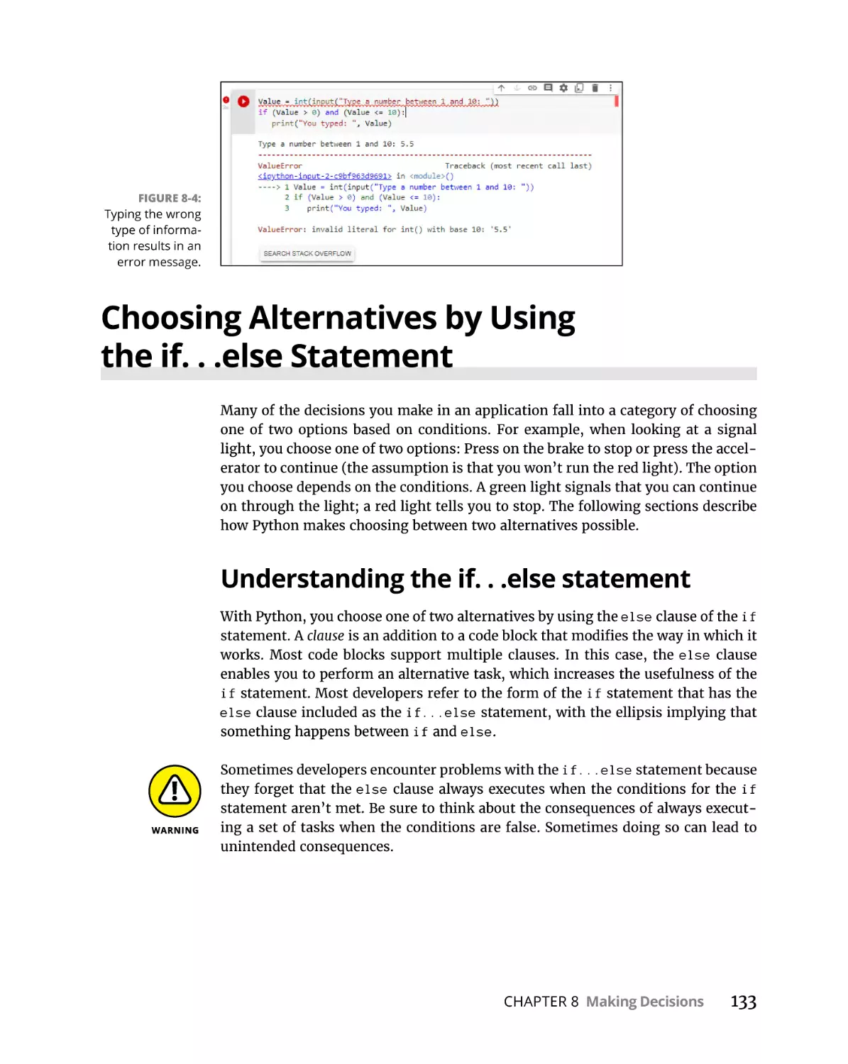


Author: Mueller J.P.
Tags: programming languages programming python programming language
ISBN: 978-1-119-91378-8
Year: 2023

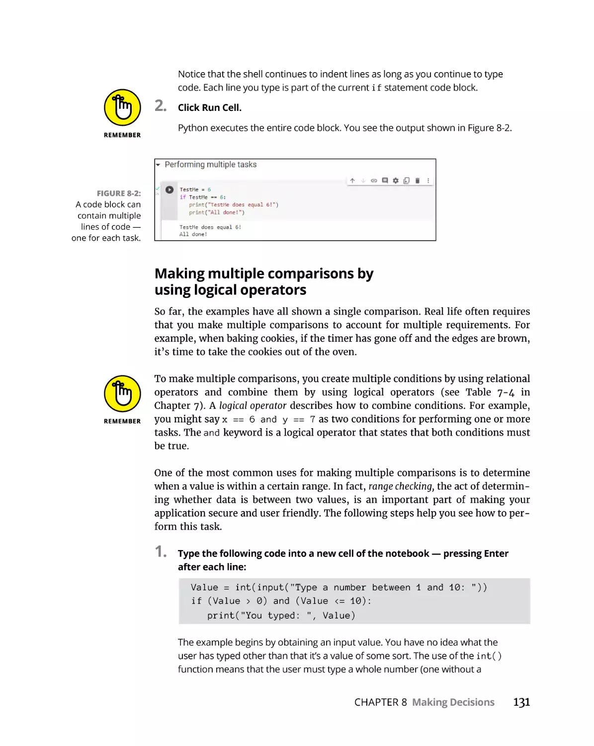
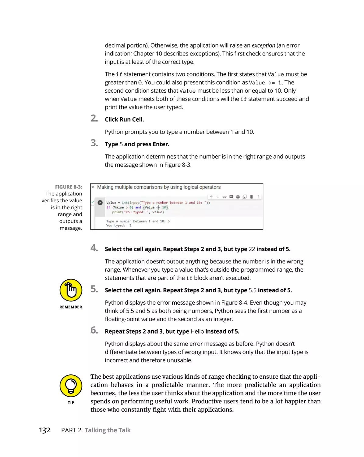
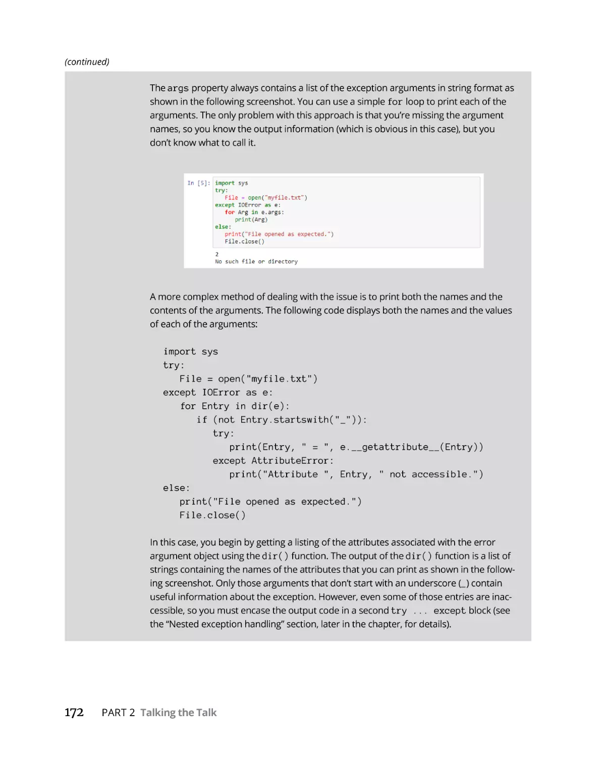
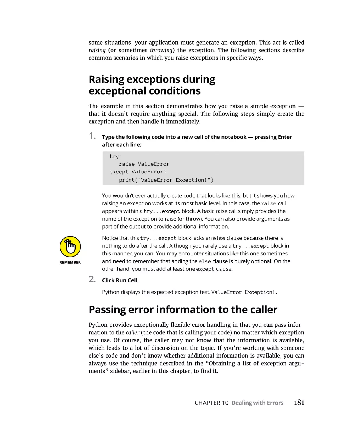
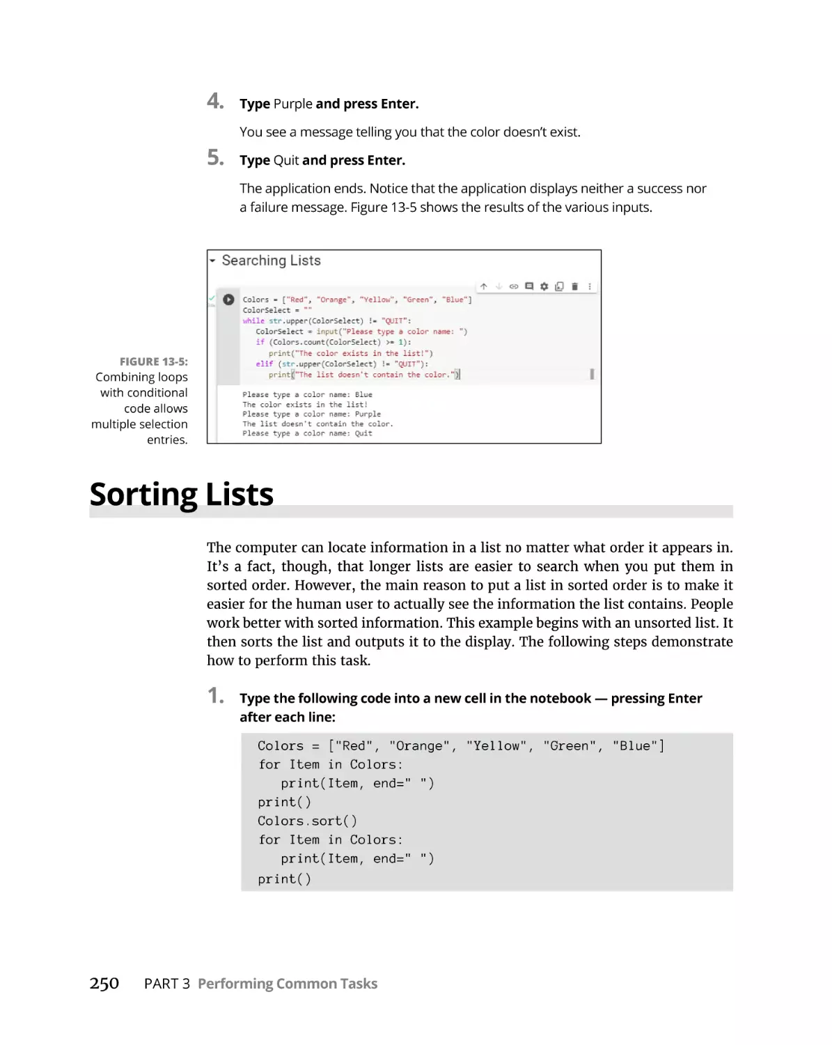
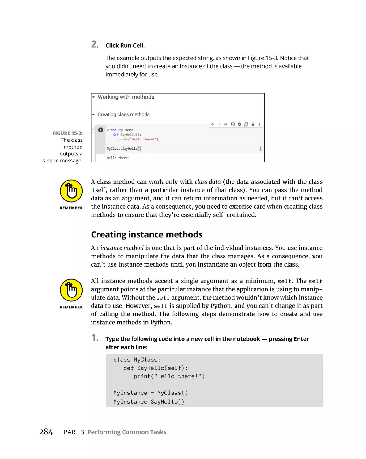
Text
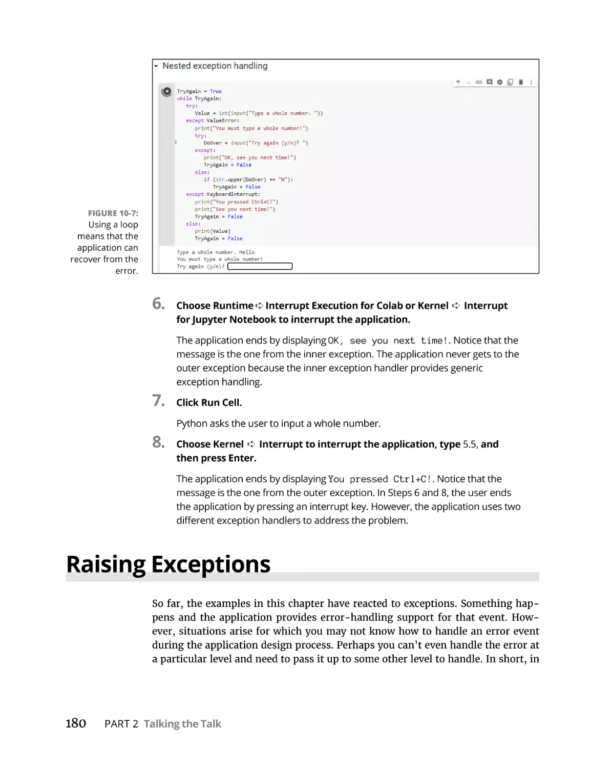
Beginning
Programming
with Python
®
Beginning
Programming
with Python
®
3rd Edition
by John Paul Mueller
Beginning Programming with Python® For Dummies®, 3rd Edition
Published by: John Wiley & Sons, Inc., 111 River Street, Hoboken, NJ 07030-5774, www.wiley.com
Copyright © 2023 by John Wiley & Sons, Inc., Hoboken, New Jersey
Media and software compilation copyright © 2023 by John Wiley & Sons, Inc. All rights reserved.
Published simultaneously in Canada
No part of this publication may be reproduced, stored in a retrieval system or transmitted in any form or by any
means, electronic, mechanical, photocopying, recording, scanning or otherwise, except as permitted under Sections
107 or 108 of the 1976 United States Copyright Act, without the prior written permission of the Publisher. Requests to
the Publisher for permission should be addressed to the Permissions Department, John Wiley & Sons, Inc., 111 River
Street, Hoboken, NJ 07030, (201) 748-6011, fax (201) 748-6008, or online at http://www.wiley.com/go/permissions.
Trademarks: Wiley, For Dummies, the Dummies Man logo, Dummies.com, Making Everything Easier, and related
trade dress are trademarks or registered trademarks of John Wiley & Sons, Inc. and may not be used without written
permission. Python is a registered trademark of Python Software Foundation Corporation. All other trademarks are
the property of their respective owners. John Wiley & Sons, Inc. is not associated with any product or vendor
mentioned in this book.
LIMIT OF LIABILITY/DISCLAIMER OF WARRANTY: WHILE THE PUBLISHER AND AUTHORS HAVE USED THEIR
BEST EFFORTS IN PREPARING THIS WORK, THEY MAKE NO REPRESENTATIONS OR WARRANTIES WITH RESPECT
TO THE ACCURACY OR COMPLETENESS OF THE CONTENTS OF THIS WORK AND SPECIFICALLY DISCLAIM ALL
WARRANTIES, INCLUDING WITHOUT LIMITATION ANY IMPLIED WARRANTIES OF MERCHANTABILITY OR
FITNESS FOR A PARTICULAR PURPOSE. NO WARRANTY MAY BE CREATED OR EXTENDED BY SALES
REPRESENTATIVES, WRITTEN SALES MATERIALS OR PROMOTIONAL STATEMENTS FOR THIS WORK. THE FACT
THAT AN ORGANIZATION, WEBSITE, OR PRODUCT IS REFERRED TO IN THIS WORK AS A CITATION AND/OR
POTENTIAL SOURCE OF FURTHER INFORMATION DOES NOT MEAN THAT THE PUBLISHER AND AUTHORS
ENDORSE THE INFORMATION OR SERVICES THE ORGANIZATION, WEBSITE, OR PRODUCT MAY PROVIDE OR
RECOMMENDATIONS IT MAY MAKE. THIS WORK IS SOLD WITH THE UNDERSTANDING THAT THE PUBLISHER IS
NOT ENGAGED IN RENDERING PROFESSIONAL SERVICES. THE ADVICE AND STRATEGIES CONTAINED HEREIN
MAY NOT BE SUITABLE FOR YOUR SITUATION. YOU SHOULD CONSULT WITH A SPECIALIST WHERE APPROPRIATE.
FURTHER, READERS SHOULD BE AWARE THAT WEBSITES LISTED IN THIS WORK MAY HAVE CHANGED OR
DISAPPEARED BETWEEN WHEN THIS WORK WAS WRITTEN AND WHEN IT IS READ. NEITHER THE PUBLISHER
NOR AUTHORS SHALL BE LIABLE FOR ANY LOSS OF PROFIT OR ANY OTHER COMMERCIAL DAMAGES, INCLUDING
BUT NOT LIMITED TO SPECIAL, INCIDENTAL, CONSEQUENTIAL, OR OTHER DAMAGES.
For general information on our other products and services, please contact our Customer Care Department within
the U.S. at 877-762-2974, outside the U.S. at 317-572-3993, or fax 317-572-4002. For technical support, please visit
https://hub.wiley.com/community/support/dummies.
Wiley publishes in a variety of print and electronic formats and by print-on-demand. Some material included with
standard print versions of this book may not be included in e-books or in print-on-demand. If this book refers to
media such as a CD or DVD that is not included in the version you purchased, you may download this material at
http://booksupport.wiley.com. For more information about Wiley products, visit www.wiley.com.
Library of Congress Control Number: 2022948492
ISBN: 978-1-119-91377-1 (pbk); ISBN 978-1-119-91378-8 (ebk); ISBN 978-1-119-91379-5 (ebk)
Contents at a Glance
Introduction. . . . . . . . . . . . . . . . . . . . . . . . . . . . . . . . . . . . . . . . . . . . . . . . . . . . . . . . . 1
Part 1: Getting Started with Python. . . . . . . . . . . . . . . . . . . . . . . . . . . . . 7
CHAPTER 1:
CHAPTER 2:
CHAPTER 3:
CHAPTER 4:
CHAPTER 5:
Talking to Your Computer. . . . . . . . . . . . . . . . . . . . . . . . . . . . . . . . . . . . . . . . . 9
Working with Google Colab. . . . . . . . . . . . . . . . . . . . . . . . . . . . . . . . . . . . . . . 23
Interacting with Python. . . . . . . . . . . . . . . . . . . . . . . . . . . . . . . . . . . . . . . . . . 41
Writing Your First Application. . . . . . . . . . . . . . . . . . . . . . . . . . . . . . . . . . . . . 57
Performing Magic. . . . . . . . . . . . . . . . . . . . . . . . . . . . . . . . . . . . . . . . . . . . . . . 79
Part 2: Talking the Talk . . . . . . . . . . . . . . . . . . . . . . . . . . . . . . . . . . . . . . . . . . . 93
Storing and Modifying Information. . . . . . . . . . . . . . . . . . . . . . . . . . . . . . . . 95
CHAPTER 7: Managing Information. . . . . . . . . . . . . . . . . . . . . . . . . . . . . . . . . . . . . . . . . 107
CHAPTER 8: Making Decisions . . . . . . . . . . . . . . . . . . . . . . . . . . . . . . . . . . . . . . . . . . . . . 127
CHAPTER 9: Performing Repetitive Tasks. . . . . . . . . . . . . . . . . . . . . . . . . . . . . . . . . . . . 143
CHAPTER 10: Dealing with Errors. . . . . . . . . . . . . . . . . . . . . . . . . . . . . . . . . . . . . . . . . . . . 157
CHAPTER 6:
Part 3: Performing Common Tasks. . . . . . . . . . . . . . . . . . . . . . . . . . .
187
Interacting with Packages. . . . . . . . . . . . . . . . . . . . . . . . . . . . . . . . . . . . . .
CHAPTER 12: Working with Strings . . . . . . . . . . . . . . . . . . . . . . . . . . . . . . . . . . . . . . . . . .
CHAPTER 13: Managing Lists. . . . . . . . . . . . . . . . . . . . . . . . . . . . . . . . . . . . . . . . . . . . . . . .
CHAPTER 14: Collecting All Sorts of Data . . . . . . . . . . . . . . . . . . . . . . . . . . . . . . . . . . . . .
CHAPTER 15: Creating and Using Classes. . . . . . . . . . . . . . . . . . . . . . . . . . . . . . . . . . . . .
189
215
239
257
279
Part 4: Performing Advanced Tasks. . . . . . . . . . . . . . . . . . . . . . . . . .
301
CHAPTER 11:
Storing Data in Files. . . . . . . . . . . . . . . . . . . . . . . . . . . . . . . . . . . . . . . . . . . 303
CHAPTER 17: Sending an Email. . . . . . . . . . . . . . . . . . . . . . . . . . . . . . . . . . . . . . . . . . . . . . 321
CHAPTER 16:
Part 5: The Part of Tens. . . . . . . . . . . . . . . . . . . . . . . . . . . . . . . . . . . . . . . . .
337
Ten Amazing Programming Resources. . . . . . . . . . . . . . . . . . . . . . . . . . .
Ten Ways to Make a Living with Python. . . . . . . . . . . . . . . . . . . . . . . . . .
CHAPTER 20: Ten Tools That Enhance Your Python Experience. . . . . . . . . . . . . . . . . .
CHAPTER 21: Ten (Plus) Libraries You Need to Know About. . . . . . . . . . . . . . . . . . . . .
339
349
357
369
Index. . . . . . . . . . . . . . . . . . . . . . . . . . . . . . . . . . . . . . . . . . . . . . . . . . . . . . . . . . . . . . .
379
CHAPTER 18:
CHAPTER 19:
Table of Contents
INTRODUCTION . . . . . . . . . . . . . . . . . . . . . . . . . . . . . . . . . . . . . . . . . . . . . . . . . . . . 1
About This Book. . . . . . . . . . . . . . . . . . . . . . . . . . . . . . . . . . . . . . . . . . . . . . .
Foolish Assumptions. . . . . . . . . . . . . . . . . . . . . . . . . . . . . . . . . . . . . . . . . . .
Icons Used in This Book. . . . . . . . . . . . . . . . . . . . . . . . . . . . . . . . . . . . . . . .
Beyond the Book. . . . . . . . . . . . . . . . . . . . . . . . . . . . . . . . . . . . . . . . . . . . . .
Where to Go from Here . . . . . . . . . . . . . . . . . . . . . . . . . . . . . . . . . . . . . . . .
1
2
3
4
5
PART 1: GETTING STARTED WITH PYTHON. . . . . . . . . . . . . . . . . . . . 7
CHAPTER 1:
Talking to Your Computer . . . . . . . . . . . . . . . . . . . . . . . . . . . . . . . 9
Understanding Why You Want to Talk to Your Computer. . . . . . . . . . .
Knowing that an Application Is a Form of Communication. . . . . . . . . .
Thinking about procedures you use daily . . . . . . . . . . . . . . . . . . . . .
Writing procedures down. . . . . . . . . . . . . . . . . . . . . . . . . . . . . . . . . . .
Seeing applications as being like any other procedure. . . . . . . . . .
Making your computer do funny things. . . . . . . . . . . . . . . . . . . . . . .
Defining What an Application Is . . . . . . . . . . . . . . . . . . . . . . . . . . . . . . . .
Understanding that computers use a special language . . . . . . . . .
Helping humans speak to the computer. . . . . . . . . . . . . . . . . . . . . .
Understanding Why Python Is So Cool. . . . . . . . . . . . . . . . . . . . . . . . . . .
Unearthing the reasons for using Python. . . . . . . . . . . . . . . . . . . . .
Deciding how you can personally benefit from Python. . . . . . . . . .
Discovering which organizations use Python . . . . . . . . . . . . . . . . . .
Finding useful Python applications. . . . . . . . . . . . . . . . . . . . . . . . . . .
Comparing Python to other languages . . . . . . . . . . . . . . . . . . . . . . .
CHAPTER 2:
10
11
11
12
13
13
13
14
14
16
16
17
18
19
20
Working with Google Colab. . . . . . . . . . . . . . . . . . . . . . . . . . . . . 23
Defining Google Colab . . . . . . . . . . . . . . . . . . . . . . . . . . . . . . . . . . . . . . . .
Understanding what Google Colab does. . . . . . . . . . . . . . . . . . . . . .
Working with Google Colab features . . . . . . . . . . . . . . . . . . . . . . . . .
Working with Notebooks . . . . . . . . . . . . . . . . . . . . . . . . . . . . . . . . . . . . . .
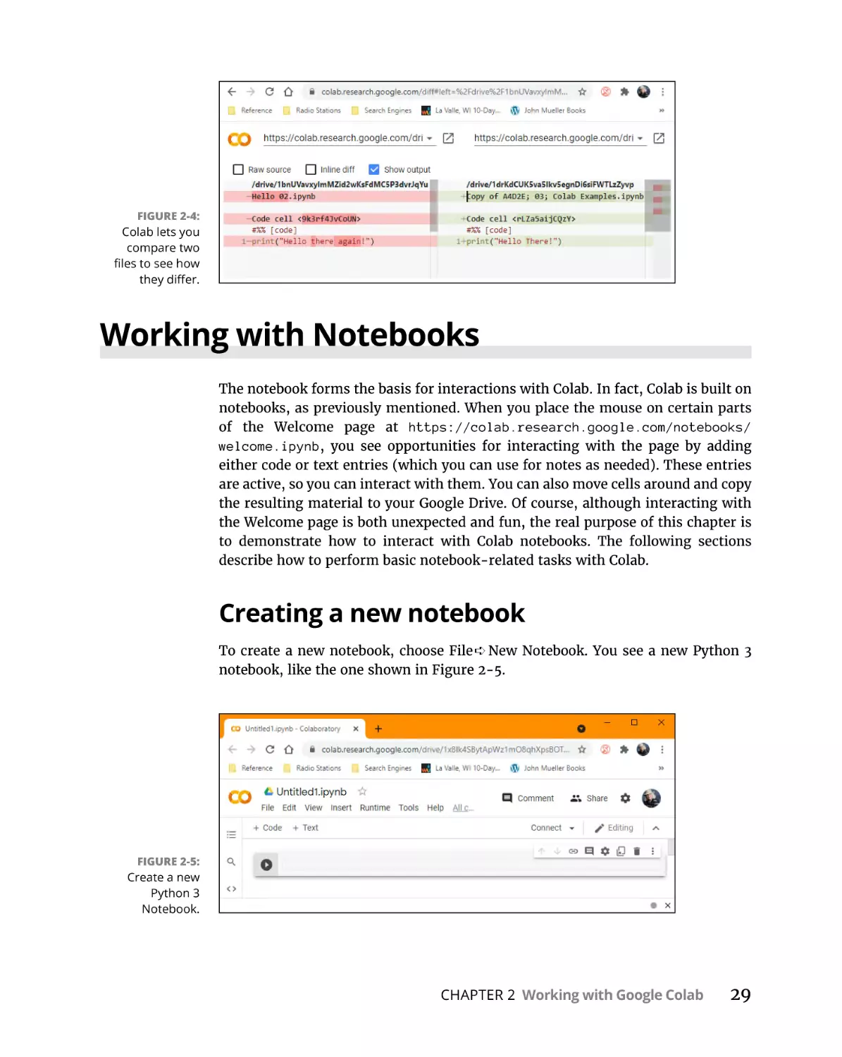
Creating a new notebook. . . . . . . . . . . . . . . . . . . . . . . . . . . . . . . . . . .
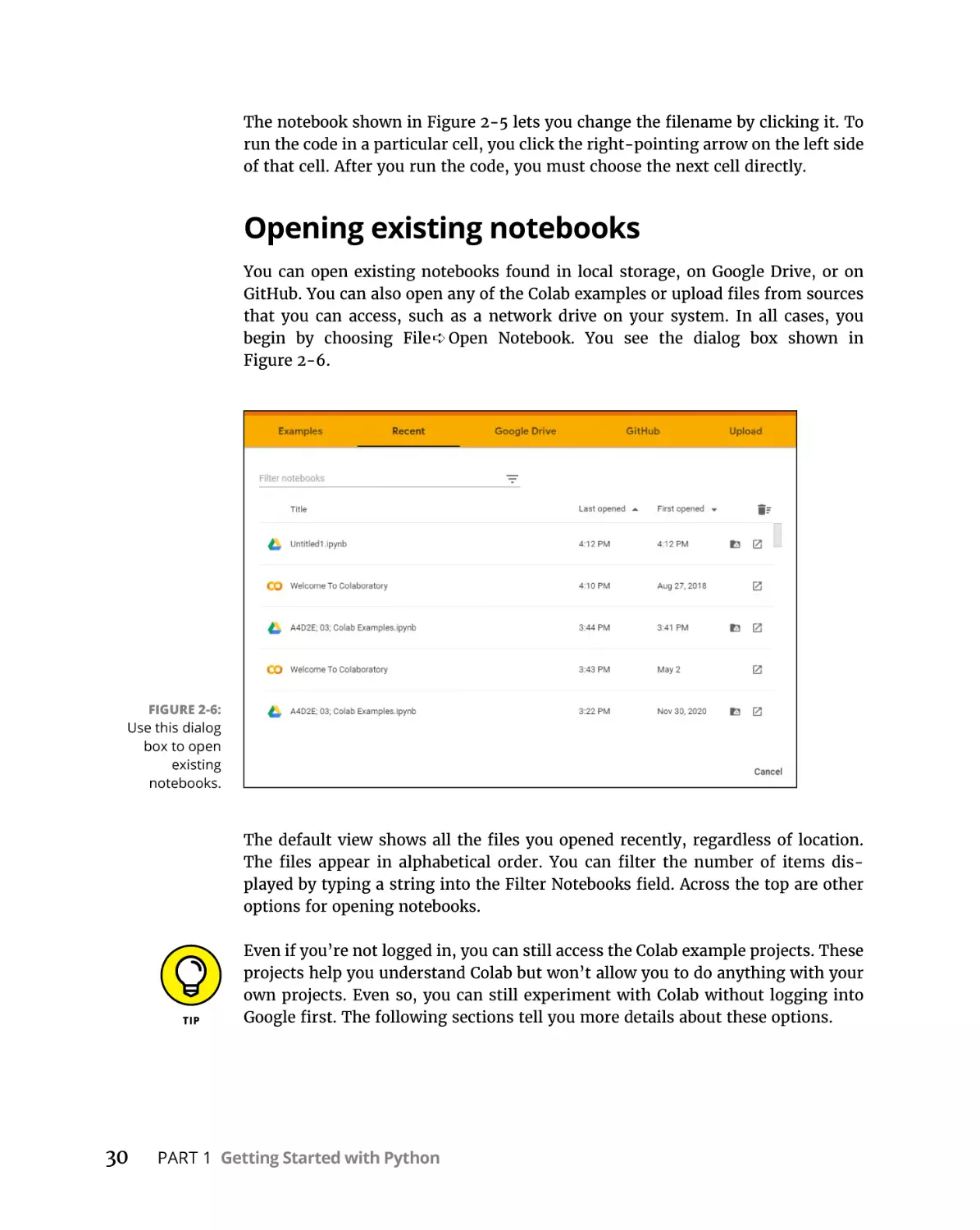
Opening existing notebooks . . . . . . . . . . . . . . . . . . . . . . . . . . . . . . . .
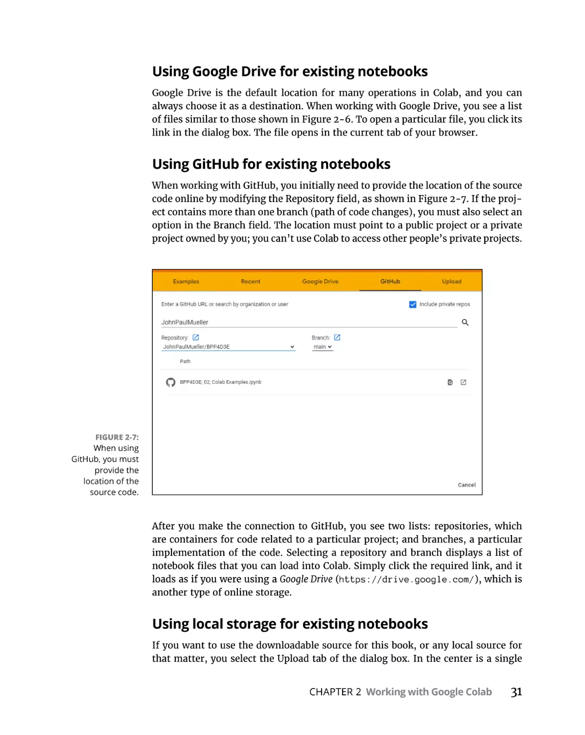
Saving notebooks using GitHub . . . . . . . . . . . . . . . . . . . . . . . . . . . . .
Getting the gist of things . . . . . . . . . . . . . . . . . . . . . . . . . . . . . . . . . . .
Working with Drive . . . . . . . . . . . . . . . . . . . . . . . . . . . . . . . . . . . . . . . .
Performing Common Tasks. . . . . . . . . . . . . . . . . . . . . . . . . . . . . . . . . . . .
Creating code cells . . . . . . . . . . . . . . . . . . . . . . . . . . . . . . . . . . . . . . . .
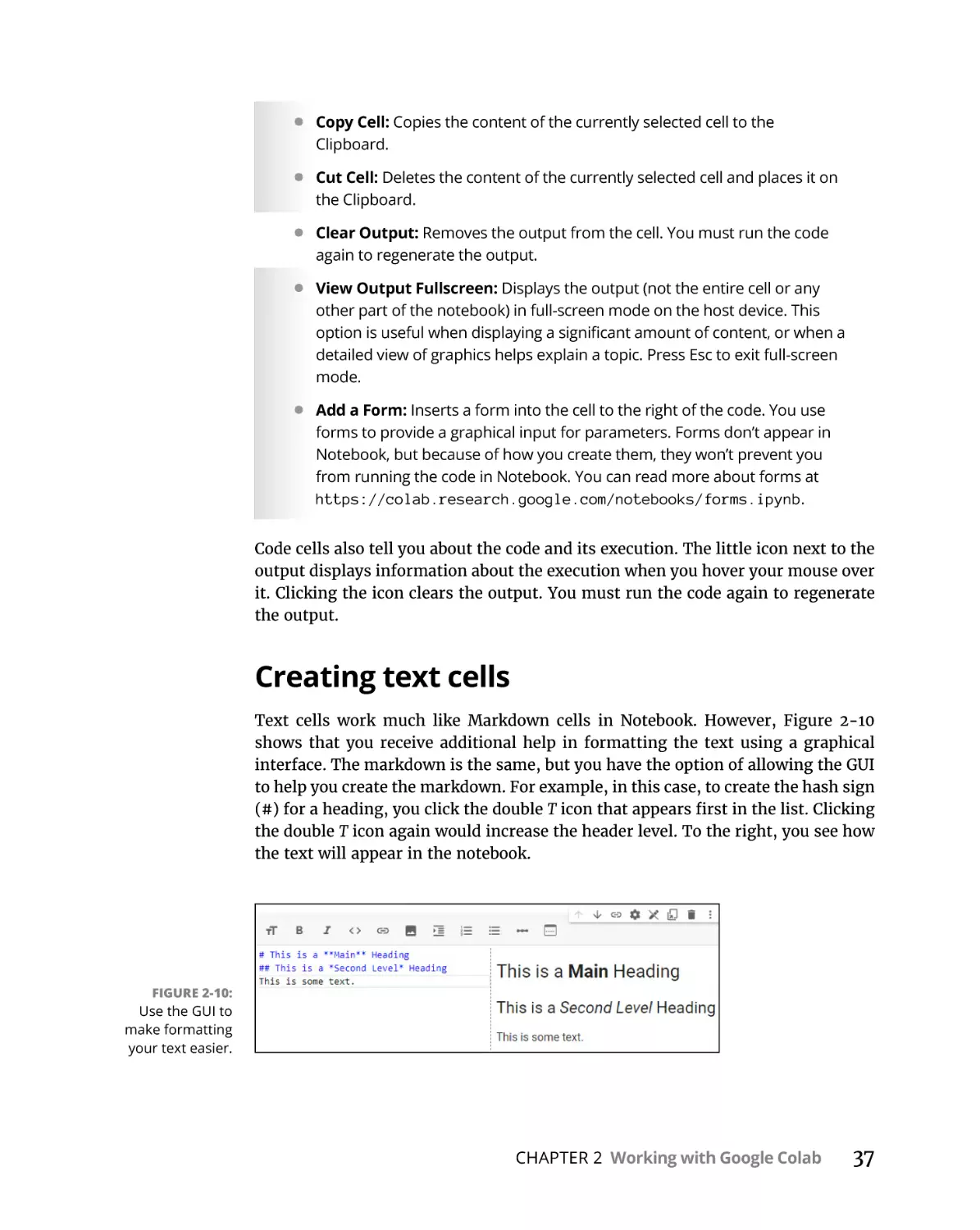
Creating text cells . . . . . . . . . . . . . . . . . . . . . . . . . . . . . . . . . . . . . . . . .
Creating special cells. . . . . . . . . . . . . . . . . . . . . . . . . . . . . . . . . . . . . . .
Table of Contents
24
24
25
29
29
30
32
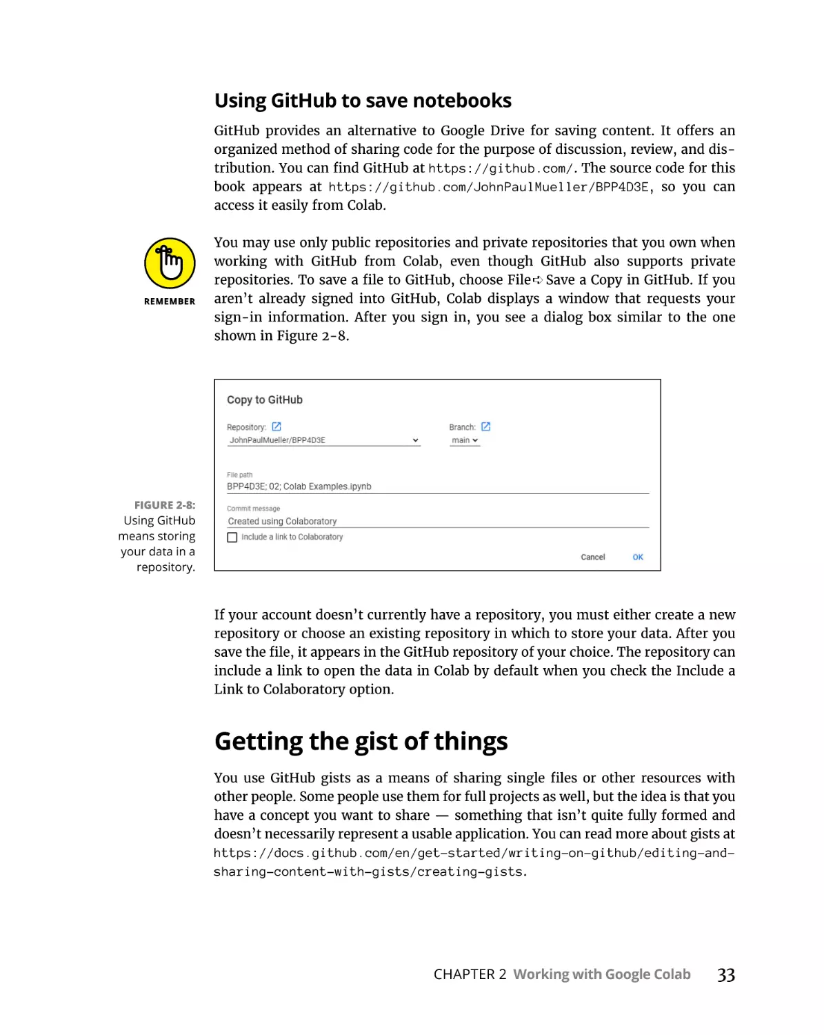
33
34
35
35
37
38
vii
Editing cells. . . . . . . . . . . . . . . . . . . . . . . . . . . . . . . . . . . . . . . . . . . . . . .
Moving cells . . . . . . . . . . . . . . . . . . . . . . . . . . . . . . . . . . . . . . . . . . . . . .
Using Hardware Acceleration . . . . . . . . . . . . . . . . . . . . . . . . . . . . . . . . . .
Executing the Code. . . . . . . . . . . . . . . . . . . . . . . . . . . . . . . . . . . . . . . . . . .
Getting Help. . . . . . . . . . . . . . . . . . . . . . . . . . . . . . . . . . . . . . . . . . . . . . . . .
CHAPTER 3:
38
39
39
39
40
Interacting with Python. . . . . . . . . . . . . . . . . . . . . . . . . . . . . . . . . 41
Typing a Command. . . . . . . . . . . . . . . . . . . . . . . . . . . . . . . . . . . . . . . . . . . 42
Telling the computer what to do. . . . . . . . . . . . . . . . . . . . . . . . . . . . . 43
Telling the computer you’re done. . . . . . . . . . . . . . . . . . . . . . . . . . . . 43
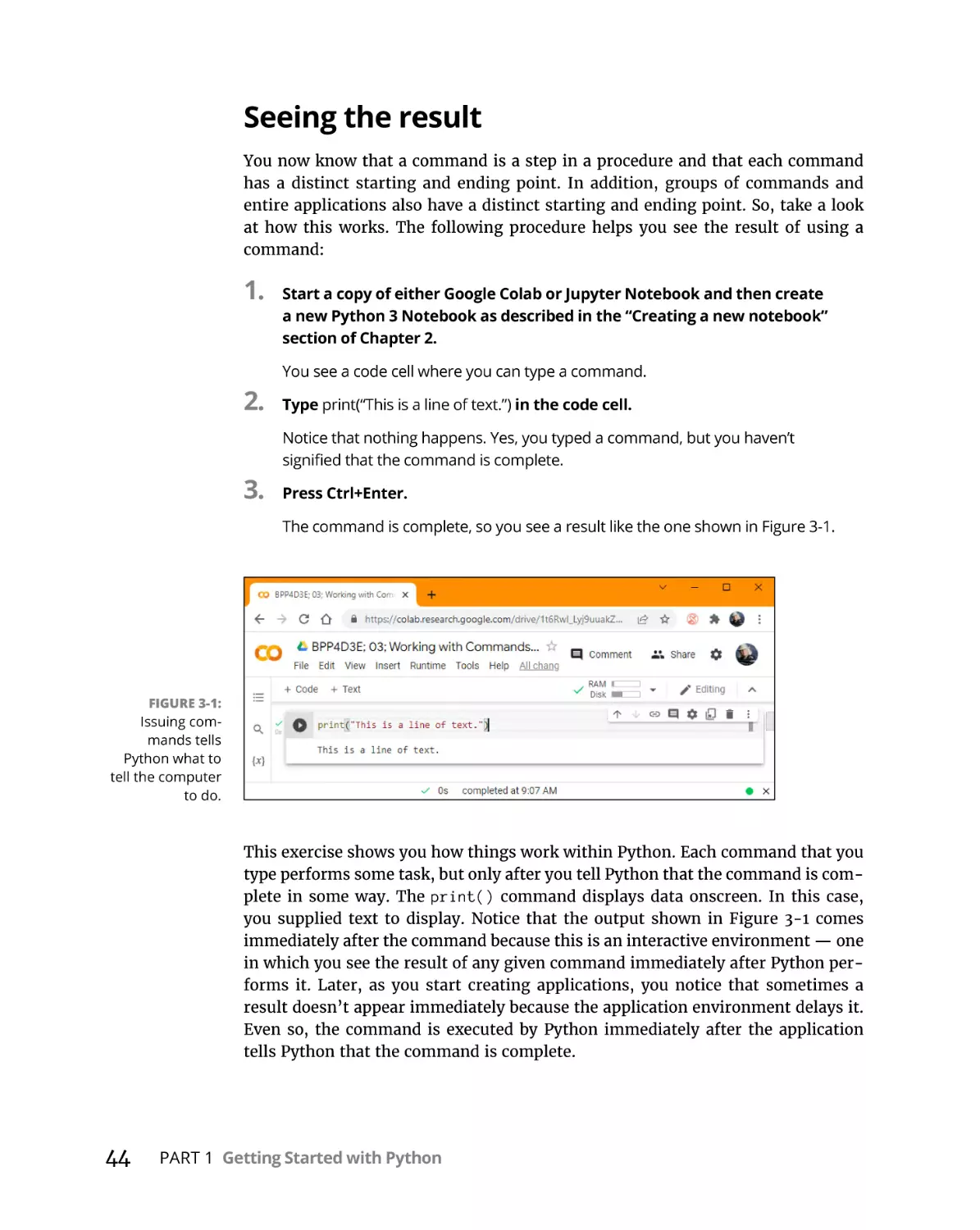
Seeing the result . . . . . . . . . . . . . . . . . . . . . . . . . . . . . . . . . . . . . . . . . . 44
Getting Python’s Help. . . . . . . . . . . . . . . . . . . . . . . . . . . . . . . . . . . . . . . . . 45
Entering into help mode. . . . . . . . . . . . . . . . . . . . . . . . . . . . . . . . . . . . 46
Asking for help. . . . . . . . . . . . . . . . . . . . . . . . . . . . . . . . . . . . . . . . . . . . 48
Leaving help mode . . . . . . . . . . . . . . . . . . . . . . . . . . . . . . . . . . . . . . . . 50
Obtaining help directly. . . . . . . . . . . . . . . . . . . . . . . . . . . . . . . . . . . . . 50
Finding Out More about Functions and Objects. . . . . . . . . . . . . . . . . . . 52
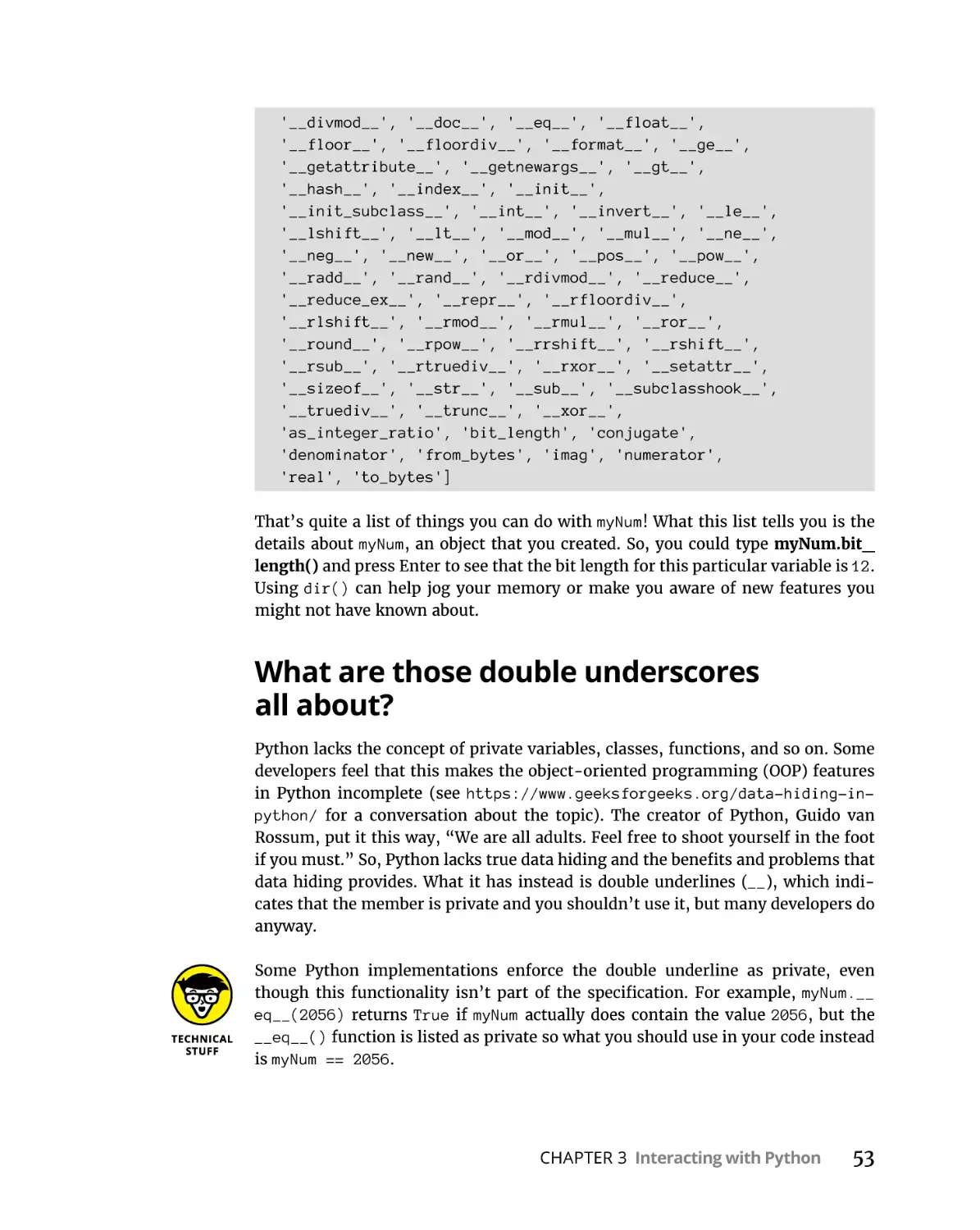
Yelling “Hello There” doesn’t help: Use dir() instead. . . . . . . . . . . . .52
What are those double underscores all about? . . . . . . . . . . . . . . . . 53
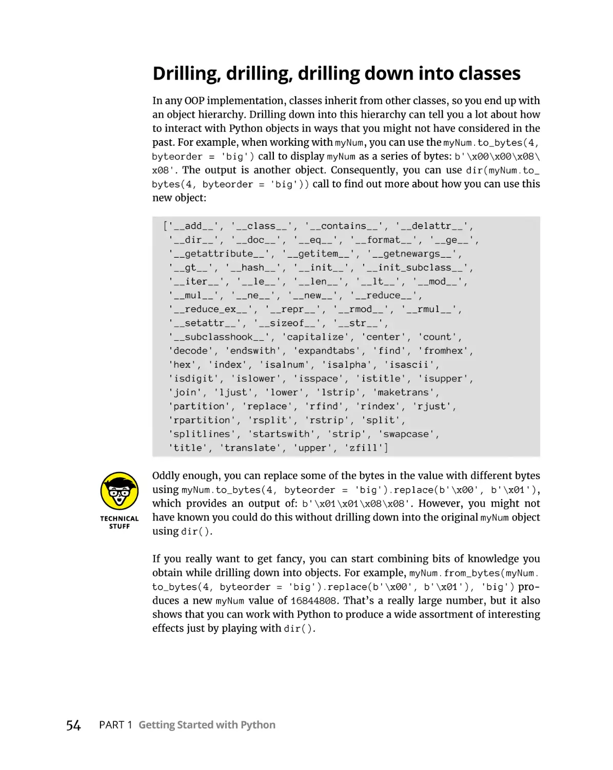
Drilling, drilling, drilling down into classes. . . . . . . . . . . . . . . . . . . . . 54
Playing the Part of Inspector. . . . . . . . . . . . . . . . . . . . . . . . . . . . . . . . . . . 55
Gaining access to inspect. . . . . . . . . . . . . . . . . . . . . . . . . . . . . . . . . . . 55
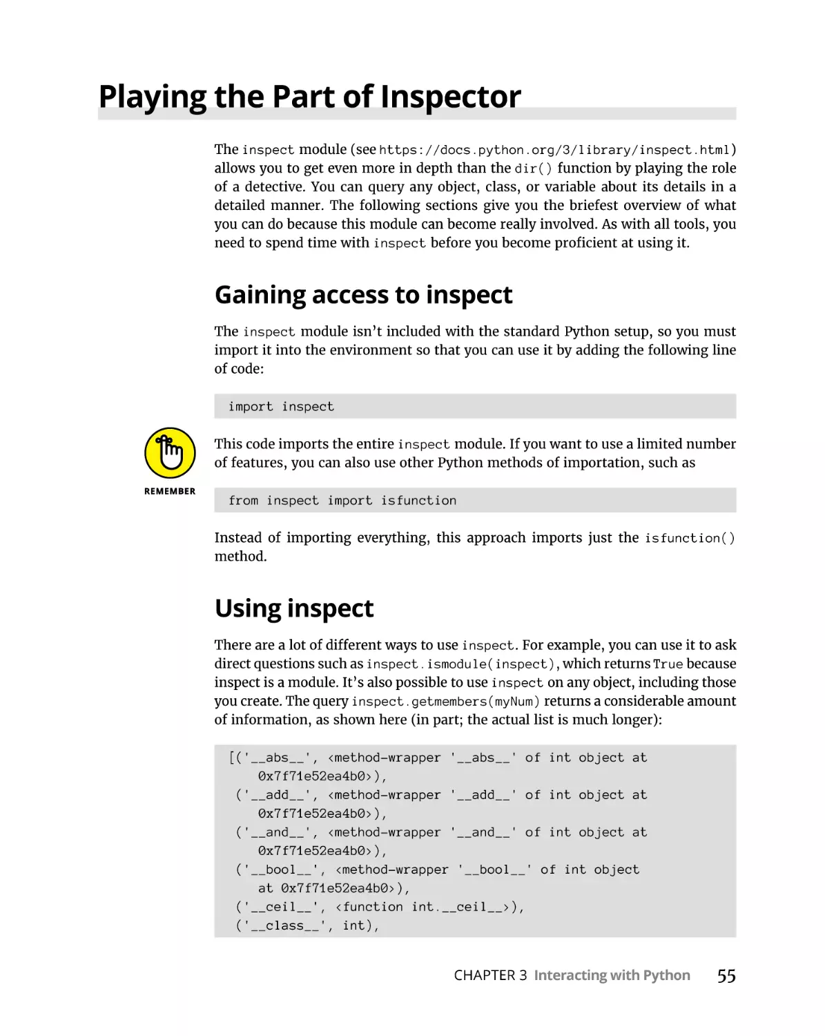
Using inspect . . . . . . . . . . . . . . . . . . . . . . . . . . . . . . . . . . . . . . . . . . . . . 55
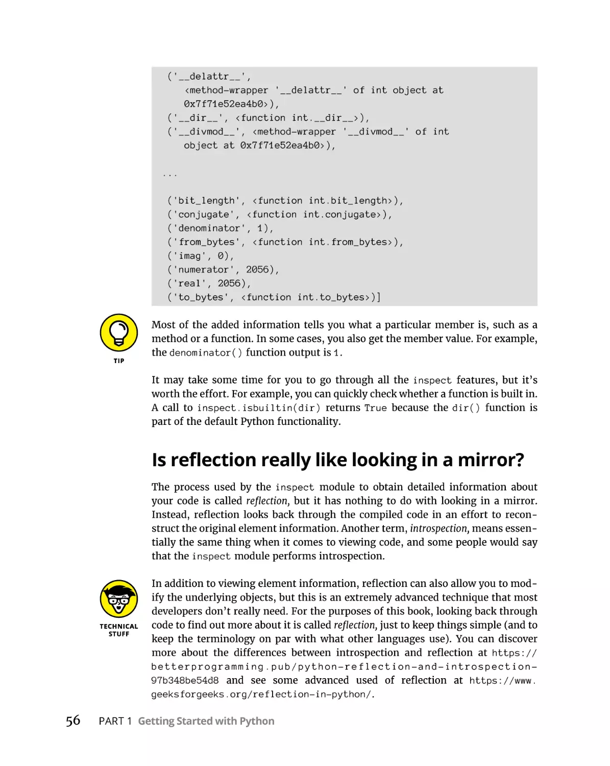
Is reflection really like looking in a mirror? . . . . . . . . . . . . . . . . . . . . 56
CHAPTER 4:
Writing Your First Application. . . . . . . . . . . . . . . . . . . . . . . . . . 57
Understanding Why IDEs Are Important. . . . . . . . . . . . . . . . . . . . . . . . .
Creating better code. . . . . . . . . . . . . . . . . . . . . . . . . . . . . . . . . . . . . . .
Debugging functionality. . . . . . . . . . . . . . . . . . . . . . . . . . . . . . . . . . . .
Defining why notebooks are useful . . . . . . . . . . . . . . . . . . . . . . . . . .
Creating the Application. . . . . . . . . . . . . . . . . . . . . . . . . . . . . . . . . . . . . . .
Developing the code. . . . . . . . . . . . . . . . . . . . . . . . . . . . . . . . . . . . . . .
Adding documentation cells . . . . . . . . . . . . . . . . . . . . . . . . . . . . . . . .
Other cell content . . . . . . . . . . . . . . . . . . . . . . . . . . . . . . . . . . . . . . . . .
Playing around with scratch cells . . . . . . . . . . . . . . . . . . . . . . . . . . . .
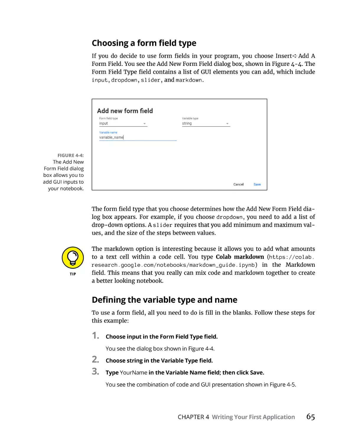
Interacting with form fields . . . . . . . . . . . . . . . . . . . . . . . . . . . . . . . . .
Running the Application. . . . . . . . . . . . . . . . . . . . . . . . . . . . . . . . . . . . . . .
Seeing the result . . . . . . . . . . . . . . . . . . . . . . . . . . . . . . . . . . . . . . . . . .
Viewing the executed code history. . . . . . . . . . . . . . . . . . . . . . . . . . .
Understanding the Use of Indentation . . . . . . . . . . . . . . . . . . . . . . . . . .
Adding Comments. . . . . . . . . . . . . . . . . . . . . . . . . . . . . . . . . . . . . . . . . . . .
Understanding comments. . . . . . . . . . . . . . . . . . . . . . . . . . . . . . . . . .
Creating multiline comments . . . . . . . . . . . . . . . . . . . . . . . . . . . . . . .
Using comments to leave yourself reminders . . . . . . . . . . . . . . . . .
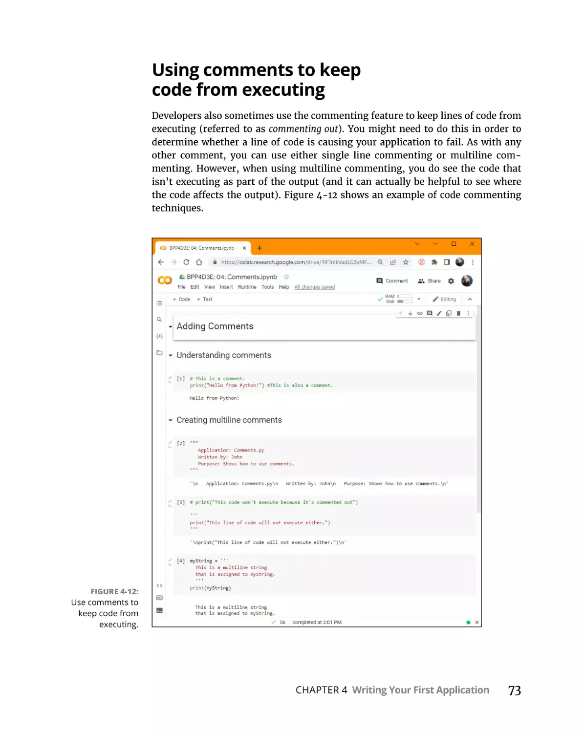
Using comments to keep code from executing . . . . . . . . . . . . . . . .
viii
Beginning Programming with Python For Dummies
58
58
59
59
60
60
61
62
63
64
66
67
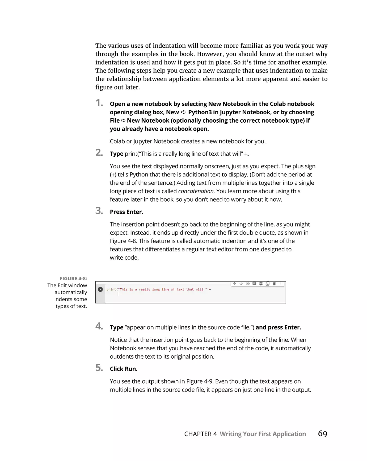
68
68
70
70
71
72
73
Making Your Notebook Informative, Descriptive, and Pretty. . . . . . . .
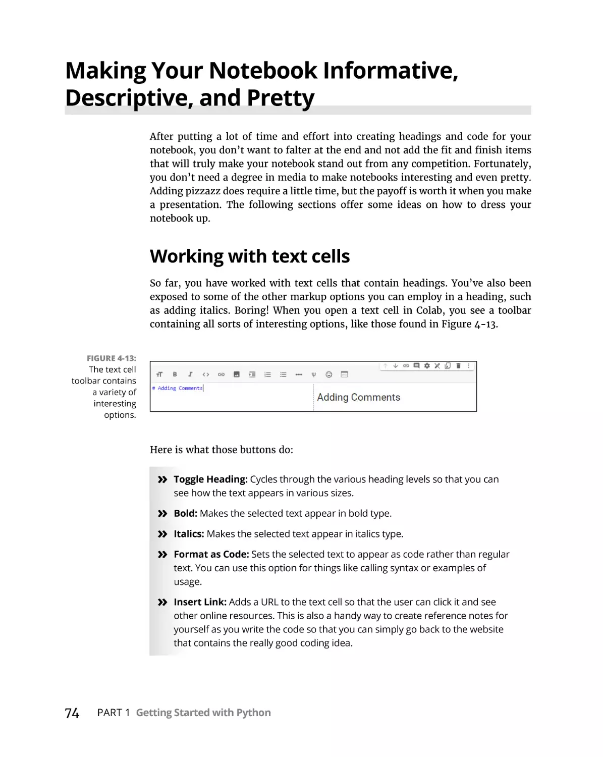
Working with text cells . . . . . . . . . . . . . . . . . . . . . . . . . . . . . . . . . . . . .
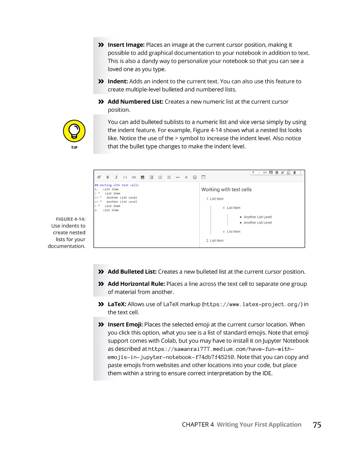
Adding section headers . . . . . . . . . . . . . . . . . . . . . . . . . . . . . . . . . . . .
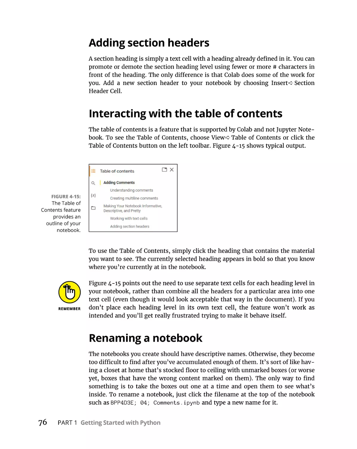
Interacting with the table of contents . . . . . . . . . . . . . . . . . . . . . . . .
Renaming a notebook. . . . . . . . . . . . . . . . . . . . . . . . . . . . . . . . . . . . . .
Closing and Halting a Notepad . . . . . . . . . . . . . . . . . . . . . . . . . . . . . . . . .
CHAPTER 5:
74
74
76
76
76
77
Performing Magic. . . . . . . . . . . . . . . . . . . . . . . . . . . . . . . . . . . . . . . . . 79
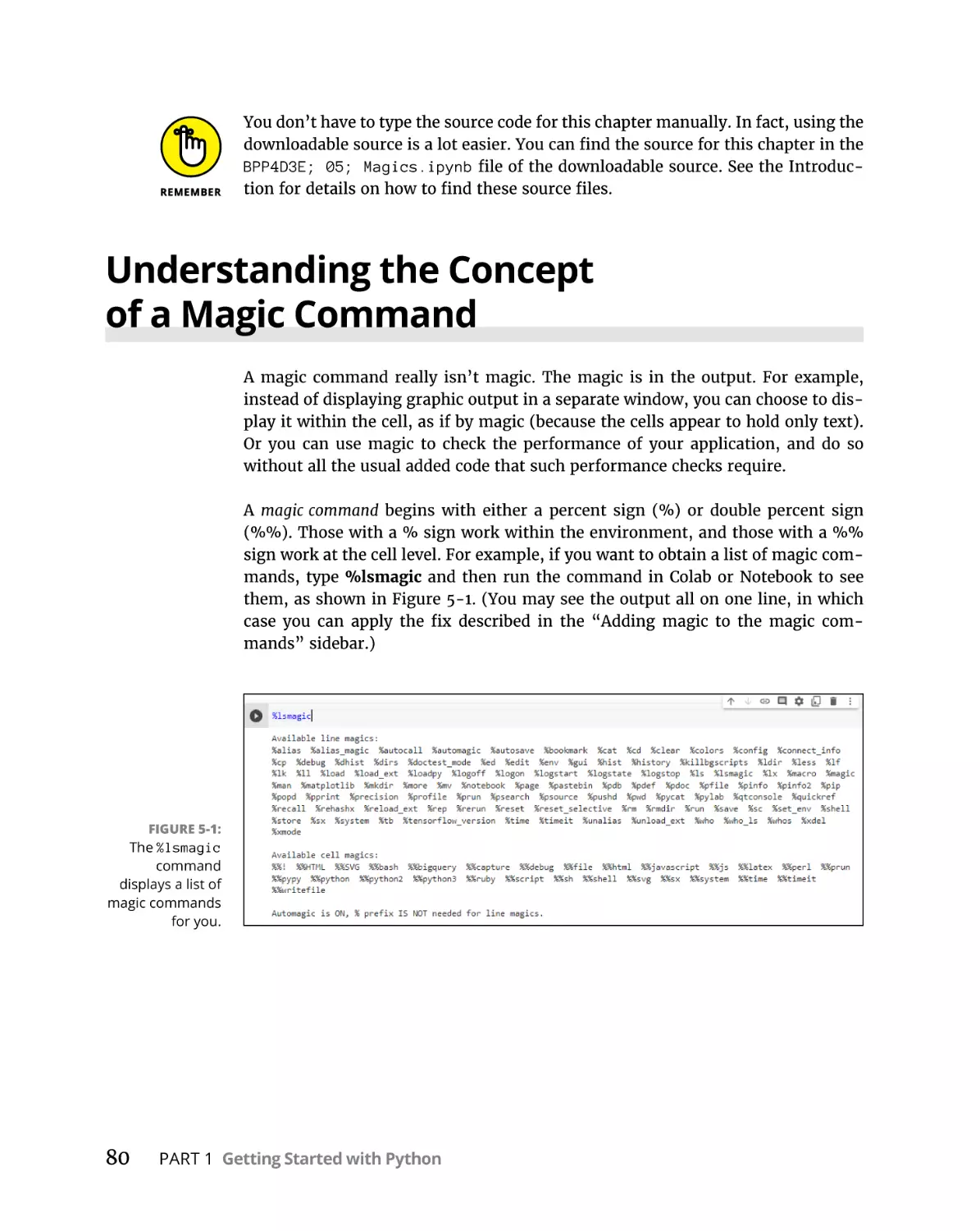
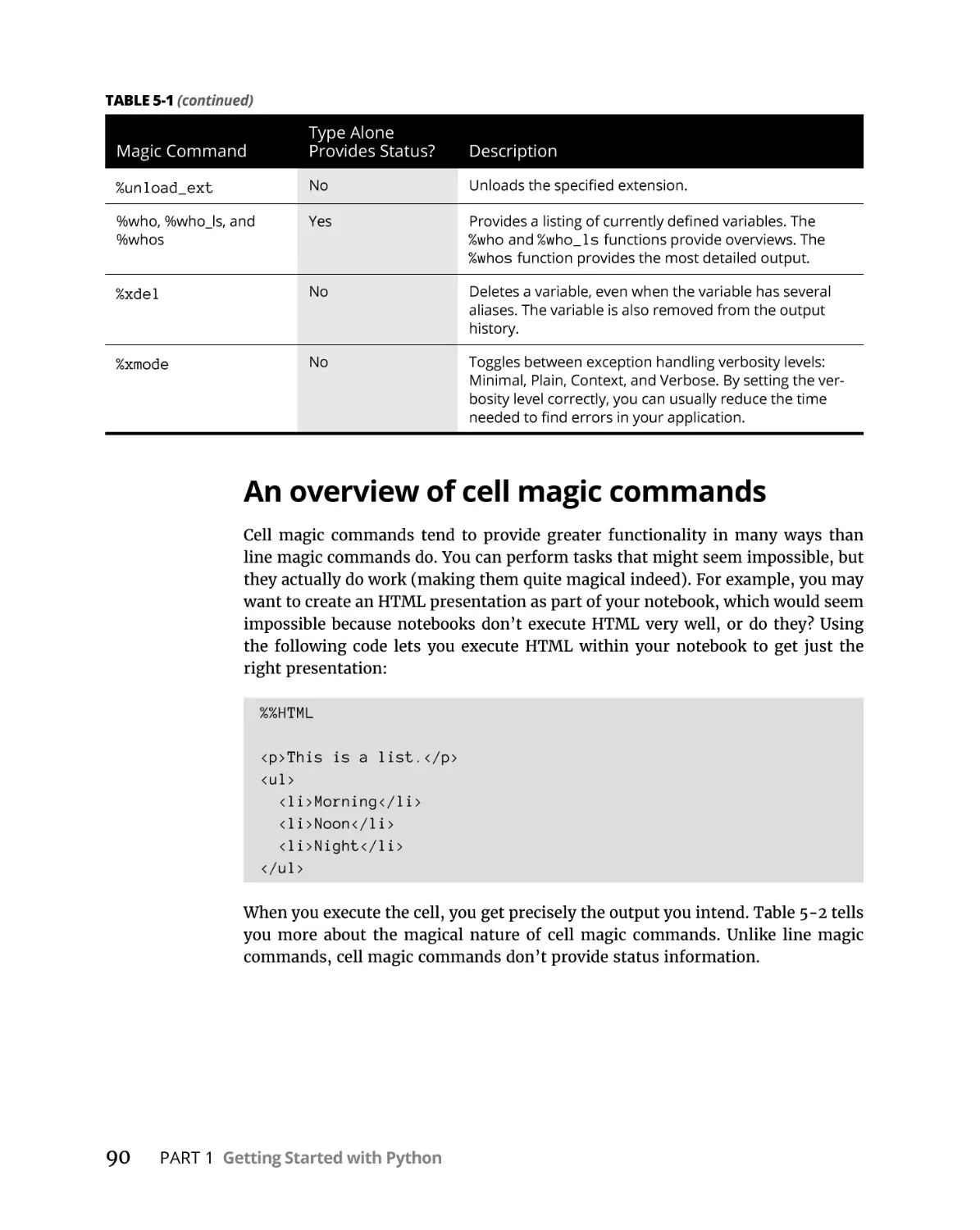
Understanding the Concept of a Magic Command . . . . . . . . . . . . . . . .
What Kind of Magic Do You Want to Perform?. . . . . . . . . . . . . . . . . . . .
Working with line magic commands. . . . . . . . . . . . . . . . . . . . . . . . . .
Working with cell magic commands. . . . . . . . . . . . . . . . . . . . . . . . . .
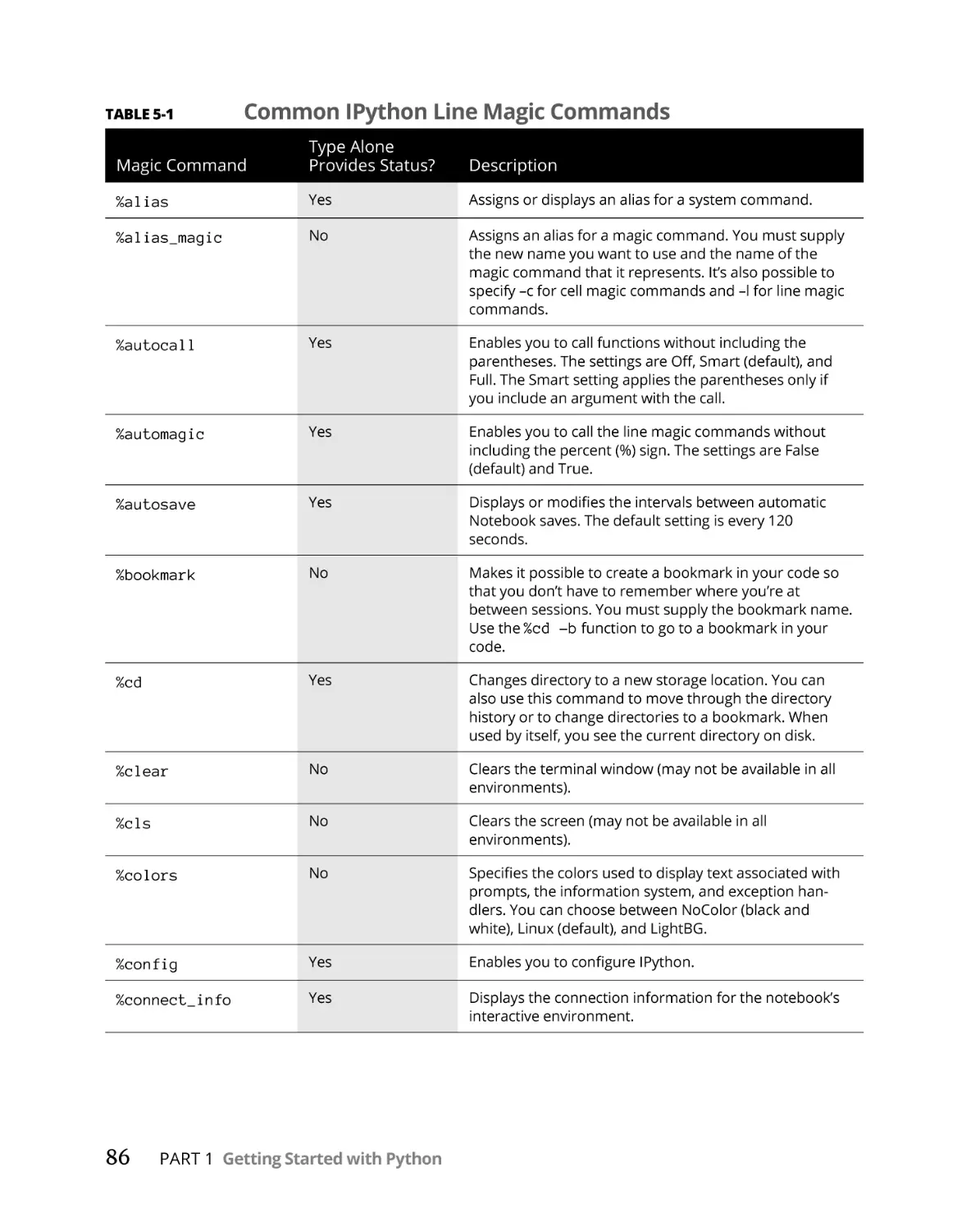
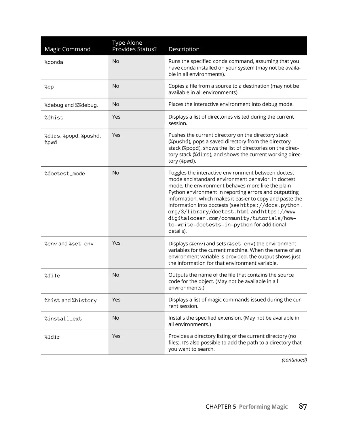
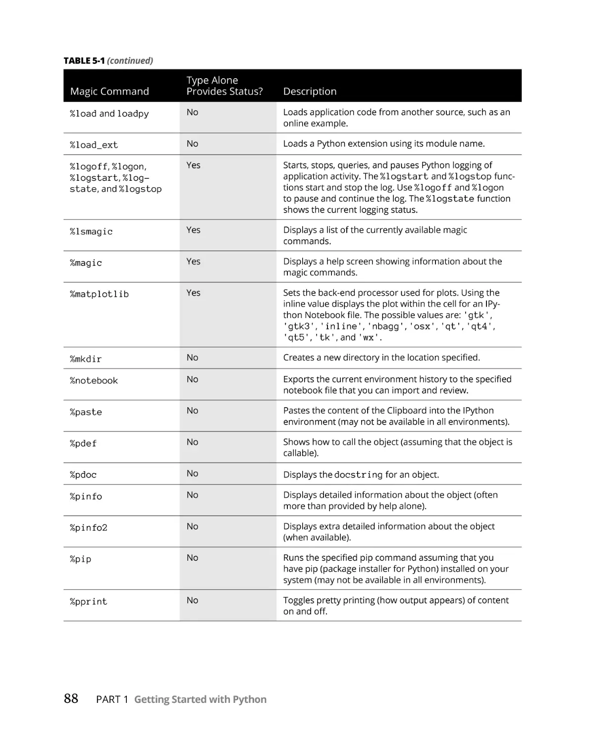
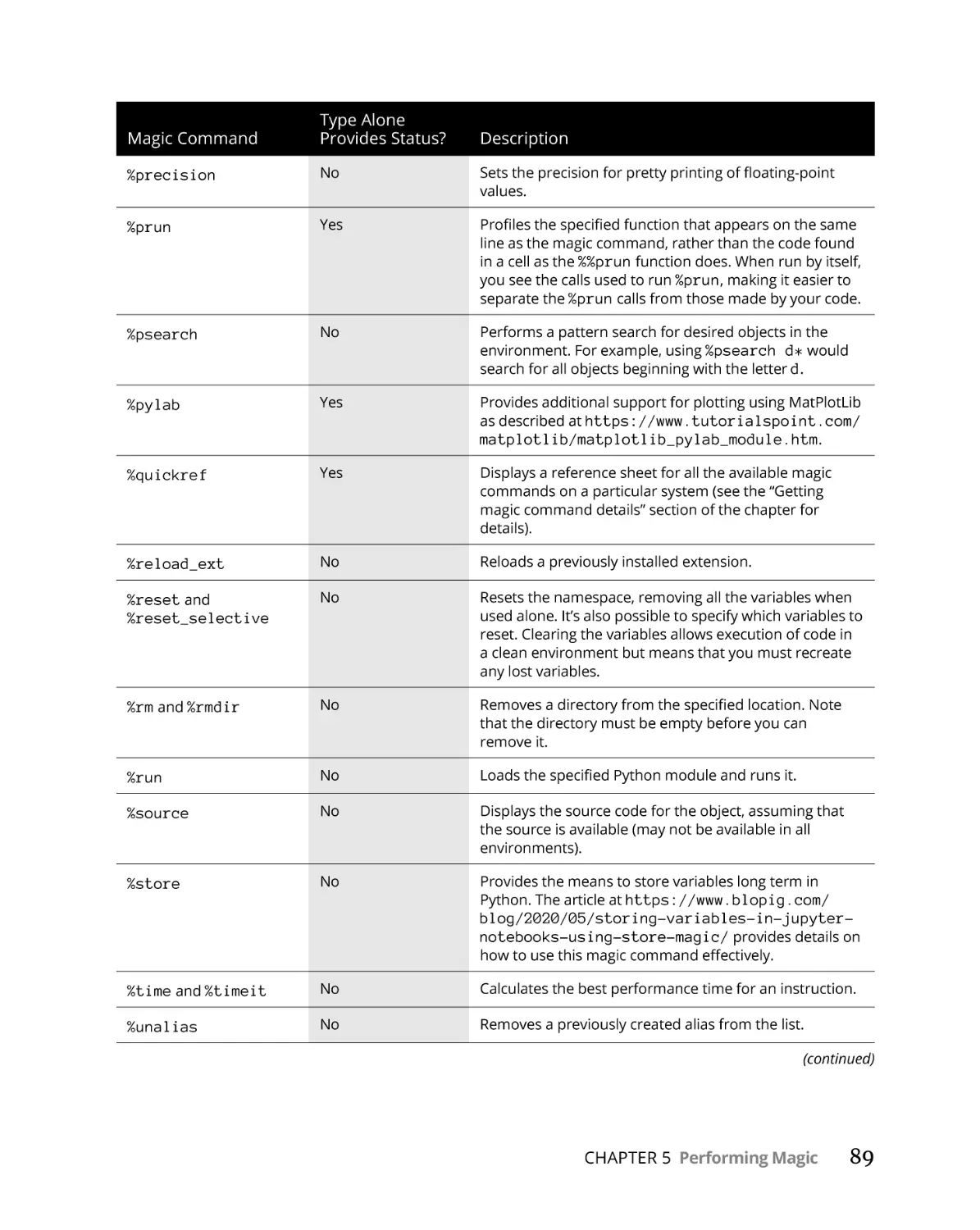
Learning the Magic Commands . . . . . . . . . . . . . . . . . . . . . . . . . . . . . . . .
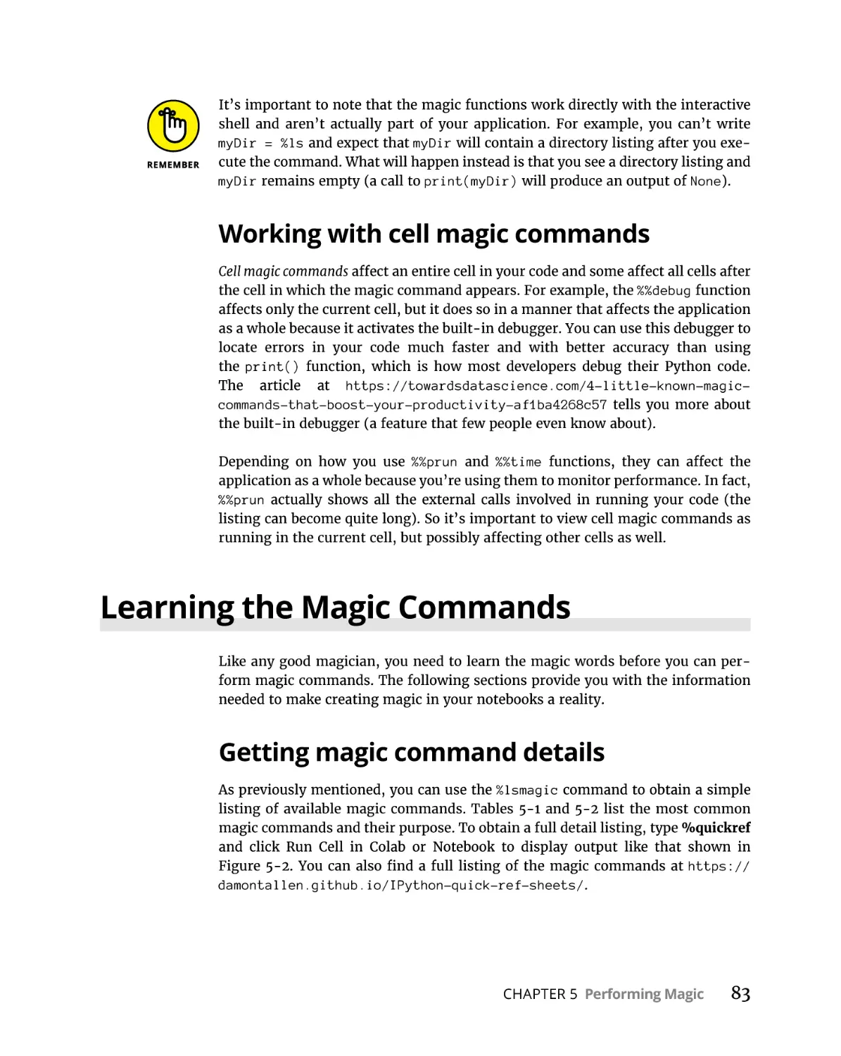
Getting magic command details. . . . . . . . . . . . . . . . . . . . . . . . . . . . .
An overview of line magic commands . . . . . . . . . . . . . . . . . . . . . . . .
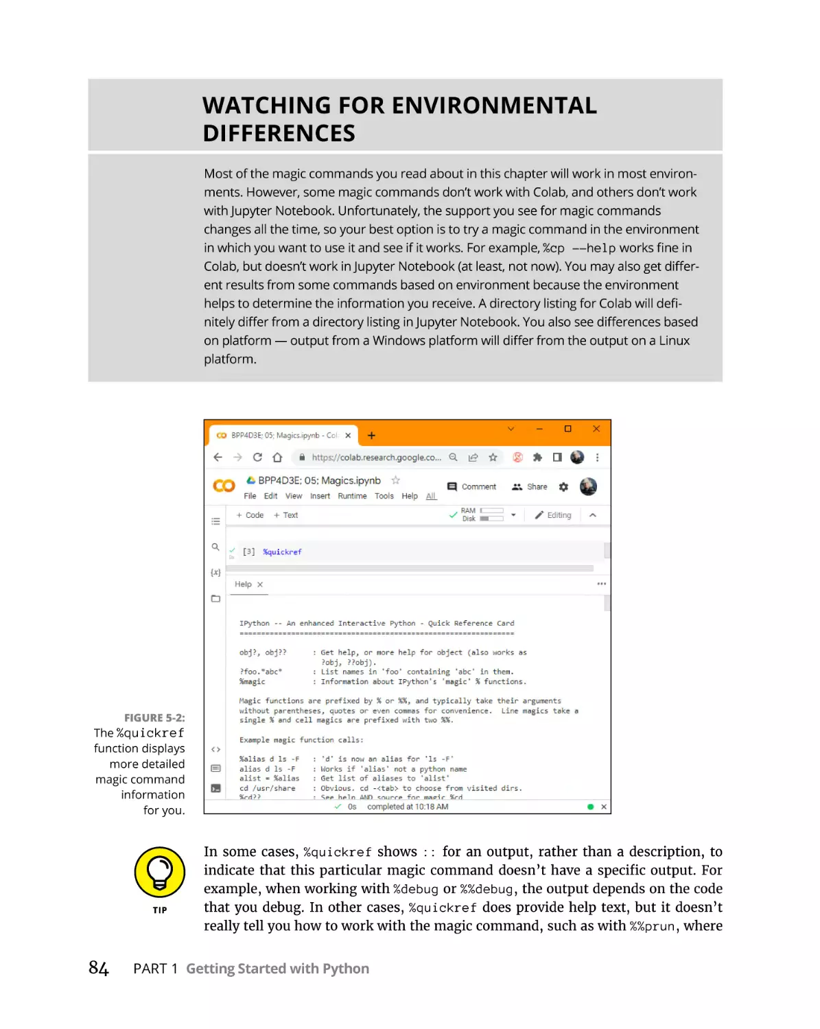
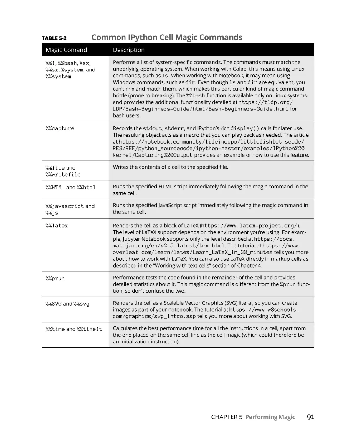
An overview of cell magic commands . . . . . . . . . . . . . . . . . . . . . . . .
80
82
82
83
83
83
85
90
PART 2: TALKING THE TALK . . . . . . . . . . . . . . . . . . . . . . . . . . . . . . . . . . . . . 93
CHAPTER 6:
Storing and Modifying Information . . . . . . . . . . . . . . . . . . . 95
Storing Information. . . . . . . . . . . . . . . . . . . . . . . . . . . . . . . . . . . . . . . . . . . 96
Seeing variables as storage boxes . . . . . . . . . . . . . . . . . . . . . . . . . . . 96
Using the right box to store the data. . . . . . . . . . . . . . . . . . . . . . . . . 96
Defining the Essential Python Data Types. . . . . . . . . . . . . . . . . . . . . . . . 97
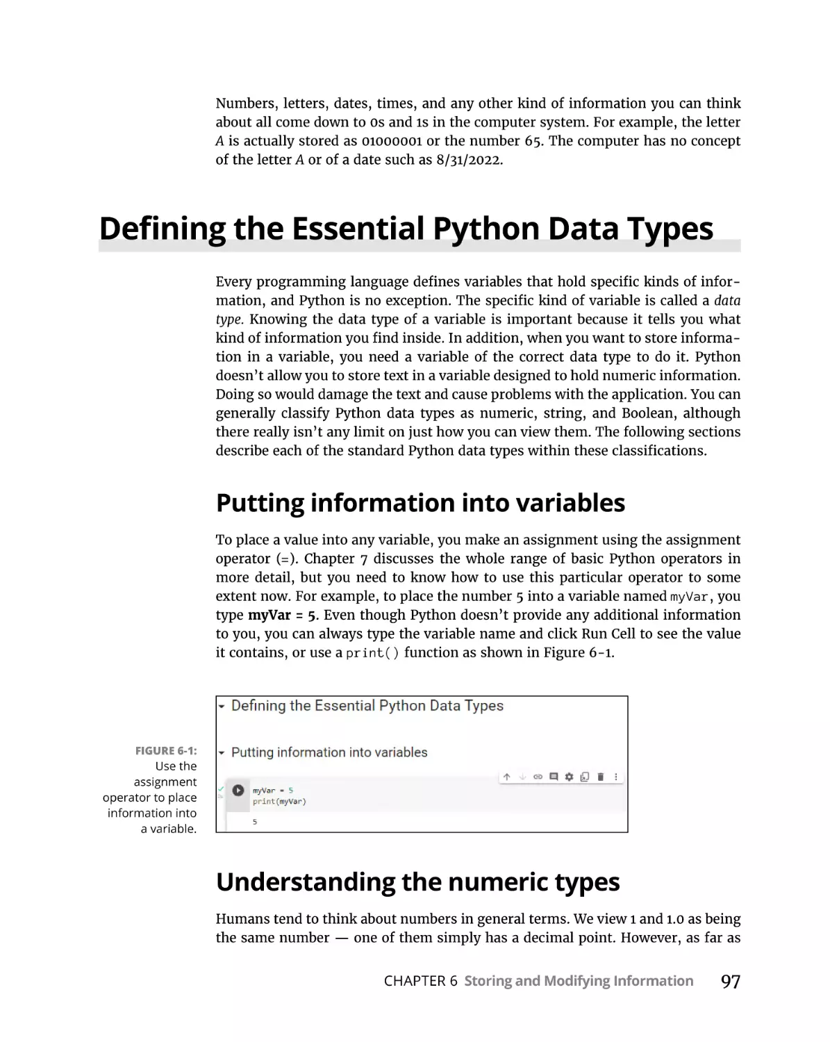
Putting information into variables . . . . . . . . . . . . . . . . . . . . . . . . . . . 97
Understanding the numeric types . . . . . . . . . . . . . . . . . . . . . . . . . . . 97
Understanding Boolean values. . . . . . . . . . . . . . . . . . . . . . . . . . . . . 102
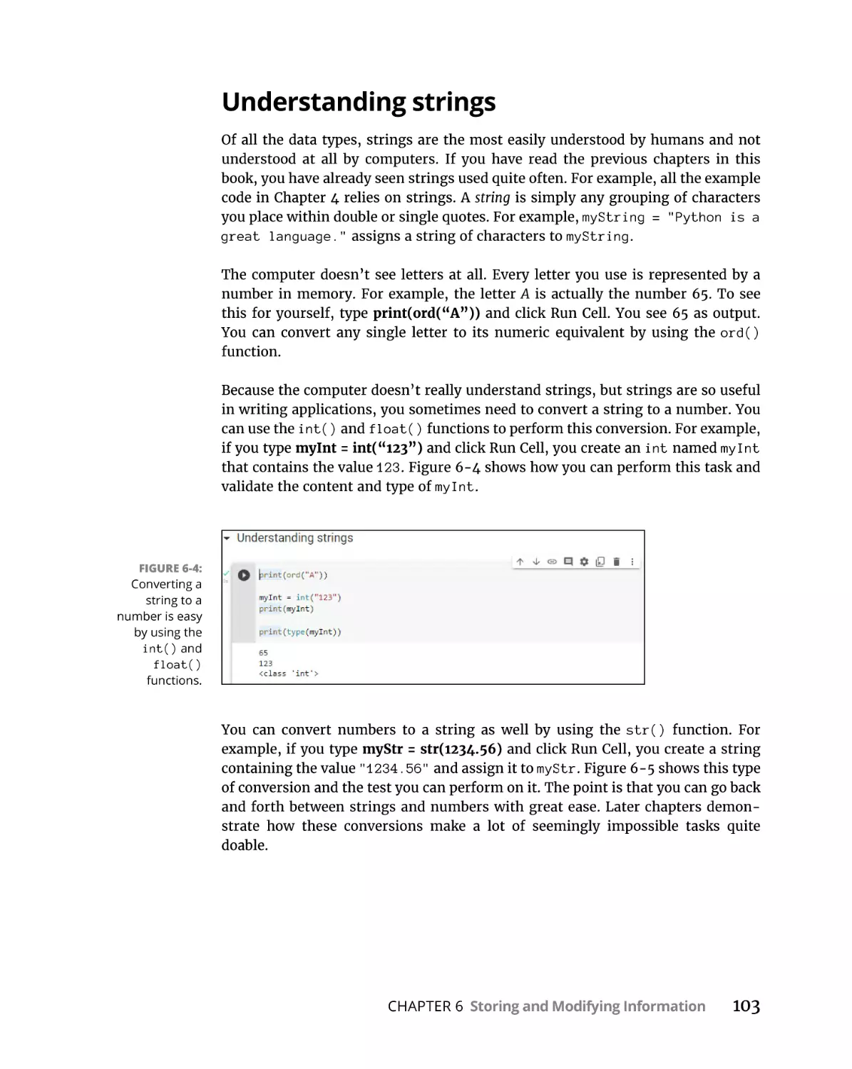
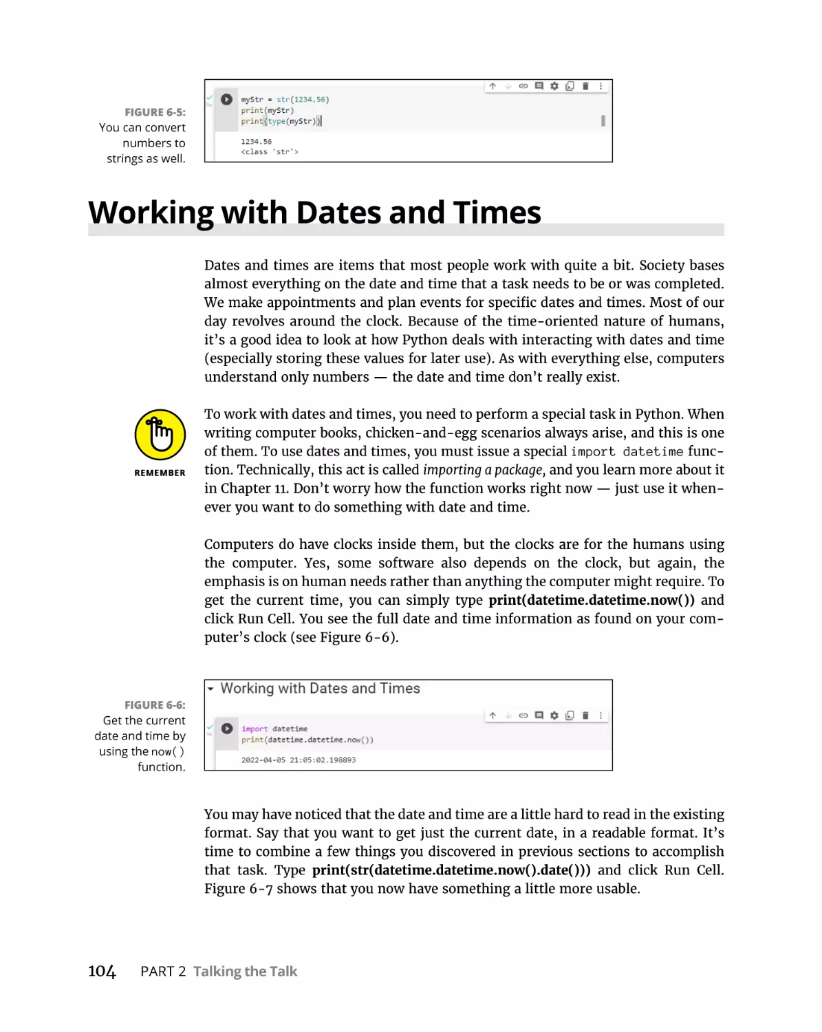
Understanding strings . . . . . . . . . . . . . . . . . . . . . . . . . . . . . . . . . . . . 103
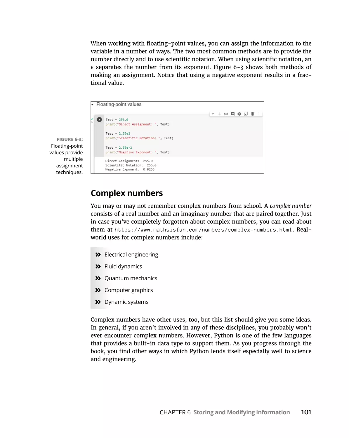
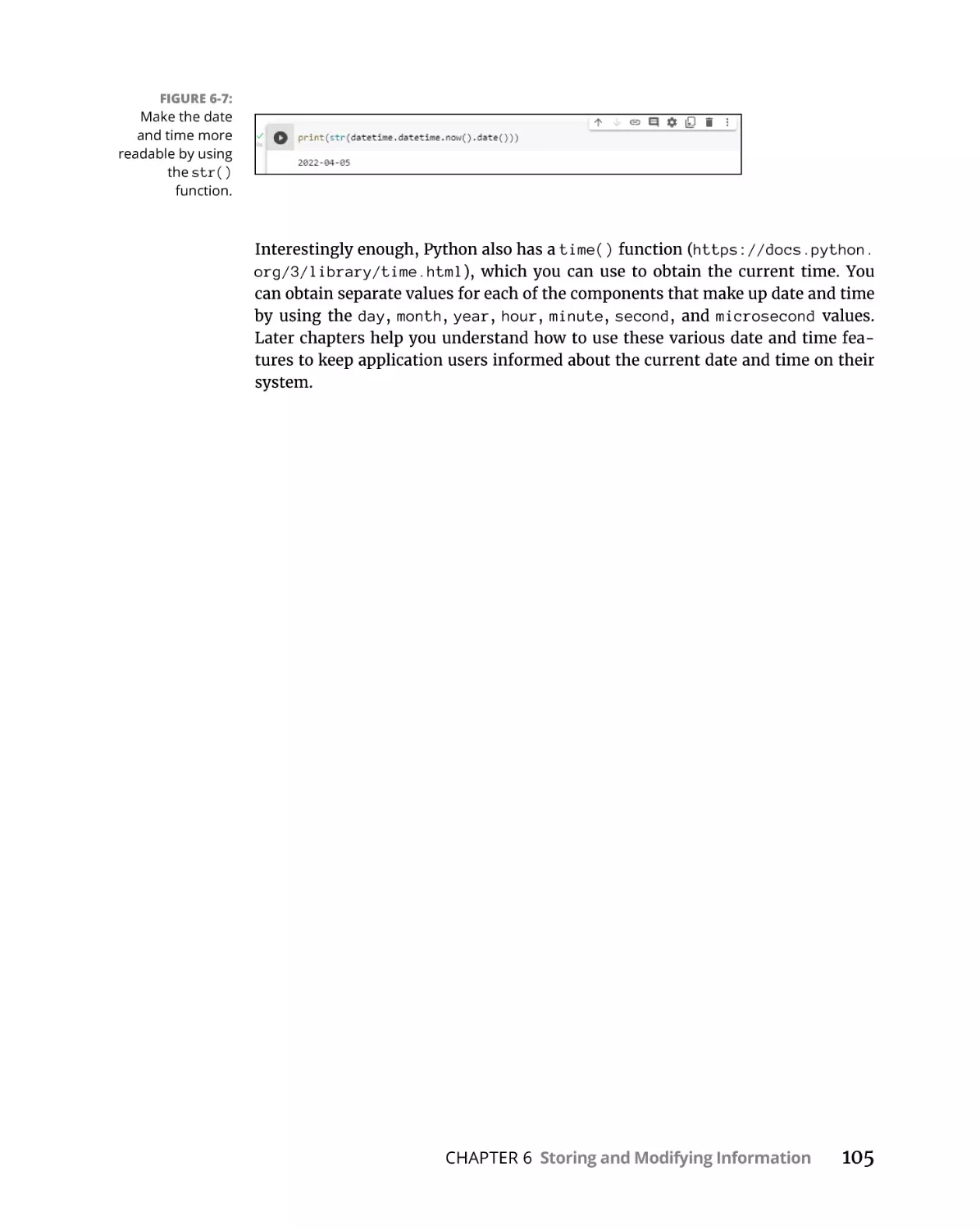
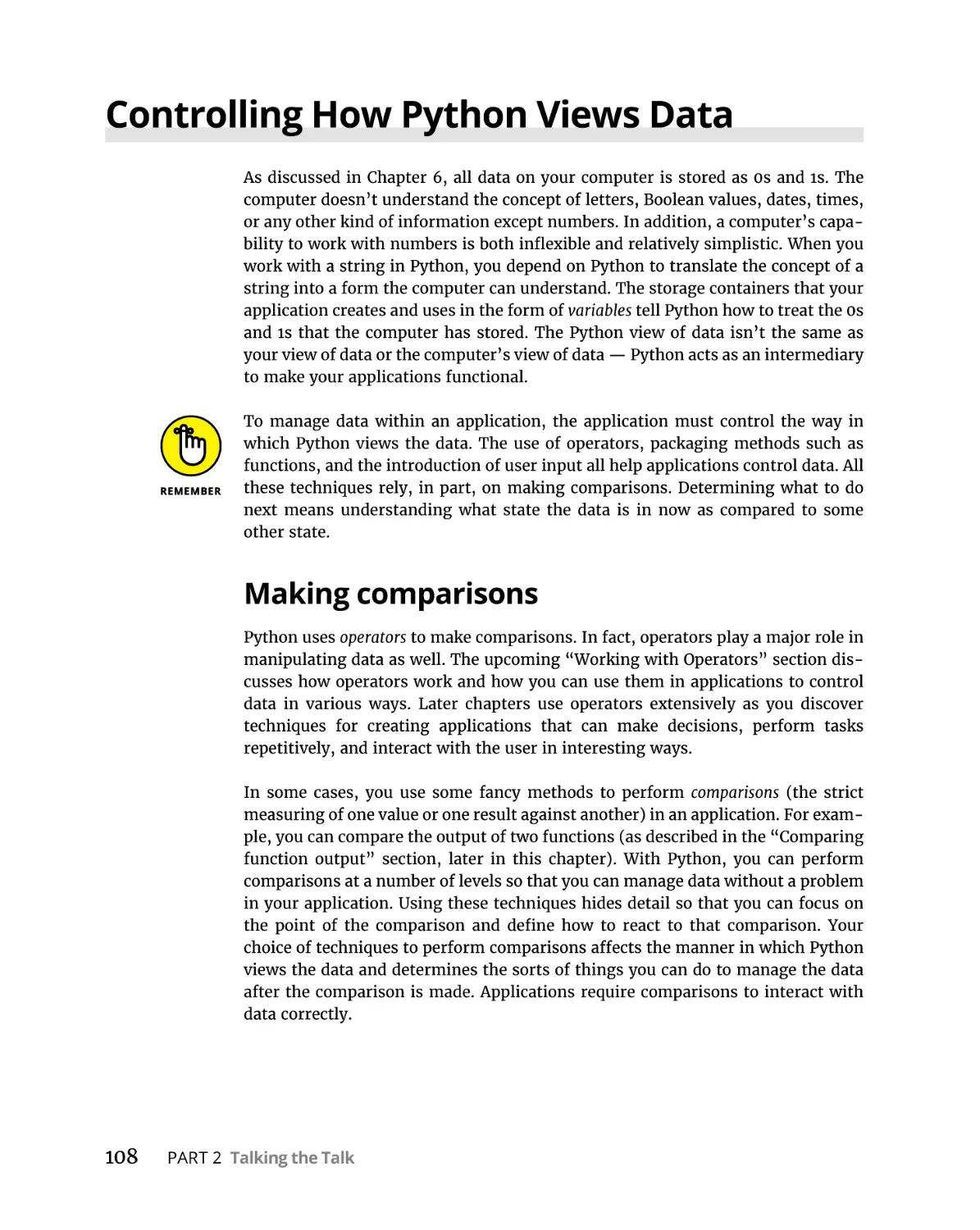
Working with Dates and Times . . . . . . . . . . . . . . . . . . . . . . . . . . . . . . . . 104
CHAPTER 7:
Managing Information. . . . . . . . . . . . . . . . . . . . . . . . . . . . . . . . .
107
Controlling How Python Views Data. . . . . . . . . . . . . . . . . . . . . . . . . . . . 108
Making comparisons. . . . . . . . . . . . . . . . . . . . . . . . . . . . . . . . . . . . . . 108
Understanding how computers make comparisons . . . . . . . . . . . 109
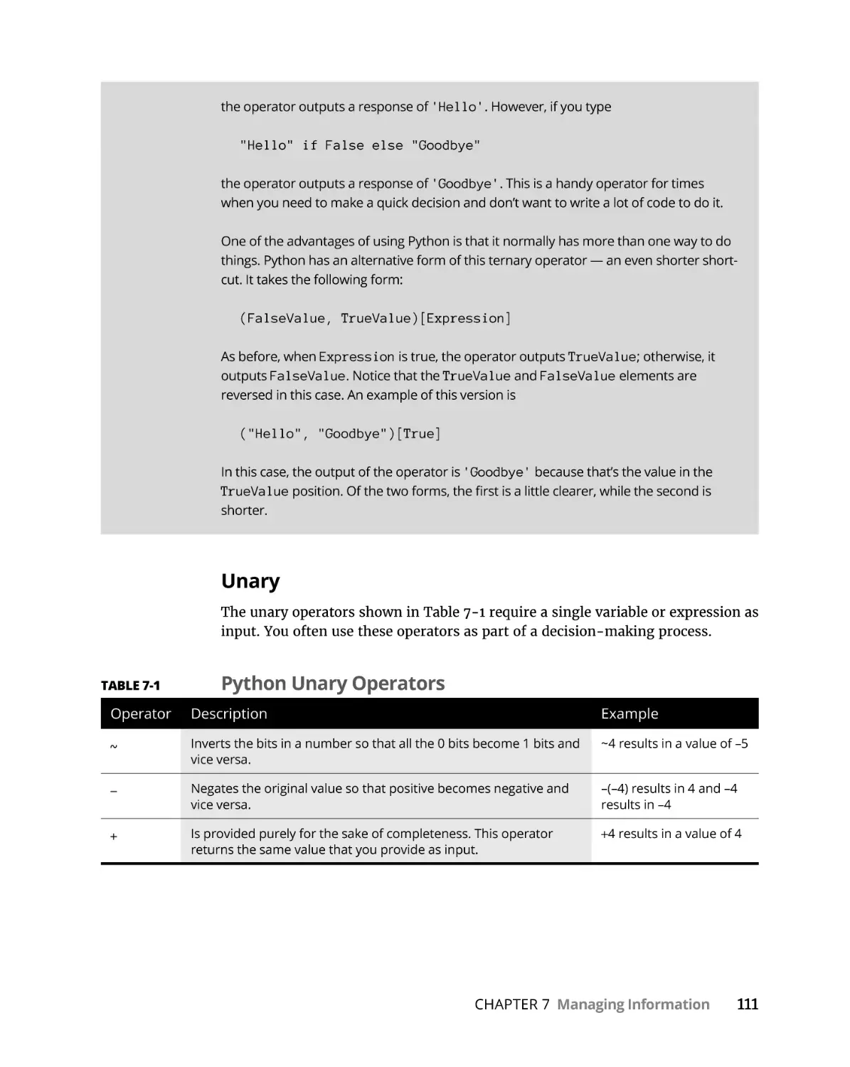
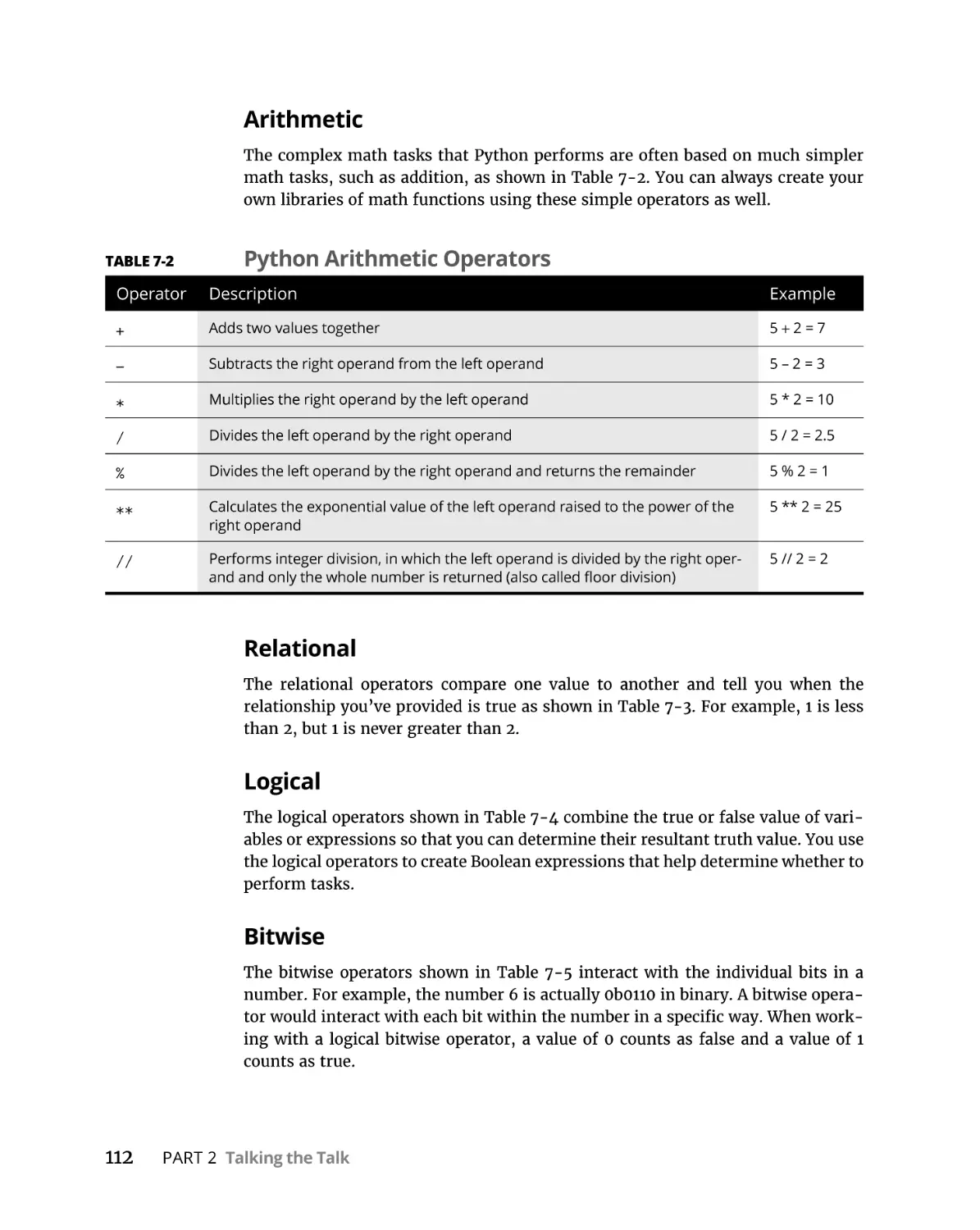
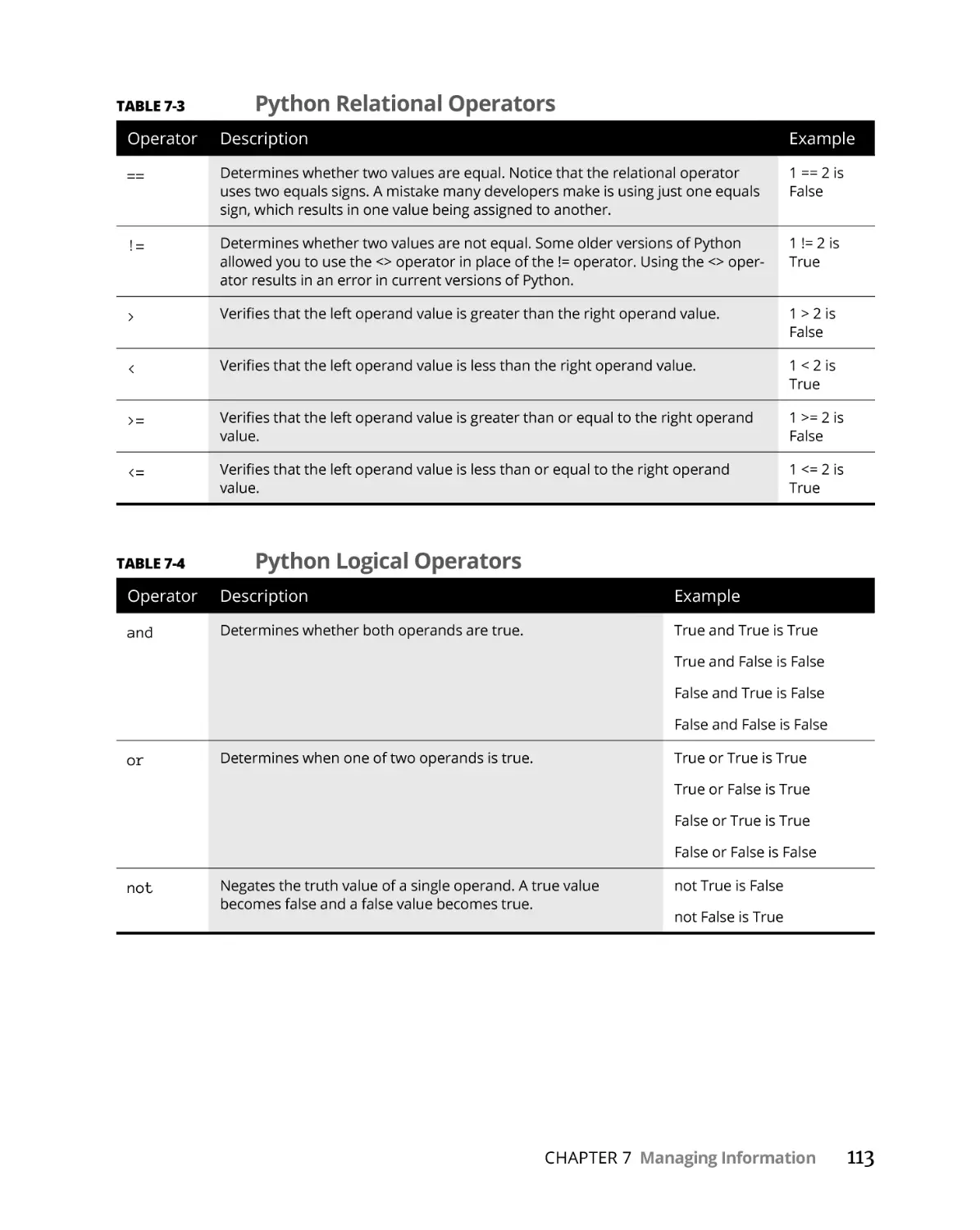
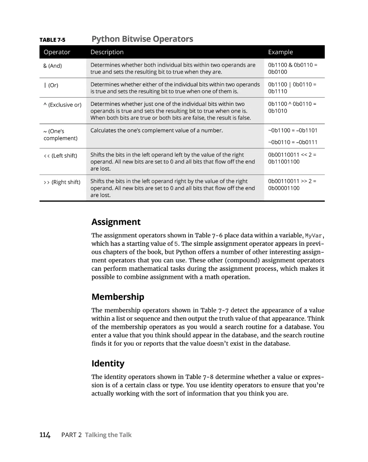
Working with Operators. . . . . . . . . . . . . . . . . . . . . . . . . . . . . . . . . . . . . . 109
Defining the operators. . . . . . . . . . . . . . . . . . . . . . . . . . . . . . . . . . . . 109
Understanding operator precedence. . . . . . . . . . . . . . . . . . . . . . . . 116
Creating and Using Functions . . . . . . . . . . . . . . . . . . . . . . . . . . . . . . . . . 117
Viewing functions as code packages. . . . . . . . . . . . . . . . . . . . . . . . .117
Understanding code reusability . . . . . . . . . . . . . . . . . . . . . . . . . . . . 117
Defining a function . . . . . . . . . . . . . . . . . . . . . . . . . . . . . . . . . . . . . . . 118
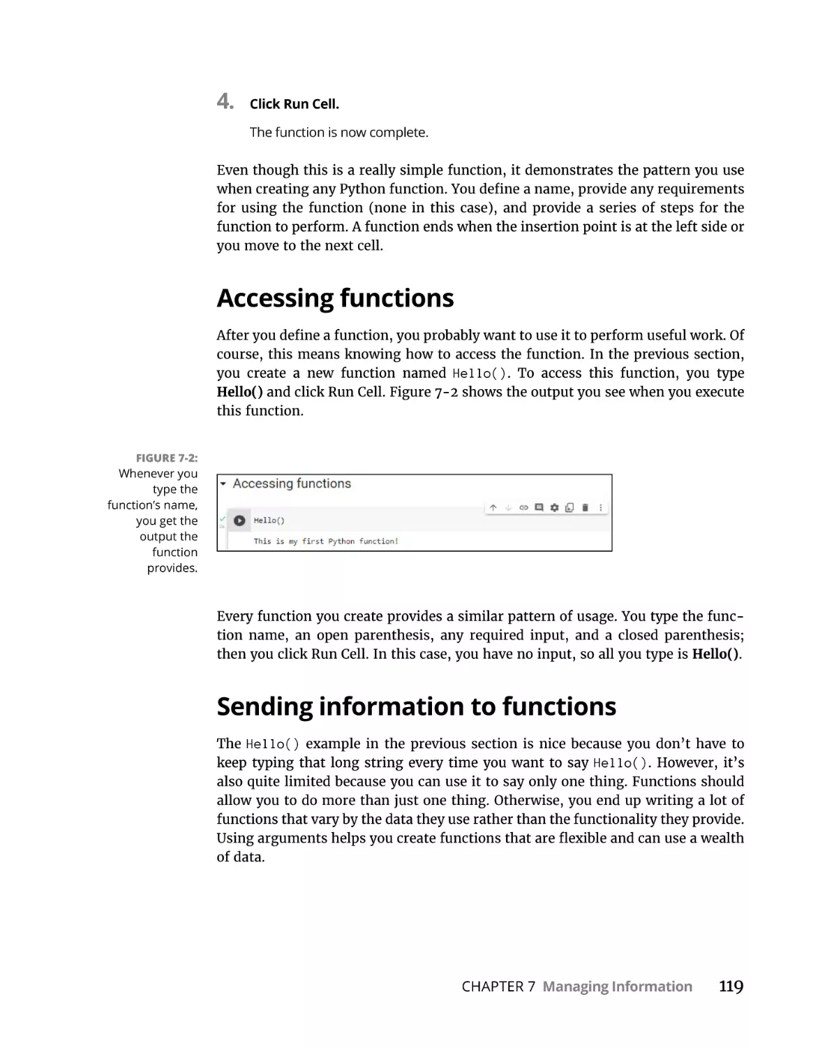
Accessing functions. . . . . . . . . . . . . . . . . . . . . . . . . . . . . . . . . . . . . . . 119
Sending information to functions. . . . . . . . . . . . . . . . . . . . . . . . . . . 119
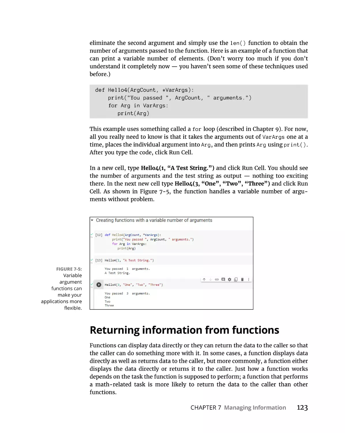
Returning information from functions. . . . . . . . . . . . . . . . . . . . . . . 123
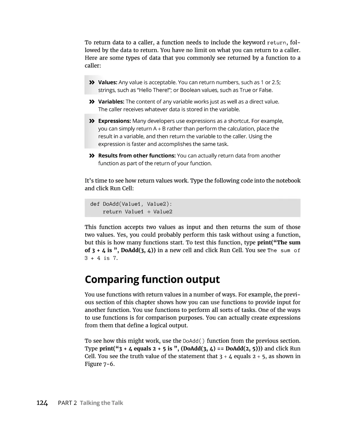
Comparing function output. . . . . . . . . . . . . . . . . . . . . . . . . . . . . . . . 124
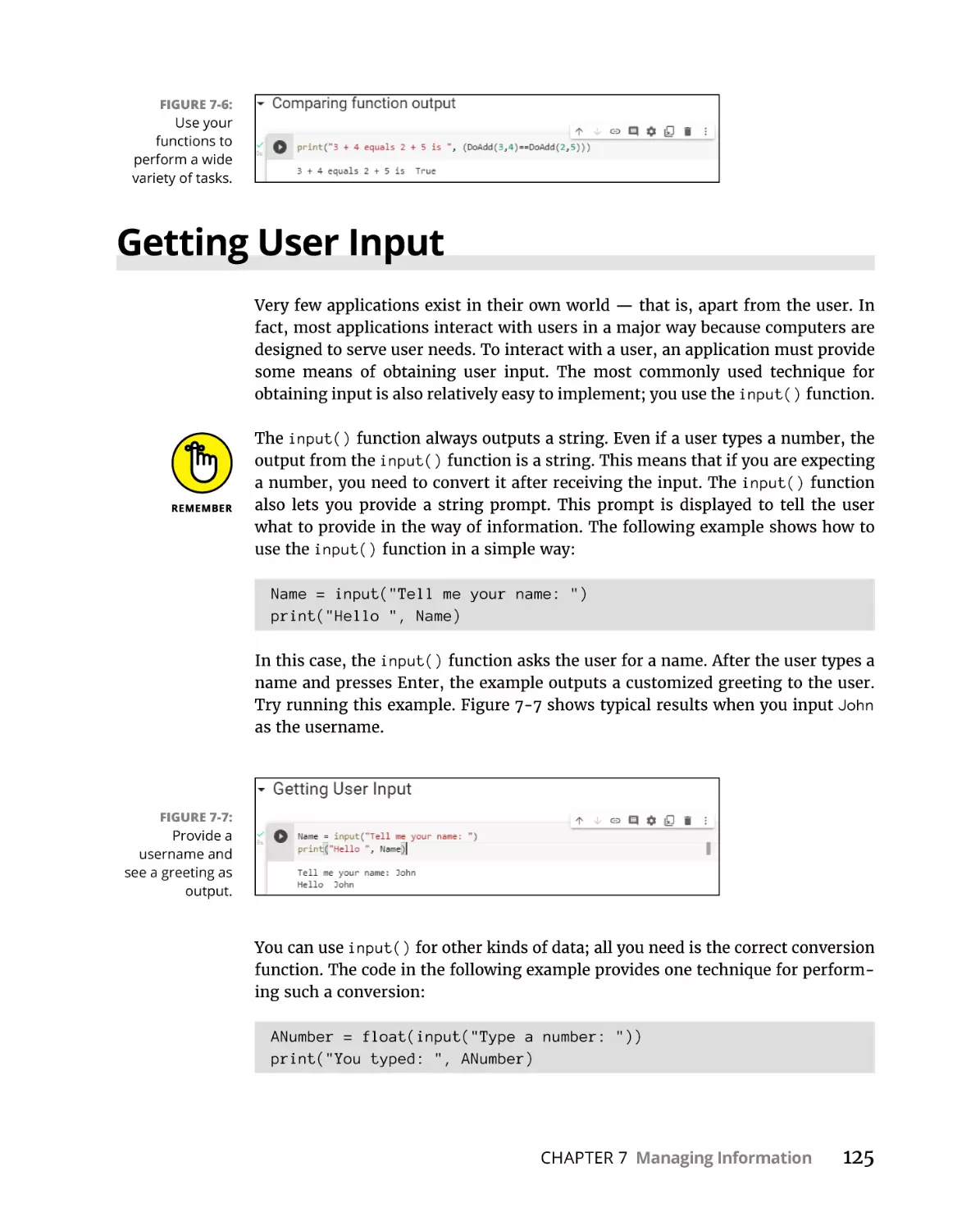
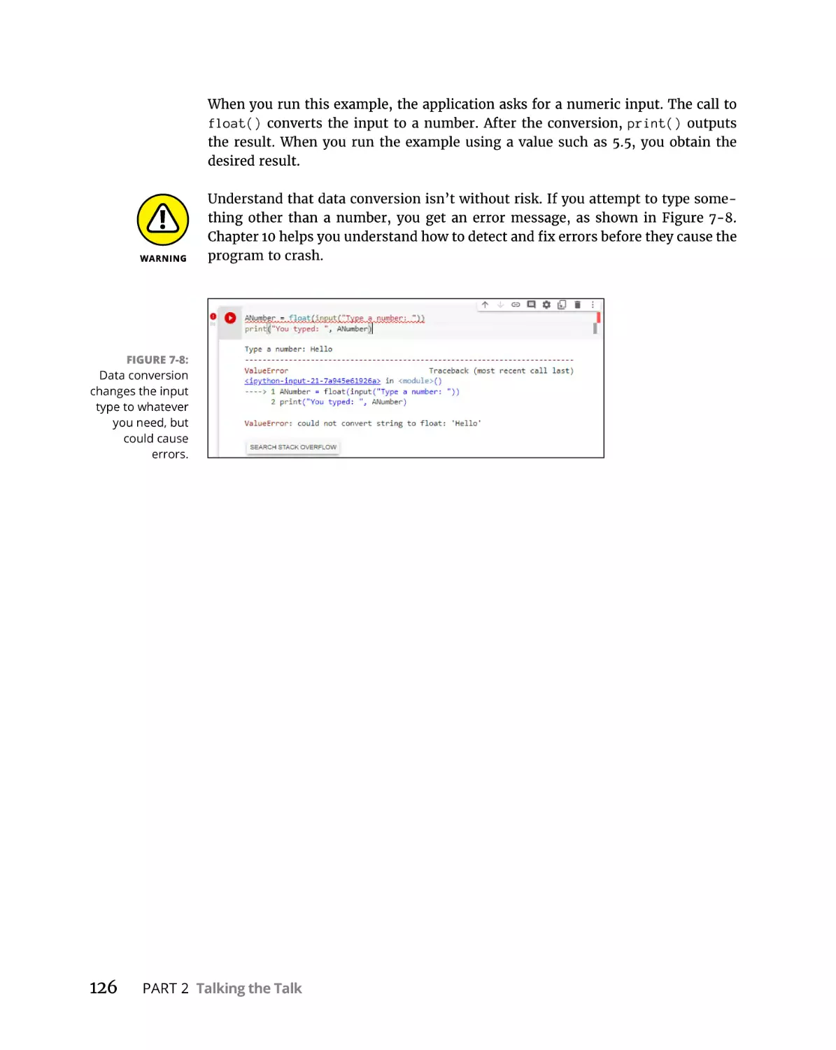
Getting User Input. . . . . . . . . . . . . . . . . . . . . . . . . . . . . . . . . . . . . . . . . . . 125
Table of Contents
ix
CHAPTER 8:
CHAPTER 9:
Making Decisions. . . . . . . . . . . . . . . . . . . . . . . . . . . . . . . . . . . . . . .
127
Making Simple Decisions by Using the if Statement . . . . . . . . . . . . . .
Understanding the if statement . . . . . . . . . . . . . . . . . . . . . . . . . . . .
Using the if statement in an application . . . . . . . . . . . . . . . . . . . . .
Choosing Alternatives by Using the if. . .else Statement. . . . . . . . . . .
Understanding the if. . .else statement . . . . . . . . . . . . . . . . . . . . . .
Using the if. . .else statement in an application . . . . . . . . . . . . . . .
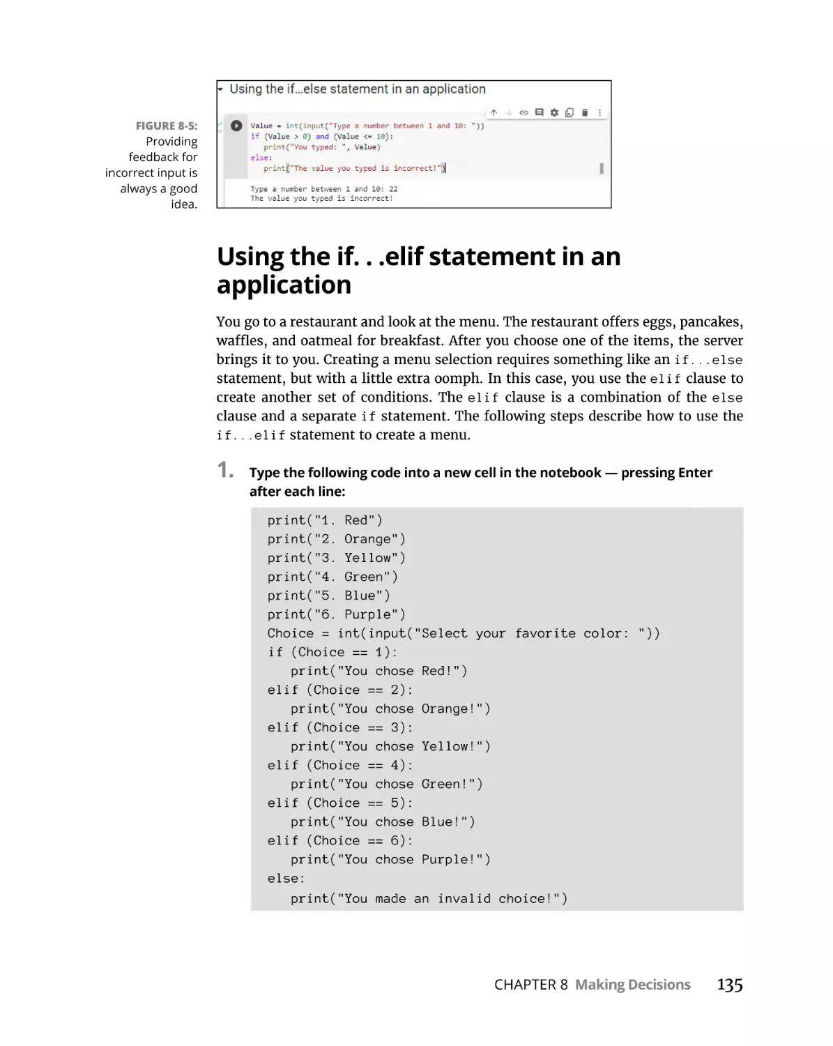
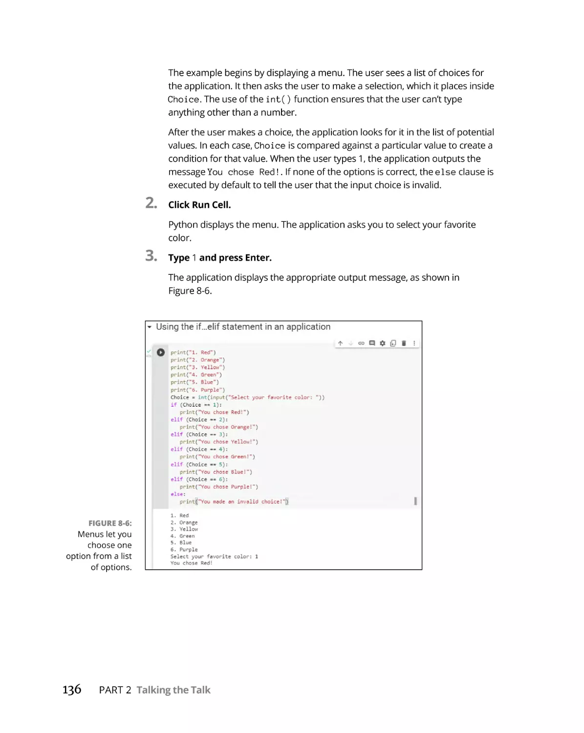
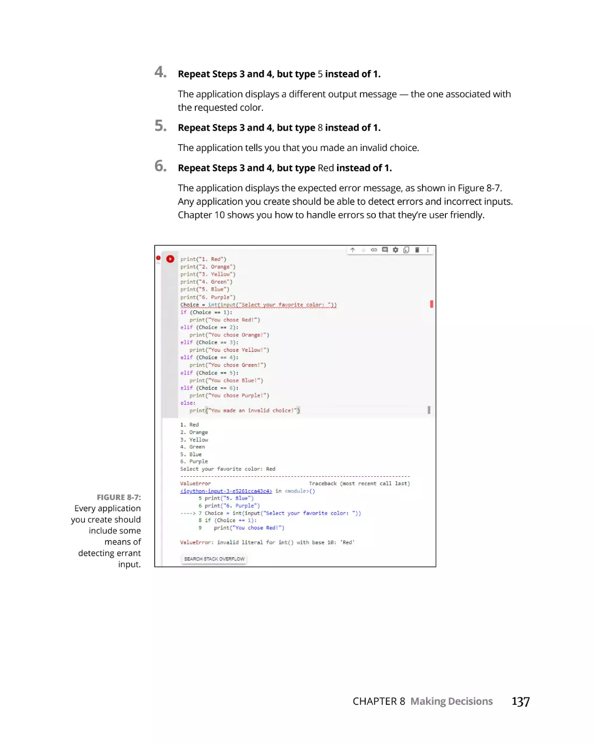
Using the if. . .elif statement in an application . . . . . . . . . . . . . . . .
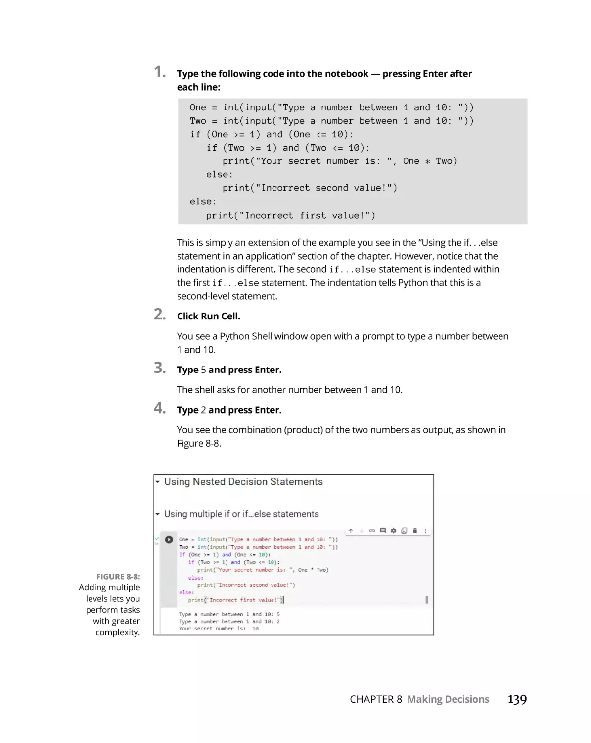
Using Nested Decision Statements. . . . . . . . . . . . . . . . . . . . . . . . . . . . .
Using multiple if or if. . .else statements . . . . . . . . . . . . . . . . . . . . .
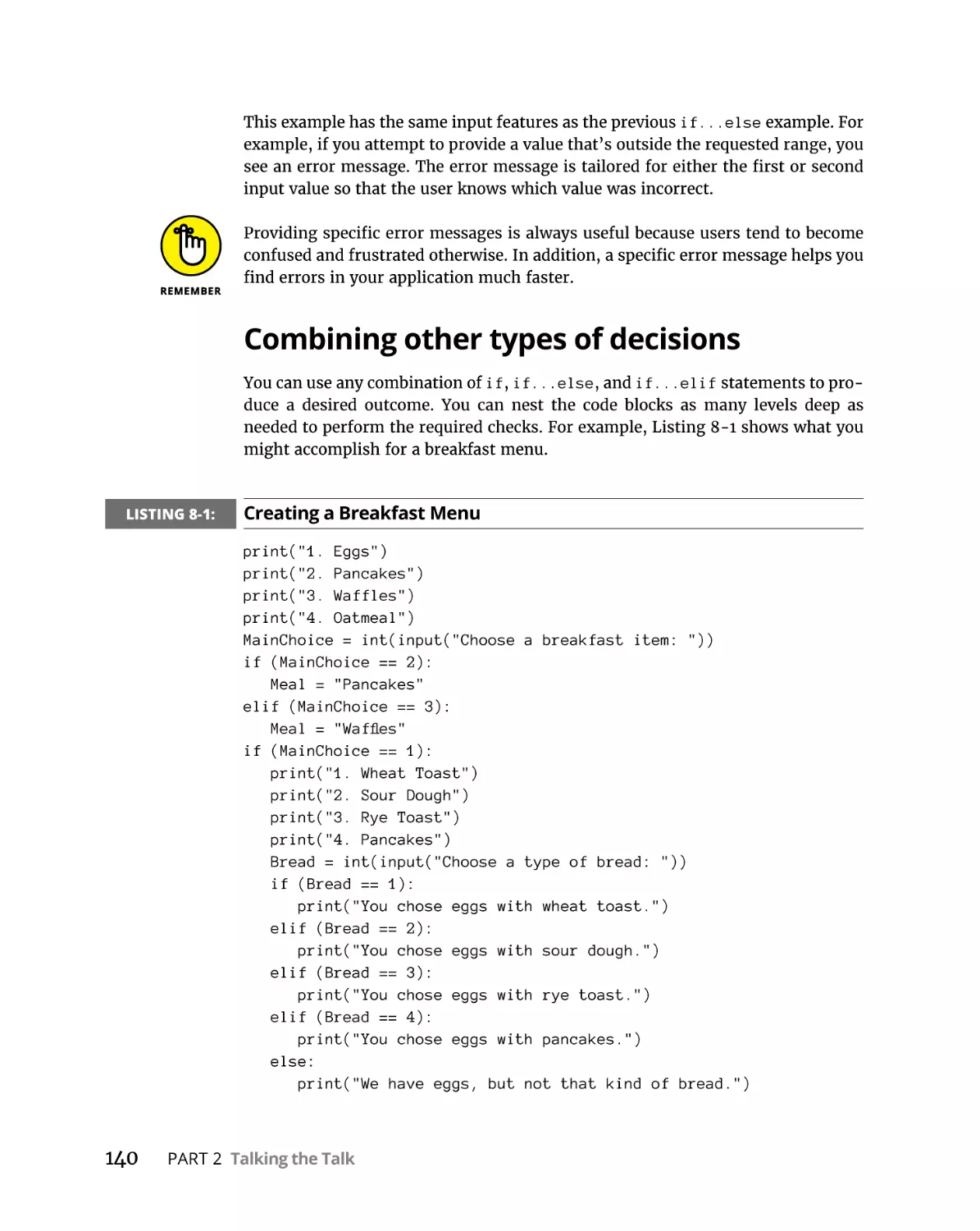
Combining other types of decisions. . . . . . . . . . . . . . . . . . . . . . . . .
128
128
129
133
133
134
135
138
138
140
Performing Repetitive Tasks . . . . . . . . . . . . . . . . . . . . . . . . .
143
Processing Data Using the for Statement . . . . . . . . . . . . . . . . . . . . . . .
Understanding the for statement. . . . . . . . . . . . . . . . . . . . . . . . . . .
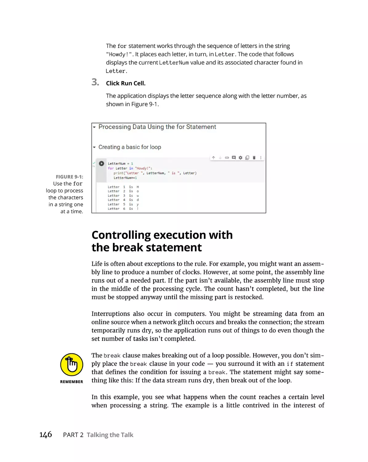
Creating a basic for loop. . . . . . . . . . . . . . . . . . . . . . . . . . . . . . . . . . .
Controlling execution with the break statement . . . . . . . . . . . . . .
Controlling execution with the continue statement. . . . . . . . . . . .
Doing nothing with the pass statement. . . . . . . . . . . . . . . . . . . . . .
Validating input with the else statement. . . . . . . . . . . . . . . . . . . . .
Processing Data by Using the while Statement . . . . . . . . . . . . . . . . . .
Understanding the while statement. . . . . . . . . . . . . . . . . . . . . . . . .
Using the while statement in an application. . . . . . . . . . . . . . . . . .
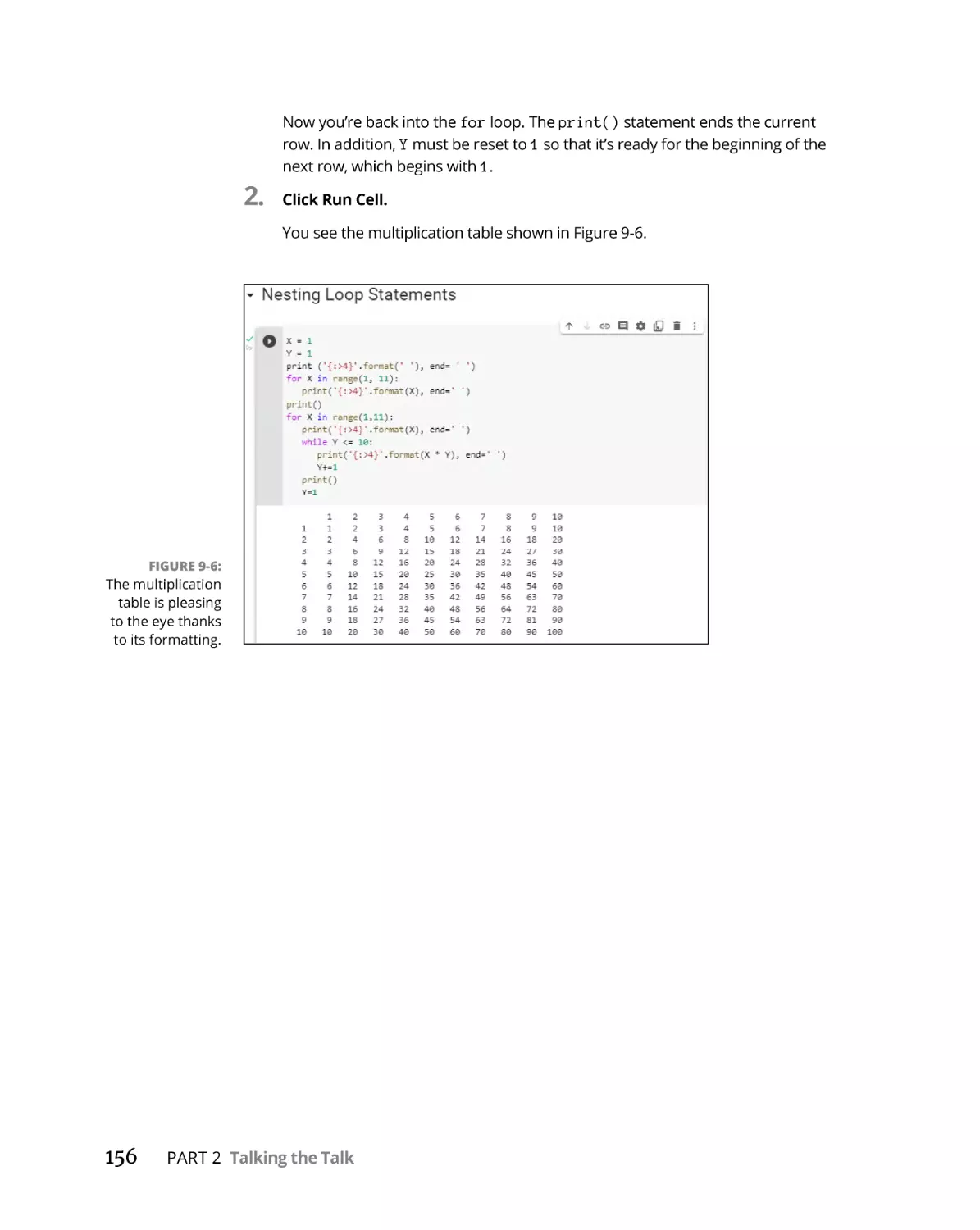
Nesting Loop Statements. . . . . . . . . . . . . . . . . . . . . . . . . . . . . . . . . . . . .
144
145
145
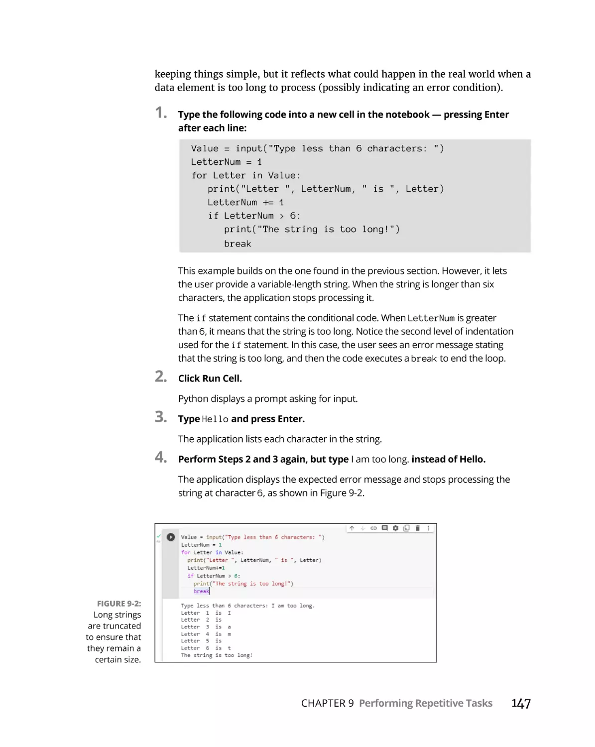
146
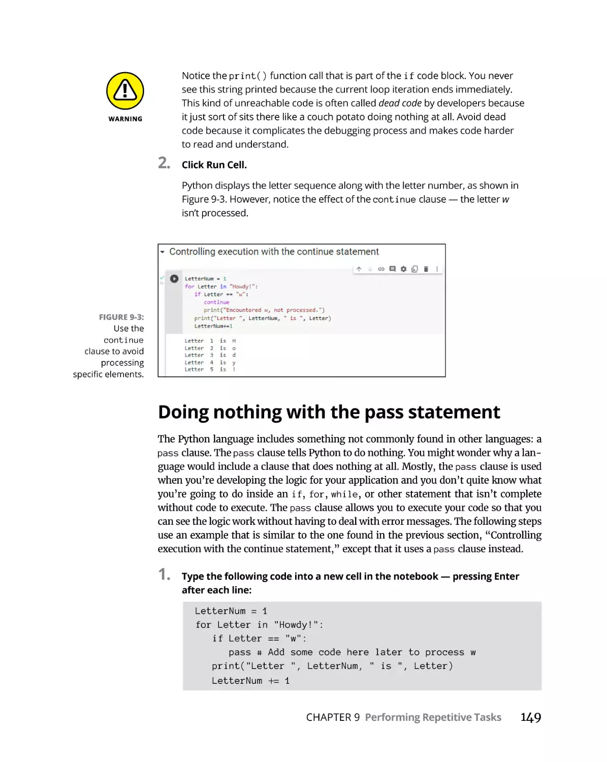
148
149
150
152
152
153
154
Dealing with Errors. . . . . . . . . . . . . . . . . . . . . . . . . . . . . . . . . . . . .
157
Knowing Why Python Doesn’t Understand You . . . . . . . . . . . . . . . . . .
Considering the Sources of Errors . . . . . . . . . . . . . . . . . . . . . . . . . . . . .
Classifying when errors occur. . . . . . . . . . . . . . . . . . . . . . . . . . . . . .
Distinguishing error types . . . . . . . . . . . . . . . . . . . . . . . . . . . . . . . . .
Catching Exceptions . . . . . . . . . . . . . . . . . . . . . . . . . . . . . . . . . . . . . . . . .
Basic exception handling . . . . . . . . . . . . . . . . . . . . . . . . . . . . . . . . . .
Handling more specific to less specific exceptions . . . . . . . . . . . .
Nested exception handling . . . . . . . . . . . . . . . . . . . . . . . . . . . . . . . .
Raising Exceptions. . . . . . . . . . . . . . . . . . . . . . . . . . . . . . . . . . . . . . . . . . .
Raising exceptions during exceptional conditions. . . . . . . . . . . . .
Passing error information to the caller . . . . . . . . . . . . . . . . . . . . . .
Deciding to Say “Oops” in Your Own Way: Custom Exceptions . . . . .
Using the finally Clause . . . . . . . . . . . . . . . . . . . . . . . . . . . . . . . . . . . . . .
158
159
160
162
164
165
176
178
180
181
181
182
184
PART 3: PERFORMING COMMON TASKS. . . . . . . . . . . . . . . . . . . .
187
Interacting with Packages . . . . . . . . . . . . . . . . . . . . . . . . . . . .
189
CHAPTER 10:
CHAPTER 11:
Creating Code Groupings. . . . . . . . . . . . . . . . . . . . . . . . . . . . . . . . . . . . . 190
I’m confused! Understanding modules versus packages . . . . . . . 190
Creating your first package . . . . . . . . . . . . . . . . . . . . . . . . . . . . . . . . 191
x
Beginning Programming with Python For Dummies
CHAPTER 12:
CHAPTER 13:
Understanding the package types . . . . . . . . . . . . . . . . . . . . . . . . . .
Considering the package cache. . . . . . . . . . . . . . . . . . . . . . . . . . . . .
Importing Packages. . . . . . . . . . . . . . . . . . . . . . . . . . . . . . . . . . . . . . . . . .
Using the import statement. . . . . . . . . . . . . . . . . . . . . . . . . . . . . . . .
Using the from. . .import statement. . . . . . . . . . . . . . . . . . . . . . . . .
Using the import. . .as statement . . . . . . . . . . . . . . . . . . . . . . . . . . .
Finding Packages. . . . . . . . . . . . . . . . . . . . . . . . . . . . . . . . . . . . . . . . . . . .
Locating packages on disk. . . . . . . . . . . . . . . . . . . . . . . . . . . . . . . . .
Locating packages online. . . . . . . . . . . . . . . . . . . . . . . . . . . . . . . . . .
Downloading Packages from Other Sources. . . . . . . . . . . . . . . . . . . . .
Opening the Anaconda Prompt. . . . . . . . . . . . . . . . . . . . . . . . . . . . .
Working with conda packages. . . . . . . . . . . . . . . . . . . . . . . . . . . . . .
And just why is conda missing in Colab? . . . . . . . . . . . . . . . . . . . . .
Installing packages by using pip . . . . . . . . . . . . . . . . . . . . . . . . . . . .
Installing packages using the %pip magics . . . . . . . . . . . . . . . . . . .
Viewing the Package Content . . . . . . . . . . . . . . . . . . . . . . . . . . . . . . . . .
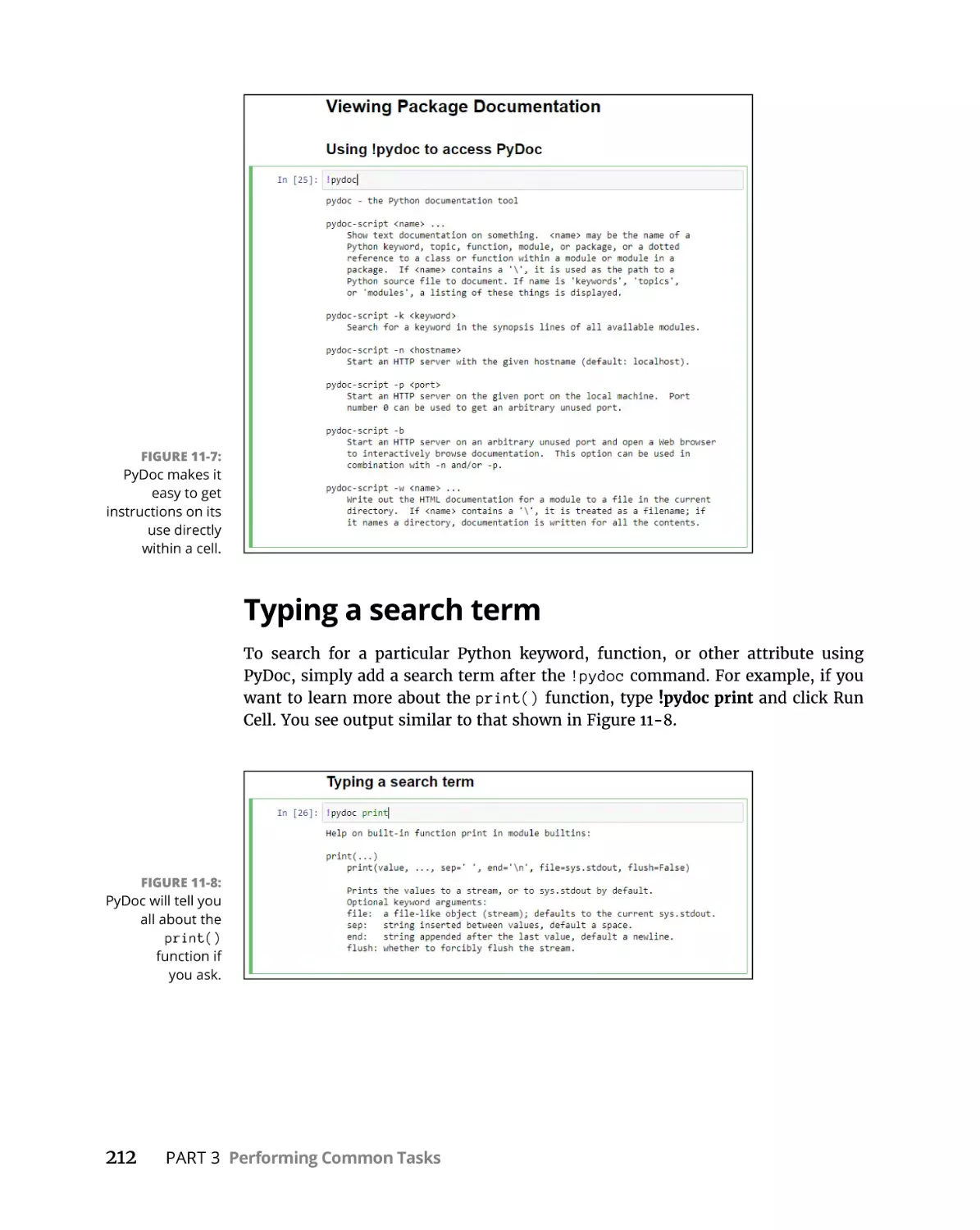
Viewing Package Documentation . . . . . . . . . . . . . . . . . . . . . . . . . . . . . .
Using !pydoc to access PyDoc . . . . . . . . . . . . . . . . . . . . . . . . . . . . . .
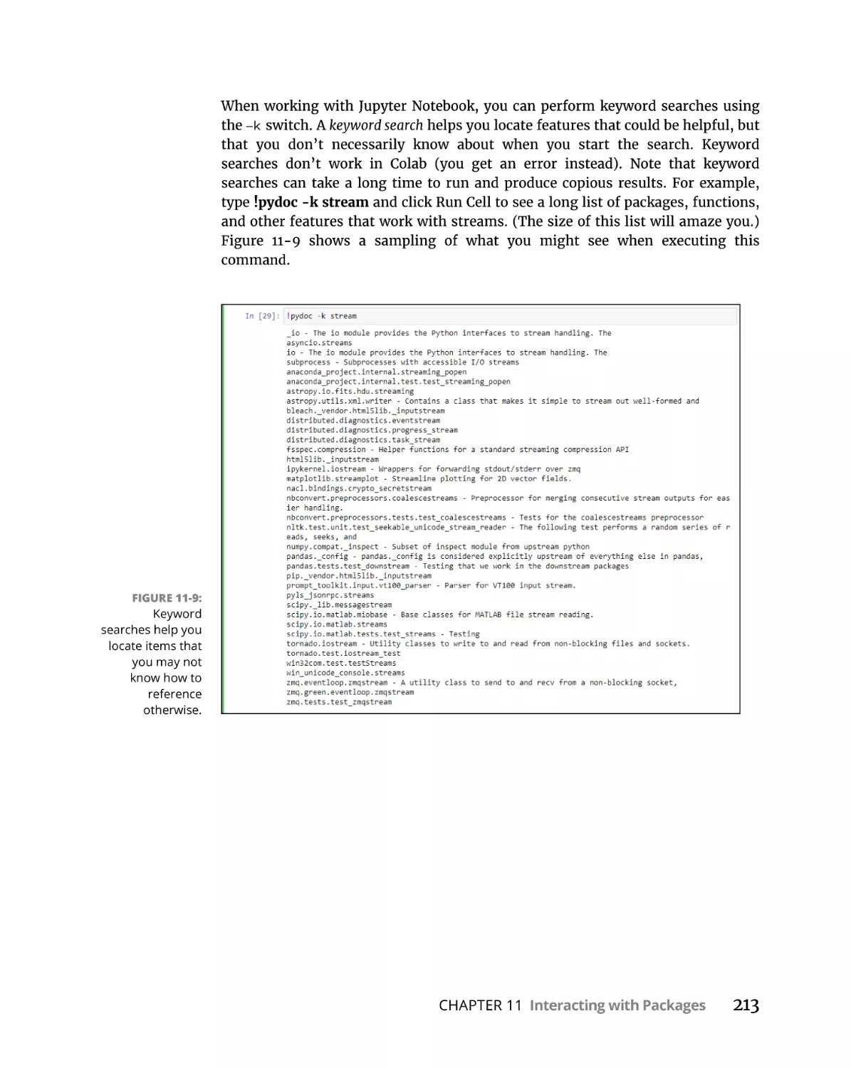
Typing a search term . . . . . . . . . . . . . . . . . . . . . . . . . . . . . . . . . . . . .
194
195
196
197
198
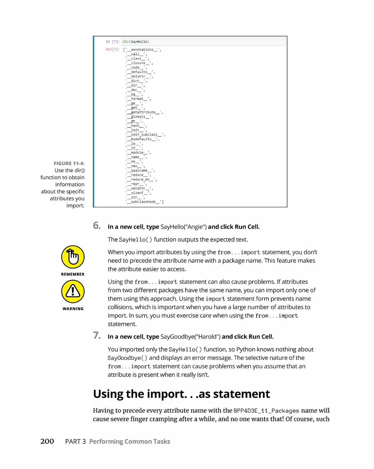
200
201
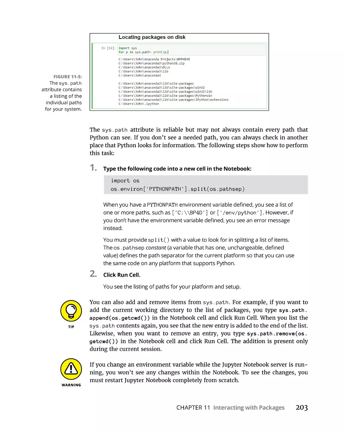
202
204
204
205
205
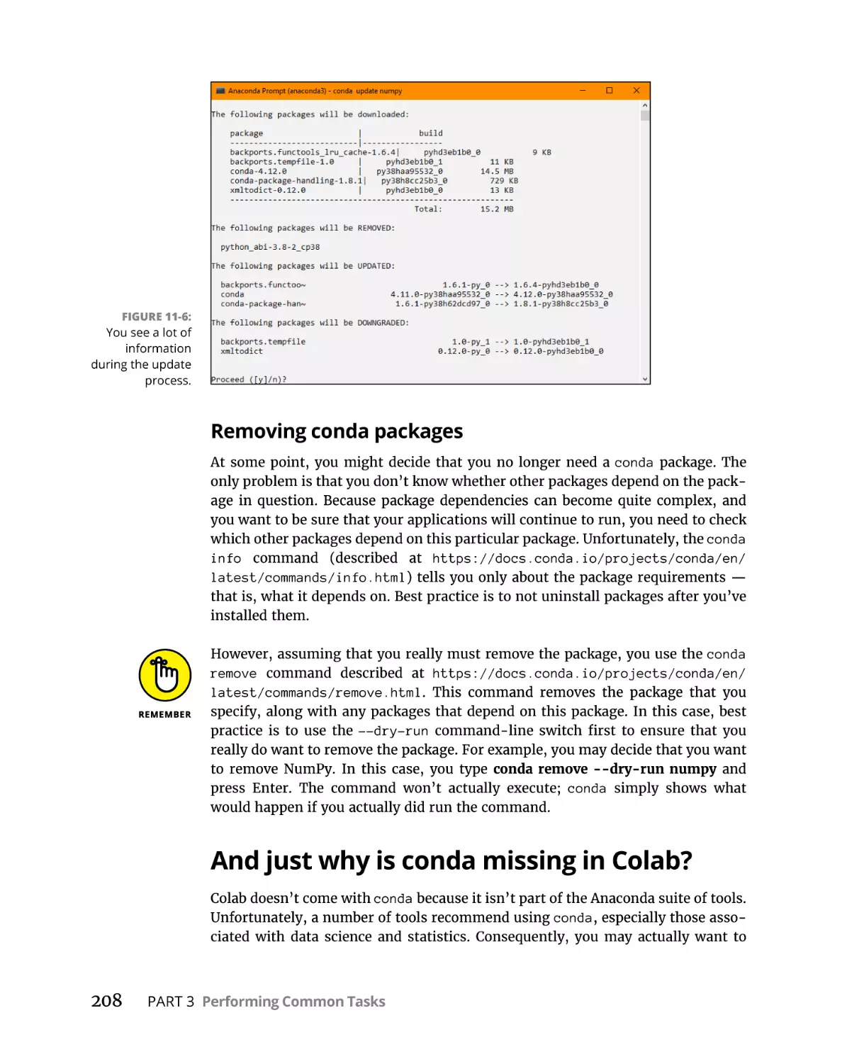
208
209
209
210
211
211
212
Working with Strings. . . . . . . . . . . . . . . . . . . . . . . . . . . . . . . . . . .
215
Understanding That Strings Are Different. . . . . . . . . . . . . . . . . . . . . . .
Defining a character by using numbers. . . . . . . . . . . . . . . . . . . . . .
Using characters to create strings . . . . . . . . . . . . . . . . . . . . . . . . . .
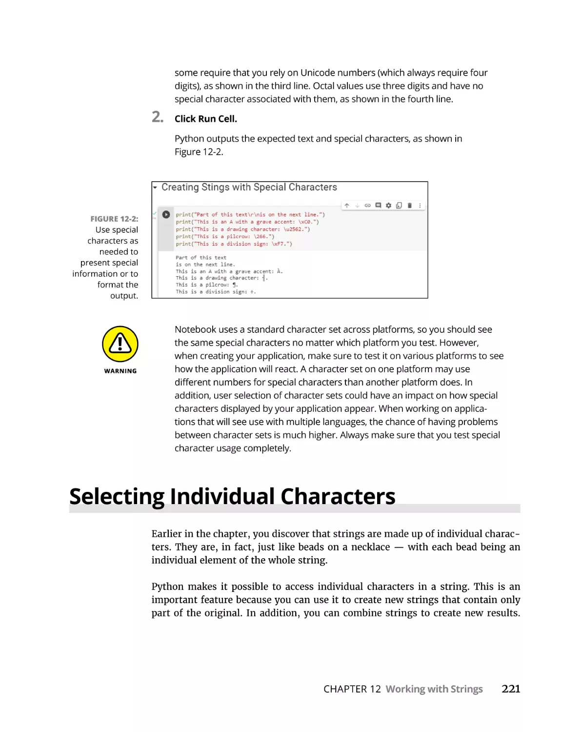
Creating Stings with Special Characters. . . . . . . . . . . . . . . . . . . . . . . . .
Selecting Individual Characters. . . . . . . . . . . . . . . . . . . . . . . . . . . . . . . .
Slicing and Dicing Strings. . . . . . . . . . . . . . . . . . . . . . . . . . . . . . . . . . . . .
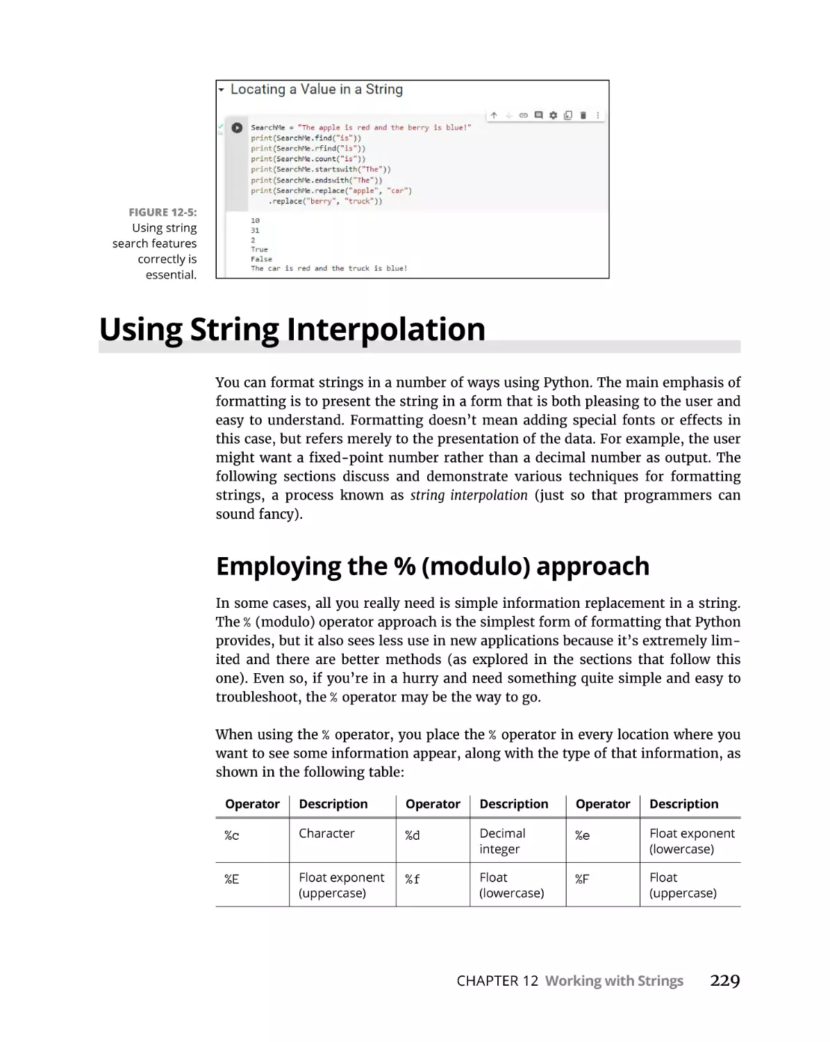
Locating a Value in a String . . . . . . . . . . . . . . . . . . . . . . . . . . . . . . . . . . .
Using String Interpolation . . . . . . . . . . . . . . . . . . . . . . . . . . . . . . . . . . . .
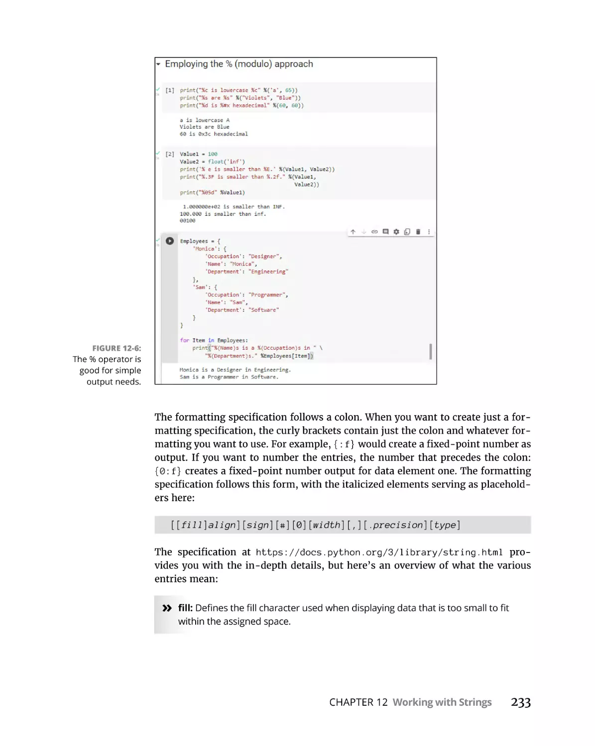
Employing the % (modulo) approach. . . . . . . . . . . . . . . . . . . . . . . .
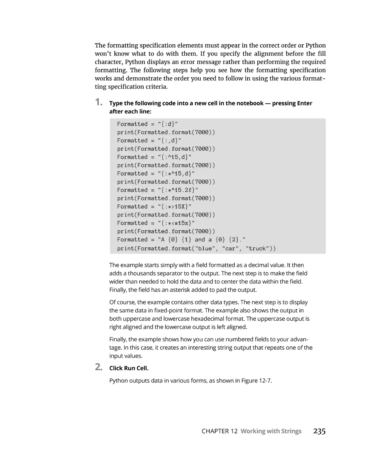
Working with the format() function . . . . . . . . . . . . . . . . . . . . . . . . .
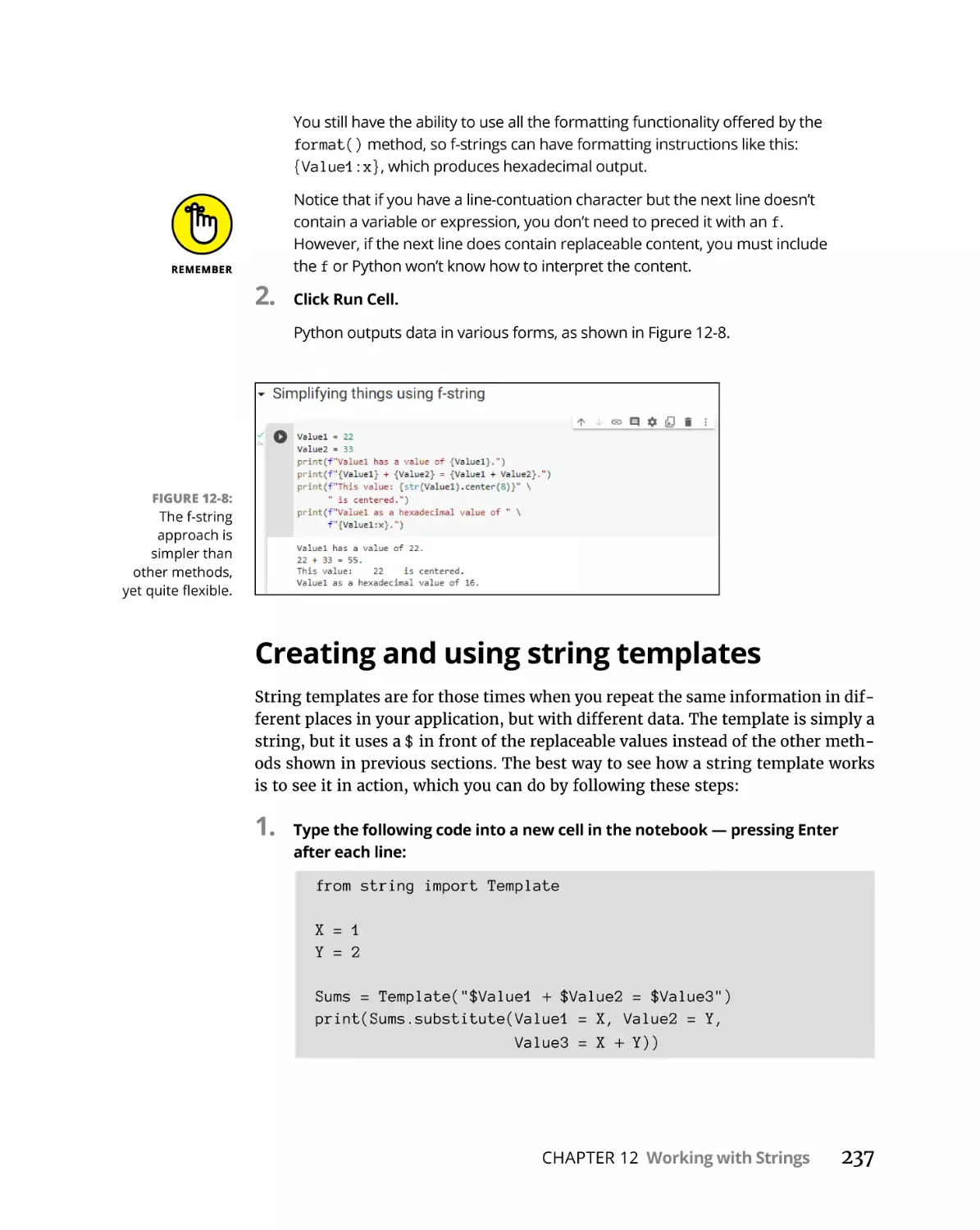
Simplifying things using f-string . . . . . . . . . . . . . . . . . . . . . . . . . . . .
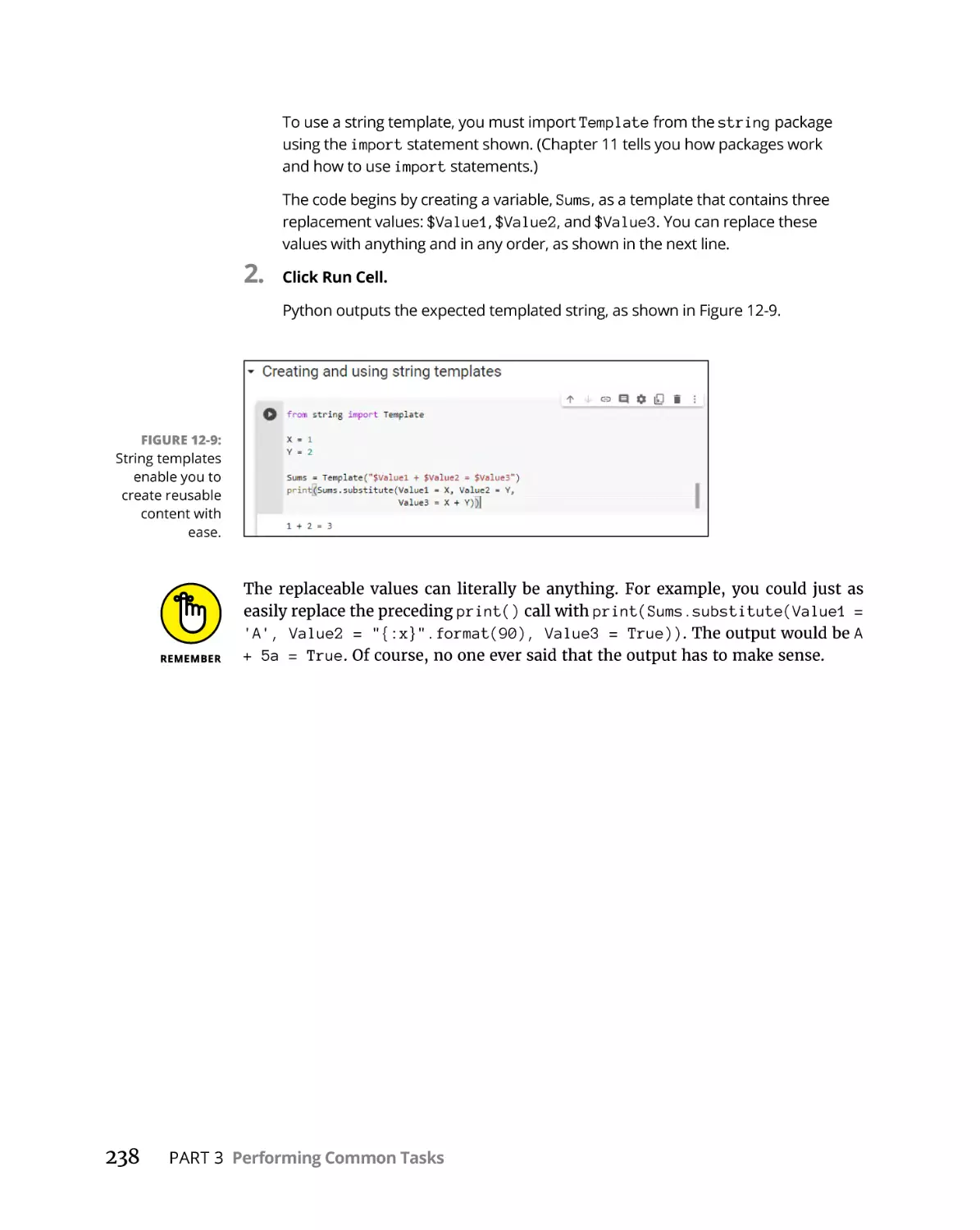
Creating and using string templates. . . . . . . . . . . . . . . . . . . . . . . . .
216
216
217
218
221
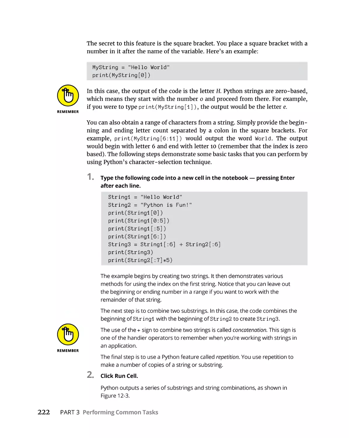
223
227
229
229
232
236
237
Managing Lists. . . . . . . . . . . . . . . . . . . . . . . . . . . . . . . . . . . . . . . . . .
239
Organizing Information in an Application . . . . . . . . . . . . . . . . . . . . . . .
Defining organization using lists. . . . . . . . . . . . . . . . . . . . . . . . . . . .
Understanding how computers view lists. . . . . . . . . . . . . . . . . . . .
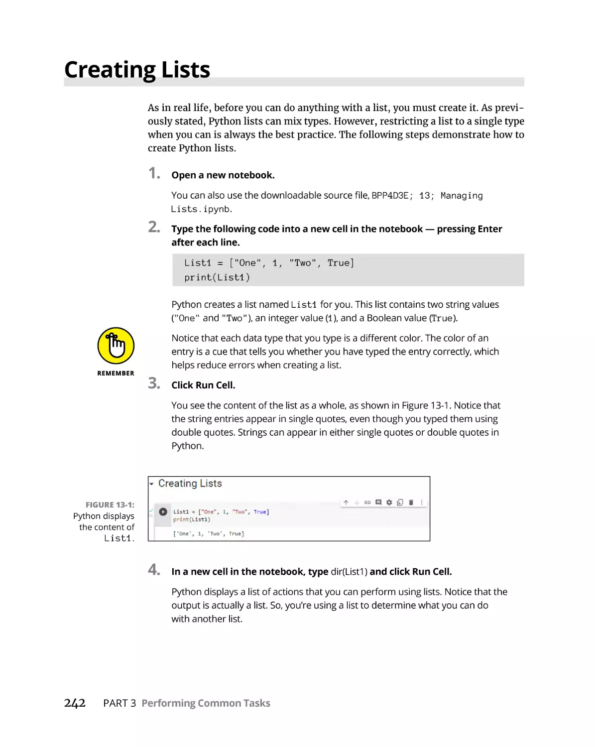
Creating Lists. . . . . . . . . . . . . . . . . . . . . . . . . . . . . . . . . . . . . . . . . . . . . . .
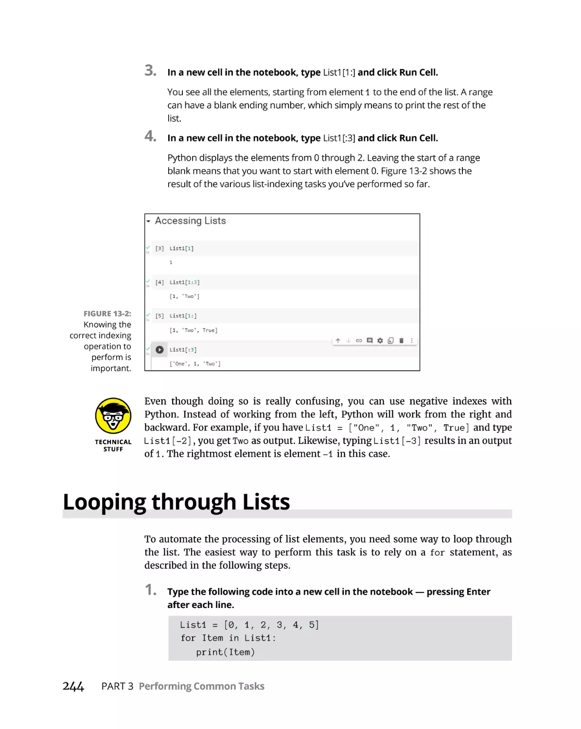
Accessing Lists. . . . . . . . . . . . . . . . . . . . . . . . . . . . . . . . . . . . . . . . . . . . . .
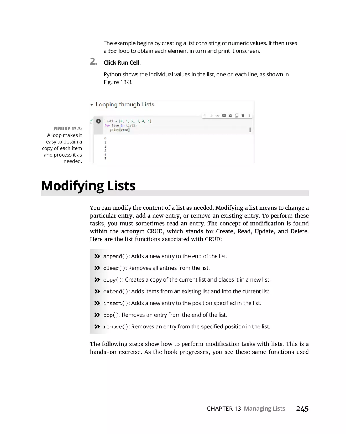
Looping through Lists. . . . . . . . . . . . . . . . . . . . . . . . . . . . . . . . . . . . . . . .
Modifying Lists. . . . . . . . . . . . . . . . . . . . . . . . . . . . . . . . . . . . . . . . . . . . . .
Searching Lists. . . . . . . . . . . . . . . . . . . . . . . . . . . . . . . . . . . . . . . . . . . . . .
240
240
241
242
243
244
245
249
Table of Contents
xi
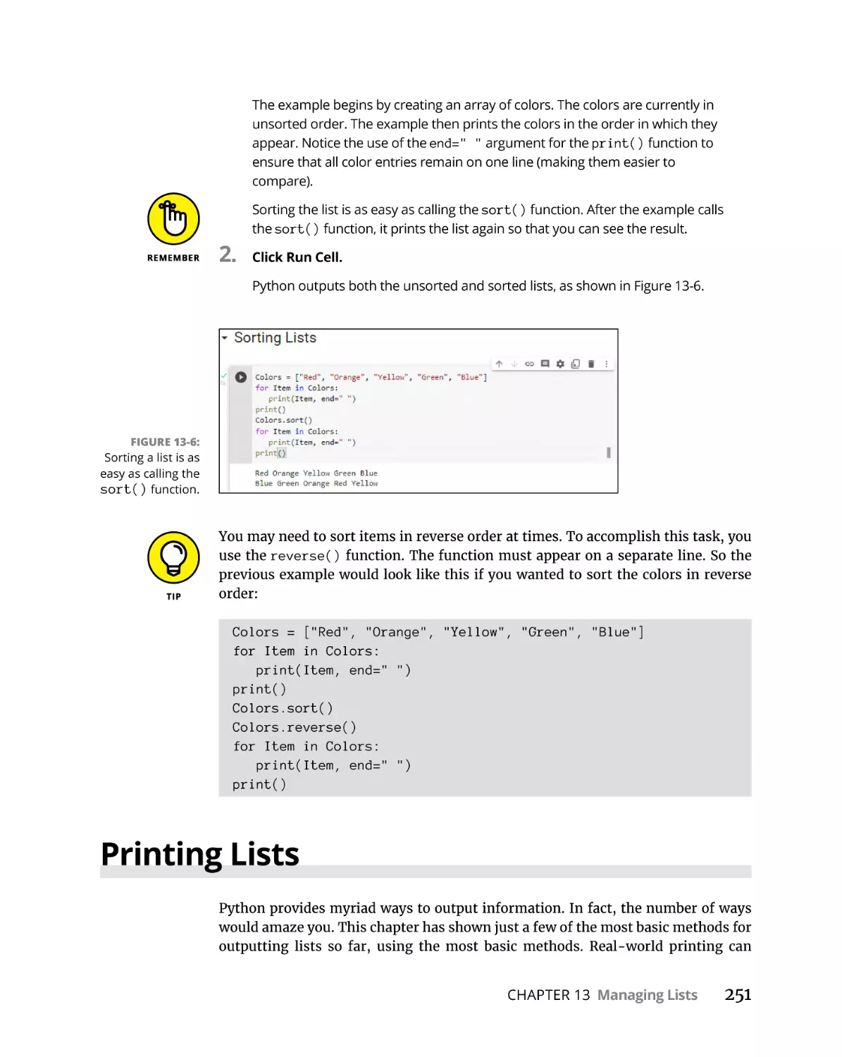
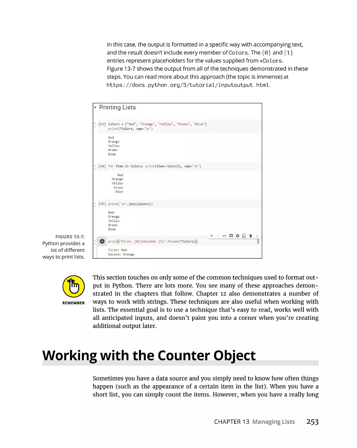
Sorting Lists . . . . . . . . . . . . . . . . . . . . . . . . . . . . . . . . . . . . . . . . . . . . . . . . 250
Printing Lists. . . . . . . . . . . . . . . . . . . . . . . . . . . . . . . . . . . . . . . . . . . . . . . . 251
Working with the Counter Object. . . . . . . . . . . . . . . . . . . . . . . . . . . . . . 253
Collecting All Sorts of Data. . . . . . . . . . . . . . . . . . . . . . . . . . . .
257
Understanding Collections. . . . . . . . . . . . . . . . . . . . . . . . . . . . . . . . . . . .
Working with Tuples. . . . . . . . . . . . . . . . . . . . . . . . . . . . . . . . . . . . . . . . .
Working with Dictionaries . . . . . . . . . . . . . . . . . . . . . . . . . . . . . . . . . . . .
Creating and using a dictionary. . . . . . . . . . . . . . . . . . . . . . . . . . . . .
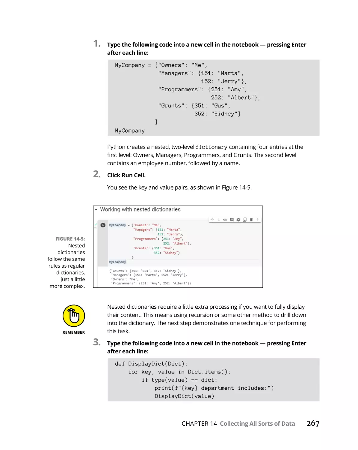
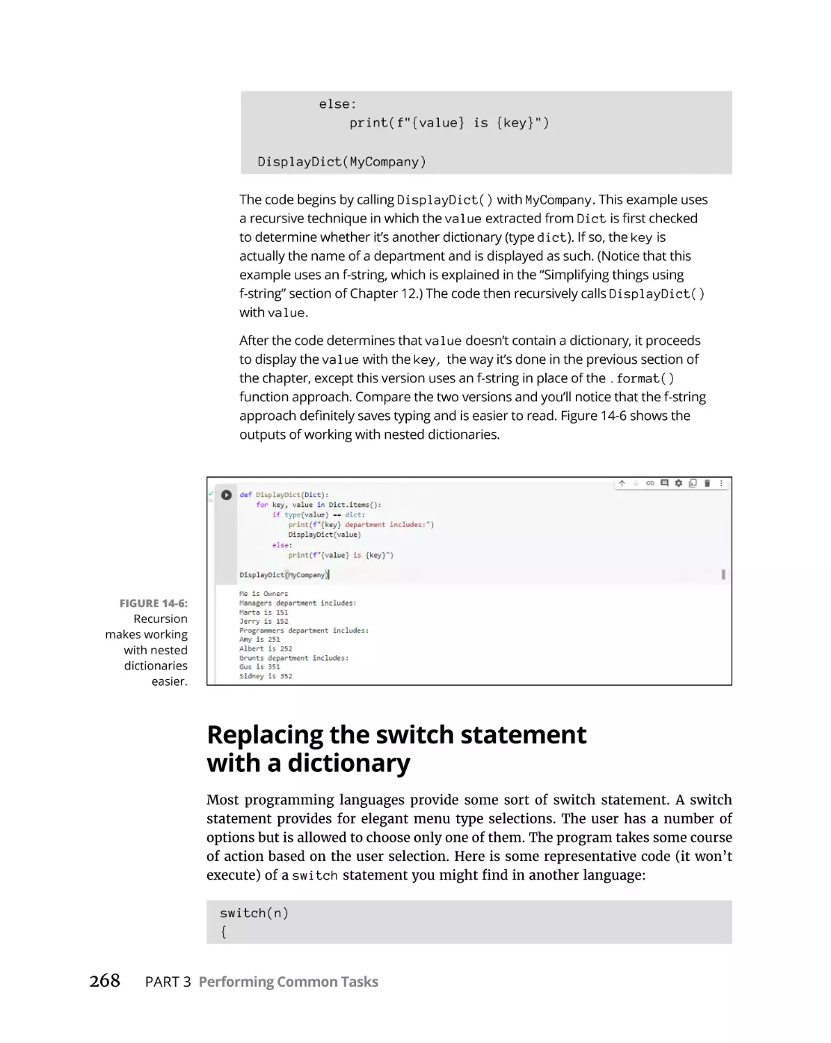
Working with nested dictionaries. . . . . . . . . . . . . . . . . . . . . . . . . . .
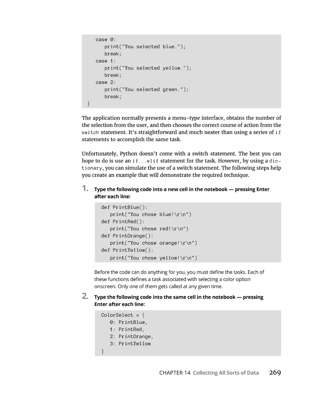
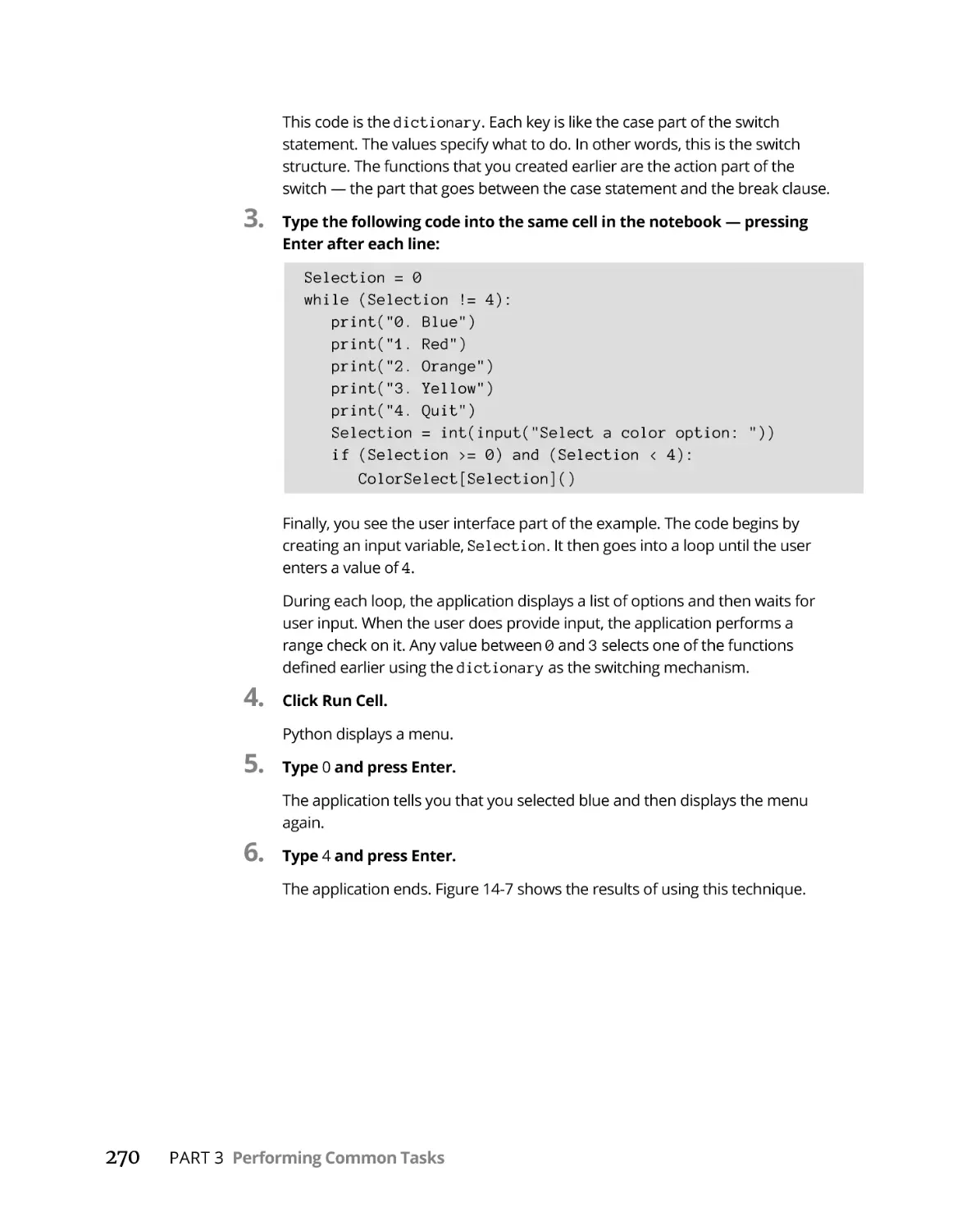
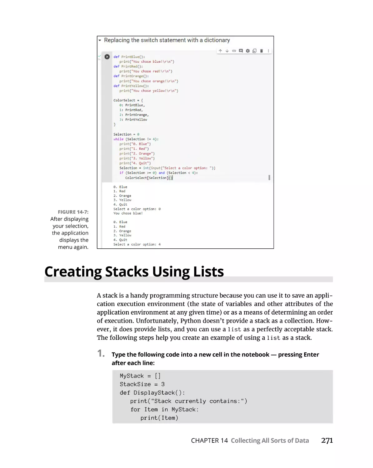
Replacing the switch statement with a dictionary . . . . . . . . . . . . .
Creating Stacks Using Lists. . . . . . . . . . . . . . . . . . . . . . . . . . . . . . . . . . . .
Working with queues . . . . . . . . . . . . . . . . . . . . . . . . . . . . . . . . . . . . . . . .
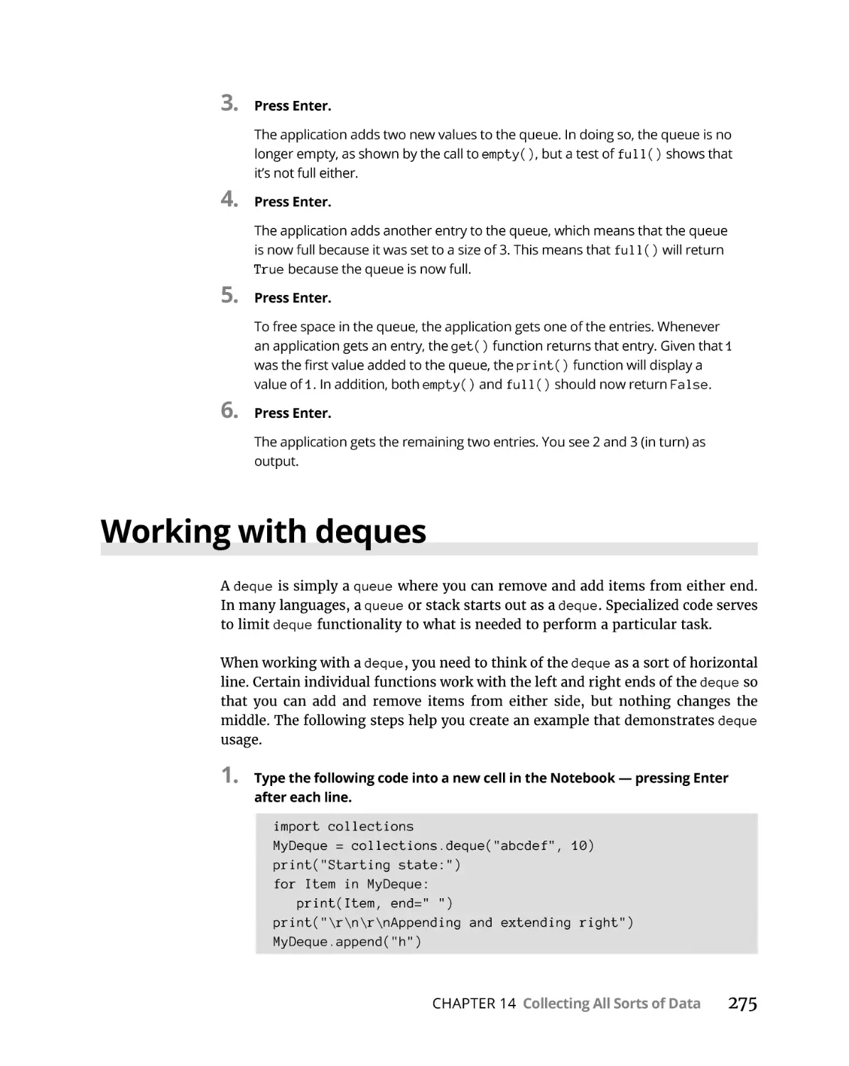
Working with deques . . . . . . . . . . . . . . . . . . . . . . . . . . . . . . . . . . . . . . . .
258
259
262
263
266
268
271
273
275
Creating and Using Classes . . . . . . . . . . . . . . . . . . . . . . . . . . .
279
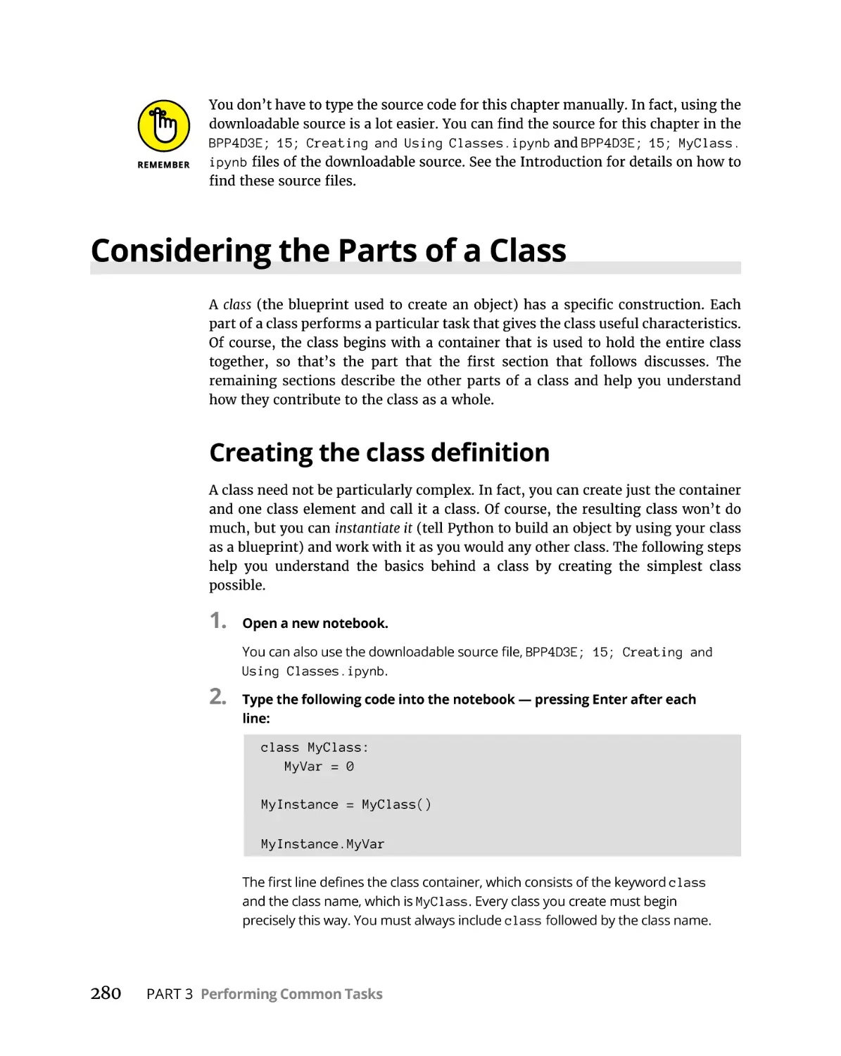
Considering the Parts of a Class . . . . . . . . . . . . . . . . . . . . . . . . . . . . . . .
Creating the class definition . . . . . . . . . . . . . . . . . . . . . . . . . . . . . . .
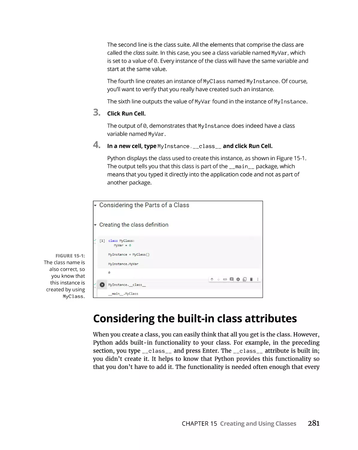
Considering the built-in class attributes . . . . . . . . . . . . . . . . . . . . .
Working with methods. . . . . . . . . . . . . . . . . . . . . . . . . . . . . . . . . . . .
Working with constructors. . . . . . . . . . . . . . . . . . . . . . . . . . . . . . . . .
Working with variables. . . . . . . . . . . . . . . . . . . . . . . . . . . . . . . . . . . .
Using methods with variable argument lists. . . . . . . . . . . . . . . . . .
Overloading operators. . . . . . . . . . . . . . . . . . . . . . . . . . . . . . . . . . . .
Creating and Using an External Class. . . . . . . . . . . . . . . . . . . . . . . . . . .
Developing the external class . . . . . . . . . . . . . . . . . . . . . . . . . . . . . .
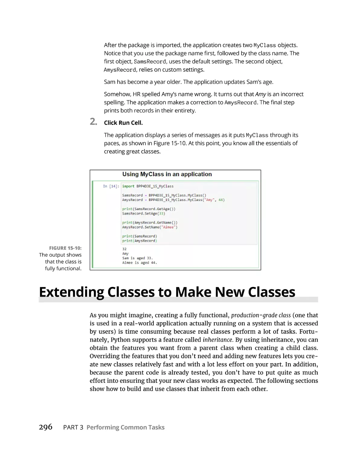
Using MyClass in an application . . . . . . . . . . . . . . . . . . . . . . . . . . . .
Extending Classes to Make New Classes. . . . . . . . . . . . . . . . . . . . . . . .
Building the child class. . . . . . . . . . . . . . . . . . . . . . . . . . . . . . . . . . . .
Testing class inheritance in an application . . . . . . . . . . . . . . . . . . .
280
280
281
282
285
287
289
291
293
293
295
296
297
298
PART 4: PERFORMING ADVANCED TASKS . . . . . . . . . . . . . . . . . .
301
Storing Data in Files. . . . . . . . . . . . . . . . . . . . . . . . . . . . . . . . . . . .
303
CHAPTER 14:
CHAPTER 15:
CHAPTER 16:
Understanding How Permanent Storage Works. . . . . . . . . . . . . . . . . .304
Creating Content for Permanent Storage . . . . . . . . . . . . . . . . . . . . . . . 306
Creating a File . . . . . . . . . . . . . . . . . . . . . . . . . . . . . . . . . . . . . . . . . . . . . . 309
Reading File Content. . . . . . . . . . . . . . . . . . . . . . . . . . . . . . . . . . . . . . . . . 313
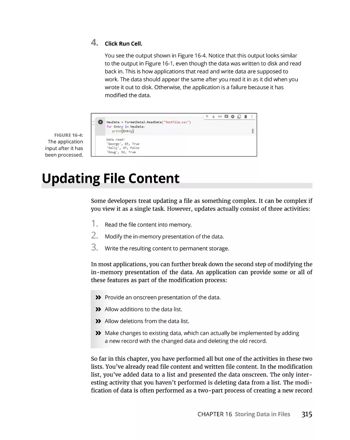
Updating File Content. . . . . . . . . . . . . . . . . . . . . . . . . . . . . . . . . . . . . . . . 315
Deleting a File. . . . . . . . . . . . . . . . . . . . . . . . . . . . . . . . . . . . . . . . . . . . . . . 319
CHAPTER 17:
Sending an Email . . . . . . . . . . . . . . . . . . . . . . . . . . . . . . . . . . . . . . .
321
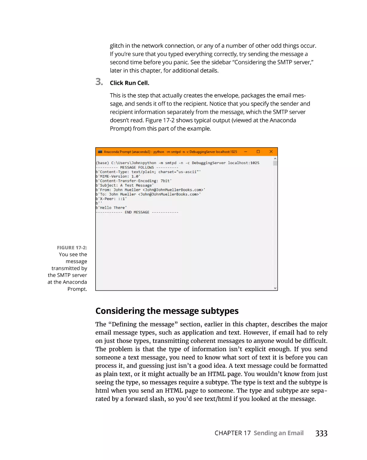
Understanding What Happens When You Send Email . . . . . . . . . . . . 322
Viewing email as you do a letter. . . . . . . . . . . . . . . . . . . . . . . . . . . . 323
Defining the parts of the envelope. . . . . . . . . . . . . . . . . . . . . . . . . . 324
xii
Beginning Programming with Python For Dummies
Defining the parts of the letter . . . . . . . . . . . . . . . . . . . . . . . . . . . . . 329
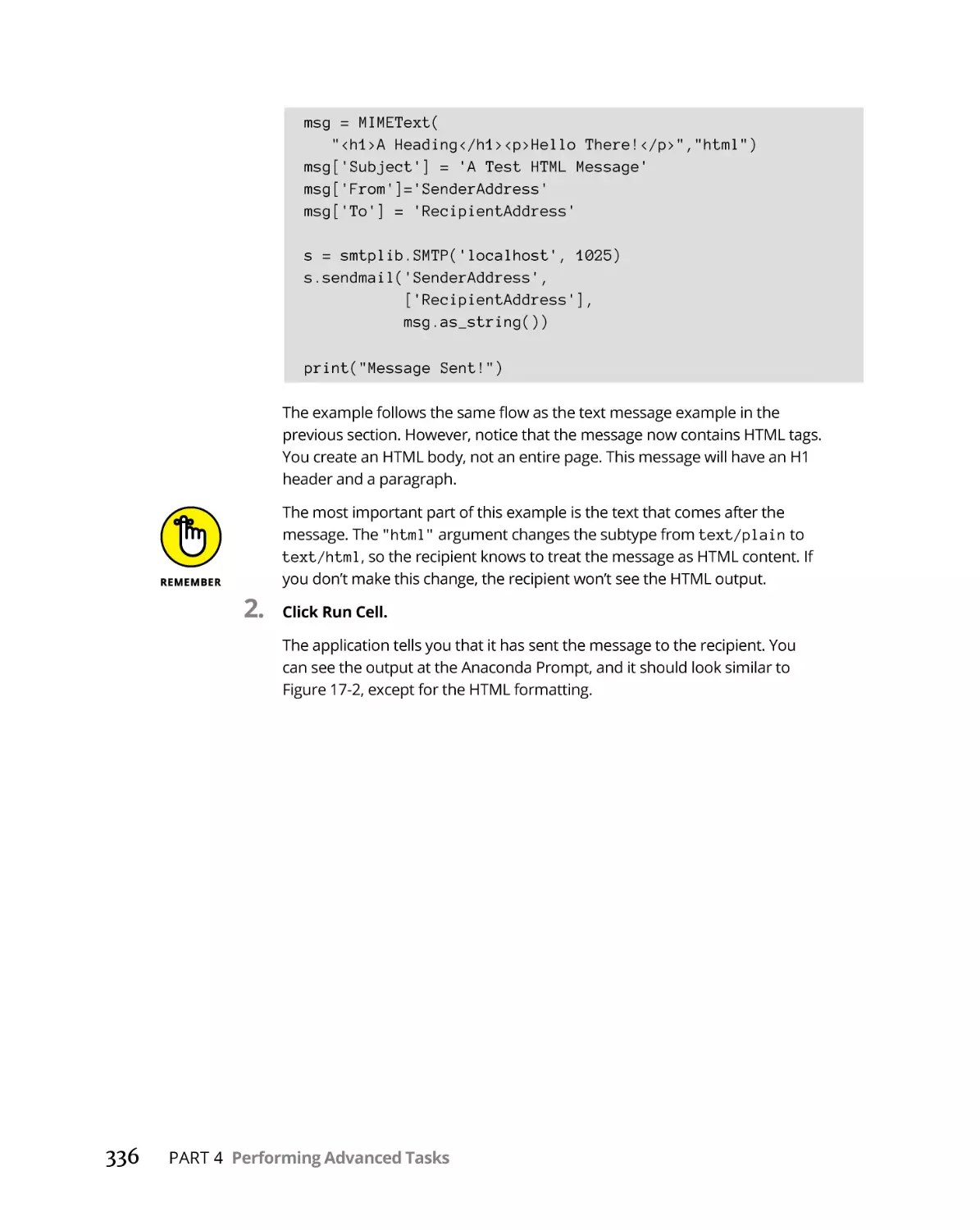
Putting everything together for text messages. . . . . . . . . . . . . . . . 334
Working with an HTML message. . . . . . . . . . . . . . . . . . . . . . . . . . . . 335
PART 5: THE PART OF TENS. . . . . . . . . . . . . . . . . . . . . . . . . . . . . . . . . . . .
CHAPTER 18:
CHAPTER 19:
337
Ten Amazing Programming Resources . . . . . . . . . . . . .
339
Working with the Python Documentation Online. . . . . . . . . . . . . . . . .
Discovering Details Using a Tutorial. . . . . . . . . . . . . . . . . . . . . . . . . . . .
Performing Web Programming by Using Python. . . . . . . . . . . . . . . . .
Locating Useful (versus Useless) Modules. . . . . . . . . . . . . . . . . . . . . . .
Creating Applications Faster by Using an IDE. . . . . . . . . . . . . . . . . . . .
Checking Your Syntax with Greater Ease. . . . . . . . . . . . . . . . . . . . . . . .
Using XML to Your Advantage. . . . . . . . . . . . . . . . . . . . . . . . . . . . . . . . .
Getting Past the Common Python Newbie Errors . . . . . . . . . . . . . . . .
Understanding Unicode. . . . . . . . . . . . . . . . . . . . . . . . . . . . . . . . . . . . . .
Making Your Python Application Fast. . . . . . . . . . . . . . . . . . . . . . . . . . .
340
341
342
343
343
344
345
346
346
347
Ten Ways to Make a Living with Python. . . . . . . . . . . .
349
Working in QA . . . . . . . . . . . . . . . . . . . . . . . . . . . . . . . . . . . . . . . . . . . . . . 350
Becoming the IT Staff for a Smaller Organization . . . . . . . . . . . . . . . . 351
Performing Specialty Scripting for Applications. . . . . . . . . . . . . . . . . . 352
Administering a Network. . . . . . . . . . . . . . . . . . . . . . . . . . . . . . . . . . . . . 353
Teaching Programming Skills. . . . . . . . . . . . . . . . . . . . . . . . . . . . . . . . . .353
Helping People Decide on Location . . . . . . . . . . . . . . . . . . . . . . . . . . . . 354
Performing Data Mining. . . . . . . . . . . . . . . . . . . . . . . . . . . . . . . . . . . . . . 354
Interacting with Embedded Systems . . . . . . . . . . . . . . . . . . . . . . . . . . . 355
Carrying Out Scientific Tasks. . . . . . . . . . . . . . . . . . . . . . . . . . . . . . . . . . 355
Performing Real-Time Analysis of Data . . . . . . . . . . . . . . . . . . . . . . . . . 356
CHAPTER 20:
Ten Tools That Enhance Your Python
Experience. . . . . . . . . . . . . . . . . . . . . . . . . . . . . . . . . . . . . . . . . . . . . . .
357
Tracking Bugs with Roundup Issue Tracker. . . . . . . . . . . . . . . . . . . . . .
Creating a Virtual Environment by Using VirtualEnv . . . . . . . . . . . . . .
Installing Your Application by Using PyInstaller . . . . . . . . . . . . . . . . . .
Building Developer Documentation by Using pdoc. . . . . . . . . . . . . . .
Developing Application Code by Using Komodo Edit. . . . . . . . . . . . . .
Debugging Your Application by Using pydbgr. . . . . . . . . . . . . . . . . . . .
Entering an Interactive Environment by Using IPython. . . . . . . . . . . .
Testing Python Applications by Using PyUnit . . . . . . . . . . . . . . . . . . . .
Tidying Your Code by Using Isort . . . . . . . . . . . . . . . . . . . . . . . . . . . . . .
Providing Version Control by Using Mercurial . . . . . . . . . . . . . . . . . . .
358
359
361
362
363
363
364
365
365
366
Table of Contents
xiii
Ten (Plus) Libraries You Need to Know About. . . . .
369
Developing a Secure Environment by Using CryptLib. . . . . . . . . . . . .
Interacting with Databases by Using SQLAlchemy. . . . . . . . . . . . . . . .
Seeing the World by Using Google Maps. . . . . . . . . . . . . . . . . . . . . . . .
Adding a Graphical User Interface by Using TkInter . . . . . . . . . . . . . .
Providing a Nice Tabular Data Presentation by Using PrettyTable . . .
Enhancing Your Application with Sound by Using PyAudio . . . . . . . .
Manipulating Images by Using PyQtGraph . . . . . . . . . . . . . . . . . . . . . .
Locating Your Information by Using Whoosh. . . . . . . . . . . . . . . . . . . .
Creating an Interoperable Java Environment by Using JPype. . . . . . .
Accessing Local Network Resources by Using Twisted Matrix. . . . . .
Accessing Internet Resources by Using Libraries. . . . . . . . . . . . . . . . .
370
371
371
372
373
373
374
375
376
377
377
INDEX. . . . . . . . . . . . . . . . . . . . . . . . . . . . . . . . . . . . . . . . . . . . . . . . . . . . . . . . . . . . . .
379
CHAPTER 21:
xiv
Beginning Programming with Python For Dummies
Introduction
P
ython is an example of a language that does everything right within the
domain of things that it’s designed to do. This isn’t just me saying it, either:
Programmers have voted by using Python enough that it’s now the firstranked language in the world (see https://www.tiobe.com/tiobe-index/ for
details). The amazing thing about Python is that you really can write an application on one platform and use it on every other platform that you need to support.
In contrast to other programming languages that promised to provide platform
independence, Python really does make that independence possible. In this case,
the promise is as good as the result you get.
Python emphasizes code readability and a concise syntax that lets you write
applications using fewer lines of code than other programming languages require.
You can also use a coding style that meets your needs, given that Python supports
the functional, imperative, object-oriented, and procedural coding styles (see
Chapter 3 for details). In addition, because of the way Python works, you find it
used in all sorts of fields that are filled with nonprogrammers. Beginning Programming with Python For Dummies, 3rd Edition is designed to help everyone, including
nonprogrammers, get up and running with Python quickly.
Some people view Python as a scripted language, but it really is so much more.
(Chapter 19 gives you just an inkling of the occupations that rely on Python to
make things work.) However, Python does lend itself to educational and other
uses for which other programming languages can fall short. In fact, this book uses
both Google Colab and Jupyter Notebook for examples, which rely on the highly
readable literate programming paradigm advanced by Stanford computer scientist
Donald Knuth (see Chapter 4 for details). Your examples end up looking like highly
readable reports that almost anyone can understand with ease.
About This Book
Beginning Programming with Python For Dummies, 3rd Edition is all about getting up
and running with Python quickly. You want to learn the language fast so that you
can become productive in using it to perform your real job, which could be anything. With the goal in mind of making things simple in every environment, this
book emphasizes a code anywhere approach. If you want to code on your
Introduction
1
smart phone (not really recommended unless you like to squint a lot), you can do
so as long as your smart phone has a browser that can access Google Colab. Likewise, coding while watching a TV equipped with a keyboard is possible, but not
necessarily recommended because of the distractions involved. Besides, trying to
write code that you can see only in that small square in the corner of the screen
would be very tough. Highly recommended is your desktop, laptop, or tablet.
Unlike most books on the topic, this one starts you right at the beginning by
showing you what makes Python different from other languages and how it can
help you perform useful work in a job other than programming. As a result, you
gain an understanding of what you need to do from the start, using hands-on
examples and spending a good deal of time performing actually useful tasks. By
the time you finish working through the examples in this book, you’ll be writing
simple programs and performing tasks such as sending an email using Python.
No, you won’t be an expert, but you will be able to use Python to meet specific
needs in the job environment. To make absorbing the concepts even easier, this
book uses the following conventions:
»» Text that you’re meant to type just as it appears in the book is bold. The
exception is when you’re working through a step list: Because each step is
bold, the text to type is not bold.
»» When you see words in italics as part of a typing sequence, you need to
replace that value with something that works for you. For example, if you see
“Type Your Name and press Enter,” you need to replace Your Name with your
actual name.
»» Web addresses and programming code appear in monofont. If you’re reading a
digital version of this book on a device connected to the Internet, note that you
can click the web address to visit that website, like this: www.dummies.com.
»» When you need to type command sequences, you see them separated by a
special arrow, like this: File ➪ New File. In this case, you go to the File menu
first and then select the New File entry on that menu. The result is that you
see a new file created.
Foolish Assumptions
You might find it difficult to believe that I’ve assumed anything about you — after
all, I haven’t even met you yet! Although most assumptions are indeed foolish,
I made these assumptions to provide a starting point for the book.
2
Beginning Programming with Python For Dummies
Familiarity with the platform you want to use is important because the book
doesn’t provide any guidance in this regard. To provide you with maximum
information about Python, this book doesn’t discuss any platform-specific issues.
You really do need to know how to install applications (when working with a
desktop system), use applications, work with your browser, and generally work
with your chosen platform before you begin working with this book.
This book also assumes that you can locate information on the Internet. Sprinkled
throughout are numerous references to online material that will enhance your
learning experience. However, these added sources are useful only if you actually
find and use them.
Icons Used in This Book
As you read this book, you see icons in the margins that indicate material of interest (or not, as the case may be). This section briefly describes each icon in this
book.
Tips are nice because they help you save time or perform some task without a lot
of extra work. The tips in this book are time-saving techniques or pointers to
resources that you should try in order to get the maximum benefit from Python.
I don’t want to sound like an angry parent or some kind of maniac, but you should
avoid doing anything marked with a Warning icon. Otherwise, you could find that
your program only serves to confuse users, who will then refuse to work with it.
Whenever you see this icon, think advanced tip or technique. You might find these
tidbits of useful information just too boring for words, or they could contain the
solution you need to get a program running. Skip these bits of information whenever you like.
If you don’t get anything else out of a particular chapter or section, remember the
material marked by this icon. This text usually contains an essential process or a
bit of information that you must know to write Python programs successfully.
Introduction
3
Beyond the Book
This book isn’t the end of your Python programming experience — it’s really just
the beginning. I provide online content to make this book more flexible and better
able to meet your needs. That way, as I receive email from you, I can do things like
address questions and tell you how updates to either Python or its associated
libraries affect book content. In fact, you gain access to all these cool additions:
»» Cheat sheet: You remember using crib notes in school to make a better mark
on a test, don’t you? You do? Well, a cheat sheet is sort of like that. It provides
you with some special notes about tasks that you can do with Python that not
every other developer knows. You can find the cheat sheet for this book by
going to www.dummies.com and searching for Beginning Programming with
Python For Dummies, 3rd Edition Cheat Sheet. It contains really neat information like how to perform magic when using Python.
»» Updates: Sometimes changes happen. For example, I might not have seen an
upcoming change when I looked into my crystal ball during the writing of this
book. In the past, that simply meant the book would become outdated and
less useful, but you can now find updates to the book by going to www.
dummies.com and searching for this book’s title.
In addition to these updates, check out the blog posts with answers to reader
questions and demonstrations of useful book-related techniques at http://
blog.johnmuellerbooks.com/.
»» Companion files: Hey! Who really wants to type all the code in the book?
Most readers would prefer to spend their time actually working through
coding examples, rather than typing. Fortunately for you, the source code is
available for download, so all you need to do is read the book to learn Python
coding techniques. Each of the book examples even tells you precisely which
example project to use. You can find these files by going to www.dummies.com
and searching for this book’s title. You can also find the downloadable source
on my website at http://www.johnmuellerbooks.com/source-code/;
just click the Download button for Beginning Programming with Python For
Dummies, 3rd Edition. Be sure to unzip the file using the instructions at
https://support.microsoft.com/en-us/windows/zip-and-unzipfiles-8d28fa72-f2f9-712f-67df-f80cf89fd4e5 before attempting to use
the source code, even if you can see it in Windows Explorer.
4
Beginning Programming with Python For Dummies
Where to Go from Here
It’s time to start your Programming with Python adventure! If you’re a complete
programming novice, you should start with Chapter 1 and progress through the
book at a pace that allows you to absorb as much of the material as possible.
If you’re a novice who’s in an absolute rush to get going with Python as quickly as
possible, you could skip to Chapter 2 with the understanding that you may find
some topics a bit confusing later. Skipping to Chapter 3 is possible if you want to
start working with Python immediately and have access to Google Colab or a
Jupyter Notebook installation.
Readers who have some exposure to Python can save time by moving directly to
Chapter 4. This chapter gets you started working with notebooks so that you have
a better idea of how to work with Google Colab or Jupyter Notebook for the examples in the remainder of the book. Make sure you also read through Chapter 5,
which tells you how to perform magic in notebooks.
Assuming that you already have access to either Google Colab or Jupyter Notebook
and know how to use your IDE of choice, you can move directly to Chapter 6. You
can always go back to earlier chapters as necessary when you have questions.
However, it’s important that you understand how each example works before
moving to the next one. Every example has important lessons for you, and you
could miss vital content if you start skipping too much information.
Introduction
5
1
Getting Started
with Python
IN THIS PART . . .
Defining the association between Python and
applications
Using Google Colab to work with Python
Performing essential tasks using Python
Creating your first application
Performing feats of magic
IN THIS CHAPTER
»» Talking to your computer
»» Creating programs to talk to your
computer
»» Understanding programs and their
creation
»» Considering why you want to use
Python
Chapter
1
Talking to Your
Computer
H
aving a conversation with your computer might sound like the script of a
science fiction movie. After all, the members of the Enterprise on Star Trek
regularly talked with their computer. In fact, the computer often talked
back. However, with the rise of Apple’s Siri (https://www.apple.com/siri/),
Amazon’s Echo (https://www.amazon.com/dp/B07XKF5RM3/) and other interactive software (https://windowsreport.com/talking-pc-software/), perhaps
you really don’t find a conversation so unbelievable.
Asking the computer for information is one thing, but providing it with instructions is quite another. This chapter considers why you want to instruct your computer about anything and what benefit you gain from it. You also discover the need
for a special language when performing this kind of communication and why you
want to use Python to accomplish it. However, the main thing to get out of this
chapter is that programming is simply a kind of communication that is akin to
other forms of communication you already have with your computer.
CHAPTER 1 Talking to Your Computer
9
Understanding Why You Want to
Talk to Your Computer
Talking to a machine may seem quite odd at first (then again, people do talk to
cats, dogs, cars, toasters, and other odd assorted things), but it’s necessary
because a computer can’t read your mind — yet. Mind-reading computers are
getting closer, as described in the article at https://www.psychnewsdaily.com/
this-computer-can-read-your-mind-and-render-your-thoughts-aspictures/. Even if the computer did read your mind, it would still be communicating with you. Nothing can occur without an exchange of information between
the machine and you. Activities such as
»» Reading your email
»» Writing about your vacation
»» Finding the greatest gift in the world
are all examples of communication that occurs between a computer and you. That
the computer further communicates with other machines or people to address
requests that you make simply extends the basic idea that communication is necessary to produce any result.
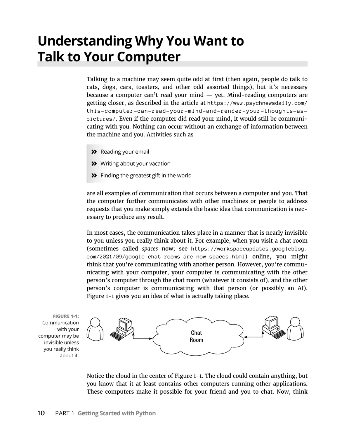
In most cases, the communication takes place in a manner that is nearly invisible
to you unless you really think about it. For example, when you visit a chat room
(sometimes called spaces now; see https://workspaceupdates.googleblog.
com/2021/09/google-chat-rooms-are-now-spaces.html) online, you might
think that you’re communicating with another person. However, you’re communicating with your computer, your computer is communicating with the other
person’s computer through the chat room (whatever it consists of), and the other
person’s computer is communicating with that person (or possibly an AI).
Figure 1-1 gives you an idea of what is actually taking place.
FIGURE 1-1:
Communication
with your
computer may be
invisible unless
you really think
about it.
Notice the cloud in the center of Figure 1-1. The cloud could contain anything, but
you know that it at least contains other computers running other applications.
These computers make it possible for your friend and you to chat. Now, think
10
PART 1 Getting Started with Python
about how easy the whole process seems when you’re using the chat application.
Even though all these things are going on in the background, it seems as if you’re
simply chatting with your friend, and the process itself is invisible.
Knowing that an Application Is a
Form of Communication
Computer communication occurs through the use of applications. You use one
application to answer your email, another to purchase goods, and still another to
create a presentation. An application (sometimes called an app) provides the means
to express human ideas to the computer in a manner the computer can understand and defines the tools needed to shape the data used for the communication
in specific ways. Data used to express the content of a presentation is different
from data used to purchase a present for your mother. The way you view, use, and
understand the data is different for each task, so you must use different applications to interact with the data in a manner that both the computer and you can
understand.
You can obtain applications to meet just about any general need you can conceive
of today. In fact, you probably have access to applications for which you haven’t
even thought about a purpose yet. Programmers have been busy creating millions
of applications of all types for many years now, so it may be hard to understand
what you can accomplish by creating some new method for talking with your
computer through an application. The answer comes down to thinking about the
data and how you want to interact with it. Some data simply isn’t common enough
to have attracted the attention of a programmer, or you may need the data in a
format that no application currently supports, so you don’t have any way to tell
the computer about it unless you create a custom application to do it. The following sections describe applications from the perspective of working with unique
data in a manner that is special in some way.
Thinking about procedures you use daily
A procedure is simply a set of steps you follow to perform a task. For example,
when making toast, you might use a procedure like this:
1.
2.
3.
Get the bread and butter from the refrigerator.
Open the bread bag and take out two pieces of bread.
Remove the cover from the toaster.
CHAPTER 1 Talking to Your Computer
11
4.
5.
6.
7.
8.
9.
Place each piece of bread in its own slot.
Push the toaster lever down to start toasting the bread.
Wait for the toasting process to complete.
Remove toast from the toaster.
Place toast on a plate.
Butter the toast.
Your procedure might vary from the one presented here, but it’s unlikely that
you’d butter the toast before placing it in the toaster. Of course, you do actually
have to remove the bread from the wrapper before you toast it (placing the bread,
wrapper and all, into the toaster would likely produce undesirable results). Most
people never actually think about the procedure for making toast. However, you
use a procedure like this one even though you don’t think about it.
Computers can’t perform tasks without a procedure. You must tell the computer
which steps to perform, the order in which to perform them, and any exceptions
to the rule that could cause failure. All this information (and more) appears within
an application. In short, an application is simply a written procedure that you use
to tell the computer what to do, when to do it, and how to do it. Because you’ve
been using procedures all your life, all you really need to do is apply the knowledge you already possess to what a computer needs to know about specific tasks.
Writing procedures down
When I was in grade school, our teacher asked us to write a paper about making
toast. After we turned in our papers, she brought in a toaster and some loaves of
bread. Each paper was read and demonstrated. None of our procedures worked as
expected, but they all produced humorous results. In my case, I forgot to tell the
teacher to remove the bread from the wrapper, so she dutifully tried to stuff the
piece of bread, wrapper and all, into the toaster. The lesson stuck with me. Writing
about procedures can be quite hard because we know precisely want we want to
do, but often we leave steps out — we assume that the other person also knows
precisely what we want to do.
Writing procedures down isn’t really sufficient, though — you also need to test
the procedure by asking someone who isn’t familiar with the task to perform it
using your procedure. When working with computers, the computer is your perfect test subject.
12
PART 1 Getting Started with Python
Seeing applications as being like
any other procedure
A computer acts like the grade school teacher in my example in the previous section. When you write an application, you’re writing a procedure that defines a
series of steps that the computer should perform to accomplish whatever task you
have in mind. If you leave out a step, the results won’t be what you expected. The
computer won’t know what you mean or that you intended for it to perform certain tasks automatically. The only thing the computer knows is that you have
provided it with a specific procedure and it needs to perform that procedure.
Making your computer do funny things
People eventually get used to the procedures you create. They automatically compensate for deficiencies in the procedure or make notes about things that were left
out. In other words, people compensate for problems with the procedures that you
write.
When you begin writing computer programs, you’ll get frustrated because computers perform tasks precisely and read your instructions literally. For example, if
you tell the computer that a certain value should equal 5, the computer will look
for a value of exactly 5. A human might see 4.9 and know that the value is good
enough, but a computer doesn’t see things that way. It sees a value of 4.9 and
decides that it doesn’t equal 5 exactly. In short, computers are inflexible, unintuitive, and unimaginative. When you write a procedure for a computer, the computer will do precisely as you ask absolutely every time and never modify your
procedure or decide that you really meant for it to do something else. In some
cases (not many), the results can actually be quite humorous (such as that time
the computer began reciting a limerick that you meant to keep private). A sense of
humor is helpful in computer programming.
Defining What an Application Is
As previously mentioned, applications provide the means to define and express
human ideas in a manner that a computer can understand. To accomplish this
goal, the application relies on one or more procedures that tell the computer how
to perform the tasks related to the manipulation of data and its presentation.
What you see onscreen is the text from your word processor, but to see that information, the computer requires procedures for retrieving the data from disk, putting it into a form you can understand, and then presenting it to you. The following
sections define the specifics of an application in more detail.
CHAPTER 1 Talking to Your Computer
13
Understanding that computers
use a special language
Human language is complex and difficult to understand. Even applications such as
Siri and Alexa have serious limits in understanding what you’re saying. Over the
years, computers have gained the capability to input human speech as data and to
interpret certain spoken words as commands, but computers still don’t understand human speech. What the computer does is match voice patterns to data it
understands and then match that data to specific commands.
Given what you know from previous sections of this chapter, computers could
never rely on human speech to understand the procedures you write. Computers
always take things literally, so you’d end up with completely unpredictable results
if you were to use human language to write applications. That’s why humans use
special languages, called programming languages, to communicate with computers.
These special languages make it possible to write procedures that are both specific
and completely understandable by both humans and computers.
Computers don’t actually speak any language. They use binary codes to flip
switches internally and to perform math calculations. Computers don’t even
understand letters — they understand only numbers. A special application turns
the computer-specific language you use to write a procedure into binary codes.
For the purposes of this book, you really don’t need to worry too much about the
low-level specifics of how computers work at the binary level. However, it’s
interesting to know that computers speak math and numbers, not really a language at all.
Helping humans speak to the computer
It’s important to keep the purpose of an application in mind as you write it. An
application is there to help humans speak to the computer in a certain way. Every
application works with some type of data that is input, stored, manipulated, and
output so that the humans using the application obtain a desired result. Whether
the application is a game or a spreadsheet, the basic idea is the same. Computers
work with data provided by humans to obtain a desired result.
When you create an application, you’re providing a new method for humans to
speak to the computer. The new approach you create will make it possible for
other humans to view data in new ways. The communication between human and
computer should be easy enough that the application actually disappears from
view. Think about the kinds of applications you’ve used in the past. The best
applications are the ones that let you focus on whatever data you’re interacting
with. For example, a game application is considered immersive only if you can
14
PART 1 Getting Started with Python
focus on the planet you’re trying to save or the ship you’re trying to fly, rather
than the application that lets you do these things.
One of the best ways to start thinking about how you want to create an application
is to look at other applications. Writing down what you like and dislike about other
applications is a useful way to start discovering how you want your applications to
look and work. Here are some questions you can ask yourself as you work with the
applications:
»» What do I find distracting about the application?
»» Which features were easy to use?
»» Which features were hard to use?
»» How did the application make it easy to interact with my data?
»» How would I make the data easier to work with?
»» What do I hope to achieve with my application that this application doesn’t
provide?
Professional developers ask many other questions as part of creating an application, but these are good starter questions because they begin to help you think
about applications as a means to help humans speak with computers. If you’ve
ever found yourself frustrated by an application you used, you already know how
other people will feel if you don’t ask the appropriate questions when you create
your application. Communication is the most important element of any application you create.
You can also start to think about the ways in which you work. Start writing procedures for the things you do. It’s a good idea to take the process one step at a
time and write everything you can think of about that step. When you get finished, ask someone else to try your procedure to see how it actually works. You
might be surprised to learn that even with a lot of effort, you can easily forget to
include steps.
The world’s worst application usually begins with a programmer who doesn’t
know what the application is supposed to do, why it’s special, what need it
addresses, or whom it is for. When you decide to create an application, make sure
that you know why you’re creating it and what you hope to achieve. Just having a
plan in place really helps make programming fun. You can work on your new
application and see your goals accomplished one at a time until you have a completed application to use and show off to your friends (all of whom will think
you’re really cool for creating it).
CHAPTER 1 Talking to Your Computer
15
Understanding Why Python Is So Cool
Many programming languages are available today. In fact, a student can spend an
entire semester in college studying computer languages and still not hear about
them all. (I did just that during my college days.) You’d think that programmers
would be happy with all these programming languages and just choose one to talk
to the computer, but they keep inventing more.
Programmers keep creating new languages for good reason. Each language has
something special to offer — something it does exceptionally well. In addition, as
computer technology evolves, so do the programming languages in order to keep
up. Because creating an application is all about efficient communication, many programmers know multiple programming languages so that they can choose just the
right language for a particular task. One language might work better to obtain data
from a database, and another might create user interface elements especially well.
As with every other programming language, Python does some things exceptionally well, and you need to know what they are before you begin using it. You might
be amazed by the really cool things you can do with Python. Knowing a programming language’s strengths and weaknesses helps you use it better as well as avoid
frustration by not using the language for things it doesn’t do well. The following
sections help you make these sorts of decisions about Python.
Unearthing the reasons for using Python
When Guido van Rossum (https://gvanrossum.github.io/) decided to create
Python, the main objective was to develop a programming language that would
make programmers efficient and productive. With that in mind, here are the reasons that you want to use Python when creating an application:
»» Less application development time: Python code is usually 2–10 times
shorter than comparable code written in languages like C/C++ and Java, which
means that you spend less time writing your application and more
time using it.
»» Ease of reading: A programming language is like any other language — you
need to be able to read it to understand what it does. Python code tends to be
easier to read than the code written in other languages, which means you
spend less time interpreting it and more time making essential changes.
»» Reduced learning time: The creators of Python wanted to make a programming language with fewer odd rules that make the language hard to learn.
After all, programmers want to create applications, not learn obscure and
difficult languages.
16
PART 1 Getting Started with Python
Although Python is a popular language, it’s not always the most popular language
out there (depending on the site you use for comparison). However, it currently
ranks first on sites such as TIOBE (https://www.tiobe.com/tiobe-index/), an
organization that tracks usage statistics (among other things). Another good place
to look is Statistics Times (https://statisticstimes.com/tech/top-computerlanguages.php), which also ranks Python as the number one language today.
If you’re looking for a language solely for the purpose of obtaining a job, Python
is a great choice, but Java, C/C++, or C# might be better choices, depending on the
kind of job you want to get. Visual Basic is also a great choice, even if it isn’t currently quite as popular as Python. Make sure to choose a language you like and one
that will address your application-development needs, but also choose on the
basis of what you intend to accomplish. You may be surprised to learn that many
colleges use Python to teach coding, and it has become the most popular language
in that venue (see https://www.pythoncentral.io/how-is-python-used-ineducation/ for details).
Deciding how you can personally
benefit from Python
Ultimately, you can use any programming language to write any sort of application you want. If you use the wrong programming language for the job, the process will be slow, error prone, bug ridden, and you’ll absolutely hate it — but you
can get the job done. Of course, most of us would rather avoid horribly painful
experiences, so you need to know what sorts of applications people typically use
Python to create. Here’s a list of the most common uses for Python (although
people do use it for other purposes):
»» Creating rough application examples: Developers often need to create a
prototype, a rough example of an application, before getting the resources to
create the actual application. Python emphasizes productivity, so you can use
it to create prototypes of an application quickly.
»» Scripting browser-based applications: Even though JavaScript is probably
the most popular language used for browser-based application scripting,
Python is a close second. Python offers functionality that JavaScript doesn’t
provide (see the comparison at https://www.educba.com/python-vsjavascript/ for details) and its high efficiency makes it possible to create
browser-based applications faster (a real plus in today’s fast-paced world).
»» Designing mathematic, scientific, and engineering applications:
Interestingly enough, Python provides access to some really cool libraries
that make it easier to create math, scientific, and engineering applications.
The two most popular libraries are NumPy (https://numpy.org/) and SciPy
CHAPTER 1 Talking to Your Computer
17
(https://scipy.org/). These libraries greatly reduce the time you spend
writing specialized code to perform common math, scientific, and engineering
tasks.
»» Working with XML: The eXtensible Markup Language (XML) is the basis of
most data storage needs on the Internet and many desktop applications
today. Unlike most languages, where XML is just sort of bolted on, Python
makes it a first-class citizen. If you need to work with a web service, the
main method for exchanging information on the Internet (or any other
XML-intensive application), Python is a great choice.
»» Interacting with databases: Business relies heavily on databases. Python
isn’t quite a query language, like the Structured Query Language (SQL) or
Language INtegrated Query (LINQ), but it does do a great job of interacting
with databases. It makes creating connections and manipulating data
relatively painless.
»» Developing user interfaces: Python isn’t like some languages like C# where
you have a built-in designer and can drag and drop items from a toolbox onto
the user interface. However, it does have an extensive array of graphical user
interface (GUI) frameworks — extensions that make graphics a lot easier to
create (see https://wiki.python.org/moin/GuiProgramming for details).
Some of these frameworks do come with designers that make the user
interface creation process easier. The point is that Python isn’t devoted to
just one method of creating a user interface — you can use the method that
best suits your needs.
Discovering which organizations
use Python
Python really is quite good at the tasks that it was designed to perform. In fact,
that’s why a lot of large organizations use Python to perform at least some
application-creation (development) tasks. You want a programming language
that has good support from these large organizations because these organizations
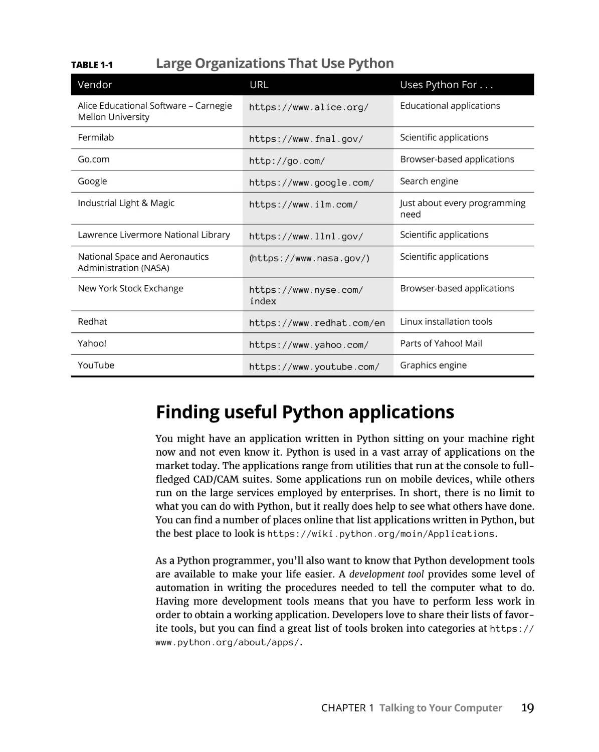
tend to spend money to make the language better. Table 1-1 lists some of the large
organizations that use Python the most.
These are just a few of the many organizations that use Python extensively. You
can find a more complete list of organizations at https://www.python.org/
about/success/. The number of success stories has become so large that even
this list probably isn’t complete and the people supporting it have had to create
categories to better organize it.
18
PART 1 Getting Started with Python
TABLE 1-1
Large Organizations That Use Python
Vendor
URL
Uses Python For . . .
Alice Educational Software – Carnegie
Mellon University
https://www.alice.org/
Educational applications
Fermilab
https://www.fnal.gov/
Scientific applications
Go.com
http://go.com/
Browser-based applications
Google
https://www.google.com/
Search engine
Industrial Light & Magic
https://www.ilm.com/
Just about every programming
need
Lawrence Livermore National Library
https://www.llnl.gov/
Scientific applications
National Space and Aeronautics
Administration (NASA)
(https://www.nasa.gov/)
Scientific applications
New York Stock Exchange
https://www.nyse.com/
index
Browser-based applications
Redhat
https://www.redhat.com/en
Linux installation tools
Yahoo!
https://www.yahoo.com/
Parts of Yahoo! Mail
YouTube
https://www.youtube.com/
Graphics engine
Finding useful Python applications
You might have an application written in Python sitting on your machine right
now and not even know it. Python is used in a vast array of applications on the
market today. The applications range from utilities that run at the console to fullfledged CAD/CAM suites. Some applications run on mobile devices, while others
run on the large services employed by enterprises. In short, there is no limit to
what you can do with Python, but it really does help to see what others have done.
You can find a number of places online that list applications written in Python, but
the best place to look is https://wiki.python.org/moin/Applications.
As a Python programmer, you’ll also want to know that Python development tools
are available to make your life easier. A development tool provides some level of
automation in writing the procedures needed to tell the computer what to do.
Having more development tools means that you have to perform less work in
order to obtain a working application. Developers love to share their lists of favorite tools, but you can find a great list of tools broken into categories at https://
www.python.org/about/apps/.
CHAPTER 1 Talking to Your Computer
19
Comparing Python to other languages
Comparing one language to another is somewhat dangerous because the selection
of a language is just as much a matter of taste and personal preference as it is any
sort of quantifiable scientific fact. So before I’m attacked by the rabid protectors
of the languages that follow, it’s important to realize that I also use a number of
languages and find at least some level of overlap among them all. There is no best
language in the world, simply the language that works best for a particular application. With this idea in mind, the following sections provide an overview comparison of Python to other languages. (You can find comparisons to other
languages at https://wiki.python.org/moin/LanguageComparisons.)
C#
A lot of people claim that Microsoft simply copied Java to create C#. That said, C#
does have some advantages (and disadvantages) when compared to Java. The
main (undisputed) intent behind C# is to create a better kind of C/C++ language —
one that is easier to learn and use. However, we’re here to talk about C# and
Python. When compared to C#, Python has these advantages:
»» Significantly easier to learn
»» Smaller (more concise) code
»» Supported fully as open source
»» Better multiplatform support
»» Easily allows use of multiple development environments
»» Easier to extend using Java and C/C++
»» Enhanced scientific and engineering support
Java
For years, programmers looked for a language that they could use to write an
application just once and have it run anywhere. Java is designed to work well on
any platform. It relies on some tricks that you’ll discover later in the book to
accomplish this magic. For now, all you really need to know is that Java was so
successful at running well everywhere that other languages have sought to emulate it (with varying levels of success). Even so, Python has some important
advantages over Java, as shown in the following list:
»» Significantly easier to learn
»» Smaller (more concise) code
20
PART 1 Getting Started with Python
»» Enhanced variables (storage boxes in computer memory) that can hold
different kinds of data based on the application’s needs while running
(dynamic typing)
»» Faster development times
Perl
Perl was originally an acronym for Practical Extraction and Report Language.
Today, people simply call it Perl and let it go at that. However, Perl still shows its
roots in that it excels at obtaining data from a database and presenting it in report
format. Of course, Perl has been extended to do a lot more than that — you can use
it to write all sorts of applications. (I’ve even used it for a web service application.)
In a comparison with Python, you’ll find that Python has these advantages over
Perl:
»» Simpler to learn
»» Easier to read
»» Enhanced protection for data
»» Better Java integration
»» Fewer platform-specific biases
R
Data scientists often have a tough time choosing between R and Python because
both languages are adept at statistical analysis and the sorts of graphing that data
scientists need to understand data patterns. Both languages are also open source
and support a large range of platforms. However, R is a bit more specialized than
Python and tends to cater to the academic market. Consequently, Python has these
advantages over R:
»» Emphasizes productivity and code readability
»» Is designed for use by enterprises
»» Offers easier debugging
»» Uses consistent coding techniques
»» Has greater flexibility
»» Is easier to learn
CHAPTER 1 Talking to Your Computer
21
Haskell
Pure functional languages, such as Haskell, have some significant advantages
because they work extremely well in multithreaded application due to the fact that
pure functions always return the same value for the same inputs. There are no
side effects. Many developers also see functional languages as easier to debug and
less likely to produce bugs. Python is an impure functional language, which means
it doesn’t strictly adhere to all of the functional language requisites. However,
Python has these advantages over Haskell:
»» Is easier to learn
»» Greater selection of libraries
»» Easier to use for prototyping and modeling
»» Viewed as a better server-side language
»» Has greater flexibility
22
PART 1 Getting Started with Python
IN THIS CHAPTER
»» Using Google Colab as an editor
»» Performing the common tasks to
create code files
»» Making your code run faster as you
execute it
»» Getting help when you need it
Chapter
2
Working with Google
Colab
B
ack in the Stone Age of computing, developers used punch cards to write
their applications and then waited, sometimes a week, to get time on the
computer to run an application that might instantly fail with an error.
Programmers in that age were a frustrated bunch, prone to grimacing a lot. So
moving to Integrated Development Environments (IDEs) (special editors that you
use to write and run code) on large desktop machines seemed like a real achievement, but things became even better with time. Now you can write your applications anywhere and at any time with browser-based IDEs like Colabortory.
Colaboratory (https://colab.research.google.com/notebooks/welcome.ipynb),
or Colab for short, is a Google cloud-based service that lets you write Python code
using a notebook-like environment, rather than the usual desktop IDE. (Jupyter
Notebook, https://jupyter.org/, provides an environment similar to Colab on
the desktop if you don’t have an Internet connection.)
You don’t have to install anything on your system to use Colab. The benefit of this
approach is that you can work with code in small pieces and obtain nearly instant
results from any work you do (no more frustrated grimacing). A notebook format
also lends itself to output in a report format that works well for presentations and
reports. The first section of this chapter helps you work through some Colab basics
and understand how Colab differs from a standard IDE (and why this difference
imparts significant benefit when learning how to program).
CHAPTER 2 Working with Google Colab
23
You can use Colab to perform specific tasks in a cell-oriented paradigm. The next
sections of the chapter present a range of task-related topics that start with the
use of notebooks. Of course, you also want to perform other sorts of tasks, such as
creating various cell types and use them to create notebooks that have a reportlike appearance with functional code.
Part of working with Colab is knowing how to run the example code, making it run
as quickly as possible. Two sections of the chapter are dedicated to using hardware
acceleration and running the example code in various ways.
Finally, this chapter can’t address every aspect of Colab, so the last section of the
chapter serves as a handy resource for locating the most reliable information
about Colab.
You don’t have to type the source code for this chapter manually. In fact, using
the downloadable source is a lot easier. You can find the source for this chapter in
the BPP4D3E; 02; Colab Examples.ipynb file of the downloadable source. See the
Introduction for details on how to find these source files.
Defining Google Colab
Colab helps you write, document, and test Python code using a single application.
It’s designed to mimic a desktop application called Jupyter Notebook (https://
jupyter.org/), so you can use Jupyter Notebook in place of Colab to run the
applications in this book. In fact, it’s somewhat difficult to tell the two applications apart in the functionality they provide. Google Colab is the cloud version of
Notebook, and the Welcome page makes this fact apparent. It even uses IPython
(the previous name for Jupyter) Notebook (.ipynb) files for the site.
Even though the two applications are similar and both use .ipynb files, they do
have some differences that you need to know about. The previous edition of this
book used Jupyter Notebook, but Colab offers the ability to compute anywhere on
any device that sports a browser, so this edition of the book focuses on Colab
instead. The following sections help you understand the Colab differences.
Understanding what Google Colab does
You can use Colab to perform many tasks, but for the purpose of this book, you use
it to write and run code, create its associated documentation, and display graphics. The downloadable source for this book is designed to run on Colab, but you can
also use it with Jupyter Notebook if you want.
24
PART 1 Getting Started with Python
Jupyter Notebook is a localized application in that you use local resources with it.
You could potentially use other sources, but doing so could prove inconvenient or
impossible in some cases. For example, according to https://docs.github.com/
repositories/working-with-files/using-files/working-with-non-codefiles, your Notebook files will appear as static HTML pages when you use a
GitHub repository. (GitHub is a cloud-based storage technology specifically oriented to working with code.) In fact, some features won’t work at all.
Colab enables you to fully interact with your Notebook files using GitHub as a
repository, and Colab supports a number of other online storage options as well,
so you can regard Colab as your online partner in creating Python code. The GitHub
repository for this book is at https://github.com/JohnPaulMueller/BPP4D3E.
The other reason you really need to know about Colab is that you can use it with
your alternative device. During the writing process, some of the example code was
tested on an Android-based tablet (an ASUS ZenPad 3S 10). The target tablet has
Chrome installed and executes the code well enough to follow the examples. All
this said, you likely won’t want to try to write code using a tablet of that size (it
has a 9.7-inch diagonal screen) — the text was incredibly small, for one thing,
and the lack of a keyboard could be a problem, too. The point is that you don’t
absolutely have to have a Windows, Linux, or macOS system to try the code, but
the alternatives might not provide quite the performance you expect.
Google Colab generally doesn’t work with browsers other than Chrome (the
browser used in this chapter), Firefox, or Safari (although initial tests with Microsoft Edge have also been encouraging). In most cases, you see an error message,
such as This site may not work in your browser. Please use a supported
browser, and no other display if you try to start Colab in a browser that it doesn’t
support. The included More Info link takes you to https://research.google.
com/colaboratory/faq.html#browsers, where you can learn more information.
Working with Google Colab features
Google Colab provides access to a number of features through the menu system.
One of these features, hardware acceleration, appears in the “Using Hardware
Acceleration” section, later in this chapter. The features in this section all appear
on the Tools menu.
Locating commands
The Tools ➪ Command Palette option displays a list of commands you can execute,
as shown in Figure 2-1. Some of these commands also have shortcut keys, such as
Ctrl+Alt+M for adding a comment to a cell. All these commands help you to perform tasks associated with Notebook content, such as adding forms.
CHAPTER 2 Working with Google Colab
25
SOME FIREFOX ODDITIES
Even with online help, you may still find that your copy of Firefox displays a
SecurityError: The operation is insecure. error message. The initial error
dialog box points to some unrelated issue, such as cookies, but you see this error message when you click Details. Simply dismissing the dialog box by clicking OK makes
Colab appear to be working because it displays your code, but you won’t see results
from running the code.
As a first step toward fixing this problem, make sure that your copy of Firefox is current;
older versions don’t provide the required support. After you’ve updated your copy, setting the network.websocket.allowInsecureFromHTTPS preference using
About:Config to True should resolve the problem, but sometimes it doesn’t. In this
case, verify that Firefox actually does allow third-party cookies by selecting both the
Always option for Accept Third Party Cookies and Site Data entry and the Remember
History option in the History section on the Privacy & Security tab of the Options dialog
box. Restart Firefox after each change and then try Colab again. If none of these fixes
works, you must use Chrome to work with Colab on your system.
FIGURE 2-1:
Using Colab
commands
makes
configuring your
Notebook easy.
Configuring settings
The Tools ➪ Settings option displays the Settings dialog box, shown in Figure 2-2.
The four common and one optional (not shown) settings tabs perform these tasks:
»» Site: Configures how the site works. The most interesting setting is the theme.
Selecting Adaptive lets Colab choose the interface colors based on lighting
conditions. You can also configure display and access settings on this tab.
26
PART 1 Getting Started with Python
»» Editor: Determines how text appears onscreen and how the interface works.
For example, you can set the key bindings to work like those in Vim (a text
editor included on Unix and Linux systems, generally as the vi utility,
https://www.vim.org/) if desired. You can also select font size, spaces for
each level of indentation, and a plethora of other settings.
»» Colab Pro: Provides an advertisement for Colab Pro (https://colab.
research.google.com/signup), which gives you some significant benefits
like faster GPUs, longer runtimes, and more memory — all of which let you
get more work done in a shorter time.
»» GitHub (optional): Shows that your GitHub account is connected to Colab
when this tab appears. The various options let you remove GitHub access and
determine whether you can see private repositories when opening files.
Figure 2-2 doesn’t show this particular tab because you won’t normally see it
until you grant GitHub access using the instructions found at https://
medium.com/analytics-vidhya/how-to-use-google-colab-withgithub-via-google-drive-68efb23a42d. You can find some additional
insights at https://stackoverflow.com/questions/67553747/
how-do-i-link-a-github-repository-to-a-google-colab-notebook.
»» Miscellaneous: Contains fun settings. You can choose from three visual
effects: adding thunder and lightning using the Power Level setting; letting a
Corgi run across the top of the display; and allowing a kitten to run across the
top of the display. You can choose any mix of these visual effects.
FIGURE 2-2:
The Settings
dialog box helps
you configure the
Colab IDE.
CHAPTER 2 Working with Google Colab
27
Customizing keyboard shortcuts
If you don’t like the default keyboard shortcuts, you can customize them to match
your needs. To do so, choose Tools ➪ Keyboard Shortcuts, and you see the Keyboard Preferences dialog box, shown in Figure 2-3. If you see Set Shortcut, it
means that the command doesn’t currently have a shortcut, so you can add one if
desired. Here’s how you work with shortcuts:
»» To add or change a shortcut, place the cursor in the box next to the command
and press the shortcut key you want to use for that command.
»» To remove a shortcut, press Delete.
FIGURE 2-3:
Customize
shortcut keys for
speed of access
to commands.
Comparing files
Sometimes you need to compare two files to see how they differ. When you select
Tools ➪ Diff Notebooks, Colab opens a new browser tab and shows you two
notebooks side by side, as shown in Figure 2-4. These are files selected by random
from your Google Drive. To select the files you actually want to work with,
click the down arrow next to the file path in each pane. The differences appear
onscreen.
28
PART 1 Getting Started with Python
FIGURE 2-4:
Colab lets you
compare two
files to see how
they differ.
Working with Notebooks
The notebook forms the basis for interactions with Colab. In fact, Colab is built on
notebooks, as previously mentioned. When you place the mouse on certain parts
of the Welcome page at https://colab.research.google.com/notebooks/
welcome.ipynb, you see opportunities for interacting with the page by adding
either code or text entries (which you can use for notes as needed). These entries
are active, so you can interact with them. You can also move cells around and copy
the resulting material to your Google Drive. Of course, although interacting with
the Welcome page is both unexpected and fun, the real purpose of this chapter is
to demonstrate how to interact with Colab notebooks. The following sections
describe how to perform basic notebook-related tasks with Colab.
Creating a new notebook
To create a new notebook, choose File ➪ New Notebook. You see a new Python 3
notebook, like the one shown in Figure 2-5.
FIGURE 2-5:
Create a new
Python 3
Notebook.
CHAPTER 2 Working with Google Colab
29
The notebook shown in Figure 2-5 lets you change the filename by clicking it. To
run the code in a particular cell, you click the right-pointing arrow on the left side
of that cell. After you run the code, you must choose the next cell directly.
Opening existing notebooks
You can open existing notebooks found in local storage, on Google Drive, or on
GitHub. You can also open any of the Colab examples or upload files from sources
that you can access, such as a network drive on your system. In all cases, you
begin by choosing File ➪ Open Notebook. You see the dialog box shown in
Figure 2-6.
FIGURE 2-6:
Use this dialog
box to open
existing
notebooks.
The default view shows all the files you opened recently, regardless of location.
The files appear in alphabetical order. You can filter the number of items displayed by typing a string into the Filter Notebooks field. Across the top are other
options for opening notebooks.
Even if you’re not logged in, you can still access the Colab example projects. These
projects help you understand Colab but won’t allow you to do anything with your
own projects. Even so, you can still experiment with Colab without logging into
Google first. The following sections tell you more details about these options.
30
PART 1 Getting Started with Python
Using Google Drive for existing notebooks
Google Drive is the default location for many operations in Colab, and you can
always choose it as a destination. When working with Google Drive, you see a list
of files similar to those shown in Figure 2-6. To open a particular file, you click its
link in the dialog box. The file opens in the current tab of your browser.
Using GitHub for existing notebooks
When working with GitHub, you initially need to provide the location of the source
code online by modifying the Repository field, as shown in Figure 2-7. If the project contains more than one branch (path of code changes), you must also select an
option in the Branch field. The location must point to a public project or a private
project owned by you; you can’t use Colab to access other people’s private projects.
FIGURE 2-7:
When using
GitHub, you must
provide the
location of the
source code.
After you make the connection to GitHub, you see two lists: repositories, which
are containers for code related to a particular project; and branches, a particular
implementation of the code. Selecting a repository and branch displays a list of
notebook files that you can load into Colab. Simply click the required link, and it
loads as if you were using a Google Drive (https://drive.google.com/), which is
another type of online storage.
Using local storage for existing notebooks
If you want to use the downloadable source for this book, or any local source for
that matter, you select the Upload tab of the dialog box. In the center is a single
CHAPTER 2 Working with Google Colab
31
button, Choose File. Clicking this button opens the File Open dialog box for your
browser. You locate the file you want to upload, just as you normally would for
opening any file.
Selecting a file and clicking Open uploads the file to Google Drive. If you make
changes to the file, those changes appear on Google Drive, not on your local drive.
Depending on your browser, you usually see a new window open with the code
loaded. However, you may also simply see a success message, in which case you
must now open the file using the same technique as you would when using Google
Drive. In some cases, your browser asks whether you want to leave the current
page. You should tell the browser to do so.
The File ➪ Upload Notebook command also uploads a file to Google Drive. In fact,
uploading a notebook works like uploading any other kind of file, and you see the
same dialog box. If you want to upload other kinds of files, using the File ➪ Upload
Notebook command is likely faster.
Saving notebooks using GitHub
Colab provides a significant number of options for saving your notebook. However, none of these options works with your local drive. After you upload content
from your local drive to Google Drive or GitHub, Colab manages the content in the
cloud and not on your local drive. To save updates to your local drive, you must
download the file to your local drive by choosing one of the options on the
File ➪ Download menu (either an .ipynb or a .py file format). The following sections review the cloud-based options for saving notebooks.
Using Drive to save notebooks
The default location for storing your data is Google Drive. When you choose
File ➪ Save, the content you create goes to the root directory of your Google Drive.
If you want to save the content to a different folder, you need to select that folder
in Google Drive.
Colab tracks the versions of your project as you perform saves. However, as these
revisions age, Colab removes them. To save a version that won’t age, you use the
File ➪ Save and Pin Revision command. To see the revisions for your project,
choose File ➪ Revision History.
You can also save a copy of your project by choosing File ➪ Save a Copy In Drive.
The copy receives the word Copy as part of its name. Of course, you can rename it
later. Colab stores the copy in the current Google Drive folder.
32
PART 1 Getting Started with Python
Using GitHub to save notebooks
GitHub provides an alternative to Google Drive for saving content. It offers an
organized method of sharing code for the purpose of discussion, review, and distribution. You can find GitHub at https://github.com/. The source code for this
book appears at https://github.com/JohnPaulMueller/BPP4D3E, so you can
access it easily from Colab.
You may use only public repositories and private repositories that you own when
working with GitHub from Colab, even though GitHub also supports private
repositories. To save a file to GitHub, choose File ➪ Save a Copy in GitHub. If you
aren’t already signed into GitHub, Colab displays a window that requests your
sign-in information. After you sign in, you see a dialog box similar to the one
shown in Figure 2-8.
FIGURE 2-8:
Using GitHub
means storing
your data in a
repository.
If your account doesn’t currently have a repository, you must either create a new
repository or choose an existing repository in which to store your data. After you
save the file, it appears in the GitHub repository of your choice. The repository can
include a link to open the data in Colab by default when you check the Include a
Link to Colaboratory option.
Getting the gist of things
You use GitHub gists as a means of sharing single files or other resources with
other people. Some people use them for full projects as well, but the idea is that you
have a concept you want to share — something that isn’t quite fully formed and
doesn’t necessarily represent a usable application. You can read more about gists at
https://docs.github.com/en/get-started/writing-on-github/editing-andsharing-content-with-gists/creating-gists.
CHAPTER 2 Working with Google Colab
33
Gists come in two forms, public and secret. A secret gist isn’t private; anyone who
has the URL can see it. The only difference between a public and a secret gist is
that someone can’t use Discover (https://gist.github.com/discover) to locate
the gist. If you really need to keep your code private, you need to use a GitHub
private repository instead of a gist.
When you choose File ➪ Save a Copy as a GitHub gist, Colab opens a new copy of
the file for you and places it on GitHub gist as a secret gist. The saved file automatically includes an Open in Colab button (badge) so that you can open the file in
Colab as needed. The problem is that you really don’t know much about the gist
(not even where Colab put it), so here are some helpful pointers:
»» Locate: To locate your gist, open Discover (https://gist.github.com/
discover), type the name of the file in the Search field, and press Enter. You
see a list of matching files, one of which is going to be the one you saved. It’s
also possible to locate your gists by accessing them on your gist page, such as
https://gist.github.com/JohnPaulMueller.
»» Delete: You may not want to keep the file around because it contains secrets,
or perhaps you’re just embarrassed about it. Open the file and click the Delete
button that appears at the top of the browser page. GitHub displays a dialog
box asking whether you’re positive that you want to delete the file. Click OK to
complete the action.
»» Publicize: After your masterpiece is complete, you may want to share it with
the world. To perform this task, open the file and click Edit at the top of the
page. GitHub will display the editable form of the file for you. Click Make
Public at the top of the page.
Making your gist public is a one-way trip. After the gist is public, you can’t
make it private again, so your only option is to delete the gist if you want to
keep it out of the public view.
»» Share: You have multiple options for sharing your gist: Embed, Share, Clone
via HTTPS, and Clone via SSH. To share a gist, choose the option you want to
use from the drop-down box (Embed is the default) and then click the Copy
button to the right of the option selection. You can now paste the link to your
gist anywhere you need to.
»» Download: If you need a local copy of your gist, click the Download ZIP button.
GitHub will download a .zip file to your local drive that contains the gist.
Working with Drive
When you upload a file or obtain it from another source, such as GitHub, you can
choose to save a copy of it to Drive by choosing File ➪ Save a Copy in Drive. When
34
PART 1 Getting Started with Python
you choose this option, Colab opens another copy of the file in a window that says
Copy Of and then the original name of the file. When you open Google Drive, you
see a new folder named Colab Notebooks with the copy of the file in it. You can
double-click this entry to open the notebook in Colab later.
Performing Common Tasks
Most tasks in Colab and Notebook work the same. Each has both code cells and
noncode cells, and you can create code cells in both Colab and Notebook by using
the options on the Insert menu. Likewise, both environments have noncode cells
that come in three forms:
»» Text
»» Section header
»» Form field, which comes in these types:
• Drop-down
• Input
• Slider
• Markdown
Noncode cells in Colab work somewhat differently from the Markdown cells found
in Notebook, but the idea is the same. Two interesting additions in Colab that
aren’t found in Notepad are the scratch code cell, which allows you to experiment
with code in real time, and code snippets, which are canned code for performing
specific tasks (you just insert them where needed).
You can also edit and move cells. One important difference between the two environments is that you can’t change a cell type in Colab but you can in Notebook. A
cell that you create as a section header can’t suddenly transform into a code cell.
The following sections offer a brief overview of the various features.
Creating code cells
The first cell that Colab creates for you is a code cell. Colab and Notebook share the
same features with regard to code, so code you write in Colab also works in Notepad (and vice versa). However, off to the side of the cell, you see a menu of extras
that you can use with Colab (see Figure 2-9); these aren’t present in Notebook.
CHAPTER 2 Working with Google Colab
35
FIGURE 2-9:
Colab code cells
contain a few
extras not found
in Notebook.
You use the icons shown in Figure 2-9 to augment your Colab code experience.
Here’s what these features do (in order of appearance, left to right, in the figure):
»» Move cell up: Moves the cell up one position in the cell ordering.
»» Move cell down: Moves the cell down one position in the cell ordering.
»» Link to cell: Displays a dialog box containing a link you can use to access a
specific cell within the notebook. You can embed this link anywhere on a web
page or within a notebook to allow someone to access that specific cell. The
person still sees the entire notebook but doesn’t have to search for the cell
you want to discuss.
»» (Optional) Add a comment (assuming that you have the right to make a
comment): Creates a comment balloon to the right of the cell. This is not the
same as a code comment, which exists inline with the code, but this kind of
comment affects the entire cell. You can edit, delete, or resolve comments.
A resolved comment is one that received attention and is no longer
applicable.
»» Open editor settings: Opens the same dialog box shown in Figure 2-2 and
discussed in the “Working with Google Colab features” section, earlier in this
chapter. This option appears when you are editing a cell.
»» Mirror cell in tab: Mirrors the currently selected cell in a Cell pane that
appears on the right side of the window. You can scroll wherever you want
within the code in the left pane and keep this code accessible. The rightpointing arrow lets you execute the cell at any time after making changes in
left-pane code. A pair of double-pointing arrows lets you move the focus back
to the selected code in the left pane with a single click. You can also move the
cell code to a scratch cell, where you can play with it without modifying your
original code. You can have more than one Cell pane. You simply select the
one you want and move between them as needed, which lets you move easily
from place to place in your code. Close a Cell pane by clicking the X next to the
word Cell.
»» Delete Cell: Removes the cell from the notebook.
»» Vertical ellipses: Contains a number of additional features in a menu (not all
of which may appear because they depend on the file you have opened, the
tasks you have performed, and your rights to work with the file content):
•
36
Select Cell: Highlights the entire content of the current cell, including the
output, which is a convenient way to copy the material for use elsewhere.
PART 1 Getting Started with Python
•
Copy Cell: Copies the content of the currently selected cell to the
Clipboard.
•
Cut Cell: Deletes the content of the currently selected cell and places it on
the Clipboard.
•
Clear Output: Removes the output from the cell. You must run the code
again to regenerate the output.
•
View Output Fullscreen: Displays the output (not the entire cell or any
other part of the notebook) in full-screen mode on the host device. This
option is useful when displaying a significant amount of content, or when a
detailed view of graphics helps explain a topic. Press Esc to exit full-screen
mode.
•
Add a Form: Inserts a form into the cell to the right of the code. You use
forms to provide a graphical input for parameters. Forms don’t appear in
Notebook, but because of how you create them, they won’t prevent you
from running the code in Notebook. You can read more about forms at
https://colab.research.google.com/notebooks/forms.ipynb.
Code cells also tell you about the code and its execution. The little icon next to the
output displays information about the execution when you hover your mouse over
it. Clicking the icon clears the output. You must run the code again to regenerate
the output.
Creating text cells
Text cells work much like Markdown cells in Notebook. However, Figure 2-10
shows that you receive additional help in formatting the text using a graphical
interface. The markdown is the same, but you have the option of allowing the GUI
to help you create the markdown. For example, in this case, to create the hash sign
(#) for a heading, you click the double T icon that appears first in the list. Clicking
the double T icon again would increase the header level. To the right, you see how
the text will appear in the notebook.
FIGURE 2-10:
Use the GUI to
make formatting
your text easier.
CHAPTER 2 Working with Google Colab
37
Notice the menu to the right of the text cell. This menu contains many of the same
options that a code cell does. For example, you can create a list of links to help
people access specific parts of your notebook through an index. In contrast to
Notebook, you can’t execute text cells to resolve the markup they contain.
You can find details of Colab markdown at https://colab.research.google.
com/notebooks/markdown_guide.ipynb. The tutorial at https://www.datacamp.
com/community/tutorials/markdown-in-jupyter-notebook is helpful in discovering how to use both Colab and Notebook markdown.
Creating special cells
The special cells that Colab provides are variations of the text cell. These special
cells, which you access using the Insert menu option, make creating the required
cells faster. However, you shouldn’t use these special cells if you need to maintain
compatibility between Colab and Notebook. The following sections describe each
of these special cell types.
Working with headings
When you choose Insert ➪ Section Header Cell, you see a new cell created below
the currently selected cell that has the appropriate header level-1 entry in it. You
can increase the heading level by clicking the double T icon. The GUI looks the
same as the one in Figure 2-10, shown previously, so you have all the standard
formatting features for your text.
Working with a table of contents
An interesting addition to Colab is the automatic generation of a table of contents
for your notebook. To use this feature, click the Table of Contents icon on the left
side of the window. The table of contents contains one entry for each heading you
provide in your notebook. The entries are automatically organized according to
level, so you see the hierarchy of your code. Clicking an entry automatically takes
you to that location in your code.
Editing cells
Both Colab and Notebook have Edit menus that contain the options you expect,
such as the ability to cut, copy, and paste cells. The two products also have some
interesting differences. For example, Notebook allows you to split and merge cells.
Colab contains an option to show or hide the code as a toggle. These differences
give each product a slightly different flavor but don’t really change your ability to
use each one to create and modify Python code.
38
PART 1 Getting Started with Python
Moving cells
The same technique you use for moving cells in Notebook also works with Colab.
The only difference is that Colab relies exclusively on toolbar buttons (refer to in
Figure 2-9); Notebook also has cell movement options on the Edit menu. To move
a cell, select it and then click the Move Cell Up or Move Cell Down buttons as
needed.
Using Hardware Acceleration
Even though you won’t need it for the examples in this book, Colab does offer
hardware acceleration in the form of a Graphics Processing Unit (GPU) or Tensor
Processing Unit (TPU). Both of these special processors offer the ability to process
multiple sets of data in parallel at high speed. When working with big data in a
machine learning or deep learning environment, a GPU or TPU can make a huge
difference in the time required to accomplish a task. The main difference between
a GPU and a TPU is that a GPU appears as part of most high-end display adapters
today and can double for rendering complex graphics, while a TPU is a custom
processor designed by Google specifically for machine learning and deep learning
tasks. (There are other differences, but they aren’t important for this book.)
GPU and TPU support are disabled by default in Colab. To enable GPU or TPU support, choose Runtime ➪ Change Runtime Type. A Notebook Settings dialog box
appears. In this dialog box is the Hardware Accelerator drop-down list, from
which you can choose None (the default), GPU, or TPU.
Executing the Code
For your code to be useful, you need to run it at some point. Previous sections have
mentioned the right-pointing arrow that appears in the current cell. Clicking it
runs just the current cell. Of course, you have other options than clicking the
right-pointing arrow, and all these options appear on the Runtime menu (the Cell
menu in Notebook). The following list summarizes these options:
»» Running the current cell: Instead of clicking the right-pointing arrow, you
can also choose Runtime ➪ Run the Focused Cell to execute the code in the
current cell.
»» Running other cells: Colab provides options on the Runtime menu for
executing the code in the next cell, the previous cell, or a selection of cells.
CHAPTER 2 Working with Google Colab
39
Simply choose the option that matches the cell or set of cells you want to
execute.
»» Running all the cells: In some cases, you want to execute all the code in a
notebook. In this case, choose Runtime ➪ Run All. Execution starts at the top
of the notebook, in the first cell containing code, and continues to the last cell
that contains code in the notebook. You can stop execution at any time by
choosing Runtime ➪ Interrupt Execution.
Choosing Runtime ➪ Manage Sessions displays a dialog box containing a list of all
the sessions that are currently executing for your account on Colab. You can use
this dialog box to determine when the code in that notebook last executed and how
much memory the notebook consumes. Click the trash can icon (also shown as a
TERMINATE link) to end execution for a particular notebook.
Getting Help
The most obvious place to obtain help with Colab is from the Colab Help menu.
The menu doesn’t have a general help link, but you can find it at https://colab.
research.google.com/notebooks/welcome.ipynb (which requires you to log
into the Colab site). This menu does contain all the usual entries (some of which
may not appear on your browser):
»» Frequently Asked Questions (FAQs): Takes you to a page with questions
that other people have asked.
»» View Release Notes: Takes you to a page that contains the release notes for
the current Colab version, along with all of the versions before it.
»» Search Code Snippets: Opens a pane showing common tasks, such as
working with a camera, in which you can search for example code that may
meet your needs with a little modification. Clicking the Insert button inserts
the code at the current cursor location in the cell that has focus. Each of the
entries also shows an example of the code.
»» Report a Bug: Takes you to a page where you can report Colab errors.
»» Ask a Question on Stack Overflow: Displays a new browser tab, where you
can ask questions from other users. You see a login screen if you haven’t
already logged in to Stack Overflow.
»» Send Feedback: Displays a dialog box with links for locations where you can
obtain additional information. If you really do want to send feedback, you click
the Continue Anyway link at the bottom of the dialog box.
40
PART 1 Getting Started with Python
IN THIS CHAPTER
»» Using commands to perform tasks
»» Obtaining help about Python
»» Discovering functions and objects
»» Employing the inspector
Chapter
3
Interacting with Python
U
ltimately, any application you create interacts with the computer and the
data it contains. The focus is on data because without data, there isn’t a
good reason to have an application. Any application you use (even one as
simple as Solitaire) manipulates data in some way. In fact, the acronym CRUD
sums up what most applications do:
»» Create
»» Read
»» Update
»» Delete
If you remember CRUD, you’ll be able to summarize what most applications do
with the data your computer contains (and some applications really are quite
cruddy). However, before your application accesses the computer, you have to
interact with a programming language that creates a list of tasks to perform in a
language the computer understands. That’s the purpose of this chapter. You begin
interacting with Python. Python takes the list of steps you want to perform on the
computer’s data and changes those steps into bits the computer understands. The
chapter helps you understand how to obtain help about data manipulation methods, work with functions and objects that interact with data, and use the Python
inspect module to perform detective work on your data.
CHAPTER 3 Interacting with Python
41
You don’t have to type the source code for this chapter manually. In fact, using the
downloadable source is a lot easier. You can find the source for this chapter in the
BPP4D3E; 03; Working with Commands.ipynb file of the downloadable source.
See the Introduction for details on how to find these source files.
Typing a Command
When you tame your lion (or cat or dog), you teach it commands such as sit, stay,
and don’t eat me. Each command instructs the animal to perform a task or do
something else interesting. Likewise, using commands in Python makes it possible to perform application tasks, test ideas that you have for writing your
application, and discover more about Python. Using the commands let you gain
hands-on experience with how Python actually works.
UNDERSTANDING THE IMPORTANCE OF
THE README FILE
Many applications include a README file (not necessarily named README). The
README file usually provides updated information that didn’t make it into the documentation before the application was put into a production status. Unfortunately, most
people ignore the README file and some don’t even know it exists. As a result, people
who should know something interesting about their shiny new product never find out.
The version of Python you use has a Release Notes file (just because the developers
didn’t want to call it a README file) that contains essential information about Python.
If you download and install a copy of Python on your local machine, this Release Notes
file is named NEWS.txt and it appears in the main Python folder. If you use Colab and
don’t download anything, you can find the same information online. For example, the
Python 3.10.3 Release Notes appear at https://docs.python.org/release/
3.10.3/whatsnew/changelog.html. You can find Release Notes links for other version of Python at https://www.python.org/downloads/. When you open this file,
you find all sorts of really interesting information, most of which centers on upgrades to
Python that you really need to know about.
Opening and reading the Release Notes file (named NEWS.txt or changelog.html
because people were apparently ignoring the other file) will help you become a Python
genius. People will be amazed that you really do know something interesting about
Python and will ask you all sorts of questions (deferring to your wisdom). Of course, you
could always just sit there, thinking that the README is just too much effort to read.
42
PART 1 Getting Started with Python
Telling the computer what to do
Python, like every other programming language in existence, relies on commands.
A command is simply a step in a procedure. In Chapter 1, you see how “Get the
bread and butter from the refrigerator” is a step in a procedure for making toast.
When working with Python, a command, such as print(), is simply the same
thing: a step in a procedure.
To tell the computer what to do, you issue one or more commands that Python
understands. Python translates these commands into instructions that the computer understands, and then you see the result. A command such as print() can
display the results onscreen so that you get an instant result. However, Python
supports all sorts of commands, many of which don’t display any results onscreen
but still do something important.
As the book progresses, you use commands to perform all sorts of tasks. Each of
these tasks will help you accomplish a goal, just as the steps in a procedure do.
When it seems as if all the Python commands become far too complex, simply
remember to look at them as steps in a procedure. Even human procedures become
complex at times, but if you take them one step at a time, you begin to see how
they work. Python commands are the same way. Don’t get overwhelmed by them;
instead, look at them one at a time and focus on just that step in your procedure.
Telling the computer you’re done
At some point, the procedure you create ends. When you make toast, the procedure ends when you finish buttering the toast. Computer procedures work precisely the same way. They have a starting and an ending point. When typing
commands, the ending point for a particular step is the Enter key. You press Enter
to tell the computer that you’re done typing the command.
Pressing Enter doesn’t actually run the command; you need to click Run Cell in
Colab or click Run in Jupyter Notebook. As an alternative, you can also type a
single command in a code cell and then press Ctrl+Enter in either IDE to run it.
As the book progresses, you find that Python provides a number of ways to signify
that a step, group of steps, or even an entire application is complete. No matter
how the task is accomplished, computer programs always have a distinct starting
and stopping point.
CHAPTER 3 Interacting with Python
43
Seeing the result
You now know that a command is a step in a procedure and that each command
has a distinct starting and ending point. In addition, groups of commands and
entire applications also have a distinct starting and ending point. So, take a look
at how this works. The following procedure helps you see the result of using a
command:
1.
Start a copy of either Google Colab or Jupyter Notebook and then create
a new Python 3 Notebook as described in the “Creating a new notebook”
section of Chapter 2.
You see a code cell where you can type a command.
2.
Type print(“This is a line of text.”) in the code cell.
Notice that nothing happens. Yes, you typed a command, but you haven’t
signified that the command is complete.
3.
Press Ctrl+Enter.
The command is complete, so you see a result like the one shown in Figure 3-1.
FIGURE 3-1:
Issuing commands tells
Python what to
tell the computer
to do.
This exercise shows you how things work within Python. Each command that you
type performs some task, but only after you tell Python that the command is complete in some way. The print() command displays data onscreen. In this case,
you supplied text to display. Notice that the output shown in Figure 3-1 comes
immediately after the command because this is an interactive environment — one
in which you see the result of any given command immediately after Python performs it. Later, as you start creating applications, you notice that sometimes a
result doesn’t appear immediately because the application environment delays it.
Even so, the command is executed by Python immediately after the application
tells Python that the command is complete.
44
PART 1 Getting Started with Python
PYTHON’S CODING STYLES
Most programming languages are dedicated to using just one coding style, which
reduces flexibility for the programmer. However, Python is different. You can use a
number of coding styles to achieve differing effects with Python. The four commonly
used Python coding styles are
•
Functional: Every statement is a kind of math equation. This style lends itself well
to use in parallel processing activities.
•
Imperative: Computations occur as changes to program state. This style is most
used for manipulating data structures.
•
Object-oriented: This is the style commonly used with other languages to simplify
the coding environment by using objects to model the real world. Python doesn’t
fully implement this coding style because it doesn’t support features like data hiding, but you can still use this approach to a significant degree. You see this style
used later in the book.
•
Procedural: All the code you’ve written so far (and much of the initial code in this
book) is procedural, meaning that tasks proceed a step at a time. This style is most
used for iteration, sequencing, selection, and modularization. It’s the simplest form
of coding you can use.
Even though this book doesn’t cover all these coding styles (and others that Python supports), it’s useful to know that you aren’t trapped using a particular coding style.
Because Python supports multiple coding styles and you can mix and match those
styles in a single application, you have the advantage of being able to use Python in the
manner that works best for a particular need. You can read more about the coding
styles at https://newrelic.com/blog/nerd-life/python-programming-styles.
Getting Python’s Help
Python is a computer language, not a human language. As a result, you won’t
speak it fluently at first. If you think about it for a moment, it makes sense that
you won’t speak Python fluently (and as with most human languages, you won’t
know every command even after you do become fluent). Having to discover Python
commands a little at a time is the same thing that happens when you learn to
speak another human language. If you normally speak English and try to say
something in German, you find that you must have some sort of guide to help you
along. Otherwise, anything you say is gibberish and people will look at you quite
oddly. Even if you manage to say something that makes sense, it may not be what
you want. You might go to a restaurant and order hot hubcaps for dinner when
what you really wanted was a steak.
CHAPTER 3 Interacting with Python
45
Likewise, when you try to speak Python, you need a guide to help you. Fortunately,
Python is quite accommodating and provides immediate help to keep you from
ordering something you really don’t want. The help provided inside Python works
at two levels:
»» Help mode, in which you can browse the available commands
»» Direct help, in which you ask about a specific command
There isn’t a correct way to use help — just the method that works best for you at
a particular time. The following sections describe how to obtain help.
Entering into help mode
One of the ways in which Jupyter Notebook excels over Google Colab is that Jupyter Notebook provides a good language reference as part of the Help menu. In fact,
you can also find references for NumPy, SciPy, MatPlotLib, SymPy, and pandas.
However, it’s also important to realize that you have access to other forms of help
that are supported by both Jupyter Notebook and Colab in the form of the four
commands shown in the following list:
»» copyright()
»» credits()
»» license()
»» help()
All four commands provide you with help, of a sort, about Python. For example,
the copyright() command tells you about who holds the right to copy, license, or
otherwise distribute Python. The credits() command tells you who put Python
together. The license() command describes the usage agreement between you
and the copyright holder. Unlike copyright() and credits(), license() requires
that you either press Enter to obtain more licensing information or type q and
press Enter to exit the licensing screen, as shown in Figure 3-2, when working
with Colab. (Jupyter Notebook simply prints the following: See https://www.
python.org/psf/license/.) Notice that the Run Cell icon to the left of the cell
continues to remain active as long as there is more licensing information to see.
The command you most want to know about is simply help(). To enter help
mode, type help() and click Run Cell. Notice that you must include the parentheses
after the command. Every Python command has parentheses associated with it.
After you enter this command, Python goes into help mode and you see a display
similar to the one shown in Figure 3-3.
46
PART 1 Getting Started with Python
FIGURE 3-2:
Some commands
require further
input from you to
complete.
FIGURE 3-3:
You ask Python
about other
commands in
help mode.
You can always tell that you’re in help mode by the help> prompt that you see in
the cell and that the Run Cell icon remains active. As long as you see the help>
prompt, you know that you’re in help mode.
CHAPTER 3 Interacting with Python
47
Asking for help
To obtain help, you need to know what question to ask. The initial help message
that you see when you go into help mode (refer to Figure 3-3) provides some helpful tips about the kinds of questions you can ask. If you want to explore Python,
the four basic topics are
»» modules
»» keywords
»» symbols
»» topics
The first two topics won’t tell you much for now. You won’t need the modules
topic until Chapter 11. The keywords topic will begin proving useful in Chapter 5.
However, the symbols and topics keywords are already useful because they help
you understand where to begin your Python adventure. When you type symbols
and press Enter, you see a list of symbols used in Python. To see what topics are
available, type topics and press Enter. You see a list of topics similar to those
shown in Figure 3-4.
FIGURE 3-4:
The topics help
topic provides
you with a
starting point for
your Python
adventure.
Chapter 7 begins the discussion of symbols when you explore the use of operators
in Python. When you see a topic that you like, such as FUNCTIONS, simply type that
topic and press Enter. To see how this works, type FUNCTIONS and press Enter
(you must type the word in uppercase — don’t worry, Python won’t think you’re
shouting). You see help information similar to that shown in Figure 3-5.
48
PART 1 Getting Started with Python
FIGURE 3-5:
You must use
uppercase when
requesting topic
information.
As you work through examples in the book, you use commands that look interesting, and you might want more information about them. For example, in the “Seeing the result” section of this chapter, you use the print() command. To see
more information about the print() command, type print and press Enter (notice
that you don’t include the parentheses this time because you’re requesting help
about print(), not actually using the command). Figure 3-6 shows typical help
information for the print() command.
FIGURE 3-6:
Request
command help
information by
typing the
command using
whatever case it
actually uses.
Unfortunately, reading the help information probably doesn’t help much yet
because you need to know more about Python. However, you can ask for more
information. For example, you might wonder what sys.stdout means — and the
help topic certainly doesn’t tell you anything about it. Type sys.stdout and press
Enter. You see the help information shown in Figure 3-7.
You may still not find the information as helpful as you need, but at least you
know a little more. In this case, help has a lot to say and it can’t all fit on one
screen (Figure 3-7 is a truncated view). To see more of the information, you’ll
need to scroll up or down in the cell.
CHAPTER 3 Interacting with Python
49
FIGURE 3-7:
You can ask for
help on the help
you receive.
Leaving help mode
At some point, you need to leave help mode to perform useful work. All you have
to do is press Enter without typing anything. When you press Enter, you see a
message about leaving help, and then the Run Cell icon changes to the standard
Python prompt, as shown in Figure 3-8.
FIGURE 3-8:
Exit help mode by
pressing Enter
without typing
anything.
Obtaining help directly
Entering help mode isn’t necessary unless you want to browse, which is always a
good idea, or unless you don’t actually know what you need to find. If you have a
good idea of what you need, all you need to do is ask for help directly (a really nice
thing for Python to do). So, instead of fiddling with help mode, you simply type
the word help, followed by a left parenthesis and single quote, whatever you want
to find, another single quote, and the right parenthesis. For example, if you want
to know more about the print() command, you type help(‘print’) and click Run
Cell. Figure 3-9 shows typical output when you access help this way.
You can browse directly within a cell, too. For example, when you type help(‘topics’)
and press Enter, you see a list of topics like the one that appears in Figure 3-10.
You can compare this list with the one shown in Figure 3-4. The two lists are
50
PART 1 Getting Started with Python
identical, even though you typed one while in help mode and the other while at the
Python prompt.
FIGURE 3-9:
Python lets you
obtain help
whenever you
need it without
leaving the
Python prompt.
FIGURE 3-10:
You can browse
at the Python
prompt if you
really want to.
You might wonder why Python has a help mode at all if you can get the same
results directly as a cell command. The answer is convenience. It’s easier to browse
in the help mode. In addition, even though you don’t do a lot of extra typing as a
separate cell command, you do perform less typing while in help mode. Help mode
also provides additional helps, such as by listing topics that you can type, as
shown previously in Figure 3-4. So you have all kinds of good reasons to enter
help mode when you plan to ask Python a lot of help questions.
No matter where you ask for help, you need to observe the correct capitalization
of help topics. For example, if you want general information about functions, you
must type help(‘FUNCTIONS’) and not help('Functions') or help('functions').
When you use the wrong capitalization, Python will tell you that it doesn’t know
what you mean or that it couldn’t find the help topic. It won’t know to tell you that
you used the wrong capitalization. Someday computers will know what you meant
to type, rather than what you did type, but that hasn’t happened yet.
CHAPTER 3 Interacting with Python
51
Finding Out More about
Functions and Objects
The help feature in Python offers an overview of the various functions and objects
found in an application. However, you often need to know more than what help
provides. In this case, you can use a type of alternative approach to help as
described in the following sections.
Yelling “Hello There” doesn’t help:
Use dir() instead
There is a need to determine the details of what an application requires without
expending a lot of effort. Of course, you could try simply asking, starting with
“Hello There!” as a form of greeting, but extensive testing shows that speaking to
your computer won’t work. The dir() function gives you a means of discovering
new things about functions and objects in Python. It also provides more information in some respects to using help() and is more flexible to boot. Using the dir()
function by itself displays a listing of functions, classes, and objects that are currently available and are similar to this list (your list could vary depending on what
you have loaded into Python):
['In', 'Out', '_', '__', '___', '__builtin__',
'__builtins__', '__doc__', '__loader__', '__name__',
'__package__', '__spec__', '_dh', '_i', '_i1', '_ih',
'_ii', '_iii', '_oh', '_sh', 'exit', 'get_ipython',
'quit']
Note that this list is reformatted into horizontal form to save space in the book.
You’ll actually see it in a vertical format that can be a little hard to read.
As you import packages, classes, and functions and execute code, the list will
change to reflect the new additions. For example, when you execute the following
code:
myNum = 2056
dir(myNum)
you see a list of the functions you can use with myNum, as shown here:
['__abs__', '__add__', '__and__', '__bool__',
'__ceil__', '__class__', '__delattr__', '__dir__',
52
PART 1 Getting Started with Python
'__divmod__', '__doc__', '__eq__', '__float__',
'__floor__', '__floordiv__', '__format__', '__ge__',
'__getattribute__', '__getnewargs__', '__gt__',
'__hash__', '__index__', '__init__',
'__init_subclass__', '__int__', '__invert__', '__le__',
'__lshift__', '__lt__', '__mod__', '__mul__', '__ne__',
'__neg__', '__new__', '__or__', '__pos__', '__pow__',
'__radd__', '__rand__', '__rdivmod__', '__reduce__',
'__reduce_ex__', '__repr__', '__rfloordiv__',
'__rlshift__', '__rmod__', '__rmul__', '__ror__',
'__round__', '__rpow__', '__rrshift__', '__rshift__',
'__rsub__', '__rtruediv__', '__rxor__', '__setattr__',
'__sizeof__', '__str__', '__sub__', '__subclasshook__',
'__truediv__', '__trunc__', '__xor__',
'as_integer_ratio', 'bit_length', 'conjugate',
'denominator', 'from_bytes', 'imag', 'numerator',
'real', 'to_bytes']
That’s quite a list of things you can do with myNum! What this list tells you is the
details about myNum, an object that you created. So, you could type myNum.bit_
length() and press Enter to see that the bit length for this particular variable is 12.
Using dir() can help jog your memory or make you aware of new features you
might not have known about.
What are those double underscores
all about?
Python lacks the concept of private variables, classes, functions, and so on. Some
developers feel that this makes the object-oriented programming (OOP) features
in Python incomplete (see https://www.geeksforgeeks.org/data-hiding-inpython/ for a conversation about the topic). The creator of Python, Guido van
Rossum, put it this way, “We are all adults. Feel free to shoot yourself in the foot
if you must.” So, Python lacks true data hiding and the benefits and problems that
data hiding provides. What it has instead is double underlines (__), which indicates that the member is private and you shouldn’t use it, but many developers do
anyway.
Some Python implementations enforce the double underline as private, even
though this functionality isn’t part of the specification. For example, myNum.__
eq__(2056) returns True if myNum actually does contain the value 2056, but the
__eq__() function is listed as private so what you should use in your code instead
is myNum == 2056.
CHAPTER 3 Interacting with Python
53
Drilling, drilling, drilling down into classes
In any OOP implementation, classes inherit from other classes, so you end up with
an object hierarchy. Drilling down into this hierarchy can tell you a lot about how
to interact with Python objects in ways that you might not have considered in the
past. For example, when working with myNum, you can use the myNum.to_bytes(4,
byteorder = 'big') call to display myNum as a series of bytes: b'\x00\x00\x08\
x08'. The output is another object. Consequently, you can use dir(myNum.to_
bytes(4, byteorder = 'big')) call to find out more about how you can use this
new object:
['__add__', '__class__', '__contains__', '__delattr__',
'__dir__', '__doc__', '__eq__', '__format__', '__ge__',
'__getattribute__', '__getitem__', '__getnewargs__',
'__gt__', '__hash__', '__init__', '__init_subclass__',
'__iter__', '__le__', '__len__', '__lt__', '__mod__',
'__mul__', '__ne__', '__new__', '__reduce__',
'__reduce_ex__', '__repr__', '__rmod__', '__rmul__',
'__setattr__', '__sizeof__', '__str__',
'__subclasshook__', 'capitalize', 'center', 'count',
'decode', 'endswith', 'expandtabs', 'find', 'fromhex',
'hex', 'index', 'isalnum', 'isalpha', 'isascii',
'isdigit', 'islower', 'isspace', 'istitle', 'isupper',
'join', 'ljust', 'lower', 'lstrip', 'maketrans',
'partition', 'replace', 'rfind', 'rindex', 'rjust',
'rpartition', 'rsplit', 'rstrip', 'split',
'splitlines', 'startswith', 'strip', 'swapcase',
'title', 'translate', 'upper', 'zfill']
Oddly enough, you can replace some of the bytes in the value with different bytes
using myNum.to_bytes(4, byteorder = 'big').replace(b'\x00', b'\x01'),
which provides an output of: b'\x01\x01\x08\x08'. However, you might not
have known you could do this without drilling down into the original myNum object
using dir().
If you really want to get fancy, you can start combining bits of knowledge you
obtain while drilling down into objects. For example, myNum.from_bytes(myNum.
to_bytes(4, byteorder = 'big').replace(b'\x00', b'\x01'), 'big') produces a new myNum value of 16844808. That’s a really large number, but it also
shows that you can work with Python to produce a wide assortment of interesting
effects just by playing with dir().
54
PART 1 Getting Started with Python
Playing the Part of Inspector
The inspect module (see https://docs.python.org/3/library/inspect.html)
allows you to get even more in depth than the dir() function by playing the role
of a detective. You can query any object, class, or variable about its details in a
detailed manner. The following sections give you the briefest overview of what
you can do because this module can become really involved. As with all tools, you
need to spend time with inspect before you become proficient at using it.
Gaining access to inspect
The inspect module isn’t included with the standard Python setup, so you must
import it into the environment so that you can use it by adding the following line
of code:
import inspect
This code imports the entire inspect module. If you want to use a limited number
of features, you can also use other Python methods of importation, such as
from inspect import isfunction
Instead of importing everything, this approach imports just the isfunction()
method.
Using inspect
There are a lot of different ways to use inspect. For example, you can use it to ask
direct questions such as inspect.ismodule(inspect), which returns True because
inspect is a module. It’s also possible to use inspect on any object, including those
you create. The query inspect.getmembers(myNum) returns a considerable amount
of information, as shown here (in part; the actual list is much longer):
[('__abs__', <method-wrapper '__abs__' of int object at
0x7f71e52ea4b0>),
('__add__', <method-wrapper '__add__' of int object at
0x7f71e52ea4b0>),
('__and__', <method-wrapper '__and__' of int object at
0x7f71e52ea4b0>),
('__bool__', <method-wrapper '__bool__' of int object
at 0x7f71e52ea4b0>),
('__ceil__', <function int.__ceil__>),
('__class__', int),
CHAPTER 3 Interacting with Python
55
('__delattr__',
<method-wrapper '__delattr__' of int object at
0x7f71e52ea4b0>),
('__dir__', <function int.__dir__>),
('__divmod__', <method-wrapper '__divmod__' of int
object at 0x7f71e52ea4b0>),
...
('bit_length', <function int.bit_length>),
('conjugate', <function int.conjugate>),
('denominator', 1),
('from_bytes', <function int.from_bytes>),
('imag', 0),
('numerator', 2056),
('real', 2056),
('to_bytes', <function int.to_bytes>)]
Most of the added information tells you what a particular member is, such as a
method or a function. In some cases, you also get the member value. For example,
the denominator() function output is 1.
It may take some time for you to go through all the inspect features, but it’s
worth the effort. For example, you can quickly check whether a function is built in.
A call to inspect.isbuiltin(dir) returns True because the dir() function is
part of the default Python functionality.
Is reflection really like looking in a mirror?
The process used by the inspect module to obtain detailed information about
your code is called reflection, but it has nothing to do with looking in a mirror.
Instead, reflection looks back through the compiled code in an effort to reconstruct the original element information. Another term, introspection, means essentially the same thing when it comes to viewing code, and some people would say
that the inspect module performs introspection.
In addition to viewing element information, reflection can also allow you to modify the underlying objects, but this is an extremely advanced technique that most
developers don’t really need. For the purposes of this book, looking back through
code to find out more about it is called reflection, just to keep things simple (and to
keep the terminology on par with what other languages use). You can discover
more about the differences between introspection and reflection at https://
betterprogramming.pub/python-reflection-and-introspection97b348be54d8 and see some advanced used of reflection at https://www.
geeksforgeeks.org/reflection-in-python/.
56
PART 1 Getting Started with Python
IN THIS CHAPTER
»» Writing and running the first
application
»» Formatting your application code
»» Using comments effectively
»» Developing manageable applications
Chapter
4
Writing Your First
Application
M
any people view application development as some sort of magic practiced by wizards called geeks who wave their keyboard to produce software both great and small. However, the truth is a lot more mundane.
Application development follows a number of processes. It’s more than a strict
procedure, but is most definitely not magic of any sort. As Arthur C. Clark once
noted, “Any sufficiently advanced technology is indistinguishable from magic.”
This chapter is all about removing the magic from the picture and introducing you
to the technology. By the time you’re finished with this chapter, you, too, will be
able to develop a simple application (and you won’t use magic to do it).
As with any other task, people use tools to write applications. In the case of
Python, you don’t have to use a tool, but using a tool makes the task so much
easier that you really will want to use one. In this chapter, you use a commonly
available Integrated Development Environment (IDE) named Google Colab (discussed in Chapter 2). An IDE is a special kind of application that makes writing,
testing, and debugging code significantly easier. You can also use Jupyter Notebook for desktop development, which appears as part of the Anaconda tool collection (https://www.anaconda.com/products/distribution) or you can get
Jupyter Notebook as a separate download at https://jupyter.org/install.
CHAPTER 4 Writing Your First Application
57
A vast number of other tools are available for you to use when writing
Python applications. This book doesn’t tell you much about them because Conda (a
command-line tool provided with Jupyter Notebook) performs every task needed
and it’s readily available free of charge. However, as your skills increase, you might
find the features in other tools such as Komodo Edit (https://www.activestate.
com/products/komodo-ide/downloads/edit/) more to your liking. You can
find a great list of these tools at https://wiki.python.org/moin/Integrated
DevelopmentEnvironments.
You don’t have to type the source code for this chapter manually. In fact, using the
downloadable source is a lot easier. You can find the source for this chapter in the
BPP4D3E; 04; Comments.ipynb, BPP4D3E; 04; Indentation.ipynb, and BPP4D3E;
04; Sample.ipynb files of the downloadable source. See the Introduction for
details on how to find these source files.
Understanding Why IDEs Are Important
A good question to ask is, why do you need an IDE to work with Python? It does
come with a command-line tool that you can open by typing python and pressing
Enter at a command line or terminal window for desktop setups. (You can make
things easier by ensuring that the folder in which Python is installed appears as
part of your system’s PATH environment variable or by installing Anaconda, which
comes with its own Anaconda prompt.) For that matter, Python actually comes
with a limited IDE called Integrated Development and Learning Environment
(IDLE) that appears in the Lib\idlelib folder of your Python installation (again,
for desktop setups, but please, no more email about just how dead the desktop
really is; I get it). Many people probably question the need for anything more during the learning process and possibly to develop full-fledged applications.
Unfortunately, the tools that come with Python are interesting and even helpful in
getting started, but they won’t help you create useful applications with any ease.
In addition, accessing these tools means creating a desktop setup that may not
provide the flexibility you require because now you can’t program on your tablet
(or smart phone, if you’re really adept). If you choose to work with Python long
term, you really need a better tool for the reasons described in the following
sections.
Creating better code
A good IDE contains a certain amount of intelligence. For example, the IDE can
suggest alternatives when you type the incorrect keyword, or it can tell you that a
certain line of code simply won’t work as written. The more intelligence that an
58
PART 1 Getting Started with Python
IDE contains, the less hard you have to work to write better code. Writing better
code is essential because no one wants to spend hours looking for errors,
called bugs.
IDEs vary greatly in the level and kind of intelligence they provide, which is why
so many IDEs exist. You may find the level of help obtained from one IDE to be
insufficient to your needs, but another IDE hovers over you like a mother hen.
Every developer has different needs and, therefore, different IDE requirements.
The point is to obtain an IDE that helps you write clean, efficient code quickly and
easily.
Debugging functionality
Finding bugs (errors) in your code is a process called debugging. Even the most
expert developer in the world spends time debugging. Writing perfect code on the
first pass is nearly impossible, especially when squinting to see the text on your
smart phone. When you do, it’s cause for celebration because it won’t happen
often. Consequently, the debugging capabilities of your IDE are critical. Unfortunately, the debugging capabilities of the native Python tools are almost nonexistent. If you spend any time at all debugging, you quickly find the native tools
annoying because of what they don’t tell you about your code.
The best IDEs double as training tools. Given enough features, an IDE can help you
explore code written by true experts. Tracing through applications using a debugger is a time-honored method of learning new skills and honing the skills you
already possess. A seemingly small advance in knowledge can often become a
huge savings in time later. When looking for an IDE, don’t just look at debugging
features as a means to remove errors — see them also as a means to learn new
things about Python.
Defining why notebooks are useful
Most IDEs look like fancy text editors, and that’s precisely what they are. Yes, you
get all sorts of intelligent features, hints, tips, code coloring, and so on, but at the
end of the day, they’re all text editors. There’s nothing wrong with text editors,
and this chapter isn’t telling you anything of the sort. However, given that Python
developers often focus on scientific applications that require something better
than pure text presentation, using notebooks instead can be helpful.
A notebook differs from a text editor in that it focuses on a technique advanced by
Stanford computer scientist Donald Knuth called literate programming. You use
literate programming to create a kind of presentation of code, notes, math equations, and graphics. In short, you wind up with a scientist’s notebook full of
CHAPTER 4 Writing Your First Application
59
everything needed to understand the code completely. You commonly see literate
programming techniques used in high-priced packages such as Mathematica and
MATLAB (see MATLAB For Dummies, 2nd Edition, by John Paul Mueller and Jim
Sizemore [Wiley] for details). Notebook development excels at
»» Demonstration
»» Collaboration
»» Research
»» Teaching objectives
»» Presentation
This book uses Colab and Jupyter Notebook because these IDEs provide you with a
great Python coding experience, as well as help you discover the enormous potential of literate programming techniques. If you spend a lot of time performing
scientific tasks, Colab and products like it are essential. In addition, both Colab
and Jupyter Notebook are free, so you get the benefits of the literate programming
style without the cost of other packages.
When working through this book, you see Colab used to reference Google Colab
specifically, Jupyter Notebook used to reference Jupyter Notebook specifically, and
Notebook (by itself) to refer to both Colab and Jupyter Notebook generically. There
are differences between the two products that you need to know about, and the
book points them out for you.
Creating the Application
You’ve actually created your first Python application by using the steps in the
“Seeing the result” section of Chapter 3. The print() method may not seem like
much, but you use it quite often. However, the literate programming approach
provided by Colab requires a little more knowledge than you currently have. The
following sections don’t tell you everything about this approach, but they do help
you gain an understanding of what literate programming can provide in the way
of functionality. However, before you begin, make sure you have the BPP4D3E;
04; Sample.ipynb file open for use because you need it to explore Notebook.
Developing the code
Real applications do something more than print a message using the print()
method. Starting with Part 2 of the book, you develop the skills required to do
60
PART 1 Getting Started with Python
something really interesting. For now though, it’s time to do something a little
better than just printing a message, even if you don’t quite understand everything
that the code does. (You definitely will later in the book.) Create a new notebook
(see the “Creating a new notebook” section of Chapter 2 if you need some help in
this regard) and type the following code into a code cell:
def addSomething(value1, value2):
return value1 + value2
print(addSomething(1, 2))
When you click the Run Cell icon (or click the Run button in Jupyter Notebook),
you see the result of 3 magically appear. Of course, the delight in seeing code that
you typed run is momentary. A second impression might be that this is an interesting group of gibberish letters that really don’t mean much to most humans. So it’s
a good time to break this code down a little and add comments to it so that you can
remember what it does. Add the following comments (in bold), as shown here:
# Define a function to encapsulate task code that accepts
# two pieces of information in boxes called variables
# named value1 and value2.
def addSomething(value1, value2):
# Add the two values together and return the result
# to the caller.
return value1 + value2
# Call the addSomething() function with two numbers to
# add and then use print() to display the result.
print(addSomething(1, 2))
Comments always begin with a hashtag (#) so that the Python interpreter doesn’t
mistake them for code. It’s amazing what a difference a few comments can make.
Of course, you still might not understand the code completely, but you have a better idea of how it works, which is why you always comment your code.
Adding documentation cells
Cells come in a number of different forms. This book doesn’t use them all. However, knowing how to use the documentation cells can come in handy. Select the
first cell (the one with the code you just created in it). Click the +Text button in
Colab or choose Insert ➪ Insert Cell Above in Jupyter Notebook. You see a new cell
added to the notebook. (When working with Jupyter Notebook, you need to select
Markdown from the drop-down list that currently contains Code in it.) Type #
Creating the Application because this is the parent heading for this section. The #
CHAPTER 4 Writing Your First Application
61
symbol is called markup, which is a method of telling Notebook how to format text
(the “Working with text cells” section of the chapter talks about using markup in
more detail). Select the next cell in Colab or click Run in Jupyter Notebook. You see
the text change into a heading. Click the Move Cell Up button in Colab as needed
to place the heading correctly, as shown in Figure 4-1.
FIGURE 4-1:
Adding headings
helps you
separate and
document your
code.
About now, you may be thinking that these special cells act just like HTML pages,
and you’d be right. Use the same process you did for adding the first heading to
add a second heading by typing ## Developing the code. As you can see in
Figure 4-2, the number of hashes (#) you add to the text affects the heading level,
but the hashes don’t show up in the actual heading.
Notice that you have also documented precisely where the code appears in the
book. The other source code examples in the book follow this same strategy so
that you can easily match the source code to the section that describes it.
Other cell content
This chapter (and book) doesn’t demonstrate all the kinds of cell content that you
can see by using Colab and Jupyter Notebook. However, you can add things like
graphics to your notebooks, too. When the time comes, you can output (print)
your notebook as a report and use it in presentations of all sorts. The literate programming technique is different from what you may have used in the past, but it
has definite advantages, as you see in upcoming chapters.
62
PART 1 Getting Started with Python
FIGURE 4-2:
Using heading
levels provides
emphasis for cell
content.
Playing around with scratch cells
There are times when you want to experiment without making code a part of your
main application. You may also need to access a shell while working with Colab.
For example, the Linux ls command (https://linuxize.com/post/how-tolist-files-in-linux-using-the-ls-command/) displays a list of files and
directories found in the location where you’re executing the Colab code. In this
case, you can create a scratch cell, like the one shown in Figure 4-3, by choosing
Insert ➪ Scratch Code Cell. This feature is available only in Colab and not in Jupyter
Notebook.
FIGURE 4-3:
A scratch cell
provides a place
to experiment
and run shell
commands.
Clicking the ellipsis in the upper-right corner displays tasks you can perform with
the scratch cell. Here are some of the most important options:
»» Copy Cell: Copies the cell contents to the Clipboard where you can paste the
information to another application.
CHAPTER 4 Writing Your First Application
63
»» Clear Output: Clears the cell output before you run the scratch code again.
»» View Output Fullscreen: Displays the cell data full screen so that you can
see all of it at one time outside the Colab panes. Press Esc to exit the
full-screen mode.
»» Move Tab to Next Pane: Places the scratch cell in the next available pane.
Normally, a scratch cell opens in its own pane, which may take up too much
screen real estate in some cases.
»» Move Tab to Previous Pane: Places the scratch cell in the previous pane,
which may be the pane originally used to hold it.
»» Close Tab: Closes the selected scratch cell tab without affecting any other
tabs.
»» Close All Tabs: Closes all the scratch cell tabs without affecting any other
Colab cells. Note that you may also see options for closing all the tabs to the
left of the current tab and all the tabs to the right of the current tab.
»» Change Page Layout: Determines the appearance of Colab with regard to
scratch cells. The default is to use two columns, but you can also use a single
column view where the scratch cell tabs appear across the top with a separate
tab labeled Notebook that holds your code. It’s also possible to place the
scratch cells below the last line in the current Notebook pane.
You can have more than one scratch cell at a time. Every time you choose
Insert ➪ Scratch Code Cell, Colab creates another scratch cell tab for you. You can
close the tabs in any order desired.
Interacting with form fields
Form fields let the user enter values that a program can then use as input. Just as
Jupyter Notebook doesn’t provide scratch cells, it also doesn’t provide access to
form fields. So even though adding form fields to your Colab notebook won’t prevent the code from also running in Jupyter Notebook, you also won’t see the functionality that form fields provide in Jupyter Notebook.
Using form fields adds the potential for incompatibility to your notebooks. Unless
you have a good reason to add GUI elements to your notebook, it’s usually best to
skip the form fields and use standard Python data-entry methods instead, like the
input() function shown here:
name = input("Type your name: ")
print(f"Your name is: {name}")
64
PART 1 Getting Started with Python
Choosing a form field type
If you do decide to use form fields in your program, you choose Insert ➪ Add A
Form Field. You see the Add New Form Field dialog box, shown in Figure 4-4. The
Form Field Type field contains a list of GUI elements you can add, which include
input, dropdown, slider, and markdown.
FIGURE 4-4:
The Add New
Form Field dialog
box allows you to
add GUI inputs to
your notebook.
The form field type that you choose determines how the Add New Form Field dialog box appears. For example, if you choose dropdown, you need to add a list of
drop-down options. A slider requires that you add minimum and maximum values, and the size of the steps between values.
The markdown option is interesting because it allows you to add what amounts
to a text cell within a code cell. You type Colab markdown (https://colab.
research.google.com/notebooks/markdown_guide.ipynb) in the Markdown
field. This means that you really can mix code and markdown together to create
a better looking notebook.
Defining the variable type and name
To use a form field, all you need to do is fill in the blanks. Follow these steps for
this example:
1.
Choose input in the Form Field Type field.
You see the dialog box shown in Figure 4-4.
2.
3.
Choose string in the Variable Type field.
Type YourName in the Variable Name field; then click Save.
You see the combination of code and GUI presentation shown in Figure 4-5.
CHAPTER 4 Writing Your First Application
65
Displaying both code and GUI presentation may seem counterproductive
because you want a nice display for your notebook. To get rid of the code,
choose the ellipsis in the cell toolbar and then select Form ➪ Hide Code from
the menu.
FIGURE 4-5:
Adding a form
field to your
notebook
displays a
combination of
code and GUI
presentation.
Using the form field
One of the interesting aspects of form fields is that they exist as part of a code cell,
so you can add code directly below the form field entry to interact with the form
field. Type print(f“Your name is: {YourName}”) directly below the YourName =
"" #@param {type:"string"} entry in the cell. Type your name in the form field,
and you see that the code changes as well. Now, click Run Cell and you see that the
code interacts with the form field as, shown in Figure 4-6.
FIGURE 4-6:
Design code to
interact with the
form fields you
create.
By linking a number of form fields together in the same cell, you can create the
appearance of a form used in any other application. The user fills out the form and
clicks Run Cell to see the result. When you hide the code area, the GUI presentation
looks seamless, and because it resides in a notebook, you have access to the presentation features that a notebook can provide as well.
Running the Application
In general, an application consists of the current notebook and any linked
resources. It’s not an application in the traditional sense because you can run it
just one cell at a time, but it does help to view the application as being the entire
notebook.
66
PART 1 Getting Started with Python
Seeing the result
To this point, you have seen applications run one cell at a time. To see the entire
result without having to click Run Cell in each and every cell like an annoying little
habit that drives sane people a little batty, you can use the following options:
»» Runtime ➪ Run All: Runs all the cells without clearing the output first.
»» Runtime ➪ Run Before: Runs all the cells above the cell that currently has
focus.
»» Selected cells: Select multiple cells using Shift+Up Arrow or Shift+Down
Arrow; then choose Runtime ➪ Run Selection to run just the selected cells.
»» Runtime ➪ Run After: Runs all the cells below the cell that currently has
focus.
»» Runtime ➪ Restart and Run All: Runs all the cells after restarting the
runtime and clearing the output.
The Jupyter Notebook options are similar, but different enough to warrant separate coverage.
»» Selected cells: Select multiple cells using Shift+Down Arrow or Shift+Up
Arrow; then choose Cell ➪ Run Cells to run just the selected cells. You can also
choose Cell ➪ Run Cells and Select Below to run the selected cells and choose
the next cell as the focused cell. If there is no next cell, Jupyter Notebook
creates one for you. Choosing Cell ➪ Run Cells and Insert Below runs the
selected cells and then inserts a new cell as the focused cell even if there is an
existing cell to use.
When using this method, ensure that you have the cell selected and not the
text within the cell. Jupyter Notebook highlights the selected cells for you in a
light color.
»» Cell ➪ Run All: Runs all the cells without clearing the output first.
»» Cell ➪ Run All Above: Runs all the cells above the cell that currently has focus.
»» Cell ➪ Run All Below: Runs all the cells below the cell that currently has focus.
»» Kernel ➪ Restart & Clear Output: Clears the output from the previous runs
without running the code. This is an important feature if you want to run
just some of the cells without having previous results interfere with the
current test.
»» Kernel ➪ Restart & Run All: Runs all the cells after restarting the runtime and
clearing the output.
CHAPTER 4 Writing Your First Application
67
Viewing the executed code history
It’s helpful to see the history of code that you’ve run while creating an application.
Doing so can help you locate errors in logic or even execution order. Sometimes,
viewing the code history simply reminds you to restart the runtime or kernel
because things have gotten messy with variables dangling about (staying when
you don’t need them any longer) and causing problems. To see the code history in
Colab, choose View ➪ Executed Code History. Figure 4-7 shows a typical execution
history for the example found in the previous sections.
FIGURE 4-7:
Viewing the
executed code
history can tell
you a lot about
your code.
The top of each entry contains the time that you executed the code. Next to the
time stamp is an icon you can click to copy the code to a scratch cell for further
analysis. The last icon in the time stamp row scrolls the display to the code in
question and selects it so that you don’t have to manually look for it.
At the bottom of the window is a cell where you can try ideas as you browse the
executed code. It acts like a scratch cell, and you use it like any other cell.
Understanding the Use of Indentation
As you work through the examples in this book, you see that certain lines are
indented. In fact, the examples also provide a fair amount of white space (such as
extra lines between lines of code). The indentation is also functional. Python uses
indentation to define code regions such as code associated with functions and
loops. So, adding indentation is an important part of your Python program.
68
PART 1 Getting Started with Python
The various uses of indentation will become more familiar as you work your way
through the examples in the book. However, you should know at the outset why
indentation is used and how it gets put in place. So it’s time for another example.
The following steps help you create a new example that uses indentation to make
the relationship between application elements a lot more apparent and easier to
figure out later.
1.
Open a new notebook by selecting New Notebook in the Colab notebook
opening dialog box, New ➪ Python3 in Jupyter Notebook, or by choosing
File ➪ New Notebook (optionally choosing the correct notebook type) if
you already have a notebook open.
Colab or Jupyter Notebook creates a new notebook for you.
2.
Type print(“This is a really long line of text that will” +.
You see the text displayed normally onscreen, just as you expect. The plus sign
(+) tells Python that there is additional text to display. (Don’t add the period at
the end of the sentence.) Adding text from multiple lines together into a single
long piece of text is called concatenation. You learn more about using this
feature later in the book, so you don’t need to worry about it now.
3.
Press Enter.
The insertion point doesn’t go back to the beginning of the line, as you might
expect. Instead, it ends up directly under the first double quote, as shown in
Figure 4-8. This feature is called automatic indention and it’s one of the
features that differentiates a regular text editor from one designed to
write code.
FIGURE 4-8:
The Edit window
automatically
indents some
types of text.
4.
Type “appear on multiple lines in the source code file.”) and press Enter.
Notice that the insertion point goes back to the beginning of the line. When
Notebook senses that you have reached the end of the code, it automatically
outdents the text to its original position.
5.
Click Run.
You see the output shown in Figure 4-9. Even though the text appears on
multiple lines in the source code file, it appears on just one line in the output.
CHAPTER 4 Writing Your First Application
69
FIGURE 4-9:
Use concatenation to make
multiple lines of
text appear on a
single line in the
output.
Adding Comments
People create notes for themselves all the time. When you need to buy groceries,
you look through your cabinets, determine what you need, and write it down on a
list or dictate it into your phone. When you get to the store, you review your list to
remember what you need. Using notes comes in handy for all sorts of needs, such
as tracking the course of a conversation between business partners or remembering the essential points of a lecture. Humans need notes to jog their memories.
Comments in source code are just another form of note. You add them to the code
so that you can remember what task the code performs later. The following sections describe comments in more detail.
Understanding comments
Computers need some special way to determine that the text you’re writing is a
comment, not code to execute. Python provides two methods of defining text as a
comment and not as code. The first method is the single-line comment. It uses
the number sign (#), like this:
# This is a comment.
print("Hello from Python!") #This is also a comment.
HEADINGS VERSUS COMMENTS
You may find headings and comments a bit confusing at first. Headings appear in separate cells; comments appear with the source code. They serve different purposes.
Headings serve to tell you about an entire code grouping, and individual comments tell
you about individual code steps or even lines of code. Even though you use both of
them for documentation, each serves a unique purpose. Comments are generally more
detailed than headings.
70
PART 1 Getting Started with Python
A single-line comment can appear on a line by itself or it can appear after executable code. It appears on only one line. You typically use a single-line comment for
short descriptive text, such as an explanation of a particular bit of code. Notebook
shows comments in a distinctive color (usually blue or green) and in italics.
Creating multiline comments
Python doesn’t actually support a multiline comment directly, but you can create
one using a triple-quoted string (called a docstring). A multiline comment both
starts and ends with three double quotes (""") or three single quotes (''') like this:
"""
Application: Comments.py
Written by: John
Purpose: Shows how to use comments.
"""
Unlike single-line comments, multiline docstrings used as comments normally
appear in red and in roman type. The interpreter does read them, but you can still
use them for comments. These lines aren’t executed. Python won’t display an
error message when they appear in your code. However, Notebook treats them
differently, as shown in Figure 4-10.
FIGURE 4-10:
Multiline
comments do
work, but they
also provide
output.
Note that the actual Python comments, those preceded by a hash (#) in cell 1,
don’t generate any output. The triple-quote docstrings, however, do generate
output. If you plan to output your notebook as a report, you need to avoid using
triple-quoted docstrings. (Some IDEs, such as IDLE, ignore the triple-quoted
strings completely.)
You can also assign a docstring to a variable, which isn’t possible with a comment.
The code and output shown in Figure 4-11 shows what a docstring looks like as
output when assigned to a variable. Notice that the docstring isn’t printed in this
case because it appears as a variable assignment. The docstring formatting does
remain in place, though, unlike the concatenation example shown in the “Understanding the Use of Indentation” section, earlier in this chapter.
CHAPTER 4 Writing Your First Application
71
FIGURE 4-11:
Use docstrings
for strings that
require multiple
lines.
You typically use multiline docstrings for longer explanations of who created an
application, why it was created, and what tasks it performs. Of course, there aren’t
any hard rules on precisely how you use comments. The main goal is to tell the
computer precisely what is and isn’t a comment so that it doesn’t become
confused.
Using comments to leave
yourself reminders
A lot of people don’t really understand comments — they don’t quite know what
to do with notes in code. Keep in mind that you might write a piece of code today
and then not look at it for years. You need notes to jog your memory so that you
remember what task the code performs and why you wrote it. In fact, here are
some common reasons to use comments in your code:
»» Reminding yourself about what the code does and why you wrote it
»» Recording who wrote the code when involved in a multiperson project (usually
along with other information, such as how to contact the person)
»» Telling others how to maintain your code
»» Making your code accessible to other developers
»» Listing ideas for future updates
»» Providing a list of documentation sources you used to write the code
»» Maintaining a list of improvements you’ve made
You can use comments in a lot of other ways, too, but these are the most common
ways. Look at the way comments are used in the examples in the book, especially
as you get to later chapters where the code becomes more complex. As your code
becomes more complex, you need to add more comments and make the comments
pertinent to what you need to remember about it.
72
PART 1 Getting Started with Python
Using comments to keep
code from executing
Developers also sometimes use the commenting feature to keep lines of code from
executing (referred to as commenting out). You might need to do this in order to
determine whether a line of code is causing your application to fail. As with any
other comment, you can use either single line commenting or multiline commenting. However, when using multiline commenting, you do see the code that
isn’t executing as part of the output (and it can actually be helpful to see where
the code affects the output). Figure 4-12 shows an example of code commenting
techniques.
FIGURE 4-12:
Use comments to
keep code from
executing.
CHAPTER 4 Writing Your First Application
73
Making Your Notebook Informative,
Descriptive, and Pretty
After putting a lot of time and effort into creating headings and code for your
notebook, you don’t want to falter at the end and not add the fit and finish items
that will truly make your notebook stand out from any competition. Fortunately,
you don’t need a degree in media to make notebooks interesting and even pretty.
Adding pizzazz does require a little time, but the payoff is worth it when you make
a presentation. The following sections offer some ideas on how to dress your
notebook up.
Working with text cells
So far, you have worked with text cells that contain headings. You’ve also been
exposed to some of the other markup options you can employ in a heading, such
as adding italics. Boring! When you open a text cell in Colab, you see a toolbar
containing all sorts of interesting options, like those found in Figure 4-13.
FIGURE 4-13:
The text cell
toolbar contains
a variety of
interesting
options.
Here is what those buttons do:
»» Toggle Heading: Cycles through the various heading levels so that you can
see how the text appears in various sizes.
»» Bold: Makes the selected text appear in bold type.
»» Italics: Makes the selected text appear in italics type.
»» Format as Code: Sets the selected text to appear as code rather than regular
text. You can use this option for things like calling syntax or examples of
usage.
»» Insert Link: Adds a URL to the text cell so that the user can click it and see
other online resources. This is also a handy way to create reference notes for
yourself as you write the code so that you can simply go back to the website
that contains the really good coding idea.
74
PART 1 Getting Started with Python
»» Insert Image: Places an image at the current cursor position, making it
possible to add graphical documentation to your notebook in addition to text.
This is also a dandy way to personalize your notebook so that you can see a
loved one as you type.
»» Indent: Adds an indent to the current text. You can also use this feature to
create multiple-level bulleted and numbered lists.
»» Add Numbered List: Creates a new numeric list at the current cursor
position.
You can add bulleted sublists to a numeric list and vice versa simply by using
the indent feature. For example, Figure 4-14 shows what a nested list looks
like. Notice the use of the > symbol to increase the indent level. Also notice
that the bullet type changes to make the indent level.
FIGURE 4-14:
Use indents to
create nested
lists for your
documentation.
»» Add Bulleted List: Creates a new bulleted list at the current cursor position.
»» Add Horizontal Rule: Places a line across the text cell to separate one group
of material from another.
»» LaTeX: Allows use of LaTeX markup (https://www.latex-project.org/) in
the text cell.
»» Insert Emoji: Places the selected emoji at the current cursor location. When
you click this option, what you see is a list of standard emojis. Note that emoji
support comes with Colab, but you may have to install it on Jupyter Notebook
as described at https://sawanrai777.medium.com/have-fun-withemojis-in-jupyter-notebook-f74db7f45210. Note that you can copy and
paste emojis from websites and other locations into your code, but place
them within a string to ensure correct interpretation by the IDE.
CHAPTER 4 Writing Your First Application
75
Adding section headers
A section heading is simply a text cell with a heading already defined in it. You can
promote or demote the section heading level using fewer or more # characters in
front of the heading. The only difference is that Colab does some of the work for
you. Add a new section header to your notebook by choosing Insert ➪ Section
Header Cell.
Interacting with the table of contents
The table of contents is a feature that is supported by Colab and not Jupyter Notebook. To see the Table of Contents, choose View ➪ Table of Contents or click the
Table of Contents button on the left toolbar. Figure 4-15 shows typical output.
FIGURE 4-15:
The Table of
Contents feature
provides an
outline of your
notebook.
To use the Table of Contents, simply click the heading that contains the material
you want to see. The currently selected heading appears in bold so that you know
where you’re currently at in the notebook.
Figure 4-15 points out the need to use separate text cells for each heading level in
your notebook, rather than combine all the headers for a particular area into one
text cell (even though it would look acceptable that way in the document). If you
don’t place each heading level in its own text cell, the feature won’t work as
intended and you’ll get really frustrated trying to make it behave itself.
Renaming a notebook
The notebooks you create should have descriptive names. Otherwise, they become
too difficult to find after you’ve accumulated enough of them. It’s sort of like having a closet at home that’s stocked floor to ceiling with unmarked boxes (or worse
yet, boxes that have the wrong content marked on them). The only way to find
something is to take the boxes out one at a time and open them to see what’s
inside. To rename a notebook, just click the filename at the top of the notebook
such as BPP4D3E; 04; Comments.ipynb and type a new name for it.
76
PART 1 Getting Started with Python
Closing and Halting a Notepad
There is no need (or option) to close and halt notebooks when working with Colab.
However, when working with Jupyter Notebook, you have a local server (called a
kernel), and you need to interact with that server to ensure that all the changes you
make to a notebook are recorded. With this idea in mind, the following list contains the menu options you use to interact with the server to ensure that your
changes are saved and that the server itself is halted when you want to end a
session.
»» File ➪ Save and Checkpoint: Saves any changes you made to disk and
creates a checkpoint so that you can restore a previous version of your file.
However, Jupyter Notebook saves only one previous version, so your undo
options are somewhat limited.
»» File ➪ Revert to Checkpoint: Presents a list of checkpoint files for this
notebook. There is usually just one such file, and selecting it will restore the
file from the previous checkpoint.
»» File ➪ Close and Halt: Closes the file and halts the server for this notebook.
The overall server functionality is unaffected. To completely shut the server
down, you must click Quit in the main Jupyter Notebook screen (the one
where you select which file to open).
»» Kernel ➪ Reconnect: Allows recovery after a software glitch if the server
breaks the connection with the current notebook. You can tell that the
connection is broken because you see a No Kernel message at the right side
of the menu bar.
»» Kernel ➪ Shutdown: Shuts the kernel down without closing the file. You see a
No Kernel message at the right side of the menu bar when the shutdown is
complete.
»» Kernel ➪ Change Kernel: Selects an alternative kernel to use when running
the current notebook. You might install multiple versions of Python, for
example, and need to test the code with each one. (The “Seeing the result”
section of the chapter talks about various restart options you can use to
ensure you have a clean environment to use between tests.)
CHAPTER 4 Writing Your First Application
77
IN THIS CHAPTER
»» Defining what is meant by magic
»» Performing magic of your own
»» Discovering the magic words
Chapter
5
Performing Magic
M
ost everyone likes magic. You see it in films, books, magazines, online,
video games, and a seemingly endless assortment of other sources.
Watching a magician perform tricks is nothing short of amazing. Unlike
other programming languages, Python comes with its own built-in set of magic
commands. A magic command is a special kind of function that does something to
the programming environment, rather than work as code. These magical words
can make you look just like a magician on a stage; others will wonder how you
created a certain effect, and the secret of your magic commands will remain yours
alone. The first part of this chapter discusses the ins and outs of magic commands
in a little more detail.
Of course, you’ll want to start performing magic commands immediately, so the
second part of the chapter gets you started with a few beginner tricks designed to
tantalize without being too hard to use. Some magic commands can become
involved, just like those on the stage (but your code won’t ever disappear and no
one will get locked up in a tank of water).
The third part of this chapter provides an overview of the magic commands keywords that you need to know. Each entry comes with a short description so that
you know which magic commands will fulfill needs you have with your notebooks.
Spending time working with the magic commands is the only way to learn
them well.
CHAPTER 5 Performing Magic
79
You don’t have to type the source code for this chapter manually. In fact, using the
downloadable source is a lot easier. You can find the source for this chapter in the
BPP4D3E; 05; Magics.ipynb file of the downloadable source. See the Introduction for details on how to find these source files.
Understanding the Concept
of a Magic Command
A magic command really isn’t magic. The magic is in the output. For example,
instead of displaying graphic output in a separate window, you can choose to display it within the cell, as if by magic (because the cells appear to hold only text).
Or you can use magic to check the performance of your application, and do so
without all the usual added code that such performance checks require.
A magic command begins with either a percent sign (%) or double percent sign
(%%). Those with a % sign work within the environment, and those with a %%
sign work at the cell level. For example, if you want to obtain a list of magic commands, type %lsmagic and then run the command in Colab or Notebook to see
them, as shown in Figure 5-1. (You may see the output all on one line, in which
case you can apply the fix described in the “Adding magic to the magic commands” sidebar.)
FIGURE 5-1:
The %lsmagic
command
displays a list of
magic commands
for you.
80
PART 1 Getting Started with Python
ADDING MAGIC TO THE MAGIC COMMANDS
Depending on the IDE and browser you use (Colab tends to have this problem;
Notebook doesn’t), you may notice that certain commands display a very long line of
text without any text wrap, which means you must scroll back and forth to see the
entire line. Of course, this can prove frustrating, especially if you’re already having a bad
day. Rather than throw your shoe at the monitor, however, you can add the following
piece of code to the beginning of your notebook and run it in a separate cell from your
other code:
from IPython.display import HTML, display
def set_css():
display(HTML('''
<style>
pre {
white-space: pre-wrap;
}
</style>
'''))
get_ipython().events.register('pre_run_cell', set_css)
It’s not essential to understand this code to make use of it, although understanding it
would be nice. This code tells the IDE to provide text wrapping using a specific
Cascading Style Sheets (CSS) style, pre {white-space: pre-wrap;}, as documented
at https://developer.mozilla.org/en-US/docs/Web/CSS/white-space. You
access this style by using the IPython.display.HTML class documented at https://
ipython.readthedocs.io/en/stable/api/generated/IPython.display.
html. You can see other IPython.display.HTML examples at https://www.
programcreek.com/python/example/83957/IPython.display.HTML.
The call to get_ipython() obtains a copy of the interactive shell object that you then
use to register a new event handler named pre_run_cell (see https://ipython.
readthedocs.io/en/stable/api/generated/IPython.core.getipython.html
and https://ipython.readthedocs.io/en/stable/config/callbacks.html for
details). Every time you run a cell, the event handler adds the bit of CSS code defined by
the set_css() function to ensure that text lines will wrap for you. You can see other
get_ipython() call examples at https://www.programcreek.com/python/
example/50972/IPython.get_ipython. The point is that the code fixes the text
wrapping problem for you.
CHAPTER 5 Performing Magic
81
Each of these magic commands is part of the IPython module that is automatically loaded when you load Python, no matter where or how you load it. So when
you work at the command line (something you won’t do in this book), you can still
use many of the magic commands. Of course, you have to have Python installed on
your machine to test it by typing ipython and pressing Enter at a command prompt
or in a terminal window. (Note that this is the interactive Python (ipython) command, not the standard Python (python) command.) Some magic commands
don’t have a use at the command line, such as %autosave, because the environment is different. The point is that Python provides magic commands no matter
where you work with it.
What Kind of Magic Do You
Want to Perform?
Magic functions are all about the programming environment rather than the
application code. When you issue a magic command, what you’re doing is accessing the underlying interactive shell in a manner that doesn’t require you to write
code similar to that found in the “Adding Magic to the Magic Commands” sidebar
in the chapter. All this code is already encapsulated for you in the form of the
magic functions. There are two kinds of magic commands: line and cell, as
described in the sections that follow.
Working with line magic commands
Line magic commands affect a single line in your code. When you start reviewing
them in the “An overview of line magic commands” section of the chapter, you
see that this limitation makes sense. For example, if you perform a directory listing using the %ls function, you don’t want to have it keep affecting every other
cell in the application. All you really want to see are the items (files and other
directories) in the current directory.
Any line magic functions that affect settings do continue to modify the environment. For example, the settings you use with the %matplotlib function remain in
effect until you change them again. However, like any other line magic commands, the %matplotlib affects only the current line where the setting is made.
That the setting remains permanent is a matter of application state, rather than
having the %matplotlib function remain active.
82
PART 1 Getting Started with Python
It’s important to note that the magic functions work directly with the interactive
shell and aren’t actually part of your application. For example, you can’t write
myDir = %ls and expect that myDir will contain a directory listing after you execute the command. What will happen instead is that you see a directory listing and
myDir remains empty (a call to print(myDir) will produce an output of None).
Working with cell magic commands
Cell magic commands affect an entire cell in your code and some affect all cells after
the cell in which the magic command appears. For example, the %%debug function
affects only the current cell, but it does so in a manner that affects the application
as a whole because it activates the built-in debugger. You can use this debugger to
locate errors in your code much faster and with better accuracy than using
the print() function, which is how most developers debug their Python code.
The article at https://towardsdatascience.com/4-little-known-magiccommands-that-boost-your-productivity-af1ba4268c57 tells you more about
the built-in debugger (a feature that few people even know about).
Depending on how you use %%prun and %%time functions, they can affect the
application as a whole because you’re using them to monitor performance. In fact,
%%prun actually shows all the external calls involved in running your code (the
listing can become quite long). So it’s important to view cell magic commands as
running in the current cell, but possibly affecting other cells as well.
Learning the Magic Commands
Like any good magician, you need to learn the magic words before you can perform magic commands. The following sections provide you with the information
needed to make creating magic in your notebooks a reality.
Getting magic command details
As previously mentioned, you can use the %lsmagic command to obtain a simple
listing of available magic commands. Tables 5-1 and 5-2 list the most common
magic commands and their purpose. To obtain a full detail listing, type %quickref
and click Run Cell in Colab or Notebook to display output like that shown in
Figure 5-2. You can also find a full listing of the magic commands at https://
damontallen.github.io/IPython-quick-ref-sheets/.
CHAPTER 5 Performing Magic
83
WATCHING FOR ENVIRONMENTAL
DIFFERENCES
Most of the magic commands you read about in this chapter will work in most environments. However, some magic commands don’t work with Colab, and others don’t work
with Jupyter Notebook. Unfortunately, the support you see for magic commands
changes all the time, so your best option is to try a magic command in the environment
in which you want to use it and see if it works. For example, %cp --help works fine in
Colab, but doesn’t work in Jupyter Notebook (at least, not now). You may also get different results from some commands based on environment because the environment
helps to determine the information you receive. A directory listing for Colab will definitely differ from a directory listing in Jupyter Notebook. You also see differences based
on platform — output from a Windows platform will differ from the output on a Linux
platform.
FIGURE 5-2:
The %quickref
function displays
more detailed
magic command
information
for you.
In some cases, %quickref shows :: for an output, rather than a description, to
indicate that this particular magic command doesn’t have a specific output. For
example, when working with %debug or %%debug, the output depends on the code
that you debug. In other cases, %quickref does provide help text, but it doesn’t
really tell you how to work with the magic command, such as with %%prun, where
84
PART 1 Getting Started with Python
you must supply the code to run as part of the cell, as shown in Figure 5-3. In this
case, the output from the code appears as part of the cell as usual, but the performance information appears in a help screen.
FIGURE 5-3:
The %quickref
function may
not tell you
everything you
need to know.
It’s possible to obtain even more detailed information about a particular magic
command by adding --help to the function. For example, %cp --help tells you
about the arguments used with the %cp function. However, this feature doesn’t
work with all magic commands.
An overview of line magic commands
Table 5-1 shows a listing of common line magic commands and their purpose. The
table also tells you when you can use the line magic command by itself. For example, when you use the %alias magic command alone, you obtain a listing of the
currently defined aliases for system commands as a list of tuples, such as ('ldir',
'ls -F -o --color %l | grep /$'), where ldir is the alias for ls -F -o
--color %l | grep /$. Typing ldir is much shorter, of course, but it accomplishes so much. Note that Table 5-1 doesn’t include a few of the most advanced
magic commands, such as %gui, or those that seem incompatible or somewhat
useless, such a %dirs. In addition, you won’t find deprecated (that is, no longer
supported) magic commands such as %profile and %sc.
CHAPTER 5 Performing Magic
85
TABLE 5-1
Common IPython Line Magic Commands
Magic Command
Type Alone
Provides Status?
Description
%alias
Yes
Assigns or displays an alias for a system command.
%alias_magic
No
Assigns an alias for a magic command. You must supply
the new name you want to use and the name of the
magic command that it represents. It’s also possible to
specify –c for cell magic commands and –l for line magic
commands.
%autocall
Yes
Enables you to call functions without including the
parentheses. The settings are Off, Smart (default), and
Full. The Smart setting applies the parentheses only if
you include an argument with the call.
%automagic
Yes
Enables you to call the line magic commands without
including the percent (%) sign. The settings are False
(default) and True.
%autosave
Yes
Displays or modifies the intervals between automatic
Notebook saves. The default setting is every 120
seconds.
%bookmark
No
Makes it possible to create a bookmark in your code so
that you don’t have to remember where you’re at
between sessions. You must supply the bookmark name.
Use the %cd -b function to go to a bookmark in your
code.
%cd
Yes
Changes directory to a new storage location. You can
also use this command to move through the directory
history or to change directories to a bookmark. When
used by itself, you see the current directory on disk.
%clear
No
Clears the terminal window (may not be available in all
environments).
%cls
No
Clears the screen (may not be available in all
environments).
%colors
No
Specifies the colors used to display text associated with
prompts, the information system, and exception handlers. You can choose between NoColor (black and
white), Linux (default), and LightBG.
%config
Yes
Enables you to configure IPython.
%connect_info
Yes
Displays the connection information for the notebook’s
interactive environment.
86
PART 1 Getting Started with Python
Magic Command
Type Alone
Provides Status?
%conda
No
Runs the specified conda command, assuming that you
have conda installed on your system (may not be available in all environments).
%cp
No
Copies a file from a source to a destination (may not be
available in all environments).
%debug and %%debug.
No
Places the interactive environment into debug mode.
%dhist
Yes
Displays a list of directories visited during the current
session.
%dirs, %popd, %pushd,
%pwd
Yes
Pushes the current directory on the directory stack
(%pushd), pops a saved directory from the directory
stack (%popd), shows the list of directories on the directory stack (%dirs), and shows the current working directory (%pwd).
%doctest_mode
No
Toggles the interactive environment between doctest
mode and standard environment behavior. In doctest
mode, the environment behaves more like the plain
Python environment in reporting errors and outputting
information, which makes it easier to copy and paste the
information into doctests (see https://docs.python.
org/3/library/doctest.html and https://www.
Description
digitalocean.com/community/tutorials/howto-write-doctests-in-python for additional
details).
%env and %set_env
Yes
Displays (%env) and sets (%set_env) the environment
variables for the current machine. When the name of an
environment variable is provided, the output shows just
the information for that environment variable.
%file
No
Outputs the name of the file that contains the source
code for the object. (May not be available in all
environments.)
%hist and %history
Yes
Displays a list of magic commands issued during the current session.
%install_ext
No
Installs the specified extension. (May not be available in
all environments.)
%ldir
Yes
Provides a directory listing of the current directory (no
files). It’s also possible to add the path to a directory that
you want to search.
(continued)
CHAPTER 5 Performing Magic
87
TABLE 5-1 (continued)
Magic Command
Type Alone
Provides Status?
%load and loadpy
No
Loads application code from another source, such as an
online example.
%load_ext
No
Loads a Python extension using its module name.
%logoff, %logon,
%logstart, %logstate, and %logstop
Yes
Starts, stops, queries, and pauses Python logging of
application activity. The %logstart and %logstop functions start and stop the log. Use %logoff and %logon
to pause and continue the log. The %logstate function
shows the current logging status.
%lsmagic
Yes
Displays a list of the currently available magic
commands.
%magic
Yes
Displays a help screen showing information about the
magic commands.
%matplotlib
Yes
Sets the back-end processor used for plots. Using the
inline value displays the plot within the cell for an IPython Notebook file. The possible values are: 'gtk',
'gtk3', 'inline', 'nbagg', 'osx', 'qt', 'qt4',
'qt5', 'tk', and 'wx'.
%mkdir
No
Creates a new directory in the location specified.
%notebook
No
Exports the current environment history to the specified
notebook file that you can import and review.
%paste
No
Pastes the content of the Clipboard into the IPython
environment (may not be available in all environments).
%pdef
No
Shows how to call the object (assuming that the object is
callable).
%pdoc
No
Displays the docstring for an object.
%pinfo
No
Displays detailed information about the object (often
more than provided by help alone).
%pinfo2
No
Displays extra detailed information about the object
(when available).
%pip
No
Runs the specified pip command assuming that you
have pip (package installer for Python) installed on your
system (may not be available in all environments).
%pprint
No
Toggles pretty printing (how output appears) of content
on and off.
88
PART 1 Getting Started with Python
Description
Magic Command
Type Alone
Provides Status?
%precision
No
Sets the precision for pretty printing of floating-point
values.
%prun
Yes
Profiles the specified function that appears on the same
line as the magic command, rather than the code found
in a cell as the %%prun function does. When run by itself,
you see the calls used to run %prun, making it easier to
separate the %prun calls from those made by your code.
%psearch
No
Performs a pattern search for desired objects in the
environment. For example, using %psearch d* would
search for all objects beginning with the letter d.
%pylab
Yes
Provides additional support for plotting using MatPlotLib
as described at https://www.tutorialspoint.com/
matplotlib/matplotlib_pylab_module.htm.
%quickref
Yes
Displays a reference sheet for all the available magic
commands on a particular system (see the “Getting
magic command details” section of the chapter for
details).
%reload_ext
No
Reloads a previously installed extension.
%reset and
%reset_selective
No
Resets the namespace, removing all the variables when
used alone. It’s also possible to specify which variables to
reset. Clearing the variables allows execution of code in
a clean environment but means that you must recreate
any lost variables.
%rm and %rmdir
No
Removes a directory from the specified location. Note
that the directory must be empty before you can
remove it.
%run
No
Loads the specified Python module and runs it.
%source
No
Displays the source code for the object, assuming that
the source is available (may not be available in all
environments).
%store
No
Provides the means to store variables long term in
Python. The article at https://www.blopig.com/
Description
blog/2020/05/storing-variables-in-jupyternotebooks-using-store-magic/ provides details on
how to use this magic command effectively.
%time and %timeit
No
Calculates the best performance time for an instruction.
%unalias
No
Removes a previously created alias from the list.
(continued)
CHAPTER 5 Performing Magic
89
TABLE 5-1 (continued)
Magic Command
Type Alone
Provides Status?
Description
%unload_ext
No
Unloads the specified extension.
%who, %who_ls, and
%whos
Yes
Provides a listing of currently defined variables. The
%who and %who_ls functions provide overviews. The
%whos function provides the most detailed output.
%xdel
No
Deletes a variable, even when the variable has several
aliases. The variable is also removed from the output
history.
%xmode
No
Toggles between exception handling verbosity levels:
Minimal, Plain, Context, and Verbose. By setting the verbosity level correctly, you can usually reduce the time
needed to find errors in your application.
An overview of cell magic commands
Cell magic commands tend to provide greater functionality in many ways than
line magic commands do. You can perform tasks that might seem impossible, but
they actually do work (making them quite magical indeed). For example, you may
want to create an HTML presentation as part of your notebook, which would seem
impossible because notebooks don’t execute HTML very well, or do they? Using
the following code lets you execute HTML within your notebook to get just the
right presentation:
%%HTML
<p>This is a list.</p>
<ul>
<li>Morning</li>
<li>Noon</li>
<li>Night</li>
</ul>
When you execute the cell, you get precisely the output you intend. Table 5-2 tells
you more about the magical nature of cell magic commands. Unlike line magic
commands, cell magic commands don’t provide status information.
90
PART 1 Getting Started with Python
TABLE 5-2
Common IPython Cell Magic Commands
Magic Comand
Description
%%!, %%bash, %sx,
%%sx, %system, and
%%system
Performs a list of system-specific commands. The commands must match the
underlying operating system. When working with Colab, this means using Linux
commands, such as ls. When working with Notebook, it may mean using
Windows commands, such as dir. Even though ls and dir are equivalent, you
can’t mix and match them, which makes this particular kind of magic command
brittle (prone to breaking). The %%bash function is available only on Linux systems
and provides the additional functionality detailed at https://tldp.org/
LDP/Bash-Beginners-Guide/html/Bash-Beginners-Guide.html for
bash users.
%%capture
Records the stdout, stderr, and IPython’s rich display() calls for later use.
The resulting object acts as a macro that you can play back as needed. The article
at https://notebook.community/lifeinoppo/littlefishlet-scode/
RES/REF/python_sourcecode/ipython-master/examples/IPython%20
Kernel/Capturing%20Output provides an example of how to use this feature.
%%file and
%%writefile
Writes the contents of a cell to the specified file.
%%HTML and %%html
Runs the specified HTML script immediately following the magic command in the
same cell.
%%javascript and
%%js
Runs the specified JavaScript script immediately following the magic command in
the same cell.
%%latex
Renders the cell as a block of LaTeX (https://www.latex-project.org/).
The level of LaTeX support depends on the environment you’re using. For example, Jupyter Notebook supports only the level described at https://docs.
mathjax.org/en/v2.5-latest/tex.html. The tutorial at https://www.
overleaf.com/learn/latex/Learn_LaTeX_in_30_minutes tells you more
about how to work with LaTeX. You can also use LaTeX directly in markup cells as
described in the “Working with text cells” section of Chapter 4.
%%prun
Performance tests the code found in the remainder of the cell and provides
detailed statistics about it. This magic command is different from the %prun function, so don’t confuse the two.
%%SVG and %%svg
Renders the cell as a Scalable Vector Graphics (SVG) literal, so you can create
images as part of your notebook. The tutorial at https://www.w3schools.
com/graphics/svg_intro.asp tells you more about working with SVG.
%%time and %%timeit
Calculates the best performance time for all the instructions in a cell, apart from
the one placed on the same cell line as the cell magic (which could therefore be
an initialization instruction).
CHAPTER 5 Performing Magic
91
2
Talking the Talk
IN THIS PART . . .
Working with various kinds of data
Changing how Python views data
Choosing paths in applications
Performing tasks more than once
Dealing with exceptional situations
IN THIS CHAPTER
»» Understanding data storage
»» Considering the kinds of data storage
»» Adding dates and times to
applications
Chapter
6
Storing and Modifying
Information
C
hapter 3 introduces you to CRUD, that is, Create, Read, Update, and Delete —
not that Chapter 3 contains cruddy material. This acronym provides an easy
method to remember precisely what tasks all computer programs perform
with information you want to manage. Of course, geeks use a special term for
information — data, but either information or data works fine for this book.
To make information useful, you have to have some means of storing it permanently. Otherwise, every time you turned the computer off, all your information
would be gone and the computer would provide limited value. In addition, Python
must provide some rules for modifying information. The alternative is to have
applications running amok, changing information in any and every conceivable
manner. This chapter is about controlling information — defining how information is stored permanently and manipulated by applications you create.
You don’t have to type the source code for this chapter manually. In fact, using the
downloadable source is a lot easier. You can find the source for this chapter in the
BPP4D3E; 06; Storing And Modifying Information.ipynb file of the downloadable source. See the Introduction for details on how to find these source files.
CHAPTER 6 Storing and Modifying Information
95
Storing Information
An application requires fast access to information or else it will take a long time
to complete tasks. As a result, applications store information in memory. However, memory is temporary. When you turn off the machine, the information must
be stored in some permanent form, such as on your hard drive, a Universal Serial
Bus (USB) flash drive, a Secure Digital (SD) card, or on the Internet using a cloudbased solution. In addition, you must also consider the form of the information,
such as whether it’s a number or text. The following sections discuss the issue of
storing information as part of an application in more detail.
Seeing variables as storage boxes
When working with applications, you store information in variables. A variable is
a kind of storage box. Whenever you want to work with the information, you
access it using the variable. If you have new information you want to store, you
put it in a variable. Changing information means accessing the variable first and
then storing the new value in the variable. Just as you store things in boxes in the
real world, so you store things in variables when working with applications.
Computers are actually pretty tidy. Each variable stores just one piece of information. Using this technique makes it easy to find the particular piece of information
you need — unlike in your closet, where things from ancient Egypt could be hidden. Even though the examples you work with in previous chapters don’t use
variables, most applications rely heavily on variables to make working with information easier.
Using the right box to store the data
People tend to store things in the wrong sort of box. For example, you might find
a pair of shoes in a garment bag and a supply of pens in a shoebox. However,
Python likes to be neat. As a result, you find numbers stored in one sort of variable
and text stored in an entirely different kind of variable. Yes, you use variables in
both cases, but the variable is designed to store a particular kind of information.
Using specialized variables makes it possible to work with the information inside
in particular ways. You don’t need to worry about the details just yet — just keep
in mind that each kind of information is stored in a special kind of variable.
Python uses specialized variables to store information to make things easy for the
programmer and to ensure that the information remains safe. However, computers don’t actually know about information types. All that the computer knows
about are 0s and 1s, which is the absence or presence of a voltage. At a higher level,
computers do work with numbers, but that’s the extent of what computers do.
96
PART 2 Talking the Talk
Numbers, letters, dates, times, and any other kind of information you can think
about all come down to 0s and 1s in the computer system. For example, the letter
A is actually stored as 01000001 or the number 65. The computer has no concept
of the letter A or of a date such as 8/31/2022.
Defining the Essential Python Data Types
Every programming language defines variables that hold specific kinds of information, and Python is no exception. The specific kind of variable is called a data
type. Knowing the data type of a variable is important because it tells you what
kind of information you find inside. In addition, when you want to store information in a variable, you need a variable of the correct data type to do it. Python
doesn’t allow you to store text in a variable designed to hold numeric information.
Doing so would damage the text and cause problems with the application. You can
generally classify Python data types as numeric, string, and Boolean, although
there really isn’t any limit on just how you can view them. The following sections
describe each of the standard Python data types within these classifications.
Putting information into variables
To place a value into any variable, you make an assignment using the assignment
operator (=). Chapter 7 discusses the whole range of basic Python operators in
more detail, but you need to know how to use this particular operator to some
extent now. For example, to place the number 5 into a variable named myVar, you
type myVar = 5. Even though Python doesn’t provide any additional information
to you, you can always type the variable name and click Run Cell to see the value
it contains, or use a print() function as shown in Figure 6-1.
FIGURE 6-1:
Use the
assignment
operator to place
information into
a variable.
Understanding the numeric types
Humans tend to think about numbers in general terms. We view 1 and 1.0 as being
the same number — one of them simply has a decimal point. However, as far as
CHAPTER 6 Storing and Modifying Information
97
we’re concerned, the two numbers are equal and we could easily use them interchangeably. Python views them as being different kinds of numbers because each
form requires a different kind of processing. The following sections describe the
integer, floating-point, and complex number classes of data types that Python
supports.
Integers
Any whole number is an integer. For example, the value 1 is a whole number, so it’s
an integer. On the other hand, 1.0 isn’t a whole number; it has a decimal part to it,
so it’s not an integer. Integers are represented by the int data type.
Unlike many programming languages, Python doesn’t have an int capacity
limit — you can make an int any size you need it. In case you want to understand
how this unlimited size feature works, the site at https://jakevdp.github.io/
PythonDataScienceHandbook/02.01-understanding-data-types.html provides additional details, but you really don’t need to know how things work under
the hood to work with Python. This unlimited size feature can cause problems
with working with third-party libraries, such as NumPy (https://numpy.org/
doc/stable/user/basics.types.html), where there are different integer data
types with specific sizes, so you need to be aware of this issue when writing an
application using third-party libraries.
When working with the int type, you have access to a number of interesting features. Many of them appear later in the book, but one feature is the ability to use
different numeric bases:
»» Base 2: Uses only 0 and 1 as numbers.
»» Base 8: Uses the numbers 0 through 7.
»» Base 10: Uses the usual numeric system.
»» Base 16: Is also called hex (or hexadecimal) and uses the numbers 0 through 9
and the letters A through F to create 16 different possible values.
To tell Python when to use bases other than base 10, you add a 0 and a special letter to the number. For example, 0b100 is the value one-zero-zero in base 2. Here
are the letters you normally use:
»» b: Base 2
»» o: Base 8
»» x: Base 16
98
PART 2 Talking the Talk
You can also convert numeric values to other bases by using the bin(), oct(), and
hex() functions. So, putting everything together, you can see how to convert
between bases using the functions shown in Figure 6-2. Try the function shown
in the figure yourself so that you can see how the various bases work. Using a different base actually makes things easier in many situations, and you’ll encounter
some of those situations later in the book. For now, all you really need to know is
that integers support different numeric bases.
FIGURE 6-2:
Integers have
many interesting
features,
including the
capability to use
different numeric
bases.
Floating-point values
Any number that includes a decimal portion is a floating-point value. For example, 1.0 has a decimal part, so it’s a floating-point value. Many people get confused about whole numbers and floating-point numbers, but the difference is
easy to remember. If you see a decimal in the number, then it’s a floating-point
value. Python stores floating-point values in the float data type.
Floating-point values have an advantage over integer values in that you can store
values with a fractional portion in them. Unlike integers, floating-point variables
do have a storage capacity because of the way in which they’re stored using
IEEE 754 format (see https://www.geeksforgeeks.org/ieee-standard-754floating-point-numbers/ for details). In their case, the maximum value that a
variable can contain is ±1.7976931348623157 × 10308 and the minimum value that a
variable can contain is ±2.2250738585072014 × 10-308 on most platforms.
CHAPTER 6 Storing and Modifying Information
99
UNDERSTANDING THE NEED FOR
MULTIPLE NUMBER TYPES
A lot of new developers (and even some older ones) have a hard time understanding
why there is a need for more than one numeric type. After all, humans can use just one
kind of number. To understand the need for multiple number types, you have to understand a little about how a computer works with numbers.
An integer is stored in the computer as simply a series of bits that the computer reads
directly. A value of 0100 in binary equates to a value of 4 in decimal. On the other hand,
numbers that have decimal points are stored in an entirely different manner. Think
back to all those classes you slept through on exponents in school — they actually come
in handy sometimes. A floating-point number is stored as a sign bit (plus or minus),
mantissa (the fractional part of the number), and exponent (the power of 2). (Some texts
use the term significand in place of mantissa — the terms are interchangeable.) To
obtain the floating-point value, you use the equation:
Value = Sign Bit, Mantissa * 2^Exponent
At one time, computers all used different floating-point representations, but they all
use the IEEE-754 standard (https://standards.ieee.org/ieee/754/6210/) now.
You can read about this standard at https://www.geeksforgeeks.org/ieeestandard-754-floating-point-numbers/. A full explanation of precisely how
floating-point numbers work is outside the scope of this book, but you can read a fairly
understandable description at https://www.cprogramming.com/tutorial/
floating_point/understanding_floating_point_representation.html.
Nothing helps you understand a concept like playing with the values. You can find a
really interesting floating-point number converter at https://www.h-schmidt.net/
FloatConverter/IEEE754.html, where you can click the individual bits (to turn them
off or on) and see the floating-point number that results.
As you might imagine, floating-point numbers tend to consume more space in memory
because of their complexity. In addition, they use an entirely different area of the
processor — one that works more slowly than the part used for integer math. Finally,
integers are precise, as contrasted to floating-point numbers, which can’t precisely represent some numbers, so you get an approximation instead. The bottom line is that
decimals are unavoidable in the real world, so you need floating-point numbers.
Computer systems have many trade-offs, and this one is unavoidable.
100
PART 2 Talking the Talk
When working with floating-point values, you can assign the information to the
variable in a number of ways. The two most common methods are to provide the
number directly and to use scientific notation. When using scientific notation, an
e separates the number from its exponent. Figure 6-3 shows both methods of
making an assignment. Notice that using a negative exponent results in a fractional value.
FIGURE 6-3:
Floating-point
values provide
multiple
assignment
techniques.
Complex numbers
You may or may not remember complex numbers from school. A complex number
consists of a real number and an imaginary number that are paired together. Just
in case you’ve completely forgotten about complex numbers, you can read about
them at https://www.mathsisfun.com/numbers/complex-numbers.html. Realworld uses for complex numbers include:
»» Electrical engineering
»» Fluid dynamics
»» Quantum mechanics
»» Computer graphics
»» Dynamic systems
Complex numbers have other uses, too, but this list should give you some ideas.
In general, if you aren’t involved in any of these disciplines, you probably won’t
ever encounter complex numbers. However, Python is one of the few languages
that provides a built-in data type to support them. As you progress through the
book, you find other ways in which Python lends itself especially well to science
and engineering.
CHAPTER 6 Storing and Modifying Information
101
The imaginary part of a complex number always appears with a j after it in Python.
So, if you want to create a complex number with 3 as the real part and 4 as the
imaginary part, you make an assignment like this:
myComplex = 3 + 4j
If you want to see the real part of the variable, you simply type print(myComplex.
real). Likewise, if you want to see the imaginary part of the variable, you type
print(myComplex.imag).
Understanding Boolean values
It may seem amazing, but computers always give you a straight answer! A computer will never provide “maybe” as output. Every answer you get is either True
or False. In fact, there is an entire branch of mathematics called Boolean algebra
( https://www.tutorialspoint.com/computer_logical_organization/
boolean_algebra.htm) that was originally defined by George Boole (https://
plato.stanford.edu/entries/boole/), a super-geek of his time, that computers rely upon to make decisions. Contrary to common belief, Boolean algebra has
existed since 1854 — long before the time of computers.
When using Boolean values in Python, you rely on the bool type. A variable of this
type can contain only two values: True or False. You can assign a value by using
the True or False keywords, or you can create an expression that defines a logical
idea that equates to true or false. For example, you could say, myBool = 1 > 2,
which would equate to False because 1 is most definitely not greater than 2. You
see the bool type used extensively in the book, so don’t worry about understanding this concept right now.
DETERMINING A VARIABLE’S TYPE
Sometimes you might want to know the variable type. Perhaps the type isn’t obvious
from the code or you’ve received the information from a source whose code isn’t accessible. Whenever you want to see the type of a variable, use the type() method. For
example, if you start by placing a value of 5 in myInt by typing myInt = 5 and clicking
Run Cell, you can find the type of myInt by typing type(myInt) and pressing Enter. The
output will be <class 'int'>, which means that myInt contains an int value.
102
PART 2 Talking the Talk
Understanding strings
Of all the data types, strings are the most easily understood by humans and not
understood at all by computers. If you have read the previous chapters in this
book, you have already seen strings used quite often. For example, all the example
code in Chapter 4 relies on strings. A string is simply any grouping of characters
you place within double or single quotes. For example, myString = "Python is a
great language." assigns a string of characters to myString.
The computer doesn’t see letters at all. Every letter you use is represented by a
number in memory. For example, the letter A is actually the number 65. To see
this for yourself, type print(ord(“A”)) and click Run Cell. You see 65 as output.
You can convert any single letter to its numeric equivalent by using the ord()
function.
Because the computer doesn’t really understand strings, but strings are so useful
in writing applications, you sometimes need to convert a string to a number. You
can use the int() and float() functions to perform this conversion. For example,
if you type myInt = int(“123”) and click Run Cell, you create an int named myInt
that contains the value 123. Figure 6-4 shows how you can perform this task and
validate the content and type of myInt.
FIGURE 6-4:
Converting a
string to a
number is easy
by using the
int() and
float()
functions.
You can convert numbers to a string as well by using the str() function. For
example, if you type myStr = str(1234.56) and click Run Cell, you create a string
containing the value "1234.56" and assign it to myStr. Figure 6-5 shows this type
of conversion and the test you can perform on it. The point is that you can go back
and forth between strings and numbers with great ease. Later chapters demonstrate how these conversions make a lot of seemingly impossible tasks quite
doable.
CHAPTER 6 Storing and Modifying Information
103
FIGURE 6-5:
You can convert
numbers to
strings as well.
Working with Dates and Times
Dates and times are items that most people work with quite a bit. Society bases
almost everything on the date and time that a task needs to be or was completed.
We make appointments and plan events for specific dates and times. Most of our
day revolves around the clock. Because of the time-oriented nature of humans,
it’s a good idea to look at how Python deals with interacting with dates and time
(especially storing these values for later use). As with everything else, computers
understand only numbers — the date and time don’t really exist.
To work with dates and times, you need to perform a special task in Python. When
writing computer books, chicken-and-egg scenarios always arise, and this is one
of them. To use dates and times, you must issue a special import datetime function. Technically, this act is called importing a package, and you learn more about it
in Chapter 11. Don’t worry how the function works right now — just use it whenever you want to do something with date and time.
Computers do have clocks inside them, but the clocks are for the humans using
the computer. Yes, some software also depends on the clock, but again, the
emphasis is on human needs rather than anything the computer might require. To
get the current time, you can simply type print(datetime.datetime.now()) and
click Run Cell. You see the full date and time information as found on your computer’s clock (see Figure 6-6).
FIGURE 6-6:
Get the current
date and time by
using the now()
function.
You may have noticed that the date and time are a little hard to read in the existing
format. Say that you want to get just the current date, in a readable format. It’s
time to combine a few things you discovered in previous sections to accomplish
that task. Type print(str(datetime.datetime.now().date())) and click Run Cell.
Figure 6-7 shows that you now have something a little more usable.
104
PART 2 Talking the Talk
FIGURE 6-7:
Make the date
and time more
readable by using
the str()
function.
Interestingly enough, Python also has a time() function (https://docs.python.
org/3/library/time.html), which you can use to obtain the current time. You
can obtain separate values for each of the components that make up date and time
by using the day, month, year, hour, minute, second, and microsecond values.
Later chapters help you understand how to use these various date and time features to keep application users informed about the current date and time on their
system.
CHAPTER 6 Storing and Modifying Information
105
IN THIS CHAPTER
»» Understanding the Python view
of data
»» Using operators to assign, modify,
and compare data
»» Organizing code using functions
»» Interacting with the user
Chapter
7
Managing Information
W
hether you use the term information or data to refer to the content that
applications manage, the fact is that you must provide some means of
working with it or your application really doesn’t have a purpose.
Throughout the rest of the book, you see information and data used interchangeably because they really are the same thing, and in real-world situations, you’ll
encounter them both, so getting used to both is a good idea. No matter which term
you use, you need some means of assigning data to variables, modifying the content of those variables to achieve specific goals, and comparing the result you
receive with desired results.
Also essential is to start working through methods of keeping your code understandable. Yes, you could write your application as a really long procedure, but
trying to understand such a procedure is incredibly hard, and you’d find yourself
repeating some steps because they must be done more than once. Functions are
one way for you to package code so that you can more easily understand and reuse
as needed.
Applications also need to interact with the user. Yes, some perfectly usable applications exist that don’t really interact with the user, but they’re rare. To provide a
useful service, most applications interact with the user to discover how the user
wants to manage data.
You don’t have to type the source code for this chapter manually. In fact, using the
downloadable source is a lot easier. You can find the source for this chapter in the
BPP4D3E; 07; Managing Information.ipynb file of the downloadable source. See
the Introduction for details on how to find these source files.
CHAPTER 7 Managing Information
107
Controlling How Python Views Data
As discussed in Chapter 6, all data on your computer is stored as 0s and 1s. The
computer doesn’t understand the concept of letters, Boolean values, dates, times,
or any other kind of information except numbers. In addition, a computer’s capability to work with numbers is both inflexible and relatively simplistic. When you
work with a string in Python, you depend on Python to translate the concept of a
string into a form the computer can understand. The storage containers that your
application creates and uses in the form of variables tell Python how to treat the 0s
and 1s that the computer has stored. The Python view of data isn’t the same as
your view of data or the computer’s view of data — Python acts as an intermediary
to make your applications functional.
To manage data within an application, the application must control the way in
which Python views the data. The use of operators, packaging methods such as
functions, and the introduction of user input all help applications control data. All
these techniques rely, in part, on making comparisons. Determining what to do
next means understanding what state the data is in now as compared to some
other state.
Making comparisons
Python uses operators to make comparisons. In fact, operators play a major role in
manipulating data as well. The upcoming “Working with Operators” section discusses how operators work and how you can use them in applications to control
data in various ways. Later chapters use operators extensively as you discover
techniques for creating applications that can make decisions, perform tasks
repetitively, and interact with the user in interesting ways.
In some cases, you use some fancy methods to perform comparisons (the strict
measuring of one value or one result against another) in an application. For example, you can compare the output of two functions (as described in the “Comparing
function output” section, later in this chapter). With Python, you can perform
comparisons at a number of levels so that you can manage data without a problem
in your application. Using these techniques hides detail so that you can focus on
the point of the comparison and define how to react to that comparison. Your
choice of techniques to perform comparisons affects the manner in which Python
views the data and determines the sorts of things you can do to manage the data
after the comparison is made. Applications require comparisons to interact with
data correctly.
108
PART 2 Talking the Talk
Understanding how computers make
comparisons
Computers don’t understand packaging, such as functions, or any of the other
structures that you create with Python. All this packaging is for your benefit, not
the computer’s. However, computers do directly support the concept of operators
at the processor level. Most Python operators have a direct corollary with a command that the computer understands directly. For example, when you ask whether
one number is greater than another number, the computer can actually perform
this computation directly, using its hardware.
Some comparisons aren’t direct. Computers work only with numbers. So, when
you ask Python to compare two strings, what Python actually does is compare the
numeric value of each character in the string. For example, the letter A is actually
the number 65 in the computer. A lowercase letter a has a different numeric
value — 97. Consequently, the computer sees ABC as different from abc because
the numeric values of their individual letters are different.
Working with Operators
Operators are the basis for both control and management of data within applications. You use operators to define how one piece of data is compared to another
and to modify the information within a single variable. In fact, operators are
essential to performing any sort of math-related task and to assigning data to
variables in the first place.
When using an operator, you must supply either a variable or an expression. You
already know that a variable is a kind of storage box used to hold data. An expression is an equation or formula that provides a description of a mathematical concept. In most cases, the result of evaluating an expression is a Boolean (true or
false) value. The following sections describe operators in detail because you use
them everywhere throughout the rest of the book.
Defining the operators
An operator accepts one or more inputs in the form of variables or expressions,
performs a task (such as comparison or addition), and then provides an output
consistent with that task. Operators are classified partially by their effect and partially by the number of elements they require. For example, a unary operator
works with a single variable or expression; a binary operator requires two; a ternary operator requires three. Python doesn’t support anything above three because
that would really be ridiculous (and possibly confusing).
CHAPTER 7 Managing Information
109
The elements provided as input to an operator are called operands. The operand on
the left side of the operator is called the left operand, while the operand on the
right side of the operator is called the right operand (ternary operators are special,
as you find out in the “Understanding Python’s one ternary operator” sidebar, so
don’t worry about it for now). The following list shows the categories of operators
that you use within Python:
»» Unary
»» Arithmetic
»» Relational
»» Logical
»» Bitwise
»» Assignment
»» Membership
»» Identity
Each of these categories performs a specific task. For example, the arithmetic
operators perform math-based tasks, while relational operators perform
comparisons. The following sections describe the operators based on the category
in which they appear.
UNDERSTANDING PYTHON’S
ONE TERNARY OPERATOR
A ternary operator requires three elements. Python supports just one such operator,
and you use it to determine the truth value of an expression. This ternary operator
takes the following form (it apparently has no actual name, but you can call it the
if. . .else operator if desired):
TrueValue if Expression else FalseValue
When the Expression is true, the operator outputs TrueValue. When the expression
is false, it outputs FalseValue. As an example, if you type
"Hello" if True else "Goodbye"
110
PART 2 Talking the Talk
the operator outputs a response of 'Hello'. However, if you type
"Hello" if False else "Goodbye"
the operator outputs a response of 'Goodbye'. This is a handy operator for times
when you need to make a quick decision and don’t want to write a lot of code to do it.
One of the advantages of using Python is that it normally has more than one way to do
things. Python has an alternative form of this ternary operator — an even shorter shortcut. It takes the following form:
(FalseValue, TrueValue)[Expression]
As before, when Expression is true, the operator outputs TrueValue; otherwise, it
outputs FalseValue. Notice that the TrueValue and FalseValue elements are
reversed in this case. An example of this version is
("Hello", "Goodbye")[True]
In this case, the output of the operator is 'Goodbye' because that’s the value in the
TrueValue position. Of the two forms, the first is a little clearer, while the second is
shorter.
Unary
The unary operators shown in Table 7-1 require a single variable or expression as
input. You often use these operators as part of a decision-making process.
TABLE 7-1
Python Unary Operators
Operator
Description
Example
~
Inverts the bits in a number so that all the 0 bits become 1 bits and
vice versa.
~4 results in a value of –5
-
Negates the original value so that positive becomes negative and
vice versa.
–(–4) results in 4 and –4
results in –4
+
Is provided purely for the sake of completeness. This operator
returns the same value that you provide as input.
+4 results in a value of 4
CHAPTER 7 Managing Information
111
Arithmetic
The complex math tasks that Python performs are often based on much simpler
math tasks, such as addition, as shown in Table 7-2. You can always create your
own libraries of math functions using these simple operators as well.
TABLE 7-2
Python Arithmetic Operators
Operator
Description
Example
+
Adds two values together
5+2=7
-
Subtracts the right operand from the left operand
5–2=3
*
Multiplies the right operand by the left operand
5 * 2 = 10
/
Divides the left operand by the right operand
5 / 2 = 2.5
%
Divides the left operand by the right operand and returns the remainder
5%2=1
**
Calculates the exponential value of the left operand raised to the power of the
right operand
5 ** 2 = 25
//
Performs integer division, in which the left operand is divided by the right operand and only the whole number is returned (also called floor division)
5 // 2 = 2
Relational
The relational operators compare one value to another and tell you when the
relationship you’ve provided is true as shown in Table 7-3. For example, 1 is less
than 2, but 1 is never greater than 2.
Logical
The logical operators shown in Table 7-4 combine the true or false value of variables or expressions so that you can determine their resultant truth value. You use
the logical operators to create Boolean expressions that help determine whether to
perform tasks.
Bitwise
The bitwise operators shown in Table 7-5 interact with the individual bits in a
number. For example, the number 6 is actually 0b0110 in binary. A bitwise operator would interact with each bit within the number in a specific way. When working with a logical bitwise operator, a value of 0 counts as false and a value of 1
counts as true.
112
PART 2 Talking the Talk
TABLE 7-3
Python Relational Operators
Operator
Description
Example
==
Determines whether two values are equal. Notice that the relational operator
uses two equals signs. A mistake many developers make is using just one equals
sign, which results in one value being assigned to another.
1 == 2 is
False
!=
Determines whether two values are not equal. Some older versions of Python
allowed you to use the <> operator in place of the != operator. Using the <> operator results in an error in current versions of Python.
1 != 2 is
True
>
Verifies that the left operand value is greater than the right operand value.
1 > 2 is
False
<
Verifies that the left operand value is less than the right operand value.
1 < 2 is
True
>=
Verifies that the left operand value is greater than or equal to the right operand
value.
1 >= 2 is
False
<=
Verifies that the left operand value is less than or equal to the right operand
value.
1 <= 2 is
True
TABLE 7-4
Python Logical Operators
Operator
Description
Example
and
Determines whether both operands are true.
True and True is True
True and False is False
False and True is False
False and False is False
or
Determines when one of two operands is true.
True or True is True
True or False is True
False or True is True
False or False is False
not
Negates the truth value of a single operand. A true value
becomes false and a false value becomes true.
not True is False
not False is True
CHAPTER 7 Managing Information
113
TABLE 7-5
Python Bitwise Operators
Operator
Description
Example
& (And)
Determines whether both individual bits within two operands are
true and sets the resulting bit to true when they are.
0b1100 & 0b0110 =
0b0100
| (Or)
Determines whether either of the individual bits within two operands
is true and sets the resulting bit to true when one of them is.
0b1100 | 0b0110 =
0b1110
^ (Exclusive or)
Determines whether just one of the individual bits within two
operands is true and sets the resulting bit to true when one is.
When both bits are true or both bits are false, the result is false.
0b1100 ^ 0b0110 =
0b1010
~ (One’s
complement)
Calculates the one’s complement value of a number.
~0b1100 = –0b1101
<< (Left shift)
Shifts the bits in the left operand left by the value of the right
operand. All new bits are set to 0 and all bits that flow off the end
are lost.
0b00110011 << 2 =
0b11001100
>> (Right shift)
Shifts the bits in the left operand right by the value of the right
operand. All new bits are set to 0 and all bits that flow off the end
are lost.
0b00110011 >> 2 =
0b00001100
~0b0110 = –0b0111
Assignment
The assignment operators shown in Table 7-6 place data within a variable, MyVar,
which has a starting value of 5. The simple assignment operator appears in previous chapters of the book, but Python offers a number of other interesting assignment operators that you can use. These other (compound) assignment operators
can perform mathematical tasks during the assignment process, which makes it
possible to combine assignment with a math operation.
Membership
The membership operators shown in Table 7-7 detect the appearance of a value
within a list or sequence and then output the truth value of that appearance. Think
of the membership operators as you would a search routine for a database. You
enter a value that you think should appear in the database, and the search routine
finds it for you or reports that the value doesn’t exist in the database.
Identity
The identity operators shown in Table 7-8 determine whether a value or expression is of a certain class or type. You use identity operators to ensure that you’re
actually working with the sort of information that you think you are.
114
PART 2 Talking the Talk
TABLE 7-6
Python Assignment Operators
Operator
Description
Example
=
Assigns the value found in the right operand to the left operand.
MyVar = 5 results in
MyVar containing 5
+=
Adds the value found in the right operand to the value found in the
left operand and places the result in the left operand.
MyVar += 2 results in
MyVar containing 7
-=
Subtracts the value found in the right operand from the value found
in the left operand and places the result in the left operand.
MyVar −= 2 results in
MyVar containing 3
*=
Multiplies the value found in the right operand by the value found in
the left operand and places the result in the left operand.
MyVar *= 2 results in
MyVar containing 10
/=
Divides the value found in the left operand by the value found in the
right operand and places the result in the left operand.
MyVar /= 2 results in
MyVar containing 2.5
%=
Divides the value found in the left operand by the value found in the
right operand and places the remainder in the left operand.
MyVar %= 2 results in
MyVar containing 1
**=
Determines the exponential value found in the left operand when
raised to the power of the value found in the right operand and places
the result in the left operand.
MyVar **= 2 results in
MyVar containing 25
//=
Divides the value found in the left operand by the value found in the
right operand and places the integer (whole number) result in the left
operand.
MyVar //= 2 results in
MyVar containing 2
TABLE 7-7
Python Membership Operators
Operator
Description
Example
in
Determines whether the value in the left operand appears in the
sequence found in the right operand.
“Hello” in “Hello Goodbye” is True
not in
Determines whether the value in the left operand is missing from
the sequence found in the right operand.
“Hello” not in “Hello
Goodbye” is False
TABLE 7-8
Python Identity Operators
Operator
Description
Example
is
Evaluates to true when the type of the value or expression in the right operand points to the same type in the left operand.
type(2) is int is
True
is not
Evaluates to true when the type of the value or expression in the right operand points to a different type than the value or expression in the left
operand.
type(2) is not int
is False
CHAPTER 7 Managing Information
115
Understanding operator precedence
When you create simple statements that contain just one operator, the order of
determining the output of that operator is also simple. However, when you start
working with multiple operators, it becomes necessary to determine which operator to evaluate first. For example, you should know whether 1 + 2 * 3 evaluates to
7 (where the multiplication is done first) or 9 (where the addition is done first). An
order of operator precedence tells you that the answer is 7 unless you use parentheses to override the default order. In this case, (1 + 2) * 3 would evaluate to 9
because the parentheses have a higher order of precedence than multiplication
does. Table 7-9 defines the order of operator precedence for Python.
TABLE 7-9
Python Operator Precedence
Operator(s)
Description
()
You use parentheses to group expressions and to override the default precedence
so that you can force an operation of lower precedence (such as addition) to take
precedence over an operation of higher precedence (such as multiplication).
**
Exponentiation raises the value of the left operand to the power of the right operand.
~ + -
Unary operators interact with a single variable or expression.
* / % //
Multiply, divide, modulo, and floor division.
+ -
Addition and subtraction.
>> <<
Right and left bitwise shift.
&
Bitwise AND.
^ |
Bitwise exclusive OR and standard OR.
<= < > >=
Comparison operators.
== !=
Equality operators.
= %= /= //= -=
+= *= **=
Assignment operators.
is
Identity operators.
is not
Membership operators.
in
not in
not or and
116
Logical operators.
PART 2 Talking the Talk
Creating and Using Functions
To manage information properly, you need to organize the tools used to perform
the required tasks. Each line of code that you create performs a specific task, and
you combine these lines of code to achieve a desired result. Sometimes you need
to repeat the instructions with different data, and in some cases your code becomes
so long that keeping track of what each part does is hard. Functions serve as organization tools that keep your code neat and tidy. In addition, functions make it
easy to reuse the instructions you’ve created as needed with different data. This
section of the chapter tells you all about functions.
Viewing functions as code packages
You go to your closet, open the door, and everything spills out. In fact, it’s an
avalanche, and you’re lucky that you’ve survived. That bowling ball in the top
shelf could have done some severe damage! However, you’re armed with storage
boxes and soon you have everything in the closet in neatly organized boxes. After
you’re done, you can find anything you want in the closet without fear of injury.
Functions are just like that: They take messy code and place it in packages that
make it easy to see what you have and understand how it works.
Understanding code reusability
You go to your closet, take out new pants and shirt and put them on. At the end of
the day, you take everything off and throw it in the trash. Hmmm . . . That really
isn’t what most people do. Most people take the clothes off, wash them, and then
put them back into the closet for reuse. Functions are reusable, too. No one wants
to keep repeating the same task; it becomes monotonous and boring. When you
create a function, you define a package of code that you can use over and over to
perform the same task. All you need to do is tell the computer to perform a specific
task by telling it which function to use.
When you work with functions, the code that needs services from the function is
named the caller, and it calls upon the function to perform tasks for it. Much of the
information you see about functions refers to the caller. The caller must supply
information to the function, and the function returns information to the caller.
At one time, computer programs didn’t include the concept of code reusability. As
a result, developers had to keep reinventing the same code. It didn’t take long for
someone to come up with the idea of functions, though, and the concept has
evolved over the years until functions have become quite flexible. You can make
CHAPTER 7 Managing Information
117
functions do anything you want. Code reusability is a necessary part of applications to
»» Reduce development time
»» Reduce programmer error
»» Increase application reliability
»» Allow entire groups to benefit from the work of one programmer
»» Make code easier to understand
»» Improve application efficiency
Defining a function
Creating a function doesn’t require much work. The following steps show you the
process of creating a function that you can later access:
1.
Create a new notebook in Notebook.
The book uses the filename BPP4D3E; 07; Managing Information.ipynb,
which is where you find all the source code for this chapter. See the
Introduction for information on using the downloadable source.
2.
Type def Hello(): and press Enter.
This step tells Python to define a function named Hello. The parentheses are
important because they define any requirements for using the function. (There
aren’t any requirements in this case.) The colon at the end tells Python that
you’re done defining the way in which people will access the function. Notice
that the insertion pointer is now indented, as shown in Figure 7-1. This
indentation is a reminder that you must give the function a task to perform.
FIGURE 7-1:
Define the name
of your function.
3.
Type print(“This is my first Python function!”) and press Enter.
You should notice something special. The insertion pointer is still indented
because Notebook is waiting for you to provide the next step in the function.
118
PART 2 Talking the Talk
4.
Click Run Cell.
The function is now complete.
Even though this is a really simple function, it demonstrates the pattern you use
when creating any Python function. You define a name, provide any requirements
for using the function (none in this case), and provide a series of steps for the
function to perform. A function ends when the insertion point is at the left side or
you move to the next cell.
Accessing functions
After you define a function, you probably want to use it to perform useful work. Of
course, this means knowing how to access the function. In the previous section,
you create a new function named Hello(). To access this function, you type
Hello() and click Run Cell. Figure 7-2 shows the output you see when you execute
this function.
FIGURE 7-2:
Whenever you
type the
function’s name,
you get the
output the
function
provides.
Every function you create provides a similar pattern of usage. You type the function name, an open parenthesis, any required input, and a closed parenthesis;
then you click Run Cell. In this case, you have no input, so all you type is Hello().
Sending information to functions
The Hello() example in the previous section is nice because you don’t have to
keep typing that long string every time you want to say Hello(). However, it’s
also quite limited because you can use it to say only one thing. Functions should
allow you to do more than just one thing. Otherwise, you end up writing a lot of
functions that vary by the data they use rather than the functionality they provide.
Using arguments helps you create functions that are flexible and can use a wealth
of data.
CHAPTER 7 Managing Information
119
Understanding arguments
The term argument doesn’t mean that you’re going to have a fight with the function; it means that you supply information to the function to use in processing a
request. Perhaps a better word for it would be input, but the term input has been
used for so many other purposes that developers decided to use something a bit
different: argument. An argument makes it possible for you to send data to the
function so that the function can use it when performing a task, making your
function more flexible.
The Hello() function is currently inflexible because it prints just one string. Adding an argument to the function can make it a lot more flexible because you can
send strings to the function to say anything you want. To see how arguments
work, create a new function in the notebook. This version of Hello(), Hello2(),
requires an argument:
def Hello2(Greeting):
print(Greeting)
Notice that the parentheses are no longer empty. They contain a word, Greeting,
which is the argument for Hello2(). The Greeting argument is a variable that
you can pass to print() to see it onscreen.
Make sure you click Run Cell after you create Hello2() or you will get a NameError
message when you try to use the function in the next section.
Sending required arguments
You have a new function, Hello2(). This function requires that you provide an
argument to use it. At least, that’s what you’ve heard so far. Type Hello2() and
click Run Cell. You see an error message, as shown in Figure 7-3, telling you that
Hello2() requires an argument.
FIGURE 7-3:
You must supply
an argument or
you get an error
message.
120
PART 2 Talking the Talk
Not only does Python tell you that the argument is missing, it tells you the name
of the argument as well. Creating a function the way you have done so far means
that you must supply an argument. Type Hello2(“This is an interesting function.”) and click Run Cell. (Note that if you’re using Jupyter Notebook, you automatically advance to the next cell after clicking Run Cell.) This time, you see the
expected output. However, you still don’t know whether Hello2() is flexible
enough to print multiple messages. Press Enter (as needed) to start another line,
type Hello2(“Another message. . .”), and click Run Cell. You see the expected output again, so Hello2() is indeed an improvement over Hello().
You might easily assume that Greeting will accept only a string from the tests
you have performed so far. Create a new cell (if necessary). Type Hello2(1234),
click Run Cell, and you see 1234 as the output. Likewise, type Hello2(5 + 5) in a
new cell, and click Run Cell. This time you see the result of the expression,
which is 10.
Sending arguments by name
As your functions become more complex and the methods to use them do as well,
you may want to provide a little more control over precisely how you call the function and provide arguments to it. Up until now, you have positional arguments,
which means that you have supplied values in the order in which they appear in
the argument list for the function definition. However, Python also has a method
for sending arguments by name. In this case, you supply the name of the argument followed by an equals sign (=) and the argument value. To see how this
works, type the following function in the notebook and run it:
def AddIt(Value1, Value2):
print(Value1, " + ", Value2, " = ", (Value1 + Value2))
Notice that the print() function argument includes a list of items to print and
that those items are separated by commas. In addition, the arguments are of different types. Python makes it easy to mix and match arguments in this manner.
Time to test AddIt(). Of course, you want to try the function using positional
arguments first, so type AddIt(2, 3) in a new cell and click Run Cell. You see the
expected output of 2 + 3 = 5. Now type AddIt(Value2 = 3, Value1 = 2) and click
Run Cell. Again, you receive the output 2 + 3 = 5 even though the positions of the
arguments have been reversed.
Giving function arguments a default value
Whether you make the call using positional arguments or named arguments, the
functions to this point have required that you supply a value. Sometimes a
CHAPTER 7 Managing Information
121
function can use default values when a common value is available. Default values
make the function easier to use and less likely to cause errors when a developer
doesn’t provide an input. To create a default value, you simply follow the argument name with an equals sign and the default value. To see how this works, type
the following function in a new cell of the notebook and click Run Cell:
def Hello3(Greeting = "No Value Supplied"):
print(Greeting)
This is yet another version of the original Hello() and updated Hello2() functions, but Hello3() automatically compensates for individuals who don’t supply
a value. When someone tries to call Hello3() without an argument, it doesn’t
raise an error. Type Hello3() and click Run Cell to see for yourself. Type
Hello3(“This is a string.”) and click Run Cell to see a normal response. Lest you
think the function is now unable to use other kinds of data, type Hello3(5) and
click Run Cell; then Hello3(2 + 7) and click Run Cell. Figure 7-4 shows the output
from all these tests.
FIGURE 7-4:
Supply default
arguments when
possible to make
your functions
easier to use.
Creating functions with a variable
number of arguments
In most cases, you know precisely how many arguments to provide with your
function. It pays to work toward this goal whenever you can because functions
with a fixed number of arguments are easier to troubleshoot later. However,
sometimes you simply can’t determine how many arguments the function will
receive at the outset. For example, when you create a Python application that
works at the command line, the user might provide no arguments, the maximum
number of arguments (assuming there is more than one), or any number of arguments in between.
Fortunately, Python provides a technique for sending a variable number of arguments to a function. You simply create an argument that has an asterisk in front
of it, such as *VarArgs. The usual technique is to provide a second argument that
contains the number of arguments passed as an input. However, you can
122
PART 2 Talking the Talk
eliminate the second argument and simply use the len() function to obtain the
number of arguments passed to the function. Here is an example of a function that
can print a variable number of elements. (Don’t worry too much if you don’t
understand it completely now — you haven’t seen some of these techniques used
before.)
def Hello4(ArgCount, *VarArgs):
print("You passed ", ArgCount, " arguments.")
for Arg in VarArgs:
print(Arg)
This example uses something called a for loop (described in Chapter 9). For now,
all you really need to know is that it takes the arguments out of VarArgs one at a
time, places the individual argument into Arg, and then prints Arg using print().
After you type the code, click Run Cell.
In a new cell, type Hello4(1, “A Test String.”) and click Run Cell. You should see
the number of arguments and the test string as output — nothing too exciting
there. In the next new cell type Hello4(3, “One”, “Two”, “Three”) and click Run
Cell. As shown in Figure 7-5, the function handles a variable number of arguments without problem.
FIGURE 7-5:
Variable
argument
functions can
make your
applications more
flexible.
Returning information from functions
Functions can display data directly or they can return the data to the caller so that
the caller can do something more with it. In some cases, a function displays data
directly as well as returns data to the caller, but more commonly, a function either
displays the data directly or returns it to the caller. Just how a function works
depends on the task the function is supposed to perform; a function that performs
a math-related task is more likely to return the data to the caller than other
functions.
CHAPTER 7 Managing Information
123
To return data to a caller, a function needs to include the keyword return, followed by the data to return. You have no limit on what you can return to a caller.
Here are some types of data that you commonly see returned by a function to a
caller:
»» Values: Any value is acceptable. You can return numbers, such as 1 or 2.5;
strings, such as “Hello There!”; or Boolean values, such as True or False.
»» Variables: The content of any variable works just as well as a direct value.
The caller receives whatever data is stored in the variable.
»» Expressions: Many developers use expressions as a shortcut. For example,
you can simply return A + B rather than perform the calculation, place the
result in a variable, and then return the variable to the caller. Using the
expression is faster and accomplishes the same task.
»» Results from other functions: You can actually return data from another
function as part of the return of your function.
It’s time to see how return values work. Type the following code into the notebook
and click Run Cell:
def DoAdd(Value1, Value2):
return Value1 + Value2
This function accepts two values as input and then returns the sum of those
two values. Yes, you could probably perform this task without using a function,
but this is how many functions start. To test this function, type print(“The sum
of 3 + 4 is ”, DoAdd(3, 4)) in a new cell and click Run Cell. You see The sum of
3 + 4 is 7.
Comparing function output
You use functions with return values in a number of ways. For example, the previous section of this chapter shows how you can use functions to provide input for
another function. You use functions to perform all sorts of tasks. One of the ways
to use functions is for comparison purposes. You can actually create expressions
from them that define a logical output.
To see how this might work, use the DoAdd() function from the previous section.
Type print(“3 + 4 equals 2 + 5 is ”, (DoAdd(3, 4) == DoAdd(2, 5))) and click Run
Cell. You see the truth value of the statement that 3 + 4 equals 2 + 5, as shown in
Figure 7-6.
124
PART 2 Talking the Talk
FIGURE 7-6:
Use your
functions to
perform a wide
variety of tasks.
Getting User Input
Very few applications exist in their own world — that is, apart from the user. In
fact, most applications interact with users in a major way because computers are
designed to serve user needs. To interact with a user, an application must provide
some means of obtaining user input. The most commonly used technique for
obtaining input is also relatively easy to implement; you use the input() function.
The input() function always outputs a string. Even if a user types a number, the
output from the input() function is a string. This means that if you are expecting
a number, you need to convert it after receiving the input. The input() function
also lets you provide a string prompt. This prompt is displayed to tell the user
what to provide in the way of information. The following example shows how to
use the input() function in a simple way:
Name = input("Tell me your name: ")
print("Hello ", Name)
In this case, the input() function asks the user for a name. After the user types a
name and presses Enter, the example outputs a customized greeting to the user.
Try running this example. Figure 7-7 shows typical results when you input John
as the username.
FIGURE 7-7:
Provide a
username and
see a greeting as
output.
You can use input() for other kinds of data; all you need is the correct conversion
function. The code in the following example provides one technique for performing such a conversion:
ANumber = float(input("Type a number: "))
print("You typed: ", ANumber)
CHAPTER 7 Managing Information
125
When you run this example, the application asks for a numeric input. The call to
float() converts the input to a number. After the conversion, print() outputs
the result. When you run the example using a value such as 5.5, you obtain the
desired result.
Understand that data conversion isn’t without risk. If you attempt to type something other than a number, you get an error message, as shown in Figure 7-8.
Chapter 10 helps you understand how to detect and fix errors before they cause the
program to crash.
FIGURE 7-8:
Data conversion
changes the input
type to whatever
you need, but
could cause
errors.
126
PART 2 Talking the Talk
IN THIS CHAPTER
»» Using the if statement to make
simple decisions
»» Making advanced decisions using
if...else
»» Nesting statements
Chapter
8
Making Decisions
T
he ability to make a decision, to take one path or another, is an essential
element of performing useful work. Math gives the computer the capability
to obtain useful information. Decisions enable you to do something with the
information after obtaining it. Without the capability to make decisions, a computer would be useless. So any language you use will include the capability to
make decisions in some manner. This chapter explores the techniques that Python
uses to make decisions.
Think through the process you use when making a decision. You obtain the actual
value of something, compare it to a desired value, and then act accordingly. For
example, when you see a signal light and see that it’s red, you compare the red
light to the desired green light, decide that the light isn’t green, and then stop
(well, you stop if you aren’t being chased by someone). Most people don’t take
time to consider the process they use because they use it so many times every day.
Decision making comes naturally to humans, but computers must perform the
following tasks every time:
1.
2.
3.
Obtain the actual or current value of something.
Compare the actual or current value to a desired value.
Perform an action that corresponds to the desired outcome of the
comparison.
CHAPTER 8 Making Decisions
127
You don’t have to type the source code for this chapter manually. In fact, using the
downloadable source is a lot easier. You can find the source for this chapter in
the BPP4D3E; 08; Making Decisions.ipynb file of the downloadable source. See
the Introduction for details on how to find these source files.
Making Simple Decisions by
Using the if Statement
The if statement is the easiest method for making a decision in Python. It simply
states that if something is true, Python should perform the steps that follow. The
following sections tell you how you can use the if statement to make decisions of
various sorts in Python. You may be surprised at what this simple statement can
do for you.
Understanding the if statement
You use if statements regularly in everyday life. For example, you may say to
yourself, “If it’s Wednesday, I’ll eat tuna salad for lunch.” The Python if statement is a little less verbose, but it follows precisely the same pattern. Say you
create a variable, TestMe, and place a value of 6 in it, like this:
TestMe = 6
You can then ask the computer to check for a value of 6 in TestMe, like this:
if TestMe == 6:
print("TestMe does equal 6!")
Every Python if statement begins, oddly enough, with the word if. When Python
sees if, it knows that you want it to make a decision. After the word if comes a
condition. A condition simply states what sort of comparison you want Python to
make. In this case, you want Python to determine whether TestMe contains the
value 6.
Notice that the condition uses the relational equality operator, ==, and not the
assignment operator, =. A common mistake that developers make is to use the
assignment operator rather than the equality operator. You can see a list of relational operators in Chapter 7.
128
PART 2 Talking the Talk
The condition always ends with a colon (:). If you don’t provide a colon, Python
doesn’t know that the condition has ended and will continue to look for additional
conditions on which to base its decision. After the colon come any tasks you want
Python to perform. In this case, Python prints a statement saying that TestMe is
equal to 6.
Using the if statement in an application
You can use the if statement in a number of ways in Python. However, you immediately need to know about three common ways to use it:
»» Use a single condition to execute a single statement when the condition is true.
»» Use a single condition to execute multiple statements when the condition
is true.
»» Combine multiple conditions into a single decision and execute one or more
statements when the combined condition is true.
The following sections explore these three possibilities and provide you with
examples of their use. You see additional examples of how to use the if statement
throughout the book because it’s such an important method of making decisions.
Working with relational operators
A relational operator determines how a value on the left side of an expression compares to the value on the right side of an expression. After it makes the determination, it outputs a value of true or false that reflects the truth value of the
expression. For example, 6 == 6 is true, while 5 == 6 is false. Table 7-3 in
Chapter 7 lists the relational operators. The following steps show how to create
and use an if statement.
1.
Open a new notebook.
You can also use the downloadable source file, BPP4D3E; 08; Making
Decisions.ipynb.
2.
Type TestMe = 6 and press Enter.
This step assigns a value of 6 to TestMe. Notice that it uses the assignment
operator and not the equality operator.
CHAPTER 8 Making Decisions
129
3.
Type if TestMe == 6: and press Enter.
This step creates an if statement that tests the value of TestMe by using the
equality operator. You should notice two features of Notebook at this point:
4.
•
•
The word if is highlighted in a different color than the rest of the statement.
The next line is automatically indented.
Type print("TestMe does equal 6!").
Notice that the word print appears in a special color because it’s a function
name. In addition, the text appears in another color to show you that it’s a
string value. Color coding makes it much easier to see how Python works.
5.
Click Run Cell.
Notebook executes the if statement, as shown in Figure 8-1. Because TestMe
contains a value of 6, the if statement works as expected.
FIGURE 8-1:
Simple if
statements can
help your
application know
what to do in
certain
conditions.
Performing multiple tasks
Sometimes you want to perform more than one task after making a decision.
Python relies on indentation to determine when to stop executing tasks as part of
an if statement. As long as the next line is indented, it’s part of the if statement.
When the next line is outdented, it becomes the first line of code outside the if
block. A code block consists of a statement and the tasks associated with that statement. The same term is used no matter what kind of statement you’re working
with, but in this case, you’re working with an if statement that is part of a code
block. The following steps show how to use indentation to execute multiple steps
as part of an if statement.
1.
Type the following code into a new cell in the notebook — pressing Enter
after each line:
TestMe = 6
if TestMe == 6:
print("TestMe does equal 6!")
print("All done!")
130
PART 2 Talking the Talk
Notice that the shell continues to indent lines as long as you continue to type
code. Each line you type is part of the current if statement code block.
2.
Click Run Cell.
Python executes the entire code block. You see the output shown in Figure 8-2.
FIGURE 8-2:
A code block can
contain multiple
lines of code —
one for each task.
Making multiple comparisons by
using logical operators
So far, the examples have all shown a single comparison. Real life often requires
that you make multiple comparisons to account for multiple requirements. For
example, when baking cookies, if the timer has gone off and the edges are brown,
it’s time to take the cookies out of the oven.
To make multiple comparisons, you create multiple conditions by using relational
operators and combine them by using logical operators (see Table 7-4 in
Chapter 7). A logical operator describes how to combine conditions. For example,
you might say x == 6 and y == 7 as two conditions for performing one or more
tasks. The and keyword is a logical operator that states that both conditions must
be true.
One of the most common uses for making multiple comparisons is to determine
when a value is within a certain range. In fact, range checking, the act of determining whether data is between two values, is an important part of making your
application secure and user friendly. The following steps help you see how to perform this task.
1.
Type the following code into a new cell of the notebook — pressing Enter
after each line:
Value = int(input("Type a number between 1 and 10: "))
if (Value > 0) and (Value <= 10):
print("You typed: ", Value)
The example begins by obtaining an input value. You have no idea what the
user has typed other than that it’s a value of some sort. The use of the int()
function means that the user must type a whole number (one without a
CHAPTER 8 Making Decisions
131
decimal portion). Otherwise, the application will raise an exception (an error
indication; Chapter 10 describes exceptions). This first check ensures that the
input is at least of the correct type.
The if statement contains two conditions. The first states that Value must be
greater than 0. You could also present this condition as Value >= 1. The
second condition states that Value must be less than or equal to 10. Only
when Value meets both of these conditions will the if statement succeed and
print the value the user typed.
2.
Click Run Cell.
Python prompts you to type a number between 1 and 10.
3.
Type 5 and press Enter.
The application determines that the number is in the right range and outputs
the message shown in Figure 8-3.
FIGURE 8-3:
The application
verifies the value
is in the right
range and
outputs a
message.
4.
Select the cell again. Repeat Steps 2 and 3, but type 22 instead of 5.
The application doesn’t output anything because the number is in the wrong
range. Whenever you type a value that’s outside the programmed range, the
statements that are part of the if block aren’t executed.
5.
Select the cell again. Repeat Steps 2 and 3, but type 5.5 instead of 5.
Python displays the error message shown in Figure 8-4. Even though you may
think of 5.5 and 5 as both being numbers, Python sees the first number as a
floating-point value and the second as an integer.
6.
Repeat Steps 2 and 3, but type Hello instead of 5.
Python displays about the same error message as before. Python doesn’t
differentiate between types of wrong input. It knows only that the input type is
incorrect and therefore unusable.
The best applications use various kinds of range checking to ensure that the application behaves in a predictable manner. The more predictable an application
becomes, the less the user thinks about the application and the more time the user
spends on performing useful work. Productive users tend to be a lot happier than
those who constantly fight with their applications.
132
PART 2 Talking the Talk
FIGURE 8-4:
Typing the wrong
type of information results in an
error message.
Choosing Alternatives by Using
the if. . .else Statement
Many of the decisions you make in an application fall into a category of choosing
one of two options based on conditions. For example, when looking at a signal
light, you choose one of two options: Press on the brake to stop or press the accelerator to continue (the assumption is that you won’t run the red light). The option
you choose depends on the conditions. A green light signals that you can continue
on through the light; a red light tells you to stop. The following sections describe
how Python makes choosing between two alternatives possible.
Understanding the if. . .else statement
With Python, you choose one of two alternatives by using the else clause of the if
statement. A clause is an addition to a code block that modifies the way in which it
works. Most code blocks support multiple clauses. In this case, the else clause
enables you to perform an alternative task, which increases the usefulness of the
if statement. Most developers refer to the form of the if statement that has the
else clause included as the if...else statement, with the ellipsis implying that
something happens between if and else.
Sometimes developers encounter problems with the if...else statement because
they forget that the else clause always executes when the conditions for the if
statement aren’t met. Be sure to think about the consequences of always executing a set of tasks when the conditions are false. Sometimes doing so can lead to
unintended consequences.
CHAPTER 8 Making Decisions
133
Using the if. . .else statement
in an application
The example in the previous section is a little less helpful than it could be when
the user enters a value that’s outside the intended range. Even entering data of the
wrong type produces an error message, but entering the correct type of data outside the range tells the user nothing. In this example, you discover the means for
correcting this problem by using an else clause. The following steps demonstrate
just one reason to provide an alternative action when the condition for an if
statement is false:
1.
Type the following code into a new cell in the notebook — pressing Enter
after each line:
Value = int(input("Type a number between 1 and 10: "))
if (Value > 0) and (Value <= 10):
print("You typed: ", Value)
else:
print("The value you typed is incorrect!")
As before, the example obtains input from the user and then determines
whether that input is in the correct range. However, in this case, the else
clause provides an alternative output message when the user enters data
outside the desired range.
Notice that the else clause ends with a colon, just as the if statement does.
Most clauses that you use with Python statements have a colon associated
with them so that Python knows when the clause has ended. If you receive a
coding error for your application, make sure that you check for the presence of
the colon as needed.
2.
Click Run Cell.
Python prompts you to type a number between 1 and 10.
3.
Type 5 and press Enter.
The application determines that the number is in the right range and outputs
the message shown previously in Figure 8-3.
4.
Repeat Steps 2 and 3, but type 22 instead of 5.
This time the application outputs the error message shown in Figure 8-5. The
user now knows that the input is incorrect and knows to try entering it again.
134
PART 2 Talking the Talk
FIGURE 8-5:
Providing
feedback for
incorrect input is
always a good
idea.
Using the if. . .elif statement in an
application
You go to a restaurant and look at the menu. The restaurant offers eggs, pancakes,
waffles, and oatmeal for breakfast. After you choose one of the items, the server
brings it to you. Creating a menu selection requires something like an if...else
statement, but with a little extra oomph. In this case, you use the elif clause to
create another set of conditions. The elif clause is a combination of the else
clause and a separate if statement. The following steps describe how to use the
if...elif statement to create a menu.
1.
Type the following code into a new cell in the notebook — pressing Enter
after each line:
print("1. Red")
print("2. Orange")
print("3. Yellow")
print("4. Green")
print("5. Blue")
print("6. Purple")
Choice = int(input("Select your favorite color: "))
if (Choice == 1):
print("You chose Red!")
elif (Choice == 2):
print("You chose Orange!")
elif (Choice == 3):
print("You chose Yellow!")
elif (Choice == 4):
print("You chose Green!")
elif (Choice == 5):
print("You chose Blue!")
elif (Choice == 6):
print("You chose Purple!")
else:
print("You made an invalid choice!")
CHAPTER 8 Making Decisions
135
The example begins by displaying a menu. The user sees a list of choices for
the application. It then asks the user to make a selection, which it places inside
Choice. The use of the int() function ensures that the user can’t type
anything other than a number.
After the user makes a choice, the application looks for it in the list of potential
values. In each case, Choice is compared against a particular value to create a
condition for that value. When the user types 1, the application outputs the
message You chose Red!. If none of the options is correct, the else clause is
executed by default to tell the user that the input choice is invalid.
2.
Click Run Cell.
Python displays the menu. The application asks you to select your favorite
color.
3.
Type 1 and press Enter.
The application displays the appropriate output message, as shown in
Figure 8-6.
FIGURE 8-6:
Menus let you
choose one
option from a list
of options.
136
PART 2 Talking the Talk
4.
Repeat Steps 3 and 4, but type 5 instead of 1.
The application displays a different output message — the one associated with
the requested color.
5.
Repeat Steps 3 and 4, but type 8 instead of 1.
The application tells you that you made an invalid choice.
6.
Repeat Steps 3 and 4, but type Red instead of 1.
The application displays the expected error message, as shown in Figure 8-7.
Any application you create should be able to detect errors and incorrect inputs.
Chapter 10 shows you how to handle errors so that they’re user friendly.
FIGURE 8-7:
Every application
you create should
include some
means of
detecting errant
input.
CHAPTER 8 Making Decisions
137
NO SWITCH STATEMENT?
If you’ve worked with other languages, you might notice that Python lacks a switch
statement (if you haven’t, there is no need to worry about it with Python). Developers
commonly use the switch statement in other languages to create menu-based applications. The if...elif statement is generally used for the same purpose in Python.
However, the if...elif statement doesn’t provide quite the same functionality as a
switch statement because it doesn’t enforce the use of a single variable for comparison
purposes. As a result, some developers rely on Python’s dictionary functionality to stand
in for the switch statement. Chapter 14 describes how to work with dictionaries. You
can also use a class approach for a switch substitute, which you can read about at
https://favtutor.com/blogs/python-switch-case. The reason the class
approach isn’t covered in the book is that it’s harder to implement, harder to read, and
harder to debug than using the dictionary approach.
Using Nested Decision Statements
The decision-making process often happens in levels. For example, when you go
to the restaurant and choose eggs for breakfast, you have made a first-level decision. Now the server asks you what type of toast you want with your eggs. The
server wouldn’t ask this question if you had ordered pancakes, so the selection of
toast becomes a second-level decision. When the breakfast arrives, you decide
whether you want to use jelly on your toast. This is a third-level decision. If you
had selected a kind of toast that doesn’t work well with jelly, you might not have
had to make this decision at all. This process of making decisions in levels, with
each level reliant on the decision made at the previous level, is called nesting.
Developers often use nesting techniques to create applications that can make
complex decisions based on various inputs. The following sections describe several kinds of nesting you can use within Python to make complex decisions.
Using multiple if or if. . .else statements
The most commonly used multiple selection technique is a combination of if and
if...else statements. This form of selection is often called a selection tree because
of its resemblance to the branches of a tree. In this case, you follow a particular
path to obtain a desired result. The following steps show how to create a selection
tree:
138
PART 2 Talking the Talk
1.
Type the following code into the notebook — pressing Enter after
each line:
One = int(input("Type a number between 1 and 10: "))
Two = int(input("Type a number between 1 and 10: "))
if (One >= 1) and (One <= 10):
if (Two >= 1) and (Two <= 10):
print("Your secret number is: ", One * Two)
else:
print("Incorrect second value!")
else:
print("Incorrect first value!")
This is simply an extension of the example you see in the “Using the if. . .else
statement in an application” section of the chapter. However, notice that the
indentation is different. The second if...else statement is indented within
the first if...else statement. The indentation tells Python that this is a
second-level statement.
2.
Click Run Cell.
You see a Python Shell window open with a prompt to type a number between
1 and 10.
3.
Type 5 and press Enter.
The shell asks for another number between 1 and 10.
4.
Type 2 and press Enter.
You see the combination (product) of the two numbers as output, as shown in
Figure 8-8.
FIGURE 8-8:
Adding multiple
levels lets you
perform tasks
with greater
complexity.
CHAPTER 8 Making Decisions
139
This example has the same input features as the previous if...else example. For
example, if you attempt to provide a value that’s outside the requested range, you
see an error message. The error message is tailored for either the first or second
input value so that the user knows which value was incorrect.
Providing specific error messages is always useful because users tend to become
confused and frustrated otherwise. In addition, a specific error message helps you
find errors in your application much faster.
Combining other types of decisions
You can use any combination of if, if...else, and if...elif statements to produce a desired outcome. You can nest the code blocks as many levels deep as
needed to perform the required checks. For example, Listing 8-1 shows what you
might accomplish for a breakfast menu.
LISTING 8-1:
Creating a Breakfast Menu
print("1. Eggs")
print("2. Pancakes")
print("3. Waffles")
print("4. Oatmeal")
MainChoice = int(input("Choose a breakfast item: "))
if (MainChoice == 2):
Meal = "Pancakes"
elif (MainChoice == 3):
Meal = "Waffles"
if (MainChoice == 1):
print("1. Wheat Toast")
print("2. Sour Dough")
print("3. Rye Toast")
print("4. Pancakes")
Bread = int(input("Choose a type of bread: "))
if (Bread == 1):
print("You chose eggs with wheat toast.")
elif (Bread == 2):
print("You chose eggs with sour dough.")
elif (Bread == 3):
print("You chose eggs with rye toast.")
elif (Bread == 4):
print("You chose eggs with pancakes.")
else:
print("We have eggs, but not that kind of bread.")
140
PART 2 Talking the Talk
elif (MainChoice == 2) or (MainChoice == 3):
print("1. Syrup")
print("2. Strawberries")
print("3. Powdered Sugar")
Topping = int(input("Choose a topping: "))
if (Topping == 1):
print ("You chose " + Meal + " with syrup.")
elif (Topping == 2):
print ("You chose " + Meal + " with strawberries.")
elif (Topping == 3):
print ("You chose " + Meal + " with powdered sugar.")
else:
print ("We have " + Meal + ", but not that topping.")
elif (MainChoice == 4):
print("You chose oatmeal.")
else:
print("We don't serve that breakfast item!")
This example has some interesting features. For one thing, you might assume that
an if...elif statement always requires an else clause. This example shows a
situation that doesn’t require such a clause. You use an if...elif statement to
ensure that Meal contains the correct value, but you have no other options to
consider.
The selection technique is the same as you saw for the previous examples. A user
enters a number in the correct range to obtain a desired result. Three of the selections require a secondary choice, so you see the menu for that choice. For example,
when ordering eggs, it isn’t necessary to choose a topping, but you do want a topping for pancakes or waffles.
Notice that this example also combines variables and text in a specific way.
Because a topping can apply equally to waffles or pancakes, you need some method
for defining precisely which meal is being served as part of the output. The Meal
variable that the application defines earlier is used as part of the output after the
topping choice is made.
The best way to understand this example is to play with it. Try various menu combinations to see how the application works.
CHAPTER 8 Making Decisions
141
IN THIS CHAPTER
»» Performing a task a specific number
of times
»» Performing a task until completion
»» Placing one task loop within another
Chapter
9
Performing Repetitive
Tasks
A
ll the examples in the book so far have performed a series of steps just one
time and then stopped. However, the real world doesn’t work this way.
Many of the tasks that humans perform are repetitious. For example, the
doctor might state that you need to exercise more and tell you to do 100 push-ups
each day. If you just do one push-up, you won’t get much benefit from the exercise and you definitely won’t be following the doctor’s orders. Of course, because
you know precisely how many push-ups to do, you can perform the task a specific
number of times. Python allows the same sort of repetition by using the for
statement.
Unfortunately, you don’t always know how many times to perform a task. For
example, consider needing to check a stack of coins for one of extreme rarity. Taking just the first coin from the top, examining it, and deciding that it either is or
isn’t the rare coin doesn’t complete the task. Instead, you must examine each coin
in turn, looking for the rare coin. Your stack may contain more than one. Only
after you have looked at every coin in the stack can you say that the task is complete. However, because you don’t know how many coins are in the stack, you
don’t know how many times to perform the task at the outset. You only know the
task is done when the stack is gone. Python performs this kind of repetition by
using the while statement.
CHAPTER 9 Performing Repetitive Tasks
143
Most programming languages call any sort of repeating sequence of events a loop.
The idea is to picture the repetition as a circle, with the code going round and
round executing tasks until the loop ends. Loops are an essential part of application elements such as menus. In fact, writing most modern applications without
using loops would be impossible.
In some cases, you must create loops within loops. For example, to create a multiplication table, you use a loop within a loop. The inner loop calculates the column values and the outer loop moves between rows. You see such an example
later in the chapter, so don’t worry too much about understanding precisely how
such things work right now.
You don’t have to type the source code for this chapter manually. In fact, using the
downloadable source is a lot easier. You can find the source for this chapter in the
BPP4D3E; 09; Performing Repetitive Tasks.ipynb file of the downloadable
source. See the Introduction for details on how to find these source files.
Processing Data Using the for Statement
The first looping code block that most developers encounter is the for statement.
It’s hard to imagine creating a conventional programming language that lacks such
a statement. In this case, the loop executes a fixed number of times, and you know
the number of times it will execute before the loop even begins. Because everything
about a for loop is known at the outset, for loops tend to be the easiest kind of loop
to use. However, in order to use one, you need to know how many times to execute
the loop. The following sections describe the for loop in greater detail.
RECURSION: ANOTHER WAY TO PERFORM
TASKS REPETITIVELY
Recursion provides a method of repeating tasks (a type of loop implementation) by using a
function that calls itself until it solves a particular problem by simplifying the original problem. It’s sort of like talking to yourself until you’ve unraveled a problem to its simplest case,
and then you notice that people are looking at you quite strangely. Functional programming languages such as Haskell get along just fine without for or while loops by using
recursion; see https://sarakhandaker.medium.com/how-to-code-with-no-loops8ed815624aae for details. Python also supports recursion as an advanced technique that
isn’t covered in this book, but you can read about it at https://realpython.com/
python-recursion/. For the most part, when working with Python, you want to use
for and while loops to keep things simple and easy to debug.
144
PART 2 Talking the Talk
Understanding the for statement
A for loop begins with a for statement. The for statement describes how to perform the loop. The Python for loop works through a sequence of some type. It
doesn’t matter whether the sequence is a series of letters in a string or items
within a collection. You can even specify a range of values to use by specifying the
range() function. Here’s a simple for statement.
for Letter in "Howdy!":
The statement begins with the keyword for. The next item is a variable that holds
a single element of a sequence. In this case, the variable name is Letter. The in
keyword tells Python that the sequence comes next. In this case, the sequence is
the string "Howdy". The for statement always ends with a colon, just as the
decision-making statements described in Chapter 8 do.
Indented under the for statement are the tasks you want performed within the
for loop. Python considers every following indented statement part of the code
block that composes the for loop. Again, the for loop works just like the decisionmaking statements in Chapter 8.
Creating a basic for loop
The best way to see how a for loop actually works is to create one. In this case, the
example uses a string for the sequence. The for loop processes each of the characters in the string in turn until it runs out of characters.
1.
Open a new notebook.
You can also use the downloadable source file, BPP4D3E; 09; Performing
Repetitive Tasks.ipynb.
2.
Type the following code into the notebook — pressing Enter after
each line:
LetterNum = 1
for Letter in "Howdy!":
print("Letter ", LetterNum, " is ", Letter)
LetterNum += 1
The example begins by creating a variable, LetterNum, to track the number of
letters that have been processed. Every time the loop completes, LetterNum is
updated (incremented) by 1.
CHAPTER 9 Performing Repetitive Tasks
145
The for statement works through the sequence of letters in the string
"Howdy!". It places each letter, in turn, in Letter. The code that follows
displays the current LetterNum value and its associated character found in
Letter.
3.
Click Run Cell.
The application displays the letter sequence along with the letter number, as
shown in Figure 9-1.
FIGURE 9-1:
Use the for
loop to process
the characters
in a string one
at a time.
Controlling execution with
the break statement
Life is often about exceptions to the rule. For example, you might want an assembly line to produce a number of clocks. However, at some point, the assembly line
runs out of a needed part. If the part isn’t available, the assembly line must stop
in the middle of the processing cycle. The count hasn’t completed, but the line
must be stopped anyway until the missing part is restocked.
Interruptions also occur in computers. You might be streaming data from an
online source when a network glitch occurs and breaks the connection; the stream
temporarily runs dry, so the application runs out of things to do even though the
set number of tasks isn’t completed.
The break clause makes breaking out of a loop possible. However, you don’t simply place the break clause in your code — you surround it with an if statement
that defines the condition for issuing a break. The statement might say something like this: If the data stream runs dry, then break out of the loop.
In this example, you see what happens when the count reaches a certain level
when processing a string. The example is a little contrived in the interest of
146
PART 2 Talking the Talk
keeping things simple, but it reflects what could happen in the real world when a
data element is too long to process (possibly indicating an error condition).
1.
Type the following code into a new cell in the notebook — pressing Enter
after each line:
Value = input("Type less than 6 characters: ")
LetterNum = 1
for Letter in Value:
print("Letter ", LetterNum, " is ", Letter)
LetterNum += 1
if LetterNum > 6:
print("The string is too long!")
break
This example builds on the one found in the previous section. However, it lets
the user provide a variable-length string. When the string is longer than six
characters, the application stops processing it.
The if statement contains the conditional code. When LetterNum is greater
than 6, it means that the string is too long. Notice the second level of indentation
used for the if statement. In this case, the user sees an error message stating
that the string is too long, and then the code executes a break to end the loop.
2.
Click Run Cell.
Python displays a prompt asking for input.
3.
Type Hello and press Enter.
The application lists each character in the string.
4.
Perform Steps 2 and 3 again, but type I am too long. instead of Hello.
The application displays the expected error message and stops processing the
string at character 6, as shown in Figure 9-2.
FIGURE 9-2:
Long strings
are truncated
to ensure that
they remain a
certain size.
CHAPTER 9 Performing Repetitive Tasks
147
This example adds length checking to your repertoire of application data error
checks. Chapter 8 shows how to perform range checks, which ensure that a value
meets specific value limits. The length check is necessary to ensure that data, especially strings, aren’t going to overrun the size of data fields. In addition, a small
input size makes it harder for intruders to perform certain types of hacks (such as
script injection, as described at https://www.stackhawk.com/blog/commandinjection-python/) on your system, which makes your system more secure.
Controlling execution with the
continue statement
Sometimes you want to check every element in a sequence, but don’t want to process certain elements. For example, you might decide that you want to process all
the information for every car in a database except brown cars. Perhaps you simply
don’t need the information about that particular color of car. The break clause
simply ends the loop, so you can’t use it in this situation. Otherwise, you won’t see
the remaining elements in the sequence.
The break clause alternative that many developers use is the continue clause. As
with the break clause, the continue clause appears as part of an if statement.
However, processing continues with the next element in the sequence rather than
ending completely.
The following steps help you see how the continue clause differs from the break
clause. In this case, the code refuses to process the letter w, but will process every
other letter in the alphabet.
1.
Type the following code into a new cell in the notebook — pressing Enter
after each line:
LetterNum = 1
for Letter in "Howdy!":
if Letter == "w":
continue
print("Encountered w, not processed.")
print("Letter ", LetterNum, " is ", Letter)
LetterNum += 1
This example is based on the one found in the “Creating a basic for loop”
section, earlier in this chapter. However, this example adds an if statement
with the continue clause in the if code block.
148
PART 2 Talking the Talk
Notice the print() function call that is part of the if code block. You never
see this string printed because the current loop iteration ends immediately.
This kind of unreachable code is often called dead code by developers because
it just sort of sits there like a couch potato doing nothing at all. Avoid dead
code because it complicates the debugging process and makes code harder
to read and understand.
2.
Click Run Cell.
Python displays the letter sequence along with the letter number, as shown in
Figure 9-3. However, notice the effect of the continue clause — the letter w
isn’t processed.
FIGURE 9-3:
Use the
continue
clause to avoid
processing
specific elements.
Doing nothing with the pass statement
The Python language includes something not commonly found in other languages: a
pass clause. The pass clause tells Python to do nothing. You might wonder why a language would include a clause that does nothing at all. Mostly, the pass clause is used
when you’re developing the logic for your application and you don’t quite know what
you’re going to do inside an if, for, while, or other statement that isn’t complete
without code to execute. The pass clause allows you to execute your code so that you
can see the logic work without having to deal with error messages. The following steps
use an example that is similar to the one found in the previous section, “Controlling
execution with the continue statement,” except that it uses a pass clause instead.
1.
Type the following code into a new cell in the notebook — pressing Enter
after each line:
LetterNum = 1
for Letter in "Howdy!":
if Letter == "w":
pass # Add some code here later to process w
print("Letter ", LetterNum, " is ", Letter)
LetterNum += 1
CHAPTER 9 Performing Repetitive Tasks
149
2.
Click Run Cell.
The output is similar to that shown in Figure 9-1. The pass clause simply makes
the if statement complete in this case.
Notice how the pass clause makes it possible for this example to run even though
the if statement would normally be considered incomplete. Using the pass clause
provides you with these advantages during development:
»» Allows you to work on the overall application first, without worrying
about details
»» Enables you to run the code in a scaffolded form so that you can verify its
overall operation
»» Reduces development time because you don’t get involved in the detailed
work of writing the application too soon
Validating input with the else statement
Python has another loop clause that you won’t find with other languages: else.
The else clause makes executing code possible even if you have no elements to
process in a sequence. For example, you might need to convey to the user that
there simply isn’t anything to do. The else clause is always partnered with an if
statement that’s part of the loop and matched with a break clause in this case, so
it’s an extension of the example in the “Controlling execution with the break
statement” section of the chapter. In fact, that’s what the following example does.
1.
Type the following code into the notebook — pressing Enter after
each line:
Value = input("Type less than 6 characters: ")
LetterNum = 1
for Letter in Value:
print("Letter ", LetterNum, " is ", Letter)
LetterNum += 1
if (Letter == "" or Letter == Value[-1]):
break
else:
print("The string is blank.")
150
PART 2 Talking the Talk
Notice the indentation levels in this case. The if statement is indented below
the for statement, but the else clause appears at the same level of indentation as the for statement. Using the correct indentation is essential in this
situation.
The if statement also has to check for two conditions in this example:
•
•
2.
The string is empty because the user pressed Enter.
The processing has reached the end of the string and is complete. (You
find the end of a string by using Value[-1] in this case; the “Selecting
Individual Characters” section of Chapter 12 tells you more about string
indexes.)
Click Run Cell.
Python displays a prompt asking for input.
3.
Type Hello and press Enter.
The application lists each character in the string, as shown previously in
Figure 9-1.
4.
Repeat Steps 2 and 3. However, simply press Enter instead of entering
any sort of text.
You see the alternative message shown in Figure 9-4 that tells you the string is
blank.
FIGURE 9-4:
The else clause
enables you to
perform tasks
based on an
empty sequence.
You can easily misuse the else clause because an empty sequence doesn’t always
signify a simple lack of input. An empty sequence can also signal an application
error or other conditions that need to be handled differently from a simple omission of data. Make sure you understand how the application works with data to
ensure that the else clause doesn’t end up hiding potential error conditions,
rather than making them visible so that they can be fixed.
CHAPTER 9 Performing Repetitive Tasks
151
Processing Data by Using the
while Statement
You use the while statement for situations when you’re not sure how much data
the application will have to process. Instead of instructing Python to process a
static number of items, you use the while statement to tell Python to continue
processing items until it runs out of items. This kind of loop is useful when you
need to perform tasks such as downloading files of unknown size or streaming
data from a source such as a radio station. Any situation in which you can’t define
at the outset how much data the application will process is a good candidate for
the while statement, which the following sections describe more fully.
Understanding the while statement
The while statement works with a condition rather than a sequence. The condition states that the while statement should perform a task until the condition is
no longer true. For example, imagine a deli with a number of customers standing
in front of the counter. The salesperson continues to service customers until no
more customers are left in line. The line could (and probably will) grow as the
other customers are handled, so it’s impossible to know at the outset how many
customers will be served. All the salesperson knows is that continuing to serve
customers until no more are left is important. Here is how a while statement
might look:
while Sum < 5:
The statement begins with the while keyword. It then adds a condition. In this
case, a variable, Sum, must be less than 5 for the loop to continue. Nothing specifies the current value of Sum, nor does the code define how the value of Sum will
change. The only thing that is known when Python executes the statement is that
Sum must be less than 5 for the loop to continue performing tasks. The statement
ends with a colon and the tasks are indented below the statement.
Because the while statement doesn’t perform a series of tasks a set number of
times, creating an endless loop is possible, meaning that the loop never ends. For
example, say that Sum is set to 0 when the loop begins, and the ending condition
is while Sum < 5. If the value of Sum never increases, the loop will continue
executing forever (or at least until the computer is shut down). Endless loops can
cause all sorts of bizarre problems on systems, such as slowdowns and even computer freezes, so it’s best to avoid them. You must always provide a method for the
loop to end when using a while loop (contrasted with the for loop, in which the
152
PART 2 Talking the Talk
end of the sequence determines the end of the loop). So, when working with the
while statement, you must perform three tasks:
1.
2.
3.
Create the environment for the condition (such as setting Sum to 0).
State the condition within the while statement (such as Sum < 5).
Update the condition as needed to ensure that the loop eventually ends (such
as adding Sum+=1 to the while code block).
As with the for statement, you can modify the default behavior of the while
statement. In fact, you have access to the same four clauses to modify the while
statement behavior:
»» break: Ends the current loop.
»» continue: Immediately ends processing of the current element, but continues on with the next element.
»» pass: Acts as a placeholder for future code.
»» else: Provides an alternative processing technique when conditions aren’t
met for the loop.
Using the while statement in an application
You can use the while statement in many ways, but this first example is
straightforward. It simply displays a count based on the starting and ending
condition of a variable named Sum. The following steps help you create and test the
example code.
1.
Type the following code into a new cell in the notebook — pressing Enter
after each line:
Sum = 0
while Sum < 5:
print(Sum)
Sum += 1
The example code demonstrates the three tasks you must perform when
working with a while loop in a straightforward manner. It begins by setting
Sum to 0, which is the first step of setting the condition environment. The
condition itself appears as part of the while statement. The end of the while
code block accomplishes the third step. Of course, the code displays the
current value of Sum before it updates the value of Sum.
CHAPTER 9 Performing Repetitive Tasks
153
A while statement provides flexibility that you don’t get with a for statement.
This example shows a relatively straightforward way to update Sum. However,
you can use any update method required to meet the goals of the application.
Nothing says that you have to update Sum in a specific manner. In addition, the
condition can be as complex as you want it to be. For example, you can track
the current value of three or four variables if you want. Of course, the more
complex you make the condition, the more likely you are to create an endless
loop, so you have a practical limit as to how complex you should make the
while loop condition.
2.
Click Run Cell.
Python executes the while loop and displays the numeric sequence shown in
Figure 9-5.
FIGURE 9-5:
The simple
while loop
displays a
sequence of
numbers.
Nesting Loop Statements
In some cases, you can use either a for loop or a while loop to achieve the same
effect. The loop statements work differently, but the effect is the same. In this
example, you create a multiplication table generator by nesting a while loop
within a for loop. Because you want the output to look nice, you use a little formatting as well. (Chapter 12 gives you the details.)
1.
Type the following code into a new cell in the notebook — pressing Enter
after each line:
X = 1
Y = 1
print ('{:>4}'.format(' '), end= ' ')
for X in range(1, 11):
print('{:>4}'.format(X), end=' ')
154
PART 2 Talking the Talk
print()
for X in range(1,11):
print('{:>4}'.format(X), end=' ')
while Y <= 10:
print('{:>4}'.format(X * Y), end=' ')
Y += 1
print()
Y=1
This example begins by creating two variables, X and Y, to hold the row and
column values of the table. X is the row variable and Y is the column variable.
To make the table readable, this example must create a heading at the top and
another along the side. When users see a 1 at the top and a 1 at the side, and
follow these values to where they intersect in the table, they can see the value
of the two numbers when multiplied.
The first print() statement adds a space (because nothing appears in the
corner of the table; see Figure 9-6 to more easily follow this discussion). All the
formatting statement says is to create a space 4 characters wide and place a
space within it. The {:>4} part of the code determines the size of the column.
The format(' ') function determines what appears in that space. The end
attribute of the print() statement changes the ending character from a
carriage return to a simple space.
The first for loop displays the numbers 1 through 10 at the top of the table.
The range() function creates the sequence of numbers for you. When using
the range() function, you specify the starting value, which is 1 in this case, and
one more than the ending value, which is 11 in this case.
At this point, the cursor is sitting at the end of the heading row. To move it to
the next line, the code issues a print() call with no other information.
Even though the next bit of code looks quite complex, you can figure it out if
you look at it a line at a time. The multiplication table shows the values from 1
* 1 to 10 * 10, so you need ten rows and ten columns to display the information. The for statement tells Python to create ten rows.
Look again at Figure 9-6 to note the row heading. The first print() call
displays the row’s label on the left. Of course, you have to format this information, and the code uses a space of four characters that end with a space, rather
than a carriage return, in order to continue printing information in that row.
The while loop comes next. This loop prints the columns in an individual row.
The column values are the multiplied values of X * Y. Again, the output is
formatted to take up four spaces. The while loop ends when Y is updated to
the next value by using Y+=1.
CHAPTER 9 Performing Repetitive Tasks
155
Now you’re back into the for loop. The print() statement ends the current
row. In addition, Y must be reset to 1 so that it’s ready for the beginning of the
next row, which begins with 1.
2.
Click Run Cell.
You see the multiplication table shown in Figure 9-6.
FIGURE 9-6:
The multiplication
table is pleasing
to the eye thanks
to its formatting.
156
PART 2 Talking the Talk
IN THIS CHAPTER
»» Understanding error sources
»» Handling error conditions
»» Specifying that an error has occurred
»» Developing your own error indicators
»» Performing tasks even after an error
occurs
Chapter
10
Dealing with Errors
M
ost application code of any complexity has errors in it. When your application suddenly freezes for no apparent reason, that’s an error. Seeing
one of those obscure message dialog boxes is another kind of error.
However, errors can occur that don’t provide you with any sort of notification. An
application might perform the wrong computation on a series of numbers you
provide, resulting in incorrect output that you may never know about unless
someone tells you that something is wrong or you check for the issue yourself.
Errors need not be consistent, either. You may see them on some occasions and
not on others. For example, an error can occur only when the weather is bad or the
network is overloaded. In short, errors occur in all sorts of situations and for all
sorts of reasons. The big thing to remember is that the computer hasn’t personally targeted you and has nothing against you — computers don’t have emotions.
This chapter is designed to alleviate any computer-related angst you might have
about errors.
It shouldn’t surprise you that errors occur. Applications are written by humans,
and humans make mistakes. Most developers call application errors exceptions,
meaning that they’re the exception to the rule. Because exceptions do occur in
applications, you need to detect and do something about them whenever possible.
The act of detecting and processing an exception is called error handling or exception handling. To properly detect errors, you need to know about error sources and
why errors occur in the first place. When you do detect the error, you must process
it by catching the exception. Catching an exception means examining it and possibly doing something about it. So, another part of this chapter is about discovering
how to perform exception handling in your own application.
CHAPTER 10 Dealing with Errors
157
Sometimes your code detects an error in the application. When this happens, you
need to raise or throw an exception. You see both terms used for the same thing,
which simply means that your code encountered an error it couldn’t handle, so it
passed the error information onto another piece of code to handle (interpret, process, and, with luck, fix the exception). In some cases, you use custom error message
objects to pass on the information. Even though Python has a wealth of generic
message objects that cover most situations, some situations are special. For example, you might want to provide special support for a database application, and Python
doesn’t normally cover that contingency with a generic message object. You need to
know when to handle exceptions locally, when to send them to the code that called
your code, and when to create special exceptions so that every part of the application
knows how to handle the exception — all of which are topics covered by this chapter.
You don’t have to type the source code for this chapter manually. In fact, using the
downloadable source is a lot easier. You can find the source for this chapter in the
BPP4D3E; 10; Dealing with Errors.ipynb file of the downloadable source. See
the Introduction for details on how to find these source files.
Knowing Why Python Doesn’t
Understand You
Developers often get frustrated with programming languages and computers
because they seemingly go out of their way to cause communication problems. Of
course, programming languages and computers are both inanimate — they don’t
“want” anything. Programming languages and computers also don’t think; they
literally accept whatever the developer says. Therein lies the problem.
Neither Python nor the computer will “know what you mean” when you type
instructions as code. Both follow whatever instructions you provide to the letter
and literally as you provide them. You may not have meant to tell Python to delete
a data file unless some absurd condition occurred. However, if you don’t make the
conditions clear, Python will delete the file whether the condition exists or not.
When an error of this sort happens, people commonly say that the application has
a bug in it. Bugs are simply coding errors that you can remove by using a debugger.
(A debugger is a special kind of tool that lets you stop or pause application execution, examine the content of variables, and generally dissect the application to see
what makes it tick.)
Errors occur in many cases when the developer makes assumptions that simply
aren’t true. Of course, this includes assumptions about the application user, who
probably doesn’t care about the extreme level of care you took when crafting your
application. The user will enter bad data. Again, Python won’t know or care that
158
PART 2 Talking the Talk
the data is bad and will process it even when your intent was to disallow the bad
input. Python doesn’t understand the concepts of good or bad data; it simply processes incoming data according to any rules you set, which means that you must
set rules to protect users from themselves.
.
Python isn’t proactive or creative — those qualities exist only in the developer.
When a network error occurs or the user does something unexpected, Python
doesn’t create a solution to fix the problem. It only processes code. If you don’t
provide code to handle the error, the application is likely to fail and crash
ungracefully — possibly taking all the user’s data with it. Of course, the developer
can’t anticipate every potential error situation, either, which is why most complex
applications have errors in them — errors of omission, in this case.
Some developers out there think they can create bulletproof code, despite the
absurdity of thinking that such code is even possible. Smart developers assume
that some number of bugs will get through the code-screening process, that nature
and users will continue to perform unexpected actions, and that even the smartest
developer can’t anticipate every possible error condition. Always assume that your
application is subject to errors that will cause exceptions; that way, you’ll have the
mindset required to actually make your application more reliable. Keeping
Murphy’s Law, “If anything can go wrong, it will” in mind will help more than you
think. (See more about Murphy’s laws at https://people.howstuffworks.com/
murphys-law.htm.) In addition, you must consider that some low-probability
events can have a high impact on your software. They’re called black-swan events
(https://betterprogramming.pub/the-black-swan-events-in-distributedsystems-d6a5d51adddf), and you need to be prepared for them as well.
Considering the Sources of Errors
You might be able to divine the potential sources of error in your application by
reading tea leaves, but that’s hardly an efficient way to do things. Errors actually
fall into well-defined categories that help you predict (to some degree) when and
where they’ll occur. By thinking about these categories as you work through your
application, you’re far more likely to discover potential error sources before they
occur and cause potential damage. The two principle categories are
»» Errors that occur at a specific time
»» Errors that are of a specific type
The following sections discuss these two categories in greater detail. The overall
concept is that you need to think about error classifications in order to start finding and fixing potential errors in your application before they become a problem.
CHAPTER 10 Dealing with Errors
159
Classifying when errors occur
Errors occur at specific times. The two major time frames are
»» Compile time
»» Runtime
No matter when an error occurs, it causes your application to misbehave. The following sections describe each time frame.
Compile time
A compile time error occurs when you ask Python to run the application. Before
Python can run the application, it must interpret the code and put it into a form
that the computer can understand. A computer relies on machine code that is specific to that processor and architecture. If the instructions you write are malformed or lack needed information, Python can’t perform the required conversion.
It presents an error that you must fix before the application can run.
Fortunately, compile-time errors are the easiest to spot and fix. Because the
application won’t run with a compile-time error in place, the user never sees this
error category. You fix this sort of error as you write your code.
The appearance of a compile-time error should tell you that other typos or omissions could exist in the code. It always pays to check the surrounding code to
ensure that no other potential problems exist that might not show up as part of
the compile cycle.
CONSIDERING THE EFFECTS OF LIBRARY/
PACKAGE UPDATES ON YOUR CODE
Python relies on a huge number of third-party libraries to perform tasks. A library is
code that someone else puts together and then you use it with your application so that
you don’t have to write so much code. These libraries are put into a convenient form
called a package, as sort of a gift from one programmer to another. As of this writing,
there are 3,409,411 released packages listed at https://pypi.org/ for use with the
Python programming language. There are 659 packages available for use with email
projects (see Chapter 17) alone. So before you write extensive code to perform a specific task, consider the fact that someone else has probably already written the code
for you.
160
PART 2 Talking the Talk
Libraries are usually a good addition to your programming toolbox because someone
else debugs them for you, so you have fewer errors to worry about. However, it’s this
whole debugging thing that causes some problems. The code that worked fine with
library version 1.0 may not work with library version 2.0 because the updated library
fixed problems that your code depends on to work. A fix of this sort is called a breaking
change because it breaks existing code and causes it to malfunction. Consequently, your
code can work one day, but not the next, when something you install updates the libraries to the new version for you without your knowledge. Yes, other programmers can
ruin your day by doing the right thing and fixing bugs in their code. Chapter 11 tells you
about importing packages (libraries) into your code and using them.
Some update errors also occur in the Python language itself. For example, when working with Python 2, you could create a statement that uses the statement version of
print like this: print "Hello World". In Python 3, you must use the function version
of print(), like this: print("Hello World"). The update information at https://
docs.python.org/3/whatsnew/3.0.html tells you more about this change (and
others).
Runtime
A runtime error occurs after Python compiles the code you write and the computer
begins to execute it. Runtime errors come in several different types, and some are
harder to find than others. You know you have a runtime error when the application suddenly stops running and displays an exception dialog box or when the
user complains about erroneous output (or at least instability).
Not all runtime errors produce an exception. Some runtime errors cause instability (the application freezes), errant output, or data damage. Runtime errors
can affect other applications or create unforeseen damage to the platform on
which the application is running. In short, runtime errors can cause you quite a
bit of grief, depending on precisely the kind of error you’re dealing with at the
time.
Many runtime errors are caused by errant code. For example, you can misspell the
name of a variable, preventing Python from placing information in the correct
variable during execution. Leaving out an optional (it’s not absolutely required in
most cases) but necessary (it is required in this specific instance) argument when
calling a method can also cause problems. These are examples of errors of commission, which are specific errors associated with your code. In general, you can find
these kinds of errors by using a debugger or by simply reading your code line by
line to check for errors.
CHAPTER 10 Dealing with Errors
161
Runtime errors can also be caused by external sources not associated with your
code (see the “Considering the effects of library/package updates on your code”
sidebar for additional information about third-party code). For example, the user
can input incorrect information that the application isn’t expecting, causing an
exception. A network error can make a required resource inaccessible. Sometimes
even the computer hardware has a glitch that causes a nonrepeatable application
error. These are all examples of errors of omission, from which the application
might recover if your application has error-trapping code in place. It’s important
that you consider both kinds of runtime errors — errors of commission and
omission — when building your application.
Distinguishing error types
You can distinguish errors by type, that is, by how they’re made. Knowing the
error types helps you understand where to look in an application for potential
problems. Exceptions work like many other things in life. For example, you know
that electronic devices don’t work without power. So, when you try to turn your
television on and it doesn’t do anything, you might look to ensure that the power
cord is firmly seated in the socket.
Understanding the error types helps you locate errors faster, earlier, and more
consistently, resulting in fewer misdiagnoses. The best developers know that fixing errors while an application is in development is always easier than fixing it
when the application is in production because users are inherently impatient and
want errors fixed immediately and correctly. In addition, fixing an error earlier in
the development cycle is always easier than fixing it when the application nears
completion because less code exists to review.
The trick is to know where to look. With this in mind, Python (and most other
programming languages) breaks errors into the following types:
»» Syntactical
»» Semantic
»» Logical
The following sections examine each of these error types in more detail. I’ve
arranged the sections in order of difficulty, starting with the easiest to find.
A syntactical error is generally the easiest; a logical error is generally the hardest.
Syntactical
Whenever you make a typo of some sort, you create a syntactical error. Some
Python syntactical errors are quite easy to find because the application simply
162
PART 2 Talking the Talk
doesn’t run. The interpreter may even point out the error for you by highlighting
the errant code and displaying an error message. However, some syntactical errors
are quite hard to find. Python is case sensitive, so you may use the wrong case for
a variable in one place and find that the variable isn’t quite working as you thought
it would. Finding the one place where you used the wrong capitalization can be
quite challenging.
Most syntactical errors occur at compile time and the interpreter points them out
for you. Fixing the error is made easy because the interpreter generally tells you
what to fix, and with considerable accuracy. Even when the interpreter doesn’t
find the problem, syntactical errors prevent the application from running correctly, so any errors the interpreter doesn’t find show up during the testing phase.
Few syntactical errors should make it into production as long as you perform adequate application testing.
Semantic
When you create a loop that executes one too many times, you don’t generally
receive any sort of error information from the application. The application will
happily run because it thinks that it’s doing everything correctly, but that one
additional loop can cause all sorts of data errors. When you create an error of this
sort in your code, it’s called a semantic error.
Semantic errors occur because the meaning behind a series of steps used to perform a task is wrong — the result is incorrect even though the code apparently
runs precisely as it should. Semantic errors are tough to find, and you sometimes
need some sort of debugger to find them. (Chapter 20 provides a discussion of
tools that you can use with Python to perform tasks such as debugging applications. You can also find blog posts about debugging on my blog at http://blog.
johnmuellerbooks.com.)
Logical
Some developers don’t create a division between semantic and logical errors, but
they are different. A semantic error occurs when the code is essentially correct but
the implementation is wrong (such as having a loop execute once too often). Logical errors occur when the developer’s thinking is faulty. In many cases, this sort
of error happens when the developer uses a relational or logical operator incorrectly. However, logical errors can happen in all sorts of other ways, too. For
example, a developer might think that data is always stored on the local hard
drive, which means that the application may behave in an unusual manner when
it attempts to load data from a network drive instead.
CHAPTER 10 Dealing with Errors
163
Logical errors are quite hard to fix because the problem isn’t with the actual code,
yet the code itself is incorrectly defined. The thought process that went into creating the code is faulty; therefore, the developer who created the error is less likely
to find it. Smart developers use a second pair of eyes to help spot logical errors.
Having a formal application specification also helps because the logic behind the
tasks the application performs is usually given a formal review.
Catching Exceptions
Generally speaking, a user should never see an exception dialog box. Your application should always catch the exception and handle it before the user sees it. Of
course, the real world is different — users do see unexpected exceptions from
time to time. However, catching every potential exception is still the goal when
developing an application. The following sections describe how to catch exceptions and handle them.
UNDERSTANDING THE BUILT-IN
EXCEPTIONS
Python comes with a host of built-in exceptions — far more than you might think possible. You can see a list of these exceptions at https://docs.python.org/3.10/
library/exceptions.html. The documentation breaks the exception list down into
categories (see the exception hierarchy at https://docs.python.org/3.10/
library/exceptions.html#exception-hierarchy). Here is a brief overview of the
Python exception categories that you work with regularly:
164
•
Base classes: The base classes provide the essential building blocks (such as the
Exception exception) for other exceptions. However, you might actually see some
of these exceptions, such as the ArithmeticError exception, when working with
an application.
•
Concrete exceptions: Applications can experience hard errors — errors that are
hard to overcome because there really isn’t a good way to handle them or they signal an event that the application must handle. For example, when a system runs
out of memory, Python generates a MemoryError exception. Recovering from this
error is hard because it isn’t always possible to release memory from other uses.
When the user presses an interrupt key (such as Ctrl+C or Delete), Python generates a KeyboardInterrupt exception. The application must handle this exception
before proceeding with any other tasks.
PART 2 Talking the Talk
•
OS exceptions: The operating system can generate errors that Python then passes
along to your application. For example, if your application tries to open a file that
doesn’t exist, the operating system generates a FileNotFoundError exception.
•
Warnings: Python tries to warn you about unexpected events or actions that could
result in errors later. For example, if you try to inappropriately use a resource, such
as an icon, Python generates a ResourceWarning exception. You want to remember that this particular category is a warning and not an actual error: Ignoring it can
cause you woe later, but you can ignore it.
Basic exception handling
To handle exceptions, you must tell Python that you want to do so and then provide code to perform the handling tasks. You have a number of ways in which you
can perform this task. The following sections start with the simplest method first
and then move on to more complex methods that offer added flexibility.
Handling a single exception
In Chapter 8, the various examples have a terrible habit of spitting out exceptions
when the user inputs unexpected values. Part of the solution is to provide range
checking. However, range checking doesn’t overcome the problem of a user typing
text such as Hello in place of an expected numeric value. Exception handling provides a more complex solution to the problem, as described in the following steps.
1.
Open a new notebook.
You can also use the downloadable source file, BPP4D3E; 10; Dealing with
Errors.ipynb.
2.
Type the following code into the notebook — pressing Enter after
each line:
try:
Value = int(input("Type a number between 1 and 10: "))
except ValueError:
print("You must type a number between 1 and 10!")
else:
if (Value > 0) and (Value <= 10):
print("You typed: ", Value)
else:
print("The value you typed is incorrect!")
CHAPTER 10 Dealing with Errors
165
The code within the try block has its ValueError exception handled. In this
case, handling the exception means getting input from the user by using the
int(input()) calls. If an exception occurs outside this block, the code doesn’t
handle it. With reliability in mind, the temptation might be to enclose all the
executable code in a try block so that every exception would be handled.
However, you want to keep your exception handling small and specific to make
locating the problem easier.
The except block looks for a specific exception in this case: ValueError. When
the user creates a ValueError exception by typing Hello instead of a numeric
value, this particular exception block is executed. If the user were to generate
some other exception, this except block wouldn’t handle it.
The else block contains all the code that is executed when the try block code
is successful (doesn’t generate an exception). The remainder of the code is in
this block because you don’t want to execute it unless the user does provide
valid input. When the user provides a whole number as input, the code can
then range check it to ensure that it’s correct.
3.
Click Run Cell.
Python asks you to type a number between 1 and 10.
4.
Type Hello and press Enter.
The application displays an error message, as shown in Figure 10-1.
FIGURE 10-1:
Typing the wrong
input type
generates an
error message
instead of an
exception.
5.
Perform Steps 3 and 4 again, but type 5.5 instead of Hello.
The application generates the same error message, as shown in Figure 10-1.
166
PART 2 Talking the Talk
6.
Perform Steps 3 and 4 again, but type 22 instead of Hello.
The application outputs the expected range error message, as shown in
Figure 10-2. Exception handling doesn’t weed out range errors. You must still
check for them separately.
FIGURE 10-2:
Exception
handling doesn’t
ensure that the
value is in the
correct range.
7.
Perform Steps 3 and 4 again, but type 7 instead of Hello.
This time, the application finally reports that you’ve provided a correct value of 7.
Even though it seems like a lot of work to perform this level of checking, you
can’t really be certain that your application is working correctly without it.
Using the except clause without an exception
You can create an exception handling block in Python that’s generic because it
doesn’t look for a specific exception. In most cases, you want to provide a specific
exception when performing exception handling for these reasons:
»» To avoid hiding an exception you didn’t consider when designing the
application
»» To ensure that others know precisely which exceptions your application will
handle
»» To handle the exceptions correctly by using specific code for that exception
However, sometimes you may need a generic exception-handling capability, such
as when you’re working with third-party libraries or interacting with an external
service. The following steps demonstrate how to use an except clause without a
specific exception attached to it.
1.
Type the following code into a new cell of the notebook — pressing Enter
after each line:
try:
Value = int(input("Type a number between 1 and 10: "))
CHAPTER 10 Dealing with Errors
167
except:
print("This is the generic error!")
except ValueError:
print("You must type a number between 1 and 10!")
else:
if (Value > 0) and (Value <= 10):
print("You typed: ", Value)
else:
print("The value you typed is incorrect!")
The only difference between this example and the previous example is that the
except clause doesn’t have the ValueError exception specifically associated
with it. The result is that this except clause will also catch any other exception
that occurs.
2.
Click Run Cell.
You see the error message shown in Figure 10-3. Python automatically detects
that you have placed the exception handlers in the wrong order. (You discover
more about this issue in the “Handling more specific to less specific exceptions”
section, later in the chapter.) Notice that the errant lines have red, squiggly lines
under them in Colab so that you can see the error with less effort.
FIGURE 10-3:
The exception
handlers are in
the wrong order.
Type the following code in a new cell to reverse the order of the two exceptions
so that they appear like this:
try:
Value = int(input("Type a number between 1 and 10: "))
except ValueError:
print("You must type a number between 1 and 10!")
except:
print("This is the generic error!")
168
PART 2 Talking the Talk
else:
if (Value > 0) and (Value <= 10):
print("You typed: ", Value)
else:
print("The value you typed is incorrect!")
3.
Click Run Cell.
Python asks you to type a number between 1 and 10.
4.
Type Hello and press Enter.
The application displays an error message (refer to Figure 10-1). When the
exceptions are in the right order, the code detects specific errors first and then
uses less specific handlers only when necessary.
5.
Click Run Cell.
Python asks you to type a number between 1 and 10.
6.
Choose Runtime ➪ Interrupt Execution (when using Colab) or
Kernel ➪ Interrupt (when using Jupyter Notebook).
This act is akin to pressing Ctrl+C or Cmd+C in other IDEs. However, nothing
actually appears to happen. If you’re working with Jupyter Notebook, you can
look at the server window to see a Kernel Interrupted message. In addition,
you see the generic error message. Python is still waiting for you to enter a
value in the input() textbox.
7.
Select the input() textbox (if necessary), type 5.5, and press Enter.
You still see the generic error message as before, now shown in Figure 10-4
because Notebook is reacting to the interrupt, rather than the incorrect input;
the reason is that the interrupt came first. Python queues errors in the order in
which it receives them. Consequently, you may find that an application outputs
what appears to be the wrong error message at times.
FIGURE 10-4:
Generic exception
handling traps
the KeyboardInterrupt exception.
CHAPTER 10 Dealing with Errors
169
8.
Perform Steps 3 and 4 again, but type 5.5 instead of Hello.
The application generates the same error message as before (again, refer to
Figure 10-1). In this case, no interrupt occurred, so you see the error message
you expected.
Working with exception arguments
Most exceptions don’t provide arguments (a list of values that you can check for
additional information). The exception either occurs or it doesn’t. However, a few
exceptions do provide arguments, and you see them used later in the book. The
arguments tell you more about the exception and provide details that you need to
correct it.
For the sake of completeness, this chapter includes a simple example that generates an exception with an argument. You can safely skip the remainder of this
section if desired because the information is covered in more detail later in the
book.
1.
Type the following code into a new cell in the notebook — pressing Enter
after each line:
import sys
try:
File = open("myfile.txt")
except IOError as e:
print("Error opening file!\r\n" +
"Error Number: {0}\r\n".format(e.errno) +
"Error Text: {0}".format(e.strerror))
else:
print("File opened as expected.")
File.close()
This example uses some advanced features. The import statement obtains
code from another file. Chapter 11 tells you how to use this Python feature.
The open() function opens a file and provides access to the file through the
File variable. Chapter 16 tells you how file access works. Given that myfile.
txt doesn’t exist in the application directory, the operating system can’t open it
and will tell Python that the file doesn’t exist.
Trying to open a nonexistent file generates an IOError exception. This
particular exception provides access to two arguments:
•
•
170
errno: Provides the operating system error number as an integer
strerror: Contains the error information as a human-readable string
PART 2 Talking the Talk
The as clause places the exception information into a variable, e, that you can
access as needed for additional information. The except block contains a
print() call that formats the error information into an easily read error
message.
If you should decide to create the myfile.txt file, the else clause executes. In
this case, you see a message stating that the file opened normally. The code
then closes the file without doing anything with it.
2.
Click Run Cell.
The application displays the Error opening file information, as shown in
Figure 10-5.
FIGURE 10-5:
Attempting
to open a
nonexistent
file never works.
OBTAINING A LIST OF EXCEPTION
ARGUMENTS
The list of arguments supplied with exceptions varies by exception and by what the
sender provides. It isn’t always easy to figure out what you can hope to obtain in the
way of additional information. One way to handle the problem is to simply print everything by using code like this:
import sys
try:
File = open("myfile.txt")
except IOError as e:
for Arg in e.args:
print(Arg)
else:
print("File opened as expected.")
File.close()
(continued)
CHAPTER 10 Dealing with Errors
171
(continued)
The args property always contains a list of the exception arguments in string format as
shown in the following screenshot. You can use a simple for loop to print each of the
arguments. The only problem with this approach is that you’re missing the argument
names, so you know the output information (which is obvious in this case), but you
don’t know what to call it.
A more complex method of dealing with the issue is to print both the names and the
contents of the arguments. The following code displays both the names and the values
of each of the arguments:
import sys
try:
File = open("myfile.txt")
except IOError as e:
for Entry in dir(e):
if (not Entry.startswith("_")):
try:
print(Entry, " = ", e.__getattribute__(Entry))
except AttributeError:
print("Attribute ", Entry, " not accessible.")
else:
print("File opened as expected.")
File.close()
In this case, you begin by getting a listing of the attributes associated with the error
argument object using the dir() function. The output of the dir() function is a list of
strings containing the names of the attributes that you can print as shown in the following screenshot. Only those arguments that don’t start with an underscore (_) contain
useful information about the exception. However, even some of those entries are inaccessible, so you must encase the output code in a second try ... except block (see
the “Nested exception handling” section, later in the chapter, for details).
172
PART 2 Talking the Talk
The attribute name is easy because it’s contained in Entry. To obtain the value associated with that attribute, you must use the __getattribute() function and supply the
name of the attribute you want. When you run this code, you see both the name and
the value of each of the attributes supplied with a particular error argument object. In
this case, the actual output is as follows:
args = (2, 'No such file or directory')
Attribute characters_written not accessible.
errno = 2
filename = myfile.txt
filename2 = None
strerror = No such file or directory
with_traceback = <built-in method with_traceback of
FileNotFoundError object at 0x7f52bf07f5f0>
Handling multiple exceptions with a
single except clause
Most applications can generate multiple exceptions for a single line of code. This
fact is demonstrated in the “Using the except clause without an exception” section of the chapter. How you handle the multiple exceptions depends on your
goals for the application, the types of exceptions, and the relative skill of your
users. Sometimes when working with a less skilled user, it’s simply easier to say
that the application experienced a nonrecoverable error and then log the details
into a log file in the application directory or a central location.
CHAPTER 10 Dealing with Errors
173
Using a single except clause to handle multiple exceptions works only when a
common action fulfills the needs of all the exception types. Otherwise, you need to
handle each exception individually. The following steps show how to handle multiple exceptions by using a single except clause.
1.
Type the following code into a new cell of the notebook — pressing Enter
after each line:
try:
Value = int(input("Type a number between 1 and 10: "))
except (ValueError, KeyboardInterrupt):
print("You must type a number between 1 and 10!")
else:
if (Value > 0) and (Value <= 10):
print("You typed: ", Value)
else:
print("The value you typed is incorrect!")
Note that the except clause now sports both a ValueError and a
KeyboardInterrupt exception. These exceptions appear within parentheses
and are separated by commas.
2.
Click Run Cell.
Python asks you to type a number between 1 and 10.
3.
Type Hello and press Enter.
The application displays an error message (refer to Figure 10-1).
4.
Click Run Cell.
Python asks you to type a number between 1 and 10.
5.
Choose Runtime ➪ Interrupt Execution for Colab or Kernel ➪ Interrupt
for Jupyter Notebook.
This act is akin to pressing Ctrl+C or Cmd+C in other IDEs.
6.
Click Run Cell, type 5.5, and press Enter.
The application displays an error message (refer to Figure 10-1).
7.
Perform Steps 2 and 3 again, but type 7 instead of Hello.
This time, the application finally reports that you’ve provided a correct
value of 7.
174
PART 2 Talking the Talk
Handling multiple exceptions with
multiple except clauses
When working with multiple exceptions, it’s usually a good idea to place each
exception in its own except clause. This approach allows you to provide custom
handling for each exception and makes it easier for the user to know precisely
what went wrong. Of course, this approach is also a lot more work. The following
steps demonstrate how to perform exception handling by using multiple except
clauses.
1.
Type the following code into a new cell of the notebook — pressing Enter
after each line:
try:
Value = int(input("Type a number between 1 and 10: "))
except ValueError:
print("You must type a number between 1 and 10!")
except KeyboardInterrupt:
print("You pressed Ctrl+C!")
else:
if (Value > 0) and (Value <= 10):
print("You typed: ", Value)
else:
print("The value you typed is incorrect!")
Notice the use of multiple except clauses in this case. Each except clause
handles a different exception. You can use a combination of techniques, with
some except clauses handling just one exception and other except clauses
handling multiple exceptions. Python lets you use the approach that works
best for the error-handling situation.
2.
Click Run Cell.
Python asks you to type a number between 1 and 10.
3.
Type Hello and press Enter.
The application displays an error message (refer to Figure 10-1).
4.
Perform Steps 2 and 3 again, but type 22 instead of Hello.
The application outputs the expected range error message (refer to
Figure 10-2).
5.
Perform Steps 2 and 3 again, but choose Runtime ➪ Interrupt Execution
for Colab or Kernel ➪ Interrupt for Jupyter Notebook.
The application outputs a specific message, You pressed Ctrl+C, that tells the
user what went wrong.
CHAPTER 10 Dealing with Errors
175
6.
Perform Steps 2 and 3 again, but type 7 instead of Hello.
This time, the application finally reports that you’ve provided a correct
value of 7.
Handling more specific to less
specific exceptions
One strategy for handling exceptions is to provide specific except clauses for all
known exceptions and generic except clauses to handle unknown exceptions. You
can see the exception hierarchy that Python uses at https://docs.python.
org/3/library/exceptions.html#exception-hierarchy. When viewing this
chart, BaseException is the uppermost exception. Most exceptions are derived
from Exception. When working through math errors, you can use the generic
ArithmeticError or a more specific ZeroDivisionError exception.
Python evaluates except clauses in the order in which they appear in the source
code file. The first clause is examined first, the second clause is examined second,
and so on. The following steps help you examine an example that demonstrates
the importance of using the correct exception order. In this case, you perform
tasks that result in math errors.
1.
Type the following code into a new cell of the notebook — pressing Enter
after each line:
try:
Value1 = int(input("Type the first number: "))
Value2 = int(input("Type the second number: "))
Output = Value1 / Value2
except ValueError:
print("You must type a whole number!")
except KeyboardInterrupt:
print("You pressed Ctrl+C!")
except ArithmeticError:
print("An undefined math error occurred.")
except ZeroDivisionError:
print("Attempted to divide by zero!")
else:
print(Output)
The code begins by obtaining two inputs: Value1 and Value2. The first two
except clauses handle unexpected input. The second two except clauses
handle math exceptions, such as dividing by zero. If everything goes well with
the application, the else clause executes, which prints the result of the
operation.
176
PART 2 Talking the Talk
2.
Click Run Cell.
Python asks you to type the first number.
3.
Type Hello and press Enter.
As expected, Python displays the ValueError exception message. However, it
always pays to check for potential problems.
4.
Click Run Cell again.
Python asks you to type the first number.
5.
Type 8 and press Enter.
The application asks you to enter the second number.
6.
Type 0 and press Enter.
You see the error message for the ArithmeticError exception, as shown in
Figure 10-6. What you should actually see is the ZeroDivisionError exception because it’s more specific than the ArithmeticError exception.
FIGURE 10-6:
The order in
which Python
processes
exceptions is
important.
7.
Reverse the order of the two exceptions so that they look like this:
except ZeroDivisionError:
print("Attempted to divide by zero!")
except ArithmeticError:
print("An undefined math error occurred.")
8.
Perform Steps 4 through 6 again.
This time, you see the ZeroDivisionError exception message because the
exceptions appear in the correct order.
CHAPTER 10 Dealing with Errors
177
9.
Perform Steps 4 through 5 again, but type 2 for the second number
instead of 0.
This time, the application finally reports an output value of 4.0.
Notice that the output is a floating-point value. Division results in a floatingpoint value unless you specify that you want an integer output by using the
floor division operator (//).
Nested exception handling
Sometimes you need to place one exception-handling routine within another in a
process called nesting. When you nest exception-handling routines, Python tries
to find an exception handler in the nested level first and then moves to the outer
layers. You can nest exception-handling routines as deeply as needed to make
your code safe.
One of the more common reasons to use a dual layer of exception-handling code
is when you want to obtain input from a user and need to place the input code in
a loop to ensure that you actually get the required information. The following
steps demonstrate how this sort of code might work.
1.
Type the following code into a new cell of the notebook — pressing Enter
after each line:
TryAgain = True
while TryAgain:
try:
Value = int(input("Type a whole number. "))
except ValueError:
print("You must type a whole number!")
try:
DoOver = input("Try again (y/n)? ")
except:
print("OK, see you next time!")
TryAgain = False
else:
if (str.upper(DoOver) == "N"):
TryAgain = False
except KeyboardInterrupt:
print("You pressed Ctrl+C!")
print("See you next time!")
TryAgain = False
else:
print(Value)
TryAgain = False
178
PART 2 Talking the Talk
The code begins by creating an input loop. Using loops for this type of purpose
is actually quite common in applications because you don’t want the application to end every time an input error is made. This is a simplified loop, and
normally you create a separate function to hold the code.
When the loop starts, the application asks the user to type a whole number. It
can be any integer value. If the user types any non-integer value or presses
Ctrl+C, Cmd+C, or another interrupt key combination, the exception-handling
code takes over. Otherwise, the application prints the value that the user
supplied and sets TryAgain to False, which causes the loop to end.
A ValueError exception can occur when the user makes a mistake. Because
you don’t know why the user input the wrong value, you have to ask if the user
wants to try again. Of course, getting more input from the user could generate
another exception. The inner try...except code block handles this secondary input.
Notice the use of the str.upper() function when getting character input from
the user. This function makes it possible to receive y or Y as input and accept
them both. Whenever you ask the user for character input, converting
lowercase characters to uppercase is a good idea so that you can perform a
single comparison (reducing the potential for error).
The KeyboardInterrupt exception displays two messages and then exits
automatically by setting TryAgain to False. The KeyboardInterrupt occurs
only when the user presses a specific key combination designed to end the
application. The user is unlikely to want to continue using the application at
this point.
2.
Click Run Cell.
Python asks the user to input a whole number.
3.
Type Hello and press Enter.
The application displays an error message and asks whether you want to try
again.
4.
Type Y and press Enter.
The application asks you to input a whole number again, as shown in
Figure 10-7.
5.
Type 5.5 and press Enter.
The application again displays the error message and asks whether you want
to try again.
CHAPTER 10 Dealing with Errors
179
FIGURE 10-7:
Using a loop
means that the
application can
recover from the
error.
6.
Choose Runtime ➪ Interrupt Execution for Colab or Kernel ➪ Interrupt
for Jupyter Notebook to interrupt the application.
The application ends by displaying OK, see you next time!. Notice that the
message is the one from the inner exception. The application never gets to the
outer exception because the inner exception handler provides generic
exception handling.
7.
Click Run Cell.
Python asks the user to input a whole number.
8.
Choose Kernel ➪ Interrupt to interrupt the application, type 5.5, and
then press Enter.
The application ends by displaying You pressed Ctrl+C!. Notice that the
message is the one from the outer exception. In Steps 6 and 8, the user ends
the application by pressing an interrupt key. However, the application uses two
different exception handlers to address the problem.
Raising Exceptions
So far, the examples in this chapter have reacted to exceptions. Something happens and the application provides error-handling support for that event. However, situations arise for which you may not know how to handle an error event
during the application design process. Perhaps you can’t even handle the error at
a particular level and need to pass it up to some other level to handle. In short, in
180
PART 2 Talking the Talk
some situations, your application must generate an exception. This act is called
raising (or sometimes throwing) the exception. The following sections describe
common scenarios in which you raise exceptions in specific ways.
Raising exceptions during
exceptional conditions
The example in this section demonstrates how you raise a simple exception —
that it doesn’t require anything special. The following steps simply create the
exception and then handle it immediately.
1.
Type the following code into a new cell of the notebook — pressing Enter
after each line:
try:
raise ValueError
except ValueError:
print("ValueError Exception!")
You wouldn’t ever actually create code that looks like this, but it shows you how
raising an exception works at its most basic level. In this case, the raise call
appears within a try...except block. A basic raise call simply provides the
name of the exception to raise (or throw). You can also provide arguments as
part of the output to provide additional information.
Notice that this try...except block lacks an else clause because there is
nothing to do after the call. Although you rarely use a try...except block in
this manner, you can. You may encounter situations like this one sometimes
and need to remember that adding the else clause is purely optional. On the
other hand, you must add at least one except clause.
2.
Click Run Cell.
Python displays the expected exception text, ValueError Exception!.
Passing error information to the caller
Python provides exceptionally flexible error handling in that you can pass information to the caller (the code that is calling your code) no matter which exception
you use. Of course, the caller may not know that the information is available,
which leads to a lot of discussion on the topic. If you’re working with someone
else’s code and don’t know whether additional information is available, you can
always use the technique described in the “Obtaining a list of exception arguments” sidebar, earlier in this chapter, to find it.
CHAPTER 10 Dealing with Errors
181
You may have wondered whether you could provide better information when
working with a ValueError exception than with an exception provided natively by
Python. The following steps show that you can modify the output so that it does
include helpful information.
1.
Type the following code into a new cell of the notebook — pressing Enter
after each line:
try:
Ex = ValueError()
Ex.strerror = "Value must be within 1 and 10."
raise Ex
except ValueError as e:
print("ValueError Exception!", e.strerror)
The ValueError exception normally doesn’t provide an attribute named
strerror (a common name for string error), but you can add it simply by
assigning a value to it as shown. When the example raises the exception, the
except clause handles it as usual but obtains access to the attributes using e.
You can then access the e.strerror member to obtain the added
information.
2.
Click Run Cell.
Python displays an expanded ValueError exception, as shown in Figure 10-8.
FIGURE 10-8:
You can add error
information to
any exception.
Deciding to Say “Oops” in Your Own Way:
Custom Exceptions
Python provides a wealth of standard exceptions that you should use whenever
possible. These exceptions are incredibly flexible, and you can even modify them
as needed (within reason) to meet specific needs. For example, the “Passing error
information to the caller” section of this chapter demonstrates how to modify a
ValueError exception to allow for additional data. However, sometimes you
182
PART 2 Talking the Talk
simply must create a custom exception because none of the standard exceptions
will work. Perhaps the exception name just doesn’t tell the viewer the purpose
that the exception serves. You may need a custom exception for specialized database work or when working with a service.
The example in this section is going to seem a little complicated for now because
you haven’t worked with classes before. Chapter 15 introduces you to classes and
helps you understand how they work. If you want to skip this section until after
you read Chapter 15, you can do so without any problem.
The example in this section shows a quick method for creating your own exceptions. To perform this task, you must create a class that uses an existing exception
as a starting point. To make things a little easier, this example creates an exception that builds upon the functionality provided by the ValueError exception. The
advantage of using this approach rather than the one shown in the preceding section, “Passing error information to the caller,” is that this approach tells anyone
who follows you precisely what the addition to the ValueError exception is. It also
makes the modified exception easier to use.
1.
Type the following code into the notebook — pressing Enter after each
line:
class CustomValueError(ValueError):
def __init__(self, arg):
self.strerror = arg
self.args = {arg}
try:
raise CustomValueError("Value must be within 1 and 10.")
except CustomValueError as e:
print("CustomValueError Exception!", e.strerror)
This example essentially replicates the functionality of the example in the
“Passing error information to the caller” section of the chapter. However, it
places the same error in both strerror and args so that the developer has
access to either (as would normally happen).
The code begins by creating the CustomValueError class that uses the
ValueError exception class as a starting point. The __init__() function
provides the means for creating a new instance of that class. Think of the class
as a blueprint and the instance as the building created from the blueprint.
Notice that the strerror attribute has the value assigned directly to it, but
args receives it as an array. The args member normally contains an array of
all the exception values as strings, so this is standard procedure, even when
args contains just one value as it does now.
CHAPTER 10 Dealing with Errors
183
The code for using the exception is considerably easier than modifying
ValueError directly. All you do is call raise with the name of the exception
and the arguments you want to pass, all on one line.
2.
Click Run Cell.
The application displays a similar error message to that shown in Figure 10-8,
except this time it notes that it’s a custom error message by saying,
CustomValueError Exception! Value must be within 1 and 10.
Using the finally Clause
Normally you want to handle any exception that occurs in a way that doesn’t
cause the application to crash. However, sometimes you can’t do anything to fix
the problem, and the application is most definitely going to crash. At this point,
your goal is to cause the application to crash gracefully, which means closing files
so that the user doesn’t lose data and performing other tasks of that nature. Anything you can do to keep damage to data and the system to a minimum is an
essential part of handling data for a crashing application.
The finally clause is part of the crashing-application strategy. You use this
clause to perform any required last-minute tasks. Normally, the finally clause is
quite short and uses only calls that are likely to succeed without further problem.
It’s essential to close the files, log the user off, and perform other required tasks,
and then let the application crash before something terrible happens (such as a
total system failure). With this necessity in mind, the following steps show a simple example of using the finally clause:
1.
Type the following code into a new cell in the notebook — pressing Enter
after each line:
import sys
try:
raise ValueError
print("Raising an exception.")
except ValueError:
print("ValueError Exception!")
sys.exit()
finally:
print("Taking care of last minute details.")
print("This code will never execute.")
184
PART 2 Talking the Talk
In this example, the code raises a ValueError exception. The except clause
executes as normal when this happens. The call to sys.exit() means that the
application exits after the exception is handled. Perhaps the application can’t
recover in this particular instance, but the application normally ends, which is
why the final print() function call won’t ever execute.
The finally clause code always executes. It doesn’t matter whether the
exception happens or not. The code you place in this block needs to be
common code that you always want to execute. For example, when working
with a file, you place the code to close the file into this block to ensure that the
data isn’t damaged by remaining in memory rather than going to disk.
2.
Click Run Cell.
The application displays the except clause message and the finally clause
message, as shown in Figure 10-9. The sys.exit() call prevents any other
code from executing.
Note that this isn’t a normal exit, so Jupyter Notepad displays additional
information for you in the form of a traceback. Colab doesn’t display this
information, but you can display it by using %tb. Simply type %tb in an empty
cell and click Run Cell to see the information. When you use some other IDEs,
the application may simply exit without displaying any additional information.
3.
Comment out the raise ValueErrorcall by preceding it with two pound
signs, like this:
## raise ValueError
FIGURE 10-9:
Use the finally
clause to ensure
that specific
actions take place
before the
application ends.
CHAPTER 10 Dealing with Errors
185
Removing the exception will demonstrate how the finally clause actually
works. Using two pound signs will make the commented code stand out and
easier to search for.
4.
Click Run Cell.
The application displays a series of messages, including the finally clause
message, as shown in Figure 10-10. This part of the example shows that the
finally clause always executes, so you need to use it carefully.
FIGURE 10-10:
Be sure to
remember that
the finally clause
always executes.
186
PART 2 Talking the Talk
3
Performing
Common Tasks
IN THIS PART . . .
Using packages instead of coding
Adding language to applications
Creating lists of things to do
Defining collections of objects
Working with classes
IN THIS CHAPTER
»» Organizing your code
»» Adding code from outside sources
»» Locating and viewing code libraries
»» Obtaining and reading library
documentation
Chapter
11
Interacting with
Packages
T
he examples in this book are small, but the functionality of the resulting
applications is extremely limited as well. Even tiny real-world applications
contain thousands of lines of code. In fact, applications that contain millions
of lines of code are somewhat common. Imagine trying to work with a file large
enough to contain millions of lines of code — you’d never find anything. In short,
you need some method to organize code into small pieces that are easier to
manage, much like the examples in this book. The Python solution is to place code
in separate code groupings called packages. Commonly used groupings that c
ontain
source code for generic needs and more than one package are called libraries.
Packages are contained in separate files. To use the package, you must tell Python
to grab the code and read it into the current application. The process of obtaining
code found in external files is called importing. You import a package or library to
use the code it contains. A few examples in the book have already shown the
import statement in use, but this chapter explains the import statement in detail
so that you know how to use it.
The library code is self-contained and well documented (at least in most cases it
is). Some developers might feel that they never need to look at the library code,
and they’re right to some degree — you never have to look at the library code in
order to use it. You might want to view the library code, though, to ensure that you
understand how the code works. In addition, the library code can teach you new
CHAPTER 11 Interacting with Packages
189
programming techniques that you might not otherwise discover. So, viewing the
library code is optional, but it can be helpful.
You don’t have to type the source code for this chapter manually. In fact, using the
downloadable source is a lot easier. You can find the source for this chapter in the
BPP4D3E; 11; Interacting with Packages.ipynb and BPP4D3E; 11; Packages.ipynb files of the downloadable source. See the Introduction for details on
how to find these source files.
Creating Code Groupings
Code groupings in the form of packages and libraries are part of working with
even the simplest program in Python. Some libraries are automatically imported
for you because you use them for every application. Other libraries require that
you import them individually. As part of the initial setup, Python created a pointer
to the general-purpose libraries it uses. That’s why you can simply add an import
statement with the name of the library, and Python can find it. However, it pays
to know how to locate the files on disk in case you ever need to update them or
want to add your own packages and libraries to the list of files that Python can use.
The one thing you do need to know how to do is obtain and use the Python library
documentation. This chapter shows you how to obtain and use the library documentation as part of the application-creation process. In the sections that follow,
you discover more about the code groupings that Python uses, including how to
interact with them at a basic level.
The example in the “Creating your first package” section that follows works well
only with Jupyter Notebook. Google Colab users can still follow along, but the act
of working online makes this particular example (the only one in the book) quite a
challenge to complete. The problems are that you would need to download the file
locally, rename it because Colab mangles the name, and then upload it to the
correct directory online, which can be insanely difficult to find. Consequently,
the steps will focus on Jupyter Notebook use in this one particular case.
I’m confused! Understanding
modules versus packages
In some sources, you may see modules used in place of packages. People often use
the two terms interchangeably because there really isn’t much of a difference
between them. Most sources define a module as a single file containing code with
an extension of .py. A package is a group of modules often organized in a
190
PART 3 Performing Common Tasks
ierarchical fashion (although, hierarchical organization isn’t a language
h
requirement). Even though there are small differences between the two, you can
view both as methods of putting code into an easily used container, so this chapter
uses “package” throughout because that’s the term you see most often in the
official documentation. If you want a more detailed view of the differences, you
can read about it at https://learnpython.com/blog/python-modulespackages-libraries-frameworks/.
Creating your first package
Grouping like pieces of code together is important to make the code easier to use,
modify, and understand. As an application grows, managing the code found in a
single file becomes harder and harder. At some point, the code becomes impossible to manage because the file has become too large for anyone to work with.
The term code is used broadly in this particular case. Code groupings can include:
»» Classes
»» Functions
»» Variables
»» Runnable code
The collection of classes, functions, variables, and runnable code within a package
is known as attributes. A package has attributes that you access by that attribute’s
name. Later sections in this chapter discuss precisely how package access works.
The runnable code can actually be written in a language other than Python. For
example, it’s somewhat common to find packages that are written in C/C++ instead
of Python. The reason that some developers use runnable code is to make the
Python application faster, less resource intensive, and better able to use a
particular platform’s resources. However, using runnable code comes with the
downside of making your application less portable (able to run on other p
latforms)
unless you have runnable code packages for each platform that you want to
support. In a
ddition, dual-language applications can be harder to maintain
because you must have developers who can speak each of the computer languages
used in the application.
The most common way to create a package is to define one or more separate files
containing the code you want to group separately from the rest of the application.
For example, you might want to create a print routine that an application uses in
CHAPTER 11 Interacting with Packages
191
a number of places. The print routine isn’t designed to work on its own but is part
of the application as a whole. You want to separate it because the application uses
it in numerous places and you could potentially use the same code in another
application. The ability to reuse code ranks high on the list of reasons to create
packages.
To make things easier to understand, the examples in this chapter use a common
package. The package doesn’t do anything too amazing, but it demonstrates the
principles of working with packages. Open a Python 3 Notebook project, name
it BPP4D3E; 11; Packages, and create the code shown in Listing 11-1. After
you complete this task, download the code as a new Python file named
BPP4D3E; 11; Packagesl.py by choosing File ➪ Download As ➪ Python (.py) in
Notebook.
LISTING 11-1:
A Simple Demonstration Package
def SayHello(Name):
print("Hello ", Name)
return
def SayGoodbye(Name):
print("Goodbye ", Name)
return
This example specifically uses a Notebook filename that contains special characters and spaces to make a point. Any package you create can’t have spaces or
special characters in the filename and still work correctly. Consequently, you must
rename BPP4D3E; 11; Packagesl.py to BPP4D3E_11_Packages.py if you want it
to work with the remainder of the example in this chapter.
You may need to copy the resulting file to your existing BPP4D3E folder, depending
on where your browser normally downloads files. When done correctly, your
Notebook dashboard should contain a copy of the file, as shown in Figure 11-1.
Using the Notebook’s Import feature makes things considerably easier. Notice
that the name of the .py file is BPP4D3E_11_Packages.py.
The example code contains two simple functions named SayHello() and SayGoodbye(). In both cases, you supply a Name to print and the function prints it
onscreen along with a greeting for you. At that point, the function returns control
to the caller. Obviously, you normally create more complicated functions, but
these functions work well for the purposes of this chapter.
192
PART 3 Performing Common Tasks
FIGURE 11-1:
Make sure you
place a copy of
the package in
your BPP4D3E
folder.
INTERACTING WITH THE CURRENT
PYTHON DIRECTORY
The directory that Python is using to access code affects which packages you can load.
The Python library files are always included in the list of locations that Python can
access, but Python knows nothing of the directory you use to hold your source code
unless you tell it to look there. Of course, you need to know how to interact with the
directory functions in order to tell Python where to look for specific bits of code.
1. Open a new notebook.
You can also use the downloadable source file, BPP4D3E; 11; Interacting
with Packages.ipynb.
2. Type import os and press Enter.
This action imports the Python os library. You need to import this library to change
the directory (the location Python sees on disk) to the working directory for this
book.
3. Type print(os.getcwd()) and click Run Cell.
You see the current working directory (CWD) that Python uses to obtain local code.
(continued)
CHAPTER 11 Interacting with Packages
193
(continued)
4. In a new cell, type for entry in os.listdir(): print(entry) and click Run Cell.
You see a listing of the directory entries. The listing lets you determine whether the
file you need is in the CWD. If not, you need to change directories to a location that
does contain the required file.
To change directories to a new location, you use the os.chdir() method and include
the new location as a string, such as os.chdir('C:\MyDir'). However, you normally
find with Notebook that the CWD does contain the files for your current project.
The code in this sidebar works with Google Colab as well as Jupyter Notebook, but the
Google Colab results are less useful. The Colab Python executable files are normally
located in the /usr/local/bin/python directory, which you can determine using the
!which python command, where the ! (bang) operator (https://anaconda.
zendesk.com/hc/en-us/articles/360023858254-Executing-TerminalCommands-in-Jupyter-Notebooks) provides access to the system shell, and the
which command (https://linuxize.com/post/linux-which-command/)
provides the location of a particular executable, python in this case.
Understanding the package types
The Python support system is immense. In fact, you’ll likely never use more than
a small fraction of it for even the most demanding applications. It’s not that
Python itself is all that huge; the language is actually somewhat concise compared
to many other languages out there. The immensity comes from the Python system
of packages and libraries that perform everything from intense scientific work, to
AI, to space exploration, to biologic modeling, to anything else you can imagine
and many things you can’t. However, not all those packages are available all the
time, so you need some idea of what sort of packages Python supports and where
you might find them (in order of preference):
»» Built-in: The built-in packages address most common needs. When working
with Jupyter Notebook as part of Anaconda (a development package containing multiple tools, including conda, that you can find at https://www.
anaconda.com/), you find them in the \Users\<Username>\Adaconda3\Lib
folder on your system, and all you need to do to use them is import them
into your application. Locating them in Google Colab is somewhat more
difficult. You may need to do a little searching. However, if you’re using Python
3.7, you could use this command (all on one line) in a Colab cell to obtain a
listing of the built-in packages (see the “Interacting with the current python
directory” sidebar for details on using os commands):
194
PART 3 Performing Common Tasks
for entry in os.listdir("/usr/local/lib/python3.7/
dist-packages"): print(entry)
»» Custom: As demonstrated in this chapter, you can create your own packages
and use them as needed. They appear on your hard drive, normally in the
same directory as your project code, and you simply import them into your
application.
»» Conda: You can find a wealth of packages specifically designed for Anaconda
(Jupyter Notebook). Many of these packages appear at https://anaconda.
org/mutirri/repo. Before you can use these packages, you must install
them by using the conda utility at the Anaconda command line, as described
in the “Installing conda packages” section of this chapter. After you have the
package installed, you use it as you would any built-in package. If you are
using Colab, you won’t have access to the conda utility, which is explained in
the “And just why is conda missing in Colab?” section of the chapter.
»» Non-conda: Just because a package isn’t specifically designed for use with
Anaconda doesn’t mean that you can’t use it. You can find a great wealth of
packages from third parties that provide significant functionality. To install
these packages, you use the pip utility, as described in the “Installing packages by using pip” and “Installing packages using the %pip magics” sections,
later in this chapter. After you have the package installed, you may have to
perform additional configuration as described by the party who created the
package. Generally, when the package is configured, you use it as you would
any built-in package.
Considering the package cache
This section doesn’t apply to Google Colab, so you can skip it if you’re working
online or simply don’t want to know about the package cache. Anaconda provides
a package cache that resides outside the Python library. This package cache lets
you easily interact with the Anaconda-specific packages by using the conda
command-line utility. To see how you use this package cache:
1.
Open an Anaconda command prompt or terminal window.
You get access to this feature through the Anaconda Prompt entry in the
Anaconda3 folder on your system.
2.
Type conda list and press Enter.
You see a list of the packages that you have installed now.
CHAPTER 11 Interacting with Packages
195
Note that the output displays the package name as you would access it from within
Anaconda, the package version, and the associated Python version. All this information is helpful in managing the packages. The following list provides the
essential conda commands for managing your packages:
»» conda
»» conda
»» conda
clean: Removes packages that you aren’t using.
config: Configures the package cache setup.
create: Defines a new conda environment that contains a specific list
of packages, which makes it easier to manage the packages and can improve
application speed.
»» conda
»» conda
help: Displays a complete list of conda commands.
info: Displays the conda configuration information, which includes
details on where conda stores packages and where it looks for new packages.
»» conda
install: Installs one or more packages into the default or specified
conda environment.
»» conda
list: Outputs a list of conda packages with varying levels of detail.
You can specify which packages to list and in which environments to look.
»» conda
»» conda
remove: Removes one or more packages from the package cache.
search: Looks for specific packages by using the search criteria you
provide.
»» conda
update: Updates some or all of the packages in the package cache.
These commands can do a lot more than you might think. Of course, it’s impossible to memorize all that information, so you can rely on the --help commandline switch to obtain full details on using a particular command. For example, to
learn more about conda list, type conda list --help and press Enter.
Importing Packages
To use a package, you must import it. Python places the package code inline with
the rest of your application in memory — as if you had created one huge file. Neither file is changed on disk — they’re still separate, but the way Python views the
code is different.
You have two ways to import packages. Each technique is used in specific
circumstances:
196
PART 3 Performing Common Tasks
»» import: You use the import statement when you want to import an entire
package. This is the most common method that developers use to import
packages because it saves time and requires only one line of code. However,
this approach also uses more memory resources than does the approach of
selectively importing the attributes you need, which the next paragraph
describes.
»» from...import: You use the from...import statement when you want to
selectively import individual package attributes. This method saves resources,
but at the cost of complexity. In addition, if you try to use an attribute that you
didn’t import, Python registers an error. Yes, the package still contains the
attribute, but Python can’t see it because you didn’t import it.
Now that you have a better idea of how to import packages, it’s time to look at
them in detail. The following sections help you work through importing packages
using the two techniques available in Python.
Using the import statement
The import statement is the most common method for importing a package into
Python. This approach is fast and ensures that the entire package is ready for use.
The following steps get you started using the import statement:
1.
Open a new notebook, if you haven’t already created one for the code in
the “Interacting with the current python directory” sidebar.
You can also use the downloadable source file, BPP4D3E; 11; Interacting
with Packages.ipynb.
2.
Change directories, if necessary, to the downloadable source code directory.
Generally, Notebook places you in the correct directory to use the source code
files, so you won’t need to perform this step. See the instructions found in the
“Interacting with the current Python directory” sidebar.
3.
In a new cell, type import BPP4D3E_11_Packages and press Enter.
This instruction tells Python to import the contents of the BPP4D3E_11_
Packages.py file that you created in the “Creating your first package” section
of the chapter. The entire library is now ready for use.
It’s important to know that Python also creates a cache of the package in the
__pycache__ subdirectory of the BPP4D3E folder. If you look into your source
code directory after you import BPP4D3E_11_Packages for the first time, you
see the new __pycache__ directory. If you want to make changes to your
package, you must delete this directory. Otherwise, Python will continue to use
the unchanged cache file instead of your updated source code file.
CHAPTER 11 Interacting with Packages
197
The cached filename includes the version of Python for which it is meant, so it’s
BPP4D3E_11_Packages.cpython-38.pyc in this case. The 38 in the filename
means that this file is Python 3.8 specific. A .pyc file represents a compiled
Python file, which is used to improve application speed.
4.
Type dir(BPP4D3E_11_Packages) and click Run Cell.
You see a listing of the package contents, which includes the SayHello() and
SayGoodbye() functions, as shown in Figure 11-2. (A discussion of the other
entries appears in the “Viewing the Package Content” section, later in this
chapter.)
FIGURE 11-2:
A directory listing
shows that
Python imports
both functions
from the package.
5.
In a new cell, type BPP4D3E_11_Packages.SayHello(“Josh”).
Notice that you must precede the attribute name, which is the SayHello()
function in this case, with the package name, which is BPP4D3E_11_Packages.
The two elements are separated by a period (also called a dot). Every call to a
package that you import follows the same pattern.
6.
Type BPP4D3E_11_Packages.SayGoodbye(“Sally”) and click Run Cell.
The SayHello() and SayGoodbye() functions output the expected text.
Using the from. . .import statement
The from...import statement has the advantage of importing only the attributes
you need from a package. This difference means that the package uses less
memory and other system resources than using the import statement does. In
addition, the from...import statement makes the package a little easier to use
because some commands, such as dir(), show less information, or only the
information that you actually need. The point is that you get only what you want
and not anything else. The following steps demonstrate using the from...import
statement. However, before you can import BPP4D3E_11_Packages selectively,
you must remove it from the environment, which is the first part of the following
process.
198
PART 3 Performing Common Tasks
1.
Type the following code into a new cell in the Notebook:
import sys
del sys.modules["BPP4D3E_11_Packages"]
del BPP4D3E_11_Packages
dir(BPP4D3E_11_Packages)
2.
Click Run Cell.
You see the error message shown in Figure 11-3. Listing the content of the
BPP4D3E_11_Packages package isn’t possible anymore because it’s no longer
loaded.
FIGURE 11-3:
Removing a
package from the
environment
requires two
steps.
3.
In a new cell, type from BPP4D3E_11_Packages import SayHello and press
Enter.
Python imports the SayHello() function from BPP4D3E_11_Packages. Only
this specific function is now ready for use.
To import both functions you need, you create a list of attributes to import; the
names can be separated by commas, such as from BPP4D3E_11_Packages
import SayHello, SayGoodbye.
4.
Type dir(BPP4D3E_11_Packages) and click Run Cell.
Python displays an error message, as shown previously in Figure 11-3. Python
imports only the attributes that you specifically request. This means that the
BPP4D3E_11_Packages package isn’t in memory — only the attributes that you
requested are in memory.
5.
In a new cell, type dir(SayHello) and click Run Cell.
You see a listing of attributes that are associated with the SayHello()
function, as shown in Figure 11-4 (which is only a partial list). You don’t need to
know how these attributes work just now, but you’ll use some of them later in
the book.
CHAPTER 11 Interacting with Packages
199
FIGURE 11-4:
Use the dir()
function to obtain
information
about the specific
attributes you
import.
6.
In a new cell, type SayHello(″Angie″) and click Run Cell.
The SayHello() function outputs the expected text.
When you import attributes by using the from...import statement, you don’t
need to precede the attribute name with a package name. This feature makes
the attribute easier to access.
Using the from...import statement can also cause problems. If attributes
from two different packages have the same name, you can import only one of
them using this approach. Using the import statement form prevents name
collisions, which is important when you have a large number of attributes to
import. In sum, you must exercise care when using the from...import
statement.
7.
In a new cell, type SayGoodbye(″Harold″) and click Run Cell.
You imported only the SayHello() function, so Python knows nothing about
SayGoodbye() and displays an error message. The selective nature of the
from...import statement can cause problems when you assume that an
attribute is present when it really isn’t.
Using the import. . .as statement
Having to precede every attribute name with the BPP4D3E_11_Packages name will
cause severe finger cramping after a while, and no one wants that! Of course, such
200
PART 3 Performing Common Tasks
a long name can also cause steaming-brain syndrome as you attempt to remember what the package name is. Fortunately, Python is concerned about your health
and provides an alternative to finger cramping and a steaming brain in the form
of the import...as statement. The as part of the statement gives the package a
shorter, easier-to-remember name that won’t cause finger problems or that other
thing. The following steps show how to use this approach.
1.
Type the following code into a new cell in the Notebook:
import BPP4D3E_11_Packages as BPP
dir(BPP)
2.
Click Run Cell.
You see the same listing of package contents as that shown in Figure 11-2, but
you had to type less code to get it.
3.
Type the following code into a new cell in the Notebook:
BPP.SayHello("Albert")
BPP.SayGoodbye("Daphne")
4.
Click Run Cell.
The two functions output the expected text. However, you typed a lot less code
to obtain the results.
Finding Packages
To use the code in a package, Python must be able to locate the package and load
it into memory, so you need to know where the package resides. When working
with Jupyter Notebook, the packages reside on your hard drive. If you don’t find
them on your hard drive, you can download what you need. Colab stores its files in
the /usr/local/lib/python3.7/dist-packages folder (with the 3.7 indicating
the Python version you’re using) online. Anything on your local disk is inaccessible. The following sections discuss how to find packages that are already available
to Python in more detail. (The “Downloading Packages from Other Sources” section, later in the chapter, tells how to obtain packages that you can’t already
access.)
CHAPTER 11 Interacting with Packages
201
USING ENVIRONMENT VARIABLES
WITH PYTHON
Environment variables tell Python how to configure itself or where to look for resources.
Using environment variables makes sense when you need to configure Python the
same way on a regular basis. You can find a list of environment variables at https://
www.geeksforgeeks.org/environment-variables-in-python/ and how to interact with them at https://www.askpython.com/python/environment-variablesin-python. Of the environment variables, the one you use most often is PYTHONPATH,
which provides a semicolon (;) separated list of directories to search for modules. This
value is stored in the sys.path variable in Python.
Locating packages on disk
Some of the information in this section works only with Jupyter Notebook; it may
not work with any browser-based IDE you use (such as Google Colab). The location information is stored as paths within Python. Whenever you request that
Python import a package, Python looks at all the files in its list of paths to find it.
The path information comes from three sources:
»» Environment variables: Environment variables, such as PYTHONPATH, tell
Python where to find packages on disk (see the “Using environment variables
with Python” sidebar for details).
»» Current directory: Earlier in this chapter, you discover that you can change
the current Python directory so that it can locate any packages used by your
application.
»» Default directories: Even when you don’t define any environment variables
and the current directory doesn’t yield any usable packages, Python can still
find its own libraries in the set of default directories that are included as part
of its own path information.
Knowing the current path information is helpful because the lack of a path can
cause your application to fail. To obtain path information, type for p in sys.path:
print(p) in a new cell and click Run Cell. You see a listing of the path information,
as shown in Figure 11-5. Your listing may be different from the one shown in Figure 11-5, depending on your platform, the version of Python you have installed,
and the Python features you have installed.
202
PART 3 Performing Common Tasks
FIGURE 11-5:
The sys.path
attribute contains
a listing of the
individual paths
for your system.
The sys.path attribute is reliable but may not always contain every path that
Python can see. If you don’t see a needed path, you can always check in another
place that Python looks for information. The following steps show how to perform
this task:
1.
Type the following code into a new cell in the Notebook:
import os
os.environ['PYTHONPATH'].split(os.pathsep)
When you have a PYTHONPATH environment variable defined, you see a list of
one or more paths, such as ['C:\\BP4D'] or ['/env/python']. However, if
you don’t have the environment variable defined, you see an error message
instead.
You must provide split() with a value to look for in splitting a list of items.
The os.pathsep constant (a variable that has one, unchangeable, defined
value) defines the path separator for the current platform so that you can use
the same code on any platform that supports Python.
2.
Click Run Cell.
You see the listing of paths for your platform and setup.
You can also add and remove items from sys.path. For example, if you want to
add the current working directory to the list of packages, you type sys.path.
append(os.getcwd()) in the Notebook cell and click Run Cell. When you list the
sys.path contents again, you see that the new entry is added to the end of the list.
Likewise, when you want to remove an entry, you type sys.path.remove(os.
getcwd()) in the Notebook cell and click Run Cell. The addition is present only
during the current session.
If you change an environment variable while the Jupyter Notebook server is running, you won’t see any changes within the Notebook. To see the changes, you
must restart Jupyter Notebook completely from scratch.
CHAPTER 11 Interacting with Packages
203
Locating packages online
When working with a browser-based IDE, you often see the results of using a virtual environment, the platform that the host has chosen to use, or simply find the
information you need in a location other than what you expected. Consequently,
the code in the “Locating packages on disk” section may work, but may not provide what you need. For example, to ensure that you can actually find the Python
path, you need to use the !echo $PYTHONPATH command for Linux and macOS, or
!echo %PYTHONPATH% for Windows (see the article at https://www3.ntu.edu.sg/
home/ehchua/programming/howto/Environment_Variables.html for details on
how environment variables work on different operating systems). Using the
wrong form of the command for a particular host doesn’t do anything terrible;
you just won’t see the path to Python (assuming that the host actually defines the
PYTHONPATH environment variable).
In many situations, you must rely more heavily on magics (as discussed in
Chapter 5) when working with packages and attempting to perform other tasks
when using a browser-based IDE. For example, when working with Colab, every !
operator command you use creates an entirely new subshell, which means that
the changes made by each statement may be lost. Consequently, if you wanted to
do something like change directories to load a package, you’d need to use the %cd
magics command rather than the !cd operator command, even though it seems as
if both should work. The result of the !cd operator command would go away as
soon as the command completed, but the %cd magics command is permanent for
a particular session. Note that the functions in the os package (as used in the
previous section) are often effective when working with browser-based IDEs. For
example, you may be able to use os.chdir(), rather than rely on the %cd magics.
Downloading Packages
from Other Sources
Your copy of Python and the associated Jupyter Notebook component of Anaconda
or Google Colab come with a wide assortment of packages that fulfill many common needs. In fact, for experimentation purposes, you seldom have to go beyond
these packages because they are already installed as part of your IDE. Of course,
someone is always thinking of some new way to do things, which requires new
code and packages to store the code. In addition, some coding techniques are so
esoteric that including the packages to support them with a default install would
consume space that most people will never use. Consequently, you may have to
install packages from online or other sources from time to time.
204
PART 3 Performing Common Tasks
The two most common methods of obtaining new packages are to use the conda
(which you find only in Jupyter Notebook) or pip (also known by the recursive
acronym Pip Installs Packages) utilities. However, you may find packages that use
other installation methods with varying degrees of success. You use conda and pip
for different purposes:
»» conda: Provides general-purpose package management for a wide range of
languages with special needs in the conda environment.
»» pip: Provides services specifically for Python in any environment. When you
need a Python-specific package, look to pip first. For example, pip gives you
access to the Python Package Index (PyPI) found at https://pypi.org/.
You can read more about the differences between conda and pip at https://
jakevdp.github.io/blog/2016/08/25/conda-myths-and-misconceptions/ and
https://docs.conda.io/projects/conda/en/latest/commands.html#condavs-pip-vs-virtualenv-commands. The following sections discuss these two
methods.
Opening the Anaconda Prompt
Before you can do much in the way of managing packages in Jupyter Notebook,
you must open the Anaconda Prompt. The Anaconda Prompt is just like any other
command prompt or terminal window, but it provides special configuration features to make working with the various command-line utilities supplied with
Anaconda easier. To open the prompt, locate its icon in the Anaconda3 folder on
your machine. For example, when using a Windows system, you can open the
Anaconda Prompt by choosing Start
➪ All Programs ➪ Anaconda3 ➪ Anaconda
Prompt. The Anaconda Prompt may take a moment or two to appear onscreen
because of its configuration requirements.
Working with conda packages
When working with Jupyter Notebook, you can perform a wide range of tasks
using conda, but some tasks are more common than others. The following sections describe how to perform five essential tasks using conda. You can obtain
additional information about this utility at https://docs.conda.io/projects/
conda/en/latest/commands.html. Typing conda --help at the Anaconda Prompt
or terminal window and pressing Enter also yields an overview of help
information.
CHAPTER 11 Interacting with Packages
205
Viewing conda packages
You can view conda packages in two ways. The first is to create a list of available
packages, while the second is to search for a specific package. Listing helps you
discover whether a package is already installed. Searching helps you discover the
details about the installed package.
You can perform searching and listing in a general way to locate everything
installed on a particular system. In this case, you use the commands by
themselves:
conda list
conda search
The output of these commands is lengthy and might scroll right off the end of the
screen buffer (making it impossible to scroll back and view all of the results). You
can use conda list | more to display the output one page at a time on some
platforms.
Note that the output shows the package name, version, and associated version of
Python. You can use this output to determine whether a package is installed on your
system. However, sometimes you need more, which requires a search. For example,
say that you want to know what you have installed from the scikit-learn package
for the Windows 64-bit platform. In this case, you type conda search --platform
win-64 scikit-learn and press Enter.
A number of flags exist to greatly increase the amount of information you receive.
For example, when you use the --json flag, you obtain details such as a complete
list of dependencies for the package, whether the package is completely installed,
and a URL containing the location of the packages online. You can learn more
about conda searches at https://docs.conda.io/projects/conda/en/latest/
commands/search.html.
Installing conda packages
The lists of conda packages appear at https://docs.anaconda.com/anaconda/
packages/pkg-docs/. The lists are grouped by Python version number and platform. To determine whether a package is available for your version of Python on a
particular platform, simply click the associated link. You can use conda to install
a package using the conda install command documented at https://docs.
conda.io/projects/conda/en/latest/commands/install.html. For example,
to install SciPy, you type conda install scipy and press Enter at the Anaconda
Prompt.
206
PART 3 Performing Common Tasks
USING CONDA INFO
Even though the conda info command is normally associated with environment information, you can also use it to work with packages. To discover the specifics of a particular package, you just add the package name, such as conda info numpy.
Unfortunately, using this command often results in information overload, so you need
to shorten it a little. One way to do this is to add a version number after the package
name separated by an equals (=) sign, such as conda info numpy=1.18.5 for version
1.18.5 of the NumPy package.
In most cases, you don’t receive any additional information using the --verbose switch
with packages. However, using the --json switch can yield a little additional information,
and this switch puts the information in a form that lets you easily manipulate the output
using code, such as a script. The point is that you can use conda info to discover even
more deep, dark secrets about your packages. You can learn more about conda info at
https://docs.conda.io/projects/conda/en/latest/commands/info.html.
Updating conda packages
The packages you use to develop applications can become outdated with time. The
developers who maintain them might add new features or apply bug fixes. The
problem with updates is that they can cause your application to work incorrectly, or
sometimes not at all if you’re depending on a broken behavior. However, it’s generally
a good idea to keep packages updated if for no other reason than to apply securityrelated bug fixes. Of course, you need to know that the package requires updating. To
find outdated packages, you use the conda search --outdated --names-only
command, followed by the name of the package you want to check.
After you know what you need to update, you can use the conda update command
to perform the task. For example, you might want to update the NumPy package,
which means typing conda update numpy and pressing Enter. Few packages are
stand-alone, so conda will present a list of items that you need to update along
with NumPy. Type y and press Enter to proceed. Figure 11-6 shows a typical
sequence of events during the update process.
You do have the option of updating all packages at one time. Simply type conda
update --all and press Enter to get started. However, you may find that interactions between packages make the update less successful than it could be if you
performed the updates individually. In addition, the update can take a long time,
so be sure to have plenty of coffee and a copy of War and Peace on hand. You can
learn more about conda updates at https://docs.conda.io/projects/conda/
en/latest/commands/update.html.
CHAPTER 11 Interacting with Packages
207
FIGURE 11-6:
You see a lot of
information
during the update
process.
Removing conda packages
At some point, you might decide that you no longer need a conda package. The
only problem is that you don’t know whether other packages depend on the package in question. Because package dependencies can become quite complex, and
you want to be sure that your applications will continue to run, you need to check
which other packages depend on this particular package. Unfortunately, the conda
info command (described at https://docs.conda.io/projects/conda/en/
latest/commands/info.html) tells you only about the package requirements —
that is, what it depends on. Best practice is to not uninstall packages after you’ve
installed them.
However, assuming that you really must remove the package, you use the conda
remove command described at https://docs.conda.io/projects/conda/en/
latest/commands/remove.html. This command removes the package that you
specify, along with any packages that depend on this package. In this case, best
practice is to use the --dry-run command-line switch first to ensure that you
really do want to remove the package. For example, you may decide that you want
to remove NumPy. In this case, you type conda remove --dry-run numpy and
press Enter. The command won’t actually execute; conda simply shows what
would happen if you actually did run the command.
And just why is conda missing in Colab?
Colab doesn’t come with conda because it isn’t part of the Anaconda suite of tools.
Unfortunately, a number of tools recommend using conda, especially those associated with data science and statistics. Consequently, you may actually want to
208
PART 3 Performing Common Tasks
install conda into your Colab environment. Installing conda as part of Colab can
become a complex undertaking and is well outside the scope of this book. However, you can find help for installing conda in Colab online in articles like the one
at https://towardsdatascience.com/conda-google-colab-75f7c867a522, and
there is even a YouTube video showing the process at https://www.youtube.com/
watch?v=Rm2ak31u1us. The video actually tells you how to access a script that can
reduce the complexity of the task.
Installing packages by using pip
Oddly enough, working with pip is much like working with conda. They both need
to perform essentially the same tasks, so if you know how to use one, you know
how to use the other. The reference at https://pip.pypa.io/en/stable/cli/
shows that pip does support essentially the same commands (with a few wording
differences). For example, if you want to find a list of outdated packages, you type
pip list --outdated and press Enter. Here is a list of the common commands that
pip supports:
»» check: Verify that the installed packages have compatible dependencies.
»» download: Download the specified packages for later installation.
»» freeze: Output installed packages in requirements format.
»» help: Display a help screen listing an overview of the commands.
»» install: Install the specified packages.
»» list: List the installed packages.
»» search: Search online at PyPI for packages.
»» show: Show information about the installed packages.
»» uninstall: Uninstall the specified packages.
When working with either Jupyter Notebook or Google Colab, you can use the !
operator to work with pip. Consequently, typing !pip list --outdated in a cell and
then clicking Run Cell produces a list of outdated packages on your system. The
advantage of this approach is that you can create a notebook that contains information about your setup that you can refer to as needed when working on projects.
Installing packages using the %pip magics
There is a magics version of the pip command that is accessible from within Colab
and Jupyter Notebook. It works just like the ! operator version, except you use
%pip instead. You use this approach when you need to work with pip within the
CHAPTER 11 Interacting with Packages
209
current kernel so that the result of a pip command doesn’t just evaporate when
the command completes. This technique allows you to execute a number of pip
commands in sequence and know that they’ll work as expected.
It shouldn’t surprise you to know that a %conda magics command exists for Jupyter Notebook users. As with %pip, %conda works the same as the command-line
version.
Viewing the Package Content
Python gives you several different ways to view package content. The method that
most developers use is to work with the dir() function, which tells you about the
attributes that the package provides.
Look at Figure 11-2, earlier in the chapter. In addition to the SayGoodbye() and
SayHello() function entries discussed previously, the list has other entries. These
attributes are automatically generated by Python for you. These attributes perform the following tasks or contain the following information:
»» __builtins__: Contains a listing of all the built-in attributes that are accessible from the package. Python adds these attributes automatically for you.
»» __cached__: Tells you the name and location of the cached file that is
associated with the package. The location information (path) is relative to the
current Python directory.
»» __doc__: Outputs help information for the package, assuming that you’ve
actually filled it in. For example, if you type print(os.__doc__) and press Enter,
Python will output the help information associated with the os library. (Using
the print() function ensures that the output is nicely formatted.)
»» __file__: Tells you the name and location of the package. The location
information (path) is relative to the current Python directory.
»» __initializing__: Determines whether the package is in the process of
initializing itself. Normally this attribute returns a value of False. This
attribute is useful when you need to wait until one package is done loading
before you import another package that depends on it.
»» __loader__: Outputs the loader information for this package. The loader is a
piece of software that gets the package and puts it into memory so that
Python can use it. This is one attribute you rarely (if ever) use.
»» __name__: Tells you just the name of the package.
210
PART 3 Performing Common Tasks
»» __package__: This attribute is used internally by the import system to make it
easier to load and manage packages. You don’t need to worry about this
particular attribute.
It may surprise you to find that you can drill down even further into the attributes.
Type dir(BPPD_11_Packages.SayHello) and press Enter. You see the attributes
associated with the SayHello() function.
Some of these entries, such as __name__, also appeared in the package listing.
However, you might be curious about some of the other entries. For example, you
might want to know what __sizeof__ is all about. One way to get additional
information is to type help(“__sizeof__”) and press Enter. You see some scanty
(but useful) help information, such as “Size of object in memory, in bytes.”
Python won’t blow up if you try the attribute. Even if the notebook does experience problems, you can always restart the kernel (or simply restart the environment as a whole). Another way to check out a package is to simply try the attributes.
For example, if you type BPPD_11_Packages.SayHello.__sizeof__() and press
Enter, you see the size of the SayHello() function in bytes, which is 120 bytes in
this case.
Viewing Package Documentation
You can use the doc() function whenever needed to get quick help. However, you
have a better way to study the packages and libraries located in the Python path —
the Python Package Documentation. This feature often appears as Package Docs in
the Python folder on your system. It’s also referred to as PyDoc. Whatever you call
it, the Python Package Documentation makes life a lot easier for developers. The
following sections describe how to work with this feature.
Using !pydoc to access PyDoc
You can access a command-line version of PyDoc from the Anaconda Prompt
when working with Jupyter Notebook, but the best and easiest way to use PyDoc is
within a notebook cell using the ! operator. This approach works equally well in
Colab and Jupyter Notebook, so you can use the same techniques even if you switch
between the two IDEs. If you type !pydoc and click Run Cell, you see the output
shown in Figure 11-7, which describes how to use PyDoc from within your IDE.
CHAPTER 11 Interacting with Packages
211
FIGURE 11-7:
PyDoc makes it
easy to get
instructions on its
use directly
within a cell.
Typing a search term
To search for a particular Python keyword, function, or other attribute using
PyDoc, simply add a search term after the !pydoc command. For example, if you
want to learn more about the print() function, type !pydoc print and click Run
Cell. You see output similar to that shown in Figure 11-8.
FIGURE 11-8:
PyDoc will tell you
all about the
print()
function if
you ask.
212
PART 3 Performing Common Tasks
When working with Jupyter Notebook, you can perform keyword searches using
the –k switch. A keyword search helps you locate features that could be helpful, but
that you don’t necessarily know about when you start the search. Keyword
searches don’t work in Colab (you get an error instead). Note that keyword
searches can take a long time to run and produce copious results. For example,
type !pydoc -k stream and click Run Cell to see a long list of packages, functions,
and other features that work with streams. (The size of this list will amaze you.)
Figure 11-9 shows a sampling of what you might see when executing this
command.
FIGURE 11-9:
Keyword
searches help you
locate items that
you may not
know how to
reference
otherwise.
CHAPTER 11 Interacting with Packages
213
IN THIS CHAPTER
»» Considering the string difference
»» Working with special and single
characters
»» Manipulating and searching strings
»» Modifying the appearance of string
output
Chapter
12
Working with Strings
Y
our computer doesn’t understand strings. It’s a basic fact. Computers
understand numbers, not letters. When you see a string on the computer
screen, the computer actually sees a series of numbers. However, humans
understand strings quite well, so applications need to be able to work with them.
Fortunately, Python makes working with strings relatively easy. It translates the
string you understand into the numbers the computer understands, and vice
versa.
To make strings useful, you need to be able to manipulate them. Of course, that
means taking strings apart and using just the pieces you need or searching the
string for specific information. This chapter describes how you can build strings
by using Python, dissect them as needed, and use just the parts you want after you
find what’s required. String manipulation is an important part of applications
because humans depend on computers performing that sort of work for them
(even though the computer has no idea of what a string is).
After you have the string you want, you need to present it to the user in an eyepleasing manner. The computer doesn’t really care how it presents the string, so
often you get the information, but it lacks pizzazz. In fact, it may be downright
difficult to read. Knowing how to format strings so that they look nice onscreen is
important because users need to see information in a form they understand. By
the time you complete this chapter, you know how to create, manipulate, and format strings so that the user sees precisely the right information.
CHAPTER 12 Working with Strings
215
You don’t have to type the source code for this chapter manually. In fact, using the
downloadable source is a lot easier. You can find the source for this chapter in the
BPP4D3E; 12; Working with Strings.ipynb file of the downloadable source. See
the Introduction for details on how to find these source files.
Understanding That Strings Are Different
Most aspiring developers (and even a few who have written code for a long time)
really have a hard time understanding that computers truly do only understand 0s
and 1s. Even larger numbers are made up of 0s and 1s. Comparisons take place with
0s and 1s. Data is moved by using 0s and 1s. In short, strings don’t exist for the computer (and numbers just barely exist). Although grouping 0s and 1s to make numbers
is relatively easy, strings are a lot harder because now you’re talking about information that the computer must manipulate as numbers but present as characters.
There are no strings in computer science. Strings are made up of characters, and
individual characters are actually numeric values. When you work with strings in
Python, what you’re really doing is creating an assembly of characters that the
computer sees as numeric values. That’s why the following sections are so important. They help you understand why strings are so special. Understanding this
material will save you a lot of headaches later.
Defining a character by using numbers
To create a character, you must first define a relationship between that character
and a number. More important, everyone must agree that when a certain number
appears in an application and is viewed as a character by that application, the
number is translated into a specific character. One of the most common ways to
perform this task is to use the American Standard Code for Information Interchange (ASCII). Python uses ASCII to translate the number 65 to the letter A. The
chart at https://www.asciitable.com/ shows the various numeric values and
their character equivalents.
Every character you use must have a different numeric value assigned to it. The
letter A uses a value of 65. To create a lowercase a, you must assign a different
number, which is 97. The computer views A and a as completely different characters, even though people view them as uppercase and lowercase versions of the
same character.
The numeric values used in this chapter are in decimal. However, the computer
still views them as 0s and 1s. For example, the letter A is really the value 01000001
216
PART 3 Performing Common Tasks
and the letter a is really the value 01100001. When you see an A onscreen, the computer sees a binary value instead.
Having just one character set to deal with would be nice. However, not everyone
could agree on a single set of numeric values to equate with specific characters.
Part of the problem is that ASCII doesn’t support characters used by other languages; also, it lacks the capability to translate special characters into an onscreen
presentation. In fact, character sets abound. You can see a number of them at
http://www.i18nguy.com/unicode/codepages.html. Click one of the character
set entries to see how it assigns specific numeric values to each character. Most
characters sets do use ASCII as a starting point.
Using characters to create strings
Python doesn’t make you jump through hoops to create strings. However, the term
string should actually give you a good idea of what happens. Think about beads or
anything else you might string. You place one bead at a time onto the string. Eventually you end up with some type of ornamentation — perhaps a necklace or tree
garland. The point is that these items are made up of individual beads.
The same concept used for necklaces made of beads holds true for strings in computers. When you see a sentence, you understand that the sentence is made up of
individual characters that are strung together by the programming language you
use. The language creates a structure that holds the individual characters together.
So, the language, not the computer, knows that so many numbers in a row (each
number being represented as a character) defines a string such as a sentence.
You may wonder why it’s important to even know how Python works with characters. The reason is that many of the functions and special features that Python
provides work with individual characters, and you need to know that Python sees
the individual characters. Even though you see a sentence, Python sees a specific
number of characters.
Unlike most programming languages, strings in Python can use either single
quotes or double quotes. For example, "Hello There!" with double quotes is a
string, as is 'Hello There!' with single quotes. Python also supports triple double and single quotes that let you create strings spanning multiple lines. The following steps help you create an example that demonstrates some of the string
features that Python provides.
1.
Open a new notebook.
You can also use the downloadable source file, BPP4D3E; 12; Working with
Strings.ipynb.
CHAPTER 12 Working with Strings
217
2.
Type the following code into the notebook — pressing Enter after each
line:
print('Hello There (Single Quote)!')
print("Hello There (Double Quote)!")
print("""This is a multiple line
string using triple double quotes.
You can also use triple single quotes.""")
Each of the three print() function calls demonstrates a different principle in
working with strings. Equally acceptable is to enclose the string in either single
or double quotes. When you use a triple quote (either single or double), the
text can appear on multiple lines.
3.
Click Run Cell.
Python outputs the expected text. Notice that the multiline text appears on
three lines (see Figure 12-1), just as it does in the source code file, so this is a
kind of formatting. You can use multiline formatting to ensure that the text
breaks where you want it to onscreen.
FIGURE 12-1:
Strings consist of
individual
characters that
are linked
together.
Creating Stings with Special Characters
Some strings include special characters. These characters are different from the
alphanumeric and punctuation characters that you’re used to using. In fact, they
fall into these categories:
»» Control: An application requires some means of determining that a particular
character isn’t meant to be displayed but rather to control the display. All the
control movements are based on the insertion pointer, the line you see when
218
PART 3 Performing Common Tasks
you type text on the screen. For example, you don’t see a tab character. The
tab character provides a space between two elements, and the size of that
space is controlled by a tab stop. Likewise, when you want to go to the next
line, you use a carriage return (which returns the insertion pointer to the
beginning of the line) and linefeed (which places the insertion pointer on the
next line) combination.
To add spice to your life and make things completely confusing, some
platforms use just a carriage return to advance to the next line, and other
platforms use just the linefeed to advance to the next line. If you encounter
problems in certain situations with too many lines or an unexpected result, try
using just a carriage return or a linefeed in place of the combination of the
two. The computer knows what it’s doing; the humans don’t.
»» Accented: Characters that have accents, such as the acute (‘), grave (`),
circumflex (^), umlaut or diaeresis (¨), tilde (~), or ring (°), represent emphasis
or special spoken sounds, in most cases. You must use special characters to
create alphabetical characters with these accents included.
»» Drawing: You can create rudimentary art with some characters. You can see
examples of the box-drawing characters at http://jrgraphix.net/r/
Unicode/2500-257F. Some people actually create art by using ASCII characters as well (http://www.asciiworld.com/).
»» Typographical: A number of typographical characters, such as the pilcrow (¶),
are used when displaying certain kinds of text onscreen, especially when the
application acts as an editor.
»» Other: Depending on the character set you use, the selection of characters is
nearly endless. Need a smile? Well, there is a smiley face character for that
need (☺). You can find a character for just about any need. The point is that
you need some means of telling Python how to present these special
characters.
A common need when working with strings, even strings from simple console
applications, is control characters. With this in mind, Python provides escape
sequences that you use to define control characters directly (and a special escape
sequence for other characters).
An escape sequence literally escapes the common meaning of a letter, such as a, and
gives it a new meaning (such as the ASCII bell or beep). The combination of the
backslash (\) and a letter (such as a) is commonly viewed as a single letter by
developers — an escape character or escape code. Table 12-1 provides an overview of
these escape sequences.
CHAPTER 12 Working with Strings
219
TABLE 12-1
Python Escape Sequences
Escape Sequence
Meaning
\newline
Ignored
\\
Backslash (\)
\’
Single quote (‘)
\"
Double quote (")
\a
ASCII Bell (BEL)
\b
ASCII Backspace (BS)
\f
ASCII Formfeed (FF)
\n
ASCII Linefeed (LF)
\r
ASCII Carriage Return (CR)
\t
ASCII Horizontal Tab (TAB)
\uhhhh
Unicode character (a specific kind of character set with broad
appeal across the world) with a hexadecimal value that replaces
hhhh
\v
ASCII Vertical Tab (VT)
\ooo
ASCII character with octal numeric value that replaces ooo
\xhh
ASCII character with hexadecimal value that replaces hh
The best way to see how the escape sequences work is to try them. The following
steps help you create an example that tests various escape sequences so that you
can see them in action.
1.
Type the following code into a new cell in the notebook — pressing Enter
after each line:
print("Part
print("This
print("This
print("This
print("This
of
is
is
is
is
this text\r\nis on the next line.")
an A with a grave accent: \xC0.")
a drawing character: \u2562.")
a pilcrow: \266.")
a division sign: \xF7.")
The example code uses various techniques to achieve the same end — to
create a special character. Of course, you can use control characters directly, as
shown in the first line. Many special letters are accessible by using a hexadecimal number that has two digits (as in the second and fifth lines). However,
220
PART 3 Performing Common Tasks
some require that you rely on Unicode numbers (which always require four
digits), as shown in the third line. Octal values use three digits and have no
special character associated with them, as shown in the fourth line.
2.
Click Run Cell.
Python outputs the expected text and special characters, as shown in
Figure 12-2.
FIGURE 12-2:
Use special
characters as
needed to
present special
information or to
format the
output.
Notebook uses a standard character set across platforms, so you should see
the same special characters no matter which platform you test. However,
when creating your application, make sure to test it on various platforms to see
how the application will react. A character set on one platform may use
different numbers for special characters than another platform does. In
addition, user selection of character sets could have an impact on how special
characters displayed by your application appear. When working on applications that will see use with multiple languages, the chance of having problems
between character sets is much higher. Always make sure that you test special
character usage completely.
Selecting Individual Characters
Earlier in the chapter, you discover that strings are made up of individual characters. They are, in fact, just like beads on a necklace — with each bead being an
individual element of the whole string.
Python makes it possible to access individual characters in a string. This is an
important feature because you can use it to create new strings that contain only
part of the original. In addition, you can combine strings to create new results.
CHAPTER 12 Working with Strings
221
The secret to this feature is the square bracket. You place a square bracket with a
number in it after the name of the variable. Here’s an example:
MyString = "Hello World"
print(MyString[0])
In this case, the output of the code is the letter H. Python strings are zero-based,
which means they start with the number 0 and proceed from there. For example,
if you were to type print(MyString[1]), the output would be the letter e.
You can also obtain a range of characters from a string. Simply provide the beginning and ending letter count separated by a colon in the square brackets. For
example, print(MyString[6:11]) would output the word World. The output
would begin with letter 6 and end with letter 10 (remember that the index is zero
based). The following steps demonstrate some basic tasks that you can perform by
using Python’s character-selection technique.
1.
Type the following code into a new cell in the notebook — pressing Enter
after each line.
String1 = "Hello World"
String2 = "Python is Fun!"
print(String1[0])
print(String1[0:5])
print(String1[:5])
print(String1[6:])
String3 = String1[:6] + String2[:6]
print(String3)
print(String2[:7]*5)
The example begins by creating two strings. It then demonstrates various
methods for using the index on the first string. Notice that you can leave out
the beginning or ending number in a range if you want to work with the
remainder of that string.
The next step is to combine two substrings. In this case, the code combines the
beginning of String1 with the beginning of String2 to create String3.
The use of the + sign to combine two strings is called concatenation. This sign is
one of the handier operators to remember when you’re working with strings in
an application.
2.
The final step is to use a Python feature called repetition. You use repetition to
make a number of copies of a string or substring.
Click Run Cell.
Python outputs a series of substrings and string combinations, as shown in
Figure 12-3.
222
PART 3 Performing Common Tasks
FIGURE 12-3:
You can select
individual pieces
of a string.
Slicing and Dicing Strings
Working with ranges of characters provides some degree of flexibility, but it
doesn’t provide you with the capability to actually manipulate the string content
or discover anything about it. For example, you might want to change the characters to uppercase or determine whether the string contains all letters. Fortunately,
Python has functions that help you perform tasks of this sort. Here are the most
commonly used functions:
»» capitalize(): Capitalizes the first letter of a string.
»» center(width, fillchar=" "): Centers a string so that it fits within the
number of spaces specified by width. If you supply a character for fillchar,
the function uses that character. Otherwise, center() uses spaces to create a
string of the desired width.
»» expandtabs(tabsize=8): Expands tabs in a string by replacing the tab with
the number of spaces specified by tabsize. The function defaults to 8 spaces
per tab when tabsize isn’t provided.
»» isalnum(): Returns True when the string has at least one character and all
characters are alphanumeric (letters or numbers).
»» isalpha(): Returns True when the string has at least one character and all
characters are alphabetic (letters only).
»» isdecimal(): Returns True when a string contains only decimal (base 10)
characters. For example, '100' would return True because the string can
represent a decimal value of 100. The string '0xF' would return False
because it represents a base 16 number, not a base 10 number. Likewise,
'10.55' would return False because this is a floating-point value, not a
decimal number.
CHAPTER 12 Working with Strings
223
»» isdigit(): Returns True when a string contains only digits (numbers and not
letters).
»» islower(): Returns True when a string has at least one alphabetic character
and all alphabetic characters are in lowercase.
»» isnumeric(): Returns True when a string contains only numeric characters.
»» isspace(): Returns True when a string contains only whitespace characters
(which includes spaces, tabs, carriage returns, linefeeds, form feeds, and
vertical tabs, but not the backspace).
»» istitle(): Returns True when a string is cased for use as a title, such as
'Hello World'. However, the function requires that even little words have
the title case. For example, 'Follow a Star' returns False, even though it’s
properly cased, but 'Follow A Star' returns True.
»» isupper(): Returns True when a string has at least one alphabetic character
and all alphabetic characters are in uppercase.
»» join(seq): Creates a string in which the base string is separated in turn by
each character in seq in a repetitive fashion. For example, if you start with
MyString = "Hello" and type print(MyString.join("!*!")), the output
is !Hello*Hello!.
The join() function is also used to join lists of characters. For example,
print('-'.join(['a', 'b', 'c'])) would result in an output of a-b-c. It
can also be used with tuples, where print(', '.join(('apples', 'cherries', 'and peaches'))) outputs apples, cherries, and peaches and sets,
such as print(', '.join({'apples', 'cherries', 'and peaches'})).
»» len(str): Obtains the length of str.
»» ljust(width, fillchar=" "): Left justifies a string so that it fits within the
number of spaces specified by width. If you supply a character for fillchar,
the function uses that character. Otherwise, ljust() uses spaces to create a
string of the desired width.
»» lower(): Converts all uppercase letters in a string to lowercase letters.
»» lstrip(): Removes all leading whitespace characters in a string.
»» max(str): Returns the character that has the maximum numeric value in
str. For example, a would have a larger numeric value than A.
»» min(str): Returns the character that has the minimum numeric value in str.
For example, A would have a smaller numeric value than a.
»» rjust(width, fillchar="
"): Right justifies a string so that it fits within the
number of spaces specified by width. If you supply a character for fillchar,
the function uses that character. Otherwise, rjust() uses spaces to create a
string of the desired width.
224
PART 3 Performing Common Tasks
»» rstrip(): Removes all trailing whitespace (right side of the string) characters
in a string.
»» split(str="
", num=string.count(str)): Splits a string into substrings
using the delimiter specified by str (when supplied). The default is to use a
space as a delimiter. Consequently, if your string contains 'A Fine Day', the
output would be three substrings consisting of A, Fine, and Day. You use num
to define the number of substrings to return. The default is to return every
substring that the function can produce.
»» splitlines(num=string.count('\n')): Splits a string that contains
newline (\n) characters into individual strings. Each break occurs at the
newline character. The output has the newline characters removed. You can
use num to specify the number of strings to return.
»» strip(): Removes all leading and trailing whitespace characters in a string.
»» swapcase(): Inverts the case for each alphabetic character in a string.
»» title(): Returns a string in which the initial letter in each word is in uppercase and all remaining letters in the word are in lowercase.
»» upper(): Converts all lowercase letters in a string to uppercase letters.
»» zfill(width): Returns a string that is left-padded with zeros so that the
resulting string is the size of width. This function is designed for use with
strings containing numeric values. It retains the original sign information (if
any) supplied with the number.
Playing with these functions a bit can help you understand them better. The following steps create an example that demonstrates some of the tasks you can perform by using these functions.
1.
Type the following code into a new cell in the notebook — pressing Enter
after each line:
MyString = " Hello World "
print(MyString.upper())
print(MyString.strip())
print(MyString.center(21, "*"))
print(MyString.strip().center(21, "*"))
print(MyString.isdigit())
print(MyString.istitle())
print(max(MyString))
print(MyString.split())
print(MyString.split()[0])
CHAPTER 12 Working with Strings
225
The code begins by creating MyString, which includes spaces before and after
the text so that you can see how space-related functions work. The initial task
is to convert all the characters to uppercase.
Removing extra space is a common task in application development. The
strip() function performs this task well. The center() function lets you add
padding to both the left and right side of a string so that it consumes a desired
amount of space. When you combine the strip() and center() functions,
the output is different from when you use the center() function alone.
You can combine functions to produce a desired result. Python executes each
of the functions one at a time from left to right. The order in which the
functions appear will affect the output, and developers commonly make the
mistake of putting the functions in the wrong order. If your output is different
from what you expected, try changing the function order.
Some functions work on the string as an input rather than on the string
instance. The max() function falls into this category. If you had typed
MyString.max(), Python would have displayed an error. The bulleted list that
appears earlier in this section shows which functions require this sort of string
input by including a str input as part of the function declaration.
When working with functions that produce a list as an output, you can access
an individual member by providing an index to it. The example shows how to
use split() to split the string into substrings. It then shows how to access just
the first substring in the list. You find out more about working with lists in
Chapter 13.
2.
Click Run Cell.
Python outputs a number of modified strings, as shown in Figure 12-4.
FIGURE 12-4:
Using functions
makes string
manipulation a
lot more flexible.
226
PART 3 Performing Common Tasks
Locating a Value in a String
Sometimes you need to locate specific information in a string. For example, you
may want to know whether a string contains the word Hello in it. One of the
essential purposes behind creating and maintaining data is to be able to search it
later to locate specific bits of information. Strings are no different — they’re most
useful when you can find what you need quickly and without any problems. Python
provides a number of functions for searching strings. Here are the most commonly used functions:
»» count(str, beg=
0, end=len(string)): Counts how many times str
occurs in a string. You can limit the search by specifying a beginning index
using beg or an ending index using end.
»» endswith(suffix, beg=0, end=len(string)): Returns True when a string
ends with the characters specified by suffix. You can limit the check by
specifying a beginning index using beg or an ending index using end.
»» find(str, beg=0, end=len(string)): Determines whether str occurs in a
string and outputs the index of the location. You can limit the search by
specifying a beginning index using beg or an ending index using end. This
function returns a value of -1 when the target isn’t present.
»» index(str, beg=0, end=len(string)): Provides the same functionality as
find(), but raises an exception when str isn’t found.
»» replace(old, new [, max]): Replaces all occurrences of the character
sequence specified by old in a string with the character sequence specified by
new. You can limit the number of replacements by specifying a value for max.
»» rfind(str, beg=0, end=len(string)): Provides the same functionality as
find(), but searches backward from the end of the string instead of the
beginning.
»» rindex(str, beg=0, end=len(string)): Provides the same functionality as
index(), but searches backward from the end of the string instead of the
beginning.
»» startswith(prefix, beg=0, end=len(string)): Returns True when a
string begins with the characters specified by prefix. You can limit the check
by specifying a beginning index using beg or an ending index using end.
CHAPTER 12 Working with Strings
227
Finding the data that you need is an essential programming task — one that is
required no matter what kind of application you create. The following steps help
you create an example that demonstrates the use of search functionality within
strings.
1.
Type the following code into a new cell in the notebook — pressing Enter
after each line:
SearchMe = "The apple is red and the berry is blue!"
print(SearchMe.find("is"))
print(SearchMe.rfind("is"))
print(SearchMe.count("is"))
print(SearchMe.startswith("The"))
print(SearchMe.endswith("The"))
print(SearchMe.replace("apple", "car")
.replace("berry", "truck"))
The example begins by creating SearchMe, a string with two instances of the
word is. The two instances are important because they demonstrate how
searches differ depending on where you start. When using find(), the
example starts from the beginning of the string. By contrast, rfind() starts
from the end of the string.
Of course, you won’t always know how many times a certain set of characters
appears in a string. The count() function lets you determine this value.
Depending on the kind of data you work with, sometimes the data is heavily
formatted and you can use a particular pattern to your advantage. For
example, you can determine whether a particular string (or substring) ends or
begins with a specific sequence of characters. You could just as easily use this
technique to look for a part number.
The final bit of code replaces apple with car and berry with truck. Notice the
technique used to place the code on two lines. In some cases, your code will
need to appear on multiple lines to make it more readable.
2.
Click Run Cell.
Python displays the output shown in Figure 12-5. Notice especially that the
searches returned different indexes based on where they started in the string.
Using the correct function when performing searches is essential to ensure
that you get the results you expected.
228
PART 3 Performing Common Tasks
FIGURE 12-5:
Using string
search features
correctly is
essential.
Using String Interpolation
You can format strings in a number of ways using Python. The main emphasis of
formatting is to present the string in a form that is both pleasing to the user and
easy to understand. Formatting doesn’t mean adding special fonts or effects in
this case, but refers merely to the presentation of the data. For example, the user
might want a fixed-point number rather than a decimal number as output. The
following sections discuss and demonstrate various techniques for formatting
strings, a process known as string interpolation (just so that programmers can
sound fancy).
Employing the % (modulo) approach
In some cases, all you really need is simple information replacement in a string.
The % (modulo) operator approach is the simplest form of formatting that Python
provides, but it also sees less use in new applications because it’s extremely limited and there are better methods (as explored in the sections that follow this
one). Even so, if you’re in a hurry and need something quite simple and easy to
troubleshoot, the % operator may be the way to go.
When using the % operator, you place the % operator in every location where you
want to see some information appear, along with the type of that information, as
shown in the following table:
Operator
Description
Operator
Description
Operator
Description
%c
Character
%d
Decimal
integer
%e
Float exponent
(lowercase)
%E
Float exponent
(uppercase)
%f
Float
(lowercase)
%F
Float
(uppercase)
CHAPTER 12 Working with Strings
229
Operator
Description
Operator
Description
Operator
Description
%g
General format
(lowercase)
%G
General
format
(uppercase)
%i
Integer
%o
Octal integer
%s
String
%u
Unsigned
integer
%x
Hexadecimal
integer
The % operator also allows the addition of some formatting information, as
described in the next section of the chapter for the format() function, but this
formatting information is generally limited to number of decimal places. The following steps show how to use the % operator in various ways:
1.
Type the following code into a new cell in the notebook — pressing Enter
after each line:
print("%c is lowercase %c" %('a', 65))
print("%s are %s" %("Violets", "Blue"))
print("%d is %#x hexadecimal" %(60, 60))
In each case, you see a print() function that uses one of the % operator
replacements, such as %c in the first case. Notice that when using %c you can
use either a character, 'a', or an ASCII number, 65. The values you want to
substitute for each of the % operator entries appear in a tuple (a series of
values enclosed in paretheses and delimited by commas) with the % operator
outside of it. The values are always replaced sequentially, and you must
provide enough values for each of the % operator entries in the string.
The % operator handles characters differently from strings. When working with
strings, you use the %s operator.
The third print() function call is for the integer value 60. Notice that you must
provide 60 twice, once for each % operator entry. In this case, the values are
output the first time as a decimal integer and the second time as a hexadecimal integer. The # in the %#x operator tells Python to place a 0x in front of the
output. The # character is one of a number of format flags:
•
•
•
•
•
230
#: Adds 0x in front of hexadecimal output.
+: Adds a plus sign in front of positive values.
-: Left justifies the output, rather than using the default right justification.
“ “: Inserts spaces before a numeric output.
0: Inserts zeros before the numeric output.
PART 3 Performing Common Tasks
2.
Click Run Cell.
Python outputs data in various forms:
a is lowercase A
Violets are Blue
60 is 0x3c hexadecimal
at the next step results in some examples of numeric formatting.
3.
Type the following code into a new cell in the notebook — pressing Enter
after each line:
Value1 = 100
Value2 = float('inf')
print('% e is smaller than %E.' %(Value1, Value2))
print("%.3F is smaller than %.2f." %(Value1,
Value2))
print("%05d" %Value1)
This part of the example focuses on an integer value of 100 and a float value
of infinity. The code formats the two values in various ways. Notice the use of
uppercase and lowercase % operators. In addition, there is a space between
the % and the e in the third line, which adds a space in front of the output
value. (Adding more spaces won’t add more spaces to the output.) The fourth
line has a .3 in front of the F that controls the number of digits after the
decimal point. The last line shows how to add zeros in front of the number.
4.
Click Run Cell.
Python outputs data in various forms:
1.000000e+02 is smaller than INF.
100.000 is smaller than inf.
00100
The final part of the example shows a special use for % operator formatting
when working with a dictionary.
5.
Type the following code into a new cell in the notebook — pressing Enter
after each line:
Employees = {
'Monica': {
'Occupation': "Designer",
'Name': "Monica",
'Department': "Engineering"
},
CHAPTER 12 Working with Strings
231
'Sam': {
'Occupation': "Programmer",
'Name': "Sam",
'Department': "Software"
}
}
for Item in Employees:
print("%(Name)s is a %(Occupation)s in " \
"%(Department)s." %Employees[Item])
This example uses a nested dictionary. Don’t worry too much about the precise
use of dictionaries for now; you discover how to use them in Chapter 14. For
now, think about this code as being a kind of database. It contains two
employees, Monica and Sam. There are entries for each employee:
Occupation, Name, and Department.
A for loop comes next. It gets the name of an employee (not the actually
employee information) from Employees and uses that name to access a
particular employee record using %Employees[Item]. Now you have a single
employee record, and you can access the information by name using the % and
enclosing the information you want within a tuple, such as %(Name). As always,
you must tell Python what kind of data format to use, so the entire operator
would be %(Name)s.
Notice the use of the line-continuation character, \, in this part of the example.
Whenever your code becomes too long, you can use a line-continuation
character to continue the code on the next line.
6.
Click Run Cell.
Python outputs data in various forms. Figure 12-6 shows the outputs for this
entire example.
Working with the format() function
The format() function provides more functionality and flexibility than using the
% operator shown in the previous section. You create a formatting specification as
part of the string and then use the format() function to add data to that string.
A format specification may be as simple as two curly brackets {} that specify a
placeholder for data. You can number the placeholder to create special effects. For
example, {0} would contain the first data element in a string. When the data elements are numbered, you can even repeat them so that the same data appears
more than once in the string.
232
PART 3 Performing Common Tasks
FIGURE 12-6:
The % operator is
good for simple
output needs.
The formatting specification follows a colon. When you want to create just a formatting specification, the curly brackets contain just the colon and whatever formatting you want to use. For example, {:f} would create a fixed-point number as
output. If you want to number the entries, the number that precedes the colon:
{0:f} creates a fixed-point number output for data element one. The formatting
specification follows this form, with the italicized elements serving as placeholders here:
[[fill]align][sign][#][0][width][,][.precision][type]
The specification at https://docs.python.org/3/library/string.html provides you with the in-depth details, but here’s an overview of what the various
entries mean:
»» fill: Defines the fill character used when displaying data that is too small to fit
within the assigned space.
CHAPTER 12 Working with Strings
233
»» align: Specifies the alignment of data within the display space. You can use
these alignments:
•
•
•
•
<: Left aligned
>: Right aligned
^: Centered
=: Justified
»» sign: Determines the use of signs for the output:
• +: Positive numbers have a plus sign and negative numbers have a minus
sign.
•
•
-: Negative numbers have a minus sign.
<space>: Positive numbers are preceded by a space and negative numbers have a minus sign.
»» #: Specifies that the output should use the alternative display format for
numbers. For example, hexadecimal numbers will have a 0x prefix added to
them.
»» 0: Specifies that the output should be sign aware and padded with zeros as
needed to provide consistent output.
»» width: Determines the full width of the data field (even if the data won’t fit in
the space provided).
»» ,: Specifies that numeric data should have commas as a thousands separator.
»» .precision: Determines the number of characters after the decimal point.
»» type: Specifies the output type, even if the input type doesn’t match. The
types are split into three groups:
•
•
•
234
String: Use an s or nothing at all to specify a string.
Integer: The integer types are as follows: b (binary); c (character); d (decimal); o (octal); x (hexadecimal with lowercase letters); X (hexadecimal with
uppercase letters); and n (locale-sensitive decimal that uses the appropriate characters for the thousands separator).
Floating point: The floating-point types are as follows: e (exponent using a
lowercase e as a separator); E (exponent using an uppercase E as a
separator); f (lowercase fixed point); F (uppercase fixed point); g (lowercase general format); G (uppercase general format); n (locale-sensitive
general format that uses the appropriate characters for the decimal and
thousands separators); and % (percentage).
PART 3 Performing Common Tasks
The formatting specification elements must appear in the correct order or Python
won’t know what to do with them. If you specify the alignment before the fill
character, Python displays an error message rather than performing the required
formatting. The following steps help you see how the formatting specification
works and demonstrate the order you need to follow in using the various formatting specification criteria.
1.
Type the following code into a new cell in the notebook — pressing Enter
after each line:
Formatted = "{:d}"
print(Formatted.format(7000))
Formatted = "{:,d}"
print(Formatted.format(7000))
Formatted = "{:^15,d}"
print(Formatted.format(7000))
Formatted = "{:*^15,d}"
print(Formatted.format(7000))
Formatted = "{:*^15.2f}"
print(Formatted.format(7000))
Formatted = "{:*>15X}"
print(Formatted.format(7000))
Formatted = "{:*<#15x}"
print(Formatted.format(7000))
Formatted = "A {0} {1} and a {0} {2}."
print(Formatted.format("blue", "car", "truck"))
The example starts simply with a field formatted as a decimal value. It then
adds a thousands separator to the output. The next step is to make the field
wider than needed to hold the data and to center the data within the field.
Finally, the field has an asterisk added to pad the output.
Of course, the example contains other data types. The next step is to display
the same data in fixed-point format. The example also shows the output in
both uppercase and lowercase hexadecimal format. The uppercase output is
right aligned and the lowercase output is left aligned.
Finally, the example shows how you can use numbered fields to your advantage. In this case, it creates an interesting string output that repeats one of the
input values.
2.
Click Run Cell.
Python outputs data in various forms, as shown in Figure 12-7.
CHAPTER 12 Working with Strings
235
FIGURE 12-7:
Use formatting to
present data in
precisely the
form you want.
Simplifying things using f-string
Most developers today use the f-string because it emcompasses all the functional
ity of earlier Python string formatting and adds a few new tricks to it. An f-string
is simply a string that is preceded by the lowercase letter f. In many respects, it
looks like a less complicated version of the format() method demonstrated in the
previous section. With this similarity in mind, it’s time to look at an example.
1.
Type the following code into a new cell in the notebook — pressing Enter
after each line:
Value1 = 22
Value2 = 33
print(f"Value1 has a value of {Value1}.")
print(f"{Value1} + {Value2} = {Value1 + Value2}.")
print(f"This value: {str(Value1).center(8)}" \
" is centered.")
print(f"Value1 as a hexadecimal value of " \
f"{Value1:x}.")
This example starts with two values: Value1 and Value2. The first print() call
shows how you begin the string with the lowercase letter f and then add the
content within single or double quotes. Notice how the use of a variable name
within the curly braces ({}) makes reading the statement easy.
Unlike other forms of string formatting, an f-string can contain expressions,
such as {Value1 + Value2}. In fact, you can make function calls and perform
data conversion as part of an f-string like this: {str(Value1).center(8)}.
236
PART 3 Performing Common Tasks
You still have the ability to use all the formatting functionality offered by the
format() method, so f-strings can have formatting instructions like this:
{Value1:x}, which produces hexadecimal output.
Notice that if you have a line-contuation character but the next line doesn’t
contain a variable or expression, you don’t need to preced it with an f.
However, if the next line does contain replaceable content, you must include
the f or Python won’t know how to interpret the content.
2.
Click Run Cell.
Python outputs data in various forms, as shown in Figure 12-8.
FIGURE 12-8:
The f-string
approach is
simpler than
other methods,
yet quite flexible.
Creating and using string templates
String templates are for those times when you repeat the same information in different places in your application, but with different data. The template is simply a
string, but it uses a $ in front of the replaceable values instead of the other methods shown in previous sections. The best way to see how a string template works
is to see it in action, which you can do by following these steps:
1.
Type the following code into a new cell in the notebook — pressing Enter
after each line:
from string import Template
X = 1
Y = 2
Sums = Template("$Value1 + $Value2 = $Value3")
print(Sums.substitute(Value1 = X, Value2 = Y,
Value3 = X + Y))
CHAPTER 12 Working with Strings
237
To use a string template, you must import Template from the string package
using the import statement shown. (Chapter 11 tells you how packages work
and how to use import statements.)
The code begins by creating a variable, Sums, as a template that contains three
replacement values: $Value1, $Value2, and $Value3. You can replace these
values with anything and in any order, as shown in the next line.
2.
Click Run Cell.
Python outputs the expected templated string, as shown in Figure 12-9.
FIGURE 12-9:
String templates
enable you to
create reusable
content with
ease.
The replaceable values can literally be anything. For example, you could just as
easily replace the preceding print() call with print(Sums.substitute(Value1 =
'A', Value2 = "{:x}".format(90), Value3 = True)). The output would be A
+ 5a = True. Of course, no one ever said that the output has to make sense.
238
PART 3 Performing Common Tasks
IN THIS CHAPTER
»» Defining why lists are important
»» Generating lists
»» Managing lists
»» Using the Counter object to your
advantage
Chapter
13
Managing Lists
A
lot of people lose sight of the fact that most programming techniques are
based on the real world. Part of the reason is that programmers often use
terms that other people don’t to describe these real-world objects. For
example, most people would call a place to store something a box or a cupboard —
but programmers insist on using the term variable. Lists are different. Everyone
makes lists and uses them in various ways to perform an abundance of tasks. In
fact, you’re probably surrounded by lists of various sorts where you’re sitting
right now as you read this book. So, this chapter is about something you already
use quite a lot. The only difference is that you need to think of lists in the same
way Python does.
You may read that lists are hard to work with. The reason that some people find
working with lists difficult is that they’re not used to actually thinking about the
lists they create. When you create a list, you simply write items down in whatever
order makes sense to you. Sometimes you rewrite the list when you’re done to put
it in a specific order. In other cases, you use your finger as a guide when going
down the list to make looking through it easier. The point is that everything you
normally do with lists is also doable within Python. The difference is that you
must now actually think about what you’re doing in order to make Python understand what you want done.
Lists are incredibly important in Python. This chapter introduces you to the concepts used to create, manage, search, and print lists (among other tasks). When
you complete the chapter, you can use lists to make your Python applications
CHAPTER 13 Managing Lists
239
more robust, faster, and more flexible. In fact, you’ll wonder how you ever got
along without using lists in the past. The important thing to keep in mind is that
you have already used lists most of your life. There really isn’t any difference now
except that you must now think about the actions that you normally take for
granted when managing your own lists.
You don’t have to type the source code for this chapter manually. In fact, using
the downloadable source is a lot easier. You can find the source for this chapter
in the BPP4D3E; 13; Managing Lists.ipynb file of the downloadable source. See
the Introduction for details on how to find these source files.
Organizing Information in an Application
People create lists to organize information and make it easier to access and change.
You use lists in Python for the same reason. In many situations, you really do need
some sort of organizational aid to hold data. For example, you might want to create a single place to look for days of the week or months of the year. The names of
these items would appear in a list, much as they would if you needed to commit
them to paper in the real world. The following sections describe lists and how they
work in more detail.
Defining organization using lists
The Python specification defines a list as a kind of sequence. Sequences simply
provide some means of allowing multiple data items to exist together in a single
storage unit, but as separate entities. Think about one of those large mail holders
you see in apartment buildings. A single mail holder contains a number of small
mailboxes, each of which can contain mail. Python supports other kinds of
sequences as well (Chapter 14 discusses a number of these sequences):
»» Tuples
»» Dictionaries
»» Stacks
»» Queues
»» Deques
Of all the sequences, lists are the easiest to understand and are the most directly
related to a real-world object. Working with lists helps you become better able to
work with other kinds of sequences that provide greater functionality and
improved flexibility. The point is that the data is stored in a list much as you
240
PART 3 Performing Common Tasks
would write it on a piece of paper — one item comes after another. The list has a
beginning, a middle, and an end. (Even if you might not normally number them in
real life, Python always numbers the items for you.)
Understanding how computers view lists
The computer doesn’t view lists in the same way that you do. It doesn’t have an
internal notepad and use a pen to write on it. A computer has memory. The computer stores each item in a list in a separate memory location. The memory is
contiguous, so as you add new items, they’re added to the next location in memory. In many respects, the computer uses something like a mailbox to hold your
list. The list as a whole is the mail holder. As you add items, the computer places
them in the next mailbox within the mail holder.
Just as the mailboxes are numbered in a mail holder, the memory slots used for a
list are numbered. The numbers begin with 0, not with 1 as you might expect.
(This is the same numbering system as that used with strings, as explained in the
“Selecting Individual Characters” section of Chapter 12.) Each mailbox receives
the next number in line. A mail holder with the months of the year would contain
12 mailboxes. The mailboxes would be numbered from 0 to 11 (not 1 to 12, as you
might think). Getting the numbering scheme down as quickly as possible is essential because even experienced developers get into trouble by using 1 and not 0 as a
starting point at times.
Depending on what sort of information you place in each mailbox, the mailboxes
need not be of the same size. Python lets you store a string in one mailbox, an
integer in another, and a floating-point value in another. The computer doesn’t
know what kind of information is stored in each mailbox and it doesn’t care. All
that the computer sees is slots that could hold anything. Python performs all the
work required to treat the data elements according to the right type and to ensure
that when you request item five, you actually get item five.
In general, it’s good practice to create lists of like items to make the data easier to
manage. When creating a list of all integers, for example, rather than of mixed
data, you can make assumptions about the information and don’t have to spend
nearly as much time checking it. However, in some situations, you might need to
mix data. Many other programming languages require that lists have just one type
of data, but Python offers the flexibility of using mixed data sorts. Just remember
that using mixed data in a list means that you must determine the data type when
retrieving the information in order to work with the data correctly. Treating a
string as an integer would cause problems in your application.
CHAPTER 13 Managing Lists
241
Creating Lists
As in real life, before you can do anything with a list, you must create it. As previously stated, Python lists can mix types. However, restricting a list to a single type
when you can is always the best practice. The following steps demonstrate how to
create Python lists.
1.
Open a new notebook.
You can also use the downloadable source file, BPP4D3E; 13; Managing
Lists.ipynb.
2.
Type the following code into a new cell in the notebook — pressing Enter
after each line.
List1 = ["One", 1, "Two", True]
print(List1)
Python creates a list named List1 for you. This list contains two string values
("One" and "Two"), an integer value (1), and a Boolean value (True).
Notice that each data type that you type is a different color. The color of an
entry is a cue that tells you whether you have typed the entry correctly, which
helps reduce errors when creating a list.
3.
Click Run Cell.
You see the content of the list as a whole, as shown in Figure 13-1. Notice that
the string entries appear in single quotes, even though you typed them using
double quotes. Strings can appear in either single quotes or double quotes in
Python.
FIGURE 13-1:
Python displays
the content of
List1.
4.
In a new cell in the notebook, type dir(List1) and click Run Cell.
Python displays a list of actions that you can perform using lists. Notice that the
output is actually a list. So, you’re using a list to determine what you can do
with another list.
242
PART 3 Performing Common Tasks
As you start working with objects of greater complexity, you need to remember
that the dir() command always shows what tasks you can perform using that
object. The actions that appear without underscores are the main actions that
you can perform using a list. These actions are the following:
•
•
•
•
•
•
•
•
•
•
•
append
clear
copy
count
extend
index
insert
pop
remove
reverse
sort
Accessing Lists
After you create a list, you want to access the information it contains. An object
isn’t particularly useful if you can’t at least access the information it contains. The
previous section shows how to use the print() and dir() functions to interact
with List1, but other ways exist to perform the task, as described in the following
steps.
1.
In a new cell in the notebook, type List1[1] and click Run Cell.
You see the value 1 as output. The use of a number within a set of square
brackets is called an index. Python always uses zero-based indexes, so asking
for the element at index 1 means getting the second element in the list.
2.
In a new cell in the notebook, type List1[1:3] and click Run Cell.
You see a range of values that includes two elements. When typing a range, the
end of the range is always one greater than the number of elements returned.
In this case, that means that you get elements 1 and 2, not elements 1 through
3 as you might expect.
CHAPTER 13 Managing Lists
243
3.
In a new cell in the notebook, type List1[1:] and click Run Cell.
You see all the elements, starting from element 1 to the end of the list. A range
can have a blank ending number, which simply means to print the rest of the
list.
4.
In a new cell in the notebook, type List1[:3] and click Run Cell.
Python displays the elements from 0 through 2. Leaving the start of a range
blank means that you want to start with element 0. Figure 13-2 shows the
result of the various list-indexing tasks you’ve performed so far.
FIGURE 13-2:
Knowing the
correct indexing
operation to
perform is
important.
Even though doing so is really confusing, you can use negative indexes with
Python. Instead of working from the left, Python will work from the right and
backward. For example, if you have List1 = ["One", 1, "Two", True] and type
List1[-2], you get Two as output. Likewise, typing List1[-3] results in an output
of 1. The rightmost element is element -1 in this case.
Looping through Lists
To automate the processing of list elements, you need some way to loop through
the list. The easiest way to perform this task is to rely on a for statement, as
described in the following steps.
1.
Type the following code into a new cell in the notebook — pressing Enter
after each line.
List1 = [0, 1, 2, 3, 4, 5]
for Item in List1:
print(Item)
244
PART 3 Performing Common Tasks
The example begins by creating a list consisting of numeric values. It then uses
a for loop to obtain each element in turn and print it onscreen.
2.
Click Run Cell.
Python shows the individual values in the list, one on each line, as shown in
Figure 13-3.
FIGURE 13-3:
A loop makes it
easy to obtain a
copy of each item
and process it as
needed.
Modifying Lists
You can modify the content of a list as needed. Modifying a list means to change a
particular entry, add a new entry, or remove an existing entry. To perform these
tasks, you must sometimes read an entry. The concept of modification is found
within the acronym CRUD, which stands for Create, Read, Update, and Delete.
Here are the list functions associated with CRUD:
»» append(): Adds a new entry to the end of the list.
»» clear(): Removes all entries from the list.
»» copy(): Creates a copy of the current list and places it in a new list.
»» extend(): Adds items from an existing list and into the current list.
»» insert(): Adds a new entry to the position specified in the list.
»» pop(): Removes an entry from the end of the list.
»» remove(): Removes an entry from the specified position in the list.
The following steps show how to perform modification tasks with lists. This is a
hands-on exercise. As the book progresses, you see these same functions used
CHAPTER 13 Managing Lists
245
within application code. The purpose of this exercise is to help you gain a feel for
how lists work.
1.
Type the following code into a new cell in the notebook — pressing Enter
after each line.
List2 = []
len(List2)
Python creates a list named List2 for you. Notice that the square brackets are
empty. List2 doesn’t contain any entries. You can create empty lists that you
fill with information later. In fact, this is precisely how many lists start because
you usually don’t know what information they will contain until the user
interacts with the list.
2.
Click Run Cell.
The len() function outputs 0. When creating an application, you can check for
an empty list by using the len() function. If a list is empty, you can’t perform
tasks such as removing elements from it because there is nothing to remove.
3.
Type the following code into a new cell in the notebook — pressing Enter
after each line.
List2.append(1)
len(List2)
4.
Click Run Cell.
The len() function now reports a length of 1.
5.
In a new cell in the notebook, type List2[0] and click Run Cell.
You see the value of 1 stored in element 0 of List2.
6.
Type the following code into a new cell in the notebook — pressing Enter
after each line.
List2.insert(0, 2)
List2
The insert() function requires two arguments. The first argument is the
index of the insertion, which is element 0 in this case. The second argument is
the object you want inserted at that point, which is 2 in this case.
7.
Click Run Cell.
Python has added another element to List2. However, using the insert()
function lets you add the new element before the first element, so the output
is now [2, 1].
246
PART 3 Performing Common Tasks
8. Type the following code into a new cell in the notebook — pressing Enter
after each line.
List3 = List2.copy()
List2.extend(List3)
List2
The new list, List3, is a precise copy of List2. Copying is often used to create
a temporary version of an existing list so that a program can make temporary
modifications to it rather than to the original list. When the user is done, the
application can either delete the temporary list or copy it to the original list.
Python copies all the elements in List3 to the end of List2. Extending is
commonly used to consolidate two lists.
9. Click Run Cell.
You see that the copy and extend processes have worked. List2 now contains
the values [2, 1, 2, 1].
10. Type List2.pop() into a new cell of the notebook and click Run Cell.
Python displays a value of 1. The 1 was stored at the end of the list, and pop()
always removes values from the end.
USING OPERATORS WITH LISTS
Lists can also rely on operators to perform certain tasks. For example, if you want to
create a list that contains four copies of the word Hello, you could use MyList =
["Hello"] * 4 to fill it. A list allows repetition as needed. The multiplication operator (*) tells Python how many times to repeat a given item. You need to remember
that every repeated element is separate, so what MyList contains is ['Hello',
'Hello', 'Hello', 'Hello'].
You can also use concatenation to fill a list. For example, using MyList =
["Hello"] + ["World"] + ["!"] * 4 creates six elements in MyList. The first
element is Hello, followed by World and ending with four elements with one exclamation mark (!) in each element.
The membership operator (in) also works with lists. This chapter uses a straightforward
and easy-to-understand method of searching lists (the recommended approach).
However, you can use the membership operator to make things shorter and simpler by
using "Hello" in MyList. Assuming that you have your list filled with ['Hello',
'World', '!', '!', '!', '!'], the output of this statement is True.
CHAPTER 13 Managing Lists
247
11. Type List2.remove(1) into a new cell of the notebook and click Run Cell.
This time, Python removes the item at element 1. Unlike the pop() function,
the remove() function doesn’t display the value of the item it removed.
12. Type the following code into a new cell in the notebook — pressing Enter
after each line.
List2.clear()
len(List2)
Using clear() means that the list shouldn’t contain any elements now. The
len() function will affirm that List2 is definitely empty.
13. Click Run Cell.
You see that the output is 0. List2 is definitely empty. At this point, you’ve
tried all the modification methods that Python provides for lists as shown in
Figure 13-4. Work with List2 some more using these various functions until
you feel comfortable making changes to the list.
FIGURE 13-4:
Python provides a
wide range of
actions you can
perform using
lists.
248
PART 3 Performing Common Tasks
Searching Lists
Modifying a list isn’t very easy when you don’t know what the list contains. The
ability to search a list is essential if you want to make maintenance tasks easier.
The following steps help you create an application that demonstrates the ability to
search a list for specific values.
1.
Type the following code into a new cell in the notebook — pressing Enter
after each line:
Colors = ["Red", "Orange", "Yellow", "Green", "Blue"]
ColorSelect = ""
while str.upper(ColorSelect) != "QUIT":
ColorSelect = input("Please type a color name: ")
if (Colors.count(ColorSelect) >= 1):
print("The color exists in the list!")
elif (str.upper(ColorSelect) != "QUIT"):
print("The list doesn't contain the color.")
The example begins by creating a list named Colors that contains color
names. It also creates a variable named ColorSelect to hold the name of the
color that the user wants to find. The application then enters a loop where the
user is asked for a color name that is placed in ColorSelect. As long as this
variable doesn’t contain the word QUIT, the application continues a loop that
requests input.
Whenever the user inputs a color name, the application asks the list to count
the number of occurrences of that color. When the value is equal to or greater
than one, the list does contain the color and an appropriate message appears
onscreen. On the other hand, when the list doesn’t contain the requested
color, an alternative message appears onscreen.
Notice how this example uses an elif clause to check whether ColorSelect
contains the word QUIT. This technique of including an elif clause ensures
that the application doesn’t output a message when the user wants to quit the
application. You need to use similar techniques when you create your applications to avoid potential user confusion or even data loss (when the application
performs a task the user didn’t actually request).
2.
Click Run Cell.
Python asks you to type a color name.
3.
Type Blue and press Enter.
You see a message telling you that the color does exist in the list.
CHAPTER 13 Managing Lists
249
4.
Type Purple and press Enter.
You see a message telling you that the color doesn’t exist.
5.
Type Quit and press Enter.
The application ends. Notice that the application displays neither a success nor
a failure message. Figure 13-5 shows the results of the various inputs.
FIGURE 13-5:
Combining loops
with conditional
code allows
multiple selection
entries.
Sorting Lists
The computer can locate information in a list no matter what order it appears in.
It’s a fact, though, that longer lists are easier to search when you put them in
sorted order. However, the main reason to put a list in sorted order is to make it
easier for the human user to actually see the information the list contains. People
work better with sorted information. This example begins with an unsorted list. It
then sorts the list and outputs it to the display. The following steps demonstrate
how to perform this task.
1.
Type the following code into a new cell in the notebook — pressing Enter
after each line:
Colors = ["Red", "Orange", "Yellow", "Green", "Blue"]
for Item in Colors:
print(Item, end=" ")
print()
Colors.sort()
for Item in Colors:
print(Item, end=" ")
print()
250
PART 3 Performing Common Tasks
The example begins by creating an array of colors. The colors are currently in
unsorted order. The example then prints the colors in the order in which they
appear. Notice the use of the end=" " argument for the print() function to
ensure that all color entries remain on one line (making them easier to
compare).
Sorting the list is as easy as calling the sort() function. After the example calls
the sort() function, it prints the list again so that you can see the result.
2.
Click Run Cell.
Python outputs both the unsorted and sorted lists, as shown in Figure 13-6.
FIGURE 13-6:
Sorting a list is as
easy as calling the
sort() function.
You may need to sort items in reverse order at times. To accomplish this task, you
use the reverse() function. The function must appear on a separate line. So the
previous example would look like this if you wanted to sort the colors in reverse
order:
Colors = ["Red", "Orange", "Yellow", "Green", "Blue"]
for Item in Colors:
print(Item, end=" ")
print()
Colors.sort()
Colors.reverse()
for Item in Colors:
print(Item, end=" ")
print()
Printing Lists
Python provides myriad ways to output information. In fact, the number of ways
would amaze you. This chapter has shown just a few of the most basic methods for
outputting lists so far, using the most basic methods. Real-world printing can
CHAPTER 13 Managing Lists
251
become more complex, so you need to know a few additional printing techniques
to get you started. Using these techniques is actually a lot easier if you play with
them as you go along.
1.
Type the following code into a new cell in the notebook — pressing Enter
after each line:
Colors = ["Red", "Orange", "Yellow", "Green", "Blue"]
print(*Colors, sep='\n')
This example begins by using the same list of colors in the previous section. In
that section, you use a for loop to print the individual items. This example
takes another approach. It uses the splat (*) operator, also called the positional
expansion operator (and an assortment of other interesting terms), to unpack
the list and send each element to the print() method one item at a time. The
sep argument tells how to separate each of the printed outputs, relying on a
newline character in this case.
2.
Click Run Cell.
Python outputs the list one item at a time.
3.
Type the following code into a new cell in the notebook and click Run Cell.
for Item in Colors: print(Item.rjust(8), sep='\n')
Code doesn’t have to appear on multiple lines. This example takes two lines of
code and places them on just a single line. However, it also demonstrates the
use of the rjust() method, which right justifies the string. Numerous
methods of this sort are described at https://docs.python.org/3.8/
library/string.html.
4.
Type the following code into a new cell in the notebook and click Run Cell.
print('\n'.join(Colors))
Python provides more than one way to perform any task. In this case, the code
uses the join() method to join the newline character with each member of
Colors. The output is the same as that shown in Step 3, even though the
approach is different. The point is to use the approach that best suits a
particular need.
5.
Type the following code into a new cell in the notebook and click Run Cell.
print('First: {0}\nSecond: {1}'.format(*Colors))
252
PART 3 Performing Common Tasks
In this case, the output is formatted in a specific way with accompanying text,
and the result doesn’t include every member of Colors. The {0} and {1}
entries represent placeholders for the values supplied from *Colors.
Figure 13-7 shows the output from all of the techniques demonstrated in these
steps. You can read more about this approach (the topic is immense) at
https://docs.python.org/3/tutorial/inputoutput.html.
FIGURE 13-7:
Python provides a
lot of different
ways to print lists.
This section touches on only some of the common techniques used to format output in Python. There are lots more. You see many of these approaches demonstrated in the chapters that follow. Chapter 12 also demonstrates a number of
ways to work with strings. These techniques are also useful when working with
lists. The essential goal is to use a technique that’s easy to read, works well with
all anticipated inputs, and doesn’t paint you into a corner when you’re creating
additional output later.
Working with the Counter Object
Sometimes you have a data source and you simply need to know how often things
happen (such as the appearance of a certain item in the list). When you have a
short list, you can simply count the items. However, when you have a really long
CHAPTER 13 Managing Lists
253
list, getting an accurate count is nearly impossible. For example, consider what it
would take if you had a really long novel like War and Peace in a list and wanted to
know the frequency of the words the novel used. The task would be nearly impossible without a computer. (Some people would insist on counting those words one
by one, using 3-x-5 cards to record the result — you know who you are.)
The Counter object lets you count items quickly. In addition, it’s incredibly easy
to use. This book shows the Counter object in use a number of times, but this
chapter shows how to use it specifically with lists. The example in this section
creates a list with repetitive elements and then counts how many times those elements actually appear.
1.
Type the following code into a new cell in the notebook — pressing Enter
after each line:
from collections import Counter
MyList = [1, 2, 3, 4, 1, 2, 3, 1, 2, 1, 5]
ListCount = Counter(MyList)
print(ListCount)
for ThisItem in ListCount.items():
print("Item: ", ThisItem[0],
" Appears: ", ThisItem[1])
print("The value 1 appears {0} times."
.format(ListCount.get(1)))
To use the Counter object, you must import it from collections. Of course, if
you work with other collection types in your application, you can import the
entire collections package by typing import collections instead.
The example begins by creating a list, MyList, with repetitive numeric elements. You can easily see that some elements appear more than once. The
example places the list into a new Counter object, ListCount. You can create
Counter objects in all sorts of ways, but this is the most convenient method
when working with a list.
The Counter object and the list aren’t actually connected in any way. When the
list content changes, you must re-create the Counter object because it won’t
automatically see the change. An alternative to re-creating the counter is to call
the clear() method first and then call the update() method to fill the
Counter object with the new data.
The application prints ListCount in various ways. The first output is the
Counter as it appears without any manipulation. The second output prints the
individual unique elements in MyList along with the number of times each
element appears. To obtain both the element and the number of times it
254
PART 3 Performing Common Tasks
appears, you must use the items() function as shown. Finally, the example
demonstrates how to obtain an individual count from the list by using the
get() function.
2.
Click Run Cell.
Python outputs the results of using the Counter object, as shown in
Figure 13-8.
Notice that the information is actually stored in the Counter as a key and value
pair. Chapter 14 discusses this topic in greater detail. All you really need to
know for now is that the element found in MyList becomes a key in
ListCount that identifies the unique element name. The value contains the
number of times that that element appears within MyList.
FIGURE 13-8:
The Counter is
helpful in
obtaining
statistics about
longer lists.
CHAPTER 13 Managing Lists
255
IN THIS CHAPTER
»» Defining a collection
»» Using tuples and dictionaries
»» Developing stacks using lists
»» Using the queue and deque packages
Chapter
14
Collecting All Sorts
of Data
P
eople collect all sorts of things. The CDs stacked near your entertainment
center, the plates that are part of a series, baseball cards, and even the pens
from every restaurant you’ve ever visited are all collections. The collections
you encounter when you write applications are the same as the collections in the
real world. A collection is simply a grouping of like items in one place and usually
organized into some easily understood form.
This chapter is about collections of various sorts. The central idea behind every
collection is to create an environment in which the collection is properly managed
and lets you easily locate precisely what you want at any given time. A set of
bookshelves works great for storing books, DVDs, and other sorts of flat items.
However, you probably put your pen collection in a holder or even a display case.
The difference in storage locations doesn’t change the fact that both house collections. The same is true with computer collections. Yes, differences exist between
a stack and a queue, but the main idea is to provide the means to manage data
properly and make it easy to access when needed.
You don’t have to type the source code for this chapter manually. In fact, using the
downloadable source is a lot easier. You can find the source for this chapter in the
BPP4D3E; 14; Collection All Sorts of Data.ipynb file of the downloadable
source. See the Introduction for details on how to find these source files.
CHAPTER 14 Collecting All Sorts of Data
257
Understanding Collections
In Chapter 13, you’re introduced to sequences. Collections are simply another kind
of sequence, albeit a more complex sequence than you find in either a string or
list. No matter which sequence you use, they all support two functions: index()
and count(). The index() function always returns the position of a specified item
in the sequence. For example, you can return the position of a character in a string
or the position of an object in a list. The count() function returns the number of
times a specific item appears in the list. Again, the kind of specific item depends
upon the kind of sequence.
You can use collections to create database-like structures using Python. Each collection type has a different purpose, and you use the various types in specific
ways. The important idea to remember is that collections are simply another kind
of sequence. As with every other kind of sequence, collections always support the
index() and count() functions as part of their base functionality.
Python is designed to be extensible. However, it does rely on a base set of collections that you can use to create most application types. This chapter describes the
most common collections (some implemented as a programming convention, like
tuple and dictionary, some implemented using another class, such as stack, and
some implemented directly using classes, such as queue and deque):
»» Tuple: A tuple is a collection used to create complex list-like sequences. An
advantage of tuples is that you can nest the content of a tuple. This feature
lets you create structures that can hold employee records or x-y coordinate pairs.
»» Dictionary: As with the real dictionaries, you create key/value pairs when
using the dictionary collection (think of a word and its associated definition).
A dictionary provides incredibly fast search times and makes ordering data
significantly easier. Python offers a number of classes to implement the
dictionary data storage collection. See https://docs.python.org/3/
library/collections.html for a typical list of collections classes.
»» Stack: Most programming languages support stacks directly. However,
Python doesn’t support the stack, although there’s a work-around for that.
A stack is a last in/first out (LIFO) sequence. Think of a pile of pancakes: You
can add new pancakes to the top and also take them off of the top. A stack is
an important collection that you can simulate in Python by using a list, which
is precisely what this chapter does.
»» queue: A queue is a first in/first out (FIFO) collection. You use it to track items
that need to be processed in some way. Think of a queue as a line at the bank.
You go into the line, wait your turn, and are eventually called to talk with a
teller.
258
PART 3 Performing Common Tasks
»» deque (pronounced deck): A double-ended queue (deque) is a queue-like
structure that lets you add or remove items from either end, but not from the
middle. You can use a deque as a queue or a stack or any other kind of
collection to which you’re adding and from which you’re removing items in an
orderly manner (in contrast to lists, tuples, and dictionaries, which allow
randomized access and management).
Working with Tuples
As previously mentioned, a tuple is a collection used to create complex lists, in
which you can embed one tuple within another. This embedding lets you create
hierarchies with tuples. A hierarchy could be something as simple as the directory
listing of your hard drive or an organizational chart for your company. The idea is
that you can create complex data structures by using a tuple.
Tuples are immutable, which means you can’t change them. You can create a new
tuple with the same name and modify it in some way, but you can’t modify an
existing tuple. Lists are mutable, which means that you can change them. So, a
tuple can seem at first to be at a disadvantage, but immutability has all sorts of
advantages, such as being more secure as well as faster. In addition, immutable
objects are easier to use with multiple processors.
The biggest difference between a tuple and a list is that a tuple is immutable;
making tuples used more often for data access, rather than data operations.
Immutability also makes a tuple faster to use, consume less memory, and have
fewer method calls associated with it. The following steps demonstrate how you
can interact with a tuple in Python.
1.
Open a new notebook.
You can also use the downloadable source file, BPP4D3E; 14; Collection
All Sorts of Data.ipynb.
2.
Type the following code into the notebook — pressing Enter after each
line:
MyTuple = ("Red", "Blue", "Green")
MyTuple
Python creates a tuple containing three strings.
CHAPTER 14 Collecting All Sorts of Data
259
3.
Click Run Cell.
You see the content of MyTuple, which is three strings, as shown in Figure 14-1.
Notice that the entries use single quotes, even though you used double quotes
to create the tuple. In addition, notice that a tuple uses parentheses rather
than square brackets, as lists do.
FIGURE 14-1:
Tuples use
parentheses, not
square brackets.
4.
Type print(dir(MyTuple)) and click Run Cell.
Python presents a list of functions that you can use with tuples as shown here:
['__add__', '__class__', '__contains__',
'__delattr__', '__dir__', '__doc__', '__eq__',
'__format__', '__ge__', '__getattribute__',
'__getitem__', '__getnewargs__', '__gt__',
'__hash__', '__init__', '__init_subclass__',
'__iter__', '__le__', '__len__', '__lt__', '__mul__',
'__ne__', '__new__', '__reduce__', '__reduce_ex__',
'__repr__', '__rmul__', '__setattr__', '__sizeof__',
'__str__', '__subclasshook__', 'count', 'index']
Notice that the list of functions appears significantly smaller than the list of
functions provided with lists in Chapter 13. The count() and index()
functions are present.
However, appearances can be deceiving. For example, you can add new items
by using the __add__() function. When working with Python objects, look at
all the entries before you make a decision as to functionality.
5.
Type the following code into a new cell in the notebook — pressing Enter
after each line:
MyTuple = MyTuple.__add__(("Purple",))
MyTuple
This code adds a new tuple to MyTuple and places the result in a new copy of
MyTuple. The old copy of MyTuple is destroyed after the call.
260
PART 3 Performing Common Tasks
The __add__() function accepts only tuples as input. This means that you
must enclose the addition in parentheses. In addition, when creating a tuple
with a single entry, you must add a comma after the entry, as shown in the
example. This is an odd Python rule that you need to keep in mind or you’ll see
an error message similar to this one:
TypeError: can only concatenate tuple (not "str") to
tuple
6. Click Run Cell.
The addition to MyTuple appears at the end of the list. Notice that it appears at
the same level as the other entries.
7. Type the following code into a new cell in the notebook — pressing Enter
after each line:
MyTuple = MyTuple.__add__(("Yellow",
("Orange", "Black")))
MyTuple[4]
This step adds three entries: Yellow, Orange, and Black. However, Orange and
Black are added as a tuple within the main tuple, which creates a hierarchy.
These two entries are actually treated as a single entry within the main tuple.
You can replace the __add__() function with the concatenation operator. For
example, if you wanted to add Magenta to the front of the tuple list, you could
type MyTuple = ("Magenta",) + MyTuple.
8. Click Run Cell.
Python displays a single member of MyTuple, 'Yellow'. Tuples use indexes to
access individual members, just as lists do. You can also specify a range when
needed. Anything you can do with a list index you can also do with a tuple
index.
9. Type MyTuple[5] and click Run Cell.
You see a tuple that contains the tuple ('Orange', 'Black'). Of course, you
might not want to use both members in tuple form.
10. Type type(MyTuple[5])
== tuple and click Run Cell.
Tuples do contain hierarchies on a regular basis. You can detect when an index
has returned another tuple, rather than a value, by testing for type. The output
is True in this case.
CHAPTER 14 Collecting All Sorts of Data 261
11. Type MyTuple[5][0] and click Run Cell.
At this point, you see Orange as output. Figure 14-2 shows the results of the
previous commands so that you can see the progression of index usage. The
indexes always appear in order of their level in the hierarchy.
Using a combination of indexes and the __add__() function (or the concatenation operator, +), you can create flexible applications that rely on tuples. For
example, you can remove an element from a tuple by making it equal to a
range of values. If you wanted to remove the tuple containing Orange and
Black, you type MyTuple = MyTuple[0:5].
FIGURE 14-2:
Use indexes to
gain access to the
individual tuple
members.
Working with Dictionaries
A Python dictionary works just the same as its real-world counterpart — you create a key and value pair. It’s just like the word and definition in a dictionary. As
with lists, dictionaries are mutable, which means that you can change them as
needed. The main reason to use a dictionary is to make information lookup faster.
The key is normally short and is always unique so that the computer doesn’t spend
a lot of time looking for the information you need.
262
PART 3 Performing Common Tasks
The following sections demonstrate how to create and use a dictionary in various
ways. When you know how to work with dictionaries, you use that knowledge to
make up for deficiencies in the Python language. Most languages include the concept of a switch statement, which is essentially a menu of choices from which one
choice is selected. Python doesn’t include this option, so you must normally rely
on if...elif statements to perform the task, but you can also use dictionaries.
(Such statements work, but they aren’t as clear as they could be.)
Creating and using a dictionary
Creating and using a dictionary is much like working with a list, except that
you must now define a key and value pair. Here are the special rules for creating
a key:
»» The key must be unique. When you enter a duplicate key, the information
found in the second entry wins — the first entry is simply replaced with
the second.
»» The key must be immutable. This rule means that you can use strings,
numbers, or tuples for the key. You can’t, however, use a list for a key.
You have no restrictions on the values you provide. A value can be any Python
object, so you can use a dictionary to access an employee record or other complex data. The following steps help you understand how to use dictionaries better.
1.
Type the following code into a new cell in the notebook — pressing Enter
after each line:
Colors = {"Sam": "Blue", "Amy": "Red",
"Sarah": "Yellow"}
Colors
Python creates a dictionary containing three entries with people’s favorite
colors. Notice how you create the key and value pair and that you use curly
braces instead of square brackets or parentheses. The key comes first,
followed by a colon and then the value. Each entry is separated by a comma.
2.
Click Run Cell.
You see the key and value pairs, as shown in Figure 14-3. The downside is that
creating the dictionary takes longer than using something like a list
because the computer needs to work with additional data.
CHAPTER 14 Collecting All Sorts of Data 263
FIGURE 14-3:
A dictionary
places entries in
sorted order.
3.
Type Colors["Sarah"] and click Run Cell.
You see the color associated with Sarah, 'Yellow'. Using a string as a key,
rather than using a numeric index, makes the code easier to read and makes it
self-documenting to an extent. By making your code more readable, dictionaries save you considerable time in the long run (which is why they’re so
popular). However, the access speed of a dictionary comes at the cost of
additional creation time and a higher use of resources, so you have trade-offs
to consider.
4.
Type Colors.keys() and click Run Cell.
The dictionary presents a list of the keys it contains: dict_keys(['Sam',
'Amy', 'Sarah']). You can use these keys to automate access to the
dictionary.
5.
Type the following code into a new cell in the notebook — pressing Enter
after each line, and then click Run Cell.
for Item in Colors.keys():
print("{0} likes the color {1}."
.format(Item, Colors[Item]))
The example code outputs a listing of each of the usernames and the user’s
favorite color:
Sam likes the color Blue.
Amy likes the color Red.
Sarah likes the color Yellow.
Using dictionaries can make creating useful output a lot easier. The use of a
meaningful key means that the key can easily be part of the output.
6.
Type the following code into a new cell in the notebook — pressing Enter
after each line, and then click Run Cell.
Colors["Sarah"] = "Purple"
Colors.update({"Harry": "Orange"})
264
PART 3 Performing Common Tasks
for name, color in Colors.items():
print("{0} likes the color {1}."
.format(name, color))
The dictionary content is updated so that Sarah now likes Purple instead of
Yellow. The code also adds new entry to the dictionary.
The loop used in this case also differs from the one used in Step 5. This version
obtains each of the items one at a time and places the key in name and the
value in color. The output will always work the same from the items()
method. You need two variables, one for the key and another for the value,
presented in the order shown. The reason to consider this second form is that
it might be easier to read in some cases. There doesn’t seem to be much of a
speed difference between the two versions. Here is the updated output:
Sam likes the color Blue.
Amy likes the color Red.
Sarah likes the color Purple.
Harry likes the color Orange.
Notice that Harry is added to the dictionary. In addition, Sarah’s entry is
changed to the color Purple.
7.
Type the following code into a new cell in the notebook — pressing Enter
after each line, and then click Run Cell.
del Colors["Sam"]
for name, color in Colors.items():
print("{0} likes the color {1}."
.format(name, color))
Python removes Sam’s entry from the dictionary. Here is the new output
from the example:
Amy likes the color Red.
Sarah likes the color Purple.
Harry likes the color Orange.
8.
Type len(Colors) and click Run Cell.
The output value of 3 verifies that the dictionary contains only three entries
now, rather than four.
9.
Type the following code into a new cell in the notebook — pressing Enter
after each line, and then click Run Cell.
Colors.clear()
len(Colors)
CHAPTER 14 Collecting All Sorts of Data
265
Python reports that Colors has 0 entries, so the dictionary is now empty.
Figure 14-4 shows the results of the previous commands so that you can see
the progression of dictionary usage.
FIGURE 14-4:
Dictionaries work
much like lists do,
but with a little
extra functionality added.
Working with nested dictionaries
Unlike the dictionary on your screen (or possibly your shelf), a Python dictionary
entry can contain another dictionary. It’s like watching one of those Dr. Strange
movies with the whole multiverse scenarios in action (see https://www.imdb.
com/title/tt9419884/ for details). Nesting dictionaries gives you all sorts of
new Python powers that will amaze friends, family, and colleagues alike! Creating
a nested dictionary is like creating a regular dictionary in that the keys still need
to be unique, but the values are now other dictionaries. Here’s how to create a
nested dictionary:
266
PART 3 Performing Common Tasks
1.
Type the following code into a new cell in the notebook — pressing Enter
after each line:
MyCompany = {"Owners": "Me",
"Managers": {151: "Marta",
152: "Jerry"},
"Programmers": {251: "Amy",
252: "Albert"},
"Grunts": {351: "Gus",
352: "Sidney"}
}
MyCompany
Python creates a nested, two-level dictionary containing four entries at the
first level: Owners, Managers, Programmers, and Grunts. The second level
contains an employee number, followed by a name.
2.
Click Run Cell.
You see the key and value pairs, as shown in Figure 14-5.
FIGURE 14-5:
Nested
dictionaries
follow the same
rules as regular
dictionaries,
just a little
more complex.
Nested dictionaries require a little extra processing if you want to fully display
their content. This means using recursion or some other method to drill down
into the dictionary. The next step demonstrates one technique for performing
this task.
3.
Type the following code into a new cell in the notebook — pressing Enter
after each line:
def DisplayDict(Dict):
for key, value in Dict.items():
if type(value) == dict:
print(f"{key} department includes:")
DisplayDict(value)
CHAPTER 14 Collecting All Sorts of Data
267
else:
print(f"{value} is {key}")
DisplayDict(MyCompany)
The code begins by calling DisplayDict() with MyCompany. This example uses
a recursive technique in which the value extracted from Dict is first checked
to determine whether it’s another dictionary (type dict). If so, the key is
actually the name of a department and is displayed as such. (Notice that this
example uses an f-string, which is explained in the “Simplifying things using
f-string” section of Chapter 12.) The code then recursively calls DisplayDict()
with value.
After the code determines that value doesn’t contain a dictionary, it proceeds
to display the value with the key, the way it’s done in the previous section of
the chapter, except this version uses an f-string in place of the .format()
function approach. Compare the two versions and you’ll notice that the f-string
approach definitely saves typing and is easier to read. Figure 14-6 shows the
outputs of working with nested dictionaries.
FIGURE 14-6:
Recursion
makes working
with nested
dictionaries
easier.
Replacing the switch statement
with a dictionary
Most programming languages provide some sort of switch statement. A switch
statement provides for elegant menu type selections. The user has a number of
options but is allowed to choose only one of them. The program takes some course
of action based on the user selection. Here is some representative code (it won’t
execute) of a switch statement you might find in another language:
switch(n)
{
268
PART 3 Performing Common Tasks
case 0:
print("You selected blue.");
break;
case 1:
print("You selected yellow.");
break;
case 2:
print("You selected green.");
break;
}
The application normally presents a menu-type interface, obtains the number of
the selection from the user, and then chooses the correct course of action from the
switch statement. It’s straightforward and much neater than using a series of if
statements to accomplish the same task.
Unfortunately, Python doesn’t come with a switch statement. The best you can
hope to do is use an if...elif statement for the task. However, by using a dictionary, you can simulate the use of a switch statement. The following steps help
you create an example that will demonstrate the required technique.
1.
Type the following code into a new cell in the notebook — pressing Enter
after each line:
def PrintBlue():
print("You chose
def PrintRed():
print("You chose
def PrintOrange():
print("You chose
def PrintYellow():
print("You chose
blue!\r\n")
red!\r\n")
orange!\r\n")
yellow!\r\n")
Before the code can do anything for you, you must define the tasks. Each of
these functions defines a task associated with selecting a color option
onscreen. Only one of them gets called at any given time.
2.
Type the following code into the same cell in the notebook — pressing
Enter after each line:
ColorSelect = {
0: PrintBlue,
1: PrintRed,
2: PrintOrange,
3: PrintYellow
}
CHAPTER 14 Collecting All Sorts of Data
269
This code is the dictionary. Each key is like the case part of the switch
statement. The values specify what to do. In other words, this is the switch
structure. The functions that you created earlier are the action part of the
switch — the part that goes between the case statement and the break clause.
3.
Type the following code into the same cell in the notebook — pressing
Enter after each line:
Selection = 0
while (Selection != 4):
print("0. Blue")
print("1. Red")
print("2. Orange")
print("3. Yellow")
print("4. Quit")
Selection = int(input("Select a color option: "))
if (Selection >= 0) and (Selection < 4):
ColorSelect[Selection]()
Finally, you see the user interface part of the example. The code begins by
creating an input variable, Selection. It then goes into a loop until the user
enters a value of 4.
During each loop, the application displays a list of options and then waits for
user input. When the user does provide input, the application performs a
range check on it. Any value between 0 and 3 selects one of the functions
defined earlier using the dictionary as the switching mechanism.
4.
Click Run Cell.
Python displays a menu.
5.
Type 0 and press Enter.
The application tells you that you selected blue and then displays the menu
again.
6.
Type 4 and press Enter.
The application ends. Figure 14-7 shows the results of using this technique.
270
PART 3 Performing Common Tasks
FIGURE 14-7:
After displaying
your selection,
the application
displays the
menu again.
Creating Stacks Using Lists
A stack is a handy programming structure because you can use it to save an application execution environment (the state of variables and other attributes of the
application environment at any given time) or as a means of determining an order
of execution. Unfortunately, Python doesn’t provide a stack as a collection. However, it does provide lists, and you can use a list as a perfectly acceptable stack.
The following steps help you create an example of using a list as a stack.
1.
Type the following code into a new cell in the notebook — pressing Enter
after each line:
MyStack = []
StackSize = 3
def DisplayStack():
print("Stack currently contains:")
for Item in MyStack:
print(Item)
CHAPTER 14 Collecting All Sorts of Data 271
def Push(Value):
if len(MyStack) < StackSize:
MyStack.append(Value)
print(f"{Value} added")
else:
print("Stack is full!")
def Pop():
if len(MyStack) > 0:
Removed = MyStack.pop()
print(f"{Removed} removed from stack")
else:
print("Stack is empty.")
Push(1)
Push(2)
Push(3)
DisplayStack()
input("Press any key when ready...")
Push(4)
DisplayStack()
input("Press any key when ready...")
Pop()
DisplayStack()
input("Press any key when ready...")
Pop()
Pop()
Pop()
DisplayStack()
In this example, the application creates a list and a variable to determine the
maximum stack size. Stacks normally have a specific size range. This is
admittedly a really small stack, but it serves well for the example’s needs.
Stacks work by pushing a value onto the top of the stack and popping values
back off the top of the stack. The Push() and Pop() functions perform these
two tasks. The code adds DisplayStack() to make it easier to see the stack
content as needed.
The remaining code exercises the stack (demonstrates its functionality) by
pushing values onto it and then removing them. Four main exercise sections
test stack functionality.
2.
Click Run Cell.
Python fills the stack with information and then displays it onscreen like this:
1 added
2 added
272
PART 3 Performing Common Tasks
3 added
Stack currently contains:
1
2
3
In this case, 3 is at the top of the stack because it’s the last value added. The
input() function provides a good way to momentarily stop application
execution so that you can see the current stack state. The input() function
argument, "Press any key when ready...", tells input() what to provide
as a prompt.
3.
Press Enter.
The application attempts to push another value onto the stack. However, the
stack is full, so the task fails with a Stack is full! message followed by the
content of the stack, which is the same as before.
4.
Press Enter.
The application pops a value from the top of the stack. Remember that 3 is the
top of the stack, so that’s the value that is missing in the output:
3 removed from stack
Stack currently contains:
1
2
5.
Press Enter.
The application tries to pop more values from the stack than it contains,
resulting in an error and then a display of the now empty stack:
2 removed from stack
1 removed from stack
Stack is empty.
Stack currently contains:
Any stack implementation that you create must be able to detect both
overflows (too many entries) and underflows (too few entries).
Working with queues
A queue works differently from a stack. Think of any line you’ve ever stood in: You
go to the back of the line, and when you reach the front of the line you get to do
whatever you stood in the line to do. A queue is often used for task scheduling and
CHAPTER 14 Collecting All Sorts of Data 273
to maintain program flow — just as it is in the real world. The following steps
help you create a queue-based application.
1.
Type the following code into a new cell in the notebook — pressing Enter
after each line:
import queue
MyQueue = queue.Queue(3)
print(MyQueue.empty())
input("Press any key when
MyQueue.put(1)
MyQueue.put(2)
print(MyQueue.empty())
print(MyQueue.full())
input("Press any key when
MyQueue.put(3)
print(MyQueue.full())
input("Press any key when
print(MyQueue.get())
print(MyQueue.empty())
print(MyQueue.full())
input("Press any key when
print(MyQueue.get())
print(MyQueue.get())
ready...")
ready...")
ready...")
ready...")
To create a queue, you must import the queue package. This package actually
contains a number of queue types, but this example uses only the standard
FIFO queue.
When a queue is empty, the empty() function returns True. Likewise, when a
queue is full, the full() function returns True. You can’t iterate through a
queue using a for loop as you have done with other collection types, so you
must monitor empty() and full() instead.
The two functions used to work with data in a queue are put(), which adds
new data, and get(), which removes data. A problem with queues is that if
you try to put more items into the queue than it can hold, it simply waits until
space is available to hold it.
2.
Click Run Cell.
Python tests the state of the queue. In this case, you see an output of True,
which means that the queue is empty.
274
PART 3 Performing Common Tasks
3.
Press Enter.
The application adds two new values to the queue. In doing so, the queue is no
longer empty, as shown by the call to empty(), but a test of full() shows that
it’s not full either.
4.
Press Enter.
The application adds another entry to the queue, which means that the queue
is now full because it was set to a size of 3. This means that full() will return
True because the queue is now full.
5.
Press Enter.
To free space in the queue, the application gets one of the entries. Whenever
an application gets an entry, the get() function returns that entry. Given that 1
was the first value added to the queue, the print() function will display a
value of 1. In addition, both empty() and full() should now return False.
6.
Press Enter.
The application gets the remaining two entries. You see 2 and 3 (in turn) as
output.
Working with deques
A deque is simply a queue where you can remove and add items from either end.
In many languages, a queue or stack starts out as a deque. Specialized code serves
to limit deque functionality to what is needed to perform a particular task.
When working with a deque, you need to think of the deque as a sort of horizontal
line. Certain individual functions work with the left and right ends of the deque so
that you can add and remove items from either side, but nothing changes the
middle. The following steps help you create an example that demonstrates deque
usage.
1.
Type the following code into a new cell in the Notebook — pressing Enter
after each line.
import collections
MyDeque = collections.deque("abcdef", 10)
print("Starting state:")
for Item in MyDeque:
print(Item, end=" ")
print("\r\n\r\nAppending and extending right")
MyDeque.append("h")
CHAPTER 14 Collecting All Sorts of Data
275
MyDeque.extend("ij")
for Item in MyDeque:
print(Item, end=" ")
print("\r\nMyDeque contains {0} items."
.format(len(MyDeque)))
print("\r\nPopping right")
print("Popping {0}".format(MyDeque.pop()))
for Item in MyDeque:
print(Item, end=" ")
print("\r\n\r\nAppending and extending left")
MyDeque.appendleft("a")
MyDeque.extendleft("bc")
for Item in MyDeque:
print(Item, end=" ")
print("\r\nMyDeque contains {0} items."
.format(len(MyDeque)))
print("\r\nPopping left")
print("Popping {0}".format(MyDeque.popleft()))
for Item in MyDeque:
print(Item, end=" ")
print("\r\n\r\nRemoving")
MyDeque.remove("a")
for Item in MyDeque:
print(Item, end=" ")
The implementation of deque is found in the collections package, so you
need to import it into your code. When you create a deque, you can optionally
specify a starting list of iterable items (items that can be accessed and processed as part of a loop structure) and a maximum size, as shown.
A deque differentiates between adding one item and adding a group of items.
You use append() or appendleft() when adding a single item. The extend()
and extendleft() functions let you add multiple items. You use the pop() or
popleft() functions to remove one item at a time. The act of popping values
returns the value popped, so the example prints the value onscreen. The
remove() function is unique in that it always works from the left side and
always removes the first instance of the requested data.
Unlike some other collections, a deque is fully iterable. This means that you can
obtain a list of items by using a for loop whenever necessary.
276
PART 3 Performing Common Tasks
2.
Click Run Cell.
Python outputs the following information:
Starting state:
a b c d e f
Appending and extending right
a b c d e f h i j
MyDeque contains 9 items.
Popping right
Popping j
a b c d e f h i
Appending and extending left
c b a a b c d e f h
MyDeque contains 10 items.
Popping left
Popping c
b a a b c d e f h
Removing
b a b c d e f h
Following the output listing closely is important. Notice how the size of the
deque changes over time. After the application pops the j, the deque still
contains eight items. When the application appends and extends from the left,
it adds three more items. However, the resulting deque contains only ten
items. When you exceed the maximum size of a deque, the extra data simply
falls off the other end.
CHAPTER 14 Collecting All Sorts of Data
277
IN THIS CHAPTER
»» Defining the characteristics of a class
»» Specifying the class components
»» Creating and using your own class
»» Working with subclasses
Chapter
15
Creating and Using
Classes
C
lasses make working with Python code more convenient by helping to make
your applications easy to read, understand, and use. You use classes to create containers for your code and data, so they stay together in one piece.
Outsiders see your class as a black box — data goes in and results come out.
At some point, you need to start constructing classes of your own if you want to
avoid the dangers of the spaghetti code that is found in older applications. Spaghetti
code is much as the name implies — various lines of procedures are interwoven
and spread out in such a way that it’s hard to figure out where one piece of
spaghetti begins and another ends. Trying to maintain spaghetti code is nearly
impossible, and some organizations have thrown out applications because no one
could figure them out.
Besides helping you understand classes as a packaging method that avoids
spaghetti code, this chapter helps you create and use your own classes for the first
time. You gain insights into how Python classes work toward making your applications convenient to work with. This is an introductory sort of chapter, though,
and you won’t become so involved in classes that your head begins to spin around
on its own. This chapter is about making class development simple and
manageable.
CHAPTER 15 Creating and Using Classes
279
You don’t have to type the source code for this chapter manually. In fact, using the
downloadable source is a lot easier. You can find the source for this chapter in the
BPP4D3E; 15; Creating and Using Classes.ipynb and BPP4D3E; 15; MyClass.
ipynb files of the downloadable source. See the Introduction for details on how to
find these source files.
Considering the Parts of a Class
A class (the blueprint used to create an object) has a specific construction. Each
part of a class performs a particular task that gives the class useful characteristics.
Of course, the class begins with a container that is used to hold the entire class
together, so that’s the part that the first section that follows discusses. The
remaining sections describe the other parts of a class and help you understand
how they contribute to the class as a whole.
Creating the class definition
A class need not be particularly complex. In fact, you can create just the container
and one class element and call it a class. Of course, the resulting class won’t do
much, but you can instantiate it (tell Python to build an object by using your class
as a blueprint) and work with it as you would any other class. The following steps
help you understand the basics behind a class by creating the simplest class
possible.
1.
Open a new notebook.
You can also use the downloadable source file, BPP4D3E; 15; Creating and
Using Classes.ipynb.
2.
Type the following code into the notebook — pressing Enter after each
line:
class MyClass:
MyVar = 0
MyInstance = MyClass()
MyInstance.MyVar
The first line defines the class container, which consists of the keyword class
and the class name, which is MyClass. Every class you create must begin
precisely this way. You must always include class followed by the class name.
280
PART 3 Performing Common Tasks
The second line is the class suite. All the elements that comprise the class are
called the class suite. In this case, you see a class variable named MyVar, which
is set to a value of 0. Every instance of the class will have the same variable and
start at the same value.
The fourth line creates an instance of MyClass named MyInstance. Of course,
you’ll want to verify that you really have created such an instance.
The sixth line outputs the value of MyVar found in the instance of MyInstance.
3.
Click Run Cell.
The output of 0, demonstrates that MyInstance does indeed have a class
variable named MyVar.
4.
In a new cell, type MyInstance.__class__ and click Run Cell.
Python displays the class used to create this instance, as shown in Figure 15-1.
The output tells you that this class is part of the __main__ package, which
means that you typed it directly into the application code and not as part of
another package.
FIGURE 15-1:
The class name is
also correct, so
you know that
this instance is
created by using
MyClass.
Considering the built-in class attributes
When you create a class, you can easily think that all you get is the class. However,
Python adds built-in functionality to your class. For example, in the preceding
section, you type __class__ and press Enter. The __class__ attribute is built in;
you didn’t create it. It helps to know that Python provides this functionality so
that you don’t have to add it. The functionality is needed often enough that every
CHAPTER 15 Creating and Using Classes
281
class should have it, so Python supplies it. The following steps help you work with
the built-in class attributes. They assume that you followed the steps in the preceding section, “Creating the class definition.”
1.
In a new cell, type print(dir(MyInstance)) and click Run Cell.
A list of attributes appears below. These attributes provide specific functionality for your class. They’re also common to every other class you create, so you
can count on always having this functionality in the classes you create.
'MyVar'
'__class__'
'__delattr__'
'__dict__'
'__dir__'
'__doc__'
'__eq__'
'__format__'
'__ge__'
'__getattribute__'
'__gt__'
'__hash__'
'__init__'
'__init_subclass__'
'__le__'
'__lt__'
'__module__'
'__ne__'
'__new__'
'__reduce__'
'__reduce_ex__'
'__repr__'
'__setattr__'
'__sizeof__'
'__str__'
'__subclasshook__'
'__weakref__'
In a new cell, type help(’__class__’) and press Enter.
Python displays information on the __class__ attribute, as partially shown in
Figure 15-2. You can use the same technique for learning more about any
attribute that Python adds to your class.
Working with methods
Methods are simply another kind of function that resides in classes. You create and
work with methods in precisely the same way that you do functions, except that
methods are always associated with a class (you don’t see freestanding methods
as you do functions). You can create two kinds of methods: those associated with
the class itself and those associated with an instance of a class. It’s important to
differentiate between the two. The following sections provide the details needed
to work with both.
282
PART 3 Performing Common Tasks
FIGURE 15-2:
Python provides
help for each of
the attributes it
adds to your
class.
Creating class methods
A class method is one that you execute directly from the class without creating an
instance of the class. Sometimes you need to create methods that execute from the
class, such as the functions you used with the str class to modify strings. As an
example, the multiple exception example in the “Nested exception handling” section of Chapter 10 uses the str.upper() function. The following steps demonstrate how to create and use a class method.
1.
Type the following code into a new cell in the notebook — pressing Enter
after each line:
class MyClass:
def SayHello():
print("Hello there!")
MyClass.SayHello()
The example class contains a single defined attribute, SayHello(). This
method doesn’t accept any arguments and doesn’t return any values. It simply
prints a message as output. However, the method works just fine for demonstration purposes.
CHAPTER 15 Creating and Using Classes
283
2.
Click Run Cell.
The example outputs the expected string, as shown in Figure 15-3. Notice that
you didn’t need to create an instance of the class — the method is available
immediately for use.
FIGURE 15-3:
The class
method
outputs a
simple message.
A class method can work only with class data (the data associated with the class
itself, rather than a particular instance of that class). You can pass the method
data as an argument, and it can return information as needed, but it can’t access
the instance data. As a consequence, you need to exercise care when creating class
methods to ensure that they’re essentially self-contained.
Creating instance methods
An instance method is one that is part of the individual instances. You use instance
methods to manipulate the data that the class manages. As a consequence, you
can’t use instance methods until you instantiate an object from the class.
All instance methods accept a single argument as a minimum, self. The self
argument points at the particular instance that the application is using to manipulate data. Without the self argument, the method wouldn’t know which instance
data to use. However, self is supplied by Python, and you can’t change it as part
of calling the method. The following steps demonstrate how to create and use
instance methods in Python.
1.
Type the following code into a new cell in the notebook — pressing Enter
after each line:
class MyClass:
def SayHello(self):
print("Hello there!")
MyInstance = MyClass()
MyInstance.SayHello()
284
PART 3 Performing Common Tasks
The example class contains a single defined attribute, SayHello(). This
method doesn’t accept any special arguments and doesn’t return any values.
It simply prints a message as output. Notice that this instance version of
SayHello() does include the self argument, which is what differentiates
it from a class method.
2.
Click Run Cell.
You see the same message shown in Figure 15-3.
Working with constructors
A constructor is a special kind of method that Python calls when it instantiates an
object by using the definitions found in your class. Python relies on the constructor to perform tasks such as initializing (assigning values to) any instance variables that the object will need when it starts. Constructors can also verify that
there are enough resources for the object and perform any other start-up task you
can think of.
The name of a constructor is always the same, __init__(). The constructor can
accept arguments when necessary to create the object. When you create a class
without a constructor, Python automatically creates a default constructor for you
that doesn’t do anything. Every class must have a constructor, even if it simply
relies on the default constructor. The following steps demonstrate how to create a
constructor:
1.
Type the following code into a new cell in the notebook — pressing Enter
after each line:
class MyClass:
Greeting = ""
def __init__(self, Name="there"):
self.Greeting = Name + "!"
def SayHello(self):
print("Hello {0}".format(self.Greeting))
MyInstance = MyClass()
MyInstance.SayHello()
This example provides your first example of Python-style method overloading.
Even though there is only one __init__() method declaration, there are
actually two versions of __init__(). The first doesn’t require any special input
because it uses the default value for the Name of "there". The second requires
a name as an input. It sets Greeting to the value of this name, plus an
exclamation mark. The SayHello() method is essentially the same as
previous examples in this chapter.
CHAPTER 15 Creating and Using Classes
285
Python doesn’t support true function overloading. Many strict adherents to
strict Object-Oriented Programming (OOP) principles consider default values to
be something different from function overloading. However, the use of default
values obtains the same result.
2.
Click Run Cell.
You see the message shown in Figure 15-3. Notice that this message provides
the default, generic greeting.
3.
Type the following code into a new cell in the notebook — pressing Enter
after each line:
MyInstance2 = MyClass("Amy")
MyInstance2.SayHello()
MyInstance.Greeting = "Harry!"
MyInstance.SayHello()
In the first line, Python creates an instance of MyClass named MyInstance2.
The instance MyInstance is completely different from the instance
MyInstance2. In the second line, Python displays the message for
MyInstance2, not the message for MyInstance.
The third line changes the greeting for MyInstance without changing the
greeting for MyInstance2. The fourth line displays the new MyInstance
message.
4.
Click Run Cell.
You see the messages shown in Figure 15-4. Notice that this code provides a
specific greeting for each of the instances. In addition, each instance is
separate, and you were able to change the message for the first instance
without affecting the second instance.
FIGURE 15-4:
Supplying the
constructor with
a name provides
a customized
output.
286
PART 3 Performing Common Tasks
Working with variables
As mentioned earlier in the book, variables are storage containers that hold data.
When working with classes, you need to consider how the data is stored and managed. A class can include both class variables and instance variables. The class
variables are defined as part of the class itself, while instance variables are defined
as part of methods. The following sections show how to use both variable types.
Creating class variables
Class variables provide global access to data that your class manipulates in some
way. The following steps demonstrate how class variables work.
1.
Type the following code into a new cell in the notebook — pressing Enter
after each line:
class MyClass:
Greeting = ""
def SayHello(self):
print("Hello {0}".format(self.Greeting))
MyClass.Greeting = "Zelda"
MyClass.Greeting
This is a version of the code found in the “Working with constructors” section,
earlier in this chapter, but this version doesn’t include the constructor.
Normally you do include a constructor to ensure that the class variable is
initialized properly. However, this series of steps shows how class variables can
go wrong.
The MyClass.Greeting = "Zelda" statement sets the value of Greeting to
something other than the value that you used when you created the class. Of
course, anyone could make this change. The big question is whether the
change will take.
2.
Click Run Cell.
You see that the value of Greeting has changed, as shown in Figure 15-5.
3.
Type the following code into a new cell in the notebook — pressing Enter
after each line:
MyInstance = MyClass()
MyInstance.SayHello()
Python creates an instance of MyClass named MyInstance.
CHAPTER 15 Creating and Using Classes
287
FIGURE 15-5:
You can change
the value of
Greeting.
4.
Click Run Cell.
You see the message shown in Figure 15-6. The change that you made to
Greeting has carried over to the instance of the class. It’s true that the use of a
class variable hasn’t really caused a problem in this example, but you can
imagine what would happen in a real application if someone wanted to cause
problems.
FIGURE 15-6:
The change to
Greeting
carries over to
the instance of
the class.
This is just a simple example of how class variables can go wrong. The two
concepts you should take away from this example are as follows:
•
•
Avoid class variables when you can because they’re inherently unsafe.
Always initialize class variables to a known good value in the constructor
code.
Creating instance variables
Instance variables are always defined as part of a method. The input arguments to a
method are considered instance variables because they exist only when the method
exists. Using instance variables is usually safer than using class variables because
it’s easier to maintain control over them and to ensure that the caller is providing
the correct input. The following steps show an example of using instance variables.
1.
Type the following code into a new cell in the notebook — pressing Enter
after each line:
class MyClass:
def DoAdd(self, Value1=0, Value2=0):
288
PART 3 Performing Common Tasks
Sum = Value1 + Value2
print("The sum of {0} plus {1} is {2}."
.format(Value1, Value2, Sum))
MyInstance = MyClass()
MyInstance.DoAdd(1, 4)
In this case, you have three instance variables. The input arguments, Value1
and Value2, have default values of 0, so DoAdd() can’t fail simply because the
user forgot to provide values. Of course, the user could always supply something other than numbers, so you should provide the appropriate checks as
part of your code. The third instance variable is Sum, which is equal to Value1
+ Value2. The code simply adds the two numbers together and displays the
result.
After defining the class, the code creates an instance of MyClass named
MyInstance. The last line executes DoAdd() with input values of 1 and 4.
2.
Click Run Cell.
You see the message shown in Figure 15-7. In this case, you see the sum of
adding 1 and 4.
FIGURE 15-7:
The output is
simply the sum of
two numbers.
Using methods with variable argument lists
Sometimes you create methods that can take a variable number of arguments.
Handling this sort of situation is something Python does well. Here are the two
kinds of variable arguments that you can create:
»» *args: Provides a list of unnamed arguments.
»» **kwargs: Provides a list of named arguments.
CHAPTER 15 Creating and Using Classes
289
The actual names of the arguments don’t matter, but Python developers use *args
and **kwargs as a convention so that other Python developers know that they’re
a variable list of arguments. Notice that the first variable argument has just one
asterisk (*) associated with it, which means the arguments are unnamed. The
second variable has two asterisks (**), which means that the arguments are
named. The following steps demonstrate how to use both approaches to writing
an application.
1.
Type the following code into a new cell in the notebook — pressing Enter
after each line:
class MyClass:
def PrintList1(*args):
for Count, Item in enumerate(args):
print("{0}. {1}".format(Count, Item))
def PrintList2(**kwargs):
for Name, Value in kwargs.items():
print("{0} likes {1}".format(Name, Value))
MyClass.PrintList1("Red", "Blue", "Green")
MyClass.PrintList2(George="Red", Sue="Blue",
Zarah="Green")
For the purposes of this example, you’re seeing the arguments implemented
as part of a class method. However, you can use them just as easily with an
instance method.
Look carefully at PrintList1() and you see a new method of using a for loop
to iterate through a list. In this case, the enumerate() function outputs both a
count (the loop count) and the string that was passed to the function.
The PrintList2() function accepts a dictionary input. Just as with
PrintList1(), this list can be any length. However, you must process the
items() found in the dictionary to obtain the individual values.
2.
Click Run Cell.
You see the output shown in Figure 15-8. The individual lists can be of any
length. In fact, in this situation, playing with the code to see what you can do
with it is a good idea. For example, try mixing numbers and strings with the
first list to see what happens. Try adding Boolean values as well. The point is
that using this technique makes your methods incredibly flexible if all you want
is a list of values as input.
290
PART 3 Performing Common Tasks
FIGURE 15-8:
The code can
process any
number of entries
in the list.
Overloading operators
In some situations, you want to be able to do something special as the result of
using a standard operator such as add (+). In fact, sometimes Python doesn’t provide a default behavior for operators because it has no default to implement. No
matter what the reason might be, overloading operators makes it possible to
assign new functionality to existing operators so that they do what you want,
rather than what Python intended. The following steps demonstrate how to overload an operator and use it as part of an application.
1.
Type the following code into a new cell in the Notebook — pressing Enter
after each line:
class MyClass:
def __init__(self, *args):
self.Input = args
def __add__(self, Other):
Output = MyClass()
Output.Input = self.Input + Other.Input
return Output
def __str__(self):
Output = ""
for Item in self.Input:
Output += Item
Output += " "
return Output
Value1 = MyClass("Red", "Green", "Blue")
Value2 = MyClass("Yellow", "Purple", "Cyan")
Value3 = Value1 + Value2
print("{0} + {1} = {2}"
.format(Value1, Value2, Value3))
CHAPTER 15 Creating and Using Classes
291
The example demonstrates a few different techniques. The constructor,
__init__(), demonstrates a method for creating an instance variable
attached to the self object. You can use this approach to create as many
variables as needed to support the instance.
When you create your own classes, no + operator is defined until you define
one, in most cases. The only exception is when you inherit from an existing
class that already has the + operator defined (see the “Extending Classes to
Make New Classes” section, later in this chapter, for details). To add two
MyClass entries together, you must define the __add__() method, which
equates to the + operator.
The code used for the __add__() method may look a little odd, too, but you
need to think about it one line at a time. The code begins by creating a new
object, Output, from MyClass. Nothing is added to Output at this point — it’s a
blank object. The two objects that you want to add, self.Input and Other.
Input, are actually tuples. (See “Working with Tuples,” in Chapter 14, for more
details about tuples.) The code places the sum of these two objects into
Output.Input. The __add__() method then returns the new combined object
to the caller.
Of course, you may want to know why you can’t simply add the two inputs
together as you would a number. The answer is that you’d end up with a tuple
as an output, rather than a MyClass as an output. The type of the output
would be changed, and that would also change any use of the resulting object.
To print MyClass properly, you also need to define a __str__() method. This
method converts a MyClass object into a string. In this case, the output is a
space-delimited string (in which each of the items in the string is separated from
the other items by a space) containing each of the values found in self.
Input. Of course, the class that you create can output any string that fully
represents the object.
The main procedure creates two test objects, Value1 and Value2. It adds
them together and places the result in Value3. The result is printed onscreen.
2.
Click Run Cell.
Figure 15-9 shows the result of adding the two objects together, converting
them to strings, and then printing the result. It’s a lot of code for such a simple
output statement, but the result definitely demonstrates that you can create
classes that are self-contained and fully functional.
292
PART 3 Performing Common Tasks
FIGURE 15-9:
The result of
adding two
MyClass objects
is a third object of
the same type.
Creating and Using an External Class
Sometimes you want to reuse the classes you create, which means making them
external to your main application. What you end up with is your own special
library that is similar to the other Python libraries found in this book. In this case,
you create a class that you place into an external package and eventually access
within an application.
Because of limitations in how Colab works, the example in the following sections
will work well only with Jupyter Notebook because it’s hard to export .py files
correctly in Colab. These sections focus on Jupyter Notebook use for this reason.
Developing the external class
Before you can do anything else, you need to create the external class, which may
eventually turn into a custom library filled with multiple classes. The following
sections describe how to create and save this class.
Defining the MyClass class
Listing 15-1 shows the code that you need to create the class. You can also find this
code in the BPP4D3E; 15; MyClass.ipynb file found in the downloadable source,
as described in the Introduction.
CHAPTER 15 Creating and Using Classes
293
LISTING 15-1:
Creating an External Class
class MyClass:
def __init__(self, Name="Sam", Age=32):
self.Name = Name
self.Age = Age
def GetName(self):
return self.Name
def SetName(self, Name):
self.Name = Name
def GetAge(self):
return self.Age
def SetAge(self, Age):
self.Age = Age
def __str__(self):
return "{0} is aged {1}.".format(self.Name,
self.Age)
In this case, the class begins by creating an object with two instance variables:
Name and Age. If the user fails to provide these values, they default to Sam and 32.
This example provides you with a new class feature. Most developers call this
feature an accessor. Essentially, it provides access to an underlying value. There are
two types of accessors: getters and setters. Both GetName() and GetAge() are getters. They provide read-only access to the underlying value. The SetName() and
SetAge() methods are setters, which provide write-only access to the underlying
value. Using a combination of methods like this allows you to check inputs for
correct type and range, as well as verify that the caller has permission to view the
information.
As with just about every other class you create, you need to define the __str__()
method if you want the user to be able to print the object. In this case, the class
provides formatted output that lists both of the instance variables.
Saving a class to disk
You could keep your class right in the same file as your test code, but that wouldn’t reflect the real world very well. To use this class in a real-world way for the
rest of the chapter, you must follow these steps:
1.
Create a new notebook called BPP4D3E; 15; MyClass.ipynb and add the
code shown in Listing 15-1 to it.
You can also use the downloadable source file, BPP4D3E; 15; MyClass.ipynb.
294
PART 3 Performing Common Tasks
2.
Click Run Cell.
Python will execute the code without error when you have typed the code
correctly.
3.
Choose File ➪ Save and Checkpoint.
Notebook saves the file.
4.
Choose File ➪ Download As ➪ Python (.py).
Notebook outputs the code as a Python file.
Note that you must name the file BPP4D3E_15_MyClass.py because Python
can’t import external libraries with spaces in their names.
Using MyClass in an application
Most of the time, you use external classes when working with Python. It isn’t very
often that a class exists within the confines of the application file because the
application would become large and unmanageable. In addition, reusing the class
code in another application would be difficult. The following steps help you use
the MyClass class that you created in the previous section.
1.
Type the following code into a new cell in the BPP4D3E; 15; Creating
and Using Classes.ipynb notebook — pressing Enter after each line:
import BPP4D3E_15_MyClass
SamsRecord = BPP4D3E_15_MyClass.MyClass()
AmysRecord = BPP4D3E_15_MyClass.MyClass("Amy", 44)
print(SamsRecord.GetAge())
SamsRecord.SetAge(33)
print(AmysRecord.GetName())
AmysRecord.SetName("Aimee")
print(SamsRecord)
print(AmysRecord)
The example code begins by importing the BPP4D3E_15_MyClass package.
The package name is the name of the file used to store the external code,
not the name of the class. A single package can contain multiple classes, so
always think of the package as being the actual file that is used to hold one
or more classes that you need to use with your application.
CHAPTER 15 Creating and Using Classes
295
After the package is imported, the application creates two MyClass objects.
Notice that you use the package name first, followed by the class name. The
first object, SamsRecord, uses the default settings. The second object,
AmysRecord, relies on custom settings.
Sam has become a year older. The application updates Sam’s age.
Somehow, HR spelled Amy’s name wrong. It turns out that Amy is an incorrect
spelling. The application makes a correction to AmysRecord. The final step
prints both records in their entirety.
2.
Click Run Cell.
The application displays a series of messages as it puts MyClass through its
paces, as shown in Figure 15-10. At this point, you know all the essentials of
creating great classes.
FIGURE 15-10:
The output shows
that the class is
fully functional.
Extending Classes to Make New Classes
As you might imagine, creating a fully functional, production-grade class (one that
is used in a real-world application actually running on a system that is accessed
by users) is time consuming because real classes perform a lot of tasks. Fortunately, Python supports a feature called inheritance. By using inheritance, you can
obtain the features you want from a parent class when creating a child class.
Overriding the features that you don’t need and adding new features lets you create new classes relatively fast and with a lot less effort on your part. In addition,
because the parent code is already tested, you don’t have to put quite as much
effort into ensuring that your new class works as expected. The following sections
show how to build and use classes that inherit from each other.
296
PART 3 Performing Common Tasks
Building the child class
Parent classes are normally supersets of something. In this case, you build a parent class named Animal and use it to define a child class named Chicken. Of
course, you can easily add other child classes after you have Animal in place, such
as a Gorilla class. However, for this example, you build just the one parent and
one child class, as shown in Listing 15-2. Type this code into a new cell in the
notebook.
LISTING 15-2:
Building a Parent and Child Class
class Animal:
def __init__(self, Name="", Age=0, Type=""):
self.Name = Name
self.Age = Age
self.Type = Type
def GetName(self):
return self.Name
def SetName(self, Name):
self.Name = Name
def GetAge(self):
return self.Age
def SetAge(self, Age):
self.Age = Age
def GetType(self):
return self.Type
def SetType(self, Type):
self.Type = Type
def __str__(self):
return "{0} is a {1} aged {2}".format(self.Name,
self.Type,
self.Age)
class Chicken(Animal):
def __init__(self, Name="", Age=0):
self.Name = Name
self.Age = Age
self.Type = "Chicken"
def SetType(self, Type):
print("Sorry, {0} will always be a {1}"
.format(self.Name, self.Type))
def MakeSound(self):
print("{0} says Cluck, Cluck, Cluck!".format(self.Name))
CHAPTER 15 Creating and Using Classes
297
The Animal class tracks three characteristics: Name, Age, and Type. A production
application would probably track more characteristics, but these characteristics
do everything needed for this example. The code also includes the required accessors for each of the characteristics. The __str__() method completes the picture
by printing a simple message stating the animal characteristics.
The Chicken class inherits from the Animal class. Notice the use of Animal in
parentheses after the Chicken class name. This addition tells Python that Chicken
is a kind of Animal, something that will inherit the characteristics of Animal.
Notice that the Chicken constructor accepts only Name and Age. The user doesn’t
have to supply a Type value because you already know that it’s a chicken. This new
constructor overrides the Animal constructor. The three attributes are still in
place, but Type is supplied directly in the Chicken constructor.
Someone might try something funny, such as setting a chicken up as a gorilla.
With this in mind, the Chicken class also overrides the SetType() setter. If someone tries to change the Chicken type, that user gets a message rather than the
attempted change. Normally, you handle this sort of problem by using an exception, but the message works better for this example by making the coding technique clearer.
Finally, the Chicken class adds a new feature, MakeSound(). Whenever you want
to see the sound a chicken makes, just call MakeSound() to see it printed on the
screen.
Testing class inheritance in an application
Testing the Chicken class also tests the Animal class to some extent. Some functionality is different, but some classes aren’t really meant to be used. The Animal
class is simply a parent for specific kinds of animals, such as Chicken. The following steps demonstrate the Chicken class so that you can see how inheritance
works.
1.
Type the following code into a new cell in the notebook — pressing Enter
after each line:
MyChicken = Chicken("Sally", 2)
print(MyChicken)
MyChicken.SetAge(MyChicken.GetAge() + 1)
print(MyChicken)
298
PART 3 Performing Common Tasks
MyChicken.SetType("Gorilla")
print(MyChicken)
MyChicken.MakeSound()
The example creates a chicken, MyChicken, named "Sally", who is age 2. It
then starts to work with MyChicken in various ways. For example, Sally has a
birthday, so the code increases Sally’s age by 1. Notice how the code
combines the use of a setter, SetAge(), with a getter, GetAge(), to perform
the task. After each change, the code displays the resulting object values
for you.
2.
Click Run Cell.
You see each of the steps used to work with MyChicken, as shown in
Figure 15-11.
FIGURE 15-11:
Sally has a
birthday and then
says a few words.
CHAPTER 15 Creating and Using Classes
299
4
Performing
Advanced Tasks
IN THIS PART . . .
Understanding local file storage
Performing CRUD operations on files
Working with email
IN THIS CHAPTER
»» Considering how permanent storage
works
»» Using permanently stored content
»» Creating, reading, updating, and
deleting file data
Chapter
16
Storing Data in Files
U
ntil now, application development might seem to be all about presenting
information onscreen. Actually, applications revolve around a need to
work with data in some way. Data is the focus of all applications because
it’s the data that users are interested in. Be prepared for a huge disappointment
the first time you present a treasured application to a user base and find that the
only thing users worry about is whether the application will help them leave work
on time after creating a presentation. The fact is, the best applications are
invisible, but they present data in the most appropriate manner possible for a
user’s needs.
If data is the focus of applications, then storing the data in a permanent manner
is equally important. For most developers, data storage revolves around permanent media such as a hard drive, Solid State Drive (SSD), Universal Serial Bus
(USB) flash drive, or some other methodology. (Cloud-based solutions work fine,
but you won’t see them used in this book because they require different programming techniques that are beyond the book’s scope.) The data in memory is temporary because it lasts only as long as the machine is running. A permanent
storage device holds onto the data long after the machine is turned off or the session has ended so that it can be retrieved during the next session.
In addition to permanent storage, this chapter also helps you understand the four
basic operations that you can perform on files: Create, Read, Update, and Delete
(CRUD). You see the CRUD acronym used quite often in database circles, but it
applies equally well to any application. No matter how your application stores the
CHAPTER 16 Storing Data in Files
303
data in a permanent location, it must be able to perform these four tasks in order
to provide a complete solution to the user. Of course, CRUD operations must be
performed in a secure, reliable, and controlled manner. This chapter also helps
you set a few guidelines for how access must occur to ensure data integrity (a measure of how often data errors occur when performing CRUD operations).
You don’t have to type the source code for this chapter manually. In fact, using the
downloadable source is a lot easier. You can find the source for this chapter in the
BPP4D3E; 16; Storing Data in Files.ipynb file of the downloadable source.
See the Introduction for details on how to find these source files.
Understanding How Permanent
Storage Works
You don’t need to understand absolutely every detail about how permanent storage works in order to use it. For example, just how the drive spins (assuming that
it spins at all) is unimportant. However, most platforms adhere to a basic set of
principles when it comes to permanent storage. These principles have developed
over a period of time, starting with mainframe systems in the earliest days of
computing. Data is generally stored in one of these ways:
»» Files: The most common method that uses pure data representing applica-
tion state information in separate containers called files, with each container
having a specific filename. Files appear on local drives, on networks, and in
the cloud.
»» Objects: A method of storing serialized class instances that can appear locally
with each object in a separate file or in the cloud with storage specifically
designed to handle objects.
»» Blocks: A method generally associated with the cloud, but also used on a
network with Fiber Channel over Ethernet (FCoE) or Internet Small Computer
Systems Interface (iSCSI), and that uses storage containers of the same size on
disk within software-controlled volumes, with each of these volumes acting as
a separate hard drive.
This chapter covers the use of files, not objects or blocks. In addition, it focuses on
files used on a local drive, rather than networks or in the cloud. You probably
know about files already because almost every useful application out there relies
on them. For example, when you open a document in your word processor, you’re
actually opening a data file containing the words that you or someone else has
typed.
304
PART 4 Performing Advanced Tasks
Files typically have an extension associated with them that defines the file type.
The extension is generally standardized for any given application and is separated
from the filename by a period, such as MyData.txt. In this case, .txt is the file
extension, and you probably have an application on your machine for opening
such files. In fact, you can likely choose from a number of applications to perform
the task because the .txt file extension is relatively common.
Internally, files structure the data in some specific manner to make it easy to
write and read data to and from the file. Any application you write must know
about the file structure in order to interact with the data the file contains. The
examples in this chapter use a simple file structure to make it easy to write the
code required to access them, but file structures can become quite complex.
Files would be nearly impossible to find if you placed them all in the same location
on the hard drive. Consequently, files are organized into directories. Many computer systems also use the term folder for this organizational feature of permanent
storage. No matter what you call it, permanent storage relies on directories to help
organize the data and make individual files significantly easier to find. To find a
particular file so that you can open it and interact with the data it contains, you
must know which directory holds the file.
Directories are arranged in hierarchies that begin at the uppermost level of the
hard drive. For example, when working with the downloadable source code for
this book, you find the code for the entire book in the BPP4D3E directory within the
user folder on your system when working with Jupyter Notebook or on GitHub
(https://github.com/JohnPaulMueller/BPP4D3E) when working with Colab. On
my Windows system, that directory hierarchy is C:\Users\John\BPP4D3E. However, my Mac and Linux systems have a different directory hierarchy to reach the
same BPP4D3E directory, and the directory hierarchy on your system will be
different as well.
Notice that I use a backslash (\) to separate the directory levels. Some platforms
use the forward slash (/); others use the backslash. You can read about this issue
on my blog at http://blog.johnmuellerbooks.com/2014/03/10/backslashversus-forward-slash/. The book uses backslashes when appropriate and
assumes that you’ll make any required changes for your platform.
A final consideration for Python developers (at least for this book) is that the hierarchy of directories is called a path. You see the term path in a few places in this
book because Python must be able to find any resources you want to use based on
the path you provide. For example, C:\Users\John\BPP4D3E is the complete path
to the source code for this chapter on my Windows system. A path that traces the
entire route that Python must search is called an absolute path. An incomplete path
that traces the route to a resource using the current directory as a starting point is
called a relative path.
CHAPTER 16 Storing Data in Files
305
To find a location using a relative path, you commonly use the current directory
as the starting point. For example, BPP4D3E\__pycache__ would be the relative
path to the Python cache. Note that it has no drive letter or beginning backslash.
However, sometimes you must add to the starting point in specific ways to define
a relative path. Most platforms define these special relative path character sets:
»» \: The root directory of the current drive. The drive is relative, but the path
begins at the root, the uppermost part, of that drive.
»» .\: The current directory. You use this shorthand for the current directory
when the current directory name isn’t known. For example, you could also
define the location of the Python cache as .\__pycache__.
»» ..\: The parent directory. You use this shorthand when the parent directory
name isn’t known.
»» ..\..\: The parent of the parent directory. You can proceed up the hierarchy
of directories as far as necessary to locate a particular starting point before
you drill back down the hierarchy to a new location.
Creating Content for Permanent Storage
A file can contain structured or unstructured data. An example of structured data is
a database in which each record has specific information in it. An employee
database would include columns for name, address, employee ID, and so on. Each
record would be an individual employee and each employee record would contain
the name, address, and employee ID fields. An example of unstructured data is a
word processing file whose text can contain any content in any order. There is no
required order for the content of a paragraph, and sentences can contain any
number of words. However, in both cases, the application must know how to perform CRUD operations with the file. This means that the content must be prepared
in such a manner that the application can both write to and read from the file.
Even with word processing files, the text must follow a certain series of rules.
Assume for a moment that the files are simple text. Even so, every paragraph must
have some sort of delimiter telling the application to begin a new paragraph. The
application reads the paragraph until it sees this delimiter, and then it begins a
new paragraph. The more that the word processor offers in the way of features,
the more structured the output becomes. For example, when the word processor
offers a method of formatting the text, the formatting must appear as part of the
output file.
306
PART 4 Performing Advanced Tasks
The cues that make content usable for permanent storage are often hidden from
sight. All you see when you work with the file is the data itself. The formatting
remains invisible for a number of reasons, such as these:
»» The cue is a control character, such as a carriage return or linefeed, that is
normally invisible by default at the platform level.
»» The application relies on special character combinations, such as commas and
double quotes, to delimit the data entries. These special character combinations are consumed by the application during reading.
»» Part of the reading process converts the character to another form, such as
when a word processing file reads in content that is formatted. The formatting
appears onscreen in visual form (you see the effect, not the actual formatting),
but in the background the file contains special characters to denote the
formatting.
»» The file is actually in an alternative format, such as eXtensible Markup
Language (XML) (see https://www.w3schools.com/xml/default.ASP for
information about XML). The alternative format is interpreted and presented
onscreen in a manner the user can understand.
Other rules likely exist for formatting data. For example, Microsoft actually uses a
.zip file to hold its latest word processing files (the .docx) file. The use of a compressed file catalog, such as .zip, makes storing a great deal of information in a
small space possible. It’s interesting to see how others store data because you can
often find more efficient and secure means of data storage for your own
applications.
Now that you have a better idea of what could happen as part of preparing content
for disk storage, it’s time to look at an example. In this case, the formatting strategy is quite simple. All this example does is accept input, format it for storage, and
present the formatted version onscreen (rather than save it to disk just yet).
1.
Open a new notebook.
You can also use the downloadable source file, BPP4D3E; 16; Storing Data
in Files.ipynb.
2.
Type the following code into the notebook — pressing Enter after each line:
class FormatData:
def __init__(self, Name="", Age=0, Married=False):
self.Name = Name
self.Age = Age
self.Married = Married
CHAPTER 16 Storing Data in Files
307
def __str__(self):
OutString = "'{0}', {1}, {2}".format(
self.Name,
self.Age,
self.Married)
return OutString
This is a shortened class. Normally, you’d add accessors (getter and setter
methods) and error-trapping code. (Remember that getter methods provide
read-only access to class data and setter methods provide write-only access to
class data.) However, the class works fine for the demonstration.
The main feature to look at is the __str__() function. Notice that it formats
the output data in a specific way. The string value, self.Name, is enclosed in
single quotes. Each of the values is also separated by a comma. This is actually
a form of a standard output format, comma-separated value (CSV), that is used
on a wide range of platforms because it’s easy to translate and is in plain text,
so nothing special is needed to work with it.
3.
Click Run Cell.
The IDE runs the code and creates the required class for you.
4.
Type the following code into a new cell in the notebook — pressing Enter
after each line:
NewData = [FormatData("George", 65, True),
FormatData("Sally", 47, False),
FormatData("Doug", 52, True)]
for Entry in NewData:
print(Entry)
Most of the time, you work with multiple records when you save data to disk.
You might have multiple paragraphs in a word processed document or
multiple records, as in this case. The example creates a list of records and
places them in NewData. In this case, NewData represents the entire document.
The representation will likely take other forms in a production application, but
the idea is the same.
Any application that saves data goes through some sort of output loop. In this
case, the loop simply prints the data onscreen. However, in the upcoming
sections, you actually output the data to a file.
5.
Click Run Cell.
You see the output shown in Figure 16-1. This is a representation of how the
data would appear in the file. In this case, each record is separated by a
308
PART 4 Performing Advanced Tasks
carriage return and linefeed control character combination. That is, George,
Sally, and Doug are all separate records in the file. Each field (data element) is
separated by a comma. Text fields appear in quotes so that they aren’t
confused with other data types.
FIGURE 16-1:
The example
presents how the
data might look in
CSV format.
Creating a File
Any data that the user creates and wants to work with for more than one session
must be put on some sort of permanent media. Creating a file and then placing the
data into it is an essential part of working with Python. You can use the following
steps to create code that will write data to the hard drive (albeit, only temporarily
for Colab).
1.
Type the following code into a new cell in the notebook — pressing Enter
after each line:
import csv
class FormatData2:
def __init__(self, Name="", Age=0, Married=False):
self.Name = Name
self.Age = Age
self.Married = Married
def __str__(self):
OutString = "'{0}', {1}, {2}".format(
self.Name,
self.Age,
CHAPTER 16 Storing Data in Files
309
self.Married)
return OutString
def SaveData(Filename = "", DataList = []):
with open(Filename,
"w", newline='\n') as csvfile:
DataWriter = csv.writer(
csvfile,
delimiter='\n',
quotechar=" ",
quoting=csv.QUOTE_NONNUMERIC)
DataWriter.writerow(DataList)
csvfile.close()
print("Data saved!")
The csv module contains everything needed to work with CSV files.
Python actually supports a huge number of file types natively, and libraries
that provide additional support are available. If you have a file type that you
need to support using Python, you can usually find a third-party library to
support it when Python doesn’t support it natively. Unfortunately, no comprehensive list of supported files exists, so you need to search online to find how
Python supports the file you need. The documentation divides the supported
files by types and doesn’t provide a comprehensive list. For example, you can
find all the archive formats at https://docs.python.org/3/library/
archiving.html and the miscellaneous file formats at https://docs.
python.org/3/library/fileformats.html.
This example uses essentially the same text formatting code as you saw in the
FormatData class, but now it adds the SaveData() method to put the
formatted data on disk. Using a new class notifies everyone who views the
code of the increased capability, so FormatData2 is the same class, but with
more features.
Notice that the SaveData() method accepts two arguments as input: a
filename used to store the data and a list of items to store. This is a class
method rather than an instance method. Later in this procedure, you see how
using a class method is an advantage. The DataList argument defaults to an
empty list so that if the caller doesn’t pass anything at all, the method won’t
throw an exception. Instead, it produces an empty output file. Of course, you
can also add code to detect an empty list as an error, if desired.
The with statement tells Python to perform a series of tasks with a specific
resource — an open csvfile named Testfile.csv. The open() function
accepts a number of inputs depending in how you use it. For this example, you
open it in write mode (signified by the w). The newline attribute tells Python to
treat the \n control character (linefeed) as a newline character.
310
PART 4 Performing Advanced Tasks
In order to write output, you need a writer object. The DataWriter object is
configured to use csvfile as the output file, to use \n as the record character,
to quote records using a space, and to provide quoting only on nonnumeric
values. This setup will produce some interesting results later, but for now, just
assume that this is what you need to make the output usable.
Actually writing the data takes less effort than you might think. A single call to
DataWriter.writerow() with the DataList as input is all you need. Always
close the file when you get done using it. This action flushes the data (makes
sure that it gets written) to the hard drive. The code ends by telling you that the
data has been saved.
2.
Click Run Cell.
The IDE runs the code and creates the required class for you.
3.
Type the following code into a new cell in the notebook — pressing Enter
after each line:
NewData = [FormatData2("George", 65, True),
FormatData2("Sally", 47, False),
FormatData2("Doug", 52, True)]
FormatData2.SaveData("TestFile.csv", NewData)
This example should look similar to the one you created in the “Creating
Content for Permanent Storage” section, earlier in the chapter. You still create
NewData as a list. However, instead of displaying the information onscreen, you
send it to a file instead by calling FormatData2.SaveData(). This is one of
those situations in which using an instance method would actually get in the
way. To use an instance method, you would first need to create an instance of
FormatData that wouldn’t actually do anything for you.
4.
Click Run Cell.
The application runs, and you see a message that the data was saved as
output. Of course, that doesn’t tell you anything about the data. You use
separate methods for viewing the data depending on whether you work with
Colab or Jupyter Notebook:
•
Colab: Click the Files icon that appears on the left side of the browser
window to display a list of files associated with this Colab session. Doubleclick TestFile.csv to see it displayed as shown in Figure 16-2. Notice that
Colab assumes that every .csv file has a header row, so it displays the first
data entry as a header.
•
Jupyter Notebook: Choose File ➪ Open to display the directory listing for
the current project. Click the TestFile.csv entry near the bottom of the
page. Jupyter Notebook displays the three entries as you might expect,
with no header row, as shown in Figure 16-3.
CHAPTER 16 Storing Data in Files
311
FIGURE 16-2:
Colab displays
the file content
using the first
row as a header.
FIGURE 16-3:
Jupyter Notebook
makes no
assumption
about the
header row.
LOCAL FILE STORAGE: COLAB VERSUS
JUPYTER NOTEBOOK
The files you create in Colab aren’t necessarily permanent. You may find that they simply disappear between sessions when Google stops the virtual machine hosting your
code. On the other hand, the files you create in Jupyter Notebook reside on your local
system and will remain in place for as long as you want to keep them. You can always
check the content of the directories for either IDE to determine whether your file is still
in place by using the following code:
import os
print(os.getcwd())
DirList = os.listdir()
print(DirList)
print("TestFile.csv" in DirList)
The first print() output tells you where your files are stored. The second print()
output provides you with a list of files in that directory. The third print() output tells
you specifically whether the file you need appears in that directory. It’s important to
know how to check for the files you need between sessions. The only way to ensure that
your files are indeed permanent when working with Colab is to save them to cloud storage, such as Google Drive. The articles at https://www.geeksforgeeks.org/
uploading-files-on-google-drive-using-python/ and https://www.
projectpro.io/recipes/upload-files-to-google-drive-using-python
give you some ideas of how to accomplish this task.
312
PART 4 Performing Advanced Tasks
Reading File Content
At this point, the data is on the hard drive. Of course, it’s nice and safe there, but
it really isn’t useful because you can’t see it. To see the data, you must read it into
memory and then do something with it. The following steps show how to read
data from the hard drive and into memory so that you can display it onscreen.
1.
Type the following code into a new cell in the notebook — pressing Enter
after each line:
import csv
class FormatData3:
def __init__(self, Name="", Age=0, Married=False):
self.Name = Name
self.Age = Age
self.Married = Married
def __str__(self):
OutString = "'{0}', {1}, {2}".format(
self.Name,
self.Age,
self.Married)
return OutString
def SaveData(Filename = "", DataList = []):
with open(Filename,
"w", newline='\n') as csvfile:
DataWriter = csv.writer(
csvfile,
delimiter='\n',
quotechar=" ",
quoting=csv.QUOTE_NONNUMERIC)
DataWriter.writerow(DataList)
csvfile.close()
print("Data saved!")
def ReadData(Filename = ""):
with open(Filename,
"r", newline='\n') as csvfile:
DataReader = csv.reader(
csvfile,
delimiter="\n",
quotechar=" ",
quoting=csv.QUOTE_NONNUMERIC)
CHAPTER 16 Storing Data in Files
313
Output = []
for Item in DataReader:
Output.append(Item[0])
csvfile.close()
print("Data read!")
return Output
Opening a file for reading is much like opening it for writing. The big difference
is that you need to specify r (for read) instead of w (for write) as part of the
open() method call. Otherwise, the arguments are precisely the same and
work the same.
It’s important to remember that you’re starting with a text file when working
with a .csv file. Yes, it has delimiters, but it’s still text. When reading the text
into memory, you must rebuild the Python structure. In this case, Output is an
empty list when it starts.
The file currently contains three records that are separated by the /n control
character. Python reads each record in using a for loop. Notice the odd use of
Item[0]. When Python reads the record, it sees the nonterminating entries
(those that aren’t last in the file) as actually being two list entries. The first entry
contains data; the second is blank. You want only the first entry. These entries
are appended to Output so that you end up with a complete list of the records
that appear in the file.
As before, make sure that you close the file when you get done with it. The
method prints a data read message when it finishes. It then returns Output (a
list of records) to the caller.
2.
Click Run Cell.
The IDE runs the code and creates the required class for you.
3.
Type the following code into a new cell in the notebook — pressing Enter
after each line:
NewData = FormatData3.ReadData("TestFile.csv")
for Entry in NewData:
print(Entry)
The first step is to create a NewData object, a list, by calling FormatData.
ReadData(). Notice that the use of a class method is the right choice in this
case as well because it makes the code shorter and simpler. In the next step,
the application uses a for loop to display the NewData content.
314
PART 4 Performing Advanced Tasks
4.
Click Run Cell.
You see the output shown in Figure 16-4. Notice that this output looks similar
to the output in Figure 16-1, even though the data was written to disk and read
back in. This is how applications that read and write data are supposed to
work. The data should appear the same after you read it in as it did when you
wrote it out to disk. Otherwise, the application is a failure because it has
modified the data.
FIGURE 16-4:
The application
input after it has
been processed.
Updating File Content
Some developers treat updating a file as something complex. It can be complex if
you view it as a single task. However, updates actually consist of three activities:
1.
2.
3.
Read the file content into memory.
Modify the in-memory presentation of the data.
Write the resulting content to permanent storage.
In most applications, you can further break down the second step of modifying the
in-memory presentation of the data. An application can provide some or all of
these features as part of the modification process:
»» Provide an onscreen presentation of the data.
»» Allow additions to the data list.
»» Allow deletions from the data list.
»» Make changes to existing data, which can actually be implemented by adding
a new record with the changed data and deleting the old record.
So far in this chapter, you have performed all but one of the activities in these two
lists. You’ve already read file content and written file content. In the modification
list, you’ve added data to a list and presented the data onscreen. The only interesting activity that you haven’t performed is deleting data from a list. The modification of data is often performed as a two-part process of creating a new record
CHAPTER 16 Storing Data in Files
315
that starts with the data from the old record and then deleting the old record after
the new record is in place in the list.
Don’t get into a rut by thinking that you must perform every activity mentioned
in this section for every application. A monitoring program wouldn’t need to display the data onscreen. In fact, doing so might be harmful (or at least inconvenient). A data logger only creates new entries — it never deletes or modifies them.
An email application usually allows the addition of new records and deletion of old
records, but not modification of existing records. On the other hand, a word processor implements all the features mentioned. What you implement and how you
implement it depends solely on the kind of application you create.
Separating the user interface from the activities that go on behind the user interface is important. To keep things simple, this example focuses on what needs to
go on behind the user interface to make updates to the file you created in the
“Creating a File” section, earlier in this chapter. The following steps demonstrate
how to read, modify, and write a file in order to update it. The updates consist of
an addition, a deletion, and a change. To allow you to run the application more
than once, the updates are actually sent to another file.
1.
Type the following code into a new cell in the notebook — pressing Enter
after each line:
import os.path
if not os.path.isfile("TestFile.csv"):
print("Please run the CreateFile.py example!")
quit()
NewData = FormatData3.ReadData("TestFile.csv")
for Entry in NewData:
print(Entry)
print("\r\nAdding a record for Harry.")
NewRecord = "'Harry', 23, False"
NewData.append(NewRecord)
for Entry in NewData:
print(Entry)
print("\r\nRemoving Doug's record.")
Location = NewData.index("'Doug', 52, True")
Record = NewData[Location]
NewData.remove(Record)
for Entry in NewData:
print(Entry)
316
PART 4 Performing Advanced Tasks
print("\r\nModifying Sally's record.")
Location = NewData.index("'Sally', 47, False")
Record = NewData[Location]
Split = Record.split(",")
NewRecord = FormatData3(Split[0].replace("'", ""),
int(Split[1]),
bool(Split[2]))
NewRecord.Married = True
NewRecord.Age = 48
NewData.append(NewRecord.__str__())
NewData.remove(Record)
for Entry in NewData:
print(Entry)
FormatData3.SaveData("ChangedFile.csv", NewData)
This example has quite a bit going on. First, it checks to ensure that the
TestFile.csv file is actually present for processing. This is a check that you
should always perform when you expect a file to be present. In this case, you
aren’t creating a new file, you’re updating an existing file, so the file must be
present. If the file isn’t present, the application ends.
The next step is to read the data into NewData. This part of the process looks
much like the data reading example earlier in the chapter.
You have already seen code for using list functions in Chapter 13. This example
uses those functions to perform practical work. The append() function adds a
new record to NewData. However, notice that the data is added as a string, not
as a FormatData object. The data is stored as strings on disk, so that’s what
you get when the data is read back in. You can either add the new data as a
string or create a FormatData object and then use the __str__() method to
output the data as a string.
The next step is to remove a record from NewData. To perform this task, you
must first find the record. Of course, that’s easy when working with just four
records (remember that NewData now has a record for Harry in it). When
working with a large number of records, you must first search for the record
using the index() function. This act provides you with a number containing the
location of the record, which you can then use to retrieve the actual record. After
you have the actual record, you can remove it using the remove() function.
Modifying Sally’s record looks daunting at first, but again, most of this code is
part of dealing with the string storage on disk. When you obtain the record
from NewData, what you receive is a single string with all three values in it. The
split() function produces a list containing the three entries as strings, which
still won’t work for the application. In addition, Sally’s name is enclosed in both
double and single quotes.
CHAPTER 16 Storing Data in Files
317
The simplest way to manage the record is to create a FormatData object and
to convert each of the strings into the proper form. This means removing the
extra quotes from the name, converting the second value to an int, and
converting the third value to a bool. The FormatData class doesn’t provide
accessors, so the application modifies both the Married and Age fields directly.
Using accessors (getter methods that provide read-only access and setter
methods that provide write-only access) is a better policy.
The application then appends the new record to and removes the existing
record from NewData. Notice how the code uses NewRecord.__str__() to
convert the new record from a FormatData object to the required string.
The final act is to save the changed record. Normally, you’d use the same file to
save the data. However, the example saves the data to a different file in order
to allow examination of both the old and new data.
2.
Click Run Cell.
You see the following output:
Data read!
'George', 65, True
'Sally', 47, False
'Doug', 52, True
Adding a record for Harry.
'George', 65, True
'Sally', 47, False
'Doug', 52, True
'Harry', 23, False
Removing Doug's record.
'George', 65, True
'Sally', 47, False
'Harry', 23, False
Modifying Sally's record.
'George', 65, True
'Harry', 23, False
'Sally', 48, True
Data saved!
Notice that the application lists the records after each change so that you can
see the status of NewData. This is actually a useful troubleshooting technique
for your own applications. Of course, you want to remove the display code
before you release the application to production.
318
PART 4 Performing Advanced Tasks
3.
Open the ChangedFile.csv file using an appropriate technique.
You see output similar to the following:
'George', 65, True
'Harry', 23, False
'Sally', 48, True
Deleting a File
The previous section of this chapter, “Updating File Content,” explains how to
add, delete, and update records in a file. However, at some point you may need to
delete the file. The following steps describe how to delete files that you no longer
need.
1.
Type the following code into a new cell in the notebook — pressing Enter
after each line:
import os
os.remove("ChangedFile.csv")
print("File Removed!")
The task looks simple in this case, and it is. All you need to do to remove a file
is call os.remove() with the appropriate filename and path (as needed,
Python defaults to the current directory, so you don’t need to specify a path if
the file you want to remove is in the default directory). The os.remove() call
will throw an exception if you try to use it to delete a non-existent file. The ease
with which you can perform this task is almost scary because it’s too easy.
Putting safeguards in place is always a good idea. You may want to remove
other items, so here are other functions you should know about:
2.
•
os.rmdir(): Removes the specified directory. The directory must be
•
shutil.rmtree(): Removes the specified directory, all subdirectories, and
all files. This function is especially dangerous because it removes everything without checking (Python assumes that you know what you’re doing).
As a result, you can easily lose data using this function.
empty or Python will display an exception message.
Click Run Cell.
The application displays the File Removed! message. When you look in the
directory that originally contained the ChangedFile.csv file, you see that the
file is gone.
CHAPTER 16 Storing Data in Files
319
IN THIS CHAPTER
»» Defining the series of events for
sending an email
»» Developing an email application
»» Testing the email application
Chapter
17
Sending an Email
T
his chapter helps you understand the process of sending an email using
Python. More important, this chapter is generally about helping you understand what happens when you communicate outside the local PC. Even
though this chapter is specifically about email, it also contains principles you can
use when performing other network tasks. For example, when working with an
external service, you often need to create the same sort of packaging as you do for
an email. So, the information you see in this chapter can help you understand all
sorts of communication needs.
To make working with email as easy as possible, this chapter uses standard mail
as a real-world equivalent of email. The comparison is apt. Email was actually
modeled on real-world mail. Originally, the term email was used for any sort of
electronic document transmission, and some forms of it required the sender and
recipient to be online at the same time. As a result, you may find some confusing
references online about the origins and development of email. This chapter views
email as it exists today — as a storing and forwarding mechanism for exchanging
documents of various types.
The examples in this chapter rely on the availability of a Simple Mail Transfer
Protocol (SMTP) server. If that sounds like Greek to you, read the sidebar entitled
“Considering the SMTP server” that appears later in the chapter.
Note that the examples in this chapter won’t work with Google Colab because of
limitations with the IDE and security concerns. However, if you need to send an
email using Colab, you can use the example at https://colab.research.google.
com/github/j-agrawal/coding/blob/master/send_mail.ipynb, which isn’t as
CHAPTER 17 Sending an Email
321
flexible as using the approach in this chapter but does work. The example at
https://docs.python.org/3/library/smtplib.html#smtp-example is an even
simpler method when you can send email without using the Secure Sockets Layer
(SSL) encryption. If you need access to the newer STARTLS (see the differences at
https://www.sparkpost.com/resources/email-explained/ssl-tls-
starttls-encyption/) that relies on either SSL or Transport Layer Security
(TLS), the discussion at https://stackoverflow.com/questions/33857698/
sending-email-from-python-using-starttls will help you out.
You don’t have to type the source code for this chapter manually. In fact, using
the downloadable source is a lot easier. You can find the source for this chapter
in the BPP4D3E; 17; Sending an Email.ipynb file of the downloadable source.
See the Introduction for details on how to find these source files.
Understanding What Happens
When You Send Email
Email has become so reliable and so mundane that most people don’t understand
what a miracle it is that it works at all. Actually, the same can be said of the real
mail service. When you think about it, the likelihood of one particular letter leaving one location and ending up precisely where it should at the other end seems
impossible — mind-boggling, even. However, both email and its real-world
equivalent have several aspects in common that improve the likelihood that they’ll
actually work as intended. The following sections examine what happens when
you write an email, click Send, and the recipient receives it on the other end. You
might be surprised at what you discover.
CONSIDERING THE SIMPLE MAIL
TRANSFER PROTOCOL
When you work with email, you see a lot of references to Simple Mail Transfer Protocol
(SMTP). Of course, the term looks really technical, and what happens under the covers
truly is technical, but all you really need to know is that it works. On the other hand,
understanding SMTP is little more than a “black box” that takes an email from the
sender and spits it out at the other end to the recipient can be useful. Taking the term
apart (in reverse order), you see these elements:
•
322
Protocol: A standard set of rules. Email works by requiring rules that everyone
agrees upon. Otherwise, email would become unreliable.
PART 4 Performing Advanced Tasks
•
Mail transfer: Documents are sent from one place to another, much the same as
what the post office does with real mail. In email’s case, the transfer process relies
on short commands that your email application issues to the SMTP server. For
example, the MAIL FROM command tells the SMTP server who is sending the email,
while the RCPT TO command states where to send it.
•
Simple: States that this activity goes on with the least amount of effort possible.
The fewer parts to anything, the more reliable it becomes.
If you were to look at the rules for transferring the information, you would find they’re
anything but simple. For example, RFC1123 is a standard that specifies how Internet
hosts are supposed to work (see http://www.faqs.org/rfcs/rfc1123.html for
details). These rules are used by more than one Internet technology, which explains why
most of them appear to work about the same (even though their resources and goals
may be different).
Another, entirely different standard, RFC2821, describes how SMTP specifically implements the rules found in RFC1123 (see http://www.faqs.org/rfcs/rfc2821.html
for details). The point is, a whole lot of rules are written in jargon that only a true geek
could love (and even the geeks aren’t sure). If you want a plain-English explanation of
how email works, check out the article at https://computer.howstuffworks.
com/e-mail-messaging/email.htm. Page 4 of this article (https://computer.
howstuffworks.com/e-mail-messaging/email3.htm) describes the commands
that SMTP uses to send information hither and thither across the Internet. In fact,
if you want the shortest possible description of SMTP, page 4 is probably the right
place to look.
Viewing email as you do a letter
The best way to view email is the same as how you view a letter. When you write
a letter, you provide two pieces of paper as a minimum. The first contains the
content of the letter, the second is an envelope. Assuming that the postal service
is honest, the content is never examined by anyone other than the recipient. The
same can be said of email. An email actually consists of these components:
»» Message: The content of the email, which is actually composed of
two subparts:
•
Header: The part of the email content that includes the subject, the list of
recipients, and other features, such as the urgency of the email.
•
Body: The part of the email content that contains the actual message. The
message can be in plain text, formatted as HTML (possibly Rich Text
Format, RTF, as well), and consisting of one or more documents, or it can
be a combination of all these elements.
CHAPTER 17 Sending an Email
323
»» Envelope: A container for the message. The envelope provides sender and
recipient information, just as the envelope for a physical piece of mail
provides. However, an email doesn’t include a stamp.
When working with email, you create a message using an email application. As
part of the email application setup, you also define account information. When
you click send:
1.
2.
3.
4.
The email application wraps up your message, with the header first, in an
envelope that includes both your sender and the recipient’s information.
The email application uses the account information to contact the SMTP server
and send the message for you.
The SMTP server reads only the information found in the message envelope
and redirects your email to the recipient.
The recipient email application logs on to the local server, picks up the email,
and then displays only the message part for the user.
The process is a little more complex than this explanation, but this is essentially
what happens. In fact, it’s much the same as the process used when working with
physical letters in that the essential steps are the same. With physical mail, the
email application is replaced by you on one end and the recipient at the other. The
SMTP server is replaced by the post office and the employees who work there
(including the postal carriers). However, someone generates a message, the message is transferred to a recipient, and the recipient receives the message in both
cases.
Defining the parts of the envelope
There is a difference in how the envelope for an email is configured and how it’s
actually handled. When you view the envelope for an email, it looks just like a letter in that it contains the address of the sender and the address of the recipient. It
may not look physically like an envelope, but the same components are there.
When you visualize a physical envelope, you see certain specifics, such as the
sender’s name, street address, city, state, and zip code. The same is true for the
recipient. These elements define, in physical terms, where the postal carrier
should deliver the letter or return the letter when it can’t be delivered.
However, when the SMTP server processes the envelope for an email, it must look
at the specifics of the address, which is where the analogy of a physical envelope
used for mail starts to break down a little. An email address contains different
information from a physical address. In summary, here is what the email address
contains:
324
PART 4 Performing Advanced Tasks
»» Host: The host is akin to the city and state used by a physical mail envelope.
A host address is the address used by the carrier or server that is physically
connected to the Internet, and it handles all the traffic that the Internet
consumes or provides for this particular machine. A PC can use Internet
resources in a lot of ways, but the host address for all these uses is the same.
»» Port: The port is akin to the street address used by a physical mail envelope. It
specifies which specific part of the system should receive the message. For
example, an SMTP server used for outgoing messages normally relies on port
25. However, the Post Office Protocol (POP3) server used for incoming email
messages usually relies on port 110. Your browser typically uses port 80 to
communicate with websites. However, secure websites (those that use https
as a protocol, rather than http) rely on port 443 instead. You can see a list of
typical ports at https://en.wikipedia.org/wiki/List_of_TCP_and_UDP_
port_numbers.
»» Local hostname: The local hostname is the human-readable form of the
combination of the host and port. For example, the website https://www.
myplace.com (not a real URL) might resolve to an address of 55.225.163.40:80
(where the first four numbers are the host address and the number after the
colon is the port). Python takes care of these details behind the scenes for
you, so normally you don’t need to worry about them. However, it’s nice to
know that this information is available.
Now that you have a better idea of how the address is put together, it’s time to
look at it more carefully. The following sections describe the envelope of an email
in more precise terms.
Host
A host address is the identifier for a connection to a server. Just as an address on an
envelope isn’t the actual location, neither is the host address the actual server. It
merely specifies the location of the server.
The connection used to access a combination of a host address and a port is called
a socket. Just who came up with this odd name and why isn’t important. What is
important is that you can use the socket to find out all kinds of information that’s
useful in understanding how email works. The following steps help you see hostnames and host addresses at work. More important, you begin to understand the
whole idea of an email envelope and the addresses it contains.
1.
Open a new notebook.
You can also use the downloadable source file, BPP4D3E; 17; Sending an
Email.ipynb, which contains the application code.
CHAPTER 17 Sending an Email
325
2.
Type the following code into the notebook — pressing Enter after each
line — and then click Run Cell.
import socket
print(socket.gethostbyname("localhost"))
print(socket.gethostbyaddr("127.0.0.1"))
Before you can work with sockets, you must import the socket library. This
library contains all sorts of confusing attributes, so use it with caution.
However, this library also contains some interesting functions that help you
see how the Internet addresses work.
The next line displays a host address as output. In this case, you should see
127.0.0.1 as output because localhost is a standard hostname. The
address, 127.0.0.1, is associated with the host name, localhost.
Be prepared for a surprise. You get a tuple as output similar to this one:
('MAIN', [], ['127.0.0.1'])
However, instead of getting localhost as the name of the host, you get the
name of your machine. You use localhost as a common name for the local
machine, but when you specify the address, you get the machine name
instead. In this case, 'MAIN' is the name of my personal machine. The name
you see on your screen will correspond to your machine.
3.
In a new cell, type print(socket.gethostbyname("www.johnmuellerbooks.com")) and click Run Cell.
You see an address for my website, which is currently:
72.167.241.46
The point is that these addresses work wherever you are and whatever you’re
doing — just like those you place on a physical envelope. The physical mail
uses addresses that are unique across the world, just as the Internet does.
Port
A port is a specific entryway for a server location. The host address specifies the
location, but the port defines where to get in. Even if you don’t specify a port every
time you use a host address, the port is implied. Access is always granted using a
combination of the host address and the port. The following steps help illustrate
how ports work with the host address to provide server access:
1.
Type the following code into a new cell in the notebook — pressing Enter
after each line — and then click Run Cell.
import socket
socket.getaddrinfo("localhost", 110)
326
PART 4 Performing Advanced Tasks
Remember that a socket provides both host address and port information. You
use the socket to create a connection that includes both items. The first value
is the name of a host you want to obtain information about. The second value
is the port on that host. In this case, you obtain the information about localhost
port 110. When you run the code, you see output similar to this:
[(<AddressFamily.AF_INET6: 23>, 0, 0, '',
('::1', 110, 0, 0)),
(<AddressFamily.AF_INET: 2>, 0, 0, '',
('127.0.0.1', 110))]
The output consists of two tuples: one for the Internet Protocol version 6 (IPv6)
output and one for the Internet Protocol version 4 (IPv4) address. The address
is indicated by the AddressFamily entry, which is AF_INET6 for IPv6 and
AF_INET for IPv4. Each of these tuples contains five entries, four of which you
really don’t need to worry about because you’ll likely never need them.
However, the last entry, ('127.0.0.1', 110), shows the IPv4 address and
port for localhost port 110.
If you really want to know more about address information content, check out
the web pages at https://www.ibm.com/docs/it/i/7.1?topic=familiesusing-af-inet-address-family and https://www.ibm.com/docs/
it/i/7.1?topic=families-using-af-inet6-address-family.
2.
In a new cell, type socket.getaddrinfo("johnmuellerbooks.com", 80)
and click Run Cell.
You see this output when you run the code:
[(<AddressFamily.AF_INET: 2>, 0, 0, '',
('72.167.241.46', 80))]
Notice that this Internet location provides only an IPv4 address, not an IPv6,
address, for port 80. The socket.getaddrinfo() method provides a useful
method for determining how you can access a particular location. Using IPv6
provides significant benefits over IPv4 (see https://www.mygreatlearning.
com/blog/ipv4-vs-ipv6/ for details), but many Internet locations provide
only IPv4 support now. (If you live in a larger city, you’ll probably see both an
IPv4 and an IPv6 address.)
3.
In a new cell, type socket.getservbyport(25) and click Run Cell.
You see the following output:
'smtp'
CHAPTER 17 Sending an Email
327
The socket.getservbyport() method provides the means to determine how
a particular port is used. Port 25 is always dedicated to SMTP support on any
server. So, when you access 127.0.0.1:25, you’re asking for the SMTP server on
localhost. In short, a port provides a specific kind of access in many situations.
Some people assume that the port information is always provided. However, this
isn’t always the case. Python will provide a default port when you don’t supply
one, but relying on the default port is a bad idea because you can’t be certain
which service will be accessed. In addition, some systems use nonstandard port
assignments as a security feature. Always get into the habit of using the port
number and ensuring that you have the right one for the task at hand.
Local hostname
A hostname is simply the human-readable form of the host address. Humans don’t
really understand 127.0.0.1 very well (and the IPv6 addresses make even less
sense). However, humans do understand localhost just fine. There is a special
server and setup to translate human-readable hostnames to host addresses, but
you really don’t need to worry about it for this book (or programming in general).
When your application suddenly breaks for no apparent reason, it helps to know
that one does exist, though.
The “Host” section, earlier in this chapter, introduces you to the hostname to a
certain extent through the use of the socket.gethostbyaddr() method, whereby
an address is translated into a hostname. You saw the process in reverse using the
socket.gethostbyname() method. The following steps help you understand some
nuances about working with the hostname:
1.
Type the following code into a new cell in the notebook — pressing Enter
after each line — and then click Run Cell.
import socket
socket.gethostname()
You see the name of the local system, which is 'MAIN' on my system, but will
be different on yours.
2.
In a new cell, type socket.gethostbyname(socket.gethostname()) and
click Run Cell.
You see the IP address of the local system, which is '192.168.0.103' on my
system. Again, your setup is likely different from mine, so the output you see
will differ. This is a method you can use in your applications to determine the
address of the sender when needed. Because it doesn’t rely on any hard-coded
value, the method works on any system.
328
PART 4 Performing Advanced Tasks
Defining the parts of the letter
The “envelope” for an email address is what the SMTP server uses to route the
email. However, the envelope doesn’t include any content — that’s the purpose of
the letter. A lot of developers get the two elements confused because the letter
contains sender and receiver information as well. This information appears in the
letter just like the address information that appears in a business letter — it’s for
the benefit of the viewer. When you send a business letter, the postal delivery
person doesn’t open the envelope to see the address information inside. Only the
information on the envelope matters.
It’s because the information in the email letter is separate from its information in
the envelope that nefarious individuals can spoof email addresses. The envelope
potentially contains legitimate sender information, but the letter may not. (When
you see the email in your email application, all that is present is the letter, not the
envelope — the envelope has been stripped away by the email application.) For
that matter, neither the sender nor the recipient information may be correct in the
letter that you see onscreen in your email reader.
The letter part of an email is actually made of separate components, just as the
envelope is. Here is a summary of the three components:
»» Sender: The sender information tells you who sent the message. It contains
just the email address of the sender.
»» Receiver: The receiver information tells you who will receive the message.
This is actually a list of recipient email addresses. Even if you want to send the
message to only one person, you must supply the single email address in a
list.
»» Message: Contains the information that you want the recipient to see. This
information can include the following:
•
•
•
From: The human-readable form of the sender.
•
BCC: Hidden recipients who also received the message, even though they
aren’t the primary targets of the message.
•
•
Subject: The purpose of the message.
To: The human-readable form of the recipients.
CC: Visible recipients who also received the message, even though they
aren’t the primary targets of the message.
Documents: One or more documents, including the text message that
appears with the email.
CHAPTER 17 Sending an Email
329
Emails can actually become quite complex and lengthy. Depending on the kind of
email that is sent, a message could include all sorts of additional information.
However, most emails contain these simple components, and this is all the information you need to send an email from your application. The following sections
describe the process used to generate a letter and its components in more detail.
Defining the message
Sending an empty envelope to someone will work, but it isn’t very exciting. In
order to make your email message worthwhile, you need to define a message.
Python supports a number of methods of creating messages. However, the easiest
and most reliable way to create a message is to use the Multipurpose Internet Mail
Extensions (MIME) functionality that Python provides (and no, a MIME is not a
silent person with white gloves who acts out in public).
As with many email features, MIME is standardized, so it works the same no matter which platform you use. There are also numerous forms of MIME that are all
part of the email.mime module described at https://docs.python.org/3/
library/email.mime.html. Here are the forms that you need to consider most
often when working with email:
»» MIMEApplication: Provides a method for sending and receiving application
input and output
»» MIMEAudio: Contains an audio file
»» MIMEImage: Contains an image file
»» MIMEMultipart: Allows a single message to contain multiple subparts, such
as including both text and graphics in a single message
»» MIMEText: Contains text data that can be in ASCII, HTML, or another standardized format
Although you can create any sort of an email message with Python, the easiest
type to create is one that contains plain text. The lack of formatting in the content
lets you focus on the technique used to create the message, rather than on the
message content. The following steps help you understand how the messagecreating process works, but you won’t actually send the message anywhere.
1.
Type the following code into a new cell in the notebook — pressing Enter
after each line.
from email.mime.text import MIMEText
msg = MIMEText("Hello There")
msg['Subject'] = "A Test Message"
330
PART 4 Performing Advanced Tasks
msg['From']='John Mueller ' + \
'<John@JohnMuellerBooks.com>'
msg['To'] = 'John Mueller ' + \
'<John@JohnMuellerBooks.com>'
msg.as_string()
This is a basic plain-text message. Before you can do anything, you must
import the required class, which is MIMEText. If you were creating some other
sort of message, you’d need to import other classes or import the email.mime
module as a whole.
The MIMEText() constructor requires message text as input. This is the body
of your message, so it might be quite long. In this case, the message is
relatively short — just a greeting.
At this point, you assign values to standard attributes. The example shows the
three common attributes that you always define: Subject, From, and To. The
two address fields, From and To, contain both a human-readable name and the
email address. All you have to include is the email address.
The call to msg.as_string() displays the actual message.
2.
Click Run Cell.
You see the output shown in Figure 17-1. This is how the message actually
looks. If you have ever looked under the covers at the messages produced by
your email application, the text probably looks familiar.
FIGURE 17-1:
Python adds
some additional
information
required to make
your message
work.
The Content-Type reflects the kind of message you created, which is a
plain-text message. The charset tells what kind of characters are used in the
message so that the recipient knows how to handle them. The MIME-Version
specifies the version of MIME used to create the message so that the recipient
CHAPTER 17 Sending an Email
331
knows whether it can handle the content. Finally, the Context-TransferEncoding determines how the message is converted into a bit stream before
it is sent to the recipient.
Specifying the transmission
An earlier section (“Defining the parts of the envelope”) describes how the envelope is used to transfer the message from one location to another. The process of
sending the message entails defining a transmission method. Python actually creates the envelope for you and performs the transmission, but you must still define
the particulars of the transmission. The following steps help you understand the
simplest approach to transmitting a message using Python. These steps won’t
result in a successful transmission unless you modify them to match your setup.
Read the “Considering the SMTP server” sidebar, later in this chapter, for additional information.
1.
Open an Anaconda Prompt, type python -m smtpd -n -c
DebuggingServer localhost:1025, and press Enter.
Older platforms would allow you to use port 25 to transmit messages. Newer
platforms display a ConnectionRefusedError instead. This is a security
feature and it shows that certain platform features aren’t installed by default.
This command creates an SMTP server on port 1025 for you to use for this
example. Don’t worry when the command doesn’t appear to have completed
and you see just a blank line. The server is simply waiting for you to use it.
2.
Type the following code into a new cell in the notebook — pressing Enter
after each line.
import smtplib
s = smtplib.SMTP('localhost', 1025)
s.sendmail('SenderAddress',
['RecipientAddress'],
msg.as_string())
The smtplib module contains everything needed to create the message
envelope and send it. The first step in this process is to create a connection to
the SMTP server, which you name as a string in the constructor. If the SMTP
server that you provide doesn’t exist, the application will fail at this point,
saying that the host actively refused the connection.
For the call to sendmail() to work, you must replace SenderAddress and
RecipientAddress with real addresses. Don’t include the human-readable
form this time — the server requires only an address. If you don’t include a real
address, you’ll definitely see an error message when you click Run Cell. You
might also see an error if your email server is temporarily offline, there is a
332
PART 4 Performing Advanced Tasks
glitch in the network connection, or any of a number of other odd things occur.
If you’re sure that you typed everything correctly, try sending the message a
second time before you panic. See the sidebar “Considering the SMTP server,”
later in this chapter, for additional details.
3.
Click Run Cell.
This is the step that actually creates the envelope, packages the email message, and sends it off to the recipient. Notice that you specify the sender and
recipient information separately from the message, which the SMTP server
doesn’t read. Figure 17-2 shows typical output (viewed at the Anaconda
Prompt) from this part of the example.
FIGURE 17-2:
You see the
message
transmitted by
the SMTP server
at the Anaconda
Prompt.
Considering the message subtypes
The “Defining the message” section, earlier in this chapter, describes the major
email message types, such as application and text. However, if email had to rely
on just those types, transmitting coherent messages to anyone would be difficult.
The problem is that the type of information isn’t explicit enough. If you send
someone a text message, you need to know what sort of text it is before you can
process it, and guessing just isn’t a good idea. A text message could be formatted
as plain text, or it might actually be an HTML page. You wouldn’t know from just
seeing the type, so messages require a subtype. The type is text and the subtype is
html when you send an HTML page to someone. The type and subtype are separated by a forward slash, so you’d see text/html if you looked at the message.
CHAPTER 17 Sending an Email
333
Theoretically, the number of subtypes is unlimited as long as the platform has a
handler defined for that subtype. However, the reality is that everyone needs to
agree on the subtypes or there won’t be a handler (unless you’re talking about a
custom application for which the two parties have agreed to a custom subtype in
advance). With this in mind, you can find a listing of standard types and subtypes
at https://www.freeformatter.com/mime-types-list.html. The nice thing
about the table on this site is that it provides you with a common file extension
associated with the subtype and a reference to obtain additional information
about it.
Putting everything together
for text messages
Text messages represent the most efficient and least resource-intensive method
of sending communication. However, text messages also convey the least amount
of information. Yes, you can use emoticons to help get the point across, but the
lack of formatting can become a problem in some situations. Here is what this
chapter has covered, put into a single code block that you can test using the SMTP
server created earlier at the Anaconda Prompt using the python -m smtpd -n -c
DebuggingServer localhost:1025 command:
from email.mime.text import MIMEText
import smtplib
msg = MIMEText("Hello There")
msg['Subject'] = "A Test Message"
msg['From']='SenderAddress'
msg['To'] = 'RecipientAddress'
s = smtplib.SMTP('localhost', 1025)
s.sendmail('SenderAddress',
['RecipientAddress'],
msg.as_string())
print("Message Sent!")
If you run this code, you see the same output as that shown in Figure 17-2 at the
Anaconda Prompt.
334
PART 4 Performing Advanced Tasks
CONSIDERING THE SMTP SERVER
If you tried the example in this chapter without modifying it, you’re probably scratching
your head right now trying to figure out what went wrong. It’s unlikely that your system has
an SMTP server connected to localhost. The reason for the examples to use localhost is to
provide a placeholder that you replace later with the information for your particular setup.
In order to see the example actually work, you need an SMTP server as well as a realworld email account. Of course, you could install all the software required to create
such an environment on your own system, and some developers who work extensively
with email applications do just that. Most platforms come with an email package that
you can install, or you can use a freely available substitute such as Sendmail, an open
source product available for download at https://www.proofpoint.com/us/
products/email-protection/open-source-email-solution.
If you choose to use the SMTP server that your email application uses, you need to discover the SMTP server name and port. When working with a local application, such as
Outlook, it’s pretty easy to discover this information. For web-based email, locating it is
usually a little harder, but some applications provide a special settings screen that contains the information you need. A problem occurs when your email application uses
encryption to protect your messages. You need to log into the server and use the same
encryption that the SMTP server does. The article at https://zetcode.com/python/
smtplib/ provides some insights into how to make this work, especially if SMTP server
uses the STARTTLS encryption technique. If you’re using Gmail, you can find a more
specific coding example at https://www.courier.com/blog/three-waysto-send-emails-using-python-with-code-tutorials/.
No matter what sort of SMTP server you eventually find, you need to have an account on
that server in most cases to use the functionality it provides. Replace the information in
the examples with the information for your SMTP server, such as smtp.myisp.com, along
with your email address for both sender and receiver. Otherwise, the example won’t work.
Working with an HTML message
An HTML message is basically a text message with special formatting. The following steps help you create an HTML email to send off.
1.
Type the following code into a new cell in the notebook — pressing Enter
after each line.
from email.mime.text import MIMEText
import smtplib
CHAPTER 17 Sending an Email
335
msg = MIMEText(
"<h1>A Heading</h1><p>Hello There!</p>","html")
msg['Subject'] = 'A Test HTML Message'
msg['From']='SenderAddress'
msg['To'] = 'RecipientAddress'
s = smtplib.SMTP('localhost', 1025)
s.sendmail('SenderAddress',
['RecipientAddress'],
msg.as_string())
print("Message Sent!")
The example follows the same flow as the text message example in the
previous section. However, notice that the message now contains HTML tags.
You create an HTML body, not an entire page. This message will have an H1
header and a paragraph.
The most important part of this example is the text that comes after the
message. The "html" argument changes the subtype from text/plain to
text/html, so the recipient knows to treat the message as HTML content. If
you don’t make this change, the recipient won’t see the HTML output.
2.
Click Run Cell.
The application tells you that it has sent the message to the recipient. You
can see the output at the Anaconda Prompt, and it should look similar to
Figure 17-2, except for the HTML formatting.
336
PART 4 Performing Advanced Tasks
5
The Part of Tens
IN THIS PART . . .
Finding the resources you need
Getting a job involving Python
Filling your programming toolbox
Locating just the right code library
IN THIS CHAPTER
»» Getting better information about
Python
»» Creating online applications using
Python
»» Extending the Python programming
environment
»» Improving both application and
developer performance
Chapter
18
Ten Amazing
Programming
Resources
T
his book is a great start to your Python programming experience, but you’ll
want additional resources at some point. This chapter provides you with ten
amazing programming resources that you can use to make your development experience better. By using these resources, you save both time and energy
in creating your next dazzling Python application.
Of course, this chapter is only the beginning of your Python resource experience.
Reams of Python documentation are out there, along with mountains of Python
code. One might be able to write an entire book (or two) devoted solely to the
Python libraries. This chapter is designed to provide you with ideas of where to
look for additional information that’s targeted toward meeting your specific
needs. Don’t let this be the end of your search — consider this chapter the start of
your search instead.
CHAPTER 18 Ten Amazing Programming Resources
339
Working with the Python
Documentation Online
An essential part of working with Python is knowing what is available in the base
language and how to extend it to perform other tasks. The Python documentation
at https://docs.python.org/3/ (created for the 3.x version of the product) contains a lot more than just the reference to the language that you receive as part of
a download. (This is a multiversion site, so you can select the version of Python
you want to read about in the top-left corner of the page.) You see these topics
discussed as part of the documentation:
»» New features in the current version of the language
»» Access to a full-fledged tutorial
»» Complete library reference
»» Complete language reference
»» How to install and configure Python
»» How to perform specific tasks in Python
»» Help with installing Python modules from other sources (as a means of
extending Python)
»» Help with distributing Python modules you create so that others can use them
»» How to extend Python using C/C++ and then embed the new features you
create
»» Complete reference for C/C++ developers who want to extend their applications using Python
»» Frequently Asked Questions (FAQ) pages
All this information is provided in a form that is easy to access and use. In addition
to the usual table-of-contents approach to finding information, you have access
to a number of indexes. For example, if you aren’t interested in anything but
locating a particular module, class, or method, you can use the Global Module
Index.
The https://docs.python.org/3/ web page is also the place where you report
problems with Python (the specific URL is https://docs.python.org/3/bugs.
html). It’s important to work through problems you’re having with the product,
but as with any other language, Python does have bugs in it. Locating and destroying the bugs will only make Python a better language.
340
PART 5 The Part of Tens
Discovering Details Using a Tutorial
You can find various Python tutorials online, and it’s usually a good idea to try
more than one of them because each tutorial has something unique to offer. In
addition, each tutorial has a unique method of presentation that may work better
with your learning skills. Here are some tutorials you can use as starting points:
»» Learn Python: https://www.learnpython.org/
»» Learn Python Programming: https://www.programiz.com/
python-programming
»» learnpython.org: https://www.learnpython.org/
»» Real Python Tutorials: https://realpython.com/
»» The Python Tutorial: https://docs.python.org/3/tutorial/
»» Tutorials Point Python Tutorial: https://www.tutorialspoint.com/
python/index.htm
»» W3Schools Python Tutorial: https://www.w3schools.com/python/
These tutorials present topics like:
»» Code introspection: Provides the ability to examine classes, functions, and
keywords to determine their purpose and capabilities.
»» Database access: Most applications require some type of database interactivity to access large datasets.
»» Data science: There are special techniques you can employ in Python to
perform data science tasks, and some tutorials excel in this regard.
»» Decorator: A method for making simple modifications to callable objects.
»» Exception handling: An extension of the methods described in Chapter 10.
»» Generators: Specialized functions that return iterators.
»» HR interview questions: No one wants to go into an interview unprepared,
so finding a tutorial to help you is a good idea.
»» List comprehensions: A method to generate new lists based on existing lists.
»» Multiple function arguments: An extension of the methods described in the
“Using methods with variable argument lists” in Chapter 15.
CHAPTER 18 Ten Amazing Programming Resources
341
»» Partial functions: A technique for creating specialized versions of simple
functions that derive from more complex functions. For example, if you have
a multiply() function that requires two arguments, a partial function named
double() may require only one argument that it always multiplies by 2.
»» Regular expressions: Wildcard setups used to match patterns of characters,
such as telephone numbers.
»» Serialization: Shows how to use a data storage methodology called JavaScript
Object Notation (JSON).
»» Sets: Demonstrates a special kind of list that never contains duplicate entries.
Performing Web Programming
by Using Python
Many developers specialize in creating online applications of various sorts using
Python. The Web Programming in Python site at https://wiki.python.org/
moin/WebProgramming helps you make the move from the desktop to online application development. It doesn’t just cover one sort of online application — it covers
almost all of them (an entire book free for the asking). The tutorials are divided
into these three major (and many minor) areas:
»» Server
• Developing server-side frameworks for applications
• Creating a Common Gateway Interface (CGI) script
• Providing server applications
• Developing Content Management Systems (CMS)
• Designing data access methods through web services solutions
»» Client
• Interacting with browsers and browser-based technologies
• Creating browser-based clients
• Accessing data through various methodologies, including web services
»» Related
• Creating common solutions for Python-based online computing
• Interacting with DataBase Management Systems (DBMSs)
342
PART 5 The Part of Tens
•
•
Designing application templates
Building Intranet solutions
Locating Useful (versus Useless) Modules
If you’re interested in useless modules, those that apparently do nothing at all (or,
at least, nothing worthwhile), you’re in the wrong spot. The UsefulModules site at
https://wiki.python.org/moin/UsefulModules provides you with all sorts of
useful modules for your Python installation, grouped by category. Of special note
is that graphics are categorized in a detailed manner for the following uses:
»» Game development: Creating game elements, including those exciting
graphics everyone enjoys
»» GUI: Designing the user interface elements for an application
»» ID3 handling: Providing support for the ID3 multimedia packaging metadata
normally associated with MP3, but used in other ways as well
»» Image manipulation: Modifying the appearance of graphics in various ways,
rather than provide a particular presentation
»» Plotting: Displaying graphs and charts onscreen, rather than taking over the
government (sorry)
»» Presentation: Preparing graphical information for public display, such as the
creation of slides
»» Resource Description Framework (RDF): Defining the interconnections
between data on the web, often in graphical format
Creating Applications Faster
by Using an IDE
An Interactive Development Environment (IDE) helps you create applications in a
specific language. The Integrated DeveLopment Environment (IDLE) editor (just
type idle and press Enter at the Anaconda Prompt to see it) that comes with Python
CHAPTER 18 Ten Amazing Programming Resources
343
works well for experimentation, but you may find it limited after a while. For
example, IDLE doesn’t provide the advanced debugging functionality that many
developers favor. In addition, you may find that you want to create graphical
applications, which is difficult using IDLE.
The problem is that you can talk to 50 developers and get little consensus as to the
best tool for any job, especially when discussing IDEs. Every developer has a
favorite product and isn’t easily swayed to try another. Developers invest many
hours learning a particular IDE and extending it to meet specific requirements
(when the IDE allows such tampering).
An inability (at times) to change IDEs later is why it’s important to try a number
of different IDEs before you settle on one. (The most common reason for not
wanting to change an IDE after you select one is that the project types are incompatible, which would mean having to re-create your projects every time you
change editors, but there are many other reasons that you can find listed online.)
The PythonEditors wiki at https://wiki.python.org/moin/PythonEditors provides an extensive list of IDEs that you can try. The table provides you with particulars about each editor so that you can eliminate some of the choices
immediately.
Checking Your Syntax with Greater Ease
Colab and Jupyter Notebook both provide syntax highlighting to help you see keywords, variables, and other elements. These IDEs also provide some advanced
error checking to point out potential errors. However, for some developers, both
these IDEs can come up short because you actually have to run the cell in order to
see the error information. Some developers prefer interactive syntax checking, in
which the IDE flags the error immediately, even before the developer leaves the
errant line of code.
The python.vim utility (https://www.vim.org/scripts/script.php?script_
id=790) provides enhanced syntax highlighting that makes finding errors in your
Python script even easier. This utility runs as a script, which makes it fast and
efficient to use on any platform. In addition, you can tweak the source code as
needed to meet particular needs.
344
PART 5 The Part of Tens
Using XML to Your Advantage
The eXtensible Markup Language (XML) is used for data storage of all types in
most applications of any substance today. You probably have a number of XML
files on your system and don’t even know it because XML data appears under a
number of file extensions. For example, many .config files, used to hold application settings, rely on XML. In short, it’s not a matter of if you’ll encounter XML
when writing Python applications, but when.
XML has a number of advantages over other means of storing data. For example,
it’s platform independent. You can use XML on any system, and the same file is
readable on any other system as long as that system knows the file format. The
platform independence of XML is why it appears with so many other technologies,
such as web services. In addition, XML is relatively easy to learn and because it’s
usually text, you can usually fix problems with it without too many problems.
It’s important to learn about XML itself, and you can do so using an easy tutorial
such as the one found on the W3Schools site at https://www.w3schools.com/
xml/default.ASP. Some developers rush ahead and later find that they can’t
understand the Python-specific materials that assume they already know how to
write basic XML files. The W3Schools site is nice because it breaks up the learning
process into chapters so that you can work with XML a little at a time, as follows:
»» Taking a basic XML tutorial
»» Validating your XML files
»» Using XML with JavaScript (which may not seem important, but JavaScript is
prominent in many online application scenarios)
»» Gaining an overview of XML-related technologies
»» Using advanced XML techniques
»» Working with XML examples that make seeing XML in action easier
After you get the fundamentals down, you need a resource that shows how to use
XML with Python. One of the better places to find this information is the Tutorials
on XML Processing with Python site at https://wiki.python.org/moin/
Tutorials%20on%20XML%20processing%20with%20Python. Between these two
resources, you can quickly build a knowledge of XML that will have you building
Python applications that use XML in no time.
CHAPTER 18 Ten Amazing Programming Resources
345
Getting Past the Common
Python Newbie Errors
Absolutely everyone makes coding mistakes — even that snobby fellow down the
hall who has been programming for the last 30 years (he started in kindergarten).
No one likes to make mistakes and some people don’t like to own up to them, but
everyone does make them. So you shouldn’t feel too bad when you make a mistake. Simply fix it up and get on with your life.
Of course, there is a difference between making a mistake and making an avoidable, common mistake. Yes, even the professionals sometimes make the avoidable
common mistakes, but it’s far less likely because they have seen the mistake in the
past and have trained themselves to avoid it. You can gain an advantage over your
competition by avoiding the newbie mistakes that everyone has to learn about
sometime. To avoid these mistakes, check out the “Common beginner mistakes in
Python” article at https://deepsource.io/blog/python-common-mistakes/.
Understanding Unicode
Although this book tries to sidestep the thorny topic of Unicode, you’ll eventually
encounter it when you start writing serious applications. Unfortunately, Unicode
is one of those topics that had a committee deciding what Unicode would look like,
so we ended up with more than one poorly explained definition of Unicode and a
multitude of standards to define it. In short, there is no one definition for Unicode.
You’ll encounter a wealth of Unicode standards when you start working with more
advanced Python applications, especially when you start working with multiple
human languages (each of which seems to favor its own flavor of Unicode). Keeping in mind the need to discover just what Unicode is, here are some resources you
should check out:
»» The Updated Guide to Unicode on Python (https://lucumr.pocoo.
org/2013/7/2/the-updated-guide-to-unicode/)
»» Python Encodings and Unicode (https://eric.themoritzfamily.com/
python-encodings-and-unicode.html)
»» Unicode Tutorials and Overviews (http://www.unicode.org/standard/
tutorial-info.html)
346
PART 5 The Part of Tens
»» unicode_literals in Python (https://www.geeksforgeeks.org/
unicode_literals-in-python/)
»» Pragmatic Unicode (https://nedbatchelder.com/text/unipain.html)
Making Your Python Application Fast
Nothing turns off a user faster than an application that performs poorly. When an
application performs poorly, you can count on users not using it at all. In fact,
poor performance is a significant source of application failure in enterprise environments. An organization can spend a ton of money to build an impressive application that does everything, but no one uses it because it runs too slowly or has
other serious performance problems.
Numerous resources are available to help you understand performance as it
applies to Python applications. However, one of the best resources out there is “A
guide to analyzing Python performance,” at http://pythonic.zoomquiet.top/
data/20170602154836/index.html. The author takes the time to explain why
something is a performance bottleneck, rather than simply tell you that it is. After
you read this article, make sure to check out the “PythonSpeed Performance Tips”
at https://wiki.python.org/moin/PythonSpeed/PerformanceTips as well.
CHAPTER 18 Ten Amazing Programming Resources
347
IN THIS CHAPTER
»» Using Python for QA
»» Creating opportunities within an
organization
»» Demonstrating programming
techniques
»» Performing specialized tasks
Chapter
19
Ten Ways to Make a
Living with Python
Y
ou can literally write any application you want using any language you
desire given enough time, patience, and effort. However, some undertakings would be so convoluted and time consuming as to make the effort a
study in frustration. In short, most (possibly all) things are possible, but not
everything is worth the effort. Using the right tool for the job is always a plus in a
world that views time as something in short supply and not to be squandered.
Python excels at certain kinds of tasks, which means that it also lends itself to
certain types of programming. Many people take this statement to mean that
you’ll be stuck in a data science job for the rest of your life (which is why data
scientist isn’t included in this chapter), but Python can do much more. For example, you may become a web developer, as described at https://www.projectpro.
io/article/python-for-data-science-vs-python-for-web-development/177.
The kind of programming you can perform determines the job you get and the way
in which you make your living. For example, Python probably isn’t a very good
choice for writing device drivers, as C/C++ are, so you probably won’t find yourself
working for a hardware company. Likewise, Python can work with databases, but
not at the same depth that comes natively to other languages such as Structured
Query Language (SQL), so you won’t find yourself working on a huge corporate
database project. However, you may find yourself using Python in academic
CHAPTER 19 Ten Ways to Make a Living with Python
349
settings because Python does make a great learning language. (See my blog post
on the topic at http://blog.johnmuellerbooks.com/2014/07/14/python-asa-learning-tool/.)
The following sections describe some of the occupations that do use Python regularly so that you know what sorts of things you might do with your new-found
knowledge. Of course, a single source can’t list every kind of job. Consider this an
overview of some of the more common uses for Python.
Working in QA
A lot of organizations have separate Quality Assurance (QA) departments that
check applications to ensure that they work as advertised. Many different test
script languages are on the market, but Python makes an excellent language in
this regard because it’s so incredibly flexible. In addition, you can use this single
language in multiple environments — both on the client and on the server. The
broad reach of Python means that you can learn a single language and use it for
testing anywhere you need to test something, and in any environment.
In this scenario, the developer usually knows another language, such as C++, and
uses Python to test the applications written in C++. However, the QA person
doesn’t need to know another language in all cases. In some situations, blind
testing may be used to confirm that an application behaves in a practical manner
or as a means for checking the functionality of an external service provider. You
need to check with the organization you want to work with as to the qualifications
required for a job from a language perspective.
WHY YOU NEED TO KNOW MULTIPLE
PROGRAMMING LANGUAGES
Most organizations see knowledge of multiple programming languages as a big plus
(some see it as a requirement). Of course, when you’re an employer, it’s nice to get the
best deal you can when hiring a new employee. Knowing a broader range of languages
means that you can work in more positions and offer greater value to an organization.
Rewriting applications in another language is time consuming, error prone, and expensive, so most companies look for people who can support an application in the existing
language, rather than rebuild it from scratch.
350
PART 5 The Part of Tens
From your perspective, knowing more languages means that you’ll get more interesting
jobs and will be less likely to get bored doing the same old thing every day. In addition,
knowing multiple languages tends to reduce frustration. Most large applications today
rely on components written in a number of computer languages. To understand the
application and how it functions better, you need to know every language used to
construct it.
Knowing multiple languages also makes it possible to learn new languages faster. After
a while, you start to see patterns in how computer languages are put together, so you
spend less time with the basics and can move right on to advanced topics. The faster
you can learn new technologies, the greater your opportunities to work in exciting areas
of computer science. In short, knowing more languages opens a lot of doors.
Becoming the IT Staff for a
Smaller Organization
A smaller organization may have only one or two IT staff, which means that you
have to perform a broad range of tasks quickly and efficiently. With Python, you
can write utilities and in-house applications quite swiftly. Even though Python
might not answer the needs of a large organization because it’s interpreted (and
potentially open to theft or fiddling by unskilled employees), using it in a smaller
organization makes sense because you have greater access control and need to
make changes fast. In addition, the ability to use Python in a significant number
of environments reduces the need to use anything but Python to meet your needs.
(There is actually a compiled form of Python called Cython; see https://www.
infoworld.com/article/3250299/what-is-cython-python-at-the-speedof-c.html for details).
Some developers are unaware that Python is available in some non-obvious
products. For example, even though you can’t use Python scripting with
Internet Information Server (IIS) right out of the box, you can add Python scripting support to this product by using the steps found in the Microsoft Knowledge
Base article at https://docs.microsoft.com/visualstudio/python/configureweb-apps-for-iis-windows. If you aren’t sure whether a particular application
can use Python for scripting, make sure that you check it out online.
You can also get Python support in some products that you might think couldn’t
possibly support it. For example, you can use Python with Visual Studio (see https://
visualstudio.microsoft.com/vs/features/python/) to make use of Microsoft
technologies with this language. The site at https://code.visualstudio.com/
docs/languages/python provides some additional details about Python support.
CHAPTER 19 Ten Ways to Make a Living with Python
351
Performing Specialty Scripting
for Applications
A number of products can use Python for scripting purposes. For example, Maya
(https://www.autodesk.com/products/maya/overview) relies on Python for
scripting purposes. (The video series at https://zurbrigg.com/tutorials/
beginning-python-for-maya provides you with additional details.) By knowing
which high-end products support Python, you can find a job working with that
application in any business that uses it. Here are some examples of products that
rely on Python for scripting needs:
»» 3ds Max
»» Abaqus
»» Blender
»» Cinema 4D
»» GIMP
»» Google App Engine
»» Houdini
»» Inkscape
»» Lightwave
»» Modo
»» MotionBuilder
»» Nuke
»» Paint Shop Pro
»» Scribus
»» Softimage
This is just the tip of the iceberg. You can also use Python with the GNU debugger
to create more understandable output of complex structures, such as those found
in C++ containers. Some video games also rely on Python as a scripting language.
In short, you could build a career around creating application scripts using Python
as the programming language.
352
PART 5 The Part of Tens
Administering a Network
More than a few administrators use Python to perform tasks such as monitoring
network health or creating utilities that automate tasks. Administrators are often
short of time, so anything they can do to automate tasks is a plus. In fact, some
network management software, such as Trigger (https://trigger.readthedocs.
io/en/latest/), is actually written in Python. A lot of these tools are open source
and free to download, so you can try them on your network. Also, some interesting
articles discuss using Python for network administration, such as “Network
Automation Using Python Programming,” at https://www.sevenmentor.com/
network-automation-using-python-programming. It’s also possible to find
courses on the topic, such as the one at https://www.globalknowledge.com/
us-en/course/182899/python-for-network-automation/. The point is that
knowing how to use Python on your network can ultimately decrease your
workload and help you perform your tasks more easily. If you want to see some
scripts that are written with network management in mind, check out 25 projects
tagged “Network Management” at http://freshmeat.sourceforge.net/tags/
network-management.
Teaching Programming Skills
Many teachers are looking for a faster, more consistent method of teaching computer technology. Raspberry Pi (https://www.raspberrypi.org/) is a singleboard computer that makes obtaining the required equipment a lot less expensive
for schools. The smallish device plugs into a television or computer monitor to
provide full computing capabilities with an incredibly simple setup. Interestingly
enough, Python plays a big role in making Raspberry Pi into a teaching platform
for programming skills (https://projects.raspberrypi.org/en/projects?
software%5B%5D=python and https://realpython.com/python-raspberry-pi/).
In reality, teachers often use Python to extend native Raspberry Pi capabilities so
that it can perform all sorts of interesting tasks (https://www.raspberrypi.org/
blog/tag/python/). The project entitled, Boris, the Twitter Dino-Bot (https://
www.raspberrypi.com/news/boris-the-twitter-dino-bot/), is especially interesting. (There is a YouTube video about it at https://www.youtube.com/
watch?v=Q5Kc9Aqf_Zk.) The point is that if you have a teaching goal in mind,
combining Raspberry Pi with Python is a fantastic idea.
CHAPTER 19 Ten Ways to Make a Living with Python
353
Helping People Decide on Location
A Geographic Information System (GIS) provides a means of viewing geographic
information with business needs in mind. For example, you could use GIS to
determine the best place to put a new business or to determine the optimum
routes for shipping goods. However, GIS is used for more than simply deciding on
locations — it also provides a means for communicating location information
better than maps, reports, and other graphics, and a method of presenting physical locations to others. Also interesting is the fact that many GIS products use
Python as their language of choice. In fact, a wealth of Python-specific information related to GIS is currently available, such as
»» 15 Python Libraries for GIS and Mapping (https://gisgeography.com/
python-libraries-gis-mapping/)
»» Python and GIS Resources (https://www.gislounge.com/
python-and-gis-resources/)
»» GIS Programming and Software Development (https://www.e-education.
psu.edu/geog485/node/17)
Many GIS-specific products, such as ArcGIS (https://www.esri.com/arcgis/),
rely on Python to automate tasks. Entire communities develop around these software offerings, such as Python for ArcGIS (https://resources.arcgis.com/en/
communities/python/). The point is that you can use your new programming
skills in areas other than computing to earn an income.
Performing Data Mining
Everyone is collecting data about everyone and everything else. Trying to sift
through the mountains of data collected is an impossible task without a lot of
fine-tuned automation. The flexible nature of Python, combined with its terse
language that makes changes extremely fast, makes it a favorite with people who
perform data mining on a daily basis. In fact, you can find an online book on the
topic, A Programmer’s Guide to Data Mining, at http://guidetodatamining.com/.
Python makes data mining tasks a lot easier. The purpose of data mining is to
recognize trends, which means looking for patterns of various sorts. The use of
artificial intelligence with Python makes such pattern recognition possible. A
paper on the topic, “Practical Data Mining with Python” (https://dzone.com/
refcardz/data-mining-discovering-and), helps you understand how such
analysis is possible. You can use Python to create just the right tool to locate a
pattern that could net sales missed by your competitor.
354
PART 5 The Part of Tens
Of course, data mining is used for more than generating sales. For example,
people use data mining to perform tasks such as locating new planets around stars
or other types of analysis that increase our knowledge of the universe. Python
figures into this sort of data mining as well. You can likely find books and other
resources dedicated to any kind of data mining that you want to perform, with
many of them mentioning Python as the language of choice.
Interacting with Embedded Systems
An embedded system exists for nearly every purpose on the planet. For example,
if you own a programmable thermostat for your house, you’re interacting with an
embedded system. Raspberry Pi (mentioned earlier in the chapter) is an example
of a more complex embedded system. Many embedded systems rely on Python as
their programming language. In fact, a special form of Python, Embedded Python
(https://wiki.python.org/moin/EmbeddedPython), is sometimes used for these
devices. You can even find a YouTube presentation on using Python to build an
embedded system at https://www.youtube.com/watch?v=WZoeqnsY9AY.
Interestingly enough, you might already be interacting with a Python-driven
embedded system. For example, Python is the language of choice for many car
security systems (https://www.pythoncarsecurity.com/). The remote start
feature that you might have relies on Python to get the job done. Your home automation and security system (https://www.activestate.com/blog/how-toautomate-your-home-with-python/) might also rely on Python.
Python is so popular for embedded systems because it doesn’t require compilation. An embedded-system vendor can create an update for any embedded system
and simply upload the Python file. The interpreter automatically uses this file
without having to upload any new executables or jump through any of the types of
hoops that other languages can require.
Carrying Out Scientific Tasks
Python seems to devote more time to scientific and numerical processing tasks
than many of the computer languages out there. The number of Python’s scientific and numeric processing packages is staggering (https://wiki.python.org/
moin/NumericAndScientific). Scientists love Python because it’s small, easy to
learn, and yet quite precise in its treatment of data. You can produce results by
CHAPTER 19 Ten Ways to Make a Living with Python
355
using just a few lines of code. Yes, you could produce the same result using another
language, but the other language might not include the prebuilt packages to perform the task, and it would most definitely require more lines of code even if
it did.
The two sciences that have dedicated Python packages are space sciences and life
sciences. For example, there is actually a package for performing tasks related to
solar physics. You can also find a package for working in genomic biology. If
you’re in a scientific field, the chances are good that your Python knowledge will
significantly impact your ability to produce results quickly while your colleagues
are still trying to figure out how to analyze the data.
Performing Real-Time Analysis of Data
Making decisions requires timely, reliable, and accurate data. Often, this data
must come from a wide variety of sources, which then require a certain amount of
analysis before becoming useful. A number of the people who report using Python
do so in a management capacity. They use Python to probe those disparate sources
of information, perform the required analysis, and then present the big picture to
the manager who has asked for the information. Given that this task occurs regularly, trying to do it manually every time would be time consuming. In fact, it
would simply be a waste of time. By the time the manager performed the required
work, the need to make a decision might already have passed. Python makes it
possible to perform tasks quickly enough for a decision to have maximum impact.
Previous sections have pointed out Python’s data-mining, number-crunching,
and graphics capabilities. A manager can combine all these qualities while using a
language that isn’t nearly as complex to learn as C++. In addition, any changes are
easy to make, and the manager doesn’t need to worry about learning programming skills such as compiling the application. A few changes to a line of code in an
interpreted package usually serve to complete the task.
As with other sorts of occupational leads in this chapter, thinking outside the box
is important when getting a job. A lot of people need real-time analysis. Launching a rocket into space, controlling product flow, ensuring that packages get
delivered on time, and all sorts of other occupations rely on timely, reliable, and
accurate data. You might be able to create your own new job simply by employing
Python to perform real-time data analysis.
356
PART 5 The Part of Tens
IN THIS CHAPTER
»» Debugging, testing, and deploying
applications
»» Documenting and versioning your
application
»» Writing your application code
»» Working within an interactive
environment
Chapter
20
Ten Tools That Enhance
Your Python Experience
P
ython, like most other programming languages, has strong third-party
support in the form of various tools. A tool is any utility that enhances the
natural capabilities of Python when building an application. So, a debugger
is considered a tool because it’s a utility, but a library isn’t. Libraries are instead
used to create better applications. (You can see some of them listed in Chapter 21.)
Even making the distinction between a tool and something that isn’t a tool, such
as a library, doesn’t reduce the list by much. Python enjoys access to a wealth of
general-purpose and special tools of all sorts. In fact, the site at https://wiki.
python.org/moin/DevelopmentTools breaks these tools down into the following
13 categories:
»» AutomatedRefactoringTools
»» BugTracking
»» ConfigurationAndBuildTools
»» DistributionUtilities
»» DocumentationTools
»» IntegratedDevelopmentEnvironments
CHAPTER 20 Ten Tools That Enhance Your Python Experience
357
»» PythonDebuggers
»» PythonEditors
»» PythonShells
»» SkeletonBuilderTools
»» TestSoftware
»» UsefulModules
»» VersionControl
Interestingly enough, the lists on the Python Development Tools site might not
even be complete. You can find Python tools listed in quite a few places online. One
of the most interesting new tools on the market now is the dashboard, a special
kind of application that makes it possible to create an interactive version of your
code for nonprogrammers, as described at https://blog.esciencecenter.nl/
forget-about-jupyter-notebooks-showcase-your-research-using-
dashboards-5d13451ba374.
Given that a single chapter can’t possibly cover all the tools out there, this chapter
discusses a few of the more interesting tools — those that merit a little extra
attention on your part. After you whet your appetite with this chapter, seeing what
other sorts of tools you can find online is a good idea. You may find that the tool
you thought you might have to create is already available, and in several different
forms.
All the tools in this chapter do work with Jupyter Notebook because you have control of the environment on your local system. They may not work with Google
Colab because you don’t have control of Google’s virtual servers. The only way to
ensure that a product will work with Colab using your particular browser on your
particular system is to test it.
Tracking Bugs with Roundup Issue Tracker
You can use a number of bug-tracking sites with Python, such as the following:
GitHub (https://github.com/); Google Code (https://code.google.com/);
BitBucket (https://bitbucket.org/); and Launchpad (https://launchpad.
net/). However, these public sites are generally not as convenient to use as your
own specific, localized bug-tracking software. You can use a number of tracking
358
PART 5 The Part of Tens
systems on your local drive, but Roundup Issue Tracker (https://roundup.
sourceforge.io/) is one of the better offerings. Roundup should work on any
platform that supports Python, and it offers these basic features without any extra
work:
»» Bug tracking
»» TODO list management
If you’re willing to put a little more work into the installation, you can get additional features, and these additional features are what make the product special.
However, to get them, you may need to install other products, such as a DataBase
Management System (DBMS). The product instructions tell you what to install
and which third-party products are compatible. After you make the additional
installations, you get these upgraded features:
»» Customer help-desk support with the following features:
• Wizard for the phone answerers
• Network links
• System and development issue trackers
»» Issue management for Internet Engineering Task Force (IETF) working groups
»» Sales lead tracking
»» Conference paper submission
»» Double-blind referee management
»» Blogging (extremely basic right now, but will become a stronger offering later)
Creating a Virtual Environment
by Using VirtualEnv
Reasons abound to create virtual environments, but the main reason to do so with
Python is to provide a safe and known testing environment. By using the same
testing environment each time, you help ensure that the application has a stable
environment until you have completed enough of it to test in a production-like
environment. VirtualEnv (https://pypi.python.org/pypi/virtualenv) provides the means to create a virtual Python environment that you can use for the
CHAPTER 20 Ten Tools That Enhance Your Python Experience
359
early testing process or to diagnose issues that could occur because of the environment. It’s important to remember that there are at least three standard levels
of testing that you need to perform:
»» Bug: Checking for errors in your application
»» Performance: Validating that your application meets speed, reliability, and
security requirements
»» Usability: Verifying that your application meets user needs and will react to
user input in the way the user expects
Because of the manner in which most Python applications are used (see Chapter 19
for some ideas), you generally don’t need to run them in a virtual environment
after the application has gone to a production site. Most Python applications
require access to the outside world, and the isolation of a virtual environment
would prevent that access.
NEVER TEST ON A PRODUCTION SERVER
A mistake that some developers make is to test their unreleased application on the production server where the user can easily get to it. Of the many reasons not to test your
application on a production server, data loss has to be the most important. If you allow
users to gain access to an unreleased version of your application that contains bugs
that might corrupt the database or other data sources, the data could be lost or
damaged permanently.
You also need to realize that you get only one chance to make a first impression. Many
software projects fail because users don’t use the end result. The application is complete, but no one uses it because of the perception that the application is flawed in
some way. Users have only one goal in mind: to complete their tasks and then go home.
When users see that an application is costing them time, they tend not to use it.
Unreleased applications can also have security holes that nefarious individuals will use
to gain access to your network. It doesn’t matter how well your security software works
if you leave the door open for anyone to come in. After they have come in, getting rid of
them is nearly impossible, and even if you do get rid of them, the damage to your data
is already done. Recovery from security breaches is notoriously difficult — and sometimes impossible. In short, never test on your production server because the costs of
doing so are simply too high.
360
PART 5 The Part of Tens
Installing Your Application
by Using PyInstaller
Users don’t want to spend a lot of time installing your application, no matter how
much it might help them in the end. Even if you can get the user to attempt an
installation, less skilled users are likely to fail. In short, you need a surefire method
of getting an application from your system to the user’s system. Installers, such
as PyInstaller (https://pyinstaller.org/en/stable/), do just that. They make
a nice package out of your application that the user can easily install.
Fortunately, PyInstaller works on all the platforms that Python supports, so you
need just the one tool to meet every installation need you have. In addition, you
can get platform-specific support when needed. For example, when working on a
Windows platform, you can create code-signed executables. Mac developers will
appreciate that PyInstaller provides support for bundles. In many cases, avoiding
the platform-specific features is best unless you really do need them. When you
use a platform-specific feature, the installation will succeed only on the target
platform.
A number of the installer tools that you find online are platform specific. For
example, when you look at an installer that reportedly creates executables, you
need to be careful that the executables aren’t platform specific (or at least match
the platform you want to use). It’s important to get a product that will work everywhere it’s needed so that you don’t create an installation package that the user
can’t use. Having a language that works everywhere doesn’t help when the installation package actually hinders installation.
AVOID THE ORPHANED PRODUCT
Some Python tools floating around the Internet are orphaned, which means that the developer is no longer actively supporting them. Developers still use the tool because they like
the features it supports or how it works. However, doing so is always risky because you
can’t be sure that the tool will work with the latest version of Python. The best way to
approach tools is to get tools that are fully supported by the vendor who created them.
If you absolutely must use an orphaned tool (such as when an orphaned tool is the only
one available to perform the task), make sure that the tool still has good community support. The vendor may not be around any longer, but at least the community will provide
a source of information when you need product support. Otherwise, you’ll waste a lot of
time trying to use an unsupported product that you might never get to work properly.
CHAPTER 20 Ten Tools That Enhance Your Python Experience
361
Building Developer Documentation
by Using pdoc
Two kinds of documentation are associated with applications: user and developer.
User documentation shows how to use the application, while developer documentation shows how the application works. A library requires only one sort of documentation, developer, while a desktop application may require only user
documentation. A service might actually require both kinds of documentation
depending on who uses it and how the service is put together. The majority of your
documentation is likely to affect developers, and pdoc (https://github.com/
mitmproxy/pdoc) is a simple solution for creating it.
The pdoc utility relies on the documentation that you place in your code in the
form of docstrings and comments. The output is in the form of a text file or an
HTML document. You can also have pdoc run in a way that provides output
through a web server so that people can see the documentation directly in a
browser.
WHAT IS A DOCSTRING?
This chapter talks about document strings (docstrings). A docstring is a special kind of
comment that appears within a triple quote, like this:
"""This is a docstring."""
You associate a docstring with an object, such as packages, functions, classes, and
methods. Any code object you can create in Python can have a docstring. The purpose
of a docstring is to document the object. Consequently, you want to use descriptive
sentences.
The easiest way to see a docstring is to follow the object’s name with the special __doc__
method. For example, typing print(MyClass.__doc__) would display the docstring for
MyClass. You can also access a docstring by using help, such as help(MyClass). Good
docstrings tell what the object does, rather than how it does it.
Third-party utilities can also make use of docstrings. Given the right utility, you can write
the documentation for an entire library without actually having to write anything. The
utility uses the docstrings within your library to create the documentation.
Consequently, even though docstrings and comments are used for different purposes,
they’re equally important in your Python code.
362
PART 5 The Part of Tens
Developing Application Code
by Using Komodo Edit
Several chapters in this book discuss the issue of Interactive Development Environments (IDEs), but none make a specific recommendation (except for the use of
Google Colab and Jupyter Notebook throughout the book). The IDE you choose
depends partly on your needs as a developer, your skill level, and the kinds of
applications you want to create. Some IDEs are better than others when it comes
to certain kinds of application development. One of the better general-purpose
IDEs for novice developers is Komodo IDE (https://www.activestate.com/
products/komodo-ide/). You can obtain this IDE for free, and it includes a wealth
of features that will make your coding experience much better than what you’ll
get from IDLE (included with Python). Here are some of those features:
»» Support for multiple programming languages
»» Automatic completion of keywords
»» Indentation checking
»» Project support so that applications are partially coded before you even begin
»» Superior support
Debugging Your Application
by Using pydbgr
A high-end IDE, such as Komodo IDE, comes with a complete debugger. However,
if you’re using something smaller, less expensive, and less capable than a
high-end IDE, you might not have a debugger at all. A debugger helps you locate
errors in your application and fix them. The better your debugger, the less effort
required to locate and fix the error. When your editor doesn’t include a debugger,
you need an external debugger such as pydbgr (https://github.com/rocky/
python2-trepan and https://pypi.org/project/trepan3k/), which is currently being updated.
CHAPTER 20 Ten Tools That Enhance Your Python Experience
363
A reasonably good debugger includes a number of standard features, such as code
colorization (the use of color to indicate things like keywords). However, pydbgr
also includes a number of nonstandard features that set it apart. Here are some of
the standard and nonstandard features that make pydbgr a good choice when your
editor doesn’t come with a debugger:
»» Smarteval: The eval command helps you see what will happen when you
execute a line of code, before you actually execute it in the application. It helps
you perform “what if” analysis to see what is going wrong with the application.
»» Out-of-process debugging: Normally you have to debug applications that
reside on the same machine. In fact, the debugger is part of the application’s
process, which means that the debugger can actually interfere with the
debugging process. Using out-of-process debugging means that the debugger
doesn’t affect the application and you don’t even have to run the application
on the same machine as the debugger.
»» Thorough byte-code inspection: Viewing how the code you write is turned
into byte code (the code that the Python interpreter actually understands) can
sometimes help you solve tough problems.
»» Event filtering and tracing: As your application runs in the debugger, it
generates events that help the debugger understand what is going on. For
example, moving to the next line of code generates an event, returning from
a function call generates another event, and so on. This feature makes it
possible to control just how the debugger traces through an application and
which events it reacts to.
Entering an Interactive Environment
by Using IPython
The Python shell works fine for many interactive tasks. However, if you have used
this product, you may have already noted that the default shell has certain deficiencies. Of course, the biggest deficiency is that the Python shell is a pure text
environment in which you must type commands to perform any given task. A
more advanced shell, such as IPython (http://ipython.org/), can make the
interactive environment friendlier by providing GUI features so that you don’t
have to remember the syntax for odd commands.
IPython is actually more than just a simple shell. It provides an environment in
which you can interact with Python in new ways, such as by displaying graphics
that show the result of formulas you create using Python. In addition, IPython is
designed as a kind of front end that can accommodate other languages. The
364
PART 5 The Part of Tens
IPython application actually sends commands to the real shell in the background,
so you can use shells from other languages such as Julia and Haskell. (Don’t worry
if you’ve never heard of these languages.)
One of the more exciting features of IPython is the ability to work in parallel computing environments. Normally a shell is single threaded, which means that you
can’t perform any sort of parallel computing. In fact, you can’t even create a
multithreaded environment. This feature alone makes IPython worthy of a trial.
Testing Python Applications
by Using PyUnit
At some point, you need to test your applications to ensure that they work as
instructed. You can test them by entering in one command at a time and verifying
the result, or you can automate the process. Obviously, the automated approach is
better because you really do want to get home for dinner someday and manual testing is really, really slow (especially when you make mistakes, which are guaranteed
to happen). Products such as PyUnit (https://wiki.python.org/moin/PyUnit)
make unit testing (the testing of individual features) significantly easier.
The nice part of this product is that you actually create Python code to perform the
testing. Your script is simply another, specialized, application that tests the main
application for problems.
You may be thinking that the scripts, rather than your professionally written
application, could be bug ridden. The testing script is designed to be extremely
simple, which will keep scripting errors small and quite noticeable. Of course,
errors can (and sometimes do) happen, so yes, when you can’t find a problem with
your application, you do need to check the script.
Tidying Your Code by Using Isort
It may seem like an incredibly small thing, but code can get messy, especially if
you don’t place all your import statements at the top of the file in alphabetical
order. In some situations, it becomes difficult, if not impossible, to figure out
what’s going on with your code when it isn’t kept neat. The Isort utility (https://
pycqa.github.io/isort/) performs the seemingly small task of sorting your
CHAPTER 20 Ten Tools That Enhance Your Python Experience
365
import statements and ensuring that they all appear at the top of the source code
file. This small step can have a significant effect on your ability to understand and
modify the source code.
Just knowing which modules a particular module needs can be a help in locating
potential problems. For example, if you somehow get an older version of a needed
module on your system, knowing which modules the application needs can make
the process of finding that module easier.
In addition, knowing which modules an application needs is important when
it comes time to distribute your application to users. Knowing that the user has
the correct modules available helps ensure that the application will run as
anticipated.
Providing Version Control
by Using Mercurial
The applications you created while working through this book aren’t very complex. In fact, after you finish this book and move on to more advanced training
applications, you’re unlikely to need version control. However, after you start
working in an organizational development environment in which you create real
applications that users need to have available at all times, version control becomes
essential. Version control is simply the act of keeping track of the changes that
occur in an application between application releases to the production environment. When you say you’re using MyApp 1.2, you’re referring to version 1.2 of the
MyApp application. Versioning lets everyone know which application release is
being used when bug fixes and other kinds of support take place.
Numerous version control products are available for Python. One of the more
interesting offerings is Mercurial (https://www.mercurial-scm.org/). You can
get a version of Mercurial for almost any platform that Python will run on, so you
don’t have to worry about changing products when you change platforms. (If your
platform doesn’t offer a binary, executable release, you can always build one from
the source code provided on the download site.)
Unlike a lot of the other offerings out there, Mercurial is free. Even if you find that
you need a more advanced product later, you can gain useful experience by working with Mercurial on a project or two.
366
PART 5 The Part of Tens
The act of storing each version of an application in a separate place so that changes
can be undone or redone as needed is called source code management or SCM. For
many people, source code management seems like a hard task. Because the
Mercurial environment is quite forgiving, you can learn about SCM in a friendly
environment. Being able to interact with any version of the source code for a
particular application is essential when you need to go back and fix problems
created by a new release.
The best part about Mercurial is that it provides a great online tutorial at https://
www.mercurial-scm.org/wiki/Tutorial. Following along on your own machine
is the best way to learn about SCM, but even just reading the material is helpful.
Of course, the first tutorial is all about getting a good installation of Mercurial.
The tutorials then lead you through the process of creating a repository (a place
where application versions are stored) and using the repository as you create your
application code. By the time you finish the tutorials, you should have a great idea
of how source control should work and why versioning is an important part of
application development.
CHAPTER 20 Ten Tools That Enhance Your Python Experience
367
IN THIS CHAPTER
»» Securing your data by using
cryptography
»» Managing and displaying data
»» Working with graphics
»» Finding the information you need
»» Allowing access to Java code
Chapter
21
Ten (Plus) Libraries You
Need to Know About
P
ython provides you with considerable power when it comes to creating aver
age applications. However, most applications aren’t average and require
some sort of special processing to make them work. That’s where libraries
come into play. A good library will extend Python functionality so that it supports
the special programming needs that you have. For example, you might need to
plot statistics or interact with a scientific device. These sorts of tasks require the
use of one or more libraries.
One of the best places to find a library listing online is the UsefulModules site at
https://wiki.python.org/moin/UsefulModules. Of course, you have many
other places to look for libraries as well. For example, the article entitled “Top 10
Python Libraries You Must Know In 2022” (https://www.edureka.co/blog/
python-libraries/) provides you with a relatively complete description of the
ten libraries its title refers to. If you’re working on a specific platform, such as
Windows, you can find platform-specific sites, such as “Unofficial Windows
Binaries for Python Extension Packages” (https://www.lfd.uci.edu/~gohlke/
pythonlibs/). The point is that you can find lists of libraries everywhere.
CHAPTER 21 Ten (Plus) Libraries You Need to Know About
369
The purpose of this chapter isn’t to add to your already overflowing list of poten
tial library candidates. Instead, it provides you with a list of ten libraries that work
on every platform and provide basic services that just about everyone will need.
Think of this chapter as a source for a core group of libraries to use for your next
coding adventure.
Developing a Secure Environment
by Using CryptLib
Data security is an essential part of any programming effort. The reason that
applications are so valued is that they make it easy to manipulate and use data of
all sorts. However, the application must protect the data or the efforts to work
with it are lost. It’s the data that is ultimately the valuable part of a business —
the application is simply a tool. Part of protecting the data is to ensure that no one
can steal it or use it in a manner that the originator didn’t intend, which is
where cryptographic libraries such as CryptLib (https://www.cs.auckland.
ac.nz/~pgut001/cryptlib/) come into play. One of the best parts of this partic
ular library is that it includes bindings for:
»» C/C++
»» C# and other .NET languages
»» Delphi
»» Java
»» Python
»» Visual Basic (VB)
The main purpose of this library is to turn your data into something that others
can’t read while it sits in permanent storage. The purposeful modification of data
in this manner is called encryption. However, when you read the data into memory,
a decryption routine takes the mangled data and turns it back into its original form
so that the application can manage it. At the center of all this is the key, which is
used to encrypt and decrypt the data.
370
PART 5 The Part of Tens
Interacting with Databases
by Using SQLAlchemy
A database is essentially an organized manner of storing repetitive or structured
data on disk. For example, customer records (individual entries in the database)
are repetitive because each customer has the same sort of information require
ments, such as name, address, and telephone number. The precise organization of
the data (such as tabular or hierarchical) determines the sort of database you
need. Some database products specialize in text organization, others in tabular
information, and still others in random bits of data (such as readings taken from
a scientific instrument). Databases can use a tree-like structure or a flat-file con
figuration to store data. You’ll hear all sorts of odd terms when you start looking
into DataBase Management System (DBMS) technology — most of which mean
something only to a DataBase Administrator (DBA) and won’t matter to you.
The most common type of database is called a Relational DataBase Management
System (RDBMS), which uses tables that are organized into records and fields (just
like a table you might draw on a sheet of paper). Each field is part of a column of the
same kind of information, such as the customer’s name. Tables are related to each
other in various ways, so creating complex relationships is possible. For example,
each customer may have one or more entries in a purchase order table, and the
customer table and the purchase order table are therefore related to each other.
An RDBMS relies on a special language called the Structured Query Language
(SQL) to access the individual records inside. Of course, you need some means of
interacting with both the RDBMS and SQL, which is where SQLAlchemy (https://
www.sqlalchemy.org/) comes into play. This product reduces the amount of work
needed to ask the database to perform tasks such as returning a specific customer
record, creating a new customer record, updating an existing customer record,
and deleting an old customer record.
Seeing the World by Using Google Maps
Geocoding (the finding of geographic coordinates, such as longitude and latitude
from geographic data, such as address) has lots of uses in the world today. People
use the information to do everything from finding a good restaurant to locating a
lost hiker in the mountains. Getting from one place to another often revolves
around geocoding today as well. Google Maps (https://pypi.org/project/
googlemaps/) lets you add directional data to your applications.
CHAPTER 21 Ten (Plus) Libraries You Need to Know About
371
In addition to getting from one point to another or finding a lost soul in the desert,
Google Maps can also help in Geographic Information System (GIS) applications.
The “Helping People Decide on Location” section of Chapter 19 describes this par
ticular technology in more detail, but essentially, GIS is all about deciding on a
location for something or determining why one location works better than another
location for a particular task. In short, Google Maps presents your application
with a look at the outside world that it can use to help your user make decisions.
Adding a Graphical User Interface
by Using TkInter
Users respond to the Graphical User Interface (GUI) because it’s friendlier and
requires less thought than using a command-line interface. Many products out
there can give your Python application a GUI. However, the most commonly used
product is TkInter (https://wiki.python.org/moin/TkInter). Developers like it
so much because TkInter keeps things simple. It’s actually an interface for the
Tool Command Language (Tcl)/Toolkit (Tk) found at http://www.tcl.tk/.
A number of languages use Tcl/Tk as the basis for creating a GUI.
You might not relish the idea of adding a GUI to your application. Doing so tends to
be time consuming and doesn’t make the application any more functional (it also
slows the application down in many cases). The point is that users like GUIs, and if
you want your application to see strong use, you need to meet user requirements.
WORKING WITH DASHBOARDS
Developers are always coming up with new ways to present information. Although you
can use your Notebooks for any presentation and allow traditional data manipulation
using a GUI like TkInter, the resulting Notebooks don’t provide an interactive experience
for nonprogrammers who simply want to work with outputs. This is where a dashboard
can come in handy. You export your Notebook as a .py file after adding dashboard
functionality to it using standard Python programming methods. To run the dashboard,
you call on the dashboard server from the command prompt or use something like a
batch file and provide the .py file as input. The user will see any plots included in your
Notebook with the addition of controls, such as sliders, that allow them to interact with
372
PART 5 The Part of Tens
the plot and play what-if scenarios that allow the user to see what happens when the
data to the plot changes. You can find a number of dashboards online, including these:
•
•
•
•
Dash (https://plotly.com/dash/)
Panel (https://panel.holoviz.org/)
Streamlit (https://streamlit.io/)
voila (https://voila.readthedocs.io/en/stable/)
Providing a Nice Tabular Data
Presentation by Using PrettyTable
Displaying tabular data in a manner the user can understand is important. From
the examples you’ve seen throughout the book, you know that Python stores this
type of data in a form that works best for programming needs. However, users
need something that is organized in a manner that humans understand and that
is visually appealing. The PrettyTable library (https://pypi.org/project/
prettytable/) makes it easy to add an appealing tabular presentation to your
command-line application.
Enhancing Your Application with
Sound by Using PyAudio
Sound is a useful way to convey certain types of information to the user. Of course,
you have to be careful in using sound because special-needs users might not be
able to hear it, and for those who can, using too much sound can interfere with
normal business operations. However, sometimes audio is an important means of
communicating supplementary information to users who can interact with it (or
of simply adding a bit of pizzazz to make your application more interesting).
One of the better platform-independent libraries to make sound work with
your Python application is PyAudio (http://people.csail.mit.edu/hubert/
pyaudio/). This library makes it possible to record and play back sounds as
needed (such as a user recording an audio note of tasks to perform later and
then playing back the list of items as needed).
CHAPTER 21 Ten (Plus) Libraries You Need to Know About
373
CLASSIFYING PYTHON SOUND
TECHNOLOGIES
Realize that sound comes in many forms in computers. The basic multimedia services
provided by Python (see the documentation at https://docs.python.org/3/
library/mm.html) provide essential playback functionality. You can also write certain
types of audio files, but the selection of file formats is limited. In addition, some packages, such as winsound (https://docs.python.org/3/library/winsound.html),
are platform dependent, so you can’t use them in an application designed to work
everywhere. The standard Python offerings are designed to provide basic multimedia
support for playing back system sounds.
The middle ground, augmented audio functionality designed to improve application
usability, is covered by libraries such as PyAudio. You can see a list of these libraries at
https://wiki.python.org/moin/Audio. However, these libraries usually focus on
business needs, such as recording notes and playing them back later. Hi-fidelity output
isn’t part of the plan for these libraries.
Gamers need special audio support to ensure that they can hear special effects, such
as a monster walking behind them. These needs are addressed by libraries such as
PyGame (http://www.pygame.org/news.html). When using these libraries, you
need higher-end equipment and have to plan to spend considerable time working on
just the audio features of your application. You can see a list of these libraries at
https://wiki.python.org/moin/PythonGameLibraries.
Working with sound on a computer always involves trade-offs. For example, a
platform-independent library can’t take advantage of special features that a par
ticular platform might possess. In addition, it might not support all the file for
mats that a particular platform uses. The reason to use a platform-independent
library is to ensure that your application provides basic sound support on all sys
tems that it might interact with.
Manipulating Images by Using PyQtGraph
Humans are visually oriented. If you show someone a table of information and then
show the same information as a graph, the graph is always the winner when it
comes to conveying information. Graphs help people see trends and understand
why the data has taken the course that it has. However, getting those pixels that
374
PART 5 The Part of Tens
represent the tabular information onscreen is difficult, which is why you need a
library such as PyQtGraph (https://www.pyqtgraph.org/) to make things simpler.
Even though the library is designed around engineering, mathematical, and
scientific requirements, you have no reason to avoid using it for other purposes.
PyQtGraph supports both 2D and 3D displays, and you can use it to generate new
graphics based on numeric input. The output is completely interactive, so a user
can select image areas for enhancement or other sorts of manipulation. In
addition, the library comes with a wealth of useful widgets (controls, such as
buttons, that you can display onscreen) to make the coding process even easier.
Make sure you review the Requirements section of the PyQtGraph website for
add-ins needed to use this product.
Locating Your Information
by Using Whoosh
Finding your information can be difficult when the information grows to a certain
size. Consider your hard drive as a large, free-form, tree-based database that
lacks a useful index. Any time such a structure becomes large enough, data simply
gets lost. (Just try to find those pictures you took last summer and you’ll get the
idea.) As a result, having some type of search capability built into your application
is important so that users can find that lost file or other information. Note that a
search library isn’t a search engine; it provides you with the means for building
your own search engine.
A number of search libraries are available for Python. The problem with most of
them is that they are hard to install or don’t provide consistent platform support.
In fact, some of them work on only one or two platforms. However, Whoosh
(https://whoosh.readthedocs.io/en/latest/intro.html) is written in pure
Python, which ensures that it works on every platform. If you find that Whoosh
doesn’t meet your needs, make sure the product you do get will provide the
required search functionality on all the platforms you select and that the installa
tion requirements are within reason.
CHAPTER 21 Ten (Plus) Libraries You Need to Know About
375
Creating an Interoperable Java
Environment by Using JPype
Python does provide access to a huge array of libraries, and you’re really unlikely
to use them all. However, you might be in a situation in which you find a
Java library that is a perfect fit but can’t use it from your Python application
unless you’re willing to jump through a whole bunch of hoops. The JPype library
(http://jpype.sourceforge.net/) makes it possible to access most (but not all)
of the Java libraries out there directly from Python. The library works by
creating a bridge between the two languages at the byte-code level. Consequently,
you don’t have to do anything weird to get your Python application to work
with Java.
CONVERTING YOUR PYTHON
APPLICATION TO JAVA
Many different ways exist to achieve interoperability between two languages. Creating a
bridge between them, as JPype does, is one way. Another alternative is to convert the
code created for one language into code for the other language. This is the approach
used by Jython (https://wiki.python.org/jython/). This utility converts your
Python code into Java code so that you can make full use of Java functionality in your
application while maintaining the features that you like about Python.
You’ll encounter trade-offs in language interoperability no matter which solution you
use. In the case of JPype, you won’t have access to some Java libraries. In addition,
there is a speed penalty in using this approach because the JPype bridge is constantly
converting calls and data. The problem with Jython is that you lose the ability to
modify your code after conversion. Any changes that you make will create an incompatibility between the original Python code and its Java counterpart. In short, no perfect
solutions exist for the problem of getting the best features of two languages into one
application.
376
PART 5 The Part of Tens
Accessing Local Network Resources
by Using Twisted Matrix
Depending on your network setup, you may need access to files and other resources
that you can’t reach using the platform’s native capabilities. In this case, you need
a library that makes such access possible, such as Twisted Matrix (https://
twisted.org/). The basic idea behind this library is to provide you with the calls
needed to establish a connection, no matter what sort of protocol is in use.
The feature that makes this library so useful is its event-driven nature. This
means that your application need not get hung up while waiting for the network
to respond. In addition, the use of an event-driven setup makes asynchronous
communication (in which a request is sent by one routine and then handled by a
completely separate routine) easy to implement.
Accessing Internet Resources
by Using Libraries
Although products such as Twisted Matrix can handle online communication,
getting a dedicated HTTP protocol library is often a better option when working
with the Internet because a dedicated library is both faster and more feature com
plete. When you specifically need HTTP or HTTPS support, using a library such as
httplib2 (https://github.com/httplib2) is a good idea. This library is written
in pure Python and makes handling HTTP-specific needs, such as setting a
Keep-Alive value, relatively easy. (A Keep-Alive is a value that determines how
long a port stays open waiting for a response so that the application doesn’t have
to continuously re-create the connection, wasting resources and time as a result.)
You can use httplib2 for any Internet-specific methodology — it provides full
support for both the GET and POST request methods. This library also includes
routines for standard Internet compression methods, such as deflate and gzip.
It also supports a level of automation. For example, httplib2 adds ETags back
into PUT requests when resources are already cached.
CHAPTER 21 Ten (Plus) Libraries You Need to Know About
377
Index
# (hashtag), 61
interacting with form fields, 64–66
% (percent sign), 80
making applications fast, 347
%% (double percent sign), 80
managing data within, 108
(#) number sign, 70
organizing information in, 240–241
/ (forward slash), 305
other cell content, 62–63
: (colon), 129
as procedure, 13
[] (square brackets), 243
questions to ask when creating, 15
\ (backslash), 219, 305
running, 66–68
{} (curly brackets), 232–233
scratch cells in, 63–64
= (assignment operator), 97
seeing result of, 66
testing class inheritance in, 298–299, 365
A
Abaqus, 352
about this book, 1–2
absolute path, 305
accented (special character category), 219
__add__( ) method, 292
Add New Form Field dialog box, 65
administrators, 353
%alias_magic line magic command, 86
%alias line magic command, 86
align formatting specification, 234
Amazon, Echo, 9
American Standard Code for Information Interchange
(ASCII), 216–217
Anaconda Prompt, 205
Android tablet, 307
append( ) function, 245, 276, 317
appendleft( ) function, 276
Apple, Siri, 9
application (app)
adding comments, 70–73
adding documentation cells, 61–62
browser-based, 17
converting to Java, 376
creating, 60–66
CRUD acronym to describe what it does, 41
defined, 11, 13–15
developing code, 60–61
as a form of communication, 11–13
using if statement in, 129–133
using indentation in, 68–70
using the if...elif statement in, 135–138
using the if...else statement in, 134
using while statement in, 152–154
viewing executed code history, 68
world’s worst, 15
writing your first, 57–77
ArcGIS, 354
arguments
creating functions with variable number of, 122–123
defined, 120
giving function arguments a default value, 121–122
positional, 121
sending by name, 121
sending required arguments, 120–121
ArithmeticError exception, 176–177
arithmetic operators, 112
assignment operator (=), 97
assignment operators, 114–115
assumptions, in this book, 2–3
attributes
automatically generated by Python, 210
built-in class, 285–286
defined, 191
audio library, 373–374
%autocall line magic command, 86
%automagic line magic command, 86
automatic indentation, 69
%autosave line magic command, 86
Index
379
B
cells
backslash (\), 219, 305
Base 2, 98
Base 8, 98
Base 10, 98
Base 16 (hex), 98
base classes, 164
bin( ) function, 99
BitBucket, 358
bitwise operators, 112, 114
black-swan events, 159
Blender, 352
blocks, data stored as, 304
body (email), 323
bold type, 74
%bookmark line magic command, 86
Boole, George, 102
Boolean algebra, 102
Boolean values, 102
bool type, 102
Boris, the Twitter Dino-Bot, 353
branches, 31
break clause, 146
breaking change, 161
break statement, 146–147
bugs, 40, 59, 158
bug-tracking sites, 358–359
built-in class attributes, 281–282
built-in exceptions, 164–165
built-in packages, 194–195
__builtins__ attribute, 210
bulleted list, adding, 75
byte code, 364
moving, 39
running all, 40
running current, 39
running other, 39–40
center( ) function, 226
center(width, fillchar=“ ”) function, 223
characters
accented, 219
creating strings with, 217–218
drawing, 219
numeric values, 216–217
selecting, 219
special, 218–221
typographical, 219
chat rooms, 9
Cheat sheet, 4
checkpoints, 77
child class, 297–298
Cinema 4D, 352
Clarke, Arthur C. (science writer)
classes
built-in class attributes, 281–282
child class, 297–298
creating and using, 279–299
creating class definition, 280–281
creating class methods, 283–284
defined, 280
extending classes to make new classes, 296–299
external, 293–296
overloading operators, 291–293
parent class, 296–297
production-grade class, 296–297
saving to disk, 294–295
C
testing class inheritance in application, 298–299
C# programming language, 17, 20
__cached__ attribute, 210
caller, 117, 181
capitalize( ) function, 223
car security systems, 355
catching exceptions, 157, 163–180
C/C++, 17
%cd line magic command, 86
cell magic commands, 83, 90–91
380
editing, 38
tests of in application, 298–299
working with constructors, 285–286
working with methods, 282–284
working with variables, 287–289
class suite, 281
class variables, 287–288
clause, 133. See also specific clauses
clear( ) function, 245, 248
%clear line magic command, 86
Beginning Programming with Python For Dummies
cloud, 304
Colab Pro, 27
%cls line magic command, 86
collections, 257–259
code
colon (:), 129
creating better code, 58–59
%colors line magic command, 86
dead, 149
command line, 58, 82, 205
developing, 60–61
commands. See also specific commands
formatting text as, 74
defined, 43
groupings, 190–196
seeing results of, 44
introspection, 341
telling computer what to do, 43
reusability, 117–118
telling computer when you’re done, 43
sorting, 365–366
spaghetti code, 279
typing, 42–44
comments
using comments to keep from executing, 73
adding, 70–73
viewing executed code history, 68
commenting out, 73
code block, 130–131
vs. headings, 70
code cells
multiline, 71–72
adding comments to, 36
adding forms to, 37
single-line, 71
understanding, 70
clearing output, 37
communication, application as a form of, 11
copying, 37
companion files, 4
creating, 35–37
comparisons, 107–108
deleting, 36
compile time error, 160
mirroring in tabs, 36
complex numbers, 101–102
moving up/down, 36
computer
selecting, 37
communicating with your, 10–11
viewing output in full-screen mode, 37
helping humans speak to, 14–15
code groupings, creating, 190–196
making computers do funny things, 13
code snippets, searching for, 40
talking to, 9
coding mistakes, 346
telling it when you’re done, 43
Colaboratory (Colab)
tell it what to do, 43
about, 23–24
understanding how computers make comparisons, 109
comparing files, 28–29
understanding how computers read instructions, 13
configuring settings, 26–27
understanding how computers view lists, 241
creating code cells, 35–37
as using special language, 14
creating text cells, 37–38
concatenation, 69–70, 222
customizing keyboard shortcuts, 28
concrete exceptions, 164
defined, 24
Conda, 58
executing the code, 39–40
conda clean command, 196
getting help, 40
conda config command, 196
local file storage, 312
conda create command, 196
locating commands, 25
conda help command, 196
performing common tasks, 35–39
conda info command, 196, 207
understanding what it does, 24–25
conda install command, 196
working with features, 25–29
%conda line magic command, 87
Index
381
conda list command, 196
DataBase Management System (DBMS), 359, 371
conda packages
databases
installing, 206
interacting with, 18
overview, 195
interacting with by using SQLAlchemy, 371
removing, 208
tutorials, 341
updating, 207–208
data mining, 354–355
viewing, 206
data science, 341
working with, 205–208
data types
conda remove command, 196
Boolean values, 102
conda search command, 196
complex numbers, 101–102
conda update command, 196
defined, 96–97
%config line magic command, 86
floating-point values, 99–101
%connect_info line magic command, 86
integers, 98–99
continue clause, 148–149
numeric types, 97–102
control, 218–219
strings, 103–104
conventions, used in this book, 2
variables, 97
copy( ) function, 245
DataWriter object, 310
copyright( ) command, 46
dates, working with, 104–105
count( ) function, 228, 258
dead code, 149
count(str, beg= 0, end=len(string)) function, 227
%%debug function, 83–84
credits( ) command, 46
debugger, 83, 158, 363–364
CRUD acronym, 41, 93, 245, 303–304
debugging, 59, 364
CryptLib, 370
%debug line magic command, 87
curly brackets ({}), 232–233
%%debug line magic command, 87
current directory, 202, 306
decision making
custom exceptions, 182–183
about, 127
custom packages, 195
nested decision statements, 138–141
Cython, 351
using the if statement in, 127–133
decorators, 341
D
decryption, 370
default directories, 202
Dash, 373
dashboards, 372–373
data
controlling how Python views data, 108–109
flushing, 311
a.ka. information, 107
integrity, 304
processing by using for statement, 144–151
processing by using while statement, 152–154
real-time data analysis, 356
storing, 96–97
storing as objects, 304
storing of in files, 303–319
structured, 306
unstructured, 306
382
deflate, 377
denominator( ) function, 56
deques, 258, 275–277
development tool, 19
%dhist line magic command, 87
dictionaries
as collections, 258
creating and using, 263–266
nested, 266–268
replacing switch statement with, 268–271
working with, 262–271
dir( ) command, 243
directories
current, 202
current directory, 306
Beginning Programming with Python For Dummies
default, 202
empty( ) function, 274–275
files as organized into, 305
encryption, 370
interacting with current Python directory, 193–194
endswith(suffix, beg=0, end=len(string)) function, 227
parent directory, 306
envelope, 324
parent of the parent directory, 306
environment variables, 202
root directory, 306
%env line magic command, 87
dir( ) function, 52–53, 210
error handling, 157
%dirs line magic command, 87
errors
__doc__ attribute, 210
classifying when errors occur, 160–162
docstring, 71, 362
considering sources of, 159–163
%doctest_mode line magic command, 87
dealing, 157–186
documentation, 340
distinguishing error types, 162–164
documentation cells, adding, 61–62
logical error, 163–164
double-ended queue, 259
of omission, 162
double percent sign (%%), 80
passing error information to caller, 181–182
double underlines (__), 53
runtime error, 161–162
drawing characters, 219
semantic error, 163
syntactical error, 162–163
E
Echo (Amazon), 9
Editor (Colab), 27
else clause, 133, 150–151
elif clausem, 135, 249
email
components of, 323–324
defining message, 329–332
defining parts of envelope, 324–326
defining parts of letter, 329–334
host, 325–326
local hostname, 325, 328
message, 328–329
message subtypes, 333–334
port, 325–328
receiver, 328
sender, 328
sending, 321–336
Simple Mail Transfer Protocol, 322–323
specifying transmission, 331–333
text messages, 334
viewing email as a letter, 323–324
working with HTML messages, 335–336
Embedded Python, 355
embedded systems, 355
emoji, inserting, 75
escape sequences, 219–220
ETags, 377
eval command, 364
event filtering and tracing, 364
except clause
handling more specific to less specific exceptions,
176–178
handling multiple exceptions with multiple except
clauses, 175–176
using except clause without an exception, 167–170
exception arguments, 169–173
exception handling
basic, 165
defined, 157
more specific to less specific exceptions, 176–177
multiple, 173–176
nested, 178–180
single, 165–167
tutorials, 341
exceptions
base classes, 164
built-in, 164–165
catching, 157, 163–180
concrete, 164
custom, 182–183
defined, 157
handling more specific to less specific exceptions,
176–178
Index
383
exceptions (continued)
float( ) command, 126
handling multiple exceptions with multiple except
clauses, 175–176
floating-point type, 234
handling multiple exceptions with single except clause,
173–174
folders, 305
handling single exception, 165–167
nested exception handling, 177–180
raising or throwing, 157, 180–182
using except clause without an exception, 167–170
using finally clause, 184–186
using the if...else statement in, 132
working with exception arguments, 170–171
execution
controlling with break statement, 146–147
controlling with continue statement, 148–149
expandtabs(tabsize=8) function, 223
exponent, 100
expressions, returning from functions, 124
extend( ) function, 245, 276
extendleft( ) function, 276
eXtensible Markup Language (XML), 18, 307, 345
extensions, 305
external class
creating and using, 293–296
developing, 293–294
saving class to disk, 294–295
for loop, creating, 145–146
FormatData class, 310
format flags, 230
format( ) function, 232–236
format method, 236–237
form fields
choosing types of, 65
defined, 64
defining variable type and name, 65–66
using, 66
forms, adding, 37
for statement, processing data using, 144–151
forward slash (/), 305
frequently asked questions (FAQs), 40
from...import statement, 197–200
f-string, 236–237
full( ) function, 274–275
functions. See also specific functions
accessing, 119
code reusability, 117–118
comparing output, 124–125
creating and using, 117–124
defining, 118–119
F
returning information from, 123–124
feedback, sending, 40
Fiber Channel over Ethernet (FCoE), 304
fields, 309, 371
__file__ attribute, 210
%file line magic command, 87
files
creating, 309–312
deleting, 319
extensions on, 305
reading file content, 313–314
storing, 304–306
storing data in, 303–319
updating file content, 315–318
fill formatting specification, 233
finally clause, 184–186
find(str, beg=0, end=len(string)) function, 227
Firefox browser, 26
384
floating-point values, 99–101
returning results from other, 124
sending information to, 119–123
with variable number of agreements, 122–123
viewing as code packages, 117
G
geocoding, 371
Geographic Information System (GIS), 354, 372
get( ) function, 274–275
getter methods, 308
GIMP, 352
gists
defined, 33
downloading, 34
locating, 34
public, 34
publicizing, 34
Beginning Programming with Python For Dummies
secret, 34
sharing, 34
GitHub, 25
bug-tracking using, 358
gists, 33–34
saving notebooks, 33
using for existing notebooks, 31
GitHub settings tab (Colab), 27
Google App Engine, 352
Google Code, 358
Google Colab, 2
Google Drive
saving notebooks, 32
using for existing notebooks, 31
working with, 34–35
Google Maps, 371–372
graphical user interface (GUI), 18
graphics processing unit (GPU), 39
gzip, 377
H
hardware acceleration, 39
hashtag (#), 61
Haskell, 22
header (email), 323
heading levels, 74
headings
vs. comments, 70
for special cells, 38
help( ) command, 46
Help menu (Colab), 40
help mode, 46–47
hexadecimal, 98
hex( ) function, 99
%hist line magic command, 87
%history line magic command, 87
home automation and security systems, 355
horizontal rule, adding, 75
host, 325–326
host address, 325
Houdini, 352
HTML messages, 335–336
httplib2, 377
HTTP protocol library, 377
humor, in programming, 13
I
icons, used in this book, 3
identity operators, 114–115
if...elif statement, 135–138
if...else statement
understanding, 133
using in application, 133–135
if statement
understanding, 128
using in application, 129–133
images, inserting, 75
images, manipulating, 374–375
import...as statement, 200–201
importing, 104, 189, 196–201
import statement, 197–198, 366
indent, 75
indentation, 68–70
index, 243
index( ) function, 258, 317
index(str, beg=0, end=len(string)) function, 227
information
a.k.a. data, 107
managing, 107–126
organizing in application, 240–241
returning from information from functions, 123–124
sending to functions, 119–123
storing, 96–97
inheritance, 296
__init__( ) constructor, 292
__init__( ) function, 183
__init__( ) method declaration, 285
initializing, 285
__initializing__ attribute, 210
Inkscape, 352
input, validating with else statement, 150–151
input( ) function, 64, 125
insert( ) function, 245–246
insertion pointer, 218–219
inspect module
defined, 55
importing, 55
using, 55–56
%install_ext line magic command, 87
installers, 361
instance methods, 284–285
Index
385
instance variable, 288–289
instantiation, 280
integers, 98–99
integer type, 234
Integrated Development Environment (IDE),
23, 57–59
K
Keep- Alive value, 377
kernel
changing, 77
closing and halting, 77
Integrated DeveLopment Environment (IDLE), 58,
343–344
defined, 77
Interactive Development Environment (IDE), 343–
344, 363
reverting to checkpoint, 77
Internet compression methods, 377
Internet Information Server (IIS), 351
Internet Small Computer Systems Interface (iSCSI), 304
introspection, 56
.ipnyb files, 24
IPython, 82, 364–365
IPython Notebook. See Jupyter Notebook
isalnum( ) function, 223
isalpha( ) function, 223
isdecimal( ) function, 223
isdigit( ) function, 224
islower( ) function, 224
reconnecting to, 77
saving, 77
shutting down, 77
key, 370
KeyboardInterrupt exception, 179
keyboard shortcuts, 28
keywords, 48
keyword search, 212–213
Knuth, Donald (computer scientist), 59
Komodo Edit, 58, 363
L
%ldir_ext line magic command, 87
isnumeric( ) function, 224
len( ) function, 246
Isort utility, 365–366
length checking, 148
isspace( ) function, 224
len(str) function, 224
istitle( ) function, 224
libraries
isupper( ) function, 224
accessing Internet resources by using, 377
italics, 74
CryptLib, 370
iterable items, 276
defined, 160, 189
IT staff, 351
effects of updates on codes, 160–161
Google Maps, 371–372
J
httplib2, 377
JPype, 376
Java
converting Python application to, 376
library, 376
vs. Python, 17, 20–21
Javascript, 17
jobs. See occupations
join(seq) function, 224
JPype, 376
Jupyter Notebook. See also notebooks
about, 23–25
downloading, 57
local file storage, 312
running applications, 67
Jython, 376
386
PrettyTable, 373
PyAudio, 373–374
PyQtGraph, 374–375
SQLAlchemy, 371
TkInter, 372
Twisted Matrix, 377
Useful Modules, 369
Whoosh, 375
license( ) command, 46
life sciences, 356
Lightwave, 352
line magic commands, 82, 85–89. See also specific line
magic commands
links, inserting, 74
Beginning Programming with Python For Dummies
LINQ (Language INtegrated Query), 18
lists
watching for environmental differences, 84
%magic line magic command, 88
accessing, 243–244
mantissa, 100
comprehension, 341
Mathematica, 60
creating, 242–243
MATLAB, 60
creating stacks using, 271–273
MATLAB For Dummies (Mueller/Sizemore), 60
defining organization by using, 240–241
%matplotlib line magic command, 88
looping through, 244–245
max(str) function, 224
managing, 239–255
Maya, 352
modifying, 245–248
membership operators, 114–115
organizing information in applications, 240–241
MemoryError exception, 164
printing, 251–253
Mercurial, 366–367
searching, 249–250
message, 323
sorting, 250–251
methods
understanding how computers view, 241
creating class methods, 283–284
using methods with variable argument lists, 289–291
creating instance methods, 284–285
using operators with, 247
defined, 282
working with Counter object, 254–255
using methods with variable argument lists, 289–291
literate programming, 59–60
working with, 282–284
ljust(width, fillchar=“ ”) function, 224
Microsoft Knowledge Base, 351
%load_ext line magic command, 88
MIMEApplication, 330
__loader__ attribute, 210
MIMEAudio, 330
%load line magic command, 88
MIMEImage, 330
%loadpy line magic command, 88
MIMEMultipart, 330
local hostname, 325, 328
MIMEText, 330
local network resources, accessing, 377
min(str) function, 224
logical error, 163–164
%mkdir line magic command, 88
logical operators, 113, 131–133
Modo, 352
%logoff line magic command, 88
modules, 48, 190–191, 343
%logon line magic command, 88
modulo (%) operator approach, 229–232
%logstart line magic command, 88
Motionbuilder, 352
%logstate line magic command, 88
Mueller, John Paul (author), 60
%logstop line magic command, 88
multiline comments, creating, 71–72
loop statements, nesting, 154–156
multiple comparisons, 131–133
lower( ) function, 224
multiple function arguments, 341
%lsmagic line magic command, 88
multiple programming languages, IT staff, 351
lstrip( ) function, 224
multiple tasks, performing, 130–131
Multipurpose Internet Mail Extensions (MIME), 330
M
magic commands
adding magic to, 81
cell, 83, 90–91
defined, 80
MyClass class, 293–296
myNum class, 54
N
nested decision statements, 138–141
line, 82, 85–89
nested dictionaries, 266–268
overview, 79
nested exception handling, 177–180
Index
387
nesting, 178
operands, 110
network administrators, 353
operators. See also specific operators
newbie errors, 346
arithmetic, 112
newline attribute, 310
assignment, 114–115
non-conda packages, 195
bitwise, 112–114
%notebook line magic command, 88
categories, 110
notebooks. See also Jupyter Notebook
defined, 109
benefits of using, 59–60
identity, 114–115
closing and halting, 77
logical, 113, 131–133
creating, 29–30
membership, 114–115
opening, 30
overloading, 291–293
renaming, 76
precedence, 116
saving using GitHub, 33
relational, 112, 129–130
section headers, 76
ternary, 110–111
table of contents, 76
unary, 111
text cell options for, 74–75
using lists with, 247
vs. text editors, 59
orphaned products, 361
using GitHub for, 30
os.chdir( ) method, 194
using Google Drive for, 30
os.rmdir( ) function, 319
using local storage for, 31–32
out-of-process debugging, 364
now( ) function, 104
Nuke, 352
numbered list, adding, 75
number sign (#), 70
numeric bases, 98
numeric data types, 97–102
P
__package__ attribute, 210
packages
built-in, 194–195
NumPy, 17
cache, 195–196
O
creating, 191–193
object-oriented programming (OOP), 53
custom, 195
objects, data stored as, 304
defined, 160, 189
occupations
downloading from other sources, 204–210
conda, 195, 205–208
creating code groupings, 190–196
data mining, 354–355
effects of updates on codes, 160–161
embedded systems, 355
finding, 201–204
Geographic Information System, 354
importing, 104, 189, 196–201
network administration, 353
installing by using pip, 209
overview, 349–350
installing using %pip magics, 209–210
quality assurance, 350
interacting with, 189–213
real-time data analysis, 356
locating on disk, 202–203
scientific tasks, 355–356
locating online, 204
scripting, 352
vs. modules, 190–191
teaching programming skills, 353
non-conda, 195
oct( ) function, 99
types, 194–195
open( ) function, 310
viewing content of, 210–211
open( ) method, 314
viewing documentation, 211–213
388
Beginning Programming with Python For Dummies
Paint Shop Pro, 352
syntax checking, 344
Panel, 373
tutorials, 340–341
parent class, 296–297
Unicode, 346–347
parent directory, 306
web programming in Python, 342–343
parent of the parent directory, 306
protocol, 322
partial functions, 342
prototype, 17
pass clause, 149–150
%prun line magic command, 88
%paste line magic command, 88
%psearch line magic command, 88
path, 305
public gists, 34
%pdef line magic command, 88
%pushd line magic command, 87
%pdoc line magic command, 88
%pwd line magic command, 87
pdoc utility, 362
PyAudio, 373–374
percent sign (%), 80
pydbgr, 363–364
Perl (Practical Extraction and Report Language), 21
PyDoc, 211–213
%pinfo2 line magic command, 88
!pydoc, 211–213
%pinfo line magic command, 88
PyGame, 374
pip (Pip Installs Packages) utilities, 205, 209
PyInstaller, 361
%pip line magic command, 88
%pylab line magic command, 88
%popd line magic command, 87
PyQtGraph, 374–375
pop( ) function, 245, 276
Python
popleft( ) function, 276
about, 1
port, 325–328
common uses of, 17–18
positional arguments, 121
comparing with other languages, 20–22
%pprint line magic command, 88
controlling how data is viewed, 108–109
.precision formatting specification, 234
data types, 97–104
%precision line magic command, 88
deciding how to personally benefit from, 17–18
PrettyTable, 373
finding useful applications written in, 19
print( ) command, 49
as the first-ranked language on Statistics Times, 17
print( ) method, 60
as the first-ranked language on TIOBE, 1, 17
procedures
help mode, 46–50
defined, 11
interacting with, 41–56
seeing application as, 13
knowing why it doesn’t understand you,
158–159
using, 11–12
writing down, 12
production-grade class, 296–297
production servers, 360
Programmer’s Guide to Data Mining, 354
programming languages, 14
programming resources
eXtensible Markup Language, 345
Interactive Development Environment, 343–344
making applications fast, 347
modules, 343
newbie errors, 346
online Python documentation, 340
overview, 339
obtaining help directly, 50–51
online documentation, 340
organizations using, 18–19
reasons for using, 16–17
topics help, 48–50
typing commands, 42–44
why it’s so cool, 16–22
Python Development Tools, 357–358
Python for ArcGIS, 354
Python Package Index (PyPI), 205
python.vim utility, 344
Python with Visual Studio, 351
PyUnit, 365
Index
389
Q
S
queues, 258, 273–275
scientific tasks, 355–356
%quickref function, 84–85
SciPy, 17–18
%quickref line magic command, 88
scratch cells, 63–64
quality assurance (QA), 350
SaveData( ) method, 310
Scribus, 352
R
scripting, 352
R (programming language), 21
raise call, 181
range checking, 131
range( ) function, 155
Raspberry Pi, 353, 355
README file, 42
real-time data analysis, 356
receiver (email), 328
recursion, 144
reflection, 56
regular expressions, 342
Relational DataBase Management System
(RDBMS), 371
relational operators, 112–113, 129–130
relative path, 305
release notes, 40, 42
%reload_ext line magic command, 88
remove( ) function, 245, 276, 317
repetition, 222
repetitive tasks, performing, 142–156
replace(old, new [, max]) function, 227
repositories, 31
%reset_selective line magic command, 88
%reset line magic command, 88
revisions, 32
RFC1123 standard, 323
rfind(str, beg=0, end=len(string)) function, 227
rindex(str, beg=0, end=len(string)) function, 227
rjust(width, fillchar=“ ”) function, 224
%rmdir line magic command, 88
%rm line magic command, 88
root directory, 306
Roundup Issue Tracker, 358–359
rstrip( ) function, 225
Run Cell icon, 46–47
%run line magic command, 88
runtime error, 161–162
390
search libraries, 375
search term, 212–213
secret gists, 34
section headers, adding, 76
Secure Sockets Layer (SSL) encryption, 322
selection tree, 138
semantic error, 163
sender (email), 328
sequences, 240
serialization, 342
%set_env line magic command, 87
sets, 342
setter methods, 308
shutil.rmtree( ) function, 319
sign formatting specification, 234
significand, 100
Simple Mail Transfer Protocol (SMTP), 321–323, 335
single-line comments, 71
Siri (Apple), 9
Sizemore, Jim (author), 60
smartphone, coding on, 1–2
smtplib module, 332
socket, 325
socket.gethostbyaddr( ) method, 328
socket.gethostbyname( ) method, 328
Softimage, 352
sound library, 373–374
source code management (SCM), 367
%source line magic command, 88
space-delimited string, 292
spaces (chat rooms), 9
space sciences, 356
spaghetti code, 279
special cells, creating, 38
special characters, 218–221
split( ) function, 317
splitlines(num=string.count(‘\n’)) function, 225
Beginning Programming with Python For Dummies
split(str=“ ”, num=string.count(str)) function, 225
SQLAlchemy, 371
square brackets ([]), 222
Stack Overflow, 40
stacks
as collections, 258
creating, 271–273
startswith(prefix, beg=0, end=len(string)) function, 227
Statistics Times, 17
storage
creating content for permanent storage, 306–309
of data in files, 303–319
local file storage, 312
understanding how permanent storage works, 304–306
%store line magic command, 88
__str__( ) function, 308
Streamlit, 373
strerror attribute, 183
string interpolation, 229
% (modulo) operator approach, 229–232
working with format( ) function, 232–236
strings
creating of with special character, 218–221
defining character by using numbers, 216–217
described, 216
locating value in, 227–229
selecting individual characters, 221–223
slicing and dicing, 223–226
space-delimited, 292
understanding, 103
using characters to create, 217–218
working with, 212–213
string templates, creating and using, 237–238
string type, 234
strip( ) function, 225–226
structured data, 306
Structured Query Language (SQL), 18, 371
str.upper( ) function, 179
swapcase( ) function, 225
switch statement, 268–271
symbols, 48
syntactical error, 162–163
syntax checking, 344
sys.exit( ) call, 185
sys.path attribute, 202
T
table of contents, 38, 76
teachers, 353
tensor processing unit (TPU), 39
ternary operator, 110–111
text cells, 37–38, 74–75
text messages, 334
3ds Max, 352
time( ) function, 105
%timeit line magic command, 88
%time line magic command, 88
times, working with, 104–105
TIOBE, 1, 17
title( ) function, 225
TkInter, 372
Tool Command Language (Tcl)/Toolkit (Tk), 372
tools
categories, 357–358
defined, 357
IPython, 364–365
Isort utility, 365–366
Komodo Edit, 363
Mercurial, 366–367
pdoc utility, 362
pydbgr, 363–364
PyInstaller, 361
PyUnit, 365
Roundup Issue Tracker, 358–359
VirtualEnv, 359–360
topics, 48
Transport Layer Security (TLS), 322
Trigger, 353
tuples, 258–262
tutorials, 340–341
Tutorials on XML Processing with Python, 345
Twisted Matrix, 377
type formatting format, 234
typographical characters, 219
U
%unalias line magic command, 88
unary operators, 111
Unicode, 346–347
%unload_ext line magic command, 89
Index
391
Unofficial Windows Binaries for Python Extension
Packages, 369
Visual Basic, 17
unstructured data, 306
voila, 373
updates, 4
upper( ) function, 225
Useful Modules, 343, 369
user input, getting, 125–126
user interfaces, 18
Visual Studio, 351
W
W3Schools, 345
Web programming in Python, 342–343
while statement, 152–154
V
%who_ls line magic command, 89
ValueError exception, 182–184
values, returning from functions, 124
Van Rossum, Guido, 15, 53
variables
class variables, 287–288
defining type and name, 65–66
determining type of, 102
environment, 202
%who line magic command, 89
Whoosh, 375
%whos line magic command, 89
width formatting specification, 234
winsound, 374
X
%xdel line magic command, 89
instance variables, 288–289
XML (eXtensible Markup Language), 18, 307, 345
putting information into, 97
%xmode line magic command, 89
returning from functions, 124
as storage boxes, 96
using methods with variable argument lists, 289–291
working with, 287–289
version control, 366–367
VirtualEnv, 359–360
Z
ZeroDivisionError exception, 176
zfill(width) function, 225
.zip file, 307
virtual environments, 359–360
392
Beginning Programming with Python For Dummies
About the Author
John Mueller is a freelance author and technical editor. He has writing in his blood,
having produced 122 books and more than 600 articles to date. The topics range
from networking to artificial intelligence and from database management to
heads-down programming. Some of his current books include discussions of data
science, machine learning, and algorithms. He also writes about computer languages
such as C++, C#, and Python. His technical editing skills have helped more than
70 authors refine the content of their manuscripts. John has provided technical
editing services to a variety of magazines, performed various kinds of consulting,
and he writes certification exams. Be sure to read John’s blog at http://blog.
johnmuellerbooks.com/. You can reach John on the Internet at John@
JohnMuellerBooks.com. John also has a website at http://www.johnmueller
books.com/.
Dedication
This book is dedicated to Paige and Parker Groom, my inspiration for many great
things and the joys of my life.
Acknowledgments
Thanks to my wife, Rebecca. Even though she is gone now, her spirit is in every
book I write and in every word that appears on the page. She believed in me when
no one else would.
Rod Stephens deserves thanks for his technical edit of this book. He greatly added
to the accuracy and depth of the material you see here. Rod’s critical thinking
skills force me to truly think through all the book elements. He’s also the sanity
check for my work.
Matt Wagner, my agent, deserves credit for helping me get the contract in the first
place and taking care of all the details that most authors don’t really consider. I
always appreciate his assistance. It’s good to know that someone wants to help.
A number of people read all or part of this book to help me refine the approach,
test the coding examples, and generally provide input that all readers wish they
could have. These unpaid volunteers helped in ways too numerous to mention
here. I especially appreciate the efforts of Eva Beattie, who provided general input,
read the entire book, and selflessly devoted herself to this project.
Finally, I would like to thank Kelsey Baird, Susan Christophersen, and the rest of
the editorial and production staff.
394
PART 5 The Part of Tens
Publisher’s Acknowledgments
Acquisitions Editor: Kelsey Baird
Production Editor: Mohammed Zafar Ali
Project Manager and Copy Editor:
Susan Christophersen
Cover Image: © antoniodiaz/Shutterstock
Technical Editor: Rod Stephens
395
Take dummies with you
everywhere you go!
Whether you are excited about e-books, want more
from the web, must have your mobile apps, or are swept
up in social media, dummies makes everything easier.
Find us online!
dummies.com
Leverage the power
Dummies is the global leader in the reference category and one
of the most trusted and highly regarded brands in the world. No
longer just focused on books, customers now have access to the
dummies content they need in the format they want. Together
we’ll craft a solution that engages your customers, stands out
from the competition, and helps you meet your goals.
Advertising & Sponsorships
Connect with an engaged audience on a powerful multimedia site,
and position your message alongside expert how-to content.
Dummies.com is a one-stop shop for free, online information
and know-how curated by a team of experts.
•
•
•
Targeted ads
Video
Email Marketing
•
•
Microsites
Sweepstakes
sponsorship
20
MILLION
PAGE VIEWS
EVERY SINGLE MONTH
15
MILLION
UNIQUE
VISITORS PER MONTH
43%
OF ALL VISITORS
ACCESS THE SITE
VIA THEIR MOBILE DEVICES
700,000 NEWSLETTER
SUBSCRIPTIONS
TO THE INBOXES OF
300,000 UNIQUE
INDIVIDUALS
EVERY WEEK
of dummies
Custom Publishing
you from competitors, amplify your message, and encourage customers to make a
buying decision.
•
•
Apps
Books
•
•
eBooks
Video
•
•
Audio
Webinars
Brand Licensing & Content
Leverage the strength of the world’s most popular reference brand to reach new
audiences and channels of distribution.
For more information, visit dummies.com/biz
PERSONAL ENRICHMENT
9781119187790
USA $26.00
CAN $31.99
UK £19.99
9781119179030
USA $21.99
CAN $25.99
UK £16.99
9781119293354
USA $24.99
CAN $29.99
UK £17.99
9781119293347
USA $22.99
CAN $27.99
UK £16.99
9781119310068
USA $22.99
CAN $27.99
UK £16.99
9781119235606
USA $24.99
CAN $29.99
UK £17.99
9781119251163
USA $24.99
CAN $29.99
UK £17.99
9781119235491
USA $26.99
CAN $31.99
UK £19.99
9781119279952
USA $24.99
CAN $29.99
UK £17.99
9781119283133
USA $24.99
CAN $29.99
UK £17.99
9781119287117
USA $24.99
CAN $29.99
UK £16.99
9781119130246
USA $22.99
CAN $27.99
UK £16.99
PROFESSIONAL DEVELOPMENT
9781119311041
USA $24.99
CAN $29.99
UK £17.99
9781119255796
USA $39.99
CAN $47.99
UK £27.99
9781119293439
USA $26.99
CAN $31.99
UK £19.99
9781119281467
USA $26.99
CAN $31.99
UK £19.99
9781119280651
USA $29.99
CAN $35.99
UK £21.99
9781119251132
USA $24.99
CAN $29.99
UK £17.99
9781119310563
USA $34.00
CAN $41.99
UK £24.99
9781119181705
USA $29.99
CAN $35.99
UK £21.99
9781119263593
USA $26.99
CAN $31.99
UK £19.99
9781119257769
USA $29.99
CAN $35.99
UK £21.99
9781119293477
USA $26.99
CAN $31.99
UK £19.99
9781119265313
USA $24.99
CAN $29.99
UK £17.99
9781119239314
USA $29.99
CAN $35.99
UK £21.99
9781119293323
USA $29.99
CAN $35.99
UK £21.99
dummies.com
Learning Made Easy
ACADEMIC
9781119293576
USA $19.99
CAN $23.99
UK £15.99
9781119293637
USA $19.99
CAN $23.99
UK £15.99
9781119293491
USA $19.99
CAN $23.99
UK £15.99
9781119293460
USA $19.99
CAN $23.99
UK £15.99
9781119293590
USA $19.99
CAN $23.99
UK £15.99
9781119215844
USA $26.99
CAN $31.99
UK £19.99
9781119293378
USA $22.99
CAN $27.99
UK £16.99
9781119293521
USA $19.99
CAN $23.99
UK £15.99
9781119239178
USA $18.99
CAN $22.99
UK £14.99
9781119263883
USA $26.99
CAN $31.99
UK £19.99
Available Everywhere Books Are Sold
dummies.com
Small books for big
imaginations
9781119177272
USA $9.99
CAN $9.99
UK £8.99
9781119177173
USA $9.99
CAN $9.99
UK £8.99
9781119262657
USA $9.99
CAN $9.99
UK £6.99
9781119291336
USA $9.99
CAN $9.99
UK £6.99
9781119177241
USA $9.99
CAN $9.99
UK £8.99
9781119233527
USA $9.99
CAN $9.99
UK £6.99
9781119291220
USA $9.99
CAN $9.99
UK £6.99
Unleash Their Creativity
dummies.com
9781119177210
USA $9.99
CAN $9.99
UK £8.99
9781119177302
USA $9.99
CAN $9.99
UK £8.99
WILEY END USER LICENSE AGREEMENT
Go to www.wiley.com/go/eula to access Wiley’s ebook EULA.