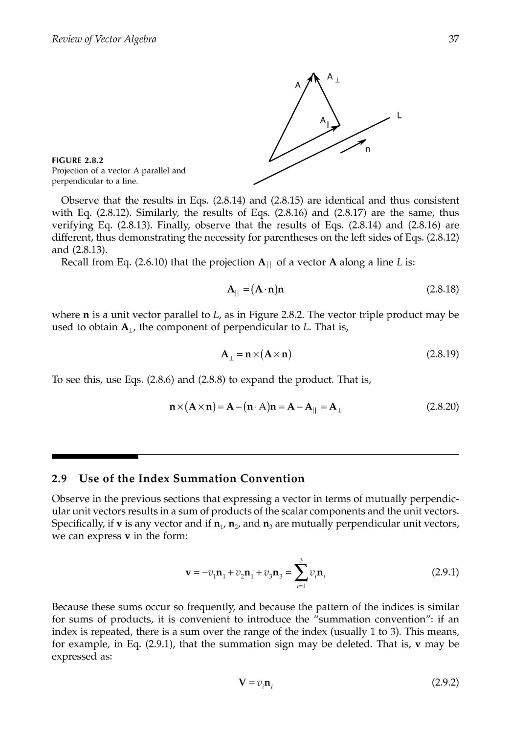
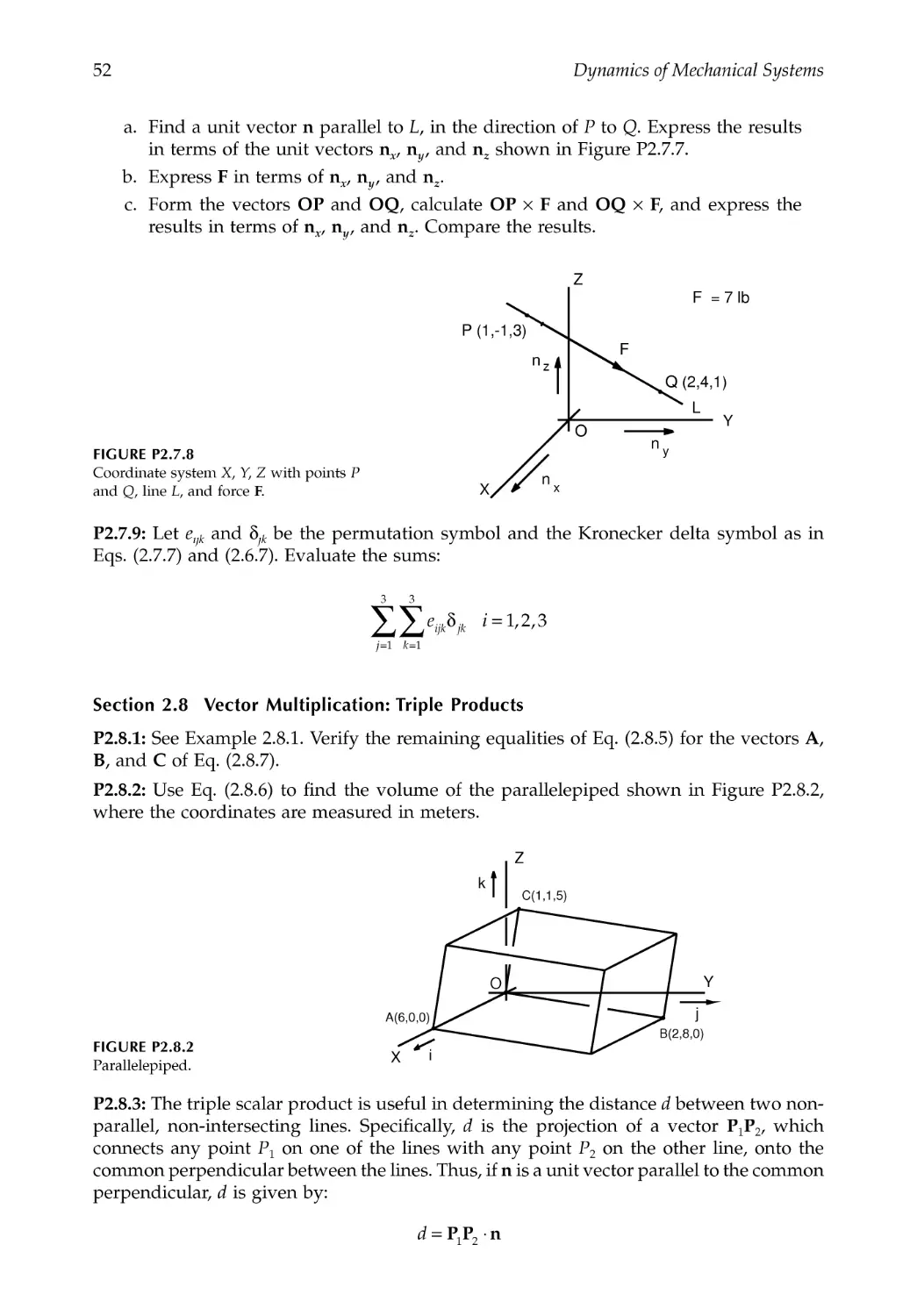
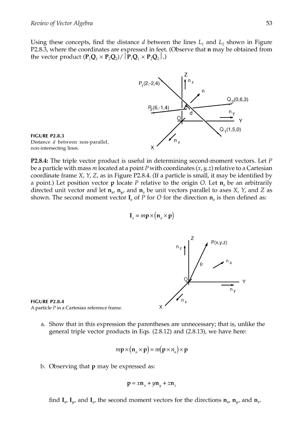
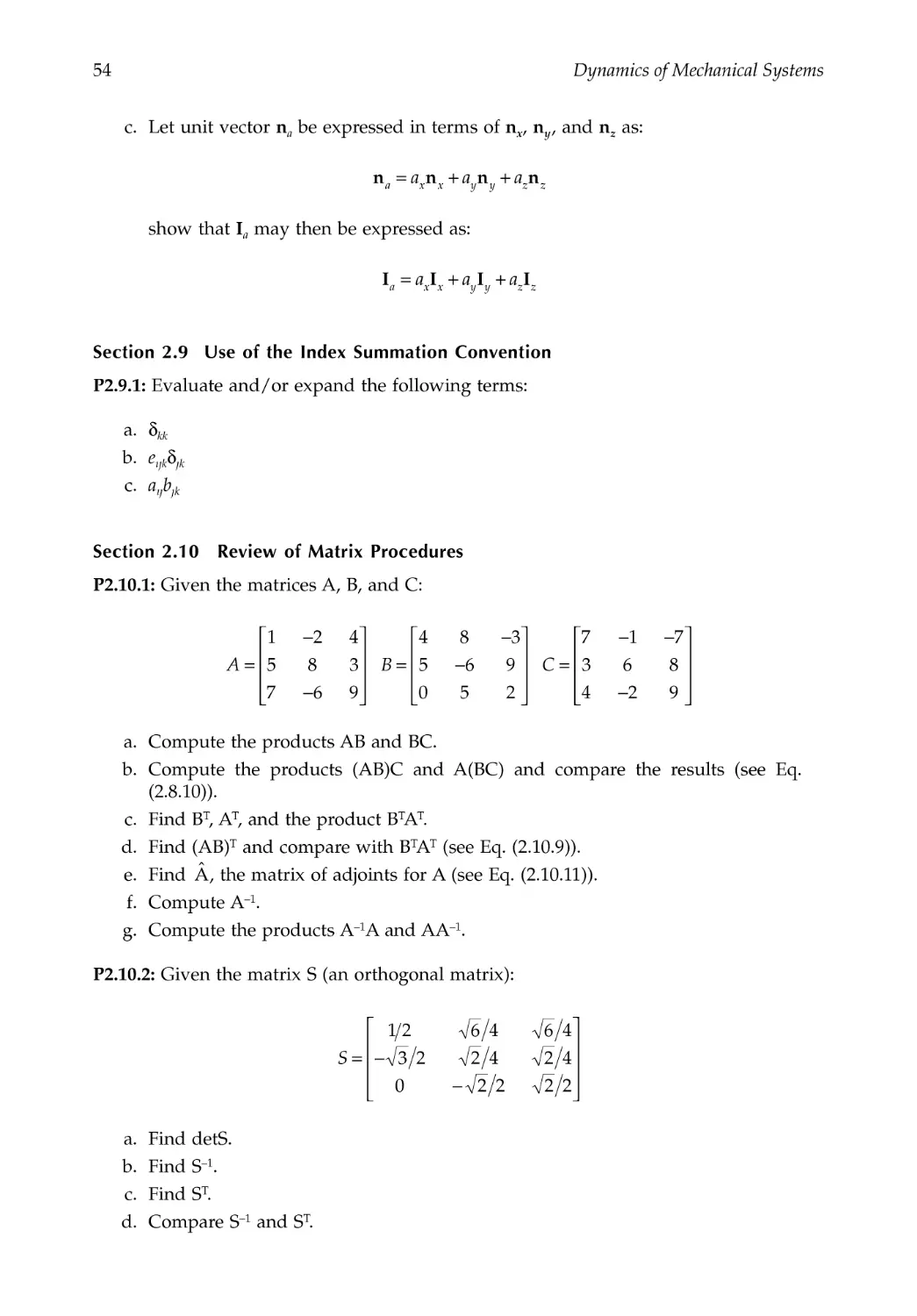
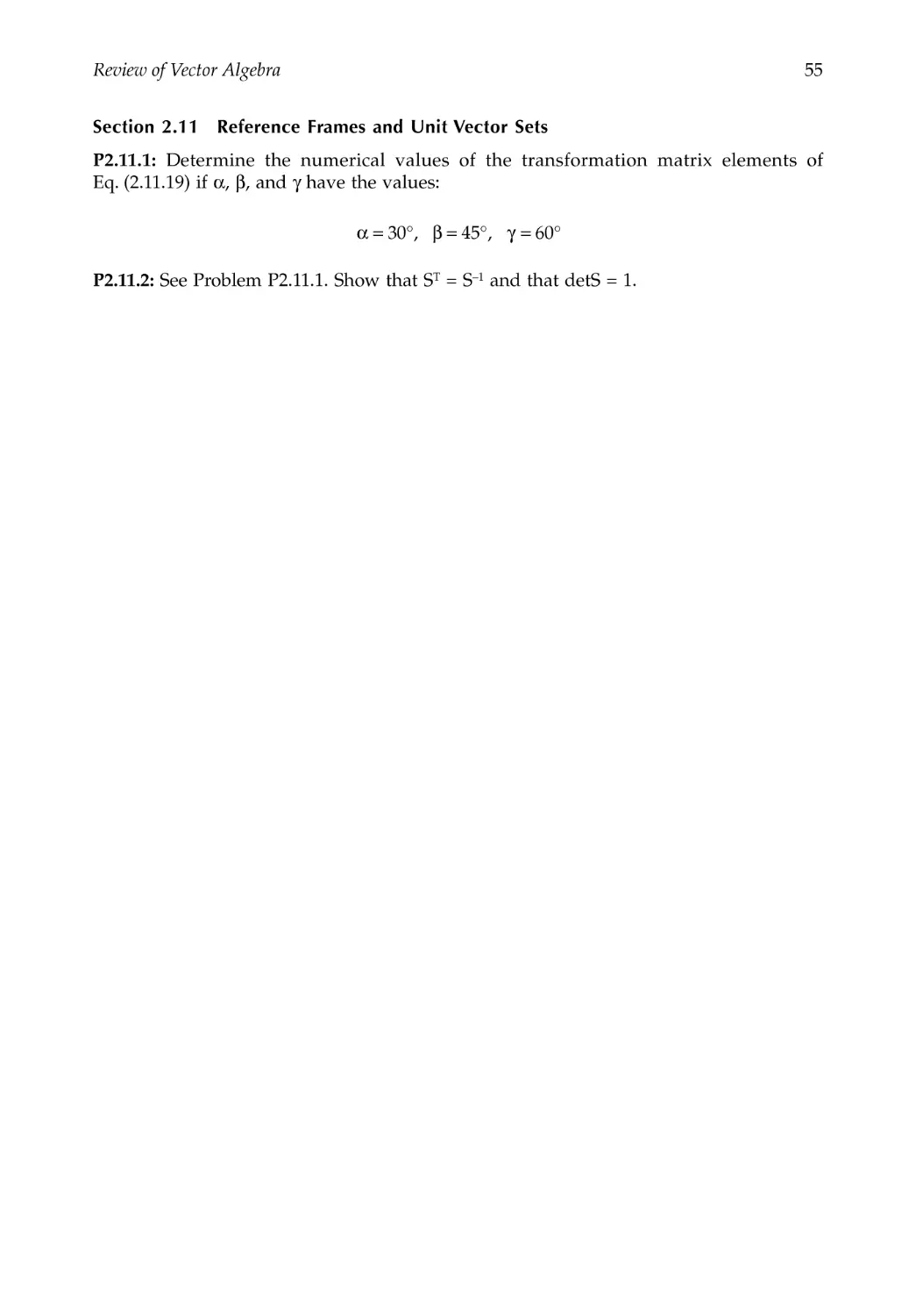
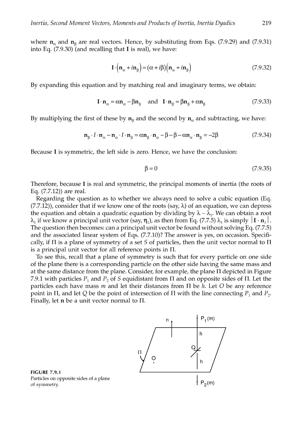
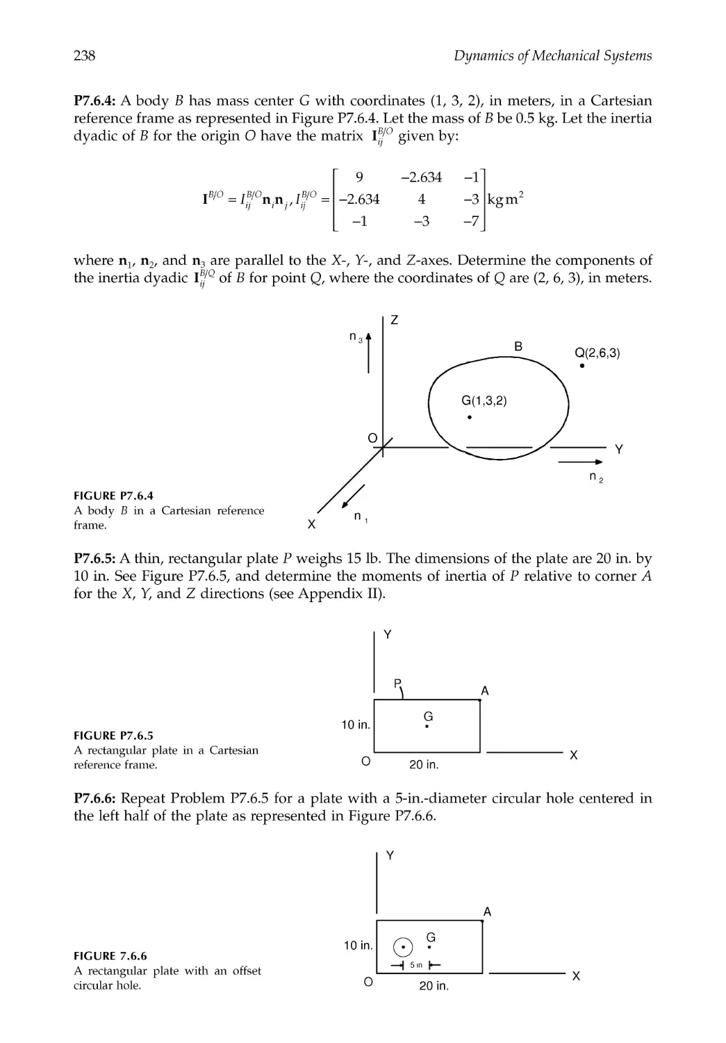
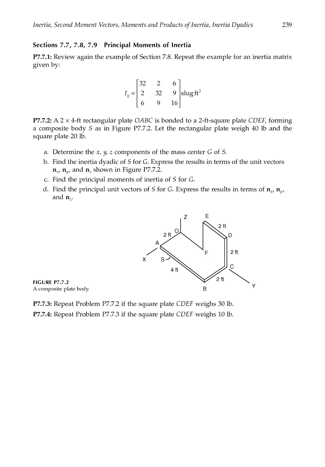
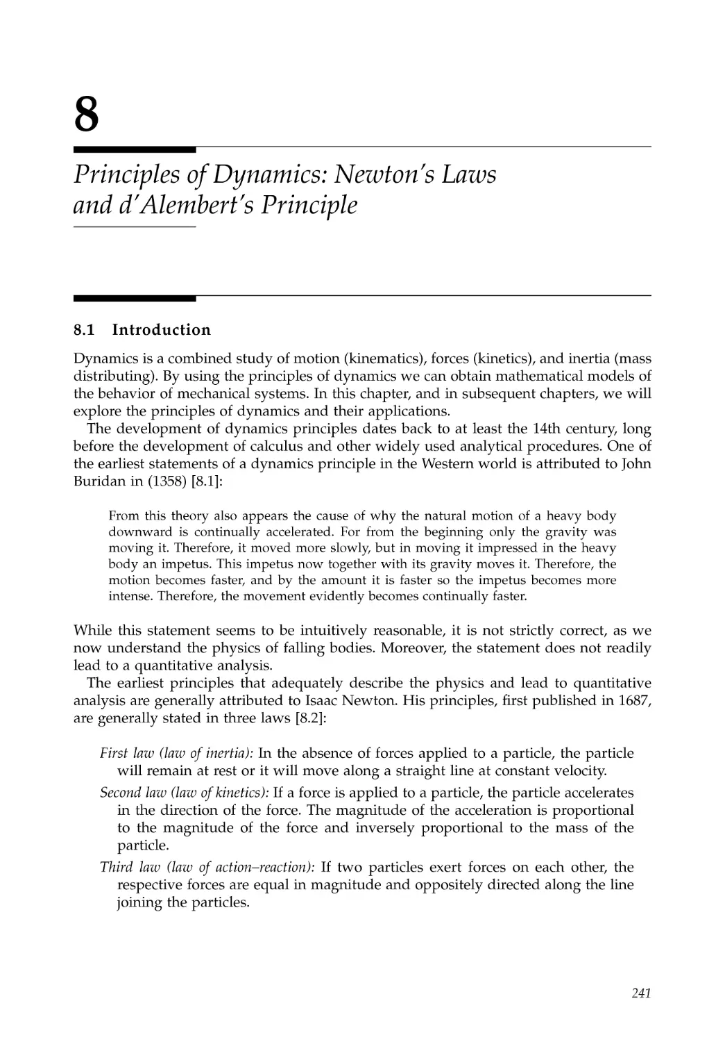
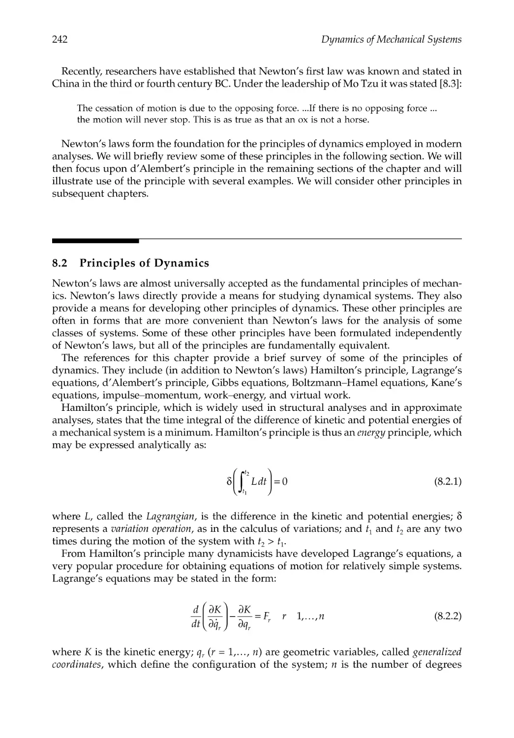
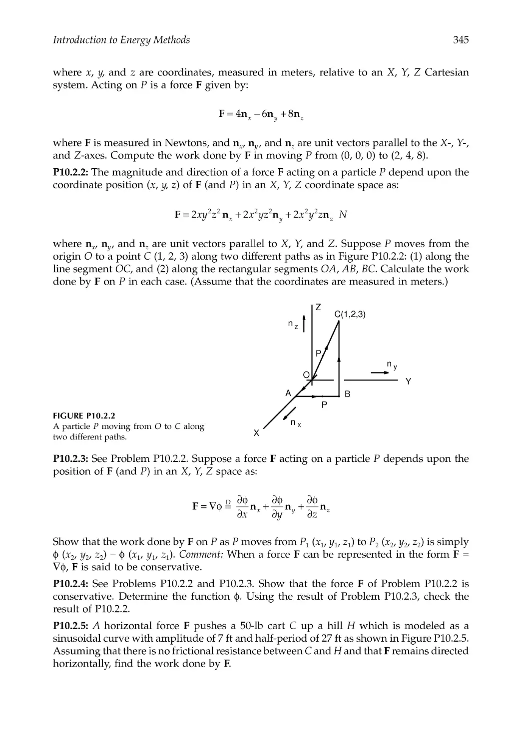
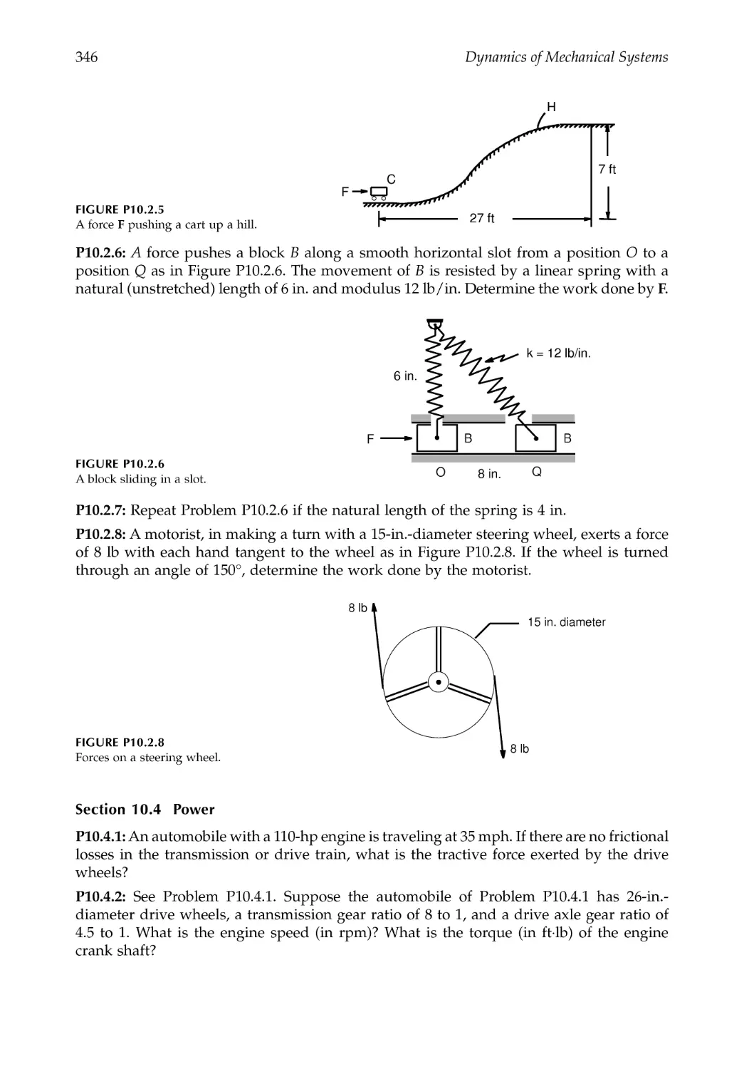
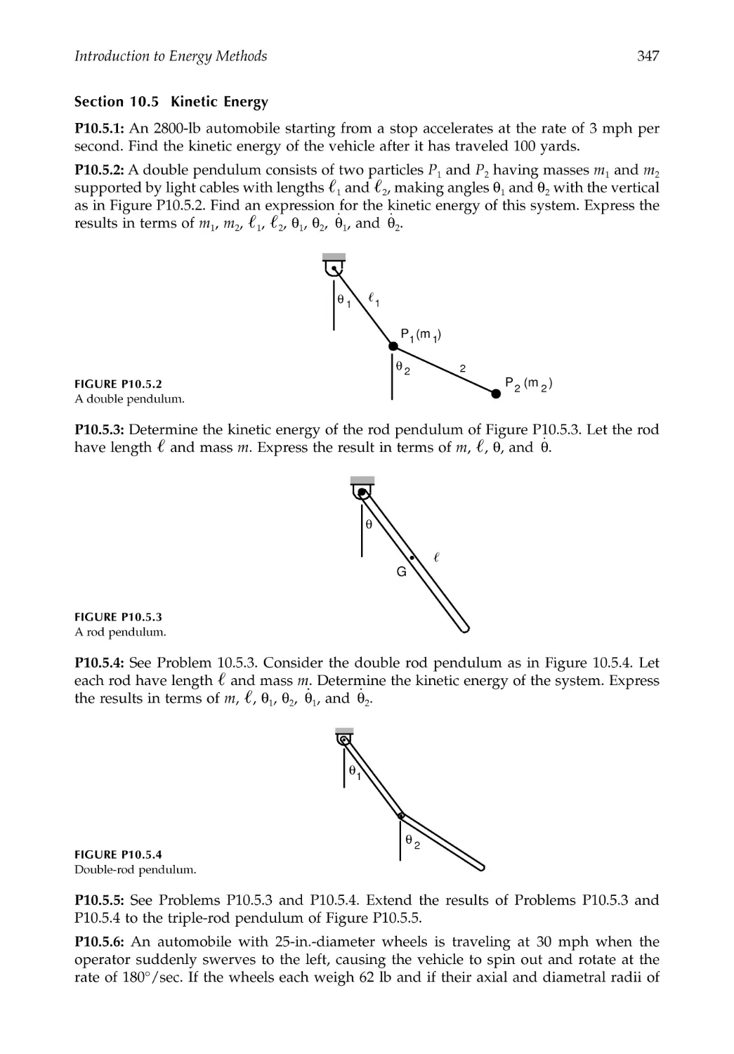
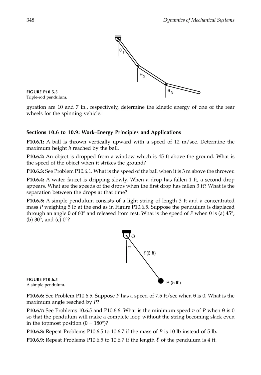
/


Text
DYNAMICS of
MECHANICAL SYSTEMS
CRC PRESS
Boca Raton London New York Washington, D.C.
Harold Josephs
Ronald L. Huston
DYNAMICS of
MECHANICAL SYSTEMS
This book contains information obtained from authentic and highly regarded sources. Reprinted material is quoted with
permission, and sources are indicated. A wide variety of references are listed. Reasonable efforts have been made to publish
reliable data and information, but the authors and the publisher cannot assume responsibility for the validity of all materials
or for the consequences of their use.
Neither this book nor any part may be reproduced or transmitted in any form or by any means, electronic or mechanical,
including photocopying, microfilming, and recording, or by any information storage or retrieval system, without prior
permission in writing from the publisher.
The consent of CRC Press LLC does not extend to copying for general distribution, for promotion, for creating new works,
or for resale. Specific permission must be obtained in writing from CRC Press LLC for such copying.
Direct all inquiries to CRC Press LLC, 2000 N.W. Corporate Blvd., Boca Raton, Florida 33431.
Trademark Notice: Product or corporate names may be trademarks or registered trademarks, and are used only for
identification and explanation, without intent to infringe.
Visit the CRC Press Web site at www.crcpress.com
© 2002 by CRC Press LLC
No claim to original U.S. Government works
International Standard Book Number 0-8493-0593-4
Library of Congress Card Number 2002276809
PrintedintheUnitedStatesofAmerica 1 2 3 4 5 6 7 8 9 0
Printed on acid-free paper
Library of Congress Cataloging-in-Publication Data
Josephs, Harold.
Dynamics of mechanical systems / by Harold Josephs and Ronald L. Huston.
p. ;cm.
Includes bibliographical references and index.
ISBN 0-8493-0593-4 (alk. paper)
1. Mechanical engineering. I. Huston, Ronald L., 1937- II. Title.
TJ145 .J67 2002.
621---dc21
2002276809
CIP
Preface
This is a textbook intended for mid- to upper-level undergraduate students in engineering
and physics. The objective of the book is to give readers a working knowledge of dynamics,
enabling them to analyze mechanical systems ranging from elementary and fundamental
systems such as planar mechanisms to more advanced systems such as robots, space
mechanisms, and human body models. The emphasis of the book is upon the fundamental
procedures underlying these dynamic analyses. Readers are expected to obtain skills
ranging from the ability to perform insightful hand analyses to the ability to develop
algorithms for numerical/computer analyses. In this latter regard, the book is also
intended to serve as an independent study text and as a reference book for beginning
graduate students and for practicing engineers.
Mechanical systems are becoming increasingly sophisticated, with applications requir-
ing greater precision, improved reliability, and extended life. These enhanced requirements
are spurred by a demand for advanced land, air, and space vehicles; by a corresponding
demand for advanced mechanisms, manipulators, and robotics systems; and by a need
to have a better understanding of the dynamics of biosystems. The book is intended to
enable its readers to make engineering advances in each of these areas. The authors believe
that the skills needed to make such advances are best obtained by illustratively studying
fundamental mechanical components such as pendulums, gears, cams, and mechanisms
while reviewing the principles of vibrations, stability, and balancing. The study of these
subjects is facilitated by a knowledge of kinematics and skill in the use of Newton's laws,
energy methods, Lagrange's equations, and Kane's equations. The book is intended to
provide a means for mastering all of these concepts.
The book is written to be readily accessible to students and readers having a background
in elementary physics, mathematics through calculus and differential equations, and ele-
mentary mechanics. The book itself is divided into 20 chapters, with the first two chapters
providing introductory remarks and a review of vector algebra. The next three chapters
are devoted to kinematics, with the last of these focusing upon planar kinematics. Chapter
6 discusses forces and force systems, and Chapter 7 provides a comprehensive review of
inertia including inertia dyadics and procedures for obtaining the principal moments of
inertia and the corresponding principal axes of inertia.
Fundamental principles of dynamics (Newton's laws and d'Alembert's principle) are
presented in Chapter 8, and the use of impulse--momentum and work--energy principles
is presented in the next two chapters with application to accident reconstruction. Chapters
11 and 12 introduce generalized dynamics and the use of Lagrange's equation and Kane's
equations with application to multiple rod pendulum problems. The next five chapters
are devoted to applications that involve the study of vibration, stability, balancing, cams,
and gears, including procedures for studying nonlinear vibrations and engine balancing.
The last three chapters present an introduction to multibody dynamics with application
to robotics and biosystems.
Application and illustrative examples are discussed and presented in each chapter, and
exercises and problems are provided at the end of each chapter. In addition, each chapter
has its own list of references for additional study. Although the earlier chapters provide
the basis for the latter chapters, each chapter is written to be as self-contained as possible,
with excerpts from earlier chapters provided as needed.
Acknowledgments
The book is an outgrowth of notes the authors have compiled over the past three decades
in teaching various courses using the subject material. These notes, in turn, are based
upon information contained in various texts used in these courses and upon the authors'
independent study and research.
The authors acknowledge the inspiration for a clearly defined procedural study of
dynamics by Professor T. R. Kane at the University of Pennsylvania, now nearly 50 years
ago. The authors particularly acknowledge the administrative support and assistance of
Charlotte Better in typing and preparing the entire text through several revisions. The
work of Xiaobo Liu and Doug Provine for preparation of many of the figures is also
acknowledged.
The Authors
Harold Josephs, Ph.D., P.E., has been a professor in the Department of Mechanical Engi-
neering at Lawrence Technological University in Southfield, MI, since 1984, subsequent
to working in industry for General Electric and Ford Motor Company. Dr. Josephs is the
author of numerous publications, holds nine patents, and has presented numerous sem-
inars to industry in the field of safety, bolting, and joining. Dr. Josephs maintains an active
consultant practice in safety, ergonomics, and accident reconstruction. His research inter-
ests are in fastening and joining, human factors, ergonomics, and safety. Dr. Josephs
received his B.S. degree from the University of Pennsylvania, his M.S. degree from Vill-
anova University, and his Ph.D. from the Union Institute. He is a licensed Professional
Engineer, Certified Safety Professional, Certified Professional Ergonomist, Certified Qual-
ity Engineer, Fellow of the Michigan Society of Engineers, and a Fellow of the National
Academy of Forensic Engineers.
Ronald L. Huston, Ph.D., P.E., is distinguished research professor and professor of
mechanics in the Department of Mechanical, Industrial, and Nuclear Engineering at the
University of Cincinnati. He is also a Herman Schneider chair professor. Dr. Huston has
been at the University of Cincinnati since 1962. In 1978, he served as a visiting professor
at Stanford University, and from 1979 to 1980 he was division director of civil and mechan-
ical engineering at the National Science Foundation. From 1990 to 1996, Dr. Huston was
a director of the Monarch Research Foundation. He is the author of over 140 journal
articles, 142 conference papers, 4 books, and 65 book reviews and is a technical editor of
Applied Mechanics Reviews, and book review editor of the International Journal of Industrial
Engineering. Dr. Huston is an active consultant in safety, biomechanics, and accident
reconstruction. His research interests are in multibody dynamics, human factors, biome-
chanics, and ergonomics and safety. Dr. Huston received his B.S. degree (1959), M.S. degree
(1961), and Ph.D. (1962) from the University of Pennsylvania, Philadelphia. He is a
Licensed Professional Engineer and a Fellow of the American Society of Mechanical
Engineers.
Contents
Chapter 1 Introduction................................................................................................................1
1.1 Approach to the Subject......................................................................................................1
1.2 Subject Matter .......................................................................................................................1
1.3 Fundamental Concepts and Assumptions .......................................................................2
1.4 Basic Terminology in Mechanical Systems ......................................................................3
1.5 Vector Review .......................................................................................................................5
1.6 Reference Frames and Coordinate Systems.....................................................................6
1.7 Systems of Units ...................................................................................................................9
1.8 Closure .................................................................................................................................11
References .......................................................................................................................................11
Problems .........................................................................................................................................12
Chapter 2 Review of Vector Algebra ......................................................................................15
2.1 Introduction.........................................................................................................................15
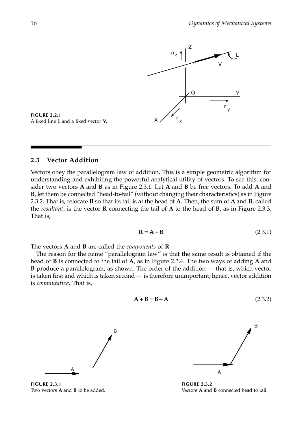
2.2 Equality of Vectors, Fixed and Free Vectors ..................................................................15
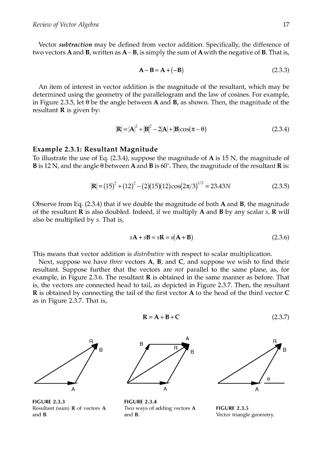
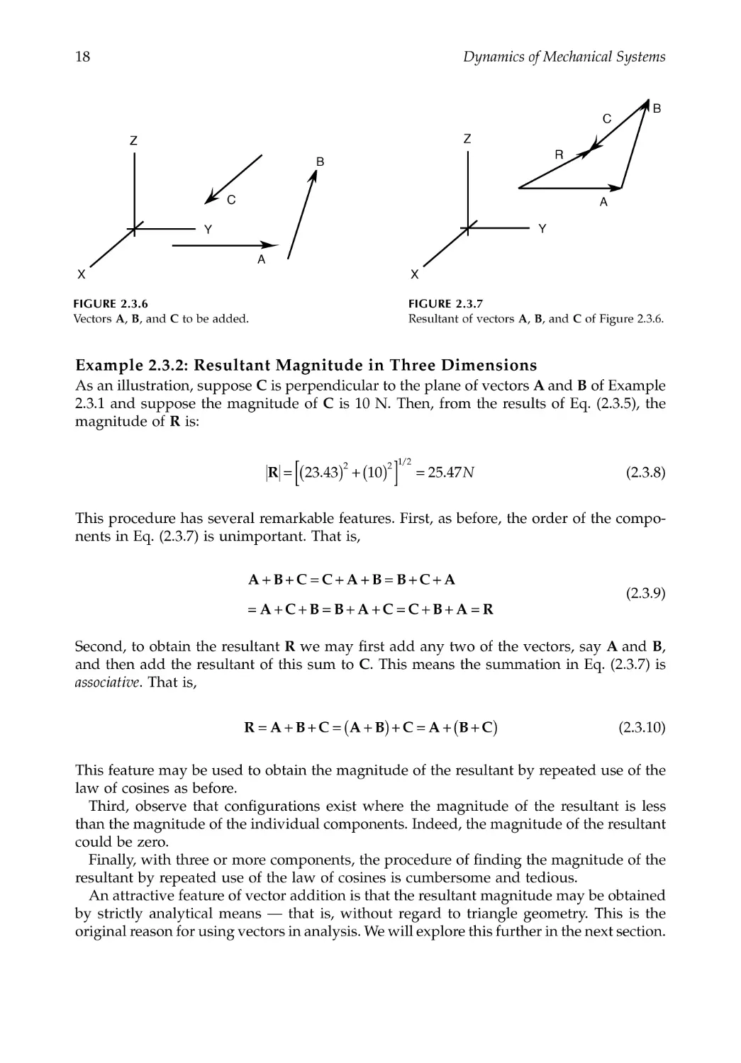
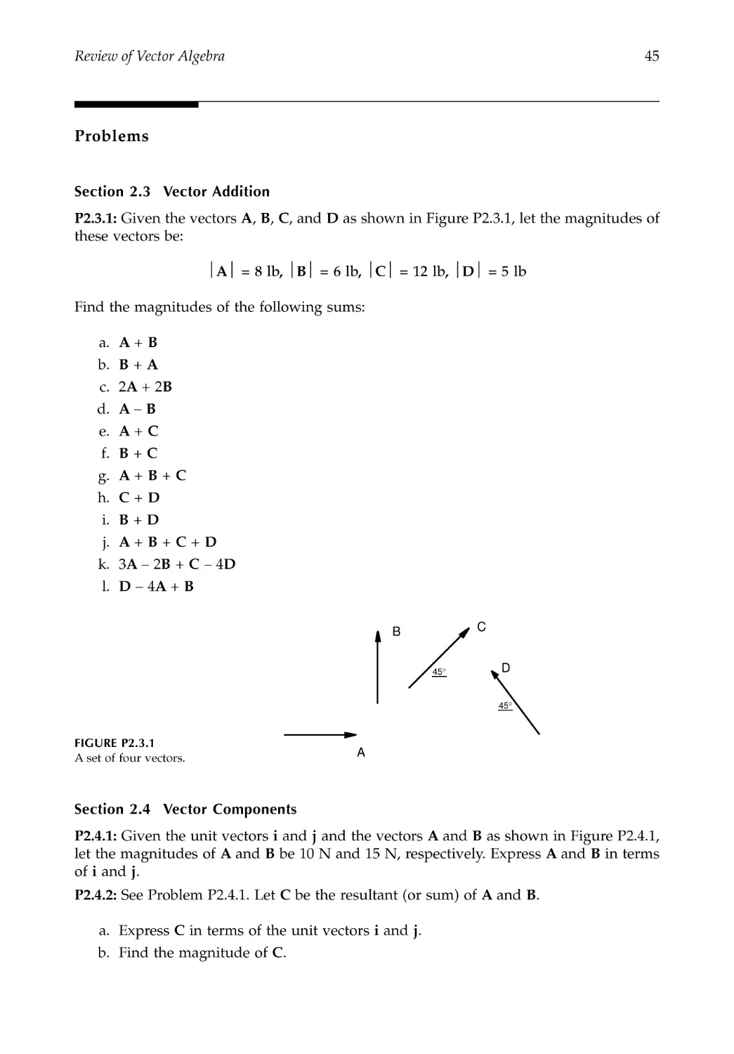
2.3 Vector Addition ..................................................................................................................16
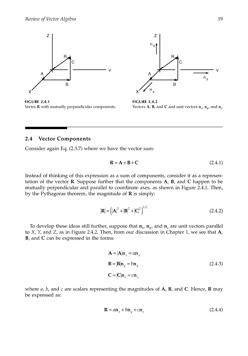
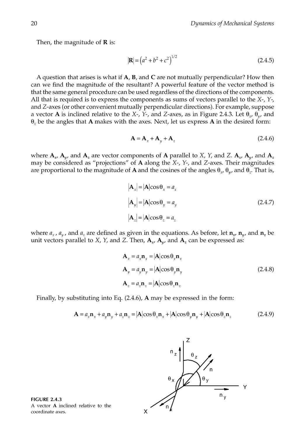
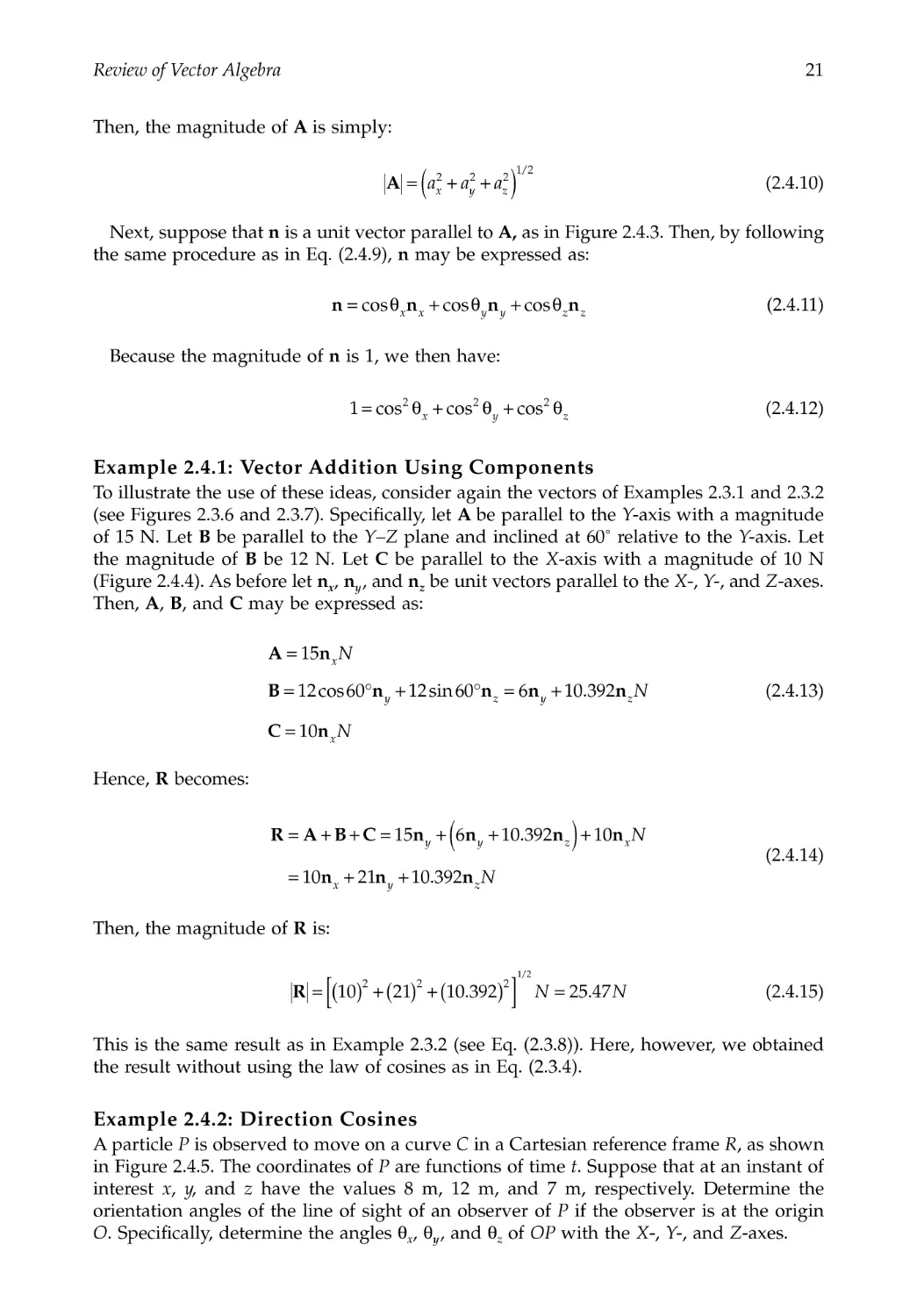
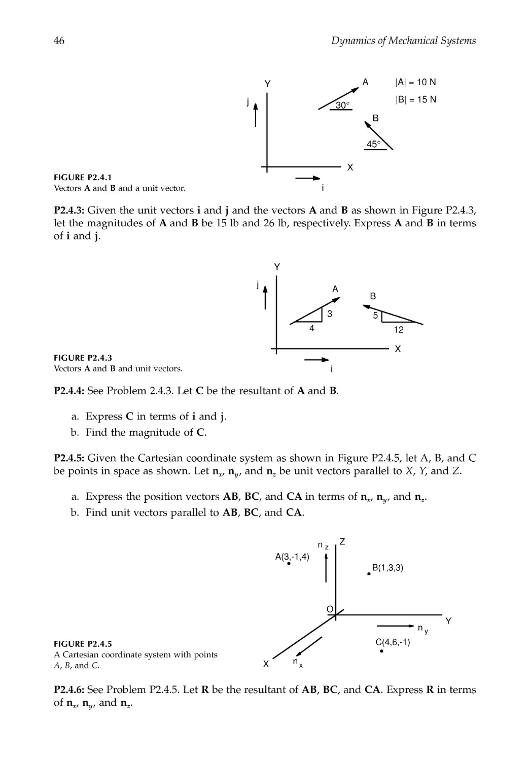
2.4 Vector Components............................................................................................................19
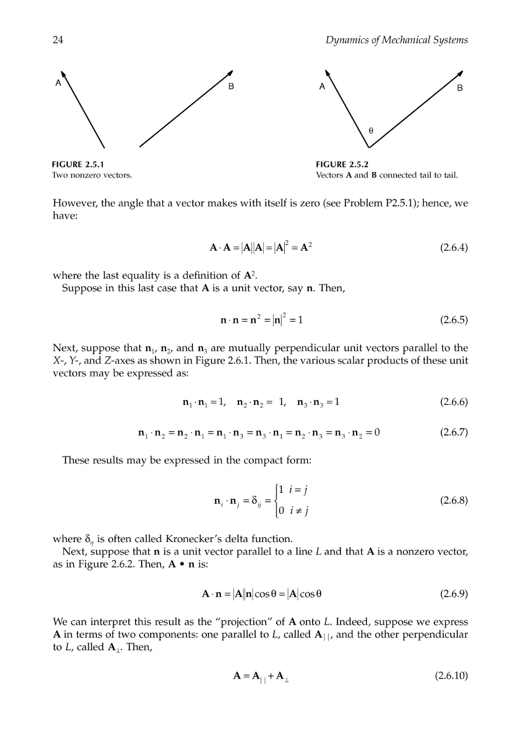
2.5 Angle Between Two Vectors.............................................................................................23
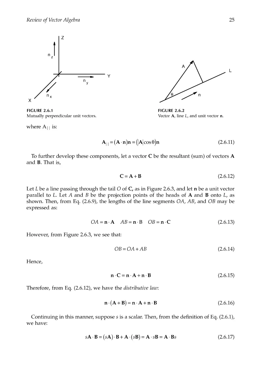
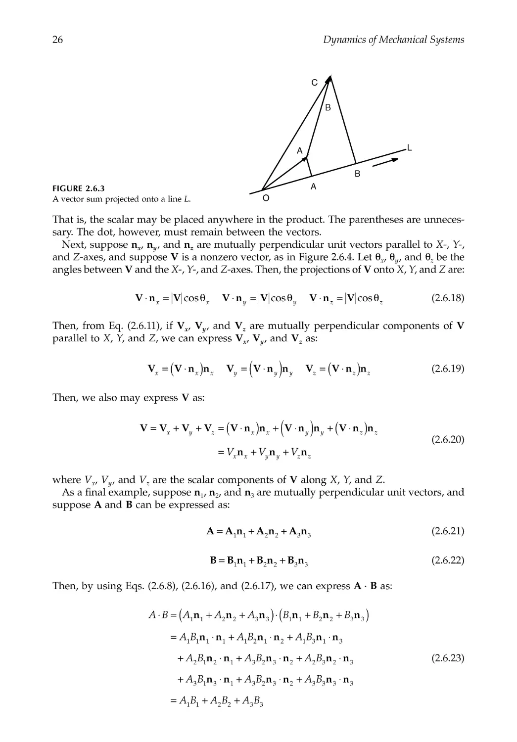
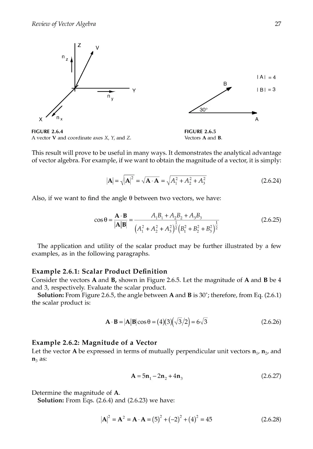
2.6 Vector Multiplication: Scalar Product .............................................................................23
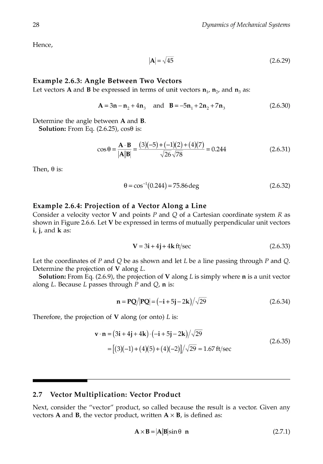
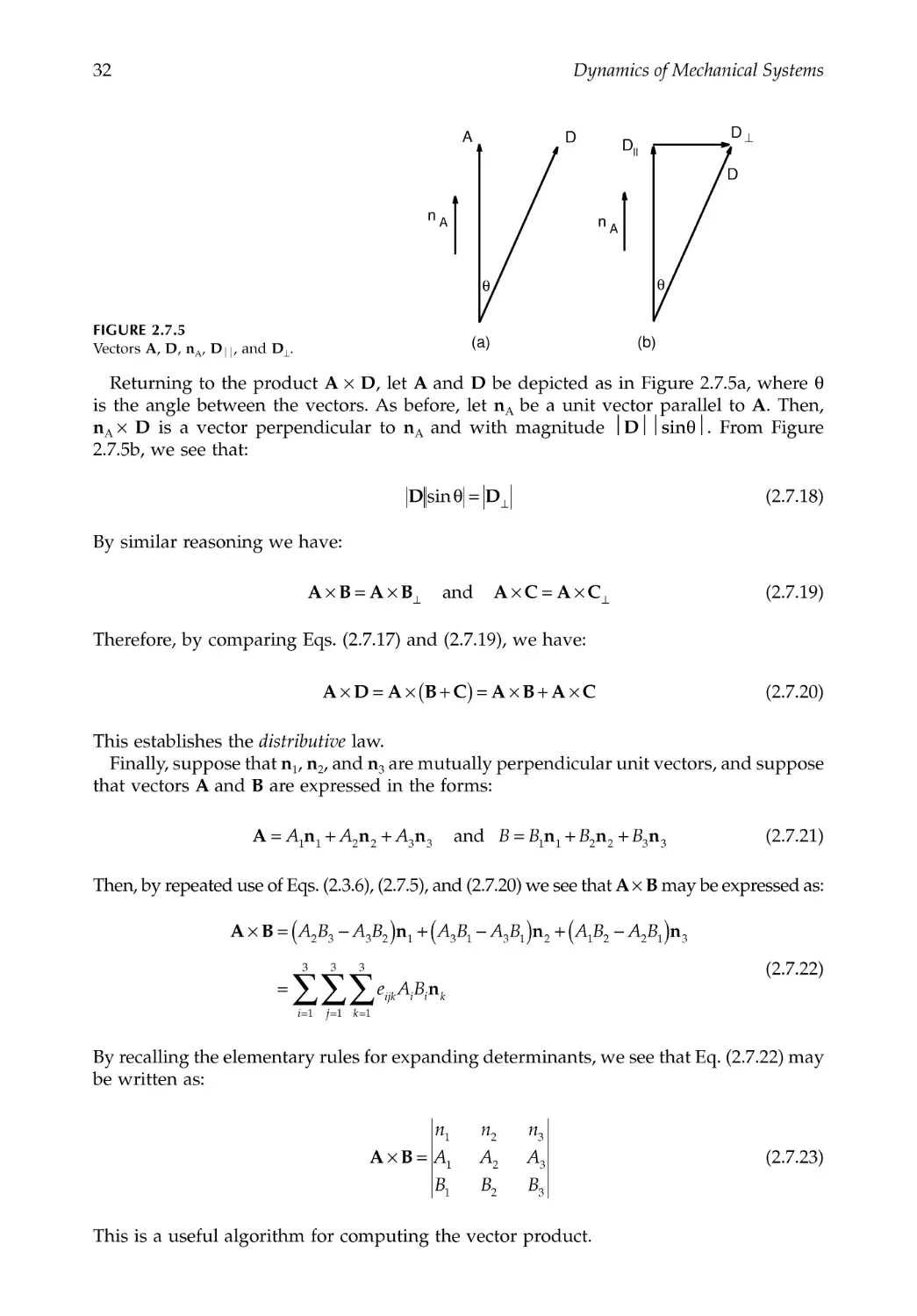
2.7 Vector Multiplication: Vector Product ............................................................................28
2.8 Vector Multiplication: Triple Products............................................................................33
2.9 Use of the Index Summation Convention .....................................................................37
2.10 Review of Matrix Procedures...........................................................................................38
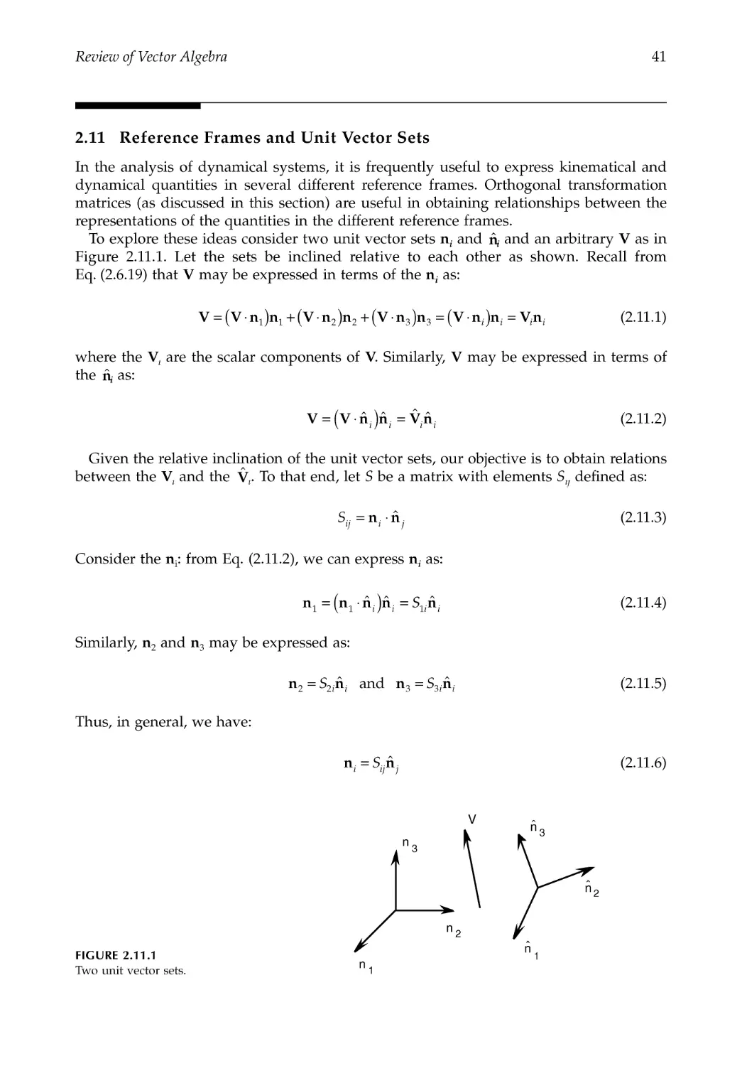
2.11 Reference Frames and Unit Vector Sets..........................................................................41
2.12 Closure .................................................................................................................................44
References .......................................................................................................................................44
Problems .........................................................................................................................................45
Chapter 3 Kinematics of a Particle..........................................................................................57
3.1 Introduction.........................................................................................................................57
3.2 Vector Differentiation ........................................................................................................57
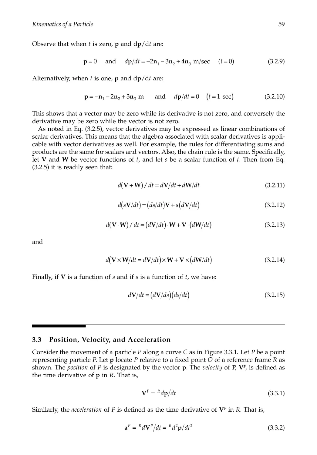
3.3 Position, Velocity, and Acceleration ................................................................................59
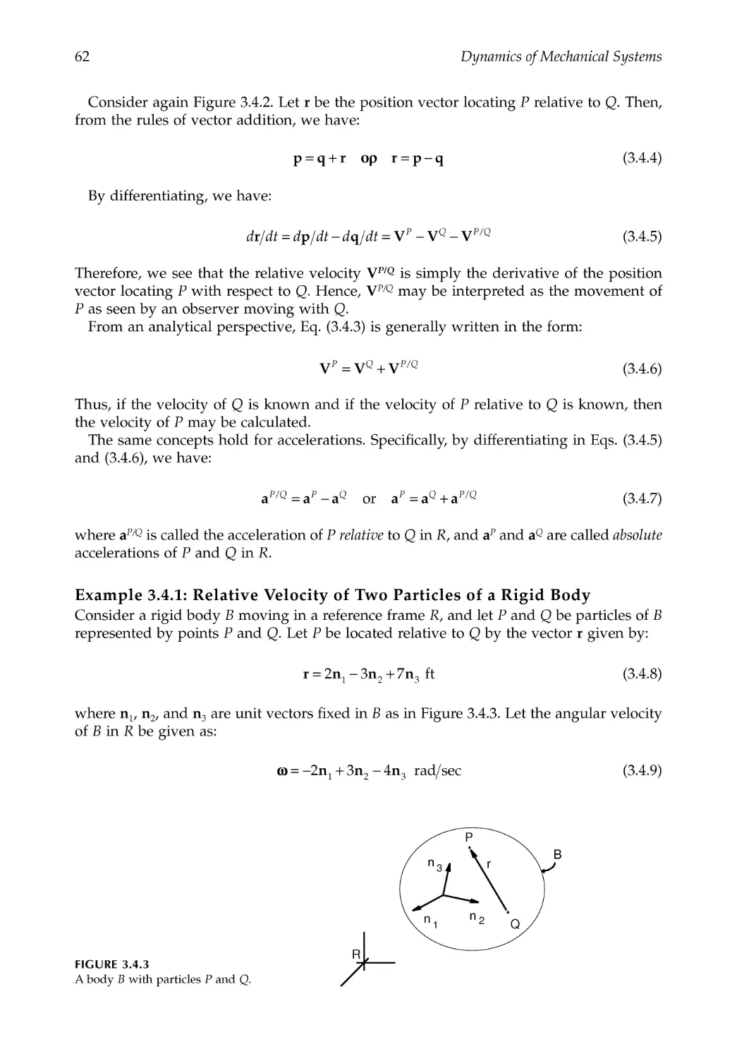
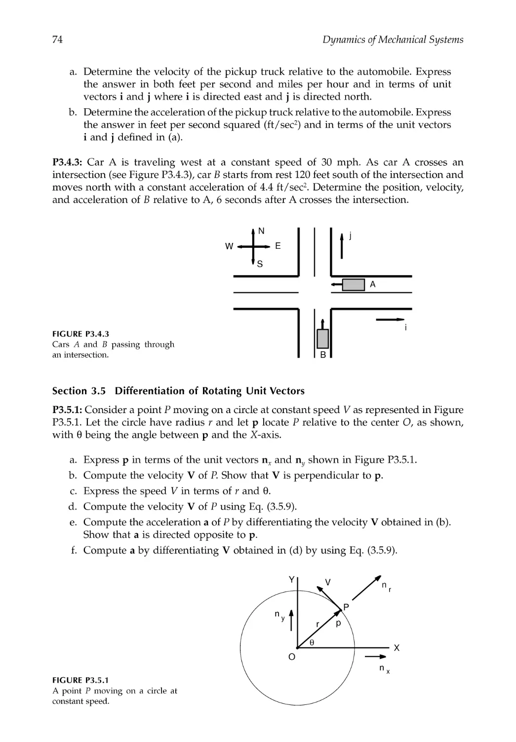
3.4 Relative Velocity and Relative Acceleration ..................................................................61
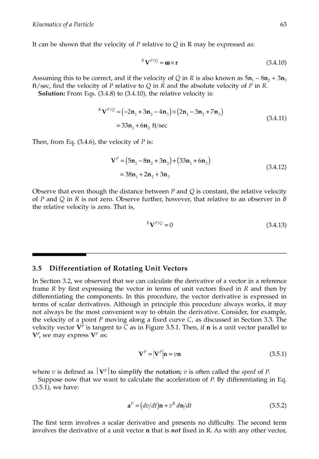
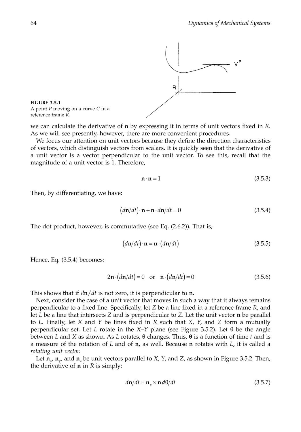
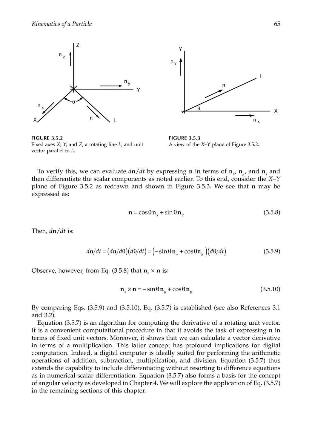
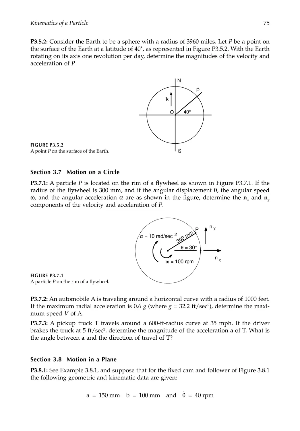
3.5 Differentiation of Rotating Unit Vectors ........................................................................63
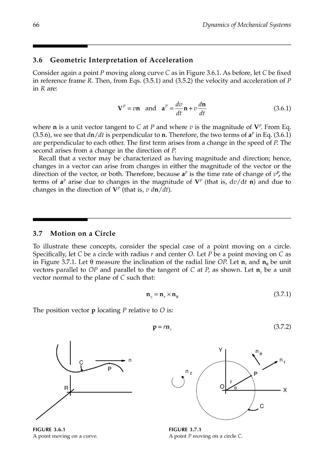
3.6 Geometric Interpretation of Acceleration.......................................................................66
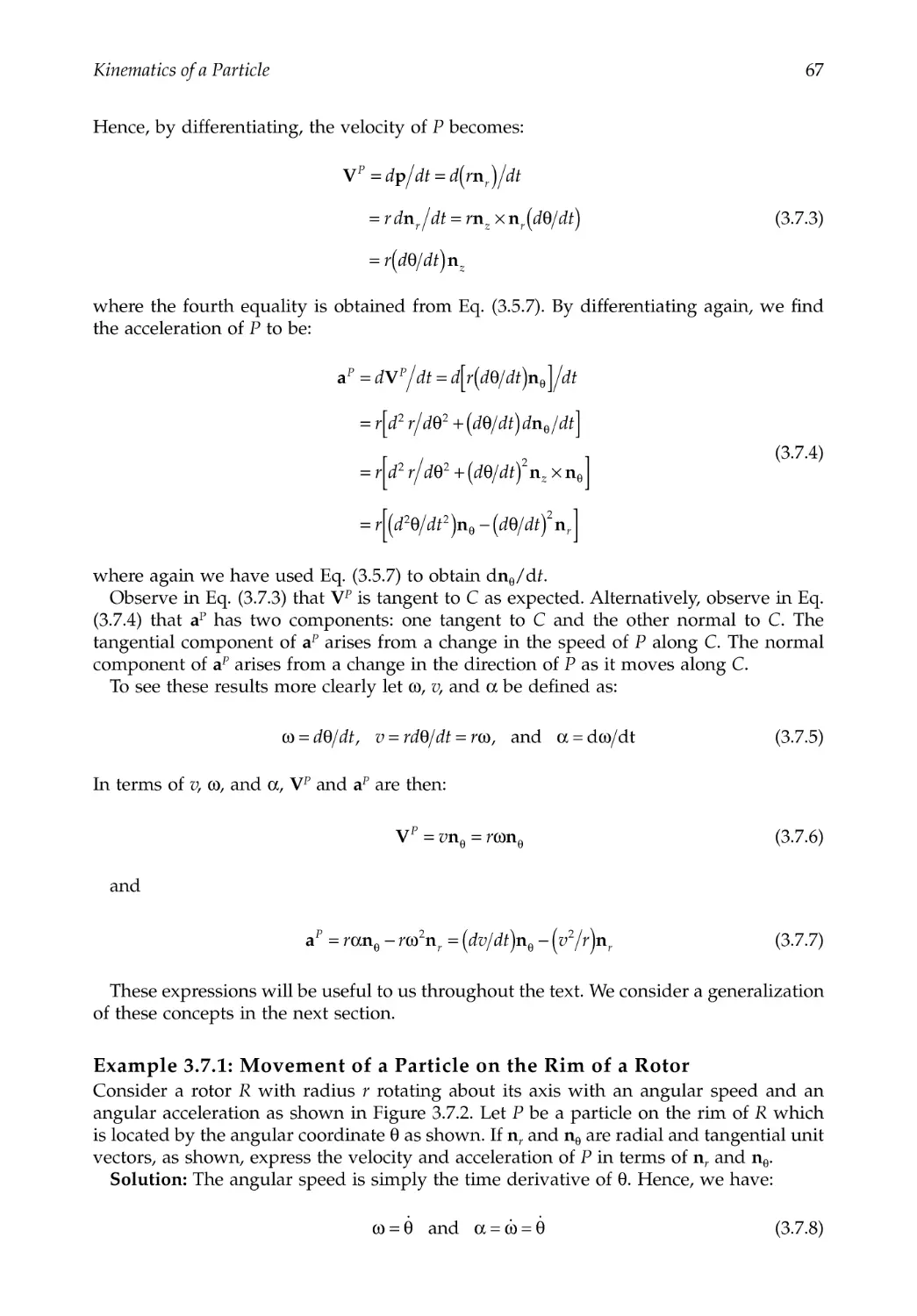
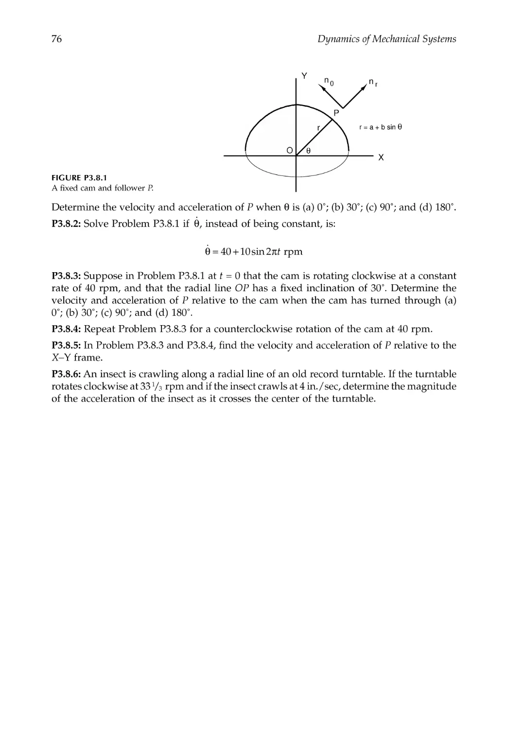
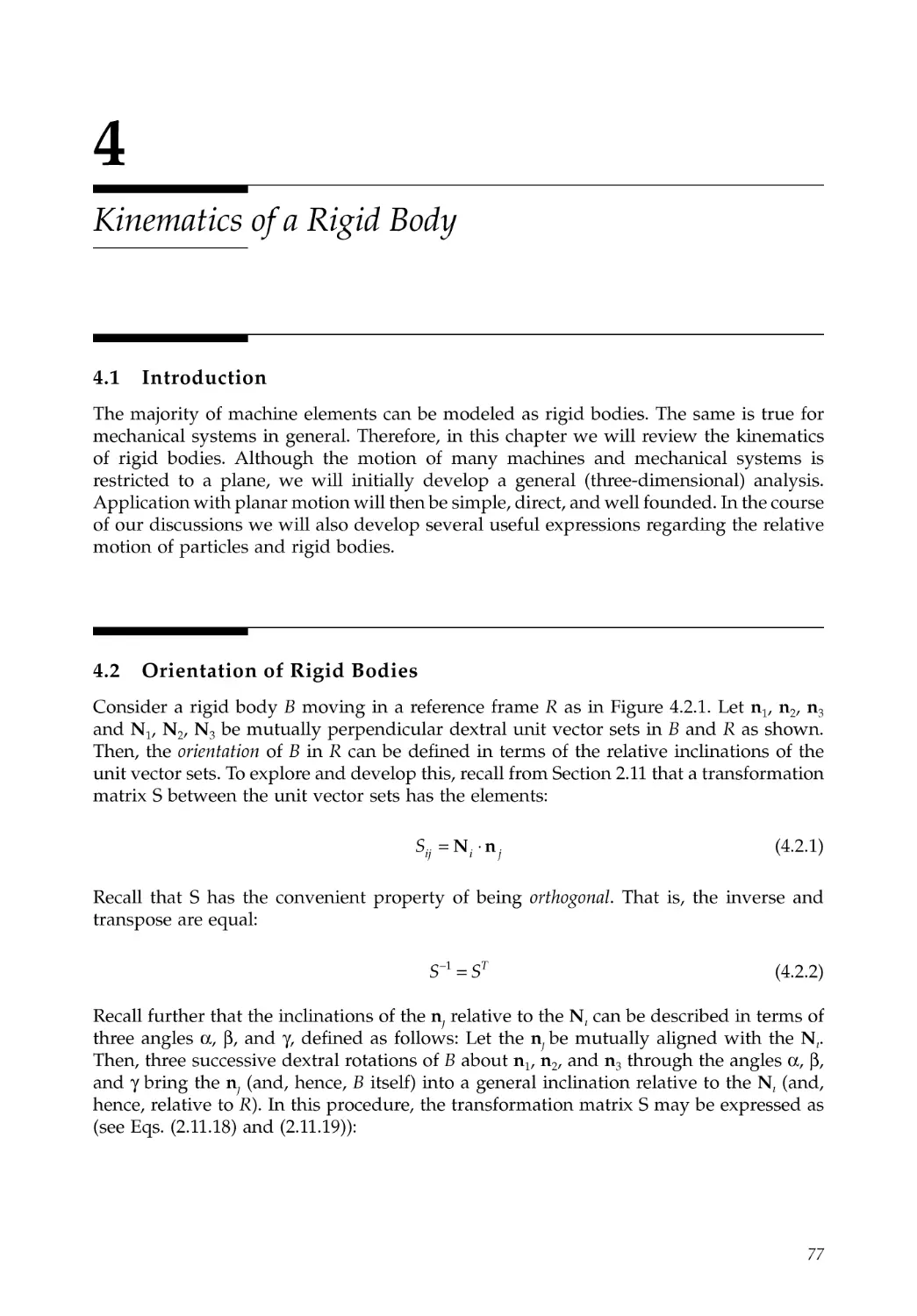
3.7 Motion on a Circle .............................................................................................................66
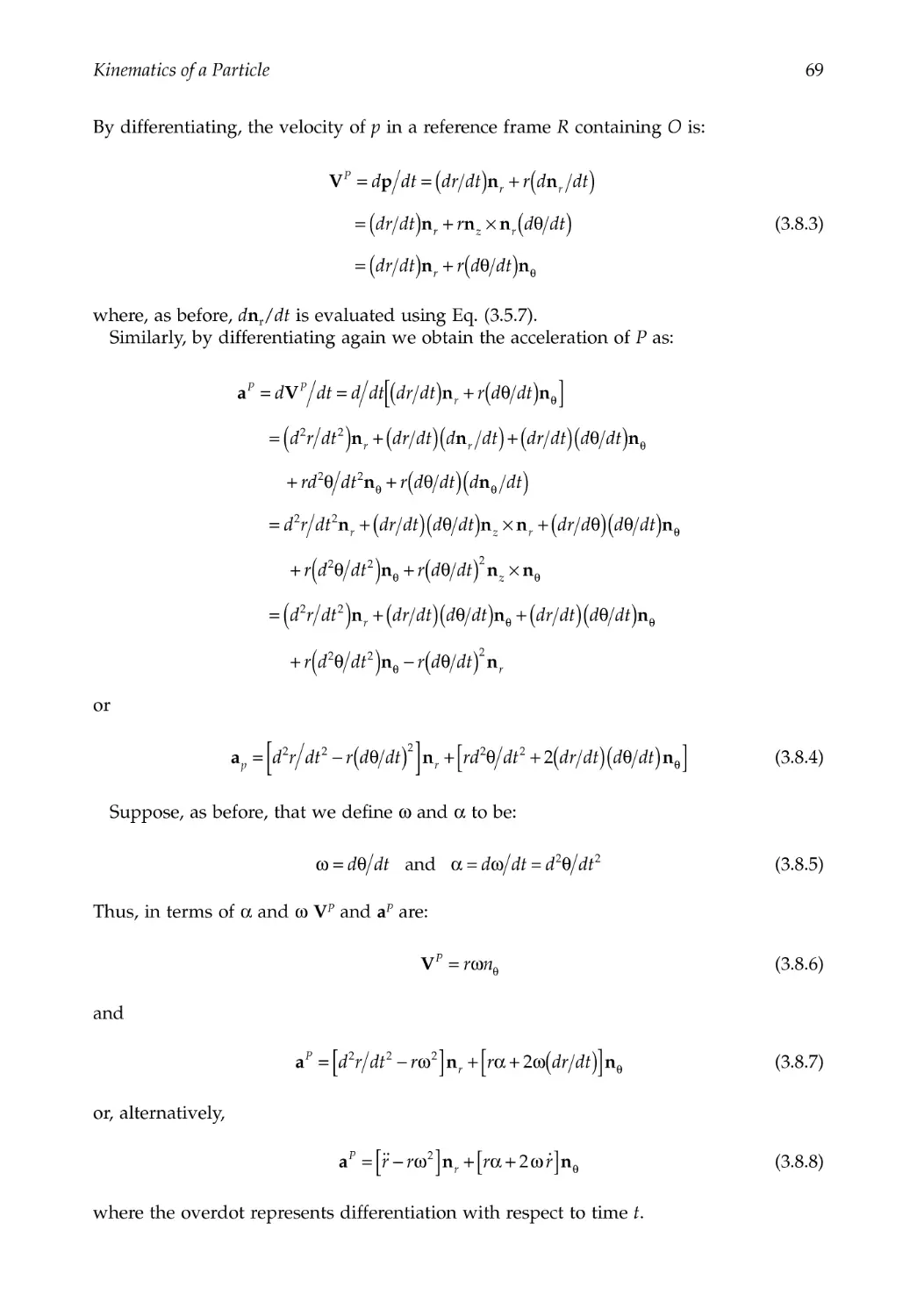
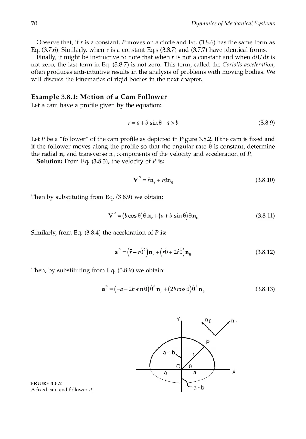
3.8 Motion in a Plane ...............................................................................................................68
3.9 Closure .................................................................................................................................71
References .......................................................................................................................................71
Problems .........................................................................................................................................71
Chapter 4 Kinematics of a Rigid Body...................................................................................77
4.1 Introduction.........................................................................................................................77
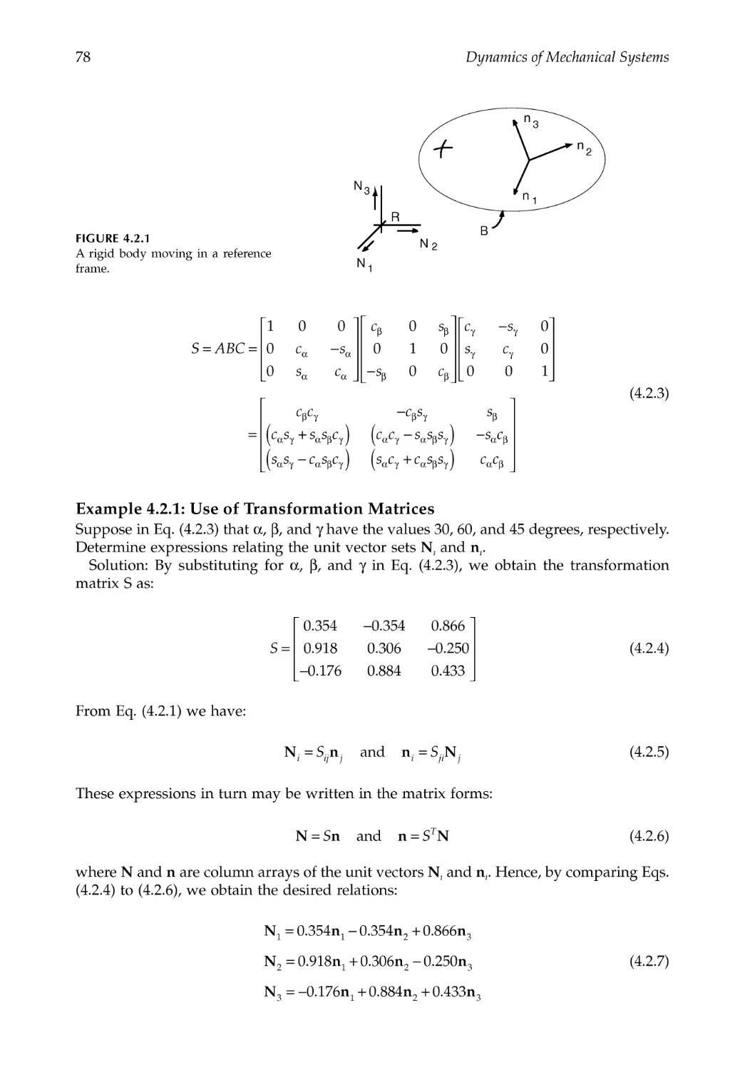
4.2 Orientation of Rigid Bodies..............................................................................................77
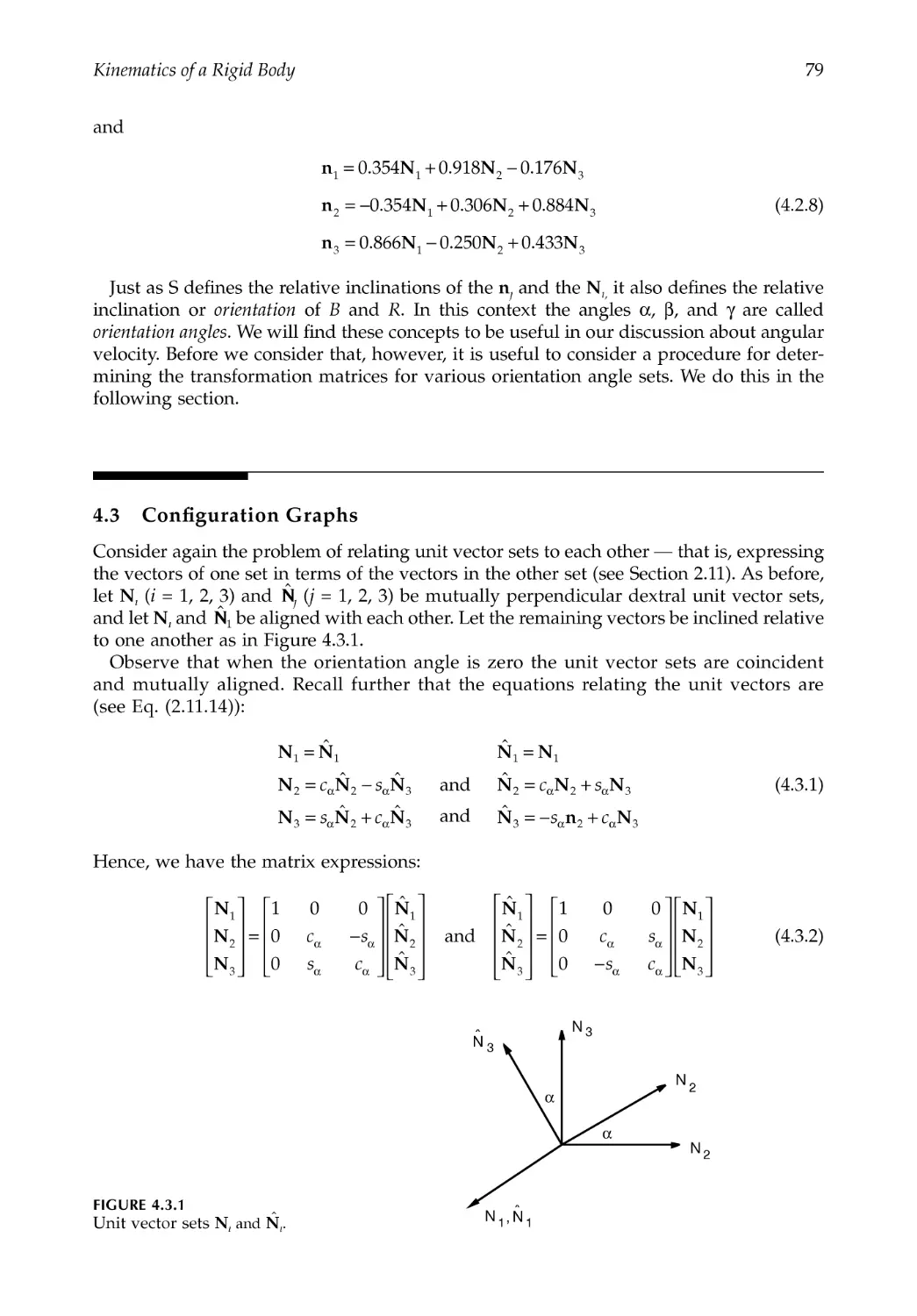
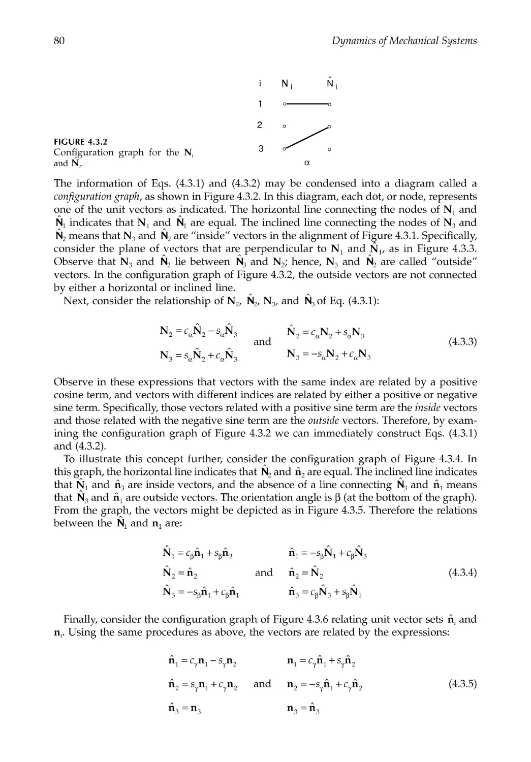
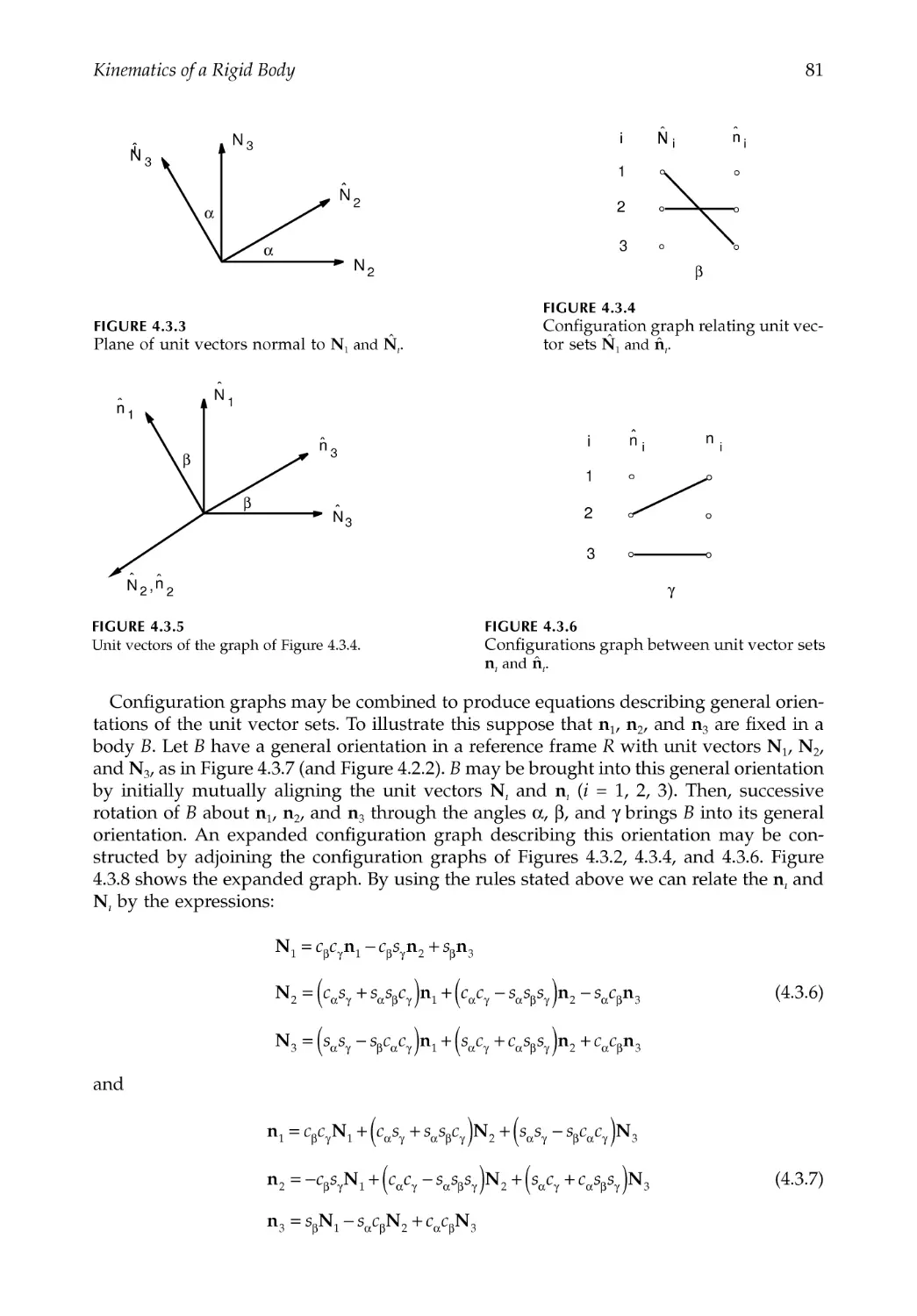
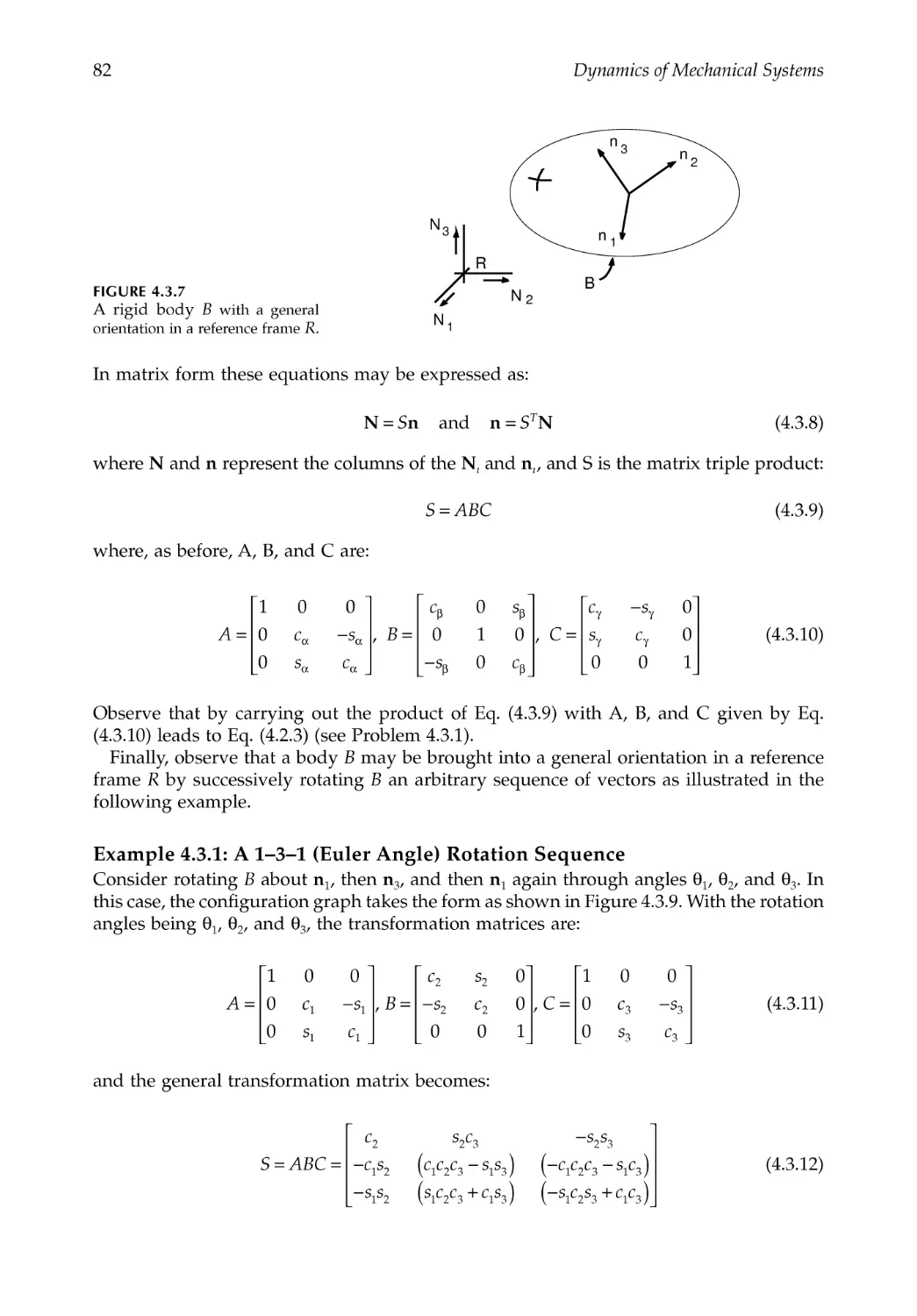
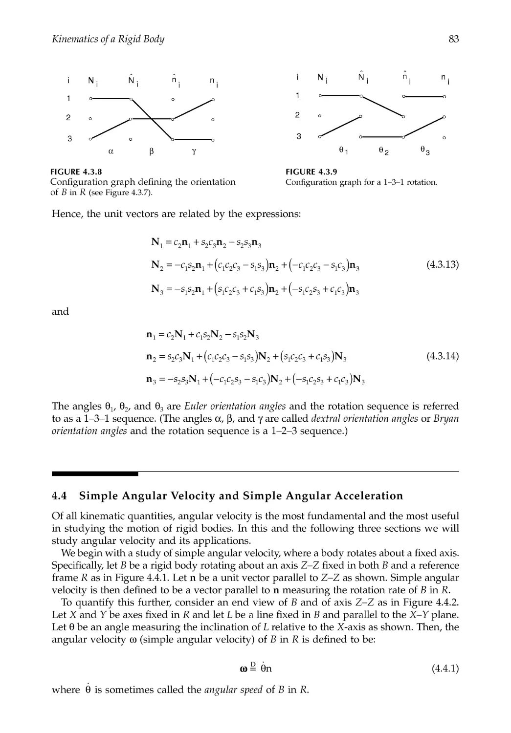
4.3 Configuration Graphs........................................................................................................79
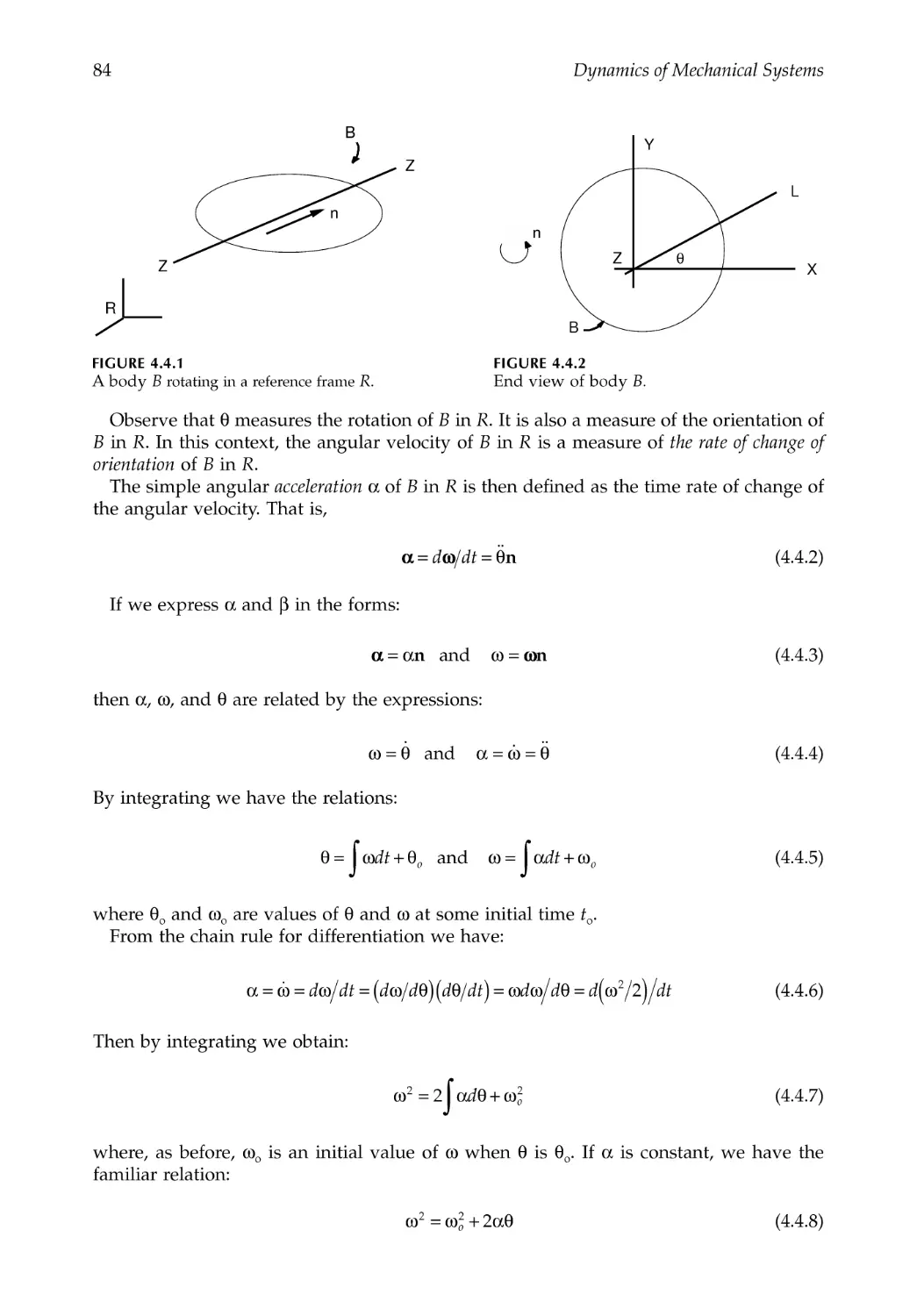
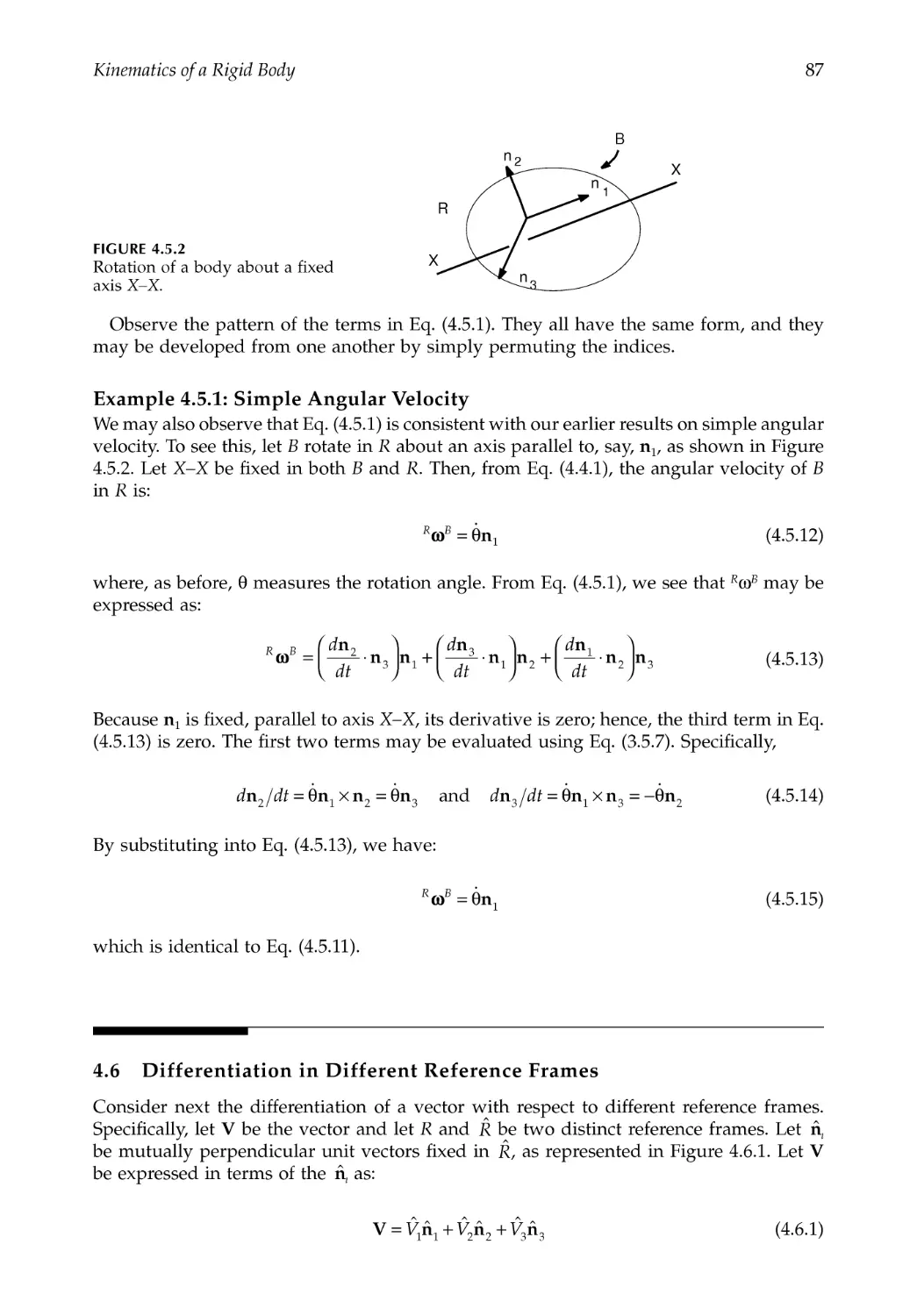
4.4 Simple Angular Velocity and Simple Angular Acceleration ......................................83
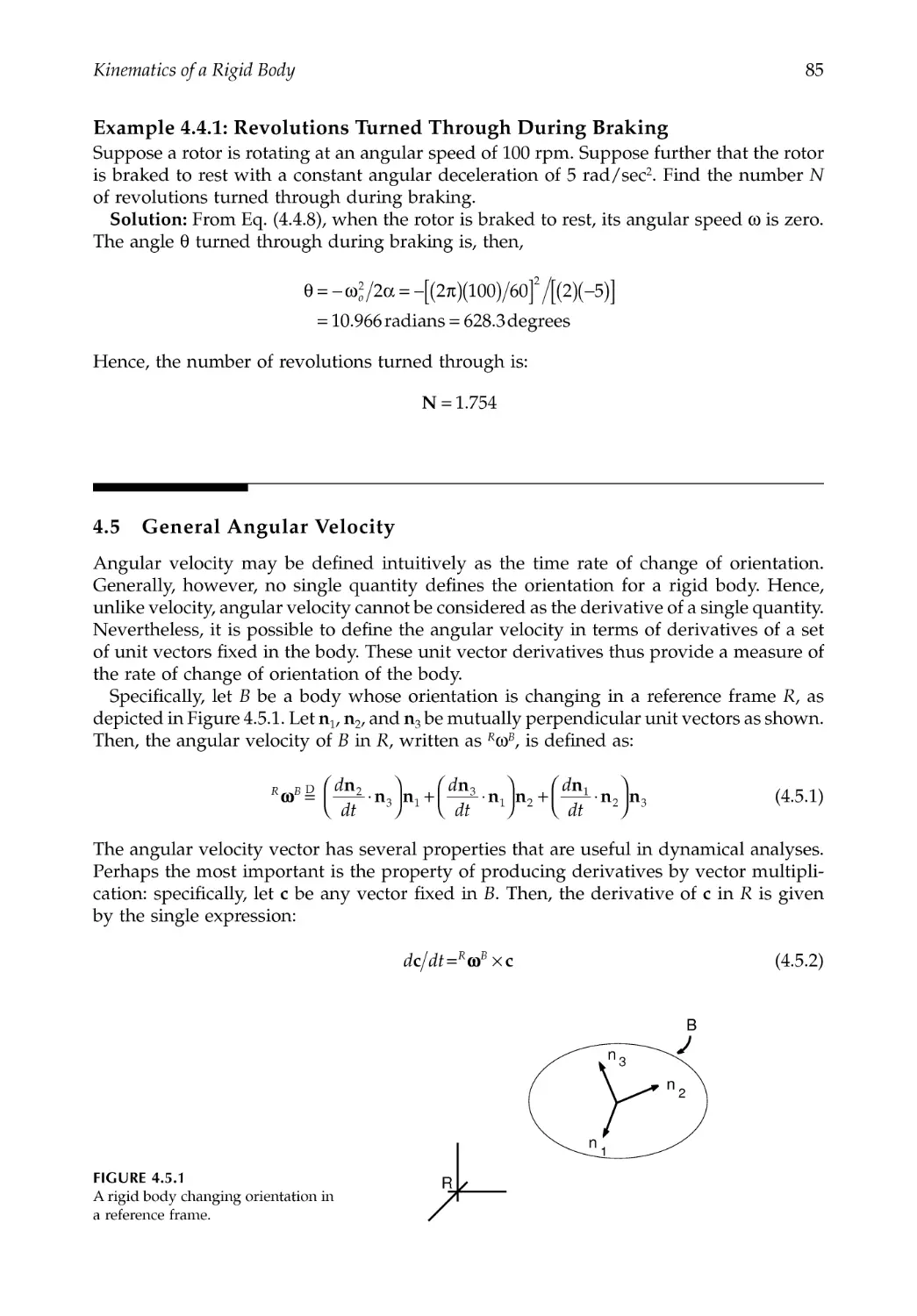
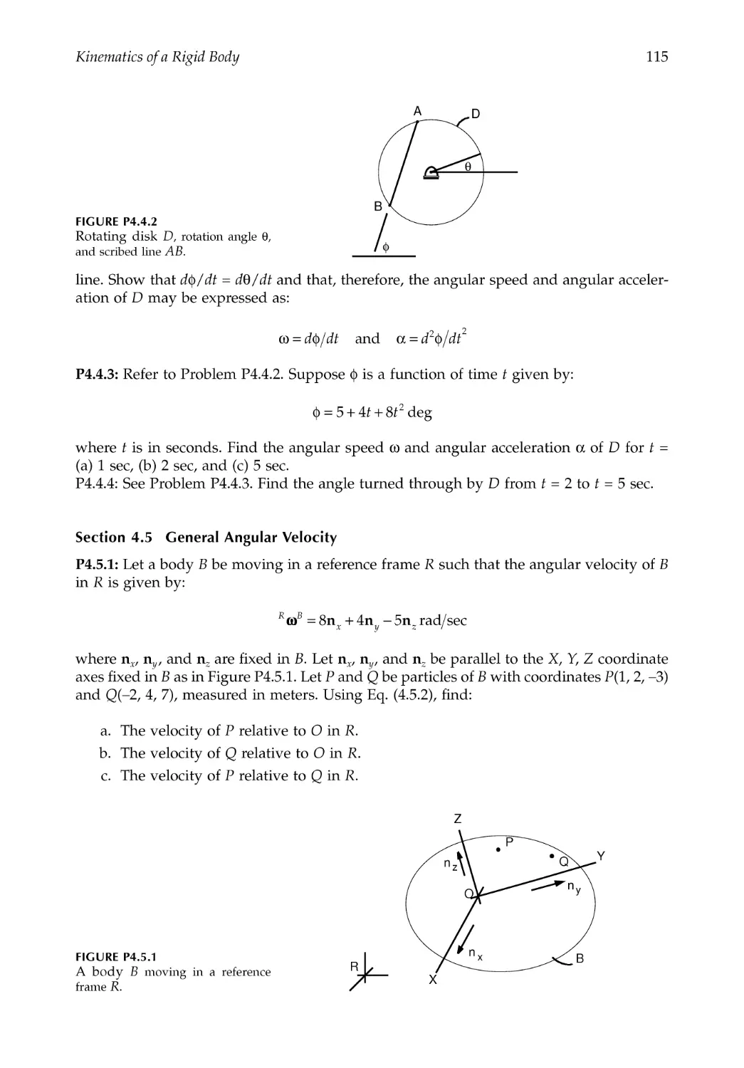
4.5 General Angular Velocity..................................................................................................85
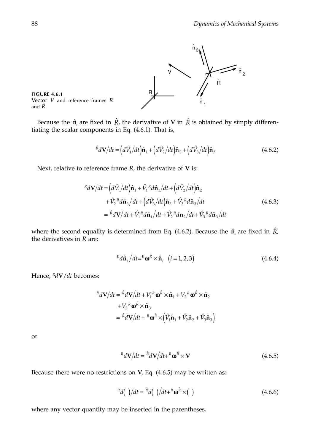
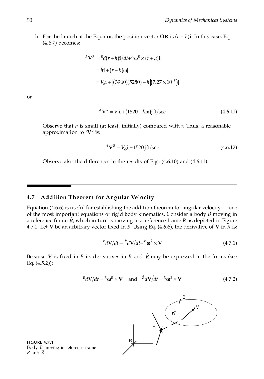
4.6 Differentiation in Different Reference Frames ..............................................................87
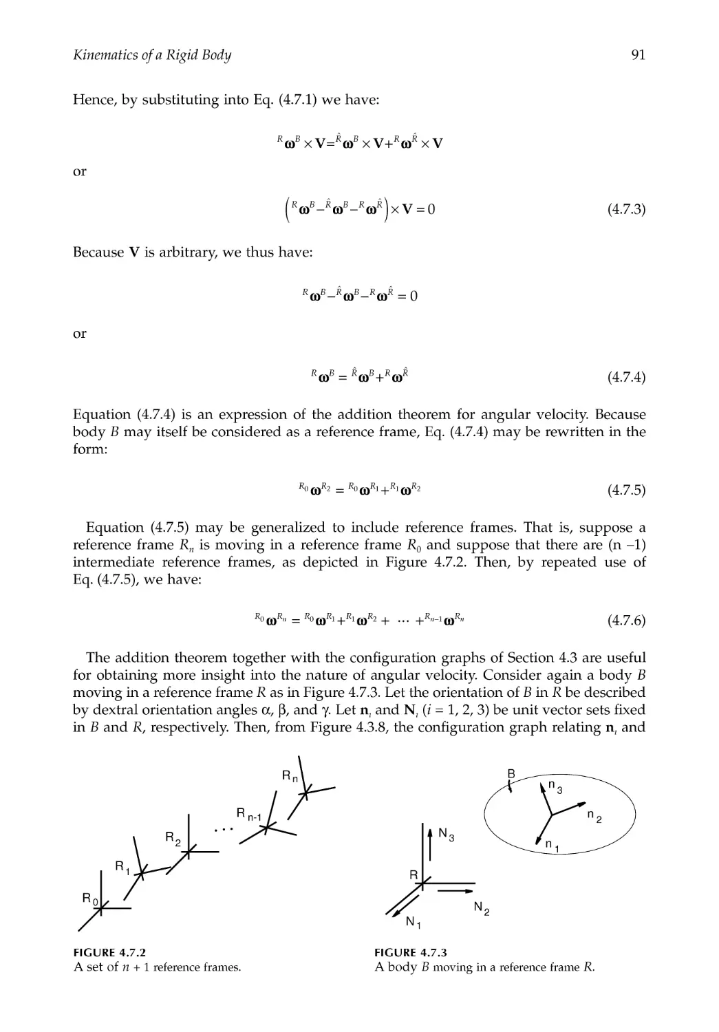
4.7 Addition Theorem for Angular Velocity ........................................................................90
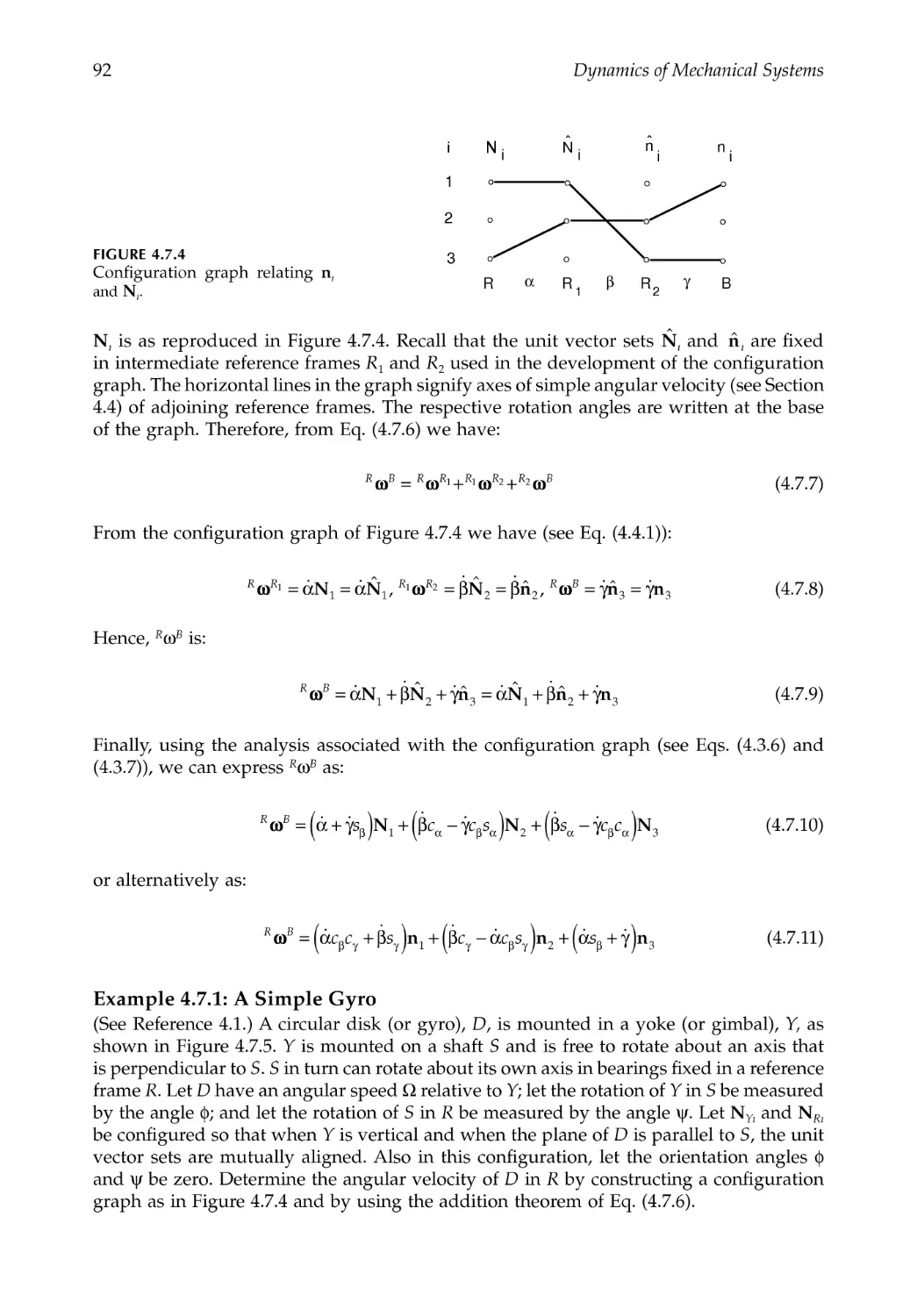
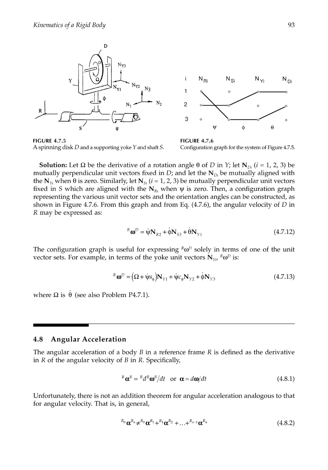
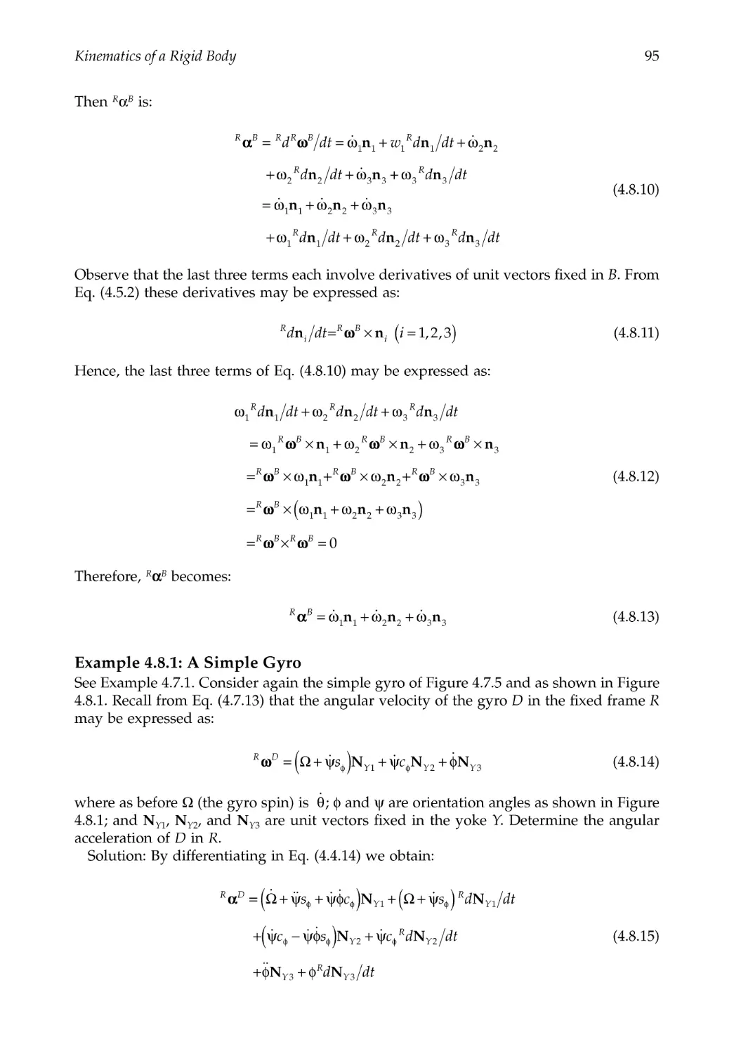
4.8 Angular Acceleration.........................................................................................................93
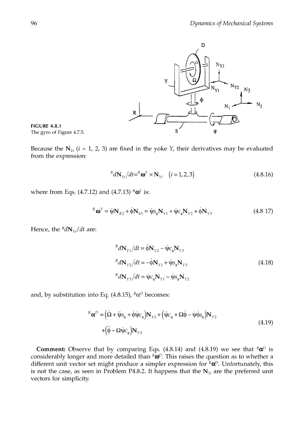
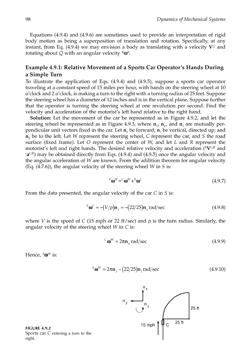
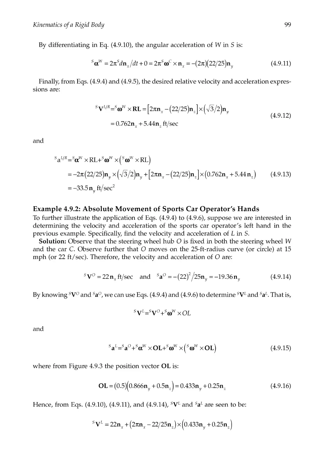
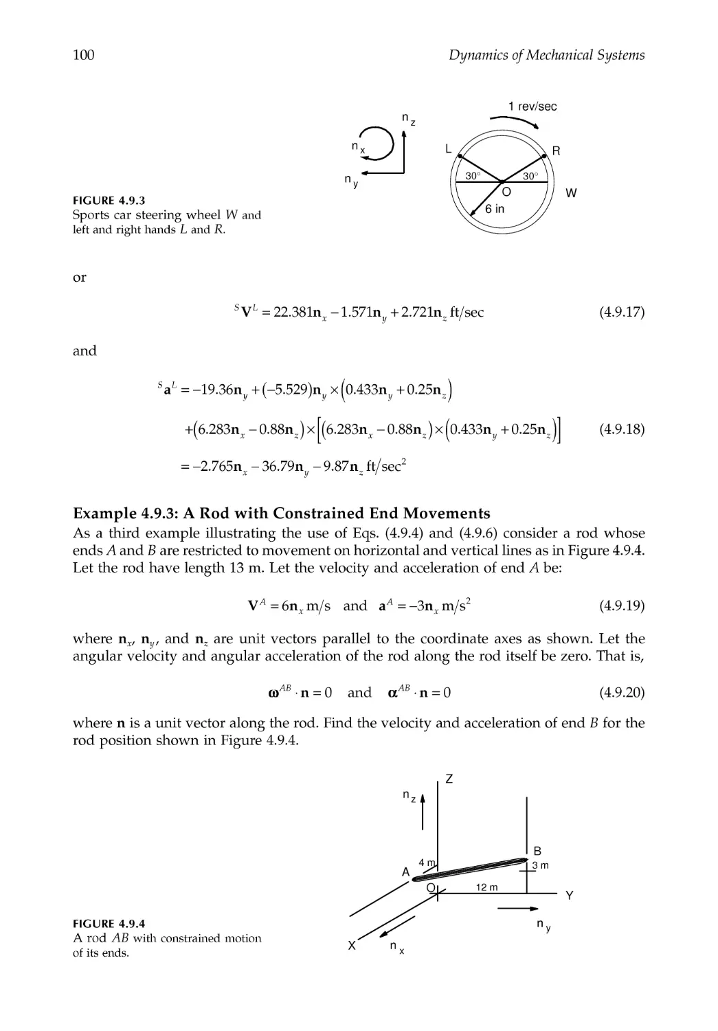
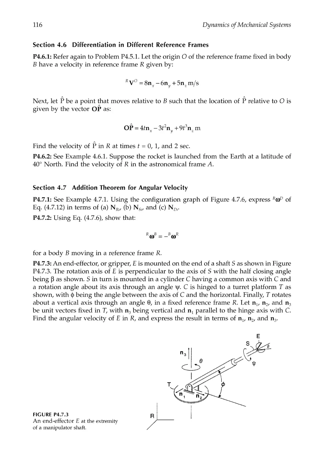
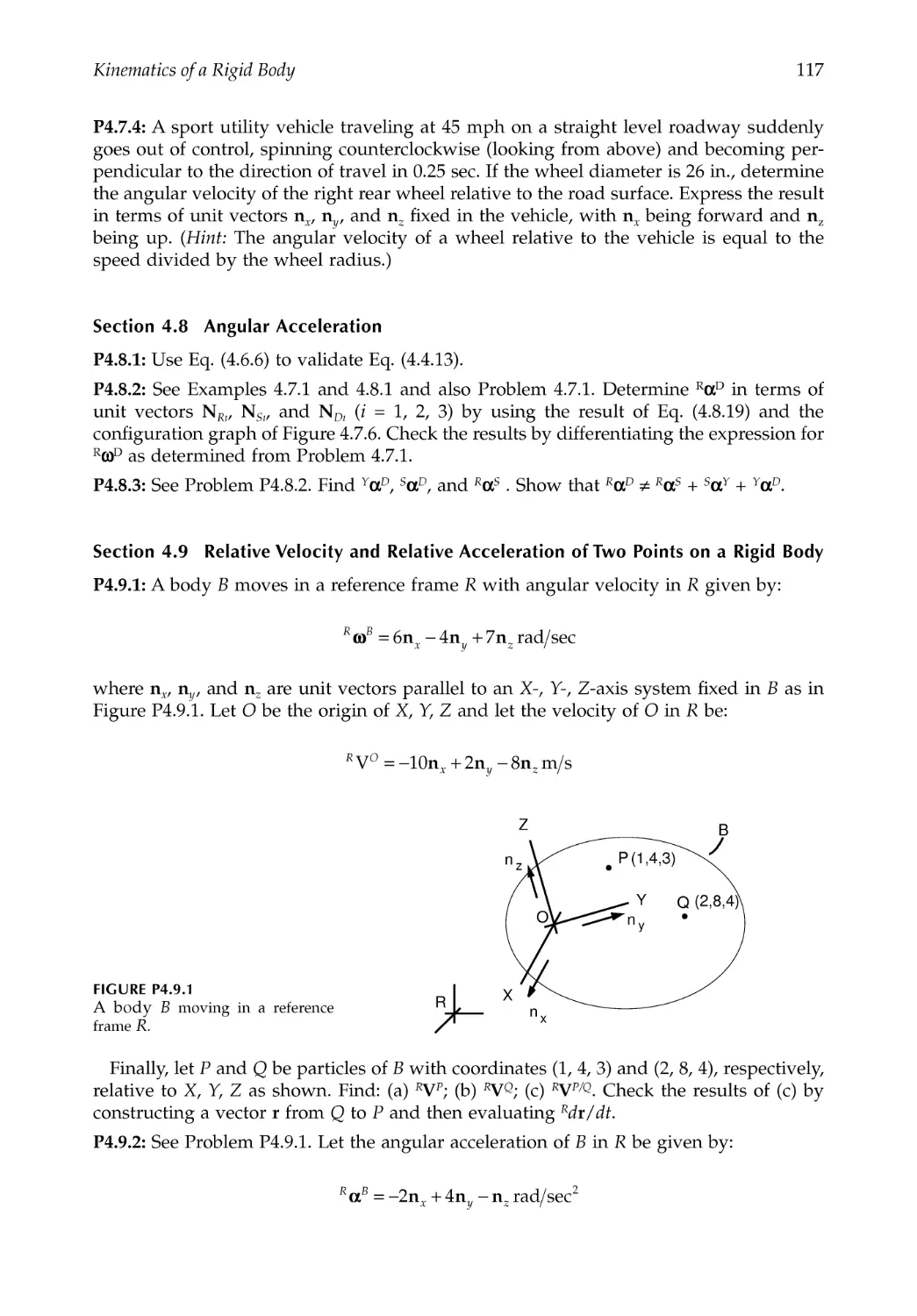
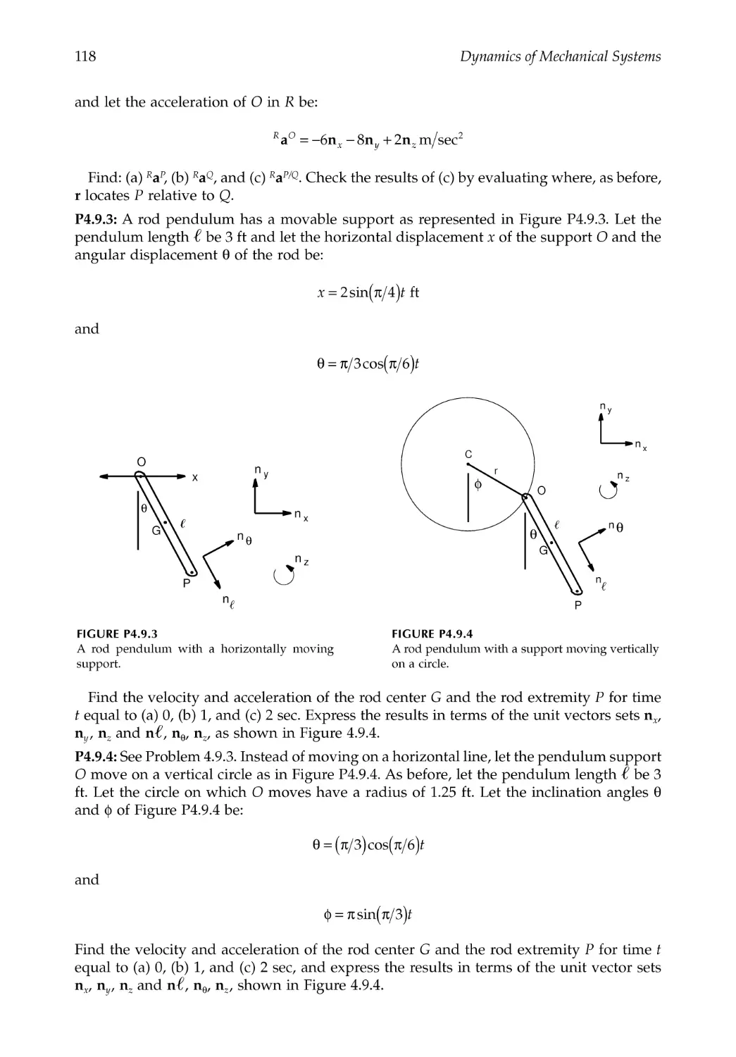
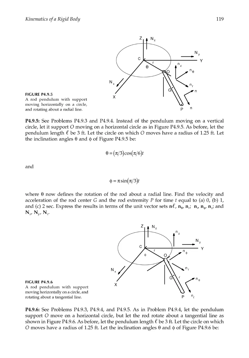
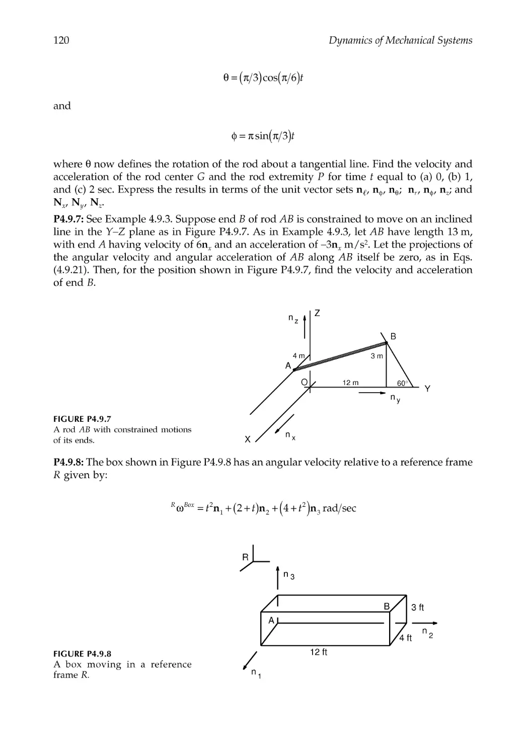
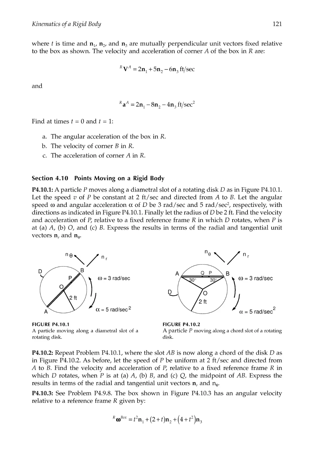
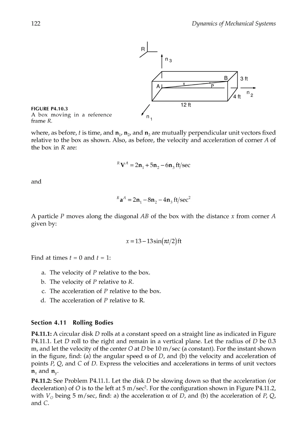
4.9 Relative Velocity and Relative Acceleration of Two Points
on a Rigid Body..................................................................................................................97
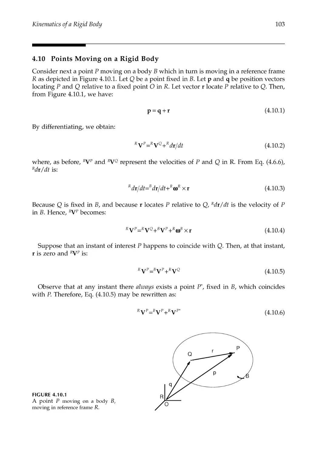
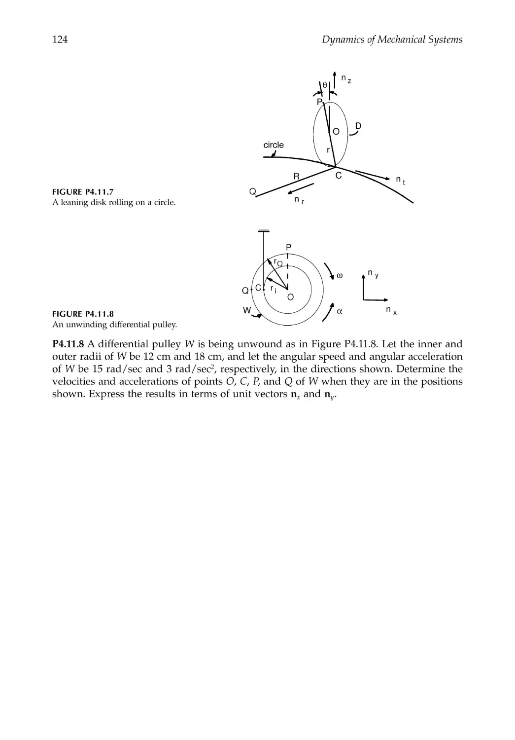
4.10 Points Moving on a Rigid Body ....................................................................................103
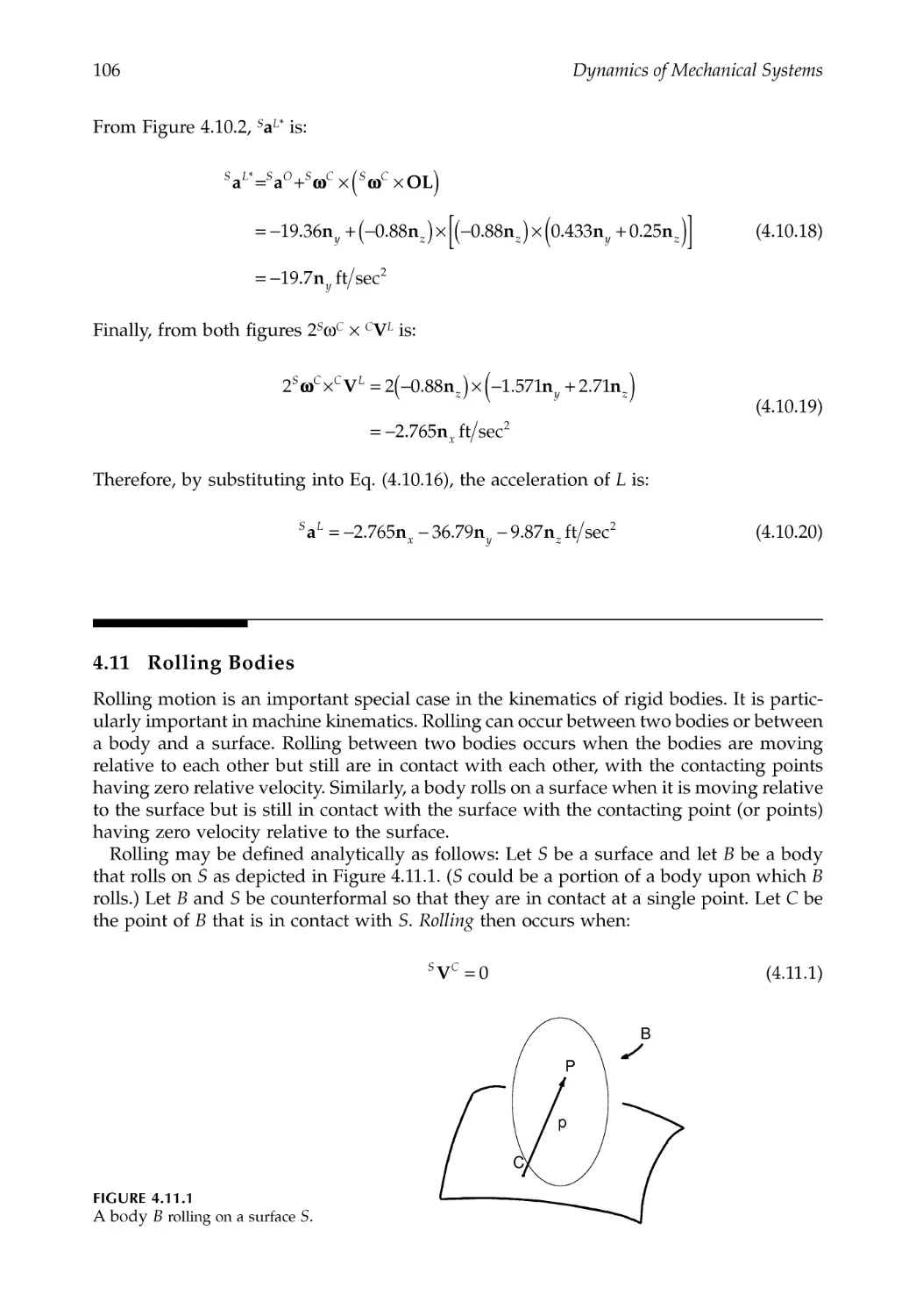
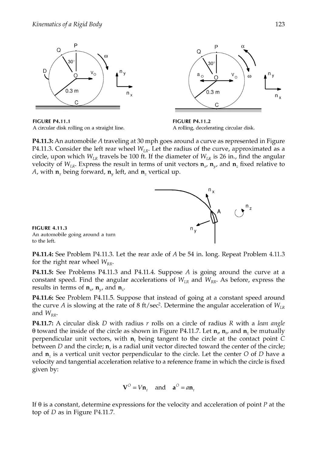
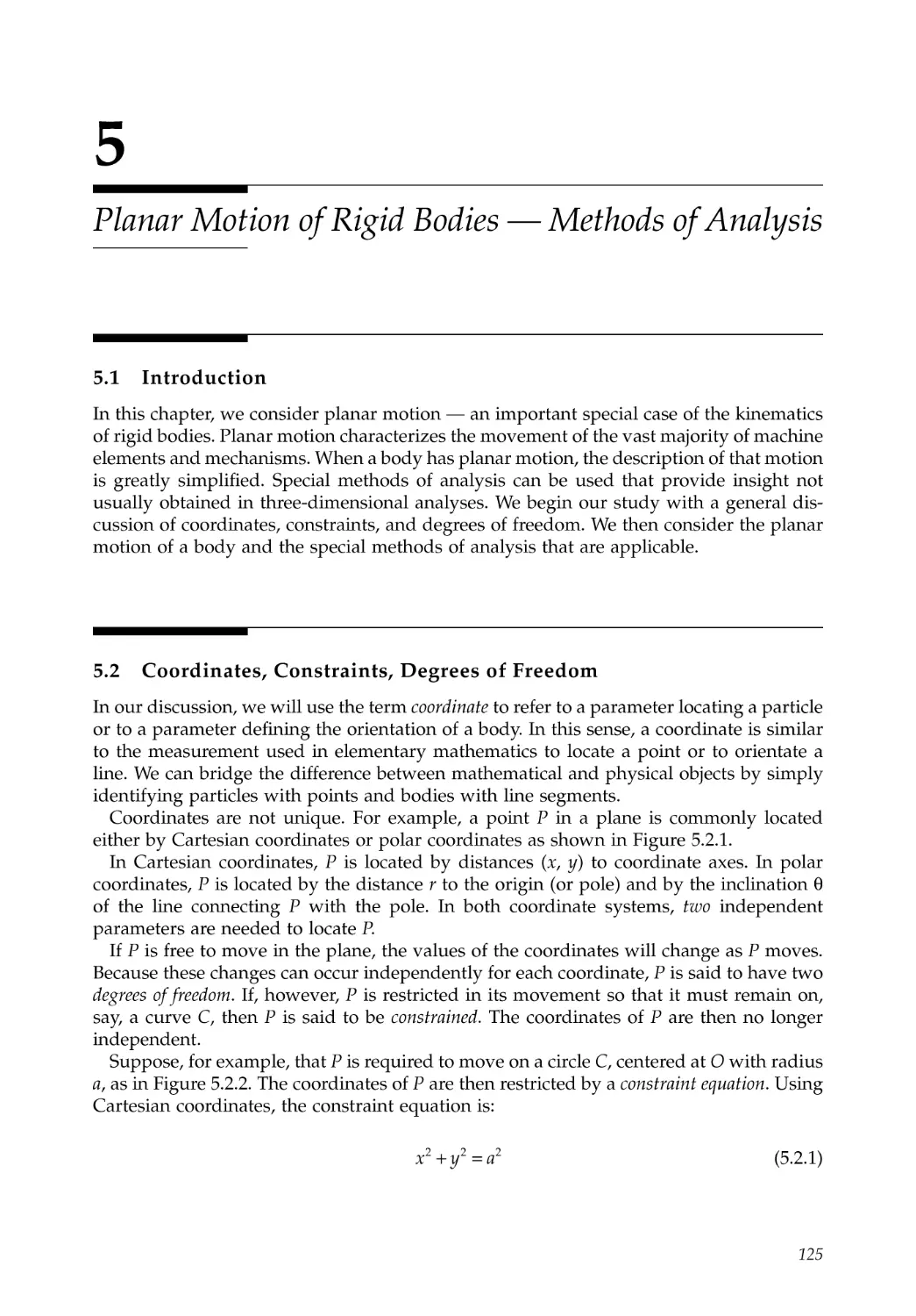
4.11 Rolling Bodies ...................................................................................................................106
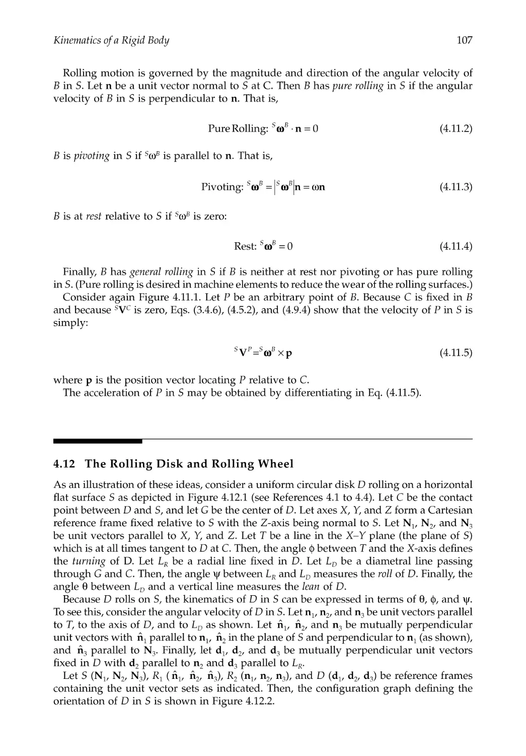
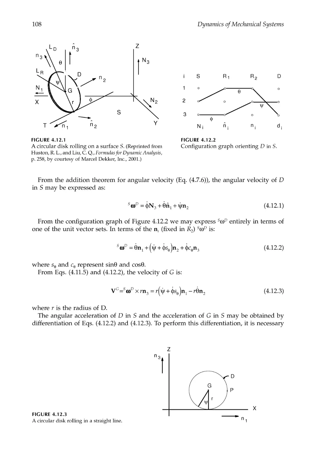
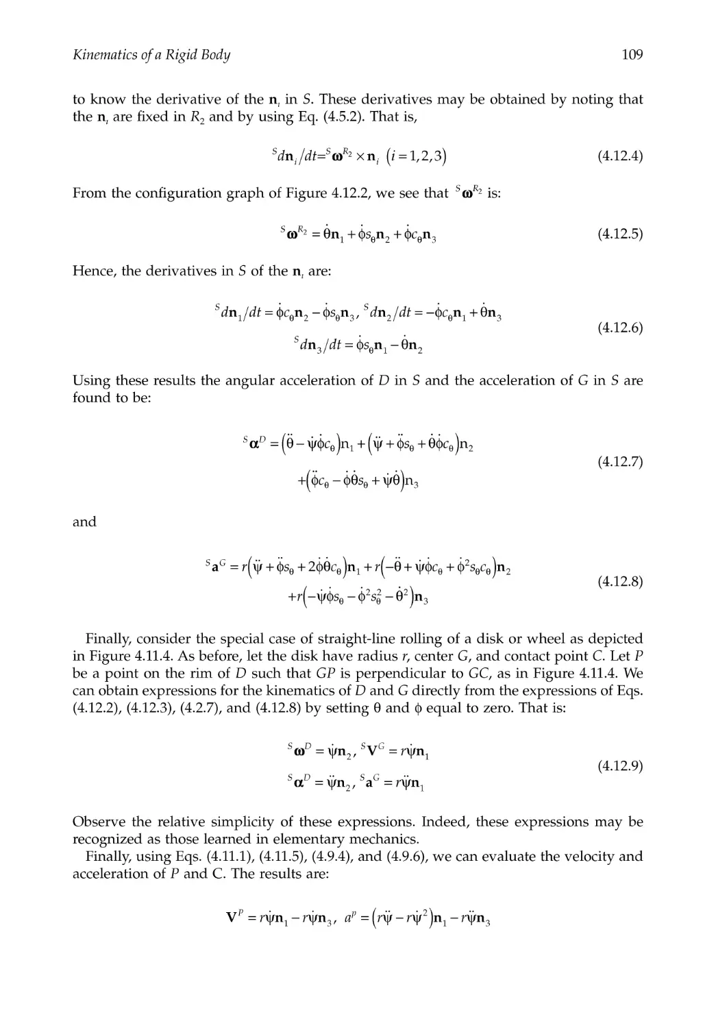
4.12 The Rolling Disk and Rolling Wheel ............................................................................107
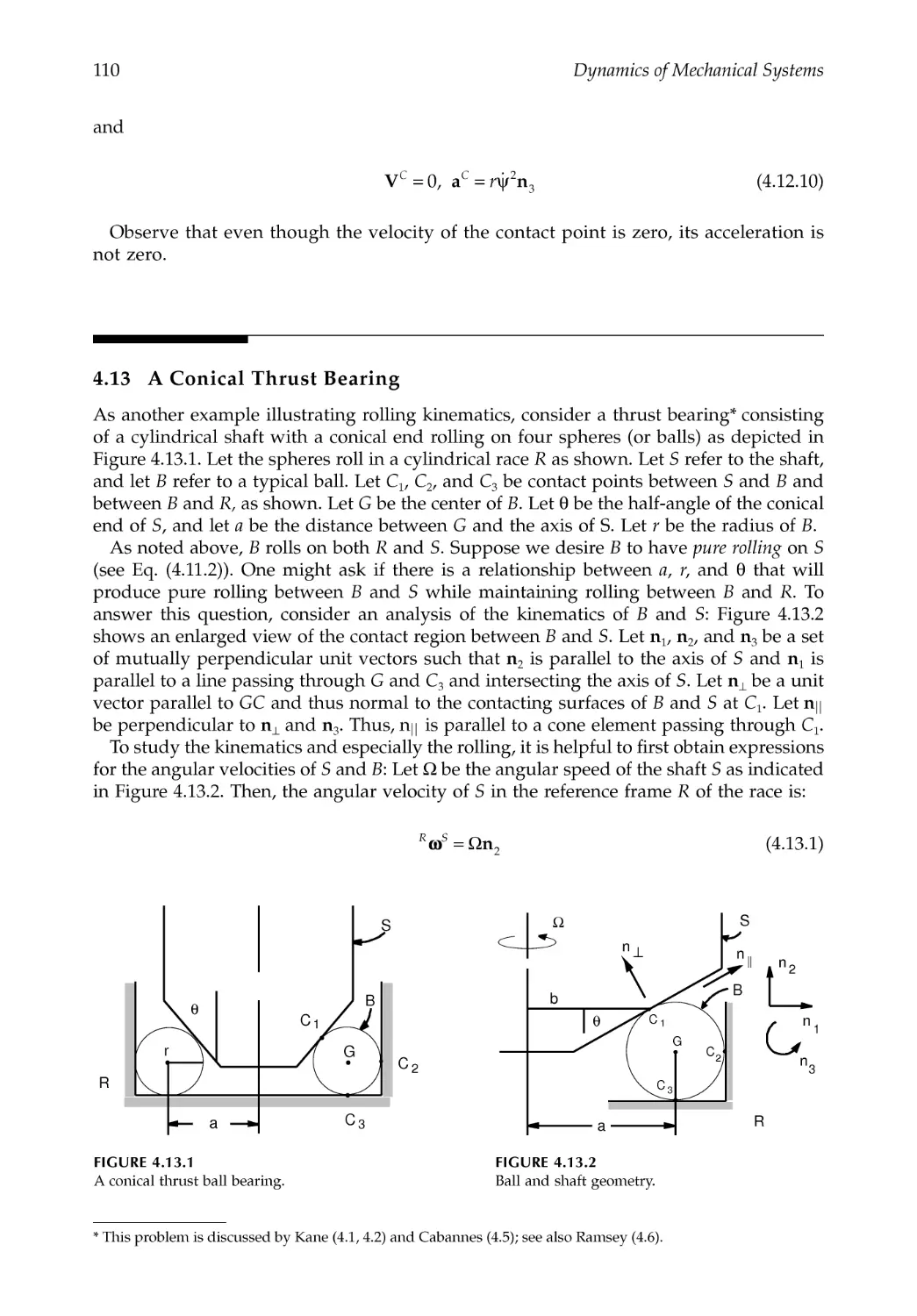
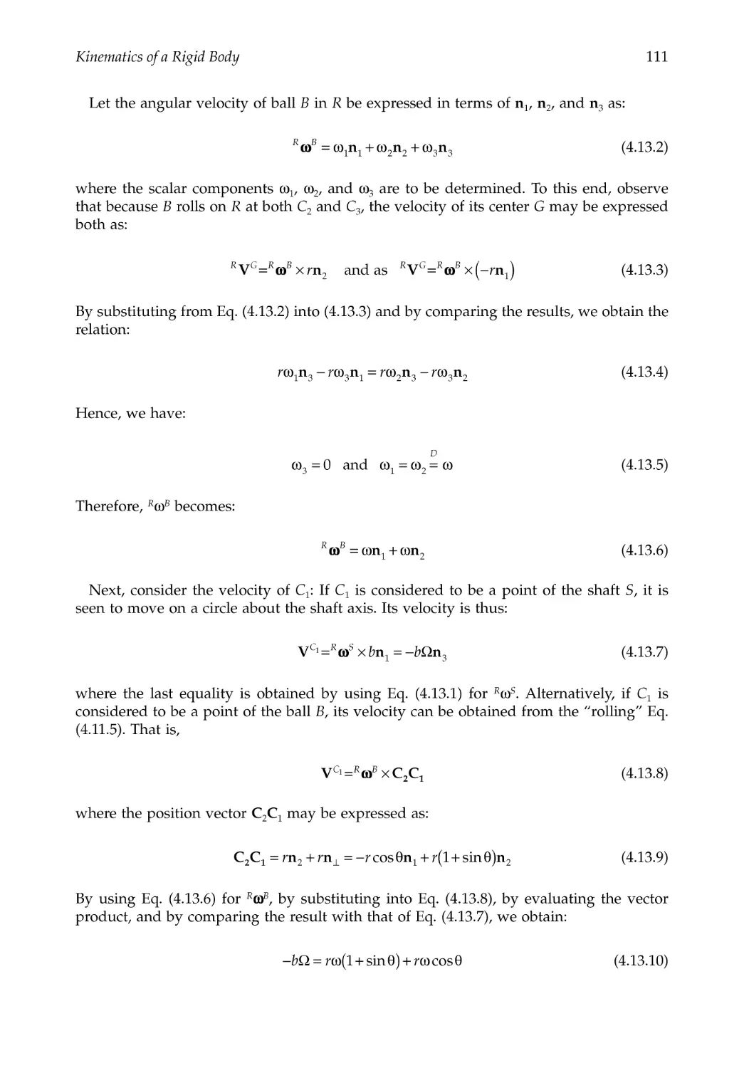
4.13 A Conical Thrust Bearing ...............................................................................................110
4.14 Closure ...............................................................................................................................113
References .....................................................................................................................................113
Problems .......................................................................................................................................114
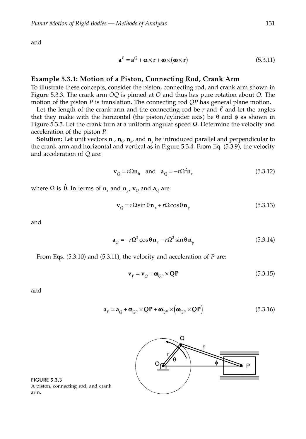
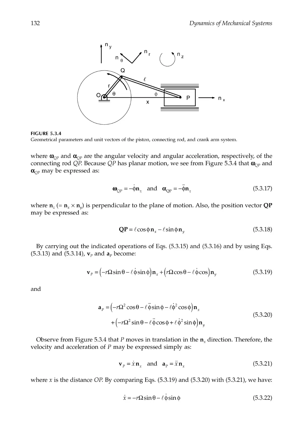
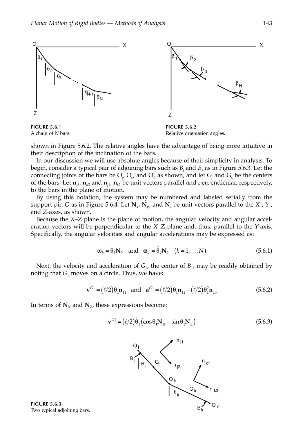
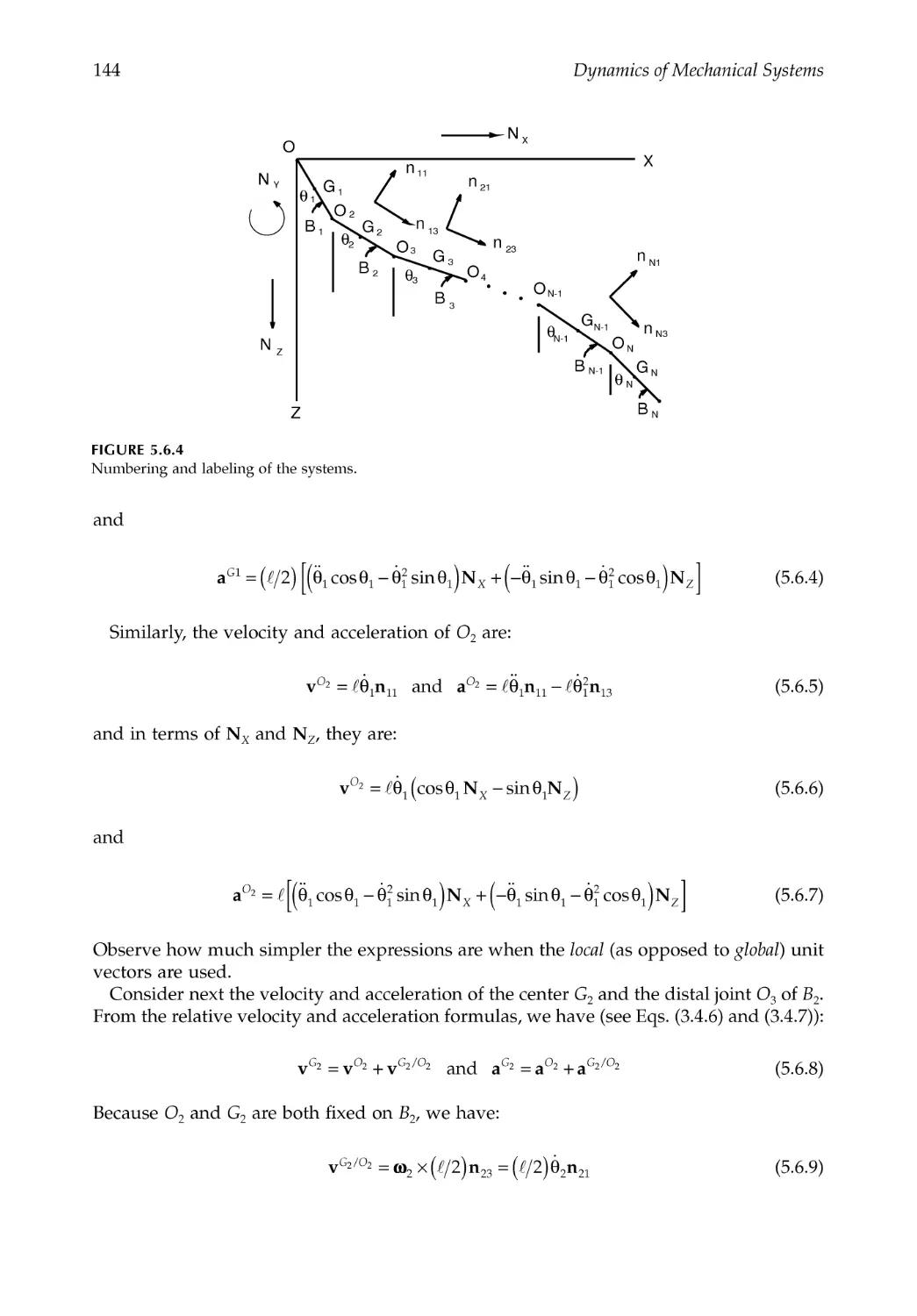
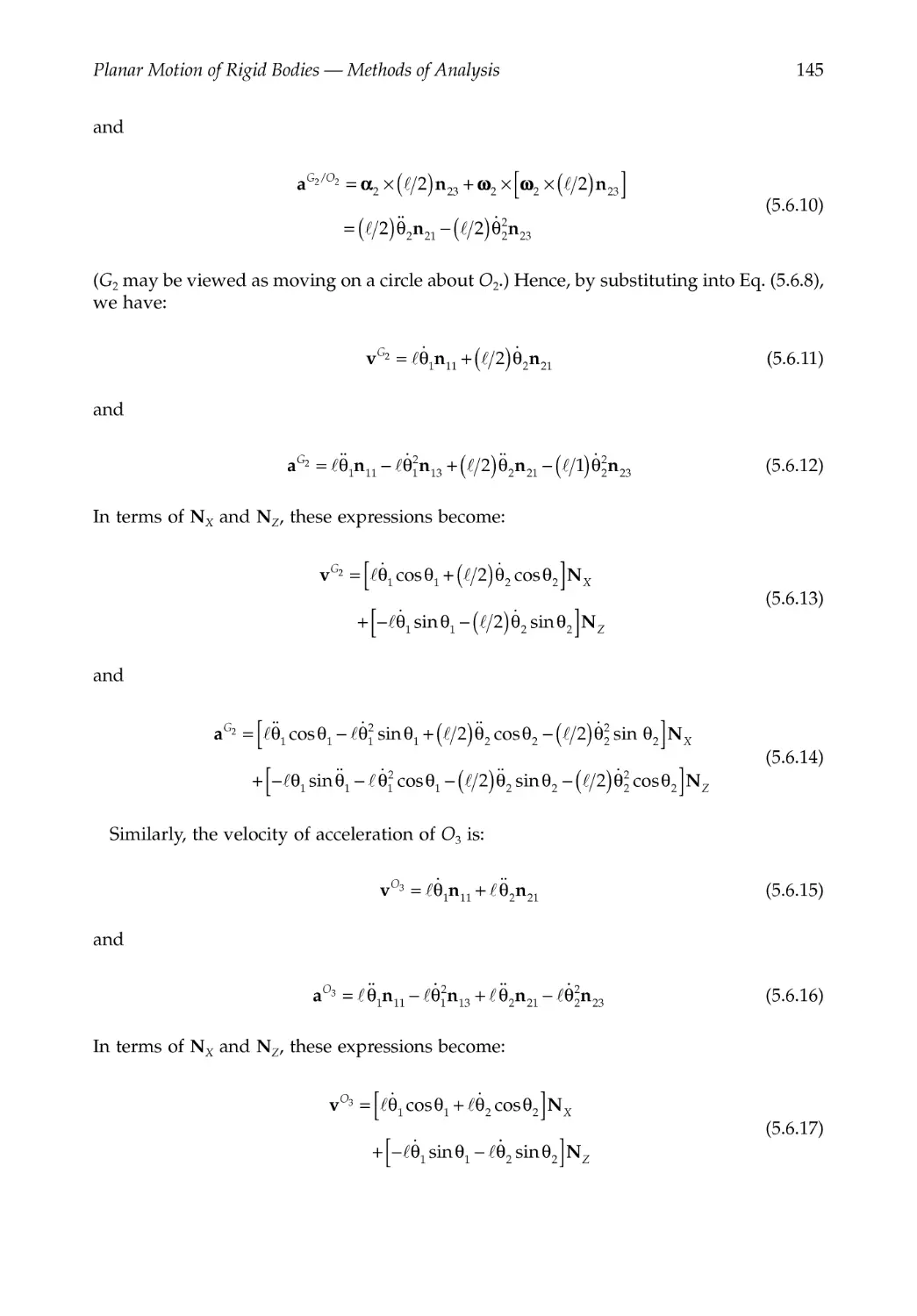
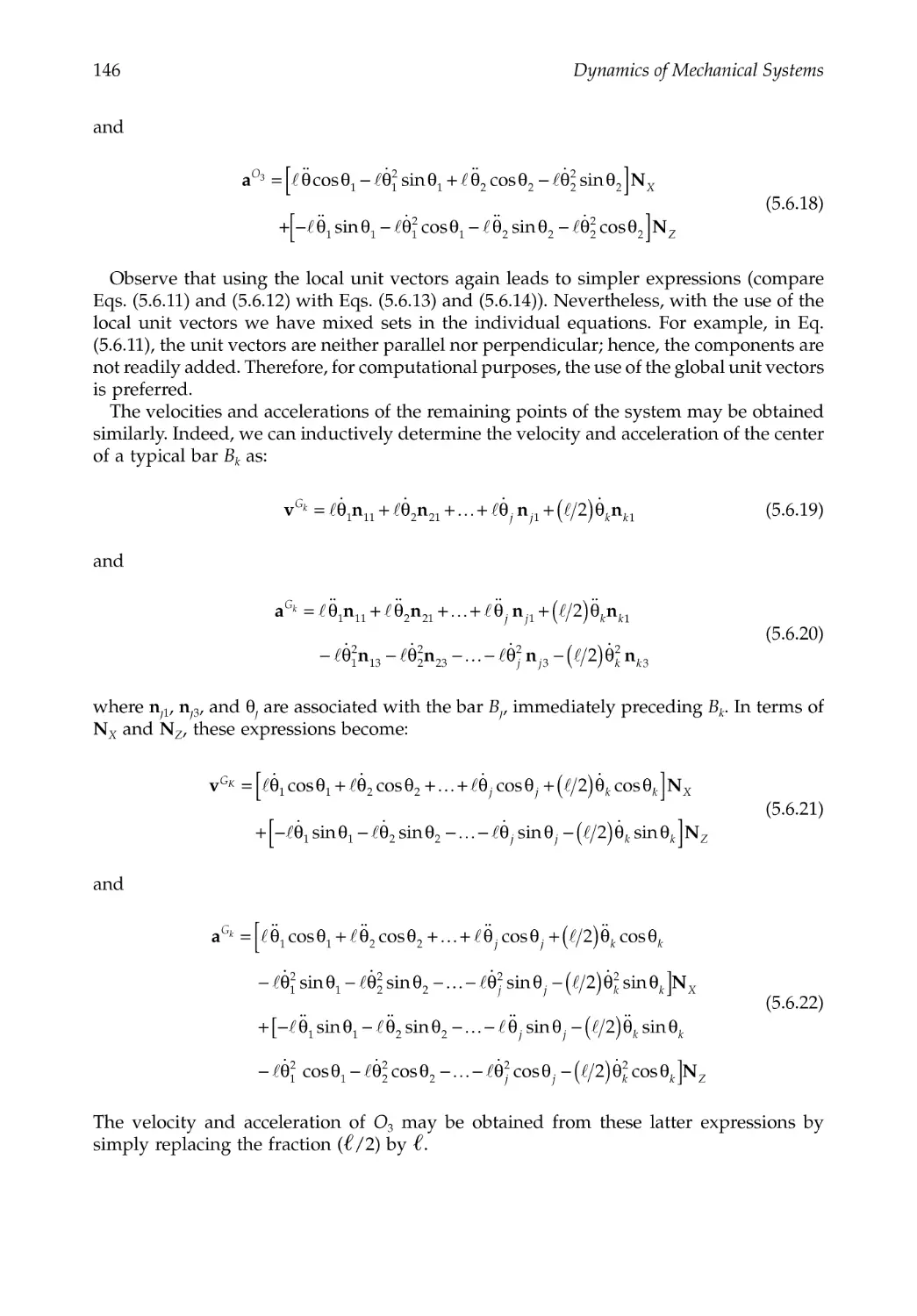
Chapter 5 Planar Motion of Rigid Bodies --- Methods of Analysis ................................125
5.1 Introduction.......................................................................................................................125
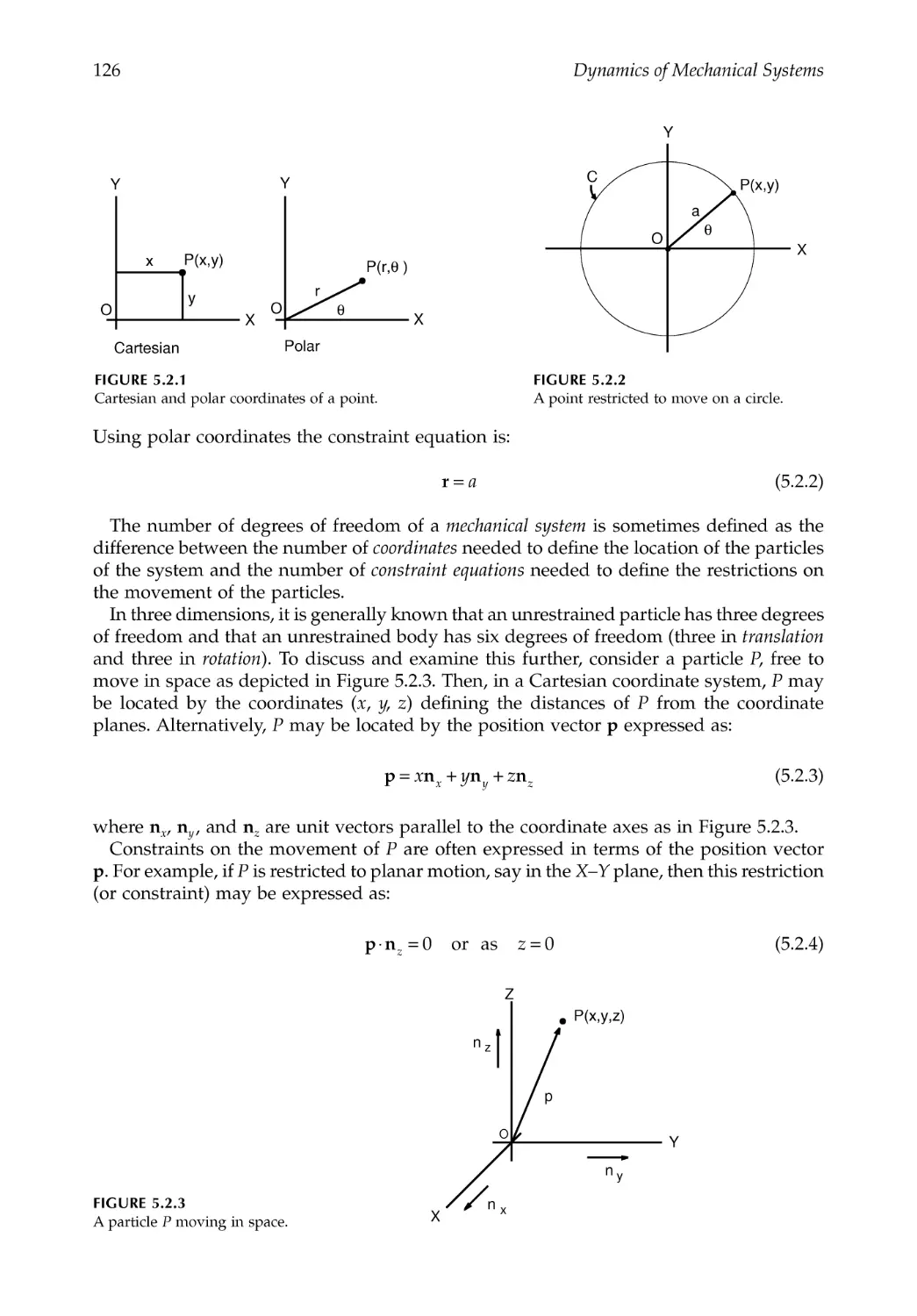
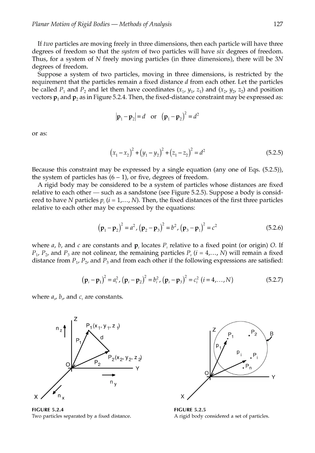
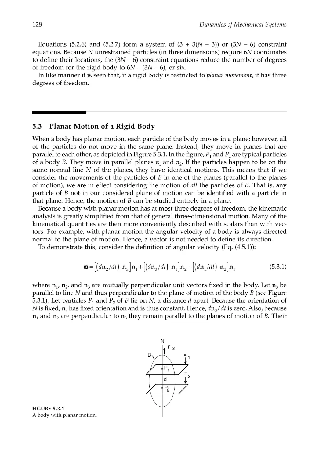
5.2 Coordinates, Constraints, Degrees of Freedom ..........................................................125
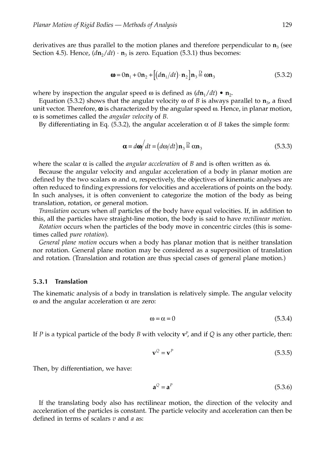
5.3 Planar Motion of a Rigid Body......................................................................................128
5.3.1 Translation .............................................................................................................129
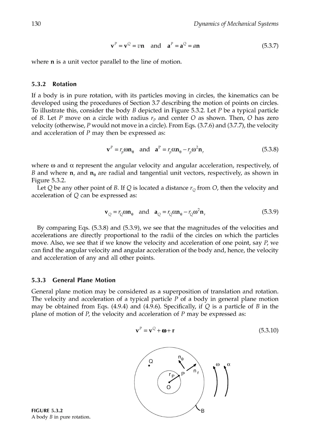
5.3.2 Rotation ..................................................................................................................130
5.3.3 General Plane Motion..........................................................................................130
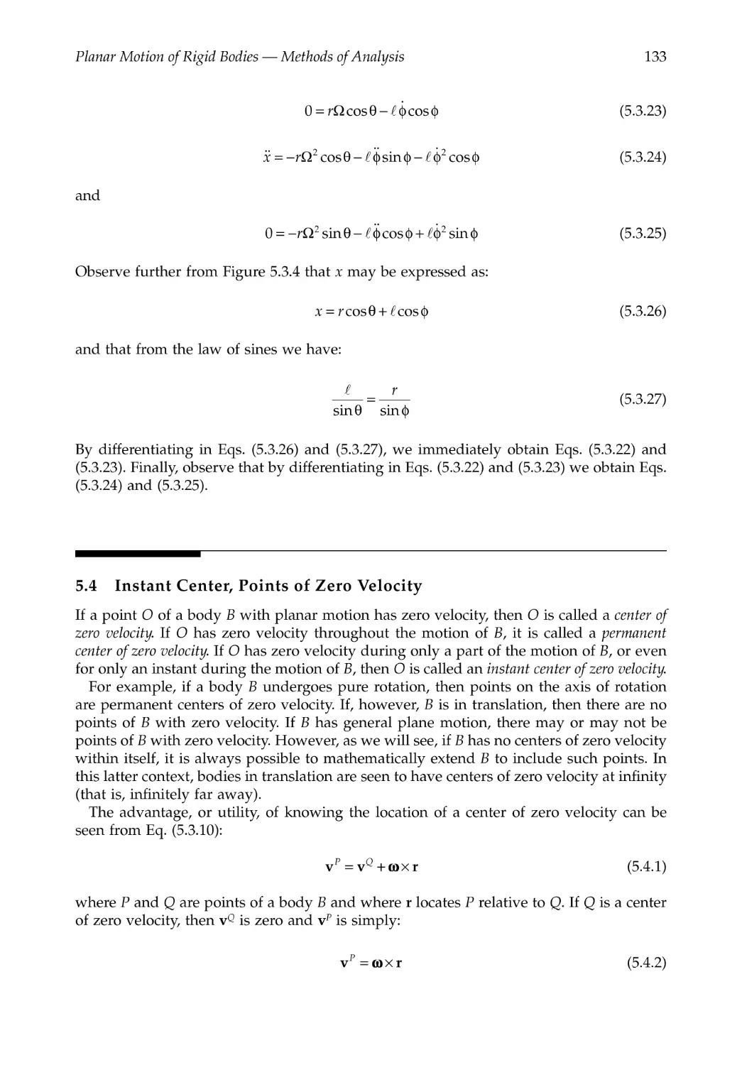
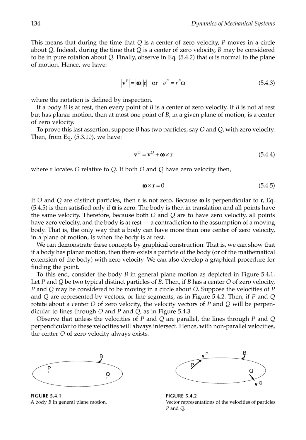
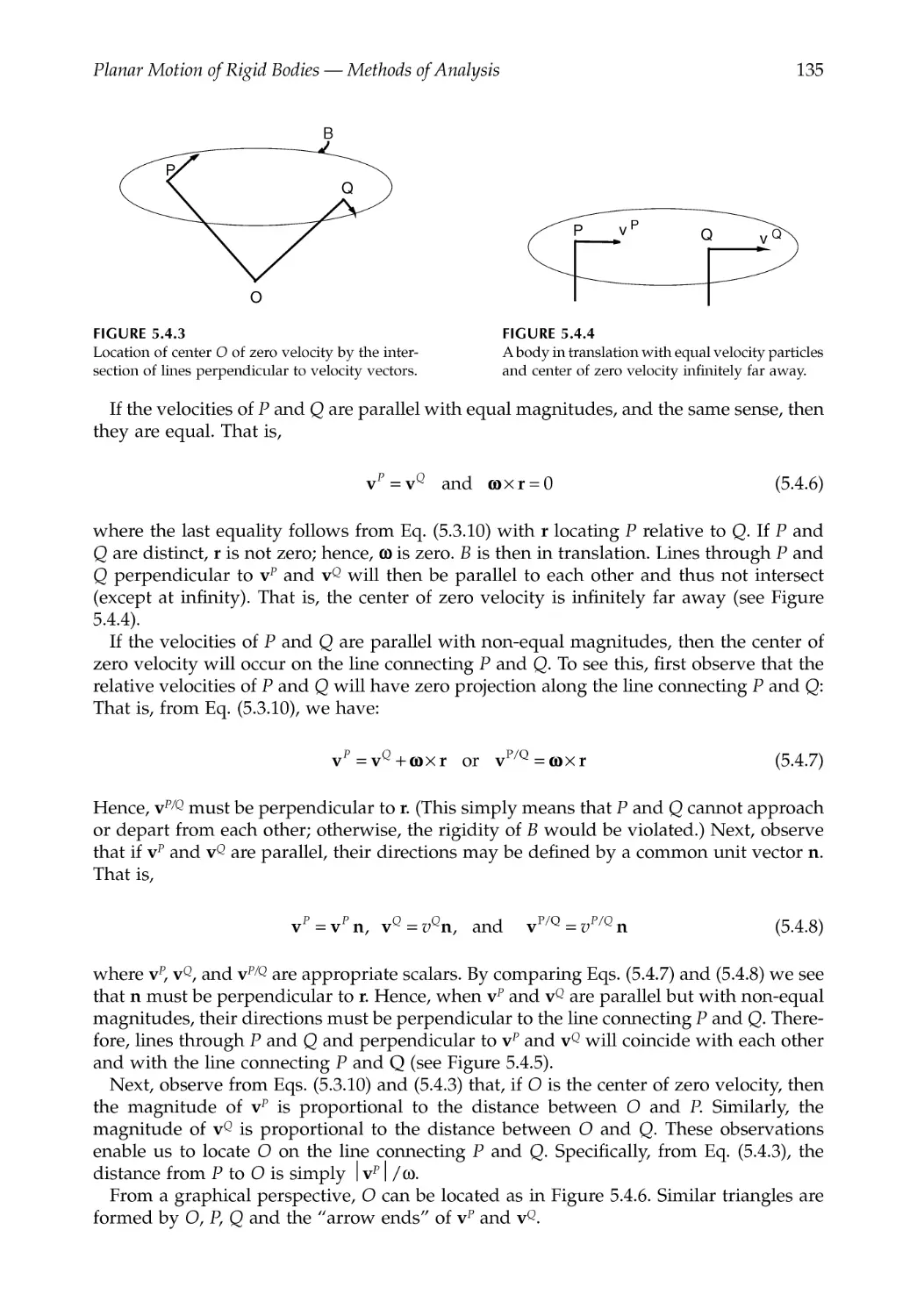
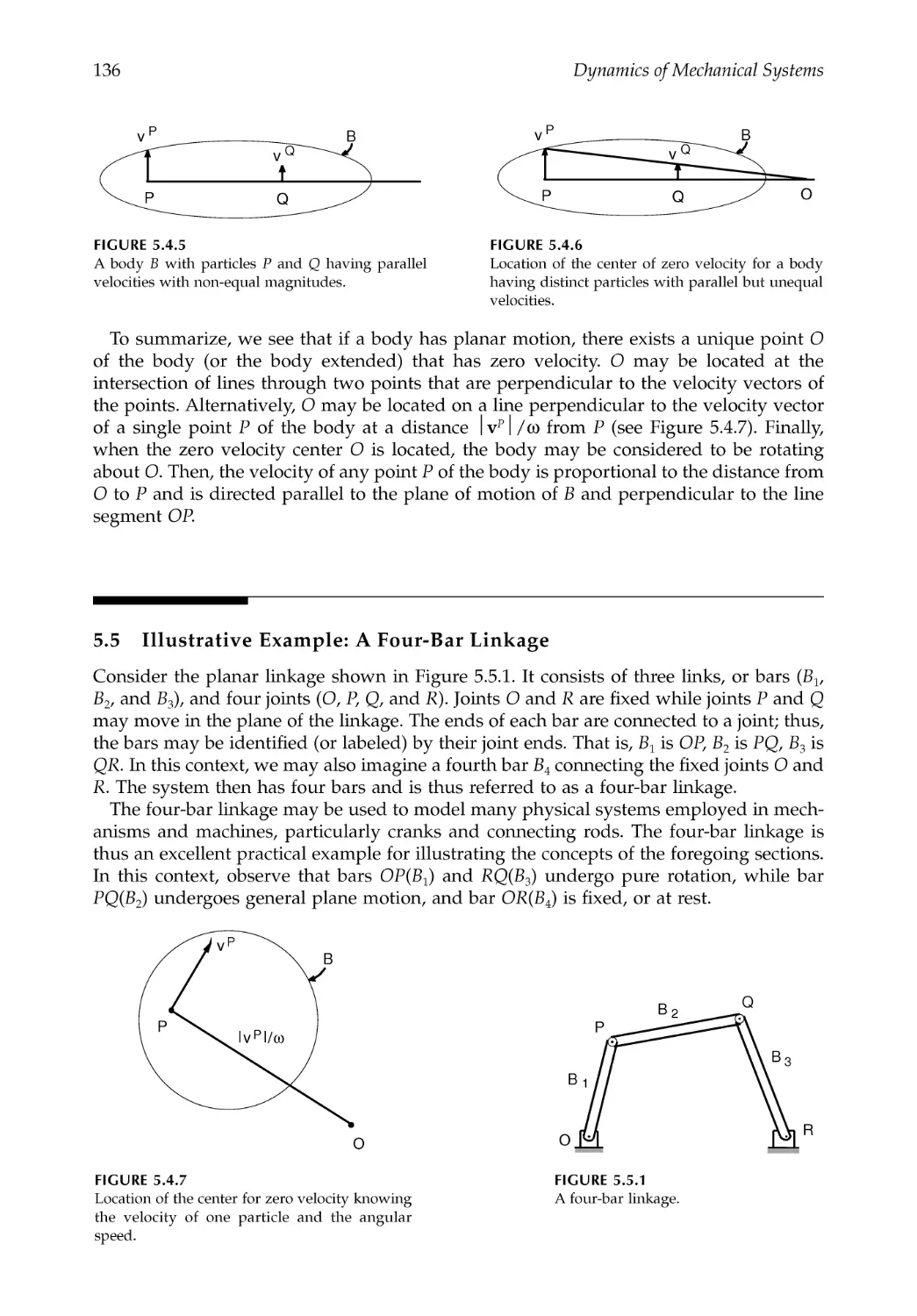
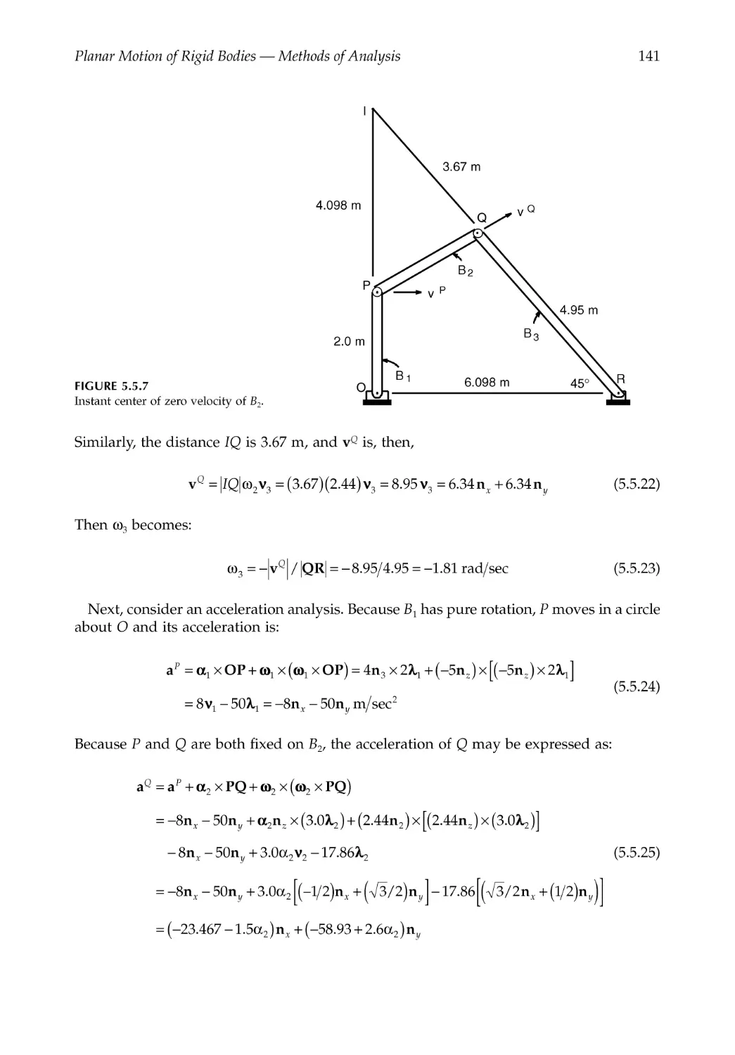
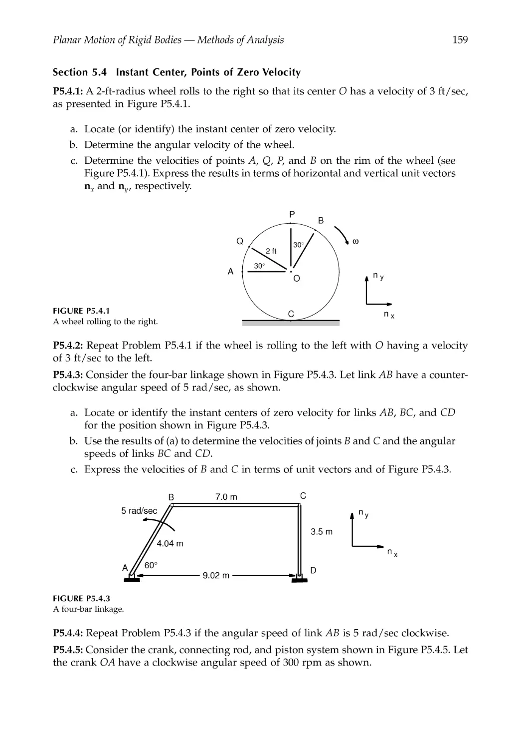
5.4 Instant Center, Points of Zero Velocity.........................................................................133
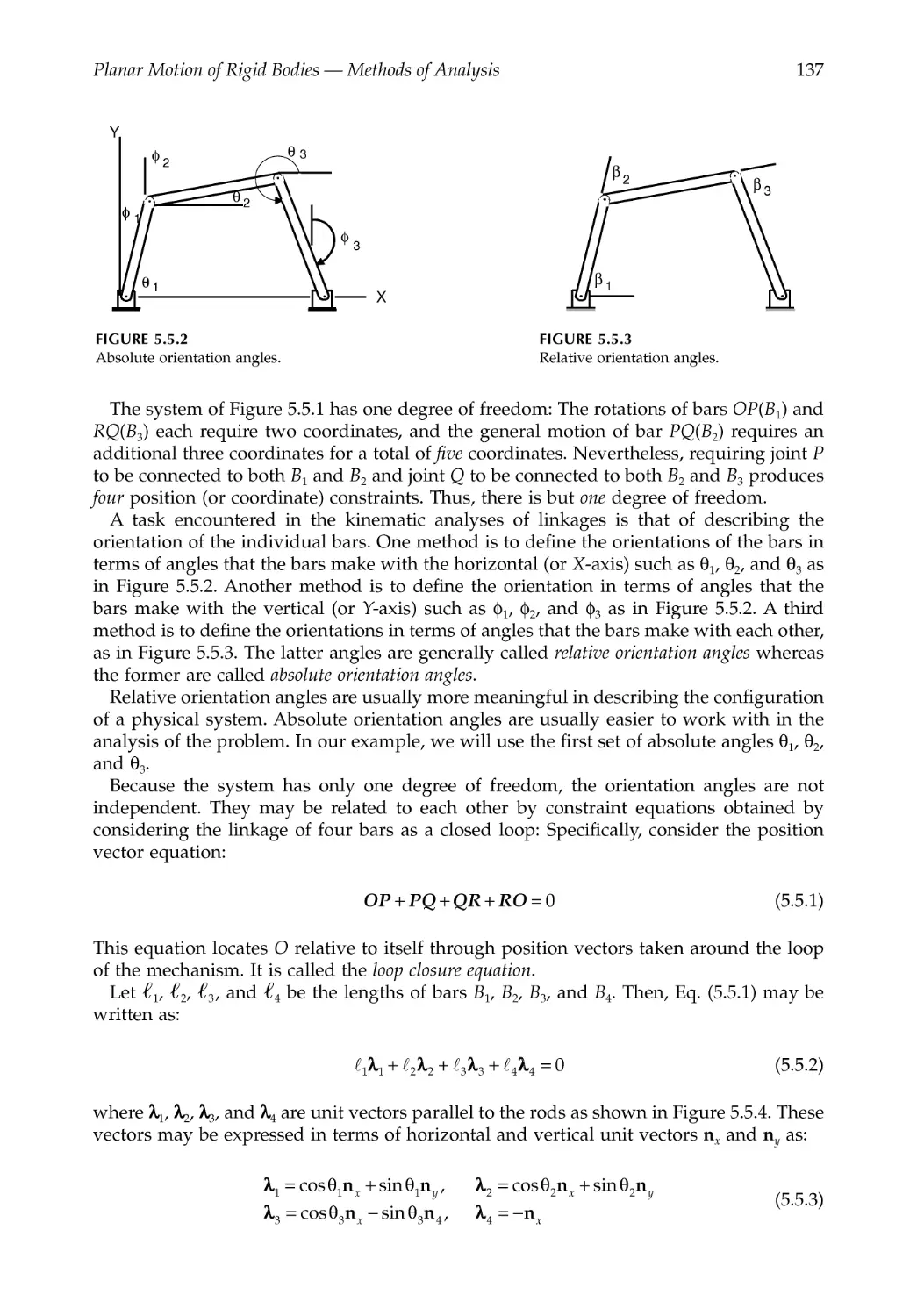
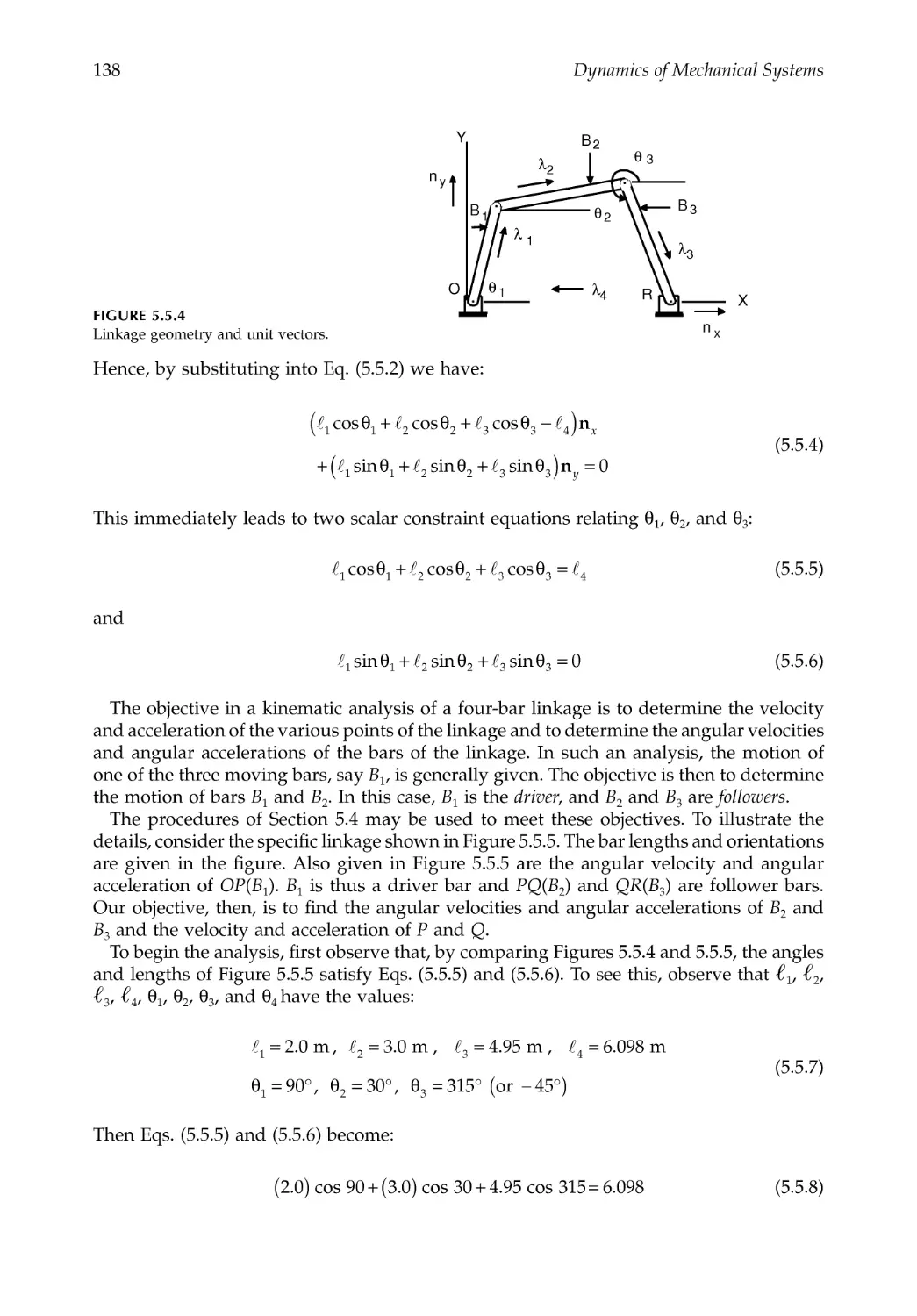
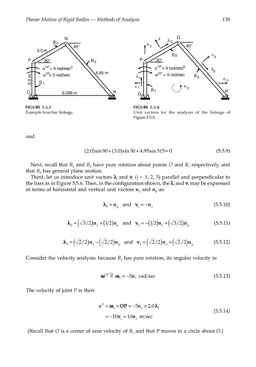
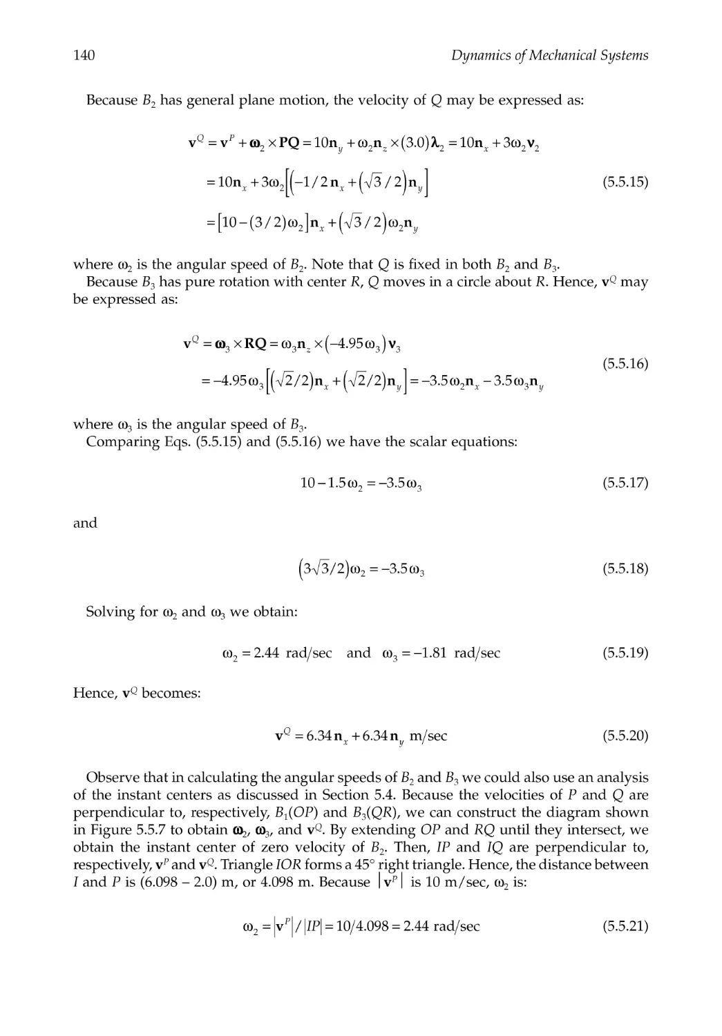
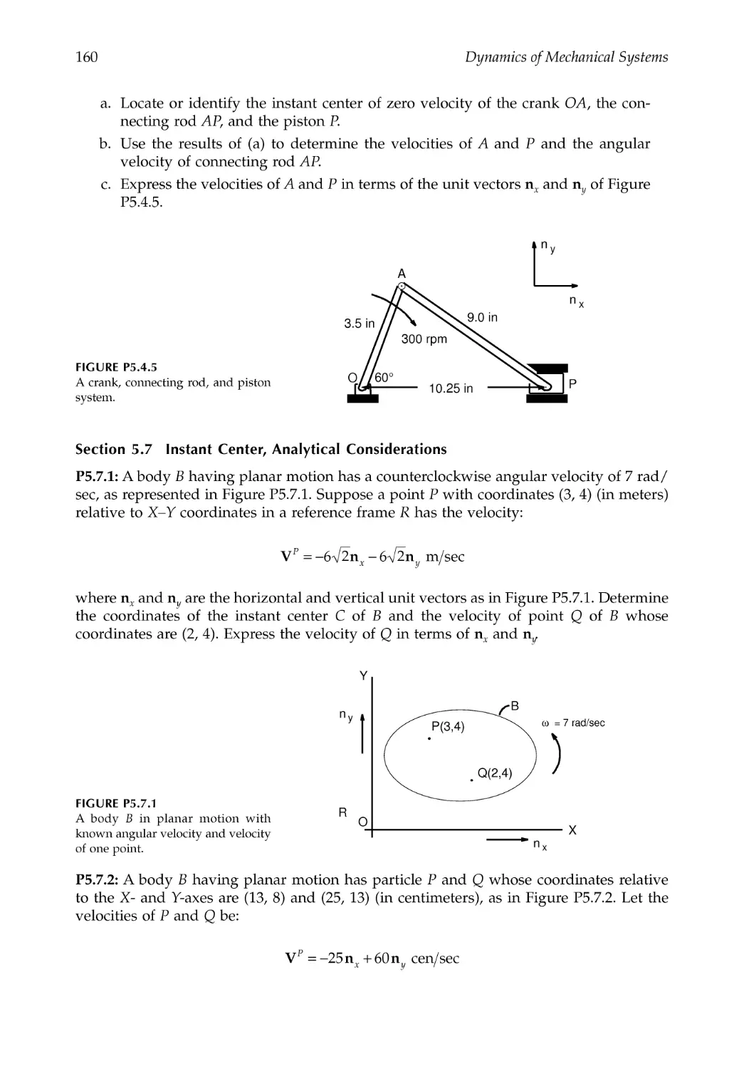
5.5 Illustrative Example: A Four-Bar Linkage ...................................................................136
5.6 Chains of Bodies...............................................................................................................142
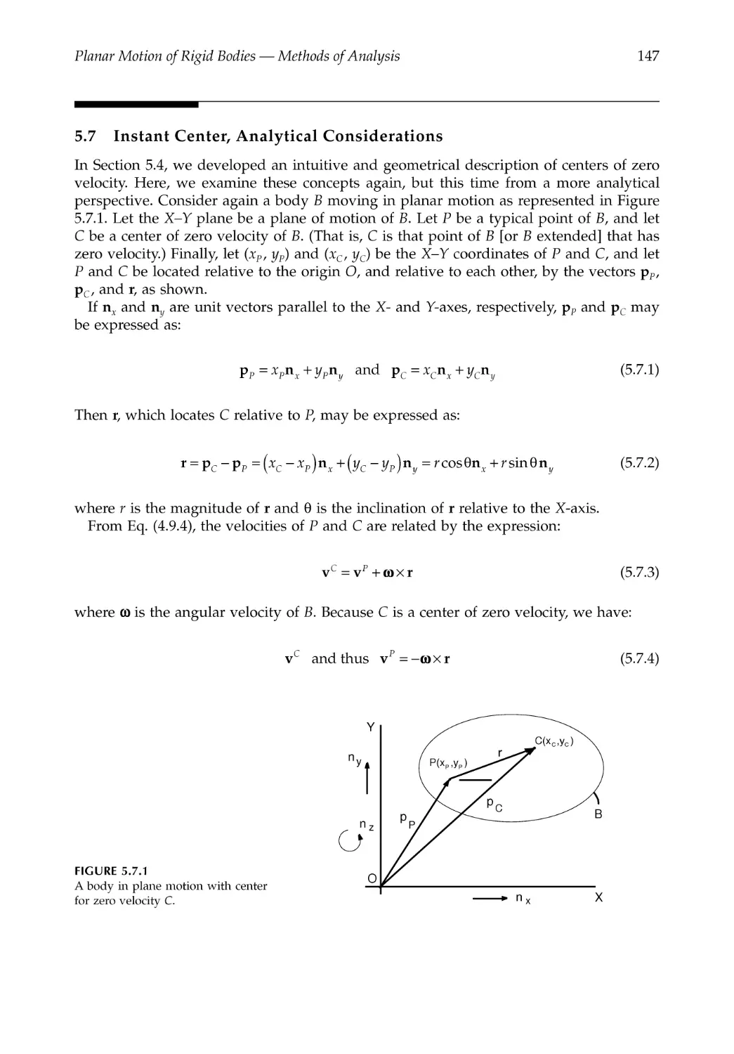
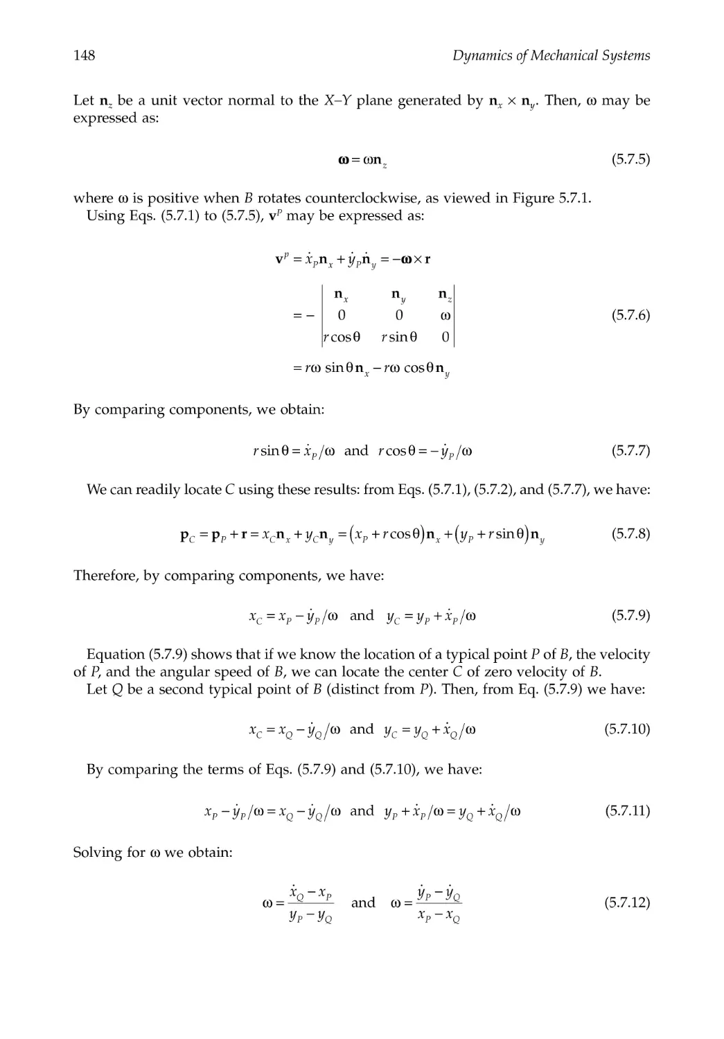
5.7 Instant Center, Analytical Considerations ...................................................................147
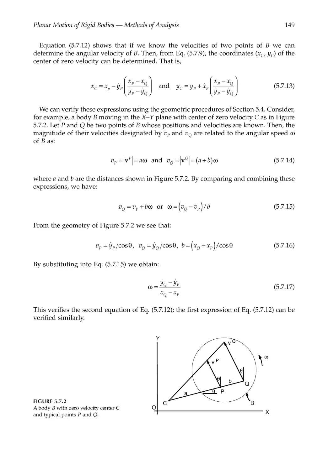
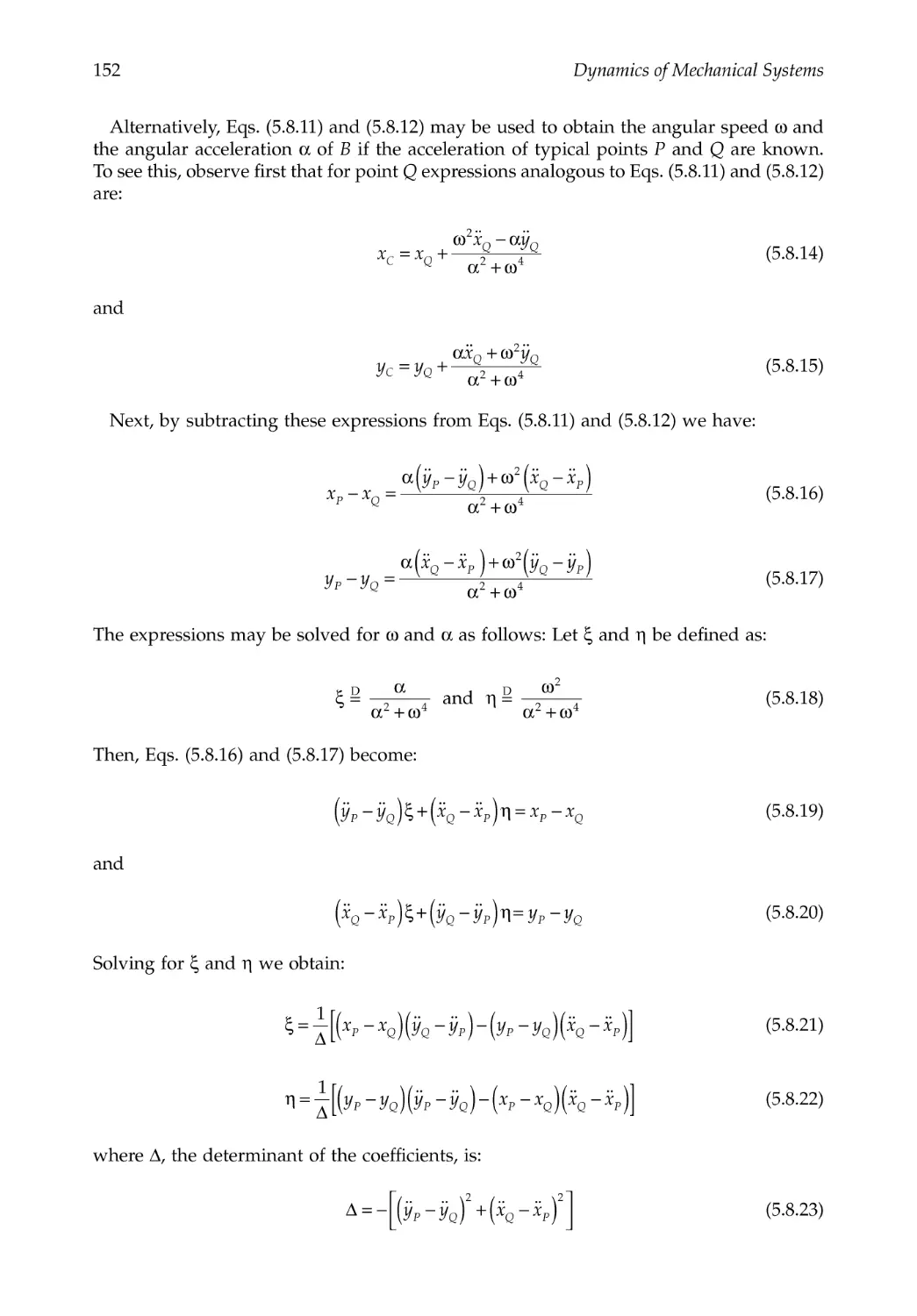
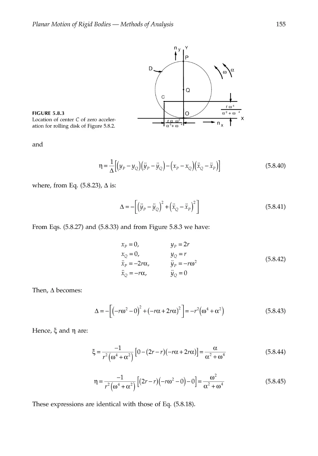
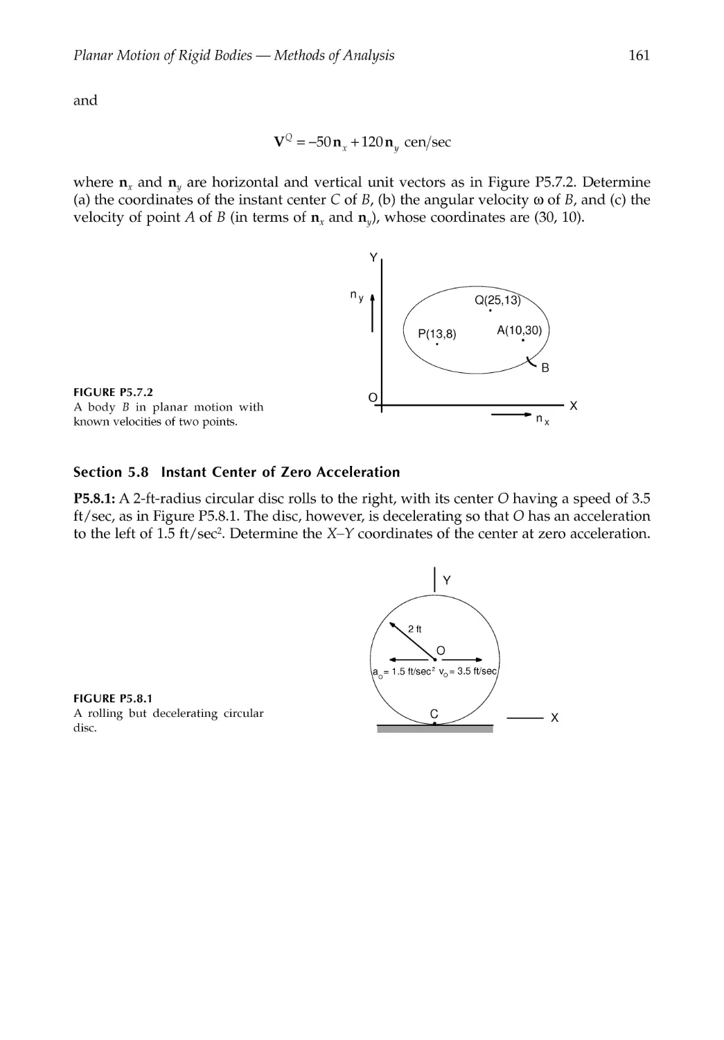
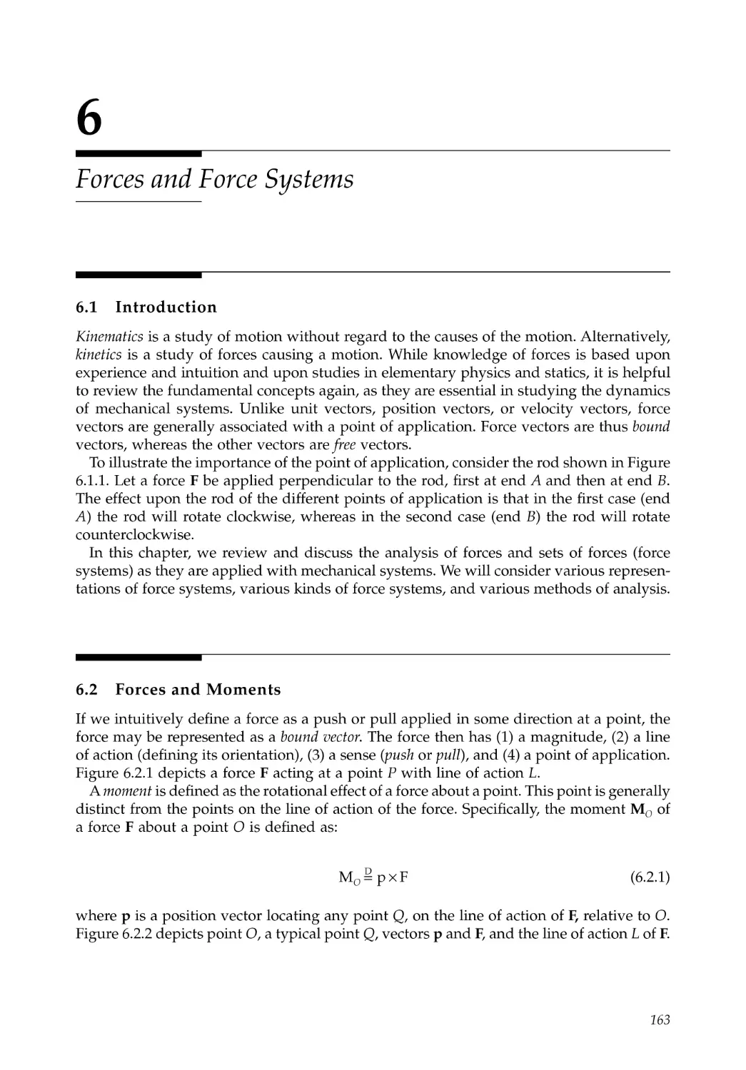
5.8 Instant Center of Zero Acceleration ..............................................................................150
Problems .......................................................................................................................................156
Chapter 6 Forces and Force Systems ....................................................................................163
6.1 Introduction.......................................................................................................................163
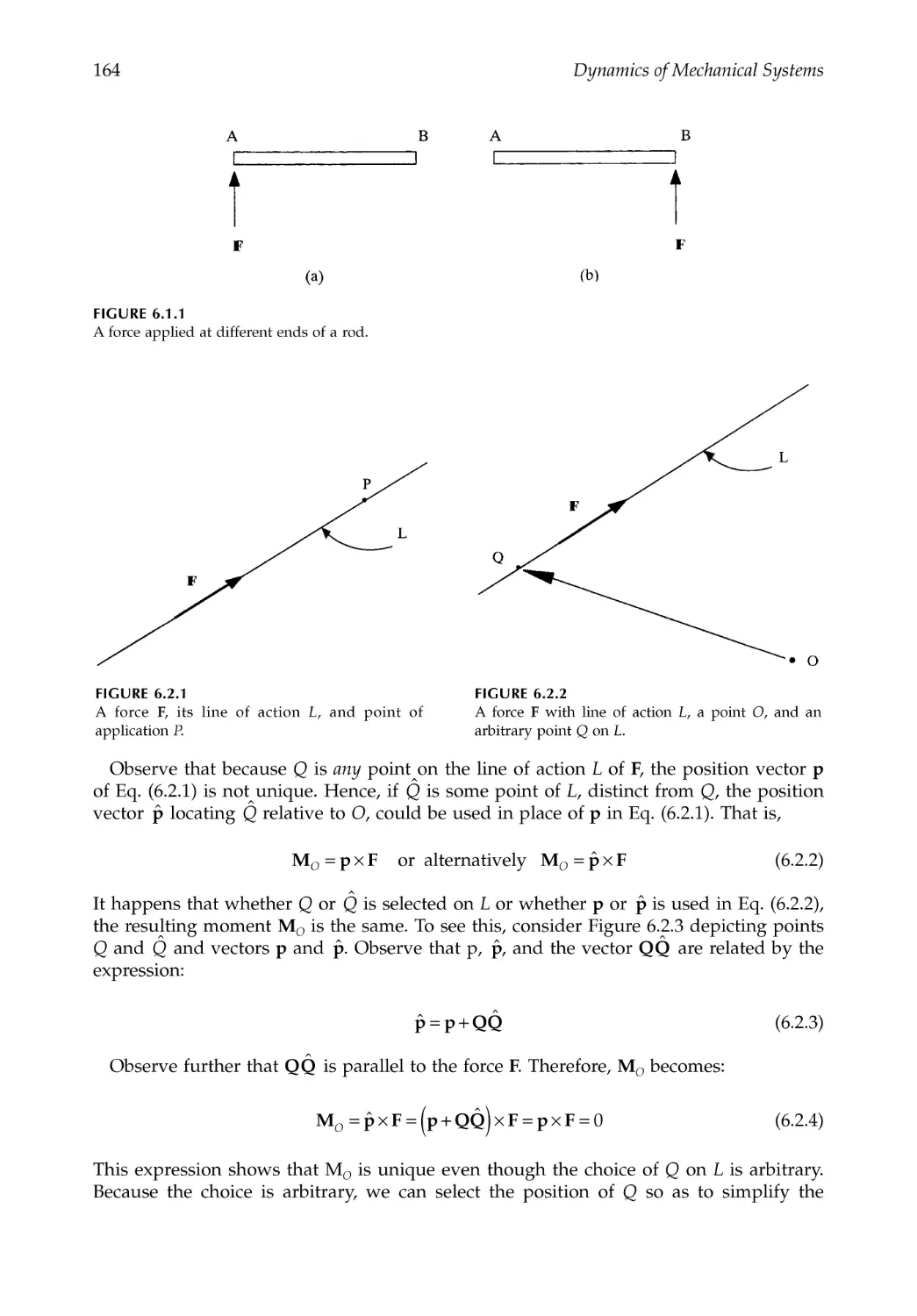
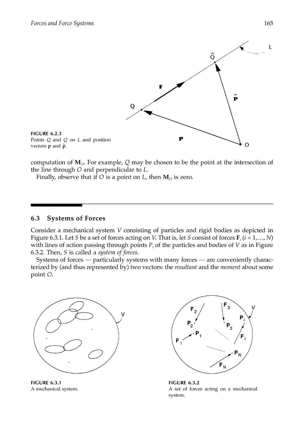
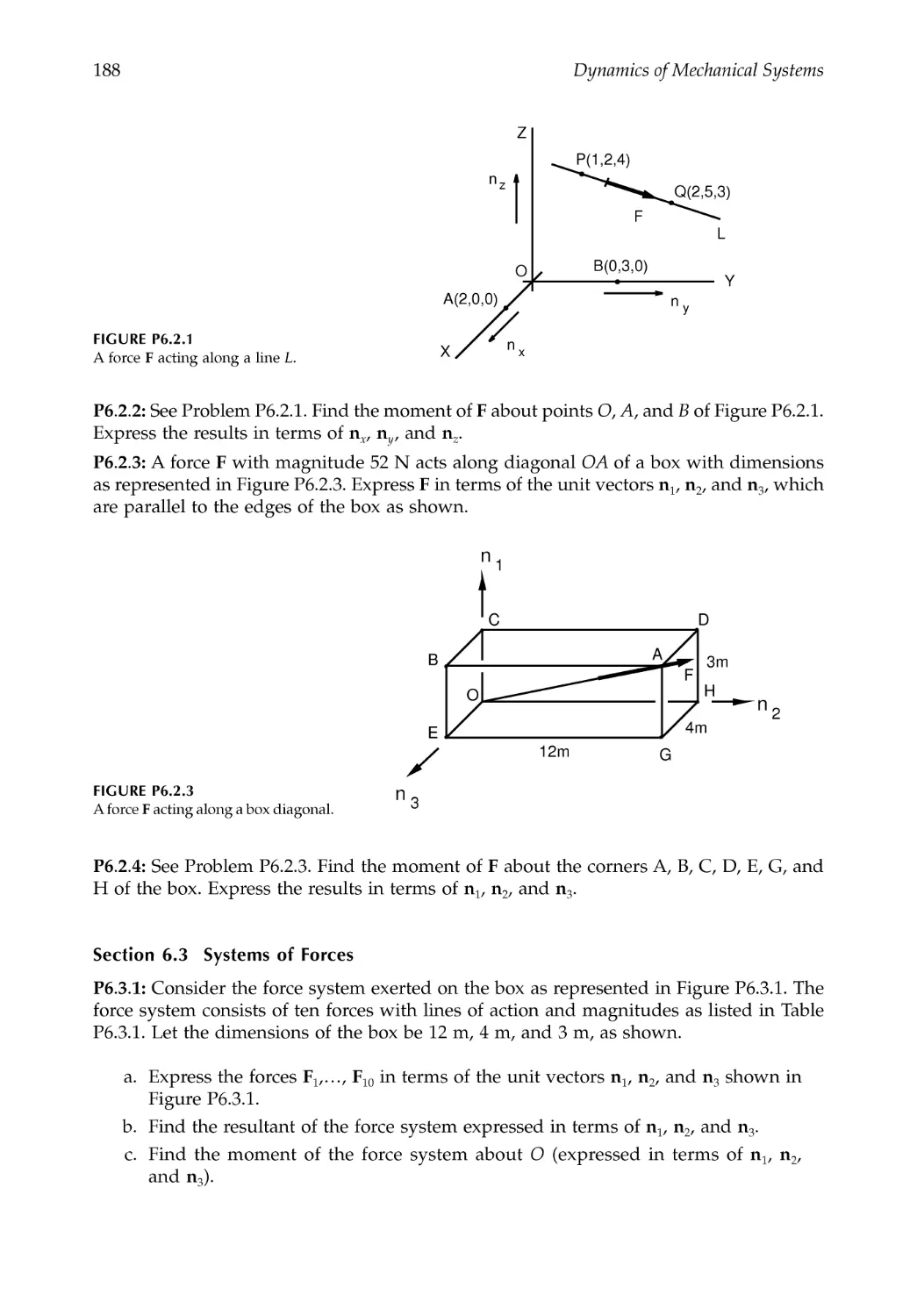
6.2 Forces and Moments........................................................................................................163
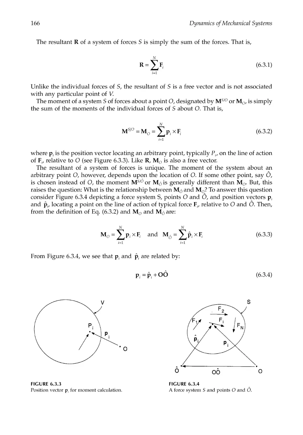
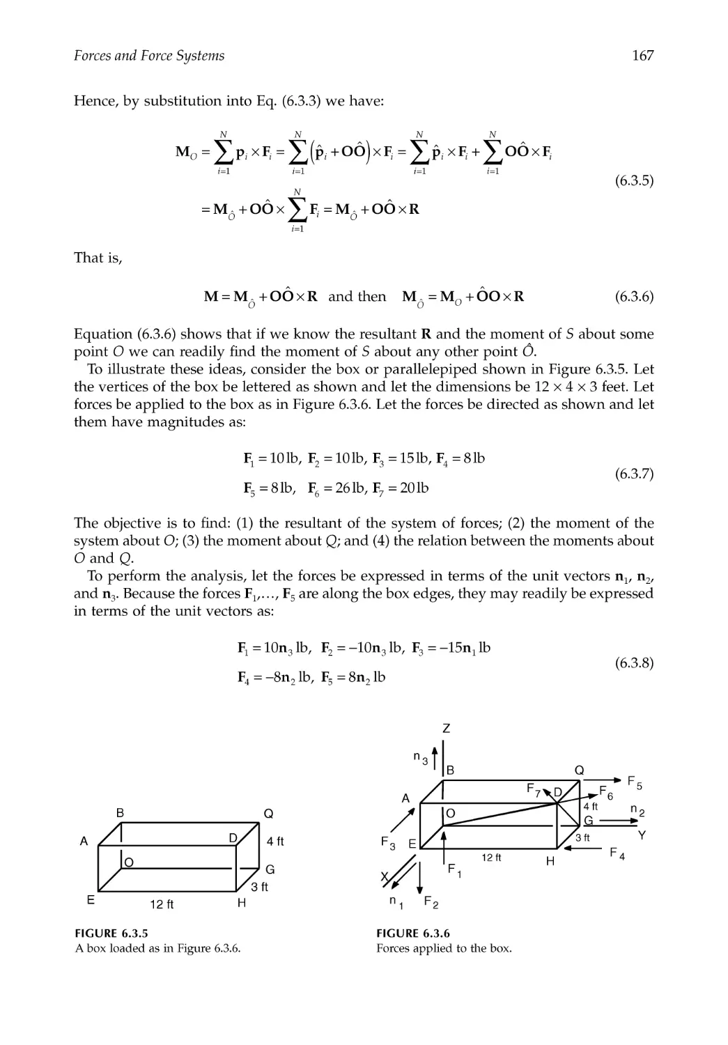
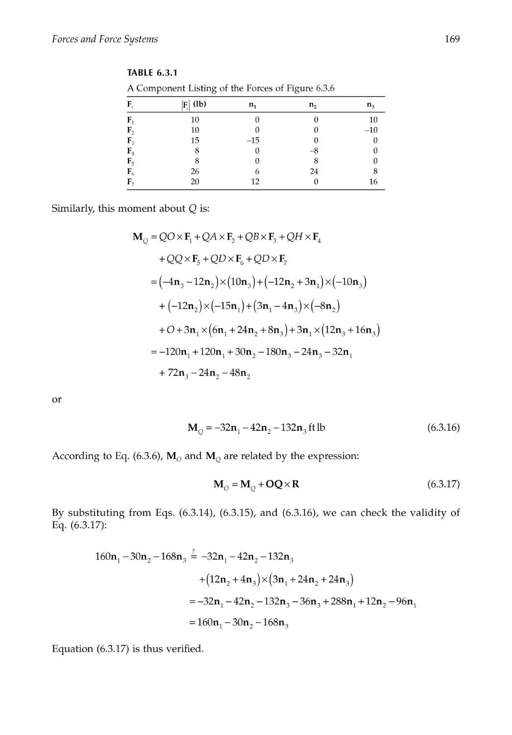
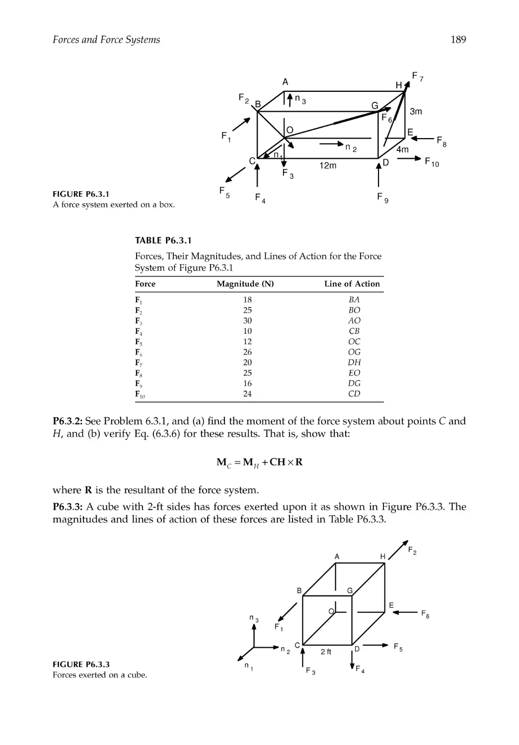
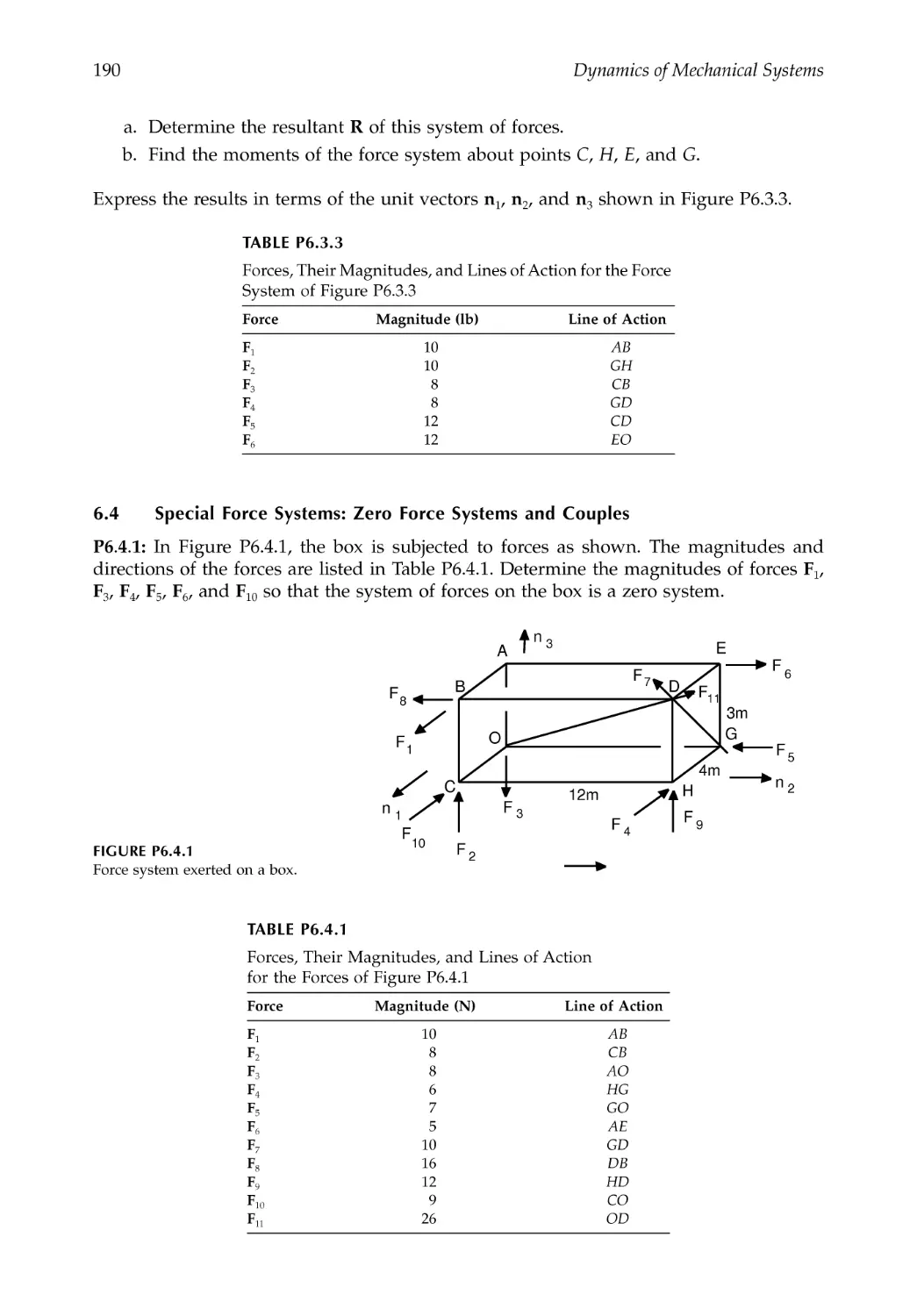
6.3 Systems of Forces .............................................................................................................165
6.4 Zero Force Systems ..........................................................................................................170
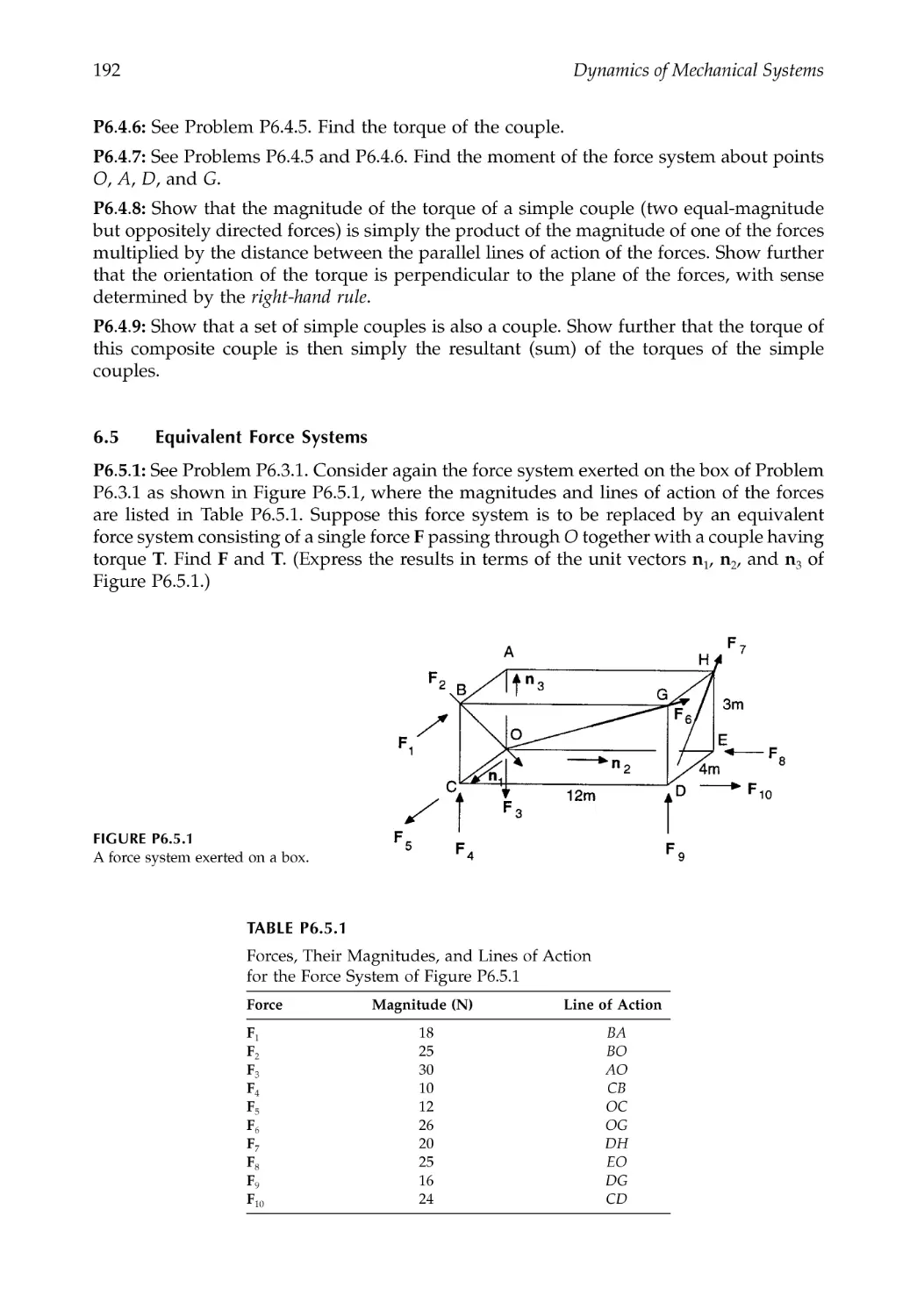
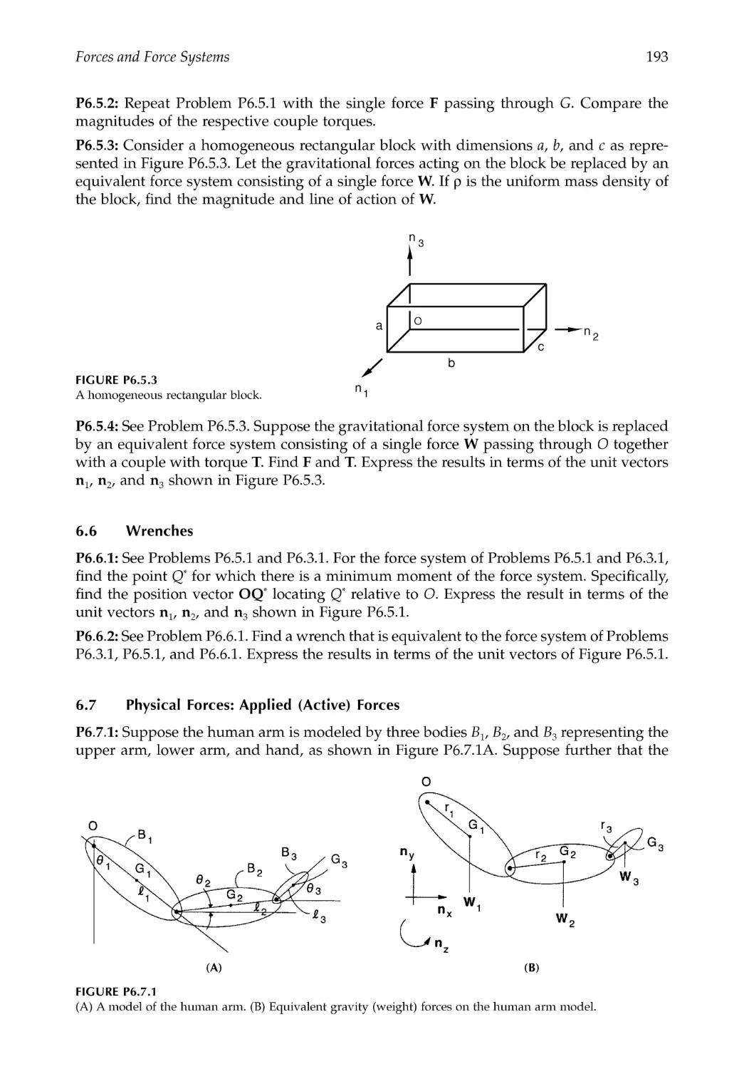
6.5 Couples ..............................................................................................................................170
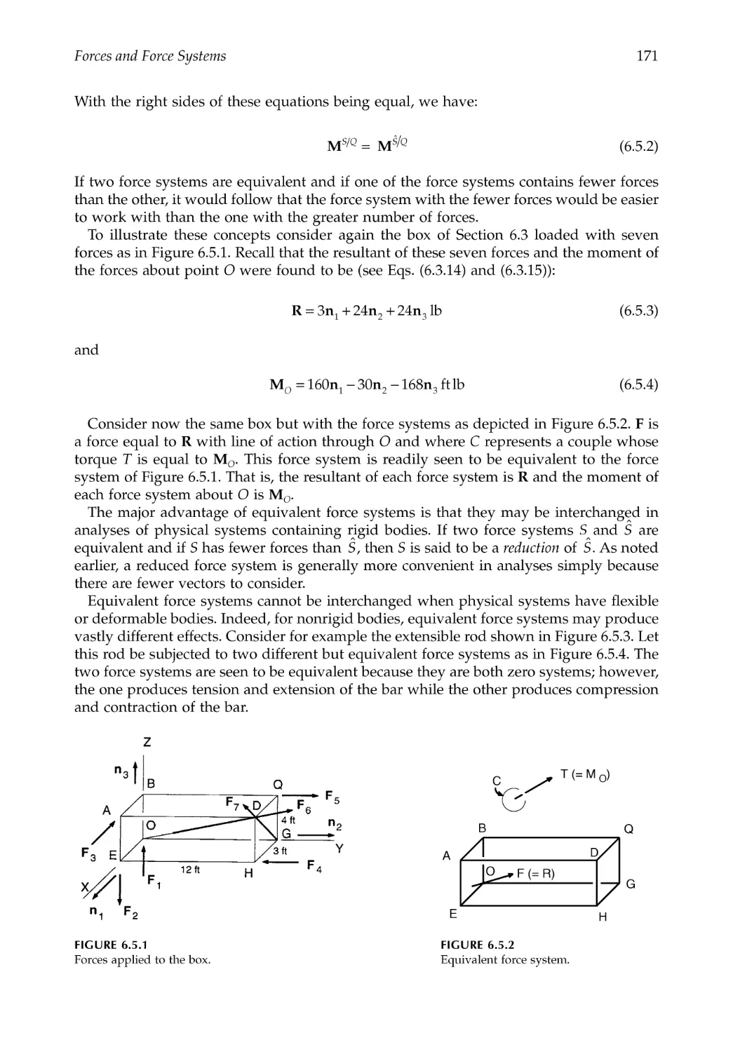
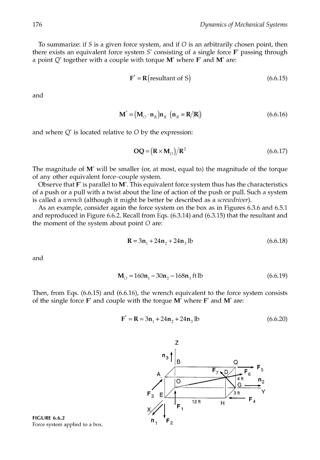
6.6 Wrenches............................................................................................................................173
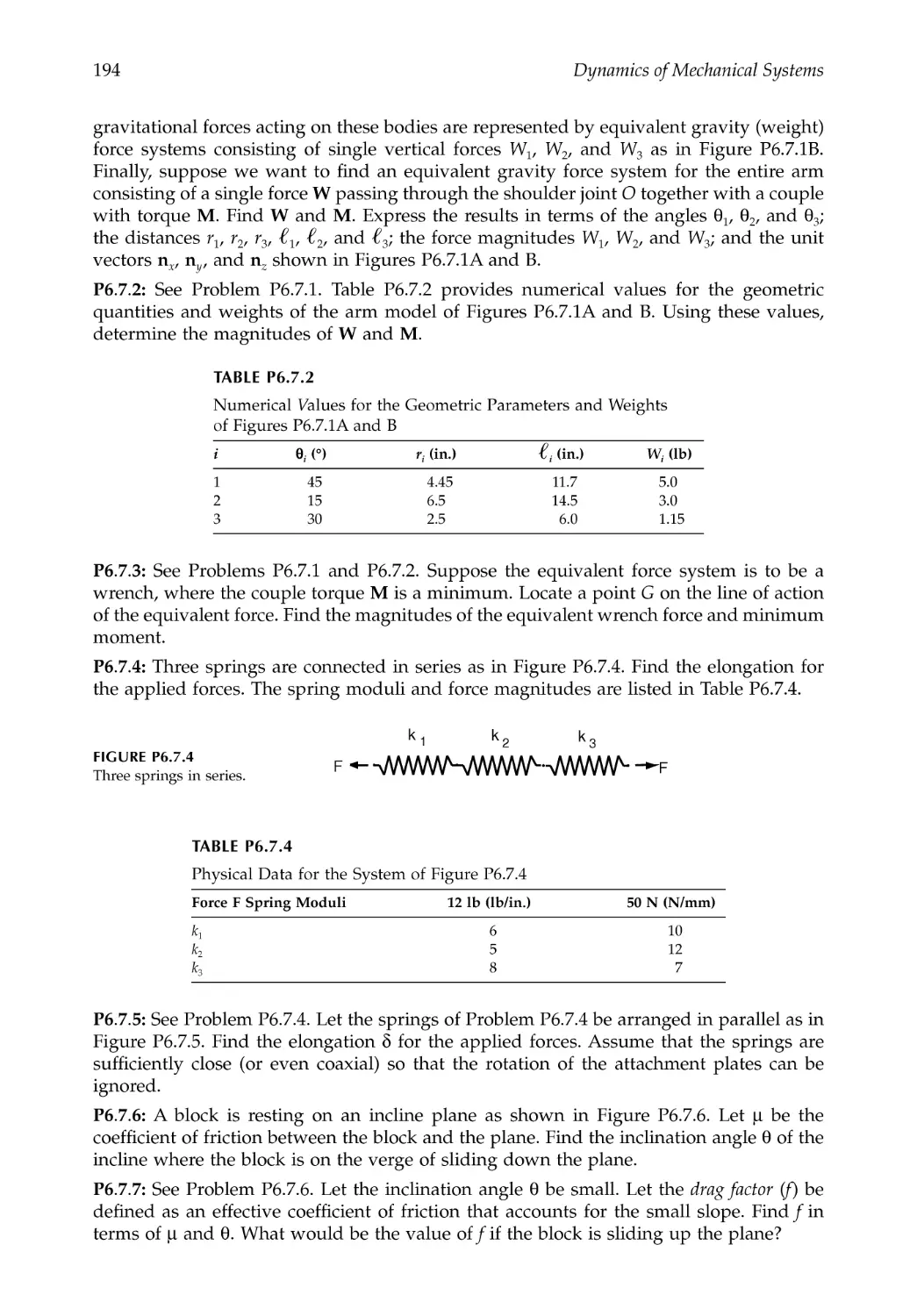
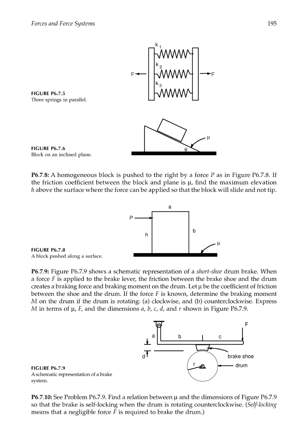
6.7 Physical Forces: Applied (Active) Forces .....................................................................177
6.7.1 Gravitational Forces .............................................................................................177
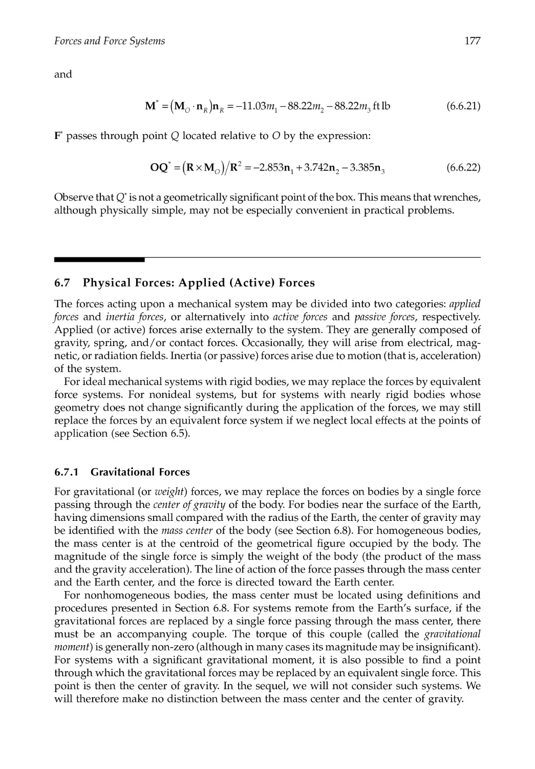
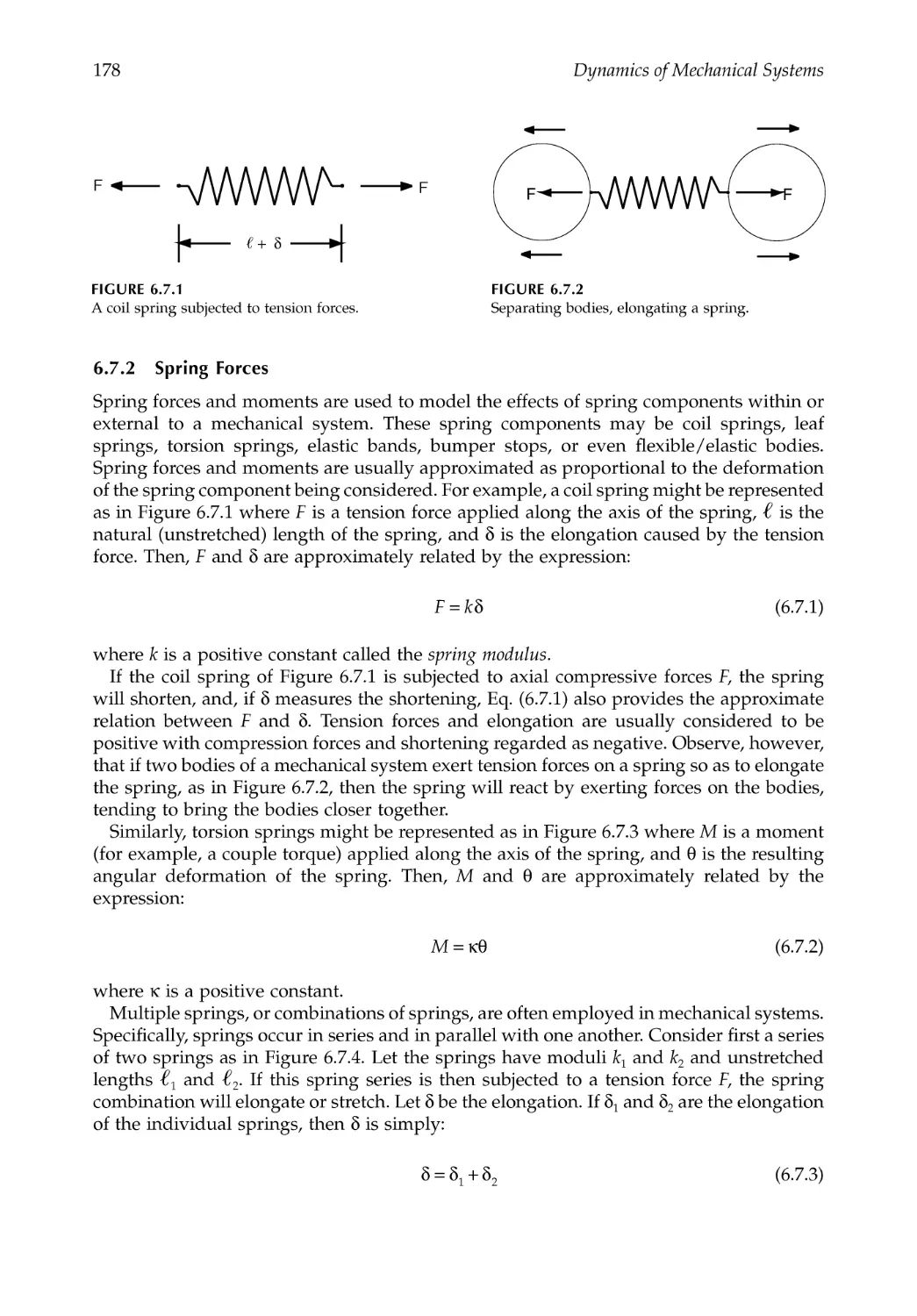
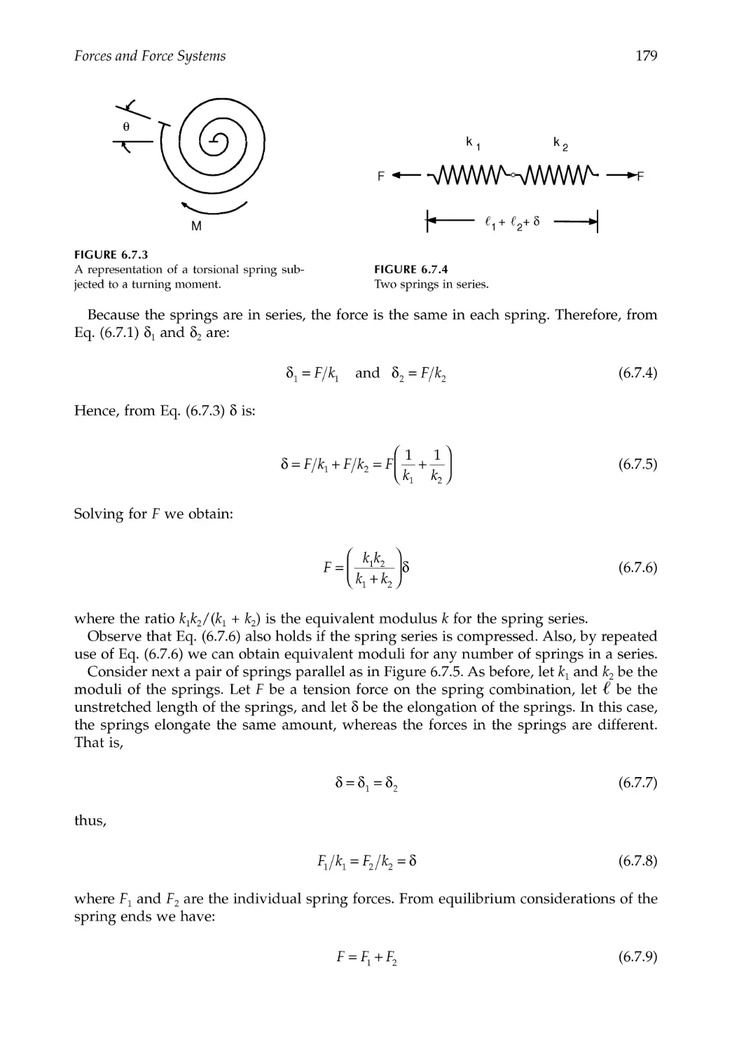
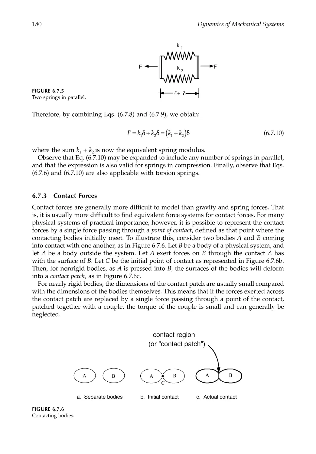
6.7.2 Spring Forces.........................................................................................................178
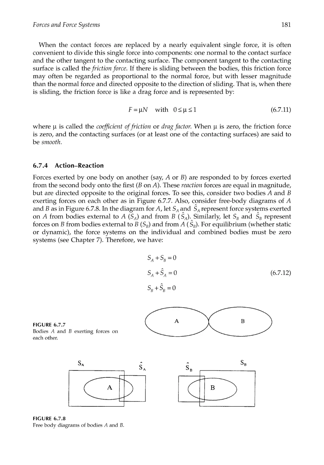
6.7.3 Contact Forces.......................................................................................................180
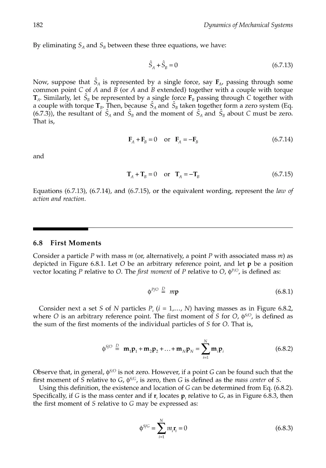
6.7.4 Action--Reaction....................................................................................................181
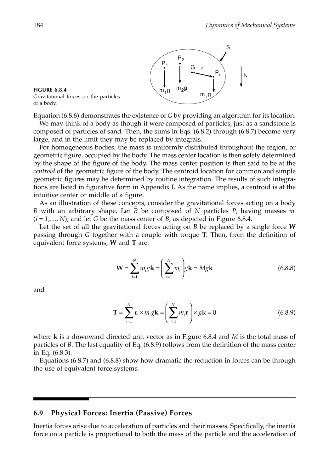
6.8 First Moments ...................................................................................................................182
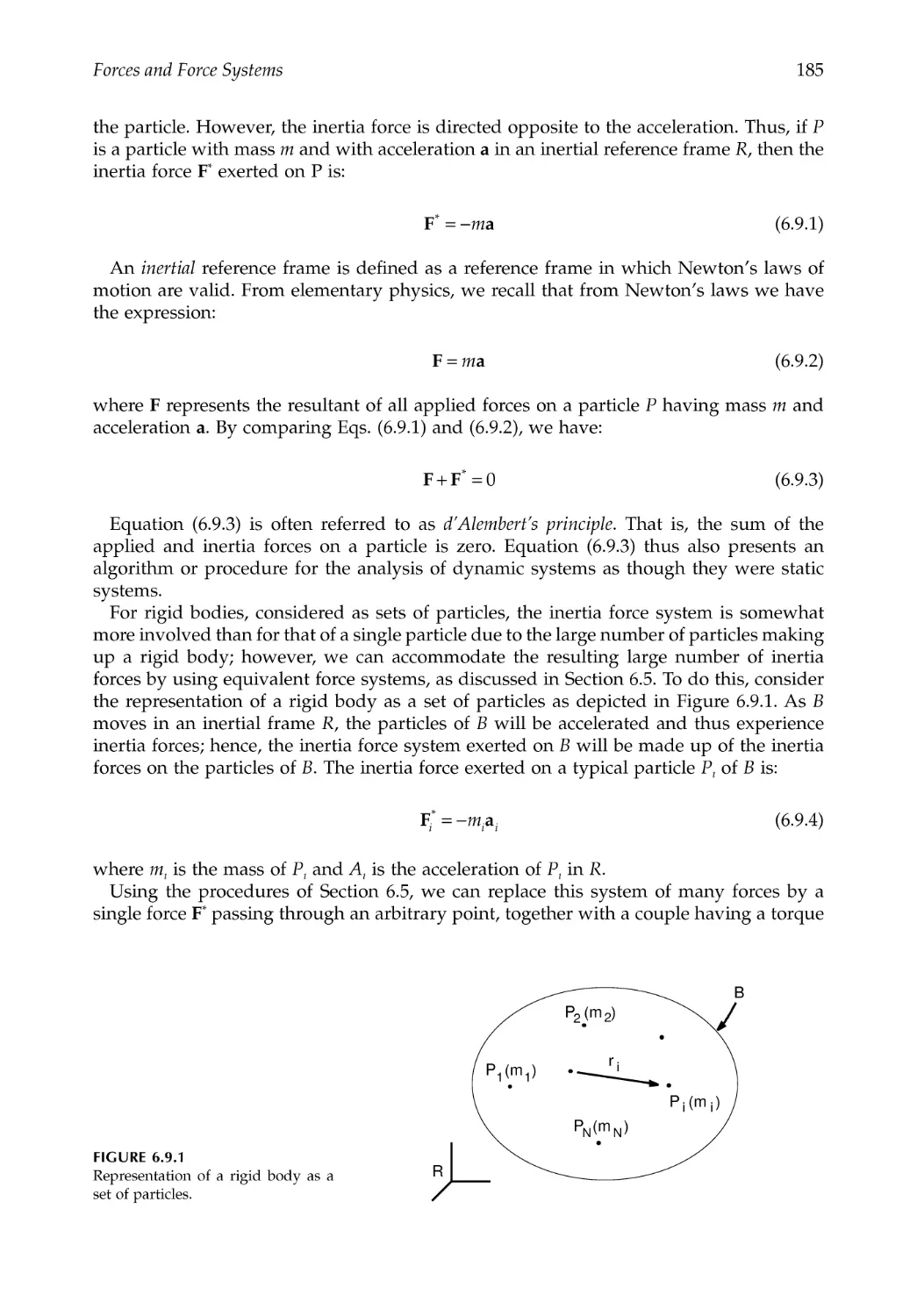
6.9 Physical Forces: Inertia (Passive) Forces ......................................................................184
References .....................................................................................................................................187
Problems .......................................................................................................................................187
Chapter 7 Inertia, Second Moment Vectors, Moments and Products of Inertia,
Inertia Dyadics .......................................................................................................199
7.1 Introduction.......................................................................................................................199
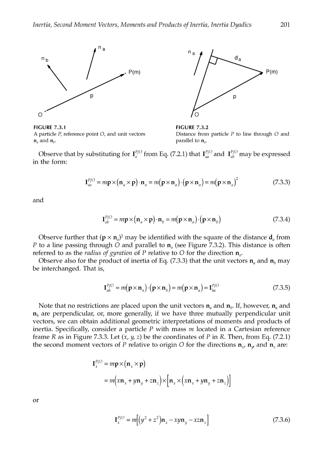
7.2 Second-Moment Vectors..................................................................................................199
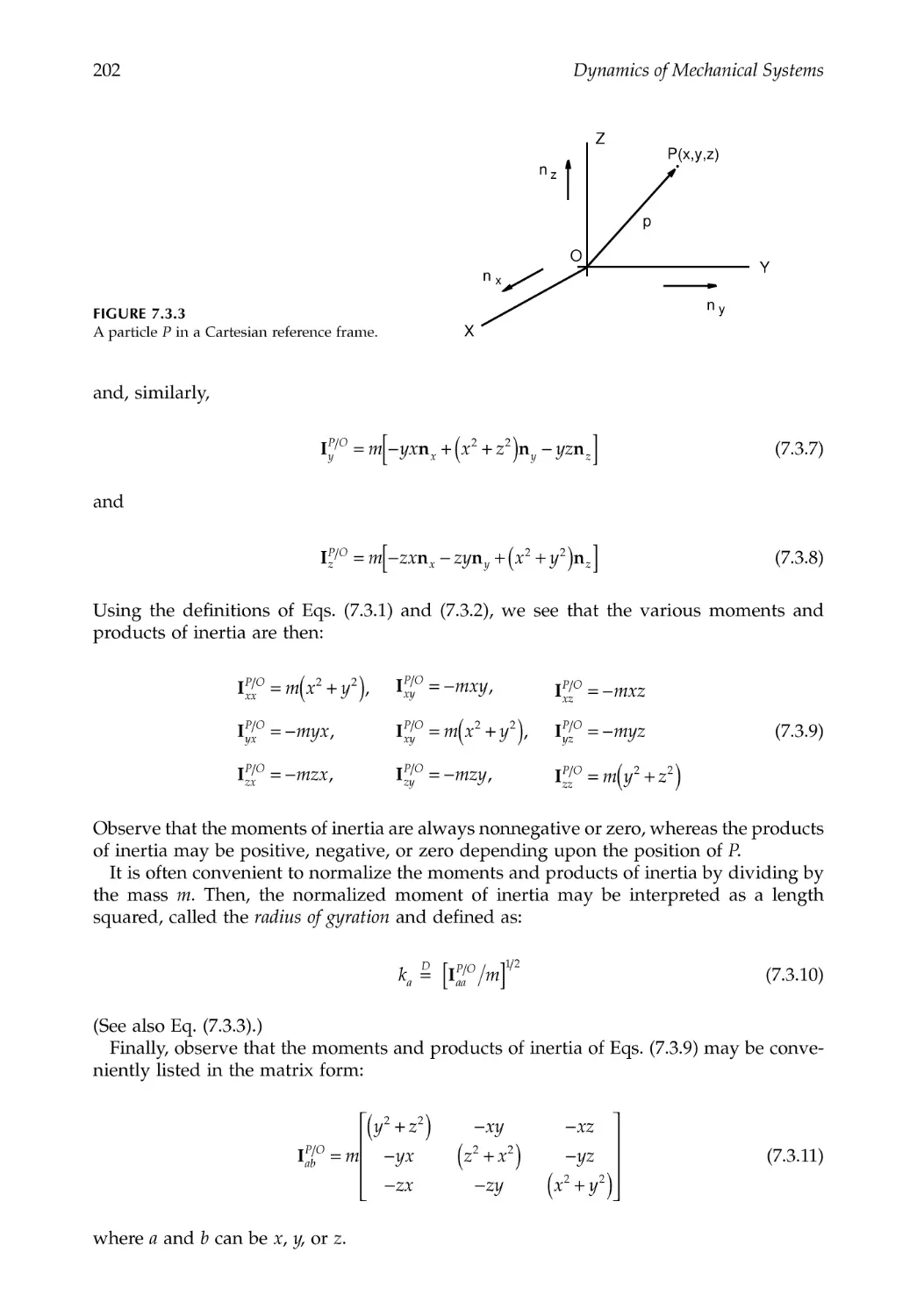
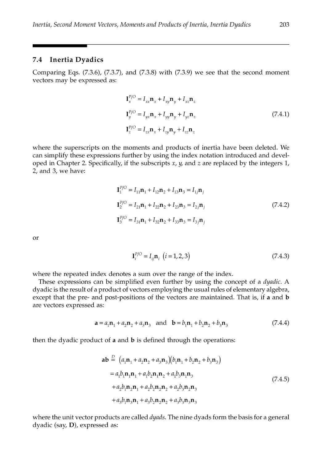
7.3 Moments and Products of Inertia .................................................................................200
7.4 Inertia Dyadics..................................................................................................................203
7.5 Transformation Rules ......................................................................................................205
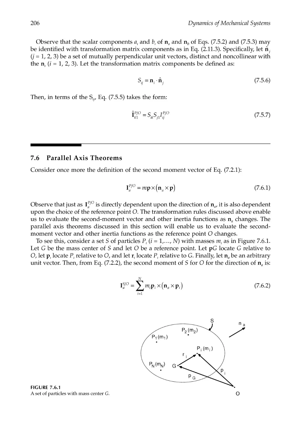
7.6 Parallel Axis Theorems....................................................................................................206
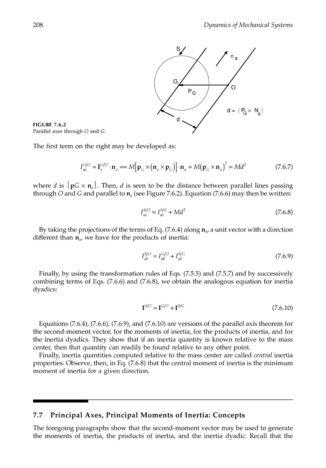
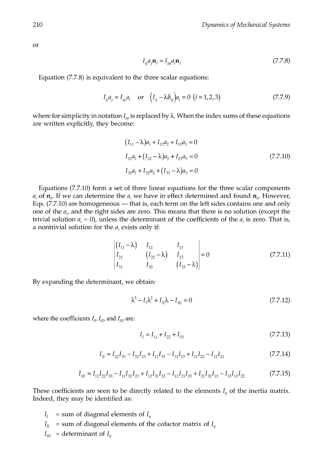
7.7 Principal Axes, Principal Moments of Inertia: Concepts ..........................................208
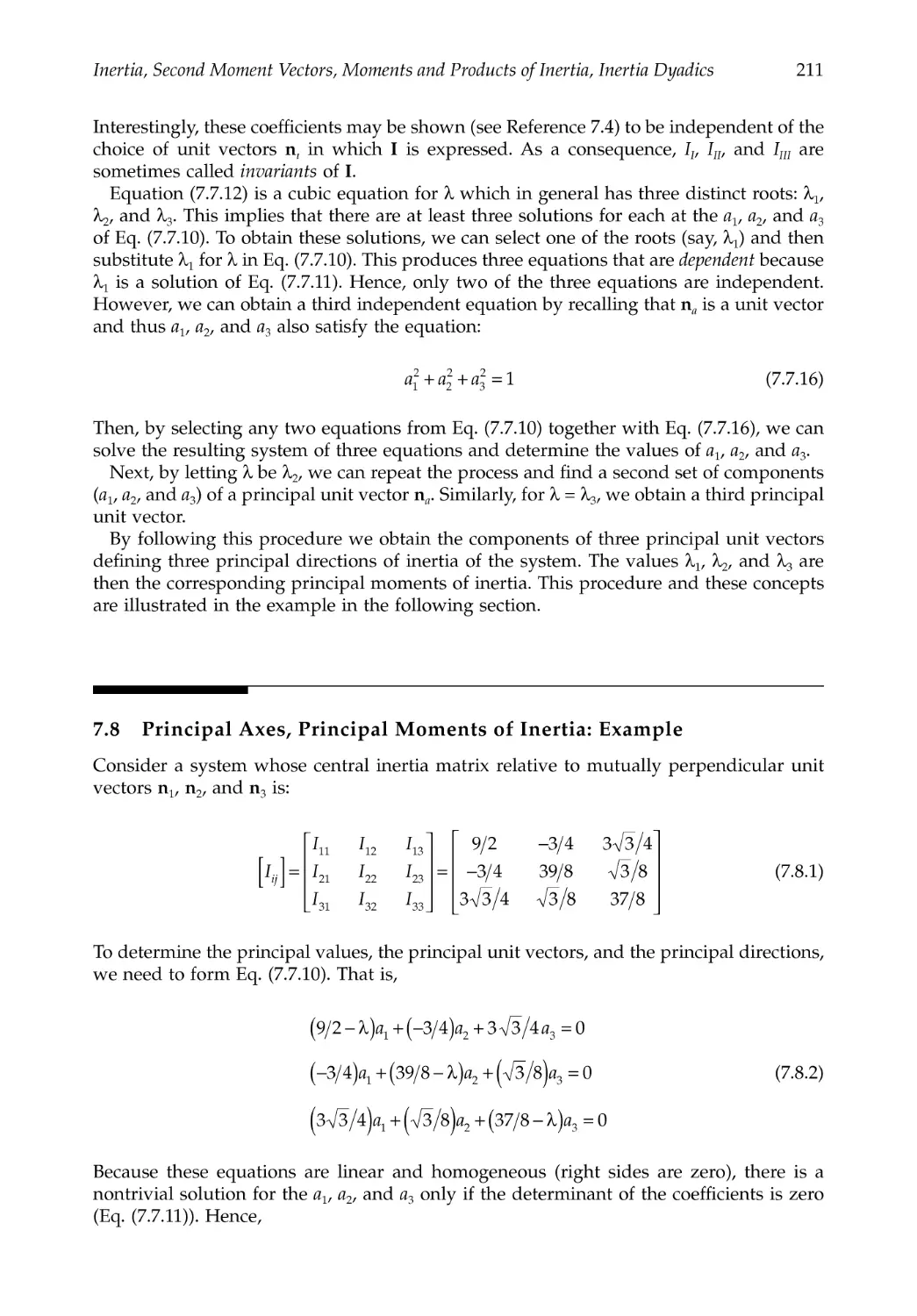
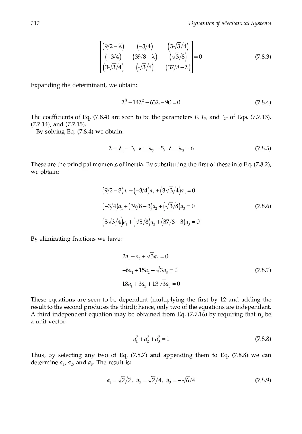
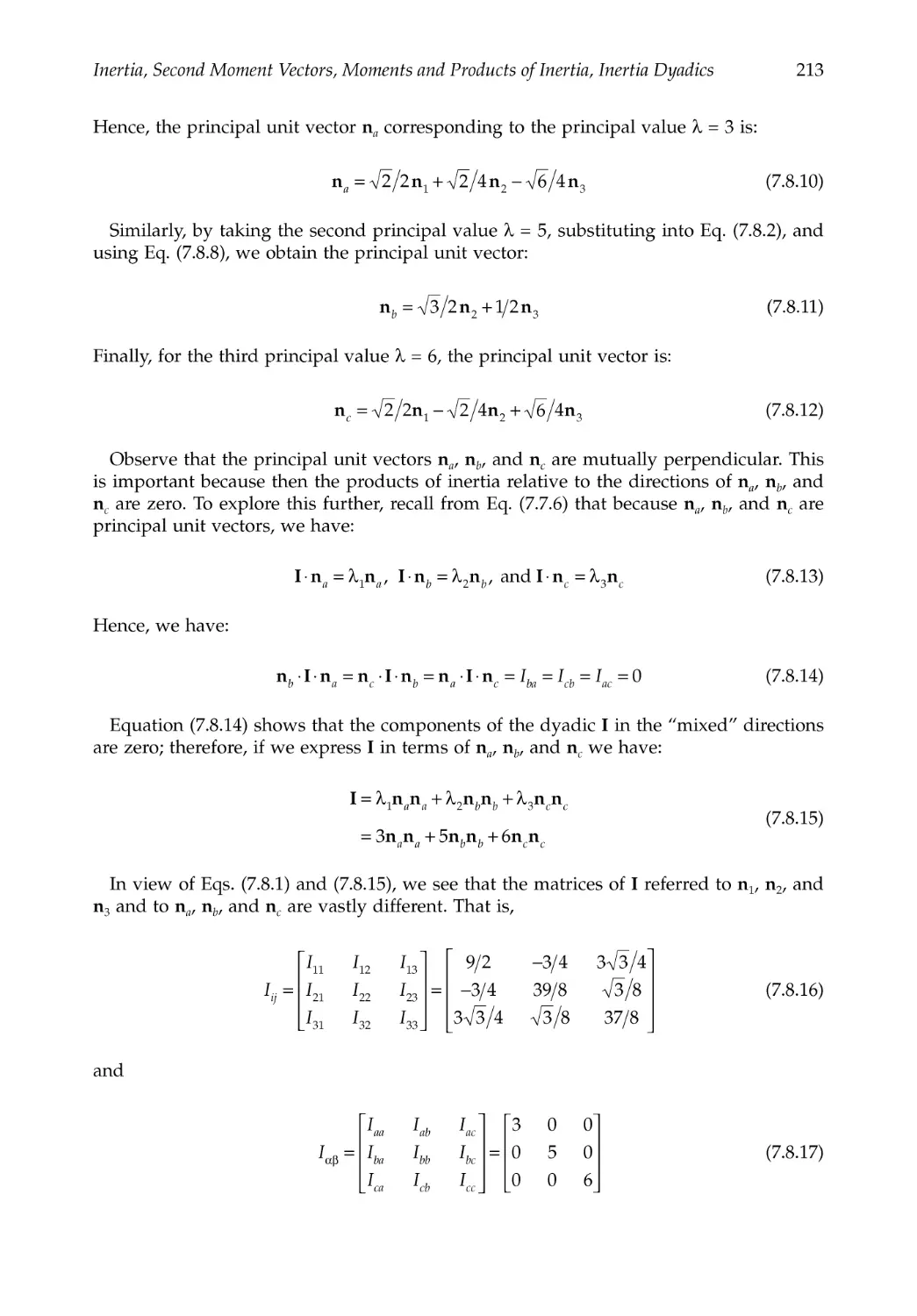
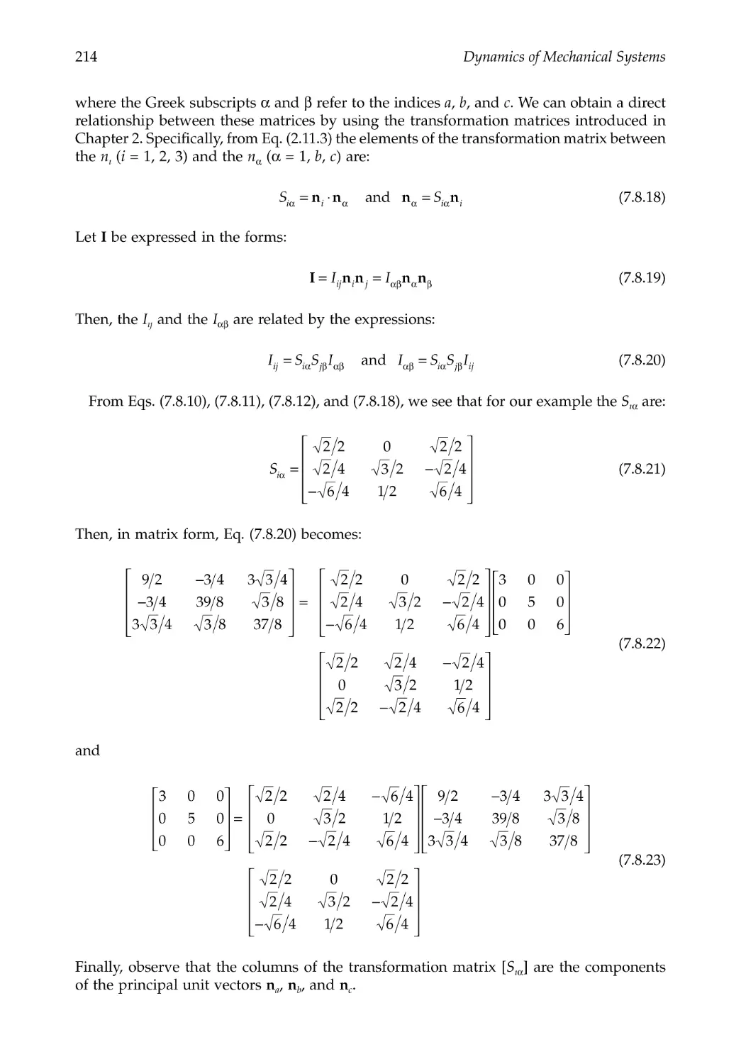
7.8 Principal Axes, Principal Moments of Inertia: Example ...........................................211
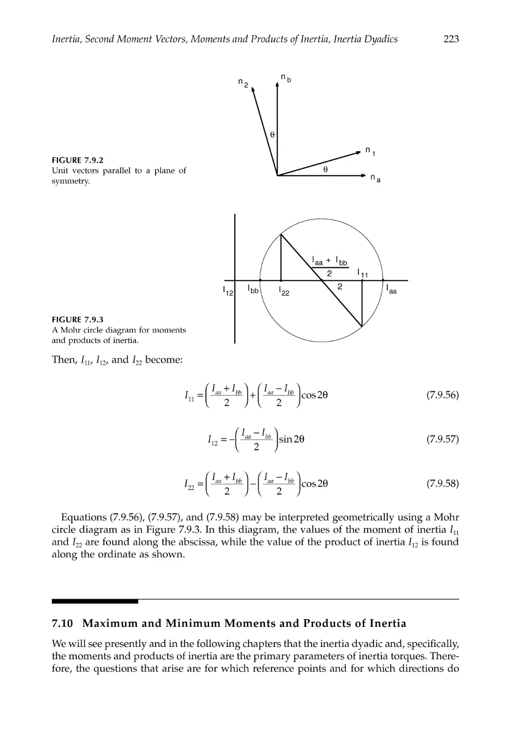
7.9 Principal Axes, Principal Moments of Inertia: Discussion........................................215
7.10 Maximum and Minimum Moments and Products of Inertia...................................223
7.11 Inertia Ellipsoid ................................................................................................................228
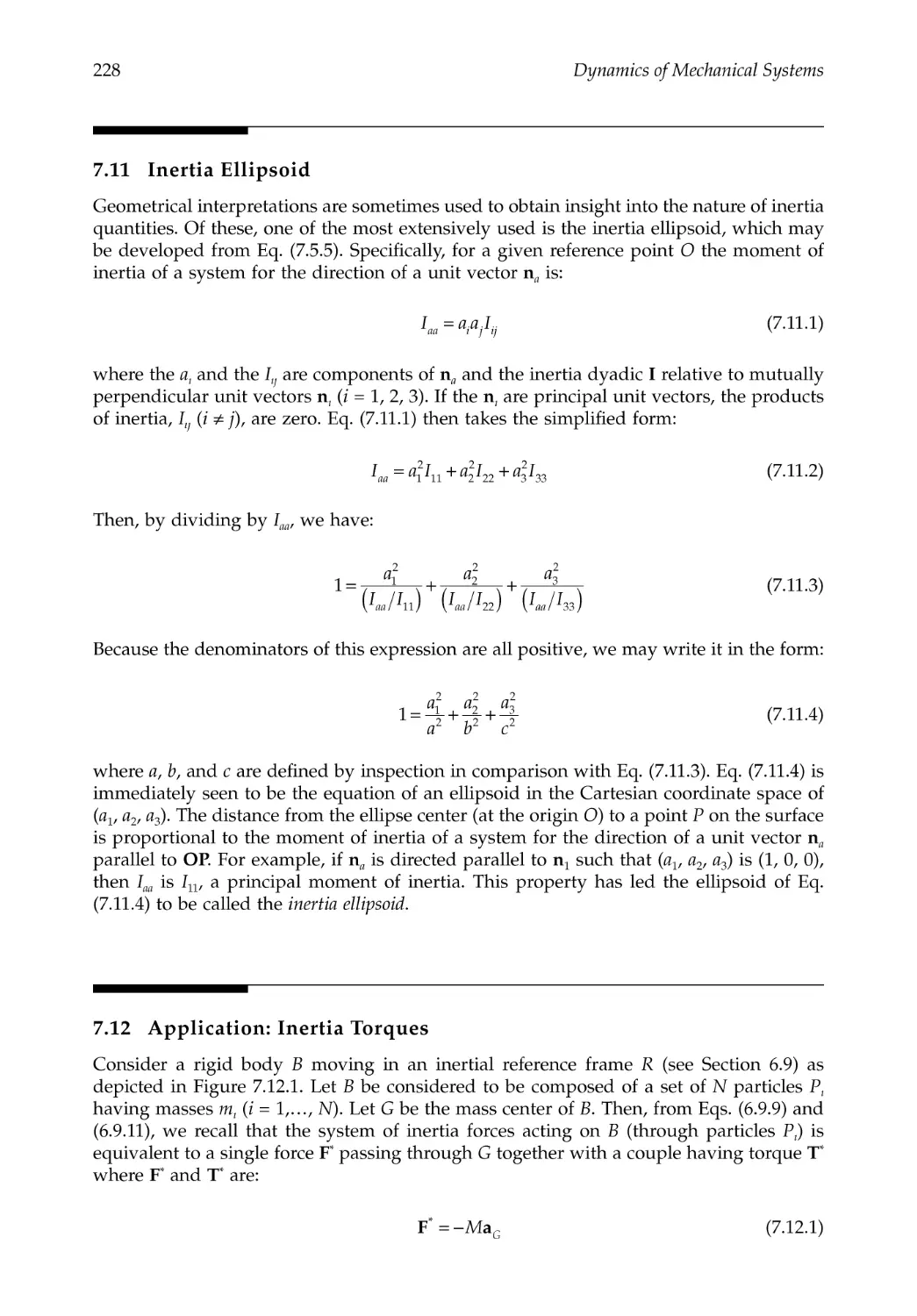
7.12 Application: Inertia Torques...........................................................................................228
References .....................................................................................................................................230
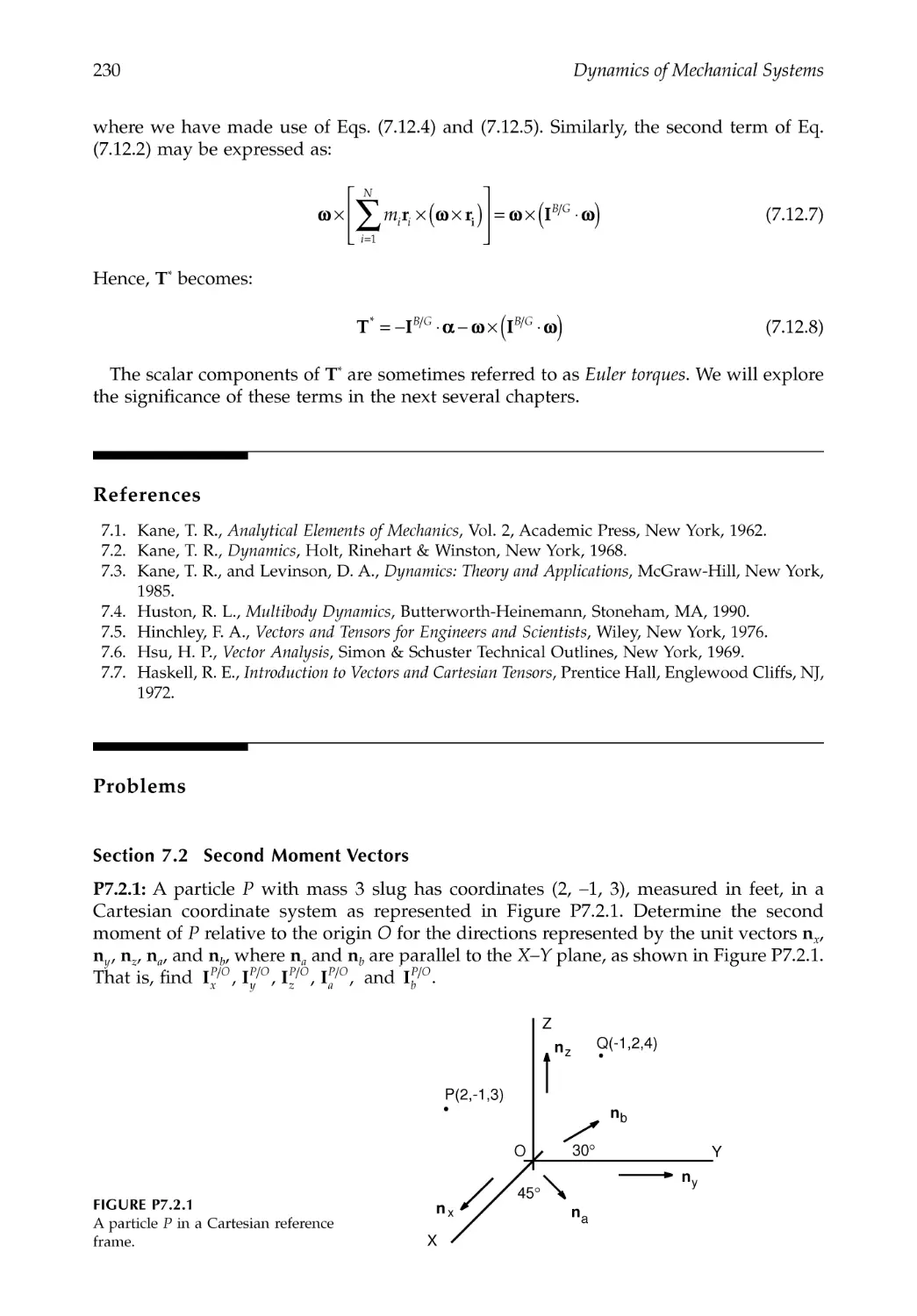
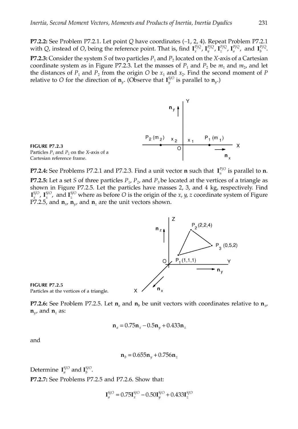
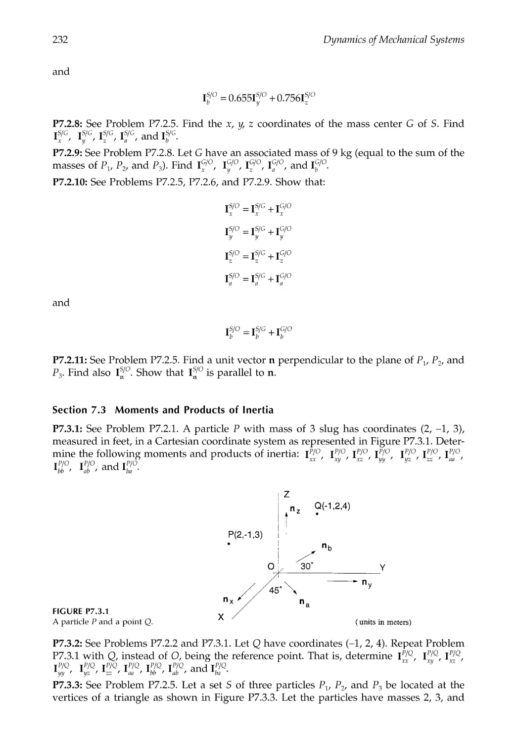
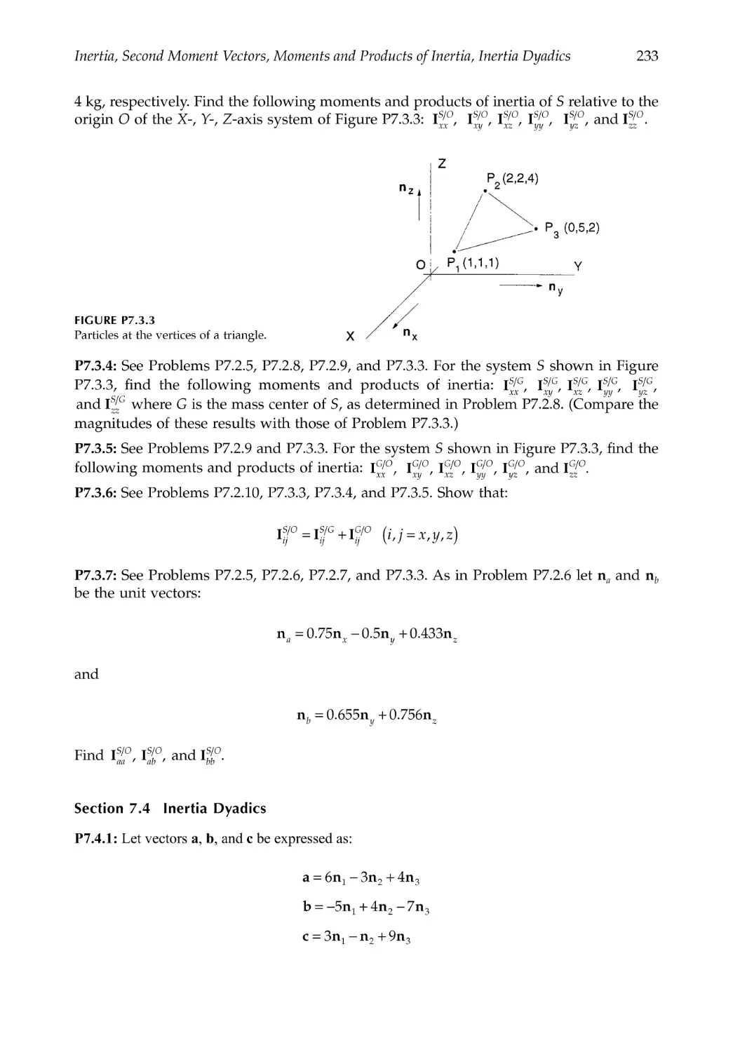
Problems .......................................................................................................................................230
Chapter 8 Principles of Dynamics: Newton's Laws and d'Alembert's Principle .........241
8.1 Introduction.......................................................................................................................241
8.2 Principles of Dynamics ...................................................................................................242
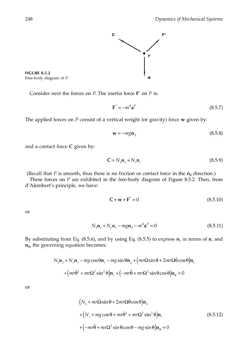
8.3 d'Alembert's Principle.....................................................................................................243
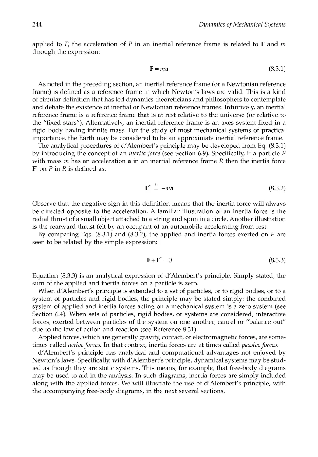
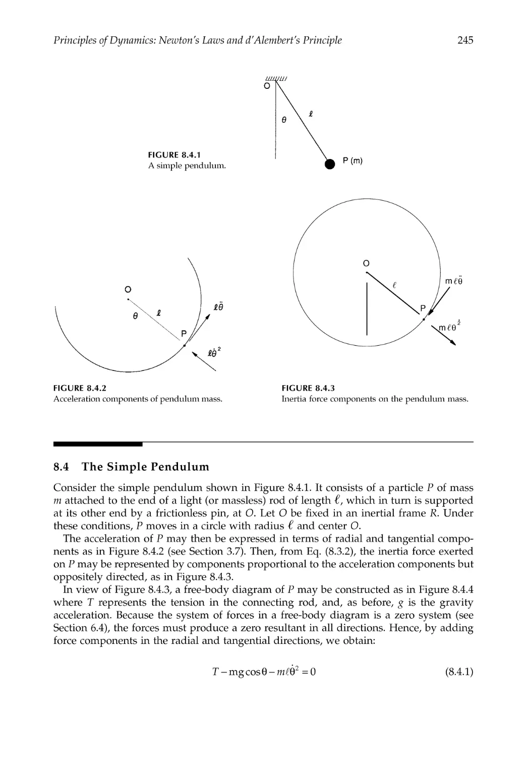
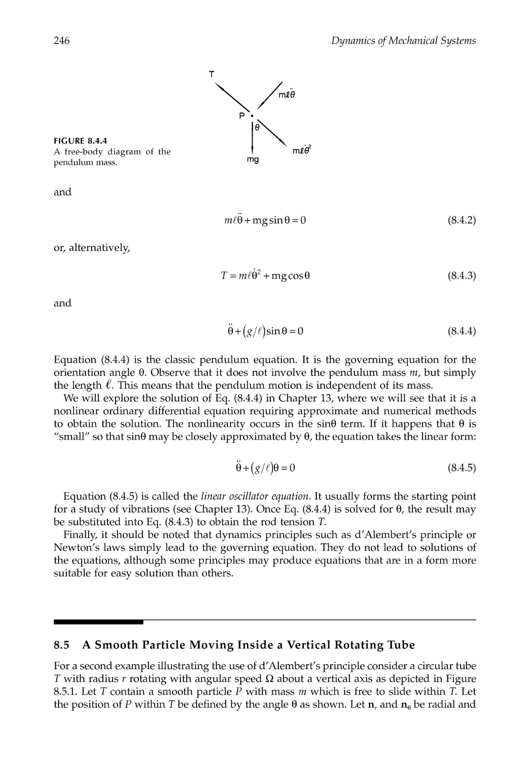
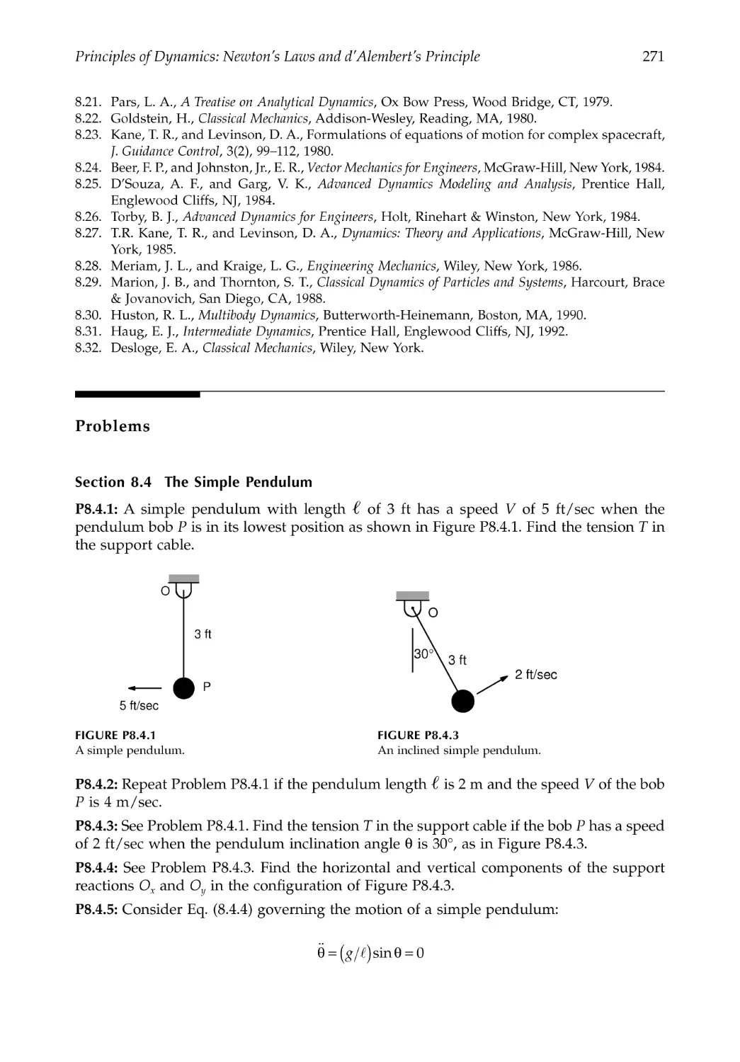
8.4 The Simple Pendulum .....................................................................................................245
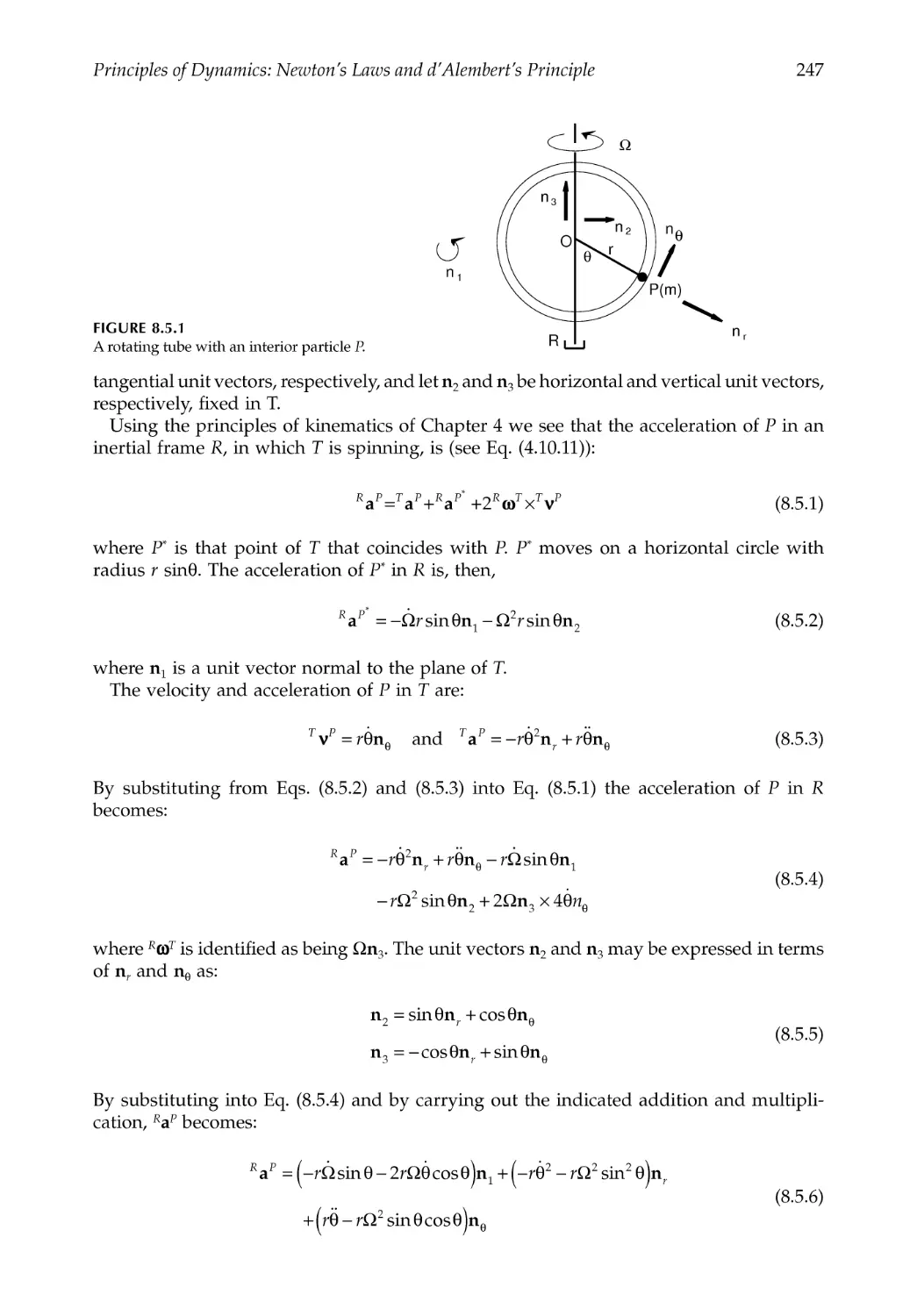
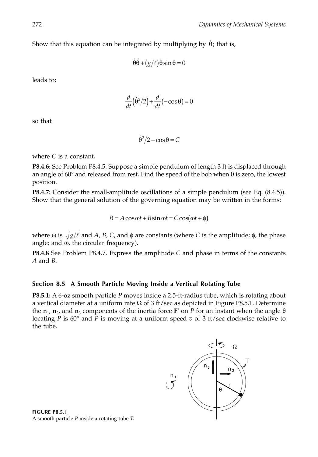
8.5 A Smooth Particle Moving Inside a Vertical Rotating Tube .....................................246
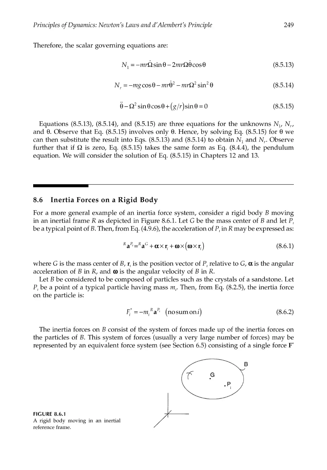
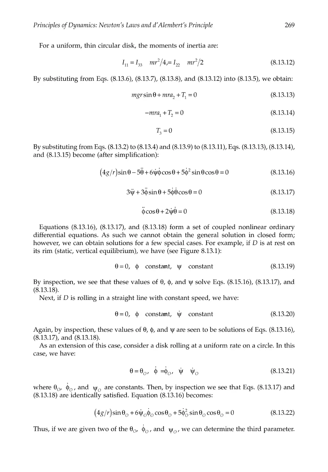
8.6 Inertia Forces on a Rigid Body ......................................................................................249
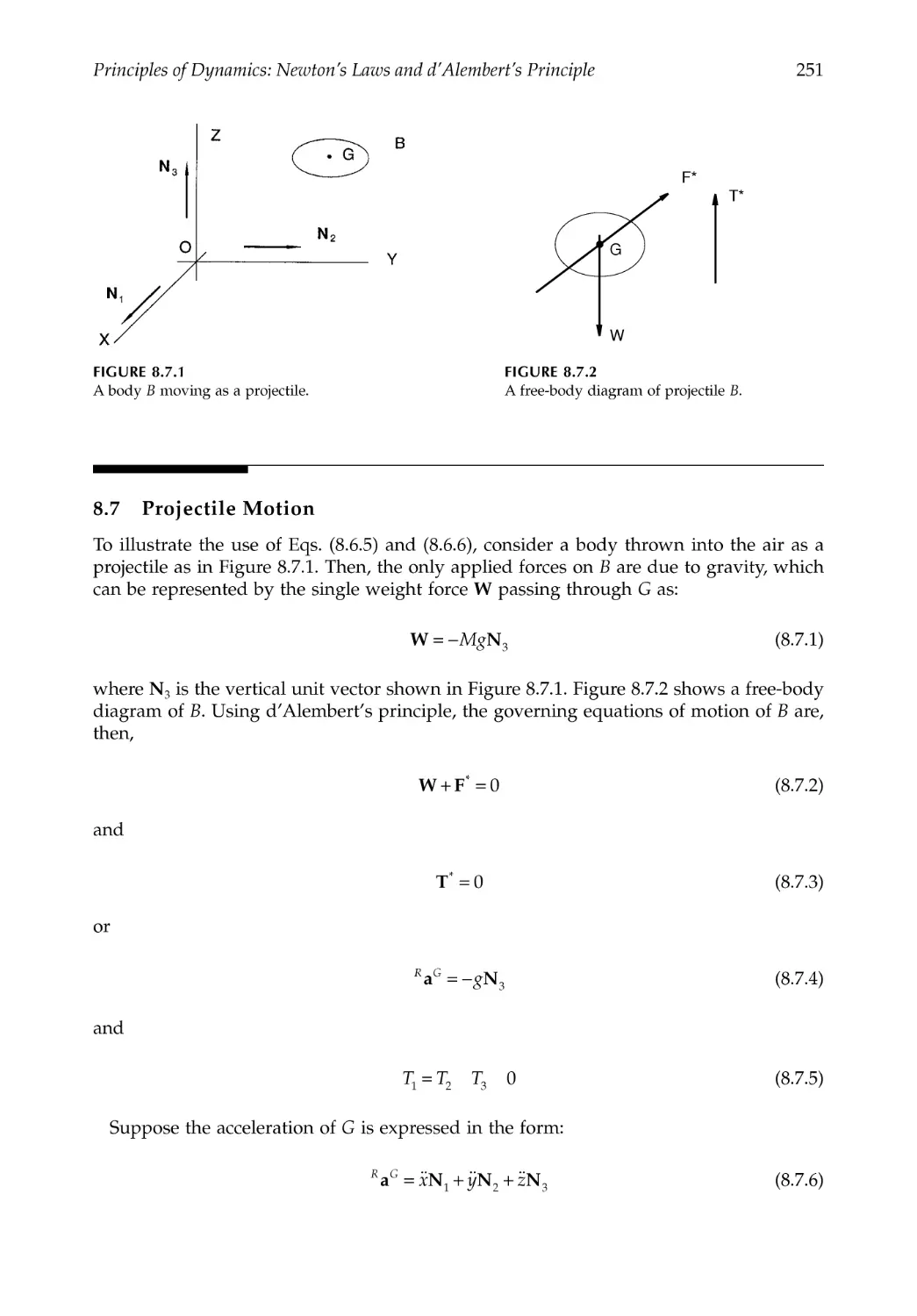
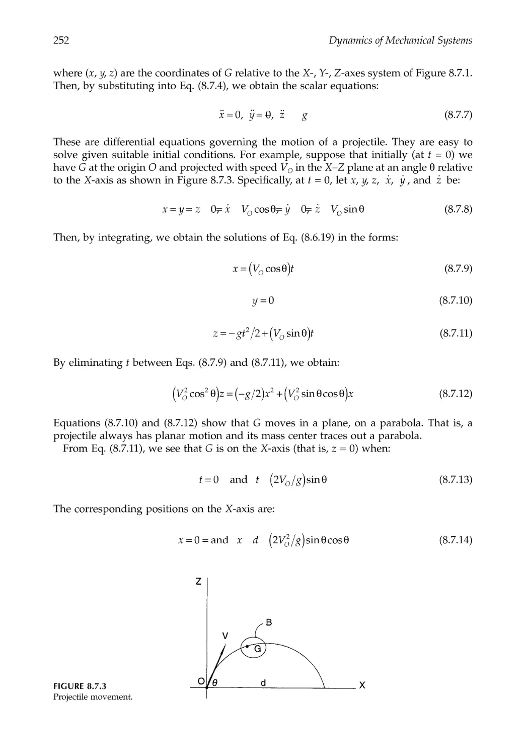
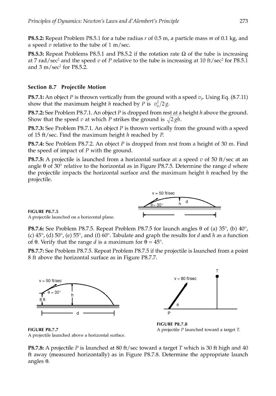
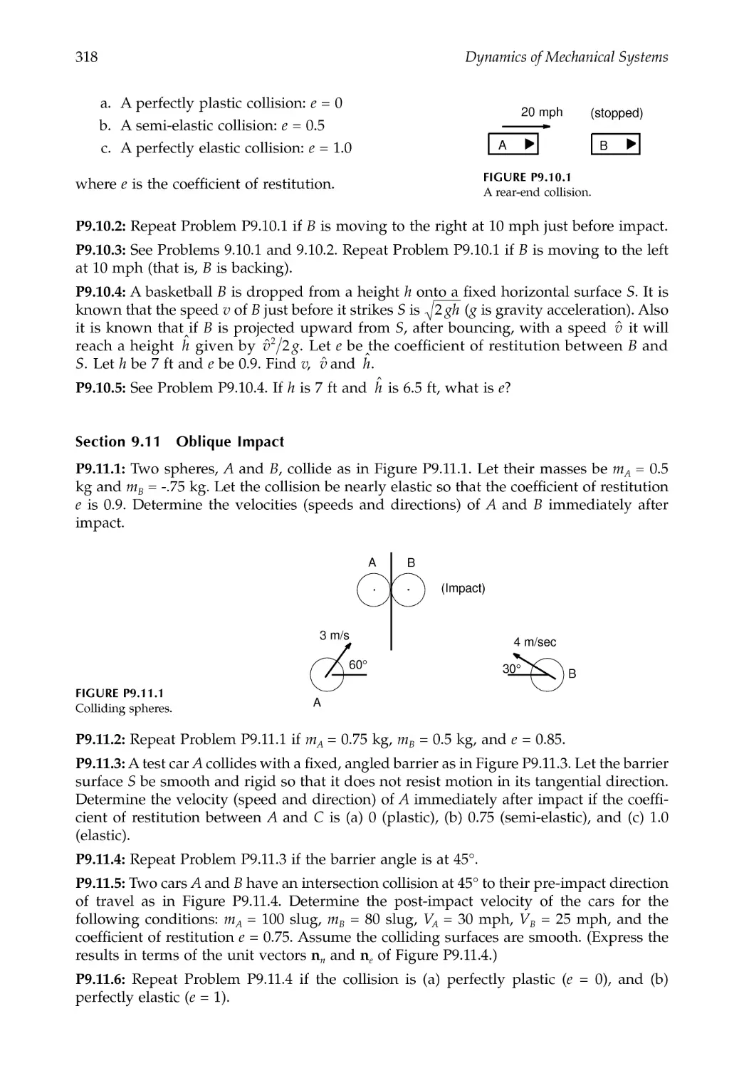
8.7 Projectile Motion ..............................................................................................................251
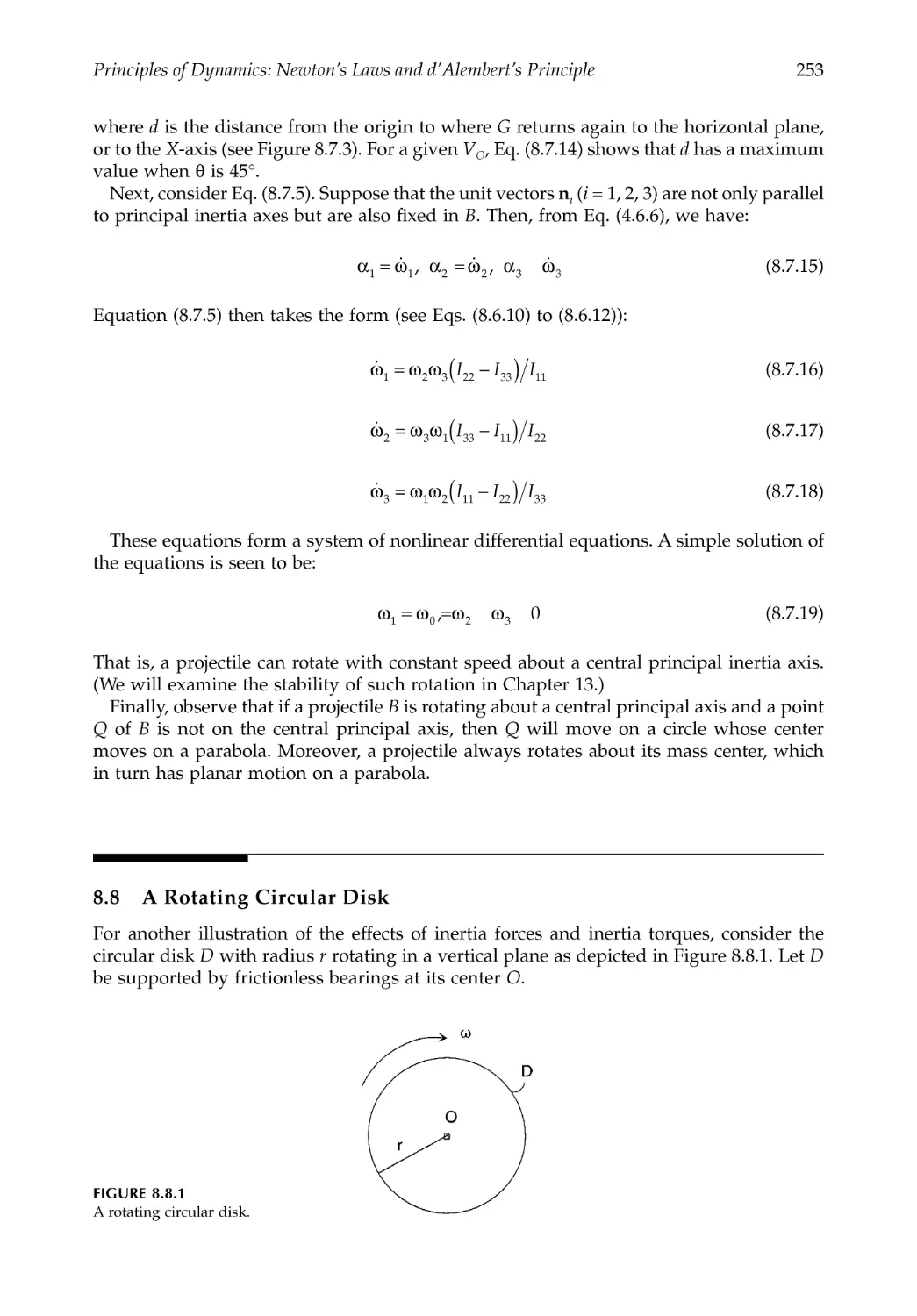
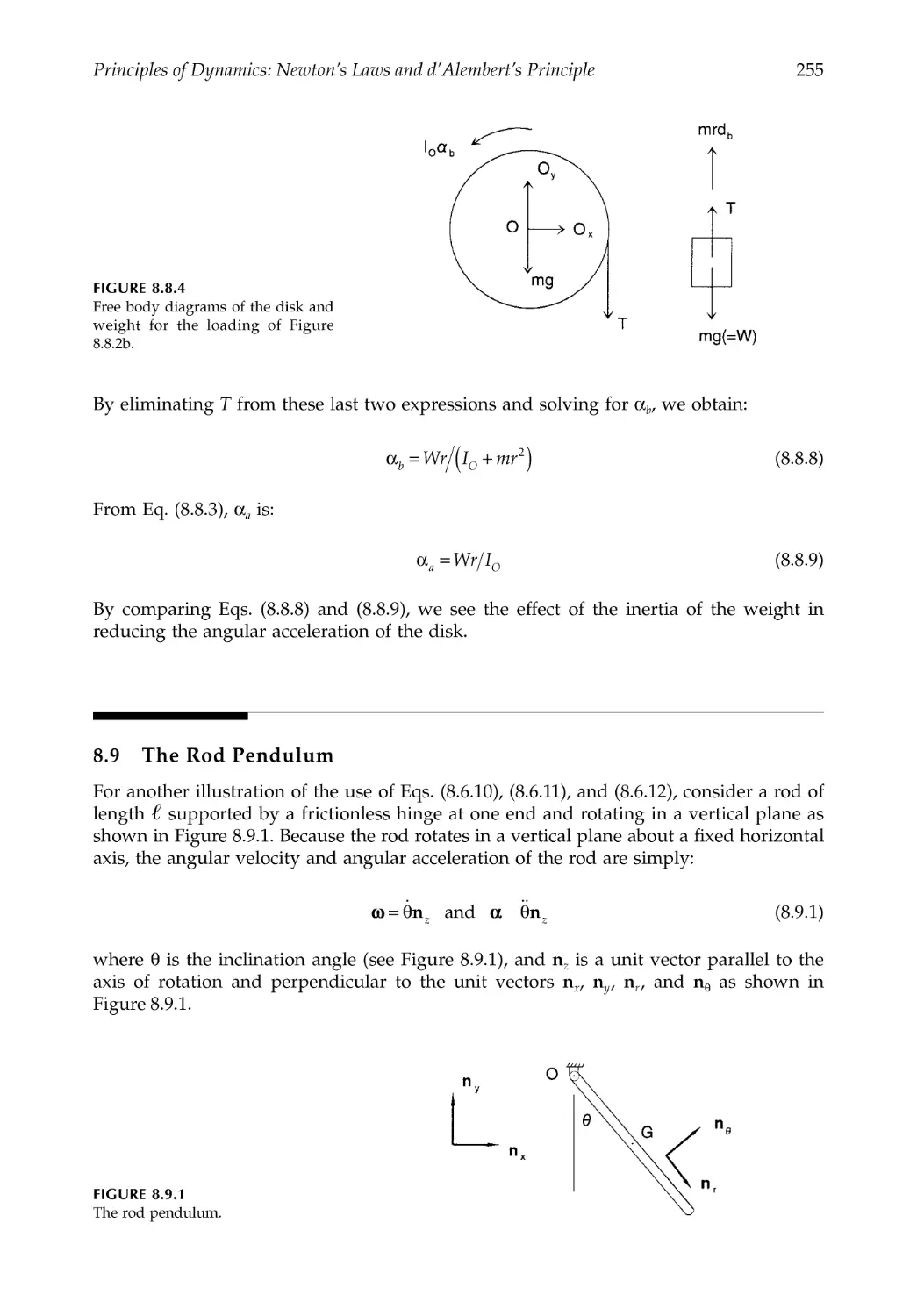
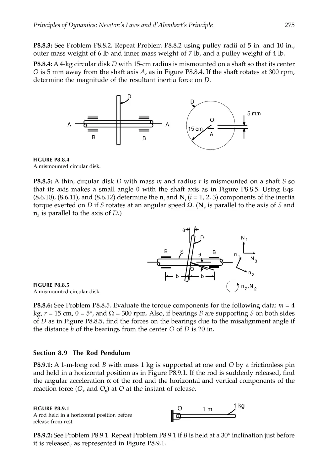
8.8 A Rotating Circular Disk ................................................................................................253
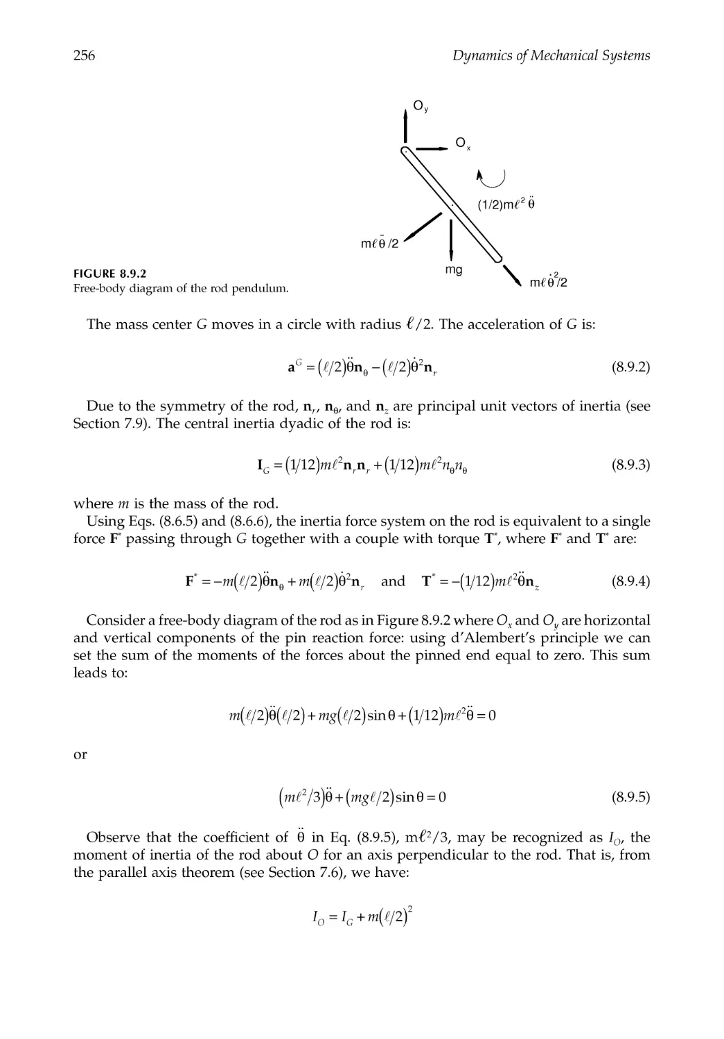
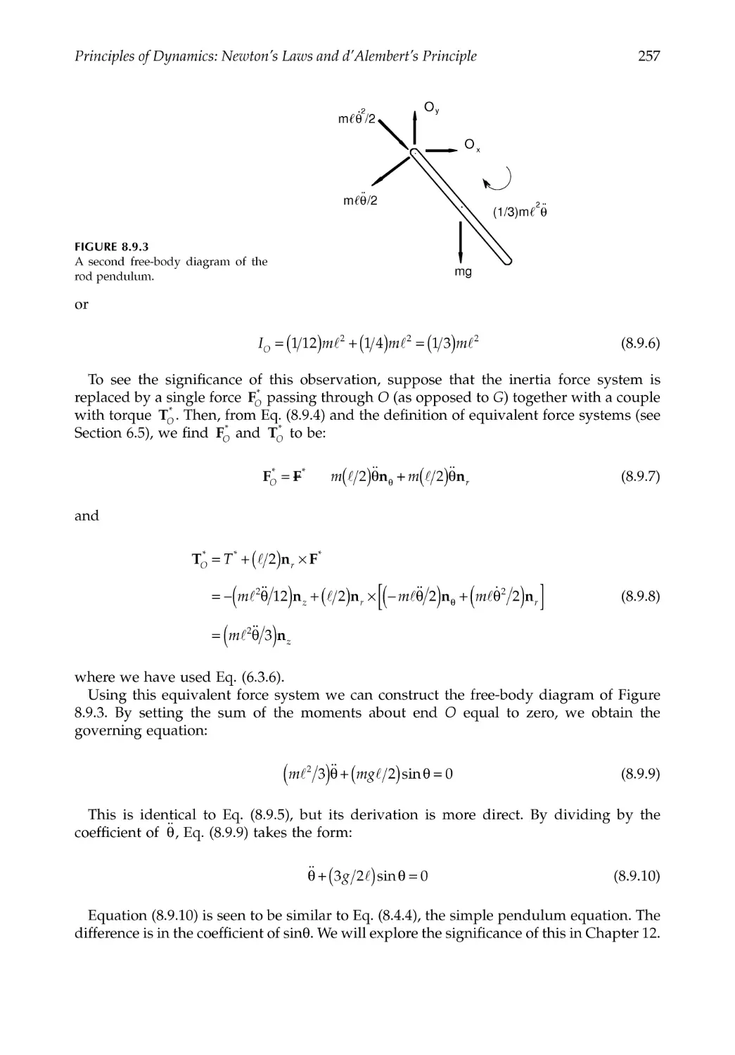
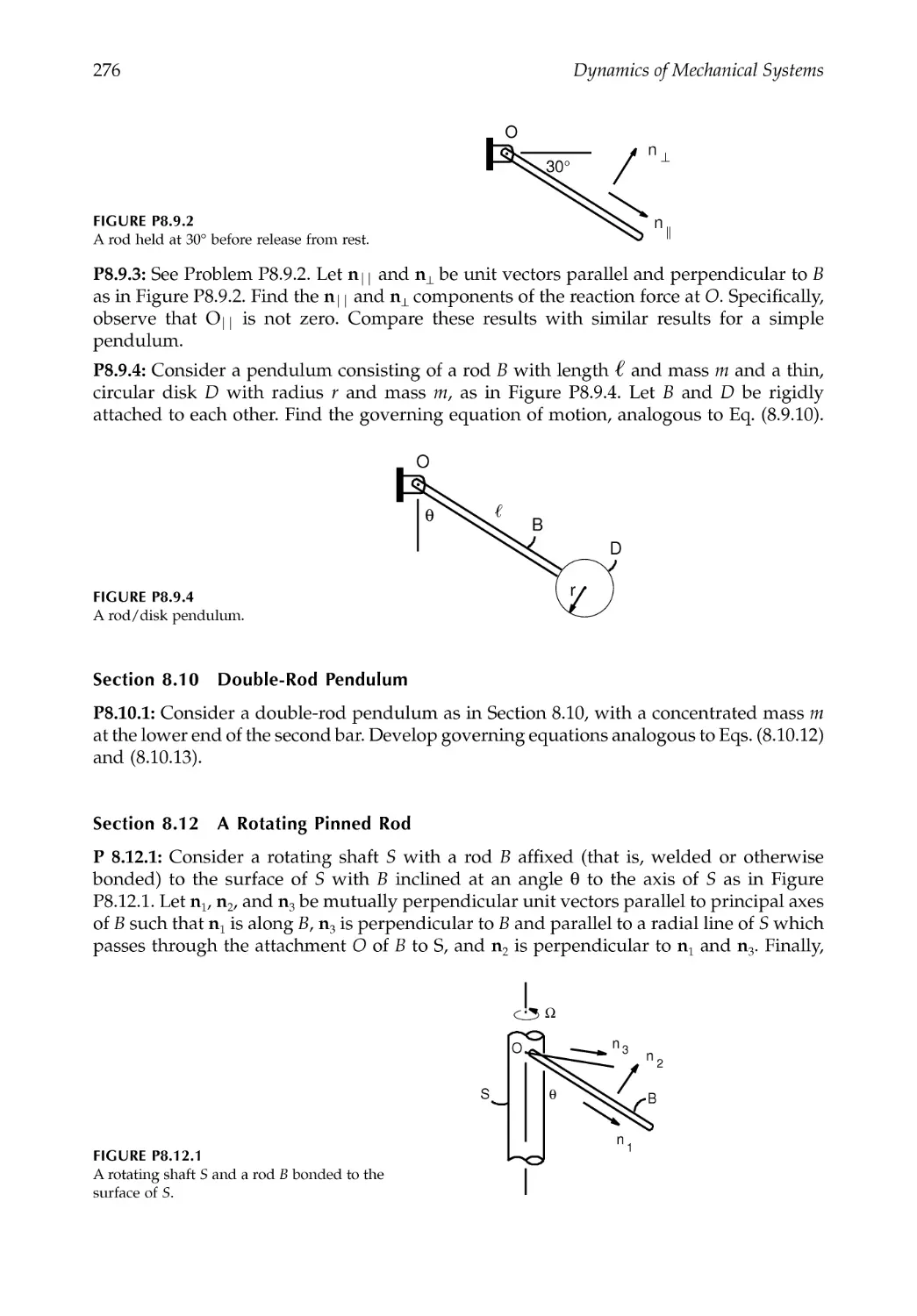
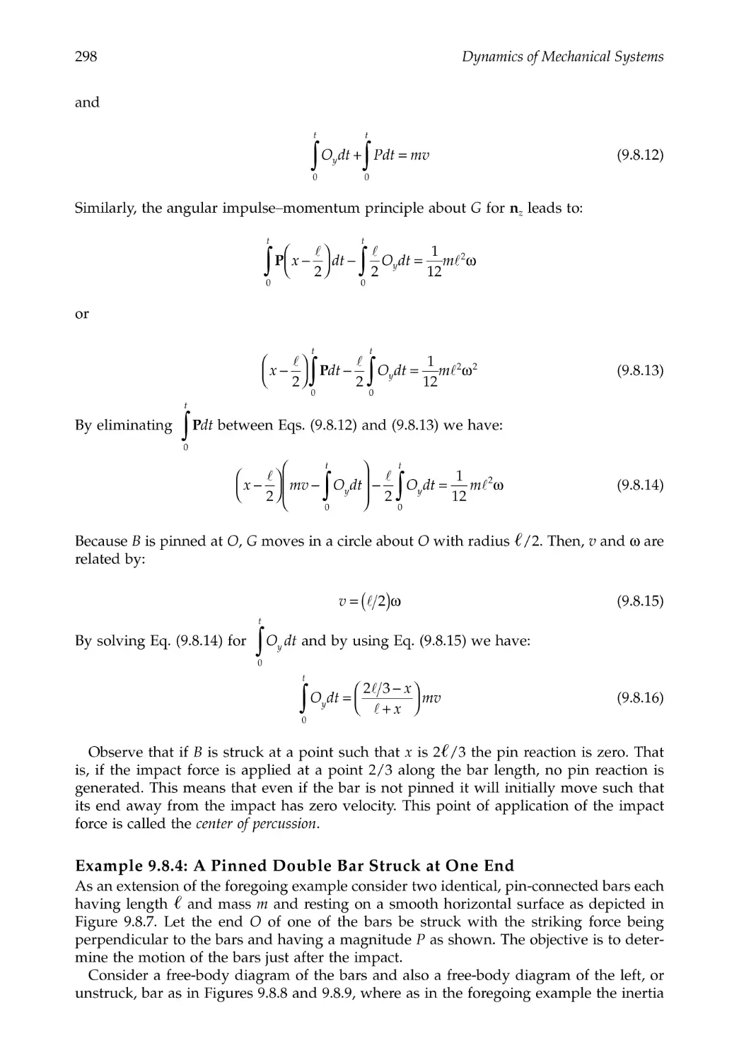
8.9 The Rod Pendulum ..........................................................................................................255
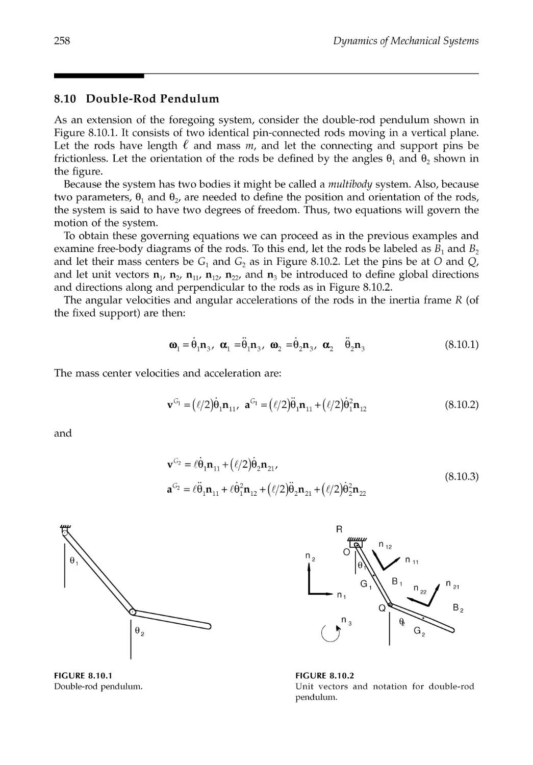
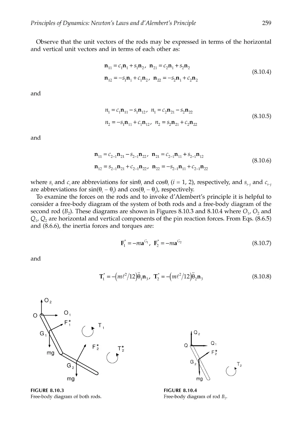
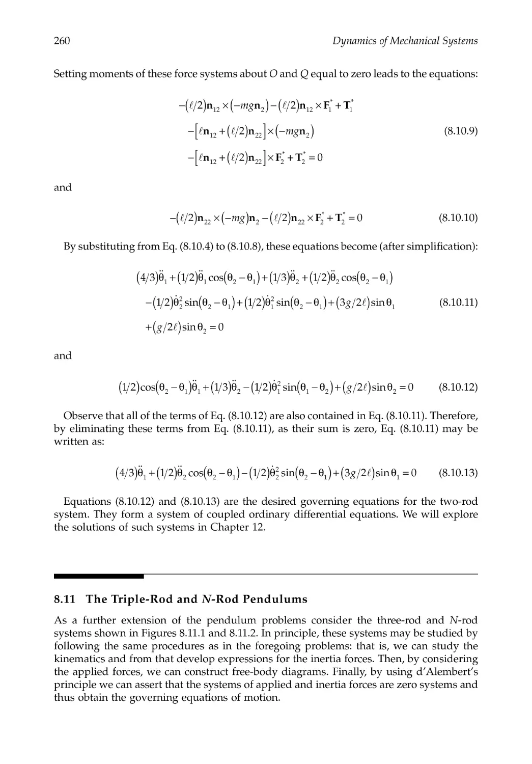
8.10 Double-Rod Pendulum ...................................................................................................258
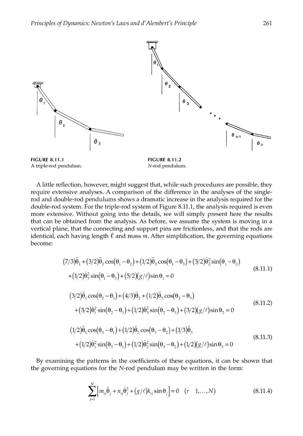
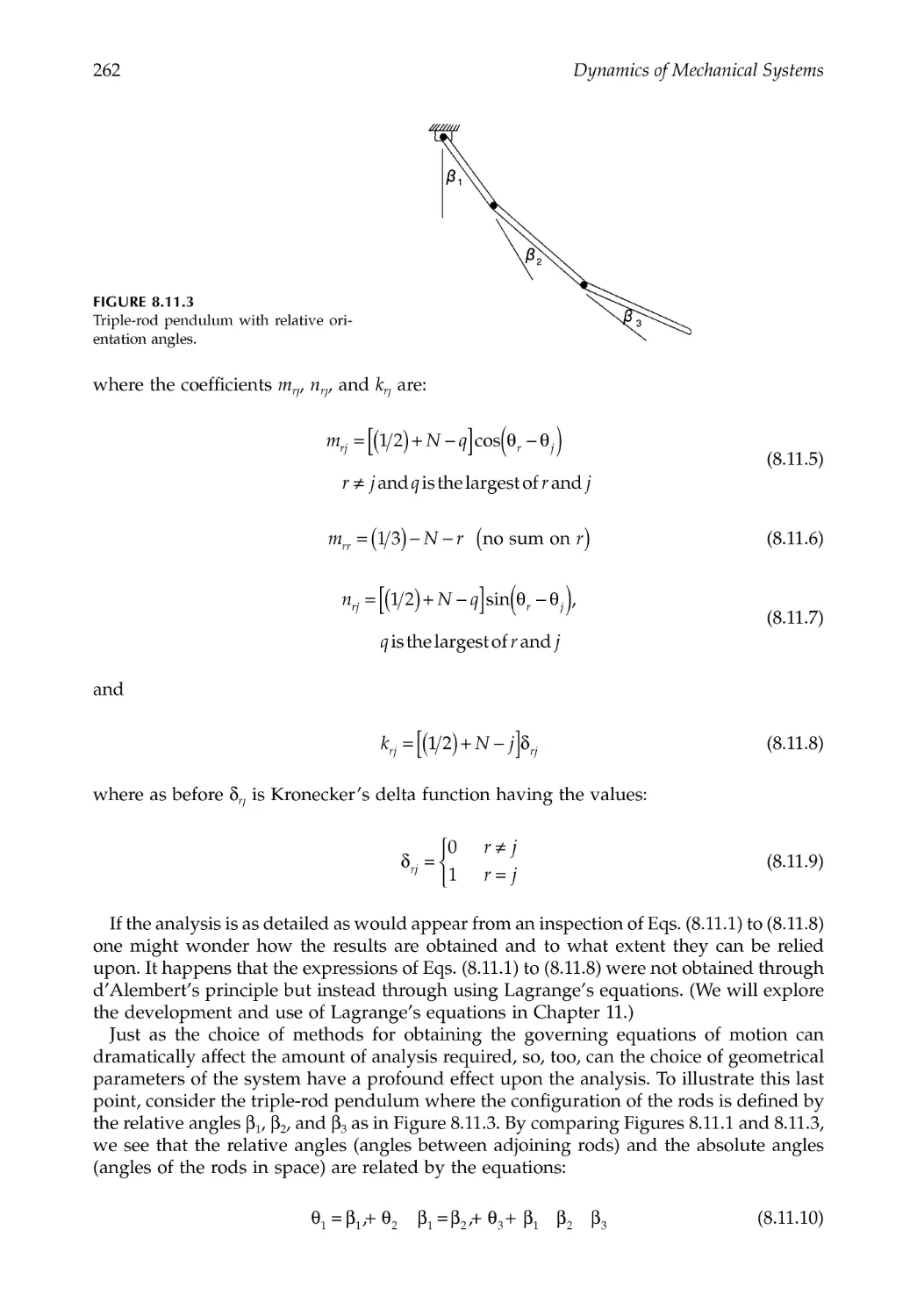
8.11 The Triple-Rod and N-Rod Pendulums .......................................................................260
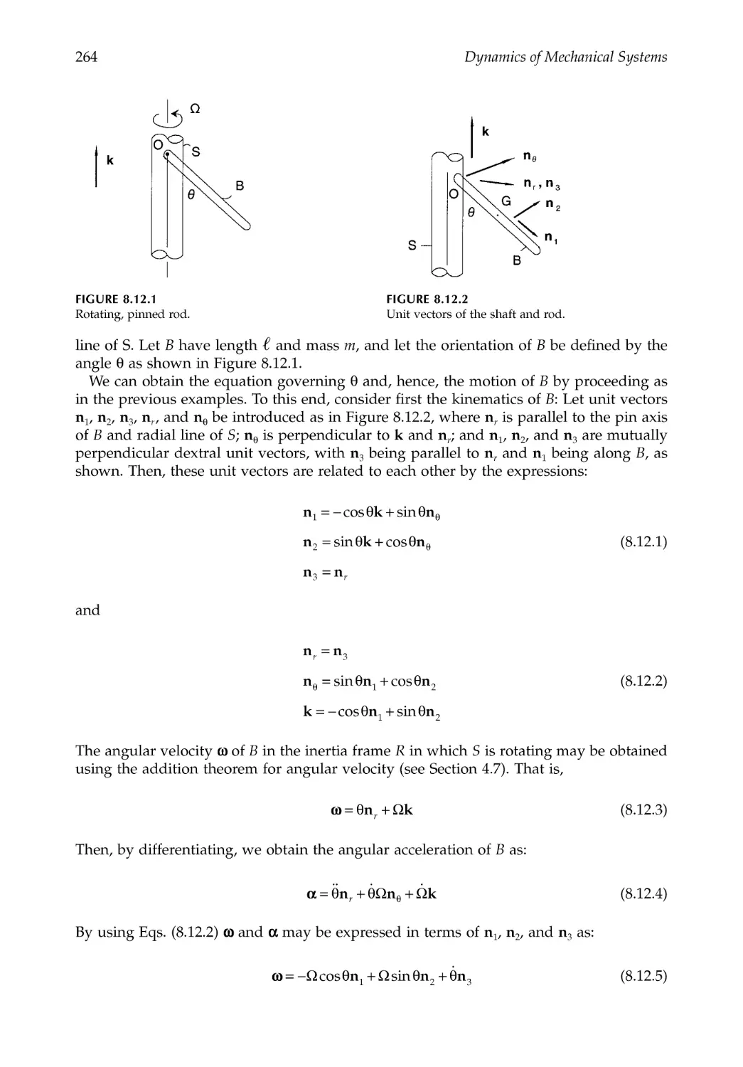
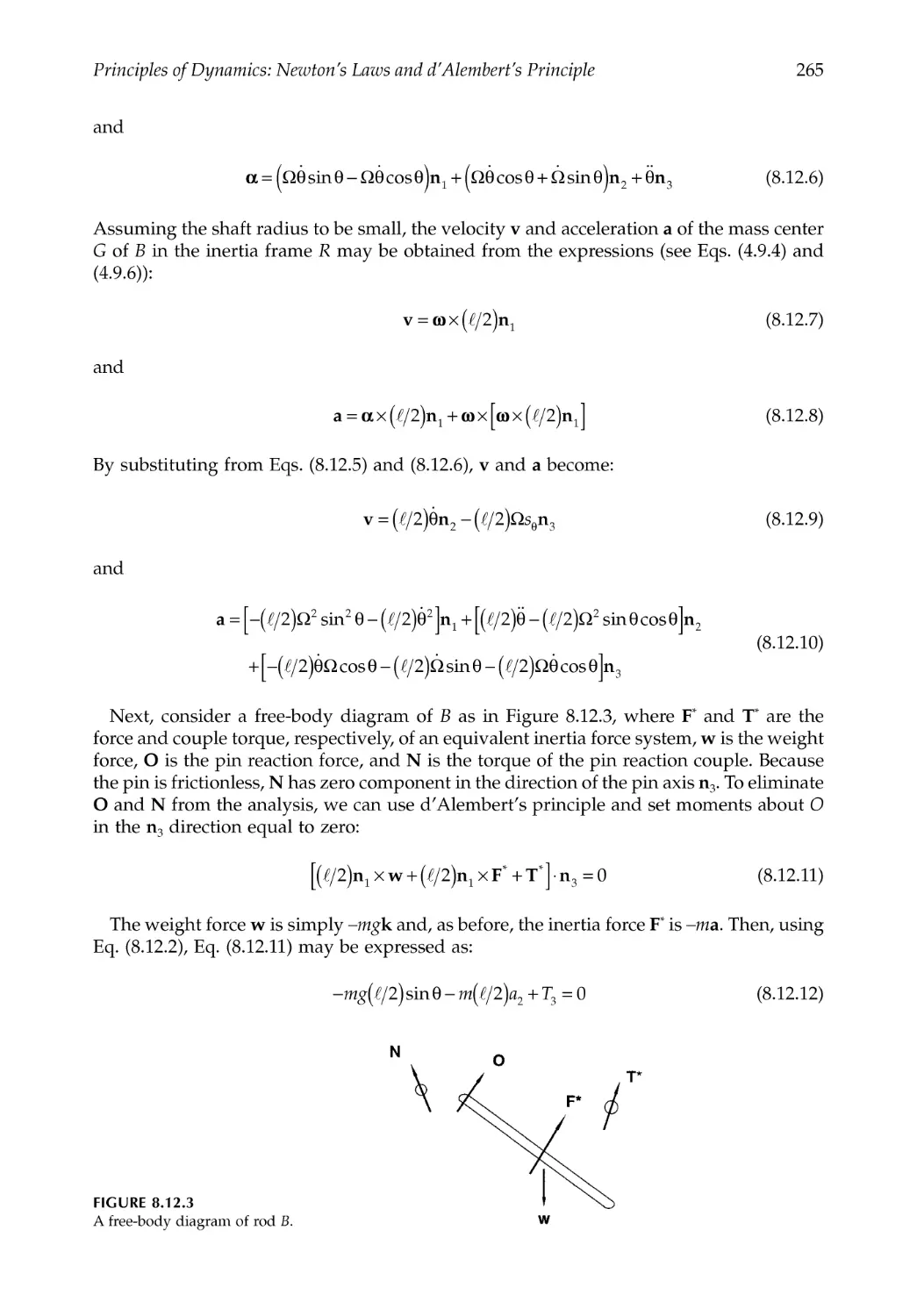
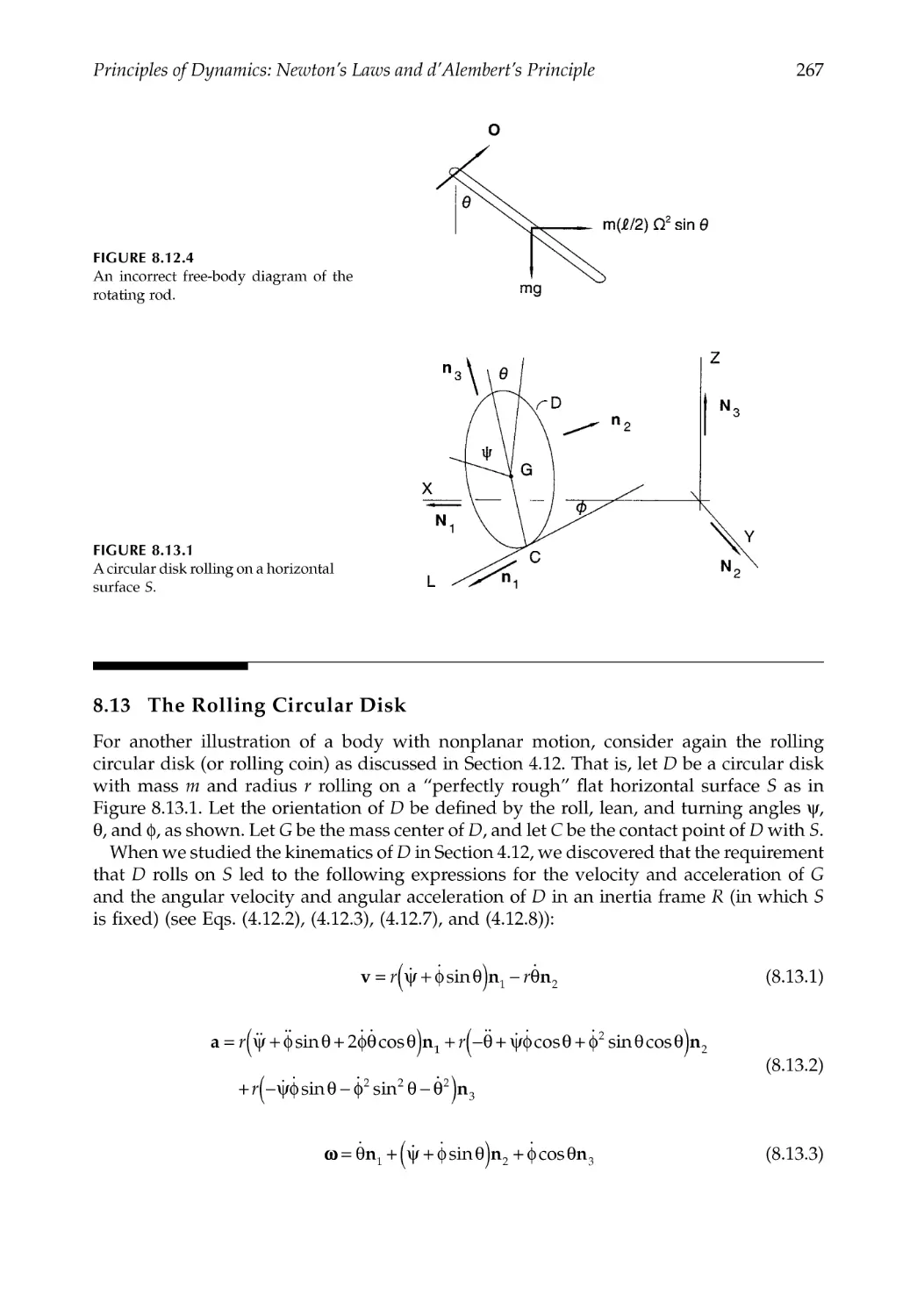
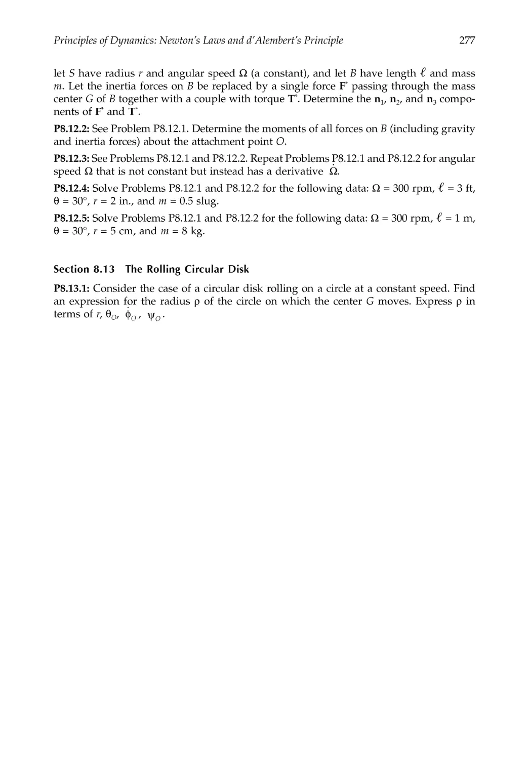
8.12 A Rotating Pinned Rod ...................................................................................................263
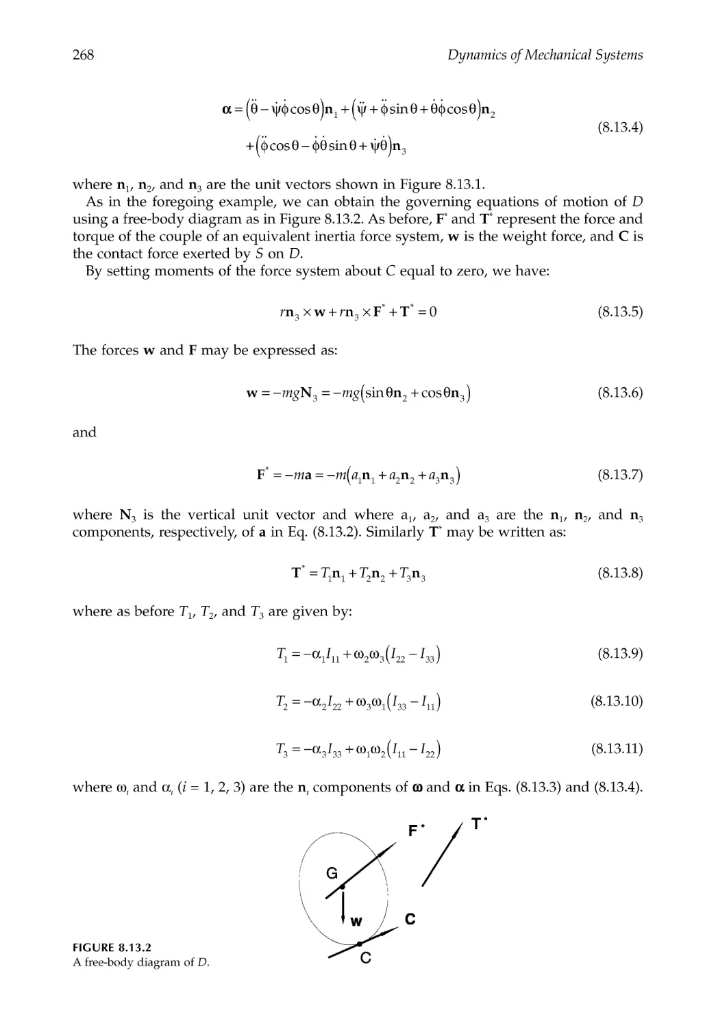
8.13 The Rolling Circular Disk ...............................................................................................267
8.14 Closure ...............................................................................................................................270
References .....................................................................................................................................270
Problems .......................................................................................................................................271
Chapter 9 Principles of Impulse and Momentum..............................................................279
9.1 Introduction.......................................................................................................................279
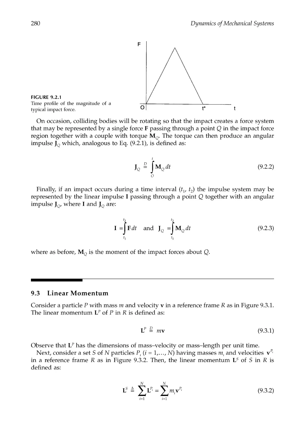
9.2 Impulse ..............................................................................................................................279
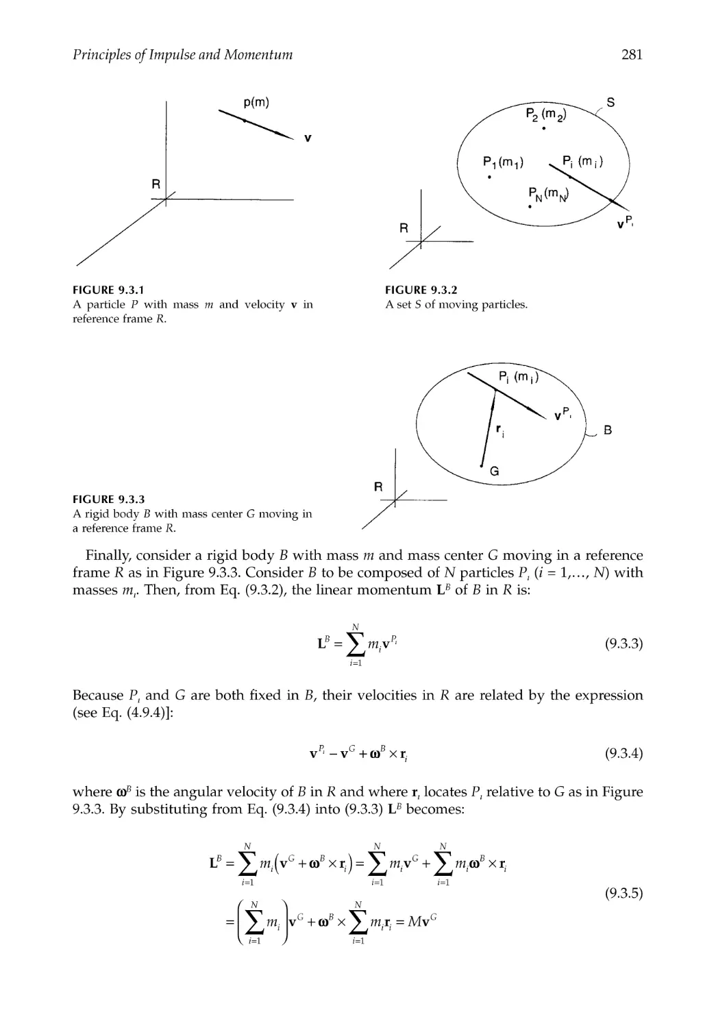
9.3 Linear Momentum ...........................................................................................................280
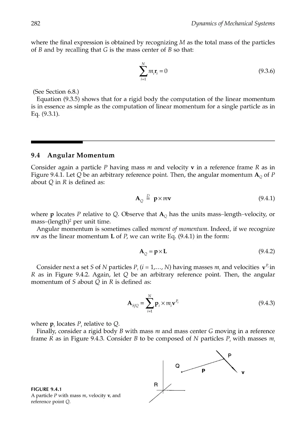
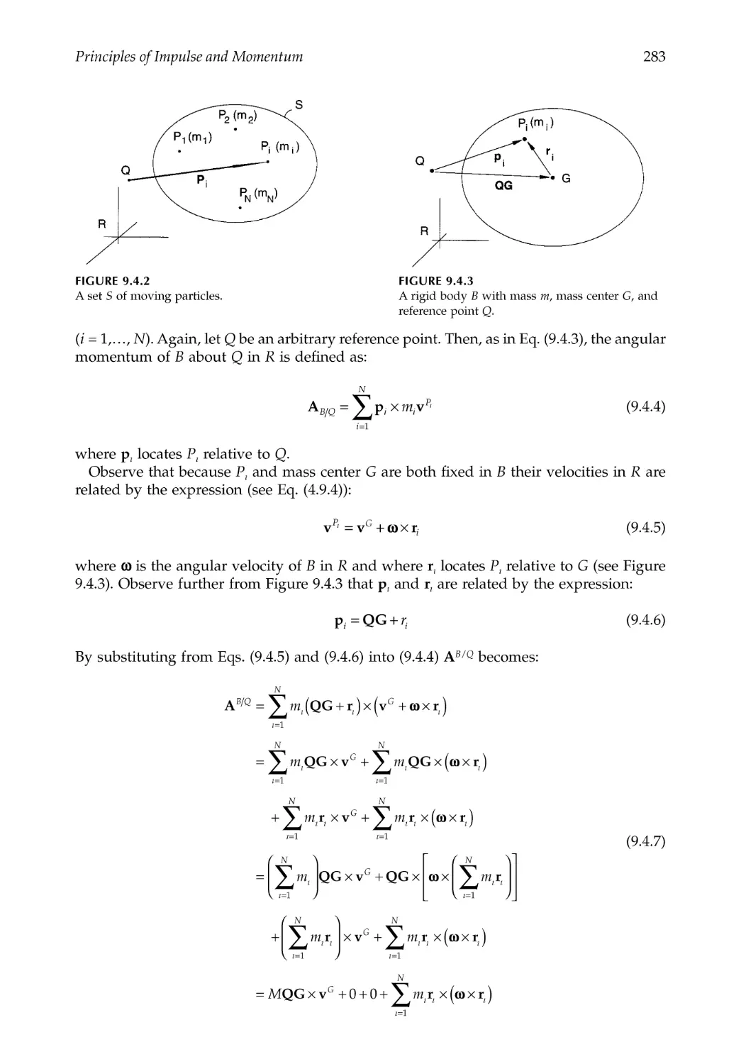
9.4 Angular Momentum ........................................................................................................282
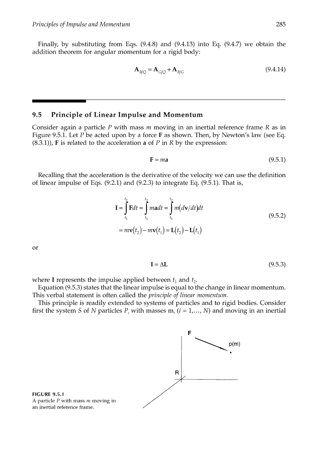
9.5 Principle of Linear Impulse and Momentum..............................................................285
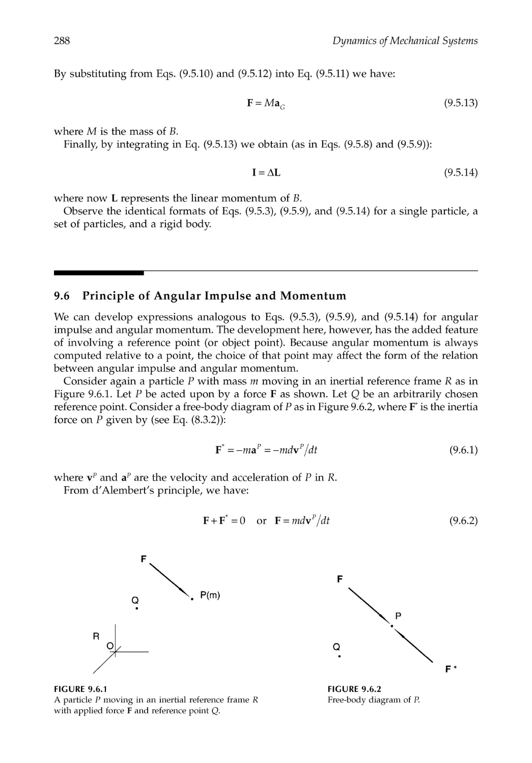
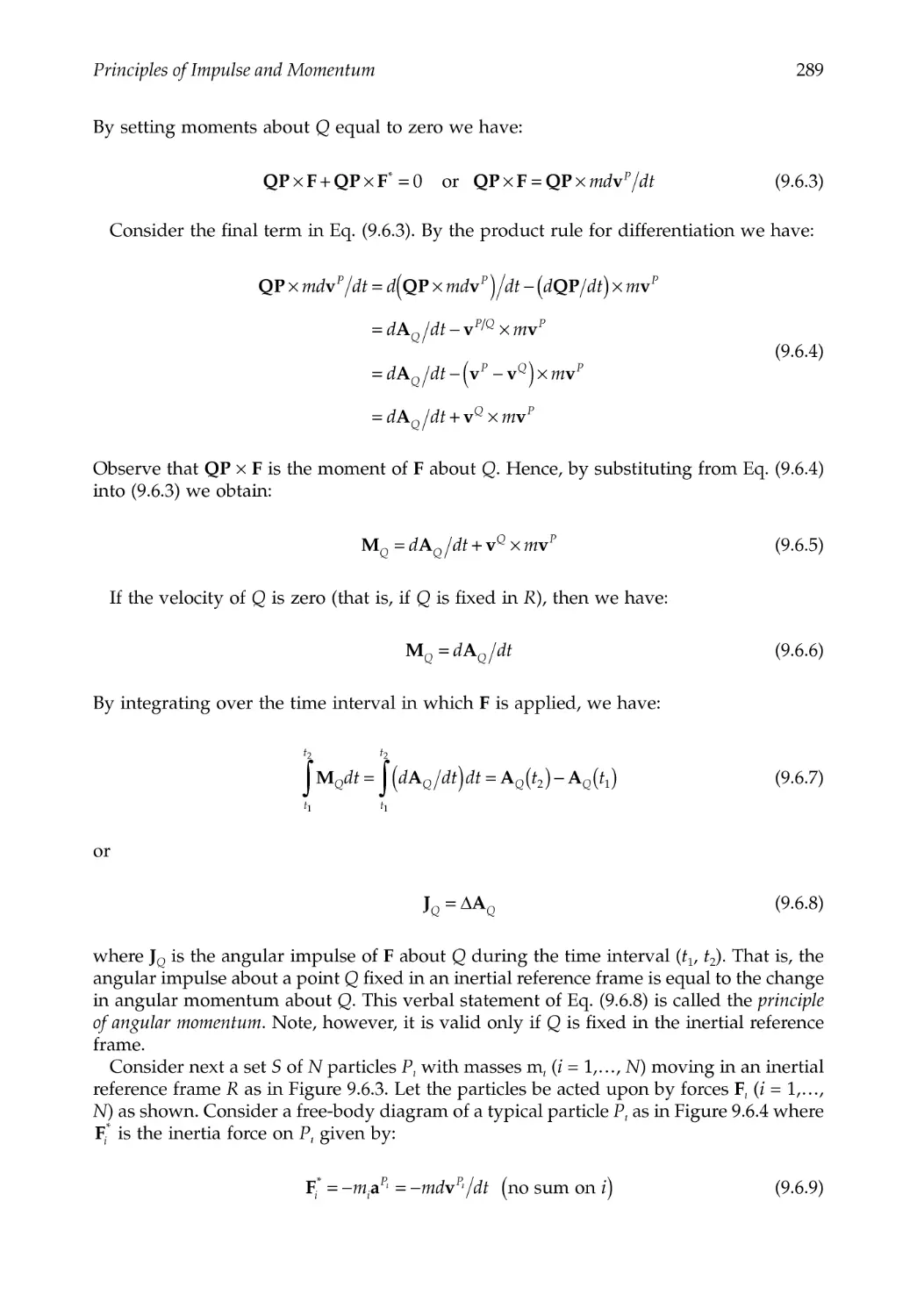
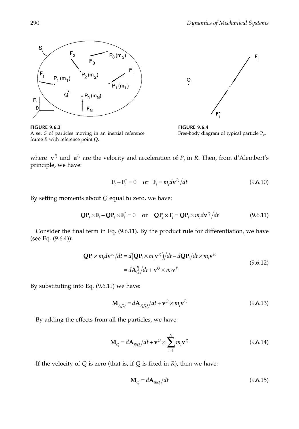
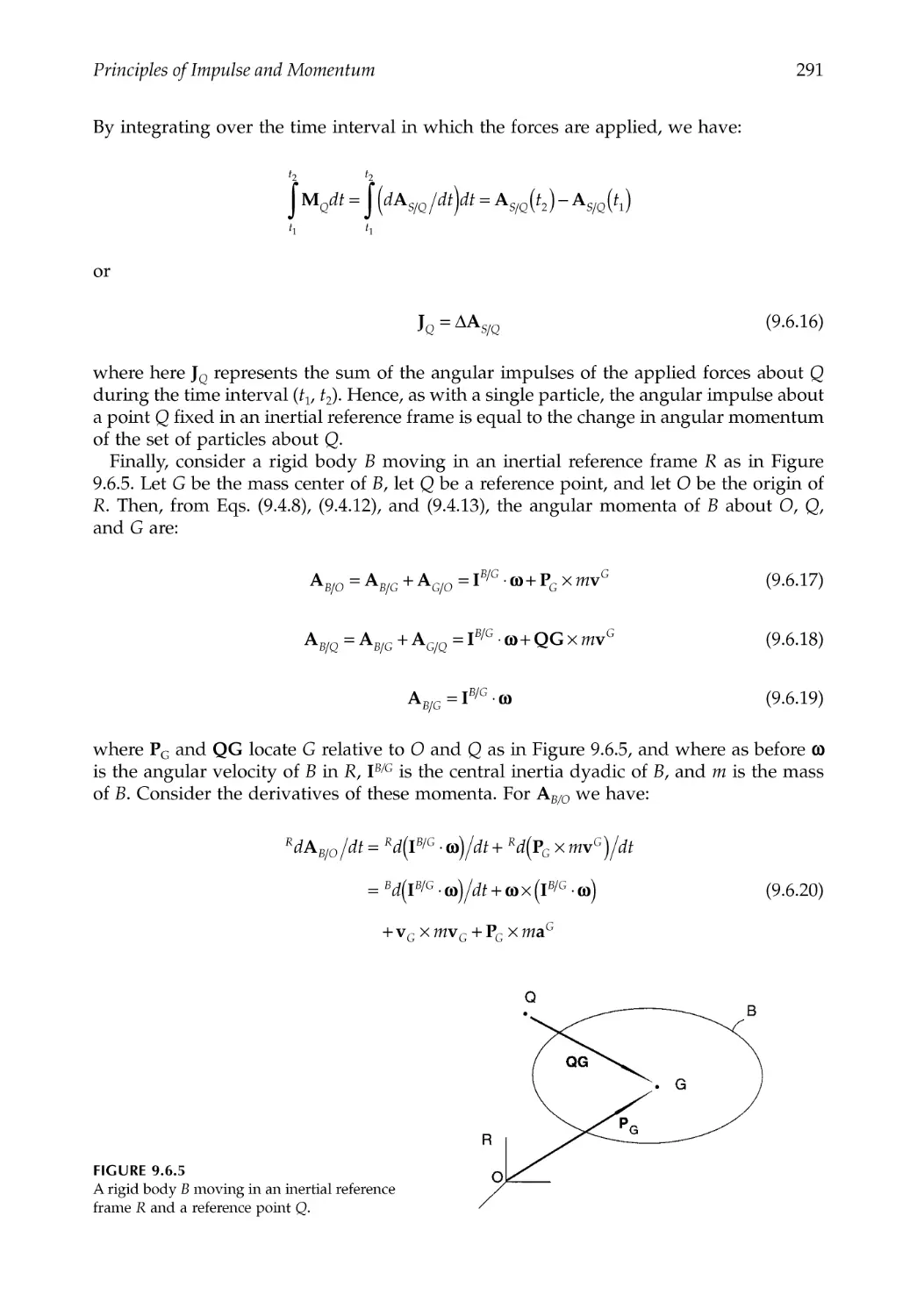
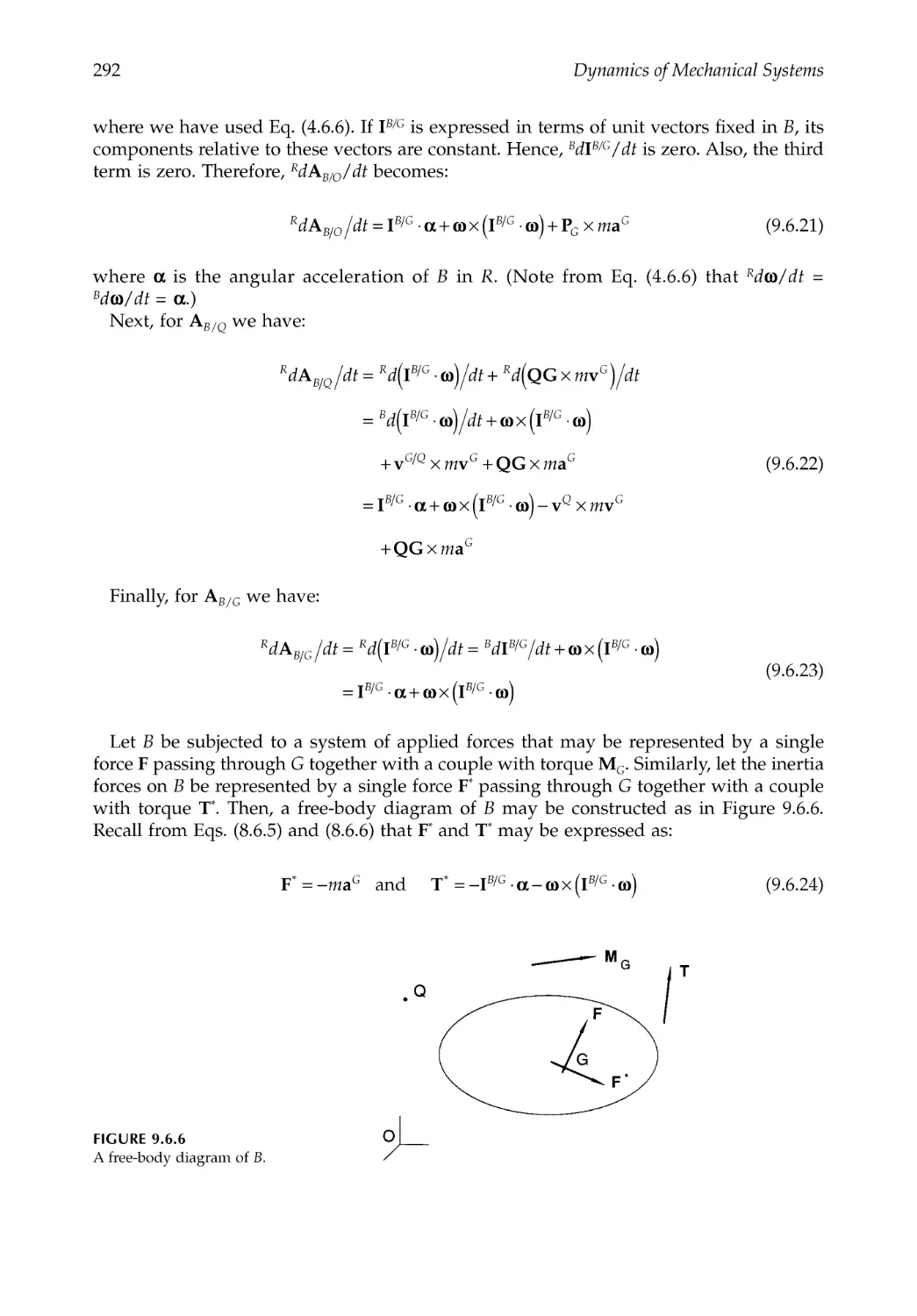
9.6 Principle of Angular Impulse and Momentum ..........................................................288
9.7 Conservation of Momentum Principles .......................................................................294
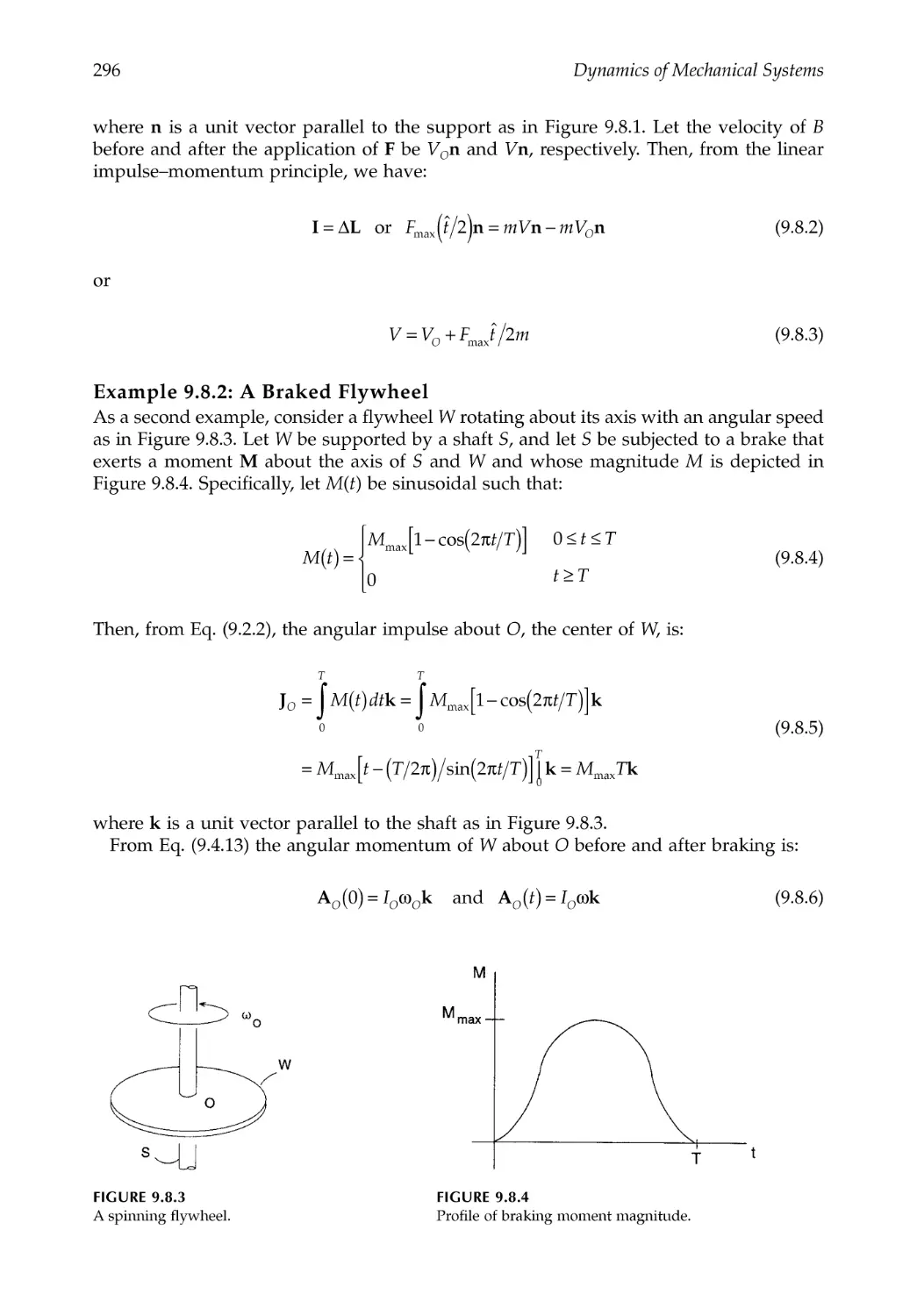
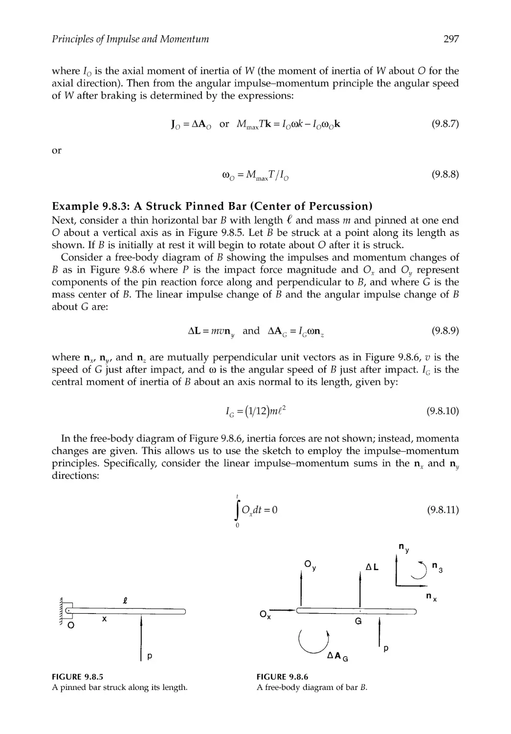
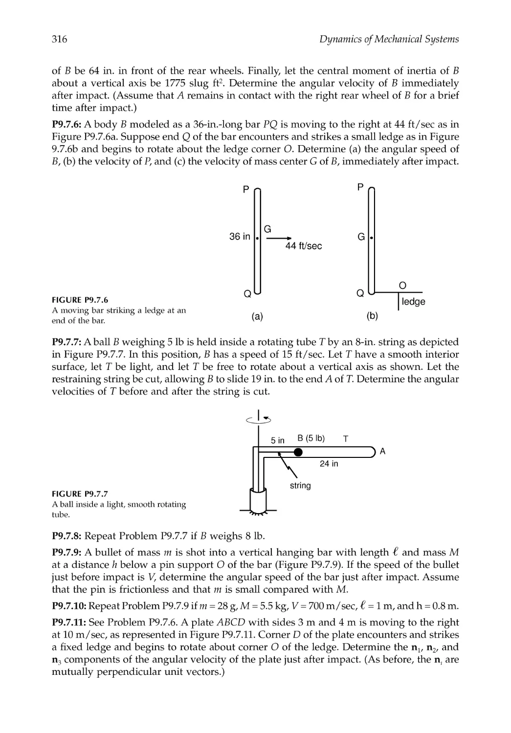
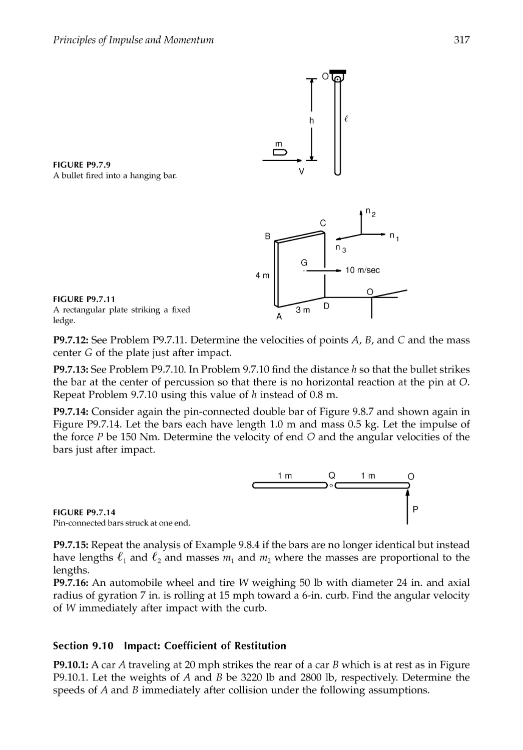
9.8 Examples............................................................................................................................295
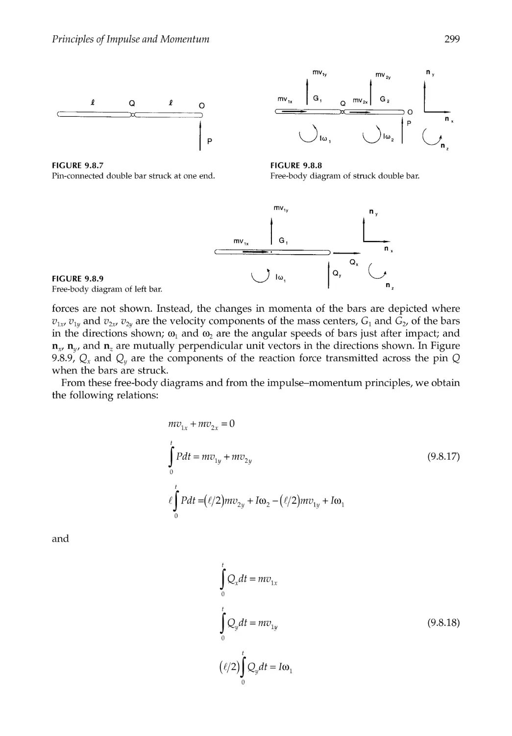
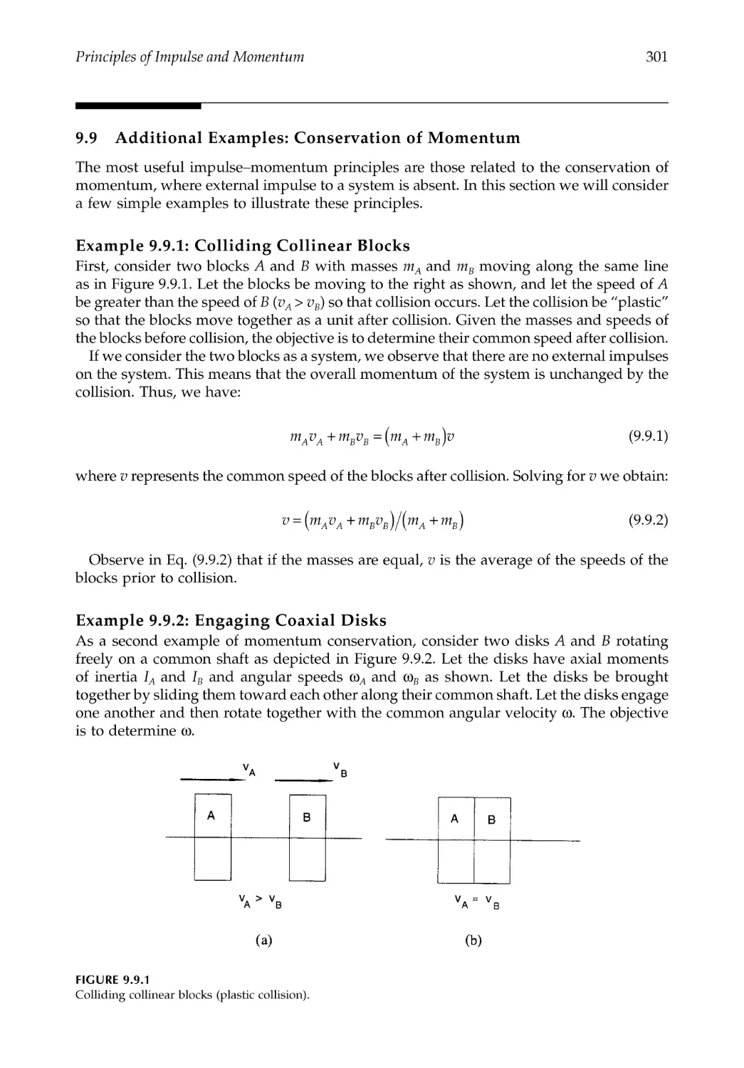
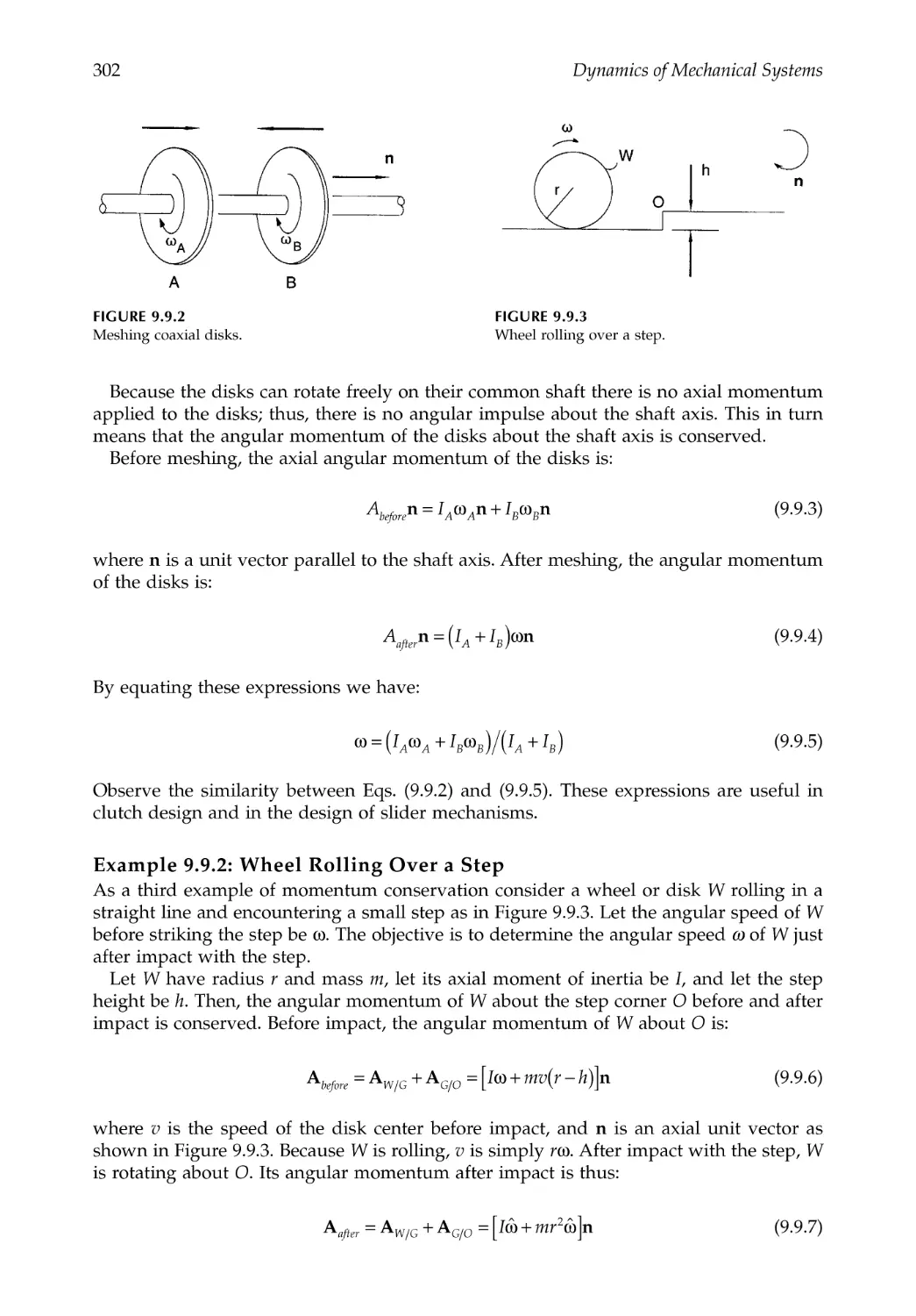
9.9 Additional Examples: Conservation of Momentum ..................................................301
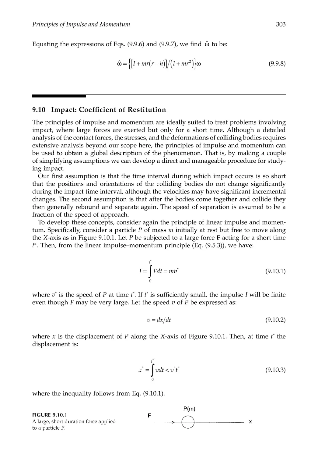
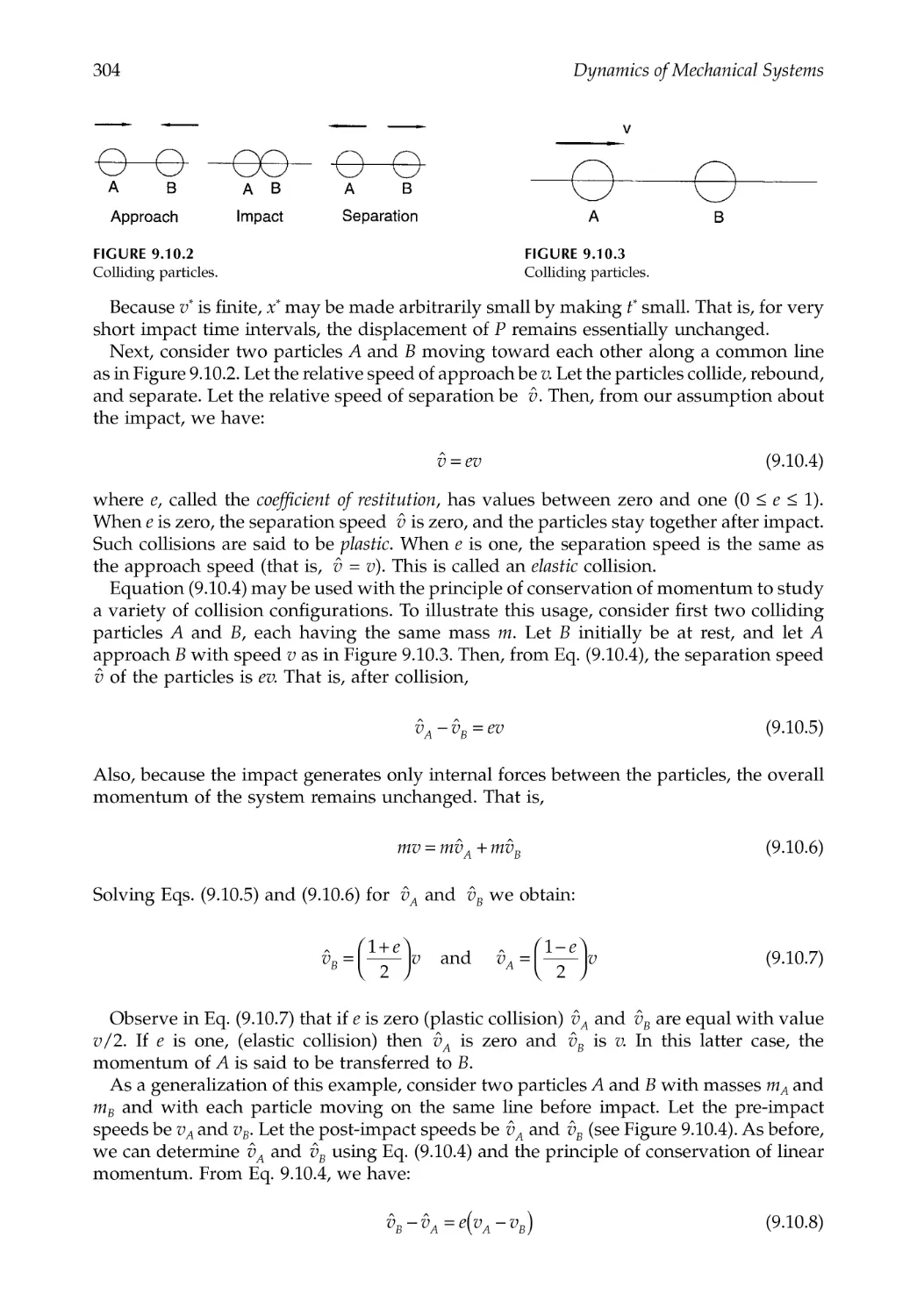
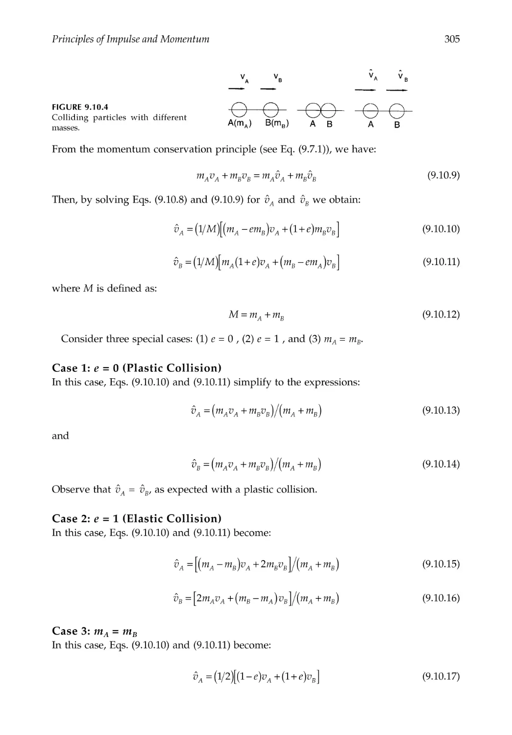
9.10 Impact: Coefficient of Restitution..................................................................................303
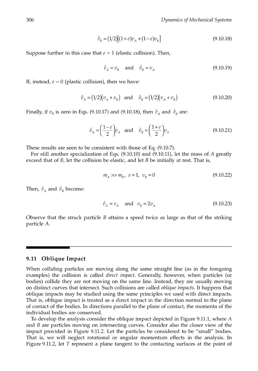
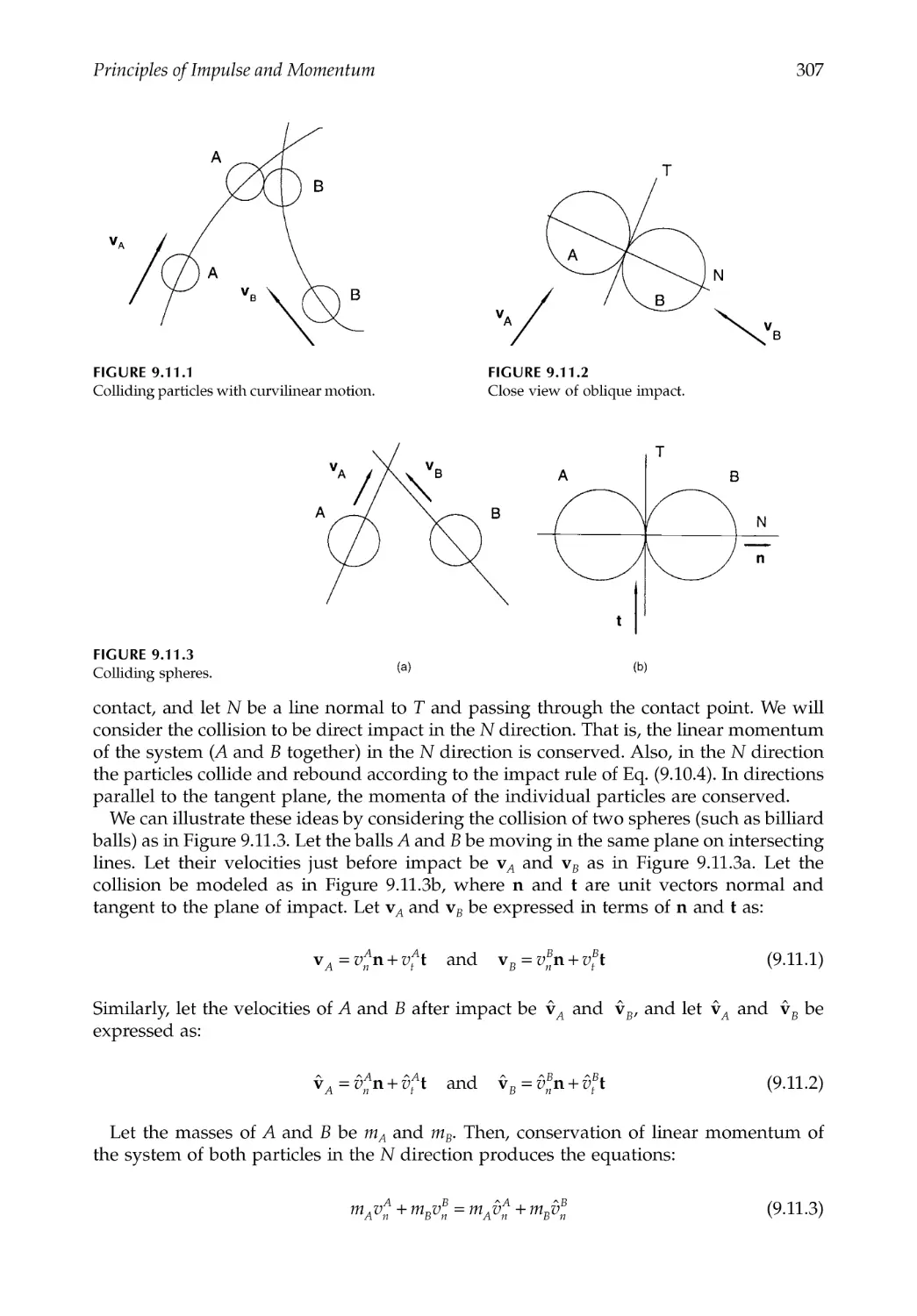
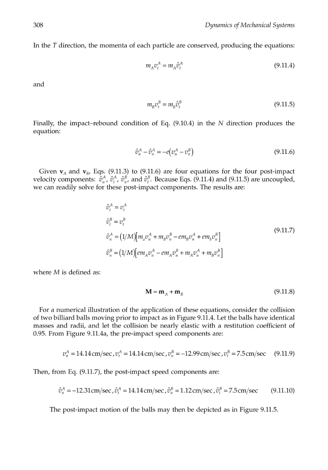
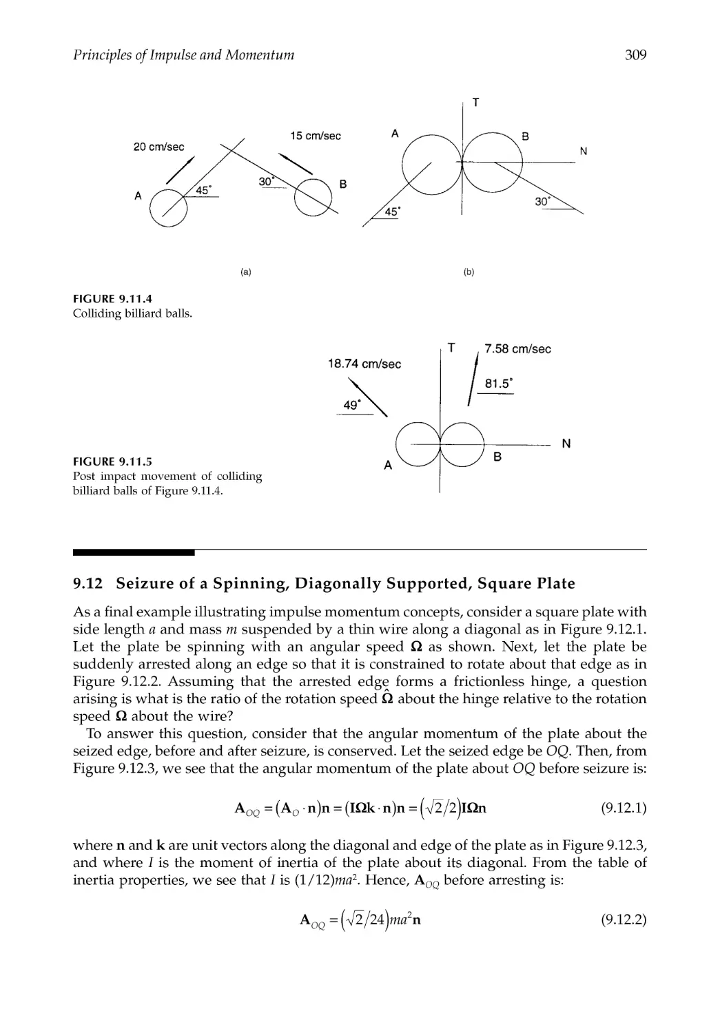
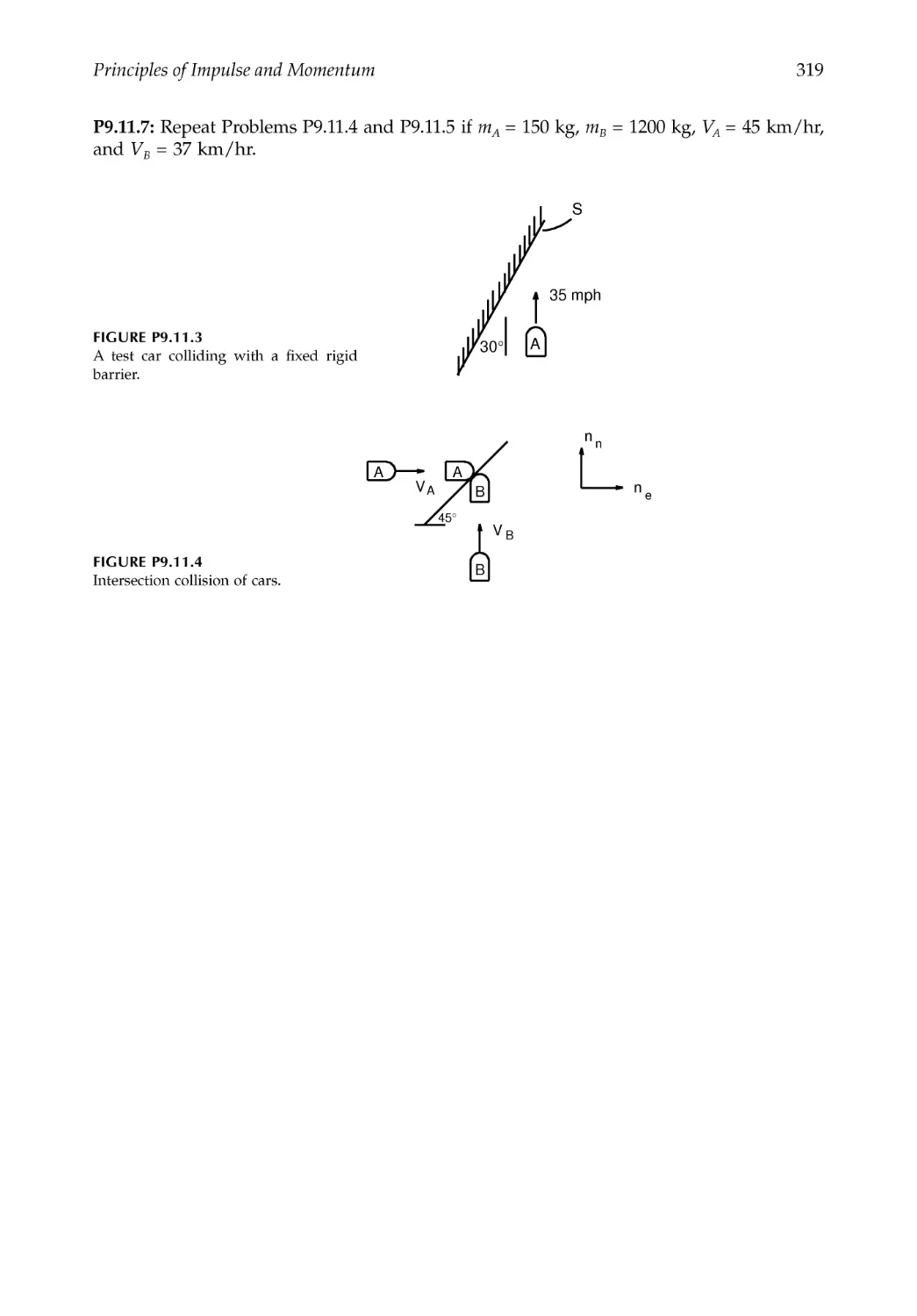
9.11 Oblique Impact .................................................................................................................306
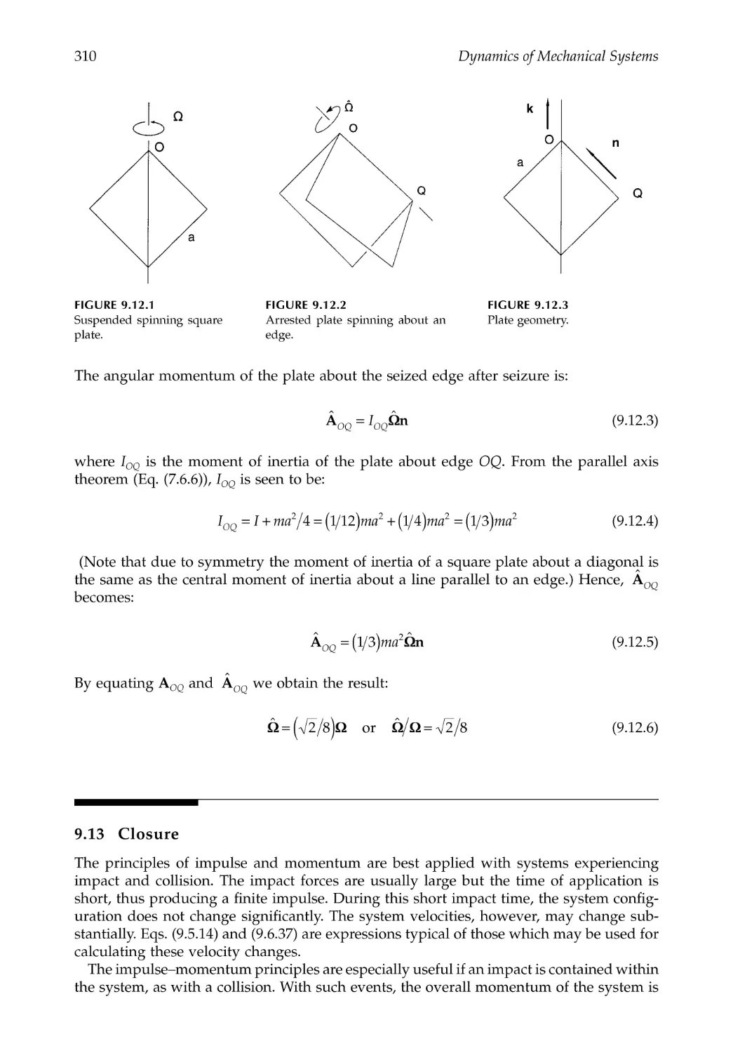
9.12 Seizure of a Spinning, Diagonally Supported, Square Plate ....................................309
9.13 Closure ...............................................................................................................................310
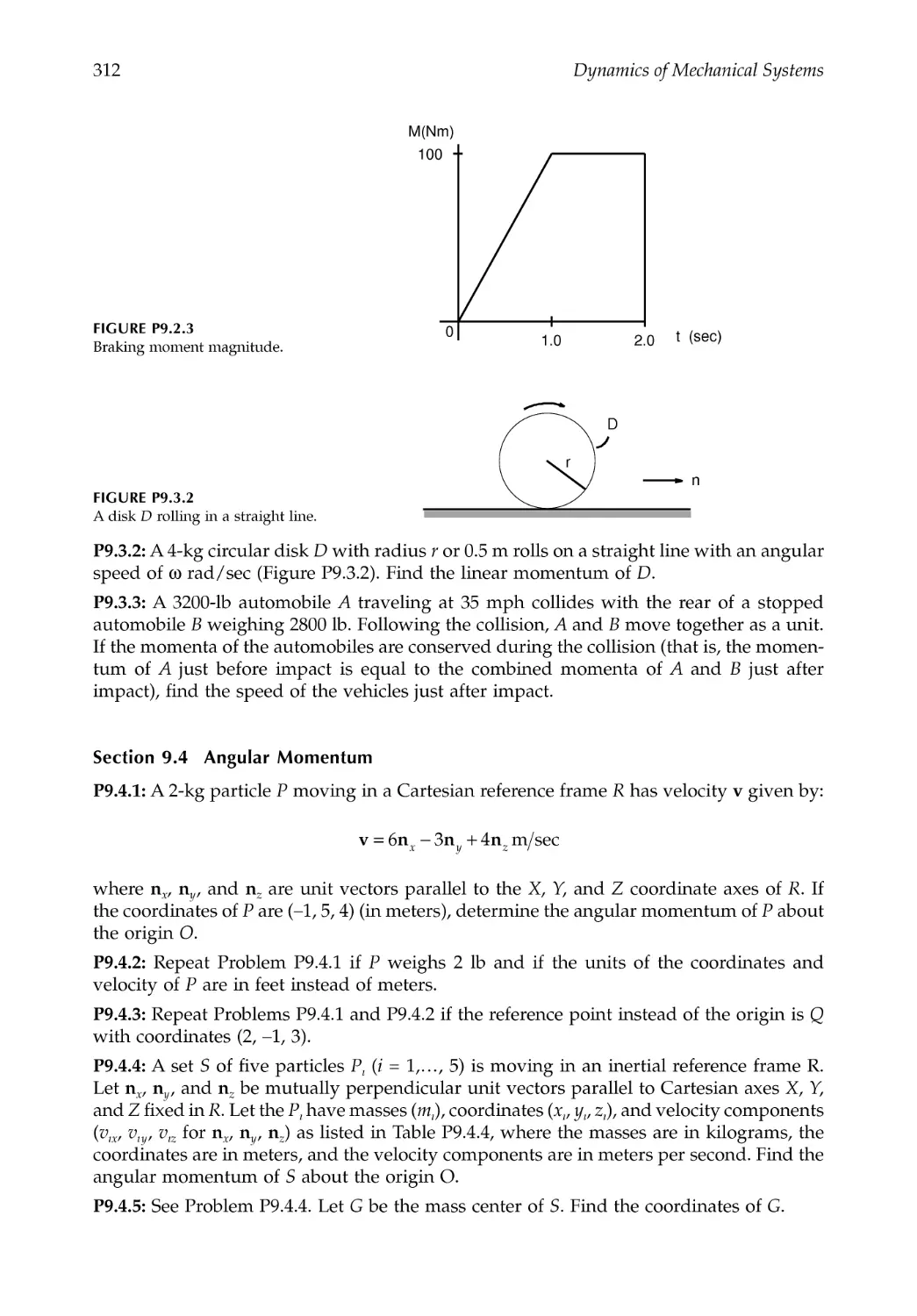
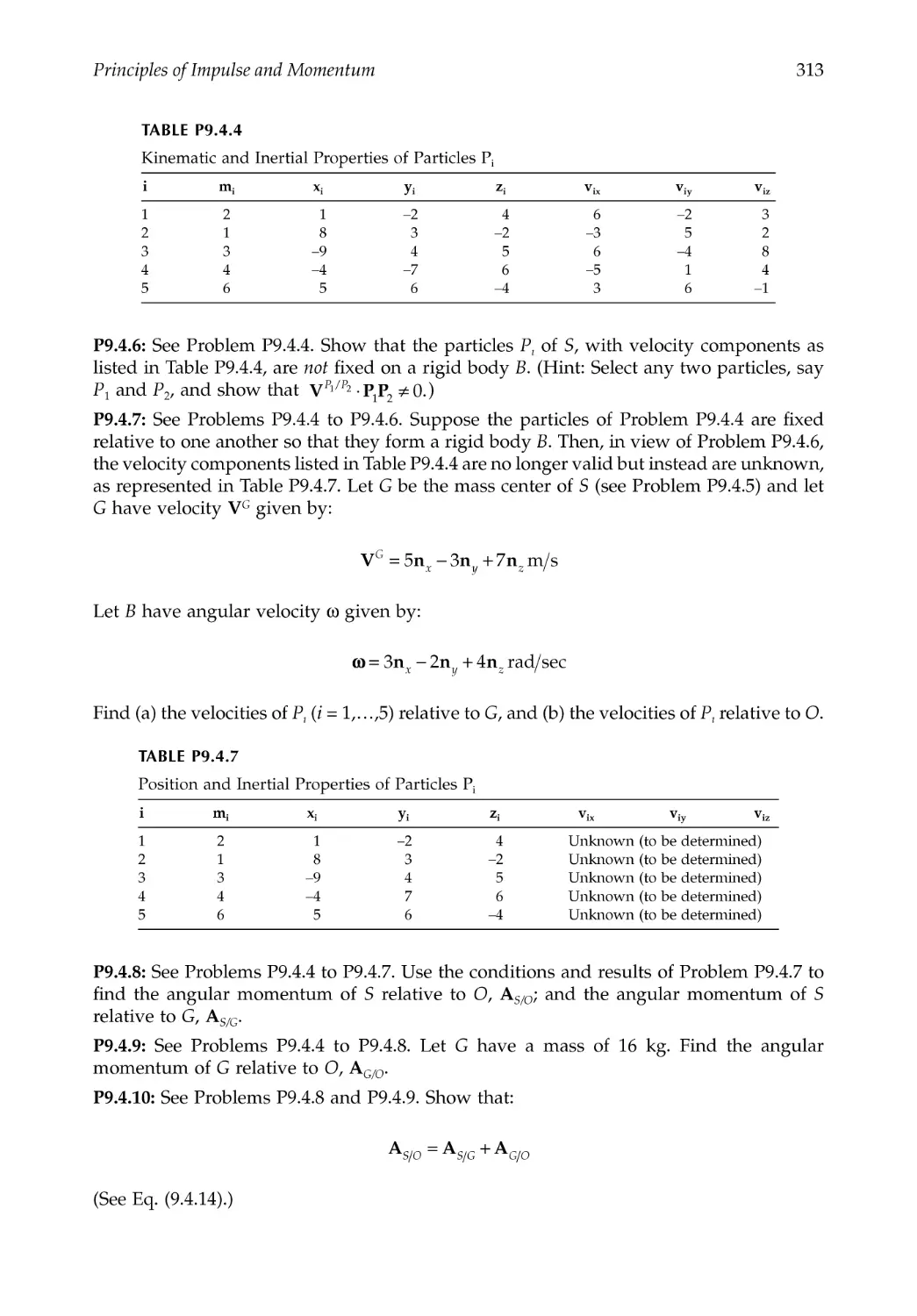
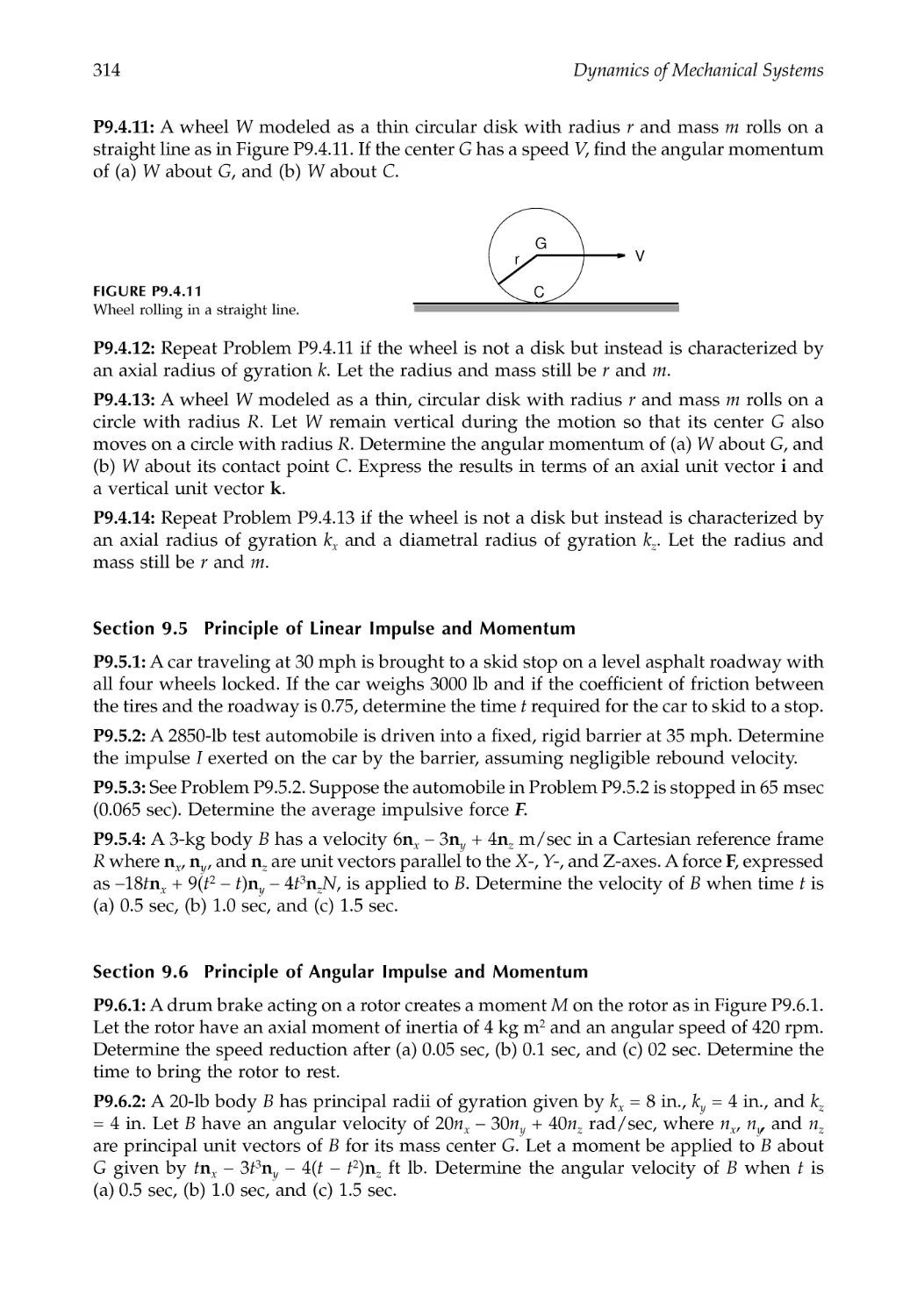
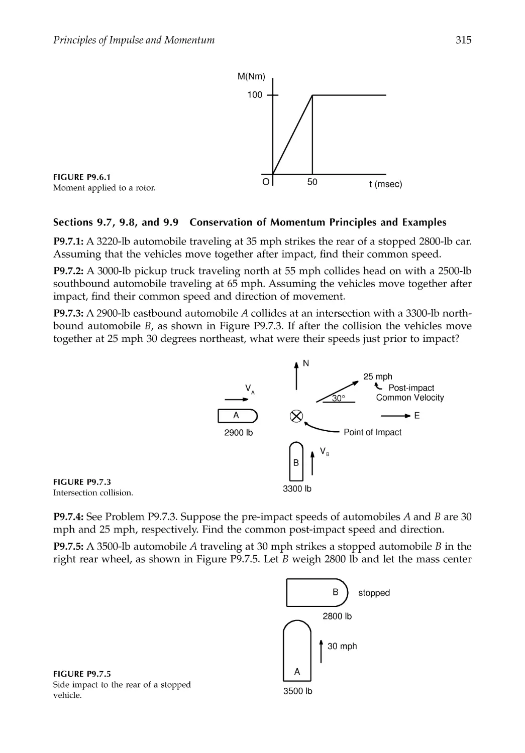
Problems .......................................................................................................................................311
Chapter 10 Introduction to Energy Methods ......................................................................321
10.1 Introduction.......................................................................................................................321
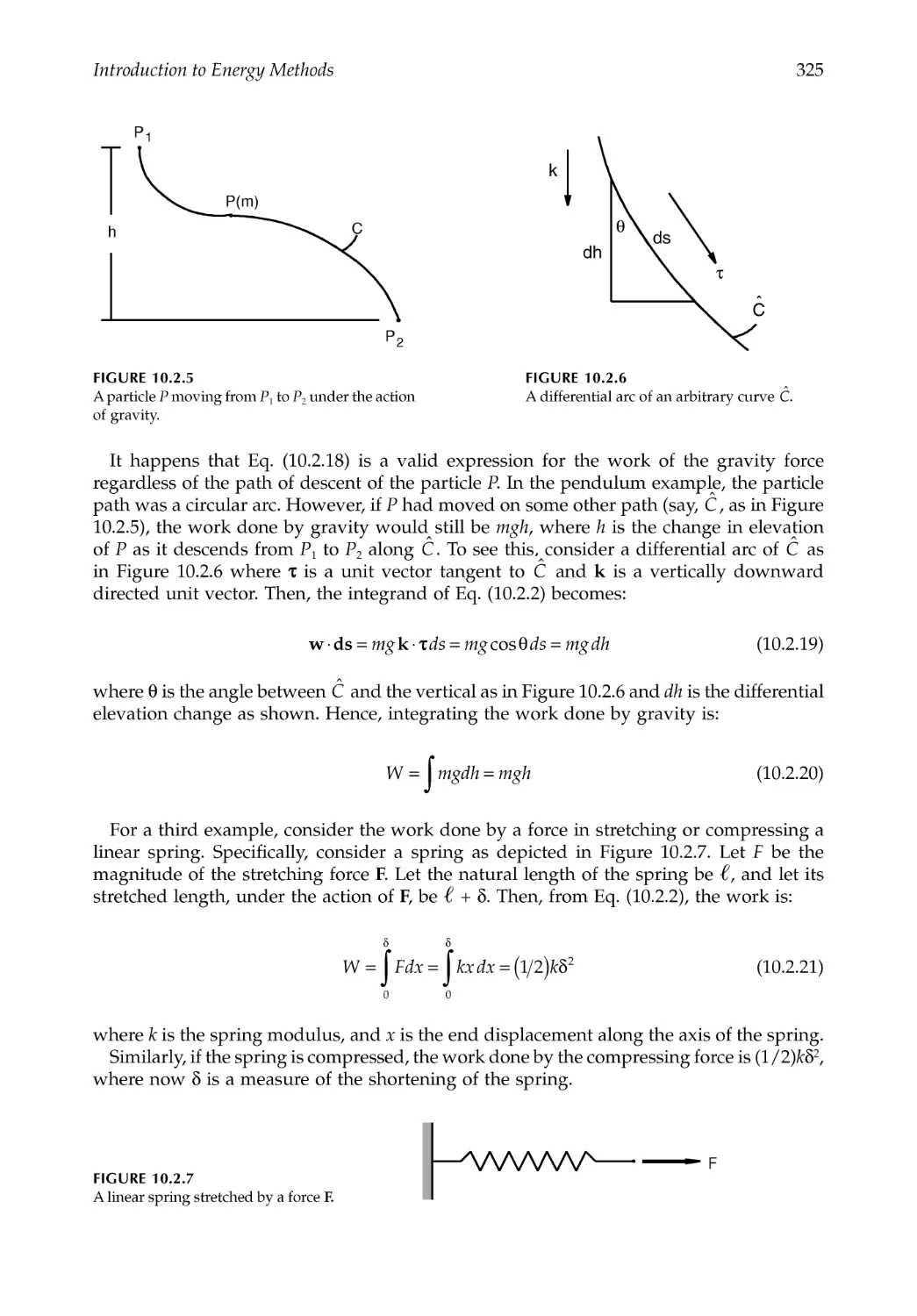
10.2 Work ...................................................................................................................................321
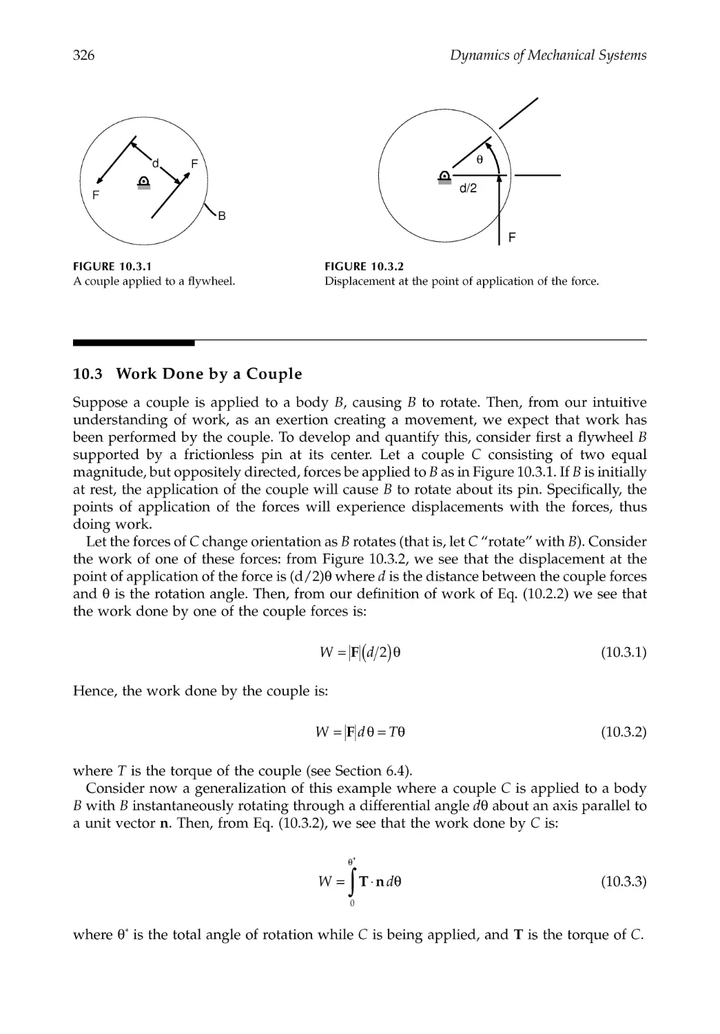
10.3 Work Done by a Couple .................................................................................................326
10.4 Power .................................................................................................................................327
10.5 Kinetic Energy ..................................................................................................................327
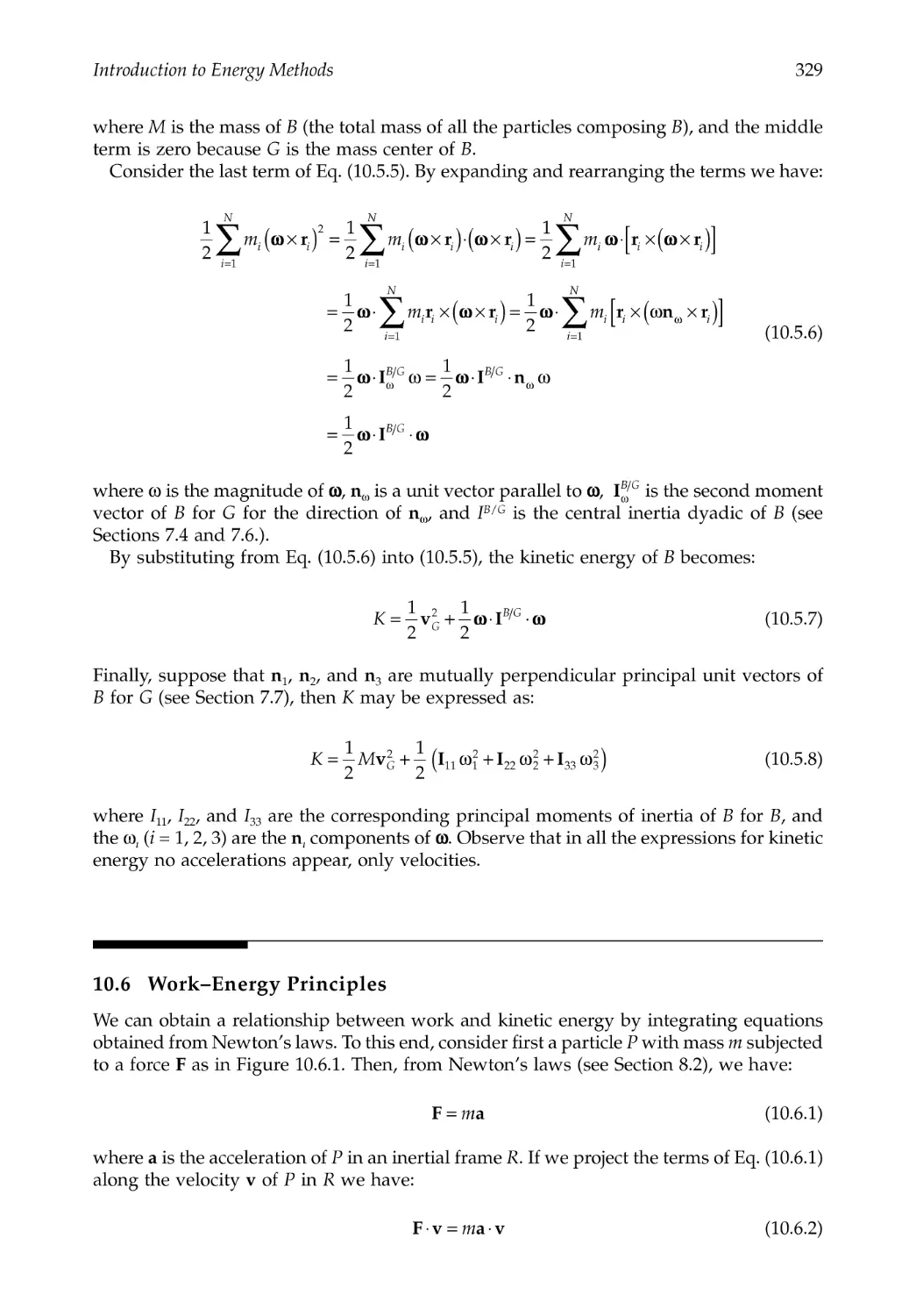
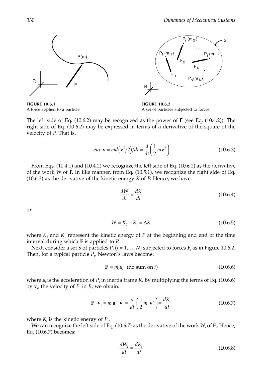
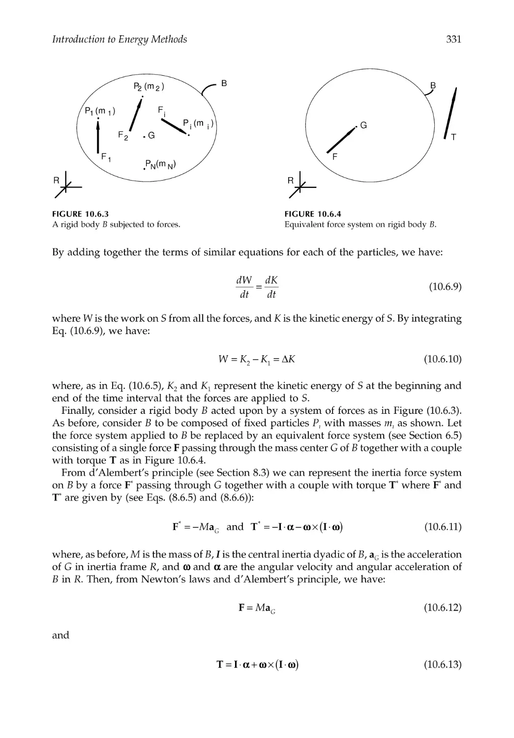
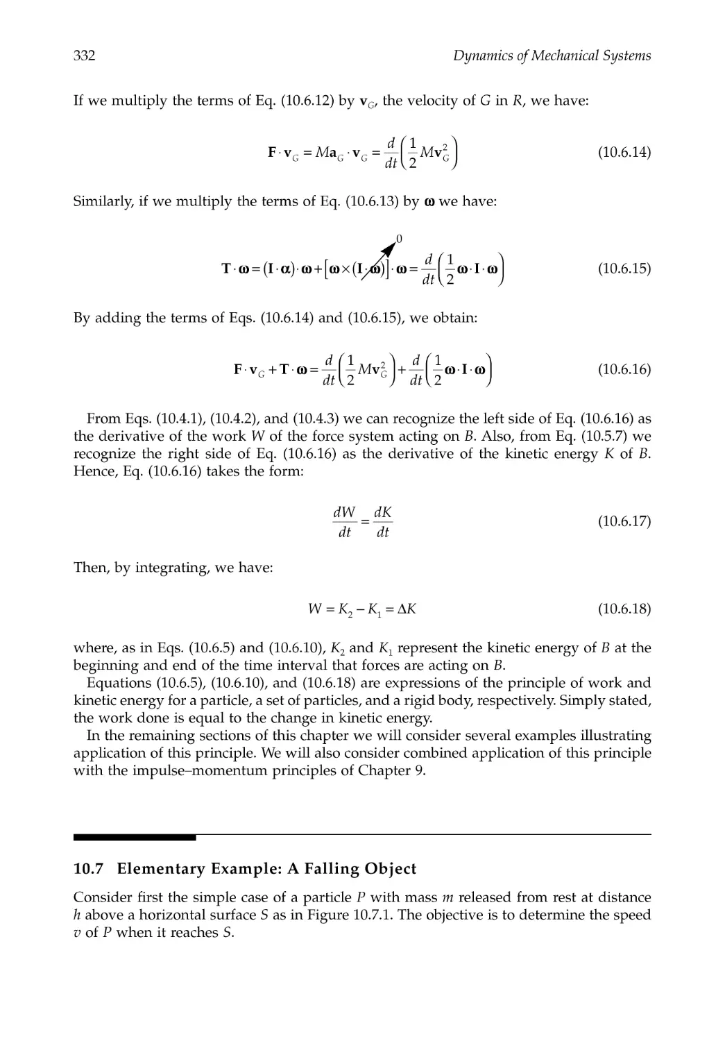
10.6 Work--Energy Principles ..................................................................................................329
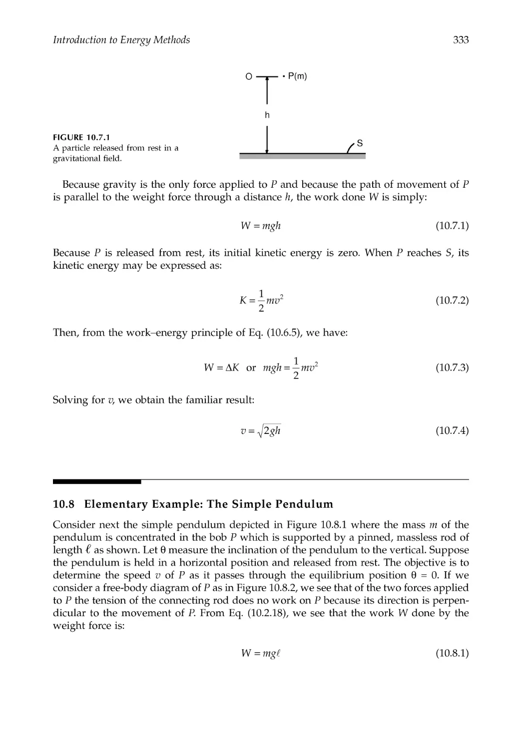
10.7 Elementary Example: A Falling Object.........................................................................332
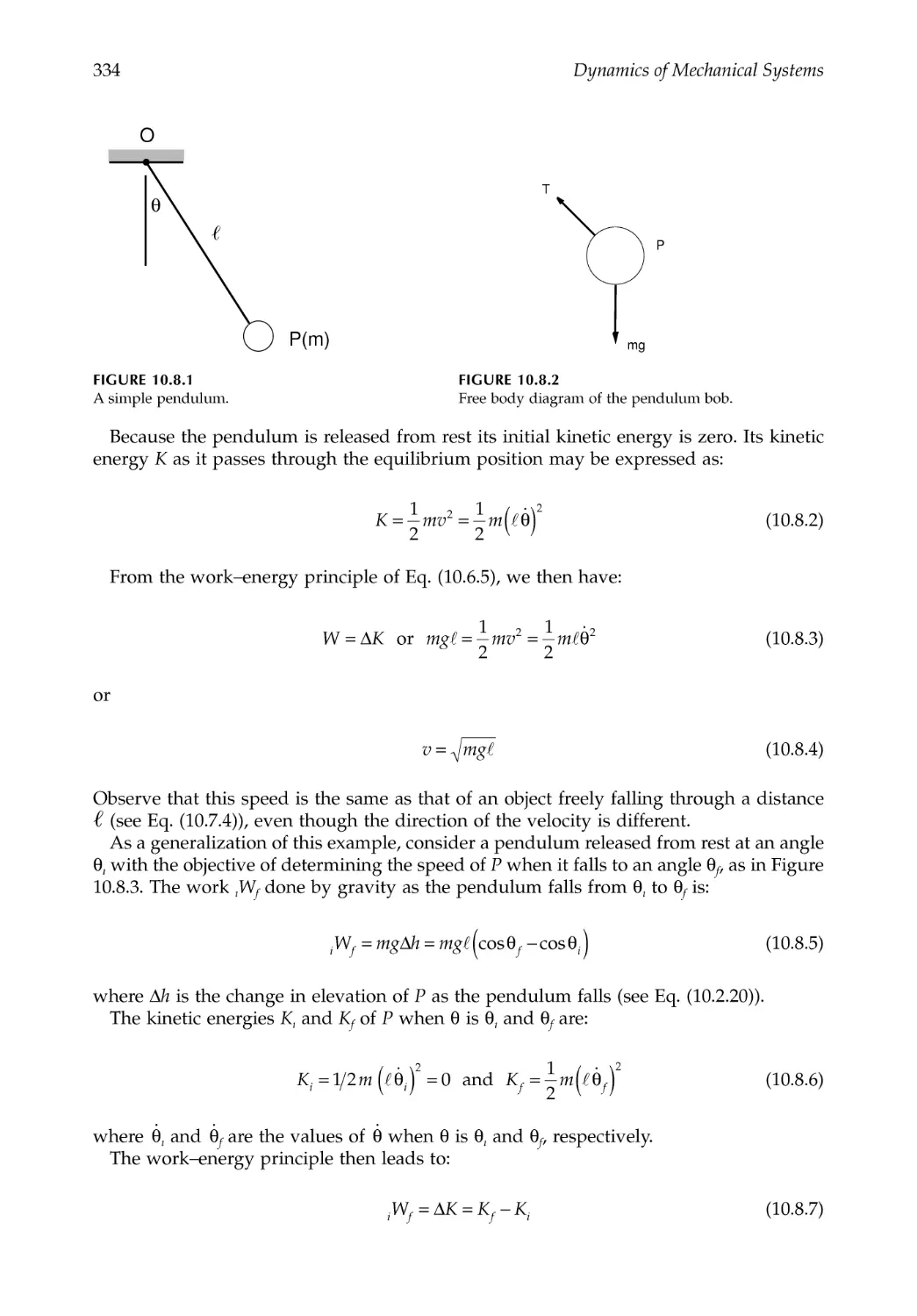
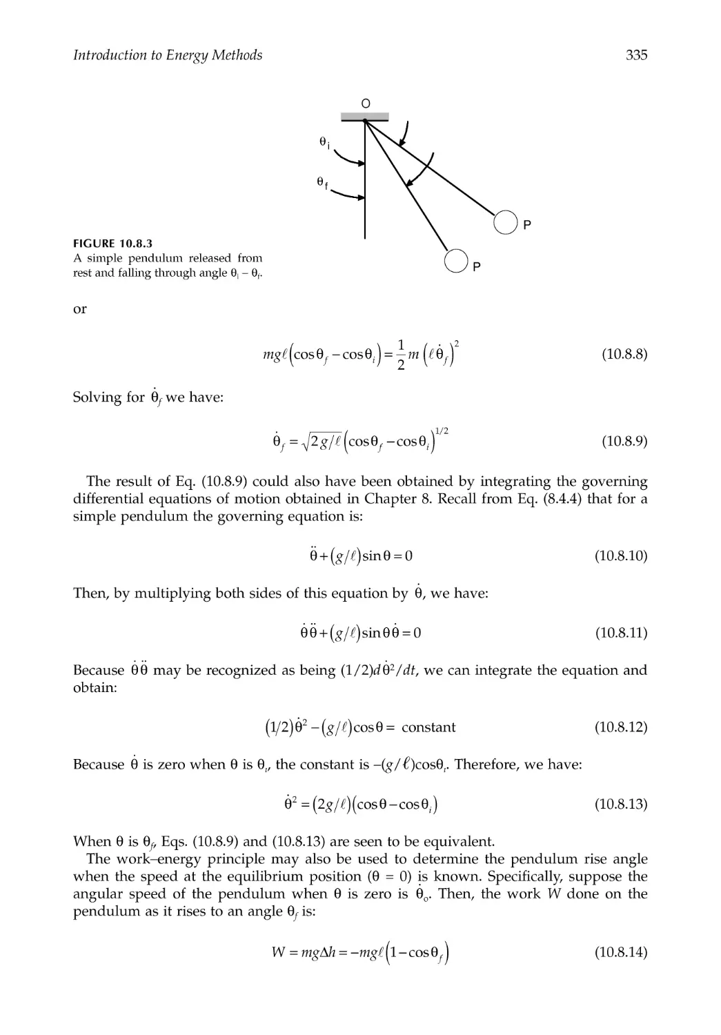
10.8 Elementary Example: The Simple Pendulum .............................................................333
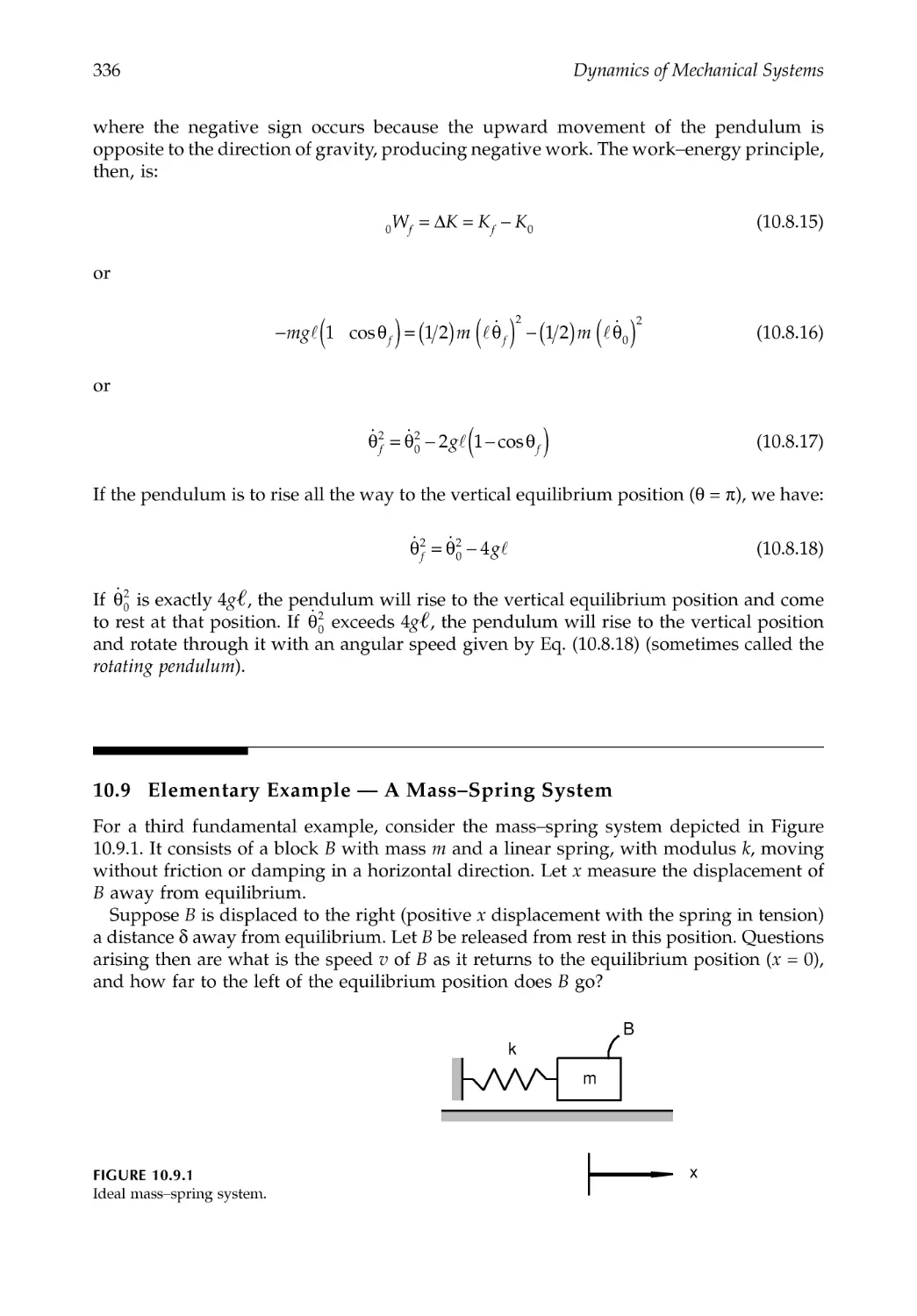
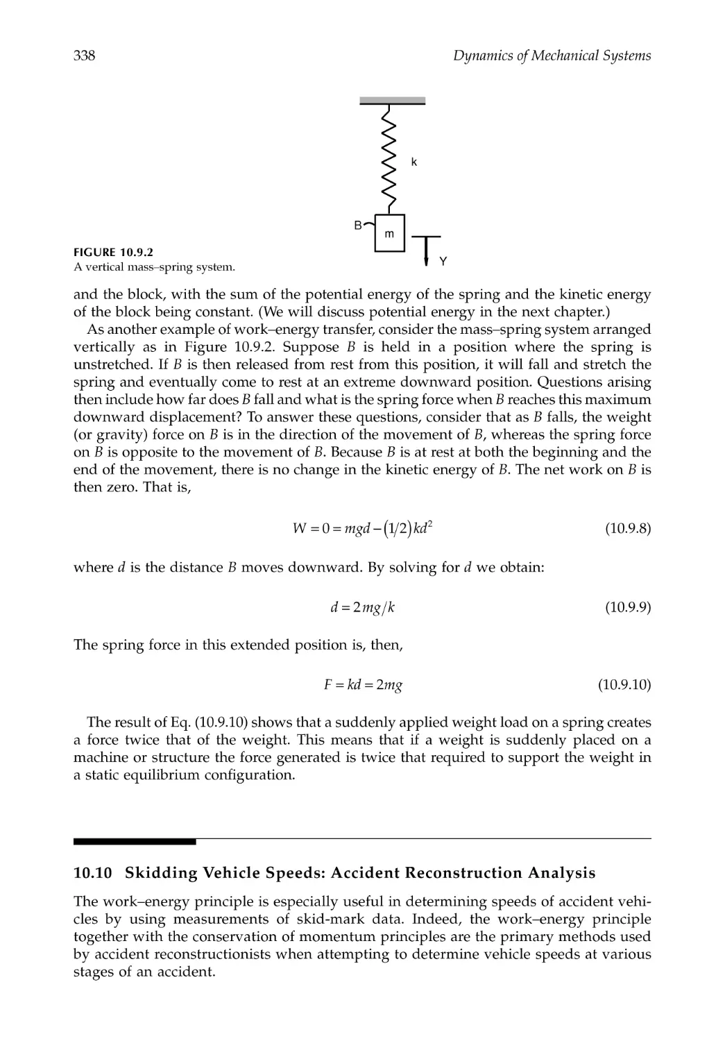
10.9 Elementary Example --- A Mass--Spring System ........................................................336
10.10 Skidding Vehicle Speeds: Accident Reconstruction Analysis ...................................338
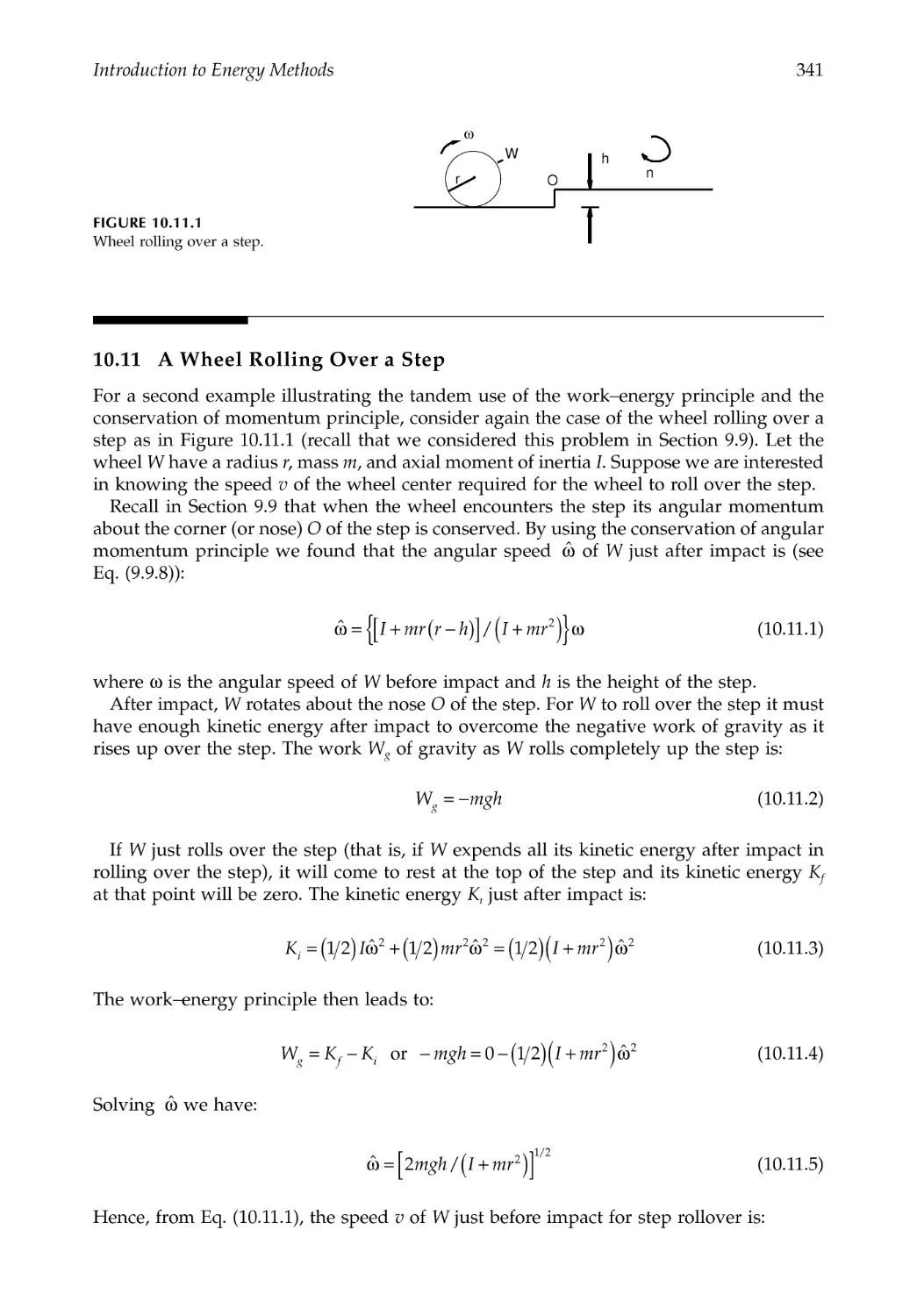
10.11 A Wheel Rolling Over a Step .........................................................................................341
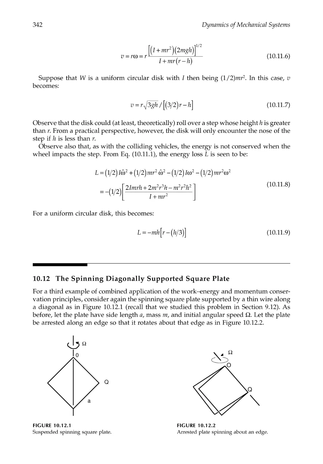
10.12 The Spinning Diagonally Supported Square Plate.....................................................342
10.13 Closure ...............................................................................................................................344
References (Accident Reconstruction)......................................................................................344
Problems .......................................................................................................................................344
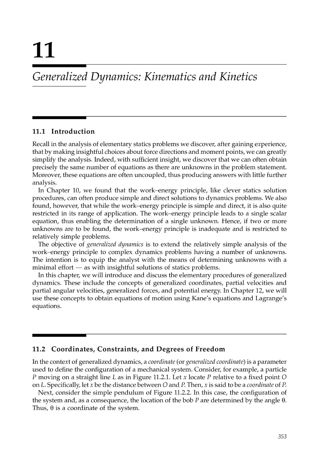
Chapter 11 Generalized Dynamics: Kinematics and Kinetics ..........................................353
11.1 Introduction.......................................................................................................................353
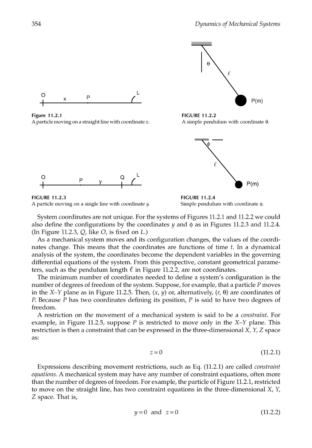
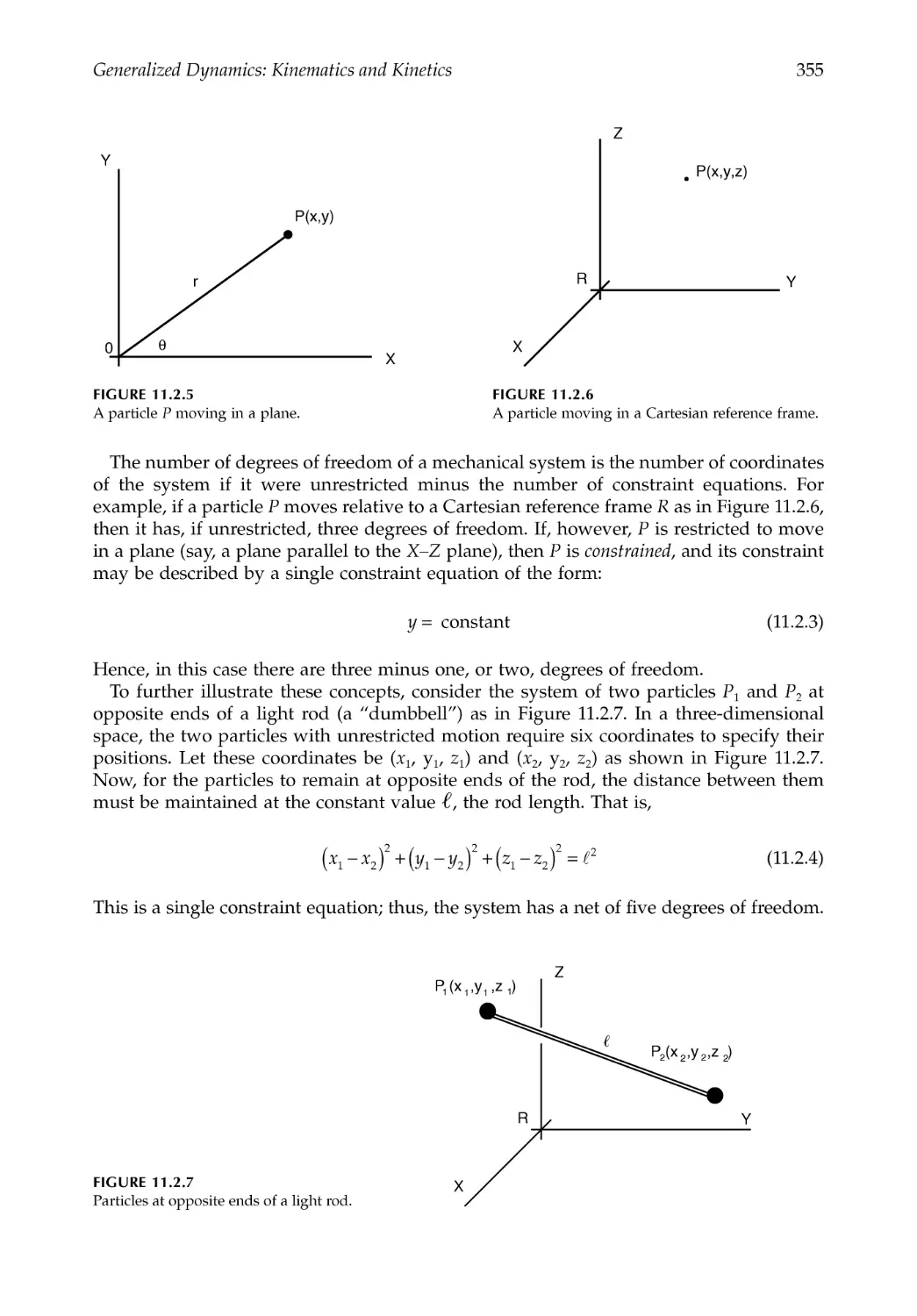
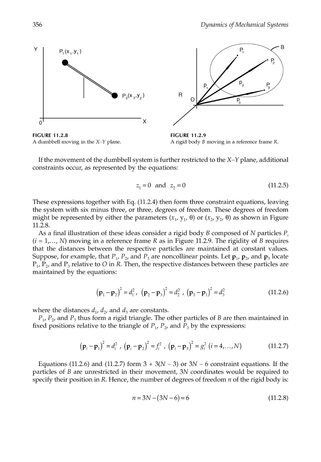
11.2 Coordinates, Constraints, and Degrees of Freedom ..................................................353
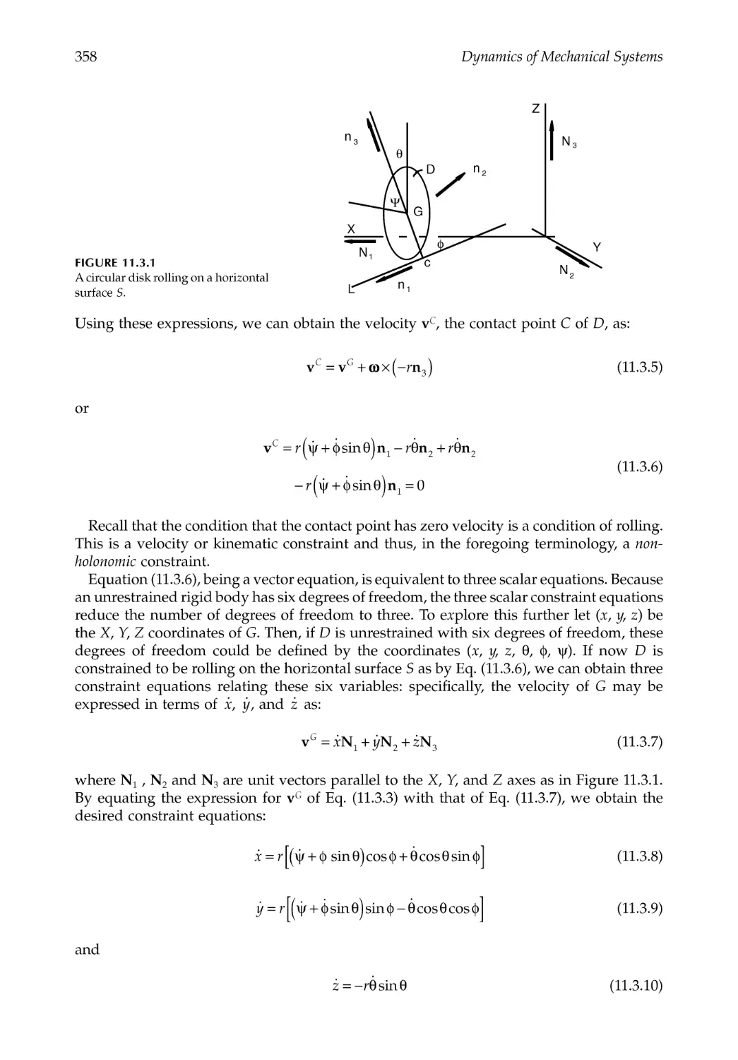
11.3 Holonomic and Nonholonomic Constraints ...............................................................357
11.4 Vector Functions, Partial Velocity, and Partial Angular Velocity .............................359
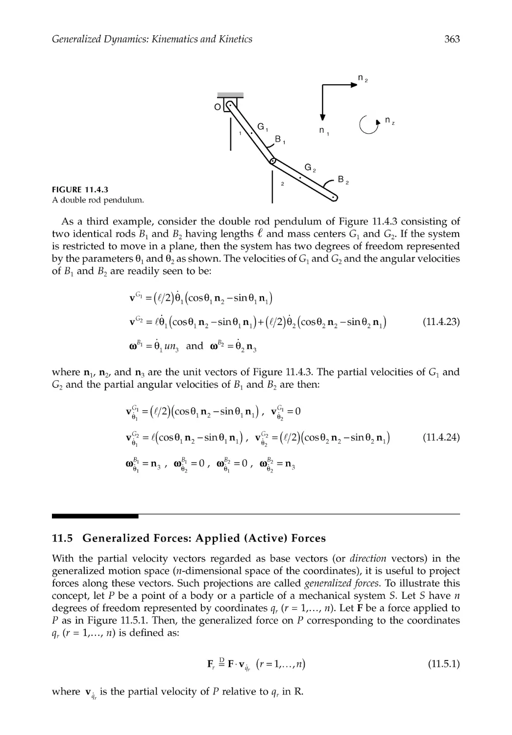
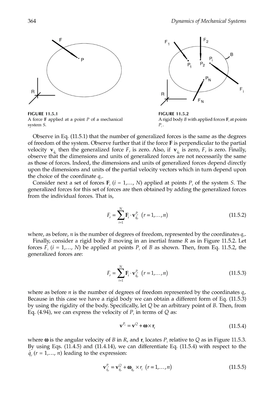
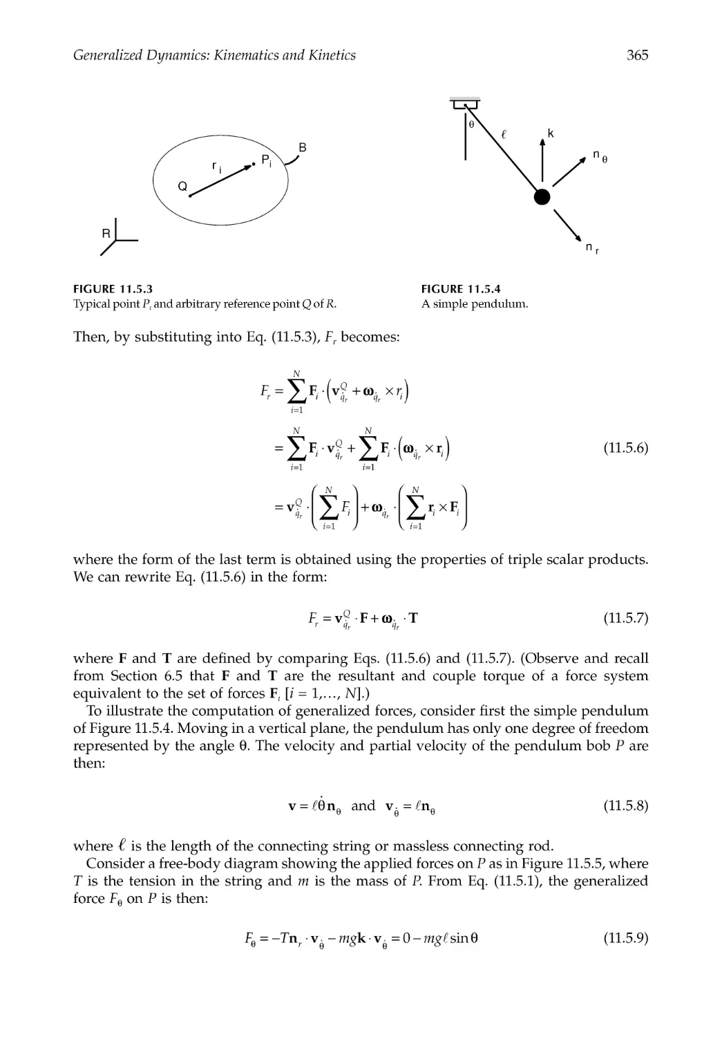
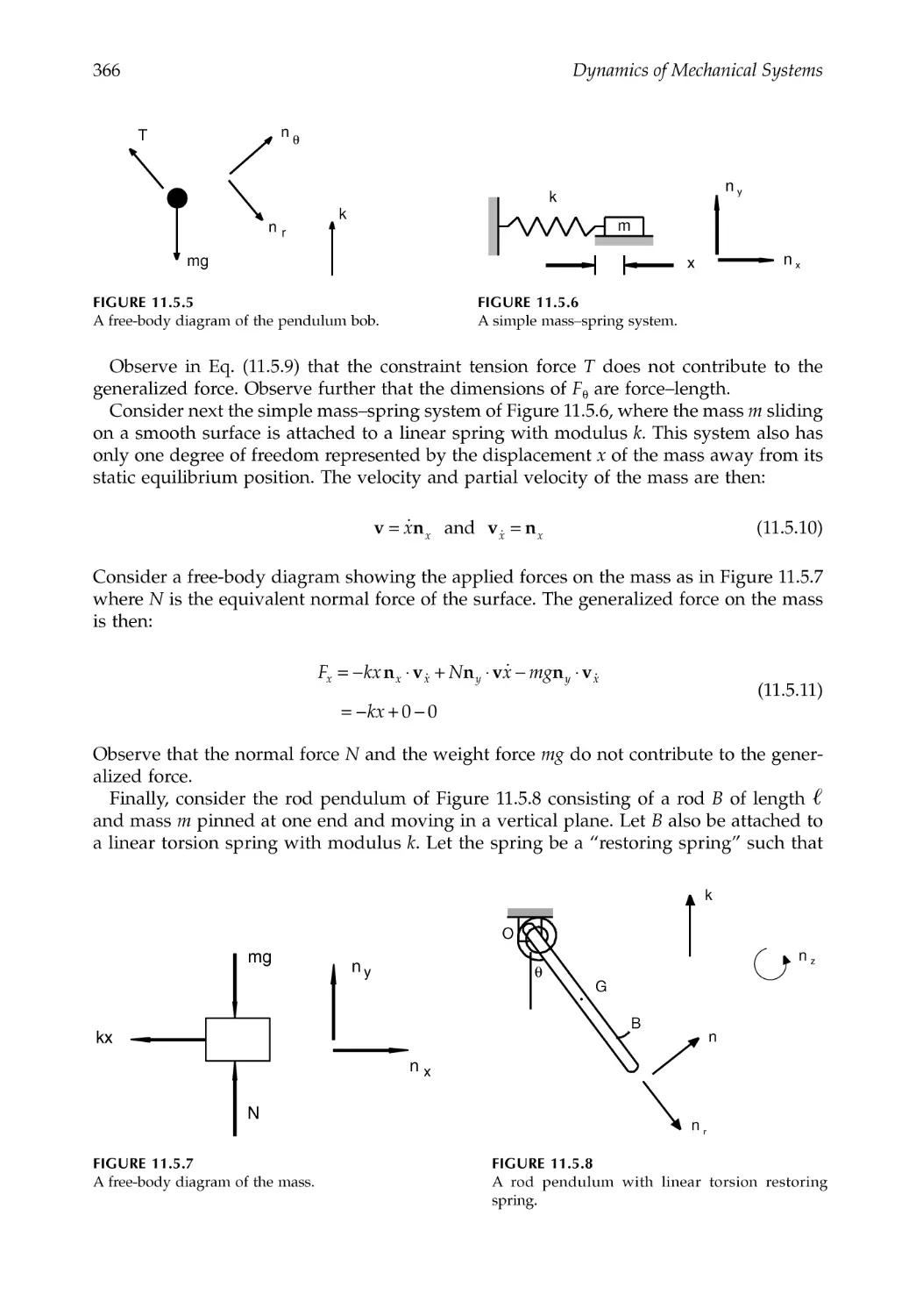
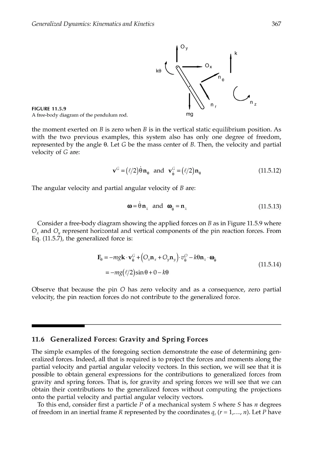
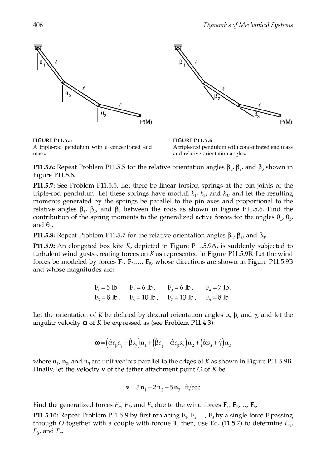
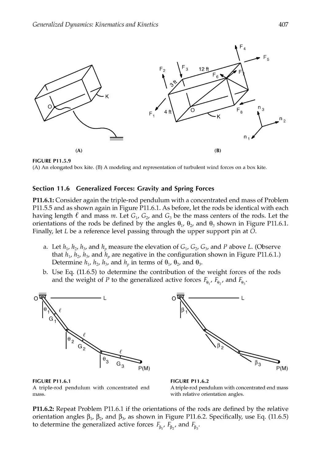
11.5 Generalized Forces: Applied (Active) Forces ..............................................................363
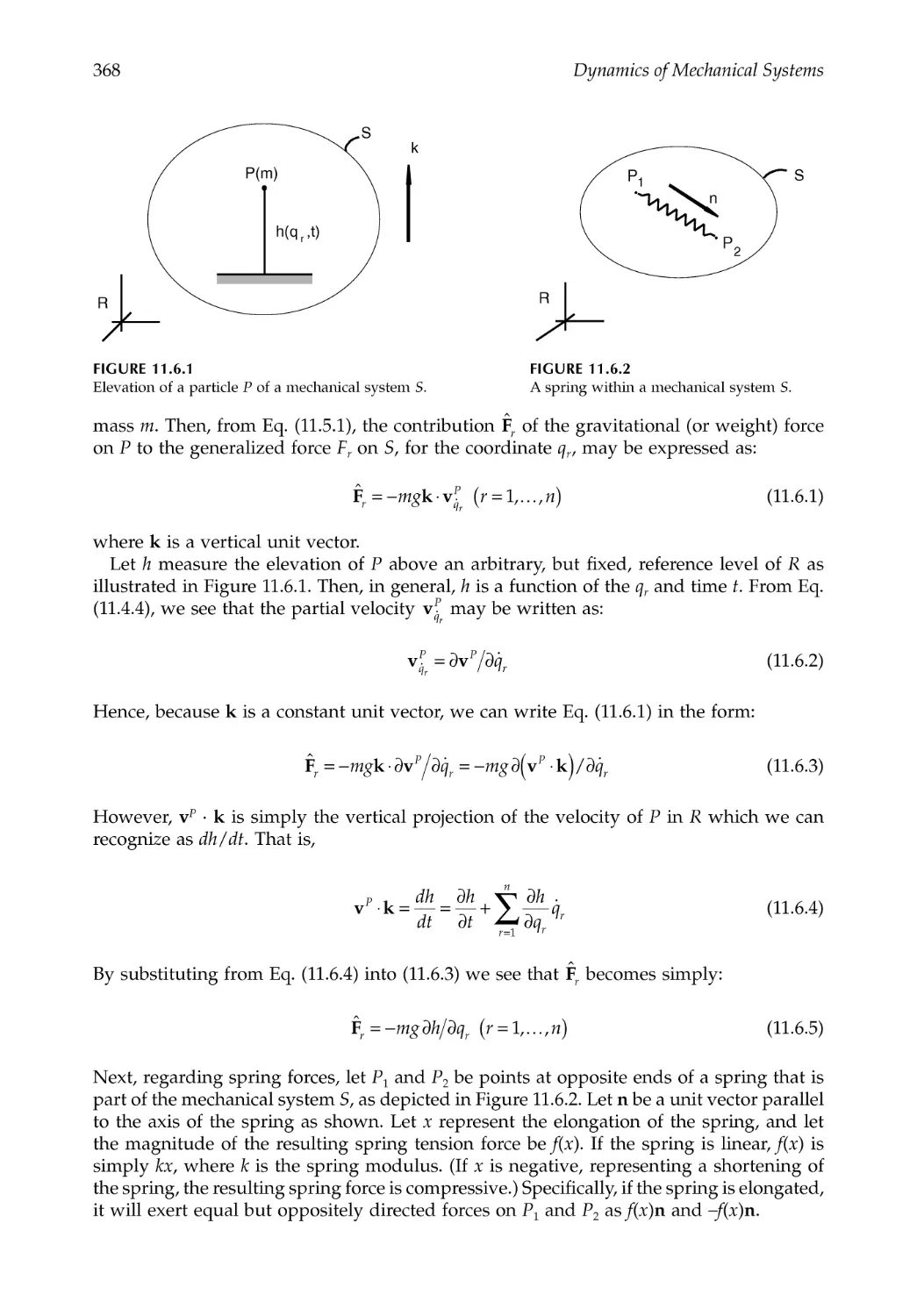
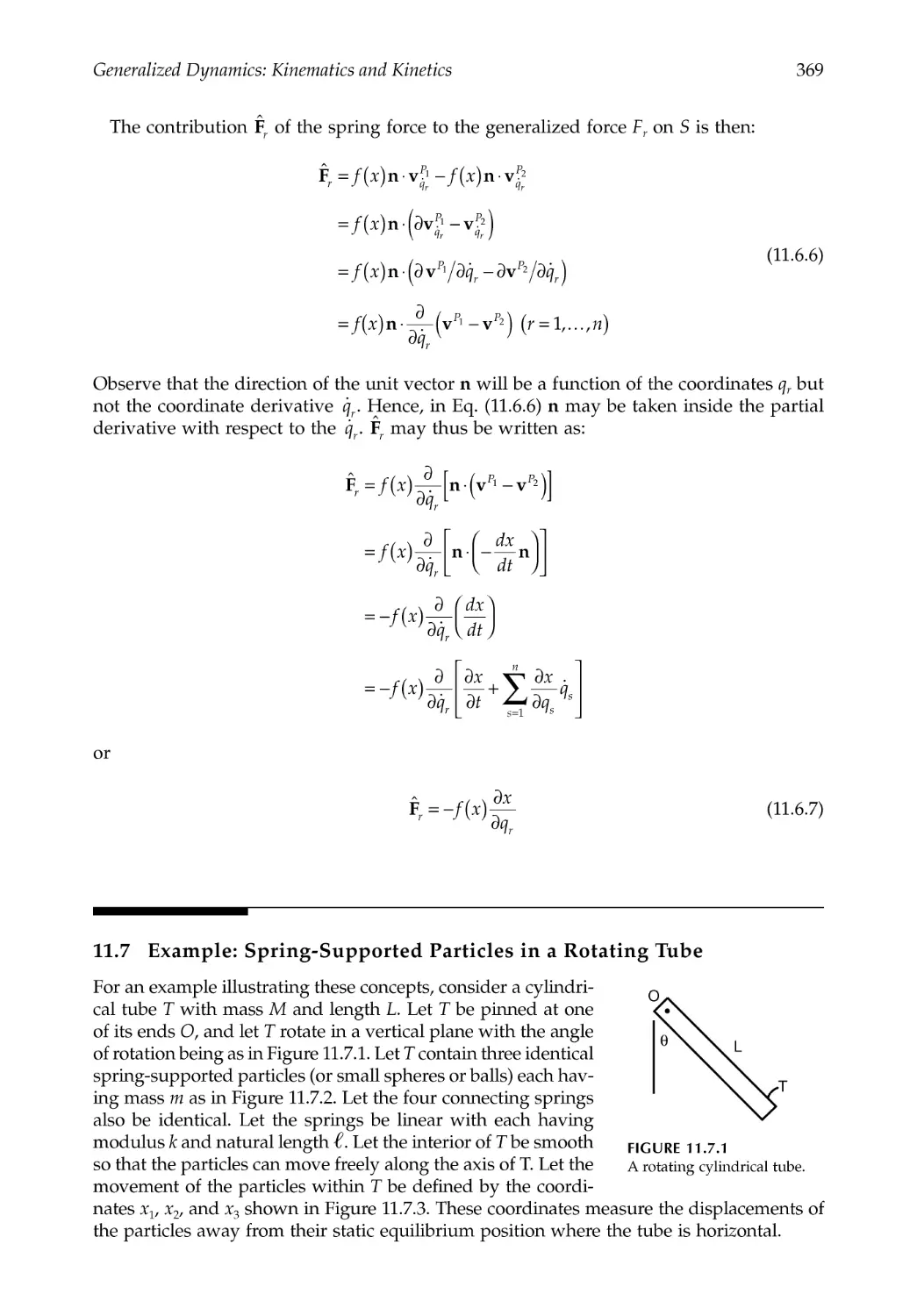
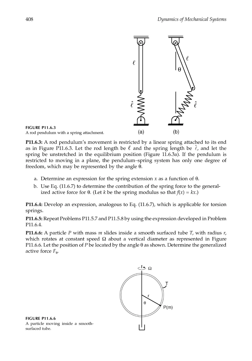
11.6 Generalized Forces: Gravity and Spring Forces .........................................................367
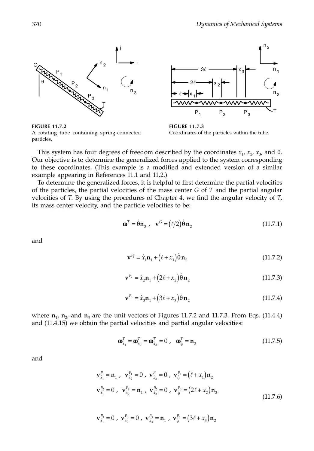
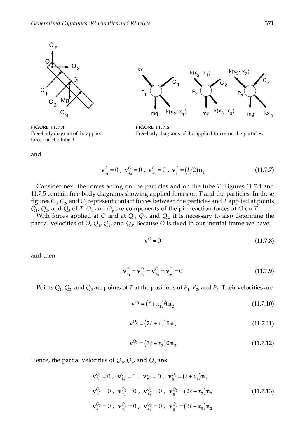
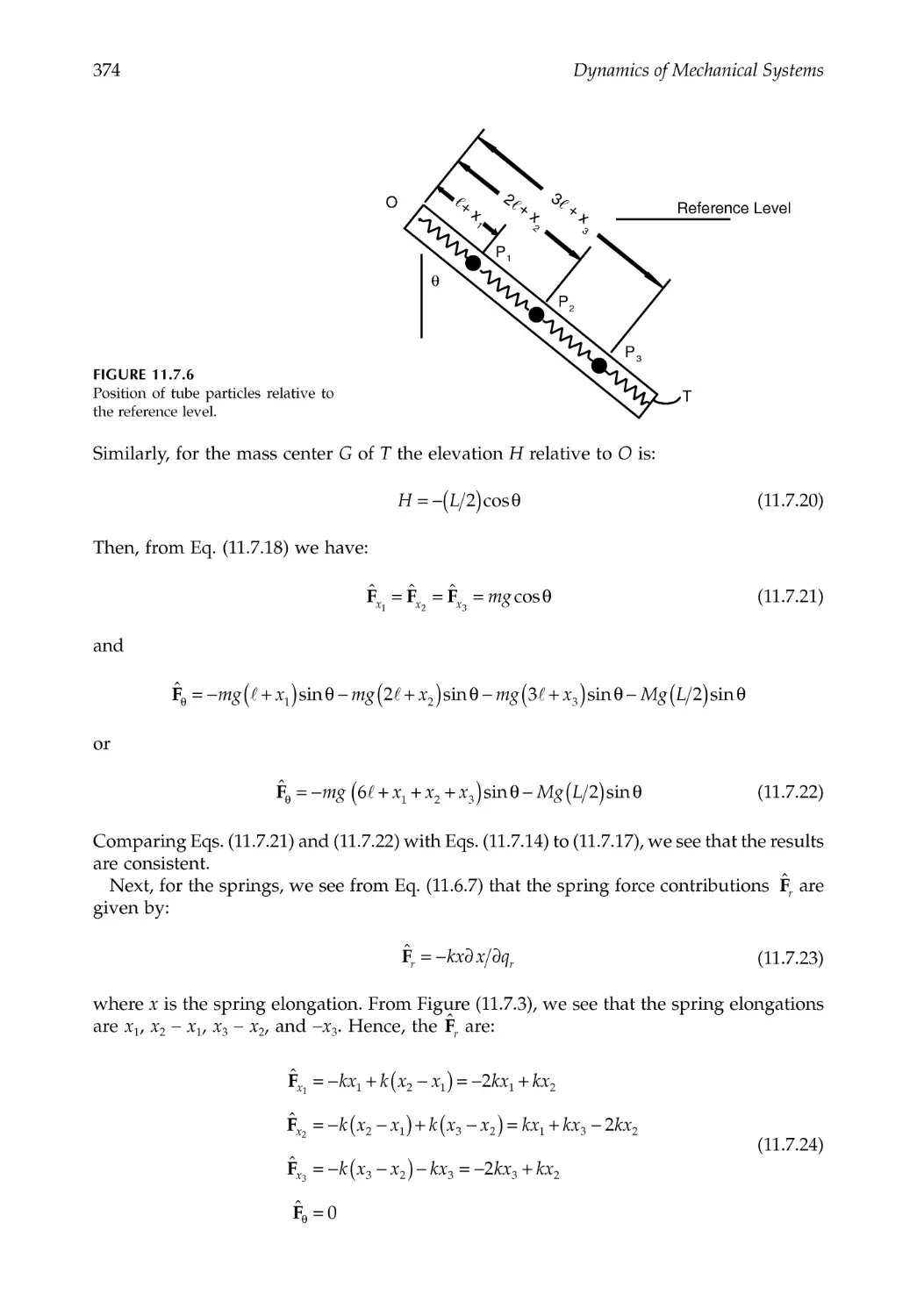
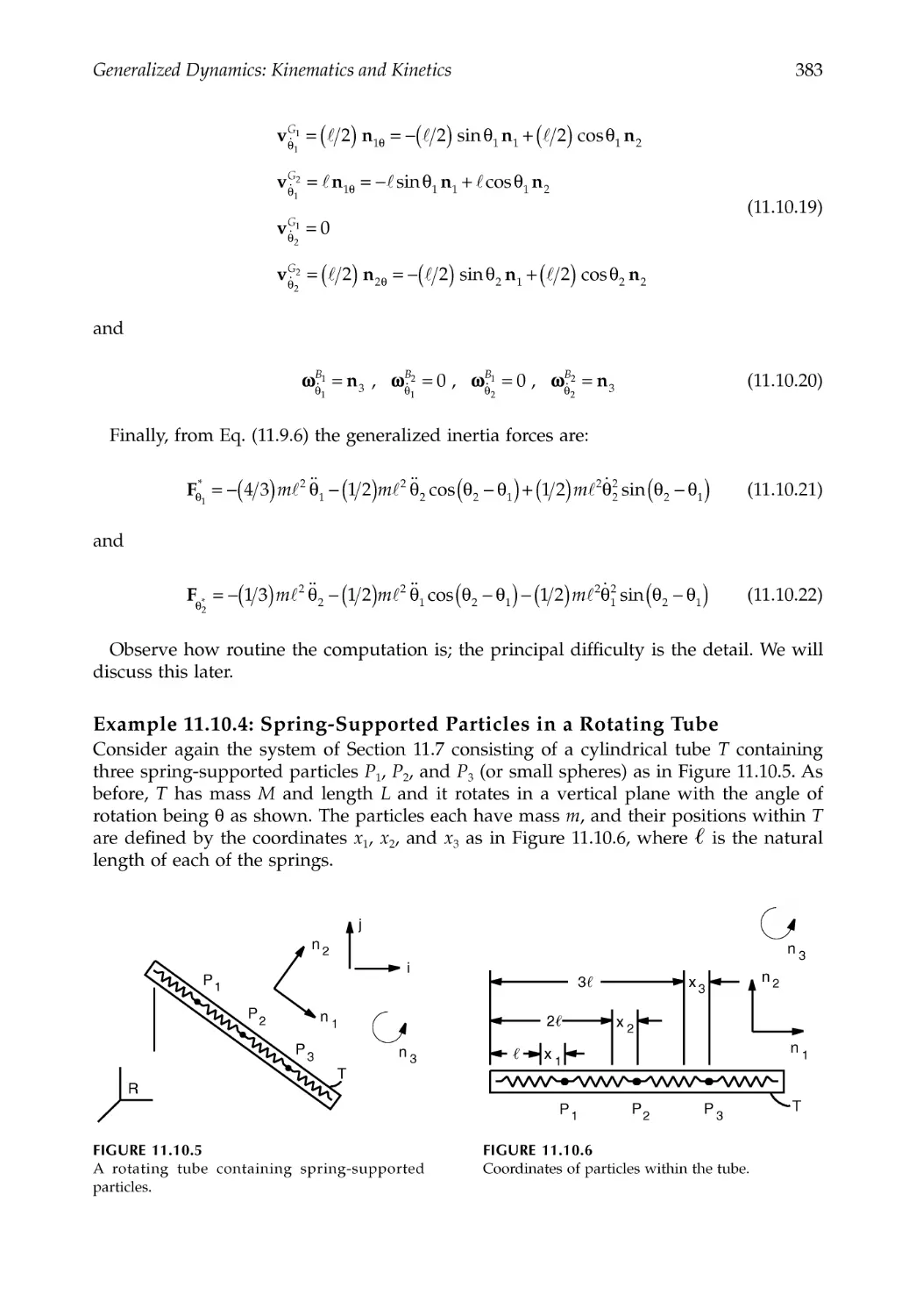
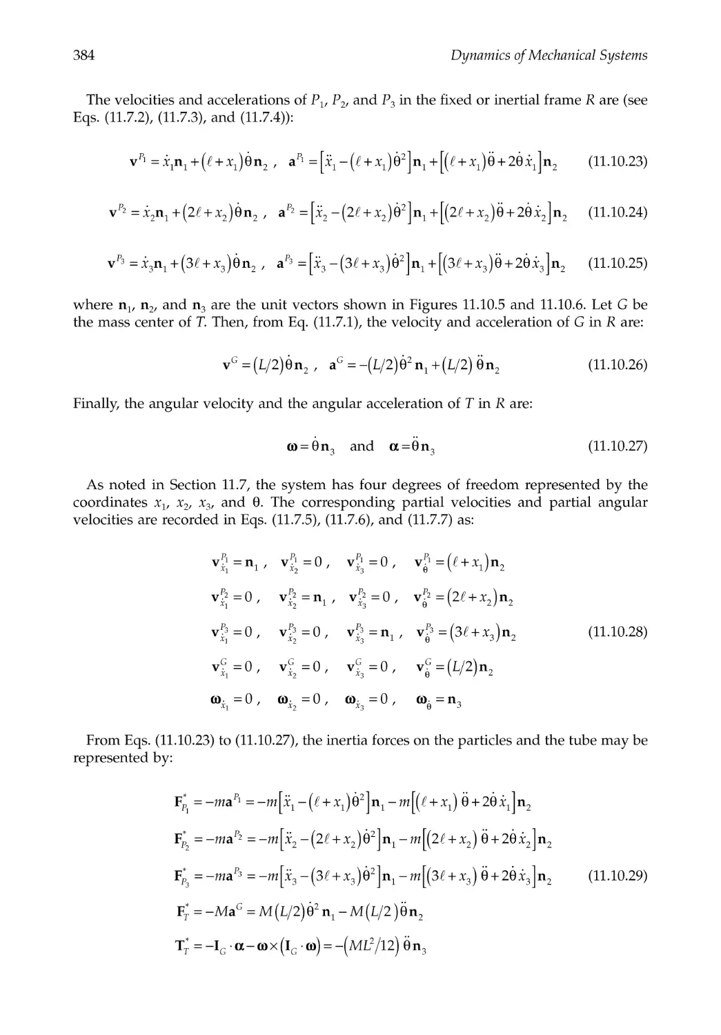
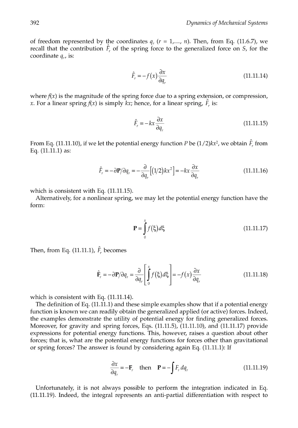
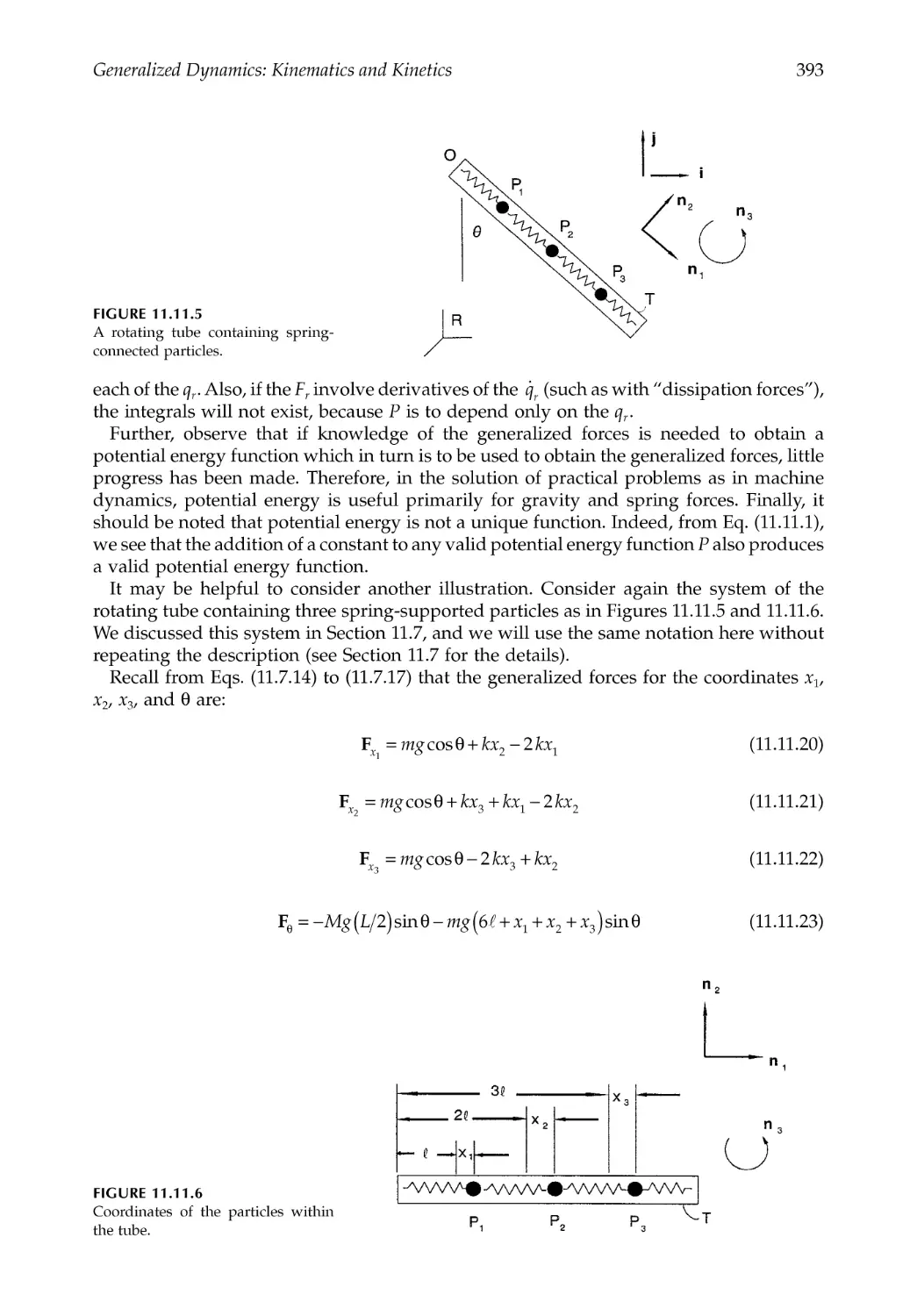
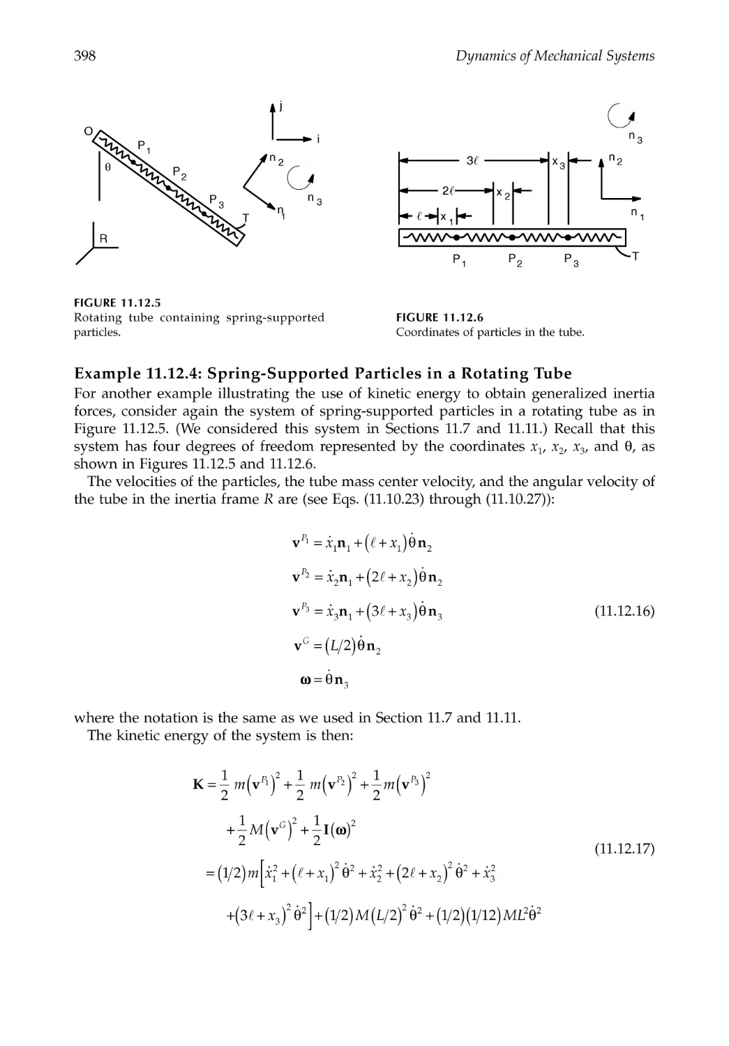
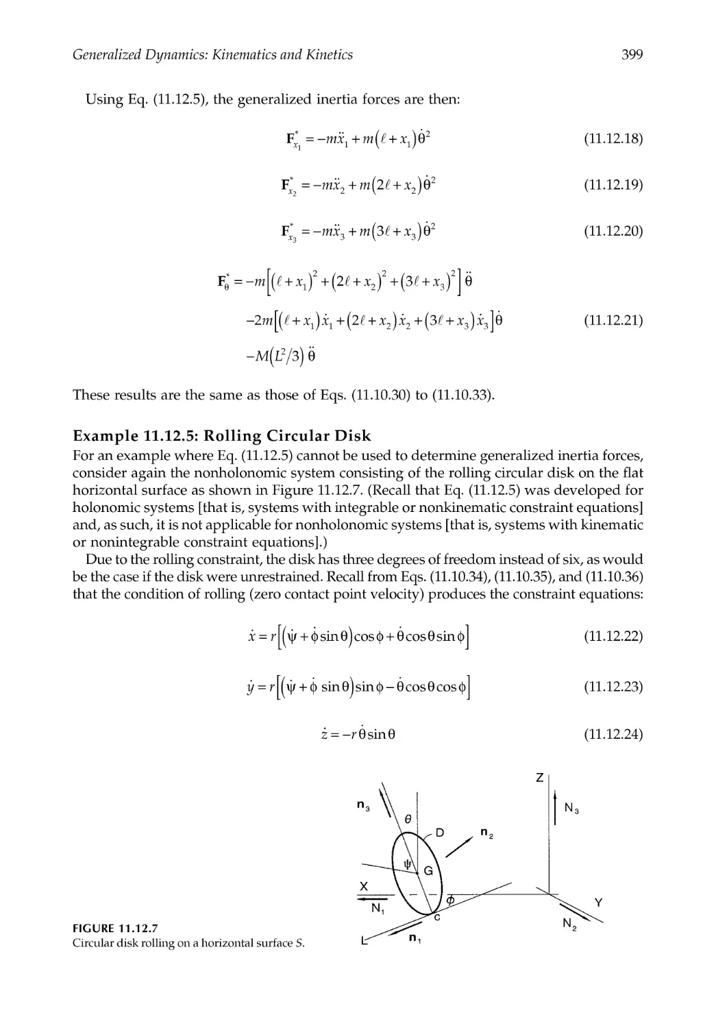
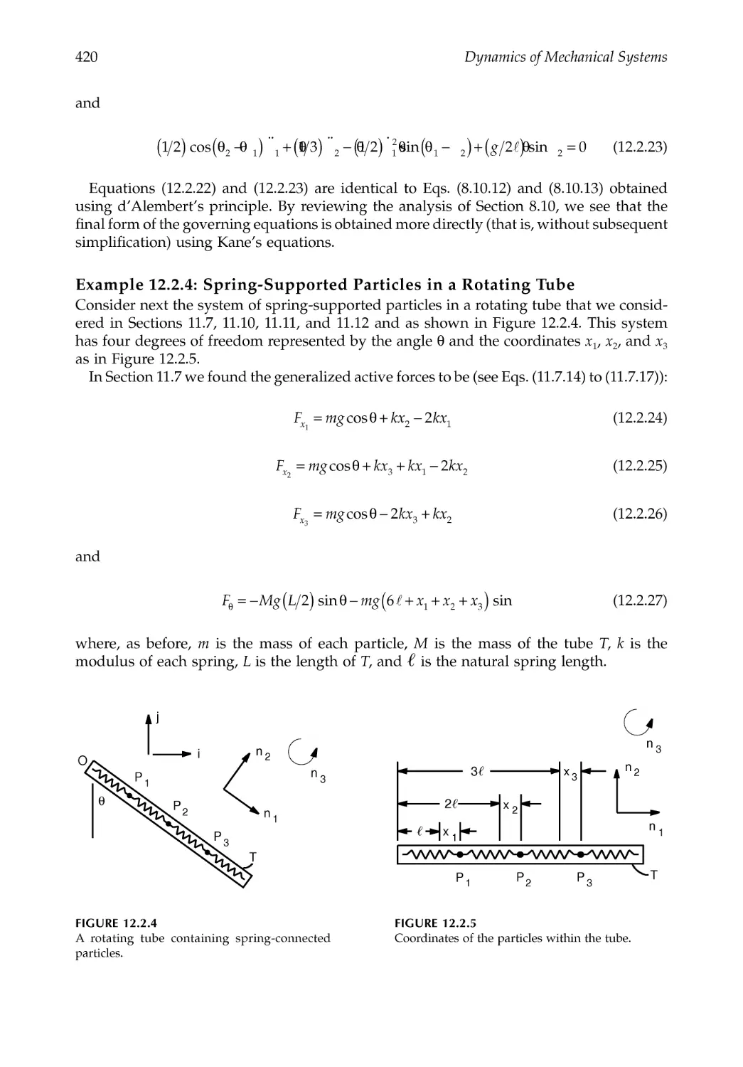
11.7 Example: Spring-Supported Particles in a Rotating Tube.........................................369
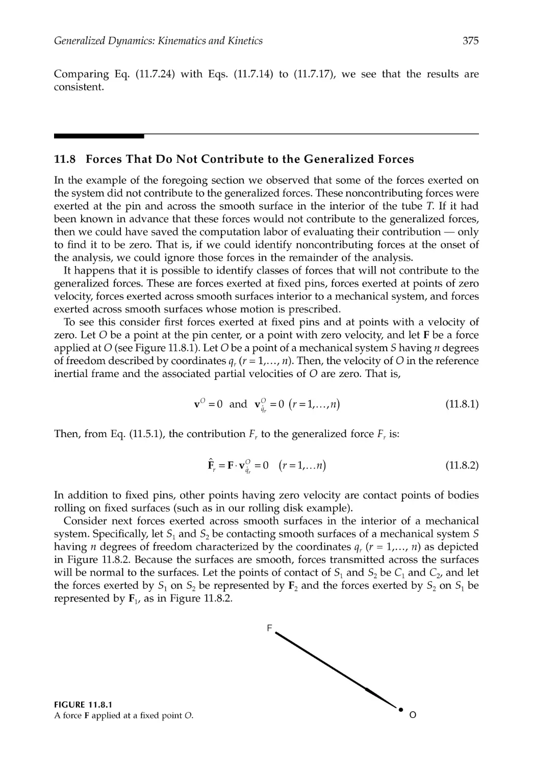
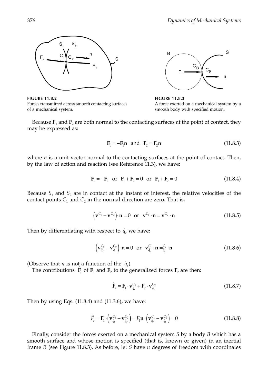
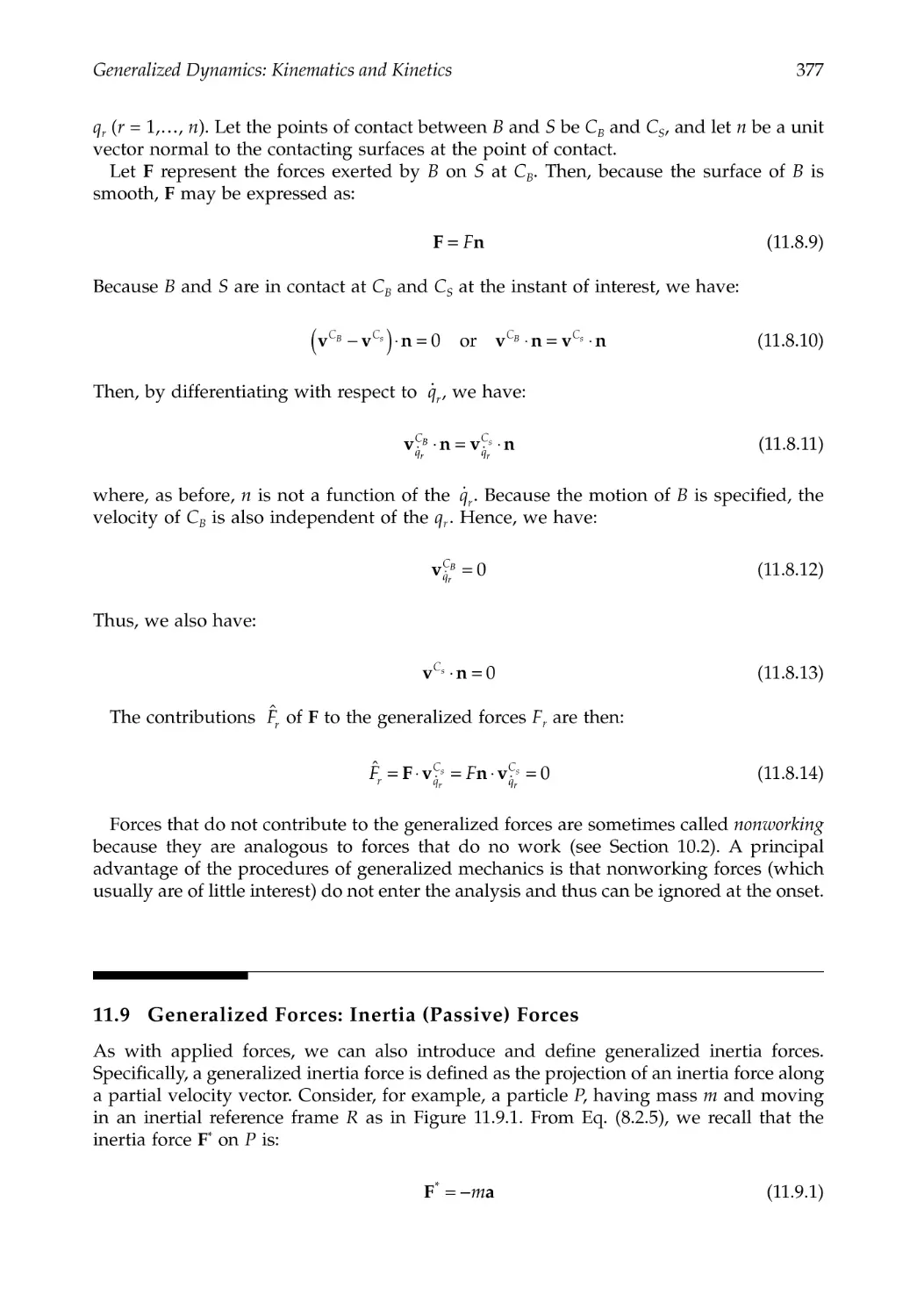
11.8 Forces That Do Not Contribute to the Generalized Forces ......................................375
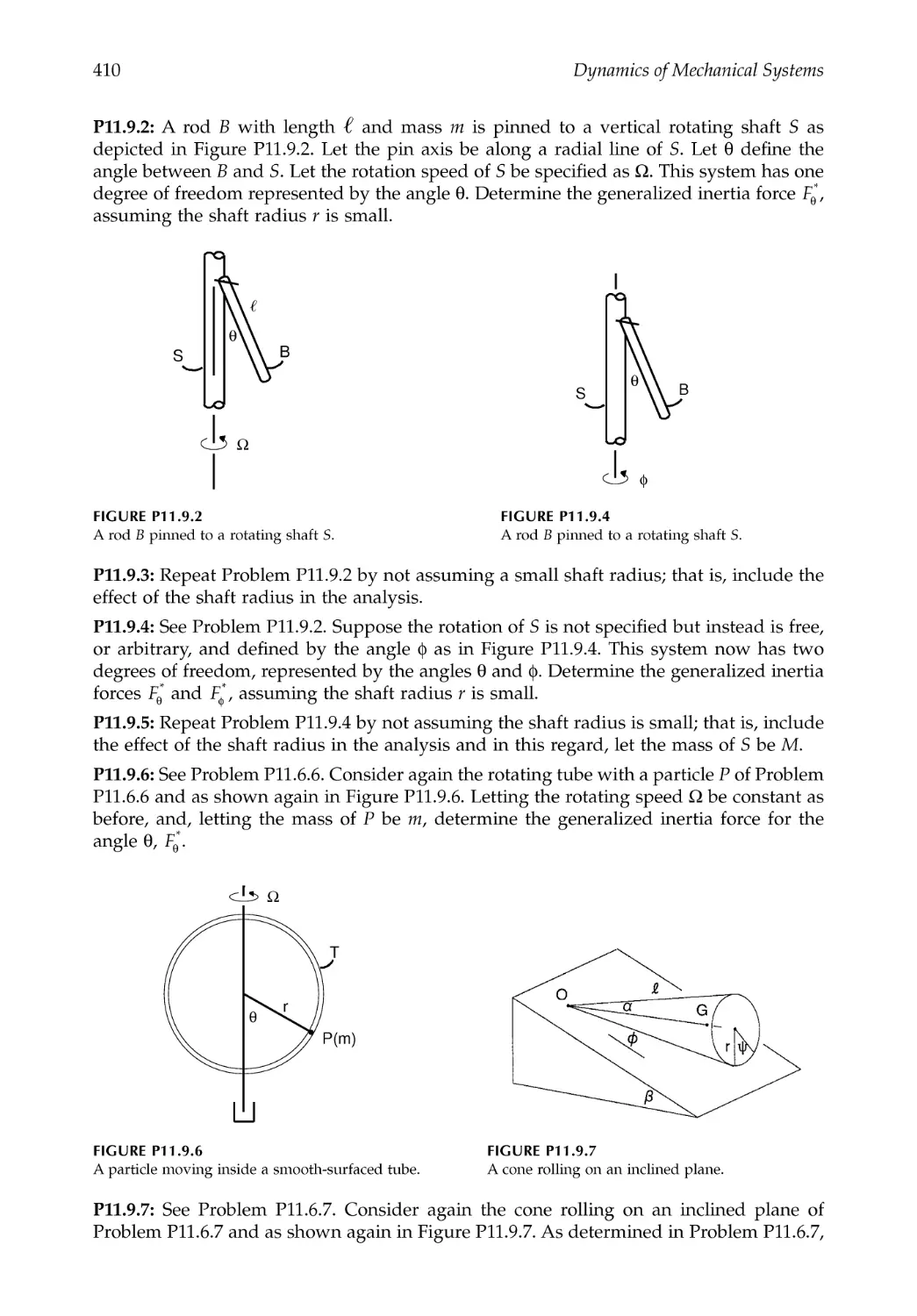
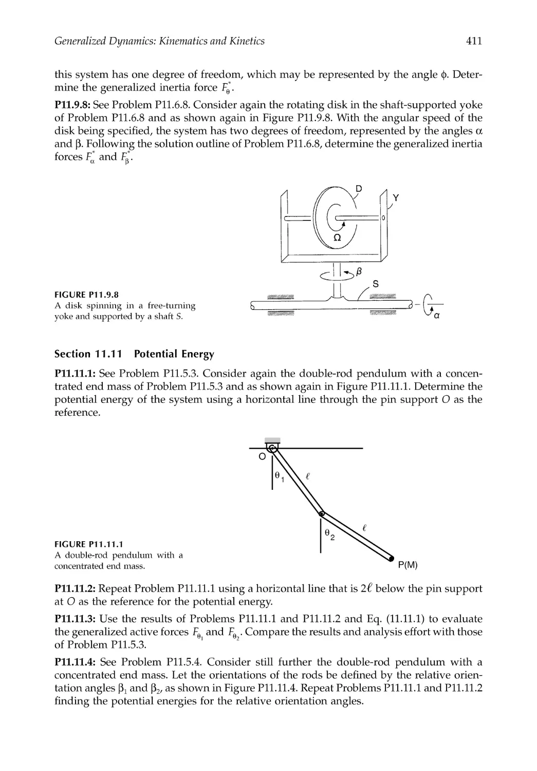
11.9 Generalized Forces: Inertia (Passive) Forces ...............................................................377
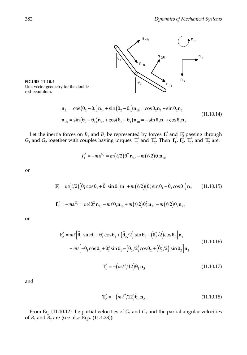
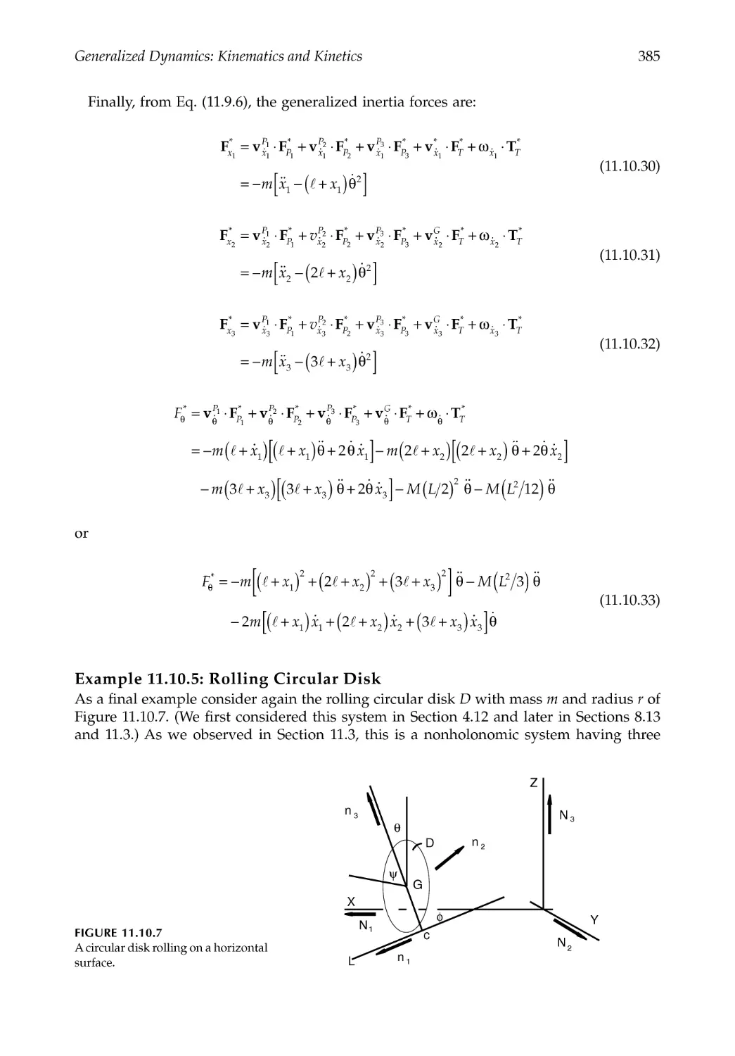
11.10 Examples............................................................................................................................379
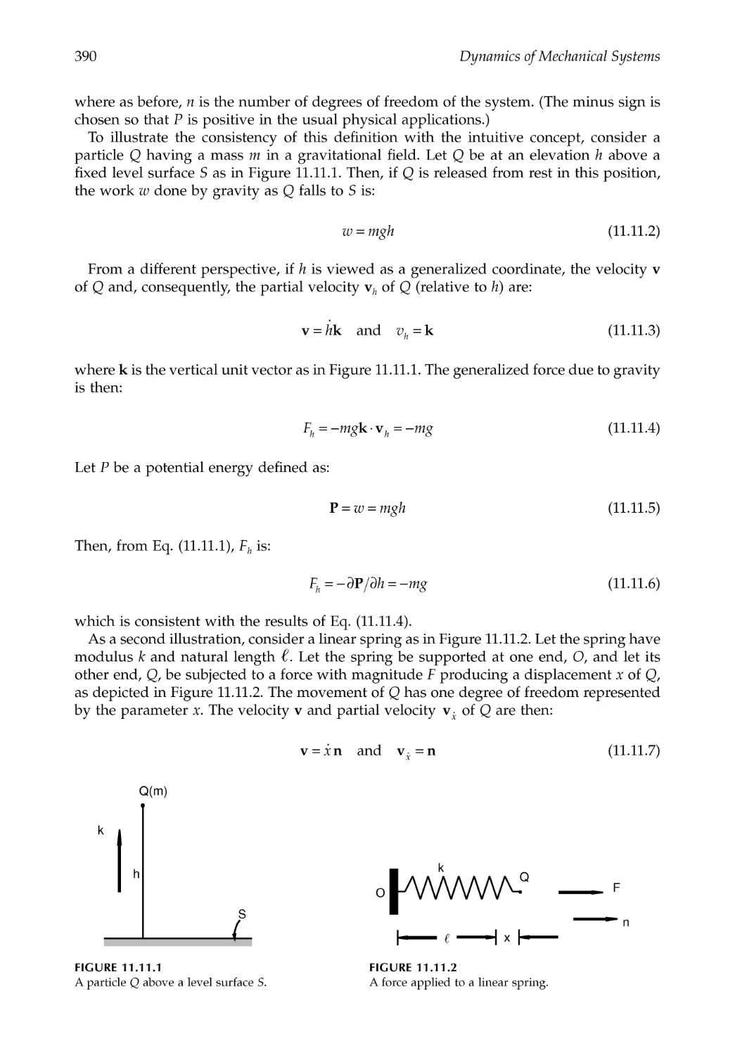
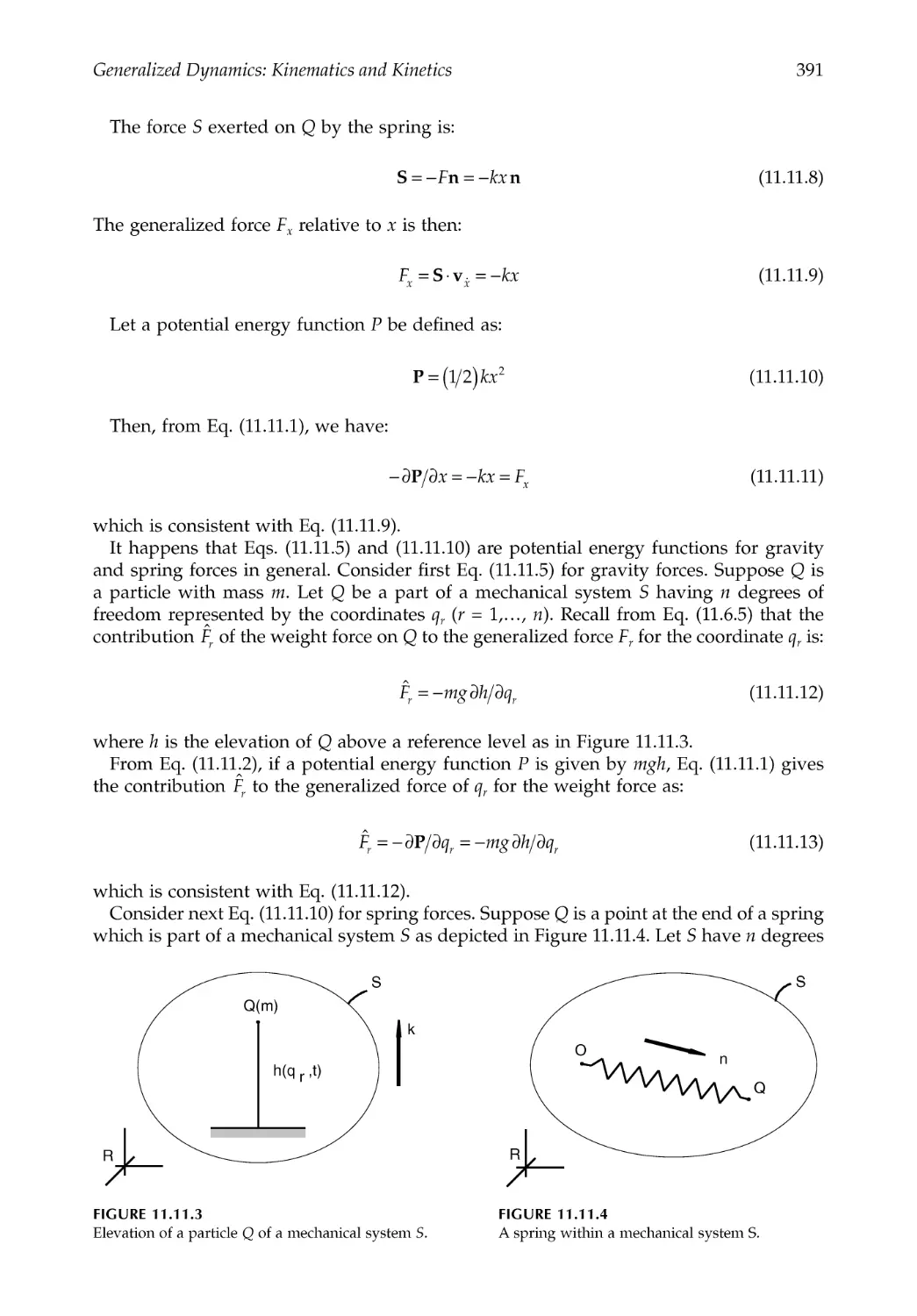
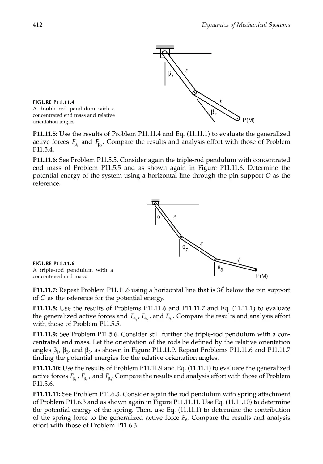
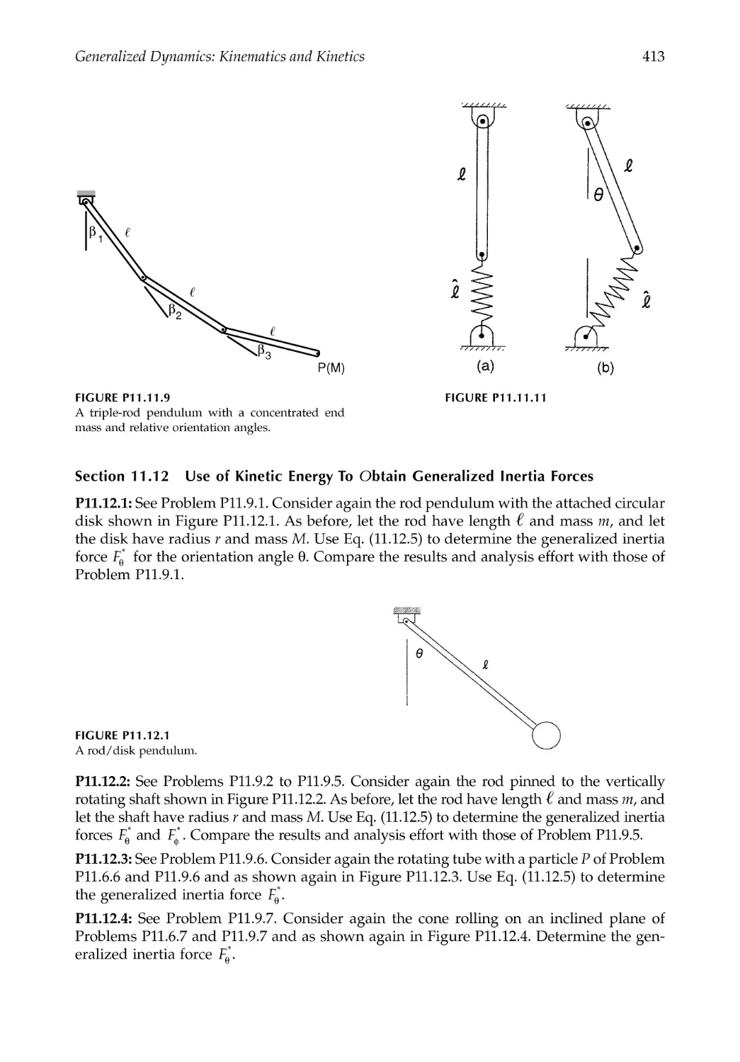
11.11 Potential Energy ...............................................................................................................389
11.12 Use of Kinetic Energy to Obtain Generalized Inertia Forces ...................................394
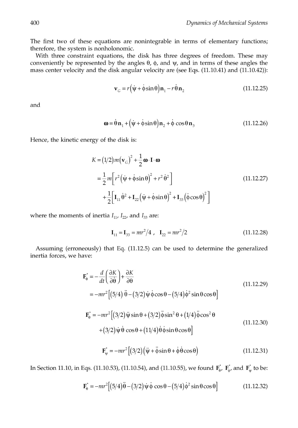
11.13 Closure ...............................................................................................................................401
References .....................................................................................................................................401
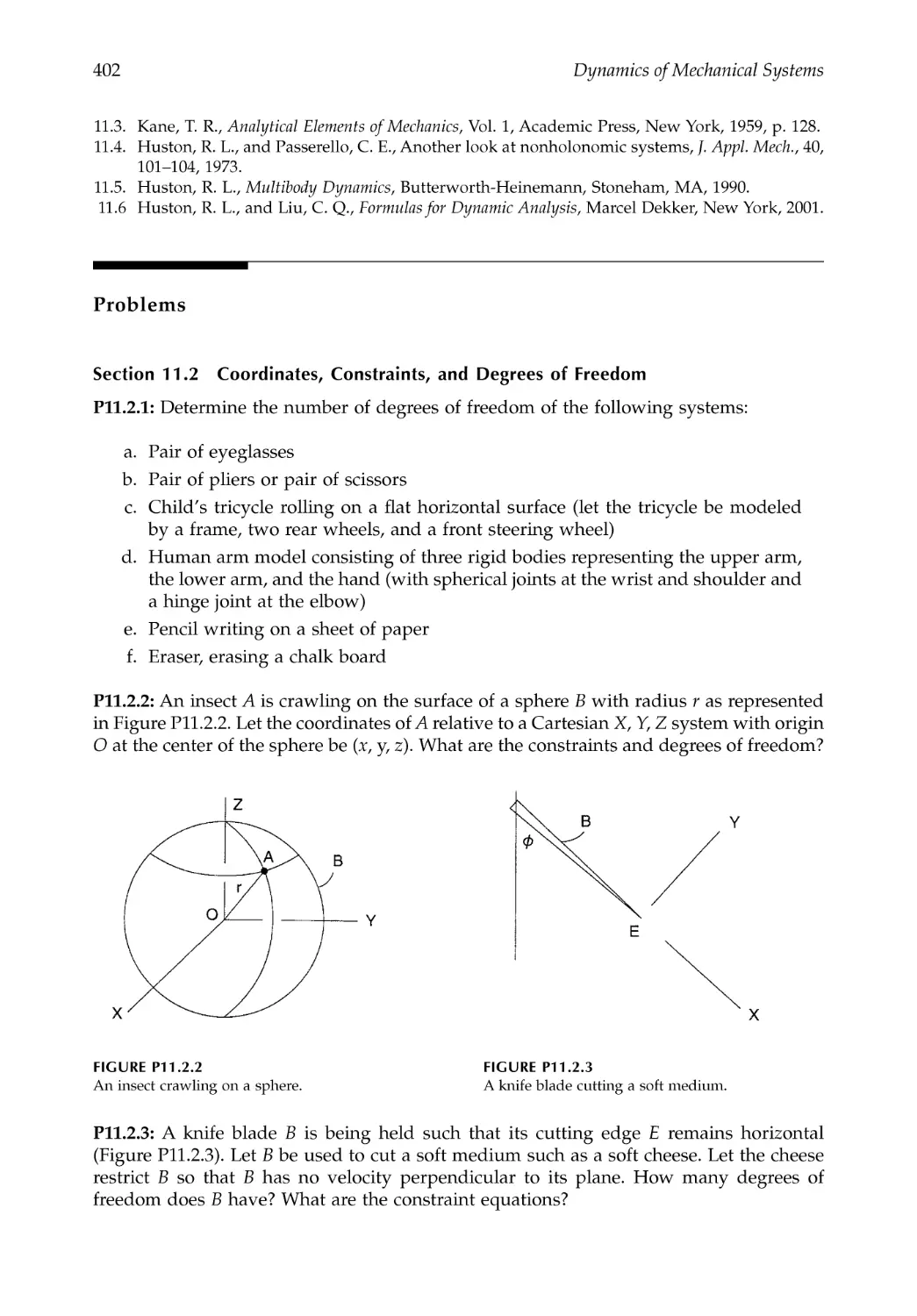
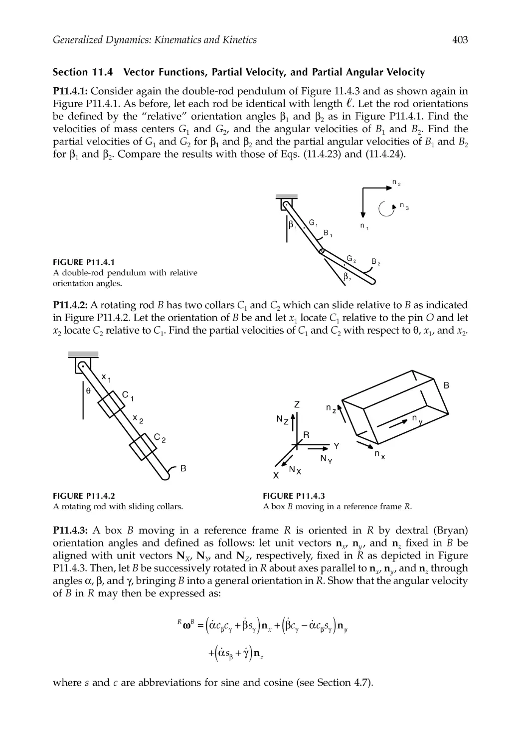
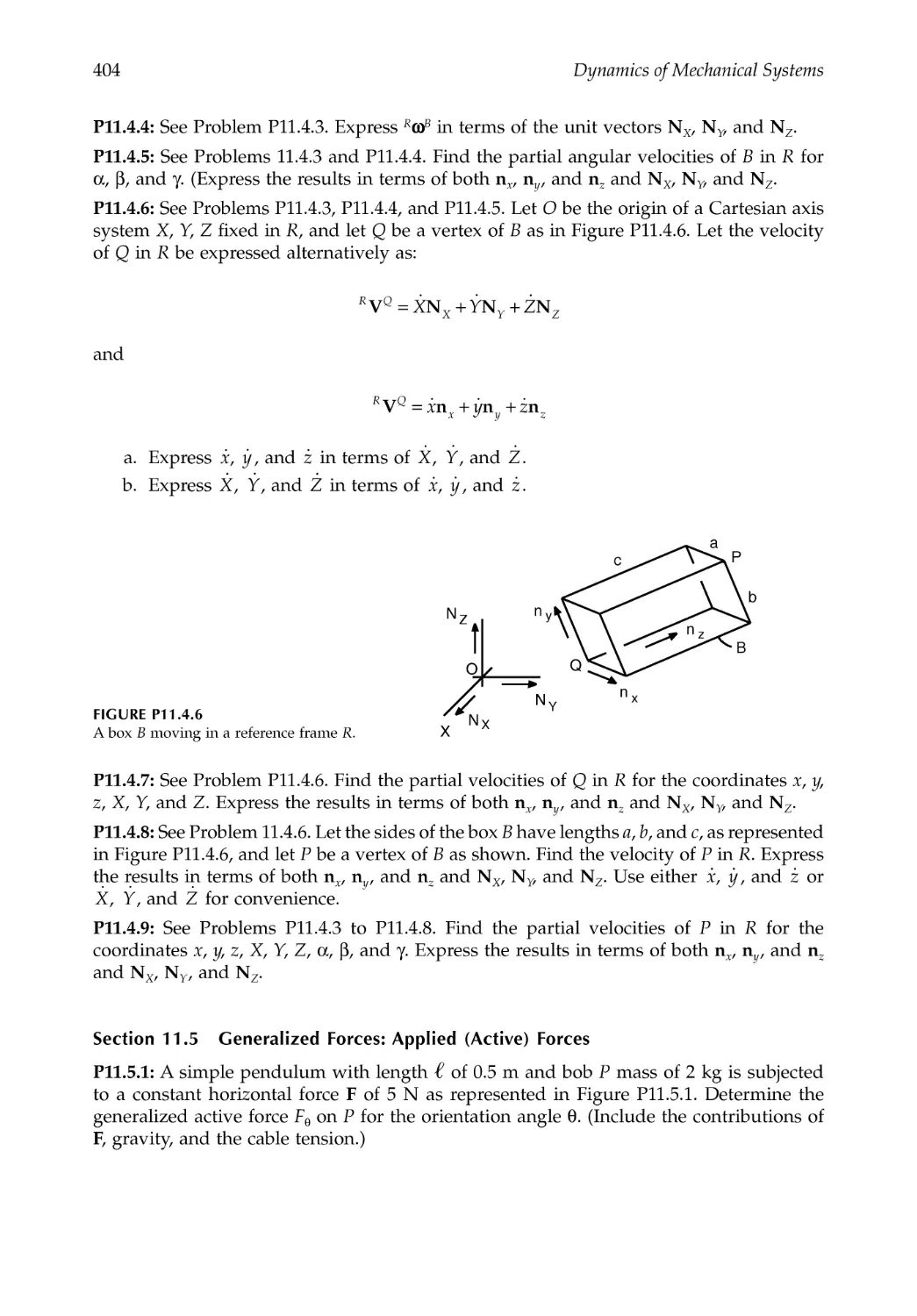
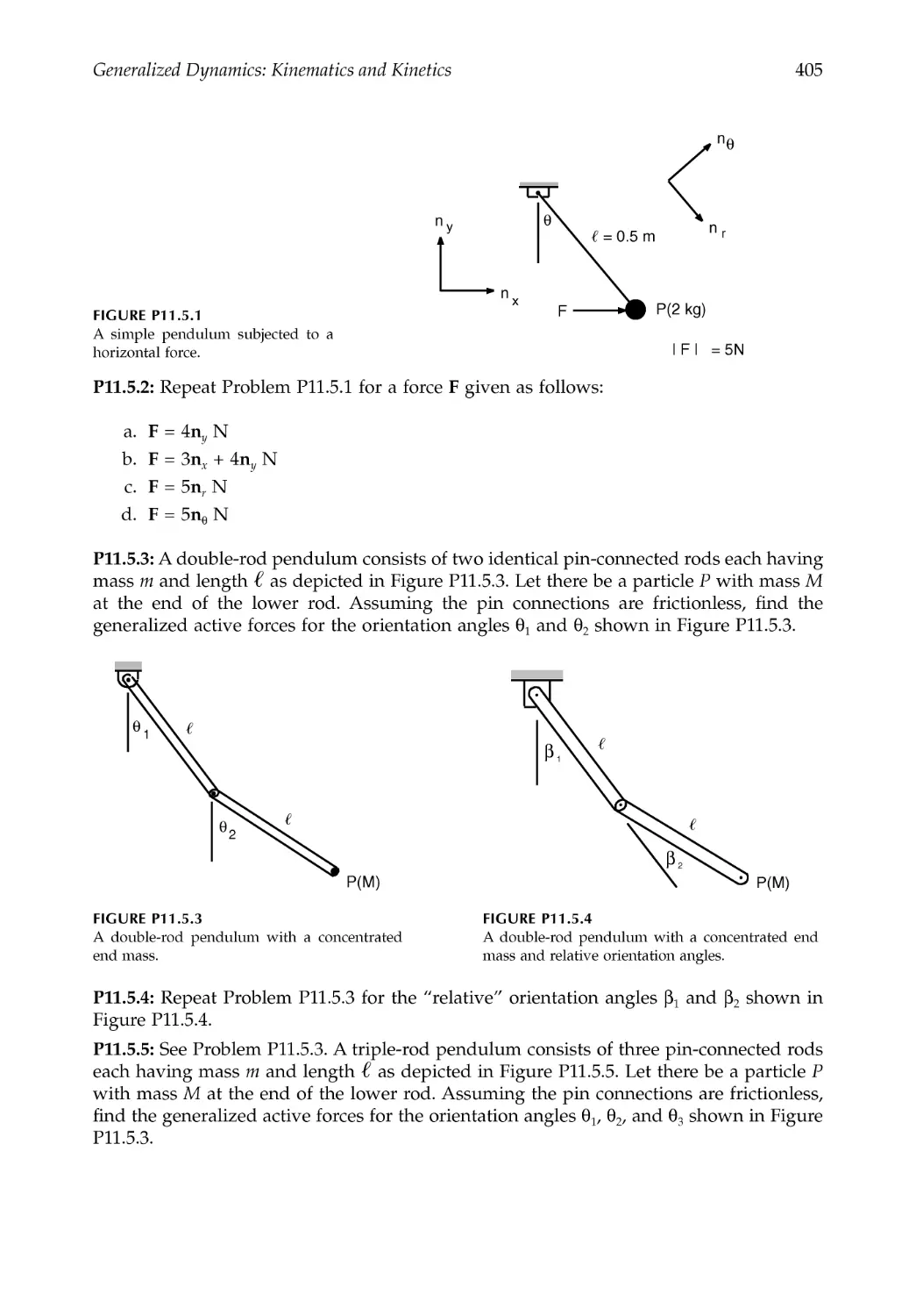
Problems .......................................................................................................................................402
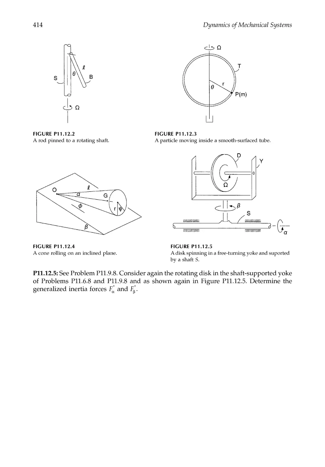
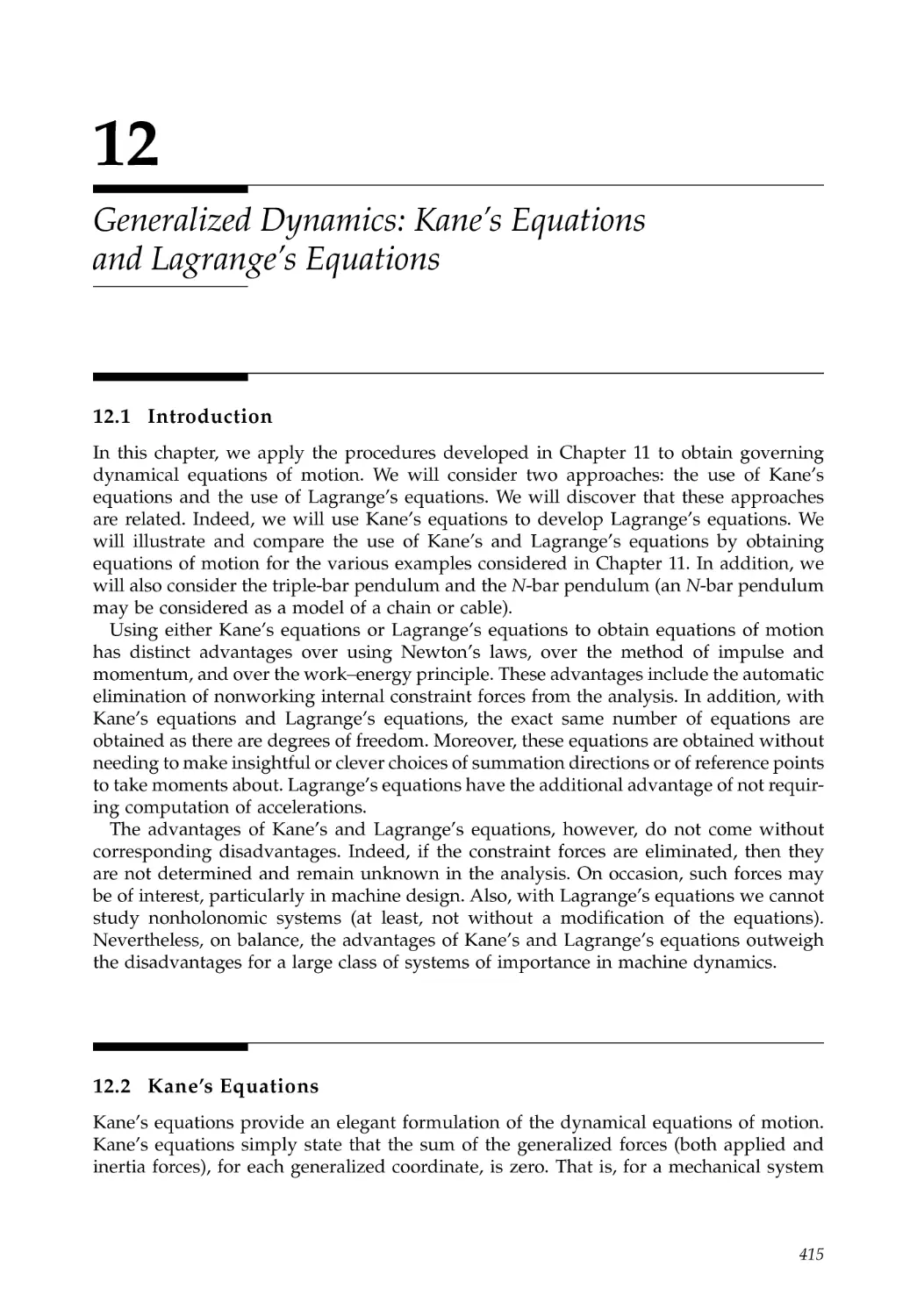
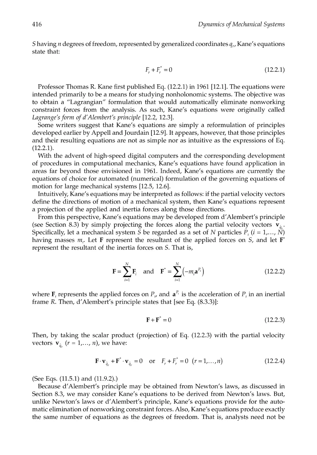
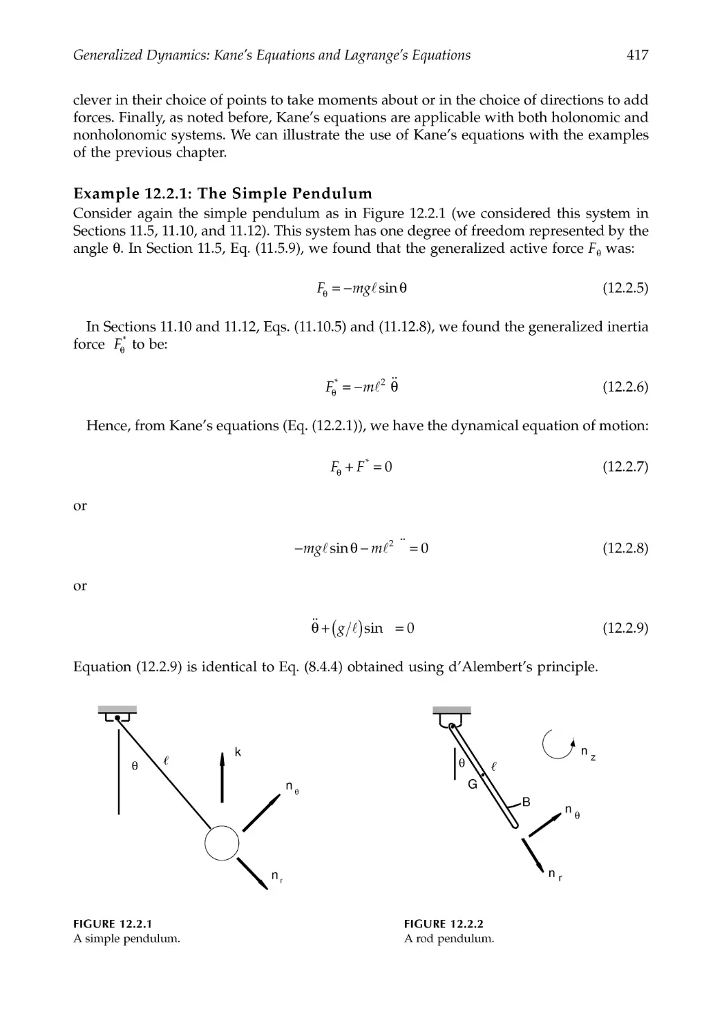
Chapter 12 Generalized Dynamics: Kane's Equations
and Lagrange's Equations .................................................................................415
12.1 Introduction.......................................................................................................................415
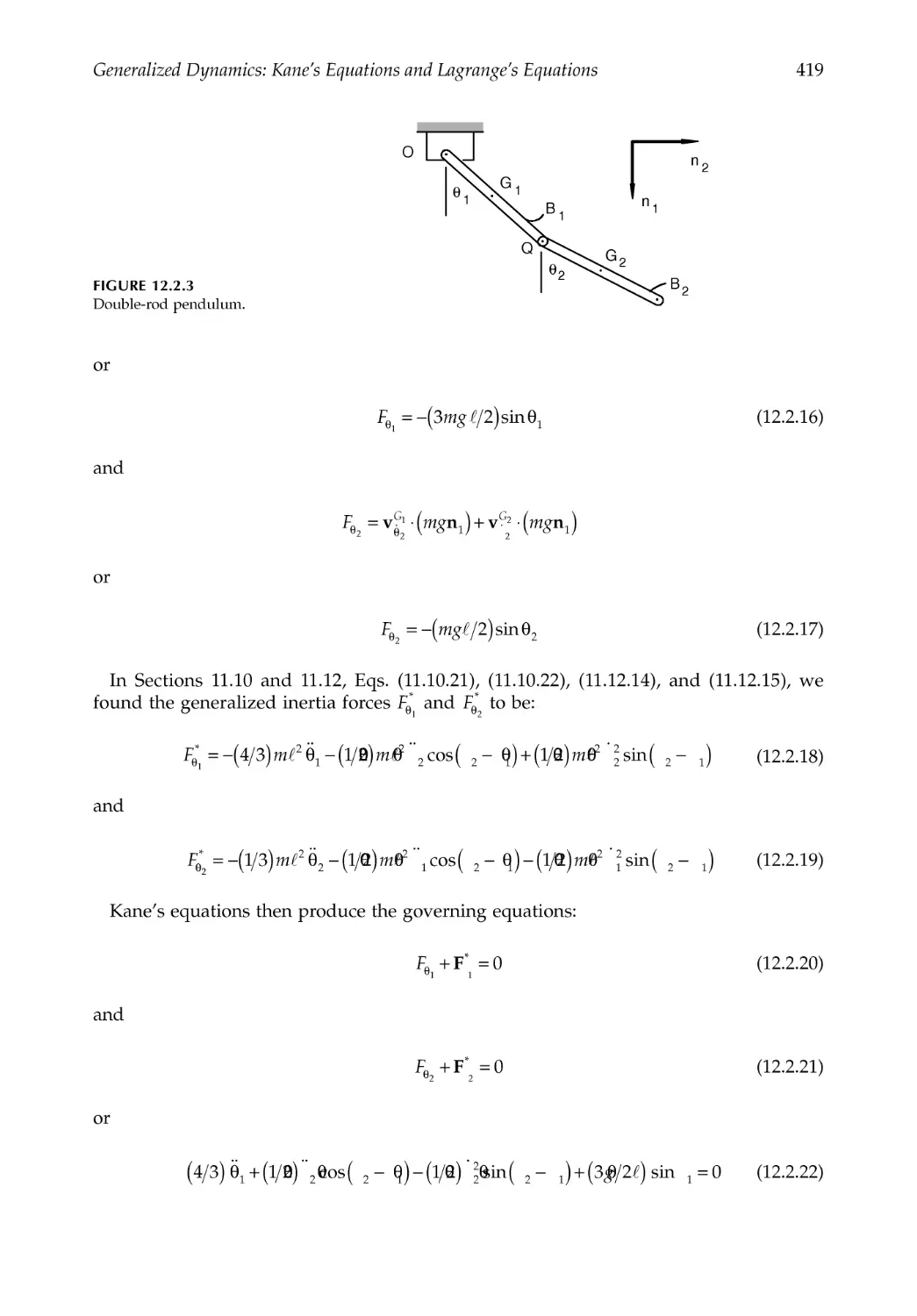
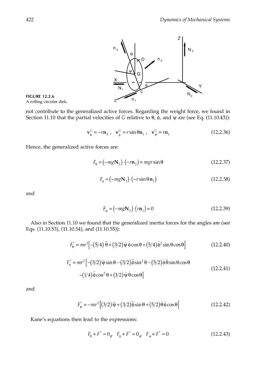
12.2 Kane's Equations ..............................................................................................................415
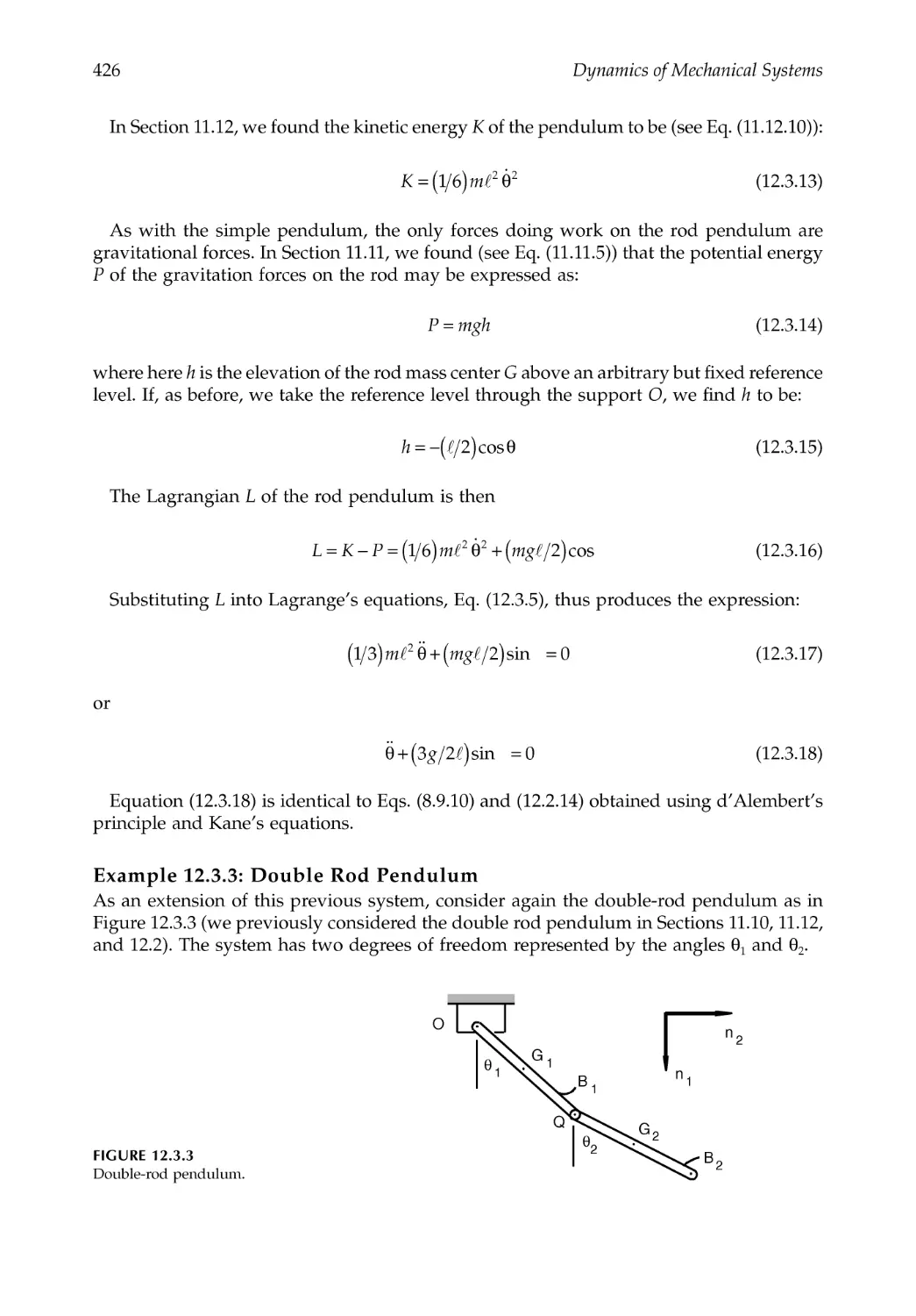
12.3 Lagrange's Equations ......................................................................................................423
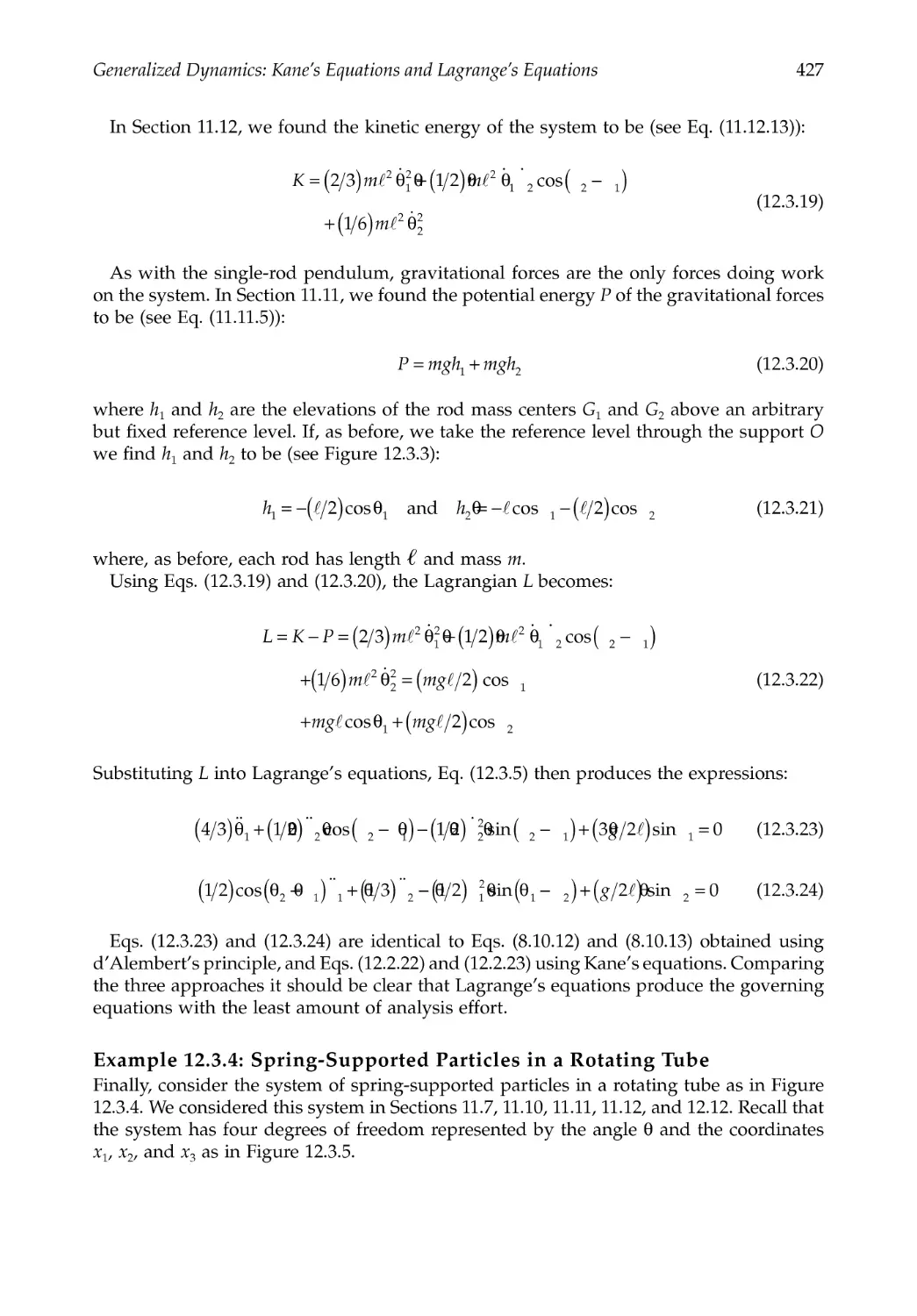
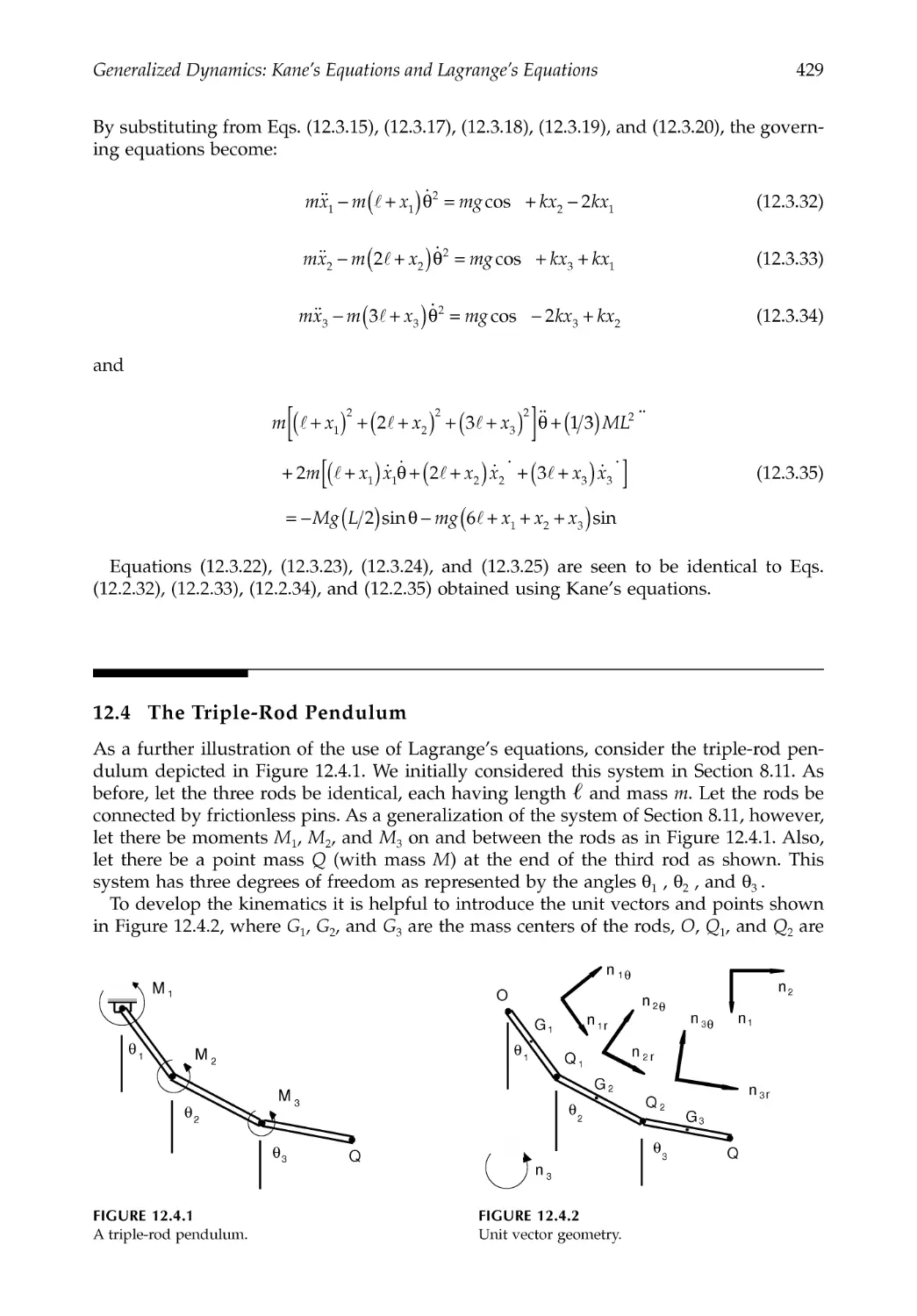
12.4 The Triple-Rod Pendulum ..............................................................................................429
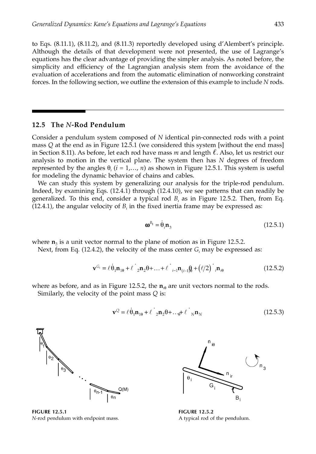
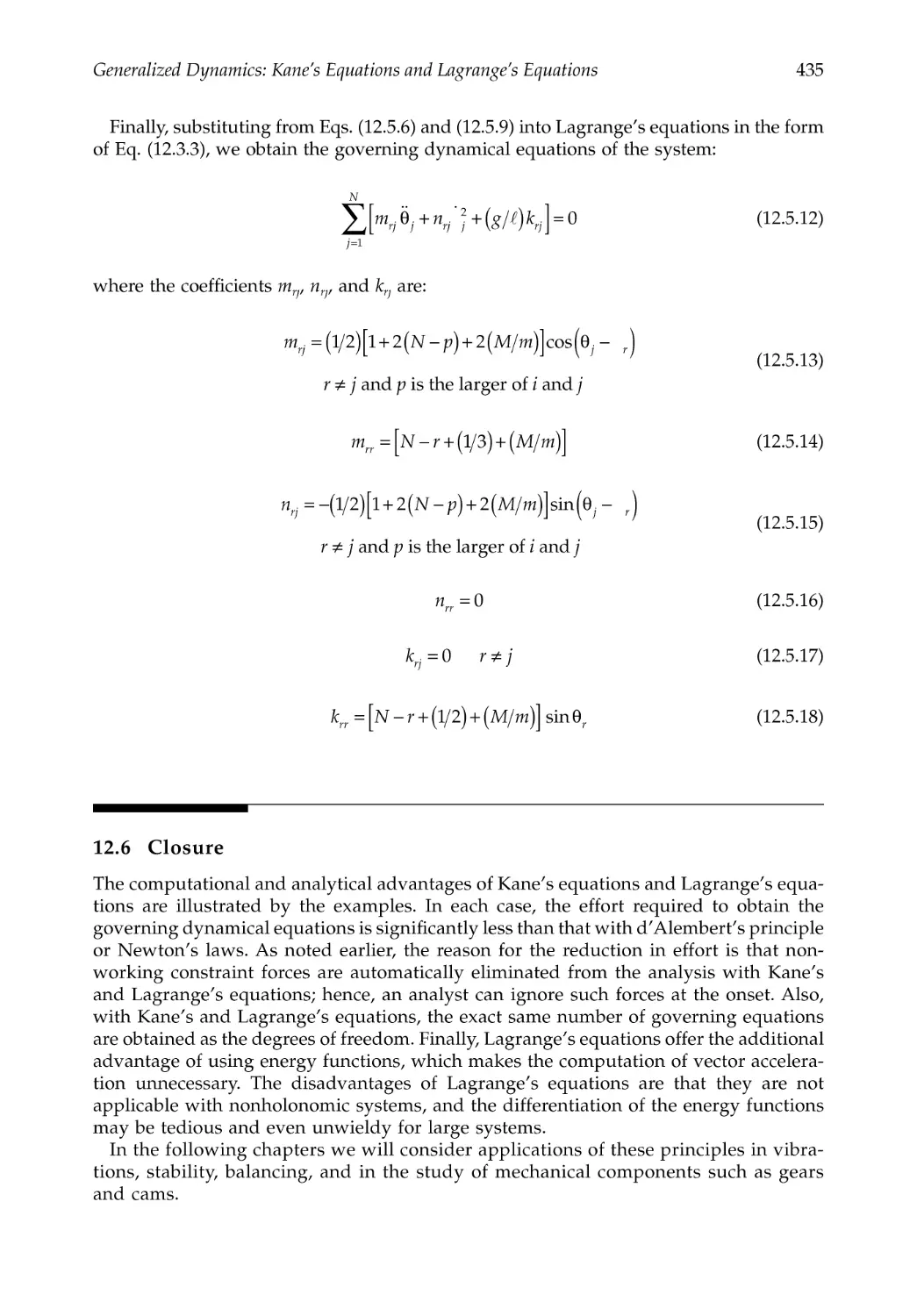
12.5 The N-Rod Pendulum .....................................................................................................433
12.6 Closure ...............................................................................................................................435
References .....................................................................................................................................436
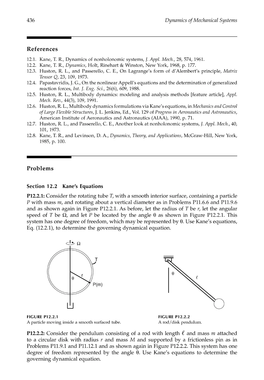
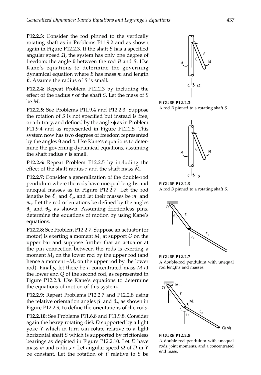
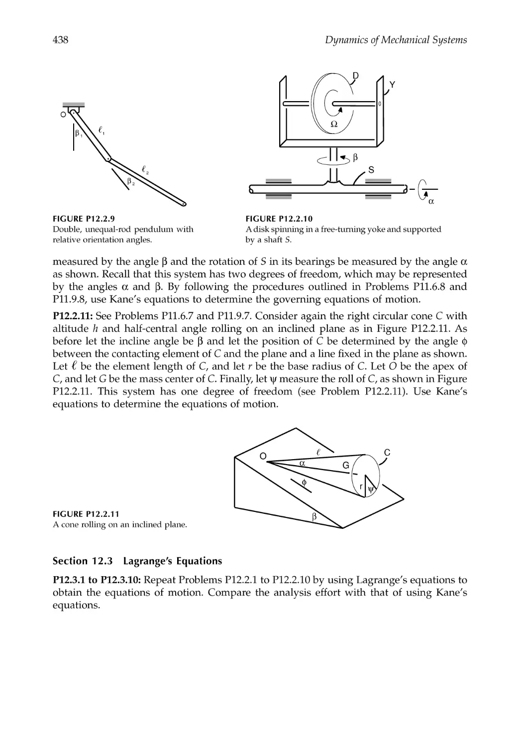
Problems .......................................................................................................................................436
Chapter 13 Introduction to Vibrations .................................................................................439
13.1 Introduction.......................................................................................................................439
13.2 Solutions of Second-Order Differential Equations .....................................................439
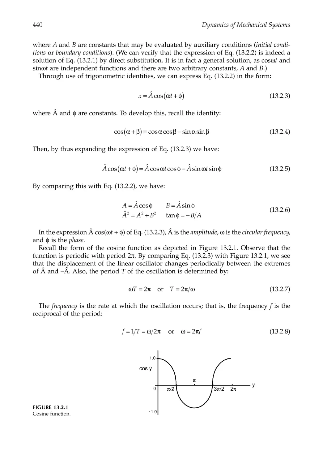
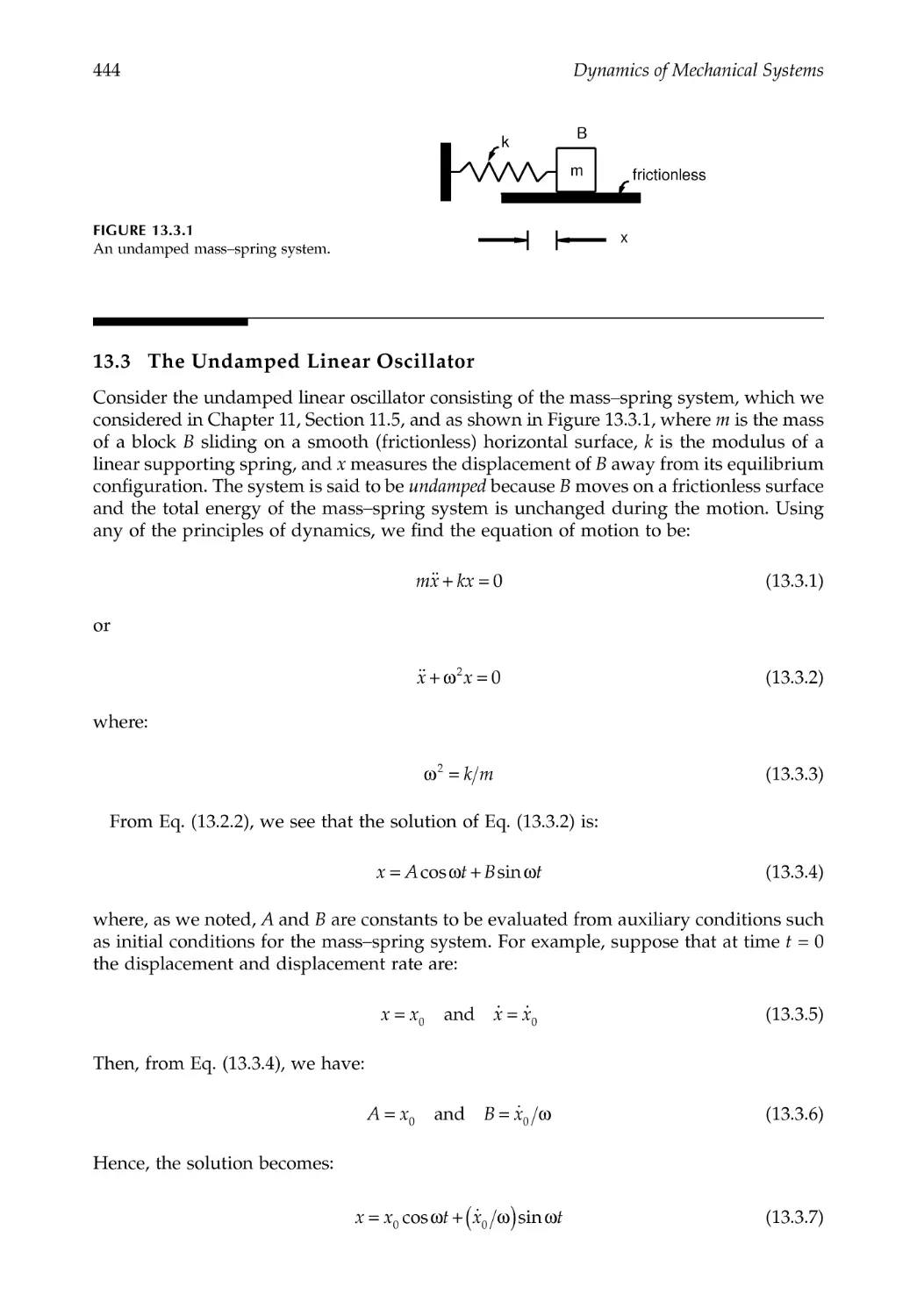
13.3 The Undamped Linear Oscillator..................................................................................444
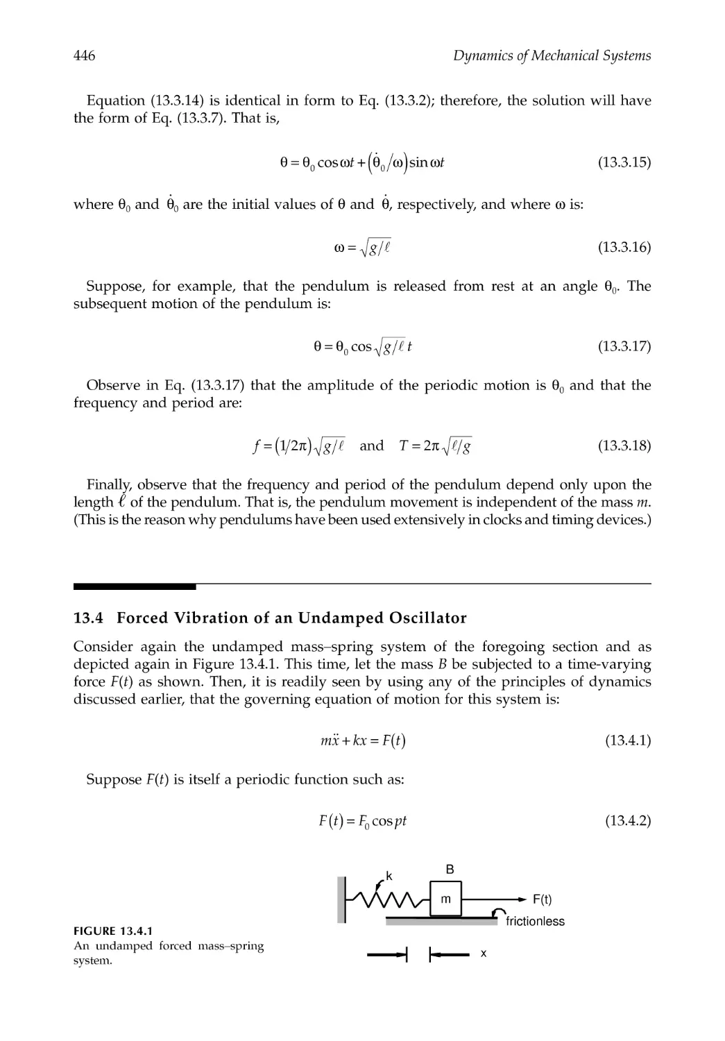
13.4 Forced Vibration of an Undamped Oscillator .............................................................446
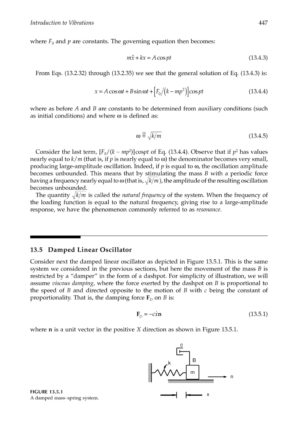
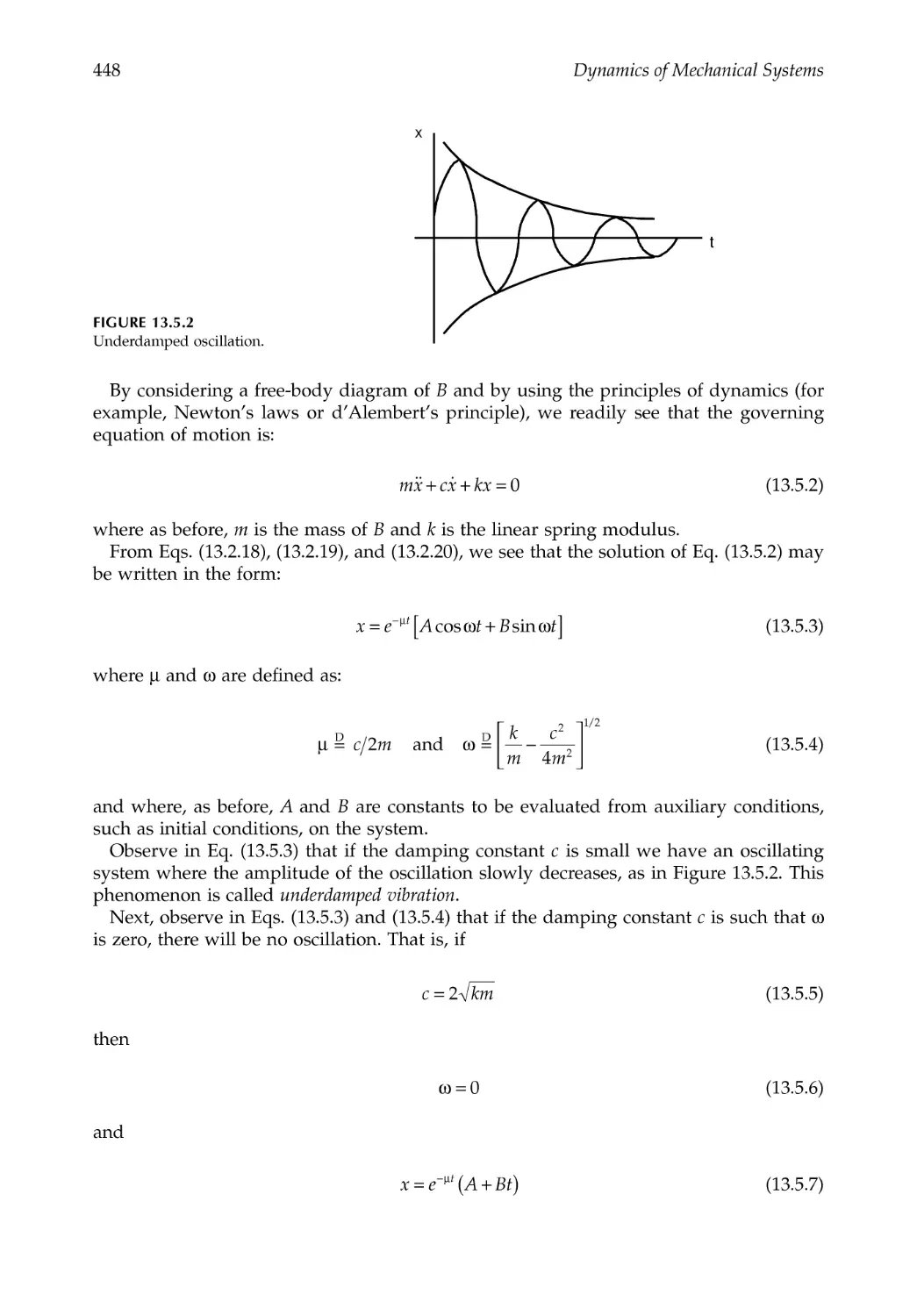
13.5 Damped Linear Oscillator ..............................................................................................447
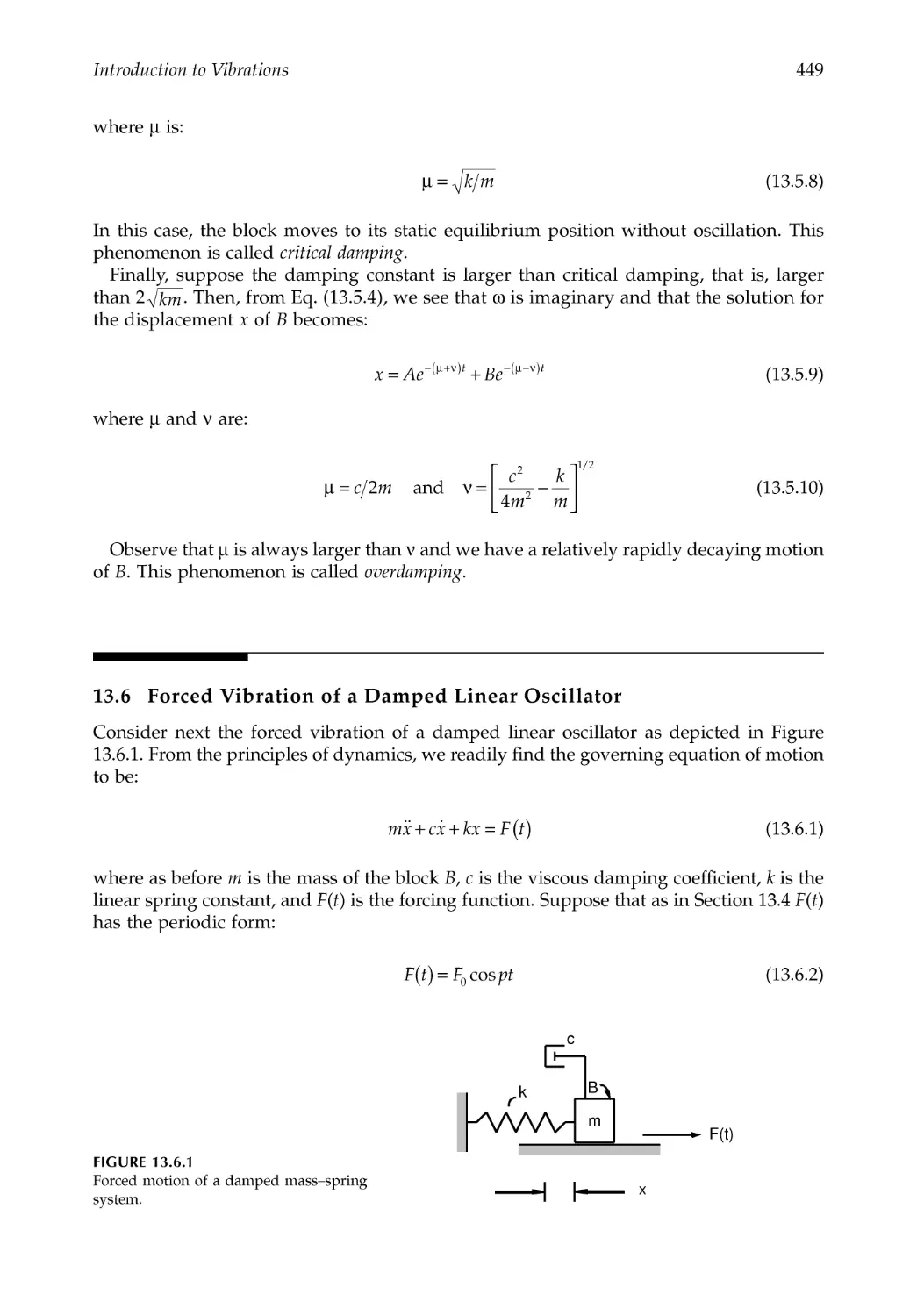
13.6 Forced Vibration of a Damped Linear Oscillator .......................................................449
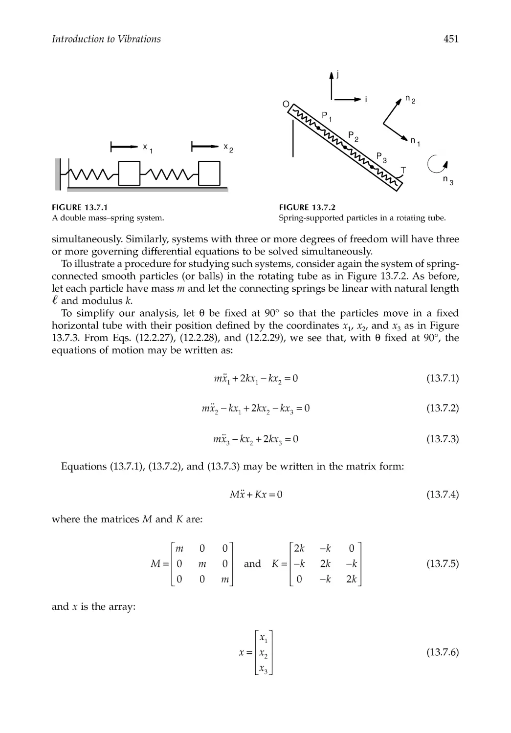
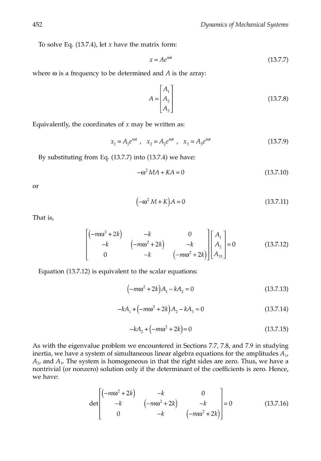
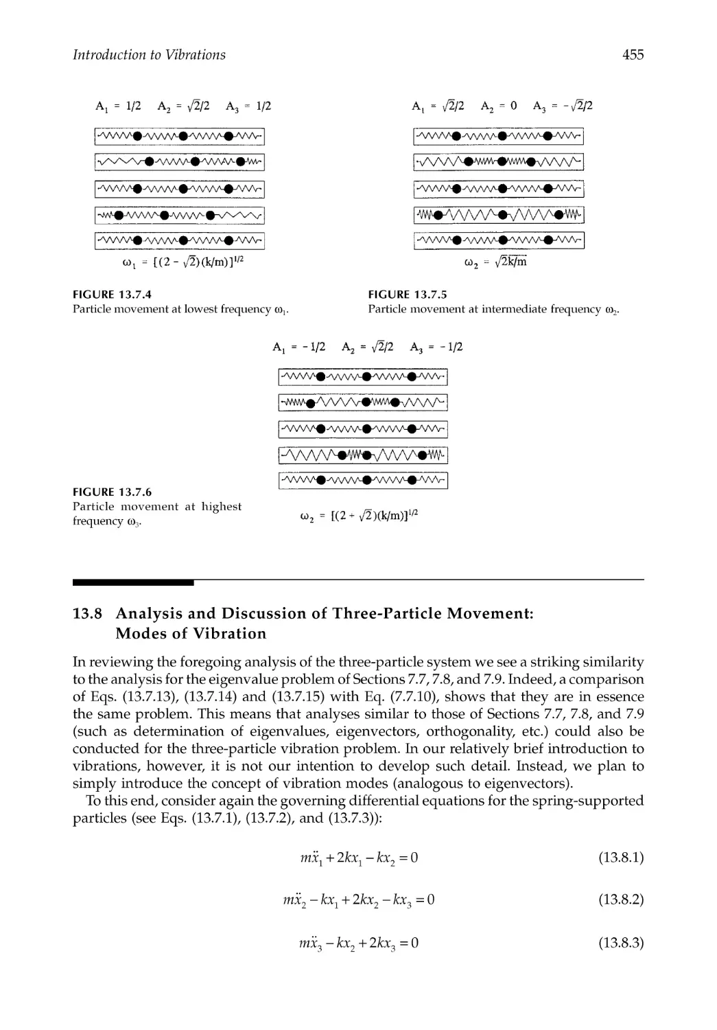
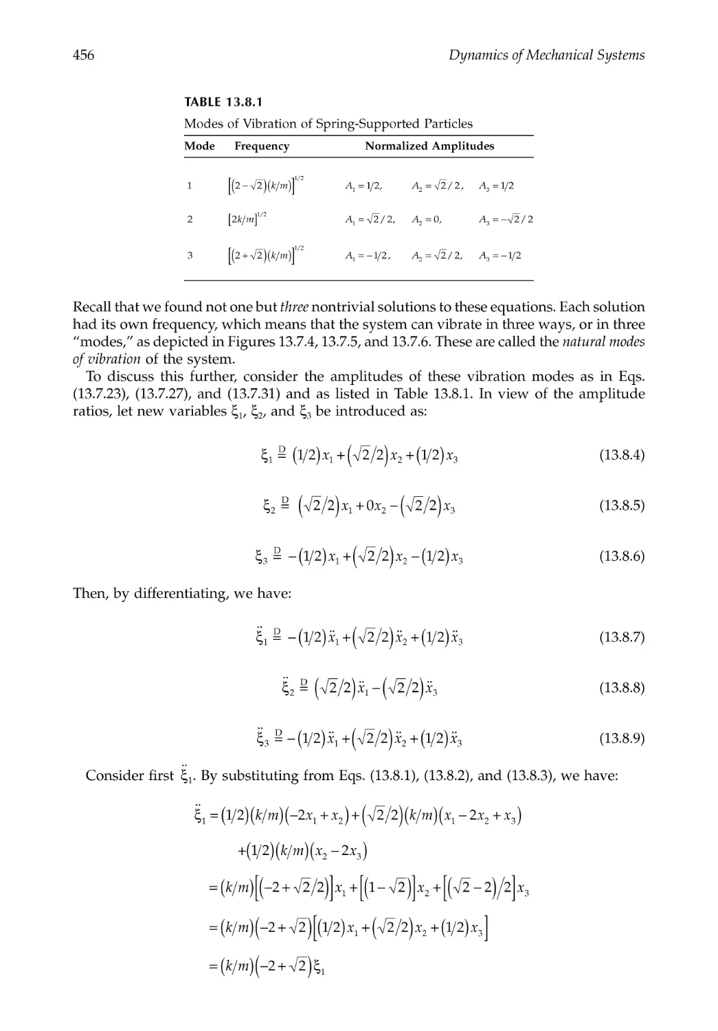
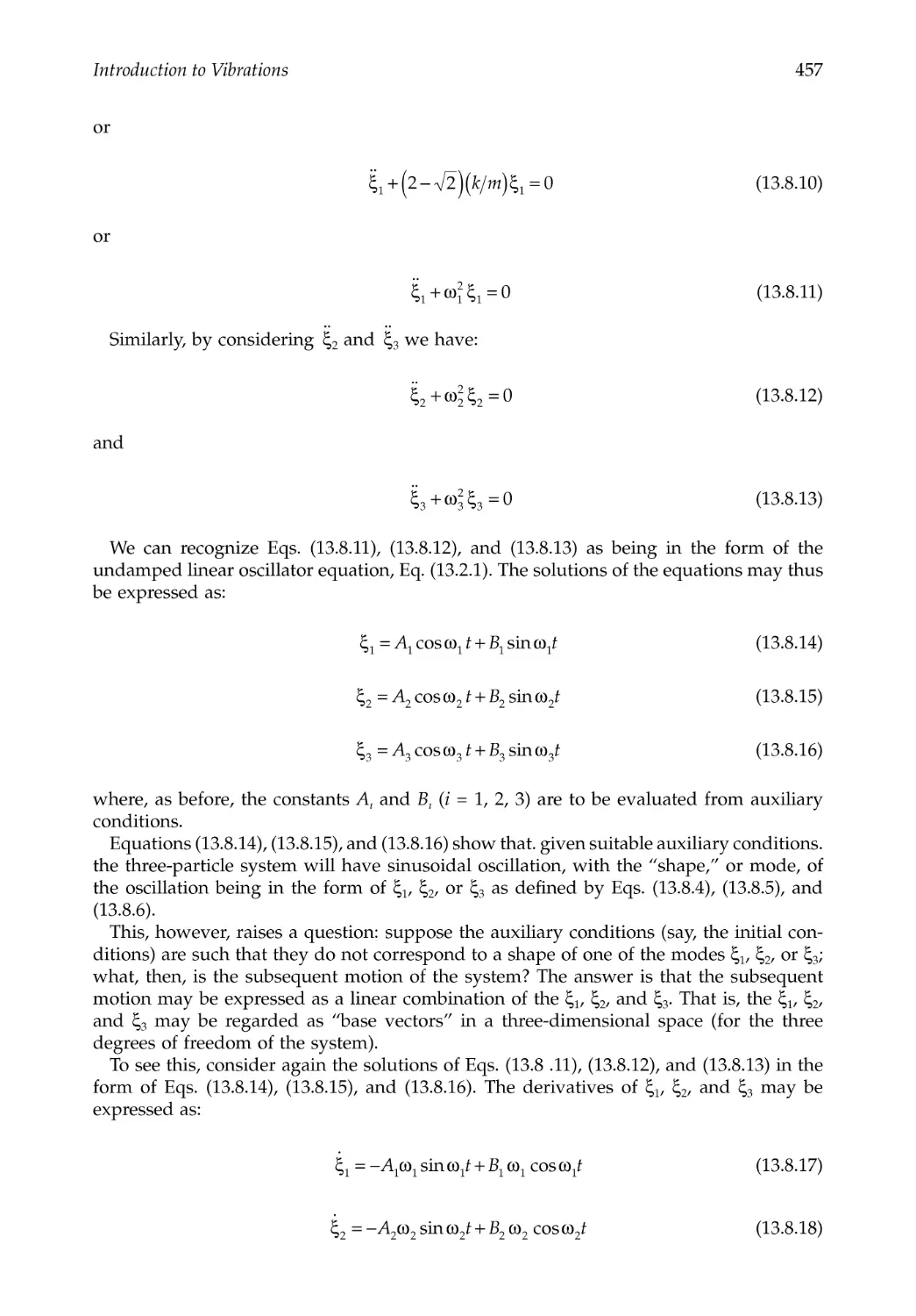
13.7 Systems with Several Degrees of Freedom..................................................................450
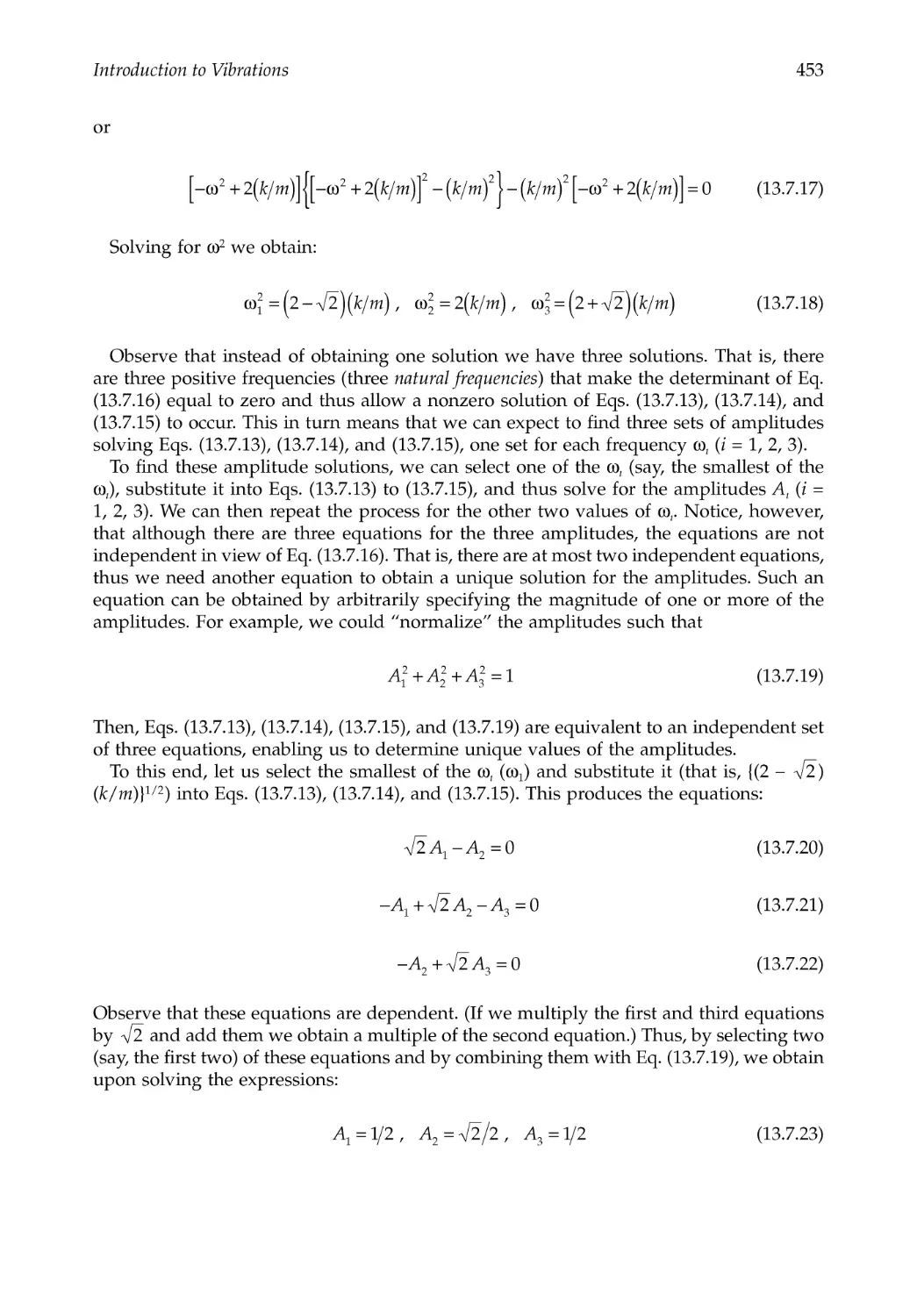
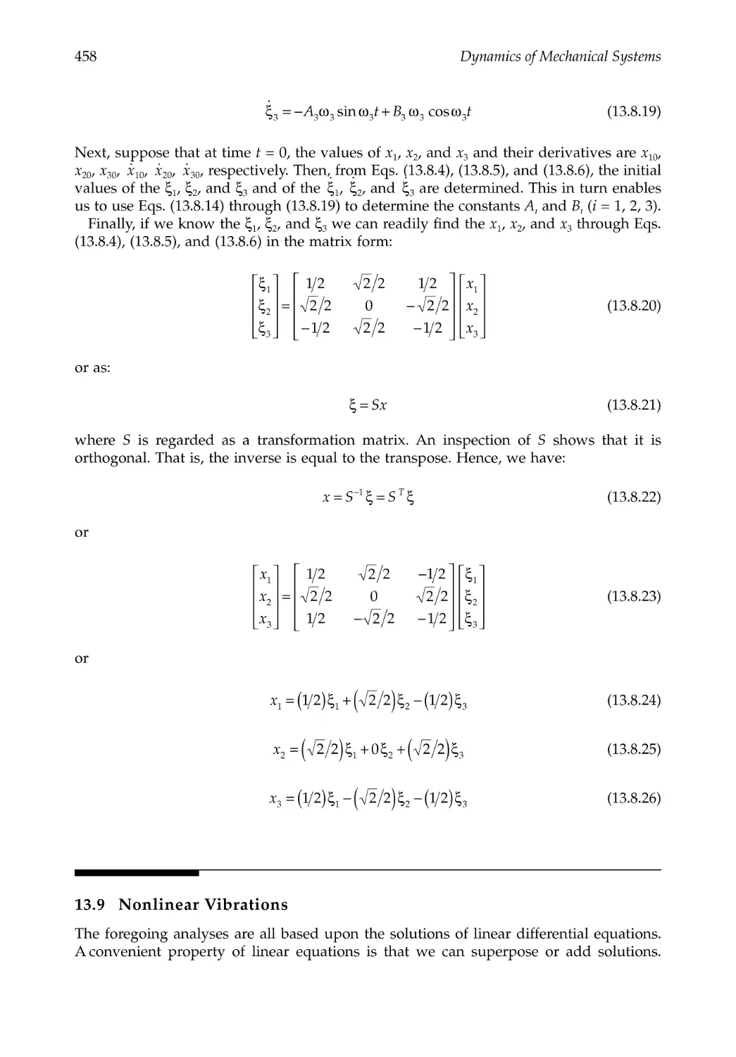
13.8 Analysis and Discussion of Three-Particle Movement:
Modes of Vibration ..........................................................................................................455
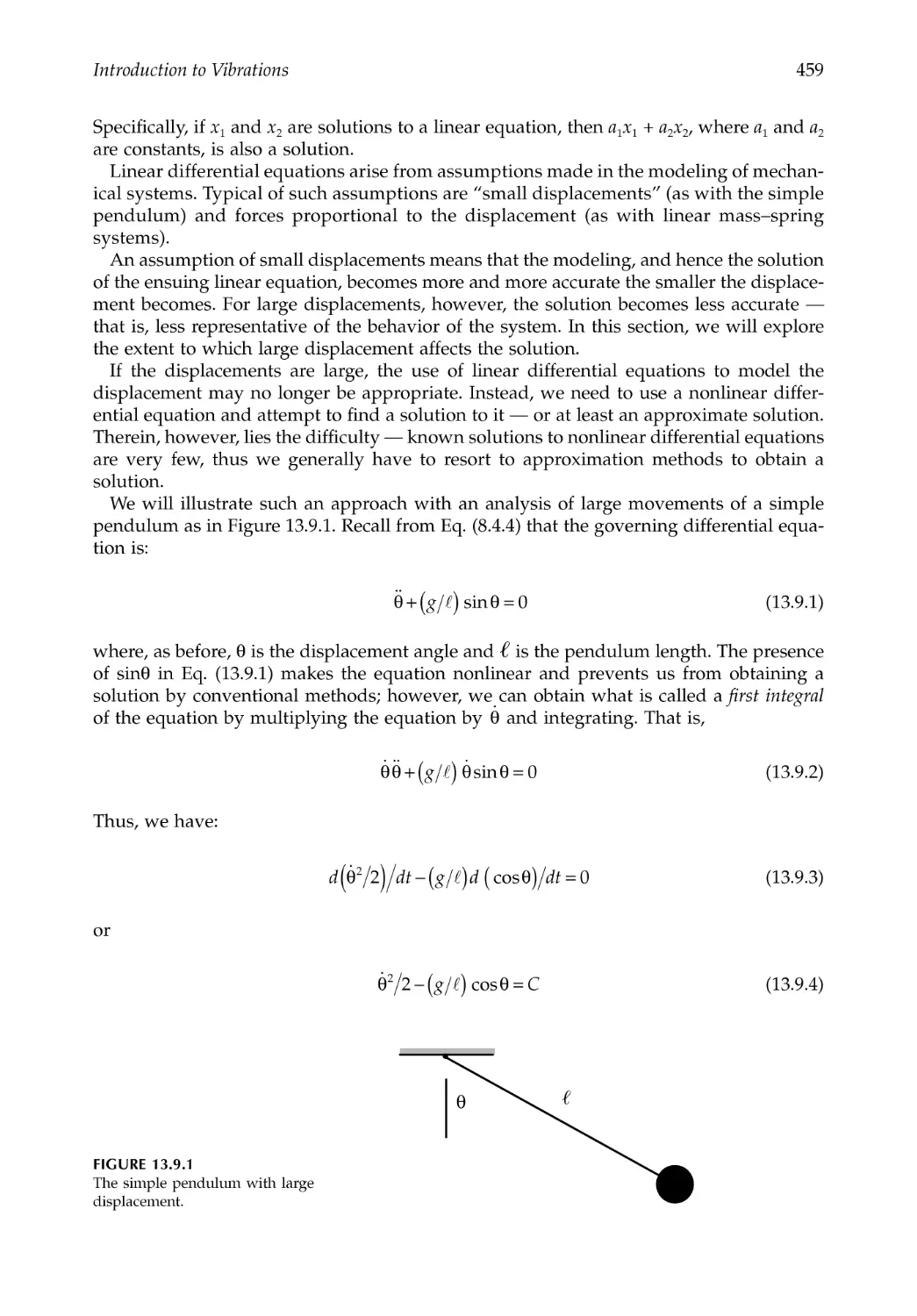
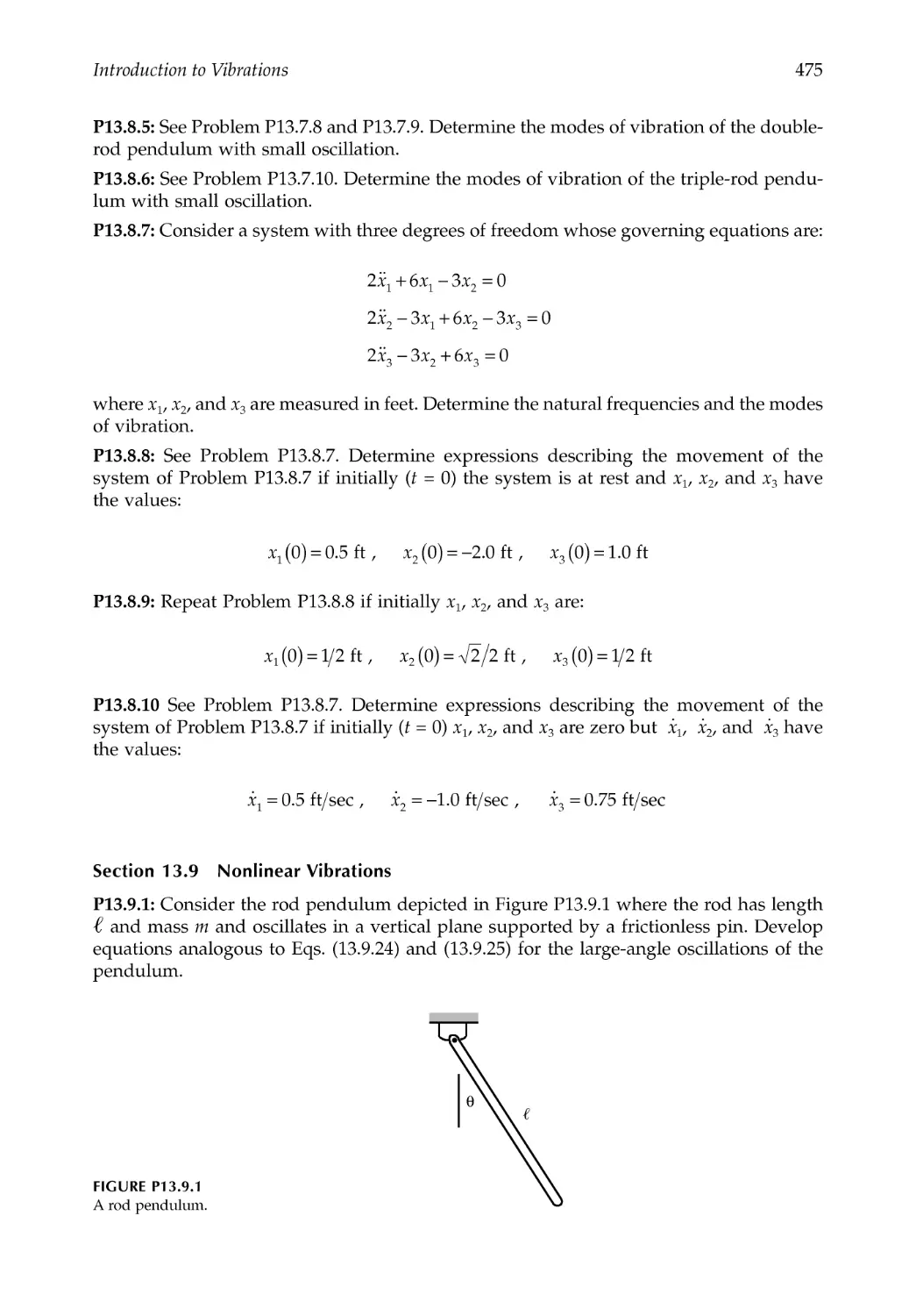
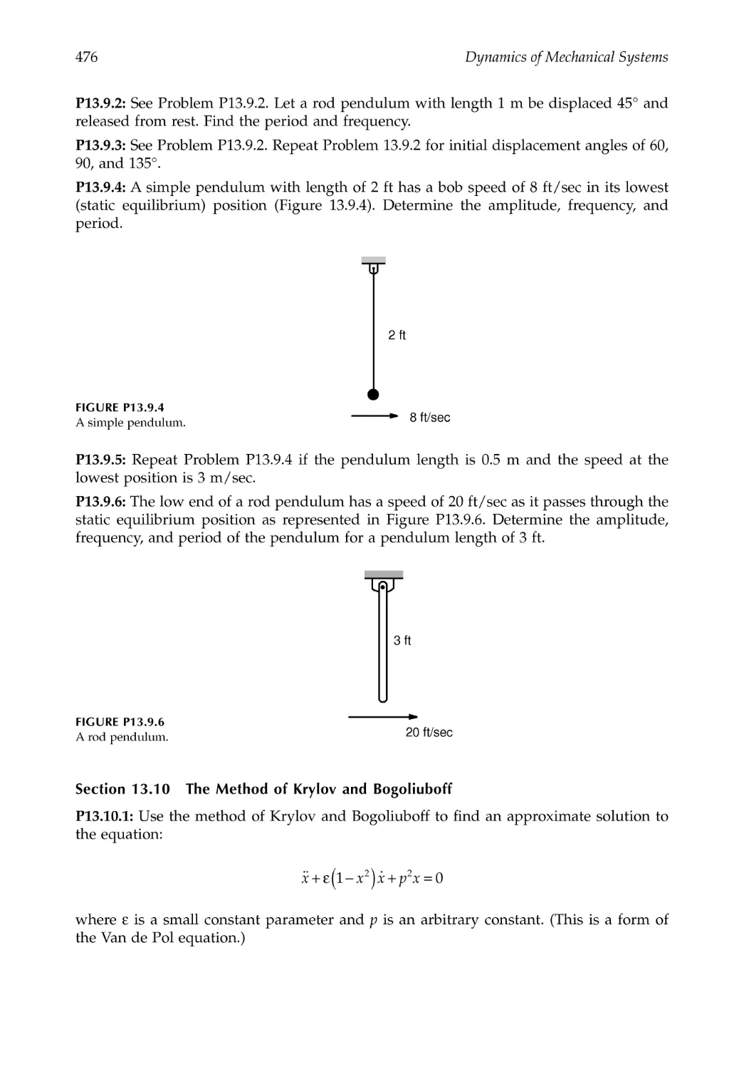
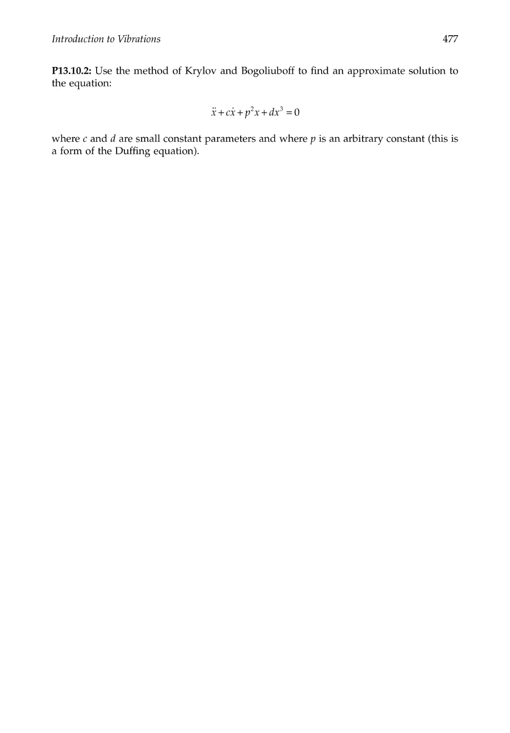
13.9 Nonlinear Vibrations .......................................................................................................458
13.10 The Method of Krylov and Bogoliuboff.......................................................................463
13.11 Closure ...............................................................................................................................466
References .....................................................................................................................................466
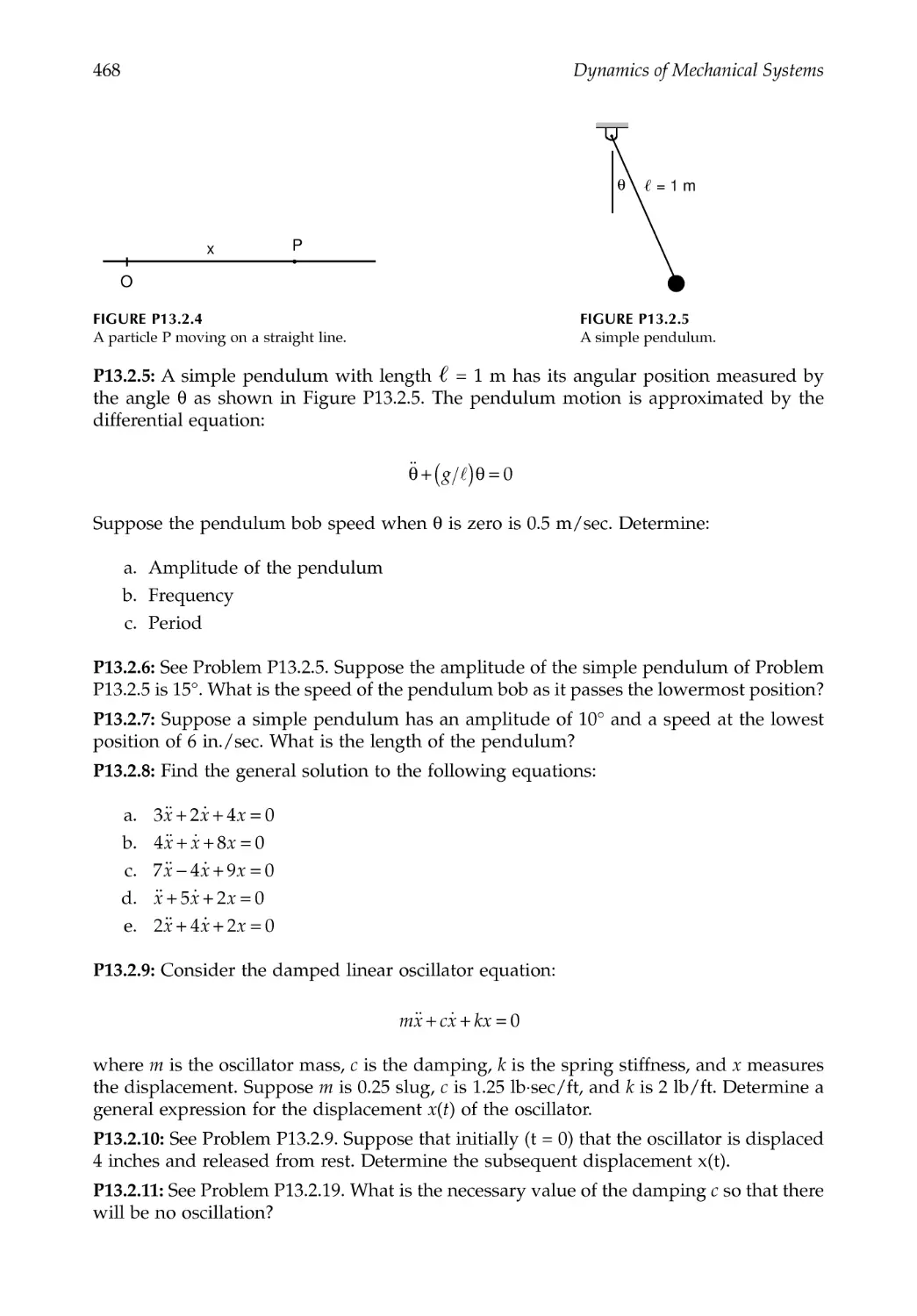
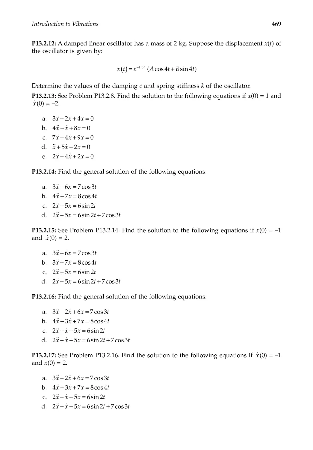
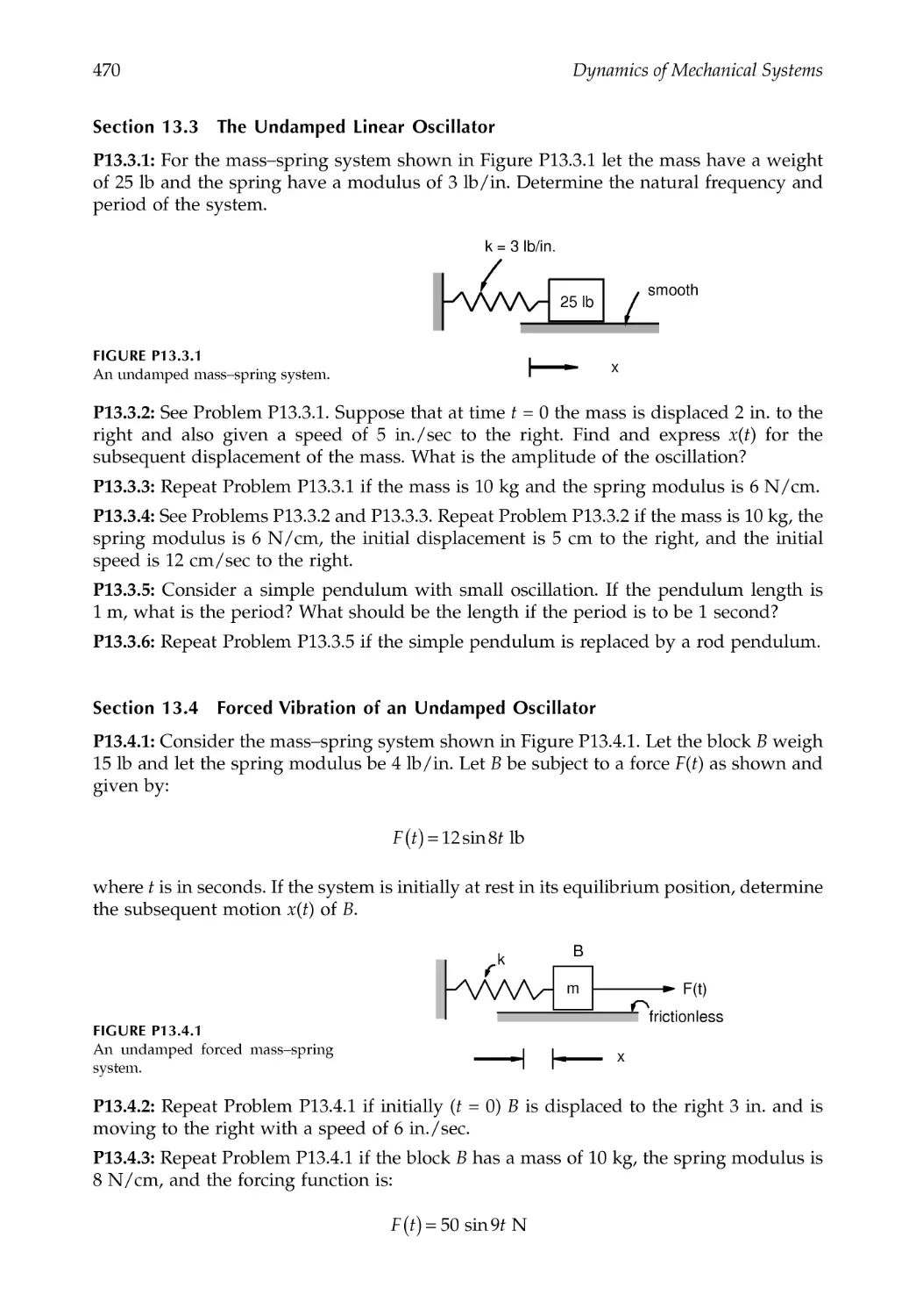
Problems .......................................................................................................................................467
Chapter 14 Stability .................................................................................................................479
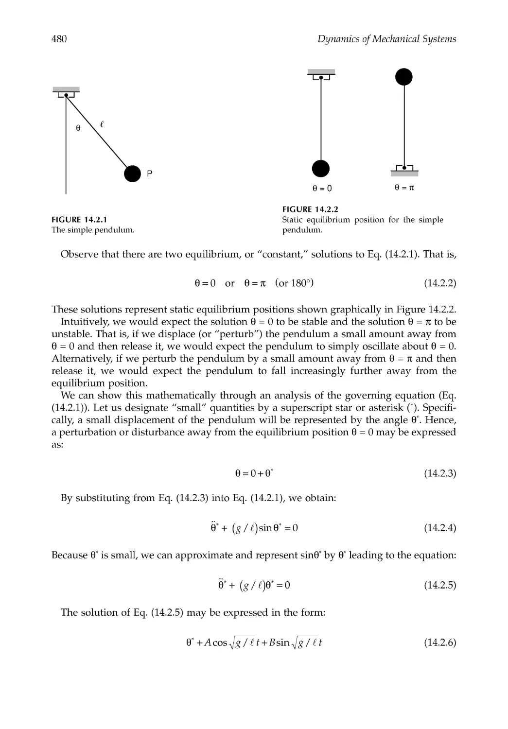
14.1 Introduction.......................................................................................................................479
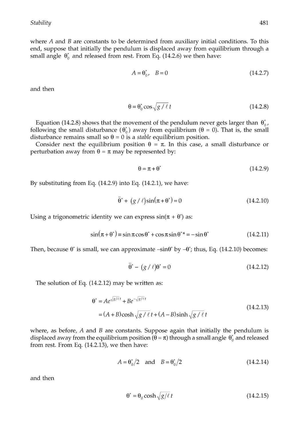
14.2 Infinitesimal Stability.......................................................................................................479
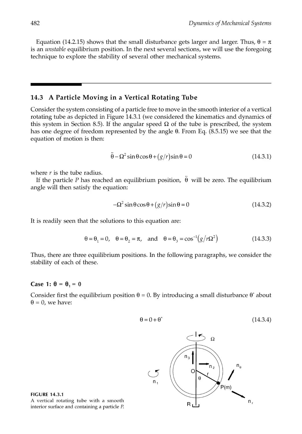
14.3 A Particle Moving in a Vertical Rotating Tube ...........................................................482
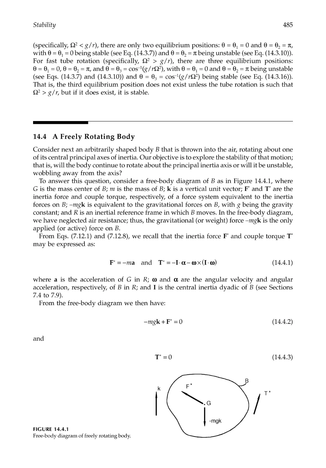
14.4 A Freely Rotating Body ...................................................................................................485
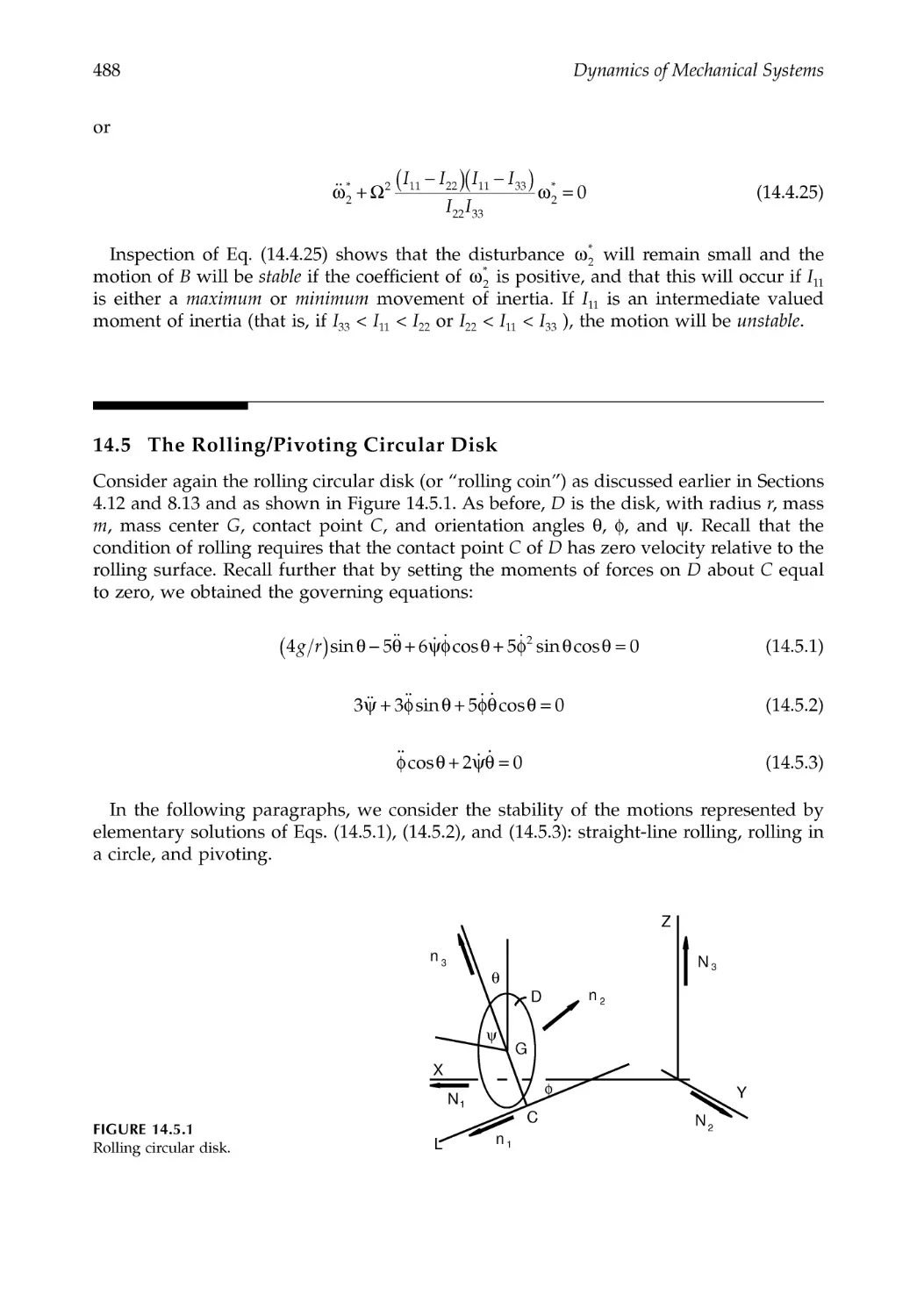
14.5 The Rolling/Pivoting Circular Disk .............................................................................488
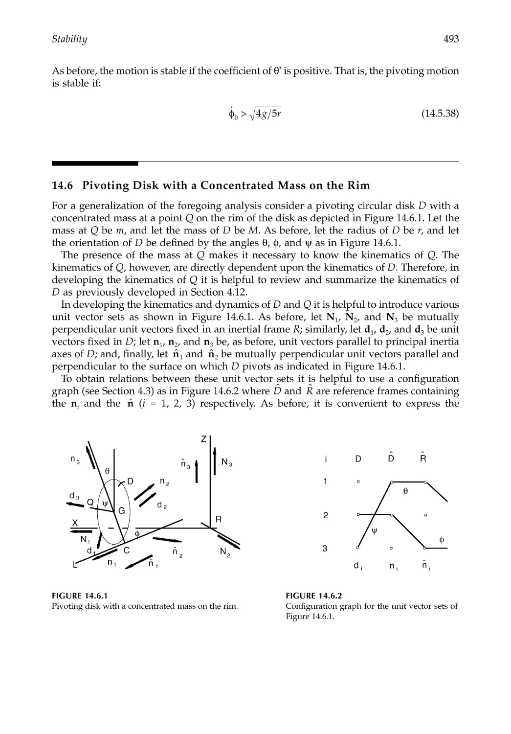
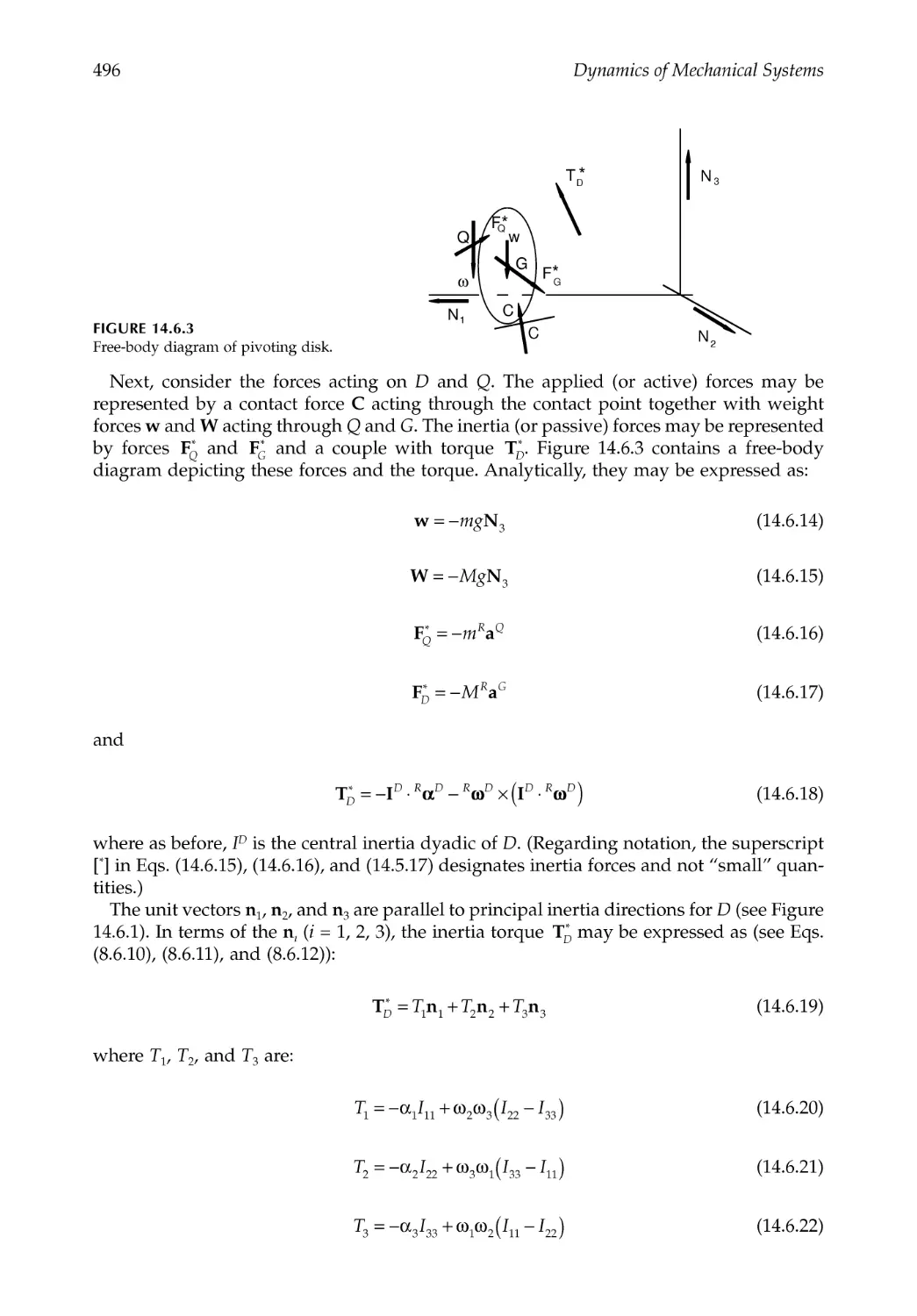
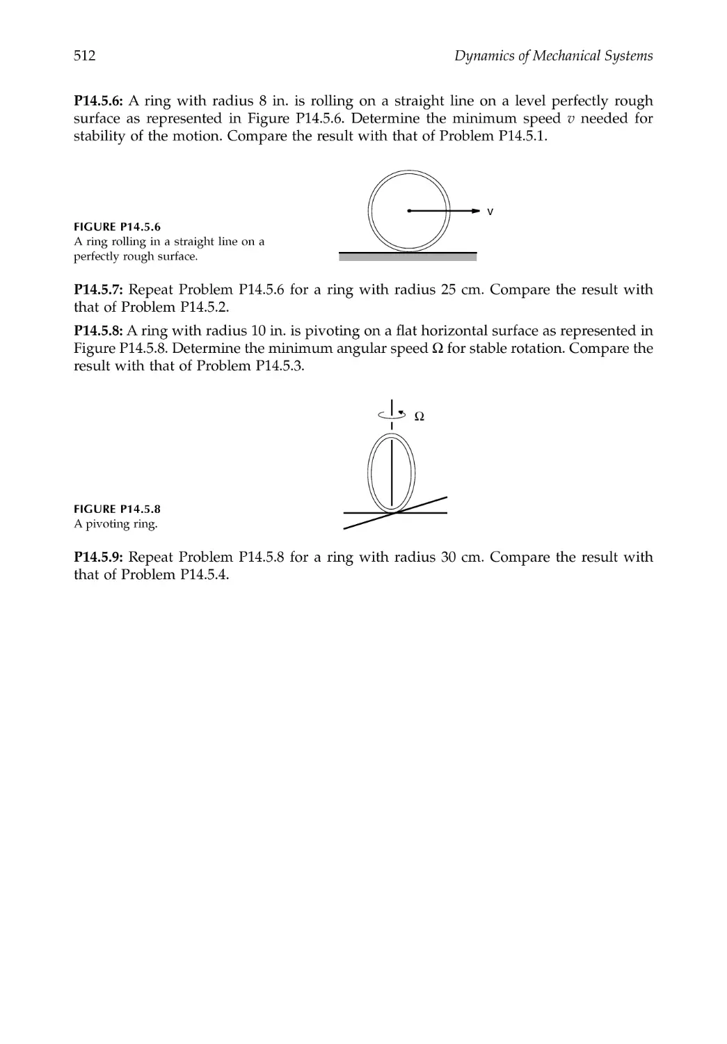
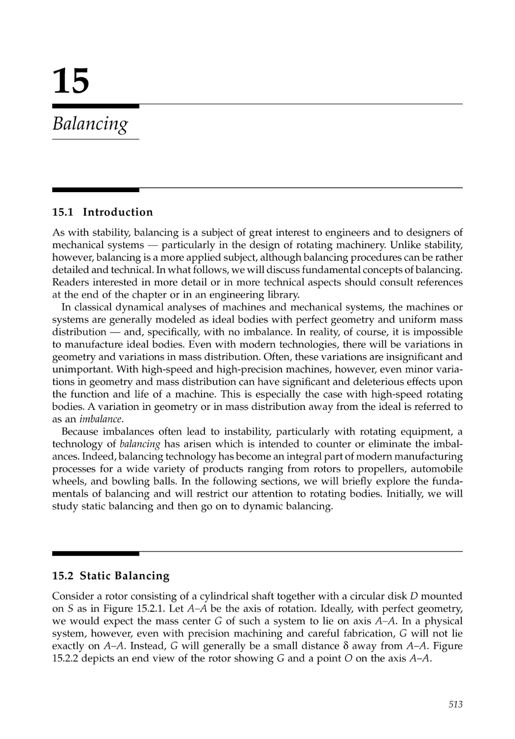
14.6 Pivoting Disk with a Concentrated Mass on the Rim ...............................................493
14.6.1 Rim Mass in the Uppermost Position ..........................................................................498
14.6.2 Rim Mass in the Lowermost Position ..........................................................................502
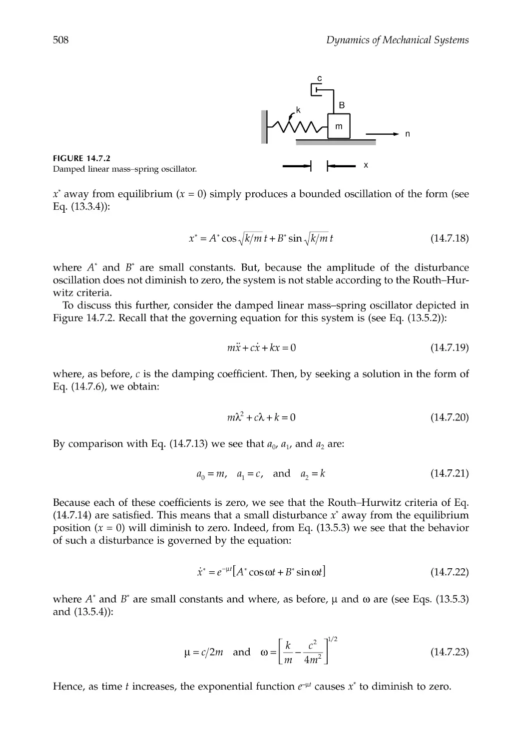
14.7 Discussion: Routh--Hurwitz Criteria.............................................................................505
14.8 Closure ...............................................................................................................................509
References .....................................................................................................................................509
Problems .......................................................................................................................................510
Chapter 15 Balancing...............................................................................................................513
15.1 Introduction.......................................................................................................................513
15.2 Static Balancing.................................................................................................................513
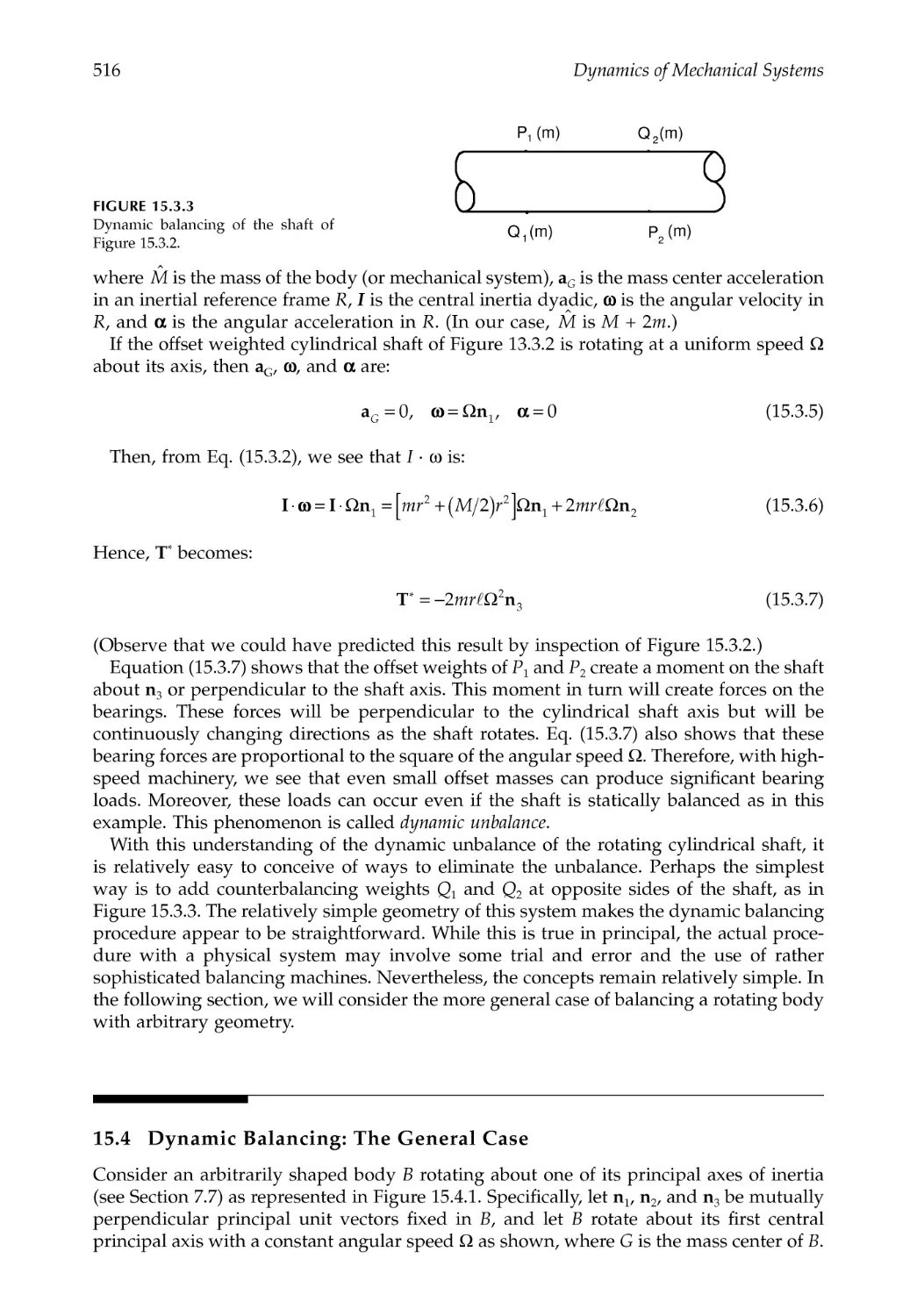
15.3 Dynamic Balancing: A Rotating Shaft ..........................................................................514
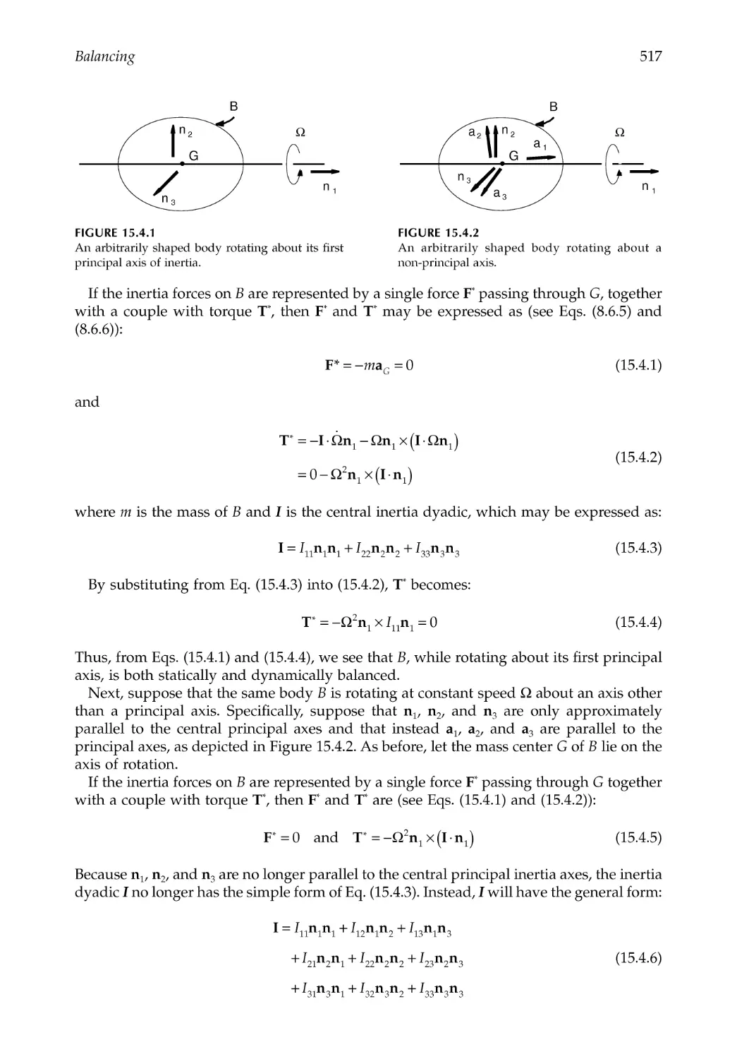
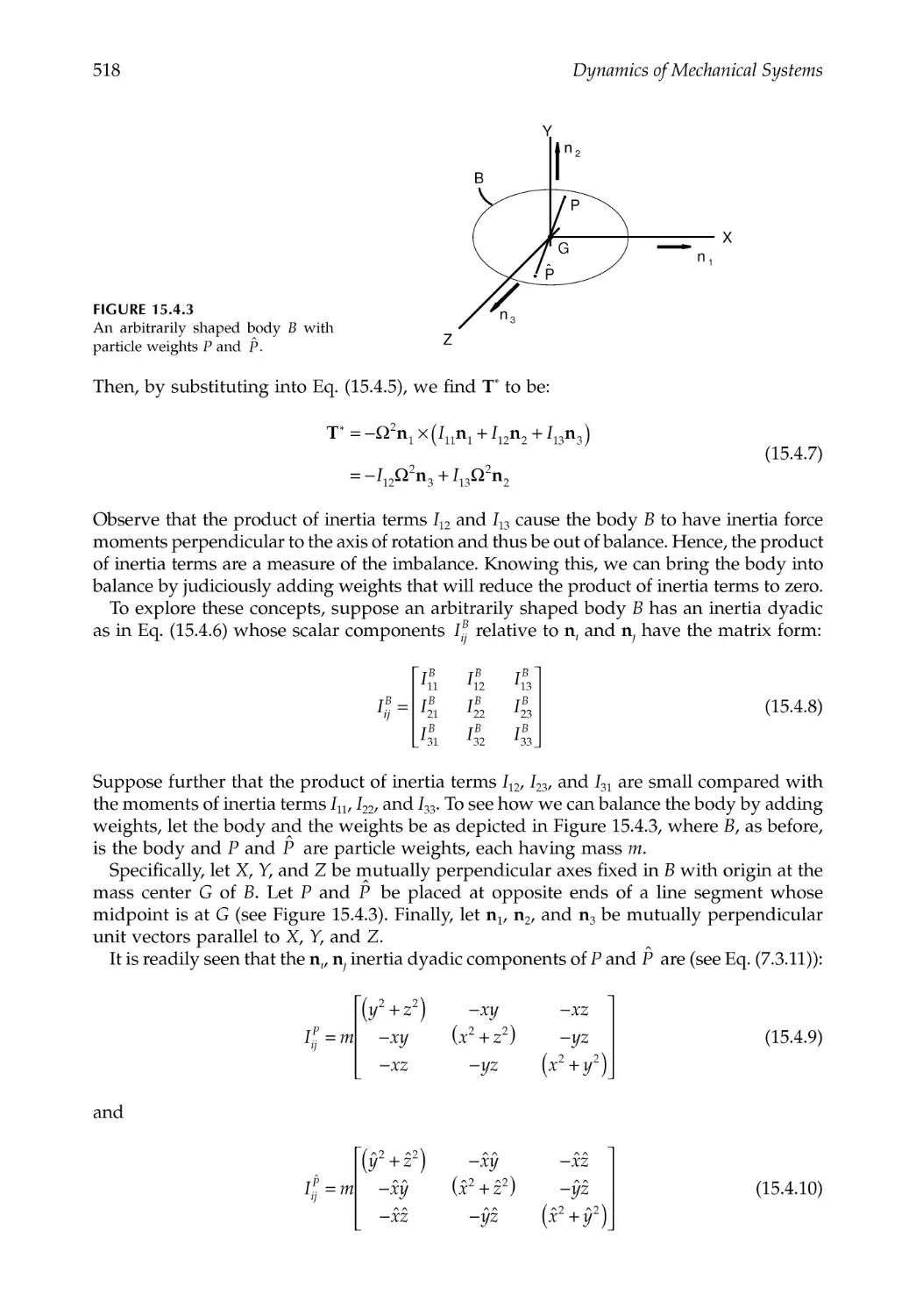
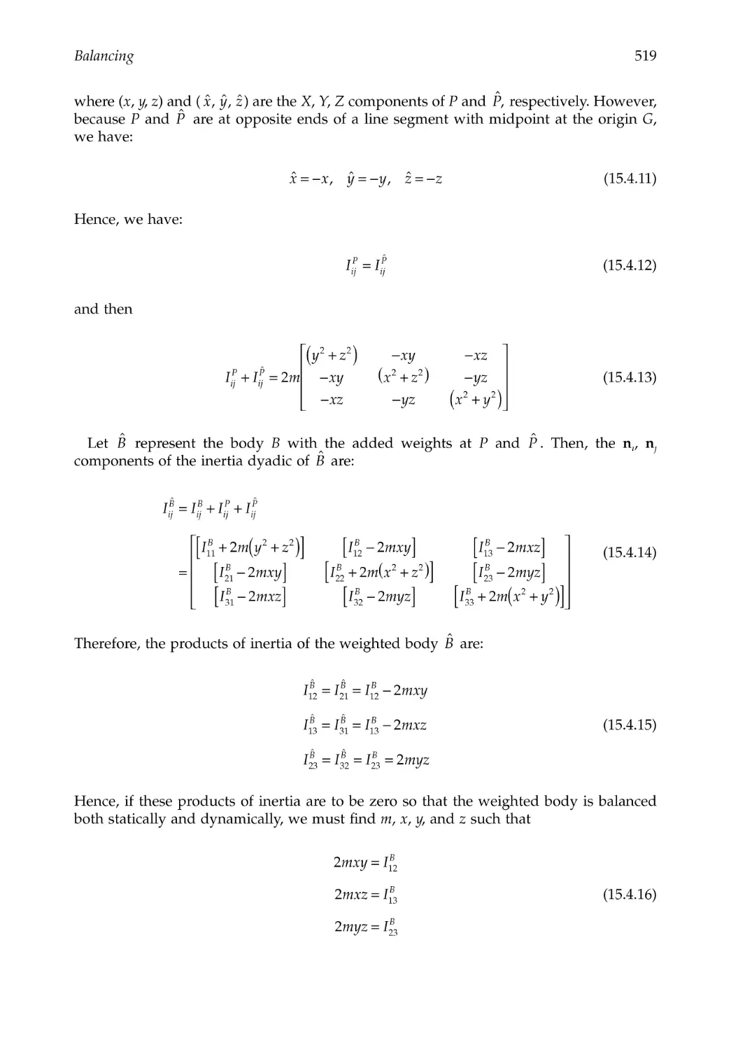
15.4 Dynamic Balancing: The General Case ........................................................................516
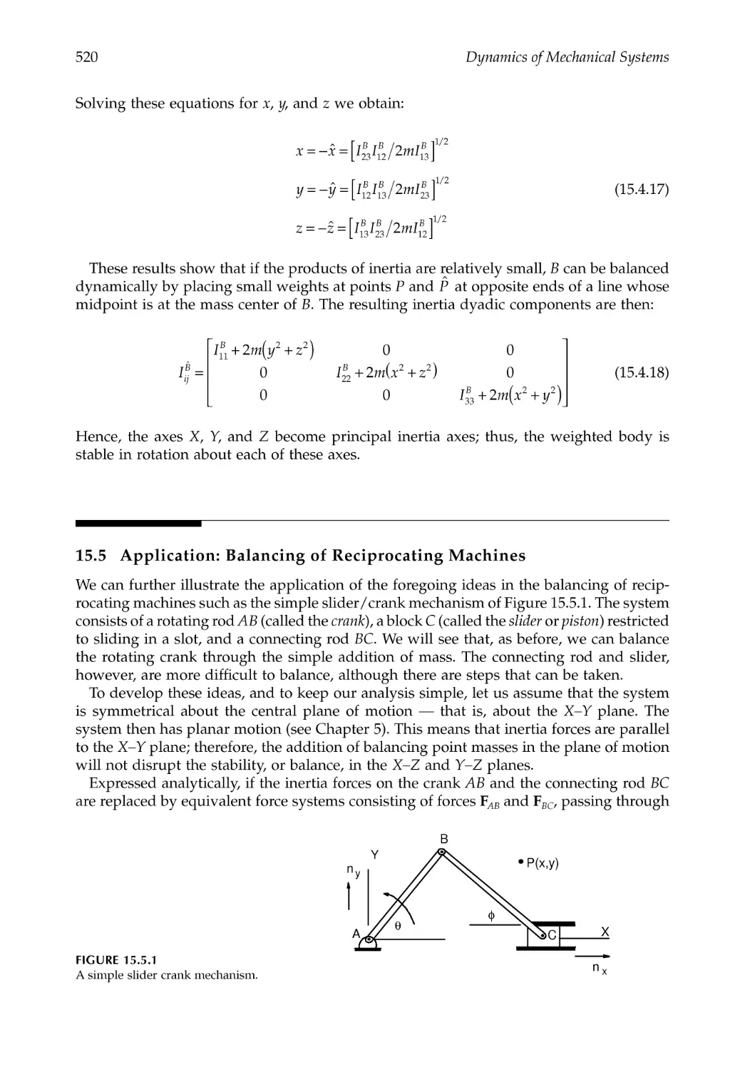
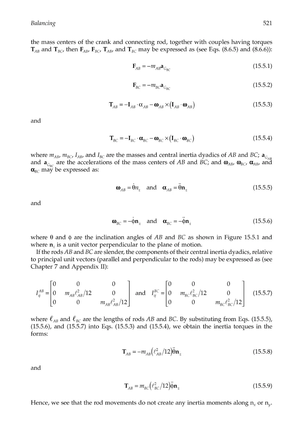
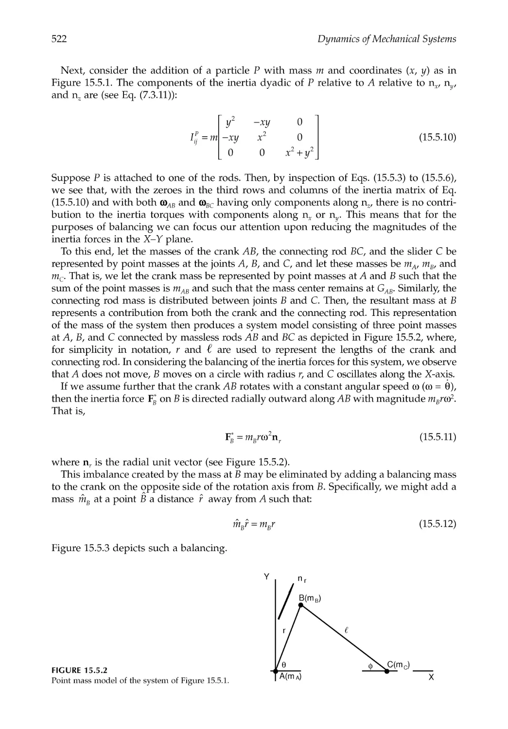
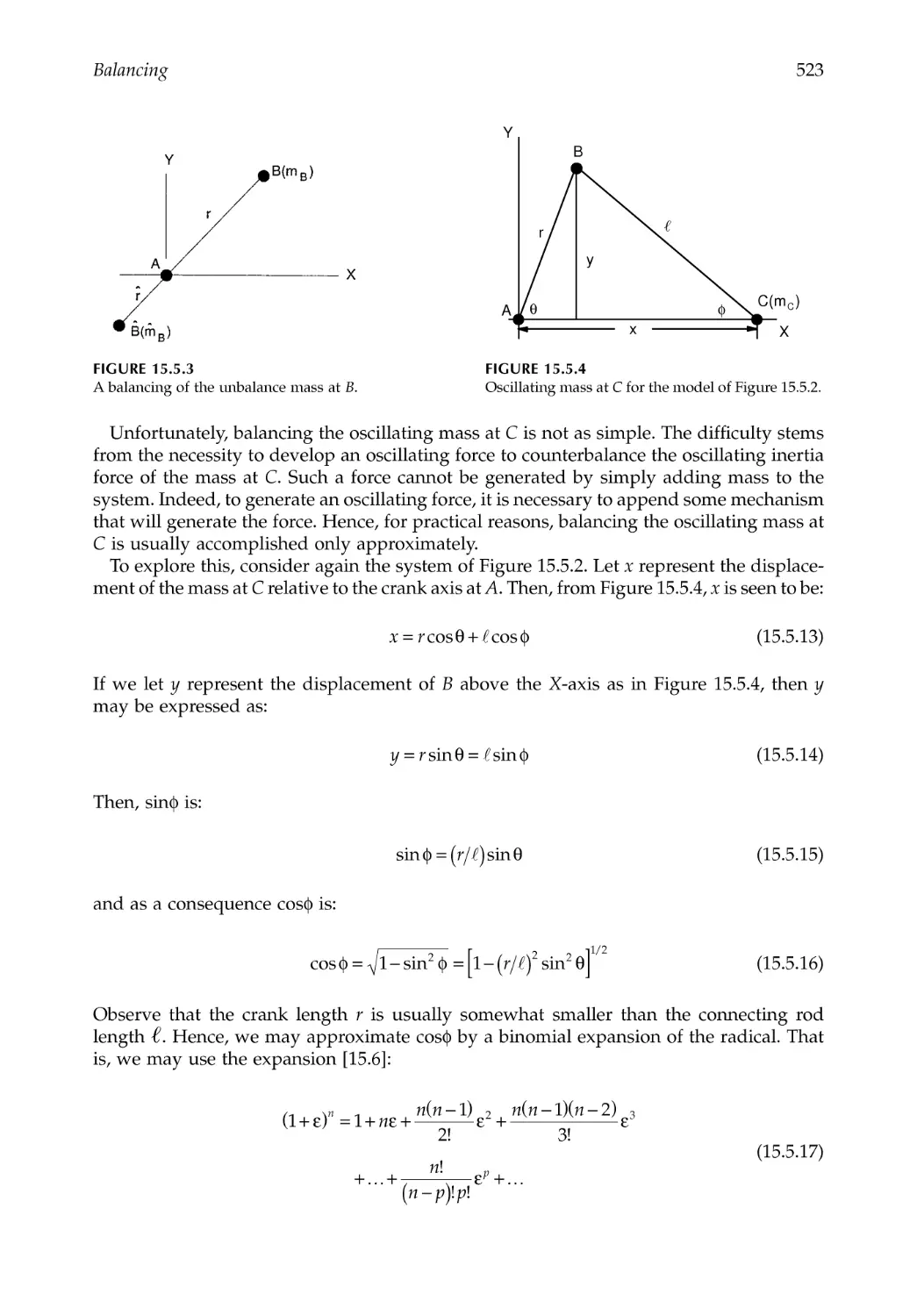
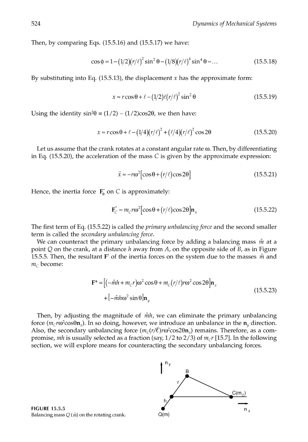
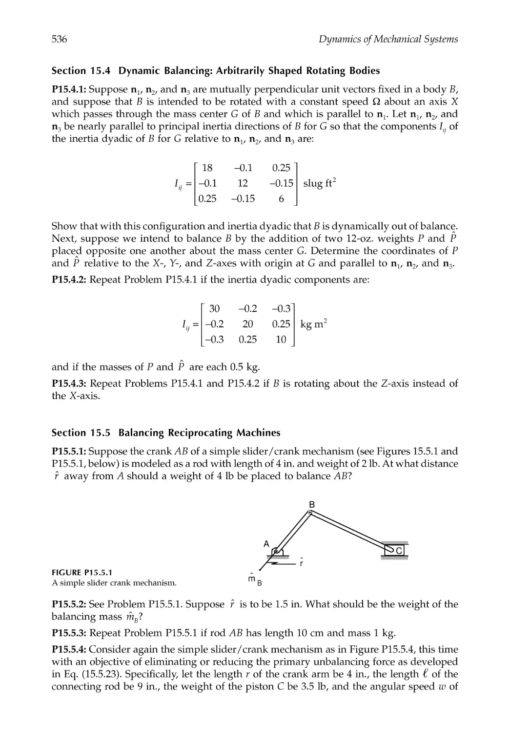
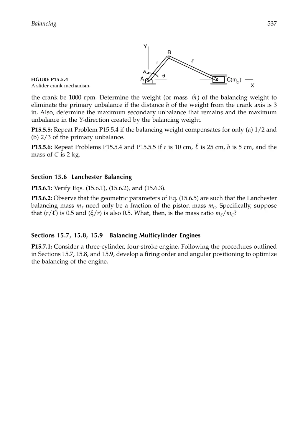
15.5 Application: Balancing of Reciprocating Machines....................................................520
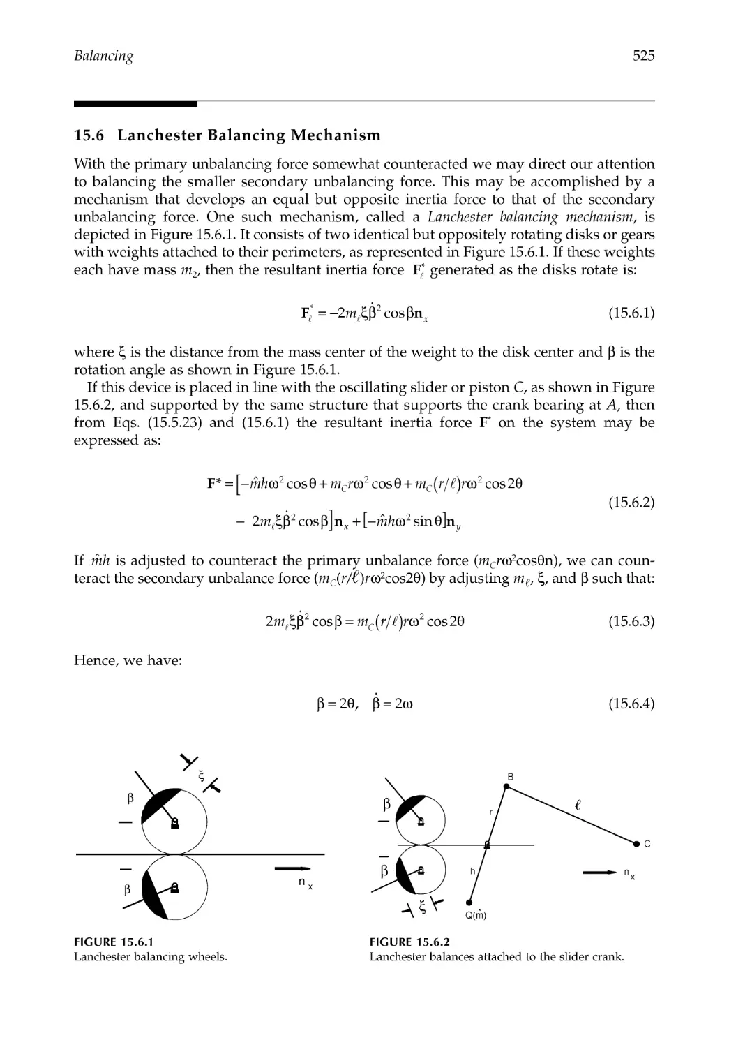
15.6 Lanchester Balancing Mechanism .................................................................................525
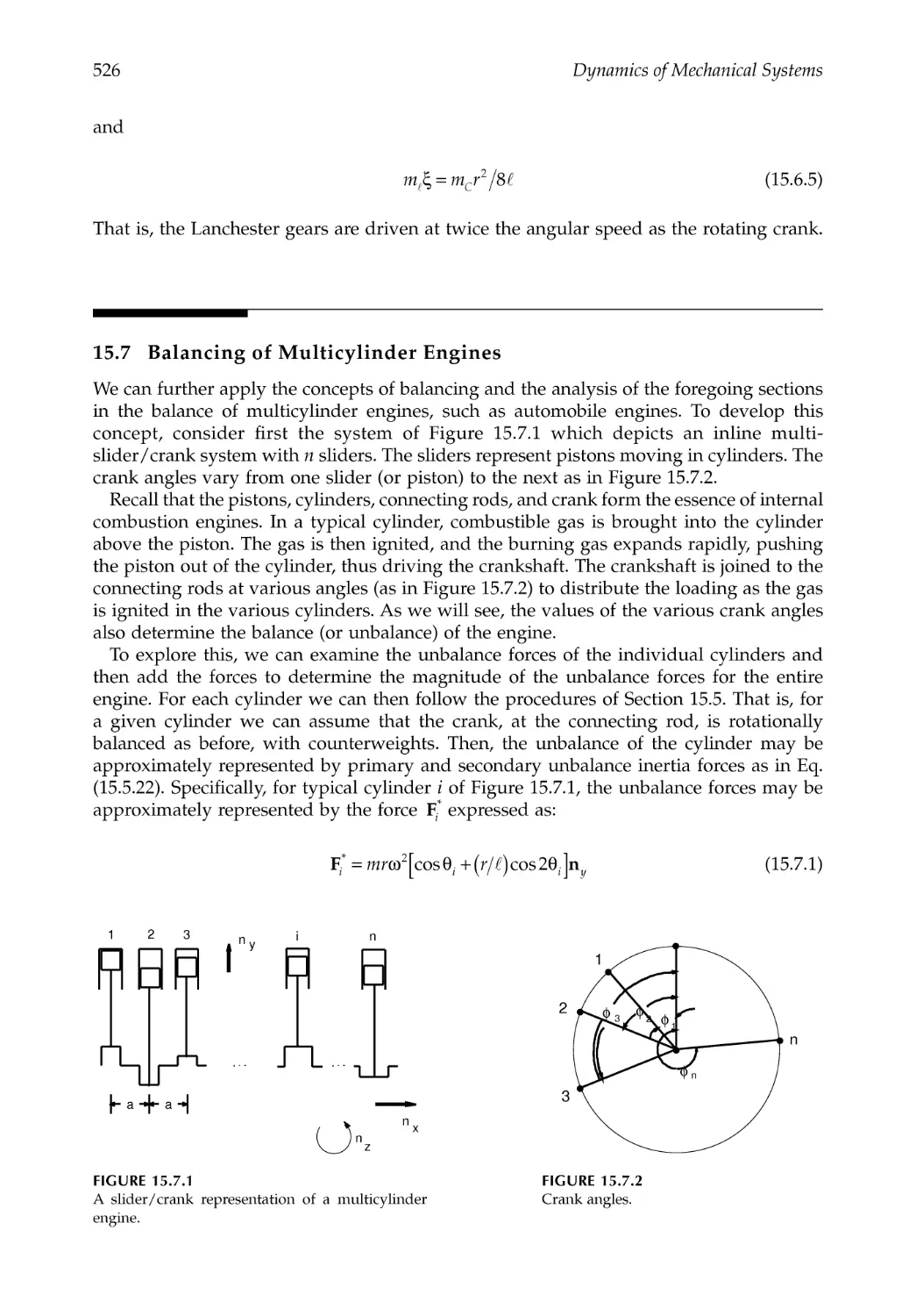
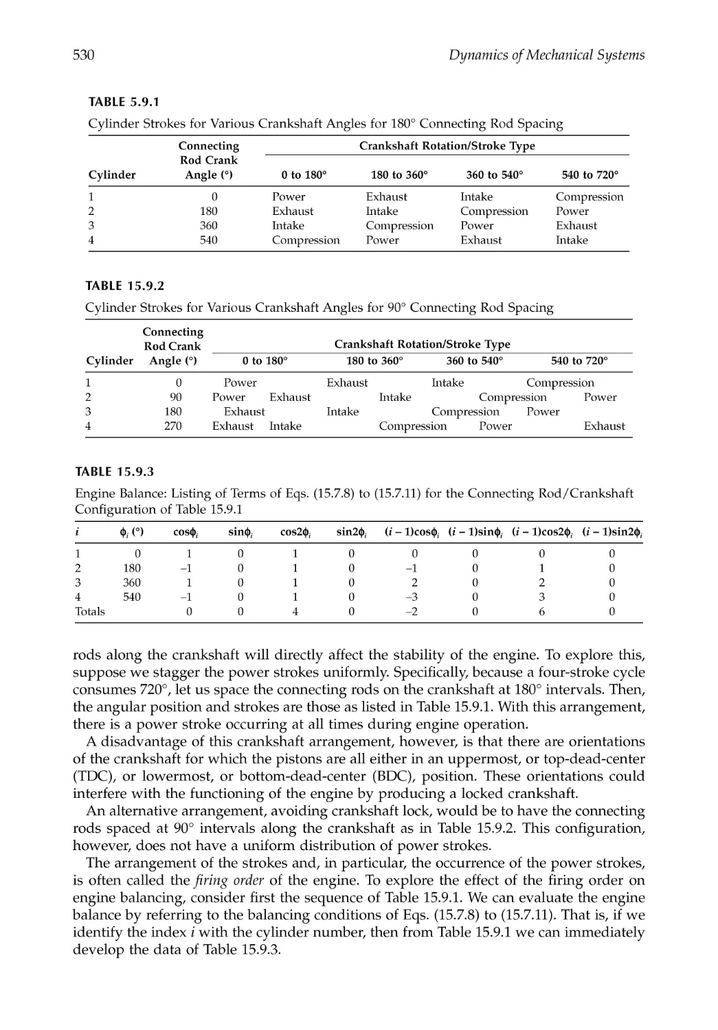
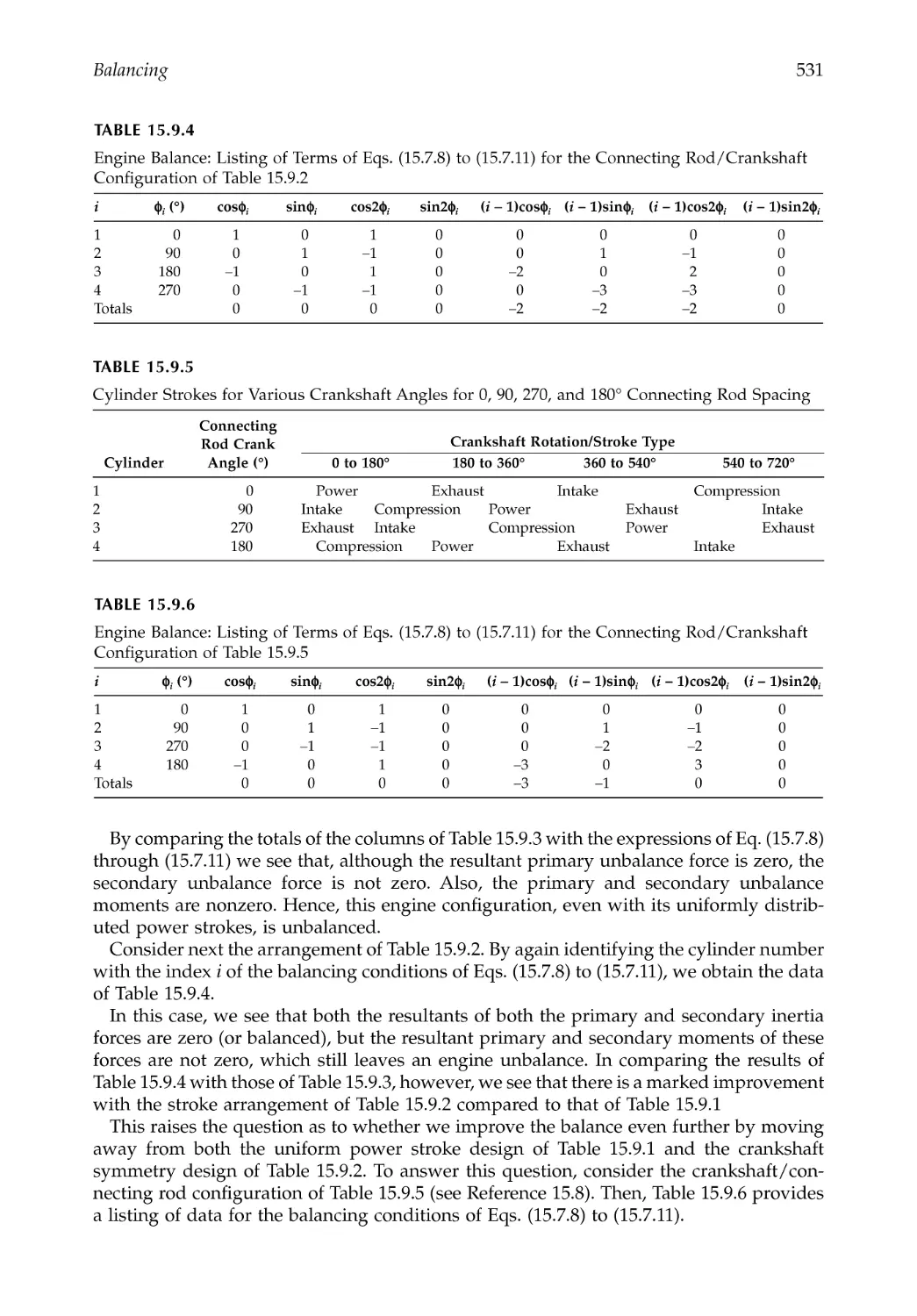
15.7 Balancing of Multicylinder Engines..............................................................................526
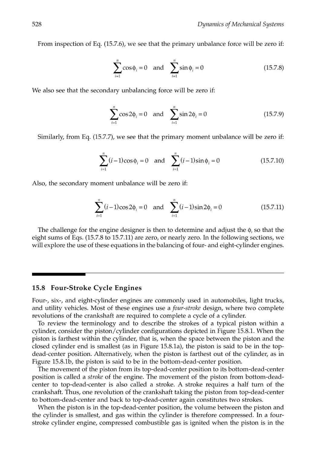
15.8 Four-Stroke Cycle Engines .............................................................................................528
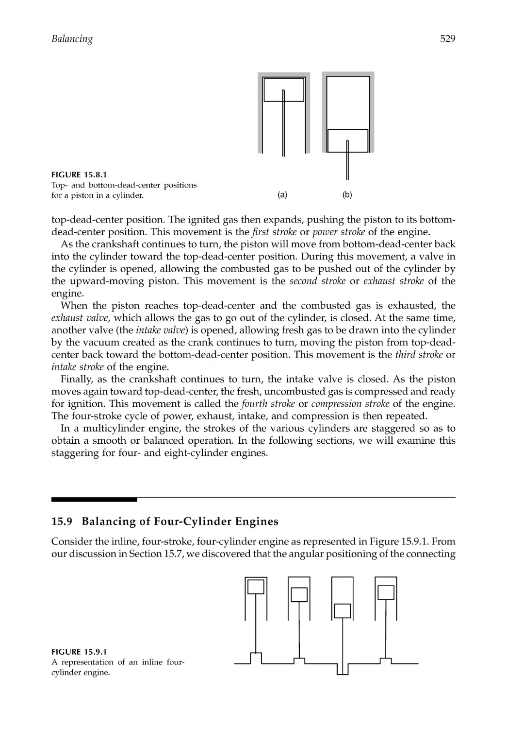
15.9 Balancing of Four-Cylinder Engines .............................................................................529
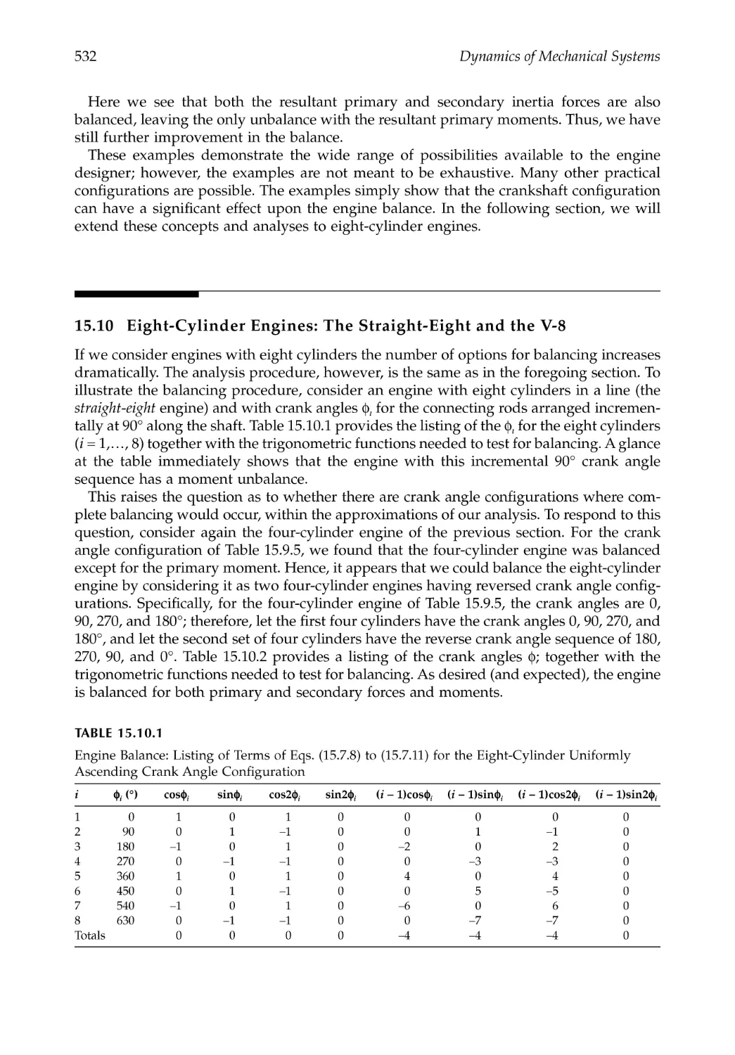
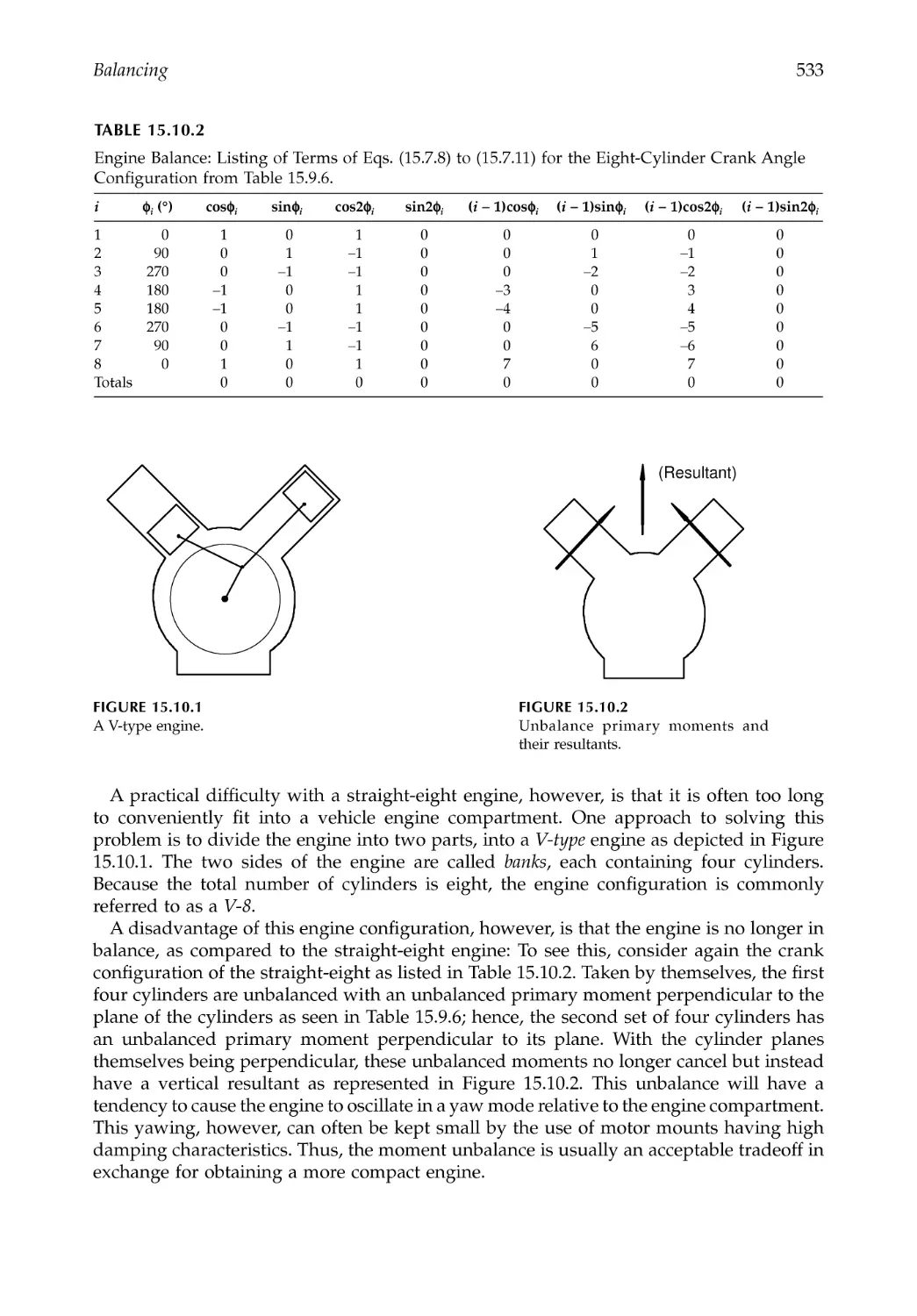
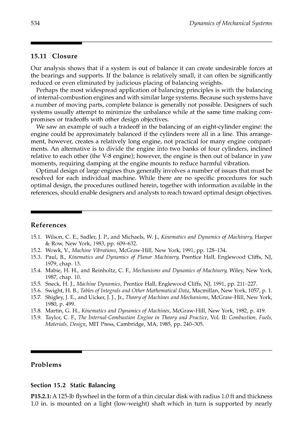
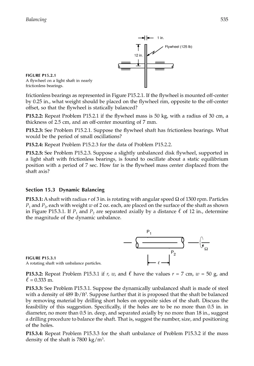
15.10 Eight-Cylinder Engines: The Straight-Eight and the V-8 ..........................................532
15.11 Closure ...............................................................................................................................534
References .....................................................................................................................................534
Problems .......................................................................................................................................534
Chapter 16 Mechanical Components: Cams .......................................................................539
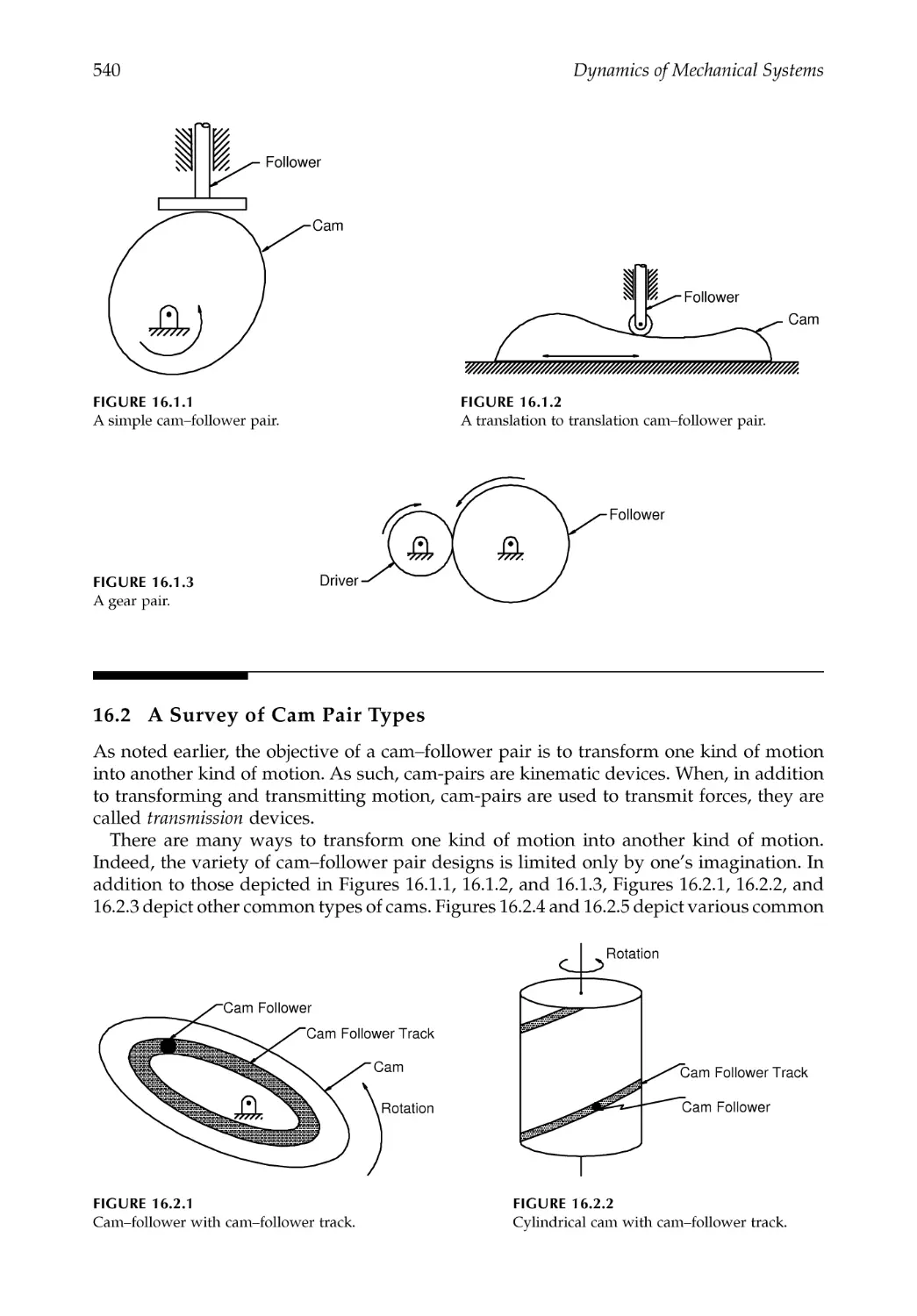
16.1 Introduction.......................................................................................................................539
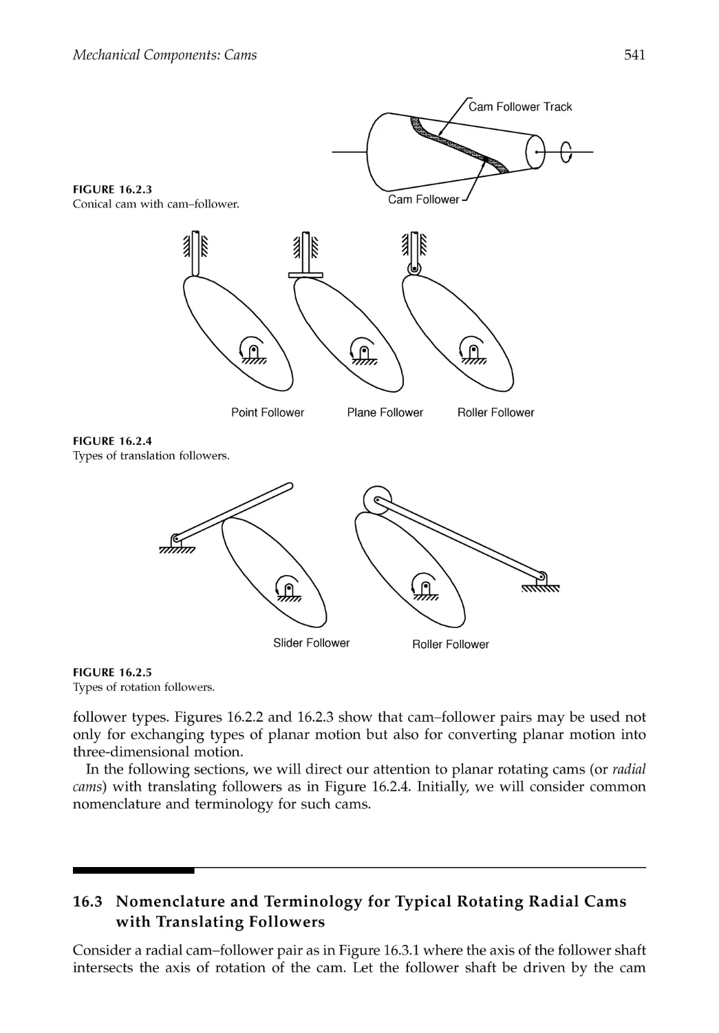
16.2 A Survey of Cam Pair Types ..........................................................................................540
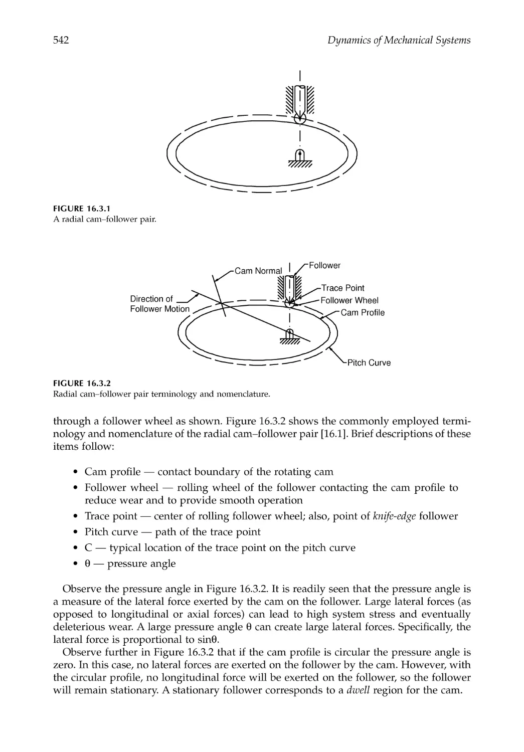
16.3 Nomenclature and Terminology for Typical Rotating Radial Cams
with Translating Followers .............................................................................................541
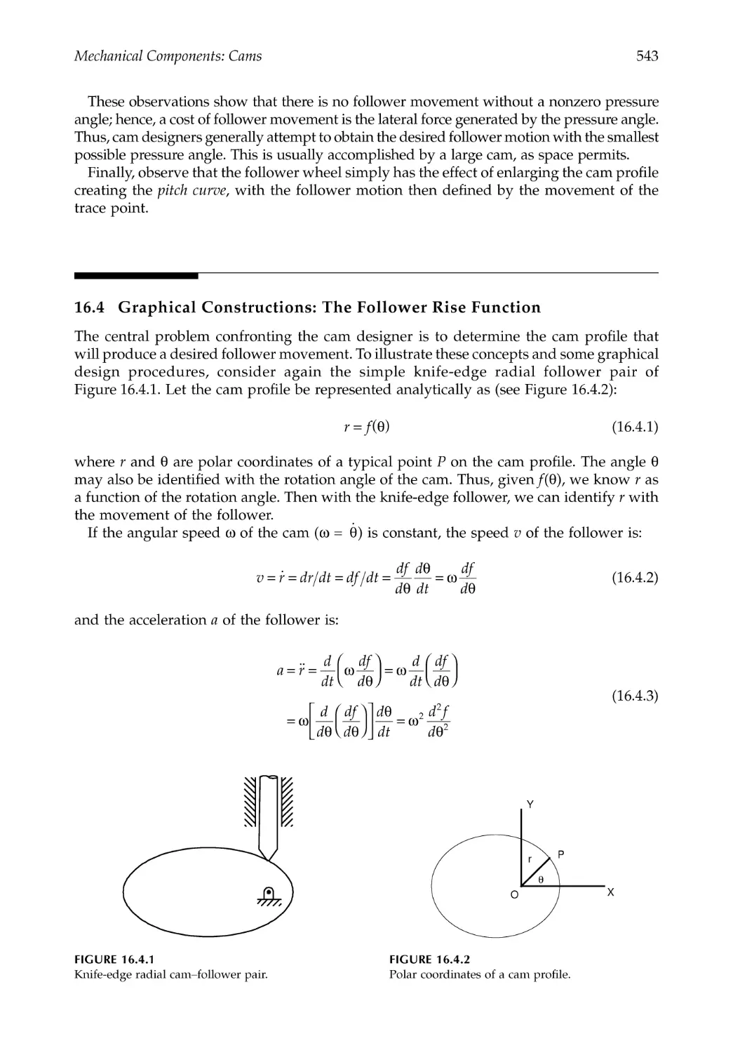
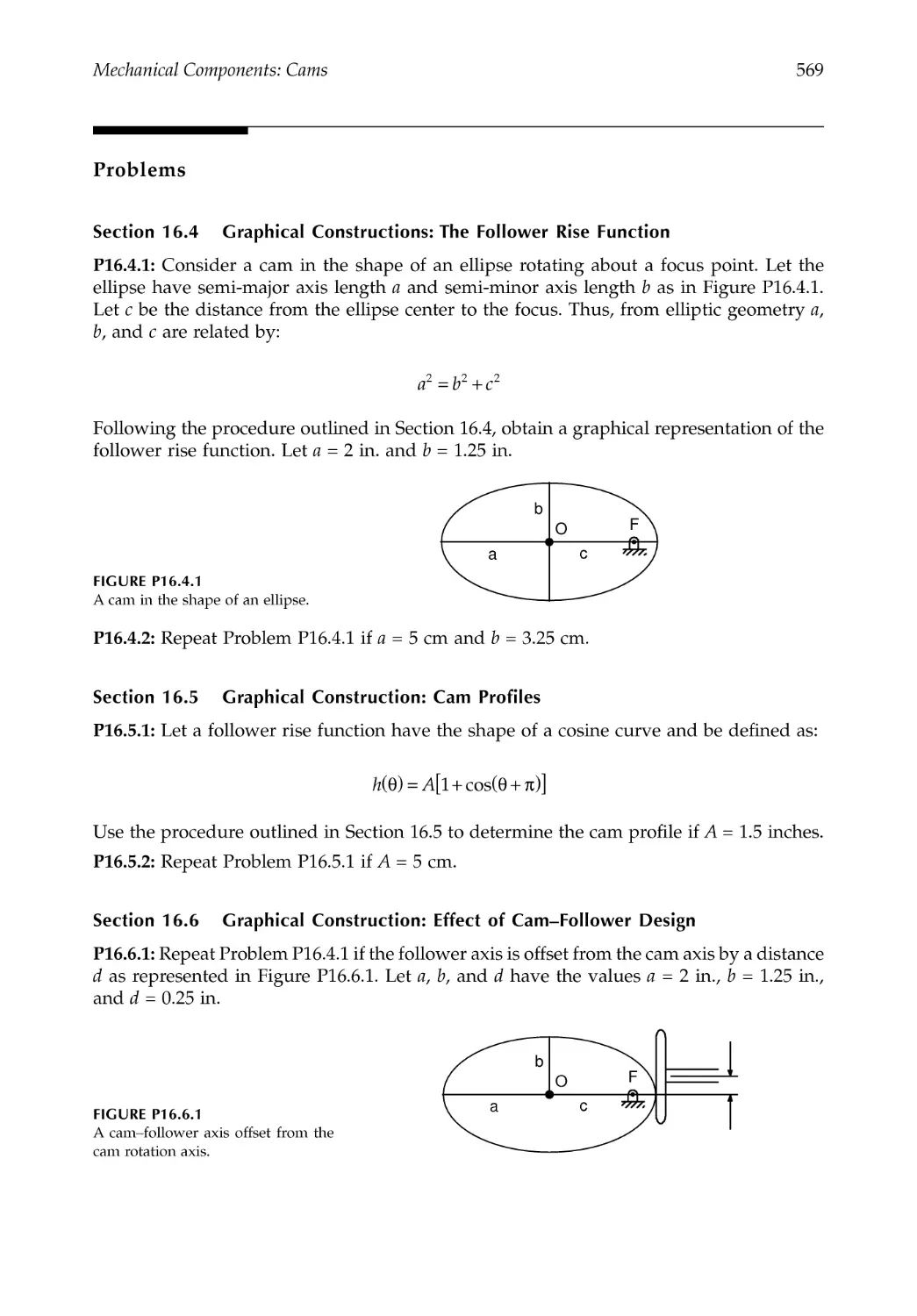
16.4 Graphical Constructions: The Follower Rise Function ..............................................543
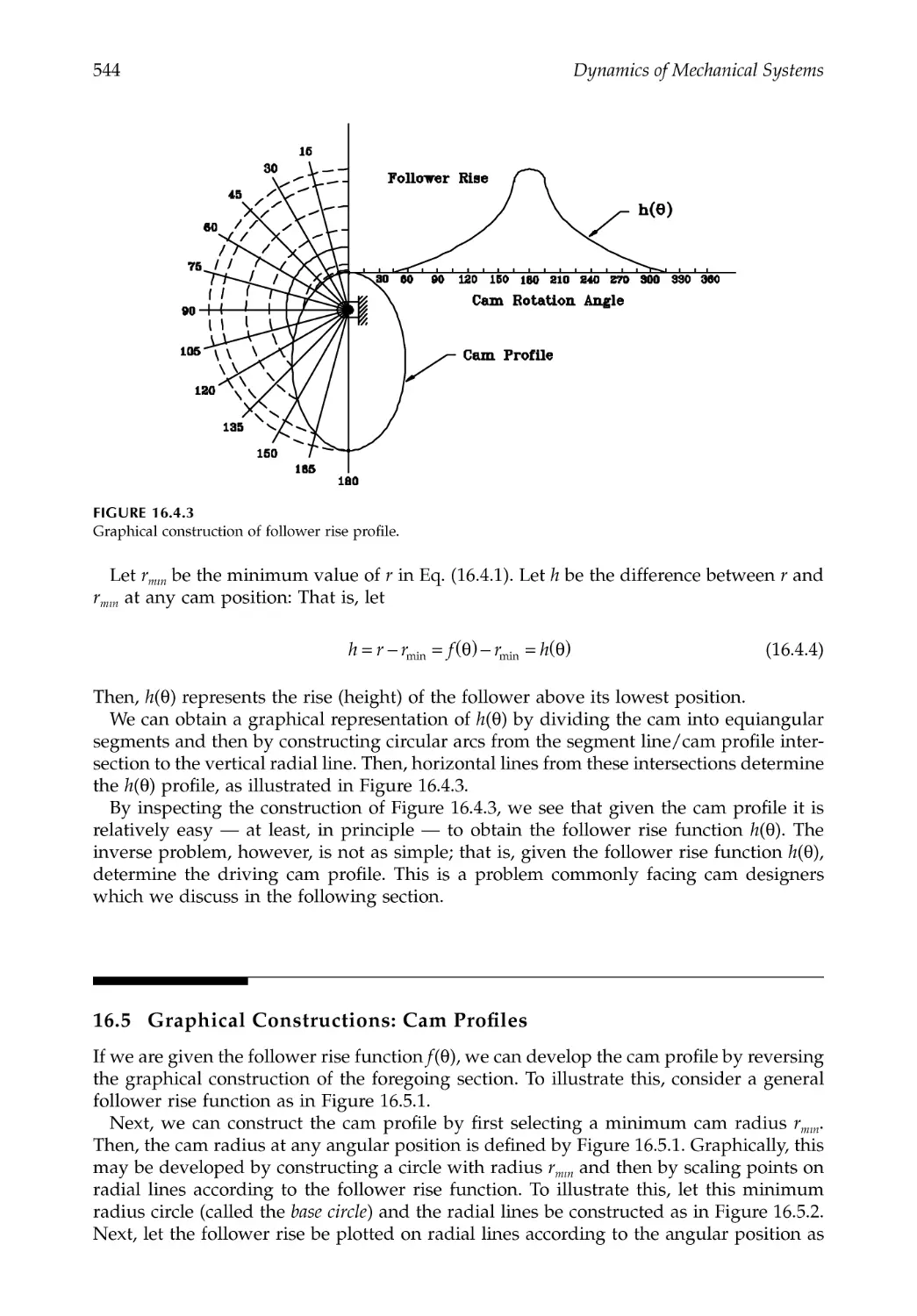
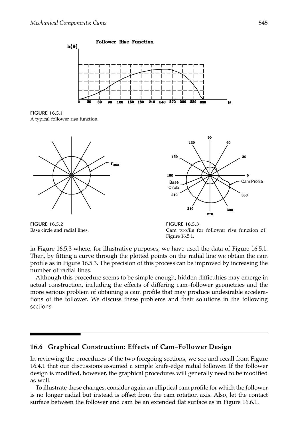
16.5 Graphical Constructions: Cam Profiles ........................................................................544
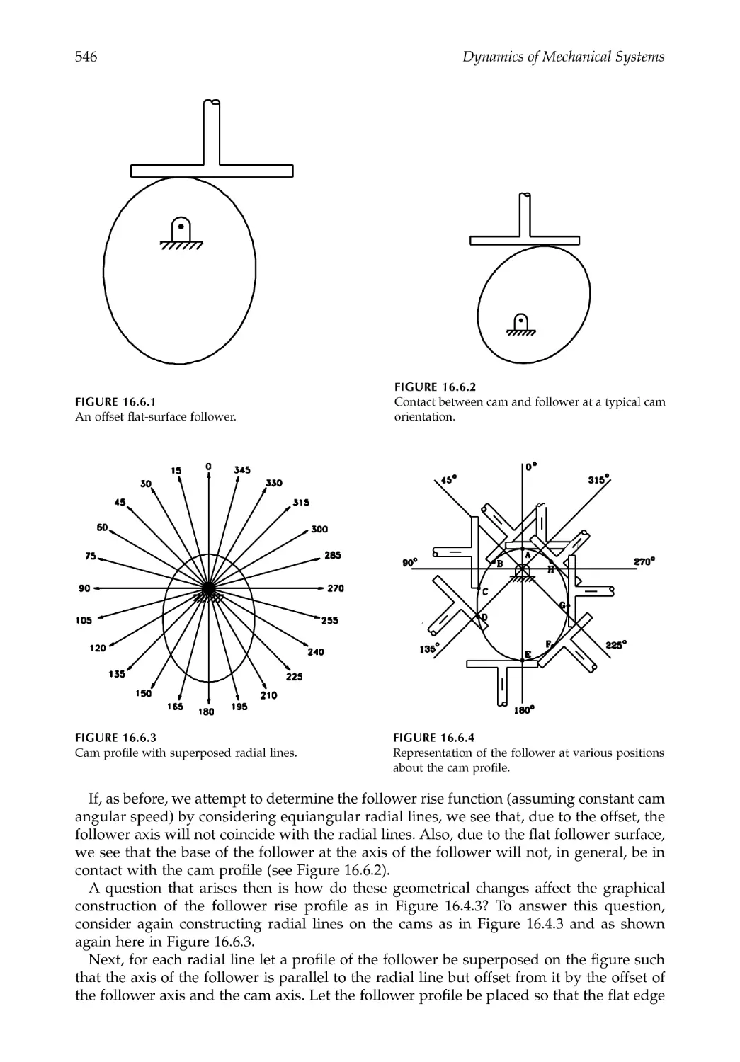
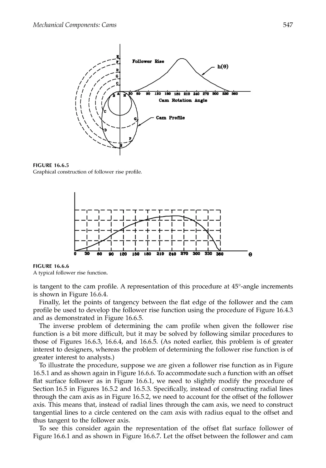
16.6 Graphical Construction: Effects of Cam--Follower Design .......................................545
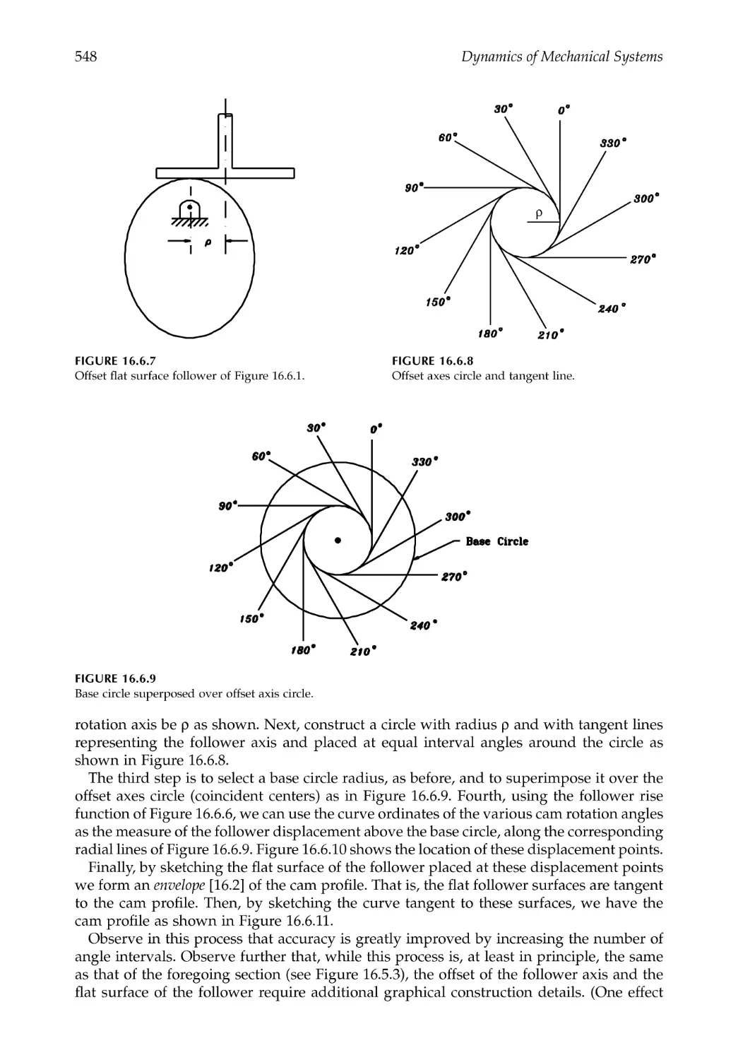
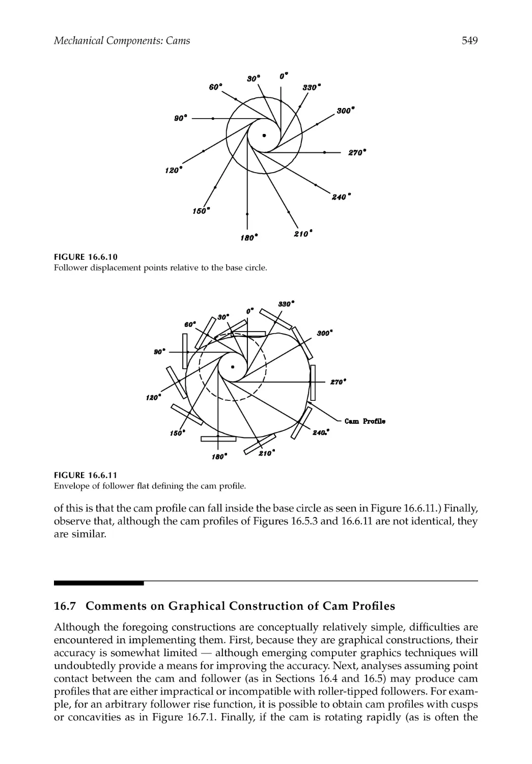
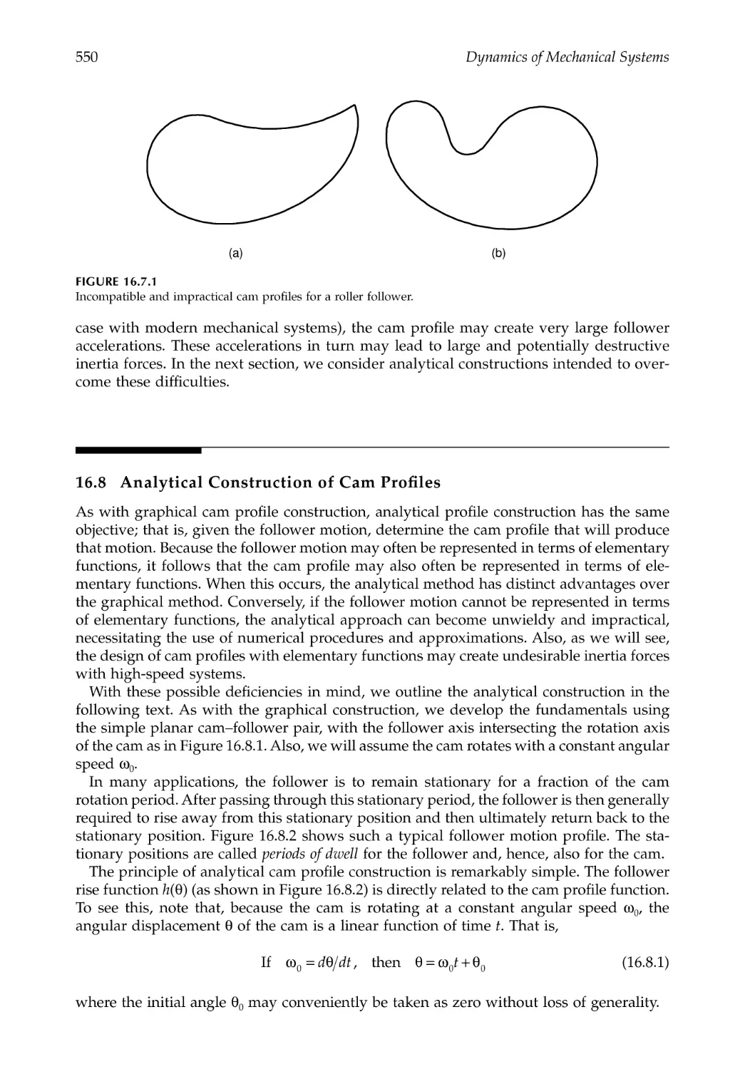
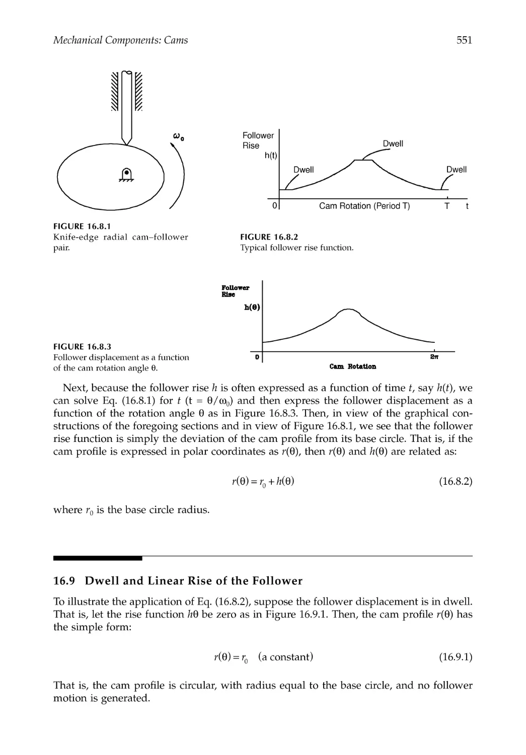
16.7 Comments on Graphical Construction of Cam Profiles ............................................549
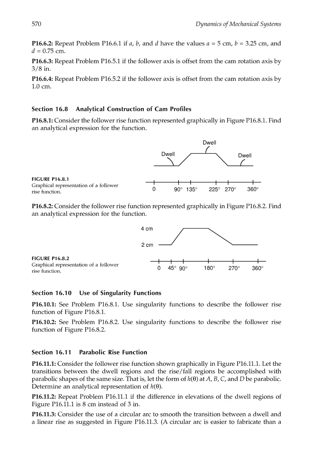
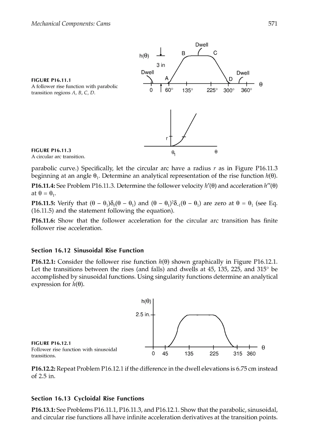
16.8 Analytical Construction of Cam Profiles .....................................................................550
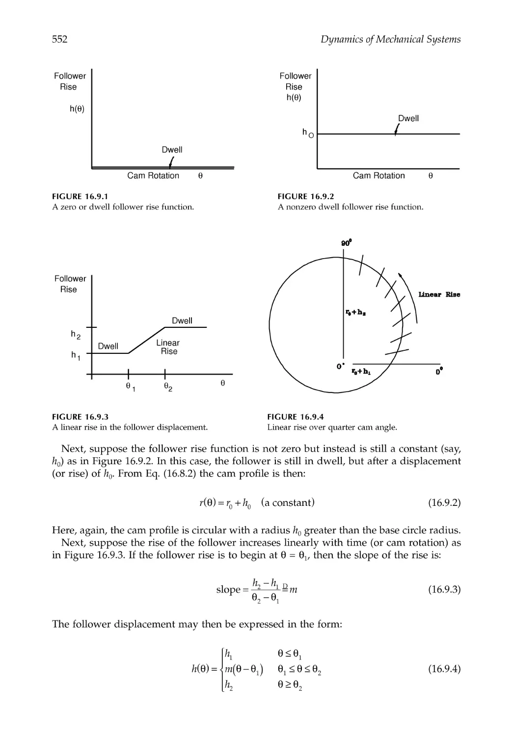
16.9 Dwell and Linear Rise of the Follower ........................................................................551
16.10 Use of Singularity Functions ..........................................................................................553
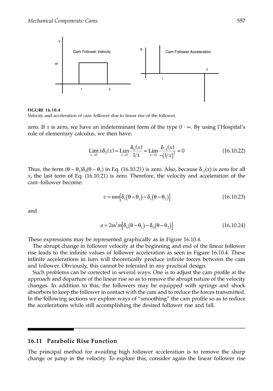
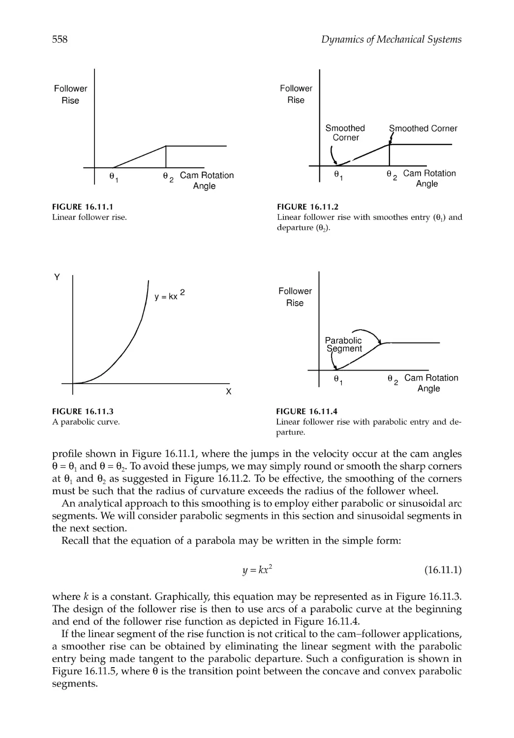
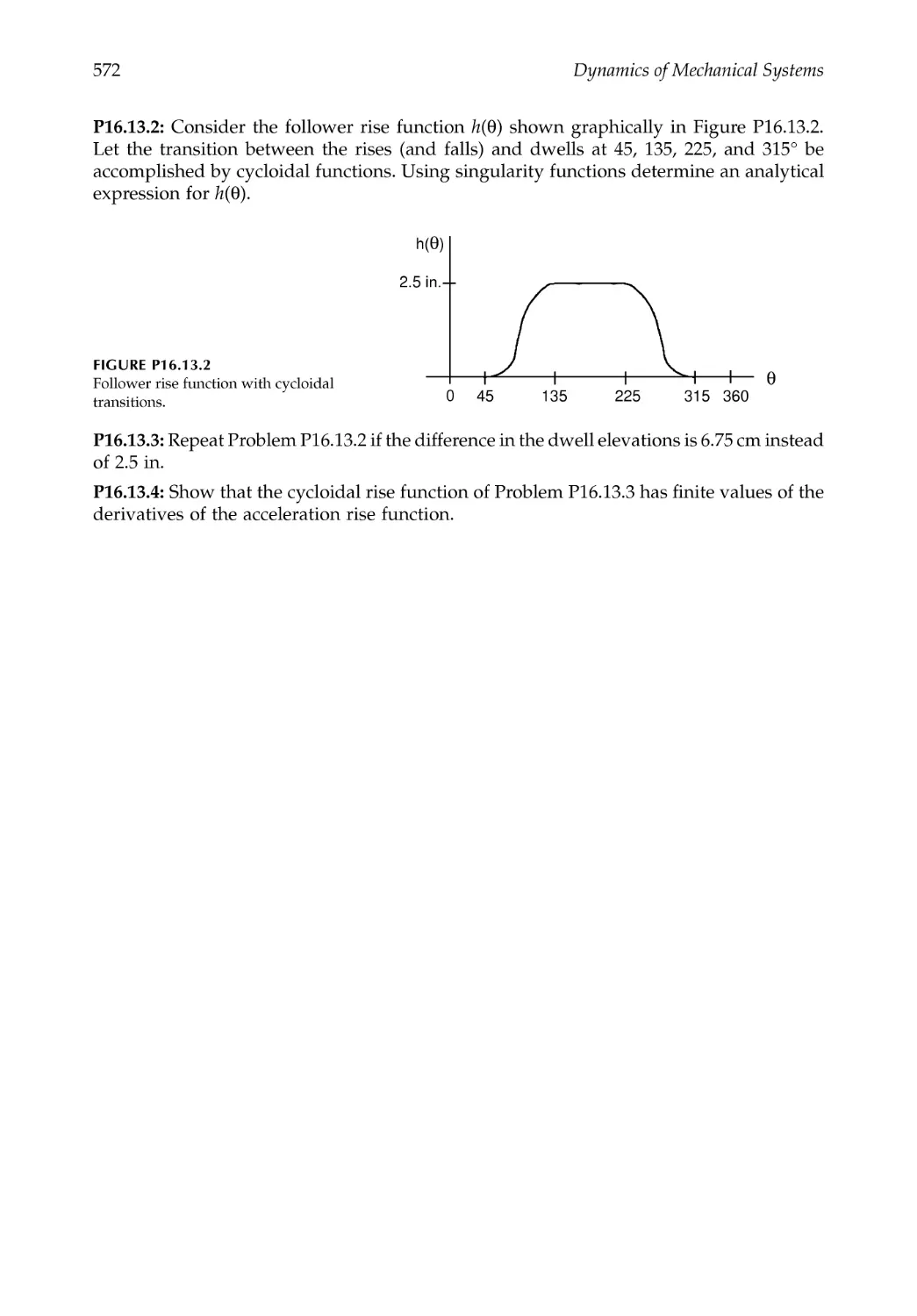
16.11 Parabolic Rise Function ...................................................................................................557
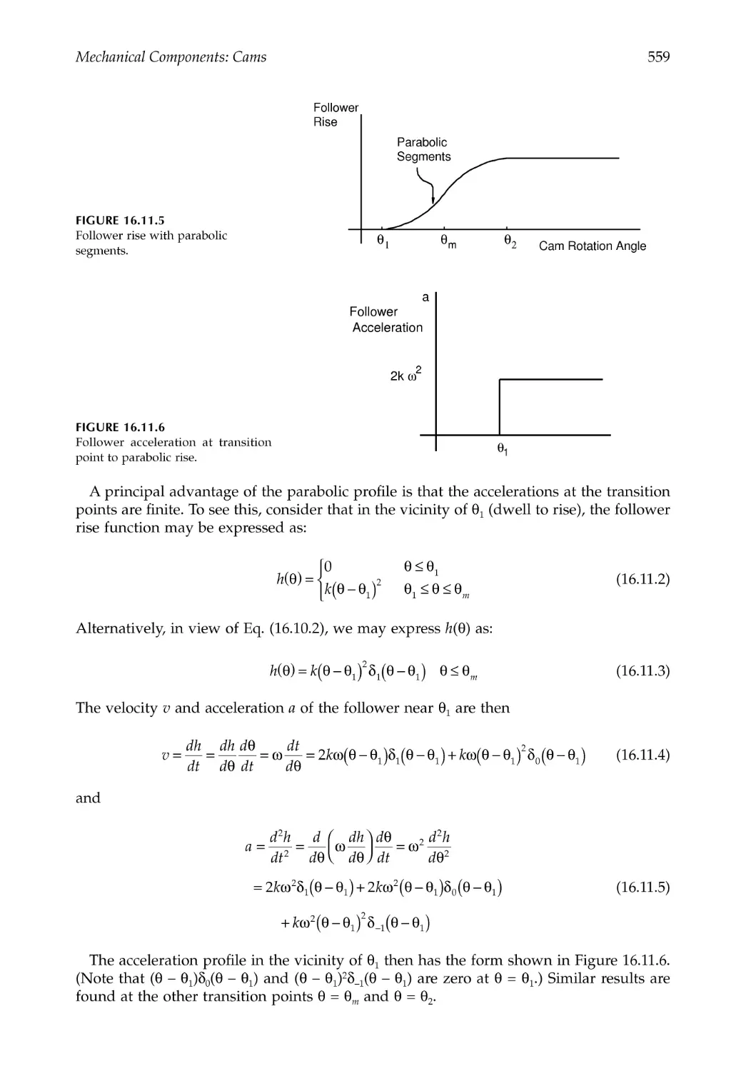
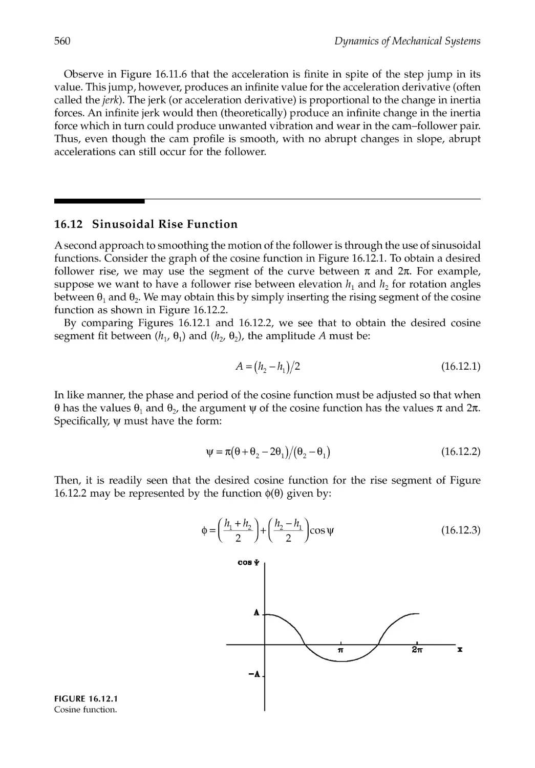
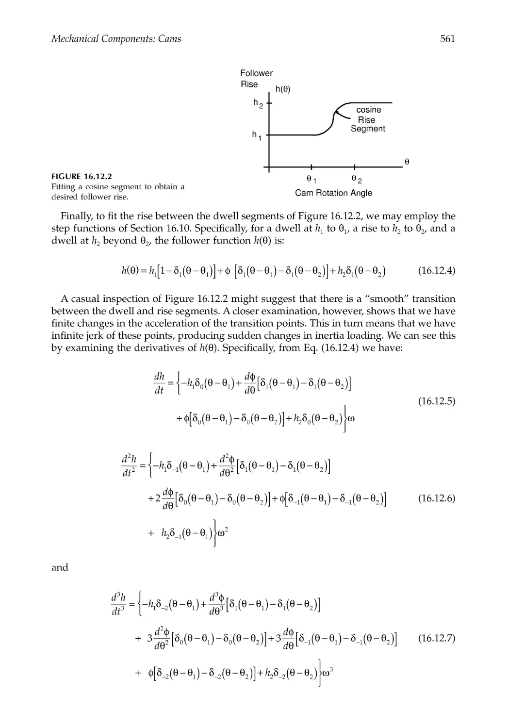
16.12 Sinusoidal Rise Function.................................................................................................560
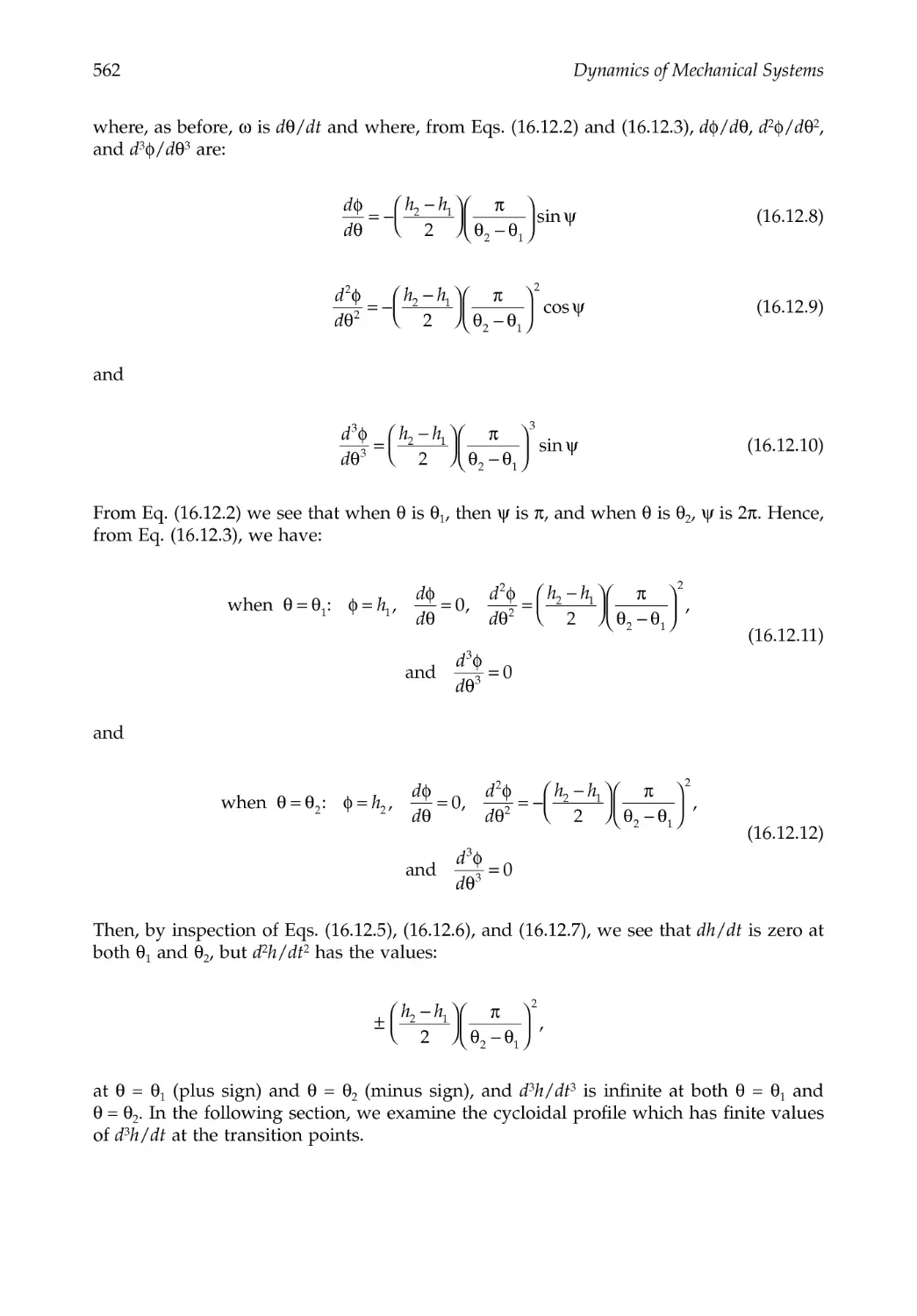
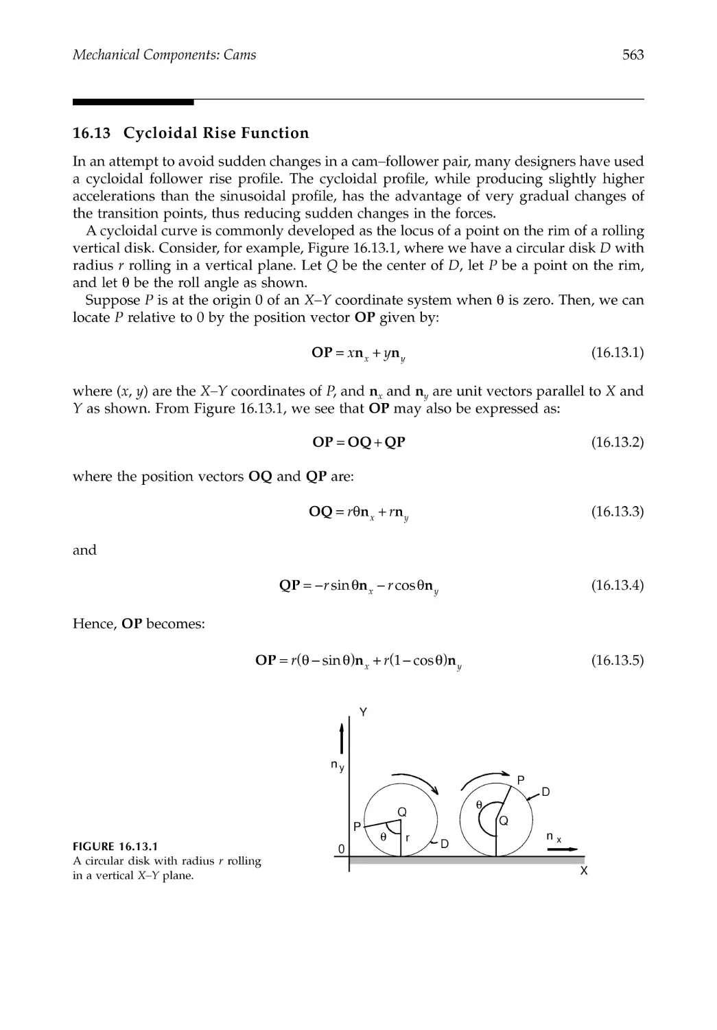
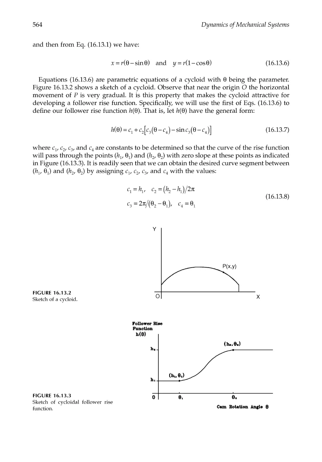
16.13 Cycloidal Rise Function ..................................................................................................563
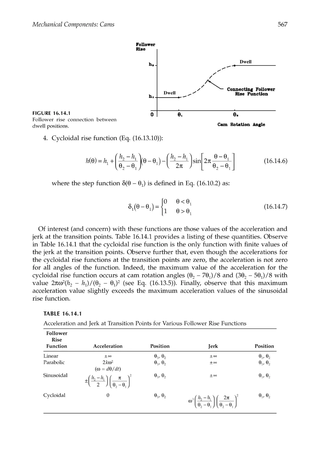
16.14 Summary: Listing of Follower Rise Functions ............................................................566
16.15 Closure ...............................................................................................................................568
References .....................................................................................................................................568
Problems .......................................................................................................................................569
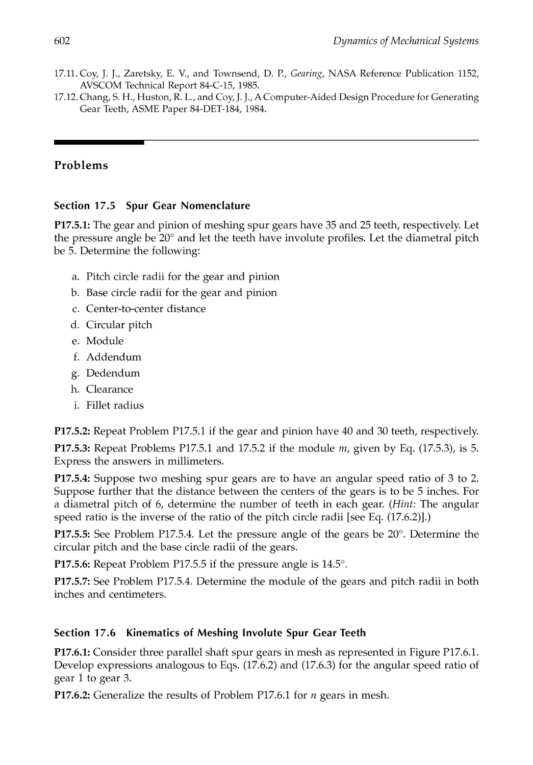
Chapter 17 Mechanical Components: Gears .......................................................................573
17.1 Introduction.......................................................................................................................573
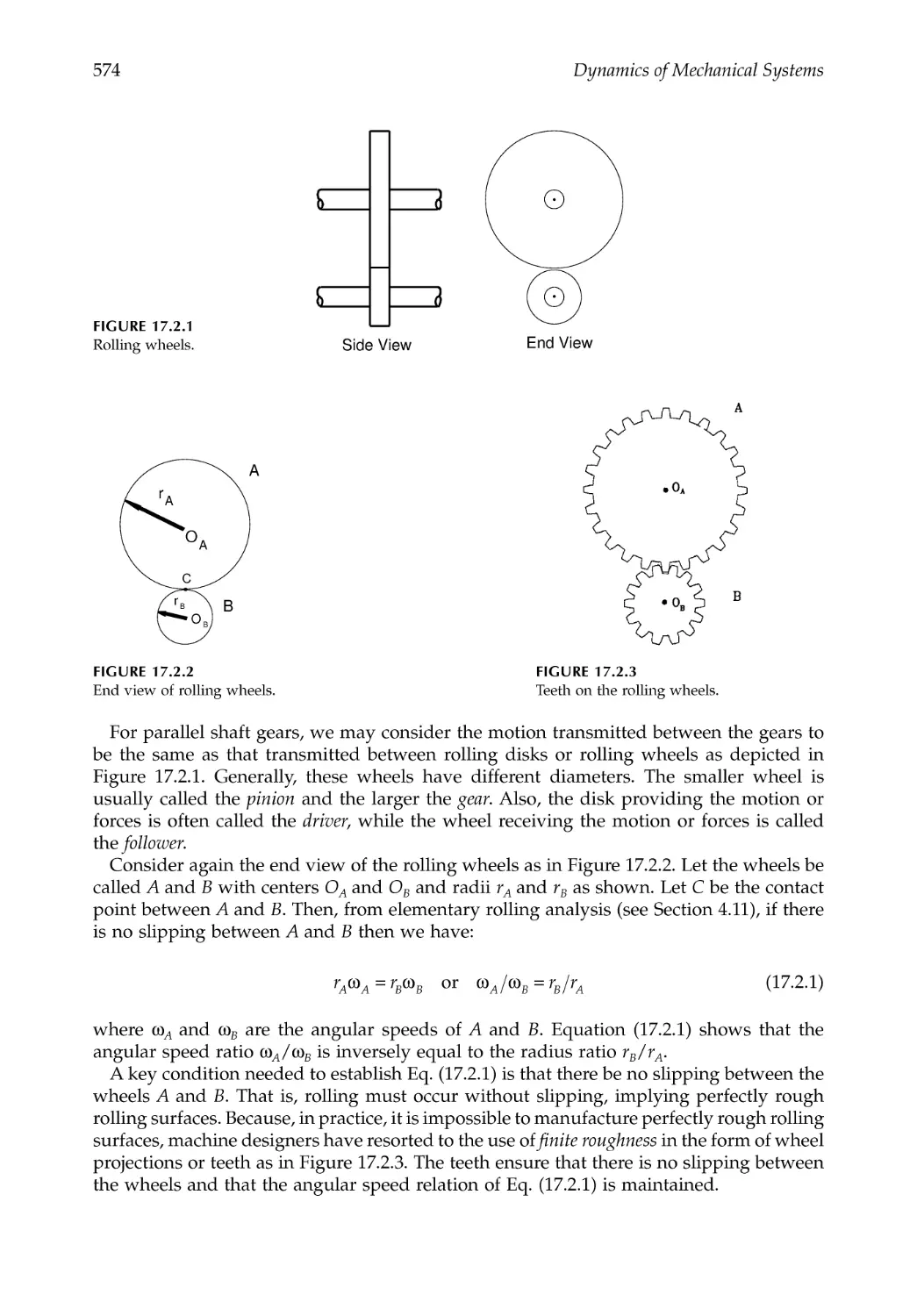
17.2 Preliminary and Fundamental Concepts: Rolling Wheels ........................................573
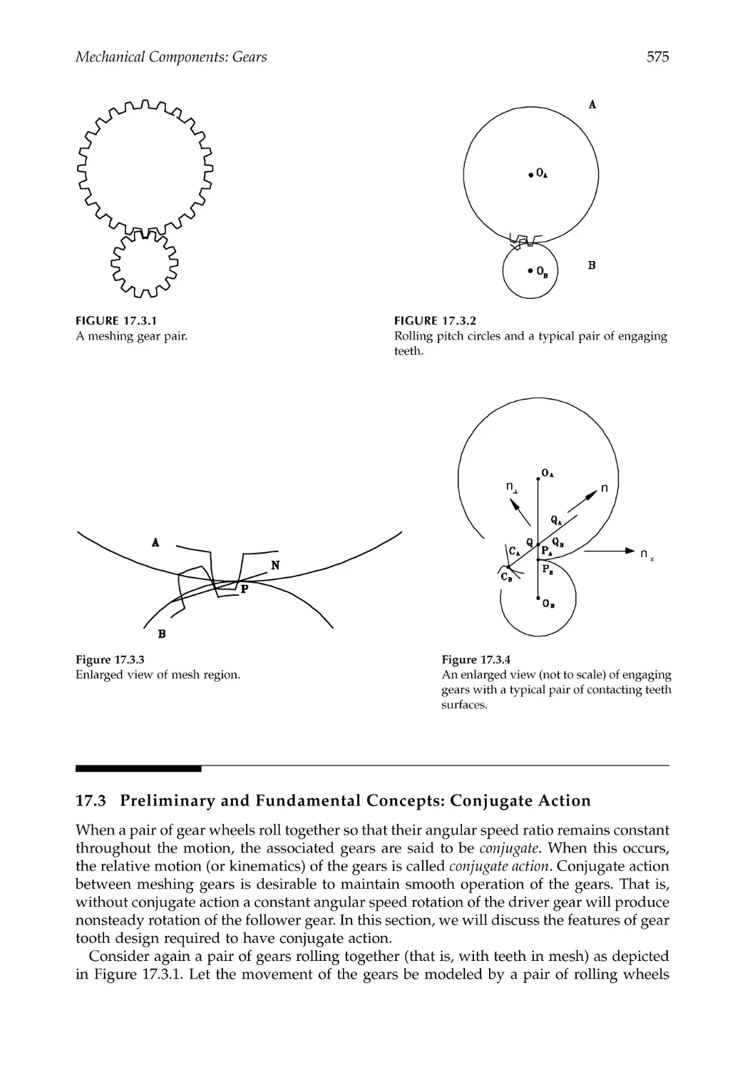
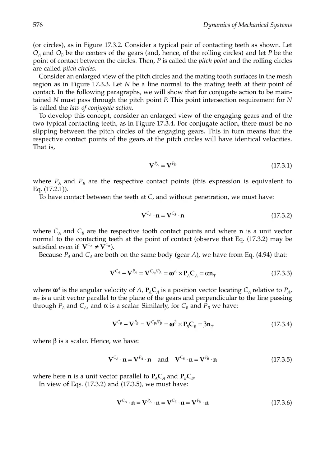
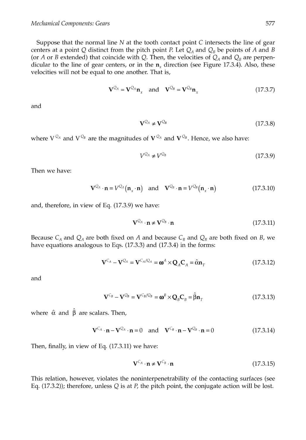
17.3 Preliminary and Fundamental Concepts: Conjugate Action ....................................575
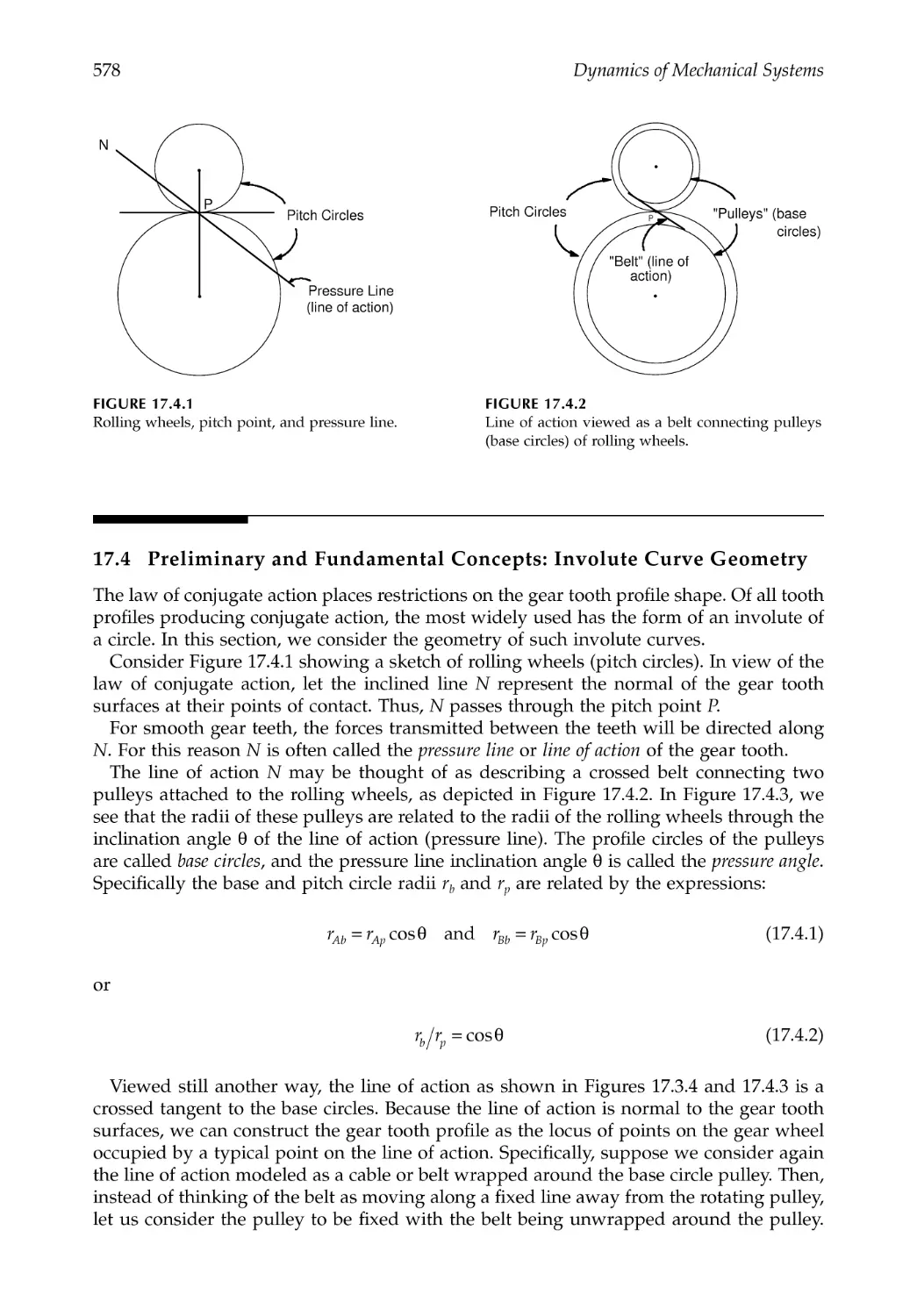
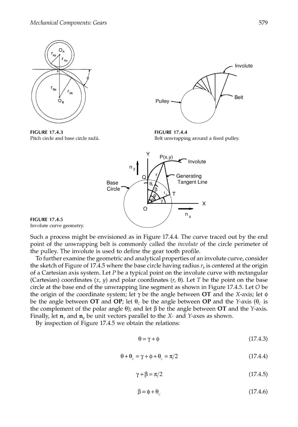
17.4 Preliminary and Fundamental Concepts: Involute Curve Geometry .....................578
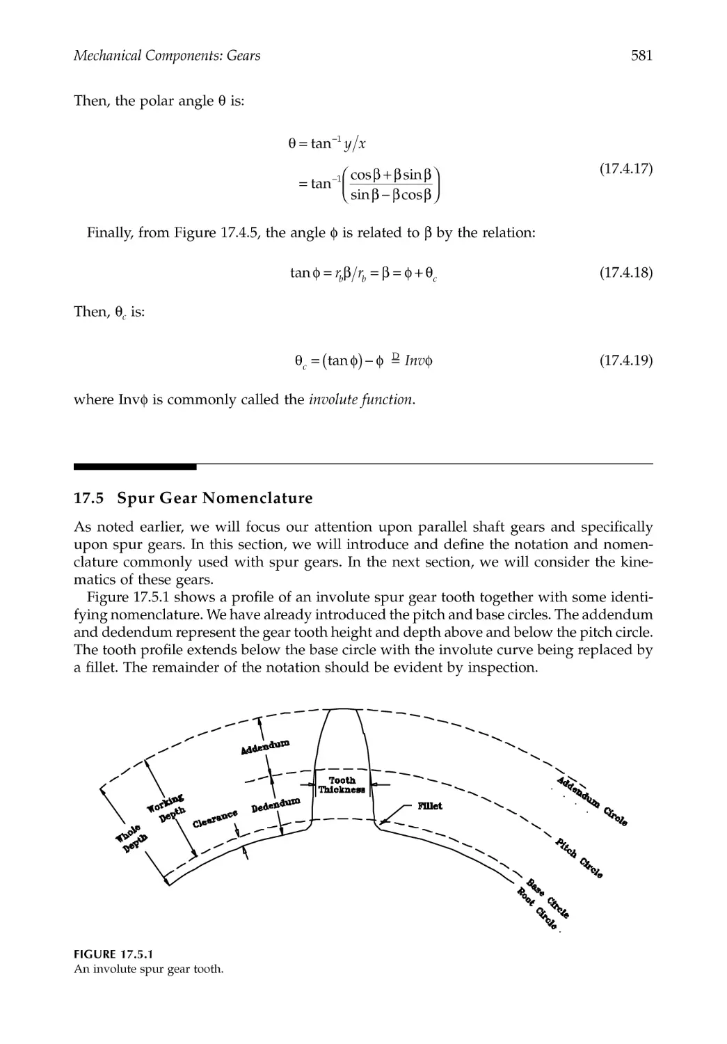
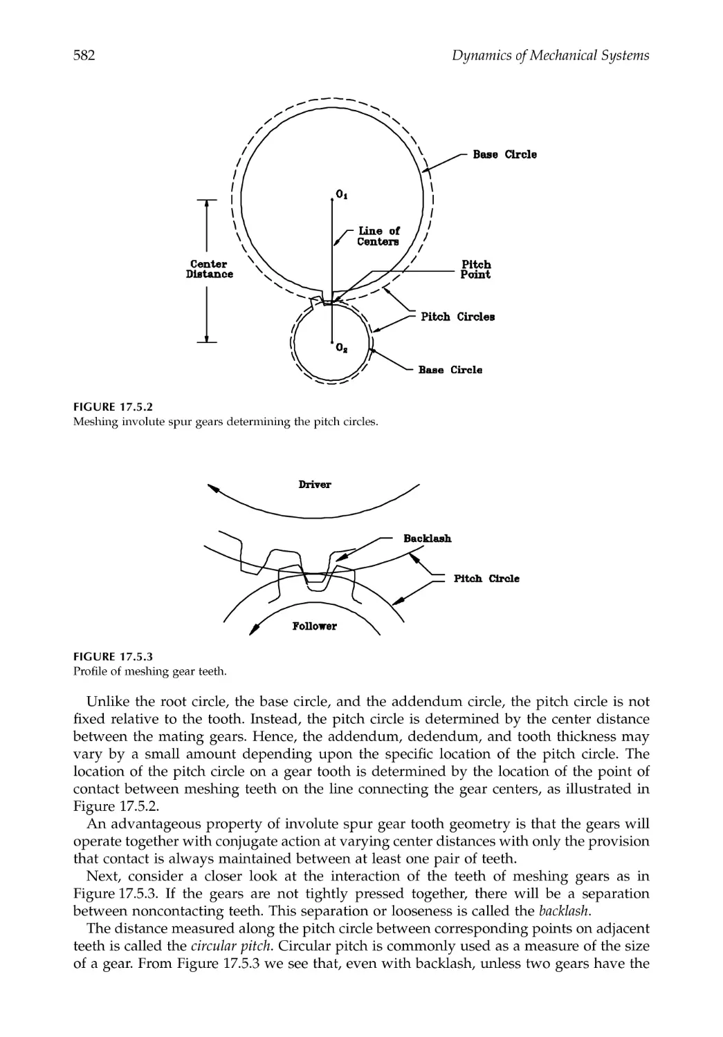
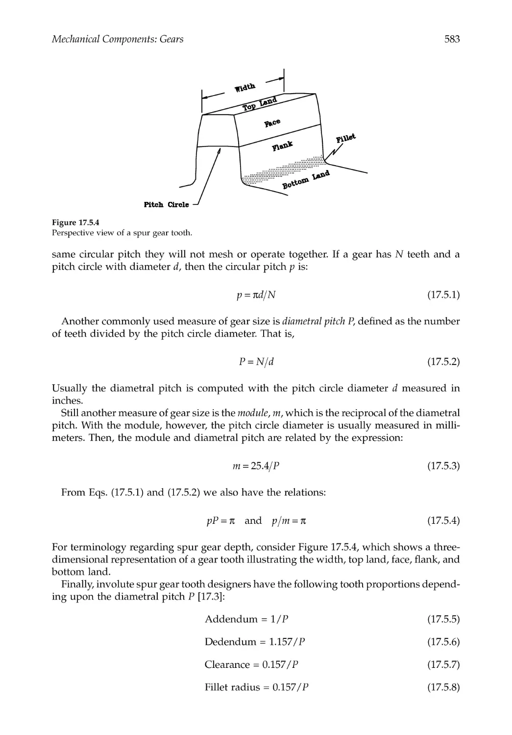
17.5 Spur Gear Nomenclature ................................................................................................581
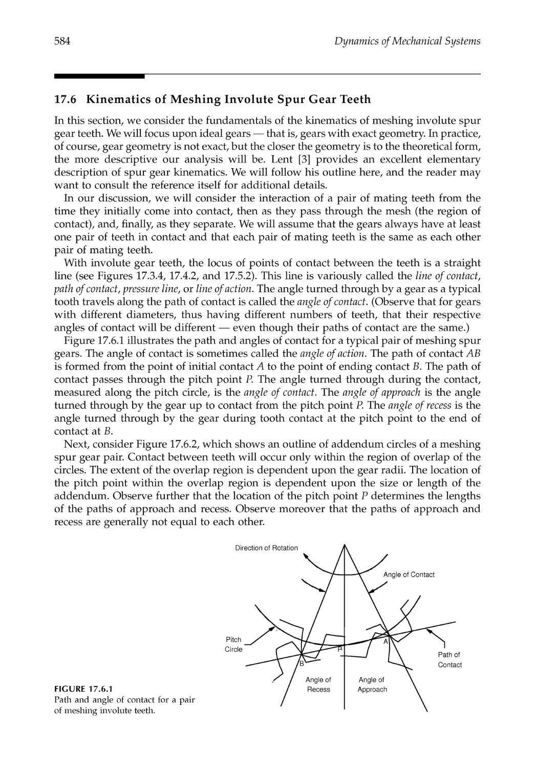
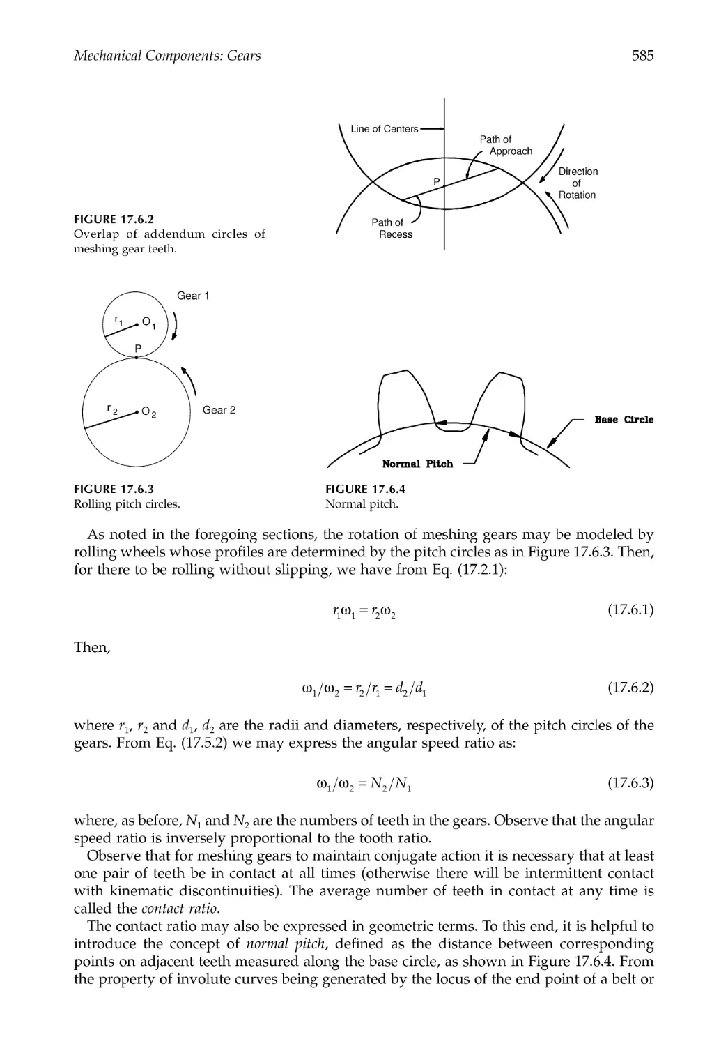
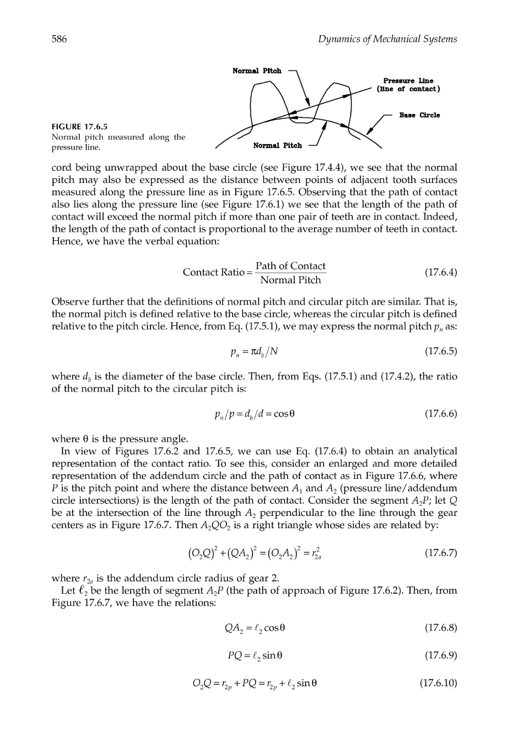
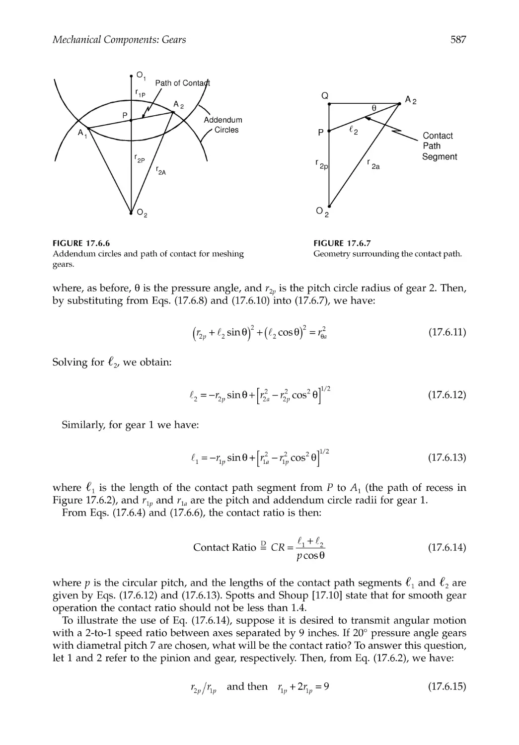
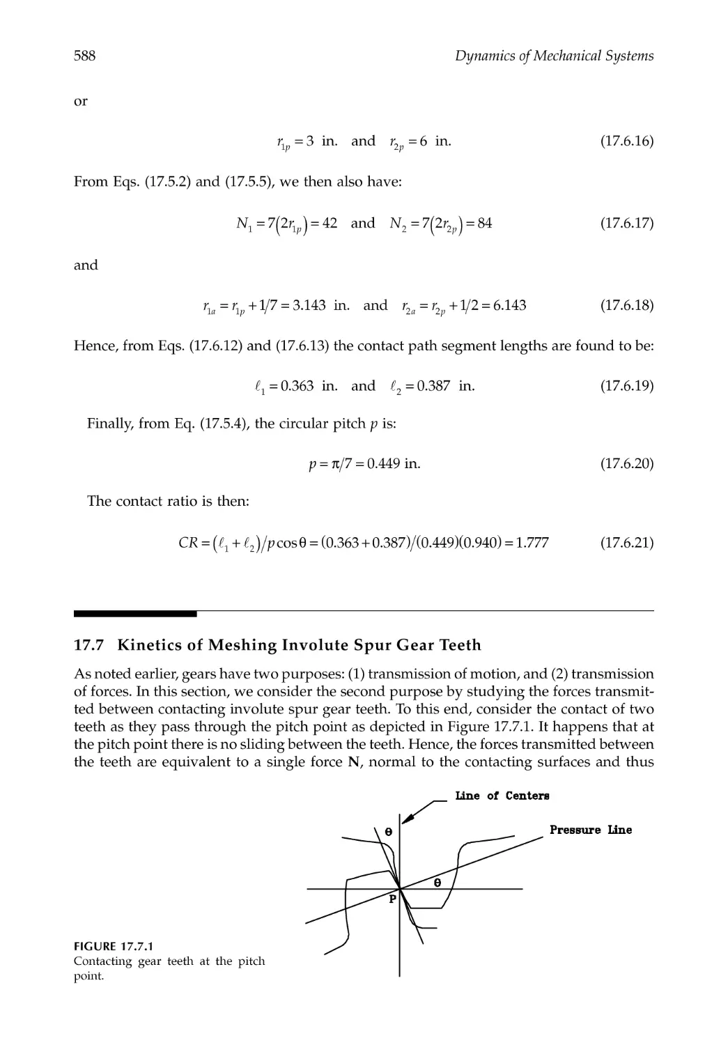
17.6 Kinematics of Meshing Involute Spur Gear Teeth .....................................................584
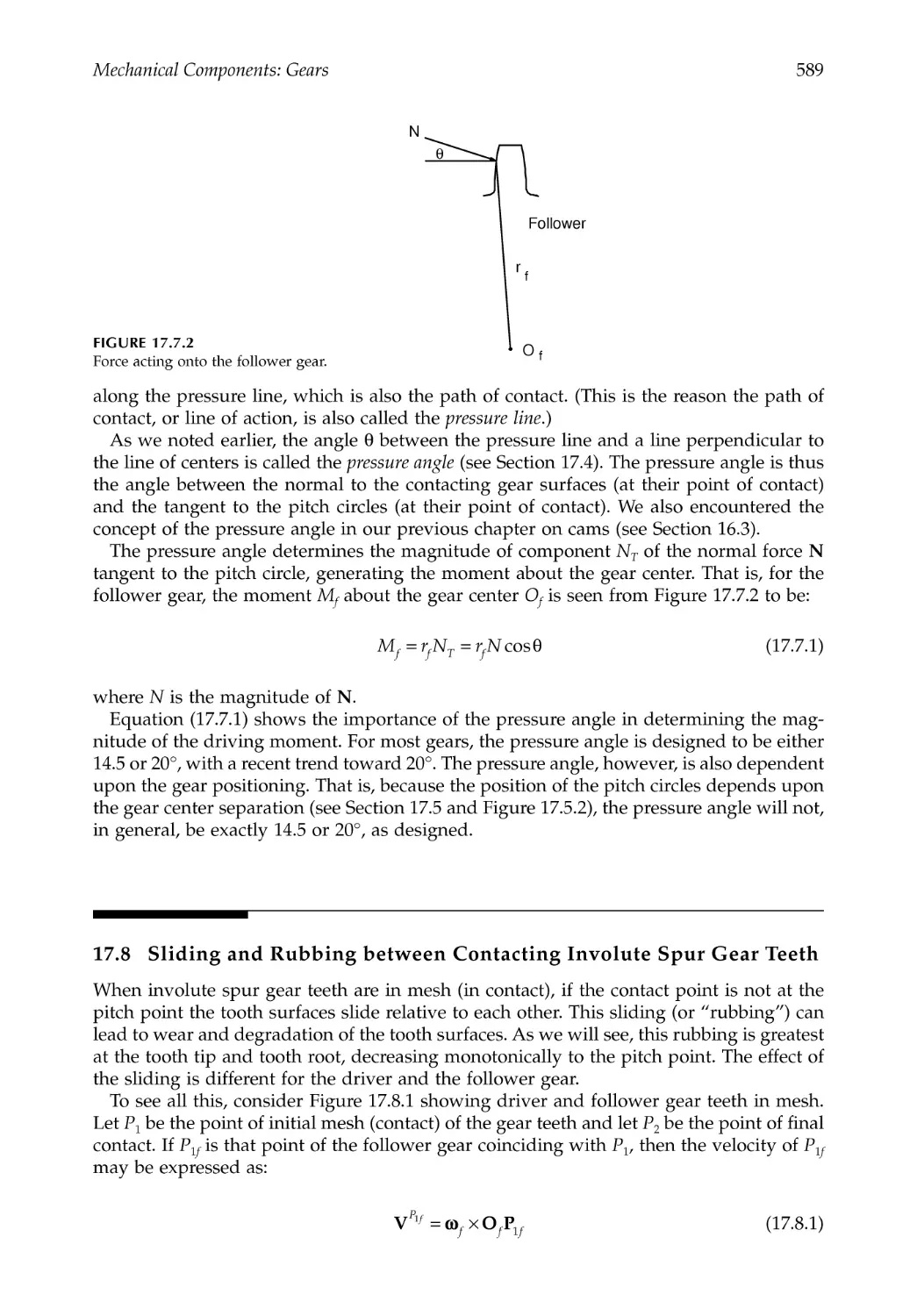
17.7 Kinetics of Meshing Involute Spur Gear Teeth...........................................................588
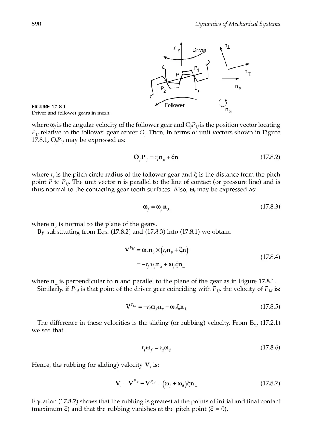
17.8 Sliding and Rubbing between Contacting Involute Spur Gear Teeth ....................589
17.9 Involute Rack ....................................................................................................................591
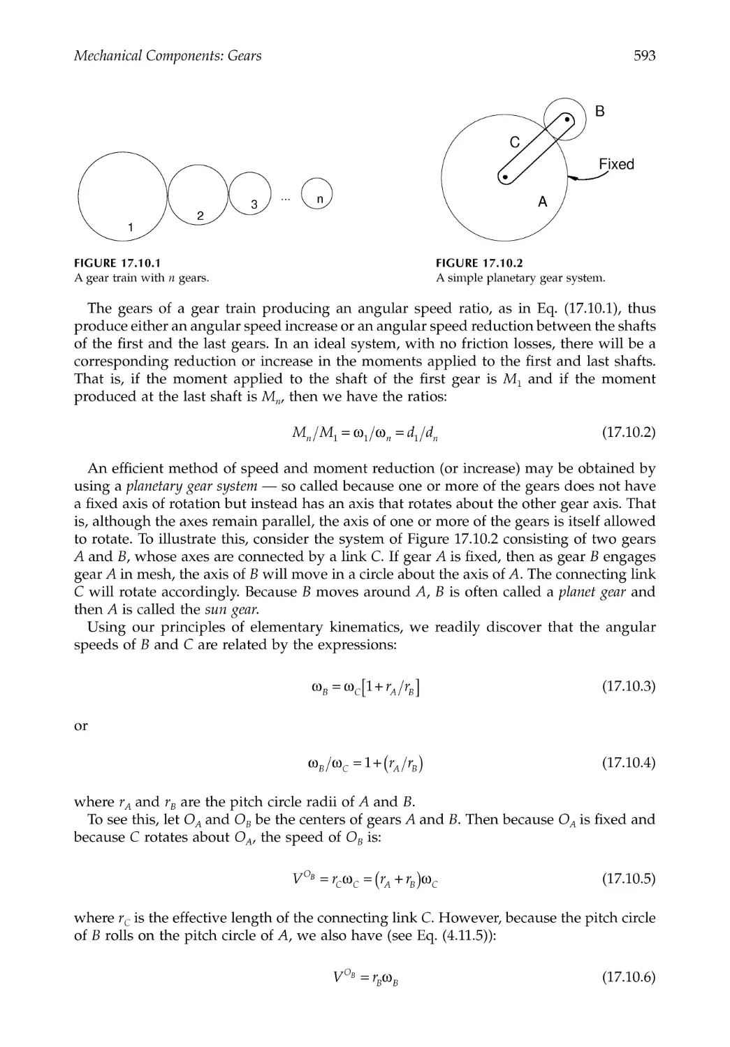
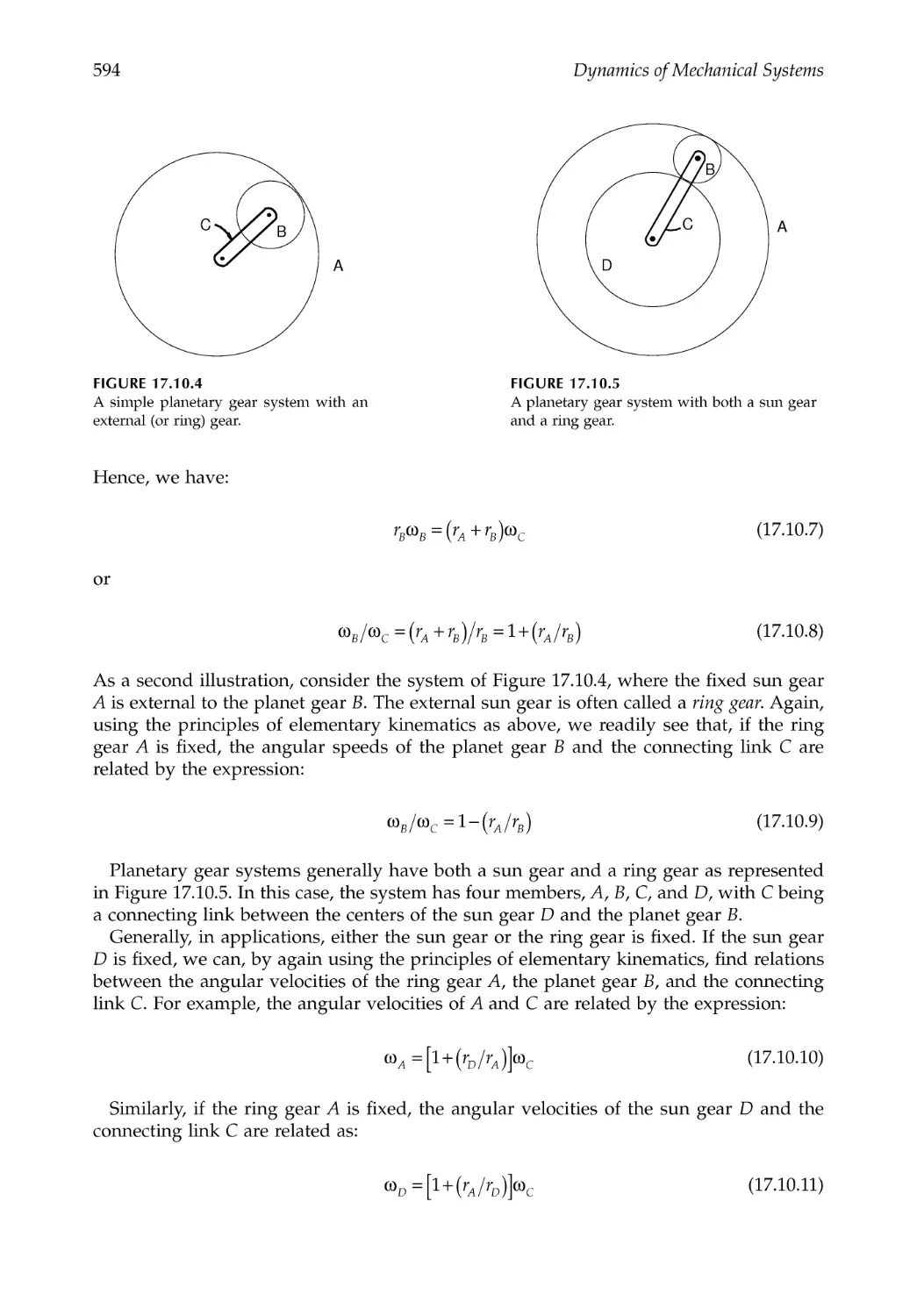
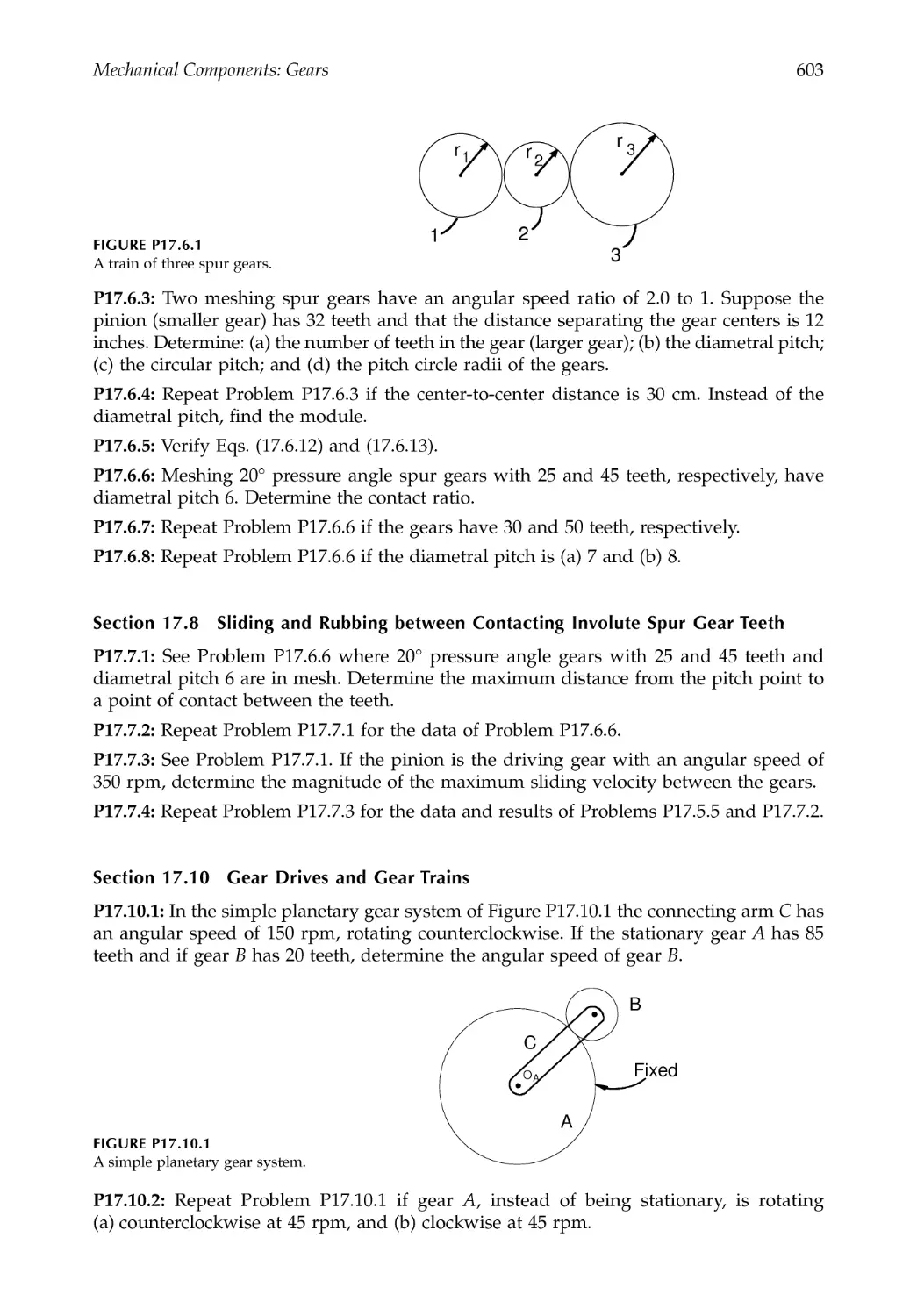
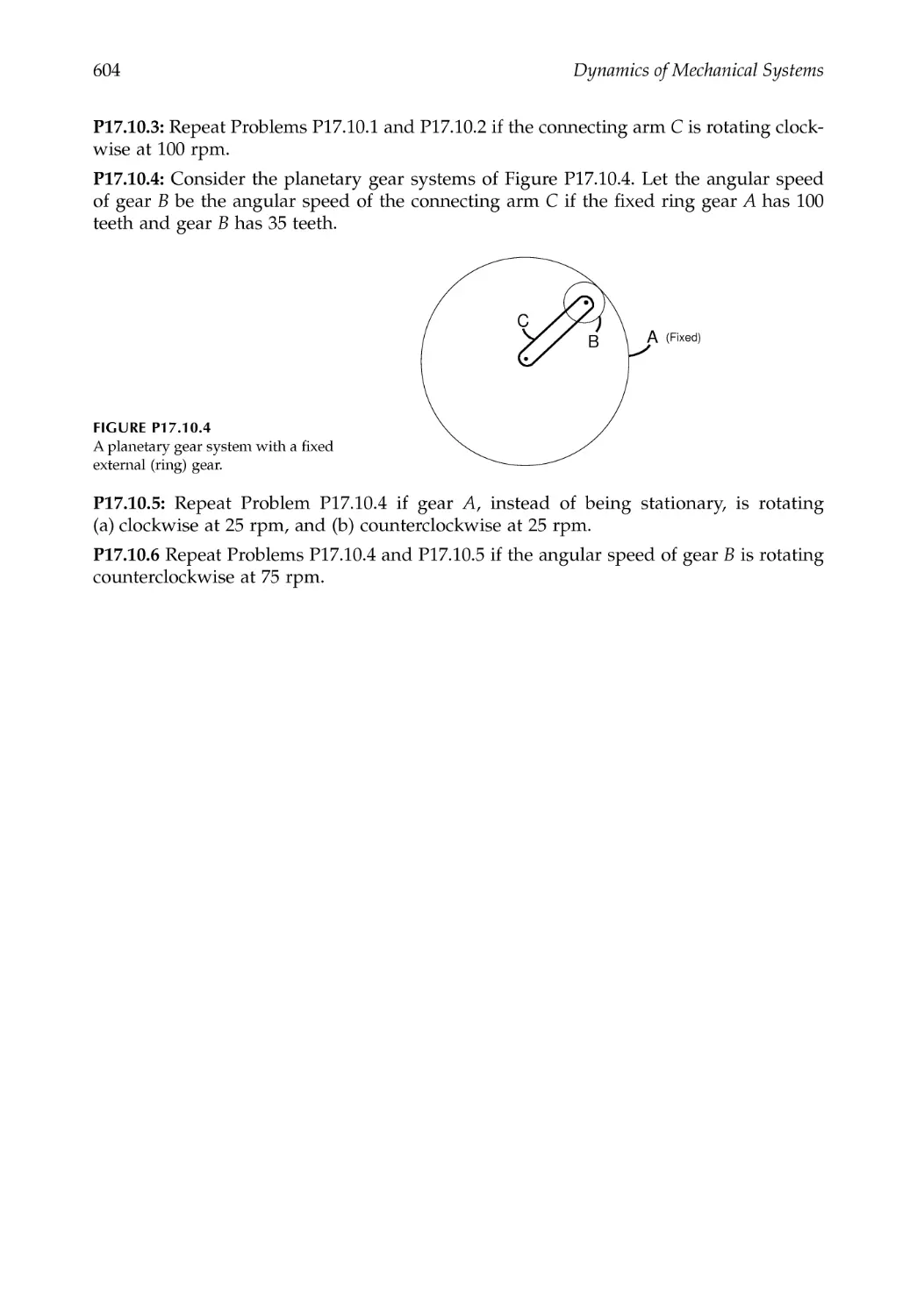
17.10 Gear Drives and Gear Trains .........................................................................................592
17.11 Helical, Bevel, Spiral Bevel, and Worm Gears ............................................................595
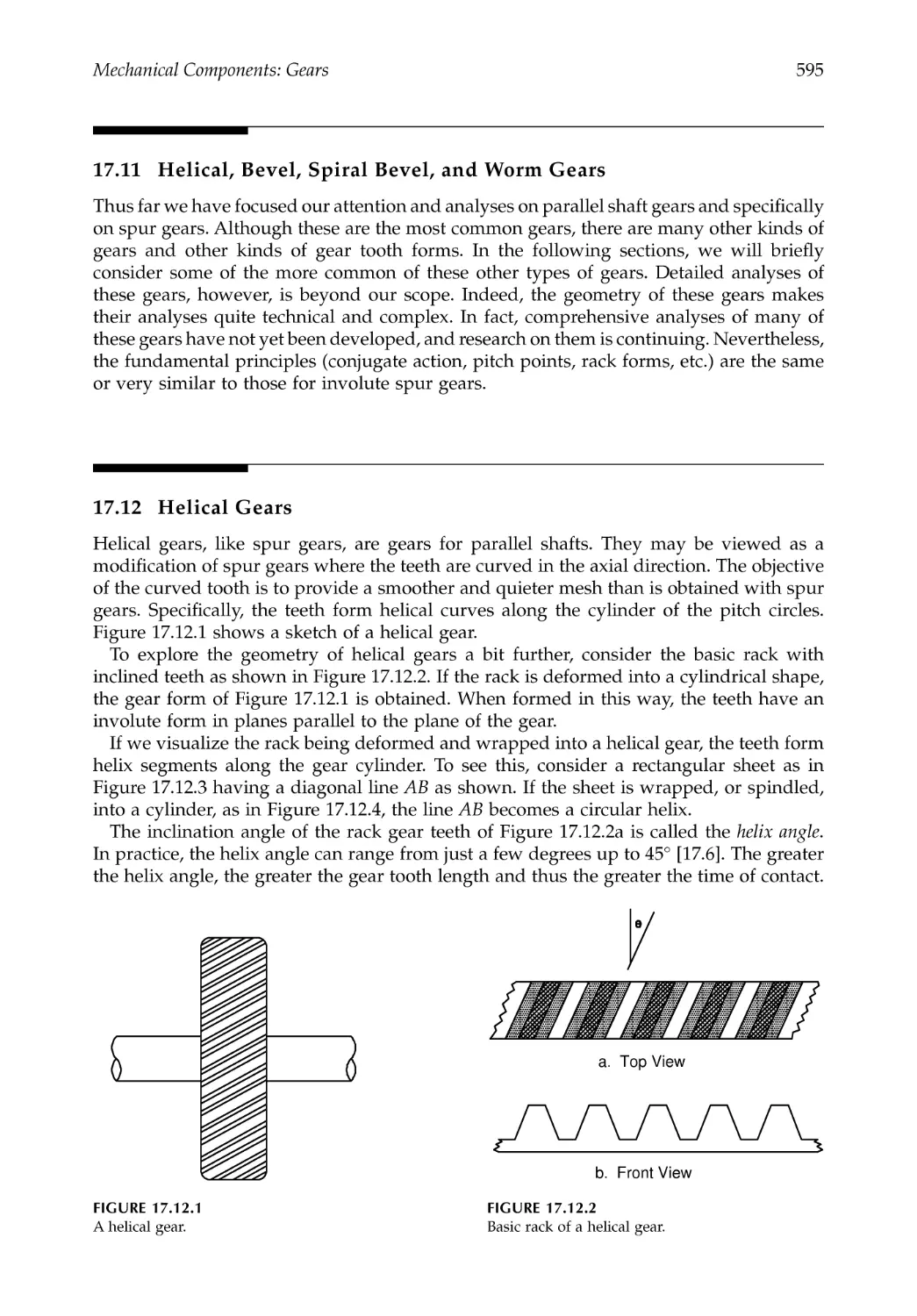
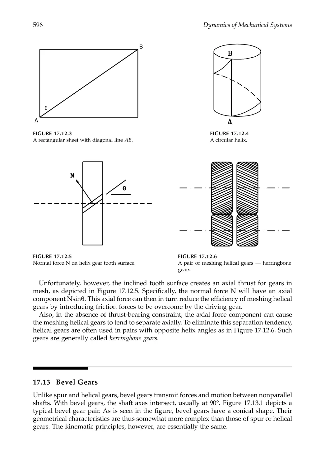
17.12 Helical Gears .....................................................................................................................595
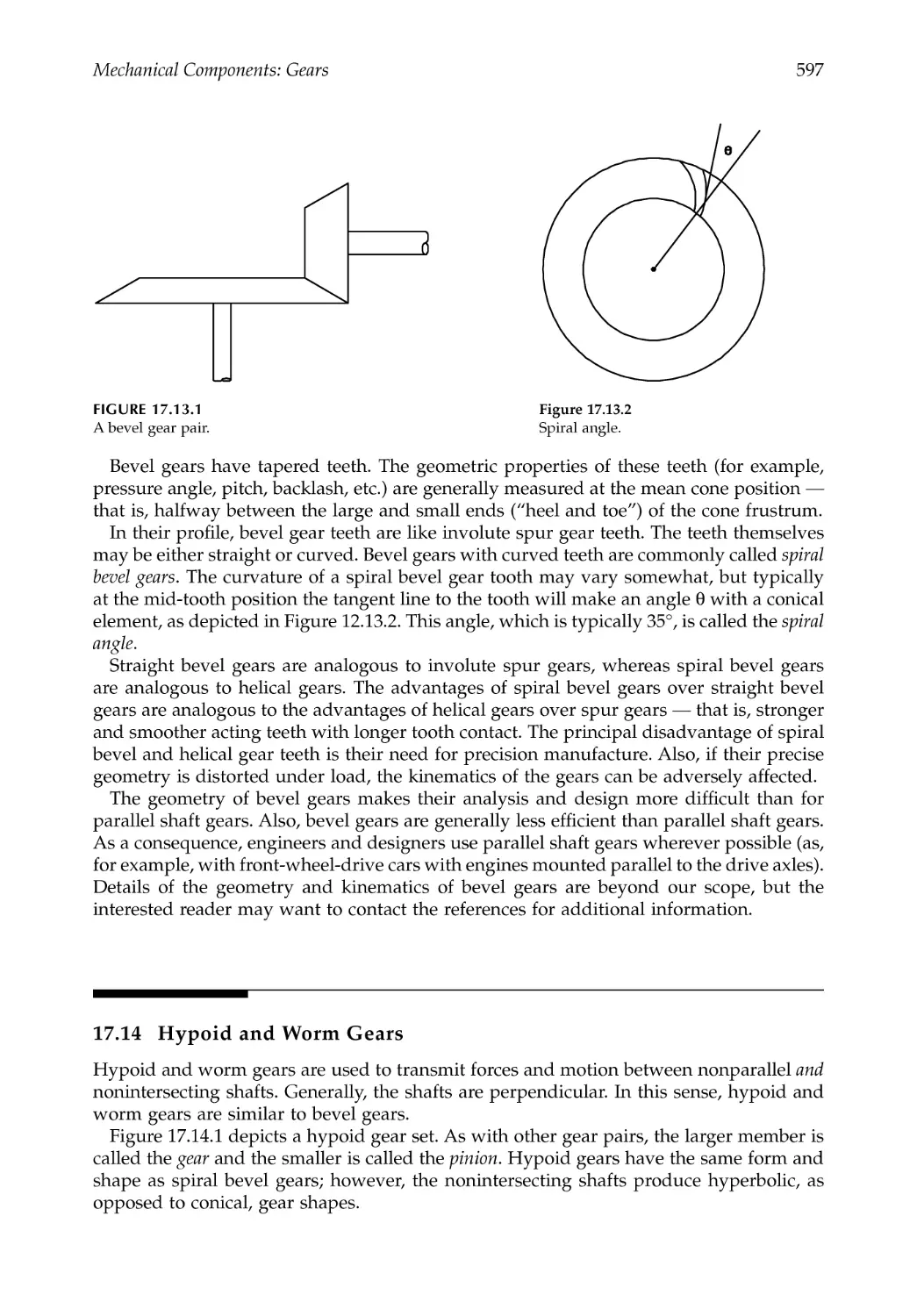
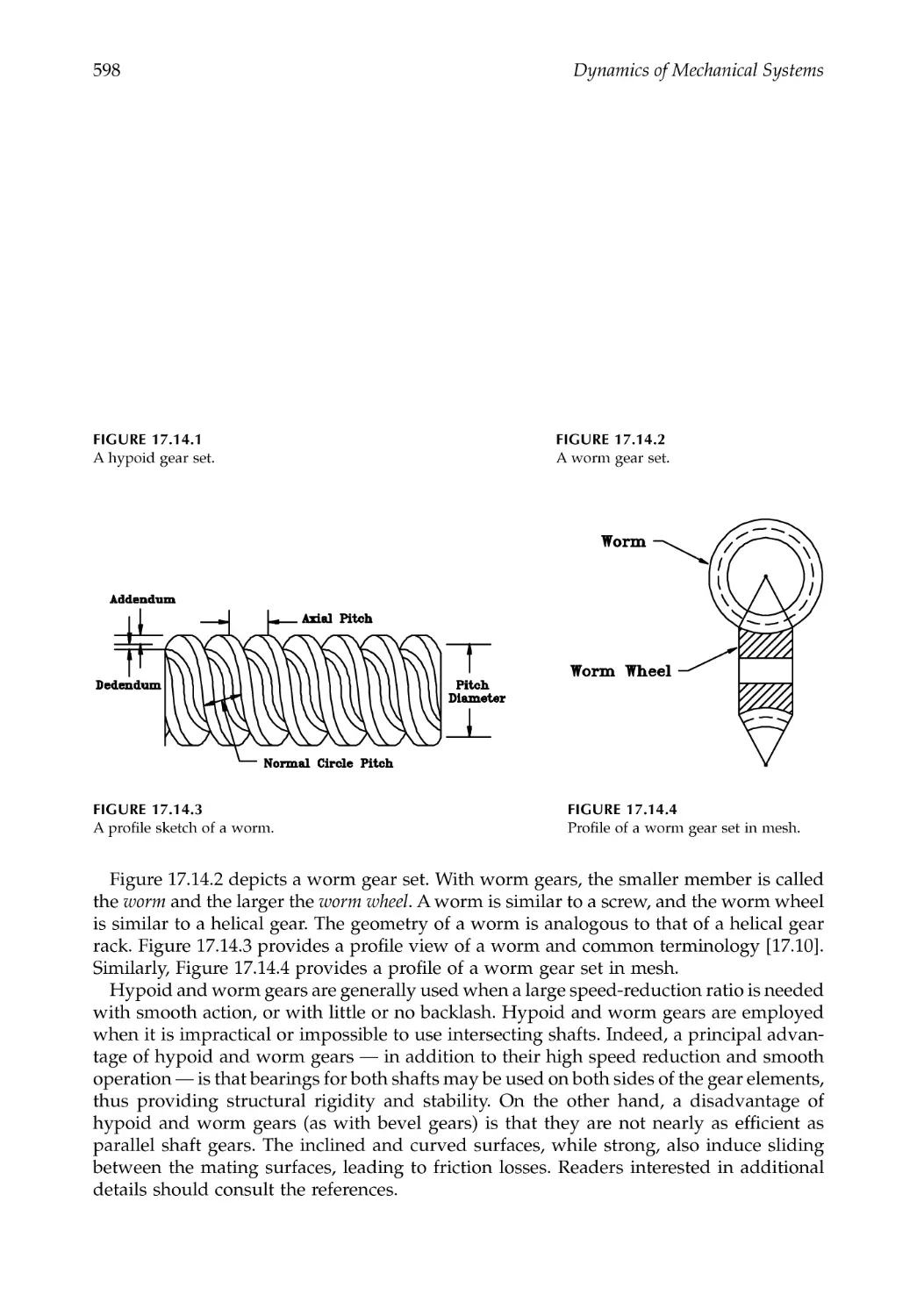
17.13 Bevel Gears........................................................................................................................596
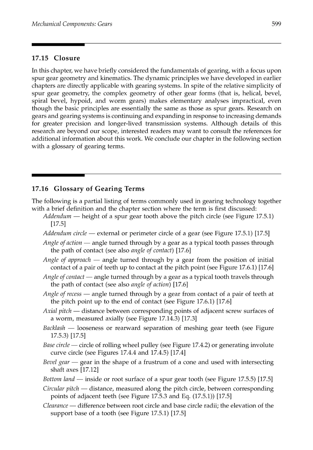
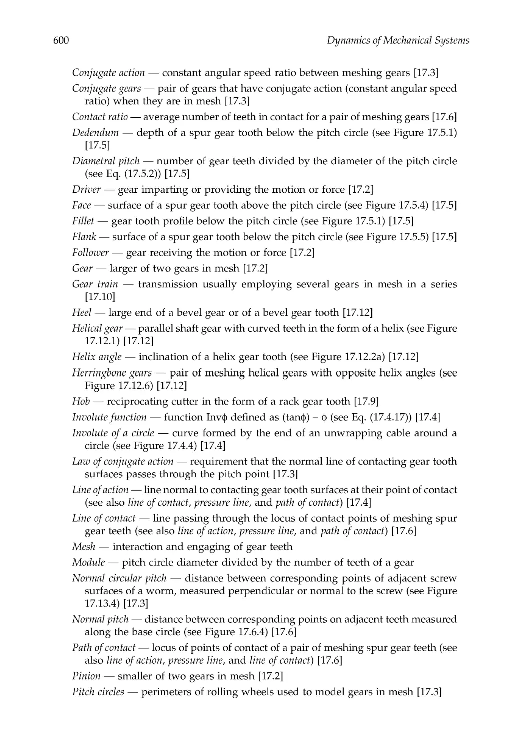
17.14 Hypoid and Worm Gears ...............................................................................................597
17.15 Closure ...............................................................................................................................599
17.16 Glossary of Gearing Terms .............................................................................................599
References .....................................................................................................................................601
Problems .......................................................................................................................................602
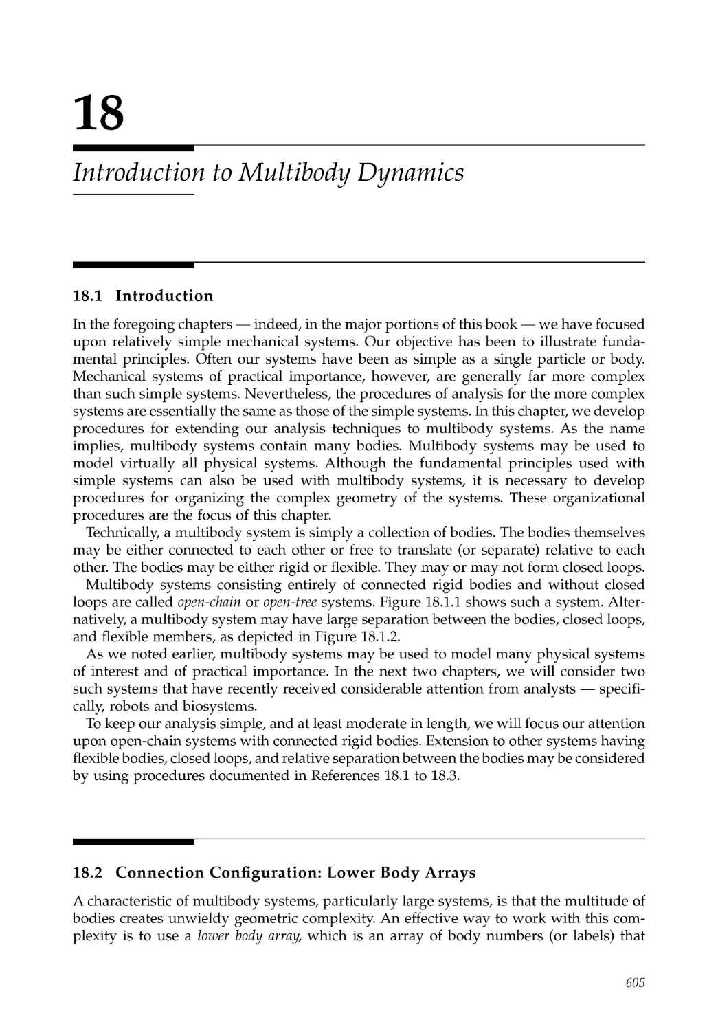
Chapter 18 Introduction to Multibody Dynamics ..............................................................605
18.1 Introduction.......................................................................................................................605
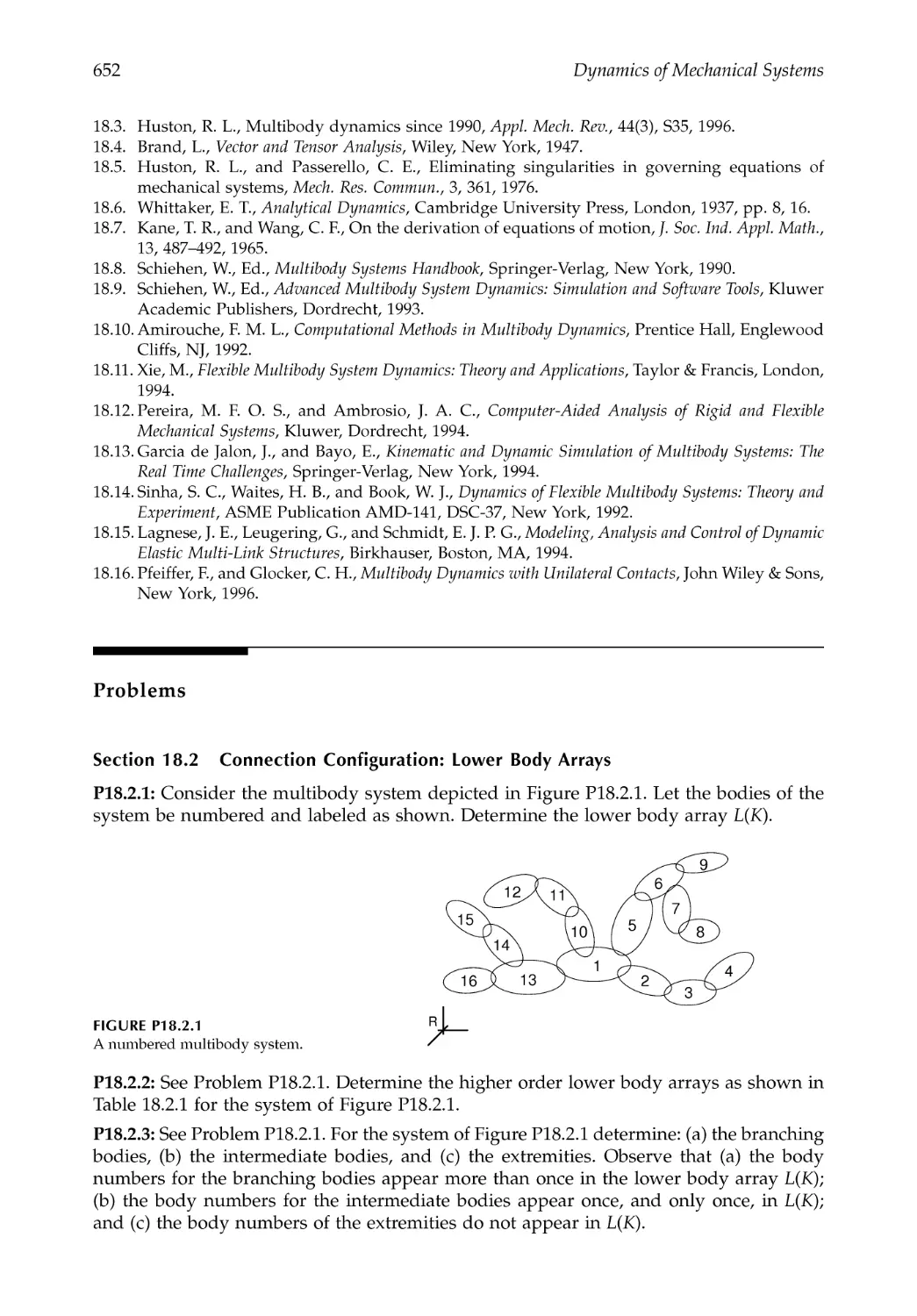
18.2 Connection Configuration: Lower Body Arrays .........................................................605
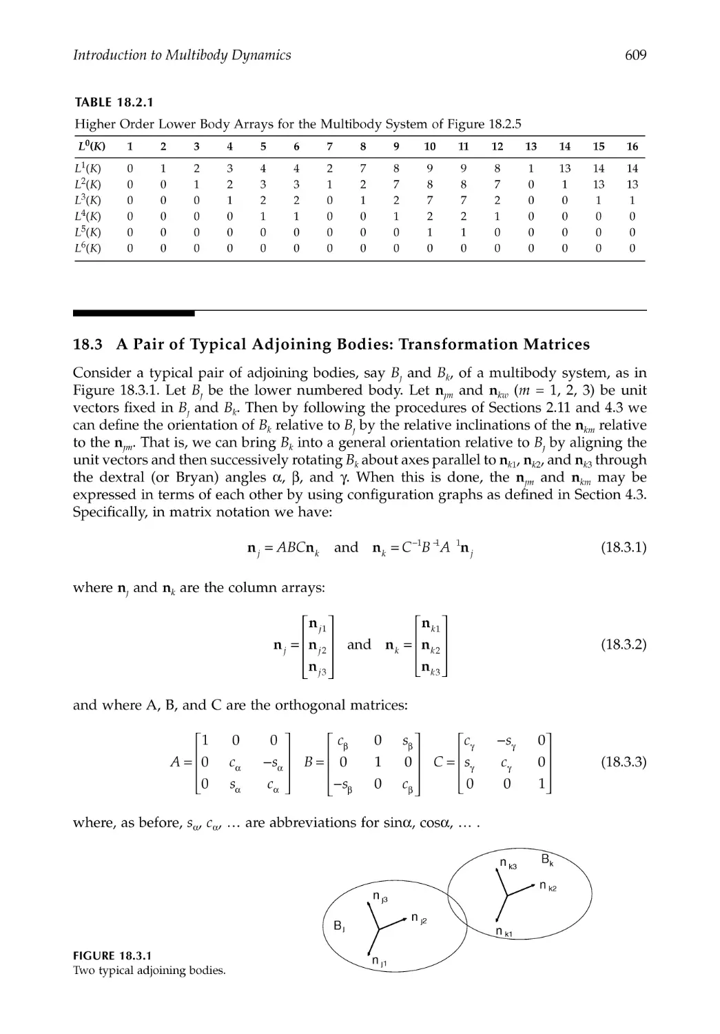
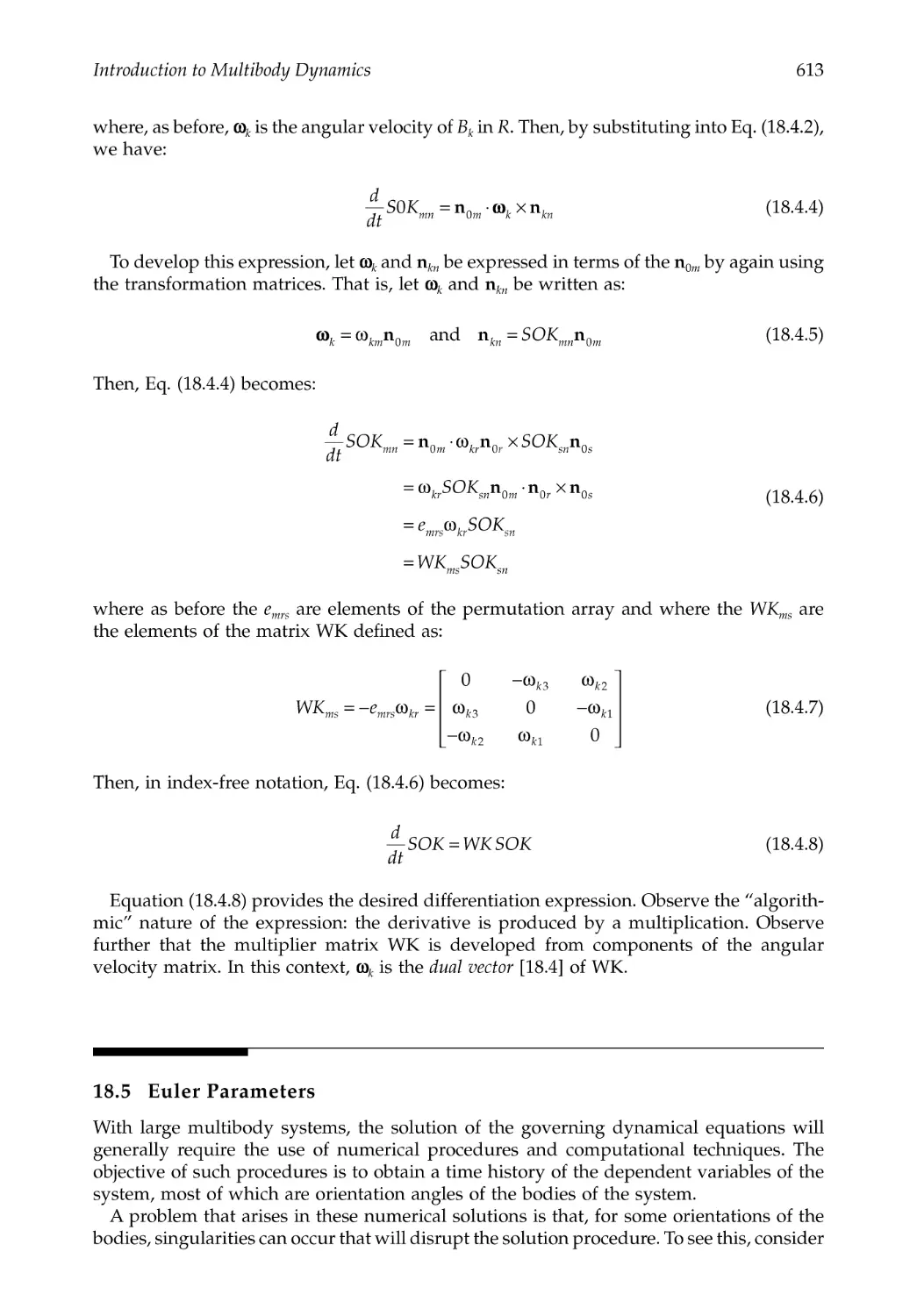
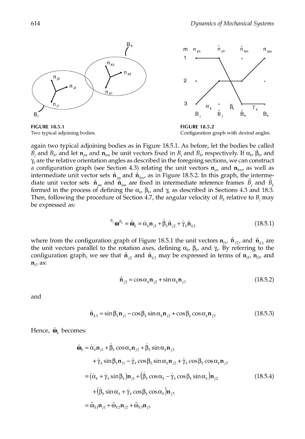
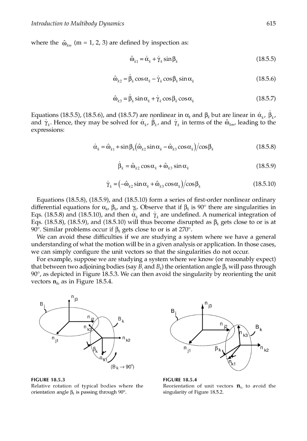
18.3 A Pair of Typical Adjoining Bodies: Transformation Matrices.................................609
18.4 Transformation Matrix Derivatives ...............................................................................612
18.5 Euler Parameters ..............................................................................................................613
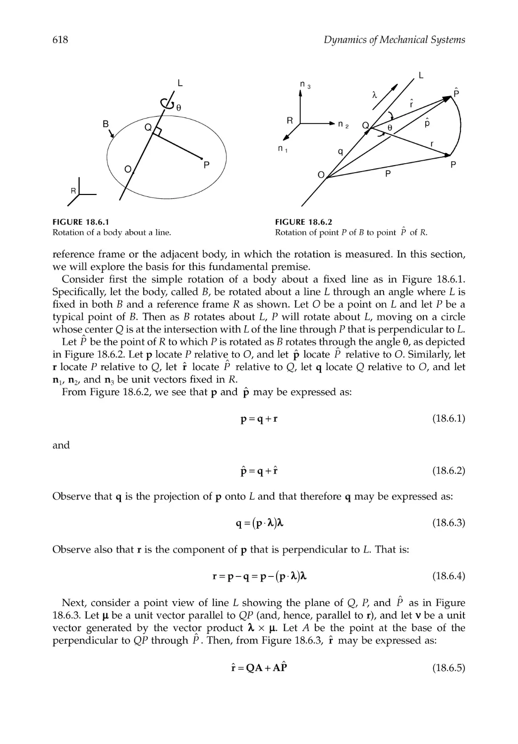
18.6 Rotation Dyadics ..............................................................................................................617
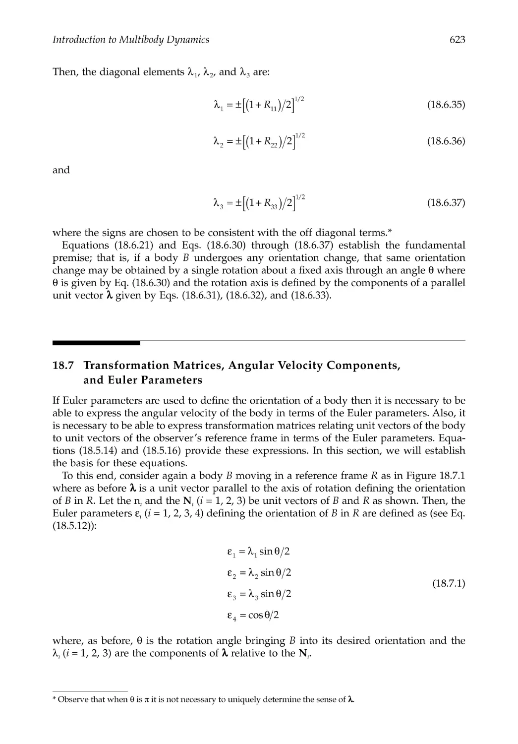
18.7 Transformation Matrices, Angular Velocity Components,
and Euler Parameters ......................................................................................................623
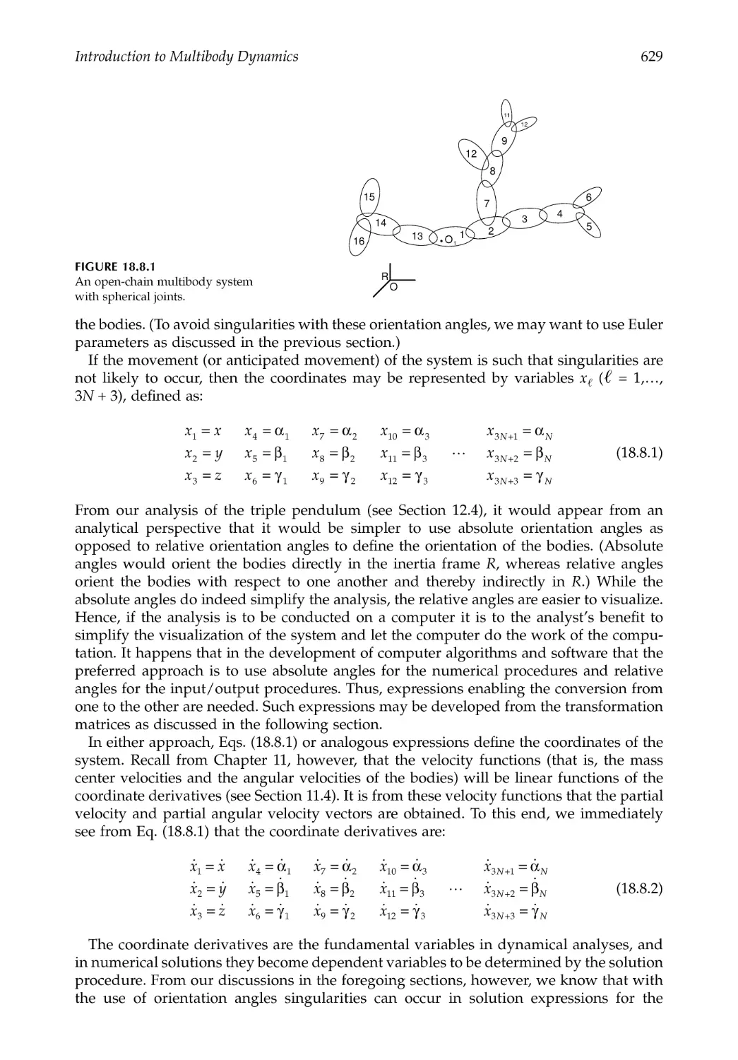
18.8 Degrees of Freedom, Coordinates, and Generalized Speeds....................................628
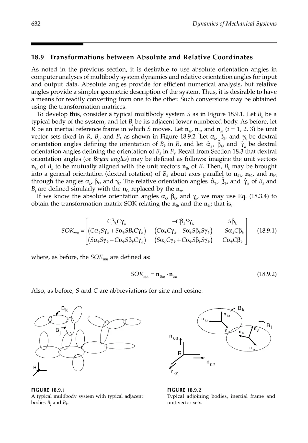
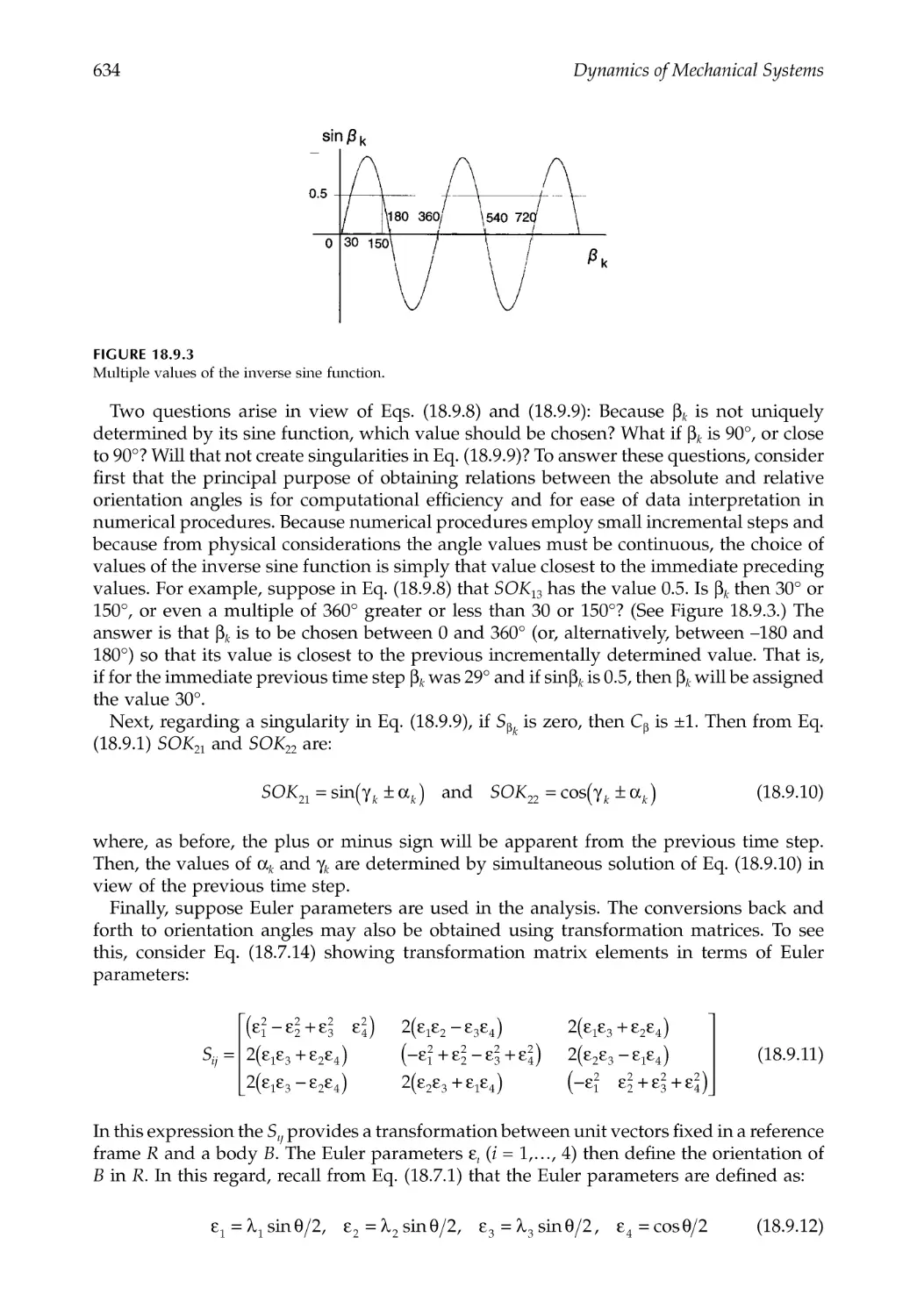
18.9 Transformations between Absolute and Relative Coordinates ................................632
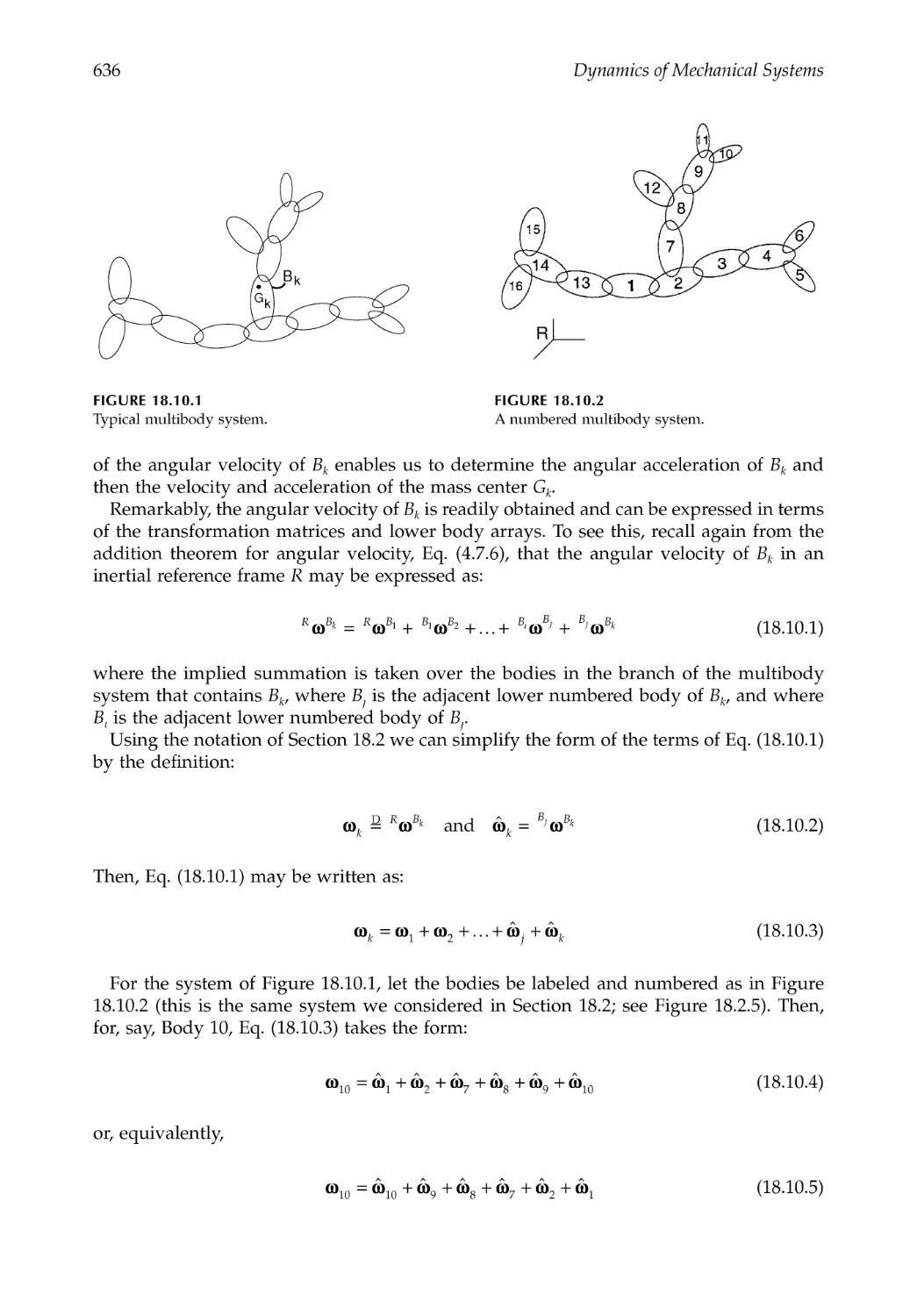
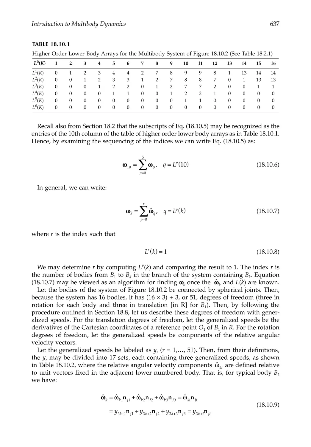
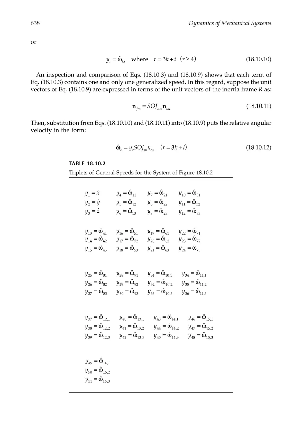
18.10 Angular Velocity...............................................................................................................635
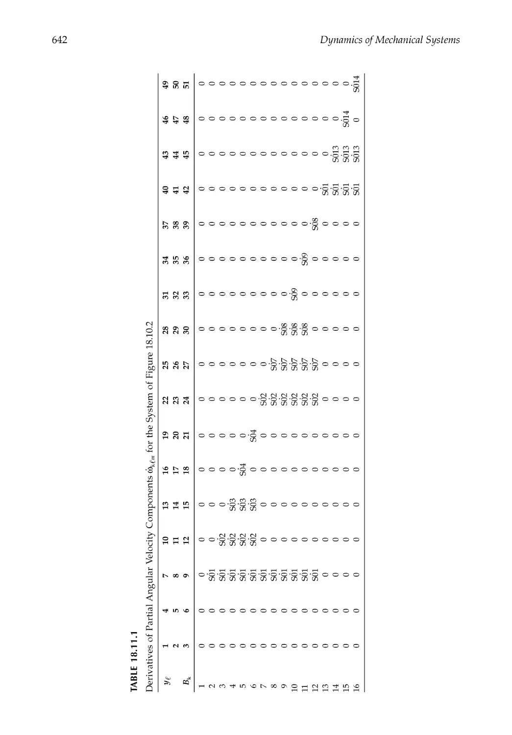
18.11 Angular Acceleration.......................................................................................................640
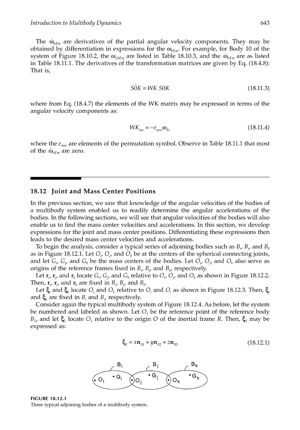
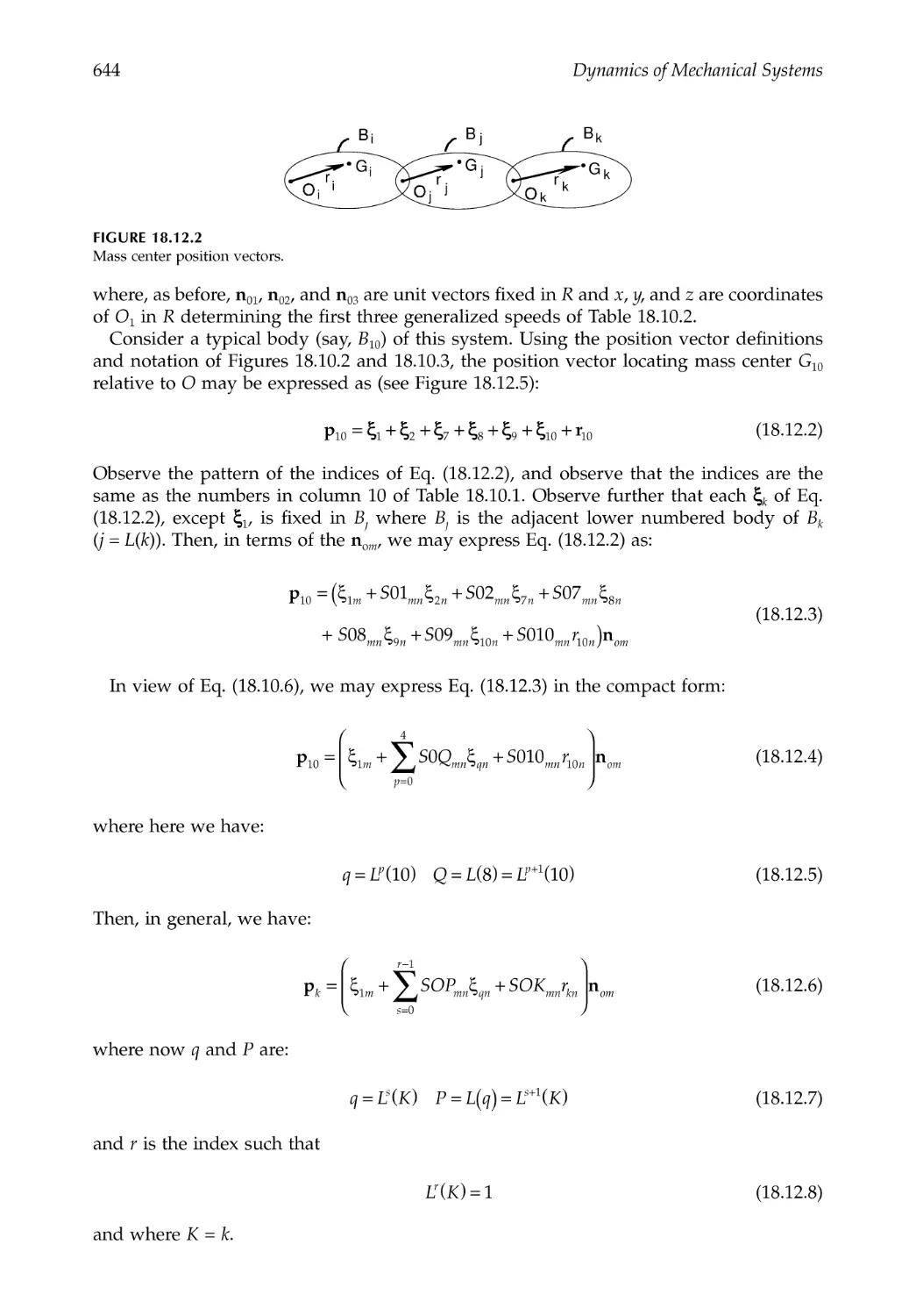
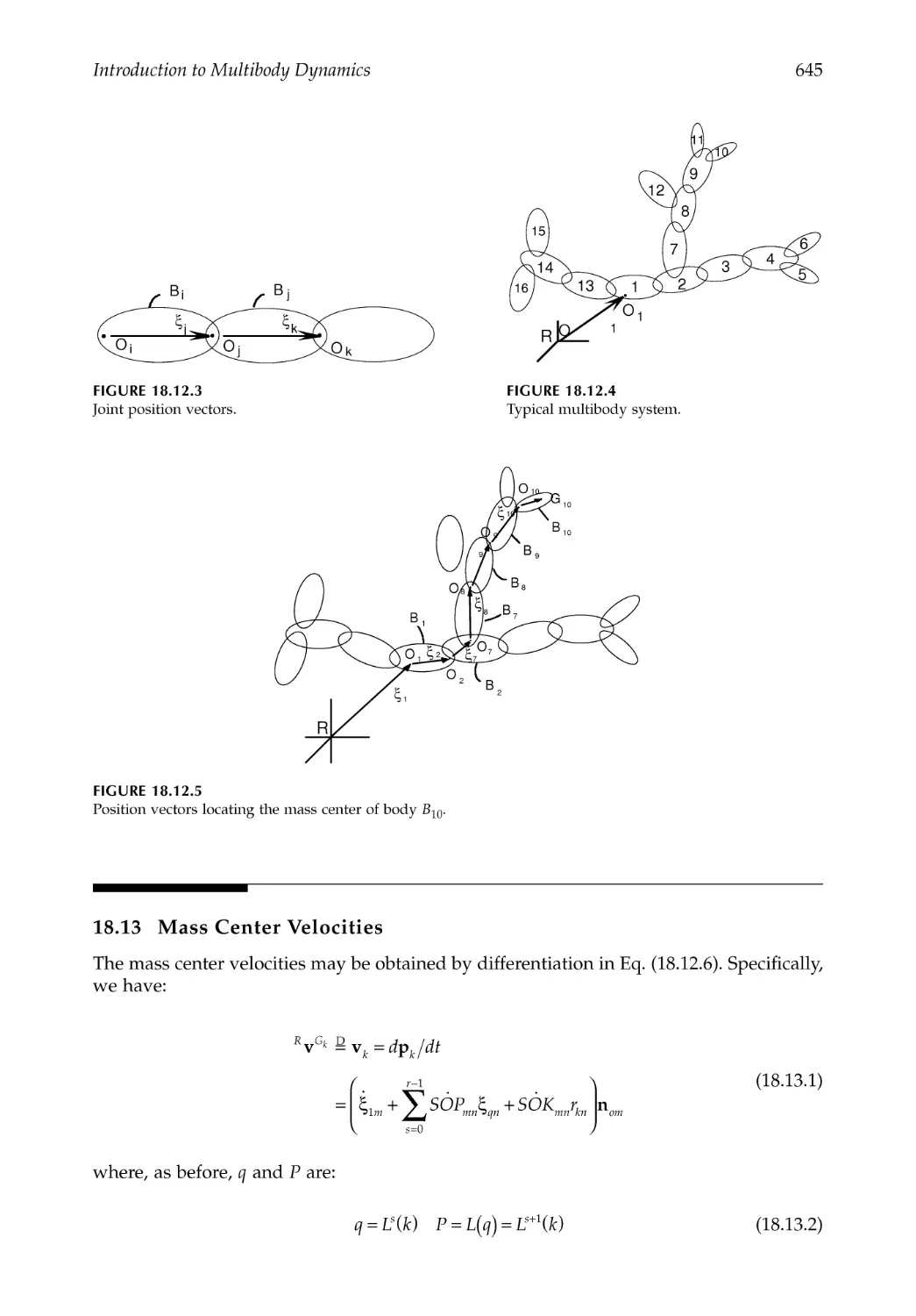
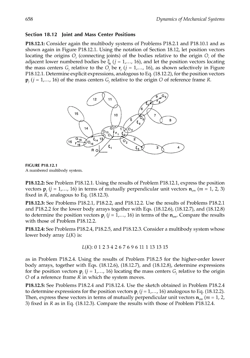
18.12 Joint and Mass Center Positions....................................................................................643
18.13 Mass Center Velocities.....................................................................................................645
18.14 Mass Center Accelerations..............................................................................................647
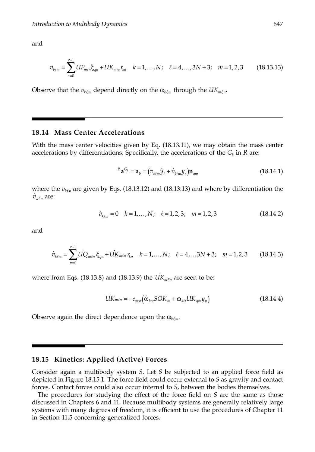
18.15 Kinetics: Applied (Active) Forces ..................................................................................647
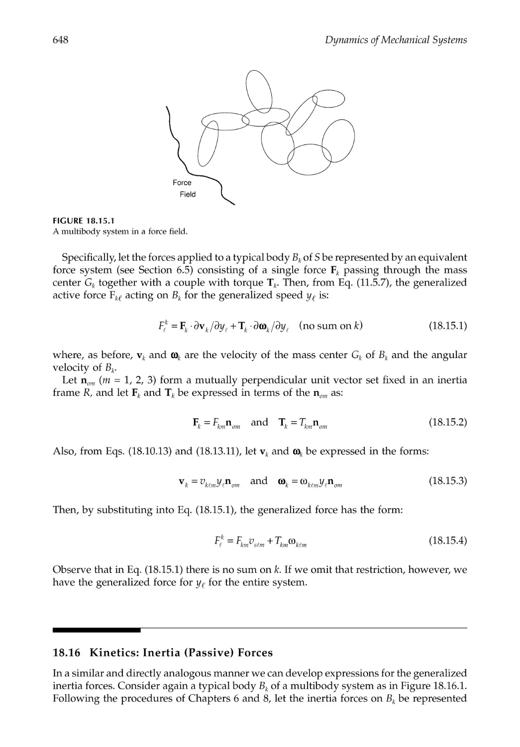
18.16 Kinetics: Inertia (Passive) Forces ...................................................................................648
18.17 Multibody Dynamics .......................................................................................................650
18.18 Closure ...............................................................................................................................651
References .....................................................................................................................................651
Problems .......................................................................................................................................652
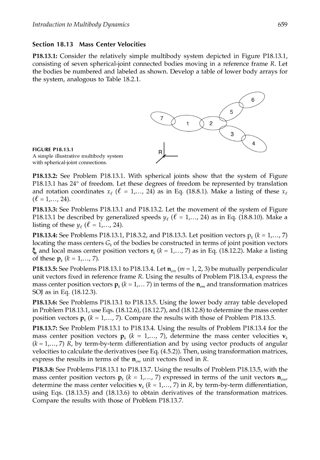
Chapter 19 Introduction to Robot Dynamics ......................................................................661
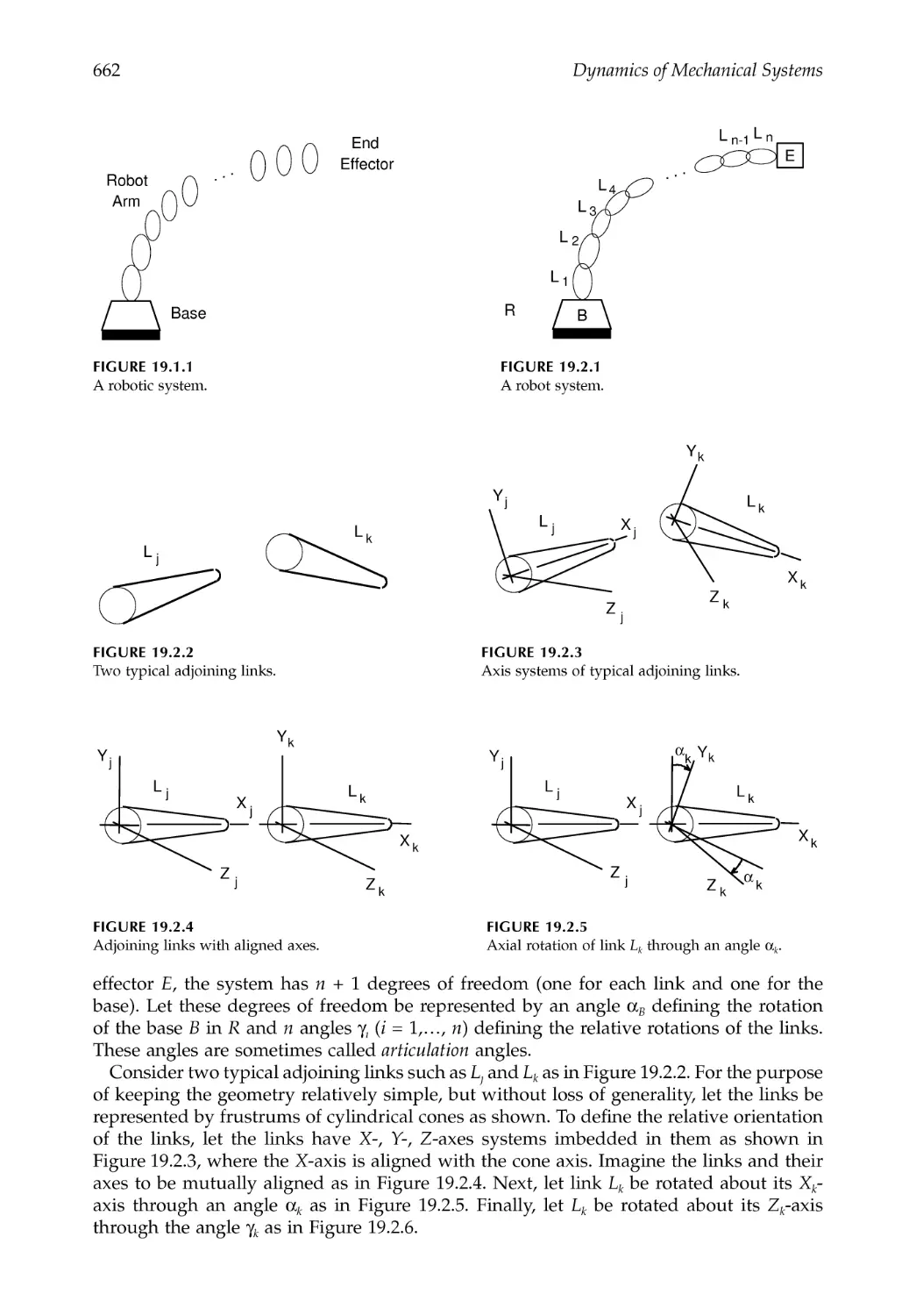
19.1 Introduction.......................................................................................................................661
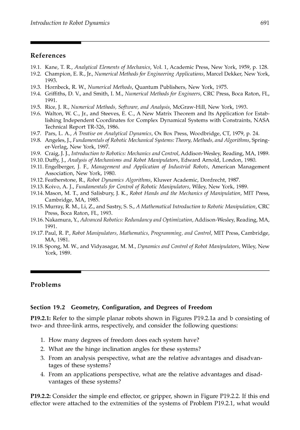
19.2 Geometry, Configuration, and Degrees of Freedom ..................................................661
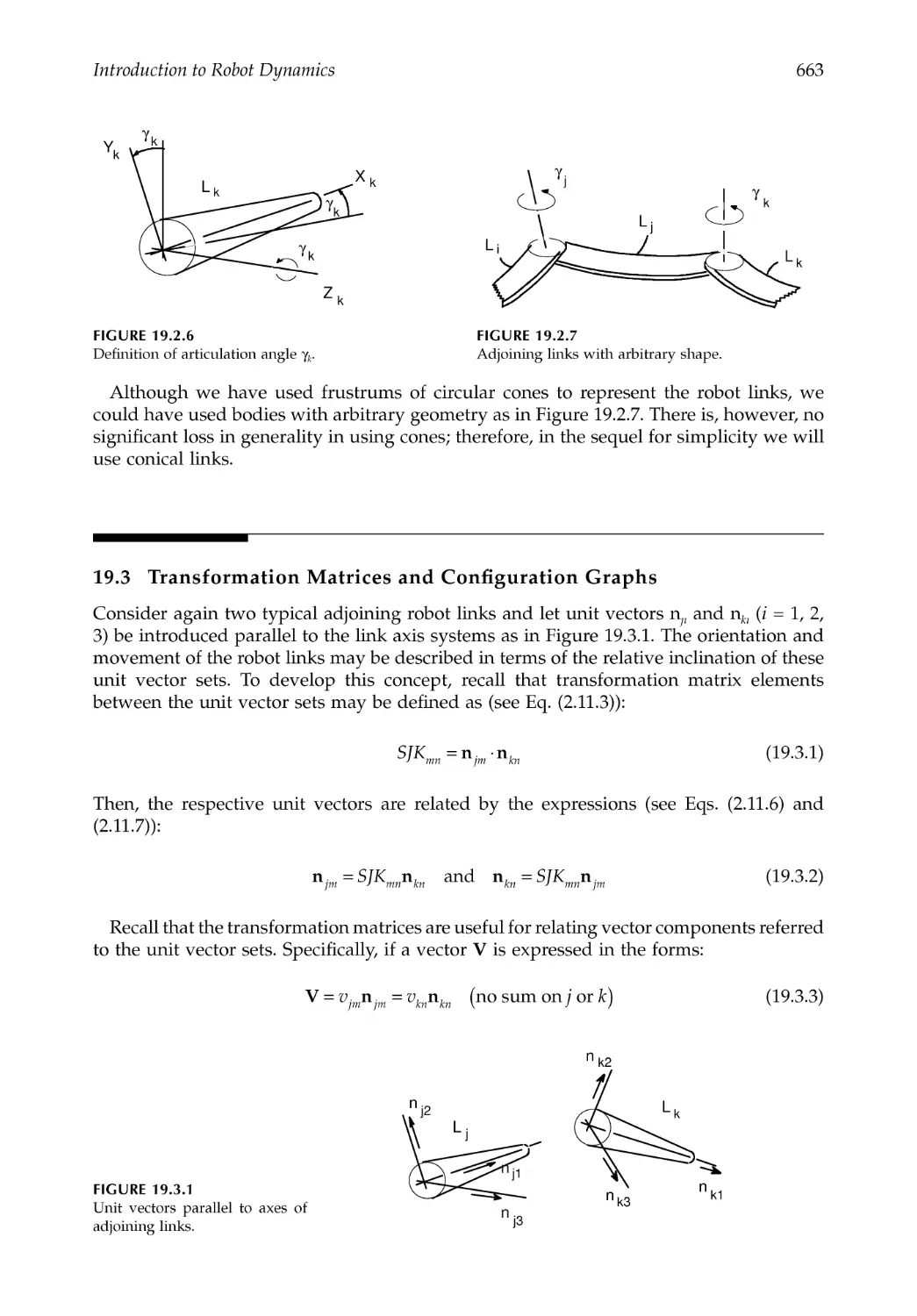
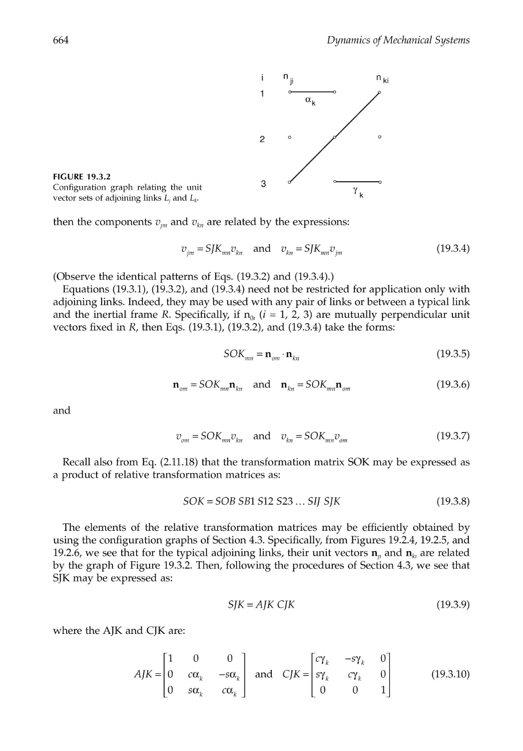
19.3 Transformation Matrices and Configuration Graphs.................................................663
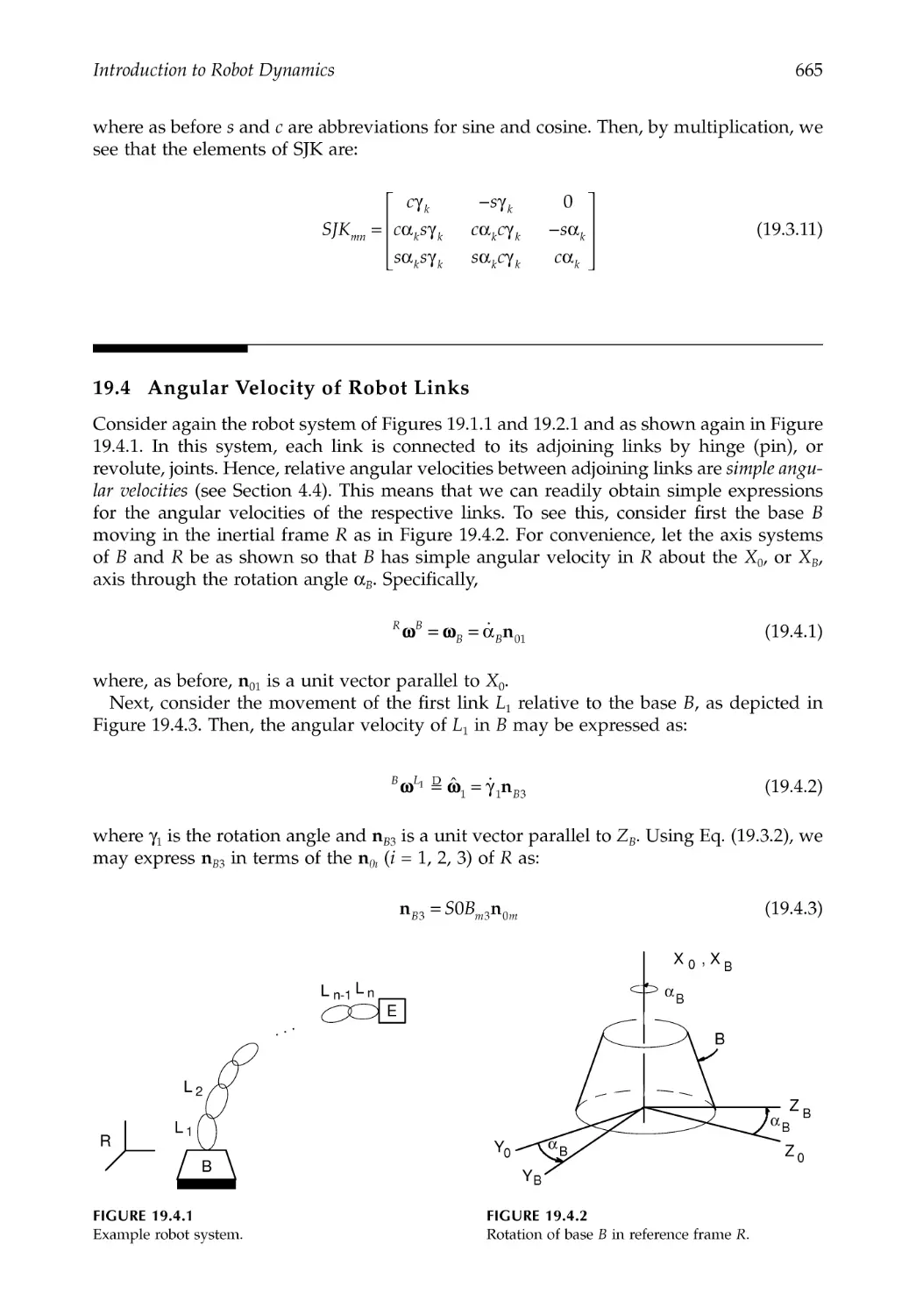
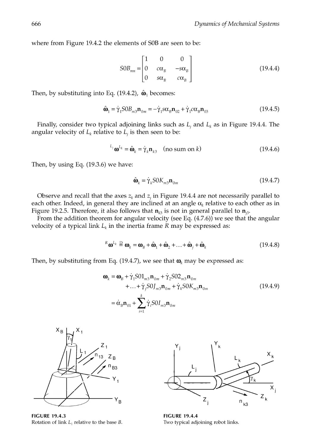
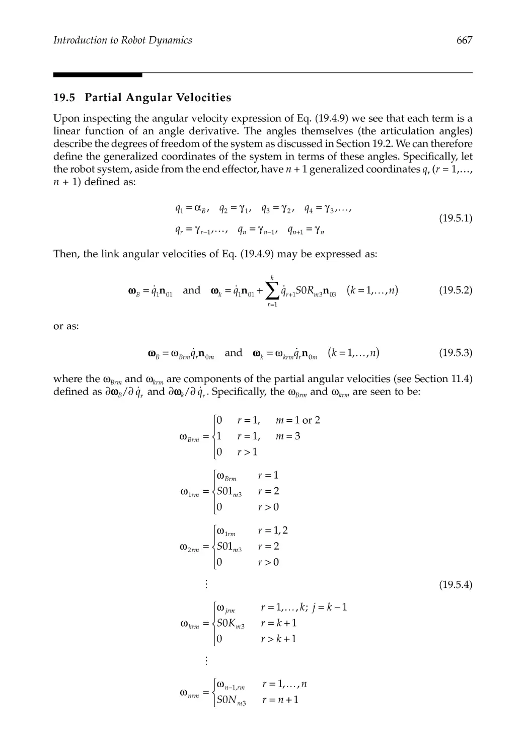
19.4 Angular Velocity of Robot Links ...................................................................................665
19.5 Partial Angular Velocities ...............................................................................................667
19.6 Transformation Matrix Derivatives ...............................................................................668
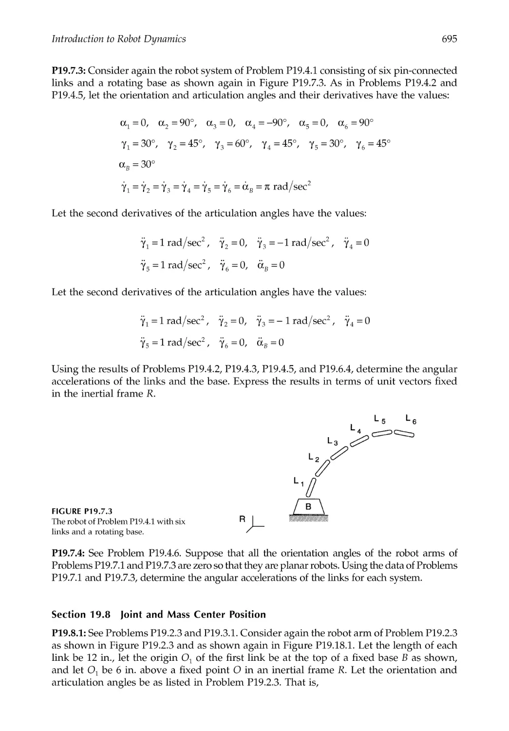
19.7 Angular Acceleration of the Robot Links ....................................................................668
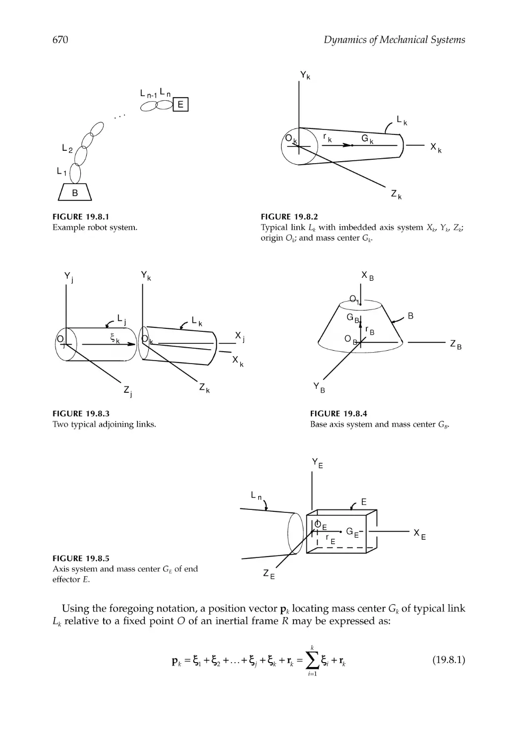
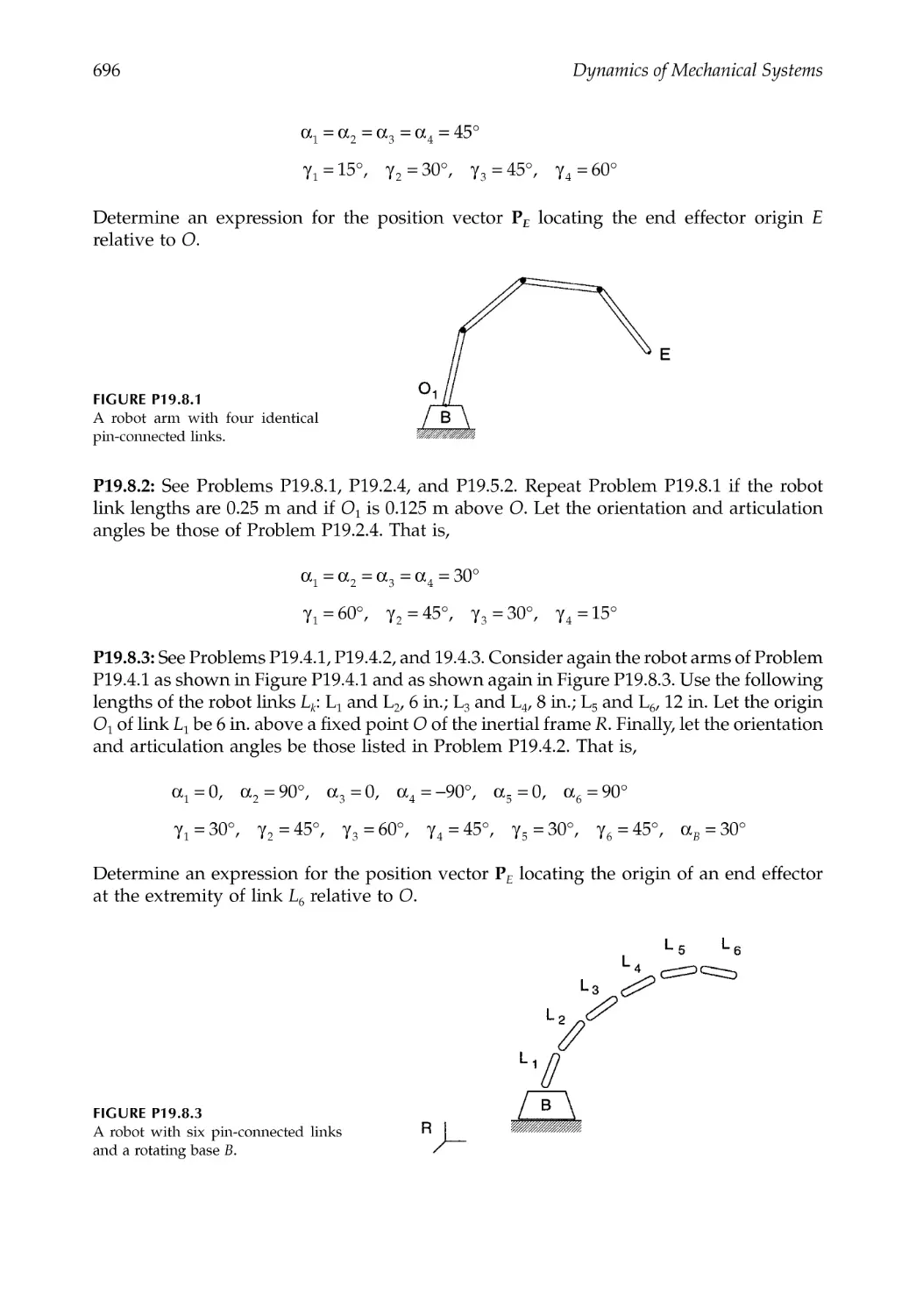
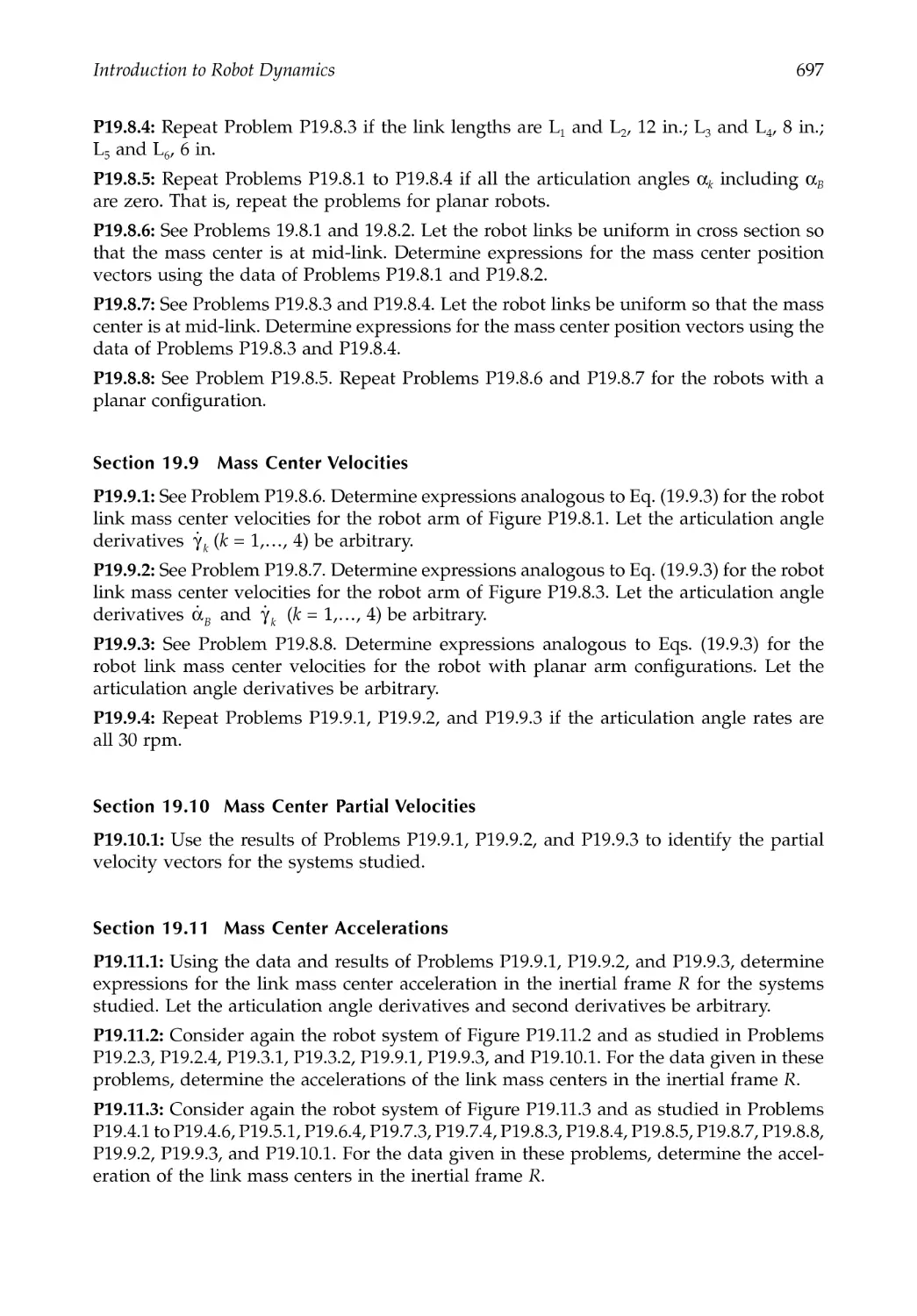
19.8 Joint and Mass Center Position .....................................................................................669
19.9 Mass Center Velocities.....................................................................................................671
19.10 Mass Center Partial Velocities ........................................................................................673
19.11 Mass Center Accelerations..............................................................................................673
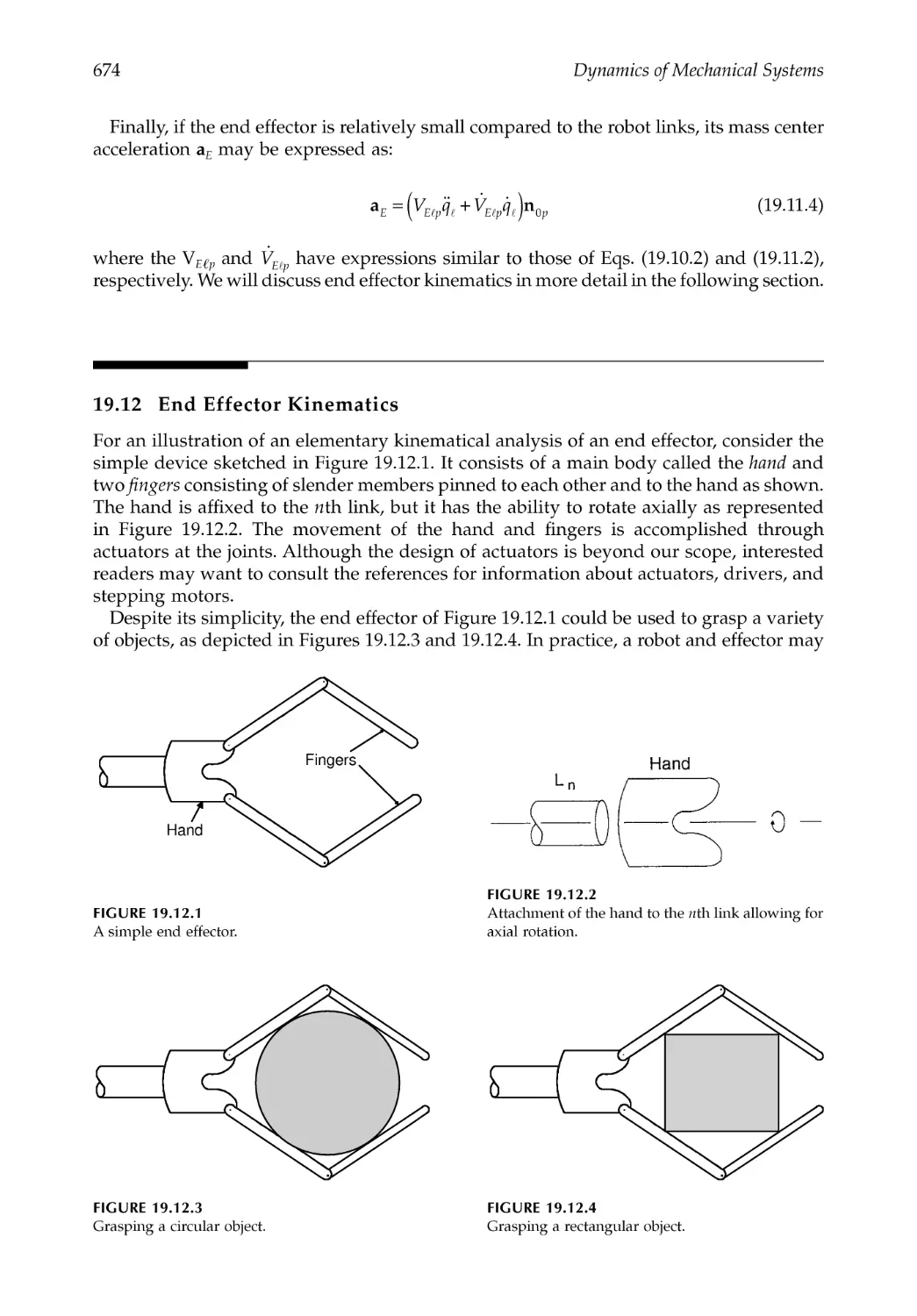
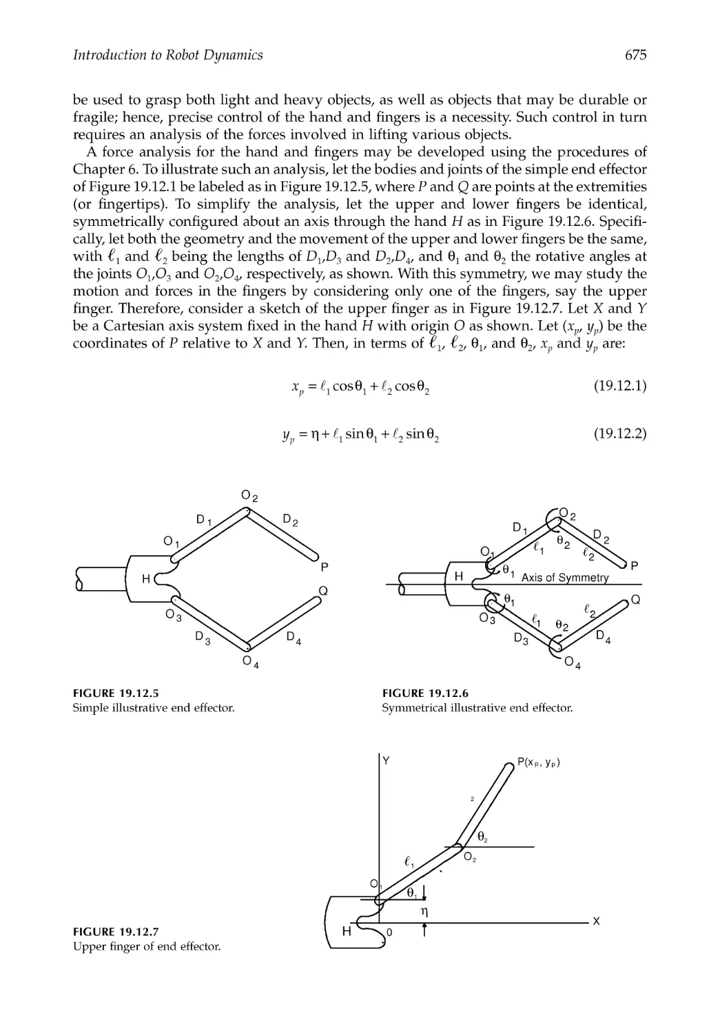
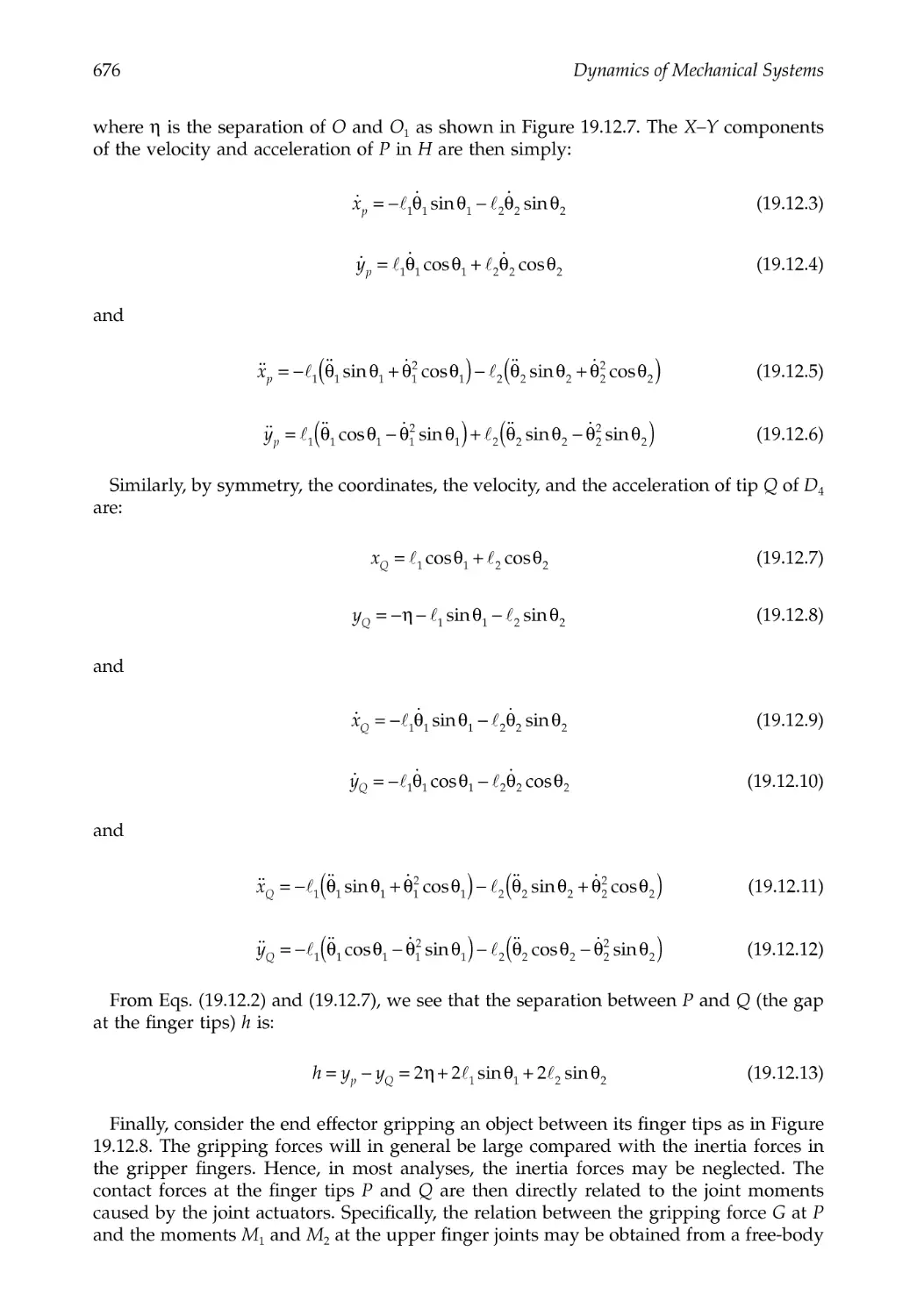
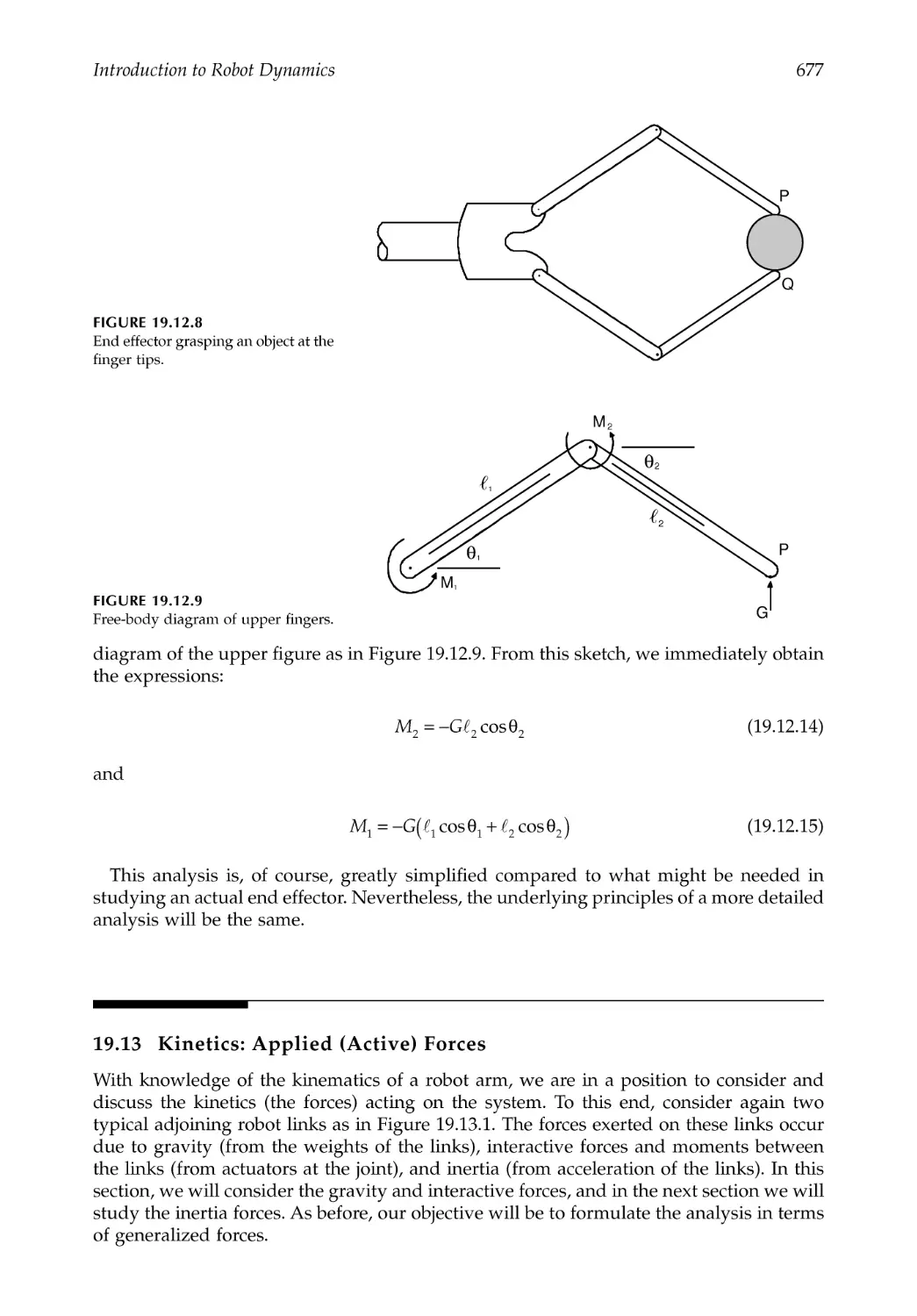
19.12 End Effector Kinematics..................................................................................................674
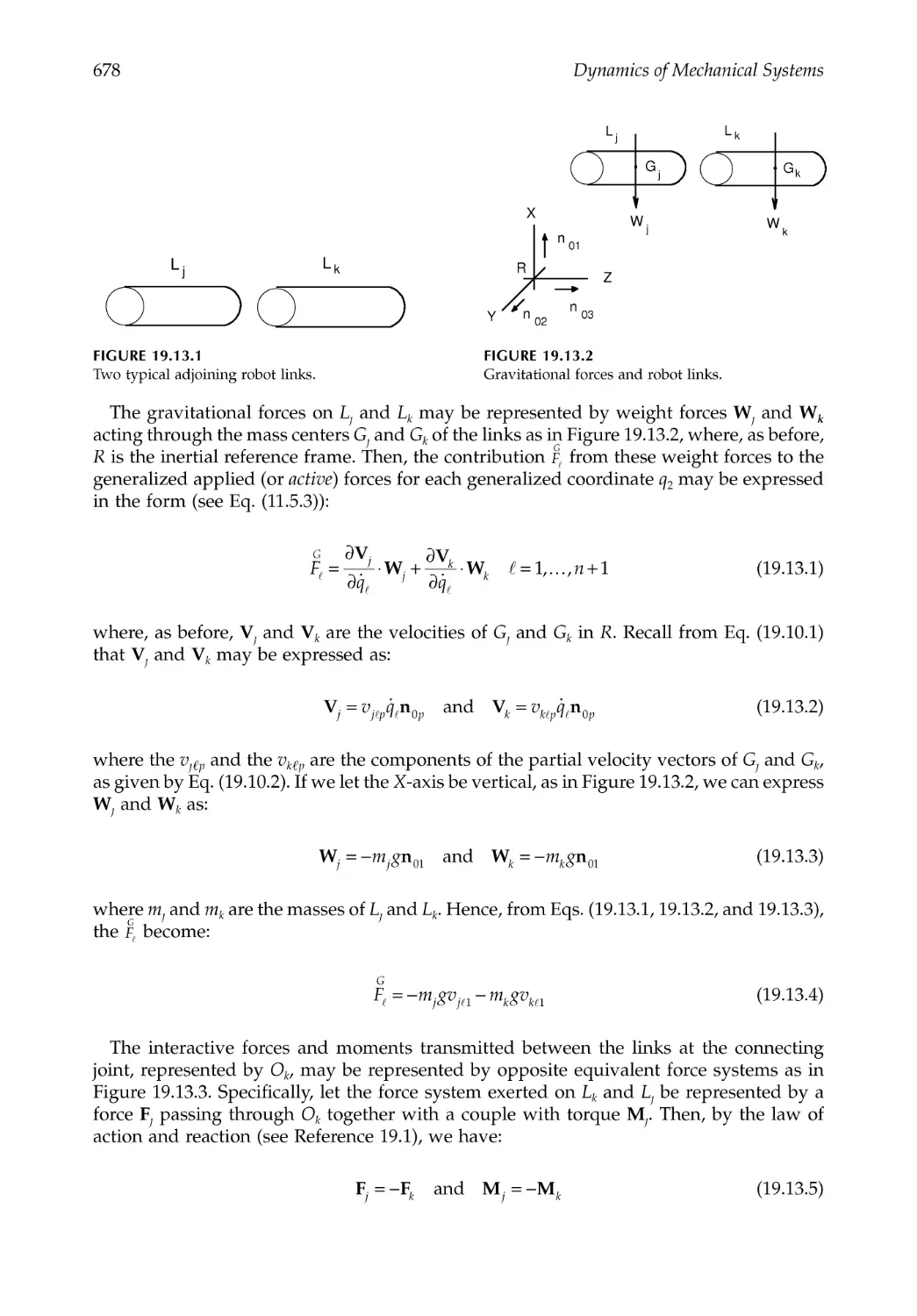
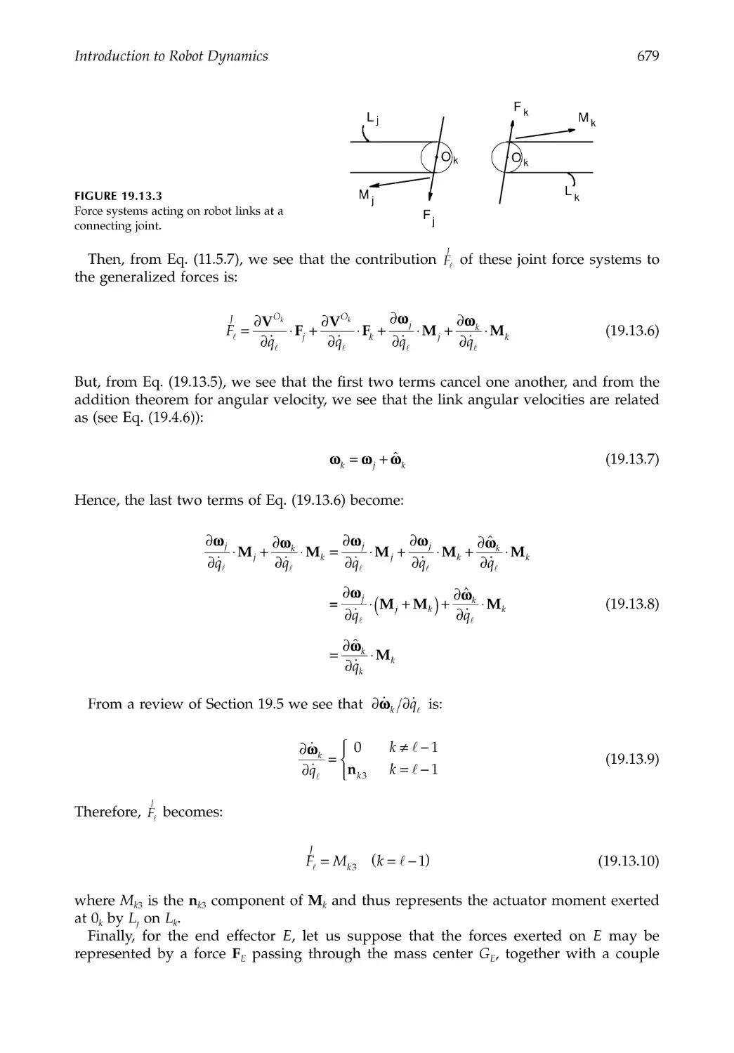
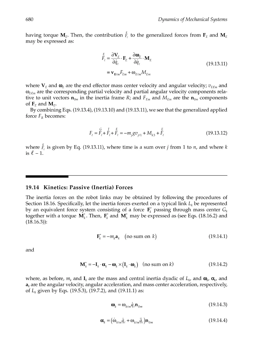
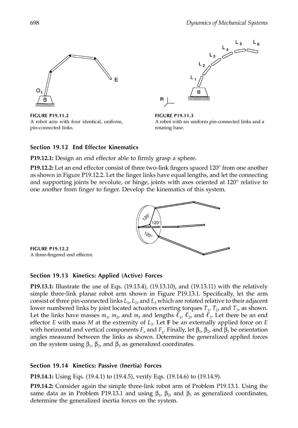
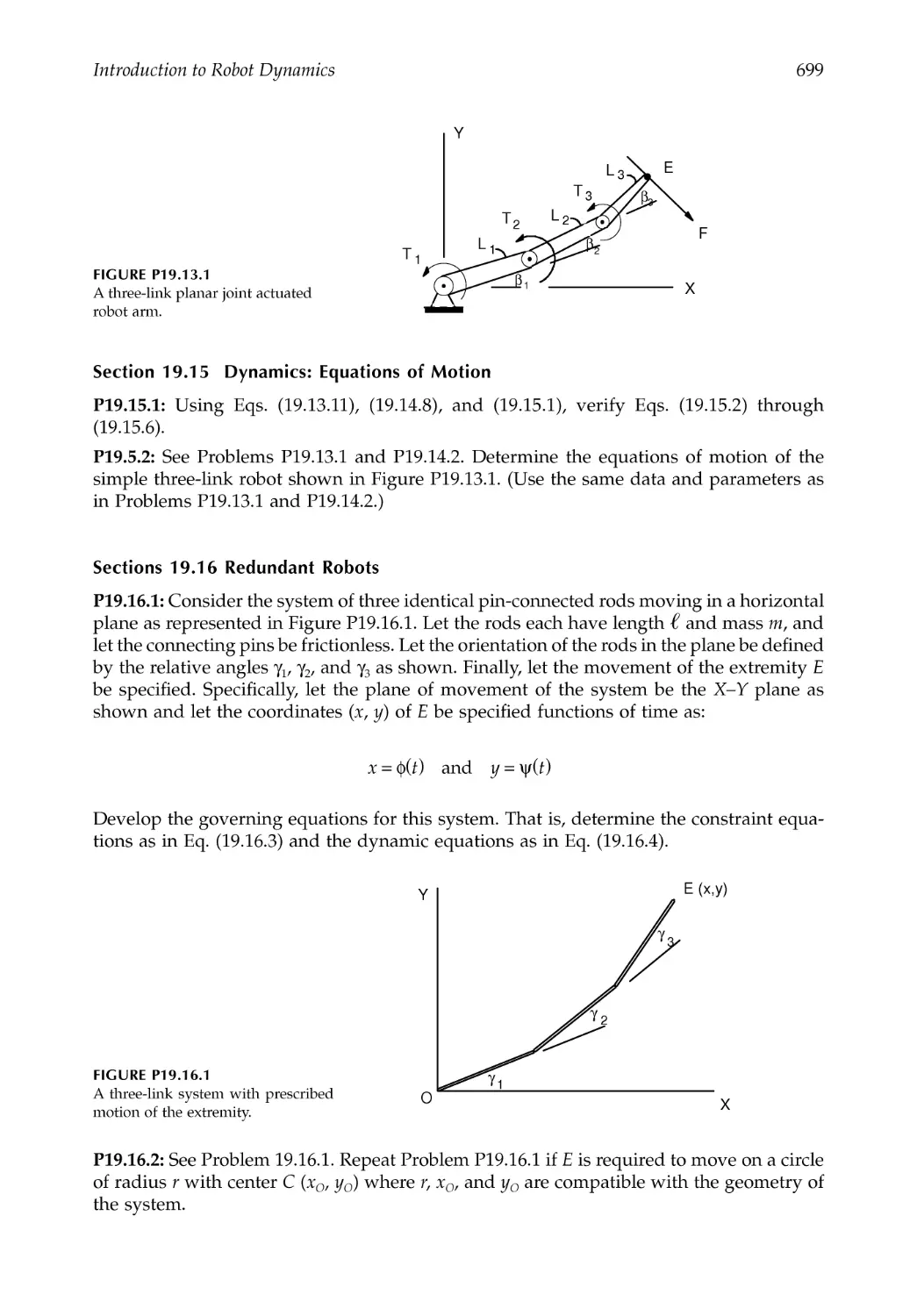
19.13 Kinetics: Applied (Active) Forces ..................................................................................677
19.14 Kinetics: Passive (Inertia) Forces ...................................................................................680
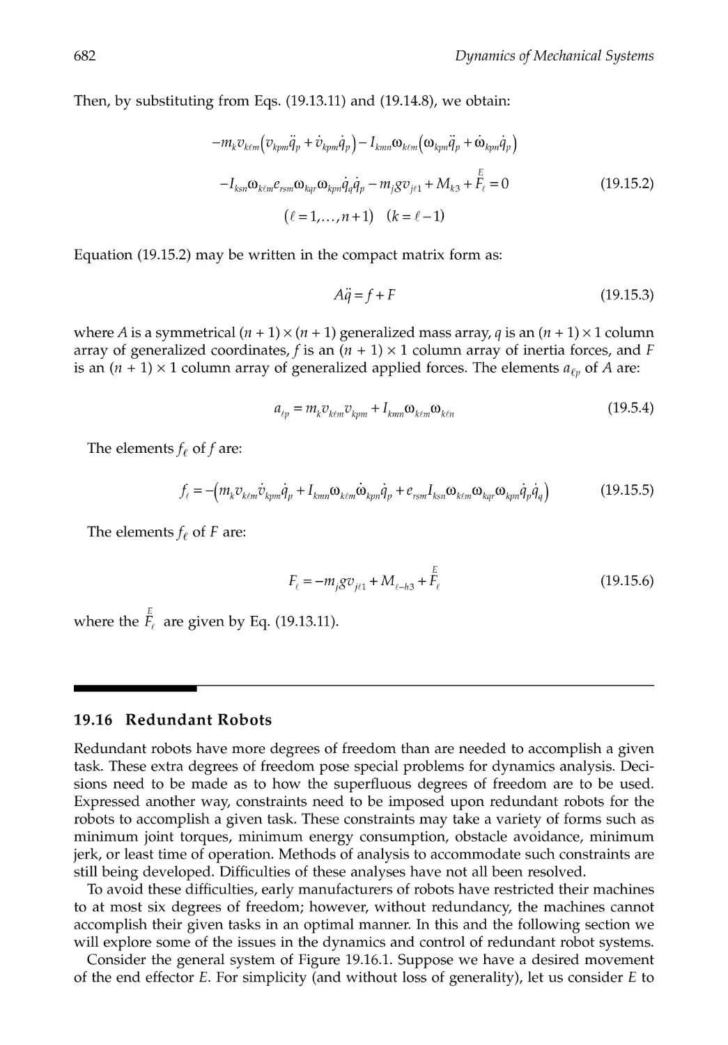
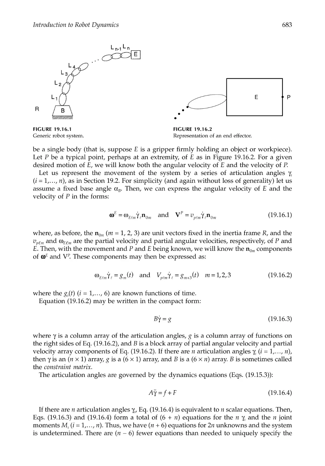
19.15 Dynamics: Equations of Motion ....................................................................................681
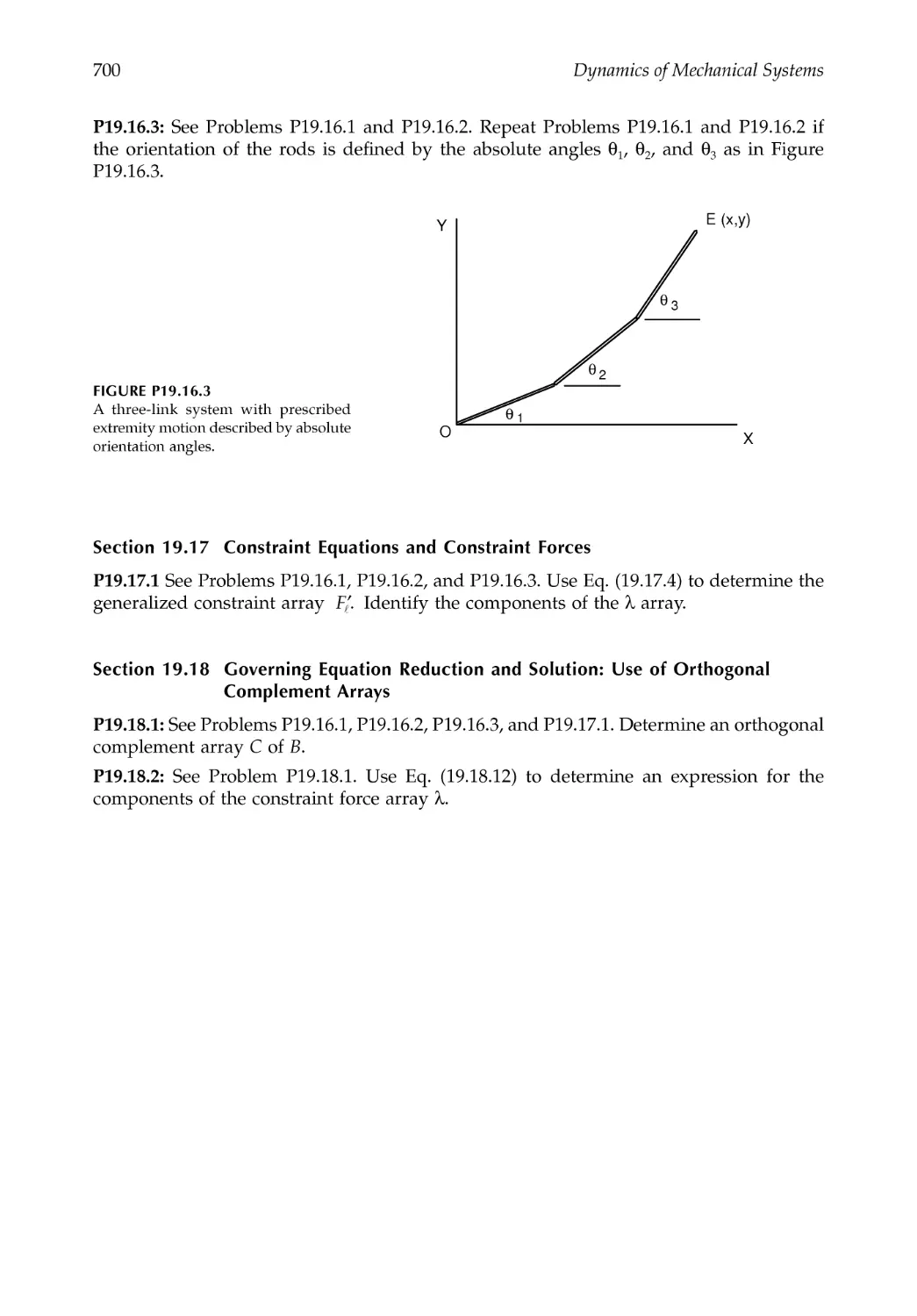
19.16 Redundant Robots............................................................................................................682
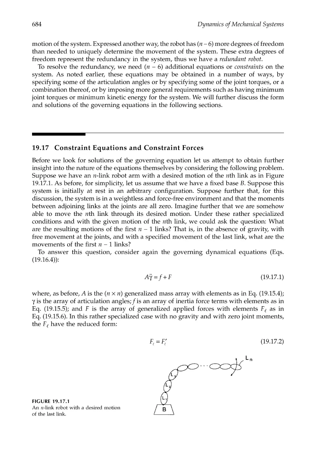
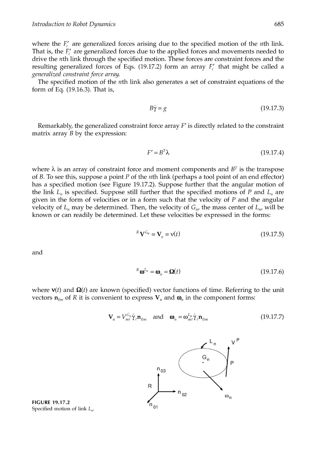
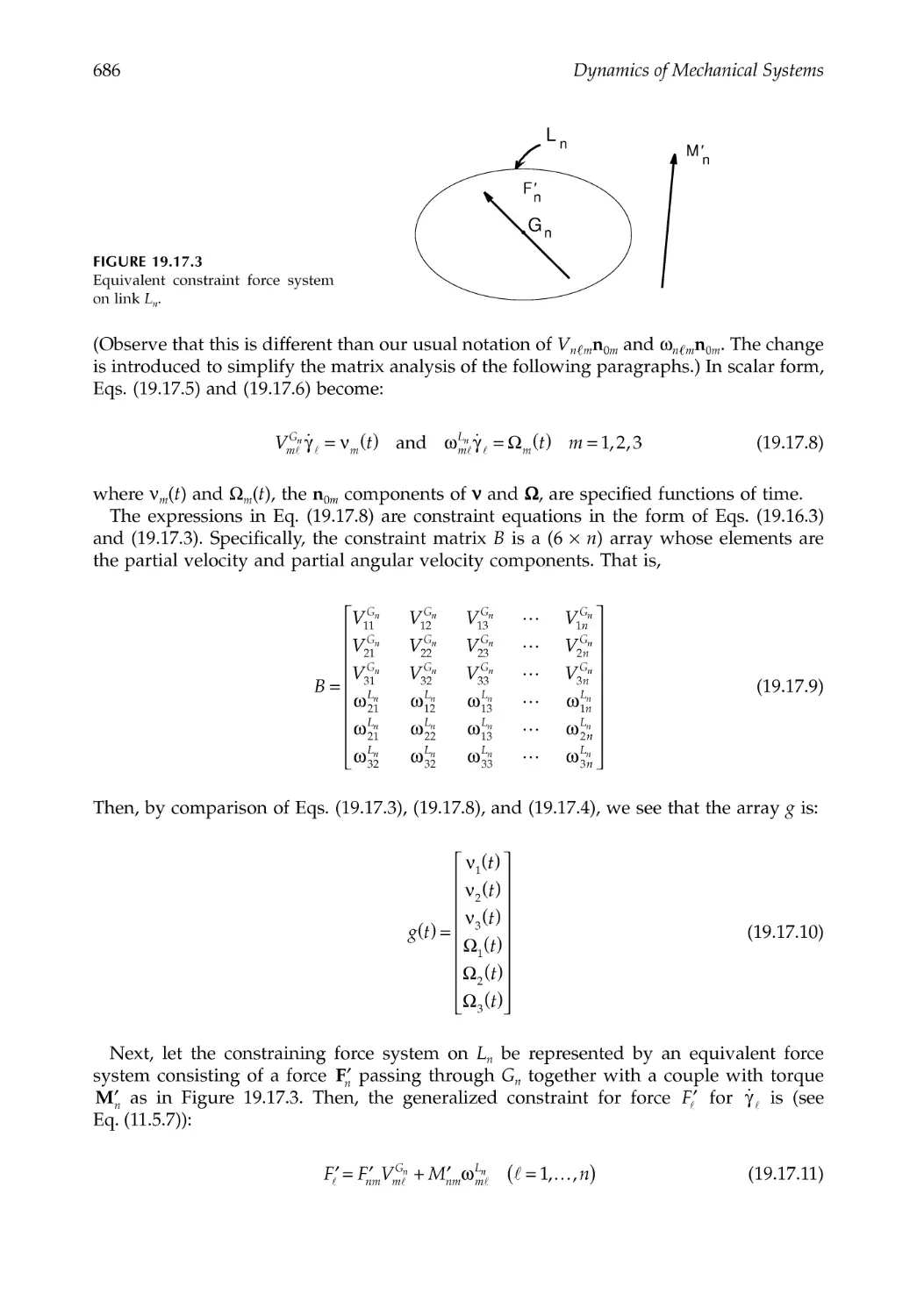
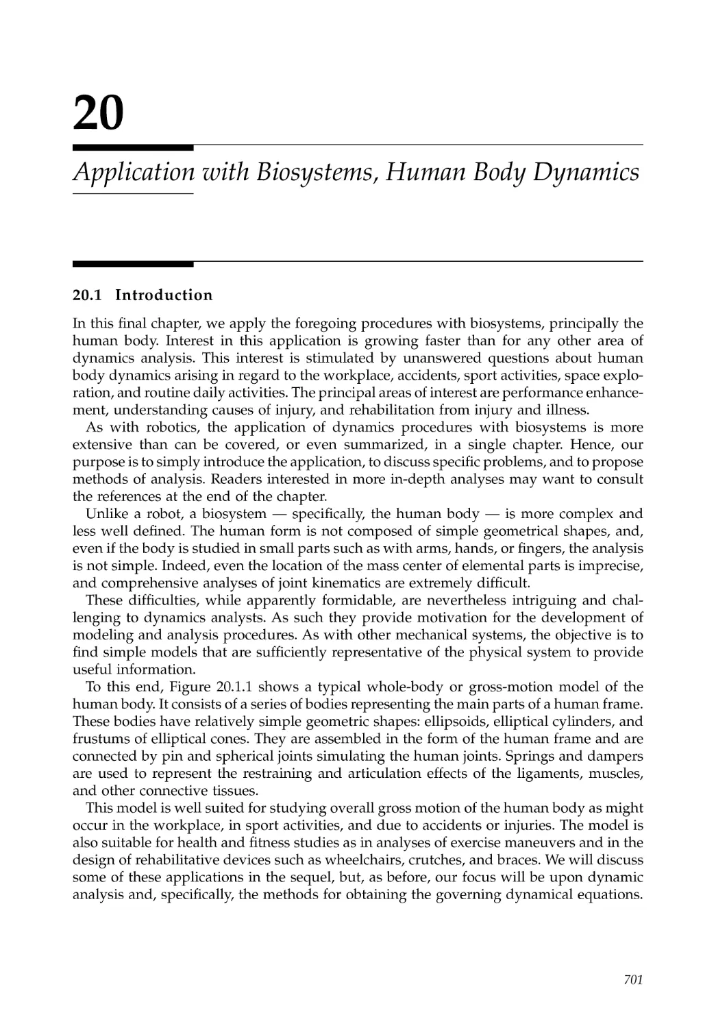
19.17 Constraint Equations and Constraint Forces...............................................................684
19.18 Governing Equation Reduction and Solution: Use of Orthogonal
Complement Arrays ........................................................................................................687
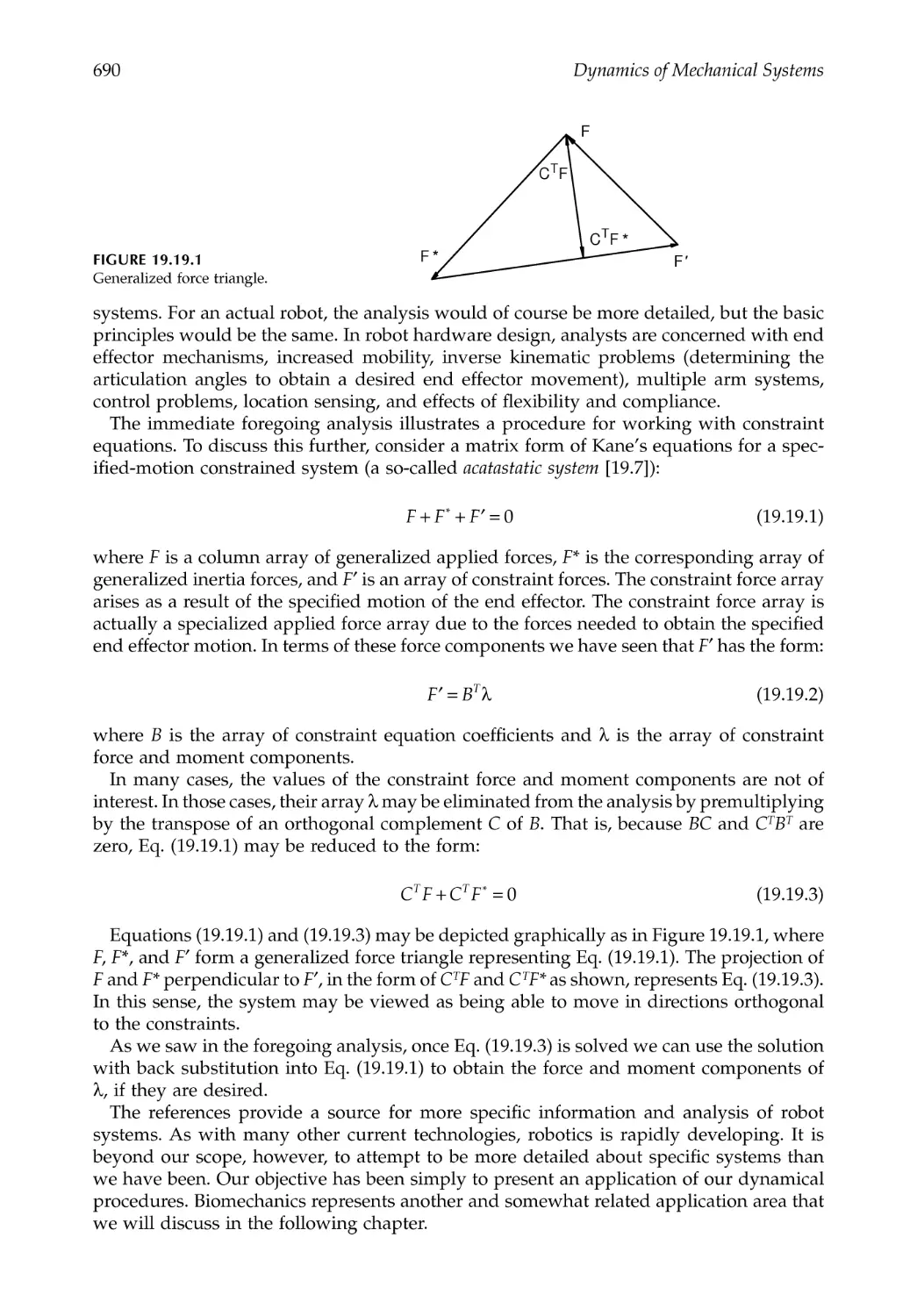
19.19 Discussion, Concluding Remarks, and Closure..........................................................689
References .....................................................................................................................................691
Problems .......................................................................................................................................691
Chapter 20 Application with Biosystems, Human Body Dynamics ...............................701
20.1 Introduction.......................................................................................................................701
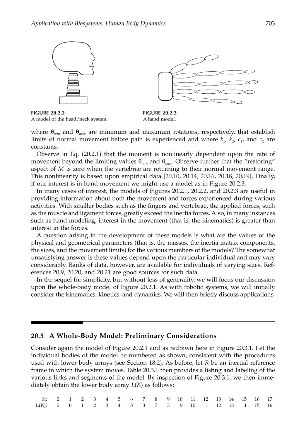
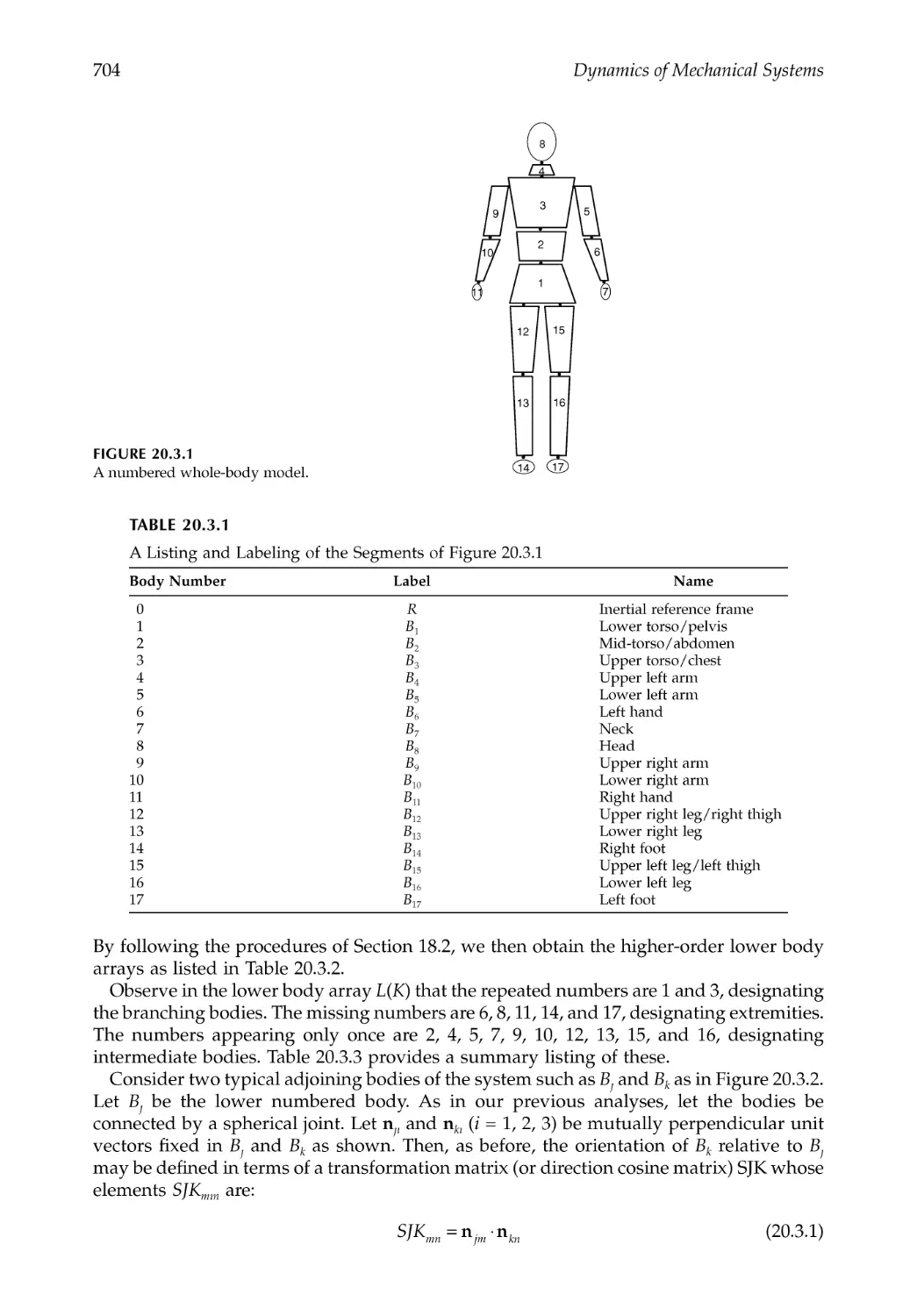
20.2 Human Body Modeling ..................................................................................................702
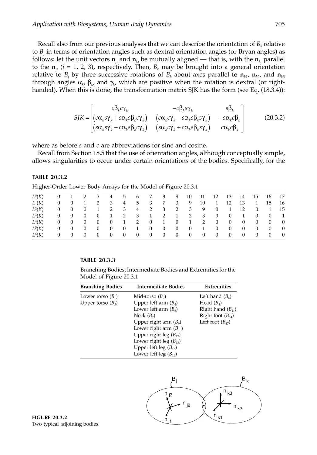
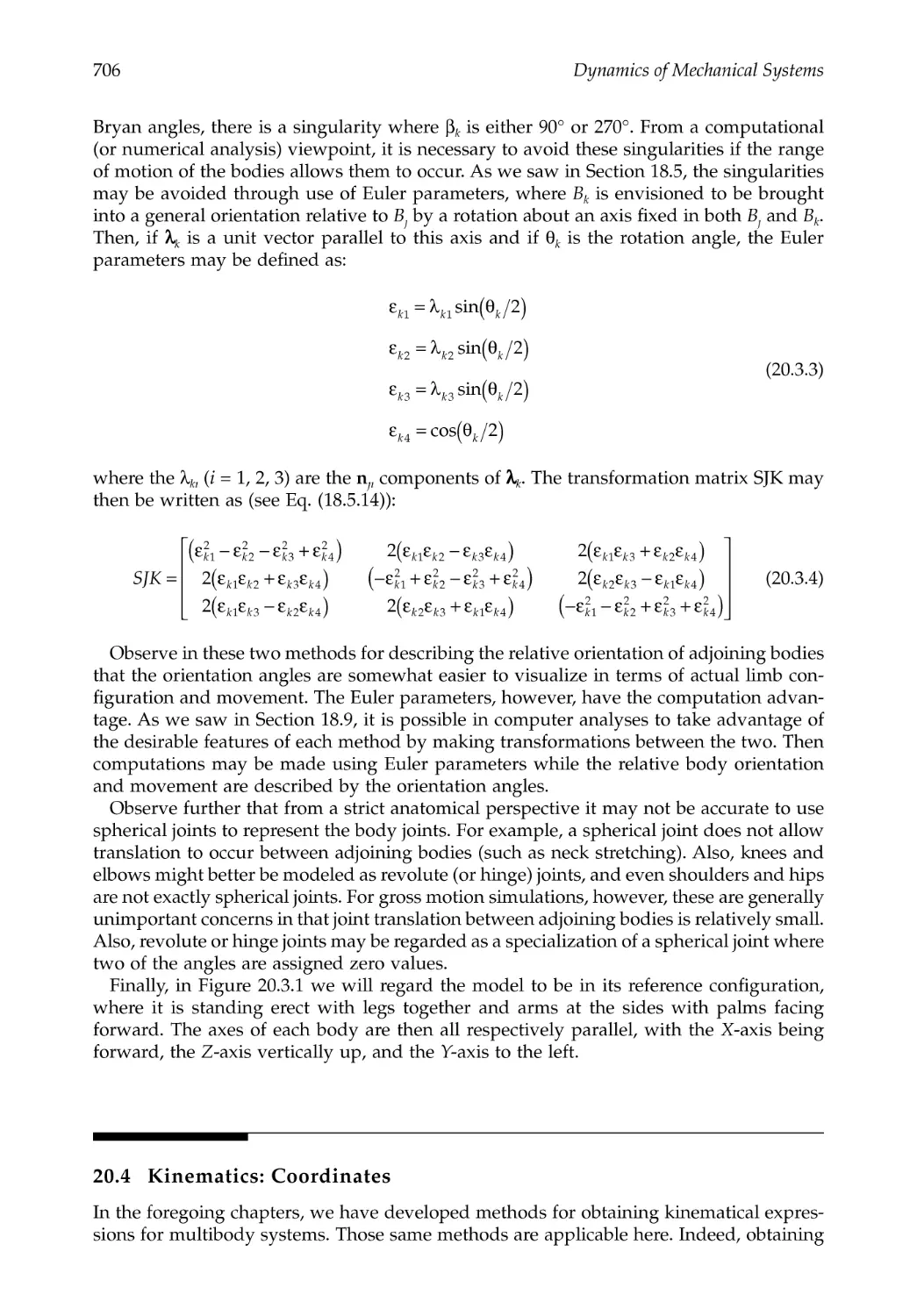
20.3 A Whole-Body Model: Preliminary Considerations ..................................................703
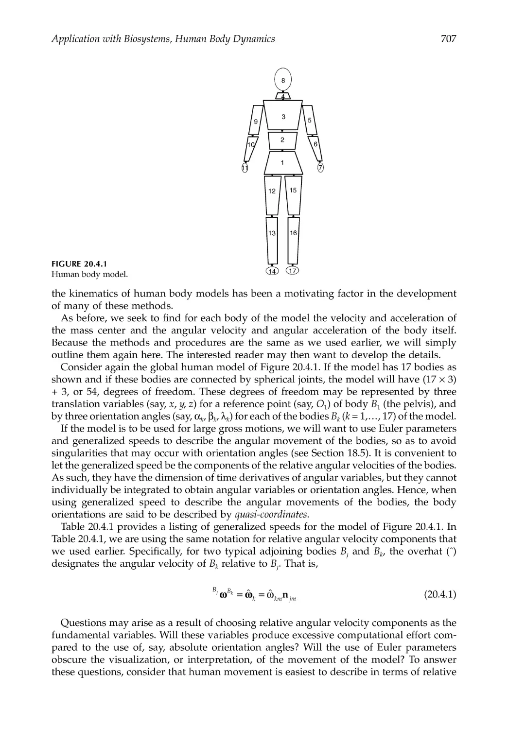
20.4 Kinematics: Coordinates .................................................................................................706
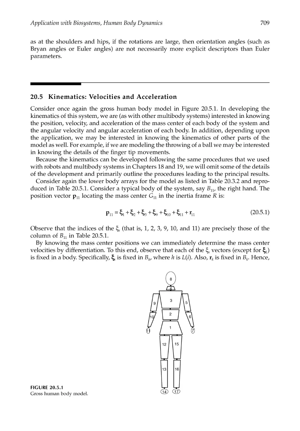
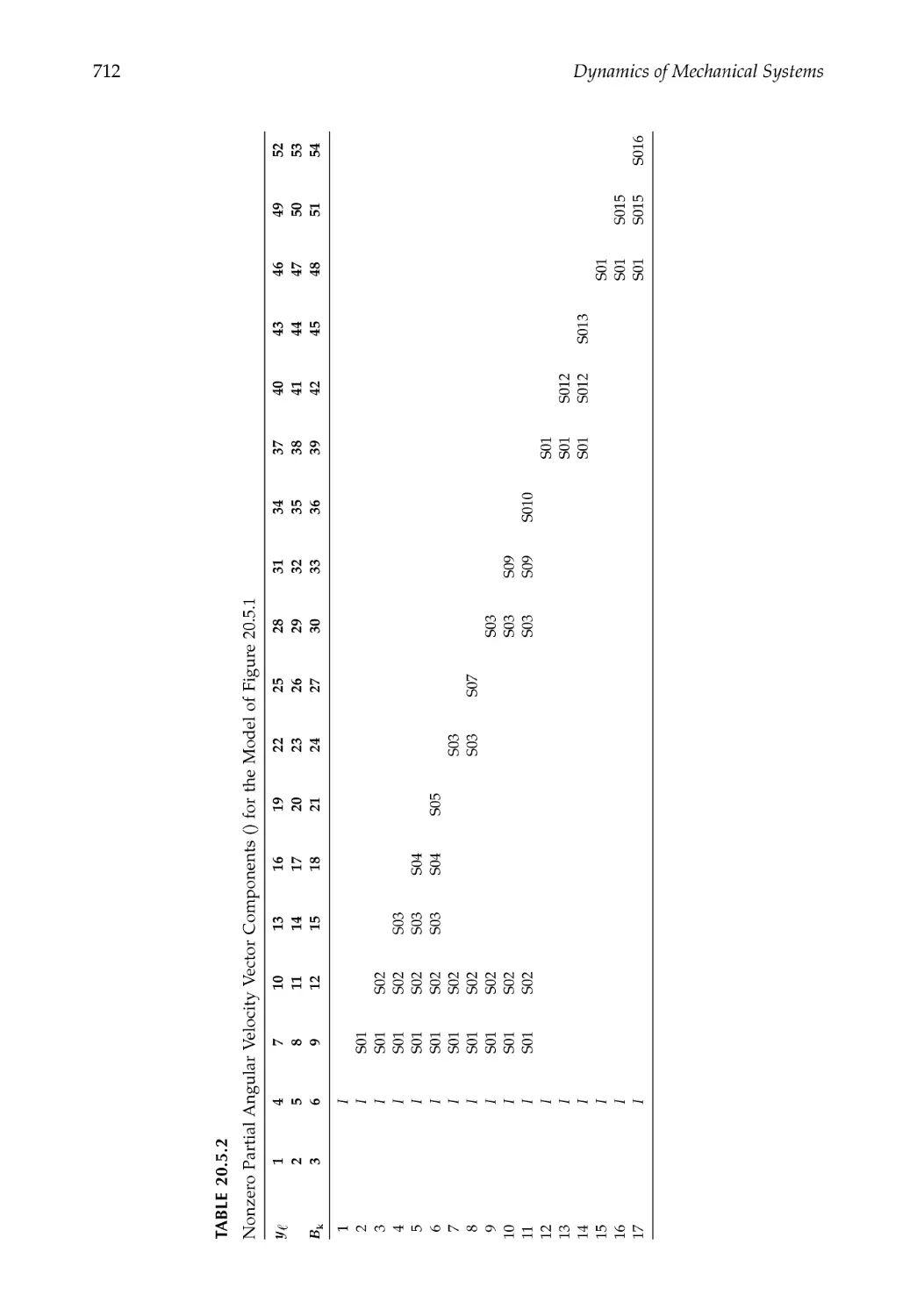
20.5 Kinematics: Velocities and Acceleration .......................................................................709
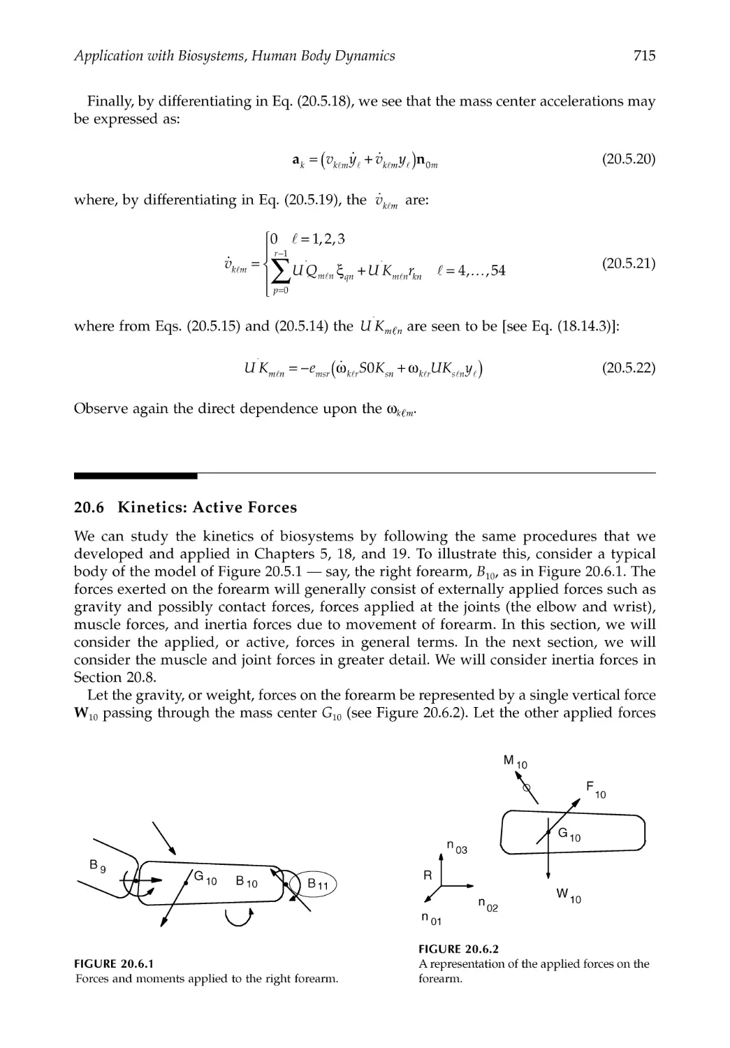
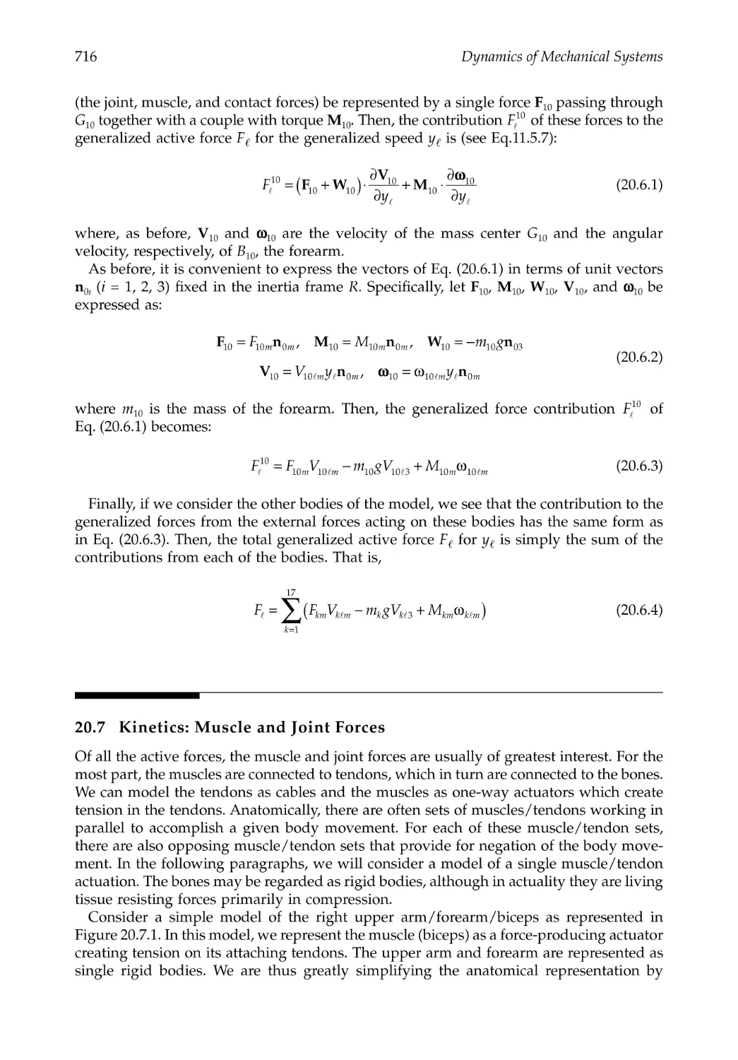
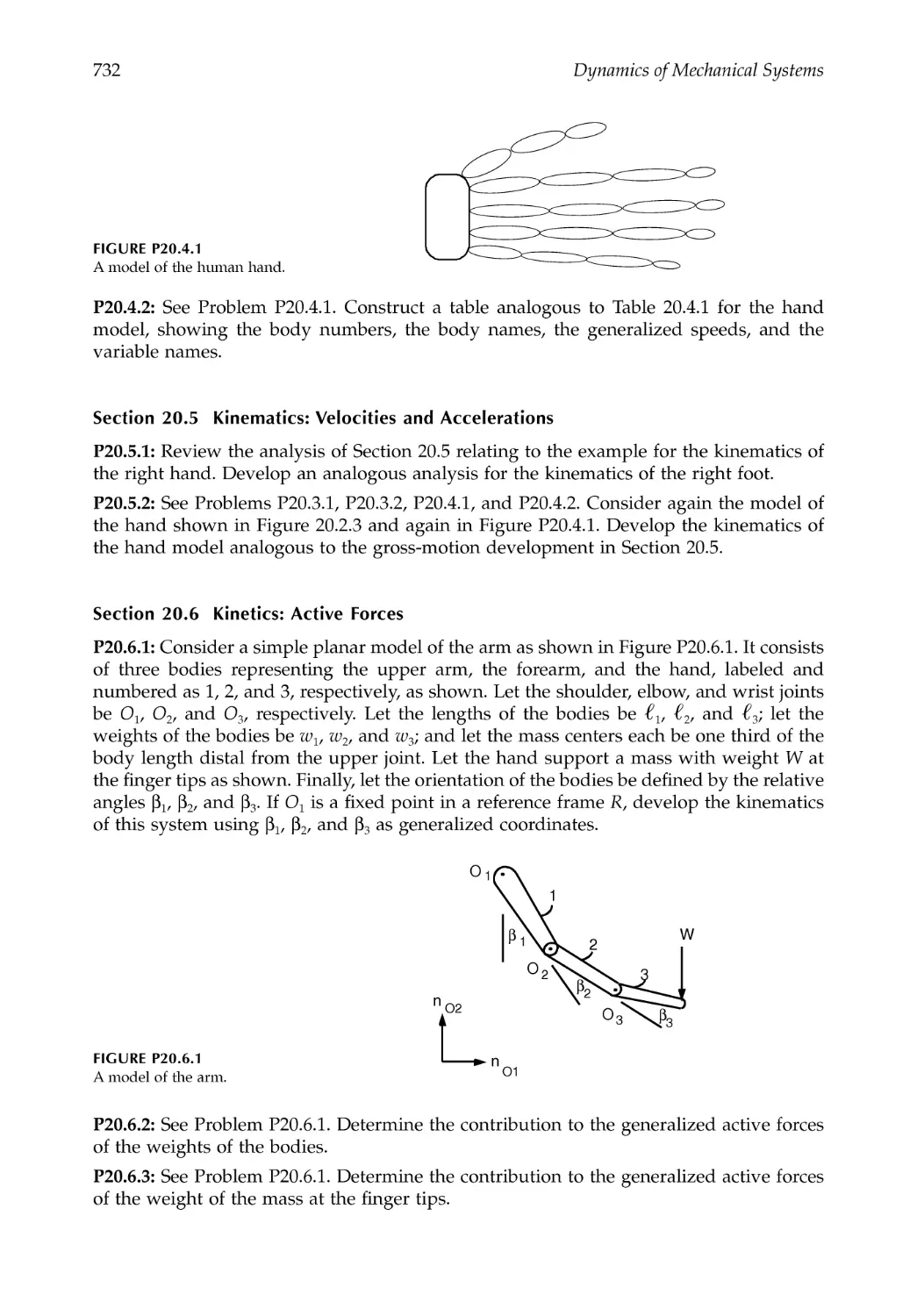
20.6 Kinetics: Active Forces ....................................................................................................715
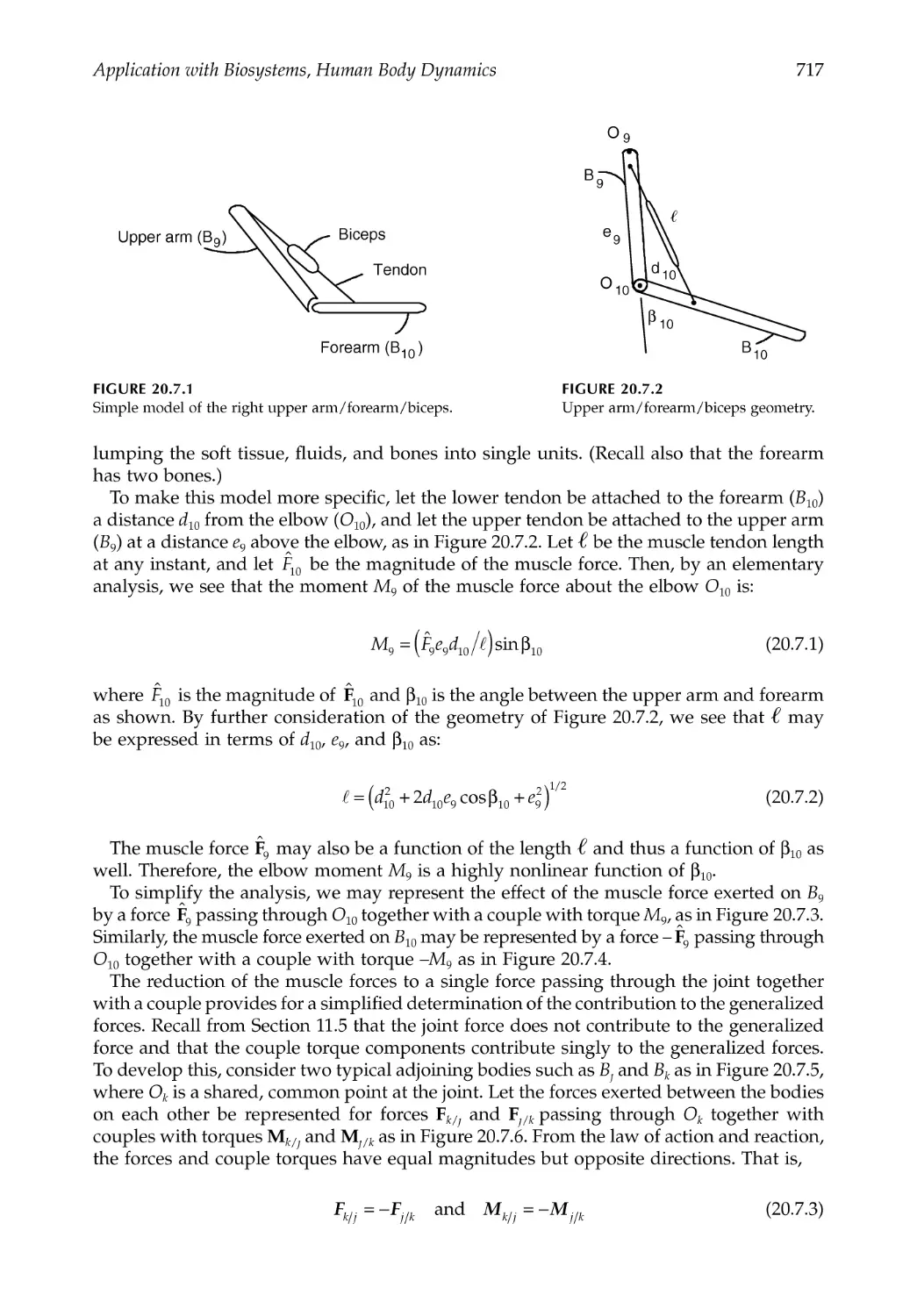
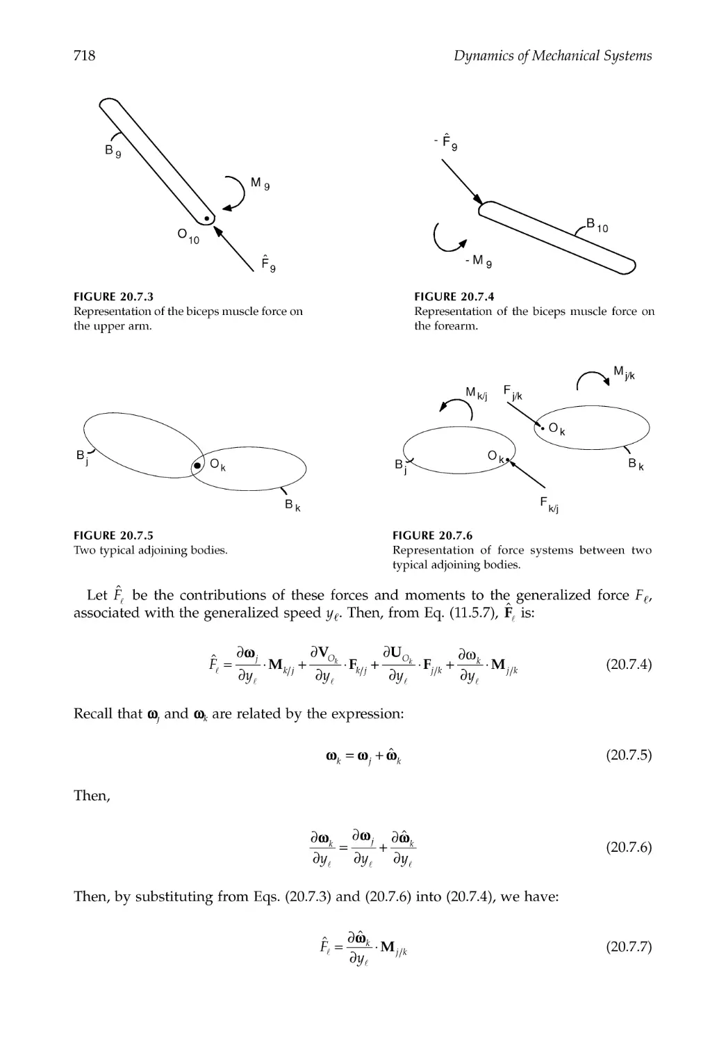
20.7 Kinetics: Muscle and Joint Forces .................................................................................716
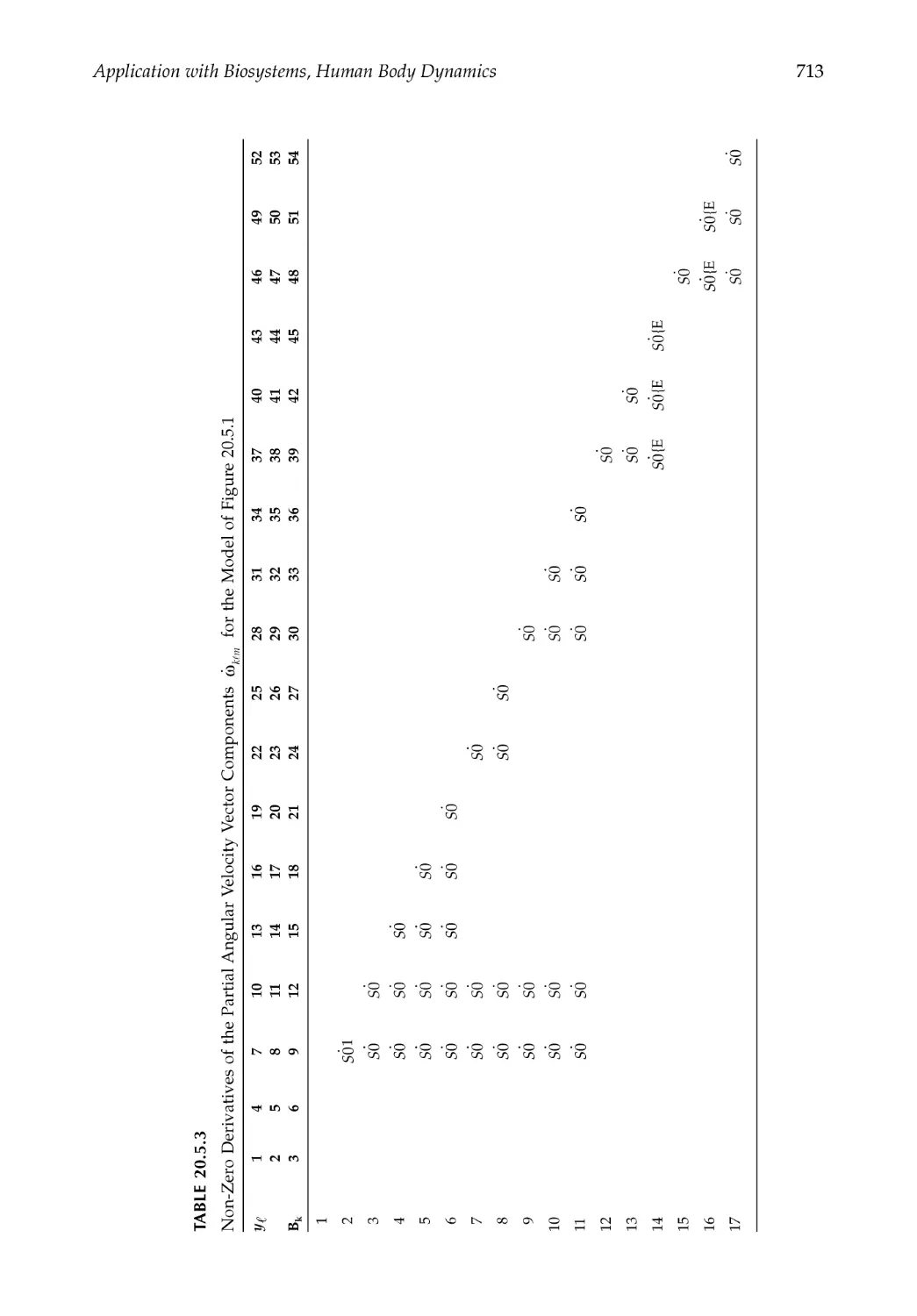
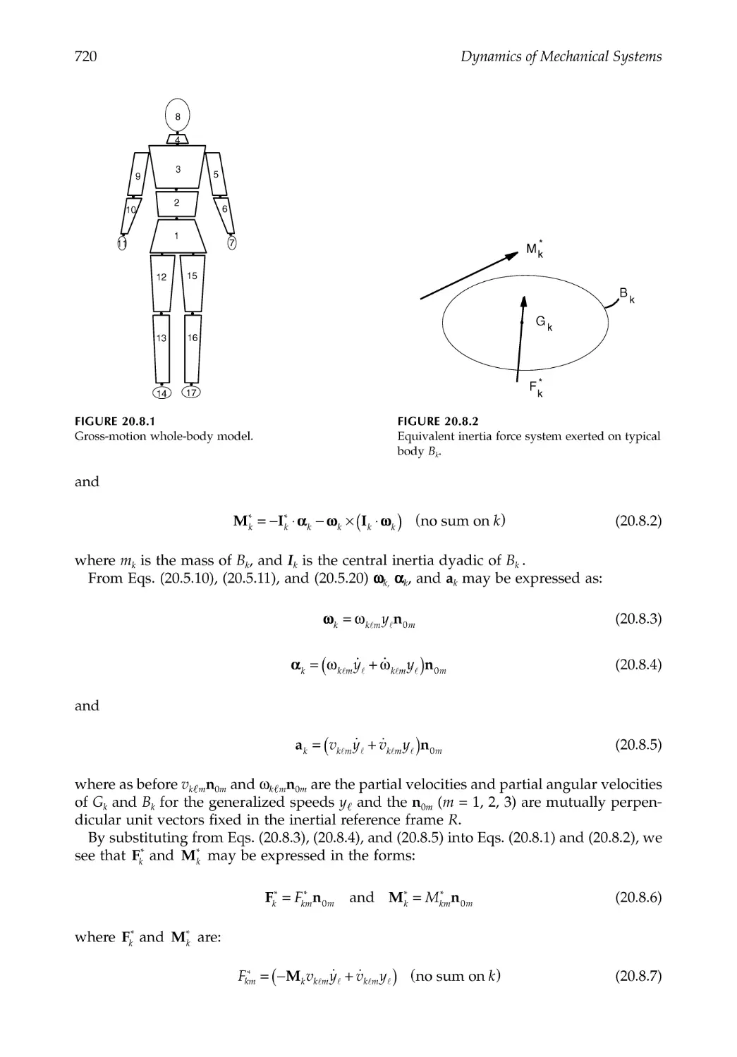
20.8 Kinetics: Inertia Forces ....................................................................................................719
20.9 Dynamics: Equations of Motion ....................................................................................721
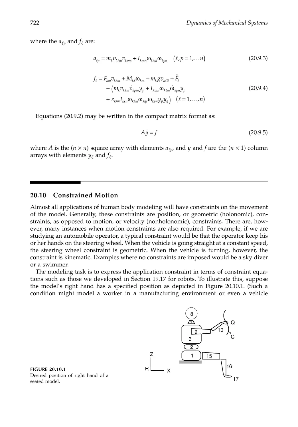
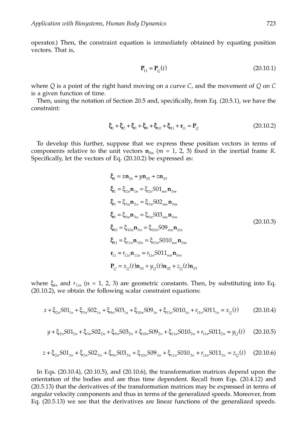
20.10 Constrained Motion .........................................................................................................722
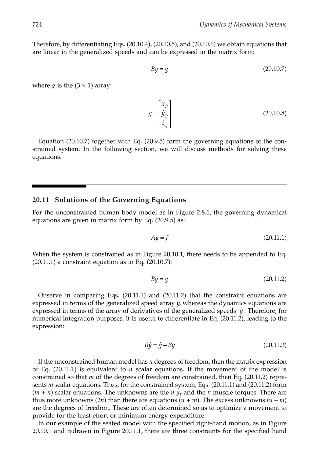
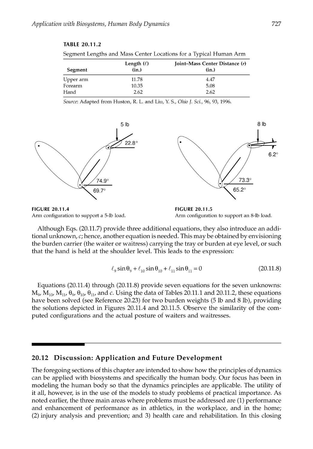
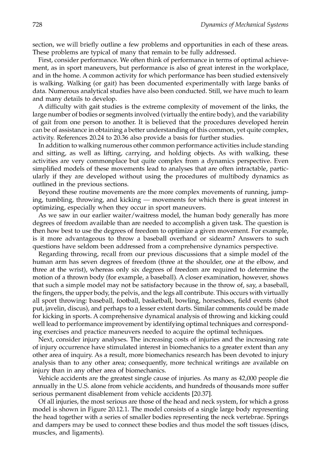
20.11 Solutions of the Governing Equations .........................................................................724
20.12 Discussion: Application and Future Development ....................................................727
References .....................................................................................................................................730
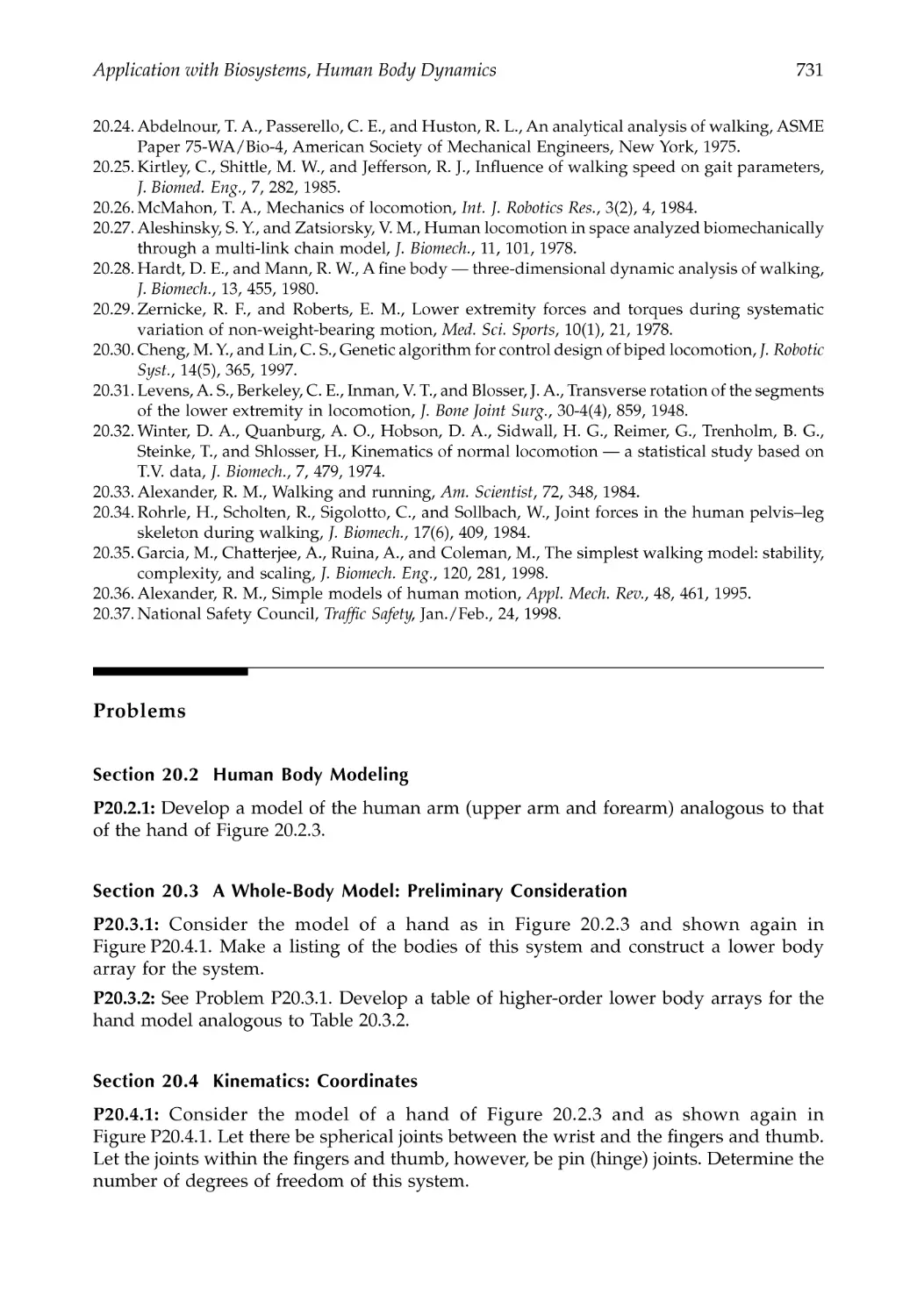
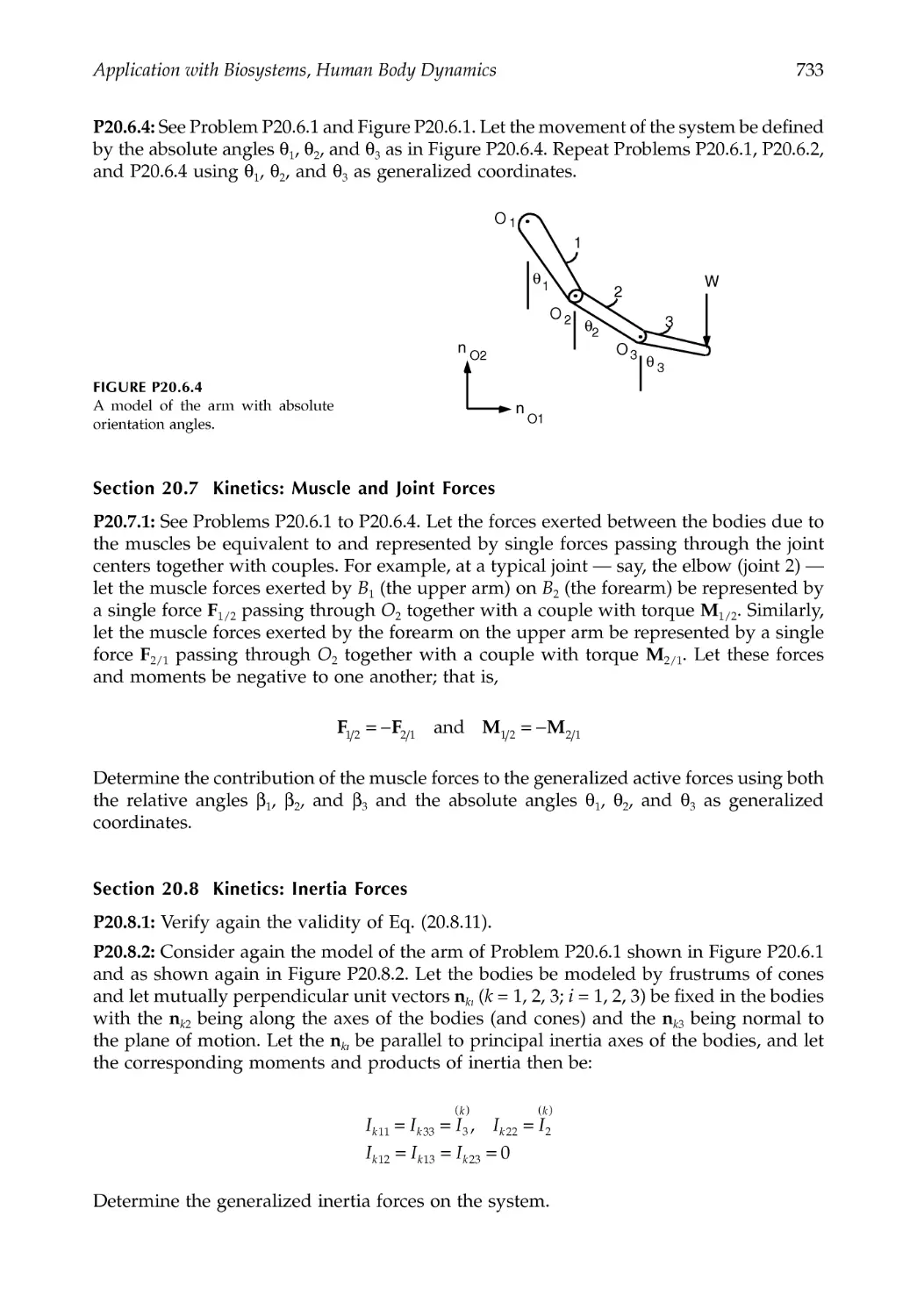
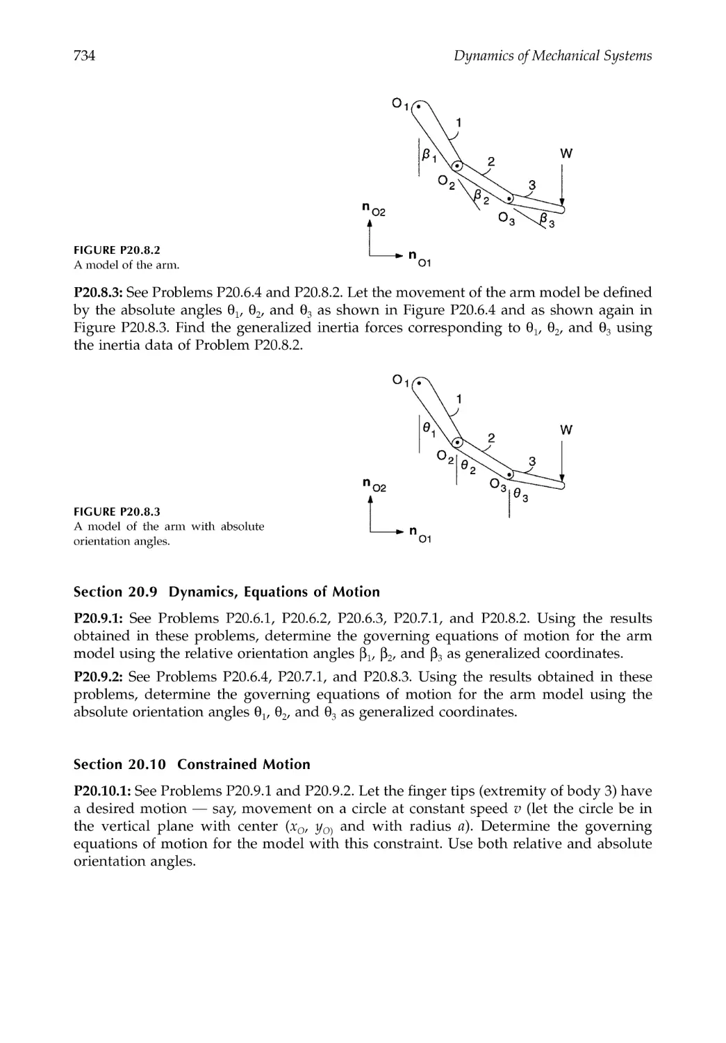
Problems .......................................................................................................................................731
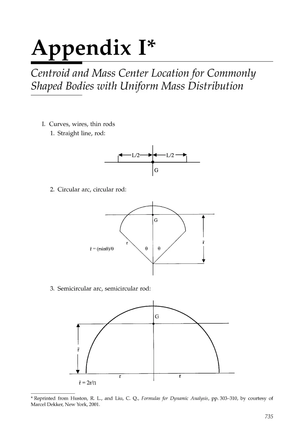
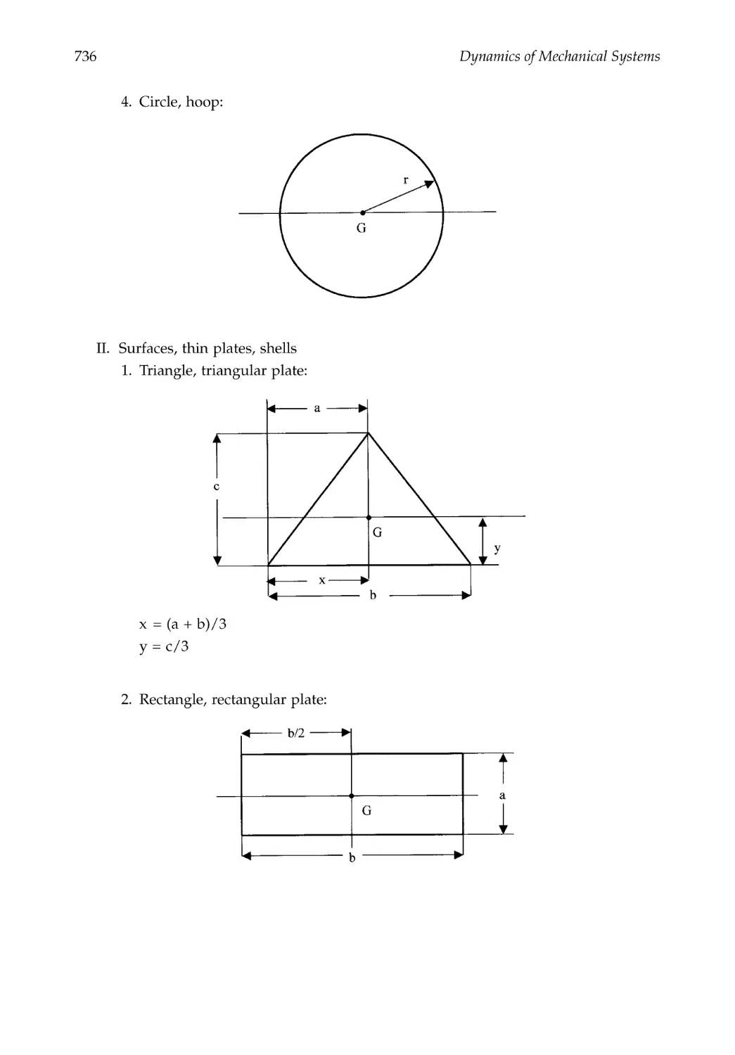
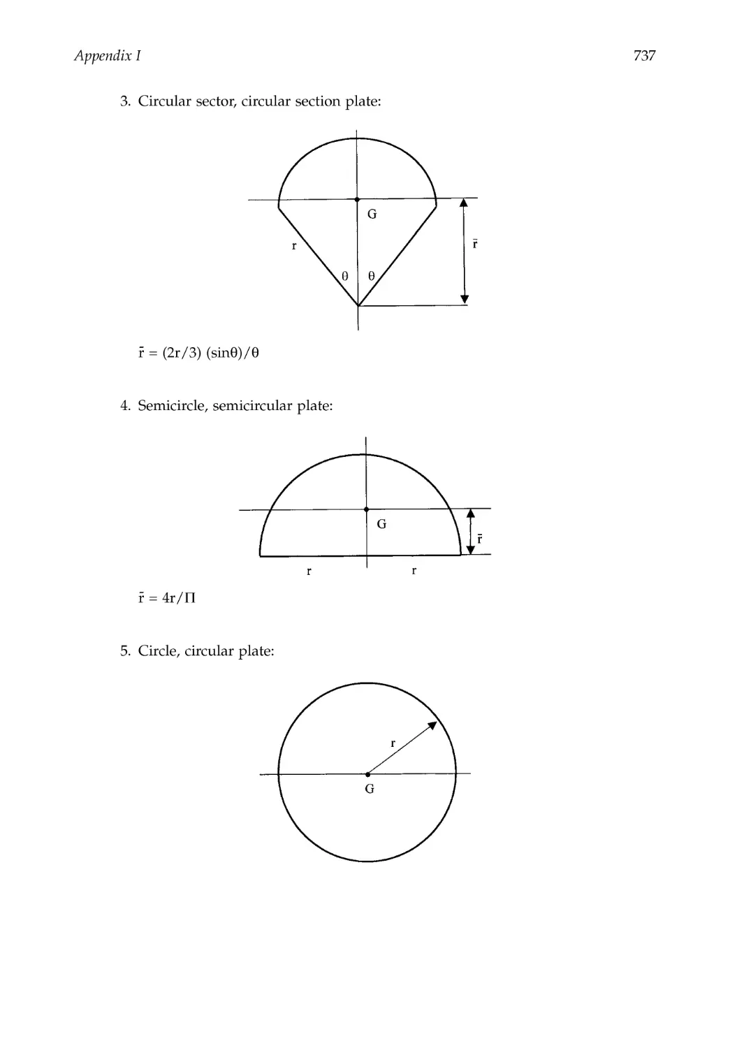
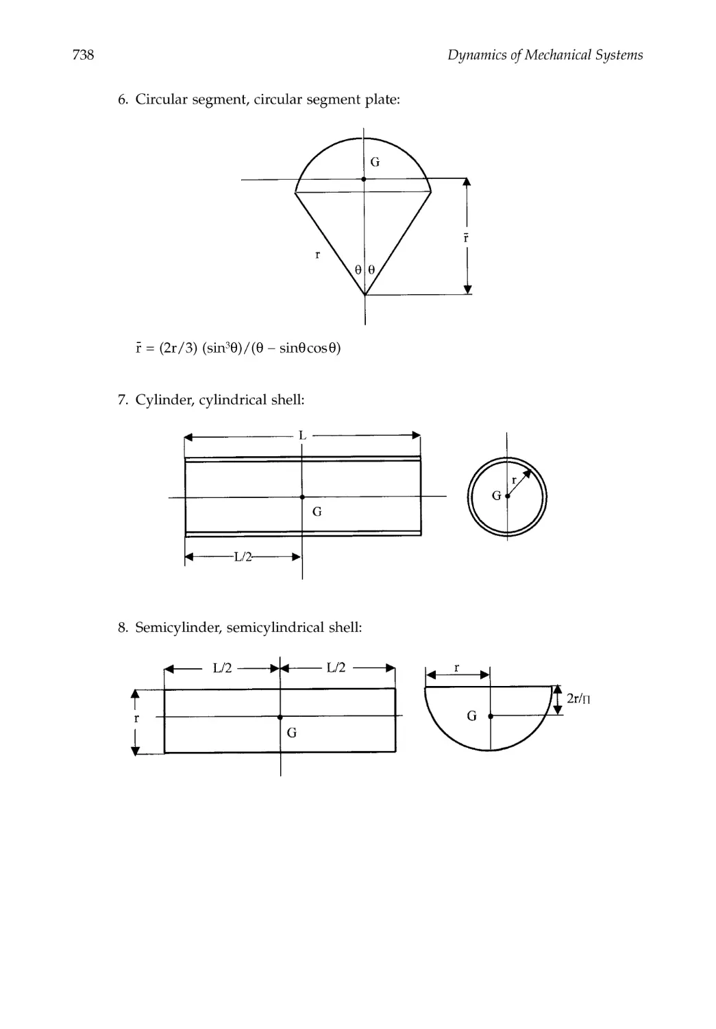
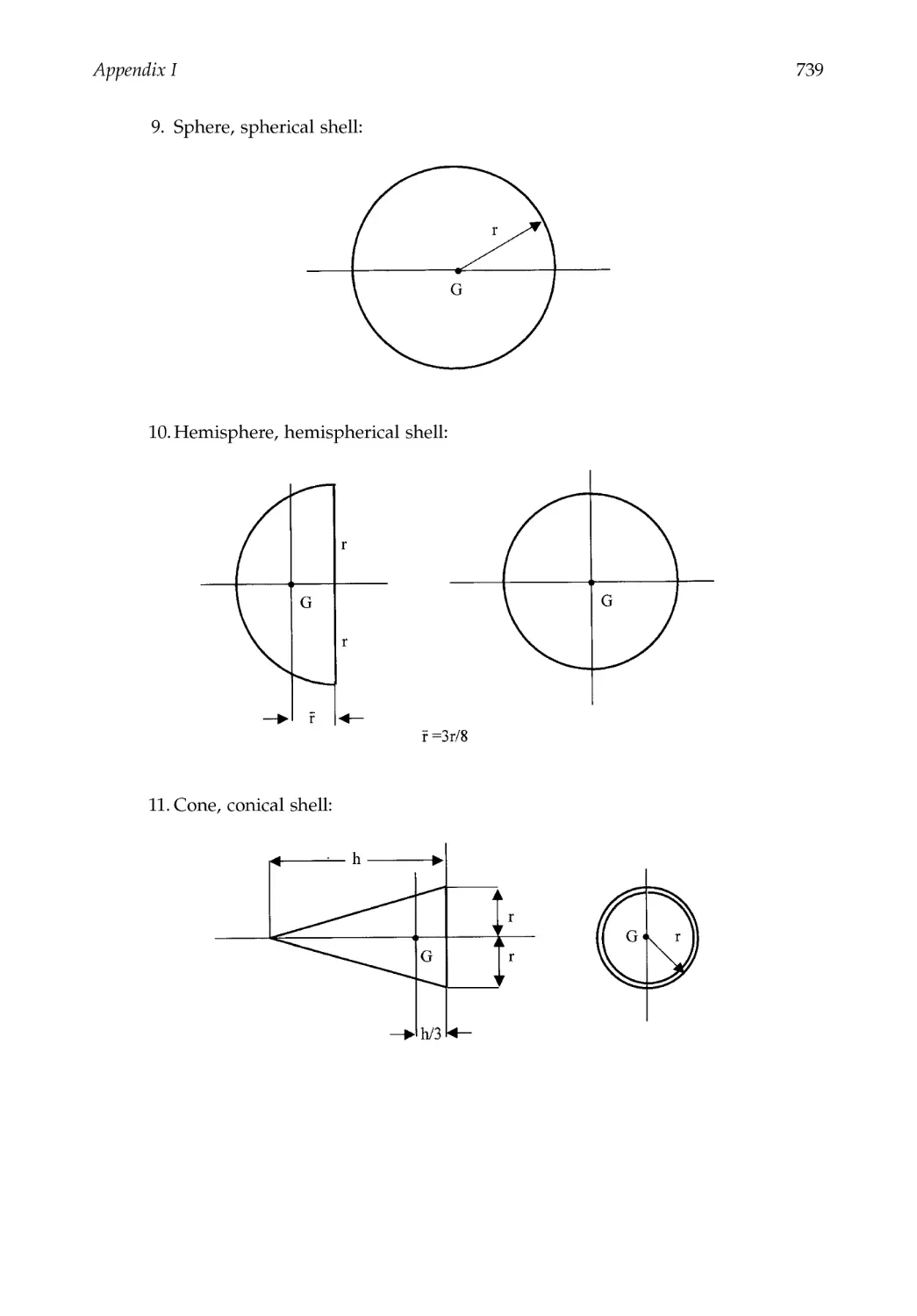
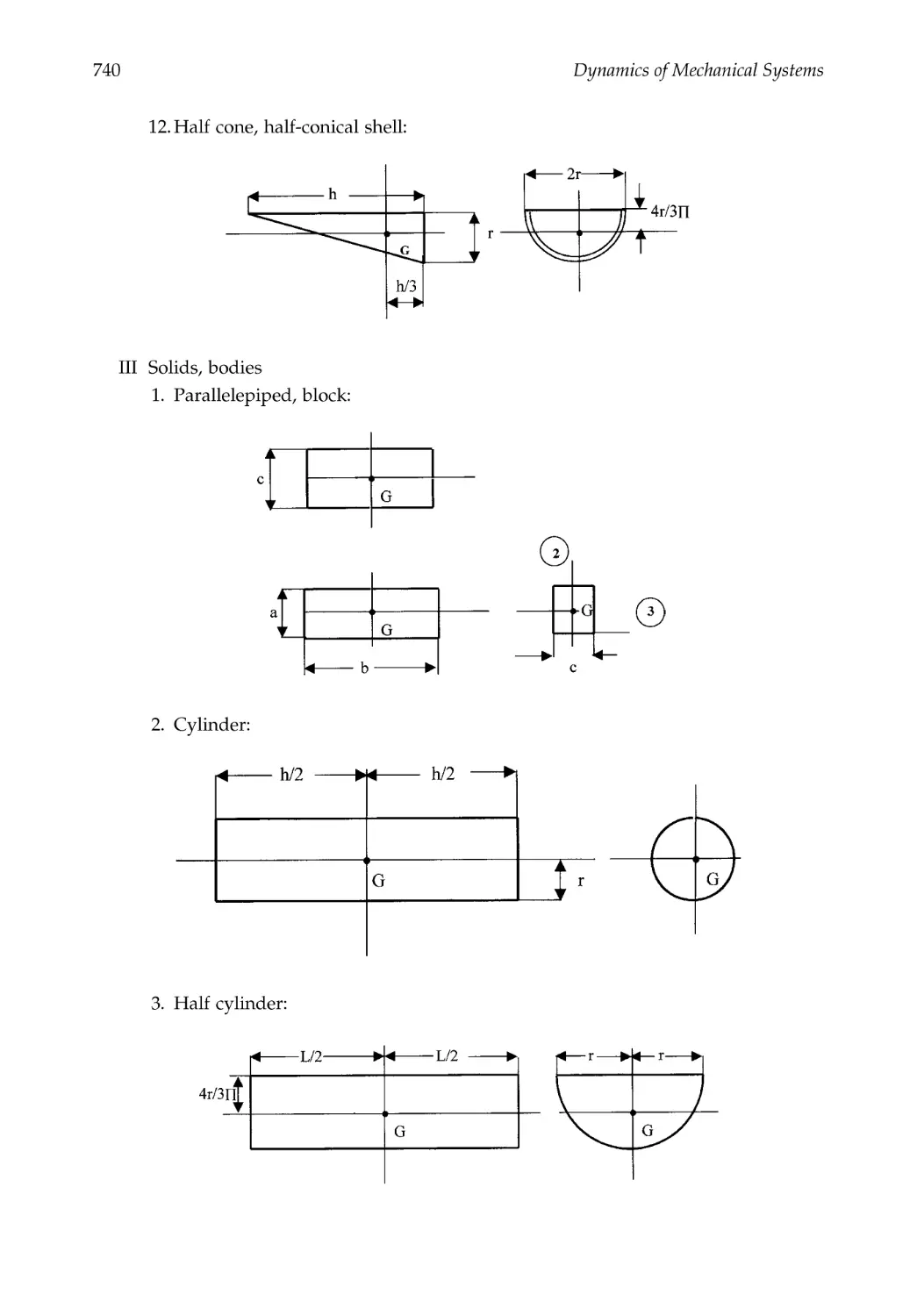
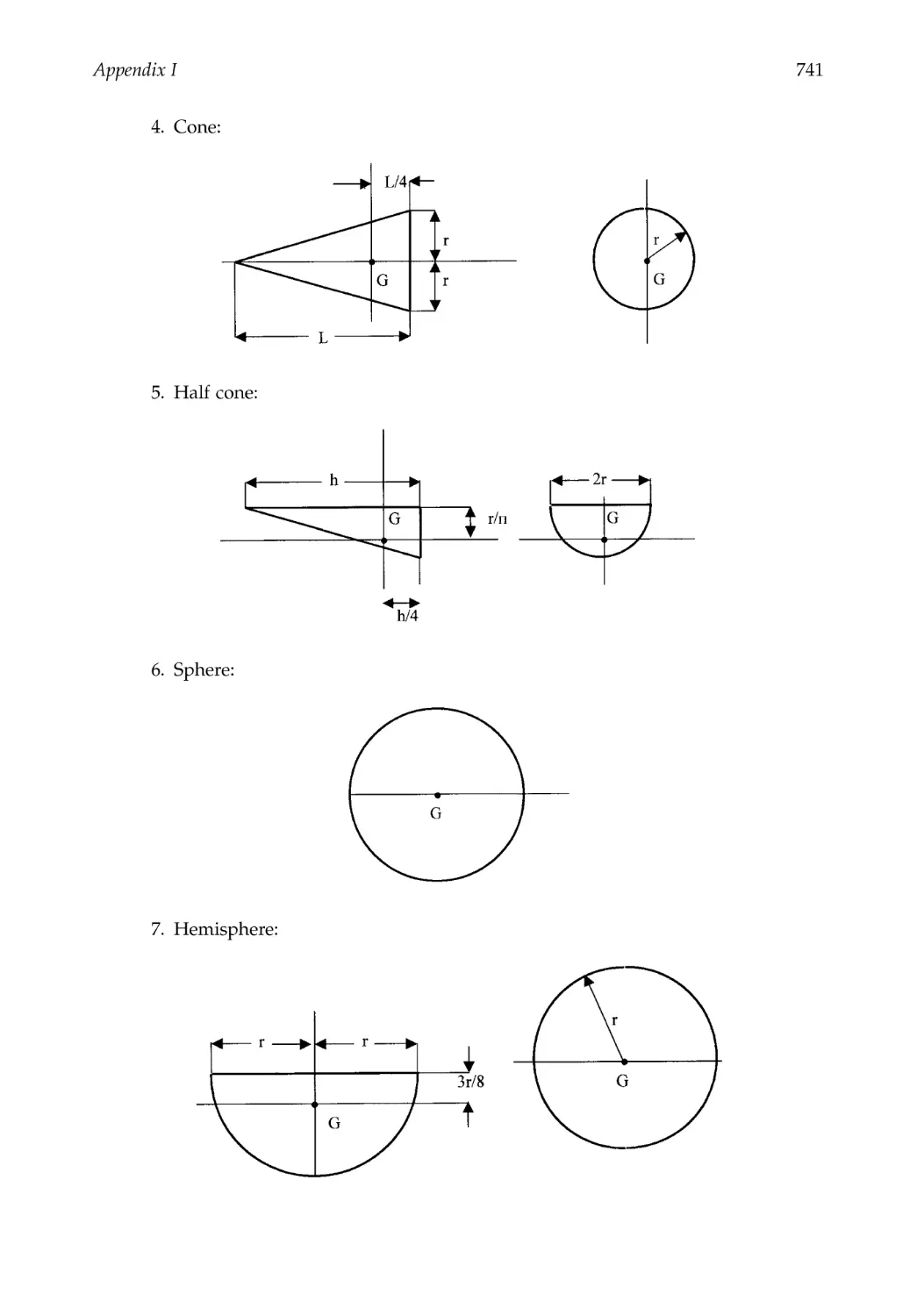
Appendix I Centroid and Mass Center Location for Commonly Shaped Bodies
with Uniform Mass Distribution ...................................................................735
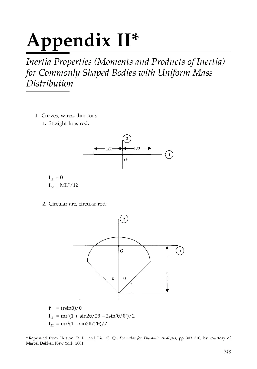
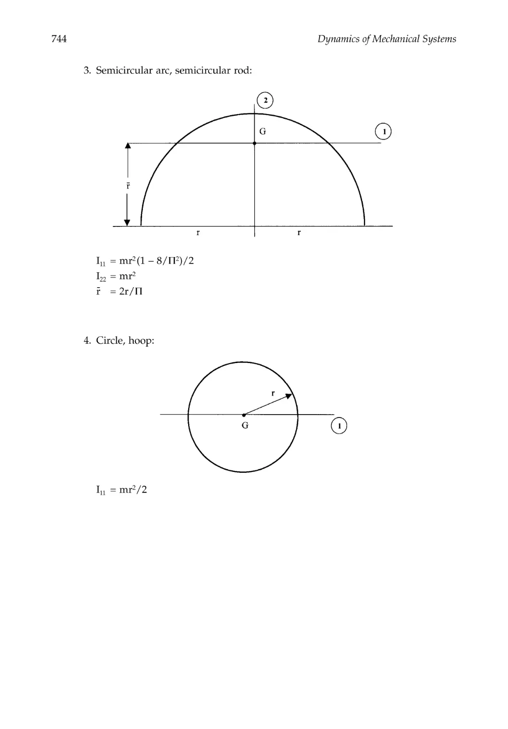
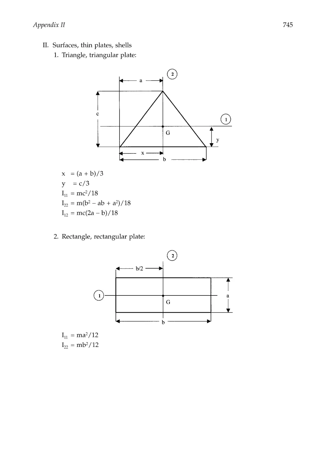
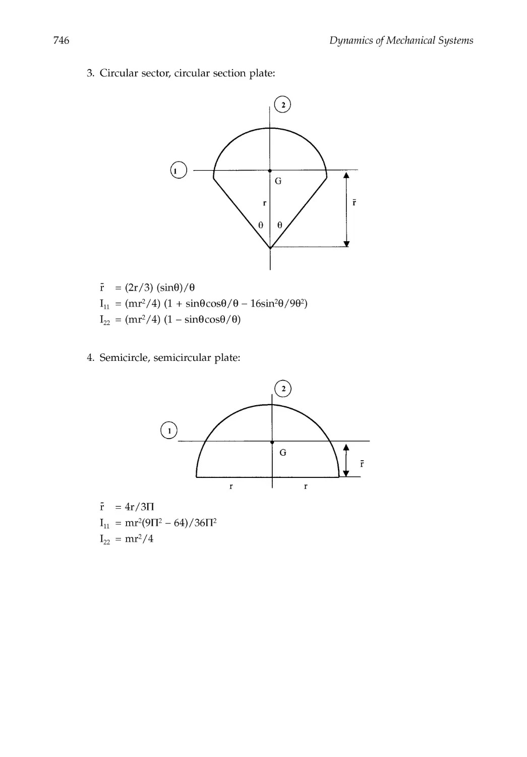
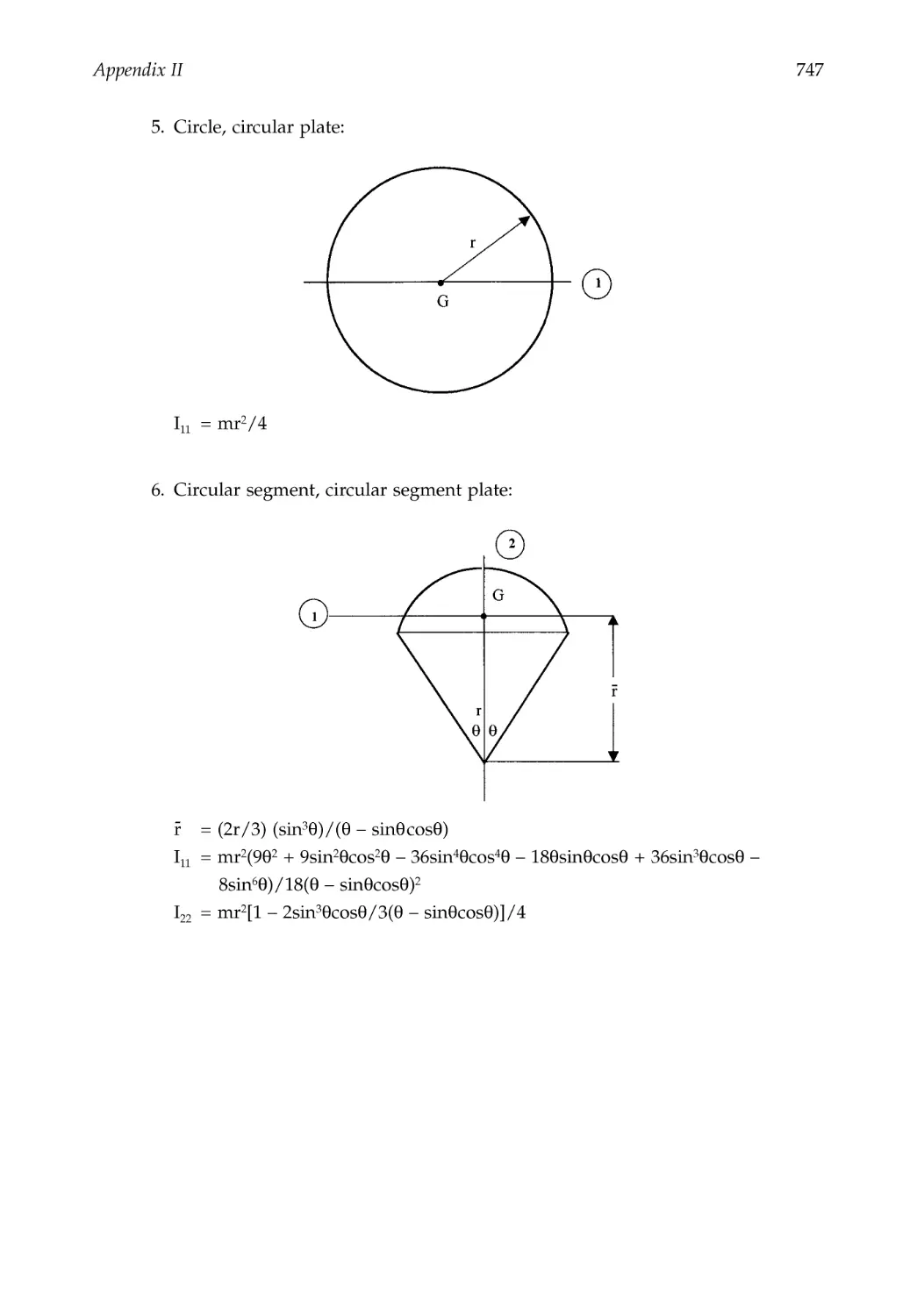
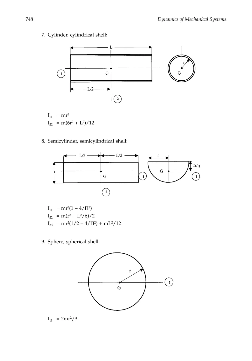
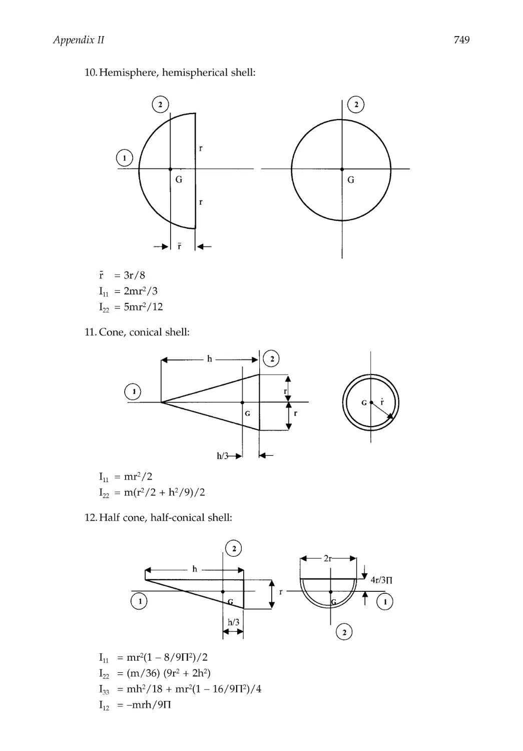
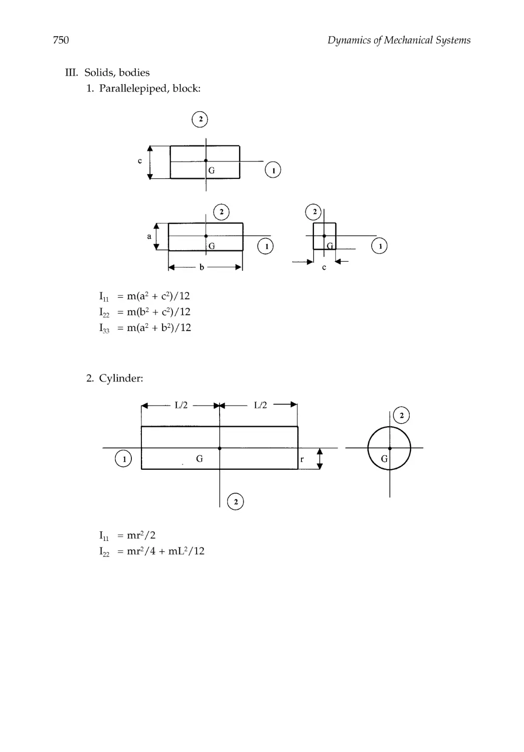
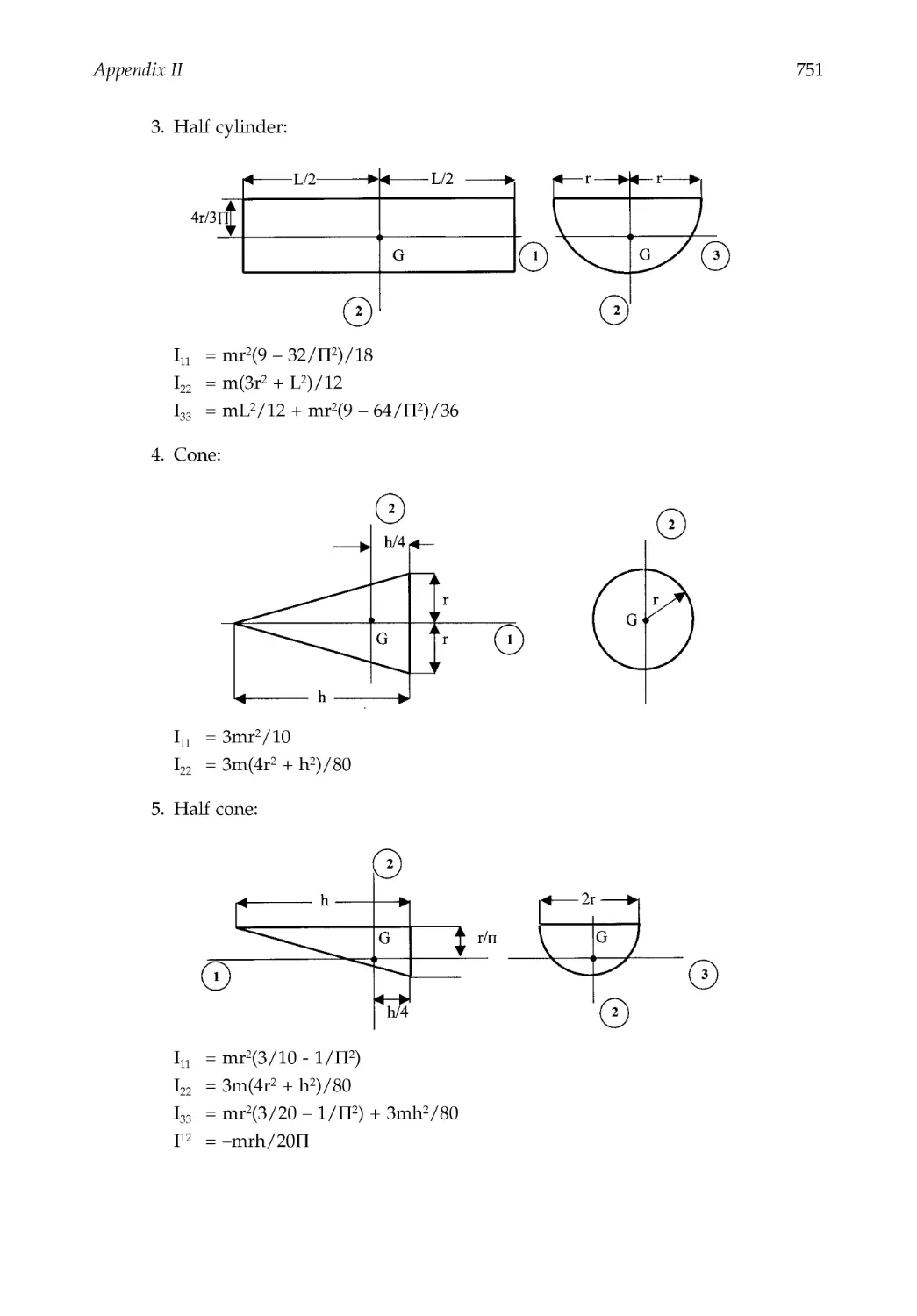
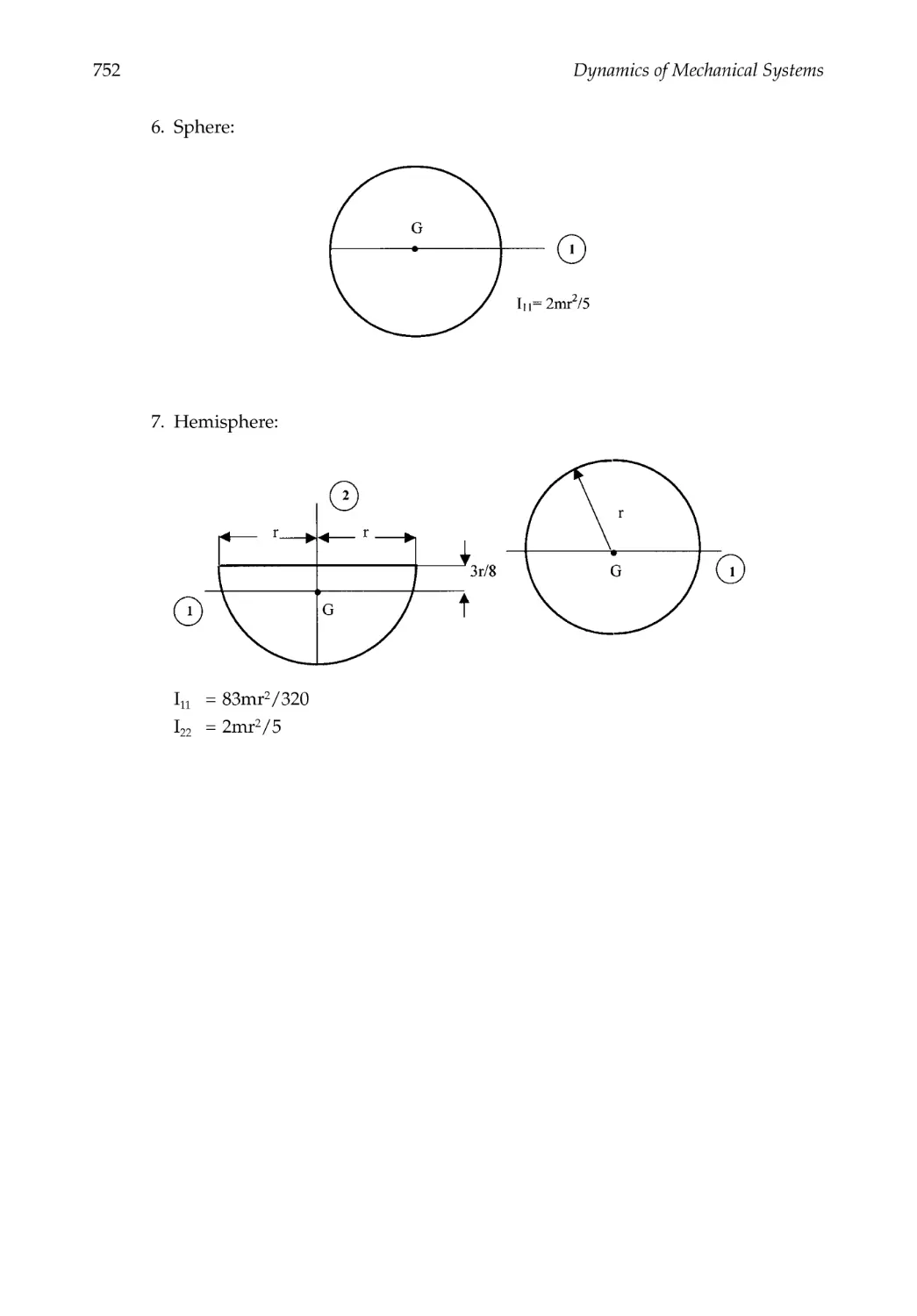
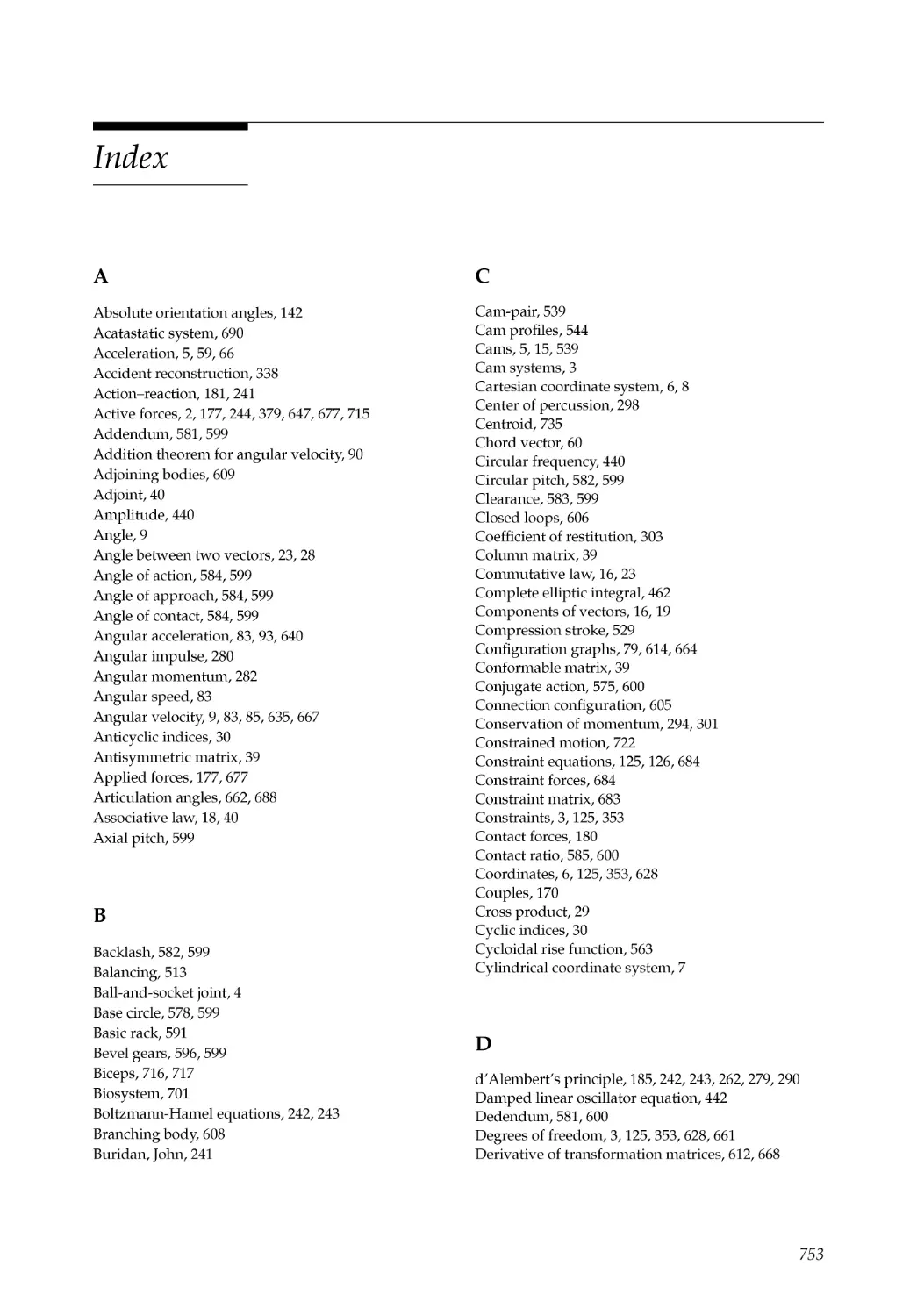
Appendix II Inertia Properties (Moments and Products of Inertia)
for Commonly Shaped Bodies with Uniform Mass Distribution ............743
Index .............................................................................................................................................753
1
1Introduction
1.1 Approach to the Subject
This book presents an introduction to the dynamics of mechanical systems; it is based
upon the principles of elementary mechanics. Although the book is intended to be self-
contained, with minimal prerequisites, readers are assumed to have a working knowledge
of fundamental mechanics' principles and a familiarity with vector and matrix methods.
The readers are also assumed to have knowledge of elementary physics and calculus. In
this introductory chapter, we will review some basic assumptions and axioms and other
preliminary considerations. We will also begin a review of vector methods, which we will
continue and expand in Chapter 2.
Our procedure throughout the book will be to develop a general methodology which
we will then simplify and specialize to topics of interest. We will attempt to illustrate
the concepts through examples and exercise problems. The reader is encouraged to solve
as many problems as possible. Indeed, it is our belief that a basic understanding of the
concepts and an intuitive grasp of the subject are best obtained through solving the
exercise problems.
1.2 Subject Matter
Dynamics is a subject in the general field of mechanics, which in turn is a discipline of
classical physics. Mechanics can be divided into two divisions: solid mechanics and fluid
mechanics. Solid mechanics may be further divided into flexible mechanics and rigid
mechanics. Flexible mechanics includes such subjects as strength of materials, elasticity,
viscoelasticity, plasticity, and continuum mechanics. Alternatively, aside from statics,
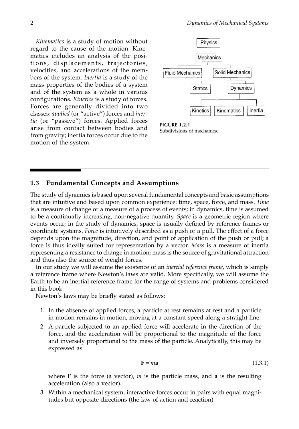
dynamics is the essence of rigid mechanics. Figure 1.2.1 contains a chart showing these
subjects and their relations to one another.
Statics is a study of the behavior of rigid body systems when there is no motion. Statics
is concerned primarily with the analysis of forces and force systems and the determination
of equilibrium configurations. In contrast, dynamics is a study of the behavior of moving
rigid body systems. As seen in Figure 1.2.1, dynamics may be subdivided into three sub-
subjects: kinematics, inertia, and kinetics.
2
Dynamics of Mechanical Systems
Kinematics is a study of motion without
regard to the cause of the motion. Kine-
matics includes an analysis of the posi-
tions, displacements, trajectories,
velocities, and accelerations of the mem-
bers of the system. Inertia is a study of the
mass properties of the bodies of a system
and of the system as a whole in various
configurations. Kinetics is a study of forces.
Forces are generally divided into two
classes: applied (or "active") forces and iner-
tia (or "passive") forces. Applied forces
arise from contact between bodies and
from gravity; inertia forces occur due to the
motion of the system.
1.3 Fundamental Concepts and Assumptions
The study of dynamics is based upon several fundamental concepts and basic assumptions
that are intuitive and based upon common experience: time, space, force, and mass. Time
is a measure of change or a measure of a process of events; in dynamics, time is assumed
to be a continually increasing, non-negative quantity. Space is a geometric region where
events occur; in the study of dynamics, space is usually defined by reference frames or
coordinate systems. Force is intuitively described as a push or a pull. The effect of a force
depends upon the magnitude, direction, and point of application of the push or pull; a
force is thus ideally suited for representation by a vector. Mass is a measure of inertia
representing a resistance to change in motion; mass is the source of gravitational attraction
and thus also the source of weight forces.
In our study we will assume the existence of an inertial reference frame, which is simply
a reference frame where Newton's laws are valid. More specifically, we will assume the
Earth to be an inertial reference frame for the range of systems and problems considered
in this book.
Newton's laws may be briefly stated as follows:
1. In the absence of applied forces, a particle at rest remains at rest and a particle
in motion remains in motion, moving at a constant speed along a straight line.
2. A particle subjected to an applied force will accelerate in the direction of the
force, and the acceleration will be proportional to the magnitude of the force
and inversely proportional to the mass of the particle. Analytically, this may be
expressed as
(1.3.1)
where F is the force (a vector), m is the particle mass, and a is the resulting
acceleration (also a vector).
3. Within a mechanical system, interactive forces occur in pairs with equal magni-
tudes but opposite directions (the law of action and reaction).
Fa
=m
FIGURE 1.2.1
Subdivisions of mechanics.
Introduction
3
1.4 Basic Terminology in Mechanical Systems
Particular terminology is associated with dynamics, and specifically with mechanical
system dynamics, which we will use in the text. We will attempt to define the terms as
we need them, but it might also be helpful to mention some of them here:
• A space is a region or geometric entity occupied by particles where, for our
purposes, dynamic events will occur.
• A reference frame may be regarded as a coordinate axis system containing and
locating the points of a space. Typical reference frames employ Cartesian axes
systems.
• A particle is a small body whose dimensions are either negligible or irrelevant
in the description of its motion and of its response to forces applied to it. "Small"
is, of course, a relative term. A body considered as a particle may be small in
some contexts but not in others (for example, an Earth satellite or an automobile).
Particles are generally identified with points in space, and they generally have
finite masses.
• A rigid body is a set of particles whose distances from one another remain fixed,
or constant, such as a sandstone. The number of particles in a body is usually
quite large. A reference frame may be regarded, for kinematic purposes, as a
rigid body whose particles have zero masses.
• A degree of freedom is defined as a way in which a particle, body, or system can
move. The number of degrees of freedom possessed by a particle, body, or system
is defined as the number of geometric parameters (for example, coordinates,
distances, or angles) needed to uniquely describe the location, orientation, and/
or configuration of the particle, body, or system.
• A constraint is a restriction on the motion of a particle, body, or system. Con-
straints can be either geometric (holonomic) or kinematic (nonholonomic).
• A machine is an arrangement of a system of bodies designed for applying, trans-
mitting, and/or changing forces and motion.
• A mechanism is a machine intended primarily for the transmission of motion.
The three general categories of machines are:
1. Gear systems, which are toothed bodies in contact whose objectives are to
transmit motion between rotating shafts.
2. Cam systems, which are bodies with curved profiles in contact whose objec-
tives are to transmit motion between a rotating member and a nonrotating
member. The term "cam" is sometimes also used to describe a gear tooth.
3. Linkages, which are multibody systems intended to provide either a desired
motion of a rigid body or the motion of a point of a body along a curve.
• A link is a connective member of a machine or a mechanism. A link maintains
a constant distance between two points of a mechanism, although links may be
one way, such as cables.
• A driver is an "input" link that stimulates a motion.
• A follower is an "output" link that responds to the input stimulus of the driver.
4
Dynamics of Mechanical Systems
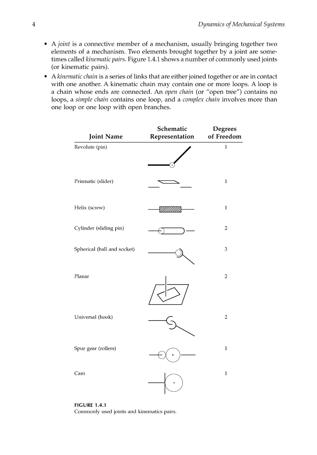
• A joint is a connective member of a mechanism, usually bringing together two
elements of a mechanism. Two elements brought together by a joint are some-
times called kinematic pairs. Figure 1.4.1 shows a number of commonly used joints
(or kinematic pairs).
• A kinematic chain is a series of links that are either joined together or are in contact
with one another. A kinematic chain may contain one or more loops. A loop is
a chain whose ends are connected. An open chain (or "open tree") contains no
loops, a simple chain contains one loop, and a complex chain involves more than
one loop or one loop with open branches.
Joint Name
Schematic
Representation
Degrees
of Freedom
Revolute (pin)
1
Prismatic (slider)
1
Helix (screw)
1
Cylinder (sliding pin)
2
Spherical (ball and socket)
3
Planar
2
Universal (hook)
2
Spur gear (rollers)
1
Cam
1
FIGURE 1.4.1
Commonly used joints and kinematics pairs.
Introduction
5
1.5 Vector Review
Because vectors are used extensively in the text,
it is helpful to review a few of their fundamental
concepts. We will expand this review in Chapter
2. Mathematically, a vector may be defined as an
element of a vector space (see, for example, Ref-
erences 1.1 to 1.3). For our purposes, we may think
of a vector simply as a directed line segment.
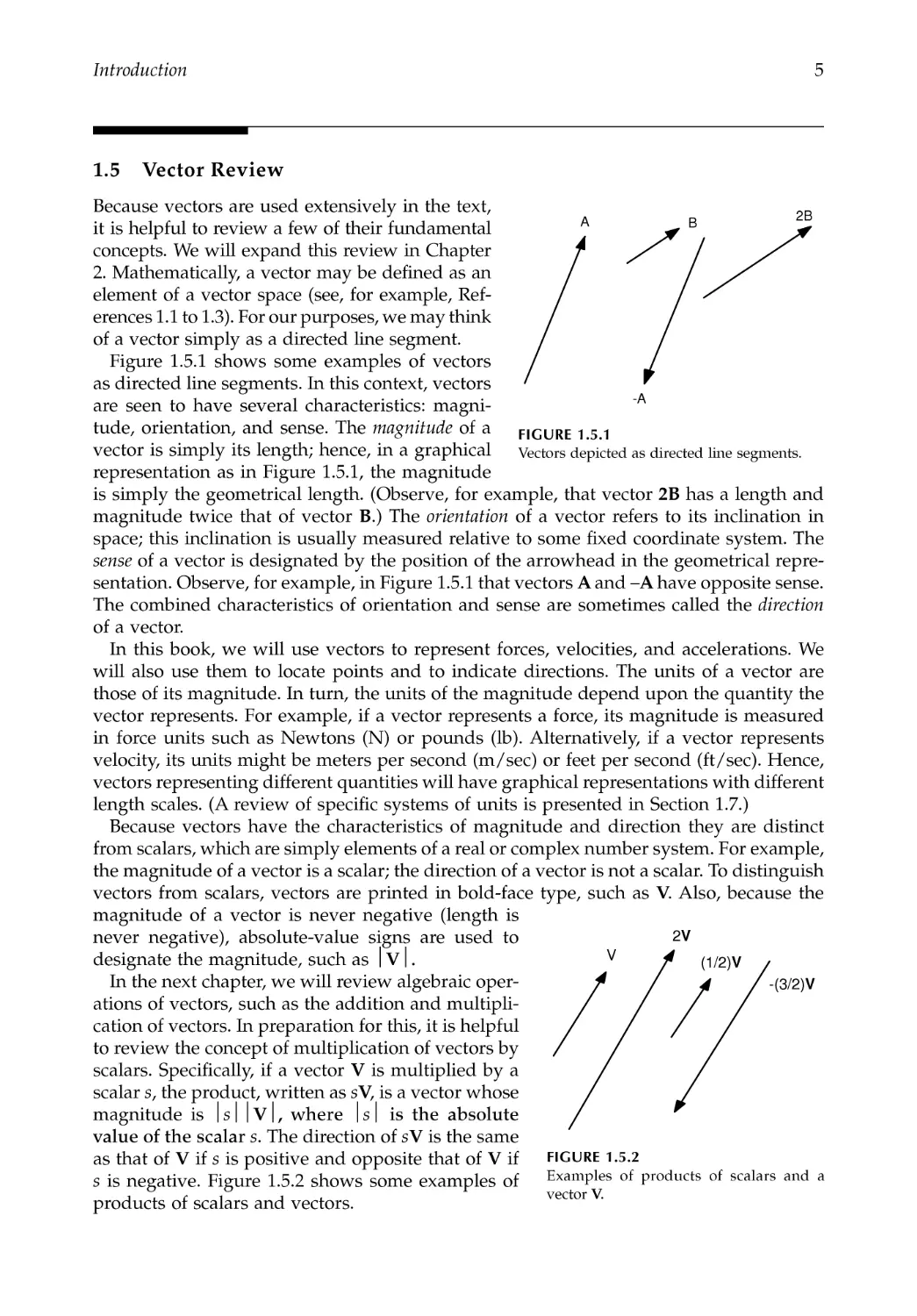
Figure 1.5.1 shows some examples of vectors
as directed line segments. In this context, vectors
are seen to have several characteristics: magni-
tude, orientation, and sense. The magnitude of a
vector is simply its length; hence, in a graphical
representation as in Figure 1.5.1, the magnitude
is simply the geometrical length. (Observe, for example, that vector 2B has a length and
magnitude twice that of vector B.) The orientation of a vector refers to its inclination in
space; this inclination is usually measured relative to some fixed coordinate system. The
sense of a vector is designated by the position of the arrowhead in the geometrical repre-
sentation. Observe, for example, in Figure 1.5.1 that vectors A and --A have opposite sense.
The combined characteristics of orientation and sense are sometimes called the direction
of a vector.
In this book, we will use vectors to represent forces, velocities, and accelerations. We
will also use them to locate points and to indicate directions. The units of a vector are
those of its magnitude. In turn, the units of the magnitude depend upon the quantity the
vector represents. For example, if a vector represents a force, its magnitude is measured
in force units such as Newtons (N) or pounds (lb). Alternatively, if a vector represents
velocity, its units might be meters per second (m/sec) or feet per second (ft/sec). Hence,
vectors representing different quantities will have graphical representations with different
length scales. (A review of specific systems of units is presented in Section 1.7.)
Because vectors have the characteristics of magnitude and direction they are distinct
from scalars, which are simply elements of a real or complex number system. For example,
the magnitude of a vector is a scalar; the direction of a vector is not a scalar. To distinguish
vectors from scalars, vectors are printed in bold-face type, such as V. Also, because the
magnitude of a vector is never negative (length is
never negative), absolute-value signs are used to
designate the magnitude, such as V .
In the next chapter, we will review algebraic oper-
ations of vectors, such as the addition and multipli-
cation of vectors. In preparation for this, it is helpful
to review the concept of multiplication of vectors by
scalars. Specifically, if a vector V is multiplied by a
scalar s, the product, written as sV, is a vector whose
magnitude is s V , where s is the absolute
value of the scalar s. The direction of sV is the same
as that of V if s is positive and opposite that of V if
s is negative. Figure 1.5.2 shows some examples of
products of scalars and vectors.
FIGURE 1.5.1
Vectors depicted as directed line segments.
A
B
-A
2B
FIGURE 1.5.2
Examples of products of scalars and a
vector V.
V
2V (1/2)V -(3/2)V
6
Dynamics of Mechanical Systems
Two kinds of vectors occur so frequently that they deserve special attention: zero vectors
and unit vectors. A zero vector is simply a vector with magnitude zero. A unit vector is a
vector with magnitude one; unit vectors have no dimensions or units.
Zero vectors are useful in equations involving vectors. Unit vectors are useful for
separating the characteristics of vectors. That is, every vector V may be expressed as the
product of a scalar and a unit vector. In such a product, the scalar represents the magnitude
of the vector and the unit vector represents the direction. Specifically, if V is written as:
(1.5.1)
where s is a scalar and n is a unit vector, then s and n are:
(1.5.2)
This means that given any non-zero vector V we can always find a unit vector n with the
same direction as V; thus, n represents the direction of V.
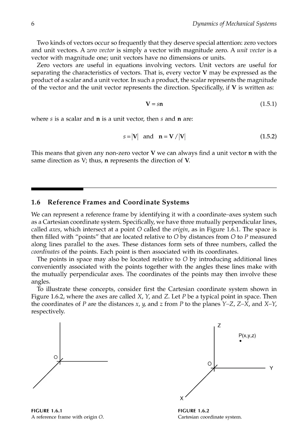
1.6 Reference Frames and Coordinate Systems
We can represent a reference frame by identifying it with a coordinate--axes system such
as a Cartesian coordinate system. Specifically, we have three mutually perpendicular lines,
called axes, which intersect at a point O called the origin, as in Figure 1.6.1. The space is
then filled with "points" that are located relative to O by distances from O to P measured
along lines parallel to the axes. These distances form sets of three numbers, called the
coordinates of the points. Each point is then associated with its coordinates.
The points in space may also be located relative to O by introducing additional lines
conveniently associated with the points together with the angles these lines make with
the mutually perpendicular axes. The coordinates of the points may then involve these
angles.
To illustrate these concepts, consider first the Cartesian coordinate system shown in
Figure 1.6.2, where the axes are called X, Y, and Z. Let P be a typical point in space. Then
the coordinates of P are the distances x, y, and z from P to the planes Y--Z, Z--X, and X--Y,
respectively.
FIGURE 1.6.1
A reference frame with origin O.
FIGURE 1.6.2
Cartesian coordinate system.
Vn
=s
s==
Vn
V
V
and
/
O
O
Z
Y
X
P(x,y,z)
Introduction
7
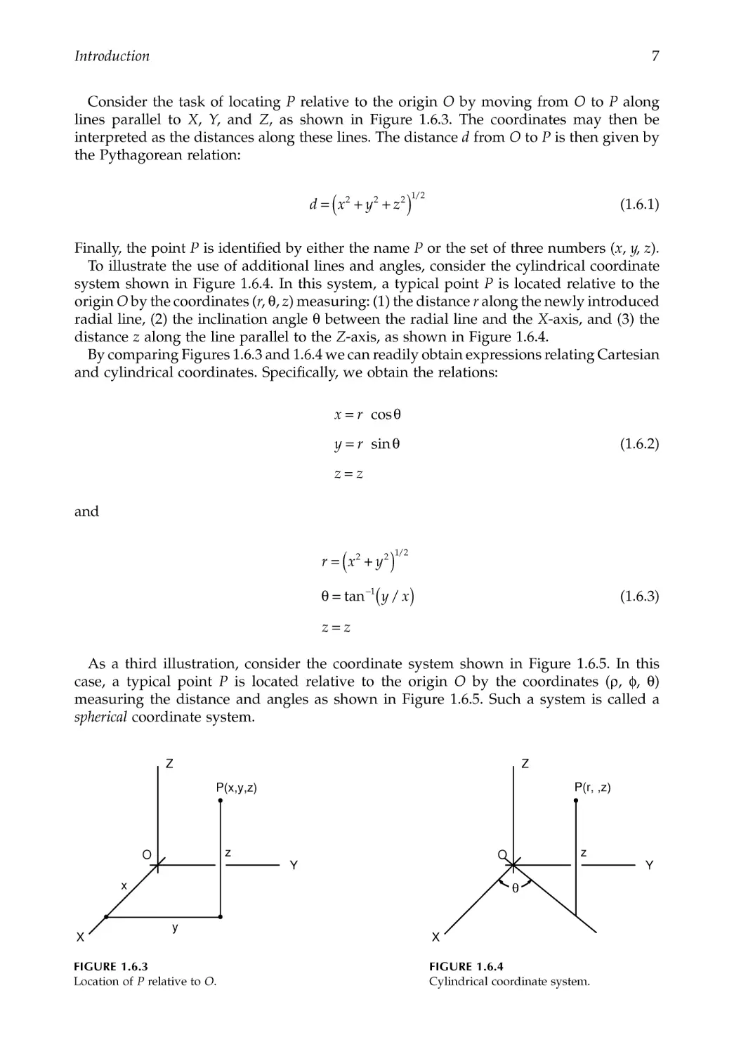
Consider the task of locating P relative to the origin O by moving from O to P along
lines parallel to X, Y, and Z, as shown in Figure 1.6.3. The coordinates may then be
interpreted as the distances along these lines. The distance d from O to P is then given by
the Pythagorean relation:
(1.6.1)
Finally, the point P is identified by either the name P or the set of three numbers (x, y, z).
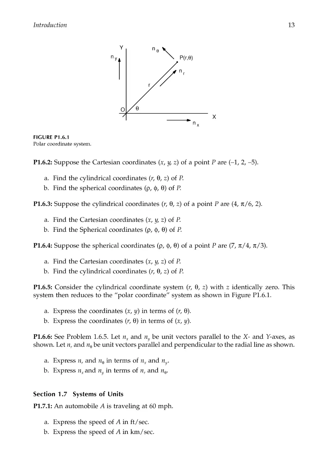
To illustrate the use of additional lines and angles, consider the cylindrical coordinate
system shown in Figure 1.6.4. In this system, a typical point P is located relative to the
origin O by the coordinates (r, θ, z) measuring: (1) the distance r along the newly introduced
radial line, (2) the inclination angle θ between the radial line and the X-axis, and (3) the
distance z along the line parallel to the Z-axis, as shown in Figure 1.6.4.
By comparing Figures 1.6.3 and 1.6.4 we can readily obtain expressions relating Cartesian
and cylindrical coordinates. Specifically, we obtain the relations:
(1.6.2)
and
(1.6.3)
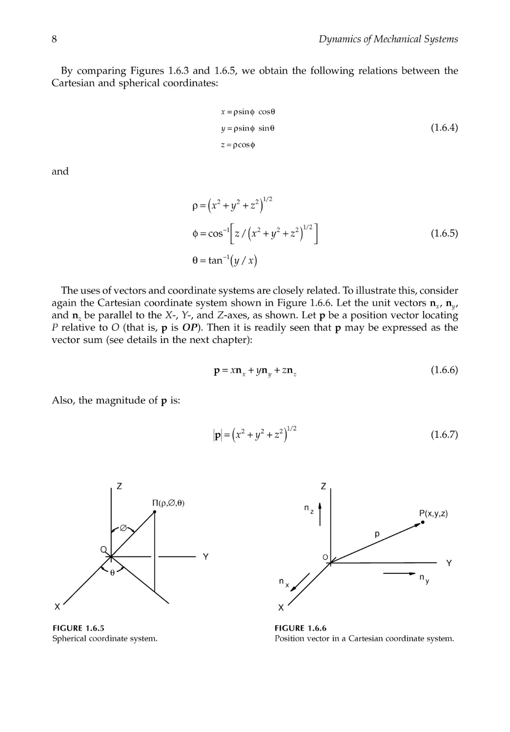
As a third illustration, consider the coordinate system shown in Figure 1.6.5. In this
case, a typical point P is located relative to the origin O by the coordinates (ρ, φ, θ)
measuring the distance and angles as shown in Figure 1.6.5. Such a system is called a
spherical coordinate system.
FIGURE 1.6.3
Location of P relative to O.
FIGURE 1.6.4
Cylindrical coordinate system.
dxyz
=++
()
222
12
/
xr
yr
zz
=
=
=
cos
sin
θ
θ
rxy
yx
zz
=+
()
=()
=
-
22
12
1
/
tan /
θ
O
Z
Y
X
P(x,y,z)
z
y
x
O
Z
Y
X
z
P(r, ,z)
θ
8
Dynamics of Mechanical Systems
By comparing Figures 1.6.3 and 1.6.5, we obtain the following relations between the
Cartesian and spherical coordinates:
(1.6.4)
and
(1.6.5)
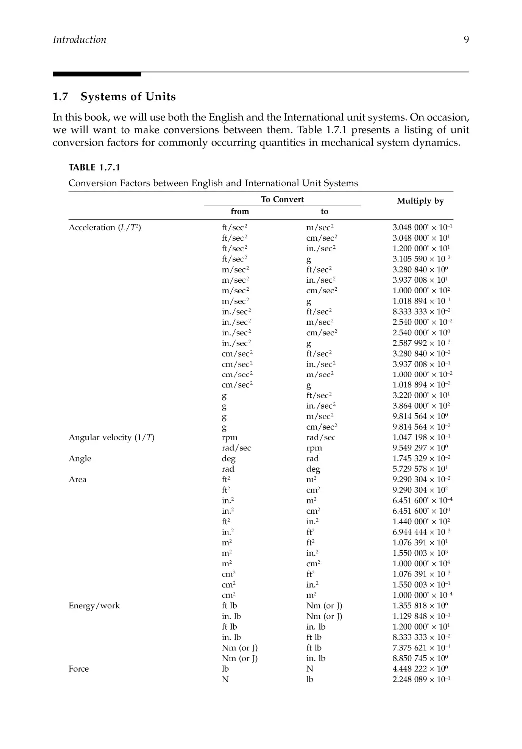
The uses of vectors and coordinate systems are closely related. To illustrate this, consider
again the Cartesian coordinate system shown in Figure 1.6.6. Let the unit vectors nx , ny,
and nz be parallel to the X-, Y- , and Z-axes, as shown. Let p be a position vector locating
P relative to O (that is, p is OP). Then it is readily seen that p may be expressed as the
vector sum (see details in the next chapter):
(1.6.6)
Also, the magnitude of p is:
(1.6.7)
FIGURE 1.6.5
Spherical coordinate system.
FIGURE 1.6.6
Position vector in a Cartesian coordinate system.
x
y
z
=
=
=
ρφθ
ρφθ
ρφ
sin cos
sin sin
cos
ρ
φ
θ
=++
()
=+
+
()
=()
-
-
xyz
zxyz
yx
222
12
12
2
2
12
1
/
/
cos /
tan /
pnnn
=++
xyz
xyz
p =++
()
xyz
222
12
/
O
Z
Y
X
θ
Π(ρ,∅,θ)
∅
Z
X
Y
p
n
P(x,y,z)
n
n
z
y
x
O
Introduction
9
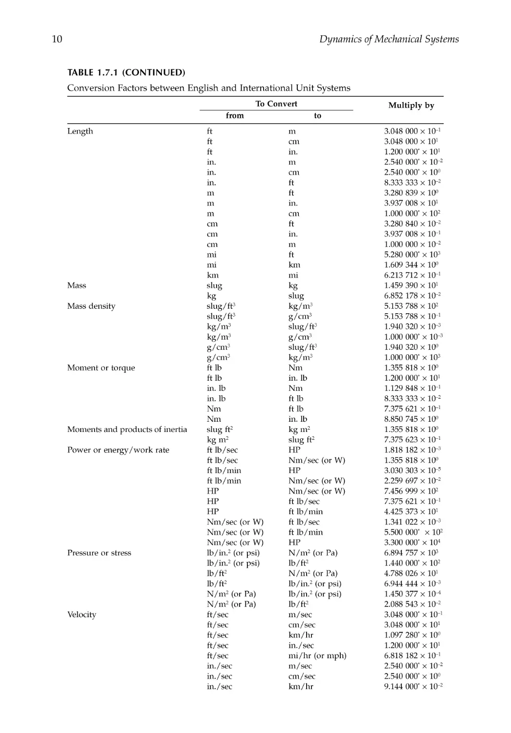
1.7 Systems of Units
In this book, we will use both the English and the International unit systems. On occasion,
we will want to make conversions between them. Table 1.7.1 presents a listing of unit
conversion factors for commonly occurring quantities in mechanical system dynamics.
TABLE 1.7.1
Conversion Factors between English and International Unit Systems
To Convert
Multiply by
from
to
Acceleration (L/T2)
ft/sec 2
m/sec 2
3.048 000* × 10--1
ft/sec 2
cm/sec 2
3.048 000* × 101
ft/sec 2
in./sec 2
1.200 000* × 101
ft/sec 2
g
3.105 590 × 10--2
m/sec 2
ft/sec 2
3.280 840 × 100
m/sec 2
in./sec 2
3.937 008 × 101
m/sec 2
cm/sec 2
1.000 000* × 102
m/sec 2
g
1.018 894 × 10--1
in./sec 2
ft/sec 2
8.333 333 × 10--2
in./sec 2
m/sec 2
2.540 000* × 10--2
in./sec 2
cm/sec 2
2.540 000* × 100
in./sec 2
g
2.587 992 × 10--3
cm/sec 2
ft/sec 2
3.280 840 × 10--2
cm/sec 2
in./sec 2
3.937 008 × 10--1
cm/sec 2
m/sec 2
1.000 000* × 10--2
cm/sec 2
g
1.018 894 × 10--3
g
ft/sec 2
3.220 000* × 101
g
in./sec 2
3.864 000* × 102
g
m/sec 2
9.814 564 × 100
g
cm/sec 2
9.814 564 × 10--2
Angular velocity (1/T)
rpm
rad/sec
1.047 198 × 10--1
rad/sec
rpm
9.549 297 × 100
Angle
deg
rad
1.745 329 × 10--2
rad
deg
5.729 578 × 101
Area
ft2
m2
9.290 304 × 10--2
ft2
cm2
9.290 304 × 102
in.2
m2
6.451 600* × 10--4
in.2
cm2
6.451 600* × 100
ft2
in.2
1.440 000* × 102
in.2
ft2
6.944 444 × 10--3
m2
ft2
1.076 391 × 101
m2
in.2
1.550 003 × 103
m2
cm2
1.000 000* × 104
cm2
ft2
1.076 391 × 10--3
cm2
in.2
1.550 003 × 10--1
cm2
m2
1.000 000* × 10--4
Energy/work
ft lb
Nm (or J)
1.355 818 × 100
in. lb
Nm (or J)
1.129 848 × 10--1
ft lb
in. lb
1.200 000* × 101
in. lb
ft lb
8.333 333 × 10--2
Nm (or J)
ft lb
7.375 621 × 10--1
Nm (or J)
in. lb
8.850 745 × 100
Force
lb
N
4.448 222 × 100
N
lb
2.248 089 × 10--1
10
Dynamics of Mechanical Systems
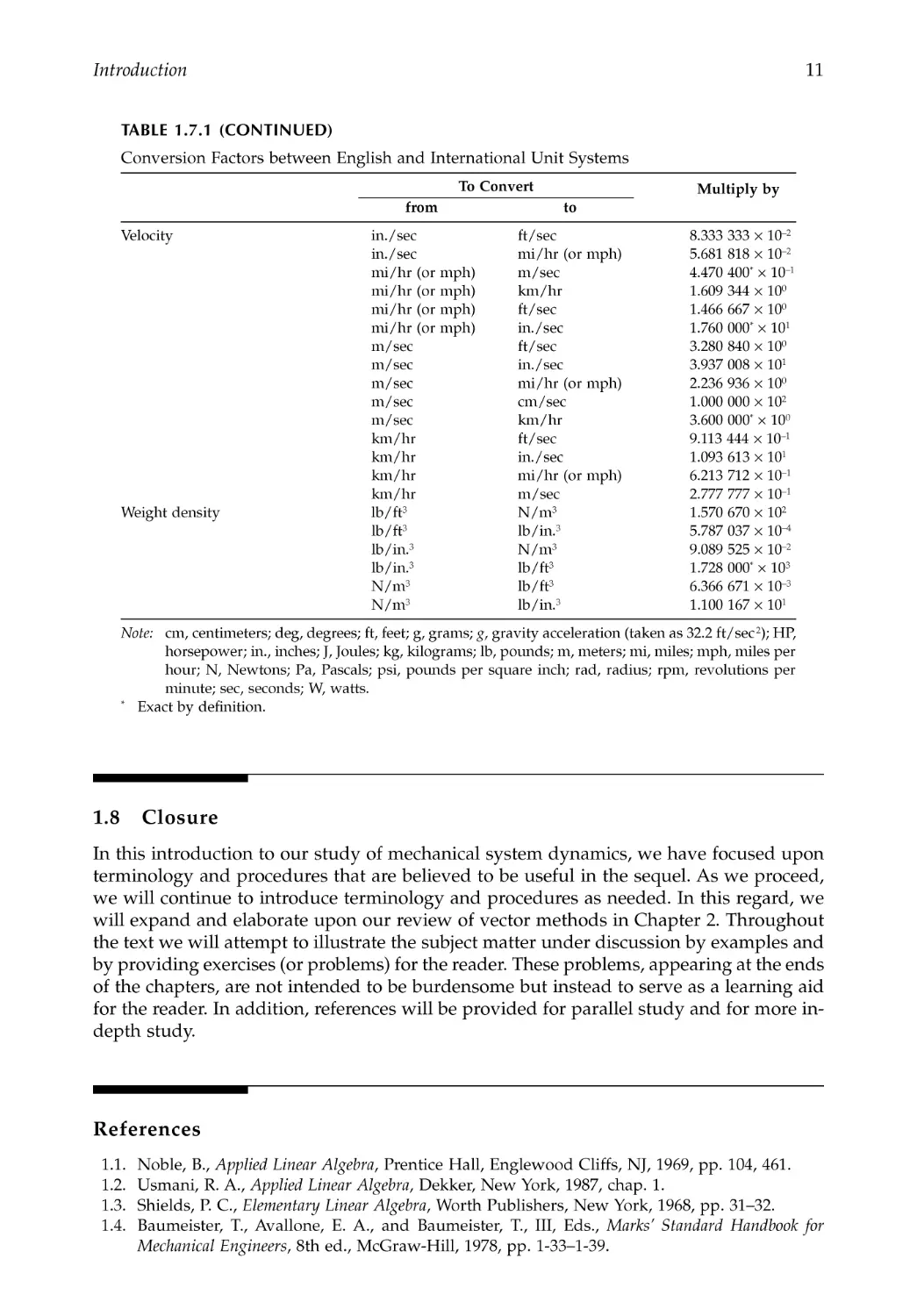
TABLE 1.7.1 (CONTINUED)
Conversion Factors between English and International Unit Systems
To Convert
Multiply by
from
to
Length
ft
m
3.048 000 × 10--1
ft
cm
3.048 000 × 101
ft
in.
1.200 000* × 101
in.
m
2.540 000* × 10--2
in.
cm
2.540 000* × 100
in.
ft
8.333 333 × 10--2
m
ft
3.280 839 × 100
m
in.
3.937 008 × 101
m
cm
1.000 000* × 102
cm
ft
3.280 840 × 10--2
cm
in.
3.937 008 × 10--1
cm
m
1.000 000 × 10--2
mi
ft
5.280 000* × 103
mi
km
1.609 344 × 100
km
mi
6.213 712 × 10--1
Mass
slug
kg
1.459 390 × 101
kg
slug
6.852 178 × 10--2
Mass density
slug/ft3
kg/m3
5.153 788 × 102
slug/ft3
g/cm3
5.153 788 × 10--1
kg/m3
slug/ft3
1.940 320 × 10--3
kg/m3
g/cm3
1.000 000* × 10--3
g/cm3
slug/ft3
1.940 320 × 100
g/cm3
kg/m3
1.000 000* × 103
Moment or torque
ft lb
Nm
1.355 818 × 100
ft lb
in. lb
1.200 000* × 101
in. lb
Nm
1.129 848 × 10--1
in. lb
ft lb
8.333 333 × 10--2
Nm
ft lb
7.375 621 × 10--1
Nm
in. lb
8.850 745 × 100
Moments and products of inertia
slug ft2
kg m2
1.355 818 × 100
kg m2
slug ft2
7.375 623 × 10--1
Power or energy/work rate
ft lb/sec
HP
1.818 182 × 10--3
ft lb/sec
Nm/sec (or W)
1.355 818 × 100
ft lb/min
HP
3.030 303 × 10--5
ft lb/min
Nm/sec (or W)
2.259 697 × 10--2
HP
Nm/sec (or W)
7.456 999 × 102
HP
ft lb/sec
7.375 621 × 10--1
HP
ft lb/min
4.425 373 × 101
Nm/sec (or W) ft lb/sec
1.341 022 × 10--3
Nm/sec (or W) ft lb/min
5.500 000* × 102
Nm/sec (or W) HP
3.300 000* × 104
Pressure or stress
lb/in.2 (or psi) N/m2 (or Pa)
6.894 757 × 103
lb/in.2 (or psi) lb/ft2
1.440 000* × 102
lb/ft2
N/m2 (or Pa)
4.788 026 × 101
lb/ft2
lb/in.2 (or psi)
6.944 444 × 10--3
N/m2 (or Pa)
lb/in.2 (or psi)
1.450 377 × 10--4
N/m2 (or Pa)
lb/ft2
2.088 543 × 10--2
Velocity
ft/sec
m/sec
3.048 000* × 10--1
ft/sec
cm/sec
3.048 000* × 101
ft/sec
km/hr
1.097 280* × 100
ft/sec
in./sec
1.200 000* × 101
ft/sec
mi/hr (or mph)
6.818 182 × 10--1
in./sec
m/sec
2.540 000* × 10--2
in./sec
cm/sec
2.540 000* × 100
in./sec
km/hr
9.144 000* × 10--2
Introduction
11
1.8 Closure
In this introduction to our study of mechanical system dynamics, we have focused upon
terminology and procedures that are believed to be useful in the sequel. As we proceed,
we will continue to introduce terminology and procedures as needed. In this regard, we
will expand and elaborate upon our review of vector methods in Chapter 2. Throughout
the text we will attempt to illustrate the subject matter under discussion by examples and
by providing exercises (or problems) for the reader. These problems, appearing at the ends
of the chapters, are not intended to be burdensome but instead to serve as a learning aid
for the reader. In addition, references will be provided for parallel study and for more in-
depth study.
References
1.1. Noble, B., Applied Linear Algebra, Prentice Hall, Englewood Cliffs, NJ, 1969, pp. 104, 461.
1.2. Usmani, R. A., Applied Linear Algebra, Dekker, New York, 1987, chap. 1.
1.3. Shields, P. C., Elementary Linear Algebra, Worth Publishers, New York, 1968, pp. 31--32.
1.4. Baumeister, T., Avallone, E. A., and Baumeister, T., III, Eds., Marks' Standard Handbook for
Mechanical Engineers, 8th ed., McGraw-Hill, 1978, pp. 1-33--1-39.
TABLE 1.7.1 (CONTINUED)
Conversion Factors between English and International Unit Systems
To Convert
Multiply by
from
to
Velocity
in./sec
ft/sec
8.333 333 × 10--2
in./sec
mi/hr (or mph)
5.681 818 × 10--2
mi/hr (or mph) m/sec
4.470 400* × 10--1
mi/hr (or mph) km/hr
1.609 344 × 100
mi/hr (or mph) ft/sec
1.466 667 × 100
mi/hr (or mph) in./sec
1.760 000* × 101
m/sec
ft/sec
3.280 840 × 100
m/sec
in./sec
3.937 008 × 101
m/sec
mi/hr (or mph)
2.236 936 × 100
m/sec
cm/sec
1.000 000 × 102
m/sec
km/hr
3.600 000* × 100
km/hr
ft/sec
9.113 444 × 10--1
km/hr
in./sec
1.093 613 × 101
km/hr
mi/hr (or mph)
6.213 712 × 10--1
km/hr
m/sec
2.777 777 × 10--1
Weight density
lb/ft3
N/m3
1.570 670 × 102
lb/ft3
lb/in.3
5.787 037 × 10--4
lb/in.3
N/m3
9.089 525 × 10--2
lb/in.3
lb/ft3
1.728 000* × 103
N/m3
lb/ft3
6.366 671 × 10--3
N/m3
lb/in.3
1.100 167 × 101
Note: cm, centimeters; deg, degrees; ft, feet; g, grams; g, gravity acceleration (taken as 32.2 ft/sec 2); HP,
horsepower; in., inches; J, Joules; kg, kilograms; lb, pounds; m, meters; mi, miles; mph, miles per
hour; N, Newtons; Pa, Pascals; psi, pounds per square inch; rad, radius; rpm, revolutions per
minute; sec, seconds; W, watts.
* Exact by definition.
12
Dynamics of Mechanical Systems
1.5. Hsu, H. P., Vector Analysis, Simon & Schuster Technical Outlines, New York, 1969.
1.6. Brand, L., Vector and Tensor Analysis, Wiley, New York, 1964.
1.7. Kane, T. R., Analytical Elements of Mechanics, Vol. 2, Academic Press, New York, 1961.
1.8. Kane, T. R., and Levinson, D. A., Dynamics: Theory and Applications, McGraw-Hill, New York,
1985, pp. 361--371.
1.9. Likins, P. W., Elements of Engineering Mechanics, McGraw-Hill, New York, 1973.
1.10. Beer, F. P., and Johnston, E. R., Jr., Vector Mechanics for Engineers, 6th ed., McGraw-Hill, New
York, 1996.
1.11. Yeh, H., and Abrams, J. I., Principles of Mechanics of Solids and Fluids, Vol. 1, Particle and Rigid-
Body Mechanics, McGraw-Hill, New York, 1960.
1.12. Haug, E. J., Intermediate Dynamics, Prentice Hall, Englewood Cliffs, NJ, 1992.
1.13. Meriam, J. L., and Kraige, L. G., Engineering Mechanics, Vol. 2, Dynamics, 3rd ed., John Wiley
& Sons, New York, 1992.
1.14. Hibbler, R. C., Engineering Mechanics: Statics and Dynamics, Macmillan, New York, 1974.
1.15. Shelley, J. P., Vector Mechanics for Engineers, Vol. II, Dynamics, Schaum's Solved Problems Series,
McGraw-Hill, New York, 1991.
1.16. Jong, I. C., and Rogers, B. G., Engineering Mechanics, Statics and Dynamics, Saunders College
Publishing, Holt, Rinehart & Winston, Philadelphia, PA, 1991.
1.17. Huston, R. L., Multibody Dynamics, Butterworth--Heinemann, Stoneham, MA, 1990.
1.18. Higdon, A., and Stiles, W. B., Engineering Mechanics, Vol. II, Dynamics, 3rd ed., Prentice Hall,
Englewood Cliffs, NJ, 1968.
1.19. Meirovitch, L., Methods of Analytical Dynamics, McGraw-Hill, New York, 1970.
1.20. Paul, B., Kinematics and Dynamics of Planar Machinery, Prentice Hall, Englewood Cliffs, NJ, 1979.
1.21. Sneck, H. J., Machine Dynamics, Prentice Hall, Englewood Cliffs, NJ, 1991.
1.22. Mabie, H. H., and Reinholtz, C. F., Mechanisms and Dynamics of Machinery, 4th ed., Wiley, New
York, 1987.
1.23. Ginsberg, J. H., Advanced Engineering Dynamics, Harper & Row, New York, 1988.
1.24. Shames, I. H., Engineering Mechanics, Prentice Hall, Englewood Cliffs, NJ, 1980.
1.25. Liu, C. Q., and Huston, R. L., Formulas for Dynamic Analyses, Marcel Dekker, New York, 1999.
Problems
Section 1.5 Vector Review
P1.5.1: Suppose a velocity vector V is expressed in the form:
where i, j, and k are mutually perpendicular unit vectors.
a. Determine the magnitude of V.
b. Find a unit vector n parallel to V and having the same sense as V.
Section 1.6 Reference Frames and Coordinate Systems
P1.6.1: Suppose the Cartesian coordinates (x, y, z) of a point P are (3, 1, 4).
a. Find the cylindrical coordinates (r, θ, z) of P.
b. Find the spherical coordinates (ρ, φ, θ) of P.
Vij k
=++
3412ftsec
Introduction
13
P1.6.2: Suppose the Cartesian coordinates (x, y, z) of a point P are (--1, 2, --5).
a. Find the cylindrical coordinates (r, θ, z) of P.
b. Find the spherical coordinates (ρ, φ, θ) of P.
P1.6.3: Suppose the cylindrical coordinates (r, θ, z) of a point P are (4, π/6, 2).
a. Find the Cartesian coordinates (x, y, z) of P.
b. Find the Spherical coordinates (ρ, φ, θ) of P.
P1.6.4: Suppose the spherical coordinates (ρ, φ, θ) of a point P are (7, π/4, π/3).
a. Find the Cartesian coordinates (x, y, z) of P.
b. Find the cylindrical coordinates (r, θ, z) of P.
P1.6.5: Consider the cylindrical coordinate system (r, θ, z) with z identically zero. This
system then reduces to the "polar coordinate" system as shown in Figure P1.6.1.
a. Express the coordinates (x, y) in terms of (r, θ).
b. Express the coordinates (r, θ) in terms of (x, y).
P1.6.6: See Problem 1.6.5. Let nx and ny be unit vectors parallel to the X- and Y-axes, as
shown. Let nr and nθ be unit vectors parallel and perpendicular to the radial line as shown.
a. Express nr and nθ in terms of nx and ny.
b. Express nx and ny in terms of nr and nθ.
Section 1.7 Systems of Units
P1.7.1: An automobile A is traveling at 60 mph.
a. Express the speed of A in ft/sec.
b. Express the speed of A in km/sec.
FIGURE P1.6.1
Polar coordinate system.
O
r
Y
X
P(r,θ)
n
n
n
n
y
x
r
θ
θ
14
Dynamics of Mechanical Systems
P1.7.2: A person weighs 150 lb.
a. What is the person's weight in N?
b. What is the person's mass in slug?
c. What is the person's mass in kg?
P1.7.3: An automobile A accelerates from a stop at 3 mph/sec.
a. Express the acceleration in ft/sec2.
b. Express the acceleration in m/sec2.
c. Express the acceleration in g.
15
2Review of Vector Algebra
2.1 Introduction
In Chapter 1, we reviewed the basic concepts of vectors. We considered vectors, scalars,
and the multiplication of vectors and scalars. We also examined zero vectors and unit
vectors. In this chapter, we will build upon these ideas as we develop a review of vector
algebra. Specifically, we will review the concepts of vector equality, vector addition, and
vector multiplication. We will also review the concepts of reference frames and unit vector
sets. Finally, we will review the elementary procedures of matrix algebra.
2.2 Equality of Vectors, Fixed and Free Vectors
Recall that the characteristics of a vector are its magnitude, its orientation, and its sense.
Indeed, we could say that a vector is defined by its characteristics. The concept of vector
equality follows from this definition: Specifically, two vectors are equal if (and only if)
they have the same characteristics. Vector equality is fundamental to the development of
vector algebra. For example, if vectors are equal, they may be interchanged in vector
equations, which enables us to simplify expressions. It should be noted, however, that
vector equality does not necessarily denote physical equality, particularly when the vec-
tors model physical quantities. This occurs, for example, with forces. We will explore this
concept later.
Two fundamental ideas useful in relating mathematical and physical quantities are the
concepts of fixed and free vectors. A fixed vector has its location restricted to a line fixed
in space. To illustrate this, consider the fixed line L as shown in Figure 2.2.1. Let v be a
vector whose location is restricted to L, and let the location of v along L be arbitrary. Then
v is a fixed vector. Because the location of v along L is arbitrary, v might even be called a
sliding vector.
Alternatively, a free vector is a vector that may be placed anywhere in space if its
characteristics are maintained. Unit vectors such as nx, ny, and nz shown in Figure 2.2.1
are examples of free vectors. Most vectors in our analyses will be free vectors. Indeed, we
will assume that vectors are free vectors unless otherwise stated.
16
Dynamics of Mechanical Systems
2.3 Vector Addition
Vectors obey the parallelogram law of addition. This is a simple geometric algorithm for
understanding and exhibiting the powerful analytical utility of vectors. To see this, con-
sider two vectors A and B as in Figure 2.3.1. Let A and B be free vectors. To add A and
B, let them be connected "head-to-tail" (without changing their characteristics) as in Figure
2.3.2. That is, relocate B so that its tail is at the head of A. Then, the sum of A and B, called
the resultant, is the vector R connecting the tail of A to the head of B, as in Figure 2.3.3.
That is,
(2.3.1)
The vectors A and B are called the components of R.
The reason for the name "parallelogram law" is that the same result is obtained if the
head of B is connected to the tail of A, as in Figure 2.3.4. The two ways of adding A and
B produce a parallelogram, as shown. The order of the addition --- that is, which vector
is taken first and which is taken second --- is therefore unimportant; hence, vector addition
is commutative. That is,
(2.3.2)
FIGURE 2.2.1
A fixed line L and a fixed vector V.
FIGURE 2.3.1
Two vectors A and B to be added.
FIGURE 2.3.2
Vectors A and B connected head to tail.
O
Y
L
Z
X
n
n
n
z
y
x
V
RAB
=+
ABBA
+=+
A
B
A
B
Review of Vector Algebra
17
Vector subtraction may be defined from vector addition. Specifically, the difference of
two vectors A and B, written as A -- B, is simply the sum of A with the negative of B. That is,
(2.3.3)
An item of interest in vector addition is the magnitude of the resultant, which may be
determined using the geometry of the parallelogram and the law of cosines. For example,
in Figure 2.3.5, let θ be the angle between A and B, as shown. Then, the magnitude of the
resultant R is given by:
(2.3.4)
Example 2.3.1: Resultant Magnitude
To illustrate the use of Eq. (2.3.4), suppose the magnitude of A is 15 N, the magnitude of
B is 12 N, and the angle θ between A and B is 60˚. Then, the magnitude of the resultant R is:
(2.3.5)
Observe from Eq. (2.3.4) that if we double the magnitude of both A and B, the magnitude
of the resultant R is also doubled. Indeed, if we multiply A and B by any scalar s, R will
also be multiplied by s. That is,
(2.3.6)
This means that vector addition is distributive with respect to scalar multiplication.
Next, suppose we have three vectors A, B, and C, and suppose we wish to find their
resultant. Suppose further that the vectors are not parallel to the same plane, as, for
example, in Figure 2.3.6. The resultant R is obtained in the same manner as before. That
is, the vectors are connected head to tail, as depicted in Figure 2.3.7. Then, the resultant
R is obtained by connecting the tail of the first vector A to the head of the third vector C
as in Figure 2.3.7. That is,
(2.3.7)
FIGURE 2.3.3
Resultant (sum) R of vectors A
and B.
FIGURE 2.3.4
Two ways of adding vectors A
and B.
FIGURE 2.3.5
Vector triangle geometry.
Α
ΑΒ
Β
-=+
-
()
AB
RAB AB
=+-+ -
()
22
2
cos πθ
R =()+()-()( )( ) ()=
15 12 21512 23 2343
22
12
cos
.
/
π
N
ssss
ABR AB
+==+
()
RABC
=++
A
B
R
A
B
A
B
R
A
B
R
θ
18
Dynamics of Mechanical Systems
Example 2.3.2: Resultant Magnitude in Three Dimensions
As an illustration, suppose C is perpendicular to the plane of vectors A and B of Example
2.3.1 and suppose the magnitude of C is 10 N. Then, from the results of Eq. (2.3.5), the
magnitude of R is:
(2.3.8)
This procedure has several remarkable features. First, as before, the order of the compo-
nents in Eq. (2.3.7) is unimportant. That is,
(2.3.9)
Second, to obtain the resultant R we may first add any two of the vectors, say A and B,
and then add the resultant of this sum to C. This means the summation in Eq. (2.3.7) is
associative. That is,
(2.3.10)
This feature may be used to obtain the magnitude of the resultant by repeated use of the
law of cosines as before.
Third, observe that configurations exist where the magnitude of the resultant is less
than the magnitude of the individual components. Indeed, the magnitude of the resultant
could be zero.
Finally, with three or more components, the procedure of finding the magnitude of the
resultant by repeated use of the law of cosines is cumbersome and tedious.
An attractive feature of vector addition is that the resultant magnitude may be obtained
by strictly analytical means --- that is, without regard to triangle geometry. This is the
original reason for using vectors in analysis. We will explore this further in the next section.
FIGURE 2.3.6
Vectors A, B, and C to be added.
FIGURE 2.3.7
Resultant of vectors A, B, and C of Figure 2.3.6.
Z
Y
X
C
A
B
Z
Y
X
C
A
B
R
R=()
+()
[]
=
2343 10
25 47
22
12
..
/
N
ABCCABBCA
ACBBAC CBA R
++=++=++
=++=++=++=
RABC ABCA BC
=++= +
()
+=+ +
()
Review of Vector Algebra
19
2.4 Vector Components
Consider again Eq. (2.3.7) where we have the vector sum:
(2.4.1)
Instead of thinking of this expression as a sum of components, consider it as a represen-
tation of the vector R. Suppose further that the components A, B, and C happen to be
mutually perpendicular and parallel to coordinate axes, as shown in Figure 2.4.1. Then,
by the Pythagoras theorem, the magnitude of R is simply:
(2.4.2)
To develop these ideas still further, suppose that nx, ny, and nz are unit vectors parallel
to X, Y, and Z, as in Figure 2.4.2. Then, from our discussion in Chapter 1, we see that A,
B, and C can be expressed in the forms:
(2.4.3)
where a, b, and c are scalars representing the magnitudes of A, B, and C. Hence, R may
be expressed as:
(2.4.4)
FIGURE 2.4.1
Vector R with mutually perpendicular components.
FIGURE 2.4.2
Vectors A, B, and C and unit vectors nx, ny , and nz.
Z
X
Y
RC
B
A
Z
X
Y
RC
B
A
n
n
n
z
x
y
RABC
=++
RABC
=+
+
()
222
12
/
AA
nn
BB
nn
CC
nn
==
==
==
xx
yy
zz
a
b
c
Rnnn
=++
abc
xyz
20
Dynamics of Mechanical Systems
Then, the magnitude of R is:
(2.4.5)
A question that arises is what if A, B, and C are not mutually perpendicular? How then
can we find the magnitude of the resultant? A powerful feature of the vector method is
that the same general procedure can be used regardless of the directions of the components.
All that is required is to express the components as sums of vectors parallel to the X-, Y-,
and Z-axes (or other convenient mutually perpendicular directions). For example, suppose
a vector A is inclined relative to the X-, Y-, and Z-axes, as in Figure 2.4.3. Let θx, θy , and
θz be the angles that A makes with the axes. Next, let us express A in the desired form:
(2.4.6)
where Ax, Ay, and Az are vector components of A parallel to X, Y, and Z. Ax, Ay , and Az
may be considered as "projections" of A along the X-, Y-, and Z-axes. Their magnitudes
are proportional to the magnitude of A and the cosines of the angles θx, θy , and θz. That is,
(2.4.7)
where ax , ay , and az are defined as given in the equations. As before, let nx, ny , and nz be
unit vectors parallel to X, Y, and Z. Then, Ax, Ay, and Az can be expressed as:
(2.4.8)
Finally, by substituting into Eq. (2.4.6), A may be expressed in the form:
(2.4.9)
FIGURE 2.4.3
A vector A inclined relative to the
coordinate axes.
R =++
()
abc
222
12
/
AAAA
=++
xyz
AA
AA
AA
xx
x
yy
y
zz
z
a
a
a
==
==
==
cos
cos
cos
θ
θ
θ
An
An
An
An
An
An
xx
x
x
x
yy
y
y
y
zz
z
z
z
a
a
a
==
==
==
cos
cos
cos
θ
θ
θ
AnnnAnAnAn
=++=
+
+
aaa
xxyyzz
xx
yy
zz
cos
cos
cos
θθθ
Z
Y
X
θ
θ
θ
n
n
n
n
z
z
y
x
y
x
Review of Vector Algebra
21
Then, the magnitude of A is simply:
(2.4.10)
Next, suppose that n is a unit vector parallel to A, as in Figure 2.4.3. Then, by following
the same procedure as in Eq. (2.4.9), n may be expressed as:
(2.4.11)
Because the magnitude of n is 1, we then have:
(2.4.12)
Example 2.4.1: Vector Addition Using Components
To illustrate the use of these ideas, consider again the vectors of Examples 2.3.1 and 2.3.2
(see Figures 2.3.6 and 2.3.7). Specifically, let A be parallel to the Y-axis with a magnitude
of 15 N. Let B be parallel to the Y--Z plane and inclined at 60˚ relative to the Y-axis. Let
the magnitude of B be 12 N. Let C be parallel to the X-axis with a magnitude of 10 N
(Figure 2.4.4). As before let nx, ny , and nz be unit vectors parallel to the X-, Y-, and Z-axes.
Then, A, B, and C may be expressed as:
(2.4.13)
Hence, R becomes:
(2.4.14)
Then, the magnitude of R is:
(2.4.15)
This is the same result as in Example 2.3.2 (see Eq. (2.3.8)). Here, however, we obtained
the result without using the law of cosines as in Eq. (2.3.4).
Example 2.4.2: Direction Cosines
A particle P is observed to move on a curve C in a Cartesian reference frame R, as shown
in Figure 2.4.5. The coordinates of P are functions of time t. Suppose that at an instant of
interest x, y, and z have the values 8 m, 12 m, and 7 m, respectively. Determine the
orientation angles of the line of sight of an observer of P if the observer is at the origin
O. Specifically, determine the angles θx, θy, and θz of OP with the X-, Y-, and Z-axes.
A =++
()
aaa
xyz
222
12
/
nnnn
=++
cos
cos
cos
θθθ
xx
yy
zz
1 222
=++
cos
cos
cos
θθθ
xyz
An
Bnn
n
n
Cn
=
=°
+°
=
+
=
15
12601260610392
10
x
yz
y
z
x
N
N
N
cos
sin
.
RABCnn
nn
nnn
=++=++
()
+
=++
15 6 10392 10
10 21 10392
yy
zx
xyz
N
N
.
.
R = ()+()+()
[]
=
10 21 10392
25 47
22
2
12
..
/NN
22
Dynamics of Mechanical Systems
Solution: The line of sight OP may be represented by the position vector p of Figure
2.4.5. In terms of unit vectors nx, ny , and nz parallel to X, Y, and Z, p may be expressed as:
(2.4.16)
Then, the magnitude of p is:
(2.4.17)
Therefore, a unit vector n parallel to p is:
(2.4.18)
Then, from Eq. (2.4.11), the direction cosines are:
(2.4.19)
Hence, θx, θy, and θz are:
(2.4.20)
Observe that the functional representation of the coordinates x, y, and z of P as:
(2.4.21)
forms a set of parametric equations defining C.
Finally, if a vector V is expressed in the form:
(2.4.22)
FIGURE 2.4.4
The system of Figure 2.3.6.
FIGURE 2.4.5
A particle P moving in a reference frame R.
C
A
B
n
Y
X
Z
n
n
z
y
x
Z
Y
X
O
R
C
P(x,y,z)
n
n
n
z
y
x
pnnnn nn
=++=+ +
xyz
m
xyzx yz
81
27
p = ()+()+()
[]
=
8127
16 03
22
2
12
/
.m
npp n
n
n
==++
0499 0749 0437
...
xyz
cos
.
, cos
.
, cos
.
θθθ
xyz
===
0 499
0 749
0 437
θθθ
xyz
===
606
4154
6411
. deg
. deg
. deg
xx
tyy
tzz
t
=() =() =()
,
,
Vnnn
=++
vvv
xxyyzz
Review of Vector Algebra
23
where nx, ny , and nz are mutually perpendicular unit vectors, then vx, vy, and vz are called
the scalar components of V relative to nx, ny , and nz. Then, from Eq. (2.4.10), the magnitude
ofVis:
(2.4.23)
Observe that if V is zero, then V is zero, and each of the scalar components is also
zero. This is the basis for force equilibrium procedures of elementary mechanics.
2.5 Angle Between Two Vectors
The concept of the angle between two vectors is useful in developing the procedures of
vector multiplication. We already used this idea in Section 2.3 with the law of cosines (see
Figure 2.3.5). The angle between two vectors is defined as follows: Let A and B be any
nonzero vectors as in Figure 2.5.1. Let the vectors be connected tail to tail, as in Figure
2.5.2. Then the angle as shown is defined as the angle between the vectors. Observe that
θ always has values between 0 and 180˚.
2.6 Vector Multiplication: Scalar Product
Multiplying vectors can be accomplished in several ways, which we will review in this
and the following sections. Consider first the scalar product, so called because the result
is a scalar: Given any two vectors A and B, the scalar product, written as A · B, is defined as:
(2.6.1)
where θ is the angle between A and B (see Section 2.5.1). Because a dot is placed between
the vectors, the operation is often called the dot product.
Observe in the definition of Eq. (2.6.1) that, if we interchange the positions of A and B,
the result remains the same. That is,
(2.6.2)
Hence, the scalar product is commutative.
Consider some special cases. First, observe that the scalar product of two perpendicular
vectors is zero, as the cosθ is zero. Next, consider the scalar product of a vector A with itself:
(2.6.3)
V =++
()
vvv
xyz
222
12
/
AB AB
⋅= cosθ
AB AB
BA
BA
⋅
===
⋅
cos
cos
θθ
AA AA
⋅= cosθ
24
Dynamics of Mechanical Systems
However, the angle that a vector makes with itself is zero (see Problem P2.5.1); hence, we
have:
(2.6.4)
where the last equality is a definition of A2.
Suppose in this last case that A is a unit vector, say n. Then,
(2.6.5)
Next, suppose that n1, n2, and n3 are mutually perpendicular unit vectors parallel to the
X-, Y-, and Z-axes as shown in Figure 2.6.1. Then, the various scalar products of these unit
vectors may be expressed as:
(2.6.6)
(2.6.7)
These results may be expressed in the compact form:
(2.6.8)
where δij is often called Kronecker 's delta function.
Next, suppose that n is a unit vector parallel to a line L and that A is a nonzero vector,
as in Figure 2.6.2. Then, A • n is:
(2.6.9)
We can interpret this result as the "projection" of A onto L. Indeed, suppose we express
A in terms of two components: one parallel to L, called A , and the other perpendicular
to L, called A⊥. Then,
(2.6.10)
FIGURE 2.5.1
Two nonzero vectors.
FIGURE 2.5.2
Vectors A and B connected tail to tail.
A
B
θ
A
B
AAAAAA
⋅=
==
2
2
nnn n
⋅===
2
21
nn
nn
nn
11
22
33
111
⋅=
⋅=
⋅=
,
,
nnnnnnnnnnnn
1221133123320
⋅=⋅=⋅=⋅=⋅=⋅=
nn
iji
jij
ij
⋅==
=
≠
δ1
0
An An
A
⋅=
=
cos
cos
θθ
AAA
=+
⊥
||
Review of Vector Algebra
25
where A is:
(2.6.11)
To further develop these components, let a vector C be the resultant (sum) of vectors A
and B. That is,
(2.6.12)
Let L be a line passing through the tail O of C, as in Figure 2.6.3, and let n be a unit vector
parallel to L. Let A and B be the projection points of the heads of A and B onto L, as
shown. Then, from Eq. (2.6.9), the lengths of the line segments OA, AB, and OB may be
expressed as:
(2.6.13)
However, from Figure 2.6.3, we see that:
(2.6.14)
Hence,
(2.6.15)
Therefore, from Eq. (2.6.12), we have the distributive law:
(2.6.16)
Continuing in this manner, suppose s is a scalar. Then, from the definition of Eq. (2.6.1),
we have:
(2.6.17)
FIGURE 2.6.1
Mutually perpendicular unit vectors.
FIGURE 2.6.2
Vector A, line L, and unit vector n.
n
Y
X
Z
n
n
z
y
x
A
L
θ
n
AA
n
nAn
||
cos
=⋅
()
=()
θ
CAB
=+
OA
AB
OB
=⋅
=⋅
=⋅
nA
n
nC
Β
OBOAAB
=+
nCnAnB
⋅=⋅+⋅
nAB nAnB
⋅+
()
=⋅ +⋅
ss sss
AB ABABABAB
⋅=()
⋅+ ⋅()=⋅ =⋅
26
Dynamics of Mechanical Systems
That is, the scalar may be placed anywhere in the product. The parentheses are unneces-
sary. The dot, however, must remain between the vectors.
Next, suppose nx, ny, and nz are mutually perpendicular unit vectors parallel to X-, Y-,
and Z-axes, and suppose V is a nonzero vector, as in Figure 2.6.4. Let θx, θy, and θz be the
angles between V and the X-, Y-, and Z-axes. Then, the projections of V onto X, Y, and Z are:
(2.6.18)
Then, from Eq. (2.6.11), if Vx, Vy, and Vz are mutually perpendicular components of V
parallel to X, Y, and Z, we can express Vx, Vy, and Vz as:
(2.6.19)
Then, we also may express V as:
(2.6.20)
where Vx, Vy, and Vz are the scalar components of V along X, Y, and Z.
As a final example, suppose n1, n2, and n3 are mutually perpendicular unit vectors, and
suppose A and B can be expressed as:
(2.6.21)
(2.6.22)
Then, by using Eqs. (2.6.8), (2.6.16), and (2.6.17), we can express A · B as:
(2.6.23)
FIGURE 2.6.3
A vector sum projected onto a line L.
A
A
B
B
C
L
O
VnV
VnV
VnV
⋅=
⋅=
⋅=
xx
yy
zz
cos
cos
cos
θθθ
VV
n
nVV
n
nVV
n
n
xx
x
yy
y
zz
z
=⋅
() =⋅
() =⋅
()
VVVVVnnVnnVnn
nnn
=++=⋅
()
+⋅
()+⋅
()
=++
xyz
x
xy
yz
z
xxyyzz
VVV
AA
nA
nA
n
=++
112233
BB
nB
nB
n
=++
112233
ABAAABBB
AB
AB
AB
AB
AB
AB
AB
AB
⋅=++
()
⋅++
()
=⋅
+⋅
+⋅
+⋅
+⋅
+⋅
+⋅
+⋅
112233112233
111112121313
212132322323
31313232
nnnnnn
nn
nn
nn
nn
nn
nn
nn
nn+⋅
=++
AB
ABABAB
333 3
112233
nn
Review of Vector Algebra
27
This result will prove to be useful in many ways. It demonstrates the analytical advantage
of vector algebra. For example, if we want to obtain the magnitude of a vector, it is simply:
(2.6.24)
Also, if we want to find the angle θ between two vectors, we have:
(2.6.25)
The application and utility of the scalar product may be further illustrated by a few
examples, as in the following paragraphs.
Example 2.6.1: Scalar Product Definition
Consider the vectors A and B, shown in Figure 2.6.5. Let the magnitude of A and B be 4
and 3, respectively. Evaluate the scalar product.
Solution: From Figure 2.6.5, the angle between A and B is 30˚; therefore, from Eq. (2.6.1)
the scalar product is:
(2.6.26)
Example 2.6.2: Magnitude of a Vector
Let the vector A be expressed in terms of mutually perpendicular unit vectors n1, n2, and
n3 as:
(2.6.27)
Determine the magnitude of A.
Solution: From Eqs. (2.6.4) and (2.6.23) we have:
(2.6.28)
FIGURE 2.6.4
A vector V and coordinate axes X, Y, and Z.
FIGURE 2.6.5
Vectors A and B.
Y
X
Z
n
n
z
y
x
V
n
30°
|A|=4
|B =3
A
B
|
AAA
A
==
⋅
=
+
+
2
12
22
32
AAA
cos θ=
⋅
=
++
++
()
++
()
AB
AB
ABABAB
AAA BBB
112233
12
22
321
21222321
2
AB AB
⋅=
=()()()
=
cosθ 43 32 63
Annn
=-+
524
123
AAA
A
2
2
22
2
524
4
5
==
⋅
=
() +-
()+()=
28
Dynamics of Mechanical Systems
Hence,
(2.6.29)
Example 2.6.3: Angle Between Two Vectors
Let vectors A and B be expressed in terms of unit vectors n1, n2, and n3 as:
(2.6.30)
Determine the angle between A and B.
Solution: From Eq. (2.6.25), cosθ is:
(2.6.31)
Then, θ is:
(2.6.32)
Example 2.6.4: Projection of a Vector Along a Line
Consider a velocity vector V and points P and Q of a Cartesian coordinate system R as
shown in Figure 2.6.6. Let V be expressed in terms of mutually perpendicular unit vectors
i,j, andkas:
(2.6.33)
Let the coordinates of P and Q be as shown and let L be a line passing through P and Q.
Determine the projection of V along L.
Solution: From Eq. (2.6.9), the projection of V along L is simply where n is a unit vector
along L. Because L passes through P and Q, n is:
(2.6.34)
Therefore, the projection of V along (or onto) L is:
(2.6.35)
2.7 Vector Multiplication: Vector Product
Next, consider the "vector" product, so called because the result is a vector. Given any
vectors A and B, the vector product, written A × B, is defined as:
(2.7.1)
A= 45
An
nn Bnnn
=-+
=
-++
34
5
2
7
23
123
and
cos
.
θ=
⋅
= ()-
()+-
()
()+ ()()=
AB
AB
351
24
7
26 78
0 244
θ= ()
=
-
cos .
. deg
10244 7586
Vik
=++
344
j ftsec
nP
QP
Q ijk
==
-
+
-
()
522
9
vnijkijk
⋅= ++
()
⋅-+ -
()
= ()-
()+ ()()+ ()-
()
[]
=
344 522
9
31454229167
. ftsec
ABA
Bn
×= sinθ
Review of Vector Algebra
29
where, as before, θ is the angle between A and B and n is a unit vector perpendicular to
both A and B. The sense of n is determined by the "right-hand rule": if A is rotated toward
B so that θ is diminished, the sense of n is in the direction of advance of a right-hand
screw, with axis perpendicular to A and B, and rotated in the same way (A to B). Because
a cross is placed between the vectors, the operation is often called the cross product.
Observe in the definition of n that the sense of n depends upon which vector occurs
first in the product; hence, the vector product is anticommutative. That is,
(2.7.2)
Observe further from the definition that, if s is a scalar, then:
(2.7.3)
That is, the scalar can be placed at any position in the operation; the parentheses are
unnecessary. The cross, however, must remain between the vectors.
Consider some examples: First, the vector product of a vector with itself is zero because
the angle a vector makes with itself is zero. That is,
(2.7.4)
Next, consider the vector product of mutually perpendicular unit vectors: Let n1, n2,
and n3 be parallel to the X-, Y-, and Z-axes, as shown in Figure 2.7.1. Then, from the
definition Eq. (2.7.1), we have the following results:
(2.7.5)
Observe that these results may be summarized by the expression:
(2.7.6)
FIGURE 2.6.6
A vector V and line L and a Cartesian
coordinate system R.
P(2,1,3)
Q(1,6,1)
L
V
Z
k
R
Y
X
i
j
n
AB BA
×=
-×
ss
ss
AB ABABAB
×=()
×= ×()=×
AA
×=
0
nn
nnnnnn
nnnnn
nnn
nnn nnnnn
11
123132
21322
231
312 32133
0
0
0
×=
×=
×=
-
×=
-
×=
×=
×=
×=
-
×=
nn
n
ijijkk
i
e
×=
=∑1
3
30
Dynamics of Mechanical Systems
where eijk is the permutation symbol defined as:
(2.7.7)
This definition is readily seen to be equivalent to the expression:
(2.7.8)
When the unit vectors are arranged as in Figure 2.7.1, so that minus signs do not appear
in the equations with cyclic indices, the system is said to be "right-handed" or dextral.
Alternatively, when the indices are anticyclic and minus signs do not occur, the system is
said to be "left-handed" or sinistral. Figure 2.7.2 shows an example of a sinistral system.
In this book we will always use right-handed systems.
Next, consider the vector product of a vector A with a sum of vectors B + C. Let D be
the resultant of B and C, and let nA be a unit vector parallel to and with the same sense
as A. Then, from Eq. (2.6.15), we have:
(2.7.9)
Let D , B , and C be defined as:
(2.7.10)
Then, from Eq. (2.7.9), we have:
(2.7.11)
FIGURE 2.7.1
Mutually perpendicular unit vectors and coordinate axes.
FIGURE 2.7.2
A sinistral unit vector system.
e
ifij k
ifij k
ifij k
ijk =-
1
1
0
,,
,,
,,
and are distinct and cyclic (for example: 1, 2, 3)
and are distinct and anticyclic (for example: 1, 3, 2)
and are not distinct and cyclic (for example: 1, 1, 3)
ei
j
j
k
k
i
ijk =-
()-
()-
()
12
nDn BC nBnC
AA
AA
⋅= ⋅+
()
=⋅
+⋅
Dn
D
nBn
B
nCn
C
n
||
||
||
,
,
=⋅
() =⋅
() =⋅
()
AA
AA
AA
and
DBC
||||||
=+
Y
X
Z
n
n
n
3
2
1
n
n
n
2
3
1
Review of Vector Algebra
31
D , B , and C are the projections of D, B, and C along A; hence, let D⊥, B⊥, and C⊥ be
defined as:
(2.7.12)
D⊥, B⊥, and C⊥ are the components of D, B, and C perpendicular to A. Because D is the
resultant of B and C (D = B + C), Eq. (2.7.11) shows that:
(2.7.13)
Hence, let D⊥, B⊥, and C⊥ be depicted as in Figure 2.7.3.
Consider the products nA × D⊥, nA × B⊥, and nA × C⊥: because nA is 1.0, and because
nA is perpendicular to D⊥, B⊥, and C⊥, the definition of Eq. (2.7.1) shows that nA × D⊥,
nA × B⊥, and nA × C⊥ are vectors in the plane of D⊥, B⊥, and C⊥ with the same magnitudes
as D⊥, B⊥, and C⊥ and with directions perpendicular to D⊥, B⊥, and C⊥. Let ⊥, ⊥, and
⊥ represent nA × D⊥, nA × B⊥, and nA × C⊥. Then, in view of Figure 2.7.3, ⊥, ⊥, and
⊥ may be represented as in Figure 2.7.4. Hence, we have:
(2.7.14)
or,
(2.7.15)
Then, from Eq. (2.7.13) we have:
(2.7.16)
By multiplying by A (a scalar) we then obtain (see Eq. (2.3.6)):
(2.7.17)
FIGURE 2.7.3
A representation of vectors perpendicular to a
vector A.
FIGURE 2.7.4
A representation of (= nA × D⊥), (= nA × B⊥),
and (=nA×C⊥).
DD
DBB
BCC
C
⊥⊥
⊥
=-
=-
=-
||
||
||
,
, and
DBC
⊥⊥⊥
=+
ˆ
DˆB
ˆC
ˆ
DˆB
ˆC
ˆˆ
ˆ
DBC
⊥⊥⊥
=+
nDnBnC
AAA
×=×+×
⊥⊥⊥
nBCnBnC
AA
A
×+
()
=×+×
⊥⊥
⊥
⊥
ABC ABAC
×+
()
=× +×
⊥⊥
⊥
⊥
B
D
C
⊥
⊥
⊥
A
B
DC
⊥
⊥
⊥
ˆ
ˆ
ˆ
ˆ
D⊥
ˆB⊥
ˆC⊥
32
Dynamics of Mechanical Systems
Returning to the product A × D, let A and D be depicted as in Figure 2.7.5a, where θ
is the angle between the vectors. As before, let nA be a unit vector parallel to A. Then,
nA × D is a vector perpendicular to nA and with magnitude D sinθ . From Figure
2.7.5b, we see that:
(2.7.18)
By similar reasoning we have:
(2.7.19)
Therefore, by comparing Eqs. (2.7.17) and (2.7.19), we have:
(2.7.20)
This establishes the distributive law.
Finally, suppose that n1, n2, and n3 are mutually perpendicular unit vectors, and suppose
that vectors A and B are expressed in the forms:
(2.7.21)
Then, by repeated use of Eqs. (2.3.6), (2.7.5), and (2.7.20) we see that A × B may be expressed as:
(2.7.22)
By recalling the elementary rules for expanding determinants, we see that Eq. (2.7.22) may
be written as:
(2.7.23)
This is a useful algorithm for computing the vector product.
FIGURE 2.7.5
Vectors A, D, nA, D , and D⊥.
(a)
(b)
θ
θ
A
D
n
Dll
D
D
A
nA
⊥
DD
sinθ= ⊥
AB AB
AC AC
×=×
×=×
⊥⊥
and
ADA BC ABAC
×=× +
()
=×+×
Annn
nnn
=++
=++
AAA B
BBB
112233
112233
and
AB
n
n
n
n
×=
-
()
+-
()
+-
()
=
=
=
=∑
∑
∑
ABAB ABAB ABAB
eAB
ijk iik
k
j
i
233213131212213
1
3
1
3
1
3
AB
×=
nnn
AAA
BBB
123
123
123
Review of Vector Algebra
33
Example 2.7.1: Vector Product Computation and Geometric Properties of
the Vector Product
Let vectors A and B be expressed in terms of mutually perpendicular dextral unit vectors
n1, n2, and n3 as:
(2.7.24)
Let C be the vector product A × B.
a. Find C.
b. Show that C is perpendicular to both A and B.
c.ShowthatB×A= --C.
Solution:
a. From Eq. (2.7.24), C is:
(2.7.25)
b. If C is perpendicular to A, with the angle θ between C and A being 90˚, C • A
is zero because cosθ is zero. Conversely, if C • A is zero, and neither C nor A is
zero, then cosθ is zero, making C perpendicular to A. From Eq. (2.6.21), C • A is:
(2.7.26)
Similarly, C · B is
(2.7.27)
c. From Eq. (2.7.23), B × A is:
(2.7.28)
which is seen to be from Eq. (2.7.25).
2.8 Vector Multiplication: Triple Products
On many occasions it is necessary to consider the product of three vectors. Such products
are called "triple" products. Two triple products that will be helpful to use are the scalar
triple product and the vector triple product.
Annn B
nnn
=-+
=
+-
724
38
123
123
and
C
nnn
nnn
=-
-
=++
123
123
724
138
46
02
3
CA
⋅=
()()+ ()-
()+ ()
()=
476022340
CB
⋅=()()+ ()
()+ ()-
()=
416032380
BA
nnn
nnn
×=
-
-
=-
-
-
123
123
138
724
46
02
3
34
Dynamics of Mechanical Systems
Given three vectors A, B, and C, the scalar triple product has the form A · (B × C). The
result is a scalar. The scalar triple product is seen to be a combination of a vector product
and a scalar product.
Recall from Eqs. (2.6.21) and (2.7.23) that if n1, n2, and n3 are mutually perpendicular
unit vectors, the algorithms for evaluating the scalar and vector products are:
(2.8.1)
and
(2.8.2)
wheretheAi andBi(i=1,2,3)arethenicomponentsofAandB.
By comparing Eqs. (2.8.1) and (2.8.2), we see that the scalar triple product A · (B × C)
may be obtained by replacing n1, n2, and n3 in:
(2.8.3)
Recall from the elementary rules of evaluating determinants that the rows and columns
may be interchanged without changing the value of the determinant. Also, the rows and
columns may be cyclically permuted without changing the determinant value. If the rows
or columns are anticyclically permuted, the value of the determinant changes sign. Hence,
we can rewrite Eq. (2.8.3) in the forms:
(2.8.4)
By examining Eq. (2.8.4), we see that the dot and the cross may be interchanged in the
product. Also, the parentheses are unnecessary. Finally, the vectors may be cyclically
permuted without changing the value of the product. An anticyclic permutation changes
the sign of the result. Specifically,
(2.8.5)
AB
⋅=++
ABABAB
112233
ABAAA
BBB
×=
nnn
123
123
123
ABC
⋅×
()
=
AAA
BBB
CCC
123
123
123
ABC
⋅×
()
===
=-
=-
=-
AAA
BBB
CCC
BBB
CCC
AAA
CCC
AAA
BBB
mp
BBB
AAA
CCC
AAA
CCC
BBB
CCC
BB
123
123
123
123
123
123
123
123
123
123
123
123
123
123
123
123
12B
AAA
3
123
ABC ABC ABC CAB
BCA BAC CBA ACB
⋅×
()
=⋅×=×⋅=⋅×
=
⋅×=
-
⋅×=
-
⋅×=
-
⋅×
Review of Vector Algebra
35
If the vectors A, B, and C coincide with the edges of a parallelepiped as in Figure 2.8.1,
the scalar triple product of A, B, and C is seen to be equal to the volume of the parallel-
epiped. That is, the volume V is:
(2.8.6)
Example 2.8.1: Verification of Interchangeability of Terms of Triple Scalar
Products
Let vectors A, B, and C be expressed in terms of mutually perpendicular unit vectors n1,
n2, and n3 as:
(2.8.7)
Verify the equalities of Eq. (2.8.5).
Solution: From Eq. (2.8.2), the vector products A × B and B × C are:
(2.8.8)
(2.8.9)
Then, from Eq. (2.6.22), the triple scalar products A × B · C and B × C · A are:
(2.8.10)
and
(2.8.11)
The other equalities are verified similarly (see Problem P2.8.1).
Next, the vector triple product has one of the two forms: A × (B × C) or (A × B) × C.
The result is a vector. The position of the parentheses is important, as the two forms
generally produce different results.
To explore this, let the vectors A, B, and C be expressed in terms of mutually perpen-
dicular unit vectors ni with scalar components Ai, Bi, and Ci (i = 1, 2, 3). Then, by using
FIGURE 2.8.1
A parallelepiped with vectors A, B,
and C along the edges.
B
A
C
V =×⋅
ABC
An
n
n
B
nnn
Cnnn
=-
-+
=+-
=-+-
32
4
7
3
5
123
123
123
,
,
AB
nnn
nnn
×=
-
-
=++
123
123
311
247
32
31
4
BC
nnn
nnn
×=
-
--
=++
123
123
247
135
17 10
ABC
×⋅ =()-
()+ ()
()+ ()-
()=-
312331454
BCA
×⋅ =()()+ ()-
()+ ()
()=-
131711014
36
Dynamics of Mechanical Systems
the algorithms of Eqs. (2.8.1) and (2.8.2), we see that the vector triple products may be
expressed as:
(2.8.12)
and
(2.8.13)
Observe that the last terms in these expressions are different.
Example 2.8.2: Validity of Eqs. (2.8.6) and (2.8.7) and the Necessity of
Parentheses
Verify Eqs. (2.8.6) and (2.8.7) using the vectors of Eq. (2.8.7).
Solution: From Eqs. (2.8.2) and (2.8.9), A × (B × C) is:
(2.8.14)
From Eq. (2.6.22), (A · C)B -- (A · B)C is:
(2.8.15)
Similarly,(A×B)×Cand(A·C)B--(B·C)Aare:
(2.8.16)
and
(2.8.17)
AB
CA
C
BA
B
C
×⋅
()
=⋅
()
-⋅
()
ABCAC
BBC
A
×
()
×=⋅
()
-⋅
()
ABC
nnn
nnn
××
()
=-=
-
-+
123
123
31
1
11
71
0
272952
ACB ACC
nnn
nnn
nnn
n
⋅
()
-⋅
()
= ()-
()+-
()
()+ ()-
()
[]
+-
()
- ()()+-
()
()+ ()-
()
[]
-+-
()
=-
() +-
()
--
()-+
311
315247
321417
35
11247
5
123
123
123
135
272952
23
123
nn
nnn
-
()
=-
-
+
ABC
nnn
nnn
×
()
×=
--
=-
++
123
123
32
31
4
135
157
32
ACB BCA
nnn
nnn
nnn
n
⋅
()
-⋅
()= ()-
()+-
()
()+ ()-
()
[]
+-
()
- ()-
()+ ()()+-
()-
()
[]
-+
()
=-
() +-
()
-() -
311
315247
21 43 753
11247
453
123
123
123
1nn
nnn
23
123
157
32
+
()
=-
++
Review of Vector Algebra
37
Observe that the results in Eqs. (2.8.14) and (2.8.15) are identical and thus consistent
with Eq. (2.8.12). Similarly, the results of Eqs. (2.8.16) and (2.8.17) are the same, thus
verifying Eq. (2.8.13). Finally, observe that the results of Eqs. (2.8.14) and (2.8.16) are
different, thus demonstrating the necessity for parentheses on the left sides of Eqs. (2.8.12)
and (2.8.13).
Recall from Eq. (2.6.10) that the projection A of a vector A along a line L is:
(2.8.18)
where n is a unit vector parallel to L, as in Figure 2.8.2. The vector triple product may be
used to obtain A⊥ , the component of perpendicular to L. That is,
(2.8.19)
To see this, use Eqs. (2.8.6) and (2.8.8) to expand the product. That is,
(2.8.20)
2.9 Use of the Index Summation Convention
Observe in the previous sections that expressing a vector in terms of mutually perpendic-
ular unit vectors results in a sum of products of the scalar components and the unit vectors.
Specifically, if v is any vector and if n1, n2, and n3 are mutually perpendicular unit vectors,
we can express v in the form:
(2.9.1)
Because these sums occur so frequently, and because the pattern of the indices is similar
for sums of products, it is convenient to introduce the "summation convention": if an
index is repeated, there is a sum over the range of the index (usually 1 to 3). This means,
for example, in Eq. (2.9.1), that the summation sign may be deleted. That is, v may be
expressed as:
(2.9.2)
FIGURE 2.8.2
Projection of a vector A parallel and
perpendicular to a line.
L
n
A
A
A
⊥
AA
n
n
|| =⋅
()
AnA
n
⊥=××
()
nAnAn nAA A
××
()
=-⋅
()
=- =⊥
A
||
vnnn n
=-++=
=∑
vvv v
ii
i
112133
1
3
Vn
= vii
38
Dynamics of Mechanical Systems
In using this convention, several rules are useful. First, in an equation or expression, a
repeated index may not be repeated more than one time. Second, any letter may be used
for a repeated index. For example, in Eq. (2.9.2) we may write:
(2.9.3)
Finally, if an index is not repeated it is a "free" index. In an equation, there must be a
correspondence of free indices on both sides of the equation and in each term of the
equation.
In using the summation convention, we can express the scalar and vector products as
follows: If n1, n2, and n3 are mutually perpendicular unit vectors and if vectors a and b
are expressed as:
(2.9.4)
thentheproductsa·banda×bare:
(2.9.5)
where, as before, eijk is the permutation symbol (see Eq. (2.7.7)).
With a little practice, the summation convention becomes natural in analysis procedures.
We will employ it when it is convenient.
Example 2.9.1: Kronecker Delta Function Interpreted
as a Substitution Symbol
Consider the expression δijVj where the δij (i, j = 1, 2, 3) are components of the Kronecker
delta function defined by Eq. (2.6.7) and where Vj are the components of a vector V relative
to a mutually perpendicular unit vector set ni (i = 1, 2, 3). From the summation convention,
we have:
(2.9.6)
In this equation, i has one of the values 1, 2, or 3. If i is 1, the right side of the equation
reduces to V1; if i is 2, the right side becomes V2; and, if i is 3, the right side is V3. Therefore,
the right side is simply Vi. That is,
(2.9.7)
The Kronecker delta function may then be interpreted as an index operator, substituting
an i for the j, thus the name substitution symbol.
2.10 Review of Matrix Procedures
In continuing our review of vector algebra, it is helpful to recall the elementary procedures
in matrix algebra. For illustration purposes, we will focus our attention primarily on square
vnnn
===
vvv
iijjkk
an bn
==
ab
ii
ii
and
ab
ab
n
⋅=
×=
ab and
eab
ii
ijk ijk
δδδ δ
ijj i
i
i
VVVV
i
=++ =
()
112233123
,,
δijj i
VV
=
Review of Vector Algebra
39
matrices and on row and column arrays. Recall that a matrix A is simply an array of
numbers aij (i = 1,..., mi; j = 1,..., n) arranged in m rows and n columns as:
(2.10.1)
The entries aij are usually called the elements of the matrix. The first subscript indicates
the row position, and the second subscript designates the column position.
Two matrices A and B are said to be equal if they have equal elements. That is,
(2.10.2)
If all the elements of matrix are zero, it is called a zero matrix. If a matrix has only one
row, it is called a row matrix or row array. If a matrix has only one column, it is called a
column matrix or column array. A matrix with an equal number of rows and columns is a
square matrix. If all the elements of a square matrix are zero except for the diagonal
elements, the matrix is called a diagonal matrix. If all the diagonal elements of a diagonal
matrix have the value 1, the matrix is called an identity matrix. If a square matrix has a
zero determinant, it is said to be a singular matrix. The transpose of a matrix A (written AT)
is the matrix obtained by interchanging the rows and columns of A. If a matrix and its
transpose are equal, the matrix is said to be symmetric. If a matrix is equal to the negative
of its transpose, it is said to be antisymmetric.
Recall that the algebra of matrices is based upon a few simple rules: First, the multipli-
cation of a matrix A by a scalar s produces a matrix B whose elements are equal to the
elements of A multiplied by s. That is,
(2.10.3)
Next, the sum of two matrices A and B is a matrix C whose elements are equal to the
sum of the respective elements of A and B. That is,
(2.10.4)
Matrix subtraction is defined similarly.
The product of matrices is defined through the "row--column" product algorithm. The
product of two matrices A and B (written AB) is possible only if the number of columns
in the first matrix A is equal to the number of rows of the second matrix B. When this
occurs, the matrices are said to be conformable. If C is the product AB, then the element cij
is the sum of products of the elements of the ith row of A with the corresponding elements
of the jth column of B. Specifically,
(2.10.5)
where n is the number of columns of A and the number of rows of B.
A
aa
a
n
aa
a
n
aa
a
mn
m
n
=
11
12
1
21
22
2
12
...
...
...
...
AB
abinjm
ij ij
==
=
=
,..., ; ,...,
if and only if
1
1
Bs
A
bs
a
ij ij
==
if and only if
CAB
cab
ijijij
=+
=+
if and only if
ca
b
ij
ik kj
k
n
=
=∑1
40
Dynamics of Mechanical Systems
Matrix products are distributive over addition and subtraction. That is,
(2.10.6)
and
(2.10.7)
Matrix products are also associative. That is, for conformable matrices A, B, and C, we
have:
(2.10.8)
Hence, the parentheses are unnecessary.
Next, it is readily seen that the transpose of a product is the product of the transposes
in reverse order. That is:
(2.10.9)
Finally, if A is a nonsingular square matrix, the inverse of A, written as A--1, is the matrix
such that:
(2.10.10)
where I is the identity matrix. A--1 may be determined as follows: Let Mij be the minor of
the element aij defined as the determinant of the matrix occurring when the ith row of A
and the jth column of a are deleted. Let Âij be the adjoint of aij defined as:
(2.10.11)
Then A--1 is the matrix with elements:
(2.10.12)
where detA designates the determinant of A and [Âij]T is the transpose of the matrix of
adjoints.
If it happens that:
(2.10.13)
then A is said to be orthogonal. In this case, the rows and columns of A may be considered
as components of mutually perpendicular unit vectors.
ABCABAC
+
()
=+
BCA B
AC
A
+
()
=+
ABC ABC ABC
()= ()
=
AB BA
T
TT
()=
AAAAI
--
==
11
ˆ
AM
ij
ij ij
=-
()+
1
AAA
ijT
- =[]
1ˆdet
AA
T
-=
1
Review of Vector Algebra
41
2.11 Reference Frames and Unit Vector Sets
In the analysis of dynamical systems, it is frequently useful to express kinematical and
dynamical quantities in several different reference frames. Orthogonal transformation
matrices (as discussed in this section) are useful in obtaining relationships between the
representations of the quantities in the different reference frames.
To explore these ideas consider two unit vector sets ni and i and an arbitrary V as in
Figure 2.11.1. Let the sets be inclined relative to each other as shown. Recall from
Eq. (2.6.19) that V may be expressed in terms of the ni as:
(2.11.1)
where the Vi are the scalar components of V. Similarly, V may be expressed in terms of
the i as:
(2.11.2)
Given the relative inclination of the unit vector sets, our objective is to obtain relations
between the Vi and the i. To that end, let S be a matrix with elements Sij defined as:
(2.11.3)
Consider the ni: from Eq. (2.11.2), we can express ni as:
(2.11.4)
Similarly, n2 and n3 may be expressed as:
(2.11.5)
Thus, in general, we have:
(2.11.6)
FIGURE 2.11.1
Two unit vector sets.
ˆ
n
VVnnVnnVnnVnnVn
=⋅
()
+⋅
()
+⋅
()
=⋅
()
=
11
22
33
iii
i
ˆ
n
VV
n
nV
n
=⋅
()
=
ˆˆ
ˆˆ
iii
i
ˆ
V
Sijij
=⋅
nn
ˆ
nn
n
nn
11
1
=⋅
()
=
ˆˆ
ˆ
iii
i
S
nn nn
22
33
==
SS
ii
ii
ˆˆ
and
nn
ii
j
j
S
=
ˆ
V
n
n
n
n
n
n
3
1
2
3
2
1
ˆ
ˆ
ˆ
42
Dynamics of Mechanical Systems
Similarly, if we express 1, 2, and 3 in terms of the i, we have:
(2.11.7)
Observe the difference between Eqs. (2.11.6) and (2.11.7): in Eq. (2.11.6), the sum is taken
over the second index of Sij, whereas in Eq. (2.11.7) it is taken over the first index. This is
consistent with Eq. (2.11.3), where we see that the first index is associated with the ni and
the second with the i. Observe the same pattern in Eqs. (2.11.6) and (2.11.7).
By substituting from Eqs. (2.11.6) and (2.11.7) into Eqs. (2.11.1) and (2.11.2), we obtain:
(2.11.8)
and
(2.11.9)
Hence, we have:
(2.11.10)
Observe that Eq. (2.11.10) has the same form as Eqs. (2.11.6) and (2.11.7).
By substituting from Eqs. (2.11.6) and (2.11.7), we obtain the expression:
(2.11.11)
where, as in Eq. (2.6.7), δik is Kronecker 's delta function. In matrix form, this may be
written as:
(2.11.12)
where, as before, I is the identity matrix. Hence, S is an orthogonal transformation matrix
(see Eq. (2.10.12)).
To illustrate these ideas, imagine the unit vector sets ni and i to be aligned with each
other such that ni and i are parallel (i = 1, 2, 3). Next, let the i be rotated relative to the
ni and i so that the angle between 2 and n2 (and also between 3 and n3) is α, as shown
in Figure 2.11.2. Then, by inspection of the figure, ni and i are related by the expressions:
(2.11.13)
ˆ
nˆ
n
ˆ
n
ˆ
n
ˆ
nn
ii
j
j
S
=
ˆ
n
Vn nn
===
VVV
ii ii
jj jj
S
ˆˆ
ˆˆ
Vn nn
===
ˆˆ
ˆ
VVV
ii ii
jj jj
S
V VandV
ii
j
jij
i
j
SS
V
==
ˆˆ
SS
SS
ijkj ik
jijk ik
==
δδ
and
SSSSISS
TT
T
==
=
-
or
1
ˆ
n
ˆ
n
ˆ
n
ˆ
n
ˆ
n
ˆ
n
ˆ
n
nn
nnn
nnn
nn
nnn
nn
n
11
23
323
11
23
32
3
=
=+
=+
=
=+
=-+
ˆ
ˆ
ˆˆ
ˆ
ˆ
ˆ
22
and
cs
sc
cs
sc
αα
αα
αα
αα
Review of Vector Algebra
43
where sα and cα represent sinα and cosα. Hence, from Eq. (2.11.3), the matrix S has the
elements:
(2.11.14)
Observe that SST and STS are:
(2.11.15)
and
(2.11.16)
Observe in Figure 2.11.2 the rotation of the i and 1 through the angle α is a dextral
rotation. Imagine analogous dextral rotations of the i about 2 and 3 through the angles
β and γ. Then, it is readily seen that the transformation matrices analogous to S of Eq.
(2.11.14) are:
(2.11.17)
(In this context, the transformation matrix of Eq. (2.11.15) might be called A.)
Finally, let the i have a general inclination relative to the ni as shown in Figure 2.11.1.
The i may be brought into this configuration by initially aligning them with the ni and
FIGURE 2.11.2
Unit vector sets ni and ˆ
ni.
α
α
n
n
nn
n
n
ˆ
ˆ
ˆ
3
3
2
2
11
,
SScs
sc
ij
=[]=-
100
0
0αα
αα
SS
c
s
sc
cs
sc
T=-
-
=
100
0
0
100
0
0
100
010
001
αα
αα
αα
αα
SS
cs
sc
cs
sc
T=
-
-
=
100
0
0
100
0
0
100
010
001
αα
αα
αα
αα
ˆ
n
ˆ
n
ˆ
n
ˆ
n
ˆ
n
B
cs
sc
C
s
sc
=
-
=
-
ββ
ββ
γγ
γγ
0
010
0
0
0
001
and
c
ˆ
n
ˆ
n
44
Dynamics of Mechanical Systems
then by performing three successive dextral rotations of the i about 1, 2, and 3 through
the angles α, β, and γ. The transformation matrix S between the ni and the i is, then:
(2.11.18)
or,
(2.11.19)
Also, it is readily seen that:
(2.11.20)
and that:
(2.11.21)
2.12 Closure
The foregoing discussion is intended primarily as a review of basic concepts of vector and
matrix algebra. Readers who are either unfamiliar with these concepts or who want to
explore the concepts in greater depth may want to consult a mathematics or vector
mechanics text as provided in the References. We will freely employ these concepts
throughout this text.
References
2.1. Hinchey, F. A., Vectors and Tensors for Engineers and Scientists, Wiley, New York, 1976.
2.2. Hsu, H. P., Vector Analysis, Simon & Schuster Technical Outlines, New York, 1969.
2.3. Haskell, R. E., Introduction to Vectors and Cartesian Tensors, Prentice Hall, Englewood Cliffs, NJ,
1972.
2.4. Shields, P. C., Elementary Linear Algebra, Worth Publishers, New York, 1968.
2.5. Ayers, F., Theory and Problems of Matrices, Schawn Outline Series, McGraw-Hill, New York,
1962.
2.6. Pettofrezzo, A. J., Elements of Linear Algebra, Prentice Hall, Englewood Cliffs, NJ, 1970.
2.7. Usamani, R. A., Applied Linear Algebra, Marcel Dekker, New York, 1987.
2.8. Borisenko, A. I., and Tarapov, I. E., Vector and Tensor Analysis with Applications (translated by
R. A. Silverman), Prentice Hall, Englewood Cliffs, NJ, 1968.
ˆ
n
ˆ
nˆ
n
ˆ
n
ˆ
n
S ABC
c
s
sc
cs
sc
cs
sc
==
-
-
-
100
0
0
0
010
0
0
0
001
αα
αα
ββ
ββ
γγ
γγ
S
cc
cs
s
cs ssc
cc sss
sc
ss csc
sc css
cc
=
-
+
()
-
()
-
-
()
+
()
βγ
βγ
β
αγ αβγα
γ
α
βγα
β
αγ αβγα
γ
α
βγα
β
SC
B
A
TT
T
T
=
SSSSI
TT
==
Review of Vector Algebra
45
Problems
Section 2.3 Vector Addition
P2.3.1: Given the vectors A, B, C, and D as shown in Figure P2.3.1, let the magnitudes of
these vectors be:
A =8lb, B =6lb, C =12lb, D =5lb
Find the magnitudes of the following sums:
a.A+B
b.B+A
c. 2A+2B
d.A--B
e.A+C
f.B+C
g.A+B+C
h.C+D
i.B+D
j.A+B+C+D
k.3A--2B+C--4D
l.D--4A+B
Section 2.4 Vector Components
P2.4.1: Given the unit vectors i and j and the vectors A and B as shown in Figure P2.4.1,
let the magnitudes of A and B be 10 N and 15 N, respectively. Express A and B in terms
ofiandj.
P2.4.2: See Problem P2.4.1. Let C be the resultant (or sum) of A and B.
a. Express C in terms of the unit vectors i and j.
b. Find the magnitude of C.
FIGURE P2.3.1
A set of four vectors.
A
B
C
D
45°
45°
46
Dynamics of Mechanical Systems
P2.4.3: Given the unit vectors i and j and the vectors A and B as shown in Figure P2.4.3,
let the magnitudes of A and B be 15 lb and 26 lb, respectively. Express A and B in terms
ofiandj.
P2.4.4: See Problem 2.4.3. Let C be the resultant of A and B.
a. Express C in terms of i and j.
b. Find the magnitude of C.
P2.4.5: Given the Cartesian coordinate system as shown in Figure P2.4.5, let A, B, and C
be points in space as shown. Let nx, ny , and nz be unit vectors parallel to X, Y, and Z.
a. Express the position vectors AB, BC, and CA in terms of nx, ny, and nz.
b. Find unit vectors parallel to AB, BC, and CA.
P2.4.6: See Problem P2.4.5. Let R be the resultant of AB, BC, and CA. Express R in terms
of nx, ny, and nz.
FIGURE P2.4.1
Vectors A and B and a unit vector.
FIGURE P2.4.3
Vectors A and B and unit vectors.
FIGURE P2.4.5
A Cartesian coordinate system with points
A,B,andC.
Y
X
j
i
A
B
30°
45°
|A|=10N
|B|=15N
Y
X
j
i
A
B
3
4
5
12
Z
Y
X
O
A(3,-1,4)
B(1,3,3)
C(4,6,-1)
n
n
n
z
y
x
Review of Vector Algebra
47
P2.4.7: See Figure P2.4.7. Forces F1,..., F6 act along the edges and diagonals of a parallel-
epiped (or box) as shown. Let i, j, and k be mutually perpendicular unit vectors parallel
to the edges of the box. Let the box be 12 inches long, 3 inches high, and 4 inches deep.
Let the magnitudes of F1,..., F6 be:
a. Find unit vectors n1,..., n6 parallel to the forces F1,..., F6. Express these unit vectors
intermsofi,j,andk.
b. Express F1,..., F6 in terms of unit vectors n1,..., n6.
c. Express F1,..., F6 in terms of i, j, and k.
d. Find the resultant R of F1. Express R in terms of i, j, and k.
e. Find the magnitude of R.
P2.4.8: Let forces be given as:
where n1, n2, and n3 are mutually perpendicular unit vectors.
a. Find a force F such that the resultant of F and the forces F1,..., F6 is zero. Express
F in terms of n1, n2, and n3.
b. Determine the magnitude of F.
P2.4.9: See Figure P2.4.9. Let P and Q be points of a Cartesian coordinate system with
coordinates as shown. Let nx, ny , and nz be unit vectors parallel to the coordinate axes as
shown.
FIGURE P2.4.7
Forces acting along the edges and diagonals
of a parallelepiped.
FFF
FFF
123
456
15
18
18
20
17
26
==
=
===
lb
lb
lb
lb
lb
lb
O
C
B
A
12 in
E
G
H
D
k
4in
F
F
F
F
F 3in
1
5
3
4
2
F6
i
j
Fnn
n
Fnnn
Fnnn
Fnnn
Fn
n
n
112
3
2123
3123
4123
51
2
3
32
462
34
783
549
=-+
=+-
=-++
=-+
=-+-
N
N
N
N
N
48
Dynamics of Mechanical Systems
a. Construct the position vectors OP, OQ, and PQ and express the results in terms
of nx, ny, and nz.
b. Determine the distance between P and Q if the coordinates are expressed in
meters.
c. Find the angles between OP and the X-, Y- , and Z-axes.
d. Find the angles between OQ and the X-, Y-, and Z-axes.
e. Find the angles between PQ and the X-, Y-, and Z-axes.
Section 2.5 Angle Between Two Vectors
P2.5.1: From the definition in Section 2.5, what is the angle between two parallel vectors
with the same sense? What is the angle if the vectors have opposite sense? What is the
angle between a vector and itself?
Section 2.6 Vector Multiplication: Scalar Product
P.2.6.1: Consider the vectors A and B shown in Figure P2.6.1. Let the magnitudes of A
and B be 8 and 5, respectively. Evaluate the scalar product A · B.
P2.6.2: See Problem P2.6.1 and Figure P2.6.1. Express A and B in terms of the unit vectors
n1 and n2 as shown in the figure. Use Eq. (2.6.2) to evaluate A · B.
P2.6.3: See Problems P2.6.1 and P2.6.2. Let C be the resultant of A and B. Find the
magnitude of C.
P2.6.4: Let n1, n2, and n3 be mutually perpendicular unit vectors. Let vectors A and B be
expressed in terms of n1, n2, and n3 as:
FIGURE P2.4.9
A Cartesian coordinate system with
points P and Q.
FIGURE P2.6.1
Vectors A and B.
P(0.5,1,3)
Q(2,5,2)
O
Z
Y
X
n
n
n
z
y
x
120°
B
A
n
n
|A|=8
|B|=5
2
1
Annn B
nnn
=
-++
=-+
356
427
123
123
and
Review of Vector Algebra
49
a. Determine the magnitudes of A and B.
b. Find the angle between A and B.
P2.6.5: Let vectors A and B be expressed in terms of mutually perpendicular unit vectors as:
Find By so that the angle between A and B is 90˚.
P2.6.6: See Figure P2.6.6. Let the vector V be expressed in terms of mutually perpendicular
unit vectors nx, ny , and nz, as:
Let the line L pass through points A and B where the coordinates of A and B are as shown.
Find the projection of V along L.
P2.6.7: A force F is expressed in terms of mutually perpendicular unit vectors nx, ny , and
nz as:
If F moves a particle P from point A (1, --2, 4) to point B (--3, 4, --5), find the projection of
F along the line AB, where the coordinates (in feet) of A and B are referred to an X, Y, Z
Cartesian system and where nx, ny, and nz are parallel to X, Y, and Z.
P2.6.8: See Problem P2.6.7. Let the work W done by F be defined as the product of the
projection of F along AB and distance between A and B. Find W.
Section 2.7 Vector Multiplication: Vector Product
P2.7.1: Consider the vectors A and B shown in Figure P2.7.1. Using Eq. (2.7.1), determine
the magnitude of the vector product A × B.
a. IfAandBareintheX--Yplane,whatisthedirectionofA×B?
b. What is the direction of B × A?
FIGURE P2.6.6
AvectorVandalineL.
Ann n BnB
nn
=+
-
=++
452
123
123
and
y
Vnnn
=+-
342
xyz
O
Z
Y
X
n
n
n
z
y
x
V
B(1,7,3)L
A(2,1,2)
Fnnn
=-+-
427
xyz
lb
50
Dynamics of Mechanical Systems
P2.7.2: See Problem P2.7.1. What is the magnitude of 6A × 2B?
P2.7.3: Consider the vectors A, B, and C shown in Figure P2.7.3. Let i, j, and k be mutually
perpendicular unit vectors as shown, with k being along the Z-axis.
a. Evaluate the sum B + C.
b. Determine the vector products A × B and A × C.
c. Usetheresultsof(b)todeterminethesumofA×BandA×C.
d. Use the results of (a) to determine the product A × (B + C). Compare the result
with that of (c).
P.2.7.4: Let n1, n2, and n3 be mutually perpendicular (dextral) unit vectors, and let vectors
A, B, and C be expressed in terms of n1, n2, and n3 as:
a. Evaluate the sum B + C.
b. Use Eq. (2.7.24) to determine the vector products A × B and A × C.
c. Usetheresultsof(b)todeterminethesumofA×BandA×C.
d. Use the results of (a) to determine the product A × (B + C). Compare the result
with that of (c).
FIGURE P2.7.1
Vectors A and B in the X--Y plane.
FIGURE P2.7.3
Vectors A, B, and C in the X--Y plane.
Y
X
A
B
30°
|A|=45
|B|=30
Y
X
A
B
30°
|A|=45
|B|=30
30°
C
O
k
j
i
|C|=35
Annn
Bnnn
Cnnn
=-
+
=-+-
=+-
6
542
357
123
122
123
Review of Vector Algebra
51
P2.7.5: Let A and B be expressed in terms of mutually perpendicular unit vectors n1, n2,
and n3 as:
Find a unit vector perpendicular to A and B.
P2.7.6: See Figure P2.7.6. Let X, Y, and Z be mutually perpendicular coordinate axes, and
let A, B, and C be points with coordinates relative to X, Y, and Z as shown.
a. Form the position vectors AB, BC, and CA, and express the results in terms of
the unit vectors nx, ny, and nz.
b. Evaluate the vector products AB × BC, BC × CA, and CA × AB.
c. Find a unit vector n perpendicular to the triangle ABC.
P2.7.7: See Figure P2.7.7. Let LP and LQ be lines passing through points P1, P2 and Q1, Q2
as shown. Let the coordinates of P1, P2, Q1, and Q2 relative to the X, Y, Z system be as
shown. Find a unit vector n perpendicular to LP and LQ, and express the results in terms
of the unit vectors nx, ny , and nz shown in Figure P2.7.7.
P2.7.8: See Figure P2.7.8. Let points P and Q have the coordinates (in feet) as shown. Let
L be a line passing through P and Q, and let F be a force acting along L. Let the magnitude
ofFbe7lb.
FIGURE P2.7.6
A triangle ABC in an X, Y, Z reference
frame.
FIGURE P2.7.7
Lines LP and LQ in an X, Y, Z reference
frame.
Annn
Bnn n
=-+
=-
-
368
45
123
123
O
Z
Y
X
A(1,1,4) B(3,7,5)
C(2,5,1)
n
n
n
z
x
y
Z
Q (-1,-2,7)
n
P (3,-1,3)
X
n
n
Y
L
L
P (0,6,4)
Q (4,5,2)
1
2
1
2
z
x
y
P
Q
52
Dynamics of Mechanical Systems
a. Find a unit vector n parallel to L, in the direction of P to Q. Express the results
in terms of the unit vectors nx, ny, and nz shown in Figure P2.7.7.
b. Express F in terms of nx, ny, and nz.
c. Form the vectors OP and OQ, calculate OP × F and OQ × F, and express the
results in terms of nx, ny, and nz. Compare the results.
P2.7.9: Let eijk and δjk be the permutation symbol and the Kronecker delta symbol as in
Eqs. (2.7.7) and (2.6.7). Evaluate the sums:
Section 2.8 Vector Multiplication: Triple Products
P2.8.1: See Example 2.8.1. Verify the remaining equalities of Eq. (2.8.5) for the vectors A,
B, and C of Eq. (2.8.7).
P2.8.2: Use Eq. (2.8.6) to find the volume of the parallelepiped shown in Figure P2.8.2,
where the coordinates are measured in meters.
P2.8.3: The triple scalar product is useful in determining the distance d between two non-
parallel, non-intersecting lines. Specifically, d is the projection of a vector P1P2, which
connects any point P1 on one of the lines with any point P2 on the other line, onto the
common perpendicular between the lines. Thus, if n is a unit vector parallel to the common
perpendicular, d is given by:
FIGURE P2.7.8
Coordinate system X, Y, Z with points P
and Q, line L, and force F.
FIGURE P2.8.2
Parallelepiped.
Z
n
X
n
n
Y
z
x
y
O
F
L
Q (2,4,1)
P (1,-1,3)
F=7lb
ei
ijk jk
k
j
δ
,,
=
=
=∑
∑ 123
1
3
1
3
Z
Y
X
O
k
i
j
A(6,0,0)
C(1,1,5)
B(2,8,0)
d=⋅
PPn
12
Review of Vector Algebra
53
Using these concepts, find the distance d between the lines L1 and L2 shown in Figure
P2.8.3, where the coordinates are expressed in feet. (Observe that n may be obtained from
the vector product (P1Q1 × P2Q2)/ P1Q1 × P2Q2 .)
P2.8.4: The triple vector product is useful in determining second-moment vectors. Let P
be a particle with mass m located at a point P with coordinates (x, y, z) relative to a Cartesian
coordinate frame X, Y, Z, as in Figure P2.8.4. (If a particle is small, it may be identified by
a point.) Let position vector p locate P relative to the origin O. Let na be an arbitrarily
directed unit vector and let nx, ny, and nz be unit vectors parallel to axes X, Y, and Z as
shown. The second moment vector Ia of P for O for the direction na is then defined as:
a. Show that in this expression the parentheses are unnecessary; that is, unlike the
general triple vector products in Eqs. (2.8.12) and (2.8.13), we have here:
b. Observing that p may be expressed as:
find Ix, Iy , and Iz, the second moment vectors for the directions nx, ny, and nz.
FIGURE P2.8.3
Distance d between non-parallel,
non-intersecting lines.
FIGURE P2.8.4
A particle P in a Cartesian reference frame.
d
n
Q (0,6,3)
Q (1,5,0)
P (2,-2,4)
P (6,-1,4)
O
X
n
n
n
Y
z
x
y
1
1
2
2
Z
Ip
n
p
aa
m
=××
()
n
O
X
n
n
n
Y
z
x
y
Z
P(x,y,z)
p
a
mm
n
aa
pnppp
××
()
=×
()
×
pnnn
=++
xyz
xyz
54
Dynamics of Mechanical Systems
c. Let unit vector na be expressed in terms of nx, ny, and nz as:
show that Ia may then be expressed as:
Section 2.9 Use of the Index Summation Convention
P2.9.1: Evaluate and/or expand the following terms:
a. δkk
b. eijkδjk
c. aijbjk
Section 2.10 Review of Matrix Procedures
P2.10.1: Given the matrices A, B, and C:
a. Compute the products AB and BC.
b. Compute the products (AB)C and A(BC) and compare the results (see Eq.
(2.8.10)).
c. Find BT, AT, and the product BTAT.
d. Find (AB)T and compare with BTAT (see Eq. (2.10.9)).
e. Find , the matrix of adjoints for A (see Eq. (2.10.11)).
f. Compute A--1.
g. Compute the products A--1A and AA--1.
P2.10.2: Given the matrix S (an orthogonal matrix):
a. Find detS.
b. Find S--1.
c. Find ST.
d. Compare S--1 and ST.
nnnn
ax
xy
yz
z
aaa
=++
IIII
ax
xy
yz
z
aaa
=++
ABC
=
-
-
=
-
-
=
--
-
124
583
76
9
483
569
052
717
368
429
ˆA
S=-
-
12
64 64
322424
02
2
2
2
Review of Vector Algebra
55
Section 2.11 Reference Frames and Unit Vector Sets
P2.11.1: Determine the numerical values of the transformation matrix elements of
Eq. (2.11.19) if α, β, and γ have the values:
P2.11.2: See Problem P2.11.1. Show that ST = S--1 and that detS = 1.
αβγ
=°=°=°
30
45
60
,
,
57
3Kinematics of a Particle
3.1 Introduction
Kinematics is a study of motion without regard to the cause of the motion. Often this motion
occurs in three dimensions. For such cases, and even when the motion is restricted to two
dimensions, it is convenient to describe the motion using vector quantities. Indeed, the
principal kinematic quantities of position, velocity, and acceleration are vector quantities.
In this chapter, we will study the kinematics of particles. We will think of a "particle"
as an object that is sufficiently small that it can be identified by and represented by a point.
Hence, we can study the kinematics of particles by studying the movement of points. In
the next chapter, we will extend our study to rigid bodies and will think of a rigid body
as being simply a collection of particles. We begin our study with a discussion of vector
differentiation.
3.2 Vector Differentiation
Consider a vector V whose characteristics (magnitude and direction) are dependent upon
a parameter t (time). Let the functional dependence of V on t be expressed as:
(3.2.1)
Then, as with scalar functions, the derivative of V with respect to t is defined as:
(3.2.2)
The manner in which V depends upon t depends in turn upon the reference frame in
which V is observed. For example, if V is fixed in a reference frame ˆR, then in ˆR, V is
independent of t. If, however, ˆR moves relative to a second reference frame, R, then in
R V depends upon t (time). Hence, even though the rate of change of V relative to an
observer in ˆR is zero, the rate of change of V relative to an observer in R is not necessarily
zero. Therefore, in general, the derivative of a vector function will depend upon the
reference frame in which that derivative is calculated. Hence, to avoid ambiguity, a super-
script is usually added to the derivative symbol to designate the reference frame in which
VV
=()
t
dd
t
ttt
t
t
V
VV
=
+
()
-()
→
D Lim
Δ
Δ
Δ
0
58
Dynamics of Mechanical Systems
the derivative is calculated. Thus, instead of simply writing dV/dt we will write RdV/dt,
unless the reference frame is clearly understood.
To explore the properties of vector differentiation, let n1, n2, and n3 be mutually perpen-
dicular unit vectors fixed in a reference frame R. Let V be a vector function of t and let V
be expressed in terms of n1, n2, and n3 as:
(3.2.3)
By substituting into Eq. (3.2.2), the derivative of V with respect to t in R is then:
(3.2.4)
Because the ni (i = 1, 2, 3) are fixed in R, they are independent of t in R and thus are
constant in R. From elementary calculus, we recall that if the limits exist, the limit of a
sum is equal to the sum of the limits. Also, if the limits exist, the limit of a constant
multiplied by a function is equal to the constant multiplied by the limit of the function.
Hence, we can rewrite Eq. (3.2.4) as:
(3.2.5)
This expression shows that vector derivatives are simply linear combinations of scalar
derivatives. Specifically, to calculate the derivative of a vector function in a reference frame
R we simply need to express V in terms of unit vectors fixed in R and then differentiate the
scalar components. Although this procedure always works, it may not be the most conve-
nient in all circumstances. We will explore and develop other procedures in Section 3.5.
Example 3.2.1: Differentiation of a Position Vector
To illustrate these ideas, consider the following example: Let the position vector p locating
a moving point P relative to the origin of a Cartesian reference frame R be expressed as:
(3.2.6)
where n1, n2, and n3 are mutually perpendicular unit vectors fixed in R. Let x, y, and z be
functions of time t given by:
(3.2.7)
where x, y, and z are measured in meters, and t is measured in seconds. Then, the derivative
ofpwithrespecttotinRis:
(3.2.8)
Vnnn
nn
==
()+()++()
vv
tv
tv
t
ii 112 223
R
t
dd
t
vtt vtt vtt
vtvtvt
t
Vn
n
n
nnn
= Lim
Δ
ΔΔΔ
Δ
→
+
()
++
()
++
()
[]
{
-()+()+()
[]
}
011
22
33
112233
/
R
t
t
dd
t
v
ttv
ttv
ttv
tt
vttvtt
dvdt dvdt dvdt
Vn
n
n
nnn
= 1Lim
Lim
Δ
Δ
ΔΔ ΔΔ
ΔΔ
→
→
+
()
-()
[]
++
()
-()
[]
++
()
-()
[]
=++
0 112
22
3033
112233
//
/
pnnn
=++
xyz
123
xty
tt
ztt
=-
()=-
=
-+
22
3
4
34
,,
dd
tt
t
t
pn
nn
=-
()
+-
()
+-+
()
223344
1
2
2
3
3msec
Kinematics of a Particle
59
Observe that when t is zero, p and dp/dt are:
(3.2.9)
Alternatively, when t is one, p and dp/dt are:
(3.2.10)
This shows that a vector may be zero while its derivative is not zero, and conversely the
derivative may be zero while the vector is not zero.
As noted in Eq. (3.2.5), vector derivatives may be expressed as linear combinations of
scalar derivatives. This means that the algebra associated with scalar derivatives is appli-
cable with vector derivatives as well. For example, the rules for differentiating sums and
products are the same for scalars and vectors. Also, the chain rule is the same. Specifically,
let V and W be vector functions of t, and let s be a scalar function of t. Then from Eq.
(3.2.5) it is readily seen that:
(3.2.11)
(3.2.12)
(3.2.13)
and
(3.2.14)
Finally, if V is a function of s and if s is a function of t, we have:
(3.2.15)
3.3 Position, Velocity, and Acceleration
Consider the movement of a particle P along a curve C as in Figure 3.3.1. Let P be a point
representing particle P. Let p locate P relative to a fixed point O of a reference frame R as
shown. The position of P is designated by the vector p. The velocity of P, VP, is defined as
the time derivative of p in R. That is,
(3.3.1)
Similarly, the acceleration of P is defined as the time derivative of VP in R. That is,
(3.3.2)
pp
n
n
n
==
-
-
+
02
3
4
123
and
m sec (t=0)
dd
t
pnnn
p
=-
-+
=
=
()
123
23
01
m and
sec
dd
tt
d
dtddtddt
VWVW
+
()=+
/
dsdtdsdt sddt
VV
V
()
=()
+()
d
dtddt
ddt
VW
VWVW
⋅
()= ()
⋅+⋅
()
/
d
dtddt
ddt
VWVWVW
×=
()
×+×
()
ddtddsdsdt
VV
=()
()
Vp
PR
dd
t
=
aVp
PRP R
dd
tdd
t
==
22
60
Dynamics of Mechanical Systems
Consider the characteristics of VP. From Eq. (3.3.1) and the definition of the derivative, we
have:
(3.3.3)
where Δp is the difference between p(t + Δt) and p(t). That is,
(3.3.4)
IfPisatP1attimetandatP2attimet+Δt,thenΔplocatesP2relativetoP1asinFigure
3.3.2. Observe that as t approaches zero, P2 approaches P1 and p becomes tangent to C. In
this latter regard, Δp is a chord vector on C. Recall from elementary calculus that the slope
of a tangent to a curve is the limiting slope of a chord as its end points (in this case, P1
and P2) approach each other. From Eq. (3.3.3), in the limiting process the velocity has the
same direction as Δp. This means that VP is tangent to C at P. Observe that the acceleration
of P is, in general, not tangent to C (see Problems 3.3.2 and 3.3.3).
Suppose now that X, Y, and Z are Cartesian coordinate axes fixed in R. Let NX, NY, and
NZ be unit vectors parallel to X, Y, and Z, as shown in Figure 3.3.3. Let x, y, and z be the
FIGURE 3.3.1
Point P moving along a curve C in a
reference frame R.
FIGURE 3.3.2
PositionofPattimestandt+Δt.
FIGURE 3.3.3
Coordinate axes and unit vectors.
CP
p
R
O
Vpp
p
P
t
t
tttt t
=+
()
-()
[]
=
→
→
Lim
Lim
Δ
Δ
ΔΔ
Δ
Δ
0
0
/
pp
p
ttt
+
()
= ()+
ΔΔ
C
p
R
(t+ t)
p (t)
p
1
2
P
P
O
Δ
Δ
C
p
R
X
Y
ZN
N
N
Z
Y
X
P
O
Kinematics of a Particle
61
coordinates of P relative to X, Y, and Z. Then, the position velocity and acceleration of P
may be expressed in terms of NX, NY, and NZ as:
and
(3.3.5)
3.4 Relative Velocity and Relative Acceleration
Consider again the movement of a particle P represented by a point P in a reference frame
R. As before, let the position vector p locate P relative to a fixed point O in R as in Figure
3.4.1. From Eq. (3.3.1), the derivative of p in R is the velocity of P in R. That is,
(3.4.1)
where we have deleted the superscript R in dp/dt because the reference frame is clearly
understood. Because O is fixed in R, VP is often called the absolute velocity of P in R.
Consider now a second particle Q represented by point Q also moving in R. Let q locate
Q relative to O as in Figure 3.4.2. Then, as with P, the velocity of Q in R is:
(3.4.2)
Again, because O is fixed in R, VQ is often called the absolute velocity of Q in R.
The difference in the absolute velocities of P and Q is called the relative velocity of P with
respect to Q in R and is written as PVP/Q or as VP/Q. That is,
(3.4.3)
FIGURE 3.4.1
A point P moving in a reference frame R.
FIGURE 3.4.2
Points P and Q moving in reference frame R.
pNNN
VNNN
=++
=++
xyz
xyz
XYZ
P
XyZ
˙
˙
˙
aNNN
p
XyZ
xyz
=++
˙˙
˙˙
˙˙
Vp
Pdd
t
=
Vq
Qdd
t
=
VV
V
PQPQ
/=-
R
O
p
P
R
O
p
q
Q
P
r
62
Dynamics of Mechanical Systems
Consider again Figure 3.4.2. Let r be the position vector locating P relative to Q. Then,
from the rules of vector addition, we have:
(3.4.4)
By differentiating, we have:
(3.4.5)
Therefore, we see that the relative velocity VP/Q is simply the derivative of the position
vector locating P with respect to Q. Hence, VP/Q may be interpreted as the movement of
P as seen by an observer moving with Q.
From an analytical perspective, Eq. (3.4.3) is generally written in the form:
(3.4.6)
Thus, if the velocity of Q is known and if the velocity of P relative to Q is known, then
the velocity of P may be calculated.
The same concepts hold for accelerations. Specifically, by differentiating in Eqs. (3.4.5)
and (3.4.6), we have:
(3.4.7)
where aP/Q is called the acceleration of P relative to Q in R, and aP and aQ are called absolute
accelerations of P and Q in R.
Example 3.4.1: Relative Velocity of Two Particles of a Rigid Body
Consider a rigid body B moving in a reference frame R, and let P and Q be particles of B
represented by points P and Q. Let P be located relative to Q by the vector r given by:
(3.4.8)
where n1, n2, and n3 are unit vectors fixed in B as in Figure 3.4.3. Let the angular velocity
ofBinRbegivenas:
(3.4.9)
FIGURE 3.4.3
A body B with particles P and Q.
pqr
rpq
=+
=-
ο
ορρ
ddtddtddt PQP
Q
rpqV
V
V
=-=
-
-
/
VVV
PQP
Q
=+/
aa
aa
a
a
PQPQ
PQPQ
//
=-
=+
or
rnnn
=-+
237
123
ft
ω
ω=-+-
234
123
nnn
rad sec
P
Q
r
B
R
n
n
n
3
2
1
Kinematics of a Particle
63
It can be shown that the velocity of P relative to Q in R may be expressed as:
(3.4.10)
Assuming this to be correct, and if the velocity of Q in R is also known as 5n1 -- 8n2 + 3n3
ft/sec, find the velocity of P relative to Q in R and the absolute velocity of P in R.
Solution: From Eqs. (3.4.8) to (3.4.10), the relative velocity is:
(3.4.11)
Then, from Eq. (3.4.6), the velocity of P is:
(3.4.12)
Observe that even though the distance between P and Q is constant, the relative velocity
of P and Q in R is not zero. Observe further, however, that relative to an observer in B
the relative velocity is zero. That is,
(3.4.13)
3.5 Differentiation of Rotating Unit Vectors
In Section 3.2, we observed that we can calculate the derivative of a vector in a reference
frame R by first expressing the vector in terms of unit vectors fixed in R and then by
differentiating the components. In this procedure, the vector derivative is expressed in
terms of scalar derivatives. Although in principle this procedure always works, it may
not always be the most convenient way to obtain the derivative. Consider, for example,
the velocity of a point P moving along a fixed curve C, as discussed in Section 3.3. The
velocity vector VP is tangent to C as in Figure 3.5.1. Then, if n is a unit vector parallel to
VP, we may express VP as:
(3.5.1)
where v is defined as VP to simplify the notation; v is often called the speed of P.
Suppose now that we want to calculate the acceleration of P. By differentiating in Eq.
(3.5.1), we have:
(3.5.2)
The first term involves a scalar derivative and presents no difficulty. The second term
involves the derivative of a unit vector n that is not fixed in R. As with any other vector,
RP
Q
Vr
/=×
ω
ω
RP
Q
Vn
n
n
n
n
n
nn
/=-+-
()
×-+
()
=+
234 237
336
123 123
12
ft sec
Vn
n
nn
n
nnn
P =-+
()
++
()
=+
+
583 3
36
3823
123 12
123
BP
Q
V/ =0
VV
nn
PPv
==
an
n
PR
dvdt vddt
=()
+
64
Dynamics of Mechanical Systems
we can calculate the derivative of n by expressing it in terms of unit vectors fixed in R.
As we will see presently, however, there are more convenient procedures.
We focus our attention on unit vectors because they define the direction characteristics
of vectors, which distinguish vectors from scalars. It is quickly seen that the derivative of
a unit vector is a vector perpendicular to the unit vector. To see this, recall that the
magnitude of a unit vector is 1. Therefore,
(3.5.3)
Then, by differentiating, we have:
(3.5.4)
The dot product, however, is commutative (see Eq. (2.6.2)). That is,
(3.5.5)
Hence, Eq. (3.5.4) becomes:
(3.5.6)
This shows that if dn/dt is not zero, it is perpendicular to n.
Next, consider the case of a unit vector that moves in such a way that it always remains
perpendicular to a fixed line. Specifically, let Z be a line fixed in a reference frame R, and
let L be a line that intersects Z and is perpendicular to Z. Let the unit vector n be parallel
to L. Finally, let X and Y be lines fixed in R such that X, Y, and Z form a mutually
perpendicular set. Let L rotate in the X--Y plane (see Figure 3.5.2). Let θ be the angle
between L and X as shown. As L rotates, θ changes. Thus, θ is a function of time t and is
a measure of the rotation of L and of n, as well. Because n rotates with L, it is called a
rotating unit vector.
Let nx, ny, and nz be unit vectors parallel to X, Y, and Z, as shown in Figure 3.5.2. Then,
the derivative of n in R is simply:
(3.5.7)
FIGURE 3.5.1
ApointPmovingonacurveCina
reference frame R.
nn
⋅=
1
dd
tdd
t
nn
n
n
()
⋅+⋅
=
0
dd
tdd
t
nn
n
n
()
⋅=⋅()
200
nn
nn
⋅()
=⋅
()
=
dd
t
dd
t
or
dd
tdd
t
z
nn
n
=×θ
Kinematics of a Particle
65
To verify this, we can evaluate dn/dt by expressing n in terms of nx, ny , and nz and
then differentiate the scalar components as noted earlier. To this end, consider the X--Y
plane of Figure 3.5.2 as redrawn and shown in Figure 3.5.3. We see that n may be
expressed as:
(3.5.8)
Then, dn/dt is:
(3.5.9)
Observe, however, from Eq. (3.5.8) that nz × n is:
(3.5.10)
By comparing Eqs. (3.5.9) and (3.5.10), Eq. (3.5.7) is established (see also References 3.1
and 3.2).
Equation (3.5.7) is an algorithm for computing the derivative of a rotating unit vector.
It is a convenient computational procedure in that it avoids the task of expressing n in
terms of fixed unit vectors. Moreover, it shows that we can calculate a vector derivative
in terms of a multiplication. This latter concept has profound implications for digital
computation. Indeed, a digital computer is ideally suited for performing the arithmetic
operations of addition, subtraction, multiplication, and division. Equation (3.5.7) thus
extends the capability to include differentiating without resorting to difference equations
as in numerical scalar differentiation. Equation (3.5.7) also forms a basis for the concept
of angular velocity as developed in Chapter 4. We will explore the application of Eq. (3.5.7)
in the remaining sections of this chapter.
FIGURE 3.5.2
Fixed axes X, Y, and Z; a rotating line L; and unit
vector parallel to L.
FIGURE 3.5.3
A view of the X--Y plane of Figure 3.5.2.
θ
Z
Y
L
X
n
n
n
n
z
y
x
L
X
Y
n
n
y
x
n
θ
nnn
=+
cos
sin
θθ
xy
ddtddddt
ddt
xy
nn
nn
=()
()
=-
+
()
()
θθ
θθθ
sin
cos
nn
n
n
zy
y
×=
-
+
sin
cos
θθ
66
Dynamics of Mechanical Systems
3.6 Geometric Interpretation of Acceleration
Consider again a point P moving along curve C as in Figure 3.6.1. As before, let C be fixed
in reference frame R. Then, from Eqs. (3.5.1) and (3.5.2) the velocity and acceleration of P
in R are:
(3.6.1)
where n is a unit vector tangent to C at P and where v is the magnitude of VP. From Eq.
(3.5.6), we see that dn/dt is perpendicular to n. Therefore, the two terms of aP in Eq. (3.6.1)
are perpendicular to each other. The first term arises from a change in the speed of P. The
second arises from a change in the direction of P.
Recall that a vector may be characterized as having magnitude and direction; hence,
changes in a vector can arise from changes in either the magnitude of the vector or the
direction of the vector, or both. Therefore, because aP is the time rate of change of vP, the
terms of aP arise due to changes in the magnitude of VP (that is, dv/dt n) and due to
changes in the direction of VP (that is, v dn/dt).
3.7 Motion on a Circle
To illustrate these concepts, consider the special case of a point moving on a circle.
Specifically, let C be a circle with radius r and center O. Let P be a point moving on C as
in Figure 3.7.1. Let θ measure the inclination of the radial line OP. Let nr and nθ be unit
vectors parallel to OP and parallel to the tangent of C at P, as shown. Let nz be a unit
vector normal to the plane of C such that:
(3.7.1)
The position vector p locating P relative to O is:
(3.7.2)
FIGURE 3.6.1
A point moving on a curve.
FIGURE 3.7.1
A point P moving on a circle C.
Vnann
PP
v
dv
dt vddt
==
+
and
nnn
zr
=×
θ
pn
=rr
R
n
P
C
n
Or
C
X
Y
n
n
P
z
θ
r
θ
Kinematics of a Particle
67
Hence, by differentiating, the velocity of P becomes:
(3.7.3)
where the fourth equality is obtained from Eq. (3.5.7). By differentiating again, we find
the acceleration of P to be:
(3.7.4)
where again we have used Eq. (3.5.7) to obtain dnθ/dt.
Observe in Eq. (3.7.3) that VP is tangent to C as expected. Alternatively, observe in Eq.
(3.7.4) that aP has two components: one tangent to C and the other normal to C. The
tangential component of aP arises from a change in the speed of P along C. The normal
component of aP arises from a change in the direction of P as it moves along C.
To see these results more clearly let ω, v, and α be defined as:
(3.7.5)
Intermsofv,ω,andα,VPandaParethen:
(3.7.6)
and
(3.7.7)
These expressions will be useful to us throughout the text. We consider a generalization
of these concepts in the next section.
Example 3.7.1: Movement of a Particle on the Rim of a Rotor
Consider a rotor R with radius r rotating about its axis with an angular speed and an
angular acceleration as shown in Figure 3.7.2. Let P be a particle on the rim of R which
is located by the angular coordinate θ as shown. If nr and nθ are radial and tangential unit
vectors, as shown, express the velocity and acceleration of P in terms of nr and nθ.
Solution: The angular speed is simply the time derivative of θ. Hence, we have:
(3.7.8)
Vpn
nn
n
n
P
r
rz
r
z
dd
td
rd
t
rddtr
ddt
rd dt
==
()
==
×
()
=() θ
θ
aV
n
n
nn
nn
PP
z
r
ddtdrddt dt
rdrd d dtd dt
rdrd d dt
rddt
ddt
==
()
[]
=+
()
[]
=+
()×
[]
=()
-()
[]
θ
θθ
θθ
θθ
θ
θ
θ
θ
22
22
2
22
2
ωθ
θω αω
==
=
ddtvrddtr
,
,and=ddt
Vnn
Pvr
==
θθ
ω
annnn
P
rr
r
r
dv dt
vr
=-=
()
-()
αω
θθ
22
ωθ αωθ
=˙
˙
˙
and =
=
68
Dynamics of Mechanical Systems
Then, from Eq. (3.7.6), the velocity of P may be expressed as:
(3.7.9)
Similarly, from Eq. (3.7.7), the acceleration of P may be expressed as:
(3.7.10)
3.8 Motion in a Plane
Let a point P move in a plane. Let the location of P be defined by the polar coordinates r
and θ as in Figure 3.8.1. As before, let nr and nθ be unit vectors parallel to the radial line
and parallel to the transverse direction. Let nz be normal to the plane as shown such that:
(3.8.1)
The position vector locating P relative to the fixed point O is then:
(3.8.2)
FIGURE 3.7.2
A particle P on the rim of a rotor.
FIGURE 3.8.1
Motion of a point in a plane.
Orθ
n
n
P
θ
r
R
ω
α
Vnn
n
P rrv
===
ωθ
θθ
θ
˙˙
annnn
nn
P
rr
r
r
r
dv dt
vr
rr
=-=
()
-()
=-
αω
θθ
θθ
θ
22
2
˙˙
˙˙
nnn
zr
=×
θ
pn
=rr
n
r
θ
X
Y
n
n
P
z
θ
r
(r, )
θ
Kinematics of a Particle
69
By differentiating, the velocity of p in a reference frame R containing O is:
(3.8.3)
where, as before, dnr/dt is evaluated using Eq. (3.5.7).
Similarly, by differentiating again we obtain the acceleration of P as:
or
(3.8.4)
Suppose, as before, that we define ω and α to be:
(3.8.5)
Thus,intermsofαandωVPandaPare:
(3.8.6)
and
(3.8.7)
or, alternatively,
(3.8.8)
where the overdot represents differentiation with respect to time t.
Vp
nn
nnn
nn
P
rr
rz
r
r
dd
td
r
d
tr
dd
t
drdt r
ddt
drdt rd dt
==
()+ ()
= ()+×()
=()+ ()
θ
θθ
aV
n
n
nn
n
nn
nn
nn
PP
r
rr
rz
r
d dtddtdrdt rddt
drdt
drdtddt drdtddt
rddt rddtddt
drdt drdtd dt
drdddt
==
()+ ()
[]
=()
+()
()
+()
()
++
()
()
=+
()
()×+
()
()
θ
θ
θθ
θθ
θ
θ
θ
θθ
22
22
22
θ
θθ
θθ
θ
θθ
θθ
θθ
+()
+ ()×
=()
+()
()+()
()
+()
-()
rd dt
rd dt
drdt
drdtddt drdtddt
rddt rddt
z
r
r
22
2
22
22
2
nn
n
nnn
nn
an
n
pr
drdt rddt
rddt drdtddt
=-
()
[]
++
()
()
[]
22
2
22
2
θθθ
θ
ωθ
αωθ
=d dt
ddtddt
and =
=22
VP rn
=ωθ
ann
P
r
drdt r
r
dr dt
=-
[]
++()
[]
222
2
ωα
ωθ
ann
P
r
rr
r
r
=-
[]
++
[]
˙˙
˙
ωα
ω
θ
2
2
70
Dynamics of Mechanical Systems
Observe that, if r is a constant, P moves on a circle and Eq. (3.8.6) has the same form as
Eq. (3.7.6). Similarly, when r is a constant Eq.s (3.8.7) and (3.7.7) have identical forms.
Finally, it might be instructive to note that when r is not a constant and when dθ/dt is
not zero, the last term in Eq. (3.8.7) is not zero. This term, called the Coriolis acceleration,
often produces anti-intuitive results in the analysis of problems with moving bodies. We
will discuss the kinematics of rigid bodies in the next chapter.
Example 3.8.1: Motion of a Cam Follower
Let a cam have a profile given by the equation:
(3.8.9)
Let P be a "follower" of the cam profile as depicted in Figure 3.8.2. If the cam is fixed and
if the follower moves along the profile so that the angular rate is constant, determine
the radial nr and transverse nθ components of the velocity and acceleration of P.
Solution: From Eq. (3.8.3), the velocity of P is:
(3.8.10)
Then by substituting from Eq. (3.8.9) we obtain:
(3.8.11)
Similarly, from Eq. (3.8.4) the acceleration of P is:
(3.8.12)
Then, by substituting from Eq. (3.8.9) we obtain:
(3.8.13)
FIGURE 3.8.2
A fixed cam and follower P.
rab ab
=+
>
sin θ
˙θ
Vnn
P
r
rr
=+
˙
˙θθ
Vnn
P
r
ba
b
= ()++
()
cos ˙
sin ˙
θθ
θθθ
ann
P
r
rr
rr
=-
()
++
()
˙˙
˙˙
˙
˙˙
θθ
θ
θ
2
2
an
n
P
r
ab
b
=--
()
+()
22
22
sin ˙
cos ˙
θθ
θθθ
Y
X
P
O
a
a
r
n
n
a+b
a-b
θ
θ
r
Kinematics of a Particle
71
3.9 Closure
In the foregoing sections, we have briefly discussed and reviewed the kinematics of points
(or particles). The emphasis has been the movement in a plane. In the following two
chapters, we will extend these concepts to study the motion of rigid bodies and of points
moving relative to rigid bodies.
References
3.1. Kane, T. R., Analytical Elements of Mechanics, Vol. 2, Dynamics, Academic Press, 1961, pp. 20--21.
3.2. Huston, R. L., Multibody Dynamics, Butterworth-Heineman, Stoneham, MA, 1990, pp. 14--16.
Problems
Section 3.2 Vector Differentiation
P3.2.1: Let the position vector p locating a point P relative to the origin O of a Cartesian
reference frame R be expressed as:
where nx, ny, and nz are unit vectors parallel to the X-, Y- , and Z-axes of R and where t is
time in seconds.
a. Let V = dp/dt (velocity of P in R). Find V and V at times 0, 2, and 4 seconds.
b. Let a = dV/dt = d2p/dt2 (acceleration of P in R). Find a and a at times 0, 2,
and 4 seconds.
c. Find the time t* such that V = 0.
d. See (c). Find p and a at t*. (Observe that even if V is zero, a is not necessarily zero.)
P3.2.2: Let scalar s and vectors V and W be given as:
where i, j, and k are mutually perpendicular constant unit vectors. Verify Eqs. (3.2.11)
through (3.2.14) for these expressions.
pnnn
=-
()
+-
()+-
()
22
23
2
2
3
tt
ttt
xyz
m
st
ttt
tt
=
=-+-
()
=-+-
sin 2
34
4
2
2
π
Vij k
Wi
j
k
72
Dynamics of Mechanical Systems
Section 3.3 Position, Velocity, and Acceleration
P3.3.1: The position vector p locating a particle P relative to a point O of a reference frame
R is:
where nx, ny, and nz are unit vectors parallel to the X-, Y- , and Z-axes of a Cartesian
coordinate system fixed in R.
a. Find expressions v and a for the velocity and acceleration of P in R.
b. Evaluate the magnitudes of the velocity and acceleration of P where t = 2 sec.
P3.3.2: See Problem P3.3.1, and find a unit vector tangent to the velocity of P when t = 1 sec.
P3.3.3: See Problems P3.3.1 and 3.3.2. Suppose the acceleration of P is expressed in the form:
where V is the magnitude ("speed") of P, ρ is the radius of curvature of the curve C on
which P moves, and τ and n are unit vectors tangent and normal to C at the position of
P. Find ρ, dV/dt, and n at t = 1. (Express n in terms of nx, ny, and nz.)
P3.3.4: A particle P moves in a plane. Let the position vector p locating P relative to the
origin O of X--Y Cartesian axes be:
where i and j are unit vectors parallel to X and Y.
a. Find expressions for the velocity and acceleration of P in terms of t, i, and j.
b. Find the velocity and acceleration of P at times t = 0, 0.5, 1, and 2 sec.
P3.3.5: See Problem 3.3.4, and let the position vector p have the general form:
a. Find expressions for the velocity and acceleration of P.
b. Show that P moves on a circle with radius r.
c. Show that the velocity of P is tangent to the circular path of P.
d. Show that the acceleration of P is radial, directed toward the origin.
e. Show that the velocity and acceleration of P are perpendicular.
f. Find the magnitudes of the velocity and acceleration of P.
P3.3.6: A particle P moves in a straight line with a constant acceleration a0. Find expressions
for the speed v and displacements s of P as functions of time t. Let v and s when t = 0 be
v0 and s0.
pn
nn
=+
-
()
+
ttt
xy
z
23
23
f
t
an
=+
()
dVdt V
τρ
2
pij
=+
77
cos
sin
ππ
tt
m
pij
=+
rt
rt
cos
sin
ωω
Kinematics of a Particle
73
P3.3.7: See Problem 3.3.6. Suppose an automobile traveling at 45 mph on a straight, level
roadway is suddenly braked so that its acceleration (or deceleration) is --μg, where μ is a
friction coefficient valued at 0.75 and g is the gravity acceleration (32.2 ft/sec2). Determine
the distance d traveled by the automobile before it stops and the time t that it takes to stop.
Section 3.4 Relative Velocity and Relative Acceleration
P3.4.1: See Example 3.4.1. Consider again rigid body B moving in reference frame R with
P and Q being two particles of B represented by points P and Q, as shown in Figure P3.4.1.
As before, let P be located relative to Q by the vector r given by:
where n1, n2, and n3 are unit vectors fixed in B. Let the angular velocity ω and the angular
acceleration α of B in R be given as:
and
It can be shown that the acceleration of P relative to Q in R may be expressed as:
Assuming this to be the case and if the acceleration of Q in R is also known as --10n1 +
9n2 +12n3 ft/sec2, find the acceleration of P relative to Q in R and the absolute acceleration
ofPinR.
P3.4.2: A southbound motorist traveling at 45 mph approaches an intersection with an
east--west highway. When the motorist is 150 feet from the intersection, a traffic light
controlling southbound traffic turns red, and the motorist brakes, causing the car to decel-
erate at 16.1 ft/sec2 (.5 g). At the same time, an eastbound motorist operating a pickup
truck on the east--west highway is traveling at 35 mph and is 200 feet west of the intersection
with the north--south highway. At that point, the traffic light turns green for the pickup
operator, causing the operator to accelerate the truck at the rate of 3 mph per second.
FIGURE P3.4.1
A body B with particles P and Q.
R
P
Q
B
n
n
n
r
3
1
2
rnnn
=-+
237
123
ft
ω
ω=-+-
234
123
nnn
rad sec
α
α=+-
468
123 2
nnn
rad sec
RPQ
arr
/ =×+××
()
α
αω
ω
ω
74
Dynamics of Mechanical Systems
a. Determine the velocity of the pickup truck relative to the automobile. Express
the answer in both feet per second and miles per hour and in terms of unit
vectors i and j where i is directed east and j is directed north.
b. Determine the acceleration of the pickup truck relative to the automobile. Express
the answer in feet per second squared (ft/sec2) and in terms of the unit vectors
i and j defined in (a).
P3.4.3: Car A is traveling west at a constant speed of 30 mph. As car A crosses an
intersection (see Figure P3.4.3), car B starts from rest 120 feet south of the intersection and
moves north with a constant acceleration of 4.4 ft/sec2. Determine the position, velocity,
and acceleration of B relative to A, 6 seconds after A crosses the intersection.
Section 3.5 Differentiation of Rotating Unit Vectors
P3.5.1: Consider a point P moving on a circle at constant speed V as represented in Figure
P3.5.1. Let the circle have radius r and let p locate P relative to the center O, as shown,
with θ being the angle between p and the X-axis.
a. Express p in terms of the unit vectors nx and ny shown in Figure P3.5.1.
b. Compute the velocity V of P. Show that V is perpendicular to p.
c. Express the speed V in terms of r and θ.
d. Compute the velocity V of P using Eq. (3.5.9).
e. Compute the acceleration a of P by differentiating the velocity V obtained in (b).
Show that a is directed opposite to p.
f. Compute a by differentiating V obtained in (d) by using Eq. (3.5.9).
FIGURE P3.4.3
Cars A and B passing through
an intersection.
FIGURE P3.5.1
A point P moving on a circle at
constant speed.
B
A
i
j
N
E
W
S
Y
V
O
θ
rp
P
n
n
n
X
y
x
r
Kinematics of a Particle
75
P3.5.2: Consider the Earth to be a sphere with a radius of 3960 miles. Let P be a point on
the surface of the Earth at a latitude of 40˚, as represented in Figure P3.5.2. With the Earth
rotating on its axis one revolution per day, determine the magnitudes of the velocity and
acceleration of P.
Section 3.7 Motion on a Circle
P3.7.1: A particle P is located on the rim of a flywheel as shown in Figure P3.7.1. If the
radius of the flywheel is 300 mm, and if the angular displacement θ, the angular speed
ω, and the angular acceleration α are as shown in the figure, determine the nx and ny
components of the velocity and acceleration of P.
P3.7.2: An automobile A is traveling around a horizontal curve with a radius of 1000 feet.
If the maximum radial acceleration is 0.6 g (where g = 32.2 ft/sec2), determine the maxi-
mum speed V of A.
P3.7.3: A pickup truck T travels around a 600-ft-radius curve at 35 mph. If the driver
brakes the truck at 5 ft/sec2, determine the magnitude of the acceleration a of T. What is
the angle between a and the direction of travel of T?
Section 3.8 Motion in a Plane
P3.8.1: See Example 3.8.1, and suppose that for the fixed cam and follower of Figure 3.8.1
the following geometric and kinematic data are given:
FIGURE P3.5.2
A point P on the surface of the Earth.
FIGURE P3.7.1
A particle P on the rim of a flywheel.
N
S
P
O 40°
k
P
θ=30°
n
n
300 mm
ω=100rpm
α = 10 rad/sec
y
x
2
a=150mm b=100mm and =40rpm
˙θ
76
Dynamics of Mechanical Systems
Determine the velocity and acceleration of P when θ is (a) 0˚; (b) 30˚; (c) 90˚; and (d) 180˚.
P3.8.2: Solve Problem P3.8.1 if , instead of being constant, is:
P3.8.3: Suppose in Problem P3.8.1 at t = 0 that the cam is rotating clockwise at a constant
rate of 40 rpm, and that the radial line OP has a fixed inclination of 30˚. Determine the
velocity and acceleration of P relative to the cam when the cam has turned through (a)
0˚; (b) 30˚; (c) 90˚; and (d) 180˚.
P3.8.4: Repeat Problem P3.8.3 for a counterclockwise rotation of the cam at 40 rpm.
P3.8.5: In Problem P3.8.3 and P3.8.4, find the velocity and acceleration of P relative to the
X--Y frame.
P3.8.6: An insect is crawling along a radial line of an old record turntable. If the turntable
rotates clockwise at 33 1/3 rpm and if the insect crawls at 4 in./sec, determine the magnitude
of the acceleration of the insect as it crosses the center of the turntable.
FIGURE P3.8.1
A fixed cam and follower P.
Y
X
P
θ
O
r
n
n
0
r
r=a+bsinθ
˙θ
˙
sin
θπ
=+
4010 2trpm
77
4Kinematics of a Rigid Body
4.1 Introduction
The majority of machine elements can be modeled as rigid bodies. The same is true for
mechanical systems in general. Therefore, in this chapter we will review the kinematics
of rigid bodies. Although the motion of many machines and mechanical systems is
restricted to a plane, we will initially develop a general (three-dimensional) analysis.
Application with planar motion will then be simple, direct, and well founded. In the course
of our discussions we will also develop several useful expressions regarding the relative
motion of particles and rigid bodies.
4.2 Orientation of Rigid Bodies
Consider a rigid body B moving in a reference frame R as in Figure 4.2.1. Let n1, n2, n3
and N1, N2, N3 be mutually perpendicular dextral unit vector sets in B and R as shown.
Then, the orientation of B in R can be defined in terms of the relative inclinations of the
unit vector sets. To explore and develop this, recall from Section 2.11 that a transformation
matrix S between the unit vector sets has the elements:
(4.2.1)
Recall that S has the convenient property of being orthogonal. That is, the inverse and
transpose are equal:
(4.2.2)
Recall further that the inclinations of the nj relative to the Ni can be described in terms of
three angles α, β, and γ, defined as follows: Let the nj be mutually aligned with the Ni.
Then, three successive dextral rotations of B about n1, n2, and n3 through the angles α, β,
and γ bring the nj (and, hence, B itself) into a general inclination relative to the Ni (and,
hence, relative to R). In this procedure, the transformation matrix S may be expressed as
(see Eqs. (2.11.18) and (2.11.19)):
Sijij
=⋅
Nn
SS
T
-=
1
78
Dynamics of Mechanical Systems
(4.2.3)
Example 4.2.1: Use of Transformation Matrices
Suppose in Eq. (4.2.3) that α, β, and γ have the values 30, 60, and 45 degrees, respectively.
Determine expressions relating the unit vector sets Ni and ni.
Solution: By substituting for α, β, and γ in Eq. (4.2.3), we obtain the transformation
matrix S as:
(4.2.4)
From Eq. (4.2.1) we have:
(4.2.5)
These expressions in turn may be written in the matrix forms:
(4.2.6)
where N and n are column arrays of the unit vectors Ni and ni. Hence, by comparing Eqs.
(4.2.4) to (4.2.6), we obtain the desired relations:
(4.2.7)
FIGURE 4.2.1
A rigid body moving in a reference
frame.
B
n
n
n
N
R
N
N
3
3
2
2
1
1
S ABC
c
s
sc
cs
sc
cs
sc
cc
cs
s
cs ssc
cc sss
==
-
-
-
=
-
+
()
-
()
-
100
0
0
0
010
0
0
0
001
αα
αα
ββ
ββ
γγ
γγ
βγ
βγ
β
αγ αβγα
γ
α
βγ
sc
ss csc
sc css
cc
αβ
αγ αβγα
γ
α
βγα
β
-
()
+
()
S=
-
-
-
0354 0354 0866
0918 0306 0250
0176 0884 0433
..
.
...
...
Nn
nN
ii
j
j
ij
i
j
SS
==
and
Nn
nN
==
SS
T
and
Nnnn
Nnnn
Nn
n
n
1123
2123
31
2
3
0354 0354 0866
0918 0306 0250
0176 0884 0433
=-+
=+-
=-
+
+
...
...
...
Kinematics of a Rigid Body
79
and
(4.2.8)
Just as S defines the relative inclinations of the nj and the Ni, it also defines the relative
inclination or orientation of B and R. In this context the angles α, β, and γ are called
orientation angles. We will find these concepts to be useful in our discussion about angular
velocity. Before we consider that, however, it is useful to consider a procedure for deter-
mining the transformation matrices for various orientation angle sets. We do this in the
following section.
4.3 Configuration Graphs
Consider again the problem of relating unit vector sets to each other --- that is, expressing
the vectors of one set in terms of the vectors in the other set (see Section 2.11). As before,
let Ni (i = 1, 2, 3) and j (j = 1, 2, 3) be mutually perpendicular dextral unit vector sets,
and let Ni and 1 be aligned with each other. Let the remaining vectors be inclined relative
to one another as in Figure 4.3.1.
Observe that when the orientation angle is zero the unit vector sets are coincident
and mutually aligned. Recall further that the equations relating the unit vectors are
(see Eq. (2.11.14)):
(4.3.1)
Hence, we have the matrix expressions:
(4.3.2)
FIGURE 4.3.1
Unit vector sets Ni and ˆ
Ni.
nNNN
nN
N
N
nNNN
1123
21
2
3
3123
0354 0918 0176
0354 0306 0884
0866 0250 0433
=+-
=-
+
+
=-+
...
...
...
ˆΝ
Ν
ˆΝ
Ν
NN
NNN
NNN
NN
NNN
Nn
N
11
23
323
11
223
32
3
=
=-
=+
=
=+
=-+
ˆ
ˆˆ
ˆˆ
ˆ
ˆ
ˆ
2
and
and
cs
sc
cs
sc
αα
αα
αα
αα
N
N
N
N
N
N
N
N
N
N
N
N
11
11
and
2
3
2
3
2
3
2
3
100
0
0
100
0
0
=-
=
-
cs
sc
cs
sc
αα
αα
αα
αα
ˆ
ˆ
ˆ
ˆ
ˆ
ˆ
α
α
N
N
NN
N
N
ˆ
ˆ
3
3
2
2
11
,
80
Dynamics of Mechanical Systems
The information of Eqs. (4.3.1) and (4.3.2) may be condensed into a diagram called a
configuration graph, as shown in Figure 4.3.2. In this diagram, each dot, or node, represents
one of the unit vectors as indicated. The horizontal line connecting the nodes of N1 and
1 indicates that N1 and 1 are equal. The inclined line connecting the nodes of N3 and
2 means that N3 and 2 are "inside" vectors in the alignment of Figure 4.3.1. Specifically,
consider the plane of vectors that are perpendicular to N1 and ˆ
N1, as in Figure 4.3.3.
Observe that N3 and 2 lie between 3 and N2; hence, N3 and 2 are called "outside"
vectors. In the configuration graph of Figure 4.3.2, the outside vectors are not connected
by either a horizontal or inclined line.
Next, consider the relationship of N2, 2, N3, and 3 of Eq. (4.3.1):
(4.3.3)
Observe in these expressions that vectors with the same index are related by a positive
cosine term, and vectors with different indices are related by either a positive or negative
sine term. Specifically, those vectors related with a positive sine term are the inside vectors
and those related with the negative sine term are the outside vectors. Therefore, by exam-
ining the configuration graph of Figure 4.3.2 we can immediately construct Eqs. (4.3.1)
and (4.3.2).
To illustrate this concept further, consider the configuration graph of Figure 4.3.4. In
this graph, the horizontal line indicates that 2 and 2 are equal. The inclined line indicates
that ˆ
N1 and 3 are inside vectors, and the absence of a line connecting 3 and 1 means
that 3 and 1 are outside vectors. The orientation angle is β (at the bottom of the graph).
From the graph, the vectors might be depicted as in Figure 4.3.5. Therefore the relations
between the 1 and n1 are:
(4.3.4)
Finally, consider the configuration graph of Figure 4.3.6 relating unit vector sets i and
ni. Using the same procedures as above, the vectors are related by the expressions:
(4.3.5)
FIGURE 4.3.2
Configuration graph for the Ni
and ˆ
Ni.
N
i
1
2
3
N
N
α
ˆ
i
i
ˆΝ
Ν
ˆΝ
Ν
ˆΝ
Ν
ˆ
Ν
Ν
ˆΝ
Ν
ˆΝ
Ν
ˆΝ
Ν
ˆ
Ν
Ν
ˆΝ
Ν
NNN
NNN
NNN
NN
N
223
323
223
32
3
=-
=+
=+
=-+
cs
sc
cs
sc
αα
αα
αα
αα
ˆˆ
ˆˆ
ˆ
and
ˆΝ
Νˆ
n
ˆ
n
ˆΝ
Ν
ˆ
n
ˆΝ
Ν
ˆ
n
ˆΝ
Ν
ˆ
ˆˆ
ˆ
ˆ
ˆ
ˆˆ
ˆ
ˆˆ
ˆ
ˆ
ˆ
ˆˆ
Nnn
Nn
Nn
n
nN
N
nN
nNN
113
22
31
1
11
3
22
331
=+
=
=-+
=-+
=
=+
cs
sc
sc
cs
ββ
ββ
ββ
ββ
and
ˆ
n
ˆ
ˆ
ˆ
ˆˆ
ˆˆ
ˆ
nnn
nnn
nn
nnn
nn
n
nn
112
212
33
112
21
2
33
=-
=+
=
=+
=-+
=
cs
sc
cs
sc
γγ
γγ
γγ
γγ
and
Kinematics of a Rigid Body
81
Configuration graphs may be combined to produce equations describing general orien-
tations of the unit vector sets. To illustrate this suppose that n1, n2, and n3 are fixed in a
body B. Let B have a general orientation in a reference frame R with unit vectors N1, N2,
and N3, as in Figure 4.3.7 (and Figure 4.2.2). B may be brought into this general orientation
by initially mutually aligning the unit vectors Ni and ni (i = 1, 2, 3). Then, successive
rotation of B about n1, n2, and n3 through the angles α, β, and γ brings B into its general
orientation. An expanded configuration graph describing this orientation may be con-
structed by adjoining the configuration graphs of Figures 4.3.2, 4.3.4, and 4.3.6. Figure
4.3.8 shows the expanded graph. By using the rules stated above we can relate the ni and
Ni by the expressions:
(4.3.6)
and
(4.3.7)
FIGURE 4.3.3
Plane of unit vectors normal to N1 and ˆ
Ni.
FIGURE 4.3.4
Configuration graph relating unit vec-
tor sets ˆ
N1andˆ
ni.
FIGURE 4.3.5
Unit vectors of the graph of Figure 4.3.4.
FIGURE 4.3.6
Configurations graph between unit vector sets
niandˆ
ni.
α
α
N
N
N
N
î
ˆ
3
3
2
2
N
i
1
2
3
N
ˆ
i
i
ˆ
n
β
n
n
n
N
N
N
ˆ
ˆ
ˆ
3
3
22
1
1
,
ˆ
ˆ
ˆ
β
β
n
i
1
2
3
ˆi
i
n
γ
Nnn
n
Nnn
n
Nnn
n
112
3
212
3
312
3
=-+
=+
()
+-
()
-
=-
()
++
()
+
cc cs
s
cs ssc
cc sss
sc
ss scc
sc css
cc
βγ
βγ
β
αγ αβγα
γ
α
βγα
β
αγ βαγ
αγ αβγα
β
nN
N
N
nN
N
N
nNNN
11
2
3
21
2
3
3123
=+
+
()
+-
()
=-
+-
()
++
()
=-+
cc
cs ssc
ss scc
cs
cc sss
sc css
ss
cc
c
βγα
γ
α
βγα
γ
βαγ
βγα
γ
α
βγα
γ
α
βγ
β
αβ
αβ
82
Dynamics of Mechanical Systems
In matrix form these equations may be expressed as:
(4.3.8)
where N and n represent the columns of the Ni and ni , and S is the matrix triple product:
(4.3.9)
where, as before, A, B, and C are:
(4.3.10)
Observe that by carrying out the product of Eq. (4.3.9) with A, B, and C given by Eq.
(4.3.10) leads to Eq. (4.2.3) (see Problem 4.3.1).
Finally, observe that a body B may be brought into a general orientation in a reference
frame R by successively rotating B an arbitrary sequence of vectors as illustrated in the
following example.
Example 4.3.1: A 1--3--1 (Euler Angle) Rotation Sequence
Consider rotating B about n1, then n3, and then n1 again through angles θ1, θ2, and θ3. In
this case, the configuration graph takes the form as shown in Figure 4.3.9. With the rotation
angles being θ1, θ2, and θ3, the transformation matrices are:
(4.3.11)
and the general transformation matrix becomes:
(4.3.12)
FIGURE 4.3.7
A rigid body B with a general
orientation in a reference frame R.
B
n
n
n
N
R
N
N
3
3
2
2
1
1
Nn
nN
==
SS
T
and
S ABC
=
Ac
s
sc
B
cs
sc
C
cs
sc
=-
=
-
=
-
100
0
0
0
010
0
0
0
001
αα
αα
ββ
ββ
γγ
γγ
,
,
Ac
s
sc
B
cs
scCcs
sc
=-
=-
=-
100
0
0
0
0
001
100
0
0
11
11
22
22
33
33
,,
S ABC
cs
cs
s
cs ccc ss
ccc sc
ss scc cs
scs cc
==
-
--
()
--
()
-+
()
-+
()
22
3
2
3
12
123 13
123 13
12
123 13
123 13
Kinematics of a Rigid Body
83
Hence, the unit vectors are related by the expressions:
(4.3.13)
and
(4.3.14)
The angles θ1, θ2, and θ3 are Euler orientation angles and the rotation sequence is referred
to as a 1--3--1 sequence. (The angles α, β, and γ are called dextral orientation angles or Bryan
orientation angles and the rotation sequence is a 1--2--3 sequence.)
4.4 Simple Angular Velocity and Simple Angular Acceleration
Of all kinematic quantities, angular velocity is the most fundamental and the most useful
in studying the motion of rigid bodies. In this and the following three sections we will
study angular velocity and its applications.
We begin with a study of simple angular velocity, where a body rotates about a fixed axis.
Specifically, let B be a rigid body rotating about an axis Z--Z fixed in both B and a reference
frame R as in Figure 4.4.1. Let n be a unit vector parallel to Z--Z as shown. Simple angular
velocity is then defined to be a vector parallel to n measuring the rotation rate of B in R.
To quantify this further, consider an end view of B and of axis Z--Z as in Figure 4.4.2.
LetXandYbeaxesfixedinRandletLbealinefixedinBandparalleltotheX--Yplane.
Let θ be an angle measuring the inclination of L relative to the X-axis as shown. Then, the
angular velocity ω (simple angular velocity) of B in R is defined to be:
(4.4.1)
where is sometimes called the angular speed of B in R.
FIGURE 4.3.8
Configuration graph defining the orientation
of B in R (see Figure 4.3.7).
FIGURE 4.3.9
Configuration graph for a 1--3--1 rotation.
N
i
1
2
3
N
N
α
ˆ
i
i
n
n
i
i
ˆ
β
γ
N
i
1
2
3
N
N
ˆ
i
i
n
n
i
i
ˆ
θ
θ
θ
1
2
3
Nnnn
Nn
n
n
Nn
n
n
12
12
3
22
3
3
2 121123132
123133
3 121123132
123133
=+-
=-
+
-
()
+-
-
()
=-
+
+
()
+-+
()
cs
cs
s
cs
ccc ss
ccc sc
ss
scc cs
scs cc
nNNN
nN
N
N
nN
N
N
12
11
2
21
2
3
2231123132123133
3 231
123132
123133
=+-
=+-
()
++
()
=-
+-
-
()
+-+
()
cc
ss
s
sc
ccc ss
scc cs
ss
ccs sc
scs cc
ω
ω=
D ˙θn
˙θ
84
Dynamics of Mechanical Systems
Observe that θ measures the rotation of B in R. It is also a measure of the orientation of
B in R. In this context, the angular velocity of B in R is a measure of the rate of change of
orientation of B in R.
The simple angular acceleration α of B in R is then defined as the time rate of change of
the angular velocity. That is,
(4.4.2)
If we express α and β in the forms:
(4.4.3)
then α, ω, and θ are related by the expressions:
(4.4.4)
By integrating we have the relations:
(4.4.5)
where θo and ωo are values of θ and ω at some initial time to.
From the chain rule for differentiation we have:
(4.4.6)
Then by integrating we obtain:
(4.4.7)
where, as before, ωo is an initial value of ω when θ is θo. If α is constant, we have the
familiar relation:
(4.4.8)
FIGURE 4.4.1
A body B rotating in a reference frame R.
FIGURE 4.4.2
End view of body B.
B
Z
Z
n
R
Y
L
X
Z
θ
B
n
α
αω
ω
==
dd
t˙˙θn
α
αω
ω
==
αω
nn
and
ωθ αωθ
==
=
˙
˙
˙˙
and
θωθ ωαω
=+
=+
∫∫
dt
dt
oo
and
αωω
ωθθ ω
ωθω
==
=()
()
==
()
˙ddtddddtddd
dt
22
ωα
θ
ω
22
2
=+
∫do
ωωα
θ
22
2
=+
o
Kinematics of a Rigid Body
85
Example 4.4.1: Revolutions Turned Through During Braking
Suppose a rotor is rotating at an angular speed of 100 rpm. Suppose further that the rotor
is braked to rest with a constant angular deceleration of 5 rad/sec2. Find the number N
of revolutions turned through during braking.
Solution: From Eq. (4.4.8), when the rotor is braked to rest, its angular speed ω is zero.
The angle θ turned through during braking is, then,
Hence, the number of revolutions turned through is:
4.5 General Angular Velocity
Angular velocity may be defined intuitively as the time rate of change of orientation.
Generally, however, no single quantity defines the orientation for a rigid body. Hence,
unlike velocity, angular velocity cannot be considered as the derivative of a single quantity.
Nevertheless, it is possible to define the angular velocity in terms of derivatives of a set
of unit vectors fixed in the body. These unit vector derivatives thus provide a measure of
the rate of change of orientation of the body.
Specifically, let B be a body whose orientation is changing in a reference frame R, as
depicted in Figure 4.5.1. Let n1, n2, and n3 be mutually perpendicular unit vectors as shown.
Then, the angular velocity of B in R, written as RωB, is defined as:
(4.5.1)
The angular velocity vector has several properties that are useful in dynamical analyses.
Perhaps the most important is the property of producing derivatives by vector multipli-
cation: specifically, let c be any vector fixed in B. Then, the derivative of c in R is given
by the single expression:
(4.5.2)
FIGURE 4.5.1
A rigid body changing orientation in
a reference frame.
θωα π
=-
=-()
()
[]
()-
()
[]
==
o2
2
2
21006025
10 966
628 3
..
radians
degrees
N=1754
.
RB ddt
ddt
ddt
ω
ω=
⋅
+⋅
+⋅
Dnnnnnnnnn
231312123
dd
tRB
cc
=×
ω
ω
B
R
n
n
n
3
2
1
86
Dynamics of Mechanical Systems
To see this, let c be expressed in terms of the unit vectors n1, n2, and n3. That is, let
(4.5.3)
Because c is fixed in B, the scalar components ci (i = 1, 2, 3) are constants; hence, the
derivative of c in R is:
(4.5.4)
Next, consider the product RωB × n1:
(4.5.5)
Recall that:
(4.5.6)
By differentiating these expressions we have:
(4.5.7)
Hence, Eq. (4.5.5) may be written as:
(4.5.8)
Because any vector V may be expressed as (V · n1)n1 + (V · n2)n2 + (V · n3)n3, we see that
the right side of Eq. (4.5.8) is an identity for dn1/dt. Thus, we have the result:
(4.5.9)
Similarly, we have the companion results:
(4.5.10)
Finally, by using these results in Eq. (4.5.4) we have:
(4.5.11)
cnnn
=++
ccc
112233
ddtcddtcdtcdt
cnn n
=++
11
22
33
RB
ddt
ddt
ddt
ddt
ddt
ω
ω×=
⋅
+⋅
+⋅
×
=-
⋅
+⋅
n
nnnnnnnnnn
nnnnnn
1
2313121231
313122
nn
nn
11
13
10
⋅=
⋅=
and
d =0and
1
nn
nnn
n
11
31
3
dt
ddt
ddt
⋅⋅
=
-
⋅
RB ddt
ddt
ddt
ω
ω×=
⋅
+⋅
+⋅
n
nnnnnnnnn
1
111122133
RB dd
t
ω
ω×=
nn
11
RB
RB
dd
t
dd
t
ω
ωω
ω
×=
×=
nn
nn
22
33
and
dd
tc
c
c
ccc
RB
RB
RB
RB
RB
cn
n
n
nnn
c
=×
+×
+×
=×++
()
=×
11
22
33
112233
ω
ωω
ωω
ω
ω
ω
ω
ω
Kinematics of a Rigid Body
87
Observe the pattern of the terms in Eq. (4.5.1). They all have the same form, and they
may be developed from one another by simply permuting the indices.
Example 4.5.1: Simple Angular Velocity
We may also observe that Eq. (4.5.1) is consistent with our earlier results on simple angular
velocity. To see this, let B rotate in R about an axis parallel to, say, n1, as shown in Figure
4.5.2. Let X--X be fixed in both B and R. Then, from Eq. (4.4.1), the angular velocity of B
inRis:
(4.5.12)
where, as before, θ measures the rotation angle. From Eq. (4.5.1), we see that RωB may be
expressed as:
(4.5.13)
Because n1 is fixed, parallel to axis X--X, its derivative is zero; hence, the third term in Eq.
(4.5.13) is zero. The first two terms may be evaluated using Eq. (3.5.7). Specifically,
(4.5.14)
By substituting into Eq. (4.5.13), we have:
(4.5.15)
which is identical to Eq. (4.5.11).
4.6 Differentiation in Different Reference Frames
Consider next the differentiation of a vector with respect to different reference frames.
Specifically, let V be the vector and let R and be two distinct reference frames. Let i
be mutually perpendicular unit vectors fixed in , as represented in Figure 4.6.1. Let V
be expressed in terms of the i as:
(4.6.1)
FIGURE 4.5.2
Rotation of a body about a fixed
axis X--X.
X
X
R
n
n
n
B
2
1
3
RB
ω
ω=
˙θn1
RB ddt
ddt
ddt
ω
ω=
⋅
+⋅
+⋅
nnnnnnnnn
231312123
dd
t
dd
t
nn
n
nnn
n
n
21
2
331
3
2
=×
=
=×
=
-
˙˙
˙˙
θθ
θθ
and
RB
ω
ω=
˙θn1
ˆ
R
ˆ
n
ˆ
R
ˆ
n
Vnnn
=++
ˆˆ
ˆˆ
ˆˆ
VVV
112233
88
Dynamics of Mechanical Systems
Because the i are fixed in , the derivative of V in is obtained by simply differen-
tiating the scalar components in Eq. (4.6.1). That is,
(4.6.2)
Next, relative to reference frame R, the derivative of V is:
(4.6.3)
where the second equality is determined from Eq. (4.6.2). Because the i are fixed in ,
the derivatives in R are:
(4.6.4)
Hence, RdV/dt becomes:
or
(4.6.5)
Because there were no restrictions on V, Eq. (4.6.5) may be written as:
(4.6.6)
where any vector quantity may be inserted in the parentheses.
FIGURE 4.6.1
Vector V and reference frames R
and ˆ
R.
R
R
V
n
n
n
ˆ
ˆ
ˆ
ˆ
3
2
1
ˆ
n
ˆ
R
ˆ
R
ˆ
ˆ
ˆ
ˆ
ˆ
ˆ
ˆ
Rdd
td
Vd
td
Vd
td
Vd
t
Vn
n
n
=()
+()
+()
112233
RR
RR
RRRR
dd
td
Vd
t Vdd
td
Vd
t
VddtdVdtVddt
dd
tVd d
tVd d
tVd d
t
Vn
nn
nn
n
Vnnn
=()
++
()
++
()
+
=+++
ˆ
ˆ
ˆ
ˆ
ˆ
ˆ
ˆ
ˆ
ˆ
ˆ
ˆ
ˆ
ˆ
ˆ
ˆˆ
ˆ
ˆ
11
1
122
23
3 333
112233
ˆ
n
ˆ
R
RR
R
i
dd
t
i
ˆˆ
,,
ˆ
nn
1
123
=×=
()
ω
ω
R
R
RR
RR
RR
RR
R
dd
tdd
tV
V
V
dd
t VVV
VVnn
n
Vn
n
n
=+×
+×
+×
=+
×
+
+
()
ˆˆ
ˆ
ˆ
ˆˆ
ˆˆ
ˆ
ˆˆ
ˆˆ
ˆˆ
11
22
33
112233
ω
ωω
ω
ω
ω
ω
ω
RR
R
R
dd
tdd
t
VVV
=+
×
ˆˆ
ω
ω
RR
R
R
dd
tdd
t
()=()+×
()
ˆˆ
ω
ω
Kinematics of a Rigid Body
89
Example 4.6.1: Effect of Earth Rotation
Equation (4.6.6) is useful for developing expressions for velocity and acceleration of
particles moving relative to rotating bodies. To illustrate this, consider the case of a rocket
R launched vertically from the Earth's surface. Let the vertical speed of R relative to the
Earth (designated as E) be V0. Suppose we want to determine the velocity of R in an
astronomical reference frame A in which E rotates for the cases when R is launched from
(a) the North Pole, and (b) the equator.
Solution: Consider a representation of R, E, and A as in Figure 4.6.2a and b, where i,
j, and k are mutually perpendicular unit vectors fixed in E, with k being along the
north/south axis, the axis of rotation of E. In both cases the velocity of R in A may be
expressed as:
(4.6.7)
where O is the center of the Earth which is also fixed in A.
a. For launch at the North Pole, the position vector OR is simply (r + h)k, where
r is the radius of E (approximately 3960 miles) and h is the height of R above
the surface of E. Thus, from Eq. (4.6.6), AVR is:
(4.6.8)
Observe that angular velocity of E in A is along k with a speed of one revolution
per day. That is,
(4.6.9)
Hence, by substituting into Eq. (4.6.8), we have:
(4.6.10)
FIGURE 4.6.2
Vertical launch of a rocket from the surface of the Earth. (a) Launch at the North Pole; (b) launch at the Equator.
O
N
S
k
j
i
A
R
V0
(a)
O
N
S
k
j
i
A
R
V0
(b)
ARA
dd
t
VO
R
=
ARE
AE
drh d
t
rh
Vkk
=+
()
[]
+×
+
()
ω
ω
AE
ω
ω=
=()
( )=×
-
ω
π
kkk
2
24 3600 727 105
.
rad sec
AR
o
h
VV
==
˙kk
90
Dynamics of Mechanical Systems
b. For the launch at the Equator, the position vector OR is (r + h)i. In this case, Eq.
(4.6.7) becomes:
or
(4.6.11)
Observe that h is small (at least, initially) compared with r. Thus, a reasonable
approximation to AVR is:
(4.6.12)
Observe also the differences in the results of Eqs. (4.6.10) and (4.6.11).
4.7 Addition Theorem for Angular Velocity
Equation (4.6.6) is useful for establishing the addition theorem for angular velocity --- one
of the most important equations of rigid body kinematics. Consider a body B moving in
a reference frame , which in turn is moving in a reference frame R as depicted in Figure
4.7.1. Let V be an arbitrary vector fixed in B. Using Eq. (4.6.6), the derivative of V in R is:
(4.7.1)
Because V is fixed in B its derivatives in R and may be expressed in the forms (see
Eq. (4.5.2)):
(4.7.2)
FIGURE 4.7.1
Body B moving in reference frame
R and ˆR.
ARE
AE
o
drhdt
rh
hr
h
Vh
Vii
ij
ij
=+
()+×
+
()
=++
()
=+
()
()
+
[]
×
()
-
ω
ω
˙
.
3960 5280 727 105
ARo
Vh
Vij
=++
()
1520 ω ft sec
ARO
V
Vij
=+
1520 ft sec
ˆ
R
RR
R
R
dd
tdd
t
VVV
=+
×
ˆˆ
ω
ω
ˆ
R
RR
R
RR
B
dd
t
dd
t
VVVV
=×
=×
ω
ωω
ω
ˆˆ
and
B
R
Rˆ
V
Kinematics of a Rigid Body
91
Hence, by substituting into Eq. (4.7.1) we have:
or
(4.7.3)
Because V is arbitrary, we thus have:
or
(4.7.4)
Equation (4.7.4) is an expression of the addition theorem for angular velocity. Because
body B may itself be considered as a reference frame, Eq. (4.7.4) may be rewritten in the
form:
(4.7.5)
Equation (4.7.5) may be generalized to include reference frames. That is, suppose a
reference frame Rn is moving in a reference frame R0 and suppose that there are (n --1)
intermediate reference frames, as depicted in Figure 4.7.2. Then, by repeated use of
Eq. (4.7.5), we have:
(4.7.6)
The addition theorem together with the configuration graphs of Section 4.3 are useful
for obtaining more insight into the nature of angular velocity. Consider again a body B
moving in a reference frame R as in Figure 4.7.3. Let the orientation of B in R be described
by dextral orientation angles α, β, and γ. Let ni and Ni (i = 1, 2, 3) be unit vector sets fixed
in B and R, respectively. Then, from Figure 4.3.8, the configuration graph relating ni and
FIGURE 4.7.2
A set of n + 1 reference frames.
FIGURE 4.7.3
A body B moving in a reference frame R.
RBRBRR
ω
ωω
ωω
ω
×=×+×
VVV
ˆˆ
RBRBRR
ω
ωω
ωω
ω
--
()
×=
ˆˆ
V0
RBRBRR
ω
ωω
ωω
ω
--=
ˆˆ
0
RB RBRR
ω
ωω
ωω
ω
=+
ˆˆ
RR RRRR
02 0112
ω
ωω
ωω
ω
=+
RR RRRR
RR
nn
n
00
1
1
21
ω
ωω
ωω
ωω
ω
=++
+
-
...
R
R
R
R
R
n-1
n
2
1
0
R
N
N
N
Bn
n
n
3
2
1
3
2
1
92
Dynamics of Mechanical Systems
Ni is as reproduced in Figure 4.7.4. Recall that the unit vector sets i and i are fixed
in intermediate reference frames R1 and R2 used in the development of the configuration
graph. The horizontal lines in the graph signify axes of simple angular velocity (see Section
4.4) of adjoining reference frames. The respective rotation angles are written at the base
of the graph. Therefore, from Eq. (4.7.6) we have:
(4.7.7)
From the configuration graph of Figure 4.7.4 we have (see Eq. (4.4.1)):
(4.7.8)
Hence, RωB is:
(4.7.9)
Finally, using the analysis associated with the configuration graph (see Eqs. (4.3.6) and
(4.3.7)), we can express RωB as:
(4.7.10)
or alternatively as:
(4.7.11)
Example 4.7.1: A Simple Gyro
(See Reference 4.1.) A circular disk (or gyro), D, is mounted in a yoke (or gimbal), Y, as
shown in Figure 4.7.5. Y is mounted on a shaft S and is free to rotate about an axis that
is perpendicular to S. S in turn can rotate about its own axis in bearings fixed in a reference
frame R. Let D have an angular speed Ω relative to Y; let the rotation of Y in S be measured
by the angle φ; and let the rotation of S in R be measured by the angle ψ. Let NYi and NRi
be configured so that when Y is vertical and when the plane of D is parallel to S, the unit
vector sets are mutually aligned. Also in this configuration, let the orientation angles φ
and ψ be zero. Determine the angular velocity of D in R by constructing a configuration
graph as in Figure 4.7.4 and by using the addition theorem of Eq. (4.7.6).
FIGURE 4.7.4
Configuration graph relating ni
and Ni.
N
i
1
2
3
N
N
α
ˆ
i
i
n
n
i
i
ˆ
β
γ
R
R
R
B
1
2
ˆ
N
ˆ
n
RBRRRRRB
ω
ωω
ωω
ωω
ω
=++
1122
RR
RR
RB
ω
ωω
ωω
ω
11
2
11
22
33
==
==
=
=
˙˙
ˆ,
˙ˆ
˙ˆ,
˙ˆ
˙
ααββγγ
NN Nn
nn
RB
ω
ω=++=++
˙
˙ˆ
˙ˆ
˙ˆ
˙ˆ
˙
αβ γαβγ
NNn Nnn
123 123
RB
sc
c
ss
c
c
ω
ω=+
()
+-
()
+-
()
˙
˙
˙
˙
˙
˙
αγβγβγ
β
α βαα
βα
NNN
123
RBccs
ccs
s
ω
ω=
+
()
+-
()
++
()
˙
˙˙
˙˙
˙
αββα α
γ
βγγ γβγ
β
nn
n
12
3
Kinematics of a Rigid Body
93
Solution: Let Ω be the derivative of a rotation angle θ of D in Y; let NDi (i = 1, 2, 3) be
mutually perpendicular unit vectors fixed in D; and let the NDi be mutually aligned with
the NYi when θ is zero. Similarly, let NSi (i = 1, 2, 3) be mutually perpendicular unit vectors
fixed in S which are aligned with the NRi when ψ is zero. Then, a configuration graph
representing the various unit vector sets and the orientation angles can be constructed, as
shown in Figure 4.7.6. From this graph and from Eq. (4.7.6), the angular velocity of D in
R may be expressed as:
(4.7.12)
The configuration graph is useful for expressing RωD solely in terms of one of the unit
vector sets. For example, in terms of the yoke unit vectors NYi, RωD is:
(4.7.13)
where Ω is (see also Problem P4.7.1).
4.8 Angular Acceleration
The angular acceleration of a body B in a reference frame R is defined as the derivative
in R of the angular velocity of B in R. Specifically,
(4.8.1)
Unfortunately, there is not an addition theorem for angular acceleration analogous to that
for angular velocity. That is, in general,
(4.8.2)
FIGURE 4.7.5
A spinning disk D and a supporting yoke Y and shaft S.
FIGURE 4.7.6
Configuration graph for the system of Figure 4.7.5.
i
1
2
3
N
N
N
N
Ri
Si
Yi
Di
ψ
φ
θ
RD
RSY
ω
ω=++
˙
˙
˙
ψφθ
NNN
231
RD
YY
Y
sc
ω
ω=+
()
++
Ω˙˙
˙
ψψφ
φφ
NN
N
12
3
˙θ
RB RRB
dd
td
d
t
α
αω
ωα
αω
ω
=
or=
RRRRRR
RR
nn
n
00
112
1
α
αα
αα
αα
α
≠++
+
-
K
94
Dynamics of Mechanical Systems
To see this, consider three reference frames R0, R1, and R2 as in Eq. (4.7.5):
(4.8.3)
By differentiating in R0 we obtain:
or
(4.8.4)
Consider the last term: From Eq. (4.6.6) we have:
(4.8.5)
Then, by substituting into Eq. (4.8.4) we have:
(4.8.6)
Hence, unless
is zero, the addition theorem for angular acceleration does not
hold as it does for angular velocity. However, if
is zero (for example, if
are parallel), then the addition theorem for angular acceleration holds as
well. This occurs if all rotations of the reference frames are parallel, or, equivalently, if all
the bodies (treated as reference frames) move parallel to the same plane.
In some occasions the angular acceleration of a body B in a reference frame R (RαB) may
be computed by simply differentiating the scalar components of the angular velocity of
B in R (RωB). This occurs if RωB is expressed either in terms of unit vectors fixed in R or in
terms of unit vectors fixed in B. To see this, consider first the case where the limit vectors
of RωB are fixed in R. That is, let Ni (i = 1, 2, 3) be mutually perpendicular unit vectors
fixed in R and let RωB be expressed as:
(4.8.7)
Then, because the Ni are fixed in R, their derivatives in R are zero. Hence, in this case,
RαB becomes:
(4.8.8)
Next, consider the case where the unit vectors of RωB are fixed in B. That is, let ni (i =
1, 2, 3) be mutually perpendicular unit vectors fixed in B and let RωB be expressed as:
(4.8.9)
RRRRRR
020112
ω
ωω
ωω
ω
=+
RRR
RRR
RRR
ddtddtddt
002
001
012
ω
ωω
ωω
ω
=+
RRRRRRR
dd
t
0201
012
α
αα
αω
ω
=+
RRRRRRRRRR
RRR RRR
dd
t
dd
t
012
112 0 112
120 112
ω
ωω
ωω
ωω
ω
α
αω
ωω
ω
=+
×
=+×
RRRRRRRRRR
0201120112
α
αα
αα
αω
ωω
ω
=++×
R RRR
0 112
ω
ωω
ω
×
R RRR
0 112
ω
ωω
ω
×
RRR
R
011
2
ω
ωω
ω
and
RB
ω
ω=++
ΩΩΩ
112233
NNN
RB
α
α=++
˙˙˙
ΩΩΩ
112233
NNN
RB
ω
ω=++
ωωω
112233
nnn
Kinematics of a Rigid Body
95
Then RαB is:
(4.8.10)
Observe that the last three terms each involve derivatives of unit vectors fixed in B. From
Eq. (4.5.2) these derivatives may be expressed as:
(4.8.11)
Hence, the last three terms of Eq. (4.8.10) may be expressed as:
(4.8.12)
Therefore, Rα
α
α
αB becomes:
(4.8.13)
Example 4.8.1: A Simple Gyro
See Example 4.7.1. Consider again the simple gyro of Figure 4.7.5 and as shown in Figure
4.8.1. Recall from Eq. (4.7.13) that the angular velocity of the gyro D in the fixed frame R
may be expressed as:
(4.8.14)
where as before Ω (the gyro spin) is ; φ and ψ are orientation angles as shown in Figure
4.8.1; and NY1, NY2, and NY3 are unit vectors fixed in the yoke Y. Determine the angular
acceleration of D in R.
Solution: By differentiating in Eq. (4.4.14) we obtain:
(4.8.15)
RB RRB
R
RR
RRR
dd
tw
d
d
t
dd
t
dd
t
ddtddtddt
α
αω
ω
==
++
++
+
=++
+++
˙˙
˙
˙˙˙
ωω
ωω
ω
ωωω
ωωω
1111
22
223
333
112233
112233
nnn
nnn
nnn
nnn
Ri
RBi
dd
t
i
nn
=×=
()
ω
ω
,,
123
ωωω
ωωω
ωωω
ωωω
112233
11
22
33
11
22
33
112233
0
RRR
RB
RB
RB
RB
RB
RB
RB
RBRB
ddtddtddt
nnn
nnn
nnn
nnn
++
=×
+×
+×
=×+×+×
=×++
()
=×=
ω
ωω
ωω
ω
ω
ωω
ωω
ω
ω
ω
ω
ωω
ω
RB
α
α=++
˙˙˙
ωωω
112233
nnn
RD
YY
Y
sc
ω
ω=+
()
++
Ω˙˙
˙
ψψφ
φφ
NN
N
12
3
˙θ
RD
Y
RY
Y
RY
Y
RY
sc
s
dd
t
csc
dd
t
dd
t
α
α=++
()
++
()
+-
()
+
++
˙
˙˙
˙˙
˙
˙˙
˙
˙
˙˙
ΩΩ
ψψ
φψ
ψψ
φψ
φφ
φφ
φ
φφφ
NN
NN
NN
11
22
33
96
Dynamics of Mechanical Systems
Because the NYi (i = 1, 2, 3) are fixed in the yoke Y, their derivatives may be evaluated
from the expression:
(4.8.16)
where from Eqs. (4.7.12) and (4.7.13) Rω
ω
ω
ωY is:
(4.8 17)
Hence, the RdNYi/dt are:
(4.18)
and, by substitution into Eq. (4.8.15), RαD becomes:
(4.19)
Comment: Observe that by comparing Eqs. (4.8.14) and (4.8.19) we see that Rα
α
α
αD is
considerably longer and more detailed than Rω
ω
ω
ωD. This raises the question as to whether a
different unit vector set might produce a simpler expression for Rα
α
α
αD. Unfortunately, this
is not the case, as seen in Problem P4.8.2. It happens that the NYi are the preferred unit
vectors for simplicity.
FIGURE 4.8.1
The gyro of Figure 4.7.5.
RYi
RY Yi
dd
t
i
NN
=×=
()
ω
ω
,,
123
RY
RSYYY
sc
ω
ω=+=
+
+
˙
˙
˙˙˙
ψφψψφ
φφ
NNNNN
23123
RYY
Y
RYY
Y
RYY
Y
dd
t
c
dd
t
s
dd
tcs
NNN
NN
N
NN
N
12
3
21
3
31
2
=-
=-
+
=-
˙
˙
˙
˙
˙˙
φψ
φψ
ψψ
φ
φ
φφ
RD
YY
Y
scc
s
c
α
α=++
()
++
-
()
+-
()
˙
˙˙
˙˙˙
˙
˙
˙˙
˙˙
˙
ΩΩ
Ω
ψφψ ψφψ
φ
φψ
φφφφ
φ
NN
N
12
3
Kinematics of a Rigid Body
97
4.9 Relative Velocity and Relative Acceleration of Two Points
on a Rigid Body
Consider a body B moving in a reference frame R as in Figure 4.9.1. Let P and Q be points
fixed in B. Consider the velocity and acceleration of P and Q and their relative velocity
and acceleration in reference frame R. Let O be a fixed point (the origin) of R. Let vectors
p and q locate P and Q relative to O and let vector r locate P relative to Q. Then, from
Figure 4.9.1, these vectors are related by the expression:
(4.9.1)
By differentiating we have:
(4.9.2)
Because P and Q are fixed in B, r is fixed in B. Hence, from Eq. (4.5.2), we have:
(4.9.3)
Then, by substituting into Eq. (4.9.2), we have:
(4.9.4)
By differentiating in Eq. (4.9.4), we obtain the following relations for accelerations:
(4.9.5)
and
(4.9.6)
FIGURE 4.9.1
A body B moving in a reference
frame R with points P and Q fixed
in B.
pqr
=+
RPRQ R
RPRQ R
RP
Q
dd
t
dd
t
VVr
VVrV
=+
-==
or
RR
B
dd
t
rr
=×
ω
ω
RP
QRB
RPRQRQ
Vr
V
Vr
=×
=+×
ω
ωω
ω
or
RPQRB RB RB
ar
r
=×
+××
()
α
αω
ωω
ω
RPRQRB RB RB
aa
r
r
=+×
+××
()
α
αω
ωω
ω
Q
P
RO
q
p
r
B
98
Dynamics of Mechanical Systems
Equations (4.9.4) and (4.9.6) are sometimes used to provide an interpretation of rigid
body motion as being a superposition of translation and rotation. Specifically, at any
instant, from Eq. (4.9.4) we may envision a body as translating with a velocity VQ and
rotating about Q with an angular velocity Rω
ω
ω
ωB.
Example 4.9.1: Relative Movement of a Sports Car Operator 's Hands During
a Simple Turn
To illustrate the application of Eqs. (4.9.4) and (4.9.5), suppose a sports car operator
traveling at a constant speed of 15 miles per hour, with hands on the steering wheel at 10
o'clock and 2 o'clock, is making a turn to the right with a turning radius of 25 feet. Suppose
the steering wheel has a diameter of 12 inches and is in the vertical plane. Suppose further
that the operator is turning the steering wheel at one revolution per second. Find the
velocity and acceleration of the motorist's left hand relative to the right hand.
Solution: Let the movement of the car be represented as in Figure 4.9.2, and let the
steering wheel be represented as in Figure 4.9.3, where nx, ny , and nz are mutually per-
pendicular unit vectors fixed in the car. Let nx be forward; nz be vertical, directed up; and
ny be to the left. Let W represent the steering wheel, C represent the car, and S the road
surface (fixed frame). Let O represent the center of W, and let L and R represent the
motorist's left and right hands. The desired relative velocity and acceleration (SVL/R and
saL/R) may be obtained directly from Eqs. (4.9.4) and (4.9.5) once the angular velocity and
the angular acceleration of W are known. From the addition theorem for angular velocity
(Eq. (4.7.6)), the angular velocity of the steering wheel W in S is:
(4.9.7)
From the data presented, the angular velocity of the car C in S is:
(4.9.8)
where V is the speed of C (15 mph or 22 ft/sec) and ρ is the turn radius. Similarly, the
angular velocity of the steering wheel W in C is:
(4.9.9)
Hence, Sω
ω
ω
ωW is:
(4.9.10)
FIGURE 4.9.2
Sports car C entering a turn to the
right.
SWCWSC
ω
ωω
ωω
ω
=+
SC
zz
V
ω
ω=
-()=-()
ρnn
22 25 rad sec
CW
x
ω
ω=
2πn rad sec
SW
xz
ω
ω=
-()
22
2
2
5
πnn
rad sec
25 ft
25 ft
C
15 mph
n
n
n
x
y
z
Kinematics of a Rigid Body
99
By differentiating in Eq. (4.9.10), the angular acceleration of W in S is:
(4.9.11)
Finally, from Eqs. (4.9.4) and (4.9.5), the desired relative velocity and acceleration expres-
sions are:
(4.9.12)
and
(4.9.13)
Example 4.9.2: Absolute Movement of Sports Car Operator 's Hands
To further illustrate the application of Eqs. (4.9.4) to (4.9.6), suppose we are interested in
determining the velocity and acceleration of the sports car operator 's left hand in the
previous example. Specifically, find the velocity and acceleration of L in S.
Solution: Observe that the steering wheel hub O is fixed in both the steering wheel W
and the car C. Observe further that O moves on the 25-ft-radius curve (or circle) at 15
mph (or 22 ft/sec). Therefore, the velocity and acceleration of O are:
(4.9.14)
By knowing SVO and SaO, we can use Eqs. (4.9.4) and (4.9.6) to determine SVL and SaL. That is,
and
(4.9.15)
where from Figure 4.9.3 the position vector OL is:
(4.9.16)
Hence, from Eqs. (4.9.10), (4.9.11), and (4.9.14), SVL and SaL are seen to be:
SW Sx
SC xy
dd
t
α
αω
ω
=+
=
×
=
-
()
()
2
02
2 2225
πππ
nn
n
SL
RSW
xzy
xz
VR
L
nnn
nn
=×= -
()
[]
×()
=+
ω
ω
22
2
2
53
2
0762 544
π
.
. ftsec
SL
RSW
SW SW
yy
xzx
z
y
aR
LR
L
ft sec2
=×
+××
()
=- ()
×()+-
()
[]
×+
()
=-
α
αω
ωω
ω
2 2225
322
22 25
0762 544
335
ππ
nn
nnn
n
n
..
.
SO
x
SO
yy
Vn
a
nn
==
-
() =-
22
22 25 1936
2
ft sec and
.
SLSOSW OL
VV
=+×
ω
ω
SLSOSW
SW SW
aa
OL
OL
=+×+× ×
()
α
αω
ωω
ω
OL
n
n
n
n
=() +
()
=+
05 0866 05 0433 025
..
.
.
.
yz yz
SL
xxzyz
Vnnnnn
=+-
()
×+
()
22 2 2225 0433 025
π
..
100
Dynamics of Mechanical Systems
or
(4.9.17)
and
(4.9.18)
Example 4.9.3: A Rod with Constrained End Movements
As a third example illustrating the use of Eqs. (4.9.4) and (4.9.6) consider a rod whose
ends A and B are restricted to movement on horizontal and vertical lines as in Figure 4.9.4.
Let the rod have length 13 m. Let the velocity and acceleration of end A be:
(4.9.19)
where nx, ny , and nz are unit vectors parallel to the coordinate axes as shown. Let the
angular velocity and angular acceleration of the rod along the rod itself be zero. That is,
(4.9.20)
where n is a unit vector along the rod. Find the velocity and acceleration of end B for the
rod position shown in Figure 4.9.4.
FIGURE 4.9.3
Sports car steering wheel W and
left and right hands L and R.
FIGURE 4.9.4
A rod AB with constrained motion
of its ends.
1 rev/sec
R
W
O
6in
L
n
n
nz
x
y
30°
30°
SL
xyz
Vn
n
n
=-
+
22381 1571 2721
.
.
. ftsec
SL
yy
y
z
xz
xz yz
xy
z
an nn
n
nnnnnn
nn
n
=-
+-
()
×+
()
+-
()
×-
()
×+
()
[]
=-
-
-
19 36
5529 0433 025
6283 088
6283 088 0433 025
2765 3679 987
...
.
.. ....
.
.
. ft sec2
Vn
an
A
x
A
x
==
-
63
2
ms and
ms
ω
ωα
α
AB
AB
⋅=
⋅=
nn
00
and
O
X
Y
Z
B
n
n
n
A
3m
4m
12m
z
y
x
Kinematics of a Rigid Body
101
Solution: From Eq. (4.9.4), the velocity of end B may be expressed as:
(4.9.21)
For the rod position of Figure 4.9.4, AB is:
(4.9.22)
Let ω
ω
ω
ωAB be expressed in the form:
(4.9.23)
Let VB be expressed as:
(4.9.24)
Then, by substituting from Eqs. (4.9.19), (4.9.22), (4.9.23), and (4.9.24) we have:
(4.9.25)
Also, from Eq. (4.9.20) we have:
(4.9.26)
Equations (4.9.25) and (4.9.26) are equivalent to the following four scalar equations for ωx,
ωy, ωz, and vB:
(4.9.27)
Solving for ωx, ωy , ωz, and vB, we obtain:
(4.9.28)
and
(4.9.29)
VVA
B
BAA
B
=+×
ω
ω
ABn
n
n
=-+
+
41
23
xy
z
m
ω
ωAB
xxyyzz
=++
ωωω
nnn
Vn
BB
z
v
=
vBzxyz
xxz
y
xy
z
nn
n
n
n
=+-
()
+-
-
()
++
()
631
234
124
ωωω
ω
ωω
-+ +=
41
230
ωω
ω
xy
z
031
206
30400
1240
0
41
2300
ωωω
ωωω
ωωω
ωω
ω
xy zB
xyzB
xyz
B
xy
z
B
v
v
v
v
+- +=
-
-+-+=
++-
=
-+ ++=
ωωω
xy
=-
=-
=-
0 568
0 296
0 426
3
.,
.,
.
rad sec
rad sec
rad sec
vB =-8m s
102
Dynamics of Mechanical Systems
Similarly, from Eq. (4.9.6), the acceleration of end A may be expressed as:
(4.9.30)
Let αAB be expressed in the form:
(4.9.31)
Let aB be expressed as:
(4.9.32)
Then, by substituting from Eqs. (4.9.19), (4.9.22), (4.9.23), (4.9.31), and (4.9.32) into (4.9.30),
we have:
(4.9.33)
Also, from Eq. (4.9.20) we have:
(4.9.34)
Using Eq. (4.9.29) for values of ωx, ωy , and ωz, Eqs. (4.9.33) and (4.9.34) are equivalent to
the following four scalar equations for αx, αy, αz, and aB:
(4.9.35)
Solving for αx, αy , αz, and aB, we obtain:
(4.9.36)
and
(4.9.37)
aa
AB
AB
ABAB
AB
AB
=+×+××
()
α
αω
ωω
ω
α
αAB
xxyyzz
=++
ααα
nnn
an
BB
z
a
=
aB zxyz
xx
z
y
xy
zy
xxz
yy
z
nn
n
n
nn
nn
=-+-
()
+-
-
()
++
()
-+
-
()
+
331
234
124
8
86
6
ααα
α
ααωωωω
-+ +=
41
230
αα
α
xy
z
031200632
30407
1
1240
1 776
41
2300
ααα
ααα
ααα
αα
α
xy zB
xyzB
xyz
B
xy
z
B
a
a
a
a
+- +=
-+-+=
++-
=
-+ ++=
.
.
.
ααα
xyz
=-
=-
=-
2 083
0 641
0 213
.,
.,
.
rad sec
rad sec
rad sec
222
aB =-29 33
.m
s
Kinematics of a Rigid Body
103
4.10 Points Moving on a Rigid Body
Consider next a point P moving on a body B which in turn is moving in a reference frame
R as depicted in Figure 4.10.1. Let Q be a point fixed in B. Let p and q be position vectors
locating P and Q relative to a fixed point O in R. Let vector r locate P relative to Q. Then,
from Figure 4.10.1, we have:
(4.10.1)
By differentiating, we obtain:
(4.10.2)
where, as before, RVP and RVQ represent the velocities of P and Q in R. From Eq. (4.6.6),
Rdr/dt is:
(4.10.3)
Because Q is fixed in B, and because r locates P relative to Q, Rdr/dt is the velocity of P
in B. Hence, RVP becomes:
(4.10.4)
Suppose that an instant of interest P happens to coincide with Q. Then, at that instant,
r is zero and RVP is:
(4.10.5)
Observe that at any instant there always exists a point P*, fixed in B, which coincides
with P. Therefore, Eq. (4.10.5) may be rewritten as:
(4.10.6)
FIGURE 4.10.1
A point P moving on a body B,
moving in reference frame R.
pqr
=+
RPRQR dd
t
VVr
=+
RBRR
dd
tdd
t
rrr
=+
×
ω
ω
RPRQBPRB
VVV r
=++×
ω
ω
RPBPRQ
VVV
=+
RPBPRP
VVV
=+*
Q
P
RO
q
p
r
B
104
Dynamics of Mechanical Systems
By differentiating in Eq. (4.10.4), we can obtain a relation determining the acceleration
of P. That is,
(4.10.7)
where, as before, RaP and RaQ are the acceleration of P and Q in R, and RαB is the acceleration
of B in R. By using Eq. (4.6.6), we can express RdBVP/dt as:
(4.10.8)
Then, by using Eq. (4.10.3), RaP may be written as:
or
(4.10.9)
Suppose again that at an instant of interest P happens to coincide with Q. Then, r is
zero and RaP is:
(4.10.10)
Hence, in general, if P* is the point of B coinciding with P we have:
(4.10.11)
The term 2Rω
ω
ω
ωB × BVP is called the Coriolis acceleration, after the French mechanician de
Coriolis (1792--1843) who is credited with being the first to discover it. We have already
seen this term in our analysis of the movement of a point in a plane in Chapter 3 (see Eq.
(3.8.7)). This term is not generally intuitive, and it often gives rise to surprising and
unexpected effects.
Example 4.10.1: Movement of Sports Car Operator 's Hands
Equations (4.10.6) and (4.10.11) may also be used to determine the velocity and acceleration
of the sports car operator 's left hand of Example 4.9.2. Recall that the sports car is making
a turn to the right at 15 mph with a turn radius of 25 feet, and that the operator 's left
hand is at 10 o'clock on a 12-in.-diameter vertical steering wheel, as in Figures 4.10.2 and
4.10.3. Recall further that the operator is turning the wheel clockwise at one revolution
per second, as in Figure 4.10.3.
Solution: From Eq. (4.10.6), the velocity of the left hand L may be expressed as:
(4.10.12)
RPRQRBP RB RBR
dd
t
d
d
t
aaV
r
r
=+
+×
+×
α
αω
ω
RBP BBP RBBPBPRBBP
dd
t
dd
t
VVV
aV
=+
×
=
+
×
ω
ωω
ω
RPRQBPRBB PRB RB B P RB
aaaVrV
r
=++++×
+×××
()
[]
ω
ωα
αω
ωω
ω
RPBPRQ RBB PRB RB RB
aaa
Vr
r
=++ ×+×
+××
()
2ω
ωα
αω
ωω
ω
RPBPRQ RBB P
aaa
V
=++ ×
2ω
ω
RPBPRP R BB P
aaa
V
=++×
*2ω
ω
SLCLSL
VVV
=+*
Kinematics of a Rigid Body
105
where L* is that point of the car C where L is located at the instant of interest and where,
as before, S is the fixed road surface. From Figure 4.10.3, CVL is:
(4.10.13)
From Figure 4.10.2, SVL* is:
(4.10.14)
Therefore, by substituting into Eq. (4.10.12), the velocity of L is:
(4.10.15)
In like manner, from Eq. (4.10.11), the acceleration of L is:
(4.10.16)
From Figure 4.10.3, CaL is:
(4.10.17)
FIGURE 4.10.2
Sports car C entering a turn to the right.
FIGURE 4.10.3
Sports car steering wheel W and left hand L.
25 ft
25 ft
C
15 mph
n
n
n
x
y
z
1 rev/sec
W
O
6in
L
n
nz
x
y
n
CLCW
xy
z
yz
VO
L
nn
n
nn
=×=× +
()
=-
+
ω
ω
2
0433 025
1571 271
π
..
.
. ftsec
SLSOSC
xz yz
x
VVO
L
nn nn
n
*
...
.
=+×
=+× +
()
=
ω
ω
22 088 0433 025
22 381 ft sec
SL
xy
z
Vn
n
n
=-
+
22381 1571 271
.
.
. ftsec
SLCLSL S CC L
aaa
V
=++ ×
*2ω
ω
CLCW CW
xxy
z
yz
aO
L
n
n
n
n
nn
=××
()
=××+
()
[]
=-
-
ω
ωω
ω
6238 6283 0433 025
17095 987
...
.
.
. ft sec2
106
Dynamics of Mechanical Systems
From Figure 4.10.2, SaL* is:
(4.10.18)
Finally, from both figures 2SωC × CVL is:
(4.10.19)
Therefore, by substituting into Eq. (4.10.16), the acceleration of L is:
(4.10.20)
4.11 Rolling Bodies
Rolling motion is an important special case in the kinematics of rigid bodies. It is partic-
ularly important in machine kinematics. Rolling can occur between two bodies or between
a body and a surface. Rolling between two bodies occurs when the bodies are moving
relative to each other but still are in contact with each other, with the contacting points
having zero relative velocity. Similarly, a body rolls on a surface when it is moving relative
to the surface but is still in contact with the surface with the contacting point (or points)
having zero velocity relative to the surface.
Rolling may be defined analytically as follows: Let S be a surface and let B be a body
that rolls on S as depicted in Figure 4.11.1. (S could be a portion of a body upon which B
rolls.) Let B and S be counterformal so that they are in contact at a single point. Let C be
the point of B that is in contact with S. Rolling then occurs when:
(4.11.1)
FIGURE 4.11.1
A body B rolling on a surface S.
SLSOSC SC
yz zy
z
y
aa
O
L
nn nn
n
n
*
..
.
.
.
.
=+× ×
()
=-
+-
()
×-
()
×+
()
[]
=-
ω
ωω
ω
19 36
088
088 0433 025
197 ftsec2
2
2 088
1571 271
2 765
SCC L
zy
z
x
ω
ω×=-
()
×-
+
()
=-
Vnn
n
n
..
.
. ft sec2
SL
xy
z
an
n
n
=-
-
-
2765 3679 987
.
.
. ft sec2
SC
V=0
B
P
p
C
Kinematics of a Rigid Body
107
Rolling motion is governed by the magnitude and direction of the angular velocity of
BinS.LetnbeaunitvectornormaltoSatC.ThenBhaspurerollinginSiftheangular
velocity of B in S is perpendicular to n. That is,
(4.11.2)
B is pivoting in S if SωB is parallel to n. That is,
(4.11.3)
B is at rest relative to S if SωB is zero:
(4.11.4)
Finally, B has general rolling in S if B is neither at rest nor pivoting or has pure rolling
in S. (Pure rolling is desired in machine elements to reduce the wear of the rolling surfaces.)
Consider again Figure 4.11.1. Let P be an arbitrary point of B. Because C is fixed in B
and because SVC is zero, Eqs. (3.4.6), (4.5.2), and (4.9.4) show that the velocity of P in S is
simply:
(4.11.5)
where p is the position vector locating P relative to C.
The acceleration of P in S may be obtained by differentiating in Eq. (4.11.5).
4.12 The Rolling Disk and Rolling Wheel
As an illustration of these ideas, consider a uniform circular disk D rolling on a horizontal
flat surface S as depicted in Figure 4.12.1 (see References 4.1 to 4.4). Let C be the contact
point between D and S, and let G be the center of D. Let axes X, Y, and Z form a Cartesian
reference frame fixed relative to S with the Z-axis being normal to S. Let N1, N2, and N3
be unit vectors parallel to X, Y, and Z. Let T be a line in the X--Y plane (the plane of S)
which is at all times tangent to D at C. Then, the angle φ between T and the X-axis defines
the turning of D. Let LR be a radial line fixed in D. Let LD be a diametral line passing
through G and C. Then, the angle ψ between LR and LD measures the roll of D. Finally, the
angle θ between LD and a vertical line measures the lean of D.
Because D rolls on S, the kinematics of D in S can be expressed in terms of θ, φ, and ψ.
To see this, consider the angular velocity of D in S. Let n1, n2, and n3 be unit vectors parallel
to T, to the axis of D, and to LD as shown. Let 1, 2, and n3 be mutually perpendicular
unit vectors with 1 parallel to n1, 2 in the plane of S and perpendicular to n1 (as shown),
and 3 parallel to N3. Finally, let d1, d2, and d3 be mutually perpendicular unit vectors
fixed in D with d2 parallel to n2 and d3 parallel to LR.
Let S (N1, N2, N3), R1 ( 1, 2, 3), R2 (n1, n2, n3), and D (d1, d2, d3) be reference frames
containing the unit vector sets as indicated. Then, the configuration graph defining the
orientation of D in S is shown in Figure 4.12.2.
Pure Rolling: SB
ω
ω⋅=
n0
Pivoting: SB SB
ω
ωω
ω
==
nn
ω
Rest: SB
ω
ω=0
SPSB
Vp
=×
ω
ω
ˆ
nˆ
n
ˆ
n
ˆ
n
ˆ
n
ˆ
nˆ
nˆ
n
108
Dynamics of Mechanical Systems
From the addition theorem for angular velocity (Eq. (4.7.6)), the angular velocity of D
in S may be expressed as:
(4.12.1)
From the configuration graph of Figure 4.12.2 we may express SωD entirely in terms of
one of the unit vector sets. In terms of the ni (fixed in R2) SωD is:
(4.12.2)
where sθ and cθ represent sinθ and cosθ.
From Eqs. (4.11.5) and (4.12.2), the velocity of G is:
(4.12.3)
where r is the radius of D.
The angular acceleration of D in S and the acceleration of G in S may be obtained by
differentiation of Eqs. (4.12.2) and (4.12.3). To perform this differentiation, it is necessary
FIGURE 4.12.1
A circular disk rolling on a surface S. (Reprinted from
Huston, R. L., and Liu, C. Q., Formulas for Dynamic Analysis,
p. 258, by courtesy of Marcel Dekker, Inc., 2001.)
FIGURE 4.12.2
Configuration graph orienting D in S.
FIGURE 4.12.3
A circular disk rolling in a straight line.
θ
X
Y
Z
r
N
N
Gφ
D
L
N
n
n
n
n
n
ˆ
ˆ
3
3
1
1
2
2
3
2
L
R
D
T
S
ψ
N
i
1
2
3
n
n
ˆ
d
S
R
R
D
1
2
i
i
i
i
θ
φ
ψ
SD
ω
ω=++
˙
˙ˆ
˙
φθψ
Nnn
312
SD
sc
ω
ω=++
()
+
˙
˙
˙˙
θψ
φφ
θθ
nn
n
12
3
Vnn
n
GSDrrsr
=×=+
()
-
ω
ω
31
2
˙
˙
˙
ψφθ
θ
Z
X
r
P
D
G
ψ
n
n
3
1
Kinematics of a Rigid Body
109
to know the derivative of the ni in S. These derivatives may be obtained by noting that
the ni are fixed in R2 and by using Eq. (4.5.2). That is,
(4.12.4)
From the configuration graph of Figure 4.12.2, we see that is:
(4.12.5)
Hence, the derivatives in S of the ni are:
(4.12.6)
Using these results the angular acceleration of D in S and the acceleration of G in S are
found to be:
(4.12.7)
and
(4.12.8)
Finally, consider the special case of straight-line rolling of a disk or wheel as depicted
in Figure 4.11.4. As before, let the disk have radius r, center G, and contact point C. Let P
be a point on the rim of D such that GP is perpendicular to GC, as in Figure 4.11.4. We
can obtain expressions for the kinematics of D and G directly from the expressions of Eqs.
(4.12.2), (4.12.3), (4.2.7), and (4.12.8) by setting θ and φ equal to zero. That is:
(4.12.9)
Observe the relative simplicity of these expressions. Indeed, these expressions may be
recognized as those learned in elementary mechanics.
Finally, using Eqs. (4.11.1), (4.11.5), (4.9.4), and (4.9.6), we can evaluate the velocity and
acceleration of P and C. The results are:
Si
SR
i
dd
t
i
nn
=×=
()
ω
ω2
123
,,
SR
ω
ω2
SR
sc
ω
ω2
123
=++
˙
˙˙
θφφ
θθ
nnn
SS
S
ddtc
sddtc
dd
ts
nn
n
nn
n
nn
n
12
3
21
3
31
2
=-
=
-+
=-
˙˙
,
˙
˙
˙
˙
φφ
φθ
φθ
θθ
θ
θ
SD
cs
c
cs
α
α=-
()
+++
()
+-+
()
˙˙
˙˙
˙˙
˙˙
˙˙
˙˙
˙˙
˙˙
θψ
φψφ
θ
φ
φφ
θψ
θ
θθ
θ
θθ
nn
n
12
3
SGrscr cs
c
rss
ann
n
=++
()
+-+ +
()
+-
-
-
()
˙˙
˙˙
˙˙˙
˙
˙˙˙
˙˙˙
˙
ψφφ
θ
θψ
φφ
ψφφ θ
θθ
θ
θ
θ
θθ
2
1
2
2
2223
SD
SG
SD
SG
r
r
ω
ω
α
α
==
==
˙
,
˙
˙˙
,
˙˙
ψψ
ψψ
nVn
nan
21
21
Vnn
nn
Pp
rra
r
rr
=-
=
-
()
-
˙˙
,
˙˙
˙
˙˙
ψψψ
ψψ
13
213
110
Dynamics of Mechanical Systems
and
(4.12.10)
Observe that even though the velocity of the contact point is zero, its acceleration is
not zero.
4.13 A Conical Thrust Bearing
As another example illustrating rolling kinematics, consider a thrust bearing* consisting
of a cylindrical shaft with a conical end rolling on four spheres (or balls) as depicted in
Figure 4.13.1. Let the spheres roll in a cylindrical race R as shown. Let S refer to the shaft,
and let B refer to a typical ball. Let C1, C2, and C3 be contact points between S and B and
between B and R, as shown. Let G be the center of B. Let θ be the half-angle of the conical
end of S, and let a be the distance between G and the axis of S. Let r be the radius of B.
As noted above, B rolls on both R and S. Suppose we desire B to have pure rolling on S
(see Eq. (4.11.2)). One might ask if there is a relationship between a, r, and θ that will
produce pure rolling between B and S while maintaining rolling between B and R. To
answer this question, consider an analysis of the kinematics of B and S: Figure 4.13.2
shows an enlarged view of the contact region between B and S. Let n1, n2, and n3 be a set
of mutually perpendicular unit vectors such that n2 is parallel to the axis of S and n1 is
parallel to a line passing through G and C3 and intersecting the axis of S. Let n⊥ be a unit
vector parallel to GC and thus normal to the contacting surfaces of B and S at C1. Let n
be perpendicular to n⊥ and n3. Thus, n is parallel to a cone element passing through C1.
To study the kinematics and especially the rolling, it is helpful to first obtain expressions
for the angular velocities of S and B: Let Ω be the angular speed of the shaft S as indicated
in Figure 4.13.2. Then, the angular velocity of S in the reference frame R of the race is:
(4.13.1)
* This problem is discussed by Kane (4.1, 4.2) and Cabannes (4.5); see also Ramsey (4.6).
FIGURE 4.13.1
A conical thrust ball bearing.
FIGURE 4.13.2
Ball and shaft geometry.
Van
CC
r
==
0
23
,
˙ψ
RS
ω
ω=Ω
n2
a
R
C
G
B
C
S
θ
r
C1
2
3
a
b
θ
S
B
R
n
n
n
n
n
Ω
G
C
C
C
2
1
3
⊥
1
2
3
Kinematics of a Rigid Body
111
Let the angular velocity of ball B in R be expressed in terms of n1, n2, and n3 as:
(4.13.2)
where the scalar components ω1, ω2, and ω3 are to be determined. To this end, observe
that because B rolls on R at both C2 and C3, the velocity of its center G may be expressed
both as:
(4.13.3)
By substituting from Eq. (4.13.2) into (4.13.3) and by comparing the results, we obtain the
relation:
(4.13.4)
Hence, we have:
(4.13.5)
Therefore, RωB becomes:
(4.13.6)
Next, consider the velocity of C1: If C1 is considered to be a point of the shaft S, it is
seen to move on a circle about the shaft axis. Its velocity is thus:
(4.13.7)
where the last equality is obtained by using Eq. (4.13.1) for RωS. Alternatively, if C1 is
considered to be a point of the ball B, its velocity can be obtained from the "rolling" Eq.
(4.11.5). That is,
(4.13.8)
where the position vector C2C1 may be expressed as:
(4.13.9)
By using Eq. (4.13.6) for Rω
ω
ω
ωB, by substituting into Eq. (4.13.8), by evaluating the vector
product, and by comparing the result with that of Eq. (4.13.7), we obtain:
(4.13.10)
RB
ω
ω=++
ωωω
112233
nnn
R GRB
R GRB
rr
VnVn
=×
=×
-
()
ω
ωω
ω
21
and as
rrrr
ωωωω
13312332
nnnn
-=-
ωω
ω
ω
31
2
0
==
=
and
D
RB
ω
ω=+
ωω
nn
12
Vn
n
C RSbb
1
13
=×=
-
ω
ωΩ
VCRB
1=×
ω
ωCC
21
CC
21
=+=
-++
()
⊥
rrr
r
nn
n
n
21
2
1
cos
sin
θθ
-=+
()
+
br
r
Ωω θωθ
1 sin
cos
112
Dynamics of Mechanical Systems
From Figure 4.13.2, however, it is seen that b may be expressed in terms of a, r, and θ as:
(4.13.11)
By substituting from Eq. (4.13.11) into (4.13.10), we can solve for the angular speed ratio
Ω/ω as:
(4.13.12)
Recall that our objective is to determine the relationship between a, r, and θ so that there
will be pure rolling between B and S at C1. We have not yet used the pure rolling criterion.
To invoke the criterion, we recall from Eq. (4.11.2) that to have pure rolling at C1, we must
have:
(4.13.13)
where BωS is the angular velocity of the shaft S relative to the ball B. From Eqs. (4.7.5),
(4.13.1), and (4.13.6), BωS is:
(4.13.14)
From Figure 4.13.2, we see that n⊥ may be expressed in terms of n1 and n2 as:
(4.13.15)
Hence, the pure rolling criterion of Eq. (4.13.13) becomes:
(4.13.16)
By solving Eq. (4.13.16) for the angular speed ratio Ω/ω, we obtain:
(4.13.17)
Finally, by equating expressions for Ω/ω of Eqs. (4.13.12) and (4.13.17), we obtain an
equation involving only a, r, and θ. By solving this equation for a/r we obtain:
(4.13.18)
This is the desired geometrical relation that will ensure pure rolling at C1.
This result can also be obtained by using a rather insightful geometrical argument:
Specifically, to have pure rolling at C1, ball B may be considered as being part of an
imaginary cone with axis along C2C3 and rolling on the conical end of S. This is depicted
in Figure 4.13.3, where O is at the apex of the rolling cones. Let h measure the elevation
of C1 above O, as shown. Then, from the figure, we see that b and h are:
(4.13.19)
bar
=-cos θ
Ωω
θθ
θ
=-++
()
[]
-
()
ra
r
1 sin cos
cos
BS
ω
ω⋅
=
⊥
n0
BSRSRB
ω
ωω
ωω
ω
=-= -
-=
-+-
()
ΩΩ
nnn n
n
213 1
2
ωωω ω
nn
n
⊥=-
+
cos
sin
θθ
12
ωθ ωθ
cos
sin
+-
()=
Ω
0
Ωωθθθ
=-
()
sin cos sin
ar=+
()-
()
1 sin cos sin
θθθ
bar h
=-
=
cos tan
θθ
Kinematics of a Rigid Body
113
and
(4.13.20)
(Note that line OC2 is inclined at 45°.) By eliminating h between these two expressions
and then solving for a/r we obtain:
(4.13.21)
This is seen to be identical to the result of Eq. (4.13.18).
4.14 Closure
This completes our study and review of the fundamentals of kinematics. In the following
chapters, we will specialize and apply these kinematic principles to mechanisms,
machines, and multibody systems.
References
4.1. Kane, T. R., Analytical Elements of Mechanics, Vol. 2, Academic Press, New York, 1961, pp. 66,
97, 205, 318.
4.2. Kane, T. R., Dynamics, Holt, New York, 1968, pp. 63, 66.
4.3. Kane, T. R., and Levinson, D. A., Dynamics: Theory and Applications, McGraw-Hill, New York,
1985.
4.4. Huston, R. L., and Liu, C. Q., Formulas for Dynamic Analysis, Marcel Dekker, New York, 2001.
4.5. Cabannes, H., General Mechanics, Blaisdell, Boston, 1968, pp. 384--387.
4.6. Ramsey, A. S., Dynamics, Part II, Cambridge University Press, London, 1937, p. 160.
FIGURE 4.13.3
Geometry of rolling cones.
a
G
θ
b
O
h
r
rC
C
θ
3
2
harr
=++sin θ
ar=+
()-
()
1 sin cos sin
θθθ
114
Dynamics of Mechanical Systems
Problems
Section 4.2 Orientation of Rigid Bodies
P4.2.1: In Eq. (4.2.3), suppose that the orientation angles are α = 30°, β = --45°, and γ = 60°.
Determine the transformation matrix S and verify that S is orthogonal; that is, the inverse
S--1 is equal to the transpose.
Section 4.3 Configuration Graphs
P4.3.1: Consider the configuration graph of Figure P4.3.1. Find the relations between the
Ni and the ni. Express the results in the matrix forms:
Show that:
P4.3.2: Repeat Problem P4.3.1 for the configuration graph of Figure P4.3.2.
Section 4.4 Simple Angular Velocity and Simple Angular Acceleration
P4.4.1: A flywheel rotating at 400 rpm is brought to rest in 3 minutes by a uniform braking
moment. Determine the angular deceleration and the number of revolutions turned
through during the braking.
P4.4.2: Consider the rotating disk D of Figure P4.4.2 where θ is the rotation angle of D.
Let AB be a line scribed on D, and let φ be the angle AB makes with a fixed horizontal
FIGURE P4.3.1
Configuration graph.
FIGURE P4.3.2
Configuration graph.
Nn
nN
==
ST
and
STS
T
==
-1
N
i
1
2
3
N
N
ˆ
i
i
n
n
i
i
ˆ
θθ
θ
1
2
3
N
i
1
2
3
N
Ni
i
n
n
i
i
1
2
3
ˆ
ˆ
θθ
θ
Kinematics of a Rigid Body
115
line. Show that dφ/dt = dθ/dt and that, therefore, the angular speed and angular acceler-
ation of D may be expressed as:
P4.4.3: Refer to Problem P4.4.2. Suppose φ is a function of time t given by:
where t is in seconds. Find the angular speed ω and angular acceleration α of D for t =
(a)1sec,(b)2sec, and(c)5sec.
P4.4.4: See Problem P4.4.3. Find the angle turned through by D from t = 2 to t = 5 sec.
Section 4.5 General Angular Velocity
P4.5.1: Let a body B be moving in a reference frame R such that the angular velocity of B
in R is given by:
where nx, ny , and nz are fixed in B. Let nx, ny, and nz be parallel to the X, Y, Z coordinate
axes fixed in B as in Figure P4.5.1. Let P and Q be particles of B with coordinates P(1, 2, --3)
and Q(--2, 4, 7), measured in meters. Using Eq. (4.5.2), find:
a. The velocity of P relative to O in R.
b. The velocity of Q relative to O in R.
c. The velocity of P relative to Q in R.
FIGURE P4.4.2
Rotating disk D, rotation angle θ,
and scribed line AB.
FIGURE P4.5.1
A body B moving in a reference
frame R.
D
A
B
φ
θ
ωφα φ
==
dd
t
dd
t
and
2
2
φ=+ +
548
2
tt
deg
RB xyz
ω
ω
=+-
845
nnn
rad sec
O
n
P
QY
B
X
Z
R
n
n
z
y
x
116
Dynamics of Mechanical Systems
Section 4.6 Differentiation in Different Reference Frames
P4.6.1: Refer again to Problem P4.5.1. Let the origin O of the reference frame fixed in body
B have a velocity in reference frame R given by:
Next, let be a point that moves relative to B such that the location of relative to O is
given by the vector
as:
Findthevelocityof inRattimest=0,1,and2sec.
P4.6.2: See Example 4.6.1. Suppose the rocket is launched from the Earth at a latitude of
40° North. Find the velocity of R in the astronomical frame A.
Section 4.7 Addition Theorem for Angular Velocity
P4.7.1: See Example 4.7.1. Using the configuration graph of Figure 4.7.6, express Rω
ω
ω
ωD of
Eq. (4.7.12) in terms of (a) NRi, (b) NSi, and (c) NDi.
P4.7.2: Using Eq. (4.7.6), show that:
for a body B moving in a reference frame R.
P4.7.3: An end-effector, or gripper, E is mounted on the end of a shaft S as shown in Figure
P4.7.3. The rotation axis of E is perpendicular to the axis of S with the half closing angle
being β as shown. S in turn is mounted in a cylinder C having a common axis with C and
a rotation angle about its axis through an angle ψ. C is hinged to a turret platform T as
shown, with φ being the angle between the axis of C and the horizontal. Finally, T rotates
about a vertical axis through an angle θ, in a fixed reference frame R. Let n1, n2, and n3
be unit vectors fixed in T, with n3 being vertical and n1 parallel to the hinge axis with C.
Find the angular velocity of E in R, and express the result in terms of n1, n2, and n3.
FIGURE P4.7.3
An end-effector E at the extremity
of a manipulator shaft.
RO xyz
Vnnn
=-+
865
m
s
ˆP
ˆP
OPˆ
OPn
n
n
ˆ =-+
439
23
ttt
xyz
m
ˆP
RB BR
ω
ωω
ω
=-
Kinematics of a Rigid Body
117
P4.7.4: A sport utility vehicle traveling at 45 mph on a straight level roadway suddenly
goes out of control, spinning counterclockwise (looking from above) and becoming per-
pendicular to the direction of travel in 0.25 sec. If the wheel diameter is 26 in., determine
the angular velocity of the right rear wheel relative to the road surface. Express the result
in terms of unit vectors nx, ny , and nz fixed in the vehicle, with nx being forward and nz
being up. (Hint: The angular velocity of a wheel relative to the vehicle is equal to the
speed divided by the wheel radius.)
Section 4.8 Angular Acceleration
P4.8.1: Use Eq. (4.6.6) to validate Eq. (4.4.13).
P4.8.2: See Examples 4.7.1 and 4.8.1 and also Problem 4.7.1. Determine Rα
α
α
αD in terms of
unit vectors NRi, NSi, and NDi (i = 1, 2, 3) by using the result of Eq. (4.8.19) and the
configuration graph of Figure 4.7.6. Check the results by differentiating the expression for
Rω
ω
ω
ωD as determined from Problem 4.7.1.
P4.8.3: See Problem P4.8.2. Find Yα
α
α
αD, Sα
α
α
αD, and Rα
α
α
αS . Show that Rα
α
α
αD≠Rα
α
α
αS+Sα
α
α
αY+Yα
α
α
αD.
Section 4.9 Relative Velocity and Relative Acceleration of Two Points on a Rigid Body
P4.9.1: A body B moves in a reference frame R with angular velocity in R given by:
where nx, ny , and nz are unit vectors parallel to an X-, Y- , Z-axis system fixed in B as in
Figure P4.9.1. Let O be the origin of X, Y, Z and let the velocity of O in R be:
Finally, let P and Q be particles of B with coordinates (1, 4, 3) and (2, 8, 4), respectively,
relative to X, Y, Z as shown. Find: (a) RVP; (b) RVQ; (c) RVP/Q. Check the results of (c) by
constructing a vector r from Q to P and then evaluating Rdr/dt.
P4.9.2: See Problem P4.9.1. Let the angular acceleration of B in R be given by:
FIGURE P4.9.1
A body B moving in a reference
frame R.
RB xyz
ω
ω=
-+
647
nnn
rad sec
RO
xyz
V=-+-
1
028
nnn
ms
O
n
P
Q
Y
B
X
Z
R
n
n
z
y
x
(1,4,3)
(2,8,4)
RB
xy
z
α
α=
-+-
24
2
nn
n
rad sec
118
Dynamics of Mechanical Systems
and let the acceleration of O in R be:
Find: (a) RaP, (b) RaQ, and (c) RaP/Q. Check the results of (c) by evaluating where, as before,
r locates P relative to Q.
P4.9.3: A rod pendulum has a movable support as represented in Figure P4.9.3. Let the
pendulum length be 3 ft and let the horizontal displacement x of the support O and the
angular displacement θ of the rod be:
and
Find the velocity and acceleration of the rod center G and the rod extremity P for time
t equal to (a) 0, (b) 1, and (c) 2 sec. Express the results in terms of the unit vectors sets nx,
ny , nz and n , nθ, nz, as shown in Figure 4.9.4.
P4.9.4: See Problem 4.9.3. Instead of moving on a horizontal line, let the pendulum support
O move on a vertical circle as in Figure P4.9.4. As before, let the pendulum length be 3
ft. Let the circle on which O moves have a radius of 1.25 ft. Let the inclination angles θ
and φ of Figure P4.9.4 be:
and
Find the velocity and acceleration of the rod center G and the rod extremity P for time t
equal to (a) 0, (b) 1, and (c) 2 sec, and express the results in terms of the unit vector sets
nx, ny , nz and n , nθ, nz , shown in Figure 4.9.4.
FIGURE P4.9.3
A rod pendulum with a horizontally moving
support.
FIGURE P4.9.4
A rod pendulum with a support moving vertically
on a circle.
RO
xyz
an
n
n
=-
-+
682msec2
xt
=()
24
sinπ ft
θππ
=()
36
cos t
θ
G
P
n
n
n
n
n
O
x
θ
y
x
z
θG
P
n
n
n
n
n
O
θ
y
x
z
C
r
φ
θππ
= ()()
36
cos t
φππ
=()
sin 3t
Kinematics of a Rigid Body
119
P4.9.5: See Problems P4.9.3 and P4.9.4. Instead of the pendulum moving on a vertical
circle, let it support O moving on a horizontal circle as in Figure P4.9.5. As before, let the
pendulum length be 3 ft. Let the circle on which O moves have a radius of 1.25 ft. Let
the inclination angles θ and φ of Figure P4.9.5 be:
and
where θ now defines the rotation of the rod about a radial line. Find the velocity and
acceleration of the rod center G and the rod extremity P for time t equal to (a) 0, (b) 1,
and (c) 2 sec. Express the results in terms of the unit vector sets n , nθ, nr; nr, nφ, nz; and
Nx, Ny, Nz.
P4.9.6: See Problems P4.9.3, P4.9.4, and P4.9.5. As in Problem P4.9.4, let the pendulum
support O move on a horizontal circle, but let the rod rotate about a tangential line as
shown in Figure P4.9.6. As before, let the pendulum length be 3 ft. Let the circle on which
O moves have a radius of 1.25 ft. Let the inclination angles θ and φ of Figure P4.9.6 be:
FIGURE P4.9.5
A rod pendulum with support
moving horizontally on a circle,
and rotating about a radial line.
FIGURE P4.9.6
A rod pendulum with support
moving horizontally on a circle, and
rotating about a tangential line.
G
P
n
n
O
C
r
θ
Y
X
Z
n
n
n
N
N
N
y
x
z
z
θ
r
θππ
= ()()
36
cos t
φππ
=()
sin 3t
G
P
n
n
O
θ
C
r
φ
Y
X
Z
n
n
n
N
N
N
y
x
z
z
φ
r
120
Dynamics of Mechanical Systems
and
where θ now defines the rotation of the rod about a tangential line. Find the velocity and
acceleration of the rod center G and the rod extremity P for time t equal to (a) 0, (b) 1,
and (c) 2 sec. Express the results in terms of the unit vector sets n , nφ, nθ; nr , nφ, nz; and
Nx, Ny, Nz.
P4.9.7: See Example 4.9.3. Suppose end B of rod AB is constrained to move on an inclined
line in the Y--Z plane as in Figure P4.9.7. As in Example 4.9.3, let AB have length 13 m,
with end A having velocity of 6nx and an acceleration of --3nx m/s2. Let the projections of
the angular velocity and angular acceleration of AB along AB itself be zero, as in Eqs.
(4.9.21). Then, for the position shown in Figure P4.9.7, find the velocity and acceleration
of end B.
P4.9.8: The box shown in Figure P4.9.8 has an angular velocity relative to a reference frame
R given by:
FIGURE P4.9.7
A rod AB with constrained motions
of its ends.
FIGURE P4.9.8
A box moving in a reference
frame R.
θππ
= ()()
36
cos t
φππ
=()
sin 3t
B
Y
X
A
Z
n
n
n
O
z
y
x
4m
3m
12m
60°
R Box ttt
ω= ++
()++
()
212
23
24
nnn
rad sec
R
n
n
n
3ft
4ft
12 ft
A
B
3
2
1
Kinematics of a Rigid Body
121
where t is time and n1, n2, and n3 are mutually perpendicular unit vectors fixed relative
to the box as shown. The velocity and acceleration of corner A of the box in R are:
and
Findattimest=0andt=1:
a. The angular acceleration of the box in R.
b. The velocity of corner B in R.
c. The acceleration of corner A in R.
Section 4.10 Points Moving on a Rigid Body
P4.10.1: A particle P moves along a diametral slot of a rotating disk D as in Figure P4.10.1.
Let the speed v of P be constant at 2 ft/sec and directed from A to B. Let the angular
speed ω and angular acceleration α of D be 3 rad/sec and 5 rad/sec2, respectively, with
directions as indicated in Figure P4.10.1. Finally let the radius of D be 2 ft. Find the velocity
and acceleration of P, relative to a fixed reference frame R in which D rotates, when P is
at (a) A, (b) O, and (c) B. Express the results in terms of the radial and tangential unit
vectors nr and nθ.
P4.10.2: Repeat Problem P4.10.1, where the slot AB is now along a chord of the disk D as
in Figure P4.10.2. As before, let the speed of P be uniform at 2 ft/sec and directed from
A to B. Find the velocity and acceleration of P, relative to a fixed reference frame R in
which D rotates, when P is at (a) A, (b) B, and (c) Q, the midpoint of AB. Express the
results in terms of the radial and tangential unit vectors nr and nθ.
P4.10.3: See Problem P4.9.8. The box shown in Figure P4.10.3 has an angular velocity
relative to a reference frame R given by:
FIGURE P4.10.1
A particle moving along a diametral slot of a
rotating disk.
FIGURE P4.10.2
A particle P moving along a chord slot of a rotating
disk.
RA
Vnnn
=+-
256
123
ft sec
RA
annn
=--
284
123 2
ft sec
D
A
2ft
O
P
B
α = 5 rad/sec
ω = 3 rad/sec
n
nθ
r
2
D
A
2ft
O
B
α = 5 rad/sec
ω = 3 rad/sec
n
nθ
r
2
QP
30°
30°
R Box ttt
ω
ω= ++
()++
()
212
23
24
nnn
122
Dynamics of Mechanical Systems
where, as before, t is time, and n1, n2, and n3 are mutually perpendicular unit vectors fixed
relative to the box as shown. Also, as before, the velocity and acceleration of corner A of
the box in R are:
and
A particle P moves along the diagonal AB of the box with the distance x from corner A
given by:
Findattimest=0andt=1:
a. The velocity of P relative to the box.
b. The velocity of P relative to R.
c. The acceleration of P relative to the box.
d. The acceleration of P relative to R.
Section 4.11 Rolling Bodies
P4.11.1: A circular disk D rolls at a constant speed on a straight line as indicated in Figure
P4.11.1. Let D roll to the right and remain in a vertical plane. Let the radius of D be 0.3
m, and let the velocity of the center O at D be 10 m/sec (a constant). For the instant shown
in the figure, find: (a) the angular speed ω of D, and (b) the velocity and acceleration of
points P, Q, and C of D. Express the velocities and accelerations in terms of unit vectors
nx and ny.
P4.11.2: See Problem P4.11.1. Let the disk D be slowing down so that the acceleration (or
deceleration) of O is to the left at 5 m/sec2. For the configuration shown in Figure P4.11.2,
with VO being 5 m/sec, find: a) the acceleration α of D, and (b) the acceleration of P, Q,
and C.
FIGURE P4.10.3
A box moving in a reference
frame R.
R
n
n
n
3ft
4ft
12 ft
A
B
3
2
1
P
x
RA
Vnnn
=+-
256
123
ft sec
RA
annn
=--
284
123 2
ft sec
xt
=- ()
13 13
2
sinπ ft
Kinematics of a Rigid Body
123
P4.11.3: An automobile A traveling at 30 mph goes around a curve as represented in Figure
P4.11.3. Consider the left rear wheel WLR. Let the radius of the curve, approximated as a
circle, upon which WLR travels be 100 ft. If the diameter of WLR is 26 in., find the angular
velocity of WLR. Express the result in terms of unit vectors nx, ny , and nz fixed relative to
A, with nx being forward, ny left, and nz vertical up.
P4.11.4: See Problem P4.11.3. Let the rear axle of A be 54 in. long. Repeat Problem 4.11.3
for the right rear wheel WRR.
P4.11.5: See Problems P4.11.3 and P4.11.4. Suppose A is going around the curve at a
constant speed. Find the angular accelerations of WLR and WRR. As before, express the
results in terms of nx, ny, and nz.
P4.11.6: See Problem P4.11.5. Suppose that instead of going at a constant speed around
the curve A is slowing at the rate of 8 ft/sec2. Determine the angular acceleration of WLR
and WRR.
P4.11.7: A circular disk D with radius r rolls on a circle of radius R with a lean angle
θ toward the inside of the circle as shown in Figure P4.11.7. Let nr, nt, and nz be mutually
perpendicular unit vectors, with nt being tangent to the circle at the contact point C
between D and the circle; nr is a radial unit vector directed toward the center of the circle;
and nz is a vertical unit vector perpendicular to the circle. Let the center O of D have a
velocity and tangential acceleration relative to a reference frame in which the circle is fixed
given by:
If θ is a constant, determine expressions for the velocity and acceleration of point P at the
top of D as in Figure P4.11.7.
FIGURE P4.11.1
A circular disk rolling on a straight line.
FIGURE P4.11.2
A rolling, decelerating circular disk.
FIGURE 4.11.3
An automobile going around a turn
to the left.
D
QP
ω
O
C
n
n
V
30°
O
y
x
0.3 m
QP
ω
O
C
n
n
V
30°
O
y
x
α
0.3 m
a
O
n
n
n
x
z
y
A
Vn an
O
t
O
t
Va
==
and
124
Dynamics of Mechanical Systems
P4.11.8 A differential pulley W is being unwound as in Figure P4.11.8. Let the inner and
outer radii of W be 12 cm and 18 cm, and let the angular speed and angular acceleration
of W be 15 rad/sec and 3 rad/sec2, respectively, in the directions shown. Determine the
velocities and accelerations of points O, C, P, and Q of W when they are in the positions
shown. Express the results in terms of unit vectors nx and ny.
FIGURE P4.11.7
A leaning disk rolling on a circle.
FIGURE P4.11.8
An unwinding differential pulley.
circle
Q
R
r
OD
C
P
θn
n
n
z
t
r
W
O
α
ω
QC
P
r
r
n
n
O
i
y
x
125
5Planar Motion of Rigid Bodies --- Methods of Analysis
5.1 Introduction
In this chapter, we consider planar motion --- an important special case of the kinematics
of rigid bodies. Planar motion characterizes the movement of the vast majority of machine
elements and mechanisms. When a body has planar motion, the description of that motion
is greatly simplified. Special methods of analysis can be used that provide insight not
usually obtained in three-dimensional analyses. We begin our study with a general dis-
cussion of coordinates, constraints, and degrees of freedom. We then consider the planar
motion of a body and the special methods of analysis that are applicable.
5.2 Coordinates, Constraints, Degrees of Freedom
In our discussion, we will use the term coordinate to refer to a parameter locating a particle
or to a parameter defining the orientation of a body. In this sense, a coordinate is similar
to the measurement used in elementary mathematics to locate a point or to orientate a
line. We can bridge the difference between mathematical and physical objects by simply
identifying particles with points and bodies with line segments.
Coordinates are not unique. For example, a point P in a plane is commonly located
either by Cartesian coordinates or polar coordinates as shown in Figure 5.2.1.
In Cartesian coordinates, P is located by distances (x, y) to coordinate axes. In polar
coordinates, P is located by the distance r to the origin (or pole) and by the inclination θ
of the line connecting P with the pole. In both coordinate systems, two independent
parameters are needed to locate P.
If P is free to move in the plane, the values of the coordinates will change as P moves.
Because these changes can occur independently for each coordinate, P is said to have two
degrees of freedom. If, however, P is restricted in its movement so that it must remain on,
say, a curve C, then P is said to be constrained. The coordinates of P are then no longer
independent.
Suppose, for example, that P is required to move on a circle C, centered at O with radius
a, as in Figure 5.2.2. The coordinates of P are then restricted by a constraint equation. Using
Cartesian coordinates, the constraint equation is:
(5.2.1)
xya
222
+=
126
Dynamics of Mechanical Systems
Using polar coordinates the constraint equation is:
(5.2.2)
The number of degrees of freedom of a mechanical system is sometimes defined as the
difference between the number of coordinates needed to define the location of the particles
of the system and the number of constraint equations needed to define the restrictions on
the movement of the particles.
In three dimensions, it is generally known that an unrestrained particle has three degrees
of freedom and that an unrestrained body has six degrees of freedom (three in translation
and three in rotation). To discuss and examine this further, consider a particle P, free to
move in space as depicted in Figure 5.2.3. Then, in a Cartesian coordinate system, P may
be located by the coordinates (x, y, z) defining the distances of P from the coordinate
planes. Alternatively, P may be located by the position vector p expressed as:
(5.2.3)
where nx, ny , and nz are unit vectors parallel to the coordinate axes as in Figure 5.2.3.
Constraints on the movement of P are often expressed in terms of the position vector
p. For example, if P is restricted to planar motion, say in the X--Y plane, then this restriction
(or constraint) may be expressed as:
(5.2.4)
FIGURE 5.2.1
Cartesian and polar coordinates of a point.
FIGURE 5.2.2
A point restricted to move on a circle.
FIGURE 5.2.3
A particle P moving in space.
Y
Y
X
X
x
y
O
O
P(x,y)
P(r,θ )
rθ
Cartesian
Polar
O
aθ
P(x,y)
Y
X
C
r=a
pnnn
=++
xyz
xyz
pn
⋅=
=
z
z
00
or as
Z
Y
X
P(x,y,z)
n
p
n
n
x
y
z
O
Planar Motion of Rigid Bodies --- Methods of Analysis
127
If two particles are moving freely in three dimensions, then each particle will have three
degrees of freedom so that the system of two particles will have six degrees of freedom.
Thus, for a system of N freely moving particles (in three dimensions), there will be 3N
degrees of freedom.
Suppose a system of two particles, moving in three dimensions, is restricted by the
requirement that the particles remain a fixed distance d from each other. Let the particles
be called P1 and P2 and let them have coordinates (x1, y1, z1) and (x2, y2, z2) and position
vectors p1 and p2 as in Figure 5.2.4. Then, the fixed-distance constraint may be expressed as:
or as:
(5.2.5)
Because this constraint may be expressed by a single equation (any one of Eqs. (5.2.5)),
the system of particles has (6 -- 1), or five, degrees of freedom.
A rigid body may be considered to be a system of particles whose distances are fixed
relative to each other --- such as a sandstone (see Figure 5.2.5). Suppose a body is consid-
ered to have N particles pi (i = 1,..., N). Then, the fixed distances of the first three particles
relative to each other may be expressed by the equations:
(5.2.6)
where a, b, and c are constants and pi locates Pi relative to a fixed point (or origin) O. If
P1, P2, and P3 are not colinear, the remaining particles Pi (i = 4,..., N) will remain a fixed
distance from P1, P2, and P3 and from each other if the following expressions are satisfied:
(5.2.7)
where ai, bi, and ci are constants.
FIGURE 5.2.4
Two particles separated by a fixed distance.
FIGURE 5.2.5
A rigid body considered a set of particles.
pp
pp
12
12
22
-=
-
()
=
dd
or
xxyyzzd
12
2
12
2
12
22
-
()
+-
()
+-
()
=
pppppp
12
2223
2231
22
-
()
=-
()
=-
()
=
abc
,,
pppppp
ii
ii
ii
abc
i
N
-
()
=-
()
=-
()
==
...
()
122
222
3224
,,
,
,
d
Z
Y
X
O
n
n
n
P
P
P(x,y,z)
P(x,y,z)
z
y
x
1
2
1111
2222
Z
Y
X
O
1
P1
P
P
P
B
2
i
n
i
p
p
128
Dynamics of Mechanical Systems
Equations (5.2.6) and (5.2.7) form a system of (3 + 3(N -- 3)) or (3N -- 6) constraint
equations. Because N unrestrained particles (in three dimensions) require 6N coordinates
to define their locations, the (3N -- 6) constraint equations reduce the number of degrees
of freedom for the rigid body to 6N -- (3N -- 6), or six.
In like manner it is seen that, if a rigid body is restricted to planar movement, it has three
degrees of freedom.
5.3 Planar Motion of a Rigid Body
When a body has planar motion, each particle of the body moves in a plane; however, all
of the particles do not move in the same plane. Instead, they move in planes that are
parallel to each other, as depicted in Figure 5.3.1. In the figure, P1 and P2 are typical particles
of a body B. They move in parallel planes π1 and π2. If the particles happen to be on the
same normal line N of the planes, they have identical motions. This means that if we
consider the movements of the particles of B in one of the planes (parallel to the planes
of motion), we are in effect considering the motion of all the particles of B. That is, any
particle of B not in our considered plane of motion can be identified with a particle in
that plane. Hence, the motion of B can be studied entirely in a plane.
Because a body with planar motion has at most three degrees of freedom, the kinematic
analysis is greatly simplified from that of general three-dimensional motion. Many of the
kinematical quantities are then more conveniently described with scalars than with vec-
tors. For example, with planar motion the angular velocity of a body is always directed
normal to the plane of motion. Hence, a vector is not needed to define its direction.
To demonstrate this, consider the definition of angular velocity (Eq. (4.5.1)):
(5.3.1)
where n1, n2, and n3 are mutually perpendicular unit vectors fixed in the body. Let n3 be
parallel to line N and thus perpendicular to the plane of motion of the body B (see Figure
5.3.1). Let particles P1 and P2 of B lie on N, a distance d apart. Because the orientation of
N is fixed, n3 has fixed orientation and is thus constant. Hence, dn3/dt is zero. Also, because
n1 and n2 are perpendicular to n3 they remain parallel to the planes of motion of B. Their
FIGURE 5.3.1
A body with planar motion.
ω
ω= ()
⋅
[]
+()
⋅
[]
+()
⋅
[]
ddt
ddt
ddt
nn
nnn
nnn
n
23
131
212
3
d
Nn
π
π
B
P
P
3
1
2
1
2
Planar Motion of Rigid Bodies --- Methods of Analysis
129
derivatives are thus parallel to the motion planes and therefore perpendicular to n3 (see
Section 4.5). Hence, (dn2/dt) · n3 is zero. Equation (5.3.1) thus becomes:
(5.3.2)
where by inspection the angular speed ω is defined as (dn1/dt) • n2.
Equation (5.3.2) shows that the angular velocity ω of B is always parallel to n3, a fixed
unit vector. Therefore, ω
ω
ω
ω is characterized by the angular speed ω. Hence, in planar motion,
ω is sometimes called the angular velocity of B.
By differentiating in Eq. (5.3.2), the angular acceleration α of B takes the simple form:
(5.3.3)
where the scalar α is called the angular acceleration of B and is often written as .
Because the angular velocity and angular acceleration of a body in planar motion are
defined by the two scalars ω and α, respectively, the objectives of kinematic analyses are
often reduced to finding expressions for velocities and accelerations of points on the body.
In such analyses, it is often convenient to categorize the motion of the body as being
translation, rotation, or general motion.
Translation occurs when all particles of the body have equal velocities. If, in addition to
this, all the particles have straight-line motion, the body is said to have rectilinear motion.
Rotation occurs when the particles of the body move in concentric circles (this is some-
times called pure rotation).
General plane motion occurs when a body has planar motion that is neither translation
nor rotation. General plane motion may be considered as a superposition of translation
and rotation. (Translation and rotation are thus special cases of general plane motion.)
5.3.1 Translation
The kinematic analysis of a body in translation is relatively simple. The angular velocity
ω and the angular acceleration α are zero:
(5.3.4)
If P is a typical particle of the body B with velocity vP, and if Q is any other particle, then:
(5.3.5)
Then, by differentiation, we have:
(5.3.6)
If the translating body also has rectilinear motion, the direction of the velocity and
acceleration of the particles is constant. The particle velocity and acceleration can then be
defined in terms of scalars v and a as:
ω
ω=++()
⋅
[]
=
00
1212
33
nnnn
nn
dd
tDω
α
αω
ω
==
()
=
dd
tdd
t
ωα
nn
33
D
˙
ω
ωα
==
0
vv
QP
=
aa
QP
=
130
Dynamics of Mechanical Systems
(5.3.7)
where n is a unit vector parallel to the line of motion.
5.3.2 Rotation
If a body is in pure rotation, with its particles moving in circles, the kinematics can be
developed using the procedures of Section 3.7 describing the motion of points on circles.
To illustrate this, consider the body B depicted in Figure 5.3.2. Let P be a typical particle
of B. Let P move on a circle with radius rP and center O as shown. Then, O has zero
velocity (otherwise, P would not move in a circle). From Eqs. (3.7.6) and (3.7.7), the velocity
and acceleration of P may then be expressed as:
(5.3.8)
where ω and α represent the angular velocity and angular acceleration, respectively, of
B and where nr and nθ are radial and tangential unit vectors, respectively, as shown in
Figure 5.3.2.
Let Q be any other point of B. If Q is located a distance rQ from O, then the velocity and
acceleration of Q can be expressed as:
(5.3.9)
By comparing Eqs. (5.3.8) and (5.3.9), we see that the magnitudes of the velocities and
accelerations are directly proportional to the radii of the circles on which the particles
move. Also, we see that if we know the velocity and acceleration of one point, say P, we
can find the angular velocity and angular acceleration of the body and, hence, the velocity
and acceleration of any and all other points.
5.3.3 General Plane Motion
General plane motion may be considered as a superposition of translation and rotation.
The velocity and acceleration of a typical particle P of a body in general plane motion
may be obtained from Eqs. (4.9.4) and (4.9.6). Specifically, if Q is a particle of B in the
plane of motion of P, the velocity and acceleration of P may be expressed as:
(5.3.10)
FIGURE 5.3.2
A body B in pure rotation.
vvn
aan
PQ
PQ
va
==
==
and
vn ann
Ppp
p
r
rr
r
==
-
ωα
ω
θθ
and P2
vn ann
QQ
QQ Qr
rr
r
==
-
ωα
ω
θθ
and
2
vvr
PQ
=+
+
ω
ω
Q
O
rP
B
n
n
θ
r
P
ωα
Planar Motion of Rigid Bodies --- Methods of Analysis
131
and
(5.3.11)
Example 5.3.1: Motion of a Piston, Connecting Rod, Crank Arm
To illustrate these concepts, consider the piston, connecting rod, and crank arm shown in
Figure 5.3.3. The crank arm OQ is pinned at O and thus has pure rotation about O. The
motion of the piston P is translation. The connecting rod QP has general plane motion.
Let the length of the crank arm and the connecting rod be r and and let the angles
that they make with the horizontal (the piston/cylinder axis) be θ and φ as shown in
Figure 5.3.3. Let the crank turn at a uniform angular speed Ω. Determine the velocity and
acceleration of the piston P.
Solution: Let unit vectors nr , nθ, nx, and ny be introduced parallel and perpendicular to
the crank arm and horizontal and vertical as in Figure 5.3.4. From Eq. (5.3.9), the velocity
and acceleration of Q are:
(5.3.12)
whereΩis .Intermsofnxandny,vQandaQare:
(5.3.13)
and
(5.3.14)
From Eqs. (5.3.10) and (5.3.11), the velocity and acceleration of P are:
(5.3.15)
and
(5.3.16)
FIGURE 5.3.3
A piston, connecting rod, and crank
arm.
aar
r
PQ
=+
×
+
××
()
α
αω
ωω
ω
vnan
Qr
rr
==
-
ΩΩ
θandQ
2
˙θ
vnn
Qxy
rr
=+
ΩΩ
sin
cos
θθ
an
n
Qx
y
rr
=-
-
ΩΩ
22
cos
sin
θθ
vvQ
P
PQQ
P
=+×
ω
ω
aa
QP
QP
PQQP
QP QP
=+×+××
()
α
αω
ωω
ω
Q
φ
θ
r
O
P
132
Dynamics of Mechanical Systems
where ω
ω
ω
ωQP and α
α
α
αQP are the angular velocity and angular acceleration, respectively, of the
connecting rod QP. Because QP has planar motion, we see from Figure 5.3.4 that ω
ω
ω
ωQP and
α
α
α
αQP may be expressed as:
(5.3.17)
where nz (= nx × ny) is perpendicular to the plane of motion. Also, the position vector QP
may be expressed as:
(5.3.18)
By carrying out the indicated operations of Eqs. (5.3.15) and (5.3.16) and by using Eqs.
(5.3.13) and (5.3.14), vP and aP become:
(5.3.19)
and
(5.3.20)
Observe from Figure 5.3.4 that P moves in translation in the nx direction. Therefore, the
velocity and acceleration of P may be expressed simply as:
(5.3.21)
where x is the distance OP. By comparing Eqs. (5.3.19) and (5.3.20) with (5.3.21), we have:
(5.3.22)
FIGURE 5.3.4
Geometrical parameters and unit vectors of the piston, connecting rod, and crank arm system.
Q
φ
θ
r
O
n
n
n
n
y
θ
r
z
x
P
nx
ω
ωα
α
QP
z
z
=-
=-
˙˙
˙
φφ
nn
and QP
QP
n
n
=-
ll
cos
sin
φφ
xy
vn
n
Px
y
rr
=-
-
()
+-
()
ΩΩ
sin
˙ sin
cos
˙ cos
θφφ
θφ
ll
an
n
Px
y
r
r
=-
-
-
()
+-
-
+
()
Ω
Ω
22
22
cos
˙˙ sin
˙ cos
sin
˙˙ cos
˙ sin
θφφφ φ
θφφφ φ
ll
ll
vn an
Px
x
xx
==
˙˙
˙
and P
˙
sin
˙ sin
xr
=-
-
Ωθφφ
l
Planar Motion of Rigid Bodies --- Methods of Analysis
133
(5.3.23)
(5.3.24)
and
(5.3.25)
Observe further from Figure 5.3.4 that x may be expressed as:
(5.3.26)
and that from the law of sines we have:
(5.3.27)
By differentiating in Eqs. (5.3.26) and (5.3.27), we immediately obtain Eqs. (5.3.22) and
(5.3.23). Finally, observe that by differentiating in Eqs. (5.3.22) and (5.3.23) we obtain Eqs.
(5.3.24) and (5.3.25).
5.4 Instant Center, Points of Zero Velocity
If a point O of a body B with planar motion has zero velocity, then O is called a center of
zero velocity. If O has zero velocity throughout the motion of B, it is called a permanent
center of zero velocity. If O has zero velocity during only a part of the motion of B, or even
for only an instant during the motion of B, then O is called an instant center of zero velocity.
For example, if a body B undergoes pure rotation, then points on the axis of rotation
are permanent centers of zero velocity. If, however, B is in translation, then there are no
points of B with zero velocity. If B has general plane motion, there may or may not be
points of B with zero velocity. However, as we will see, if B has no centers of zero velocity
within itself, it is always possible to mathematically extend B to include such points. In
this latter context, bodies in translation are seen to have centers of zero velocity at infinity
(that is, infinitely far away).
The advantage, or utility, of knowing the location of a center of zero velocity can be
seen from Eq. (5.3.10):
(5.4.1)
where P and Q are points of a body B and where r locates P relative to Q. If Q is a center
of zero velocity, then vQ is zero and vP is simply:
(5.4.2)
0=-
rΩ cos
˙ cos
θφφ
l
˙˙
cos
˙˙ sin
˙ cos
xr
=-
-
-
Ω22
θφφφ φ
ll
022
=-
-
+
rΩ sin
˙˙ cos
˙ sin
θφφφ φ
ll
xr
=+
cos
cos
θφ
l
l
sin sin
θφ
=r
vvr
PQ
=+
×
ω
ω
vr
P=×
ω
ω
134
Dynamics of Mechanical Systems
This means that during the time that Q is a center of zero velocity, P moves in a circle
about Q. Indeed, during the time that Q is a center of zero velocity, B may be considered
to be in pure rotation about Q. Finally, observe in Eq. (5.4.2) that ω is normal to the plane
of motion. Hence, we have:
(5.4.3)
where the notation is defined by inspection.
If a body B is at rest, then every point of B is a center of zero velocity. If B is not at rest
but has planar motion, then at most one point of B, in a given plane of motion, is a center
of zero velocity.
To prove this last assertion, suppose B has two particles, say O and Q, with zero velocity.
Then, from Eq. (5.3.10), we have:
(5.4.4)
where r locates O relative to Q. If both O and Q have zero velocity then,
(5.4.5)
If O and Q are distinct particles, then r is not zero. Because ω
ω
ω
ω is perpendicular to r, Eq.
(5.4.5) is then satisfied only if ω
ω
ω
ω is zero. The body is then in translation and all points have
the same velocity. Therefore, because both O and Q are to have zero velocity, all points
have zero velocity, and the body is at rest --- a contradiction to the assumption of a moving
body. That is, the only way that a body can have more than one center of zero velocity,
in a plane of motion, is when the body is at rest.
We can demonstrate these concepts by graphical construction. That is, we can show that
if a body has planar motion, then there exists a particle of the body (or of the mathematical
extension of the body) with zero velocity. We can also develop a graphical procedure for
finding the point.
To this end, consider the body B in general plane motion as depicted in Figure 5.4.1.
Let P and Q be two typical distinct particles of B. Then, if B has a center O of zero velocity,
P and Q may be considered to be moving in a circle about O. Suppose the velocities of P
and Q are represented by vectors, or line segments, as in Figure 5.4.2. Then, if P and Q
rotate about a center O of zero velocity, the velocity vectors of P and Q will be perpen-
dicular to lines through O and P and Q, as in Figure 5.4.3.
Observe that unless the velocities of P and Q are parallel, the lines through P and Q
perpendicular to these velocities will always intersect. Hence, with non-parallel velocities,
the center O of zero velocity always exists.
FIGURE 5.4.1
A body B in general plane motion.
FIGURE 5.4.2
Vector representations of the velocities of particles
PandQ.
vr
PP
P
vr
==
ω
ωor
ω
vvr
OQ
=+
×
ω
ω
ω
ω×=
r0
P
Q
B
P
Q
B
v
v
P
Q
Planar Motion of Rigid Bodies --- Methods of Analysis
135
If the velocities of P and Q are parallel with equal magnitudes, and the same sense, then
they are equal. That is,
(5.4.6)
where the last equality follows from Eq. (5.3.10) with r locating P relative to Q. If P and
Q are distinct, r is not zero; hence, ω
ω
ω
ω is zero. B is then in translation. Lines through P and
Q perpendicular to vP and vQ will then be parallel to each other and thus not intersect
(except at infinity). That is, the center of zero velocity is infinitely far away (see Figure
5.4.4).
If the velocities of P and Q are parallel with non-equal magnitudes, then the center of
zero velocity will occur on the line connecting P and Q. To see this, first observe that the
relative velocities of P and Q will have zero projection along the line connecting P and Q:
That is, from Eq. (5.3.10), we have:
(5.4.7)
Hence, vP/Q must be perpendicular to r. (This simply means that P and Q cannot approach
or depart from each other; otherwise, the rigidity of B would be violated.) Next, observe
that if vP and vQ are parallel, their directions may be defined by a common unit vector n.
That is,
(5.4.8)
where vP, vQ, and vP/Q are appropriate scalars. By comparing Eqs. (5.4.7) and (5.4.8) we see
that n must be perpendicular to r. Hence, when vP and vQ are parallel but with non-equal
magnitudes, their directions must be perpendicular to the line connecting P and Q. There-
fore, lines through P and Q and perpendicular to vP and vQ will coincide with each other
and with the line connecting P and Q (see Figure 5.4.5).
Next, observe from Eqs. (5.3.10) and (5.4.3) that, if O is the center of zero velocity, then
the magnitude of vP is proportional to the distance between O and P. Similarly, the
magnitude of vQ is proportional to the distance between O and Q. These observations
enable us to locate O on the line connecting P and Q. Specifically, from Eq. (5.4.3), the
distance from P to O is simply vP /ω.
From a graphical perspective, O can be located as in Figure 5.4.6. Similar triangles are
formed by O, P, Q and the "arrow ends" of vP and vQ.
FIGURE 5.4.3
Location of center O of zero velocity by the inter-
section of lines perpendicular to velocity vectors.
FIGURE 5.4.4
A body in translation with equal velocity particles
and center of zero velocity infinitely far away.
P
Q
B
O
P
Q
v
v
P
Q
vv
r
PQ
=×
and
=0
ω
ω
vvrv
r
PQ
=+
×
=
×
ω
ωω
ω
or P/Q
vv
n
vn
v
n
PP QQ
P
Q
vv
==
=
,,
/
and P/Q
136
Dynamics of Mechanical Systems
To summarize, we see that if a body has planar motion, there exists a unique point O
of the body (or the body extended) that has zero velocity. O may be located at the
intersection of lines through two points that are perpendicular to the velocity vectors of
the points. Alternatively, O may be located on a line perpendicular to the velocity vector
of a single point P of the body at a distance vP /ω from P (see Figure 5.4.7). Finally,
when the zero velocity center O is located, the body may be considered to be rotating
about O. Then, the velocity of any point P of the body is proportional to the distance from
O to P and is directed parallel to the plane of motion of B and perpendicular to the line
segment OP.
5.5 Illustrative Example: A Four-Bar Linkage
Consider the planar linkage shown in Figure 5.5.1. It consists of three links, or bars (B1,
B2, and B3), and four joints (O, P, Q, and R). Joints O and R are fixed while joints P and Q
may move in the plane of the linkage. The ends of each bar are connected to a joint; thus,
the bars may be identified (or labeled) by their joint ends. That is, B1 is OP, B2 is PQ, B3 is
QR. In this context, we may also imagine a fourth bar B4 connecting the fixed joints O and
R. The system then has four bars and is thus referred to as a four-bar linkage.
The four-bar linkage may be used to model many physical systems employed in mech-
anisms and machines, particularly cranks and connecting rods. The four-bar linkage is
thus an excellent practical example for illustrating the concepts of the foregoing sections.
In this context, observe that bars OP(B1) and RQ(B3) undergo pure rotation, while bar
PQ(B2) undergoes general plane motion, and bar OR(B4) is fixed, or at rest.
FIGURE 5.4.5
A body B with particles P and Q having parallel
velocities with non-equal magnitudes.
FIGURE 5.4.6
Location of the center of zero velocity for a body
having distinct particles with parallel but unequal
velocities.
FIGURE 5.4.7
Location of the center for zero velocity knowing
the velocity of one particle and the angular
speed.
FIGURE 5.5.1
A four-bar linkage.
P
Q
v
v
P
Q
B
P
Q
v
v
P
Q
B
O
B
P
O
v
/
v
||
P
Pω
P
Q
R
O
B
B
B
1
2
3
Planar Motion of Rigid Bodies --- Methods of Analysis
137
The system of Figure 5.5.1 has one degree of freedom: The rotations of bars OP(B1) and
RQ(B3) each require two coordinates, and the general motion of bar PQ(B2) requires an
additional three coordinates for a total of five coordinates. Nevertheless, requiring joint P
to be connected to both B1 and B2 and joint Q to be connected to both B2 and B3 produces
four position (or coordinate) constraints. Thus, there is but one degree of freedom.
A task encountered in the kinematic analyses of linkages is that of describing the
orientation of the individual bars. One method is to define the orientations of the bars in
terms of angles that the bars make with the horizontal (or X-axis) such as θ1, θ2, and θ3 as
in Figure 5.5.2. Another method is to define the orientation in terms of angles that the
bars make with the vertical (or Y-axis) such as φ1, φ2, and φ3 as in Figure 5.5.2. A third
method is to define the orientations in terms of angles that the bars make with each other,
as in Figure 5.5.3. The latter angles are generally called relative orientation angles whereas
the former are called absolute orientation angles.
Relative orientation angles are usually more meaningful in describing the configuration
of a physical system. Absolute orientation angles are usually easier to work with in the
analysis of the problem. In our example, we will use the first set of absolute angles θ1, θ2,
and θ3.
Because the system has only one degree of freedom, the orientation angles are not
independent. They may be related to each other by constraint equations obtained by
considering the linkage of four bars as a closed loop: Specifically, consider the position
vector equation:
(5.5.1)
This equation locates O relative to itself through position vectors taken around the loop
of the mechanism. It is called the loop closure equation.
Let 1, 2, 3 , and 4 be the lengths of bars B1, B2, B3, and B4. Then, Eq. (5.5.1) may be
written as:
(5.5.2)
where λλλλ1, λλλλ2, λλλλ3, and λλλλ4 are unit vectors parallel to the rods as shown in Figure 5.5.4. These
vectors may be expressed in terms of horizontal and vertical unit vectors nx and ny as:
(5.5.3)
FIGURE 5.5.2
Absolute orientation angles.
FIGURE 5.5.3
Relative orientation angles.
Y
X
φ
θ
φ
θ
θ
2
2
3
1
1
3
φ
3
1
β
β2
β
OPPQQRRO
+++ =
0
llll
112233440
λλλ
λλ
λλ
λ
+++ =
λλλ
λ
λλλ
λ
111222
333
4
4
=+
=+
=-
=
-
cos
sin
,
cos
sin
cos
sin
,
θθ
θθ
θθ
nn
nn
nnn
xy
xy
xx
138
Dynamics of Mechanical Systems
Hence, by substituting into Eq. (5.5.2) we have:
(5.5.4)
This immediately leads to two scalar constraint equations relating θ1, θ2, and θ3:
(5.5.5)
and
(5.5.6)
The objective in a kinematic analysis of a four-bar linkage is to determine the velocity
and acceleration of the various points of the linkage and to determine the angular velocities
and angular accelerations of the bars of the linkage. In such an analysis, the motion of
one of the three moving bars, say B1, is generally given. The objective is then to determine
the motion of bars B1 and B2. In this case, B1 is the driver, and B2 and B3 are followers.
The procedures of Section 5.4 may be used to meet these objectives. To illustrate the
details, consider the specific linkage shown in Figure 5.5.5. The bar lengths and orientations
are given in the figure. Also given in Figure 5.5.5 are the angular velocity and angular
acceleration of OP(B1). B1 is thus a driver bar and PQ(B2) and QR(B3) are follower bars.
Our objective, then, is to find the angular velocities and angular accelerations of B2 and
B3 and the velocity and acceleration of P and Q.
To begin the analysis, first observe that, by comparing Figures 5.5.4 and 5.5.5, the angles
and lengths of Figure 5.5.5 satisfy Eqs. (5.5.5) and (5.5.6). To see this, observe that 1, 2,
3, 4, θ1, θ2, θ3, and θ4 have the values:
(5.5.7)
Then Eqs. (5.5.5) and (5.5.6) become:
(5.5.8)
FIGURE 5.5.4
Linkage geometry and unit vectors.
Y
X
θ
θ
θ
2
3
1
3
λ
λ
λ
λ
n
O1
B2
2
n
R
B3
B1
4
x
y
llll
lll
11
22
33
4
11
22
330
cos
cos
cos
sin
sin
sin
θθθ
θθθ
++-
()
+++
()
=
n
n
x
y
llll
11
22
33
4
cos
cos
cos
θθθ
++=
lll
11
22
33
0
sin
sin
sin
θθθ
++=
lll l
13
4
23
20
30
495
6098
90
30
315
=== =
=°=°=°
°
()
...
.
,,
m,2
m,
m,
m
or --45
1
θθθ
20 9030 30495 3156098
. cos
. cos
. cos
.
() +() +=
Planar Motion of Rigid Bodies --- Methods of Analysis
139
and
(5.5.9)
Next, recall that B1 and B3 have pure rotation about points O and R, respectively, and
that B2 has general plane motion.
Third, let us introduce unit vectors λλλλi and ν
ν
ν
νi (i = 1, 2, 3) parallel and perpendicular to
the bars as in Figure 5.5.6. Then, in the configuration shown, the λλλλi and ν
ν
ν
νi may be expressed
in terms of horizontal and vertical unit vectors nx and ny as:
(5.5.10)
(5.5.11)
(5.5.12)
Consider the velocity analysis: because B1 has pure rotation, its angular velocity is:
(5.5.13)
The velocity of joint P is then:
(5.5.14)
(Recall that O is a center of zero velocity of B1 and that P moves in a circle about O.)
FIGURE 5.5.5
Example four-bar linkage.
FIGURE 5.5.6
Unit vectors for the analysis of the linkage of
Figure 5.5.5.
45°
30°
B
B
B
Q
4.95 m
6.098 m
3.0 m
R
O
P
2.0 m
α = 4 rad/sec
ω = 5 rad/sec
2
1
3
2
OP
OP
45°
30° B
B
B
Q
R
O
P
α = 4 rad/sec
ω = 5 rad/sec
2
1
3
2
OP
OP
n
n
n
λ
λ1
1
λ2
2
3
3
y
z
x
ν
ν
209030304953150
. sin
. sin
. sin
() +() +=
λλν
ν
11
==
-
nn
yx
and
λλν
ν
23212
12
32
=( ) +() =-()+( )
//
nn
nn
xy
xy
and 2
λλν
ν
322
22
22
22
=()-()
=()+()
//
//
nn
nn
xy
xy
and 3
ω
ωω
ω
OP
z
=
=-
D
rad sec
15n
vO
P
n
n
P
z
x
=×=
-×
=-
=
ω
ωλ
λ
ν
ν
11
1
52
0
10 10
.
m sec
140
Dynamics of Mechanical Systems
Because B2 has general plane motion, the velocity of Q may be expressed as:
(5.5.15)
where ω2 is the angular speed of B2. Note that Q is fixed in both B2 and B3.
Because B3 has pure rotation with center R, Q moves in a circle about R. Hence, vQ may
be expressed as:
(5.5.16)
where ω3 is the angular speed of B3.
Comparing Eqs. (5.5.15) and (5.5.16) we have the scalar equations:
(5.5.17)
and
(5.5.18)
Solving for ω2 and ω3 we obtain:
(5.5.19)
Hence, vQ becomes:
(5.5.20)
Observe that in calculating the angular speeds of B2 and B3 we could also use an analysis
of the instant centers as discussed in Section 5.4. Because the velocities of P and Q are
perpendicular to, respectively, B1(OP) and B3(QR), we can construct the diagram shown
in Figure 5.5.7 to obtain ω
ω
ω
ω2, ω
ω
ω
ω3, and vQ. By extending OP and RQ until they intersect, we
obtain the instant center of zero velocity of B2. Then, IP and IQ are perpendicular to,
respectively, vP and vQ. Triangle IOR forms a 45° right triangle. Hence, the distance between
I and P is (6.098 -- 2.0) m, or 4.098 m. Because vP is 10 m/sec, ω2 is:
(5.5.21)
vv
PQn
n
n
nn
n
nn
QP
yz
x
xx
y
xy
=+×=+×
()=+
=+- +
(
()
[]
=-
()
[]
+()
ω
ωλ
λν
ν
22
2
2
2
2
22
10
30103
10312
32
1032
32
ωω
ω
ωω
.
//
//
vR
Q
n
nnn
n
Q
z
xyx
y
=×= ×
-
()
=-()+()
[]
=-
-
ω
ων
ν
333
3
32
3
495
495 22
22
35
35
ωω
ωω
ω
.
.//..
1015 35
23
-=
-
..
ωω
332 35
23
()=-
/.
ωω
ωω
23
244
181
==
-
..
rad sec and
rad sec
vnn
Q
xy
=+
634 634
.
.
m sec
ω2
104098 244
===
vP IP
/
.
. rad sec
Planar Motion of Rigid Bodies --- Methods of Analysis
141
Similarly, the distance IQ is 3.67 m, and vQ is, then,
(5.5.22)
Then ω3 becomes:
(5.5.23)
Next, consider an acceleration analysis. Because B1 has pure rotation, P moves in a circle
about O and its acceleration is:
(5.5.24)
Because P and Q are both fixed on B2, the acceleration of Q may be expressed as:
(5.5.25)
FIGURE 5.5.7
Instant center of zero velocity of B2.
B
B
B
Q
R
O
P
2
1
3
4.95 m
6.098 m
45°
v
v
4.098 m
3.67 m
I
2.0 m
P
Q
vn
n
Q
xy
IQ
==
()
()== +
ω23
3
3
367 244 895 634 634
ν
νν
νν
ν
..
.
.
.
ω3
895 495 181
=-
=-
=-
vQ
R
Q/
.
.
. rad sec
aO
PO
P
nnn
nn
P
zz
xy
=×+××
()
=×+
-
()
×-
()
×
[]
=-=
-
-
α
αω
ωω
ωλ
λλ
λ
ν
νλ
λ
11
13
1
1
11
42552
850 850msec2
aa
PQ
PQ
nnn
nn
nn
nn
n
QP
xyz
z
xy
xy
x
=+×+××
()
=-
-
+
×()
+()
×()
×()
[]
--+ -
=-
-
+()+()
α
αω
ωω
ω
α
αλ
λλ
λ
ν
νλ
λ
22
2
222
2
22
2
2
850
30 244
244 30
85
03
01
7
8
6
85
03
0
3
2
..
.
.
..
./
α
α --12
nn
n
nn
yx
y
xy
[]
-(+())
[]
=-
-
()
+-+
()
1786 32
23467 15
5893 26
22
./
..
.
.
12
αα
142
Dynamics of Mechanical Systems
Because Q also moves in a circle about R, we have:
(5.5.26)
Comparing Eqs. (5.5.25) and (5.5.26), we have:
(5.5.27)
and
(5.5.28)
Solving for α2 and α3 we obtain:
(5.5.29)
Hence, the acceleration of Q is:
(5.5.30)
Observe how much more effort is required to obtain accelerations than velocities.
5.6 Chains of Bodies
Consider next a chain of identical pin-connected bars moving in a vertical plane and
supported at one end as represented in Figure 5.6.1. Let the chain have N bars, and let
their orientations be measured by N angles θi (i = 1,..., N) that the bars make with the
vertical Z-axis as in Figure 5.6.1. Because N angles are required to define the configuration
and positioning of the system, the system has N degrees of freedom. A chain may be
considered to be a finite-segment model of a cable; hence, an analysis of the system of
Figure 5.6.1 can provide insight into the behavior of cable and tether systems.
A kinematical analysis of a chain generally involves determining the velocities and
accelerations of the connecting joints and the centers of the bars and also the angular
velocities and angular accelerations of the bars. To determine these quantities, it is easier
to use the absolute orientation angles of Figure 5.6.1 than the relative orientation angles
aR
QR
Q
nn
n
nn
n
Q
zz
z
xy
x
=×+××
()
=×
-
()
+-
()
×-
()
×-
()
[]
=-
+
=-()+()
[]
+()-()
α
αω
ωω
ω
α
αλ
λλ
λ
ν
νλ
λ
α
α
33
3
33
3
33
3
3
495
181
181
495
495 1621
495 22
22 1621 22
22
.. ..
..
./ /.
//
α
n
nnnn
nn
y
xyxy
xy
[]
=-
-
+
-
=-
()
+-
-
()
35
35
1146 1146
1146 35
1146 35
33
33
.. ..
..
..
α
αα
α
α
αα
α
--
=
-
23467 15 1146 35
23
..
.
.
αα
-+=
--
5893 26 1146 35
23
..
..
αα
αα
2 306
1128
==
..
rad sec and
rad sec
2
3
2
an
n
Q
xy
=-
-
2802 5094
.
. ft sec2
Planar Motion of Rigid Bodies --- Methods of Analysis
143
shown in Figure 5.6.2. The relative angles have the advantage of being more intuitive in
their description of the inclination of the bars.
In our discussion we will use absolute angles because of their simplicity in analysis. To
begin, consider a typical pair of adjoining bars such as Bj and Bk as in Figure 5.6.3. Let the
connecting joints of the bars be Oj, Ok, and O as shown, and let Gj and Gk be the centers
of the bars. Let nj3, nk3 and nj1, nk1 be unit vectors parallel and perpendicular, respectively,
to the bars in the plane of motion.
By using this notation, the system may be numbered and labeled serially from the
support pin O as in Figure 5.6.4. Let Nx, Ny , and Nz be unit vectors parallel to the X-, Y-,
and Z-axes, as shown.
Because the X--Z plane is the plane of motion, the angular velocity and angular accel-
eration vectors will be perpendicular to the X--Z plane and, thus, parallel to the Y-axis.
Specifically, the angular velocities and angular accelerations may be expressed as:
(5.6.1)
Next, the velocity and acceleration of G1, the center of B1, may be readily obtained by
noting that G1 moves on a circle. Thus, we have:
(5.6.2)
In terms of NX and NZ, these expressions become:
(5.6.3)
FIGURE 5.6.1
A chain of N bars.
FIGURE 5.6.2
Relative orientation angles.
FIGURE 5.6.3
Two typical adjoining bars.
O
X
Z
θ
θ
θ
θ
θ
N
N-1
3
2
1
O
X
Z
N
3
2
1β
β
β
β
ωθ
θ
kk
Y
kYkN
==
=
...
()
˙˙
˙
,,
NN
and k
α
α
1
vn
ann
GG
1
11
1
1
11
1
1
213
22
2
=()
=() -()
ll
l
˙˙
˙
˙
θθ
θ
and
vN
N
G
XZ
1
11
1
2
=() -
()
l˙cos
sin
θθθ
O
O
O
θ
θ
G
G
B
B
n
n
n
n
j
jj
k
k
k
k
j1
j3
k1
k3
144
Dynamics of Mechanical Systems
and
(5.6.4)
Similarly, the velocity and acceleration of O2 are:
(5.6.5)
and in terms of NX and NZ, they are:
(5.6.6)
and
(5.6.7)
Observe how much simpler the expressions are when the local (as opposed to global) unit
vectors are used.
Consider next the velocity and acceleration of the center G2 and the distal joint O3 of B2.
From the relative velocity and acceleration formulas, we have (see Eqs. (3.4.6) and (3.4.7)):
(5.6.8)
Because O2 and G2 are both fixed on B2, we have:
(5.6.9)
FIGURE 5.6.4
Numbering and labeling of the systems.
N
N
N
O
X
Z
n
n
n
n
n
n
O
O
O
O
O
G
G
G
G
G
θ
θ
θ
θ
θ
B
B
B
B
B
X
Y
Z
21
23
N1
N3
N
N
N-1
11
13
N
N
N-1
N-1
N-1
1
1
1
2
2
2
2
3
3
3
3
4
aN
N
G
XZ
1
11
1
2
11
1
1
2
1
2
=() -
()
+-
-
()
[]
l ˙˙cos
˙ sin
˙˙ sin
˙ cos
θθ
θθ θθ
θθ
vn ann
OO
22
111
111
12 13
==
-
ll
l
˙˙
˙
˙
θθ
θ
and
vN
N
O
XZ
2
11
1
=-
()
l˙ cos
sin
θθθ
aN
N
O
XZ
2
11
1
2
11
1
1
2
1
=-
()
+-
-
()
[]
l˙˙cos
˙ sin
˙˙ sin
˙ cos
θθ
θθ θθ
θθ
vvv
aaa
GOGO
GOGO
2222
2222
=+
=+
//
and
vn
n
GO
22 22
32
2
1
22
/
˙
=×
()=()
ω
ωll
θ
Planar Motion of Rigid Bodies --- Methods of Analysis
145
and
(5.6.10)
(G2 may be viewed as moving on a circle about O2.) Hence, by substituting into Eq. (5.6.8),
we have:
(5.6.11)
and
(5.6.12)
In terms of NX and NZ, these expressions become:
(5.6.13)
and
(5.6.14)
Similarly, the velocity of acceleration of O3 is:
(5.6.15)
and
(5.6.16)
In terms of NX and NZ, these expressions become:
(5.6.17)
ann
nn
GO
22 22
3
2
22
3
22
1
2
223
22
22
/
˙˙
˙
=×
()+× ×
()
[]
=() -()
α
αω
ωω
ω
ll
ll
θθ
vnn
G2
11
1
22
1
2
=+
()
ll
˙˙
θθ
annnn
G2
11
11
213
221
22 23
21
=-+
() -()
lll l
˙˙
˙
˙˙
˙
θθθθ
vN
N
G
X
Z
2
11 22
11 22
2
2
=+
()
[]
+-
-()
[]
ll
ll
˙ cos
˙ cos
˙ sin
˙ sin
θθ θθ
θθ θθ
aN
N
G
X
Z
2
111
2
12
22
2
2
111
2
12
22
2
2
22
22
=-+
() -()
[]
+-
-
-() -()
[]
lll l
lll l
˙˙ cos
˙ sin
˙˙ cos
˙ sin
sin ˙˙
˙ cos
˙˙ sin
˙ cos
θθθθ θθ θθ
θθθθ θθ θθ
vnn
O3
11
122
1
=+
ll
˙˙
˙
θθ
annnn
O3
11
11
213
221
22 23
=-+-
lll l
˙˙
˙
˙˙
˙
θθ θθ
vN
N
O
X
Z
3
112 2
112 2
=+
[]
+-
-
[]
ll
ll
˙ cos
˙ cos
˙ sin
˙ sin
θθθθ
θθθθ
146
Dynamics of Mechanical Systems
and
(5.6.18)
Observe that using the local unit vectors again leads to simpler expressions (compare
Eqs. (5.6.11) and (5.6.12) with Eqs. (5.6.13) and (5.6.14)). Nevertheless, with the use of the
local unit vectors we have mixed sets in the individual equations. For example, in Eq.
(5.6.11), the unit vectors are neither parallel nor perpendicular; hence, the components are
not readily added. Therefore, for computational purposes, the use of the global unit vectors
is preferred.
The velocities and accelerations of the remaining points of the system may be obtained
similarly. Indeed, we can inductively determine the velocity and acceleration of the center
of a typical bar Bk as:
(5.6.19)
and
(5.6.20)
where nj1, nj3, and θj are associated with the bar Bj, immediately preceding Bk. In terms of
NX and NZ, these expressions become:
(5.6.21)
and
(5.6.22)
The velocity and acceleration of O3 may be obtained from these latter expressions by
simply replacing the fraction ( /2) by .
aN
N
O
X
Z
3
11
2
12 22
2
2
111
2
12 22
2
2
=-+ -
[]
+-
-
-
-
[]
lll l
llll
˙˙ cos
˙ sin
˙˙ cos
˙ sin
˙˙ sin
˙ cos
˙˙ sin
˙ cos
θθθθθ θθθ
θθθθθθθθ
vnnnn
G
jj
kk
k =++
...
++
()
ll ll
˙˙
˙
˙
θθθθ
111
221
1
1
2
annnn
nn
nn
G
jj
kk
jj
kk
k =++
...
++
()
---
...
--
()
ll ll
ll ll
˙˙
˙˙
˙˙
˙˙
˙˙
˙
˙
θθθθ
θθθθ
111
221
1
1
12 13
22 23
23
23
2
2
vN
N
G
jj kk
X
jj kk
Z
K =++
...
++
()
[]
+-
-
-
...
-
-()
[]
ll ll
ll ll
˙ cos
˙ cos
˙ cos
˙ cos
˙ sin
˙ sin
˙ sin
˙ sin
θθθθ θθ θθ
θθθθ θθ θθ
112 2
112 2
2
2
a
N
G
jj kk
jj kk
X
k =++
...
++
()
[-- -
...
--
()]
+-
[
--
...
-
ll ll
ll ll
lll
˙˙ cos
˙˙ cos
˙˙ cos
˙˙ cos
˙ sin
˙ sin
˙ sin
˙ sin
˙˙ sin
˙˙ sin
˙˙
θθθθ θθ θθ
θθθθ θθ θθ
θθθθ θ
112 2
12
12
2
2
22
112 2
2
2
jj kk
jj kk
Z
sin
˙˙ sin
˙ cos
˙ cos
˙ cos
˙ cos
θθ
θ
θθθθ θθ θθ
-()
--
-
...
-
-
()]
l
ll ll
2
2
12
12
2
2
22
N
Planar Motion of Rigid Bodies --- Methods of Analysis
147
5.7 Instant Center, Analytical Considerations
In Section 5.4, we developed an intuitive and geometrical description of centers of zero
velocity. Here, we examine these concepts again, but this time from a more analytical
perspective. Consider again a body B moving in planar motion as represented in Figure
5.7.1. Let the X--Y plane be a plane of motion of B. Let P be a typical point of B, and let
C be a center of zero velocity of B. (That is, C is that point of B [or B extended] that has
zero velocity.) Finally, let (xP , yP) and (xC , yC) be the X--Y coordinates of P and C, and let
P and C be located relative to the origin O, and relative to each other, by the vectors pP ,
pC , and r, as shown.
If nx and ny are unit vectors parallel to the X- and Y- axes, respectively, pP and pC may
be expressed as:
(5.7.1)
Then r, which locates C relative to P, may be expressed as:
(5.7.2)
where r is the magnitude of r and θ is the inclination of r relative to the X-axis.
From Eq. (4.9.4), the velocities of P and C are related by the expression:
(5.7.3)
where ω
ω
ω
ω is the angular velocity of B. Because C is a center of zero velocity, we have:
(5.7.4)
FIGURE 5.7.1
A body in plane motion with center
for zero velocity C.
pnn pnn
PP
xP
y
CC
xC
y
xy
xy
=+
=+
and
rpp
n
n
n
n
=-= -
()
+-
()
=+
CP CP
xCP
y
x
y
xxyyr
r
cos
sin
θθ
vvr
CP
=+
×
ω
ω
vv
r
CP
and thus
=-×
ω
ω
Y
X
n
n
n
O
r
p
B
y
z
x
CC
PP
P(x,y)
C(x,y)
C
pP
148
Dynamics of Mechanical Systems
Let nz be a unit vector normal to the X--Y plane generated by nx × ny . Then, ω may be
expressed as:
(5.7.5)
where ω is positive when B rotates counterclockwise, as viewed in Figure 5.7.1.
Using Eqs. (5.7.1) to (5.7.5), vP may be expressed as:
(5.7.6)
By comparing components, we obtain:
(5.7.7)
We can readily locate C using these results: from Eqs. (5.7.1), (5.7.2), and (5.7.7), we have:
(5.7.8)
Therefore, by comparing components, we have:
(5.7.9)
Equation (5.7.9) shows that if we know the location of a typical point P of B, the velocity
of P, and the angular speed of B, we can locate the center C of zero velocity of B.
Let Q be a second typical point of B (distinct from P). Then, from Eq. (5.7.9) we have:
(5.7.10)
By comparing the terms of Eqs. (5.7.9) and (5.7.10), we have:
(5.7.11)
Solving for ω we obtain:
(5.7.12)
ω
ω=ωn z
vnn r
nn
n
nn
pPxPy
xy
z
xy
xy
rr
rr
=+=
-
×
=-
=-
˙
˙
˙
cos
sin
sin
cos
ω
ω
00
0
ω
θθ
ωθ ωθ
rx ry
PP
sin ˙
cos
˙
θω θω
==
-
and
pprnn
n
n
CPC
xC
yP
xP
y
xyx
ry
r
=+
=+=+
()
++
()
cos
sin
θθ
xxy
yyx
CPP
CPP
=-
=+
˙
˙
ωω
and
xxy
yyx
CQQ
CQQ
=-
=+
˙
˙
ωω
and
xy xy
yx yx
PP QQ
PP QQ
-=
-
+=
+
˙˙
˙˙
ωω ωω
and
ωω
=
-
-
=
-
-
˙
˙˙
xx
yy
yy
xx
QP
PQ
PQ
PQ
and
Planar Motion of Rigid Bodies --- Methods of Analysis
149
Equation (5.7.12) shows that if we know the velocities of two points of B we can
determine the angular velocity of B. Then, from Eq. (5.7.9), the coordinates (xC , yC) of the
center of zero velocity can be determined. That is,
(5.7.13)
We can verify these expressions using the geometric procedures of Section 5.4. Consider,
for example, a body B moving in the X--Y plane with center of zero velocity C as in Figure
5.7.2. Let P and Q be two points of B whose positions and velocities are known. Then, the
magnitude of their velocities designated by vP and vQ are related to the angular speed ω
ofBas:
(5.7.14)
where a and b are the distances shown in Figure 5.7.2. By comparing and combining these
expressions, we have:
(5.7.15)
From the geometry of Figure 5.7.2 we see that:
(5.7.16)
By substituting into Eq. (5.7.15) we obtain:
(5.7.17)
This verifies the second equation of Eq. (5.7.12); the first expression of Eq. (5.7.12) can be
verified similarly.
FIGURE 5.7.2
A body B with zero velocity center C
and typical points P and Q.
xxyxx
yy
yyxxx
yy
CpPPQ
PQ
CPPPQ
PQ
=-
-
-
=+-
-
˙
˙˙
˙
˙˙
and
vav a
b
P
P
QQ
==
==
+
()
vv
ωω
and
vvb
vvb
QP
QP
=+
=-
()
ωω
or
/
vy vy bxx
PP
QQ
QP
==
=
-
()
˙cos,
˙cos,
/cos
θθθ
ω=
-
-
˙˙
yy
xx
QP
QP
a
P
Q
b
OC
v
B
ω
Y
X
v
θ
θ
θ
P
Q
150
Dynamics of Mechanical Systems
5.8 Instant Center of Zero Acceleration
We can extend and generalize these procedures to obtain a center of zero acceleration ---
that is, a point of a body (or the body extended) that has zero acceleration. To this end,
consider again a body B moving in planar motion as depicted in Figure 5.8.1. As before,
let P and Q be typical points of B, and let C be the sought-after center of zero acceleration.
Let (xP , yP), (xQ, yQ), and (xC, yC) be the X--Y coordinates of P, Q, and C. Let r locate C
relative to P. Let r have magnitude r and inclination θ relative to the X-axis as shown in
the figure. Finally, let ω and α represent the angular speed and angular acceleration of B.
Because P and C are fixed in B, their accelerations are related by the expression (see
Eq. (4.9.6)):
(5.8.1)
Therefore, if the acceleration of C is zero, then the acceleration of P is:
(5.8.2)
If nz is a unit vector normal to the X--Y plane, then the angular velocity and angular
acceleration vectors may be expressed as (see Eq. (5.7.5)):
(5.8.3)
Also, from Figure 5.8.1, the position vector r may be written as:
(5.8.4)
Thentermsα×randω×(ω×r)inEq.(5.8.2)are:
(5.8.5)
and
(5.8.6)
FIGURE 5.8.1
A body B in planar motion with center
C of zero acceleration.
aar
r
CP
=+
×
+××
()
α
αω
ωω
ω
arr
P=-×-××
()
α
αω
ωω
ω
ω
ωα
α
==
ωα
nn
zz
and
rnn
=+
rr
xy
cos
sin
θθ
α
α× =-
+
rnn
rr
xy
αθ αθ
sin
cos
ω
ωω
ω
××
()
=-
-
rn
n
rr
xy
ωθ ωθ
22
cos
sin
Y
X
O
P
C
Q
rθ
P
P
B
n
n
αω
C
P
y
x
Planar Motion of Rigid Bodies --- Methods of Analysis
151
Hence, Eq. (5.8.2) becomes:
(5.8.7)
Then, and are:
and
(5.8.8)
Solving for r sinθ and r cosθ we obtain:
and
(5.8.9)
From Figure 5.8.1, we see that C may be located relative to O by the equation:
(5.8.10)
This leads to the component and coordinate expressions:
(5.8.11)
and
(5.8.12)
Equations (5.8.11) and (5.8.12) can be used to locate C if we know the position and
acceleration of a typical point P of B and the angular speed and angular acceleration of
B. Then, once C is located, the acceleration of any other point Q may be obtained from
the expression:
(5.8.13)
where q is a vector locating Q relative to C.
ann
n
n
PPxPy
x
y
xyr r
rr
=+= +
()
+-
+
()
˙˙
˙˙
sin
cos
cos
sin
αθω θ
αθω θ
2
2
˙˙
xP
˙˙yP
˙˙
sin
cos
xr
r
P=+
αθω θ
2
˙˙
cos
sin
yrr
P=-
+
αθω θ
2
r
xy
PP
sin
˙˙
˙˙
θαω
αω
=
+
+
2
24
r
xy
PP
cos
˙˙
˙˙
θωα
αω
=
-
+
2
24
pnn
p
r
nnnn
CC
xC
yP
Px Py
x
y
xy
xyr r
=+=
+
=++ +
cos
sin
θθ
xxrxxy
CP
PPP
=+=+-
+
cos
˙˙
˙˙
θ
ωα
αω
2
24
yyr yxy
CP
PPP
=+ =++
+
sin
˙˙
˙˙
θ
αω
αω
2
24
aqq
Q=×+××
()
α
αω
ωω
ω
152
Dynamics of Mechanical Systems
Alternatively, Eqs. (5.8.11) and (5.8.12) may be used to obtain the angular speed ω and
the angular acceleration α of B if the acceleration of typical points P and Q are known.
To see this, observe first that for point Q expressions analogous to Eqs. (5.8.11) and (5.8.12)
are:
(5.8.14)
and
(5.8.15)
Next, by subtracting these expressions from Eqs. (5.8.11) and (5.8.12) we have:
(5.8.16)
(5.8.17)
The expressions may be solved for ω and α as follows: Let ξ and η be defined as:
(5.8.18)
Then, Eqs. (5.8.16) and (5.8.17) become:
(5.8.19)
and
(5.8.20)
Solving for ξ and η we obtain:
(5.8.21)
(5.8.22)
where Δ, the determinant of the coefficients, is:
(5.8.23)
xx xy
CQ QQ
=+-
+
ωα
αω
2
24
˙˙
˙˙
yy xy
CQ QQ
=++
+
αω
αω
˙˙
˙˙
2
24
xxyyxx
PQPQQP
-=
-
()
+-
()
+
αω
αω
˙˙
˙˙
˙˙
˙˙
2
24
yyxxyy
PQQPQP
-=
-
()
+-
()
+
αω
αω
˙˙
˙˙
˙˙
˙˙
2
24
ξα
αωηω
αω
=+
=+
DD
and
24
2
24
˙˙
˙˙
˙˙
˙˙
yyxxxx
PQQPPQ
-
()
+-
()
=-
ξη
˙˙
˙˙
˙˙
˙˙
xxyyyy
QPQPPQ
-
()
+-
()
=-
ξη
ξ=
-
()
-
()
--
()
-
()
[]
1
Δ xxyy yyxx
PQQP PQQP
˙˙
˙˙
˙˙
˙˙
η=
-
()
-
()
--
()
-
()
[]
1
Δ yyyy xxxx
PQPQ PQQP
˙˙
˙˙
˙˙
˙˙
Δ=-
-
()
+-
()
˙˙
˙˙
˙˙
˙˙
yy xx
PQ QP
22
Planar Motion of Rigid Bodies --- Methods of Analysis
153
Finally, from Eq. (5.8.18) we have:
(5.8.24)
Hence, α and ω2 are:
(5.8.25)
To illustrate the application of these ideas, consider a circular disk D rolling to the left
in a straight line on a surface S as in Figure 5.8.2. Let Q be the center of D, let O be the
contact point (instant center of zero velocity) of D with S, and let P be a point on the
periphery or rim of D. Finally, let D have radius r, angular speed ω, and angular acceler-
ation α, as indicated.
Because Q moves on a straight line, its velocity may be expressed as:
(5.8.26)
Then, by differentiating, the acceleration of Q is:
(5.8.27)
Because O and P are also fixed on D, their velocities and acceleration may be obtained
from the expressions:
(5.8.28)
and
(5.8.29)
By substituting from Eqs. (5.8.26) and (5.8.27), by recognizing that ω
ω
ω
ωandα
α
α
α are ωnz and
αnz, and by carrying out the indicated operations, we obtain:
(5.8.30)
FIGURE 5.8.2
A rolling disk.
D
S
O
Q
P
α
ω
n
n
n
y
x
z
ξα
αωη
ω
αω ξηαω
2
2
24
2
2
4
24
2
2
24
1
=+
()= +
() +=+
,
,and2
αξξη ω ηξη
=+
() =+
()
//
22
222
and
vn
Q
x
r
=-ω
av
n
QQ
x
dd
tr
==
-
α
vv
nvv
n
OQ
y
PQ
y
rr
=+
×
-
() =+
×
()
ω
ωω
ω
,
aa
n
naa
n
n
OQ
yy
PQ
yy
rr
r
r
=+
×
-
()
+××
-
()
[]
=+
×()
+× ×()
[]
α
αω
ωω
ωα
αω
ωω
ω
,
vn
n
n
O
xzy
rr
=-
+ ×-()
=
ωω
0
154
Dynamics of Mechanical Systems
(5.8.31)
(5.8.32)
(5.8.33)
Observe that the velocity of O is zero, as expected, but the acceleration of O is not zero.
To find the point C with zero acceleration, we can use Eqs. (5.8.11) and (5.8.12): specifically,
for a Cartesian (X--Y) axes system with origin at O, we find the coordinates of C to be:
(5.8.34)
and
(5.8.35)
For positive values of ω and α, the position of C is depicted in Figure 5.8.3.
To verify the results, consider calculating the acceleration of C using the expression:
(5.8.36)
where QC is:
(5.8.37)
Using Eq. (5.8.27), aC becomes:
(5.8.38)
Finally, we can check the consistency of Eqs. (5.8.18), (5.8.21), and (5.8.22): from Eqs.
(5.8.21) and (5.8.22), ξ and η are:
(5.8.39)
vn
n
nn
P
xzy
x
rr
r
=- + ×()=-
ωω
ω
2
an
n
n
n
n
nn
O
xzyzzy y
rr
r
r
=- + ×-()
+××
-
()
[]
=
αα
ωω
ω
2
an
n
n
n
n
n
nn
P
xzyzzy
xy
rr
r
rr
=-+×()
+××
()
[]
=-
-
αα
ωω
αω
2
2
xx xy
r
r
CQ QQ
=+-
+
=+-
()
-()
+
=-+
ωα
αω
ωα
α
αω
αω
αω
2
24
2
24
2
24
0
0
˙˙
˙˙
yy xy
r
r
r
CQ QQ
=++
+
=+-
()
+()
+
=+
αω
αω
ααω
αω
ω
αω
˙˙
˙˙
2
24
2
24
4
24
0
aaQCQC
CQ
=+
×+×
()
α
αω
ω
QC
n
n
=-+
--+
r
r
r
xy
αω
αω
ω
αω
2
24
4
24
an
n
n
nn
C
xy
x
xy
r
r
r
r
r
r
r
=-
-+
+-+
+
+
+-
+
=
αα
αω
αωα
ω
αω
ωαω
αωω
ω
αω
2
24
4
24
2
2
242
4
240
ξ=
-
()
-
()
--
()
-
()
[]
1
Δ xxyy yyxx
PQQP PQQP
˙˙
˙˙
˙˙
˙˙
Planar Motion of Rigid Bodies --- Methods of Analysis
155
and
(5.8.40)
where, from Eq. (5.8.23), Δ is:
(5.8.41)
From Eqs. (5.8.27) and (5.8.33) and from Figure 5.8.3 we have:
(5.8.42)
Then, Δ becomes:
(5.8.43)
Hence, ξ and η are:
(5.8.44)
(5.8.45)
These expressions are identical with those of Eq. (5.8.18).
FIGURE 5.8.3
Location of center C of zero acceler-
ation for rolling disk of Figure 5.8.2.
D
O
Q
P
α
ω
n
n
y
x
C
X
rω
α+ω
Y
rαω
α+ω
4
4
2
2
2
4
η=
-
()
-
()
--
()
-
()
[]
1
Δ yyyy xxxx
PQPQ PQQP
˙˙
˙˙
˙˙
˙˙
Δ=-
-
()
+-
()
˙˙
˙˙
˙˙
˙˙
yy xx
PQ QP
22
xy
r
xy
r
xr yr
xry
PP
QQ
PP
QQ
==
==
=-
=-
=-
=
02
0
2
0
2
,
,
˙˙
,
˙˙
˙˙
,
˙˙
αω
α
Δ=-
-
-
()
+-+
()
=-
+
()
rr
r
r
ωα
α
ω
α
2
2
2
242
02
ξωα
ααα
αω
=
-
+
()
--
()
-+
()
[]
=+
102
2
242
24
r
rrr r
ηωα
ω
ω
αω
=
-
+
()-
()
--
()
-
[]
=+
1
20
0
242
2
2
24
r
rrr
156
Dynamics of Mechanical Systems
Problems
Section 5.2 Coordinates, Constraints, Degrees of Freedom
P5.2.1: Consider a pair of eyeglasses to be composed of a frame containing the lenses and
two rods hinged to the frame for fitting over the ears. How many degrees of freedom do
the eyeglasses have?
P5.2.2: Let a simple model of the human arm consist of three bodies representing the
upper arm, the lower arm, and the hands. Let the upper arm have a spherical (ball-and-
socket) connection with the chest, let the elbow be represented as a pin (or hinge), and
let the hand movement be governed by a twist of the lower arm and vertical and horizontal
rotations. How many degrees of freedom does the model have?
P5.2.3: How many degrees of freedom does a vice, as commonly found in a workshop,
have? (Include the axial rotation of the adjustment handle about its long axis and the
potential rotation of the vice itself about a vertical axis.)
P5.2.4: See Figure P5.2.4. A wheel W, having planar motion, rolls without slipping in a
straight line. Let C be the contact point between W and the rolling surface S. How many
degrees of freedom does W have? What are the constraint equations?
P5.2.5: See Problem P5.2.4. Suppose W is allowed to slip along S. How many degrees of
freedom does W then have?
P5.2.6: How many degrees of freedom are there in a child's tricycle whose wheels roll
without slipping on a flat horizontal surface? (Neglect the rotation of the pedals about
their individual axes.)
Section 5.3 Planar Motion of a Rigid Body
P5.3.1: Classify the movement of the following bodies as being (1) translation, (2) rotation,
and/or (3) general plane motion.
a. Eraser on a chalk board
b. Table-saw blade
c. Radial-arm-saw blade
d. Bicycle wheel of a bicycle moving in a straight line
e. Seat of a bicycle moving in a straight line
f. Foot pedal of a bicyclist moving in a straight line
FIGURE P5.2.4
A wheel rolling in a straight line.
C
S
W
Planar Motion of Rigid Bodies --- Methods of Analysis
157
P5.3.2: Consider again the piston, connecting rod, and crank arm of Figure 5.3.3 and as
shown again in Figure P5.3.2. Let the length of the crank arm OQ be 6 in., and let the
connecting rod be 15 in. long. Let the crank arm be rotating counterclockwise at 750 rpm.
Determine the velocity and acceleration of Q and P when θ has the values 0, 30, 45, 60, and
90 degrees. Express the results in terms of unit vectors nx and ny as shown in Figure P5.3.2.
P5.3.3: Repeat Problem P5.3.2 if the crank arm is rotating clockwise at 1000 rpm.
P5.3.4: Review the analysis of Example 5.3.1. Develop equations analogous to Eqs. (5.3.24)
to (5.3.27) (i.e., the crank arm OQ has an angular acceleration α).
P5.3.5: See Problems P5.3.2 and P5.3.4. Repeat Problem P5.3.2 if the crank arm OQ is
increasing its rotation rate at 50 rpm per second.
P5.3.6: A wheel W having planar motion rolls on an inner rim as represented in Figure
P5.3.6. Suppose the inner rim radius ri is 8 cm and the outer radius rO is 14 cm. Suppose
further that the velocity and acceleration of the center O of W are 24nx cm/sec and --28nx
cm/sec2, respectively, where nx and ny are horizontal and vertical unit vectors, respectively,
as shown. Determine the velocity and acceleration of points P, Q, C, and R of W when
they are in the positions shown in Figure P5.3.6.
P5.3.7: A wheel with a cable wrapped around its hub is rolling to the left (without slipping)
as shown in Figure P5.3.7. Let the velocity and acceleration of the center O of W be --5n1
ft/sec and --3n1 ft/sec2, respectively. Let the wheel radius rO be 1.4 ft, and let the hub
radius ri be 0.8 ft. Let the cable pass over a pulley and support a block B as shown.
a. Find the velocity and acceleration of B.
b. Find the velocity and acceleration of points P and Q on the rim of W in the
positions shown in Figure P5.3.7.
FIGURE P5.3.2
A piston, connecting rod, and crank
arm.
FIGURE P5.3.6
A wheel rolling on an inner rim.
R
P
W
Q
C
O
n
n
r
r
O
i
y
x
158
Dynamics of Mechanical Systems
P5.3.8: For the linkage shown in Figure P5.3.8 and for the position shown, determine the
velocity and acceleration of points A and B.
P5.3.9: Repeat Problem P5.3.8 for the linkage shown in Figure P5.3.9.
FIGURE P5.3.7
A wheel with a hub/cable lifting a block B.
FIGURE P5.3.8
A four-bar linkage.
FIGURE P5.3.9
A four-bar linkage.
P
W
Q
C
O
n
n
r
r
O
i
2
1
B
100 cm
Q
B
30 cm
40 cm
A
O
ω = 5 rad/sec
α = 2 rad/sec
OA
OA
O
Q
3in
1.5 in
A
B
α = 3 rad/sec
ω = 5 rad/sec
8in
30ø
OA
OA
2
Planar Motion of Rigid Bodies --- Methods of Analysis
159
Section 5.4 Instant Center, Points of Zero Velocity
P5.4.1: A 2-ft-radius wheel rolls to the right so that its center O has a velocity of 3 ft/sec,
as presented in Figure P5.4.1.
a. Locate (or identify) the instant center of zero velocity.
b. Determine the angular velocity of the wheel.
c. Determine the velocities of points A, Q, P, and B on the rim of the wheel (see
Figure P5.4.1). Express the results in terms of horizontal and vertical unit vectors
nx and ny , respectively.
P5.4.2: Repeat Problem P5.4.1 if the wheel is rolling to the left with O having a velocity
of 3 ft/sec to the left.
P5.4.3: Consider the four-bar linkage shown in Figure P5.4.3. Let link AB have a counter-
clockwise angular speed of 5 rad/sec, as shown.
a. Locate or identify the instant centers of zero velocity for links AB, BC, and CD
for the position shown in Figure P5.4.3.
b. Use the results of (a) to determine the velocities of joints B and C and the angular
speeds of links BC and CD.
c. Express the velocities of B and C in terms of unit vectors and of Figure P5.4.3.
P5.4.4: Repeat Problem P5.4.3 if the angular speed of link AB is 5 rad/sec clockwise.
P5.4.5: Consider the crank, connecting rod, and piston system shown in Figure P5.4.5. Let
the crank OA have a clockwise angular speed of 300 rpm as shown.
FIGURE P5.4.1
A wheel rolling to the right.
FIGURE P5.4.3
A four-bar linkage.
A
Q
PB
30°
O
ω
C
n
n
y
x
2ft 30°
5 rad/sec
4.04 m
60°
A
B
7.0 m
9.02 m
C
D
3.5 m
n
n
y
x
160
Dynamics of Mechanical Systems
a. Locate or identify the instant center of zero velocity of the crank OA, the con-
necting rod AP, and the piston P.
b. Use the results of (a) to determine the velocities of A and P and the angular
velocity of connecting rod AP.
c. Express the velocities of A and P in terms of the unit vectors nx and ny of Figure
P5.4.5.
Section 5.7 Instant Center, Analytical Considerations
P5.7.1: A body B having planar motion has a counterclockwise angular velocity of 7 rad/
sec, as represented in Figure P5.7.1. Suppose a point P with coordinates (3, 4) (in meters)
relative to X--Y coordinates in a reference frame R has the velocity:
where nx and ny are the horizontal and vertical unit vectors as in Figure P5.7.1. Determine
the coordinates of the instant center C of B and the velocity of point Q of B whose
coordinates are (2, 4). Express the velocity of Q in terms of nx and ny.
P5.7.2: A body B having planar motion has particle P and Q whose coordinates relative
to the X- and Y-axes are (13, 8) and (25, 13) (in centimeters), as in Figure P5.7.2. Let the
velocities of P and Q be:
FIGURE P5.4.5
A crank, connecting rod, and piston
system.
FIGURE P5.7.1
A body B in planar motion with
known angular velocity and velocity
of one point.
P
n
n
9.0 in
10.25 in
60°
O
3.5 in
A
300 rpm
y
x
Vn
n
P
xy
=-
-
6262ms
e
c
Y
X
RO
B
n
n
P(3,4)
Q(2,4)
ω = 7 rad/sec
y
x
Vn
n
P
xy
=-+
25 60 cen sec
Planar Motion of Rigid Bodies --- Methods of Analysis
161
and
where nx and ny are horizontal and vertical unit vectors as in Figure P5.7.2. Determine
(a) the coordinates of the instant center C of B, (b) the angular velocity ω of B, and (c) the
velocity of point A of B (in terms of nx and ny), whose coordinates are (30, 10).
Section 5.8 Instant Center of Zero Acceleration
P5.8.1: A 2-ft-radius circular disc rolls to the right, with its center O having a speed of 3.5
ft/sec, as in Figure P5.8.1. The disc, however, is decelerating so that O has an acceleration
to the left of 1.5 ft/sec2. Determine the X--Y coordinates of the center at zero acceleration.
FIGURE P5.7.2
A body B in planar motion with
known velocities of two points.
FIGURE P5.8.1
A rolling but decelerating circular
disc.
Vnn
Q
xy
=-
+
50 120 cen sec
Y
X
O
B
n
n
y
x
Q(25,13)
P(13,8) A(10,30)
Y
O
C
X
2ft
a = 1.5 ft/sec v = 3.5 ft/sec
O
O
2
163
6Forces and Force Systems
6.1 Introduction
Kinematics is a study of motion without regard to the causes of the motion. Alternatively,
kinetics is a study of forces causing a motion. While knowledge of forces is based upon
experience and intuition and upon studies in elementary physics and statics, it is helpful
to review the fundamental concepts again, as they are essential in studying the dynamics
of mechanical systems. Unlike unit vectors, position vectors, or velocity vectors, force
vectors are generally associated with a point of application. Force vectors are thus bound
vectors, whereas the other vectors are free vectors.
To illustrate the importance of the point of application, consider the rod shown in Figure
6.1.1. Let a force F be applied perpendicular to the rod, first at end A and then at end B.
The effect upon the rod of the different points of application is that in the first case (end
A) the rod will rotate clockwise, whereas in the second case (end B) the rod will rotate
counterclockwise.
In this chapter, we review and discuss the analysis of forces and sets of forces (force
systems) as they are applied with mechanical systems. We will consider various represen-
tations of force systems, various kinds of force systems, and various methods of analysis.
6.2 Forces and Moments
If we intuitively define a force as a push or pull applied in some direction at a point, the
force may be represented as a bound vector. The force then has (1) a magnitude, (2) a line
of action (defining its orientation), (3) a sense (push or pull), and (4) a point of application.
Figure 6.2.1 depicts a force F acting at a point P with line of action L.
A moment is defined as the rotational effect of a force about a point. This point is generally
distinct from the points on the line of action of the force. Specifically, the moment MO of
a force F about a point O is defined as:
(6.2.1)
where p is a position vector locating any point Q, on the line of action of F, relative to O.
Figure 6.2.2 depicts point O, a typical point Q, vectors p and F, and the line of action L of F.
Mp
F
O=×
D
164
Dynamics of Mechanical Systems
Observe that because Q is any point on the line of action L of F, the position vector p
of Eq. (6.2.1) is not unique. Hence, if is some point of L, distinct from Q, the position
vector locating relative to O, could be used in place of p in Eq. (6.2.1). That is,
(6.2.2)
It happens that whether Q or is selected on L or whether p or is used in Eq. (6.2.2),
the resulting moment MO is the same. To see this, consider Figure 6.2.3 depicting points
Q and and vectors p and . Observe that p, , and the vector Q are related by the
expression:
(6.2.3)
Observe further that Q is parallel to the force F. Therefore, MO becomes:
(6.2.4)
This expression shows that MO is unique even though the choice of Q on L is arbitrary.
Because the choice is arbitrary, we can select the position of Q so as to simplify the
FIGURE 6.1.1
A force applied at different ends of a rod.
FIGURE 6.2.1
A force F, its line of action L, and point of
application P.
FIGURE 6.2.2
A force F with line of action L, a point O, and an
arbitrary point Q on L.
ˆQ
ˆp
ˆQ
Mp
F
Mp
F
OO
=×
=×
ˆ
or alternatively
ˆQ
ˆp
ˆQ
ˆp
ˆp
ˆQ
ˆ
ˆ
ppQ
Q
=+
ˆQ
Mp
Fp
Q
QFp
F
O=×=+
()
×=×=
ˆ
ˆ
0
Forces and Force Systems
165
computation of MO. For example, Q may be chosen to be the point at the intersection of
the line through O and perpendicular to L.
Finally, observe that if O is a point on L, then MO is zero.
6.3 Systems of Forces
Consider a mechanical system V consisting of particles and rigid bodies as depicted in
Figure 6.3.1. Let S be a set of forces acting on V. That is, let S consist of forces Fi (i = 1,..., N)
with lines of action passing through points Pi of the particles and bodies of V as in Figure
6.3.2. Then, S is called a system of forces.
Systems of forces --- particularly systems with many forces --- are conveniently charac-
terized by (and thus represented by) two vectors: the resultant and the moment about some
point O.
FIGURE 6.2.3
Points Q and Q on L and position
vectors p and ˆp.
FIGURE 6.3.1
A mechanical system.
FIGURE 6.3.2
A set of forces acting on a mechanical
system.
166
Dynamics of Mechanical Systems
The resultant R of a system of forces S is simply the sum of the forces. That is,
(6.3.1)
Unlike the individual forces of S, the resultant of S is a free vector and is not associated
with any particular point of V.
The moment of a system S of forces about a point O, designated by MS/O or MO, is simply
the sum of the moments of the individual forces of S about O. That is,
(6.3.2)
where pi is the position vector locating an arbitrary point, typically Pi, on the line of action
of Fi, relative to O (see Figure 6.3.3). Like R, MO is also a free vector.
The resultant of a system of forces is unique. The moment of the system about an
arbitrary point O, however, depends upon the location of O. If some other point, say ˆ
O,
is chosen instead of O, the moment MS/Oˆ or MOˆ is generally different than MO. But, this
raises the question: What is the relationship between MOˆ and MO? To answer this question
consider Figure 6.3.4 depicting a force system S, points O and ˆ
O, and position vectors pi
and i, locating a point on the line of action of typical force Fi, relative to O and ˆ
O. Then,
from the definition of Eq. (6.3.2) and MO and MOˆ are:
(6.3.3)
From Figure 6.3.4, we see that pi and i are related by:
(6.3.4)
FIGURE 6.3.3
Position vector pi for moment calculation.
FIGURE 6.3.4
A force system S and points O and ˆ
O.
RF
=
=∑i
i
N
1
MMp
F
SO
Oi
i
i
N
==×
=∑1
ˆp
Mp
FMp
F
Oi
iO
ii
i
N
i
N
=×
=×
=
=
∑
∑
ˆ
ˆ
and
1
1
ˆp
ppO
O
ii
=+
ˆ
ˆ
Forces and Force Systems
167
Hence, by substitution into Eq. (6.3.3) we have:
(6.3.5)
That is,
(6.3.6)
Equation (6.3.6) shows that if we know the resultant R and the moment of S about some
point O we can readily find the moment of S about any other point Ô.
To illustrate these ideas, consider the box or parallelepiped shown in Figure 6.3.5. Let
the vertices of the box be lettered as shown and let the dimensions be 12 × 4 × 3 feet. Let
forces be applied to the box as in Figure 6.3.6. Let the forces be directed as shown and let
them have magnitudes as:
(6.3.7)
The objective is to find: (1) the resultant of the system of forces; (2) the moment of the
system about O; (3) the moment about Q; and (4) the relation between the moments about
OandQ.
To perform the analysis, let the forces be expressed in terms of the unit vectors n1, n2,
and n3. Because the forces F1,..., F5 are along the box edges, they may readily be expressed
in terms of the unit vectors as:
(6.3.8)
FIGURE 6.3.5
A box loaded as in Figure 6.3.6.
FIGURE 6.3.6
Forces applied to the box.
Mp
Fp
O
O
Fp
FO
O
F
MO
O FMO
O
R
Oi
ii
i
N
i
N
ii
i
i
i
N
i
N
O
i
O
i
N
=×
=+
()
×= ×+
×
=+× =+×
=
==
=
=
∑
∑∑
∑
∑
ˆ
ˆ
ˆ
ˆ
ˆˆ
ˆˆ
1
11
1
1
MMO
OR
MMO
OR
=+×
=+×
ˆˆ
ˆ
ˆ
OO
O
and then
FFFF
FFF
1234
567
10
10
15
8
82
62
0
====
===
lb,
lb,
lb, lb
lb,
lb,
lb
FnFnFn
FnF
n
132 3
31
42
5
2
10
10
15
88
==
-
=
-
=-
=
lb,
lb,
lb
lb,
lb
B
A
Q
D
G
O
E
H
12 ft
3ft
4ft
B
A
Q
D
G
O
E
H
Z
n
Y
X
F
F
F
F
F
F
n
n
F
3
7
65
4
1
2
1
3
2
12 ft
3ft
4ft
168
Dynamics of Mechanical Systems
The forces F6 and F7 may be expressed in terms of n1, n2, and n3 by first expressing them
in terms of unit vectors μ
μμ
μandν
ν
ν
ν along the box diagonals as:
(6.3.9)
where μ
μμ
μandν
ν
ν
ν are directed along OQ and GQ, respectively. Then, μ
μμ
μandν
ν
ν
ν are:
(6.3.10)
and
(6.3.11)
Hence, F6 and F7 are:
(6.3.12)
and
(6.3.13)
These results may be tabulated as in Table 6.3.1.
The components of the resultant R are then obtained by adding the columns in Table
6.3.1. That is,
(6.3.14)
The moment of the system about O may be calculated using Eq. (6.3.2): using convenient
position vectors MO becomes:
or:
(6.3.15)
FF
67
26
20
==
μμν
ν
and
μμ=
=+
+
()
OQOQ 31
241
3
12
3
nnn
ν
ν=
=+
()
GQ GQ 345
13
nn
Fn nn
61 23
62
48
=+ +lb
Fnn
713
12 16
=+lb
Rnnn
=++
32
42
4
123
lb
MFF
F
FF
FFF
nn
nn
n
n
nn
nnn
nnnn
OOO OC OB
OC
OBOOOG
=×
+×
+×
+
+×
+×
+×
+×
=+ ×-
()
+×
-
()
+×
-
()
+×
()
++×+
()
==-
-
123
34
567
13
31
1
2
32
213
223
03104
1538
480121216
30 60 24 32131
144 192
-+
nn
Mn
nn
O=-
-
160 30 168
123
ft lb
Forces and Force Systems
169
Similarly, this moment about Q is:
or
(6.3.16)
According to Eq. (6.3.6), MO and MQ are related by the expression:
(6.3.17)
By substituting from Eqs. (6.3.14), (6.3.15), and (6.3.16), we can check the validity of
Eq. (6.3.17):
Equation (6.3.17) is thus verified.
TABLE 6.3.1
A Component Listing of the Forces of Figure 6.3.6
Fi
(lb)
n1
n2
n3
F1
10
0
0
10
F2
10
0
0
--10
F3
15
--15
0
0
F4
80
--80
F5
8080
F6
26
6
24
8
F7
20
12
0
16
Fi
MFF
FF
FFF
nnnn
nn
nn
n
n
n
nnn
QQOQAQBQH
QQQDQD
O
=×
+×
+×
+×
+×
+×
+×
=-
-
()
×()
+-+
()
×-
()
+-
()
×-
()
+-
()
×-
()
++×+
123 4
567
3232
13
21
1
3
2
11
41
21
01
231
0
12
1534
8
362
4
23133
11
23
3
1
322
831216
120120301802432
722448
+
()
+×+
()
=-
+
+
-
-
-
+-
-
nn nn
nn
nnn
n
nnn
Mn
nn
Q=-
-
-
32 42 132
123
ft lb
MMOQR
OQ
=+×
160 30 168
32 42 132
12432424
3242132362881296
160 30 168
123 123
23123
12 33 121
123
nnn nnn
nnnnn
nn nn nnn
nnn
--=
-
--
++
()
×++
()
=-
-
-
-
+
+
-
=-
-
?
170
Dynamics of Mechanical Systems
6.4 Zero Force Systems
If a system of forces has a zero resultant and a zero moment about some point O, it is
called a zero force system. Recall from Eq. (6.3.6) the moment of the system about a point
Ô, distinct from O, is:
(6.4.1)
Thus, if R is zero, MO and MÔ are equal. This means that if the resultant is zero, the
moment of the force system about all points is the same. Then, if MO is also zero, the
moment of the force system about all points is zero.
The concept of a zero force system is the basic principle of static analysis: If a mechanical
system is in static equilibrium, the set of all the forces exerted on the system is a zero
force system.
6.5 Couples
Closely related to zero force systems is the concept of a couple. Specifically, a force system
that has a zero resultant but a non-zero moment about some point O is called a couple.
Observe again from Eq. (6.4.1) that if R is zero, the force system has the same moment
about all points. Thus, a couple has the same moment about all points. This moment is
called the torque of the couple.
A couple may have a large number of forces or it may have as few as two forces (see
Figure 6.4.1). If a couple has only two forces it is called a simple couple. If a force system
S has many forces, it is often tedious and time consuming to conduct an analysis of the
effect of S on a physical system. This difficulty can be overcome by the use of equivalent
force systems. Two force systems are said to be equivalent if they have equal resultants and
equal moments about some point.
Observe from Eq. (6.3.6) that if two force systems (say S and ) have equal resultants
(R = ) and equal moments about some point O, then they have equal moments about
all points. To see this, let Q be any point distinct from O. Then, from Eq. (6.3.6) we have:
(6.5.1)
FIGURE 6.4.1
Couples.
MMO
O
R
ˆ
ˆ
O
O
=+×
ˆS
ˆ
R
MMQ
O
R MMQ
O
R
SQ SO
SQ SO
=+
×
=+
×
ˆ
ˆˆ
and
Forces and Force Systems
171
With the right sides of these equations being equal, we have:
(6.5.2)
If two force systems are equivalent and if one of the force systems contains fewer forces
than the other, it would follow that the force system with the fewer forces would be easier
to work with than the one with the greater number of forces.
To illustrate these concepts consider again the box of Section 6.3 loaded with seven
forces as in Figure 6.5.1. Recall that the resultant of these seven forces and the moment of
the forces about point O were found to be (see Eqs. (6.3.14) and (6.3.15)):
(6.5.3)
and
(6.5.4)
Consider now the same box but with the force systems as depicted in Figure 6.5.2. F is
a force equal to R with line of action through O and where C represents a couple whose
torque T is equal to MO. This force system is readily seen to be equivalent to the force
system of Figure 6.5.1. That is, the resultant of each force system is R and the moment of
each force system about O is MO.
The major advantage of equivalent force systems is that they may be interchanged in
analyses of physical systems containing rigid bodies. If two force systems S and are
equivalent and if S has fewer forces than , then S is said to be a reduction of . As noted
earlier, a reduced force system is generally more convenient in analyses simply because
there are fewer vectors to consider.
Equivalent force systems cannot be interchanged when physical systems have flexible
or deformable bodies. Indeed, for nonrigid bodies, equivalent force systems may produce
vastly different effects. Consider for example the extensible rod shown in Figure 6.5.3. Let
this rod be subjected to two different but equivalent force systems as in Figure 6.5.4. The
two force systems are seen to be equivalent because they are both zero systems; however,
the one produces tension and extension of the bar while the other produces compression
and contraction of the bar.
FIGURE 6.5.1
Forces applied to the box.
FIGURE 6.5.2
Equivalent force system.
MM
SQ SQ
=
ˆ
Rnnn
=++
32
42
4
123
lb
Mn
nn
O=-
-
160 30 168
123
ft lb
ˆS
ˆS
ˆS
B
A
Q
D
G
O
E
H
F(=R)
C
T(=M )
O
172
Dynamics of Mechanical Systems
As a second example consider the force analysis of a homogeneous block resting on a
table as in Figure 6.5.5. An initial step in a force analysis of the block is to construct a free-
body diagram of the block --- that is, a sketch of the block with all forces acting on the
block shown in the sketch. A typical free-body diagram of the block of Figure 6.5.5 might
be that as shown in Figure 6.5.6, where W represents the weight or gravitational force on
the block and N represents the supporting contact force from the table on the block.
A little reflection reveals that W and N are not the actual physical forces on the block
but instead are simply a representation of the physical forces. Indeed, for a homogeneous
block, gravitational forces are acting on each particle of the block. These forces are dis-
tributed uniformly throughout the volume occupied by the block. Similarly, for a smooth
table surface with ideal (flat) surface geometry, the contact forces are distributed uniformly
across the surface. Thus, the actual physical gravitational and contact forces are very large
in number. The forces W and N are forces equivalent to the large number of gravitational
and contact forces. If the block is rigid (and thus infinitely strong), the effect on the block
of the physical forces and of W and N are the same. That is, W and N provide an accurate
representation of the physical forces. Also, by being much fewer in number, W and N lead
to a simple analysis. That is,
(6.5.5)
If, however, the block is not rigid, then, with W and N being concentrated forces, infinite
stresses occur at their points of application, leading to deformation of the block.
This raises questions as to when equivalent forces can have meaningful application with
actual physical systems, because no physical systems are perfectly rigid or infinitely strong.
To answer this question, consider that even though physical bodies, such as structural
members, are not rigid, they often behave like rigid bodies in that their geometry does
not appreciably change when they are subject to customary loads. This observation forms
FIGURE 6.5.3
An extensible (elastic) rod.
FIGURE 6.5.4
An elastic rod subjected to different but equivalent force systems.
FIGURE 6.5.5
A homogeneous block resting on a table.
FIGURE 6.5.6
A free-body diagram of a homogeneous
block.
WN
=
Forces and Force Systems
173
the basis of Saint Venant's principle, which states that if two equivalent force systems are
applied to a physical body, the stress distributions resulting from the force systems are
different, but the difference is only significant in the regions of application of the force
systems. At points distant from the regions of force applications, the stress distributions
are essentially the same. That is, equivalent but distinct force systems produce distinct
effects locally, but the same effects globally. This means that even for nonrigid, nonideal
bodies equivalent force systems may often be interchanged for the purpose of global
analysis.
Finally, observe that for every force system there is an equivalent force system consisting
of a single force passing through an arbitrary point together with a couple. That is, for
rigid (or nearly rigid) bodies every force system may be replaced by an equivalent force
system consisting of a single force and a couple.
To see this let S be a given force system. Let R be the resultant of S and let MO be the
moment of S about some point O. Let be a force system consisting of a single force F,
equal to R, with the line of action passing through O together with a couple with torque
T equal to MO (see Figure 6.5.7). Then, S and are equivalent because they have equal
resultants and equal moments about point O.
6.6 Wrenches
Consider again the example of the equivalent force system of the forces on the box of the
foregoing section (see Figures 6.5.1 and 6.5.2). Recall, in that example, that we replaced
the original force system by a force system consisting of a single force F passing through
O together with a couple with torque T (see Figure 6.5.2). Suppose that instead of having
the line of action of F pass through O we pass it through Q as in Figure 6.6.1. Then, for
the force systems to be equivalent, we must adjust the torque of the couple, so that now
the torque is MQ, which is the moment of the original system of forces about Q.
Observe that aside from the placement of the force F the only difference in the two
equivalent force systems is in the torques T and of the accompanying couples. For the
system of Figure 6.5.2, the torque T is MO, whereas here (Figure 6.6.1) the torque is
MQ. From Eqs. (6.3.15) and (6.3.16), MO and MQ are:
(6.6.1)
FIGURE 6.5.7
Equivalent force systems.
S
O
F
F
F
F
1
2
N
i
S
O
F(=R) T(=M )
O
ˆS
ˆS
ˆT
ˆT
Mn
nn Mn
nn
OQ
=-
-
=
-
-
-
160 30 168
32 42 132
123
123
ft lb and
ft lb
174
Dynamics of Mechanical Systems
Their magnitudes are:
(6.6.2)
Because the magnitudes of MO and MQ are different, the question arises as to whether
there is a point Q* such that, if the line of action of F is placed through Q*, then the
magnitude of the torque is a minimum.
(6.6.3)
To answer this question, consider again Eq. (6.3.6), which provides a relationship
between force system moments about distinct points: let nR be a unit vector parallel to R
and consider the projection of MO and MOˆ along nR:
(6.6.4)
where the last term is zero because NR is parallel to R.
Eq. (6.6.4) shows that the projections of MO and MOˆ parallel to nR are equal. This means
that, for a given force system, the projections in the R direction of the moments about all
points are the same. Therefore, if Q is any point, MQ may be expressed as:
(6.6.5)
where n⊥ is a unit vector perpendicular to nR (and R), and M* and M⊥ are scalar components
of MQ in the nR and n⊥ directions. The component M* is the same for all points Q. That is,
if is any other point, then MOˆ has the form:
(6.6.6)
From Eqs. (6.6.5) and (6.6.6) we see that the squares of the magnitudes of MQ and MOˆ are:
(6.6.7)
FIGURE 6.6.1
Alternative equivalent force system
on box (see Figure 6.5.2).
B
A
Q
D
G
O
E
H
C
T(=M )
F(=R)
ˆ
Q
MT
MT
OQ
==
==
243
142
ft lb and
ft lb
ˆ
MMO
O
R
O
O
=+×
ˆ
ˆ
nMnMnO
OR
RORO R
⋅=
⋅+
⋅×
ˆ
ˆ
MM
nM
n
QR
=+
⊥⊥
*
ˆQ
MM
nM
n
ˆ
*
ˆ
Q
R
=+
⊥⊥
MMM MMM
Q
Q
2
22
2
22
=+
=+
⊥⊥
*
ˆ
*
ˆ
and
Forces and Force Systems
175
These expressions show that if there is some point Q* such that the component of MQ*
along n⊥ is zero, then MQ* will be smaller or, at most, equal to the magnitude of the
moment about any other point. That is, if Q is any point, then:
(6.6.8)
The question that remains, however, is do such points Q* exist? To answer this question,
observe that if Q* exists, then for any point O we have:
(6.6.9)
If we consider the vector product of nR with the terms of this equation, we have:
(6.6.10)
By expanding the triple product and by dividing by R , we obtain:
(6.6.11)
Solving for OQ*, we obtain:
(6.6.12)
Observe that the terms (R × MO)/R2 and (OQ* • nR)nR are perpendicular (R × MO is
perpendicular to R, and nR is parallel to R). Hence, let Q* be selected such that:
(6.6.13)
Then, from Eq. (6.6.9), we have:
(6.6.14)
Therefore, if Q* is located according to Eq. (6.6.13), then
is smaller than (or at most
equal to) the magnitude of the moment about any other point. That is, is a minimum
moment. Moreover, upon examination of Eqs. (6.6.11) to (6.6.14) we see that if L is a line
through Q* and parallel to nR, then all points on L produce minimum moments.
MMM
Q
Q
≥=
*
*
MMQ
O
R
M
n
Q
OR
*
**
=+×
=
nMn Q
OR
ROR
×+× ×
()
=
*
0
nM
R QOnQOn
RO
RR
×
()
+-
⋅
()
**
OQQORM
R OQnn
**
*
=-
=× +⋅
()
O
RR
2
OQRMR
*=×
()
O2
MMQORMOQR
MRM
R
R
MM MR
R
Mnn n
QO
O
O
O
OOO
ORR
R
M
**
*
*
=+×
=-×
=-
×
()
×
=-+⋅
=⋅
()
=
2
2
MQ
*
MQ
*
176
Dynamics of Mechanical Systems
To summarize: if S is a given force system, and if O is an arbitrarily chosen point, then
there exists an equivalent force system S* consisting of a single force F* passing through
a point Q* together with a couple with torque M* where F* and M* are:
(6.6.15)
and
(6.6.16)
and where Q* is located relative to O by the expression:
(6.6.17)
The magnitude of M* will be smaller (or, at most, equal to) the magnitude of the torque
of any other equivalent force--couple system.
Observe that F* is parallel to M*. This equivalent force system thus has the characteristics
of a push or a pull with a twist about the line of action of the push or pull. Such a system
is called a wrench (although it might be better be described as a screwdriver).
As an example, consider again the force system on the box as in Figures 6.3.6 and 6.5.1
and reproduced in Figure 6.6.2. Recall from Eqs. (6.3.14) and (6.3.15) that the resultant and
the moment of the system about point O are:
(6.6.18)
and
(6.6.19)
Then, from Eqs. (6.6.15) and (6.6.16), the wrench equivalent to the force system consists
of the single force F* and couple with the torque M* where F* and M* are:
(6.6.20)
FIGURE 6.6.2
Force system applied to a box.
FR
*=()
resultant of S
MM
n
n
nR
R
*=⋅
()=
()
ORR R
OQRMR
=×
()
O2
Rnnn
=++
32
42
4
123
lb
Mn
nn
O=-
-
160 30 168
123
ft lb
FRnnn
*==++
32
42
4
123
lb
Forces and Force Systems
177
and
(6.6.21)
F* passes through point Q located relative to O by the expression:
(6.6.22)
Observe that Q* is not a geometrically significant point of the box. This means that wrenches,
although physically simple, may not be especially convenient in practical problems.
6.7 Physical Forces: Applied (Active) Forces
The forces acting upon a mechanical system may be divided into two categories: applied
forces and inertia forces, or alternatively into active forces and passive forces, respectively.
Applied (or active) forces arise externally to the system. They are generally composed of
gravity, spring, and/or contact forces. Occasionally, they will arise from electrical, mag-
netic, or radiation fields. Inertia (or passive) forces arise due to motion (that is, acceleration)
of the system.
For ideal mechanical systems with rigid bodies, we may replace the forces by equivalent
force systems. For nonideal systems, but for systems with nearly rigid bodies whose
geometry does not change significantly during the application of the forces, we may still
replace the forces by an equivalent force system if we neglect local effects at the points of
application (see Section 6.5).
6.7.1 Gravitational Forces
For gravitational (or weight) forces, we may replace the forces on bodies by a single force
passing through the center of gravity of the body. For bodies near the surface of the Earth,
having dimensions small compared with the radius of the Earth, the center of gravity may
be identified with the mass center of the body (see Section 6.8). For homogeneous bodies,
the mass center is at the centroid of the geometrical figure occupied by the body. The
magnitude of the single force is simply the weight of the body (the product of the mass
and the gravity acceleration). The line of action of the force passes through the mass center
and the Earth center, and the force is directed toward the Earth center.
For nonhomogeneous bodies, the mass center must be located using definitions and
procedures presented in Section 6.8. For systems remote from the Earth's surface, if the
gravitational forces are replaced by a single force passing through the mass center, there
must be an accompanying couple. The torque of this couple (called the gravitational
moment) is generally non-zero (although in many cases its magnitude may be insignificant).
For systems with a significant gravitational moment, it is also possible to find a point
through which the gravitational forces may be replaced by an equivalent single force. This
point is then the center of gravity. In the sequel, we will not consider such systems. We
will therefore make no distinction between the mass center and the center of gravity.
MM
n
n
*
...
=⋅
()
=-
-
-
ORR
mmm
1103 8822 8822
123
ft lb
OQRMR
n
n
n
*
...
=×
()
=-
+
-
O2
123
2853 3742 3385
178
Dynamics of Mechanical Systems
6.7.2 Spring Forces
Spring forces and moments are used to model the effects of spring components within or
external to a mechanical system. These spring components may be coil springs, leaf
springs, torsion springs, elastic bands, bumper stops, or even flexible/elastic bodies.
Spring forces and moments are usually approximated as proportional to the deformation
of the spring component being considered. For example, a coil spring might be represented
as in Figure 6.7.1 where F is a tension force applied along the axis of the spring, is the
natural (unstretched) length of the spring, and δ is the elongation caused by the tension
force. Then, F and δ are approximately related by the expression:
(6.7.1)
where k is a positive constant called the spring modulus.
If the coil spring of Figure 6.7.1 is subjected to axial compressive forces F, the spring
will shorten, and, if δ measures the shortening, Eq. (6.7.1) also provides the approximate
relation between F and δ. Tension forces and elongation are usually considered to be
positive with compression forces and shortening regarded as negative. Observe, however,
that if two bodies of a mechanical system exert tension forces on a spring so as to elongate
the spring, as in Figure 6.7.2, then the spring will react by exerting forces on the bodies,
tending to bring the bodies closer together.
Similarly, torsion springs might be represented as in Figure 6.7.3 where M is a moment
(for example, a couple torque) applied along the axis of the spring, and θ is the resulting
angular deformation of the spring. Then, M and θ are approximately related by the
expression:
(6.7.2)
where κ is a positive constant.
Multiple springs, or combinations of springs, are often employed in mechanical systems.
Specifically, springs occur in series and in parallel with one another. Consider first a series
of two springs as in Figure 6.7.4. Let the springs have moduli k1 and k2 and unstretched
lengths 1 and 2. If this spring series is then subjected to a tension force F, the spring
combination will elongate or stretch. Let δ be the elongation. If δ1 and δ2 are the elongation
of the individual springs, then δ is simply:
(6.7.3)
FIGURE 6.7.1
A coil spring subjected to tension forces.
FIGURE 6.7.2
Separating bodies, elongating a spring.
F
F
+δ
F
F
Fk
=δ
M =κθ
δδδ
=+
12
Forces and Force Systems
179
Because the springs are in series, the force is the same in each spring. Therefore, from
Eq. (6.7.1) δ1 and δ2 are:
(6.7.4)
Hence, from Eq. (6.7.3) δ is:
(6.7.5)
Solving for F we obtain:
(6.7.6)
where the ratio k1k2/(k1 + k2) is the equivalent modulus k for the spring series.
Observe that Eq. (6.7.6) also holds if the spring series is compressed. Also, by repeated
use of Eq. (6.7.6) we can obtain equivalent moduli for any number of springs in a series.
Consider next a pair of springs parallel as in Figure 6.7.5. As before, let k1 and k2 be the
moduli of the springs. Let F be a tension force on the spring combination, let be the
unstretched length of the springs, and let δ be the elongation of the springs. In this case,
the springs elongate the same amount, whereas the forces in the springs are different.
That is,
(6.7.7)
thus,
(6.7.8)
where F1 and F2 are the individual spring forces. From equilibrium considerations of the
spring ends we have:
(6.7.9)
FIGURE 6.7.3
A representation of a torsional spring sub-
jected to a turning moment.
FIGURE 6.7.4
Two springs in series.
θ
M
F
F
++δ
12
k
k
1
2
δδ
11 22
==
Fk
Fk
and
δ=+=
+
Fk Fk Fkk
12 12
11
Fkk
kk
=+
12
12
δ
δδδ
==
12
Fk Fk
11 22
==
δ
FFF
=+
12
180
Dynamics of Mechanical Systems
Therefore, by combining Eqs. (6.7.8) and (6.7.9), we obtain:
(6.7.10)
where the sum k1 + k2 is now the equivalent spring modulus.
Observe that Eq. (6.7.10) may be expanded to include any number of springs in parallel,
and that the expression is also valid for springs in compression. Finally, observe that Eqs.
(6.7.6) and (6.7.10) are also applicable with torsion springs.
6.7.3 Contact Forces
Contact forces are generally more difficult to model than gravity and spring forces. That
is, it is usually more difficult to find equivalent force systems for contact forces. For many
physical systems of practical importance, however, it is possible to represent the contact
forces by a single force passing through a point of contact, defined as that point where the
contacting bodies initially meet. To illustrate this, consider two bodies A and B coming
into contact with one another, as in Figure 6.7.6. Let B be a body of a physical system, and
let A be a body outside the system. Let A exert forces on B through the contact A has
with the surface of B. Let C be the initial point of contact as represented in Figure 6.7.6b.
Then, for nonrigid bodies, as A is pressed into B, the surfaces of the bodies will deform
into a contact patch, as in Figure 6.7.6c.
For nearly rigid bodies, the dimensions of the contact patch are usually small compared
with the dimensions of the bodies themselves. This means that if the forces exerted across
the contact patch are replaced by a single force passing through a point of the contact,
patched together with a couple, the torque of the couple is small and can generally be
neglected.
FIGURE 6.7.5
Two springs in parallel.
FIGURE 6.7.6
Contacting bodies.
F
F
k2
k1
+δ
Fkkkk
=+ =+
()
121
2
δδδ
A
B
A
B
A
B
C
contact region
(or "contact patch")
a. Separate bodies
b. Initial contact
c. Actual contact
Forces and Force Systems
181
When the contact forces are replaced by a nearly equivalent single force, it is often
convenient to divide this single force into components: one normal to the contact surface
and the other tangent to the contacting surface. The component tangent to the contacting
surface is called the friction force. If there is sliding between the bodies, this friction force
may often be regarded as proportional to the normal force, but with lesser magnitude
than the normal force and directed opposite to the direction of sliding. That is, when there
is sliding, the friction force is like a drag force and is represented by:
(6.7.11)
where μ is called the coefficient of friction or drag factor. When μ is zero, the friction force
is zero, and the contacting surfaces (or at least one of the contacting surfaces) are said to
be smooth.
6.7.4 Action--Reaction
Forces exerted by one body on another (say, A or B) are responded to by forces exerted
from the second body onto the first (B on A). These reaction forces are equal in magnitude,
but are directed opposite to the original forces. To see this, consider two bodies A and B
exerting forces on each other as in Figure 6.7.7. Also, consider free-body diagrams of A
and B as in Figure 6.7.8. In the diagram for A, let SA and A represent force systems exerted
on A from bodies external to A (SA) and from B ( A). Similarly, let SB and B represent
forces on B from bodies external to B (SB) and from A ( B). For equilibrium (whether static
or dynamic), the force systems on the individual and combined bodies must be zero
systems (see Chapter 7). Therefore, we have:
(6.7.12)
FIGURE 6.7.7
Bodies A and B exerting forces on
each other.
FIGURE 6.7.8
Free body diagrams of bodies A and B.
FN
=≤
≤
μμ
with0 1
ˆS
ˆS
ˆS
ˆS
SS
SS
SS
AB
AA
BB
+=
+=
+=
0
0
0
ˆ
ˆ
182
Dynamics of Mechanical Systems
By eliminating SA and SB between these three equations, we have:
(6.7.13)
Now, suppose that A is represented by a single force, say FA, passing through some
common point C of A and B (or A and B extended) together with a couple with torque
TA. Similarly, let B be represented by a single force FB passing through C together with
a couple with torque TB. Then, because A and B taken together form a zero system (Eq.
(6.7.3)), the resultant of A and B and the moment of A and B about C must be zero.
That is,
(6.7.14)
and
(6.7.15)
Equations (6.7.13), (6.7.14), and (6.7.15), or the equivalent wording, represent the law of
action and reaction.
6.8 First Moments
Consider a particle P with mass m (or, alternatively, a point P with associated mass m) as
depicted in Figure 6.8.1. Let O be an arbitrary reference point, and let p be a position
vector locating P relative to O. The first moment of P relative to O, φP/O, is defined as:
(6.8.1)
Consider next a set S of N particles Pi (i = 1,..., N) having masses as in Figure 6.8.2,
where O is an arbitrary reference point. The first moment of S for O, φS/O, is defined as
the sum of the first moments of the individual particles of S for O. That is,
(6.8.2)
Observe that, in general, φS/O is not zero. However, if a point G can be found such that the
first moment of S relative to G, φS/G, is zero, then G is defined as the mass center of S.
Using this definition, the existence and location of G can be determined from Eq. (6.8.2).
Specifically, if G is the mass center and if ri locates pi relative to G, as in Figure 6.8.3, then
the first moment of S relative to G may be expressed as:
(6.8.3)
ˆˆ
SS
AB
+=
0
ˆS
ˆS
ˆS
ˆS
ˆS
ˆS
ˆS
ˆS
FF
FF
AB
AB
+=
=
-
0or
TT
TT
AB
AB
+=
=
-
0or
φPOD m
=p
φSO D
NN
ii
i
N
=++
+=
=∑
mpmp mp
mp
11 22
1
K
φSG
ii
i
N
m
==
=∑r
1
0
Forces and Force Systems
183
From Figure 6.8.3, we have:
(6.8.4)
Hence, by substituting into Eq. (6.8.3), we obtain:
(6.8.5)
By solving the last equation for pG, we obtain:
(6.8.6)
where M is the total mass of S. That is,
(6.8.7)
FIGURE 6.8.1
A particle P and reference point O.
FIGURE 6.8.2
A set S of particles and a reference point O.
FIGURE 6.8.3
A set S of particles with mass center G.
p
O
P(m)
p
P(m)
P(m) P(m)
P(m)
O
11
22
ii
NN
i
S
p
P(m)
P(m)
P(m)
O
11
22
ii
i
S
G
ri
pG
ppr rpp
iG
i iiG
=+
=
-
or
mm
mm
mm
ii
i
N
iiG
i
N
ii
iG
i
N
i
N
ii
i
i
N
i
N
G
rp
p
pp
pp
==
=
=
=
=
∑∑
∑
∑
∑
∑
=-
()
=-
=-
=
11
1
1
1
1
0
pp
Gi
i
i
N
Mm
=()
=∑
11
Mm
i
i
N
=
=∑1
184
Dynamics of Mechanical Systems
Equation (6.8.6) demonstrates the existence of G by providing an algorithm for its location.
We may think of a body as though it were composed of particles, just as a sandstone is
composed of particles of sand. Then, the sums in Eqs. (6.8.2) through (6.8.7) become very
large, and in the limit they may be replaced by integrals.
For homogeneous bodies, the mass is uniformly distributed throughout the region, or
geometric figure, occupied by the body. The mass center location is then solely determined
by the shape of the figure of the body. The mass center position is then said to be at the
centroid of the geometric figure of the body. The centroid location for common and simple
geometric figures may be determined by routine integration. The results of such integra-
tions are listed in figurative form in Appendix I. As the name implies, a centroid is at the
intuitive center or middle of a figure.
As an illustration of these concepts, consider the gravitational forces acting on a body
B with an arbitrary shape. Let B be composed of N particles Pi having masses mi
(i = 1,..., N), and let G be the mass center of B, as depicted in Figure 6.8.4.
Let the set of all the gravitational forces acting on B be replaced by a single force W
passing through G together with a couple with torque T. Then, from the definition of
equivalent force systems, W and T are:
(6.8.8)
and
(6.8.9)
where k is a downward-directed unit vector as in Figure 6.8.4 and M is the total mass of
particles of B. The last equality of Eq. (6.8.9) follows from the definition of the mass center
in Eq. (6.8.3).
Equations (6.8.7) and (6.8.8) show how dramatic the reduction in forces can be through
the use of equivalent force systems.
6.9 Physical Forces: Inertia (Passive) Forces
Inertia forces arise due to acceleration of particles and their masses. Specifically, the inertia
force on a particle is proportional to both the mass of the particle and the acceleration of
FIGURE 6.8.4
Gravitational forces on the particles
of a body.
1
i
S
P
P
G
k
mgmg mg
i
1
ri
2
P
2
Wkk
k
==
=
==
∑∑
mg
mg Mg
i
i
N
i
i
N
11
Trk rk
=×=
×=
==
∑∑
ii
i
N
ii
i
N
mg
mg
11
0
Forces and Force Systems
185
the particle. However, the inertia force is directed opposite to the acceleration. Thus, if P
is a particle with mass m and with acceleration a in an inertial reference frame R, then the
inertia force F* exerted on P is:
(6.9.1)
An inertial reference frame is defined as a reference frame in which Newton's laws of
motion are valid. From elementary physics, we recall that from Newton's laws we have
the expression:
(6.9.2)
where F represents the resultant of all applied forces on a particle P having mass m and
acceleration a. By comparing Eqs. (6.9.1) and (6.9.2), we have:
(6.9.3)
Equation (6.9.3) is often referred to as d'Alembert's principle. That is, the sum of the
applied and inertia forces on a particle is zero. Equation (6.9.3) thus also presents an
algorithm or procedure for the analysis of dynamic systems as though they were static
systems.
For rigid bodies, considered as sets of particles, the inertia force system is somewhat
more involved than for that of a single particle due to the large number of particles making
up a rigid body; however, we can accommodate the resulting large number of inertia
forces by using equivalent force systems, as discussed in Section 6.5. To do this, consider
the representation of a rigid body as a set of particles as depicted in Figure 6.9.1. As B
moves in an inertial frame R, the particles of B will be accelerated and thus experience
inertia forces; hence, the inertia force system exerted on B will be made up of the inertia
forces on the particles of B. The inertia force exerted on a typical particle Pi of B is:
(6.9.4)
where mi is the mass of Pi and Ai is the acceleration of Pi in R.
Using the procedures of Section 6.5, we can replace this system of many forces by a
single force F* passing through an arbitrary point, together with a couple having a torque
FIGURE 6.9.1
Representation of a rigid body as a
set of particles.
Fa
* =-m
Fa
=m
FF
+=
*0
Fa
ii
i
m
*=-
P(m)
P(m)
P(m)
11
22
NN
i
B
r
P(m)
ii
R
186
Dynamics of Mechanical Systems
T*. It is generally convenient to let F* pass through the mass center G of the body. Then,
F* and T* are:
(6.9.5)
and:
(6.9.6)
where ri locates Pi relative to G.
Using Eq. (4.9.6), we see that because both Pi and G are fixed on B, ai may be expressed as:
(6.9.7)
where α
α
α
αandω
ω
ω
ω are the angular acceleration and angular velocity of B in R. Hence, by
substituting into Eq. (6.9.5), F* becomes:
(6.9.8)
or
(6.9.9)
where M is the total mass of B and where the last two terms of Eq. (6.9.8) are zero because
G is the mass center of B (see Eq. (6.8.3)).
Similarly, by substituting for ai in Eq. (6.9.6), T* becomes:
(6.9.10)
Fa
*=-
()
=∑ mii
i
N
1
Tra
*=×
-
()
=∑ ii
i
i
N
m
1
aar
r
iGi
i
=+
×
+××
()
α
αω
ωω
ω
Fa
rr
ar
r
a
*=-+
×
+
××
()
[]
=- -× ()
-××()
=-
-×-××
()
=
==
=
∑
∑∑∑
m
mmm
M
iG
i
i
i
N
i
i
N
Gi
i
i
N
ii
i
N
G
α
αω
ωω
ω
α
αω
ωω
ω
α
αω
ωω
ω
1
11
1
00
Fa
=-M G
Trar r
ra
rr
r
r
ar
rr
*=×
-
()+×+ × ×
()
[]
=- ×- ××
()
-×
×
×
()
[]
=-× -
××
()
-×
=
==
=
∑
∑∑∑
ii
i
N
Gi
i
ii
i
N
Gi
ii
i
N
ii
i
i
N
Gi
ii
i
i
m
mmm
mm
1
111
0
α
αω
ωω
ω
α
αω
ωω
ω
α
αω
ω××
()
=
=
∑
∑
ω
ωri
i
N
i
N
1
1
Forces and Force Systems
187
or
(6.9.11)
where the first term of Eq. (6.9.10) is zero because G is the mass center, and the last term
is obtained from its counterpart in the previous line by using the identity:
(6.9.12)
To see this, simply expand the triple products of Eq. (6.9.10) using the identity. Specifically,
(6.9.13)
and
(6.9.14)
where the first terms are zero because ri and ω
ω
ω
ω are perpendicular to ω
ω
ω
ω × ri. Comparing
Eqs. (6.9.13) and (6.9.14), we see the results are the same. That is,
(6.9.15)
Neither of the terms of Eq. (6.9.11) is in a form convenient for computation or analysis;
however, the terms have similar forms. Moreover, we can express these forms in terms of
the inertia dyadic of the body as discussed in the next chapter. This, in turn, will enable us
to express T* in terms of the moments and products of inertia of B for its mass center G.
References
6.1. Kane, T. R., Analytical Elements of Mechanics, Vol. 1, Academic Press, New York, 1961, p. 150.
6.2. Kane, T. R., Dynamics, Holt, Rinehart & Winston, New York, 1968, pp. 92--115.
6.3. Huston, R. L., Multibody Dynamics, Butterworth-Heinemann, Stoneham, MA, 1990, pp. 153--212.
Problems
Section 6.2 Forces and Moments
P6.2.1: A force F with magnitude 12 lb acts along a line L passing through points P and
Q as in Figure P6.2.1. Let the coordinates of P and Q relative to a Cartesian reference frame
be as shown, measured in feet. Express F in terms of unit vectors nx, ny , and nz, which are
parallel to the X-, Y-, and Z-axes.
Tr
r
r
r
*=×
×
()
-×
××
()
∑∑
mm
ii
i
i
N
ii
i
i
N
α
αω
ωω
ω
=
==
=
11
abc a
c
ba
b
c
××
()
≡⋅
()-⋅
()
rr
r
r
rr
rr
ii
i
i
ii
ii
×××
()
[]
=⋅×
()
-⋅
()×=
-⋅
()×
ω
ωω
ωω
ωω
ωω
ωω
ωω
ωω
ω
ω
ωω
ωω
ωω
ωω
ωω
ωω
ωω
ω
×××
()
[]
=⋅×
()
-⋅
()
×=
-⋅
()
×
rr
r
rrr rr
ii
i
iii ii
rr
r
r
ii
i
i
×××
()
[]
=×× ×
()
[]
ω
ωω
ωω
ωω
ω
188
Dynamics of Mechanical Systems
P6.2.2: See Problem P6.2.1. Find the moment of F about points O, A, and B of Figure P6.2.1.
Express the results in terms of nx, ny , and nz.
P6.2.3: A force F with magnitude 52 N acts along diagonal OA of a box with dimensions
as represented in Figure P6.2.3. Express F in terms of the unit vectors n1, n2, and n3, which
are parallel to the edges of the box as shown.
P6.2.4: See Problem P6.2.3. Find the moment of F about the corners A, B, C, D, E, G, and
H of the box. Express the results in terms of n1, n2, and n3.
Section 6.3 Systems of Forces
P6.3.1: Consider the force system exerted on the box as represented in Figure P6.3.1. The
force system consists of ten forces with lines of action and magnitudes as listed in Table
P6.3.1. Let the dimensions of the box be 12 m, 4 m, and 3 m, as shown.
a. Express the forces F1,..., F10 in terms of the unit vectors n1, n2, and n3 shown in
Figure P6.3.1.
b. Find the resultant of the force system expressed in terms of n1, n2, and n3.
c. Find the moment of the force system about O (expressed in terms of n1, n2,
and n3).
FIGURE P6.2.1
A force F acting along a line L.
FIGURE P6.2.3
A force F acting along a box diagonal.
O
Z
Y
X
n
n
n
z
y
x
P(1,2,4)
Q(2,5,3)
B(0,3,0)
A(2,0,0)
F
L
n
n
n
1
2
3
F
C
D
H
G
E
B
O
A
12m
4m
3m
Forces and Force Systems
189
P6.3.2: See Problem 6.3.1, and (a) find the moment of the force system about points C and
H, and (b) verify Eq. (6.3.6) for these results. That is, show that:
where R is the resultant of the force system.
P6.3.3: A cube with 2-ft sides has forces exerted upon it as shown in Figure P6.3.3. The
magnitudes and lines of action of these forces are listed in Table P6.3.3.
FIGURE P6.3.1
A force system exerted on a box.
TABLE P6.3.1
Forces, Their Magnitudes, and Lines of Action for the Force
System of Figure P6.3.1
Force
Magnitude (N)
Line of Action
F1
18
BA
F2
25
BO
F3
30
AO
F4
10
CB
F5
12
OC
F6
26
OG
F7
20
DH
F8
25
EO
F9
16
DG
F10
24
CD
FIGURE P6.3.3
Forces exerted on a cube.
n
n
n
A
HF
F
F
F
F
F
F
F
F
F
B
O
C
D
E
3m
4m
12m
G
8
10
9
4
3
5
1
2
2
3
1
7
6
MMCHR
CH
=+×
A
2ft
D
E
H
G
B
C
O
F
F
F
F
F
F
n
n
n
2
6
5
4
3
1
1
2
3
190
Dynamics of Mechanical Systems
a. Determine the resultant R of this system of forces.
b. Find the moments of the force system about points C, H, E, and G.
Express the results in terms of the unit vectors n1, n2, and n3 shown in Figure P6.3.3.
6.4 Special Force Systems: Zero Force Systems and Couples
P6.4.1: In Figure P6.4.1, the box is subjected to forces as shown. The magnitudes and
directions of the forces are listed in Table P6.4.1. Determine the magnitudes of forces F1,
F3, F4, F5, F6, and F10 so that the system of forces on the box is a zero system.
TABLE P6.3.3
Forces, Their Magnitudes, and Lines of Action for the Force
System of Figure P6.3.3
Force
Magnitude (lb)
Line of Action
F1
10
AB
F2
10
GH
F3
8
CB
F4
8
GD
F5
12
CD
F6
12
EO
FIGURE P6.4.1
Force system exerted on a box.
TABLE P6.4.1
Forces, Their Magnitudes, and Lines of Action
for the Forces of Figure P6.4.1
Force
Magnitude (N)
Line of Action
F1
10
AB
F2
8
CB
F3
8
AO
F4
6
HG
F5
7
GO
F6
5
AE
F7
10
GD
F8
16
DB
F9
12
HD
F10
9
CO
F11
26
OD
n
n
A
H
F
F
F
F
F
F
F
F
B
O
C
D
E
3m
4m
12m
G
8
9
4
3
5
1
2
2
3
6
n 1F10
F
F
11
7
Forces and Force Systems
191
P6.4.2: Three cables support a 1500-lb load as depicted in Figure P6.4.2. By considering
the connecting joint O of the cables to the load to be in static equilibrium and by recalling
that forces in cables are directed along the cable, determine the forces in each of the cables.
The location of the fixed ends of the cables (A, B, and C) are determined by their x, y, z
coordinates (measured in feet) as shown in Figure P6.4.2.
P6.4.3: Repeat Problem P6.4.2 if the load is 2000 lb.
P6.4.4: Repeat Problem P6.4.3 if the coordinates of the cable supports (A, B, and C) are
given in meters instead of feet.
P6.4.5: Show that the force system exerted on the box shown in Figure P6.4.5 is a couple.
The magnitudes and directions of the forces are listed in Table P6.4.5.
FIGURE P6.4.2
Cables OA, OB, and OC supporting
a vertical load.
FIGURE P6.4.5
Forces system exerted on a box.
TABLE P6.4.5
Forces, Their Magnitudes, and Lines of Action
for the Forces of Figure P6.4.5
Force
Magnitude (N)
Line of Action
F1
8
OC
F2
8
BA
F3
15
BO
F4
12
CB
F5
10
GA
F6
10
CD
F7
15
HE
F8
12
AO
Z
Y
X
O(0,0,0)
C(3,7,5)
B(-2,2,10)
A(6,-3,8)
1500 lb
A
H
F
F
F
F
O
C
D
E
G
8
4
3
5
2
6
1
F
F7
B
F
F
60 cm
40 cm
30 cm
192
Dynamics of Mechanical Systems
P6.4.6: See Problem P6.4.5. Find the torque of the couple.
P6.4.7: See Problems P6.4.5 and P6.4.6. Find the moment of the force system about points
O,A,D,andG.
P6.4.8: Show that the magnitude of the torque of a simple couple (two equal-magnitude
but oppositely directed forces) is simply the product of the magnitude of one of the forces
multiplied by the distance between the parallel lines of action of the forces. Show further
that the orientation of the torque is perpendicular to the plane of the forces, with sense
determined by the right-hand rule.
P6.4.9: Show that a set of simple couples is also a couple. Show further that the torque of
this composite couple is then simply the resultant (sum) of the torques of the simple
couples.
6.5 Equivalent Force Systems
P6.5.1: See Problem P6.3.1. Consider again the force system exerted on the box of Problem
P6.3.1 as shown in Figure P6.5.1, where the magnitudes and lines of action of the forces
are listed in Table P6.5.1. Suppose this force system is to be replaced by an equivalent
force system consisting of a single force F passing through O together with a couple having
torque T. Find F and T. (Express the results in terms of the unit vectors n1, n2, and n3 of
Figure P6.5.1.)
FIGURE P6.5.1
A force system exerted on a box.
TABLE P6.5.1
Forces, Their Magnitudes, and Lines of Action
for the Force System of Figure P6.5.1
Force
Magnitude (N)
Line of Action
F1
18
BA
F2
25
BO
F3
30
AO
F4
10
CB
F5
12
OC
F6
26
OG
F7
20
DH
F8
25
EO
F9
16
DG
F10
24
CD
Forces and Force Systems
193
P6.5.2: Repeat Problem P6.5.1 with the single force F passing through G. Compare the
magnitudes of the respective couple torques.
P6.5.3: Consider a homogeneous rectangular block with dimensions a, b, and c as repre-
sented in Figure P6.5.3. Let the gravitational forces acting on the block be replaced by an
equivalent force system consisting of a single force W. If ρ is the uniform mass density of
the block, find the magnitude and line of action of W.
P6.5.4: See Problem P6.5.3. Suppose the gravitational force system on the block is replaced
by an equivalent force system consisting of a single force W passing through O together
with a couple with torque T. Find F and T. Express the results in terms of the unit vectors
n1, n2, and n3 shown in Figure P6.5.3.
6.6 Wrenches
P6.6.1: See Problems P6.5.1 and P6.3.1. For the force system of Problems P6.5.1 and P6.3.1,
find the point Q* for which there is a minimum moment of the force system. Specifically,
find the position vector OQ* locating Q* relative to O. Express the result in terms of the
unit vectors n1, n2, and n3 shown in Figure P6.5.1.
P6.6.2: See Problem P6.6.1. Find a wrench that is equivalent to the force system of Problems
P6.3.1, P6.5.1, and P6.6.1. Express the results in terms of the unit vectors of Figure P6.5.1.
6.7 Physical Forces: Applied (Active) Forces
P6.7.1: Suppose the human arm is modeled by three bodies B1, B2, and B3 representing the
upper arm, lower arm, and hand, as shown in Figure P6.7.1A. Suppose further that the
FIGURE P6.5.3
A homogeneous rectangular block.
(A)
(B)
FIGURE P6.7.1
(A) A model of the human arm. (B) Equivalent gravity (weight) forces on the human arm model.
n
n
n1
2
3
O
a
b
c
194
Dynamics of Mechanical Systems
gravitational forces acting on these bodies are represented by equivalent gravity (weight)
force systems consisting of single vertical forces W1, W2, and W3 as in Figure P6.7.1B.
Finally, suppose we want to find an equivalent gravity force system for the entire arm
consisting of a single force W passing through the shoulder joint O together with a couple
with torque M. Find W and M. Express the results in terms of the angles θ1, θ2, and θ3;
the distances r1, r2, r3, 1, 2, and 3; the force magnitudes W1, W2, and W3; and the unit
vectors nx, ny , and nz shown in Figures P6.7.1A and B.
P6.7.2: See Problem P6.7.1. Table P6.7.2 provides numerical values for the geometric
quantities and weights of the arm model of Figures P6.7.1A and B. Using these values,
determine the magnitudes of W and M.
P6.7.3: See Problems P6.7.1 and P6.7.2. Suppose the equivalent force system is to be a
wrench, where the couple torque M is a minimum. Locate a point G on the line of action
of the equivalent force. Find the magnitudes of the equivalent wrench force and minimum
moment.
P6.7.4: Three springs are connected in series as in Figure P6.7.4. Find the elongation for
the applied forces. The spring moduli and force magnitudes are listed in Table P6.7.4.
P6.7.5: See Problem P6.7.4. Let the springs of Problem P6.7.4 be arranged in parallel as in
Figure P6.7.5. Find the elongation δ for the applied forces. Assume that the springs are
sufficiently close (or even coaxial) so that the rotation of the attachment plates can be
ignored.
P6.7.6: A block is resting on an incline plane as shown in Figure P6.7.6. Let μ be the
coefficient of friction between the block and the plane. Find the inclination angle θ of the
incline where the block is on the verge of sliding down the plane.
P6.7.7: See Problem P6.7.6. Let the inclination angle θ be small. Let the drag factor (f) be
defined as an effective coefficient of friction that accounts for the small slope. Find f in
terms of μ and θ. What would be the value of f if the block is sliding up the plane?
TABLE P6.7.2
Numerical Values for the Geometric Parameters and Weights
of Figures P6.7.1A and B
i
θθθθi (°)
ri (in.)
i (in.)
Wi (lb)
1
45
4.45
11.7
5.0
2
15
6.5
14.5
3.0
3
30
2.5
6.0
1.15
FIGURE P6.7.4
Three springs in series.
TABLE P6.7.4
Physical Data for the System of Figure P6.7.4
Force F Spring Moduli
12 lb (lb/in.)
50 N (N/mm)
k1
61
0
k2
51
2
k3
87
F
F
k
k
1
2
k3
Forces and Force Systems
195
P6.7.8: A homogeneous block is pushed to the right by a force P as in Figure P6.7.8. If
the friction coefficient between the block and plane is μ, find the maximum elevation
h above the surface where the force can be applied so that the block will slide and not tip.
P6.7.9: Figure P6.7.9 shows a schematic representation of a short-shoe drum brake. When
a force F is applied to the brake lever, the friction between the brake shoe and the drum
creates a braking force and braking moment on the drum. Let μ be the coefficient of friction
between the shoe and the drum. If the force F is known, determine the braking moment
M on the drum if the drum is rotating: (a) clockwise, and (b) counterclockwise. Express
M in terms of μ, F, and the dimensions a, b, c, d, and r shown in Figure P6.7.9.
P6.7.10: See Problem P6.7.9. Find a relation between μ and the dimensions of Figure P6.7.9
so that the brake is self-locking when the drum is rotating counterclockwise. (Self-locking
means that a negligible force F is required to brake the drum.)
FIGURE P6.7.5
Three springs in parallel.
FIGURE P6.7.6
Block on an inclined plane.
FIGURE P6.7.8
A block pushed along a surface.
FIGURE P6.7.9
A schematic representation of a brake
system.
F
F
k
k
1
2
k3
θ
μ
μ
a
b
h
P
r
drum
brake shoe
b
c
F
a
d
196
Dynamics of Mechanical Systems
Section 6.8 Mass Center
P6.8.1: Let a system of 10 particles Pi (i = 1,..., 10) have masses mi and coordinates (xi, yi, zi)
relative to a Cartesian coordinate system as in Table P6.8.1. Find the coordinates --
x,--y,--
z
of the mass center of this set of particles if the mi are expressed in kilograms and the xi,
yi, zi are in meters. How does the result change if the mi are expressed in slug and the xi,
yi, zi in feet?
P6.8.2: See Problem P6.8.1. From the definition of mass center as expressed in Eq. (6.8.3)
show that the coordinates of the mass center may be obtained by the simple expressions:
where
.
P6.8.3: Use the definition of mass center as expressed in Eq. (6.8.3) to show that the mass
center of a system of bodies may be obtained by: (a) letting each body Bi be represented
by a particle Gi located at the mass center of the body and having the mass mi of the body;
and (b) by then locating the mass center of this set of particles.
P6.8.4: See Problem P6.8.3. Consider a thin, uniform-density, sheet-metal panel with a
circular hole as in Figure P6.8.4. Let the center O of the hole be on the diagonal BC 13 in.
from corner B. Locate the mass center relative to corner A (that is, distance from A in the
AB direction and distance from A in the AC direction).
TABLE P6.8.1
Masses and Coordinates of a Set of Particles
Pi
mi
xi
yi
zi
P1
6
--10
2
P2
43
--74
P3
34
--5
--5
P4
880
7
P5
1
--2
--3
--9
P6
91
--20
P7
47
--83
P8
5
--34
--2
P9
51
--89
P10
26
--51
FIGURE P6.8.4
A thin, uniform-density panel with a
circular hole.
xx
yy
zz
ii
i
N
ii
i
N
ii
i
N
=() =() =()
===
∑∑∑
111
111
mm
mm
mm
m=
mi
i
N
=∑1
C
A
D
B
O
3.7 in.
31 in.
17 in.
OB=13in.
Forces and Force Systems
197
P6.8.5: See Problem P6.8.4. Let the panel of Problem P6.8.4 be augmented by the addition
of: (a) a triangular plate as in Figure P6.8.5A, and (b) by both a triangular plate and a
semicircular plate as in Figure P6.8.5B. Locate the mass center in each case.
P6.8.6: See Problem P6.8.5. Let the semicircular plate of Figure P6.8.5b be bent upward as
depicted in a side view of the panel as in Figure P6.8.6. Locate the mass center parallel to
the main panel relative to corner A as before and in terms of its distance, or elevation,
above the main panel.
P6.8.7: See Problems P6.7.1, P6.7.2, and P6.7.3. Consider again the model of the human arm
as depicted in Figures P6.7.1A and B and in Figures P6.8.7A and B. Let the physical and
geometrical data for the arm model be as in Table P6.7.2 and as listed again in Table P6.8.7.
Determine the location of the mass center of the arm model relative to the shoulder joint O
for the configuration of Table P6.8.7. Compare the results with those of Problem P6.7.3.
(A)
(B)
FIGURE P6.8.5
(A) A thin, uniform-density panel consisting of a triangular plate and a rectangular plate with a circular hole (see
Figure P6.8.4). (B) A thin, uniform-density panel consisting of a triangular plate, a semicircular plate, and a
rectangular plate with a circular hole (see Figures P6.8.4 and P6.8.5A).
FIGURE P6.8.6
Side view of the panel of Figure
P6.8.5B with bent upward semicircu-
lar plate (see Figure P6.8.5B).
FIGURE P6.8.7
(A) A model of the human arm. (B)
Equivalent gravity (weight) forces on
the human arm model.
TABLE P6.8.7
Numerical Values for the Geometric Parameters and Weights of
Figures P6.8.7A and B
i
θθθθi (%)
ri (in.)
i (in.)
Wi (lb)
1
45
4.45
11.7
5.0
2
15
6.5
14.5
3.0
3
30
2.5
6.0
1.15
C
A
D
B
O
3.7 in.
31 in.
17 in.
OB=13in.
E
10.05 in.
C
A
D
B
O
3.7 in.
31 in.
17 in.
OB=13in.
E
10.05 in.
H
A,C,E
31 in.
B,D
30°
H
8.5 in.
199
7Inertia, Second Moment Vectors, Moments
and Products of Inertia, Inertia Dyadics
7.1 Introduction
In this chapter we review various topics and concepts about inertia. Many readers will
be familiar with a majority of these topics; however, some topics, particularly those
concerned with three-dimensional aspects of inertia, may not be as well understood, yet
these topics will be of most use to us in our continuing discussion of mechanical system
dynamics. In a sense, we have already begun our review with our discussion of mass
centers in the previous chapter. At the end of the chapter, however, we discovered that
we need additional information to adequately describe the inertia torque of Eq. (6.9.11),
shown again here:
(7.1.1)
Indeed, the principal motivation for our review of inertia is to obtain simplified expres-
sions for this torque. Our review will parallel the development in Reference 7.4 with a
basis found in References 7.1 to 7.3. We begin with a discussion about second-moment
vectors --- a topic that will probably be unfamiliar to most readers. As we shall see, though,
second-moment vectors provide a basis for the development of the more familiar topics,
particularly moments and products of inertia.
7.2 Second-Moment Vectors
Consider a particle P with mass m and an arbitrary reference point O. Consider also an
arbitrarily directed unit vector na as in Figure 7.2.1. Let p be a position vector locating P
relative to O. The second moment of P relative to O for the direction na is defined as:
(7.2.1)
Tr
rr
r
*=-
××
()
-×
××
()
==
∑∑
mm
ii
i
i
N
ii
i
i
N
α
αω
ωω
ω
11
Ip
n
p
aPO D
a
m
=×
×
()
200
Dynamics of Mechanical Systems
Observe that the second moment is somewhat more detailed than the first moment (mp)
defined in Eq. (6.8.1). The second moment depends upon the square of the distance of P
from O and it also depends upon the direction of the unit vector na.
The form of the definition of Eq. (7.2.1) is motivated by the form of the terms of the
inertia torque of Eq. (7.1.1). Indeed, for a set S of particles, representing a rigid body B
(Figure 7.2.2), the second moment is defined as the sum of the second moments of the
individual particles. That is,
(7.2.2)
Then, except for the presence of na instead of α
α
α
αorω
ω
ω
ω, the form of Eq. (7.2.2) is identical to
the forms of Eq. (7.7.1). Hence, by examining the properties of the second moment vector,
we can obtain insight into the properties of the inertia torque. We explore these properties
in the following subsections.
7.3 Moments and Products of Inertia
Consider again a particle P, with mass m, a reference point O, unit vector na, and a second
unit vector nb as in Figure 7.3.1. The moment and product of inertia of P relative to O for
the directions na and nb are defined as the scalar projections of the second moment vector
(Eq. (7.2.1)) along na and nb. Specifically, the moment of inertia of P relative to O for the
direction na is defined as:
(7.3.1)
Similarly, the product of inertia of P relative to O for the directions na and nb is defined as:
(7.3.2)
FIGURE 7.2.1
A particle P, reference point O, and unit vector na.
FIGURE 7.2.2
A set S of particles, reference point O and unit
vector na.
O
p
P(m)
na
n
p
P(m)
P(m) P(m)
P(m)
O
a
11
22
ii
NN
i
IIp
n
p
aSO D
aPO
iiai
i
N
i
N
i
m
==×
×
()
=
=∑
∑1
1
II
n
aa
POD
aPO a
=⋅
II
n
ab
POD
aPO b
=⋅
Inertia, Second Moment Vectors, Moments and Products of Inertia, Inertia Dyadics
201
Observe that by substituting for from Eq. (7.2.1) that and may be expressed
in the form:
(7.3.3)
and
(7.3.4)
Observe further that (p × na)2 may be identified with the square of the distance da from
P to a line passing through O and parallel to na (see Figure 7.3.2). This distance is often
referred to as the radius of gyration of P relative to O for the direction na.
Observe also for the product of inertia of Eq. (7.3.3) that the unit vectors na and nb may
be interchanged. That is,
(7.3.5)
Note that no restrictions are placed upon the unit vectors na and nb. If, however, na and
nb are perpendicular, or, more generally, if we have three mutually perpendicular unit
vectors, we can obtain additional geometric interpretations of moments and products of
inertia. Specifically, consider a particle P with mass m located in a Cartesian reference
frame R as in Figure 7.3.3. Let (x, y, z) be the coordinates of P in R. Then, from Eq. (7.2.1)
the second moment vectors of P relative to origin O for the directions nx, ny, and nz are:
or
(7.3.6)
FIGURE 7.3.1
A particle P, reference point O, and unit vectors
na and nb.
FIGURE 7.3.2
Distance from particle P to line through O and
parallel to na.
O
p
P(m)
na
nb
n
d
P(m)
O
a
a
p
IaPO
Iaa
PO Iab
PO
Ip
n
p
np
n
p
np
n
aa
PO
aa
aa
a
mmm
=××
()
⋅=×
()
⋅×
()
=×
()
2
Ip
n
p
np
n
p
n
ab
PO
a
b
a
b
mm
=××
()
⋅=×
()
⋅×
()
Ip
n
p
np
n
I
ab
PO
a
b
aba
PO
mm
=×
()
⋅×
()
=×
()
=
Ip
n
p
nnnn nnn
xPO
x
xyz x xyz
m
mxyz
xyz
=××
()
=+
+
()
×× ++
()
[]
In
n
n
xPO
xyz
myz
x
yx
z
=+
()
--
[]
22
202
Dynamics of Mechanical Systems
and, similarly,
(7.3.7)
and
(7.3.8)
Using the definitions of Eqs. (7.3.1) and (7.3.2), we see that the various moments and
products of inertia are then:
(7.3.9)
Observe that the moments of inertia are always nonnegative or zero, whereas the products
of inertia may be positive, negative, or zero depending upon the position of P.
It is often convenient to normalize the moments and products of inertia by dividing by
the mass m. Then, the normalized moment of inertia may be interpreted as a length
squared, called the radius of gyration and defined as:
(7.3.10)
(See also Eq. (7.3.3).)
Finally, observe that the moments and products of inertia of Eqs. (7.3.9) may be conve-
niently listed in the matrix form:
(7.3.11)
whereaandbcanbex,y,orz.
FIGURE 7.3.3
A particle P in a Cartesian reference frame.
P(x,y,z)
Y
Z
X
n
p
n
n
O
z
y
x
Inn
n
yPO
xy
z
my
xxzy
z
=- ++
()
-
[]
22
In
nn
zPO
xy
z
mz
xz
yxy
=-
-++
()
[]
22
I
I
I
I
I
I
I
I
I
xx
PO
yx
PO
zx
PO
xy
PO
xy
PO
zy
PO
xz
PO
yz
PO
zz
PO
mxy
myx
mzx
mxy
mxy
mzy
mxz
myz
myz
=+
()
=-
=-
=-
=+
()
=-
=-
=-
=+
()
22
22
22
,
,
,
,
,
,
km
a
D
aa
PO
=[]
I
12
Iab
POm
yz
xy
xz
yx
zx
yz
zx
zyxy
=
+
()--
-+
()-
--+
()
22
22
22
Inertia, Second Moment Vectors, Moments and Products of Inertia, Inertia Dyadics
203
7.4 Inertia Dyadics
Comparing Eqs. (7.3.6), (7.3.7), and (7.3.8) with (7.3.9) we see that the second moment
vectors may be expressed as:
(7.4.1)
where the superscripts on the moments and products of inertia have been deleted. We
can simplify these expressions further by using the index notation introduced and devel-
oped in Chapter 2. Specifically, if the subscripts x, y, and z are replaced by the integers 1,
2, and 3, we have:
(7.4.2)
or
(7.4.3)
where the repeated index denotes a sum over the range of the index.
These expressions can be simplified even further by using the concept of a dyadic. A
dyadic is the result of a product of vectors employing the usual rules of elementary algebra,
except that the pre- and post-positions of the vectors are maintained. That is, if a and b
are vectors expressed as:
(7.4.4)
then the dyadic product of a and b is defined through the operations:
(7.4.5)
where the unit vector products are called dyads. The nine dyads form the basis for a general
dyadic (say, D), expressed as:
In
n
n
In
n
n
In
n
n
xPOxxx
xyyxzz
yPOyxxyyyyzz
zPOzxx
zyyzzz
III
III
III
=++
=++
=++
In
n
n
n
In
n
n
n
In
n
n
n
1
111122 133 1
2
211222 233 2
3
311322 333 3
PO
jj
PO
jj
PO
jj
IIII
IIII
IIII
=++=
=++=
=++=
In
iPO iji
Ii
==
()
,,
123
annn bnnn
=++
=++
aaa
bbb
112233
112233
and
abn
n
nn
n
n
nn
nn
nn
nn
nn
nn
nn
nn
nn
=+
+
()
++
()
=++
+++
+++
D aa abbb
ab ab
ab
ab ab
ab
ab ab
ab
112233112233
1111 1212 1313
2121 2222 2323
3131 3222 3333
204
Dynamics of Mechanical Systems
(7.4.6)
Observe that a dyadic may be thought of as being a vector whose components are vectors;
hence, dyadics are sometimes called vector--vectors. Observe further that the scalar com-
ponents of D (the dij of Eq. (7.4.6)) can be considered as the elements of a 3 × 3 matrix and
as the components of a second-order tensor (see References 7.5, 7.6, and 7.7).
In Eq. (7.3.12), we see that the moments and products of inertia may be assembled as
elements of a matrix. In Eq. (7.4.3) these elements are seen to be Iij (i, j = 1, 2, 3). If these
matrix elements are identified with dyadic components, we obtain the inertia dyadic
defined as:
(7.4.7)
or
(7.4.8)
By comparing Eqs. (7.4.2) and (7.4.7), we see that the inertia dyadic may also be expressed
in the form:
(7.4.9)
Equation (7.3.5) shows that the matrix of moments and products of inertia is symmetric
(that is, Iij = Iji). Then, by rearranging the terms of Eq. (7.4.7), we see that IP/O may also be
expressed as:
(7.4.10)
The inertia dyadic may thus be interpreted as a vector whose components are second-
moment vectors.
A principal advantage of using the inertia dyadic is that it can be used to generate
second-moment vectors, moments of inertia, and products of inertia. Specifically, once the
inertia dyadic is known, these other quantities may be obtained simply by dot product
multiplication with unit vectors. That is,
(7.4.11)
and
(7.4.12)
Dn
nn
nn
n
nn
nn
nn
nn
nn
nn
nn
=++
+++
+++=
ddd
ddd
dddd
ijij
1111 1212 1313
2121 2222 2323
3131 2232 3333
In
n
n
n
n
n
nn
nn
nn
nn
nn
nn
PODIII
III
III
=++
+++
+++
1111 1212 1313
21212222 2323
31313232 3333
In
n
PO ijij
I
=
In
In
In
I
PO
PO
PO
PO
=++
11
22
33
II
n
I
n
I
n
PO PO
PO
PO
=++
112233
IIn
n
I
iPO PO ii
POi
=⋅
=
⋅
=
()
,,
123
In
In
ijPOiPOji
=⋅
⋅
=
()
,,
123
Inertia, Second Moment Vectors, Moments and Products of Inertia, Inertia Dyadics
205
Finally, for systems of particles or for rigid bodies, the inertia dyadic is developed from
the contributions of the individual particles. That is, for a system S of N particles we have:
(7.4.13)
7.5 Transformation Rules
Consider again the definition of the second moment vector of Eq. (7.2.1):
(7.5.1)
Observe again the direct dependency of upon na. Suppose the unit vector na is
expressed in terms of mutually perpendicular unit vectors ni (i = 1, 2, 3) as:
(7.5.2)
Then, by substitution from Eq. (7.5.1) into (7.5.2), we have:
or
(7.5.3)
Equation (7.5.3) shows that if we know the second moment vectors for each of three
mutually perpendicular directions, we can obtain the second moment vector for any
direction na.
Similarly, suppose nb is a second unit vector expressed as:
(7.5.4)
Then, by forming the projection of onto nb we obtain the product of inertia , which
in view of Eq. (7.5.3) can be expressed as:
or
(7.5.5)
II
SO
PO
i
N
i
=
=∑1
Ip
n
p
aPO
a
m
=××
()
IaPO
nnnnn
ai
i
aaaa
=++=
112233
I pnp pnp
aPO
ii
i
i
ma
a
m
=××
()
=×
×
()
IIIII
aPO ii
PO
PO
PO
PO
aaaa
==++
11
22
33
nnnnn
b
jj
bbbb
=++=
112233
IaPO
Iab
PO
In
In
I
ab
PO b aPO ijji
PO
ab
=⋅=
⋅
II
ab
PO iji
j
PO
ab
=
206
Dynamics of Mechanical Systems
Observe that the scalar components ai and bi of na and nb of Eqs. (7.5.2) and (7.5.3) may
be identified with transformation matrix components as in Eq. (2.11.3). Specifically, let
(j = 1, 2, 3) be a set of mutually perpendicular unit vectors, distinct and noncollinear with
the ni (i = 1, 2, 3). Let the transformation matrix components be defined as:
(7.5.6)
Then, in terms of the Sij, Eq. (7.5.5) takes the form:
(7.5.7)
7.6 Parallel Axis Theorems
Consider once more the definition of the second moment vector of Eq. (7.2.1):
(7.6.1)
Observe that just as is directly dependent upon the direction of na, it is also dependent
upon the choice of the reference point O. The transformation rules discussed above enable
us to evaluate the second-moment vector and other inertia functions as na changes. The
parallel axis theorems discussed in this section will enable us to evaluate the second-
moment vector and other inertia functions as the reference point O changes.
To see this, consider a set S of particles Pi (i = 1,..., N) with masses mi as in Figure 7.6.1.
Let G be the mass center of S and let O be a reference point. Let pG locate G relative to
O, let pi locate Pi relative to O, and let ri locate Pi relative to G. Finally, let na be an arbitrary
unit vector. Then, from Eq. (7.2.2), the second moment of S for O for the direction of na is:
(7.6.2)
FIGURE 7.6.1
A set of particles with mass center G.
ˆ
nj
Sijij
=⋅
nn
ˆ
ˆIkPO ik ji
j
PO
SSI
1
1
=
Ip
n
p
aPO
a
m
=××
()
IaPO
Ip
n
p
aSO
iiai
i
N
m
=×
×
()
=∑1
P(m)
P(m)
P(m)
P(m)
O
G
r
p
p
n
S
11
G
i
i
ii
a
2
NN
2
Inertia, Second Moment Vectors, Moments and Products of Inertia, Inertia Dyadics
207
From Figure 7.6.1, we see that pi, ri, and pG are related by:
(7.6.3)
Then, by substituting into Eq. (7.6.2) we have:
or
(7.6.4)
where is defined as:
(7.6.5)
where M is the total mass,
,
of the particles of S; and is the second moment of a particle located at G with a mass
equal to the total mass M of S.
Eq. (7.6.4) is often called a parallel axis theorem. The reason for this name can be seen
from the analogous equation for the moments of inertia: that is, by examining the projec-
tion of the terms of Eq. (7.6.4) along na, we have:
or
(7.6.6)
ppr
iG
i
=+
Ip
r
n
p
r
pnp pn
r
rnp rnr
aPO
iGiaGi
i
N
i
i
N
Ga
Gi
Ga
i
i
N
iiaG
i
N
iiai
i
N
i
i
N
m
mm
mm
m
=+
()
××+
()
[]
{}
=×
×
()
+×
×
()
+×
×
()
+×
×
()
=
=
==
==
=
∑
∑∑
∑∑
∑
1
11
11
1 ××
()
+××
+ ××
()
+×
×
()
=
==
∑
∑∑
pnpp n
r
rn
pr
n
r
Ga
GGa i
i
i
N
ii
i
N
aG
i
i
i
N
ai
m
mm
1
11
O
O
III
aSO aGO aSG
=+
IaGO
Ip
n
p
aGO D
Ga
G
M
=×
×
()
mi
i
N
=∑
1
IaGO
InI nIn
aSO aa
GO aa
SGa
⋅= ⋅+⋅
III
aa
SO aa
GO aa
SG
=+
208
Dynamics of Mechanical Systems
The first term on the right may be developed as:
(7.6.7)
where d is pG × na . Then, d is seen to be the distance between parallel lines passing
through O and G and parallel to na (see Figure 7.6.2). Equation (7.6.6) may then be written:
(7.6.8)
By taking the projections of the terms of Eq. (7.6.4) along nb, a unit vector with a direction
different than na, we have for the products of inertia:
(7.6.9)
Finally, by using the transformation rules of Eqs. (7.5.5) and (7.5.7) and by successively
combining terms of Eqs. (7.6.6) and (7.6.8), we obtain the analogous equation for inertia
dyadics:
(7.6.10)
Equations (7.6.4), (7.6.6), (7.6.9), and (7.6.10) are versions of the parallel axis theorem for
the second-moment vector, for the moments of inertia, for the products of inertia, and for
the inertia dyadics. They show that if an inertia quantity is known relative to the mass
center, then that quantity can readily be found relative to any other point.
Finally, inertia quantities computed relative to the mass center are called central inertia
properties. Observe, then, in Eq. (7.6.8) that the central moment of inertia is the minimum
moment of inertia for a given direction.
7.7 Principal Axes, Principal Moments of Inertia: Concepts
The foregoing paragraphs show that the second-moment vector may be used to generate
the moments of inertia, the products of inertia, and the inertia dyadic. Recall that the
FIGURE 7.6.2
Parallel axes through O and G.
d
G
O
P
n
S
a
a
G
G
d=|P×N|
Iaa
GO aGO aG
a
G
a
G
a
MM
M
d
=⋅
=
=××
()
[]
⋅=×
()
=
In pnpn pn
2
2
IIM
d
aa
SO aa
SG
=+2
III
ab
SO ab
GO ab
SG
=+
III
SOGOSG
=+
Inertia, Second Moment Vectors, Moments and Products of Inertia, Inertia Dyadics
209
second-moment vector is dependent upon the direction of the unit vector na, used in the
definition. That is, for a system of particles we have:
(7.7.1)
Observe that for an arbitrary unit vector, it is unlikely that will be parallel to na. If it
happens, however, that is parallel to na, then na is said to be a principal unit vector or
an eigen unit vector.
Observe that if na is a principal unit vector and if nb is perpendicular to na, then the
product of inertia is zero. That is,
(7.7.2)
Observe further that if na is a principal unit vector, the moment of inertia is the
magnitude of . Then, we have:
(7.7.3)
The direction of a principal unit vector is called a principal direction. The corresponding
moment of inertia is called a principal moment of inertia or eigenvalue of inertia.
Consider again the inertia dyadic defined in Section 7.4. From Eq. (7.4.11) we have:
(7.7.4)
Hence, if na is a principal unit vector, we have:
(7.7.5)
In view of these concepts and equations, the obvious questions that arise are do principal
unit vectors exist and, if they exist, how can they be found? Equation (7.7.5) is often used
as point of departure for an analysis to answer these questions and to discuss principal
unit vectors in general.
To begin the analysis, let Eq. (7.7.5) be rewritten without the superscripts:
(7.7.6)
Next, let I and na be expressed in terms of mutually perpendicular unit vectors ni (i = 1,
2, 3) as:
(7.7.7)
Then, Eq. (7.7.6) becomes:
Ip
n
p
aSO D
iiai
i
N
m
=×
×
()
=∑1
IaSO
IaSO
Iab
SO
IIn
ab
SOaSOb
=⋅
=
0
Iaa
SO
IaS O
IIn
III
n
aa
SO aSO aa
SO
aSO aa
SOa
=⋅
=
=
and
IIn
aSOSOa
=⋅
InI
n
SO aa
a
SOa
⋅=
In In
⋅=
aa
a
a
In
nnn
==
Ia
ijij
akk
and
Innnn
nnn
nn
nn
⋅=
⋅=⋅
⋅
==
==
ai
j
i
jkkijkijk
ijkijk ijji
aaa
aa kk
IaI
a
Ia
Ia
II
a
δ
210
Dynamics of Mechanical Systems
or
(7.7.8)
Equation (7.7.8) is equivalent to the three scalar equations:
(7.7.9)
where for simplicity in notation Iaa is replaced by λ. When the index sums of these equations
are written explicitly, they become:
(7.7.10)
Equations (7.7.10) form a set of three linear equations for the three scalar components
ai of na. If we can determine the ai we have in effect determined and found na. However,
Eqs. (7.7.10) are homogeneous --- that is, each term on the left sides contains one and only
one of the ai, and the right sides are zero. This means that there is no solution (except the
trivial solution ai = 0), unless the determinant of the coefficients of the ai is zero. That is,
a nontrivial solution for the ai exists only if:
(7.7.11)
By expanding the determinant, we obtain:
(7.7.12)
where the coefficients II, III, and IIII are:
(7.7.13)
(7.7.14)
(7.7.15)
These coefficients are seen to be directly related to the elements Iij of the inertia matrix.
Indeed, they may be identified as:
II = sum of diagonal elements of Iij
III = sum of diagonal elements of the cofactor matrix of Iij
IIII = determinant of Iij
Ia Ia
ijji aaii
nn
=
Ia Ia
I
ai
ijj aai
ij iji
=-
()
==
()
,,
or
λδ 01
2
3
Ia
I
a
I
a
IaI aIa
IaIaIa
11
1 122 133
211 22
2 233
311 322 33
3
0
0
0
-
()
++=
+-
()
+=
++
-
()
=
λ
λ
λ
III
II
I
III
11
12
13
21
22
23
31
32
33
0
-
()-
()-
()
=
λ
λ
λ
λλλ
32
0
-+-
=
III
I
II
III
IIII
I =++
112233
II
II
II
II
II
II
I
II = -+-+-
2233 3223 1133 3113 1122 1221
I III III III III III III
III =-+-+-
112233 113223 123123 122133 213213 311322
Inertia, Second Moment Vectors, Moments and Products of Inertia, Inertia Dyadics
211
Interestingly, these coefficients may be shown (see Reference 7.4) to be independent of the
choice of unit vectors ni in which I is expressed. As a consequence, II, III, and IIII are
sometimes called invariants of I.
Equation (7.7.12) is a cubic equation for λ which in general has three distinct roots: λ1,
λ2, and λ3. This implies that there are at least three solutions for each at the a1, a2, and a3
of Eq. (7.7.10). To obtain these solutions, we can select one of the roots (say, λ1) and then
substitute λ1 for λ in Eq. (7.7.10). This produces three equations that are dependent because
λ1 is a solution of Eq. (7.7.11). Hence, only two of the three equations are independent.
However, we can obtain a third independent equation by recalling that na is a unit vector
and thus a1, a2, and a3 also satisfy the equation:
(7.7.16)
Then, by selecting any two equations from Eq. (7.7.10) together with Eq. (7.7.16), we can
solve the resulting system of three equations and determine the values of a1, a2, and a3.
Next, by letting λ be λ2, we can repeat the process and find a second set of components
(a1, a2, and a3) of a principal unit vector na. Similarly, for λ = λ3, we obtain a third principal
unit vector.
By following this procedure we obtain the components of three principal unit vectors
defining three principal directions of inertia of the system. The values λ1, λ2, and λ3 are
then the corresponding principal moments of inertia. This procedure and these concepts
are illustrated in the example in the following section.
7.8 Principal Axes, Principal Moments of Inertia: Example
Consider a system whose central inertia matrix relative to mutually perpendicular unit
vectors n1, n2, and n3 is:
(7.8.1)
To determine the principal values, the principal unit vectors, and the principal directions,
we need to form Eq. (7.7.10). That is,
(7.8.2)
Because these equations are linear and homogeneous (right sides are zero), there is a
nontrivial solution for the a1, a2, and a3 only if the determinant of the coefficients is zero
(Eq. (7.7.11)). Hence,
aaa
12 22 321
++=
I
III
III
III
ij[]=
=
-
-
11
12
13
21
22
23
31
32
33
92 34 334
34 398 38
334383
78
92
343340
34 398
380
334383
78
0
123
12
3
123
-
()
+-
()+=
-()+-
()
+()=
()
+()+-
()
=
λ
λ
λ
aaa
aa
a
aaa
212
Dynamics of Mechanical Systems
(7.8.3)
Expanding the determinant, we obtain:
(7.8.4)
The coefficients of Eq. (7.8.4) are seen to be the parameters II, III, and IIII of Eqs. (7.7.13),
(7.7.14), and (7.7.15).
By solving Eq. (7.8.4) we obtain:
(7.8.5)
These are the principal moments of inertia. By substituting the first of these into Eq. (7.8.2),
we obtain:
(7.8.6)
By eliminating fractions we have:
(7.8.7)
These equations are seen to be dependent (multiplying the first by 12 and adding the
result to the second produces the third); hence, only two of the equations are independent.
A third independent equation may be obtained from Eq. (7.7.16) by requiring that na be
a unit vector:
(7.8.8)
Thus, by selecting any two of Eq. (7.8.7) and appending them to Eq. (7.8.8) we can
determine a1, a2, and a3. The result is:
(7.8.9)
92
34 334
34 398
38
334383
78
0
-
()-() ()
-() -
()
()
()() -
()
=
λ
λ
λ
λλλ
32
1463900
-+-
=
λλλλλλ
======
123
356
,
,
923343340
34 3983
380
334383
783 0
123
12
3
123
-
()
+-
()+()
=
-()+-
()
+()=
()
+()+-
()
=
aaa
aa
a
aaa
23
0
61
530
1831330
123
123
123
aaa
aaa
aaa
-+=
-++=
++=
aaa
12 22 321
++=
aaa
123
22
24
64
===
-
,
,
Inertia, Second Moment Vectors, Moments and Products of Inertia, Inertia Dyadics
213
Hence, the principal unit vector na corresponding to the principal value λ = 3 is:
(7.8.10)
Similarly, by taking the second principal value λ = 5, substituting into Eq. (7.8.2), and
using Eq. (7.8.8), we obtain the principal unit vector:
(7.8.11)
Finally, for the third principal value λ = 6, the principal unit vector is:
(7.8.12)
Observe that the principal unit vectors na, nb, and nc are mutually perpendicular. This
is important because then the products of inertia relative to the directions of na, nb, and
nc are zero. To explore this further, recall from Eq. (7.7.6) that because na, nb, and nc are
principal unit vectors, we have:
(7.8.13)
Hence, we have:
(7.8.14)
Equation (7.8.14) shows that the components of the dyadic I in the "mixed" directions
are zero; therefore, if we express I in terms of na, nb, and nc we have:
(7.8.15)
In view of Eqs. (7.8.1) and (7.8.15), we see that the matrices of I referred to n1, n2, and
n3 and to na, nb, and nc are vastly different. That is,
(7.8.16)
and
(7.8.17)
nnnn
a =+-
222464
123
nn
n
b=+
32 12
23
nnnn
c =-+
222464
123
In nIn
nIn
n
⋅=
⋅=
⋅=
aabb cc
λλλ
12
3
,
, and
nIn nIn nIn
b
acb ac
ba
cb ac
III
⋅⋅=⋅⋅=⋅⋅====0
In
nn
nn
n
nnnnnn
=++
=++
λλλ
123
356
aa
bb
cc
aabbcc
I
III
III
III
ij=
=
-
-
11
12
13
21
22
23
31
32
33
92 34 334
34 398 38
334383
78
I
III
III
III
aa
ab
ac
ba
bb
bc
ca
cb
cc
αβ=
=
300
050
006
214
Dynamics of Mechanical Systems
where the Greek subscripts α and β refer to the indices a, b, and c. We can obtain a direct
relationship between these matrices by using the transformation matrices introduced in
Chapter 2. Specifically, from Eq. (2.11.3) the elements of the transformation matrix between
theni(i=1,2,3)andthenα(α=1,b,c)are:
(7.8.18)
Let I be expressed in the forms:
(7.8.19)
Then, the Iij and the Iαβ are related by the expressions:
(7.8.20)
From Eqs. (7.8.10), (7.8.11), (7.8.12), and (7.8.18), we see that for our example the Siα are:
(7.8.21)
Then, in matrix form, Eq. (7.8.20) becomes:
(7.8.22)
and
(7.8.23)
Finally, observe that the columns of the transformation matrix [Siα] are the components
of the principal unit vectors na, nb, and nc.
SS
ii
i
i
ααα
α
=⋅
=
nn
nn
and
In
nn
n
==
II
ijij αβαβ
I SSI
I SSI
ijij
ijij
==
α βαβ
αβαβ
and
Siα =-
-
22022
243224
641264
92 34 334
34 398 38
334383
78
22022
243224
641264
300
050
006
222424
03
2
1
2
222464
-
-
=-
-
-
-
300
050
006
222464
03
2
1
2
222464
92 34 334
34 398 38
334383
78
22022
243224
641264
=
-
-
-
-
-
-
Inertia, Second Moment Vectors, Moments and Products of Inertia, Inertia Dyadics
215
7.9 Principal Axes, Principal Moments of Inertia: Discussion
In view of these results, several questions arise:
1. Are principal unit vectors always mutually perpendicular?
2. What if the roots of the cubic equation Eq. (7.7.12) are not all distinct?
3. What if the roots are not real?
4. Do we always need to solve a cubic equation to obtain the principal moments
of inertia?
5. Will the procedures of the example always work?
To answer these questions consider again the definition of a principal unit vector, having
the property expressed in Eq. (7.7.5). That is, if na is a principal unit vector, then:
(7.9.1)
Similarly if nb is also a principal unit vector:
(7.9.2)
If we take the scalar product of the terms of Eqs. (7.9.1) and (7.9.2) with nb and na and
subtract the results, we obtain:
(7.9.3)
Because the inertia dyadic I is symmetric, na · I · nb and nb · I · na are equal, thus the left
side of Eq. (7.9.3) is zero. Then, if the principal moments of inertia Iaa and Ibb are not equal,
we have:
(7.9.4)
This shows that principal unit vectors of distinct principal moments of inertia are mutually
perpendicular.
Next, suppose that the principal moments of inertia are not all distinct. Suppose, for
example, that Iaa and Ibb are equal. Are the associated principal unit vectors still perpen-
dicular? To address this question, consider again Eq. (7.7.12):
(7.9.5)
Recall from elementary algebra that if Iaa, Ibb, and Icc are the roots of this equation then the
equation may be written in the equivalent form:
(7.9.6)
In
n
⋅= ()
aa
a
a
Ia
no sum on
In
n
⋅=
bb
b
b
I
nIn nIn bn nn
nn
b
aab aabaa
a
ab
aabbab
II
II
⋅⋅
-
⋅⋅=
⋅
-
⋅
=-
()
⋅
nn
ab
⋅=
0
λλλ
32
0
-+-
=
III
I
II
III
λλλ
-
()
-
()
-
()
=
III
aa
bb
cc0
216
Dynamics of Mechanical Systems
By expanding Eq. (7.9.6) and by comparing the coefficients with those of Eq. (7.9.5), we
discover that the roots are related to the coefficients (the invariants) by the expressions:
(7.9.7)
Now, if Icc is distinct from Iaa (= Ibb), then by the reasoning of the foregoing paragraph the
two corresponding principal unit vectors na and nc will be distinct and perpendicular.
That is,
(7.9.8)
Let nb be a unit vector perpendicular to na and nc. Then, I • nb will be some vector, say
β. However, because na, nb, and nc are mutually perpendicular, I can be expressed in the
form:
(7.9.9)
Then, in view of Eq. (7.9.8) and if I · nb is ββββ, we have:
(7.9.10)
Because I is also symmetric, we have:
(7.9.11)
Therefore, ββββ must be parallel to nb. That is,
(7.9.12)
where β is the magnitude of ββββ. Hence, I takes the form:
(7.9.13)
Then, because II is the sum of the diagonal elements of the matrix of I (independently of
the unit vectors in which I is expressed) and in view of the first of Eq. (7.9.7), we have:
(7.9.14)
or
(7.9.15)
IIII
II
II
II
I
II
I
I
Ia
abb cc
II aabb bbcc
cc aa
III aabbcc
=++
=++
=
In
nIn n
nn
⋅=
⋅=
⋅=
aa
a
acc
c
c
a
c
II
,
, and
0
II
n
nI
n
nI
n
n
=⋅
()+⋅
()+⋅
()
aabbcc
In
nnn
n
=+
+
II
aaaa
bcccc
ββ
βββ
β
nn
bb
=
βββ
β
=nb
In
nn
nn
n
=+
+
II
aaaa
bbcccc
β
II IIII
Ia
a
c
ca
abb cc
=+
+=++
β
β=Ibb
Inertia, Second Moment Vectors, Moments and Products of Inertia, Inertia Dyadics
217
Hence, by assuming that Ibb and Iaa are equal, Eq. (7.9.13) produces an expression for I in
the form:
(7.9.16)
Then, if η
η
η
η is any unit vector parallel to the plane of na and nb (that is, perpendicular to
nc), we have:
(7.9.17)
Therefore, η
η
η
η is a principal unit vector (see Eq. (7.7.5)). This means that all unit vectors
parallel to the plane of na and nb are principal unit vectors. Thus, if two of the principal
moments of inertia are equal, an infinite number of principal unit vectors are parallel to
the plane that is normal to the principal unit vector associated with the distinct root of
Eq. (7.7.12).
We can consider the case when all three of the roots of Eq. (7.7.12) are equal by similar
reasoning. In this case, only one principal unit vector is found by the procedure of the
previous sections. Let this vector be nc and let na and nb be unit vectors perpendicular to
nc such that na, nb, and nc form a mutually perpendicular set. Then, I has the form:
(7.9.18)
where α
α
α
α and ββββ are vectors to be determined and I is the triple root of Eq. (7.7.12). Because
I is symmetric, we have:
(7.9.19)
or, equivalently, α
α
α
α and ββββ must be parallel to a plane normal to nc. Thus, α
α
α
α and ββββ have the
forms:
(7.9.20)
Hence, I becomes:
(7.9.21)
The matrix of I relative to na, nb, and nc is:
(7.9.22)
In
nn
nn
n
nn nn
nn
=++
=+
()
+
III
II
aaaa
aabbcccc
aaaabbcccc
In
n
n
nn
n
⋅=
+
()
⋅+
⋅
=+
ηηη
ηη
η
ηη
II
I
aaaabb
cccc
aa0
In nn
n
=++
α
αβ
β
a
b
cc
I
α
αβ
βα
αβ
β
nn
nn
a
ba
b
+=+
α
αβ
β
=+
=+
αα
ββ
aa bb
aa bb
nn
nn
and
In
nn
nn
nn
nn
n
=++++
αβαβ
aaa aabb
b
abbbcc
I
αβ
αβ
aa
bb
0
0
001
218
Dynamics of Mechanical Systems
Because I is symmetric we have:
(7.9.23)
From Eq. (7.9.7), the invariants II, III, and IIII are:
(7.9.24)
where the right sides of these expressions are obtained from the description of II, III, and
IIII in Eqs. (7.7.13), (7.7.14), and (7.7.15) and from the matrix of I in Eq. (7.9.22). By solving
for αa, αb, and βb, we obtain:
(7.9.25)
Hence, α
α
α
α and ββββ are:
(7.9.26)
Finally, I becomes (see Eq. (7.9.21)):
(7.9.27)
Then, if η
η
η
η is any vector:
(7.9.28)
Hence, when there is a triple root of Eq. (7.7.12) all unit vectors are principal unit vectors.
Regarding the question of real roots of Eq. (7.7.12), suppose a root is not real. That is,
let a root λ have the complex form:
(7.9.29)
where α and β are real and i is the imaginary
Let n be a principal unit vector
associated with the complex root λ. Then, from Eq. (7.7.5), we have:
(7.9.30)
By following the procedures of the previous sections we can obtain n by knowing λ.
Because λ is complex, the components of n will be complex. Then, n could be expressed
in the form:
(7.9.31)
αβ
ba
=
II
I
II II
III
Ia
b
II
b
aa
bb
III
abb
== ++
==++ -
==
-
()
3
322
32
αβ
βαα
βα
αβα
αα
ββ
a
ba
b
II
==
==
,
,
0
α
αβ
β
aa
b
II
==
nn
and
In
nn
nn
n
=++
III
aabbcc
I⋅=
ηηη
η
I
λαβ
=+
i
-1.
Inn
⋅=
λ
nnn
=+
αβ
i
Inertia, Second Moment Vectors, Moments and Products of Inertia, Inertia Dyadics
219
where nα and nβ are real vectors. Hence, by substituting from Eqs. (7.9.29) and (7.9.31)
into Eq. (7.9.30) (and recalling that I is real), we have:
(7.9.32)
By expanding this equation and by matching real and imaginary terms, we obtain:
(7.9.33)
By multiplying the first of these by nβ and the second by nα and subtracting, we have:
(7.9.34)
Because I is symmetric, the left side is zero. Hence, we have the conclusion:
(7.9.35)
Therefore, because I is real and symmetric, the principal moments of inertia (the roots of
Eq. (7.7.12)) are real.
Regarding the question as to whether we always need to solve a cubic equation (Eq.
(7.7.12)), consider that if we know one of the roots (say, λ) of an equation, we can depress
the equation and obtain a quadratic equation by dividing by λ -- λ1. We can obtain a root
λ1 if we know a principal unit vector (say, η
η
η
η1), as then from Eq. (7.7.5) λ1 is simply I · n1 .
The question then becomes: can a principal unit vector be found without solving Eq. (7.7.5)
and the associated linear system of Eqs. (7.7.10)? The answer is yes, on occasion. Specifi-
cally, if Π is a plane of symmetry of a set S of particles, then the unit vector normal to Π
is a principal unit vector for all reference points in Π.
To see this, recall that a plane of symmetry is such that for every particle on one side
of the plane there is a corresponding particle on the other side having the same mass and
at the same distance from the plane. Consider, for example, the plane Π depicted in Figure
7.9.1 with particles P1 and P2 of S equidistant from Π and on opposite sides of Π. Let the
particles each have mass m and let their distances from Π be h. Let O be any reference
point in Π, and let Q be the point of intersection of Π with the line connecting P1 and P2.
Finally, let n be a unit vector normal to Π.
FIGURE 7.9.1
Particles on opposite sides of a plane
of symmetry.
Inn
nn
⋅+
()
=+
()+
()
αβ
αβ
αβ
ii
i
Innn
Innn
⋅=-
⋅=+
ααββ
β
β
αβ
βα
and
nn
nnn
n
n
n
β ααββ
αα
β
αβ
β
αβ
⋅
⋅-⋅
⋅= ⋅-
-
-
⋅=
-
II
2
β=0
n
h
h
Q
O
P (m)
P (m)
Π
1
2
220
Dynamics of Mechanical Systems
Let P1 and P2 be a typical pair of particles taken from a set S of particles for which Π is
a plane of symmetry. Then, from Eq. (7.7.2) we see that the contributions of P1 and P2 to
the second moment of S relative to O for the direction of n are represented by:
(7.9.36)
where the last equality follows from expanding the triple products of the previous equality
and where the terms not written in Eq. (7.9.36) represent the contributions to from the
other pairs of particles of S. However, by analyses identical to those shown in Eq. (7.9.36),
these contributions to
are also parallel to n. Therefore, is parallel to n, and thus
n is a principal unit vector of S for O.
A specialization of these ideas occurs if the system of particles all lie in the same plane,
as with a planar body. A unit vector normal to the plane is then a principal unit vector.
There are other ways of determining principal unit vectors without solving Eqs. (7.7.10)
and (7.7.12). For homogeneous bodies occupying common geometric shapes, we can
simply refer to a table of results as in Appendix II. We can also make use of a number of
theorems for principal unit vectors stated here, but without proof (see References 7.1 and
7.2 for additional information). If a line is parallel to a principal unit vector for a given
reference point, then that line is called a principal axis for that reference point. A principal
axis for the mass center as a reference point is called a central principal axis. Then, it can
be shown that:
1. If a principal axis for a reference point other than the mass center also passes
through the mass center, then it is also a central principal axis.
2. Mutually perpendicular principal axes that include a central principal axis for
any point on the central principal axis are parallel to mutually perpendicular
central principal axes.
3. A central principal axis is a principal axis for each of its points.
Finally, regarding the question as to whether the procedures of the example of the
previous section will always produce principal unit vectors and principal moments of
inertia, the answer is yes, but as seen above there may exist simpler procedures for any
given problem. That is, a principal unit vector may often be identified by inspection ---
for example, as being normal to a plane of symmetry. In this case, the task of solving a
cubic equation may be reduced to that of solving a quadratic equation.
To illustrate the procedure, suppose that a principal unit vector found by inspection is
called n3. Then, let n1 and n2 be unit vectors perpendicular to n3 and also perpendicular
to each other so that n1, n2, and n3 form a mutually perpendicular set. Then, because n3
is a principal unit vector, the inertia dyadic I expressed in terms of n1, n2, and n3 has a
matrix of components in the form:
(7.9.37)
Ip
n
pp
n
p
OPnnOQn
OQn nOQn
OQn
nSO mm
mh
h
mh
h
m
=×
×
()
+×
×
()
+
=+
()
××+
()
[]
+-
()
××-
()
[]
+
=+
11
22
2
2
K
K
K
IaSO
IaSO
InSO
I
II
II
I
ij =
11
12
21
22
33
0
0
00
Inertia, Second Moment Vectors, Moments and Products of Inertia, Inertia Dyadics
221
From Eq. (7.7.5), if na is a principal unit vector, we have:
(7.9.38)
The associated scalar equations, Eq. (7.7.10), then become:
(7.9.39)
where, as before, a1, a2, and a3 are the components of na relative to n1, n2, and n3. By
inspection, a solution to these equations is:
(7.9.40)
If, however, Iaa is not equal to I33, then a3 is zero and the equations for a1, a2, and Iaa reduce to:
(7.9.41)
Because the first two of these equations are linear and homogeneous, the third equation
will be violated unless the determinant of the coefficients of the first two equations is zero.
That is,
(7.9.42)
Expanding the determinant we obtain:
(7.9.43)
Solving for Iaa we find:
(7.9.44)
When Iaa has the values as in Eq. (7.9.44), the first two equations of Eq. (7.9.41) become
dependent. Hence, by taking the first and third of Eq. (7.9.41) we have a1 and a2 to be:
(7.9.45)
In
n
⋅=
aa
a
a
Ia
no sum on
II
aI
a
IaIIa
II
a
aa
aa
aa
11
1 122
211 22
2
33
3
0
0
0
-
()
+=
+-
()
=
-
()
=
II
aa
aa
a
==
=
=
333
12
10
,,
II
aI
a
IaIIa
aa
aa
aa
11
1 122
211 22
2
12 22
0
0
1
-
()
+=
+-
()
=
+=
III
II
I
aa
aa
11
12
21
22
0
-
()-
()
=
II
III
II
aa
aa
2
11 22 1122 12
20
-+
()
+-
=
IIIIII
aa=+±-
+
11 22
11 22
2
12
2
12
22
aII II
aa
11
21
2
2
11
212
=+
-
()
[]
222
Dynamics of Mechanical Systems
and
(7.9.46)
When a plane of symmetry is identified or when a system or body is planar, the analysis
is two dimensional, as above. In this case, the transformation between different unit vector
sets is also simplified. Recall from Eqs. (7.5.5) and (7.5.7) that the moments and products
of inertia referred to unit vectors and ni are related by the expression:
(7.9.47)
where the transformation matrix components are defined by Eq. (7.5.6) as:
(7.9.48)
Suppose the unit vectors na, nb, and nc are principal unit vectors, with nc being normal
to a plane of symmetry. Let n1, n2, and n3 be mutually perpendicular unit vectors, with
n3 being parallel to nc. Let θ be the angle between n1 and na as in Figure 7.9.2. Then, the
transformation matrix components between the ni (i = 1, 2, 3) and the nα (α = a, b, c) are:
(7.9.49)
Using Eq. (7.9.47), the moments and products of inertia Iij, relative to ni and nj, then become:
(7.9.50)
(7.9.51)
(7.9.52)
(7.9.53)
(7.9.54)
Equations (7.9.50), (7.9.51), and (7.9.52) may be expressed in an even simpler form by
using the trigonometric identities:
(7.9.55)
aIIIII
aa
aa
21
1
1
2
2
11
212
=-
()+-
()
[]
ˆ
nk
ˆIS
S
I
ki
k
ji
j
l
l
=
Sikik
=⋅
nn
ˆ
nn
i⋅=
-
α
θθ
θθ
cos
sin
sin
cos
0
0
00
1
III
aa
bb
11
22
=+
cos
sin
θθ
II
II
aa bb
12 21
==
-
-
()
sin cos
θθ
III
aa
bb
22
22
=+
sin
cos
θθ
IIII
133123320
====
II
cc
33=
sin
cos
cos
cos
sin cos
sin
2
2
12122
12122
122
θθ
θ
θθθ
≡-
≡+
≡
Inertia, Second Moment Vectors, Moments and Products of Inertia, Inertia Dyadics
223
Then, I11, I12, and I22 become:
(7.9.56)
(7.9.57)
(7.9.58)
Equations (7.9.56), (7.9.57), and (7.9.58) may be interpreted geometrically using a Mohr
circle diagram as in Figure 7.9.3. In this diagram, the values of the moment of inertia I11
and I22 are found along the abscissa, while the value of the product of inertia I12 is found
along the ordinate as shown.
7.10 Maximum and Minimum Moments and Products of Inertia
We will see presently and in the following chapters that the inertia dyadic and, specifically,
the moments and products of inertia are the primary parameters of inertia torques. There-
fore, the questions that arise are for which reference points and for which directions do
FIGURE 7.9.2
Unit vectors parallel to a plane of
symmetry.
FIGURE 7.9.3
A Mohr circle diagram for moments
and products of inertia.
θ
n
n
n
n
2
b
1
a
θ
I
2
I
I
I
I
2
bb
12
22
aa
11
bb
aa
I+I
IIIII
aa bb
aa bb
11
22
2
=+
+ -
cos θ
I
II
aa bb
12
2
2
=-
-
sin θ
I IIII
aa bb
aa bb
22
22
2
=+
-
-
cos θ
224
Dynamics of Mechanical Systems
the moments and products of inertia have maximum and minimum values? To address
these questions, consider first the parallel axis theorem as expressed in Eq. (7.6.10):
(7.10.1)
From this expression we see that if O is sufficiently far away from the mass center G, the
components of IG/O become arbitrarily large; thus, there are no absolute maximum
moments and products of inertia. However, if the reference point O is at the mass center
G, the moments and products of inertia may have minimum values. Thus, we have the
following question: if the mass center G is the reference point, for which directions do the
moments and products of inertia have maximum and minimum values? To answer this
question, consider the two-dimensional case and the Mohr circle analysis discussed at the
end of the previous section. From Figure 7.9.3, we see that the maximum and minimum
moments of inertia are the principal moments of inertia Iaa and Ibb. Also, the maximum
absolute value of the product of inertia I12 occurs at 45° to the principal moment of inertia
directions with value (Iaa -- Ibb)/2. The minimum absolute value of the product of inertia
is zero. This occurs in directions corresponding to the directions of the principal moments
of inertia. These results can also be seen by inspection of Eqs. (7.9.56), (7.9.57), and (7.9.58).
Do similar results hold, in general, in the three-dimensional case? The answer is yes,
but the vertification is not as simple. Nevertheless, the results are readily obtained by
using the Lagrange multiplier method. For readers not familiar with this method, it is
sufficient to know that the method is used to find maximum and minimum values of
functions of several variables which in turn are related to each other by constraint equa-
tions. For example, if the maximum or minimum value of a function f(x, y, z) is to be found
subject to a constraint:
(7.10.2)
then a function h(x, y, z) is defined as:
(7.10.3)
where λ is a parameter, called a Lagrange multiplier, to be determined along with x, y, and
z such that h has maximum or minimum values. Specifically, if h is to be a maximum or
minimum, the following equations need to be satisfied simultaneously:
(7.10.4)
The last of these equations is identical with Eq. (7.10.2). Thus, Eq. (7.10.4) provides the
necessary conditions for f(x, y, z) to have maximum or minimum values. The solution of
these equations then determines the values of x, y, z, and λ, producing the maximum or
minimum values of f.
The advantage of the Lagrange multiplier method is that the constraint equation need
not be solved independently in the analysis. The disadvantage is that an additional
parameter λ is to be determined; however, the parameter λ may often be identified with
an important physical or geometrical parameter in a given problem.
To apply this method in obtaining maximum and minimum central (mass center refer-
ence point) moments of inertia, let I be a central inertia dyadic with components Iij relative
to an arbitrary set of mutually perpendicular unit vectors ni. Then, if na is an arbitrarily
III
SOSGGO
=+
gxyz
,,
()
=0
hxyz fxyz gxyz
D
,,,
,,
,,
λλ
()
=()
+()
∂∂= ∂∂= ∂∂= ∂∂=
hxhyhzh
0000
,
,
,λ
Inertia, Second Moment Vectors, Moments and Products of Inertia, Inertia Dyadics
225
directed unit vector, the moment of inertia relative to the na direction may be expressed
as (see Eq. (7.5.5)):
(7.10.5)
where the ai are the ni components of na and where we are again employing the summation
convention. Because na is a unit vector, the ai must satisfy the relation:
(7.10.6)
This latter expression is a constraint equation analogous to Eq. (7.10.2). Thus, from Eq.
(7.10.3), if we wish to find the direction na such that Iaa is a maximum or minimum, then
we can form the function h(ai,λ) as:
(7.10.7)
By setting the derivation of h with respect to the ak equal to zero, as in Eq. (7.10.4), we have:
or
(7.10.8)
where we have used the symmetry of the inertia dyadic components. By setting the
derivative of h with respect to λ equal to zero, we obtain Eq. (7.10.6):
(7.10.9)
Equations (7.10.8) and (7.10.9) are identical to Eqs. (7.7.9) and (7.7.16), which determine
the principal moments of inertia and their directions. Therefore, the directions producing
the maximum and minimum central moments of inertia are the principal directions, and
the maximum and minimum moments of inertia are to be found among the principal
moments of inertia. Finally, the Lagrange multiplier λ is seen to be a principal moment
of inertia.
We can use the same procedure to obtain the direction for the maximum products of
inertia. From Eq. (7.5.5), the product of inertia relative to the directions of unit vectors na
and nb is:
(7.10.10)
Ia
a
I
aa ijij
=
aa
aa
ii
ii
=-
=
110
or
ha
aaI
aa
i
D
iji
j
ii
,λλ
()
=+
-
()
1
∂∂=∂∂
()
+∂∂
()
-∂
∂
=+-
=-
=
ha aaa
IaaaI
aaa
aIaIa
Iaa
k
ikjijijkij
iik
ik iij ijk ij
iik
kjj
k
2
2
220
λ
δδ
λ
δ
λ
Ia ak
kjj k
==
()
λ
,,
123
aaI
kk=
Ia
b
I
ab iji
j
=
226
Dynamics of Mechanical Systems
where, as before, the ai and bi are the ni components of na and nb. Then, because na and
nb are unit vectors, the ai and bi must satisfy the equations:
(7.10.11)
If na and nb are also perpendicular to each other, we have:
(7.10.12)
Equations (7.10.11) and (7.10.12) form three constraint equations to be satisfied while
maximum values of Iab of Eq. (7.10.10) are sought. Then, by generalizing the foregoing
procedure, we form a function h(ai, bi, λ, μ, ν) defined as:
(7.10.13)
where λ, μ, and ν are Lagrange multipliers. By setting the derivative of h with respect to
ak and bk equal to zero, we obtain:
(7.10.14)
and
(7.10.15)
If we multiply these equations by ak and bk, respectively (and sum over k), we obtain:
(7.10.16)
(7.10.17)
(7.10.18)
(7.10.19)
where we have used Eqs. (7.10.11) and (7.10.12). By comparing Eqs. (7.10.16) and (7.10.19)
and by recalling that Iik is symmetric, we have:
(7.10.20)
Then, Eqs. (7.10.14) and (7.10.15) may be rewritten in the forms:
(7.10.21)
and
(7.10.22)
10 10
-=
-=
aa
bb
ii
ii
and
ab
ii= 0
hab
abI
aa
bb ab
ii
iiij
ii
ii
ii
,,,,
λμν
λ
μ
ν
()
=+
-
()
+-
()
+
11
∂∂=
-+=
haIbab
kk
j
j
kk
20
λν
∂∂=
-+=
hbIaba
ki
k
i
kk
20
μν
aIb
kkjj -=
20
λ
bIb
kkjj +=
ν0
aIa
ki
ki +=
ν0
bIa
ki
hi -=
20
μ
λμ
=
Ibab
kjj
kk
=-
2λν
Iaba
kjj
kk
=-
2λν
Inertia, Second Moment Vectors, Moments and Products of Inertia, Inertia Dyadics
227
By adding and subtracting these equations we have:
(7.10.23)
and
(7.10.24)
These equations in turn may be expressed as:
(7.10.25)
and
(7.10.26)
Thus, (na + nb) and (na -- nb) are principal vectors of I corresponding to the principal values
(2λ -- ν) and --(2λ + ν). From our previous discussions, however, we know that for the
general three-dimensional case with three distinct principal values, the principal values
contain the maximum, the minimum, and intermediate values of the moments of inertia.
For our discussion here, let these principal moments of inertia be designated as Iαα, Iββ,
and Iγγ, with principal unit vectors nα, nβ, and nγ. That is,
(7.10.27)
Then, comparing Eqs. (7.10.25) and (7.10.26) with Eq. (7.10.27) we see that (2λ -- ν) and
--(2λ + ν) are to be identified with Iαα, Iββ, and Iγγ and (na + nb) and (na -- nb) are in the
direction of nα, nβ, and nγ. Specifically, if (2λ -- ν) and --(2λ + ν) are identified with Iαα and
Iββ, we have:
(7.10.28)
Then, by adding these equations we have:
(7.10.29)
However, from Eq. (7.10.16) we see that:
(7.10.30)
Therefore, the maximum absolute values of the products of inertia are the half differences
of the principal moments of inertia, and the directions where they occur are at 45° to the
principal directions of the moments of inertia.
Iab
ab
kj jj
kk
+
()
=-
()
+
()
2λν
Iab
ab
kj jj
kk
-
()
=-+
()
-
()
2λν
Inn
nn
⋅+
()
=-
()
+
()
ab
ab
2λν
Inn
nn
⋅-
()
=-+
()
-
()
ab
ab
2λν
III
⋅=
⋅=
⋅= ()
nI
nnI
nnI
n
αα
α
αββ
β
βγγ
γ
γ
,
,
no sum
22
λν
λν
ββ
ββ
-=
+=
-
II
and
22
λααββ
=-
()
II
2λ=
=
⋅⋅
=
aIb
I
kkjja ba
b
nIn
228
Dynamics of Mechanical Systems
7.11 Inertia Ellipsoid
Geometrical interpretations are sometimes used to obtain insight into the nature of inertia
quantities. Of these, one of the most extensively used is the inertia ellipsoid, which may
be developed from Eq. (7.5.5). Specifically, for a given reference point O the moment of
inertia of a system for the direction of a unit vector na is:
(7.11.1)
where the ai and the Iij are components of na and the inertia dyadic I relative to mutually
perpendicular unit vectors ni (i = 1, 2, 3). If the ni are principal unit vectors, the products
of inertia, Iij (i ≠ j), are zero. Eq. (7.11.1) then takes the simplified form:
(7.11.2)
Then, by dividing by Iaa, we have:
(7.11.3)
Because the denominators of this expression are all positive, we may write it in the form:
(7.11.4)
where a, b, and c are defined by inspection in comparison with Eq. (7.11.3). Eq. (7.11.4) is
immediately seen to be the equation of an ellipsoid in the Cartesian coordinate space of
(a1, a2, a3). The distance from the ellipse center (at the origin O) to a point P on the surface
is proportional to the moment of inertia of a system for the direction of a unit vector na
parallel to OP. For example, if na is directed parallel to n1 such that (a1, a2, a3) is (1, 0, 0),
then Iaa is I11, a principal moment of inertia. This property has led the ellipsoid of Eq.
(7.11.4) to be called the inertia ellipsoid.
7.12 Application: Inertia Torques
Consider a rigid body B moving in an inertial reference frame R (see Section 6.9) as
depicted in Figure 7.12.1. Let B be considered to be composed of a set of N particles Pi
having masses mi (i = 1,..., N). Let G be the mass center of B. Then, from Eqs. (6.9.9) and
(6.9.11), we recall that the system of inertia forces acting on B (through particles Pi) is
equivalent to a single force F* passing through G together with a couple having torque T*
where F* and T* are:
(7.12.1)
Ia
a
I
aa ijij
=
Ia
Ia
Ia
I
aa =++
1211 2222 3233
112
11
22
22
32
33
=()
+()
+()
a
II
a
II
a
II
aa
aa
aa
112
222
232
2
=++
a
a
aba
c
Fa
*=-MG
Inertia, Second Moment Vectors, Moments and Products of Inertia, Inertia Dyadics
229
and
(7.12.2)
where aG is the acceleration of G in R; ω
ω
ω
ωandα
α
α
α are the angular velocity and angular
acceleration, respectively, of B in R; and ri is a position vector locating Pi relative to G.
We are now in a position to further develop the terms of Eq. (7.12.2). Specifically, we
can conveniently express them in terms of the inertia dyadic of Section 7.4. Recall first
from Eq. (7.2.2) that the second moment of B for G, for a direction of a unit vector na, is:
(7.12.3)
(Observe the similarity of the sum of Eq. (7.12.3) with those of Eq. (7.12.2).) Then, recall
from Eq. (7.4.11) that the second moment may be expressed in terms of the inertia dyadic
ofBforGas:
(7.12.4)
Consider now the terms of Eq. (7.12.2). Let α
α
α
αandω
ω
ω
ω be written in the forms:
(7.12.5)
where nα and nω are unit vectors in the directions of α
α
α
αandω
ω
ω
ω at any instant, with α and
ω then being three magnitudes of α
α
α
αandω
ω
ω
ω. Then, the first term of Eq. (7.12.2) may be
expressed as:
(7.12.6)
FIGURE 7.12.1
A body B moving in an inertial frame R.
R
G
B
Tr
rr
r
ii
*=-
××
()
-×
××
()
==
∑∑
mm
ii
i
N
ii
i
N
α
αω
ω
11
ω
Imr
aBG
ia
i
i
N
=×
×
()
=∑ rn
i
1
IaBG a BG
=⋅
nI
α
αω
ω
==
αnn
αω
ω
and
mm
m
ii
i
N
ii
i
N
ii
i
N
BG
BG
BG
rrr
n
r
rnr
I
nI
I
ii
i
××
()
=×
×
()
=×
×
()
=
=⋅
=⋅
==
=
∑∑
∑
α
α
α
α
α
α
11
1
α
α
α
α
α
α
α
230
Dynamics of Mechanical Systems
where we have made use of Eqs. (7.12.4) and (7.12.5). Similarly, the second term of Eq.
(7.12.2) may be expressed as:
(7.12.7)
Hence, T* becomes:
(7.12.8)
The scalar components of T* are sometimes referred to as Euler torques. We will explore
the significance of these terms in the next several chapters.
References
7.1. Kane, T. R., Analytical Elements of Mechanics, Vol. 2, Academic Press, New York, 1962.
7.2. Kane, T. R., Dynamics, Holt, Rinehart & Winston, New York, 1968.
7.3. Kane, T. R., and Levinson, D. A., Dynamics: Theory and Applications, McGraw-Hill, New York,
1985.
7.4. Huston, R. L., Multibody Dynamics, Butterworth-Heinemann, Stoneham, MA, 1990.
7.5. Hinchley, F. A., Vectors and Tensors for Engineers and Scientists, Wiley, New York, 1976.
7.6. Hsu, H. P., Vector Analysis, Simon & Schuster Technical Outlines, New York, 1969.
7.7. Haskell, R. E., Introduction to Vectors and Cartesian Tensors, Prentice Hall, Englewood Cliffs, NJ,
1972.
Problems
Section 7.2 Second Moment Vectors
P7.2.1: A particle P with mass 3 slug has coordinates (2, --1, 3), measured in feet, in a
Cartesian coordinate system as represented in Figure P7.2.1. Determine the second
moment of P relative to the origin O for the directions represented by the unit vectors nx,
ny, nz, na, and nb, where na and nb are parallel to the X--Y plane, as shown in Figure P7.2.1.
That is, find
and .
FIGURE P7.2.1
A particle P in a Cartesian reference
frame.
ω
ωω
ωω
ωω
ω
××
×
()
=× ⋅
()
=∑mii
i
N
BG
rrI
i
1
TI
I
*=-
⋅
-×⋅
()
BG
BG
α
αω
ωω
ω
IIII
xPO yPO zPO aPO
,,,, IbPO
O
Z
Y
X
Q(-1,2,4)
P(2,-1,3)
n
n
n
n
n
30°
45°
z
b
y
a
x
Inertia, Second Moment Vectors, Moments and Products of Inertia, Inertia Dyadics
231
P7.2.2: See Problem P7.2.1. Let point Q have coordinates (--1, 2, 4). Repeat Problem P7.2.1
with Q, instead of O, being the reference point. That is, find
and .
P7.2.3: Consider the system S of two particles P1 and P2 located on the X-axis of a Cartesian
coordinate system as in Figure P7.2.3. Let the masses of P1 and P2 be m1 and m2, and let
the distances of P1 and P2 from the origin O be x1 and x2. Find the second moment of P
relative to O for the direction of ny. (Observe that is parallel to ny.)
P7.2.4: See Problems P7.2.1 and P7.2.3. Find a unit vector n such that is parallel to n.
P7.2.5: Let a set S of three particles P1, P2, and P3 be located at the vertices of a triangle as
shown in Figure P7.2.5. Let the particles have masses 2, 3, and 4 kg, respectively. Find
where as before O is the origin of the x, y, z coordinate system of Figure
P7.2.5, and nx, ny , and nz are the unit vectors shown.
P7.2.6: See Problem P7.2.5. Let na and nb be unit vectors with coordinates relative to nx,
ny, and nz as:
and
Determine
P7.2.7: See Problems P7.2.5 and P7.2.6. Show that:
FIGURE P7.2.3
Particles P1 and P2 on the X-axis of a
Cartesian reference frame.
FIGURE P7.2.5
Particles at the vertices of a triangle.
IIII
xPQ yPQ zPQ aPQ
,,,, IbPQ
IyS O
Y
X
O
x
P(m)
P(m)
n
n
y
2
1
2x2
11
x
InPO
III
xSO xSO
zSO
,
, and
O
Z
Y
X
n
n
n
z
y
x
P (0,5,2)
P (1,1,1)
2
1
3
P (2,2,4)
nn
nn
ax
yz
=-
+
075 05 0433
..
.
nnn
b
yz
=+
0655 0756
..
II
aSO
bSO
and .
III I
aSO
xSO
ySO
zSO
=-+
075 050 0433
...
232
Dynamics of Mechanical Systems
and
P7.2.8: See Problem P7.2.5. Find the x, y, z coordinates of the mass center G of S. Find
P7.2.9: See Problem P7.2.8. Let G have an associated mass of 9 kg (equal to the sum of the
masses of P1, P2, and P3). Find
P7.2.10: See Problems P7.2.5, P7.2.6, and P7.2.9. Show that:
and
P7.2.11: See Problem P7.2.5. Find a unit vector n perpendicular to the plane of P1, P2, and
P3. Find also Show that is parallel to n.
Section 7.3 Moments and Products of Inertia
P7.3.1: See Problem P7.2.1. A particle P with mass of 3 slug has coordinates (2, --1, 3),
measured in feet, in a Cartesian coordinate system as represented in Figure P7.3.1. Deter-
mine the following moments and products of inertia:
P7.3.2: See Problems P7.2.2 and P7.3.1. Let Q have coordinates (--1, 2, 4). Repeat Problem
P7.3.1 with Q, instead of O, being the reference point. That is, determine
P7.3.3: See Problem P7.2.5. Let a set S of three particles P1, P2, and P3 be located at the
vertices of a triangle as shown in Figure P7.3.3. Let the particles have masses 2, 3, and
FIGURE P7.3.1
A particle P and a point Q.
III
bSO
ySO
zSO
=+
0655 0756
..
IIII I
xSG ySG zSG aSG
bSG
,
,
,
,and .
IIII I
xGO yGO zGO aGO
bGO
,
,
,
,and .
III
III
III
III
xSO xSG xGO
ySO ySG yGO
zSO zSG zGO
aSO aSG aGO
=+
=+
=+
=+
III
bSO bSG bGO
=+
In
SO.
In
SO
I III III
xx
PO xy
PO xz
PO yy
PO yz
PO zz
PO aa
PO
, ,,, ,,,
III
bb
PO ab
PO
ba
PO
,
,and .
III
xx
PQ xy
PQ xz
PQ
,
,
,
I IIIII I
yy
PQ yz
PQ zz
PQ aa
PQ bb
PQ ab
PQ
ba
PQ
,
,
,
,
,
,and .
Inertia, Second Moment Vectors, Moments and Products of Inertia, Inertia Dyadics
233
4 kg, respectively. Find the following moments and products of inertia of S relative to the
origin O of the X-, Y-, Z-axis system of Figure P7.3.3:
P7.3.4: See Problems P7.2.5, P7.2.8, P7.2.9, and P7.3.3. For the system S shown in Figure
P7.3.3, find the following moments and products of inertia:
where G is the mass center of S, as determined in Problem P7.2.8. (Compare the
magnitudes of these results with those of Problem P7.3.3.)
P7.3.5: See Problems P7.2.9 and P7.3.3. For the system S shown in Figure P7.3.3, find the
following moments and products of inertia:
P7.3.6: See Problems P7.2.10, P7.3.3, P7.3.4, and P7.3.5. Show that:
P7.3.7: See Problems P7.2.5, P7.2.6, P7.2.7, and P7.3.3. As in Problem P7.2.6 let na and nb
be the unit vectors:
and
Find
Section 7.4 Inertia Dyadics
P7.4.1: Let vectors a, b, and c be expressed as:
FIGURE P7.3.3
Particles at the vertices of a triangle.
IIIII I
xx
SO xy
SO xz
SO yy
SO yz
SO
zz
SO
,
,
,
,
,and .
IIIII
xx
SG xy
SG xz
SG yy
SG yz
SG
,,,,,
and Izz
SG
IIIII I
xx
GO xy
GO xz
GO yy
GO yz
GO
zz
GO
,
,
,
,
,and .
III
ijSO ijSG ijGO ij xyz
=+
=
()
,,
,
nn
nn
ax
yz
=-
+
075 05 0433
..
.
nnn
b
yz
=+
0655 0756
..
III
aa
SO ab
SO
bb
SO
,,
.
and
annn
bnnn
cnn n
=-+
=-+-
=-
+
634
547
39
123
123
123
234
Dynamics of Mechanical Systems
where n1, n2, and n3 are mutually perpendicular unit vectors. Compute the following
dyadic products: (a) ab, (b) ba, (c) ca + cb, (d) c(a + b), (e) (a + b)c, and (f) ac + bc.
P7.4.2: See Problem 7.2.1. A particle P with mass 3 slug has coordinates (2, --1, 3), measured
in feet, in a Cartesian coordinate system as represented in Figure P7.4.2. Determine the
inertia dyadic of P relative to the origin O, IP/O. Express the results in terms of the unit
vectors nx, ny , and nz.
P7.4.3: See Problem P7.2.2. Let Q have coordinates (--1, 2, 4). Repeat Problem P7.4.2 with
Q instead of O being the reference point. That is, find IP/Q.
P7.4.4: See Problems P7.2.5 and P7.3.3. Let S be the set of three particles P1, P2, and P3
located at the vertices of a triangle as shown in Figure P7.4.4. Let the particles have masses:
2, 3, and 4 kg, respectively. Find the inertia dyadic of S relative to O, IS/O. Express the
results in terms of the unit vectors nx, ny, and nz.
P7.4.5: See Problems P7.2.8, P7.2.9, P7.3.4, and P7.4.4. Let G be the mass center of S. Find
the inertia dyadic of S relative to G, IS/G. Express the results in terms of the unit vectors
nx, ny, and nz.
P7.4.6: See Problems P7.4.4 and P7.4.5. Let G have an associated mass of 9 kg. Find the
inertia dyadic of G relative to the origin O, IG/O. Express the result in terms of the unit
vectors nx, ny , and nz.
P7.4.7: See Problems P7.4.5 and P7.4.6. Show that:
FIGURE P7.4.2
A particle P in a Cartesian reference
frame.
FIGURE P7.4.4
Particles at the vertices of a triangle.
O
Z
Y
X
Q(-1,2,4)
P(2,-1,3)
n
n
n
z
y
x
O
Z
Y
X
n
n
n
z
y
x
P (0,5,2)
P (1,1,1)
(units in meters)
2
3
1
P (2,2,4)
III
SOSGGO
=+
Inertia, Second Moment Vectors, Moments and Products of Inertia, Inertia Dyadics
235
P7.4.7: See Problems P7.2.5 and P7.4.4. Find the second moments of S relative to O for the
directions of nx, ny, and nz.
P7.4.8: See Problems P7.3.3 and P7.4.4. Find the following moments and products of inertia
ofSforO:
P7.4.9: See Problems P7.2.6 and P7.4.4. Let na and nb be unit vectors with coordinates
relative to nx, ny, and nz as:
Find the second moment vectors
P7.4.10: See Problems P7.2.5, P7.2.6, P7.3.7, P7.4.4, and P7.4.9. Let na and nb be the unit
vectors of Problem P7.4.9. Find the following moments and products of inertia of S relative
to O:
Section 7.5 Transformation Rules
P7.5.1: Let S be a set of eight particles Pi (i = 1,..., 8) located at the vertices of a cube as
in Figure P7.5.1. Let the masses mi of the Pi be as listed in the figure. Determine the second-
moment vectors
for the directions of the unit vectors n1, n2, and n3 shown
in Figure P7.5.1.
P7.5.2: See Problem P7.5.1. Let na, nb, and nc be unit vectors with components relative to
n1, n2, and n3 as:
FIGURE P7.5.1
Particles at the vertices of a cube.
IIII I
xx
SO xz
SO yy
SO yz
SO
zz
SO
,
,
,
,and .
nn
nn
nnn
ax
yz
b
yz
=-
+
=+
075 05 0433
0655 0756
..
.
..
II
aSO
bSO
and .
III
aa
SO ab
SO
bb
SO
,,
.
and
III
12
3
SO SO
SO
,
, and
O
Z
X
Y
2m
2m
2m
P
n
n
n
P
P
P
P
P
P
P
3
4
8
5
6
2
7
1
1
2
3
m =2kg,
1
m =3kg,
2
m =1kg,
3
m =5kg,
4
m =4kg
5
m =6kg
6
m =3kg
7
m =2kg
8
nnn
nn
n
n
nnn
n
a
b
c
=+
=-
+
+
=-+
05 0866
0433 025 0866
075 0433 05
12
123
12
3
..
..
.
..
.
236
Dynamics of Mechanical Systems
Determine the second moment vectors
P7.5.3: See Problem P7.5.1. Determine the moments and products of inertia (i, j = 1, 2, 3).
P7.5.4: See Problem P7.5.2. Let the transformation matrix between na, nb, nc and n1, n2, n3
have elementsSjα(j=1,2,3;α= a,b, c)definedas:
Find the Sjα.
P7.5.5: See Problems P7.5.1 to P7.5.4. Find the moments and products of inertia
(α, β = a, b, c). Also verify that:
and
P7.5.6: See Problem P7.5.3. Find the inertia dyadic IS/O. Express the results in terms of the
unit vectors n1, n2, and n3 of Figure P7.5.1.
P7.5.7: See Problems P7.5.5 and P7.5.6. Verify that (α, β = a, b, c) is given by:
P7.5.8: See Problems P7.5.3 and P7.5.5. Verify that:
P7.5.9: A 3-ft bar B weighs 18 pounds. Let the bar be homogeneous and uniform so that
its mass center G is at the geometric center. Let the bar be placed on an X--Y plane so that
it is inclined at 30° to the X-axis as shown in Figure P7.5.9. It is known that the moment
of inertia of a homogeneous, uniform bar relative to its center is zero for directions parallel
to the bar and m 2/12 for directions perpendicular to the bar where m is the bar mass
and is its length (see Appendix II). It is also known that the products of inertia for a bar
for directions parallel and perpendicular to the bar are zero. Determine the moments and
products of inertia:
FIGURE P7.5.9
A homogeneous bar in the X--Y plane
with center at the origin.
III
aSO bSO
cSO
,,
.
and
IijS O
Sjj
αα
=⋅
nn
Iαβ
SO
II
αβ αβ
SO ijijSO
SS
=
II
ijSO ijSO
SS
= αβαβ
Iαβ
SO
In
In
αβα
β
SO
SO
=⋅⋅
III III
11
22
33
SOSOSOaa
SO bb
SO cc
SO
++=++
IIIII I
xx
BG yy
BG zz
BG xy
BG xz
BG
yz
BG
,,,,,
.
and
Y
X
B
30°
O
G
=3ft
weight = 18 lb
Inertia, Second Moment Vectors, Moments and Products of Inertia, Inertia Dyadics
237
P7.5.10: A thin uniform circular disk D with mass m and radius r is mounted on a shaft
S with a small misalignment, measured by the angle θ as represented in Figure P7.5.10.
Knowing that the moments of inertia of D for its center for directions parallel to and
perpendicular to its axis are mr2/2 and mr2/4, respectively, and that the corresponding
products of inertia of D for its axis and diameter directions are zero (see Appendix II),
find the moment of inertia of D for its center G for the shaft axis direction x :
Section 7.6 Parallel Axis Theorems
P7.6.1: Consider the homogeneous rectangular parallepiped (block) B shown in Figure
P7.6.1. From Appendix II, we see that the moments of inertia of B for the mass center G
for the X, Y, and Z directions are:
where m is the mass of B and a, b and c are the dimensions as shown in Figure P7.6.1. Let
B have the following properties:
Determine the moments of inertia of B relative to G for the directions of X, Y, and Z.
P7.6.2: Repeat Problem P7.6.1 with B having the following properties:
P7.6.3: See Problems P7.6.1 and P7.6.2. For the properties of Problems P7.6.1 and P7.6.2,
find the moments of inertia of B for Q for the direction X, Y, and Z where Q is a vertex
of B with coordinates (a, b, c) as shown in Figure P7.6.1.
FIGURE P7.5.10
A misaligned circular disk on a shaft S.
FIGURE P7.6.1
A homogeneous rectangular block.
Ixx
DG.
X
D
G
S
Im
b
c
Im
a
c
Im
a
b
xx
BG
yy
BG
zz
BG
=+
()=+
()=+
()
1
12
1
12
1
12
22
22
22
,
,
ma
bc
==
=
=
12
2
4
3
kg,
m
m
m
,
,
O
Z
Y
X
b
a
c
G
Q
ma bc
===
=
15
25
5
3
lb,
ft
ft ft
.,
,
238
Dynamics of Mechanical Systems
P7.6.4: A body B has mass center G with coordinates (1, 3, 2), in meters, in a Cartesian
reference frame as represented in Figure P7.6.4. Let the mass of B be 0.5 kg. Let the inertia
dyadic of B for the origin O have the matrix given by:
where n1, n2, and n3 are parallel to the X-, Y- , and Z-axes. Determine the components of
the inertia dyadic
of B for point Q, where the coordinates of Q are (2, 6, 3), in meters.
P7.6.5: A thin, rectangular plate P weighs 15 lb. The dimensions of the plate are 20 in. by
10 in. See Figure P7.6.5, and determine the moments of inertia of P relative to corner A
for the X, Y, and Z directions (see Appendix II).
P7.6.6: Repeat Problem P7.6.5 for a plate with a 5-in.-diameter circular hole centered in
the left half of the plate as represented in Figure P7.6.6.
FIGURE P7.6.4
A body B in a Cartesian reference
frame.
FIGURE P7.6.5
A rectangular plate in a Cartesian
reference frame.
FIGURE 7.6.6
A rectangular plate with an offset
circular hole.
IijBO
In
n
BO ijBO iji
j
BO
II
==
--
--
--
-
,
.
.
9
2634 1
2634 4
3
13
7
kgm2
IijBQ
G(1,3,2)
Q(2,6,3)
B
Z
Y
X
O
n
n
n
3
2
1
Y
A
X
O
P
G
10 in.
20 in.
Y
A
X
O
G
10 in.
20 in.
5in
Inertia, Second Moment Vectors, Moments and Products of Inertia, Inertia Dyadics
239
Sections 7.7, 7.8, 7.9 Principal Moments of Inertia
P7.7.1: Review again the example of Section 7.8. Repeat the example for an inertia matrix
given by:
P7.7.2: A 2 × 4-ft rectangular plate OABC is bonded to a 2-ft-square plate CDEF, forming
a composite body S as in Figure P7.7.2. Let the rectangular plate weigh 40 lb and the
square plate 20 lb.
a. Determine the x, y, z components of the mass center G of S.
b. Find the inertia dyadic of S for G. Express the results in terms of the unit vectors
nx, ny , and nz shown in Figure P7.7.2.
c. Find the principal moments of inertia of S for G.
d. Find the principal unit vectors of S for G. Express the results in terms of nx, ny,
and nz.
P7.7.3: Repeat Problem P7.7.2 if the square plate CDEF weighs 30 lb.
P7.7.4: Repeat Problem P7.7.3 if the square plate CDEF weighs 10 lb.
FIGURE P7.7.2
A composite plate body.
Iij=
3226
23
29
691
6
slug ft2
X
Y
E
D
F
2ft
2ft
C
B
A
O
S
2ft
Z
2ft
4ft
241
8Principles of Dynamics: Newton's Laws
and d'Alembert's Principle
8.1 Introduction
Dynamics is a combined study of motion (kinematics), forces (kinetics), and inertia (mass
distributing). By using the principles of dynamics we can obtain mathematical models of
the behavior of mechanical systems. In this chapter, and in subsequent chapters, we will
explore the principles of dynamics and their applications.
The development of dynamics principles dates back to at least the 14th century, long
before the development of calculus and other widely used analytical procedures. One of
the earliest statements of a dynamics principle in the Western world is attributed to John
Buridan in (1358) [8.1]:
From this theory also appears the cause of why the natural motion of a heavy body
downward is continually accelerated. For from the beginning only the gravity was
moving it. Therefore, it moved more slowly, but in moving it impressed in the heavy
body an impetus. This impetus now together with its gravity moves it. Therefore, the
motion becomes faster, and by the amount it is faster so the impetus becomes more
intense. Therefore, the movement evidently becomes continually faster.
While this statement seems to be intuitively reasonable, it is not strictly correct, as we
now understand the physics of falling bodies. Moreover, the statement does not readily
lead to a quantitative analysis.
The earliest principles that adequately describe the physics and lead to quantitative
analysis are generally attributed to Isaac Newton. His principles, first published in 1687,
are generally stated in three laws [8.2]:
First law (law of inertia): In the absence of forces applied to a particle, the particle
will remain at rest or it will move along a straight line at constant velocity.
Second law (law of kinetics): If a force is applied to a particle, the particle accelerates
in the direction of the force. The magnitude of the acceleration is proportional
to the magnitude of the force and inversely proportional to the mass of the
particle.
Third law (law of action--reaction): If two particles exert forces on each other, the
respective forces are equal in magnitude and oppositely directed along the line
joining the particles.
242
Dynamics of Mechanical Systems
Recently, researchers have established that Newton's first law was known and stated in
China in the third or fourth century BC. Under the leadership of Mo Tzu it was stated [8.3]:
The cessation of motion is due to the opposing force. ...If there is no opposing force ...
the motion will never stop. This is as true as that an ox is not a horse.
Newton's laws form the foundation for the principles of dynamics employed in modern
analyses. We will briefly review some of these principles in the following section. We will
then focus upon d'Alembert's principle in the remaining sections of the chapter and will
illustrate use of the principle with several examples. We will consider other principles in
subsequent chapters.
8.2 Principles of Dynamics
Newton's laws are almost universally accepted as the fundamental principles of mechan-
ics. Newton's laws directly provide a means for studying dynamical systems. They also
provide a means for developing other principles of dynamics. These other principles are
often in forms that are more convenient than Newton's laws for the analysis of some
classes of systems. Some of these other principles have been formulated independently
of Newton's laws, but all of the principles are fundamentally equivalent.
The references for this chapter provide a brief survey of some of the principles of
dynamics. They include (in addition to Newton's laws) Hamilton's principle, Lagrange's
equations, d'Alembert's principle, Gibbs equations, Boltzmann--Hamel equations, Kane's
equations, impulse--momentum, work--energy, and virtual work.
Hamilton's principle, which is widely used in structural analyses and in approximate
analyses, states that the time integral of the difference of kinetic and potential energies of
a mechanical system is a minimum. Hamilton's principle is thus an energy principle, which
may be expressed analytically as:
(8.2.1)
where L, called the Lagrangian, is the difference in the kinetic and potential energies; δ
represents a variation operation, as in the calculus of variations; and t1 and t2 are any two
times during the motion of the system with t2 > t1.
From Hamilton's principle many dynamicists have developed Lagrange's equations, a
very popular procedure for obtaining equations of motion for relatively simple systems.
Lagrange's equations may be stated in the form:
(8.2.2)
where K is the kinetic energy; qr (r = 1,..., n) are geometric variables, called generalized
coordinates, which define the configuration of the system; n is the number of degrees
δ Ldt
t
t
1
2
0
∫ =
d
dt
K
qK
qFrn
rr
r
∂∂
-∂∂ =
˙
,,
1K
Principles of Dynamics: Newton's Laws and d'Alembert's Principle
243
of freedom of the system; and the Fr (r = 1,..., n) are generalized forces exerted on the
system.
Another procedure, similar to Lagrange's equations, is Gibbs equations, which state that:
(8.2.3)
where G, called the Gibbs function, is a kinetic energy of acceleration defined as:
(8.2.4)
where Pi is a typical particle of the mechanical system, mi is the mass of Pi, is the
acceleration of Pi in an inertial reference frame R, and N is the number of particles of the
system. An inertial reference frame is defined as a reference frame in which Newton's
laws are valid.
A principle which we will examine and use in the remaining sections of this chapter,
called d'Alembert's principle, is closely associated with Newton's laws. d'Alembert's prin-
ciple introduces the concept of an inertial force, defined for a particle as:
(8.2.5)
Then, d'Alembert's principle states that the set of all applied and inertia forces on a
mechanical system is a zero force system (see Section 6.4).
A relatively recent (1961) principle of dynamics, known as Kane's equations, states that
the sum of the generalized applied and inertia forces on a mechanical system is zero for
each generalized coordinate. That is,
(8.2.6)
Kane's equations combine the computational advantages of d'Alembert's principle and
Lagrange's equations for a wide variety of mechanical systems. For this reason, Kane's
equations were initially called Lagrange's form of d'Alembert's principle.
Finally, still other principles of dynamics include impulse--momentum, work--energy,
virtual work, Boltzmann--Hamel equations, and Jourdain's principle. We will consider the
impulse--momentum and work--energy principles in the next two chapters. The principles
of virtual work and Jourdain's principle are similar to Kane's equations, and the Boltz-
mann--Hamel equations are similar to Lagrange's equations and Gibbs equations.
8.3 d'Alembert's Principle
Newton's second law, which is probably the best known of all dynamics principles, may
be stated in analytical form as follows: Given a particle P with mass m and a force F
∂∂=
()
G
qFrn
r
r
˙˙
,,
1K
Gm
iRP
i
N
i
=()
=∑
121
2
a
RPi
a
Fa
i
D
iRP
mi
*=-
FFr
n
rr
+=
=
*
,,
01
K
244
Dynamics of Mechanical Systems
applied to P, the acceleration of P in an inertial reference frame is related to F and m
through the expression:
(8.3.1)
As noted in the preceding section, an inertial reference frame (or a Newtonian reference
frame) is defined as a reference frame in which Newton's laws are valid. This is a kind
of circular definition that has led dynamics theoreticians and philosophers to contemplate
and debate the existence of inertial or Newtonian reference frames. Intuitively, an inertial
reference frame is a reference frame that is at rest relative to the universe (or relative to
the "fixed stars"). Alternatively, an inertial reference frame is an axes system fixed in a
rigid body having infinite mass. For the study of most mechanical systems of practical
importance, the Earth may be considered to be an approximate inertial reference frame.
The analytical procedures of d'Alembert's principle may be developed from Eq. (8.3.1)
by introducing the concept of an inertia force (see Section 6.9). Specifically, if a particle P
with mass m has an acceleration a in an inertial reference frame R then the inertia force
F*onPinRisdefinedas:
(8.3.2)
Observe that the negative sign in this definition means that the inertia force will always
be directed opposite to the acceleration. A familiar illustration of an inertia force is the
radial thrust of a small object attached to a string and spun in a circle. Another illustration
is the rearward thrust felt by an occupant of an automobile accelerating from rest.
By comparing Eqs. (8.3.1) and (8.3.2), the applied and inertia forces exerted on P are
seen to be related by the simple expression:
(8.3.3)
Equation (8.3.3) is an analytical expression of d'Alembert's principle. Simply stated, the
sum of the applied and inertia forces on a particle is zero.
When d'Alembert's principle is extended to a set of particles, or to rigid bodies, or to a
system of particles and rigid bodies, the principle may be stated simply: the combined
system of applied and inertia forces acting on a mechanical system is a zero system (see
Section 6.4). When sets of particles, rigid bodies, or systems are considered, interactive
forces, exerted between particles of the system on one another, cancel or "balance out"
due to the law of action and reaction (see Reference 8.31).
Applied forces, which are generally gravity, contact, or electromagnetic forces, are some-
times called active forces. In that context, inertia forces are at times called passive forces.
d'Alembert's principle has analytical and computational advantages not enjoyed by
Newton's laws. Specifically, with d'Alembert's principle, dynamical systems may be stud-
ied as though they are static systems. This means, for example, that free-body diagrams
may be used to aid in the analysis. In such diagrams, inertia forces are simply included
along with the applied forces. We will illustrate the use of d'Alembert's principle, with
the accompanying free-body diagrams, in the next several sections.
Fa
=m
Fa
*=-
Dm
FF
+=
*0
Principles of Dynamics: Newton's Laws and d'Alembert's Principle
245
8.4 The Simple Pendulum
Consider the simple pendulum shown in Figure 8.4.1. It consists of a particle P of mass
m attached to the end of a light (or massless) rod of length , which in turn is supported
at its other end by a frictionless pin, at O. Let O be fixed in an inertial frame R. Under
these conditions, P moves in a circle with radius and center O.
The acceleration of P may then be expressed in terms of radial and tangential compo-
nents as in Figure 8.4.2 (see Section 3.7). Then, from Eq. (8.3.2), the inertia force exerted
on P may be represented by components proportional to the acceleration components but
oppositely directed, as in Figure 8.4.3.
In view of Figure 8.4.3, a free-body diagram of P may be constructed as in Figure 8.4.4
where T represents the tension in the connecting rod, and, as before, g is the gravity
acceleration. Because the system of forces in a free-body diagram is a zero system (see
Section 6.4), the forces must produce a zero resultant in all directions. Hence, by adding
force components in the radial and tangential directions, we obtain:
(8.4.1)
FIGURE 8.4.1
A simple pendulum.
FIGURE 8.4.2
Acceleration components of pendulum mass.
FIGURE 8.4.3
Inertia force components on the pendulum mass.
O
P
θ
2
m
m θ
¨
Tm
--
=
mg cos
˙
θθ
l20
246
Dynamics of Mechanical Systems
and
(8.4.2)
or, alternatively,
(8.4.3)
and
(8.4.4)
Equation (8.4.4) is the classic pendulum equation. It is the governing equation for the
orientation angle θ. Observe that it does not involve the pendulum mass m, but simply
the length . This means that the pendulum motion is independent of its mass.
We will explore the solution of Eq. (8.4.4) in Chapter 13, where we will see that it is a
nonlinear ordinary differential equation requiring approximate and numerical methods
to obtain the solution. The nonlinearity occurs in the sinθ term. If it happens that θ is
"small" so that sinθ may be closely approximated by θ, the equation takes the linear form:
(8.4.5)
Equation (8.4.5) is called the linear oscillator equation. It usually forms the starting point
for a study of vibrations (see Chapter 13). Once Eq. (8.4.4) is solved for θ, the result may
be substituted into Eq. (8.4.3) to obtain the rod tension T.
Finally, it should be noted that dynamics principles such as d'Alembert's principle or
Newton's laws simply lead to the governing equation. They do not lead to solutions of
the equations, although some principles may produce equations that are in a form more
suitable for easy solution than others.
8.5 A Smooth Particle Moving Inside a Vertical Rotating Tube
For a second example illustrating the use of d'Alembert's principle consider a circular tube
T with radius r rotating with angular speed Ω about a vertical axis as depicted in Figure
8.5.1. Let T contain a smooth particle P with mass m which is free to slide within T. Let
the position of P within T be defined by the angle θ as shown. Let nr and nθ be radial and
FIGURE 8.4.4
A free-body diagram of the
pendulum mass.
ml˙˙
sin
θθ
+=
mg
0
Tm
=+
l˙
cos
θθ
2mg
˙˙
sin
θθ
+() =
gl
0
˙˙θθ
+ ()=
gl0
Principles of Dynamics: Newton's Laws and d'Alembert's Principle
247
tangential unit vectors, respectively, and let n2 and n3 be horizontal and vertical unit vectors,
respectively, fixed in T.
Using the principles of kinematics of Chapter 4 we see that the acceleration of P in an
inertial frame R, in which T is spinning, is (see Eq. (4.10.11)):
(8.5.1)
where P* is that point of T that coincides with P. P* moves on a horizontal circle with
radius r sinθ. The acceleration of P* in R is, then,
(8.5.2)
where n1 is a unit vector normal to the plane of T.
The velocity and acceleration of P in T are:
(8.5.3)
By substituting from Eqs. (8.5.2) and (8.5.3) into Eq. (8.5.1) the acceleration of P in R
becomes:
(8.5.4)
where Rω
ω
ω
ωT is identified as being Ωn3. The unit vectors n2 and n3 may be expressed in terms
ofnrandnθas:
(8.5.5)
By substituting into Eq. (8.5.4) and by carrying out the indicated addition and multipli-
cation, RaP becomes:
(8.5.6)
FIGURE 8.5.1
A rotating tube with an interior particle P.
n
Or
n
n
R
n
P(m)
3
2
r
1
n
Ω
θ
θ
RPTPRP R TTP
aaa
=++×
*2ω
ων
ν
RP
rr
an
n
*
˙ sin
sin
=-
-
ΩΩ
θθ
1
2
2
TP
TP
r
rr
r
ν
ν=
=
-+
˙
˙˙
˙
θθ
θ
θθ
na
n
n
and
2
RP
r
rrr
rn
an
nn
nn
=-
+-
-+
×
˙˙
˙
˙
sin
sin
˙
θθθ
θθ
θ
θ
2
1
2
23
24
Ω
ΩΩ
nnn
nn
n
2
3
=+
=-
+
sin
cos
cos
sin
θθ
θθ
θ
θ
r
r
RP
r
rr
r
r
rr
an
n
n
=-
-
()
+-
-
()
+-
()
˙ sin
˙ cos
˙
sin
˙˙
sin cos
ΩΩ
Ω
Ω
θθ
θθθ
θθ
θ
θ
2
1
22
2
2
248
Dynamics of Mechanical Systems
Consider next the forces on P. The inertia force F* on P is:
(8.5.7)
The applied forces on P consist of a vertical weight (or gravity) force w given by:
(8.5.8)
and a contact force C given by:
(8.5.9)
(Recall that P is smooth, thus there is no friction or contact force in the nθ direction.)
These forces on P are exhibited in the free-body diagram of Figure 8.5.2. Then, from
d'Alembert's principle, we have:
(8.5.10)
or
(8.5.11)
By substituting from Eq. (8.5.6), and by using Eq. (8.5.5) to express n3 in terms of nr and
nθ, the governing equation becomes:
or
(8.5.12)
FIGURE 8.5.2
Free-body diagram of P.
Fa
* =-mRP
wn
=-mg 3
Cnn
=+
NN
rr
11
CwF
++=
*0
NNmgm
rr
RP
11
3
0
nnna
+- -=
NNmg
mg
mr
mr
mr mr
mr mr
rr
r
q
r
11
1
22
2
2
2
0
nn
n
n
n
nn
+-
-
+
+
()
++
()
+-+
()
=
cos
sin
˙ sin
˙ cos
˙
sin
˙˙
sin cos
θθθ
θ
θ
θθ
θ
θ
θ
θ
ΩΩ
ΩΩ
Nm
r
m
r
Nm
gm
rm
r
mr mr
mg
rr
11
22
2
2
2
0
++
()
++ ++
()
+-+
-
()
=
˙ sin
˙ cos
cos
˙
sin
˙˙
sin cos
sin
ΩΩ
Ω
Ω
θθ
θ
θθ
θ
θθ
θ
θ
θ
n
n
n
Principles of Dynamics: Newton's Laws and d'Alembert's Principle
249
Therefore, the scalar governing equations are:
(8.5.13)
(8.5.14)
(8.5.15)
Equations (8.5.13), (8.5.14), and (8.5.15) are three equations for the unknowns N1, Nr ,
and θ. Observe that Eq. (8.5.15) involves only θ. Hence, by solving Eq. (8.5.15) for θ we
can then substitute the result into Eqs. (8.5.13) and (8.5.14) to obtain N1 and Nr . Observe
further that if Ω is zero, Eq. (8.5.15) takes the same form as Eq. (8.4.4), the pendulum
equation. We will consider the solution of Eq. (8.5.15) in Chapters 12 and 13.
8.6 Inertia Forces on a Rigid Body
For a more general example of an inertia force system, consider a rigid body B moving
in an inertial frame R as depicted in Figure 8.6.1. Let G be the mass center of B and let Pi
be a typical point of B. Then, from Eq. (4.9.6), the acceleration of Pi in R may be expressed as:
(8.6.1)
where G is the mass center of B, ri is the position vector of Pi relative to G, α
α
α
α is the angular
acceleration of B in R, and ω
ω
ω
ω is the angular velocity of B in R.
Let B be considered to be composed of particles such as the crystals of a sandstone. Let
Pi be a point of a typical particle having mass mi. Then, from Eq. (8.2.5), the inertia force
on the particle is:
(8.6.2)
The inertia forces on B consist of the system of forces made up of the inertia forces on
the particles of B. This system of forces (usually a very large number of forces) may be
represented by an equivalent force system (see Section 6.5) consisting of a single force F*
FIGURE 8.6.1
A rigid body moving in an inertial
reference frame.
Nm
r
m
r
1
2
=-
-
˙ sin
˙ cos
ΩΩ
θθ
θ
Nm
gm
rm
r
r=-
-
-
cos
˙
sin
θθ
θ
22
2
Ω
˙˙
sin cos
sin
θθ
θθ
-+
()=
Ω2
0
gr
RPRG
ii
i
aar
r
=+
×
+
××
()
α
αω
ωω
ω
Fm
i
ii
RPi
*=-()
a nosumon
250
Dynamics of Mechanical Systems
passing through an arbitrary point (say G) together with a couple with torque T*. Then,
F* and T* are:
(8.6.3)
and
(8.6.4)
where N is the number of particles of B. Recall that we already examined the summation
in Eqs. (8.6.3) and (8.6.4) in Section 7.12. Specifically, by using the definitions of mass
center and inertia dyadic we found that F* and T* could be expressed as (see Eqs. (6.9.9),
(7.12.1), and (7.12.8)):
(8.6.5)
and
(8.6.6)
where M is the total mass of B.
Consider the form of the inertia torque: Suppose n1, n2, and n3 are mutually perpen-
dicular unit vectors parallel to central principal inertia axes of B. Then, the inertia dyadic
IB/G may be expressed as:
(8.6.7)
Let the angular acceleration and angular velocity of B be expressed as:
(8.6.8)
Then, in terms of the αi, ωi, Iii, and the ni (i = 1, 2, 3), the inertia torque T* may be expressed
as:
(8.6.9)
where the components Ti (i = 1, 2, 3) are:
(8.6.10)
(8.6.11)
(8.6.12)
FFa
*
*
=
=
=∑
∑i
iRP
i
N
i
N
mi
1
1
Tr
Fr
a
*
*
=×
=
-×
=
=∑
∑ii
ii RP
i
N
i
N
m
i
1
1
Fa
* =-MRG
TI
I
*=-
⋅
-×⋅
()
BG
BG
α
αω
ωω
ω
In
n
n
n
n
n
BG III
=++
1
111 2
222 3
333
α
α
ω
ω
=++=
=++=
αααα
ωωωω
112233
112233
nn nn
nn nn
ii
ii
and
Tnnnn
* =++=
TTTT
ii
112233
TII
I
1
111 232233
=-+
-
()
αω
ω
TII
I
2
222 313311
=-+
-
()
αω
ω
TII
I
3
333 121122
=-+
-
()
αω
ω
Principles of Dynamics: Newton's Laws and d'Alembert's Principle
251
8.7 Projectile Motion
To illustrate the use of Eqs. (8.6.5) and (8.6.6), consider a body thrown into the air as a
projectile as in Figure 8.7.1. Then, the only applied forces on B are due to gravity, which
can be represented by the single weight force W passing through G as:
(8.7.1)
where N3 is the vertical unit vector shown in Figure 8.7.1. Figure 8.7.2 shows a free-body
diagram of B. Using d'Alembert's principle, the governing equations of motion of B are,
then,
(8.7.2)
and
(8.7.3)
or
(8.7.4)
and
(8.7.5)
Suppose the acceleration of G is expressed in the form:
(8.7.6)
FIGURE 8.7.1
A body B moving as a projectile.
FIGURE 8.7.2
A free-body diagram of projectile B.
G
W
F* T*
W =-MgN3
W+=
F*0
T* =0
RGg
aN
=-3
TTT
1230
=
RG xyz
aNNN
=++
˙˙
˙˙
˙˙
123
252
Dynamics of Mechanical Systems
where (x, y, z) are the coordinates of G relative to the X-, Y-, Z-axes system of Figure 8.7.1.
Then, by substituting into Eq. (8.7.4), we obtain the scalar equations:
(8.7.7)
These are differential equations governing the motion of a projectile. They are easy to
solve given suitable initial conditions. For example, suppose that initially (at t = 0) we
have G at the origin O and projected with speed VO in the X--Z plane at an angle θ relative
to the X-axis as shown in Figure 8.7.3. Specifically, at t = 0, let x, y, z, ,
, and be:
(8.7.8)
Then, by integrating, we obtain the solutions of Eq. (8.6.19) in the forms:
(8.7.9)
(8.7.10)
(8.7.11)
By eliminating t between Eqs. (8.7.9) and (8.7.11), we obtain:
(8.7.12)
Equations (8.7.10) and (8.7.12) show that G moves in a plane, on a parabola. That is, a
projectile always has planar motion and its mass center traces out a parabola.
From Eq. (8.7.11), we see that G is on the X-axis (that is, z = 0) when:
(8.7.13)
The corresponding positions on the X-axis are:
(8.7.14)
FIGURE 8.7.3
Projectile movement.
˙˙
,˙˙
,˙˙
xyz
g
==
-
00
˙
x˙y
˙z
xyzxVyzV
OO
==
=
=
=
00
,˙
cos, ˙
,˙
sin
θθ
xVt
O
=()
cos θ
y=0
zg
tVt
O
=-
+()
22 sinθ
Vz
g
x
Vx
OO
22
22
2
cos
sin cos
θθ
θ
()
=-
()+()
tt
V
g
O
=()
02
sin
and
θ
xx
d
V
g
O
=
=()
02
2 sin cos
and
θθ
Principles of Dynamics: Newton's Laws and d'Alembert's Principle
253
where d is the distance from the origin to where G returns again to the horizontal plane,
or to the X-axis (see Figure 8.7.3). For a given VO, Eq. (8.7.14) shows that d has a maximum
value when θ is 45°.
Next, consider Eq. (8.7.5). Suppose that the unit vectors ni (i = 1, 2, 3) are not only parallel
to principal inertia axes but are also fixed in B. Then, from Eq. (4.6.6), we have:
(8.7.15)
Equation (8.7.5) then takes the form (see Eqs. (8.6.10) to (8.6.12)):
(8.7.16)
(8.7.17)
(8.7.18)
These equations form a system of nonlinear differential equations. A simple solution of
the equations is seen to be:
(8.7.19)
That is, a projectile can rotate with constant speed about a central principal inertia axis.
(We will examine the stability of such rotation in Chapter 13.)
Finally, observe that if a projectile B is rotating about a central principal axis and a point
Q of B is not on the central principal axis, then Q will move on a circle whose center
moves on a parabola. Moreover, a projectile always rotates about its mass center, which
in turn has planar motion on a parabola.
8.8 A Rotating Circular Disk
For another illustration of the effects of inertia forces and inertia torques, consider the
circular disk D with radius r rotating in a vertical plane as depicted in Figure 8.8.1. Let D
be supported by frictionless bearings at its center O.
FIGURE 8.8.1
A rotating circular disk.
αωαωαω
112233
==
˙,
˙,
˙
˙
ωω
ω
12
3
2
2
3
3
1
1
=-
()
III
˙
ωω
ω
23
1
3
3
1
1
2
2
=-
()
III
˙
ωω
ω
31
2
1
1
2
2
3
3
=-
()
III
ωωω ω
102 3
0
=
=
,
254
Dynamics of Mechanical Systems
Consider two loading conditions on D: First, let D be loaded by a force W applied to
the rim of D as in Figure 8.8.2a. Next, let D be loaded by a weight having mass m attached
by a cable to the rim of D as in Figure 8.8.2b. Let m have the value W/g (that is, the mass
has weight W).
Consider first the loading of Figure 8.8.2a. The force W will cause a clockwise angular
acceleration αa as viewed in Figure 8.8.2a. This angular acceleration will in turn induce a
counterclockwise inertia torque component when the equivalent inertia force is passed
through O. A free-body diagram is shown in Figure 8.8.3, where IO is the axial moment
of inertia of D, M is the mass of D, and Ox and Oy are horizontal and vertical bearing
reaction components. By adding forces horizontally and vertically, by setting the results
equal to zero, and by setting moments about O equal to zero, we obtain:
(8.8.1)
(8.8.2)
and
(8.8.3)
Next, for the loading of Figure 8.8.2b, the weight will create a tension T in the attachment
cable which in turn will induce a clockwise angular acceleration αb of D and a resulting
counterclockwise inertia torque. Free-body diagrams for D and the attached weight are
shown in Figure 8.8.4, where the term rαb is the magnitude of the acceleration of the
weight. By setting the resultant forces and moments about O equal to zero, we obtain:
(8.8.4)
(8.8.5)
(8.8.6)
(8.8.7)
FIGURE 8.8.2
Two loading conditions on a circular disk.
FIGURE 8.8.3
Free-body diagram of disk in
Figure 8.8.2a.
Ox =0
Om
gW
y--
=
0
IW
Oar
α- =0
Ox =0
OM
gT
y--
=
0
IT
r
Ob
α-
-0
mr TW
b
α+- =0
Principles of Dynamics: Newton's Laws and d'Alembert's Principle
255
By eliminating T from these last two expressions and solving for αb, we obtain:
(8.8.8)
From Eq. (8.8.3), αa is:
(8.8.9)
By comparing Eqs. (8.8.8) and (8.8.9), we see the effect of the inertia of the weight in
reducing the angular acceleration of the disk.
8.9 The Rod Pendulum
For another illustration of the use of Eqs. (8.6.10), (8.6.11), and (8.6.12), consider a rod of
length supported by a frictionless hinge at one end and rotating in a vertical plane as
shown in Figure 8.9.1. Because the rod rotates in a vertical plane about a fixed horizontal
axis, the angular velocity and angular acceleration of the rod are simply:
(8.9.1)
where θ is the inclination angle (see Figure 8.9.1), and nz is a unit vector parallel to the
axis of rotation and perpendicular to the unit vectors nx, ny, nr , and nθ as shown in
Figure 8.9.1.
FIGURE 8.8.4
Free body diagrams of the disk and
weight for the loading of Figure
8.8.2b.
FIGURE 8.9.1
The rod pendulum.
αb
O
WrImr
=+
()
2
αaO
WrI
=
ω
ωα
α
=
˙˙
˙
θθ
nn
zz
and
256
Dynamics of Mechanical Systems
The mass center G moves in a circle with radius /2. The acceleration of G is:
(8.9.2)
Due to the symmetry of the rod, nr , nθ, and nz are principal unit vectors of inertia (see
Section 7.9). The central inertia dyadic of the rod is:
(8.9.3)
where m is the mass of the rod.
Using Eqs. (8.6.5) and (8.6.6), the inertia force system on the rod is equivalent to a single
force F* passing through G together with a couple with torque T*, where F* and T* are:
(8.9.4)
Consider a free-body diagram of the rod as in Figure 8.9.2 where Ox and Oy are horizontal
and vertical components of the pin reaction force: using d'Alembert's principle we can
set the sum of the moments of the forces about the pinned end equal to zero. This sum
leads to:
or
(8.9.5)
Observe that the coefficient of in Eq. (8.9.5), m 2/3, may be recognized as IO, the
moment of inertia of the rod about O for an axis perpendicular to the rod. That is, from
the parallel axis theorem (see Section 7.6), we have:
FIGURE 8.9.2
Free-body diagram of the rod pendulum.
O
O
m /2
mg
(1/2)m
y
x
2
2θ
θ
m /2
θ
¨
¨
ann
G
r
=()-()
ll
22
2
˙˙
˙
θθ
θ
In
n
Gr
r
mm
n
n
=() +()
112
112
22
ll
θθ
Fnn
Tn
**
˙˙
˙
˙˙
=-()+ ()
=-()
mm
m
rz
ll
l
22
1
1
2
22
θθ
θ
θ
and
mm
gm
lll
l
22
2
112
0
2
()()
+ ()+()=
˙˙
sin
˙˙
θθ
θ
mm
g
ll
232
0
()
+ ()=
˙˙
sin
θθ
˙˙θ
IIm
OG
=+()
l22
Principles of Dynamics: Newton's Laws and d'Alembert's Principle
257
or
(8.9.6)
To see the significance of this observation, suppose that the inertia force system is
replaced by a single force passing through O (as opposed to G) together with a couple
with torque . Then, from Eq. (8.9.4) and the definition of equivalent force systems (see
Section 6.5), we find and to be:
(8.9.7)
and
(8.9.8)
where we have used Eq. (6.3.6).
Using this equivalent force system we can construct the free-body diagram of Figure
8.9.3. By setting the sum of the moments about end O equal to zero, we obtain the
governing equation:
(8.9.9)
This is identical to Eq. (8.9.5), but its derivation is more direct. By dividing by the
coefficient of , Eq. (8.9.9) takes the form:
(8.9.10)
Equation (8.9.10) is seen to be similar to Eq. (8.4.4), the simple pendulum equation. The
difference is in the coefficient of sinθ. We will explore the significance of this in Chapter 12.
FIGURE 8.9.3
A second free-body diagram of the
rod pendulum.
O
O
m /2
mg
y
x
2
(1/3)m
2
θ
m /2
θ
θ
¨
¨
Immm
O =()+() =()
112
14
13
222
lll
FO*
TO*
FO* TO*
FF
n
n
Or
mm
**
˙˙
˙˙
=
-()+()
ll
22
θθ
θ
Tn
F
nn
nn
n
Or
zr
r
z
T
mm
m
m
**
*
˙˙
˙˙
˙
˙˙
=+
()×
=-()
+ ()×-
()
+()
[]
=()
l
ll ll
l
2
12
2
2
2
3
22
2
θθ
θ
θ
θ
mm
g
ll
232
0
()
+ ()=
˙˙
sin
θθ
˙˙θ
˙˙
sin
θθ
+ ()=
320
gl
258
Dynamics of Mechanical Systems
8.10 Double-Rod Pendulum
As an extension of the foregoing system, consider the double-rod pendulum shown in
Figure 8.10.1. It consists of two identical pin-connected rods moving in a vertical plane.
Let the rods have length and mass m, and let the connecting and support pins be
frictionless. Let the orientation of the rods be defined by the angles θ1 and θ2 shown in
the figure.
Because the system has two bodies it might be called a multibody system. Also, because
two parameters, θ1 and θ2, are needed to define the position and orientation of the rods,
the system is said to have two degrees of freedom. Thus, two equations will govern the
motion of the system.
To obtain these governing equations we can proceed as in the previous examples and
examine free-body diagrams of the rods. To this end, let the rods be labeled as B1 and B2
and let their mass centers be G1 and G2 as in Figure 8.10.2. Let the pins be at O and Q,
and let unit vectors n1, n2, n11, n12, n22, and n3 be introduced to define global directions
and directions along and perpendicular to the rods as in Figure 8.10.2.
The angular velocities and angular accelerations of the rods in the inertia frame R (of
the fixed support) are then:
(8.10.1)
The mass center velocities and acceleration are:
(8.10.2)
and
(8.10.3)
FIGURE 8.10.1
Double-rod pendulum.
FIGURE 8.10.2
Unit vectors and notation for double-rod
pendulum.
ω
ωα
αω
ωα
α
11
311
322
322
3
===
˙
,
˙˙
,
˙
,
˙˙
θθθθ
nnnn
vn
ann
GG
11
22
2
111
111
12 12
=() =() +()
ll
l
˙
,
˙˙
˙
θθ
θ
vnn
annnn
G
G
2
2
11
1
22
1
11
11
212
221
22 22
2
22
=+
()
=++
() +()
ll
lll l
˙˙
,
˙˙
˙
˙˙
˙
θθ
θθθθ
θ1
2
θ
R
O
n
Q
B
B
G
θ
θ
G
n
n
n
n
n
n
12
3
21
22
1
1
1
1
11
2
2
2
2
Principles of Dynamics: Newton's Laws and d'Alembert's Principle
259
Observe that the unit vectors of the rods may be expressed in terms of the horizontal
and vertical unit vectors and in terms of each other as:
(8.10.4)
and
(8.10.5)
and
(8.10.6)
where si and ci are abbreviations for sinθi and cosθi (i = 1, 2), respectively, and si--j and ci--j
are abbreviations for sin(θi -- θj) and cos(θi -- θj), respectively.
To examine the forces on the rods and to invoke d'Alembert's principle it is helpful to
consider a free-body diagram of the system of both rods and a free-body diagram of the
second rod (B2). These diagrams are shown in Figures 8.10.3 and 8.10.4 where O1, O2 and
Q1, Q2 are horizontal and vertical components of the pin reaction forces. From Eqs. (8.6.5)
and (8.6.6), the inertia forces and torques are:
(8.10.7)
and
(8.10.8)
FIGURE 8.10.3
Free-body diagram of both rods.
FIGURE 8.10.4
Free-body diagram of rod B2.
nn
n
nnn
nn
n
nn
n
111112212122
12
111222
2122
=+
=+
=-+
=-+
cs
cs
sc
sc
,
,
ncsncs
nscn
sc
11111121221222
2
111112 2 221222
=-
=-
=-+
=
+
nn
nn
nn
nn
,
,
nnn
nnn
nnn
nnn
11 2121 2122 21 2111 2112
12 2121 2122 22
2111 2122
=-
=+
=+
=
-+
--
--
--
--
cs
cs
sc
sc
,
,
Fa
Fa
12
12
**
,
=-
=-
mm
GG
Tn
Tn
1
2
132
2
23
12
12
**
˙˙
,
˙˙
=-() =-()
mm
ll
θθ
O
O
O
G
mg
F
T
F
T
G
mg
2
1
*
1
1
1
2
2
2
*
*
G
mg
F
T
2
1
*
2
Q
Q
Q
2
2
260
Dynamics of Mechanical Systems
Setting moments of these force systems about O and Q equal to zero leads to the equations:
(8.10.9)
and
(8.10.10)
By substituting from Eq. (8.10.4) to (8.10.8), these equations become (after simplification):
(8.10.11)
and
(8.10.12)
Observe that all of the terms of Eq. (8.10.12) are also contained in Eq. (8.10.11). Therefore,
by eliminating these terms from Eq. (8.10.11), as their sum is zero, Eq. (8.10.11) may be
written as:
(8.10.13)
Equations (8.10.12) and (8.10.13) are the desired governing equations for the two-rod
system. They form a system of coupled ordinary differential equations. We will explore
the solutions of such systems in Chapter 12.
8.11 The Triple-Rod and N-Rod Pendulums
As a further extension of the pendulum problems consider the three-rod and N-rod
systems shown in Figures 8.11.1 and 8.11.2. In principle, these systems may be studied by
following the same procedures as in the foregoing problems: that is, we can study the
kinematics and from that develop expressions for the inertia forces. Then, by considering
the applied forces, we can construct free-body diagrams. Finally, by using d'Alembert's
principle we can assert that the systems of applied and inertia forces are zero systems and
thus obtain the governing equations of motion.
-() ×-
()
-()×+
-+
()
[]
×-
()
-+
()
[]
×+=
ll
ll
ll
22
2
20
12
2
1211
12
22
2
12
22
22
nnn
F
T
nnn
nn
F
T
mg
mg
**
**
-() ×-
()-()×+ =
ll
22
0
22
2
2222
nn
n
F
T
mg
**
43 12
13 12
12
12
32
20
1
121
2
221
22
21
1
2
21
1
2
()+() -
()
+()+() -
()
-() -
()
+() -
()
+()
+() =
˙˙
˙˙ cos
˙˙
˙˙ cos
˙ sin
˙ sin
sin
sin
θθθθθθθθ
θθ
θθθ
θ
θ
θ
g
g
l
l
12
13 12
2
0
21
1
2
1
2
12
2
()-
()
+()-() -
()
+() =
cos
˙˙
˙˙
˙ sin
sin
θθ
θθθθθ
θ
gl
43 12
12
32
0
12
2
12
2
21
1
()+() -
()
-() -
()
+()=
˙˙
˙˙ cos
˙ sin
sin
θθ
θ
θθ
θ
θ
θ
gl
Principles of Dynamics: Newton's Laws and d'Alembert's Principle
261
A little reflection, however, might suggest that, while such procedures are possible, they
require extensive analyses. A comparison of the difference in the analyses of the single-
rod and double-rod pendulums shows a dramatic increase in the analysis required for the
double-rod system. For the triple-rod system of Figure 8.11.1, the analysis required is even
more extensive. Without going into the details, we will simply present here the results
that can be obtained from the analysis. As before, we assume the system is moving in a
vertical plane, that the connecting and support pins are frictionless, and that the rods are
identical, each having length and mass m. After simplification, the governing equations
become:
(8.11.1)
(8.11.2)
(8.11.3)
By examining the patterns in the coefficients of these equations, it can be shown that
the governing equations for the N-rod pendulum may be written in the form:
(8.11.4)
FIGURE 8.11.1
A triple-rod pendulum.
FIGURE 8.11.2
N-rod pendulum.
73 32
12
32
12
52
0
12
1
23
1
32
2
12
32
13
1
()+() -
()
+() -
()
+() -
()
+() -
()
+()
()=
˙˙
˙˙ cos
˙˙ cos
˙ sin
˙ sin
sin
θθθθ θθθ θθθ
θθ
θ
θ
gl
32
43 12
32
12
32
0
12
1232
3
12
21
3
2
23
2
()-
()
+()+() -
()
+() -
()
+() -
()
+()
()=
˙˙ cos
˙˙
˙˙ cos
˙ sin
˙ sin
sin
θθ
θθθθ
θ
θθ
θθθ
θ
θ
gl
12
12
13
12
12
12
0
13
123
23
12
31
2
2
32
3
()-
()
+() -
()
+()
+() -
()
+() -
()
+()
()=
˙˙ cos
˙˙ cos
˙˙
˙ sin
˙ sin
sin
θθ
θθθ
θθ
θθ
θθθ
θ
θ
gl
mng
k
rN
rjj rjj
rjj
j
N
˙˙
˙
sin
,,
θθ
θ
++
()
[]
=
()
=∑2
1
01
lK
262
Dynamics of Mechanical Systems
where the coefficients mrj, nrj, and krj are:
(8.11.5)
(8.11.6)
(8.11.7)
and
(8.11.8)
where as before δrj is Kronecker 's delta function having the values:
(8.11.9)
If the analysis is as detailed as would appear from an inspection of Eqs. (8.11.1) to (8.11.8)
one might wonder how the results are obtained and to what extent they can be relied
upon. It happens that the expressions of Eqs. (8.11.1) to (8.11.8) were not obtained through
d'Alembert's principle but instead through using Lagrange's equations. (We will explore
the development and use of Lagrange's equations in Chapter 11.)
Just as the choice of methods for obtaining the governing equations of motion can
dramatically affect the amount of analysis required, so, too, can the choice of geometrical
parameters of the system have a profound effect upon the analysis. To illustrate this last
point, consider the triple-rod pendulum where the configuration of the rods is defined by
the relative angles β1, β2, and β3 as in Figure 8.11.3. By comparing Figures 8.11.1 and 8.11.3,
we see that the relative angles (angles between adjoining rods) and the absolute angles
(angles of the rods in space) are related by the equations:
(8.11.10)
FIGURE 8.11.3
Triple-rod pendulum with relative ori-
entation angles.
mN
q
rjq
rj
rj
rj
=()
+-
[]
-
()
≠
12
cos θθ
and is the largest of and
mN
rr
rr =()
--()
13
no sum on
nN
q
qr
j
rj
rj
=()
+-
[]
-
()
12
sin
,
θθ
is the largest of and
kN
j
rj
rj
=()
+-
[]
12
δ
δrj
rj
rj
=
≠
=
0
1
θβθββθβββ
11212 3123
=
+=
+
+
,
,
Principles of Dynamics: Newton's Laws and d'Alembert's Principle
263
and
(8.11.11)
The governing equations are then:
(8.11.12)
(8.11.13)
and
(8.11.14)
Although these equations (developed using Kane's equations; see Chapter 11), are not
necessarily in their simplest form, they are nevertheless far more detailed than Eqs. (8.11.1),
(8.11.2), and (8.11.3).
8.12 A Rotating Pinned Rod
For an example illustrating nonplanar motion, consider the rotating pinned rod B depicted
in Figure 8.12.1, where S is a shaft rotating with an angular speed Ω about a vertical axis.
Let k be a unit vector parallel to the axis of S as shown. Let the radius of S be small. Let
B be attached to S at one of its ends O by a frictionless pin whose axis is fixed on a radial
βθβθθβθθ
11221332
=
-=
-
,
,
43
5
33
2
12
13 12
12
32
32
232
3
1
23
232
3
233
12
2
2
++
++
()
[]
+()
+() +
[
+() +
()
] +()
+() ++
()+
()
[]
-()+
()+(
cos
cos
cos
˙˙
cos
cos
cos
˙˙
cos
cos
˙˙
˙˙sin
βββ
β
β
ββ
βββ
β
βββ
βββ)+()+
()
+()+
() -()++
()
-()++
()+
()
+()
() +()
()
˙ sin
˙ sin
˙˙sin
˙˙ ˙sin
˙˙ ˙sin
sin
sin
ββ βββ
ββββββββββββ
ββ
12
21
2
23
12
2
31
2
3
2
31
2
3
2
23
1
12
12
12
12
52
32
gg
ll
12
123
12
0
+
()
+()
() ++
()
=
ββ
β
β
glsin
53 32
12
53
13 12
32
12
12
23
2
3
1
3
2
33
1
2
21
2
23
12
2
3
()
+() ++
()+
()
[]
+()
+
[]
+()
+()
[]
+() +() +
()
+()+
()
cos
cos
cos
˙˙
cos ˙˙
cos ˙˙
˙ sin
˙ sin
˙˙sin
βββ
β
ββ
β
βββββββ
ββ β- ()++
()
+()
()+
()
+()
() ++
()
=
12
32
12
0
123
2
31
2
123
˙˙ ˙sin
sin
sin
βββ β
ββ
βββ
g
g
l
l
13 12
12
13 12
13 12
12
12
0
32
3
1
3
2
31
2
23
12
2
3
123
()
+() +() +
()
[]
+()
+()
[]
+()+() +
()
+ ()+
()
+()
() ++
()
=
cos
cos
˙˙
cos ˙˙
˙˙
˙ sin
˙˙sin
sin
ββ
β
ββ
β
ββ
β
ββ
ββ
βββ
gl
264
Dynamics of Mechanical Systems
line of S. Let B have length and mass m, and let the orientation of B be defined by the
angle θ as shown in Figure 8.12.1.
We can obtain the equation governing θ and, hence, the motion of B by proceeding as
in the previous examples. To this end, consider first the kinematics of B: Let unit vectors
n1, n2, n3, nr , and nθ be introduced as in Figure 8.12.2, where nr is parallel to the pin axis
of B and radial line of S; nθ is perpendicular to k and nr; and n1, n2, and n3 are mutually
perpendicular dextral unit vectors, with n3 being parallel to nr and n1 being along B, as
shown. Then, these unit vectors are related to each other by the expressions:
(8.12.1)
and
(8.12.2)
The angular velocity ω
ω
ω
ω of B in the inertia frame R in which S is rotating may be obtained
using the addition theorem for angular velocity (see Section 4.7). That is,
(8.12.3)
Then, by differentiating, we obtain the angular acceleration of B as:
(8.12.4)
By using Eqs. (8.12.2) ω
ω
ω
ωandα
α
α
α may be expressed in terms of n1, n2, and n3 as:
(8.12.5)
FIGURE 8.12.1
Rotating, pinned rod.
FIGURE 8.12.2
Unit vectors of the shaft and rod.
nk
n
nkn
nn
1
2
3
=-
+
=+
=
cos
sin
sin
cos
θθ
θθ
θ
θ
r
nn
nnn
kn
n
r=
=+
=-
+
3
12
12
θθθ
θθ
sin
cos
cos
sin
ω
ω=+
θnk
rΩ
α
α=+
+
˙˙
˙
˙
θθθ
nnk
rΩΩ
ω
ω=-
+
+
ΩΩ
cos
sin
˙
θθ
θ
nn
n
12
3
Principles of Dynamics: Newton's Laws and d'Alembert's Principle
265
and
(8.12.6)
Assuming the shaft radius to be small, the velocity v and acceleration a of the mass center
G of B in the inertia frame R may be obtained from the expressions (see Eqs. (4.9.4) and
(4.9.6)):
(8.12.7)
and
(8.12.8)
By substituting from Eqs. (8.12.5) and (8.12.6), v and a become:
(8.12.9)
and
(8.12.10)
Next, consider a free-body diagram of B as in Figure 8.12.3, where F* and T* are the
force and couple torque, respectively, of an equivalent inertia force system, w is the weight
force, O is the pin reaction force, and N is the torque of the pin reaction couple. Because
the pin is frictionless, N has zero component in the direction of the pin axis n3. To eliminate
O and N from the analysis, we can use d'Alembert's principle and set moments about O
in the n3 direction equal to zero:
(8.12.11)
The weight force w is simply --mgk and, as before, the inertia force F* is --ma. Then, using
Eq. (8.12.2), Eq. (8.12.11) may be expressed as:
(8.12.12)
FIGURE 8.12.3
A free-body diagram of rod B.
α
α=
-
()
++
()
+
ΩΩ ΩΩ
˙ sin
˙ cos
˙cos ˙sin
˙˙
θθθθ θθ θθ
nn
n
12
3
vn
=×()
ω
ωl21
an
n
=×()+× ×()
[]
α
αω
ωω
ω
ll
22
11
vnn
=()-()
ll
22
23
˙θ
θ
Ωs
ann
n
=-() - ()
[]
+ ()-()
[]
+-() -() -()
[]
ll
l
l
ll
l
22
2
2
22
2
22
2
1
2
2
3
ΩΩ
ΩΩΩ
sin
˙˙
˙
sin cos
˙ cos
˙ sin
˙ cos
θθθθ
θ
θθ θθ
θ
ll
22
0
113
()×+
()×+
[]
⋅=
nw nFTn
**
-()-()+=
mg
m
aT
ll
22
0
23
sin θ
266
Dynamics of Mechanical Systems
where a2 is the n2 component of a and T3 is the n3 component of T*; a2 may be obtained
directly from Eq. (8.12.8), and, because n1, n2, and n3 are parallel to principal inertia
directions of B for G, T3 is given by Eq. (8.6.12) as:
(8.12.13)
where α3, ω1, and ω2 can be obtained directly from Eqs. (8.12.5) and (8.12.6) and where
from the inertia properties of a slender rod, I11, I22, and I33 are:
(8.12.14)
Finally, by substituting from Eqs. (8.12.5), (8.12.6), (8.12.10), (8.12.13), and (8.12.14) into
(8.12.12), we obtain:
or
(8.12.15)
Observe that does not appear in this governing equation. This means that the angular
speed change of S does not affect the movement of B, except indirectly through Ω. Observe
further that, if Ω is constant, B has two equilibrium positions, that is, positions of constant θ:
(8.12.16)
This last result shows that the inertia torque is important even when a body is moving at
a uniform rate. Indeed, if the body is not moving with uniform planar motion, its inertia
torque is not generally zero. Consider again the expression for T3 of Eq. (8.12.13):
(8.12.17)
Observe that even if α3 is zero, T3 is not zero unless the second term is also zero.
The erroneous neglect of the inertia torque can of course produce incorrect results. For
example, suppose that in the current problem, where we are seeking the equilibrium
position with Ω constant, we construct an incorrect free-body diagram, as in Figure 8.12.4.
By setting moments about O equal to zero, we would obtain:
(8.12.18)
or
(8.12.19)
The incorrectness of this result is seen by comparison with Eq. (8.12.16).
TII
I
3
333 121122
=-+
-
()
αω
ω
II
I
m
11
22 33
2
01
2
=
=
,
l
-()-()
()- ()
[]
-()
+() =
mg
m
m
m
ll
l
l
l
l
22
2
2
1
2
12
0
22
22
sin
˙˙
sin cos
˙˙
sin cos
θθθ
θ
θ
θθ
Ω
Ω
˙˙
sin
sin cos
θθ
θ
θ
+ ()-=
32
0
2
gl
Ω
˙Ω
θθ
=()
-
03
2
12
cos
and
glΩ
TII
I
3
333 121122
=-+
-
()
αω
ω
mm
g
ll
22
0
22
() -()=
Ω sin cos
sin
θθ
θ
cos
cos
θθ
=()
-
22
21
2
gg
ll
ΩΩ
or
Principles of Dynamics: Newton's Laws and d'Alembert's Principle
267
8.13 The Rolling Circular Disk
For another illustration of a body with nonplanar motion, consider again the rolling
circular disk (or rolling coin) as discussed in Section 4.12. That is, let D be a circular disk
with mass m and radius r rolling on a "perfectly rough" flat horizontal surface S as in
Figure 8.13.1. Let the orientation of D be defined by the roll, lean, and turning angles ψ,
θ, and φ, as shown. Let G be the mass center of D, and let C be the contact point of D with S.
When we studied the kinematics of D in Section 4.12, we discovered that the requirement
that D rolls on S led to the following expressions for the velocity and acceleration of G
and the angular velocity and angular acceleration of D in an inertia frame R (in which S
is fixed) (see Eqs. (4.12.2), (4.12.3), (4.12.7), and (4.12.8)):
(8.13.1)
(8.13.2)
(8.13.3)
FIGURE 8.12.4
An incorrect free-body diagram of the
rotating rod.
FIGURE 8.13.1
A circular disk rolling on a horizontal
surface S.
vn
n
=+
()
-
rr
˙
˙ sin
˙
ψφθ θ
12
an
n
n
1
=++
()
+-+
+
()
+-
-
-
()
rr
r
˙˙
˙˙ sin
˙ ˙cos
˙˙
˙ ˙cos ˙sincos
˙ ˙sin ˙sin
˙
ψφθφ
θθθ
ψ
φθφ θθ
ψφθφθθ
2
2
2
222
3
ω
ω=++
()
+
˙
˙
˙ sin
˙ cos
θψ
φθφθ
nn
n
12
3
268
Dynamics of Mechanical Systems
(8.13.4)
where n1, n2, and n3 are the unit vectors shown in Figure 8.13.1.
As in the foregoing example, we can obtain the governing equations of motion of D
using a free-body diagram as in Figure 8.13.2. As before, F* and T* represent the force and
torque of the couple of an equivalent inertia force system, w is the weight force, and C is
the contact force exerted by S on D.
By setting moments of the force system about C equal to zero, we have:
(8.13.5)
The forces w and F may be expressed as:
(8.13.6)
and
(8.13.7)
where N3 is the vertical unit vector and where a1, a2, and a3 are the n1, n2, and n3
components, respectively, of a in Eq. (8.13.2). Similarly T* may be written as:
(8.13.8)
where as before T1, T2, and T3 are given by:
(8.13.9)
(8.13.10)
(8.13.11)
whereωiandαi(i=1,2,3)arethenicomponentsofω
ω
ω
ωandα
α
α
α in Eqs. (8.13.3) and (8.13.4).
FIGURE 8.13.2
A free-body diagram of D.
α
α=
-
()
+++
()
+-+
()
˙˙
˙ ˙cos
˙˙
˙˙sin ˙ ˙cos
˙˙cos˙˙sin˙˙
θψ
φθ ψφθθ
φθ
φθφ
θθψ
θ
nn
n
12
3
rr
nwnFT
330
×+ ×+=
**
wN nn
=-
=-
+
()
mg mg
32
3
sin
cos
θθ
Fan
n
n
*=-
=-
++
()
mm
aaa
112233
Tnnn
* =++
TTT
112233
TII
I
1
111 232233
=-+
-
()
αω
ω
TII
I
2
222 313311
=-+
-
()
αω
ω
TII
I
3
333 121122
=-+
-
()
αω
ω
Principles of Dynamics: Newton's Laws and d'Alembert's Principle
269
For a uniform, thin circular disk, the moments of inertia are:
(8.13.12)
By substituting from Eqs. (8.13.6), (8.13.7), (8.13.8), and (8.13.12) into (8.13.5), we obtain:
(8.13.13)
(8.13.14)
(8.13.15)
By substituting from Eqs. (8.13.2) to (8.13.4) and (8.13.9) to (8.13.11), Eqs. (8.13.13), (8.13.14),
and (8.13.15) become (after simplification):
(8.13.16)
(8.13.17)
(8.13.18)
Equations (8.13.16), (8.13.17), and (8.13.18) form a set of coupled nonlinear ordinary
differential equations. As such we cannot obtain the general solution in closed form;
however, we can obtain solutions for a few special cases. For example, if D is at rest on
its rim (static, vertical equilibrium), we have (see Figure 8.13.1):
(8.13.19)
By inspection, we see that these values of θ, φ, and ψ solve Eqs. (8.15.16), (8.13.17), and
(8.13.18).
Next, if D is rolling in a straight line with constant speed, we have:
(8.13.20)
Again, by inspection, these values of θ, φ, and ψ are seen to be solutions of Eqs. (8.13.16),
(8.13.17), and (8.13.18).
As an extension of this case, consider a disk rolling at a uniform rate on a circle. In this
case, we have:
(8.13.21)
where θO,
, and are constants. Then, by inspection we see that Eqs. (8.13.17) and
(8.13.18) are identically satisfied. Equation (8.13.16) becomes:
(8.13.22)
Thus, if we are given two of the θO,
, and , we can determine the third parameter.
IImrImr
11 33
2
22
2
42
=
=
,
mgr
mra T
sin θ+
+=
210
-+
=
mra T
120
T30
=
45
650
2
gr
() -+
+
=
sin
˙˙
˙ ˙cos
˙ sin cos
θθψ
φθφθθ
3350
˙˙
˙˙ sin
˙ ˙cos
ψφθφ
θθ
++=
˙˙ cos
˙˙
φθψ
θ
+=
20
θφψ
=
=
0,
constant,
constant
θφψ
=
=
0,
˙
constant,
constant
θθφφψψ
==
OOO
,˙˙
,˙˙
˙φO
ψO
465 0
2
gr OO
OOOOO
()++ =
sin
˙
˙ cos
˙ sin cos
θψ
φθφθ θ
˙φO
ψO
270
Dynamics of Mechanical Systems
Finally, if D is spinning (or pivoting) at a constant rate in a vertical position, we have:
(8.13.23)
These values of θO,
, and are also seen to be solutions of Eqs. (8.13.16), (8.13.17),
and (8.13.18).
In Chapter 13, we will investigate the stability of these special case solutions.
8.14 Closure
Newton's laws, together with their modification to form d'Alembert's principle, are
undoubtedly the most widely used of all dynamics principles --- particularly in the anal-
ysis of elementary problems. The reason for this widespread use and popularity is that
Newton's laws and d'Alembert's principle are always applicable and, in principle, they
always produce the governing equations of motion. For many mechanical systems, how-
ever, Newton's laws and d'Alembert's principle are not especially convenient. Their suc-
cessful and efficient application often requires insight not available to many analysts. In
the following chapters, we will consider other dynamics principles which, while being
more specialized, are more efficient and easier to use.
References
8.1. Levinson, D. A., paper presented at the Seminar on Dynamics, University of Cincinnati, 1990.
8.2. Newton, I., Philosophiae Naturalis Principia Mathematics, First Ed., London, 1687.
8.3. Temple, R., The Genius of China, Simon & Schuster, New York, 1987, p. 161.
8.4. d'Alembert, J. L., Traite' de Dynamique, Paris, 1743.
8.5. Hamilton, W. R., Second essay on a general method of dynamics, Philosophical Transactions of
the Royal Society of London, 1835.
8.6. Gibbs, J. W., On the fundamental formulae of dynamics, Am. J. Math., Vol. II, pp. 49--64, 1879.
8.7. Appell, P., Sur une Forme Generale Eqs. de Dynamique, Journal fur die Reine und Angewandte
Mathematic, Vol. 121, pp. 310--319, 1900.
8.8. Whittaker, E. T., A Treatise on the Analytical Dynamics of Particles and Rigid Bodies, Cambridge
University Press, London, 1937.
8.9. Brand, L., Vectorial Mechanics, Wiley, New York, 1947.
8.10. Hamel, G., Theoretische Mechanik, Springer-Verlag, Berlin, 1949.
8.11. Halfman, R. L., Dynamics, Addison-Wesley, Reading, MA, 1959.
8.12. Housner, G. W., and Hudson, D. E., Applied Mechanics: Dynamics, D. van Nostrand, Princeton,
NJ, 1959.
8.13. McCaskey, S. W., An Introduction to Advanced Dynamics, Addison-Wesley, Reading, MA, 1959.
8.14. Yeh, H., and Abrams, J. I., Principles of Mechanics of Solids and Fluids, Vol. 1, McGraw-Hill, New
York, 1960.
8.15. Kane, T. R., Analytical Elements of Mechanics, Vol. 1, Academic Press, New York, 1961.
8.16. Kane, T. R., Dynamics of nonholonomic systems, J. Appl. Mech., 28, 574--578, 1961.
8.17. Greenwood, D. T., Principles of Dynamics, Prentice Hall, Englewood Cliffs, NJ, 1965.
8.18. Kane, T. R., Dynamics, Holt, Rinehart & Winston, New York, 1968.
8.19. Meirovitch, L., Methods of Analytical Dynamics, McGraw-Hill, New York, 1970.
8.20. Tuma, J. J., Dynamics, Quantum Publishers, New York, 1974.
θφψ
=
=
0, ˙ constant,
constant
˙φO
ψO
Principles of Dynamics: Newton's Laws and d'Alembert's Principle
271
8.21. Pars, L. A., A Treatise on Analytical Dynamics, Ox Bow Press, Wood Bridge, CT, 1979.
8.22. Goldstein, H., Classical Mechanics, Addison-Wesley, Reading, MA, 1980.
8.23. Kane, T. R., and Levinson, D. A., Formulations of equations of motion for complex spacecraft,
J. Guidance Control, 3(2), 99--112, 1980.
8.24. Beer, F. P., and Johnston, Jr., E. R., Vector Mechanics for Engineers, McGraw-Hill, New York, 1984.
8.25. D'Souza, A. F., and Garg, V. K., Advanced Dynamics Modeling and Analysis, Prentice Hall,
Englewood Cliffs, NJ, 1984.
8.26. Torby, B. J., Advanced Dynamics for Engineers, Holt, Rinehart & Winston, New York, 1984.
8.27. T.R. Kane, T. R., and Levinson, D. A., Dynamics: Theory and Applications, McGraw-Hill, New
York, 1985.
8.28. Meriam, J. L., and Kraige, L. G., Engineering Mechanics, Wiley, New York, 1986.
8.29. Marion, J. B., and Thornton, S. T., Classical Dynamics of Particles and Systems, Harcourt, Brace
& Jovanovich, San Diego, CA, 1988.
8.30. Huston, R. L., Multibody Dynamics, Butterworth-Heinemann, Boston, MA, 1990.
8.31. Haug, E. J., Intermediate Dynamics, Prentice Hall, Englewood Cliffs, NJ, 1992.
8.32. Desloge, E. A., Classical Mechanics, Wiley, New York.
Problems
Section 8.4 The Simple Pendulum
P8.4.1: A simple pendulum with length of 3 ft has a speed V of 5 ft/sec when the
pendulum bob P is in its lowest position as shown in Figure P8.4.1. Find the tension T in
the support cable.
P8.4.2: Repeat Problem P8.4.1 if the pendulum length is 2 m and the speed V of the bob
P is 4 m/sec.
P8.4.3: See Problem P8.4.1. Find the tension T in the support cable if the bob P has a speed
of 2 ft/sec when the pendulum inclination angle θ is 30°, as in Figure P8.4.3.
P8.4.4: See Problem P8.4.3. Find the horizontal and vertical components of the support
reactions Ox and Oy in the configuration of Figure P8.4.3.
P8.4.5: Consider Eq. (8.4.4) governing the motion of a simple pendulum:
FIGURE P8.4.1
A simple pendulum.
FIGURE P8.4.3
An inclined simple pendulum.
O
3ft
P
5 ft/sec
O
3ft
30°
2 ft/sec
˙˙
sin
θθ
=() =
gl
0
272
Dynamics of Mechanical Systems
Show that this equation can be integrated by multiplying by ; that is,
leads to:
so that
where C is a constant.
P8.4.6: See Problem P8.4.5. Suppose a simple pendulum of length 3 ft is displaced through
an angle of 60° and released from rest. Find the speed of the bob when θ is zero, the lowest
position.
P8.4.7: Consider the small-amplitude oscillations of a simple pendulum (see Eq. (8.4.5)).
Show that the general solution of the governing equation may be written in the forms:
where ω is
and A, B, C, and φ are constants (where C is the amplitude; φ, the phase
angle; and ω, the circular frequency).
P8.4.8 See Problem P8.4.7. Express the amplitude C and phase in terms of the constants
AandB.
Section 8.5 A Smooth Particle Moving Inside a Vertical Rotating Tube
P8.5.1: A 6-oz smooth particle P moves inside a 2.5-ft-radius tube, which is rotating about
a vertical diameter at a uniform rate Ω of 3 ft/sec as depicted in Figure P8.5.1. Determine
the n1, n2, and n3 components of the inertia force F* on P for an instant when the angle θ
locating P is 60° and P is moving at a uniform speed v of 3 ft/sec clockwise relative to
the tube.
FIGURE P8.5.1
A smooth particle P inside a rotating tube T.
˙θ
˙˙
˙
˙ sin
θθ
θθ
+() =
gl
0
d
dt
d
dt
˙
cos
θθ
220
()
+-
()
=
˙
cos
θθ
2 2-=
C
θωω ω
φ
=+= +
()
At
Bt
Ct
cos
sin
cos
gl
n
r
n
n
θ
3
2
1
Ω
T
Principles of Dynamics: Newton's Laws and d'Alembert's Principle
273
P8.5.2: Repeat Problem P8.5.1 for a tube radius r of 0.5 m, a particle mass m of 0.1 kg, and
a speed v relative to the tube of 1 m/sec.
P8.5.3: Repeat Problems P8.5.1 and P8.5.2 if the rotation rate Ω of the tube is increasing
at 7 rad/sec2 and the speed v of P relative to the tube is increasing at 10 ft/sec2 for P8.5.1
and 3 m/sec2 for P8.5.2.
Section 8.7 Projectile Motion
P8.7.1: An object P is thrown vertically from the ground with a speed v0. Using Eq. (8.7.11)
show that the maximum height h reached by P is
P8.7.2: See Problem P8.7.1. An object P is dropped from rest at a height h above the ground.
Show that the speed v at which P strikes the ground is
P8.7.3: See Problem P8.7.1. An object P is thrown vertically from the ground with a speed
of 15 ft/sec. Find the maximum height h reached by P.
P8.7.4: See Problem P8.7.2. An object P is dropped from rest from a height of 30 m. Find
the speed of impact of P with the ground.
P8.7.5: A projectile is launched from a horizontal surface at a speed v of 50 ft/sec at an
angle θ of 30° relative to the horizontal as in Figure P8.7.5. Determine the range d where
the projectile impacts the horizontal surface and the maximum height h reached by the
projectile.
P8.7.6: See Problem P8.7.5. Repeat Problem P8.7.5 for launch angles θ of (a) 35°, (b) 40°,
(c) 45°, (d) 50°, (e) 55°, and (f) 60°. Tabulate and graph the results for d and h as a function
of θ. Verify that the range d is a maximum for θ = 45°.
P8.7.7: See Problem P8.7.5. Repeat Problem P8.7.5 if the projectile is launched from a point
8 ft above the horizontal surface as in Figure P8.7.7.
P8.7.8: A projectile P is launched at 80 ft/sec toward a target T which is 30 ft high and 40
ft away (measured horizontally) as in Figure P8.7.8. Determine the appropriate launch
angles θ.
FIGURE P8.7.5
A projectile launched on a horizontal plane.
FIGURE P8.7.7
A projectile launched above a horizontal surface.
FIGURE P8.7.8
A projectile P launched toward a target T.
vg
02 2.
2 gh.
v = 50 ft/sec
θ
h
= 30°
d
v = 50 ft/sec
d
h
θ=30°
8ft
v = 80 ft/sec
θ
P
T
274
Dynamics of Mechanical Systems
P8.7.9: A basketball player wants to shoot a free throw with the minimum possible speed
(thus presumably using the minimum energy and therefore having the greatest control).
If the foul line is 13.75 ft away from the center of the basket (measured horizontally), if
the basket is 10 ft above the floor, and if the player launches the ball 7.5 ft above the floor
as in Figure P8.7.9, what is the optimal angle θ and the minimum speed v?
P8.7.10: During the kickoff in a football game, the ball is kicked end-over-end, rotating 4
revolutions per second. If the ball is kicked 60 yards at a 45° launch angle, determine the
maximum and minimum horizontal components of the velocity of the ends of the ball.
(The ball length is 10 inches.)
Section 8.8 A Rotating Circular Disk
P8.8.1: A thin, circular disk/pulley weighing 35 lb and with radius 15 in. supports (a) a
10-lb force, and (b) a 10-lb weight, as in Figure P8.8.l. In each case, determine the angular
acceleration of the disk and the cable tension.
P8.8.2: A differential pulley has an inner radius of 8 cm and an outer radius of 16 cm.
Cables wrapped around the rim and the inner hub support masses of 5 kg and 3 kg,
respectively, as represented in Figure P8.8.2. Let the pulley be modeled as a thin, circular
disk with mass of 4 kg. If the system is released from rest in the configuration shown,
determine the angular acceleration of the disk and the tensions in each cable.
FIGURE P8.7.9
A basketball free throw.
FIGURE P8.8.1
A disk supporting (a) a force, and
(b) a weight.
FIGURE P8.8.2
Differential pulley supporting different masses.
10 ft
7.5 ft
13.75 ft
θ
v
(a)
(b)
10 lb
10 lb
16cm 8cm
5kg
3kg
Principles of Dynamics: Newton's Laws and d'Alembert's Principle
275
P8.8.3: See Problem P8.8.2. Repeat Problem P8.8.2 using pulley radii of 5 in. and 10 in.,
outer mass weight of 6 lb and inner mass weight of 7 lb, and a pulley weight of 4 lb.
P8.8.4: A 4-kg circular disk D with 15-cm radius is mismounted on a shaft so that its center
O is 5 mm away from the shaft axis A, as in Figure P8.8.4. If the shaft rotates at 300 rpm,
determine the magnitude of the resultant inertia force on D.
P8.8.5: A thin, circular disk D with mass m and radius r is mismounted on a shaft S so
that its axis makes a small angle θ with the shaft axis as in Figure P8.8.5. Using Eqs.
(8.6.10), (8.6.11), and (8.6.12) determine the ni and Ni (i = 1, 2, 3) components of the inertia
torque exerted on D if S rotates at an angular speed Ω. (N3 is parallel to the axis of S and
n3 is parallel to the axis of D.)
P8.8.6: See Problem P8.8.5. Evaluate the torque components for the following data: m = 4
kg, r = 15 cm, θ = 5°, and Ω = 300 rpm. Also, if bearings B are supporting S on both sides
of D as in Figure P8.8.5, find the forces on the bearings due to the misalignment angle if
the distance b of the bearings from the center O of D is 20 in.
Section 8.9 The Rod Pendulum
P8.9.1: A 1-m-long rod B with mass 1 kg is supported at one end O by a frictionless pin
and held in a horizontal position as in Figure P8.9.1. If the rod is suddenly released, find
the angular acceleration α of the rod and the horizontal and vertical components of the
reaction force (Ox and Oy) at O at the instant of release.
P8.9.2: See Problem P8.9.1. Repeat Problem P8.9.1 if B is held at a 30° inclination just before
it is released, as represented in Figure P8.9.1.
FIGURE P8.8.4
A mismounted circular disk.
FIGURE P8.8.5
A mismounted circular disk.
FIGURE P8.9.1
A rod held in a horizontal position before
release from rest.
B
A
B
A
D
5mm
O
A
15 cm
D
B
B
D
b
b
θ
O
N
N
N
n
n
n
S
1
3
1
3
22
,
θ
1m
1kg
O
276
Dynamics of Mechanical Systems
P8.9.3: See Problem P8.9.2. Let n and n⊥ be unit vectors parallel and perpendicular to B
as in Figure P8.9.2. Find the n and n⊥ components of the reaction force at O. Specifically,
observe that O is not zero. Compare these results with similar results for a simple
pendulum.
P8.9.4: Consider a pendulum consisting of a rod B with length and mass m and a thin,
circular disk D with radius r and mass m, as in Figure P8.9.4. Let B and D be rigidly
attached to each other. Find the governing equation of motion, analogous to Eq. (8.9.10).
Section 8.10 Double-Rod Pendulum
P8.10.1: Consider a double-rod pendulum as in Section 8.10, with a concentrated mass m
at the lower end of the second bar. Develop governing equations analogous to Eqs. (8.10.12)
and (8.10.13).
Section 8.12 A Rotating Pinned Rod
P 8.12.1: Consider a rotating shaft S with a rod B affixed (that is, welded or otherwise
bonded) to the surface of S with B inclined at an angle θ to the axis of S as in Figure
P8.12.1. Let n1, n2, and n3 be mutually perpendicular unit vectors parallel to principal axes
of B such that n1 is along B, n3 is perpendicular to B and parallel to a radial line of S which
passes through the attachment O of B to S, and n2 is perpendicular to n1 and n3. Finally,
FIGURE P8.9.2
A rod held at 30° before release from rest.
FIGURE P8.9.4
A rod/disk pendulum.
FIGURE P8.12.1
A rotating shaft S and a rod B bonded to the
surface of S.
O
30°
n
n
⊥
O
θ
D
B
r
S
O
B
Ω
nn
n
32
1
θ
Principles of Dynamics: Newton's Laws and d'Alembert's Principle
277
let S have radius r and angular speed Ω (a constant), and let B have length and mass
m. Let the inertia forces on B be replaced by a single force F* passing through the mass
center G of B together with a couple with torque T*. Determine the n1, n2, and n3 compo-
nents of F* and T*.
P8.12.2: See Problem P8.12.1. Determine the moments of all forces on B (including gravity
and inertia forces) about the attachment point O.
P8.12.3: See Problems P8.12.1 and P8.12.2. Repeat Problems P8.12.1 and P8.12.2 for angular
speed Ω that is not constant but instead has a derivative
P8.12.4: Solve Problems P8.12.1 and P8.12.2 for the following data: Ω = 300 rpm, = 3 ft,
θ=30°,r=2in.,andm=0.5slug.
P8.12.5: Solve Problems P8.12.1 and P8.12.2 for the following data: Ω = 300 rpm, = 1 m,
θ=30°,r=5cm,andm=8kg.
Section 8.13 The Rolling Circular Disk
P8.13.1: Consider the case of a circular disk rolling on a circle at a constant speed. Find
an expression for the radius ρ of the circle on which the center G moves. Express ρ in
terms of r, θO,
,
.
˙
.
Ω
˙φO ψO
279
9Principles of Impulse and Momentum
9.1 Introduction
Impact is a common phenomenon in machine dynamics. Collisions occur repeatedly
between machine elements such as gear teeth, cams and followers, clutch plates, brake
pads, chain links, and gripper jaws. The principles of impulse and momentum are ideally
suited for the study of such collisions. These collisions produce impact phenomena where
large forces occur over a short time interval.
As with d'Alembert's principle, the principles of impulse and momentum may be
developed directly from Newton's laws. For impact phenomena, these principles of
impulse and momentum are more convenient to use than either Newton's laws or
d'Alembert's principle in that accelerations do not need to be computed. In this chapter,
we will examine these principles and their applications.
From a strictly theoretical perspective, impact phenomena and the resulting contact
stresses and deformations are difficult topics. From a global perspective, however, the
overall behavior of colliding particles or bodies is relatively easy to study using the
principles of impulse and momentum, and the results agree relatively well with observed
phenomena. Therefore, our emphasis will be placed upon understanding these principles
and their underlying assumptions from a global perspective.
9.2 Impulse
When bodies collide the impact time is usually very short --- one tenth of a second or less.
The forces, however, may be quite large. Such forces are conveniently represented by
impulses. Specifically, if a force F is applied between bodies over a time t*, the linear
impulse of F is defined as:
(9.2.1)
Typically, the magnitude of the impact force will have the form shown in Figure 9.2.1.
It is often triangular. The magnitude of the impulse is then the average of the impact force
magnitude multiplied by the impact time t*. The direction of the impulse is the same as
that of the force. The dimensions of an impulse are thus force--time.
IF
*
=∫
D
O
tdt
280
Dynamics of Mechanical Systems
On occasion, colliding bodies will be rotating so that the impact creates a force system
that may be represented by a single force F passing through a point Q in the impact force
region together with a couple with torque MQ. The torque can then produce an angular
impulse JQ which, analogous to Eq. (9.2.1), is defined as:
(9.2.2)
Finally, if an impact occurs during a time interval (t1, t2) the impulse system may be
represented by the linear impulse I passing through a point Q together with an angular
impulse JQ, where I and JQ are:
(9.2.3)
where as before, MQ is the moment of the impact forces about Q.
9.3 Linear Momentum
Consider a particle P with mass m and velocity v in a reference frame R as in Figure 9.3.1.
The linear momentum LP of P in R is defined as:
(9.3.1)
Observe that LP has the dimensions of mass--velocity or mass--length per unit time.
Next, consider a set S of N particles Pi (i = 1,..., N) having masses mi and velocities
in a reference frame R as in Figure 9.3.2. Then, the linear momentum LS of S in R is
defined as:
(9.3.2)
FIGURE 9.2.1
Time profile of the magnitude of a
typical impact force.
JM
QD
Q
O
tdt
=∫
IF JM
==
∫∫
dt
dt
t
t
QQ
t
t
1
2
1
2
and
Lv
PDm
=
vPi
LLv
S
P
iP
i
N
i
N
ii
m
==
=
=∑
∑
Δ
1
1
Principles of Impulse and Momentum
281
Finally, consider a rigid body B with mass m and mass center G moving in a reference
frame R as in Figure 9.3.3. Consider B to be composed of N particles Pi (i = 1,..., N) with
masses mi. Then, from Eq. (9.3.2), the linear momentum LB of B in R is:
(9.3.3)
Because Pi and G are both fixed in B, their velocities in R are related by the expression
(see Eq. (4.9.4)]:
(9.3.4)
where ω
ω
ω
ωB is the angular velocity of B in R and where ri locates Pi relative to G as in Figure
9.3.3. By substituting from Eq. (9.3.4) into (9.3.3) LB becomes:
(9.3.5)
FIGURE 9.3.1
A particle P with mass m and velocity v in
reference frame R.
FIGURE 9.3.2
A set S of moving particles.
FIGURE 9.3.3
A rigid body B with mass center G moving in
a reference frame R.
Lv
B
iP
i
N
mi
=
=∑1
vv
r
PGB
i
i -+×
ω
ω
Lv
rvr
vr
v
B
i
i
N
GB
ii
G
iBi
i
N
i
N
i
i
N
GB ii
i
N
G
mm
m
mm
M
=+
×
()
=+×
= +× =
==
=
==
∑∑
∑
∑∑
11
1
11
ω
ωω
ω
ω
ω
282
Dynamics of Mechanical Systems
where the final expression is obtained by recognizing M as the total mass of the particles
of B and by recalling that G is the mass center of B so that:
(9.3.6)
(See Section 6.8.)
Equation (9.3.5) shows that for a rigid body the computation of the linear momentum
is in essence as simple as the computation of linear momentum for a single particle as in
Eq. (9.3.1).
9.4 Angular Momentum
Consider again a particle P having mass m and velocity v in a reference frame R as in
Figure 9.4.1. Let Q be an arbitrary reference point. Then, the angular momentum AQ of P
about Q in R is defined as:
(9.4.1)
where p locates P relative to Q. Observe that AQ has the units mass--length--velocity, or
mass--(length)2 per unit time.
Angular momentum is sometimes called moment of momentum. Indeed, if we recognize
mv as the linear momentum L of P, we can write Eq. (9.4.1) in the form:
(9.4.2)
Consider next a set S of N particles Pi (i = 1,..., N) having masses mi and velocities in
R as in Figure 9.4.2. Again, let Q be an arbitrary reference point. Then, the angular
momentum of S about Q in R is defined as:
(9.4.3)
where pi locates Pi relative to Q.
Finally, consider a rigid body B with mass m and mass center G moving in a reference
frame R as in Figure 9.4.3. Consider B to be composed of N particles Pi with masses mi
FIGURE 9.4.1
A particle P with mass m, velocity v, and
reference point Q.
mii
i
N
r
=∑=
1
0
Apv
QD
m
=×
Ap
L
Q=×
vPi
Ap
v
SQ
iiP
i
N
mi
=×
=∑1
Principles of Impulse and Momentum
283
(i = 1,..., N). Again, let Q be an arbitrary reference point. Then, as in Eq. (9.4.3), the angular
momentum of B about Q in R is defined as:
(9.4.4)
where pi locates Pi relative to Q.
Observe that because Pi and mass center G are both fixed in B their velocities in R are
related by the expression (see Eq. (4.9.4)):
(9.4.5)
where ω
ω
ω
ω is the angular velocity of B in R and where ri locates Pi relative to G (see Figure
9.4.3). Observe further from Figure 9.4.3 that pi and ri are related by the expression:
(9.4.6)
By substituting from Eqs. (9.4.5) and (9.4.6) into (9.4.4) AB/Q becomes:
(9.4.7)
FIGURE 9.4.2
A set S of moving particles.
FIGURE 9.4.3
A rigid body B with mass m, mass center G, and
reference point Q.
Ap
v
BQ
iiP
i
N
mi
=×
=∑1
vvr
P
G
i
i=+
×
ω
ω
pQ
G
ii
r
=+
AQ
G
r
v
r
QGv
QG
r
rv
r
r
QGvQG
r
BQ
i
i
N
i
G
i
i
G
ii
i
N
i
N
iiG
ii
i
i
N
i
N
i
i
N
G
ii
i
N
m
mm
mm
mm
=+
()
×+
×
()
=×
+×
×
()
+×
+×
×
()
= ×+ ××
=
=
=
=
=
==
∑
∑
∑
∑
∑
∑∑
1
1
1
1
1
11
ω
ω
ω
ω
ω
ω
ω
ω
+ ×+ ××
()
=
× +++
××
()
==
=
∑∑
∑
mm
Mm
ii
i
N
G
ii
i
i
N
G
ii
i
i
N
rv
rr
QGv
r
r
11
1
00
ω
ω
ω
ω
284
Dynamics of Mechanical Systems
where the middle two terms in the last line are zero because G is the mass center of B (see
Section 6.8). The first term may be recognized as the moment of the linear momentum of
a particle with mass M at G about Q. That is,
(9.4.8)
The last term of Eq. (9.4.7) may be expressed in terms of the central inertia dyadic (see
Sections 7.4 and 7.6) as follows: Let nω be a unit vector with the same direction as ω
ω
ω
ω. Then,
ω
ω
ω
ω may be expressed as:
(9.4.9)
where ω is the magnitude of ω
ω
ω
ω. Hence, we have:
(9.4.10)
From Eqs. (7.2.2) and (7.4.11), this last expression in turn may be expressed in terms of
the inertia dyadic as:
(9.4.11)
We can obtain yet a different form of the last term of Eq. (9.4.7) by recognizing that the
parenthetical term (ω
ω
ω
ω × ri) may be identified as
or as
(see Eq. (4.9.4)). Hence,
we have:
(9.4.12)
where the last equality is obtained from Eq. (9.4.4) and by recalling that G is the mass
center of B. Then, by comparing the results in Eqs. (9.4.11) and (9.4.12), we have:
(9.4.13)
MM
Q
G
GG
D
GD GQ
QGvQGv
LA
×=×=×=
ω
ω=ω ω
n
mmm
ii
i
N
ii
i
i
N
ii
i
i
N
i
rrr
n
rr
n
r
==
=
∑∑∑
××
()
=×
×
()
=×
×
()
11
1
ω
ωω
ω
ωω
ωω
ω
ω
ωωω
ω
mii
i
N
i
BG
BG
BG
BG
rnrIIn
In
I
=∑ ××
()
==⋅
=⋅
()
=⋅
1
ω
ω
vPG
i/
vv
PG
i-
mm
mm
ii
i
N
ii
i
i
N
PG
ii
i
N
P
ii
i
N
G
BG
i
i
rrr
v
v
rv
rv
A
==
==
∑∑
∑∑
××
()
=×
-
()
=×
-×
=-
11
11
0
ω
ω
mii
i
N
i
BG
BG
rr
IA
=∑ ××
()
=⋅
=
1
ω
ωω
ω
Principles of Impulse and Momentum
285
Finally, by substituting from Eqs. (9.4.8) and (9.4.13) into Eq. (9.4.7) we obtain the
addition theorem for angular momentum for a rigid body:
(9.4.14)
9.5 Principle of Linear Impulse and Momentum
Consider again a particle P with mass m moving in an inertial reference frame R as in
Figure 9.5.1. Let P be acted upon by a force F as shown. Then, by Newton's law (see Eq.
(8.3.1)), F is related to the acceleration a of P in R by the expression:
(9.5.1)
Recalling that the acceleration is the derivative of the velocity we can use the definition
of linear impulse of Eqs. (9.2.1) and (9.2.3) to integrate Eq. (9.5.1). That is,
(9.5.2)
or
(9.5.3)
where I represents the impulse applied between t1 and t2.
Equation (9.5.3) states that the linear impulse is equal to the change in linear momentum.
This verbal statement is often called the principle of linear momentum.
This principle is readily extended to systems of particles and to rigid bodies. Consider
first the system S of N particles Pi with masses mi (i = 1,..., N) and moving in an inertial
FIGURE 9.5.1
A particle P with mass m moving in
an inertial reference frame.
AAA
BQGQBG
=+
Fa
=m
IFa
v
vv
L
L
== =()
= ()-()=()-()
∫∫∫
dt mdt mddtdt
mtmttt
t
t
t
t
t
t
1
2
1
2
1
2
21
2
1
IL
=Δ
286
Dynamics of Mechanical Systems
frame R as in Figure 9.5.2. Let the particles be acted upon by forces Fi (i = 1,..., N) as
shown. Then, from Newton's law, we have for each particle:
(9.5.4)
where ai is the acceleration of Pi in R.
Let G be the mass center of S. Then,
(9.5.5)
where ri locates Pi relative to G as in Figure 9.5.2.
Let the system of forces Fi be represented by an equivalent force system (see Section 6.5)
consisting of a single force F passing through G together with a couple with torque T.
Then, F and T are:
(9.5.6)
Hence, from Eqs. (9.5.4) and (9.5.5), we have:
(9.5.7)
where M is the total mass of S and where the operations of summation and integration
may be interchanged because N is finite. (The sum
is zero because G is the mass center.)
FIGURE 9.5.2
A set of particles moving in an iner-
tial reference frame R.
Fa
ii
i
miN
==
()
()
,,
1K
no sum
aar
iGi
dd
t
=+
22
FF Tr
F
==
×
==
∑∑
i
i
N
ii
i
N
11
and
Faa
r
ar
a
==+
()
= + =
==
==
∑∑
∑∑
mm
d
d
t
m
d
dt
mM
ii
i
N
iGi
i
N
i
i
N
Gi
i
i
N
G
1
22
1
1
2
2
1
mii
i
N
r
=∑1
Principles of Impulse and Momentum
287
Finally, by integrating in Eq. (9.5.7) we have:
(9.5.8)
or
(9.5.9)
where L represents the linear momentum of S as in Eq. (9.3.2).
We can develop a similar analysis for a rigid body B as in Figure 9.5.3 where, as before,
we consider B to be composed of a set of N particles Pi having masses mi (i = 1,..., N). Let
G be the mass center of B and let R be an inertial reference frame in which B moves. Let
ri locate Pi relative to G. Then, because Pi and G are both fixed in B, their accelerations are
related by the expression (see Eq. (4.9.6)):
(9.5.10)
where as before ai represents the acceleration of Pi in R and where α
α
α
αandω
ω
ω
ω are the angular
acceleration and angular velocity of B in R.
Let Pi be acted upon by a force Fi as shown in Figure 9.5.3. Let the set of forces Fi (i =
1,..., N) be represented by an equivalent force system consisting of a single force F passing
through G together with a couple with torque T. Then, F and T are:
(9.5.11)
Again, from Newton's law we have:
(9.5.12)
FIGURE 9.5.3
A rigid body B moving in an inertia
reference frame R.
IFa
v
vv
L
==
=()
= ()- ()=()-()
∫∫∫
dtMdtMddtdt
MtMt tL
t
t
t
G
t
t
G
t
t
GG
1
2
1
2
1
2
21
2
1
IL
=Δ
aar
r
iGi
i
=+
×
+××
()
α
αω
ωω
ω
FF Tr
F
==
×
==
∑∑
i
i
N
i
i
N
i
11
and
Fa
ii
i
m
=()
no sum
288
Dynamics of Mechanical Systems
By substituting from Eqs. (9.5.10) and (9.5.12) into Eq. (9.5.11) we have:
(9.5.13)
where M is the mass of B.
Finally, by integrating in Eq. (9.5.13) we obtain (as in Eqs. (9.5.8) and (9.5.9)):
(9.5.14)
where now L represents the linear momentum of B.
Observe the identical formats of Eqs. (9.5.3), (9.5.9), and (9.5.14) for a single particle, a
set of particles, and a rigid body.
9.6 Principle of Angular Impulse and Momentum
We can develop expressions analogous to Eqs. (9.5.3), (9.5.9), and (9.5.14) for angular
impulse and angular momentum. The development here, however, has the added feature
of involving a reference point (or object point). Because angular momentum is always
computed relative to a point, the choice of that point may affect the form of the relation
between angular impulse and angular momentum.
Consider again a particle P with mass m moving in an inertial reference frame R as in
Figure 9.6.1. Let P be acted upon by a force F as shown. Let Q be an arbitrarily chosen
reference point. Consider a free-body diagram of P as in Figure 9.6.2, where F* is the inertia
force on P given by (see Eq. (8.3.2)):
(9.6.1)
where vP and aP are the velocity and acceleration of P in R.
From d'Alembert's principle, we have:
(9.6.2)
FIGURE 9.6.1
A particle P moving in an inertial reference frame R
with applied force F and reference point Q.
FIGURE 9.6.2
Free-body diagram of P.
Fa
=MG
IL
=Δ
Fav
*=-
=-
mm
d
d
t
PP
FF
Fv
+=
=
*0or
md dt
P
Principles of Impulse and Momentum
289
By setting moments about Q equal to zero we have:
(9.6.3)
Consider the final term in Eq. (9.6.3). By the product rule for differentiation we have:
(9.6.4)
Observe that QP × F is the moment of F about Q. Hence, by substituting from Eq. (9.6.4)
into (9.6.3) we obtain:
(9.6.5)
If the velocity of Q is zero (that is, if Q is fixed in R), then we have:
(9.6.6)
By integrating over the time interval in which F is applied, we have:
(9.6.7)
or
(9.6.8)
where JQ is the angular impulse of F about Q during the time interval (t1, t2). That is, the
angular impulse about a point Q fixed in an inertial reference frame is equal to the change
in angular momentum about Q. This verbal statement of Eq. (9.6.8) is called the principle
of angular momentum. Note, however, it is valid only if Q is fixed in the inertial reference
frame.
Consider next a set S of N particles Pi with masses mi (i = 1,..., N) moving in an inertial
reference frame R as in Figure 9.6.3. Let the particles be acted upon by forces Fi (i = 1,...,
N) as shown. Consider a free-body diagram of a typical particle Pi as in Figure 9.6.4 where
is the inertia force on Pi given by:
(9.6.9)
QPFQPF
QPFQP v
×+ ×=
×=×
*0or
md dt
P
QPv
QPv
QP
v
Avv
Av
v
v
Av
v
×=
×
()
-()
×
=-
×
=-
-
()
×
=+
×
mddtdmddtddtm
dd
tm
dd
t
m
dd
tm
PPP
Q
PQP
Q
PQP
Q
QP
MA vv
QQ QP
dd
tm
=+
×
MA
QQ
dd
t
=
MAA
A
QQ
t
t
t
t
QQ
dt d dtdt
t
t
=()
=()-()
∫
∫1
2
1
2
21
JA
QQ
=Δ
Fi*
Fav
ii
PP
mm
d
d
t
i
ii
*=-
=- ()
no sum on
290
Dynamics of Mechanical Systems
where
and are the velocity and acceleration of Pi in R. Then, from d'Alembert's
principle, we have:
(9.6.10)
By setting moments about Q equal to zero, we have:
(9.6.11)
Consider the final term in Eq. (9.6.11). By the product rule for differentiation, we have
(see Eq. (9.6.4)):
(9.6.12)
By substituting into Eq. (9.6.11) we have:
(9.6.13)
By adding the effects from all the particles, we have:
(9.6.14)
If the velocity of Q is zero (that is, if Q is fixed in R), then we have:
(9.6.15)
FIGURE 9.6.3
A set S of particles moving in an inertial reference
frame R with reference point Q.
FIGURE 9.6.4
Free-body diagram of typical particle Pi.
vPi
aPi
FF
Fv
ii
iiP
md dt
i
+=
=
*0or
QPFQPF
QPFQP v
ii ii
ii iiP
md dt
i
×+ ×=
×=×
*0or
QPv
QPv
QP
v
Av
v
ii
P
ii
P
ii
P
QP
QiP
mddtdmdtddtm
dd
tm
iii
i
i
×=
×
()
-×
=+
×
MAv
v
FQ PQ
QiP
ii
i
dd
tm
=+
×
MAv
v
QS
QQ
iP
i
N
dd
tm
i
=+
×
=∑1
MA
QS
Q
dd
t
=
Principles of Impulse and Momentum
291
By integrating over the time interval in which the forces are applied, we have:
or
(9.6.16)
where here JQ represents the sum of the angular impulses of the applied forces about Q
during the time interval (t1, t2). Hence, as with a single particle, the angular impulse about
a point Q fixed in an inertial reference frame is equal to the change in angular momentum
of the set of particles about Q.
Finally, consider a rigid body B moving in an inertial reference frame R as in Figure
9.6.5. Let G be the mass center of B, let Q be a reference point, and let O be the origin of
R. Then, from Eqs. (9.4.8), (9.4.12), and (9.4.13), the angular momenta of B about O, Q,
and G are:
(9.6.17)
(9.6.18)
(9.6.19)
where PG and QG locate G relative to O and Q as in Figure 9.6.5, and where as before ω
ω
ω
ω
is the angular velocity of B in R, IB/G is the central inertia dyadic of B, and m is the mass
of B. Consider the derivatives of these momenta. For AB/O we have:
(9.6.20)
FIGURE 9.6.5
A rigid body B moving in an inertial reference
frame R and a reference point Q.
MAA
A
Q
t
t
SQ
SQ
SQ
t
t
dt d dtdt
t
t
1
2
1
2
21
∫∫
=()
=()-()
JA
QS
Q
=Δ
AAAI Pv
BOBGGOBG
G
G
m
=+=
⋅
+
×
ω
ω
AAAIQGv
BQBGGQBG
G
m
=+=
⋅
+×
ω
ω
AI
BG BG
=⋅
ω
ω
RBO
RB
G
RG
G
BB
G
B
G
GG
GG
ddtd
dtdmdt
dd
t
mm
AIP
v
II
vv
Pa
=⋅
()
+×
()
=⋅
()
+×⋅
()
+× +×
ω
ω
ω
ωω
ωω
ω
292
Dynamics of Mechanical Systems
where we have used Eq. (4.6.6). If IB/G is expressed in terms of unit vectors fixed in B, its
components relative to these vectors are constant. Hence, BdIB/G/dt is zero. Also, the third
term is zero. Therefore, RdAB/O/dt becomes:
(9.6.21)
where α
α
α
α is the angular acceleration of B in R. (Note from Eq. (4.6.6) that Rdω
ω
ω
ω/dt =
Bdω
ω
ω
ω/dt=α
α
α
α.)
Next, for AB/Q we have:
(9.6.22)
Finally, for AB/G we have:
(9.6.23)
Let B be subjected to a system of applied forces that may be represented by a single
force F passing through G together with a couple with torque MG. Similarly, let the inertia
forces on B be represented by a single force F* passing through G together with a couple
with torque T*. Then, a free-body diagram of B may be constructed as in Figure 9.6.6.
Recall from Eqs. (8.6.5) and (8.6.6) that F* and T* may be expressed as:
(9.6.24)
FIGURE 9.6.6
A free-body diagram of B.
RBO
BG
BG
G
G
dd
t
m
AI IP
a
=⋅
+
×⋅
()
+×
α
αω
ωω
ω
RBQ
RB
G
R
G
BB
G
B
G
GQG
G
BG
BG
QG
G
ddtd
dtdmdt
dd
t
mm
m
m
A
I
QGv
II
v
vQGa
II
v
v
QGa
=⋅
()
+×
()
=⋅
()
+×⋅
()
+× +×
=⋅
+
×⋅
()
-×
+×
ω
ω
ω
ωω
ωω
ω
α
αω
ωω
ω
RBG
RBG
BBG
BG
BG
BG
ddtd
dtddt
AI II
II
=⋅
()
=+
×
⋅
()
=⋅
+
×⋅
()
ω
ωω
ωω
ω
α
αω
ωω
ω
FaT
II
**
=-
=-
⋅
-×⋅
()
mGB
G
B
G
and
α
αω
ωω
ω
Principles of Impulse and Momentum
293
From d'Alembert's principle, the entire force system of a free-body diagram is a zero
system. Thus, the moment of the force system about any and all points is zero. Hence,
consider setting moments about O, Q, and G equal to zero: for O we have:
(9.6.25)
By substituting for F* and T* from Eq. (9.6.24) we have:
(9.6.26)
where MO is defined as MG + P × F and is identified as the moment of the applied forces
about O. By comparing Eqs. (9.6.21) and (9.6.26) we have:
(9.6.27)
Next, by setting moments about Q equal to zero we obtain:
(9.6.28)
Then, by substituting from Eq. (9.6.24), we have:
(9.6.29)
where MQ is defined as QG × F + MG and is identified as the moment of the applied forces
about Q. By comparing Eqs. (9.6.22) and (9.6.29), we have:
(9.6.30)
Finally, by setting moments about G equal to zero we have:
(9.6.31)
Hence, by substituting from Eq. (9.6.8) we have:
(9.6.32)
By comparing Eqs. (9.6.23) and (9.6.32), we obtain:
(9.6.33)
By inspecting Eqs. (9.6.27), (9.6.30), and (9.6.33), we see that if the object point is either
fixed in the inertia frame R or is the mass center of the body, then the moment of the
applied forces about the object point is equal to the derivative of the angular momentum
about the object point.
PFPFM T
GGG
×+×++=
**
0
MP aI
I
OG GB
G
B
G
m
=× +⋅
+×⋅
()
α
αω
ωω
ω
MA
ORBO
dd
t
=
QGFMQGFT
×++×+=
G
**
0
MQ
GaI
I
Q
GB
G
B
G
m
=× +⋅
+
×⋅
()
α
αω
ωω
ω
MAv
v
QRBQ
QG
dd
tm
=+
×
MT
G+=
*0
MI
I
GBG
BG
+⋅
+
×⋅
()
α
αω
ωω
ω
MA
GRBG
dd
t
=
294
Dynamics of Mechanical Systems
By integrating Eqs. (9.6.27) and (9.6.33) over the time interval when the forces are
applied, we obtain:
(9.6.34)
and
(9.6.35)
or
(9.6.36)
and
(9.6.37)
where JO and JG are the angular impulses of the applied forces about O and G.
Eqs. (9.6.36) and (9.6.37) are, of course, analogous to Eqs. (9.6.8) and (9.6.16) for a single
particle and for a set of particles. They all state that the angular impulse is equal to the
change in angular momentum when the object point is fixed in an inertial reference frame.
For a rigid body, the object point may also be the mass center. Other object points do not
produce the simple relation between angular impulse and angular momentum as in Eqs.
(9.6.8), (9.6.16), (9.6.36), and (9.6.37).
9.7 Conservation of Momentum Principles
Before looking at examples illustrating the impulse momentum principles, it is helpful to
consider also the conservation of momentum principles. Simply stated, these principles
assert that if the impulse is zero, the momentum is unchanged --- that is, the momentum
is conserved.
Referring to Eq. (9.5.3), if the impulse I on a particle is zero we have:
(9.7.1)
Specifically, the linear momentum is the same at the beginning and end of the impulse
time interval. Moreover, because the impulse is zero the time interval is arbitrary. Hence,
t1 and t2 are arbitrary, and the linear momentum is unchanged throughout all time inter-
vals. That is, the linear momentum is constant, or conserved. Expressions analogous to
Eq. (9.7.1) may also be obtained for sets of particles and for a rigid body using Eqs. (9.5.9)
and (9.5.14).
MAA
A
O
RBO
t
t
t
t
BO
BO
dt d dtdt
t
t
=()
=()-()
∫
∫1
2
1
2
21
MAA
A
G
RBG
t
t
t
t
BG
BG
dt d dtdt
t
t
=()
=()-()
∫
∫1
2
1
2
21
JA
OB
O
=Δ
JA
GB
G
=Δ
ΔLL
L
= ()=()
0
21
or tt
Principles of Impulse and Momentum
295
Similarly, from Eq. (9.6.8), if the angular impulse JQ on a particle is zero, we have:
(9.7.2)
Therefore, if the angular impulse is zero, the angular momentum is the same at the
beginning and end of the impulse time interval and thus throughout the time interval;
hence, the angular momentum is constant, or conserved. Similar statements can be made
for sets of particles and for a rigid body using Eqs. (9.6.16), (9.6.36), and (9.6.37).
Observe that because linear and angular impulses are vectors, they may be nonzero but
still have zero projection in some directions. In such cases, the projection of the momenta
along those directions is conserved. For example, if n is a unit vector such that:
(9.7.3)
then, from Eq. (9.5.3), we have:
(9.7.4)
That is, the linear momentum is conserved in the n direction. Similar results occur for
angular momenta.
9.8 Examples
Example 9.8.1: A Sliding Collar
Consider a sliding block (or collar) of mass m moving on a smooth rod as in Figure
9.8.1. Let a force F be exerted on B as shown and let the magnitude of F have a time profile
as in Figure 9.8.2. From Eq. (9.2.1), the impulse of F is:
(9.8.1)
FIGURE 9.8.1
A slider block and an applied force F.
FIGURE 9.8.2
Force profile.
ΔAA
A
QQ
tt
= ()=()
0
21
orQ
In
⋅=
0
ΔLn
LnLn
()
⋅= ()⋅=()⋅
0
21
or tt
Inn n
===
()
∫
∫Fdt FdtFt
t
t
max
ˆ
ˆ2
0
0
296
Dynamics of Mechanical Systems
where n is a unit vector parallel to the support as in Figure 9.8.1. Let the velocity of B
before and after the application of F be VOn and Vn, respectively. Then, from the linear
impulse--momentum principle, we have:
(9.8.2)
or
(9.8.3)
Example 9.8.2: A Braked Flywheel
As a second example, consider a flywheel W rotating about its axis with an angular speed
as in Figure 9.8.3. Let W be supported by a shaft S, and let S be subjected to a brake that
exerts a moment M about the axis of S and W and whose magnitude M is depicted in
Figure 9.8.4. Specifically, let M(t) be sinusoidal such that:
(9.8.4)
Then, from Eq. (9.2.2), the angular impulse about O, the center of W, is:
(9.8.5)
where k is a unit vector parallel to the shaft as in Figure 9.8.3.
From Eq. (9.4.13) the angular momentum of W about O before and after braking is:
(9.8.6)
FIGURE 9.8.3
A spinning flywheel.
FIGURE 9.8.4
Profile of braking moment magnitude.
IL
nnn
= ()=-
ΔorFt
mV mVO
max ˆ2
VV Ftm
O
=+
max
ˆ2
Mt Mt
T
tT
tT
()=
-()
[]
≤≤
≥
max cos
12
0
0
π
Jk
k
kk
O
TT
T
Mtdt M
tT
MtT
t
TMT
=()=-
()
[]
=-
()( )
[]
=
∫∫
00
0
12
22
max
max
max
cos
sin |
π
ππ
Ak
A
k
OO
O
OO
It
I
0()=
()=
ωω
and
Principles of Impulse and Momentum
297
where IO is the axial moment of inertia of W (the moment of inertia of W about O for the
axial direction). Then from the angular impulse--momentum principle the angular speed
of W after braking is determined by the expressions:
(9.8.7)
or
(9.8.8)
Example 9.8.3: A Struck Pinned Bar (Center of Percussion)
Next, consider a thin horizontal bar B with length and mass m and pinned at one end
O about a vertical axis as in Figure 9.8.5. Let B be struck at a point along its length as
shown. If B is initially at rest it will begin to rotate about O after it is struck.
Consider a free-body diagram of B showing the impulses and momentum changes of
B as in Figure 9.8.6 where P is the impact force magnitude and Ox and Oy represent
components of the pin reaction force along and perpendicular to B, and where G is the
mass center of B. The linear impulse change of B and the angular impulse change of B
about G are:
(9.8.9)
where nx, ny , and nz are mutually perpendicular unit vectors as in Figure 9.8.6, v is the
speed of G just after impact, and ω is the angular speed of B just after impact. IG is the
central moment of inertia of B about an axis normal to its length, given by:
(9.8.10)
In the free-body diagram of Figure 9.8.6, inertia forces are not shown; instead, momenta
changes are given. This allows us to use the sketch to employ the impulse--momentum
principles. Specifically, consider the linear impulse--momentum sums in the nx and ny
directions:
(9.8.11)
FIGURE 9.8.5
A pinned bar struck along its length.
FIGURE 9.8.6
A free-body diagram of bar B.
JA
k
k
OO
OO
O
MT IkI
==
-
Δormax
ωω
ωOO
MT
I
=
max
ΔΔ
Ln An
==
mv
I
yG
G
z
and
ω
Im
G =()
112 2
l
Odt
x
t
=
∫0
0
298
Dynamics of Mechanical Systems
and
(9.8.12)
Similarly, the angular impulse--momentum principle about G for nz leads to:
or
(9.8.13)
By eliminating
between Eqs. (9.8.12) and (9.8.13) we have:
(9.8.14)
Because B is pinned at O, G moves in a circle about O with radius /2. Then, v and ω are
related by:
(9.8.15)
By solving Eq. (9.8.14) for dt and by using Eq. (9.8.15) we have:
(9.8.16)
Observe that if B is struck at a point such that x is 2 /3 the pin reaction is zero. That
is, if the impact force is applied at a point 2/3 along the bar length, no pin reaction is
generated. This means that even if the bar is not pinned it will initially move such that
its end away from the impact has zero velocity. This point of application of the impact
force is called the center of percussion.
Example 9.8.4: A Pinned Double Bar Struck at One End
As an extension of the foregoing example consider two identical, pin-connected bars each
having length and mass m and resting on a smooth horizontal surface as depicted in
Figure 9.8.7. Let the end O of one of the bars be struck with the striking force being
perpendicular to the bars and having a magnitude P as shown. The objective is to deter-
mine the motion of the bars just after the impact.
Consider a free-body diagram of the bars and also a free-body diagram of the left, or
unstruck, bar as in Figures 9.8.8 and 9.8.9, where as in the foregoing example the inertia
Odt Pdt mv
y
tt
+=
∫∫
00
PxdtOdtm
t
y
t
-
-=
∫∫
lll
221
12
00
2ω
x
dtOdtm
t
y
t
-
-=
∫∫
lll
221
12
00
22
P
ω
P
0
tdt
∫xm
v
O
d
tO
d
tm
y
t
y
t
-
-
-=
∫∫
ll
l
22
1
12
00
2ω
v =()
l2ω
Oy
t
0∫ Odt
x
xmv
y
t
=
-
+
∫23
0
ll
Principles of Impulse and Momentum
299
forces are not shown. Instead, the changes in momenta of the bars are depicted where
v1x, v1y and v2x, v2y are the velocity components of the mass centers, G1 and G2, of the bars
in the directions shown; ω1 and ω2 are the angular speeds of bars just after impact; and
nx, ny , and nz are mutually perpendicular unit vectors in the directions shown. In Figure
9.8.9, Qx and Qy are the components of the reaction force transmitted across the pin Q
when the bars are struck.
From these free-body diagrams and from the impulse--momentum principles, we obtain
the following relations:
(9.8.17)
and
(9.8.18)
FIGURE 9.8.7
Pin-connected double bar struck at one end.
FIGURE 9.8.8
Free-body diagram of struck double bar.
FIGURE 9.8.9
Free-body diagram of left bar.
mv mv
Pdt mv mv
Pdt
mvI
mvI
xx
yy
t
t
yy
12
12
0
0
22 11
0
22
+=
=+
=() +-
()+
∫
∫ll
l
ωω
Qdt mv
Qdt mv
Qdt I
xx
t
y
t
y
y
t
=
=
()=
∫
∫
∫
1
0
0
1
1
0
2
l
ω
300
Dynamics of Mechanical Systems
where the third and sixth equations are obtained by evaluating moments about Q and G1,
and where I is the central moment of inertia: (1/12)m 2. Observe from the kinematics of
the bars that we can obtain the expressions:
(9.8.19)
Hence, from the first expressions of Eqs. (9.8.17), (9.8.18), and (9.8.19), we find:
(9.8.20)
Also, by eliminating the linear impulses
and
from Eqs. (9.8.17) and (9.8.18),
respectively, we obtain:
(9.8.21)
and
(9.8.22)
Then, by substituting for v1y and v2y from Eqs. (9.8.19), we have:
(9.8.23)
and
(9.8.24)
or, after simplification:
(9.8.25)
and
(9.8.26)
Finally, by eliminating v0, we obtain:
(9.8.27)
Observe that the bars rotate in opposite directions immediately after the impact and that
the left bar rotates clockwise.
vvv v
vv
vv
xxy
Q
yQ
1220 2 02
1
1
22
==
-
() =-
=-
()
,
,
,
lll
ωωω
vvQ
xxx
1200
==
=
,
P
0
tdt
∫ Qdt
y
t
0∫
lll
ll
l
mv
mv
mv
m
mv
m
yyy
y
122
22121
2
112
2
112
+=
() +() -() +()
ωω
ll
21
1
2
1
21
() =()
mv
m
y
ω
vvv
v
021
0202
20
211
22
1
2
2
112
12
2 112
--
()+-
()= ()- ()
[]
+()- ()--
()
[]
+()
ll
l
l
ll
ll
ωωω
ω
ωω
ω
ω
12
2 112
021
1
()--
()
[]
=()
vll
l
ωωω
v01 2
512 1112
=()+()
ll
ωω
v01
2
23
=()+
ll
ωω
ωωωω
211
2
31
3
-=
-
()
or
Principles of Impulse and Momentum
301
9.9 Additional Examples: Conservation of Momentum
The most useful impulse--momentum principles are those related to the conservation of
momentum, where external impulse to a system is absent. In this section we will consider
a few simple examples to illustrate these principles.
Example 9.9.1: Colliding Collinear Blocks
First, consider two blocks A and B with masses mA and mB moving along the same line
as in Figure 9.9.1. Let the blocks be moving to the right as shown, and let the speed of A
be greater than the speed of B (vA > vB) so that collision occurs. Let the collision be "plastic"
so that the blocks move together as a unit after collision. Given the masses and speeds of
the blocks before collision, the objective is to determine their common speed after collision.
If we consider the two blocks as a system, we observe that there are no external impulses
on the system. This means that the overall momentum of the system is unchanged by the
collision. Thus, we have:
(9.9.1)
where v represents the common speed of the blocks after collision. Solving for v we obtain:
(9.9.2)
Observe in Eq. (9.9.2) that if the masses are equal, v is the average of the speeds of the
blocks prior to collision.
Example 9.9.2: Engaging Coaxial Disks
As a second example of momentum conservation, consider two disks A and B rotating
freely on a common shaft as depicted in Figure 9.9.2. Let the disks have axial moments
of inertia IA and IB and angular speeds ωA and ωB as shown. Let the disks be brought
together by sliding them toward each other along their common shaft. Let the disks engage
one another and then rotate together with the common angular velocity ω. The objective
is to determine ω.
FIGURE 9.9.1
Colliding collinear blocks (plastic collision).
mvmvmmv
AABBAB
+=
+
()
vm
vm
vmm
AABBAB
=+
()
+
()
302
Dynamics of Mechanical Systems
Because the disks can rotate freely on their common shaft there is no axial momentum
applied to the disks; thus, there is no angular impulse about the shaft axis. This in turn
means that the angular momentum of the disks about the shaft axis is conserved.
Before meshing, the axial angular momentum of the disks is:
(9.9.3)
where n is a unit vector parallel to the shaft axis. After meshing, the angular momentum
of the disks is:
(9.9.4)
By equating these expressions we have:
(9.9.5)
Observe the similarity between Eqs. (9.9.2) and (9.9.5). These expressions are useful in
clutch design and in the design of slider mechanisms.
Example 9.9.2: Wheel Rolling Over a Step
As a third example of momentum conservation consider a wheel or disk W rolling in a
straight line and encountering a small step as in Figure 9.9.3. Let the angular speed of W
before striking the step be ω. The objective is to determine the angular speed ω of W just
after impact with the step.
Let W have radius r and mass m, let its axial moment of inertia be I, and let the step
height be h. Then, the angular momentum of W about the step corner O before and after
impact is conserved. Before impact, the angular momentum of W about O is:
(9.9.6)
where v is the speed of the disk center before impact, and n is an axial unit vector as
shown in Figure 9.9.3. Because W is rolling, v is simply rω. After impact with the step, W
is rotating about O. Its angular momentum after impact is thus:
(9.9.7)
FIGURE 9.9.2
Meshing coaxial disks.
FIGURE 9.9.3
Wheel rolling over a step.
AII
before
AA BB
nnn
=+
ωω
AI
I
after
AB
nn
=+
()
ω
ωωω
=+
()
+
()
III
I
AABBAB
AAA
n
before
WG GOIm
v
r
h
=+=
+-
()
[]
ω
AAA
n
after
WG GOIm
r
=+=
+
[]
ˆˆ
ωω
2
Principles of Impulse and Momentum
303
Equating the expressions of Eqs. (9.9.6) and (9.9.7), we find to be:
(9.9.8)
9.10 Impact: Coefficient of Restitution
The principles of impulse and momentum are ideally suited to treat problems involving
impact, where large forces are exerted but only for a short time. Although a detailed
analysis of the contact forces, the stresses, and the deformations of colliding bodies requires
extensive analysis beyond our scope here, the principles of impulse and momentum can
be used to obtain a global description of the phenomenon. That is, by making a couple
of simplifying assumptions we can develop a direct and manageable procedure for study-
ing impact.
Our first assumption is that the time interval during which impact occurs is so short
that the positions and orientations of the colliding bodies do not change significantly
during the impact time interval, although the velocities may have significant incremental
changes. The second assumption is that after the bodies come together and collide they
then generally rebound and separate again. The speed of separation is assumed to be a
fraction of the speed of approach.
To develop these concepts, consider again the principle of linear impulse and momen-
tum. Specifically, consider a particle P of mass m initially at rest but free to move along
the X-axis as in Figure 9.10.1. Let P be subjected to a large force F acting for a short time
t*. Then, from the linear impulse--momentum principle (Eq. (9.5.3)), we have:
(9.10.1)
where v* is the speed of P at time t*. If t* is sufficiently small, the impulse I will be finite
even though F may be very large. Let the speed v of P be expressed as:
(9.10.2)
where x is the displacement of P along the X-axis of Figure 9.10.1. Then, at time t* the
displacement is:
(9.10.3)
where the inequality follows from Eq. (9.10.1).
FIGURE 9.10.1
A large, short duration force applied
to a particle P.
ˆ
ω
ˆ
ωω
=+-
()
[]
+
()
{}
Im
r
rh Im
r
2
IFdtmv
t
==
∫*
*
0
vd
x
d
t
=
x
vdt vt
t
**
*
*
=<
∫0
304
Dynamics of Mechanical Systems
Because v* is finite, x* may be made arbitrarily small by making t* small. That is, for very
short impact time intervals, the displacement of P remains essentially unchanged.
Next, consider two particles A and B moving toward each other along a common line
as in Figure 9.10.2. Let the relative speed of approach be v. Let the particles collide, rebound,
and separate. Let the relative speed of separation be . Then, from our assumption about
the impact, we have:
(9.10.4)
where e, called the coefficient of restitution, has values between zero and one (0 ≤ e ≤ 1).
When e is zero, the separation speed is zero, and the particles stay together after impact.
Such collisions are said to be plastic. When e is one, the separation speed is the same as
the approach speed (that is,
= v). This is called an elastic collision.
Equation (9.10.4) may be used with the principle of conservation of momentum to study
a variety of collision configurations. To illustrate this usage, consider first two colliding
particles A and B, each having the same mass m. Let B initially be at rest, and let A
approach B with speed v as in Figure 9.10.3. Then, from Eq. (9.10.4), the separation speed
of the particles is ev. That is, after collision,
(9.10.5)
Also, because the impact generates only internal forces between the particles, the overall
momentum of the system remains unchanged. That is,
(9.10.6)
Solving Eqs. (9.10.5) and (9.10.6) for
and we obtain:
(9.10.7)
Observe in Eq. (9.10.7) that if e is zero (plastic collision) and are equal with value
v/2. If e is one, (elastic collision) then is zero and is v. In this latter case, the
momentum of A is said to be transferred to B.
As a generalization of this example, consider two particles A and B with masses mA and
mB and with each particle moving on the same line before impact. Let the pre-impact
speeds be vA and vB. Let the post-impact speeds be and (see Figure 9.10.4). As before,
we can determine and using Eq. (9.10.4) and the principle of conservation of linear
momentum. From Eq. 9.10.4, we have:
(9.10.8)
FIGURE 9.10.2
Colliding particles.
FIGURE 9.10.3
Colliding particles.
ˆ
v
ˆ
ve
v
=
ˆ
v
ˆ
v
ˆ
v
ˆˆ
vve
v
AB
-=
mvmvmv
AB
=+
ˆˆ
ˆ
vA
ˆ
vB
ˆ
ˆ
v
evv
ev
BA
=+
=
-
12
12
and
ˆ
vA
ˆ
vB
ˆ
vA
ˆ
vB
ˆ
vA
ˆ
vB
ˆ
vA
ˆ
vB
ˆˆ
vve
vv
BA AB
-=-
()
Principles of Impulse and Momentum
305
From the momentum conservation principle (see Eq. (9.7.1)), we have:
(9.10.9)
Then, by solving Eqs. (9.10.8) and (9.10.9) for and we obtain:
(9.10.10)
(9.10.11)
where M is defined as:
(9.10.12)
Considerthreespecialcases:(1)e=0,(2)e=1, and(3)mA=mB.
Case 1: e = 0 (Plastic Collision)
In this case, Eqs. (9.10.10) and (9.10.11) simplify to the expressions:
(9.10.13)
and
(9.10.14)
Observe that =
, as expected with a plastic collision.
Case 2: e = 1 (Elastic Collision)
In this case, Eqs. (9.10.10) and (9.10.11) become:
(9.10.15)
(9.10.16)
Case3:mA=mB
In this case, Eqs. (9.10.10) and (9.10.11) become:
(9.10.17)
FIGURE 9.10.4
Colliding particles with different
masses.
mvmvmvmv
AABBAABB
+=+
ˆˆ
ˆ
vA
ˆ
vB
ˆ
vM
m
e
m
ve
m
v
AA
B
A
B
B
=()-
()
++
()
[]
11
ˆ
vMm
evmemv
BA
A
B
A
B
=() +
()+-
()
[]
11
Mmm
AB
=+
ˆ
vm
v
m
vm
m
AA
A
B
BA
B
=+
()
+
()
ˆ
vm
vm
vmm
BA
A
B
BA
B
=+
()
+
()
ˆ
vAˆ
vB
ˆ
vm
m
vm
v
m
m
AA
B
AB
B
A
B
=-
()
+
[]
+
()
2
ˆ
vm
v
m
m
v
m
m
BA
A
B
A
B
A
B
=+
-
()
[]
+
()
2
ˆ
ve
v
e
v
AA
B
= ()-
()++
()
[]
121
1
306
Dynamics of Mechanical Systems
(9.10.18)
Suppose further in this case that e = 1 (elastic collision). Then,
(9.10.19)
If, instead, e = 0 (plastic collision), then we have:
(9.10.20)
Finally, if vB is zero in Eqs. (9.10.17) and (9.10.18), then and are:
(9.10.21)
These results are seen to be consistent with those of Eq. (9.10.7).
For still another specialization of Eqs. (9.10.10) and (9.10.11), let the mass of A greatly
exceed that of B, let the collision be elastic, and let B be initially at rest. That is,
(9.10.22)
Then, and become:
(9.10.23)
Observe that the struck particle B attains a speed twice as large as that of the striking
particle A.
9.11 Oblique Impact
When colliding particles are moving along the same straight line (as in the foregoing
examples) the collision is called direct impact. Generally, however, when particles (or
bodies) collide they are not moving on the same line. Instead, they are usually moving
on distinct curves that intersect. Such collisions are called oblique impacts. It happens that
oblique impacts may be studied using the same principles we used with direct impacts.
That is, oblique impact is treated as a direct impact in the direction normal to the plane
of contact of the bodies. In directions parallel to the plane of contact, the momenta of the
individual bodies are conserved.
To develop the analysis consider the oblique impact depicted in Figure 9.11.1, where A
and B are particles moving on intersecting curves. Consider also the closer view of the
impact provided in Figure 9.11.2. Let the particles be considered to be "small" bodies.
That is, we will neglect rotational or angular momentum effects in the analysis. In
Figure 9.11.2, let T represent a plane tangent to the contacting surfaces at the point of
ˆ
ve
v
e
v
BA
B
= ()+
()+-
()
[]
121
1
ˆ
ˆ
vv
vv
AB
BA
==
and
ˆ
ˆ
vv
vvv
v
AA
BBA
B
=()+
() =()+
()
12
12
and
ˆ
vA
ˆ
vB
ˆ
ˆ
v
evv
ev
AA
BA
=
-
=+
12
12
and
mm
ev
ABB
>>
=
=
,
,
10
ˆ
vA
ˆ
vB
ˆ
vv
vv
AA
BA
==
and 2
Principles of Impulse and Momentum
307
contact, and let N be a line normal to T and passing through the contact point. We will
consider the collision to be direct impact in the N direction. That is, the linear momentum
of the system (A and B together) in the N direction is conserved. Also, in the N direction
the particles collide and rebound according to the impact rule of Eq. (9.10.4). In directions
parallel to the tangent plane, the momenta of the individual particles are conserved.
We can illustrate these ideas by considering the collision of two spheres (such as billiard
balls) as in Figure 9.11.3. Let the balls A and B be moving in the same plane on intersecting
lines. Let their velocities just before impact be vA and vB as in Figure 9.11.3a. Let the
collision be modeled as in Figure 9.11.3b, where n and t are unit vectors normal and
tangent to the plane of impact. Let vA and vB be expressed in terms of n and t as:
(9.11.1)
Similarly, let the velocities of A and B after impact be and , and let and be
expressed as:
(9.11.2)
Let the masses of A and B be mA and mB. Then, conservation of linear momentum of
the system of both particles in the N direction produces the equations:
(9.11.3)
FIGURE 9.11.1
Colliding particles with curvilinear motion.
FIGURE 9.11.2
Close view of oblique impact.
FIGURE 9.11.3
Colliding spheres.
vn
tvn
t
An
A
tA
Bn
B
tB
vv
vv
=+
=+
and
ˆ
vA
ˆ
vB
ˆ
vA
ˆ
vB
ˆ
ˆˆ
ˆ
ˆˆ
vn
tvn
t
An
A
tA
Bn
B
tB
vv
vv
=+
=+
and
mvmvmvmv
An
ABn
B
An
ABn
B
+=+
ˆˆ
308
Dynamics of Mechanical Systems
In the T direction, the momenta of each particle are conserved, producing the equations:
(9.11.4)
and
(9.11.5)
Finally, the impact--rebound condition of Eq. (9.10.4) in the N direction produces the
equation:
(9.11.6)
Given vA and vB, Eqs. (9.11.3) to (9.11.6) are four equations for the four post-impact
velocity components:
Because Eqs. (9.11.4) and (9.11.5) are uncoupled,
we can readily solve for these post-impact components. The results are:
(9.11.7)
where M is defined as:
(9.11.8)
For a numerical illustration of the application of these equations, consider the collision
of two billiard balls moving prior to impact as in Figure 9.11.4. Let the balls have identical
masses and radii, and let the collision be nearly elastic with a restitution coefficient of
0.95. From Figure 9.11.4a, the pre-impact speed components are:
(9.11.9)
Then, from Eq. (9.11.7), the post-impact speed components are:
(9.11.10)
The post-impact motion of the balls may then be depicted as in Figure 9.11.5.
mv mv
At
A
At
A
=
ˆ
mv mv
Bt
B
Bt
B
=
ˆ
ˆˆ
vve
vv
nA nA
nA nB
-=
-
-
()
ˆ,ˆ,ˆ,
ˆ.
vvv v
nAtAnB
tB
and
ˆ
ˆ
ˆ
ˆ
vv
vv
vM
m
v
m
v
e
m
v
e
m
v
vM
e
m
v
e
m
v
m
v
m
v
tA tA
tB tB
nA
an
A
Bn
B
Bn
A
bnB
nB
An
A
An
BAn
ABn
B
=
=
=()+-+
[]
=() -++
[]
1
1
Mmm
=+
AB
vvv v
nA
tA
nB
tB
===
-
=
14 14
14 14
12 99
75
.,
.,
.,
.
cm sec
cm sec
cm sec
cm sec
ˆ
.,
ˆ
.,
ˆ
.,
ˆ
.
vv
v
v
nA
tA
nB
tB
=-
=
=
=
12 31
14 14
112
75
cm sec
cm sec
cm sec
cm sec
Principles of Impulse and Momentum
309
9.12 Seizure of a Spinning, Diagonally Supported, Square Plate
As a final example illustrating impulse momentum concepts, consider a square plate with
side length a and mass m suspended by a thin wire along a diagonal as in Figure 9.12.1.
Let the plate be spinning with an angular speed Ω
Ω
Ω
Ω as shown. Next, let the plate be
suddenly arrested along an edge so that it is constrained to rotate about that edge as in
Figure 9.12.2. Assuming that the arrested edge forms a frictionless hinge, a question
arising is what is the ratio of the rotation speed Ω
Ω
Ω
Ω
ˆ about the hinge relative to the rotation
speed Ω
Ω
Ω
Ω about the wire?
To answer this question, consider that the angular momentum of the plate about the
seized edge, before and after seizure, is conserved. Let the seized edge be OQ. Then, from
Figure 9.12.3, we see that the angular momentum of the plate about OQ before seizure is:
(9.12.1)
where n and k are unit vectors along the diagonal and edge of the plate as in Figure 9.12.3,
and where I is the moment of inertia of the plate about its diagonal. From the table of
inertia properties, we see that I is (1/12)ma2. Hence, AOQ before arresting is:
(9.12.2)
FIGURE 9.11.4
Colliding billiard balls.
FIGURE 9.11.5
Post impact movement of colliding
billiard balls of Figure 9.11.4.
A AnnIknn
In
OQO
=⋅
()
=⋅
()
=()
Ω
ΩΩ
Ω
22
An
OQ
ma
=()
224 2
310
Dynamics of Mechanical Systems
The angular momentum of the plate about the seized edge after seizure is:
(9.12.3)
where IOQ is the moment of inertia of the plate about edge OQ. From the parallel axis
theorem (Eq. (7.6.6)), IOQ is seen to be:
(9.12.4)
(Note that due to symmetry the moment of inertia of a square plate about a diagonal is
the same as the central moment of inertia about a line parallel to an edge.) Hence,
becomes:
(9.12.5)
By equating AOQ and we obtain the result:
(9.12.6)
9.13 Closure
The principles of impulse and momentum are best applied with systems experiencing
impact and collision. The impact forces are usually large but the time of application is
short, thus producing a finite impulse. During this short impact time, the system config-
uration does not change significantly. The system velocities, however, may change sub-
stantially. Eqs. (9.5.14) and (9.6.37) are expressions typical of those which may be used for
calculating these velocity changes.
The impulse--momentum principles are especially useful if an impact is contained within
the system, as with a collision. With such events, the overall momentum of the system is
FIGURE 9.12.1
Suspended spinning square
plate.
FIGURE 9.12.2
Arrested plate spinning about an
edge.
FIGURE 9.12.3
Plate geometry.
ˆ
ˆ
An
OQ OQ
I
=Ω
Ω
I Ima
ma
ma
ma
OQ =+ =()+() =()
22
2
2
41
1
21
41
3
ˆ
AOQ
ˆ
ˆ
An
OQ
ma
=()
13 2Ω
Ω
ˆ
AOQ
ˆ
ˆ
Ω
ΩΩ
ΩΩ
ΩΩ
Ω
=() =
28
28
or
Principles of Impulse and Momentum
311
conserved or unchanged. The analyst then need only be concerned with velocities, thus
avoiding the calculation of accelerations and the evaluation of force systems as required
with Newton's law and d'Alembert's principle. In the next chapter we will consider energy
methods that also avoid the calculation of accelerations.
Problems
Section 9.2 Impulse
P9.2.1: A triangular impulsive force F has a profile with magnitude as in Figure P9.2.1. If
F is in the direction of a unit vector n, determine the resulting impulse I.
P9.2.2: A 3000-lb automobile collides with a fixed barrier producing a deceleration of the
car as in Figure P9.2.2. Determine the magnitude of the impulse.
P9.2.3: A brake for a rotor creates a moment about the axis of the rotor (or parallel to the
axis of the rotor) with the magnitude of the moment depicted in Figure P9.2.3. Let n be
a unit vector parallel to the axis of the rotor and in the direction of rotation of the rotor
(according to the right-hand rule). Determine the angular impulse J of the braking moment.
Section 9.3 Linear Momentums
P9.3.1: A 15-lb particle P has a velocity 6n1 -- 3n2 + 8n3 ft/sec, where n1, n2, and n3 are
mutually perpendicular unit vectors. Find the linear momentum of P. Express the result
in both English and international (SI) units.
FIGURE P9.2.1
Impulsive force magnitude.
FIGURE P9.2.2
Deceleration profile.
5000 lb
Force
O
0.1 Time (sec)
0.1 Time (sec)
0.02
28g
Deceleration
312
Dynamics of Mechanical Systems
P9.3.2: A 4-kg circular disk D with radius r or 0.5 m rolls on a straight line with an angular
speed of ω rad/sec (Figure P9.3.2). Find the linear momentum of D.
P9.3.3: A 3200-lb automobile A traveling at 35 mph collides with the rear of a stopped
automobile B weighing 2800 lb. Following the collision, A and B move together as a unit.
If the momenta of the automobiles are conserved during the collision (that is, the momen-
tum of A just before impact is equal to the combined momenta of A and B just after
impact), find the speed of the vehicles just after impact.
Section 9.4 Angular Momentum
P9.4.1: A 2-kg particle P moving in a Cartesian reference frame R has velocity v given by:
where nx, ny , and nz are unit vectors parallel to the X, Y, and Z coordinate axes of R. If
the coordinates of P are (--1, 5, 4) (in meters), determine the angular momentum of P about
the origin O.
P9.4.2: Repeat Problem P9.4.1 if P weighs 2 lb and if the units of the coordinates and
velocity of P are in feet instead of meters.
P9.4.3: Repeat Problems P9.4.1 and P9.4.2 if the reference point instead of the origin is Q
with coordinates (2, --1, 3).
P9.4.4: A set S of five particles Pi (i = 1,..., 5) is moving in an inertial reference frame R.
Let nx, ny , and nz be mutually perpendicular unit vectors parallel to Cartesian axes X, Y,
and Z fixed in R. Let the Pi have masses (mi), coordinates (xi, yi, zi), and velocity components
(vix, viy, viz for nx, ny, nz) as listed in Table P9.4.4, where the masses are in kilograms, the
coordinates are in meters, and the velocity components are in meters per second. Find the
angular momentum of S about the origin O.
P9.4.5: See Problem P9.4.4. Let G be the mass center of S. Find the coordinates of G.
FIGURE P9.2.3
Braking moment magnitude.
FIGURE P9.3.2
A disk D rolling in a straight line.
M(Nm)
100
0
1.0
2.0 t (sec)
D
n
r
vnnn
=-+
634
xyz
m sec
Principles of Impulse and Momentum
313
P9.4.6: See Problem P9.4.4. Show that the particles Pi of S, with velocity components as
listed in Table P9.4.4, are not fixed on a rigid body B. (Hint: Select any two particles, say
P1 and P2, and show that
)
P9.4.7: See Problems P9.4.4 to P9.4.6. Suppose the particles of Problem P9.4.4 are fixed
relative to one another so that they form a rigid body B. Then, in view of Problem P9.4.6,
the velocity components listed in Table P9.4.4 are no longer valid but instead are unknown,
as represented in Table P9.4.7. Let G be the mass center of S (see Problem P9.4.5) and let
G have velocity VG given by:
Let B have angular velocity ω given by:
Find (a) the velocities of Pi (i = 1,...,5) relative to G, and (b) the velocities of Pi relative to O.
P9.4.8: See Problems P9.4.4 to P9.4.7. Use the conditions and results of Problem P9.4.7 to
find the angular momentum of S relative to O, AS/O; and the angular momentum of S
relative to G, AS/G.
P9.4.9: See Problems P9.4.4 to P9.4.8. Let G have a mass of 16 kg. Find the angular
momentum of G relative to O, AG/O.
P9.4.10: See Problems P9.4.8 and P9.4.9. Show that:
(See Eq. (9.4.14).)
TABLE P9.4.4
Kinematic and Inertial Properties of Particles Pi
im
i
xi
yi
zi
vix
viy
viz
12 1 --246--23
2183--2
--35
2
33 --9456--48
44 --4
--76--51
4
56 5 6--436
--1
TABLE P9.4.7
Position and Inertial Properties of Particles Pi
im
i
xi
yi
zi
vix
viy
viz
12 1--2
4
Unknown (to be determined)
2183--2
Unknown (to be determined)
33 --9
4
5
Unknown (to be determined)
44 --4
7
6
Unknown (to be determined)
5656--4
Unknown (to be determined)
VP
P
PP
12120
/
.
⋅≠
Vnnn
G
xyz
=-+
537
m
s
ω
ω=
-+
324
nnn
xyz
rad sec
AAA
SOSGGO
=+
314
Dynamics of Mechanical Systems
P9.4.11: A wheel W modeled as a thin circular disk with radius r and mass m rolls on a
straight line as in Figure P9.4.11. If the center G has a speed V, find the angular momentum
of(a)WaboutG, and(b)WaboutC.
P9.4.12: Repeat Problem P9.4.11 if the wheel is not a disk but instead is characterized by
an axial radius of gyration k. Let the radius and mass still be r and m.
P9.4.13: A wheel W modeled as a thin, circular disk with radius r and mass m rolls on a
circle with radius R. Let W remain vertical during the motion so that its center G also
moves on a circle with radius R. Determine the angular momentum of (a) W about G, and
(b) W about its contact point C. Express the results in terms of an axial unit vector i and
a vertical unit vector k.
P9.4.14: Repeat Problem P9.4.13 if the wheel is not a disk but instead is characterized by
an axial radius of gyration kx and a diametral radius of gyration kz. Let the radius and
mass still be r and m.
Section 9.5 Principle of Linear Impulse and Momentum
P9.5.1: A car traveling at 30 mph is brought to a skid stop on a level asphalt roadway with
all four wheels locked. If the car weighs 3000 lb and if the coefficient of friction between
the tires and the roadway is 0.75, determine the time t required for the car to skid to a stop.
P9.5.2: A 2850-lb test automobile is driven into a fixed, rigid barrier at 35 mph. Determine
the impulse I exerted on the car by the barrier, assuming negligible rebound velocity.
P9.5.3: See Problem P9.5.2. Suppose the automobile in Problem P9.5.2 is stopped in 65 msec
(0.065 sec). Determine the average impulsive force F.
P9.5.4: A 3-kg body B has a velocity 6nx -- 3ny + 4nz m/sec in a Cartesian reference frame
R where nx, ny, and nz are unit vectors parallel to the X-, Y-, and Z-axes. A force F, expressed
as --18tnx + 9(t2 -- t)ny -- 4t3nzN, is applied to B. Determine the velocity of B when time t is
(a) 0.5 sec, (b) 1.0 sec, and (c) 1.5 sec.
Section 9.6 Principle of Angular Impulse and Momentum
P9.6.1: A drum brake acting on a rotor creates a moment M on the rotor as in Figure P9.6.1.
Let the rotor have an axial moment of inertia of 4 kg m2 and an angular speed of 420 rpm.
Determine the speed reduction after (a) 0.05 sec, (b) 0.1 sec, and (c) 02 sec. Determine the
time to bring the rotor to rest.
P9.6.2: A 20-lb body B has principal radii of gyration given by kx = 8 in., ky = 4 in., and kz
= 4 in. Let B have an angular velocity of 20nx -- 30ny + 40nz rad/sec, where nx, ny, and nz
are principal unit vectors of B for its mass center G. Let a moment be applied to B about
G given by tnx -- 3t3ny -- 4(t -- t2)nz ft lb. Determine the angular velocity of B when t is
(a) 0.5 sec, (b) 1.0 sec, and (c) 1.5 sec.
FIGURE P9.4.11
Wheel rolling in a straight line.
rG
V
C
Principles of Impulse and Momentum
315
Sections 9.7, 9.8, and 9.9 Conservation of Momentum Principles and Examples
P9.7.1: A 3220-lb automobile traveling at 35 mph strikes the rear of a stopped 2800-lb car.
Assuming that the vehicles move together after impact, find their common speed.
P9.7.2: A 3000-lb pickup truck traveling north at 55 mph collides head on with a 2500-lb
southbound automobile traveling at 65 mph. Assuming the vehicles move together after
impact, find their common speed and direction of movement.
P9.7.3: A 2900-lb eastbound automobile A collides at an intersection with a 3300-lb north-
bound automobile B, as shown in Figure P9.7.3. If after the collision the vehicles move
together at 25 mph 30 degrees northeast, what were their speeds just prior to impact?
P9.7.4: See Problem P9.7.3. Suppose the pre-impact speeds of automobiles A and B are 30
mph and 25 mph, respectively. Find the common post-impact speed and direction.
P9.7.5: A 3500-lb automobile A traveling at 30 mph strikes a stopped automobile B in the
right rear wheel, as shown in Figure P9.7.5. Let B weigh 2800 lb and let the mass center
FIGURE P9.6.1
Moment applied to a rotor.
FIGURE P9.7.3
Intersection collision.
FIGURE P9.7.5
Side impact to the rear of a stopped
vehicle.
M(Nm)
100
O
50
t (msec)
A
B
2900 lb
3300 lb
V
V
N
E
30°
25 mphPost-impact
Common Velocity
Point of Impact
A
B
B
A
stopped
2800 lb
3500 lb
30 mph
316
Dynamics of Mechanical Systems
of B be 64 in. in front of the rear wheels. Finally, let the central moment of inertia of B
about a vertical axis be 1775 slug ft2. Determine the angular velocity of B immediately
after impact. (Assume that A remains in contact with the right rear wheel of B for a brief
time after impact.)
P9.7.6: A body B modeled as a 36-in.-long bar PQ is moving to the right at 44 ft/sec as in
Figure P9.7.6a. Suppose end Q of the bar encounters and strikes a small ledge as in Figure
9.7.6b and begins to rotate about the ledge corner O. Determine (a) the angular speed of
B, (b) the velocity of P, and (c) the velocity of mass center G of B, immediately after impact.
P9.7.7: A ball B weighing 5 lb is held inside a rotating tube T by an 8-in. string as depicted
in Figure P9.7.7. In this position, B has a speed of 15 ft/sec. Let T have a smooth interior
surface, let T be light, and let T be free to rotate about a vertical axis as shown. Let the
restraining string be cut, allowing B to slide 19 in. to the end A of T. Determine the angular
velocities of T before and after the string is cut.
P9.7.8: Repeat Problem P9.7.7 if B weighs 8 lb.
P9.7.9: A bullet of mass m is shot into a vertical hanging bar with length and mass M
at a distance h below a pin support O of the bar (Figure P9.7.9). If the speed of the bullet
just before impact is V, determine the angular speed of the bar just after impact. Assume
that the pin is frictionless and that m is small compared with M.
P9.7.10:RepeatProblemP9.7.9ifm=28g,M=5.5kg,V=700m/sec, =1m,andh=0.8m.
P9.7.11: See Problem P9.7.6. A plate ABCD with sides 3 m and 4 m is moving to the right
at 10 m/sec, as represented in Figure P9.7.11. Corner D of the plate encounters and strikes
a fixed ledge and begins to rotate about corner O of the ledge. Determine the n1, n2, and
n3 components of the angular velocity of the plate just after impact. (As before, the ni are
mutually perpendicular unit vectors.)
FIGURE P9.7.6
A moving bar striking a ledge at an
end of the bar.
FIGURE P9.7.7
A ball inside a light, smooth rotating
tube.
O
ledge
G
P
Q
G
44 ft/sec
Q
P
36 in
(a)
(b)
A
T
24 in
string
5in B(5lb)
Principles of Impulse and Momentum
317
P9.7.12: See Problem P9.7.11. Determine the velocities of points A, B, and C and the mass
center G of the plate just after impact.
P9.7.13: See Problem P9.7.10. In Problem 9.7.10 find the distance h so that the bullet strikes
the bar at the center of percussion so that there is no horizontal reaction at the pin at O.
Repeat Problem 9.7.10 using this value of h instead of 0.8 m.
P9.7.14: Consider again the pin-connected double bar of Figure 9.8.7 and shown again in
Figure P9.7.14. Let the bars each have length 1.0 m and mass 0.5 kg. Let the impulse of
the force P be 150 Nm. Determine the velocity of end O and the angular velocities of the
bars just after impact.
P9.7.15: Repeat the analysis of Example 9.8.4 if the bars are no longer identical but instead
have lengths 1 and 2 and masses m1 and m2 where the masses are proportional to the
lengths.
P9.7.16: An automobile wheel and tire W weighing 50 lb with diameter 24 in. and axial
radius of gyration 7 in. is rolling at 15 mph toward a 6-in. curb. Find the angular velocity
of W immediately after impact with the curb.
Section 9.10 Impact: Coefficient of Restitution
P9.10.1: A car A traveling at 20 mph strikes the rear of a car B which is at rest as in Figure
P9.10.1. Let the weights of A and B be 3220 lb and 2800 lb, respectively. Determine the
speeds of A and B immediately after collision under the following assumptions.
FIGURE P9.7.9
A bullet fired into a hanging bar.
FIGURE P9.7.11
A rectangular plate striking a fixed
ledge.
FIGURE P9.7.14
Pin-connected bars struck at one end.
h
m
V
O
G
B
C
A
D
O
4m
3m
10 m/sec
n
n
n
2
1
3
1m
Q1m
O
P
318
Dynamics of Mechanical Systems
a. A perfectly plastic collision: e = 0
b. A semi-elastic collision: e = 0.5
c. A perfectly elastic collision: e = 1.0
where e is the coefficient of restitution.
P9.10.2: Repeat Problem P9.10.1 if B is moving to the right at 10 mph just before impact.
P9.10.3: See Problems 9.10.1 and 9.10.2. Repeat Problem P9.10.1 if B is moving to the left
at 10 mph (that is, B is backing).
P9.10.4: A basketball B is dropped from a height h onto a fixed horizontal surface S. It is
known that the speed v of B just before it strikes S is (g is gravity acceleration). Also
it is known that if B is projected upward from S, after bouncing, with a speed it will
reach a height given by
Let e be the coefficient of restitution between B and
S.Lethbe7ftandebe0.9.Findv, and .
P9.10.5: See Problem P9.10.4. If h is 7 ft and is 6.5 ft, what is e?
Section 9.11 Oblique Impact
P9.11.1: Two spheres, A and B, collide as in Figure P9.11.1. Let their masses be mA = 0.5
kg and mB = -.75 kg. Let the collision be nearly elastic so that the coefficient of restitution
e is 0.9. Determine the velocities (speeds and directions) of A and B immediately after
impact.
P9.11.2: Repeat Problem P9.11.1 if mA = 0.75 kg, mB = 0.5 kg, and e = 0.85.
P9.11.3: A test car A collides with a fixed, angled barrier as in Figure P9.11.3. Let the barrier
surface S be smooth and rigid so that it does not resist motion in its tangential direction.
Determine the velocity (speed and direction) of A immediately after impact if the coeffi-
cient of restitution between A and C is (a) 0 (plastic), (b) 0.75 (semi-elastic), and (c) 1.0
(elastic).
P9.11.4: Repeat Problem P9.11.3 if the barrier angle is at 45°.
P9.11.5: Two cars A and B have an intersection collision at 45° to their pre-impact direction
of travel as in Figure P9.11.4. Determine the post-impact velocity of the cars for the
following conditions: mA = 100 slug, mB = 80 slug, VA = 30 mph, VB = 25 mph, and the
coefficient of restitution e = 0.75. Assume the colliding surfaces are smooth. (Express the
results in terms of the unit vectors nn and ne of Figure P9.11.4.)
P9.11.6: Repeat Problem P9.11.4 if the collision is (a) perfectly plastic (e = 0), and (b)
perfectly elastic (e = 1).
FIGURE P9.11.1
Colliding spheres.
2gh
ˆ
v
ˆh
ˆ
.
vg
22ˆ
v
ˆh ˆh
AB
(Impact)
60°
30°
A
B
3 m/s
4 m/sec
FIGURE P9.10.1
A rear-end collision.
A
B
20 mph (stopped)
Principles of Impulse and Momentum
319
P9.11.7: Repeat Problems P9.11.4 and P9.11.5 if mA = 150 kg, mB = 1200 kg, VA = 45 km/hr,
and VB = 37 km/hr.
FIGURE P9.11.3
A test car colliding with a fixed rigid
barrier.
FIGURE P9.11.4
Intersection collision of cars.
A
S
30°
35 mph
A
B
AB
V
V
n
n
A
B
e
n
45°
321
10
Introduction to Energy Methods
10.1 Introduction
In this chapter, we consider energy methods with a focus on the work--energy principle.
Energy methods are very convenient for a broad class of systems --- particularly those
with relatively simple geometrics and those for which limited information is desired.
Energy methods, like impulse--momentum principles, are formulated in terms of veloc-
ities, thus avoiding the computation of accelerations as is required with Newton's laws
and d'Alembert's principle. But, unlike the impulse--momentum principles, energy
methods are formulated in terms of scalars. By thus avoiding vector operations, energy
methods generally involve simpler analyses. The information gained, however, may
be somewhat limited because often only one equation is obtained with the work--energy
method.
We begin our study with a brief discussion of "work" and its computation. We then
discuss power and kinetic energy and their relation to work. The balance of the chapter
is then devoted to examples illustrating applications and combined use with
impulse--momentum principles. In the next chapter we will discuss more advanced energy
methods and the concepts of generalized mechanics.
10.2 Work
Intuitively, work is related to expended effort or expenditure of energy. In elementary
physics, work is defined as the product of a force (effort) and the displacement (movement)
of an object to which the force is applied. To develop these concepts, let P be a particle
and let F be a force applied to P as represented in Figure 10.2.1. Let P move through a
distance d in the direction of F as shown. Then, the work W done by F is defined as:
(10.2.1)
Generally when a force is applied on a particle (or object) the force does not remain
constant during the movement of the particle (or object). Both the magnitude and the
direction of the force may change. Also, the particle (or object) will in general not move
on a straight line.
WF
=
Dd
322
Dynamics of Mechanical Systems
In view of these observations, it is necessary to generalize the definition of Eq. (10.2.1):
specifically, let a force F be applied to a particle P which moves along a curve C as in
Figure 10.2.2. Then, the work W done by F as P moves along C is defined as:
(10.2.2)
where ds is a differential arc length vector tangent to C at the position of P and where δ
is the distance P moves along C under the action of F.
From this generalized definition of work we see that if F is always directed perpendicular
to the movement of P, the work is zero. Also, we see that if P moves in a direction opposed
to F, the work is negative.
As an example, consider a particle P moving on a curve C defined by the parametric
equations:
(10.2.3)
where C may be recognized as a circular helix as depicted in Figure 10.2.3. Let F be a force
defined as:
(10.2.4)
FIGURE 10.2.1
A force F moving a particle P.
FIGURE 10.2.2.
A force F applied to a particle P moving on a curve C.
FIGURE 10.2.3
A particle moving on a circular helix.
F
P
P
d
F
P
C
WF
d
s
=
⋅
∫D
0
δ
xr tyr tzt
===
cos ,
sin ,
Fnnn
=++
ttt
xyz
23
X
Y
Z
n
n
n
O
P
p
C
x
y
z
Introduction to Energy Methods
323
where nx, ny, and nz are unit vectors parallel to the coordinate axes as shown. We can
determine the work done by F on P as follows: knowing F, we need an expression for ds,
the differential arc length along C. Because the direction of ds is tangent to C, ds may be
expressed as:
(10.2.5)
where τ
τ
τ
τ is a unit vector tangent to C at the position of P and ds is the differential arc length.
We can obtain expressions for both τ
τ
τ
τ and ds from Eq. (10.2.3), the defining equations of
C. Recall that the velocity of a particle is tangent to its path (or curve) of travel. Hence,
by considering the parameter t in Eq. (10.2.3) as time, the velocity of P is:
(10.2.6)
Then, τ
τ
τ
τ becomes:
(10.2.7)
The differential arc length is:
(10.2.8)
By substituting from Eqs. (10.2.4), (10.2.7), and (10.2.8) into (10.2.2), we find the work of
Ftobe:
(10.2.9)
where t* is the value of t locating the ending position of P. For example, if t* is π, W becomes:
(10.2.10)
By comparing Eqs. (10.2.5) and (10.2.7), we see that ds may be written as:
(10.2.11)
By recognizing v as ds/dt, ds becomes:
(10.2.12)
Hence, the definition of work of Eq. (10.2.2) takes the form:
ds =τ
τds
vnnn
n
nn
=++=
-
=+
˙
˙
˙
sin
cos
xyz rt rt
xyz
x
y
z
ττ=
=-
+
+
()
+
()
vv
n
nn
/
sin
cos
//
rt rt
r
xy
z
1212
ds =++
()
=+
()
˙
˙
˙//
xyz d
trd
t
222
12
212
1
W
rttrtttdt
t
t
=⋅
=
-++
()
∫
∫Fds
sin
cos
/
*
*
23
12
0
0
Wrt
tt
r
tt
tt
t
r
=-
-
[]
++
-
()
[]
+
{}
=-
sin cos
cos
sin /
224
3
24
0
π
π
ds=vds v
/
ds=vdt
324
Dynamics of Mechanical Systems
(10.2.13)
where t* is the time of action of F. The integrand of Eq. (10.2.13), F • v, is often called the
power of F (see Section 10.4).
As a second example, consider the work done by gravity on a simple pendulum as it
falls from a horizontal position to the vertical equilibrium position as in Figure 10.2.4. Let
the pendulum mass be m and let its length be as shown. The gravity (or weight) force
is, then,
(10.2.14)
where k is a vertically downward directed unit vector as shown in Figure 10.2.4.
To apply Eq. (10.2.2), consider that the differential arc vector may be expressed as:
(10.2.15)
where φ measures the angle of the pendulum to the horizontal and nφ is a unit vector
tangent to the circular arc of the pendulum as shown in Figure 10.2.4. Hence, the work
of the weight force is:
(10.2.16)
Observe from the next to last expression of Eq. (10.2.16) that the work done by gravity
as the pendulum falls through an arbitrary angle φ is:
(10.2.17)
The distance sinφ may be recognized as the vertical drop h of the pendulum; hence,
the gravitational work is:
(10.2.18)
FIGURE 10.2.4
A falling pendulum.
Wd
t
t
=⋅
∫Fv
0
*
wk
=mg
ds
n
=ldφ φ
Wm
g
d
mg
dmg
mg
=⋅
⋅
==
=
=
=∫∫
∫
wds kn
φ
φπ
π
φ
π
π
φ
φφφ
0
2
0
2
0
2
0
2
/
/
/
/
cos
sin
l
ll
l
Wm
g
= lsinθ
W mgh
=
φ
O
k
P(m)
n
P(m)
φ
Introduction to Energy Methods
325
It happens that Eq. (10.2.18) is a valid expression for the work of the gravity force
regardless of the path of descent of the particle P. In the pendulum example, the particle
path was a circular arc. However, if P had moved on some other path (say,
, as in Figure
10.2.5), the work done by gravity would still be mgh, where h is the change in elevation
of P as it descends from P1 to P2 along . To see this, consider a differential arc of as
in Figure 10.2.6 where τ
τ
τ
τ is a unit vector tangent to and k is a vertically downward
directed unit vector. Then, the integrand of Eq. (10.2.2) becomes:
(10.2.19)
where θ is the angle between and the vertical as in Figure 10.2.6 and dh is the differential
elevation change as shown. Hence, integrating the work done by gravity is:
(10.2.20)
For a third example, consider the work done by a force in stretching or compressing a
linear spring. Specifically, consider a spring as depicted in Figure 10.2.7. Let F be the
magnitude of the stretching force F. Let the natural length of the spring be , and let its
stretched length, under the action of F, be + δ. Then, from Eq. (10.2.2), the work is:
(10.2.21)
where k is the spring modulus, and x is the end displacement along the axis of the spring.
Similarly, if the spring is compressed, the work done by the compressing force is (1/2)kδ2,
where now δ is a measure of the shortening of the spring.
FIGURE 10.2.5
A particle P moving from P1 to P2 under the action
of gravity.
FIGURE 10.2.6
A differential arc of an arbitrary curve ˆ
C.
FIGURE 10.2.7
A linear spring stretched by a force F.
h
P
P
P(m)
C
1
2
C
dh
θ
k
τ
ˆ
ds
ˆ
C
ˆ
C
ˆ
C
ˆ
C
wds k
⋅=
⋅=
=
mgdsmgdsmgdh
ττ
cos θ
ˆ
C
W mgdh mgh
==
∫
WFdxkxdxk
===
()
∫∫
00
2
12
δδδ
F
326
Dynamics of Mechanical Systems
10.3 Work Done by a Couple
Suppose a couple is applied to a body B, causing B to rotate. Then, from our intuitive
understanding of work, as an exertion creating a movement, we expect that work has
been performed by the couple. To develop and quantify this, consider first a flywheel B
supported by a frictionless pin at its center. Let a couple C consisting of two equal
magnitude, but oppositely directed, forces be applied to B as in Figure 10.3.1. If B is initially
at rest, the application of the couple will cause B to rotate about its pin. Specifically, the
points of application of the forces will experience displacements with the forces, thus
doing work.
Let the forces of C change orientation as B rotates (that is, let C "rotate" with B). Consider
the work of one of these forces: from Figure 10.3.2, we see that the displacement at the
point of application of the force is (d/2)θ where d is the distance between the couple forces
and θ is the rotation angle. Then, from our definition of work of Eq. (10.2.2) we see that
the work done by one of the couple forces is:
(10.3.1)
Hence, the work done by the couple is:
(10.3.2)
where T is the torque of the couple (see Section 6.4).
Consider now a generalization of this example where a couple C is applied to a body
B with B instantaneously rotating through a differential angle dθ about an axis parallel to
a unit vector n. Then, from Eq. (10.3.2), we see that the work done by C is:
(10.3.3)
where θ* is the total angle of rotation while C is being applied, and T is the torque of C.
FIGURE 10.3.1
A couple applied to a flywheel.
FIGURE 10.3.2
Displacement at the point of application of the force.
d
F
F
B
θ
d/2
F
Wd
=()
F2θ
WdT
==
Fθθ
Wd
=⋅
∫Tn
0
θ
θ
*
Introduction to Energy Methods
327
A question that arises, however, is how do we determine n, the unit vector parallel to
the axis of rotation of B? To answer this question, recall the example of the previous section
where a particle P was pushed along a circular helix. In that example, we obtained the
direction of motion of P from the velocity vector. In like manner, the instantaneous axis
of rotation of body B is parallel to the angular velocity ω
ω
ω
ω of B. Then, in Eq. (10.3.3), n is
given by:
(10.3.4)
Because angular velocity is a measure of the rate of change of orientation, we see that
ω
ω
ω
ω may be identified with dθ/dt. Hence, we may also express the work of Eq. (10.3.3)
in the form:
(10.3.5)
where t* is the time of action of T. Observe the similarity of Eqs. (10.2.13) and (10.3.5).
10.4 Power
Power is defined as the rate at which work is done. That is,
(10.4.1)
For a force F doing work on a particle or body, the power of the force may be obtained
by differentiating in Eq. (10.2.13):
(10.4.2)
where v is the velocity of the point of application of F.
Similarly, for a couple doing work on a body, the power developed by the couple may
be obtained by differentiating in Eq. (10.3.5):
(10.4.3)
where, as before, T is the torque of the couple and ω
ω
ω
ω is the angular velocity of the body.
10.5 Kinetic Energy
Kinetic energy is probably the most familiar and most widely used of all the energy
functions. Kinetic energy is sometimes described as energy due to motion.
n=ω
ωω
ω
/
Wd
t
t
=⋅
∫T
0
*
ω
ω
Pd
Wd
t
=
P=⋅
Fv
P=⋅
Tω
ω
328
Dynamics of Mechanical Systems
If P is a particle with mass m, the kinetic energy K of P is defined as:
(10.5.1)
where v is the velocity of P in an inertial reference frame R. The factor 1/2 is introduced
for convenience in relating kinetic energy to work and to other energy functions.
If S is a set of particles, the kinetic energy of S is defined as the sum of the kinetic
energies of the individual particles. Specifically, if S contains N particles Pi with masses
mi and velocities vi (i = 1,..., N) in inertial frame R, the kinetic energy of S is defined as:
(10.5.2)
For a rigid body B we can define the kinetic energy of B as the sum of the kinetic energies
of the particles making up B. To see this, consider a depiction of B as in Figure 10.5.1. Let
G be the mass center of B (see Section 6.8). Then, from Eq. (4.9.4), the velocity vi of typical
particle Pi of B in an inertial reference frame R is:
(10.5.3)
where vG is the velocity of G in R, ω
ω
ω
ω is the angular velocity of B in R, and ri locates Pi
relative to G. Then, from Eq. (10.5.2), the kinetic energy of B is:
(10.5.4)
By expanding the terms in Eq. (10.5.4), the kinetic energy becomes:
(10.5.5)
FIGURE 10.5.1
A rigid body composed.
Km
=
D12 2
v
Km
i
N
ii
=
=∑
D12
1
2
v
vvr
iGi
=+
×
ω
ω
Kmm
i
N
ii
i
N
iGi
==+
×
()
==
∑∑
12
12
1
2
1
2
vv
r
ω
ω
Kmm
m
mm
m
Mm
iG
i
i
N
Gii
i
N
i
i
N
i
i
N
GG
i
i
i
N
i
i
N
i
Gi
=+
⋅
×
+×
()
= +⋅
×
+×
()
=+
+
==
=
==
=
∑∑
∑
∑∑
∑
12
12
12
12
12
012
2
11
2
1
1
2
11
2
2
vv
r
r
vv
r
r
v
ω
ωω
ω
ω
ωω
ω
i
N
i
=∑×
()
1
2
ω
ωr
R
B
P(m) P(m)
P(m)
Gr
11
22
i
ii
P(m)
NN
Introduction to Energy Methods
329
where M is the mass of B (the total mass of all the particles composing B), and the middle
term is zero because G is the mass center of B.
Consider the last term of Eq. (10.5.5). By expanding and rearranging the terms we have:
(10.5.6)
where ω is the magnitude of ω
ω
ω
ω, nω is a unit vector parallel to ω
ω
ω
ω, is the second moment
vector of B for G for the direction of nω, and IB/G is the central inertia dyadic of B (see
Sections 7.4 and 7.6.).
By substituting from Eq. (10.5.6) into (10.5.5), the kinetic energy of B becomes:
(10.5.7)
Finally, suppose that n1, n2, and n3 are mutually perpendicular principal unit vectors of
B for G (see Section 7.7), then K may be expressed as:
(10.5.8)
where I11, I22, and I33 are the corresponding principal moments of inertia of B for B, and
theωi(i=1,2,3)arethe ni components ofω
ω
ω
ω. Observe that in all the expressions for kinetic
energy no accelerations appear, only velocities.
10.6 Work--Energy Principles
We can obtain a relationship between work and kinetic energy by integrating equations
obtained from Newton's laws. To this end, consider first a particle P with mass m subjected
to a force F as in Figure 10.6.1. Then, from Newton's laws (see Section 8.2), we have:
(10.6.1)
where a is the acceleration of P in an inertial frame R. If we project the terms of Eq. (10.6.1)
along the velocity v of P in R we have:
(10.6.2)
12
12
12
12
12
12
2
11
1
11
mm
m
mm
ii
i
N
i
i
N
iii
i
N
ii
ii
i
N
ii
i
N
ii
BG
ω
ωω
ωω
ωω
ωω
ω
ω
ωω
ωω
ω
ω
ω
×
()
=×
()
⋅×
()
=⋅
×
×
()
[]
=⋅×
×
()
=⋅ ××
()
[]
=⋅
==
=
==
∑∑∑
∑∑
rr
r
r
r
rr
r
n
r
ωω
ω
Iωω
ω
=⋅
⋅
=⋅
⋅
12
12
ω
ω
ω
ωω
ω
In
I
BG
BG
Iω
BG
KG
BG
=+
⋅
⋅
12 12
2
vI
ω
ωω
ω
KM
G
=++
+
()
12
12
2
111222223332
vII I
ωωω
Fa
=m
Fv av
⋅=⋅
m
330
Dynamics of Mechanical Systems
The left side of Eq. (10.6.2) may be recognized as the power of F (see Eq. (10.4.2)). The
right side of Eq. (10.6.2) may be expressed in terms of a derivative of the square of the
velocity of P. That is,
(10.6.3)
From Eqs. (10.4.1) and (10.4.2) we recognize the left side of Eq. (10.6.2) as the derivative
of the work W of F. In like manner, from Eq. (10.5.1), we recognize the right side of Eq.
(10.6.3) as the derivative of the kinetic energy K of P. Hence, we have:
(10.6.4)
or
(10.6.5)
where K2 and K1 represent the kinetic energy of P at the beginning and end of the time
interval during which F is applied to P.
Next, consider a set S of particles Pi (i = 1,..., N) subjected to forces Fi as in Figure 10.6.2.
Then, for a typical particle Pi, Newton's laws become:
(10.6.6)
where ai is the acceleration of Pi in inertia frame R. By multiplying the terms of Eq. (10.6.6)
by vi, the velocity of Pi in R, we obtain:
(10.6.7)
where Ki is the kinetic energy of Pi.
We can recognize the left side of Eq. (10.6.7) as the derivative of the work Wi of Fi. Hence,
Eq. (10.6.7) becomes:
(10.6.8)
FIGURE 10.6.1
A force applied to a particle.
FIGURE 10.6.2
A set of particles subjected to forces.
P(m)
F
R
R
P(m)
F
FF
P(m)
P(m)
P(m)
11
NN
ii
22
1
2
N
S
.
.
.
.
.
.
mm
dd
t
d
dtm
av
v
v
⋅=()=
22
2
12
dW
dt dK
dt
=
WKK K
=-=
21
Δ
Fa
ii
i
mi
= (nosumon)
Fv av
v
iii
ii
i
i
i
m
d
dtm
dK
dt
⋅= ⋅= =
122
dW
dt dK
dt
ii
=
Introduction to Energy Methods
331
By adding together the terms of similar equations for each of the particles, we have:
(10.6.9)
where W is the work on S from all the forces, and K is the kinetic energy of S. By integrating
Eq. (10.6.9), we have:
(10.6.10)
where, as in Eq. (10.6.5), K2 and K1 represent the kinetic energy of S at the beginning and
end of the time interval that the forces are applied to S.
Finally, consider a rigid body B acted upon by a system of forces as in Figure (10.6.3).
As before, consider B to be composed of fixed particles Pi with masses mi as shown. Let
the force system applied to B be replaced by an equivalent force system (see Section 6.5)
consisting of a single force F passing through the mass center G of B together with a couple
with torque T as in Figure 10.6.4.
From d'Alembert's principle (see Section 8.3) we can represent the inertia force system
on B by a force F* passing through G together with a couple with torque T* where F* and
T* are given by (see Eqs. (8.6.5) and (8.6.6)):
(10.6.11)
where, as before, M is the mass of B, I is the central inertia dyadic of B, aG is the acceleration
of G in inertia frame R, and ω
ω
ω
ωandα
α
α
α are the angular velocity and angular acceleration of
B in R. Then, from Newton's laws and d'Alembert's principle, we have:
(10.6.12)
and
(10.6.13)
FIGURE 10.6.3
A rigid body B subjected to forces.
FIGURE 10.6.4
Equivalent force system on rigid body B.
R
P(m)
F
F
F
P(m)
P(m)
P(m)
11
NN
ii
22
1
2G
B
i
R
F
G
B
T
dW
dt dK
dt
=
WKK K
=-=
21
Δ
FaT
II
*=-
=-⋅
-×⋅
()
MGand*
α
αω
ωω
ω
Fa
=MG
TI
I
=⋅+×⋅
()
α
αω
ωω
ω
332
Dynamics of Mechanical Systems
If we multiply the terms of Eq. (10.6.12) by vG, the velocity of G in R, we have:
(10.6.14)
Similarly, if we multiply the terms of Eq. (10.6.13) by ω
ω
ω
ω we have:
(10.6.15)
By adding the terms of Eqs. (10.6.14) and (10.6.15), we obtain:
(10.6.16)
From Eqs. (10.4.1), (10.4.2), and (10.4.3) we can recognize the left side of Eq. (10.6.16) as
the derivative of the work W of the force system acting on B. Also, from Eq. (10.5.7) we
recognize the right side of Eq. (10.6.16) as the derivative of the kinetic energy K of B.
Hence, Eq. (10.6.16) takes the form:
(10.6.17)
Then, by integrating, we have:
(10.6.18)
where, as in Eqs. (10.6.5) and (10.6.10), K2 and K1 represent the kinetic energy of B at the
beginning and end of the time interval that forces are acting on B.
Equations (10.6.5), (10.6.10), and (10.6.18) are expressions of the principle of work and
kinetic energy for a particle, a set of particles, and a rigid body, respectively. Simply stated,
the work done is equal to the change in kinetic energy.
In the remaining sections of this chapter we will consider several examples illustrating
application of this principle. We will also consider combined application of this principle
with the impulse--momentum principles of Chapter 9.
10.7 Elementary Example: A Falling Object
Consider first the simple case of a particle P with mass m released from rest at distance
h above a horizontal surface S as in Figure 10.7.1. The objective is to determine the speed
v of P when it reaches S.
Fv
av
v
⋅= ⋅=
GG
G
G
M
d
dtM
122
TI
I
⋅=⋅
()
⋅+ ×⋅
()
[]
⋅=
⋅
⋅
ω
ωα
αω
ωω
ωω
ωω
ωω
ωω
ω
I
d
dt 12
0
FvT
v
I
⋅+
⋅
= +⋅
⋅
GG
d
dtMd
dt
ω
ωω
ωω
ω
12
12
2
dW
dt dK
dt
=
WKK K
=-=
21
Δ
Introduction to Energy Methods
333
Because gravity is the only force applied to P and because the path of movement of P
is parallel to the weight force through a distance h, the work done W is simply:
(10.7.1)
Because P is released from rest, its initial kinetic energy is zero. When P reaches S, its
kinetic energy may be expressed as:
(10.7.2)
Then, from the work--energy principle of Eq. (10.6.5), we have:
(10.7.3)
Solving for v, we obtain the familiar result:
(10.7.4)
10.8 Elementary Example: The Simple Pendulum
Consider next the simple pendulum depicted in Figure 10.8.1 where the mass m of the
pendulum is concentrated in the bob P which is supported by a pinned, massless rod of
length as shown. Let θ measure the inclination of the pendulum to the vertical. Suppose
the pendulum is held in a horizontal position and released from rest. The objective is to
determine the speed v of P as it passes through the equilibrium position θ = 0. If we
consider a free-body diagram of P as in Figure 10.8.2, we see that of the two forces applied
to P the tension of the connecting rod does no work on P because its direction is perpen-
dicular to the movement of P. From Eq. (10.2.18), we see that the work W done by the
weight force is:
(10.8.1)
FIGURE 10.7.1
A particle released from rest in a
gravitational field.
h
S
O
P(m)
W mgh
=
Km
v
=12 2
WKmghmv
==
Δor
122
vg
h
=2
Wm
g
=l
334
Dynamics of Mechanical Systems
Because the pendulum is released from rest its initial kinetic energy is zero. Its kinetic
energy K as it passes through the equilibrium position may be expressed as:
(10.8.2)
From the work--energy principle of Eq. (10.6.5), we then have:
(10.8.3)
or
(10.8.4)
Observe that this speed is the same as that of an object freely falling through a distance
(see Eq. (10.7.4)), even though the direction of the velocity is different.
As a generalization of this example, consider a pendulum released from rest at an angle
θi with the objective of determining the speed of P when it falls to an angle θf, as in Figure
10.8.3. The work iWf done by gravity as the pendulum falls from θi to θf is:
(10.8.5)
where Δh is the change in elevation of P as the pendulum falls (see Eq. (10.2.20)).
The kinetic energies Ki and Kf of P when θ is θi and θf are:
(10.8.6)
where i and f are the values of when θ is θi and θf, respectively.
The work--energy principle then leads to:
(10.8.7)
FIGURE 10.8.1
A simple pendulum.
FIGURE 10.8.2
Free body diagram of the pendulum bob.
O
θ
P(m)
T
mg
P
Km
vm
==()
12
12
2
2
l˙θ
WKmgmv
m
==
=
Δorll
12
12
22
˙θ
vm
g
=l
iff
i
Wm
g
hm
g
==
-
()
Δ
l cos cos
θθ
Km
Km
ii ff
= ()==
()
12
0
12
2
2
ll
˙˙
θθ
and
˙θ ˙θ
˙θ
iff
i
WK
K
K
==
-
Δ
Introduction to Energy Methods
335
or
(10.8.8)
Solving for f we have:
(10.8.9)
The result of Eq. (10.8.9) could also have been obtained by integrating the governing
differential equations of motion obtained in Chapter 8. Recall from Eq. (8.4.4) that for a
simple pendulum the governing equation is:
(10.8.10)
Then, by multiplying both sides of this equation by , we have:
(10.8.11)
Because
may be recognized as being (1/2)d 2/dt, we can integrate the equation and
obtain:
(10.8.12)
Because is zero when θ is θi, the constant is --(g/ )cosθi. Therefore, we have:
(10.8.13)
When θ is θf, Eqs. (10.8.9) and (10.8.13) are seen to be equivalent.
The work--energy principle may also be used to determine the pendulum rise angle
when the speed at the equilibrium position (θ = 0) is known. Specifically, suppose the
angular speed of the pendulum when θ is zero is o. Then, the work W done on the
pendulum as it rises to an angle θf is:
(10.8.14)
FIGURE 10.8.3
A simple pendulum released from
rest and falling through angle θi -- θf.
O
P
P
θi
f
θ
mg
m
f
i
f
ll
cos cos
˙
θθθ
-
()
=()
12
2
˙θ
˙
cos cos /
θθ
θ
ff
i
g
=-
()
2
12
l
˙˙
sin
θθ
+() =
gl
0
˙θ
˙˙
˙
sin ˙
θθ
θθ
+() =
gl
0
˙θ ˙˙θ
˙θ
122
()-() =
˙
cos
θθ
gl
constant
˙θ
˙
cos cos
θθ
θ
22
=() -
()
g
i
l
˙θ
Wm
ghm
g
f
==
-
-
()
Δ
l1 cosθ
336
Dynamics of Mechanical Systems
where the negative sign occurs because the upward movement of the pendulum is
opposite to the direction of gravity, producing negative work. The work--energy principle,
then, is:
(10.8.15)
or
(10.8.16)
or
(10.8.17)
If the pendulum is to rise all the way to the vertical equilibrium position (θ = π), we have:
(10.8.18)
If is exactly 4g , the pendulum will rise to the vertical equilibrium position and come
to rest at that position. If exceeds 4g , the pendulum will rise to the vertical position
and rotate through it with an angular speed given by Eq. (10.8.18) (sometimes called the
rotating pendulum).
10.9 Elementary Example --- A Mass--Spring System
For a third fundamental example, consider the mass--spring system depicted in Figure
10.9.1. It consists of a block B with mass m and a linear spring, with modulus k, moving
without friction or damping in a horizontal direction. Let x measure the displacement of
B away from equilibrium.
Suppose B is displaced to the right (positive x displacement with the spring in tension)
a distance δ away from equilibrium. Let B be released from rest in this position. Questions
arising then are what is the speed v of B as it returns to the equilibrium position (x = 0),
and how far to the left of the equilibrium position does B go?
FIGURE 10.9.1
Ideal mass--spring system.
00
WK
K
K
ff
==
-
Δ
-()
= ()()- ()()
mg
m
m
ff
ll
l
11
21
2
2
0
2
cos
˙˙
θθθ
˙˙
cos
θθ
θ
ff
g
2 0221
=-
-
()
l
˙˙
θθ
f
g
2 024
=-l
˙θ02
˙θ02
m
x
B
k
Introduction to Energy Methods
337
To answer these questions using the work--energy principle, recall from Eq. (10.2.22)
that when a linear spring is stretched (or compressed) a distance δ, the corresponding
work W done by the stretching (or compressing) force is (1/2)kδ2. Because the force exerted
on the spring is equal, but oppositely directed, to the force exerted on B, the work done
on B as the spring is relaxed is also (1/2)kδ2. (That is, the work on B is positive because
the force of the spring on B is in the same direction as the movement of B.)
Because B is released from rest, its initial kinetic energy is zero. The kinetic energy at
the equilibrium position is:
(10.9.1)
Then, from the work--energy principle, we have:
(10.9.2)
or
(10.9.3)
where the minus sign is selected because B is moving to the left.
Next, as B continues to move to the left past the equilibrium position, the spring force
will be directed opposite to the movement of B. Therefore, the work W done on B as B
moves to the left a distance d from the equilibrium position is:
(10.9.4)
When B moves to its leftmost position, its kinetic energy is zero. From Eqs. (10.9.1) and
(10.9.2), the kinetic energy of B at the equilibrium position is:
(10.9.5)
The work--energy principle then produces:
(10.9.6)
or
(10.9.7)
That is, the block moves to the left by precisely the same amount as it was originally
displaced to the right.
The usual explanation of this phenomenon is that when the spring is stretched (or
compressed) the work done by the stretching (or compressing) force stores energy (potential
energy) in the spring. This stored energy in the spring is derived from the kinetic energy
of the block. Then, as the spring is relaxing, its potential energy is transferred back to
kinetic energy of the block. There is thus a periodic transfer of energy between the spring
Km
vm
x
=() =()
12
12
22
˙
WKkm
v
= ()=()-
Δ or12
120
22
δ
vxk
m
==
˙
δ
Wk
d
=-()
122
Km
vk
=() =()
12
12
22
δ
WK
kd
k
=-
() =-()
Δor12
012
22
δ
d=δ
338
Dynamics of Mechanical Systems
and the block, with the sum of the potential energy of the spring and the kinetic energy
of the block being constant. (We will discuss potential energy in the next chapter.)
As another example of work--energy transfer, consider the mass--spring system arranged
vertically as in Figure 10.9.2. Suppose B is held in a position where the spring is
unstretched. If B is then released from rest from this position, it will fall and stretch the
spring and eventually come to rest at an extreme downward position. Questions arising
then include how far does B fall and what is the spring force when B reaches this maximum
downward displacement? To answer these questions, consider that as B falls, the weight
(or gravity) force on B is in the direction of the movement of B, whereas the spring force
on B is opposite to the movement of B. Because B is at rest at both the beginning and the
end of the movement, there is no change in the kinetic energy of B. The net work on B is
then zero. That is,
(10.9.8)
where d is the distance B moves downward. By solving for d we obtain:
(10.9.9)
The spring force in this extended position is, then,
(10.9.10)
The result of Eq. (10.9.10) shows that a suddenly applied weight load on a spring creates
a force twice that of the weight. This means that if a weight is suddenly placed on a
machine or structure the force generated is twice that required to support the weight in
a static equilibrium configuration.
10.10 Skidding Vehicle Speeds: Accident Reconstruction Analysis
The work--energy principle is especially useful in determining speeds of accident vehi-
cles by using measurements of skid-mark data. Indeed, the work--energy principle
together with the conservation of momentum principles are the primary methods used
by accident reconstructionists when attempting to determine vehicle speeds at various
stages of an accident.
FIGURE 10.9.2
A vertical mass--spring system.
k
Y
m
B
Wmgdkd
==
-()
01
2
2
dm
g
k
=2
Fk
dm
g
==
2
Introduction to Energy Methods
339
To illustrate the procedure, suppose an automobile leaves skid marks from all four
wheels in coming to an emergency stop. Given the length d of the skid marks, the objective
is to determine the vehicle speed when the marks first began.
Skid marks are created by abrading and degrading tires sliding on a roadway surface.
The tire degradation is due to friction forces and heat abrading the rubber. The friction
forces are proportional to the normal (perpendicular to the roadway surface) forces on
the tires and to the coefficient of friction μ. The friction coefficient, ranging in value from
0 to 1.0, is a measure of the relative slipperiness between the tires and the roadway
pavement. If F and N are equivalent friction and normal forces (see Section 6.5), they are
related by the expression:
(10.10.1)
If an automobile is sliding on a flat, level (horizontal) roadway, a free-body diagram of
the vehicle shows that the normal force N is equal to the vehicle weight w. Then, as the
vehicle slides a distance d, the work W done by the friction force (acting opposite to the
direction of the sliding) is:
(10.10.2)
where m is the mass of the automobile.
Let v be the desired speed of the automobile when the skid marks first appear. Then,
the kinetic energy Ki of the vehicle at that point is:
(10.10.3)
Because the kinetic energy Kf at the end of the skid marks is zero (the vehicle is then
stopped), the work energy principle produces:
(10.10.4)
or
(10.10.5)
Observe that the calculated speed is independent of the automobile mass.
To illustrate how the work--energy principle may be used in conjunction with the
momentum conservation principles, suppose an automobile with mass m1 slides a distance
d1 before colliding with a stopped automobile having mass m2. Suppose further that the
two vehicles then slide together (a plastic collision) for a distance d2 before coming to rest.
The questions arising then are what were the speeds of the vehicles just before and just
after impact and what was the speed of the first vehicle when it first began to slide?
To answer these questions, consider first from Eq. (10.10.5) that the speed va of the
vehicles just after impact is:
(10.10.6)
FN
=μ
WFdNdwdmgd
=-
=-
=-
=-
μμμ
Km
v
i =()
122
WKKK
mgd
mv
fi
==
-
-=
-
()
Δ
orμ01
22
vg
d
=2μ
vg
d
a=22
μ
340
Dynamics of Mechanical Systems
Next, during impact, the momentum is conserved. That is,
(10.10.7)
where vb is the speed of the first vehicle just before impact (see Eq. (9.7.1)).
From Eq. (10.10.2), the work W done by friction forces on the first vehicle as it slides a
distance d1 before the collision is:
(10.10.8)
If v0 is the speed of the first vehicle when skidding begins, the change in kinetic energy
of the vehicle from the beginning of skidding until the collision is:
(10.10.9)
The work--energy principle then gives:
(10.10.10)
Finally, using Eqs. (10.10.6) and (10.10.7), we can solve Eq. (10.10.10) for :
(10.10.11)
Observe from Eq. (10.10.7) that the speed va of the first vehicle just after the collision
with the second vehicle is reduced by the factor [m1/(m1 + m2)]. That is, the change in
speed Δv is:
(10.10.12)
Observe further that because the velocity changes during the impact the kinetic energy
also changes. That is, even though the momentum is conserved, the kinetic energy is not
conserved. Indeed, the change in kinetic energy ΔK just before and just after the impact is:
(10.10.13)
In actual accidents, the vehicles do not usually leave uniform skid marks from all four
wheels. Also, collisions are not usually perfectly plastic nor do the vehicles always move
in a straight line on a level surface. However, with minor modifications, the work--energy
and momentum conservation principles may still be used to obtain reasonable estimates
of vehicle speeds at various stages of an accident. The details of these modifications and
the corresponding application of the principles are beyond the scope of this text; the reader
is referred to the references for further information.
mvmmv
b
a
11
2
=+
()
Wm
g
d
=-μ 11
ΔKm
vm
v
b
=() -()
12
12
12
10
2
WKm
g
dm
vm
v
b
=-
=
() -()
Δorμ11
1
2
10
2
12
12
v02
vvgd
mmvgd
mmgdgd
b
a
022 12
1
22
1
21
2
21
21
2
12
2
=+ =+
()
[]
+
=+()
[]
+
μμ
μμ
Δvvv mmmv
abb
=-=
-
+
()
[]
212
ΔKm
vm
vm
mm
m
m
mm
v
a
bb
=() -() =-() ++
+
()
12
12
12 22
12
12
1
12
123
2
12
2
2
Introduction to Energy Methods
341
10.11 A Wheel Rolling Over a Step
For a second example illustrating the tandem use of the work--energy principle and the
conservation of momentum principle, consider again the case of the wheel rolling over a
step as in Figure 10.11.1 (recall that we considered this problem in Section 9.9). Let the
wheel W have a radius r, mass m, and axial moment of inertia I. Suppose we are interested
in knowing the speed v of the wheel center required for the wheel to roll over the step.
Recall in Section 9.9 that when the wheel encounters the step its angular momentum
about the corner (or nose) O of the step is conserved. By using the conservation of angular
momentum principle we found that the angular speed of W just after impact is (see
Eq. (9.9.8)):
(10.11.1)
where ω is the angular speed of W before impact and h is the height of the step.
After impact, W rotates about the nose O of the step. For W to roll over the step it must
have enough kinetic energy after impact to overcome the negative work of gravity as it
rises up over the step. The work Wg of gravity as W rolls completely up the step is:
(10.11.2)
If W just rolls over the step (that is, if W expends all its kinetic energy after impact in
rolling over the step), it will come to rest at the top of the step and its kinetic energy Kf
at that point will be zero. The kinetic energy Ki just after impact is:
(10.11.3)
The work--energy principle then leads to:
(10.11.4)
Solving we have:
(10.11.5)
Hence, from Eq. (10.11.1), the speed v of W just before impact for step rollover is:
FIGURE 10.11.1
Wheel rolling over a step.
W
ω
hn
r
O
ˆ
ω
ˆ
/
ωω
=+-
()
[]
+
()
{}
Im
r
rh Im
r
2
W mgh
g=-
K
I
mr
Imr
i =() +() =()+
()
12
12
12
22
2
2
2
ˆˆ
ˆ
ωω
ω
WKK
mgh
Imr
gfi
=-
-=
-
()+
()
or
012
22
ˆ
ω
ˆ
ω
ˆ
/
/
ω=
+
()
[]
2
212
mghImr
342
Dynamics of Mechanical Systems
(10.11.6)
Suppose that W is a uniform circular disk with I then being (1/2)mr2. In this case, v
becomes:
(10.11.7)
Observe that the disk could (at least, theoretically) roll over a step whose height h is greater
than r. From a practical perspective, however, the disk will only encounter the nose of the
step if h is less than r.
Observe also that, as with the colliding vehicles, the energy is not conserved when the
wheel impacts the step. From Eq. (10.11.1), the energy loss L is seen to be:
(10.11.8)
For a uniform circular disk, this becomes:
(10.11.9)
10.12 The Spinning Diagonally Supported Square Plate
For a third example of combined application of the work--energy and momentum conser-
vation principles, consider again the spinning square plate supported by a thin wire along
a diagonal as in Figure 10.12.1 (recall that we studied this problem in Section 9.12). As
before, let the plate have side length a, mass m, and initial angular speed Ω. Let the plate
be arrested along an edge so that it rotates about that edge as in Figure 10.12.2.
FIGURE 10.12.1
Suspended spinning square plate.
FIGURE 10.12.2
Arrested plate spinning about an edge.
vrrImr mgh
Im
r
rh
==+
()
()
[]
+-
()
ω
2
12
2/
vrg
hrh
= ()-
[]
33
2
/
L
I
mr
I
mr
Imrh mrhmrh
Im
r
=() +() -() -()
=-() +-
+
12
12
12
12
12 22
22
222
2
23
222
2
ˆˆ
ωω
ωω
Lm
h
rh
=-
-()
[]
3
Q
a
0
Ω
Q
O
Ω
Introduction to Energy Methods
343
Recall that in Section 9.12 we discovered through the conservation of angular momen-
tum principle that the post-seizure rotation speed is related to the pre-seizure speed Ω
by the expression:
(10.12.1)
In view of the result of Eq. (10.12.1), a question that may be posed is what should the
pre-seizure speed be so that after seizure the plate rotates through exactly 180°, coming
to rest in the upward configuration shown in Figure 10.12.3?
We can answer this question using the work--energy principle. Because gravity is the
only force doing work on the plate, the work W is simply the plate weight multiplied by
the mass center elevation change (see Figure 10.12.4):
(10.12.2)
where the negative sign occurs because the mass center elevation movement is opposite
to the direction of gravity.
The final kinetic energy Kf is zero because the plate comes to rest. The initial kinetic
energy Ki just after the plate edge is seized, is:
(10.12.3)
The work--energy principle then produces:
(10.12.4)
Solving for , we obtain:
(10.12.5)
Then, from Eq. (10.12.1), Ω, the pre-seizure angular speed, is:
(10.12.6)
FIGURE 10.12.3
Upward resting configuration of the plate.
FIGURE 10.12.4
Plate mass center elevation change.
Q
O
Q
O
h=a 2/2
a
G
G
ˆ
Ω
ˆ/
ΩΩ
=()
28
W mgh mga
=-
=- 22
/
Km
a
m
a
m
a
i =()()
[]
+()( )
[]
=
12
2
12 112
6
2
22
22
ˆˆ
ˆ
ΩΩ
Ω
WKK
mga
ma
fi
=-
-
=
-
or
220
6
22
/
ˆ
Ω
ˆ
Ω
ˆ
/
Ω=[]
32 12
ga
ΩΩ
=()=[]
82 96212
ˆ
/
ga
344
Dynamics of Mechanical Systems
10.13 Closure
The work--energy principle is probably the most widely used of all the principles of
dynamics. The primary advantage of the work--energy principle is that it only requires
knowledge of velocities and not accelerations. Also, calculation of the work done is often
accomplished by inspection of the system configuration.
The major disadvantage of the work--energy principle is that only a single equation is
obtained. Hence, if there are several unknowns with a given mechanical system, at most
one of these can be obtained using the work--energy principle. This in turn means that
the principle is most advantageous for relatively simple mechanical systems. However,
the utility of the principle may often be enhanced by using it in tandem with other
dynamics principles --- particularly impulse--momentum principles.
In the next two chapters we will consider more general energy methods. We will consider
the procedures of generalized dynamics, Lagrange's equations, and Kane's equations.
These procedures, while not as simple as those of the work--energy principle, have the
advantage of still being computationally efficient and of producing the same number of
equations as there are degrees of freedom of a system.
References (Accident Reconstruction)
10.1. Baker, J. S., Traffic Accident Investigation Manual, The Traffic Institute, Northwestern University,
Evanston, IL, 1975.
10.2. Backaitis, S. H., Ed., Reconstruction of Motor Vehicle Accidents: A Technical Compendium, Publi-
cation PT-34, Society of Automotive Engineers (SAE), Warrendale, PA, 1989.
10.3. Platt, F. N., The Traffic Accident Handbook, Hanrow Press, Columbia, MD, 1983.
10.4. Moffatt, E. A., and Moffatt, C. A., Eds., Highway Collision Reconstruction, American Society of
Mechanical Engineers, New York, 1980.
10.5. Gardner, J. D., and Moffatt, E. A., Eds., Highway Truck Collision Analysis, American Society of
Mechanical Engineers, New York, 1982.
10.6. Adler, U., Ed., Automotive Handbook, Robert Bosch, Stuttgart, Germany, 1986.
10.7. Collins, J. C., Accident Reconstruction, Charles C Thomas, Springfield, IL, 1979.
10.8. Limpert, R., Motor Vehicle Accident Reconstruction and Cause Analysis, The Michie Company,
Low Publishers, Charlottesville, VA, 1978.
10.9. Noon, R., Introduction to Forensic Engineering, CRC Press, Boca Raton, FL, 1992.
Problems
Sections 10.2 and 10.3 Work
P10.2.1: A particle P moves on a curve C defined by the parametric equations:
xtytzt
===
,,
23
Introduction to Energy Methods
345
where x, y, and z are coordinates, measured in meters, relative to an X, Y, Z Cartesian
system. Acting on P is a force F given by:
where F is measured in Newtons, and nx, ny , and nz are unit vectors parallel to the X-, Y- ,
and Z-axes. Compute the work done by F in moving P from (0, 0, 0) to (2, 4, 8).
P10.2.2: The magnitude and direction of a force F acting on a particle P depend upon the
coordinate position (x, y, z) of F (and P) in an X, Y, Z coordinate space as:
where nx, ny , and nz are unit vectors parallel to X, Y, and Z. Suppose P moves from the
origin O to a point C (1, 2, 3) along two different paths as in Figure P10.2.2: (1) along the
line segment OC, and (2) along the rectangular segments OA, AB, BC. Calculate the work
done by F on P in each case. (Assume that the coordinates are measured in meters.)
P10.2.3: See Problem P10.2.2. Suppose a force F acting on a particle P depends upon the
position of F (and P) in an X, Y, Z space as:
Show that the work done by F on P as P moves from P1 (x1, y1, z1) to P2 (x2, y2, z2) is simply
φ (x2, y2, z2) -- φ (x1, y1, z1). Comment: When a force F can be represented in the form F =
∇φ, F is said to be conservative.
P10.2.4: See Problems P10.2.2 and P10.2.3. Show that the force F of Problem P10.2.2 is
conservative. Determine the function φ. Using the result of Problem P10.2.3, check the
result of P10.2.2.
P10.2.5: A horizontal force F pushes a 50-lb cart C up a hill H which is modeled as a
sinusoidal curve with amplitude of 7 ft and half-period of 27 ft as shown in Figure P10.2.5.
Assuming that there is no frictional resistance between C and H and that F remains directed
horizontally, find the work done by F.
FIGURE P10.2.2
A particle P moving from O to C along
two different paths.
Fnnn
=-+
468
xyz
Fnnn
=++
222
22
22
22
xyz
xyz
xyz N
xyz
P
P
A
C(1,2,3)
B
Z
Y
X
n
n
n
O
z
y
x
Fn
n
n
=∇=∂∂ +∂∂ +∂∂
φ φφφ
D
xyz
xyz
346
Dynamics of Mechanical Systems
P10.2.6: A force pushes a block B along a smooth horizontal slot from a position O to a
position Q as in Figure P10.2.6. The movement of B is resisted by a linear spring with a
natural (unstretched) length of 6 in. and modulus 12 lb/in. Determine the work done by F.
P10.2.7: Repeat Problem P10.2.6 if the natural length of the spring is 4 in.
P10.2.8: A motorist, in making a turn with a 15-in.-diameter steering wheel, exerts a force
of 8 lb with each hand tangent to the wheel as in Figure P10.2.8. If the wheel is turned
through an angle of 150°, determine the work done by the motorist.
Section 10.4 Power
P10.4.1: An automobile with a 110-hp engine is traveling at 35 mph. If there are no frictional
losses in the transmission or drive train, what is the tractive force exerted by the drive
wheels?
P10.4.2: See Problem P10.4.1. Suppose the automobile of Problem P10.4.1 has 26-in.-
diameter drive wheels, a transmission gear ratio of 8 to 1, and a drive axle gear ratio of
4.5 to 1. What is the engine speed (in rpm)? What is the torque (in ft⋅lb) of the engine
crank shaft?
FIGURE P10.2.5
A force F pushing a cart up a hill.
FIGURE P10.2.6
A block sliding in a slot.
FIGURE P10.2.8
Forces on a steering wheel.
7ft
27 ft
F
H
C
6 in.
k = 12 lb/in.
B
B
F
O
Q
8 in.
8lb
8lb
15 in. diameter
Introduction to Energy Methods
347
Section 10.5 Kinetic Energy
P10.5.1: An 2800-lb automobile starting from a stop accelerates at the rate of 3 mph per
second. Find the kinetic energy of the vehicle after it has traveled 100 yards.
P10.5.2: A double pendulum consists of two particles P1 and P2 having masses m1 and m2
supported by light cables with lengths 1 and 2, making angles θ1 and θ2 with the vertical
as in Figure P10.5.2. Find an expression for the kinetic energy of this system. Express the
results in terms of m1, m2, 1, 2, θ1, θ2, 1, and 2.
P10.5.3: Determine the kinetic energy of the rod pendulum of Figure P10.5.3. Let the rod
have length and mass m. Express the result in terms of m, , θ, and .
P10.5.4: See Problem 10.5.3. Consider the double rod pendulum as in Figure 10.5.4. Let
each rod have length and mass m. Determine the kinetic energy of the system. Express
the results in terms of m, , θ1, θ2, 1, and 2.
P10.5.5: See Problems P10.5.3 and P10.5.4. Extend the results of Problems P10.5.3 and
P10.5.4 to the triple-rod pendulum of Figure P10.5.5.
P10.5.6: An automobile with 25-in.-diameter wheels is traveling at 30 mph when the
operator suddenly swerves to the left, causing the vehicle to spin out and rotate at the
rate of 180°/sec. If the wheels each weigh 62 lb and if their axial and diametral radii of
FIGURE P10.5.2
A double pendulum.
FIGURE P10.5.3
A rod pendulum.
FIGURE P10.5.4
Double-rod pendulum.
˙θ
˙θ
θ
P(m)
P(m)
11
11
2
2
22
θ
˙θ
θ
G
˙θ
˙θ
θ
1
2
θ
348
Dynamics of Mechanical Systems
gyration are 10 and 7 in., respectively, determine the kinetic energy of one of the rear
wheels for the spinning vehicle.
Sections 10.6 to 10.9: Work--Energy Principles and Applications
P10.6.1: A ball is thrown vertically upward with a speed of 12 m/sec. Determine the
maximum height h reached by the ball.
P10.6.2: An object is dropped from a window which is 45 ft above the ground. What is
the speed of the object when it strikes the ground?
P10.6.3: See Problem P10.6.1. What is the speed of the ball when it is 3 m above the thrower.
P10.6.4: A water faucet is dripping slowly. When a drop has fallen 1 ft, a second drop
appears. What are the speeds of the drops when the first drop has fallen 3 ft? What is the
separation between the drops at that time?
P10.6.5: A simple pendulum consists of a light string of length 3 ft and a concentrated
mass P weighing 5 lb at the end as in Figure P10.6.5. Suppose the pendulum is displaced
through an angle θ of 60° and released from rest. What is the speed of P when θ is (a) 45°,
(b) 30°, and (c) 0°?
P10.6.6: See Problem P10.6.5. Suppose P has a speed of 7.5 ft/sec when θ is 0. What is the
maximum angle reached by P?
P10.6.7: See Problems 10.6.5 and P10.6.6. What is the minimum speed v of P when θ is 0
so that the pendulum will make a complete loop without the string becoming slack even
in the topmost position (θ = 180°)?
P10.6.8: Repeat Problems P10.6.5 to 10.6.7 if the mass of P is 10 lb instead of 5 lb.
P10.6.9: Repeat Problems P10.6.5 to 10.6.7 if the length of the pendulum is 4 ft.
FIGURE P10.5.5
Triple-rod pendulum.
FIGURE P10.6.5
A simple pendulum.
θ1
2
3
θ
θ
θ
O
(3 ft)
P(5lb)
Introduction to Energy Methods
349
P10.6.10: Repeat Problems P10.6.5 and P10.6.6 if the simple pendulum of Figure P10.6.5
is replaced by a rod pendulum of length 3 ft and weight 5 lb as in Figure P10.6.10, with
P being the end point of the rod.
P10.6.11: A block B with mass m is attached to a vertical linear spring with modulus k as
in Figure P10.6.11. Suppose B is held in a position where the spring is neither stretched
nor compressed and is then released from rest. Find:
a. The maximum downward displacement of B
b. The maximum force in the spring
c. The maximum speed of B
d. The position where the maximum speed of B occurs
P10.6.12: Solve Problem P10.6.11 for k = 7 lb/in. and m = 0.25 slug.
P10.6.13: Solve Problem P10.6.11 for k = 12 N/cm and m = 2 kg.
P10.6.14: A 5-lb block B sliding in a smooth vertical slot is attached to a linear spring with
modulus k of 4 lb/in. as in Figure P10.6.14. Let the natural length of the spring be 8 in.
Let the displacement y of B be measured downward from O, opposite the spring anchor
Qasshown.FindthespeedofBwhen(a)y=0, and(b)y=5in.
P10.6.15: Solve Problem P10.6.14 if the natural length of the spring is 6 in.
P10.6.16: A 10-kg block B is placed at the top of an incline which has a smooth surface as
represented in Figure P10.6.16. If B is released from rest and slides down the incline, what
will its speed be when it reaches the bottom of the incline?
FIGURE P10.6.10
A rod pendulum.
FIGURE P10.6.11
A vertical mass--spring
system.
FIGURE P10.6.14
A spring connected block in a smooth
vertical slot.
θ
O
(3 ft)
P
k
B(m)
6 in.
O
y
8 in.
Q
k=4lb/in.
B(5lb)
350
Dynamics of Mechanical Systems
P10.6.17: See Problem P10.6.16. A 10-kg circular disk D with 0.25-m diameter is placed at
the top of an incline that has a perfectly rough surface as represented in Figure P10.6.17.
If D is released from rest and rolls down the incline, what will be the speed of the center
O of D when it reaches the bottom of the incline? Compare the result with that of Problem
P10.6.16.
P10.6.18: A solid half-cylinder C, with radius r and mass m, is placed on a horizontal
surface S and held with its flat side vertical as represented in Figure P10.6.18. Let C be
released from rest and let S be perfectly rough so that C rolls on S. Determine the angular
speed of C when its mass center G is in the lowest most position.
P10.6.19: Repeat Problem P10.6.18 if S is smooth instead of rough.
P10.6.20: A 7-kg, 1.5-m-long rod AB has its end pinned to light blocks that are free to move
in frictionless horizontal and vertical slots as represented in Figure P10.6.20. If the pins
are also frictionless, and if AB is released from rest in the position shown, determine the
speed of the mass center G and the angular speed of AB when AB falls to a horizontal
position and when AB has fallen to a vertical position. Assume that the guide blocks at
A and B remain in their vertical and horizontal slots, respectively, throughout the motion.
P10.6.21: Repeat Problem P10.6.20 if the guide blocks at A and B are no longer light but
instead have masses of 1 kg each.
FIGURE P10.6.16
A block sliding down a smooth inclined
surface.
FIGURE P10.6.17
A circular disk D rolling down an incline plane.
FIGURE P10.6.18
A half-cylinder (end view) on a
horizontal surface.
FIGURE P10.6.20
A rod with ends moving in
frictionless guide slots.
4m
B
30°
smooth
4m
30°
D
O
Perfectly
rough
G
C
S
Perfectly rough
A
B
G
1.5 m
Introduction to Energy Methods
351
P10.6.22: A 300-lb flywheel with radius of gyration of 15 in. is rotating at 3000 rpm. A
bearing failure causes a small friction moment of 2 ft⋅lb which in turn causes the flywheel
to slow and eventually stop. How many turns does the flywheel make before coming to
a stop?
Section 10.10 Motor Vehicle Accident Reconstruction
P10.10.1: All four wheels of a car leave 75-ft-long skid marks in coming to a stop on a
level roadway. If the coefficient of friction between the tires and the road surface is 0.75,
determine the speed of the car at the beginning of the skid marks.
P10.10.2: The front wheels of a car leave 70 ft of skid marks and its rear wheels leave 50
ft of skid marks in coming to a stop on a level roadway. If the coefficient of friction between
the tires and the roadway is 0.80, and if 60% of the vehicle weight is on the front wheels,
determine the speed of the car at the beginning of the skid marks.
P10.10.3: A car slides to a stop leaving skid marks of length s (measured in feet) on a level
roadway. If the coefficient of friction between the tires and the roadway is μ, show that
the speed v (in miles per hour) of the car at the beginning of the skid marks is given by
the simple expression:
P10.10.4: See Problem P10.10.3. Suppose that the roadway, instead of being level, has a
slight down slope in the direction of travel as represented in Figure P10.10.4. If the down
slope angle is θ (measured in radians) as shown, show that the speed formula of Problem
P10.10.3 should be modified to:
P10.10.5: An automobile leaves 50 ft of skid marks before striking a pole at 20 mph. Find
the speed of the vehicle at the beginning of the skid marks if the roadway is level and if
the coefficient of friction between the tires and the roadway is 0.65. Assume the vehicle
stops upon hitting the pole.
P10.10.6: A pickup truck leaves 30 ft of skid marks before colliding with the rear of a
stopped automobile. Following the collision, the two vehicles slide together (a plastic
collision) for 25 ft. Let the coefficient of friction between the pickup truck tires and the
roadway be 0.7; after the collision, for the sliding vehicles together, let the coefficient of
friction with the roadway be 0.5. Let the weights of the pickup truck and automobile be
3500 lb and 2800 lb, respectively. Find the speed of the pickup truck at the beginning of
the skid marks.
P10.10.7: Repeat Problem P10.10.6 if just before collision, instead of being stopped, the
automobile is moving at 10 mph in the same direction as the pickup truck.
FIGURE P10.10.4
An automobile A skidding to a stop on
a downslope.
vs
= 30μ
vs
=-
()
30 μθ
A
θ
v
352
Dynamics of Mechanical Systems
P10.10.8: Repeat Problem P10.10.6 if just before collision, instead of being stopped, the
automobile is moving toward the pickup truck at 10 mph (that is, a head-on collision).
Sections 10.11 and 10.12 Work, Energy, and Impact
P10.11.1: A 60-gauge bullet is fired into a 20-kg block suspended by a 7-m cable as depicted
in Figure P10.11.1. The impact causes the block pendulum to swing through an angle of
15°. Determine the speed v of the bullet.
P10.11.2: A 14-in. diameter wheel W1 is rotating at 350 rpm when it is brought into contact
with a 10-in.-diameter wheel W2, which is initially at rest, as represented in Figure P10.11.2.
After the wheels come into contact, they roll together without slipping. Although W1 is free
to rotate, with negligible friction, W2 is subjected to a frictional moment of 2 ft⋅lb in its
bearings. Let the weights of W1 and W2 be 28 lb and 20 lb, respectively. Let the radii of
gyration of W1 and W2 be 5 in. and 3.5 in., respectively. Determine the number of revolutions
N1 and N2 turned by each wheel after the meshing contact until they come to rest.
P10.11.3: A 1-m rod B with a mass of 1 kg is hanging
vertically and supported by a frictionless pin at O as
in Figure P10.11.3. A particle P with a mass of 0.25
kg moving horizontally with speed v collides with
the rod as also indicated in Figure P10.11.3. If the
collision is perfectly plastic (with coefficient of resti-
tution e = 0), determine v so that B completes exactly
one half of a revolution and then comes to rest in a
vertically up position. Let the point of impact x be
(a) 0.5 m; (b) 0.667 m; and (c) 1.0 m.
P10.11.4: Repeat Problem P10.11.3 for a perfectly
elastic collision (coefficient of restitution e = 1).
FIGURE P10.11.1
A bullet fired into a block.
FIGURE P10.11.2
Meshing wheels.
60g
v
7m
20 kg
W (20 lb)
5 in. Initially at rest
2
7 in.
300 rpm
1
W (28 lb)
FIGURE P10.11.3
A particle P colliding with a vertical pin
supported rod initially at rest.
P
x
O
B
1m
v
353
11
Generalized Dynamics: Kinematics and Kinetics
11.1 Introduction
Recall in the analysis of elementary statics problems we discover, after gaining experience,
that by making insightful choices about force directions and moment points, we can greatly
simplify the analysis. Indeed, with sufficient insight, we discover that we can often obtain
precisely the same number of equations as there are unknowns in the problem statement.
Moreover, these equations are often uncoupled, thus producing answers with little further
analysis.
In Chapter 10, we found that the work--energy principle, like clever statics solution
procedures, can often produce simple and direct solutions to dynamics problems. We also
found, however, that while the work--energy principle is simple and direct, it is also quite
restricted in its range of application. The work--energy principle leads to a single scalar
equation, thus enabling the determination of a single unknown. Hence, if two or more
unknowns are to be found, the work--energy principle is inadequate and is restricted to
relatively simple problems.
The objective of generalized dynamics is to extend the relatively simple analysis of the
work--energy principle to complex dynamics problems having a number of unknowns.
The intention is to equip the analyst with the means of determining unknowns with a
minimal effort --- as with insightful solutions of statics problems.
In this chapter, we will introduce and discuss the elementary procedures of generalized
dynamics. These include the concepts of generalized coordinates, partial velocities and
partial angular velocities, generalized forces, and potential energy. In Chapter 12, we will
use these concepts to obtain equations of motion using Kane's equations and Lagrange's
equations.
11.2 Coordinates, Constraints, and Degrees of Freedom
In the context of generalized dynamics, a coordinate (or generalized coordinate) is a parameter
used to define the configuration of a mechanical system. Consider, for example, a particle
P moving on a straight line L as in Figure 11.2.1. Let x locate P relative to a fixed point O
on L. Specifically, let x be the distance between O and P. Then, x is said to be a coordinate of P.
Next, consider the simple pendulum of Figure 11.2.2. In this case, the configuration of
the system and, as a consequence, the location of the bob P are determined by the angle θ.
Thus, θ is a coordinate of the system.
354
Dynamics of Mechanical Systems
System coordinates are not unique. For the systems of Figures 11.2.1 and 11.2.2 we could
also define the configurations by the coordinates y and φ as in Figures 11.2.3 and 11.2.4.
(In Figure 11.2.3, Q, like O, is fixed on L.)
As a mechanical system moves and its configuration changes, the values of the coordi-
nates change. This means that the coordinates are functions of time t. In a dynamical
analysis of the system, the coordinates become the dependent variables in the governing
differential equations of the system. From this perspective, constant geometrical parame-
ters, such as the pendulum length in Figure 11.2.2, are not coordinates.
The minimum number of coordinates needed to define a system's configuration is the
number of degrees of freedom of the system. Suppose, for example, that a particle P moves
in the X--Y plane as in Figure 11.2.5. Then, (x, y) or, alternatively, (r, θ) are coordinates of
P. Because P has two coordinates defining its position, P is said to have two degrees of
freedom.
A restriction on the movement of a mechanical system is said to be a constraint. For
example, in Figure 11.2.5, suppose P is restricted to move only in the X--Y plane. This
restriction is then a constraint that can be expressed in the three-dimensional X, Y, Z space
as:
(11.2.1)
Expressions describing movement restrictions, such as Eq. (11.2.1) are called constraint
equations. A mechanical system may have any number of constraint equations, often more
than the number of degrees of freedom. For example, the particle of Figure 11.2.1, restricted
to move on the straight line, has two constraint equations in the three-dimensional X, Y,
Z space. That is,
(11.2.2)
Figure 11.2.1
A particle moving on a straight line with coordinate x.
FIGURE 11.2.2
A simple pendulum with coordinate θ.
FIGURE 11.2.3
A particle moving on a single line with coordinate y.
FIGURE 11.2.4
Simple pendulum with coordinate φ.
O
x
P
L
θ
P(m)
O
P
L
y
Q
φ
P(m)
z=0
yz
==
00
and
Generalized Dynamics: Kinematics and Kinetics
355
The number of degrees of freedom of a mechanical system is the number of coordinates
of the system if it were unrestricted minus the number of constraint equations. For
example, if a particle P moves relative to a Cartesian reference frame R as in Figure 11.2.6,
then it has, if unrestricted, three degrees of freedom. If, however, P is restricted to move
in a plane (say, a plane parallel to the X--Z plane), then P is constrained, and its constraint
may be described by a single constraint equation of the form:
(11.2.3)
Hence, in this case there are three minus one, or two, degrees of freedom.
To further illustrate these concepts, consider the system of two particles P1 and P2 at
opposite ends of a light rod (a "dumbbell") as in Figure 11.2.7. In a three-dimensional
space, the two particles with unrestricted motion require six coordinates to specify their
positions. Let these coordinates be (x1, y1, z1) and (x2, y2, z2) as shown in Figure 11.2.7.
Now, for the particles to remain at opposite ends of the rod, the distance between them
must be maintained at the constant value , the rod length. That is,
(11.2.4)
This is a single constraint equation; thus, the system has a net of five degrees of freedom.
FIGURE 11.2.5
A particle P moving in a plane.
FIGURE 11.2.6
A particle moving in a Cartesian reference frame.
FIGURE 11.2.7
Particles at opposite ends of a light rod.
Y
X
P(x,y)
r
θ
0
X
Y
Z
R
P(x,y,z)
y = constant
xxyyzz
12
2
12
2
12
22
-
()
+-
()
+-
()
=l
X
Y
Z
R
P(x,y,z)
P(x,y,z)
1111
2222
356
Dynamics of Mechanical Systems
If the movement of the dumbbell system is further restricted to the X--Y plane, additional
constraints occur, as represented by the equations:
(11.2.5)
These expressions together with Eq. (11.2.4) then form three constraint equations, leaving
the system with six minus three, or three, degrees of freedom. These degrees of freedom
might be represented by either the parameters (x1, y1, θ) or (x2, y2, θ) as shown in Figure
11.2.8.
As a final illustration of these ideas consider a rigid body B composed of N particles Pi
(i = 1,..., N) moving in a reference frame R as in Figure 11.2.9. The rigidity of B requires
that the distances between the respective particles are maintained at constant values.
Suppose, for example, that P1, P2, and P3 are noncollinear points. Let p1, p2, and p3 locate
P1, P2, and P3 relative to O in R. Then, the respective distances between these particles are
maintained by the equations:
(11.2.6)
where the distances d1, d2, and d3 are constants.
P1, P2, and P3 thus form a rigid triangle. The other particles of B are then maintained in
fixed positions relative to the triangle of P1, P2, and P3 by the expressions:
(11.2.7)
Equations (11.2.6) and (11.2.7) form 3 + 3(N -- 3) or 3N -- 6 constraint equations. If the
particles of B are unrestricted in their movement, 3N coordinates would be required to
specify their position in R. Hence, the number of degrees of freedom n of the rigid body is:
(11.2.8)
FIGURE 11.2.8
A dumbbell moving in the X--Y plane.
FIGURE 11.2.9
A rigid body B moving in a reference frame R.
Y
111
222
P(x,y)
,y)
(x
P
0
X
RO
p
P
B
P
P
p
p
1
1
2
2
3
3
zz
12
00
==
and
pp
pp
pp
12
2
12
23
2
22
31
2
32
-
()
=-
()
=-
()
=
ddd
,,
pp
pp
pp
ii
ii
ii
dfg
i
N
-
()
=-
()
=-
()
==
...
()
1
22
2
22
3
224
,,
,
,
nNN
=-
-
()
=
336
6
Generalized Dynamics: Kinematics and Kinetics
357
11.3 Holonomic and Nonholonomic Constraints
The constraint equations of the examples of the foregoing section might be described as
being positional or geometrical. That is, they involve the relative positions of, or distances
between, points of a mechanical system. They are developed from position vectors of the
system. They do not involve velocities, accelerations, or derivatives of system coordinates.
Such positional or geometrical constraints are said to be holonomic, and the associated
mechanical system is said to be a holonomic system. If, however, a system has constraint
equations that involve velocities, accelerations, or derivatives of system coordinates, the
constraint equations are said to be nonholonomic, or kinematic, and the mechanical system
is said to be a nonholonomic system.
Specifically, suppose a constraint equation has the form:
(11.3.1)
where the qr (r = 1,..., n) are coordinates of the system (n is the number of degrees of
freedom of the unrestrained system). Such a constraint is said to be holonomic (or geometric).
Alternatively, suppose a constraint equation has the form:
(11.3.2)
Such a constraint is said to be nonholonomic (or kinematic).
If a nonholonomic constraint equation does not involve second-order or higher-order
derivatives of the coordinates, and if it is a linear function of the first derivatives, then it
is said to be a simple nonholonomic constraint.
As might be expected, holonomic systems are easier to study and analyze than non-
holonomic systems. The reason is that holonomic systems produce algebraic constraint
equations, whereas nonholonomic systems produce differential constraint equations.
Indeed, expressions of the form of Eq. (11.3.2) are generally nonintegrable and as a con-
sequence cannot be solved in terms of elementary functions. Fortunately, the vast majority
of mechanical systems of interest and importance in machine dynamics can be modeled
as holonomic systems.
To illustrate these concepts, consider again the rolling circular disk (or "rolling coin")
discussed in Sections 4.12 and 8.13 and as shown in Figure 11.3.1. Recall from Eqs. (4.12.3)
and (8.13.1) that the velocity vG of the mass center G of the disk D in the inertia reference
frame R was found to be:
(11.3.3)
where, as before, θ, φ, and ψ are the angles shown in Figure 11.3.1. Also, from Eqs. (4.12.2)
and (8.13.3) the angular velocity ω
ω
ω
ωofDinRis:
(11.3.4)
fqt
r,
()
=0
fqqq t
rrr
,˙,˙˙,,
...
()
=0
vn
n
Grr
=+
()
-
˙
˙ sin
˙
ψφθ θ
12
ω
ω=++
()
-
˙
˙
˙ sin
˙ cos
θψ
φ
θφθ
nn
n
12
3
358
Dynamics of Mechanical Systems
Using these expressions, we can obtain the velocity vC, the contact point C of D, as:
(11.3.5)
or
(11.3.6)
Recall that the condition that the contact point has zero velocity is a condition of rolling.
This is a velocity or kinematic constraint and thus, in the foregoing terminology, a non-
holonomic constraint.
Equation (11.3.6), being a vector equation, is equivalent to three scalar equations. Because
an unrestrained rigid body has six degrees of freedom, the three scalar constraint equations
reduce the number of degrees of freedom to three. To explore this further let (x, y, z) be
the X, Y, Z coordinates of G. Then, if D is unrestrained with six degrees of freedom, these
degrees of freedom could be defined by the coordinates (x, y, z, θ, φ, ψ). If now D is
constrained to be rolling on the horizontal surface S as by Eq. (11.3.6), we can obtain three
constraint equations relating these six variables: specifically, the velocity of G may be
expressed in terms of , , and as:
(11.3.7)
where N1 , N2 and N3 are unit vectors parallel to the X, Y, and Z axes as in Figure 11.3.1.
By equating the expression for vG of Eq. (11.3.3) with that of Eq. (11.3.7), we obtain the
desired constraint equations:
(11.3.8)
(11.3.9)
and
(11.3.10)
FIGURE 11.3.1
A circular disk rolling on a horizontal
surface S.
D
Y
N
Z
N
n
G
c
n
L
N
X
θ
φ
n3
2
1
1
2
3
Ψ
vv
n
CGr
=+
×
-
()
ω
ω
3
vn
n
n
n
Crr
r
r
=+
()
-+
-+
()
=
˙
˙ sin
˙˙
˙
˙ sin
ψφθθθ
ψφθ
122
10
˙
x˙y ˙z
vNNN
G xyz
=++
˙
˙
˙
123
˙
˙
sin cos ˙ cos sin
xr
=+
()
+
[]
ψφθφθθφ
˙
˙
˙sin sin ˙cos cos
yr
=+
()
-
[]
ψφθφθθφ
˙
˙ sin
zr
=-θ θ
Generalized Dynamics: Kinematics and Kinetics
359
Observe that Eqs. (11.3.8), (11.3.9), and (11.3.10) constitute three constraint equations.
Hence, the disk D has three degrees of freedom, as expected. Observe next that the third
equation, Eq. (11.3.10), is integrable in terms of elementary functions. That is,
(11.3.11)
From Figure 11.3.1, we see that this expression is simply a requirement that D remains in
contact with the surface S --- a geometric, or holonomic, constraint. Finally, observe that
Eqs. (11.3.8) and (11.3.9) are not integrable in terms of elementary functions. Instead, they
are coupled nonlinear differential equations requiring numerical solution. These expres-
sions arise from the requirement that C must have zero velocity in S --- a kinematic, or
nonholonomic, constraint.
In the following and subsequent sections we will see that simple analyses using energy
functions (that is, the use of kinetic energy and Lagrange's equations) are precluded with
nonholonomic systems. With Kane's equations, however, the analysis is essentially the
same for both holonomic and nonholonomic systems. Nevertheless, our focus will be on
holonomic systems because, as noted earlier, the vast majority of mechanical systems of
interest are holonomic systems.
11.4 Vector Functions, Partial Velocity, and Partial Angular Velocity
Consider a holonomic mechanical system S having n degrees of freedom represented by
the coordinates qr (r = 1,..., n). Let P be a typical point of S. Then, a position vector p
locating P relative to a fixed point O in an inertia frame R will, in general, be a function
of the qr and time t. That is,
(11.4.1)
Then, from the chain rule for differentiation, the velocity of P in R is:
(11.4.2)
The terms ∂p/∂t and ∂p/∂qr (r = 1,..., n) are called partial velocity vectors. These vectors
are fundamental vectors in the development of generalized dynamics theories and pro-
cedures. Indeed, they may be viewed as base vectors in the generalized space of motion
of a mechanical system. Because of their fundamental nature and widespread use, they
are given a separate notation defined as:
(11.4.3)
Then, from Eq. (11.4.2), we have:
(11.4.4)
zr
= cosθ
pp
=()
qt
r,
vppp
==
∂∂+ ∂∂
=∑
ddt t
qq
r
r
n
r
1
˙
vp vp
t
q
r
tq
r
=∂∂
=∂∂
DD
and ˙
vv
˙
˙
q
r
r
q
=∂∂
360
Dynamics of Mechanical Systems
Thus, Eq. (11.4.2) may be expressed in the form:
(11.4.5)
From Eq. (11.4.2), we see that the partial rate of change of the velocity v with respect to
qs is:
(11.4.6)
Because the partial velocity vectors are analogous to base vectors or to unit vectors, it
is useful to compute the projections of forces along these vectors. These force projections
are called generalized forces. For example, the projections of inertia forces along partial
velocity vectors are called generalized inertia forces.
To further develop and illustrate these concepts, recall that inertia forces are proportional
to accelerations; hence, it is helpful to consider the projection of the acceleration a of a
particle P along the partial velocities Thus, we have:
(11.4.7)
Observe in Eq. (11.4.7) that the common factor (1/2)v2 in each term is proportional to
kinetic energy. Indeed, Eq. (11.4.7) forms a basis for the development of Lagrange's equa-
tions that use kinetic energy. We will use it for this purpose in subsequent sections.
Consider next a rigid body B. Recall that in Section 4.5 we saw that, if c is a vector fixed
in B, the derivative of c in a reference frame R is ((see Eq. (4.5.2)):
(11.4.8)
where ω
ω
ω
ω is the angular velocity of B in R defined as (see Eq. (4.5.1)):
(11.4.9)
where n1, n2, and n3 are mutually perpendicular unit vectors fixed in B.
vvv
=+
=∑
t
q
r
n
r
rq
˙
˙
1
∂∂=∂
∂∂∂+∂∂
= ∂
∂∂∂
+ ∂
∂∂∂
=∂∂
=
==
∑∑
vp
ppp
pv
qqt q
qtqqqq
d
dtq
d
dt
ss
r
r
n
r
sr
r
n
s
r
s
qs
11
˙˙
˙
v˙
.
qr
av vvv
v
v
v
v
vv
vv
⋅=⋅= ⋅
()
-⋅ ()
=∂∂
-⋅∂∂
=∂∂
- ∂∂
˙˙
˙
˙
˙
˙
qqqq
rr
rr
rrr
r
ddt
d
dt
d
dt
d
dtq
q
d
dtq
q
12
12
12
2
22
Rd
dt
c
c
=×
ω
ω
ω
ω=
⋅
+⋅
+⋅
R
R
R
ddt
ddt
ddt
nnn
nnn
nnn
231
312
123
Generalized Dynamics: Kinematics and Kinetics
361
Let B be a part of a mechanical system S which has n degrees of freedom represented
by n generalized coordinates qr (r = 1,..., n). Specifically, let the movement of B in an
inertial reference frame R be determined by the coordinates qr and time t. Then, if c is
fixed in B, the derivative of c in R is:
(11.4.10)
By following the exact same procedure as in Section 4.5 in the development of Eq. (11.4.8)
we can readily show that the partial derivatives ∂c/∂t and ∂c/∂qr may be expressed as:
(11.4.11)
where ω
ω
ω
ωt and are defined as:
(11.4.12)
(11.4.13)
where, as in Eq. (11.4.9) n1, n2, and n3 are mutually perpendicular unit vectors fixed in B,
and the partial derivatives are all computed in R. Then, by substituting from Eq. (11.4.11)
into (11.4.10), Rdc/dt becomes:
(11.4.14)
Recalling that c is an arbitrary vector fixed in B and by comparing Eqs. (11.4.8) and (11.4.14)
we see that the angular velocity of B in R may be expressed as:
(11.4.15)
The vectors ωt and are called partial angular velocity vectors of B in R. As with the
partial velocity vectors of Eq. (11.4.3), the partial angular velocity vectors may be thought
of as being base vectors for the movement of B in the n-dimensional space of the qr .
Partial velocity and partial angular velocity vectors are remarkably easy to evaluate:
from Eqs. (11.4.5) and (11.4.15) we see that the partial velocity and partial angular velocity
vectors
and are simply the coefficients of the . Specifically, we see from Eq.
(11.4.15) that analogous to Eq. (11.4.4):
(11.4.16)
To illustrate the ease of evaluation of these vectors, consider first the motion of a particle
P in a three-dimensional inertia frame R as in Figure 11.4.1. Let p locate P relative to a
R
r
r
n
r
d
dtt
qq
ccc
=∂∂+ ∂
∂
=∑1
˙
∂∂=× ∂∂=×
cc
cc
tq
tr
qr
ω
ωω
ω
and
˙
ω
ω ˙qr
ω
ωt ttt
=∂∂⋅
+∂∂⋅
+∂∂⋅
nnnnnnnnn
231312123
ω
ω˙q
rrr
r qqq
=∂∂⋅
+∂∂⋅
+∂∂⋅
nnnnnnnnn
231312123
R
t
r
n
q
rtq
r
n
r
d
dt
qq
rr
c
cc
c
=×
+
×
()
=+
×
==
∑∑
ω
ωω
ωω
ω
11
˙˙
˙˙
ω
ω
ωω
ωω
ω
=+
=∑
t
q
r
n
r
rq
˙
˙
1
ω
ω ˙qr
v ˙qr
ω
ω ˙qr
˙qr
ω
ωω
ω
˙
˙
q
r
r
q
=∂∂
362
Dynamics of Mechanical Systems
fixed point O in R. Let the coordinates of P be (x, y, z), the X, Y, Z Cartesian coordinates
of a point at the same position as P. Then the position vector p may be expressed as:
(11.4.17)
where nx, ny, and nz are constant unit vectors parallel to the X-, Y-, and Z-axes as in Figure
11.4.1. The velocity of P in R is then:
(11.4.18)
From Eqs. (11.4.4) and (11.4.5), the partial velocities of P relative to x, y, and z are:
(11.4.19)
Observe in this case that the partial velocity vectors are simply the unit vectors normally
used in analyses with Cartesian reference frames.
As a second example, consider the motion of a particle P in a plane as in Figure 11.4.2.
In this case, let the coordinates of P be the polar coordinates (r, θ) as shown. Then, the
position vector p locating P relative to the origin O is:
(11.4.20)
where nr (and nθ) are the radial (and transverse) unit vectors shown in Figure 11.4.2. The
velocity of P is then (see Eq. (3.8.3)):
(11.4.21)
Hence, by comparison with Eq. (11.4.5), we see that the partial velocities of P relative to
randθare:
(11.4.22)
Observe in this case the partial velocity is not a unit vector, neither is it dimensionless.
Instead, has the unit of length, as a consequence of the differentiation with respect to
FIGURE 11.4.1
A particle P moving in an inertial frame R.
FIGURE 11.4.2
Movement of a particle P in a plane.
p
P(x,y,z)
Y
n
O
R
Z
Xn
nz
x
y
r
θ
n
n
p
O
Y
X
p(r,θ)
θ
pnnn
=++
xyz
xyz
vnnn
=++
˙
˙
˙
xyz
xyz
vnvnvn
˙˙˙
,,
x
x
yy
z
z
===
pn
=rr
vnn
=+
˙
˙
rr
rθθ
vn vn
˙˙
r
r
r
==
and θ
θ
v˙θ
v˙θ
˙
.
θ
Generalized Dynamics: Kinematics and Kinetics
363
As a third example, consider the double rod pendulum of Figure 11.4.3 consisting of
two identical rods B1 and B2 having lengths and mass centers G1 and G2. If the system
is restricted to move in a plane, then the system has two degrees of freedom represented
by the parameters θ1 and θ2 as shown. The velocities of G1 and G2 and the angular velocities
of B1 and B2 are readily seen to be:
(11.4.23)
where n1, n2, and n3 are the unit vectors of Figure 11.4.3. The partial velocities of G1 and
G2 and the partial angular velocities of B1 and B2 are then:
(11.4.24)
11.5 Generalized Forces: Applied (Active) Forces
With the partial velocity vectors regarded as base vectors (or direction vectors) in the
generalized motion space (n-dimensional space of the coordinates), it is useful to project
forces along these vectors. Such projections are called generalized forces. To illustrate this
concept, let P be a point of a body or a particle of a mechanical system S. Let S have n
degrees of freedom represented by coordinates qr (r = 1,..., n). Let F be a force applied to
P as in Figure 11.5.1. Then, the generalized force on P corresponding to the coordinates
qr (r = 1,..., n) is defined as:
(11.5.1)
where is the partial velocity of P relative to qr in R.
FIGURE 11.4.3
A double rod pendulum.
G
G
O
n
n
n
B
B
1
1
1
1
2
z
2
2
2
vn
n
vn
nn
n
n
G
G
BB
un
1
2
12
2
2
11
21
1
11
21
122
22
1
13
2
3
=() -
()
=-
()
+() -
()
==
l
ll
˙ cos
sin
˙ cos
sin
˙ cos
sin
˙˙
θθθ
θθθθθθ
θθ
ω
ωω
ω
and
vn
n
v
vn
n
vn
n
nn
˙˙
˙˙
˙˙
˙
˙
cos
sin
,
cos
sin
,
cos
sin
,,,
θθ
θθ
θθ
θ
θ
θθ
θθ
θθ
1
1
2
1
1
2
2
2
1
1
2
1
1
2
2
2
20
2
00
12
11
12
11
22
21
33
GG
GG
BB
B
B
=() -
()
=
=-
()
=() -
()
= ===
l
ll
ω
ωω
ωω
ωω
ω
FF
v
r
qr rn
=⋅=
...
()
D
˙
,,
1
v ˙qr
364
Dynamics of Mechanical Systems
Observe in Eq. (11.5.1) that the number of generalized forces is the same as the degrees
of freedom of the system. Observe further that if the force F is perpendicular to the partial
velocity then the generalized force Fr is zero. Also, if is zero, Fr is zero. Finally,
observe that the dimensions and units of generalized forces are not necessarily the same
as those of forces. Indeed, the dimensions and units of generalized forces depend directly
upon the dimensions and units of the partial velocity vectors which in turn depend upon
the choice of the coordinate qr .
Consider next a set of forces Fi (i = 1,..., N) applied at points Pi of the system S. The
generalized forces for this set of forces are then obtained by adding the generalized forces
from the individual forces. That is,
(11.5.2)
where, as before, n is the number of degrees of freedom, represented by the coordinates qr .
Finally, consider a rigid body B moving in an inertial frame R as in Figure 11.5.2. Let
forces Fi (i = 1,..., N) be applied at points Pi of B as shown. Then, from Eq. 11.5.2, the
generalized forces are:
(11.5.3)
where as before n is the number of degrees of freedom represented by the coordinates qr.
Because in this case we have a rigid body we can obtain a different form of Eq. (11.5.3)
by using the rigidity of the body. Specifically, let Q be an arbitrary point of B. Then, from
Eq. (4.94), we can express the velocity of Pi in terms of Q as:
(11.5.4)
where ω
ω
ω
ω is the angular velocity of B in R, and ri locates Pi relative to Q as in Figure 11.5.3.
By using Eqs. (11.4.5) and (11.4.14), we can differentiate Eq. (11.5.4) with respect to the
(r = 1,..., n) leading to the expression:
(11.5.5)
FIGURE 11.5.1
A force F applied at a point P of a mechanical
system S.
FIGURE 11.5.2
A rigid body B with applied forces Fi at points
Pi.
F
P
R
R
F
F
F
F
P
P
P
P
1
2
i
N
1
2
N
i
B
v ˙qr
v ˙qr
Fr
n
ri
i
N
qP
r
i
=⋅=
...
()
=∑Fv
1
1
˙
,,
Fr
n
ri
i
N
qP
r
i
=⋅=
...
()
=∑Fv
1
1
˙
,,
vvr
PQ
i
i=+
×
ω
ω
˙qr
vv
˙˙˙
,,
qP
qQqi
r
i
rr
rr
n
=+× =
...
()
ω
ω
1
Generalized Dynamics: Kinematics and Kinetics
365
Then, by substituting into Eq. (11.5.3), Fr becomes:
(11.5.6)
where the form of the last term is obtained using the properties of triple scalar products.
We can rewrite Eq. (11.5.6) in the form:
(11.5.7)
where F and T are defined by comparing Eqs. (11.5.6) and (11.5.7). (Observe and recall
from Section 6.5 that F and T are the resultant and couple torque of a force system
equivalent to the set of forces Fi [i = 1,..., N].)
To illustrate the computation of generalized forces, consider first the simple pendulum
of Figure 11.5.4. Moving in a vertical plane, the pendulum has only one degree of freedom
represented by the angle θ. The velocity and partial velocity of the pendulum bob P are
then:
(11.5.8)
where is the length of the connecting string or massless connecting rod.
Consider a free-body diagram showing the applied forces on P as in Figure 11.5.5, where
T is the tension in the string and m is the mass of P. From Eq. (11.5.1), the generalized
force Fθ on P is then:
(11.5.9)
FIGURE 11.5.3
Typical point Pi and arbitrary reference point Q of R.
FIGURE 11.5.4
A simple pendulum.
Q
P
R
r
B
i
i
k
n
n
θ
r
θ
Fr
F
ri
i
N
qQqi
i
i
N
qQ
i
i
N
qi
qQ
i
i
N
q
i
i
N
i
rr
rr
rr
=⋅
+
×
()
=⋅
+⋅
×
()
=⋅
+⋅ ×
=
==
==
∑
∑∑
∑∑
Fv
FvFr
vr
F
1
11
11
˙˙
˙˙
˙˙
ω
ω
ω
ω
ω
ω
Fr qQ
q
rr
=⋅
+⋅
vFT
˙˙
ω
ω
vn vn
==
ll
˙
˙
θθ
θ
θ
and
FT
mg
mg
r
θ
θθθ
=-
⋅
-
⋅
=-
nv kv
˙˙ sin
0l
366
Dynamics of Mechanical Systems
Observe in Eq. (11.5.9) that the constraint tension force T does not contribute to the
generalized force. Observe further that the dimensions of Fθ are force--length.
Consider next the simple mass--spring system of Figure 11.5.6, where the mass m sliding
on a smooth surface is attached to a linear spring with modulus k. This system also has
only one degree of freedom represented by the displacement x of the mass away from its
static equilibrium position. The velocity and partial velocity of the mass are then:
(11.5.10)
Consider a free-body diagram showing the applied forces on the mass as in Figure 11.5.7
where N is the equivalent normal force of the surface. The generalized force on the mass
is then:
(11.5.11)
Observe that the normal force N and the weight force mg do not contribute to the gener-
alized force.
Finally, consider the rod pendulum of Figure 11.5.8 consisting of a rod B of length
and mass m pinned at one end and moving in a vertical plane. Let B also be attached to
a linear torsion spring with modulus k. Let the spring be a "restoring spring" such that
FIGURE 11.5.5
A free-body diagram of the pendulum bob.
FIGURE 11.5.6
A simple mass--spring system.
FIGURE 11.5.7
A free-body diagram of the mass.
FIGURE 11.5.8
A rod pendulum with linear torsion restoring
spring.
k
n
n
θ
r
T
mg
n
n
m
k
x
y
x
vn
vn
==
˙
˙
xx
x
x
and
Fk
xNx
m
g
kx
xx
x
yy
x
=-
⋅+⋅
-
⋅
=-+-
nvnvnv
˙˙
˙
00
kx
N
mg
n
n
y
x
G
O
n
n
n
θ
B
z
k
r
Generalized Dynamics: Kinematics and Kinetics
367
the moment exerted on B is zero when B is in the vertical static equilibrium position. As
with the two previous examples, this system also has only one degree of freedom,
represented by the angle θ. Let G be the mass center of B. Then, the velocity and partial
velocity of G are:
(11.5.12)
The angular velocity and partial angular velocity of B are:
(11.5.13)
Consider a free-body diagram showing the applied forces on B as in Figure 11.5.9 where
Ox and Oy represent horizontal and vertical components of the pin reaction forces. From
Eq. (11.5.7), the generalized force is:
(11.5.14)
Observe that because the pin O has zero velocity and as a consequence, zero partial
velocity, the pin reaction forces do not contribute to the generalized force.
11.6 Generalized Forces: Gravity and Spring Forces
The simple examples of the foregoing section demonstrate the ease of determining gen-
eralized forces. Indeed, all that is required is to project the forces and moments along the
partial velocity and partial angular velocity vectors. In this section, we will see that it is
possible to obtain general expressions for the contributions to generalized forces from
gravity and spring forces. That is, for gravity and spring forces we will see that we can
obtain their contributions to the generalized forces without computing the projections
onto the partial velocity and partial angular velocity vectors.
To this end, consider first a particle P of a mechanical system S where S has n degrees
of freedom in an inertial frame R represented by the coordinates qr (r = 1,..., n). Let P have
FIGURE 11.5.9
A free-body diagram of the pendulum rod.
O
kθ
mg
n
O
k
n
n
y
x
θ
r
z
vn
v
n
GG
=() =()
ll
22
˙
˙
θθ
θ
θ
and
ω
ωω
ω
==
˙
˙
θ
θ
nn
zz
and
Fk
vn
nn
θ
θθ
θ
θ
θθ
=-
⋅+
+
()
⋅-
⋅
=-()+-
mg
OOvk
mg
k
G
xxyyO
z
˙˙
˙
sin
ω
ω
l20
368
Dynamics of Mechanical Systems
mass m. Then, from Eq. (11.5.1), the contribution of the gravitational (or weight) force
on P to the generalized force Fr on S, for the coordinate qr , may be expressed as:
(11.6.1)
where k is a vertical unit vector.
Let h measure the elevation of P above an arbitrary, but fixed, reference level of R as
illustrated in Figure 11.6.1. Then, in general, h is a function of the qr and time t. From Eq.
(11.4.4), we see that the partial velocity may be written as:
(11.6.2)
Hence, because k is a constant unit vector, we can write Eq. (11.6.1) in the form:
(11.6.3)
However, vP · k is simply the vertical projection of the velocity of P in R which we can
recognize as dh/dt. That is,
(11.6.4)
By substituting from Eq. (11.6.4) into (11.6.3) we see that becomes simply:
(11.6.5)
Next, regarding spring forces, let P1 and P2 be points at opposite ends of a spring that is
part of the mechanical system S, as depicted in Figure 11.6.2. Let n be a unit vector parallel
to the axis of the spring as shown. Let x represent the elongation of the spring, and let
the magnitude of the resulting spring tension force be f(x). If the spring is linear, f(x) is
simply kx, where k is the spring modulus. (If x is negative, representing a shortening of
the spring, the resulting spring force is compressive.) Specifically, if the spring is elongated,
it will exert equal but oppositely directed forces on P1 and P2 as f(x)n and --f(x)n.
FIGURE 11.6.1
Elevation of a particle P of a mechanical system S.
FIGURE 11.6.2
A spring within a mechanical system S.
k
S
P(m)
h(q ,t)
R
r
R
P
P
n
S
1
2
ˆFr
ˆ
,,
˙
Fk
v
r
qP
mg
r
n
r
=-
⋅
=...
()
1
v ˙qP
r
vv
˙
˙
qPP
r
r
q
=∂∂
ˆ
˙
/˙
Fk
v
v
k
r
Pr
P
r
mg
qmg
q
=-
⋅∂∂=-∂⋅
()
∂
vk
P
r
r
n
r
dh
dt ht
h
qq
⋅==
∂∂+ ∂
∂
=∑1
˙
ˆFr
ˆ
,,
Frr
mghqr
n
=-∂∂=...
()
1
Generalized Dynamics: Kinematics and Kinetics
369
The contribution of the spring force to the generalized force Fr on S is then:
(11.6.6)
Observe that the direction of the unit vector n will be a function of the coordinates qr but
not the coordinate derivative . Hence, in Eq. (11.6.6) n may be taken inside the partial
derivative with respect to the . may thus be written as:
or
(11.6.7)
11.7 Example: Spring-Supported Particles in a Rotating Tube
For an example illustrating these concepts, consider a cylindri-
cal tube T with mass M and length L. Let T be pinned at one
of its ends O, and let T rotate in a vertical plane with the angle
of rotation being as in Figure 11.7.1. Let T contain three identical
spring-supported particles (or small spheres or balls) each hav-
ing mass m as in Figure 11.7.2. Let the four connecting springs
also be identical. Let the springs be linear with each having
modulus k and natural length . Let the interior of T be smooth
so that the particles can move freely along the axis of T. Let the
movement of the particles within T be defined by the coordi-
nates x1, x2, and x3 shown in Figure 11.7.3. These coordinates measure the displacements of
the particles away from their static equilibrium position where the tube is horizontal.
ˆFr
ˆ
˙˙
˙
,,
˙˙
˙˙
Fn
vn
v
nvv
nv
v
nv
v
r
qP
qP
qP qP
Pr
Pr
r
PP
fx fx
fx
fx
q
q
fxq
rn
rr
rr
= ()⋅-()⋅
=()⋅∂-
()
=()⋅∂ ∂-∂ ∂
()
=()⋅∂
∂-
()
=...
()
12
12
12
121
˙qr
˙qr
ˆFr
ˆ
˙
˙
˙
˙
˙
Fn
v
v
nn
r
r
PP
r
r
rs
s
n
s
fxq
fxq
dx
dt
fxq dx
dt
fxq x
t
x
qq
= ()∂
∂⋅-
()
[]
= ()∂
∂⋅-
=- ()∂
∂
=- ()∂
∂∂∂+∂
∂
=∑
12
1
ˆFr
r
fxx
q
=- ()∂
∂
FIGURE 11.7.1
A rotating cylindrical tube.
O
θ
L
T
370
Dynamics of Mechanical Systems
This system has four degrees of freedom described by the coordinates x1, x2, x3, and θ.
Our objective is to determine the generalized forces applied to the system corresponding
to these coordinates. (This example is a modified and extended version of a similar
example appearing in References 11.1 and 11.2.)
To determine the generalized forces, it is helpful to first determine the partial velocities
of the particles, the partial velocities of the mass center G of T and the partial angular
velocities of T. By using the procedures of Chapter 4, we find the angular velocity of T,
its mass center velocity, and the particle velocities to be:
(11.7.1)
and
(11.7.2)
(11.7.3)
(11.7.4)
where n1, n2, and n3 are the unit vectors of Figures 11.7.2 and 11.7.3. From Eqs. (11.4.4)
and (11.4.15) we obtain the partial velocities and partial angular velocities:
(11.7.5)
and
(11.7.6)
FIGURE 11.7.2
A rotating tube containing spring-connected
particles.
FIGURE 11.7.3
Coordinates of the particles within the tube.
P
P
P
n
n
n
T
2
1
3
3
1
2
θ
j
i
O
3
2
P
P
P
n
n
n
T
x
x
x
2
1
3
3
3
1
1
2
2
ω
ωTG
==
()
˙
,
˙
θθ
nv
n
32
2
l
vn
n
Pxx
111
12
=+
+
()
˙
˙
lθ
vn
n
Pxx
221
22
2
=+
+
()
˙
˙
lθ
vn
n
Pxx
331
32
3
=+
+
()
˙
˙
lθ
ω
ωω
ωω
ωω
ω
˙˙˙
˙
,
xT
xT
xTT
123
0
3
===
=
θn
vnvvv
n
vv
n
vvn
vvv
n
v
˙˙
˙
˙
˙˙
˙
˙
˙˙˙
˙
,,,
,,
,
,,,
xP
xP
xPP
xP
xP
xP
P
xP
xP
xPP
x
x
1
1
2
1
3
11
1
2
2
2
3
2
3
1
3
2
3
3
3
11
2
12
2
1
00
00
2
00
==
=
=
+
()
== ==
+
()
===
θ
θ
θ
l
l
3332
=+
()
lxn
Generalized Dynamics: Kinematics and Kinetics
371
and
(11.7.7)
Consider next the forces acting on the particles and on the tube T. Figures 11.7.4 and
11.7.5 contain free-body diagrams showing applied forces on T and the particles. In these
figures C1, C2, and C3 represent contact forces between the particles and T applied at points
Q1, Q2, and Q3 of T. Ox and Oy are components of the pin reaction forces at O on T.
With forces applied at O and at Q1, Q2, and Q3, it is necessary to also determine the
partial velocities of O, Q1, Q2, and Q3. Because O is fixed in our inertial frame we have:
(11.7.8)
and then:
(11.7.9)
Points Q1, Q2, and Q3 are points of T at the positions of P1, P2, and P3. Their velocities are:
(11.7.10)
(11.7.11)
(11.7.12)
Hence, the partial velocities of Q1, Q2, and Q3 are:
(11.7.13)
FIGURE 11.7.4
Free-body diagram of the applied
forces on the tube T.
FIGURE 11.7.5
Free-body diagrams of the applied forces on the particles.
O
O
O
C
C
C
Mg
G
y
x
3
2
1
P
kx
mg k(x-x)
k(x-x) k(x-x)
kx
k(x-x)
mg
mg
P
P
1
1
1
1
1
2
3
2
2
2
2
3
3
3
3
2
C
C
C
vvvv n
˙˙˙˙
,,,
xG
xG
xGG
L
123
000 2
2
====
()
θ
vO =0
vvvv
˙˙ ˙˙
xO
xO
xOO
123 0
====
θ
vn
Q
x
1
12
=+
()
l˙θ
vn
Q
x
2222
=+
()
l˙θ
vn
Q
x
3333
=+
()
l˙θ
vvvv n
vvvv n
vvvv
˙˙˙˙
˙˙˙˙
˙˙˙˙
,,,
,,,
,,,
xQ
xQ
xQQ
xQ
xQ
xQQ
xQ
xQ
xQQ
x
x
1
1
2
1
3
11
1
2
2
2
3
22
1
3
2
3
3
33
000
000 2
000 3
12
22
====
+
()
====
+
()
====
θ
θ
θ
l
l
l+
()
x32
n
372
Dynamics of Mechanical Systems
By projecting the forces applied to T and the particles along the partial velocities at the
points of application, we obtain the generalized forces as:
or
(11.7.14)
and
or
(11.7.15)
and
Fijvjvnvnv
nvj
nnnv
jn
xx
y
xO
xG
xQ
xQ
xQ
xP
OOM
gCC
C
mgkxxkxC
mgkxx kx
1
111
1
1
2
1
3
1
1
12
22
32
2111112
32
12
=+
()
⋅-
⋅+⋅+⋅
+⋅
+
-
+-
()
--
[]
⋅
+-+-
()
-
˙˙˙
˙
˙˙
-
()
-
[]
⋅
+-
-
-
-
()
-
[]
⋅
= -++++
+-++
xC
mgkxkxxC
mg
kx kx
xP
P
x
112
2
31
32132
21
1
2
1
3
00000
200
nn
v
jn
nn
v
˙
˙
cos θ
Fx mg
kx kx
1
21
2
=+
-
cos θ
Fijvjvnvnv
nvj
nnnv
jn
xx
y
xO
xG
xQ
xQ
xQ
xP
OOM
gCC
C
mgkxxkxC
mgkxx kx
2
222
1
2
2
2
3
2
1
12
22
32
2111112
32
12
=+
()
⋅-
⋅+⋅+⋅
+⋅
+
-
+-
()
--
[]
⋅
+-+-
()
-
˙˙˙
˙
˙˙
-
()
-
[]
⋅
+-
-
-
-
()
-
[]
⋅
= -++++
++-+
xC
mgkxkxxC
mg
kxkxkx
xP
P
x
112
2
31
32132
312
2
2
2
3
00000
20
nn
v
jn
nn
v
˙
˙
cos θ
Fxm
gk
xk
xk
x
23
1
2
2
=+
+
-
cos θ
Fijvjvnvnv
nvj
nnnv
jn
xOO M
gCC
C
mgkxxkxC
mgkxx kx
xyxO
xG
xQ
xQ
xQ
xP
31
2
2
2
32
2111112
32
12
333
1
32
33
3
1
=+
()
⋅-
⋅+⋅+⋅
+⋅
+
-+-
()
--
[]
⋅
+-+-
()
-
˙˙˙
˙
˙˙
-
()
-
[]
⋅
+-
-
-
-
()
-
[]
⋅
= -++++++
-+
xC
mgkxkxxC
mg
kx kx
xP
xP
112
2
31
32132
32
32
33
0000000
2
nn
v
jn
nn
v
˙
˙
cos θ
Generalized Dynamics: Kinematics and Kinetics
373
or
(11.7.16)
and
or
(11.7.17)
Observe that neither the pin forces nor the contact forces exerted across the smooth
surface of T appear in the expressions for the generalized forces. The pin forces are absent
because they are exerted at the point O, which has zero velocity and zero partial velocities.
The contact forces across the smooth surface of T do not appear because they are perpen-
dicular to the partial velocities of their points of application. In the following section, we
will explore and identify conditions that will always lead to the elimination of force
components from the generalized forces.
Finally, observe that the force components appearing in the generalized forces are from
gravitational and spring forces. This means that we could have obtained the generalized
forces using Eqs. (11.6.5) and (11.6.7). Specifically, the contribution to the generalized
forces from the gravitational forces are:
(11.7.18)
where mi is the mass of particle Pi and hi is the elevation of Pi above an arbitrary reference
level. If we take the reference level to be the elevation of the pin O, we find the hi (i = 1,
2, 3) to be (see Figure 11.7.6):
(11.7.19)
Fx mg
kx kx
3
232
=-
+
cos θ
Fijvjvnvnv
nvj
nnnv
jnn
θ
θθθ θ
θθ
=+
()
⋅-
⋅+⋅+⋅
+⋅+
-+-
()
--
[]
⋅
+-+-
()
--
()
OOM
gCC
C
mgkxxkxC
mgkxxkxx
xyOG QQ
Q
P
˙˙˙
˙
˙˙
12
22
32
2111112
32
121
1
12
3
1
-
[]
⋅
+-
-
-
-
()
-
[]
⋅
=-()++
()
++
()
++
()
-+
()-+
()
-+
()-
C
mgkxkxxC
MgL
CxCxCx
mgx
Cxmgx
P
P
22
31
32132
112233
11
12
2
3
02
23
2
nv
jn
nn
v
˙
˙
sin
sin
sin
θ
θ
θ
θθ
lll
ll
l
Cx
mgx
Cx
22
33
3
2
33
l
ll
+
()
-+
()-+
()
sin θ
Fθ
θθ
=-()-+
+
+
()
MgL
mgxxx
26
123
sin
sin
l
ˆFr
ˆFri
i
r
mghq
=-∂∂
hx
hx
hx
11
22
33
2
3
=-+
()
=-+
()
=-+
()
l
l
l
cos
cos
cos
θ
θ
θ
374
Dynamics of Mechanical Systems
Similarly, for the mass center G of T the elevation H relative to O is:
(11.7.20)
Then, from Eq. (11.7.18) we have:
(11.7.21)
and
or
(11.7.22)
Comparing Eqs. (11.7.21) and (11.7.22) with Eqs. (11.7.14) to (11.7.17), we see that the results
are consistent.
Next, for the springs, we see from Eq. (11.6.7) that the spring force contributions are
given by:
(11.7.23)
where x is the spring elongation. From Figure (11.7.3), we see that the spring elongations
are x1, x2 -- x1, x3 -- x2, and --x3. Hence, the are:
(11.7.24)
FIGURE 11.7.6
Position of tube particles relative to
the reference level.
P
P
P
3
1
2
3
T
+x
+x
+x
1
2
3
O
Reference Level
θ
2
HL
=-()
2 cosθ
ˆˆˆ cos
FFF
xxx
mg
123
=== θ
ˆ
sin
sin
sin
sin
Fθ
θθθ
θ
=-
+
()-+
()-+
()- ()
mgx
mgx
mgx
MgL
lll
123
232
ˆ
sin
sin
Fθ
θθ
=-
+++
()
-()
mgxxx
MgL
62
123
l
ˆFr
ˆFrr
kxxq
=-∂∂
ˆFr
ˆ
ˆ
ˆ
ˆ
F
F
F
F
x
x
x
kxkxx kxkx
kxxkxxkxkxkx
kxxkxkxkx
1
2
3
12
11
2
2132132
323 32
2
2
2
0
=-+-
()
=-+
=-
-
()
+-
()
=+-
=-
-
()
-=
-+
=
θ
Generalized Dynamics: Kinematics and Kinetics
375
Comparing Eq. (11.7.24) with Eqs. (11.7.14) to (11.7.17), we see that the results are
consistent.
11.8 Forces That Do Not Contribute to the Generalized Forces
In the example of the foregoing section we observed that some of the forces exerted on
the system did not contribute to the generalized forces. These noncontributing forces were
exerted at the pin and across the smooth surface in the interior of the tube T. If it had
been known in advance that these forces would not contribute to the generalized forces,
then we could have saved the computation labor of evaluating their contribution --- only
to find it to be zero. That is, if we could identify noncontributing forces at the onset of
the analysis, we could ignore those forces in the remainder of the analysis.
It happens that it is possible to identify classes of forces that will not contribute to the
generalized forces. These are forces exerted at fixed pins, forces exerted at points of zero
velocity, forces exerted across smooth surfaces interior to a mechanical system, and forces
exerted across smooth surfaces whose motion is prescribed.
To see this consider first forces exerted at fixed pins and at points with a velocity of
zero. Let O be a point at the pin center, or a point with zero velocity, and let F be a force
applied at O (see Figure 11.8.1). Let O be a point of a mechanical system S having n degrees
of freedom described by coordinates qr (r = 1,..., n). Then, the velocity of O in the reference
inertial frame and the associated partial velocities of O are zero. That is,
(11.8.1)
Then, from Eq. (11.5.1), the contribution Fr to the generalized force Fr is:
(11.8.2)
In addition to fixed pins, other points having zero velocity are contact points of bodies
rolling on fixed surfaces (such as in our rolling disk example).
Consider next forces exerted across smooth surfaces in the interior of a mechanical
system. Specifically, let S1 and S2 be contacting smooth surfaces of a mechanical system S
having n degrees of freedom characterized by the coordinates qr (r = 1,..., n) as depicted
in Figure 11.8.2. Because the surfaces are smooth, forces transmitted across the surfaces
will be normal to the surfaces. Let the points of contact of S1 and S2 be C1 and C2, and let
the forces exerted by S1 on S2 be represented by F2 and the forces exerted by S2 on S1 be
represented by F1, as in Figure 11.8.2.
FIGURE 11.8.1
A force F applied at a fixed point O.
vv
O
qO
r
rn
==
=
...
()
00
1
and ˙
,,
ˆ
,
˙
FF
v
r
qO
r
rn
=⋅=
=...
()
01
F
O
376
Dynamics of Mechanical Systems
Because F1 and F2 are both normal to the contacting surfaces at the point of contact, they
may be expressed as:
(11.8.3)
where n is a unit vector normal to the contacting surfaces at the point of contact. Then,
by the law of action and reaction (see Reference 11.3), we have:
(11.8.4)
Because S1 and S2 are in contact at the instant of interest, the relative velocities of the
contact points C1 and C2 in the normal direction are zero. That is,
(11.8.5)
Then by differentiating with respect to we have:
(11.8.6)
(Observe that n is not a function of the )
The contributions of F1 and F2 to the generalized forces Fr are then:
(11.8.7)
Then by using Eqs. (11.8.4) and (11.3.6), we have:
(11.8.8)
Finally, consider the forces exerted on a mechanical system S by a body B which has a
smooth surface and whose motion is specified (that is, known or given) in an inertial
frame R (see Figure 11.8.3). As before, let S have n degrees of freedom with coordinates
FIGURE 11.8.2
Forces transmitted across smooth contacting surfaces
of a mechanical system.
FIGURE 11.8.3
A force exerted on a mechanical system by a
smooth body with specified motion.
F
n
F
S
1
2
2
1
1
2
SS
CC
B
F
S
n
BS
CC
FF
nFF
n
11
2
2
=-
=
and
FFFF
FF
1212
12
00
=
-
+=
+=
or
or
vvn
v
n
v
n
CC
CC
12
12
0
-
()
⋅=
⋅=⋅
or
˙qr
vvn
v
nn
˙˙
˙
˙
qC
qC
qC
qC
rr
rr
12
12
0
-
()
⋅=
⋅=⋅
or
˙qr
ˆFr
ˆ
˙˙
FFv Fv
r
qC
qC
rr
=⋅ +⋅
12
12
ˆ
˙˙
˙˙
FF
r
qC
qC
qC
qC
rr
rr
=⋅
-
()
=⋅-
()
=
Fvv nvv
11
12
120
Generalized Dynamics: Kinematics and Kinetics
377
qr(r=1,...,n).LetthepointsofcontactbetweenBandSbeCB andCS, andletnbea unit
vector normal to the contacting surfaces at the point of contact.
Let F represent the forces exerted by B on S at CB. Then, because the surface of B is
smooth, F may be expressed as:
(11.8.9)
Because B and S are in contact at CB and CS at the instant of interest, we have:
(11.8.10)
Then, by differentiating with respect to , we have:
(11.8.11)
where, as before, n is not a function of the . Because the motion of B is specified, the
velocity of CB is also independent of the qr . Hence, we have:
(11.8.12)
Thus, we also have:
(11.8.13)
The contributions of F to the generalized forces Fr are then:
(11.8.14)
Forces that do not contribute to the generalized forces are sometimes called nonworking
because they are analogous to forces that do no work (see Section 10.2). A principal
advantage of the procedures of generalized mechanics is that nonworking forces (which
usually are of little interest) do not enter the analysis and thus can be ignored at the onset.
11.9 Generalized Forces: Inertia (Passive) Forces
As with applied forces, we can also introduce and define generalized inertia forces.
Specifically, a generalized inertia force is defined as the projection of an inertia force along
a partial velocity vector. Consider, for example, a particle P, having mass m and moving
in an inertial reference frame R as in Figure 11.9.1. From Eq. (8.2.5), we recall that the
inertia force F* on P is:
(11.9.1)
Fn
=F
vvn
v
n
v
n
C
C
C
C
B
s
B
s
-
()
⋅=
⋅=⋅
0or
˙qr
vnvn
˙˙
qC
qC
r
B
r
s
⋅=⋅
˙qr
v˙qCrB =0
vn
Cs ⋅=
0
ˆFr
ˆ
˙˙
FF
r
qC
qC
r
s
r
s
=⋅=⋅=
Fv nv0
Fa
* =-m
378
Dynamics of Mechanical Systems
where a is the acceleration of P in R. If P is part of a mechanical system S having n degrees
of freedom represented by coordinates qr (r = 1,..., n), then the generalized inertia forces
associated with these coordinates are defined as:
(11.9.2)
Consider next a set S of N particles Pi (i = 1,..., N) having masses mi and moving in an
inertial reference frame R as depicted in Figure 11.9.2. Let S have n degrees of freedom
with coordinates qr (r = 1,..., n). Then, the generalized inertia forces on S are defined as:
(11.9.3)
where, as before, is the inertia force on Pi and ai is the acceleration of Pi in R.
Finally, consider a rigid body B that is part of a mechanical system S. As before, let S
have n degrees of freedom represented by coordinates qr (r = 1,..., n). Also, as we have
done before, let B be considered to be made up of particles Pi (i = 1,..., N) having masses
mi as in Figure 11.9.3 where G is the mass center of B and R is an inertial reference frame.
Then, based upon the definitions of Eqs. (11.9.2) and (11.9.3), the generalized inertia forces
on B are:
(11.9.4)
where, as before, is the inertia force on Pi and ai is the acceleration of Pi in R.
We can simplify Eq. (11.9.4) by taking advantage of the rigidity of B. Specifically, we
can represent the system of inertia forces on B by a single force F* passing through the
mass center G together with a couple with torque T*, where from Eqs. (8.6.5) and (8.6.6)
F* and T* are:
(11.9.5)
FIGURE 11.9.1
A particle P moving in an inertial reference
frame R.
FIGURE 11.9.2
A set S of N particles moving in an inertial reference
frame R.
P(m)
R
R
S
P(m)
P(m)
P(m)
P(m)
11
2
i
N
2
N
i
Fr
*
Fm
r
n
r
qq
rr
**
˙˙
,,
=
⋅=
-
⋅
=
...
()
DFv
av1
Fr
*
Fm
r
n
ri
i
N
qP
i
i
N
iqP
ri
ri
**
˙˙
,,
=
⋅=
-
⋅
=
...
()
==
∑∑
DFv
av
111
Fi*
Fr
*
Fm
r
n
r
i
i
N
qP
i
i
N
iqP
ri
ri
*
˙˙
*
,,
=Fv
av
==
∑∑
⋅=
-
⋅
=
...
()
111
Fi*
FM
a
TII
*=-
=-⋅
-×⋅
()
Gand*
α
αω
ωω
ω
Generalized Dynamics: Kinematics and Kinetics
379
where M is the mass of B, I is the central inertia dyadic of B, aG is the acceleration of G
inR,andω
ω
ω
ωandα
α
α
α are the angular velocity and angular acceleration of B in R. Then, by
following the procedures of Section 11.5 leading to Eq. (11.5.7), we can express the gen-
eralized inertia forces on B as:
(11.9.6)
As noted earlier, inertia forces are sometimes called passive forces. In this context, applied
forces (such as gravity and contact forces) are sometimes called active forces; hence, the
generalized forces of the foregoing section are often called generalized active forces.
11.10 Examples
We can illustrate the concept of generalized inertia forces with a few elementary examples.
Example 11.10.1: A Simple Pendulum
Consider first the simple pendulum of Figure 11.10.1. Recall that the pendulum bob P
moves in a circle with radius and that the velocity and acceleration of P in an inertial
reference frame R may be expressed as:
(11.10.1)
FIGURE 11.9.3
A rigid body B, modeled as a set
of particles, moving in an inertial
reference frame R.
FIGURE 11.10.1
The simple pendulum.
R
P(m)
P(m)
P(m)
P(m)
11
2
i
N
2
N
i
P(m)
33
G
B
Fr
n
r
qG
q
rr
*
˙
*
˙
*
,,
=⋅+ ⋅
=
...
()
vFT
ω
ω
1
vn
P=l˙θθ
R
O
P
n
n
θ
r
θ
380
Dynamics of Mechanical Systems
and
(11.10.2)
where is the pendulum length, θ is the orientation angle, and nr and nθ are the radial
and transverse unit vectors, respectively, shown in Figure 11.10.1. The inertia force F* on
P is, then,
(11.10.3)
where m is the mass of P.
From Eqs. (11.4.4) and (11.10.1), the partial velocity vθ of P with respect to is:
(11.10.4)
From Eq. (11.9.2), the generalized inertia force is:
(11.10.5)
Example 11.10.2: Rod Pendulum
Consider next the rod pendulum consisting of a uniform rod B having mass m, length ,
and mass center G. Let B be pinned at one end so that it is free to move in a vertical plane
as described by the angle θ as in Figure 11.10.2. The velocity and acceleration of G and
the angular velocity and angular acceleration of B itself in an inertial reference frame R are:
(11.10.6)
and
(11.10.7)
where nr , nθ, and nz are mutually perpendicular unit vectors as shown in Figure 11.10.2.
Let the inertia force system on B be represented by an equivalent force system consisting
of a single force F* passing through G together with a couple with torque T. Then, F* and
T* are:
(11.10.8)
and
(11.10.9)
The partial velocity of G and the partial angular velocity of B with respect to θ are:
(11.10.10)
an
n
P
r
=-
+
ll
˙˙
˙
θθ
θ
2
Fa nn
*
˙˙
˙
=-
=-
-
mmm
P
r
ll
θθ
θ
2
˙θ
vn
˙θ
θ
=l
Fθ*
Fm
θ
θ
θ
**
˙
˙˙
=⋅=
-
Fv l2
vnann
GGr
=()
=() -()
ll
l
22
2
˙˙
˙
˙
θθ
θ
θθ
and
ω
ωα
α
==
˙˙
˙
θθ
nn
zz
and
Fa
n
n
*
˙˙
˙
=-
=-()+()
mm
m
G
r
ll
22
θθ
θ
Tn
*
˙˙
=- ()
m
z
l212θ
vn
n
˙˙
θ
θ
θ
G
z
=() =
l2 andω
ω
Generalized Dynamics: Kinematics and Kinetics
381
From Eq. (11.9.6) we find the generalized inertia force to be:
or
(11.10.11)
Example 11.10.3: Double-Rod Pendulum
As an extension of the foregoing example, consider the double-rod pendulum as in Figure
11.10.3. Let the rods, B1 and B2, be identical, each having mass m and length . Let the
rods be pinned together at Q and supported at O by frictionless pins such that the system
is free to move in a vertical plane as depicted in Figure 11.10.3. The system then has two
degrees of freedom as represented by the angles θ1 and θ2 as shown.
The velocities and accelerations of the mass centers G1 and G2 and the angular velocities
and angular accelerations of the rods themselves are:
(11.10.12)
where the unit vectors are shown in Figure 11.10.4. The unit vectors are related to one
another by the expressions:
(11.10.13)
FIGURE 11.10.2
A rod pendulum.
FIGURE 11.10.3
A double-rod pendulum.
G
B
n
n
θ
nz
r
θ
O
θ
B
G
G
B
1
2
1
1
2
2
Qθ
F
mm
G
θ
θθ
θθ
*
˙
*
˙
*
˙˙
˙˙
=⋅+⋅
=- ()- ()
vFT
ω
ω
ll
22
41
2
Fm
θ
θ
*
˙˙
=- ()
l23
vn
v
nn
ann
annnn
GG
G
r
G
rr
12
2
22
22
22
11
11
22
11
11
21
111
212
22
22
=() =+
()
=() -()
=-+
() -()
ll
l
ll
lll l
˙
,
˙˙
˙˙
˙
˙˙
˙
˙˙
˙
θθ
θ
θθ
θθθθ
θθ
θ
θ
θθ
ω
ωω
ω
α
αα
α
BB
BB
12
12
13
23
13
23
==
==
˙
,
˙
˙˙
,
˙˙
θθ
θθ
nn
nn
nnn
n
n
nnn
n
n
12
1
22
1
21
1
1
2
12
1
22
1
21
1
1
2
rr
r
=-
()
--
()=+
=-
()
+-
()=-
+
cos
sin
cos
sin
sin
cos
sin
cos
θθ
θθ
θθ
θθ
θθ
θθ
θ
θθ
382
Dynamics of Mechanical Systems
(11.10.14)
Let the inertia forces on B1 and B2 be represented by forces and passing through
G1 and G2 together with couples having torques and . Then ,
,
, and are:
or
(11.10.15)
or
(11.10.16)
(11.10.17)
and
(11.10.18)
From Eq. (11.10.12) the partial velocities of G1 and G2 and the partial angular velocities
of B1 and B2 are (see also Eqs. (11.4.23)):
FIGURE 11.10.4
Unit vector geometry for the double-
rod pendulum.
n
n
n
θ1
1
z
2
2
n
n
n
n1
1r
2
2r
θ
θ
θ
nnn
n
n
nnn
n
n
22
1
12
1
12
1
2
2
22
1
12
1
12
1
2
2
rr
r
=-
()
+-
()
=+
=-
()
+-
()
=-
+
cos
sin
cos
sin
sin
cos
sin
cos
θθ
θθ
θθ
θθ
θθ
θθ
θ
θθ
F1* F2*
T1* T2*
F1* F2* T1*
T2*
Fmm
m
G
r
r
11
211
1
22
*
˙˙
˙
=-
=()-()
an
n
ll
θθ
θ
Fnn
11
2
111
1
1
2
11 12
22
*
˙cos ˙˙sin
˙ sin
˙˙ cos
=() +
()
+() -
()
mm
ll
θθ
θθ
θθ
θθ
Fann
n
n
21
211
12
222
2
2
22
*
˙˙
˙
˙
˙
˙
=-
=
-
+()-()
mmmm
m
G
rr
lll l
θθθθ
θθ
Fn
n
21
1
1
2
12
22
2
21
11
1
2
12 22
2
22
22
22
*
˙˙ sin
cos
˙˙
sin
˙ cos
˙˙ cos
˙ sin
˙˙ cos
˙
sin
=+
+
() +()
[]
+-+-
() +()
[]
m
m
l
l
θθ
θθθθθθ
θθ
θθθθθθ
Tn
1
2
13
12
*
˙˙
=-()
mlθ
Tn
2
2
23
12
*
˙˙
=-()
mlθ
Generalized Dynamics: Kinematics and Kinetics
383
(11.10.19)
and
(11.10.20)
Finally, from Eq. (11.9.6) the generalized inertia forces are:
(11.10.21)
and
(11.10.22)
Observe how routine the computation is; the principal difficulty is the detail. We will
discuss this later.
Example 11.10.4: Spring-Supported Particles in a Rotating Tube
Consider again the system of Section 11.7 consisting of a cylindrical tube T containing
three spring-supported particles P1, P2, and P3 (or small spheres) as in Figure 11.10.5. As
before, T has mass M and length L and it rotates in a vertical plane with the angle of
rotation being θ as shown. The particles each have mass m, and their positions within T
are defined by the coordinates x1, x2, and x3 as in Figure 11.10.6, where is the natural
length of each of the springs.
FIGURE 11.10.5
A rotating tube containing spring-supported
particles.
FIGURE 11.10.6
Coordinates of particles within the tube.
vn
n
n
vn
n
n
v
vn
n
n
˙
˙
˙
˙
sin
cos
sin
cos
sin
cos
θ
θ
θ
θ
θ
θ
θ
θθ
θθ
θθ
1
1
1
2
2
1
2
2
222
0
222
11
1
1
2
11
1
1
2
22
1
2
2
G
G
G
G
=() =-() +()
==
-+
=
=() =-() +()
lll
lll
lll
ω
ωω
ωω
ωω
ω
˙˙
˙
˙
,,,
θθ
θ
θ
1
1
1
2
2
1
2
2
33
00
BB
B
B
==
=
=
nn
Fθ
θθ
θ
θθ
θ
θ
143
12
12
21
222
1
222
21
*
˙˙
˙˙ cos
˙ sin
=-() -() -
()
+() -
()
mm
m
ll
l
Fθ
θθ
θ
θθ
θ
θ
213
12
12
22
212
1
212
21
*
˙˙
˙˙ cos
˙ sin
=-() -() -
()
-() -
()
mm
m
ll
l
P
P
P
n
n
n
T
2
1
3
3
1
2
R
j
i
3
2
P
P
P
n
n
n
T
x
x
x
2
1
3
3
3
1
1
2
2
384
Dynamics of Mechanical Systems
The velocities and accelerations of P1, P2, and P3 in the fixed or inertial frame R are (see
Eqs. (11.7.2), (11.7.3), and (11.7.4)):
(11.10.23)
(11.10.24)
(11.10.25)
where n1, n2, and n3 are the unit vectors shown in Figures 11.10.5 and 11.10.6. Let G be
the mass center of T. Then, from Eq. (11.7.1), the velocity and acceleration of G in R are:
(11.10.26)
Finally, the angular velocity and the angular acceleration of T in R are:
(11.10.27)
As noted in Section 11.7, the system has four degrees of freedom represented by the
coordinates x1, x2, x3, and θ. The corresponding partial velocities and partial angular
velocities are recorded in Eqs. (11.7.5), (11.7.6), and (11.7.7) as:
(11.10.28)
From Eqs. (11.10.23) to (11.10.27), the inertia forces on the particles and the tube may be
represented by:
(11.10.29)
vn
n
a
n
n
PP
xx
x
x
x
x
11
11
12
1
12 111
2
2
=+
+
() =-
+
()
[]
++
()
+
[]
˙
˙
,
˙˙
˙˙
˙
˙
˙
ll
l
θθ
θ
θ
vn
n
a
n
n
PP
xxx
x
x
x
22
21
22
2
22 12
2
2
22
2
2
=+
+
() =-+
()
[]
++
()
+
[]
˙
˙
,
˙˙
˙˙
˙
˙
˙
ll
l
θθ
θ
θ
vn
n
a
n
n
PP
xxx
x
x
x
33
31
32
3
32 13
3
2
33
3
2
=+
+
() =-+
()
[]
++
()
+
[]
˙
˙
,
˙˙
˙˙
˙
˙
˙
ll
l
θθ
θ
θ
vn
ann
GG
LL
L
=() =-() +()
22
2
2
212
˙
,
˙˙
˙
θθ
θ
ω
ωα
α
==
˙˙
˙
θθ
nn
33
and
vnv
v
v
n
vv
n
vvn
vvv
n
v
˙˙
˙
˙
˙˙˙
˙
˙˙˙ ˙
,,,
,,
,
,,,
xP
xP
xPP
xP
xP
xPP
xP
xP
xPP
x
x
1
1
2
1
3
11
1
2
2
2
3
22
1
3
2
3
3
3
11
2
12
2
1
00
00
2
00
==
=
=
+
()
===
=
+
()
===
θ
θ
θ
l
l
3
123
123
3
000 2
000
32
2
3
=+
()
====
()
====
lx
L
xG
xG
xGG
xxx
n
vvv vn
n
˙˙˙ ˙
˙˙˙ ˙
,,,
,,,
θ
θ
ω
ωω
ωω
ωω
ω
Fa
n
n
Fa
n
n
Fa
P
P
P
P
P
P
mm
xxm
xx
mm
xxmxx
m
1
1
2
2
3
11
211
1
2
22
212
2
2
2
22
2
*
*
*
˙˙
˙˙
˙
˙
˙
˙˙
˙˙
˙
˙
˙
=-
=-
-+
()
[]
-+
()
+
[]
=-
=-
-+
()
[]
-+
()
+
[]
=-
ll
ll
θθ
θ
θθ
θ
3
33
213
3
2
212
2
3
33
2
22
12
=-
-+
()
[]
-+
()
+
[]
=-
=()-()
=-
⋅
-×⋅
()
=-()
mx
x
m
x
x
MM
LM
L
ML
T
G
TG
G
˙˙
˙˙
˙
˙
˙
˙˙
˙
˙˙
*
*
ll
θθ
θ
θθ
θ
nn
Fa
n
n
TI
n
α
αω
ωω
ω
I
Generalized Dynamics: Kinematics and Kinetics
385
Finally, from Eq. (11.9.6), the generalized inertia forces are:
(11.10.30)
(11.10.31)
(11.10.32)
or
(11.10.33)
Example 11.10.5: Rolling Circular Disk
As a final example consider again the rolling circular disk D with mass m and radius r of
Figure 11.10.7. (We first considered this system in Section 4.12 and later in Sections 8.13
and 11.3.) As we observed in Section 11.3, this is a nonholonomic system having three
FIGURE 11.10.7
A circular disk rolling on a horizontal
surface.
FvFvFvFvF T
x
xPP
xPP
xPP
xT
xT
mx
x
1
1
1
1
1
2
2
1
3
3
11
11
2
*
˙
*
˙
*
˙
*
˙
**
˙
*
˙˙
˙
=⋅+⋅+⋅+⋅+ ⋅
=-
-+
()
[]ω
θ
l
FvF FvFvF T
x
xPPxPP
xPP
xGT
xT
v
mx
x
2
2
1
1
2
2
2
2
3
3
22
22
2
2
*
˙
*
˙
*
˙
*
˙
*
˙
*
˙˙
˙
= ⋅+⋅+⋅+⋅+ ⋅
=-
-+
()
[]ω
θ
l
FvF FvFvF T
x
xPPxPP
xPP
xGT
xT
v
mx
x
3
3
1
1
3
2
2
3
3
3
33
33
2
3
*
˙
*
˙
*
˙
*
˙
*
˙
*
˙˙
˙
= ⋅+⋅+⋅+⋅+ ⋅
=-
-+
()
[]ω
θ
l
F
mxxxmxxx
mx
PP
PP
PP
GTT
θ
θθθθθ
ω
θθ
θθ
*
˙
*
˙
*
˙
*
˙
*
˙
*
˙
˙˙
˙
˙
˙˙
˙
˙
=⋅+⋅+⋅+⋅+⋅
=-+
()+
()
+
[]
-+
()+
()
+
[]
-+
(
vFvFvFvF T
1
1
2
2
3
3
111
222
3
22
22
3
ll
ll
l)+
()
+
[]
-()-()
3221
2
33
2
2
lx
xML
ML
˙˙
˙
˙
˙˙
˙˙
θθ
θ
θ
Fmx
x
xM
L
mx
xx
xx
x
θ
θθ
θ
*
˙˙
˙˙
˙˙˙
˙
=-+
()
++
()
++
()
[]
-()
-+
()
++
()
++
()
[]
lll
lll
1
2
2
2
3
2
2
11
22
33
23
3
22
3
D
Y
N
Z
N
n
G
c
n
L
N
X
θ
φ
n3
2
1
1
2
3
ψ
386
Dynamics of Mechanical Systems
degrees of freedom. Recall that if we introduce six parameters (say, x, y, z, θ, φ, and ψ) to
define the position and orientation of D we find that the conditions of rolling lead to the
constraint equations (see Eq. (11.3.8), (11.3.9), and (11.3.10)):
(11.10.34)
(11.10.35)
(11.10.36)
where x, y, and z are the Cartesian coordinates of G and θ, φ, and ψ are the orientation
angles of D as in Figure 11.10.7.
The last of these equations is integrable leading to the expression:
(11.10.37)
This expression simply means that D must remain in contact with the surface S. It is
therefore a geometric (or holonomic) constraint. Equations (11.10.34) and (11.10.35), how-
ever, are not integrable in terms of elementary functions. These equations are kinematic
(or nonholonomic) constraints. They ensure that the instantaneous velocity of the contact
point C, relative to S, is zero.
To obtain the generalized inertia forces for this nonholonomic system we may simply
select three of the six parameters as our independent variables. Then the partial velocities
and partial angular velocities may be determined from the coefficients of the derivatives
of these three variables in the expressions for the velocities and angular velocity. That is,
observe that the coordinate derivatives are linearly related in Eqs. (11.10.34), (11.10.35),
and (11.10.36). This means that we can readily solve for the nonselected coordinate deriv-
atives in terms of the selected coordinate derivatives. To illustrate this, suppose we want
to describe the movement of D in terms of the orientation angles θ, φ, and ψ. We may
express the velocity of the mass center G as:
(11.10.38)
where N1, N2, and N3 are unit vectors parallel to the X-, Y- , and Z-axes as in Figure 11.10.7.
Then, from Eqs. (11.10.34), (11.10.35), and (11.10.36), we may express vG as:
(11.10.39)
˙
˙ sin cos ˙cos sin
xr
=+
()
+
[]
ψφθφθθθ
˙
˙ sin sin ˙cos cos
yr
=+
()
-
[]
ψφθφθθφ
˙
˙ sin
zr
=-θ θ
zr
= cosθ
vNNN
G xyz
=++
˙
˙
˙
123
vN
N
N
Gr
r
r
=+
()
+
[]
++
()
-
[]
-
˙
˙sin cos ˙cos sin
˙
˙sin sin ˙cos cos
˙ sin
ψφθφθθφ
ψφθφθθφ
θθ
1
2
3
Generalized Dynamics: Kinematics and Kinetics
387
From Figure 11.10.7, we see that N1, N2, and N3 may be expressed in terms of the unit
vectors n1, n2, and n3 as:
(11.10.40)
Hence, by substituting into Eq. (11.10.39) vG becomes:
(11.10.41)
Also, the angular velocity ω
ω
ω
ω of D relative to S may be expressed as (see Eq. (4.12.2)):
(11.10.42)
Observe that the result of Eq. (11.10.41) could have been obtained directly as ω
ω
ω
ω×rn3,the
expression for velocities of points of rolling bodies (see Section 4.11, Eq. (4.11.5)).
The partial velocities of G and the partial angular velocities of D with respect to θ, φ,
and ψ are then:
(11.10.43)
and
(11.10.44)
The inertia force system on D may be represented by a single force F* passing through G
together with a couple with torque T* where F* and T* are (see Section 8.13, Eqs. (8.13.7)
to (8.13.12)):
(11.10.45)
and
(11.10.46)
where
(11.10.47)
Nn
nn
Nn
n
n
Nnn
11
1
3
21
2
3
323
=-+
=+
-
=+
cos
sin cos
sin sin
sin
cos cos
cos sin
sin
cos
φφ
θθ
φ
φφ
θφ
θ
θθ
vn
n
Grr
=+
()
-
˙
˙ sin
˙
ψφθ θ
12
ω
ω=++
()
+
˙
˙
˙ sin
˙ cos
θψ
φ
θφ
θ
nn
n
12
3
vn
vn
v
n
˙˙
˙
,
sin
,
θ
φ
ψ
θ
GGG
rr
r
=-
=
=
21
1
ω
ωω
ωω
ω
˙˙
˙
,
sin
cos
,
θ
φ
ψ
θθ
==+
=
nn
n
n
12
3
2
Fan
n
n
*=-
=-
++
()
mm
a
aa
G
112233
Tnnn
* =++
TTT
112233
T
T
T
1
111232233
2
222 313311
3
333121122
=-+
-
()
=-+
-
()
=-+
-
()
αω
ω
αω
ω
αω
ω
ΙΙ
Ι
ΙΙ
Ι
ΙΙ
Ι
388
Dynamics of Mechanical Systems
where aG is the acceleration of G relative to the fixed surface S (the inertia frame); where
ωiandαi(i=1,2,3)arethenicomponentsofω
ω
ω
ω and the angular acceleration α
α
α
α of D relative
to S; and, finally, where:
(11.10.48)
From Eqs. (4.12.7) and (4.12.8), aG and α
α
α
α are:
(11.10.49)
and
(11.10.50)
Hence, F* and T* may be written as:
(11.10.51)
and
(11.10.52)
Finally, by using Eq. (11.9.6), the generalized inertia forces become:
(11.10.53)
ΙΙ
Ι
11 33
2
22
2
42
==
=
mr
mr
,
an
n
Grr
r
=++
()
+-+
+
()
+-
-
-
()
˙˙
˙˙ sin
˙ ˙cos
˙˙
˙
˙cos ˙ sin cos
˙
˙sin ˙ sin
˙
ψφθφ
θθ
θψ
φθφθθ
ψφθφθθ
2
1
2
222
3
α
α=
-
()
+++
()
+-+
()
˙˙
˙
˙ cos
˙˙
˙˙sin ˙ ˙cos
˙˙cos ˙ ˙sin ˙
˙
θ
ψ
φθ ψφθ
θ
φθ
φθφ
θθ
ψ
θ
nn
n
12
3
Fn
nn
*
˙˙
˙˙ sin
˙ ˙cos
˙˙
˙
˙ cos
˙ sin cos
˙
˙sin ˙ sin
˙
=-
+
+
()
+-+
(
[
+
)+-
-
-
()
]
mrψφθφ
θθ θψ
φθ
φθθ ψ
φθ
φθ
θ
2
1
2
2
222
3
Tn
n
n
*
˙˙
˙
˙cos ˙ sin cos
˙˙
˙˙ sin
˙ ˙cos
˙˙ cos
˙
˙
=-()--
()
[
+++
()
++
()
]
mr22
1
2
3
42
222
2
θψ
φθφ θθ
ψφθθ
φθ
φθψ
θ
F
mr
mr
mr
G
θ
θθ
θψ
θθφθθ
θψ
φθφ θθ
θψ
φ
θφ
θ
θ
*
˙
*
˙
*
˙˙
˙
˙cos ˙ sin cos
˙˙
˙
˙cos ˙ sin cos
˙˙
˙
˙ cos
˙ sin cos
=⋅+⋅
=-
++
()
-()
--
()
=-
()+() +()
[]
vFT
ω
ω
22
22
22
42
54 32
54
Generalized Dynamics: Kinematics and Kinetics
389
(11.10.54)
and
(11.10.55)
As an aside, we can readily develop the generalized applied (or active) forces for this
system. Indeed, the only applied forces are gravity and contact forces, and of these only
the gravity (or weight) forces contribute to the generalized forces. (The contact forces do
not contribute because they are applied at a point of zero velocity.)
The weight forces may be represented by a single vertical force W passing through G
given by:
(11.10.56)
Then, from Eq. (11.10.43), the generalized forces are:
(11.10.57)
11.11 Potential Energy
In elementary mechanics, potential energy is often defined as the "ability to do work."
While this is an intuitively satisfying concept it requires further development to be com-
putationally useful. To this end, we will define potential energy to be a scalar function of
the generalized coordinates which when differentiated with respect to one of the coordi-
nates produces the negative of the generalized force for that coordinate. Specifically, we
define potential energy P(qr) as the function such that:
(11.11.1)
F
mr
mr
mr
mr
G
φφφ
θψφθφθθ
θψφθθ
φθ
θφθψθ
ψθφ
*
˙
*
˙
*
sin ˙˙
˙˙ sin
˙ ˙cos
sin ˙˙
˙˙ sin
˙ ˙cos
cos ˙˙ cos
˙
˙
˙˙ sin
˙˙ sin
=⋅+⋅
=-
+
+
()
-() ++
()
-() +
()
=-
() -()
vFT
ω
ω
2
2
2
22
2
42
22
42
32
32 θφ
θ
θ
θ
φθψ
θθ
-()
[
-() +() ]
52
14
12
2
˙ ˙sin cos
˙˙ cos
˙
˙ cos
Fm
r
mr
mr
ψ
ψφθφ
θθ
ψφθθ
φθ
ψφ
θθ
φ
θ
*
˙˙
˙˙ sin
˙ ˙cos
˙˙
˙˙ sin
˙ ˙cos
˙˙
˙˙ sin
˙ ˙cos
=-
+
+
()
-()++
()
=- ()+() +()
[]
2
2
2
2
422
2
32 32
52
WN
nn
=-
=-
+
()
mg mg
32
3
sin
cos
θθ
Fm
gFF
x
θφ
θ
==
=
sin ,
,
00
Fq
r
n
rr
=-∂∂=...
()
DP
1,
,
390
Dynamics of Mechanical Systems
where as before, n is the number of degrees of freedom of the system. (The minus sign is
chosen so that P is positive in the usual physical applications.)
To illustrate the consistency of this definition with the intuitive concept, consider a
particle Q having a mass m in a gravitational field. Let Q be at an elevation h above a
fixed level surface S as in Figure 11.11.1. Then, if Q is released from rest in this position,
the work w done by gravity as Q falls to S is:
(11.11.2)
From a different perspective, if h is viewed as a generalized coordinate, the velocity v
of Q and, consequently, the partial velocity vh of Q (relative to h) are:
(11.11.3)
where k is the vertical unit vector as in Figure 11.11.1. The generalized force due to gravity
is then:
(11.11.4)
Let P be a potential energy defined as:
(11.11.5)
Then, from Eq. (11.11.1), Fh is:
(11.11.6)
which is consistent with the results of Eq. (11.11.4).
As a second illustration, consider a linear spring as in Figure 11.11.2. Let the spring have
modulus k and natural length . Let the spring be supported at one end, O, and let its
other end, Q, be subjected to a force with magnitude F producing a displacement x of Q,
as depicted in Figure 11.11.2. The movement of Q has one degree of freedom represented
by the parameter x. The velocity v and partial velocity of Q are then:
(11.11.7)
FIGURE 11.11.1
A particle Q above a level surface S.
FIGURE 11.11.2
A force applied to a linear spring.
w mgh
=
vk
k
==
˙hv
h
and
Fm
gm
g
hh
=-
⋅
=-
kv
P==
w mgh
Fh
m
g
h=-∂∂=-
P
v˙
x
vn
vn
==
˙
˙
x
x
and
k
h
Q(m)
S
n
k
Q
F
x
O
Generalized Dynamics: Kinematics and Kinetics
391
The force S exerted on Q by the spring is:
(11.11.8)
The generalized force Fx relative to x is then:
(11.11.9)
Let a potential energy function P be defined as:
(11.11.10)
Then, from Eq. (11.11.1), we have:
(11.11.11)
which is consistent with Eq. (11.11.9).
It happens that Eqs. (11.11.5) and (11.11.10) are potential energy functions for gravity
and spring forces in general. Consider first Eq. (11.11.5) for gravity forces. Suppose Q is
a particle with mass m. Let Q be a part of a mechanical system S having n degrees of
freedom represented by the coordinates qr (r = 1,..., n). Recall from Eq. (11.6.5) that the
contribution of the weight force on Q to the generalized force Fr for the coordinate qr is:
(11.11.12)
where h is the elevation of Q above a reference level as in Figure 11.11.3.
From Eq. (11.11.2), if a potential energy function P is given by mgh, Eq. (11.11.1) gives
the contribution to the generalized force of qr for the weight force as:
(11.11.13)
which is consistent with Eq. (11.11.12).
Consider next Eq. (11.11.10) for spring forces. Suppose Q is a point at the end of a spring
which is part of a mechanical system S as depicted in Figure 11.11.4. Let S have n degrees
FIGURE 11.11.3
Elevation of a particle Q of a mechanical system S.
FIGURE 11.11.4
A spring within a mechanical system S.
Snn
=-
=-
Fk
x
Fk
x
x
x
=⋅=
-
Sv˙
P =()
122
kx
-∂∂=-
=
Pxk
x
F
x
ˆFr
ˆFm
g
h
q
rr
=-∂∂
ˆFr
ˆFq
m
g
h
q
rrr
=-∂∂=-∂∂
P
Q(m)
r
h(q ,t)
R
S
k
R
O
Q
n
S
392
Dynamics of Mechanical Systems
of freedom represented by the coordinates qr (r = 1,..., n). Then, from Eq. (11.6.7), we
recall that the contribution of the spring force to the generalized force on S, for the
coordinate qr , is:
(11.11.14)
where f(x) is the magnitude of the spring force due to a spring extension, or compression,
x. For a linear spring f(x) is simply kx; hence, for a linear spring, is:
(11.11.15)
From Eq. (11.11.10), if we let the potential energy function P be (1/2)kx2, we obtain from
Eq. (11.11.1) as:
(11.11.16)
which is consistent with Eq. (11.11.15).
Alternatively, for a nonlinear spring, we may let the potential energy function have the
form:
(11.11.17)
Then, from Eq. (11.11.1), becomes
(11.11.18)
which is consistent with Eq. (11.11.14).
The definition of Eq. (11.11.1) and these simple examples show that if a potential energy
function is known we can readily obtain the generalized applied (or active) forces. Indeed,
the examples demonstrate the utility of potential energy for finding generalized forces.
Moreover, for gravity and spring forces, Eqs. (11.11.5), (11.11.10), and (11.11.17) provide
expressions for potential energy functions. This, however, raises a question about other
forces; that is, what are the potential energy functions for forces other than gravitational
or spring forces? The answer is found by considering again Eq. (11.11.1): If
(11.11.19)
Unfortunately, it is not always possible to perform the integration indicated in Eq.
(11.11.19). Indeed, the integral represents an anti-partial differentiation with respect to
ˆFr
ˆFf
x
x
q
r
r
=- ()∂
∂
ˆFr
ˆFk
x
x
q
r
r
=-∂
∂
ˆFr
ˆFq
qkxkxx
q
rr
rr
=-∂∂ =-∂
∂()
[]
=-∂
∂
P
122
P= ()
∫fd
x
0ξξ
ˆFr
ˆFP
rr
r
x
r
qqfdf
xx
q
=-∂∂=∂
∂()
=- ()∂
∂
∫0 ξξ
∂
∂=-
=-∫
x
q
Fdq
r
rr
r
FP
then
Generalized Dynamics: Kinematics and Kinetics
393
each of the qr . Also, if the Fr involve derivatives of the (such as with "dissipation forces"),
the integrals will not exist, because P is to depend only on the qr .
Further, observe that if knowledge of the generalized forces is needed to obtain a
potential energy function which in turn is to be used to obtain the generalized forces, little
progress has been made. Therefore, in the solution of practical problems as in machine
dynamics, potential energy is useful primarily for gravity and spring forces. Finally, it
should be noted that potential energy is not a unique function. Indeed, from Eq. (11.11.1),
we see that the addition of a constant to any valid potential energy function P also produces
a valid potential energy function.
It may be helpful to consider another illustration. Consider again the system of the
rotating tube containing three spring-supported particles as in Figures 11.11.5 and 11.11.6.
We discussed this system in Section 11.7, and we will use the same notation here without
repeating the description (see Section 11.7 for the details).
Recall from Eqs. (11.7.14) to (11.7.17) that the generalized forces for the coordinates x1,
x2, x3, and θ are:
(11.11.20)
(11.11.21)
(11.11.22)
(11.11.23)
FIGURE 11.11.5
A rotating tube containing spring-
connected particles.
FIGURE 11.11.6
Coordinates of the particles within
the tube.
˙qr
Fx mg
kx kx
1
21
2
=+
-
cos θ
Fx mg
kxkxkx
2
312
2
=+
+
-
cos θ
Fx mg
kx kx
3
232
=-
+
cos θ
Fθ
θθ
=-()-+
+
+
()
MgL
mgxxx
26
123
sin
sin
l
394
Dynamics of Mechanical Systems
In the development of these generalized forces we discovered that the only forces
contributing to these forces were gravity and spring forces. The contact forces between
the smooth tube and the particles did not contribute to the generalized forces; hence, we
should be able to form a potential energy function for the system. To this end, using Eqs.
(11.11.5) and (11.11.10) we obtain the potential energy function:
(11.11.24)
where the reference level for the gravitational forces is taken through the support pin O.
From Eq. (11.11.1) we can immediately determine the generalized forces. That is,
(11.11.25)
By substituting from Eq. (11.11.24) into (11.11.25), we obtain results identical to those of
Eqs. (11.11.20) to (11.11.23).
11.12 Use of Kinetic Energy to Obtain Generalized Inertia Forces
Just as potential energy can be used to obtain generalized applied (active) forces, kinetic
energy can be used to obtain generalized inertia (passive) forces. In each case, the forces
are obtained through differentiation of the energy functions. In this section, we will
establish the procedures for using kinetic energy to obtain the generalized inertia forces.
To begin the analysis, recall Eq. (11.4.7) concerning the projection of the acceleration of
a particle on the partial velocity vectors:
(11.12.1)
This expression, which is valid only for holonomic systems (see Section 11.3), provides a
means for relating the generalized inertia forces and kinetic energy. To this end, let P be
a particle with mass m of a holonomic mechanical system S having n degrees of freedom
represented by the coordinates qr (r = 1,..., n). Then, the inertia force F* on P is:
(11.12.2)
where a is the acceleration of P in an inertial reference frame R. Recall further that the
kinetic energy K of P is:
(11.12.3)
P=-
+
()-+
()-+
()
- () +()+() -
()
+() -
()
mgx
mgx
mgx
MgL
kx
kxx
kxx
lll
123
12
21
2
32
2
23
21
2
1
21
2
cos
cos
cos
cos
θθθ
θ
FPFP
PFP
xxx
xx
F
x
123
123
=-∂∂ =-∂∂
=-∂∂ =-∂∂
,,,
θ
θ
av
vv
⋅= ∂∂
- ∂∂
˙q
rr
rd
dtq
q
12
12
22
Fa
* =-m
K=12 2
v
Generalized Dynamics: Kinematics and Kinetics
395
By multiplying Eq. (11.12.1) by the mass m of P, we have:
(11.12.4)
or by using Eqs. (11.12.2) and (11.12.3) we have:
(11.12.5)
Consider next a set of particles Pi (i = 1,..., N) as parts of a mechanical system S having
n degrees of freedom. Then, by superposing (or adding together) equations as Eq. (11.12.5)
for each of the particles, we obtain an expression identical in form to Eq. (11.12.5) and valid
for the set of particles. Finally, if the set of particles is a rigid body, Eq. (11.12.5) also holds.
To illustrate the use of Eq. (11.12.5), consider again the elementary examples of the
foregoing section.
Example 11.12.1: Simple Pendulum
Consider first the simple pendulum as in Figure 11.12.1, where we are using the same
notation as before. Recall that this system has one degree of freedom represented by the
angle and that the velocity and partial velocity of the bob P are (see Eqs. (11.10.1) and
(11.10.4)):
(11.12.6)
The kinetic energy of P is then:
(11.12.7)
Then, by using Eq. (11.12.5), the generalized inertia force is:
(11.12.8)
This result is identical with that of Eq. (11.10.5).
FIGURE 11.12.1
The simple pendulum.
m
d
dtqm
q
q
rr
r
av
v
v
⋅=∂
∂
- ∂
∂
˙
˙12
12
22
Fq
rr
rd
dt
K
qK
q
*
˙
=- ∂∂
+∂∂
vnv
n
PP
==
ll
˙
˙
θθ
θ
θ
and
Km
m
P
= ()=()
12
12
2
22
v
l˙θ
Fθ*
Fθ
θ
θ
θ
θθ
*
˙˙
˙
=-∂
∂
+ ∂
∂ =-
d
dt
mm
m
12
12
22
22
2
ll
l
θ
R
O
P
n
nr
θ
396
Dynamics of Mechanical Systems
Example 11.12.2: Rod Pendulum
Consider next the rod pendulum of Figure 11.12.2, using the same notation as before.
Recall that the mass center velocity vG and the angular velocity of the rod are (see Eqs.
(11.10.6) and (11.10.7)):
(11.12.9)
Hence, the kinetic energy K of the rod is:
(11.12.10)
Then, from Eq. (11.12.5), the generalized inertia force is:
(11.12.11)
This result is the same as in Eq. (11.10.11).
Example 11.12.3: Double-Rod Pendulum
To extend this last example, consider again the double-rod pendulum of Figure 11.12.3.
Unlike the two above examples, this system has two degrees of freedom, as represented
by the angles θ1 and θ2.
FIGURE 11.12.2
The rod pendulum.
FIGURE 11.12.3
A double-rod pendulum.
vn
n
Gz
=() =
l2˙˙
θθ
θandω
ω
Km
mm
m
GG
=() +()
=()() +()
()
=()
12
12
12 2 12112
16
22
222
2
22
vI
ω
ω
ll
l
˙˙
˙
θθ
θ
Fθ*
Fθ
θ
*
˙˙
=-()
132
ml
O
θ
B
G
G
B
1
2
1
1
2
2
Qθ
Generalized Dynamics: Kinematics and Kinetics
397
In our earlier analysis of this system we found that the mass center velocities and the
angular velocities of the rods were (see Eqs. (11.10.12)):
(11.12.12)
where, as before, the unit vectors are as shown in Figure 11.12.4.
The kinetic energy of the system is then:
(11.12.13)
Then, from Eq. (11.12.5), the generalized inertia forces
and are:
(11.12.14)
and
(11.12.15)
These results are identical with the Eqs. (11.10.21) and (11.10.22).
FIGURE 11.12.4
Unit vector geometry for the double-
rod pendulum.
θ
n
n
n
n
n
n
n1
1r
2θ
2r
3
2
1
θ
vn
v
nn
nn
GG
BB
12
12
22
11
11
22
13
23
=() =+
()
==
ll
l
˙
,
˙˙
˙
,
˙
θθ
θ
θθ
θθ
θ
ω
ωω
ω
Kv
v
= ()()+ ()()
+ ()()+ ()()
= ()()+ ()
()
+() +-
()
+
12
12
12
12
12 4 12112
12
1
1
1
2
2
2
22
22
2
122
12
2 122
12
212
m
m
mm
m
G
GB
G
GB
I
I
ω
ω
ω
ω
ll
l
ll
l
˙˙
˙˙
˙
cos
θθ
θθ
θθ
θ4
12 112
23
12
16
22
222
2 122
12
21
222
()
[
+()( )
=() +()
-
()
+()
˙
˙
˙˙
˙
cos
˙
θ
θ
θθ
θ
θ
θ
θ
mm
mm
m
l
ll
l
Fθ1
*
Fθ2
*
Fθ
θθ
θ
θθ
θ
θ
143
12
12
21
222
1
222
21
*
˙˙
˙˙ cos
˙ sin
=-() -() -
()
+() -
()
mm
m
ll
l
Fθ
θθ
θ
θθ
θ
θ
213
12
12
22
212
1
212
21
*
˙˙
˙˙ cos
˙ sin
=-() -() -
()
-() -
()
mm
m
ll
l
398
Dynamics of Mechanical Systems
Example 11.12.4: Spring-Supported Particles in a Rotating Tube
For another example illustrating the use of kinetic energy to obtain generalized inertia
forces, consider again the system of spring-supported particles in a rotating tube as in
Figure 11.12.5. (We considered this system in Sections 11.7 and 11.11.) Recall that this
system has four degrees of freedom represented by the coordinates x1, x2, x3, and θ, as
shown in Figures 11.12.5 and 11.12.6.
The velocities of the particles, the tube mass center velocity, and the angular velocity of
the tube in the inertia frame R are (see Eqs. (11.10.23) through (11.10.27)):
(11.12.16)
where the notation is the same as we used in Section 11.7 and 11.11.
The kinetic energy of the system is then:
(11.12.17)
FIGURE 11.12.5
Rotating tube containing spring-supported
particles.
FIGURE 11.12.6
Coordinates of particles in the tube.
P
P
P
n
n
n
T
2
1
3
3
1
2
R
θ
j
i
O
3
2
P
P
P
n
n
n
T
x
x
x
2
1
3
3
3
1
1
2
2
vn
n
vn
n
vn
n
vn
n
P
P
P
G
xx
xx
xx
L
1
2
3
11
12
21
22
31
33
2
3
2
3
2
=+
+
()
=+
+
()
=+
+
()
=()
=
˙
˙
˙
˙
˙
˙
˙
˙
l
l
l
θ
θ
θ
θ
θ
ω
ω
Kvvv
v
=()+()+()
+()+()
=() ++
()++ +
()
+
[
++
()]+()( )
12
12
12
12
12
12
2
31
2
2
123
222
2
2
12
1
22 22
2
22 32
3
22
2
mmm
M
mx
x
x
x
x
xM
L
PPP
GIω
ω
˙
˙
˙
˙
˙
˙˙
ll
l
θθ
θ
θθ
22
2
12 112
+()
()
ML˙
Generalized Dynamics: Kinematics and Kinetics
399
Using Eq. (11.12.5), the generalized inertia forces are then:
(11.12.18)
(11.12.19)
(11.12.20)
(11.12.21)
These results are the same as those of Eqs. (11.10.30) to (11.10.33).
Example 11.12.5: Rolling Circular Disk
For an example where Eq. (11.12.5) cannot be used to determine generalized inertia forces,
consider again the nonholonomic system consisting of the rolling circular disk on the flat
horizontal surface as shown in Figure 11.12.7. (Recall that Eq. (11.12.5) was developed for
holonomic systems [that is, systems with integrable or nonkinematic constraint equations]
and, as such, it is not applicable for nonholonomic systems [that is, systems with kinematic
or nonintegrable constraint equations].)
Due to the rolling constraint, the disk has three degrees of freedom instead of six, as would
be the case if the disk were unrestrained. Recall from Eqs. (11.10.34), (11.10.35), and (11.10.36)
that the condition of rolling (zero contact point velocity) produces the constraint equations:
(11.12.22)
(11.12.23)
(11.12.24)
FIGURE 11.12.7
Circular disk rolling on a horizontal surface S.
Fxmxmx
1
11
2
*
˙˙
˙
=-++
()
lθ
Fx
mxm
x
2
22
2
2
*
˙˙
˙
=-+
+
()
lθ
Fx
mxm
x
3
33
2
3
*
˙˙
˙
=-+
+
()
lθ
Fθ
θ
θ
θ
*
˙˙
˙˙˙
˙
˙˙
=-+
()
++
()
++
()
[]
-+
()
++
()
++
()
[]
-()
mx
x
x
mx
xx
xx
x
ML
lll
lll
1
2
2
2
3
2
11
22
33
2
23
22
3
3
˙
˙
˙sin cos ˙cos sin
xr
=+
()
+
[]
ψφθφθθφ
˙
˙
˙sin sin ˙cos cos
yr
=+
()
-
[]
ψφθφθθφ
˙
˙ sin
zr
=-θ θ
400
Dynamics of Mechanical Systems
The first two of these equations are nonintegrable in terms of elementary functions;
therefore, the system is nonholonomic.
With three constraint equations, the disk has three degrees of freedom. These may
conveniently be represented by the angles θ, φ, and ψ, and in terms of these angles the
mass center velocity and the disk angular velocity are (see Eqs. (11.10.41) and (11.10.42)):
(11.12.25)
and
(11.12.26)
Hence, the kinetic energy of the disk is:
(11.12.27)
where the moments of inertia I11, I22, and I33 are:
(11.12.28)
Assuming (erroneously) that Eq. (11.12.5) can be used to determine the generalized
inertia forces, we have:
(11.12.29)
(11.12.30)
(11.12.31)
In Section 11.10, in Eqs. (11.10.53), (11.10.54), and (11.10.55), we found ,
,and tobe:
(11.12.32)
vn
n
Grr
=+
()
-
˙
˙ sin
˙
ψφθ θ
12
ω
ω=++
()
+
˙
˙
˙ sin
˙ cos
θψ
φ
θφθ
nn
n
12
3
Km
mr
r
G
= ()()+⋅
⋅
=+
()
+
++
+
()
+()
12
12
12
12
2
2
222
112 22
2
33
2
vI
ω
ωω
ω
˙
˙ sin
˙
˙
˙
˙ sin
˙ cos
ψφθ θ
θψ
φ
θφ
θ
II
I
II
I
11 33
2
22
2
42
==
=
mr
mr
,
Fθ
θθ
θψ
φ
θφ
θ
θ
*
˙
˙˙
˙
˙ cos
˙ sin cos
=- ∂∂
+∂∂
=- ()-() -()
[]
d
dt
KK
mr22
54 32
54
Fθ
ψθφθφθ
ψθθ
θφθθ
*
˙˙ sin
˙˙ sin
˙˙ cos
˙
˙ cos
˙ ˙sin cos
=- () +() +()
[
+() +() ]
mr 22
2
32
32
14
32
114
Fψ
ψφ θφ
θθ
*
˙˙
˙˙sin ˙ ˙cos
=- ()
[++
()
mr2 32
Fθ* Fφ* Fψ*
Fθ
θψ
φ
θφ
θ
θ
*
˙˙
˙
˙ cos
˙ sin cos
=- ()-() -()
[]
mr22
54 32
54
Generalized Dynamics: Kinematics and Kinetics
401
(11.12.33)
and
(11.12.34)
While Eqs. (11.12.29), (11.12.30), and (11.12.31) are similar to Eqs. (11.12.32), (11.12.33),
and (11.12.34), they are not identical; therefore, Eq. (11.12.5) is not valid for nonholonomic
systems. It happens, however, that Eq. (11.12.5) may be modified and expanded to also
accommodate nonholonomic systems. Although the details of this expansion are beyond
the scope of this text, the interested reader is referred to References 11.2 and 11.4.
11.13 Closure
Our objective in this chapter has been to introduce the principles and procedures of
generalized dynamics. Our intention was to obtain a working knowledge of the elementary
procedures. More advanced procedures, such as those applicable with large multibody
systems and, to some extent, those concerned with nonholonomically constrained systems,
have not been discussed because they are beyond our scope at this time. The interested
reader may want to refer to References 11.2 and 11.4 and later chapters for a discussion
of these topics.
The examples are intended to demonstrate the principal advantages of the generalized
procedures over the procedures used in elementary mechanics, including: (1) non-working
constraint forces do not contribute to the generalized forces so these forces may be simply
ignored in the analysis; and (2) for holonomic systems (which include the vast majority
of systems of interest in machine dynamics), generalized inertia forces may be computed
from kinetic energy functions. This in turn means that vector acceleration need not be
computed, thus saving considerable analysis effort.
In addition to these advantages, if a system possesses a potential energy function, the
generalized active (or applied) forces may be obtained by a single derivative of the
potential energy function. Moreover, for gravity and spring forces (which are prevalent
in machine dynamics), the potential energy functions may often be directly obtained from
Eqs. (11.11.5) and (11.11.10). In the next chapter, we will consider the application of these
procedures in obtaining equations of motion.
References
11.1. Kane, T. R., Dynamics, Holt, Rinehart & Winston, New York, 1968, p. 78.
11.2. Kane, T. R., and Levinson, D. A., Dynamics: Theory and Applications, McGraw-Hill, New York,
1985, p. 100.
Fφ
ψθφθφ
θθθ
φθψ
θθ
*
˙˙ sin
˙˙ sin
˙ ˙sin cos
˙˙ cos
˙
˙ cos
=- ()
[ +() +()
+() -() ]
mr 22
32
32
52
14
12
Fψ
ψφ
θθ
φ
θ
*
˙˙
˙˙ sin
˙ ˙cos
=- ()+() +()
[]
mr2 32 32
52
402
Dynamics of Mechanical Systems
11.3. Kane, T. R., Analytical Elements of Mechanics, Vol. 1, Academic Press, New York, 1959, p. 128.
11.4. Huston, R. L., and Passerello, C. E., Another look at nonholonomic systems, J. Appl. Mech., 40,
101--104, 1973.
11.5. Huston, R. L., Multibody Dynamics, Butterworth-Heinemann, Stoneham, MA, 1990.
11.6 Huston, R. L., and Liu, C. Q., Formulas for Dynamic Analysis, Marcel Dekker, New York, 2001.
Problems
Section 11.2 Coordinates, Constraints, and Degrees of Freedom
P11.2.1: Determine the number of degrees of freedom of the following systems:
a. Pair of eyeglasses
b. Pair of pliers or pair of scissors
c. Child's tricycle rolling on a flat horizontal surface (let the tricycle be modeled
by a frame, two rear wheels, and a front steering wheel)
d. Human arm model consisting of three rigid bodies representing the upper arm,
the lower arm, and the hand (with spherical joints at the wrist and shoulder and
a hinge joint at the elbow)
e. Pencil writing on a sheet of paper
f. Eraser, erasing a chalk board
P11.2.2: An insect A is crawling on the surface of a sphere B with radius r as represented
in Figure P11.2.2. Let the coordinates of A relative to a Cartesian X, Y, Z system with origin
O at the center of the sphere be (x, y, z). What are the constraints and degrees of freedom?
P11.2.3: A knife blade B is being held such that its cutting edge E remains horizontal
(Figure P11.2.3). Let B be used to cut a soft medium such as a soft cheese. Let the cheese
restrict B so that B has no velocity perpendicular to its plane. How many degrees of
freedom does B have? What are the constraint equations?
FIGURE P11.2.2
An insect crawling on a sphere.
FIGURE P11.2.3
A knife blade cutting a soft medium.
Generalized Dynamics: Kinematics and Kinetics
403
Section 11.4 Vector Functions, Partial Velocity, and Partial Angular Velocity
P11.4.1: Consider again the double-rod pendulum of Figure 11.4.3 and as shown again in
Figure P11.4.1. As before, let each rod be identical with length . Let the rod orientations
be defined by the "relative" orientation angles β1 and β2 as in Figure P11.4.1. Find the
velocities of mass centers G1 and G2, and the angular velocities of B1 and B2. Find the
partial velocities of G1 and G2 for β1 and β2 and the partial angular velocities of B1 and B2
for β1 and β2. Compare the results with those of Eqs. (11.4.23) and (11.4.24).
P11.4.2: A rotating rod B has two collars C1 and C2 which can slide relative to B as indicated
in Figure P11.4.2. Let the orientation of B be and let x1 locate C1 relative to the pin O and let
x2 locate C2 relative to C1. Find the partial velocities of C1 and C2 with respect to θ, x1, and x2.
P11.4.3: A box B moving in a reference frame R is oriented in R by dextral (Bryan)
orientation angles and defined as follows: let unit vectors nx, ny , and nz fixed in B be
aligned with unit vectors NX, NY, and NZ, respectively, fixed in R as depicted in Figure
P11.4.3. Then, let B be successively rotated in R about axes parallel to nx, ny , and nz through
angles α, β, and γ, bringing B into a general orientation in R. Show that the angular velocity
of B in R may then be expressed as:
where s and c are abbreviations for sine and cosine (see Section 4.7).
FIGURE P11.4.1
A double-rod pendulum with relative
orientation angles.
FIGURE P11.4.2
A rotating rod with sliding collars.
FIGURE P11.4.3
A box B moving in a reference frame R.
G
G
n
n
n
B
B
1
1
1
1
2
2
2
2
β
3
β
B
C
C
θ
x
x
1
1
2
2
N
XN
N
B
n
n
nz
x
y
Z
Y
X
RY
Z
RB
xy
z
ccs
ccs
s
ω
ω=
+
()
+-
()
++
()
˙
˙˙
˙
˙
˙
αββ
α
αγ
βγγ γβγ
β
nn
n
404
Dynamics of Mechanical Systems
P11.4.4: See Problem P11.4.3. Express Rω
ω
ω
ωB in terms of the unit vectors NX, NY, and NZ.
P11.4.5: See Problems 11.4.3 and P11.4.4. Find the partial angular velocities of B in R for
α, β, and γ. (Express the results in terms of both nx, ny, and nz and NX, NY, and NZ.
P11.4.6: See Problems P11.4.3, P11.4.4, and P11.4.5. Let O be the origin of a Cartesian axis
system X, Y, Z fixed in R, and let Q be a vertex of B as in Figure P11.4.6. Let the velocity
of Q in R be expressed alternatively as:
and
a.Express , ,and intermsof ,
,and .
b. Express ,
,and intermsof , ,and .
P11.4.7: See Problem P11.4.6. Find the partial velocities of Q in R for the coordinates x, y,
z, X, Y, and Z. Express the results in terms of both nx, ny , and nz and NX, NY, and NZ.
P11.4.8: See Problem 11.4.6. Let the sides of the box B have lengths a, b, and c, as represented
in Figure P11.4.6, and let P be a vertex of B as shown. Find the velocity of P in R. Express
the results in terms of both nx, ny, and nz and NX, NY, and NZ. Use either , , and or
,
, and for convenience.
P11.4.9: See Problems P11.4.3 to P11.4.8. Find the partial velocities of P in R for the
coordinates x, y, z, X, Y, Z, α, β, and γ. Express the results in terms of both nx, ny, and nz
and NX, NY, and NZ.
Section 11.5 Generalized Forces: Applied (Active) Forces
P11.5.1: A simple pendulum with length of 0.5 m and bob P mass of 2 kg is subjected
to a constant horizontal force F of 5 N as represented in Figure P11.5.1. Determine the
generalized active force Fθ on P for the orientation angle θ. (Include the contributions of
F, gravity, and the cable tension.)
FIGURE P11.4.6
A box B moving in a reference frame R.
RQ XYZ
XYZ
VNNN
=++
˙
˙
˙
RQ xyz
xyz
Vnnn
=++
˙
˙
˙
˙
x˙y ˙z
˙
X˙Y
˙Z
˙
X˙Y
˙Z
˙
x˙y ˙z
O
N
XN
N
c
a
b
P
B
n
n
n
Q
z
x
y
Z
Y
X
˙
x˙y ˙z
˙
X˙Y
˙Z
Generalized Dynamics: Kinematics and Kinetics
405
P11.5.2: Repeat Problem P11.5.1 for a force F given as follows:
a. F=4nyN
b.F=3nx+4nyN
c. F=5nrN
d. F=5nθN
P11.5.3: A double-rod pendulum consists of two identical pin-connected rods each having
mass m and length as depicted in Figure P11.5.3. Let there be a particle P with mass M
at the end of the lower rod. Assuming the pin connections are frictionless, find the
generalized active forces for the orientation angles θ1 and θ2 shown in Figure P11.5.3.
P11.5.4: Repeat Problem P11.5.3 for the "relative" orientation angles β1 and β2 shown in
Figure P11.5.4.
P11.5.5: See Problem P11.5.3. A triple-rod pendulum consists of three pin-connected rods
each having mass m and length as depicted in Figure P11.5.5. Let there be a particle P
with mass M at the end of the lower rod. Assuming the pin connections are frictionless,
find the generalized active forces for the orientation angles θ1, θ2, and θ3 shown in Figure
P11.5.3.
FIGURE P11.5.1
A simple pendulum subjected to a
horizontal force.
FIGURE P11.5.3
A double-rod pendulum with a concentrated
end mass.
FIGURE P11.5.4
A double-rod pendulum with a concentrated end
mass and relative orientation angles.
θ
n
nr
F
|F| =5N
P(2 kg)
=0.5m
n
n
y
x
θ
θ1
2
P(M)
θ
1
2
β
P(M)
β
406
Dynamics of Mechanical Systems
P11.5.6: Repeat Problem P11.5.5 for the relative orientation angles β1, β2, and β3 shown in
Figure P11.5.6.
P11.5.7: See Problem P11.5.5. Let there be linear torsion springs at the pin joints of the
triple-rod pendulum. Let these springs have moduli k1, k2, and k3, and let the resulting
moments generated by the springs be parallel to the pin axes and proportional to the
relative angles β1, β2, and β3 between the rods as shown in Figure P11.5.6. Find the
contribution of the spring moments to the generalized active forces for the angles θ1, θ2,
and θ3.
P11.5.8: Repeat Problem P11.5.7 for the relative orientation angles β1, β2, and β3.
P11.5.9: An elongated box kite K, depicted in Figure P11.5.9A, is suddenly subjected to
turbulent wind gusts creating forces on K as represented in Figure P11.5.9B. Let the wind
forces be modeled by forces F1, F2,..., F8, whose directions are shown in Figure P11.5.9B
and whose magnitudes are:
Let the orientation of K be defined by dextral orientation angles α, β, and γ, and let the
angular velocity ω
ω
ω
ω of K be expressed as (see Problem P11.4.3):
where n1, n2, and n3 are unit vectors parallel to the edges of K as shown in Figure P11.5.9B.
Finally, let the velocity v of the tether attachment point O of K be:
Find the generalized forces Fα, Fβ, and Fγ due to the wind forces F1, F2,..., F8.
P11.5.10: Repeat Problem P11.5.9 by first replacing F1, F2,..., F8 by a single force F passing
through O together with a couple with torque T; then, use Eq. (11.5.7) to determine Fα ,
Fβ, and Fγ.
FIGURE P11.5.5
A triple-rod pendulum with a concentrated end
mass.
FIGURE P11.5.6
A triple-rod pendulum with concentrated end mass
and relative orientation angles.
θ1
2
3
P(M)
θ
θ
1
2
3
P(M)
β
β
β
FFFF
FFFF
1234
5678
5667
81
01
38
====
====
lb,
lb,
lb,
lb,
lb,
lb,
lb,
lb
ω
ω=
+
()
+-
()
++
()
˙
˙˙
˙˙
˙
αββα α
γ
βγγ
γβγ
β
ccs
ccs
s
nn
n
12
3
vnnn
=-+
325
123
ft sec
Generalized Dynamics: Kinematics and Kinetics
407
Section 11.6 Generalized Forces: Gravity and Spring Forces
P11.6.1: Consider again the triple-rod pendulum with a concentrated end mass of Problem
P11.5.5 and as shown again in Figure P11.6.1. As before, let the rods be identical with each
having length and mass m. Let G1, G2, and G3 be the mass centers of the rods. Let the
orientations of the rods be defined by the angles θ1, θ2, and θ3 shown in Figure P11.6.1.
Finally, let L be a reference level passing through the upper support pin at O.
a. Let h1, h2, h3, and hp measure the elevation of G1, G2, G3, and P above L. (Observe
that h1, h2, h3, and hp are negative in the configuration shown in Figure P11.6.1.)
Determine h1, h2, h3, and hp in terms of θ1, θ2, and θ3.
b. Use Eq. (11.6.5) to determine the contribution of the weight forces of the rods
and the weight of P to the generalized active forces
P11.6.2: Repeat Problem P11.6.1 if the orientations of the rods are defined by the relative
orientation angles β1, β2, and β3, as shown in Figure P11.6.2. Specifically, use Eq. (11.6.5)
to determine the generalized active forces
(A)
(B)
FIGURE P11.5.9
(A) An elongated box kite. (B) A modeling and representation of turbulent wind forces on a box kite.
FIGURE P11.6.1
A triple-rod pendulum with concentrated end
mass.
FIGURE P11.6.2
A triple-rod pendulum with concentrated end mass
with relative orientation angles.
O
K
12 ft
F
F
F
F
F
F
F
F
3ft
4ft
n
n
n
4
5
6
7
8
3
2
1
2
3
1
O
K
FFF
θθ
θ
12
3
,,
.
and
θ1
2
3
P(M)
L
G
G
G
1
2
3
O
θ
θ
1
2
3 P(M)
L
O
β
β
β
FFF
βββ
12
3
,,
.
and
408
Dynamics of Mechanical Systems
P11.6.3: A rod pendulum's movement is restricted by a linear spring attached to its end
as in Figure P11.6.3. Let the rod length be and the spring length be , and let the
spring be unstretched in the equilibrium position (Figure 11.6.3a). If the pendulum is
restricted to moving in a plane, the pendulum--spring system has only one degree of
freedom, which may be represented by the angle θ.
a. Determine an expression for the spring extension x as a function of θ.
b. Use Eq. (11.6.7) to determine the contribution of the spring force to the general-
ized active force for θ. (Let k be the spring modulus so that f(x) = kx.)
P11.6.4: Develop an expression, analogous to Eq. (11.6.7), which is applicable for torsion
springs.
P11.6.5: Repeat Problems P11.5.7 and P11.5.8 by using the expression developed in Problem
P11.6.4.
P11.6.6: A particle P with mass m slides inside a smooth surfaced tube T, with radius r,
which rotates at constant speed Ω about a vertical diameter as represented in Figure
P11.6.6. Let the position of P be located by the angle θ as shown. Determine the generalized
active force Fθ.
FIGURE P11.6.3
A rod pendulum with a spring attachment.
FIGURE P11.6.6
A particle moving inside a smooth-
surfaced tube.
θ
ˆ
(a)
(b)
ˆ
ˆl
T
r
θ
P(m)
Ω
Generalized Dynamics: Kinematics and Kinetics
409
P11.6.7: A right circular cone C with altitude h and half-central angle α rolls on a plane
inclined at an angle β as shown in Figure P11.6.7. Let the position of C be located by the
angle φ between a contacting element of C with the plane and a line fixed in the plane.
Let the element length of C be , and let the base radius be r. Let O be the apex of C, and
let G be its mass center. Let ψ measure the "roll" of C as shown in Figure P11.6.7.
a. Expressrand intermsofhandα.
b. Observe that while C rolls and oscillates on the inclined plane its apex O does
not move relative to the plane.
c. Find the distance x between O and G.
d. Find a relationship between ψ and φ.
e. Show that C has only one degree of freedom. If that degree of freedom is
represented by the angle φ, determine the generalized active force Fθ.
P11.6.8: A heavy disk D rotates with a constant angular speed Ω in a light yoke Y which
in turn rotates relative to a light horizontal shaft S as depicted in Figure P11.6.8. Let D
have mass m and radius r. Let the rotation of Y relative to S be measured by the angle β,
and the rotation of S relative to its bearings be measured by the angle α. Let all the bearings
be frictionless. Observe that the system has two degrees of freedom, which may be
represented by the angles α and β. Determine the generalized forces Fα and Fβ. Suggestion:
introduce unit vector sets in the fixed frame, in S, in Y, and in D, and then develop the
kinematics of the system. Identify the contributing forces to the generalized forces. Then,
from partial velocity vectors, determine the generalized
active forces.
Section 11.9 Generalized Forces: Inertia
(Passive) Forces
P11.9.1: A pendulum consists of a rod with length
and mass m supported by a frictionless pin at one end
and rigidly attached to a circular disk with radius r and
mass M (as in a clock) as depicted in Figure P11.9.1.
This system has one degree of freedom represented by
the angle θ. Determine the generalized inertia force .
FIGURE P11.6.7
A cone rolling on an inclined plane. (Reprinted from
Huston, R. L., and Liu, C. Q., Formulas for Dynamic Anal-
ysis, p. 517, by courtesy of Marcel Dekker, Inc., 2001.
FIGURE P11.6.8
A disk spinning in a free-turning yoke and support-
edbyashaftS.
O
rψ
G
φ
α
β
Ω
D
S
Y
α
β
Fθ*
FIGURE P11.9.1
A rod/disk pendulum.
θ
410
Dynamics of Mechanical Systems
P11.9.2: A rod B with length and mass m is pinned to a vertical rotating shaft S as
depicted in Figure P11.9.2. Let the pin axis be along a radial line of S. Let θ define the
angle between B and S. Let the rotation speed of S be specified as Ω. This system has one
degree of freedom represented by the angle θ. Determine the generalized inertia force ,
assuming the shaft radius r is small.
P11.9.3: Repeat Problem P11.9.2 by not assuming a small shaft radius; that is, include the
effect of the shaft radius in the analysis.
P11.9.4: See Problem P11.9.2. Suppose the rotation of S is not specified but instead is free,
or arbitrary, and defined by the angle φ as in Figure P11.9.4. This system now has two
degrees of freedom, represented by the angles θ and φ. Determine the generalized inertia
forces and , assuming the shaft radius r is small.
P11.9.5: Repeat Problem P11.9.4 by not assuming the shaft radius is small; that is, include
the effect of the shaft radius in the analysis and in this regard, let the mass of S be M.
P11.9.6: See Problem P11.6.6. Consider again the rotating tube with a particle P of Problem
P11.6.6 and as shown again in Figure P11.9.6. Letting the rotating speed Ω be constant as
before, and, letting the mass of P be m, determine the generalized inertia force for the
angle θ,
.
P11.9.7: See Problem P11.6.7. Consider again the cone rolling on an inclined plane of
Problem P11.6.7 and as shown again in Figure P11.9.7. As determined in Problem P11.6.7,
FIGURE P11.9.2
A rod B pinned to a rotating shaft S.
FIGURE P11.9.4
A rod B pinned to a rotating shaft S.
FIGURE P11.9.6
A particle moving inside a smooth-surfaced tube.
FIGURE P11.9.7
A cone rolling on an inclined plane.
Fθ*
S
Ω
B
θ
SθB
φ
Fθ* Fφ*
Fθ*
T
r
θ
P(m)
Ω
Generalized Dynamics: Kinematics and Kinetics
411
this system has one degree of freedom, which may be represented by the angle φ. Deter-
mine the generalized inertia force .
P11.9.8: See Problem P11.6.8. Consider again the rotating disk in the shaft-supported yoke
of Problem P11.6.8 and as shown again in Figure P11.9.8. With the angular speed of the
disk being specified, the system has two degrees of freedom, represented by the angles α
and β. Following the solution outline of Problem P11.6.8, determine the generalized inertia
forces
.
Section 11.11 Potential Energy
P11.11.1: See Problem P11.5.3. Consider again the double-rod pendulum with a concen-
trated end mass of Problem P11.5.3 and as shown again in Figure P11.11.1. Determine the
potential energy of the system using a horizontal line through the pin support O as the
reference.
P11.11.2: Repeat Problem P11.11.1 using a horizontal line that is 2 below the pin support
at O as the reference for the potential energy.
P11.11.3: Use the results of Problems P11.11.1 and P11.11.2 and Eq. (11.11.1) to evaluate
the generalized active forces and . Compare the results and analysis effort with those
of Problem P11.5.3.
P11.11.4: See Problem P11.5.4. Consider still further the double-rod pendulum with a
concentrated end mass. Let the orientations of the rods be defined by the relative orien-
tation angles β1 and β2, as shown in Figure P11.11.4. Repeat Problems P11.11.1 and P11.11.2
finding the potential energies for the relative orientation angles.
FIGURE P11.9.8
A disk spinning in a free-turning
yoke and supported by a shaft S.
FIGURE P11.11.1
A double-rod pendulum with a
concentrated end mass.
Fθ*
FF
α
β
**
and
θ1
2
P(M)
O
θ
Fθ1 Fθ2
412
Dynamics of Mechanical Systems
P11.11.5: Use the results of Problem P11.11.4 and Eq. (11.11.1) to evaluate the generalized
active forces and . Compare the results and analysis effort with those of Problem
P11.5.4.
P11.11.6: See Problem P11.5.5. Consider again the triple-rod pendulum with concentrated
end mass of Problem P11.5.5 and as shown again in Figure P11.11.6. Determine the
potential energy of the system using a horizontal line through the pin support O as the
reference.
P11.11.7: Repeat Problem P11.11.6 using a horizontal line that is 3 below the pin support
of O as the reference for the potential energy.
P11.11.8: Use the results of Problems P11.11.6 and P11.11.7 and Eq. (11.11.1) to evaluate
the generalized active forces and
. Compare the results and analysis effort
with those of Problem P11.5.5.
P11.11.9: See Problem P11.5.6. Consider still further the triple-rod pendulum with a con-
centrated end mass. Let the orientation of the rods be defined by the relative orientation
angles β1, β2, and β3, as shown in Figure P11.11.9. Repeat Problems P11.11.6 and P11.11.7
finding the potential energies for the relative orientation angles.
P11.11.10: Use the results of Problem P11.11.9 and Eq. (11.11.1) to evaluate the generalized
active forces
. Compare the results and analysis effort with those of Problem
P11.5.6.
P11.11.11: See Problem P11.6.3. Consider again the rod pendulum with spring attachment
of Problem P11.6.3 and as shown again in Figure P11.11.11. Use Eq. (11.11.10) to determine
the potential energy of the spring. Then, use Eq. (11.11.1) to determine the contribution
of the spring force to the generalized active force Fθ. Compare the results and analysis
effort with those of Problem P11.6.3.
FIGURE P11.11.4
A double-rod pendulum with a
concentrated end mass and relative
orientation angles.
FIGURE P11.11.6
A triple-rod pendulum with a
concentrated end mass.
1
2
β
P(M)
β
Fβ1 Fβ2
θ1
2
3
P(M)
θ
θ
FFF
θθ
θ
12
3
,
, and
FFF
βββ
12
3
,
, and
Generalized Dynamics: Kinematics and Kinetics
413
Section 11.12 Use of Kinetic Energy To Obtain Generalized Inertia Forces
P11.12.1: See Problem P11.9.1. Consider again the rod pendulum with the attached circular
disk shown in Figure P11.12.1. As before, let the rod have length and mass m, and let
the disk have radius r and mass M. Use Eq. (11.12.5) to determine the generalized inertia
force for the orientation angle θ. Compare the results and analysis effort with those of
Problem P11.9.1.
P11.12.2: See Problems P11.9.2 to P11.9.5. Consider again the rod pinned to the vertically
rotating shaft shown in Figure P11.12.2. As before, let the rod have length and mass m, and
let the shaft have radius r and mass M. Use Eq. (11.12.5) to determine the generalized inertia
forces and . Compare the results and analysis effort with those of Problem P11.9.5.
P11.12.3: See Problem P11.9.6. Consider again the rotating tube with a particle P of Problem
P11.6.6 and P11.9.6 and as shown again in Figure P11.12.3. Use Eq. (11.12.5) to determine
the generalized inertia force .
P11.12.4: See Problem P11.9.7. Consider again the cone rolling on an inclined plane of
Problems P11.6.7 and P11.9.7 and as shown again in Figure P11.12.4. Determine the gen-
eralized inertia force .
FIGURE P11.11.9
A triple-rod pendulum with a concentrated end
mass and relative orientation angles.
FIGURE P11.11.11
FIGURE P11.12.1
A rod/disk pendulum.
1
2
3
P(M)
β
β
β
Fθ*
Fθ* Fφ*
Fθ*
Fθ*
414
Dynamics of Mechanical Systems
P11.12.5: See Problem P11.9.8. Consider again the rotating disk in the shaft-supported yoke
of Problems P11.6.8 and P11.9.8 and as shown again in Figure P11.12.5. Determine the
generalized inertia forces
.
FIGURE P11.12.2
A rod pinned to a rotating shaft.
FIGURE P11.12.3
A particle moving inside a smooth-surfaced tube.
FIGURE P11.12.4
A cone rolling on an inclined plane.
FIGURE P11.12.5
A disk spinning in a free-turning yoke and suported
by a shaft S.
FF
α
β
*and*
415
12
Generalized Dynamics: Kane's Equations
and Lagrange's Equations
12.1 Introduction
In this chapter, we apply the procedures developed in Chapter 11 to obtain governing
dynamical equations of motion. We will consider two approaches: the use of Kane's
equations and the use of Lagrange's equations. We will discover that these approaches
are related. Indeed, we will use Kane's equations to develop Lagrange's equations. We
will illustrate and compare the use of Kane's and Lagrange's equations by obtaining
equations of motion for the various examples considered in Chapter 11. In addition, we
will also consider the triple-bar pendulum and the N-bar pendulum (an N-bar pendulum
may be considered as a model of a chain or cable).
Using either Kane's equations or Lagrange's equations to obtain equations of motion
has distinct advantages over using Newton's laws, over the method of impulse and
momentum, and over the work--energy principle. These advantages include the automatic
elimination of nonworking internal constraint forces from the analysis. In addition, with
Kane's equations and Lagrange's equations, the exact same number of equations are
obtained as there are degrees of freedom. Moreover, these equations are obtained without
needing to make insightful or clever choices of summation directions or of reference points
to take moments about. Lagrange's equations have the additional advantage of not requir-
ing computation of accelerations.
The advantages of Kane's and Lagrange's equations, however, do not come without
corresponding disadvantages. Indeed, if the constraint forces are eliminated, then they
are not determined and remain unknown in the analysis. On occasion, such forces may
be of interest, particularly in machine design. Also, with Lagrange's equations we cannot
study nonholonomic systems (at least, not without a modification of the equations).
Nevertheless, on balance, the advantages of Kane's and Lagrange's equations outweigh
the disadvantages for a large class of systems of importance in machine dynamics.
12.2 Kane's Equations
Kane's equations provide an elegant formulation of the dynamical equations of motion.
Kane's equations simply state that the sum of the generalized forces (both applied and
inertia forces), for each generalized coordinate, is zero. That is, for a mechanical system
416
Dynamics of Mechanical Systems
S having n degrees of freedom, represented by generalized coordinates qr , Kane's equations
state that:
(12.2.1)
Professor Thomas R. Kane first published Eq. (12.2.1) in 1961 [12.1]. The equations were
intended primarily to be a means for studying nonholonomic systems. The objective was
to obtain a "Lagrangian" formulation that would automatically eliminate nonworking
constraint forces from the analysis. As such, Kane's equations were originally called
Lagrange's form of d'Alembert's principle [12.2, 12.3].
Some writers suggest that Kane's equations are simply a reformulation of principles
developed earlier by Appell and Jourdain [12.9]. It appears, however, that those principles
and their resulting equations are not as simple nor as intuitive as the expressions of Eq.
(12.2.1).
With the advent of high-speed digital computers and the corresponding development
of procedures in computational mechanics, Kane's equations have found application in
areas far beyond those envisioned in 1961. Indeed, Kane's equations are currently the
equations of choice for automated (numerical) formulation of the governing equations of
motion for large mechanical systems [12.5, 12.6].
Intuitively, Kane's equations may be interpreted as follows: if the partial velocity vectors
define the directions of motion of a mechanical system, then Kane's equations represent
a projection of the applied and inertia forces along those directions.
From this perspective, Kane's equations may be developed from d'Alembert's principle
(see Section 8.3) by simply projecting the forces along the partial velocity vectors .
Specifically, let a mechanical system S be regarded as a set of N particles Pi (i = 1,..., N)
having masses mi. Let F represent the resultant of the applied forces on S, and let F*
represent the resultant of the inertia forces on S. That is,
(12.2.2)
where Fi represents the applied forces on Pi, and is the acceleration of Pi in an inertial
frame R. Then, d'Alembert's principle states that [see Eq. (8.3.3)]:
(12.2.3)
Then, by taking the scalar product (projection) of Eq. (12.2.3) with the partial velocity
vectors (r = 1,..., n), we have:
(12.2.4)
(See Eqs. (11.5.1) and (11.9.2).)
Because d'Alembert's principle may be obtained from Newton's laws, as discussed in
Section 8.3, we may consider Kane's equations to be derived from Newton's laws. But,
unlike Newton's laws or d'Alembert's principle, Kane's equations provide for the auto-
matic elimination of nonworking constraint forces. Also, Kane's equations produce exactly
the same number of equations as the degrees of freedom. That is, analysts need not be
FF
rr
+=
*0
v ˙qr
FFFa
==
-
()
==
∑∑
i
i
N
iP
i
N
mi
11
and *
aPi
FF
+=
*0
v ˙qr
Fv Fv
⋅+⋅ =
+==
...
()
˙
*
˙
*
,,
qq
rr
rrFFr
n
00
1
or
Generalized Dynamics: Kane's Equations and Lagrange's Equations
417
clever in their choice of points to take moments about or in the choice of directions to add
forces. Finally, as noted before, Kane's equations are applicable with both holonomic and
nonholonomic systems. We can illustrate the use of Kane's equations with the examples
of the previous chapter.
Example 12.2.1: The Simple Pendulum
Consider again the simple pendulum as in Figure 12.2.1 (we considered this system in
Sections 11.5, 11.10, and 11.12). This system has one degree of freedom represented by the
angle θ. In Section 11.5, Eq. (11.5.9), we found that the generalized active force Fθ was:
(12.2.5)
In Sections 11.10 and 11.12, Eqs. (11.10.5) and (11.12.8), we found the generalized inertia
force to be:
(12.2.6)
Hence, from Kane's equations (Eq. (12.2.1)), we have the dynamical equation of motion:
(12.2.7)
or
(12.2.8)
or
(12.2.9)
Equation (12.2.9) is identical to Eq. (8.4.4) obtained using d'Alembert's principle.
FIGURE 12.2.1
A simple pendulum.
FIGURE 12.2.2
A rod pendulum.
Fm
g
θ
θ
=- lsin
Fθ*
Fm
θ
θ
*
˙˙
=- l2
FF
θ
+=
*0
--
=
mg
m
ll
sin
˙˙
θ
20
˙˙
sin
θ
+() =
gl
0
θ
k
n
nr
θ
G
Bn
n
θ
nz
θ
r
418
Dynamics of Mechanical Systems
Example 12.2.2: The Rod Pendulum
Consider next the rod pendulum of Figure 12.2.2. (We also considered this system in
Sections 11.5, 11.10, and 11.12.) As with the simple pendulum, this system also has one
degree of freedom represented by the angle θ. In Section 11.5, Eq. (11.5.14), we found that
the generalized active force Fθ was (neglecting the torsion spring):
(12.2.10)
In Sections 11.10 and 11.12, Eqs. (11.10.11) and (11.12.11), we found the generalized inertia
force to be:
(12.2.11)
Hence, from Kane's equations [Eq. (12.2.1)], we have:
(12.2.12)
or
(12.2.13)
or
(12.2.14)
Equation (12.2.14) is seen to be equivalent to Eq. (8.9.9), obtained using d'Alembert's
principle.
Example 12.2.3: Double-Rod Pendulum
As an extension of the rod pendulum, consider again the double-rod pendulum of Figure
12.2.3 (we previously considered this system in Sections 11.10 and 11.12). This system has
two degrees of freedom as represented by the angles θ1 and θ2. In Section 11.10, Eq.
(11.10.19), we found that the partial velocities of the mass centers G1 and G2 are:
(12.2.15)
The only applied forces contributing to the generalized active forces are the weight, or
gravity, forces. These may be represented by single vertical forces mgn1 passing through
G1 and G2. Hence, the generalized active forces are:
Fm
g
θ
θ
=- ()
l2sin
Fθ*
Fm
θ
θ
*
˙˙
=- ()
l23
FF
θ
+=
*0
-()-()=
mg
m
ll
23
0
2
sin
˙˙
θ
˙˙
sin
θ
+()
32
gl
vn
n
vn
n
v
vn
n
˙
˙
˙
˙
sin
cos
sin
cos
sin
cos
θ
θ
θ
θ
θ
θ
θ
1
1
1
2
1
2
2
1
22
0
22
11
12
11
12
21
22
G
G
G
G
=-() + ()
=-
+
=
=-() + ()
ll
ll
ll
Fm
gm
g
GG
θ
θ
1
1
1
1
2
11
=⋅
()
+⋅
()
vn
vn
˙˙
Generalized Dynamics: Kane's Equations and Lagrange's Equations
419
or
(12.2.16)
and
or
(12.2.17)
In Sections 11.10 and 11.12, Eqs. (11.10.21), (11.10.22), (11.12.14), and (11.12.15), we
found the generalized inertia forces and to be:
(12.2.18)
and
(12.2.19)
Kane's equations then produce the governing equations:
(12.2.20)
and
(12.2.21)
or
(12.2.22)
FIGURE 12.2.3
Double-rod pendulum.
O
θ
B
G
G
B
1
2
1
1
2
2
Q
n
n
1
2
θ
Fm
g
θ
θ
1 321
=-()
l sin
Fm
gm
g
GG
θ
θ
2
2
1
2
2
11
=⋅
()
+⋅
()
vn
vn
˙˙
Fm
g
θ
θ
2
22
=-()
l sin
Fθ1
* Fθ2
*
Fmm
m
θ
θ
θ
θθ
θ
θ
143
12
12
21
222
1
222
21
*
˙˙
˙˙ cos
˙ sin
=-() -() -
()
+() -
()
ll
l
Fmm
m
θ
θ
θ
θθ
θ
θ
213
12
12
22
212
1
212
21
*
˙˙
˙˙ cos
˙ sin
=-() -() -
()
-() -
()
ll
l
Fθ
11
0
+=
F*
Fθ
22
0
+=
F*
43 12
12
32
0
12
2
12
2
21
1
()+() -
()
-() -
()
+()=
˙˙
˙˙ cos
˙ sin
sin
θ
θ
θθ
θ
θ
θ
gl
420
Dynamics of Mechanical Systems
and
(12.2.23)
Equations (12.2.22) and (12.2.23) are identical to Eqs. (8.10.12) and (8.10.13) obtained
using d'Alembert's principle. By reviewing the analysis of Section 8.10, we see that the
final form of the governing equations is obtained more directly (that is, without subsequent
simplification) using Kane's equations.
Example 12.2.4: Spring-Supported Particles in a Rotating Tube
Consider next the system of spring-supported particles in a rotating tube that we consid-
ered in Sections 11.7, 11.10, 11.11, and 11.12 and as shown in Figure 12.2.4. This system
has four degrees of freedom represented by the angle θ and the coordinates x1, x2, and x3
as in Figure 12.2.5.
In Section 11.7 we found the generalized active forces to be (see Eqs. (11.7.14) to (11.7.17)):
(12.2.24)
(12.2.25)
(12.2.26)
and
(12.2.27)
where, as before, m is the mass of each particle, M is the mass of the tube T, k is the
modulus of each spring, L is the length of T, and is the natural spring length.
FIGURE 12.2.4
A rotating tube containing spring-connected
particles.
FIGURE 12.2.5
Coordinates of the particles within the tube.
12
13 12
2
0
21
1
2
1
2
12
2
()-
()
+()-() -
()
+() =
cos
˙˙
˙˙
˙ sin
sin
θθθθθθ
θ
gl
Fm
gk
xk
x
x1
21
2
=+
-
cos θ
Fm
gk
xk
xk
x
x2
312
2
=+
+
-
cos θ
Fm
gk
xk
x
x3
232
=-
+
cos θ
F MgL
mgxxx
θ
θ
=-()-+
+
+
()
26
123
sin
sin
l
P
P
P
n
n
n
T
2
1
3
3
1
2
θ
j
i
O
3
2
P
P
P
n
n
n
T
x
x
x
2
1
3
3
3
1
1
2
2
Generalized Dynamics: Kane's Equations and Lagrange's Equations
421
In Section 11.10, we found the generalized inertia forces to be (see Eqs. (11.10.30) to
(11.10.33)):
(12.2.28)
(12.2.29)
(12.2.30)
and
(12.2.31)
Hence, from Kane's equations, the governing dynamical equations are:
(12.2.32)
(12.2.33)
(12.2.34)
and
(12.2.35)
Example 12.2.5: Rolling Circular Disk
As a final example, consider again the rolling circular disk of Figure 12.2.6 (we considered
this system in Sections 4.12, 8.13, 11.3, 11.10, and 11.12). This is a nonholonomic system
with three degrees of freedom represented by the angles as shown.
The applied forces acting on the disk D may be represented by a weight force --mgN3
passing through the mass center G together with a contact force C passing through the
contact point C. Because the contact point has zero velocity (the rolling condition), C does
Fm
xx
x1
11
2
*
˙˙
˙
=-
-+
()
[]
lθ
Fm
xx
x2
22
2
2
*
˙˙
˙
=-
-+
()
[]
lθ
Fm
xx
x3
33
2
3
*
˙˙
˙
=-
-+
()
[]
lθ
Fmx
x
xM
L
mx
xx
xx
x
θ
θ
θ
*
˙˙
˙˙
˙˙˙
˙
=-+
()
++
()
++
()
[]
-()
-+
()
++
()
++
()
[]
lll
lll
1
2
2
2
3
2
2
11
22
33
23
3
22
3
mg
kxkxmx
x
cos
˙˙
˙
θ
+-
-
-
+
()
[]
=
211 1
2
20
l
mg
kxkxmx
x
cos
˙˙
˙
θ
++-
-+
()
[]
=
312
2
2
20
l
mg
kxkxmx
x
cos
˙˙
˙
θ
-+
--
+
()
[]
=
23
0
323 3
2
l
- ()-+
+
+
()
-+
()
++
()
++
()
[]
-()
-+
()
++
()
++
()
[]
=
MgL
mgxxx
mx
x
xM
L
mx
xx
xx
x
26
23
3
22
3
0
123
1
2
2
2
3
2
2
11
22
33
sin
sin
˙˙
˙˙
˙˙˙
˙
θ
θ
θ
l
lll
lll
422
Dynamics of Mechanical Systems
not contribute to the generalized active forces. Regarding the weight force, we found in
Section 11.10 that the partial velocities of G relative to θ, φ, and ψ are (see Eq. (11.10.43)):
(12.2.36)
Hence, the generalized active forces are:
(12.2.37)
(12.2.38)
and
(12.2.39)
Also in Section 11.10 we found that the generalized inertia forces for the angles are (see
Eqs. (11.10.53), (11.10.54), and (11.10.55)):
(12.2.40)
(12.2.41)
and
(12.2.42)
Kane's equations then lead to the expressions:
(12.2.43)
FIGURE 12.2.6
A rolling circular disk.
D
Y
N
Z
N
n
G
c
n
L
N
X
θ
φ
n3
2
1
1
2
3
ψ
vn
vn
v
n
˙˙
˙
,
sin
,
θ
φ
ψ
θ
GGG
rr
r
=-
=
=
21
1
Fmgr
mgr
θ
θ
=-
()
⋅-
()
=
Nn
32 sin
Fm
gr
φ
θ
=-
()
⋅-
()
Nn
31
sin
Fm
gr
ψ=-
()
⋅()
=
Nn
31
0
Fm
r
θ
θψ
φ
θφ
θ
θ
*
˙˙
˙
˙ cos
˙ sin cos
=-
()+() +()
[]
22
54 32
54
Fm
r
φ
ψθφθφ
θθθ
φθψ
θθ
*
˙˙ sin
˙˙ sin
˙ ˙sin cos
˙˙ cos
˙
˙ cos
=-
()
[ -() -()
-() +() ]
22
2
32
32
52
14
12
Fm
r
ψ
ψφ
θθ
φ
θ
*
˙˙
˙˙ sin
˙ ˙cos
=- ()+() +()
[]
232 32
52
FFFFFF
θφφψψ
+=+=+=
***
,,
000
Generalized Dynamics: Kane's Equations and Lagrange's Equations
423
or
(12.2.44)
(12.2.45)
(12.2.46)
After simplification, these equations may be written in the forms:
(12.2.47)
(12.2.48)
(12.2.49)
(Note that in this simplification process the terms of Eqs. (12.2.46) were recognized as the
first three terms in Eq. (12.2.45).)
Equations (12.2.47), (12.2.48), and (12.2.49) are identical to Eqs. (8.13.16), (8.13.17), and
(8.13.18), obtained using d'Alembert's principle.
12.3 Lagrange's Equations
Next to Newton's laws, Lagrange's equations are probably the most widely used equations
for studying systems with several degrees of freedom. Lagrange's equations can be
obtained directly from Kane's equations. Unlike Kane's equations, however, Lagrange's
equations are primarily restricted to holonomic systems.
Consider a holonomic mechanical system S with n degrees of freedom represented by
the coordinates qr (r = 1,..., n). Then, the generalized inertia forces may be expressed
in terms of the kinetic energy K of S as [see Eq. 11.12.5)]:
(12.3.1)
Kane's equations state that (see Eq. (12.2.1)):
(12.3.2)
mgr
mr
sin
˙˙
˙
˙ cos
˙ sin cos
θ
ψ
φ
θ
φ
θ
θ
+-
()+() +() =
[25432
54
0
03
23
25
2
14
12
0
22
2
+-
() -()
[
-()
-() +() ]=
mr
˙˙ sin
˙˙ sin
˙ ˙sincos
˙˙ cos
˙
˙ cos
ψθφθφ
θθθ
φθψ
θθ
03
2
3
25
20
2
- ()+() +()
[]
=
mr
˙˙
˙˙ sin
˙ ˙cos
ψφ
θθ
φ
θ
45
650
2
gr
() -+
+
=
sin
˙˙
˙
˙ cos
˙ sin cos
θψ
φθφ θθ
˙˙ cos
˙
˙
φθψ
θ
+=
20
3350
˙˙
˙˙ sin
˙ ˙cos
ψφθφ
θθ
++=
Fr
*
Fd
dt
K
qK
qrn
r
rr
*
˙
,,
=- ∂∂
+∂∂ =...
()
1
FFr
n
rr
+=
=
...
()
*
,,
01
424
Dynamics of Mechanical Systems
By substituting from Eqs. (12.3.1) into (12.3.2) we have:
(12.3.3)
Next, if the system S is such that a potential energy function P exists, the generalized
active forces Fr may be expressed as (see Eq. (11.11.1)):
(12.3.4)
By substituting into Eq. (12.3.3), we have:
(12.3.5)
where L is defined as:
(12.3.6)
and is called the Lagrangian.
Equations (12.3.3) and (12.3.5) are the common forms of Lagrange's equations. The
principle advantage of these equations is that vector accelerations need not be computed;
that is, the inertia forces are developed independently by differentiation of the kinetic
energy function. Another advantage of Lagrange's equations is that, like Kane's equations,
nonworking forces are automatically eliminated from the equations through use of gen-
eralized active forces. As such, nonworking forces may be neglected at the onset of an
analysis. Finally, as with Kane's equations, Lagrange's equations produce exactly the same
number of equations as the degrees of freedom.
Disadvantages of Lagrange's equations are that they are not readily applicable with
nonholonomic systems and the scalar differentiations in Eqs. (12.3.3) and (12.3.5) can be
tedious and burdensome for large systems. (References 12.7 and 12.8 discuss extending
Lagrange's equations to nonholonomic systems.)
To illustrate the use of Lagrange's equations we can again consider the examples of the
foregoing sections.
Example 12.3.1: The Simple Pendulum
Consider first the simple pendulum of Figure 12.3.1. We considered this system in several
previous sections including Sections 11.5, 11.10. 11.12, and 12.2. The system has one degree
of freedom represented by the angle θ. In Section 11.12, we found the kinetic energy K of
the pendulum to be (see Eq. (11.12.7)):
(12.3.7)
d
dt
K
qK
qFrn
rr
r
∂∂
-∂∂ ==
...
()
˙
,,
1
Fqrn
r
1
1
=-∂∂ =...
()
P
,,
d
dt
L
qL
q
rn
rr
∂∂
-∂∂ ==
...
()
˙
,,
01
LK
=
-
DP
Km
=12 22
l˙θ
Generalized Dynamics: Kane's Equations and Lagrange's Equations
425
The only forces doing work on the pendulum are gravitational. In Section 11.11, we
found (see Eqs. (11.11.5)) that the potential energy of the gravitational forces on the
pendulum bob may be expressed as:
(12.3.8)
where h is the elevation of the bob above an arbitrary but fixed reference level. If we take
the reference level through the support O, we find h to be:
(12.3.9)
The Lagrangian L of the pendulum is then
(12.3.10)
Substituting L into Lagrange's equations, Eq. (12.3.5), then produces the expression:
(12.3.11)
or
(12.3.12)
Equation (12.3.12) is seen to be identical to Eqs. (8.4.5) and (12.2.9) obtained using
d'Alembert's principle and Kane's equations.
Example 12.3.2: The Rod Pendulum
Consider next the rod pendulum of Figure 12.3.2 (we previously considered this system
in Sections 11.5, 11.10, 11.12, and 12.2). As with the simple pendulum, this system has one
degree of freedom represented by the angle θ.
FIGURE 12.3.1
A simple pendulum.
FIGURE 12.3.2
A rod pendulum.
P mgh
=
h =-lcosθ
LKPmm
g
=-=() +
12 22
ll
˙
cos
θ
mm
g
ll
2
0
˙˙
sin
θ
+=
˙˙
sin
θ
+() =
gl
0
θ
k
n
nr
θ
G
Bn
n
θ
nz
r
426
Dynamics of Mechanical Systems
In Section 11.12, we found the kinetic energy K of the pendulum to be (see Eq. (11.12.10)):
(12.3.13)
As with the simple pendulum, the only forces doing work on the rod pendulum are
gravitational forces. In Section 11.11, we found (see Eq. (11.11.5)) that the potential energy
P of the gravitation forces on the rod may be expressed as:
(12.3.14)
where here h is the elevation of the rod mass center G above an arbitrary but fixed reference
level. If, as before, we take the reference level through the support O, we find h to be:
(12.3.15)
The Lagrangian L of the rod pendulum is then
(12.3.16)
Substituting L into Lagrange's equations, Eq. (12.3.5), thus produces the expression:
(12.3.17)
or
(12.3.18)
Equation (12.3.18) is identical to Eqs. (8.9.10) and (12.2.14) obtained using d'Alembert's
principle and Kane's equations.
Example 12.3.3: Double Rod Pendulum
As an extension of this previous system, consider again the double-rod pendulum as in
Figure 12.3.3 (we previously considered the double rod pendulum in Sections 11.10, 11.12,
and 12.2). The system has two degrees of freedom represented by the angles θ1 and θ2.
FIGURE 12.3.3
Double-rod pendulum.
Km
=()
16 22
l˙θ
P mgh
=
h =-()
l2cosθ
LKP m
m
g
=-=() + ()
16
2
22
ll
˙
cos
θ
13
2
0
2
() +()=
mm
g
ll
˙˙
sin
θ
˙˙
sin
θ
+ ()=
320
gl
O
θ
B
G
G
B
1
2
1
1
2
2
Q
n
n
1
2
θ
Generalized Dynamics: Kane's Equations and Lagrange's Equations
427
In Section 11.12, we found the kinetic energy of the system to be (see Eq. (11.12.13)):
(12.3.19)
As with the single-rod pendulum, gravitational forces are the only forces doing work
on the system. In Section 11.11, we found the potential energy P of the gravitational forces
to be (see Eq. (11.11.5)):
(12.3.20)
where h1 and h2 are the elevations of the rod mass centers G1 and G2 above an arbitrary
but fixed reference level. If, as before, we take the reference level through the support O
we find h1 and h2 to be (see Figure 12.3.3):
(12.3.21)
where, as before, each rod has length and mass m.
Using Eqs. (12.3.19) and (12.3.20), the Lagrangian L becomes:
(12.3.22)
Substituting L into Lagrange's equations, Eq. (12.3.5) then produces the expressions:
(12.3.23)
(12.3.24)
Eqs. (12.3.23) and (12.3.24) are identical to Eqs. (8.10.12) and (8.10.13) obtained using
d'Alembert's principle, and Eqs. (12.2.22) and (12.2.23) using Kane's equations. Comparing
the three approaches it should be clear that Lagrange's equations produce the governing
equations with the least amount of analysis effort.
Example 12.3.4: Spring-Supported Particles in a Rotating Tube
Finally, consider the system of spring-supported particles in a rotating tube as in Figure
12.3.4. We considered this system in Sections 11.7, 11.10, 11.11, 11.12, and 12.12. Recall that
the system has four degrees of freedom represented by the angle θ and the coordinates
x1, x2, and x3 as in Figure 12.3.5.
Kmm
m
=() +()
-
()
+()
23
12
16
2 122
12
21
222
ll
l
˙˙
˙
cos
˙
θ
θ
θ
θ
θ
P mgh mgh
=+
12
hh
11
2
1
2
22
=-()
=-
-()
ll
l
cos
cos
cos
θ
θ
and
LKP m
m
mm
g
mg
mg
=-=() + ()
-
()
+() =()
++
()
23
12
16
2
2
2 122
12
21
222
1
12
ll
ll
ll
˙˙
˙
cos
˙
cos
cos
cos
θ
θ
θ
θ
θ
θ
43 12
12
32
0
12
2
12
2
21
1
()+() -
()
-() -
()
+ ()=
˙˙
˙˙ cos
˙ sin
sin
θ
θ
θθ
θ
θ
θ
gl
12
13 12
2
0
21
1
2
1
2
12
2
()-
()
+()-() -
()
+() =
cos
˙˙
˙˙
sin
sin
θθθθθθ
θ
gl
428
Dynamics of Mechanical Systems
In Section 11.12 (Eq. (11.12.17)), we found the kinetic energy of the system to be:
(12.3.25)
where, as before, m is the mass of each particle, M is the mass of the tube T, is the natural
length of the springs, and L is the length of the tube T.
The forces doing work in this system are the gravity and spring forces. In Section 11.11
(Eq. (11.11.24)), we found the potential energy of the system to be:
(12.3.26)
At this point we could use Eq. (12.3.6) to form the Lagrangian and then use Lagrange's
equations in the form of Eq. (12.3.5) to obtain the equations of motion. For this system,
however, it might be simpler to use Lagrange's equations in the form of Eq. (12.3.3), employing
generalized active forces and thus avoiding the differentiation of the potential energy function.
In Section 11.7 (Eqs. (11.7.14) to (11.7.17)), we found the generalized active forces to be:
(12.3.27)
(12.3.28)
(12.3.29)
(12.3.30)
Lagrange's equations are then (Eq. (12.3.3)):
(12.3.31)
FIGURE 12.3.4
Spring-supported particles in a rotating tube.
FIGURE 12.3.5
Coordinates of the particles within the tube.
P
P
P
n
n
n
T
2
1
3
3
1
2
θ
j
i
O
3
2
P
P
P
n
n
n
T
x
x
x
2
1
3
3
3
1
1
2
2
Km
xxx x
xxM
L
=() ++
()++ +
()
[
+++
()
]+()
12
2
31
6
12
1
22 22
2
22
32
3
222
2
˙
˙
˙
˙
˙
˙˙
ll
l
θ
θ
Pm
gx
m
gx
m
gx
MgL
kx
kxx
kxx
=-
+
() -+
()-+
()
- () +()+() -
()
+() -
()
lll
123
12
21
2
32
2
23
21
2
1
21
2
cos
cos
cos
cos
θ
θ
Fm
gk
xk
x
x1
21
2
=+
-
cos θ
Fm
gk
xk
xk
x
x2
312
2
=+
+
-
cos θ
Fm
gk
xk
x
x3
232
=-
+
cos θ
F MgL
mgxxx
θ
θ
=-()-+
+
+
()
26
123
sin
sin
l
d
dt
K
qK
q Frx
x
x
rr
r
∂∂
-∂∂ ==
˙
,,,
123θ
Generalized Dynamics: Kane's Equations and Lagrange's Equations
429
By substituting from Eqs. (12.3.15), (12.3.17), (12.3.18), (12.3.19), and (12.3.20), the govern-
ing equations become:
(12.3.32)
(12.3.33)
(12.3.34)
and
(12.3.35)
Equations (12.3.22), (12.3.23), (12.3.24), and (12.3.25) are seen to be identical to Eqs.
(12.2.32), (12.2.33), (12.2.34), and (12.2.35) obtained using Kane's equations.
12.4 The Triple-Rod Pendulum
As a further illustration of the use of Lagrange's equations, consider the triple-rod pen-
dulum depicted in Figure 12.4.1. We initially considered this system in Section 8.11. As
before, let the three rods be identical, each having length and mass m. Let the rods be
connected by frictionless pins. As a generalization of the system of Section 8.11, however,
let there be moments M1, M2, and M3 on and between the rods as in Figure 12.4.1. Also,
let there be a point mass Q (with mass M) at the end of the third rod as shown. This
system has three degrees of freedom as represented by the angles θ1 , θ2 , and θ3 .
To develop the kinematics it is helpful to introduce the unit vectors and points shown
in Figure 12.4.2, where G1, G2, and G3 are the mass centers of the rods, O, Q1, and Q2 are
FIGURE 12.4.1
A triple-rod pendulum.
FIGURE 12.4.2
Unit vector geometry.
mxmx
mg
kx kx
˙˙
˙
cos
11
2
21
2
-+
()=+
-
lθ
mxm
x
mg
kx kx
˙˙
˙
cos
22
2
31
2
-+
()
=+
+
lθ
mxm
x
mg
kx kx
˙˙
˙
cos
33
2
32
32
-+
()
=-
+
lθ
mx
x
x
M
L
mx
xx
xx
x
MgL
mgxxx
lll
lll
l
+
()
++
()
++
()
[]
+()
++
()++
()
++
()
[]
=-()-+
+
+
()
1
2
2
2
3
2
2
11
22
33
123
231
3
22
3
26
˙˙
˙˙
˙
˙
˙
˙
˙
˙
sin
sin
θ
θ
θ
θ1
2
3
Q
M
M
M
1
2
3
θ
θ
θ1
2
3
Q
Q
Q1
2
G
G
G
1
2
3
n
n
n
n
n
n
n
n
1
2
1
1
2
2
3
3
r
r
r
θ
n3
O
θ
θ
θ
θ
430
Dynamics of Mechanical Systems
points on the pin axes, and B1, B2, and B3 are the rods themselves. Using this notation, the
angular velocities of the rods are:
(12.4.1)
Also with this notation, the mass center and pin velocities are:
(12.4.2)
and
(12.4.3)
The partial angular velocities of the rods are then
(12.4.4)
Similarly, the partial velocities of the mass centers and of point Q are:
(12.4.5)
and
(12.4.6)
The applied forces that contribute to the generalized forces are weight forces mgn1
through the mass centers, the weight force Mgn1 through Q, and the moments at the pin
joints. Hence, the generalized forces become:
(12.4.7)
ω
ωω
ωω
ω
BBB
123
13
23
33
===
˙
,
˙
,
˙
θθ
nnn
vn
vnn
vnn n
G
G
G
1
2
3
2
2
2
11
11
22
11 22
33
=()
=+
()
=++
()
l
ll
lll
˙
˙˙
˙˙
˙
θ
θ
θθ
θ
θ
θθ
vn
vnn
vnnn
Q
Q
Q
1
2
3
11
11
22
112233
=
=+
=++
l
ll
lll
˙
˙˙
˙˙˙
θ
θ
θθ
θ
θ
θ
ω
ωω
ωω
ω
ω
ωω
ωω
ω
ω
ωω
ωω
ω
˙˙˙
˙˙˙
˙˙˙
,,
,,
,,
θθ
θθ
θθ
1
1
2
1
3
1
1
2
2
2
3
2
1
3
2
3
3
3
3
3
3
00
00
00
BBB
BBB
BBB
===
===
===
n
n
n
vn
v
v
vn
vnv
vn
vn
vn
˙˙˙
˙˙˙
˙˙˙
,,
,,
,,
θ
θ
θ
θ
θ
θ
θ
θ
θ
θ
θ
θ
θ
θ
1
1
2
1
3
1
1
2
2
2
3
2
1
3
2
3
2
3
200
20
2
1
12
123
GGG
GGG
GGG
=() ==
==
()=
===
()
l
ll
lll
vnvnvn
˙˙˙
,,
θ
θ
θ
θ
θ
θ
123
123
QQQ
===
lll
Fm
gm
gm
g
Mg
MM
MM
M
GGG
Q
B
B
B
θ
θθ
θ
θ
1
1
1
1
2
1
3
11
1
1
2
1
3
111
11
2
3
23
3
3
3
=⋅
+⋅
+⋅
+⋅
+
-
()
⋅
+-
()
⋅+⋅
nv
nv
nv
nv
n
nn
˙˙˙
˙˙
˙˙
ω
ω
ω
ωω
ω
Generalized Dynamics: Kane's Equations and Lagrange's Equations
431
By substituting from Eqs. (12.4.4), (12.4.5), and (12.4.6), becomes:
or
(12.4.8)
Similarly,
are:
(12.4.9)
and
(12.4.10)
The kinetic energy K of the system may be expressed as:
(12.4.11)
where I is the central moment of inertia of a rod about an axis normal to the rod and given
by:
(12.4.12)
Using Eqs. (12.4.1) and (12.4.2) K becomes (after simplification):
(12.4.13)
By differentiating in Eq. (12.4.13), we obtain the following terms, useful in Lagrange's
equations:
(12.4.14)
Fθ1
Fm
g
m
gm
gM
M
M
g
θ
θ
θ
1
2 111
1
21
=- () --+
-
-
ll
l
l
sin
sin
sin
sin
Fm
gM
M
M
g
θ
θ
152
112
1
=-() +- -
ll
sin
sin
FF
θ
23
and
F
m
g MMM
g
θ
θ
232
223
2
=-() +--
ll
sin
sin
Fm
gM
M
g
θ
θ
312
33
3
=-() +-
ll
sin
sin
Km
m
m
GB GB
GBQ
= ()()+ ()()+ ()()+ ()()
+()()+ ()()+ ()()
12
12
12
12
12
12
12
11 22
33
22 22
222
vv
I
vM
v
I
I
ω
ωω
ω
ω
ω
I =()
122
ml
Km
M
=() ()+()+()+-
()
[
+-
()
+-
()
]
+() +++
-
127343133
12
2
2
12
22
32
12
21
23
3213
31
2122232
13
2
l
l
˙˙
˙
˙
˙
cos
˙˙cos
˙˙cos
˙˙
˙
˙
cos
θθ
θ
θ
θ
θ
θ
θθθ
θθ
θθ
θθ
1
23
32 31
31
22
()
[
+-
()
+-
()
]
˙˙cos
˙˙cos
θθθθθθ
∂∂=()
-
()
--
()
[]
+()
-
()
--
()
[]
Km
M
θ
θ
θ
θ
θ
θ
θ
θ
θθθθθθθ
1
212
2113
13
212
2131
13
123
122
2
l
l
˙˙ sin
˙˙sin
˙ sin
˙ sin
432
Dynamics of Mechanical Systems
(12.4.15)
(12.4.16)
(12.4.17)
(12.4.18)
(12.4.19)
By substituting from Eqs. (12.4.8), (12.4.9), and (12.4.10) and Eqs. (12.4.14) through
(12.4.19) into Lagrange's equations, Eq. (12.3.3), we obtain the governing equations:
(12.4.20)
(12.4.21)
(12.4.22)
If we let the joint moments (M1, M2, and M3) be zero and if we let the point mass M
also be zero in Eqs. (12.4.20), (12.4.21), and (12.4.22), we see that the equations are identical
∂∂=() --
()
+-
()
[]
+() --
()
+-
()
[]
Km
M
θ
θ
θ
θ
θ
θ
θ
θ
θ
θθθ
θθ
2
2
12
2123
32
2
12
21 23
32
12
3
12
2
2
l
l
˙˙ sin
˙˙sin
˙ sin
˙ sin
∂∂=() --
()
+-
()
[]
+() --
()
+-
()
[]
Km
M
θ
θ
θ
θ
θ
θ
θ
θ
θθθθθθ
3
2
23
3213
23
2
23323113
12
12
2
2
l
l
˙˙sin
˙˙sin
˙ sin
˙˙sin
∂∂=() ( )+-
()
+-
()
[]
+() +-
()
+-
()
[]
Km
M
˙˙
˙
cos
˙ cos
˙˙
cos
˙ cos
θ
θ
θ
θ
θ
θ
θ
θθθθθ
θ
1
2
122
131
3
2 122
131
3
121433
1222
2
l
l
∂∂=() ()+-
()
+-
()
[]
+() +-
()
+-
()
[]
Km
M
˙˙
˙
cos
˙ cos
˙˙
cos
˙ cos
θ
θ
θ
θ
θ
θ
θ
θθ
θθθ
θ
2
2
212
133
2
2 212
133
2
12833
1222
2
l
l
∂∂=() ()+-
()
+-
()
[]
+() +-
()
+-
()
[]
Km
M
˙˙
˙
cos
˙ cos
˙˙
cos
˙ cos
θ
θ
θ
θ
θ
θ
θ
θθ
θθθ
θ
3
2
32 321 13
2 323
211
3
12 23
1222
2
l
l
73 32
12
32
12
12
1
23
1
32
2
12
32
13
12 123 13
2
()+() -
()
+() -
()
+() -
()
+() -
()
+ ()+-
()
[
+-
()
+
˙˙
˙˙ cos
˙˙ cos
˙ sin
˙ sin
˙˙
˙˙ cos
˙˙ cos
˙
θθθθθθθθ
θ
θθ
θθ
θ
θθ
θ
θ
Mm
2
123
2
13
223
52
0
sin
˙ sin
sin
θθ θθ
θ
-
()
+-
()
]+()
() -+=
gM
M
l
43 32
12
32
12
21
2
13
2
32
1
21
32
23
21 213 23
1
()+() -
()
+() -
()
+() -
()
+() -
()
+ ()+-
()
[
+-
()
+
˙˙
˙˙ cos
˙˙ cos
˙ sin
˙ sin
˙˙
˙˙ cos
˙˙ cos
˙
θθθθθθθθ
θ
θθ
θθ
θ
θθ
θ
θ
Mm
2
213
2
23
223
32
0
sin
˙ sin
sin
θθ θθ
θ
-
()
+-
()
]+()
() -+=
gM
M
l
13 12
12
12
12
31
3
12
3
21
2
31
22
32
31 312 32
1
()+() -
()
+() -
()
+() -
()
+() -
()
+ ()+-
()
[
+-
()
+
˙˙
˙˙ cos
˙˙ cos
˙ sin
˙ sin
˙˙
˙˙ cos
˙˙ cos
˙
θθθθθθθθ
θ
θθ
θθ
θ
θθ
θ
θ
Mm
2
312
2
32
33
12
0
sin
˙ sin
sin
θθ θθ
θ
-
()
+-
()
]+()
() -=
gM
l
Generalized Dynamics: Kane's Equations and Lagrange's Equations
433
to Eqs. (8.11.1), (8.11.2), and (8.11.3) reportedly developed using d'Alembert's principle.
Although the details of that development were not presented, the use of Lagrange's
equations has the clear advantage of providing the simpler analysis. As noted before, the
simplicity and efficiency of the Lagrangian analysis stem from the avoidance of the
evaluation of accelerations and from the automatic elimination of nonworking constraint
forces. In the following section, we outline the extension of this example to include N rods.
12.5 The N-Rod Pendulum
Consider a pendulum system composed of N identical pin-connected rods with a point
mass Q at the end as in Figure 12.5.1 (we considered this system [without the end mass]
in Section 8.11). As before, let each rod have mass m and length . Also, let us restrict our
analysis to motion in the vertical plane. The system then has N degrees of freedom
represented by the angles θi (i = 1,..., n) as shown in Figure 12.5.1. This system is useful
for modeling the dynamic behavior of chains and cables.
We can study this system by generalizing our analysis for the triple-rod pendulum.
Indeed, by examining Eqs. (12.4.1) through (12.4.10), we see patterns that can readily be
generalized. To this end, consider a typical rod Bi as in Figure 12.5.2. Then, from Eq.
(12.4.1), the angular velocity of Bi in the fixed inertia frame may be expressed as:
(12.5.1)
where n3 is a unit vector normal to the plane of motion as in Figure 12.5.2.
Next, from Eq. (12.4.2), the velocity of the mass center Gi may be expressed as:
(12.5.2)
where as before, and as in Figure 12.5.2, the niθ are unit vectors normal to the rods.
Similarly, the velocity of the point mass Q is:
(12.5.3)
FIGURE 12.5.1
N-rod pendulum with endpoint mass.
FIGURE 12.5.2
A typical rod of the pendulum.
ω
ωB
i
1
3
= ˙θn
vnn
n
n
G
ii
ii
i =++
...
++
()
-
-
()
llll
˙˙
˙
˙
θθ
θ
θ
θ
θ
11
22
112
vnn
n
Q
NN
=++
...
+
lll
˙˙
˙
θθ
θ
θ
11
22
θ1
2
3
n-1 n
Q(M)
θ
θ
θ
θ
θ
G
B
n
n
n
iθ
ir
3
i
i
i
434
Dynamics of Mechanical Systems
From Eq. (12.4.4) we see that the partial angular velocities of Bi are:
(12.5.4)
Similarly, from Eq. (12.4.5), we see that the partial velocities of Gi are:
(12.5.5)
From an examination of Eqs. (12.4.8), (12.4.9), and (12.4.10), the generalized forces are:
(12.5.6)
where M is the mass of Q.
From a generalization of Eq. (12.4.11) the kinetic energy K of the N-rod system is:
(12.5.7)
where as before I is the central moment of inertia of a rod about an axis parallel to n3 and
is given by:
(12.5.8)
Then, by substituting into Eq. (12.5.7) from Eqs. (12.5.1), (12.5.2), and (12.5.3), K becomes:
(12.5.9)
where the coefficients mij are:
(12.5.10)
and
(12.5.11)
ω
ω˙θji
B
ij
ij
=
≠
=
0
3
n
ω
ω˙θ
θ
θ
ji
G
j
jji
ji
ji
=
<
()=
>
l
l
n
n
2
0
FN
im
gM
g
i
ii
θ
θ
=-
- +()
[]-
12 ll
sin
sin
Km
m
m
III
M
GGG
Q
N
= ()()+ ()()+...+()()
+()()+ ()()+...+()()
+()()
12
12
12
12
12
12
12
12
22
2
22
2
2
vvv
v
BB
B
12
N
ω
ωω
ωω
ω
Im
=()
112 2
l
Kmm
ij
j
N
i
N
ij
=() =
=∑
∑
122
1
1
l
˙˙
θ
mN
p
M
m
ijp
ij
ij
ji
= ()+-
()
+()
[]
-
()
≠
1212
2
cos θ
and is the larger of and
mN
iM
m
ii =-
+
()
+()
[]
13
Generalized Dynamics: Kane's Equations and Lagrange's Equations
435
Finally, substituting from Eqs. (12.5.6) and (12.5.9) into Lagrange's equations in the form
of Eq. (12.3.3), we obtain the governing dynamical equations of the system:
(12.5.12)
where the coefficients mrj, nrj, and krj are:
(12.5.13)
(12.5.14)
(12.5.15)
(12.5.16)
(12.5.17)
(12.5.18)
12.6 Closure
The computational and analytical advantages of Kane's equations and Lagrange's equa-
tions are illustrated by the examples. In each case, the effort required to obtain the
governing dynamical equations is significantly less than that with d'Alembert's principle
or Newton's laws. As noted earlier, the reason for the reduction in effort is that non-
working constraint forces are automatically eliminated from the analysis with Kane's
and Lagrange's equations; hence, an analyst can ignore such forces at the onset. Also,
with Kane's and Lagrange's equations, the exact same number of governing equations
are obtained as the degrees of freedom. Finally, Lagrange's equations offer the additional
advantage of using energy functions, which makes the computation of vector accelera-
tion unnecessary. The disadvantages of Lagrange's equations are that they are not
applicable with nonholonomic systems, and the differentiation of the energy functions
may be tedious and even unwieldy for large systems.
In the following chapters we will consider applications of these principles in vibra-
tions, stability, balancing, and in the study of mechanical components such as gears
and cams.
mng
k
rjjrjj
rj
j
N
˙˙
˙
θ
++
()
[]
=
=∑2
1
0
l
mN
p
M
m
rjp
ij
rj
jr
= ()+-
()
+()
[]
-
()
≠
1212
2
cos θ
and is the larger of and
mN
rM
m
rr =-
+
()
+()
[]
13
nN
p
M
m
rjp
ij
rj
jr
=-()+-
()
+()
[]
-
()
≠
1212
2
sin θ
and is the larger of and
nrr =0
kr
j
rj =≠
0
kN
rM
m
rr
r
=-
+
()
+()
[]
12
sin θ
436
Dynamics of Mechanical Systems
References
12.1. Kane, T. R., Dynamics of nonholonomic systems, J. Appl. Mech., 28, 574, 1961.
12.2. Kane, T. R., Dynamics, Holt, Rinehart & Winston, New York, 1968, p. 177.
12.3. Huston, R. L., and Passerello, C. E., On Lagrange's form of d'Alembert's principle, Matrix
Tensor Q, 23, 109, 1973.
12.4. Papastavridis, J. G., On the nonlinear Appell's equations and the determination of generalized
reaction forces, Int. J. Eng. Sci., 26(6), 609, 1988.
12.5. Huston, R. L., Multibody dynamics: modeling and analysis methods [feature article], Appl.
Mech. Rev., 44(3), 109, 1991.
12.6. Huston, R. L., Multibody dynamics formulations via Kane's equations, in Mechanics and Control
of Large Flexible Structures, J. L. Jenkins, Ed., Vol. 129 of Progress in Aeronautics and Astronautics,
American Institute of Aeronautics and Astronautics (AIAA), 1990, p. 71.
12.7. Huston, R. L., and Passerello, C. E., Another look at nonholonomic systems, J. Appl. Mech., 40,
101, 1973.
12.8. Kane, T. R., and Levinson, D. A., Dynamics, Theory, and Applications, McGraw-Hill, New York,
1985, p. 100.
Problems
Section 12.2 Kane's Equations
P12.2.1: Consider the rotating tube T, with a smooth interior surface, containing a particle
P with mass m, and rotating about a vertical diameter as in Problems P11.6.6 and P11.9.6
and as shown again in Figure P12.2.1. As before, let the radius of T be r, let the angular
speed of T be Ω, and let P be located by the angle θ as shown in Figure P12.2.1. This
system has one degree of freedom, which may be represented by θ. Use Kane's equations,
Eq. (12.2.1), to determine the governing dynamical equation.
P12.2.2: Consider the pendulum consisting of a rod with length and mass m attached
to a circular disk with radius r and mass M and supported by a frictionless pin as in
Problems P11.9.1 and P11.12.1 and as shown again in Figure P12.2.2. This system has one
degree of freedom represented by the angle θ. Use Kane's equations to determine the
governing dynamical equation.
FIGURE P12.2.1
A particle moving inside a smooth surfaced tube.
FIGURE P12.2.2
A rod/disk pendulum.
T
r
θ
P(m)
Ω
θ
Generalized Dynamics: Kane's Equations and Lagrange's Equations
437
P12.2.3: Consider the rod pinned to the vertically
rotating shaft as in Problems P11.9.2 and as shown
again in Figure P12.2.3. If the shaft S has a specified
angular speed Ω, the system has only one degree of
freedom: the angle θ between the rod B and S. Use
Kane's equations to determine the governing
dynamical equation where B has mass m and length
. Assume the radius of S is small.
P12.2.4: Repeat Problem P12.2.3 by including the
effect of the radius r of the shaft S. Let the mass of S
be M.
P12.2.5: See Problems P11.9.4 and P12.2.3. Suppose
the rotation of S is not specified but instead is free,
or arbitrary, and defined by the angle φ as in Problem
P11.9.4 and as represented in Figure P12.2.5. This
system now has two degrees of freedom represented
by the angles θ and φ. Use Kane's equations to deter-
mine the governing dynamical equations, assuming
the shaft radius r is small.
P12.2.6: Repeat Problem P12.2.5 by including the
effect of the shaft radius r and the shaft mass M.
P12.2.7: Consider a generalization of the double-rod
pendulum where the rods have unequal lengths and
unequal masses as in Figure P12.2.7. Let the rod
lengths be 1 and 2, and let their masses be m1 and
m2. Let the rod orientations be defined by the angles
θ1 and θ2, as shown. Assuming frictionless pins,
determine the equations of motion by using Kane's
equations.
P12.2.8: See Problem P12.2.7. Suppose an actuator (or
motor) is exerting a moment M1 at support O on the
upper bar and suppose further that an actuator at
the pin connection between the rods is exerting a
moment M2 on the lower rod by the upper rod (and
hence a moment --M2 on the upper rod by the lower
rod). Finally, let there be a concentrated mass M at
the lower end Q of the second rod, as represented in
Figure P12.2.8. Use Kane's equations to determine
the equations of motion of this system.
P12.2.9: Repeat Problems P12.2.7 and P12.2.8 using
the relative orientation angles β1 and β2, as shown in
Figure P12.2.9, to define the orientations of the rods.
P12.2.10: See Problems P11.6.8 and P11.9.8. Consider
again the heavy rotating disk D supported by a light
yoke Y which in turn can rotate relative to a light
horizontal shaft S which is supported by frictionless
bearings as depicted in Figure P12.2.10. Let D have
mass m and radius r. Let angular speed Ω of D in Y
be constant. Let the rotation of Y relative to S be
FIGURE P12.2.3
A rod B pinned to a rotating shaft S
FIGURE P12.2.5
A rod B pinned to a rotating shaft S.
FIGURE P12.2.7
A double-rod pendulum with unequal
rod lengths and masses.
FIGURE P12.2.8
A double-rod pendulum with unequal
rods, joint moments, and a concentrated
end mass.
S
Ω
θ
B
SθB
φ
O
θ1
1
2
2
θ
θ1
1
2
2
Q(M)
M
M
O
1
2
θ
438
Dynamics of Mechanical Systems
measured by the angle β and the rotation of S in its bearings be measured by the angle α
as shown. Recall that this system has two degrees of freedom, which may be represented
by the angles α and β. By following the procedures outlined in Problems P11.6.8 and
P11.9.8, use Kane's equations to determine the governing equations of motion.
P12.2.11: See Problems P11.6.7 and P11.9.7. Consider again the right circular cone C with
altitude h and half-central angle rolling on an inclined plane as in Figure P12.2.11. As
before let the incline angle be β and let the position of C be determined by the angle φ
between the contacting element of C and the plane and a line fixed in the plane as shown.
Let be the element length of C, and let r be the base radius of C. Let O be the apex of
C, and let G be the mass center of C. Finally, let ψ measure the roll of C, as shown in Figure
P12.2.11. This system has one degree of freedom (see Problem P12.2.11). Use Kane's
equations to determine the equations of motion.
Section 12.3 Lagrange's Equations
P12.3.1 to P12.3.10: Repeat Problems P12.2.1 to P12.2.10 by using Lagrange's equations to
obtain the equations of motion. Compare the analysis effort with that of using Kane's
equations.
FIGURE P12.2.9
Double, unequal-rod pendulum with
relative orientation angles.
FIGURE P12.2.10
A disk spinning in a free-turning yoke and supported
by a shaft S.
FIGURE P12.2.11
A cone rolling on an inclined plane.
O
1
1
2
2
β
β
Ω
D
S
α
β
Y
O
rψ
G
φ
α
β
C
439
13
Introduction to Vibrations
13.1 Introduction
Vibration is sometimes defined as periodic (repeating) oscillatory movement. It occurs in
virtually all mechanical systems. Vibration produces noise, unwanted wear, and even
catastrophic failure. On the other hand, for many systems vibration is essential for the
proper functioning of the systems. Therefore, analysis and control of vibration are principal
problems of mechanical design.
In this chapter we will develop a brief and elementary introduction to mechanical
vibration. It is only an introduction and is not intended to replace a course or a more
intense study. The reader is referred to the references, which provide a partial listing of
the many books devoted to the subject.
We begin with a brief review of solutions to second-order ordinary differential equations.
We then consider single and multiple degree of freedom systems. We conclude with a
brief discussion of nonlinear vibrations.
13.2 Solutions of Second-Order Differential Equations
Vibration phenomena are often modeled by second-order ordinary differential equations.
Solutions of these equations provide a representation of the movement of vibrating sys-
tems; therefore, to begin our study, it is helpful to review the solution procedures of second-
order ordinary differential equations. The reader is encouraged to also independently
review these procedures. References 13.1 to 13.7 provide a sampling of the many texts
available on the subject.
We will consider first the so-called linear oscillator equation:
(13.2.1)
where, as before, the overdot represents differentiation with respect to time, and ω is a
constant.
In Eq. (13.2.1) the time t is the independent variable and x is the dependent variable to
be determined. It is readily verified that the solution of Eq. (13.2.1) may be expressed in
the form:
(13.2.2)
˙˙
xx
+=
ω20
xAtBt
=+
cos
sin
ωω
440
Dynamics of Mechanical Systems
where A and B are constants that may be evaluated by auxiliary conditions (initial condi-
tions or boundary conditions). (We can verify that the expression of Eq. (13.2.2) is indeed a
solution of Eq. (13.2.1) by direct substitution. It is in fact a general solution, as cosωt and
sinωt are independent functions and there are two arbitrary constants, A and B.)
Through use of trigonometric identities, we can express Eq. (13.2.2) in the form:
(13.2.3)
where  and φ are constants. To develop this, recall the identity:
(13.2.4)
Then, by thus expanding the expression of Eq. (13.2.3) we have:
(13.2.5)
By comparing this with Eq. (13.2.2), we have:
(13.2.6)
In the expression  cos(ωt + φ) of Eq. (13.2.3),  is the amplitude, ω is the circular frequency,
and φ is the phase.
Recall the form of the cosine function as depicted in Figure 13.2.1. Observe that the
function is periodic with period 2π. By comparing Eq. (13.2.3) with Figure 13.2.1, we see
that the displacement of the linear oscillator changes periodically between the extremes
of  and --Â. Also, the period T of the oscillation is determined by:
(13.2.7)
The frequency is the rate at which the oscillation occurs; that is, the frequency f is the
reciprocal of the period:
(13.2.8)
FIGURE 13.2.1
Cosine function.
xAt
=+
()
ˆcosωφ
cos
cos cos sin sin
αβαβαβ
+
()
≡-
ˆ cos
ˆcos cos ˆsin sin
AtAt At
ωφωφωφ
+
()
=-
AA
BA
AAB
B
A
==
=+
=
-
ˆ cos
ˆ sin
ˆ
tan
φφ
φ
222
ωπ
π
ω
TT
==
22
or
fT
f
=1=
or
=2
ωπ
ωπ
2
1.0
0
1.0
-
y
cos y
π/2
π
3π/2 2π
Introduction to Vibrations
441
As noted earlier, the constants in Eqs. (13.2.2) and (13.2.3) are to be evaluated by auxiliary
conditions. These auxiliary conditions are generally initial conditions or boundary condi-
tions. Initial conditions (where t = 0) might be expressed as:
(13.2.9)
Then, by requiring the solution of Eq. (13.2.2) to meet these conditions, we have:
(13.2.10)
and thus,
(13.2.11)
Boundary conditions might be expressed as:
(13.2.12)
Then, by requiring the solution of Eq. (13.2.2) to meet these conditions, we see that the
constants A and B must satisfy:
(13.2.13)
The second expression is satisfied by either:
(13.2.14)
If B = 0, we have the trivial solution x = 0. Alternatively, if sinω = 0, ω must be an
integer multiple of π. That is,
(13.2.15)
Thus, there is a nontrivial solution only for selected values of ω --- that is, for ω = nπ/ .
The solution for the displacement then takes the multiple forms:
(13.2.16)
Then, by superposition, we have:
(13.2.17)
where the constants Bn are to be determined from other conditions of the specific system
being studied. (Eq. (13.2.17) is a Fourier series representation of the solution.)
xx xx
00
00
()=
()=
and ˙˙
Ax
Bx
=00
and=˙ω
xx tx
t
=+
()
00
cos
˙
sin
ωω
ω
xx
00
0
()=
()=
and l
AB
==
00
and sin ωl
B==
00
or sin ωl
ωπω
ωπ
ll
==
=
nn
n
or
xxBntn
nn
==
=...
sin
,,
πl
12
xB
n
t
n
n
=
=
∞∑1
sinπl
442
Dynamics of Mechanical Systems
By comparing the solution procedures between the initial and boundary value problems,
we see that the solution of the initial value problem is simpler and more direct than that
of the boundary value problem. Therefore, for simplicity, in the sequel we will consider
primarily initial value problems.
Consider next the damped linear oscillator equation:
(13.2.18)
where m, c, and k are constants. This is the classical second-order homogeneous linear
ordinary differential equation with constant coefficients. From References 13.9 to 13.13,
we see that the solution depends upon the relative magnitudes of m, c, and k. If the product
4km is less than c2, we can write the solution in the form:
(13.2.19)
where μ and ω are defined as:
(13.2.20)
If, in Eq. (13.2.18), the product c2 exceeds 4km, the solution takes the form:
(13.2.21)
where μ and ν are defined as:
(13.2.22)
Finally, if in Eq. (13.2.18), the product 4km is exactly equal to c2, the solution takes the
form:
(13.2.23)
where μ is:
(13.2.24)
Next, consider the forced linear oscillator described by the equation (with 4km > c2):
(13.2.25)
where f(t) is the forcing function. The forcing function typically has the form:
(13.2.26)
mxcxkx
˙˙
˙
++=
0
xeAtBt
t
=+
[]
-μ
ωω
cos
sin
μω
==
-
DD
and
cm
k
m
c
m
2
4
2
2
12
/
xA
eB
e
vt
vt
=+
-+
() --
()
μμ
μν
=
=-
D
and
cm
c
mk
m
2
4
2
2
12
/
xe AB
t
t
=+
()
-μ
μ=
=
cm km
2
mxcxkxft
˙˙
˙
++ =()
ftFpt
()= cos
Introduction to Vibrations
443
Equation (13.2.25) then becomes:
(13.2.27)
From References 13.9 to 13.13, we see that the general solution may be expressed as:
(13.2.28)
where xh is the general solution of the homogeneous equation (right side equal to zero)
as in Eqs. (13.2.18) and (13.2.19), and where xp is any solution of the nonhomogeneous
equation (right side equal to Fcospt, as in Eq. (13.2.27)). xp is commonly called the particular
solution. From Eq. (13.2.19). we see that xh is:
(13.2.29)
where, as before, μ and ω are defined by Eq. (13.2.20). Also, from the references, we see
that xp may be expressed as:
(13.2.30)
where Δ is defined as:
(13.2.31)
(The validity of Eq. (13.2.26) may be verified by direct substitution into Eq. (13.2.23).)
Finally, if c is zero in Eq. (13.2.27), we have the forced undamped linear oscillator
equation:
(13.2.32)
From Eqs. (13.2.28), (13.2.29), and (13.2.30), we see that the solution is:
(13.2.33)
where xh and xp are:
(13.2.34)
and
(13.2.35)
where from Eq. (13.2.20) ω is defined as:
(13.2.36)
In the following section, we will examine the undamped linear oscillator in more detail.
mxcxkxFpt
˙˙
˙
cos
++=
xxx
hp
=+
xeAtBt
h
t
=+
[]
-μ
ωω
cos
sin
xFk
m
pp
t
c
pp
t
p =()-
()+
[]
Δ
2 cos
sin
Δ=
-
()
+
Dkm
pcp
22 22
mxkxFpt
˙˙
cos
+=
xxx
hp
=+
xAtBt
h=+
cos
sin
ωω
xF
k
m
pp
t
p=-
()
[]
2 cos
ω=
Dkm
444
Dynamics of Mechanical Systems
13.3 The Undamped Linear Oscillator
Consider the undamped linear oscillator consisting of the mass--spring system, which we
considered in Chapter 11, Section 11.5, and as shown in Figure 13.3.1, where m is the mass
of a block B sliding on a smooth (frictionless) horizontal surface, k is the modulus of a
linear supporting spring, and x measures the displacement of B away from its equilibrium
configuration. The system is said to be undamped because B moves on a frictionless surface
and the total energy of the mass--spring system is unchanged during the motion. Using
any of the principles of dynamics, we find the equation of motion to be:
(13.3.1)
or
(13.3.2)
where:
(13.3.3)
From Eq. (13.2.2), we see that the solution of Eq. (13.3.2) is:
(13.3.4)
where, as we noted, A and B are constants to be evaluated from auxiliary conditions such
as initial conditions for the mass--spring system. For example, suppose that at time t = 0
the displacement and displacement rate are:
(13.3.5)
Then, from Eq. (13.3.4), we have:
(13.3.6)
Hence, the solution becomes:
(13.3.7)
FIGURE 13.3.1
An undamped mass--spring system.
m
k
x
B
frictionless
mx kx
˙˙ +=
0
˙˙
xx
+=
ω20
ω2 =km
xAtBt
=+
cos
sin
ωω
xx
xx
==
00
and ˙˙
Ax
Bx
==
00
and ˙ω
xx tx
t
=+
()
00
cos
˙
sin
ωω
ω
Introduction to Vibrations
445
IfBisatrestwhent=0,(thatis,
= 0), then the displacement x becomes:
(13.3.8)
In this context, the initial displacement x0 is the amplitude and ω is the circular frequency.
That is,
(13.3.9)
or
(13.3.10)
where f is the frequency (or natural frequency) and T is the period.
Consider next the simple pendulum as in Figure 13.3.2. From Eq. (12.2.9), we see that
the equation of motion is:
(13.3.11)
where as before, θ measures the displacement away from equilibrium, g is the gravity
constant, and is the pendulum length. Observe that if θ is small, as is the case with most
pendulums, we can approximate sinθ by the first few terms of a Taylor series expansion
of sinθ about the equilibrium position θ = 0. That is,
(13.3.12)
Hence, for small θ, we have:
(13.3.13)
The governing equation. Eq. (13.3.11), then becomes:
(13.3.14)
FIGURE 13.3.2
The simple pendulum.
θ
˙
x0
xxt
= 0cosω
ωπ
==
2fk
m
fk
m
T
m
k
=()
=
12
2
ππ
and
˙˙
sin
θθ
+()
gl
sin
!!
θθθ θ
=-+-
...
35
35
sin θθ
≈
˙˙θθ
+ ()=
gl0
446
Dynamics of Mechanical Systems
Equation (13.3.14) is identical in form to Eq. (13.3.2); therefore, the solution will have
the form of Eq. (13.3.7). That is,
(13.3.15)
where θ0 and 0 are the initial values of θ and , respectively, and where ω is:
(13.3.16)
Suppose, for example, that the pendulum is released from rest at an angle θ0. The
subsequent motion of the pendulum is:
(13.3.17)
Observe in Eq. (13.3.17) that the amplitude of the periodic motion is θ0 and that the
frequency and period are:
(13.3.18)
Finally, observe that the frequency and period of the pendulum depend only upon the
length of the pendulum. That is, the pendulum movement is independent of the mass m.
(This is the reason why pendulums have been used extensively in clocks and timing devices.)
13.4 Forced Vibration of an Undamped Oscillator
Consider again the undamped mass--spring system of the foregoing section and as
depicted again in Figure 13.4.1. This time, let the mass B be subjected to a time-varying
force F(t) as shown. Then, it is readily seen by using any of the principles of dynamics
discussed earlier, that the governing equation of motion for this system is:
(13.4.1)
Suppose F(t) is itself a periodic function such as:
(13.4.2)
FIGURE 13.4.1
An undamped forced mass--spring
system.
θθωθωω
=+
()
00
cos
˙
sin
tt
˙θ
˙θ
ω=gl
θθ
= 0cos gt
l
fgT
g
=() =
12
2
ππ
ll
and
mxkxFt
˙˙ +=()
FtFpt
()= 0 cos
m
k
x
B
frictionless
F(t)
Introduction to Vibrations
447
where F0 and p are constants. The governing equation then becomes:
(13.4.3)
From Eqs. (13.2.32) through (13.2.35) we see that the general solution of Eq. (13.4.3) is:
(13.4.4)
where as before A and B are constants to be determined from auxiliary conditions (such
as initial conditions) and where ω is defined as:
(13.4.5)
Consider the last term, [F0/(k -- mp2)]cospt of Eq. (13.4.4). Observe that if p2 has values
nearly equal to k/m (that is, if p is nearly equal to ω) the denominator becomes very small,
producing large-amplitude oscillation. Indeed, if p is equal to ω, the oscillation amplitude
becomes unbounded. This means that by stimulating the mass B with a periodic force
having a frequency nearly equal to ω (that is, ), the amplitude of the resulting oscillation
becomes unbounded.
The quantity
is called the natural frequency of the system. When the frequency of
the loading function is equal to the natural frequency, giving rise to a large-amplitude
response, we have the phenomenon commonly referred to as resonance.
13.5 Damped Linear Oscillator
Consider next the damped linear oscillator as depicted in Figure 13.5.1. This is the same
system we considered in the previous sections, but here the movement of the mass B is
restricted by a "damper" in the form of a dashpot. For simplicity of illustration, we will
assume viscous damping, where the force exerted by the dashpot on B is proportional to
the speed of B and directed opposite to the motion of B with c being the constant of
proportionality. That is, the damping force FD on B is:
(13.5.1)
where n is a unit vector in the positive X direction as shown in Figure 13.5.1.
FIGURE 13.5.1
A damped mass--spring system.
mxkxApt
˙˙
cos
+=
xA tB tFkm
pp
t
=++
-
()
[]
cos
sin
cos
ωω
0
2
ω=
Dkm
km
km
Fn
Dcx
=-˙
m
k
x
B
n
c
448
Dynamics of Mechanical Systems
By considering a free-body diagram of B and by using the principles of dynamics (for
example, Newton's laws or d'Alembert's principle), we readily see that the governing
equation of motion is:
(13.5.2)
where as before, m is the mass of B and k is the linear spring modulus.
From Eqs. (13.2.18), (13.2.19), and (13.2.20), we see that the solution of Eq. (13.5.2) may
be written in the form:
(13.5.3)
where μ and ω are defined as:
(13.5.4)
and where, as before, A and B are constants to be evaluated from auxiliary conditions,
such as initial conditions, on the system.
Observe in Eq. (13.5.3) that if the damping constant c is small we have an oscillating
system where the amplitude of the oscillation slowly decreases, as in Figure 13.5.2. This
phenomenon is called underdamped vibration.
Next, observe in Eqs. (13.5.3) and (13.5.4) that if the damping constant c is such that ω
is zero, there will be no oscillation. That is, if
(13.5.5)
then
(13.5.6)
and
(13.5.7)
FIGURE 13.5.2
Underdamped oscillation.
t
x
mxcxkx
˙˙
˙
++=
0
xeAtBt
t
=+
[]
-μ
ωω
cos
sin
μω
==
-
DD
and
cm
km
c
m
2
4
2
2
12
/
ck
m
=2
ω=0
xe AB
t
t
=+
()
-μ
Introduction to Vibrations
449
where μ is:
(13.5.8)
In this case, the block moves to its static equilibrium position without oscillation. This
phenomenon is called critical damping.
Finally, suppose the damping constant is larger than critical damping, that is, larger
than 2 . Then, from Eq. (13.5.4), we see that ω is imaginary and that the solution for
the displacement x of B becomes:
(13.5.9)
where μ and ν are:
(13.5.10)
Observe that μ is always larger than ν and we have a relatively rapidly decaying motion
of B. This phenomenon is called overdamping.
13.6 Forced Vibration of a Damped Linear Oscillator
Consider next the forced vibration of a damped linear oscillator as depicted in Figure
13.6.1. From the principles of dynamics, we readily find the governing equation of motion
to be:
(13.6.1)
where as before m is the mass of the block B, c is the viscous damping coefficient, k is the
linear spring constant, and F(t) is the forcing function. Suppose that as in Section 13.4 F(t)
has the periodic form:
(13.6.2)
FIGURE 13.6.1
Forced motion of a damped mass--spring
system.
μ= km
km
xA
eB
e
tt
=+
-+
() --
()
μν
μν
μν
==
-
cm
c
mkm
2
4
2
2
12
and
/
mxcxkxFt
˙˙
˙
++ =()
FtFpt
()= 0 cos
m
k
x
B
c
F(t)
450
Dynamics of Mechanical Systems
Equation (13.6.1) then takes the form:
(13.6.3)
From Eqs. (13.2.27) through (13.2.31), we see that the solution of Eq. (13.6.3) may be
written as:
(13.6.4)
where xh and xp are:
(13.6.5)
and
(13.6.6)
where μ, ω, and Δ are defined by:
(13.6.7)
where we assume that c2 < 4km. As before, the constants A and B in Eq. (13.6.5) are to be
evaluated by auxiliary (initial) conditions on the system.
Observe that the last term of Eq. (13.6.6) can become quite large if the damping coefficient
c is small and if the frequency p of the forcing function is nearly equal to the natural
frequency
of the undamped system. Note, however, that unlike the undamped
system, the presence of damping assures that the amplitude of the oscillation remains
finite. Thus, we see that damping (or effects of friction and viscosity) can have a beneficial
effect in preventing harmful or unbounded vibration of a mechanical system.
The phenomenon of damping in physical systems, however, is generally more complex
than our relatively simple model of Eq. (13.5.1). Indeed, damping is generally a nonlinear
phenomenon that varies from system to system and is generally not well understood.
Theoretical and experimental research on damping is currently a major interest of vibration
analysts.
13.7 Systems with Several Degrees of Freedom
We consider next mechanical systems where more than one body can oscillate. An example
of such a system might be a double mass--spring system as in Figure 13.7.1. This system
has two degrees of freedom as represented by the displacements x1 and x2 of the masses.
Accordingly, we expect to obtain two governing differential equations that must be solved
mxcxkxFpt
˙˙
˙
cos
++=
0
xxx
hp
=+
xeAtBt
h
t
=+
[]
-μ
ωω
cos
sin
xFk
m
pp
t
c
pp
t
p =()-
()+
[]
0
2
Δ
cos
sin
μω
==
-
=
-
()
+
DD
D
cm
k
m
c
m
km
pcp
2
4
2
2
12
22 22
,
/
Δ
km
Introduction to Vibrations
451
simultaneously. Similarly, systems with three or more degrees of freedom will have three
or more governing differential equations to be solved simultaneously.
To illustrate a procedure for studying such systems, consider again the system of spring-
connected smooth particles (or balls) in the rotating tube as in Figure 13.7.2. As before,
let each particle have mass m and let the connecting springs be linear with natural length
and modulus k.
To simplify our analysis, let θ be fixed at 90° so that the particles move in a fixed
horizontal tube with their position defined by the coordinates x1, x2, and x3 as in Figure
13.7.3. From Eqs. (12.2.27), (12.2.28), and (12.2.29), we see that, with θ fixed at 90°, the
equations of motion may be written as:
(13.7.1)
(13.7.2)
(13.7.3)
Equations (13.7.1), (13.7.2), and (13.7.3) may be written in the matrix form:
(13.7.4)
where the matrices M and K are:
(13.7.5)
and x is the array:
(13.7.6)
FIGURE 13.7.1
A double mass--spring system.
FIGURE 13.7.2
Spring-supported particles in a rotating tube.
x
x1
2
P
P
P
n
n
n
T
2
1
3
3
1
2
j
i
O
mxkxkx
˙˙11
2
20
+-
=
mxkxkxkx
˙˙21 23
20
-+ -=
mxkxkx
˙˙32 3
20
-+=
Mx Kx
˙˙ +=
0
M
m
m
m
K
kk
kkk
kk
=
=
-
--
-
00
00
00
20
2
02
and
x
x
x
x
=
1
2
3
452
Dynamics of Mechanical Systems
To solve Eq. (13.7.4), let x have the matrix form:
(13.7.7)
where ω is a frequency to be determined and A is the array:
(13.7.8)
Equivalently, the coordinates of x may be written as:
(13.7.9)
By substituting from Eq. (13.7.7) into (13.7.4) we have:
(13.7.10)
or
(13.7.11)
That is,
(13.7.12)
Equation (13.7.12) is equivalent to the scalar equations:
(13.7.13)
(13.7.14)
(13.7.15)
As with the eigenvalue problem we encountered in Sections 7.7, 7.8, and 7.9 in studying
inertia, we have a system of simultaneous linear algebra equations for the amplitudes A1,
A2, and A3. The system is homogeneous in that the right sides are zero. Thus, we have a
nontrivial (or nonzero) solution only if the determinant of the coefficients is zero. Hence,
we have:
(13.7.16)
xA
e
it
=
ω
A
A
A
A
=
1
2
3
xA
exA
exA
e
it
it
it
112233
===
ωωω
,,
-+
=
ω2
0
MA KA
-+
()
=
ω2
0
MKA
-+
()-
--
+
()-
--
+
()
=
mkk
km
kk
km
k
A
A
A
ω
ω
ω
2
2
2
1
2
33
20
2
02
0
-+
()
-=
mk
A
k
A
ω2
12
20
-+
-+
()
-=
kAmkAkA
1
2
23
20
ω
-+
-+
()
=
kAmk
2
220
ω
det
-+
()-
--
+
()-
--
+
()
=
mkk
km
kk
km
k
ω
ω
ω
2
2
2
20
2
02
0
Introduction to Vibrations
453
or
(13.7.17)
Solving for ω2 we obtain:
(13.7.18)
Observe that instead of obtaining one solution we have three solutions. That is, there
are three positive frequencies (three natural frequencies) that make the determinant of Eq.
(13.7.16) equal to zero and thus allow a nonzero solution of Eqs. (13.7.13), (13.7.14), and
(13.7.15) to occur. This in turn means that we can expect to find three sets of amplitudes
solving Eqs. (13.7.13), (13.7.14), and (13.7.15), one set for each frequency ωi (i = 1, 2, 3).
To find these amplitude solutions, we can select one of the ωi (say, the smallest of the
ωi), substitute it into Eqs. (13.7.13) to (13.7.15), and thus solve for the amplitudes Ai (i =
1, 2, 3). We can then repeat the process for the other two values of ωi. Notice, however,
that although there are three equations for the three amplitudes, the equations are not
independent in view of Eq. (13.7.16). That is, there are at most two independent equations,
thus we need another equation to obtain a unique solution for the amplitudes. Such an
equation can be obtained by arbitrarily specifying the magnitude of one or more of the
amplitudes. For example, we could "normalize" the amplitudes such that
(13.7.19)
Then, Eqs. (13.7.13), (13.7.14), (13.7.15), and (13.7.19) are equivalent to an independent set
of three equations, enabling us to determine unique values of the amplitudes.
To this end, let us select the smallest of the ωi (ω1) and substitute it (that is, {(2 -- )
(k/m)}1/2) into Eqs. (13.7.13), (13.7.14), and (13.7.15). This produces the equations:
(13.7.20)
(13.7.21)
(13.7.22)
Observe that these equations are dependent. (If we multiply the first and third equations
by and add them we obtain a multiple of the second equation.) Thus, by selecting two
(say, the first two) of these equations and by combining them with Eq. (13.7.19), we obtain
upon solving the expressions:
(13.7.23)
-+()
[]
-+()
[]
-()
{}
- ()-+()
[]
=
ωω
ω
22
2
22
2
22
2
0
km
kmkmkm
km
ωω
ω
12
22
32
22
2
22
=-
()
()=()=+
()
()
km
km
km
,,
AAA
12
22 321
++=
2
20
12
AA
-=
-+ -=
AA
A
12
3
20
-+=
AA
23
20
2
AAA
123
12
22
12
===
,,
454
Dynamics of Mechanical Systems
Next, let ω be ω2 (that is, ). By substituting into Eqs. (13.7.13), (13.7.14), and
(13.7.15), we obtain the equations:
(13.7.24)
(13.7.25)
(13.7.26)
These equations are also dependent (the first and third are the same). By using the first
two of these together with Eq. (13.7.19) and solving for A1, A2, and A3, we have:
(13.7.27)
Finally, let ω be ω3 (that is, {(2 + ) (k/m)}1/2). Substituting into Eqs. (13.7.13), (13.7.14),
and (13.7.15), we obtain the equations:
(13.7.28)
(13.7.29)
(13.7.30)
Observe that these equations are also dependent. (If we multiply the first and third by
and add them, we obtain a multiple of the second equation.) Using the first two of
these with Eq. (13.7.19) then produces:
(13.7.31)
Equations (13.7.23), (13.7.27), and (13.7.26) represent the amplitude solutions corre-
sponding to the three frequencies of Eq. (13.7.18). Figures 13.7.4, 13.7.5, and 13.7.6 provide
a pictorial representation of these solutions depicting the movements of the particles of
the tube. We will discuss these solutions in greater detail in the following section.
FIGURE 13.7.3
Coordinates of particles in the fixed
horizontal tube.
2km
A20
=
AA
13
=-
A20
=
AA
A
12
3
22
0
22
==
=
-
,,
2
20
12
AA
+=
AA
A
12
3
20
++
=
AA
23
20
+=
2
AAA
123
12
22
12
=-
=
=-
,,
3
2
P
P
P
n
n
n
T
x
x
x
2
1
3
3
3
1
1
2
2
Introduction to Vibrations
455
13.8 Analysis and Discussion of Three-Particle Movement:
Modes of Vibration
In reviewing the foregoing analysis of the three-particle system we see a striking similarity
to the analysis for the eigenvalue problem of Sections 7.7, 7.8, and 7.9. Indeed, a comparison
of Eqs. (13.7.13), (13.7.14) and (13.7.15) with Eq. (7.7.10), shows that they are in essence
the same problem. This means that analyses similar to those of Sections 7.7, 7.8, and 7.9
(such as determination of eigenvalues, eigenvectors, orthogonality, etc.) could also be
conducted for the three-particle vibration problem. In our relatively brief introduction to
vibrations, however, it is not our intention to develop such detail. Instead, we plan to
simply introduce the concept of vibration modes (analogous to eigenvectors).
To this end, consider again the governing differential equations for the spring-supported
particles (see Eqs. (13.7.1), (13.7.2), and (13.7.3)):
(13.8.1)
(13.8.2)
(13.8.3)
FIGURE 13.7.4
Particle movement at lowest frequency ω1.
FIGURE 13.7.5
Particle movement at intermediate frequency ω2.
FIGURE 13.7.6
Particle movement at highest
frequency ω3.
mxkxkx
˙˙11
2
20
+-
=
mxkxkxkx
˙˙21 23
20
-+ -=
mxkxkx
˙˙32 3
20
-+=
456
Dynamics of Mechanical Systems
Recall that we found not one but three nontrivial solutions to these equations. Each solution
had its own frequency, which means that the system can vibrate in three ways, or in three
"modes," as depicted in Figures 13.7.4, 13.7.5, and 13.7.6. These are called the natural modes
of vibration of the system.
To discuss this further, consider the amplitudes of these vibration modes as in Eqs.
(13.7.23), (13.7.27), and (13.7.31) and as listed in Table 13.8.1. In view of the amplitude
ratios, let new variables ξ1, ξ2, and ξ3 be introduced as:
(13.8.4)
(13.8.5)
(13.8.6)
Then, by differentiating, we have:
(13.8.7)
(13.8.8)
(13.8.9)
Consider first 1. By substituting from Eqs. (13.8.1), (13.8.2), and (13.8.3), we have:
TABLE 13.8.1
Modes of Vibration of Spring-Supported Particles
Mode Frequency
Normalized Amplitudes
12
2
1
22
21
2
22
2
20
2
2
32
2
1
22
21
2
12
123
12
123
12
123
-
()
()
[] ===
[]
===
-
+
()
()
[] =-
=
=-
km
A
A
A
km
A
A
A
km
A
A
A
/
/
/
,/
,
/,
,
/
,/
,
ξ11 23
12
22 12
= ()+()+()
D
xx
x
ξ21
2
3
22022
= ()+-
()
D
xx
x
ξ312
3
12
22 12
= - ()+()- ()
D
xx
x
˙˙
˙˙
˙˙
˙˙
ξ112
3
12
22 12
= -()+()+()
D
xx
x
˙˙
˙˙
˙˙
ξ21
3
22
22
= ()-()
D
xx
˙˙
˙˙
˙˙
˙˙
ξ312
3
12
22 12
= -()+()+()
D
xx
x
˙˙ξ
˙˙ξ11
21
2
3
23
123
1
12
2
22
2
12
2
22
2122
2
2
221
22
2
=()
( )-+
()
+()
()-+
()
+()
()-
()
= ()-+
()
[]
+-
()
[]
+-
()
[]
=()
-+
()
()+(
kmxx
kmxxx
kmx x
km
x
x
x
km
x )+()
[]
=()
-+
() xx
km
23
1
12
22
ξ
Introduction to Vibrations
457
or
(13.8.10)
or
(13.8.11)
Similarly, by considering 2 and 3 we have:
(13.8.12)
and
(13.8.13)
We can recognize Eqs. (13.8.11), (13.8.12), and (13.8.13) as being in the form of the
undamped linear oscillator equation, Eq. (13.2.1). The solutions of the equations may thus
be expressed as:
(13.8.14)
(13.8.15)
(13.8.16)
where, as before, the constants Ai and Bi (i = 1, 2, 3) are to be evaluated from auxiliary
conditions.
Equations (13.8.14), (13.8.15), and (13.8.16) show that. given suitable auxiliary conditions.
the three-particle system will have sinusoidal oscillation, with the "shape," or mode, of
the oscillation being in the form of ξ1, ξ2, or ξ3 as defined by Eqs. (13.8.4), (13.8.5), and
(13.8.6).
This, however, raises a question: suppose the auxiliary conditions (say, the initial con-
ditions) are such that they do not correspond to a shape of one of the modes ξ1, ξ2, or ξ3;
what, then, is the subsequent motion of the system? The answer is that the subsequent
motion may be expressed as a linear combination of the ξ1, ξ2, and ξ3. That is, the ξ1, ξ2,
and ξ3 may be regarded as "base vectors" in a three-dimensional space (for the three
degrees of freedom of the system).
To see this, consider again the solutions of Eqs. (13.8 .11), (13.8.12), and (13.8.13) in the
form of Eqs. (13.8.14), (13.8.15), and (13.8.16). The derivatives of ξ1, ξ2, and ξ3 may be
expressed as:
(13.8.17)
(13.8.18)
˙˙ξξ
11
22
0
+-
()
()=
km
˙˙ξωξ
11
210
+=
˙˙ξ ˙˙ξ
˙˙ξωξ
22
220
+=
˙˙ξωξ
33
230
+=
ξωω
11111
=+
At
Bt
cos
sin
ξωω
22222
=+
At
Bt
cos
sin
ξωω
33333
=+
At
Bt
cos
sin
˙
sin
cos
ξω
ωω
ω
11
11
1
11
=-
+
At
Bt
˙
sin
cos
ξω
ωω
ω
22
22
2
22
=-
+
At
Bt
458
Dynamics of Mechanical Systems
(13.8.19)
Next, suppose that at time t = 0, the values of x1, x2, and x3 and their derivatives are x10,
x20, x30, 10, 20, 30, respectively. Then, from Eqs. (13.8.4), (13.8.5), and (13.8.6), the initial
values of the ξ1, ξ2, and ξ3 and of the 1, 2, and 3 are determined. This in turn enables
us to use Eqs. (13.8.14) through (13.8.19) to determine the constants Ai and Bi (i = 1, 2, 3).
Finally, if we know the ξ1, ξ2, and ξ3 we can readily find the x1, x2, and x3 through Eqs.
(13.8.4), (13.8.5), and (13.8.6) in the matrix form:
(13.8.20)
or as:
(13.8.21)
where S is regarded as a transformation matrix. An inspection of S shows that it is
orthogonal. That is, the inverse is equal to the transpose. Hence, we have:
(13.8.22)
or
(13.8.23)
or
(13.8.24)
(13.8.25)
(13.8.26)
13.9 Nonlinear Vibrations
The foregoing analyses are all based upon the solutions of linear differential equations.
A convenient property of linear equations is that we can superpose or add solutions.
˙
sin
cos
ξω
ωω
ω
33
33
3
33
=-
+
At
Bt
˙
x˙
x˙
x
˙ξ˙ξ ˙ξ
ξξξ
1
2
3
1
2
3
122212
220
22
122212
=-
--
x
x
x
ξ=Sx
xSS
T
==
-1 ξξ
x
x
x
1
2
3
1
2
3
122212
22022
12
22 12
=
-
--
ξξξ
x11 23
12
22 12
=()+()-()
ξξ
ξ
x21
23
22022
= ()++
()
ξξξ
x31 23
12
22 12
=()-()-()
ξξ
ξ
Introduction to Vibrations
459
Specifically, if x1 and x2 are solutions to a linear equation, then a1x1 + a2x2, where a1 and a2
are constants, is also a solution.
Linear differential equations arise from assumptions made in the modeling of mechan-
ical systems. Typical of such assumptions are "small displacements" (as with the simple
pendulum) and forces proportional to the displacement (as with linear mass--spring
systems).
An assumption of small displacements means that the modeling, and hence the solution
of the ensuing linear equation, becomes more and more accurate the smaller the displace-
ment becomes. For large displacements, however, the solution becomes less accurate ---
that is, less representative of the behavior of the system. In this section, we will explore
the extent to which large displacement affects the solution.
If the displacements are large, the use of linear differential equations to model the
displacement may no longer be appropriate. Instead, we need to use a nonlinear differ-
ential equation and attempt to find a solution to it --- or at least an approximate solution.
Therein, however, lies the difficulty --- known solutions to nonlinear differential equations
are very few, thus we generally have to resort to approximation methods to obtain a
solution.
We will illustrate such an approach with an analysis of large movements of a simple
pendulum as in Figure 13.9.1. Recall from Eq. (8.4.4) that the governing differential equa-
tion is:
(13.9.1)
where, as before, θ is the displacement angle and is the pendulum length. The presence
of sinθ in Eq. (13.9.1) makes the equation nonlinear and prevents us from obtaining a
solution by conventional methods; however, we can obtain what is called a first integral
of the equation by multiplying the equation by and integrating. That is,
(13.9.2)
Thus, we have:
(13.9.3)
or
(13.9.4)
FIGURE 13.9.1
The simple pendulum with large
displacement.
˙˙
sin
θθ
+() =
gl
0
˙θ
˙˙
˙
˙sin
θθ
θθ
+() =
gl
0
dd
t
g
dd
t
˙
cos
θθ
220
()- ()( )=
l
˙
cos
θθ
22-()=
gC
l
θ
460
Dynamics of Mechanical Systems
where C is a constant that can be evaluated by initial conditions. Suppose, for example,
that the pendulum is displaced through an angle θ0 and released from rest. Then, the
initial conditions are:
(13.9.5)
Thus, the first integral of Eq. (13.9.4) becomes:
(13.9.6)
By solving Eq. (13.9.4) for we have:
(13.9.7)
Thus, we have a nonlinear first-order differential equation to solve. By separating the
variables, we have:
(13.9.8)
Suppose we are interested in determining the time of descent of the pendulum from the
angle θ0 to some smaller angle . Hence, by integration of Eq. (13.9.8) we have:
(13.9.9)
where we have selected the negative sign and eliminated it by interchanging the limits
on the integral.
Unfortunately, the integral of Eq. (13.9.9) cannot be evaluated in terms of elementary
functions. We could, however, expand the integrand in a series (say, the binomial series)
and integrate term by term. Alternatively, we can change the variables and convert the
integral into the form of an elliptic integral (see, for example, Reference 13.14). To this end,
let us introduce the constant k and parameter z as:
(13.9.10)
and
(13.9.11)
(The motivation for such substitutions is to convert the integral of Eq. (13.9.9) into a
standard form of elliptic integrals.)*
* The authors initially learned of this substitution in a course given by Professor T. R. Kane at the University of
Pennsylvania.
when
and
t==
=
00
0
,
˙
θθθ
˙
cos
cos
θθ
θ
2
0
2 -() =-()
gg
ll
˙θ
˙
cos cos /
θθ
θ
θ
=±() -
()
[]
=
2
0
12
gd
d
t
l
dt
g
d
=±-
()
-
l2
0
12
cos cos /
θθθ
ˆθ
tg
d
=-
()
-
∫
l2
0
12
0
cos cos /
ˆ θθθ
θ
θ
kk
= ()<
D sin
,
θ0 21
kz
sin sin
=()
Dθ2
Introduction to Vibrations
461
We can express cosθ and cosθ0 in terms of k and z by using the identity:
(13.9.12)
That is,
(13.9.13)
Then, in view of Eqs. (13.9.10) and (13.9.11), we have:
(13.9.14)
Using these results, we can develop the integrand of Eq. (13.9.9) as:
(13.9.15)
Consider next the differential dθ. From Eq. (13.9.11), we have:
(13.9.16)
Observe that in view of Eq. (13.9.11), (1/2)cos(θ/2) may be expressed as:
(13.9.17)
Then, by combining the terms of Eqs. (13.9.16) and (13.9.17) we have:
(13.9.18)
sin
cos
221
21
2
θθ
()
≡()
-()
cos
sin
sin
θθ
=- ()
=-
12 212
22
2
kz
cos θ0
2
12
=-k
cos cos
sin
sin
cos
cos
/
/
/
/
θθ
-
()
=-
--
()
[]
=-
()
[]
=()
=()
-
-
0
12
22
2
12
22
12
2212
12
12
21
2
12
kzk
kz
kz
kz
d
d
d
dkz
kz
dz
d
θθθ
θ
θ
sin
cos
sin
cos
21
22
()
=()()
=()
=
12
2 121
2
121
2
12
22
12
() ()
=()- ()
[]
= ()-
()
cos
sin
sin
/
/
θθ
kz
kz
dz
d
kz
cos
cos
sin /
θ
θ
=()()
= ()-
()
12
212122
12
462
Dynamics of Mechanical Systems
and then
(13.9.19)
or
(13.9.20)
Regarding the limits of the integral of Eq. (13.9.9) we have from Eq. (13.9.10) and (13.9.11)
that:
(13.9.21)
Finally, by substituting from Eqs. (13.9.15), (13.9.20), and (13.9.21), the time of descent
integral may be expressed as:
(13.9.22)
where F(k, π/2) and F(k, ) are "complete" and "incomplete" elliptic integrals of the first
kind [13.14].
To illustrate the use of Eq. (13.9.22), suppose we are interested in determining the period
T and frequency f of the oscillation of a simple, undamped pendulum released from rest
from an initial angle θ0. For one complete cycle of oscillation, the orientation angle θ of
the pendulum will first decrease from θ0 to zero, then rise to --θ0, and then go back to zero
again, finally returning again to θ. The time for each of these four phases is the same: T/4.
Hence, from Eq. (13.9.22), the period T is:
(13.9.23)
The complete elliptic integral of Eq. (13.9.23) is sometimes designated by K(k) [13.14].
As an example, suppose the pendulum is initially displaced 60°. Then, from Eq. (13.9.10),
we see that k is 0.5. From Reference 13.14 (or a comparable book of tables), we find K(k)
to be 1.6858. Therefore, the period T is:
(13.9.24)
dz
d
kzk
z
θ =()-
()
121 22
1
2
sin
cos
/
d
kz
d
z
kz
θ=
-
()
2
122
12
cos
sin /
when
and when
θθπ
θθ
==
=
=
0
2
,,
ˆ,
ˆ
zz
z
tg dz
kz
g
dz
kzg
dz
kz
gFk Fkz
z
z
=
-
()
=
-
()
-
-
()
=()
-()
[]
∫
∫∫
l
ll
l
1
11
2
22
12
2
22
12
0
2
22
12
0
sin
sin
sin
,,
ˆ
/
ˆ
/
/
/
/
ˆ
π
π
π
ˆ
z
Tg dz
kz
=
-
()
∫
4
122
12
0
2
l
sin /
/
π
Tg
g
=()
=
4 16858 67432
ll
..
Introduction to Vibrations
463
Consequently the frequency f is:
(13.9.25)
Recall from Eq. (13.3.14) that the linearized form of the pendulum equation is:
(13.9.26)
Then, from Eq. (13.3.18), the period and frequency for this linear representation are:
(13.9.27)
and
(13.9.28)
Comparing Eqs. (13.9.24) and (13.9.27), we see that the linearizing approximation of sinθ
by θ produces a shorter period and consequently a higher frequency. That is, linearization
produces a higher frequency estimate than that occurring in the physical system.
13.10 The Method of Krylov and Bogoliuboff
The foregoing analysis with the nonlinear pendulum equation is illustrative of how com-
plex the analysis can become for even a relatively simple physical system. Exact solutions
in closed form for nonlinear governing differential equations are virtually impossible to
obtain.
In this section we present an approximate method for finding solutions to nonlinear
differential equations that are "nearly linear" --- that is, where the nonlinear terms are
relatively small compared to the linear terms. The method, called the Krylov--Bogoliuboff
method, is intended for use with equations of the type:
(13.10.1)
where p is a constant and ε is a small parameter. The method is developed through use
of an approximate Fourier series expansion of the solution. Although it is beyond our
scope to present details of the derivation of the method, we will nonetheless outline the
procedure itself. Readers interested in more details may consult References 13.2 and 13.15.
The method proceeds as follows: For equations that may be put in the form of Eq.
(13.10.1), let a function F(A, ψ) be introduced such that
(13.10.2)
fg
=01483
.
l
˙˙θθ
+ ()=
gl0
Tgg
==
2
6 283
πll
.
fgg
=() =
12
0 1592
πll
.
˙˙
,˙
xf
x
xp
x
+∈ ()
+2
FAfAAp
,
sin , cos
ψψ
ψ
()
=()
464
Dynamics of Mechanical Systems
where A is an amplitude to be determined and where ψ is defined as:
(13.10.3)
where φ is a phase angle to be determined.
Next, let dA/dt and dφ/dt be given by:
(13.10.4)
and
(13.10.5)
If Eqs. (13.10.4) and (13.10.5) can be solved for A and φ, then an approximate solution
to Eq. (13.10.1) may be expressed in the form:
(13.10.6)
with the derivative given by:
(13.10.7)
To illustrate the procedure, consider again the nonlinear pendulum equation:
(13.10.8)
Suppose we approximate sinθ as:
(13.10.9)
Then, Eq. (13.10.8) becomes:
(13.10.10)
Hence, by comparison with Eq. (13.10.1), we can identify , f, and p as:
(13.10.11)
(13.10.12)
ψφ
=+
Dpt
dA
dt
p FdA
=-
=()
∫
20
2
π
ψψα
π
cos
ddt pA FdA
φπ
ψψβ
π
==
()
∫
20
2
sin
xAp
t
=+
()
sin φ
˙
x
˙
cos
xA
pp
t
=+
()
φ
˙˙
sin
θθ
+() =
gl
0
sin θθθ
≈-3 6
˙˙θθθ
- ()+ ()=
gg
60
3
ll
=g6l
fθθ θ
,˙
()=- 3
Introduction to Vibrations
465
and
(13.10.13)
Hence, from Eq. (13.11.2), F(A, ψ) is:
(13.10.14)
Then, Eqs. (13.10.4) and (13.10.5) become:
(13.10.15)
and
(13.10.16)
Upon integration of Eqs. (13.10.15) and (13.10.16) we obtain:
(13.10.17)
and
(13.10.18)
where φ0 is a constant.
Therefore, from Eq. (13.10.6), the approximate solution to Eq. (13.10.8) is:
(13.10.19)
Comparing Eq. (13.10.19) with the linear equation solution, A0sinωt, we see that ω is:
(13.10.20)
pg
=l
FAA
,
sin
ψψ
()
=- 33
dA
dt gg
Ad
gA
=-() -
==
∫
61
2
12
4
0
33
0
2
34
0
2
ll
l
πψ
ψ
ψ
π
ψ
π
π
sin cos
sin |
ddt gg
A
A
d
gA
gA
φ
πψ
ψ
πψ
ψψ
π
π
=-()
()
=-
-
+
=-
∫
61
2
12 38
2
4
4
32
16
3
0
2
4
2
0
2
ll
l
l
sin
sin
sin |
AA
=()
0 a constant
φφ
=-() +
116
02
0
gA
t
l
θφ
=-
()
[]
-
{}
AgAt
00
0
11
6
sin l
ωπ
==-
()
[]
21
1
6
0
TgA
l
466
Dynamics of Mechanical Systems
where as before T is the period. Solving Eq. (13.11.20) for T we obtain:
(13.10.21)
For a measure of the accuracy of the approximation, consider again the example of the
foregoing section where the pendulum is displaced through 60° and released from rest.
Then, A0 is π/3, and T becomes:
(13.10.22)
Recall that for the linearized equation we obtained (see Eq. (13.3.18)):
(13.10.23)
Recall also that the "exact" solution, obtained with elliptic integrals, is (see Eq. (13.9.24)):
(13.10.24)
13.11 Closure
Vibration analysis is based primarily upon the solution of differential equations; therefore,
vibration analyses are largely dependent upon available methods for solving differential
equations. This means that most analyses are confined to systems that can be modeled by
linear equations. Linear models, however, may fail to adequately represent a mechanical
system if displacements are large or if damping is not proportional to the velocity. Thus,
most vibration analyses ultimately involve approximate numerical and experimental pro-
cedures. Research in vibration is ongoing, with an emphasis upon experimental techniques
for determining natural frequencies, mode shapes, and damping characteristics. In the
following chapter, we will use some of our fundamental results in examining stability of
mechanical systems.
References
13.1. Meirovitch, L., Elements of Vibration Analysis, McGraw-Hill, New York, 1975.
13.2. Newland, D. E., Mechanical Vibration Analysis and Computation, Wiley, New York, 1989.
13.3. Thompson, W. T., Theory of Vibration with Application, Prentice Hall, Englewood Cliffs, NJ, 1988.
13.4. Tse, F. S., Morse, I. E., and Hinkle, R. T., Mechanical Vibration Theory and Applications, Allyn &
Bacon, Boston, MA, 1978.
13.5. Steidel, R. F., An Introduction to Mechanical Vibration, Wiley, New York, 1989.
13.6. Weaver, W., Timoshenko, S. P., and Young, D. H., Vibration Problems in Engineering, John Wiley
& Sons, New York, 1990.
Tg
A
=-
()
[]
21
1
6
02
πl
Tg
g
=-
()
[]
{}
=
2
1 31667455
2
ππ
ll
.
Tgg
==
2
6 2832
πll
.
Tg
=67432
.
l
Introduction to Vibrations
467
13.7. Wowk, V., Machinery Vibration, McGraw-Hill, New York, 1991.
13.8. Ayres, F., Theory and Problems of Differential Equations, Schaum's Outline Series, McGraw-Hill,
New York, 1958.
13.9. Boyce, W. E., and DiPrima, R. C., Elementary Differential Equations, Wiley, New York, 1965.
13.10. Coddington, E. A., An Introduction to Ordinary Differential Equations, Prentice Hall, Englewood
Cliffs, NJ, 1961.
13.11. Golomb, M., and Shanks, M., Elements of Ordinary Differential Equations, McGraw-Hill, New
York, 1965.
13.12. Murphy, G. M., Ordinary Differential Equations and their Solutions, Van Nostrand, New York,
1960.
13.13. Rainville, E. D., Elementary Differential Equations, Macmillan, New York, 1964.
13.14. CRC Standard Mathematical Tables, CRC Press, Boca Raton, FL, 1972.
13.15. Schmidt, G., and Tondl, A., Non-Linear Vibrations, Cambridge University Press, New York, 1986.
Problems
Section 13.2 Solutions of Second-Order Ordinary Differential Equations
P13.2.1: Show that the solution of Eq. (13.2.1) may also be expressed in the form:
where and are constants. Compare this solution with the solutions given by Eqs.
(13.2.2) and (13.2.3).
P13.2.2: Find the solution to the equation:
ifλ=36sec--2,x(0)=0, and (0)=3m/sec.
P13.2.3: Solve Problem P13.2.2 if λ = --36 sec--2.
P13.2.4: A particle P moves on a straight line as represented in Figure P13.2.4. Let x measure
the displacement of P away from a fixed point O as shown. Suppose x is given by the
expression:
where x is measured in feet and t in seconds. Find the following:
a. Amplitude of the motion
b. Circular frequency
c. Frequency
d. Period
e. Phase
xBt
=+
()
ˆ sin
ˆ
ωφ
ˆB
ˆφ
˙˙
xx
+=
λ0
˙
x
xtt
=+
6585
cos
sin
468
Dynamics of Mechanical Systems
P13.2.5: A simple pendulum with length = 1 m has its angular position measured by
the angle θ as shown in Figure P13.2.5. The pendulum motion is approximated by the
differential equation:
Suppose the pendulum bob speed when θ is zero is 0.5 m/sec. Determine:
a. Amplitude of the pendulum
b. Frequency
c. Period
P13.2.6: See Problem P13.2.5. Suppose the amplitude of the simple pendulum of Problem
P13.2.5 is 15°. What is the speed of the pendulum bob as it passes the lowermost position?
P13.2.7: Suppose a simple pendulum has an amplitude of 10° and a speed at the lowest
position of 6 in./sec. What is the length of the pendulum?
P13.2.8: Find the general solution to the following equations:
a.
b.
c.
d.
e.
P13.2.9: Consider the damped linear oscillator equation:
where m is the oscillator mass, c is the damping, k is the spring stiffness, and x measures
the displacement. Suppose m is 0.25 slug, c is 1.25 lb⋅sec/ft, and k is 2 lb/ft. Determine a
general expression for the displacement x(t) of the oscillator.
P13.2.10: See Problem P13.2.9. Suppose that initially (t = 0) that the oscillator is displaced
4 inches and released from rest. Determine the subsequent displacement x(t).
P13.2.11: See Problem P13.2.19. What is the necessary value of the damping c so that there
will be no oscillation?
FIGURE P13.2.4
A particle P moving on a straight line.
FIGURE P13.2.5
A simple pendulum.
P
x
O
θ =1m
˙˙θθ
+ ()=
gl0
324 0
˙˙
˙
xxx
++=
48
0
˙˙
˙
xxx
++=
7490
˙˙
˙
xxx
-+=
˙˙
˙
xxx
++=
520
2420
˙˙
˙
xxx
++=
mxcxkx
˙˙
˙
++=
0
Introduction to Vibrations
469
P13.2.12: A damped linear oscillator has a mass of 2 kg. Suppose the displacement x(t) of
the oscillator is given by:
Determine the values of the damping c and spring stiffness k of the oscillator.
P13.2.13: See Problem P13.2.8. Find the solution to the following equations if x(0) = 1 and
(0) = --2.
a.
b.
c.
d.
e.
P13.2.14: Find the general solution of the following equations:
a.
b.
c.
d.
P13.2.15: See Problem P13.2.14. Find the solution to the following equations if x(0) = --1
and (0)=2.
a.
b.
c.
d.
P13.2.16: Find the general solution of the following equations:
a.
b.
c.
d.
P13.2.17: See Problem P13.2.16. Find the solution to the following equations if (0) = --1
and x(0) = 2.
a.
b.
c.
d.
xteAtBt
t
()=+
-15
44
.(cos
sin )
˙
x
324 0
˙˙
˙
xxx
++=
48
0
˙˙
˙
xxx
++=
7490
˙˙
˙
xxx
-+=
˙˙
˙
xxx
++=
520
2420
˙˙
˙
xxx
++=
367 3
˙˙
cos
xxt
+=
4784
˙˙
cos
xxt
+=
2562
˙˙
sin
xxt
+=
25627 3
˙˙
sin
cos
xxtt
+=+
˙
x
367 3
˙˙
cos
xxt
+=
3784
˙˙
cos
xxt
+=
2562
˙˙
sin
xxt
+=
25627 3
˙˙
sin
cos
xxtt
+=+
3267 3
˙˙
˙
cos
xxx t
++=
43784
˙˙
˙
cos
xxx t
++=
25
6
2
˙˙
˙
sin
xxx t
++=
25
6
2
7
3
˙˙
˙
sin
cos
xxx t
t
++=
+
˙
x
3267 3
˙˙
˙
cos
xxx t
++=
43784
˙˙
˙
cos
xxx t
++=
25
6
2
˙˙
˙
sin
xxx t
++=
25
6
2
7
3
˙˙
˙
sin
cos
xxx t
t
++=
+
470
Dynamics of Mechanical Systems
Section 13.3 The Undamped Linear Oscillator
P13.3.1: For the mass--spring system shown in Figure P13.3.1 let the mass have a weight
of 25 lb and the spring have a modulus of 3 lb/in. Determine the natural frequency and
period of the system.
P13.3.2: See Problem P13.3.1. Suppose that at time t = 0 the mass is displaced 2 in. to the
right and also given a speed of 5 in./sec to the right. Find and express x(t) for the
subsequent displacement of the mass. What is the amplitude of the oscillation?
P13.3.3: Repeat Problem P13.3.1 if the mass is 10 kg and the spring modulus is 6 N/cm.
P13.3.4: See Problems P13.3.2 and P13.3.3. Repeat Problem P13.3.2 if the mass is 10 kg, the
spring modulus is 6 N/cm, the initial displacement is 5 cm to the right, and the initial
speed is 12 cm/sec to the right.
P13.3.5: Consider a simple pendulum with small oscillation. If the pendulum length is
1 m, what is the period? What should be the length if the period is to be 1 second?
P13.3.6: Repeat Problem P13.3.5 if the simple pendulum is replaced by a rod pendulum.
Section 13.4 Forced Vibration of an Undamped Oscillator
P13.4.1: Consider the mass--spring system shown in Figure P13.4.1. Let the block B weigh
15 lb and let the spring modulus be 4 lb/in. Let B be subject to a force F(t) as shown and
given by:
where t is in seconds. If the system is initially at rest in its equilibrium position, determine
the subsequent motion x(t) of B.
P13.4.2: Repeat Problem P13.4.1 if initially (t = 0) B is displaced to the right 3 in. and is
moving to the right with a speed of 6 in./sec.
P13.4.3: Repeat Problem P13.4.1 if the block B has a mass of 10 kg, the spring modulus is
8 N/cm, and the forcing function is:
FIGURE P13.3.1
An undamped mass--spring system.
FIGURE P13.4.1
An undamped forced mass--spring
system.
x
25 lb
smooth
k=3lb/in.
Ft
t
()=12 8
sin lb
m
k
x
B
frictionless
F(t)
Ft
t
()=50 9
sin N
Introduction to Vibrations
471
P13.4.4: Suppose an undamped mass--spring system is subjected to two forcing functions
as represented in Figure P13.4.4. Determine the governing equation of motion and its
general solution. Let the forcing functions F1(t) and F2(t) have the forms:
and
P13.4.5: Solve Eq. (13.4.1) if F(t) has the form:
where F0, p, and φ are constants.
Section 13.5 Damped Linear Oscillator
P13.5.1: Consider the damped mass--spring system depicted in Figure P13.5.1. Let the
block B have a mass of 0.25 slug, let the spring modulus be 4 lb/ft, and let the damping
coefficient c be 0.5 lb⋅sec/ft. Let B be displaced to the right 1.5 ft from its equilibrium
position and then released from rest. Determine the subsequent motion x(t) of the system.
P13.5.2: See Problem P13.5.1. Show that the system is underdamped (see Eq. (13.5.5)).
P13.5.3: See Problem P13.5.1. The logarithm δ of the ratio of amplitudes of successive
cycles of vibration is called the logarithmic decrement. Compute δ for the system of Problem
P13.5.1.
P13.5.4: See Problem P13.5.1. Determine the value of the damping coefficient c so that the
system is critically damped.
P13.5.4: Repeat Problems P13.5.1 through P13.5.4 if m, k, and c have the values 3.5 kg,
60 N/m, and 6.5 N⋅sec/m, respectively.
FIGURE P13.4.4
An undamped mass--spring system
with two forcing functions.
FIGURE P13.5.1
A damped mass--spring system.
frictionless
F (t)
F (t)
2
1
m
B
FtFpt
11
0
1
()= cos
FtF pt
22
0
2
()= cos
FtFpt
()=+
()
0cos φ
m
k
x
B
c
472
Dynamics of Mechanical Systems
Section 13.6 Forced Vibration of a Damped Linear Oscillator
P13.6.1: Consider the damped mass--spring system subjected to a forcing function as
represented in Figure P13.6.1. Let the block B have a mass of 0.5 slug, let the spring
stiffness be 8 lb/ft, let the damping coefficient be 1.0 lb⋅sec/ft, and let the forcing function
be given by:
At time t = 0, let B be at rest in its equilibrium position x = 0. Determine the subsequent
movement x(t) of B.
P13.6.2: See Problem P13.6.1. What should be the value of the forcing function frequency
so that the vibration amplitude is maximized? What is the corresponding maximum
amplitude?
P13.6.3: Repeat Problem P13.6.1 if at t = 0, B is displaced to the right 9 in. with a speed
of 3 ft/sec to the right.
P13.6.4: Repeat Problem P13.6.1 if the mass, stiffness, and damping parameters are
m=6kg,k=100N/m,andc=10N⋅sec/m.LettheforcingfunctionbeF(t)=50sin3tN.
P13.6.5: Repeat Problem P13.6.2 using the data of Problem P13.6.4.
Section 13.7 Systems with Several Degrees of Freedom
P13.7.1: Consider the mass--spring system consisting of two blocks B1 and B2, having
masses m1 and m2, respectively, supported by three springs with moduli k1, k2, and k3 as
depicted in Figure P13.7.1. Let B1 and B2 move in a straight line on a frictionless horizontal
surface. Let the natural lengths of the springs be 1, 2, and 3, and let the springs have
their natural lengths in the static equilibrium configuration of the system. Finally, let the
displacements of the blocks be measured by the coordinates x1 and x2 as shown. Determine
the governing equations of motion of the system.
FIGURE P13.6.1
Forced motion of a damped
mass--spring system.
FIGURE P13.7.1
Spring-supported mass--spring system.
m
k
x
B
c
F(t)
Ft
t
()=10 3
sin lb
k
Bk
k
B
x
x
m
m
1
2
3
1
1
1
2
2
2
Introduction to Vibrations
473
P13.7.2: See Problem P13.7.1. Suppose the end supports of the system are such that in the
static equilibrium position the springs are stretched by a distance δ. Determine the defor-
mations δ1, δ2, and δ3 of the springs.
P13.7.3: Determine the governing equations of motion for the systems of Problem P13.7.2.
P13.7.4: Consider the following system of equations for a vibrating system with three
degrees of freedom:
Determine the frequencies (the natural frequencies) of the vibration.
P13.7.5: Find the natural frequencies for the vibrating system governed by the following
equations:
P13.7.6: Find the general solution to the following system of equations:
where k, m, and a are constants.
P13.7.7: Find the general solution to the following system of equations:
P13.7.8: Consider again the double-rod pendulum as discussed in Section 8.10 and as shown
in Figure P13.7.8. As before, let the rods be identical, with each having length and mass
m. Let the system move in a vertical plane with the rod orientation being defined by the
FIGURE P13.7.8
A double-rod pendulum.
320
320
32
0
11
2
21 23
323
˙˙
˙˙
˙˙
xx
x
xx xx
xxx
+-
=
-+ -=
-+=
432 0
4232 0
423 0
112
2123
323
˙˙
˙˙
˙˙
xxx
xxxx
xxx
+-=
-+- =
-+=
mxkxkxa
mxkxkxa
˙˙
˙˙
11
2
212
2
2
+-
=
-+=
232 0
325 0
112
212
˙˙
˙˙
xxx
xxx
+-=
-+=
θ
θ
1
2
474
Dynamics of Mechanical Systems
angles θ1 and θ2 as shown. Determine the governing equation of motion assuming θ1 and
θ2 are sufficiently small that all nonlinear terms in θ1, θ2, 1, and 2 may be neglected.
P13.7.9: See Problem P13.7.8. Determine the natural frequencies of vibration for the small-
displacement, double-rod pendulum.
P13.7.10: Repeat Problems P13.7.8 and P13.7.9 for the triple-rod pendulum of Section 8.11
and as shown in Figure P13.7.10. As before, let the rods be identical with each having
length and mass m. Let the joint pins be frictionless. Let the system move in a vertical
plane with the rod orientation being defined by the angles θ1, θ2, and θ3 as shown.
Section 13.8 Modes of Vibration
P13.8.1: Consider a vibrating system with two degrees of freedom governed by the fol-
lowing equations:
where m1 and m2 are masses; k1, k2, and k3 are spring stiffness; and x1 and x2 are displace-
ments. Determine the natural frequencies for this system.
P13.8.2: See Problem P13.8.1. Let m1, m2, k1, k2, and k3 have the following values: m1 = 2 kg,
m2 = 3 kg, k1 = 200 N/m, k2 = 150 N/m, and k3 = 250 N/m. Determine the natural
frequencies and the modes of vibration.
P13.8.3: See Problem P13.7.4. Determine the modes of vibration for the system governed
by the equation:
P13.8.4: See Problem P13.7.5. Determine the modes of vibration for the system governed
by the equations:
FIGURE P13.7.10
A triple-rod pendulum.
˙θ
˙θ
θ
θ
1
2
θ3
mxkkxkx
mxkkxkx
1112122
2223221
0
0
˙˙
˙˙
++
()
-=
++
()
-=
320
320
32
0
11
2
21 23
323
˙˙
˙˙
˙˙
xx
x
xx xx
xxx
+-
=
-+ -=
-+=
432 0
4232 0
423 0
112
2123
323
˙˙
˙˙
˙˙
xxx
xxxx
xxx
+-=
-+- =
-+=
Introduction to Vibrations
475
P13.8.5: See Problem P13.7.8 and P13.7.9. Determine the modes of vibration of the double-
rod pendulum with small oscillation.
P13.8.6: See Problem P13.7.10. Determine the modes of vibration of the triple-rod pendu-
lum with small oscillation.
P13.8.7: Consider a system with three degrees of freedom whose governing equations are:
where x1, x2, and x3 are measured in feet. Determine the natural frequencies and the modes
of vibration.
P13.8.8: See Problem P13.8.7. Determine expressions describing the movement of the
system of Problem P13.8.7 if initially (t = 0) the system is at rest and x1, x2, and x3 have
the values:
P13.8.9: Repeat Problem P13.8.8 if initially x1, x2, and x3 are:
P13.8.10 See Problem P13.8.7. Determine expressions describing the movement of the
system of Problem P13.8.7 if initially (t = 0) x1, x2, and x3 are zero but 1, 2, and 3 have
the values:
Section 13.9 Nonlinear Vibrations
P13.9.1: Consider the rod pendulum depicted in Figure P13.9.1 where the rod has length
and mass m and oscillates in a vertical plane supported by a frictionless pin. Develop
equations analogous to Eqs. (13.9.24) and (13.9.25) for the large-angle oscillations of the
pendulum.
FIGURE P13.9.1
A rod pendulum.
263 0
2363 0
236 0
112
2123
323
˙˙
˙˙
˙˙
xxx
xxxx
xxx
+-=
-+- =
-+=
xxx
123
00
5
02
0
01
0
()=
()=-
()=
..
.
ft,
ft,
ft
xxx
123
01
2
02
2
01
2
()=
()=
()=
ft,
ft,
ft
˙
x˙
x
˙
x
˙
.
˙
.
˙
.
xxx
123
05
10
075
==
-=
ftsec,
ftsec,
ft sec
θ
476
Dynamics of Mechanical Systems
P13.9.2: See Problem P13.9.2. Let a rod pendulum with length 1 m be displaced 45° and
released from rest. Find the period and frequency.
P13.9.3: See Problem P13.9.2. Repeat Problem 13.9.2 for initial displacement angles of 60,
90, and 135°.
P13.9.4: A simple pendulum with length of 2 ft has a bob speed of 8 ft/sec in its lowest
(static equilibrium) position (Figure 13.9.4). Determine the amplitude, frequency, and
period.
P13.9.5: Repeat Problem P13.9.4 if the pendulum length is 0.5 m and the speed at the
lowest position is 3 m/sec.
P13.9.6: The low end of a rod pendulum has a speed of 20 ft/sec as it passes through the
static equilibrium position as represented in Figure P13.9.6. Determine the amplitude,
frequency, and period of the pendulum for a pendulum length of 3 ft.
Section 13.10 The Method of Krylov and Bogoliuboff
P13.10.1: Use the method of Krylov and Bogoliuboff to find an approximate solution to
the equation:
where ε is a small constant parameter and p is an arbitrary constant. (This is a form of
the Van de Pol equation.)
FIGURE P13.9.4
A simple pendulum.
FIGURE P13.9.6
A rod pendulum.
2ft
8 ft/sec
3ft
20 ft/sec
˙˙
˙
xx
x
p
x
+-
()
+=
ε10
22
Introduction to Vibrations
477
P13.10.2: Use the method of Krylov and Bogoliuboff to find an approximate solution to
the equation:
where c and d are small constant parameters and where p is an arbitrary constant (this is
a form of the Duffing equation).
˙˙
˙
xc
xpxd
x
+++=
23
0
479
14
Stability
14.1 Introduction
Stability and balancing are among the topics of greatest interest to designers and analysts
of mechanical systems with moving parts. In this chapter, we introduce and discuss the
fundamentals of infinitesimal stability theory. We will consider balancing in the next
chapter.
Engineers, physicists, and mathematicians have been exploring and defining concepts
of stability for many years. Indeed, stability is a subject with numerous theoretical aspects,
many of which are still being developed. In our discussions, however, we will simply
introduce the fundamentals of infinitesimal stability theory and the associated analysis
procedures. As in earlier chapters, we introduce the concepts through elementary exam-
ples. Readers interested in more theoretical and more extensive discussion may want to
consult the references at the end of the chapter.
14.2 Infinitesimal Stability
The term stability has an intuitive meaning in everyday conversation. Stability means
"firmness" or "ability to resist change." For our purposes, however, we can simply define
stability as the ability to return to or maintain a closeness to an equilibrium position
following a small displacement or disturbance away from that equilibrium position. The
term small displacement is often described as a "perturbation." As before, the term small
means that, if approximations are made based upon a quantity being "small," then those
approximations become increasingly reliable the smaller the quantity becomes. Finally,
the expression equilibrium position for a mechanical system means a constant or steady-
state solution of the governing equations of motion of the system.
To illustrate these concepts, consider again the simple pendulum of Figure 14.2.1, here
consisting of the concentrated mass (or bob) P connected to a pin supported by a light
(massless) rod, as opposed to a string. Recall from Eq. (8.4.4) that the governing differential
equation for this system is:
(14.2.1)
where as before θ describes the orientation of the pendulum, is its length, and g is the
gravity constant.
˙˙ /sin
θθ
+() =
gl
0
480
Dynamics of Mechanical Systems
Observe that there are two equilibrium, or "constant," solutions to Eq. (14.2.1). That is,
(14.2.2)
These solutions represent static equilibrium positions shown graphically in Figure 14.2.2.
Intuitively, we would expect the solution θ = 0 to be stable and the solution θ = π to be
unstable. That is, if we displace (or "perturb") the pendulum a small amount away from
θ = 0 and then release it, we would expect the pendulum to simply oscillate about θ = 0.
Alternatively, if we perturb the pendulum by a small amount away from θ = π and then
release it, we would expect the pendulum to fall increasingly further away from the
equilibrium position.
We can show this mathematically through an analysis of the governing equation (Eq.
(14.2.1)). Let us designate "small" quantities by a superscript star or asterisk (*). Specifi-
cally, a small displacement of the pendulum will be represented by the angle θ*. Hence,
a perturbation or disturbance away from the equilibrium position θ = 0 may be expressed
as:
(14.2.3)
By substituting from Eq. (14.2.3) into Eq. (14.2.1), we obtain:
(14.2.4)
Because θ* is small, we can approximate and represent sinθ* by θ* leading to the equation:
(14.2.5)
The solution of Eq. (14.2.5) may be expressed in the form:
(14.2.6)
FIGURE 14.2.1
The simple pendulum.
FIGURE 14.2.2
Static equilibrium position for the simple
pendulum.
θ
P
θ=0
θ=π
θθ
π
==°
()
0or
or 180
θθ
=+
0*
˙˙ /sin
**
θθ
+()=
gl
0
˙˙/
**
θθ
+ ()=
gl0
θ* cos/sin/
++
Ag
t
Bg
t
ll
Stability
481
where A and B are constants to be determined from auxiliary initial conditions. To this
end, suppose that initially the pendulum is displaced away from equilibrium through a
small angle and released from rest. From Eq. (14.2.6) we then have:
(14.2.7)
and then
(14.2.8)
Equation (14.2.8) shows that the movement of the pendulum never gets larger than ,
following the small disturbance ( ) away from equilibrium (θ = 0). That is, the small
disturbance remains small so θ = 0 is a stable equilibrium position.
Consider next the equilibrium position θ = π. In this case, a small disturbance or
perturbation away from θ = π may be represented by:
(14.2.9)
By substituting from Eq. (14.2.9) into Eq. (14.2.1), we have:
(14.2.10)
Using a trigonometric identity we can express sin(π + θ*) as:
(14.2.11)
Then, because θ* is small, we can approximate --sinθ* by --θ*; thus, Eq. (14.2.10) becomes:
(14.2.12)
The solution of Eq. (14.2.12) may be written as:
(14.2.13)
where, as before, A and B are constants. Suppose again that initially the pendulum is
displaced away from the equilibrium position (θ = π) through a small angle and released
from rest. From Eq. (14.2.13), we then have:
(14.2.14)
and then
(14.2.15)
θ0*
AB
==
θ0
0
*,
θθ
= 0*cos /
gt
l
θ0*
θ0*
θπθ
=+*
˙˙ /sin
**
θπ
θ
+()+
()
=
gl
0
sin
sin cos cos sin * sin
**
*
*
πθπθπθ
θ
+
()
≡+=
-
˙˙/
**
θθ
- ()=
gl0
θ*
//
cosh /
sinh /
=+
=+
() +-
()
-
Ae
Be
AB gtAB gt
gt
gt
ll
ll
θ0*
AB
==
θθ
00
22
**
and
θθ
*
cosh
=0
gt
l
482
Dynamics of Mechanical Systems
Equation (14.2.15) shows that the small disturbance gets larger and larger. Thus, θ = π
is an unstable equilibrium position. In the next several sections, we will use the foregoing
technique to explore the stability of several other mechanical systems.
14.3 A Particle Moving in a Vertical Rotating Tube
Consider the system consisting of a particle free to move in the smooth interior of a vertical
rotating tube as depicted in Figure 14.3.1 (we considered the kinematics and dynamics of
this system in Section 8.5). If the angular speed Ω of the tube is prescribed, the system
has one degree of freedom represented by the angle θ. From Eq. (8.5.15) we see that the
equation of motion is then:
(14.3.1)
where r is the tube radius.
If the particle P has reached an equilibrium position, will be zero. The equilibrium
angle will then satisfy the equation:
(14.3.2)
It is readily seen that the solutions to this equation are:
(14.3.3)
Thus, there are three equilibrium positions. In the following paragraphs, we consider the
stability of each of these.
Case1:θθθθ=θθθθ1=0
Consider first the equilibrium position θ = 0. By introducing a small disturbance θ* about
θ=0,wehave:
(14.3.4)
FIGURE 14.3.1
A vertical rotating tube with a smooth
interior surface and containing a particle P.
˙˙
sin cos
sin
θθ
θθ
-+
()=
Ω2
0
gr
˙˙θ
-+
()=
Ω2
0
sin cos
sin
θθ
θ
gr
θθ θθπ
θθ
==
==
== ()
-
12
3
12
0,
,
cos
and
grΩ
θθ
=+
0*
n
Or
n
n
R
n
θ
P(m)
3
2
r
1
n
Ω
θ
Stability
483
Then, to the first order in θ*, sinθ and cosθ may be approximated as:
and
(14.3.5)
By substituting from Eqs. (14.3.4) and (14.3.5) into (14.3.1), we obtain:
(14.3.6)
By referring to the solutions of Eqs. (14.2.5) and (14.2.12), we see that if [(g/r) -- Ω2] is
positive, the solution of Eq. (14.3.6) may be expressed in terms of trigonometric functions
and thus will be bounded and stable. Alternatively, if [g/r -- Ω2] is negative, the solution
of Eq. (14.3.6) will be expressed in terms of exponential or hyperbolic functions and thus
will be unbounded and unstable. Hence, the equilibrium position θ = 0 is stable if:
(14.3.7)
Case2:θθθθ=θθθθ2=0
Consider next the equilibrium position θ = π. A small disturbance about θ = π may be
expressed as:
(14.3.8)
Then, sinθ and cosθ may be approximated to the first order in θ* as:
(14.3.9)
By substituting from Eqs. (14.3.8) and (14.3.9) into (14.3.1) we obtain:
(14.3.10)
In this case, the coefficient of θ* is negative for all values of Ω. Therefore, the solution of
Eq. (14.3.10) will involve exponential or hyperbolic functions; thus, the equilibrium posi-
tion is unstable.
Case 3: θθθθ = θθθθ3 = cos--1(g/rΩ
Ω
Ω
Ω2)
Finally, consider the equilibrium position θ = cos--1(g/rΩ2). Observe that this equilibrium
position will not exist unless g/rΩ2 is smaller than 1. That is, Ω2 must be greater than g/r
for equilibrium at θ = cos--1(g/rΩ2).
sin sin
**
θθ
θ
=+
()
=
0
cos cos
*
θθ
=+
()
=
01
˙˙ **
θθ
+()
=
[]
=
grΩ2 0
gr
gr
><
ΩΩ
22
or
θπθ
=+*
sin sin
cos cos
**
*
θπ
θθ
θπ
θ
=+
()
=-
=+
()
=-1
˙˙ **
θθ
-+
()
[]
=
Ω2
0
gr
484
Dynamics of Mechanical Systems
If Ω2 > g/r, a small disturbance about the equilibrium position may be expressed as:
(14.3.11)
Then, to the first order in θ*, sinθ and cosθ and may be approximated as:
and
(14.3.12)
By substituting from Eqs. (14.3.11) and (14.3.12) into (14.3.1) we obtain:
(14.3.13)
Because the right side of Eq. (14.3.13) is a constant, the stability (or instability) of the
equilibrium position is determined by the sign of the coefficient of θ*. Specifically, the
equilibrium position is stable if the term [Ω2(sin2θ3 -- cos2θ3) + (g/r)cosθ3] is positive. If
the term is negative, the equilibrium position is unstable.
From the definition of θ3 in Eq. (14.3.3), we see that:
and
(14.3.14)
Hence, the coefficient of θ* in Eq. (14.3.13) becomes:
(14.3.15)
Therefore, the equilibrium position is stable if [1 -- (g/r Ω2)2] is positive or if:
(14.3.16)
Comparing the inequality of Eq. (14.3.16) with that of Eq. (14.3.7) we see that they are
opposite. Also, as noted earlier, we see that Eq. (14.3.16) is a necessary condition for the
existence of the equilibrium position θ = θ3 = cos--1(g/rΩ2). That is, for slow tube rotation
θθθ
=+
3*
sin sin
sin
cos
**
θθ
θθ
θ
θ
=+
()
=+
33
3
cos cos
cos
sin
**
θθ
θθ
θ
θ
=+
()
=-
33
3
˙˙
sin
cos
cos
sin cos
sin
**
θθ
θθ
θ
θθ
θ
+-
()
+()
[]
=-
()
Ω
Ω
22
3
233
2
33
3
gr
gr
cos
, cos
θθ
3
22
3 224
==
gr
gr
ΩΩ
sin
cos
23
23
224
11
θθ
=-
=-()
gr
Ω
ΩΩ
ΩΩ
ΩΩΩ
ΩΩ
22
3
22
33
22
2
4
2224 222
22
2
1
1
sin
cos
cos
θθθ
-+
() =-
()
[]
-()
+()
=-
()
[]
gr
gr
gr gr
gr
Ω2>gr
Stability
485
(specifically, Ω2 < g/r), there are only two equilibrium positions: θ = θ1 = 0 and θ = θ2 = π,
with θ = θ1 = 0 being stable (see Eq. (14.3.7)) and θ = θ2 = π being unstable (see Eq. (14.3.10)).
For fast tube rotation (specifically, Ω2 > g/r), there are three equilibrium positions:
θ=θ1=0,θ=θ2=π,andθ=θ3=cos--1(g/rΩ2),withθ=θ1=0andθ=θ2=πbeingunstable
(see Eqs. (14.3.7) and (14.3.10)) and θ = θ3 = cos--1(g/rΩ2) being stable (see Eq. (14.3.16)).
That is, the third equilibrium position does not exist unless the tube rotation is such that
Ω2 > g/r, but if it does exist, it is stable.
14.4 A Freely Rotating Body
Consider next an arbitrarily shaped body B that is thrown into the air, rotating about one
of its central principal axes of inertia. Our objective is to explore the stability of that motion;
that is, will the body continue to rotate about the principal inertia axis or will it be unstable,
wobbling away from the axis?
To answer this question, consider a free-body diagram of B as in Figure 14.4.1, where
G is the mass center of B; m is the mass of B; k is a vertical unit vector; F* and T* are the
inertia force and couple torque, respectively, of a force system equivalent to the inertia
forces on B; --mgk is equivalent to the gravitational forces on B, with g being the gravity
constant; and R is an inertial reference frame in which B moves. In the free-body diagram,
we have neglected air resistance; thus, the gravitational (or weight) force --mgk is the only
applied (or active) force on B.
From Eqs. (7.12.1) and (7.12.8), we recall that the inertia force F* and couple torque T*
may be expressed as:
(14.4.1)
where a is the acceleration of G in R; ω
ω
ω
ωandα
α
α
α are the angular velocity and angular
acceleration, respectively, of B in R; and I is the central inertia dyadic of B (see Sections
7.4 to 7.9).
From the free-body diagram we then have:
(14.4.2)
and
(14.4.3)
FIGURE 14.4.1
Free-body diagram of freely rotating body.
FaT
II
**
=-
=-⋅
-×⋅
()
m and
α
αω
ωω
ω
-+
=
mgkF
*0
T* =0
B
G
F
k
T
-mgk
*
*
486
Dynamics of Mechanical Systems
By inspection of Eqs. (14.4.1) and (14.4.2), we have:
(14.4.4)
Thus, G moves as a projectile particle having a parabolic path (see Section 8.7). Note
further that points of B not lying on the central principal inertia axis of rotation will not
have a parabolic path. That is, as B rotates it rotates about the central inertia axis.
From an inspection of Eqs. (14.4.1) and (14.4.3) we have:
(14.4.5)
Let n1, n2, and n3 be mutually perpendicular unit vectors fixed in B and parallel to the
central principal inertia axes of B. Let ω and α be expressed in terms of n1, n2, and n3 as:
(14.4.6)
Because the ni (i = 1, 2, 3) are fixed in B the αi are derivatives of the ωi (see Eq. (4.4.6)). That is,
(14.4.7)
By substituting from Eqs. (14.4.6) and (14.4.7) into (14.4.5), we obtain:
(14.4.8)
(14.4.9)
(14.4.10)
where I11, I22, and I33 are the central principal moments of inertia.
Equations (14.4.8), (14.4.9), and (14.4.10) form a set of three coupled nonlinear ordinary
differential equations for the three ωi (i = 1, 2, 3). To use these equations to determine the
stability of rotation of the body, let B be thrown into the air such that B is initially rotating
about the central principal inertia axis parallel to n1. That is, let B be thrown into the air
such that its initial angular velocity components ωi are:
(14.4.11)
(14.4.12)
(14.4.13)
ak
=-g
II
⋅+ ×⋅
()
=
α
αω
ωω
ω0
ω
ω
α
α
=++=
=++=
ωωωω
αααα
112233
112233
nn nn
nn nn
ii
ii
αω
ii
=˙
-+-
()
=
II
I
111 2322330
˙
ωω
ω
-+-
()
=
II
I
222 3133110
˙
ωω
ω
-+-
()
=
II
I
333 1211220
˙
ωω
ω
ω1 =Ω
ω30
=
ω20
=
Stability
487
By inspection, we see that the ωi (i = 1, 2, 3) of Eqs. (14.4.11), (14.4.12), and (14.4.13) are
solutions of Eqs. (14.4.8), (14.4.9), and (14.4.10). To test for the stability of this solution, let
small disturbances to the motion occur such that:
(14.4.14)
(14.4.15)
(14.4.16)
where as before the (*) quantities are small. Then, by substituting these expressions into
Eqs. (14.4.8), (14.4.9), and (14.4.10), we have:
(14.4.17)
(14.4.18)
(14.4.19)
By neglecting products of small quantities, these equations take the form:
(14.4.20)
(14.4.21)
(14.4.22)
Equation (14.4.20) has a solution:
(14.4.23)
Equations (14.4.21) and (14.4.22) may be solved by eliminating one of the variables (say, )
between the equations. Specifically, from Eq. (14.4.21), we have:
(14.4.24)
Then, by substituting into Eq. (14.4.22), we obtain:
ωω
11
=+
Ω*
ωω
22
0
=+*
ωω
33
0
=+*
-+-
()
=
II
I
111 2322330
˙**
*
ωω
ω
-++
()-
()
=
II
I
222 3
133110
˙**
*
ωωω
Ω
-+
+
()-
()
=
II
I
333
1211220
˙**
*
ωω
ω
Ω
˙*
ω10
=
-+-
()
=
II
I
222333110
˙**
ωω
Ω
-+-
()
=
II
I
333
211220
˙**
ωω
Ω
ωω
11
0
**
,
=
a constant
ω3*
ωω
3
22
33112
**
˙
=
-
()
I
II
Ω
-
-
()
+-
()
=
II
II II
33 22
331121
1
2
2
2
0
Ω
Ω
˙˙ **
ωω
488
Dynamics of Mechanical Systems
or
(14.4.25)
Inspection of Eq. (14.4.25) shows that the disturbance
will remain small and the
motion of B will be stable if the coefficient of is positive, and that this will occur if I11
is either a maximum or minimum movement of inertia. If I11 is an intermediate valued
moment of inertia (that is, if I33 < I11 < I22 or I22 < I11 < I33 ), the motion will be unstable.
14.5 The Rolling/Pivoting Circular Disk
Consider again the rolling circular disk (or "rolling coin") as discussed earlier in Sections
4.12 and 8.13 and as shown in Figure 14.5.1. As before, D is the disk, with radius r, mass
m, mass center G, contact point C, and orientation angles θ, φ, and ψ. Recall that the
condition of rolling requires that the contact point C of D has zero velocity relative to the
rolling surface. Recall further that by setting the moments of forces on D about C equal
to zero, we obtained the governing equations:
(14.5.1)
(14.5.2)
(14.5.3)
In the following paragraphs, we consider the stability of the motions represented by
elementary solutions of Eqs. (14.5.1), (14.5.2), and (14.5.3): straight-line rolling, rolling in
a circle, and pivoting.
FIGURE 14.5.1
Rolling circular disk.
˙˙ **
ωω
2
211221133
22 33
20
+
-
()
-
()
=
Ω IIII
II
ω2*
ω2*
45
650
2
gr
() -+
+
=
sin
˙˙
˙ ˙cos
˙ sin cos
θθψ
φθφ θθ
3350
˙˙
˙˙ sin
˙ ˙cos
ψφθφ
θθ
++=
˙˙ cos
˙˙
φθψ
θ
+=
20
D
Y
N
Z
N
n
G
n
L
N
X
ψ
θ
φ
n3
2
1
1
2
3
C
Stability
489
Case 1: Straight-Line Rolling
Recall from Eq. (8.13.20) that if D is rolling in a straight line with constant speed the angles
θ, φ, and ψ are (see Figure 14.5.1):
(14.5.4)
By inspection we readily see that Eq. (14.5.4) forms a solution of Eqs. (14.5.1), (14.5.2), and
(14.5.3).
Suppose that the disk D encounters a small disturbance such that θ, φ, and have the
forms:
(14.5.5)
where as before the quantities with a (*) are small. By substituting from Eq. (14.5.5) into
Eqs. (14.5.1), (14.5.2), and (14.5.3), we obtain:
(14.5.6)
(14.5.7)
(14.5.8)
Equations (14.5.7) and (14.5.8) may be integrated, leading to:
(14.5.9)
(14.5.10)
where and are small constants. By substituting from Eq. (14.5.10) into Eqs. (14.5.5),
eliminating φ*, we obtain:
(14.5.11)
or
(14.5.12)
where is the small constant
. As before, the motion is stable if the coefficient
of θ* is positive. That is, the motion is stable if:
(14.5.13)
θφ
φ
ψ
ψ
==
0
0
,,
˙˙
,
a constant,
=
a constant
0
˙ψ
θθ
φ
φ
φ
ψ
ψ
ψ
=+
=+
=+
0
00
*,
*,
˙˙˙
*
45
6
0
0
gr
()-+ =
θθψ
φ
**
*
˙˙
˙
˙
˙˙*
ψ=0
˙˙
˙
˙
*
*
φψ
θ
+=
20
0
˙*
*
ψ=
c1
˙
˙
**
*
φψ
θ
+=
202
c
c1*
c2*
45
620
020
gr
c
()
-+-
()
=
θθψ ψ
θ
**
*
*
˙˙
˙˙
˙˙
˙
**
*
θψθ
+ ()-()
[]
=
125 45
02
3
grc
c3*
65
022
˙
*
ψc
˙ψ0 3
>gr
490
Dynamics of Mechanical Systems
Thus, if the angular speed of D exceeds
, D will remain erect and continue to roll
in a straight line. If the angular speed of D is less than
, the motion is unstable. D
will wobble and eventually fall.
Case 2: Rolling in a Circle
Next, suppose D is rolling in a circle with uniform speed such that θ,
, and are (see
Figure 14.5.1):
(14.5.14)
By inspection of the governing equations, we see that Eqs. (14.5.2) and (14.5.3) are then
identically satisfied and that Eq. (14.5.1) becomes:
(14.5.15)
Equation (14.5.15) provides a relationship between θ0, 0, and 0. By inspection of
Figure 14.5.1 we see that if 0 and 0 are positive, then Eq. (14.5.15) requires that θ0 be
negative. That is, the disk will lean toward the interior of the circle on which it rolls.
To test the stability of this motion, let the disk encounter a small disturbance such that
θ,
, and have the forms:
(14.5.16)
where, as before, the quantities with the (*) are small. Then, sinθ and cosθ are:
(14.5.17)
and
(14.5.18)
By substituting from Eqs. (14.5.16), (14.5.17), and (14.5.18) into Eqs. (14.5.1), (14.5.2), and
(14.5.3) and by neglecting quadratic (second) and higher order terms in the (*) terms we
obtain:
(14.5.19)
(14.5.20)
gr
3
gr
3
˙φ ˙ψ
θθφφψψ
===
000
,˙˙
,
˙˙
465 0
00
000
2
00
gr
()++ =
sin
˙
˙ cos
sin cos
θψ
φθφθθ
˙φ
˙ψ
˙φ ˙ψ
˙φ ˙ψ
θθθφφφψψψ
=+=+=+
000
***
,˙˙˙
,
˙˙˙
sin sin
sin
cos
**
θθ
θθ
θ
θ
=+
()
=+
00
0
cos cos
cos
sin
**
θθ
θθ
θ
θ
=+
()
=-
00
0
465 4
56
6
6
10
5
5
00
000
2
00
0
000
0
0
00
00
0
0
22
00
2
gr
gr
()++ +
()
-+
+
-
++
-
sin
˙
˙ cos
˙ sin cos
cos
˙˙
˙
˙ cos
˙
˙ cos
˙
˙ sin
˙˙sin cos
˙ cos
˙
*
**
*
*
**
θψ
φθφθθ θθ
θψ
φθψ
φθψ
φ
θθ
φφθθφθθφθ*sin200
θ=
335
0
000
˙˙
˙˙ sin
˙
˙ cos
**
*
ψφθφ
θθ
++=
Stability
491
and
(14.5.21)
In view of Eq. (14.5.15), the sum of the first three terms of Eq. (14.5.19) is zero, thus they
may be neglected. Also, Eqs. (14.5.20) and (14.5.21) may be integrated as:
(14.5.22)
and
(14.5.23)
where and are constants. Solving Eq. (14.5.23) for we have:
(14.5.24)
Then, by substituting into Eq. (14.5.22), we have:
(14.5.25)
Finally, by solving for
and by substituting for and into Eq. (14.5.19) (without
the first three terms) we have:
(14.5.26)
where λ and κ* are defined as:
(14.5.27)
and
(14.5.28)
We recall from our previous analyses that stability will occur if the coefficient λ of θ* in
Eq. (14.5.26) is positive; as a corollary, instability will occur if λ is negative. (λ = 0 represents
a neutral condition, bordering between stability and instability.) Recall also from Eq.
(14.5.15) and by inspection of Figure 14.5.1, that if 0 and 0 are positive, then θ0 must
be negative. Hence, from Eq. (14.5.27) we see that λ is positive; thus, stability occurs, if:
(14.5.29)
˙˙ cos
˙
˙
**
φθψ
θ
00
20
+=
335
000
1
˙
˙ sin
˙ cos
**
*
*
ψφθφ
θθ
++=
c
˙ cos
˙
**
*
φθψ
θ
002
2
+=
c
c1*
c2*
˙*
φ
˙
˙
cos
**
*
φψ
θθ
=-+
()
2020
c
363 5
020
00
1
˙˙ tan
˙ cos
**
*
*
*
ψψ
θθ
φ
θ
θ
+-
+
()
+=
cc
˙*
ψ
˙*
φ˙*
ψ
˙˙
**
θλ
θκ
+=
λψφ
ψ
θ
φ
θ
=()+() +
-()
D125 145
45
02
0000
2
0
˙
˙
˙ sin
cos
gr
κψ φθφθ
*
˙
˙ cos
˙ sin
**
*
=() +() +()
D65
25
45
02
01
0
020
cc
c
˙ψ
˙φ
125
45
145
02 02
00
0
0
()+>
()-()
˙
˙
cos
˙
˙ sin
ψφ
θφ
ψθ
gr
492
Dynamics of Mechanical Systems
Therefore, by making 0 and 0 sufficiently large, we can attain stability. Finally, note
that in the limiting case when 0 = 0 and θ0 = 0, we have rolling in a straight line and
then Eq. (14.5.29) becomes identical with Eq. (14.5.27).
Case 3. Pivoting
Finally, suppose that disk D is pivoting such that (see Figure 14.5.1):
(14.5.30)
Then, by inspection, we readily see that Eq. (14.5.30) forms a solution of Eqs. (14.5.1),
(14.5.2), and (14.5.3).
Suppose that during the pivoting D encounters a small disturbance such that θ, ψ, and
have the forms:
(14.5.31)
where, as before, the quantities with a (*) are small. By substituting from Eq. (14.5.31) into
Eqs. (14.5.1), (14.5.2), and (14.5.3) and by neglecting quadratic and higher powers of small
quantities, we obtain:
(14.5.32)
(14.5.33)
(14.5.34)
Equations (14.5.33) and (14.5.34) may be integrated, leading to:
(14.5.35)
and
(14.5.36)
where, as before, and are small constants. By substituting from Eq. (14.5.35) into
(14.5.32), eliminating , we obtain:
or
(14.5.37)
˙ψ
˙φ˙φ
θψ
ψ
φ
φ
==
0
0
,,
˙˙
,
a constant,
=
a constant
0
˙φ
θθ
ψ
ψ
ψ
φ
φ
φ
=+
=+
=+
0
00
**
*
,,
˙˙˙
45
6
5
0
00
2
gr
()-++=
θθψ
φφ
θ
***
*
˙˙
˙
˙
350
0
˙˙
˙
˙
**
ψφ
θ
+=
˙˙*
φ=0
35
01
˙**
*
ψφ
θ
+=
c
˙*
*
φ=c2
c1*
c2*
˙*
ψ
45
65
35
0
01
0
0
2
gr
c
()
-+-
()
[]
+=
θθφ φ
θφ
θ
**
*
**
˙˙
˙˙
˙
˙˙
˙
*
*
θφθ
+-
()
[]
=
02
1
45 65
gr
c
Stability
493
As before, the motion is stable if the coefficient of θ* is positive. That is, the pivoting motion
is stable if:
(14.5.38)
14.6 Pivoting Disk with a Concentrated Mass on the Rim
For a generalization of the foregoing analysis consider a pivoting circular disk D with a
concentrated mass at a point Q on the rim of the disk as depicted in Figure 14.6.1. Let the
massatQbem,andletthemassofDbeM.Asbefore,lettheradiusofDber,andlet
the orientation of D be defined by the angles θ, φ, and ψ as in Figure 14.6.1.
The presence of the mass at Q makes it necessary to know the kinematics of Q. The
kinematics of Q, however, are directly dependent upon the kinematics of D. Therefore, in
developing the kinematics of Q it is helpful to review and summarize the kinematics of
D as previously developed in Section 4.12.
In developing the kinematics and dynamics of D and Q it is helpful to introduce various
unit vector sets as shown in Figure 14.6.1. As before, let N1, N2, and N3 be mutually
perpendicular unit vectors fixed in an inertial frame R; similarly, let d1, d2, and d3 be unit
vectors fixed in D; let n1, n2, and n3 be, as before, unit vectors parallel to principal inertia
axes of D; and, finally, let 1 and 2 be mutually perpendicular unit vectors parallel and
perpendicular to the surface on which D pivots as indicated in Figure 14.6.1.
To obtain relations between these unit vector sets it is helpful to use a configuration
graph (see Section 4.3) as in Figure 14.6.2 where and are reference frames containing
the ni and the (i = 1, 2, 3) respectively. As before, it is convenient to express the
FIGURE 14.6.1
Pivoting disk with a concentrated mass on the rim.
FIGURE 14.6.2
Configuration graph for the unit vector sets of
Figure 14.6.1.
˙φ0 45
>gr
ˆ
n
ˆ
n
ˆ
Dˆ
R
ˆ
n
D
N
Z
N
n
G
n
L
N
X
ψ
θ
φ
n3
2
1
1
2
3
Q
d
d
d
3
2
3
2
1
1
n
n
ˆn
R
Cˆ
ˆ
D
1
2
3
ˆ
i
D
R
θ
φ
ψ
d
n
n
i
i
i
ˆ
ˆ
494
Dynamics of Mechanical Systems
kinematical quantities in terms of n1, n2, and n3. To this end, the configuration graph may
be used to obtain the relations:
(14.6.1)
(14.6.2)
and
(14.6.3)
Using the procedures of Chapter 4 and the configuration graph of Figure 14.6.2, we
readily find the angular velocity of D in R to be (see Eq. (4.7.6)):
(14.6.4)
Then, by using the third expression of Eq. (14.6.2) to express n3 in terms of n2 and n3,
Rω
ω
ω
ωD becomes:
(14.6.5)
Observe in Eq. (14.6.4) that in computing the angular acceleration of D in R we will
need to compute the derivatives of the unit vectors n1, n2, and n3. Observe further from
the configuration graph of Figure 14.6.1 that the ni (i = 1, 2, 3) are fixed in reference frame
. Then, also from the configuration graph, we see that:
(14.6.6)
Hence, from Eq. (4.5.2) the derivatives of the ni in R are:
(14.6.7)
dnn
dn
dnn
113
22
313
=-
=
=+
cos
sin
sin
cos
ψψ
ψψ
ˆ
ˆ cos
sin
ˆ sin
cos
nn
nnn
nnn
11
223
323
=
=-
=+
θθ
θθ
Nn
n
n
Nn
n
n
Nnn
11
2
3
21
2
3
323
=-+
=+
-
=+
cos
sin cos
sin sin
sin
cos cos
cos sin
sin
cos
φφ
θφ
θ
φφ
θφ
θ
θθ
RD
ω
ω=++
˙
˙
˙ˆ
ψθφ
nnn
213
RD
ω
ω=++
()
+
˙
˙
˙ sin
˙ cos
θψ
φ
θφθ
nn
n
12
3
ˆ
D
RD
ω
ωˆ
˙
˙ sin
˙ cos
=++
θφθφθ
nnn
123
dd
t
dd
t
dd
t
RD
RD
RD
nn
n
n
nn
n
n
nn
n
n
11
2
3
22
1
3
33
2
1
=×
=
-
=×
=
-+
=×
=
-+
ω
ω
ω
ω
ω
ω
ˆ
ˆ
ˆ
˙ cos
˙ sin
˙ cos
˙
˙
˙ sin
φθ φθ
φθθ
θφθ
Stability
495
Using Eq. (14.6.7) we can now differentiate Eq. (14.6.5) to obtain the angular acceleration
ofDinRas:
(14.6.8)
Recall that because D is pivoting (a special case of rolling; see Section 4.11) on a surface
in the X--Y plane, the velocity of the center G of D in R is (see Eq. (4.11.5)):
(14.6.9)
Similarly, because Q is fixed in D, the velocity of Q in R is:
(14.6.10)
Then, by using Eqs. (14.6.1) and (14.6.6), we obtain:
(14.6.11)
Finally, by differentiating in Eqs. (14.6.9) and (14.6.11) and by using Eq. (14.6.7), we
obtain the accelerations of G and Q in R to be:
(14.6.12)
and
(14.6.13)
RD
α
α=-
()
+++
()
++-
()
˙˙
˙ ˙cos
˙˙
˙ ˙cos ˙˙sin
˙˙
˙˙cos ˙ ˙sin
θ
ψ
φθψ
θ
φθφθ
ψθφθφθ θ
nn
n
12
3
RG RDrr
r
Vn
n
n
=×=+
()
-
ω
ω
31
2
˙
˙ sin
˙
ψφθ θ
RGRDrr
Vn
d
=×+
()
ω
ω
33
RQr
r
r
Vn
n
n
=+
()
++
()
[]
+-
+
()
[]
-+
()
[]
˙ cos
˙ cos sin
˙sin cos ˙ cos
˙
˙ sin sin
ψψ
φψ
θ
φψθ
θψ
ψφθ ψ
11
1
1
2
3
RGr
r
r
an
n
n
=++
()
+-+
+
()
+-
-
-
()
˙˙
˙˙ sin
˙ ˙cos
˙˙
˙sincos ˙ ˙cos
˙˙ ˙sin ˙ sin
˙
ψφθθ
φθ
θφθθψ
φθ
ψφθφθθ
2
1
2
2
222
3
RQr
r
a
n
=+
()
-+
+
()
[-+
+
()
-]
++
()
++
()
[
-+
()
+
+
˙˙ cos
˙ sin
˙˙ cos sin
˙ ˙sin sin
˙˙coscos
sin
˙˙coscos˙
cos sin cos
˙˙ cos
˙˙ sin cos
˙
ψψ
ψ
ψ
φψ
θ
φψθψφθ
ψθ
φψ
ψφψθφ
ψθθ
θψ
φ
ψ
θ
φ
11
22
1
11
1
2
2
1
2
˙ cos cos
˙ ˙sin
˙˙sin˙
cos sin
˙ ˙cos sin
˙
cos
˙ cos
˙˙ sin
˙˙ sin sin
ψψθθ
ψψ
ψφθφ
ψθψφψθ
θψ
ψ
ψ
ψ
ψ
φ
θ
ψ
+]
+-
-+
()
-
[-+
()
-
-]
2
12
1
2
22
22
3
n
n
496
Dynamics of Mechanical Systems
Next, consider the forces acting on D and Q. The applied (or active) forces may be
represented by a contact force C acting through the contact point together with weight
forces w and W acting through Q and G. The inertia (or passive) forces may be represented
by forces
and and a couple with torque . Figure 14.6.3 contains a free-body
diagram depicting these forces and the torque. Analytically, they may be expressed as:
(14.6.14)
(14.6.15)
(14.6.16)
(14.6.17)
and
(14.6.18)
where as before, ID is the central inertia dyadic of D. (Regarding notation, the superscript
[*] in Eqs. (14.6.15), (14.6.16), and (14.5.17) designates inertia forces and not "small" quan-
tities.)
The unit vectors n1, n2, and n3 are parallel to principal inertia directions for D (see Figure
14.6.1). In terms of the ni (i = 1, 2, 3), the inertia torque may be expressed as (see Eqs.
(8.6.10), (8.6.11), and (8.6.12)):
(14.6.19)
where T1, T2, and T3 are:
(14.6.20)
(14.6.21)
(14.6.22)
FIGURE 14.6.3
Free-body diagram of pivoting disk.
N
N
G
N1
2
3
T
F
ω
Qw
F*
*
*
Q
D
G
CC
FQ*
FG*
TD
*
wN
=-mg 3
WN
=-Mg 3
Fa
Q
RQ
m
*=-
Fa
D
RG
M
*=-
TI
I
D
DRD RD DRD
*=-
⋅
-×⋅
()
α
αω
ωω
ω
TD
*
Tnnn
D TTT
* =++
112233
TII
I
1
111 232233
=-+
-
()
αω
ω
TII
I
2
222 313311
=-+
-
()
αω
ω
TII
I
3
333 121122
=-+
-
()
αω
ω
Stability
497
where the αi and the ωi (i = 1, 2, 3) are the ni components of Rα
α
α
αD and Rω
ω
ω
ωD and where I11,
I22, and I33 are:
(14.6.23)
Consider next the free-body diagram itself in Figure 14.6.2. By setting moments of the
forces, about C, equal to zero we have:
(14.6.24)
Then, by substituting from Eqs. (14.6.13) through (14.6.18), we obtain the scalar equations:
(14.6.25)
(14.6.26)
and
(14.6.27)
where the and the
are the ni (i = 1, 2, 3) components of RaG and RaQ. Then, by
substituting from Eqs. (14.6.12), (14.6.13), (14.6.25), (14.6.26), and (14.6.27), we have:
(14.6.28)
(14.6.29)
IIMr
IMr
11 33
2
22
2
42
==
=
,
rr
r
GQ
D
nW
F ndw
FT
33
30
×+
()
++
()
×+
()
+=
**
*
Mgr
Mra mr
a
T mgr
GQ
sin
cos
cos sin
θψ
ψθ
++
+
()
+++
()
=
22
1
1
10
-+
()
+
++
=
Mra mr
a mra
T mgr
GQ
Q
11
3
2
1
0
cos
sin
sin cos
ψψ
ψθ
-+
-
=
mra
T mgr
Q
23
0
sin
sin sin
ψθ
ψ
aiG
aiQ
Mgr
Mr
II
I
mr
sin
˙˙
˙sincos ˙ ˙cos
˙˙
˙ ˙cos
˙
˙sin ˙cos
cos
cos ˙ ˙cos ˙sincos ˙˙
˙˙sin cos ˙ ˙cos cos
θθ
φ
θ
θ
ψ
φ
θ
θψ
φθ
ψφθφθ
ψψ
ψ
φ
θ
φ
θ
θ
θ
φψ θφ
ψψ
+-
+
+
()
-()
+-
()
+
()
++
()
+
() +-
()
[
++
22
11
22 33
22
11
θθ
ψψ
ψθ
+]
++
()
=
2
10
˙ ˙sin
cos sin
mgr
-++
()
-+
(
+ )+-
() -+
()
([
++)+
()
-+
()
-
]
Mr
I
II
m
r
2
22
33 11
2
22
2
1
21
2
˙˙
˙˙ sin
˙ ˙cos
˙˙
˙ ˙cos
˙˙ sin
˙ ˙cos
cos ˙˙
˙˙ sin
˙ ˙cos
cos
˙
˙ sin
˙ ˙sin sin
ψφθθ
φθ ψθ
φθ
φθ
θ
φθ
ψψ
φθφ
θθ ψψφψ
φψθψ+-
([
-)+
()
-
-
-
]
+=
mr
mgr
22
2
2
2
1
0
sin
˙ sin
˙˙sin˙
cos
˙ ˙cos sin
˙ cos ˙˙sin ˙˙sin sin
sin cos
ψφθ
ψφθθ
ψψφψθ
ψψ
ψψ
φθψ
ψθ
498
Dynamics of Mechanical Systems
and
(14.6.30)
Equations (14.6.28), (14.6.29), and (14.6.30) are the governing equations of motion of the
rim-weighted disk. Observe that if we remove the mass on the rim (that is, let m = 0) and
if we let I11, I22, and I33 have the values as in Eq. (14.6.23), then Eqs. (14.6.28), (14.6.29), and
(14.6.30) reduce to:
(14.6.31)
(14.6.32)
and
(14.6.33)
After simplification, these equations are seen to be identical to Eqs. (14.5.1), (14.5.2), and
(14.5.3), the governing equations for the uniform rolling/pivoting circular disk.
Next, observe that two steady-state solutions of Eqs. (14.5.28), (14.6.29), and (14.6.30)
occur when the disk D is pivoting with the mass at Q in either the upper-most or lower-
most position. Specifically, for Q in the upper- or top-most position, we have:
(14.6.34)
where 0 is the steady-state spin speed. Similarly, for Q in the lower- or bottom-most
position, we have:
(14.6.35)
In the following paragraphs we examine the stability of these two positions.
14.6.1 Rim Mass in the Uppermost Position
Let there be a small disturbance to the equilibrium position with the rim mass in its upper-
most position, as defined by Eq. (14.6.34). Specifically, let θ,
, and ψ have the forms:
(14.6.36)
-+
-
()
+
()
[
++ +]
-+-
()
+-
()
+
()
-=
mr
I
II
mgr
22
33
11 22
1
2
0
sin ˙ ˙cos ˙sincos ˙˙
cos
˙˙sin cos ˙ ˙cos cos
˙ ˙sin
˙˙
˙˙cos ˙ ˙sin
˙
˙
˙ sin
sin sin
ψψφθφθθθ ψ
φψ θφ
ψψθθ
ψψ
ψθφθφθ θ
θψφθ
θψ
44
44
0
2
gr
() -+
+
-
++
()
=
sin
˙˙
˙ sin cos
˙ ˙cos ˙˙
˙˙cos˙
˙sin ˙cos
θθφ θθψ
φθθ
ψφθψφθφθ
335
˙˙
˙˙ sin
˙ ˙cos
ψφθθ
φθ
++
˙˙
˙˙cos ˙ ˙sin ˙
˙
˙ sin
ψθφθφθθθψφθ
+-+
+
()
=0
θφ
φ
ψ
===
00
0
,˙˙
,
˙φ
θφ
φ
ψ
π
===
0
0
,˙˙
,
˙φ
θθ
φ
φ
φ
ψψ
=+
=+
=+
00
0
***
,˙˙˙
,
Stability
499
where, as before, the quantities with the (*) are small. Then, Eqs. (14.6.28), (14.6.29), and
(14.6.30) become (after simplification):
(14.3.37)
(14.6.38)
and
(14.6.39)
To solve these equations, let I11 = I33 = (1/2)I22 = (1/4)Mr2, and let Eqs. (14.6.37) and
(14.6.38) be written in the forms:
(14.6.40)
and
(14.6.41)
where the coefficients ai and bi (i = 1, 2, 3) are:
(14.6.42)
Observe that the signs of these coefficients are:
(14.6.43)
Observe further that the ai and bi (i = 1, 2, 3) may be written in the forms:
(14.6.44)
MrImr
MrImr
MgrmgrMrIImr
211
22
22
20
22233
202
46
24
0
+
()
+-
-
-
()
+-
-
- +-+
()
[]
=
˙˙
˙
˙
˙
**
*
θφ
ψ
φθ
MrImr
MrImr
mr
mgr
222
22
22
20
202
428
20
++
()
++
+
()
-+
()
=
˙˙
˙
˙
˙
**
*
ψφ
θ
φψ
˙˙*
φ=0
aaa
12 30
˙˙
˙
**
*
θψθ
++=
bbb
1230
˙˙
˙
***
ψθψ
++=
a
Mrmra
Mr mr
a Mgr mgr
Mr mr
b
Mrmrb
Mr mr
bm
r
g
r
1
22
2
22
0
3
22
02
1
22
2
22
0
3
2
02
454
326
25
44
324
528
2
=() +=
-
()+
[]
=-
-
-() +
[]
=() +=
()+
[]
=- ()
+
[]
,
˙
˙
,
˙
˙
φ
φ
φ
φ
a
b
a
b
a
b
1
1
2
2
3
3
0
0
0
0
0
0
>
>
<
>
<
<
,
,
,
,
ac
bc
ac
bc
ac
c
bc
c
11
15
22
0
26
0
33
4
0
2
37
8
0
2
=
=
=-
=
=-
-
=-
-
,
,
˙,
˙,
˙
˙
φ
φ
φ
φ
500
Dynamics of Mechanical Systems
where by comparison of Eqs. (14.6.42) and (14.6.44) the ci (i = 1,..., 8) are seen to be:
(14.6.45)
Note that each ci is positive.
To solve Eqs. (14.6.40) and (14.6.41), let θ* and ψ* have the forms:
(14.6.46)
Then, Eqs. (14.6.40) and (14.6.41) become:
(14.6.47)
and
(14.6.48)
or
(14.6.49)
and
(14.6.50)
Equations (14.6.49) and (14.6.50) are simultaneous, homogeneous, linear, algebraic equa-
tions similar to those we obtained in the eigenvalue inertia problem (see Section 7.7, Eqs.
(7.7.10) and (7.7.11)). There is a nonzero solution to these equations only if the determinant
of the coefficients is zero. That is,
(14.6.51)
or
(14.6.52)
or
(14.6.53)
cM
r
m
r
c Mgr mgr
cM
r
m
r
c mgr
cM
r
m
r
cM
r
m
r
cM
r
m
r
cm
r
1
22
3
5
22
7
2
22
4
22
6
22
8
2
544
2
324
326
544
528
2
=() +
=+
=() +
=
=() +
=() +
=() +
=
,
,
,
,
θψ
λλ
**
**
==
ΘΨ
ee
tt
and
ae
ae
a
e
tt
t
12
23
0
λλ
λλ
λ
ΘΨ
Θ
**
*
++
=
be
be
b
e
tt
t
12
23
0
λλ
λλ
λ
ΨΘΨ
**
*
++=
aaa
12 320
λλ
+
()
+=
ΘΨ
**
bb
b
21
230
λλ
ΘΨ
**
++
()
=
aa
bba
b
12 31
232
2
20
λλλ
+
()
+
()
-=
ab abbaab ab
114
31 31 222 330
λλ
++
-
()
+=
ABC
λλ
420
++
=
Stability
501
where A, B, and C are (see Eqs. (14.6.43)):
(14.6.54)
or
(14.6.55)
and
(14.6.56)
Finally, by solving Eq. (14.6.53) for λ2, we have:
(14.6.57)
Observe from Eq. (14.6.46) that the solutions θ* and ψ* for the motion following the
disturbance will be bounded (that is, the motion is stable) if λ is either negative or
imaginary. Expressed another way, the motion is stable if λ does not have any positive
real part. Thus, from Eq. (14.6.57) we see that λ2 will be negative, and there will be
stability if:
(14.6.58)
The first of these conditions is satisfied if A and B have the same signs. From Eq. (14.6.54)
we see that A is positive because c1 and c5 are positive. Therefore, the first inequality in
Eq. (14.6.58) is satisfied if B is positive. From Eq. (14.6.55), we see that B will be positive if:
(14.6.59)
and
(14.6.60)
Because each of the ci (i = 1,..., 8) is positive (see Eq. (14.6.45)), the inequality of Eq. (14.6.60)
will be satisfied if the spin rate 0 is sufficiently large and the inequality of Eq. (14.6.59)
is satisfied. That is, the first inequality of Eq. (14.6.58) will be satisfied if 0 is sufficiently
large and if:
(14.6.61)
Aa
bc
c
==
11 15
Ba
bb
aa
b
=+-
313122
Bc
c
c
cc
c
c
c
c
c
=-+
()
+-
-
()
35172645180
2
˙φ
Ca
bc
cc
cc
cc
c
==+ +
()
+
333738470
2 480
4
˙˙
φφ
λ2
2
12
4
2
=
-±-
()
BBA
C
A
/
BA
ACB
BACB
>>
-
[]
<
044
22
12
and either
or
/
cccccc
26 45 180
->
˙φ02
3517264518
>+
()
-
()
cccccccccc
˙φ
˙φ
cccccc
26 45 180
->
502
Dynamics of Mechanical Systems
From Eq. (14.6.45) we see after computation and simplification that:
(14.6.62)
Therefore, the inequality of Eq. (14.6.61) is inherently satisfied.
Next, the second inequality of Eq. (14.6.58) will be satisfied if AC is positive. By inspec-
tion of Eqs. (14.6.54) and (14.6.56) we see immediately that both A and C are positive, thus
the second inequality of Eq. (14.6.58) is satisfied. Therefore, the motion of the pivoting
disk with the rim mass in the upper-most position is stable if 0 is sufficiently large to
satisfy Eq. (14.6.60). From Eq. (14.6.45) we see that:
(14.6.63)
Hence, from Eqs. (14.6.60), (14.6.62), and (14.6.63) we have the stability criterion:
(14.6.64)
Finally, observe that if m = 0, the stability criterion reduces to:
(14.6.65)
which is identical to Eq. (14.5.38).
14.6.2 Rim Mass in the Lowermost Position
Next, let there be a small disturbance to the equilibrium position with the rim mass in its
lower-most position as defined by Eq. (14.6.35). That is, let θ, , and ψ have the forms:
(14.6.66)
where, as before, the quantities with the (*) are small. The governing equations, Eqs.
(14.6.28), (14.6.29), and (14.6.30), then become (after simplification):
(14.6.67)
(14.6.68)
and
(14.6.69)
cccccc
Mr
mMr
mr
264518
24
2
24
158
272
24
-
-()+()+
˙φ
cc cc
M
Mm mgr
35 17
22
3
32
334
12
+=
()+()+
[]
˙φ02
22
22
42
23
2
53
66
4
>
++
++
()
MM
m
m
MM
m
m
gr
˙φ02 45
>()
gr
˙φ
θθ
φ
φ
φ
ψ
π
ψ
=+
=+
=+
0
0
***
,˙˙˙
,
˙
54
32
54
0
22
0
202
() -()
-+
()
[]
=
Mr
Mr
Mgr
Mr
˙˙
˙
˙
˙
**
*
θφ
ψ
φθ
32
52
0
22
0
() +() +=
Mr
Mr
mgr
˙˙
˙
˙
**
*
ψφ
θ
ψ
˙˙*
φ=0
Stability
503
Note that in the development of these equations we have neglected all products of small
quantities (those with a [*]). Also, we have approximated trigonometric functions as:
(14.6.70)
The last of these makes the sum (1 + cosψ) vanish, leading to the simple forms of Eqs.
(14.6.67), (14.6.68), and (14.6.69).
After further simplification, we see that Eqs. (14.6.67) and (14.6.68) may be written in
the forms:
(14.6.71)
and
(14.6.72)
wheretheai andbi(i=1,2,3)are:
and
(14.6.73)
Following the procedure of the foregoing case we can solve Eqs. (14.6.67) and (14.6.68)
by letting θ* and ψ* have the forms:
(14.6.74)
Then, Eqs. (14.6.67) and (14.6.68) become:
(14.6.75)
and
(14.6.76)
or
(14.6.77)
and
(14.6.78)
sin
, cos
, sin
, cos
**
θθθ
ψψψ
=
=
=-
=-
11
ˆ˙˙
ˆ˙
ˆ
**
*
aaa
12 30
θψθ
++=
ˆ˙˙
ˆ˙
ˆ
***
bbb
1230
ψθψ
++=
ˆ
,ˆ
˙,ˆ
˙
aa ag
r
12
0
3
0
2
564
5
==
-=
-
()
-
φφ
ˆ
,ˆ
˙,ˆ
bbb
m
g
M
r
12
0
3
352
===
()
φ
θψ
λλ
**
**
==
ΘΨ
ee
tt
and
ˆˆˆ
**
*
ae
ae
a
e
tt
t
12
23
0
λλ
λλ
λ
ΘΨ
Θ
++
=
ˆˆ
ˆ
**
*
be
be
b
e
tt
t
12
23
0
λλ
λλ
λ
ΨΘΨ
++=
ˆˆ
ˆ
**
aaa
12 320
λλ
+
()
+=
ΘΨ
ˆˆ
ˆ
**
bb
b
21
230
λλ
ΘΨ
++
()
=
504
Dynamics of Mechanical Systems
As with Eqs. (14.6.49) and (14.6.50), Eqs. (14.6.77) and (14.6.78) are simultaneous, homo-
geneous, linear, algebraic equations. Thus, there is a nonzero solution to these equations
only if the determinant of the coefficients is zero. That is,
(14.6.79)
or
(14.6.80)
or
(14.6.81)
where ,
, and are:
(14.6.82)
(14.6.83)
(14.6.84)
Solving for λ2 we have:
(14.6.85)
As before, the solutions θ* and ψ* of Eq. (14.6.74) are stable if λ does not have any positive
real part. From Eq. (14.6.85), this means that stability occurs if (see Eq. (14.6.58)):
(14.6.86)
From Eqs. (14.6.73), (14.6.82), (14.6.83), and (14.6.84), we see that ,
, and are:
(14.6.87)
(14.6.88)
and
(14.6.89)
ˆˆ
ˆˆ
ˆˆ
aa
bba
b
12 31
232
2
20
λλλ
+
()
+
()
-=
ˆˆ
ˆˆˆ
ˆˆ
ˆ
ˆˆ
ab abbaab ab
114
3131 222 330
λλ
++-
()
+=
ˆ
ˆ
ˆ
ABC
λλ
420
++
=
ˆ
AˆB
ˆ
C
ˆ
ˆˆ
Aa
b
=11
ˆ
ˆˆˆ
ˆˆ
ˆ
Ba
bb
aa
b
=+-
313122
ˆ
ˆˆ
Ca
b
=33
λ2
2
12
4
2
=
-±-
[]
ˆˆ
ˆˆ
ˆ
/
BBA
C
A
ˆ
ˆ
ˆ
ˆˆ
ˆ
/
BA
BACB
>-
[]
<
04
2
12
and
ˆ
AˆB
ˆ
C
ˆ
A=15
ˆ
˙
Bm
M
g
r
=+()
-
[]
()
15 10
12
02
φ
ˆ
˙
C mMgr
mMgr
=- ()
()
-()
()
81
0
2
02
φ
Stability
505
By inspection of Eqs. (14.6.87) and (14.6.88), we see that the first condition of Eq. (14.6.86)
is satisfied if 0 is sufficiently large. The second condition of Eq. (14.6.86), however, will
not be satisfied if is positive and is negative independent of the magnitude or sign
of 0. Thus, for all pivoting speeds, the disk with the rim mass in the lower position is
unstable.
Finally, observe that with m = 0, Eq. (14.6.89) shows that = 0, thus stability can be
attained by having > 0. This in turn will occur if:
(14.6.90)
which is identical to Eqs. (14.6.65) and (14.5.38).
14.7 Discussion: Routh--Hurwitz Criteria
Recall that in the previous section we solved the governing equations for the disturbance
motion by seeking to simultaneously solve the equations. Consider again Eqs. (14.6.50)
and (14.6.41):
(14.7.1)
(14.7.2)
Instead of seeking simultaneous solutions to these equations we could have eliminated
one of the dependent variables, leaving a single equation of higher order for the other
variable. Specifically, suppose we solve Eq. (14.7.1) for , giving us:
(14.7.3)
Then, by differentiating, we have:
(14.7.4)
Also, by differentiating Eq. (14.7.2), we have:
(14.7.5)
Finally, by substituting from Eqs. (14.7.3) and (14.7.4), we obtain (after simplification):
(14.7.6)
To solve Eq. (14.7.6), let θ* have the form:
(14.7.7)
˙φˆ
A
ˆ
C
˙φ
ˆ
C
ˆB
˙φ02 45
>()
()
gr
aaa
12 30
˙˙
˙
**
*
θψθ
++=
bbb
1230
˙˙
˙
***
ψθψ
++=
˙*
ψ
˙
˙˙
**
*
ψθ
θ
=-()
-()
aa
aa
12
32
˙˙
˙
˙˙
˙˙
˙˙
**
*
ψθ
θ
=-()
-()
aa
aa
12
32
bbb
1230
˙˙
˙
˙˙
˙
***
ψθψ
++=
ab ababab ab
11
311322
330
˙˙
˙˙
˙˙
**
*
θθ
θ
++
-
()
+=
θ
λ
**
=Θe t
506
Dynamics of Mechanical Systems
Then, we obtain:
(14.7.8)
Equation (14.7.8) is identical to Eq. (14.6.52), which was obtained by the simultaneous
solution of Eqs. (14.6.40) and (14.6.41).
It happens, in infinitesimal stability procedures in the analysis of small disturbances of
a system from equilibrium, that we can generally convert the governing simultaneous
linear differential equations into a single differential equation of higher order, as Eq.
(14.7.6). Then, in the solution of the higher order equation, we generally obtain a polyno-
mial equation of the form:
(14.7.9)
From our previous analyses we see that a solution to the governing equations in the
form of θ* in Eq. (14.7.7) is stable if (and only if) λ does not have a positive real part.
Necessary and sufficient conditions such that Eq. (14.7.9) will produce no λi (i = 1,..., n)
with positive real parts may be determined using the Routh--Hurwitz criteria (see Refer-
ence 14.1). Specifically, let determinants Δi (i = 1,..., n) be defined as:
(14.7.10)
Then, the criteria, such that the solutions λi (i = 1,..., n) have no positive real part, are that
each of the Δi (i = 1,..., n) must be positive and that each of the ak (k = 0,..., n) must have
the same sign.
The above statements asserting that the ai and the Δi need to be positive for the λi to
have no real parts are commonly called the Routh--Hurwitz stability criteria. It is seen that
ab ababab ab
114
3113 222 330
λλ
++-
()
+=
aa
aa
nn
nn
01
1
1
0
λλ
λ
++
...
++
=
-
-
Δ
Δ
Δ
Δ
Δ
11
2
10
32
3
10
321
543
4
10
3210
5432
7654
10
321
0
543
2
0
00
00
0
0
0
=
=
=
=
=
...
...
...
a
aa
aa
aa
aaa
aaa
aa
aaaa
aaaa
aaaa
aa
aaa
a
aaa
a
-------------
---
-
n
--
---
---
---
---
---
---
---
aa
a
mm
m
21 22
-
Stability
507
these criteria form a stronger stability test than that used in the foregoing sections. Spe-
cifically, if the Routh--Hurwitz criteria are satisfied, the dynamical system will return to
the equilibrium position after a disturbance. In the foregoing sections, however, we simply
required that a small disturbance away from equilibrium remain small or bounded.
To illustrate these concepts consider a system governed by the differential equation:
(14.7.11)
Let the solution x have the form of Eq. (14.6.46). That is,
(14.7.12)
Then, we immediately obtain:
(14.7.13)
The Routh--Hurwitz criteria for stability are then:
(14.7.14)
To interpret this result, consider again the undamped linear mass--spring oscillator
depicted in Figure 14.7.1. Recall that the governing equation for this system is (see Eq.
(13.3.1)):
(14.7.15)
where, as before, m is the mass, x is the displacement, and k is the spring modulus. Then,
by seeking a solution in the form of Eq. (14.7.12), we immediately obtain:
(14.7.16)
By comparison with Eq. (14.7.13), see that the coefficients a0, a1, and a2 are:
(14.7.17)
The first and third expressions of Eq. (14.7.17) satisfy Eq. (14.7.14), but the second
expression violates the requirement a1 > 0. Thus, the equilibrium position x = 0 of the
mass--spring oscillator is unstable according to the Routh--Hurwitz criteria. Intuitively,
however, we would expect the equilibrium position to be stable because a small disturbance
FIGURE 14.7.1
Undamped linear mass--spring oscillator.
m
k
x
B
frictionless
F(t)
adx
dt adx
dt ax
0
2
212
0
++
=
xX
e
t
=λ
aaa
02 12
0
λλ
++=
aa
a
01
2
000
>>
>
,
, and
mx kx
˙˙ +=
0
mk
λ20
+=
ama
ak
01
2
0
==
=
,
, and
508
Dynamics of Mechanical Systems
x* away from equilibrium (x = 0) simply produces a bounded oscillation of the form (see
Eq. (13.3.4)):
(14.7.18)
where A* and B* are small constants. But, because the amplitude of the disturbance
oscillation does not diminish to zero, the system is not stable according to the Routh--Hur-
witz criteria.
To discuss this further, consider the damped linear mass--spring oscillator depicted in
Figure 14.7.2. Recall that the governing equation for this system is (see Eq. (13.5.2)):
(14.7.19)
where, as before, c is the damping coefficient. Then, by seeking a solution in the form of
Eq. (14.7.6), we obtain:
(14.7.20)
By comparison with Eq. (14.7.13) we see that a0, a1, and a2 are:
(14.7.21)
Because each of these coefficients is zero, we see that the Routh--Hurwitz criteria of Eq.
(14.7.14) are satisfied. This means that a small disturbance x* away from the equilibrium
position (x = 0) will diminish to zero. Indeed, from Eq. (13.5.3) we see that the behavior
of such a disturbance is governed by the equation:
(14.7.22)
where A* and B* are small constants and where, as before, μ and ω are (see Eqs. (13.5.3)
and (13.5.4)):
(14.7.23)
Hence, as time t increases, the exponential function e--μt causes x* to diminish to zero.
FIGURE 14.7.2
Damped linear mass--spring oscillator.
m
k
x
B
n
c
xA kmtB kmt
**
*
cos
sin
=+
mxcxkx
˙˙
˙
++=
0
mck
λλ
2
0
++
=
amac
ak
01
2
==
=
,
, and
˙
cos
sin
***
xeAtBt
t
=+
[]
-μ
ωω
μω
==
-
cm
km
c
m
2
4
2
2
12
and
/
Stability
509
To further illustrate the Routh--Hurwitz criteria, consider a system governed by the
equation:
(14.7.24)
In this case the criteria of Eqs. (14.7.10) become:
(14.7.25)
and
(14.7.26)
Finally, consider a system governed by the equation:
(14.7.27)
Here, the Routh--Hurwitz criteria of Eqs. (14.7.10) become:
(14.7.28)
and
(14.7.29)
14.8 Closure
This concludes our relatively brief introduction to stability and its associated computa-
tional procedures. Our discussions have been limited to infinitesimal stability. There are
other less stringent stability criteria, but these are beyond the limited scope of our discus-
sion. Those interested in these more advanced concepts and their associated procedures
may want to refer to the references or to more theoretical works devoted exclusively to
stability.
References
14.1. Meirovitch, L., Methods of Analytical Dynamics, McGraw-Hill, New York, 1970, pp. 222--224.
14.2. Di Stefano, J. J., Stubberud, A. R., and Williams, I. J., Theory and Problems of Feedback and Control
Systems, Schaum's Outline Series, McGraw-Hill, New York, 1967, 114 ff.
14.3. Davis, S. A., Feedback and Control Systems, Simon & Shuster, New York, 1974, 262 ff.
14.4. Skelton, R. E., Dynamic Systems Control: Linear Systems Analysis and Synthesis, Wiley, New York,
1988, chap. 7.
adx
dt adx
dt adx
dt ax
0
3
31
2
223
0
+++
=
aaa
a
012
3
000 0
>>>
>
,
,
, and
aa aa
12 03
>
adx
dt adx
dt adx
dt adx
dt ak
0
4
41
3
32
2
234
0
++ ++
=
aaaa
a
0123
4
0000 0
>>>>
>
,,,,
a
n
d
aa aa
aaa aa aa
12 03
123 03
2 124
>>
+
and
510
Dynamics of Mechanical Systems
14.5. Meirovitch, L., Elements of Vibration Analysis, McGraw-Hill, New York, 1975, 329 ff.
14.6. Meirovitch, L., Dynamics and Control of Structures, Wiley-Interscience, New York, 1990, 68 ff.
Problems
Section 14.2 Infinitesimal Stability
P14.2.1: A rod with length and mass m is supported by a frictionless pin and a torsion
spring at the support as represented in Figure P14.2.1. Determine the value of the minimum
spring modulus κmin so that the rod is stable in a vertical equilibrium position while being
supported at its lower end.
P14.2.2: See Problem P14.2.1. Let the torsion spring modulus have a value of 0.8 κmin.
Determine the governing equation defining the static equilibrium position θ (in addition
toθ=0).
P14.2.3: See Problem P14.2.1. Let the rod length be 1 m and let the mass be 2 kg. Determine
κmin.
P14.2.4: See Problems P14.2.1, P14.2.2, and P14.2.3. Determine the equilibrium angle θ
(aside from θ = 0) for the values of and m of Problem P14.2.3.
P14.2.5: Repeat Problem P14.2.4 if the rod length is 3 ft and the rod weight is 5 lb.
Section 14.3 A Particle in a Vertical Rotating Tube
P14.3.1: Consider the particle moving inside a smooth vertical rotating tube as discussed
in Section 14.3 and as depicted again in Figure P14.3.1. Determine the angular speed Ω
so that there is an equilibrium position at θ = 30° if the tube radius r is 18 in.
FIGURE P14.2.1
A pin-supported rod with a torsion
spring at the support.
FIGURE P14.3.1
A vertical rotating tube with a smooth
interior surface and containing a particle P.
θ
Torsion Spring
Stability
511
P14.3.2: See Problem P14.3.1. If the tube radius r is 0.5 m, determine the angular speed Ω
so that the particle position θ = 0 is unstable.
Section 14.5 The Rolling/Pivoting Circular Disk
P14.5.1: A uniform circular disk with radius 8 in. is rolling on a straight line on a level,
perfectly rough surface as represented in Figure P14.5.1. Determine the minimum speed
v needed for stability of the motion.
P14.5.2: Repeat Problem P14.5.1 for a disk with radius 25 cm.
P14.5.3: A uniform circular disk with radius 10 in. is pivoting on a flat horizontal surface
as represented in Figure P14.5.3. Determine the minimum angular speed Ω for stable
rotation.
P14.5.4: Repeat Problem P14.5.3 for a disk with radius 30 cm.
P14.5.5: Consider a ring or hoop with radius r rolling on a perfectly rough horizontal
surface as in Figure 14.5.5. Following the procedures of Section 14.5, develop the governing
dynamical equations analogous to Eqs. (14.5.1), (14.5.2), and (14.5.3).
FIGURE P14.5.1
A circular disk rolling in a straight
line on a perfectly rough surface.
FIGURE P14.5.3
A pivoting circular disk.
FIGURE P14.5.5
A rolling ring.
v
Ω
Y
Z
G
X
θ
φ
ψ
r
512
Dynamics of Mechanical Systems
P14.5.6: A ring with radius 8 in. is rolling on a straight line on a level perfectly rough
surface as represented in Figure P14.5.6. Determine the minimum speed v needed for
stability of the motion. Compare the result with that of Problem P14.5.1.
P14.5.7: Repeat Problem P14.5.6 for a ring with radius 25 cm. Compare the result with
that of Problem P14.5.2.
P14.5.8: A ring with radius 10 in. is pivoting on a flat horizontal surface as represented in
Figure P14.5.8. Determine the minimum angular speed Ω for stable rotation. Compare the
result with that of Problem P14.5.3.
P14.5.9: Repeat Problem P14.5.8 for a ring with radius 30 cm. Compare the result with
that of Problem P14.5.4.
FIGURE P14.5.6
A ring rolling in a straight line on a
perfectly rough surface.
FIGURE P14.5.8
A pivoting ring.
v
Ω
513
15
Balancing
15.1 Introduction
As with stability, balancing is a subject of great interest to engineers and to designers of
mechanical systems --- particularly in the design of rotating machinery. Unlike stability,
however, balancing is a more applied subject, although balancing procedures can be rather
detailed and technical. In what follows, we will discuss fundamental concepts of balancing.
Readers interested in more detail or in more technical aspects should consult references
at the end of the chapter or in an engineering library.
In classical dynamical analyses of machines and mechanical systems, the machines or
systems are generally modeled as ideal bodies with perfect geometry and uniform mass
distribution --- and, specifically, with no imbalance. In reality, of course, it is impossible
to manufacture ideal bodies. Even with modern technologies, there will be variations in
geometry and variations in mass distribution. Often, these variations are insignificant and
unimportant. With high-speed and high-precision machines, however, even minor varia-
tions in geometry and mass distribution can have significant and deleterious effects upon
the function and life of a machine. This is especially the case with high-speed rotating
bodies. A variation in geometry or in mass distribution away from the ideal is referred to
as an imbalance.
Because imbalances often lead to instability, particularly with rotating equipment, a
technology of balancing has arisen which is intended to counter or eliminate the imbal-
ances. Indeed, balancing technology has become an integral part of modern manufacturing
processes for a wide variety of products ranging from rotors to propellers, automobile
wheels, and bowling balls. In the following sections, we will briefly explore the funda-
mentals of balancing and will restrict our attention to rotating bodies. Initially, we will
study static balancing and then go on to dynamic balancing.
15.2 Static Balancing
Consider a rotor consisting of a cylindrical shaft together with a circular disk D mounted
on S as in Figure 15.2.1. Let A--A be the axis of rotation. Ideally, with perfect geometry,
we would expect the mass center G of such a system to lie on axis A--A. In a physical
system, however, even with precision machining and careful fabrication, G will not lie
exactly on A--A. Instead, G will generally be a small distance δ away from A--A. Figure
15.2.2 depicts an end view of the rotor showing G and a point O on the axis A--A.
514
Dynamics of Mechanical Systems
To "balance" the system we need to add or remove weight to diminish δ so that G moves
toward the axis A--A. Although a perfect balance cannot be obtained, we can nevertheless
generally improve the balance by the small addition or removal of mass along the line
passing through O and G. Specifically, suppose we add a mass m at a point P along the
line passing through O and G where P is on the opposite side of O from G. Then, a
theoretical balance occurs if P is a distance dP from O such that:
(15.2.1)
where M is the mass of the rotor.
In practice, it is often relatively easy to locate the line through O and G. The rotor is
simply placed horizontally and supported by frictionless or nearly frictionless bearings.
Then, if the rotor is given a slow rotation, it should eventually oscillate and come to rest
with the mass center G directly below O.
By trial and error, a mass m may be placed along the upper part of the line through O
and G such that the rotor mass center (including m) is nearly on the axis. This procedure
is called static balancing because the rotor with the mass center on the axis can be at rest
at any orientation about the axis. Note that if the rotor is not in static balance, a whirling
centrifugal inertia force is created when the rotor is rotating. This force will increase
linearly with the square of the angular speed, possibly reaching harmful and undesirable
magnitudes. Finally, observe that an alternative to placing a mass on the upper portion
of the line through O and G is to remove some mass along the lower portion of the line
through O and G.
15.3 Dynamic Balancing: A Rotating Shaft
Even if a body is statically balanced, it still may not rotate freely without generating
unwanted inertia forces. To see this, consider the cylindrical shaft of Figure 15.3.1 having
equal point masses P1 and P2 on the cylindrical surface separated from each other axially
and also by 180° circumferentially. With ideal geometry, the mass center of this system is
at G, a point on the axis of the cylinder.
In the context of the foregoing section, the system of Figure 15.3.1 is statically balanced;
however, as the cylindrical shaft rotates, the point masses generate radial inertia (centrif-
ugal) forces axially separated from each other. These separated forces will have equal
FIGURE 15.2.1
A cylindrical shaft with a mounted circular disk.
FIGURE 15.2.2
End view of rotor showing mass center
offset.
S
D
A
A
δ
OG
mdM
P=δ
Balancing
515
magnitudes and be oppositely directed; thus, they form a simple couple having a torque
perpendicular to the axis of the shaft. This torque will in turn create forces at the bearings
A and B, possibly leading to unwanted bearing wear. Such a system is said to be dynamically
out of balance.
To further explore these concepts, let the cylindrical shaft have radius r, length L, and
mass M. Let P1 and P2 each have mass m, and let these masses be separated axially by a
distance 2 . Finally, let n1, n2, and n3 be mutually perpendicular unit vectors fixed in the
shaft, with n1 being parallel to the shaft axis; n2 parallel to the plane of P1, P2, and the
shaft axis; and n3 normal to this plane such that n3 is generated by n1 × n2, as shown in
Figure 15.3.2.
Using the procedures of Chapter 7 we readily see that the central inertia dyadic of the
shaft with the offset weights may be expressed as:
(15.3.1)
In matrix form, the ni nj components of I may be expressed as:
(15.3.2)
Recall from Chapters 7 and 8 (see Section 7.12 and 8.6) that if we represent the inertia
forces on a body, or a mechanical system, by a single force F* passing through the mass
center G together with a couple with torque T*, then F* and T* are (Equation (7.12.1) and
(7.12.8)):
(15.3.3)
and
(15.3.4)
FIGURE 15.3.1
Rotating cylindrical shaft with 180° offset and
separated point masses.
FIGURE 15.3.2
Cylindrical shaft with offset masses and mutually
perpendicular unit vectors.
P
G
P
A
B
ê
1
2
G
P2
P (m)
(m)
n
n
n
2
1
3
1
In
n
n
n
n
n
nn
nn
=+
()
[]
++
++
()+
()
[]
++
()
+ ()+
()
[]
mr Mr
mr
mr
m
r
Mr
m
rMr
22
11
12
21
22
2
22
22
2233
222
123
123
ll
lll
I
mrMr
mr
mr
mMr
Mr
Mr
ij[]=
+()
[]
+ ()+
()
[]
+
()
+ ()+
()
[]
22
22
2
22
22
22
0
21
2
30
0
0
123
l
lll
ll
Fa
*
ˆ
=-M G
TI
*=-⋅
-×⋅
()
α
αω
ωΙ
Ιω
ω
516
Dynamics of Mechanical Systems
where is the mass of the body (or mechanical system), aG is the mass center acceleration
in an inertial reference frame R, I is the central inertia dyadic, ω
ω
ω
ω is the angular velocity in
R,andα
α
α
α is the angular acceleration in R. (In our case, is M + 2m.)
If the offset weighted cylindrical shaft of Figure 13.3.2 is rotating at a uniform speed Ω
about its axis, then aG, ω
ω
ω
ω,andα
α
α
α are:
(15.3.5)
Then, from Eq. (15.3.2), we see that I · ω is:
(15.3.6)
Hence, T* becomes:
(15.3.7)
(Observe that we could have predicted this result by inspection of Figure 15.3.2.)
Equation (15.3.7) shows that the offset weights of P1 and P2 create a moment on the shaft
about n3 or perpendicular to the shaft axis. This moment in turn will create forces on the
bearings. These forces will be perpendicular to the cylindrical shaft axis but will be
continuously changing directions as the shaft rotates. Eq. (15.3.7) also shows that these
bearing forces are proportional to the square of the angular speed Ω. Therefore, with high-
speed machinery, we see that even small offset masses can produce significant bearing
loads. Moreover, these loads can occur even if the shaft is statically balanced as in this
example. This phenomenon is called dynamic unbalance.
With this understanding of the dynamic unbalance of the rotating cylindrical shaft, it
is relatively easy to conceive of ways to eliminate the unbalance. Perhaps the simplest
way is to add counterbalancing weights Q1 and Q2 at opposite sides of the shaft, as in
Figure 15.3.3. The relatively simple geometry of this system makes the dynamic balancing
procedure appear to be straightforward. While this is true in principal, the actual proce-
dure with a physical system may involve some trial and error and the use of rather
sophisticated balancing machines. Nevertheless, the concepts remain relatively simple. In
the following section, we will consider the more general case of balancing a rotating body
with arbitrary geometry.
15.4 Dynamic Balancing: The General Case
Consider an arbitrarily shaped body B rotating about one of its principal axes of inertia
(see Section 7.7) as represented in Figure 15.4.1. Specifically, let n1, n2, and n3 be mutually
perpendicular principal unit vectors fixed in B, and let B rotate about its first central
principal axis with a constant angular speed Ω as shown, where G is the mass center of B.
FIGURE 15.3.3
Dynamic balancing of the shaft of
Figure 15.3.2.
P2
P (m)
(m)
1
Q (m)
Q (m)
1
2
ˆ
M
ˆ
M
an
G==
=
00
1
,,
ω
ωα
α
Ω
II
n
n
n
⋅=
⋅
= +()
[]
+
ω
ωΩ
ΩΩ
1
22
12
22
mrMr
mrl
Tn
*=-2 23
mrlΩ
Balancing
517
If the inertia forces on B are represented by a single force F* passing through G, together
with a couple with torque T*, then F* and T* may be expressed as (see Eqs. (8.6.5) and
(8.6.6)):
(15.4.1)
and
(15.4.2)
where m is the mass of B and I is the central inertia dyadic, which may be expressed as:
(15.4.3)
By substituting from Eq. (15.4.3) into (15.4.2), T* becomes:
(15.4.4)
Thus, from Eqs. (15.4.1) and (15.4.4), we see that B, while rotating about its first principal
axis, is both statically and dynamically balanced.
Next, suppose that the same body B is rotating at constant speed Ω about an axis other
than a principal axis. Specifically, suppose that n1, n2, and n3 are only approximately
parallel to the central principal axes and that instead a1, a2, and a3 are parallel to the
principal axes, as depicted in Figure 15.4.2. As before, let the mass center G of B lie on the
axis of rotation.
If the inertia forces on B are represented by a single force F* passing through G together
with a couple with torque T*, then F* and T* are (see Eqs. (15.4.1) and (15.4.2)):
(15.4.5)
Because n1, n2, and n3 are no longer parallel to the central principal inertia axes, the inertia
dyadic I no longer has the simple form of Eq. (15.4.3). Instead, I will have the general form:
(15.4.6)
FIGURE 15.4.1
An arbitrarily shaped body rotating about its first
principal axis of inertia.
FIGURE 15.4.2
An arbitrarily shaped body rotating about a
non-principal axis.
B
Ω
G
n
n
n
2
3
1
B
Ω
G
n
n
n
2
3
1
a
a
a
2
3
1
Fa
*=-
=
mG0
TI
nnI
n
nI
n
*
˙
=-⋅
-×⋅
()
=- ×⋅
()
ΩΩΩ
Ω
111
211
0
In
nn
nn
n
=++
III
1
111 2
222 3
333
Tn
n
*=-
×
=
Ω2 11
1
10
I
FT
n
I
n
**
==
-
×
⋅
()
0
211
and
Ω
In
nn
nn
n
nn
nn
nn
nn
nn
nn
=++
+++
+++
III
III
III
1111 1212 1313
21212222 2323
31313232 3333
518
Dynamics of Mechanical Systems
Then, by substituting into Eq. (15.4.5), we find T* to be:
(15.4.7)
Observe that the product of inertia terms I12 and I13 cause the body B to have inertia force
moments perpendicular to the axis of rotation and thus be out of balance. Hence, the product
of inertia terms are a measure of the imbalance. Knowing this, we can bring the body into
balance by judiciously adding weights that will reduce the product of inertia terms to zero.
To explore these concepts, suppose an arbitrarily shaped body B has an inertia dyadic
as in Eq. (15.4.6) whose scalar components relative to ni and nj have the matrix form:
(15.4.8)
Suppose further that the product of inertia terms I12, I23, and I31 are small compared with
the moments of inertia terms I11, I22, and I33. To see how we can balance the body by adding
weights, let the body and the weights be as depicted in Figure 15.4.3, where B, as before,
is the body and P and are particle weights, each having mass m.
Specifically, let X, Y, and Z be mutually perpendicular axes fixed in B with origin at the
mass center G of B. Let P and be placed at opposite ends of a line segment whose
midpoint is at G (see Figure 15.4.3). Finally, let n1, n2, and n3 be mutually perpendicular
unit vectors parallel to X, Y, and Z.
It is readily seen that the ni, nj inertia dyadic components of P and are (see Eq. (7.3.11)):
(15.4.9)
and
(15.4.10)
FIGURE 15.4.3
An arbitrarily shaped body B with
particle weights P and .
ˆP
B
G
n
n
n
2
3
1
P
X
Y
Z
Pˆ
Tn
n
n
n
nn
*=-
×
+
+
()
=-
+
Ω
ΩΩ
211
1
11
2
21
3
3
12231
3
22
III
II
IijB
I
III
III
III
ijB
BBB
BBB
BBB
=
11
12
13
21
22
23
31
32
33
ˆP
ˆP
ˆP
Im
yz
xy
xz
xyxz
yz
xz
yz
xy
ijP =
+
()--
-+
()-
--+
()
22
22
22
Im
yz
xy
xz
xyxz
yz
xz
yz
xy
ijPˆ
ˆ
ˆˆ
ˆ
ˆˆ
ˆˆ
ˆˆ
ˆˆ
ˆˆ
ˆˆˆ
ˆ
=
+
()--
-+
()-
--+
()
22
22
22
Balancing
519
where (x, y, z) and ( ) are the X, Y, Z components of P and respectively. However,
because P and are at opposite ends of a line segment with midpoint at the origin G,
we have:
(15.4.11)
Hence, we have:
(15.4.12)
and then
(15.4.13)
Let represent the body B with the added weights at P and . Then, the ni, nj
components of the inertia dyadic of are:
(15.4.14)
Therefore, the products of inertia of the weighted body are:
(15.4.15)
Hence, if these products of inertia are to be zero so that the weighted body is balanced
both statically and dynamically, we must find m, x, y, and z such that
(15.4.16)
ˆ,ˆ,ˆ
xyz
ˆ,
P
ˆP
ˆ
,ˆ
,ˆ
xxyyzz
=-
=-
=-
II
ijP ijP
=
ˆ
IIm
yz
xy
xz
xyxz
yz
xz
yz
xy
ijP ijP
+=
+
()--
-+
()-
--+
()
ˆ2
22
22
22
ˆB
ˆP
ˆB
IIII
Imyz
I mxy
I mxz
I mxy
Imxz
I myz
I mxz
I myz
Imxy
ijB ijB ijP ijP
BB
B
BB
B
BB
B
ˆˆ
=++
=
++
()
[]
-
[]-
[]
-
[]++
()
[]
-
[]
-
[]-
[]++
()
[]
11
22
12
13
21
22
22
23
31
32
33
22
22
2
222
22
2
ˆB
IIImxy
IIImxz
IIImyz
BBB
BBB
BBB
122112
133113
233223
2
2
2
ˆˆ
ˆˆ
ˆˆ
==-
==-
===
2
2
2
12
13
23
mxy I
mxz I
myz I
B
B
B
=
=
=
520
Dynamics of Mechanical Systems
Solving these equations for x, y, and z we obtain:
(15.4.17)
These results show that if the products of inertia are relatively small, B can be balanced
dynamically by placing small weights at points P and at opposite ends of a line whose
midpoint is at the mass center of B. The resulting inertia dyadic components are then:
(15.4.18)
Hence, the axes X, Y, and Z become principal inertia axes; thus, the weighted body is
stable in rotation about each of these axes.
15.5 Application: Balancing of Reciprocating Machines
We can further illustrate the application of the foregoing ideas in the balancing of recip-
rocating machines such as the simple slider/crank mechanism of Figure 15.5.1. The system
consists of a rotating rod AB (called the crank), a block C (called the slider or piston) restricted
to sliding in a slot, and a connecting rod BC. We will see that, as before, we can balance
the rotating crank through the simple addition of mass. The connecting rod and slider,
however, are more difficult to balance, although there are steps that can be taken.
To develop these ideas, and to keep our analysis simple, let us assume that the system
is symmetrical about the central plane of motion --- that is, about the X--Y plane. The
system then has planar motion (see Chapter 5). This means that inertia forces are parallel
to the X--Y plane; therefore, the addition of balancing point masses in the plane of motion
will not disrupt the stability, or balance, in the X--Z and Y--Z planes.
Expressed analytically, if the inertia forces on the crank AB and the connecting rod BC
are replaced by equivalent force systems consisting of forces FAB and FBC, passing through
FIGURE 15.5.1
A simple slider crank mechanism.
xxI
Im
I
yyI
Im
I
zzI
Im
I
BB
B
BB
B
BB
B
=- =[]
=- =[]
=- =[]
ˆ
ˆ
ˆ
/
/
/
23 12
13
12
12 13
23
12
13 23
12
12
2
2
2
ˆP
I
Im
y
z
Im
x
z
Im
x
y
ijB
B
B
B
ˆ
=
++
()++
()++
()
11
22
22
22
33
22
20
0
020
00
2
B
X
C
Aθ
φ
P(x,y)
Y
n
n
y
x
Balancing
521
the mass centers of the crank and connecting rod, together with couples having torques
TAB and TBC, then FAB, FBC, TAB, and TBC may be expressed as (see Eqs. (8.6.5) and (8.6.6)):
(15.5.1)
(15.5.2)
(15.5.3)
and
(15.5.4)
where mAB, mBC, IAB, and IBC are the masses and central inertia dyadics of AB and BC;
and are the accelerations of the mass centers of AB and BC; and ω
ω
ω
ωAB, ω
ω
ω
ωBC, α
α
α
αAB, and
α
α
α
αBC may be expressed as:
(15.5.5)
and
(15.5.6)
where θ and φ are the inclination angles of AB and BC as shown in Figure 15.5.1 and
where nz is a unit vector perpendicular to the plane of motion.
If the rods AB and BC are slender, the components of their central inertia dyadics, relative
to principal unit vectors (parallel and perpendicular to the rods) may be expressed as (see
Chapter 7 and Appendix II):
(15.5.7)
where AB and BC are the lengths of rods AB and BC. By substituting from Eqs. (15.5.5),
(15.5.6), and (15.5.7) into Eqs. (15.5.3) and (15.5.4), we obtain the inertia torques in the
forms:
(15.5.8)
and
(15.5.9)
Hence, we see that the rod movements do not create any inertia moments along nx or ny.
Fa
AB
ABG
mBC
=-
Fa
BC
BCG
mBC
=-
TI
I
AB
ABABABABAB
=-
⋅
-×⋅
()
αω
ωω
ω
TI
I
BC
BCBCBCBCBC
=-
⋅
-×⋅
()
α
αω
ωω
ω
aGAB
aGBC
ω
ωα
α
AB
z
AB
z
n
==
˙˙
˙
θθ
and
n
ω
ωα
α
BC
z
BC
z
=-
=-
˙˙
˙
φφ
nn
and
Im
m
Im
m
ijAB
AB AB
AB AB
ijBC
BC BC
BC BC
=
=
000
01
2
0
00
1
2
000
01
2
0
00
1
2
2
2
2
2
l
l
l
l
and
Tn
AB
AB AB
z
m
=- ()
l2 12 ˙˙θ
Tn
AB
BC BC
z
m
=()
l2 12 ˙˙φ
522
Dynamics of Mechanical Systems
Next, consider the addition of a particle P with mass m and coordinates (x, y) as in
Figure 15.5.1. The components of the inertia dyadic of P relative to A relative to nx, ny,
and nz are (see Eq. (7.3.11)):
(15.5.10)
Suppose P is attached to one of the rods. Then, by inspection of Eqs. (15.5.3) to (15.5.6),
we see that, with the zeroes in the third rows and columns of the inertia matrix of Eq.
(15.5.10) and with both ω
ω
ω
ωAB and ω
ω
ω
ωBC having only components along nz, there is no contri-
bution to the inertia torques with components along nx or ny. This means that for the
purposes of balancing we can focus our attention upon reducing the magnitudes of the
inertia forces in the X--Y plane.
To this end, let the masses of the crank AB, the connecting rod BC, and the slider C be
represented by point masses at the joints A, B, and C, and let these masses be mA, mB, and
mC. That is, we let the crank mass be represented by point masses at A and B such that the
sum of the point masses is mAB and such that the mass center remains at GAB. Similarly, the
connecting rod mass is distributed between joints B and C. Then, the resultant mass at B
represents a contribution from both the crank and the connecting rod. This representation
of the mass of the system then produces a system model consisting of three point masses
at A, B, and C connected by massless rods AB and BC as depicted in Figure 15.5.2, where,
for simplicity in notation, r and are used to represent the lengths of the crank and
connecting rod. In considering the balancing of the inertia forces for this system, we observe
that A does not move, B moves on a circle with radius r, and C oscillates along the X-axis.
If we assume further that the crank AB rotates with a constant angular speed ω (ω = ),
then the inertia force on B is directed radially outward along AB with magnitude mBrω2.
That is,
(15.5.11)
where nr is the radial unit vector (see Figure 15.5.2).
This imbalance created by the mass at B may be eliminated by adding a balancing mass
to the crank on the opposite side of the rotation axis from B. Specifically, we might add a
mass
at a point a distance away from A such that:
(15.5.12)
Figure 15.5.3 depicts such a balancing.
FIGURE 15.5.2
Point mass model of the system of Figure 15.5.1.
Im
yx
y
xyx
xy
ijP =
-
-
+
2
2
22
0
0
00
˙θ
FB*
Fn
BBr
mr
*=ω
2
ˆ
mB
ˆB
ˆ
r
ˆˆ
mr mr
BB
=
Y
X
A(m )
θ
φ C(m)
B(m )
n
r
B
A
C
r
Balancing
523
Unfortunately, balancing the oscillating mass at C is not as simple. The difficulty stems
from the necessity to develop an oscillating force to counterbalance the oscillating inertia
force of the mass at C. Such a force cannot be generated by simply adding mass to the
system. Indeed, to generate an oscillating force, it is necessary to append some mechanism
that will generate the force. Hence, for practical reasons, balancing the oscillating mass at
C is usually accomplished only approximately.
To explore this, consider again the system of Figure 15.5.2. Let x represent the displace-
ment of the mass at C relative to the crank axis at A. Then, from Figure 15.5.4, x is seen to be:
(15.5.13)
If we let y represent the displacement of B above the X-axis as in Figure 15.5.4, then y
may be expressed as:
(15.5.14)
Then, sinφ is:
(15.5.15)
and as a consequence cosφ is:
(15.5.16)
Observe that the crank length r is usually somewhat smaller than the connecting rod
length . Hence, we may approximate cosφ by a binomial expansion of the radical. That
is, we may use the expansion [15.6]:
(15.5.17)
FIGURE 15.5.3
A balancing of the unbalance mass at B.
FIGURE 15.5.4
Oscillating mass at C for the model of Figure 15.5.2.
x
X
A
Y
r
B
y
θφ
C(m )
C
xr
=+
cos
cos
θφ
l
yr
==
sin
sin
θφ
l
sin
sin
φθ
=()
rl
cos
sin
sin /
φφθ
=-
=
-
()
[]
11
2
2212
rl
111
2
12
3
23
+
()
=++-
()+ -
()
-
()
+...+ -
() +...
εεε
ε
ε
n
p
nnn
nnn
n
npp
!!
!
!!
524
Dynamics of Mechanical Systems
Then, by comparing Eqs. (15.5.16) and (15.5.17) we have:
(15.5.18)
By substituting into Eq. (15.5.13), the displacement x has the approximate form:
(15.5.19)
Using the identity sin2θ ≡ (1/2) -- (1/2)cos2θ, we then have:
(15.5.20)
Let us assume that the crank rotates at a constant angular rate ω. Then, by differentiating
in Eq. (15.5.20), the acceleration of the mass C is given by the approximate expression:
(15.5.21)
Hence, the inertia force on C is approximately:
(15.5.22)
The first term of Eq. (15.5.22) is called the primary unbalancing force and the second smaller
term is called the secondary unbalancing force.
We can counteract the primary unbalancing force by adding a balancing mass at a
point Q on the crank, at a distance h away from A, on the opposite side of B, as in Figure
15.5.5. Then, the resultant F* of the inertia forces on the system due to the masses and
mC become:
(15.5.23)
Then, by adjusting the magnitude of , we can eliminate the primary unbalancing
force (mCrω2cosθnx). In so doing, however, we introduce an unbalance in the ny direction.
Also, the secondary unbalancing force (mC(r/ )rω2cos2θnx) remains. Therefore, as a com-
promise, mh is usually selected as a fraction (say, 1/2 to 2/3) of mCr [15.7]. In the following
section, we will explore means for counteracting the secondary unbalancing forces.
FIGURE 15.5.5
Balancing mass Q ( ) on the rotating crank.
cos
sin
sin
φθ
θ
=-()
() -()
() -...
11
2
1
8
22
44
rr
ll
xr
r
≈+
-
()()
cos
sin
θθ
ll
l
1222
xr
r
r
≈+
-
()
()+ ()
()
cos
cos
θθ
ll
l
l
14
4
2
22
˙˙
cos
cos
xr
r
≈-
+()
[]
ωθθ
2
2
l
Fθ*
Fn
CC
x
mr
r
*
cos
cos
≈+
()
[]
ωθθ
2
2
l
ˆ
m
ˆ
m
Fn
n
*
ˆ
cos
cos
ˆ sin
=-+
()+ ()
[]
+-
[]
mhmr
mrr
mh
CCx
y
ωθ ωθ
ωθ
22
2
2
l
ˆ
mh
ˆ
m
B
r
h
Q(m)
C(m )
n
n
y
x
C
Balancing
525
15.6 Lanchester Balancing Mechanism
With the primary unbalancing force somewhat counteracted we may direct our attention
to balancing the smaller secondary unbalancing force. This may be accomplished by a
mechanism that develops an equal but opposite inertia force to that of the secondary
unbalancing force. One such mechanism, called a Lanchester balancing mechanism, is
depicted in Figure 15.6.1. It consists of two identical but oppositely rotating disks or gears
with weights attached to their perimeters, as represented in Figure 15.6.1. If these weights
each have mass m2, then the resultant inertia force generated as the disks rotate is:
(15.6.1)
where ξ is the distance from the mass center of the weight to the disk center and β is the
rotation angle as shown in Figure 15.6.1.
If this device is placed in line with the oscillating slider or piston C, as shown in Figure
15.6.2, and supported by the same structure that supports the crank bearing at A, then
from Eqs. (15.5.23) and (15.6.1) the resultant inertia force F* on the system may be
expressed as:
(15.6.2)
If is adjusted to counteract the primary unbalance force (mCrω2cosθn), we can coun-
teract the secondary unbalance force (mC(r/ )rω2cos2θ) by adjusting m , ξ, and β such that:
(15.6.3)
Hence, we have:
(15.6.4)
FIGURE 15.6.1
Lanchester balancing wheels.
FIGURE 15.6.2
Lanchester balances attached to the slider crank.
Fl*
Fn
ll
*
˙ cos
=-2 2
m
x
ξββ
F
nn
*
ˆ cos
cos
cos
˙ cos
ˆ sin
=-
+
+()
[- ]+-
[]
mh
mr
mrr
mm
h
CC
xy
ωθωθ ωθ
ξββ
ωθ
22
2
22
2
2
l
l
ˆ
mh
22
22
mm
r
r
C
l
l
ξββ
ωθ
˙ cos
cos
=()
βθβω
==
22
,˙
β
ξ
β
nx
β
β
B
C
nx
r
h
Q(m)
ˆ
ξ
526
Dynamics of Mechanical Systems
and
(15.6.5)
That is, the Lanchester gears are driven at twice the angular speed as the rotating crank.
15.7 Balancing of Multicylinder Engines
We can further apply the concepts of balancing and the analysis of the foregoing sections
in the balance of multicylinder engines, such as automobile engines. To develop this
concept, consider first the system of Figure 15.7.1 which depicts an inline multi-
slider/crank system with n sliders. The sliders represent pistons moving in cylinders. The
crank angles vary from one slider (or piston) to the next as in Figure 15.7.2.
Recall that the pistons, cylinders, connecting rods, and crank form the essence of internal
combustion engines. In a typical cylinder, combustible gas is brought into the cylinder
above the piston. The gas is then ignited, and the burning gas expands rapidly, pushing
the piston out of the cylinder, thus driving the crankshaft. The crankshaft is joined to the
connecting rods at various angles (as in Figure 15.7.2) to distribute the loading as the gas
is ignited in the various cylinders. As we will see, the values of the various crank angles
also determine the balance (or unbalance) of the engine.
To explore this, we can examine the unbalance forces of the individual cylinders and
then add the forces to determine the magnitude of the unbalance forces for the entire
engine. For each cylinder we can then follow the procedures of Section 15.5. That is, for
a given cylinder we can assume that the crank, at the connecting rod, is rotationally
balanced as before, with counterweights. Then, the unbalance of the cylinder may be
approximately represented by primary and secondary unbalance inertia forces as in Eq.
(15.5.22). Specifically, for typical cylinder i of Figure 15.7.1, the unbalance forces may be
approximately represented by the force expressed as:
(15.7.1)
FIGURE 15.7.1
A slider/crank representation of a multicylinder
engine.
FIGURE 15.7.2
Crank angles.
mm
r
C
l
l
ξ= 28
Fi*
Fn
ii
i
y
mr
r
*
cos
cos
=+
()
[]
ωθ
θ
2
2
l
123
i
n
n
a
a
n
n
y
z
x
2
1
3
n
φφφ
φ
321
n
Balancing
527
where as before m is the mass concentrated at the piston, r is the crank radius, is the
length of the connecting rod, ω is the angular speed of the crankshaft (assumed to be
constant), and θi is the angular position of the crank arm. In terms of the connecting rod
crank angles of Figure 15.7.2, θi may be expressed as:
(15.7.2)
where θ is the crank rotation angle. In our analysis we will assume that the n piston/cyl-
inders are identical, with each having the same geometrical dimensions and each having
the same unbalance mass m. We will also assume that the cylinders are equally spaced
along the axis of the crankshaft with the distance between them being a, as in Figure
15.7.1. It happens that the unbalancing forces of the various cylinders may to some extent
cancel one another; however, the unbalancing forces may also create a moment unbalance
in the nz direction.
From Eqs. (15.7.1) and (15.7.2), we see that the equivalent unbalance force F* is:
(15.7.3)
Similarly, the moment M* of the unbalancing forces about the crankshaft point at the center
of the first cylinder is:
(15.7.4)
To explore the implications of these results, we can expand the terms on the right sides
of Eqs. (15.7.3) and (15.7.4) using the identity:
(15.7.5)
Equations (15.7.3) and (15.7.4) then become:
(15.7.6)
and
(15.7.7)
θθφ
ii
=+
FF
n
*
cos
cos
*
==
+
()
+() +
()
==
=
∑∑∑
i
i
m
i
i
n
i
i
n
y
mr
r
1
2
11
2
ωθ
φθ
φ
l
Mn
*
cos
cos
=-
()+
()
+() -
()+
()
=
=
∑
∑
mrai
r
i
ii
i
n
i
n
z
ωθ
φθ
φ
2
1
111
2
l
cos
cos cos sin sin
θφθφθφ
+
()
≡-
ii
i
F
n
*
cos
cos sin
sin
cos
cos
sin
sin
=-
+()
-()
=
=
=
=
∑
∑
∑
∑
mr
rr
ii
i
n
i
n
ii
i
n
i
n
y
ωθφθφ
θφ θφ
2
1
1
1
1
22 22
ll
M
n
*
cos
cos sin
sin
cos
cos
sin
sin
=-
() --
()
+() -
()-()-
()
=
=
=
=
∑
∑
∑
∑
mra
i
i
ri ri
ii
i
n
i
n
ii
i
n
i
n
z
ωθφθφ
θφ
θφ
2
1
1
1
1
11
21
221
2
ll
528
Dynamics of Mechanical Systems
From inspection of Eq. (15.7.6), we see that the primary unbalance force will be zero if:
(15.7.8)
We also see that the secondary unbalancing force will be zero if:
(15.7.9)
Similarly, from Eq. (15.7.7), we see that the primary moment unbalance will be zero if:
(15.7.10)
Also, the secondary moment unbalance will be zero if:
(15.7.11)
The challenge for the engine designer is then to determine and adjust the φi so that the
eight sums of Eqs. (15.7.8 to 15.7.11) are zero, or nearly zero. In the following sections, we
will explore the use of these equations in the balancing of four- and eight-cylinder engines.
15.8 Four-Stroke Cycle Engines
Four-, six-, and eight-cylinder engines are commonly used in automobiles, light trucks,
and utility vehicles. Most of these engines use a four-stroke design, where two complete
revolutions of the crankshaft are required to complete a cycle of a cylinder.
To review the terminology and to describe the strokes of a typical piston within a
cylinder, consider the piston/cylinder configurations depicted in Figure 15.8.1. When the
piston is farthest within the cylinder, that is, when the space between the piston and the
closed cylinder end is smallest (as in Figure 15.8.1a), the piston is said to be in the top-
dead-center position. Alternatively, when the piston is farthest out of the cylinder, as in
Figure 15.8.1b, the piston is said to be in the bottom-dead-center position.
The movement of the piston from its top-dead-center position to its bottom-dead-center
position is called a stroke of the engine. The movement of the piston from bottom-dead-
center to top-dead-center is also called a stroke. A stroke requires a half turn of the
crankshaft. Thus, one revolution of the crankshaft taking the piston from top-dead-center
to bottom-dead-center and back to top-dead-center again constitutes two strokes.
When the piston is in the top-dead-center position, the volume between the piston and
the cylinder is smallest, and gas within the cylinder is therefore compressed. In a four-
stroke cylinder engine, compressed combustible gas is ignited when the piston is in the
cos
sin
φφ
ii
i
n
i
n
==
=
=
∑
∑00
1
1
and
cos
sin
20
20
1
1φφ
ii
i
n
i
n
==
=
=
∑
∑ and
ii
ii
i
n
i
n
-
() =-
()=
=
=
∑
∑10
10
1
1
cos
sin
φφ
and
ii
ii
i
n
i
n
-
() =-
()=
=
=
∑
∑ 120
120
1
1
cos
sin
φφ
and
Balancing
529
top-dead-center position. The ignited gas then expands, pushing the piston to its bottom-
dead-center position. This movement is the first stroke or power stroke of the engine.
As the crankshaft continues to turn, the piston will move from bottom-dead-center back
into the cylinder toward the top-dead-center position. During this movement, a valve in
the cylinder is opened, allowing the combusted gas to be pushed out of the cylinder by
the upward-moving piston. This movement is the second stroke or exhaust stroke of the
engine.
When the piston reaches top-dead-center and the combusted gas is exhausted, the
exhaust valve, which allows the gas to go out of the cylinder, is closed. At the same time,
another valve (the intake valve) is opened, allowing fresh gas to be drawn into the cylinder
by the vacuum created as the crank continues to turn, moving the piston from top-dead-
center back toward the bottom-dead-center position. This movement is the third stroke or
intake stroke of the engine.
Finally, as the crankshaft continues to turn, the intake valve is closed. As the piston
moves again toward top-dead-center, the fresh, uncombusted gas is compressed and ready
for ignition. This movement is called the fourth stroke or compression stroke of the engine.
The four-stroke cycle of power, exhaust, intake, and compression is then repeated.
In a multicylinder engine, the strokes of the various cylinders are staggered so as to
obtain a smooth or balanced operation. In the following sections, we will examine this
staggering for four- and eight-cylinder engines.
15.9 Balancing of Four-Cylinder Engines
Consider the inline, four-stroke, four-cylinder engine as represented in Figure 15.9.1. From
our discussion in Section 15.7, we discovered that the angular positioning of the connecting
FIGURE 15.8.1
Top- and bottom-dead-center positions
for a piston in a cylinder.
FIGURE 15.9.1
A representation of an inline four-
cylinder engine.
(a)
(b)
530
Dynamics of Mechanical Systems
rods along the crankshaft will directly affect the stability of the engine. To explore this,
suppose we stagger the power strokes uniformly. Specifically, because a four-stroke cycle
consumes 720°, let us space the connecting rods on the crankshaft at 180° intervals. Then,
the angular position and strokes are those as listed in Table 15.9.1. With this arrangement,
there is a power stroke occurring at all times during engine operation.
A disadvantage of this crankshaft arrangement, however, is that there are orientations
of the crankshaft for which the pistons are all either in an uppermost, or top-dead-center
(TDC), or lowermost, or bottom-dead-center (BDC), position. These orientations could
interfere with the functioning of the engine by producing a locked crankshaft.
An alternative arrangement, avoiding crankshaft lock, would be to have the connecting
rods spaced at 90° intervals along the crankshaft as in Table 15.9.2. This configuration,
however, does not have a uniform distribution of power strokes.
The arrangement of the strokes and, in particular, the occurrence of the power strokes,
is often called the firing order of the engine. To explore the effect of the firing order on
engine balancing, consider first the sequence of Table 15.9.1. We can evaluate the engine
balance by referring to the balancing conditions of Eqs. (15.7.8) to (15.7.11). That is, if we
identify the index i with the cylinder number, then from Table 15.9.1 we can immediately
develop the data of Table 15.9.3.
TABLE 5.9.1
Cylinder Strokes for Various Crankshaft Angles for 180° Connecting Rod Spacing
Cylinder
Connecting
Rod Crank
Angle (°)
Crankshaft Rotation/Stroke Type
0 to 180°
180 to 360°
360 to 540°
540 to 720°
1
0
Power
Exhaust
Intake
Compression
2
180
Exhaust
Intake
Compression Power
3
360
Intake
Compression Power
Exhaust
4
540
Compression Power
Exhaust
Intake
TABLE 15.9.2
Cylinder Strokes for Various Crankshaft Angles for 90° Connecting Rod Spacing
Connecting
Rod Crank
Angle (°)
Cylinder
Crankshaft Rotation/Stroke Type
0 to 180°
180 to 360°
360 to 540°
540 to 720°
1
0
Power
Exhaust
Intake
Compression
2
90 Power Exhaust
Intake
Compression
Power
3
180
Exhaust
Intake
Compression Power
4
270 Exhaust Intake
Compression
Power
Exhaust
TABLE 15.9.3
Engine Balance: Listing of Terms of Eqs. (15.7.8) to (15.7.11) for the Connecting Rod/Crankshaft
Configuration of Table 15.9.1
i
φφφφi (°) cosφφφφi
sinφφφφi
cos2φφφφi
sin2φφφφi (i -- 1)cosφφφφi (i -- 1)sinφφφφi (i -- 1)cos2φφφφi (i -- 1)sin2φφφφi
10
1
01000 0 0
2
180
--1010--1010
3
360
1
0
1
0
2
0
2
0
4
540
--1010--3030
Totals
0
0
4
0
--2060
Balancing
531
By comparing the totals of the columns of Table 15.9.3 with the expressions of Eq. (15.7.8)
through (15.7.11) we see that, although the resultant primary unbalance force is zero, the
secondary unbalance force is not zero. Also, the primary and secondary unbalance
moments are nonzero. Hence, this engine configuration, even with its uniformly distrib-
uted power strokes, is unbalanced.
Consider next the arrangement of Table 15.9.2. By again identifying the cylinder number
with the index i of the balancing conditions of Eqs. (15.7.8) to (15.7.11), we obtain the data
of Table 15.9.4.
In this case, we see that both the resultants of both the primary and secondary inertia
forces are zero (or balanced), but the resultant primary and secondary moments of these
forces are not zero, which still leaves an engine unbalance. In comparing the results of
Table 15.9.4 with those of Table 15.9.3, however, we see that there is a marked improvement
with the stroke arrangement of Table 15.9.2 compared to that of Table 15.9.1
This raises the question as to whether we improve the balance even further by moving
away from both the uniform power stroke design of Table 15.9.1 and the crankshaft
symmetry design of Table 15.9.2. To answer this question, consider the crankshaft/con-
necting rod configuration of Table 15.9.5 (see Reference 15.8). Then, Table 15.9.6 provides
a listing of data for the balancing conditions of Eqs. (15.7.8) to (15.7.11).
TABLE 15.9.4
Engine Balance: Listing of Terms of Eqs. (15.7.8) to (15.7.11) for the Connecting Rod/Crankshaft
Configuration of Table 15.9.2
i
φφφφi (°) cosφφφφi
sinφφφφi
cos2φφφφi
sin2φφφφi (i -- 1)cosφφφφi (i -- 1)sinφφφφi (i -- 1)cos2φφφφi (i -- 1)sin2φφφφi
10
10100000
29
0
01
--1001--10
3
180
--1010 --20 2 0
4
270
0
--1
--100--3
--30
Totals
0
0
0
0
--2
--2
--20
TABLE 15.9.5
Cylinder Strokes for Various Crankshaft Angles for 0, 90, 270, and 180° Connecting Rod Spacing
Connecting
Rod Crank
Angle (°)
Cylinder
Crankshaft Rotation/Stroke Type
0 to 180°
180 to 360°
360 to 540°
540 to 720°
1
0
Power
Exhaust
Intake
Compression
2
90
Intake Compression Power
Exhaust
Intake
3
270
Exhaust Intake
Compression
Power
Exhaust
4
180
Compression Power
Exhaust
Intake
TABLE 15.9.6
Engine Balance: Listing of Terms of Eqs. (15.7.8) to (15.7.11) for the Connecting Rod/Crankshaft
Configuration of Table 15.9.5
i
φφφφi (°) cosφφφφi
sinφφφφi
cos2φφφφi
sin2φφφφi (i -- 1)cosφφφφi (i -- 1)sinφφφφi (i -- 1)cos2φφφφi (i -- 1)sin2φφφφi
10
1
0
1
000 00
29
0
0
1
--1001--10
3
270
0
--1
--100--2
--20
4
180
--10 10 --30 30
Totals
0
0
0
0
--3
--10
0
532
Dynamics of Mechanical Systems
Here we see that both the resultant primary and secondary inertia forces are also
balanced, leaving the only unbalance with the resultant primary moments. Thus, we have
still further improvement in the balance.
These examples demonstrate the wide range of possibilities available to the engine
designer; however, the examples are not meant to be exhaustive. Many other practical
configurations are possible. The examples simply show that the crankshaft configuration
can have a significant effect upon the engine balance. In the following section, we will
extend these concepts and analyses to eight-cylinder engines.
15.10 Eight-Cylinder Engines: The Straight-Eight and the V-8
If we consider engines with eight cylinders the number of options for balancing increases
dramatically. The analysis procedure, however, is the same as in the foregoing section. To
illustrate the balancing procedure, consider an engine with eight cylinders in a line (the
straight-eight engine) and with crank angles φi for the connecting rods arranged incremen-
tally at 90° along the shaft. Table 15.10.1 provides the listing of the φi for the eight cylinders
(i = 1,..., 8) together with the trigonometric functions needed to test for balancing. A glance
at the table immediately shows that the engine with this incremental 90° crank angle
sequence has a moment unbalance.
This raises the question as to whether there are crank angle configurations where com-
plete balancing would occur, within the approximations of our analysis. To respond to this
question, consider again the four-cylinder engine of the previous section. For the crank
angle configuration of Table 15.9.5, we found that the four-cylinder engine was balanced
except for the primary moment. Hence, it appears that we could balance the eight-cylinder
engine by considering it as two four-cylinder engines having reversed crank angle config-
urations. Specifically, for the four-cylinder engine of Table 15.9.5, the crank angles are 0,
90, 270, and 180°; therefore, let the first four cylinders have the crank angles 0, 90, 270, and
180°, and let the second set of four cylinders have the reverse crank angle sequence of 180,
270, 90, and 0°. Table 15.10.2 provides a listing of the crank angles φ; together with the
trigonometric functions needed to test for balancing. As desired (and expected), the engine
is balanced for both primary and secondary forces and moments.
TABLE 15.10.1
Engine Balance: Listing of Terms of Eqs. (15.7.8) to (15.7.11) for the Eight-Cylinder Uniformly
Ascending Crank Angle Configuration
i
φφφφi (°) cosφφφφi
sinφφφφi
cos2φφφφi
sin2φφφφi (i -- 1)cosφφφφi (i -- 1)sinφφφφi (i -- 1)cos2φφφφi (i -- 1)sin2φφφφi
10
10100000
29
001--10 0 1 --10
3
180
--10 10 --20 20
4
270
0
--1
--100--3
--30
5
360
1
0
1
0
4
0
4
0
6
450
0
1
--1005--50
7
540
--10 10 --60 60
8
630
0
--1
--100--7
--70
Totals
0
0
0
0
--4
--4
--40
Balancing
533
A practical difficulty with a straight-eight engine, however, is that it is often too long
to conveniently fit into a vehicle engine compartment. One approach to solving this
problem is to divide the engine into two parts, into a V-type engine as depicted in Figure
15.10.1. The two sides of the engine are called banks, each containing four cylinders.
Because the total number of cylinders is eight, the engine configuration is commonly
referred to as a V-8.
A disadvantage of this engine configuration, however, is that the engine is no longer in
balance, as compared to the straight-eight engine: To see this, consider again the crank
configuration of the straight-eight as listed in Table 15.10.2. Taken by themselves, the first
four cylinders are unbalanced with an unbalanced primary moment perpendicular to the
plane of the cylinders as seen in Table 15.9.6; hence, the second set of four cylinders has
an unbalanced primary moment perpendicular to its plane. With the cylinder planes
themselves being perpendicular, these unbalanced moments no longer cancel but instead
have a vertical resultant as represented in Figure 15.10.2. This unbalance will have a
tendency to cause the engine to oscillate in a yaw mode relative to the engine compartment.
This yawing, however, can often be kept small by the use of motor mounts having high
damping characteristics. Thus, the moment unbalance is usually an acceptable tradeoff in
exchange for obtaining a more compact engine.
TABLE 15.10.2
Engine Balance: Listing of Terms of Eqs. (15.7.8) to (15.7.11) for the Eight-Cylinder Crank Angle
Configuration from Table 15.9.6.
i
φφφφi (°) cosφφφφi
sinφφφφi
cos2φφφφi
sin2φφφφi (i -- 1)cosφφφφi (i -- 1)sinφφφφi (i -- 1)cos2φφφφi (i -- 1)sin2φφφφi
10
10100000
29
001--10 0 1 --10
3
270
0
--1
--100--2
--20
4
180
--10 10 --30 30
5
180
--10 10 --40 40
6
270
0
--1
--100--5
--50
79
001--10 0 6 --60
80
10107070
Totals
0
0
0
0
0
0
0
0
FIGURE 15.10.1
A V-type engine.
FIGURE 15.10.2
Unbalance primary moments and
their resultants.
(Resultant)
534
Dynamics of Mechanical Systems
15.11 Closure
Our analysis shows that if a system is out of balance it can create undesirable forces at
the bearings and supports. If the balance is relatively small, it can often be significantly
reduced or even eliminated by judicious placing of balancing weights.
Perhaps the most widespread application of balancing principles is with the balancing
of internal-combustion engines and with similar large systems. Because such systems have
a number of moving parts, complete balance is generally not possible. Designers of such
systems usually attempt to minimize the unbalance while at the same time making com-
promises or tradeoffs with other design objectives.
We saw an example of such a tradeoff in the balancing of an eight-cylinder engine: the
engine could be approximately balanced if the cylinders were all in a line. This arrange-
ment, however, creates a relatively long engine, not practical for many engine compart-
ments. An alternative is to divide the engine into two banks of four cylinders, inclined
relative to each other (the V-8 engine); however, the engine is then out of balance in yaw
moments, requiring damping at the engine mounts to reduce harmful vibration.
Optimal design of large engines thus generally involves a number of issues that must be
resolved for each individual machine. While there are no specific procedures for such
optimal design, the procedures outlined herein, together with information available in the
references, should enable designers and analysts to reach toward optimal design objectives.
References
15.1. Wilson, C. E., Sadler, J. P., and Michaels, W. J., Kinematics and Dynamics of Machinery, Harper
& Row, New York, 1983, pp. 609--632.
15.2. Wowk, V., Machine Vibrations, McGraw-Hill, New York, 1991, pp. 128--134.
15.3. Paul, B., Kinematics and Dynamics of Planar Machinery, Prentice Hall, Englewood Cliffs, NJ,
1979, chap. 13.
15.4. Mabie, H. H., and Reinholtz, C. F., Mechanisms and Dynamics of Machinery, Wiley, New York,
1987, chap. 10.
15.5. Sneck, H. J., Machine Dynamics, Prentice Hall, Englewood Cliffs, NJ, 1991, pp. 211--227.
15.6. Swight, H. B., Tables of Integrals and Other Mathematical Data, Macmillan, New York, 1057, p. 1.
15.7. Shigley, J. E., and Uicker, J. J., Jr., Theory of Machines and Mechanisms, McGraw-Hill, New York,
1980, p. 499.
15.8. Martin, G. H., Kinematics and Dynamics of Machines, McGraw-Hill, New York, 1982, p. 419.
15.9. Taylor, C. F., The Internal-Combustion Engine in Theory and Practice, Vol. II: Combustion, Fuels,
Materials, Design, MIT Press, Cambridge, MA, 1985, pp. 240--305.
Problems
Section 15.2 Static Balancing
P15.2.1: A 125-lb flywheel in the form of a thin circular disk with radius 1.0 ft and thickness
1.0 in. is mounted on a light (low-weight) shaft which in turn is supported by nearly
Balancing
535
frictionless bearings as represented in Figure P15.2.1. If the flywheel is mounted off-center
by 0.25 in., what weight should be placed on the flywheel rim, opposite to the off-center
offset, so that the flywheel is statically balanced?
P15.2.2: Repeat Problem P15.2.1 if the flywheel mass is 50 kg, with a radius of 30 cm, a
thickness of 2.5 cm, and an off-center mounting of 7 mm.
P15.2.3: See Problem P15.2.1. Suppose the flywheel shaft has frictionless bearings. What
would be the period of small oscillations?
P15.2.4: Repeat Problem P15.2.3 for the data of Problem P15.2.2.
P15.2.5: See Problem P15.2.3. Suppose a slightly unbalanced disk flywheel, supported in
a light shaft with frictionless bearings, is found to oscillate about a static equilibrium
position with a period of 7 sec. How far is the flywheel mass center displaced from the
shaft axis?
Section 15.3 Dynamic Balancing
P15.3.1: A shaft with radius r of 3 in. is rotating with angular speed Ω of 1300 rpm. Particles
P1 and P2, each with weight w of 2 oz. each, are placed on the surface of the shaft as shown
in Figure P15.3.1. If P1 and P2 are separated axially by a distance of 12 in., determine
the magnitude of the dynamic unbalance.
P15.3.2: Repeat Problem P15.3.1 if r, w, and have the values r = 7 cm, w = 50 g, and
=0.333m.
P15.3.3: See Problem P15.3.1. Suppose the dynamically unbalanced shaft is made of steel
with a density of 489 lb/ft3. Suppose further that it is proposed that the shaft be balanced
by removing material by drilling short holes on opposite sides of the shaft. Discuss the
feasibility of this suggestion. Specifically, if the holes are to be no more than 0.5 in. in
diameter, no more than 0.5 in. deep, and separated axially by no more than 18 in., suggest
a drilling procedure to balance the shaft. That is, suggest the number, size, and positioning
of the holes.
P15.3.4: Repeat Problem P15.3.3 for the shaft unbalance of Problem P15.3.2 if the mass
density of the shaft is 7800 kg/m3.
FIGURE P15.2.1
A flywheel on a light shaft in nearly
frictionless bearings.
FIGURE P15.3.1
A rotating shaft with unbalance particles.
1 in.
Flywheel (125 lb)
12 in.
P
P
Ω
1
2
536
Dynamics of Mechanical Systems
Section 15.4 Dynamic Balancing: Arbitrarily Shaped Rotating Bodies
P15.4.1: Suppose n1, n2, and n3 are mutually perpendicular unit vectors fixed in a body B,
and suppose that B is intended to be rotated with a constant speed Ω about an axis X
which passes through the mass center G of B and which is parallel to n1. Let n1, n2, and
n3 be nearly parallel to principal inertia directions of B for G so that the components Iij of
the inertia dyadic of B for G relative to n1, n2, and n3 are:
Show that with this configuration and inertia dyadic that B is dynamically out of balance.
Next, suppose we intend to balance B by the addition of two 12-oz. weights P and
placed opposite one another about the mass center G. Determine the coordinates of P
and relative to the X-, Y-, and Z-axes with origin at G and parallel to n1, n2, and n3.
P15.4.2: Repeat Problem P15.4.1 if the inertia dyadic components are:
and if the masses of P and are each 0.5 kg.
P15.4.3: Repeat Problems P15.4.1 and P15.4.2 if B is rotating about the Z-axis instead of
the X-axis.
Section 15.5 Balancing Reciprocating Machines
P15.5.1: Suppose the crank AB of a simple slider/crank mechanism (see Figures 15.5.1 and
P15.5.1, below) is modeled as a rod with length of 4 in. and weight of 2 lb. At what distance
away from A should a weight of 4 lb be placed to balance AB?
P15.5.2: See Problem P15.5.1. Suppose is to be 1.5 in. What should be the weight of the
balancing mass ?
P15.5.3: Repeat Problem P15.5.1 if rod AB has length 10 cm and mass 1 kg.
P15.5.4: Consider again the simple slider/crank mechanism as in Figure P15.5.4, this time
with an objective of eliminating or reducing the primary unbalancing force as developed
in Eq. (15.5.23). Specifically, let the length r of the crank arm be 4 in., the length of the
connecting rod be 9 in., the weight of the piston C be 3.5 lb, and the angular speed w of
FIGURE P15.5.1
A simple slider crank mechanism.
Iij =
-
--
-
18 01 025
01 12 015
025 015 6
..
..
..
slug ft 2
ˆP
ˆP
Iij =
--
-
-
300203
02 20 025
03 025 10
..
..
..
kg m2
ˆP
ˆ
r
C
r
m
A
B
ˆ
ˆ
B
ˆ
r
ˆ
mB
Balancing
537
the crank be 1000 rpm. Determine the weight (or mass ) of the balancing weight to
eliminate the primary unbalance if the distance h of the weight from the crank axis is 3
in. Also, determine the maximum secondary unbalance that remains and the maximum
unbalance in the Y-direction created by the balancing weight.
P15.5.5: Repeat Problem P15.5.4 if the balancing weight compensates for only (a) 1/2 and
(b) 2/3 of the primary unbalance.
P15.5.6: Repeat Problems P15.5.4 and P15.5.5 if r is 10 cm, is 25 cm, h is 5 cm, and the
massofCis2kg.
Section 15.6 Lanchester Balancing
P15.6.1: Verify Eqs. (15.6.1), (15.6.2), and (15.6.3).
P15.6.2: Observe that the geometric parameters of Eq. (15.6.5) are such that the Lanchester
balancing mass m need only be a fraction of the piston mass mC. Specifically, suppose
that (r/ ) is 0.5 and (ξ/r) is also 0.5. What, then, is the mass ratio m /mC?
Sections 15.7, 15.8, 15.9 Balancing Multicylinder Engines
P15.7.1: Consider a three-cylinder, four-stroke engine. Following the procedures outlined
in Sections 15.7, 15.8, and 15.9, develop a firing order and angular positioning to optimize
the balancing of the engine.
FIGURE P15.5.4
A slider crank mechanism.
A
B
θ
Y
r
C(m )
CX
w
ˆ
m
539
16
Mechanical Components: Cams
16.1 Introduction
In this chapter, we consider the design and analysis of cams and cam--follower systems.
As before, we will focus upon basic and fundamental concepts. Readers interested in
more details than those presented here may want to consult the references at the end
of the chapter.
A cam (or cam-pair) is a mechanical device intended to transform one kind of motion
into another kind of motion (for example, rotation into translation). In this sense, a cam
is primarily a kinematic device or mechanism. The most common cam-pairs transform
simple uniform (constant speed) rotation into translation (or rectilinear motion).
Figure 16.1.1 shows a sketch of such a device. In such mechanisms, the actuator (or active)
component (in this case, the rotating disk) is called the cam. The responding (or passive)
component is called the follower.
Some cam-pairs simply convert one kind of translation into another kind of translation,
as in Figure 16.1.2. Here, again, the actuator or driving component is the cam and the
responding component is the follower. An analogous cam-pair that transforms simple
rotation into simple rotation is a pair of meshing gears depicted schematically in
Figure 16.1.3. Because gears are used so extensively, they are usually studied separately,
which we will do in the next chapter. Here, again, however, the actuator gear is called the
driver and the responding gear is called the follower. Also, the smaller of the gears is called
the pinion and the larger is called the gear.
To some extent, the study of cams employs different procedures than those used in our
earlier chapters; the analysis of cams is primarily a kinematic analysis. Although the study
of forces is important in mechanism analyses, the forces generated between cam--follower
pairs are generally easy to determine once the kinematics is known. The major focus of
cam analysis is that of cam design. Whereas in previous chapters we were generally given
a mechanical system to analyze, with cams we are generally given a desired motion and
asked to determine or design a cam--follower pair to produce that motion.
In the following sections, we will consider the essential features of cam and follower
design. We will focus our attention upon simple cam pairs as in Figure 16.1.1. Similar
analyses of more complex cam mechanisms can be found in the various references. Before
directing our attention to simple cam pairs, it may be helpful to briefly review configu-
rations of more complex cam mechanisms. We do this in the following section and then
consider simple cam--follower design in the subsequent sections.
540
Dynamics of Mechanical Systems
16.2 A Survey of Cam Pair Types
As noted earlier, the objective of a cam--follower pair is to transform one kind of motion
into another kind of motion. As such, cam-pairs are kinematic devices. When, in addition
to transforming and transmitting motion, cam-pairs are used to transmit forces, they are
called transmission devices.
There are many ways to transform one kind of motion into another kind of motion.
Indeed, the variety of cam--follower pair designs is limited only by one's imagination. In
addition to those depicted in Figures 16.1.1, 16.1.2, and 16.1.3, Figures 16.2.1, 16.2.2, and
16.2.3 depict other common types of cams. Figures 16.2.4 and 16.2.5 depict various common
FIGURE 16.1.1
A simple cam--follower pair.
FIGURE 16.1.2
A translation to translation cam--follower pair.
FIGURE 16.1.3
A gear pair.
FIGURE 16.2.1
Cam--follower with cam--follower track.
FIGURE 16.2.2
Cylindrical cam with cam--follower track.
Follower
Cam
Follower
Cam
Driver
Follower
Cam Follower
Cam Follower Track
Cam
Rotation
Rotation
Cam Follower Track
Cam Follower
Mechanical Components: Cams
541
follower types. Figures 16.2.2 and 16.2.3 show that cam--follower pairs may be used not
only for exchanging types of planar motion but also for converting planar motion into
three-dimensional motion.
In the following sections, we will direct our attention to planar rotating cams (or radial
cams) with translating followers as in Figure 16.2.4. Initially, we will consider common
nomenclature and terminology for such cams.
16.3 Nomenclature and Terminology for Typical Rotating Radial Cams
with Translating Followers
Consider a radial cam--follower pair as in Figure 16.3.1 where the axis of the follower shaft
intersects the axis of rotation of the cam. Let the follower shaft be driven by the cam
FIGURE 16.2.3
Conical cam with cam--follower.
FIGURE 16.2.4
Types of translation followers.
FIGURE 16.2.5
Types of rotation followers.
Cam Follower Track
Cam Follower
Point Follower
Plane Follower Roller Follower
Slider Follower
Roller Follower
542
Dynamics of Mechanical Systems
through a follower wheel as shown. Figure 16.3.2 shows the commonly employed termi-
nology and nomenclature of the radial cam--follower pair [16.1]. Brief descriptions of these
items follow:
• Cam profile --- contact boundary of the rotating cam
• Follower wheel --- rolling wheel of the follower contacting the cam profile to
reduce wear and to provide smooth operation
• Trace point --- center of rolling follower wheel; also, point of knife-edge follower
• Pitch curve --- path of the trace point
• C --- typical location of the trace point on the pitch curve
• θ --- pressure angle
Observe the pressure angle in Figure 16.3.2. It is readily seen that the pressure angle is
a measure of the lateral force exerted by the cam on the follower. Large lateral forces (as
opposed to longitudinal or axial forces) can lead to high system stress and eventually
deleterious wear. A large pressure angle θ can create large lateral forces. Specifically, the
lateral force is proportional to sinθ.
Observe further in Figure 16.3.2 that if the cam profile is circular the pressure angle is
zero. In this case, no lateral forces are exerted on the follower by the cam. However, with
the circular profile, no longitudinal force will be exerted on the follower, so the follower
will remain stationary. A stationary follower corresponds to a dwell region for the cam.
FIGURE 16.3.1
A radial cam--follower pair.
FIGURE 16.3.2
Radial cam--follower pair terminology and nomenclature.
Direction of
Follower Motion
Cam Normal
Follower
Trace Point
Follower Wheel
Cam Profile
Pitch Curve
Mechanical Components: Cams
543
These observations show that there is no follower movement without a nonzero pressure
angle; hence, a cost of follower movement is the lateral force generated by the pressure angle.
Thus, cam designers generally attempt to obtain the desired follower motion with the smallest
possible pressure angle. This is usually accomplished by a large cam, as space permits.
Finally, observe that the follower wheel simply has the effect of enlarging the cam profile
creating the pitch curve, with the follower motion then defined by the movement of the
trace point.
16.4 Graphical Constructions: The Follower Rise Function
The central problem confronting the cam designer is to determine the cam profile that
will produce a desired follower movement. To illustrate these concepts and some graphical
design procedures, consider again the simple knife-edge radial follower pair of
Figure 16.4.1. Let the cam profile be represented analytically as (see Figure 16.4.2):
(16.4.1)
where r and θ are polar coordinates of a typical point P on the cam profile. The angle θ
may also be identified with the rotation angle of the cam. Thus, given f(θ), we know r as
a function of the rotation angle. Then with the knife-edge follower, we can identify r with
the movement of the follower.
If the angular speed ω of the cam (ω = ) is constant, the speed v of the follower is:
(16.4.2)
and the acceleration a of the follower is:
(16.4.3)
FIGURE 16.4.1
Knife-edge radial cam--follower pair.
FIGURE 16.4.2
Polar coordinates of a cam profile.
rf
=()
θ
˙θ
vrdrdtdfdtdf
dddt df
d
==
=
=
=
˙
θθωθ
ard
dt df
d
d
dt df
d
d
ddf
dddtdf
d
== =
=
=
˙˙
ωθωθ
ωθθθωθ
22
2
Y
X
P
O
r
θ
544
Dynamics of Mechanical Systems
Let rmin be the minimum value of r in Eq. (16.4.1). Let h be the difference between r and
rmin at any cam position: That is, let
(16.4.4)
Then, h(θ) represents the rise (height) of the follower above its lowest position.
We can obtain a graphical representation of h(θ) by dividing the cam into equiangular
segments and then by constructing circular arcs from the segment line/cam profile inter-
section to the vertical radial line. Then, horizontal lines from these intersections determine
the h(θ) profile, as illustrated in Figure 16.4.3.
By inspecting the construction of Figure 16.4.3, we see that given the cam profile it is
relatively easy --- at least, in principle --- to obtain the follower rise function h(θ). The
inverse problem, however, is not as simple; that is, given the follower rise function h(θ),
determine the driving cam profile. This is a problem commonly facing cam designers
which we discuss in the following section.
16.5 Graphical Constructions: Cam Profiles
If we are given the follower rise function f(θ), we can develop the cam profile by reversing
the graphical construction of the foregoing section. To illustrate this, consider a general
follower rise function as in Figure 16.5.1.
Next, we can construct the cam profile by first selecting a minimum cam radius rmin.
Then, the cam radius at any angular position is defined by Figure 16.5.1. Graphically, this
may be developed by constructing a circle with radius rmin and then by scaling points on
radial lines according to the follower rise function. To illustrate this, let this minimum
radius circle (called the base circle) and the radial lines be constructed as in Figure 16.5.2.
Next, let the follower rise be plotted on radial lines according to the angular position as
FIGURE 16.4.3
Graphical construction of follower rise profile.
hrrfrh
=-
=()-=
()
min
min
θθ
Mechanical Components: Cams
545
in Figure 16.5.3 where, for illustrative purposes, we have used the data of Figure 16.5.1.
Then, by fitting a curve through the plotted points on the radial line we obtain the cam
profile as in Figure 16.5.3. The precision of this process can be improved by increasing the
number of radial lines.
Although this procedure seems to be simple enough, hidden difficulties may emerge in
actual construction, including the effects of differing cam--follower geometries and the
more serious problem of obtaining a cam profile that may produce undesirable accelera-
tions of the follower. We discuss these problems and their solutions in the following
sections.
16.6 Graphical Construction: Effects of Cam--Follower Design
In reviewing the procedures of the two foregoing sections, we see and recall from Figure
16.4.1 that our discussions assumed a simple knife-edge radial follower. If the follower
design is modified, however, the graphical procedures will generally need to be modified
as well.
To illustrate these changes, consider again an elliptical cam profile for which the follower
is no longer radial but instead is offset from the cam rotation axis. Also, let the contact
surface between the follower and cam be an extended flat surface as in Figure 16.6.1.
FIGURE 16.5.1
A typical follower rise function.
FIGURE 16.5.2
Base circle and radial lines.
FIGURE 16.5.3
Cam profile for follower rise function of
Figure 16.5.1.
Base
Circle
Cam Profile
546
Dynamics of Mechanical Systems
If, as before, we attempt to determine the follower rise function (assuming constant cam
angular speed) by considering equiangular radial lines, we see that, due to the offset, the
follower axis will not coincide with the radial lines. Also, due to the flat follower surface,
we see that the base of the follower at the axis of the follower will not, in general, be in
contact with the cam profile (see Figure 16.6.2).
A question that arises then is how do these geometrical changes affect the graphical
construction of the follower rise profile as in Figure 16.4.3? To answer this question,
consider again constructing radial lines on the cams as in Figure 16.4.3 and as shown
again here in Figure 16.6.3.
Next, for each radial line let a profile of the follower be superposed on the figure such
that the axis of the follower is parallel to the radial line but offset from it by the offset of
the follower axis and the cam axis. Let the follower profile be placed so that the flat edge
FIGURE 16.6.1
An offset flat-surface follower.
FIGURE 16.6.2
Contact between cam and follower at a typical cam
orientation.
FIGURE 16.6.3
Cam profile with superposed radial lines.
FIGURE 16.6.4
Representation of the follower at various positions
about the cam profile.
Mechanical Components: Cams
547
is tangent to the cam profile. A representation of this procedure at 45°-angle increments
is shown in Figure 16.6.4.
Finally, let the points of tangency between the flat edge of the follower and the cam
profile be used to develop the follower rise function using the procedure of Figure 16.4.3
and as demonstrated in Figure 16.6.5.
The inverse problem of determining the cam profile when given the follower rise
function is a bit more difficult, but it may be solved by following similar procedures to
those of Figures 16.6.3, 16.6.4, and 16.6.5. (As noted earlier, this problem is of greater
interest to designers, whereas the problem of determining the follower rise function is of
greater interest to analysts.)
To illustrate the procedure, suppose we are given a follower rise function as in Figure
16.5.1 and as shown again in Figure 16.6.6. To accommodate such a function with an offset
flat surface follower as in Figure 16.6.1, we need to slightly modify the procedure of
Section 16.5 in Figures 16.5.2 and 16.5.3. Specifically, instead of constructing radial lines
through the cam axis as in Figure 16.5.2, we need to account for the offset of the follower
axis. This means that, instead of radial lines through the cam axis, we need to construct
tangential lines to a circle centered on the cam axis with radius equal to the offset and
thus tangent to the follower axis.
To see this consider again the representation of the offset flat surface follower of
Figure 16.6.1 and as shown in Figure 16.6.7. Let the offset between the follower and cam
FIGURE 16.6.5
Graphical construction of follower rise profile.
FIGURE 16.6.6
A typical follower rise function.
548
Dynamics of Mechanical Systems
rotation axis be ρ as shown. Next, construct a circle with radius ρ and with tangent lines
representing the follower axis and placed at equal interval angles around the circle as
shown in Figure 16.6.8.
The third step is to select a base circle radius, as before, and to superimpose it over the
offset axes circle (coincident centers) as in Figure 16.6.9. Fourth, using the follower rise
function of Figure 16.6.6, we can use the curve ordinates of the various cam rotation angles
as the measure of the follower displacement above the base circle, along the corresponding
radial lines of Figure 16.6.9. Figure 16.6.10 shows the location of these displacement points.
Finally, by sketching the flat surface of the follower placed at these displacement points
we form an envelope [16.2] of the cam profile. That is, the flat follower surfaces are tangent
to the cam profile. Then, by sketching the curve tangent to these surfaces, we have the
cam profile as shown in Figure 16.6.11.
Observe in this process that accuracy is greatly improved by increasing the number of
angle intervals. Observe further that, while this process is, at least in principle, the same
as that of the foregoing section (see Figure 16.5.3), the offset of the follower axis and the
flat surface of the follower require additional graphical construction details. (One effect
FIGURE 16.6.7
Offset flat surface follower of Figure 16.6.1.
FIGURE 16.6.8
Offset axes circle and tangent line.
FIGURE 16.6.9
Base circle superposed over offset axis circle.
ρ
Mechanical Components: Cams
549
of this is that the cam profile can fall inside the base circle as seen in Figure 16.6.11.) Finally,
observe that, although the cam profiles of Figures 16.5.3 and 16.6.11 are not identical, they
are similar.
16.7 Comments on Graphical Construction of Cam Profiles
Although the foregoing constructions are conceptually relatively simple, difficulties are
encountered in implementing them. First, because they are graphical constructions, their
accuracy is somewhat limited --- although emerging computer graphics techniques will
undoubtedly provide a means for improving the accuracy. Next, analyses assuming point
contact between the cam and follower (as in Sections 16.4 and 16.5) may produce cam
profiles that are either impractical or incompatible with roller-tipped followers. For exam-
ple, for an arbitrary follower rise function, it is possible to obtain cam profiles with cusps
or concavities as in Figure 16.7.1. Finally, if the cam is rotating rapidly (as is often the
FIGURE 16.6.10
Follower displacement points relative to the base circle.
FIGURE 16.6.11
Envelope of follower flat defining the cam profile.
550
Dynamics of Mechanical Systems
case with modern mechanical systems), the cam profile may create very large follower
accelerations. These accelerations in turn may lead to large and potentially destructive
inertia forces. In the next section, we consider analytical constructions intended to over-
come these difficulties.
16.8 Analytical Construction of Cam Profiles
As with graphical cam profile construction, analytical profile construction has the same
objective; that is, given the follower motion, determine the cam profile that will produce
that motion. Because the follower motion may often be represented in terms of elementary
functions, it follows that the cam profile may also often be represented in terms of ele-
mentary functions. When this occurs, the analytical method has distinct advantages over
the graphical method. Conversely, if the follower motion cannot be represented in terms
of elementary functions, the analytical approach can become unwieldy and impractical,
necessitating the use of numerical procedures and approximations. Also, as we will see,
the design of cam profiles with elementary functions may create undesirable inertia forces
with high-speed systems.
With these possible deficiencies in mind, we outline the analytical construction in the
following text. As with the graphical construction, we develop the fundamentals using
the simple planar cam--follower pair, with the follower axis intersecting the rotation axis
of the cam as in Figure 16.8.1. Also, we will assume the cam rotates with a constant angular
speed ω0.
In many applications, the follower is to remain stationary for a fraction of the cam
rotation period. After passing through this stationary period, the follower is then generally
required to rise away from this stationary position and then ultimately return back to the
stationary position. Figure 16.8.2 shows such a typical follower motion profile. The sta-
tionary positions are called periods of dwell for the follower and, hence, also for the cam.
The principle of analytical cam profile construction is remarkably simple. The follower
rise function h(θ) (as shown in Figure 16.8.2) is directly related to the cam profile function.
To see this, note that, because the cam is rotating at a constant angular speed ω0, the
angular displacement θ of the cam is a linear function of time t. That is,
(16.8.1)
where the initial angle θ0 may conveniently be taken as zero without loss of generality.
FIGURE 16.7.1
Incompatible and impractical cam profiles for a roller follower.
(a)
(b)
If
then
ωθ
θ
ωθ
00
0
==
+
dd
t
t
,
Mechanical Components: Cams
551
Next, because the follower rise h is often expressed as a function of time t, say h(t), we
can solve Eq. (16.8.1) for t (t = θ/ω0) and then express the follower displacement as a
function of the rotation angle θ as in Figure 16.8.3. Then, in view of the graphical con-
structions of the foregoing sections and in view of Figure 16.8.1, we see that the follower
rise function is simply the deviation of the cam profile from its base circle. That is, if the
cam profile is expressed in polar coordinates as r(θ), then r(θ) and h(θ) are related as:
(16.8.2)
where r0 is the base circle radius.
16.9 Dwell and Linear Rise of the Follower
To illustrate the application of Eq. (16.8.2), suppose the follower displacement is in dwell.
That is, let the rise function hθ be zero as in Figure 16.9.1. Then, the cam profile r(θ) has
the simple form:
(16.9.1)
That is, the cam profile is circular, with radius equal to the base circle, and no follower
motion is generated.
FIGURE 16.8.1
Knife-edge radial cam--follower
pair.
FIGURE 16.8.2
Typical follower rise function.
FIGURE 16.8.3
Follower displacement as a function
of the cam rotation angle θ.
Dwell
Dwell
Dwell
Cam Rotation (Period T)
Follower
Rise h(t)
0
Tt
rr
h
θθ
()=+()
0
rr
θ
()= ()
0 a constant
552
Dynamics of Mechanical Systems
Next, suppose the follower rise function is not zero but instead is still a constant (say,
h0) as in Figure 16.9.2. In this case, the follower is still in dwell, but after a displacement
(or rise) of h0. From Eq. (16.8.2) the cam profile is then:
(16.9.2)
Here, again, the cam profile is circular with a radius h0 greater than the base circle radius.
Next, suppose the rise of the follower increases linearly with time (or cam rotation) as
in Figure 16.9.3. If the follower rise is to begin at θ = θ1, then the slope of the rise is:
(16.9.3)
The follower displacement may then be expressed in the form:
(16.9.4)
FIGURE 16.9.1
A zero or dwell follower rise function.
FIGURE 16.9.2
A nonzero dwell follower rise function.
FIGURE 16.9.3
A linear rise in the follower displacement.
FIGURE 16.9.4
Linear rise over quarter cam angle.
Dwell
Follower
Rise
h(θ)
Cam Rotation θ
Dwell
Follower
Rise
h(θ)
Cam Rotation θ
hO
Dwell
Follower
Rise
h
h Dwell
Linear
Rise
θ
θ
θ
2
1
2
1
rr
h
θ
()=+ ()
00a constant
slope =
D
hhm
21
21
-
-
=
θθ
h
h
m
h
θ
θθ
θθ θθθ
θθ
()=
≤
-
() ≤≤
≥
11
112
22
Mechanical Components: Cams
553
Hence, from Eq. (16.8.2) the cam profile radius r(θ) is:
(16.9.5)
Using Eq. (16.9.4) produces a profile as in Figure 16.9.4, where a linearly increasing radius
is shown for 90° of the cam angle.
16.10 Use of Singularity Functions
The foregoing analysis may be facilitated by the use of singularity or delta functions. To
develop this idea, let us first introduce the step function δ1(x) defined as (see References
16.3 to 16.6):
(16.10.1)
where δ1(0) is left undefined (or, on occasion, defined as 1/2). Then, by shifting the
independent variable, we have:
(16.10.2)
We can immediately apply Eq. (16.10.2) with the follower rise function h(θ). For example,
consider the linear rise function of Eq. (16.9.4):
(16.10.3)
Then, by using Eq. (16.10.2), the follower rise function may be written as:
(16.10.4)
By integrating, we may generalize the definition of Eq. (16.10.1) and thus introduce
higher order step-type functions (or singularity [16.6] functions) as:
(16.10.5)
where δ2(0) is defined as 0. Similarly, we have:
rr
h
θθ
()=+()
0
δ1 00
10
x
x
x
()=
<
>
D
δ1
0
1
xa
xa
xa
-
()
=
<
>
h
h
m
h
θ
θθ
θθ θθθ
θθ
()=
≤
-
() ≤≤
≥
11
112
22
hh
m
hhh
θθ
θ
δ
θ
θ
δ
θ
θ
θθ
θθδθθ δθθ
()=+ -
()-
()
--
()
[]
=+-
()
-
-
-
()
--
()
[]
11
1
1
1
2
121 1
2111
12
δδ
21
0
00
xxx xx
x
()= ()=
>
<
D
554
Dynamics of Mechanical Systems
(16.10.6)
(16.10.7)
(16.10.8)
Observe that the definitions:
(16.10.9)
allow the functions to be continuous at x = 0.
Graphically, these functions may be represented as in Figure 16.10.1. Observe that except
for δ1(x) all the functions are continuous at x = 0.
Observe further that just as δn+1(x) represents the integration (or antiderivative) of δn(x),
it follows that δn(x) is the derivative of δn+1(x). This raises the question, however, as to the
derivative of δ1(x). From the definition of Eq. (16.10.1), we see that, if x ≠ 0, then dδ1(x)/dx
is zero. At x = 0, however, the derivative is undefined, representing an infinite change in
the function. Thus, we have:
(16.10.10)
δ0(x) is often referred to as Dirac's delta function --- analogous to Kronecker 's delta
function of Section 2.6. The analogy is seen through the "sifting" or "substitution" property
of the functions. Recall from Eq. (2.6.7) that we have:
(16.10.11)
Similarly, it is seen (see References 16.1 to 16.5) that:
(16.10.12)
or
(16.10.13)
Interpreting an integral as a sum, we see that Eqs. (16.10.11) and (16.10.11) are simply
discrete and continuous forms of the same procedure with analogous results.
δδ
δ
3
2
1
2
3
2
20
00
00
xx xxx
x
()= ()()=
>
< ()=
DD
,
δδ
δ
4
31
3
4
6
60
00
00
xx xxx
x
()= ()()=
>
< ()=
DD
,
δδ
δ
n
n
n
n
xx
nxxn x
x
++
()= ()
()=
>
< ()=
11
1
0
0000
DD
!
!
,
δδ δδ
23
1
00 00
0
()= ()=...= ()= ()=
+
nn
dxdx
x
x
x
δδ
10
00
0
()=()=
≠
∞=
D
δijj i
vv
=
fx xdxf b
b
b()()=()>
()
-∫ δ0
00
fx xadxfa ba
b
b()-
()=() >
()
-∫ δ0
Mechanical Components: Cams
555
The functions δ2(x), δ3(x), δ4(x),..., δn+1(x) of Eqs. (16.10.5) through (16.10.8), as well as
δ0(x) of Eq. (16.10.10), may also be represented with the independent variable shifted as
in Eq. (16.10.2). That is,
(16.10.14)
and
(16.10.15)
From Eq. (16.10.15), we see that δ0(x -- a) may be represented graphically as in
Figure 16.10.2.
Symbolically, or by appealing to generalized function theory [16.5], we may develop
derivatives of Dirac's delta function as:
(16.10.16)
where δ--1(x) has the form of an impulsive doublet function as in Figure 16.10.3. (Graphical
representations of the higher order derivatives are not as readily obtained, thus the graph-
ical representations of the higher order derivatives are not as helpful.)
There has been extensive application of these influence or interval functions in structural
mechanics --- particularly in beam theory (see, for example, Reference 16.6). For cam profile
analysis, they may be used to conveniently define the profile, as in Eq. (16.10.4). The
principal application of the functions in cam analysis, however, is in the differentiation of
FIGURE 16.10.1
Graphical form of the singularity function.
1
0
x
δ (x)
1
0
x
δ (x)
2
0
x
δ (x)
3
0
x
δ (x)
n
.
.
.
δδ
δδ
23
2
4
3
1
0
2
0
6
00
xaxaxa
xaxaxa
xa
xa
xa xa
xa
xa
xa xan xa
xa
n
n
-
()
=
-≥
≤
-
()
=
-
()≥
≤
-
()
=
-
()≥
≥
...-
()
=
-
()≥
≤
+
,,
,,
!
δ0
0
xa
xa
xa
-
()
=
≠
∞=
dxd
x xdxd
xx
d xdx
x
n
n
δδδ δ
δδ
01
12
1
()=() ()=()
...()=()
--
-
-
-+
()
,
556
Dynamics of Mechanical Systems
the follower rise function, providing information about the follower velocity, acceleration,
and rate of change of acceleration (jerk).
To demonstrate this, consider again the piecewise-linear follower rise function of Figure
16.9.3 and as expressed in Eq. (16.10.4):
(16.10.17)
where as before m is (h2 -- h1)/(θ2 -- θ1) (see Figure 16.9.3). The velocity v and the acceleration
a of the follower are then:
(16.10.18)
and
(16.10.19)
where, as before, we have assumed the cam rotation dθ/dt (= ω) to be constant. Then, by
substituting from Eq. (16.10.17) into (16.10.18) and (16.10.19), we find v and a to be:
(16.10.20)
and
(16.10.21)
We can readily see that the final terms in both Eqs. (16.10.20) and (16.10.21) are zero. To
see this, consider first the expression xδ0(x). If x is not zero, then δ0(x) and thus xδ0(x) are
FIGURE 16.10.2
Representation of Dirac's delta function.
FIGURE 16.10.3
Representation of the derivative of Dirac's delta
function.
0
a
x
δ(x-a)
0
0
a
x
δ(x-a)
-1
hh
m
θθ
θ
δ
θ
θ
δ
θ
θ
()=+ -
()-
()
--
()
[]
11
1
1
1
2
vdh
dt dh
dddt dh
d
==
=
θθωθ
adh
dtd
dt dh
dtd
ddh
dtddt d
ddh
d
dh
d
== = =
=
2
2
22
2
θ
θ θωθωωθ
vm
m
=-
()
--
()
[]
+-
()-
()
--
()
[]
ω δθθ δθθ ω θθδθθ δθθ
11
12
1
01
02
am
=-
()
--
()
[]
+-
()-
()
--
()
[]
--
22 01
02
1
1112
ω δθθ δθθ ωθθδθθ δθθ
Mechanical Components: Cams
557
zero. If x is zero, we have an indeterminant form of the type 0 ⋅ ∞. By using l'Hospital's
rule of elementary calculus, we then have:
(16.10.22)
Thus, the term (θ -- θ1)δ0(θ -- θ1) in Eq. (16.10.21) is zero. Also, because δ--1(x) is zero for all
x, the last term of Eq. (16.10.21) is zero. Therefore, the velocity and acceleration of the
cam--follower become:
(16.10.23)
and
(16.10.24)
These expressions may be represented graphically as in Figure 16.10.4.
The abrupt change in follower velocity at the beginning and end of the linear follower
rise leads to the infinite values of follower acceleration as seen in Figure 16.10.4. These
infinite accelerations in turn will theoretically produce infinite forces between the cam
and follower. Obviously, this cannot be tolerated in any practical design.
Such problems can be corrected in several ways. One is to adjust the cam profile at the
approach and departure of the linear rise so as to remove the abrupt nature of the velocity
changes. In addition to this, the followers may be equipped with springs and shock
absorbers to keep the follower in contact with the cam and to reduce the forces transmitted.
In the following sections we explore ways of "smoothing" the cam profile so as to reduce
the accelerations while still accomplishing the desired follower rise and fall.
16.11 Parabolic Rise Function
The principal method for avoiding high follower acceleration is to remove the sharp
change or jump in the velocity. To explore this, consider again the linear follower rise
FIGURE 16.10.4
Velocity and acceleration of cam--follower due to linear rise of the follower.
v
m
Cam Follower Velocity
1
2
a
Cam Follower Acceleration
1
2
Lim
Lim
Lim
xx
x
xx
x
x
x
x
→→
→
-
()= ()=
()
-()=
00
0
0
0
12
1
10
δ
δδ
vm
=-
()
--
()
[]
ωδθθ δθθ
11
12
am
=-
()
--
()
[]
22 01
02
ωδ
θθδ
θ
θ
558
Dynamics of Mechanical Systems
profile shown in Figure 16.11.1, where the jumps in the velocity occur at the cam angles
θ = θ1 and θ = θ2. To avoid these jumps, we may simply round or smooth the sharp corners
at θ1 and θ2 as suggested in Figure 16.11.2. To be effective, the smoothing of the corners
must be such that the radius of curvature exceeds the radius of the follower wheel.
An analytical approach to this smoothing is to employ either parabolic or sinusoidal arc
segments. We will consider parabolic segments in this section and sinusoidal segments in
the next section.
Recall that the equation of a parabola may be written in the simple form:
(16.11.1)
where k is a constant. Graphically, this equation may be represented as in Figure 16.11.3.
The design of the follower rise is then to use arcs of a parabolic curve at the beginning
and end of the follower rise function as depicted in Figure 16.11.4.
If the linear segment of the rise function is not critical to the cam--follower applications,
a smoother rise can be obtained by eliminating the linear segment with the parabolic
entry being made tangent to the parabolic departure. Such a configuration is shown in
Figure 16.11.5, where θ is the transition point between the concave and convex parabolic
segments.
FIGURE 16.11.1
Linear follower rise.
FIGURE 16.11.2
Linear follower rise with smoothes entry (θ1) and
departure (θ2).
FIGURE 16.11.3
A parabolic curve.
FIGURE 16.11.4
Linear follower rise with parabolic entry and de-
parture.
Follower
Rise
θ
θ Cam Rotation
Angle
1
2
Follower
Rise
θ
θ Cam Rotation
Angle
1
2
Smoothed
Corner
Smoothed Corner
y=kx
Y
X
2
Follower
Rise
θ
θ Cam Rotation
Angle
1
2
Parabolic
Segment
yk
x
=2
Mechanical Components: Cams
559
A principal advantage of the parabolic profile is that the accelerations at the transition
points are finite. To see this, consider that in the vicinity of θ1 (dwell to rise), the follower
rise function may be expressed as:
(16.11.2)
Alternatively, in view of Eq. (16.10.2), we may express h(θ) as:
(16.11.3)
The velocity v and acceleration a of the follower near θ1 are then
(16.11.4)
and
(16.11.5)
The acceleration profile in the vicinity of θ1 then has the form shown in Figure 16.11.6.
(Note that (θ -- θ1)δ0(θ -- θ1) and (θ -- θ1)2δ--1(θ -- θ1) are zero at θ = θ1.) Similar results are
found at the other transition points θ = θm and θ = θ2.
FIGURE 16.11.5
Follower rise with parabolic
segments.
FIGURE 16.11.6
Follower acceleration at transition
point to parabolic rise.
Follower
Rise
Parabolic
Segments
Cam Rotation Angle
θ1
θm
θ2
2kω
a
θ
Follower
Acceleration
2
1
hk
m
θ
θθ
θθ θθθ
()=
≤
-
() ≤≤
0
1
1
2
1
hk
m
θθ
θ
δ
θ
θθ
θ
()=-
()-
()≤
1
2
11
vdh
dt dh
dddt dt
dkk
==
==
-
()-
()
+-
()-
()
θθωθ ωθθδθθ ωθθδθθ
2
111
1
201
adh
dtd
ddh
dddtdh
d
kk
k
== =
=-
()
+-
()-
()
+-
()-
()
-
2
2
22
2
2112
101
2
12 11
22
θωθθωθ
ωδθθ ωθθδθθ
ωθθδθθ
560
Dynamics of Mechanical Systems
Observe in Figure 16.11.6 that the acceleration is finite in spite of the step jump in its
value. This jump, however, produces an infinite value for the acceleration derivative (often
called the jerk). The jerk (or acceleration derivative) is proportional to the change in inertia
forces. An infinite jerk would then (theoretically) produce an infinite change in the inertia
force which in turn could produce unwanted vibration and wear in the cam--follower pair.
Thus, even though the cam profile is smooth, with no abrupt changes in slope, abrupt
accelerations can still occur for the follower.
16.12 Sinusoidal Rise Function
A second approach to smoothing the motion of the follower is through the use of sinusoidal
functions. Consider the graph of the cosine function in Figure 16.12.1. To obtain a desired
follower rise, we may use the segment of the curve between π and 2π. For example,
suppose we want to have a follower rise between elevation h1 and h2 for rotation angles
between θ1 and θ2. We may obtain this by simply inserting the rising segment of the cosine
function as shown in Figure 16.12.2.
By comparing Figures 16.12.1 and 16.12.2, we see that to obtain the desired cosine
segment fit between (h1, θ1) and (h2, θ2), the amplitude A must be:
(16.12.1)
In like manner, the phase and period of the cosine function must be adjusted so that when
θ has the values θ1 and θ2, the argument ψ of the cosine function has the values π and 2π.
Specifically, ψ must have the form:
(16.12.2)
Then, it is readily seen that the desired cosine function for the rise segment of Figure
16.12.2 may be represented by the function φ(θ) given by:
(16.12.3)
FIGURE 16.12.1
Cosine function.
Ahh
=-
()
21
2
ψπ
θθθθθ
=+
-
()
-
()
212
1
2
φψ
=+
+-
hh hh
12 21
22
cos
Mechanical Components: Cams
561
Finally, to fit the rise between the dwell segments of Figure 16.12.2, we may employ the
step functions of Section 16.10. Specifically, for a dwell at h1 to θ1, a rise to h2 to θ2, and a
dwell at h2 beyond θ2, the follower function h(θ) is:
(16.12.4)
A casual inspection of Figure 16.12.2 might suggest that there is a "smooth" transition
between the dwell and rise segments. A closer examination, however, shows that we have
finite changes in the acceleration of the transition points. This in turn means that we have
infinite jerk of these points, producing sudden changes in inertia loading. We can see this
by examining the derivatives of h(θ). Specifically, from Eq. (16.12.4) we have:
(16.12.5)
(16.12.6)
and
(16.12.7)
FIGURE 16.12.2
Fitting a cosine segment to obtain a
desired follower rise.
h(θ)
h
θ
h
θ
θ
cosine
Rise
Segment
Follower
Rise
2
1
2
1
Cam Rotation Angle
hh
h
θ δθθ φδθθ δθθ δθθ
()=- -
()
[]
+-
()
--
()
[]
+-
()
111 11
122
12
1
dh
dth
dd
h
=-
-
()
+-
()
--
()
[]
+-
()
--
()
[]
+-
()
10
1
1
11
2
01
022
02
δθθ φθ δθθ δθθ
φδθθδθθ δθθω
dh
dth
dd
dd
h
2
2
111
2
211
12
01
02 1112
21 12
2
=-
-
()
+-
()
--
()
[]
+-
()
--
()
[]
+-
()
--
()
[]
+-
()
-
--
-
δθθ φ
θ δθθ δθθ
φθ δθθ δθθ φδθθ δθθ
δθθ ω
dh
dth
dd
dd
dd
3
3
121
3
311
12
2
201
02
1112
212
33
=-
-
()
+-
()
--
()
[]
+-
()
--
()
[]
+-
()
--
()
[]
+-
()
-
-
--
--
δθθ φ
θ δθθ δθθ
φ
θδθθδθθ φθδθθδθθ
φδθθδθθ δθθω
-
()
[]
+-
()
-
22
22
3
h
562
Dynamics of Mechanical Systems
where, as before, ω is dθ/dt and where, from Eqs. (16.12.2) and (16.12.3), dφ/dθ, d2φ/dθ2,
and d3φ/dθ3 are:
(16.12.8)
(16.12.9)
and
(16.12.10)
From Eq. (16.12.2) we see that when θ is θ1, then ψ is π, and when θ is θ2, ψ is 2π. Hence,
from Eq. (16.12.3), we have:
(16.12.11)
and
(16.12.12)
Then, by inspection of Eqs. (16.12.5), (16.12.6), and (16.12.7), we see that dh/dt is zero at
both θ1 and θ2, but d2h/dt2 has the values:
at θ = θ1 (plus sign) and θ = θ2 (minus sign), and d3h/dt3 is infinite at both θ = θ1 and
θ = θ2. In the following section, we examine the cycloidal profile which has finite values
of d3h/dt at the transition points.
dd hh
φθ
π
θθψ
=-
-
-
21
21
2
sin
dd
hh
2
2
21
21
2
2
φ
θ
π
θθψ
=-
-
-
cos
dd hh
3
3
21
21
3
2
φ
θ
π
θθψ
=
-
-
sin
when
and
:,,
,
θθφ φθ
φ
θ
π
θθ
φ
θ
====
-
-
=
11
2
2
21
21
2
3
3
0
2
0
hdd
dd hh
dd
when
and
:,,
,
θθφ φθ
φ
θ
π
θθ
φ
θ
====
-
-
-
=
22
2
2
21
21
2
3
3
0
2
0
hdd
dd
hh
dd
±-
-
hh
21
21
2
2
π
θθ,
Mechanical Components: Cams
563
16.13 Cycloidal Rise Function
In an attempt to avoid sudden changes in a cam--follower pair, many designers have used
a cycloidal follower rise profile. The cycloidal profile, while producing slightly higher
accelerations than the sinusoidal profile, has the advantage of very gradual changes of
the transition points, thus reducing sudden changes in the forces.
A cycloidal curve is commonly developed as the locus of a point on the rim of a rolling
vertical disk. Consider, for example, Figure 16.13.1, where we have a circular disk D with
radius r rolling in a vertical plane. Let Q be the center of D, let P be a point on the rim,
and let θ be the roll angle as shown.
Suppose P is at the origin 0 of an X--Y coordinate system when θ is zero. Then, we can
locate P relative to 0 by the position vector OP given by:
(16.13.1)
where (x, y) are the X--Y coordinates of P, and nx and ny are unit vectors parallel to X and
Y as shown. From Figure 16.13.1, we see that OP may also be expressed as:
(16.13.2)
where the position vectors OQ and QP are:
(16.13.3)
and
(16.13.4)
Hence, OP becomes:
(16.13.5)
FIGURE 16.13.1
A circular disk with radius r rolling
in a vertical X--Y plane.
OPn
n
=+
xy
xy
OPOQQP
=+
OQnn
=+
rr
xy
θ
QP
n
n
=-
-
rr
xy
sin
cos
θθ
OP
n
n
=-
()
+-
()
rr
xy
θθ
θ
sin
cos
1
D
D
Q
Q
θ
θ
r
P
P
0
Y
X
n
n
y
x
564
Dynamics of Mechanical Systems
and then from Eq. (16.13.1) we have:
(16.13.6)
Equations (16.13.6) are parametric equations of a cycloid with θ being the parameter.
Figure 16.13.2 shows a sketch of a cycloid. Observe that near the origin O the horizontal
movement of P is very gradual. It is this property that makes the cycloid attractive for
developing a follower rise function. Specifically, we will use the first of Eqs. (16.13.6) to
define our follower rise function h(θ). That is, let h(θ) have the general form:
(16.13.7)
where c1, c2, c3, and c4 are constants to be determined so that the curve of the rise function
will pass through the points (h1, θ1) and (h2, θ2) with zero slope at these points as indicated
in Figure (16.13.3). It is readily seen that we can obtain the desired curve segment between
(h1, θ1) and (h2, θ2) by assigning c1, c2, c3, and c4 with the values:
(16.13.8)
FIGURE 16.13.2
Sketch of a cycloid.
FIGURE 16.13.3
Sketch of cycloidal follower rise
function.
xr
yr
=-
() =-
()
θθ
θ
sin
cos
and
1
hc
c
cc cc
θθθ
()=+ -
()
--
()
[]
1
2
34 34
sin
chc hh
cc
112 21
32
1
4
1
2
2
==
-
()
=-
()=
,
,
π
πθθ
θ
Y
O
X
P(x,y)
Mechanical Components: Cams
565
Hence, h(θ)becomes:
(16.13.9)
or
(16.13.10)
Then, by differentiation, we obtain the follower velocity as:
(16.13.11)
where ω is the (constant) angular speed of the cam. Hence,
(16.13.12)
Similarly, for the follower acceleration we have:
(16.13.13)
Finally, for the jerk we obtain:
(16.13.14)
Observe that at the transition points (θ = θ1 and θ = θ2) the jerk has the finite value:
Observe further from Eq. (16.13.13) that the maximum values of the follower acceleration
occur at cam rotation angles where the sine argument 2π(θ -- θ1)/(θ2 -- θ1) has values π/4
and 3π/4. At these angles, the magnitude of the maximum acceleration amax is:
(16.13.15)
From Eqs. (16.12.11) and (16.12.12) we see that for the sinusoidal rise function the maxi-
mum follower acceleration is (π2/2)(h2 -- h1)/(θ2 -- θ1)2. Because 2π is greater than π2/2, we
see that the maximum follower acceleration of the cycloidal rise function is larger than
hhhh
θ
π
π
θθθθ
π
θθθθ
()=+ -
-
-
()
-
-
-
()
1
21
211
211
2
22
sin
hhhh
hh
θ
θθθθ π
πθθ
θθ
()=+ -
-
-
()
-
-
-
-
1
21
211
21
1
21
2
2
sin
vdh
dt dh
dddt dh
d
==
=
θθωθ
v hhhh
=
-
-
-
-
-
-
-
ωθθθθπθθ
θθ
21
21
21
21
1
21
2
cos
adh
dt
dh
d
hh
==
=
-
-
-
-
-
2
2
22
2
221
21 21
1
21
2
2
ωθωθθπ
θθ πθθ
θθ
sin
jerk dh
dt
dh
d
hh
==
=
-
-
-
-
-
3
3
33
3
321
21
2
21
2
1
21
2
2
ωθωθθπ
θθ πθθ
θθ
cos
ωθθπ
θθ
321
21 21
2
2
hh
-
-
-
ah
h
max =-
()-
()
222121
2
πω
θθ
566
Dynamics of Mechanical Systems
that of the sinusoidal rise function, even though the jerk remains finite for the cycloidal
function but has infinite values for the sinusoidal function.
Finally, we may obtain an expression for the cycloidal rise function beyond the cam
rotation interval [θ1, θ2] by using the singularity functions of Section 16.10. Specifically,
from Eq. (16.13.10), we may express h(θ) as:
(16.13.16)
16.14 Summary: Listing of Follower Rise Functions
To summarize the results of the foregoing sections we provide here a tabular listing of
the follower rise functions we have developed. Recall that for each case we have developed
functions that serve as connections between two dwell regions, as shown in Figure 16.14.1.
Specifically, we have the following follower rise functions:
1. Linear rise function (Eq. (16.10.16)):
(16.14.1)
2. Parabolic rise function (Eq. (16.11.3)):
(16.14.2)
3. Sinusoidal rise function (Eq. (16.12.4)):
(16.14.3)
where (see Eq. (16.12.3)):
(16.14.4)
where (see Eq. (16.12.2)):
(16.14.5)
hh
hhh
hh
h
θδ
θ
θθθθθπ
πθθ
θθ
δθθ δθθ δθθ
()=-
()
++-
-
-
()
-
-
-
-
-
()
[--
()
]+-
()
11
121
211
21
1
21
11122
12
2
2
sin
hhhh
θ
θθθθδθθ δθθ
()=+ -
-
-
()-
()
--
()
[]
1
21
2111112
hk
θθ
θ
δ
θ
θ
()=-
()-
()
()
1
2
11
k = constant
hh
h
θ δθθ φδθθ δθθ δθθ
()=- -
()
[]
+-
()
--
()
[]
+-
()
111 11
122
12
1
φψ
=+
+ -
hh hh
12 21
22
cos
ψπ
θθθθθ
=+
-
()
-
()
21
2
1
2
Mechanical Components: Cams
567
4. Cycloidal rise function (Eq. (16.13.10)):
(16.14.6)
where the step function δ(θ -- θ1) is defined in Eq. (16.10.2) as:
(16.14.7)
Of interest (and concern) with these functions are those values of the acceleration and
jerk at the transition points. Table 16.14.1 provides a listing of these quantities. Observe
in Table 16.14.1 that the cycloidal rise function is the only function with finite values of
the jerk at the transition points. Observe further that, even though the accelerations for
the cycloidal rise functions at the transition points are zero, the acceleration is not zero
for all angles of the function. Indeed, the maximum value of the acceleration for the
cycloidal rise function occurs at cam rotation angles (θ2 -- 7θ1)/8 and (3θ2 -- 5θ1)/8 with
value 2πω2(h2 -- h1)/(θ2 -- θ1)2 (see Eq. (16.13.5)). Finally, observe that this maximum
acceleration value slightly exceeds the maximum acceleration values of the sinusoidal
rise function.
FIGURE 16.14.1
Follower rise connection between
dwell positions.
TABLE 16.14.1
Acceleration and Jerk at Transition Points for Various Follower Rise Functions
Follower
Rise
Function
Acceleration
Position
Jerk
Position
Linear
±∞θ
1, θ2
±∞θ
1, θ2
Parabolic
2 kω2
(ω = dθ/dt)
θ1, θ2
±∞θ
1, θ2
Sinusoidal
θ1, θ2
±∞θ
1, θ2
Cycloidal
0
θ1, θ2
θ1, θ2
Dwell
Dwell
hhhh
hh
θ
θθθθ π
πθθ
θθ
()=+ -
-
-
()
-
-
-
-
1
21
211
21
1
21
2
2
sin
δθθ
θθ
θθ
11
1
1
0
1
-
()
=
<
>
±-
-
hh
21
21
2
2
π
θθ
ωθθπ
θθ
321
21 21
2
2
hh
-
-
-
568
Dynamics of Mechanical Systems
16.15 Closure
This concludes our relatively brief introduction to cams and to cam--follower pairs.
Although we have focused our attention upon two-dimensional movements, the same
principles may readily be applied with cams and followers moving in three dimensions.
The difference is simply geometry. The kinematic principles are the same.
A principal concern in cam and follower design is that unwanted accelerations and jerks
may be generated. These accelerations and jerks may then produce unwanted and harmful
forces, especially with high-speed systems. In the immediate foregoing sections, we have
considered various follower rise functions and their effects upon the follower acceleration
and jerk. We have seen that the cycloidal function reduces the jerk but at the cost of slightly
higher acceleration.
Another way of alleviating the effects of large acceleration and jerk is to use large cams.
The disadvantage of large cams, of course, is that they may not be practical for use with
small and compact machines. Still another concern in cam--follower design is that the
pressure angle between the cam and follower should be kept as small as possible to reduce
contact forces.
Finally, for efficient and relatively low-stress cam--follower systems, it is important that
precision manufacturing be used to ensure adherence to the desired design geometry.
Also, regular maintenance and inspection are essential for long wear and long-lived
systems. Readers interested in more advanced aspects of cam--follower design may wish
to consult the references.
In the following chapter, we consider gears, another widely used component in machine
design. A gear tooth may be viewed as a specialized cam.
References
16.1. Paul, B., Kinematics and Dynamics of Planar Machinery, Prentice Hall, Englewood Cliffs, NJ,
1979, chap. 4.
16.2. Graustein, W. C., Differential Geometry, Dover, New York, 1962, pp. 64--67.
16.3. Davis, S. A., Feedback and Control Systems, rev. ed., Simon & Schuster Technical Outlines,
New York, 1974, pp. 44--46.
16.4. Tuma, J. J., Engineering Mathematics Handbook, 2nd ed., McGraw-Hill, New York, 1979,
p. 230.
16.5. Butkov, E., Mathematical Physics, Addison-Wesley, Reading, MA, 1968, chap. 6.
16.6. Roark, R. J., and Young, W. C., Formulas for Stress and Strain, 5th ed., McGraw-Hill, New
York, 1975, pp. 11, 94.
16.7. Oberg, E., Jones, F. D., and Horton, H. L., in Machinery's Handbook, 23rd ed., Ryftel, H. H.,
Ed., Industrial Press, New York, 988, pp. 2049--2075.
16.8. Erdman, A. G., and Sandov, G. N., Mechanism Design: Analysis and Synthesis, Vol. I, 2nd
ed., Prentice Hall, Englewood Cliffs, NJ, 1984, chap. 6.
16.9. Wilson, C. F., Sadler, J. P., and Michels, W. J., Kinematics and Dynamics of Machinery, Harper
& Row, New York, 1983, chap. 5.
Mechanical Components: Cams
569
Problems
Section 16.4 Graphical Constructions: The Follower Rise Function
P16.4.1: Consider a cam in the shape of an ellipse rotating about a focus point. Let the
ellipse have semi-major axis length a and semi-minor axis length b as in Figure P16.4.1.
Let c be the distance from the ellipse center to the focus. Thus, from elliptic geometry a,
b, and c are related by:
Following the procedure outlined in Section 16.4, obtain a graphical representation of the
follower rise function. Let a = 2 in. and b = 1.25 in.
P16.4.2: Repeat Problem P16.4.1 if a = 5 cm and b = 3.25 cm.
Section 16.5 Graphical Construction: Cam Profiles
P16.5.1: Let a follower rise function have the shape of a cosine curve and be defined as:
Use the procedure outlined in Section 16.5 to determine the cam profile if A = 1.5 inches.
P16.5.2: Repeat Problem P16.5.1 if A = 5 cm.
Section 16.6 Graphical Construction: Effect of Cam--Follower Design
P16.6.1: Repeat Problem P16.4.1 if the follower axis is offset from the cam axis by a distance
d as represented in Figure P16.6.1. Let a, b, and d have the values a = 2 in., b = 1.25 in.,
andd=0.25in.
FIGURE P16.4.1
A cam in the shape of an ellipse.
FIGURE P16.6.1
A cam--follower axis offset from the
cam rotation axis.
abc
222
=+
a
bOc
F
hA
θθ
π
()=+ +
()
[]
1 cos
a
bO
c
F
570
Dynamics of Mechanical Systems
P16.6.2: Repeat Problem P16.6.1 if a, b, and d have the values a = 5 cm, b = 3.25 cm, and
d=0.75cm.
P16.6.3: Repeat Problem P16.5.1 if the follower axis is offset from the cam rotation axis by
3/8 in.
P16.6.4: Repeat Problem P16.5.2 if the follower axis is offset from the cam rotation axis by
1.0 cm.
Section 16.8 Analytical Construction of Cam Profiles
P16.8.1: Consider the follower rise function represented graphically in Figure P16.8.1. Find
an analytical expression for the function.
P16.8.2: Consider the follower rise function represented graphically in Figure P16.8.2. Find
an analytical expression for the function.
Section 16.10 Use of Singularity Functions
P16.10.1: See Problem P16.8.1. Use singularity functions to describe the follower rise
function of Figure P16.8.1.
P16.10.2: See Problem P16.8.2. Use singularity functions to describe the follower rise
function of Figure P16.8.2.
Section 16.11 Parabolic Rise Function
P16.11.1: Consider the follower rise function shown graphically in Figure P16.11.1. Let the
transitions between the dwell regions and the rise/fall regions be accomplished with
parabolic shapes of the same size. That is, let the form of h(θ) at A, B, C, and D be parabolic.
Determine an analytical representation of h(θ).
P16.11.2: Repeat Problem P16.11.1 if the difference in elevations of the dwell regions of
Figure P16.11.1 is 8 cm instead of 3 in.
P16.11.3: Consider the use of a circular arc to smooth the transition between a dwell and
a linear rise as suggested in Figure P16.11.3. (A circular arc is easier to fabricate than a
FIGURE P16.8.1
Graphical representation of a follower
rise function.
FIGURE P16.8.2
Graphical representation of a follower
rise function.
Dwell
Dwell
Dwell
0
90° 135°
360°
225° 270°
0
90°
360°
45°
180° 270°
2cm
4cm
Mechanical Components: Cams
571
parabolic curve.) Specifically, let the circular arc have a radius r as in Figure P16.11.3
beginning at an angle θ1. Determine an analytical representation of the rise function h(θ).
P16.11.4: See Problem P16.11.3. Determine the follower velocity h′(θ) and acceleration h′′(θ)
atθ=θ1.
P16.11.5: Verify that (θ -- θ1)δ0(θ -- θ1) and (θ -- θ1)2δ--1(θ -- θ1) are zero at θ = θ1 (see Eq.
(16.11.5) and the statement following the equation).
P16.11.6: Show that the follower acceleration for the circular arc transition has finite
follower rise acceleration.
Section 16.12 Sinusoidal Rise Function
P16.12.1: Consider the follower rise function h(θ) shown graphically in Figure P16.12.1.
Let the transitions between the rises (and falls) and dwells at 45, 135, 225, and 315° be
accomplished by sinusoidal functions. Using singularity functions determine an analytical
expression for h(θ).
P16.12.2: Repeat Problem P16.12.1 if the difference in the dwell elevations is 6.75 cm instead
of 2.5 in.
Section 16.13 Cycloidal Rise Functions
P16.13.1: See Problems P16.11.1, P16.11.3, and P16.12.1. Show that the parabolic, sinusoidal,
and circular rise functions all have infinite acceleration derivatives at the transition points.
FIGURE P16.11.1
A follower rise function with parabolic
transition regions A, B, C, D.
FIGURE P16.11.3
A circular arc transition.
FIGURE P16.12.1
Follower rise function with sinusoidal
transitions.
Dwell
Dwell
Dwell
0
135°
360°
60°
225°
3in
300°
A
B
C
D
θ
h(θ)
r
θ
θ
1
0
h(θ)
2.5 in.
45
135
225 315 360 θ
572
Dynamics of Mechanical Systems
P16.13.2: Consider the follower rise function h(θ) shown graphically in Figure P16.13.2.
Let the transition between the rises (and falls) and dwells at 45, 135, 225, and 315° be
accomplished by cycloidal functions. Using singularity functions determine an analytical
expression for h(θ).
P16.13.3: Repeat Problem P16.13.2 if the difference in the dwell elevations is 6.75 cm instead
of 2.5 in.
P16.13.4: Show that the cycloidal rise function of Problem P16.13.3 has finite values of the
derivatives of the acceleration rise function.
FIGURE P16.13.2
Follower rise function with cycloidal
transitions.
0
h(θ)
2.5 in.
45
135
225 315 360 θ
573
17
Mechanical Components: Gears
17.1 Introduction
As with cams, gears and gearing systems are fundamental mechanical components.
Indeed, in the design of machines and mechanical systems, gears are even more common
than cams. Gears are perhaps the most common of all mechanical components. From
another perspective, however, gears may be viewed as special kinds of cams. Gears and
gearing systems have two purposes: (1) to transmit motion, and (2) to transmit forces
during that motion. Hence, gearing systems are often called transmissions.
Gear design is a very old subject dating back to antiquity with the use of cog-type
devices as early as 330 BC or earlier [17.6]. Numerous books, monographs, articles, and
research reports have been written about gears. (The references at the end of the chapter
represent a small sampling of writings that could be of interest and use for further study.)
In recent years, the technical literature has grown dramatically as a result of increased
numbers of research efforts stimulated by a quest to obtain higher precision, stronger,
more efficient, and longer-lived gearing systems.
The large body of information and knowledge about gears cannot be fully documented
or even summarized in a single book chapter, or for that matter even in a single volume.
Hence, in this chapter, we will simply attempt to summarize the most fundamental aspects
of gearing systems, with an emphasis on gear geometry and kinematics. We will not
discuss in any detail such topics as gear vibration, gear strength or deformation, or gear
wear and life. Readers interested in those subjects may want to consult the references.
We begin our discussion in the next section with a brief review of the fundamental
concepts of gearing and of conjugate action (uniform motion transmission). In subsequent
sections, we discuss gear tooth geometry, gear nomenclature, gearing kinematics, and gear
trains. Section 17.16 has a glossary of commonly used gearing terms.
17.2 Preliminary and Fundamental Concepts: Rolling Wheels
The transmission of motion and forces is commonly called power transmission. With gears,
power transmission almost always occurs between rotating shafts. For the most part, these
shafts are parallel (as with spur and helical gears), but they may also be intersecting (as
with bevel and spiral bevel gears) or even nonparallel and nonintersecting (as with hypoid
and worm gears). In the sequel, we will develop our analysis with parallel shaft gears
and specifically with spur gears. The analysis of other types of gears is fundamentally the
same but somewhat more detailed due to their more complex geometries.
574
Dynamics of Mechanical Systems
For parallel shaft gears, we may consider the motion transmitted between the gears to
be the same as that transmitted between rolling disks or rolling wheels as depicted in
Figure 17.2.1. Generally, these wheels have different diameters. The smaller wheel is
usually called the pinion and the larger the gear. Also, the disk providing the motion or
forces is often called the driver, while the wheel receiving the motion or forces is called
the follower.
Consider again the end view of the rolling wheels as in Figure 17.2.2. Let the wheels be
called A and B with centers OA and OB and radii rA and rB as shown. Let C be the contact
point between A and B. Then, from elementary rolling analysis (see Section 4.11), if there
is no slipping between A and B then we have:
(17.2.1)
where ωA and ωB are the angular speeds of A and B. Equation (17.2.1) shows that the
angular speed ratio ωA/ωB is inversely equal to the radius ratio rB/rA.
A key condition needed to establish Eq. (17.2.1) is that there be no slipping between the
wheels A and B. That is, rolling must occur without slipping, implying perfectly rough
rolling surfaces. Because, in practice, it is impossible to manufacture perfectly rough rolling
surfaces, machine designers have resorted to the use of finite roughness in the form of wheel
projections or teeth as in Figure 17.2.3. The teeth ensure that there is no slipping between
the wheels and that the angular speed relation of Eq. (17.2.1) is maintained.
FIGURE 17.2.1
Rolling wheels.
FIGURE 17.2.2
End view of rolling wheels.
FIGURE 17.2.3
Teeth on the rolling wheels.
Side View
End View
A
B
O
r
O
rB
C
A
B
A
rr
r
r
AA BB
ABBA
ωωω
ω
==
or
Mechanical Components: Gears
575
17.3 Preliminary and Fundamental Concepts: Conjugate Action
When a pair of gear wheels roll together so that their angular speed ratio remains constant
throughout the motion, the associated gears are said to be conjugate. When this occurs,
the relative motion (or kinematics) of the gears is called conjugate action. Conjugate action
between meshing gears is desirable to maintain smooth operation of the gears. That is,
without conjugate action a constant angular speed rotation of the driver gear will produce
nonsteady rotation of the follower gear. In this section, we will discuss the features of gear
tooth design required to have conjugate action.
Consider again a pair of gears rolling together (that is, with teeth in mesh) as depicted
in Figure 17.3.1. Let the movement of the gears be modeled by a pair of rolling wheels
FIGURE 17.3.1
A meshing gear pair.
FIGURE 17.3.2
Rolling pitch circles and a typical pair of engaging
teeth.
Figure 17.3.3
Enlarged view of mesh region.
Figure 17.3.4
An enlarged view (not to scale) of engaging
gears with a typical pair of contacting teeth
surfaces.
n
n
n
x
576
Dynamics of Mechanical Systems
(or circles), as in Figure 17.3.2. Consider a typical pair of contacting teeth as shown. Let
OA and OB be the centers of the gears (and, hence, of the rolling circles) and let P be the
point of contact between the circles. Then, P is called the pitch point and the rolling circles
are called pitch circles.
Consider an enlarged view of the pitch circles and the mating tooth surfaces in the mesh
region as in Figure 17.3.3. Let N be a line normal to the mating teeth at their point of
contact. In the following paragraphs, we will show that for conjugate action to be main-
tained N must pass through the pitch point P. This point intersection requirement for N
is called the law of conjugate action.
To develop this concept, consider an enlarged view of the engaging gears and of the
two typical contacting teeth, as in Figure 17.3.4. For conjugate action, there must be no
slipping between the pitch circles of the engaging gears. This in turn means that the
respective contact points of the gears at the pitch circles will have identical velocities.
That is,
(17.3.1)
where PA and PB are the respective contact points (this expression is equivalent to
Eq. (17.2.1)).
To have contact between the teeth at C, and without penetration, we must have:
(17.3.2)
where CA and CB are the respective tooth contact points and where n is a unit vector
normal to the contacting teeth at the point of contact (observe that Eq. (17.3.2) may be
satisfied even if
).
Because PA and CA are both on the same body (gear A), we have from Eq. (4.94) that:
(17.3.3)
where ω
ω
ω
ωA is the angular velocity of A, PACA is a position vector locating CA relative to PA,
nT is a unit vector parallel to the plane of the gears and perpendicular to the line passing
through PA and CA, and α is a scalar. Similarly, for CB and PB we have:
(17.3.4)
where β is a scalar. Hence, we have:
(17.3.5)
where here n is a unit vector parallel to PACA and PBCB.
In view of Eqs. (17.3.2) and (17.3.5), we must have:
(17.3.6)
VV
PP
AB
=
VnVn
CC
AB
⋅=
⋅
VV
CC
AB
≠
VVV
P
Cn
CPC
PAAAT
AAA
A
-=
=×=
ω
ωα
VVV
P
Cn
CPC
PBBBT
BBB
B
-=
=×=
ω
ωβ
VnVn VnVn
CP
CP
AA
BB
⋅=
⋅
⋅=⋅
and
VnVnVnVn
CPCP
AA BB
⋅=
⋅=
⋅=⋅
Mechanical Components: Gears
577
Suppose that the normal line N at the tooth contact point C intersects the line of gear
centers at a point Q distinct from the pitch point P. Let QA and QB be points of A and B
(or A or B extended) that coincide with Q. Then, the velocities of QA and QB are perpen-
dicular to the line of gear centers, or in the nx direction (see Figure 17.3.4). Also, these
velocities will not be equal to one another. That is,
(17.3.7)
and
(17.3.8)
where V and V are the magnitudes of V and V . Hence, we also have:
(17.3.9)
Then we have:
(17.3.10)
and, therefore, in view of Eq. (17.3.9) we have:
(17.3.11)
Because CA and QA are both fixed on A and because CB and QB are both fixed on B, we
have equations analogous to Eqs. (17.3.3) and (17.3.4) in the forms:
(17.3.12)
and
(17.3.13)
where and are scalars. Then,
(17.3.14)
Then, finally, in view of Eq. (17.3.11) we have:
(17.3.15)
This relation, however, violates the noninterpenetrability of the contacting surfaces (see
Eq. (17.3.2)); therefore, unless Q is at P, the pitch point, the conjugate action will be lost.
VV
nVV
n
QQ
x
QQ
x
AA
BB
==
and
VV
QQ
AB
≠
QA
QB
QA
QB
VV
QQ
AB
≠
Vnn
nVnn
n
QQ
x
QQ
x
AA
BB
VV
⋅=
⋅
() ⋅=
⋅
()
and
VnVn
QQ
AB
⋅≠⋅
VVV Q
Cn
CQC
QA
AAT
AAA
A
-=
=
×=
ω
ω
ˆ
α
VVV Q
Cn
CQC
QB
BBT
BBB
B
-=
=
×=
ω
ω
ˆβ
ˆ
α
ˆβ
VnVn
VnVn
CQ
CQ
AA
BB
⋅-
⋅=
⋅-
⋅=
00
and
VnVn
CC
AB
⋅≠⋅
578
Dynamics of Mechanical Systems
17.4 Preliminary and Fundamental Concepts: Involute Curve Geometry
The law of conjugate action places restrictions on the gear tooth profile shape. Of all tooth
profiles producing conjugate action, the most widely used has the form of an involute of
a circle. In this section, we consider the geometry of such involute curves.
Consider Figure 17.4.1 showing a sketch of rolling wheels (pitch circles). In view of the
law of conjugate action, let the inclined line N represent the normal of the gear tooth
surfaces at their points of contact. Thus, N passes through the pitch point P.
For smooth gear teeth, the forces transmitted between the teeth will be directed along
N. For this reason N is often called the pressure line or line of action of the gear tooth.
The line of action N may be thought of as describing a crossed belt connecting two
pulleys attached to the rolling wheels, as depicted in Figure 17.4.2. In Figure 17.4.3, we
see that the radii of these pulleys are related to the radii of the rolling wheels through the
inclination angle θ of the line of action (pressure line). The profile circles of the pulleys
are called base circles, and the pressure line inclination angle θ is called the pressure angle.
Specifically the base and pitch circle radii rb and rp are related by the expressions:
(17.4.1)
or
(17.4.2)
Viewed still another way, the line of action as shown in Figures 17.3.4 and 17.4.3 is a
crossed tangent to the base circles. Because the line of action is normal to the gear tooth
surfaces, we can construct the gear tooth profile as the locus of points on the gear wheel
occupied by a typical point on the line of action. Specifically, suppose we consider again
the line of action modeled as a cable or belt wrapped around the base circle pulley. Then,
instead of thinking of the belt as moving along a fixed line away from the rotating pulley,
let us consider the pulley to be fixed with the belt being unwrapped around the pulley.
FIGURE 17.4.1
Rolling wheels, pitch point, and pressure line.
FIGURE 17.4.2
Line of action viewed as a belt connecting pulleys
(base circles) of rolling wheels.
Pitch Circles
P
N
(line of action)
Pressure Line
Pitch Circles
"Pulleys" (base
circles)
"Belt" (line of
action)
P
rr
rr
Ab Ap
Bb Bp
==
cos
cos
θθ
and
rr
b p=cosθ
Mechanical Components: Gears
579
Such a process might be envisioned as in Figure 17.4.4. The curve traced out by the end
point of the unwrapping belt is commonly called the involute of the circle perimeter of
the pulley. The involute is used to define the gear tooth profile.
To further examine the geometric and analytical properties of an involute curve, consider
the sketch of Figure of 17.4.5 where the base circle having radius rb is centered at the origin
of a Cartesian axis system. Let P be a typical point on the involute curve with rectangular
(Cartesian) coordinates (x, y) and polar coordinates (r, θ). Let T be the point on the base
circle at the base end of the unwrapping line segment as shown in Figure 17.4.5. Let O be
the origin of the coordinate system; let γ be the angle between OT and the X-axis; let φ
be the angle between OT and OP; let θC be the angle between OP and the Y-axis (θC is
the complement of the polar angle θ); and let β be the angle between OT and the Y-axis.
Finally, let nx and ny be unit vectors parallel to the X- and Y-axes as shown.
By inspection of Figure 17.4.5 we obtain the relations:
(17.4.3)
(17.4.4)
(17.4.5)
(17.4.6)
FIGURE 17.4.3
Pitch circle and base circle radii.
FIGURE 17.4.4
Belt unwrapping around a fixed pulley.
FIGURE 17.4.5
Involute curve geometry.
Pulley
Involute
Belt
n
n
Q
Y
X
T
r
P(x,y) Involute
Base
Circle
Generating
Tangent Line
O
βφ
θ
θ
y
x
γ
rb
c
θγφ
=+
θθγφθπ
+=++=
cc
2
γβπ
+=2
βφθ
=+c
580
Dynamics of Mechanical Systems
Let Q be the intersection point of the Y-axis and the base circle. Q is then at the origin of
the involute curve. The arc then has the same length as the generating line segment
TP. Hence, we have:
(17.4.7)
The angle β may be considered as the unwrapping angle. It is often helpful to express the
coordinates of P in terms of β. From Figure 17.4.5 we have:
(17.4.8)
or
(17.4.9)
Also, from Figure 17.4.5 we can obtain the coordinates x and y as follows:
(17.4.10)
But, OT may be expressed as:
(17.4.11)
and as:
(17.4.12)
Similarly, TP may be expressed as:
(17.4.13)
and as:
(17.4.14)
Then, from Eq. (17.4.10) we have:
(17.4.15)
or
(17.4.16)
TQ
TP ==
TQ rbβ
rO
PO
TT
Prr r
bbb
2
222
22
222
1
==+=
+=
+
()
ββ
rr
b
=+
12
β
OPOTTP
=+
OT
n
n
=+
rr
b
xb
y
cos
sin
γγ
OT
n
n
=+
rr
b
xb
y
sin
cos
ββ
TP
n
n
=-+
()
rb
xy
βγγ
sin
cos
TP
n
n
=-+
()
rb
xy
βββ
cos
sin
OP
n
n
n
n
nn
nn
=+- +
=-
()
++
()
=+
rrr r
rr
xy
b
xb
yb
xb
y
b
xb
y
xy
sin
cos
cos
sin
sin
cos
cos
sin
ββ
β
β
β
β
βββ
βββ
xr
yr
bb
=-
()
=+
()
sin
cos
cos
sin
βββ
βββ
and
Mechanical Components: Gears
581
Then, the polar angle θ is:
(17.4.17)
Finally, from Figure 17.4.5, the angle φ is related to β by the relation:
(17.4.18)
Then, θc is:
(17.4.19)
where Invφ is commonly called the involute function.
17.5 Spur Gear Nomenclature
As noted earlier, we will focus our attention upon parallel shaft gears and specifically
upon spur gears. In this section, we will introduce and define the notation and nomen-
clature commonly used with spur gears. In the next section, we will consider the kine-
matics of these gears.
Figure 17.5.1 shows a profile of an involute spur gear tooth together with some identi-
fying nomenclature. We have already introduced the pitch and base circles. The addendum
and dedendum represent the gear tooth height and depth above and below the pitch circle.
The tooth profile extends below the base circle with the involute curve being replaced by
a fillet. The remainder of the notation should be evident by inspection.
FIGURE 17.5.1
An involute spur gear tooth.
θ
βββ
βββ
=
=
+
-
-
-
tan
tan cos
sin
sin
cos
1
1
yx
tan φβ βφθ
==
=
+
rr
bb
c
θφ
φφ
c
Inv
=()
-=
tan
D
582
Dynamics of Mechanical Systems
Unlike the root circle, the base circle, and the addendum circle, the pitch circle is not
fixed relative to the tooth. Instead, the pitch circle is determined by the center distance
between the mating gears. Hence, the addendum, dedendum, and tooth thickness may
vary by a small amount depending upon the specific location of the pitch circle. The
location of the pitch circle on a gear tooth is determined by the location of the point of
contact between meshing teeth on the line connecting the gear centers, as illustrated in
Figure 17.5.2.
An advantageous property of involute spur gear tooth geometry is that the gears will
operate together with conjugate action at varying center distances with only the provision
that contact is always maintained between at least one pair of teeth.
Next, consider a closer look at the interaction of the teeth of meshing gears as in
Figure 17.5.3. If the gears are not tightly pressed together, there will be a separation
between noncontacting teeth. This separation or looseness is called the backlash.
The distance measured along the pitch circle between corresponding points on adjacent
teeth is called the circular pitch. Circular pitch is commonly used as a measure of the size
of a gear. From Figure 17.5.3 we see that, even with backlash, unless two gears have the
FIGURE 17.5.2
Meshing involute spur gears determining the pitch circles.
FIGURE 17.5.3
Profile of meshing gear teeth.
Mechanical Components: Gears
583
same circular pitch they will not mesh or operate together. If a gear has N teeth and a
pitch circle with diameter d, then the circular pitch p is:
(17.5.1)
Another commonly used measure of gear size is diametral pitch P, defined as the number
of teeth divided by the pitch circle diameter. That is,
(17.5.2)
Usually the diametral pitch is computed with the pitch circle diameter d measured in
inches.
Still another measure of gear size is the module, m, which is the reciprocal of the diametral
pitch. With the module, however, the pitch circle diameter is usually measured in milli-
meters. Then, the module and diametral pitch are related by the expression:
(17.5.3)
From Eqs. (17.5.1) and (17.5.2) we also have the relations:
(17.5.4)
For terminology regarding spur gear depth, consider Figure 17.5.4, which shows a three-
dimensional representation of a gear tooth illustrating the width, top land, face, flank, and
bottom land.
Finally, involute spur gear tooth designers have the following tooth proportions depend-
ing upon the diametral pitch P [17.3]:
Addendum = 1/P
(17.5.5)
Dedendum = 1.157/P
(17.5.6)
Clearance = 0.157/P
(17.5.7)
Fillet radius = 0.157/P
(17.5.8)
Figure 17.5.4
Perspective view of a spur gear tooth.
pd
N
=π
PN
d
=
mP
=254
.
pP
pm
==
ππ
and
584
Dynamics of Mechanical Systems
17.6 Kinematics of Meshing Involute Spur Gear Teeth
In this section, we consider the fundamentals of the kinematics of meshing involute spur
gear teeth. We will focus upon ideal gears --- that is, gears with exact geometry. In practice,
of course, gear geometry is not exact, but the closer the geometry is to the theoretical form,
the more descriptive our analysis will be. Lent [3] provides an excellent elementary
description of spur gear kinematics. We will follow his outline here, and the reader may
want to consult the reference itself for additional details.
In our discussion, we will consider the interaction of a pair of mating teeth from the
time they initially come into contact, then as they pass through the mesh (the region of
contact), and, finally, as they separate. We will assume that the gears always have at least
one pair of teeth in contact and that each pair of mating teeth is the same as each other
pair of mating teeth.
With involute gear teeth, the locus of points of contact between the teeth is a straight
line (see Figures 17.3.4, 17.4.2, and 17.5.2). This line is variously called the line of contact,
path of contact, pressure line, or line of action. The angle turned through by a gear as a typical
tooth travels along the path of contact is called the angle of contact. (Observe that for gears
with different diameters, thus having different numbers of teeth, that their respective
angles of contact will be different --- even though their paths of contact are the same.)
Figure 17.6.1 illustrates the path and angles of contact for a typical pair of meshing spur
gears. The angle of contact is sometimes called the angle of action. The path of contact AB
is formed from the point of initial contact A to the point of ending contact B. The path of
contact passes through the pitch point P. The angle turned through during the contact,
measured along the pitch circle, is the angle of contact. The angle of approach is the angle
turned through by the gear up to contact from the pitch point P. The angle of recess is the
angle turned through by the gear during tooth contact at the pitch point to the end of
contact at B.
Next, consider Figure 17.6.2, which shows an outline of addendum circles of a meshing
spur gear pair. Contact between teeth will occur only within the region of overlap of the
circles. The extent of the overlap region is dependent upon the gear radii. The location of
the pitch point within the overlap region is dependent upon the size or length of the
addendum. Observe further that the location of the pitch point P determines the lengths
of the paths of approach and recess. Observe moreover that the paths of approach and
recess are generally not equal to each other.
FIGURE 17.6.1
Path and angle of contact for a pair
of meshing involute teeth.
Angle of Contact
Path of
Contact
A
Direction of Rotation
Pitch
Circle
B
P
Angle of
Recess
Angle of
Approach
Mechanical Components: Gears
585
As noted in the foregoing sections, the rotation of meshing gears may be modeled by
rolling wheels whose profiles are determined by the pitch circles as in Figure 17.6.3. Then,
for there to be rolling without slipping, we have from Eq. (17.2.1):
(17.6.1)
Then,
(17.6.2)
where r1, r2 and d1, d2 are the radii and diameters, respectively, of the pitch circles of the
gears. From Eq. (17.5.2) we may express the angular speed ratio as:
(17.6.3)
where, as before, N1 and N2 are the numbers of teeth in the gears. Observe that the angular
speed ratio is inversely proportional to the tooth ratio.
Observe that for meshing gears to maintain conjugate action it is necessary that at least
one pair of teeth be in contact at all times (otherwise there will be intermittent contact
with kinematic discontinuities). The average number of teeth in contact at any time is
called the contact ratio.
The contact ratio may also be expressed in geometric terms. To this end, it is helpful to
introduce the concept of normal pitch, defined as the distance between corresponding
points on adjacent teeth measured along the base circle, as shown in Figure 17.6.4. From
the property of involute curves being generated by the locus of the end point of a belt or
FIGURE 17.6.2
Overlap of addendum circles of
meshing gear teeth.
FIGURE 17.6.3
Rolling pitch circles.
FIGURE 17.6.4
Normal pitch.
Line of Centers
Path of
Recess
Path of
Approach
Direction
of
Rotation
P
O
Gear 1
Gear 2
O
P
r
r
1
1
2
2
rr
11 22
ωω
=
ωω
122
121
==
rr dd
ωω
12 21
=NN
586
Dynamics of Mechanical Systems
cord being unwrapped about the base circle (see Figure 17.4.4), we see that the normal
pitch may also be expressed as the distance between points of adjacent tooth surfaces
measured along the pressure line as in Figure 17.6.5. Observing that the path of contact
also lies along the pressure line (see Figure 17.6.1) we see that the length of the path of
contact will exceed the normal pitch if more than one pair of teeth are in contact. Indeed,
the length of the path of contact is proportional to the average number of teeth in contact.
Hence, we have the verbal equation:
(17.6.4)
Observe further that the definitions of normal pitch and circular pitch are similar. That is,
the normal pitch is defined relative to the base circle, whereas the circular pitch is defined
relative to the pitch circle. Hence, from Eq. (17.5.1), we may express the normal pitch pn as:
(17.6.5)
where db is the diameter of the base circle. Then, from Eqs. (17.5.1) and (17.4.2), the ratio
of the normal pitch to the circular pitch is:
(17.6.6)
where θ is the pressure angle.
In view of Figures 17.6.2 and 17.6.5, we can use Eq. (17.6.4) to obtain an analytical
representation of the contact ratio. To see this, consider an enlarged and more detailed
representation of the addendum circle and the path of contact as in Figure 17.6.6, where
P is the pitch point and where the distance between A1 and A2 (pressure line/addendum
circle intersections) is the length of the path of contact. Consider the segment A2P; let Q
be at the intersection of the line through A2 perpendicular to the line through the gear
centers as in Figure 17.6.7. Then A2QO2 is a right triangle whose sides are related by:
(17.6.7)
where r2a is the addendum circle radius of gear 2.
Let 2 be the length of segment A2P (the path of approach of Figure 17.6.2). Then, from
Figure 17.6.7, we have the relations:
(17.6.8)
(17.6.9)
(17.6.10)
FIGURE 17.6.5
Normal pitch measured along the
pressure line.
Contact Ratio = Path of Contact
Normal Pitch
pd
N
n
b
=π
pp dd
n
b
==
cos θ
OQQAOAra
22
22
222 22
()
+()
=()
=
QA22
=l cosθ
PQ=l2sinθ
OQr PQr
pp
22
22
=+ =+
l sinθ
Mechanical Components: Gears
587
where, as before, θ is the pressure angle, and r2p is the pitch circle radius of gear 2. Then,
by substituting from Eqs. (17.6.8) and (17.6.10) into (17.6.7), we have:
(17.6.11)
Solving for 2, we obtain:
(17.6.12)
Similarly, for gear 1 we have:
(17.6.13)
where 1 is the length of the contact path segment from P to A1 (the path of recess in
Figure 17.6.2), and r1p and r1a are the pitch and addendum circle radii for gear 1.
From Eqs. (17.6.4) and (17.6.6), the contact ratio is then:
(17.6.14)
where p is the circular pitch, and the lengths of the contact path segments 1 and 2 are
given by Eqs. (17.6.12) and (17.6.13). Spotts and Shoup [17.10] state that for smooth gear
operation the contact ratio should not be less than 1.4.
To illustrate the use of Eq. (17.6.14), suppose it is desired to transmit angular motion
with a 2-to-1 speed ratio between axes separated by 9 inches. If 20° pressure angle gears
with diametral pitch 7 are chosen, what will be the contact ratio? To answer this question,
let 1 and 2 refer to the pinion and gear, respectively. Then, from Eq. (17.6.2), we have:
(17.6.15)
FIGURE 17.6.6
Addendum circles and path of contact for meshing
gears.
FIGURE 17.6.7
Geometry surrounding the contact path.
O
r
r
r
O
A
A
Addendum
Circles
Path of Contact
1P
2P
2A
2
1
2
1
P
Q
P
A
O
r
r
Contact
Path
Segment
2
2a
2
2p
2
θ
rr
pa
222
2
22
+
()
+()
=
ll
sin
cos
θθ
θ
l22
2
2 222
12
=-
+-
[]
rr
r
pa
p
sin
cos /
θθ
l11
1
2 122
12
=-
+-
[]
rr
r
pa
p
sin
cos /
θθ
Contact Ratio D
=
=+
CR pll
12
cos θ
rr
rr
pp
pp
21
11
29
and then
+=
588
Dynamics of Mechanical Systems
or
(17.6.16)
From Eqs. (17.5.2) and (17.5.5), we then also have:
(17.6.17)
and
(17.6.18)
Hence, from Eqs. (17.6.12) and (17.6.13) the contact path segment lengths are found to be:
(17.6.19)
Finally, from Eq. (17.5.4), the circular pitch p is:
(17.6.20)
The contact ratio is then:
(17.6.21)
17.7 Kinetics of Meshing Involute Spur Gear Teeth
As noted earlier, gears have two purposes: (1) transmission of motion, and (2) transmission
of forces. In this section, we consider the second purpose by studying the forces transmit-
ted between contacting involute spur gear teeth. To this end, consider the contact of two
teeth as they pass through the pitch point as depicted in Figure 17.7.1. It happens that at
the pitch point there is no sliding between the teeth. Hence, the forces transmitted between
the teeth are equivalent to a single force N, normal to the contacting surfaces and thus
FIGURE 17.7.1
Contacting gear teeth at the pitch
point.
rr
pp
12
36
==
.
.
in and
in
Nr
Nr
pp
11
22
72 42
72 84
=()
==
()
=
and
rr
rr
ap
ap
11
22
17 3143
12 6143
=+=
=+=
.
.
in. and
ll
12
0 363
0 387
==
.
.
.
in and
in.
p==
π7 0449
. in.
CR
p
=+
() =+
()
(
)
(
)
=
ll
12
0363 0387 0449 0940 1777
cos
.
.
.
.
.
θ
Mechanical Components: Gears
589
along the pressure line, which is also the path of contact. (This is the reason the path of
contact, or line of action, is also called the pressure line.)
As we noted earlier, the angle θ between the pressure line and a line perpendicular to
the line of centers is called the pressure angle (see Section 17.4). The pressure angle is thus
the angle between the normal to the contacting gear surfaces (at their point of contact)
and the tangent to the pitch circles (at their point of contact). We also encountered the
concept of the pressure angle in our previous chapter on cams (see Section 16.3).
The pressure angle determines the magnitude of component NT of the normal force N
tangent to the pitch circle, generating the moment about the gear center. That is, for the
follower gear, the moment Mf about the gear center Of is seen from Figure 17.7.2 to be:
(17.7.1)
where N is the magnitude of N.
Equation (17.7.1) shows the importance of the pressure angle in determining the mag-
nitude of the driving moment. For most gears, the pressure angle is designed to be either
14.5 or 20°, with a recent trend toward 20°. The pressure angle, however, is also dependent
upon the gear positioning. That is, because the position of the pitch circles depends upon
the gear center separation (see Section 17.5 and Figure 17.5.2), the pressure angle will not,
in general, be exactly 14.5 or 20°, as designed.
17.8 Sliding and Rubbing between Contacting Involute Spur Gear Teeth
When involute spur gear teeth are in mesh (in contact), if the contact point is not at the
pitch point the tooth surfaces slide relative to each other. This sliding (or "rubbing") can
lead to wear and degradation of the tooth surfaces. As we will see, this rubbing is greatest
at the tooth tip and tooth root, decreasing monotonically to the pitch point. The effect of
the sliding is different for the driver and the follower gear.
To see all this, consider Figure 17.8.1 showing driver and follower gear teeth in mesh.
Let P1 be the point of initial mesh (contact) of the gear teeth and let P2 be the point of final
contact. If P1f is that point of the follower gear coinciding with P1, then the velocity of P1f
may be expressed as:
(17.8.1)
FIGURE 17.7.2
Force acting onto the follower gear.
N
θ
Follower
r
O
f
f
Mr
Nr
N
ff
Tf
==
cos θ
VO
P
Pff
f
f
1
1
=×
ω
ω
590
Dynamics of Mechanical Systems
where ωf is the angular velocity of the follower gear and OfP1f is the position vector locating
P1f relative to the follower gear center Of. Then, in terms of unit vectors shown in Figure
17.8.1, OfP1f may be expressed as:
(17.8.2)
where rf is the pitch circle radius of the follower gear and ξ is the distance from the pitch
point P to P1f. The unit vector n is parallel to the line of contact (or pressure line) and is
thus normal to the contacting gear tooth surfaces. Also, ω
ω
ω
ωf may be expressed as:
(17.8.3)
where n3 is normal to the plane of the gears.
By substituting from Eqs. (17.8.2) and (17.8.3) into (17.8.1) we obtain:
(17.8.4)
where n⊥
⊥
⊥
⊥ is perpendicular to n and parallel to the plane of the gear as in Figure 17.8.1.
Similarly, if P1d is that point of the driver gear coinciding with P1f, the velocity of P1d is:
(17.8.5)
The difference in these velocities is the sliding (or rubbing) velocity. From Eq. (17.2.1)
we see that:
(17.8.6)
Hence, the rubbing (or sliding) velocity Vs is:
(17.8.7)
Equation (17.8.7) shows that the rubbing is greatest at the points of initial and final contact
(maximum ξ) and that the rubbing vanishes at the pitch point (ξ = 0).
FIGURE 17.8.1
Driver and follower gears in mesh.
P
P
P
Driver
Follower
n
n
n
n
n
y
3
x
⊥
⊥
1
2
OPnn
ff fy
r
1=+
ξ
ω
ωff
=ω n3
Vn
n
n
nn
Pff
y
ffx f
f
r
r
1
3
=×+
()
=-
+
⊥
ωξ
ωω
ξ
Vn
n
P
ddx d
dr
1=-
-
⊥
ωω
ξ
rr
ff dd
ωω
=
VVV
n
s
P
P
fd
f
d
=-=+
()
⊥
1
1 ωωξ
Mechanical Components: Gears
591
Consider now the rubbing itself: First, for the follower gear, as the meshing begins the
contact point is at the tip P1f. The contact point then moves down the follower tooth to
the pitch point P. During this movement we see from Eq. (17.8.7) that with ξ > 0 the sliding
velocity Vs is in the n⊥
⊥
⊥
⊥ direction. This means that, because Vs is the sliding velocity of the
follower gear relative to the driver gear, the upper portion of the follower gear tooth has
the rubbing directed toward the pitch point.
Next, after reaching the pitch point, the contact point continues to move down the
follower gear tooth to the root point P2f. During this movement, however, ξ is negative;
thus, we see from Eq. (17.8.7) that the sliding velocity Vs is now in the --n⊥
⊥
⊥
⊥ direction. This
in turn means that the rubbing on the lower portion of the follower gear tooth is also
directed toward the pitch point.
Finally, for the driver gear tooth the rubbing is in the opposite directions. When the
contact is on the lower portion of the tooth (below the pitch point), the rubbing is directed
away from the pitch point and toward the root. When the contact is on the upper portion
of the tooth (above the pitch point), the rubbing is also directed away from the pitch point,
but now toward the tooth tip.
Figure 17.8.2 shows this rubbing pattern on the driver and follower teeth. For tooth
wear (or degradation), this rubbing pattern has the tendency to pull the driver tooth
surface away from the pitch point. On the follower gear tooth the rubbing tends to push
the tooth surface toward the pitch point. If the gear teeth are worn to the point of fracture,
the fracture will initiate as small cracks directed as shown in Figure 17.8.3.
17.9 Involute Rack
Many of the fundamentals of involute tooth geometry can be understood and viewed as
being generated by the basic rack gear. A basic rack is a gear of infinite radius as in Figure
17.9.1. For an involute spur gear the basic rack has straight-sided teeth. The inclination
of the tooth then defines the pressure angle as shown.
A rack can be used to define the gear tooth geometry by visualizing a plastic (perfectly
deformable) wheel, or gear blank, rolling on its pitch circle over the rack, as in Figure
17.9.2. With the wheel being perfectly plastic the rack teeth will create impressions, or
footprints on the wheel, thus forming involute gear teeth, as in Figure 17.9.3.
The involute rack may also be viewed as a reciprocating cutter forming the gear teeth
on the gear blank as in Figure 17.9.4. Indeed, a reciprocating rack cutter, as a hob, is a
common procedure for involute spur gear manufacture [17.2]. The proof that the
FIGURE 17.8.2
Sliding or rubbing direction for meshing
drives and follower gear teeth.
FIGURE 17.8.3
Fracture pattern for meshing driver and follower
gear teeth.
P
Driver
Follower
P
592
Dynamics of Mechanical Systems
straight-sided rack cutter generates an involute spur gear tooth is somewhat beyond
our scope; however, a relatively simple proof using elementary procedures of differential
geometry may be found in Reference 17.12.
17.10 Gear Drives and Gear Trains
As we have noted several times, gears are used for the transmission of forces and motion.
Thus, a pair of meshing gears is called a transmission. Generally speaking, however, a
transmission usually employs a series of gears, and is sometimes called a gear train. Figure
17.10.1 depicts a gear train of parallel shaft gears. If the pitch diameter of the first gear is
d1 and the pitch diameter of the nth gear is dn, then by repeated use of Eq. (17.2.1) we find
the angular speed ratio to be:
(17.10.1)
Theoretically, there is no limit to this speed ratio; however, the larger the number of
gears, the greater is the friction loss. Also, from a practical viewpoint, the number of gears
is often limited by the space available in a given mechanical system.
FIGURE 17.9.1
Basic involute rack.
FIGURE 17.9.2
A plastic gear blank rolling on its pitch circle over a
rack gear.
FIGURE 17.9.3
Involute teeth formed on a plastic rolling wheel.
FIGURE 17.9.4
A reciprocating hob cutter cutting a tooth on a
gear blank.
θ
Speed Ratio = 1
ωω
nn
dd
=1
Mechanical Components: Gears
593
The gears of a gear train producing an angular speed ratio, as in Eq. (17.10.1), thus
produce either an angular speed increase or an angular speed reduction between the shafts
of the first and the last gears. In an ideal system, with no friction losses, there will be a
corresponding reduction or increase in the moments applied to the first and last shafts.
That is, if the moment applied to the shaft of the first gear is M1 and if the moment
produced at the last shaft is Mn, then we have the ratios:
(17.10.2)
An efficient method of speed and moment reduction (or increase) may be obtained by
using a planetary gear system --- so called because one or more of the gears does not have
a fixed axis of rotation but instead has an axis that rotates about the other gear axis. That
is, although the axes remain parallel, the axis of one or more of the gears is itself allowed
to rotate. To illustrate this, consider the system of Figure 17.10.2 consisting of two gears
A and B, whose axes are connected by a link C. If gear A is fixed, then as gear B engages
gear A in mesh, the axis of B will move in a circle about the axis of A. The connecting link
C will rotate accordingly. Because B moves around A, B is often called a planet gear and
then A is called the sun gear.
Using our principles of elementary kinematics, we readily discover that the angular
speeds of B and C are related by the expressions:
(17.10.3)
or
(17.10.4)
where rA and rB are the pitch circle radii of A and B.
To see this, let OA and OB be the centers of gears A and B. Then because OA is fixed and
because C rotates about OA, the speed of OB is:
(17.10.5)
where rC is the effective length of the connecting link C. However, because the pitch circle
of B rolls on the pitch circle of A, we also have (see Eq. (4.11.5)):
(17.10.6)
FIGURE 17.10.1
A gear train with n gears.
FIGURE 17.10.2
A simple planetary gear system.
...
1
2
3
n
C
A
B
Fixed
MM
dd
nn
n
111
==
ωω
ωω
BCA
B
rr
=+
[]
1
ωω
BCA
B
rr
=+()
1
Vrr
r
OCCABC
B==
+
()
ωω
Vr
OBB
B=ω
594
Dynamics of Mechanical Systems
Hence, we have:
(17.10.7)
or
(17.10.8)
As a second illustration, consider the system of Figure 17.10.4, where the fixed sun gear
A is external to the planet gear B. The external sun gear is often called a ring gear. Again,
using the principles of elementary kinematics as above, we readily see that, if the ring
gear A is fixed, the angular speeds of the planet gear B and the connecting link C are
related by the expression:
(17.10.9)
Planetary gear systems generally have both a sun gear and a ring gear as represented
in Figure 17.10.5. In this case, the system has four members, A, B, C, and D, with C being
a connecting link between the centers of the sun gear D and the planet gear B.
Generally, in applications, either the sun gear or the ring gear is fixed. If the sun gear
D is fixed, we can, by again using the principles of elementary kinematics, find relations
between the angular velocities of the ring gear A, the planet gear B, and the connecting
link C. For example, the angular velocities of A and C are related by the expression:
(17.10.10)
Similarly, if the ring gear A is fixed, the angular velocities of the sun gear D and the
connecting link C are related as:
(17.10.11)
FIGURE 17.10.4
A simple planetary gear system with an
external (or ring) gear.
FIGURE 17.10.5
A planetary gear system with both a sun gear
and a ring gear.
C
A
B
D
C
A
B
rr
r
BBABC
ωω
=+
()
ωω
BC ABB
A
B
rrr r
r
=+
()
=+()
1
ωω
BCA
B
rr
=-()
1
ωω
AD
A
C
rr
=+()
[]
1
ωω
DA
D
C
rr
=+()
[]
1
Mechanical Components: Gears
595
17.11 Helical, Bevel, Spiral Bevel, and Worm Gears
Thus far we have focused our attention and analyses on parallel shaft gears and specifically
on spur gears. Although these are the most common gears, there are many other kinds of
gears and other kinds of gear tooth forms. In the following sections, we will briefly
consider some of the more common of these other types of gears. Detailed analyses of
these gears, however, is beyond our scope. Indeed, the geometry of these gears makes
their analyses quite technical and complex. In fact, comprehensive analyses of many of
these gears have not yet been developed, and research on them is continuing. Nevertheless,
the fundamental principles (conjugate action, pitch points, rack forms, etc.) are the same
or very similar to those for involute spur gears.
17.12 Helical Gears
Helical gears, like spur gears, are gears for parallel shafts. They may be viewed as a
modification of spur gears where the teeth are curved in the axial direction. The objective
of the curved tooth is to provide a smoother and quieter mesh than is obtained with spur
gears. Specifically, the teeth form helical curves along the cylinder of the pitch circles.
Figure 17.12.1 shows a sketch of a helical gear.
To explore the geometry of helical gears a bit further, consider the basic rack with
inclined teeth as shown in Figure 17.12.2. If the rack is deformed into a cylindrical shape,
the gear form of Figure 17.12.1 is obtained. When formed in this way, the teeth have an
involute form in planes parallel to the plane of the gear.
If we visualize the rack being deformed and wrapped into a helical gear, the teeth form
helix segments along the gear cylinder. To see this, consider a rectangular sheet as in
Figure 17.12.3 having a diagonal line AB as shown. If the sheet is wrapped, or spindled,
into a cylinder, as in Figure 17.12.4, the line AB becomes a circular helix.
The inclination angle of the rack gear teeth of Figure 17.12.2a is called the helix angle.
In practice, the helix angle can range from just a few degrees up to 45° [17.6]. The greater
the helix angle, the greater the gear tooth length and thus the greater the time of contact.
FIGURE 17.12.1
A helical gear.
FIGURE 17.12.2
Basic rack of a helical gear.
a. Top View
b. Front View
596
Dynamics of Mechanical Systems
Unfortunately, however, the inclined tooth surface creates an axial thrust for gears in
mesh, as depicted in Figure 17.12.5. Specifically, the normal force N will have an axial
component Nsinθ. This axial force can then in turn reduce the efficiency of meshing helical
gears by introducing friction forces to be overcome by the driving gear.
Also, in the absence of thrust-bearing constraint, the axial force component can cause
the meshing helical gears to tend to separate axially. To eliminate this separation tendency,
helical gears are often used in pairs with opposite helix angles as in Figure 17.12.6. Such
gears are generally called herringbone gears.
17.13 Bevel Gears
Unlike spur and helical gears, bevel gears transmit forces and motion between nonparallel
shafts. With bevel gears, the shaft axes intersect, usually at 90°. Figure 17.13.1 depicts a
typical bevel gear pair. As is seen in the figure, bevel gears have a conical shape. Their
geometrical characteristics are thus somewhat more complex than those of spur or helical
gears. The kinematic principles, however, are essentially the same.
FIGURE 17.12.3
A rectangular sheet with diagonal line AB.
FIGURE 17.12.4
A circular helix.
FIGURE 17.12.5
Normal force N on helix gear tooth surface.
FIGURE 17.12.6
A pair of meshing helical gears --- herringbone
gears.
A
B
θ
Mechanical Components: Gears
597
Bevel gears have tapered teeth. The geometric properties of these teeth (for example,
pressure angle, pitch, backlash, etc.) are generally measured at the mean cone position ---
that is, halfway between the large and small ends ("heel and toe") of the cone frustrum.
In their profile, bevel gear teeth are like involute spur gear teeth. The teeth themselves
may be either straight or curved. Bevel gears with curved teeth are commonly called spiral
bevel gears. The curvature of a spiral bevel gear tooth may vary somewhat, but typically
at the mid-tooth position the tangent line to the tooth will make an angle θ with a conical
element, as depicted in Figure 12.13.2. This angle, which is typically 35°, is called the spiral
angle.
Straight bevel gears are analogous to involute spur gears, whereas spiral bevel gears
are analogous to helical gears. The advantages of spiral bevel gears over straight bevel
gears are analogous to the advantages of helical gears over spur gears --- that is, stronger
and smoother acting teeth with longer tooth contact. The principal disadvantage of spiral
bevel and helical gear teeth is their need for precision manufacture. Also, if their precise
geometry is distorted under load, the kinematics of the gears can be adversely affected.
The geometry of bevel gears makes their analysis and design more difficult than for
parallel shaft gears. Also, bevel gears are generally less efficient than parallel shaft gears.
As a consequence, engineers and designers use parallel shaft gears wherever possible (as,
for example, with front-wheel-drive cars with engines mounted parallel to the drive axles).
Details of the geometry and kinematics of bevel gears are beyond our scope, but the
interested reader may want to contact the references for additional information.
17.14 Hypoid and Worm Gears
Hypoid and worm gears are used to transmit forces and motion between nonparallel and
nonintersecting shafts. Generally, the shafts are perpendicular. In this sense, hypoid and
worm gears are similar to bevel gears.
Figure 17.14.1 depicts a hypoid gear set. As with other gear pairs, the larger member is
called the gear and the smaller is called the pinion. Hypoid gears have the same form and
shape as spiral bevel gears; however, the nonintersecting shafts produce hyperbolic, as
opposed to conical, gear shapes.
FIGURE 17.13.1
A bevel gear pair.
Figure 17.13.2
Spiral angle.
598
Dynamics of Mechanical Systems
Figure 17.14.2 depicts a worm gear set. With worm gears, the smaller member is called
the worm and the larger the worm wheel. A worm is similar to a screw, and the worm wheel
is similar to a helical gear. The geometry of a worm is analogous to that of a helical gear
rack. Figure 17.14.3 provides a profile view of a worm and common terminology [17.10].
Similarly, Figure 17.14.4 provides a profile of a worm gear set in mesh.
Hypoid and worm gears are generally used when a large speed-reduction ratio is needed
with smooth action, or with little or no backlash. Hypoid and worm gears are employed
when it is impractical or impossible to use intersecting shafts. Indeed, a principal advan-
tage of hypoid and worm gears --- in addition to their high speed reduction and smooth
operation --- is that bearings for both shafts may be used on both sides of the gear elements,
thus providing structural rigidity and stability. On the other hand, a disadvantage of
hypoid and worm gears (as with bevel gears) is that they are not nearly as efficient as
parallel shaft gears. The inclined and curved surfaces, while strong, also induce sliding
between the mating surfaces, leading to friction losses. Readers interested in additional
details should consult the references.
FIGURE 17.14.1
A hypoid gear set.
FIGURE 17.14.2
A worm gear set.
FIGURE 17.14.3
A profile sketch of a worm.
FIGURE 17.14.4
Profile of a worm gear set in mesh.
Mechanical Components: Gears
599
17.15 Closure
In this chapter, we have briefly considered the fundamentals of gearing, with a focus upon
spur gear geometry and kinematics. The dynamic principles we have developed in earlier
chapters are directly applicable with gearing systems. In spite of the relative simplicity of
spur gear geometry, the complex geometry of other gear forms (that is, helical, bevel,
spiral bevel, hypoid, and worm gears) makes elementary analyses impractical, even
though the basic principles are essentially the same as those as spur gears. Research on
gears and gearing systems is continuing and expanding in response to increasing demands
for greater precision and longer-lived transmission systems. Although details of this
research are beyond our scope, interested readers may want to consult the references for
additional information about this work. We conclude our chapter in the following section
with a glossary of gearing terms.
17.16 Glossary of Gearing Terms
The following is a partial listing of terms commonly used in gearing technology together
with a brief definition and the chapter section where the term is first discussed:
Addendum --- height of a spur gear tooth above the pitch circle (see Figure 17.5.1)
[17.5]
Addendum circle --- external or perimeter circle of a gear (see Figure 17.5.1) [17.5]
Angle of action --- angle turned through by a gear as a typical tooth passes through
the path of contact (see also angle of contact) [17.6]
Angle of approach --- angle turned through by a gear from the position of initial
contact of a pair of teeth up to contact at the pitch point (see Figure 17.6.1) [17.6]
Angle of contact --- angle turned through by a gear as a typical tooth travels through
the path of contact (see also angle of action) [17.6]
Angle of recess --- angle turned through by a gear from contact of a pair of teeth at
the pitch point up to the end of contact (see Figure 17.6.1) [17.6]
Axial pitch --- distance between corresponding points of adjacent screw surfaces of
a worm, measured axially (see Figure 17.14.3) [17.3]
Backlash --- looseness or rearward separation of meshing gear teeth (see Figure
17.5.3) [17.5]
Base circle --- circle of rolling wheel pulley (see Figure 17.4.2) or generating involute
curve circle (see Figures 17.4.4 and 17.4.5) [17.4]
Bevel gear --- gear in the shape of a frustrum of a cone and used with intersecting
shaft axes [17.12]
Bottom land --- inside or root surface of a spur gear tooth (see Figure 17.5.5) [17.5]
Circular pitch --- distance, measured along the pitch circle, between corresponding
points of adjacent teeth (see Figure 17.5.3 and Eq. (17.5.1)) [17.5]
Clearance --- difference between root circle and base circle radii; the elevation of the
support base of a tooth (see Figure 17.5.1) [17.5]
600
Dynamics of Mechanical Systems
Conjugate action --- constant angular speed ratio between meshing gears [17.3]
Conjugate gears --- pair of gears that have conjugate action (constant angular speed
ratio) when they are in mesh [17.3]
Contact ratio --- average number of teeth in contact for a pair of meshing gears [17.6]
Dedendum --- depth of a spur gear tooth below the pitch circle (see Figure 17.5.1)
[17.5]
Diametral pitch --- number of gear teeth divided by the diameter of the pitch circle
(see Eq. (17.5.2)) [17.5]
Driver --- gear imparting or providing the motion or force [17.2]
Face --- surface of a spur gear tooth above the pitch circle (see Figure 17.5.4) [17.5]
Fillet --- gear tooth profile below the pitch circle (see Figure 17.5.1) [17.5]
Flank --- surface of a spur gear tooth below the pitch circle (see Figure 17.5.5) [17.5]
Follower --- gear receiving the motion or force [17.2]
Gear --- larger of two gears in mesh [17.2]
Gear train --- transmission usually employing several gears in mesh in a series
[17.10]
Heel --- large end of a bevel gear or of a bevel gear tooth [17.12]
Helical gear --- parallel shaft gear with curved teeth in the form of a helix (see Figure
17.12.1) [17.12]
Helix angle --- inclination of a helix gear tooth (see Figure 17.12.2a) [17.12]
Herringbone gears --- pair of meshing helical gears with opposite helix angles (see
Figure 17.12.6) [17.12]
Hob --- reciprocating cutter in the form of a rack gear tooth [17.9]
Involute function --- function Invφ defined as (tanφ) -- φ (see Eq. (17.4.17)) [17.4]
Involute of a circle --- curve formed by the end of an unwrapping cable around a
circle (see Figure 17.4.4) [17.4]
Law of conjugate action --- requirement that the normal line of contacting gear tooth
surfaces passes through the pitch point [17.3]
Line of action --- line normal to contacting gear tooth surfaces at their point of contact
(see also line of contact, pressure line, and path of contact) [17.4]
Line of contact --- line passing through the locus of contact points of meshing spur
gear teeth (see also line of action, pressure line, and path of contact) [17.6]
Mesh --- interaction and engaging of gear teeth
Module --- pitch circle diameter divided by the number of teeth of a gear
Normal circular pitch --- distance between corresponding points of adjacent screw
surfaces of a worm, measured perpendicular or normal to the screw (see Figure
17.13.4) [17.3]
Normal pitch --- distance between corresponding points on adjacent teeth measured
along the base circle (see Figure 17.6.4) [17.6]
Path of contact --- locus of points of contact of a pair of meshing spur gear teeth (see
also line of action, pressure line, and line of contact) [17.6]
Pinion --- smaller of two gears in mesh [17.2]
Pitch circles --- perimeters of rolling wheels used to model gears in mesh [17.3]
Mechanical Components: Gears
601
Pitch point --- point of contact between rolling pitch circles [17.3]
Planet gear --- gear of a planetary gear system whose center moves in a circle about
the center of the sun gear [17.10]
Planetary gear system --- gear train or transmission where one or more of the gears
rotate on moving axes [17.10]
Pressure angle --- inclination of line of action (see Figure 17.4.3) [17.4]
Pressure line --- line normal to contacting gear tooth surfaces at this point of contact
(see also line of action, line of contact, and path of contact) [17.4]
Rack gear --- gear with infinite radius [17.9]
Ring gear --- external sun gear of a planetary gear system (see Figure 17.10.4) [17.10]
Root circle --- boundary of the root, or open space, between spur gear teeth (see
Figure 17.5.1) [17.5]
Spiral angle --- angle between the tangent to a spiral bevel gear tooth and a conical
element (see Figure 17.12.2) [17.12]
Spiral bevel gear --- bevel gear with curved teeth [17.12]
Sun gear --- central gear of a planetary gear system with a fixed center [17.10]
To e --- small end of a bevel gear or of a bevel gear tooth [17.12]
Tooth thickness --- distance between opposite points at the pitch circle for an involute
spur gear tooth (see Figure 17.5.1) [17.5]
Top land --- outside surface of a spur gear tooth (see Figure 17.5.4) [17.5]
Transmission --- pair of gears in mesh [17.1]
Whole depth --- total height of a spur gear tooth (see Figure 17.6.1) [17.3]
Width --- axial thickness of a spur gear tooth (see Figure 17.5.4) [17.5]
Working depth --- height of the involute portion of a spur gear tooth (see Figure
17.5.1) [17.5]
Worm --- smaller member of a worm gear set, in the form of a screw (see Figure
17.13.2) [17.3]
Worm wheel --- larger member of a worm gear set, similar to a helical gear (see
Figure 17.3.2) [17.3]
References
17.1. Buckingham, E., Analytical Mechanics of Gears, Dover, New York, 1963.
17.2. Townsend, D. P., Ed., Dudley's Gear Handbook, 2nd ed., McGraw-Hill, New York, 1991.
17.3. Lent, D., Analysis and Design of Mechanisms, 2nd ed., Prentice Hall, Englewood Cliffs, NJ, 1970,
chap. 6.
17.4. Oberg, E., Jones, F. D., and Horton, H. L., Machinery's Handbook, 23rd ed., Industrial Press,
New York, pp. 1765--2076.
17.5. Dudley, D. W., Handbook of Practical Gear Design, McGraw-Hill, New York, 1984.
17.6. Drago, R. J., Fundamentals of Gear Design, Butterworth, Stoneham, MA, 1988.
17.7. Michalec, G. W., Precision Gearing Theory and Practice, Wiley, New York, 1966.
17.8. Jones, F. D., and Tyffel, H. H., Gear Design Simplified, 3rd ed., Industrial Press, New York, 1961.
17.9. Litvin, F. L., Gear Geometry and Applied Theory, Prentice Hall, Englewood Cliffs, NJ, 1994.
17.10. Spotts, M. F., and Shoup, T. E., Design of Machine Elements, 7th ed., Prentice Hall, Englewood
Cliffs, NJ, 1998, p. 518.
602
Dynamics of Mechanical Systems
17.11. Coy, J. J., Zaretsky, E. V., and Townsend, D. P., Gearing, NASA Reference Publication 1152,
AVSCOM Technical Report 84-C-15, 1985.
17.12. Chang, S. H., Huston, R. L., and Coy, J. J., A Computer-Aided Design Procedure for Generating
Gear Teeth, ASME Paper 84-DET-184, 1984.
Problems
Section 17.5 Spur Gear Nomenclature
P17.5.1: The gear and pinion of meshing spur gears have 35 and 25 teeth, respectively. Let
the pressure angle be 20° and let the teeth have involute profiles. Let the diametral pitch
be 5. Determine the following:
a. Pitch circle radii for the gear and pinion
b. Base circle radii for the gear and pinion
c. Center-to-center distance
d. Circular pitch
e. Module
f. Addendum
g. Dedendum
h. Clearance
i. Fillet radius
P17.5.2: Repeat Problem P17.5.1 if the gear and pinion have 40 and 30 teeth, respectively.
P17.5.3: Repeat Problems P17.5.1 and 17.5.2 if the module m, given by Eq. (17.5.3), is 5.
Express the answers in millimeters.
P17.5.4: Suppose two meshing spur gears are to have an angular speed ratio of 3 to 2.
Suppose further that the distance between the centers of the gears is to be 5 inches. For
a diametral pitch of 6, determine the number of teeth in each gear. (Hint: The angular
speed ratio is the inverse of the ratio of the pitch circle radii [see Eq. (17.6.2)].)
P17.5.5: See Problem P17.5.4. Let the pressure angle of the gears be 20°. Determine the
circular pitch and the base circle radii of the gears.
P17.5.6: Repeat Problem P17.5.5 if the pressure angle is 14.5°.
P17.5.7: See Problem P17.5.4. Determine the module of the gears and pitch radii in both
inches and centimeters.
Section 17.6 Kinematics of Meshing Involute Spur Gear Teeth
P17.6.1: Consider three parallel shaft spur gears in mesh as represented in Figure P17.6.1.
Develop expressions analogous to Eqs. (17.6.2) and (17.6.3) for the angular speed ratio of
gear 1 to gear 3.
P17.6.2: Generalize the results of Problem P17.6.1 for n gears in mesh.
Mechanical Components: Gears
603
P17.6.3: Two meshing spur gears have an angular speed ratio of 2.0 to 1. Suppose the
pinion (smaller gear) has 32 teeth and that the distance separating the gear centers is 12
inches. Determine: (a) the number of teeth in the gear (larger gear); (b) the diametral pitch;
(c) the circular pitch; and (d) the pitch circle radii of the gears.
P17.6.4: Repeat Problem P17.6.3 if the center-to-center distance is 30 cm. Instead of the
diametral pitch, find the module.
P17.6.5: Verify Eqs. (17.6.12) and (17.6.13).
P17.6.6: Meshing 20° pressure angle spur gears with 25 and 45 teeth, respectively, have
diametral pitch 6. Determine the contact ratio.
P17.6.7: Repeat Problem P17.6.6 if the gears have 30 and 50 teeth, respectively.
P17.6.8: Repeat Problem P17.6.6 if the diametral pitch is (a) 7 and (b) 8.
Section 17.8 Sliding and Rubbing between Contacting Involute Spur Gear Teeth
P17.7.1: See Problem P17.6.6 where 20° pressure angle gears with 25 and 45 teeth and
diametral pitch 6 are in mesh. Determine the maximum distance from the pitch point to
a point of contact between the teeth.
P17.7.2: Repeat Problem P17.7.1 for the data of Problem P17.6.6.
P17.7.3: See Problem P17.7.1. If the pinion is the driving gear with an angular speed of
350 rpm, determine the magnitude of the maximum sliding velocity between the gears.
P17.7.4: Repeat Problem P17.7.3 for the data and results of Problems P17.5.5 and P17.7.2.
Section 17.10 Gear Drives and Gear Trains
P17.10.1: In the simple planetary gear system of Figure P17.10.1 the connecting arm C has
an angular speed of 150 rpm, rotating counterclockwise. If the stationary gear A has 85
teeth and if gear B has 20 teeth, determine the angular speed of gear B.
P17.10.2: Repeat Problem P17.10.1 if gear A, instead of being stationary, is rotating
(a) counterclockwise at 45 rpm, and (b) clockwise at 45 rpm.
FIGURE P17.6.1
A train of three spur gears.
FIGURE P17.10.1
A simple planetary gear system.
1
2
3
r
r
r1
3
2
C
A
B
Fixed
OA
604
Dynamics of Mechanical Systems
P17.10.3: Repeat Problems P17.10.1 and P17.10.2 if the connecting arm C is rotating clock-
wise at 100 rpm.
P17.10.4: Consider the planetary gear systems of Figure P17.10.4. Let the angular speed
of gear B be the angular speed of the connecting arm C if the fixed ring gear A has 100
teeth and gear B has 35 teeth.
P17.10.5: Repeat Problem P17.10.4 if gear A, instead of being stationary, is rotating
(a) clockwise at 25 rpm, and (b) counterclockwise at 25 rpm.
P17.10.6 Repeat Problems P17.10.4 and P17.10.5 if the angular speed of gear B is rotating
counterclockwise at 75 rpm.
FIGURE P17.10.4
A planetary gear system with a fixed
external (ring) gear.
C
A
B
(Fixed)
605
18
Introduction to Multibody Dynamics
18.1 Introduction
In the foregoing chapters --- indeed, in the major portions of this book --- we have focused
upon relatively simple mechanical systems. Our objective has been to illustrate funda-
mental principles. Often our systems have been as simple as a single particle or body.
Mechanical systems of practical importance, however, are generally far more complex
than such simple systems. Nevertheless, the procedures of analysis for the more complex
systems are essentially the same as those of the simple systems. In this chapter, we develop
procedures for extending our analysis techniques to multibody systems. As the name
implies, multibody systems contain many bodies. Multibody systems may be used to
model virtually all physical systems. Although the fundamental principles used with
simple systems can also be used with multibody systems, it is necessary to develop
procedures for organizing the complex geometry of the systems. These organizational
procedures are the focus of this chapter.
Technically, a multibody system is simply a collection of bodies. The bodies themselves
may be either connected to each other or free to translate (or separate) relative to each
other. The bodies may be either rigid or flexible. They may or may not form closed loops.
Multibody systems consisting entirely of connected rigid bodies and without closed
loops are called open-chain or open-tree systems. Figure 18.1.1 shows such a system. Alter-
natively, a multibody system may have large separation between the bodies, closed loops,
and flexible members, as depicted in Figure 18.1.2.
As we noted earlier, multibody systems may be used to model many physical systems
of interest and of practical importance. In the next two chapters, we will consider two
such systems that have recently received considerable attention from analysts --- specifi-
cally, robots and biosystems.
To keep our analysis simple, and at least moderate in length, we will focus our attention
upon open-chain systems with connected rigid bodies. Extension to other systems having
flexible bodies, closed loops, and relative separation between the bodies may be considered
by using procedures documented in References 18.1 to 18.3.
18.2 Connection Configuration: Lower Body Arrays
A characteristic of multibody systems, particularly large systems, is that the multitude of
bodies creates unwieldy geometric complexity. An effective way to work with this com-
plexity is to use a lower body array, which is an array of body numbers (or labels) that
606
Dynamics of Mechanical Systems
define the connection configuration of the multibody system. The lower body arrays may
be used to develop a simplified approach to the kinematics of the system.
To d e fine and develop the lower body array, consider the multibody system of Figure
18.2.1. This is an open-chain (or open-tree) multibody system moving in an inertial refer-
ence frame R. Let the bodies of the system be numbered and labeled as follows: arbitrarily
select a body, perhaps one of the larger bodies, as a reference body and call it Body 1, or
B1, and label it 1 as in Figure 18.2.2. Next, number and label the other bodies of the system
in ascending progression away from B1 through the branches of the tree system. Specifi-
cally, consider the representation of the multibody system of Figures 18.2.1 and 18.2.2 as
a projection of the images of the bodies onto a plane. Next, select a body adjacent to B1,
call it B2, and label it 2. Then, continue to number the bodies in a serial manner through
the branch of bodies containing B2 until the extremity of the branch (B5) is reached, as in
Figure 18.2.3. Observe that two extremity bodies branch off of B4. Let the other body be
called B6 and label it 6. Next, return to B2, which is also a branching body, and number
the bodies in the other branch of B2 in a similar manner, as in Figure 18.2.4. Then label
the remaining bodies in the second branch in ascending progression, moving clockwise
in the projected image of the system. Finally, return to B1 and number and label the bodies
in the remaining branch, leading to a complete numbering and labeling of the system, as
in Figure 18.2.5.
Once the bodies of the system are numbered and labeled, the connection configuration
may be described by a lower body array defined as follows: First, observe that except for
B1 each body of the system has a unique adjacent lower numbered body. (A body may
have more than one adjacent higher numbered bodies [such as B2, B4, B8, B9, and B14 of
FIGURE 18.1.1
An open-chain, open-tree multibody system.
FIGURE 18.1.2
A multibody system with a closed loop, separation
between the bodies, and long flexible members.
FIGURE 18.2.1
A multibody system.
FIGURE 18.2.2
Reference body B1 for the system of Figure 18.2.1.
R
R
1
B
15
1614 13
2
7
8
9
12
345
6
10
11
1
Introduction to Multibody Dynamics
607
Figure 18.2.5] but only one adjacent lower numbered body.) Next, consider the inertial
frame R to be the adjacent lower body for B1 and let the number or label of R be 0. Finally,
form a listing of labels of the adjacent lower numbered bodies. This listing is the lower
body array for the system. For the numbering and labeling of the system of Figure 18.2.5,
the lower body array L(K) is:
(18.2.1)
where K is an index corresponding to the body number --- that is, Bk with k = K.
The labeling and numbering of a multibody system is somewhat arbitrary in that the
reference body B1 may be arbitrarily selected. Also, the order of the choice of branching
away from B1 is arbitrary. However, once the system is numbered and labeled, the lower
body array is unique. Moreover, the listing of the lower body array, L(K), is a numerical
description and definition of the connection configuration of the multibody system. That
is, the graphical representation (as in Figure 18.2.5) and the lower body array, as in Eq.
(18.2.1), are equivalent.
The lower body array also provides information about the bodies themselves. If a body
number does not appear in the L(K) listing, then that body is an extremity of the system.
FIGURE 18.2.3
A numbering and labeling of the bodies in a
branch of the multibody system.
FIGURE 18.2.4
A numbering and labeling of the bodies of two
branches of the multibody system.
FIGURE 18.2.5
A complete numbering and labeling of the multibody system.
R
12345
6
7
8
9
10
R
12345
6
7
8
910
12
13
14
11
15
16
K
LK
:
:
1234567891
01
11
21
31
41
51
6
0123442789981131414
()
608
Dynamics of Mechanical Systems
That is, the body is an ending body of a branch. For the system of Figure 18.2.5, bodies
B5, B6, B10, B11, B12, B15, and B16 are seen to be extremities or ending bodies. Correspondingly,
the numbers 5, 6, 10, 11, 12, 15, and 16 do not appear in L(K) of Eq. (18.2.1).
Next, a body number that occurs more than once in the L(K) array designates a branching
body. In Figure 18.2.5, we see that bodies B2, B4, B8, B9, and B14 are branching bodies. As
a consequence, we see in Eq. (18.2.1), that the numbers 1, 2, 4, 8, 9, and 14 are repeated
in the L(K) array.
Finally, if a body number occurs once but only once in the L(K) array, the corresponding
body is an intermediate body (that is, neither a branching nor an ending body). In Eq.
(18.2.1), body numbers 3, 7, and 13 occur singly in the L(K) array, and from Figure 18.2.5
we see that B1, B7, and B13 are intermediate bodies. Observe that each of the bodies of the
system may be classified as being a branching body, an intermediate body, or an ending body.
In dynamical analyses of multibody systems we will see that it is useful to know not
only the lower body array but also the array of lower bodies of the lower body array itself.
For example, for the system of Figure 18.2.5, the lower body array of the lower body array,
written as L(L(K)) is:
(18.2.2)
where we have assigned L(0) to be 0.
Observe that once L(K) is known, it is possible to obtain L(L(K)) without referring to the
figure depicting the system (Figure 18.2.5) but instead by simply using L(K) and the (K)
array as in Eq. (18.2.1). In this sense L(K) could be considered as an operator on K (as a
differential operator). Thus, L(L(K)) might be written as L2(K). In this context, L(K) is L1(K),
and (K) is L0(K). We can continue to develop lower body arrays until all zeros occur. Again
using the system of Figure 18.2.5 as an example, we obtain the listing of Table 18.2.1.
To see how these higher order lower body arrays might be useful in kinematic analyses,
consider a typical extremity body of the system of Figure 18.2.5, say B10. The numbers in
the 10th column of Table 18.2.1 (that is, 10, 9, 8, 7, 2, 1, and 0) designate a listing of the
bodies (B10, B9, B8, B7, B2, B1, and R) in the branch of the system containing B10, from R out
to B10. Then, from Figure 18.2.5 if, for example, we want to obtain the angular velocity of
B10 in R we could use the addition theorem for angular velocity (see Eq. (4.7.6)), which
leads to the expression:
(18.2.3)
(Observe how the sequence of numbers in the 10th column of Table 18.2.1 occurs in this
expression.)
We may simplify the form of Eq. (18.2.3) by adopting the notation:
(18.2.4)
where, as before, Bj is the adjacent lower numbered body of Bk. Thus, Eq. (18.2.3) becomes:
(18.2.5)
(Observe again that the subscripts on the right side of this equation occur in the 10th
column of Table 18.2.1.)
LK
LLK
()
()
()0123442789981131414
0012331278870 1 1
31
3
RBB
BB
BBBBBBBRB
ω
ωω
ωω
ωω
ωω
ωω
ωω
ω
10
910
89
78
27 12
1
=+++++
RB
k
BB
k
k
jk
ω
ωω
ωω
ωω
ω
==
D
and
ˆ
ω
ωω
ωω
ωω
ωω
ωω
ωω
ω
10
10987
21
=+++++
ˆˆ
ˆ
ˆ
ˆ
ˆ
Introduction to Multibody Dynamics
609
18.3 A Pair of Typical Adjoining Bodies: Transformation Matrices
Consider a typical pair of adjoining bodies, say Bj and Bk, of a multibody system, as in
Figure 18.3.1. Let Bj be the lower numbered body. Let njm and nkw (m = 1, 2, 3) be unit
vectors fixed in Bj and Bk. Then by following the procedures of Sections 2.11 and 4.3 we
can define the orientation of Bk relative to Bj by the relative inclinations of the nkm relative
to the njm. That is, we can bring Bk into a general orientation relative to Bj by aligning the
unit vectors and then successively rotating Bk about axes parallel to nk1, nk2, and nk3 through
the dextral (or Bryan) angles α, β, and γ. When this is done, the njm and nkm may be
expressed in terms of each other by using configuration graphs as defined in Section 4.3.
Specifically, in matrix notation we have:
(18.3.1)
where nj and nk are the column arrays:
(18.3.2)
and where A, B, and C are the orthogonal matrices:
(18.3.3)
where, as before, sα, cα, ... are abbreviations for sinα, cosα, ... .
TABLE 18.2.1
Higher Order Lower Body Arrays for the Multibody System of Figure 18.2.5
L0(K)1234567891
01
11
21
31
41
51
6
L1(K)01234427899811
31
41
4
L2(K)001233127887011
31
3
L3(K)0001220127720011
L4(K)0000110012210000
L5(K)0000000001100000
L6(K)0000000000000000
FIGURE 18.3.1
Two typical adjoining bodies.
nnn
n
j
kkj
ABC
CBA
==
-
-
and
111
n
n
n
n
n
n
n
n
j
j
j
j
k
k
k
k
=
=
1
2
3
1
2
3
and
Ac
s
sc
B
cs
sc
C
cs
sc
=-
=
-
=
-
100
0
0
0
010
0
0
0
001
αα
αα
ββ
ββ
γγ
γγ
B
B
n
n
n
n
n
n
j3
j2
j1
k3
k2
k1
j
k
610
Dynamics of Mechanical Systems
The matrix product ABC is also an orthogonal matrix given by:
(18.3.4)
Recall that an "orthogonal" matrix has the property that its inverse is also its transpose;
that is,
(18.3.5)
Hence, from Eq. (18.3.4) we have:
(18.3.6)
In view of Eqs. (18.3.4), (18.3.5), and (18.3.6), we can rewrite Eq. (18.3.1) in the simple
forms:
(18.3.7)
The elements Smn of the transformation matrix may be expressed in terms of the unit
vectors njm and nkm as:
(18.3.8)
Then, in index notation, we can write Eqs. (18.3.7) in the forms:
(18.3.9)
where as before repeated indices (such as the m and n) designate a sum over the range
(in this case from 1 to 3) of the index.
FIGURE 18.3.2
Three typical adjoining bodies.
B
n
n
n
i
i3
i2
i1
B
n
n
n
j3
j
j2
j3
B
n
n
n
j3
j
j2
j3
ABC S
cc
cs
s
cs ssc
cc sss
sc
ss csc
sc css
cc
==
-
+
()
-
()
-
-
()
+
()
βγ
βγ
β
αγ αβγα
γ
α
βγα
β
αγ αβγα
γ
α
βγα
β
SABCCBACBACBAS
TTT
TT
-
-
-
-
=()
==
=
()
=
1
1
111
SS
cc
cs sss
ss csc
cs cc sss
sc css
ss
cc
c
T
-==
+
()
-
()
-
()
+
()
-
1
βγα
γ
α
βγα
γ
α
βγ
βγα
γ
α
βγα
γ
α
βγ
β
αβ
αβ
nn
nn
jkk
Tj
sS
==
and
Smn jm kn
=⋅
nn
nn nn
jm
mn kn
kn
mn jm
SS
==
and
Introduction to Multibody Dynamics
611
Recall further from Section 2.11 that a principal use of the transformation matrices is to
obtain expressions relating the components of a vector referred to the different unit vector
sets. Specifically, if a vector V is expressed as:
(18.3.10)
then the components
and may be related as:
(18.3.11)
Observe the similarity in the pattern of the indices of Eqs. (18.3.9) and (18.3.11).
Finally, regarding notation, observe that S is a transformation matrix between the unit
vectors of the typical adjoining bodies Bj and Bk. To keep an account of this, let S be
replaced by:
(18.3.12)
Similarly, let the matrices A, B, and C and the angles α, β, and γ be replaced by:
(18.3.13)
and
(18.3.14)
Consider next a series of three adjoining bodies Bi, Bj, and Bk as in Figure 18.3.2. As
before, let Bj be the adjacent lower numbered body of Bj. Let nim, njm, and nkm (m = 1, 2, 3)
be unit vector sets fixed in Bi, Bj, and Bk as in Figure 18.3.2. Let SJK be the transformation
matrix between njm and nkm and let SIJ be the analogous transformation matrix between
nim and njm. Then, from Eq. (18.3.7), we have:
(18.3.15)
Hence, by substitution for nj, we also have:
(18.3.16)
That is,
(18.3.17)
Observe the transitive nature of Eq. (18.3.17). By repeated use of this expression, we can
obtain a transformation matrix between the unit vectors of a typical body, say Bk, and the
unit vectors of the inertial frame R. For example, consider again the multibody system of
Vn
n
=()
()
VV
mj jm
nk kn
and as
Vmj() Vn k
()
VS
VVS
V
mjmnnk
nk
mn mj
() ()
() ()
==
and
S SJK
=
AAJKBBJKCCJK
===
ααββγγ
===
kkk
nn nn
ij jk
SIJ
SJK
==
and
nn
n
i
kk
SIJ SJK SIK
==
SIK SIJ SJK
=
612
Dynamics of Mechanical Systems
Figure 18.2.5 and as shown again in Figure 18.3.3. A transformation matrix relating the
unit vectors of say B10 to those of R may be obtained from Equation (18.3.17) as:
(18.3.18)
Then the unit vector relationships are:
(18.3.19)
Finally, observe the pattern of the numbers in Eq. (18.3.18): 1, 2, 7, 8, 9, 10. These are
the same indices as occur in the column of B10 in Table 18.2.1 and also in Eq. (18.2.5).
18.4 Transformation Matrix Derivatives
In developing the kinematics of multibody systems it is useful to have expressions for
derivatives of the transformation matrices. To obtain these derivatives, consider the trans-
formation matrix SOK of a typical body Bk relative to the inertia frame R. From Eq. (18.3.8),
we see that the elements of SOK are:
(18.4.1)
Because the n0m are fixed in R, they are constants in R. Hence, we have:
(18.4.2)
Because the nkn are fixed in Bk, their derivatives are simply:
(18.4.3)
FIGURE 18.3.3
A typical multibody system.
R
2345
6
1
13
14
15
16
7
8
910
11
12
SS
S
S
S
S
S
0100112277889910
=
nnnn
01
01
00
010
010
ii
m
mim
i
m
SS
==
and
SKmn
mkn
0
0
=⋅
nn
d
dtSK d
dt
ddt
mn
mkn
m
Rkn
0
00
=⋅
()
=⋅
nnnn
Rkn
kk
n
ddt
n
n
=×
ω
ω
Introduction to Multibody Dynamics
613
where, as before, ω
ω
ω
ωk is the angular velocity of Bk in R. Then, by substituting into Eq. (18.4.2),
we have:
(18.4.4)
To develop this expression, let ω
ω
ω
ωk and nkn be expressed in terms of the n0m by again using
the transformation matrices. That is, let ω
ω
ω
ωk and nkn be written as:
(18.4.5)
Then, Eq. (18.4.4) becomes:
(18.4.6)
where as before the emrs are elements of the permutation array and where the WKms are
the elements of the matrix WK defined as:
(18.4.7)
Then, in index-free notation, Eq. (18.4.6) becomes:
(18.4.8)
Equation (18.4.8) provides the desired differentiation expression. Observe the "algorith-
mic" nature of the expression: the derivative is produced by a multiplication. Observe
further that the multiplier matrix WK is developed from components of the angular
velocity matrix. In this context, ω
ω
ω
ωk is the dual vector [18.4] of WK.
18.5 Euler Parameters
With large multibody systems, the solution of the governing dynamical equations will
generally require the use of numerical procedures and computational techniques. The
objective of such procedures is to obtain a time history of the dependent variables of the
system, most of which are orientation angles of the bodies of the system.
A problem that arises in these numerical solutions is that, for some orientations of the
bodies, singularities can occur that will disrupt the solution procedure. To see this, consider
d
dt SKmn
mkk
n
0
0
=⋅
×
nn
ω
ω
ω
ωkk
m
m
kn
mnm
SOK
==
ω nnn
00
and
d
dt SOK
SOK
SOK
e SOK
WK SOK
mn
mkrrs
n
s
kr
snm
r
s
mrs kr
sn
ms
sn
=⋅×
=⋅
×
=
=
nnn
nnn
000
000
ω
ω
ω
WKe
ms
mrs kr
kk
kk
kk
=-
=
-
-
-
ω
ωω
ωω
ωω
0
0
0
32
31
21
d
dt SOK WK SOK
=
614
Dynamics of Mechanical Systems
again two typical adjoining bodies as in Figure 18.5.1. As before, let the bodies be called
Bj and Bk, and let njm and nkm be unit vectors fixed in Bj and Bk, respectively. If αk, βk, and
γk are the relative orientation angles as described in the foregoing sections, we can construct
a configuration graph (see Section 4.3) relating the unit vectors njm and nkm, as well as
intermediate unit vector sets
and , as in Figure 18.5.2. In this graph, the interme-
diate unit vector sets
and are fixed in intermediate reference frames and
formed in the process of defining the αk, βk, and γk as described in Sections 4.3 and 18.3.
Then, following the procedure of Section 4.7, the angular velocity of Bk relative to Bj may
be expressed as:
(18.5.1)
where from the configuration graph of Figure 18.5.1 the unit vectors nj1,
, and are
the unit vectors parallel to the rotation axes, defining αk, βk, and γk. By referring to the
configuration graph, we see that and may be expressed in terms of nj1, nj2, and
nj3 as:
(18.5.2)
and
(18.5.3)
Hence, becomes:
(18.5.4)
FIGURE 18.5.1
Two typical adjoining bodies.
FIGURE 18.5.2
Configuration graph with dextral angles.
B
B
n
n
n
n
n
n
j3
j2
j1
k3
k2
k1
j
k
m
n
n
n
1
2
3
B
Β
B
B
α
βγ
ˆ
ˆ
ˆ
ˆjm
km
km
j
j
k
k
k
k
k
njm
ˆ
njm
ˆ
nkm
ˆ
njm
ˆ
nkm
ˆBj
ˆBk
BB
kk
jkjkk
jk
ω
ωω
ω
==++
ˆ
˙
˙ˆ
˙ˆ
αβγ
nnn
123
ˆ
nj2
ˆ
nk3
ˆ
nj2
ˆ
nk3
ˆ cos
sin
nnn
j
kj
kj
223
=+
αα
ˆ sin
cos sin
cos cos
nn
n
n
kk
j
kk
j
kk
j
3
123
=-
+
ββ
αβ
α
ˆ
ω
ωk
ˆ
˙
˙ cos
˙ sin
˙ sin
˙ cos sin
˙ cos cos
˙
˙ sin
˙ cos
˙ cos sin
˙ sin
˙ cos
ω
ωkk
jkk
jkk
j
kk
j kkk
j kkk
j
kkkj kk
kkk
j
kk
k
=+
+
+-
+
=+
()
+-
()
++
αβαβα
γβ γβα γβα
αγβ βαγβα
βαγ
nnn
nnn
nn
123
123
12
βα
ωωω
kk
j
kjkjkj
cos
ˆˆˆ
()
=++
n
nnn
3
11
22
33
Introduction to Multibody Dynamics
615
where the (m = 1, 2, 3) are defined by inspection as:
(18.5.5)
(18.5.6)
(18.5.7)
Equations (18.5.5), (18.5.6), and (18.5.7) are nonlinear in αk and βk but are linear in ,
,
and . Hence, they may be solved for ,
, and in terms of the , leading to the
expressions:
(18.5.8)
(18.5.9)
(18.5.10)
Equations (18.5.8), (18.5.9), and (18.5.10) form a series of first-order nonlinear ordinary
differential equations for αk, βk, and γk. Observe that if βk is 90° there are singularities in
Eqs. (18.5.8) and (18.5.10), and then and are undefined. A numerical integration of
Eqs. (18.5.8), (18.5.9), and (18.5.10) will thus become disrupted as βk gets close to or is at
90°. Similar problems occur if βk gets close to or is at 270°.
We can avoid these difficulties if we are studying a system where we have a general
understanding of what the motion will be in a given analysis or application. In those cases,
we can simply configure the unit vectors so that the singularities do not occur.
For example, suppose we are studying a system where we know (or reasonably expect)
that between two adjoining bodies (say Bj and Bk) the orientation angle βk will pass through
90°, as depicted in Figure 18.5.3. We can then avoid the singularity by reorienting the unit
vectors nki as in Figure 18.5.4.
FIGURE 18.5.3
Relative rotation of typical bodies where the
orientation angle βk is passing through 90°.
FIGURE 18.5.4
Reorientation of unit vectors nki to avoid the
singularity of Figure 18.5.2.
ˆ
ωkm
ˆ
˙
˙ sin
ωαγ β
kk
kk
1=+
ˆ
˙ cos
˙ cos sin
ωβαγβα
kkk
kkk
2=-
ˆ
˙ sin
˙ cos cos
ωβαγβα
kkk
kkk
3=+
˙
αk ˙βk
˙γk
˙
αk ˙βk
˙γk
ˆ
ωkm
˙
ˆsinˆsin
ˆ cos
cos
αωβωαωαβ
kkk
kkkkk
=+
-
()
123
˙
ˆ cos
ˆ sin
βωαωα
kkkkk
=+
23
˙
ˆ sin
ˆ cos
cos
γωα
ωαβ
kkk
kkk
=-
+
()
23
˙
αk
˙γk
(B →90)
B
n
B
n
n
n
n
n
j
j1
j3
j2
k3
k
k1
k2
k
k
β
o
B
n
B
n
n
n
n
n
j
j1
j3
j2
k3
k
k1
k2
k
β
616
Dynamics of Mechanical Systems
Such adjustments, however, may not always be convenient or even possible. Indeed, in
analyses of large multibody systems, it will not generally be known in advance when
singularities might occur. Therefore, it is desirable to have a procedure that will not be
disrupted by such singularities.*
In the early 1970s, it was discovered that a little known procedure attributed to Leonard
Euler could be used to eliminate the singularity problem (see References 18.5 and 18.6).
This procedure uses four parameters (called Euler parameters) to define the relative orien-
tation of adjoining bodies. Because only three angles are needed to define orientation, the
use of four Euler parameters introduces a redundancy and, as a consequence, when the
governing equations are developed, an additional equation must be solved for each body.
The benefit in exchange for this redundancy and additional governing equations is that
the singularities do not occur.
The method proceeds as follows. Consider again two typical adjoining bodies of a
multibody system such as Bj and Bk of Figure 18.5.5. It has been shown (as will be discussed
in the following section) that Bk may be brought into a general orientation relative to Bj
by a single rotation about an axis fixed in both Bj and Bk. Let λλλλk be a unit vector parallel
to this axis, and let θk be the rotation angle. Then, four Euler parameters εki (i = 1,..., 4)
are defined as:
(18.5.11)
where the λλλλkm (m = 1, 2, 3) are components of λλλλk relative to the njm (m = 1, 2, 3), unit vectors
fixed in Bj (see Figure 18.5.4).
Observe that the four Euler parameters are not independent. That is, they are related
by the expression:
(18.5.12)
FIGURE 18.5.5
Two typical adjoining bodies.
* One might wonder whether a different choice of orientation angles might not produce singularities, but it hap-
pens that singularities as in Eqs. (18.5.8) and (18.5.10) occur no matter how the orientation angles are defined (see
Problems P18.5.2 and P18.5.3).
B
n
λ
θ
B
n
n
n
n
n
j
j3 j2
j1
k
k3
k2
k1
k
k
ελθ
ελθ
ελθ
εθ
kkk
kkk
kkk
kk
11
22
33
4
2
2
2
2
=()
=()
=()
=()
D
D
D
D
sin
sin
sin
cos
εεεε
kkkk
1
2
2
2
3
2
4
21
+++ =
Introduction to Multibody Dynamics
617
The Euler parameters take the place of orientation angles in defining the orientation,
rotation, and angular velocity. In this regard, we will see (Section 18.7) that the transfor-
mation matrix SJK between unit vectors of Bj and Bk may be expressed in terms of the
Euler parameters εki as:
(18.5.13)
Also, we will see that the angular velocity of Bk relative to Bj may be expressed in terms
of the εki as:
(18.5.14)
where the
are:
(18.5.15)
Finally, by using Eq. (18.5.12) we may solve Eq. (18.5.15) for the in terms of the
as:
(18.5.16)
Equation (18.5.16) is analogous to Eqs. (18.5.8), (18.5.9), and (18.5.10), but due to the linear
nature of Eq. (18.5.16) no singularities occur.
In the following section we will explore the basis for these equations in greater detail.
18.6 Rotation Dyadics
The fundamental premise providing the basis for the development and use of Euler
parameters is that a body may undergo any given orientation change by a single rotation
about an axis through an appropriate angle. This axis is fixed in both the body and the
SJKkkkk
kk kk
kk kk
kk kk
kkkk
kk kk
kk
=
-+
()
-
()+
()
+
()
-+-+
()
-
()
-
εεεε
εε εε
εε εε
εε εε
εεεε
εε εε
εε
1
2
2
2
3
2
4
2
12 34
13 24
12 34
1
2
2
2
3
2
4
2
23 14
13
22
22
2
εε
εε εε
εεεε
kk
kk kk
kkkk
24
23 14
1
2
2
2
3
2
4
2
2
()+
()
-++
()
BB
kk
m
jm
jk
ω
ωω
ω
==
ˆˆ
ωn
ˆ
ωkm
ˆ
˙˙
˙˙
ˆ
˙˙˙ ˙
ˆ
˙˙˙˙
ωε
ε
ε
ε
ε
ε
ε
ε
ωε
εε
εε
εε
ε
ωε
ε
ε
ε
ε
ε
ε
ε
kk
k
k
kk
k
k
kk
kk
kk
kk
k
kk
k
k
k
k
k
k
k
14
1
3
2
231
4
23
1
4
2
1
3
2
4
32
1
1
2
4
3
3
4
2
2
2
=-
+
-
()
=+
-
-
()
=-
-+-
()
˙ε km
ˆ
ωkm
˙
ˆˆˆ
˙
ˆˆˆ
˙
ˆˆˆ
˙
ˆ
εε
ω
ε
ω
ε
ω
εε
ω
ε
ω
ε
ω
εε
ω
ε
ω
ε
ω
εε
kk
k
k
k
k
k
kk
k
k
k
k
k
kk
k
k
k
k
k
kk
14
1
3
2
2
3
23
1
4
2
1
3
32
1
1
2
4
3
41
12
12
12
12
=() +-
()
=()-+ +
()
=() -+
()
= ()-ωε
ωε
ω
kk
kk
k
12
23
3
-
()
ˆˆ
618
Dynamics of Mechanical Systems
reference frame or the adjacent body, in which the rotation is measured. In this section,
we will explore the basis for this fundamental premise.
Consider first the simple rotation of a body about a fixed line as in Figure 18.6.1.
Specifically, let the body, called B, be rotated about a line L through an angle where L is
fixedinbothBandareferenceframeRasshown.LetObeapointonLandletPbea
typical point of B. Then as B rotates about L, P will rotate about L, moving on a circle
whose center Q is at the intersection with L of the line through P that is perpendicular to L.
Let be the point of R to which P is rotated as B rotates through the angle θ, as depicted
in Figure 18.6.2. Let p locate P relative to O, and let locate relative to O. Similarly, let
r locate P relative to Q, let locate relative to Q, let q locate Q relative to O, and let
n1, n2, and n3 be unit vectors fixed in R.
From Figure 18.6.2, we see that p and may be expressed as:
(18.6.1)
and
(18.6.2)
Observe that q is the projection of p onto L and that therefore q may be expressed as:
(18.6.3)
Observe also that r is the component of p that is perpendicular to L. That is:
(18.6.4)
Next, consider a point view of line L showing the plane of Q, P, and as in Figure
18.6.3. Let μ
μμ
μ be a unit vector parallel to QP (and, hence, parallel to r), and let ν
ν
ν
νbeaunit
vector generated by the vector product λλλλ × μ
μμ
μ.LetAbethepointatthebaseofthe
perpendicular to QP through . Then, from Figure 18.6.3, may be expressed as:
(18.6.5)
FIGURE 18.6.1
Rotation of a body about a line.
FIGURE 18.6.2
Rotation of point P of B to point of R.
B
R
L
θ
Q
O
P
P
O
P
P
Q
L
θ
r
p
λ
q
R
n
n
n
3
2
1
ˆ
ˆ
ˆ
r
ˆP
ˆP
ˆp
ˆP
ˆr
ˆP
ˆp
pqr
=+
ˆˆ
pqr
=+
qp
=⋅
()
λλλ
λ
rpqp p
=-=- ⋅
()
λλλ
λ
ˆP
ˆP
ˆr
ˆ
ˆ
rQ
AA
P
=+
Introduction to Multibody Dynamics
619
But, also from Figure 18.6.3, we can express QA and A in the forms:
(18.6.6)
Because is the rotation of r through θ about L, we have:
(18.6.7)
Hence, QA and A may be written as:
(18.6.8)
and
(18.6.9)
Then, by substituting from Eqs. (18.6.4), (18.6.8), and (18.6.9) into Eq. (18.6.5), we can
express as:
(18.6.10)
Finally, by substituting from Eq. (18.63) and (18.6.10) into Eq. (18.6.2) we can express as:
(18.6.11)
or as:
(18.6.12)
FIGURE 18.6.3
View of the plane of QPP.
ˆ
r
P
θ
Q
A
P
υ
λ
ˆ
ˆ
μ
ˆP
QAr
APr
==
ˆ cos
ˆ
ˆ sin
θθ
μμν
ν
and
ˆr
ˆrr
=
ˆP
QAr
r
==
cos
cos
θθ
μμ
APr
r
rr
ˆ
sin
sin
sin
sin
==×
=×()
=×
θθ
θθ
ν
νλ
λμ
μ
λλμ
μλ
λ
ˆr
ˆ cos sin
cos
sin
rrr
pp
p
=+×
=-
×
()
[]
+×
θθ
θθ
λλ
λλλ
λλ
λ
ˆp
ˆˆ
cos
sin
cos
cos
sin
pqr p
pp
p
ppp
=+= ⋅
()+-
⋅
()
[]
+×
=-
()
⋅++×
λλλ
λλ
λλ
λλ
λ
λλλλλ
λ
θθ
θθ
θ
1
ˆpp
=⋅
R
620
Dynamics of Mechanical Systems
where R is the dyadic defined as:
(18.6.13)
where I is the identity dyadic.
It is helpful to express R in component form as:
(18.6.14)
where the ni (i = 1, 2, 3) are unit vectors fixed in reference frame R (see Figure 18.6.2). In
terms of the ni, λλλλ and I may be expressed as:
(18.6.15)
and
(18.6.16)
where, as before, δij is Kronecker 's delta function (see Eq. (2.6.7), Section 2.6). Then, by
substituting from Eqs. (18.6.15) and (18.6.16) into Eq. (18.6.13), the Rij of Eq. (18.6.14) are
seen to be:
(18.6.17)
where, as before, the eijk are components of the permutation symbol (see Eq. (2.7.7),
Section 2.7).
R is called a rotation dyadic. Viewed as an operator, we see from Eq. (18.6.12) that R
"rotates" the vector p about L, through the angle θ, into the vector . Because P is an arbitrary
point of body B, p is an arbitrary vector fixed in B. Hence, if V is any vector fixed in B,
R will rotate V about L through θ into a vector . That is,
(18.6.18)
Equation (18.6.18) might be visualized as in Figure 18.6.4. In this regard, suppose a
mutually perpendicular unit vector set bi (i = 1, 2, 3) fixed in B coincides with the ni of R
before B is rotated. Then, when B is rotated about L through θ the bi will be rotated away
FIGURE 18.6.4
Rotation of body B and imbedded vector V about L.
R=-
()
++×
1 cos
cos sin
θθ
θ
λλλλλ
λ
II
R=Rij i j
nn
λλ=λii
n
In
n
=δijij
Re
ij
ij
ij
ijk k
=-
()
+-
1 cos
cos
sin
θλλ θδ θλ
ˆp
ˆ
V
ˆ
VV
=⋅
R
L
θ
B
θ
V
R
n
n
n
Vˆ
3
2
1
Introduction to Multibody Dynamics
621
from the ni. Let be unit vectors fixed in R that coincide with the bi after rotation. Then,
from Eq. (8.16.18), we have:
(18.6.19)
By substituting from Eq. (18.6.14), the may be expressed as:
or
(18.6.20)
Equation (18.6.20) has exactly the same form as Eq. (2.11.7) of Section 2.11, which means
that the elements of the transformation matrix Sij may be obtained by direct identification
with the elements of the rotation tensor dyadic. That is,
(18.6.21)
As we will see, Eq. (18.6.21) is useful for establishing the validity of Eq. (18.5.13). One
word of caution, however. Eq. (18.6.21) does not mean that the rotation dyadic and the
transformation matrix are the same. The Rij of Eq. (18.6.21) are referred to the ni whereas
the Sij are referred to both ni and . The Sij are elements of the identity dyadic referred
to the two different unit vector sets.
From Eq. (18.6.17) we can readily see that, like the transformation matrix, the matrix of
the rotation dyadic is orthogonal; that is, the inverse is the transpose. Specifically,
(18.6.22)
Equation (18.6.22) may be verified by direct substitution from Eq. (18.6.17). In the process
of this verification it is helpful to recall that the permutation symbol eijk is antisymmetric
in any pair of its indices so that forms of the type eijkλjλk are zero (that is, λλλλ × λλλλ = 0).
Specifically,
(18.6.23)
Also, because λλλλ is a unit vector, we have:
(18.6.24)
Finally, products of permutation symbols may be expressed in terms of Kronecker delta
symbols as:
(18.6.25)
Then, by substituting from Eq. (18.6.17) and by using Eqs. (18.6.23), (18.6.24), and (18.6.25),
we immediately obtain Eq. (18.6.22).
ˆ
ni
ˆ
nn
ii
=⋅
R
ˆ
ni
ˆ
nn
n
nn
i kjkjikjkji
RR
=⋅
=
δ
ˆ
nn
i kik
R
=
SR
ij ij
=
ˆ
ni
RR
ijji
ll
=δ
ee
ijk
ikj
=-
λλ
kk= 1
ee
ijk mk ij
mi
mj
l
ll
=-
δδ δδ
622
Dynamics of Mechanical Systems
Equation (18.6.22) shows that we can reverse a rotation (that is, find its inverse) simply
by using the transpose. Specifically,
(18.6.26)
Hence, from Eq. (18.6.18), we have:
(18.6.27)
We can use Eq. (18.6.17) to obtain an explicit form of the rotation dyadic matrix as:
(18.6.28)
Observe that if we know the rotation angle θ and the components λ1, λ2, λ3 of a unit vector
parallel to the rotation axis we can immediately obtain the rotation dyadic matrix from
Eq. (18.6.25). Alternatively, if we know the elements of the rotation dyadic matrix we can
use Eq. (18.6.25) to obtain the rotation angle θ and the unit vector components λ1, λ2, λ3.
That is, from the sum of the diagonal elements (the trace), we have:
(18.6.29)
or
(18.6.30)
Then, knowing θ, and if sinθ is not zero, we can determine λ1, λ2, λ3 from the off-diagonal
elements as:
(18.6.31)
(18.6.32)
and
(18.6.33)
If sinθ is zero, then θ is zero or π. If θ is zero, then there is no rotation, the rotation dyadic
is the identity dyadic, and λλλλ is undefined and need not be determined. If θ is π, then the
rotation dyadic matrix has the simplified form:
(18.6.34)
RR
-=
1
T
VVV
=⋅
=
⋅
-
RR
1ˆˆ
T
Rij =
-
()
+
[]
-
()
-
[]
-
()
+
[]
-
()
+
[]
-
()
+
[]
-
()
-
[]
-
()
-
[
λθ
θλ
λθ
λ
θ
λ
λθ
λ
θ
λλ
θλθλ
θθ
λλ
θλθ
λλ
θλθ
1
2
12
3
13
2
12
3
2
2
23
1
31
2
11
1
111
1
cos cos
cos
sin
cos
sin
cos
sin
cos cos
cos
sin
cos
sin] -
()
+
[]
-
()
+
[]
λλ
θλθλ
θθ
23
1
3
2
11
cos
sin
cos cos
Rkk =+
1 2cosθ
cos
cos
θθ
=-
() =-
()
[]
-
RR
kk
kk
12
12
1
and
λθ
13
2
2
3
2
=-
()
RR sin
λθ
21
3
3
1
2
=-
()
RR sin
λθ
32
1
1
2
2
=-
()
RR sin
Rij =
-
()-
()-
()
212 2
22
1
2
222
1
1
2
12
13
12
2
2
23
13
23
3
2
λλ
λ
λ
λ
λλλ
λλ
λλ
λλλ
Introduction to Multibody Dynamics
623
Then, the diagonal elements λ 1, λ 2, and λ 3 are:
(18.6.35)
(18.6.36)
and
(18.6.37)
where the signs are chosen to be consistent with the off diagonal terms.*
Equations (18.6.21) and Eqs. (18.6.30) through (18.6.37) establish the fundamental
premise; that is, if a body B undergoes any orientation change, that same orientation
change may be obtained by a single rotation about a fixed axis through an angle θ where
θ is given by Eq. (18.6.30) and the rotation axis is defined by the components of a parallel
unit vector λλλλ given by Eqs. (18.6.31), (18.6.32), and (18.6.33).
18.7 Transformation Matrices, Angular Velocity Components,
and Euler Parameters
If Euler parameters are used to define the orientation of a body then it is necessary to be
able to express the angular velocity of the body in terms of the Euler parameters. Also, it
is necessary to be able to express transformation matrices relating unit vectors of the body
to unit vectors of the observer 's reference frame in terms of the Euler parameters. Equa-
tions (18.5.14) and (18.5.16) provide these expressions. In this section, we will establish
the basis for these equations.
To this end, consider again a body B moving in a reference frame R as in Figure 18.7.1
where as before λλλλ is a unit vector parallel to the axis of rotation defining the orientation
ofBinR.LettheniandtheNi(i=1,2,3)beunitvectorsofBandRasshown.Then,the
Euler parameters εi (i = 1, 2, 3, 4) defining the orientation of B in R are defined as (see Eq.
(18.5.12)):
(18.7.1)
where, as before, θ is the rotation angle bringing B into its desired orientation and the
λi (i = 1, 2, 3) are the components of λλλλ relative to the Ni.
* Observe that when θ is π it is not necessary to uniquely determine the sense of λλλλ.
λ11
1
12
12
=±+
()
[]
R/
λ22
2
12
12
=±+
()
[]
R/
λ33
3
12
12
=±+
()
[]
R/
ελθ
ελθ
ελθ
εθ
11
22
33
4
2
2
2
2
=
=
=
=
sin
sin
sin
cos
624
Dynamics of Mechanical Systems
Recall from Eqs. (18.6.21) and (18.6.28) of the foregoing section that the elements of the
transformation matrix relating the Ni and the ni may be expressed in terms of the λi and
θ as:
(18.7.2)
Then, by solving Eq. (18.7.1) for λ1, λ2, and λ3 and by using trigonometric identities we
can express the elements of Sij in terms of the εi. Consider S11. From Eq. (18.7.2), we have:
(18.7.3)
But, from Eq. (18.7.1), we have:
or
(18.7.4)
Also, from Eq. (18.2.1), we have:
or
(18.7.5)
FIGURE 18.7.1
Orientation of a body B in a reference frame R.
B
λ
R
N
N
N
n
n
n
3
2
1
3
2
1
θ
Sij =
-
()
+
[]
-
()
-
[]
-
()
+
[]
-
()
+
[]
-
()
+
[]
-
()
-
[]
-
()
-
[]
λθ
θλ
λθ
λ
θ
λ
λθ
λ
θ
λλ
θλθλ
θθ
λλ
θλθ
λλ
θλθ
1
2
12
3
13
2
12
3
2
2
23
1
31
2
11
111
1
cos cos
cos
sin
cos
sin
cos
cos
cos cos
cos
sin
cos
sin λλ
θλθλ
θθ
23
1
3
2
11
-
()
+
[]
-
()
+
[]
cos
sin
cos cos
S11
1
21
=-
()
+
λθ
θ
cos cos
ελ θλ
θ
12
1
221
2
21
2
1
2
=≡-
sin
cos
λθ
ε
1
2
12
12
-
()
=
cos
εθθ
422
21
2
1
2
=≡+
cos
cos
cos θε
=-
21
42
Introduction to Multibody Dynamics
625
Next, recall the identity of Eq. (18.5.13):
(18.7.6)
By combining Eqs. (18.7.5) and (18.7.6), we have:
(18.7.7)
Finally, by substituting from Eqs. (18.7.4) and (18.7.7) into Eq. (18.7.3), we can eliminate
both λ1 and θ and thus express S11 as:
(18.7.8)
Consider next S12. From Eq. (18.7.2) we have:
(18.7.9)
From Eq. (18.7.1) we have:
or
(18.7.10)
By recalling the trigonometric identity:
(18.7.11)
and, by using Eq. (18.7.1), we can express λ3 sinθ as:
(18.7.12)
Finally, by substituting from Eqs. (18.7.10 and (18.7.12) into Eq. (18.7.9), we can express
S12 as:
(18.7.13)
In like manner, we can eliminate λ1, λ2, and λ3 and θ from the remaining elements of
the Sij matrix, so that Sij may be expressed as:
(18.7.14)
This therefore establishes Eq. (18.5.14).
εεεε
122232421
+++ =
cosθεεεε
=-
42122232
S1112223242
=-
-+
εεεε
S12
12
3
1
=-
()
-
λλ
θλθ
cos
sin
εελλθλλ
θ
12122
12
21
2
1
2
=≡-
()
sin
cos
λλ
θεε
12
12
12
-
()
=
cos
sin
sin
cos
θθθ
≡ ()()
222
λθλθθε
ε
33
3
4
22
2
2
sin
sin
cos
= ()()
=
S12
12
34
22
=-
εε εε
Sij =
-+
()
-
()+
()
+
()
-+-+
()
-
()
-
()+
()-
εεεε ε
εε
ε
ε
εε
ε
ε
εε
ε
εεεε ε
εε
ε
εε εε
εε εε
εε
12223242
12 34
13 24
12 34
1
2223242
23 14
13 24
23 14
1
22
22
22
22
23242
++
()
εε
626
Dynamics of Mechanical Systems
Next, concerning the angular velocity, recall from Eq. (18.4.8) that the transformation
matrix derivative may be expressed as:
(18.7.15)
or as:
(18.7.16)
where the elements Wms of the array W are:
(18.7.17)
where the ωr (r = 1, 2, 3) are the components of the angular velocity of body B in the
reference frame R in which B moves. Hence, we can also express the transformation matrix
element derivatives as:
(18.7.18)
We may use Eq. (18.7.18) to obtain the individual transformation matrix element deriv-
atives as:
(18.7.19)
(18.7.20)
(18.7.21)
Recall that the transformation matrix is orthogonal; the inverse and the transpose are
the same. That is,
(18.7.22)
By using these expressions we may solve Eqs. (18.7.19), (18.7.20), and (18.7.21) for ω1, ω2,
and ω3. If we multiply the expressions in Eq. (18.7.19) by S31, S32, and S33, respectively, and
then add the equations, we have:
(18.7.23)
dSdt WS
=
dSdtWS
mn
ms sn
=
We
ms
msr r
=-ω
dS dt
eS
mn
rrmssn
=-ω
dSdtSS
dSdtSS
dSdtSS
11
321
231
12
322
232
13
323
233
=-
+
=-
+
=-
+
ωω
ωω
ωω
dSdtSS
dSdtSS
dSdtSS
21
131
311
22
132
312
23
133
313
=-
+
=-
+
=-
+
ωω
ωω
ωω
dSdtSS
dSdtSS
dSdtSS
31
211
121
32
212
122
33
213
123
=-
+
=-
+
=-
+
ωω
ωω
ωω
SS
SSS
mn mr
nr
mn rn
mr
==
δ and
ω23
1
1
13
2
1
23
3
1
3
=++
SdSdtSdSdtSdSdt
Introduction to Multibody Dynamics
627
Similarly, by multiplying the expressions in Eqs. (18.7.20) by S11, S12, and S13, respectively,
and adding we obtain:
(18.7.24)
Finally, by multiplying the expressions in Eq. (18.7.22) by S21, S22, and S23, respectively,
and adding we obtain:
(18.7.25)
By substituting for the Sij elements from Eq. (18.7.14) into Eqs. (18.7.23), (18.7.24), and
(18.7.25), we obtain the angular velocity components in terms of the Euler parameters and
their derivatives as:
(18.7.26)
This therefore establishes Eq. (18.5.16).
Finally, in Section 18.5 it was stated that with the use of Eq. (18.5.12) we could solve Eq.
(18.5.15) (or, equivalently, Eq. (18.7.26)) for the Euler parameter derivatives in terms of the
angular velocity components. To see this, recall from Eqs. (18.5.12) and (18.7.6) that the
Euler parameters satisfy the identity:
(18.7.27)
Then, by differentiating, we have:
(18.7.28)
Observe the similarity in form of this expression with the expressions of Eq. (18.7.26).
Indeed, if we define the left side of Eq. (18.7.28) to be ω4 and then append this expression
to Eq. (18.7.26), we have the set of four equations:
(18.7.29)
where ω4 is zero.
The expressions in Eq. (18.7.29) are linear equations in both the Euler parameters and
their derivatives. They may therefore be written in the matrix form:
(18.7.30)
ω31
1
2
11
2
2
21
3
2
3
=++
SdSdtSdSdtSdSdt
ω12
1
3
12
2
3
22
3
3
3
=++
SdSdtSdSdtSdSdt
ωε
ε
ε
ε
ε
ε
ε
ε
ωε
εε
εε
εε
ε
ωε
ε
ε
ε
ε
ε
ε
ε
14
1
3
2
2
3
1
4
23
1
4
2
1
3
2
4
32
1
1
2
4
3
3
4
2
2
2
=-
+
-
()
=+
-
-
()
=-
-+-
()
˙˙ ˙˙
˙˙˙ ˙
˙˙˙˙
εεεε
122232421
+++ ≡
20
11223344
εεεεεεεε
˙˙˙˙
+++
()
=
ωε
ε
ε
ε
ε
ε
ε
ε
ωε
εε
εε
εε
ε
ωε
ε
ε
ε
ε
ε
ε
ε
ωε
εε
εε
εε
ε
14
1
3
2
2
3
1
4
23
1
4
2
1
3
2
4
32
1
1
2
4
3
3
4
41
1
2
2
3
3
4
4
2
2
2
2
=-
+
-
()
=+
-
-
()
=-++-
()
= +++
()
˙˙ ˙˙
˙˙˙ ˙
˙˙˙˙
˙˙˙˙
ω
ω
ω
ω
εε
εε
εε εε
εεε ε
εεεε
ε
ε
ε
ε
1
2
3
4
43
21
34 12
214 3
1234
1
2
3
4
2
=
-
-
-
˙
˙
˙
˙
628
Dynamics of Mechanical Systems
or more succinctly as:
(18.7.31)
where the arrays ω, E, and are defined by inspection and comparison of the two
equations. Then, may be written as:
(18.7.32)
The solution of Eq. (18.7.29) for the Euler parameter derivatives is thus at hand once
we know the inverse E--1 of the matrix E. By inspection, however, we can see that E is
orthogonal so that its inverse is its transpose. That is,
(18.7.33)
Therefore, from Eq. (18.7.32), we immediately obtain (with ω4 = 0) the desired expressions:
(18.7.34)
This establishes Eq. (18.5.17).
18.8 Degrees of Freedom, Coordinates, and Generalized Speeds
Returning our attention to multibody systems, consider the open-chain system of Figure
18.8.1. Suppose the bodies are connected to one another by spherical (ball-and-socket)
joints. Such joints will allow three rotational degrees of freedom of each body relative
to its adjacent lower numbered body (see Sections 11.2 and 18.2). Hence, a system with
N bodies will have 3N rotational degrees of freedom. If the system is moving in a
reference frame R, then R (or BO) is the lower numbered body for B1. The translation
of the system in R may then be measured by the coordinates of an arbitrarily selected
reference point (say, O1) of B1 in R. Thus, in addition to the rotational degrees of freedom,
there are three translation degrees of freedom leading to a total of 3N + 3 degrees of
freedom.
Following the procedures of Chapter 11, we may describe these degrees of freedom with
variables (or "coordinates") representing the translation of O1 in R and the rotation of
each body relative to its adjacent lower numbered body. While the choice of these variables
is somewhat arbitrary, it is natural to let Cartesian coordinates (x, y, z) describe the
translation of O1 in R, and to let orientation angles (say, α, β, γ) describe the rotations of
ωε
= 2Ε˙
˙ε
˙ε
˙εω
=
-
121
Ε
Ε-=
-
-
-
---
1
43 21
3412
21
43
1234
εε εε
εεεε
εε
εε
εεεε
˙
˙
˙
˙
εε
ω
ε
ω
ε
ω
εε
ω
ε
ω
ε
ω
εε
ω
ε
ω
ε
ω
εε
ω
ε
ω
ε
ω
14
1
3
2
2
3
23
1
4
2
1
3
32
1
1
2
4
3
41
1
2
2
3
3
12
12
12
12
=+
-
()
=-+ +
()
=-
+
()
=--
-
()
Introduction to Multibody Dynamics
629
the bodies. (To avoid singularities with these orientation angles, we may want to use Euler
parameters as discussed in the previous section.)
If the movement (or anticipated movement) of the system is such that singularities are
not likely to occur, then the coordinates may be represented by variables x ( = 1,...,
3N + 3), defined as:
(18.8.1)
From our analysis of the triple pendulum (see Section 12.4), it would appear from an
analytical perspective that it would be simpler to use absolute orientation angles as
opposed to relative orientation angles to define the orientation of the bodies. (Absolute
angles would orient the bodies directly in the inertia frame R, whereas relative angles
orient the bodies with respect to one another and thereby indirectly in R.) While the
absolute angles do indeed simplify the analysis, the relative angles are easier to visualize.
Hence, if the analysis is to be conducted on a computer it is to the analyst's benefit to
simplify the visualization of the system and let the computer do the work of the compu-
tation. It happens that in the development of computer algorithms and software that the
preferred approach is to use absolute angles for the numerical procedures and relative
angles for the input/output procedures. Thus, expressions enabling the conversion from
one to the other are needed. Such expressions may be developed from the transformation
matrices as discussed in the following section.
In either approach, Eqs. (18.8.1) or analogous expressions define the coordinates of the
system. Recall from Chapter 11, however, that the velocity functions (that is, the mass
center velocities and the angular velocities of the bodies) will be linear functions of the
coordinate derivatives (see Section 11.4). It is from these velocity functions that the partial
velocity and partial angular velocity vectors are obtained. To this end, we immediately
see from Eq. (18.8.1) that the coordinate derivatives are:
(18.8.2)
The coordinate derivatives are the fundamental variables in dynamical analyses, and
in numerical solutions they become dependent variables to be determined by the solution
procedure. From our discussions in the foregoing sections, however, we know that with
the use of orientation angles singularities can occur in solution expressions for the
FIGURE 18.8.1
An open-chain multibody system
with spherical joints.
RO
16
15
14 13
12345
6
7
8
9
12
O
11
12
1
xxx
x
x
x
xyx
x
x
x
xzx
x
x
x
NN
NN
NN
14
1
7
2
1
0
33
1
25
1
8
2
1
1
33
2
36
1
9
2
1
2
33
3
====
=
====
=
====
=
+
+
+
ααα
α
βββ β
γγγ
γ
L
˙˙ ˙˙
˙
˙
˙
˙
˙
˙
˙
˙
˙
˙
˙
˙
˙
˙
˙
˙
˙˙ ˙˙
˙
˙
˙
˙
˙
˙
xxx
x
x
x
xyx
x
x
x
xzx
x
x
x
NN
NN
NN
14
1
7
2
1
0
33
1
25
1
8
2
1
1
33
2
36
1
9
2
1
2
33
3
====
=
====
=
====
=
+
+
+
ααα
α
βββ β
γγγ
γ
L
630
Dynamics of Mechanical Systems
coordinate derivatives. We saw that we can avoid these singularities with the use of Euler
parameters. To facilitate the use of Euler parameters, it is helpful to group or arrange
the coordinate derivatives into sets called generalized speeds.
A generalized speed is a linear combination of coordinate derivatives. Specifically, if a
system has n degrees of freedom, represented by coordinates xr (r = 1,..., n) with coordinate
derivatives r (r = 1,..., n), then n generalized speeds ys (s = 1,..., n) may be introduced as:
(18.8.3)
or as:
(18.8.4)
where the asr and the bs (r, s = 1,..., n) may be functions of the coordinates xr and time t.
The asr and bs are arbitrary, provided only that Eq. (18.8.4) may be solved for the r in
terms of the ys. That is, the asr and bs may be selected in any way provided only that:
(18.8.5)
The coordinate derivatives r may then be expressed in terms of these generalized
speeds as:
(18.8.6)
where the are the elements of the inverse of the matrix whose elements are asr.
Generalized speeds may be conveniently used in dynamical analyses in place of the
coordinate derivatives. When this is done, the partial velocities, the partial angular veloc-
ities, and the generalized forces (see Chapter 11) may each be expressed in terms of the
generalized speeds. Specifically, if P is a typical particle of a mechanical system S and if
B is a typical body of S, then the partial velocity of P and the partial angular velocity of
B relative to the generalized speeds Ys are defined as:
(18.8.7)
By using Eq. (18.8.6) and by recalling our original definitions of the partial velocity and
partial angular velocity vectors (see Eqs. (11.4.4) and (11.4.16)), we immediately obtain the
relations:
(18.8.8)
˙
x
ya
xa
xa
xb
ya
xa
xa
xb
ya
xa
xa
xb
nn
nn
nnn
n
n
nn
1 111 122
1
1
2 211 222
2
2
11 22
=++
++
=++
++
=++
++
˙˙
˙
˙˙
˙
˙˙
˙
L
L
M
L
ya
x
b
ss
r
r
s
r
n
=+
=∑˙
1
˙
x
detasr ≠0
˙
x
˙
xa
y
b
rs
r
s
s
s
n
=-
()
-
=∑1
1
asr
-1
VV
ys
PP
sy
BB
s
yy
s
=∂∂
=∂∂
DD
and ω
ωω
ω
VV
yP
sr xP
r
n
yB
sr xB
r
n
s
r
s
r
aa
==
-
=
-
=
∑∑
1
1
1
1
˙˙
and ω
ωω
ω
Introduction to Multibody Dynamics
631
Suppose P is now a point of B and suppose the force system on B is replaced by an
equivalent force system consisting of a single force F passing through P together with a
couple with torque M. Then, the generalized applied force (or active force) acting on B for
the generalized speed ys may be expressed as:
(18.8.9)
Similarly, if the inertia forces acting on B are replaced by a force F* passing through P
together with a couple with torque M*, the generalized inertia force (or passive force) acting
on B for the generalized speed ys may be expressed as:
(18.8.10)
At this point it might be helpful to make several comments about the actual use of
general speeds. First, in practice, it is usually convenient to express velocities and angular
velocities in terms of the generalized speeds, then the partial velocities and partial angular
velocities may be obtained directly from Eq. (18.8.7) as opposed to using the more cum-
bersome chain rule of Eq. (18.8.8).
Next, we see that even though the expressions of Eq. (18.8.4) are invertible and may be
solved for the coordinate derivatives r in terms of the general speeds ys, the individual
generalized speeds are not generally integrable in terms of elementary functions. That is,
even though the r may be integrated to produce xr , there are in general no elementary
functions (say, zs) such that = ys. Hence, with the use of generalized speeds there are
in general no corresponding generalized coordinates for which derivatives produce the
generalized speeds. (This nonexistence of corresponding generalized coordinates has
sometimes led analysts to refer to formulations using generalized speeds as formulations
based upon quasi-coordinates.)
Finally, in practice the most widely used generalized speeds are components of the
angular velocity vectors. Specifically, for a typical multibody system, as in Figure 18.8.1,
it is usually convenient to define the first three generalized speeds as derivatives of the
translation coordinates of the reference point O1 of Body 1. The remaining generalized
speeds are then defined as the components of the relative angular velocities of the bodies.
That is,
(18.8.11)
where, as before, N is the number of bodies of the system, n is the number of degrees of
freedom, and the angular velocity components are defined relative to unit vectors fixed
in the adjacent lower numbered bodies. That is, the angular velocity components of Eq.
(18.8.11) are defined in terms of the relative angular velocity vectors expressed in the form:
(18.8.12)
where j = L(k).
Fsy
P
yB
ss
=⋅
+⋅
VFM
ω
ω
Fsy
P
yB
ss
***
=⋅
+⋅
VFM
ω
ω
˙
x
˙
x
˙zs
yxy y
y
yyy y
y
yzy y
y
nN
nN
nN
14
1
1
7
2
13
2
1
25
1
2
8
2
23
1
2
3
6
13
9
23
3
3
===
=
===
=
===
=
-
-
˙
ˆˆ
ˆ
˙
ˆˆ
ˆ
˙
ˆˆ
ˆ
ωω
ω
ωω
ω
ωω
ω
L
ˆˆ
ˆ
ˆ
ˆ
ω
ωkk
i
ji
kijkjkj
==+ +
ωωω ω
nnnn
1
22
33
632
Dynamics of Mechanical Systems
18.9 Transformations between Absolute and Relative Coordinates
As noted in the previous section, it is desirable to use absolute orientation angles in
computer analyses of multibody system dynamics and relative orientation angles for input
and output data. Absolute angles provide for efficient numerical analysis, but relative
angles provide a simpler geometric description of the system. Thus, it is desirable to have
a means for readily converting from one to the other. Such conversions may be obtained
using the transformation matrices.
To develop this, consider a typical multibody system S as in Figure 18.9.1. Let Bk be a
typical body of the system, and let Bj be its adjacent lower numbered body. As before, let
R be an inertial reference frame in which S moves. Let nsi, nji, and nki (i = 1, 2, 3) be unit
vector sets fixed in R, Bj, and Bk as shown in Figure 18.9.2. Let αk, βk, and γk be dextral
orientation angles defining the orientation of Bk in R, and let ,
, and be dextral
orientation angles defining the orientation of Bk in Bj. Recall from Section 18.3 that dextral
orientation angles (or Bryan angles) may be defined as follows: imagine the unit vectors
nki of Bk to be mutually aligned with the unit vectors n0i of R. Then, Bk may be brought
into a general orientation (dextral rotation) of Bk about axes parallel to nk1, nk2, and nk3
through the angles αk, βk, and γk. The relative orientation angles ,
,and ofBkand
Bj are defined similarly with the n0i replaced by the nji.
If we know the absolute orientation angles αk, βk, and γk, we may use Eq. (18.3.4) to
obtain the transformation matrix SOK relating the n0i and the nki; that is,
(18.9.1)
where, as before, the SOKmn are defined as:
(18.9.2)
Also, as before, S and C are abbreviations for sine and cosine.
FIGURE 18.9.1
A typical multibody system with typical adjacent
bodies Bj and Bk.
FIGURE 18.9.2
Typical adjoining bodies, inertial frame and
unit vector sets.
ˆ
αk ˆβk
ˆγk
ˆ
αk ˆβk
ˆγk
SOK
CC
CS
S
CS SS
B
C CCSSS SC
SSCSC SCCSS CC
mn
kk
kk
k
kk kkk
kk kkk
kk
kk kkk
kk kkk
kk
=
-
+
()
-
()
-
-
()
+
()
βγ
βγ
β
αγαγ αγαβγ αβ
αγαβγαγαβγαβ
SOKmn
mkn
=⋅
nn
0
B
B
k
j
R
B
B
R
n
n
n
n
k
j
n
n
n
n
n
k1
k3
k2
j1
j3
j2
03
02
01
Introduction to Multibody Dynamics
633
Similarly, if we know the relative orientation angles ,
, and , we obtain the
transformation matrix SJK relating the nji and nki as:
(18.9.3)
Recall from Eqs. (18.3.17) and (18.3.18) that the absolute transformation matrix SOK may
be expressed as products of relative transformation matrices as:
(18.9.4)
where the products are taken over the relative transformation matrices of the bodies in
the branches of the system containing Bk. Therefore, if we know the relative transformation
matrices, we can obtain the absolute transformation matrix.
Recall further from Eq. (18.3.7) that SOK may be expressed as:
(18.9.5)
Hence, SJK may be expressed as:
(18.9.6)
Therefore, if we know the absolute transformation matrices we can readily obtain the
relative transformation matrices.
In summary, we see from Eqs. (18.9.1) and (18.9.3) that if we know the orientation angles,
be they absolute or relative, we can immediately obtain the absolute and relative trans-
formation matrices. What remains to be shown is that if we know the transformation
matrices we can obtain the orientation angles. To develop this, consider again the elements
of the transformation matrices. Specifically, from Eq. (18.9.1), we have:
(18.9.7)
thus βk is:
(18.9.8)
Similarly, once βk is known, αk and γk may be obtained from SOK33 and SOK11, respectively.
That is,
(18.9.9)
Therefore, if we know the elements of the absolute transformation matrix, we can obtain
the absolute orientation angles. In exactly the same manner, if we know the elements of
the relative transformation matrix we can obtain the relative orientation angles. Thus,
because we can relate the absolute and relative transformation matrices to each other we
have the desired relations between the absolute and relative orientation angles.
ˆ
αk ˆβk
ˆγk
SJK
CC
CS
S
CSSSC CCSSS SC
SSCSC SCCS
mn
kk
kk
k
kk kkk
kk kkk
kk
kk kkk
kkk
=
-
+
()
-
()
-
-
()
+
ˆ
ˆ
ˆ
ˆ
ˆ
ˆ
ˆ
ˆ
ˆ
ˆ
ˆ
ˆ
ˆ
ˆ
ˆ
ˆ
ˆ
ˆ
ˆ
ˆ
ˆ
ˆ
ˆ
ˆ
ˆ
ˆ
βγ
βγ
β
αγαβγ αγαβγ αβ
αγαβγαγαβγαβ
kk
kk
SC
C
ˆ
ˆ
ˆ
()
SOK SO S SIJSJK
=...
11
2
SOK SOJ SJK
=
SJK SOJ SOK
=
-1
SOK Sk
13 =β
βk
SOK
=[]
-
sin 1
13
αβ
γβ
kk
kk
SOK C
SOK C
=[]=[]
-
cos
cos
1
33
1
11
and
634
Dynamics of Mechanical Systems
Two questions arise in view of Eqs. (18.9.8) and (18.9.9): Because βk is not uniquely
determined by its sine function, which value should be chosen? What if βk is 90°, or close
to 90°? Will that not create singularities in Eq. (18.9.9)? To answer these questions, consider
first that the principal purpose of obtaining relations between the absolute and relative
orientation angles is for computational efficiency and for ease of data interpretation in
numerical procedures. Because numerical procedures employ small incremental steps and
because from physical considerations the angle values must be continuous, the choice of
values of the inverse sine function is simply that value closest to the immediate preceding
values. For example, suppose in Eq. (18.9.8) that SOK13 has the value 0.5. Is βk then 30° or
150°, or even a multiple of 360° greater or less than 30 or 150°? (See Figure 18.9.3.) The
answer is that βk is to be chosen between 0 and 360° (or, alternatively, between --180 and
180°) so that its value is closest to the previous incrementally determined value. That is,
if for the immediate previous time step βk was 29° and if sinβk is 0.5, then βk will be assigned
the value 30°.
Next, regarding a singularity in Eq. (18.9.9), if Sβk is zero, then Cβ is ±1. Then from Eq.
(18.9.1) SOK21 and SOK22 are:
(18.9.10)
where, as before, the plus or minus sign will be apparent from the previous time step.
Then, the values of αk and γk are determined by simultaneous solution of Eq. (18.9.10) in
view of the previous time step.
Finally, suppose Euler parameters are used in the analysis. The conversions back and
forth to orientation angles may also be obtained using transformation matrices. To see
this, consider Eq. (18.7.14) showing transformation matrix elements in terms of Euler
parameters:
(18.9.11)
In this expression the Sij provides a transformation between unit vectors fixed in a reference
frame R and a body B. The Euler parameters εi (i = 1,..., 4) then define the orientation of
B in R. In this regard, recall from Eq. (18.7.1) that the Euler parameters are defined as:
(18.9.12)
FIGURE 18.9.3
Multiple values of the inverse sine function.
SOK
SOK
kk
kk
21
22
=±
() =±
()
sin
cos
γα
γα
and
Sij =
-+
()
-
()+
()
+
()
-+-+
()
-
()
-
()+
()-
εεεε ε
εε
ε
ε
εε
ε
ε
εε
ε
εεεε ε
εε
ε
εε εε
εε εε
εε
12223242
12 34
13 24
13 24
1
2223242
23 14
13 24
23 14
1
22
22
22
22
23242
++
()
εε
ελθελθελθε θ
11
22
33
4
222
2
=== =
sin ,
sin ,
sin ,
cos
Introduction to Multibody Dynamics
635
where B is considered to be brought into its general orientation by a single rotation through
the angle θ about an axis L fixed in both B and R and where the λi are the components
relative to unit vectors in R of a unit vector λ parallel to L.
If we know the λi and θ we may immediately obtain the Euler parameters using Eq.
(18.9.12) and then the transformation matrix elements using Eq. (18.9.11). Then, as before,
Eqs. (18.9.8) and (18.9.9) provide the orientation angles.
What remains to be shown is how to obtain the Euler parameters if we know the
orientation angles. To do this, consider first that in knowing the orientation angles we
may use Eq. (18.9.1) to obtain the transformation matrix elements. Next, from Eq. (18.9.11)
we see that the sum of the diagonal elements Skk of the transformation matrix is:
(18.9.13)
where the last equality is obtained using the identity of Eq. (18.7.6). Then, from the last
expression of Eq. (18.9.12) we immediately obtain θ as:
(18.9.14)
Finally, consider the off-diagonal elements of the transformation matrix. From Eqs.
(18.9.11) and (18.9.12) we see that:
(18.9.15)
Then,theλi(i=1,2,3)are:
(18.9.16)
Hence, if we know the transformation matrix elements Sij we can obtain the rotation angle
θ from Eq. (18.9.14) and then the components of λλλλ from Eq. (18.9.16). The Euler parameters
are then immediately obtained from Eq. (18.9.12).
18.10 Angular Velocity
Consider again a typical multibody system as in Figure 18.10.1. Let Bk be a typical body
of the system and let Gk be its mass center. The movement of Gk, and of all the particles
of Bk, is known (or can be determined) if we know the velocity and acceleration of Gk and
the angular velocity and angular acceleration of Bk itself. Of these four kinematical quan-
tities, it is the angular velocity that is the most fundamental. We will see that knowledge
SSSS
kk=++=
-
-+=
-
+
112233
122232
42
42
31
4
εεε ε
ε
θ=
+
()
-
21
4
1
cos Skk
SS
SS
SS
32 23
14
1
1
13 31
24
2
2
21 12
34
3
3
44 22
2
44 22
2
44 22
2
-=
=
=
-=
=
=
-=
=
=
εελθθλθ
εελθθλθ
εελθθλθ
sin cos
sin
sin cos
sin
sin cos
sin
λθ
λθ
λθ
13
2
2
3
21
3
3
1
32
1
1
2
2
2
2
=-
()
=-
()
=-
()
SS
SS
SS
sin
sin
sin
636
Dynamics of Mechanical Systems
of the angular velocity of Bk enables us to determine the angular acceleration of Bk and
then the velocity and acceleration of the mass center Gk.
Remarkably, the angular velocity of Bk is readily obtained and can be expressed in terms
of the transformation matrices and lower body arrays. To see this, recall again from the
addition theorem for angular velocity, Eq. (4.7.6), that the angular velocity of Bk in an
inertial reference frame R may be expressed as:
(18.10.1)
where the implied summation is taken over the bodies in the branch of the multibody
system that contains Bk, where Bj is the adjacent lower numbered body of Bk, and where
Bi is the adjacent lower numbered body of Bj.
Using the notation of Section 18.2 we can simplify the form of the terms of Eq. (18.10.1)
by the definition:
(18.10.2)
Then, Eq. (18.10.1) may be written as:
(18.10.3)
For the system of Figure 18.10.1, let the bodies be labeled and numbered as in Figure
18.10.2 (this is the same system we considered in Section 18.2; see Figure 18.2.5). Then,
for, say, Body 10, Eq. (18.10.3) takes the form:
(18.10.4)
or, equivalently,
(18.10.5)
FIGURE 18.10.1
Typical multibody system.
FIGURE 18.10.2
A numbered multibody system.
Bk
k
G
RBRBB
B
BBB
B
ki
jj
k
ω
ωω
ωω
ωω
ωω
ω
=++
...
++
11
2
ω
ωω
ωω
ωω
ω
kRB
kBB
k
jk
==
D
and ˆ
ω
ωω
ωω
ωω
ωω
ω
k
jk
=++
...
++
12 ˆˆ
ω
ωω
ωω
ωω
ωω
ωω
ωω
ω
10
1
2
7
8
9
10
=+++++
ˆˆˆˆˆˆ
ω
ωω
ωω
ωω
ωω
ωω
ωω
ω
10
10
9
8
7
2
1
=+++++
ˆˆ
ˆ
ˆ
ˆ
ˆ
Introduction to Multibody Dynamics
637
Recall also from Section 18.2 that the subscripts of Eq. (18.10.5) may be recognized as the
entries of the 10th column of the table of higher order lower body arrays as in Table 18.10.1.
Hence, by examining the sequencing of the indices we can write Eq. (18.10.5) as:
(18.10.6)
In general, we can write:
(18.10.7)
where r is the index such that
(18.10.8)
We may determine r by computing LP(k) and comparing the result to 1. The index r is
the number of bodies from B1 to Bk in the branch of the system containing Bk. Equation
(18.10.7) may be viewed as an algorithm for finding ω
ω
ω
ωk once the
and L(k) are known.
Let the bodies of the system of Figure 18.10.2 be connected by spherical joints. Then,
because the system has 16 bodies, it has (16 × 3) + 3, or 51, degrees of freedom (three in
rotation for each body and three in translation [in R] for B1). Then, by following the
procedure outlined in Section 18.8, let us describe these degrees of freedom with gener-
alized speeds. For the translation degrees of freedom, let the generalized speeds be the
derivatives of the Cartesian coordinates of a reference point O1 of B1 in R. For the rotation
degrees of freedom, let the generalized speeds be components of the relative angular
velocity vectors.
Let the generalized speeds be labeled as yr (r = 1,..., 51). Then, from their definitions,
the yr may be divided into 17 sets, each containing three generalized speeds, as shown
in Table 18.10.2, where the relative angular velocity components
are defined relative
to unit vectors fixed in the adjacent lower numbered body. That is, for typical body Bk
we have:
(18.10.9)
TABLE 18.10.1
Higher Order Lower Body Arrays for the Multibody System of Figure 18.10.2 (See Table 18.2.1)
L0(K)1234567891
01
11
21
31
41
51
6
L1(K)01234427899811
31
41
4
L2(K)001233127887011
31
3
L3(K)0001220127720011
L4(K)0000110012210000
L5(K)0000000001100000
L6(K)0000000000000000
ω
ωω
ω
10
8
0
5
10
==
()
=∑p
p
qL
,
ω
ωω
ω
k
q
p
r
p
qLk
==
()
=∑ˆ ,
0
Lk
r()= 1
ˆ
ω
ωk
ˆ
ωki
ˆˆ
ˆ
ˆ
ˆ
ω
ωkk
jkjkjkiji
kjkjkjkiji
yyyy
=++=
=++=
++++
ωωωω
11
22
33
311 322 333 3
nn nn
nn nn
638
Dynamics of Mechanical Systems
or
(18.10.10)
An inspection and comparison of Eqs. (18.10.3) and (18.10.9) shows that each term of
Eq. (18.10.3) contains one and only one generalized speed. In this regard, suppose the unit
vectors of Eq. (18.10.9) are expressed in terms of the unit vectors of the inertia frame R as:
(18.10.11)
Then, substitution from Eqs. (18.10.10) and (18.10.11) into (18.10.9) puts the relative angular
velocity in the form:
(18.10.12)
TABLE 18.10.2
Triplets of General Speeds for the System of Figure 18.10.2
yr
k
i
r
r
ki
==
+
≥
()
ˆ
ω where 3
4
nn
jm
nm on
SOJ
=
ˆ
ω
ωk rn
i
o
n
ySOJn rki
==
+
()
3
yxy
y
y
yyy
y
y
yzy
y
y
yyyy
yyyy
1
4
11
7
21
10
31
2
5
12
8
22
11
32
3
6
13
9
23
12
33
13
41
16
51
19
61
22
71
14
42
17
52
20
62
23
=== =
=== =
=== =
====
====
˙
ˆˆˆ
˙
ˆˆˆ
˙
ˆˆˆ
ˆˆˆ ˆ
ˆˆˆˆ
ωωω
ωωω
ωωω
ωωωω
ωωωω
72
15
43
18
53
21
63
24
73
25
81
28
91
31
101
34
111
26
82
29
92
32
102
35
112
27
83
30
93
33
103
36
113
37
yyyy
yyy y
yyy y
yyy y
y
=== =
=== =
=== =
=== =
=
ˆˆˆ ˆ
ˆˆˆ ˆ
ˆˆˆ ˆ
ˆˆˆ ˆ
ˆ
,,
,,
,,
ωωωω
ωωω ω
ωωω ω
ωωω ω
ω12 1
40
131
43
141
46
151
38
122
41
132
44
142
47
152
39
123
42
133
45
143
48
153
49
161
50
162
51
16
,,,,
,,,,
,,,,
,
,
,
ˆˆˆ
ˆˆˆˆ
ˆˆˆˆ
ˆ
ˆ
ˆ
yyy
yyyy
yyyy
yyy
===
====
====
=
=
=
ωωω
ωωωω
ωωωω
ω
ω
ω3
Introduction to Multibody Dynamics
639
Finally, by substituting into Eq. (18.10.3), we see that the angular velocity of Bk in R may
be expressed in the form:
(18.10.13)
where, as before, there is a sum on repeated indices over the range of the index (in this
case,mfrom1to3and from1to51).
In Eq. (18.10.12), the ωk m may be recognized as scalar components (relative to the nom)
of the partial angular velocity vectors (see Section 11). That is,
(18.10.14)
By comparing Eqs. (18.10.12) and (18.10.14) we see that the ωk m may be expressed in terms
of the transformation matrices.
To illustrate this, consider again B10 of Figure 18.10.2. Recall from Eq. (18.10.4) that the
angular velocity of B10 in the inertia frame R may be written as:
(18.10.15)
Consider a typical term (say, 8) of this expression. Because B7 is the adjacent lower
numbered body of B8, we have:
(18.10.16)
Then, from Table 18.10.2, we have:
(18.10.17)
From Eq. (18.10.11), we have:
(18.10.18)
Therefore, 8 may be written as:
(18.10.19)
By similar analyses we can readily obtain the expressions:
(18.10.20)
(18.10.21)
(18.10.22)
ω
ωkk
m
om
y
=ωl ln
∂∂=
ω
ωkk
m
om
yl
l
ωn
ω
ωω
ωω
ωω
ωω
ωω
ωω
ω
10
1278910
=+++++
ˆˆˆˆˆˆ
ˆ
ω
ω
ˆˆ
ˆ
ˆ
ˆ
ω
ω88
1
7
18
2
7
28
3
7
38
7
=++=
ωωωω
nnn n
nn
ˆ
ω
ω82
5
7
12
6
7
22
7
7
32
47
=++ =
+
yyy y
nn
nnn n
nn
7
7
nm
n
o
m
SO
=
ˆ
ω
ω
ˆ
ω
ω82
47
=
+
yS
O
nm
n
o
m
n
ˆ
ω
ω13
=+
ynm
no
m
δn
ˆ
ω
ω26 1
=+
yS
O
nm
n
o
m
n
ˆ
ω
ω72
12
=
+
yS
O
nm
n
o
m
n
640
Dynamics of Mechanical Systems
(18.10.23)
(18.10.24)
Hence, if we write ω
ω
ω
ω10 in the form:
we can by inspection of Eqs. (18.10.19) to (18.10.24) identify the ω10 m as:
(18.10.25)
By similar analyses, we may obtain the other ωk m. The results may be tabulated as in
Table 18.10.3.
Observe that most of the entries of Table 18.10.3 are zero. Observe also the nonzero
entries in the rows and columns. The entries in any given column are all the same. Finally,
note that the pattern in the rows follows that of the columns of the higher-order lower
body arrays of Table 18.10.1.
18.11 Angular Acceleration
Once we know the angular velocities of the bodies, we can obtain their angular acceler-
ations by differentiation. Specifically, from Eq. (18.10.13), let the angular velocity of a
typical body Bk of the system be expressed as:
(18.11.1)
Then, recalling that the nom are unit vectors fixed in the inertial frame R, the angular
acceleration of Bk in R is:
(18.11.2)
where as before the overdot represents time differentiation.
ˆ
ω
ω92
78
=
+
yS
O
nm
n
o
m
n
ˆ
ω
ω10309
=
+
yS
O
nm
n
o
m
n
ω
ω10
10
=ω ll
mo
m
yn
ω
δ
10
3
6
21
24
27
30
01
2
3
456
17
8
9
01
0
2
1
22
2
2
3
2
4
72
5
2
6
2
7
8
282930
93
1
3
2
3
3
03
4
l
l
l
l
l
l
l
l
l
l
l
l
l
l
l
l
m
m
m
m
m
m
m
SO
SO
SO
SO
SO
=
=
=
=
=...
=
=
=
=
≥
-
-
-
-
-
-
,,
,,
,,
,,
,,
,,
,,
,,
=
()
m 123
,,
ω
ωkk
m
om
y
=ωl ln
α
αω
ω
k
k
km
km
om
dd
tyy
==+
()
ωω
ll
ll
˙
˙
n
Introduction to Multibody Dynamics
641
TABLE 18.10.3
Partial Angular Velocity Components ω
ω
ω
ωk m for the System of Figure 18.10.2
y
Bk
123
456
789
10
11
12
13
14
15
16
17
18
19
20
21
22
23
24
25
26
27
28
29
30
31
32
33
34
35
36
37
38
39
40
41
42
43
44
45
46
47
48
49
50
51
123456789
10
11
12
13
14
15
16
0000000000000000
IIIIIIIIIIIIIIII
0
S01
S01
S01
S01
S01
S01
S01
S01
S01
S01
S01
0000
00
S02
S02
S02
S02
0000000000
000
S03
S03
S03
0000000000
0000
S04
00000000000
00000
S04
0000000000
000000
S02
S02
S02
S02
S02
S02
0000
0000000
S07
S07
S07
S07
S07
0000
00000000
S08
S08
S08
00000
000000000
S09
000000
0000000000
S09
00000
00000000000
S08
0000
000000000000
S01
S01
S01
S01
0000000000000
S013
S013
S013
00000000000000
S014
0
000000000000000
S014
642
Dynamics of Mechanical Systems
TABLE 18.11.1
Derivatives of Partial Angular Velocity Components ·
ωk m for the System of Figure 18.10.2
y
Bk
123
456
789
10
11
12
13
14
15
16
17
18
19
20
21
22
23
24
25
26
27
28
29
30
31
32
33
34
35
36
37
38
39
40
41
42
43
44
45
46
47
48
49
50
51
123456789
10
11
12
13
14
15
16
0000000000000000
0000000000000000
0·
S01
·
S01
·
S01
·
S01
·
S01
·
S01
·
S01
·
S01
·
S01
·
S01
·
S01
0000
00·
S02
·
S02
·
S02
·
S02
0000000000
000·
S03
·
S03
·
S03
0000000000
0000·
S04
00000000000
00000·
S04
0000000000
000000·
S02
·
S02
·
S02
·
S02
·
S02
·
S02
0000
0000000·
S07
·
S07
·
S07
·
S07
·
S07
0000
00000000·
S08
·
S08
·
S08
00000
000000000·
S09
000000
0000000000·
S09
00000
00000000000·
S08
0000
000000000000·
S01
·
S01
·
S01
·
S01
0000000000000
·
S013
·
S013
·
S013
00000000000000
·
S014
0
000000000000000
·
S014
Introduction to Multibody Dynamics
643
The k m are derivatives of the partial angular velocity components. They may be
obtained by differentiation in expressions for the ωk m. For example, for Body 10 of the
system of Figure 18.10.2, the ω10 m are listed in Table 18.10.3, and the k m are as listed
in Table 18.11.1. The derivatives of the transformation matrices are given by Eq. (18.4.8):
That is,
(18.11.3)
where from Eq. (18.4.7) the elements of the WK matrix may be expressed in terms of the
angular velocity components as:
(18.11.4)
where the emsr are elements of the permutation symbol. Observe in Table 18.11.1 that most
of the k m are zero.
18.12 Joint and Mass Center Positions
In the previous section, we saw that knowledge of the angular velocities of the bodies of
a multibody system enabled us to readily determine the angular accelerations of the
bodies. In the following sections, we will see that angular velocities of the bodies will also
enable us to find the mass center velocities and accelerations. In this section, we develop
expressions for the joint and mass center positions. Differentiating these expressions then
leads to the desired mass center velocities and accelerations.
To begin the analysis, consider a typical series of adjoining bodies such as Bi, Bj, and Bk
as in Figure 18.12.1. Let Oi, Oj, and Ok be at the centers of the spherical connecting joints,
and let Gi, Gj, and Gk be the mass centers of the bodies. Let Oi, Oj, and Ok also serve as
origins of the reference frames fixed in Bi, Bj, and Bk, respectively.
Let ri, rj, and rk locate Gi, Gj, and Gk relative to Oi, Oj, and Ok as shown in Figure 18.12.2.
Then, ri, rj, and rk are fixed in Bi, Bj, and Bk.
Let ξξξξj and ξξξξk locate Oj and Ok relative to Oi and Oj as shown in Figure 18.12.3. Then, ξξξξj
and ξξξξk are fixed in Bi and Bj, respectively.
Consider again the typical multibody system of Figure 18.12.4. As before, let the system
be numbered and labeled as shown. Let O1 be the reference point of the reference body
B1, and let ξξξξ1 locate O1 relative to the origin O of the inertial frame R. Then, ξξξξ1 may be
expressed as:
(18.12.1)
FIGURE 18.12.1
Three typical adjoining bodies of a multibody system.
˙
ω
˙
ω
SK WKSK
˙00
=
WKe
ms
msr kr
=-ω
˙
ω
ξξ10
10
20
3
=++
xyz
nnn
644
Dynamics of Mechanical Systems
where, as before, n01, n02, and n03 are unit vectors fixed in R and x, y, and z are coordinates
of O1 in R determining the first three generalized speeds of Table 18.10.2.
Consider a typical body (say, B10) of this system. Using the position vector definitions
and notation of Figures 18.10.2 and 18.10.3, the position vector locating mass center G10
relative to O may be expressed as (see Figure 18.12.5):
(18.12.2)
Observe the pattern of the indices of Eq. (18.12.2), and observe that the indices are the
same as the numbers in column 10 of Table 18.10.1. Observe further that each ξξξξk of Eq.
(18.12.2), except ξξξξ1, is fixed in Bj where Bj is the adjacent lower numbered body of Bk
(j = L(k)). Then, in terms of the nom, we may express Eq. (18.12.2) as:
(18.12.3)
In view of Eq. (18.10.6), we may express Eq. (18.12.3) in the compact form:
(18.12.4)
where here we have:
(18.12.5)
Then, in general, we have:
(18.12.6)
where now q and P are:
(18.12.7)
and r is the index such that
(18.12.8)
andwhereK=k.
FIGURE 18.12.2
Mass center position vectors.
B
B
B
O
O
O
G
G
G
i
j
k
i
i
j
j
k
k
i
j
k
r
r
r
pr
10127891010
=+++++ +
ξξξ
ξξ
ξξ
ξξ
ξξ
ξ
p
n
10
1
2
7
8
91
01
0
01
02
07
08
09
010
=+++
(+++)
ξξξξ
ξξ
mm
n
nm
n
nm
n
n
mnn
mn
n
mnnom
SSS
SSS
r
pn
10
1
10
0
40
010
=+
+
=∑
ξξ
mm
n
q
n
m
n
n
p
om
SQSr
qLQLL
pp
=()=()=()
+
10
8
10
1
pn
k
mm
n
q
n
m
n
kn
s
r
om
SOP SOK r
=+
+
=
-∑
ξξ
1
0
1
qLK PL
qLK
ss
=()=()=()
+1
LK
r()= 1
Introduction to Multibody Dynamics
645
18.13 Mass Center Velocities
The mass center velocities may be obtained by differentiation in Eq. (18.12.6). Specifically,
we have:
(18.13.1)
where, as before, q and P are:
(18.13.2)
FIGURE 18.12.3
Joint position vectors.
FIGURE 18.12.4
Typical multibody system.
FIGURE 18.12.5
Position vectors locating the mass center of body B10.
B
B
O
O
O
i
j
i
j
k
j
k
ξ
ξ
R
2345
6
7
8
910
12
13
14
11
15
16
O
O11
1
R
ξ
ξ
ξ
ξ
ξ
B
B
B
B
B
B
G
O
O
O
O
O
O
1
1
1
2
2
2
77
7
8
8
8
9
9
9
10
10
10
10
RG
kk
mm
n
q
n
m
n
kn
s
r
om
k
dd
t
SOP SOK r
vvp
n
==
=+
+
=
-∑
D
˙
˙˙
ξξ
1
0
1
qLk PL
qLk
ss
=()=()=()
+1
646
Dynamics of Mechanical Systems
and r is the index such that:
(18.13.3)
The
in Eq. (18.13.1) may be obtained from Eq. (18.4.8) as:
(18.13.4)
or in component form from Eq. (18.4.6) as:
(18.13.5)
where the WKms are:
(18.13.6)
where the ωkr are the nor components of the ω
ω
ω
ωk. From Eq. (18.10.13), we have:
(18.13.7)
Thus, by substitution, Eq. (18.13.5) may be written in the form:
(18.13.8)
where by inspection the UKm n are defined as:
(18.13.9)
Then, from Eq. (18.13.1), the vk in turn become:
(18.13.10)
By examining Eq. (18.13.10), we see that, analogous to Eq. (18.10.13) for angular velocity,
we can express the mass center velocities in the form:
(18.13.11)
where by inspection of Eq. (18.13.10) the vk m are seen to be:
(18.13.12)
LK
r()= 1
SOK
˙
SOK WK SOK
˙
=
SOK WK SOK
mn
ms
sn
˙
=
WKe
ms
msr kr
=-ω
ωω
kr
kry
=ll
SOK e ySOKUKy
mn
msr kr
sn
mn
˙
=-
=
ωl ll
l
D
UK
e SOK
mn
msr kr
sn
l
l
=-
D
ω
vn
k
mm
n
q
n
s
r
mnkn om
UPy UKyr
=+
+
=
-∑
˙ξξ
1
0
1
ll
ll
vn
kk
mom
vy
=ll
vk
Nm
km km
l
l
==
...=
=
δ
11
2
3
1
2
3
,,; ,
,;,
,
Introduction to Multibody Dynamics
647
and
(18.13.13)
Observe that the vk m depend directly on the ωk m through the UKm n.
18.14 Mass Center Accelerations
With the mass center velocities given by Eq. (18.13.11), we may obtain the mass center
accelerations by differentiations. Specifically, the accelerations of the Gk in R are:
(18.14.1)
where the vk n are given by Eqs. (18.13.12) and (18.13.13) and where by differentiation the
k n are:
(18.14.2)
and
(18.14.3)
where from Eqs. (18.13.8) and (18.13.9) the m n are seen to be:
(18.14.4)
Observe again the direct dependence upon the ωk m.
18.15 Kinetics: Applied (Active) Forces
Consider again a multibody system S. Let S be subjected to an applied force field as
depicted in Figure 18.15.1. The force field could occur external to S as gravity and contact
forces. Contact forces could also occur internal to S, between the bodies themselves.
The procedures for studying the effect of the force field on S are the same as those
discussed in Chapters 6 and 11. Because multibody systems are generally relatively large
systems with many degrees of freedom, it is efficient to use the procedures of Chapter 11
in Section 11.5 concerning generalized forces.
vU
PU
K
r
kNN
m
km
mn qn
mnkn
s
r
l
ll
l
=+=
...
=
...
+
=
=
-∑ξ
0
1
14
3
3
1
2
3
,,;,,;,
,
RG
kk
mk
mom
k
vy vy
aa
n
==+
()
ll
ll
˙
˙
˙
v
˙
,,; ,
,;,
,
vkN m
km
l
l
==
...=
=
011
2
31
2
3
˙
,,; ,
;,
,
vU
QU
K
r
kNN
m
km
mn qn
mn kn
p
r
l
l
l
l
=
⋅
+⋅
=...
=...+ =
=
-∑ξ
0
1
14
3
3
1
2
3
UK
⋅
UK
e
SOK
UKy
mn
msr kr
sn kr spnp
⋅
=-
+
()
l
ll
˙
ωω
648
Dynamics of Mechanical Systems
Specifically, let the forces applied to a typical body Bk of S be represented by an equivalent
force system (see Section 6.5) consisting of a single force Fk passing through the mass
center Gk together with a couple with torque Tk. Then, from Eq. (11.5.7), the generalized
active force Fk acting on Bk for the generalized speed y is:
(18.15.1)
where, as before, vk and ω
ω
ω
ωk are the velocity of the mass center Gk of Bk and the angular
velocity of Bk.
Let nom (m = 1, 2, 3) form a mutually perpendicular unit vector set fixed in an inertia
frame R, and let Fk and Tk be expressed in terms of the nom as:
(18.15.2)
Also, from Eqs. (18.10.13) and (18.13.11), let vk and ω
ω
ω
ωk be expressed in the forms:
(18.15.3)
Then, by substituting into Eq. (18.15.1), the generalized force has the form:
(18.15.4)
Observe that in Eq. (18.15.1) there is no sum on k. If we omit that restriction, however, we
have the generalized force for y for the entire system.
18.16 Kinetics: Inertia (Passive) Forces
In a similar and directly analogous manner we can develop expressions for the generalized
inertia forces. Consider again a typical body Bk of a multibody system as in Figure 18.16.1.
Following the procedures of Chapters 6 and 8, let the inertia forces on Bk be represented
FIGURE 18.15.1
A multibody system in a force field.
Force
Field
Fyy k
kkkkk
lll
=⋅
∂ ∂+⋅
∂∂()
Fv Tω
ω
no sum on
Fn Tn
kk
m
om
kk
m
om
FT
==
and
vn
n
kk
mom
kk
m
om
vy
y
==
ll
ll
and ω
ωω
FF
vT
k kmsmkmkm
lll
=+
ω
Introduction to Multibody Dynamics
649
by a single force passing through the mass center Gk together with a couple with torque
, as in Figure 18.16.1. Then, analogous to Eq. (18.15.4), the generalized inertia force on
Bk for the generalized speed y is:
(18.16.1)
where and are the nom components of and .
Observe in Eq. (18.16.1), as in Eq. (18.15.4), if we add the forces for each body (that is,
sum over k), we have the generalized inertia force for y for the entire system.
By using Eqs. (8.6.5) and (8.6.6) of Chapter 8, we can obtain a more detailed and explicit
expression for the generalized inertia forces. Specifically, from Eqs. (8.6.5) and (8.6.6) we
can express and in the forms:
(18.16.2)
and
(18.16.3)
where mk is the mass of Bk, and Ik is the central inertia dyadic of Bk. From Eqs. (18.10.13),
(18.11.2), and (18.14.1), we can express ω
ω
ω
ωk, α
α
α
αk, and ak as:
(18.6.4)
(18.6.5)
and
(18.6.6)
Then, by substituting into Eqs. (18.16.2) and (18.16.3), we can express and as:
(18.6.7)
FIGURE 18.16.1
Equivalent inertia force system on a typical body Bk of a multibody system.
F*
T*
B
G
R
n
n
n
03
02
01
k
k
k
k
Fk*
Tk*
FF
vT
k kmkmkmkm
l
ll
**
*
=+
ω
Fkm
*
Tkm
*
Fk* Tk*
Fk* Tk*
Fa
kk
k
mk
*=- ()
no sum on
TI
I
kk
k
k
k
k
k
*=-
⋅
-×⋅
()
()
α
αω
ωω
ω nosumon
ω
ωkk
m
om
y
=ωl ln
α
αkk
mk
m
om
yy
=+
()
ωω
ll
ll
˙
˙
n
an
kk
mk
mom
yy
=+
()
νν
ll
ll
˙
˙
Fk* Tk*
Fn
k
kkm
km
om
mvyvy
*
˙
˙
=-
+
()
ll
ll
650
Dynamics of Mechanical Systems
and
(18.6.8)
where Ikmn are the nom and non components of Ik, and the ersm are the components of the
permutation symbol. Finally, by substituting into Eq. (18.16.1), we can express the gener-
alized inertia force on Bk in the form:
(18.6.9)
Observe again the dependence upon the partial velocity and partial angular velocity arrays
vk m, k m, ωk m, and k m.
18.17 Multibody Dynamics
Once we know the generalized forces we can immediately obtain the governing dynamical
equations by using Kane's equation (see Chapter 12, Section 12.2). Specifically, from Eq.
(12.2.1) we have:
(18.17.1)
where as in the foregoing sections F and represent the generalized applied (active)
and inertia (passive) forces on a multibody system for the generalized speed y and where
n is the number of degrees of freedom. Hence, by substituting from Eqs. (18.15.4) and
(18.16.9), we have:
(18.17.2)
Equation (18.17.2) may be written in the simplified form:
(18.17.3)
where the a p and f are:
(18.17.4)
T
n
k
km
nkn
kn
rsm kr kpnksn po
m
Iyy
eI
y
y
*
˙
˙
=-
+
()
[
+
]
ωω
ωω
ll
ll
l
l
Fk
kkmkpmp kpmp
kmnkm kpnp kpnp
ksn km rsm kqr kpn qp
m
v vyvy
Iy
y
Iey
y
ll
l
l
*
˙
˙
˙
˙
=-
+
()
-+
()
-
ωωω
ωω
ω
˙
v
˙
ω
FF
n
lll
+==
...
*
,
01
Fl*
FvT
mvvyvy
Iy
y
Iey
y
kmkm kmkm kkmkpmp kpmp
kmnkm kpnp kpnp
ksn km rsm bqr kpn qp
ll
l
l
l
+-
+
()
-+
()
-=
ω
ωωω
ωω
ω
˙
˙
˙
˙
0
ayf
pp
ll
˙=
am
v
vI
p
kkmkpm kmnkmkpn
l
ll
=+
ω
ω
Introduction to Multibody Dynamics
651
and
(18.17.5)
where the a p are sometimes called inertia coefficients.
Observe from Eq. (18.17.4) that a p = ap so the inertia coefficients form the elements of
a symmetric n × n matrix A. In this context, Eq. (18.17.3) may be written in the matrix form:
(18.17.6)
where y and f are n × 1 column arrays with elements y and f , respectively.
Finally, observe the direct dependence of A and f upon the four partial velocity arrays
ωk m, k m, vk m, and k m. By determining these arrays, using the procedures of the fore-
going sections, we can readily obtain the multibody dynamical equations.
18.18 Closure
In this relatively long chapter we have attempted to summarize the modern analyses
procedures for studying multibody systems. Because our objective was to summarize the
procedures, we restricted our discussions to open-chain systems with spherical joints.
Systems with closed loops or with other constraints, systems with other kinds of connect-
ing joints, systems allowing translation or separation between adjoining bodies, and sys-
tems having flexible members may be studied using procedures similar to those discussed
here. Interested readers may want to consult the references for details on analysis of such
systems.
To a large extent, multibody dynamics is an evolving field of research with new analyses
and numerical solution procedures still being developed (see References 18.2 and 18.3).
Nevertheless, the governing equations will have the form of Eq. (18.17.3) or (18.17.6).
Moreover, these equations are readily developed once the partial velocity arrays ωk m,
k m, vk m, and k m are known.
Finally, observe that, through the use of generalized speeds, the governing equations
form a set of first-order ordinary differential equations. As such, they are in a form ideally
suited for numerical integration. To conduct the integration with a numerical integrator,
we need to append to the dynamical equations a set of first-order equations such as
Eq. (18.8.6) defining the generalized coordinate derivatives in terms of the generalized
speeds. In the remaining two chapters, we will look at application of these concepts in
the analyses of robotic and biosystems.
References
18.1. Huston, R. L., Multibody Dynamics, Butterworth-Heinemann, Stoneham, MA, 1990.
18.2. Huston, R. L., Multibody dynamics: modeling and analysis methods, Appl. Mech. Rev., 44(3),
109, 1991.
ffvT m
vvyI
y
Iy
e
Iy
y
kmkm kmkm
kkmkpmp kmnkmkpnp
kmnkmkpnp rsmksnkmkqrkpnpq
l
lll
l
ll
=+-
+
(
++)
ωω
ω
ωω
ωωω
˙
˙
˙
Ayf
˙=
˙
ω
˙
v
˙
ω
˙
v
652
Dynamics of Mechanical Systems
18.3. Huston, R. L., Multibody dynamics since 1990, Appl. Mech. Rev., 44(3), S35, 1996.
18.4. Brand, L., Vector and Tensor Analysis, Wiley, New York, 1947.
18.5. Huston, R. L., and Passerello, C. E., Eliminating singularities in governing equations of
mechanical systems, Mech. Res. Commun., 3, 361, 1976.
18.6. Whittaker, E. T., Analytical Dynamics, Cambridge University Press, London, 1937, pp. 8, 16.
18.7. Kane, T. R., and Wang, C. F., On the derivation of equations of motion, J. Soc. Ind. Appl. Math.,
13, 487--492, 1965.
18.8. Schiehen, W., Ed., Multibody Systems Handbook, Springer-Verlag, New York, 1990.
18.9. Schiehen, W., Ed., Advanced Multibody System Dynamics: Simulation and Software Tools, Kluwer
Academic Publishers, Dordrecht, 1993.
18.10. Amirouche, F. M. L., Computational Methods in Multibody Dynamics, Prentice Hall, Englewood
Cliffs, NJ, 1992.
18.11. Xie, M., Flexible Multibody System Dynamics: Theory and Applications, Taylor & Francis, London,
1994.
18.12. Pereira, M. F. O. S., and Ambrosio, J. A. C., Computer-Aided Analysis of Rigid and Flexible
Mechanical Systems, Kluwer, Dordrecht, 1994.
18.13. Garcia de Jalon, J., and Bayo, E., Kinematic and Dynamic Simulation of Multibody Systems: The
Real Time Challenges, Springer-Verlag, New York, 1994.
18.14. Sinha, S. C., Waites, H. B., and Book, W. J., Dynamics of Flexible Multibody Systems: Theory and
Experiment, ASME Publication AMD-141, DSC-37, New York, 1992.
18.15. Lagnese, J. E., Leugering, G., and Schmidt, E. J. P. G., Modeling, Analysis and Control of Dynamic
Elastic Multi-Link Structures, Birkhauser, Boston, MA, 1994.
18.16. Pfeiffer, F., and Glocker, C. H., Multibody Dynamics with Unilateral Contacts, John Wiley & Sons,
New York, 1996.
Problems
Section 18.2 Connection Configuration: Lower Body Arrays
P18.2.1: Consider the multibody system depicted in Figure P18.2.1. Let the bodies of the
system be numbered and labeled as shown. Determine the lower body array L(K).
P18.2.2: See Problem P18.2.1. Determine the higher order lower body arrays as shown in
Table 18.2.1 for the system of Figure P18.2.1.
P18.2.3: See Problem P18.2.1. For the system of Figure P18.2.1 determine: (a) the branching
bodies, (b) the intermediate bodies, and (c) the extremities. Observe that (a) the body
numbers for the branching bodies appear more than once in the lower body array L(K);
(b) the body numbers for the intermediate bodies appear once, and only once, in L(K);
and (c) the body numbers of the extremities do not appear in L(K).
FIGURE P18.2.1
A numbered multibody system.
R
1234
8
7
69
5
10
11
12
15
14
13
16
Introduction to Multibody Dynamics
653
P18.2.4: Suppose a multibody system has a lower body array L(K) given by:
L(K):01234267696111131315
Draw a sketch of the multibody system.
P18.2.5: See Problem P18.2.4. Determine the higher-order lower body arrays as shown in
Table 18.2.1 for the system defined by the lower body array L(K).
P18.2.6: See Problem P18.2.4. Determine: (a) the branching bodies; (b) the intermediate
bodies; and (c) the extremities for the system defined by the lower body array L(K).
P18.2.7: See Problems P18.2.1, P18.2.2, and P18.2.3. Determine expressions for the angular
velocities of the extremity bodies of the system of Figure P18.2.1. Write the expressions in
the form of Eq. (18.2.5).
Section 18.3 Transformation Matrices
P18.3.1: Verify that the product of the matrices A, B, and C of Eq. (18.3.3) give the matrix
in Eq. (18.3.4).
P18.3.2: Verify that the product of the matrices of Eqs. (18.3.5) and (18.3.6) is the identity
matrix.
P18.3.3: In the matrix of Eq. (18.3.4) let α, β, and γ have the values 30, 45, and 60°,
respectively. Show that the determinant of the matrix is 1.
P18.3.4: See Problems P18.2.1 and P18.2.3. Determine expressions for the transformation
matrices in a form similar to Eq. (18.3.18) for the extremity bodies of the system of
Figure 18.3.3.
Section 18.4 Transformation Matrix Derivatives
P18.4.1: Suppose a body B is moving in a reference frame R. Let ni (i = 1, 2, 3) be mutually
perpendicular unit vectors fixed in B and let Ni (i = 1, 2, 3) be mutually perpendicular
unit vectors fixed in R. Let α, β, and γ be dextral orientation angles defining the orientation
of B in R, as in Section 18.3. Suppose the angular velocity of B in R may be expressed as:
Suppose further that at an instant of interest α, β, and γ are 30, 45, and 60°, respectively.
Determine: (a) the transformation matrix S between B and R, and (b) the derivative dS/dt
of S.
P18.4.2: Repeat Problem P18.4.1 if α, β, and γ have the values 15, --30, and --45°, respectively.
P18.4.3: Repeat Problem P18.4.1 if the angular velocity of B in R is expressed as:
P18.4.4: Let a body B be moving in a reference frame R. Let the orientation of B in R be
determined by the inclination of mutually perpendicular unit vectors ni (i = 1, 2, 3) fixed
in B relative to analogous unit vectors Ni (i = 1, 2, 3) fixed in R. Let the transformation
matrix S relating the Ni and ni have elements Sij given by:
ω=
-+
435
123
NNN
rad sec
ω
ω=-++
576
123
nnn
rad sec
654
Dynamics of Mechanical Systems
where t is time.
a. Determine dS/dt by differentiation of the elements Sij.
b. From the definition of S and its elements (that is, Sij = Ni · ni; see Eq. (2.11.3)),
express the Ni in terms of the ni.
c. Similarly, express the ni in terms of the Ni.
d. Verify that the results of (b) and (c) satisfy the relations:
P18.4.5: See Problem P18.4.4. From the results of (c) determine the derivatives Rdn1/dt,
Rdn2/dt, and Rdn3/dt.
P18.4.6: See Problems P18.4.4 and P18.4.5. From the results of Problem P18.4.5 determine
the angular velocity ω
ω
ω
ω of B in R. Recall from Eq. (4.5.1) that ω
ω
ω
ω may be expressed as:
Express ω
ω
ω
ω both in terms of the ni and the Ni.
P18.4.7: See Problem P18.4.6. Let ω
ω
ω
ω be expressed in the forms:
Show that the ω
ω
ω
ωi and Ωj as determined in Problem P18.4.6 are related by the expressions:
where, as before, Sij is given in Problem P18.4.4.
P18.4.8: Review Problems P18.4.4 to P18.4.7. Use the results of Problem P18.4.6 to deter-
mine the angular velocity array W of Eq. (18.4.7).
P18.4.9: See Problem P18.4.4 and P18.4.8. Use W as determined in Problem P18.4.8 to find
dS/dt as in Eq. (18.4.8). Compare the results with those of Problem P18.4.4.
Section 18.5 Euler Parameters
P18.5.1: Consider the configuration graph shown in Figure P18.5.1 relating unit vector sets
njm and nkm (m = 1, 2, 3) of adjoining bodies Bj and Bk of a multibody system. Determine
expressions for
, the angular velocity of Bk relative to Bj. Express the results in terms
of both the njm and the nkm.
P18.5.2: For the results of Problem P18.5.1, find expressions for k, k, and k in terms of
the angular velocity components relative to both the njm and the nkm unit vector sets.
Identify the singularities.
S
tt
ttt
t
tt
t
t
ij=
-
-
cos
sin
sin cos cos
sin
sin
sin cos cos
0
2
2
Nn nN
ii
j
j
ij
i
j
SS
==
and
ω
ω= ()
⋅
[]
+()
⋅
[]
+()
⋅
[]
ddt
ddt
ddt
nn
nnn
nnn
n
23
131
212
3
ω
ω=
=
Ωii jj
Nn
ω
ΩΩ
ii
j
j
ji
j
i
SS
==
ωω
and
BB
jk
ω
ω
˙
α˙β˙γ
Introduction to Multibody Dynamics
655
P18.5.3: Repeat Problems P18.5.1 and P18.5.2 for the configuration graphs of Figures
P18.5.3A and B.
P18.5.4: Let a body B be moving in a reference frame R. Suppose the movement of B in R
may be described as a rotation through an angle θ about an axis fixed in both B and R
and parallel to a unit vector λλλλ. If θ is 60° and if λλλλ is given by:
where N1, N2, and N3 are mutually perpendicular unit vectors fixed in R, determine the
Euler parameters expressed by Eq. (18.5.11).
P18.5.5: Using the results of Problem P18.5.4, determine the transformation matrix of
Eq. (18.5.13).
P18.5.6: Verify that the matrix obtained in Problem P18.5.5 is orthogonal (that is, the inverse
is the same as the transpose).
Section 18.6 Rotation Dyadics
P18.6.1: Show that the matrix of components of a rotation dyadic is orthogonal. Specifically,
verify Eq. (18.6.22) using the components defined by Eq. (18.6.17).
P18.6.2: Consider the matrix T given by:
FIGURE P18.5.1
Configuration graph relating unit
vectors of adjoining bodies Bj and Bk.
FIGURE P18.5.3
(A) Configuration graph relating unit vectors of adjoining bodies. (B) Configuration graph relating unit
vectors of adjoining bodies.
m
n
1
2
3
B
B
αβ
km
j
k
k
k
k
njm
m
n
1
2
3
B
B
αβ
km
j
k
k
k
k
njm
m
n
1
2
3
B
B
αβ
γ
km
j
k
k
k
k
njm
λλ=()+ ()+ ()
313 413 1213
123
NNN
T=
-
-
-
05266 07639 03729
08349 08494 00578
01599 03418 09260
...
...
...
656
Dynamics of Mechanical Systems
Show that to a reasonable degree of accuracy, T is orthogonal.
P18.6.3: See Problem P18.6.2. If T contains the components of a rotation dyadic, determine
the rotation angle θ and the components of a unit vector parallel to the axis of rotation.
P18.6.4: Determine the components of the rotation dyadic if θ is 60° and λλλλ is given by:
where N1, N2, and N3 are mutually perpendicular unit vectors. Compare the results with
those of Problem P18.5.4.
Section 18.7 Transformation Matrices, Angular Velocity Components,
and Euler Parameters
P18.7.1: Verify the correctness of the elements of Eq. (18.7.14) by following the procedure
outlined in Eqs. (18.7.3) to (18.7.13).
P18.7.2: Let a body B moving in a reference frame R rotate about a line L fixed in both B
and R. Let λλλλ be a unit vector parallel to L given by:
where n1, n2, and n3 are mutually perpendicular unit vectors fixed in R. Let the rotation
angle θ be 30°. Use Eq. (18.7.2) to determine the transformation matrix S between the ni
(i = 1, 2, 3) and mutually perpendicular unit vectors i (i = 1, 2, 3) fixed in B and which
coincide with the ni before rotation.
P18.7.3: See Problem P18.7.2. Use Eq. (18.5.12) to determine the Euler parameters for the
30° rotation about L.
P18.7.4: See Problems P18.7.2 and P18.7.3. Use the results of Problems P18.7.3 and Eq.
(18.7.4) to determine the elements of the transformation matrix. Compare these results
with those of Problem P18.7.2.
P18.7.5: Verify that matrix E of Eq. (18.7.30) is orthogonal (that is, E--1 = ET).
Section 18.8 Degrees of Freedom, Coordinates, and Generalized Speeds
P18.8.1: See Problem 11.2.1. Determine the number of degrees of freedom of the following
systems.
a. Pair of eyeglasses
b. Pair of pliers or a pair of scissors
c. Child's tricycle rolling on a flat horizontal surface; let the tricycle be modeled
by a frame, two rear wheels, and a front steering wheel
d. Human arm model consisting of three rigid bodies representing the upper arm,
the lower arm, and the hand; let there be spherical joints at the wrist and shoulder
and a hinge joint at the elbow
λλ=()+ ()+ ()
313 413 1213
123
NNN
λλ=()+ ()+ ()
132323
123
nnn
ˆ
n
Introduction to Multibody Dynamics
657
P18.8.2: Consider the relatively simple six-body system shown in Figure P18.8.2. (This
system might represent the end effector of a robot arm.) Develop explicit expressions
analogous to Eqs. (18.8.1) to (18.8.11) for this system. For simplicity, assume that the bodies
are connected by spherical joints and that the entire system may move in an inertial
frame R.
Section 18.10 Angular Velocity
P18.10.1: See Problems P18.2.1 and P18.2.2. Consider the multibody system depicted and
shown in Figure P18.2.1 and shown again in Figure P18.10.1. Let the system be connected
by spherical joints and let the system be moving in a reference frame R. Determine the
triplets of generalized speeds as in Table 18.10.2.
P18.10.2: See Problems P18.10.1. Using the results of Problems P18.2.1 and P18.2.2, deter-
mine a table of partial angular velocity components for the system of Figure P18.10.1
analogous to Table 18.10.3.
P18.10.3: See Problems P18.2.4 and P18.2.5. Repeat Problems P18.10.1 and P18.10.2 for the
system defined by the lower body array L(K) given by:
L(K):01234267696111131315
Section 18.11 Angular Acceleration
P18.11.1: See Problems P18.10.1, P18.10.2, and P18.10.3. Determine the derivation of the
partial angular velocity components for the systems of Problems P18.10.1 and P18.10.3.
List the results in tables analogous to Table 18.11.1.
FIGURE P18.8.2
A six-body system.
FIGURE P18.10.1
A numbered multibody system.
R
1
2
3
4
5
6
R
1234
5
6
78
9
12
13
14
15
16
11
10
658
Dynamics of Mechanical Systems
Section 18.12 Joint and Mass Center Positions
P18.12.1: Consider again the multibody systems of Problems P18.2.1 and P18.10.1 and as
shown again in Figure P18.12.1. Using the notation of Section 18.12, let position vectors
locating the origins Oj (connecting joints) of the bodies relative to the origin Oi of the
adjacent lower numbered bodies be ξj (j = 1,..., 16), and let the position vectors locating
the mass centers Gj relative to the Oj be rj (j = 1,..., 16), as shown selectively in Figure
P18.12.1. Determine explicit expressions, analogous to Eq. (18.12.2), for the position vectors
pj (j = 1,..., 16) of the mass centers Gj relative to the origin O of reference frame R.
P18.12.2: See Problem P18.12.1. Using the results of Problem P18.12.1, express the position
vectors pj (j = 1,..., 16) in terms of mutually perpendicular unit vectors nom (m = 1, 2, 3)
fixed in R, analogous to Eq. (18.12.3).
P18.12.3: See Problems P18.2.1, P18.2.2, and P18.12.2. Use the results of Problems P18.2.1
and P18.2.2 for the lower body arrays together with Eqs. (18.12.6), (18.12.7), and (18.12.8)
to determine the position vectors pj (j = 1,..., 16) in terms of the nom. Compare the results
with those of Problem P18.12.2.
P18.12.4: See Problems P18.2.4, P18.2.5, and P18.12.3. Consider a multibody system whose
lower body array L(K) is:
L(K):01234267696111131315
as in Problem P18.2.4. Using the results of Problem P18.2.5 for the higher-order lower
body arrays, together with Eqs. (18.12.6), (18.12.7), and (18.12.8), determine expressions
for the position vectors pj (j = 1,..., 16) locating the mass centers Gj relative to the origin
O of a reference frame R in which the system moves.
P18.12.5: See Problems P18.2.4 and P18.12.4. Use the sketch obtained in Problem P18.2.4
to determine expressions for the position vectors pj (j = 1,..., 16) analogous to Eq. (18.12.2).
Then, express these vectors in terms of mutually perpendicular unit vectors nom (m = 1, 2,
3) fixed in R as in Eq. (18.12.3). Compare the results with those of Problem P18.12.4.
FIGURE P18.12.1
A numbered multibody system.
Introduction to Multibody Dynamics
659
Section 18.13 Mass Center Velocities
P18.13.1: Consider the relatively simple multibody system depicted in Figure P18.13.1,
consisting of seven spherical-joint connected bodies moving in a reference frame R. Let
the bodies be numbered and labeled as shown. Develop a table of lower body arrays for
the system, analogous to Table 18.2.1.
P18.13.2: See Problem P18.13.1. With spherical joints show that the system of Figure
P18.13.1 has 24° of freedom. Let these degrees of freedom be represented by translation
and rotation coordinates x ( = 1,..., 24) as in Eq. (18.8.1). Make a listing of these x
( = 1,..., 24).
P18.13.3: See Problems P18.13.1 and P18.13.2. Let the movement of the system of Figure
P18.13.1 be described by generalized speeds y ( = 1,..., 24) as in Eq. (18.8.10). Make a
listing of these y ( = 1,..., 24).
P18.13.4: See Problems P18.13.1, P18.3.2, and P18.13.3. Let position vectors pk (k = 1,..., 7)
locating the mass centers Gk of the bodies be constructed in terms of joint position vectors
ξξξξj and local mass center position vectors rk (k = 1,..., 7) as in Eq. (18.12.2). Make a listing
of these pk (k = 1,..., 7).
P18.13.5: See Problems P18.13.1 to P18.13.4. Let nom (m = 1, 2, 3) be mutually perpendicular
unit vectors fixed in reference frame R. Using the results of Problem P18.13.4, express the
mass center position vectors pk (k = 1,... 7) in terms of the nom and transformation matrices
SOJ as in Eq. (18.12.3).
P18.13.6: See Problems P18.13.1 to P18.13.5. Using the lower body array table developed
in Problem P18.13.1, use Eqs. (18.12.6), (18.12.7), and (18.12.8) to determine the mass center
position vectors pk (k = 1,..., 7). Compare the results with those of Problem P18.13.5.
P18.13.7: See Problem P18.13.1 to P18.13.4. Using the results of Problem P18.13.4 for the
mass center position vectors pk (k = 1,..., 7), determine the mass center velocities vk
(k = 1,..., 7) R, by term-by-term differentiation and by using vector products of angular
velocities to calculate the derivatives (see Eq. (4.5.2)). Then, using transformation matrices,
express the results in terms of the nom unit vectors fixed in R.
P18.3.8: See Problems P18.13.1 to P18.13.7. Using the results of Problem P18.13.5, with the
mass center position vectors pk (k = 1,..., 7) expressed in terms of the unit vectors nom,
determine the mass center velocities vk (k = 1,..., 7) in R, by term-by-term differentiation,
using Eqs. (18.13.5) and (18.13.6) to obtain derivatives of the transformation matrices.
Compare the results with those of Problem P18.13.7.
FIGURE P18.13.1
A simple illustrative multibody system
with spherical-joint connections.
R
1
2
3
4
5
6
7
660
Dynamics of Mechanical Systems
P18.13.9: See Problems P18.13.1 to P18.3.8. Use Eq. (18.13.10) together with the supporting
equations to determine the mass center velocities vk (k = 1,..., 7) in R. Compare the results
with these of Problems P18.13.7 and P18.13.8.
Section 18.14 Mass Center Acceleration
P18.14.1: See Problems P18.13.1 to P18.13.9. Continue the process of differentiation to
obtain the mass center accelerations of the bodies of the simple system of Figure P18.13.1.
Specifically, obtain the acceleration expressions by direct differentiation of the results of
Problems P18.3.8 and P18.3.9. Then, obtain acceleration expressions by using Eqs. (18.14.1)
to (18.14.4).
Section 18.16 Kinetics: Inertia (Passive) Forces
P18.16.1: By substituting from Eqs. (18.16.4), (18.16.5), and (18.16.6) into Eqs. (18.16.2) and
(18.16.3) verify the results of Eqs. (18.16.7), (18.16.8), and (18.16.9).
661
19
Introduction to Robot Dynamics
19.1 Introduction
A robot is a system of intelligently controlled connected bodies whose objective is to
accomplish a given task. As such, robots come in a wide variety of sizes and shapes. In
manufacturing settings, however, robots typically have the forms shown in Figure 19.1.1
--- a series of connected bodies attached to a fixed base at one end with a tool (or end
effector) at the other end. The end effector is sometimes called a gripper, and the connected
series of bodies is generally called a robot arm. The task or job of a robot is usually to
produce a movement or to produce a force through its end effector.
Around 1980 there began an outpouring of interest in robots. Robots were viewed as
machines of the future that promised to provide dramatic changes in the workplace and
even in the home. Since then, as robots have become more commonplace, the excitement
has ebbed a bit. For analysts, however, the interest is still strong, as these machines are
becoming increasingly sophisticated with an ever-increasing range of applications. Some
of the more sophisticated machines may have more than one arm, so-called multi-arm
robots, and some have a moveable base, so-called mobile robots.
In this chapter we will apply the procedures of multibody dynamics analysis in the
study of robotic systems. These procedures are ideally suited for studying all kinds of
robotic systems including mobile robots and multi-arm robots. For simplicity, however,
we will focus our attention upon single-arm robots with a fixed base, as in Figure 19.1.1.
For additional simplicity, we will consider the bodies to be connected with hinge (or
revolute) joints. We will, however, allow the hinge joints to be inclined relative to one
another so that the end effector may move in three dimensions. Also, we will consider
robots with an arbitrary number of bodies so that the system may have more degrees of
freedom than needed to accomplish a given task (so-called redundant robots). Finally, the
end effector may vary considerably from one machine to another and may contain a
number of parts. For simplicity, however, we will initially think of the end effector as a
relatively small body at the end of the robot arm.
19.2 Geometry, Configuration, and Degrees of Freedom
Consider the robot system depicted in Figures 19.1.1 and 19.2.1. Let the system consist of
a chain of n pin-connected links Lk (k = 1,..., n) connected at one end to a base B and at
the other end to a gripper, or end effector tool E. Let the base B be able to pivot or swivel
about a vertical axis in a fixed (or inertial) reference frame R. Thus, aside from the end
662
Dynamics of Mechanical Systems
effector E, the system has n + 1 degrees of freedom (one for each link and one for the
base). Let these degrees of freedom be represented by an angle αB defining the rotation
of the base B in R and n angles γi (i = 1,..., n) defining the relative rotations of the links.
These angles are sometimes called articulation angles.
Consider two typical adjoining links such as Lj and Lk as in Figure 19.2.2. For the purpose
of keeping the geometry relatively simple, but without loss of generality, let the links be
represented by frustrums of cylindrical cones as shown. To define the relative orientation
of the links, let the links have X-, Y-, Z-axes systems imbedded in them as shown in
Figure 19.2.3, where the X-axis is aligned with the cone axis. Imagine the links and their
axes to be mutually aligned as in Figure 19.2.4. Next, let link Lk be rotated about its Xk-
axis through an angle αk as in Figure 19.2.5. Finally, let Lk be rotated about its Zk-axis
through the angle γk as in Figure 19.2.6.
FIGURE 19.1.1
A robotic system.
FIGURE 19.2.1
A robot system.
FIGURE 19.2.2
Two typical adjoining links.
FIGURE 19.2.3
Axis systems of typical adjoining links.
FIGURE 19.2.4
Adjoining links with aligned axes.
FIGURE 19.2.5
Axial rotation of link Lk through an angle αk.
...
Robot
Arm
End
Effector
Base
...
E
B
R
L
L
LL
LL
1
2
3
4
n-1 n
L
L
j
k
L
L
j
k
Y
X
Z
j
j
j
Y
Z
X
k
k
k
L
L
j
k
Y
X
Z
j
j
j
Y
Z
X
k
k
k
L
L
j
k
Y
X
Z
j
j
j
Y
Z
X
k
k
k
αk
k
α
Introduction to Robot Dynamics
663
Although we have used frustrums of circular cones to represent the robot links, we
could have used bodies with arbitrary geometry as in Figure 19.2.7. There is, however, no
significant loss in generality in using cones; therefore, in the sequel for simplicity we will
use conical links.
19.3 Transformation Matrices and Configuration Graphs
Consider again two typical adjoining robot links and let unit vectors nji and nki (i = 1, 2,
3) be introduced parallel to the link axis systems as in Figure 19.3.1. The orientation and
movement of the robot links may be described in terms of the relative inclination of these
unit vector sets. To develop this concept, recall that transformation matrix elements
between the unit vector sets may be defined as (see Eq. (2.11.3)):
(19.3.1)
Then, the respective unit vectors are related by the expressions (see Eqs. (2.11.6) and
(2.11.7)):
(19.3.2)
Recall that the transformation matrices are useful for relating vector components referred
to the unit vector sets. Specifically, if a vector V is expressed in the forms:
(19.3.3)
FIGURE 19.2.6
Definition of articulation angle γk.
FIGURE 19.2.7
Adjoining links with arbitrary shape.
FIGURE 19.3.1
Unit vectors parallel to axes of
adjoining links.
Y
L
X
Z
k
k
k
k
γ
γ
γ
k
k
k
L
γ
γ
L
L
j
k
k
j
i
SJKmn jm kn
=⋅
nn
nn nn
jm
mn kn
kn
mn jm
SJK
SJK
==
and
Vnn
== ()
vv
j
k
jm jm kn kn nosumon or
L
L
j
k
n
n
n
n
n
n
j2
j1
j3
k2
k1
k3
664
Dynamics of Mechanical Systems
then the components vjm and vkn are related by the expressions:
(19.3.4)
(Observe the identical patterns of Eqs. (19.3.2) and (19.3.4).)
Equations (19.3.1), (19.3.2), and (19.3.4) need not be restricted for application only with
adjoining links. Indeed, they may be used with any pair of links or between a typical link
and the inertial frame R. Specifically, if n0i (i = 1, 2, 3) are mutually perpendicular unit
vectors fixed in R, then Eqs. (19.3.1), (19.3.2), and (19.3.4) take the forms:
(19.3.5)
(19.3.6)
and
(19.3.7)
Recall also from Eq. (2.11.18) that the transformation matrix SOK may be expressed as
a product of relative transformation matrices as:
(19.3.8)
The elements of the relative transformation matrices may be efficiently obtained by
using the configuration graphs of Section 4.3. Specifically, from Figures 19.2.4, 19.2.5, and
19.2.6, we see that for the typical adjoining links, their unit vectors nji and nki are related
by the graph of Figure 19.3.2. Then, following the procedures of Section 4.3, we see that
SJK may be expressed as:
(19.3.9)
where the AJK and CJK are:
(19.3.10)
FIGURE 19.3.2
Configuration graph relating the unit
vector sets of adjoining links Lj and Lk.
in
n
α
γ
ji
ki
k
k
1
2
3
vSJKv
vSJKv
jm
mn kn
kn
mn jm
==
and
SOKmn
om kn
=⋅
nn
nn
nn
om
mn kn
kn
mn om
SOK
SOK
==
and
vSOKv
vSOKv
om
mn kn
kn
mn om
==
and
SOK SOBSB S S SIJSJK
=...
11
22
3
SJK AJK CJK
=
AJK
c
s
sc
CJK
cs
sc
kk
kk
kk
kk
=-
=
-
100
0
0
0
0
001
αα
αα
γγ
γγ
and
Introduction to Robot Dynamics
665
where as before s and c are abbreviations for sine and cosine. Then, by multiplication, we
see that the elements of SJK are:
(19.3.11)
19.4 Angular Velocity of Robot Links
Consider again the robot system of Figures 19.1.1 and 19.2.1 and as shown again in Figure
19.4.1. In this system, each link is connected to its adjoining links by hinge (pin), or
revolute, joints. Hence, relative angular velocities between adjoining links are simple angu-
lar velocities (see Section 4.4). This means that we can readily obtain simple expressions
for the angular velocities of the respective links. To see this, consider first the base B
moving in the inertial frame R as in Figure 19.4.2. For convenience, let the axis systems
of B and R be as shown so that B has simple angular velocity in R about the X0, or XB,
axis through the rotation angle αB. Specifically,
(19.4.1)
where, as before, n01 is a unit vector parallel to X0.
Next, consider the movement of the first link L1 relative to the base B, as depicted in
Figure 19.4.3. Then, the angular velocity of L1 in B may be expressed as:
(19.4.2)
where γ1 is the rotation angle and nB3 is a unit vector parallel to ZB. Using Eq. (19.3.2), we
mayexpressnB3intermsofthen0i(i=1,2,3)ofRas:
(19.4.3)
FIGURE 19.4.1
Example robot system.
FIGURE 19.4.2
Rotation of base B in reference frame R.
SJK
cs
csccs
ssscc
mn
kk
kk kk
k
kk kk
k
=
-
-
γγ
αγαγα
αγαγα
0
RB BB
ω
ωω
ω
==
˙
α n01
BL
B
ω
ωω
ω
1
11
3
==
Dˆ
˙γn
nn
Bm
m
SB
33
0
0
=
E
B
R
L
L
LL
1
2
n-1 n
...
B
Z
Z
Y
Y
α
B
B
B
B
αB
αB
X,X
0
0
0
666
Dynamics of Mechanical Systems
where from Figure 19.4.2 the elements of S0B are seen to be:
(19.4.4)
Then, by substituting into Eq. (19.4.2), 1 becomes:
(19.4.5)
Finally, consider two typical adjoining links such as Lj and Lk as in Figure 19.4.4. The
angular velocity of Lk relative to Lj is then seen to be:
(19.4.6)
Then, by using Eq. (19.3.6) we have:
(19.4.7)
Observe and recall that the axes zk and zj in Figure 19.4.4 are not necessarily parallel to
each other. Indeed, in general they are inclined at an angle αk relative to each other as in
Figure 19.2.5. Therefore, it also follows that nk3 is not in general parallel to nj3.
From the addition theorem for angular velocity (see Eq. (4.7.6)) we see that the angular
velocity of a typical link Lk in the inertia frame R may be expressed as:
(19.4.8)
Then, by substituting from Eq. (19.4.7), we see that ω
ω
ω
ωk may be expressed as:
(19.4.9)
FIGURE 19.4.3
Rotation of link L1 relative to the base B.
FIGURE 19.4.4
Two typical adjoining robot links.
SB
c
s
sc
mn
B
B
BB
0
100
0
0
=-
αα
αα
ˆ
ω
ω
ˆ
˙˙
˙
ω
ω11 3
010
210
3
0
==
-
+
γγ
α
γ
α
SB
s
c
mm
B
B
nn
n
LL
kk
k
jk
k
ω
ωω
ω
== ()
ˆ
˙γn3 nosumon
ˆ
˙
ω
ωkk mm
SK
=γ030
n
RL
k
Bj
k
k
ω
ωω
ωω
ωω
ωω
ωω
ωω
ω
==+++
...
++
D
ˆˆ
ˆˆ
12
ω
ωω
ω
k
Bm
mm
m
jmmk mm
Bi
m
m
i
k
SS
SJ
SK
SI
=+
+
+...+
+
=+
=∑
˙˙
˙˙
˙
˙
γγ
γγ
αγ
13
023
0
30
30
01
30
1
01
02
00
0
nn
nn
nn
L
Z
Y
Y
Z
X
γ
n
n
B
1
B
1
1
1
1
XB
13
B3
Y
X
Z
Z
L
n
j
j
L
X
k
k
j
k
j
k3
k
γ
Yk
Introduction to Robot Dynamics
667
19.5 Partial Angular Velocities
Upon inspecting the angular velocity expression of Eq. (19.4.9) we see that each term is a
linear function of an angle derivative. The angles themselves (the articulation angles)
describe the degrees of freedom of the system as discussed in Section 19.2. We can therefore
define the generalized coordinates of the system in terms of these angles. Specifically, let
the robot system, aside from the end effector, have n + 1 generalized coordinates qr (r = 1,...,
n + 1) defined as:
(19.5.1)
Then, the link angular velocities of Eq. (19.4.9) may be expressed as:
(19.5.2)
or as:
(19.5.3)
where the ωBrm and ωkrm are components of the partial angular velocities (see Section 11.4)
defined as ∂ω
ω
ω
ωB/∂ and ∂ω
ω
ω
ωk/∂ . Specifically, the ωBrm and ωkrm are seen to be:
(19.5.4)
qqqq
qq
q
B
rr
nnnn
12
1
3
2
4
3
11
1
==
==
...
=...=
=
--
+
αγγγ
γγ
γ
,,,,
,
,,
,
ω
ωω
ω
B
k
rm
r
k
qq
q
S
R
k
n
==
+=
...
()
+
=∑
˙˙
˙,,
101
101
1
303
101
nnn
and
ω
ωω
ω
B
Brmr m
k
krm rm
qq
k
n
==
=
...
()
ωω
˙˙
,,
nn
00
1
and
˙qr
˙qr
ω
ω
ω
ω
ω
ω
ω
Brm
rm
Brm
m
rm
rm
m
krm
jrm
m
rm
rm
r
r
Sr
r
r
Sr
r
rk
j
k
SK rk
rk
=
==
=
=
=
>
=
=
=
>
=
=...
=-
=+
>+
011
1
01
2
00
12
01
2
00
11
01
01
13
2
1
3
3
,
,
,,;
or2
1=
1
,=
3
0>
1
M
=
=...
=+
-
M
ω
ω
nrm
nr
m
m
rn
SN rn
1
3
1
01
,
,,
668
Dynamics of Mechanical Systems
The partial angular velocity components are useful in the sequel as we develop the
governing dynamics equations.
19.6 Transformation Matrix Derivatives
By knowing the angular velocities of the links, we can follow the procedures of Section
18.4 to obtain expressions for derivatives of the transformation matrices. Specifically, from
Eq. (19.3.5), we have:
(19.6.1)
Then, the derivative of S0Kmn may be developed as:
(19.6.2)
where the WKms are the elements of an array W defined as:
(19.6.3)
Then, Eq. (19.6.2) may be written in the simple matrix form:
(19.6.4)
19.7 Angular Acceleration of the Robot Links
We can immediately obtain expressions for the angular acceleration of the links by differ-
entiating the angular velocity expressions. Specifically, from Eq. (19.5.3), we have:
(19.7.1)
SKmn
mkn
0
0
=⋅
nn
dSK dtd
dt
dd
t
k
SK
SK
eSK
WKSK
mm
mkn
mkn
mkk
n
mkrrs
n
s
kr
snm
r
s
kr mrs
sn
ms
sn
0
0
0
0
0
0
0
0
000
000
()
=⋅
()
=⋅
=⋅
×()
=⋅×
=⋅
×
=
=
nn
nn
nn
nnn
nnn
ω
ω
no sum on
ω
ω
ω
WK
e
ms
msr kr
=-
D
ω
SK WKSK
˙00
=
α
αω
ω
B
B
Brm r
Brm r
m
dd
tqq
==+
()
˙
˙˙
˙
ωω
n0
Introduction to Robot Dynamics
669
and
(19.7.2)
where, from Eqs. (19.5.4), the Brm and the krm are:
(19.7.3)
where the K are given by Eq. (19.6.4).
19.8 Joint and Mass Center Position
In our example robot system of Figure 19.4.1 and shown again in Figure 19.8.1, let the
connecting joints serve as origins of the axis system of the links. Specifically, for typical
link Lk let Ok be the origin of an axis system, Xk, Yk, and Zk, fixed in Lk. Let Ok be located
on the pin axis connecting links Lj and Lk, and as before let the Xk axis be aligned with
the link axis, as in Figure 19.8.2. Let Gk be the mass center of Lk and let rk locate Gk relative
to Ok. Then, rk is fixed in Lk.
Next, consider again two typical adjoining links Lj and Lk as in Figure 19.8.3. Let Xj, Yj,
and Zj be axes fixed in Lj with origin Oj as shown. Let ξξξξk locate Ok relative to Oj. Then ξξξξk
is fixed in Lj.
Finally, let the axis systems and origins for the base B and end effector E be as shown
in Figures 19.8.4 and 19.8.5. In these figures, XB, YB, and ZB and XE, YE, and ZE are axes
fixed in B and E, respectively, with OB and OE being the respective origins. The mass
centers GB and GE are located relative to OB and OE by the vectors rB and rE as shown.
As before, we are representing the end effector E by a generic block. We will consider
a more detailed representation of E in Section 19.12.
α
αω
ω
k
k
krmr krmrm
dd
tqqkn
==+
()
=...
()
˙
˙˙
˙
,,
ωω
n0
1
˙
ω
˙
ω
˙
˙
˙
˙
˙
,
˙
˙
˙
,,;
˙
˙
˙
ω
ω
ω
ω
ω
ω
ω
ω
Brm
rm
m
rm
rm
m
krm
jrm
m
nrm
n
r
Sr
r
r
Sr
r
rk
j
k
SK rk
rk
=
=
=
=
>
=
=
=
>
=
=...
=-
=+
>+
=
-
0
01
01
2
00
12
02
3
03
11
01
01
13
2
1
3
3
1
M
M
,
,,
˙
rm
m
rn
Sr
n
=...
=+
1
01
1
3
S˙0
670
Dynamics of Mechanical Systems
Using the foregoing notation, a position vector pk locating mass center Gk of typical link
Lk relative to a fixed point O of an inertial frame R may be expressed as:
(19.8.1)
FIGURE 19.8.1
Example robot system.
FIGURE 19.8.2
Typical link Lk with imbedded axis system Xk, Yk, Zk;
origin Ok; and mass center Gk.
FIGURE 19.8.3
Two typical adjoining links.
FIGURE 19.8.4
Base axis system and mass center GB.
FIGURE 19.8.5
Axis system and mass center GE of end
effector E.
E
B
L
L
LL
1
2
n-1 n
...
L
Y
X
Z
G
r
k
k
k
k
k
k
k
O
Z
Z
Y
Y
L
L
X
X
ξ
j
k
j
j
j
j
k
k
k
k
k
O
O
B
Y
X
Z
Gr
B
B
B
B
B
B
1
O
O
Y
E
X
G
Z
L
r
E
n
E
E
E
E
E
O
pr
r
k
jkkik
i
k
=++
...
+++= +
=∑
ξξξ
ξξ
ξξ
ξξ
ξ
12
1
Introduction to Robot Dynamics
671
Then, for end effector E, the position vector locating GE relative to O is:
(19.8.2)
Because the end effector E (or gripper) may itself contain a number of bodies depending
upon its purpose, rE will generally not be fixed in E. However, if we regard E to be "small"
compared to the robot links, we may obtain a reasonable representation of the dynamical
effects of E by considering rE to be fixed in E.
19.9 Mass Center Velocities
By differentiating in Eqs. (19.8.1) and (19.8.2), we may immediately obtain expressions for
the velocities of the mass centers of the robot links. Specifically, the velocities of GB, Gk,
and GE in inertia frame R are:
(19.9.1)
(19.9.2)
and
(19.9.3)
where in Eq. (19.9.1) the velocity of GB is found to be zero because, from Figure 19.8.4, GB
is seen to be fixed in R as B has axial rotation about the vertical axis XB. Then, from Eqs.
(19.8.1) and (19.8.2), we have:
(19.9.4)
and
(19.9.5)
pr
Ei
E
i
n
=+
=∑ξ
1
RG
BRB
B
dd
t
VVr
==
=
D
0
RG
kRk
k
dd
t
VVp
==
D
RG
ERE
E
dd
t
VVP
==
D
Vr
r
kRR
R
j
Rk
Rk
Ri
Rk
i
k
ddtddt
ddtddtddt
dd
tdd
t
=++
...
+++
=+
=∑
ξξξ
ξξ
ξξ
ξ
ξξ
12
1
Vr
E
Ri
RE
i
ndd
tdd
t
=+
=∑ ξξ
1
672
Dynamics of Mechanical Systems
Observe that ξξξξk is fixed in Lj, the adjacent lower numbered link, and that rk is fixed in Lk.
Then, the derivatives of ξξξξk and rk may be expressed as:
(19.9.6)
If the end effector E is relatively small compared to the robot links, we may regard rE
as being fixed in E. Then, RdrE/dt is approximately:
(19.9.7)
From Eqs. (19.9.4) and (19.9.6), we see that Vk may thus be expressed as:
(19.9.8)
VE may be expressed in a similar form.
Recall from Eqs. (19.5.3) that the angular velocities ω
ω
ω
ωBandω
ω
ω
ωk may be expressed as:
(19.9.9)
where the partial angular velocity components ωBrm and ωkrm are given by Eq. (19.5.4) and
the ·qr are defined in Eq. (19.5.1). As before, the n0m (m = 1, 2, 3) are mutually perpendicular
unit vectors fixed in R. Also, from Figures 19.8.2 and 19.8.3 we see that ξξξξk and rk may be
expressed as:
(19.9.10)
where j is the length of link Lj and as before nji and nki (i = 1, 2, 3) are unit vectors fixed
in Lj and Lk with nj1 and nk1 being parallel to the axes of Lj and Lk. In terms of the n0m, ξξξξk
and rk may be expressed as:
(19.9.11)
Finally, recall from Figure 19.4.2 that the base B rotates about its own axis. Hence, ω
ω
ω
ωB is
parallel to ξξξξ1 so the first term of Eq. (19.9.6) is zero. Therefore, Vk may be expressed in the
form:
(19.9.12)
Then, by substituting from Eqs. (19.9.7) and (19.9.9), we obtain:
(19.9.13)
Rk
jk
Rkk
k
ddt
ddt
k
ξξω
ωξ
ξω
ω
=×
=× ()
and
no sum on
rr
REE
E
dd
t
rr
=×
ω
ω
Vr
k
Bi
j
kk
=×+×+
...
+×+×
ω
ωξ
ξω
ωξ
ξω
ωξ
ξω
ω
112
ω
ωω
ω
B
Brmr m
k
krm rm
qq
==
ωω
˙˙
nn
00
and
ξξk jj
kk
k
jrk
=()=()
lnr
n
1
1
no sum on and
no sum on
ξξk jmm
kk mm
SJ
rSK
==
l00
10
10
nrn
and
Vr
s
r
k
rs kk
r
k
=×
+
×=
+
()
=
-∑ω
ωξ
ξω
ω
1
1
1
V
qSR
q rSK
eS
R
qeS
K
r
q
k
rm
mr
nmkm
mknn
r
k
mnprm
nrpmnpkm
nkp
r
k
=×
+
×
=+
=
-
=
-∑
∑
ωω
ωω
ll
ll
lll
l
l
l
˙˙
˙˙
nn
nn
nn
01
001
0
1
1
10
10
1
1
00
00
Introduction to Robot Dynamics
673
19.10 Mass Center Partial Velocities
From Eq. (19.9.13) we see that the mass center velocities may be expressed in the compact
form:
(19.10.1)
where, by inspection of Eq. (19.9.13), the Vk p are seen to be:
(19.10.2)
The Vk p are the n0p components of the partial velocity vectors of the link mass centers
with respect to the generalized coordinate q (see Eq. (19.5.1)).
Similarly, the velocities of the base and end effector mass centers may be expressed as:
(19.10.3)
where from Eq. (19.9.1) the VB p are seen to be zero, and from Eq. (19.9.4) and (19.9.5) the
VE p are seen to have expressions similar in form to those of Eq. (19.10.2).
19.11 Mass Center Accelerations
By differentiating in Eqs. (19.10.1) and (19.10.2) we immediately obtain expressions for
the accelerations ak of the link mass centers in an inertial frame R. Specifically, we have:
(19.11.1)
where, from Eq. (19.10.2), the Vk p are seen to be:
(19.11.2)
where the r m and k m are given by Eq. (19.7.3) and where the Rn1 and Kn1 may
be obtained from Eq. (19.6.4).
From Eqs. (19.9.1) we see that the acceleration aB of the base mass center is:
(19.11.3)
Vn
kk
pp
Vqkn
==
...
ll
˙
,,
0
1
VeS
R
eS
K
r
kp
mnprm
nr
mnp km
nk
r
k
l
ll
l
l
l
=+
=
-∑ ωω
00
1
1
Vn Vn
BB
pp
EE
pp
Vq
Vq
==
ll
ll
˙˙
00
and
an
kk
pk
pp
VqVqkn
=+
()
=...
ll
ll
˙˙
˙
˙
,,
0
1
˙
˙
˙
˙
˙
V
eSRSReSKSKr
kp
mnp rm
n
rm
nr
mnp km
n
km
nk
r
k
l
ll
ll
l
=+
()
++
()
=
-∑ ωω
ωω
00
00
11
11
1
1
˙
ω
˙
ω
S˙0
S˙0
aB =0
674
Dynamics of Mechanical Systems
Finally, if the end effector is relatively small compared to the robot links, its mass center
acceleration aE may be expressed as:
(19.11.4)
where the VE p and have expressions similar to those of Eqs. (19.10.2) and (19.11.2),
respectively. We will discuss end effector kinematics in more detail in the following section.
19.12 End Effector Kinematics
For an illustration of an elementary kinematical analysis of an end effector, consider the
simple device sketched in Figure 19.12.1. It consists of a main body called the hand and
two fingers consisting of slender members pinned to each other and to the hand as shown.
The hand is affixed to the nth link, but it has the ability to rotate axially as represented
in Figure 19.12.2. The movement of the hand and fingers is accomplished through
actuators at the joints. Although the design of actuators is beyond our scope, interested
readers may want to consult the references for information about actuators, drivers, and
stepping motors.
Despite its simplicity, the end effector of Figure 19.12.1 could be used to grasp a variety
of objects, as depicted in Figures 19.12.3 and 19.12.4. In practice, a robot and effector may
FIGURE 19.12.1
A simple end effector.
FIGURE 19.12.2
Attachment of the hand to the nth link allowing for
axial rotation.
FIGURE 19.12.3
Grasping a circular object.
FIGURE 19.12.4
Grasping a rectangular object.
an
EE
pE
pp
Vq Vq
=+
()
ll ll
˙˙
˙
˙0
˙
VEp
l
Hand
Fingers
Introduction to Robot Dynamics
675
be used to grasp both light and heavy objects, as well as objects that may be durable or
fragile; hence, precise control of the hand and fingers is a necessity. Such control in turn
requires an analysis of the forces involved in lifting various objects.
A force analysis for the hand and fingers may be developed using the procedures of
Chapter 6. To illustrate such an analysis, let the bodies and joints of the simple end effector
of Figure 19.12.1 be labeled as in Figure 19.12.5, where P and Q are points at the extremities
(or fingertips). To simplify the analysis, let the upper and lower fingers be identical,
symmetrically configured about an axis through the hand H as in Figure 19.12.6. Specifi-
cally, let both the geometry and the movement of the upper and lower fingers be the same,
with 1 and 2 being the lengths of D1,D3 and D2,D4, and θ1 and θ2 the rotative angles at
the joints O1,O3 and O2,O4, respectively, as shown. With this symmetry, we may study the
motion and forces in the fingers by considering only one of the fingers, say the upper
finger. Therefore, consider a sketch of the upper finger as in Figure 19.12.7. Let X and Y
be a Cartesian axis system fixed in the hand H with origin O as shown. Let (xp, yp) be the
coordinates of P relative to X and Y. Then, in terms of 1, 2, θ1, and θ2, xp and yp are:
(19.12.1)
(19.12.2)
FIGURE 19.12.5
Simple illustrative end effector.
FIGURE 19.12.6
Symmetrical illustrative end effector.
FIGURE 19.12.7
Upper finger of end effector.
xp =+
ll
11
22
cos
cos
θθ
yp =+
+
ηθθ
ll
11
22
sin
sin
H
O
D
P
Q
O
O
O
D
D
D
1
2
4
3
4
1
2
3
Axis of Symmetry
θ
H
O
O
O
O
D
D
D
P
Q
θ
θ
θ
2
2
2
22
1
1
1
1
1
2
3
3
4
4
D1
H
O1
1
0
η
θ
P(x,y)
O
θ
1
1
2
2
2
p
p
Y
X
676
Dynamics of Mechanical Systems
where η is the separation of O and O1 as shown in Figure 19.12.7. The X--Y components
of the velocity and acceleration of P in H are then simply:
(19.12.3)
(19.12.4)
and
(19.12.5)
(19.12.6)
Similarly, by symmetry, the coordinates, the velocity, and the acceleration of tip Q of D4
are:
(19.12.7)
(19.12.8)
and
(19.12.9)
(19.12.10)
and
(19.12.11)
(19.12.12)
From Eqs. (19.12.2) and (19.12.7), we see that the separation between P and Q (the gap
at the finger tips) h is:
(19.12.13)
Finally, consider the end effector gripping an object between its finger tips as in Figure
19.12.8. The gripping forces will in general be large compared with the inertia forces in
the gripper fingers. Hence, in most analyses, the inertia forces may be neglected. The
contact forces at the finger tips P and Q are then directly related to the joint moments
caused by the joint actuators. Specifically, the relation between the gripping force G at P
and the moments M1 and M2 at the upper finger joints may be obtained from a free-body
˙
˙ sin
˙ sin
xp =-
-
ll
111222
θθ θθ
˙
˙ cos
˙ cos
yp =+
ll
11122
2
θθθθ
˙˙
˙˙ sin
˙ cos
˙˙ sin
˙ cos
xp =-
+
()
-+
()
ll
11 11
2
12
222
2
2
θθ
θθ θθθθ
˙˙
˙˙ cos
˙ sin
˙˙ sin
˙ sin
yp =-
()
+-
()
ll
11 11
2
12
222
2
2
θθ
θθ θθ
θθ
xQ =+
ll
11
22
cos
cos
θθ
yQ =-
-
-
ηθθ
ll
11
22
sin
sin
˙
˙ sin
˙ sin
xQ =-
-
ll
111222
θθ θθ
˙
˙ cos
˙ cos
yQ =-
-
ll
11122
2
θθθθ
˙˙
˙˙ sin
˙ cos
˙˙ sin
˙ cos
xQ =-
+
()
-+
()
ll
11 11
2
12
222
2
2
θθ
θθ θθ
θθ
˙˙
˙˙ cos
˙ sin
˙˙ cos
˙ sin
yQ =-
-
()
--
()
ll
11 11
2
12
222
2
2
θθ
θθ θθ
θθ
hyy
pQ
=-=+
+
222
112 2
ηθθ
ll
sin
sin
Introduction to Robot Dynamics
677
diagram of the upper figure as in Figure 19.12.9. From this sketch, we immediately obtain
the expressions:
(19.12.14)
and
(19.12.15)
This analysis is, of course, greatly simplified compared to what might be needed in
studying an actual end effector. Nevertheless, the underlying principles of a more detailed
analysis will be the same.
19.13 Kinetics: Applied (Active) Forces
With knowledge of the kinematics of a robot arm, we are in a position to consider and
discuss the kinetics (the forces) acting on the system. To this end, consider again two
typical adjoining robot links as in Figure 19.13.1. The forces exerted on these links occur
due to gravity (from the weights of the links), interactive forces and moments between
the links (from actuators at the joint), and inertia (from acceleration of the links). In this
section, we will consider the gravity and interactive forces, and in the next section we will
study the inertia forces. As before, our objective will be to formulate the analysis in terms
of generalized forces.
FIGURE 19.12.8
End effector grasping an object at the
finger tips.
FIGURE 19.12.9
Free-body diagram of upper fingers.
P
Q
P
M
G
θ
M
θ
1
2
1
1
2
2
MG
22
2
=- l cosθ
MG
11
1
2
2
=-
+
()
ll
cos
cos
θθ
678
Dynamics of Mechanical Systems
The gravitational forces on Lj and Lk may be represented by weight forces Wj and Wk
acting through the mass centers Gj and Gk of the links as in Figure 19.13.2, where, as before,
R is the inertial reference frame. Then, the contribution from these weight forces to the
generalized applied (or active) forces for each generalized coordinate q2 may be expressed
in the form (see Eq. (11.5.3)):
(19.13.1)
where, as before, Vj and Vk are the velocities of Gj and Gk in R. Recall from Eq. (19.10.1)
that Vj and Vk may be expressed as:
(19.13.2)
where the vj p and the vk p are the components of the partial velocity vectors of Gj and Gk,
as given by Eq. (19.10.2). If we let the X-axis be vertical, as in Figure 19.13.2, we can express
Wj and Wk as:
(19.13.3)
where mj and mk are the masses of Lj and Lk. Hence, from Eqs. (19.13.1, 19.13.2, and 19.13.3),
the become:
(19.13.4)
The interactive forces and moments transmitted between the links at the connecting
joint, represented by Ok, may be represented by opposite equivalent force systems as in
Figure 19.13.3. Specifically, let the force system exerted on Lk and Lj be represented by a
force Fj passing through Ok together with a couple with torque Mj. Then, by the law of
action and reaction (see Reference 19.1), we have:
(19.13.5)
FIGURE 19.13.1
Two typical adjoining robot links.
FIGURE 19.13.2
Gravitational forces and robot links.
L
L
j
k
L
L
j
k
R
X
Z
Y
n
n
n
01
03
02
W
W
j
k
G
G
j
k
FG
l
Fqqn
G
jjkk
l
ll
l
=∂
∂⋅+
∂∂ ⋅=
...
+
VWVW
˙˙
,,
11
Vn Vn
jj
pp
kk
pp
vq
vq
==
ll
ll
˙˙
00
and
Wn Wn
jj
kk
mg
mg
=-
=-
01
01
and
FG
l
F mgv mgv
G
jj kk
lll
=-
-
1
1
FF MM
jk
j
k
=-
=-
and
Introduction to Robot Dynamics
679
Then, from Eq. (11.5.7), we see that the contribution of these joint force systems to
the generalized forces is:
(19.13.6)
But, from Eq. (19.13.5), we see that the first two terms cancel one another, and from the
addition theorem for angular velocity, we see that the link angular velocities are related
as (see Eq. (19.4.6)):
(19.13.7)
Hence, the last two terms of Eq. (19.13.6) become:
(19.13.8)
From a review of Section 19.5 we see that
is:
(19.13.9)
Therefore, becomes:
(19.13.10)
where Mk3 is the nk3 component of Mk and thus represents the actuator moment exerted
at0kbyLjonLk.
Finally, for the end effector E, let us suppose that the forces exerted on E may be
represented by a force FE passing through the mass center GE, together with a couple
FIGURE 19.13.3
Force systems acting on robot links at a
connecting joint.
F
F
M
L
L
M
O
O
j
j
j
k
k
k
k
k
FJ
l
F qqqq
J
O
j
O
kjjkk
kk
l
llll
=∂∂ ⋅+
∂∂ ⋅+
∂
∂⋅+
∂∂⋅
VFVFMM
˙˙
˙˙
ω
ω
ω
ω
ω
ωω
ωω
ω
kjk
=+
ˆ
∂∂ ⋅+
∂∂ ⋅=
∂∂ ⋅+
∂∂ ⋅+
∂∂⋅
∂∂ ⋅+
()
+∂∂ ⋅
=∂∂ ⋅
ω
ω
ω
ω
ω
ωω
ω
ω
ω
ω
ω
ω
ω
ω
ω
jjkk
jjjk
kk
jjk
kk
k
k
k
qq qqq
qq
q
˙˙ ˙˙
ˆ
˙
˙
ˆ
˙
ˆ
˙
ll lll
ll
MMMMM
=M
MM
M
∂∂
˙
˙
ω
ωk ql
∂∂=
≠-
=-
˙
˙
ω
ωk
k
q
k
k
l
l
l
01
1
3
n
FJ
l
FMk
J
k
l
l
==
-
()
3
1
680
Dynamics of Mechanical Systems
having torque ME. Then, the contribution to the generalized forces from FE and ME
may be expressed as:
(19.13.11)
where VE and ω
ω
ω
ωE are the end effector mass center velocity and angular velocity; vE m and
ωE m are the corresponding partial velocity and partial angular velocity components rela-
tive to unit vectors n0m in the inertia frame R; and FEm and MEm are the n0m components
of FE and ME.
By combining Eqs. (19.13.4), (19.13.10) and (19.13.11), we see that the generalized applied
force FR becomes:
(19.13.12)
where is given by Eq. (19.13.11), where time is a sum over j from 1 to n, and where k
is --1.
19.14 Kinetics: Passive (Inertia) Forces
The inertia forces on the robot links may be obtained by following the procedures of
Section 18.16. Specifically, let the inertia forces exerted on a typical link Lk be represented
by an equivalent force system consisting of a force passing through mass center Gk
together with a torque . Then, and may be expressed as (see Eqs. (18.16.2) and
(18.16.3)):
(19.14.1)
and
(19.14.2)
where, as before, mk and Ik are the mass and central inertia dyadic of Lk, and ω
ω
ω
ωk, α
α
α
αk, and
ak are the angular velocity, angular acceleration, and mass center acceleration, respectively,
of Lk given by Eqs. (19.5.3), (19.7.2), and (19.11.1) as:
(19.14.3)
(19.14.4)
FE
l
Fqq
FM
E
EE
EE
mE
m EmE
m
l
ll
ll
=∂∂ ⋅+
∂∂⋅
+
VFM
=vE
˙˙
ω
ω
ω
FFFF m
g
vMF
GJE
jjk
E
l lll
l
l
=++ =
-++
1
3
FE
l
Fk*
Mk*
Fk* Mk*
Fa
kk
k
mk
*=-()
no sum on
MI
I
kk
kk
k
k
k
*=-
⋅
-×⋅
()
()
α
αω
ωω
ω nosumon
ω
ωkk
mm
q
=ωl l
˙n0
α
αkk
mk
mm
qq
=+
()
˙
˙˙
˙
ωω
ll
l ln0
Introduction to Robot Dynamics
681
and
(19.14.5)
where the partial velocity and partial angular velocity components and their derivatives
are given by Eqs. (19.10.2), (19.11.2), (19.5.4), and (19.7.3). Then, by substituting from Eqs.
(19.14.3), (19.14.4), and (19.14.5) into Eqs. (19.14.1) and (19.14.2), and become:
(19.14.6)
and
(19.14.7)
where, as before, the Ikmn are the n0m and n0n components of Ik, and the ersm are permutation
symbol components.
The generalized inertia force on Lk, for the generalized coordinate q , is given by
Eq. (18.16.1) as:
(19.14.8)
where the and are the n0m components of and . Then, by substituting from
Eqs. (19.14.6) and (19.14.7) into (19.14.8), we may express the as:
(19.14.9)
Observe again the major dependence of the generalized inertia forces upon the partial
velocity and partial angular velocity vector components and their derivatives. Observe
also that if we relax the no-sum restriction, we obtain the generalized inertia forces for all
of the links.
19.15 Dynamics: Equations of Motion
By knowing the generalized applied and inertia forces we can use Kane's equations (see
Chapter 12) to obtain the governing equations of motion. Specifically, from Eq. (12.2.1)
we have:
(19.15.1)
an
kk
mk
mm
vq vq
=+
()
˙˙
˙
˙
ll
ll0
Fk* Mk*
Fn
k
kkm
km
m
mvqvq
*
˙˙
˙
˙
=-
+
()
ll
ll0
Mn
k
km
nkn
kn
rsm kr kpnksn pm
Iqq
eI
q
q
*
˙
˙
˙˙
˙
=-
+
()
+
[]
ωωω
ω
ll
ll
l
l
0
FF
vM
k
km km
km km
l
ll
**
*
=+ ()
ω
no sum on
Fkm
* Mkm
*
Fk* Mk*
Fl*
Fm
v
v
q
v
q
Iq
q
Ieq
q
k
kkmkpmp kpmp
kmnkm kpnp kpnp
ksn km rsm kqr kpnqp
l
l
l
l
*
˙˙
˙
˙
˙˙
˙
˙
˙˙
=-
+
()
-+
()
-
()
ωωω
ωω
ω nosumon
FF
n
lll
+=
=
...+
()
*
,,
011
682
Dynamics of Mechanical Systems
Then, by substituting from Eqs. (19.13.11) and (19.14.8), we obtain:
(19.15.2)
Equation (19.15.2) may be written in the compact matrix form as:
(19.15.3)
where A is a symmetrical (n + 1) × (n + 1) generalized mass array, q is an (n + 1) × 1 column
array of generalized coordinates, f is an (n + 1) × 1 column array of inertia forces, and F
is an (n + 1) × 1 column array of generalized applied forces. The elements a p of A are:
(19.5.4)
The elements f of f are:
(19.15.5)
The elements f of F are:
(19.15.6)
where the are given by Eq. (19.13.11).
19.16 Redundant Robots
Redundant robots have more degrees of freedom than are needed to accomplish a given
task. These extra degrees of freedom pose special problems for dynamics analysis. Deci-
sions need to be made as to how the superfluous degrees of freedom are to be used.
Expressed another way, constraints need to be imposed upon redundant robots for the
robots to accomplish a given task. These constraints may take a variety of forms such as
minimum joint torques, minimum energy consumption, obstacle avoidance, minimum
jerk, or least time of operation. Methods of analysis to accommodate such constraints are
still being developed. Difficulties of these analyses have not all been resolved.
To avoid these difficulties, early manufacturers of robots have restricted their machines
to at most six degrees of freedom; however, without redundancy, the machines cannot
accomplish their given tasks in an optimal manner. In this and the following section we
will explore some of the issues in the dynamics and control of redundant robot systems.
Consider the general system of Figure 19.16.1. Suppose we have a desired movement
of the end effector E. For simplicity (and without loss of generality), let us consider E to
-+
()
-+
()
--
+
+
=
=...+
()
=-
()
m
vvqvqI
qq
Ieq
q
m
g
v
M
F
nk
kkmkpmp kpmp kmnkm kpnp kpnp
ksnkmrsmkqrkpnqp jj k
E
ll
l
ll
ll
˙˙
˙
˙
˙˙
˙
˙
˙˙
,,
ωωω
ωω
ω
1
3
0
111
AqfF
˙˙ =+
am
v
vI
p
kkmkpm kmnkmkn
l
ll
l
=+
ω
ω
fm
v
v
q
Iq
e
I
q
q
kkmkpmp kmnkmkpnp rsmksnkmkqrkpnpq
l
lll
=-
+
+
()
˙˙
˙
˙˙
˙
ωω
ωωω
Fm
g
vMF
jjh
E
ll
l
l
=-
+
+
-
1
3
FE
l
Introduction to Robot Dynamics
683
be a single body (that is, suppose E is a gripper firmly holding an object or workpiece).
Let P be a typical point, perhaps at an extremity, of E as in Figure 19.16.2. For a given
desired motion of E, we will know both the angular velocity of E and the velocity of P.
Let us represent the movement of the system by a series of articulation angles γi
(i = 1,..., n), as in Section 19.2. For simplicity (and again without loss of generality) let us
assume a fixed base angle αB. Then, we can express the angular velocity of E and the
velocity of P in the forms:
(19.16.1)
where, as before, the n0m (m = 1, 2, 3) are unit vectors fixed in the inertia frame R, and the
vp m and ωE m are the partial velocity and partial angular velocities, respectively, of P and
E. Then, with the movement and P and E being known, we will know the n0m components
ofω
ω
ω
ωE and VP. These components may then be expressed as:
(19.16.2)
where the gi(t) (i = 1,..., 6) are known functions of time.
Equation (19.16.2) may be written in the compact form:
(19.16.3)
where γ is a column array of the articulation angles, g is a column array of functions on
the right sides of Eq. (19.16.2), and B is a block array of partial angular velocity and partial
velocity array components of Eq. (19.16.2). If there are n articulation angles γi (i = 1,..., n),
thenγisan(n×1)array,gisa(6×1)array,andBisa(6×n)array.Bissometimescalled
the constraint matrix.
The articulation angles are governed by the dynamics equations (Eqs. (19.15.3)):
(19.16.4)
If there are n articulation angles γi, Eq. (19.16.4) is equivalent to n scalar equations. Then,
Eqs. (19.16.3) and (19.16.4) form a total of (6 + n) equations for the n γi and the n joint
moments Mi (i = 1,..., n). Thus, we have (n + 6) equations for 2n unknowns and the system
is undetermined. There are (n -- 6) fewer equations than needed to uniquely specify the
FIGURE 19.16.1
Generic robot system.
FIGURE 19.16.2
Representation of an end effector.
E
P
ω
ωE
Em
m
Ppm
m
v
==
ωγ
γ
ll
ll
˙˙
nVn
00
and
ωγ
γ
Em
m
pm
m
gt
V gtm
ll
ll
˙˙
,,
=()
=()=
+
and
3
123
Bg
˙γ=
AfF
˙˙γ= +
684
Dynamics of Mechanical Systems
motion of the system. Expressed another way, the robot has (n -- 6) more degrees of freedom
than needed to uniquely determine the movement of the system. These extra degrees of
freedom represent the redundancy in the system, thus we have a redundant robot.
To resolve the redundancy, we need (n -- 6) additional equations or constraints on the
system. As noted earlier, these equations may be obtained in a number of ways, by
specifying some of the articulation angles or by specifying some of the joint torques, or a
combination thereof, or by imposing more general requirements such as having minimum
joint torques or minimum kinetic energy for the system. We will further discuss the form
and solutions of the governing equations in the following sections.
19.17 Constraint Equations and Constraint Forces
Before we look for solutions of the governing equation let us attempt to obtain further
insight into the nature of the equations themselves by considering the following problem.
Suppose we have an n-link robot arm with a desired motion of the nth link as in Figure
19.17.1. As before, for simplicity, let us assume that we have a fixed base B. Suppose this
system is initially at rest in an arbitrary configuration. Suppose further that, for this
discussion, the system is in a weightless and force-free environment and that the moments
between adjoining links at the joints are all zero. Imagine further that we are somehow
able to move the nth link through its desired motion. Under these rather specialized
conditions and with the given motion of the nth link, we could ask the question: What
are the resulting motions of the first n -- 1 links? That is, in the absence of gravity, with
free movement at the joints, and with a specified movement of the last link, what are the
movements of the first n -- 1 links?
To answer this question, consider again the governing dynamical equations (Eqs.
(19.16.4)):
(19.17.1)
where, as before, A is the (n × n) generalized mass array with elements as in Eq. (19.15.4);
γ is the array of articulation angles; f is an array of inertia force terms with elements as in
Eq. (19.15.5); and F is the array of generalized applied forces with elements F as in
Eq. (19.15.6). In this rather specialized case with no gravity and with zero joint moments,
the F have the reduced form:
(19.17.2)
FIGURE 19.17.1
An n-link robot with a desired motion
of the last link.
AfF
˙˙γ= +
FF
ll
=′
Introduction to Robot Dynamics
685
where the are generalized forces arising due to the specified motion of the nth link.
That is, the are generalized forces due to the applied forces and movements needed to
drive the nth link through the specified motion. These forces are constraint forces and the
resulting generalized forces of Eqs. (19.17.2) form an array that might be called a
generalized constraint force array.
The specified motion of the nth link also generates a set of constraint equations of the
form of Eq. (19.16.3). That is,
(19.17.3)
Remarkably, the generalized constraint force array F′ is directly related to the constraint
matrix array B by the expression:
(19.17.4)
where λ is an array of constraint force and moment components and BT is the transpose
of B. To see this, suppose a point P of the nth link (perhaps a tool point of an end effector)
has a specified motion (see Figure 19.17.2). Suppose further that the angular motion of
the link Ln is specified. Suppose still further that the specified motions of P and Ln are
given in the form of velocities or in a form such that the velocity of P and the angular
velocity of Ln may be determined. Then, the velocity of Gn, the mass center of Ln, will be
known or can readily be determined. Let these velocities be expressed in the forms:
(19.17.5)
and
(19.17.6)
where ν
ν
ν
ν(t) and Ω
Ω
Ω
Ω(t) are known (specified) vector functions of time. Referring to the unit
vectors n0m of R it is convenient to express Vn and ω
ω
ω
ωn in the component forms:
(19.17.7)
FIGURE 19.17.2
Specified motion of link Ln.
′
Fl
′
Fl
′
Fl
Bg
˙γ=
′=
FB
Tλ
RG
n
n
t
VV
==
()
ν
RL
n
n
t
ω
ωω
ωΩ
Ω
==()
Vn
n
nm
G
mn
m
L
m
Vnn
==
ll
ll
˙˙
γω
γ
00
and ω
ω
R
n
n
n
L
V
P
ω
G
P
n
n
n
03
02
01
686
Dynamics of Mechanical Systems
(Observe that this is different than our usual notation of Vn mn0m and ωn mn0m. The change
is introduced to simplify the matrix analysis of the following paragraphs.) In scalar form,
Eqs. (19.17.5) and (19.17.6) become:
(19.17.8)
where νm(t) and Ωm(t), the n0m components of ν
ν
ν
νandΩ
Ω
Ω
Ω, are specified functions of time.
The expressions in Eq. (19.17.8) are constraint equations in the form of Eqs. (19.16.3)
and (19.17.3). Specifically, the constraint matrix B is a (6 × n) array whose elements are
the partial velocity and partial angular velocity components. That is,
(19.17.9)
Then, by comparison of Eqs. (19.17.3), (19.17.8), and (19.17.4), we see that the array g is:
(19.17.10)
Next, let the constraining force system on Ln be represented by an equivalent force
system consisting of a force passing through Gn together with a couple with torque
as in Figure 19.17.3. Then, the generalized constraint for force for is (see
Eq. (11.5.7)):
(19.17.11)
FIGURE 19.17.3
Equivalent constraint force system
on link Ln.
L
Gn
n
M'n
F'n
Vt
t
m
mG
mm
L
m
nn
ll
ll
˙˙
,,
γν
ω
γ
=()
=()=
and
Ω
123
B
VVV V
VVV V
VVV V
GGG
n
G
GGG
n
G
GGG
n
G
LLL
n
L
LLL
n
L
LLL
n
L
nnn
n
nnn
n
nnn
n
nnn
n
nnn
n
nnn
n
=
11
12
13
1
21
22
23
2
31
32
33
3
21
12
13
1
21
22
13
2
32
32
33
3
L
L
L
L
L
L
ωωω
ω
ωωω
ω
ωωω
ω
gt
t
t
t
t
t
t
()=
()
()
()
()
()
()
ν
ν
ν
1
2
3
1
2
3
Ω
Ω
Ω
′
Fn
′
Mn
′
Fl
˙γl
′=′
+′
=...
()
FF
VM
n
nm mG
nmm
L
nn
lll
l
ω
1,
,
Introduction to Robot Dynamics
687
where the
and are the n0m components of and . Let λ be the (6 × 1) column
array of these components. That is,
(19.17.12)
Observe from Eq. (19.17.9) that the transpose of B is:
(19.17.13)
Then, by inspection of Eq. (19.17.11) and by comparison with Eqs. (19.17.12) and (19.17.13),
we see that:
(19.17.14)
thus establishing Eq. (19.17.4).
In view of Eq. (19.17.14) the governing equations, Eqs. (19.17.1) and (19.17.3), may be
written as:
(19.17.15)
and
(19.17.16)
We will consider solutions to these equations in the following section.
19.18 Governing Equation Reduction and Solution: Use of Orthogonal
Complement Arrays
Recall that Eqs. (19.17.15) and (19.17.16) are the governing equations for an n-link robot
whose nth link is driven with a prescribed motion. The joints are moment free, and no
gravitational or externally applied forces are present, other than the constraint forces
′
Fnm
′
Mnm
′
Fn
′
Mn
λ=
′
′
′
′
′
′
F
F
F
M
M
M
n
n
n
n
n
n
1
2
3
1
2
3
B
VVV
VVV
VVV
VVV
T
GGGLLL
GGGLLL
GGGLLL
n
G
n
G
n
G
n
L
n
L
n
L
nnnnnn
nnnnnn
nnnnnn
nnnnnn
=
11
21
31
11
21
31
12
22
32
12
22
32
13
23
33
13
23
33
123 123
ωωω
ωωω
ωωω
ωωω
MMMMMM
′=
FB
Tλ
AfB
T
˙˙γλ
=+
Bg
˙γ=
688
Dynamics of Mechanical Systems
needed to drive the nth link through its desired motion. Also, the base is fixed. Under
these specialized conditions, Eq. (19.17.15) is equivalent to n scalar equations involving
the n articulation angles γi (i = 1,..., n) and the six constraint (or driving) force and moment
components. Correspondingly, Eq. (19.17.16) is equivalent to six scalar constraint equations
involving the articulation angles. Therefore, taken together, Eqs. (19.17.15) and (19.17.16)
are equivalent to (n + 6) scalar equations for the (n + 6) variables consisting of the n
articulation angles and the six driving force and moment components.
Equations (19.17.15) and (19.17.16) are nonlinear, coupled differential--algebraic equa-
tions. As such, we cannot expect to obtain an analytical solution. Instead, we are left to
seek numerical solutions. Generally, we are more interested in knowing the system motion
than in knowing the constraint force and moment components. Hence, the question arising
is can we reduce and thus simplify the equations by eliminating the λ array? To answer
this question, observe that λ may be eliminated if we could find an (n -- 6) × n array (say,
CT), with rank (n -- 6) such that CTBT is zero. That is, λ may be eliminated from Eq. (19.17.15)
by premultiplying by CT if CTBT is zero. Equation (19.17.15) then becomes:
(19.18.1)
Equation (19.17.16) may then be differentiated and cast into the same format as:
(19.18.2)
Equations (19.18.1) and (19.18.2) may be combined into a single matrix equation of the
form:
(19.18.3)
where Q is an (n × n) array which has the partitioned form:
(19.18.4)
and h is an (n × 1) column array with the partitioned form:
(19.18.5)
Then, with Q being nonsingular, Eq. (19.18.3) may be solved for the as:
(19.18.6)
Equation (19.18.6) is equivalent to n scalar differential equations for the n articulation
angles. They are in a format that is ideally suited for numerical integration using any of
a number of numerical integration algorithms (solvers).*
* A discussion of such software is beyond our scope here, but interested readers may want to consider numerical
analysis writings, such as References 19.2 to 19.5, for information about such software.
CA Cf
TT
˙˙γ=
Bg
B
˙˙
˙
˙˙
γγ
=-
Qh
˙˙γ=
QCA
B
T
=
hCf
gB
T
=
-
˙
˙˙γ
˙˙γ
˙˙γ= -
Qh
1
Introduction to Robot Dynamics
689
The key to developing Eq. (19.18.6) is in obtaining the (n -- 6) × n array CT with rank (n
-- 6) such that:
(19.18.7)
Taking the transpose of Eq. (19.18.7), we have:
(19.18.8)
In this context, C is often called an orthogonal complement of B.
One way of obtaining an orthogonal complement of B is to use a rather ingenious zero-
eigenvalues theorem as developed by Walton and Steeves [19.6]. In this procedure, the
(6 × n) array B is premultiplied by its transpose BT, forming an (n × n) symmetric array
BTB of rank 6. Then, in the eigenvalue problem:
(19.18.9)
there are (n -- 6) zero eigenvalues μ. Let xi (i = 1,..., n -- 6) be the eigenvectors x associated
with the zero eigenvalues. Next, let C be an n × (n -- 6) array whose columns are the (n -- 6)
eigenvectors xi, associated with the zero eigenvalues. Then, with the eigenvalues μ being
zero, we have:
(19.18.10)
Finally, by premultiplying by CT we have:
(19.18.11)
Thus, C is the desired orthogonal complement array. Once C is known, the arrays Q
and h may be immediately calculated from Eqs. (19.18.4) and (19.18.5), and the articulation
angles γi may then be obtained by integrating Eq. (19.18.6).
Observe that Eq. (19.18.3) represents a reduced form of the governing equations obtained
by eliminating the constraint force and moment component array λ from Eq. (19.17.15).
If one is interested in knowing these constraint force and moment components, they may
be obtained by back substitution into Eq. (19.17.15). Specifically, Eq. (19.17.15) may be
solved for λ as:
(19.18.12)
19.19 Discussion, Concluding Remarks, and Closure
The foregoing analysis, although somewhat specialized by our simplifying assumptions,
is nevertheless typical of the kinds of analyses used when studying the dynamics of large
CB
TT= 0
BC=0
BBx x
T=μ
BBC
T=0
CBBC
BC BC
BC
BC
CB
TT
T
TT
= ()= ()=
==
00
0
00
2
or
or
or
and
λγ
=() -
()
-
BBAf
T1˙˙
690
Dynamics of Mechanical Systems
systems. For an actual robot, the analysis would of course be more detailed, but the basic
principles would be the same. In robot hardware design, analysts are concerned with end
effector mechanisms, increased mobility, inverse kinematic problems (determining the
articulation angles to obtain a desired end effector movement), multiple arm systems,
control problems, location sensing, and effects of flexibility and compliance.
The immediate foregoing analysis illustrates a procedure for working with constraint
equations. To discuss this further, consider a matrix form of Kane's equations for a spec-
ified-motion constrained system (a so-called acatastatic system [19.7]):
(19.19.1)
where F is a column array of generalized applied forces, F* is the corresponding array of
generalized inertia forces, and F′ is an array of constraint forces. The constraint force array
arises as a result of the specified motion of the end effector. The constraint force array is
actually a specialized applied force array due to the forces needed to obtain the specified
end effector motion. In terms of these force components we have seen that F′ has the form:
(19.19.2)
where B is the array of constraint equation coefficients and λ is the array of constraint
force and moment components.
In many cases, the values of the constraint force and moment components are not of
interest. In those cases, their array λ may be eliminated from the analysis by premultiplying
by the transpose of an orthogonal complement C of B. That is, because BC and CTBT are
zero, Eq. (19.19.1) may be reduced to the form:
(19.19.3)
Equations (19.19.1) and (19.19.3) may be depicted graphically as in Figure 19.19.1, where
F, F*, and F′ form a generalized force triangle representing Eq. (19.19.1). The projection of
F and F* perpendicular to F′, in the form of CTF and CTF* as shown, represents Eq. (19.19.3).
In this sense, the system may be viewed as being able to move in directions orthogonal
to the constraints.
As we saw in the foregoing analysis, once Eq. (19.19.3) is solved we can use the solution
with back substitution into Eq. (19.19.1) to obtain the force and moment components of
λ, if they are desired.
The references provide a source for more specific information and analysis of robot
systems. As with many other current technologies, robotics is rapidly developing. It is
beyond our scope, however, to attempt to be more detailed about specific systems than
we have been. Our objective has been simply to present an application of our dynamical
procedures. Biomechanics represents another and somewhat related application area that
we will discuss in the following chapter.
FIGURE 19.19.1
Generalized force triangle.
F
F'
F
CF
*
CF*
T
T
FFF
++
′=
*
0
′=
FB
Tλ
CF CF
TT
+=
*0
Introduction to Robot Dynamics
691
References
19.1. Kane, T. R., Analytical Elements of Mechanics, Vol. 1, Academic Press, New York, 1959, p. 128.
19.2. Champion, E. R., Jr., Numerical Methods for Engineering Applications, Marcel Dekker, New York,
1993.
19.3. Hornbeck, R. W., Numerical Methods, Quantum Publishers, New York, 1975.
19.4. Griffiths, D. V., and Smith, I. M., Numerical Methods for Engineers, CRC Press, Boca Raton, FL,
1991.
19.5. Rice, J. R., Numerical Methods, Software, and Analysis, McGraw-Hill, New York, 1993.
19.6. Walton, W. C., Jr., and Steeves, E. C., A New Matrix Theorem and Its Application for Estab-
lishing Independent Coordinates for Complex Dynamical Systems with Constraints, NASA
Technical Report TR-326, 1986.
19.7. Pars, L. A., A Treatise on Analytical Dynamics, Ox Box Press, Woodbridge, CT, 1979, p. 24.
19.8. Angeles, J., Fundamentals of Robotic Mechanical Systems: Theory, Methods, and Algorithms, Spring-
er-Verlag, New York, 1997.
19.9. Craig, J. J., Introduction to Robotics: Mechanics and Control, Addison-Wesley, Reading, MA, 1989.
19.10. Duffy, J., Analysis of Mechanisms and Robot Manipulators, Edward Arnold, London, 1980.
19.11. Engelberger, J. F., Management and Application of Industrial Robots, American Management
Association, New York, 1980.
19.12. Featherstone, R., Robot Dynamics Algorithms, Kluwer Academic, Dordrecht, 1987.
19.13. Koivo, A. J., Fundamentals for Control of Robotic Manipulators, Wiley, New York, 1989.
19.14. Mason, M. T., and Salisbury, J. K., Robot Hands and the Mechanics of Manipulation, MIT Press,
Cambridge, MA, 1985.
19.15. Murray, R. M., Li, Z., and Sastry, S. S., A Mathematical Introduction to Robotic Manipulation, CRC
Press, Boca Raton, FL, 1993.
19.16. Nakamura, Y., Advanced Robotics: Redundancy and Optimization, Addison-Wesley, Reading, MA,
1991.
19.17. Paul, R. P., Robot Manipulators, Mathematics, Programming, and Control, MIT Press, Cambridge,
MA, 1981.
19.18. Spong, M. W., and Vidyasagar, M. M., Dynamics and Control of Robot Manipulators, Wiley, New
York, 1989.
Problems
Section 19.2 Geometry, Configuration, and Degrees of Freedom
P19.2.1: Refer to the simple planar robots shown in Figures P19.2.1a and b consisting of
two- and three-link arms, respectively, and consider the following questions:
1. How many degrees of freedom does each system have?
2. What are the hinge inclination angles for these systems?
3. From an analysis perspective, what are the relative advantages and disadvan-
tages of these systems?
4. From an applications perspective, what are the relative advantages and disad-
vantages of these systems?
P19.2.2: Consider the simple end effector, or gripper, shown in Figure P19.2.2. If this end
effector were attached to the extremities of the systems of Problem P19.2.1, what would
692
Dynamics of Mechanical Systems
be the resulting degrees of freedom of each system? Would the presence of the end effector
affect the relative advantages and disadvantages of each system?
P19.2.3: Consider a robot arm consisting of four identical links each having length 0.5 m
(Figure P19.2.3). Let the links be pin-connected to each other with articulation angles γi
(i = 1,..., 4) as defined in Section 19.2. Also, let the pin axes be oriented relative to each
other with inclination angles αi (i = 1,..., 4), as defined in Section 19.2. Let the αi and γi
have the values:
Determine the coordinates of the extremity E of the fourth link relative to an axis system
fixed in the base B with origin O1.
P19.2.4: Repeat Problem P19.2.3 if the link lengths are 12 inches long and the inclination
and articulation angles are:
Section 19.3 Transformation Matrices and Configuration Graphs
P19.3.1: See Problem P19.2.3. Let the robot arm links be numbered outward from the base
B. Using the angles listed in the problem statement, determine the transformation matrices,
S01, S02, S03, and S04. Assume that the base B is fixed in the inertial reference frame R
(that is, S0B = I).
P19.3.2: Repeat Problem P19.3.1 for the orientation angles listed in Problem P19.2.4.
FIGURE P19.2.1
Two- and three-link planar robots.
FIGURE P19.2.2
An end effector.
FIGURE P19.2.3
A robot arm consisting of four identical
pin-connected links.
a. Two-Link System b. Three-Link System
αααα
γγγγ
1234
1234
45
15
30
45
60
====
°
=°
=°
=°
=°
,,,
B
E
O1
αααα
γγγγ
1234
1234
30
60
45
30
15
====
°
=°=°=°=°
,,,
Introduction to Robot Dynamics
693
Section 19.4 Angular Velocity of Robot Links
P19.4.1: Consider a robot arm with six links Lk (k = 1,..., 6) connected to each other by
hinge joints as in Figure 19.4.4 and with a rotating base B as in Figure 19.4.2, as represented
in Figure P19.4.1. Let the orientation of the links be defined by the angles αk (k = 1,..., 6)
as in Section 19.4. How many degrees of freedom does this system have? Using the notation
and unit vector directions of Section 9.4, develop expressions for the transformation
matrices S0K (K = 1,..., 6).
P19.4.2: See Problem P19.4.1. Let the orientation angles αk (k = 1,..., 6) of the link axes and
the articulation angles αB and γk (k = 1,..., 6) and be:
Determine the numerical values of the elements of the transformation matrices S0K
(K = 1,..., 6).
P19.4.3: See Problems P19.4.1 and P19.4.2. Develop equations analogous to Eq. (19.4.9) for
the robot links of the system of Figure P19.4.1 with the angles αk (k = 1,..., 6) of Problem
P19.4.2.
P19.4.4: See Problem P19.4.3. Develop more explicit expressions for the link angular
velocities if at an instant of interest the articulation angles αB and γk (k = 1,..., 6) are:
P19.4.5: See Problem P19.4.4. Let the articulation angle rates all be equal to 30 rpm.
Determine the link angular velocities in terms of unit vectors n0i fixed in the inertia frame
R. Assume the orientation angles αk (k = 1,..., 6) and the articulation angles αB and γk
(k = 1,..., 6) are the same as those of Problems P19.14.2 and P19.14.4.
P19.4.6: See Problems P19.4.1 and P19.4.5. Suppose all the orientation angles αk (k = 1,..., 6)
as well as αB are zero. We then have a planar robot. Repeat Problems P19.4.1 to P19.4.5
for this planar system.
FIGURE P19.4.1
A robot with six links and a rotating base.
R
B
L
L
L
LL
L
1
2
3
4
5
6
αααααα
γγγγγγ
α
123456
123456
0
90
0
90
0
90
30
45
60
45
30
45
30
==
°
==
-
°
==
°
=°=°=°=°=°=°
=°
,,
,,
,
,,,,,
B
αγγγ
γγγ
B=°=°=°=°
=°=°=°
30
30
45
60
45
30
45
123
456
,,,
,,
694
Dynamics of Mechanical Systems
Section 19.5 Partial Angular Velocities
P19.5.1: See Problems P19.4.1 to P19.4.6. Develop expressions for the partial angular
velocity components as in Eq. (19.5.4) for the system of Figure P19.4.1 as described in
Problems P19.4.1 to P19.4.6.
Section 19.6 Transformation Matrix Derivative
P19.6.1: See Problems P19.3.1 and P19.3.2. Determine, by direct differentiation, the deriv-
ative of the transformation matrices.
P19.6.2: See Problems P19.2.3 and P19.2.4. Determine expressions for the link angular
velocities.
P19.6.3: See Problem P19.6.2. Use the results of Problem P19.6.2 to determine the WK
(K = 1,..., 4) as defined by Eq. (19.6.3) for the robot links. Then, use Eq. (19.6.4) to determine
the transformation matrix derivatives. Compare the results with those of Problem P19.6.1.
P19.6.4: Repeat the procedure of Problems P19.6.1, P19.6.2, and P19.6.3 for the robot system
of Problem P19.4.1.
Section 19.7 Angular Acceleration of Robot Links
P19.7.1: Consider again the robot system of Problem P19.2.3 consisting of four identical
pin-connected links and as shown again in Figure P19.7.1. Recall that the hinge inclination
angles αk (k = 1,..., 4) are all 45°. At an instant of interest, let the articulation angles γk
(k = 1,..., 4) and their derivatives be:
Let the base B be, and remain, at rest in an inertial frame R. Using the results of Problems
P19.3.1, P19.6.1, and P19.6.3, determine the angular acceleration of the robot links. Express
the results in terms of unit vectors fixed in R.
P19.7.2: Repeat Problem P19.7.1 for the following data:
FIGURE P19.7.1
The robot arm of Problem P19.2.3 with
four identical pin-connected links.
γγ
γγ
γπ
γπ
γπ
γπ
γγ
γγ
12
34
12
34
12
34
15
30
45
60
2
32
2
10
0
=°
=°
=°
=°
==
==
=-
=
=
=
,,
,
˙
sec ,
˙
sec ,
˙
sec ,
˙
sec
˙˙
,
˙˙
,
˙˙
,
˙˙
rad
rad
rad
rad
rad sec
1 rad sec
22
γγ γγ
γπ
γπ
γπ
γπ
γγ γγ
123
4
123
4
123
4
60
45
30
15
2
322
01 01
=°
=°
=°
=°
===
=
===
=
-
,,,
˙
,
˙
,
˙
,
˙
˙˙
,
˙˙
,
˙˙
,
˙˙
rad sec
rad sec
rad sec
rad sec
rad sec
rad sec
22
Introduction to Robot Dynamics
695
P19.7.3: Consider again the robot system of Problem P19.4.1 consisting of six pin-connected
links and a rotating base as shown again in Figure P19.7.3. As in Problems P19.4.2 and
P19.4.5, let the orientation and articulation angles and their derivatives have the values:
Let the second derivatives of the articulation angles have the values:
Let the second derivatives of the articulation angles have the values:
Using the results of Problems P19.4.2, P19.4.3, P19.4.5, and P19.6.4, determine the angular
accelerations of the links and the base. Express the results in terms of unit vectors fixed
in the inertial frame R.
P19.7.4: See Problem P19.4.6. Suppose that all the orientation angles of the robot arms of
Problems P19.7.1 and P19.7.3 are zero so that they are planar robots. Using the data of Problems
P19.7.1 and P19.7.3, determine the angular accelerations of the links for each system.
Section 19.8 Joint and Mass Center Position
P19.8.1: See Problems P19.2.3 and P19.3.1. Consider again the robot arm of Problem P19.2.3
as shown in Figure P19.2.3 and as shown again in Figure P19.18.1. Let the length of each
link be 12 in., let the origin O1 of the first link be at the top of a fixed base B as shown,
and let O1 be 6 in. above a fixed point O in an inertial frame R. Let the orientation and
articulation angles be as listed in Problem P19.2.3. That is,
FIGURE P19.7.3
The robot of Problem P19.4.1 with six
links and a rotating base.
αααααα
γγγγγγ
α
γγγγγγαπ
123456
123456
123456
0
90
0
90
0
90
30
45
60
45
30
45
30
==
°
==
-
°
==
°
=°=°=°=°=°=°
=°
====== =
,,
,,
,
,,,,,
˙˙˙˙˙˙˙
B
B
rad sec2
˙˙
,˙˙
,˙˙
,˙˙
˙˙
,˙˙
,˙˙
γγ
γγ
γγ
α
12
34
56
10
10
10
0
==
=
-=
==
=
rad sec
rad sec
rad sec
22
2
B
˙˙
,˙˙
,˙˙
,˙˙
˙˙
,˙˙
,˙˙
γγ
γγ
γγ
α
12
34
56
10
10
10
0
==
=
-=
==
=
rad sec
rad sec
rad sec
22
2
B
696
Dynamics of Mechanical Systems
Determine an expression for the position vector PE locating the end effector origin E
relative to O.
P19.8.2: See Problems P19.8.1, P19.2.4, and P19.5.2. Repeat Problem P19.8.1 if the robot
link lengths are 0.25 m and if O1 is 0.125 m above O. Let the orientation and articulation
angles be those of Problem P19.2.4. That is,
P19.8.3: See Problems P19.4.1, P19.4.2, and 19.4.3. Consider again the robot arms of Problem
P19.4.1 as shown in Figure P19.4.1 and as shown again in Figure P19.8.3. Use the following
lengths of the robot links Lk: L1 and L2, 6 in.; L3 and L4, 8 in.; L5 and L6, 12 in. Let the origin
O1 of link L1 be 6 in. above a fixed point O of the inertial frame R. Finally, let the orientation
and articulation angles be those listed in Problem P19.4.2. That is,
Determine an expression for the position vector PE locating the origin of an end effector
at the extremity of link L6 relative to O.
FIGURE P19.8.1
A robot arm with four identical
pin-connected links.
FIGURE P19.8.3
A robot with six pin-connected links
and a rotating base B.
αααα
γγγγ
1234
1234
45
15
30
45
60
====
°
=°
=°
=°
=°
,,,
αααα
γγγγ
1234
1234
30
60
45
30
15
====
°
=°=°=°=°
,,,
αααααα
γγγγγγα
123456
123456
0
90
0
90
0
90
30
45
60
45
30
45
30
==
°
==
-
°
==
°
=°=°=°=°=°=°
=°
,,
,,
,
,,,,,,
B
Introduction to Robot Dynamics
697
P19.8.4: Repeat Problem P19.8.3 if the link lengths are L1 and L2, 12 in.; L3 and L4, 8 in.;
L5andL6,6in.
P19.8.5: Repeat Problems P19.8.1 to P19.8.4 if all the articulation angles αk including αB
are zero. That is, repeat the problems for planar robots.
P19.8.6: See Problems 19.8.1 and 19.8.2. Let the robot links be uniform in cross section so
that the mass center is at mid-link. Determine expressions for the mass center position
vectors using the data of Problems P19.8.1 and P19.8.2.
P19.8.7: See Problems P19.8.3 and P19.8.4. Let the robot links be uniform so that the mass
center is at mid-link. Determine expressions for the mass center position vectors using the
data of Problems P19.8.3 and P19.8.4.
P19.8.8: See Problem P19.8.5. Repeat Problems P19.8.6 and P19.8.7 for the robots with a
planar configuration.
Section 19.9 Mass Center Velocities
P19.9.1: See Problem P19.8.6. Determine expressions analogous to Eq. (19.9.3) for the robot
link mass center velocities for the robot arm of Figure P19.8.1. Let the articulation angle
derivatives (k = 1,..., 4) be arbitrary.
P19.9.2: See Problem P19.8.7. Determine expressions analogous to Eq. (19.9.3) for the robot
link mass center velocities for the robot arm of Figure P19.8.3. Let the articulation angle
derivatives
and (k = 1,..., 4) be arbitrary.
P19.9.3: See Problem P19.8.8. Determine expressions analogous to Eqs. (19.9.3) for the
robot link mass center velocities for the robot with planar arm configurations. Let the
articulation angle derivatives be arbitrary.
P19.9.4: Repeat Problems P19.9.1, P19.9.2, and P19.9.3 if the articulation angle rates are
all 30 rpm.
Section 19.10 Mass Center Partial Velocities
P19.10.1: Use the results of Problems P19.9.1, P19.9.2, and P19.9.3 to identify the partial
velocity vectors for the systems studied.
Section 19.11 Mass Center Accelerations
P19.11.1: Using the data and results of Problems P19.9.1, P19.9.2, and P19.9.3, determine
expressions for the link mass center acceleration in the inertial frame R for the systems
studied. Let the articulation angle derivatives and second derivatives be arbitrary.
P19.11.2: Consider again the robot system of Figure P19.11.2 and as studied in Problems
P19.2.3, P19.2.4, P19.3.1, P19.3.2, P19.9.1, P19.9.3, and P19.10.1. For the data given in these
problems, determine the accelerations of the link mass centers in the inertial frame R.
P19.11.3: Consider again the robot system of Figure P19.11.3 and as studied in Problems
P19.4.1 to P19.4.6, P19.5.1, P19.6.4, P19.7.3, P19.7.4, P19.8.3, P19.8.4, P19.8.5, P19.8.7, P19.8.8,
P19.9.2, P19.9.3, and P19.10.1. For the data given in these problems, determine the accel-
eration of the link mass centers in the inertial frame R.
˙γk
˙
αB
˙γk
698
Dynamics of Mechanical Systems
Section 19.12 End Effector Kinematics
P19.12.1: Design an end effector able to firmly grasp a sphere.
P19.12.2: Let an end effector consist of three two-link fingers spaced 120° from one another
as shown in Figure P19.12.2. Let the finger links have equal lengths, and let the connecting
and supporting joints be revolute, or hinge, joints with axes oriented at 120° relative to
one another from finger to finger. Develop the kinematics of this system.
Section 19.13 Kinetics: Applied (Active) Forces
P19.13.1: Illustrate the use of Eqs. (19.13.4), (19.13.10), and (19.13.11) with the relatively
simple three-link planar robot arm shown in Figure P19.13.1. Specifically, let the arm
consist of three pin-connected links L1, L2, and L3 which are rotated relative to their adjacent
lower numbered links by joint located actuators exerting torques T1, T2, and T3, as shown.
Let the links have masses m1, m2, and m3 and lengths 1, 2, and 3. Let there be an end
effector E with mass M at the extremity of L3. Let F be an externally applied force on E
with horizontal and vertical components Fx and Fg. Finally, let β1, β2, and β3 be orientation
angles measured between the links as shown. Determine the generalized applied forces
on the system using β1, β2, and β3 as generalized coordinates.
Section 19.14 Kinetics: Passive (Inertia) Forces
P19.14.1: Using Eqs. (19.4.1) to (19.4.5), verify Eqs. (19.14.6) to (19.14.9).
P19.14.2: Consider again the simple three-link robot arm of Problem P19.13.1. Using the
same data as in Problem P19.13.1 and using β1, β2, and β3 as generalized coordinates,
determine the generalized inertia forces on the system.
FIGURE P19.11.2
A robot arm with four identical, uniform,
pin-connected links.
FIGURE P19.11.3
A robot with six uniform pin-connected links and a
rotating base.
FIGURE P19.12.2
A three-fingered end effector.
120°
120°
120°
Introduction to Robot Dynamics
699
Section 19.15 Dynamics: Equations of Motion
P19.15.1: Using Eqs. (19.13.11), (19.14.8), and (19.15.1), verify Eqs. (19.15.2) through
(19.15.6).
P19.5.2: See Problems P19.13.1 and P19.14.2. Determine the equations of motion of the
simple three-link robot shown in Figure P19.13.1. (Use the same data and parameters as
in Problems P19.13.1 and P19.14.2.)
Sections 19.16 Redundant Robots
P19.16.1: Consider the system of three identical pin-connected rods moving in a horizontal
plane as represented in Figure P19.16.1. Let the rods each have length and mass m, and
let the connecting pins be frictionless. Let the orientation of the rods in the plane be defined
by the relative angles γ1, γ2, and γ3 as shown. Finally, let the movement of the extremity E
be specified. Specifically, let the plane of movement of the system be the X--Y plane as
shown and let the coordinates (x, y) of E be specified functions of time as:
Develop the governing equations for this system. That is, determine the constraint equa-
tions as in Eq. (19.16.3) and the dynamic equations as in Eq. (19.16.4).
P19.16.2: See Problem 19.16.1. Repeat Problem P19.16.1 if E is required to move on a circle
of radius r with center C (xO, yO) where r, xO, and yO are compatible with the geometry of
the system.
FIGURE P19.13.1
A three-link planar joint actuated
robot arm.
FIGURE P19.16.1
A three-link system with prescribed
motion of the extremity.
Y
E
T
L
F
X
T
T
L
L
1
2
3
1
2
3
β
β
β
2
3
1
xt yt
=()
=()
φψ
and
Y
X
O
γ
γ
γ1
2
3
E (x,y)
700
Dynamics of Mechanical Systems
P19.16.3: See Problems P19.16.1 and P19.16.2. Repeat Problems P19.16.1 and P19.16.2 if
the orientation of the rods is defined by the absolute angles θ1, θ2, and θ3 as in Figure
P19.16.3.
Section 19.17 Constraint Equations and Constraint Forces
P19.17.1 See Problems P19.16.1, P19.16.2, and P19.16.3. Use Eq. (19.17.4) to determine the
generalized constraint array Identify the components of the λ array.
Section 19.18 Governing Equation Reduction and Solution: Use of Orthogonal
Complement Arrays
P19.18.1: See Problems P19.16.1, P19.16.2, P19.16.3, and P19.17.1. Determine an orthogonal
complement array C of B.
P19.18.2: See Problem P19.18.1. Use Eq. (19.18.12) to determine an expression for the
components of the constraint force array λ.
FIGURE P19.16.3
A three-link system with prescribed
extremity motion described by absolute
orientation angles.
Y
X
O
1
2
3
E (x,y)
θ
θ
θ
′
Fl.
701
20
Application with Biosystems, Human Body Dynamics
20.1 Introduction
In this final chapter, we apply the foregoing procedures with biosystems, principally the
human body. Interest in this application is growing faster than for any other area of
dynamics analysis. This interest is stimulated by unanswered questions about human
body dynamics arising in regard to the workplace, accidents, sport activities, space explo-
ration, and routine daily activities. The principal areas of interest are performance enhance-
ment, understanding causes of injury, and rehabilitation from injury and illness.
As with robotics, the application of dynamics procedures with biosystems is more
extensive than can be covered, or even summarized, in a single chapter. Hence, our
purpose is to simply introduce the application, to discuss specific problems, and to propose
methods of analysis. Readers interested in more in-depth analyses may want to consult
the references at the end of the chapter.
Unlike a robot, a biosystem --- specifically, the human body --- is more complex and
less well defined. The human form is not composed of simple geometrical shapes, and,
even if the body is studied in small parts such as with arms, hands, or fingers, the analysis
is not simple. Indeed, even the location of the mass center of elemental parts is imprecise,
and comprehensive analyses of joint kinematics are extremely difficult.
These difficulties, while apparently formidable, are nevertheless intriguing and chal-
lenging to dynamics analysts. As such they provide motivation for the development of
modeling and analysis procedures. As with other mechanical systems, the objective is to
find simple models that are sufficiently representative of the physical system to provide
useful information.
To this end, Figure 20.1.1 shows a typical whole-body or gross-motion model of the
human body. It consists of a series of bodies representing the main parts of a human frame.
These bodies have relatively simple geometric shapes: ellipsoids, elliptical cylinders, and
frustums of elliptical cones. They are assembled in the form of the human frame and are
connected by pin and spherical joints simulating the human joints. Springs and dampers
are used to represent the restraining and articulation effects of the ligaments, muscles,
and other connective tissues.
This model is well suited for studying overall gross motion of the human body as might
occur in the workplace, in sport activities, and due to accidents or injuries. The model is
also suitable for health and fitness studies as in analyses of exercise maneuvers and in the
design of rehabilitative devices such as wheelchairs, crutches, and braces. We will discuss
some of these applications in the sequel, but, as before, our focus will be upon dynamic
analysis and, specifically, the methods for obtaining the governing dynamical equations.
702
Dynamics of Mechanical Systems
20.2 Human Body Modeling
The model of Figure 20.1.1 and shown again in Figure 20.2.1 is a global or gross representation
of the human frame. The segments represent the major human links. They are connected
with pin and spherical joints. The actuating muscles and ligaments are represented by
springs and dampers. The segments themselves are in the form of elementary geometrical
shapes such as ellipsoids, elliptical cylinders, cones, and frustums of elliptical cones. As
such, the modeling system is a rather simplified and idealized representation of the human
body. It is best used for gross-motion simulation. It is not particularly useful for studying
the movement of individual body parts such as the hands, the feet, or even the head/neck
system. Also, a close examination of the human joints shows that they are not pins or
spherical joints. Instead they are somewhat more complex, having both translation and
rotation between adjoining bodies. Therefore, if we are interested in a more detailed repre-
sentation of the human than that of Figure 20.2.2, we will need more detailed models.
Figure 20.2.2 shows a more detailed model of the head and neck system. Here, the
individual bodies represent the vertebrae, the upper torso, and the head. In head and neck
studies, the effects of the discs, muscles, and ligaments connecting and separating the
vertebrae are of particular interest. These may be effectively modeled by nonlinear springs
and dampers. For example, suppose θ represents a relative rotation of a pair of adjoining
vertebrae. Then, the moment exerted by the discs, muscles, and ligaments on the vertebrae
may be represented by an equivalent moment M of the form [20.10, 20.14, 20.16]:
(20.2.1)
FIGURE 20.1.1
A gross-motion human body model.
FIGURE 20.2.1
A global representation of the human frame.
M
Mkc
Mkc
M
M
=≤
≤
=-
-
-
() >>
=-
-
-
() <<
><
=<>
0
0
0
0
00
11
22
for
for
and
for
and
=0 for
and
for
and
θθ
θ
θθ
θθθ
θ
θ
θθ
θθθ
θθ
θθ
θ
θθ
θ
min
max
max
max
min
min
max
min
˙˙
˙˙
˙
˙
Application with Biosystems, Human Body Dynamics
703
where θmin and θmax are minimum and maximum rotations, respectively, that establish
limits of normal movement before pain is experienced and where k1, k2, c1, and c2 are
constants.
Observe in Eq. (20.2.1) that the moment is nonlinearly dependent upon the rate of
movement beyond the limiting values θmin and θmax. Observe further that the "restoring"
aspect of M is zero when the vertebrae are returning to their normal movement range.
This nonlinearity is based upon empirical data [20.10, 20.14, 20.16, 20.18, 20.19]. Finally,
if our interest is in hand movement we might use a model as in Figure 20.2.3.
In many cases of interest, the models of Figures 20.2.1, 20.2.2, and 20.2.3 are useful in
providing information about both the movement and forces experienced during various
activities. With smaller bodies such as the fingers and vertebrae, the applied forces, such
as the muscle and ligament forces, greatly exceed the inertia forces. Also, in many instances
such as hand modeling, interest in the movement (that is, the kinematics) is greater than
interest in the forces.
A question arising in the development of these models is what are the values of the
physical and geometrical parameters (that is, the masses, the inertia matrix components,
the sizes, and the movement limits) for the various members of the models? The somewhat
unsatisfying answer is these values depend upon the particular individual and may vary
considerably. Banks of data, however, are available for individuals of varying sizes. Ref-
erences 20.9, 20.20, and 20.21 are good sources for such data.
In the sequel for simplicity, but without loss of generality, we will focus our discussion
upon the whole-body model of Figure 20.2.1. As with robotic systems, we will initially
consider the kinematics, kinetics, and dynamics. We will then briefly discuss applications.
20.3 A Whole-Body Model: Preliminary Considerations
Consider again the model of Figure 20.2.1 and as redrawn here in Figure 20.3.1. Let the
individual bodies of the model be numbered as shown, consistent with the procedures
used with lower body arrays (see Section 18.2). As before, let R be an inertial reference
frame in which the system moves. Table 20.3.1 then provides a listing and labeling of the
various links and segments of the model. By inspection of Figure 20.3.1, we then imme-
diately obtain the lower body array L(K) as follows:
FIGURE 20.2.2
A model of the head/neck system.
FIGURE 20.2.3
A hand model.
K
:01234567891
01
11
21
31
41
51
61
7
L(K):0012345373 91
011
21
311
51
6
704
Dynamics of Mechanical Systems
By following the procedures of Section 18.2, we then obtain the higher-order lower body
arrays as listed in Table 20.3.2.
Observe in the lower body array L(K) that the repeated numbers are 1 and 3, designating
the branching bodies. The missing numbers are 6, 8, 11, 14, and 17, designating extremities.
The numbers appearing only once are 2, 4, 5, 7, 9, 10, 12, 13, 15, and 16, designating
intermediate bodies. Table 20.3.3 provides a summary listing of these.
Consider two typical adjoining bodies of the system such as Bj and Bk as in Figure 20.3.2.
Let Bj be the lower numbered body. As in our previous analyses, let the bodies be
connected by a spherical joint. Let nji and nki (i = 1, 2, 3) be mutually perpendicular unit
vectors fixed in Bj and Bk as shown. Then, as before, the orientation of Bk relative to Bj
may be defined in terms of a transformation matrix (or direction cosine matrix) SJK whose
elements SJKmin are:
(20.3.1)
FIGURE 20.3.1
A numbered whole-body model.
TABLE 20.3.1
A Listing and Labeling of the Segments of Figure 20.3.1
Body Number
Label
Name
0
R
Inertial reference frame
1
B1
Lower torso/pelvis
2
B2
Mid-torso/abdomen
3
B3
Upper torso/chest
4
B4
Upper left arm
5
B5
Lower left arm
6
B6
Left hand
7
B7
Neck
8
B8
Head
9
B9
Upper right arm
10
B10
Lower right arm
11
B11
Right hand
12
B12
Upper right leg/right thigh
13
B13
Lower right leg
14
B14
Right foot
15
B15
Upper left leg/left thigh
16
B16
Lower left leg
17
B17
Left foot
8
4
5
6
3
2
1
9
10
11
7
12 15
13 16
14 17
SJKmn jm kn
=⋅
nn
Application with Biosystems, Human Body Dynamics
705
Recall also from our previous analyses that we can describe the orientation of Bk relative
to Bj in terms of orientation angles such as dextral orientation angles (or Bryan angles) as
follows: let the unit vectors nji and nki be mutually aligned --- that is, with the nki parallel
to the nji (i = 1, 2, 3), respectively. Then, Bk may be brought into a general orientation
relative to Bj by three successive rotations of Bk about axes parallel to nk1, nk2, and nk3
through angles αk, βk, and γk, which are positive when the rotation is dextral (or right-
handed). When this is done, the transformation matrix SJK has the form (see Eq. (18.3.4)):
(20.3.2)
where as before s and c are abbreviations for sine and cosine.
Recall from Section 18.5 that the use of orientation angles, although conceptually simple,
allows singularities to occur under certain orientations of the bodies. Specifically, for the
TABLE 20.3.2
Higher-Order Lower Body Arrays for the Model of Figure 20.3.1
L0(K) 01234567891
01
11
21
31
41
51
61
7
L1(K) 001234537391
011
21
311
51
6
L2(K) 000123423239011
2011
5
L3(K) 000012312123001001
L4(K) 000001201012000000
L5(K) 000000100001000000
L6(K) 000000000000000000
TABLE 20.3.3
Branching Bodies, Intermediate Bodies and Extremities for the
Model of Figure 20.3.1
Branching Bodies
Intermediate Bodies
Extremities
Lower torso (B1) Mid-torso (B2)
Left hand (B6)
Upper torso (B3) Upper left arm (B4)
Head (B8)
Lower left arm (B5)
Right hand (B11)
Neck (B2)
Right foot (B14)
Upper right arm (B9) Left foot (B17)
Lower right arm (B10)
Upper right leg (B12)
Lower right leg (B13)
Upper left leg (B15)
Lower left leg (B16)
FIGURE 20.3.2
Two typical adjoining bodies.
SJK
cc
cs
s
cs ssc
cc sss
sc
ss csc
sc css
cc
kk
kk
k
kk kkk
kk kkk
kk
kk kkk
kk kkk
kk
=
-
+
()
-
()
-
-
()
+
()
βγ
βγ
β
αγαβγ αγαβγ αβ
αγαβγ αγαβγ αβ
n
B
B
n
n
n
n
n
j
k
j3
j2
j1
k3
k2
k1
706
Dynamics of Mechanical Systems
Bryan angles, there is a singularity where βk is either 90° or 270°. From a computational
(or numerical analysis) viewpoint, it is necessary to avoid these singularities if the range
of motion of the bodies allows them to occur. As we saw in Section 18.5, the singularities
may be avoided through use of Euler parameters, where Bk is envisioned to be brought
into a general orientation relative to Bj by a rotation about an axis fixed in both Bj and Bk.
Then, if λλλλk is a unit vector parallel to this axis and if θk is the rotation angle, the Euler
parameters may be defined as:
(20.3.3)
where the λki (i = 1, 2, 3) are the nji components of λλλλk. The transformation matrix SJK may
then be written as (see Eq. (18.5.14)):
(20.3.4)
Observe in these two methods for describing the relative orientation of adjoining bodies
that the orientation angles are somewhat easier to visualize in terms of actual limb con-
figuration and movement. The Euler parameters, however, have the computation advan-
tage. As we saw in Section 18.9, it is possible in computer analyses to take advantage of
the desirable features of each method by making transformations between the two. Then
computations may be made using Euler parameters while the relative body orientation
and movement are described by the orientation angles.
Observe further that from a strict anatomical perspective it may not be accurate to use
spherical joints to represent the body joints. For example, a spherical joint does not allow
translation to occur between adjoining bodies (such as neck stretching). Also, knees and
elbows might better be modeled as revolute (or hinge) joints, and even shoulders and hips
are not exactly spherical joints. For gross motion simulations, however, these are generally
unimportant concerns in that joint translation between adjoining bodies is relatively small.
Also, revolute or hinge joints may be regarded as a specialization of a spherical joint where
two of the angles are assigned zero values.
Finally, in Figure 20.3.1 we will regard the model to be in its reference configuration,
where it is standing erect with legs together and arms at the sides with palms facing
forward. The axes of each body are then all respectively parallel, with the X-axis being
forward, the Z-axis vertically up, and the Y-axis to the left.
20.4 Kinematics: Coordinates
In the foregoing chapters, we have developed methods for obtaining kinematical expres-
sions for multibody systems. Those same methods are applicable here. Indeed, obtaining
ελθ
ελθ
ελθ
εθ
kkk
kkk
kkk
kk
11
22
33
4
2
2
2
2
=()
=()
=()
=()
sin
sin
sin
cos
SJKkkkk
kk kk
kk kk
kk kk
kkkk
kk kk
kk
=
--+
()
-
()+
()
+
()
-+-+
()
-
()
-
εεεε
εε εε
εε εε
εε εε
εεεε
εε εε
εε
1
2
2
2
3
2
4
2
12 34
13 24
12 34
1
2
2
2
3
2
4
2
23 14
13
22
22
2
εε
εε εε
εεεε
kk
kk kk
kkkk
24
23 14
1
2
2
2
3
2
4
2
2
()+
()
--++
()
Application with Biosystems, Human Body Dynamics
707
the kinematics of human body models has been a motivating factor in the development
of many of these methods.
As before, we seek to find for each body of the model the velocity and acceleration of
the mass center and the angular velocity and angular acceleration of the body itself.
Because the methods and procedures are the same as we used earlier, we will simply
outline them again here. The interested reader may then want to develop the details.
Consider again the global human model of Figure 20.4.1. If the model has 17 bodies as
shown and if these bodies are connected by spherical joints, the model will have (17 × 3)
+ 3, or 54, degrees of freedom. These degrees of freedom may be represented by three
translation variables (say, x, y, z) for a reference point (say, O1) of body B1 (the pelvis), and
by three orientation angles (say, αk, βk, λk) for each of the bodies Bk (k = 1,..., 17) of the model.
If the model is to be used for large gross motions, we will want to use Euler parameters
and generalized speeds to describe the angular movement of the bodies, so as to avoid
singularities that may occur with orientation angles (see Section 18.5). It is convenient to
let the generalized speed be the components of the relative angular velocities of the bodies.
As such, they have the dimension of time derivatives of angular variables, but they cannot
individually be integrated to obtain angular variables or orientation angles. Hence, when
using generalized speed to describe the angular movements of the bodies, the body
orientations are said to be described by quasi-coordinates.
Table 20.4.1 provides a listing of generalized speeds for the model of Figure 20.4.1. In
Table 20.4.1, we are using the same notation for relative angular velocity components that
we used earlier. Specifically, for two typical adjoining bodies Bj and Bk, the overhat (ˆ)
designates the angular velocity of Bk relative to Bj. That is,
(20.4.1)
Questions may arise as a result of choosing relative angular velocity components as the
fundamental variables. Will these variables produce excessive computational effort com-
pared to the use of, say, absolute orientation angles? Will the use of Euler parameters
obscure the visualization, or interpretation, of the movement of the model? To answer
these questions, consider that human movement is easiest to describe in terms of relative
FIGURE 20.4.1
Human body model.
8
4
5
6
3
2
1
9
10
11
7
12 15
13 16
14 17
BB
kk
m
jm
jk
ω
ωω
ω
==
ˆˆ
ωn
708
Dynamics of Mechanical Systems
variables. For example, hand orientation and movement are easier to define and describe
in terms of wrist and elbow angles than in terms of orientation angles of the hand in
space. Although it is true that the use of absolute orientation angles will produce simpler
coefficients in the governing equations of motion (see, for example, the triple pendulum
of Section 12.4), the computational burden is borne by the computer. It is preferable to
have a simplified description of the movement with an increased computational burden
than to use an obscure description of the movement to ease the burden on the computer.
Expressed another way, it is preferable to shift the burden of complexity away from the
analyst and to the computer. Even then the computational burden for the computer need
not be excessive, as we can convert from relative to absolute variables (as in Section 18.9)
to obtain computational efficiency.
Regarding the use of Euler parameters, observe that human joints are usually best
modeled as either revolute (hinge) or spherical (ball-and-socket) joints. For hinges, as at
the elbows and knees, the use of Euler parameters involves only the rotation angle itself
so that two of the four parameters are zero throughout the analysis. For spherical joints,
TABLE 20.4.1
Generalized Speeds and Variable Names for the Model of Figure 20.4.1
Body
Body Name
Generalized Speeds
Variable Names
B1
Lower torso
y1, y2, y3
y4, y5, y6
B2
Mid-torso
y7, y8, y9
B3
Upper torso
y10, y11, y12
B4
Upper left arm
y13, y14, y15
B5
Lower left arm
y16, y17, y18
B6
Left hand
y19, y20, y21
B7
Neck
y22, y23, y24
B8
Head
y25, y26, y27
B9
Upper right arm
y28, y29, y30
B10
Lower right arm
y31, y32, y33
B11
Right hand
y34, y35, y36
B12
Upper right leg
y37, y38, y39
B13
Lower right leg
y40, y41, y42
B14
Right foot
y43, y44, y45
B15
Upper left leg
y46, y47, y48
B16
Lower left leg
y49, y50, y51
B17
Left foot
y52, y53, y54
ˆ,ˆ,ˆ
xyz(translation)
ˆ,ˆ,ˆ
ωωω
11 12 13 (rotation)
ˆ,ˆ,ˆ
ωωω
212223
ˆ,ˆ,ˆ
ωωω
313233
ˆ,ˆ,ˆ
ωωω
414243
ˆ,ˆ,ˆ
ωωω
515253
ˆ,ˆ,ˆ
ωωω
616263
ˆ,ˆ,ˆ
ωωω
717273
ˆ,ˆ,ˆ
ωωω
818283
ˆ,ˆ,ˆ
ωωω
919293
ˆ
,ˆ
,ˆ
,,,
ωωω
101 102 103
ˆ
,ˆ
,ˆ
,,,
ωωω
111 112 113
ˆ
,ˆ
,ˆ
,,,
ωωω
121 122 123
ˆ
,ˆ
,ˆ
,,,
ωωω
131 132 133
ˆ
,ˆ
,ˆ
,,,
ωωω
141 142 143
ˆ
,ˆ
,ˆ
,,,
ωωω
151 152 153
ˆ
,ˆ
,ˆ
,,,
ωωω
161 162 163
ˆ
,ˆ
,ˆ
,,,
ωωω
171 172 173
Application with Biosystems, Human Body Dynamics
709
as at the shoulders and hips, if the rotations are large, then orientation angles (such as
Bryan angles or Euler angles) are not necessarily more explicit descriptors than Euler
parameters.
20.5 Kinematics: Velocities and Acceleration
Consider once again the gross human body model in Figure 20.5.1. In developing the
kinematics of this system, we are (as with other multibody systems) interested in knowing
the position, velocity, and acceleration of the mass center of each body of the system and
the angular velocity and angular acceleration of each body. In addition, depending upon
the application, we may be interested in knowing the kinematics of other parts of the
model as well. For example, if we are modeling the throwing of a ball we may be interested
in knowing the details of the finger tip movements.
Because the kinematics can be developed following the same procedures that we used
with robots and multibody systems in Chapters 18 and 19, we will omit some of the details
of the development and primarily outline the procedures leading to the principal results.
Consider again the lower body arrays for the model as listed in Table 20.3.2 and repro-
duced in Table 20.5.1. Consider a typical body of the system, say B11, the right hand. The
position vector p11 locating the mass center G11 in the inertia frame R is:
(20.5.1)
Observe that the indices of the ξi (that is, 1, 2, 3, 9, 10, and 11) are precisely those of the
column of B11 in Table 20.5.1.
By knowing the mass center positions we can immediately determine the mass center
velocities by differentiation. To this end, observe that each of the ξi vectors (except for ξξξξ1)
is fixed in a body. Specifically, ξξξξi is fixed in Bh, where h is L(i). Also, rk is fixed in Bk. Hence,
FIGURE 20.5.1
Gross human body model.
pr
111239101111
=++++ + +
ξξξ
ξξ
ξξ
ξξ
ξξ
ξ
8
4
5
6
3
2
1
9
10
11
7
12 15
13 16
14 17
710
Dynamics of Mechanical Systems
in differentiating the mass center position vectors we need simply compute vector prod-
ucts by angular velocity vectors. Thus, for the velocity of G11 we have:
(20.5.2)
where is simply:
(20.5.3)
where (x, y, z) are the coordinates of the origin O1 of B1 relative to a Cartesian axis system
fixed in R.
In like manner, the mass center accelerations may be obtained by differentiating the
expressions for the mass center velocities. For example, the acceleration of G11 is:
(20.5.4)
where ¨ξ1 is:
(20.5.5)
Observe in both Eqs. (20.5.2) and (20.5.4) that we need to know the angular velocities
and the angular acceleration of the bodies to complete the indicated computations. Recall
that we can obtain the angular velocities of the bodies by using the addition theorem for
angular velocity (see Eq. (4.7.5)) with the terms determined by the indices of the
higher-order lower body arrays of Table 20.5.1 (see Section 18.2). For example, for the
right hand, the angular velocity is simply:
(20.5.6)
TABLE 20.5.1
Higher-Order Lower Body Arrays for the Model of Figure 20.5.1
L0(K) 01234567891
01
11
21
31
41
51
61
7
L1(K) 001234537391
011
21
311
51
6
L2(K) 000123423239011
2011
5
L3(K) 000012312123001001
L4(K) 000001201012000000
L5(K) 000000100001000000
L6(K) 000000000000000000
Vp
r
11
11
112
2339910
10111111
=
=+×+×+×+×
+×+×
Rdd
t
˙ξξω
ωξ
ξω
ωξ
ξω
ωξ
ξω
ωξ
ξ
ω
ωξ
ξω
ω
˙ξξ1
˙
˙
˙
˙
ξ10
10
20
3
=++
xyz
nnn
aV
rr
11
11
1111
12
23
22
33
433
4
91
09 91
01
01
1
10
10 11
111111
11 11
==
+
×
+
×
×
()
+×
+××
()
+×+× ×
()
+×+× ×
()
+×
+××
()
+×+× ×
()
Rdd
t
˙˙ξξα
αξ
ξω
ωω
ωξ
ξα
αξ
ξ
ω
ωω
ωξ
ξα
αξ
ξω
ωω
ωξ
ξ
α
αξ
ξω
ωω
ωξ
ξα
αξ
ξ
ω
ωω
ωξ
ξα
αω
ωω
ω
˙˙
˙˙
˙˙
˙˙
ξ10
10
20
3
=++
xyz
nnn
ω
ωω
ωω
ωω
ωω
ωω
ωω
ω
11
11109321
=+++++
ˆˆˆˆˆˆ
Application with Biosystems, Human Body Dynamics
711
where the indices (11, 10, 9, 8, 3, 2, 1) are the entries in column 11 of Table 20.5.1. Regarding
notation, as before, the overhat (ˆ) designates relative angular velocity with respect to the
adjacent lower numbered body. That is,
(20.5.7)
Then, in view of the generalized speeds listed in Table 20.4.1, we see that the relative
angular velocity terms may be expressed in terms of the generalized speeds. For example,
11 and 3 may be expressed as:
(20.5.8)
and
(20.5.9)
where, as before, the S0K are transformation matrices (see Section 18.3). Then, in view of
Eqs. (20.5.6), (20.5.8), and (20.5.9), we see that the angular velocities of the bodies may be
expressed as:
(20.5.10)
where the ωk m are components of the partial angular velocity vectors (see Sections 11.4
and 18.10). As we see in Eq. (20.5.9) and in Section 18.10, the ωk m may be expressed in
terms of the transformation matrices and that most of them are zero. Specifically, for the
model of Figure 20.5.1 the nonzero ωk m are listed in Table 20.5.2.
Observe the pattern of the indices in Table 20.5.2. Observe that the numbers follow the
sequences of the higher-order lower body arrays as listed in Table 20.5.1.
By knowing the angular velocities of the bodies we can immediately obtain the angular
accelerations of the bodies by differentiating in Eq. (20.5.10). For typical body Bk the
angular acceleration is:
(20.5.11)
where k m the are immediately obtained by differentiating the ωk m listed in Table 20.5.2.
As with the ωk m, most of the k m are zero. Table 20.5.3 provides a listing of the nonzero
k m for the model of Figure 20.5.2.
Observe that the entries in Table 20.5.3 consist of derivatives of the transformation
matrices. Interestingly, through Eq. (18.4.8) and the procedures of Section 18.4, we see that
ω
ωω
ωω
ωω
ω
11
11
11
10 11
==
RB
BB
and ˆ
ˆ
ω
ω
ˆ
ω
ω
ˆ
,,,
,
ω
ω11 34101 35102 36103
310
30
010
11
=++
=
==
()
+
+
yyy
y
Syk
knn
mnknm
nnn
n
n
ˆ
ω
ω31
02
11
12
21
22
3
32
30
02
3
=++
=
==
()
+
+
yyy
y
Syk
knn
mmknm
nnn
n
n
ω
ωkk
mm
y
=ωl ln0
α
αkk
mk
mm
yy
=+
()
ωω
ll
ll
˙
˙
n0
˙
ω
˙
ω
˙
ω
712
Dynamics of Mechanical Systems
TABLE 20.5.2
Nonzero Partial Angular Velocity Vector Components () for the Model of Figure 20.5.1
y
Bk
123
456
789
10
11
12
13
14
15
16
17
18
19
20
21
22
23
24
25
26
27
28
29
30
31
32
33
34
35
36
37
38
39
40
41
42
43
44
45
46
47
48
49
50
51
52
53
54
1
I
2
I
S01
3
I
S01 S02
4
I
S01 S02 S03
5
I
S01 S02 S03 S04
6
I
S01 S02 S03 S04 S05
7
I
S01 S02
S03
8
I
S01 S02
S03 S07
9
I
S01 S02
S03
10
I
S01 S02
S03 S09
11
I
S01 S02
S03 S09 S010
12
I
S01
13
I
S01 S012
14
I
S01 S012 S013
15
I
S01
16
I
S01 S015
17
I
S01 S015 S016
Application with Biosystems, Human Body Dynamics
713
TABLE 20.5.3
Non-Zero Derivatives of the Partial Angular Velocity Vector Components
for the Model of Figure 20.5.1
y
Bk
123
456
789
10
11
12
13
14
15
16
17
18
19
20
21
22
23
24
25
26
27
28
29
30
31
32
33
34
35
36
37
38
39
40
41
42
43
44
45
46
47
48
49
50
51
52
53
54
1
21
3
4
5
6
7
8
9
10
11
12
13
14
{E{E{E
15
16
{E {E
17
˙
ωkm
l
S˙0
S˙0 S˙0
S˙0 S˙0 S˙0
S˙0 S˙0 S˙0 S˙0
S˙0 S˙0 S˙0 S˙0 S˙0
S˙0 S˙0
S˙0
S˙0 S˙0
S˙0 S˙0
S˙0 S˙0
S˙0
S˙0 S˙0
S˙0 S˙0
S˙0 S˙0
S˙0 S˙0 S˙0
S˙0
S˙0 S˙0
S˙0 S˙0 S˙0
S˙0
S˙0 S˙0
S˙0 S˙0 S˙0
714
Dynamics of Mechanical Systems
these derivatives may be expressed in terms of the angular velocity components. Specif-
ically, the
are:
(20.5.12)
where from Eq. (18.4.7) the WK elements are:
(20.5.13)
Alternatively, by expressing the ωkr in terms of the partial angular velocity components
as ωk ry , we see from Eq. (18.3.6) that the elements of the
arrays may be expressed as:
(20.5.14)
where the UKm n are:
(20.5.15)
Returning now to our mass center velocity expressions, as in Eq. (20.5.2), we see that
these velocities may also be expressed in terms of angular velocity components and thus
in terms of transformation matrices. Specifically, from Eq. (18.3.1), we have:
(20.5.16)
Then, by substituting from Eq. (20.5.14), we see that the Vk may be expressed as (see Eq.
(18.3.8)):
(20.5.17)
By examining Eq. (20.5.17) in view of Eq. (20.5.3) and Table 20.4.1, we see that the Vk
may be expressed in the compact form as:
(20.5.18)
where the vk m (the partial velocity components) are:
(20.5.19)
Observe from Eq. (20.5.15) that through the UKm n the vk m depend directly upon the ωk m.
SK
˙0
SK dSKdt WKSK
˙00 0
==
WKe
mn
msr kr
kk
kk
kk
=-
=
-
-
-
ω
ωω
ωω
ωω
0
0
0
32
31
21
SK
˙0
SKeySKUKy
mn
msr kr
sn
mn
˙00
=-
=
ωl ll
l
UK
eSK
mn
msr kr
sn
l
l
=-ω0
Vp
n
kk mm
n
q
n
m
n
kn
p
r
m
dd
t
S
QS
K
r
==
+
+
=
-∑
˙
˙˙
ξξ
1
0
1
0
00
Vn
k
mm
n
q
n
m
n
kn
p
r
m
UQy UKyr
=+
+
=
-∑
˙ξξ
1
0
1
0
ll
ll
Vn
kk
mm
vy
=ll0
v
UQ UKr
km
km
mn qn
mnkn
p
r
l
ll
l
l
=
=
+=
...
=
-∑
δ
ξ
123
45
4
0
1
,,
,,
Application with Biosystems, Human Body Dynamics
715
Finally, by differentiating in Eq. (20.5.18), we see that the mass center accelerations may
be expressed as:
(20.5.20)
where, by differentiating in Eq. (20.5.19), the
are:
(20.5.21)
where from Eqs. (20.5.15) and (20.5.14) the
m n are seen to be [see Eq. (18.14.3)]:
(20.5.22)
Observe again the direct dependence upon the ωk m.
20.6 Kinetics: Active Forces
We can study the kinetics of biosystems by following the same procedures that we
developed and applied in Chapters 5, 18, and 19. To illustrate this, consider a typical
body of the model of Figure 20.5.1 --- say, the right forearm, B10, as in Figure 20.6.1. The
forces exerted on the forearm will generally consist of externally applied forces such as
gravity and possibly contact forces, forces applied at the joints (the elbow and wrist),
muscle forces, and inertia forces due to movement of forearm. In this section, we will
consider the applied, or active, forces in general terms. In the next section, we will
consider the muscle and joint forces in greater detail. We will consider inertia forces in
Section 20.8.
Let the gravity, or weight, forces on the forearm be represented by a single vertical force
W10 passing through the mass center G10 (see Figure 20.6.2). Let the other applied forces
FIGURE 20.6.1
Forces and moments applied to the right forearm.
FIGURE 20.6.2
A representation of the applied forces on the
forearm.
an
kk
mk
mm
vy vy
=+
()
ll
ll
˙
˙
0
˙
vkm
l
˙
,,
,,
v
UQ UKr
km
mn qn
mnkn
p
r
l
l
l
l
l
=
=
+=
...
⋅
⋅
=
-∑
01
2
3
45
4
0
1ξ
UK
⋅
UKeSK
UKy
mn
msr kr
snkrsn
⋅
=-
+
()
l
ll
ll
˙
ωω
0
B
B
B
G
9
11
10
10
G10
F
W
M
10
10
10
R
n
n
n
03
02
01
716
Dynamics of Mechanical Systems
(the joint, muscle, and contact forces) be represented by a single force F10 passing through
G10 together with a couple with torque M10. Then, the contribution of these forces to the
generalized active force F for the generalized speed y is (see Eq.11.5.7):
(20.6.1)
where, as before, V10 and ω
ω
ω
ω10 are the velocity of the mass center G10 and the angular
velocity, respectively, of B10, the forearm.
As before, it is convenient to express the vectors of Eq. (20.6.1) in terms of unit vectors
n0i (i = 1, 2, 3) fixed in the inertia frame R. Specifically, let F10, M10, W10, V10, and ω
ω
ω
ω10 be
expressed as:
(20.6.2)
where m10 is the mass of the forearm. Then, the generalized force contribution
of
Eq. (20.6.1) becomes:
(20.6.3)
Finally, if we consider the other bodies of the model, we see that the contribution to the
generalized forces from the external forces acting on these bodies has the same form as
in Eq. (20.6.3). Then, the total generalized active force F for y is simply the sum of the
contributions from each of the bodies. That is,
(20.6.4)
20.7 Kinetics: Muscle and Joint Forces
Of all the active forces, the muscle and joint forces are usually of greatest interest. For the
most part, the muscles are connected to tendons, which in turn are connected to the bones.
We can model the tendons as cables and the muscles as one-way actuators which create
tension in the tendons. Anatomically, there are often sets of muscles/tendons working in
parallel to accomplish a given body movement. For each of these muscle/tendon sets,
there are also opposing muscle/tendon sets that provide for negation of the body move-
ment. In the following paragraphs, we will consider a model of a single muscle/tendon
actuation. The bones may be regarded as rigid bodies, although in actuality they are living
tissue resisting forces primarily in compression.
Consider a simple model of the right upper arm/forearm/biceps as represented in
Figure 20.7.1. In this model, we represent the muscle (biceps) as a force-producing actuator
creating tension on its attaching tendons. The upper arm and forearm are represented as
single rigid bodies. We are thus greatly simplifying the anatomical representation by
Fl10
F
yy
l
ll
10
10
10
10
10
10
=+
()
⋅∂∂ +⋅
∂∂
FWVMω
ω
Fn
Mn
Wn
Vn
n
10100
10
100
10
10 03
10 10
0
10
10
0
===
-
==
FMm
g
Vy
y
mm
mm
mm
mm
,,
,
ll
ll
ω
ωω
Fl10
FFVmgVM
mm
mm
llll
101010
10 103
10 10
=-+
ω
F
FVmgVM
kmkmkk
km km
k
l
lll
=-
+
()
=∑
3
1
17
ω
Application with Biosystems, Human Body Dynamics
717
lumping the soft tissue, fluids, and bones into single units. (Recall also that the forearm
has two bones.)
To make this model more specific, let the lower tendon be attached to the forearm (B10)
a distance d10 from the elbow (O10), and let the upper tendon be attached to the upper arm
(B9) at a distance e9 above the elbow, as in Figure 20.7.2. Let be the muscle tendon length
at any instant, and let be the magnitude of the muscle force. Then, by an elementary
analysis, we see that the moment M9 of the muscle force about the elbow O10 is:
(20.7.1)
where is the magnitude of and β10 is the angle between the upper arm and forearm
as shown. By further consideration of the geometry of Figure 20.7.2, we see that may
be expressed in terms of d10, e9, and β10 as:
(20.7.2)
The muscle force may also be a function of the length and thus a function of β10 as
well. Therefore, the elbow moment M9 is a highly nonlinear function of β10.
To simplify the analysis, we may represent the effect of the muscle force exerted on B9
by a force passing through O10 together with a couple with torque M9, as in Figure 20.7.3.
Similarly, the muscle force exerted on B10 may be represented by a force -- passing through
O10 together with a couple with torque --M9 as in Figure 20.7.4.
The reduction of the muscle forces to a single force passing through the joint together
with a couple provides for a simplified determination of the contribution to the generalized
forces. Recall from Section 11.5 that the joint force does not contribute to the generalized
force and that the couple torque components contribute singly to the generalized forces.
To develop this, consider two typical adjoining bodies such as Bj and Bk as in Figure 20.7.5,
where Ok is a shared, common point at the joint. Let the forces exerted between the bodies
on each other be represented for forces Fk/j and Fj/k passing through Ok together with
couples with torques Mk/j and Mj/k as in Figure 20.7.6. From the law of action and reaction,
the forces and couple torques have equal magnitudes but opposite directions. That is,
(20.7.3)
FIGURE 20.7.1
Simple model of the right upper arm/forearm/biceps.
FIGURE 20.7.2
Upper arm/forearm/biceps geometry.
Biceps
Tendon
9
10
Upper arm (B )
Forearm (B )
B
e
d
B
β
9
9
9
10
10
10
10
O
O
ˆF10
MF
e
d
99
9
1
01
0
=()
ˆ
sin
lβ
ˆF10
ˆF10
l=+
+
()
dd
e
e
10
2
109
10 9212
2 cos
/
β
ˆF9
ˆF9
ˆF9
FF MM
kj jk
kj
jk
=-
=-
and
718
Dynamics of Mechanical Systems
Let be the contributions of these forces and moments to the generalized force F ,
associated with the generalized speed y . Then, from Eq. (11.5.7), is:
(20.7.4)
Recall that ω
ω
ω
ωjandω
ω
ω
ωk are related by the expression:
(20.7.5)
Then,
(20.7.6)
Then, by substituting from Eqs. (20.7.3) and (20.7.6) into (20.7.4), we have:
(20.7.7)
FIGURE 20.7.3
Representation of the biceps muscle force on
the upper arm.
FIGURE 20.7.4
Representation of the biceps muscle force on
the forearm.
FIGURE 20.7.5
Two typical adjoining bodies.
FIGURE 20.7.6
Representation of force systems between two
typical adjoining bodies.
B
M
Fˆ
9
9
10
9
O
B
M
Fˆ
9
9
-
-
10
B
B
O
j
k
k
B
B
O
j
k
k
Ok
M
F
F
M
k/j
k/j
j/k
j/k
ˆFl
ˆFl
ˆF yyyy
jkjOkjOjk
kjk
kk
l
lll
l
=∂
∂⋅+
∂
∂⋅+
∂
∂⋅+
∂∂⋅
ω
ωMVFUFM
ω
ω
ωω
ωω
ω
kjk
=+
ˆ
∂∂ =∂
∂ +∂∂
ω
ω
ω
ωω
ω
k
j
k
yyy
lll
ˆ
ˆ
ˆ
Fykjk
l
l
=∂∂ ⋅
ω
ωM
Application with Biosystems, Human Body Dynamics
719
Recall that k is the angular velocity of Bk relative to Bj . Then, ∂ k/∂y is:
(20.7.8)
and
(20.7.9)
Let the moment Mj/k be expressed as:
(20.7.10)
Then, from Eqs. (20.7.7) through (20.7.10), becomes:
(20.7.11)
and
(20.7.12)
Observe the convenience of Eqs. (20.7.11) and (20.7.12). Most of the are zero, and the
contributions of the moments Mj/k occur singly. Observe further that the forces Fj/k and
Fk/j do not contribute to the .
20.8 Kinetics: Inertia Forces
We can develop the generalized inertia forces in the same manner as we did with robotic
systems and as we did with multibody systems in Chapter 18. Specifically, consider again
the gross-motion, whole-body model of Figure 20.8.1. Consider a typical body Bk repre-
sented by a force passing through the mass center Gk together with a couple with torque
as in Figure 20.8.2. Then, and as given by Eqs. (8.6.5) and (8.6.6) are:
(20.8.1)
ˆ
ω
ω
ˆ
ω
ω
∂∂=
=+
=+
=+
ˆ
ω
ωkj
j
j
y
k
k
k
l
l
l
l
n
n
n
1
2
3
31
32
33
∂∂
ˆ
ω
ωk
y
kk
l
ll
=≤
>
+
033
3
or
Mnnn
jk
kjkjkj
MMM
=++
()
()
()
112233
ˆFl
ˆF
Mk
Mk
Mk
k
k
k
l
l
l
l
=
=+
=+
=+
()
()
()
1
2
3
31
32
33
ˆFk k
lll
=≤>
+
033
3
or
ˆFl
ˆFl
Fk*
Mk*
Fk* Mk*
Fa
kk
k
mk
*=- ()
no sum on
720
Dynamics of Mechanical Systems
and
(20.8.2)
where mk is the mass of Bk, and Ik is the central inertia dyadic of Bk .
From Eqs. (20.5.10), (20.5.11), and (20.5.20) ω
ω
ω
ωk, α
α
α
αk, and ak may be expressed as:
(20.8.3)
(20.8.4)
and
(20.8.5)
where as before vk mn0m and ωk mn0m are the partial velocities and partial angular velocities
of Gk and Bk for the generalized speeds y and the n0m (m = 1, 2, 3) are mutually perpen-
dicular unit vectors fixed in the inertial reference frame R.
By substituting from Eqs. (20.8.3), (20.8.4), and (20.8.5) into Eqs. (20.8.1) and (20.8.2), we
see that and may be expressed in the forms:
(20.8.6)
where and are:
(20.8.7)
FIGURE 20.8.1
Gross-motion whole-body model.
FIGURE 20.8.2
Equivalent inertia force system exerted on typical
body Bk.
8
4
5
6
3
2
1
9
10
11
7
12 15
13 16
14 17
M
B
G
F
k*
k
k
k*
MI
I
kk
kk
k
k
k
**
=-
⋅
-×⋅
()
()
α
αω
ωω
ω nosumon
ω
ωkk
mm
y
=ωl ln0
α
αkk
mk
mm
yy
=+
()
ωω
ll
ll
˙
˙
n0
an
kk
mk
mm
vy vy
=+
()
ll
ll
˙
˙
0
Fk* Mk*
Fn Mn
kk
m
m
kk
m
m
FM
**
**
==
00
and
Fk* Mk*
Fv
y
v
yk
km
kkm
km
*
˙
˙
=-
+
()
()
Mll
l l nosumon
Application with Biosystems, Human Body Dynamics
721
and
(20.8.8)
(See Eqs. (18.16.7) and (18.16.8).)
Finally, from Eq. (18.16.1), the generalized inertia force
on Bk for the generalized
speed y is:
(20.8.9)
Hence, by substituting from Eqs. (20.8.7) and (20.8.8), becomes:
(20.8.10)
Let be the total generalized inertia force on the model for the generalized speed y .
Then, is simply equal to the sum of the generalized inertia forces for the individual
bodies. Thus, is simply the same as of Eq. (20.8.10) with the deletion of the no-sum
condition. That is,
(20.8.11)
20.9 Dynamics: Equations of Motion
With knowledge of the generalized forces, the governing dynamical equations are readily
obtained using Kane's equations (see Chapter 12, Section 12.2). Recall that Kane's equa-
tions simply state that the sums of the generalized active (applied) forces and passive
(inertia) forces are zero, for each generalized speed y . That is, from Eq. (12.2.1), we have:
(20.9.1)
where n is the number of degrees of freedom. (The gross-motion model of the foregoing
sections [see, for example, Figure 20.8.1], has 54 degrees of freedom.)
By substituting from Eqs. (20.6.4), (20.7.11), (20.7.12), and (20.8.11), the dynamics equa-
tions take the form:
(20.9.2)
MI yy
eI
y
y
km
kmn km
kn
rsmkrkpnksn p
*
˙
˙
=-
+
()
+
[]
ωωω
ω
ll
ll
l
l
Fkl
*
FyyvFM
k
k
kk
kkk
m
k
mk
m
k
m
l
ll ll
*
**
*
*
=∂∂ ⋅+
∂∂⋅=+()
vFM
ω
ω
ω
no sum on
Fkl
*
Fm
v
v
y
v
y
Iy
y
Iey
y
k
k
kkmkpmp kpmp
kmnkm kpnp kpnp
ksn km rsm kqr kpn qp
ll
l
l
*
˙
˙
˙
˙
=-
+
()
-+
()
-
()
ωωω
ωω
ω nosumon
Fl*
Fl*
Fl*
Fkl
*
Fm
v
v
y
v
y
Iy
y
Iey
y
kkmkpmp kpmp
kmnkm kpnp kpnp
ksn km rsm kqr kpn qp
l
l
l
l
*
˙
˙
˙
˙
=-
+
()
-+
()
-
ωωω
ωω
ω
FF
n
lll
+==
...
*
,,
01
ayfpn
pp
ll
l
˙
,,
==
...
()
1
722
Dynamics of Mechanical Systems
where the a p and f are:
(20.9.3)
(20.9.4)
Equations (20.9.2) may be written in the compact matrix format as:
(20.9.5)
where A is the (n × n) square array with elements a p, and y and f are the (n × 1) column
arrays with elements y and f .
20.10 Constrained Motion
Almost all applications of human body modeling will have constraints on the movement
of the model. Generally, these constraints are position, or geometric (holonomic), con-
straints, as opposed to motion, or velocity (nonholonomic), constraints. There are, how-
ever, many instances when motion constraints are also required. For example, if we are
studying an automobile operator, a typical constraint would be that the operator keep his
or her hands on the steering wheel. When the vehicle is going straight at a constant speed,
the steering wheel constraint is geometric. When the vehicle is turning, however, the
constraint is kinematic. Examples where no constraints are imposed would be a sky diver
or a swimmer.
The modeling task is to express the application constraint in terms of constraint equa-
tions such as those we developed in Section 19.17 for robots. To illustrate this, suppose
the model's right hand has a specified position as depicted in Figure 20.10.1. (Such a
condition might model a worker in a manufacturing environment or even a vehicle
FIGURE 20.10.1
Desired position of right hand of a
seated model.
am
v
vI
pn
p
kkmkpm kmnkmkpn
l
ll
l
=+
=
...
()
ωω ,,
1
fF
vMm
g
vF
mvvyI
y
eI
y
y
n
km km
kkmkk
kkmkpmp kmnkmkpnp
rsmksn km kqr kpn pq
l
ll
l
l
ll
l
l
=+-+
-+
(
+
)=...
()
ω
ωω
ωωω
3
1
ˆ
˙
˙
,,
Ayf
˙=
8
Q
C
R
Z
X
9
3
2
115
10
16
17
7
Application with Biosystems, Human Body Dynamics
723
operator.) Then, the constraint equation is immediately obtained by equating position
vectors. That is,
(20.10.1)
where Q is a point of the right hand moving on a curve C, and the movement of Q on C
is a given function of time.
Then, using the notation of Section 20.5 and, specifically, from Eq. (20.5.1), we have the
constraint:
(20.10.2)
To develop this further, suppose that we express these position vectors in terms of
components relative to the unit vectors n0m (m = 1, 2, 3) fixed in the inertial frame R.
Specifically, let the vectors of Eq. (20.10.2) be expressed as:
(20.10.3)
where ξkn and r11n (n = 1, 2, 3) are geometric constants. Then, by substituting into Eq.
(20.10.2), we obtain the following scalar constraint equations:
(20.10.4)
(20.10.5)
(20.10.6)
In Eqs. (20.10.4), (20.10.5), and (20.10.6), the transformation matrices depend upon the
orientation of the bodies and are thus time dependent. Recall from Eqs. (20.4.12) and
(20.5.13) that the derivatives of the transformation matrices may be expressed in terms of
angular velocity components and thus in terms of the generalized speeds. Moreover, from
Eq. (20.5.13) we see that the derivatives are linear functions of the generalized speeds.
PP
11= ()
Qt
ξξξ
ξξ
ξξ
ξξ
ξξ
ξ
1239101111
++++ + +=
rP
Q
ξξ
ξξ
ξξ
ξξ
ξξ
ξξ
10
10
20
3
22
12
0
33
23
0
99
39
0
10109
10
0
111110
11
0
11 11
01
02
03
09
010
=++
==
==
==
==
==
=
xyz
S
S
S
S
S
r
nnnm
nm
nnnm
nm
nnnm
nm
nn
nm
nm
nnnm
nm
n
nnn
nn
nn
nn
nn
nn
rn
ξξ
ξξ
ξξ
ξξ
ξξ
11 11
0
01
02
03
011
n
n
mnm
QQQQ
rS
xtytzt
=
=()+()+()
n
Pnnn
xSSSSSr
Sx
t
nnnnnn nn n nn nQ
+++++ +=
()
ξξξξ ξ
213 19 11
011
111
11
01
02
03
09
010
011
ySSSSSr
Sy
t
nnnnnn nn n nn nQ
+++++ +=
()
ξξξξ ξ
2
2
3
2
9
2
10
2
11
211
2
01
02
03
09
010
011
zSSSSSr
Sz
t
nnnnnn nn n nn nQ
+++++ +=
()
ξξξξ ξ
2
3
3
3
9
3
10
3
11
311
3
01
02
03
09
010
011
724
Dynamics of Mechanical Systems
Therefore, by differentiating Eqs. (20.10.4), (20.10.5), and (20.10.6) we obtain equations that
are linear in the generalized speeds and can be expressed in the matrix form:
(20.10.7)
where g is the (3 × 1) array:
(20.10.8)
Equation (20.10.7) together with Eq. (20.9.5) form the governing equations of the con-
strained system. In the following section, we will discuss methods for solving these
equations.
20.11 Solutions of the Governing Equations
For the unconstrained human body model as in Figure 2.8.1, the governing dynamical
equations are given in matrix form by Eq. (20.9.5) as:
(20.11.1)
When the system is constrained as in Figure 20.10.1, there needs to be appended to Eq.
(20.11.1) a constraint equation as in Eq. (20.10.7):
(20.11.2)
Observe in comparing Eqs. (20.11.1) and (20.11.2) that the constraint equations are
expressed in terms of the generalized speed array y, whereas the dynamics equations are
expressed in terms of the array of derivatives of the generalized speeds . Therefore, for
numerical integration purposes, it is useful to differentiate in Eq. (20.11.2), leading to the
expression:
(20.11.3)
If the unconstrained human model has n degrees of freedom, then the matrix expression
of Eq. (20.11.1) is equivalent to n scalar equations. If the movement of the model is
constrained so that m of the degrees of freedom are constrained, then Eq. (20.11.2) repre-
sents m scalar equations. Thus, for the constrained system, Eqs. (20.11.1) and (20.11.2) form
(m + n) scalar equations. The unknowns are the n y and the n muscle torques. There are
thus more unknowns (2n) than there are equations (n + m). The excess unknowns (n -- m)
are the degrees of freedom. These are often determined so as to optimize a movement to
provide for the least effort or minimum energy expenditure.
In our example of the seated model with the specified right-hand motion, as in Figure
20.10.1 and redrawn in Figure 20.11.1, there are three constraints for the specified hand
Byg
=
g xyz
Q
Q
Q
=
˙
˙
˙
Ayf
˙=
Byg
=
˙y
BygBy
˙
˙
˙
=-
Application with Biosystems, Human Body Dynamics
725
motion. In addition, there are position constraints on Body 1 at the seat and Bodies 14
and 17 at the feet. To simplify this and to illustrate the optimization concept of the previous
paragraph, we can consider the right shoulder joint as being fixed in the inertial frame R
and focus upon the right-arm movement as represented in Figure 20.11.2. If the right-hand
movement was not specified, the right-arm model could be considered as having seven
degrees of freedom: three at the shoulder, one at the elbow, and three at the wrist. In this
case, Eq. (20.11.1) would be equivalent to seven equations. If now the hand movement is
constrained, Eq. (20.11.2), or, equivalently, Eq. (20.11.3), would be equivalent to three
constraint equations. Then, in the notation of the foregoing paragraph n = 7 and m = 3.
Continuing this discussion about the right-arm movement, there are seven generalized
speeds and seven muscle moments, for a total of 14 unknowns. Equations (20.11.1) and
(20.11.2) produce ten equations; hence, four additional equations are needed. Otherwise,
the solution will not be unique.
The non-uniqueness of the solution may be physically interpreted by observing that the
model of Figure 20.11.1 can accommodate the desired hand movement with a variety of
arm configurations. For example, the elbow could be up or down, in or out, etc. Some of
these configurations would doubtless be more comfortable than others. Some would be
more efficient. Some would be less fatiguing. The questions arising then, in view of the
large number of solution configurations, are which one should be chosen and how is that
selection to be made? The answers to these questions are dependent upon the task objec-
tive. That is, how the arm is to be configured depends upon whether the task is to be
accomplished with the least effort, with the most comfort, in the least time, or under some
other optimizing criteria.
To illustrate the use of an optimization criterion in solving Eqs. (20.11.1) and (20.11.2),
consider that the comfort or ease of a given motion will depend largely upon the stress
created in the muscles driving and controlling the arm movement. Because muscles vary
in size, it is reasonable to expect that the larger muscles will bear the greater burden in
accomplishing a desired task. The muscle stress is simply the muscle force divided by the
muscle cross-section area. For the purposes of illustration, let us assume that the muscle
cross-section area is proportional to the arm cross-section area. Then, for uniform muscle
stress in the arm, the muscle moment at the shoulder would exceed the moment at the
elbow which in turn would exceed the moment at the wrist. Hence, as a person is carrying
a burden, as a waiter or waitress carrying a tray, the arm will assume a configuration to
obtain comfort by having the muscle moments at the joints proportional to the cross-
section areas of the joints. Table 20.11.1 provides a listing of typical segment weights and
joint cross-section areas for a human arm, as taken from Reference 20.23.
FIGURE 20.11.1
Specified motion for the right hand of a
seated model.
FIGURE 20.11.2
Specified movement of the right arm with fixed
right shoulder.
8
Q
C
R
Z
X
9
3
2
115
10
16
17
7
Q
C
9
10
11
9
O
726
Dynamics of Mechanical Systems
Next, consider a free-body diagram of the arm as in Figure 20.11.3. Let the orientations
of the segments (the upper arm, the forearm, and the hand) be defined by the angles θ9,
θ10, and θ11 as shown. Let the segment weights be W9, W10, and W11, and let the joint
moments be M9, M10, and M11. Let L be the load, or weight, supported by the hand, and
let R9X and R9Y be forces exerted at the shoulder joint. Then, by successively setting
moments about the joints equal to zero in Figure 20.11.3, we readily obtain the equations:
(20.11.4)
(20.11.5)
(20.11.6)
where 9, 10, and 11 are the lengths of the upper arm, the forearm, and hand, respectively,
and r9, r10, and r11 are the distances of the mass centers of the upper arm, forearm, and
hand from the shoulder, elbow, and wrist, respectively. Table 20.11.2 provides a listing of
these lengths and distances for a typical human arm [20.23].
Equations (20.11.4), (20.11.5), and (20.11.6) are three equations for six unknowns: M9,
M10, M11, θ9, θ10, and θ11. Hence, additional equations are needed. Our uniform muscle
stress criterion stating that the joint moments are proportional to the joint cross-section
areas leads to the equations:
(20.11.7)
where c is a constant, and A9, A10, and A11 are the cross-section areas of the shoulder, elbow,
and wrist as listed in Table 20.11.1.
FIGURE 20.11.3
Free-body diagram of the arm.
TABLE 20.11.1
Segment Weights and Joint Cross-Section Areas of a Typical Human Arm
Segment/Joint
Weight
(lb.)
Cross-Section Area
(in.2)
Upper arm (B9)/shoulder
4.68
17.9
Forearm (B10)/elbow
2.71
8.0
Hand (B11)/wrist
1.18
3.4
Source: Adapted from Huston, R. L. and Liu, Y. S., Ohio J. Sci., 96, 93, 1996.
R
R
W
L
θ
W
W
θ
M
M
M
9Y
9X
9
9
9
10
10
10
11 11
11
θ
MW
r
L
11
11 11
11
11
110
--
=
cos
cos
θθ
l
MMW
r
WL
10
11
10 10
10
11
10
100
--
-+
()=
cos
cos
θθ
l
MMW
r WWL
9
10
99
9
10
11
9
90
--
-++
()
=
cos
cos
θθ
l
McAMcAMcA
9
9
10
10
11
11
===
,,
Application with Biosystems, Human Body Dynamics
727
Although Eqs. (20.11.7) provide three additional equations, they also introduce an addi-
tional unknown, c; hence, another equation is needed. This may be obtained by envisioning
the burden carrier (the waiter or waitress) carrying the tray or burden at eye level, or such
that the hand is held at the shoulder level. This leads to the expression:
(20.11.8)
Equations (20.11.4) through (20.11.8) provide seven equations for the seven unknowns:
M9, M10, M11, θ9, θ10, θ11, and c. Using the data of Tables 20.11.1 and 20.11.2, these equations
have been solved (see Reference 20.23) for two burden weights (5 lb and 8 lb), providing
the solutions depicted in Figures 20.11.4 and 20.11.5. Observe the similarity of the com-
puted configurations and the actual posture of waiters and waitresses.
20.12 Discussion: Application and Future Development
The foregoing sections of this chapter are intended to show how the principles of dynamics
can be applied with biosystems and specifically the human body. Our focus has been in
modeling the human body so that the dynamics principles are applicable. The utility of
it all, however, is in the use of the models to study problems of practical importance. As
noted earlier, the three main areas where problems must be addressed are (1) performance
and enhancement of performance as in athletics, in the workplace, and in the home;
(2) injury analysis and prevention; and 3) health care and rehabilitation. In this closing
TABLE 20.11.2
Segment Lengths and Mass Center Locations for a Typical Human Arm
Segment
Length ( )
(in.)
Joint--Mass Center Distance (r)
(in.)
Upper arm
11.78
4.47
Forearm
10.35
5.08
Hand
2.62
2.62
Source: Adapted from Huston, R. L. and Liu, Y. S., Ohio J. Sci., 96, 93, 1996.
FIGURE 20.11.4
Arm configuration to support a 5-lb load.
FIGURE 20.11.5
Arm configuration to support an 8-lb load.
5lb
22.8 °
74.9°
69.7°
8lb
73.3°
65.2°
6.2°
lll
9
910
10 11
110
sin
sin
sin
θθθ
++=
728
Dynamics of Mechanical Systems
section, we will briefly outline a few problems and opportunities in each of these areas.
These problems are typical of many that remain to be fully addressed.
First, consider performance. We often think of performance in terms of optimal achieve-
ment, as in sport maneuvers, but performance is also of great interest in the workplace,
and in the home. A common activity for which performance has been studied extensively
is walking. Walking (or gait) has been documented experimentally with large banks of
data. Numerous analytical studies have also been conducted. Still, we have much to learn
and many details to develop.
A difficulty with gait studies is the extreme complexity of movement of the links, the
large number of bodies or segments involved (virtually the entire body), and the variability
of gait from one person to another. It is believed that the procedures developed herein
can be of assistance in obtaining a better understanding of this common, yet quite complex,
activity. References 20.24 to 20.36 also provide a basis for further studies.
In addition to walking numerous other common performance activities include standing
and sitting, as well as lifting, carrying, and holding objects. As with walking, these
activities are very commonplace but quite complex from a dynamics perspective. Even
simplified models of these movements lead to analyses that are often intractable, partic-
ularly if they are developed without using the procedures of multibody dynamics as
outlined in the previous sections.
Beyond these routine movements are the more complex movements of running, jump-
ing, tumbling, throwing, and kicking --- movements for which there is great interest in
optimizing, especially when they occur in sport maneuvers.
As we saw in our earlier waiter/waitress model, the human body generally has more
degrees of freedom available than are needed to accomplish a given task. The question is
then how best to use the degrees of freedom to optimize a given movement. For example,
is it more advantageous to throw a baseball overhand or sidearm? Answers to such
questions have seldom been addressed from a comprehensive dynamics perspective.
Regarding throwing, recall from our previous discussions that a simple model of the
human arm has seven degrees of freedom (three at the shoulder, one at the elbow, and
three at the wrist), whereas only six degrees of freedom are required to determine the
motion of a thrown body (for example, a baseball). A closer examination, however, shows
that such a simple model may not be satisfactory because in the throw of, say, a baseball,
the fingers, the upper body, the pelvis, and the legs all contribute. This occurs with virtually
all sport throwing: baseball, football, basketball, bowling, horseshoes, field events (shot
put, javelin, discus), and perhaps to a lesser extent darts. Similar comments could be made
for kicking in sports. A comprehensive dynamical analysis of throwing and kicking could
well lead to performance improvement by identifying optimal techniques and correspond-
ing exercises and practice maneuvers needed to acquire the optimal techniques.
Next, consider injury analyses. The increasing costs of injuries and the increasing rate
of injury occurrence have stimulated interest in biomechanics to a greater extent than any
other area of inquiry. As a result, more biomechanics research has been devoted to injury
analysis than to any other area; consequently, more technical writings are available on
injury than in any other area of biomechanics.
Vehicle accidents are the greatest single cause of injuries. As many as 42,000 people die
annually in the U.S. alone from vehicle accidents, and hundreds of thousands more suffer
serious permanent disablement from vehicle accidents [20.37].
Of all injuries, the most serious are those of the head and neck system, for which a gross
model is shown in Figure 20.12.1. The model consists of a single large body representing
the head together with a series of smaller bodies representing the neck vertebrae. Springs
and dampers may be used to connect these bodies and thus model the soft tissues (discs,
muscles, and ligaments).
Application with Biosystems, Human Body Dynamics
729
If the model of Figure 20.12.1 is used in conjunction
with a gross-motion model such as that of Figure 20.8.1,
reasonable representations of head and neck motions can
be obtained in the high-acceleration environments as
occur in vehicle accidents. Specifically, the gross-motion
model is used to obtain chest movement, and this move-
ment in turn is used to derive the base of the neck.
A number of drawbacks and deficiencies are inherent
with this approach, however. First, the model simulates
primarily inertia loading on the head and neck members,
as opposed to direct impact loading. Thus, the modeling
is better suited for studying neck injury than head injury.
Next, even for neck injuries, the relative movement of the vertebrae may not be sufficient
to accurately model spinal injury, as such injuries can occur with only minor shifts in
vertebral and disc positions and geometry. Third, the large disparity in size between the
head and vertebrae can cause numerical difficulties and inefficiencies in solving the gov-
erning equation. Therefore, to study more detail about head and neck injuries, more
detailed models than those of Figures 20.12.1 and 20.8.1 are needed. Just as the gross-
motion, whole-body model of Figure 20.8.1 is used to provide input motion data for the
head and neck model of Figure 20.12.1, so also can the head and neck model be used for
input data for a more refined model of either the head or the neck.
The gross-motion, whole-body model and the head and neck model of Figure 20.12.1
and 20.8.1 may also be used to study and design protective devices for injury prevention.
In motor vehicles, such devices include seat belts, air bags, helmets, head rests, seats,
doors, flooring, and roofs. Also, the models can be used to study the effects of vehicle
steering wheels, dashboards, and windshields upon occupant dynamics during crashes.
Aside from vehicle accidents, major sources of injuries are slips and falls. Unfortunately,
the modeling of slip-and-fall accidents lags behind that of vehicle accidents. Nevertheless,
the procedures outlined in this and the preceding chapters would seem to be ideally suited
for modeling slips and falls. The difficulty is that slipping and falling are complex, three-
dimensional motions involving the entire human frame. Thus, considerable care and
insight are needed in the modeling to obtain accurate simulation.
Finally, consider rehabilitation. Here we have perhaps the greatest challenges and oppor-
tunities in dynamic modeling. Whereas performance and injury analyses require skill in
studying a given system, rehabilitation requires the ingenuity to create the designs of the
rehabilitative devices, be they crutches, braces, implants, or prosthetics. The problems,
and hence the opportunities, for the design and analysis of these devices are manifold.
Most of these devices must be designed and fabricated individually to meet the particular
requirements of the person in need of rehabilitation. Complicating the design and analysis
is the complex geometry of both the devices and the human body itself. For example, at
first glance a shoulder or hip joint may appear to be simply a spherical joint. A closer
examination, however, reveals a nonspherical geometry that is extremely difficult to dupli-
cate in an implant. Similarly, the knee has much greater flexibility than that offered by a
single hinge. Indeed, a knee provides for rolling, sliding, and even to some extent a
translation between the tibia and femur. Hence, simple designs of artificial joints are almost
certain to be deficient and the opportunity for design optimization is great.
In a related area, there is increasing evidence that biological tissue heals best and remains
healthy under alternating periods of stimulation (or loading) and rest. Without loading,
healing is greatly retarded. Alternatively, too much loading can aggravate a wound or a
fracture. Therefore, the challenge is to determine optimum loads and appropriate exercises
and maneuvers to apply those loads.
FIGURE 20.12.1
A gross-motion head/neck model.
730
Dynamics of Mechanical Systems
In summary, unsolved dynamic problems in healing, in rehabilitation, and in biome-
chanics in general, are undoubtedly more numerous and have greater complexity than
those in any other area of dynamics analysis. It is our belief that the methods presented
herein are ideally suited for studying these problems.
References
20.1. Smith, P. G., and Kane, T. R., On the dynamics of the human body in free fall, J. Appl. Mech.,
35, 167, 1968.
20.2. Kane, T. R., and Scher, M. P., Human self-rotation by means of limb movements, J. Biomech.,
3, 39, 1970.
20.3. Passerello, C. E., and Huston, R. L., Human attitude control, J. Biomech., 4, 95, 1971.
20.4. Huston, R. L., and Passerello, C. E., On the dynamics of a human body model, J. Biomech., 4,
369, 1971.
20.5. Gallenstein, J., and Huston, R. L., Analysis of swimming motions, Hum. Factors, 15, 91, 1973.
20.6. Huston, R. L., Hessel, R. E., and Winget, J. W., Dynamics of a crash victim --- a finite segment
model, AIAA J., 14(2), 173, 1976.
20.7. King, A. I., and Chou, C. C., Mathematical modelling, simulation and experimental testing of
biomechanical system crash response, J. Biomech., 9, 301, 1976.
20.8. King, A. I., A review of biomechanical models, J. Biomech. Eng., 106, 97, 1984.
20.9. Hanavan, E. P., A Mathematical Model of the Human Body, Report AMRL-TR-64- 102, Aero-
space Medical Research Laboratory, Wright Patterson Air Force Base, Dayton, OH, 1964.
20.10. Advani, S., Huston, J., Powell, W., and Cook, W., Human head--neck dynamics response:
analytical models and experimental data, Aircraft Crashworthiness, University Press of Virginia,
Charlottesville, VA, 1975, p. 197.
20.11. Merrill, T., Goldsmith, W., and Deng, Y. C., Three-dimensional response of a lumped parameter
head--neck model due to impact and impulsive loading, J. Biomech., 17(2), 81, 1984.
20.12. Kabo, J. M., and Goldsmith, W., Response of a human head--neck model to transient sagittal
plane loading, J. Biomech., 16, 313, 1983.
20.13. Reber, J. A., and Goldsmith, W., Analysis of large head--neck motion, J. Biomech., 3, 211, 1979.
20.14. Huston, R. L., Harlow, M. W., and Huston, J. C., Comprehensive three-dimensional head--neck
model for impact and high acceleration studies, Aviation, Space, and Environ. Med., 49, 205, 1978.
20.15. Huston, R. L., and Sears, J., Effect of protective helmet mass on head/neck dynamics,
J. Biomech. Eng., 109, 163, 1987.
20.16. Tein, C. S., and Huston, R. L., Numerical advances in gross-motion simulation of head/neck
dynamics, J. Biomech. Eng., 109, 163, 1987.
20.17. Huston, R. L., A summary of three-dimensional gross-motion, crash-victim simulators, Struc-
tural Mechanics Software Series, Vol. I, University Press of Virginia, Charlottesville, VA, 1977,
p. 611.
20.18. Ewing, C. L., and Thomas, D. J., Human Head and Neck Response to Impact Acceleration,
Army--Navy Joint Report, Naval Aerospace Medical Research Laboratory, NAMRL Mono-
graph 21, 1972.
20.19. Young, R. D., A Three-Dimensional Mathematical Model of an Automobile Passenger, Re-
search Report 140-2, NTIS Report No. PB 197 159, Texas Transportation Institute, Texas A&M
University, College Station, TX, 1970.
20.20. Web Associates, Anthropometry for designers, in Anthropometric Source Book, Vol. I, NASA
Reference Publication 1024, 1978.
20.21. Tilley, A. R., The Measure of Man and Woman --- Human Factors in Design, Whitney Library of
Design, New York, 1993.
20.22. Kane, T. R., Analytical Elements of Mechanics, Vol. 2, Academic Press, New York, 1961, p. 229.
20.23. Huston, R. L., and Liu, Y. S., Optimal human posture --- analysis of a waitperson holding a
tray, Ohio J. Sci., 96, 93, 1996.
Application with Biosystems, Human Body Dynamics
731
20.24. Abdelnour, T. A., Passerello, C. E., and Huston, R. L., An analytical analysis of walking, ASME
Paper 75-WA/Bio-4, American Society of Mechanical Engineers, New York, 1975.
20.25. Kirtley, C., Shittle, M. W., and Jefferson, R. J., Influence of walking speed on gait parameters,
J. Biomed. Eng., 7, 282, 1985.
20.26. McMahon, T. A., Mechanics of locomotion, Int. J. Robotics Res., 3(2), 4, 1984.
20.27. Aleshinsky, S. Y., and Zatsiorsky, V. M., Human locomotion in space analyzed biomechanically
through a multi-link chain model, J. Biomech., 11, 101, 1978.
20.28. Hardt, D. E., and Mann, R. W., A fine body --- three-dimensional dynamic analysis of walking,
J. Biomech., 13, 455, 1980.
20.29. Zernicke, R. F., and Roberts, E. M., Lower extremity forces and torques during systematic
variation of non-weight-bearing motion, Med. Sci. Sports, 10(1), 21, 1978.
20.30. Cheng, M. Y., and Lin, C. S., Genetic algorithm for control design of biped locomotion, J. Robotic
Syst., 14(5), 365, 1997.
20.31. Levens, A. S., Berkeley, C. E., Inman, V. T., and Blosser, J. A., Transverse rotation of the segments
of the lower extremity in locomotion, J. Bone Joint Surg., 30-4(4), 859, 1948.
20.32. Winter, D. A., Quanburg, A. O., Hobson, D. A., Sidwall, H. G., Reimer, G., Trenholm, B. G.,
Steinke, T., and Shlosser, H., Kinematics of normal locomotion --- a statistical study based on
T.V. data, J. Biomech., 7, 479, 1974.
20.33. Alexander, R. M., Walking and running, Am. Scientist, 72, 348, 1984.
20.34. Rohrle, H., Scholten, R., Sigolotto, C., and Sollbach, W., Joint forces in the human pelvis--leg
skeleton during walking, J. Biomech., 17(6), 409, 1984.
20.35. Garcia, M., Chatterjee, A., Ruina, A., and Coleman, M., The simplest walking model: stability,
complexity, and scaling, J. Biomech. Eng., 120, 281, 1998.
20.36. Alexander, R. M., Simple models of human motion, Appl. Mech. Rev., 48, 461, 1995.
20.37. National Safety Council, Traffic Safety, Jan./Feb., 24, 1998.
Problems
Section 20.2 Human Body Modeling
P20.2.1: Develop a model of the human arm (upper arm and forearm) analogous to that
of the hand of Figure 20.2.3.
Section 20.3 A Whole-Body Model: Preliminary Consideration
P20.3.1: Consider the model of a hand as in Figure 20.2.3 and shown again in
Figure P20.4.1. Make a listing of the bodies of this system and construct a lower body
array for the system.
P20.3.2: See Problem P20.3.1. Develop a table of higher-order lower body arrays for the
hand model analogous to Table 20.3.2.
Section 20.4 Kinematics: Coordinates
P20.4.1: Consider the model of a hand of Figure 20.2.3 and as shown again in
Figure P20.4.1. Let there be spherical joints between the wrist and the fingers and thumb.
Let the joints within the fingers and thumb, however, be pin (hinge) joints. Determine the
number of degrees of freedom of this system.
732
Dynamics of Mechanical Systems
P20.4.2: See Problem P20.4.1. Construct a table analogous to Table 20.4.1 for the hand
model, showing the body numbers, the body names, the generalized speeds, and the
variable names.
Section 20.5 Kinematics: Velocities and Accelerations
P20.5.1: Review the analysis of Section 20.5 relating to the example for the kinematics of
the right hand. Develop an analogous analysis for the kinematics of the right foot.
P20.5.2: See Problems P20.3.1, P20.3.2, P20.4.1, and P20.4.2. Consider again the model of
the hand shown in Figure 20.2.3 and again in Figure P20.4.1. Develop the kinematics of
the hand model analogous to the gross-motion development in Section 20.5.
Section 20.6 Kinetics: Active Forces
P20.6.1: Consider a simple planar model of the arm as shown in Figure P20.6.1. It consists
of three bodies representing the upper arm, the forearm, and the hand, labeled and
numbered as 1, 2, and 3, respectively, as shown. Let the shoulder, elbow, and wrist joints
be O1, O2, and O3, respectively. Let the lengths of the bodies be 1, 2, and 3; let the
weights of the bodies be w1, w2, and w3; and let the mass centers each be one third of the
body length distal from the upper joint. Let the hand support a mass with weight W at
the finger tips as shown. Finally, let the orientation of the bodies be defined by the relative
angles β1, β2, and β3. If O1 is a fixed point in a reference frame R, develop the kinematics
of this system using β1, β2, and β3 as generalized coordinates.
P20.6.2: See Problem P20.6.1. Determine the contribution to the generalized active forces
of the weights of the bodies.
P20.6.3: See Problem P20.6.1. Determine the contribution to the generalized active forces
of the weight of the mass at the finger tips.
FIGURE P20.4.1
A model of the human hand.
FIGURE P20.6.1
A model of the arm.
n
W
O
1
2
3
β
β
β
O
O
n
1
1
2
2
3
3
O1
O2
Application with Biosystems, Human Body Dynamics
733
P20.6.4: See Problem P20.6.1 and Figure P20.6.1. Let the movement of the system be defined
by the absolute angles θ1, θ2, and θ3 as in Figure P20.6.4. Repeat Problems P20.6.1, P20.6.2,
and P20.6.4 using θ1, θ2, and θ3 as generalized coordinates.
Section 20.7 Kinetics: Muscle and Joint Forces
P20.7.1: See Problems P20.6.1 to P20.6.4. Let the forces exerted between the bodies due to
the muscles be equivalent to and represented by single forces passing through the joint
centers together with couples. For example, at a typical joint --- say, the elbow (joint 2) ---
let the muscle forces exerted by B1 (the upper arm) on B2 (the forearm) be represented by
a single force F1/2 passing through O2 together with a couple with torque M1/2. Similarly,
let the muscle forces exerted by the forearm on the upper arm be represented by a single
force F2/1 passing through O2 together with a couple with torque M2/1. Let these forces
and moments be negative to one another; that is,
Determine the contribution of the muscle forces to the generalized active forces using both
the relative angles β1, β2, and β3 and the absolute angles θ1, θ2, and θ3 as generalized
coordinates.
Section 20.8 Kinetics: Inertia Forces
P20.8.1: Verify again the validity of Eq. (20.8.11).
P20.8.2: Consider again the model of the arm of Problem P20.6.1 shown in Figure P20.6.1
and as shown again in Figure P20.8.2. Let the bodies be modeled by frustrums of cones
and let mutually perpendicular unit vectors nki (k = 1, 2, 3; i = 1, 2, 3) be fixed in the bodies
with the nk2 being along the axes of the bodies (and cones) and the nk3 being normal to
the plane of motion. Let the nki be parallel to principal inertia axes of the bodies, and let
the corresponding moments and products of inertia then be:
Determine the generalized inertia forces on the system.
FIGURE P20.6.4
A model of the arm with absolute
orientation angles.
n
W
O
1
2
3
O
O
n
1
1
22
33
O1
O2
θ
θ
θ
FF MM
12
21
12
21
=-
=-
and
IIIII
III
kk
k
k
k
kkk
11
333
222
12
13
230
==
=
===
()
()
,
734
Dynamics of Mechanical Systems
P20.8.3: See Problems P20.6.4 and P20.8.2. Let the movement of the arm model be defined
by the absolute angles θ1, θ2, and θ3 as shown in Figure P20.6.4 and as shown again in
Figure P20.8.3. Find the generalized inertia forces corresponding to θ1, θ2, and θ3 using
the inertia data of Problem P20.8.2.
Section 20.9 Dynamics, Equations of Motion
P20.9.1: See Problems P20.6.1, P20.6.2, P20.6.3, P20.7.1, and P20.8.2. Using the results
obtained in these problems, determine the governing equations of motion for the arm
model using the relative orientation angles β1, β2, and β3 as generalized coordinates.
P20.9.2: See Problems P20.6.4, P20.7.1, and P20.8.3. Using the results obtained in these
problems, determine the governing equations of motion for the arm model using the
absolute orientation angles θ1, θ2, and θ3 as generalized coordinates.
Section 20.10 Constrained Motion
P20.10.1: See Problems P20.9.1 and P20.9.2. Let the finger tips (extremity of body 3) have
a desired motion --- say, movement on a circle at constant speed v (let the circle be in
the vertical plane with center (xO, yO) and with radius a). Determine the governing
equations of motion for the model with this constraint. Use both relative and absolute
orientation angles.
FIGURE P20.8.2
A model of the arm.
FIGURE P20.8.3
A model of the arm with absolute
orientation angles.
735
Appendix I*
Centroid and Mass Center Location for Commonly
Shaped Bodies with Uniform Mass Distribution
I. Curves, wires, thin rods
1. Straight line, rod:
2. Circular arc, circular rod:
3. Semicircular arc, semicircular rod:
* Reprinted from Huston, R. L., and Liu, C. Q., Formulas for Dynamic Analysis, pp. 303--310, by courtesy of
Marcel Dekker, New York, 2001.
736
Dynamics of Mechanical Systems
4. Circle, hoop:
II. Surfaces, thin plates, shells
1. Triangle, triangular plate:
2. Rectangle, rectangular plate:
x=(a+b)/3
y=c/3
Appendix I
737
3. Circular sector, circular section plate:
4. Semicircle, semicircular plate:
5. Circle, circular plate:
r- = (2r/3) (sinθ)/θ
r- = 4r/Π
738
Dynamics of Mechanical Systems
6. Circular segment, circular segment plate:
7. Cylinder, cylindrical shell:
8. Semicylinder, semicylindrical shell:
r- = (2r/3) (sin3θ)/(θ -- sinθ cos θ)
Appendix I
739
9. Sphere, spherical shell:
10. Hemisphere, hemispherical shell:
11. Cone, conical shell:
740
Dynamics of Mechanical Systems
12. Half cone, half-conical shell:
III Solids, bodies
1. Parallelepiped, block:
2. Cylinder:
3. Half cylinder:
Appendix I
741
4. Cone:
5. Half cone:
6. Sphere:
7. Hemisphere:
743
Appendix II*
Inertia Properties (Moments and Products of Inertia)
for Commonly Shaped Bodies with Uniform Mass
Distribution
I. Curves, wires, thin rods
1. Straight line, rod:
2. Circular arc, circular rod:
* Reprinted from Huston, R. L., and Liu, C. Q., Formulas for Dynamic Analysis, pp. 303--310, by courtesy of
Marcel Dekker, New York, 2001.
I11 =0
I22 = ML2/12
r-
= (rsinθ)/θ
I11 = mr2(1 + sin2θ/2θ -- 2sin2θ/θ2)/2
I22 = mr2(1 -- sin2θ/2θ)/2
744
Dynamics of Mechanical Systems
3. Semicircular arc, semicircular rod:
4. Circle, hoop:
I11 = mr2(1 -- 8/Π2)/2
I22 = mr2
r-
= 2r/Π
I11 = mr2/2
Appendix II
745
II. Surfaces, thin plates, shells
1. Triangle, triangular plate:
2. Rectangle, rectangular plate:
x =(a+b)/3
y =c/3
I11 = mc2/18
I22 =m(b2--ab+a2)/18
I12 = mc(2a -- b)/18
I11 = ma2/12
I22 = mb2/12
746
Dynamics of Mechanical Systems
3. Circular sector, circular section plate:
4. Semicircle, semicircular plate:
r-
= (2r/3) (sinθ)/θ
I11 = (mr2/4) (1 + sinθ cosθ/θ -- 16sin2θ/9θ2)
I22 = (mr2/4) (1 -- sinθ cosθ/θ)
r-
= 4r/3Π
I11 = mr2(9Π2 -- 64)/36Π2
I22 = mr2/4
Appendix II
747
5. Circle, circular plate:
6. Circular segment, circular segment plate:
I11 = mr2/4
r-
= (2r/3) (sin3θ)/(θ -- sinθ cosθ)
I11 = mr2(9θ2 + 9sin2θcos2θ -- 36sin4θcos4θ -- 18θsinθcosθ + 36sin3θcosθ --
8sin6θ)/18(θ -- sinθcosθ)2
I22 = mr2[1 -- 2sin3θcosθ/3(θ -- sinθcosθ)]/4
748
Dynamics of Mechanical Systems
7. Cylinder, cylindrical shell:
8. Semicylinder, semicylindrical shell:
9. Sphere, spherical shell:
I11 = mr2
I22 = m(6r2 + L2)/12
I11 = mr2(1 -- 4/Π2)
I22 = m(r2 + L2/6)/2
I33 = mr2(1/2 -- 4/Π2) + mL2/12
I11 = 2mr2/3
Appendix II
749
10. Hemisphere, hemispherical shell:
11. Cone, conical shell:
12. Half cone, half-conical shell:
r-
= 3r/8
I11 = 2mr2/3
I22 = 5mr2/12
I11 = mr2/2
I22 = m(r2/2 + h2/9)/2
I11 = mr2(1 -- 8/9Π2)/2
I22 = (m/36) (9r2 + 2h2)
I33 = mh2/18 + mr2(1 -- 16/9Π2)/4
I12 = --mrh/9Π
750
Dynamics of Mechanical Systems
III. Solids, bodies
1. Parallelepiped, block:
2. Cylinder:
I11 = m(a2 + c2)/12
I22 = m(b2 + c2)/12
I33 = m(a2 + b2)/12
I11 = mr2/2
I22 = mr2/4 + mL2/12
Appendix II
751
3. Half cylinder:
4. Cone:
5. Half cone:
I11 = mr2(9 -- 32/Π2)/18
I22 = m(3r2 + L2)/12
I33 = mL2/12 + mr2(9 -- 64/Π2)/36
I11 = 3mr2/10
I22 = 3m(4r2 + h2)/80
I11 = mr2(3/10 - 1/Π2)
I22 = 3m(4r2 + h2)/80
I33 = mr2(3/20 -- 1/Π2) + 3mh2/80
I12 = --mrh/20Π
752
Dynamics of Mechanical Systems
6. Sphere:
7. Hemisphere:
I11 = 83mr2/320
I22 = 2mr2/5
753
Index
A
Absolute orientation angles, 142
Acatastatic system, 690
Acceleration, 5, 59, 66
Accident reconstruction, 338
Action--reaction, 181, 241
Active forces, 2, 177, 244, 379, 647, 677, 715
Addendum, 581, 599
Addition theorem for angular velocity, 90
Adjoining bodies, 609
Adjoint, 40
Amplitude, 440
Angle, 9
Angle between two vectors, 23, 28
Angle of action, 584, 599
Angle of approach, 584, 599
Angle of contact, 584, 599
Angular acceleration, 83, 93, 640
Angular impulse, 280
Angular momentum, 282
Angular speed, 83
Angular velocity, 9, 83, 85, 635, 667
Anticyclic indices, 30
Antisymmetric matrix, 39
Applied forces, 177, 677
Articulation angles, 662, 688
Associative law, 18, 40
Axial pitch, 599
B
Backlash, 582, 599
Balancing, 513
Ball-and-socket joint, 4
Base circle, 578, 599
Basic rack, 591
Bevel gears, 596, 599
Biceps, 716, 717
Biosystem, 701
Boltzmann-Hamel equations, 242, 243
Branching body, 608
Buridan, John, 241
C
Cam-pair, 539
Cam profiles, 544
Cams, 5, 15, 539
Cam systems, 3
Cartesian coordinate system, 6, 8
Center of percussion, 298
Centroid, 735
Chord vector, 60
Circular frequency, 440
Circular pitch, 582, 599
Clearance, 583, 599
Closed loops, 606
Coefficient of restitution, 303
Column matrix, 39
Commutative law, 16, 23
Complete elliptic integral, 462
Components of vectors, 16, 19
Compression stroke, 529
Configuration graphs, 79, 614, 664
Conformable matrix, 39
Conjugate action, 575, 600
Connection configuration, 605
Conservation of momentum, 294, 301
Constrained motion, 722
Constraint equations, 125, 126, 684
Constraint forces, 684
Constraint matrix, 683
Constraints, 3, 125, 353
Contact forces, 180
Contact ratio, 585, 600
Coordinates, 6, 125, 353, 628
Couples, 170
Cross product, 29
Cyclic indices, 30
Cycloidal rise function, 563
Cylindrical coordinate system, 7
D
d'Alembert's principle, 185, 242, 243, 262, 279, 290
Damped linear oscillator equation, 442
Dedendum, 581, 600
Degrees of freedom, 3, 125, 353, 628, 661
Derivative of transformation matrices, 612, 668
754
Dynamics of Mechanical Systems
Determinant, 40
Dextral rotation, 43
Dextral vectors, 30
Diagonal matrix, 39
Diametral pitch, 583
Dirac's delta function, 554
Directed line segment, 5
Direct impact, 306
Direction cosines, 21
Direction of a vector, 5
Distributive law, 17, 25, 32, 40
Dot product, 23
Double-rod pendulum, 258, 381, 396, 418, 426
Driver, 3, 539
Driver gear, 574
Dwell, 542
Dyad, 203
Dyadic, 203
Dynamic balancing, 514
Dynamics, 1
Dynamic unbalance, 516
E
Earth rotation effect, 89
Eigen unit vector, 209
Eigenvalue of inertia, 209
Elastic collision, 304
Elements of a matrix, 39
Elliptic integral 460
End effector, 661, 674, 692, 698
Ending body, 607-608
Energy, 9, 10
Equality of vectors, 15
Equivalent force systems, 170
Euler angles, 82
Euler parameters, 613, 707-709
Euler torque, 230
Exhaust stroke, 529
Extremity body, 607
F
Fillet radius, 583
Finite segment model, 142
Firing order of internal combustion engines, 530
First integral, 459
First moments, 182
Fixed stars, 244
Fixed vector, 15
Follower, 3, 539
Follower gear, 574
Force, 2, 5, 9, 163
Forced vibration, 446, 449
Forcing function, 442
Four-bar linkage, 136
Four-stroke engines, balancing of, 528
Free-body diagram, 245-246
Free index, 38
Free vector, 15
Frequency, 440
G
Gear drive, 592
Gear glossary, 599-601
Gears, 539, 573
Gear systems, 3
Gear train, 592
Generalized active force, 363
Generalized applied force, 363
Generalized coordinates, 242, 353
Generalized forces, 360
Generalized inertia forces, 360, 377
Generalized passive force, 377
Generalized speeds, 628
General plane motion, 129, 130
Gibbs equations, 243
Gibbs function, 243
Gravity forces, 177
Gripper, 661
Gross-motion model, 702
H
Hamilton's principle, 242
Helical gears, 595
Helix joint, 4
Holonomic constraint, 357
Human body dynamics, 702
Human body model, 704
Hypoid gears, 597
I
Identity matrix, 39
Imbalance, 513
Impact, 303
Impulse, 279
Impulse-momentum, 242
Incomplete elliptic integral, 462
Inertia, 1, 2, 199, 241
Inertia coefficients, 651
Inertia ellipsoid, 228
Inertia forces, 177, 184, 243, 244, 248, 648, 680, 719
Inertial reference frame, 2, 185, 244
Inertia properties (common shapes), 743
Inertia torque, 228, 249-250
Infinitesimal stability, 479
Inside unit vector, 80
Instant center of zero acceleration, 150
Instant center of zero velocity, 133, 147
Index
755
Intake stroke, 529
Integration algorithms, 688
Intermediate body, 608
Inverse matrix, 40
Involute curve, 578
Involute function, 579-581
Involute rack, 591
JJoint, 3
Joint forces, 716
Jourdain's principle, 243
K
Kane's equations, 242, 243, 263, 415, 422, 435
Kane, T. R., 416, 460
Kinematic chain, 4
Kinematics, 1, 2, 57, 241
Kinetic energy, 327
Kinetics, 163, 241
Kronecker 's delta function, 24, 38, 42
Krylov and Bogoliuboff method, 463
L
Lagrange multiplier, 224
Lagrange's equations, 242, 262, 423, 435
Lagrange's form of d'Alembert's principle, 243, 416
Lagrangian, 242, 424
Lanchester balancing mechanism, 525
Law of action and reaction, 717
Law of conjugate action, 576
Linear impulse, 279
Linear momentum, 280
Linear oscillator equation, 246, 439
Linear rise function, 551
Line of action, 578
Line of centers, 585
Line of contact, 584
Link, 3
Linkage, 3
Logarithmic decrement, 471
Loop closure equation, 137
Lower body arrays, 605
M
Machine, 3
Magnitude of a vector, 5, 15, 27
Mass, 2, 10, 241
Mass center, 177
Mass center locations (common shapes), 735
Mass density, 10
Mass-spring system, 336
Matrix, 39
Matrix inverse, 40
Maximum moment of inertia, 223
Mechanism, 3
Mesh, 575
Minimum moment of inertia, 223
Minimum moments, 175
Minor, 40
Mobile robot, 661
Modes of vibration, 455
Module, 583
Moment, 10, 163
Moment of inertia, 200, 743
Moment of momentum, 282
Momentum, 280
Motion on a circle, 66
Motion on a plane, 68
Multi-arm robot, 662
Multibody system, 258, 605
Muscle forces, 716
N
Natural modes of vibration, 456
Newton, I., 241
Newton's laws, 2, 241, 285, 287
Nonholonomic constraint, 357
Nonlinear vibrations, 458
Normal pitch, 585
N-rod pendulum, 260, 433
O
Oblique impact, 306
Open-chain system, 606
Open-tree system, 606
Orientation angles, 79
Orientation of a vector, 5, 15
Orientation of bodies, 77, 84
Orthogonal complement arrays, 687, 689
Orthogonal matrix, 40
Orthogonal transformation, 42, 77
Outside unit vector, 80
P
Parabolic rise function, 557
Parallel axis theorem, 206, 207
Parallelogram law, 16
Partial angular velocity, 359, 667
Partial angular velocity array, 639
Partial velocity, 359
756
Dynamics of Mechanical Systems
Partial velocity arrays, 651
Particle, 3, 57
Passive forces, 2, 177, 184, 244, 377, 680
Period, 440
Permutation symbol, 30
Perturbation, 479
Phase, 440
Pinion, 539
Pinion gear, 574, 597
Pitch circle, 576
Pitch point, 582
Pivoting, 107
Planar joint, 4
Planar motion, 128
Planetary gear system, 593
Planet gear, 593
Plastic collision, 304
Position, 58
Position vector, 8
Potential energy, 389
Power, 10, 327
Power stroke, 529
Power transmission, 573
Pressure, 10
Pressure angle, 542, 578
Pressure line, 578, 584
Principal axis of inertia, 208, 215
Principal moment of inertia, 208, 209
Principal unit vector, 209
Principle of angular momentum, 289
Principle of linear momentum, 285
Product of inertia, 200, 743
Projectile motion, 251
Projection of a vector, 24, 28, 31
Pure rolling, 107
Pythagorean theorem, 7
R
Radius of gyration, 202
Reciprocating machines, balancing of, 520
Reduction of a force system, 171
Redundant robots, 661, 684
Reference frame, 3, 6, 41
Relative acceleration, 63, 97
Relative orientation angles, 137, 142
Relative velocity, 61, 97
Resultant, 16, 165
Right-hand rule, 29
Rigid body, 3
Ring gear, 594
Rise of cam follower, 543
Robot, 663
Robot arm, 663
Rod pendulum, 255, 380, 396, 418, 425
Rolling, 106
Rolling circular disk, 267
Rolling disk, 107, 357, 385, 399, 421, 488
Root circle, 581
Rotating pinned rod, 263
Rotating unit vectors, 63
Rotation, 129, 130
Rotation dyadics, 617
Routh-Hurwitz stability criteria, 505
Row--column product of matrices, 39
Row matrix, 39
S
Scalar, 5, 9, 15
Scalar product, 23, 27
Scalar triple product, 33
Screw joint, 4
Second-moment vectors, 199
Sense of a vector, 5, 15
Simple angular velocity, 83, 87, 665
Simple chains, 4
Simple pendulum, 245, 324, 333, 365, 379, 395, 417,
424, 445, 459, 479
Singularity functions, 553
Singular matrix, 39
Sinistral vectors, 30
Sinusoidal rise function, 560
Sliding joint, 4
Sliding vector, 15
Solver, 688
Space, 2, 3
Speed, 63, 64
Spherical coordinate system, 7
Spherical joint, 4
Spiral angle, 597
Spiral bevel gears, 597
Spring forces, 178
Spur gear, 4, 581
Stability, 479
Static balancing, 513
Statics, 1
Stress, 10
Stroke, 528
Substitution symbol, 38
Summation convention, 37
Sun gear, 593
Symmetric matrix, 39
System of forces, 165
T
Tensor, 204
Thrust bearing, 110
Time, 2
Torque, 10, 170
Transformation matrices, 78, 609, 663, 704
Transformation matrix derivatives, 612, 668
Translation, 129
Transmission, 540, 573
Transpose of a matrix, 39
Index
757
Triple-rod pendulum, 260, 429
Tzu, Mo, 242
U
Units, 9
Unit vector, 6, 15
Universal joint, 4
Unstable system, 482
V
Vector, 5, 15
Vector addition, 16
Vector characteristics, 5, 57
Vector components, 16, 19
Vector differentiation, 57
Vector multiplication, 23, 28
Vector product, 28, 33
Vector space, 5
Vector subtraction, 17
Vector triple product, 33
Velocity, 5, 10, 59
Vibration, 439
Virtual work, 242
W
Weight, 177
Wheel rolling over a step, 302, 341
Whole-body model, 701, 703
Work, 321
Work-energy, 242
Work-energy principles, 329
Worm gears, 597
Worm wheel, 598
Wrench, 173
Z
Zero force systems, 170
Zero vector, 6, 15