TOPOLOGICAL
VECTOR SPACES,
DISTRIBUTIONS
AND KERNELS
Francois Treves
PURDUE UNIVERSITY
LAFAYETTE, INDIANA
1967
ACADEMIC PRESS New York • London
Copyright © 1967, by Academic Press, Inc
ALL RIGHTS RESERVED
NO PART OF THIS BOOK MAY BE REPRODUCED IN ANY FORM
BY PHOTOSTAT, MICROFILM, RETRIEVAL SYSTEM, OR ANY
OTHER MEANS, WITHOUT WRITTEN PERMISSION FROM
THE PUBLISHERS.
ACADEMIC PRESS, INC.
Ill Fifth Avenue, New York, New York 10003
United Kingdom Edition published by
ACADEMIC PRESS, INC. (LONDON) LTD.
Berkeley Square House, London W1X 6BA
Library of Congress Catalog Card Number: 66-30175
Second Printing, January 1970
Third Printing, November 1970
PRINTED IN THE UNITED STATES OF AMERICA
To Gioia and Dario Treves

Preface
This is not a treatise on functional analysis. It is a set of lecture
notes aimed at acquainting the graduate student with that section of
functional analysis which reaches beyond the boundaries of Hilbert
spaces and Banach spaces theory and whose influence is now deeply
felt in analysis, particularly in the field of partial differential equations.
It is admittedly with an eye on this kind of application that the material
has been selected. To the student who works his way through Part I
(Topological Vector Spaces—Spaces of Functions) and Part II (Duality
—Spaces of Distributions), all the essential information on these subjects
has been made available. Part I starts at a very elementary level by
recalling the definitions of a vector space and of a topological space;
later, the completion of a topological vector space is described in
detail. Inevitably, the difficulty of the reading increases, but I have
tried to make this increase very gradual, at the risk of irritating some
readers with my overexplanations. The student who has gone as far
as Chapters 31 and 32 should jump, at this point, to Part III and
read the first three or four chapters there—so as to learn some-
thing, if he has not done so yet, about tensor products and bilinear
mappings. Further progress, through the remainder of Part III
(Tensor Products—Kernels), as well as the end of Part II, although
not difficult in any sense, presupposes a good assimilation of the exposi-
tion that precedes.
For Parts I and II, the prerequisites are a standard course in point-set
topology, a decent undergraduate course on the theory of functions of
one complex variable, and a standard course on the theory of functions
of real variables and Lebesgue integration. Some knowledge of measure
theory is assumed here and there. No serious result of linear algebra
(such as the reduction to Jordan canonical form) is ever used, but it is
clear that the student who has never heard of linear spaces or linear
mappings should be deterred from opening this book.
Pedagogical considerations have been given dominant weight, some-
times at the expense of systematic exposition. I have made a special
X
PREFACE
point of breaking the monotony of the text by alternating topics—from
functional analysis to analysis proper and back again. In teaching this
material, I have found that such tactics were successful. The book
concentrates on what, in the author’s opinion, are key notions and key
results (quotient spaces, transposes, the open mapping theorem, and the
theorems of Hahn-Banach, Banach-Steinhaus, and Mackey, to mention
only a few examples in functional analysis and not to speak of Part III).
Other concepts have seemed to be of less crucial importance, or else easier
to reconstruct from the context, and are learned only by use, without
any formal definition (this applies, for instance, to product spaces, to
linear subspaces, and to induced topologies). Many important concepts
are missing. There are various reasons for this. Sometimes these concepts
partake of a degree of specialization higher than the surrounding
material (e.g., bornological spaces versus barreled spaces, Laplace
transform versus Fourier transform). In other instances, they have
seemed somewhat alien to the general trend of the book (I think mainly
here of ordered topological vector spaces and of extremal points of
compact sets). But the most compelling factor, at the root of those
omissions, has been the lack of space. Some standard notions are not
defined until the very moment they are needed: such is the case of
general inductive and projective limits and topological direct sums,
whose definitions will not be found before Chapter 49! All this is based
on the belief that, once the main strongholds are secured, the conquest
of larger territory should not prove difficult. It does however require
further reading and recourse to the true treatises on the subject (see
General Bibliography at the end of the book).
The advanced theory of Hilbert spaces and Banach spaces, and of
their linear operators, constitutes, in a sense, the other wing of functional
analysis. Its importance and depth cannot be overestimated. But there
is no reason why I should have embarked on a description, even frag-
mentary, of this theory. Its ramifications toward C* and von Neumann
algebras, its applications to harmonic analysis and to group representa-
tion, give it a highly distinctive character that sets it aside. Furthermore,
there are excellent books on the subject. Most graduate schools offer a
course on spectral theory—which is more than they do for the brand
of functional analysis upheld here! This is not to say, of course, that
the basic facts about Hilbert and Banach spaces are not to be found
in this book. They are duly presented and, because of their great
importance, the applications of the general theorems to these spaces
are carefully pointed out. The spaces Lp and lp are looked at from
a variety of viewpoints, and much of the “illustrating” material
originates with them.
PREFACE
XI
The contents of Parts I and II correspond, more or less, to a one-
year course given at Purdue University. Some additions are aimed
at making the book self-contained. The subdivision of Part III is
more fictitious, as I have never taught a course on topological tensor
products. Part III has been added because I firmly believe that analysts
should have some familiarity with tensor products, their natural topol-
ogies, and their completions.
I wish to thank Mrs. Judy Snider who typed, with great competence,
the manuscript of Parts I and II.
Franqois Treves
April 1967
Paris

Contents
............................................................ ix
Topological Vector Spaces. Spaces of Functions . .	2
Filters. Topological Spaces. Continuous Mappings............. 6
Vector Spaces. Linear Mappings.............................. 14
Topological Vector Spaces. Definition....................... 20
Hausdorff Topological Vector Spaces. Quotient Topological
Vector Spaces. Continuous Linear Mappings................... 31
Hausdorff Topological Vector Spaces....................... 31
Quotient Topological Vector Spaces........................ 33
Continuous Linear Mappings................................ 34
Cauchy Filters. Complete Subsets. Completion................ 37
Compact Sets................................................ 50
Locally Convex Spaces. Seminorms............................ 57
Metrizable Topological Vector Spaces........................ 70
Finite Dimensional Hausdorff Topological Vector Spaces.
Linear Subspaces with Finite Codimension. Hyperplanes . .	78
Frechet Spaces. Examples.................................... 85
Example I.	The Space of Functions in a Open Subset Q
of R"..................................................... 85
Example II.	The Space of Holomorphic Functions in an
Open Subset Q of Cn....................................... 89
Example III.	The Space of Formal Power Series in
n Indeterminates........................................... 91
Example IV.	The Space of Functions in Rn, Rapidly
Decreasing at Infinity.................................... 92
Normable Spaces. Banach Spaces. Examples.................... 95
Hilbert Spaces...............................................112
Spaces LF. Examples..........................................126
xiii
xiv	CONTENTS
14.	Bounded Sets..................................................136
15.	Approximation Procedures in Spaces	of Functions...............150
16.	Partitions of Unity...........................................161
17.	The Open Mapping Theorem......................................166
Part II. Duality> Spaces of Distributions...............................175
18.	The Hahn-Banach Theorem.......................................181
(1)	Problems of Approximation..............................186
(2)	Problems of Existence..................................187
(3)	Problems of Separation.................................189
19.	Topologies on the Dual .......................................195
20.	Examples of Duals among Lp Spaces.............................202
Example I. The Duals of the Spaces of Sequences lp
(1 < p < + oo)..............................................206
Example II. The Duals of the Spaces (1 < p < +oc) . .	210
21.	Radon Measures. Distributions.................................216
Radon Measures in an Open Subset of Rn......................216
Distributions in an Open Subset of Rn.......................222
22.	More Duals: Polynomials and Formal Power Series.
Analytic Functionals....................................................227
Polynomials and Formal Power Series.........................227
Analytic Functionals in an Open Subset Q of Cn..............231
23.	Transpose of a Continuous Linear Map..........................240
Example I.	Injections of Duals.............................243
Example II.	Restrictions and Extensions....................245
Example III.	Differential Operators.........................247
24.	Support and Structure of a Distribution.......................253
Distributions with Support at the Origin .•.................264
25.	Example of Transpose: Fourier Transformation of
Tempered Distributions..................................................267
26.	Convolution of Functions......................................278
27.	Example of Transpose: Convolution of Distributions .... 284
28.	Approximation of Distributions by Cutting and Regularizing . 298
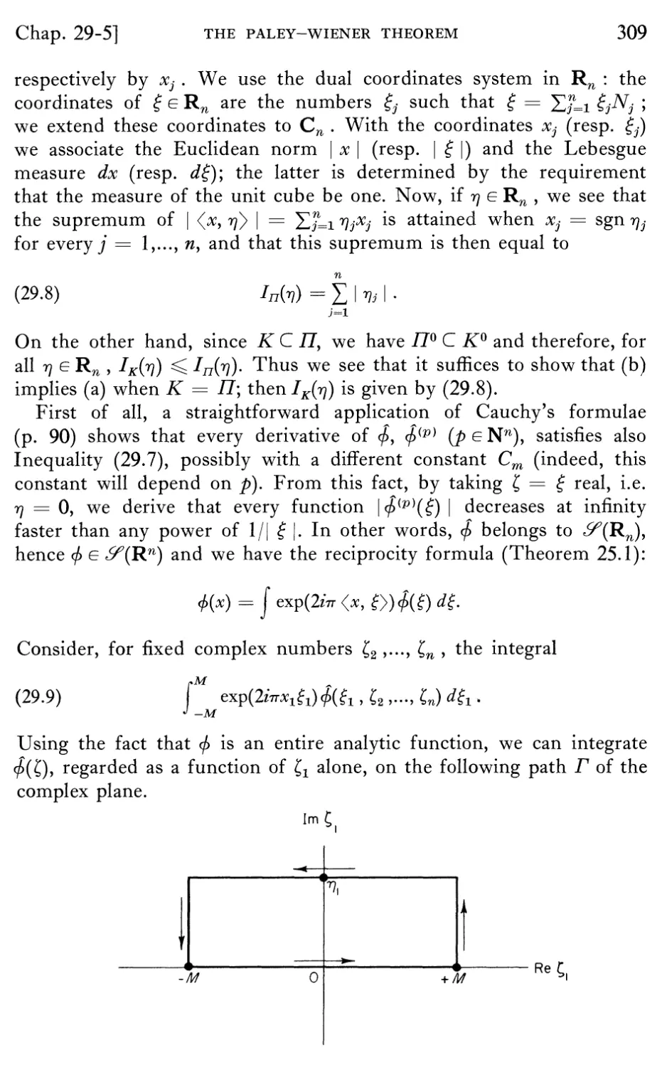
29.	Fourier Transforms of Distributions with Compact Support.
The Paley-Wiener Theorem................................................305
30.	Fourier Transforms of Convolutions and	Multiplications ...	314
31.	The Sobolev Spaces............................................322
32.	Equicontinuous Sets of Linear Mappings........................335
CONTENTS	XV
33.	Barreled Spaces. The Banach-Steinhaus Theorem.................346
34.	Applications of the Banach-Steinhaus	Theorem.................351
34.1.	Application to Hilbert Spaces.........................351
34.2.	Application to Separately Continuous Functions on Products 352
34.3.	Complete Subsets of F)................................354
34.4.	Duals of Montel Spaces................................356
35.	Further Study of the Weak Topology............................360
36.	Topologies Compatible with a Duality. The Theorem of
Mackey. Reflexivity ....................................................368
The Normed Space EB.........................................370
Examples of Semireflexive and Reflexive Spaces..............374
37.	Surjections of Frechet Spaces.................................378
Proof of Theorem 37.1	  379
Proof of Theorem 37.2...................................... 383
38.	Surjections of Frechet Spaces (continued). Applications	. . .	387
Proof of Theorem 37.3...................................... 387
An Application of Theorem 37.2: A Theorem of E. Borel ....	390
An Application of Theorem 37.3: A Theorem of Existence of ^°°
Solutions of a Linear Partial Differential Equation.........391
Part III. Tensor Products. Kernels......................................395
39.	Tensor Product of Vector Spaces...............................403
40.	Differentiable Functions with Values in Topological Vector
Spaces. Tensor Product of Distributions.................................411
41.	Bilinear Mappings. Hypocontinuity.............................420
Proof of Theorem 41.1.......................................421
42.	Spaces of Bilinear Forms. Relation with Spaces of Linear
Mappings and with Tensor Products.......................................427
43.	The Two Main Topologies on Tensor Products.
Completion of Topological Tensor Products...............................434
44.	Examples of Completion of Topological Tensor Products:
Products 8..............................................................446
Example 44.	1. The Space E) of Functions Valued in a
Locally Convex Hausdorff Space E
(0 < m < +oo).................................446
Example 44.	2. Summable Sequences in a Locally Convex Hausdorff
Space.......................................................451
45.	Examples of Completion of Topological Tensor Products:
Completed тт-Product of Two Frechet Spaces..............................459
XVI
CONTENTS
46.	Examples of Completion of Topological Tensor Products:
Completed тт-Products with a Space L1.....................467
46.1.	The Spaces L“(E)	........................467
46.2.	The Theorem of Dunford-Pettis.............469
46.3.	Application to L1 (x)^ E .............. 473
47.	Nuclear Mappings..................................477
Example. Nuclear Mappings of a Banach Space into a Space L1 .	486
48.	Nuclear Operators in Hilbert	Spaces...............488
49.	The Dual of E(x)eF. Integral	Mappings.............500
50.	Nuclear Spaces ...................................509
Proof of Proposition 50.1.......................516
51.	Examples of Nuclear Spaces.	The Kernels Theorem .... 526
52.	Applications......................................535
Appendix: The Borel Graph Theorem.................549
Bibliography for Appendix ......................557
General Bibliography..............................558
Index of Notation ........................	559
Subject Index.............................................561
PART I
Topological
Vector Spaces.
Spaces of Functions

Part I is devoted to the basic definitions and properties about
topological vector spaces, with no detailed reference to duality. We use
filters quite systematically, after having introduced them in Chapter 1
(which is devoted to recalling what a topological space is, with emphasis
on the filter of neighborhoods of a point). Chapter 2 recalls what a
vector space is, without going into any algebraic subtlety, as we shall
never need any in what follows. The scalars are always complex
numbers; no other field is ever considered (we shall switch to the field
of real numbers for a very short moment, when talking about the theorem
of Hahn-Banach, in Part II, and switch quickly back to complex
numbers). Chapter 3 makes the synthesis, in a sense, combining the
topology with the linear structure, under the natural compatibility
conditions. In relation to this, I have thought that the students might
like to see a meaningful example of a topology on an algebra A which
does not turn A into a topological vector space. Such an example is
provided by the algebra C[[X]] of formal power series, equipped with
the topology defined by the powers of the maximal ideal. It is instructive
to compare it with the topology of simple convergence of the coefficients,
noting that C[[X]] is metrizable and complete for both topologies.
Chapter 4 is devoted essentially to quotient topological vector spaces;
quotient spaces will be much needed in Part II, when they will be
carrying many a different topology, and it is the experience of the
author that this is what students find most difficult: to visualize and
manipulate correctly the various useful topologies, related to weak
duality, on quotients of duals and on duals of quotients, and this is
unfortunately inevitable.
Chapter 5 is devoted to the completion of a (Hausdorff) topological
vector space; the theorem on completion is proved in all details. Although
it is by no means a deep theorem, I have chosen to devote an entire
Chapter to it so as to familiarize the reader with Cauchy filters, and also
because I have too often been faced with audiences who simply did not
know what a complete (nonmetric) uniform space is.
Chapter 6 is devoted to compact subsets of a topological vector space.
Chapter 7 introduces locally convex spaces and seminorms. Needless to
say we shall not be dealing with any TVS that is not locally convex.
In Chapter 8 we look at metrizable TVS, that is to say TVS whose
3
4
TOPOLOGICAL VECTOR SPACES
topology can be defined by a metric. We construct a metric when the
underlying space is locally convex; we do this out of a sense of duty,
because people in a nondistant past liked to think in terms of metrics.
Inspection of the reasoning shows quickly that, most of the time, the
consideration of a metric is unnecessary, that countable bases of neigh-
borhoods would do. Furthermore, metrics have generally the drawback
that the balls are not convex; and outside of local convexity there is little
hope for salvation! There is no doubt that the proof of the open mapping
theorem would be quite awkward without a metric, but the actual form
of the latter is irrelevant (provided that it is translation invariant). The
criteria about continuity, compactness, and completeness in metrizable
spaces are given, together with the proof of the fact that every complete
metrizable space is a Baire space. In Chapter 9 we study rapidly the
most primitive examples of metrizable and complete TVS: the finite
dimensional Hausdorff spaces! Linear subspaces of finite codimension
are considered, as they will be useful later, and the correspondence
between closed hyperplanes and kernels of continuous linear functionals
is shown. The next three chapters are devoted to examples of locally
convex metrizable spaces. These are (in decreasing order of generality):
Frechet spaces, normed and Banach spaces, Hilbert spaces. Frechet
spaces will be the most important topological vector spaces for our
purposes. About Banach and Hilbert spaces, the student should expect
to find in this book only the most basic and elementary information:
for instance, in the chapter devoted to Hilbert spaces we prove the
projection theorem and its consequence, the fundamental theorem of
Hilbert space theory: the canonical isomorphy between a Hilbert space
and its antidual. After this we describe rapidly (finite) Hilbert sums and
orthonormal bases. The basic examples of F-spaces, В-spaces, and
Hilbert spaces are introduced:
open subset of Rn;	1 С? C oo);
H(Q), space of holomorphic functions in an open subset Q of Cn ;
(^k(Q') (K, compact subset of Rn; £?, bounded open subset
of Rn);
JF, space of ^°° functions in R' , rapidly decaying at infinity.
Chapter 13 is devoted to a class of locally convex spaces which are not
metrizable (in general) but which are of great importance to us: the
spaces LF (strict inductive limits of a sequence of F-spaces); as examples,
we present the space of polynomials C[X] (as inductive limit of the finite
dimensional spaces of polynomials of bounded degree) and the spaces
of functions with compact support,	The space ^"(£2) will
SPACES OF FUNCTIONS
5
be the space of test functions on which distributions in Q will be defined:
the distributions in Q are the continuous linear functionals on ^"(й),
i.e., the elements of the dual of ^°(£?).
After this string of examples of spaces of functions, we return to the
general theory and introduce bounded subsets of topological vector
spaces. Bounded sets will be much used in relation with duality. By using
Ascoli’s theorem we prove that many of the spaces used in the theory
of distributions (namely ^(й),	^(й)) have the property that closed
bounded sets are compact (this property never holds in infinite
dimensional normed spaces). In the infinite dimension situation, this
property was first encountered by Montel in the study of normal
family of holomorphic functions. We prove also Montel’s theorem which
states that in H(Q) any closed bounded set is compact (H(Q): space of
holomorphic functions in the open set Q C Cn).
Chapter 15 is devoted to approximation techniques in the standard
spaces of functions, ^fc(£?),/>(£?),	We study approximation
by entire functions, by polynomials, and by functions with compact
support (in the cases where this makes sense!). In Chapter 16 we apply
some of these approximation results to showing that, given an arbitrary
locally finite covering of an open subset Q of R \ there is a partition of
unity in ^(й) subordinated to it. The last chapter of Part I, Chapter 17,
is devoted to the statement and the proof of the open mapping theorem.
1
Filters. Topological Spaces.
Continuous Mappings
A topological vector space E is, roughly speaking, a set which carries
two structures: a structure of topological space; a structure of vector
space. Furthermore, some kind of compatibility condition must relate
these two structures on E. We begin by recalling briefly what each one of
them is, in the absence of any relation between the two.
One defines usually a topology on a set E by specifying what the open
subsets of E are going to be. However, in dealing with topological vector
spaces, as we are going to do in this book, it is more convenient to define
a topology by specifying what the neighborhoods of each point are going
to be. It is well known that the two approaches are equivalent: an open
set will be a set which, whenever it contains a point, contains a neighbor-
hood of this point; one can also say that an open set is a set which is a
neighborhood of each one of its points; on the other hand, a neighborhood
of a point x of E is simply a set which contains some open set containing x.
In order to define a topology by the system of the neighborhoods of
the points, it is convenient to use the notion of filter. This is a very
primitive notion, and the student should find it easy to become familiar
with it, and to learn how to use filters, just as he learned how to use
sequences. The notion of filter is perfectly independent of topology.
A filter is given on a set which need not carry any other structure. Let
E be the set. A filter is a family of subsets of E, submitted to three
conditions:
(Fx) The empty set 0 should not belong to the family .
(F2) The intersection of any two sets, belonging to the family, also
belongs to the family .
(F3) Any set, which contains a set belonging to 3F, should also belong
to .
The simplest example of a filter on a set E is the family of all subsets of
E which contain a given subset A, provided the latter is nonempty.
6
FILTERS. TOPOLOGICAL SPACES
7
With every infinite sequence of points of E is associated a filter. Let
^1 J ^2 > * * * be the sequence under consideration. The associated filter is
the family of all subsets of E which have the following property:
(AF) The subset of E contains all elements xr , x2,... except possibly a
finite number of them.
A family & of subsets of E is a basis of a filter on E if the following
two conditions are satisfied:
(BFJ C i.e.y any subset which belongs to Sd must belong to .
(BF2) Every subset of E belonging to contains some subset of E which
belongs to S3.
A familiar example of a basis of filter on the straight line is given by the
family of all intervals (~ay a) with я > 0: it is a basis of the filter of
the neighborhoods of zero in the usual topology on the real line. Another
useful example is the following one: let be the filter associated with a
sequence 5 = {x±, x2 xn >•••}• F°r eac^ n = Ъ 2,..., let us set
— {xn , xn+± ?•••}
and view Sn as a subset of E. Then the sequence of subsets 5 =
3 S2 3 • • • Sn D • • • is a basis of
Let be some family of subsets of our set E. We may ask the question:
is there a filter having as a basis (note that a filter can have several
different bases) ? In view of the filters axioms, (FJ, (F2), (F3), that filter
if it exists, is completely and uniquely determined: it is the family
of subsets of E which contains some subset belonging to j/. Observe
that the latter property defines perfectly well a certain family, which we
have called of subsets of E. Then our question can be rephrased as
follows: is a filter? Obviously satisfies (F3); it also satisfies (FJ
if we take care of requiring that no set belonging to j/ be the empty set.
As for (F2) it is equivalent, as we see easily, with the following property
of :
(BF) The intersection of any two sets, belonging to contains a set
which belongs to sd.
The difference with Condition (F2) is that the intersection of two subsets
which belong to j/ is not requested to belong to j/, but only to contain
some set belonging to j/. Thus we may state: a basis of filter on E is a
family of nonempty subsets of E satisfying Condition (BF). The filter
generated by the basis is uniquely determined: by Condition (BF2).
8
TOPOLOGICAL VECTOR SPACES
[Part I
Next step: comparison of filters. We want to be able to say: this filter
is finer than this other filter. Keep in mind that filters are sets of sets,
or rather of subsets. In other words, filters are subsets of the set of subsets
of E, usually denoted by 45(E). As filters are subsets (of some set, in
this case 45(E)), there is a natural order relation among them: the
inclusion relation. We can write C if and are two filters on
the same set E. It means that every subset of E which belongs to also
belongs to J*7' (the converse being in general false). Instead of saying
that is contained in one usually says that is finer than or
that is less fine than Let (resp. J^') be the family of all subsets
of E which contain a given subset A (resp. A') of E; is finer than
if and only if A’ C A.
A topology on the set E is the assignment, to each point x of E, of a
filter J^(a) on E, with the additional requirement that the following two
conditions be satisfied:
(N-J If a set belongs to J^(a), it contains the point x.
(N2) If a set U belongs to ^(x\ there is another set V belonging also
to J^(a) such thaty given any point у of L, U belongs to J^(y).
When these conditions are satisfied we say that we have a topology on E
and we call J^(a) the filter of neighborhoods of the point x. At first sight
Condition (N2) may seem involved. It expresses, however, a very intuitive
fact. Roughly speaking, it says that given any point z near x (i.e., z is a
generic element of L7), if a third point у lies sufficiently near to x (the
sufficiently near is made precise by the neighborhood of a, F, of which у
is an element), then z lies near to у (i.e., z e U e ^\y)). In the language
of open sets, (N2) becomes evident: since U is a neighborhood of a,
U contains an open set containing a; let V be such an open set. Since V
is open, and V C (7, U is obviously a neighborhood of each point of V.
A basis of the filter J^(a) is called a basis of neighborhoods of a. This
simple notion will play an important role in the forthcoming definitions.
Once we have the notion of filter of neighborhoods of a point, hence
of neighborhood of a point (any subset of E belonging to the filter of
neighborhoods), we can review quickly the concepts that are used to
describe a topology. As we have already said, an open set is a set which is
a neighborhood of each one of its points. A subset of E is closed if its
complement is open. The closure of a set AC E is the smallest closed set
containing A. It will be denoted by A. The following is easy to check:
a point belongs to A if and only if everyone of its neighborhoods meets
A (that is to say, has a nonempty intersection with A). The interior of
a set is the largest open set contained in it; if A is the set, its interior
will be denoted by A.
Chap. 1-4]	FILTERS. TOPOLOGICAL SPACES	9
A very important notion is the one of a set A dense in another set B;
both A and В are subsets of the same topological space E. Then, one
says that A is dense in В if the closure A of A contains B. In particular,
A is said to be dense in E (or everywhere dense) if A = E. To say that
A is dense in В means that, given any neighborhood of any point x of B,
17(a), there is a pointy of A which belongs to 17(a), i.e., А П 17(a)	0.
A standard example of a set everywhere dense is the set of rational
numbers Q, when regarded as a subset of the real line R (with the usual
topology); note that the complement R — Q of Q is also dense in R.
Examples of sets which are dense and open are given by the complement
of a straight line in the plane or in space, by the complements of a plane
in space, etc. Easy to check are the basic intersection and union properties
about open or closed sets: that the intersection of a finite number of
open sets is open (this follows immediately from the fact, itself obvious
in virtue of Axiom (F2), that the intersection of a finite number of
neighborhoods of a point is again a neighborhood of that point); that the
union of any number of open sets, be that number finite or infinite, is
open (this follows from the fact that the union of a neighborhood of a
point with an arbitrary set is a neighborhood of the same point:
Axiom (F3)). By going to the complements, one concludes that finite
unions of closed sets are closed, arbitrary intersections of closed sets are
also closed, etc.
Observe that a set E may very well carry several different topologies.
When dealing with topological vector spaces, we shall very often
encounter this situation of a set, in fact a vector space, carrying several
topologies (all compatible with the linear structure, in a sense that is
going to be specified soon). For instance, any set may carry the following
two topologies (which, in practice, are almost never used):
(1) the trivial topology: every point of E has only one neighborhood,
the set E itself;
(2) the discrete topology: given any point a of B, every subset of E is
a neighborhood of a provided that it contains a; in particular,
{a} is a neighborhood of a, and constitutes in fact a basis of the
filter of neighborhoods of a.
We may compare topologies, in analogy with the way we have compared
filters. Let ST' be two topologies on the same set E. We say that
is finer than FF' if every subset of E which is open for is also open
for ?F, or equivalent, if every subset of E which is a neighborhood of a
point for is also a neighborhood of that same point for the topology ,
Let J^(a) (resp. JF'(a)) be the filter of neighborhoods of an arbitrary
point a of E in the topology ZF (resp. ^F'y is finer than which we
10	topological vector spaces	[Part I
shorten into ZT', if, for every x e Ey ^(a) is finer than J^'(a).
Given two topologies on the same set, it may very well happen that
none is finer than the other. If one is finer than the other, one says
sometimes that they are comparable. The discrete topology is finer, on
a set E, than any other topology on E; the trivial topology is less fine
than all the others. Topologies on a set form thus a partially ordered set,
having a maximal and a minimal element, respectively the discrete and
the trivial topology.
The notion of a topology has been introduced in order to provide a
solid ground for the notions of convergence and of continuity. Of course,
the latter were correctly manipulated (or most of the time, at least) well
before anybody thought of topology. We proceed now to give their
general definition.
Convergence. This concerns filters: filters are the “objects” which
may (or may not) converge. When do we say that a filter -F on a
topological space E converges ? We should recall that is a family of
subsets of E. If is to converge to a point x of E, it means that elements
of which, we repeat again, are subsets of E, get “smaller and smaller”
about a, and that the points of these subsets get “nearer and nearer” to a.
This can be made precise in terms of the neighborhoods of a, which
we have at our disposal, since E is a topological space: we must express
the fact that, however small a neighborhood of a is, it should contain
some subset of E belonging to the filter SF and, consequently, all the
elements of which are contained in that particular one. But in view
of Axiom (F3), this means that the neighborhood of a under consideration
must itself belong to the filter , since it must contain some element of
. The phrase “however small a neighborhood of a is” has to be made
mathematically meaningful: it simply means “whatever is the neighbor-
hood of a.” In brief, we see that the filter converges to the point x if
every neighborhood of x belongs to in other words if is finer than the
filter of neighborhoods of x, &\x). This is what the convergence to a point
of a filter means.
We recall how the convergence of a sequence to a point is defined. Let
5 = {ax , a2 ,...} be the sequence. We say that 5 converges to a if, given
an arbitrary neighborhood U of a, there is an integer nfU) such that
n n(U) implies xn e U. Let 5 = Э 52	’ be the
subsequences introduced on p. 7: 5 converges to a if to every U gJF(a)
there is an integer n(U) such that Sn(u) C U. As the subsets Sn of E
form a basis of the filter associated with the sequence S, we see immedi-
ately that a sequence S converges to x if and only if the associated filter
converges to x.
Note that a filter may converge to several different points. Suppose,
Chap. 1-6]	FILTERS. TOPOLOGICAL SPACES	11
for instance, that E carries the trivial topology (p. 9): then every filter
on E converges to every point of E. Note also that a filter may not
converge: for instance, if it is the filter associated with some sequence and
if this sequence does not converge. Another example is given by a filter
on E which is not the filter of all subsets of E which contain a given
point x—when E carries the discrete topology: in this topology, the
only converging filters are the filters of neighborhoods of the points.
So much for convergence in general topological spaces.
Continuity. This concerns mappings. In point set topology, a map
ft ECF, this is to say a map from a topological space E into another
topological space F, is .said to be continuous if any one of the following
two conditions is satisfied:
(a)	given any point x of E and any neighborhood V of the image
f(x) 6 F of x, the preimage of V, that is to say the set
/-1(F) = {agE;/(a)g V},
is a neighborhood of x. In short,
VxeE, 7e J(/(x)) implies /-1(F) _g J^(a);
(b)	the preimage of any open subset (9 of F,
= {agE;/(a)g$},
is an open subset of E.
The student will easily check the equivalence of (a) and (b). As for the
intuitive meaning of these conditions, we may say the following. If the
mapping f is to be continuous at the point a, it should mean that if x' G E
“converges to a,” then/(a') should converge to/(a). Note that “ f(x')
converges to /(a)” can be made precise in the following way: given an
arbitrary neighborhood of /(a), /(a') should eventually belong to it; and
the “eventually” means here: provided that a' is sufficiently near to a.
Thus given an arbitrary neighborhood V of /(a), if x belongs to a
sufficiently small neighborhood of a, then /(a') g V. The “sufficiently
small” can only be determined by the existence of a certain neighborhood
U of a, such that, as soon as xf g U, then f(x'} g V. This is exactly
Property (a): to every neighborhood V of /(a) there is a neighborhood U
of a such that
a' g U implies /(a') g V.
12	TOPOLOGICAL VECTOR spaces	[Part I
It is immediately seen that, if a sequence {xr , a2 ,...} converges in E to
a point x, and if f is a continuous function from E into F, then the
sequence {/(^i),/(^2)v} converges to /(a) inF. Convergence of filters is
also easily related to continuity of mappings. Let
be a mapping from a set E into a set F. Let be a filter on E. The image
ft'F of under f is defined as being the filter having the basis
(f^ = {f(U)eF,Ue^}.
Observe that, in general, (/^)0 is not itself a filter; it is always the
basis of a filter (the student may check this point as an exercise). Now,
if the filter converges to a point x in E and if f is a continuous function,
then f^ converges to /(a) in F. Indeed, the continuity of f implies that
/>(a) is finer than ^(^a)); this is simply a restatement of Property (a)
above. If then -SF is finer than J^(a) (which means that converges to a).
fSF is finer than /J^(a) and a fortiori finer than JF(/(a)).
We have only considered continuous functions, which is to say
functions defined everywhere and continuous everywhere. Of course,
one may prefer to talk about functions continuous at a point. This is
defined by the condition (where a is the point under consideration):
for every 7ё^(/(а)),	/-1(Ю belongs to J^(a),
or, equivalently,
/^(A)	^(/(a)).
Let us insist on the fact that all the functions or mapping which will be
considered in this book are defined everywhere.
As a last remark, let us consider the case where F is identical with
E as a set, but carries a different topology from the one given on E, and
where f is the identity mapping of E onto F, I. The following two
properties are obviously equivalent:
(i)	I: E ->F is continuous;
(ii)	the topology of E is finer than the topology of F (these two
topologies are defined on the same set).
Exercises
1*1* Let X be a topological space, Л, В two subsets of X. Prove that if A is open
we have
A n В С A n B.
Give an example of sets A and В such that A is not open and that the preceding
inclusion is not true.
Chap. 1-8]	FILTERS. TOPOLOGICAL SPACES	13
1*2* Prove that the image of a dense set under a map, which is continuous and surjective
(i.e., onto), is dense.
1*3* Let X, У be two topological spaces, / : X Y a continuous function, В a subset
of У, and В its closure. Do we always have
closure of /-1(В) = /-1(Л) ?
1*4* Give an example of the following situation: X and У are topological spaces,
f : X -> У is a continuous mapping, A is a closed subset of X, andf(A) is not closed in У.
1*5* Consider a straight line L in the plane R2. The filter of neighborhoods of L in R2
is the filter formed by the sets which contain an open set containing L. Prove that there
is no basis of this filter which is countable.
1*6* Let / be a real-valued, continuous function on the closed interval [0, 1]. Show
that there is a “natural” filter & on the real line, defined by means of the Riemann sums
7=0
where 0 = tQ < tr < ••• < tj < ••• < tr+1 = 1 and tj < t3- < t3+1 for each j. Show
that the filter converges to the integral
Г/W dt.
J 0
1*7* Prove that the filter of neighborhoods of the closed unit disk {(#, y) e R2;
x2 + y2 < 1} in the plane has a countable basis (cf. Exercise 1.5).
1*8* Let Xa (a e A) be a family of topological spaces. Consider their product set
*=гк-
Let us denote by pa the projection mapping on the ath coordinate axis Xa :
Pa : x = (»«) ->	•
The product topology on X is defined in the following way: a subset U of X is a neighbor-
hood of one of its points x = (xf) if, for every a, £a(U) is a neighborhood of xa and if,
for all a except possibly a. finite number of them, £a(L) = Xa . Prove that this is the least
fine topology on X such that all the mappings ра be continuous.
1*9* Let be a filter on the product space X of Exercise 1.8. Let us denote by
the image of under the projection p^ . Show that is the family of subsets of X^ of
the form pajM} as M ranges over and that converges if and only if every does.
1*10* Let us say that a set A is predirected if there is a preorder relation a < b on A
and if, for any pair of elements a, b of A, there is c e A such that a < c, b < c (the
relation a < b is a preorder relation if it is reflexive, i.e., a < a for all a, and transitive,
i.e.) a < b and b < c imply a < c; it is an order relation if, furthermore, a < b and
b < a imply a = b). Let Ф be the set of all filters on X, Ф' the set of all mappings of
predirected sets into X. Prove that there is a canonical mapping of Ф' onto Ф (this mapping
is not one-to-one ). Under this mapping, the image of a function/on the “predirected”
set of positive integers into X is the filter associated with a sequence in X.
Vector Spaces. Linear Mappings
We recall first what a vector space is. The vector spaces we shall
consider will be defined only on one of the two “classical” fields: the
field of real numbers, R, or the field of complex numbers, C. As a rule,
we shall suppose that the field is C. When we specifically need the field
to be R, we shall always say so. In other words, we deal always with
complex vector spaces. A vector space E over C is a system of three
objects (£*, Av , Ms) consisting of a set E and of two mappings:
Av : E x E E,
MS:C X E-+E,
(x, y)	X + y,
(А, x)	Xx.
Of course, there are conditions to be satisfied by these objects. The
mapping Av , called vector addition, must be a commutative group
composition law, i.e., it must have the following properties:
(associativity):	(x + y) 4- z = X +• (y + z);
(commutativity) :	x + у —у + x;
(existence of a neutral element):	There exists an element, denoted by 0, in E such that Vx, x + 0 = x;
(existence of an inverse):	To every x e E there is a unique element of E, denoted by —x, such that x + (— x) = 0.
Of course, we write x — у instead of x + (— y). The mapping Ms is
called scalar multiplication, or multiplication by scalars, and should
satisfy the following conditions:
(i)	A(^x) = (Ap,)x;
(ii)	(A +	= Ax +
(iii)	1 • x = x;
(iv)	0 • x = 0;
(v)	A(x + y) = Ax + Ay.
14
VECTOR SPACES. LINEAR MAPPINGS
15
We do not recall the meaning of such notions as linear independence,
basis, vector (or linear) subspace, etc. A mapping f: E ->F of a vector
space E into another, F, is called linear if for all x, у e E, A, p, e C,
f(Xx -J- py) = Xf(x) -J- p,f(y).
Let us recall that a linear mapping f: E ->F is one-to-one if and only if
/(a) = 0 implies x = 0. Indeed, if f is one-to-one, /(a) = 0 must imply
x — 0. Conversely, suppose that /(a) = 0 implies x = 0, and let a,
у 6 E be such that/(a) =f(y). This equation can be written f(x — y) = 0,
implying then x — у = 0.	q.e.d.
A notion with which the student may not be so familiar is the one
of quotient space. As it will play a crucial role in the sequel, we shall
recall its definition.
Let £ be a vector space (over C) and M a linear subspace of E. For
two arbitrary elements x and у of £, the property
x — у g M
defines an equivalence relation', it is reflexive, since x — x = 0 6 M
(every linear subspace contains the origin); it is symmetric, since
x — у g M implies — (x — у) = у — x g M (if a linear subspace contains
an element, it contains its inverse); it is transitive, since
x — у g M, у — z g M implies x — z = (x — y) + (y — z) e M
(when a linear subspace contains two vectors, it also contains their sum).
Then we may define the quotient set E}M: it is the set of equivalence
classes for the relation x — у eM. There is a “canonical” mapping of£
onto EfM\ the mapping which, to each x g E, assigns its class modulo
the relation x — у G M. It helps the intuition to visualize the class of
elements equivalent to x modulo M, that is to say the y’s such that
x — у g M, as a linear subvariety', indeed, they constitute the set
M 4- x == {xf 4- v I v' g 7И},
which is the translation of M by x. Observe the following, which is easy
to check (using the fact that M is a linear subspace):
(2.1)	if x^vmodM,	and if AgC,	then	Ax^AymodM;
(2.2)	if x^vmodM,	and if zeE,	then	x 4- s У + s mod M.
Thus	we define vector	addition and	scalar	multiplication in EjM'.	if
Ф(х) is the class of x mod	7И, Хф(х) = </>(Aa) and </>(a) + </>(y) === ф(х 4~ y).
16
TOPOLOGICAL VECTOR SPACES
[Part I
These definitions are unambiguous by virtue of (2.1) and (2.2); they turn
E^M into a vector space, and ф : E —> E^M, the canonical mapping, is
then a linear map. It is, of course, onto.
Now let E, F be two linear spaces (over C), and f a linear map E ->F.
We define the image of/, and denote it by Im/, as the subset ofF:
Im/ = {y e F; there exists x e E such that у = /(a)}.
We define the kernel of/, and denote it by Ker/, as the subset of F:
Ker / = {x e E;f(x) = 0}.
Both Im/and Ker/are linear subspaces (ofF and F resp.). We have then
the diagram
E----£—+ Imf-^F
Ф „ /i
E/Kerf
where i is the natural injection of Im / into F, that is to say the mapping
which to each element у of Im / assigns that same element y, regarded
as an element ofF; / is the canonical map of F onto its quotient, F/Ker /.
The mapping/is defined so as to make the diagram commutative, which
means that the image of x e F under / is identical with the image of
/(a) (i.e., the class of x modulo Ker/) under/. The mapping / is well
defined by the equation
/Ш) = /(a).
Indeed, if </>(a) = <^>(y), in other words if a. — у e Ker /, then/(a) = f(y).
It is an immediate consequence of the linearity of / and of the linear
structure of the quotient space F/Ker /that/ is also linear. Now,/is a
one-to-one linear map of F/Ker/onto Im/. The onto property is evident
from the definition of Im / and of /. As for the one-to-one property,
observe that, if/(/(a)) = /(/(y)), it means by definition that/(a) = f(y),
hence /(a — y) = 0 or a—ye Ker /, which means that/(a) = /(y). Q.e.d.
Let F be an arbitrary set (not necessarily a vector space) and F a
vector space. Let us denote by J^(F; F) the set of all mappings of F
into F. It can be equipped with a natural structure of vector space.
We must first define the sum of two mappings f,g:E->F. It must be
a function of the same kind, and we must therefore say what its value
Chap. 2-4] vector spaces, linear mappings	17
should be at an arbitrary point x of E. Naturally, we take this value to
be equal to the sum of the values of the factors,/(a), g(x):
(f + £)(a) = /(a) + g(x) (this is a definition).
Similarly, to define А/, where A is an arbitrary scalar, we define its value
at an arbitrary point x of E. We set (this is again a definition):
(A/)(x) = A/(a).
When E also is a vector space (over the same scalar field as F, for us
the field of complex numbers C), we will be particularly interested in
the linear mappings of E intoF. They form a linear subspace of J^(F; F),
as immediately checked, which we shall denote by J?(F; F).
When F = C, J?(F; F) is denoted by F* and called the algebraic dual
of F. When F is a topological vector space (see next chapter) we shall
be interested in a “smaller” dual of F, namely the linear subspace of F*
consisting of the linear mappings F —> C which are continuous; this will
be called the dual of F and denoted by F'. One should always be careful
to distinguish between F* and F' (except in exceptional cases, e.g., when
F is finite dimensional*). The elements of F* are most of the time
referred to as the linear functionals, or the linear forms on F.
If F, F, G are three vector spaces over C, and и : F —> F, v : F —> G
two linear mappings, it is clear that the compose v о u, defined by
(v о w)(a) = v(u(x)), хе E,
is a linear map of F into G. If G = C, v is a linear functional on F,
i.e., v is an element a* of the algebraic dualF* ofF; the compose а* о u
is a linear functional on F. We obtain thus a mapping a* a* о zz of
F* into F* for each given и 6 J?(F; F). This mapping is obviously
linear. It is called the algebraic transpose of щ we shall denote it by u*.
As is readily seen, и u* is a linear mapping of J?(F; F) into J?(F*; F*).
Exercises
2Л+ Give an example of a linear space E and of two linear mappings u, v of E into
itself with the following properties:
(i)	и is injective (i.e., one-to-one) but not surjective (i.e., onto);
(ii)	v is surjective but not injective.
f Also Hausdorff; see Chapter 9.
18	TOPOLOGICAL VECTOR spaces	[Part I
2*2* Let E be a vector space, M a linear subspace of E, and и a linear map of M into
a vector space F. Prove that there is a linear map v E -+F which extends u, i.e., such
that u[x) = v(x) for all x g M.
2*3* Let E, F be two vector spaces, и : E -+F a linear map, and u* : F* —> E* the
algebraic transpose of u. Prove that the following properties are equivalent:
(a)	и is surjective;
(b)	u* is injective.
2*4* Let E,F be two vector spaces, and и : E F a linear map. Let M (resp. N) be
a linear subspace of E (resp. F), and ф (resp. ф) the canonical mapping of E (resp. F) onto
E/M (resp. F/N), Prove the equivalence of the following two properties:
(a)	u(M) С ДГ;
(b)	there exists a linear map v such that the following diagram is commutative:
и
E ------> F
4	4
E/M	F/N.
Prove that, if (a) holds, the mapping v above is unique.
2*5* Let M be a linear subspace of E,j the natural injection of M into E, and ф the
canonical map of E onto E/M. Let us set
M1- = {#* g E*', for all x g M, x*(x) = 0}.
(i)	Prove that there is a linear map k such that the following diagram is commutative:
E* 3* > M*
z k
E*/M\
where ф* is the canonical mapping onto the quotient vector space. Moreover,
prove that k is an isomorphism onto.
(ii)	Prove that ф* : (E/M)* E* is one-to-one and that the image of ф*, ф*((Е/М)*),
is equal to
2*6* Let (Еа) (a g A) be an arbitrary family of vector spaces over the complex numbers.
Consider the product set
ocGA
it carries a vector space structure where vector addition and scalar multiplication are
performed componentwise. The direct sum of the Ea is the linear subspace of E consisting
of those elements x = (хл)аеА for which all the components x^ are equal to zero with the
possible exception of a finite number of them; we shall denote by EQ this direct sum.
Prove that there is a canonical isomorphism between the algebraic dual of the direct sum
Eq and the product of the algebraic duals E* of the Ea .
2*7* Let us keep the notation of Exercise 2.6. Let a g A We denote by the (linear)
mapping of into E defined as follows: if z g E^ , Ja(^) is the element x = (xp)@eA of
E such that x& = 0 if /3 a and xa = z. It is evident that is one-to-one; if pa is the
coordinate projection # = (x£) xa , we have Oja = identity of E^ . Let/* : E* E*
Chap. 2-6] vector spaces, linear mappings
19
be the algebraic transpose of ya . We may define the following linear map of E* into the
product Ё* = ПаеЛ E*, j*:
E* э x* »*/*(«*) = (у*(л:*))с,ел e Ё*.
Prove the equivalence of the following properties:
(a)	the set of indices A is finite;
(b)	j* is one-to-one;
(c)	j* is an isomorphism of E* onto E*.
2*8	* Prove that every vector space E is isomorphic to the direct sum of a family of
one-dimensional vector spaces. Then, by making use of the results stated in Exercises 2.6
and 2.7, prove that the following properties are equivalent:
(a)	E is finite dimensional;
(b)	the canonical mapping
X (x*	x*(x))
is an isomorphism of E onto the algebraic dual E** of its own algebraic dual E*.
3
Topological Vector Spaces. Definition
Let E be a vector space over the field of complex numbers C (in short,
a vector space). Let
Av: E x E-+E,	(x,y)	x	V,
Ms :C X E-+E,	(Л, x)	Ax,
be the vector addition and the scalar multiplication in E. A topology	in E
is said to be compatible with the linear structure of E if Av and Ms are
continuous when we provide E with the topology E X E with the
product topology X and С X E with the product topology
X AT, where is the usual topology in the complex plane C. We
recall the meaning of a “product topology.” Consider two topological
spaces E, F, In order to say what the product topology on E X F is, it
suffices to exhibit a basis of the filter of neighborhoods of each point
(x, y) of E X F. Such a basis is provided by the rectangles
U X V — {(я', у') e E x F; x' eU,y'e V},
where U (resp. V) is a neighborhood of x (resp. j) in E (resp. F). That
these rectangles form a basis of filter is trivial; they obviously do not
form a filter (except in trivial cases), since a set which contains a
rectangle does not have to be a rectangle. It remains to check that the
filters thus defined, for each pair (x, j), indeed can be taken as filters of
neighborhoods of (x, y) in a topology on E X F (Axiom (N2), p. 8,
has to be verified). We leave this point to the student. The topology
assigns to each point A of the complex plane a remarkable basis of
neighborhoods, the disks, open or closed, with center at this point (and
with positive radius p). When provided with a topology compatible with
its linear structure, E becomes a topological vector space, which we shall
abbreviate into TVS.
Suppose that E is a TVS. Then its topology is “translation invariant,”
which, roughly speaking, means that, topologically, E looks about any
20
DEFINITION
21
point as it does about any other point. More precisely: the filter of
neighborhoods -^(x) of the point x is the family of sets V + x, where V
varies over the filter of neighborhoods of the neutral element, J^(0). Proof of
this statement: Let U be an arbitrary neighborhood of x. As the mapping
у у y. x from E into (as a matter of fact, onto) itself is continuous,
which follows immediately from the continuity of the mapping
: (x, y) x + y, the inverse image of U under this mapping must
be a neighborhood of the preimage of x under this mapping; this pre-
image is obviously the neutral element 0. Let V be the inverse image of U.
We have U = V f- x. Conversely, given an arbitrary neighborhood V
of 0, V + x is a neighborhood of x by virtue of symmetry, or by virtue
of the continuity of the mapping у у — x. Thus: in order to study the
topology of a topological vector space E, it suffices to study the filter of
neighborhoods of the origin.
In practice, one always begins by giving the filter of neighborhoods of
the origin, or (more frequently) a basis of this filter. It follows from
there that we need some criteria on a filter which would insure that it is
the filter of neighborhoods of the origin in a topology compatible with
the linear structure of E.
Theorem 3.1. A filter on a vector space E is the filter of neighborhoods
of the origin in a topology compatible with the linear structure of E if and
only if it has the following properties:
(3.1)	The origin belongs to every subset U belonging to .
(3.2)	To every Ue!F there is VeP such that V + V C U.
(3.3)	For every Ue^ and for every А e С, Л Ф 0, we have XU e
(3.4)	Every U e is absorbing.
(3.5)	Every Ue^ contains some VeP which is balanced.
We have used two words, absorbing and balanced, which have not yet
been defined.
Definition 3.1. A subset A of a vector space E is said to be absorbing if to
every xeE there is a number cx > 0 such that, for all A 6 C, | A | cx ,
we have Xx e A.
In more colorful but less precise language, we may say that A is
absorbing if it can be made, by dilation, to swallow any single point of
the space.
Definition 3.2. A subset A of a vector space E is said to be balanced if for
every x g A and every A 6 C, | A |	1, we have Xx e A.
22	TOPOLOGICAL VECTOR spaces	[Part I
The only balanced subsets of the complex plane are the open or the
closed disks centered at the origin.
Proof of Theorem 3.1. We begin by proving the necessity of Properties
(3.1)—(3.5). The necessity of (3.1) goes without saying.
Necessity of (3.2). By V + V we mean the set of points x + y,
where x and у run over V. Let U be an arbitrary neighborhood of the
origin. Its preimage under the mapping (a, y) x + у of U must be a
neighborhood of 0, therefore must contain a rectangular neighborhood
W X W', where W and W' are neighborhoods of 0 in E. But then it
contains a “square,” namely (W П W') x (W П W'). If we take
V = W C\ W', this means precisely that V + V C U.
Necessity of (3.3). By XU we mean the set of vectors Xx, where x
varies over U. Because of the continuity of the mapping (A, a) —> Xx
from С X E into E, if we fix A g С, Л ф 0, the map a —> A-1a of E into
itself must be continuous. The preimage of any neighborhood U of the
origin in E must be such a neighborhood; this preimage is obviously XU.
Necessity of (3.4). Again we use the continuity of the mapping
(A, a) —> Aa, this time at a point (0, a) where a is an arbitrary point of E.
The preimage of a neighborhood U of 0 in E must be a neighborhood
of (0, a), since (0, a) is mapped into 0. Hence that preimage must
contain a rectangle N X W where N (resp. W) is a neighborhood of 0
(resp. of a) in C (resp. in E). By definition of the topology of a TVS,
W is of the form Wf + where W is a neighborhood of 0 in E
(see p. 21). On the other hand, N contains a disk of the complex plane,
centered at the origin, Dp — {A g C; | A | Xj p}, p > 0. Thus we see that,
for all у g Wf + a and all complex numbers A such that | A | Xj p, we
have Xy g U. In particular, we may take у = x.
Necessity of (3.5). We duplicate the proof of the necessity of (3.4)
but taking this time a = 0, hence W' — W. We have seen that the
preimage of U contains a rectangle Dp X W, which means that the set
V= |J XW
И< P
is contained in U. This set V is obviously balanced. It is a neighborhood
of zero, since each XW, A 5X 0, is one (in view of (3.3)).
Sufficiency of Conditions (3.1)—(3.5). We must first of all show that,
if we define the filter of the neighborhoods of an arbitrary point a of E
as the image of the given filter under the translation у a + y,
we have indeed a topology on the set E. Once we have proved this, we
Chap. 3-4]	definition	23
must show that this topology is compatible with the linear structure of E.
Let us call J^(x) the image of under у x + y, that is to say the
family of subsets U + x, where U varies over Since 0 6 U, x belongs
to ?7 + x Thus Axiom (N2), p. 8, is satisfied. Let V 6 be such that
V + V 6 U. Take an arbitrary point у of the set V + x; then U x
contains V + (V + x), hence V + У- But V + У belongs to ^(y), and
therefore so does U x. Thus Axiom (N2), p. 8, is satisfied when we
take U + x and V + x, respectively, in the place of U and V in the
statement of p. 8. We conclude that we have indeed a topology on E.
The last two steps consist in proving that the mappings Av and Ms are
continuous. The continuity of Av follows immediately from (3.2).
Indeed, let (x, y) be an arbitrary element of E X E; let W be a neighbor-
hood of its image, x + y. We know that W = U -C x y, U 6 J*7.
Choose Vg & such that V + VC U. Then (V + x) + (V + у) C W.
which means that the image of the neighborhood of (x, y),
(T + x) x (T+y),
is contained in W. Then the preimage of W contains that same neighbor-
hood of (x, y) and, consequently, is a neighborhood of (x, y).
Last step: continuity of
Mь : (A, x) Ax.
Let U' be a neighborhood of Aoxo; U' is of the form U + Aoxo , where U
is a neighborhood of zero in E. Let us select another neighborhood of
0, W, such that
(1)	W+W+WCU;
(2)	IV is balanced.
Such a neighborhood of zero, JT, exists in view of Properties (3.2) and
(3.5). In view of (3.4), W is absorbing. In other words, there is a number
p > 0, which we may as well take 1, such that
A e C, | A | p, implies Ax0 e W.
Let Dp be the disk centered at the origin, in the complex plane, with
radius p. Suppose first that Ao = 0, which implies Aoxo = 0 and U' = U.
Then we look at the image under Ms of the set Dp X (JV + x0); it is
the set
(3.6)	{Ay + Ax0;|A|<p,yeIF}.
As | A | p 1 and as W is balanced, у e W implies Ay 6 W. As
24
TOPOLOGICAL VECTOR SPACES
[Part I
| A | p, we have also Ax0 6 W. We conclude that the set (3.6) is
contained in W + W, hence in U. Thus the preimage of U contains
Dp X (W + v0), which is a neighborhood of (0, a0); the preimage of U
is a neighborhood of (0, <r0). Let us suppose finally that Ao Ф 0. In this
case we look at the image under Ms of the set
(3.7)	(Bff+A0) x (| Ao |-W + v0),
where <r - inf(p, | Ao |), the smallest of the two numbers p, | Ao |. The
image of (3.7) is the set
(3.8)	{A| Ao I"1? + Ax0 + Ao| Ao py -J- Aoxo; | A | < <t, у e W}.
Since the complex numbers A| Ao I-1, Ao| Ao |-1 both have absolute value
Xj 1, and since W is balanced, the sum
A| Ao + Ao| Ao
belongs to W + W. Since | A | <r Xj p, Aa0 e TV, so that the set (3.8)
is contained in
W + W + W + Aovo C U + Aovo .
In other words, the preimage of U + Aoao contains (3.7) and, therefore,
it is a neighborhood of (Ao , <r0).	Q.e.d.
The following property of the filter of neighborhoods of zero in a
TVS E is important:
Proposition 3.1. There is a basis of neighborhoods of zero in a TVS E
which consists of closed sets.
Proof. It suffices to show that an arbitrary neighborhood of zero U in E
contains a closed neighborhood of 0. Let V be another neighborhood of
0 such that V — V C U. I contend that V C U. Indeed, let x e F, which
means that every neighborhood of x, in particular V + <r, meets V.
Thus, there are elements y, z 6 V such that z = x + У—in other words,
X = z - у eV -VCU.
Corollary. There is a basis of neighborhoods of 0 in E consisting of
closed balanced sets.
Indeed, every neighborhood U of 0 in E contains a closed neighbor-
hood of 0, F, which in turn (Theorem 3.1) contains a balanced neighbor-
hood of 0. W. Then W is closed and balanced; W С V C U. q.e.d.
Chap. 3-6J
DEFINITION
25
The student will easily see that, whatever may be the vector space E,
the trivial topology (p. 9) is always compatible with the linear structure of
A, and the discrete topology (p. 9) never is—unless E consists of a
single element (the origin). We proceed now to discuss a less trivial
example.
Example. Let us denote by C[[X]] the ring of formal power series in
one variable, X, with complex coefficients. Such a formal power series
is written
и = u(X) = £ unXn,
n=0
where the coefficients un are complex numbers. It is the same thing as a
power series as encountered in the theory of analytic functions, except
that one does not care if it converges or not. Essentially, it is a sequence
of complex numbers (uQ , ur , u2,..., un ,...). Addition and multiplication
are immediately defined, by just extending what one does with
polynomials or with Taylor expansions of analytic functions about the
origin. If
V = VnXn,
we have
И + V = Y (un + vn)Xn,
n=0
00	00 n
UV = Un^vXn^ = £ ( X Un-Vv J Xn-
n,29=O	n=0 XJ9=0
Multiplication by scalars is defined in the obvious way:
A« = f
n=0
Addition and multiplication by scalars turn C[[X]] into a vector space;
multiplication of formal power series turn it then into an algebra. There
is a unit element in this algebra: the formal power series 1, that is to say
the series и having all its coefficients un equal to zero if n 1, and
such that uQ = 1. The following fact is not difficult to prove:
For a formal power series и to have an inverse, it is necessary and sufficient
that its first coefficient, u0 , be different from zero.
Let us denote by 9Л the set of elements which do not have an inverse,
26	TOPOLOGICAL VECTOR spaces	[Part I
that is to say the set of formal power series и such that u0 = 0. The
set is an ideal of the algebra C[[AT]], which means that
(1)	9Л is a vector subspace of C[[X]];
(2)	for all и 6 and all v 6 C[[X]] we have uv 6 9Л.
Both properties are evident. The student may easily check that is the
largest proper (i.e., different from the whole algebra C[[X]]) ideal of
C[[X]]. It suffices to observe that any ideal which is not contained in Ж
must contain an invertible element, hence must contain the series 1, in
view of (2), and hence must be identical with the whole algebra.
For n > 1, let us denote by ШР the set of formal power series и such
that up = 0 if p < n. Any element of Wln can be written
u(X) =
with u± 6 9Л. As the series X (i.e., all coefficients except the one of X1
are equal to zero, and the coefficient of X1 is equal to 1) belongs
obviously to 9Л, we see that every element of is the product of n
elements of 9Л, which justifies the notation. It is also easily checked
that each № is an ideal of C[[X]]. The intersection of the as
n —> +	is obviously the zero power series (i.e., the power series
having all its coefficients equal to zero). As the sequence of sets
9Л° = C[[A]] D	-ЭГО •••
is totally ordered for inclusion, it certainly satisfies Axiom (BF), p. 7,
for bases of filters. Let be the filter it generates: a set U of formal
power series belongs to if it contains %Jln for large enough n. Let и
be an arbitrary formal power series, and let %Jln + н be the set of formal
power series v + u, where v 6 %Jln. Let us denote by JF(u) the filter
generated by the basis + w, n = 0, 1, 2,.... Observe that satisfies
Condition (3.2) in Theorem 3.1. Indeed, each being a vector subspace,
we have
(3.9)	ШГ+ШГСШП
This implies immediately that the filters J^(w) are the filters of neighbor-
hoods of the points и in a topology on C[[X]]: if v 6 ШР + щ ШР + и
contains	and hence is a neighborhood of v. In other words,
5UF + и is a neighborhood of each one of its points, i.e., ШР + и is open.
But (3.9) also implies that the preimage of
{^Яп + и + v\ и, v e C[[X]]},
Chap. 3-8]
DEFINITION
27
under the addition mapping, viewed as a map from the topological space
C[[X]] x C[[X]] into the topological space C[[X]], contains
(да + w) x (да -J- v),
and hence is a neighborhood of the pair (w, ^). This proves the continuity
of addition.
The continuity of multiplication,
C[[X]] x C[[AT]] -^C[[X]] : (и, v) uv,
follows from the obvious inclusion
ют -дасда+s
where the left-hand side is the set of products uv where и 6 да and
г; 6 да.
These continuity properties turn C[[X]] into what is called a topological
ring.
However they do not turn C[[X]] into a topological vector space. The
reason for this fact is that there are neighborhoods of the origin which
are not absorbing. Indeed, да is not absorbing as soon as n > 0: for
there is no complex number A 0 such that A • 1 6 да. Thus the
multiplication by scalars (A, u) Xu, viewed as a map from С X C[[X]]
into C[[X]], is not continuous (although it is continuous if we identify A
with the formal power series и such that u0 = A, up = 0 for p > 0, and
if we view the multiplication by scalars as a mapping Tom [C[X]] X
C[[X]] into C[[X]]).
Observe furthermore that the да are open. They are also linear
subspaces. Now the following is easy to check:
Proposition 3.2. In a TVS E, if a vector subspace M is open, we have
M=E.
Indeed, M being open is a neighborhood of each one of its points, in
particular of the origin, hence must be absorbing (Property (3.4) of
Theorem 3.1). But if Xx 6 M with A ^0, then x = X~\Xx) e M.
One sees easily that every ideal ШТ (m = 0, 1, 2,...) is closed, so that
the basis of neighborhoods of zero ШТ consists of sets which are both
closed and open (cf. Exercise 3.4).
The topology which we have just described is actually used in algebra.
Note that every point has a countable basis of neighborhoods in that
topology.
There is another topology which is used on C[[X]], and which is
28	TOPOLOGICAL VECTOR spaces	[Part I
compatible with the linear structure of C[[X]]. It is the topology of
simple convergence of the coefficients. A formal power series и =
Hn=o unXn is said to converge to another formal power series v =
vn^n f°r еас^ n separately, the complex number un converges to
vn . Note that in the first topology described, и did converge to v if the
numbers p = 0, 1,..., such that un = vn for n < p converged to infinity.
The latter convergence therefore obviously implies the simple conver-
gence of the coefficients. In other words, the topology defined by the
ideals ЮР is finer than the topology of simple convergence of the
coefficients which we are now going to define in a precise way. (Obviously
a topology is finer than another topology, on the same set, if
any filter which converges for 2Г also converges for .)
As we shall always do in these chapters, we define a topology on a
vector space, compatible with its linear structure, by exhibiting a basis
of neighborhoods of zero. In our case, the basis will be the collection
of the following sets of formal power series:
,00	X
vm,n = и = x	V/> < и, I «„К 1/m .
' J)=o	'
Here m and n are integers, n = 0, 1,..., m = 1, 2,.... We leave to the
student, as an exercise, the task of checking that the filter generated
by the basis {Tm>n} (m = 1, 2,..., n = 0, 1,...) satisfies Conditions (3.1)-
(3.5) in Theorem 3.1. That the Vm,n indeed form a basis of a filter is an
obvious consequence of the fact that
Vm,n	,sup(n,n') >
where sup(«, b) means the greatest of the two numbers a, b. Let {zz(v)}
(v = 1, 2,...) be a sequence of formal power series. It converges to a
series и if and only if, to every pair of integers m 1, n 0, there is
another v(m, n) 1 such that
v v(m, ri) implies uW e Vm>n + u.
This means, roughly speaking, that converges to и if more and more
coefficients of get nearer and nearer to the coefficients with the same
index of u. This is precisely what expresses the name: “topology of
simple convergence of the coefficients.” For this topology, the ideals
ЮР are closed, as is immediately seen (if a formal power series и is a limit
of formal power series v such that vp — Q for p < n, in the sense that
the coefficients of и are the limits of the corresponding coefficients of
the z/s, we must have up = 0 for p < n). They are not open in view of
Chap. 3-10]
DEFINITION
29
Proposition 3.2. It should also be noted that in the topology of simple
convergence of the coefficients, the origin, and therefore each point, has
a countable basis of neighborhoods. This property was also valid for the
first topology we have defined on C[[2l]].
Exercises
3*1* Let X be a set. Let us assign, to each x е X, a topological vector space Ex ; let
us denote by E the disjoint union of the spaces Ex as x varies over X and by Г(Х\ E)
the set of mappings f of X into E such that, for every x е X, f(x) e Ex . Show that there
is a “natural” structure of vector space over E(X; E). Next, consider a finite subset /S'
of X and, for every x e S, a neighborhood of zero, Ux , in Ex . We may then consider the
following subset of Г(Х; E):
{f e Г(Х; E); for all xeS, f(x) e Ux}.
Show that, when varies in all possible ways and so do also the neighborhoods of zero Ux
in each Ex , the above sets form a basis of a neighborhood of zero in Г(Х; E) for a topology
compatible with the linear structure of Г(Х; E) (called topology of pointwise convergence
in X).
3*2* Prove that, in a topological vector space E over the field of complex numbers,
a set different from 0 and from E cannot be both open and closed.
3*3* Let E be a vector space, {E^ (a £ A) a family of topological vector space and,
for each a, a set of linear mappings of E into Ea . Prove that there is at least one topology
on E, compatible with the linear structure of E, such that, for every a, all the mappings
belonging to the sets are continuous. Describe the least fine topology with these
properties (it is called projective limit of the topologies of the Ел with respect to the sets
of mappings HJ.
Suppose that E is the product vector space of the Ea and that each one of the sets
consists of only one map, the projection p^ on the “coordinate axis” Ea (cf. Exercise 2.6).
Prove that the projective limit topology on E and the product topology are identical.
3*4* Let Nn be the set of «-tuples p = (p± , ..., pn) of n integers p} > 0 (1 < j < «).
Show that the following vector spaces are naturally isomorphic:
(a)	the space C) of complex-valued functions defined in Nn;
(b)	the product space
CN” = П С» (С» = C for all p)-
p&Nn
(c)	the space of complex sequences depending on n indices о = (аДрег^п
(d)	the space C[[A\ ,..., XJ] of formal power series.
Prove that the “natural” isomorphisms extend to the topologies when (a) carries the
topology of pointwise convergence in Nn (cf. Exercise 3.1), (b) carries the product topology,
(c) carries the topology of convergence of each term gv , and (d) carries the topology of
simple convergence of the coefficients (cf. p. 28). Show that the isomorphism between
(a) and (d) does not extend to the ring (or multiplicative) structure when ^(N71; C)
carries the usual multiplication of complex functions and С[[Хг ,..., Xn]] carries the
multiplication of formal power series (see p. 25).
30
TOPOLOGICAL VECTOR SPACES
33* Let us denote by J^(N; C) the vector space of complex-valued functions in the
set N of integers > 0 which vanish outside a finite subset of N. Let {en} (n = 0, 1, 2,...)
be a sequence of numbers > 0 such that en > en+1 0. The subsets of J^(N; C),
= {f;P>n=> \f(P) | < en},
form, when the sequence {en} varies in all possible ways, a basis of neighborhoods of zero
for a topology compatible with the linear structure of J^(N; C). Prove this statement.
Prove also that there is no basis of neighborhoods of zero in this topology which
is countable.
3*6* We keep the notation of Exercise 3.5. We denote by ^c(ri) the linear subspace of
; C) consisting of the functions f such that/( p) = 0 for all p > n. Prove the following
assertions: (i) is a linear space of dimension n + 1; (ii) ^c(n) is closed in the TVS
J%(N; C) (equipped with the topology defined in Exercise 3.5); (iii) the topology induced
by J^(N; C) on ^c(n) is identical with the topology carried over from Cn+1 by using any
isomorphism J^(w)	Cn+1.
3*7* Let E be a vector space, and U a subset of E which is convex (i.e., if x, у e U,
tx + (1 — t)y e U for all t, 0 < t < 1), balanced, and absorbing. Prove that the sets
(l/n)C7 (n = 1, 2,...) form a basis of neighborhoods of zero in a topology on E which is
compatible with the linear structure of E.
Is this always true when we drop the assumption that U is convex ?
4
Hausdorff Topological Vector Spaces.
Quotient Topological Vector Spaces.
Continuous Linear Mappings
Throughout this chapter, we denote by E a TVS over the field of
complex numbers.
Hausdorff Topological Vector Spaces
A topological space X is said to be Hausdorff if, given any two distinct
points x and у of AT, there is a neighborhood U of x and a neighborhood
V of у which do not intersect, i.e., such that U П V = 0. A very
important property of Hausdorff topological spaces is the so-called
uniqueness of the limit:
A filter on a Hausdorff topological space X converges to at most one point.
Indeed, suppose that a filter on X would converge to two distinct
points x and y. Let П (resp. T) be a neighborhood of x (resp. y) such
that U П V = 0. But both U and V must belong to which demands
that their intersection be nonempty!
In a Hausdorff space, any set consisting of a single point is closed (there
are topological spaces with the same property which are not Hausdorff;
but such spaces are not TVS, as will be seen). A TVS E is Hausdorff
if, given any two distinct points x andy, there is a neighborhood U of x
which does not contain у. As a matter of fact, we have the following result:
Proposition 4.1. A TVS E is Hausdorff if and only if to every point
x 0 there is a neighborhood U of 0 such that x ф U.
The necessity of the condition is trivial. Suppose it is satisfied. Let
x, у be two distinct points of E, which means that x — у =£ 0. Then
there is a neighborhood U of 0 such that x — у ф U. Choose a balanced
31
32	TOPOLOGICAL VECTOR spaces	[Part I
neighborhood of О, V, such that V + V C U (Theorem 3.1, p. 21).
Since V is balanced, we have — V = F, hence V — V C U. Suppose that
the intersection
(4.1)	(F + W+j')
is nonempty, and let z be one of its points: z = x + x', z = у + yf,
with V, у 6 V. We have
x—y=y' — x'eV—VeU,
which contradicts our choice of U. Thus (4.1) must be empty.
Proposition 4.2. In a TVS E, the intersection of all neighborhoods of
the origin is a vector subspace of E, which is the closure of the set {0}.
Let us first prove that the intersection of all the neighborhoods of the
origin, which we denote temporarily by N, is a vector subspace of E.
Let U be an arbitrary neighborhood of the origin, x, у two elements of
TV, and a, /3 two complex numbers, which are not both equal to zero.
Let Fbe a neighborhood of 0 such that V + V C (7; assume furthermore
that V is balanced (Definition 3.2, Theorem 3.1, p. 21). As x, у e N,
we have
x,y E(a2 +p2)~1V;
hence, ax + fiyE a(a2 + /З2)-^ + /3(a2 + C V + V C U. This
implies that ax + /Зу e N since U is arbitrary.
Let x belong to N. Then every neighborhood U of 0 contains x,
which can also be written
0e(-l/) + x.
But (— U) + x is an arbitrary neighborhood of x (since multiplication of
vectors by —1 is a homeomorphism, that is to say a bicontinuous
one-to-one mapping onto). Thus every neighborhood of x contains the
origin, which means that x E {0} (see p. 8). Conversely, suppose that
an arbitrary neighborhood of x contains 0; such an arbitrary neighbor-
hood can be written — U + <v, where U is an arbitrary neighborhood of
0; and 0 6 — U + x is equivalent to x e U, which means that x e N.
Q.E.D.
Corollary. For a TVS E to be Hausdorff, it is necessary and sufficient
that the set {0} be closed in E, or that the complement of the origin be open
in E
Chap. 4-3] quotient topological vector spaces	33
Indeed, to say that {0} is closed in E is equivalent to saying that
N = {0} or that no point x 0 may belong to all the neighborhoods of 0.
An important consequence of the corollary of Proposition 4.2 is the
next result:
Proposition 4.3. Let /, gy be two continuous mappings of a topological
space X into a Hausdorff TVS E. The set A in which f and g coincide,
A = {x e X; fix) — e(a)},
is closed in X,
Indeed, A is the preimage of the closed set {0} С E under the
continuous mapping x ~^f(x) — g(x).
Proposition 4.4. Let X, E, f, g be as in Proposition 4.3. If f and g are
equal on a dense subset Y of Xy they are equal everywhere in X.
Indeed, f = g on a closed subset of X (Proposition 4.3) containing Y.
Quotient Topological Vector Spaces
Let M be a vector subspace of Ey and let us consider the quotient
vector space (p. 15) E[M and the canonical map ф : E-^EjM which
assigns to every x g E its class ф(х) modulo M. We know that the mapping
ф is linear. On E we have a topology (since E is a TVS). We may define
then, in a canonical way, a topology on EjM which is called the quotient
topology on E}M. As always, we say what the filter of neighborhoods of
the origin in EjM is going to be: it is simply the image under ф of the
filter of neighborhoods of the origin in E. This is the same as saying
the following: a subset fj of EjM is a neighborhood of zero for the quotient
topology if and only if there is a neighborhood U of zero in E whose image
under ф is equal to tJy i.e., tJ = The neighborhoods of zero in
E/M are the direct images under ф of the neighborhoods of 0 in E.
Note that ф transforms neighborhoods of a point into neighborhoods
of a point. This is not true in general about continuous functions: the
preimage of a neighborhood under a continuous function is a neighbor-
hood, but nothing is said about the image. On the other hand, we
do not know a priori if ф is continuous. But it is easy to see that this is
indeed so: let fJ be a neighborhood of the origin in EfM\ there is a
neighborhood U of zero in E such that ф(11) = hence U C</>_1(t7),
which prove that ф~\ U) is a neighborhood of zero in E.
Going to open sets, we see that ф transforms open sets into open sets
and the preimages of open sets under ф are open sets.
34	TOPOLOGICAL VECTOR spaces	[Part I
It is not true, in general, that the direct images of closed sets, under </>,
are closed sets.
A familiar counterexample is the following one. Consider in the plane
R2 the hyperbola {(#x , xf) g R2; xrx2 = 1}. Take for M one of the
coordinate axes. Then E/M can be identified with the other coordinate
axis and ф with the orthogonal projection on it; all these identifications
are also valid for the topologies. The hyperbola above is closed in R2
but its image under ф is the complement of the origin on a straight line,
which is open.
The student may easily verify the following point: the quotient topology
on EfM is the finest topology on E/M such that ф is continuous.
From our definition it follows immediately that the quotient topology
on EjM is compatible with the linear structure of EjM (see p. 20).
Proposition 4.5. Let E be a TVS, and M a vector subspace of E. The
two following properties are equivalent:
(a)	M is closed',
(b)	E/M is Hausdorff.
In view of the corollary of Proposition 4.2, (b) can be restated as saying
that the complement of the origin is open in E^M. But the complement
of the origin is exactly the image under ф of the complement of M, and
ф maps open sets into open sets, and is continuous, whence the equiv-
alence of (a) and (b).
Corollary. The TVS E/{0} is Hausdorff.
The TVS E/{0} is said to be the Hausdorff topological vector space
associated with the TVS E. When E itself is Hausdorff, ф : E —> E/{0}
(canonical mapping) is one-to-one onto, since then {0} = {0}, and E/{0]
is identified with E.
Continuous Linear Mappings
Let E, F be two TVS, and f a linear map of E into F. We suppose that
F is Hausdorff and that f is continuous, in the usual sense (see p. 11
et seq.). Then the kernel (p. 16) of f is closed. Indeed, Ker f is the
preimage of the set {0} C F, which is closed when F is Hausdorff. Of
course, Ker/might be closed also whenF is not Hausdorff (Example 1,
f = 0; Example 2, / is one-to-one and E is Hausdorff; in this case,
Ker/ = {0} is closed in E).
Chap. 4-5]	continuous linear mappings	35
Let us consider the usual diagram (p. 16):
E ——> Im/-----------------------------p
E/Kerf
where i is the natural injection, ф the canonical map, and f the unique
linear map which makes the diagram commutative.
Proposition 4.6. The map f is continuous if and only if the map f is
continuous.
Suppose f continuous and let Q be an open subset in F or in Im f
(an open set in Im / is the intersection of an open set in F with Im/).
The preimage of Q under/is equal to the image, under/, of the preimage
of Q under/. By hypothesis,/-1^) is open, and / transforms open sets
into open sets; therefore the preimage of Q under / is open.
When both / and/ are continuous, so is / = / о /.	q.e.d.
In general, the inverse of /, which is well defined on Im /, since / is
one-to-one, will not be continuous; in other words, / will not be
bicontinuous.
Definition 4.1. Iff is continuous and if the inverse of f, defined on Im /
(this subspace of F being equipped with the topology induced by F), is also
continuous, we say that f is a homomorphism. If furthermore f is one-to-one,
we say that f is an isomorphism of E into F or onto Im /.
The set of continuous linear maps of a TVS E into another TVS F
will be denoted by L(E\ F). Of course, it is a subset of JF(E; F), the
vector space of linear maps, continuous or not, from E into F. It is
evident that L(E\ F) is a vector subspace of J?(F; F), hence is a vector
space, for the natural addition and multiplication by scalars, of functions.
When FC, one denotes usually L(F; F) by E' and calls this vector
the dual of E (sometimes, the topological dual of E, in order to underline
the difference between Er and F*, the algebraic dual of F; see p. 17).
Naturally, F' is a vector subspace of F*; E' is the vector space of the
continuous linear functionals, or continuous linear forms, on F. Elements
of F' will usually be denoted by x', y’, etc. The vector spaces F' and
L(F; F) will play an important role in the forthcoming and will be
equipped with various topologies.
We conclude this section with a property of continuous linear
mappings which is well known, and reflects the “homogeneity” of the
topology in a TVS:
36
TOPOLOGICAL VECTOR SPACES
Proposition 4.7. Let E, F be two TVS, и a linear map of E into F.
The mapping и is continuous if (and only if!) и is continuous at the origin.
Indeed, an arbitrary neighborhood of u{x) (x e E) in F is of the form
V + u(x), where V is a neighborhood of 0 in F. Since и is linear, we have
u~\V + u(x))3u~1(V) + x.
If и is continuous at the origin, u~\V) is a neighborhood of zero in E.
Exercises
4*1* Consider the topological vector space P(X; E) defined in Exercise 3.1. Prove
that it is Hausdorff if and only if the spaces Ex are Hausdorff for all x.
4*2* Prove that the product of a family of TVS Ea (a £ A) is Hausdorff if and only
if every E& is Hausdorff.
4*3* Let M be a linear subspace of a TVS E. Another linear subspace, N, of E is
called an algebraic supplementary of M in E if the mapping (x, y) x 4 у of M X N
into E is an isomorphism onto E for the vector space structure; jVis called a topological
supplementary of M if (x, у) x + у is an isomorphism of M x N onto E for the TVS
structure. One says then that E is the topological direct sum of M and N.
Prove the equivalence of the following two properties:
(a)	N is a topological supplementary of M;
(b)	the restriction to N of the canonical mapping of E onto EfM is an isomorphism
(for the TVS structure) of N onto EfM.
Prove that M has at least one topological supplementary in E if there is a continuous
linear map p of E onto M such that pop - p (then p(x) = x is equivalent with x £ M).
4*4	* Let f be a continuous linear map of a TVS E onto another one, F. Prove the
equivalence of the following properties:
(a)	Ker f has a topological supplementary in E (cf. Exercise 4.3);
(b)	tnere is a continuous linear map g of F into E such that f О g = identity ofF.
4*5* Let E be a TVS, and M a linear subspace of E. For every TVS G, the restriction
to M of the continuous linear mappings f: E G defines a linear mapping of L(E\ G)
into L(M\ G). Prove that this mapping is onto for every TVS G if and only if M has a
topological supplementary in E.
5
Cauchy Filters. Complete Subsets.
Completion
The definition of a Cauchy sequence in a TVS E is simple enough.
Let 5 = {X-j^ у Vg , * * * } be the sequence; S is a Cauchy sequence if to
every neighborhood U of the origin in E, there is an integer n( U) such that
(5.1)
n, m n( U) implies xm — xne U.
This definition obviously agrees with the usual one when the TVS E is
the complex plane (it suffices then to take for U a disk of radius e > 0,
centered at the origin). Let us introduce the usual subsequences
{^n+l > xn+2 >•••}.
We see that (5.1) simply means
$n(u) — Sn(u) C U.
Observing that the Sn form a basis of the filter associated with the
sequence 5, this suggests what the definition of a Cauchy filter should be:
Definition 5.1. A filter on a subset A of the TVS E is said to be a
Cauchy filter if to every neighborhood U of 0 in E there is a subset M of
A, belonging to SF\ such that
M~MC u.
It may help to illustrate this definition by an example in a metric
space. Suppose that there is a metric d(x, y) on E X E defining the
topology of E. Choose U such that, for some number e > 0, the relation
x — у 6 U means exactly that d(x, y) < e, If M is any subset of E, the
diameter of M is defined as being the supremum of the positive numbers
^(<v, j) when both x and у vary over M. Now M — M C U simply
means that the diameter of M is Definition 5.1 can then be rephrased
37
38	TOPOLOGICAL VECTOR spaces	[Part I
as follows in the case of a metric TVS E: a filter on A С E is a Cauchy
filter if it contains subsets of A of arbitrarily small diameter.
Going back to the general case, the following statement is obvious:
Proposition 5.1. The filter associated with a Cauchy sequence is a
Cauchy filter.
Also obvious are the following statements:
Proposition 5.2. (a) The filter of neighborhoods of a point x e E is a
Cauchy filter.
(b) A filter finer than a Cauchy filter is a Cauchy filter.
(c) Every converging filter is a Cauchy filter.
(a)	follows from the fact that if U is a neighborhood of zero there
is another neighborhood of 0, F, such that V — V C U, hence such that
(F + x) -(F + x)G U.
(b)	is evident; (c) follows from (a) and (b), since a filter converges
to a point x if it is finer than the filter of neighborhoods of that point.
It is well known that the converse of (c) is false, in other words that
not every Cauchy filter converges.
Definition 5.2. A subset A of E is said to be complete if every Cauchy
filter on A converges to a point x of A.
It makes sense to ask if E itself is complete. We also use the term
sequentially complete for any set A С E such that any Cauchy sequence in
A converges to a limit in A. Complete always implies sequentially
complete, the converse being in general false. We shall encounter an
important class of TVS, the so-called metrizable spaces, for which the
converse is true.
As an exercise, the student may attempt to prove the next two
propositions:
Proposition 5.3. In a Hausdorff TVS E, any complete subset is closed.
Proposition 5.4. In a complete TVS E, any closed subset is complete.
We must now describe an abstract procedure which, to an arbitrary
Hausdorff TVS E, associates—in a canonical way—a complete (and
Hausdorff) TVS Ё, called its completion.
But before doing this, we must establish a certain number of
Chap. 5-3J cauchy filters, complete subsets	39
properties of uniformly continuous functions, defined in a subset A of a
TVS E and valued in a TVSF. Here is the definition of these functions:
Definition 5.3. A mapping f: A~>F is said to be uniformly continuous
if to every neighborhood of zero, V, in F, there is a neighborhood of zero,
U, in E, such that for all pairs of elements xr , x2 6 A,
хг — x2 e U implies f(xf) — /(v2) e V.
The student may compare this definition with the usual one, when
E = F = R or C. Any uniformly continuous map is continuous at
every point; the converse is false. The following two statements have
easy proofs, left to the reader:
Proposition 5.5. Every continuous linear map of a linear subspace A of
TVS E into a TVS F is uniformly continuous.
Proposition 5.6. Let f be a uniformly continuous map of AC E into F.
The image under f of a Cauchy filter on A is a Cauchy filter on F.
From there follows (as will be shown now) the main extension result
about uniformly continuous functions:
Theorem 5.1. Let E, F be two Hausdorff TVS, A a dense subset of E,
and f a uniformly continuous mapping of A into F.
If F is complete, there is a unique continuous mapping f of E into F which
extends f, i.e., such that for all x 6 A,
/>) = f(x).
Moreover, f is uniformly continuous, and f is linear if A is a linear
subspace and if f is linear.
Proof. As we have said, it is essentially based on Proposition 5.6. The
uniqueness of the extension f follows immediately from Proposition 4.4.
We shall therefore prove its existence.
Let x be an arbitrary point of E, the filter of its neighborhoods.
Each neighborhood of x intersects A, since A is everywhere dense,
therefore none of the sets V П A is empty, when V 6 ^(x), and therefore
they form the basis of a filter on A. The filter generated by this basis
on A is called the trace of J^(x) on A. It is obviously a Cauchy filter;
let us denote it by ^(x) П A. Thus its image in F is a Cauchy filter,
because of Proposition 5.6. AsF is complete and Hausdorff, this Cauchy
filter has a unique limit inF, which we call/(a). If x 6 A, then J^(x) П A
40	TOPOLOGICAL VECTOR spaces	[Part I
is the filter of neighborhoods of x in A for the topology induced by E,
and since f is continuous /(a) = f(x).
Let us prove, now, that f is continuous. Let a be a point in E, and V
a closed neighborhood of /(a). By definition of /(a), V belongs to the
image of J^(a) П Л, i.e., there is L7, neighborhood of a, such that
Uc\ A
Let у then belong to the closure of U C\ A\ this means that none of the
sets U' C\ U C\ A is empty, when U' varies over hence these sets
form the basis of a filter on Л, which is obviously a Cauchy filter, finer
than H A; hence its image is a filter on F which converges to
J(y). This means that every neighborhood of f(y) contains a set of
the form/((7' n U П Л), hence some point belonging to f(U П А) С V.
As V is closed, this implies that/(y) belongs to V. Thus,
UC\A
But now observe that we may take U open. Let, then, у g U. Every
neighborhood of у intersects U\ choose an open neighborhood of y, U'.
Since U П Uf is open and A is dense, U П Uf intersects Л, hence U'
intersects U П A, which means that у G U П A. This proves that
U = uTFa
This implies that the preimage of V under f is a neighborhood of a,
which is what we wanted to prove.
We shall leave the proof of the uniform continuity of/as an exercise
to the student.
Suppose now that / is linear. Consider the following two mappings:
(x, y} ~J(x + y),	(x, y) + f(y),
defined on E X E and valued in F. Since addition is continuous in E and
in F, and since f is continuous, these mappings are continuous in E X E.
But they coincide on A x A, which is a dense subset of E X E. Hence
they coincide everywhere, by Proposition 4.4. This proves that
/(a +y) =/(a) +/(y).
A similar argument holds for proving that /(Aa) = A /(a) for all a g E,
AgC. This proves the last part in the statement of Theorem 5.1.
Chap. 5-5]
CAUCHY FILTERS. COMPLETE SUBSETS
41
We proceed now to state and prove the theorem on completion of
topological vector spaces:
Theorem 5.2. Let E be a TVS. If E is Hausdorff, there exists a complete
Hausdorff TVS Ё and a mapping i of E into Ё with the following properties'.
(a)	The mapping i is an isomorphism (for the TVS structure) of E
into Ё.
(b)	The image of E under i is dense in Ё.
(c)	To every complete Hausdorff TVS F and to every continuous linear
map f: E ~>F, there is a continuous linear map f: Ё > F such
that the following diagram is commutative:
Furthermore:
(I) Any other pair (£x , if), consisting of a complete Hausdorff TVS Ёу
and of a mapping i± : E E± such that Properties (a) and (b) hold
with Ё± substituted for Ё and f substituted for i, is isomorphic to
(E, i), which means that there is an isomorphism j of Ё onto Ё± such
that the following diagram is commutative:
E-F~S1
(5-3)	. Z
4 Z 7
Ё .
(II) Given F and f as in Property (c), the continuous linear map f is
unique.
Proof of Theorem 5.2
We prove the existence of Ё by constructing it. First we construct the
set that is going to be Ё, next we define vector addition and multiplication
by scalars on this set, definitions which turn Ё into a vector space, then
we define the topology of Ё (this topology is going to be compatible
with the linear structure). This gives us the TVS Ё. We prove that Ё is
Hausdorff. Then we construct the isomorphism i of E into Ё (called the
42	TOPOLOGICAL VECTOR spaces	[Part I
natural injection of E into Ё): we define it first as a mapping, show that
it is linear (this will be quite evident), and show that it is an homeo-
morphism, i.e., bicontinuous and one-to-one. We prove next that Im i is
dense in Д then that Ё is complete, and finally that Property (c) holds.
This will conclude the existence part of the proof. The second and last
part will be the uniqueness (up to isomorphisms), that is to say the
proofs of Properties (I) and (II).
(1)	The Set Ё
The set Ё is going to be the quotient of the set of all Cauchy filters
on E modulo the equivalence relation:
(R)	if to every neighborhood U of 0 in E there is an element
A of and an element В of such that A — В C U.
If the topology of E is defined by a metric dy we may take as U the
neighborhood of 0 such that x — у 6 U means exactly d(xy y) < e. Then
A — В C U means that A is contained in the open neighborhood of
order e of В and that В is contained in the open neighborhood of order
e of A (the open neighborhood of order e of a set 5 is the set of points
x 6 E such that
inf d(xy y) < e).
Whether this indeed defines an equivalence relation has to be checked. If
is a Cauchy filter, given any neighborhood of 0, Uy there is d e J
such that A — A C U (reflexivity of R). The symmetry of R comes from
the fact that A — В C U implies В — A C — Uy and that — U is a
generic neighborhood of 0 in the same right as U. As for the transitivity
of Ry let V be a neighborhood of 0 such that V + V C U. Let
be three Cauchy filters and suppose that we have
& ~	~ Ж
R	R
Then there exist A g By B' g and C g Ж such that
A - В C Vy B'-CCV.
This immediately implies
A - В П В' С У, BOB' -CCV.
By adding we obtain
A-CC(A-BOB') + (BOB'-C)CV+VCU.
Chap. 5-7] cauchy filters, complete subsets	43
This proves that R is an equivalence relation. Then Ё is the set of
equivalence classes modulo R.
(2)	Vector Addition and Multiplication by Scalars in Ё
From now on, elements of Ё will be denoted by a, y, etc. As x is an
equivalence class of Cauchy filters we may talk about its elements or
representatives.
If A is a scalar =£ 0, the element Xx of E will be the equivalence class
mod R of the filter
XA^ = {XA; A E^}y
where AF is any representative of x. That this definition does not depend
on a specific choice of a representative AF is easy to see. Indeed, if
is another representative of x and if U is an arbitrary neighborhood of 0,
there must exist subsets of Ey A e A' e such that
A - А' С A'117, whence ХА - ХА' C Uy
which proves that А7У and AJ^' are equivalent mod R.
If A — 0, we have A • x = 6y where 6 is the equivalence class mod R
of the filter of neighborhoods of the origin (or, which is the same, of
the Cauchy filter consisting of all the subsets of E which contain 0).
Let now xy у be two arbitrary elements of Ey and (resp. a
representative of x (resp. y). Let us denote by JF + the filter generated
by the basis of filter
(J^ + ^)0 = {A +B; A E^y Be 0}.
That (J^ + ^)0 is indeed the basis of a filter is easy to check. None of its
elements is the empty set, and if Ay A' g By e then
(A n A') -(Bn В') С (A + В) n (A' + B'),
which shows that Axiom (BF) (p. 7) is satisfied. Also easy to check is
the fact that
’ &
R	R
implies
(jr + ^)T(^ + ^).
Indeed, let U be two neighborhoods of 0 in В such that V + V C U.
There are sets A e AF y A’ e , В e and B' e & such that
A - A' C Vy В — В' СУ,
44	topological vector spaces	[Part I
whence
(A + В) - (Л' + В') С V + V C U.
The sum x + у will thus be the equivalence class mod R of
(3)	Topology on Ё
Let U be an arbitrary neighborhood of zero in E. We shall set
(5.4)	U = {xeE\ U belongs to some representative of x}.
If V is another neighborhood of 0 in E, the following inclusion is
obvious:
uTTv CUc\V,
This shows that the sets U form the basis of a filter & on Ё as U varies
over the filter of neighborhoods of 0 in E. We leave it to the student to
check that all properties in Theorem 3.1, (3.1)—(3.5), are satisfied when
we replace, in Theorem 3.1, E by Ё and by
(4)	Ё Is Hausdorff
Let x be an element of E, x 0. This means that given any represent-
ative of x and any representative of d, these two Cauchy filters are
not equivalent modulo R. We may take as filter the filter of all subsets
of E which contain 0. Then the fact that 3F is not equivalent to mod R
means that there is some neighborhood U of 0 in E such that we cannot
find A g Ao g such that A — Ao C U. In particular, since
{0} g , we have А ф U for all Л g which simply means that U
does not belong to JC Let, then, V be another neighborhood of 0 such
that V + V C (7, and let be a Cauchy filter, equivalent to modulo
R (hence another representative of x\ I claim that V cannot belong to .
For otherwise, let A g Ж, A' g be such that A — А' С V. We would
have A' n V g , in particular A’ C\ V 7^ 0, and we would have
A - (A' n F) C F,
hence
А С V + (Af n F)C F+ FC U,
which is contrary to the fact U ф . Thus the neighborhood of 0, F,
does not belong to any representative of a, which means, in view of
definition (5.4), that x ф F. This proves Statement (4).
Chap. 5-9] cauchy filters, complete subsets	45
(5)	There Is a Natural Injection of E into Ё
The image of x e E into Ё is the equivalence class modulo R of the
filter of neighborhoods of x\ we shall denote it by z(<v), at least for the
time being. Note that we have the following properties:
Lemma 5.1. (a) Two filters on E which converge to one and the same
point are equivalent modulo R.
(b) If a filter SF is equivalent modulo R to a filter which converges to xy
then also converges to x.
The proofs are easy, and left to the student. Lemma 5.1 implies that
the equivalence class modulo R of the filter of neighborhoods of x
consists exactly of the filters which converge to x.
That the mapping x i(x) is linear is also very easy to check.
(6)	The Mapping i Is One-to-One, Bicontinuous y and Its Image Is Dense
Suppose that z(v) == z(y): this means that the filter of neighborhoods of
x in E and the filter of neighborhoods of у in E are equivalent modulo Ry
therefore, in view of Lemma 5.1(b), they both converge to both points x
and y. But this is impossible, unless x = yy in view of the uniqueness of
the limit in a Hausdorff space (see p. 31). Let us now prove that i is a
homeomorphism (i.e., i is continuous, and its inverse z-1 : z(2?) —> E is
continuous). This means that z transforms every neighborhood U of 0
in E into a neighborhood of zero in /(E), for the topology induced by Ёу
and that the preimage of such a neighborhood of zero in i(E) must be a
neighborhood of zero in E. Thus, first of all, we must show that if U
is a neighborhood of 0 in Ey z( U) contains a set of the form Lf П i(E)y
where Ur is another neighborhood of zero in E and where
if = {x G Ёу If belongs to some representative of x}.
Indeed, the sets Lf C\ i(E) form a basis of neighborhoods in the topology
induced by Ё on i(E) and the inclusion
(5.5)	i(U)D tfr\i(E)
would imply that z(£7) is a neighborhood of zero in the induced topology.
Conversely, we must also show that, given a neighborhood of zero,
U± , in Ey there is another neighborhood of 0, Uy in Ey such that
(5.6)
i(U)G tfni(E).
46	topological vector spaces	[Part I
This would mean that the topology induced on z(E) by Ё is less fine than
the one carried over z(E) from E by means of the one-to-one mapping i.
In other words, (5.6) proves the continuity of i : E —> z(E) С E, and (5.5)
proves the continuity of z-1 : z(E) —> E.
In order to prove these facts, we shall prove the following:
(5.7) z( (7) C U П z(E) C z( Ё) for all neighborhoods U of 0 in E.
We recall that is the interior of U; it is, of course, a neighborhood of 0,
and if x G C, ?7 is a neighborhood of a, which means that U belongs to
a representative of z(a) i.e., z(a) g U. Suppose then that z(a) g this
means that U belongs to some representative of z(a), in other words that
U belongs to some filter converging to x. Let, then, V be an arbitrary
neighborhood of 0; V + x belongs to all the filters which converge to a,
hence U (V -f- x) / 0, which means precisely that a g U.
(5.7) implies immediately (5.6) since и is a neighborhood of zero. It
also implies (5.5), in view of the fact (Proposition 3.1) that the closed
neighborhoods of the origin in a TVS E form a basis of neighborhoods of
zero in E.
This completes the proof that z is a homeomorphism, hence an
isomorphism for the TVS structure. Next, we prove that the image of z,
z(E), is dense in Ё.
Let a0 be an arbitrary point of Ё\ we must show that any neighborhood
of a0 contains some point z(a), with a g E. It suffices to consider the
neighborhoods of the form О + V) , where U is defined by (5.4). The
relation z(a) — a0 g (7 means that U belongs to some representative of
z(a) — a0 , i.e., that there is a filter converging to a and a filter ,
representing a0 , some set A g and a set Ao g such that
A - Ao C U.
Let us then prove that such a point a exists. We select a neighborhood V
of 0 in E such that V + V C U. Let be any Cauchy filter representing
a0 and let Ao be an element of such that
Ao — Ао С V (remember that is a Cauchy filter!).
We choose, as point a, an arbitrary point of the set Ao . We have
(T + a) - Ao С V + (Ao - Ao) С V + VC U.
But V + x belongs to any filter converging to a.
Chap. 5-11] cauchy filters, complete subsets	47
(7)	Ё Is Complete
Let & be a Cauchy filter on Ё. We consider the family of subsets of E,
M + U, Me U, neighborhood of zero in Ё.
They form the basis of a filter; indeed, none of them is zero, and
(M -J- U) П (M' + Uf)D M Гу M' + U n U'.
(The filter	generated by this basis is less fine than y since any
element of the basis belongs to &.) The filter	is a Cauchy filter.
Indeed, let £7 be any neighborhood of zero in Ё. Select another neighbor-
hood of 0 in Ё, F, such that
F+ V — FC U
(for instance take Fo balanced, Fo C (7, and V = ^Fo). Let M be an
element of & such that M — M С V. This implies (7И + F) —
(M + F) C V + V - V C 0.
Now, let J*7' be the family of subsets of z(E) of the form А n z(£),
with A e&' . These intersections contain intersections of the form
(AT + U) Pi	with Me &, Uy neighborhood of 0 in Ё.
As M cannot be empty, they contain intersections of the form
(у + U) H i(E)y with у e Ё.
As i(E) is dense in Д these intersections are never empty. From there on,
is is quite obvious that is a filter on i(E)y and in fact a Cauchy filter
on i(E). Using the fact that i is an isomorphism of E onto z(S), we
conclude that z-1^') is a Cauchy filter on E. Its equivalence class
modulo Ry a, is the limit of &. The student might try to prove this
point as an exercise.
(8)	Proof of Property (c)
It suffices to apply Theorem 5.1 with E replaced by Ё and A by E.
We also obtain the uniqueness of the extension/, stated in Property (II).
(9)	Proof of the Uniqueness (up to Isomorphisms) of Ё
We prove now Property (I) of Theorem 5.2. In Diagram (5.3), we may
define j as ir with the notation of Property (c). Let, on the other hand,
f be the mapping from i±(E) into Ё defined by
48	topological vector spaces	[Part I
Let us apply Theorem 5.1 with i^E) instead of Л, Ёх instead of E,
and Ё instead of F. Then f has a unique extension, f : Ё1—> Ё. It is easy
to check, using the density of z(£) С Ё and of i±(E) С Ё± , and the
continuity of the mappings involved, that
/(j(v)) = x for all x G Ё;
j(/(^i)) = f°r e A •
This means that j and f are the inverse of each other and that both are
isomorphisms.
The proof of Theorem 5.2 is complete.
In the sequel, we shall always identify E with i(E) and regard E as a
(dense) vector subspace of Ё.
Exercises
5*1* Let E,F be two TVS. Show that there is a canonical isomorphism between
Ё x F and (E x F)^.
5*2* Let <^’1(R1) be the vector space of functions with complex values, defined and
once continuously differentiable on the real line, and ^(R1) the space of functions/ e <^’1(R1)
which vanish outside some finite interval [a, Z>] (— co < a < b < +co). For e > 0
and n = 1, 2,..., we set
= {/e ^(R1); sup {|/(0l + 1/401) < e).
hi <n
Show that the sets n form a basis of neighborhoods of zero for a Hausdorff topology on
^(R1) compatible with the linear structure.
Prove that the TVS ^(R1) is complete.
Prove that the linear subspace ^(R1) is dense in ^(R1). Does that mean that <^?1(R1)
is isomorphic to the completion of ^(R1) ?
5*3* We suppose that ^(R1) and ^(R1) carry the topology defined in Exercise 5.2.
Let <^’°(R1) be the space of continuous complex functions in R1 equipped with the topology
where a basis of neighborhoods of zero is made up by the sets
{/e ПИ1); sup |/(0l <d, e > o, n = i,2,....
\t\<n
Consider the mapping/ , which we denote by Z>. Prove that Z> is continuous as a map
of ^(R1) (resp. ^(R1)) into <^’°(R1). Make use of the properties of the operator D in the
spaces ^(R1) and ^(R1) to prove the following fact: if E and F are two TVS, и : E F
a continuous linear injection (i.e., one-to-one mapping), and й : Ё -+F the continuous
extension of и to the completions, then u is not necessarily one-to-one. Prove that u is
one-to-one whenever и is an isomorphism into.
5*4* Let E be a TVS and E* its algebraic dual. Provide E* with the topology of
pointwise convergence in E. A basis of neighborhoods of zero in this topology is provided
by the sets
1F\St e) = {x* G E*\ sup I x*(x)| < e}
x€S
as S ranges over the family of finite subsets of E and e over the set of numbers > 0.
Prove that E* is complete.
Chap. 5-13] cauchy filters, complete subsets	49
5*5* Let {Ea} be an arbitrary family of TVS, E their product, and pa the coordinate
projection of E onto Ea . Prove that a filter & on E is a Cauchy filter if and only if every
, image of under , is a Cauchy filter in Ел and that E is complete if and only if
every Ел is complete (cf. Exercise 1.9).
5*6* Indicate, in the list below, which ones are the TVS that are complete and which
ones are the TVS that are not complete:
(1)	the space C[[X]] of formal power series in one indeterminate, equipped with the
topology of simple convergence of the coefficients (see p. 25 et seq.)\
(2)	the space of finite sequences of complex numbers 5 = (^ ,..., sv) (v < co but
depending on ^1), with the topology defined by the basis of neighborhoods of
zero consisting of the sets
^(0 = {s = fe); sup I s3 | < e},	£ > 0;
3
(3)	the space of continuous (complex) functions f on the real line, which converge
to zero at infinity (i.e., | /(01 -^0 as \t | co), equipped with the topology of
uniform convergence, i.e., the topology defined by the basis of neighborhoods
of zero
^i(0 = {/; sup |/(0l C 4, e >0;
(4)	the space of continuous complex functions/on the closed interval [0, 1], equipped
with the topology defined by the basis of neighborhoods of zero
Л0 = !/; Г 1/(01 Л	e>0.
’ J 0	'
5*7* Prove that the TVS ^(N, C), defined in Exercise 3.5, is complete.
6
Compact Sets
A topological space X (not necessarily the subset of a TVS) is said
to be compact if X is Hausdorff and if every open covering of X
contains a finite subcovering. The fact that {QJ is an open covering of X
means that each is an open subset of X and the union of the sets
is equal to X. By a finite subcovering of the covering {QJ we mean a
finite collection	of sets whose union is still equal to X.
By going to the complements of the open sets we obtain an equivalent
definition of compactness: a Hausdorff space X is compact if every
family of closed sets {FJ whose intersection is empty contains a finite
subfamily whose intersection is empty.
In the sequel, we shall almost always be concerned with compact
spaces which are subsets of a TVS and which carry the topology induced
by the TVS in question; we shall then refer to them as compact sets.
Let У be a subset of a Hausdorff topological space X; a subset of У, J5,
is open in the sense of the topology induced by X if and only if there is
an open subset A of X such that В = А П У. In view of this, open
coverings of Y are “induced” by families of open subsets of X whose
union contains У. Thus a subset К of X is compact if every family
of open subsets of X, whose union contains K, contains a finite subfamily
whose union contains K. It should be pointed out that compactness is
such that many properties of compact sets are independent, to a large
extent, of the surrounding space. This will become apparent soon.
We begin by stating without proof a few well-known properties of
compact spaces (no linear structure is considered). If the student is not
familiar with these properties, we strongly suggest that he proceed no
further without having proved them by himself.
Proposition 6.1. A closed subset of a compact space is compact.
Proposition 6.2. Let f be a continuous mapping of a compact space X
into a Hausdorff topological space Y. Then f(X) is a compact subset of Y.
50
COMPACT SETS
51
Proposition 6.3. Let f be a one-to-one-continuous mapping of a compact
space X onto a compact space Y. Then f is a homeomorphism (i.e., /-1 is
also continuous).
Proposition 6.4. Let -X,	be two Hausdorff topologies on a set X.
Suppose that ST is finer than	and that X, equipped with ST, is compact.
Then -X = X'.
Finite unions and arbitrary intersections of compact sets are compact.
In a Hausdorff space X, every point is compact; every converging
sequence is compact—provided that we include in it its limit point!
The student should keep in mind that compact sets can be very
complicated sets. Take for instance the real line R1. The Borel-
Lebesgue-Heine theorem says that the compact subsets of R1 are exactly
the sets which are both closed and bounded. Note also that the Lebesgue
measure of a sequence is equal to zero, and that if a set A is measurable,
given any e > 0, there is a compact set К C A such that the measure of
A C\ CK is Take then the points x, with 0 X X 1, which are
nonrational\ they form a set of measure 1, since the rationals, which
form a sequence, form a set of measure zero. This means that there are
compact sets, contained in the interval [0, 1], which do not contain any
rational number and whose Lebesgue measure is arbitrarily close to 1.
Try to draw one of them!
As the Weierstrass-Bolzano theorem shows, compact sets have
interesting properties in relation with sequences of points. This extends
to filters, as we are now going to see. In the immediate sequel, E is a
Hausdorff topological space; when it is expressly mentioned, E is a TVS.
The following terminology is useful:
Definition 6.1. A point x of E is called an accumulation point of a filter X
if x belongs to the closure of every set which belongs to X.
Let 5 = {x0 , xr,...} be a sequence; a point x of E is often called an
accumulation point of 5 if every neighborhood of x contains a point of
S different from x. This terminology coincides with the one introduced
by Definition 6.1 if we apply the latter to the filter Xs associated with
S (see p. 7). Let Me Xs be arbitrary; M contains a subsequence of
the form
Sn {xn ,	>•••}•
If, then, x is an accumulation point of S, any neighborhood U of x
contains some point xk with k arbitrarily large, in particular k^n. Thus
U has a nonempty intersection with M, which means that x e M. In
52
TOPOLOGICAL VECTOR SPACES
[Part I
other words, any accumulation point of the sequence 5 is an accumulation
point of the filter . Conversely, if x is an accumulation point of the
filter GTS , x belongs to the closure of all the sets belonging to GTS, in
particular to the closures of the sets Sn , n = 0, 1,.... This means that
given any neighborhood U of x and any integer n, there is k n such
that xk g U.
Proposition 6.5. If a filter	converges to a point x, x is an accumulation
point of
Indeed, suppose that x were not an accumulation point of There
would be a set Me cF such that x ф M. Hence the complement U of M,
which is open, would be a neighborhood of a, and hence should belong
to But then we ought to have U C\ M Ф 0, whence a contradiction.
Of course, a filter might have more than one accumulation point. For
instance, let be the filter of all subsets of E containing a given subset
A of E. Then every point of A is an accumulation point of
Proposition 6.6. The following two conditions are equivalent:
(a)	x is an accumulation point of ;
(b)	there is a filter GF' which is finer than both and the filter of
neighborhoods of x, J^(a), in other words: there is a filter GF'
converging to x, which is finer than GF.
(a)	=> (b). Indeed, consider the family of subsets of E of the form
U C\ M, where U varies over J^(a) and M varies over These sets
are never empty if x is an accumulation point of and they obviously
have Property (BF) of p. 7, hence they generate a filter which is
obviously finer than and J^(a).
(b)	=> (a). If a filter is less fine than another filter JF' and if a' is
an accumulation point of then a is also an accumulation point of
Thus it suffices to combine (b) with Proposition 6.5.
Proposition 6.7. If a Cauchy filter GF on the TVS E has an accumulation
point x, it converges to x.
Let C be an arbitrary neighborhood of the origin and V another
neighborhood of zero such that V + V C U. There is a set M g GF such
that M — M С V. On the other hand, V + a intersects M, hence
M — Mr\ (F + a) C F, or
MGV + Mc\(V + x)GV+V + xGU + x.	q.e.d.
Chap. 6-4]	compact sets	53
Proposition 6.8. Let К be a Hausdorff topological space. The following
properties are equivalent:
(a)	К is compact]
(b)	every filter on К has at least one accumulation point.
(a)	(b). Let be any filter on K, and consider the family of
closed sets M when M varies over As no finite intersection of sets M
can be empty, neither can that be true of the intersection of all of them.
(b)	(a). Let Ф be a family of closed sets whose total intersection
is empty. Suppose that Ф does not contain any finite subfamily whose
intersection is empty. Then take the family Ф' of all the finite inter-
sections of subsets belonging to Ф: it obviously forms a basis of a filter.
This filter has an accumulation point, say x: thus x belongs to the closure
of any subset belonging to the filter, in particular to any set belonging
to Ф', for these are closed. In other words, x belongs to the intersection
of all the sets belonging to Ф', which is the same as the intersection of
all the sets belonging to Ф. But the latter was supposed to be empty1
Q.E.D.
Corollary 1. A compact subset К of a Hausdorff topological space E is
closed.
Proof. Let x 6 K\ let ^(x)\K be the filter on К generated by the sets
U C\ К when U ranges over the filter of neighborhoods of x in E] that
the sets U C\ К form the basis of a filter means precisely that x belongs
to the closure of K. In view of Proposition 6.8, ^(x)\K must have an
accumulation point xr e K. Necessarily xr — x: otherwise we could
find a neighborhood U of x whose complement in E is a neighborhood
of хг and we could certainly not have xT g U, even less хг e U C\ K.
Thus x belongs to K.
Corollary 2. A compact subset of a Hausdorff TVS is complete.
It suffices to combine Propositions 6.7 and 6.8.
Corollary 3. In a compact topological space K, every sequence has an
accumulation point.
Definition 6.2. A subset A of a topological space X is said to be relatively
compact if the closure A of A is compact.
A converging sequence (without the limit point) is a relatively
compact set.
Definition 6.3. A subset A of a Hausdorff TVS E is said to be precompact
if A is relatively compact when viewed as a subset of the completion Ё of E.
54
TOPOLOGICAL VECTOR SPACES
[Part I
A Cauchy sequence in E is precompact; it is not necessarily relatively
compact! For this would mean that it converges (Proposition 6.7).
Another example illustrating the difference between relatively compact
sets and precompact sets is the following one: let Q be an open subset
of R', different from Rn. In virtue of the Heine-Borel-Lebesgue
theorem, every bounded open subset of Q is precompact; but an open
subset Qf of Q is relatively compact, in Q, if and only if at the same time
Qf is bounded and its closure is contained in Q.
A subset К of the Hausdorff TVS E is compact if and only if К is
both complete and precompact. Indeed, if К is compact when viewed
as subset of E, К is still compact when viewed as subset of Ё: therefore,
by Corollaries 1 and 2 of Proposition 6.8, we know that К is closed in Д
hence complete; of course its closure in Д identical to К itself, is compact.
Conversely, if К is complete, we have К = К and therefore, if К is
compact, К is also compact.
Our purpose is to prove a criterion of precompactness which is to
be used later. The proof of it is made very easy if we use the notion of
ultrafilter:
Definition 6.4. A filter Vi on a set A is called an ultrafilter if every filter
on A which is finer than U is identical to U.
Lemma 6.1. Let be a filter on a set A} there is at least one ultrafilter
on A which is finer than .
Proof. Let Ф be the family of all filters on A finer than ordered by
the relation “to be finer than,” and Ф' a subfamily of Ф totally ordered
for this relation. The elements of Ф' are filters, that is to say subsets of
the set of subsets ^Р(Л) of Л; we may therefore consider their union .
It is immediately seen that 37' is a filter on Л, obviously finer than
We may therefore apply Zorn’s lemma to the family Ф, whence
Lemma 6.1.
Lemma 6.2. Let A be a topological space} if an ultrafilter U on A has an
accumulation point in Л, U converges to x.
Proof. We apply Proposition 6.6: if x is an accumulation point of U,
there is a filter fF which is finer than U and converges to x. As U is an
ultrafilter, we must have JF = U.
Lemma 6.3. A Hausdorff topological space К is compact if and only if
every ultrafilter on К converges.
Proof. If К is compact, every filter on К has an accumulation point
Chap. 6-6]	compact sets	55
(Proposition 6.8), therefore every ultrafilter converges, by Lemma 6.2.
Conversely, suppose that every ultrafilter converges in К and let be
some filter on K. By Lemma 6.1, there is an ultrafilter U on К which is
finer than U converges to some point x. By Proposition 6.6, x is an
accumulation point of JF	q.e.d.
We may now state and prove the announced criterion of pre-
compactness:
Proposition 6.9. The following properties of a subset К of a Hausdorff
TVS E are equivalent:
(a)	К is precompact}
(b)	given any neighborhood of the origin V in E, there is a finite family
of points of K, xr ,..., xr , such that the sets хг + V form a covering
of К, i.e., such that
KC(X1 + F)u + F).
Proof, (a) implies (b). Let U be an open neighborhood of zero in E,
contained in V. There exists an open neighborhood of zero in Ё, U,
such that U = U C\ E. Consider the family of sets x + U when x
varies over K. They form an open covering of the closure of К in E.
Indeed, let у be an arbitrary point of E and let IF be a neighborhood of
of zero in Ё such that W = — W C U. Then there is x 6 К such that
x ey + W, i.e., у e x + W C x + U. This open covering of the compact
set К contains a finite subcovering, xx + U,..., xr + U. We have:
К = К n E C [(^ + U) n E] n ••• n [(vr + U) n E]
C + F)u ••• и (xr + F).
(b) implies (a). If К possesses Property (b), its closure E in Ё
possesses the same property in Ё. Indeed, let V be an arbitrary neighbor-
hood of zero in E; let IF be a closed neighborhood of zero in Ё, contained
in F. There is a finite number of points of K, x± ,..., xr, such that
KC(x} + JF)u •••u(vr + W).
But as the right-hand side is a closed subset of Ё, it also contains the
closure of К in Ё, whence our assertion. In view of this, it will suffice
to prove that if a closed subset К of a complete Hausdorff TVS E has
Property (b), it is compact. We shall apply Lemma 6.3 and show that an
arbitrary ultrafilter U on К converges to a point of K.
56
TOPOLOGICAL VECTOR SPACES
Let V be an arbitrary neighborhood of zero in E, and . f Xy a finite
family of points of К such that the sets + V) form a covering of K.
We contend that at least one of these sets Xj + V belongs to the filter U.
First of all, we show that at least one of these sets intersects every set
belonging to U. If this were not true, for each j = 1,..., r, we would be
able to find a set Mj 6 U which does not intersect Xj + F; then the
intersection M± C\ • • • П Mr would be empty, contrary to the fact that U
is a filter, since it would not intersect any one of the sets x^ + V and
since these form a covering of K. Thus one of the sets x^ + F, say xt + F,
intersects all the sets which belong to U. This means that, if we consider
the family of subsets of К of the form M C\ (xf + F), where M runs
over U, it is the basis of a filter on K. This filter is obviously finer than,
therefore equal to, the ultrafilter U. In other words, the set (*< + V)
belongs to U. If j, z are two elements of this set, we have у — z 6 F. In
other words, we have proved that, given any neighborhood of zero F in
E, there is a set M 6 U such that M — M C F: U is a Cauchy filter.
But as E is complete, U must converge to some point x e E; as К is
closed, x e K.	Q.E.D.
Exercises
6*1* By using the compactness criterion provided by Lemma 6.3, prove the following
version of Tychonoff’s theorem:
Theorem 6.1. Let {Ег} (i e I) be a family of Hausdorff TVS, and E = ГТе/their
product (equipped with the product TVS structure). Let Аг be a subset of ELfor each index i,
and A = Пге/ Аг the product of the Afs, regarded as a subset of E.
Then A is compact in E if and only if, for every i g I, Аг is compact in Et .
6*2* Prove that the balanced hull of a compact subset AT of a Hausdorff TVS E
(i.e., the smallest balanced set containing K) is compact.
6*3* Prove that a TVS E is compact if and only if it consists of a single element, 0.
6*4* Consider the TVS «^(N; C) of complex functions on the set N of nonnegative
integers with the topology defined in Exercise 3.5. Prove that every converging sequence
in ^c(N; C) must be contained in some space ^fri) (see Exercise 3.6). Derive from this
the fact that every compact subset of ^(N, C) is contained in a finite dimensional linear
subspace.
6*5* Let E be any one of the TVS, (a)-(d), of Exercise 3.4. Prove that any infinite
dimensional linear subspace M of E contains a sequence which converges in E and which
is not contained in any finite dimensional linear subspace of M.
7
Locally Convex Spaces. Seminorms
A subset К of a vector space E is convex if, whenever К contains two
points x and К also contains the segment of straight line joining them:
if x, у 6 К and if a, fl are two numbers >0 and such that a + fl — 1,
then
olx + fly g K.
Let 5 be any subset of E. Let us call the convex hull of 5 the set of all
finite linear combinations of elements of 5 with nonnegative coefficients
and such, furthermore, that the sum of the coefficients be equal to one.
Thus a set is convex if it is equal to its own convex hull. And the convex
hull of a set 5 is the smallest convex set containing S.
Arbitrary intersections of convex sets are convex sets. Unions of
convex sets are generally not convex. The vector sum of two convex
sets is convex. The image and the preimage of a convex set under a
linear map is convex.
Proposition 7.1. Let E be a TVS. The closure and the interior of
convex sets are convex sets.
The statement relative to the closure is evident. Not so the one about
the interior. Let К be a convex set, К its interior, and let x, у be any two
points of K, z a point in the segment joining x to y. We know that z g К
and we must show that z g K. We have
z = tx + (1 —- t)y for some number 0 t 1.
On the other hand, there exists a neighborhood U of 0 in E such that
x + U С К and у + UGK. Then, of course, the claim is that
% + UGK. This is indeed so, since any element z + и of z + U can be
written in the form
tx + (1 — t)y + tu + (1 — t)u = t(x + u) + (1 — t)(y + w),
and since both vectors x + и and у и belong to K, so does z + u.
57
58	TOPOLOGICAL VECTOR spaces	[Part I
Definition 7.1. A subset T of a TVS E is called a barrel if T has the
following four properties:
(1)	T is absorbing (Definition 3.1);
(2)	T is balanced (Definition 3.2);
(3)	T is closed]
(4)	T is convex.
Let U be any neighborhood of 0 in E. Let us denote by T(U) the
closed convex hull (i.e., the closure of the convex hull) of the set
(7.1)	(J XU.
ЛеС,|Л|^1
Then T(U) is a barrel. Properties (3) and (4) are evident; Property (1)
holds since U C T(C7). It remains to show that T(U) is balanced. It
suffices to prove that the convex hull of the set (7.1) is balanced (the
closure of a balanced set is obviously balanced). Any point of the convex
hull can be written
z = tx -J- (1 — t)y,
with x 6 XU, у 6 fid, for some t, A, /z, 0	1, | A | < 1, |/z| < 1.
If £ 6 C, | £ |	1, we have
= t(fx) -J- (1 - t)(fy) and £v e tfU, у e &U.
Thus, every neighborhood of 0 in a TVS is contained in a neighbor-
hood of 0 which is barrel. But, of course, not every neighborhood of 0
contains another one which is a barrel, nor is any barrel a neighborhood
of zero.
Definition 7.2. A TVS E is said to be a locally convex space if there is a
basis of neighborhoods in E consisting of convex sets.
Locally convex spaces are by far the most important class of TVS.
Proposition 7.2. In a locally convex space E, there is a basis of neighbor-
hoods of zero consisting of barrels.
Let t/j be an arbitrary neighborhood of zero in E. Since E is a TVS,
Ur contains a closed neighborhood of 0, say V (Proposition 3.1). But since,
on the other hand, E is locally convex, V contains a convex neighborhood
of zero, W] and finally, W contains a balanced neighborhood of 0, say U.
As U is balanced, the set (7.1) associated with U is identical with U.
Its convex hull is contained in W, and the closure of this convex hull,
which is a barrel, is contained in V, hence in Ur .	q.e.d.
Chap. 7-3] LOCALLY CONVEX SPACES. SEMINORMS	59
When we deal with a family & of convex balanced absorbing subsets
of a vector space E, it is very simple to ascertain that it constitutes a
basis of neighborhoods of zero in a topology on E compatible with the
linear structure of E (and necessarily locally convex!). Indeed, it is
enough that & possess the following two properties:
(*)	For every pair I/, Fe.f, there exists W 6 Sd such that
WC Un V.
(**	) For every U 6 SS and every p > 0, there is W 6 3$ such that
WCpU.
It suffices to check that the filter generated by Sd satisfies Conditions
(3.1)—(3.5) of Theorem 3.1. In particular, the set of all multiples pU of
a convex balanced absorbing subset U of E form a basis of neighborhoods
of 0 in a locally convex topology on E (this ceases to be true, in general,
if we relax the conditions on U).
Definition 7.3. A nonnegative function x p(x) on a vector space E is
called a seminorm if it satisfies the following conditions:
(1)	p is subadditive, i.e., for all x, у G E, p(x + y) p(x) + P(yf
(2)	p is positively homogeneous of degree 1, i.e., for all x 6 E and all
Л 6 C, p(Xx) = | Л | />(a);
(3)	p(Q) = 0 (implied by Property (2)).
Definition 7.4. A seminorm on a vector space E is called a norm if
x e E, p(x) = 0	implies x = 0.
Example (1). Suppose E Cn and let M be a vector subspace of E.
S^pM(x) = distance from x to M, in the usual sense of the distance in Cn.
If dim M 1, then pM is a seminorm and not a norm (M is exactly
the kernel of pM). When M - {0}, pM is the Euclidean norm.
Examples of norms in Cn (cf. Theorem 11.1 and Chapter 11,
Example IV):
s = (^,..., q -> । a = (i Si 4- - 4-1 Sn и1/2\ i < p < +<*>,
S—I SI- = sup |£J.
1 < i < n
Observe that | £ |2 is the Euclidean, or Hermitian norm; it will always be
60	TOPOLOGICAL VECTOR spaces	[Part I
denoted by | £ | in this text. Later on, when studying differential
operators, we shall use the norm | |x on vectors whose coordinates
are nonnegative integers.
Example (2). LetE be a vector space on which is defined a sesquilinear
form B(e, f) {sesquilinear means that
B{e1+e2,f)=B{e1,f)+B{e2,ff,
B{e,f1+f2)=B{e,f1)+B{e,f2\,
B(Xe,f)=XB(e,ff,
B(e, Xf) =X B(e,f);
and B{e,f} is complex valued). Suppose that B(e,f) is Hermitian, which
means that
B{e,f) = В^.
Observe then that, for all e 6 E, B(e, e) is a real number. Let us say that
В is nonnegative if this number is never negative. Then it can be proved,
by using the Schwarz inequality (cf. Chapter 12, Proposition 12.1 and
Corollary) that
(7.2)	e - (B(e, e))1'2
is a seminorm on E. It is a norm on E if and only if В is definite positive,
which means that B{e, e) > 0 for all e -=fi 0.
Definition 7.5. A vector space E over the field of complex numbers,
provided with a Hermitian nonnegative form, is called a complex pre-Hilbert
space.
Example (3). Let ^(R1) be the vector space (over the field of complex
numbers) of complex-valued continuous functions on the real line. For
any bounded interval [a, b] (—co < a < b < Too), and any function
f 6 ^(R1), we set
= SUP
a^t^b
Then f	is a seminorm. It is never a norm, since f may
very well vanish in the interval [a, b] without being identically zero.
Other seminorms are the following ones:
/ —1/(0)|;
(7.3)	f(f	with 1</><4-со.
Chap. 7-5] LOCALLY CONVEX spaces, seminorms	61
The fact that (7.3) is a seminorm is not absolutely obvious: one has to
prove the triangular inequality, that is to say the subadditivity of the
function (7.3). When p < 1, (7.3) is not subadditive, and therefore it
cannot be a seminorm.
Example (4). Let us denote by lp (1	< +°°) the vector space of
of complex sequences {q> , cr,..., ck ,...} such that
/ 00	xl/p
(7.4)	<+*>.
4=0
Then the left-hand side of (7.4) can be regarded as the value of a norm
on lp. Here again, the fact that the subadditivity holds depends on p
being ^1. One also defines /°° as the vector space of bounded complex
sequences, that is to say of sequences {f0 , c± ,..., ck ,...} such that
(7.5)	sup | c3 | < +oo;
2=0,1,...
then the left-hand side of (7.5) defines a norm on /°°.
Definition 7.6. Let E be a vector space, and p a seminorm on E. The sets
Up=(xe E; p(x) 1}, Up = {x e E; p{x) < 1},
will be called, respectively, the closed and the open unit semiball of p.
Proposition 7.3. Let E be a topological vector space, and p a seminorm
on E. Then the following conditions are equivalent'.
(a)	the open unit semiball of p is an open set',
(b)	p is continuous at the origin',
(c)	p is continuous at every point.
(a)	implies (b) since el7p , for e > 0 arbitrary, is the preimage under
p of the open interval] — e, efCR1. Because of (a), efjp is an open set,
hence a neighborhood of zero.
(b)	implies (c), since />(<v) — p(y) p(x — y) (subadditivity of p).
(c)	implies (a) since the preimage of an open set under a continuous
mapping is open.
Proposition 7.4. If p is a continuous seminorm on a TVS E, its closed
unit semiball is a barrel.
This is obvious in view of the definitions.
62
TOPOLOGICAL VECTOR SPACES
[Part I
Proposition 7.5. Let Ebe a topological vector space, and T a barrel in E.
There exists a unique seminorm p on E such that T is the closed unit semiball
ofp. The seminorm p is continuous if and only if T is a neighborhood ofQ.
The last part follows immediately from the fact that T is the closed
unit semiball of p, and from Proposition 7.3. Let us therefore prove the
first part of the statement.
We set
p(x} = inf A.
First of all, p is indeed a nonnegative function; that is to say p is every-
where finite, because T is absorbing. That p(fx) = | £ | p(x) is pretty
obvious. What has to be checked is the subadditivity of p. Let x, у g E
be arbitrary. Given any e > 0, there are two numbers, A, > 0, such that
(/>(X)^)A />(v) + £, and xgXT;
(p(yf^ < Aj) + and У tP'T-
Since T is convex, we have
A + A +
whence x + у 6 (A + pP)T, which means that
A* + У) A < P(x) + P(y) 4-
As e is arbitrary, it shows that p is subadditive. Let us show that T is
the closed unit semiball of p. If p(x) 1, it means that, for all e > 0,
there exists yE 6 T such that x = (1 + e)yE, but when e -> 0, y£ =
(1 + e)lx converges to x in E (continuity of the scalar multiplication
in a TVS), hence x belongs to the closure of T. But T is closed. Con-
versely, any vector x 6 T is obviously such that p(x) 1. This proves
that T is indeed the closed unit semiball of p.
It remains to prove the uniqueness of the seminorm p. Let p' be
another seminorm on E whose closed unit semiball is identical with T.
This means that p(x) 1 if and only if p\x) 1. Taking in succession
« = yf{p(y) 4-«), X = y/(p'(y) + «),
with у 6 E and e > 0 arbitrary, we see that
Р’(у) < Pty) + P(y) < P'(y) 4- e-
As e is arbitrary, this means that p(y) = pf(y).
Chap. 7-7] LOCALLY CONVEX spaces, seminorms	63
Corollary. Let E be a locally convex space. The closed unit semiballs
of the continuous seminorms on E form a basis of neighborhoods of the origin.
Combine Proposition 7.5 with Proposition 7.2.
Definition 7.7. A family of continuous & seminorms on a locally convex
space E will be called a basis of continuous seminorms on E if to any
continuous seminorm p on E there is a seminorm q belonging to & and a
constant C > 0 such that, for all x 6 E,
(7.6)	p(x) C q(x).
Let us denote by Uf) (resp. Uf) the closed unit semiball of p (resp. q).
Then (7.6) means
(7.7)	C~4JqCUv.
We leave the proof of the following result to the student:
Proposition 7.6. Let & be a basis of continuous seminorms on the locally
convex space E. Then the sets XUp , where Up is the closed unit semiball
of p and where p varies SP and Л on the set of numbers >0, form a basis of
neighborhoods of zero. Conversely, given any family of neighborhoods of
zero, Sd, consisting of barrels and such that the set XU when U E Ed and
X > 0 form a basis of neighborhoods of 0 in E, then the seminorms whose
closed unit semiballs are the barrels belonging to 3d form a basis of continuous
seminorms in E.
We shall often say that a basis of continuous seminorms on a locally
convex space E defines the topology (or the TVS structure) of E. Thus,
for instance, the seminorms ЗР[а,ь] on ^(R1) (Example 3) define the
topology of uniform convergence of continuous functions on the bounded
intervals of the real line.
We shall also use the expression “a family of seminorms on E defining
the topology of E,” in which the family under consideration, say {pa}
(a 6 A), need not be a basis of continuous seminorm. The meaning of
it is the following: first, every seminorm pa is continuous; second, the
family obtained by forming the supremums of finite numbers of semi-
norms pa is a basis of continuous seminorms on E. This family consists
of the seminorms
A W = sup pfjx),
a.GB
where В ranges over all the finite subsets of the set of indices A of the
family [paf. Forming the supremum of a finite number of seminorms is
the equivalent of forming the intersection of their closed unit semiballs
64
TOPOLOGICAL VECTOR SPACES
[Part I
and taking the “gauge” of this intersection (a seminorm p is the gauge
of a set U if U is the closed unit semiball of p).
The following statements are obvious:
Proposition 7.7. Let E, F be two locally convex spaces. A linear map
f : E > F is continuous if and only if to every continuous seminorm q on F
there is a continuous seminorm p on E such that, for all x 6 E,
?(/(*)) 0(4
Corollary. A linear form f on a locally convex space E is continuous if
and only if there is a continuous seminorm p on E such that, for all x 6 E,
l/WI
Proposition 7.7 and its corollary are very often used in the following
form: we are given a basis of continuous seminorms EP (resp. J) on E
(resp. F); then the mapping / is continuous if to every seminorm q 6 =2
there is a seminorm p 6 & and a constant C > 0 such that, for all x 6 E,
?(/(•*)) < c P(x)-
For instance, suppose that both topologies of E and F can be defined by a
single (continuous) seminorm which we denote, in both spaces, by || ||
(this notation is usual when the seminorms are norms, but this is of no
importance here). Then a linear map / : E -+F is continuous if and only
if there is a constant C > 0 such that, for all x 6 E,
H»|KC|K
Similarly, in this case, a linear functional / on E is continuous if and
only if there is a constant C such that
l/WKC||v||.
Of course, the absolute value in C1 defines a continuous norm on CT(for the
usual topology) and constitutes, by itself, a basis of continuous seminorms
in C1, in other words defines the topology of C1. The Euclidean (or
Hermitian, as one prefers) norm on Cn (or on R ' if we deal with real
vector spaces) defines the topology of Cn (or Rn).
Proposition 7.8. Let E be a locally convex space. Let F be a basis of
continuous seminorms on E. A filter F onE converges to a point x if and
Chap. 7-9] LOCALLY CONVEX SPACES. SEMINORMS	65
only if to every e > 0 and to every seminorm p 6 SP there is a subset M of E
belonging to such that, for all у 6 M,
p(x — y) <8.
Corollary. A sequence xn ,...} in E converges to x if and only if
to every e > 0 and to every seminorm pE^ there is an integer n(p, e)
such that n n(j>, e) implies
p(x — xn) < 8.
Both statements are obvious.
Proposition 7.9. Let Ebe a locally convex space, and M a linear subspace
of E. Let ф be the canonical mapping of E onto EjM. Then the following
facts are true'.
(1)	the topology of the quotient TVS EjM is locally convex',
(2)	if & is a basis of continuous seminorms on E, let us denote by 0
the family of seminorms on EfM consisting of the seminorms
(7.8)	Е^Мэх^р(х)= inf p(x).
ф(х)=‘Х
Then & is a basis of continuous seminorms of EfM,
The proof consists of routine checking. That p, defined by (7.8), is a
seminorm follows from the subadditivity of p and of the fact that f is
linear. In relation with (7.8), let us consider the complex two-dimensional
space C2, playing the role of E, and its subspace
M = ,f2)eC2K = 0}.
The quotient EjM can be identified with
M* = {(^ , f2) |f2 = 0}
and the canonical mapping E EjM with the projection
(fi,f2)-(fi,0).
The Euclidean norm on C2 (resp. M°) defines the topology of C2
(resp. M°). If for one moment we call p the Euclidean norm in C2 and
view it as a seminorm, which it actually is, we see that
№ , 0) = inf p(fA , U) = inf (|	|2 + | £2 |2)1/2
= I fl I-
66	topological vector spaces	[Part I
This shows that we find as associated seminorm p exactly what we would
expect to find.
The student should be very careful not to think that if a family of
continuous seminorms defines the topology of E, without being a basis
of continuous seminorms on £, then the family of continuous seminorms
on EjM obtained by Formula (7.8) necessarily defines the topology
of EjM. A counterexample to this is provided by E = С2, M =
, ^2)eC2;	= ^2}> when we take the pair of seminorms on E,
pr : z =	, #2) I I and	I ^2 I- This pair obviously defines
the topology of E, but
A(*) = inf A(*)
z=z+M
is equal to zero for i = 1,2, and all z 6 E/M. Indeed, every equivalence
class z + M intersects both subspaces % = 0 and z2 = 0.
Let us go back to the general case. We call kernel of a seminorm p on
E the set of vectors x such that/>(<x?) = 0, and denote this set by Ker/>.
In view of the subadditivity of p and of the positive homogeneity of p,
one sees immediately that Ker/> is a vector subspace of E. If p is con-
tinuous, it is closed, since it is the preimage of zero when we view p as a
mapping of E into the real line. In a locally convex space E, the closure
of the origin is exactly the intersection
QKer/>,
p
when p runs over the family of all continuous seminorms on E. This is
pretty obvious, just as the next statement is obvious:
Proposition 7.10. In a locally convex space E, the closure of {0} is the
intersection of the {closed) linear subspace Ker p, when p varies over a basis
of continuous seminorms on E.
Thus the Hausdorff space associated with anE(see the remark following
corollary to Proposition 4.5) is locally convex (Proposition 7.9); it is
the quotient space
£/(ПКег/>),
where 3? is any basis of continuous seminorms on E.
In particular, suppose that E has a basis of continuous seminorms
consisting of a single seminorm pQ . Then E/Ker pQ is the Hausdorff space
associated with E, and its topology can be defined by the seminorm
a />0(x)	A)(x) f°r some x 6 E such that f{x) = x. Indeed, it should
Chap. 7-11] LOCALLY CONVEX SPACES. SEMINORMS	67
be noted that the seminorm p0 is constant along the submanifolds
x + Ker pQ : if x — у 6 Ker pQ , we have (by virtue of the triangular
inequality)
I PoW - A>(v)l < p0(x — y)=0.
Now, it is evident that, if a seminorm is going to define the topology
of a locally convex space, all by itself, and if this topology is Hausdorff,
then the seminorm must be a norm. Thus p0 is a norm. In this context,
E/Ker p0 is called the normed space associated with E.
We shall need, later on, the following result:
Proposition 7.11. Let E be a locally convex Hausdorff TVS, and К a
precompact subset of E. The convex hull I\K) of К is precompact.
Proof. This consists in applying Proposition 6.9 several times. Let V
be an arbitrary neighborhood of zero in E, and U a convex balanced
neighborhood of zero such that U + U С V. As К is precompact,
Proposition 6.9 implies that there is a finite set of points of K, xr ,..., xr ,
such that К C (£7 + -vju	+ xf). If we denote by 5 the convex
hull of the finite set of points x± ,..., xr , we see that T(K) C S + U.
Observe that S is a bounded subset of a finite dimensional subspace
M of E\ as the topology induced by E on M is Hausdorff, this induced
topology is the usual one, as we shall see in Chapter 9 (Theorem 9.1);
S is bounded and closed, hence compact in view of the Borel-Lebesgue
theorem. Since S is compact in E, we may apply again Proposition 6.9:
there is finite set of points yr ,..., ys in 5 such that S C (jT + L7)U •••
U (js + L7), whence
Г(К) C (b + U + U) и - и (ys 4- U + U) С (yt + V) и - и (ys + V).
Since V is arbitrary, we see, by taking into account the implication
(b)	(a) in Proposition 6.9, that T(K) is precompact.
Corollary. If E is complete, the closed convex hull of a compact subset
of E is compact.
The convex hull of a compact set is not necessarily compact, even
not closed.
If the surrounding space E is not complete, the closed convex hull of
a compact set is not necessarily compact.
68
TOPOLOGICAL VECTOR SPACES
[Part I
Exercises
7*1* Prove that a seminorm on a locally convex space E is continuous if and only if
there is a continuous seminorm on E which is at least equal to it (at every point of E).
7*2* Prove that the product TVS of an arbitrary family of locally convex spaces is
locally convex.
7*3* Prove that if a locally convex space E has at least one continuous norm it has a
basis of continuous seminorms consisting of norms.
7*4* Let be a family of continuous seminorms on a locally convex space E, not
necessarily finite. Suppose that, for every x e E,
p0(x) = swpp(x)
is finite. Prove that/>0 is a seminorm on E and that its closed unit semiball {x е E; Ро(х} < 1}
is a closed subset of E, i.e., is a barrel.
7*5* Prove that if 0 < p < 1 the function
I = (fxW HU = (I h + I L I®)1'®
is not a seminorm on Cn.
7*6* Prove that, for any vector £ G Cn,
lim | С = I C loo (see p. 59).
oo
7*7* Let C[[X]] be the space of formal power series in one variable X, with complex
coefficients. Construct a basis of continuous seminorms for the topology of simple con-
vergence of the coefficients, on C[[X]] (see p. 25).
7*8* The convex balanced hull of a subset A of a vector space E is the smallest balanced
convex set containing A.
(a)	Prove that the convex balanced hull of A is the convex hull of the balanced hull
of A (the latter is the smallest balanced set containing the set A).
(b)	Give an example of a set A whose convex balanced hull is different from the
balanced hull of its convex hull.
7*9	* Let F be the space of complex valued continuous functions defined in the interval
{t; 0 < t < 1} of the real line; let E be the space of all mappings of F into the complex
plane C. Let us set, for each real number t, 0 < t < 1, 8^ if f(t), mapping from F
into C (thus the 8t belong to E)', let us also set dt : f jj/(t) dt, also a mapping of F
into C, hence an element of E. We provide the space E with the locally convex topology
defined by the basis of seminorms
M sup | ^(/)l,
feS
where S runs over the family of all finite subsets of F.
(a)	Prove that when t varies over the interval 0 < t < 1 the elements 8t form a
compact subset of E (hint: identify E to the product space
CF = П C,, cf : copy of the complex plane C;
/eF
show that the topology of E is identical to the product topology on CF, then apply
Tychonoff’s theorem (Exercise 6.1, Theorem 6.1)).
Chap. 7-13] LOCALLY CONVEX SPACES. SEMINORMS
69
(b)	Prove that the mapping dt belongs to the closure of the convex hull of the set
formed by the but not to the convex hull of this set (approximate the integral
over (0, 1) by the Riemann sums).
7*10 Give an example of a closed subset of the plane R2 whose convex hull is not
closed.
8
Metrizable Topological Vector Spaces
A TVS E is said to be metrizable if it is Hausdorff and if there is a
countable basis of neighborhoods of zero in E. The motivation for the
name metrizable lies in the following fact (which we shall not prove in
such a general form):
The topology of a TVS E can be defined by a metric if and only if E is
Hausdorff and has a countable basis of neighborhoods of 0.
We recall that a metric d on E is a mapping (v, j) rf(v, y) from
E X E into the nonnegative half real line	with the following
properties:
(1)	d(xy j) = 0 if and only if x = у (two points with zero distance are
identical)}
(2)	d(xy y) = d(yy x) for all xy у 6 E (the distance is a symmetric
function);
(3)	d(xy z) d(xy y) + d(yy z) for all xy yy z e E (triangular in-
equality),
Tо say then that the topology of E is defined by the metric d means that,
for every x 6 Ey the sets
Bp(x) = {у e E} d(xy y) < p}y p > 0,
form a basis of neighborhoods of x. The metric d is said to be translation
invariant if the following condition is verified:
(4)	d(xy y) = d(x + zy у + z) for all xy yy z e E.
Property (4) is equivalent with saying that, for all x 6 E and all p > 0,
BP(X) = Bp(ty + x>
or that, for all pairs of points xy у 6 Ey
d(xy y) = d(x — y, 0).
70
METRIZABLE TOPOLOGICAL VECTOR SPACES
71
The following can be proved: in any metrizable TVS E, there is a
translation invariant metric which defines the topology of E.
Note that a norm on a vector space E defines a metric on E. If we
denote the norm by || ||, the metric is simply (x, у) || x — у ||. But, as
we shall see, it is not true that the topology of a metrizable space can
always be defined by a norm.
Proposition 8.1. Let E be a locally convex metrizable TVS, and
{Pi > P2 >•••} a nondecreasing countable basis of continuous seminorms on E.
Let {a± , «2 ,....} be a sequence of numbers > 0, such that
+ GO
E a< < +00-
7=1
Then the following function on E X E,
4-oo
(x, y) d(x, y) = Ya> PAX -	+ PAX - 4)]>
7 = 1
is a translation invariant metric on E which defines the topology of E.
Proof. Let us first observe that, if E is a locally convex metrizable TVS,
then there certainly exists a countable basis of continuous seminorms
which is nondecreasing, meaning by this that, for all n = 1, 2,..., and
all xeE,
Рп(у) Рп+1(У)*
Indeed, there is a countable basis of neighborhoods of 0 in £, U± , U2
Un,.... Since E is locally convex, each Un contains a barrel, and we may
therefore assume that each Un is itself a barrel. We may then take
Vr = Ur,	V2=U1c\ U2,... Vn = Ur n U2 n ••• n Un ,...,
as a basis of neighborhoods of zero. Each Vn is a barrel, and we have
Ln+1 C Vn . If we call pn the seminorm whose closed unit semiball is
Vn , we obtain a basis of continuous seminorms on E such that
Pn Pn+i • Furthermore, as the space E is Hausdorff, we must have
4-oo
Q Кегд, = 0.
n=0
This implies immediately that d(x, у) ~ 0 if and only if x = y. That
^(x, jy) = d(y, x) is evident. We must therefore check the triangular
inequality:
d(xy z) d(xy y) + d(y, #) for all x, y, z e E.
72
TOPOLOGICAL VECTOR SPACES
[Part I
This will follow if we prove, for each j, that
PAU + O/[l +	+ ^)] < PMj[\ + Pj(u)\
+ Pj(v)I[1 +/ф)]> u,vgE.
Taking then и = x — y, v = у — z yields easily the desired result. As
we know that
A(« + *0 < Рз W + РзИ
what we have really to prove is that if ay b, c are three nonnegative
numbers and if
(8.1)	c a + b,
then
(8.2)	c/(l +c)^al(l +a)+bl(l + b).
If c or a + b are equal to zero, there is nothing to prove so that we may
assume that none of these two numbers is equal to zero. Then (8.1) is
equivalent with
(a + 6)-i < 1/c,
which implies
(1 + l/ф1 < (1 + l/(a + б))"1 = a/(l + a + b) + <1 + a + b).
The left-hand side is с/(I + c)\ the right-hand side is obviously at most
equal to
a/(l + a) + b/(l + b\
whence (8.2). This proves that d is indeed a metric. That it is translation
invariant is obvious on the definition. What is left to prove is that the
topology defined by the metric d is identical with the topology initially
given on E or, which is the same, the topology defined by the seminorms
pn . We must show that every set
#р(я) = {у e E; d(x, y) < />}, p > 0,
contains some set of the form x + XVn , where A is > 0 and Vn is the
closed unit semiball of the seminorm pn , and conversely that every set
x + Vn contains some Bp(x). Because of the translation invariant
character of d, we may of course assume x = 0.
Chap. 8-4]
METRIZABLE TOPOLOGICAL VECTOR SPACES
73
Since the series of positive numbers, SjS. aj > converges, we may find
an integer j(p) 1 such that
+CO
(8-3)	£ «,-</,/2.
3=3 (p)
As the sequence {рг, />2 ,..., pn is nondecreasing, we have
(8-4)	X + AW/(1 + />X*)) < (X M)W-
7=1	7=1	7
Let us denote by A the sum of the series aj • If the point x belongs
to the set
(р/2Л)Г,(р) = {у e E- pj(p}(y) < р/2Л},
we have
d(x, 0) = X aiPi(.x)Ki + MX)) + X aiPi(.x)Kl + P,(X))<P
3=1	7=7(p)+l
by combining (8.3) and (8.4). This shows that (pl2A)V^p) C Bp(0).
In order to prove the result in the other direction, we use the fact that
every number is > 0. In view of this fact, we have
pj[x) <1 a~A d(x, 0) (1 + pj(x)) for all / = 1, 2,... and all хе E.
If we therefore impose upon x the condition
d(x, 0) < а>-/2,
we see that
P&) < 1-
In other words,
Ваз/2(0)СГ,-.
The proof of Proposition 8.1 is complete.
Exercises
Let d(x, y) be the metric on E defined in Proposition 8.1.
8*1. Prove that, for all x, у e E,
d(x + У, 0) ;C d(x, 0) + d(y, 0).
Is that true of any translation invariant metric ?
8.2. Prove that the nonnegative function x d(x, 0) is not a seminorm on E.
74	TOPOLOGICAL VECTOR spaces	[Part I
We go back now to the general case of a metrizable, not necessarily
locally convex, TVS E. We shall prove three well-known results in the
theory of metric spaces.
Proposition 8.2. A subset К of a metrizable space E is complete if and
only if every Cauchy sequence in К converges to a point of K.
In other words, in metrizable spaces, sequentially complete implies
complete.
Proof. That every Cauchy sequence should converge in a complete set,
we already know. We must prove that, if E has a countable basis of
neighborhoods of zero, Ux , E/2 >•••, Un >•••> and & is sequentially
complete, any Cauchy filter 37 in К converges in K. To every
n= 1,2,..., there is a subset Mn of К which belongs to 3 and which is
such that Mn — Mn C Un . Noting that no finite intersection of the sets
Mn can be empty, since these sets belong to the same filter we may
choose for each n a point xn in the set Mr П ТИ2 П ••• П Mn . It is
obvious that the sequence of points x± , x2,..., xn ,... is a Cauchy
sequence and therefore converges to some point x of K. Let us show
that the filter 3? converges also to x. Let n be any integer ^1, and choose
k such that Uk + Uk C Un\ then choose h k so that хъ e Uk + x.
As we have xh e Mk , we may write
C Uk + xhG Uk + Uk + x C Un + x.	q.e.d.
Proposition 8.3. A complete metrizable TVS E is a Baire space, i.e.,
has the property:
(B) The union of any countable family of closed sets, none of which has
interior points, has no interior points.
Remarks. 1. The union of a sequence of closed sets is not a closed set,
in general.
2.	The closure of the union of a sequence of closed sets may have
interior points even if the space E is a Baire space: take for E the real
line, with its usual topology; every point is closed. The set of rational
numbers Q is the union of a countable family of closed sets without
interior points (the rational numbers); it has no interior point, but its
closure is the entire real line.
3.	By going to the complements, Property (B) can be stated in the
following equivalent manner:
(B') The intersection of any countable family of everywhere dense open
sets is an everywhere dense set.
Chap. 8-6] METRIZABLE TOPOLOGICAL VECTOR SPACES	75
Indeed, the complement of a closed set without interior points is an
everywhere dense open set.
4.	There exist complete TVS which are not Baire spaces. The
so-called LF-spaces will provide us with examples of such TVS.
5.	There exist Baire spaces which are not metrizable, and metrizable
spaces (of course, noncomplete) which are not Baire spaces. There exist
noncomplete metrizable spaces which are Baire spaces.
Proof of Proposition 8.3. We shall prove that Property (B') holds in a
complete metrizable space. Let , Q2,..., Qn ,... be a sequence of dense
open subsets of E. We must show that their intersection, which we
denote by Л, intersects every open subset of E (this means indeed that
A is dense, since every neighborhood of every point contains some open
set, hence some point of A). Let Q be an arbitrary open subset of E.
We are going to show that A C\ Q 0. Let Ur , U2,..., Uk ,... be a
(countable) basis of neighborhoods of 0 in E; we may take all the sets
Uk closed. Observe that Q C\ Q± is nonempty. As it is open, it contains
some set of the form x± + Uk ; let us call Gr the interior of the latter set.
As Q2 is an everywhere dense set and as Gv is a nonempty open set,
GT C\ Q2 contains some set of the form x2 + Uk^ . Choosing k2 > k± ,
we call G2 the interior of the set x2 + Ukct . Proceeding in the indicated
way, we define step by step a sequence Gr, G2,..., Gx of open sets such
that, for each l, Q (~\ furthermore, (7И1 C GT and Gt C xt + Uki,
which implies Gt — GT C Uk — Uk (we have also kT I). Thus the
family of sets Gr , G2 ,..., Gf ,... forms the basis of a Cauchy filter,
which has a limit point x. Of course, we have then xeGl for all /,
which implies
xe Q G;C	Q Ц	Л nL	q.e.d.
1=1	1=1
The third statement is the following well-known criterion of
compactness in metrizable spaces. In the general case, we know that a
set К is compact if and only if every filter on К has an accumulation point
(Proposition 6.4). By making use of the criterion of precompactness
already proved (Proposition 6.9), we may prove the following:
Proposition 8.4. In a metrizable TVS E, a set К is compact if and only
if every sequence in К has an accumulation point (in K).
Proof. The necessity of the condition is true even in the absence of
metrizability (Corollary 3 of Proposition 6.8). We must prove the
sufficiency. In view of the general properties of precompact sets (see
Definition 6.2), it is enough to show that it implies that К is complete
16	topological vector spaces	[Part I
and precompact. The completeness follows from Proposition 8.2 and
from the fact that, if a Cauchy sequence has an accumulation point, it
converges to it (Proposition 5.1, Proposition 6.7). As for the precom-
pactness, we show that, if every sequence in К has an accumulation
point, then Property (b) in Proposition 6.9 holds. Suppose it did not
hold. Then there would exist a neighborhood V of 0 such that there is
no finite covering of К by sets of the form x + V, x e K. Choose then
any point xr of K\ since хг + V does not cover A, there is some point
a2 e К, x2 ф x± + V. Since К ф (хг -f- V) U (a2 + F), there is a third
point x3e К which does not belong to this union, etc. We construct
thus, by induction, a sequence , x2 ,..., xn ,... such that, given any
integers n, m, we have xn — хтф V (supposing, which we might, that
V == — F). The sequence {xn} could certainly not have an accumulation
point.	Q.E.D.
Another useful property of metrizable spaces is the equivalence of
continuity with sequential continuity. In the statements below, the
mappings f are not supposed to be linear.
Definition 8.1. A mapping f of a topological space E into a topological
space F is said to be sequentially continuous if, for every sequence {ап}
which converges to a point x in E, the sequence {/(<vn)} converges tof(x) inF.
Proposition 8.5. A mapping f (not necessarily linear) of a metrizable
TVS E into a TVS F (not necessarily metrizable) is continuous if and
only if it is sequentially continuous.
Proof. If f is continuous, it is obviously sequentially continuous.
Suppose, then, Eto be metrizable. We show that a function/: E—>F
which is not continuous cannot be sequentially continuous. As / is not
continuous, there is a point x° of E and a neighborhood V of /(a0) in F
such that/-1(F) is not a neighborhood of x° in E. Let Ur Э U2 D •••
D Un ••• be a countable basis of neighborhoods of zero in E. For each
n = 1, 2,..., we can find a point xn e Un + a0 which does not belong to
/-1(F); if we could not find such a point it would mean that Un +
a0 С/-1(Ю> and therefore that /-1(Ю a neighborhood of x° . As we
have f(xf) ф V for all n, the sequence {/(vn)} does not converge to/(a0)
in F. But the sequence {xn} does converge to a0 in E. Therefore / is not
sequentially continuous.	q.e.d.
Exercises
Let d be a metric on a TVS E defining the topology of E. One defines the distance of
a point x to a subset A of E as the nonnegative number
d(x, A) = inf d(x, y).
veA
Chap. 8-8] METRIZABLE TOPOLOGICAL VECTOR SPACES	77
8*3* Prove that d(x, A) = 0 if and only if x belongs to the closure of A.
8*4* Let N be a closed vector subspace of E, and </> the canonical mapping of E onto
E/N. Prove that the function on (Е/N) X (E/N),
d(x, y) = inf d(x,
ф(Х)=Х
is a metric on E/N.
8*5* By using Theorem 5.1 and Exercise 5.1 prove that there is a unique metric ct
on the completion E of E which extends the metric d.
8*6* We use the same notation as in Exercise 8.4. Let ф : E -+ (E/N)^ be the canonical
extension of the mapping ф (Theorem 5.1). Let N be the closure of N in E.
Prove that ф(х) = 0 if and only if ct(x, N) = 0. Derive from this that there is a canonical
isomorphism of E/N onto (E/N)^ and that this isomorphism transforms the quotient
metric constructed out of cl (Exercise 8.4) into the extension (Exercise 8.5) of the quotient
metric d on E/N (Exercise 8.4).
8*7* Prove the following statements:
Proposition 8.6. In a metrizable TVS E a point x is an accumulation point of a sequence
S if and only if S contains a subsequence which converges to x.
Corollary. A subset К of a metrizable TVS E is compact if and only if every sequence
in К contains a subsequence which converges in K.
9
Finite Dimensional Hausdorff
Topological Vector Spaces.
Linear Subspaces with Finite
Codimension. Hyperplanes
Let £ be a vector space over the field of complex numbers, C. There
is equivalence between the following two properties:
(a)	E is finite dimensional;
(b)	there is an integer n 0 such that there exists a one-to-one linear
map of E onto O.
Indeed, (a) means that there is some integer nf 0 such that there does
not exist, in E, any linearly independent set of n' + 1 vectors. The
number n in (b) can then be taken as the smallest of those numbers nr.
There exist then, in E, linearly independent sets consisting of exactly n
vectors; any such set spans the whole space E, hence constitutes a basis.
Let (^, e2 ,...,en) be a basis of E. Given any vector g E we can write
x = x1e1 + • • • + xnen ,
where the “components” xj of x are uniquely determined complex
numbers. This can be precisely expressed by saying that the mapping
x (x1,..., xn) is an isomorphism (in the linear sense) of E onto Cn.
Then n is called the dimension of E; we shall denote it by dim E. If E is
not finite dimensional, we say that it is infinite dimensional.
are going to show that if a finite dimensional TVS E is Hausdorff,
then its structure is the usual one, meaning by this that there exists an
isomorphism (for the TVS structure) of E onto CdimK. The isomorphism
is in fact any one of the mappings ОС (x у ••• у ОС ) considered above.
7Я
FINITE DIMENSIONAL VECTOR SPACES	79
Theorem 9.1	. Let E be a finite dimensional Hausdorff TVS. Then:
(a)	E is isomorphic, as a TVS, to Cd, where d = dim E. More precisely,
given any basis (ег,..., ea) in E, the mapping
(9.1)	Cd э (л:1,..., xd) x1e1 + ••• + xded
is an isomorphism, for the TVS structure, of Cd onto E.
(b)	Every linear functional on E is continuous.
(c)	Every linear map of E into any TVS F is continuous.
Proof. Observe that (9.1) is always continuous. Indeed, if all the
“coordinates” xj converge to zero, then each vector xje^ must converge
to zero and also the sum of these vectors must converge to zero (continuity
of multiplication by scalars and of vector addition). What has therefore
to be proven is the continuity of the inverse of (9.1).
As a first step, we prove this in dimension one, that is to say for d = 1.
Let V be a balanced neighborhood of zero in E which does not contain
6e1, where в is an arbitrary number >0. Such a neighborhood of zero
V exists because E is Hausdorff. Let x be any vector in V; we have
x = £e± for some complex number Suppose we have | £ | ^9; then,
since V is balanced and since | 9/^ |	1, we would have
(9/£)х == 9et e V, contrary to our choice of V.
Thus, for all x 6 V, we have | £ | 9 (if x = £ef). This means precisely
that the linear functional x = ^e± is continuous. So the bicontinuity
of (9.1) is proved when d = 1.
Property (b) is now trivial when d - 1. Indeed, if f is a linear form
on the one-dimensional space E, let us select a vector v0 in E such that
/(<v0) = 1. This is always possible when f is nonidentically zero; if
f = 0 there is nothing to prove. Then, if we write any vector x of E
in the form x = £xQ , we know that £ is continuous. But £ = f(xf).
The next step is to prove (b) in dimension d > 1. We assume that we
have proved both (a) and (b) in all dimensions — 1. Let f be an
arbitrary linear functional on E (we assume dim E = d), nonidentically
zero. Choose v0 6 E such that/(<v0) = 1. Then, given any vector x 6 E,
x ~~ f(x)xo belongs to Ker/. If we denote by / the canonical map of E
onto its quotient Е/Kerf, we see that /(<v) = /(v) /(<v0), in other words
that /(<v0) spans Е/Kerf. This simply means that Е/Ker/ is one-
dimensional. Then the dimension of Ker / is <d (in fact, it is exactly
d — 1). Since we suppose that we have proved (a) in all dimensions <zd,
we conclude that Ker / is isomorphic to some space Cn. In particular,
80	TOPOLOGICAL VECTOR spaces	[Part I
Ker/is complete, hence closed in the Hausdorff TVS E. This implies
that Е/Ker/ is Hausdorff (Proposition 4.5). Now let us look at the
commutative diagram:
E—t-—> C1
£/Ker/
The mapping f is a linear functional on the one-dimensional Hausdorff
TVS Е/Ker/, therefore it is continuous. The canonical map / is always
continuous, therefore f = f о / is continuous.
We have proved (b) in dimension d. It immediately implies (a) in
dimension d. Indeed, we know already that the mapping (9.1) is
continuous. If x converges to zero in E, each one of its components
converges to zero in C1 since they are linear functionals on E, therefore
they are continuous. Thus (a1 ,..., xd) 0 in Cd; this proves that the
inverse of (9.1) is continuous.
Property (c) is a trivial consequence of (b). Let er ed be a basis of
E, and и a linear map of E into a TVS F. If b„- = u(ej), j = 1,..., d, the
mapping и is the mapping
d ,	d
x = У x3e3	У x3b3	.
y=i	}=i
As the forms x — x3 are continuous, и is also continuous.	q.e.d.
Corollary 1. Every finite dimensional Hausdorff TVS is complete.
Indeed, a Hausdorff TVS E of dimension d < +oo is a “copy” of Cd.
Corollary 2. Every finite dimensional linear subspace of a Hausdorff
TVS is closed.
It suffices to combine Corollary 1 with Proposition 5.3.
Exercise 9Л* Show that every seminorm on a finite dimensional Hausdorff TVS is
continuous.
In virtue of the Heine-Borel-Lebesgue theorem, the closures of
bounded open subsets of Cd are compact; thus the origin, and con-
sequently every point of a finite dimensional TVS, has a basis of
neighborhoods consisting of compact sets. A topological space with
such a property is said to be locally compact (this, for us, implies
Chap. 9-4]	FINITE DIMENSIONAL VECTOR SPACES	81
Hausdorff). Locally compact spaces have remarkable properties. Locally
compact groups have been the object of thorough and fruitful study and
have provided a sound basis for a general theory of the Fourier trans-
formation. One should like to know if locally compact TVS are also the
receptacle of astounding properties. Indeed, they are! But these properties
are nothing new to us, in view of the following theorem, due to F. Riesz:
Theorem 9.2	. A locally compact TVS is finite dimensional.
Proof. Let £ be a locally compact TVS, and К a compact neighborhood
of 0 in E. Since К contains a closed balanced neighborhood of zero and
since a closed subset of a compact set is compact, we may assume that К
is balanced. On the other hand, as К is compact and as is a neighbor-
hood of zero, there is a finite family of points X-^ у • • • у Xj. such that
К С (ax + %K) U ••• и (xr + ^K). Let M be the linear subspace
spanned by X-^ ,.. •, Xr ; dim M is finite, hence M is closed in E. The
quotient space is Hausdorff; let ф be the canonical homomorphism
E-^EfM- as we have KCM+±K, we have ф(К)С±ф(К), i.e,
2ф(К) С ф(К). By iteration, we see that
ф(2пК)Сф(К).
As К is balanced, we have E = |£0 2nK. Thus ф(Е) = Е[МСф(К).
But ф being continuous and EfM being Hausdorff (Proposition 4.5),
ф(К) is compact. Thus EjM is a Hausdorff TVS which is compact; it
must be of zero dimension, i.e, reduced to one point. Otherwise EfM
would contain a subset of the form Re with e 6 E{M, e 0; such a
subset, necessarily closed, would be compact. But the real line is
certainly not compact!
We shall now take a look at linear subspaces of a TVS E which are of
finite codimension. We recall that the codimension of a linear subspace M
of a vector space E is the dimension of the quotient space EfM. We also
recall the following definition:
Definition 9.1. A linear subspace of co dimension one is called a hyperplane.
Let M be a linear subspace of a vector space E of codimension
n < +oo. Consider the canonical map ф : E-^E^M. If b± ,., bn is a
basis of the quotient space E{M, we can lift it into a linear independent
set of n vectors in E, er ,..., en . Let N be the linear subspace of E spanned
by e± ,.., en . We claim that
(9.2)	E = M @ A,
where the symbol © stand for direct sum: (9.2) means that every vector x
82	TOPOLOGICAL VECTOR spaces	[Part I
of E can be written x = у + z with у e M, z e N, and that this decom-
position is unique, in other words that the intersection of M and N is
the set consisting of a single point, the origin. Let us prove that (9.2)
indeed holds. If x = £ x'Lei e N belongs also to M, we have
о = ф(х) = £ хгЬг,
which is possible only if every хг is equal to zero. This means that
M n N = {0}.
Let x e E be arbitrary. We have, for some numbers x1,..., xn ,
= y, хгьг,
hence
~	= 0’	i,e*’ x ~~ У xiei E
This shows that
E С M + N (vector addition).	q.e.d.
From what we have just said, it follows that, if H is a hyperplane of
a vector space E, we have
(9.3)	E = H@N,
where dim N = 1, i.e., N is a “line” (in a complex vector space, one
should rather say that N is a plane, since it is a copy of the complex
plane; but the general agreement is that one-dimensional linear subspaces
are called lines}.
Of course, (9.2) implies that EfM is isomorphic to N, as the student
can easily check (isomorphic means here isomorphic for the vector space
structure: there is no topology!). Thus if E is the direct sum of its
subspace M and of a subspace N of finite dimension, M is of finite
codimension, exactly equal to the dimension of N. In particular, if we
have (9.3) and if we know that dim N = 1, we know that H is a hyper-
plane.
Proposition 9.1. A hyperplane H in a vector space E is a maximal
proper linear subspace of E.
Trivial (that H is proper means that H E).
Proposition 9.2. A hyperplane H in a TVS E either is everywhere
dense or it is closed.
Chap. 9-6]	FINITE DIMENSIONAL VECTOR SPACES	83
Indeed, the closure H of H is a linear subspace of E (the closure of
any linear subspace is a linear subspace), and, according to Propo-
sition 9.1, we must have either H = E or H = H.
Proposition 9.3. Let E be a TVS, and M a closed linear subspace of E
of finite codimension. Then there is a homomorphism p of E 'onto M such
that p2 = p. We have E = M © Ker p.
A linear mapping p of a vector space E into itself such that p2 = /?,
i.e., such that XXх)) = P^x} f°r x E E, is called a projection. As
immediately seen, usual projection in finite dimensional vector spaces
enters in that category. The important part, in the statement above, is
that p be a homomorphism, which means both continuous and open.
Proof of Proposition 9.3. Let b± bn be a basis of E/M, which is
Hausdorff since M is closed. Choose n vectors e± en in E such that
^(^.) — bj for each j = 1,..., n (</> is the canonical map of E onto EfMf This
defines a mapping of E/M onto the vector subspace N of E spanned by
the efs:
(9.4)	Х^)=Е^г-Е pereN.
We know that this mapping is continuous (Theorem 9.1(c)). It is open
for we know that its inverse is continuous: its inverse is the restriction
of to N. As the efs must obviously be linearly independent, (9.4) is an
isomorphism of E^M onto N. Let us call q the compose of f by (9.4):
it is a homomorphism of E onto N. The student may check that the
mapping
p = I — q, I: identity map of E,
from E into itself, is a homomorphism of E onto M such that p2 = p.
We have N = Ker /?, whence Proposition 9.3.
Exercises
9.2. Let E be a vector space, and p a linear map of E into itself such that p2 = p. Let I
be the identity mapping of E. Prove that I — p is also a projection (i.e., (/ — p)2 = I — p)
and that
E = Ker p © Ker(/ — p) = Im p © Im(/ — p)
(where © means the algebraic direct sum).
9*3* Let E be a Hausdorff TVS, and p a continuous projection of E. Prove that p
is open.
Remarks. 1. Let E be a TVS, and M a linear subspace of E. Even
assuming that M is closed, it is not true, in general, that there is a
continuous projection/? of E onto M.
84
TOPOLOGICAL VECTOR SPACES
2.	Let E be a TVS, and А, В two closed linear subspaces of E.
Suppose that E is the direct sum of A and B, in the algebraic sense:
that E = A + В and that А П В = {0}, which we have denoted by
E = A © B. It is not true in general that there is a continuous projection
p of E onto A. One says that E is the topological direct sum of A and В if
the mapping
(v, y) X + у
from A X В into E, is one-to-one, onto and continuous both ways.
Because of the continuity of vector addition, if x and у converge to
zero in A and B, respectively (for the topologies induced by B), their
sum x + у also converges to zero. It is the converse, in the above
definition, that is the nontrivial part: if a © у converges to zero, both x
and у must converge to zero. If E (supposed to be Hausdorff) is the
topological direct sum of two linear subspaces A and B, they are
automatically closed in E. Then, of course, E/A is isomorphic (for the
TVS structures) with B.
Exercises
9*4* Prove the following proposition:
Proposition 9.4. Let Ebe a vector space, andf a linear functional on E nonidentically zero.
Then Ker f is a hyperplane of E.
Conversely, given any hyperplane H of E, there is a linear form on E, f, such that H = Ker f.
Any other linear form g on E such that H = Ker g is of the form Xf, where Л is a complex
number.
Let E be a Hausdorff TVS, H a hyperplane of E,f a linear form on E having H as kernel.
Then the following properties are equivalent'.
(a)	H is closed’,
(b)	f is continuous.
9*5* Let E be a Hausdorff TVS, and A* a subset of the algebraic dual E* of E with
the property that, for every x e E, x ф 0, there is a* e A* such that (a*, x) ф 0. Prove
that, if there is a finite number of elements of A*, a* ,..., af, such that the hyperplanes
{x e E; (a*, x~> = 0}, j = 1,..., r,
have an intersection reduced to {0}, then dim E < r.
9*6* Let E be a normed space (the norm in E is denoted by || ||). Let S be the unit
sphere of E, S = {x e E; || x || = 1}. Let E' be the dual of E, that is to say the vector
space of continuous linear forms on E. The student is asked to admit the following result
(which is a consequence of the Hahn-Banach theorem to be proved later on; see Theorem
17. 1): for every x e E, x ф 0, there is x' e E' such that <V, хУ ф 0.
Prove that the intersection of all the closed sets S^H, where H ranges over the family
of all closed hyperplanes of E, is empty. Derive from this the fact that, if E is locally
compact, it must be finite dimensional (use Exercise 9.5).
10
Frechet Spaces. Examples
A Frechet space (or, in short, an F-space) is a TVS with the following
three properties:
(a)	it is metrizable (in particular, it is Hausdorff);
(b)	it is complete (hence a Baire space, in view of Proposition 8.3);
(c)	it is locally convex (hence it carries a metric d of the type con-
sidered in Proposition 8.1).
Any closed subspace of an F-space is an F-space (for the induced topology).
Any product of two F-spaces is an F-space.
The quotient of anF-space modulo a closed subspace isanF-space. (Combine
Proposition 7.9 with Exercise 8.6). Hausdorff finite dimensional TVS
(cf. Chapter 9), Hilbert spaces, and Banach spaces (see later on) are
F-spaces. We shall now look at some other examples of F-spaces which
are very important in Analysis and which do not enter in any of the
latter categories (i.e., which are not Banach spaces).
Example L
The Space of Functions in an Open Subset Q of Rn
We must list the notations which we are going to use. The variable
in Rn will be denoted by x = (*i,..., xn), £ = (^ ,..., £n), etc. The
first-order partial differentiations with respect to the variables x/s, will
be denoted by d/dxj ,j = 1,..., n. We shall use, as differentiation indices,
vectors p = (y>i,..., pnf with nonnegative integers as components,
what we shall systematically call n-tuples, and thus we shall
write
(d/dx)p =	••• (d/dxn)pn.
We shall denote by | p | the “length” of the тг-tuple p, i.e.,
\P I = Pi +	+ Pn •
(This length | p | is the norm denoted by | p |2 in p. 59.) The length
I P I is the order of the differentiation operator (d/dx)F
85
86	topological vector spaces	[Part I
We shall be dealing with complex-valued functions /(x) of the variables
x = xn), defined in some open subset Q of Rn; Q will remain
fixed throughout the forthcoming description. A complex function /,
defined in Q, is said to be a function, k being a nonnegative integer,
if it is continuous and, when k 1, if all the derivatives of/of order
exist (at every point of Q) and are continuous functions in Q. One also
says that / is a k-times continuously differentiable function. Any 4>k
function is a function (for k 1). A function/in Q is said to be a
^°° function if it is a ^k function for all integers k = 0, 1, 2, ... . A
function is also called an infinitely differentiable function. The <ёк
functions in Q (0 k +oo) form a vector space over the field of
complex numbers, which we shall denote by ^k(Qf We shall now put a
structure of topological space on ^k(p) which will turn it into a F-space.
As it is going to be a locally convex space, it suffices to define a basis of
continuous seminorms (Definition 7.7). We shall choose the following
seminorms:
\f\m,K= sup (sup |(а/а^/(л))|).
xeK
We must say what m and К are. First of all, К is any compact subset of Q
(we recall that a compact set in Rn is a closed and bounded subset of Rn;
a compact subset of Q is a compact subset of Rn contained in Qf Observe
that a continuous function is always bounded on a compact set. Thus,
if / is a <ёк function and if m is an integer the quantities \f\m>K
are finite. Thus, if k is finite, we take m = k\ if k is infinite, we take m
varying over the sequence of positive integers.
We shall provide ^(£?) with the topology defined by the seminorms
/ I /	•
This topology is often referred to as the %>k topology, or as the topology
of uniform convergence on compact subsets of the functions and of their
derivatives of order (of order is dropped when k = +oo). The
last phrase obviously describes the kind of convergence which is defined
by the seminorms | \m K . The <ёк topology turns ^k(Q) into a locally
convex space. (This LC-space is evidently Hausdorff, since | / |ож = 0
for all compact subsets К of Q means in particular that I/=
|/(x)| = 0 for all points x of Q.) The next step consists of showing that
the topology just defined on <ёк(О) is metrizable or, what amounts to
the same, that there is a basis of continuous seminorms which is countable.
In order to show this, let us first observe that, if mf m, Kf D 7<, we have
\ f \m',K'	\f\m,K •
Chap. 10-3]	FRECHET SPACES. EXAMPLES	87
It will therefore suffice to show that there is a sequence of compact subsets
of P, Kx , K2 ,..., Kr ,..., such that to every compact subset of Q there
is an integer/ such that KG . For then we will have
I f G,K A I f \m,K3
for all functions/. As the | |w K formed a basis of continuous semi-
norms in when m = k < Too and when k = Too for m = 1. 2,...,
the same will be true of the | \mJ^ , and the latter form a countable
family.
Lemma 10.1. Let Q be an open subset of Rn. There is a sequence of
compact subsets K± , K2 ,..., Kr ,... of Q with the following two properties:
(a)	For each j = 1, 2,..., Kj is contained in the interior of Kj+1 .
(b)	The union of the sets Kj is equal to Q.
Proof. If Q = Rn, we take
K3 = B3 = {x e R ; | x | </},
where | x | is the Euclidean norm on Rn. If Q Rn, let us call Aj the
set of points of Q at a distance from the boundary of Q which is ^1//.
The set Aj is a closed set, and A^ is contained in the interior of Aj+1 .
But of course the Aj are not bounded, in general, therefore they will
not be compact. We take K.- = Aj n 7/ . It is easily seen that the Kj
have all the properties which we require from them.
Thus the space ^(£?) is metrizable; we must now show that it is
complete. It suffices to show that it is sequentially complete (Proposi-
tion 8.2). Let/L ,/2 ,...,/,,... be a Cauchy sequence in In order
to prove that the functions//s converge to a function/g ^(P), we
use the following three facts:
(10.1)	The complex plane is complete.
(10.2)	Let A be a subset of Rn, and gr , g2 ,..., gv,... a sequence of
continuous functions in Л, converging uniformly to a function
g on A. Then g is continuous in A.
(10.3)	Let A be an open subset of Rn, and g± , g2 ,..., gv,... a sequence of
functions in A. We assume that the gv converge uniformly in A
to a function g, and that their first derivatives dgjdx3 (which are
continuous functions in A) converge uniformly to a function g^
(j = 1,..., n). Then we have, for all/,
g(>} = 8g/dx};
in particular, g is
88	topological vector spaces	[Part I
We suppose that the student is familiar with (10.1) (observe that
complete, in this statement, is equivalent with sequentially complete!).
He should also be familiar with Facts (10.2) and (10.3), but we shall
nevertheless recall rapidly how they are proved.
Proof of (10.2). Let x0 be an arbitrary point of A. We should prove
that to every e > 0 there is у > 0 such that | x — x0 | < ту (x e A)
implies |/(x) — /(x0)| < e. We have now the “three-epsilon” argument:
(10.4)	|/(x) - /(x0)| < \f(x) ~fn(x)\ + | fn(x) -fn(x0)\ + | fn(x0) -/(x0)|.
We use the uniform convergence in choosing n large enough so as to
have, for all у e A, \f(y) — fn(y)\ < e- Once n is chosen, and kept fixed,
we use the continuity of /n: it enables us to choose 8 > 0 so that
| x — x0 | <8 implies |/n(x) — /n(x0)| < s. The point y, above, is then
taken to be any point in the set
{x e A; | x — x0 | < 8}.
Taking all the properties into account in (10.4), we obtain
\f(x) -/(x0)| < 3e if | x — x0 | < 8.
Proof of (10.3). We shall do the reasoning in the case of one variable
x = x± . The extension to n variables, quite automatic, is left to the
student. We may then assume that A is some open interval and we pick
up any point of this interval, say a. We have then
(Ю-5)	gSx) ~ £„(«) = f g'S!) dt>
d (1
where gv is the first derivative of gv, and where the integral has to be
taken in the usual way, which is to say that, if x < я, then
gJX) - &,(«) = - f dt-
d X
At any event, the g'v converge uniformly in A to the function g(1), hence
g'ff) dt converges to g{1}(f) dt (observe that g(V> is a continuous
function in view of (10.2)). On the other hand, thegp converge uniformly
in A. Therefore, because of (10.5), we must have
£(*) - g(a) = f g^(t) dt.
J a
But this simply means that g{1) is the derivative of g.
Chap. 10-5]	FRECHET SPACES. EXAMPLES	89
We return then to the completeness of ^(£?). Because of the definition
of the topology of &k(Q)y for each x e Q, the numbers /,(#) form a
Cauchy sequence in the complex plane. Indeed, we know that, given
any integer m k and any compact subset К of Q, to every e > 0
there is an N(e) such that
v,	implies \fv — fi\m,K<E.
It suffices to take m = 0 and К = {x} to draw the conclusion which we
stated. From (10.1), it follows that the complex numbers/p(x) have a
limit, which we denote by/(v). Obviously x is a function in Q,
and it is immediately seen that the functions /,(#) converge uniformly
to f in every compact subset of Q. By taking this subset identical with a
suitable neighborhood of any point of £?, we conclude (by (10.2)) that/
is a continuous function in Q. If k = 0, this finishes the argument. If
k > 0, observe that since the fv form a Cauchy sequence in ^(£2), the
first derivatives
a/v/a^
form, for each /, a Cauchy sequence in ^k~\Q). Suppose k < Ц-оо.
Then induction on k allows us to conclude that, for each / the д/,/сЦ-
converge to a function, which, by (10.3), must be the derivative of/
with respect to x.j . If k = + oo, we have just shown that the fv converge
in ^h(Q) to the element / of whatever be the integer A, which
means precisely that the fv converge to / in ^?co(1C).
The last phrase is related to the fact that the topology of ^?G0(1Q) is
exactly the superior limit of the topologies induced by the ^fc(£2): a
subset U of ^?CO(1Q) is a neighborhood of zero for the topology if and
only if there exists some finite integer k such that U be a neighborhood
of zero for the topology induced on ^°°(£?) by (in other words,
for the ^k topology on ^?co(1C)).
Example IL
The Space of Holomorphic Functions in an Open Subset Q of Cn
Let now Q be an open subset of the complex space Cn. The variable
in Cn will be denoted by z = (^ ,..., z^. For each j = 1,..., ny we have
— хз +	> * == (1)1/2- We denote by the vector space of
holomorphic functions in Q. Let h be a function in £2 (^ in the sense
discussed in Example I, which has a meaning if we identify Cn to the
real vector space R2n by way of the mapping
z = (^ ,..., zn) (x,y) = (xr,..., xn,y1
90
TOPOLOGICAL VECTOR SPACES
[Part I
Then Q becomes an open subset of R2n; thus means that h has first
continuous derivatives with respect to the v/s and then’s). We say that
h is holomorphic if it satisfies the Cauchy-Riemann equations
in Q (i.e., at every point of Q). We remind the reader that this definition
implies that the function h is infinitely differentiable in £?, and not
just Let us write
(a/a^ = (a/a^i ••• (dldzn)*\ p = (л Ю,
where each differential operator Э/сЦ- is defined by
a/ / x i /	. . а/ . л
We recall how the Cauchy formulas read. Let z° be any point of Qy
z° — (#? ,..., ^). Consider the polydisk:
rn) = {z eCn; |	— * • I < rjyj = 1,..., n}.
Suppose that it is contained in Q. Then, if h is holomorphic in £?, for
each p = {p} ,...,pn) we have
— (dldz^ h(z°} =	<£	<6	(2^)~K h(z) dzx- dzn
1*1-311=^1... lzn-4l=r„
where each integral represents usual complex integration (in the complex
plane). Cauchy’s formula has the immediate consequence that if a sequence
of holomorphic functions in Q converges uniformly on every compact
subset of £?, then their derivatives of any order also converge uniformly
on every compact subset of Q. From the Cauchy-Riemann equations
it follows that, if a function h is holomorphic in Qy
dh/dzj = dh/dxj
(1 j n).
dhldzj = — i dh/dyj
Thus, if we view H(Q) as a vector subspace of any one of the spaces
^(£2), which we may since its elements are we see that the induced
Chap. 10-7]	FRECHET SPACES. EXAMPLES	91
topologies all coincide. Indeed, this is true for the least fine and for the
finest of them, the and the topologies, respectively: as far as
holomorphic functions are concerned, it amounts to the same to say that
a sequence of functions converges uniformly on every compact subset of
Q or that the functions and all their derivatives converge uniformly on the
compact subsets of Q.
We shall provide H(Q) with this topology. Observe that 7/(P) is a
linear subspace of ^(-Q), and carries the induced topology. It is obvious
that is a closed subspace of ^(й). Indeed, if a sequence of
holomorphic functions converges in or, for that matter, in ^(P),
to a function /, the latter is, needless to say, a function in Q and
satisfies the Cauchy-Riemann equations since its first derivatives are
limits (for the uniform convergence on compact subsets) of the cor-
responding derivatives of functions which do satisfy those equations.
As a closed subspace of a F-space, H(Q) is itself an F-space.
Example IIL
The Space of Formal Power Series in n Indeterminates
Let us denote by С[[Хх ,..., Xn]], or shortly by C[[X]], the vector
space of formal power series in n letters X± ,..., Xn , with complex
coefficients, that is to say the series
(10.6)
where the summation is performed over all the vectors p — (pr y^p^}
whose components are nonnegative integers (the set of all these vectors p
will be denoted by Nn from now on). The coefficients up are complex
numbers and Xp stands for the “monomial”
Xfi ••• X^n,
1	n
No condition of convergence is imposed upon the series (10.6). One can
view и as a sequence depending on n indices, p] y-,pn, with no
condition whatsoever on the complex numbers which constitute it.
We provide C[[X]] with the topology defined by the seminorms
I U |m = sup | uv I, m = 0, 1,....
|P| <:m
When n = 1, we have already considered this topology (Chapter 3,
p. 28). Whatever n is, it is sometimes referred to as the topology of
92
TOPOLOGICAL VECTOR SPACES
[Part I
simple convergence of the coefficients. Provided with it, C[[X]] is a
locally convex metrizable space. We leave to the student the proof of its
completeness (one has only to use Statement (10.1) above). Thus C[[X]]
is an F-space.
We may put on the set Nn of тг-tuples p = (/>x ,...,/>n) the discrete
topology: a basis of neighborhoods of a point in Nn consists of the
point itself. A subset of Nn is then compact if and only if it is finite
(indeed, observe that every point is both open and closed and, for every
subset of Nn, we have an open covering just by taking the family of its
points, regarded as sets). A formal power series и may then be viewed as
a function on Nn: to each p e Nn it assigns its />th coefficient, up . On a
discrete space, every function is continuous and thus C[[X]] may be
regarded as the space of all functions, or of all continuous functions on
Nn. The topology of simple convergence of the coefficients is then
nothing else but the topology of pointwise convergence in Nn or the
one of uniform (!) convergence on the compact subsets of Nn.
Example IV.
The Space У of Functions in Rn Rapidly Decreasing at
Infinity
Our last example will be an important space in the theory of distri-
butions, in connection with Fourier transformation. It is a space of
functions in the whole of the Euclidean space Rn. The functional space in
question is denoted by if: its elements are the complex-valued functions /,
which are defined and infinitely differentiable in Rn, and which have the
additional property, regulating their growth (or rather, their decrease) at
infinity, that all their derivatives tend to zero at infinity, faster than any
power of 1/| x |. We use here the notation
\x I =(*i + ‘- +<)1/2-
This means that, given any element / of У, any тг-tuple p =
(Av, Pn) G Nn, and any integer k 0,
lim | x \k \(dldx)p f(x)\ = 0.
We equip У with the topology defined by the seminorms
= sup (sup {(1 + I x\)k\(8/8xy	rn, k = 0, 1, 2, ... .
xeRn
Of course, У is metrizable. Observe that У is a vector subspace of
Chap. 10-9]
FRECHET SPACES. EXAMPLES
93
(for the linear structure), but that its topology is strictly finer
than the one induced by ^°°. A sequence of functions/, 6 if converges
to zero in if and only if the functions
(1 + | x \)k(d/dx)p ffx)
converge uniformly, in the whole of R7, to zero—for every k — 0, 1,...
and every p 6 Nn. In particular, for each py the derivatives
(W%
must converge uniformly in Rn to zero. It implies immediately that the/,
must converge to zero in ^?0° . This enables us to show without difficulty
that Sf is complete. For a Cauchy sequence {/,} in if is a fortiori a
Cauchy sequence in ^°°, hence converges (in ^°°) to a certain
function/. Choose then arbitrarily h and m. There is a constant Mm к
such that, for all p,
(10.7)	I/, \т,к C Mmtk •
(This fact will soon be generalized when we prove that a Cauchy
sequence in a TVS is a bounded set; the proof of this general statement
duplicates the proof that we are about to give.) Indeed, we know that
there is an integer N (depending on m and k) such that, for all v N,
I fv f N I m, к	1 •
This comes simply from the fact that we are dealing with a Cauchy
sequence. We conclude that, for all p,
\fv \m,k < 1 + sup |/M U.fc ,
1, ,A
which proves exactly what we want.
Now, observe that (10.7) can be expressed as follows:
For every x 6 Rn,
sup |(a/a^/,(v)| < мтгк{\ + । x |)-fc.
|P|
But we know that the derivatives (d/dx)p ffx) converge uniformly in
R' (therefore also pointwise in Rzz) to the corresponding derivative of /,
(fldx)pf It follows that we must have, for all x 6 Rn,
sup \(dldx)pf(x)\ <	+ I X \)~k.
|p|
94
TOPOLOGICAL VECTOR SPACES
This proves that f belongs indeed to У7 (until now we only knew that f
was a function). The last step consists in proving that fv converges
to f in and not just in ^°°. We might as well exchange our initial
sequence {fv} with the sequence {fv — /}, which is obviously also a
Cauchy sequence in У7, and suppose therefore that the limit function f
is zero. We are reduced to proving the following fact:
(10.8)	If a Cauchy sequence {f} in if converges to zero in ^°°(RW), then
it also converges to zero in if.
I think it is a good exercise for the student to try to prove (10.8).
Thus if is complete; it is therefore a Frechet space. The elements of
if are sometimes called functions rapidly decreasing at infinity.
(This implicitly means that also their derivatives are rapidly decreasing
at infinity!) When we have to avoid confusion, we shall write У(ИП)
instead of if.
Exercises
10*1* Let {En} (n = 1, 2,...) be a sequence of Frechet spaces. Prove that the product
TVS E = ГК=л En is a Frechet space.
10*2* Let К be a compact subset of R71, and the space of complex functions,
infinitely differentiable in R71, having their support contained in K\ we consider on
the topology in which a basis of neighborhoods of zero is formed by the sets
У^(т, e) = !ф G	(K); sup	\(8/дх)р ф(х)\ < e?
(	XGK |p|
as m = 1, 2,... and e > 0 vary in all possible ways.
Prove that is a Frechet space.
10*3* Consider the dual E' of the space E = ^(N; C) defined in Exercise 3.5. Let
us denote by Bn the subset of ^c(n) (Exercise 3.6) defined by the condition
l/(0)l2 + ••• + l»l2 < I-
Set then, for all n = 0, 1,... and all e > 0,
>T(n, e) = { f' G E'\ sup |</',/>| < 4-
Prove that the sets e) form a basis of neighborhoods of zero for a structure of Frechet
space on E'.
11
Normable Spaces. Banach Spaces.
Examples
We shall say that a TVS E is normable if its topology can be defined by
a norm, i.e., if there is a norm || || on E such that the balls
Br = {x e В', || x ||	r}, r > 0,
form a basis of neighborhoods of the origin. Finite-dimensional Hausdorff
spaces are normable. Infinite dimensional metrizable TVS are not—in
general. In this chapter and in the next one, we shall study two very
important classes of normable spaces. The topology of a normable space E
can be defined by many different norms. For instance, the topology of Cn
can be defined by any one of the norms |	see Chapter 7,
Example (1)).
Definition 11.1. Let py q be two seminorms on a vector space E. We say
that p is stronger than q when there exists a constant C > 0 such that, for
all x 6 E,
q(x) C p{x}.
We say that p and q are equivalent if each one is stronger than the other.
If p is stronger than q, the topology defined by p on E is finer than
the one induced by q. If, then, q is a norm, so is p.
Proposition 11.1. If two norms define the topology of a normable space E,
they are equivalent.
Indeed, the unit ball of one of them, say p, contains a multiple of the
unit ball of the other, q, which means that q is stronger than p.
Corollary. Any two norms on a finite dimensional vector space are
equivalent.
Indeed, a norm on a finite dimensional space E turns E into a Hausdorff
95
96	topological vector spaces	[Part I
space, therefore into a TVS homeomorphic with CdimF, which means
that all the norms on E define the same topology on E.
An application of the above corollary. Let us denote by the
vector space of polynomials with complex coefficients, in one indeter-
minate X, of degree Let P(X) be such a polynomial:
F(X) - amXm + ат_лХ™~1 + ••• + tz0, tz0am_r, am e C1.
Consider the following two seminorms on
/ m	\l/2
ERd2 ,
S=o
P~+ sup I	£ > 0.
treal, \t\ <e
They are both norms; it is evident as far as the first one is concerned.
As for the second one, it suffices to observe that a polynomial cannot
vanish in a nonempty interval of the real line without vanishing
identically. We conclude that there is a constant CE > 0, depending only
on m and e, such that, for all polynomials P 6
CE sup \P(t)\^\\P\\.
teR1, \t\ <e
It is obvious that we could have replaced the interval | t | < e of the real
line by any subset of the complex plane containing at least fn + 1)
points.
A normed space is something different from a normable space. A
normed space is a pair consisting of a vector space E and a norm on E.
Of course, one usually puts on E the topology defined by the norm.
This topology can then be defined by many other norms but, when
dealing with a normed space, one should, at least in principle, continue
to consider the initially given norm. If (F, p) and (F, q) are two normed
spaces, an isomorphism of E into F for the structure of normed spaces
is a linear isometry of E into F, that is to say a linear mapping и : E > F
such that, for all x 6 F,
?(«(*)) = P(x')-
Definition 11.2. A normed space E which is complete is called a Banach
space (or a B-space).
The meaning of Definition 11.2 is obvious: if (B, p) is a normed space,
one provides E with the topology defined by the norm p. If the TVS E
Chap. 11-3] NORMABLE SPACES. BANACH SPACES	97
thus obtained is complete (which, in the present situation, means
sequentially complete; cf. Proposition 8.2), we say that the pair (E,p) is
a Banach space. Of course, one usually drops the mention of p. Since a
normed space is metrizable (in particular, it is Hausdorff!), B-spaces
are a particular type of Frechet space (see Chapter 10); they are Baire’s
spaces.
A few words now about quotient space and completion of a normed
space (E, p). If M is a closed linear subspace of E, we may turn the
quotient space EfM into a normed space by equipping it with the
quotient norm
p(x\ = inf p(x\
(/, canonical map E —> E/M). That p is a norm is evident. It is also
evident that / defines the quotient topology on E/M (cf. Proposition 7.9).
The normed space (E/M, p) is the quotient modulo M of the normed space
As for the completion, we remark that the norm p is uniformly
continuous and therefore, by Theorem 5.1, there is a unique extension/
of p to the completion Ё of E. The student may easily check that the
topology of E, as it has been defined in Chapter 5, is the topology defined
by the seminorm p (that p is a seminorm follows immediately by
continuation of equalities and inequalities). As the topology of Ё is
Hausdorff, p is a norm. The normed space (£, /), which, needless to say,
is a Banach space, is called the completion of the normed space (Ey p).
Note that, until now, we have considered only completions of topological
vector spaces. But a normed space is something more than a special
type of TVS. The canonical injection of E into Ё is an isometry.
Example I.	Finite dimensional normed spaces.
Since any finite dimensional Hausdorff TVS is complete, finite
dimensional normed spaces are Banach spaces. As a matter of fact,
they are the only locally compact Banach spaces.
Example II.	The space of continuous functions on a compact set.
Let К be a compact topological space. There is no algebraic structure
on К (in particular, К does not have to be a subset of a TVS). Here
compact means Hausdorff plus the property that any open covering of К
contains a finite subcovering (cf. Chapter 6).
We shall denote by ЩК) the vector space of complex-valued
continuous functions defined on K. We turn into a normed space
by considering in it the norm maximum of the absolute value'.
f Hl/ll = sup \f(x)\.
xgK
98
TOPOLOGICAL VECTOR SPACES
[Part I
In order to verify that \\f\\ is a norm, which demands, in particular, that
it be finite, it suffices to observe that a continuous function is always
bounded on a compact set (indeed, must be a compact, therefore
bounded, subset of the complex plane; cf. Proposition 6.2). To say that
a sequence of functions fv converges to a function/in the normed space
is to say that the/, converge uniformly on К to/. Thus the topology
of is the topology of uniform convergence on K. If then we consider
a Cauchy sequence {/,} in ^(A?), we know that, for each point x of Ky
the complex numbers /,(#) form a Cauchy sequence in the complex
plane C, hence have a limit /(x). Thus the /, converge pointwise to a
function / in K. But it is easy to see that they also converge uniformly
to /. Indeed, let e > 0 be given arbitrarily. Let be such that
p, /г 7V(s) implies, for all x G Ky
(11.1)
(we are using the fact that the /, form a Cauchy sequence in
Then, for each x 6 Ky select p,x	such that
(И.2)	|»-/Jx)|<e/2.
Then, by combining (11.1) and (11.2) we see that, for all v 7V(e) and
all x G Ky
l/(*)-Л(Ж)Кe-	Q-E-D-
But if the /, converge uniformly to /, then / also must be continuous, as
we see by the argument already expounded in Chapter 10, Example I,
Proof of (10.2), p. 88.
Thus/is an element of and it is the limit in this space of the
Cauchy sequence fv , which proves that is complete, i.e., is a
Banach space.
Example III.	The space ^k{Q)y Q: bounded open subset of Rn.
Let Q be an open subset of Rn whose closure Q is compact (in other
words, a bounded open subset of Rn). Let k be & finite nonnegative integer.
Consider the subset of ^(£?) consisting of the following functions (see
Chapter 10, Example I): for each /г-tuple p G Nn, such that | p | ky
the />th derivative of /,
(a/a*)VW>
which is a continuous function in Qy can be extended as a continuous
function in the closure Q of Q. We denote by ^fc(£2) this set of
Chap. 11-5] NORMABLE SPACES. BANACH SPACES	99
functions in Q\ it is a vector subspace of which we turn into a
normed space by considering the norm
f^\\f\\k= sup (sup [(d/ft^/WI)-
We leave to the student the proof of its completeness; in addition to
(10.2), one now uses also (10.3) (p. 87). Of course, ^°(£?) is what we
have denoted by ^(£?) in Example II.
Before studying the next two examples, we must state and prove
Minkowski’s inequalities. In order to attain a fair amount of generality
we consider a set X and a positive measure dx on it. We shall always
suppose that X is the union of a sequence of integrable subsets, i.e., that
dx is сг-finite. We shall deal with the upperintegral of a nonnegative
function /which we denote by f dx. We recall that this is the infimum
of the integrals of the countably infinite linear combinations, with
nonnegative coefficients, of integrable step functions, which are ^/.
The number f dx is equal to 4~oo for many an/! Two particular
cases will be important in the sequel: (1) X is the set N of integers ^0,
dx is the measure with mass +1 at every point; then functions on X are
nothing else but sequences and the upper integral of a sequence with
terms ^0 is its sum; (2) X is an open subset of the Euclidean space
Rn and dx is the (induced) Lebesgue measure in n variables.
Theorem 11.1. Let p be a real number 1, andf, g, two complex functions
in X. We have:
a*	yl/P /	xl/39	/	\l/p
\f + g\pdxj	\f\pdxj +Q \g\pdxj .
Proof. It is clear that we may assume that / and g are J>0, since
|/ + g | < |/| + | g |. We begin by studying the case where / and g
are integrable step-functions, i.e., finite linear combinations (with
nonnegative coefficients) of characteristic functions of integrable sets.
By subdividing further, if necessary, those integrable sets, we may even
assume that / and g are finite linear combinations of the same charac-
teristic functions and that the latter have pairwise products equal to
zero, i.e., are characteristic functions of disjoint sets. We see then that
=	+ =	+ Ш’
where all the summations are performed over/ = 1,..., k. If we set
/ Г \1/29	/ Г \1/зэ
Aj = a3 dx\ , By = by I \ фу dx\
100
TOPOLOGICAL VECTOR SPACES
[Part I
we see that we are reduced to prove an inequality:
/ k	xl/V / k xl/D / k \1/P
(11.3) m + V < 2X +(ZBf •
7=1	7=1	7=1
It suffices to prove (11.3) for k = 2. For now suppose it has been done.
We reason by induction on k > 2. We have
/fc-l	Л/Р
7=1	’
/гД1 \1/P	/fc-1 xl/PiP	\1/Z>
+(£/?) ] +(A + M •
From there, we derive (11.3) from the result for k = 2. Now, for k = 2,
(11.3) means that the positively homogeneous function
(a, y) (| x \v + I У I39)1739
is a seminorm or, which is the same, the set {(л?, у); | x I29 + | у I29	1}
is convex. It suffices to consider the portion of this set which is contained
in the region x 0, у 0 and therefore the piece of curve
у = (1 — v39)1739,	0 x 1-
For 0 < x < 1, the second derivative y" is <0, which proves what we
wanted.
From this point on, the proof of Theorem 11.1 is easy to complete:
(1) We have proved it when f and g are finite linear combinations,
with coefficients ^0, of characteristic functions of integrable sets. But
then it is true if we consider countably infinite such linear combinations.
This is immediately verified by taking the limit on increasing sequences
of finite ones.
(2) Suppose now that f and g are arbitrary nonnegative functions on
X\ let us denote by the set of countably infinite linear combinations,
with coefficients ^0, of integrable characteristic functions, which are
than a given function h 0. From the result stated in (1) for such linear
combinations, we obtain
Chap. 11-7] NORMABLE SPACES. BANACH SPACES	101
It is immediately seen that the right-hand side is equal to
(J \f\vdxj +Q \g\pdxj .
As for the left-hand side, it is at least equal to (J* (/ + g)p dx)Vp- This
follows easily from the fact that + ЕЛ Yf+9 	Q.E.D.
Example IV. The spaces of sequences lp (1 p +oo).
We denote by lp the vector space of sequences o- = (<q) (/ — 0, 1,...)
of complex numbers with the property that the quantity
I CT II” = (E I	Ij	if 1 </><+«=>,
S=o
|а|г»= sup | <j, |	if p = +co,
0< J <+oo
is finite. Then, in view of Theorem 11.1, | ci is a seminorm on lp.
In fact, it is a norm and turns lp into a normed space. This space is
complete. It is a good exercise for the beginner to try to prove this fact
directly. It will follow from the general Fisher-Riesz theorem proved
when we discuss the next example:
Example V. The spaces Lp (1	7? < +oo).
We deal with a set Xy a positive measure dx on X; dx is cr-finite.
We assume that the student is familiar with the elementary facts of
integration theory. We denote by IFP the space of complex functions in
X, /, such that
J \f\pdx<Z +oo.
In virtue of Theorem 11.1, f (J* \f\p dx)Vp is a seminorm on $~р.
We denote then by I£p the closure in ^p, in the sense of that seminorm,
of the linear subspace of the integrable step-functions (finite linear
combinations, with complex coefficients, of characteristic functions of
integrable sets). When p = 1, £CP is simply the space of integrable
functions. It can be proved that a function/belongs to <S?p if and only if
f E ^p and if / is measurable. For integrable functions, such as \f\p
when fe I£p, one omits the upper asterisk in the integral sign. So we set
I г	\1/p
№ = (/ \fW\Pdx) 
Outside of exceptional cases, /	not a norm on J?p. We have
102	topological vector spaces	[Part I
||/||^ = 0 if and only if f = 0 almost everywhere. Thus the kernel
A^p of the seminorm || ||£J> consists of the elements of Ж29, which vanish
almost everywhere, and the associated normed space, which is denoted
by Lp (often also by Lp), Lp = ^p^p, is a space of equivalence classes
of functions modulo the relation “ f = g almost everywhere (a.e.)” Let
JeLp\ we set
ll/llz- = ll/llz-,
where / is any representative of the class / (note indeed that any other
representative g of / is such that || g ||z₽ = ||/||z₽; this is a trivial
consequence of the triangular inequality, here Theorem 11.1, as we
have already pointed out on p. 67). In accordance with a well-established
and convenient tradition, we shall often deal with the classes f of Lp as
if they were really functions, and not simply “functions defined almost
everywhere.” Thus we shall drop, most of the time, the dots and write
/ instead of /.
Next, we state and prove the classical Fischer-Riesz theorem:
Theorem 11.2. Every Cauchy sequence in £Pp converges.
Proof. Let {/J be a Cauchy sequence in £Pp. We select an increasing
sequence of integers vk such that v vk implies
\\fv -/JL*< 2-^-1	(6=0,1,...).
We set gk = f„k — f„ki for A > 1; £0 = Д . We have then
К
f»K E &k •
k=0
It is clear that it suffices to show that the series Yik=ogk converges in £fp.
Its sum will be the limit of the f , hence of the/, (Proposition 6.7).
For h, n = 1, 2,..., let us denote by NnJl the set of points x 6 X such
that
E 1Ы*)1 > iln-
k=h
In order to estimate meas(A/ h) (Nn h is measurable!), we apply the
following straightforward generalization of Minkowski’s inequalities:
a* I 00	|P Xl/P	00 / Л*	\l/p
Хеди» <X 1едгл .
1 1=0	17	1=0	'
We take Gx = gh+l^N (Xa: characteristic function of A).
Chap. 11-9] NORMABLE SPACES. BANACH SPACES	1U3
We obtain
1 (meas(./V„rft))1/z> < f || gk ||£» <
П	k=h
Now observe that, for fixed ny the sets NnJl (h = 1, 2,...) form a non-
increasing sequence; their intersection, Nn , is obviously of measure
zero; the union of the Nn (n = 1, 2,...) is therefore also of measure zero.
It is immediately seen that the series 12k=ogk(x) converges absolutely
for every x e X — N\ its sum will be denoted by g(x). If x e N, we set
g(x) = 0. Since g is the limit, almost everywhere, of a sequence of
measurable functions, it follows from Egoroff’s theorem that g is
measurable. On the other hand, for all x e X,
fc=0
By applying once more (11.4), we obtain
f ||Л ||£р < iiAlk” +1-
7	fc=0
This proves thatg e The last step consists in proving thatg is indeed
the sum (in of the series £ gk . It follows from the fact that we have,
for all h 1 and all x e X — Ny
- E gk(x) < e \gk(x)\.
fc=0	fc=7i+l
Raising both sides to the ^)th power and integrating over X — N yields
immediately, by application of (11.4),
which shows what we wanted, by taking h—> Too.	q.e.d.
Corollary. Lp is a Banach space.
We consider now the case where X is an open subset of Rn and dx is
the induced Lebesgue measure. We observe that a continuous function
f in X cannot vanish almost everywhere without vanishing identically:
for if /(a?) =4 0 at some point, /(<v) =4 0 in some open neighborhood of
that point, and such a set cannot have measure zero. This implies
104	TOPOLOGICAL VECTOR spaces	[Part I
immediately that a class f eLp contains at most one representative which
is a continuous function; when/contains one, we say that/z\ a continuous
function. At this stage, it is convenient to introduce the following
definition, which is going to be much used in the sequel:
Definition 11.3. Let X be a topological space, E a vector space, and f a
mapping of X into E. The closure of the set {x e X; f(x) =£ 0} is called the
support of f\ we denote it by supp /.
The support of / can be defined as the complement of the (open) set
of points xeE with the following property: / vanishes identically in
some neighborhood of x.
Theorem 11.3. Let X be an open subset of Rn. If 1	< +00, the
continuous functions with compact support in X form a dense linear subspace
of ^(X)J
We state and prove Theorem 11.3 for the Lebesgue measure. It
should be pointed out, however, that it is more generally true for any
Radon measure (cf. Chapter 21) on a locally compact space.
Proof. By definition of <&P(X), integrable step-functions are dense in it.
It suffices therefore to show that every such step-function is a limit of
continuous functions with compact support; but since an integrable
step-function is a finite linear combination of characteristic functions of
integrable sets, it suffices to show that every one of the latter can be
approximated. Let А С X be integrable, and its characteristic function.
Given any e > 0, there is an open subset Q£ С X, a compact subset
K£ of X such that K£C A C Q£ and such that meas(7Q > meas(^) — e
and meas(£/) < meas(^) + e. Let, then, H£ be a compact neighborhood
of K£ contained in Q£, U£ its complement, 8 = d{K£, U£) (d: Euclidean
distance). Let, then, / be a continuous function on the real line such that
0 ^f(f) C 1 for all t and /(?) — 1 if t 0, /(£) = 0 if t > J>. We set
g(x) =f(l —- 8-1 d(x, U£f); g is continuous (cf. Lemma 16.1) with
support contained in H£, hence compact. We have:
Xk£ g "C Xh£ Xq£ ,
+ When there is some risk of confusion about the set which is being considered, if this
set is X, one writes rather than If moreover we wish to make clear that we are
talking about a given measure dx, we write ^P(X, dx), or &рх , or £?px(X); similar remarks
apply to Lp and also to the case p = 1 oo to be considered in the next example. When the
measure dx is the Lebesgue measure on R\ one often reserves the notation £EP and Lp to
the spaces -Xp(R/l, dx) and Lp(Rn, dx).
Chap. 11-11] NORMABLE SPACES. BANACH SPACES	105
where we denote by x the characteristic functions. We see immediately
that
J I g — Xa I dx £.	Q.E.D.
Corollary. If X is open, the continuous functions with compact support
form a dense subspace of 1Х(Х) (1	< Too).
Thus, LP(X) in this case (X open in Rn, dx the Lebesgue measure)
can be regarded as a “concrete” realization of the completion of the space
of continuous functions with compact support in X, equipped with
the norm || ||£J>.
Example VI. The Space IX.
Let X be a set, and dx a positive measure on it. We recall that
dx is ст-finite, i.e., that X is the union of a sequence of d^-integrable
sets. We denote by JSf00 the vector space of all complex-valued, measurable
functions f in X such that there is a finite constant M 0 with the
following property:
(11.5) There is a subset N of X, with measure zero, such that |/(x)| M
for all x e X — N.
We denote by ||/IL°° the infimum of all numbers M 0 with
Property (11.5); /-41/il Zoo is clearly a seminorm. In general, it is not a
norm; its kernel is exactly the set of functions f which are equal to zero
almost everywhere. Indeed, if f = 0 in the complement of a set N of
measure zero, we may take M = 0 in (11.5). Conversely, suppose that
to every integer k 1 there is a set Nk of measure zero such that
| /(<v)| Ijk if x ф Nk, the union of the sets Nk is a set N of measure zero
and f = 0 in the complement of N. The normed space associated to the
seminormed space will be denoted by L00, its norm by /^||/L°°‘,
one often writes instead of IX. The elements of L00 are not functions
in X but equivalence classes of functions modulo the relation “to be
equal almost everywhere.” However, we shall often deal with them as
if they were functions. An element/of (or ofL00) is often said to be
essentially bounded in X (with respect to the measure dx) and Ц/Ц^оо is
called its essential supremum.
We have the equivalent of Theorem 11.2:
Theorem 11.4. Every Cauchy sequence converges in IXX
Proof. The proof is a simplified version of that of Theorem 11.2.
106	TOPOLOGICAL VECTOR spaces	[Part I
Let {fk} be a Cauchy sequence in J?00. First of all, we note that the
sequence of numbers \\fk ||£Oo is bounded and that there is, therefore, a
number 0 < A < + oo and, for each k a set of measure zero Nk such
that |Д(л?)| C A for хф Nk, the union N of the sets Nk has measure
zero and we have	A for all x e X — N. Next, we use the fact
that to every v = 1,2,... there is kv such that Л, I kv implies
II fk ~~ fi IL00	there is a set NV}kjl of measure zero such that
|Д(л?) — fi(x)\ C 2/r for all x^Nv>k>l. We denote by Nr the union of
all the sets NVik}l as v varies and so do kv\ N' has measure zero,
and we have, if k, I kv and x e X — N', | fk(x) — fi(x)\ 2/r. We
derive from this that the sequence {/fc} converges uniformly in
X — (N U AT); let / be its limit there; we may extend f by zero to
N U N': we have | f(x)\ A in the complement of this set; but N U N'
is of measure zero. On the other hand, f is the limit almost everywhere
of the fksy therefore (Egoroff’s theorem) is measurable, hence belongs
to J?°°. It is evident that/is the limit of the/^’s in ^°°.	q.e.d.
Corollary. L00 is a Banach space.
Let us consider the case where X is an open subset of Rn and dx the
Lebesgue measure. The space of bounded continuous functions in X,
J?°(X), is a linear subspace of J?°°(X). We have, for/6^°(X),
(11.6)	II f\\L- = sup|»|.
xeX
This is trivial to check. That the left-hand side, in (11.6), is at most
equal to the right-hand side is evident. On the other hand, given any
e > 0, there is a nonempty open subset Q of X such that |/(y)|
suPa?exl/(^)l —£ for all у e Q. This implies immediately that the
supremum of |/(v)| on the complement of any set of measure zero (this
complement necessarily intersects Q) is ^supa,GJ f(x)\ — e. As e is
arbitrary, we derive (11.6).
Also observe that two functions belonging to J?°(X) cannot be equal
almost everywhere without being equal everywhere. Thus (11.6) shows
that the canonical homomorphism of J?°°(X) onto £°°(Х) induces an
isometry of J?°(X) into L°°(X). Now, it is quite obvious that J?°(X) is a
Banach space (cf. Example II); therefore, this isometry maps it onto a
closed linear subspace of L°°(X). This subspace is not the whole of
L°°(X): indeed, there are discontinuous functions in X which are not
equal almost everywhere to a bounded continuous function! As we see
by comparing this with Theorem 11.3, the situation with respect to
approximation by continuous functions is very different in the case
Chap. 11-13] NORMABLE SPACES. BANACH SPACES	107
p = from what it is in the case of p finite. This difference has
far-reaching consequences.
Let E be a normed space, and || || the norm on E. Let E' be the dual
of £, that is to say the vector space of all continuous linear maps of E
into the complex plane. In view of the corollary of Proposition 7.7,
if/e Er there is a finite constant C 0 such that, for all x e E,
(И.7)	|»|<C||v||.
The infimum of the numbers C such that (11.7) holds (for all x) is
denoted by ||/||. Given any xeE, we have
(11.8)	|»| C ll/ll • || x ||.
The student may check that we could have defined \\f\\ by either of
the two equalities below:
(И.9)	11/11=	sup |/«
xeE, || x || < 1
(11-10)	11/11= sup |»|.
xeE, || x || =1
Thus ll/ll is the lowest upper bound of the function x |/(л?) | on the
unit sphere {x e E; || x || = 1} of E. From this follows immediately:
Proposition 11.2. Let E be a normed space: f ~^\\f\\ is a norm on the
dual Ef of E.
Whenever we shall be dealing with a normed space E and we refer
to its dual E' as a normed space, this will mean that we consider on E'
the norm defined by (11.9) or (11.10).
One should be careful not to think that there is always a point x of the
unit sphere of E in which |/(л?)| = ||/||.
The notion of the norm of a continuous linear functional on a normed
space can be immediately generalized to continuous linear maps of a
normed space E into another normed space F. Let us denote by || ||
both norms in E and F, and let и : E —be a continuous linear map.
From Proposition 7.7 it follows that there is a constant C 0 such that,
for all хе E,
ПФ)1КС||х||.
Then again we define the norm of iz, || и ||, as the infimum of the constants
C above. We have
(11.11)	lh||= sup II ф)|| = sup II ф)||.
xeE, и x ||	1	xeE, || x || =1
108	topological vector spaces	[Part I
The absolute value of complex numbers has been replaced here by the
norm in F. Proposition 11.2 can be immediately extended, since here
again || и || is defined as the lowest upper bound of a nonnegative function,
v ~> || u(x)||, on a set (e.g., the unit sphere of E), and that the nonnegative
function in question is obviously subadditive with respect to u.
Let L(E\ F) be the vector space of all continuous linear maps of E
into F. Assuming that E and F are both normed spaces, whenever we
refer to L(E\F) as a normed space, it will be implicit that it carries the
norm defined by (11.11).
Theorem 11.5. Let E and F be two normed spaces. Suppose that F is
complete. Then the normed space L(E\ F) is also complete.
That the fact that E is complete or not should be irrelevant, in
connection with Theorem 11.5, is obvious: indeed, any continuous linear
map of E into F (assuming that F is complete) can be extended, in a
unique way, into a continuous linear map of Ey completion of Ey into F
(Theorem 5.2, (c) and (II)). Thus, the extension of mappings from E to Ё
defines an isomorphism, for the vector space structures, of E(E; F) into
L(£;F). We leave to the student the verification of the fact that this
isomorphism is an isometry (we recall that an isometry is a mapping which
preserves the norms).
Proof of Theorem 11.5. We must prove that E(E; F) is sequentially
complete. Let {uj be a Cauchy sequence in L(E; F).For every e > 0, there
is N(e)y integer 0, such that, for all p, (jl ^V(e), || uv — uf\\ e.
Whatever be the continuous linear map и : E—>F, we have (cf. (11.8)),
(11.12)	for all хеёу	|| w(v)||	|| и || || x ||.
In particular, we shall have, for all x e E and all vy V > N(e),
(П.13)	|| uv(x)~ u,^)||< £|| x ||.
This means that, for fixed x e E, the sequence {ufx}} is a Cauchy
sequence in F. But F is complete, hence this sequence converges to
some element of F, which we shall denote by u(x). This defines im-
mediately a mapping x u(x) of E intoF. Let us show that this mapping
is linear.
Let xy у be two elements of E, arbitrary e > 0, and select v sufficiently
large so as to have
II ufx) - Ф)|| < s/3,	|| ufy) - u(y)\\ < s/3,
II ufx + y) — Ф + y)|| < s/3.
Chap. 11-15] NORMABLE SPACES. BANACH SPACES	109
This is possible, since the uv converge pointwise to u. Combining the
three preceding inequalities, we obtain that
II u(x + y) — u(x) — w(j)||	«•
As £ is arbitrary, we conclude that u(x + y) = u(x) + Ф0- We use a
similar argument in order to prove that w(Aa) = A w(a) for all x 6 E,
AgC.
We prove now that и is continuous. Choose an integer W(l) sufficiently
large so as to have, for all v W(l),
II Uv UN(1) II 1?
which implies, for all x 6 E,
Н*Ф0 - ^v(i)WIK Ikll-
Choose now e > 0 and x arbitrarily. There exists p W(l) such that
II ufx) — ф)|| < e.
This implies
II Ф)Н < Il *Ф0Н + « < II ^d)(x)|| + II x II + 8 < (II ^(1)|| + 1) II X II + 8
As £ is arbitrarily small, we conclude that
11Ф)1К(11 WI + 1)INI-
This means that и is continuous.
It remains to prove that the uv converge to и in the sense of the norm
of continuous linear maps. Here again, let £ > 0 be arbitrary; and let
7V(s) be as chosen in relation with (11.13). Choose arbitrarily xeE,
|| x || = 1, and then take v = ф) N(e) such that || ufx) — u(x) || s.
We have
II - ФОН < II Ф*0 - Ф)И + IIФ*0 - «v(e)WH < 2s.
Since x is an arbitrary point of the unit sphere of E, it means that
II uN(e) — и ||	2s.	Q.E.D.
Corollary. Let E be a normed space. The normed space E', dual of E,
is a Banach space.
110	TOPOLOGICAL VECTOR spaces	[Parti
Exercises
ILL Prove that, for q > p, we have lp C 1« and that the injection lp lq is continuous
and has a norm equal to one.
1L2> Let a g I1. Prove that
! cr L00 = lim | а |гг .
1L3* Let E,F be two Banach spaces (with norms denoted by || ||), и a continuous
linear map of E into a Hausdorff TVS G, and / a continuous one-to-one linear map of F into
G. Let Eq = {x g E; u(x) g j\F)}.
Prove that the norm on EQ ,
x II X il + ||/"1(w(x))||,
turns Eq into a Banach space.
1L4* Let X be a set, and ^(X; C) the space of complex-valued functions in X
equipped with the topology of pointwise convergence. Prove that ^(X; C) is not normable
unless X is finite.
1L5* Let ^oo(Rn) be the space of continuous functions in R71 which converge to zero
at infinity, equipped with the topology of uniform convergence on R71, i.e., the topology
defined by the norm
</> sup I </>(x)\.
iceR71
Prove that ^(R71) is a Banach space.
1L6* Let E = C2, and || || the norm
C = «1 , Q - I £ loo = sup(| I, I Ц I).
Let Ex be the linear subspace g C2; £2 = 0}- For every £° g E, characterize the set
of £ g Ег such that
(11.14)	Ц = inf ||^-Г11.
In particular, prove that, if £°	, there is an infinity of points £ with the above property
(11.14).
1L7* We keep the notation of Exercise 11.6 with one exception: the norm || || now
denotes a norm
s - ia = а £i ip + i s2 ip)i/j?
with p < + 00. Prove that there is one and only one point £ such that (11.14) holds.
1L8* Let E — Iе0, || || the norm a | ст | zoo , and Zoo the subspace of Z00 consisting of
the sequences a = (сгп)(п = 0, 1,...) converging to zero, i.e., such that an -+ 0 as n -+ + 00.
Let В be the closed unit ball of Zoo ,
{a g Zoo ; sup I un 1 < 1}.
n
Let B+ be the subset of В consisting of the sequences having all their terms > 0. Finally,
let e be the sequence having all its terms equal to one. Prove:
(1)	that B+ is closed in Z00;
(2)	that the distance between В and e is exactly equal to one;
Chap. 11-17] NORMABLE SPACES. BANACH SPACES
(3)	that the distance between e and every element of B+ is exactly equal to one;
(4)	that the distance between e and every element of В which does not belong to B+
is > 1.
11*9* A TVS E is said to be separable if there is a dense countable set in E. Prove that,
if a metrizable TVS E is separable, every noncountable subset A of E contains a converging
sequence.
11*10* Prove that L^R1) is not separable (see Exercise 11.9).
12
Hilbert Spaces
Historically, the first infinite dimensional topological vector spaces
whose theory has been studied and applied have been the so-called
Hilbert spaces. They play a most important role in pure mathematics
(e.g., in the theories of boundary value problems, of probability, of
group representations), as well as in applied mathematics (e.g., in
quantum mechanics and in statistics). Although many functional spaces
are not Hilbert spaces, they can often be represented meaningfully as
union of subspaces which carry a Hilbert structure (most of the time,
finer than the structure induced by the surrounding space). The
knowledge of the properties of these “Hilbert subspaces” may reveal
important properties of the surrounding space, usually in relation with
existence and uniqueness of solutions of functional equations.
The reason for the impressive success of the theory of Hilbert space
is simple enough: they closely resemble finite dimensional Euclidean
spaces. This, in two respects: they are complete, as all the finite
dimensional TVS are; they carry an inner product, which is a positive
definite sesquilinear form (see below) and which, roughly speaking,
determines their properties. The usefulness of an inner product can best
be emphasized by recalling how useful are orthonormal bases in the
finite dimensional case (especially in relation with the diagonalization of
self-adjoint matrices).
We begin by recalling what is a sesquilinear form on a vector space E.
It is a mapping (<v, y) —>B(x, y) from E x E into the complex plane, C,
with the following properties:
(1)	B(x1 + x2 ,y) = B(x± ,y) + B(x2 ,y)-,
B(x, уг + y2) = B(x, ji) + B(x, y2);
(2)	B(Xx, у) = X B(x, y\,
(3)	B(x, Ay) = A B(x, y).
It is Property (3) which is responsible for the name sesquilinear'. sesqui
means “one time and a half” in Latin; (2) means that, for fixed y, the
112
HILBERT SPACES
113
map x B(x, y) is linear, whereas (3) says that, for fixed x, the map
у B(x, y) is semilinear (if we had B(x, Ay) = A B(x, y), we would refer
to В as a bilinear form). The importance of Condition (3) is a direct
consequence of the importance of Hermitian forms. A Hermitian form В
is a form with Properties (1) and (2), and with the additional property:
(4)	B(x, y) = B{y, x).
It is then obvious that В must also have Property (3) above and thus be
sesquilinear.
A sesquilinear form В on £ is said to be nondegenerate if it has the
following property:
(5)	If xeE is such that, for all у e E, B(x, y) - 0, then x = 0. If
у 6 E is such that B(x, y) = 0 for all xeE, then у = 0.
Examples in Finite Dimensional Spaces Cn
The usual Hermitian product (£, £') =	+ ••• T is a non-
degenerate Hermitian form on Cn.
The form
B^, £') = ад - ад
is a nondegenerate Hermitian form on C2 (it would be degenerate if
viewed as a form on Cn with n > 2).
A sesquilinear form is Hermitian if and only if B(x, x) is a real number
for all xeE. It is obvious one way, just by applying (4) with у — x.
On the other hand, we have:
(12.1)	B(x + y, x + y) — B(x, x) — B(y, y) = B(x, y) + B(y, x).
If the left-hand side of (12.1) is real for all x, y, so must be the right-hand
side, which shows that Im B{y, x) = — Im B(x, y). Apply (12.1) with
iy substituted for y. The left-hand side must again be real, and so must
be the right-hand side which is now, in view of sesquilinearity,
i[B(x,y) — B(y, v)].
This shows that Re B(y, x) — Re B(x, y), whence (4).
We shall essentially be interested, in this chapter, in positive definite
forms. These are sequilinear forms which satisfy the following condition:
(6)	For all x e E, x 0, B(x, x) > 0.
114	TOPOLOGICAL VECTOR spaces	[Parti
In particular, positive definite sequilinear forms are Hermitian. They are
obviously nondegenerate.
We might also introduce nonnegative sequilinear forms, as we did in
Chapter 7 (p. 60). These are forms which satisfy:
(7)	For all x 6 E, B(x, x) 0.
A nonnegative sesquilinear form is nondegenerate if and only if it is
definite positive. One way, it is already known. The other way, our
statement follows from the next result, the celebrated Schwarz inequality
(or Cauchy-Schwarz inequality):
Proposition 12.1. Let B( ,	) be a nonnegative sesquilinear form
on E. Then, for all x and у in E, we have
|B(x, y)|2 B(x, x) B(y,y).
Proof. Since В is nonnegative, we have
(12.2)	0 B(x + Ay, x + Ay) = B(x, x) + 2 Re[A B(x, y)] + | A |2 B(y, y).
It suffices then to take X = B(x, y)t. The right-hand side of (12.2)
becomes a polynomial in the variable t. Schwarz inequality expresses
the fact that this polynomial does not have two distinct real roots.
Corollary. If В is nonnegative,
(12.3)	x -B(x, x)1/2
is a seminorm on E. If В is positive definite, it is a norm.
Indeed, we have B(Xx, Ax)1/2 = | A | B(x, x)1/2, and
B(x + y, x + y)1/2 "C (B(x, x) + 2| B(x, y)| + B(y, y))1/2
<B(x, x)1/2 + B(y,y)1/2,
by Schwarz inequality.
We recall Definition 7.5: the pair consisting of a vector space E and
of a nonnegative sesquilinear form В on £ is called a (complex) pre-Hilbert
space.
Definition 12.1. The pair consisting of a vector space E and a positive
definite sesquilinear form В on E is called a complex Hausdorff pre-Hilbert
space.
Let (£, B) be a pre-Hilbert space which is not Hausdorff. Let N be
the subset of E consisting of the vectors x such that B(x, y) = 0 for all
Chap. 12-4]	hilbert spaces	115
у e E. Because of Schwarz inequality, this subset N is exactly the kernel
of the seminorm (12.3). The quotient space E/N can then be regarded
as a normed space. Observing that, if x, у 6 E and z 6 N,
B(x + z,y) = B(x, y),
we derive that there is a canonical sesquilinear form В on E/N: if ф is
the canonical map of E onto E/N, we have
B(x, y) = B(x, y) if x = </>(x), у = </>(y).
Then В is positive definite, and the norm of E/N is nothing else but
x B(x, xf*.
We say that (E/N, B) is the Hausdorff pre-Hilbert space associated with
the pre-Hilbert space (E, B).
Let (E, B) be a pre-Hilbert space; we may then regard E as a TVS:
we consider on E the topology defined by the seminorm (12.3). When we
speak about the topology, or the TVS structure, of a pre-Hilbert space
(E, B), it will always be in this sense, unless we specify otherwise.
Definition 12.2. A Hausdorff pre-Hilbert space which is complete is called
a Hilbert space.
Given a normed space (£, || ||), one could ask the following question:
is it a (Hausdorff) pre-Hilbert space ? In other words, is there a positive
definite sesquilinear form B( ,	) on E such that, for all x 6 E, || x || =
B(x, a)1/2? If this is true, we say that the norm || || of E is a Hilbert
norm. The answer to our question is provided by the following result:
Proposition 12.2. The norm || || on the space E is a Hilbert norm if
and only if the following relation holds, for all x, у 6 E,
(HN)	|| x ||2 + || у II2 = |(|| x + у ||2 + || v - у ||2).
Proof. If the norm || || is given by (12.3), we derive immediately (HN)
from (12.1). Conversely, suppose that (HN) holds and set
#(x, y) = |(|| x + у ||2 - || x - у ||2),
Дх, у) = КП X + iy II2 - II X - iy II2).
Then
B(x, y) = R(x, y) + iJ(x, y)
is a sesquilinear form on E, as easily verified, and the norm || || is equal
to (12.3).	Q.E.D.
116	TOPOLOGICAL VECTOR spaces	[Parti
Let now (E, B) be a Hausdorff pre-Hilbert space, and || || its norm
(12.3). Let Ё be the normed space which is the completion of the normed
space (E, || ||). In virtue of the continuation of the identities, (HN) holds
in Д hence the norm of Ё is a Hilbert norm; let В be the positive definite
sesquilinear form on Ё associated to its norm. It is immediate that В
extends В; (Д B) is a Hilbert space, which is called the completion of
the Hausdorff pre-Hilbert space (E, B).
We could have proceeded otherwise: as easily seen, (a, y) B(x, j) is
a separately uniformly continuous function on the product TVS E X E,
hence has a unique extension to the completion of E X E, which is
canonically isomorphic to Ё X Ё; this extension is the form В and
turns Ё into a Hilbert space.
We shall now introduce the anti-dual of a TVS E. It is the vector space
(over the field of complex numbers) of the continuous mappings f of E
into the complex plane, C, which have the following properties:
(i) > + У)=»+./Ь');
(2) /(Ь) = АД4
We shall denote by Ef the anti-dual of E; its elements will be called
continuous antilinear forms (or functionals, or semilinear forms or
functionals) in E. We underline the fact that E' is a vector space: if
f e E', the product of/by a scalar is meant in the usual sense: (A/)(a) =
A/(a). Of course, there is a canonical mapping of Er onto E', which is
one-to-one, onto and antilinear: to a continuous linear functional / on
E it assigns the continuous antilinear functional x f(x) on E.
Let (E, B) be a pre-Hilbert space, not necessarily Hausdorff, not
necessarily complete. Consider the following mapping:
(12.4)	x (y B(x, y)).
It is a mapping of E into the anti-dual of E. Indeed, for fixed x e E, the
antilinear functional
(12.5)	y~+B(x,y)
is continuous, as follows immediately from Schwarz inequality. Let us
denote by x the mapping (12.5). Then (12.4) can be written x x. This
latter mapping is one-to-one if and only if В is nondegenerate, that is
to say positive definite. At any event, we call it the canonical mapping of
(E, B) into the anti-dual E' of E. It is one-to-one if and only if (E, B) is
Hausdorff. The fundamental theorem of the theory of Hilbert spaces
states that it is onto if and only if (E, B) is a Hilbert space (i.e., is
Hausdorff and complete). When E is a Hausdorff pre-Hilbert space,
Chap. 12-6]	HILBERT SPACES	117
we may regard it as a normed space (the norm is given by (12.3)), and
we can also regard its dual as a normed space, which moreover is a
Banach space (Corollary of Theorem 11.5). The fundamental theorem
of Hilbert spaces states that x —> x is an isometry of the Hilbert space
E onto its anti-dual, Ё'. This is the theorem that we are now going
to prove, and which is often summarized (quite incorrectly) by saying
that a Hilbert space is its own dual.
The proof is based on the following important theorem:
Theorem 12.1. Let (E, B) be a Hausdorff pre-Hilbert space, and К a
nonempty convex complete subset of E. To every x e E, there is a unique
point Xq of К such that
II* -*oll = inf II X -y ||.
We have used the notation
|| v|| =B(v, </2;
we shall do this systematically from now on.
Proof. Let us set
d = inf || x — у ||.
yeK" j "
We denote by An (n = 1, 2,...) the subset of К consisting of the points у
such that
|| v — у || ^	+ 1/w.
By definition of inf and of d, none of these sets An is empty; as An+1 C An ,
they form a basis of a filter on K. By using the geometry defined on E
by the form B( ,	) and the convexity of K, we are going to show that
the filter generated by the An is a Cauchy filter. The completeness of К
implies then that this filter has a limit, necessarily unique, which will be
the point x0 that we are seeking.
Let e > 0 be given arbitrarily. We must show that there is an integer
7V(e)	0 such that, if n, m 7V(e), given any points yn of An and ym
of Am, we must have
II Уп -Ут\\ <
The argument, at this stage, is purely two-dimensional: everything takes
place in a plane P containing x, yn , ym . And because of the properties
118	TOPOLOGICAL VECTOR spaces	[Parti
of the sesquilinear form B, the geometry in P induced by the surrounding
space E is the usual one. Consider the circumference Г of radius d and
center x. As yn and ym get arbitrarily close to Л, while remaining in the
exterior of it, and because of the fact that they belong to one and the
same convex closed set, they must get arbitrarily close to each other.
This argument is formalized as follows. We have
(12.6)	|| j[(x - yn) + (x - yw)]||2 + || j(yn - ym)\|2
=	- Jnll2 + |b -yw||2).
(This follows immediately from (12.1), applied with x — yn instead of x
and x — ym first, — (x — ym) next, instead of y.) Because of the convexity
of K, we have |(yn + уш) e K, thus
II X - Vjn + Jm)ll d.
Taking into account howyn andym were chosen, we derive, from (12.6),
вУ.2[(^ +1'1*+ if]
ы G+i)'2 (i+if
which easily implies what we wanted.
Definition 12.3. The point x0 in Theorem 12.1 is called the orthogonal
projection of x into the complete convex set K.
We may now prove easily the fundamental theorem of Hilbert spaces.
In order to make clear the situation, we state a result about pre-Hilbert
spaces which contains some of the statements on p. 116:
Proposition 12.3. Let (В, B) be apre-Hilbert space. The mapping (12.4),
x — x : у — B(x, y),
is a linear map of E into its anti-dual, E'. Let us regard E’ as a normed space,
with the usual norm of antilinear continuous functionals (see (11.9) and
(11.10)). Then (12.4) is a continuous linear map of E into E’. It is an
isometry into if and only if E is Hausdorff, i.e., B( ,	) is nondegenerate
(i.e., positive definite).
That x is a continuous antilinear form on E follows immediately from
Chap. 12-8]
HILBERT SPACES
119
Schwarz inequality, as we have already said. Also from Schwarz
inequality it follows that
Pll = sup I B(x, y)\ II A II,
II VII =1
whence the continuity of x x. Suppose now that E is Hausdorff, and
let x be Ф 0. Take у = x/\\ x ||. We have || у || = 1, and
B(v, y) = || x ||,
which, by (11.10), implies that p || = || x ||. As E' is a normed space, in
particular is Hausdorff, if (12.4) is an injection, E itself must be
Hausdorff, hence В must be nondegenerate.
Here now is the fundamental theorem:
Theorem 12.	2. Let (E, B) be a Hausdorff pre-Hilbert space. The
canonical isometry of E into its anti-dual, E', i.e., the mapping (12.4),
is onto if and only if (£, B) is a Hilbert space.
Proof. One way, the statement is obvious. The normed space E’
which, by complex conjugation of linear functionals, is nothing but a
copy of the normed space E', is complete (corollary of Theorem 11.5).
If E is to be an isometric image of E', E also has to be complete.
Conversely, let us assume that E is complete. By Proposition 12.3, we
know that (12.4) is an isometry into', we must show that it is onto, in
other words that, given any continuous antilinear functional f on E,
there is an element xf of E such that, for all у e E,
f(y) = B(xf , y).
Let H be the kernel of f supposed to be 0. Since f is continuous,
H is a closed hyperplane of E (Exercise 9.4, Proposition 9.4); in
particular, H is a closed convex set. As E is complete so is H. Let x e E,
x ф 7/. By Theorem 12.1, x has a unique orthogonal projection, xQ , in H.
As x ф H, we have x Ф x0 .
We claim that x — x0 is orthogonal to H, that is to say that, given any
у 6 H, we have
B(x — x0, y) = 0.
Indeed, we have, for all numbers t > 0,
0 A II x — xQ — ty ||2 — || x — xQ II2 = —12 Re B(x — x0 , y) + Z2|| у ||2,
120
TOPOLOGICAL VECTOR SPACES
[Part I
whence
2 Re B(x — xQ, y) t\\у ||2.
Replacing there у by —y, then by ±iy (z = (—I)1/2), we obtain
| B(x — xQ ,y)| t\\y II2.
Taking t —> 0 shows that x0 — x is orthogonal to y.
Let us go back to our functional f. We cannot have f(x — xQ) = 0,
since H = Ker /, and we cannot have x — x0 e H. Let us set z =
[/(^	*o)] 1(л?	*o)-
Fig. 1
Let now у be any vector in E. We may write у = yr + and it
is clear, since f(z) = 1, that
/W = f(y) = 0.	i-e-> У1 e H-
Then
B(zy y) = B(z, yj + /(y) B(z, z) = f(y) B(zy z).
It suffices then to take
xf = (B(z, z^^z.
Q.E.D.
Let us go back to Theorem 12.1. A closed linear subspace M of E is,
in particular, a closed convex subset of E. Therefore, given any point
x of A, we may consider its orthogonal projection (Definition 12.3) into
M, which we denote by PM(x). We call PM the orthogonal projection
into M. It maps E onto 7И; its restriction to M is the identity mapping
Chap. 12-10]	hilbert spaces	121
of M. It is of norm exactly equal to one. Furthermore, PM is a projection,
that is to say,
(12.7)	P2M-PM-
The mapping PM is self-adjoint, that is to say,
(12.8)	B(PMx,y)=B(x,PMy).
(A linear map и of a pre-Hilbert space (£, B) into itself is self-adjoint
if B(u(x), y) = B(x, u(yf) for all x, ye E). The kernel of PM is the
orthogonal of 7И, MQ (two vectors x, у of E are orthogonal when
B(x, y) = 0; two sets A and В are orthogonal if, for all x e А, у e B,
we have B(x, y) = 0). We have the direct sum decomposition of E,
(12.9)	E = MQM\
Here the symbol © means that the two subspaces which are factors in
the direct sum are orthogonal; this is usually expressed by saying that it
is the Hilbert direct sum, or Hilbert sum.
Equation (12.9) has a very important implication: in a Hilbert space E,
a closed subspace M always has a supplementary, which means that there
always is another linear subspace of E, N, also closed, such that
E = M + A' and M П N = {0}: we may take N = M°, orthogonal of M.
This feature of Hilbert space is exceptional among TVS and even among
B-spaces.
A set of vectors 5 is said to be orthonormal if || x || = 1 for all x E S,
and if B(x, y) = 0 (i.e., x and у are orthogonal) for all x, у e S such
that x =4 y. An orthonormal set of vectors S in a pre-Hilbert space
(E, B) is called an orthonormal basis of E if the vector space spanned by 5
is dense in E.+
Let us keep considering a Hausdorff pre-Hilbert space (E, B). We
recall the following results (without proof; the student may try to prove
them: they are not difficult consequences of the previous theorems):
Theorem 12.	3. Let S be an orthonormal set in E, and Vs the closure of
the linear subspace spanned by S. Then the following facts are true:
(1) ForallxEE,
(12.10)	£ I B(x> eW A II x II2 (Bessel's inequality),
eeS
+	If dim E = + oo, an orthonormal basis of E is not a basis in the algebraic sense: one
cannot express every vector of E as ъ finite linear combination of vectors belonging to B.
122	TOPOLOGICAL VECTOR spaces	[Part I
from which it follows that the subset Sx of S consisting of the
elements s of S such that B(x, s')	0 is countable.
(2)	For xeE, the following properties are equivalent:
(a)	x 6 Vs\
(b)	in (12.10) the sign may be replaced by equality, = ;
(c)	the series B(x, e)e converges (with respect to the norm
|| || of E), and we have
x = B(x’ e)e'
eeS
(3)	If Vs is complete, then, for all xeE, the series B(x, e)e
converges, and we have
= E B(x, e)e,
e&S
II ^Vs-WII2 = IL I ^)l2 (Parseval's identity).
eeS
Let 5 be an arbitrary set. Let us denote by l\S) the set of complex-
valued functions A defined in 5 such that
(12.11)	X |A«<+oo.
s&S
If a function A on 5 belongs to l\S) it vanishes identically on the
complement of some countable subset of 5 (i.e., its support i§ countable;
we have put on 5 the discrete topology so that every subset of 5 is
closed: the support of a function is then the set in which it is different
from zero). We take as norm of A 6 l\S) the square root of the left-hand
side of (12.11). It is easily seen that this norm, which we denote by || ||,
satisfies (HN) (Proposition 12.2); it is therefore defined by a positive
definite sesquilinear form, which is in fact
(AI p) = E A(5) pW-
s^S
One can prove easily that l\S) is complete, i.e., is a Hilbert space.
From Theorems 12.1 and 12.3 the next result follows easily:
Theorem 12.4. In a Hilbert space (E, B), there is always an orthonormal
basis. Furthermore, given any orthonormal subset L of E, there is an
orthonormal basis of E containing L.
Chap. 12-12]	hilbert spaces	123
Let S be an orthonormal basis of the Hilbert space E. To every x 6 E
there corresponds a complex-valued function, defined in S, namely the
function
fx:s — B(x, s).
The mapping
is a linear isometry of E onto l2(S).
From Theorem 12.4 follows immediately that an orthonormal set 5
in E is an orthonormal basis of E if and only if, for any x 6 E, B(x, s') = 0
for all s e S' implies x = 0.
Examples of Hilbert Spaces
I.	The space Z2 of complex sequences cr = (crn) such that
f к I2 < +co-
n=0
The inner product (that is to say the sesquilinear form that turns Z2 into
a Hilbert space) is
(ст lт) = E •
II.	The space L2 (cf. Chapter 11, Example IV): this is the space of
(classes of) square-integrable functions f (with respect to some
positive measure dx on a set X). The inner product is given by
(f\g) = fi(^g(x)dx-,
the norm is therefore
/Г	\i/2
\\f\\^ = [j\f(x)\2dx) .
It is the recognized importance of the space L2 (at first, with respect to
the Lebesgue measure on open subsets of Rn and later on, with respect
to general measures) that has been the starting point of the Hilbert
space theory.
III.	Any finite dimensional space Cn with the usual Hermitian
product.
124
TOPOLOGICAL VECTOR SPACES
[Part I
Remark 12.1. An isomorphism of a normed space (Eyp') onto another
normed space (F, q) is a linear mapping и of E onto F such that, for all
x 6 E,
q(u(x)) = p(x),
in other words it is a linear isometry of E onto F (such a mapping is
obviously one-to-one).
Similarly, one may define an isomorphism of a pre-Hilbert space
(E, B) onto another pre-Hilbert space (E± , BJ as a linear map и of E
onto E± , one-to-one and such that, for all x, у 6 E,
B1(w(v), u(y)) = B(x,y).
If now both (E, B) and (Elf are Hausdorff, i.e., if the sesquilinear
forms are positive definite, we may regard them as normed spaces. It
follows immediately from Identity (HN) that an isomorphism of E onto
E± in the sense of the normed space structure or in the sense of the
Hausdorff pre-Hilbert structure are one and the same thing.
Remark 12.2. A linear subspace M of a pre-Hilbert space E is naturally
equipped with a structure of pre-Hilbert space: it suffices to take the
restriction B\M to M of the inner product (x, y) B(x, y) which
makes out of E a pre-Hilbert space. If (E, B) is Hausdorff, so is
(M, B|M). If (E, B) is a Hilbert space and M closed, then (7И,В|М) is
also a Hilbert space.
Remark 12.3. If (Ex , Bx) and (E2 , B2) are two pre-Hilbert spaces, one
turns the product vector space E± x E2 into a pre-Hilbert space by
considering on it the sesquilinear form
B((v1, x>),	, y2)) = B1(x1 , yj + B2(v2, y2).
The latter is called the product pre-Hilbert space of the two given ones.
Exercises
12*1* Let и be a continuous linear map of a Hilbert space E into itself which is a self-
adjoint projection (see (12.7) and (12.8)). Prove that и is the orthogonal projection of E
onto a closed linear subspace M of E.
12*2* Let E be a Hilbert space (over the field of complex numbers), not reduced to
{0}. Prove that the topology of E can be defined by a norm which is not a Hilbert norm
(cf. Proposition 12.2).
12*3* Let E, F be two Hilbert spaces. Prove that there is a unique Hilbert norm on the
product E X F with the following properties:
(a)	the topology defined by this norm is the product topology;
(b)	the canonical projections on the “coordinates axes” E and F are exactly of norm
one.
Chap. 12-14J
HILBERT SPACES
12*4* Let E, F be two Hilbert spaces, G an arbitrary Hausdorff TVS, и : E G
a continuous map, and j : F -+ G a continuous linear injection. Prove that there exists
a Hilbert norm || || on the linear subspace of E,
H = {x G E; u(x) g j(F)},
with the following properties:
(a)	the natural injection of H into E is of norm < 1;
(b)	the mapping j”1 О и : H F is of norm V 1;
(c)	with the norm || ||, H is a Hilbert space.
12*5* Let (E-l X E2 , B) be the pre-Hilbert space, product of two pre-Hilbert spaces
(Fx, Bx), (F2, B2) (see Remark 12.3). Prove that (Fj X F2 , B) is Hausdorff if and only if
both (Fj , B}) are Hausdorff, and that it is a Hilbert space if and only if both (E} , B}) are
Hilbert spaces (/ = 1,2).
12*6* Let (F, B) be a Hilbert space, and M a closed linear subspace of F. Show that
there is a canonical structure of Hilbert space on the quotient vector space EfM. Prove
that this structure has the following properties:
(a)	the quotient topology on EfM is the topology associated with the canonical
Hilbert space structure;
(b)	let ф : F —> B/7W be the canonical map; then the restriction of ф to 7И0, orthogonal
of M in F (equipped with the Hilbert space structure induced by F, i.e., with the
restriction of В to 2И°), is an isomorphism (for the Hilbert space structures) onto
EfM.
12*7* A TVS E is said to be separable if there is a countable subset of E which is
everywhere dense. A pre-Hilbert (В, B) is said to be separable if the “underlying” TVS E
is separable. Prove that a Hilbert space (В, B) is separable if and only if it has a countable
orthonormal basis (cf. p. 121), i.e., if and only if there is an isomorphism of (F, B) onto
the Hilbert space Z2 (isomorphism for the Hilbert space structures).
12*8* Quote a theorem on Fourier series which implies that the exponentials
t	k = 0, ±1, ±2,...,
form an orthonormal basis in L2([0, 1]).
12*9* For every w-tuple p = (pr ,..., pn) g N71, let us set
hptx) = exp[| x ^(d/dx^i ••• (д/дхп)рп exp[ —7r| x |2].
Prove that, as p ranges over N71, the functions hp are pairwise orthogonal in L2(R71). (One
can prove that, for a suitable choice of the constants olv > 0, the functions ocvhv form an
orthonormal basis in L2(R71). This implies that L2(R71) is separable; cf. Exercise 12.7.)
12*10* Let (F, B) be a Hilbert space, and S an orthonormal set in F. Prove that, if
dim F = -|- oo, there is x G F such that the series
B(x, s) s
sgS
does not converge absolutely in F, i.e., we have
B(x, s) (B(s, s))1/2 = + oo.
seS
(Hint: by using Theorem 12.4, prove that, if the preceding assertion were not true, we
would have
Z2 = Z1.)
13
Spaces LF. Examples
Let £ be a vector space over the field of complex numbers. Let us
suppose that E is the union of an increasing sequence of subspaces En ,
n = 1, 2,..., and that on each En there is a structure of Frechet space
such that the natural injection of En into En+1 (we have EnGEn+f) is
an isomorphism, which means that the topology induced by En+1 on En
is identical to the topology initially given on En . Then we may define
on E a structure of Hausdorff locally convex space, in the following way:
a subset V of E, assumed to be convex, is a neighborhood of zero if and
only if, for every n = 1,2,..., V C\ En is a neighborhood of zero in the
Frechet space En . When we provide E with this topology, we say that
E is an LF-space or, equivalently, a countable strict inductive limit of
Frechet spaces, and that the sequence of Frechet spaces, {En}
(n — 1, 2,...), is a sequence of definition of E. A spaceLF may have several,
and in fact infinitely many, sequences of definition, as will soon be
clear in the examples.
Let be a sequence of definition of an LF-space E. Each En is
isomorphically embedded in the subsequent ones, En+1, En+2 But a
priori we do not know if En is isomorphically embedded in E, in other
words if the topology induced by E on En is identical to the topology
initially given on En . If U is a neighborhood of 0 in E, it contains a
convex neighborhood of zero V in E, and V C\ En must be a neighbor-
hood of zero in En; this means that the topology induced by E on En
is less fine than the original topology of En . That it is identical to the
original topology will be a direct consequence of the following lemma:
Lemma 13.1. Let E be a locally convex space, Fo a closed subspace of E,
U a convex neighborhood of 0 in EQ , and x0 a point of E which does not
belong to U. Then there exists a convex neighborhood V of 0 in E, not
containing x0 and such that V C\ Fo = U.
Proof. In the statement, L() carries the induced topology. Therefore
there is a neighborhood of zero, W, in E, such that U = W C\ Eo .
126
SPACES LF. EXAMPLES
127
The trouble is that W may not be convex and that it may contain a0;
we shall modify W in such a way that this does not happen. First of all,
W contains a convex neighborhood of zero Wo in E. Let Wr be the
convex hull of U U Жо; we claim that
(13.1)	W± П Eq = U (of course, we have U C W± П Eq).
Indeed, let x e W1C\ Eq\ since x e W± f we may write x = ty + (1 — t)z
with 0 < / < 1, у £ U, and z 6 Wo. If t = 1, x = у belongs to (7; if
t < 1, we have z = (1 — Z)-1(v — ty) 6 Eo , hence z e Wo П Eo C
W Eq = U\ but as U is convex, we must then also have x e U. This
proves (13.1).
We must now “cut down” W± so that it does not contain v0 . However,
if xoe EQ , there is nothing to be done since х0 ф U: it suffices to apply
(13.1). Let us therefore suppose that xQ ф Eq . Consider the quotient
space E/Eq and let ф> be the canonical mapping of E onto E^Eq\ the
quotient space is a Hausdorff locally convex TVS, and we have </>(a0)	0.
Choose a convex neighborhood of zero in E^Eq which does not contain
(/>(a0); its preimage Q is a convex neighborhood of Eq , and therefore
also of 0, in £, which does not contain a0 ; the neighborhood of zero
V = W± C\ Q fulfills all the requirements of the Lemma (see figure).
Fig. 2
Let us show now how Lemma 13.1 implies the result that £, strict
inductive limit of the F-spaces En , induces on each En the initially
given topology. Let Un be an arbitrary (convex) neighborhood of 0 in
En . There exists a convex neighborhood of zero Un+1 such that
Un+1 C\ En = Un: this follows from Lemma 1.13. By induction on n,
we see that, for every k = 1, 2,..., there exists a convex neighborhood
of zero Un+k in En+k such that
Li+fc -^n+fc—i	i •
If we set
u = U >
k=0
128	topological vector spaces	[Part I
we see that U П En = Un\ furthermore, U is a neighborhood of zero
in E since U C\ Em is a neighborhood of zero in Em for all m.
Proposition 13.1. Let E be an LF-space, {Ek} (Л = 0, 1,...) a sequence
of definition of F, F an arbitrary locally convex TVS, and и a linear map
of E into F. The mapping и is continuous if and only if, for each k, the
restriction u\Ek of и to Ek is a continuous linear map of Ek intoF.
Proof. Suppose that и : E —>F is continuous. Let V be a neighborhood
of zero in F; u~\V) contains a convex neighborhood of zero U in E.
For each k, Uk= U П Ffc is a neighborhood of zero in Ek , and we have
Uk=u-\V^Ek = (u\Ekf\V).
Suppose now that, for each k, u\Ek : Ek ->F is continuous. Let Vbe a
neighborhood of 0 in F. We use now (for the first time) the fact that F
is locally convex, for we might then assume that V, hence also u~\V),
is convex. But, for each k,
u-\V)aEk = (u\Ekf\V).
is a neighborhood of zero in Ek . Thus u~\V\ being convex, must be
a neighborhood of zero in E.	q.e.d.
Corollary. A linear form on E is continuous if and only if its restriction
to every Ek is continuous.
These results have a great simplifying value when applied to the
theory of distributions, as will be shown.
Remark 13.1. Unless E = ind limn En is a Frechet space, E is never a
Baire space. Indeed, each En is a complete, therefore closed, linear
subspace of E (we are using here the fact that the topology induced by E
on En is the one initially given on En : otherwise we could not assert in
all generality that En is closed in F). Thus E is a countable union of
closed subsets, the Efs\ one of these, say En^, ought to have an interior
point x0 , if E were to be a Baire space.
As x —> x — xQ is a homeomorphism of E onto itself, the origin should
also be an interior point of Eny, mother words, En^ should be a neighbor-
hood of the origin. As a neighborhood of zero is absorbing, En^ should
be absorbing. As En^ is a linear subspace, this would imply imme-
diately that En^ ~ E. But this would mean, in particular, that E is an
F- space.
Remark 13.2. Let E be an LF-space, {En} a sequence of definition ofF,
Chap. 13-4]	spaces LF. examples	129
and M a closed linear subspace of E. It is not true in general that the
topology induced on M by E is the same as the inductive limit topology
of the F-spaces En C\ M. One should be careful not to overlook this fact
(the author has made the mistake a few times in his life and so also have a
few other utilizers of the LF-spaces!).
Theorem 13.1. Any space LF is complete.
Proof. Let E be a space LF, {Fn} (n = 1, 2,...) a sequence of definition
of E (see p. 126), SF a Cauchy filter on E. The collection of sets M + F,
as M runs over SF and V runs over the filter of neighborhoods of 0 in
F, is a basis of filter on F, since
M n M' + V n V' С (M + V) n (M' + F');
let be the filter that it spans. It is a Cauchy filter. Indeed, let U be an
arbitrary neighborhood of 0 in F, V another neighborhood of zero such
that V + V — V C U, M a set belonging to such that M — M C V\
then
(M + F) - (M + F) С M - M + V - V C U.
Observe that is finer than <&. We shall then prove the following
assertion:
(13.2)	There is an integer p 1 such that none of the sets A C\ Ep ,
as A runs over y is empty.
This will imply Theorem 13.1. Indeed, if none of the sets A П Ep is
empty, they form a filter <&p on Ep ; since the topology induced by F
on Ep is identical with the original topology of Ep , <Sp is a Cauchy
filter, and since Ep is a Frechet space, <&p converges to an element x
in Ep . It is clear that x is an accumulation point of which therefore
converges to x; a fortiori, converges to x.
Proof of (13.2). We shall suppose that (13.2) is false and show that
this leads to a contradiction. Thus, suppose that, for every n = 1, 2,...,
there is An - Mn Ц- Vn e which does not intersect En . By shrinking
An if necessary, we may assume that each neighborhood of zero Vn
is convex and balanced, and that Vn C Fn_x for all n > 1. Let, then,
Wn be the convex hull of
Vn u U (Vk n Ek).
к <n
I contend that Mn + Wn does not intersect En . If it did, there would
be x g Mn , у e Vn and z g En_± such that x Ц- ty Ц- z g En for some
number t, 0 t 1; but ty g Vn as this set is balanced, and z G En ;
130	topological vector spaces	[Parti
therefore, x + tу g (Mn Ц- Vn) would belong to En contrary to our
choice of An . Now call W the convex hull of |jt=i (Vk Ekf As W
is convex and as W П Ek contains Vk П Ek for all Л, IF is a neighborhood
of 0 in E. On the other hand, since the sequence {Vn} is decreasing,
we have, for all n,
Knu и	U (VknEk),
к<n	k=l
hence W C Wn for all n. Now, since SP is a Cauchy filter, we may find
a set В g SP such that В — В C W C Wn (for all n). But we must have,
for all я, В П M Ф 0, hence В — (В П M ) С Wn , hence
В c wn + (B n Mn) c wn + Mn .
This demands that В П En = 0 for all n, i.e., В ~ 0, which is
impossible.	Q.e.d.
Example I. The space of polynomials
Let us denote by C[X] the vector space of polynomials in n letters
X ~ (X± ,..., Xn) (or in n variables, if the reader prefers) with complex
coefficients. This vector space has a canonical algebraic basis, the
monomials
x* = jqi - x^ p = (P1 gn\
(We recall that Nn is the set of vectors of Rz whose coordinates are
nonnegative integers.) Any polynomial is a finite linear combination of
the monomials	Xp. Let	be the vector	space spanned by the	Xp
such that | p |	= p± + • • • + pn m. The	elements of are	the
polynomials of	degree ^ym.	The degree of	a polynomial P(X) is	the
smallest integer	m such that	P(X) g we	shall denote by deg P	this
integer. An elementary computation shows that there are exactly
(™+n) monomials Xp such that | p | m, in other words
dim^3™ = (m +
Let P(v) be a polynomial,
P(X) =	£ c„X-
|39|^degP
It is obvious that P can be viewed as a function on the set Nn: precisely
the function which, to each py assigns the value cp if | p | deg P and
equal to zero otherwise. Note that this mapping of polynomials into
Chap. 13-6]	SPACES LF. EXAMPLES	1J1
functions on Nn does not preserve multiplication: the function corre-
sponding to the product of the polynomials is not the product of the
functions corresponding to each one of these polynomials (we shall see
later that multiplication of polynomials is transformed into convolution
of functions). At any event, if we put on Nn the discrete topology and we
note that every set is closed in this topology, we see that the functions
corresponding to polynomials are exactly the functions with compact
support: a subset of Nn is compact if and only if it is finite. Arbitrary
functions on Nn correspond (via the coefficients) to formal power series;
it is obvious that we can regard C[X] as a vector subspace, or even as a
subalgebra (or a subring) of the space C[[X]] of formal power series in
n letters (with complex coefficients).
Being a finite dimensional vector space, carries a unique Hausdorff
topology, for which it becomes an F-space. We may then view C[AT] as
the union of the F-spaces as m = 0, 1, 2,..., and provide it with the
inductive limit topology; thus C[X] becomes a space LF. It should be
noted that the topology thus defined on C[X] is strictly finer than the
topology induced on C[X] by C[[X]], when the latter carries the
topology of simple convergence of the coefficients (Chapter 10,
Example III).
Example II. Spaces of test functions
Let Q be a nonempty open subset of R/z. Let us denote by F(Q) any
one of the following spaces:
0 < k < oo, ^°°(72),	(1 < p < +oo).
The first ones, 0 k 4-°°, are F-spaces; the last oneSjL29^),
are В-spaces. The space L2(72) is a Hilbert space.
Let К be a compact subset of 72, which means that it is bounded and
closed in Rz and that its closure is contained in Q. Consider the subset
of F(Q), denoted by FfK), consisting of the functions f whose support
lies in 74; it should be recalled that the support of/, supp/, is the closure
in Q of the subset
{x e 72;/(v) Ф 0}.
It may of course happen that FfK) contains only the function zero
(i.e., the function identically equal to zero). This happens for instance
when F(72) — ^°(72) (or, for that matter, when F(72) is any of the spaces
considered above), and К contains a single point (or has Lebesgue
measure zero). At any event, FC(K) is always a linear subspace of F(72)
and it is easily seen that it is always closed: for if a sequence of functions
{A} converges to a function / in any of the spaces above, chosen as
132	TOPOLOGICAL VECTOR spaces	[Part I
F(&)y and if the fk all vanish in the open set Q — K, then obviously
their limit must also vanish in Q — K. Thus, regarded as a subspace of
F(p\ FC(K) is an F-space, i.e., it is complete. When F = Lp, then FC(K)
is even a В-space, and it is a Hilbert space when F = L2. This turns out
to be true also when F ~ for 0 k < + oo. Indeed, it is fairly
obvious in this case that the topology of F(K) can be described by the
single norm
/ sup (sup | d/dx)pf(x)\).
xeJRn
This is equivalent with saying that, when functions are required to have
their support in some fixed compact set KG Q, it amounts to the same
to ask that they converge uniformly on the whole space or on every
compact subset of Q.
WhenF = ^°°, it is not any more true that FC{K) is a В-space (outside
of the case where it is zero); it is an F-space which, as will be seen in the
following chapter, is not normable.
Notation. We shall adopt the following notation:
whenF(^) = ^(й), 0 < k < + oo, we write %k(K) for FC(K)\
Nhen F(Q) = LP(Q), 1 +oo, we write LP(K) for FC(K).
We leave to the student the verification of the fact thatl/^TQ is the same
thing as the space normally denoted in that way, that is to say the
В-space of classes of functions almost everywhere defined in K, Lebesgue
measurable, and Lp. We may now consider the union of the subspaces
FC(K) as К varies in all possible ways over the family of compact subsets
of Q. We denote by FC(Q) this union; it is a vector subspace of F(Q),
precisely the subspace consisting of all the functions belonging to
F(Q) which have a compact support. This is what the subscript c is meant
to indicate. We shall not put on Fc(£?) the topology induced by F(£?),
but a finer one, which will turn it into a spaceLF. We proceed as follows:
We consider a sequence of compact sets KrG K2C ••• C K^G ••• C Q
whose union is equal to Q. It might even be advantageous, for further
purposes, that the Kj be chosen so as to be the closures of (relatively
compact) open subsets of Qy and such that Kj be contained in the interior
of К^+1 . That such sequences of compact sets do exist has already been
proved (Lemma 10.1). The space FC(Q) can then be regarded as the
union of the spaces Fc(Kj) for j ~ 1, 2,...; this is simply saying that an
arbitrary compact subset К of Q is contained in Kj for sufficiently large j.
Because of our way of defining the F-spaces Fc(K)y we see that FC(Z^+1)
induces on Fc(7^) the same topology as the one originally given on
Fc(Ki) (i.e., the one induced by F(£?)). Thus we may provide FC(Q)
Chap. 13-8]	spaces LF. examples	133
with the inductive limit of the topologies of the F-spaces FfKj). It is an
easy matter to check that this topology does not really depend on the
choice of the sequence of compact sets {Kj\ (provided they fill £?). With
this topology, Fc(fF) becomes anLF-space.
Notation. We shall write	and Lf (£?) for FfQ) when
F is meant for , and Lpy respectively. The topology just defined
on FC(<Q) will be called the canonical LF topology.
The space ^(£?) plays a basic role in the theory of distributions;
its elementswill be called test functions (they are the functions with
compact support in Q). A distribution in D is nothing else but a con-
tinuous linear functional on ^“(й) when the latter carries the canonical
LF topology.
Proposition 13.2. We have the following continuous injections:
-> <^(£) ->	->	(0 < k < +<ю)
and
-> L»(Q) ->	(1 < P < +<*>)•
Proof. If we want to prove that we have a continuous injection
FC(Q) —> Gc(Qf where F and G are two functions spaces of the type
above, it suffices to show that we have a continuous injection
FC(K) —> GfK) for each compact set KG Qy for after having shown this
it will suffice to apply Proposition 13.1. The statement relative to the
upper sequence becomes evident. The one about the lower sequence
follows from Holder’s inequalities, which will be proved only later
(Chapter 20) but which the student probably knows already. Let py q
be two real numbers, 1	< q Too. Let us denote by %K the
characteristic function of the compact set Ky equal to one in К and to
zero everywhere else. LetfeLq with supp/C K. We may suppose at
first that f is of a simple type, for instance a bounded measurable step-
function. We have (cf. Lemma 20.1)
J\f\*dx = \\f\rJXKdx^\\f\\»L,\\xK\\Lr,
with r ~ ql(q — p). We obtain thus
/r	\s	/1	1\
(13.3)	ll/lk- < ( dx) \\f\y	*=---•
\J к /	 P	F
By going to the limit, e.g., along sequences of bounded measurable
step-functions, we obtain easily (13.3) for all fe Lp(K)y thus proving
134
TOPOLOGICAL VECTOR SPACES
[Part I
what we wanted: that f eL? and that the natural injection of Lq into Lp
is continuous.
Exercises
13.1	. Let &n be the space of polynomials in n variables, with complex coefficients,
provided with the LF topology defined on p. 129. Prove the following two facts:
(a)	The LF topology on	is the finest locally convex topology on this space.
(b)	Every linear map of	into any TVS is continuous.
13.2	. Let£ be a positive number, 1 < p < oo. Let {ek} (k = 0, 1,...) be a decreasing
sequence of numbers гк > 0, converging to zero. Prove that the subsets of L^R71),
^B(W) = l/eLcP(R”); f | f(x)\v dx <ek,k = 0, 1,. J
(	Ы > fc	'
form, as the sequence {efc) varies in all possible ways, a basis of neighborhoods of zero for
the LF topology onL^R71) (see p. 131).
13.3	. Let E be a normed space, whose norm is denoted by || [[- Let, for every
k = 0, 1, 2,..., Ek be a linear subspace of E of dimension k, such that Ек С Ek+1 . Let Ею
be the union of the subspaces Ek , equipped with the LF topology defined by means of
the sequence {Ek}. Let {ek} (k = 0, 1,...) be a decreasing sequence, converging to 0, of
numbers > 0. Set
^({sfc}) = {x G Eoo ; x ф Ek => II x II < ek , k = 0, 1,...}.
Prove that 'F ({ej) is not a neighborhood of zero in Eoo .
13.4	. Let E,F be two LF- spaces, {Em},{Fn} (m, n = 1, 2,...) two sequences of definition
of E andF, respectively (see p. 126), and и : E -> F a continuous linear map. By using the
fact that a Frechet space is a Baire space, prove that to every m there is n such that
u(Lm) CFn .
13.5	. Let E,F, {Em}, and {Fn} be as in Exercise 13.4. If и is an isomorphism (for the
TVS structures) of E into F, prove that to every n there is m such that u_1(Fn) C Em .
13.6	. Let E be a vector space, {La}, (a e A) a family of locally convex spaces, and, for
each index a e A, : Ea —> E a linear map. Let 2Г be the finest locally convex topology
on E such that all the mappings be continuous. Prove that a convex subset U of E is
a neighborhood of zero for if and only if </»~г(С7) is a neighborhood of zero in Fx for
each a, but that this is not necessarily true if U is not convex, Let F be a locally convex
TVS. Prove that a linear map и : E F is continuous (when E carries the topology -F)
if and only if, for every a g А, и О </>a : Fa —> F is continuous.
13.7	. Let К be a compact subset of C71, and Qk (k = 0, 1, 2,...) a sequence of open
sets of C71 containing К such that
C71 = Qo Э • • • D Qk D Qk+1 D • • •
and such that any open subset of C71 which contains К contains some Qk (in other words,
Chap. 13-10]
SPACES LF. EXAMPLES
135
the Qk form a decreasing basis of neighborhoods of K). On the other hand, let
denote the vector space of functions in К which can be extended as holomorphic functions
in some open set containing K. We have the natural mapping pk : H(Qk) -> H(K), the
mapping “restriction to K.” Apply the scheme of Exercise 13.6 with E = H(K), A = N,
= H(Qk), and = pk if ot = k. Prove that is complete and that is not
(unless К ~ 0) the strict inductive limit of the sequence of Frechet spaces
14
Bounded Sets
Let E be a TVS (not necessarily Hausdorff nor locally convex). We
wish to generalize the notion of bounded set, familiar to us in finite
dimensional spaces or even in normed spaces (see Chapter 11).
Definition 14.1. A subset В of the TVS E is said to be bounded if to every
neighborhood of zero U in E there is a number A 0 such that
BCXU.
It may be said that a subset В of E is bounded if В can be “swallowed”
by any neighborhood of zero. Of course, it suffices, in order that В be
bounded, that any neighborhood in some basis of neighborhoods of zero
swallows B. Since there is a basis of neighborhoods of zero in E
consisting of closed neighborhoods of zero (Proposition 3.1), we see that
the closure of a bounded set is bounded. It is quite obvious that finite sets,
bounded subsets (in the usual sense) of finite dimensional spaces, balls
with finite radii in normed spaces, are bounded sets. Also obvious are the
following properties:
(1)	Finite unions of bounded sets are bounded sets (we recall that any
neighborhood of zero contains a balanced one).
(2)	Any subset of a bounded set is a bounded set.
Notice that these properties are, in a sense, dual of the properties
of neighborhoods of a point (they are also shared by the family of
complements of neighborhoods of a point). This leads to the following:
Definition 14.2. A family of bounded subsets of E, {Ba} (a g D), is called
a basis of bounded subsets of E if to every bounded subset В of E there is an
index a g Q such that В C Ba .
A basis of neighborhoods of zero is a family of neighborhoods of 0
such that any given neighborhood of zero contains some neighborhood
belonging to the family. A basis of bounded sets is a family of bounded
sets such that any given bounded subset of E is contained in some bounded
136
BOUNDED SETS
137
subset belonging to the family. As we shall see when we study the strong
topology on the dual of a TVS, this “duality” between neighborhoods of
zero and bounded sets has important implications.
What sets do we know to be bounded ? Sets consisting of a single point
are bounded: this is to be expected and it is obvious on Definition 11.1
when we take into account the fact that neighborhoods of zero are
absorbing (Definition 3.1).
Proposition 14.1. Compact sets are bounded.
Let К be a compact set, and U a neighborhood of zero in E which we
can take to be open and balanced. Then we have
KG (J nU = E.
n=0
From compactness it follows that there is a finite family of integers
n± ,..., nr such that
К С пги U ••• U nrU = ( sup nffU.
In finite dimensional spaces, every bounded set, provided that it is
closed, is a compact set. This is not true, in general, in infinite
dimensional TVS. For instance, let E be an infinite dimensional normed
space. If every bounded set in E were compact, this would be true, in
particular, of all the balls centered at the origin. Then E would have to
be locally compact, which is impossible as dim 7:	:x (Theorem 9.2).
There is however an important class of infinite dimensional vector spaces,
the so-called Montel spaces, in which it is true that every closed bounded
set is compact. We shall study the Montel spaces later on in relation to
duality. The spaces ^?со(й), 5^, and (Chapter 10 and 12) are
Montel spaces (Theorem 14.4, Exercises 14.9, 14.10, p. 148).
Corollary 1. Suppose that E is Hausdorff. Then precompact subsets of E
are bounded in E.
Let К be a precompact subset of E. This means that the closure К of К
in the completion Ё of E is compact. Let U be any neighborhood of zero
in E. Since the injection E —> Ё is an isomorphism for the TVS structure,
there is a neighborhood of zero U in Ё such that U = E C\ U. By virtue
of Proposition 14.1, there is a number A > 0 such that KCXU, whence
KGEc\KGEo (AL) C A(E n U) = XU.
Corollary 2. Suppose that E is Hausdorff. The union of a converging
sequence in E and of its limit is a bounded set.
138	TOPOLOGICAL VECTOR spaces	[Part I
For such a union is a compact set.
Corollary 3. Let E be Hausdorff. Any Cauchy sequence in E is a
bounded set.
For a Cauchy sequence is a precompact subset of E.
The Cauchy filter associated with a Cauchy sequence contains a
bounded set. This is not true about a Cauchy filter in general.
Proposition 14.2. The image of a bounded set under a continuous linear
mapping is a bounded set.
Let E, F be two TVS, и a continuous linear map of E into F, В a
bounded subset of E, and V an arbitrary neighborhood of zero in F.
Since the preimage u~\V) of V under и is a neighborhood of zero in E,
there is A > 0 such that
В C A-1u(T) which implies u(B) С XV.
Corollary. Let f be a continuous linear functional on E, and В a bounded
subset of E. Then f is bounded on B, i.e.,
sup| f(x)| < +oo.
xeB
Proposition 14.3. Let E be any TVS. A subset В of E is bounded if and
only if every sequence contained in В is bounded (in E).
The necessity of the condition is obvious; let us prove its sufficiency.
Suppose that В is unbounded; we shall prove that it contains a sequence
of points which is also unbounded. There exists a neighborhood Е/ of
zero in E, which we might as well suppose to be balanced, which does
not swallow B. In other words, for each n — 1, 2,..., there is a point
xnE В which does not belong to nU. The sequence of points xn cannot
be bounded.
Any ball in a normed space is a bounded set; thus we see that
there exist, in normed spaces, sets which are at the same time bounded
and neighborhoods of zero. This property is characteristic of normable
spaces, at least among Hausdorff locally convex spaces.
Proposition 14.4. Let Ebe a Hausdorff locally convex space. If there is a
neighborhood of zero in E which is a bounded set, then E is normable.
Let U be a bounded neighborhood of zero in E. We may assume that
U is a barrel, since it does contain a neighborhood of zero which is a
barrel. We claim that, under these circumstances, the multiples (l/n)U
Chap. 14-4]	bounded sets	139
form a basis of neighborhoods of zero in E. Indeed, given any neighbor-
hood of zero V in E, it swallows U. We may assume V balanced; hence
there is an integer n > 0 such that U C nV, which means that (l/n)UG V.
As the space E is Hausdorff, the intersection of the sets (lfn)U must be
equal to {0}, which means that the seminorm associated with U is a
norm.	Q.E.D.
Proposition 14.5. Let E be a locally convex space. A subset В of E is
bounded if and only if every seminorm, belonging to some basis of continuous
seminorms of E, is bounded on B.
To say that a seminorm p is bounded on a set В simply means that
suP.reB P(x) < + °°- The proof of Proposition 14.5 is left to the student.
Proposition 14.6. Let E be an LF-space, and {En} (n = 0, 1, 2,...) a
sequence of definition of E (see Definition 12.1.). A subset В of E is bounded
in E if and only if В is contained in En for a sufficiently large n, and if В
is bounded in that F-space En .
Proof. Suppose first that В is contained and bounded in some En . Let
U be an arbitrary neighborhood of zero in E. We must show that U
swallows B. As Un = U C\ En is a neighborhood of zero in En , there
is a number A > 0 such that В G XUnG XU.
We assume now that В is bounded in E. We shall first show that В
must be contained in some space En . We shall suppose that this is not
so and show that it leads to a contradiction. For each n, there is a point
xn 6 В, хпф En .We shall construct, with the help of Lemma 13.1, a
neighborhood of zero U in E which cannot swallow the sequence {xn}, a
fortiori cannot swallow B. Since x1^Elf given an arbitrary convex
neighborhood of zero U± in E± , there is a convex neighborhood of zero
U2 in E2 , with the properties
U± = U2 n If,	x^U2.
It may of course happen that E3 contains xT , but, since x± ф U2, again
in virtue of Lemma 13.1, we may find V3 , convex neighborhood of
zero in £3 , such that
L2 = V' П E2, M ^3 •
On the other hand, since x2 ф E2, hence 2x2 ф E2, we may find a convex
neighborhood of zero in E3 , V3 , such that
U2 = V3 П E2,	2x2 ф V3.
140
TOPOLOGICAL VECTOR SPACES
[Part I
We set L3 = F3 П V'3 . We have
U2 = U3 E2, хг , 2x2 ф U3 .
Thus, by induction on n, we build a sequence of sets {Un} with the
following properties:
Un is a convex neighborhood of zero in En\
Un Un+1
the points x1 , 2x2 ,..., nxn do not belong to Un+1 .
Let then U be the union of those sets Un . For each n, we have Un =
U C\ En , thus U is a neighborhood of zero in E. And obviously U cannot
swallow the sequence {хг , x2 xn ,
This proves that a bounded subset В of E must be contained in En
for sufficiently large n. Let Un be any neighborhood of zero in a space En
containing B. We apply once more Lemma 13.1: there is a neighborhood
of zero U in E such that U C\ EnG Un . By hypothesis, there is A > 0
such that В C XU. This yields
В = В n En C (AL) n En = X(U n En) C XUn .
Thus В is bounded in En .
Q.E.D.
Corollary 1. Let E and the En be as in Proposition 14.6. A sequence
{xk} converges in E if and only if it is contained in some subspace En and
converges there.
Exercises
14.0.	I^et E be a locally convex metrizable space. Prove that, if E is not normable,
there is no countable basis of bounded sets in E.
14.1.	Let Q be an open subset of R71, Kr , K2 ,..., Kv ,... a sequence of compact subsets
of Q, whose union is equal to Q, and such that, for each v, Kv is contained in the interior
of Kv+1 . Let Ze be a nonnegative integer (k < + oo). Show that, when the sequence of
nonnegative numbers {Mv} (y = 1,2,...) varies in all possible ways, the sets
B,({MV}) =	sup (sup | д/дх)р ф(х)\) < Mv}
X&Kv
form a basis of bounded sets in ^(Q). Conclude that (unless Q is empty!) ^k(Q) is not
normable.
14.2.	Show that a subset В of ^°°(f2) is bounded if and only if it is bounded in every
&k(Q), k < У oo. Derive from this fact a remarkable basis of bounded sets in ^(Q) using
the same compact sets Kv as in Exercise 14.1.
Chap. 14-6]	BOUNDED SETS	141
14.3 A subset В of 'tfj(P) (0 < k < + oo) is bounded if and only if it consists of
functions having their support contained in one and the same compact subset К of Q,
and if В is bounded in Prove that, if k is finite, there is a countable basis of bounded
sets in Compare with the situation in ^(.Q).
14*4* Construct bases of bounded sets in the following locally convex TVS: the space
H(fL) of holomorphic functions in an open subset Q of Cn (Chapter 10, Example II);
the space of formal power series C[[X]] (Chapter 10, Example III); the space 5^ of
functions rapidly decreasing at infinity in R? (Chapter 10, Example IV). Prove that a
subset В of the space of polynomials in n letters, with complex coefficients, С[ЛГ], is
bounded in C[X] if the degrees of all the polynomials belonging to В are at most equal
to some fixed integer m, and if В is bounded in C[[X]].
14*5* Prove the following result:
Proposition 14.7. Let E be an LF-space. A linear map of E into a locally convex space is
continuous if and only if it is sequentially continuous.
(cf. Proposition 8.5.)
14*6* Let E be anLF-space such that there is a sequence of definition {E^(k = 0,1,2,...)
of E consisting of finite dimensional (Frechet) spaces. Prove the following facts:
(a)	if F is a normed space and и : F —> E is a continuous linear map, Ker и has a finite
codimension (i.e., dim(F/Ker u) < Too);
(b)	if M is a linear subspace of E such that the topology induced by E on M turns M
into a normable space, then dim M < + oo.
14*7* Let E be a metrizable space, and {Bf\ (k = 0, 1, 2,...) a sequence of bounded
subsets of E. Prove that there is a sequence {ej of numbers > 0 such that the union
fc=0
is bounded in E.
Let E, F be two TVS, and и a linear map of E into F. Let us say that
и is bounded if, for every bounded subset В of E, u(B) is a bounded
subset of F.
Proposition 14.8. Let E be a metrizable space. If a linear map of E into
a TVS F is bounded, it is continuous.
Let f: E —>F be bounded. Suppose that f were not continuous. Then
there would be a neighborhood of zero V in F whose preimage f~\ V)
is not a neighborhood of 0 in E. Let us suppose that V is balanced and
let Ur C U2 C ••• C Um C ••• be a totally ordered countable basis of
neighborhoods of zero in E. For all m, we have
L Um
in other words, there is xm G	such that/(<vm) ф V. As mxm G Um ,
142	topological vector spaces	[Part I
we see that the sequence [mxm] converges to zero in E, in particular is
bounded in E. Therefore, as и is bounded, the sequence {^/(vm)} must
be bounded in F. This means that there is a positive number p such that
m/(xz/J e pT for all m. Take m p; we have
f(xm)e-^VCV (since V is balanced),
contrary to our assumption. We have reached a contradiction.
Corollary. A bounded linear map of a Frechet space (resp. a normed
space, resp. an LF space) into a TVS is continuous.
The Frechet and normed cases are trivial consequences of Propo-
sition 14.8; the LF case follows from the same combined with Propo-
sitions 13.1 and 14.6.
We recall that continuous linear mappings are always bounded
(Proposition 14.2).
We show now that the spaces ^(й),	(Q) (Q: open subset of Rn),
and -CF - 5^(Rn) have the property that all bounded and closed subsets
are compact. The proof is based on Ascoli’s theorem, which we recall
now. First of all, we introduce the notion of equicontinuous sets of
functions:
Definition 14.3. Let X be a topological space, F a TVS, and x° a point
of X. A set S of mappings of X into F is said to be equicontinuous at the
point x° if, to every neighborhood of zero, V, in F, there is a neighborhood
U(x°) of x° in X such that, for all f g S,
x G U(x°) implies /(x) —/(x°) G V.
The condition in Definition 14.3 implies that each mapping/g S is
continuous at x° (but this, of course, is not enough to ensure that S is
equicontinuous at x°).
The definitions of an equicontinuous set of mappings /: X~>F on a
set А С X, of uniformly equicontinuous sets of mappings, etc., are
obvious. Now, if X is a compact space, a set A of mappings from X
into F which is equicontinuous at every point is uniformly equicontinuous
(a compact space carries a canonical uniform structure; if the student
does not want to hear about uniform structures, he may imagine that
X is a compact subset of a TVS). In this chapter, we shall not be
concerned with equicontinuous sets of linear mappings of a TVS E into
another TVS F, but let us point out (for future purposes) that in order
that such a set of mappings be equicontinuous everywhere, and also
Chap. 14-8]	bounded sets	143
uniformly equicontinuous, it is necessary and sufficient that it be
equicontinuous at the origin. If S is the set under consideration, the
definition of equicontinuity reads: to every F, neighborhood of zero
in F, there is U, neighborhood of zero in E, such that, for all f 6 S,
f(U)CV, or UCf~\V).
Let us turn our eyes to complex-valued functions (not necessarily
linear). A set S of mappings f : X C is equicontinuous at x° if, to every
e > 0, there is a neighborhood U(x°) of x° in X such that, for all f e S,
x e L(x°) implies |/(x) — /(x°)| < f.
Now, we state and prove Ascoli's theorem:
Theorem 14.1. Let {fn} be a sequence of complex-valued functions
defined in a compact subset of Rrf. We make the following assumptions:
(a)	the set of functions [fn] is equicontinuous on K\
(b)	there is a constant M < -(-oo such that, for every n and every
X E K,
\Ш\ < M.
We conclude that the sequence {fn} contains a subsequence {fnf which
converges uniformly in K.
Proof. Let e > 0 be given arbitrarily. By hypothesis, to every point
of К there is ?у(л?0) > 0 such that
| x — x° |	t?(x°) implies |/n(v) — /n(v°)| e for all n.
The compactness of К implies immediately that we may take ?у(л?0)
independently of x° (this has already been mentioned in the remarks
preceding the statement of Theorem 14.1: on compact sets, equi-
continuity at each point implies uniform equicontinuity). Let us then
write r) instead of ?у(л?0).
Let us choose a finite number of points of K, x1xm, such that the
balls {x e Rr/ | x — x3'| ^77} (j = 1,..., m) cover K. We focus our
attention on x1 first, and consider the set of complex numbers {f^fx1)}.
In view of Assumption (b), this set is contained in the disk of the complex
plane, {^; I I M}; by the theorem of Weierstrass-Bolzano we can
extract a subsequence that converges; let it be {/Пл(л4)}, A = 1,2,....
Next, we repeat the same argument at the point x2, but after having
substituted the sequence {fnA} for the sequence {fn}, which we obviously
may do: if the sequence {fn} has Properties (a) and (b), so does every
144
TOPOLOGICAL VECTOR SPACES
[Part I
subsequence of the {fn}. Thus we find a subsequence {fn.A } of the fn^
such that the sequence of numbers {/Пд (л?2)} converges; *and so on.
Repeating m times this procedure, we end up with a subsequence S'
of the originally given sequence {/n}, and whose elements we shall
represent, for the sake of simplicity, by gn, which has the following
property: for every j = 1,..., m, the sequence of numbers {gn(x3)}
converges. Let us choose an integer 2V(e) so large that nA , n2 N(e)
implies, whatever bej, 1 m,
I< e-
Let then x be an arbitrary point of K; there is some j such that
| x — xd | <77. We have, for nr, n2 N(e),
I	< I £4*) ~£4x’)I + Ы*3)
+ I&#’)	<3e-
In view of the properties of the sequence {^(£) , gN{e)+1and after
replacing e by e/3, we see that we have proved the following fact:
(14.1) Let S = {/n} be a sequence of functions in the compact set K,
having Properties (a) and (b) in Theorem 14.1. Given any e > 0,
there is a subsequence S' of S such that, if fnx , fn2 E S',
sup Щ(х) -/Jx)| < e.
xeK
From there, the proof of Theorem 14.1 follows easily: for we apply
(14.1) to S with e = 1, obtaining thus a subsequence of S which we
shall denote by next, we apply (14.1) with instead of S and £ = ^
and we obtain a subsequence S2 of etc. By induction, we obtain a
totally ordered sequence of sequences
S	•••
V	x	£	1J	-L
with the property that, if fn^ , fn^ E Sp , then
sup Щ(х) -/n2(x)| < 2~p.
xgK
We choose arbitrarily f in So , fn in ,..., and fn in 5^ ,...; it is
clear that the sequence (k = 0, 1,...) is a Cauchy sequence for the
uniform convergence in K\ it has therefore a limit, which is a continuous
function.	Q.E.D.
Chap. 14-10]	bounded sets	145
Remark 14.1. Consider the Banach space	of the continuous
functions in K, with the topology of uniform convergence, that is to say
with the norm
/'-sup |/(x)|.
xeK
Ascoli’s theorem states that a subset of which is both bounded and
equicontinuous has a compact closure.
Ascoli’s theorem has a converse, which we are not going to use: any
subset of which has a compact closure is bounded and equicontinuous.
The next result provides us with a criterion of equicontinuity; it is
sometimes referred to as Arzela’s theorem. Given any bounded subset
of we cannot assert, of course, that it is compact (otherwise the
closed unit ball of would be compact, would therefore be
locally compact, hence it would be finite dimensional!). But if, given a
set 5 of functions in K, we know that it is bounded (for the maximum
of the absolute value) and moreover that the functions in the set S have
continuous first derivatives which are also uniformly bounded by one
and the same finite constant, then we may conclude that the set 5 is
equicontinuous, therefore relatively compact in	(“relatively
compact” means “has a compact closure”). But we must make this
statement more precise: for what does it mean that a function/, defined
in a compact set K, has continuous first-order derivatives? To give a
meaning, we shall assume that К is contained in a bounded open subset
Q of Rn, and we shall be concerned with the space introduced in
Chapter 11 (Example III, p. 98): it is the space of once continuously
differentiable functions in Q whose derivatives of order 0 and 1 can be
extended as continuous functions to the closure Q of Q. The space
carries the norm
II/Hi = SUP (sup(|/(*)|, sup |(a/ax3)
xeQ	o=l, ,n
or any equivalent norm, like for instance
/'-sup (I/(x)I + £ l(0/s^)/(«)D-
xgQ
With any one of these norms, ^(й) is a В-space. We may now state
Arzela’s theorem:
Theorem 14.	2. Let К be a compact subset of a bounded open subset Q
of^Rn. The restriction mapping f f \ K, which assigns to a function in Q
146	topological vector spaces	[Part I
its restriction to K, transforms bounded subsets of into relatively
compact subsets of &(K).
“Relatively compact” means “has a compact closure.”
Proof of Theorem 14.2. In view of Ascoli’s theorem (Theorem 14.1)
it suffices to prove that the restriction to К of a bounded subset of
is an equicontinuous set of functions in К (it is obviously bounded in
^(K): Proposition 14.2). In fact, we might consider only balls centered
at the origin, in ^(й).
Let f be a function belonging to '^(Й). It follows easily, say from a
Taylor expansion of order 1, that to every x° g Q there is p(<v°) >0
such that, if | x — x° |	p(<x°), then x G Q and
l/W -/(x°)| < sup ( sup \(d/dx3)f(y)\) | x - x° | < \\f\\r | x - xQ |.
yeQ 3=1,. ,n
This implies obviously that any ball (of finite radius), centered at the
origin, in ^(й), is an equicontinuous set in Q, that is to say at every
point of Q. In particular, the image of such a ball by the restriction
mapping is an equicontinuous set of functions in K.	q.e.d.
Exercise 14*8* Prove directly or derive from Theorem 14.2 the following one-dimen-
sional version of Arzela’s theorem:
Theorem 14.	3. Let [«,	be a closed and bounded interval of the real line, and S a bounded
subset of £>]). The set S is relatively compact in ^([«, £>]).
We may now prove the first of the announced results (all the others
follow from this first one, as can be shown):
Theorem 14.	4. Let Q be an open subset of Rn. If k < oo, any bounded
subset of ^k+\Q) is relatively compact in &k(Q). Any bounded subset of
is relatively compact in
Proof. Let KQ С K{ C • • • C Kj C • • • be the usual sequence of compact
subsets of Й, whose union is £?, and such that Kj is the closure of its
interior, Qj\ for all j, Kj C Qj+1. Since all the spaces under consideration
are F-spaces, it suffices to show that any bounded sequence contains a
converging subsequence (Proposition 8.4). We shall begin by considering
the case where k is finite.
Let j be J>1. Let S be any bounded sequence in ^+1(/?y). This means
that, for each тг-tuple p such that | p | C k, fhe sequence of functions
(W f^s,
Chap. 14-12]	bounded sets	147
is bounded in	In view of Arzela’s theorem, we may find a
subsequence of S such that the restrictions
(14.2)	(WM-i, /gs15
converge in <^1(/2y_1) (to see this, order the ^-tuples p, | p | k, in any
fashion: select a sequence C S such that the restrictions (14.2)
converge in ^?0(1Qy_1) as f runs over with the first тг-tuple p\ then
select a subsequence S12 of ^1,1 such that the restrictions (14.2) converge
as f runs over S12 with the second тг-tuple p, and so on; in a finite
number of steps, we obtain the subsequence S1). It follows immediately
from a standard argument (based on (10.2) and (10.3), p. 87) that if f°
is the limit of the restrictions (14.2) in ^?0(1Qy_1) when p = 0, then, for
each p, | p | k, (d/dx)pf° is the limit of the restrictions (14.2) in that
same space. In other words, the sequence converges in
We have proved the following fact:
(14.3)	Gwen any j 1, and any bounded sequence S in ^k+\Q3f there is a
subsequence Sx of S such that the restrictions of the functions f e S±
to Q^form a converging sequence in
Let now S be a bounded sequence in ^k+1(Qf By restriction to Qr,
it gives rise to a bounded sequence 5]^ in <^7fc+1(1Q1). By (14.3), we may
find a subsequence of S such that the sequence of restrictions
to Qo converges in c£k{QQf But is also bounded in ^fc+1(^); by
restriction to Q2 , it defines a bounded sequence in ^?fc+1(1Q2). In view of
(14.3), we may find a subsequence S2 of such that S2|1Q1 converges
in	and so forth. We obtain in this way a totally ordered sequence
of sequences
S = SqDS/DS.D	•••
such that, for each j 1,	converges in ^?fc(1Qy_1). For each
/	1, let/7' be the limit of the sequence SfQj^ in <^’fc(i^_1). Let/) be
an element of Sj such that
sup (sup ка/ал^Л -/7)|) < i/р
xeQj_r
It is obvious that the sequence S' = {/х ,/2 ,..., fj ,...} converges in
^fc(.Q); its limit is the function/in Q whose restriction to 1Qy_1 is/7 for
each j > 1; obviously, S' C S. Thus we have proved the result for k
finite.
148	TOPOLOGICAL VECTOR spaces	[Part I
Let now л? be a bounded sequence of ^°°(£?); a fortiori, S is bounded in
each ^%Q), k = 1,2,..., therefore S is relatively compact in each
Let Sq be a subsequence of S' which converges in (see
Exercise 8.7), and let f be its limit. Let be a subsequence of So
converging in ^(.Q); the limit of must also be/(which, by way of conse-
quence, is ^); let S2 be a subsequence of converging (to /) in ^2(<Q),
etc. We see that / is in Q, and we have now a sequence of sequences
this time with the property that, for each j 1, S}- converges to / in
^(£?). For each / we select an element /• g S3- such that
sup (sup |(a/ax)^(/ -/)(*)!) < 1//
The subsequence of S, {fi,f%,obviously converges to /in
Q.E.D.
Exercises
14*9* Prove the following corollaries of Theorem 14.4:
Corollary 1. Any bounded subset of Скс+1{&) {Chapter 13, Example II), 0 < k < -f-oo,
is relatively compact in ^(P).
Corollary 2. Any closed bounded subset of ^(P) is compact (in ^”(P)).
14*10* Prove the analog of Theorem 14.4 (or of its Corollary 2) for the space & of
'^’00 functions rapidly decaying at infinity (Chapter 10, Example IV):
Theorem 14.	5. Any closed bounded subset of & is compact.
We consider now the space of holomorphic functions in an open
subset Q of the complex я-space Cn (see Chapter 10, Example II, p. 89).
The TVS H(Q) carries the topology of uniform convergence of functions
on every compact subset of Q. We may identify Cn with R2n via the
canonical mapping
(*i + iyi V xn + iyn) -> (^ ,..., xn , yr,..., yn)
and regard as a subspace of any of the spaces ^fc(£?) (0 < k < oo).
On H(Q) all the topologies Шк coincide (see Chapter 10, loc. cit.); in
particular, they all coincide with the topology: H(Q) is a closed
Chap. 14-14]
BOUNDED SETS
149
subspace of <^00(1Q), meaning by this that the topology proper of
is identical with the one induced by <^00(1Q). Let now В be a closed and
bounded subset of В is closed and bounded in <^00(1Q), hence it is
compact (where it is compact—in 7/(62) or in ^°°(62)—is irrelevant!).
Thus we have proved Mantel's theorem:
Theorem 14.	6. Any closed and bounded subset of is compact.
15
Approximation Procedures
in Spaces of Functions
It has been a standard tactic of the analyst, since the dawn of analysis,
that, when forced to deal with a “bad” function, he should try to
approximate it with “nice” ones, study the latter and prove that some
of the properties in which he happens to be interested, if valid for the
approximating nice functions, would carry over to their limit. Of course,
the concept of a “bad” function has evolved in time, with the resulting
effect that the set of functions considered “good” has steadily increased
(but so has also the set of functions, or, more generally, of “function-like”
objects, considered “bad”). We might imagine that Taylor and
Mac Laurin felt ill at ease when confronted with analytic functions, and
that is why they strove to approximate them by polynomials, whereas
for our purposes here, from the local point of view, analytic functions
will be regarded as the nicest type of functions (right after polynomials,
which retain their supremacy); later on, nondifferentiable continuous
functions and then functions which are only measurable would be
regarded as bad (they still are), and approximation techniques were
devised to deal with them (e.g., approximation by step functions).
As we shall see in Part II, functions can become so bad as to stop being
functions: they become Dirac’s “function” and measures, and in
distribution theory we shall be dealing with derivatives of arbitrary order
of measures. In any one of these situations, it will help to have at our
disposal approximation techniques, so as to approximate those objects
by very smooth functions. In talking about smoothness, we deal only
with the local aspect: but there is also a global aspect, not to be forgotten,
for instance when considering integrals
f f(x) g(x) dx,
J
where f and g are both nice locally, and “nice” means here integrable,
but where g is allowed to grow at infinity arbitrarily fast. Then it becomes
APPROXIMATION PROCEDURES
151
necessary that f decay at infinity arbitrarily fast: the latter can have
only one meaning: f must vanish outside some bounded set. Similar
global requirements will force us to study the approximation of “bad”
functions, measures, and distributions, by smooth functions with
compact support. Of course, we would like to combine the global and
the local aspects, and approximate by means of functions with the best
possible local properties and with the best possible global ones: if it were
possible, we would like to approximate by analytic functions with
compact support. But nature bars such a path, since the only analytic
function with compact support is the zero function: such an analytic
function would have to be identically zero in the complement of a
compact set, which is a big open set; this implies that the function be
zero everywhere! We shall therefore deal with the two viewpoints
somehow separately (although trying not to keep them too far apart):
we shall approximate by analytic functions with a high order of decay
at infinity, or by functions with compact support which are sufficiently
smooth, say ^°°.
There is another reason to the usefulness of approximation techniques,
and a reason of very fundamental importance. The objects manipulated
by analysts are always extracted from topological vector spaces, spaces
of functions if the objects are functions, or duals of spaces of functions.
In fact, the latter provide us with the largest fishing ponds, as (generally
speaking) the spaces of functions can be embedded in the duals of other
spaces of functions. The question then arises of the mutual relation
existing between those spaces or those duals, and it is important to know
when inclusions Ef C F' hold (E', dual of a TVS E, F', dual of another
TVS E), and more precisely to what relation between E and F could we
relate such an inclusion. A much used criterion is the following one:
Ef can be regarded as a vector subspace of F' if:
(1)	as a vector space, F can be regarded as a subspace of E;
(2)	F is a dense linear subspace of E;
(3)	the topology ofF is at least as fine as the one induced by E.
Indeed, by (1) and (3) any continuous linear form on E defines by
restriction to E a continuous linear form on F; if any two continuous
linear forms on E define the same form on E, they coincide on a dense
subset of E by (2), hence everywhere in E: they must be identical. Thus,
to every continuous linear form on E corresponds one and only one
continuous linear form on E, and this is the meaning of the inclusion
E'CF'. Now, Properties (1) and (3) are always clear enough by the
definition of E and F and the definition of their respective topologies
132	TOPOLOGICAL VECTOR SPACES	[Part I
(e.g., it is clear that ^(б?) C ^k(Q) and that the <^700 topology is finer
than the one). In practice, the point to be checked is that (2) is true
(when it is true!), and to that purpose one uses approximation (e.g., we
shall see that every <ёк function is the limit of a sequence of ^°°
functions—in the sense of ^fc(£?)). We shall see later that, instead of
constructing approximating sequences or filters, one may, in certain
instances, use a direct approach and functional analysis techniques
(namely the theorem of Hahn-Banach), but in many of the basic
instances, this leads to cruder results, and for instance does not enable
us always to conclude that the object to be approximated is the limit of
a sequence', for we must remember that the density of F in E means that
every element of E is the limit of a filter of elements belonging to F, not
necessarily of a sequence (when E is metrizable, then we know that
density is equivalent with “sequential density”; it is also true in other
instances, as we shall see, but it is not always true).
We begin by studying analytic functions and, as a matter of fact,
entire functions of n variables. We recall that the holomorphic (i.e.,
complex analytic) functions in an open subset Q of the complex тг-space
Cn form a vector space which is usually equipped with the topology of
uniform convergence of functions on every compact subset of 12; this
turns it into a Frechet space, which we have denoted by H(£2). When
Q = Cn, we write H, if no confusion is liable to arise (see Chapter 10,
Example II, and Chapter 14, Theorem 14.6).
Theorem 15.	1. The polynomials (with respect to z) are dense in the space
of entire functions in Cn. More precisely, every entire function f is the limit
in H of its finite Taylor expansions
£ l/T>!/(^(0)^, ш = 0,1,2,....
\P\^m
The last part of the statement is the proof of the theorem. We have
used the notation
p\ = P^ pffi f(p} = (S/a^i ••• (dldzjvnf z* = z^--- z^n.
When we consider open sets Q Cn, we must be careful. It is not
always true that an holomorphic function in Q is the limit of polynomials
or of entire functions (the two facts are equivalent by Theorem 15.1).
Definition 15.1. An open subset Q of Cn is called a Runge domain if the
restrictions of the entire functions to Q are dense in
The next result is almost obvious:
Chap. 15-4]	APPROXIMATION PROCEDURES
Theorem 15.	2. Open polydisks
153
{z e Cn; |^| < Rj +oo, j = 1,..., n}
are Runge domains.
The following lemma is going to be used in order to derive a result
of approximation by polynomials.
Lemma 15.1. Let f be a continuous function in Rn with compact support.
For each integer k = 1, 2,..., the function
fk(x) = (k/VTr)n f exp(—Ze21 x — у |2)/(j) dy
J Rrc
can be extended to the complex values of the variables x as an entire function.
When k —> +oo, the functions fk converge to f uniformly in Rn.
Proof of Lemma 15.1. The part of the statement concerning the fact
that/д. can be extended to Cn as an entire function is trivial. It suffices to
consider the “integral representation’’
(15.1)	(k/Vir)” f exp(—A2[(«! - Ji)2 + ••• + (zn -yn)2])f(y) dy,
J Rrc
where ,..., zn are complex variables. Observe that the integral is
performed over a compact subset of R", the support of /. We may apply
the Cauchy-Riemann operators d/dz1,..., d/dzn by differentiating under
the integral sign (by Leibniz’ rule), and we obtain that the function
defined by (15.1) satisfies the Cauchy-Riemann equations in the whole
of Cn (by differentiating under the integral sign with respect to the real
variables Re z^, Im Zj ,j = 1,..., n, one sees immediately that the function
(15.1) is ^°° with respect to those variables; the legitimacy of applying
Leibniz’ rule is obvious).
Let us prove now that the fk converge uniformly to /. By changing
variables in the integrals, we see that
AW = WVrr)n f e-^vfflx - y) dy.
J Rn
Observe then that we have, for all k,
(15.2)	WV^)" f e~kWdy = 1.
J R»
154
TOPOLOGICAL VECTOR SPACES
[Part I
Indeed, the left-hand side is equal to
[WV^)	dt]”,
where Zis a real variable. But it is well known that
/»+oO	z»+oo	_
k j е~к2*2 dt = J e~t2 dt = Vtt,
whence (15.2). Using this, we see that we may write
AW — f(x) = (k/Vтт)п f e-^\y\2 [f(x - y) dx.
J R'
The key feature about the functions (Л/ул’У* e~k2yy\2 is that their total
mass is equal to one, according to (15.2), but tends to concentrate near
the origin, as k —> +oo. Notice indeed that the value of this function
at zero is (Тг/д/тг), which converges to infinity, but that its value at any
point j # 0 converges to zero quite fast. The student may plot the
curves (say, when n = 1) and get some idea of the situation; we shall
see, in due time, that these “bell-shaped” functions converge to Dirac’s
measure (and that any other sequence with similar properties could
have been used!).
As f is a continuous function with compact support, f is uniformly
continuous; in other words, to every e > 0 there is 77 > 0 such that
I x — x' I <77 implies |/(x) —/(x')| < e.
Let us choose Л(е) sufficiently large so as to have, for k > &(e),
(к1'\/тт)п f e-^2\y\2 dy < 8.
Ы >7)
We have then
I AW —/Wl < SUP l/W — f(x — j)l (klVir)n f e-k2W2dy
|v| <v	J Wl <77
+ 2 sup |/(y)| (Л/лЛт)72 f e~k2\y\2 dy
y^n	J\y\>v
< (1 + 2 sup |/(y)|>.
VGRn
Q.E.D.
Corollary 1. Let f be a function with compact support in Rz
(0 C +00). For every differentiation index p = {p± ,..., pf) such that
Chap. 15-6]	APPROXIMATION PROCEDURES	155
| p ( < m + 1, the functions (^/^x)pfk converge uniformly to (d/dx)pf in
Rn, as k —> +°O-
Indeed, if we make the change of variables x — у x in the integral
expressing fk , we obtain
AM = WV^)" f	— y) dy.
J Rn
By Leibniz’rule, we can differentiate “p times” under the integral sign:
(д/дху fk(x) = (к/у/ттУ f e-^2M2 [(f]dx)pf](x — y) dy
J R«
and it suffices then to apply Lemma 15.1 with (B/dx)pf instead of f
Corollary 2. Every function fe ^(Rn) in the limit, in ^m(Rw), of a
sequence of polynomials.
The idea of the proof of Corollary 2 is obvious: the function f can be
approximated by entire functions in the sense of the <£m convergence, by
Corollary 1. By Theorem 15.1, each entire function can be approximated
by polynomials in the ^°° sense (remember that the topology of H(Cn) is
the topology induced by ^°°(R2n)). It is then only natural that f will be
the limit of a sequence of polynomials in ^m(Rn). If the student wishes,
he can work out the details, with the appropriate e’s.
We examine now the approximation by ^°° functions with compact
support. The student might have noticed that we have not yet exhibited any
function of this type, and he may after all be uncertain as to the existence
of such functions. Here is an example, which will be constantly used in
the forthcoming; in particular, it will help us to prove that not only do
functions exist, but that they are everywhere dense in the spaces
(0 C h < oo), Lp (1 CJ<oo). The function is the following one:
(15.3)	pW= j«exp(~r=W f°r M<1;
(o	for | x | > 1.
The constant a is defined by
Чк'АгАМ'
so that we have
(15.4)	f p(x)dx = \.
J Rn
156	TOPOLOGICAL VECTOR spaces	[Parti
The function p is analytic (i.e., its Taylor’s series has a nonzero radius
of convergence) about every point in the open ball {x; | x | < 1}; it is
obviously regular in the exterior {л?; | x | > 1} of that ball, so that the
only question about it being ^°° could arise at the boundary of the ball,
that is to say for | x | = 1. As p is rotation-invariant, it suffices to check
that the function of one variable,
(exp( —1/(1 — t2)) for | t | < 1
(0	for | d > 1,
is ^°° about t = 1, and the problem is readily reduced to proving that
the function
(exp( — 1/j)	for s>0
(0	for s 0,
is ^°°, which is a well-known and evident fact (note indeed that
exp(-l/(l - ^)) = exp (-	exp (-
(15.5)	Notation (used throughout the book):
For e > 0, we set p£(x) = e~n p(x/e).
In view of (15.4), we have, for all e > 0,
(15.6)	f pE(x)dx = \.
j R«
It suffices to make the change of variables ex—> x in (15.6) to transform
it into (15.4).
Observe, also, that
supp pE — {x g Rn; | x | < £}
and that
p£(0)=£-”,
so that these functions pE have a lot in common with the functions
(15.7)
considered in relation with Lemma 15.1. Of course, the pE have compact
support whereas the functions (15.7) do not: but in both cases, the total
Chap. 15-8]	approximation procedures	157
mass of the associated densities is one, and the mass tends (as e —> 0 or
as k —> oo) to concentrate about the origin. As we have already mentioned,
these features will be eventually related to Dirac’s measure S.
Lemma 15.2. Let f be a continuous function with compact support in Rn.
For each e > 0, the functions
= f ps(x -y)f(y)dy
J Rn
are functions in R". Furthermore, the support of fE is contained in the
neighborhood of order e of supp f, i.e., in the set
{x e Rn; d(x, supp/) s}.
When e —> 0, the functions fE converge uniformly to f in Rn.
If S is a set and x a point, d(x, S) means the Euclidean distance from x
to S, i.e.,
d(x, S) = inf | x — у |.
Proof of Lemma 15.2. We can differentiate//#) under the integral
sign; we see immediately then that fE is ^°°. The integral expressing fE
is performed over the set of points у such that у 6 supp / and that
x — у 6 supp p£, i.e., | x — у | < e. If x does not belong to the neighbor-
hood of order e of supp / there do not exist such points y, and the integral
is identically zero. Finally, we must prove that the/£ converge uniformly
t0 /•
Here again we use the fact that /, being continuous and identically zero
outside some compact set, is uniformly continuous. Hence, to every
7/ > 0 there is e > 0 such that
I # — У I < £ implies | f(x) —f(y)\ < tj.
In virtue of (15.6), we have
/(*) -AW = J p& -y) [/W -f(y)] dy,
hence
\f(x) “AWI < SUP I f(x) -f(y)\ [ P& -y)dy^ 7).
\X—y\<£	J
Q.E.D.
158
TOPOLOGICAL VECTOR SPACES
[Part I
Corollary 1. Let f be a function with compact support in Rn
(0 k C +oo). Then, for each differentiation index p — {pr ^^,p^ such
that | p | < k + 1, the functions
^l^pf£
converge uniformly in Rn to (d/dx)pf (as e —> 0).
Proof. We can make the change of variables x — у x in the integral
expressing fE, obtaining thus
Л(7 = f Pe(y)f(x -y)dy.
J R«
By Leibniz’ rule we see that
= f л(з') K8/8»)7] (* - y) dy
Jr«
and it suffices to apply Lemma 15.2 with (д/dx)pf instead of/.
Theorem 15.	3. Let 0 k +oo, Q, be an open set ofRn. Any function
fe &k(Q) is the limit of a sequence {fd} (j — 1, 2,...) of functions with
compact support in Q such that, for each compact subset К of Q, the set
К C\ supp/ converges to К П supp /.
A sequence of sets Sj converges to a set S if to every e > 0 there is an
integer /(e) such that, forj /(e), Sj is contained in the neighborhood
of order e of S, and S is contained in the neighborhood of order e of Sj.
Proof of Theorem 15.3. We use a sequence of open subsets
£?0 , ,..., ,..., whose union is equal to Q, and such that, for each
j 1, is compact and contained in Lf. Let dj be the distance from
to the complement of Qy, we have dj > 0 for all j. We can build a
continuous function gj with the following properties:
gfx) = 1	if d(x, Q Qj) > 3djl4,
gfx) — 0	if C ^‘) < ^72-
We choose then = df4, and consider the function
hi(x) = f Pe,(x-y)g>(y)dy-
Suppose that xety-y, then, if x — у 6 supp p£., we must have
dfy, СЦ.) > d(x, Cf/) — | x ~ у | > dj — df4 = 3df4, which implies
Chap. 15-10]
APPROXIMATION PROCEDURES
159
gj(y) = h hence hj(x) = J p (x — y) dy = 1, in view of (15.6). Thus
Ay =1 in . In view of Lemma 15.2, we know that the functions hj
are and have compact support, and it is obvious that hj converges to
the function identically equal to 1, that is to say l(.v), in ^(й). Further-
more, given any function fe <£к(О), we have hjf g ^k(Q), for the product
of а function with a ^k function is a ^k function; and since hjf = f
in Qj~i , the functions hjf converge to f in ^(42). If К is a compact
subset of £?, for j large enough we have К C Qj-±. This implies that
supp f C\ К = svpp(hjf) П K.
We have approximated f by &k functions with compact support,
namely the functions hjf. We must now approximate f by ^°° functions
with compact support. In order to do this, it suffices to apply Corollary 1
of Lemma 15.2 to each function hjf (with the additional information
about the supports contained in the statement of Lemma 15.2). Suppose
for instance k finite. Then, by Corollary 1 of Lemma 15.2, we may find
а function, which we shall denote by fj , having a compact support
contained in a neighborhood of order 1/j of supp(Ay/), and such that
sup (sup \(d/dx)p (ffx) - hfx)f(x))\) < 1/j.
iceR71
It is trivial that the functions fj converge to f in ^(й). If a compact set
К is contained in some open set Qj_±, we know that К П supp fj is
contained in the neighborhood of order 1 /J of К n supp(Ay/) =
К П supp f. Conversely, if e > 0 is given, let c > 0 be a number such
that К П supp f is contained in the set
{x g K; | f(x)\ c} + {x g Rn; | x | < e}.
Choose ; large enough so as to have К C Qj^ and 1/j	c/2; then we
have, in Qj_x ,
|Дх)-»К^/2,
which implies immediately that the set {x g K; | f(x)\ c} is contained
in К П supp fa thus К П supp / is contained in the neighborhood of
order e of К C\ supp /• .
We leave to the student, as an exercise, the proof for k = oo.
Corollary 1. ^(й) is dense in &k(Q) (0 C k < + oo).
Corollary 2. ^/(^2) is sequentially dense in (0 < k	+ oo).
Corollary 3. If 1	< 4~oo, ^(42) is dense in UfQ).
160
TOPOLOGICAL VECTOR SPACES
It suffices to combine Corollary 2 (for k = 0) with Theorem 11.3.
Corollary 4. The polynomials form a dense linear subspace of
(0 k + oo).
It suffices to combine Corollary 1 of Theorem 15.3 with Corollary 2
of Lemma 15.1.
Exercises
15.1. Let g be a continuous > 0 function in R77. Prove that there is an entire analytic
function h (this means that h can be extended to Cn as a function everywhere holomorphic
or, equivalently, that the radius of convergence of the Taylor expansion of h about any
point is infinite) such that, for all x e R71,
0 < h(x) < g(x).
15*2* Let (v = 1, 2,...) be a sequence of continuous > 0 functions in R71. Let/
be a continuous function with compact support in R77, co an arbitrary open neighborhood
of supp/. Prove that there is a sequence {Лр} (v = 1,2,...) of entire functions which
converge uniformly on R77 to/and such that, for all x e R77, x ф
I hv(x)\ < &,(*)•
(Use Exercise 15.1 and look at the proof of Lemma 15.1.)
15*3* Let d be a number > 0, and Q an open subset of R77. One calls cZth Gevrey class in
C, and denotes by Gd{Q\ the space of ^°° functions/such that, to every compact subset К
of Q, there is a constant A(f, K) > 0 such that, for all p e N77,
sup |(a/ax)vwi < Л(/, aon+1(£!)/
xeK
What are the elements of G0(f2) and of G^Q) ? What are the elements of
U СТЙ(Р)?
d<A
Is it true or false that every entire function belongs to this union ?
15*4* Let now d be > 1. Explore the properties of the function
= e'1/*" for t > 0,	=0 for t < 0,
for a suitable choice of cz, so as to prove that there is a function ст e (//R71) (see Exercise
15.3) which is > 0 and whose support is equal to {я e R77; | x | < 1} (cf. construction of
the function p, on p. 156).
15*5* We recall that = V^R77) is the space of ^°° functions rapidly decreasing at
infinity (Chapter 10, Example IV; carries its Frechet space topology). Prove:
Theorem 15.	4. ^/(R77) is dense in .
15*6* Prove the following density theorem:
Theorem 15.	5. The entire analytic functions which belong to Sf are dense in
16
Partitions of Unity
In this chapter, we shall apply some of the results of the previous one.
We shall show that a function can always be represented as a sum of
^k functions whose support has an arbitrarily small diameter. This is in
striking contrast with the situation for analytic functions: one can
certainly not represent an analytic function as a sum of other analytic
functions with small support, as there are no analytic functions which
have compact support (unless they are identically zero). It is obvious
that, if we can represent the function identically equal to one as a sum
of ^°° functions {g1} (z 6 /) with arbitrarily small support, we shall have
in our hands the analog representation for arbitrary functions / by
just writing f —	A family of functions like {g1} is called a
partition of unity in ^°°. We are going to show how to construct such
partitions of unity (our definition will add the requirement that all the
gvs be nonnegative, according to a well-established custom). The fact
that the supports of the gvs are arbitrarily small is best expressed by
introducing open coverings, as we shall now do.
Let A be an arbitrary subset of Rn. An open covering of A is a family
of open sets {U1} in Rn whose union contains A. Such a definition has
the disadvantage of using the surrounding space. This is obviously
unnecessary: for let A be any topological space, an open covering of A
is a family of open subsets Vi of A whose union is identical to A. In the
situation where A C Rn, we can then take V* = U1 C\ A (A is a
topological space if equipped with the induced topology). The open
covering {P} wiH be called locally finite if every point of A has a
neighborhood which intersects only a finite number of open sets P.
If {WQ is another open covering of A, one says that {Wty is finer than
{P} if every open set is contained in some open set V\
Theorem 16.	1. Let Q be an open subset of R \ To every open covering
{Ц1} (z g/) of Q there is a finer open covering {P} (jg /) of Q which is
locally finite.
Proof. As usual, we select a sequence of relatively compact open subsets
161
162	TOPOLOGICAL VECTOR spaces	[Part I
of Q, k = 0, 1, 2,..., whose union is equal to Q and such that, for
each k 1, the closure of Qk^r, &k-i (which is compact), is contained
in Qk . For each k = 0, 1,..., we select then a finite family of open sets
U1, Uk ,..., Uk\ covering Qk. Let us then set
for k>1	a=1
P“’°> = Цх n	for а=1 >
For fixed k, the V(a>k) cover Qk n Q ЙА,_1, and the F(a’0) cover £?0; this
implies immediately that, as both k and a vary, the V(a”k} cover Q. Since
every point of Q is contained in some i2k^ and since ^k^± H V(a’l) = 0
as soon as I k, we see that the covering {F(a’fc)} is locally finite;
that it is finer than the covering {U1} is obvious, for, whatever be
k and a, V^k} C Uak .
Remark 16.1. The open covering	constructed in the proof of
Theorem 17.1 is countable. It is obvious that any locally finite covering
of an open set Q C Rn must be countable. Note that, if {P} is a locally
finite open covering of Q and if К is any compact subset of Q, К inter-
sects only a finite number of open sets P.
The next theorem says that, given a locally finite open covering {P}
of Q, we may shrink slightly each set P and still have a covering of Q:
Theorem 16.	2. Let {P} be a locally finite open covering of Q. To each j
there is an open subset Wj of Q such that the closure of is contained in P
and such that, when j varies, the W} form an open covering (necessarily
locally finite) of Q.
Proof. We represent Q as the union of a sequence of relatively compact
open sets Qk such that 42^ C Qk (k 1). For each k, let us consider the
(finite) family of sets P, j 6 J, which do intersect Qk; let Jk be the set
of indices j such that P П Qk 0. Of course, we have fik C (J^ej P.
Consider then the function
(16.1)	x sup d(x, Q P) (d(x, A): distance from the point x to the set A).
This is a continuous function in Rn, in view of the fact that the supremum
of a finite number of nonnegative continuous functions is continuous,
and of the following result, whose proof we leave to the reader:
Lemma 16.1. Let A be any subset of Rn. The function in Rn,
(16.2)	x d(x, A) = inf | x — у |,
is continuous.
Chap. 16-3]	PARTITIONS OF UNITY	163
The function (16.1) is >0 at every point of the compact set Qk\ we
conclude that there is a constant ck > 0 such that (16.1) is ck every-
where in Qk . For each/ 6 Jk let us
W[ = {x e P; d(x, С P) > ckl2}.
It might happen that W{. is empty, but in any case we set W3 = (J^=o
it is easily seen that the open sets W3 satisfy the requirements in
Theorem 2.6.
We begin now the construction that will lead us to partitions of unity
in ^°°(£?). We consider a locally finite open covering {V3} (J E J) of Q.
For each k = 0, 1, 2,..., there is a finite subset Jk of indices j 6 J such
that V3 C\Qk 0 and such that V3 does not intersect Qk if j ф Jk (the open
sets Qk are the ones introduced above). Let us set Vk>3 = Qkn V3 for j e Jk .
The sets Vk>3 form a locally finite open covering of Q. We shall first apply
to them Theorem 16.2 and form an open covering (Wk’3j of Q such that,
for every pair (&,/), Wk>3 is a compact subset of the (relatively compact)
open set Vk>3. The idea of the proof is then the following one: we begin
by constructing a continuous function gk>3, identically equal to one in
Wk’3 and whose support is compact and contained in Vk>3\ this is easy
to do and uses Lemma 16.1. Next, we take advantage of Corollary 1 of
Lemma 15.2 and approximate^’7 by a ^°° function yk>3 whose support
lies in a sufficiently small neighborhood of supp gk>3, in other words of
Wk’3, so that the support of yk>3 is also a compact subset of Vk’3. We
require that yk’3 be so close to gk>3 so as to have yk>3(x) > J for all
x G Wk>3. As supp yk’3 C Vk>3, every point of Q has a neighborhood which
intersects only a finite number of sets supp yk>3. We may therefore form
the sum -/(a) — 57c j yk’3(x) (summation performed over k = 0, 1,... and
over je Jk), and this sum defines a function, x ~>y(<v), inf2. We shall
construct the gkj so that they be everywhere nonnegative; then,
inspection of the proof of Lemma 15.2 shows right away that we may
also take the yk>3' so as to be nonnegative everywhere. As yk’3 > J in
Wk>3 and as the Wk>3 form a covering of Q, we have у > everywhere.
This implies immediately that 1/y is also a function in Q, and that
we may set
1	00 /
where the symbol 57 means that the summation is performed over those
integers k such that/ 6 Jk (simply because otherwise yfc’7is not defined).
The functions ft3 have the following properties:
(16.3)	for each index/, is a ^°° function in C;
164	TOPOLOGICAL VECTOR spaces	[Part I
(16.4)	for each index/, the support of fl3 is contained in V3\
(16.5)	for each index/, the function ft3 is everywhere 0 in
(16.6)	for all a g,Q,
ЕЖ) = 1.
j
(This follows immediately from the fact that the covering {P} is locally
finite and from (16.4), every point x0 of Q has a neighborhood in which
all functions ft vanish except a finite number of them.)
Definition 16.1. Let {V3} (/6 J} be a locally finite open covering of an
open set Q C Rn. A set of functions {/P}, indexed by the same set of indices J
as the covering {V3} and having Properties (16.3)—(16.6), is called a partition
of unity in subordinated to the covering
Observe that, if all the sets P were relatively compact, the function ft
would all have a compact support, in view of (16.4); i.e., we would
have a partition of unity in ^(D). It should be kept in mind however
that, if the sets P are not relatively compact, it will not be possible, in
general, to have partitions of unity in ^“(й) subordinated to the covering
{P}. A trivial counterexample is obtained by taking the index set J
with a single element.
The reasonings which precede Definition 16.1 constitute essentially
a proof of the existence of partitions of unity in subordinated to
an arbitrary locally finite open covering {P} of D. It will suffice to indicate
how to construct the continuous functions gk’3 by which the whole
construction begins. This is easily done by considering the following
function /(Z) of the real variable t:
A-2t for t < 1/2;
(0	for t^ 1/2.
Let then dk j be the distance from Wk'3 to the complement of P<
It suffices to take
g^(x) =f(d(x, W^)ldkJ).
As it is the compose of two continuous functions, by Lemma 16.1,
gk>3 is continuous; it is equal to one in Wk>3 and to zero outside the
neighborhood of order dkJ/2 of WkJ\ this neighborhood is obviously a
relatively compact subset of F4 The remaining details of the proof
can be worked out without difficulty by the student, if he wishes to
do so.
Chap. 16-5]	partitions of unity	165
We may now state:
Theorem 16.	3. Given an arbitrary locally finite open covering of an
open subset Q of Rn, there is a partition of unity in subordinated to
this covering.
Corollary. Let {LQ be a locally finite open covering of Q, and f a
function 6	(0 C k +oo). We may write
j
where р С ^(£?) and supp fi C W for every j.
Theorem 16.	4. Let F be a closed subset of R7', and U an arbitrary open
neighborhood of F. There is a function g 6 ^X:(R'rj which is equal to one
in some neighborhood of F and vanishes identically in the complement of U.
Proof. Let V be an open neighborhood of F whose closure, V, is
contained in U. Let us set W = Rn — V. The pair (U, W) is an open
covering of Rn, obviously locally finite! In view of Theorem 16.3, there
is a partition of unity in ^°°(Rn) subordinated to this covering. This
implies, in particular, that the partition of unity in question consists of
two elements, g, h. Since the support of h is contained in W, h vanishes
identically in V. Since g + h = 1, we must have g == 1 in V. Since
supp g C U, g fulfills all our requirements.
Exercises
16.1.	Prove that there is an integer v(n), depending only on the dimension n of the
space Rn, such that the following is true. There is a set of functions {£*(*, G P °f
xe R” and t > 0 such that the following properties hold:
(a)	For each fixed t, {gl(x, t)}(i e I) is a partition of unity in ^°(Rn);
(b)	for each i, the diameter of the support of every g^x, t), regarded as a function of
x e Rn, is < 1/t;
(c)	for each t and every i e 7, the number of indices i' e I such that supp g\-, t) П
suppg*'(’, t) Ф 0 is at most equal to v(n);
(d)	for each i, there is a function g e ^“(Rw) such that to every i e I corresponds one
point хг e Rn such that g\x, t) = g(x — x*) for all x.
16.2.	Let {Uj} {j e J) be an arbitrary locally finite open covering of Rn. Prove that
there is a partition of unity {gj}(j G 7) subordinated to the covering {Uj} such that, for all j,
gj belongs to the </th Gevrey class in Rn, Gd(Rn) (see Exercise 15.3), provided that d > 1
(use Exercise 15.4).
17
The Open Mapping Theorem
This is the last section of Part I; we return, in it, to the general theory.
We shall state and prove the celebrated “open mapping theorem” or
Banach theorem. Consider two TVS E,F over the field of complex numbers,
and / a linear map of E into F. We have the usual triangular diagram
E------—► Im/----*—
in which / is the canonical mapping, i the injection of the image of /,
Im/, intoE, and/the uniquely determined linear map which makes the
diagram commutative. We know that / is continuous if and only if/ is
continuous. Observe that, in any case, whether/is continuous or not,/is
one-to-one, and, if viewed as a mapping of E/Ker/into Im/, it is onto.
By definition, / is a homomorphism when / is an isomorphism of E/Ker /
onto Im/. One also says that/is an open mapping (assuming implicitly
that we are only dealing with continuous mappings). Suppose then that
F is Hausdorff. If / is continuous, Ker/ is closed and Е/Ker/ is also
Hausdorff. Suppose for a moment that Im / is finite dimensional;
then Im/ and E/Ker / have the same dimension and / is always an
isomorphism, i.e., / is a homomorphism: any continuous linear map of a
TVS E into a Hausdorff TVS E, whose image is finite dimensional,
is a homomorphism. We may then ask the following question: is there
a class of TVS such that, if E and Im / both belong to that class, then
/ is a homomorphism as soon as it is continuous ? We have just seen
that this is so, whatever be E, whenever Im / is a finite dimensional
linear subspace of a Hausdorff TVS. Of course, we are really interested
in loosening the restriction on Im/: for the condition that Im/ be finite
dimensional is a rather awkward one. We cannot hope that E will still
be allowed to be any kind of TVS.
We shall have to give up some of the generality on E but, as will be
166
THE OPEN MAPPING THEOREM
167
shown in this chapter, it is possible to obtain a great deal of generality
on Im/, while retaining a great deal of it about E, so as to have the
desired property. As a matter of fact, it is possible to have the same
conditions on E and on Im/, and these conditions are of a nature with
which we are already familiar: we shall only have to ask that both E
and Im / be metrizable and complete (no local convexity is involved in
this problem).
Let j/, & be two classes of topological vector spaces. We might say
that the open mapping theorem is valid for the pair (j/, if, given any
TVS £ g X any TVS Fe , and any continuous linear map of E onto F,
this linear map is a homomorphism (for reasons of simplicity, we have
assumed that the image of the mapping is identical with the whole space
of values; we shall go on doing this, in other words we shall only consider
mappings which are onto). The validity of the open mapping theorem
has great advantages; to try to prove it is not a matter of sheer curiosity.
We shall illustrate it by an example.
Let (ей/, J?) be a pair of classes of TVS for which the open mapping
theorem is valid; let E be a TVS belonging to the class ей/, and F a TVS
belonging to Let us be given a linear map g of F into £, and suppose
that we are interested in proving that g is continuous. Suppose further-
more that we have the following information about g : g is onto; g is
one-to-one; the inverse of g, which exists by the two preceding properties,
is continuous. Let/ : E —be this inverse. In virtue of the open mapping
theorem, we are able to conclude that/is open, i.e., that g is continuous,
which is what we were seeking.
Consider the graph of the mapping g just introduced; the graph of g,
Gr g, is the subset of F X E consisting of the pairs (x, y), x eF, у 6 E,
such that у = g(x). Let us go back to the basic information we have
about g: that g is one-to-one, onto, and has a continuous inverse,
/: E -+ F. But let us not suppose that g is continuous. For simplicity,
we shall restrict ourselves to metrizable spaces. Let (x, y) be an element
of the closure of Gr g in E X F; the product space £ X £ is also metriz-
able, ?nd we can select a sequence of elements (xn , yn), n = 1, 2,...,
of Gr g, converging to (x, y). This means that xn x in F, and yn у
in E. But for each n, yn = £(xn), i.e.,	= xn , and, in view of the
continuity of/, we see that/(yn) converges to/(y) in£. As it also converges
to x we conclude that x = /(y), i.e., у = g(x), i.e., (x, y) 6 Gr^. In
other words, the graph of g is closed. If we wish then to conclude that
g is continuous, we might raise the question: in what situation can we
derive that a linear mapping is continuous from the fact that its graph
is closed ? In relation to this question, we leave to the student, as an
exercise, the proof of the following statement:
168	TOPOLOGICAL VECTOR spaces	[Part I
Proposition 17.1. Let X, Y be two topological spaces (not necessarily
carrying an algebraic structure). Suppose that Y is Hausdorff. Let f be a
continuous mapping of X into Y. Then the graph off in the product topo-
logical space X x Y is closed.
Here again, we may consider the pairs of classes of TVS (j/, such
that, given any TVS E 6 j/, any TVSand any linear map/: E—>F
whose graph is closed, we have the right to conclude that/is continuous.
If this is so, we shall say that the closed graph theorem is valid for the
pair (j/, J?). It should be expected that the validity of the closed graph
theorem has advantages, as it must be easier, in many a situation, to
prove that the graph of a mapping is closed than to prove directly that
the mapping is continuous. This is indeed so; the reason for it lies in
the following much used result:
Proposition 17.2. Let E, F, and G be three Hausdorff TVS, and j a
one-to-one continuous linear map of F into G.
Let f: E —> F be a linear map such that the composed j о /: E —> G is
continuous. Then the graph off is closed.
The mapping / has the following intuitive meaning: through / F can
be regarded as a vector subspace of G; furthermore, as j is continuous,
the topology of F is finer than the topology induced on F by G.
Proof of Proposition 17.2. Let (a0 , y0) be an element of the closure of
Gr / in E X F. There is a filter in Gr /, which generates a filter
in E X F converging to (a0,j0): it suffices to take as the filter
defined by the intersection of the neighborhoods of (a0 ,y0) with Gr/.
Let and J/, respectively, be the images of FF under the two
coordinate projections: (a, y) x and (a, y)^y. To say that 3F
converges to (a0 , y0) is equivalent with saying that FFE converges to a0
and J/ converges to y0 (this is the definition of convergence in a product
space). As the compose mapping j о / is continuous, we derive that
j(f ^e) is a biter in G, converging to/(/(A0)); as/ is continuous, we derive
that/is also a filter in G which converges; its limit is/(j0). But if we
go back to the definition of the filter , precisely to the fact that it was
a filter on Gr/, we see immediately that/(/J^) and/ J/ must be one
and the same filter on G. Indeed, a generic element of is a subset of
E x F consisting of elements of the form (a, /(a)); if we apply / о / to
the first projection of this element, we obtain/(/(a)), which is the same
thing as if we apply / to its second projection.
Since G is Hausdorff, we conclude that j(yf) = jffffxof) As / is
one-to-one, we may conclude that y0 = /(a0), i.e., (a0 , j0) g Gr/. q.e.d.
Chap. 17-4]	the open mapping theorem	169
The next corollary generalizes what we have said, above, about linear
mappings of a metrizable space into another one:
Corollary. Let E, F be two Hausdorff TVS, and g a linear mapping of
F onto E which is one-to-one and has a continuous inverse. Then the graph
of g is closed.
The student should try to prove this result by deriving it directly
from Proposition 17.2.
What is the relation between the open mapping theorem and the closed
graph theorem? Let f : E—>F be a linear map, and let us consider
its graph Gr/; note that it is a linear subspace of the product vector
space E X F. If we put on E X F the product topology, it induces on
Gr f a topology which turns Gr/into a topological vector space. Let us
denote by p (resp. q) the first coordinate (resp. the second coordinate)
projection restricted to Gr/:
/>(*,/(*)) =	=f(x)-
We see that p is one-to-one and onto, and that, if we denote by р~г its
inverse, we have
f = qo p-1.
If we have to prove that/is continuous, we may try to prove that/?-1 is
continuous. The definition of the product topology implies that both
p and q are continuous. In dealing with /?, we are dealing with a one-to-
one mapping onto which is continuous; if we can prove that it is also
open, it will follow that/?-1 and therefore also/are continuous. We may
then state:
Proposition 17.3. Suppose that E and F are two TVS having the
following property:
(17.1)	If G is any closed linear subspace of the product E X F and и any
continuous linear map of G onto E, then и is an open mapping.
Under this condition, if f is a linear map of E into F with a closed graph,
f is continuous.
It is clear from the considerations which precede, that we could have
restricted Condition (17.1) to the mappings of G into E which are onto
and one-to-one. As we shall prove the open mapping theorem for
metrizable and complete TVS, and that any closed subspace of the
product of two metrizable and complete TVS is metrizable and complete,
we shall also obtain the closed graph theorem for metrizable and complete
TVS.
170	TOPOLOGICAL VECTOR spaces	[Part I
Finally, we state and prove the open mapping theorem:
Theorem 17.1. Let Ey F be two metrizable and complete TVS. Every
continuous linear map of E onto F is a homomorphism.
Proof. The proof consists of two rather distinct parts. In the first one,
we make use only of the fact that the mapping under consideration,
и : E -+Fy is onto and that F has Baire’s property (p. 74). In the second
part, we take advantage of the fact that both E and F can be turned into
metric spaces, and that E is complete.
Lemma 17.1. Let и be a linear map of a TVS E onto a Baire space F.
Given an arbitrary neighborhood of zero U in Ey the closure of its image
u(U)y u(U\ is a neighborhood of zero in F.
Proof of Lemma 17.1. The fact that F is a Baire space has the
consequence that F cannot be the union of a countable family of closed
sets, none of which has interior points. Let V be a balanced neighborhood
of zero in E, such that V + V C U. Since V is absorbing, we have
E = Q nV.
n=l
Since и is onto we have
F = (J n u(V) = 0 n ^V),
n-=l	n=l
and at least one of the closed sets n u(F) must have a nonempty interior;
since x — (l/ri)x is an isomorphism of F onto itself, u(V) must have an
interior point, say x0; let W + x0 be some neighborhood of x0 contained
in u(F). Here IT is a neighborhood of 0 in F; the affine mapping
x x — x0 is a homomorphism of F onto itself, and maps u(V) onto
w(F) — x0; as it maps W + x0 onto W, we have W C u(V) — x0 .
Obviously, we have also u(V) — x0 C u(V) — u(V) = u(V — V) C u(U)
(we have V = — F), whence WCu(U), which proves that the closure
of u(U) is a neighborhood of zero inF.	q.e.d.
Now we know that, because F is a Baire space and и is onto, the image
of any neighborhood of zero in E is everywhere dense in a neighborhood
of zero in F. The next lemma tells us that, under the assumptions of
Theorem 17.1, if we enlarge a little the neighborhood of zero in E, then
not only will its image be dense in a neighborhood of zero in F, but it
will be itself a neighborhood of zero in F. We are going to make use of
Chap. 17-6]	THE OPEN MAPPING THEOREM	171
a metric in E and a metric in F, both of which we shall denote by the
same letter, d, as no confusion is to be feared. If z is a point either of E
or of F, we denote by Bfz) the ball with radius r > 0 centered at z,
i.e., the set
{s'; d(z, z')	r}.
In the proof of Theorem 17.1, we shall need metrics on E and F which
are translation-invariant. Every metrizable TVS carries such a metric
which defines its topology (when we talk about metrics, it should always
be understood that they define the underlying topology!); we have not
proved this fact in general. We have only proved it for locally convex
metrizable spaces; the student reluctant to take our word for the general
result may confine himself to the locally convex case.
Lemma 17.2. Let и be a continuous linear map of a metrizable and
complete TVS E into a metrizable (not necessarily complete) TVS F.
Suppose that и has the following property:
(17.2)	To every number r > 0 there is a number p > 0 such that, for all xeE,
Bp(u(x)) C u{Br(x)).
Then, if r and p are related as in Property (17.2) and if a > r, we have,
for all x e E,
Bp(u(x)) C u{Ba{x)).
Proof of Lemma 17.2. We may represent a as a sum of an infinite
series of positive numbers:
a = £ rn , r0 = r, rn > 0 for all n.
n=0
Let у be an arbitrary point of Bp(u(x)). We must show that there is a
point x e Ba(x) such that w(a') = y. We shall define a sequence of
points xn such that u(xf) converges to у in F, and which will be a Cauchy
sequence in E. Using then the completeness of E, we shall conclude that
the xn converge to an element x of E, which necessarily satisfies
w(a') = у. The way we define the sequence xn will imply that d(x, x') < a.
We shall take advantage of Property (17.2). To each n we can find a
number pn > 0 such that pn > pn+1 —> 0, and such that, for every
X E E,
#₽„(«(*)) c u(Br(x)).
172	topological vector spaces	[Part I
As a first step, we can select a point x± of Brfx) such that d(u(xf)y у) < рг,
which means that у e Bpfufxff). Therefore, we may find a point x2 of
Brfx±) such that d(w(A2), j) < p2 , that is to say у e BP2(w(a2)), and so on;
for each ny we may find a point xn+1 of Brfxf) such that rf(w(<vn+1), y) <
pn . The sequence of points xn has all the properties required: for each ny
d(xn , xn+i) < rn , hence the xn form a Cauchy sequence and their
limit x' satisfies d(xy x') Xn=o rn = a\ moreover, d(w(An), y) —> 0. Q.e.d.
End of the Proof of Theorem 17.1. By Lemma 17.1 we know that to
every r > 0 there is p > 0 such that
Bp(0)C^(0)).
We use now the property that the metrics employed are translation-
invariant: for all real numbers 8 > 0 and all points
B5(^) = B5(0) + z.
We conclude that Property (17.2) is valid. By Lemma 17.2, we conclude
that, for a > r,
Вр(0)СЦВа(0)).
This proves obviously that и transforms neighborhoods of ^ero into
neighborhoods of zero.
Corollary 1. A one-to-one continuous linear map of a metrizable and
complete TVS E onto another metrizable and complete TVS F is an
isomorphism (i.e., is bicontinuous).
Corollary 2. Let be two metrizable topologies on the same vector
space Ey both turning it into a complete TVS. Suppose that one is weaker
than the other. Then they are equivalent.
Corollary 3. Let py q be two norms on a vector space E. Suppose that
both normed spaces (£, p) and (Ey q) are Banach spacesy and thaty for some
constant C > 0 and all x e E.
p(x) C q(x).
Then the norms p and q are equivalent, i.e.y there is a constant C" > 0
sueh thaty for all x e Ey
q(x) C' p{x).
Chap. 17-8] the open mapping theorem	173
In view of Proposition 17.3 and the remark following it, we obtain
the closed graph theorem for metrizable and complete TVS:
Corollary 4. Let E, F be two metrizable and complete TVS, and f a
linear map of E into F. If the graph off is closed, f is continuous.
Exercises
17*1* Let Q be an open subset of C”, and the vector space of holomorphic
functions in Q. Let us identify canonically Cn to R2n, and regard -0 as an open subset of
R2rt and H(^2) as a vector subspace of (0 < k < + co). Derive from the open
mapping theorem that the topologies induced by ^(^2) (1 < k < + co) on are all
identical.
17*2* Let E,F be two metrizable and complete TVS, and / a linear mapping of E
into F. Prove that f is continuous if and only if, for every sequence {xn} converging to
zero in E and such that the sequence/(XJ converges inF, the limit of the/(rvn) is zero.
17*3* Give an example of a continuous linear mapping of a Frechet space E into
another, F, which has a dense image but is not a homomorphism.
17*4* Give an examples of two topologies on a vector space E, both metrizable and
complete, one of which turns E into a TVS and is less fine than the other, but which are
not identical.
17*5* Prove the following result:
Proposition 17.4. Any linear map f of an LF-space E into a Frechet space F whose graph
is closed is continuous.
17*6* Let E be a linear subspace of the space ^°([0, 1]) of the continuous functions
on the closed unit interval [0, 1]. Let (( (( be a norm on E which turns E into a Banach
space and defines a topology on E which is finer than the topology of pointwise convergence
on [0, 1]. Let 1]) (0 < m < + co) be the space of functions / in the open
interval ]0, 1 [ such that all the derivatives of order < m + 1 of / can be extended to the
closure of ]0, 1[ as continuous functions on [0, 1]; &m([0, 1]) carries the topology defined
by the norms
к
f Pk(J) =	k < m + 1-
7=0
Suppose that ^([O, 1]) is contained in E. Prove (by using Corollary 4 of Theorem 17.1,
or else Exercise 17.2) that the natural injection of ^([O, 1]) into E is continuous and that,
for some finite integer m > 0, it can be extended as a continuous linear injection of
^w([0, 1]) into E. The latter injection, composed with the injection of E into ^°([0, 1]),
is equal to the natural injection of ^m([0, 1]) into ^°([0, 1]): in other words, ^m([0, 1]) С E
and the injection is continuous (also prove these assertions).

PART II
Duality.
Spaces of Distributions

In this part, the reader will find an exposition of the main body of
distribution theory and of the theory of duality between topological
vector spaces. The main spaces of distributions (<®', S', ^') are defined
as duals of spaces of functions (of ^°, ^°°, and , respectively).
The standard operations—differentiation, multiplication by а
function, convolution, Fourier transformation—are systematically defined
as transposes of analog operations in spaces of functions. It is evident
that such an approach, by duality and transposition, requires a minimum
amount of knowledge about these concepts. This is provided in
Chapter 18 (The Theorem of Hahn-Banach), 19 (Topologies on the
Dual), and 23 (Transpose of a Continuous Linear Map). In the Chapter
presenting the Hahn-Banach theorem, a few pages are devoted to
showing how the theorem is used in the treatment of various problems
(e.g., problems of approximation, of existence of solutions to a functional
equation, and also problems of separation of convex sets). In Chapters 20,
21, and 22, examples of duals are given; Chapter 20 is entirely devoted
to the duality between Lp and IX, the so-called Lebesgue spaces (and
also between and lp', the spaces of sequences). A proof of Holder’s
inequality is given. Chapter 21 studies the dual of the space of continuous
functions with compact support, which is the space of Radon measures,
then the dual of the space of functions with compact support, which
is the space of distributions. Chapter 22 studies two cases of duality of a
somewhat more abstract nature: the duality between polynomials and
formal power series, and the duality between entire analytic functions
in Cn and analytic functionals. We prove the important theorem that
the Fourier-Borel transformation is an isomorphism of the space of
analytic functionals onto the space of entire functions of exponential
type in Cn (this theorem may be viewed as describing the duality
between entire functions and entire functions of exponential type; this
duality is closely related to the one between polynomials and power
series). At the end of Chapters 20, 21, and 22, we find ourselves with a
stock of spaces in duality that should provide us with a good number of
examples on which to rely in the later study of duality. It should
be pointed out, however, that we have at our disposal the space of all
the distributions, but that we are not yet able to identify any one
of its subspaces to the duals of the other spaces of functions which have
177
178
DUALITY
been introduced. In order to be able to do this, we need the notion of
transpose of a linear map and the fact that the transpose is injective
whenever the image of the map is dense. For then we may take advantage
of the fact that the natural injection of into Lv (1 < p < + oo),
(0 k +°o), and has a dense image. Consequently,
the dual of each one of these spaces can be identified with a linear sub-
space of i.e., can be regarded as a space of distributions. The notion
of transpose, needless to say, is important in many respects, the material
treated in Chapters 23-38 bears witness to this. It is by transposition that
we define the (linear partial) differential operators acting on distributions
(Chapter 23), the Fourier transformation of tempered distributions
(Chapter 25), and the convolution of distributions (Chapter 27).
Transposition is the key to the study of the weak dual topology, as
carried through in Chapter 35 (where attention is centered on the dual
of a subspace and the dual of a quotient space and the related weak
topologies), and to the study of reflexivity (Chapter 36: in the terms
set down by Mackey and Bourbaki, with particular emphasis on reflexive
Banach spaces, on one hand, and on Montel spaces, on the other). The
main theorem in Chapter 37, due to S. Banach, may be regarded as the
culmination of this line of thought: it shows the equivalence between
the surjectivity of a continuous linear map of a Frechet space into
another Frechet space, and the property that its transpose be one-to-one
and have a weakly closed image. This theorem is complemented with a
characterization of weakly closed linear subspaces in the dual of a
Frechet space, also due to Banach. In order to impress the importance
of these theorems on the mind of the student, Chapter 38 (the last in
Part II) shows how they can be applied to the proof of a classical theorem
of E. Borel and also to the proof of one of the main results about
existence of solutions of linear partial differential equations (this
last application is essentially due to B. Malgrange).
We have preceded these chapters by a description of the standard
aspects of distribution theory: the support of a distribution is introduced
in Chapter 24, where the main theorem of structure is stated and proved;
the procedures of approximation of distributions by cutting and
regularizing are described in Chapter 28; the Fourier transforms of
distributions with compact support are characterized in Chapter 29
(this characterization forms the celebrated Paley-Wiener theorem).
In Chapter 30, we show that Fourier transformation exchanges, so
to speak, multiplication and convolution. We have added a section
(Chapter 26) on convolution of functions, where we prove the
Minkowski-Holder-Young inequality. We have thought that it was
appropriate to add also a rather lengthy section (Chapter 31) on
SPACES OF DISTRIBUTIONS	179
Sobolev’s spaces: these spaces play an increasingly important role in
the theory of linear (and even of nonlinear) partial differential equations,
and it is mainly with the application of functional analysis to partial
differential equations in mind that the material presented here has been
selected.
Finally, no exposition of the theory of topological vector spaces, even
admittedly succinct, could dispense with the statement and the proof of
the Banach-Steinhaus theorem; we fulfill this obligation in Chapter 33.
We give some of the applications of the theorem in Chapter 34. As it is
a statement about equicontinuous sets of linear maps, we introduce
these sets in Chapter 32 and establish their main properties. The
Banach-Steinhaus theorem is extensively applied in the section on
reflexivity (Chapter 36).

18
The Hahn-Banach Theorem
Let E be a topological vector space, and Ef its dual, i.e., the vector
space of all continuous linear functionals on E (i.e., of all continuous
linear maps of E into the scalar field). Let M be a linear subspace of E\
we suppose that M is equipped with the induced topology. Then M is a
TVS and we may consider its dual, M'. It is clear that the restriction to M
of any continuous linear functional on E defines a continuous linear
functional on M. This gives a meaning to the restriction mapping
rM : E' -> M', rM : E' эх'	x'\Me M'.
This restriction mapping (evidently linear) has no reason to be one-to-
one. For, given some continuous linear functional x' on E', nonidentically
zero, the subspace M may very well happen to be contained in Ker x',
and thus rM(x') will be zero without x' being zero. Nor is there any a
priori reason that the mapping rM should be onto. Indeed, there are
examples of Hausdorff TVS E on which the only continuous linear
functional is the functional identically equal to zero, which means that
= {0}. But take for M any finite dimensional subspace of E\ certainly
M' is not reduced to zero if M {0}, for M and M' have the same
dimension, and thus rM cannot be onto. One remarkable feature of the
Hausdorff TVS E whose dual is reduced to {0} is that they are not locally
convex; for we shall see in this chapter that, when E is locally convex,
the restriction map rM is always onto, regardless of what the subspace M
is. Observe that the fact that the restriction rM is onto means that, given
any continuous linear functional on 7И, it can be extended as a continuous
linear functional on E. We would like first to show that the fact that rM
is always onto is obvious when we are dealing with a Hilbert space E.
Indeed, let y' be a continuous linear functional on M. By continuity,
we may extend y' to the closure of M in E (Theorem 5.1); in other
words, we might have supposed at the start that M was closed. Let then
M° be the orthogonal of M in E; we have E = M © M° (©: Hilbert
sum). Let x' be the linear functional on E which is equal to y' on M and
to zero on M°. Any element x of E can be written as x = x± © x2 with
181
182	duality, spaces of distributions	[Part II
x± e My x2e and the mapping x x± from E onto M is continuous
(it is simply the orthogonal projection onto M); thus, if x converges to
zero in E, x'(x) = У(#1) must converge to zero in the complex plane,
recalling that y' is continuous. In other words, x' is a continuous linear
functional in £, and obviously the restriction of x' to M is identical with
y'. This proves that rM is onto in the present context. In the general case,
when E is locally convex but not a Hilbert space, most of the time we
cannot represent E as a direct sum M + N such that, if x = x± + x2,
x± g ТИ, x2 g TV, the mapping x — xr is continuous. If we could, then the
extension to E of continuous linear functionals (and, for that matter, of
any continuous linear map) defined in M would be quite automatic.
However, when E is locally convex, we need not have at our disposal a
representation of E as a direct sum to be able to extend continuous
linear functionals, as will be shown.
Let E be a locally convex space, M a linear subspace of E, and f a
continuous linear functional defined in M. The fact that/is continuous
can be expressed by saying that there is a seminorm />, defined and
continuous in £*, such that, for all x g TH,
l/WI < A4
Consider then the subset of ТИ,
N = {xEM;f(x) = 1}.
Taking any vector x0 belonging to TV, it is clear that TV — x0 is the kernel
of / in M, which is a hyperplane of M, say Mo: TV = MQ + v0 is thus
the translation of a hyperplane, a linear submanifold of M which we
shall call a hyperplane (to be precise, one could say an affine hyperplane
so as to make the difference with the hyperplanes considered until now,
which pass through the origin, and are simply linear subspaces of
codimension one). Observe that the datum of TV determines completely
f in M; for we have the decomposition in direct sum
M = MQ + Cx0 ,
where C<v0 is the one-dimensional linear subspace (i.e., the complex line)
through Xq . In other words, every element x of M can be written in one
and only one manner:
x = у + Ax0 , у g ТИ0 , A g C.
As у g Ker /, we have
f(x) = Xf(x0) = A,
183
Chap. 18-3]	THE HAHN-BANACH THEOREM
since/(<v0) = 1. Consider now the open unit semiball of p:
U = {x e E; p{x) < 1}.
We know that U is an open convex subset of E, and it is obvious that
N c\U = 0.
Suppose we could find a closed (affine) hyperplane H of E with the
property that
Then Я — xQ would be the kernel of a continuous linear functional on E
(Proposition 9.4) and this functional would be completely determined if
we impose the condition that/= 1 in Я (the reasoning is identical to
the one just presented, showing that the datum of N determines
completely f in M). As the restriction of f to M is equal, in TV, to fy it
means that the restriction of / to M is equal to f in the whole of M.
Furthermore, the fact that Я H U ~ 0 means that /(v) = 1 implies
p(<v) 1. Let then у 6 E be any vector such that /(j) 0. Then
= 1 implies p(ylf(y)) 1,
which can be rewritten into
(18.2)
This remains obviously true when/(y) = 0.
184	duality, spaces of distributions	[Part II
Summarizing, we see that the existence of a closed hyperplane // with
Properties (18.1) implies that the continuous linear form/in M can be
extended as a linear form/to the whole of E, satisfying (18.2). Condition
(18.2) implies immediately that/is continuous. In other words, we have
reduced the problem of extending continuous linear functionals to the
problem of separating by a closed hyperplane a convex open set and an
affine submanifold (the image by a translation of a linear subspace)
which do not intersect.
We have proved that, of the two forms of the Hahn-Banach theorem
stated below, the second one, or geometric form, implies the first one,
the analytic form. It will therefore suffice to prove the geometric form.
Theorem 18	.1 (Analytic form of the Hahn-Banach theorem). Let p
be a seminorm on a vector space E, M a linear subspace of E, and f a linear
form in M such that
|/(я)| P(x) for aW XE M.
There exists a linear form on E,f, extending /, i.e., such that
f(x) = f(x) for all хе M,
and such that, furthermore,
\f(x)\^ip(x) for all xeE.
Theorem 18	.2 (Geometric form of the Hahn-Banach theorem). Let E
be a topological vector space, N a linear subspace of E, and Q a convex
open subset of E such that
N nQ = 0.
There exists a closed hyperplane of E, H, such that
NCH, HnQ=0.
It should be remarked that E does not carry any topology in
Theorem 18.1, but this is somehow deluding because the datum of a
semi-norm on E is equivalent to the datum of the topology defined by
this semi-norm. In Theorem 18.2, E is a TVS which does not need to
be Hausdorff nor locally convex.
Proof of Theorem 18.2. We assume that Q Ф 0, otherwise there is
nothing to prove.
Chap. 18-5]	the hahn-banach theorem	185
The first part of the proof is quite simple and consists in a straight-
forward application of Zorn’s lemma: one considers the family of all
linear subspaces L of E such that
(18.3)	NGL, Lc\Q=0.
If we have a totally ordered subfamily of Ф (totally ordered for the
inclusion relation L C £'), is obvious that the union of all the linear
subspaces belonging to Ф is a linear subspace of E having Prop-
erties (18.3). Thus Zorn’s lemma applies and we may conclude that
possesses maximal elements. Let H be one of them. The second part of
the proof consists in showing that H is a closed hyperplane.
That H must be closed is obvious. For if H is contained in the
complement of Q, so is its closure, since Q is open. And the closure of H
is a linear subspace of E containing N. As H is maximal, it must be
equal to its closure.
The fact that H is closed implies that EjH is Hausdorff (Proposition
4.3). We must show that H is a hyperplane, i.e., that dim EfH = 1. We
shall do it in two steps.
(1) The scalar field is the field of real numbers.
Let ф be the canonical map of E onto EjH} ф is a homomorphism,
therefore </>(£?) is an open convex subset of E/H and, since H C\Q = 0,
the origin of E/H is not contained in Let us set
A = U Л </>(&).
л>о
The subset A is open, convex, and it is a cone. If dim E/H 2, the
boundary of A must contain at least one point x 0. It will suffice
to show that, under our hypotheses, the point — x cannot belong to A.
But if both x and —x belong to the complement of A in E/H, so also
does the straight line L which these two points define; the preimage
</>(L) would then be a vector subspace of E, which does not intersect Q
since L П A = 0, which contains H, as 0 gL, but is distinct from //, as
L {0}. This contradicts the maximally of H.
Why cannot —x belong to A ? If it did, there would be a neighborhood
V of — x entirely contained in A. But then — V is a neighborhood of x;
as a is a boundary point of A, we should be able to find у g (— F) П A.
But —у e V G A, hence, in view of the convexity of Л, the whole line
segment between у and — у should be contained in Л, in particular the
origin, which is contrary to the definition of A.
186	DUALITY. SPACES OF DISTRIBUTIONS	[Part II
(2) The scalar field is the field of complex numbers.
Although the scalars are the complex numbers, we may view E as a
vector space over the real numbers; it is obvious that its topology, as
originally given, is compatible with its linear structure (only the
continuity on R X E of the scalar multiplication (A, x) Xx has to be
checked and it is obvious since the topology of R is the same as the
topology induced on R by C). Because of the result in Step 1, we know
that there is a real hyperplane Ho of E which contains N and does not
intersect Q. By a real hyperplane, we mean a linear subspace of E viewed
as a vector space over the field of real numbers, such that dimR E/Ho = 1.
But we must remember that complex numbers act linearly, through
multiplication, on the elements of E; we have iN = N (i = (—I)1/2),
hence N C Ho C\ iH0 . But Ho П iH0 is a complex hyperplane, which
does not intersect Q. The fact that Ho C\ iH0 is a complex hyperplane is
easy to check: it is obviously a complex linear subspace of E (viewed now
as a complex vector space) and its real codimension is 1 and 2
(the intersection of two distinct hyperplanes is always a linear subspace
with codimension two), hence its complex codimension is equal to one.
The proof of the Hahn-Banach theorem is complete.
The Hahn-Banach theorem is frequently applied in analysis, as will
be seen in the forthcoming. We shall briefly indicate three important
types of problems to which it is sometimes applied: the first type are
problems of approximation, the second, of existence of solutions to
a functional equation, the third, of “separation” of convex sets.
(1) Problems of Approximation
Consider a locally convex space E, a closed linear subspace M of E,
and a linear subspace Mo of M. We want to show that every element of
M is the limit of elements belonging to Mo . As an example of this
situation, the student may think of E as a space of functions, of M as the
subspace of E consisting of the solutions of some functional equation
(e.g., of a partial differential equation with constant coefficients), and of
MQ as a special class of such solutions (e.g., solutions which are
polynomials, or analytic functions, or functions). We want to prove
that MQ is dense in M. In order to do this, we may take advantage of
the following result:
Corollary 1. Let E be a locally convex space, M a closed linear subspace
of E, and Mo a linear subspace of M. Then Mo is everywhere dense in M
if and only if every continuous linear form on E vanishing identically in Mo
vanishes identically also in M.
Chap. 18-7]	the hahn-banach theorem	187
For suppose that 7И0 were there would be an element x0 of M
which does not belong to Mo . Consider the quotient space E^Mq and let
ф be the canonical map of E onto E^MQ\ we have /(<v0)	0. Let L be
the one-dimensional linear subspace of E^MQ spanned by /(<v0); every
vector belonging to L is of the form A /(<v0). Let then f be the linear form
on L. Л/(я0) —>A. Since E^MQ is Hausdorff, / is continuous. In virtue
of the Hahn-Banach theorem, f can be extended as a continuous linear
form to the whole of EIMQ; we denote by /this extension. Let/ = /о /;
/ is a continuous linear form on E, which vanishes on 7l/0 , since
7И0 = Ker/, but not on x0 , since/(x0) = /(/(x0)) = 1.	q.e.d.
In proving Corollary 1, we have proved the following result (it suffices
to take MQ = {0} in the proof of Corollary 1, when we deal with the
quotient space E^MQ and the linear form/):
$
Corollary 2. Let Ebe a Hausdorff LCS, andx0 an element of E, x0	0.
There exists a continuous linear form f on E such thatf(x0) 7^ 0.
In particular, Corollary 2 shows that, if E {0}, the dual of E cannot
be reduced to {0}. On a Hausdorff locally convex space there are always
nontrivial continuous linear forms.
An obvious consequence of Corollary 1 is the following one:
Corollary 3. Let M be a closed linear subspace of an LCS E. If M E,
there is a continuous linear form /, nonidentically zero but vanishing
identically in M.
(2) Problems of Existence
Let F, F be two LCS, and и a continuous linear map of E into F.
Given any continuous linear functional y' on F, it is clear that the
composition у' о и is a continuous linear functional on E. This defines
a mapping
: F' э у' у о и e E'
(E',F': duals of E and F, respectively); lu is called the transpose of u,
it is obviously linear (see Chapter 19). The application of the Hahn-
Banach theorem we indicate now concerns the possibility of proving the
existence of a solution y' eF' to the equation
ЧУ) = у,
where x'o is a given element of E'. An example of such a problem is
encountered when dealing with a differential operator (in the role of и):
188
DUALITY. SPACES OF DISTRIBUTIONS
[Part II
Xq could then be the Dirac measure, for instance, and F', some space
of distributions. In such a situation, one often applies the following
consequence of Theorem 18.1:
Corollary 4. Let E, F, iz, lu , and x'o be as said. Suppose that the linear
form, defined in Im u,
(18.4)	w(v) v'(v),
is continuous when we provide Im и with the topology induced by F. Then
there is a continuous linear form y' in F such that
(18.5)	ЧУ) = <
Proof. If (18.4) is continuous in Im u, we can extend it as a continuous
linear form to the whole of F\ let y' be such an extension of (18.4).
For x g E, we have
1и(у'}(х) = у\и(хУ) = я'(х).	q.e.d.
In general, the solution y' of (18.5) is not unique; if z' is any solution
of the homogeneous equation
(18.6)	*ф')=0,
we see that у' + z' is again a solution of (18.5). Again, from the Hahn-
Banach theorem, it follows that Eq. (18.6) has nontrivial solutions if and
only if Im и is nondense in F. This is a fact important enough to be
stated as a corollary of Theorem 18.1:
Corollary 5. Let E, F, и : E ->F, and lu : F' —> E' be as before. The
following two conditions are equivalent:
(a)	Im и is dense in F;
(b)	lu is one-to-one.
From Corollary 3 we derive that Im и 7^ F if and only if there is a
continuous linear form z' which vanishes identically on Im и but
z' 0; now, the fact that zf = 0 identically in Im и is obviously
equivalent with lu(z') = 0.
Observe that, when Im и is dense in F, we do not need the Hahn-
Banach theorem to derive the existence of the solution уr to (18.5) from
the continuity of (18.4): y' is then the unique extension of (18.4) to the
Chap. 18-9]
THE HAHN-BANACH THEOREM
189
whole of F; this extension is obtained by continuity. Thus, when Im и
is not dense in F, we may apply the Hahn-Banach theorem to show both
facts: that Eq. (18.6) has nontrivial solutions, and that the continuity
of (18.4) in Im и implies the solvability of (18.5).
(3) Problems of Separation
Let F be a TVS over the field of real numbers; let Я be a closed
hyperplane of F. Then F/H is a Hausdorff one-dimensional TVS, that
is to say a copy of the real line. In particular, the complement of the
origin in F/H consists of two disjoint open half-lines, say Dx and D.> .
Let ф be the canonical homomorphism of F onto E/H', the preimages
and
are the two open half-spaces of E determined by H; their closures are the
two closed half-spaces determined by H. Two subsets A and В of F are
said to be separated (resp. strictly separated) by H if A is contained in
one of the closed (resp. open) half-spaces determined by 7/, and В is
contained in the other closed (resp. open) half-space determined by H.
These definitions enable us to formulate the type of problems examined
in the present paragraph: can one separate, or separate strictly, two
disjoint convex subsets of a TVS F? It is immediately seen that further
hypotheses are necessary, on A and 5, if we are to give a positive answer
to this question.
Proposition 18.1. Let E be a TVS over the real numbers, and A, В two
disjoint convex subsets of F. If A is open and В is nonempty, there exists a
closed hyperplane H of E separating A and B. If В is also open, the
hyperplane H can be chosen so as to separate strictly A and B.
Proof. The vector subtraction A — В is an open subset of F (as it is
the union of the open sets A — у as у varies over B); it is convex and
does not contain the origin. In view of Theorem 18.2, there is a closed
hyperplane H of F which does not intersect A — В (and passes through 0)
or, which is equivalent, a continuous linear form f on F such that
f(A — B) > 0, which means that /(x) > f(y) for all x 6 A and у 6 В.
Since В is nonempty, we have a = infxeAf(x) > —co. The hyperplane
/f = {z e E; f(z) = a) obviously separates A and B.
If now В also is open, we may find a closed hyperplane H1 separating
A and the closure В of B. It is then obvious that Нг separates strictly A
and B.	q.e.d.
190	duality, spaces of distributions	[Part II
If В is not open, there will not be, in general, a closed hyperplane
separating A and В strictly: even if E is finite dimensional; even if
A and В do not intersect each other (see Exercise 18.2).
Proposition 18.2. Let E be a locally convex TVS over the real numbers,
and A, К two nonempty and disjoint convex subsets of E.
If A is closed and К is compact, there is a closed hyperplane of E which
separates strictly A and K.
Proof. Let 23 be a basis of neighborhoods of zero in E consisting of
closed convex balanced neighborhoods of zero. For each V 6 23, let Qv
be the complement of the closure of J - К As F varies over 23, the
sets Qv form an open covering of K. Indeed, let x be an arbitrary point
of K; the complement Q of A is an open neighborhood of x; therefore
there is V 6 23 such that V + V + x is contained in Q. As V is balanced,
this means that V + x С ()(Л + F); the interior of V + x does not
intersect A + V, hence does not intersect its closure. We use now
the compactness of K: there is a finite family of sets V 6 23 such that
the corresponding Qv form an open covering of K; taking W equal to
the intersection of that finite family of F’s, we see that KG Qw . Let us
then choose an open neighborhood U of zero in E, also convex and
balanced, such that U + U C W. The set К is contained in the com-
plement of the closure of A + U + U, therefore К + U is contained
in the complement of A + U. Since U is open, both A + U and Kj-U
are open; since A, K, U are convex, A + U and Kj-U are both
convex; since they are disjoint, we may apply the last part in the
statement of Proposition 18.1 and conclude that there is a closed
hyperplane H of E which separates strictly A + U and Kj-U and,
a fortiori, A and K.
Corollary 1. In a locally convex Hausdorff TVS E over the real
numbers, every closed convex set is equal to the intersection of the closed
half-spaces which contain it.
Indeed, every point of the complement of a closed convex subset
A of E is compact; by Proposition 18.2, there is a closed hyperplane H
which separates strictly A and the set consisting of such a point.
Corollary 2. In a locally convex Hausdorff space E over the real
numbers, the closure of a linear subspace M is the intersection of all the closed
hyperplanes which contain M.
Let xQ ф M; by Proposition 18.2 there is a closed hyperplane separating
strictly M and x°; let /(x) = a be an equation of that hyperplane; M is
Chap. 18-11]	THE HAHN-BANACH THEOREM	191
contained in the set {x; /(x) < a} and we have /(x°) > a. If there were
a point у 6 M such that /(y)	0, then we would also have by 6 M with
b = a iffy), which would imply ffby) = a : M would not be contained
in the set {x;/(x) < a}. Thus M C Ker/and x° Ker/.	q.e.d.
For future purposes, it is important that we have the analogs of some
of the previous results when the field of scalars is the complex field,
C. It should be noticed, however, that the notion of separation by
hyperplanes does not make any sense in a complex TVS: the complement
of a closed hyperplane is always connected and we cannot talk about
one side of the hyperplane, as we could in the real case. Of course,
Corollary 2 of Proposition 18.2 still makes sense and, as a matter of
fact, is still valid:
Corollary 3. Let E be a locally convex Hausdorff TVS over the
complex numbers у and M a linear subspace of E. The closure of M is the
intersection of all the closed hyperplanes containing M.
Proof. Let x° ф M\ there is a closed hyperplane H of E when we regard
£ as a TVS over the real numbers, such that M С H and x° ф H. Then
H C\ iH is a closed hyperplane (when we regard E as a TVS over the
complex numbers) which contains M, since M - z’M, but which does
not contain x°.
The next result will be useful to us, later on.
Proposition 18.3. Let E be a vector space over the complex numbers у
and (j = 1, 2) two locally convex Hausdorff topologies on E (compatible
with the C-linear structure of E) such that the continuous linear forms
on E are the same for both and . Let A be a convex subset of E.
The closures of A for and are identical.
Proof. Let / be a linear map of E into the field of real numbers, R,
i.e., an R-linear form on E. Let us set, for every x 6 Ey
g(x) = M/W - if(ix)).
Let у = a + ip be an arbitrary complex number. We have
2g(yx) = ffyx) — i ffiyx) =f(ocx + fiix) — iffodx — j3x)
= a f(x) + p ffix) — iocffix) + ipffx)
= “(/(*) —	+ $(/(*) + г-1/(«)) = 2у£(я).
This shows that£ is a C-linear form. Since we have^(x) = J(/(^)+?/(w)),
remembering that f is real valued, we see that
/(v) = g(x) + g(x).
192
DUALITY. SPACES OF DISTRIBUTIONS
[Part II
The definition of g and this equality show that f is continuous if and
only if g is continuous.
From this fact, we derive that the continuous R-linear forms on E are
the same for the topologies and • This is equivalent to saying that
the closed half-spaces are the same for and . Proposition 18.3
follows then immediately from Corollary 1 of Proposition 18.2.
Exercises
18*1* Let (E,p} be a normed space, and M a linear subspace of E. Let us denote by
pM the restriction of/> to M and consider the normed space (M,pM). Let/be a continuous
linear form on the normed space (M, pM). Prove that there is a continuous linear form /
on the normed space (E, p) such that f(x) = f(x) for all x e M and such that
sup |/(ж) I = sup \f(x)\.
xeE,p(x)=l	xzM,pM(x)=l
18*2* Consider the following subset of R3: C = {(x, y, z); # > 0, у > 0, # > 0,
xy z2}. Show that the straight line D = {(#, y, z); x = 0, z = 1} does not intersect C
but that there is no plane which contains D and does not intersect C (see remark after
proof of Proposition 18.1).
18*3* Let Q be the Banach space of real sequences a = (an), n = 0, 1, 2,... such that
I I < + 00 (cf. Chapter 11, Example IV). Let us call D the one-dimensional
subspace generated by the sequence (1, 0,..., 0,...), i.e., the straight line {a £ I1; an = 0
for all n > 0}. Let us set
A = {о e I1-, o0 > | anan — bn\, n = 0, 1, 2,...}.
In the definition of Л, (яп) and (Z>rt) (n = 0, 1, 2,...) are two sequences of real numbers.
Prove that these two sequences can be chosen so that A — D is everywhere dense in
and that A does not intersect D. Derive from this that there is no closed hyperplane in
Iji which separates A and D.
18*4* Let E be the vector space of polynomials in one variable with real
coefficients (thus E is a vector space over the real). Let C be the set of polynomials
adXd +	+ ••• + «о with ad > 0 (d = 0, 1, 2,...). Prove that C is a convex cone,
that Cn(-C) = {0}, and that С U ( — С) = E. Prove also that there is no hyperplane
in E, H, such that C lies on one side of H (i.e., for every hyperplane H of E, the image
of C under the canonical homomorphism of E onto E)H is not contained in any “half-
line”). (Note that no topology is given on E and that no condition of closedness is imposed
upon EL)
18*5* A subset C of a vector space E over the field of real numbers is called a cone
(cf. Exercise 18.4) if pC E C for all p > 0; C is, moreover, a convex cone if C is a cone
and if C is a convex set. Prove the following facts:
(a)	a subset C of E is a convex cone if and only if C is a cone and if С + С С C;
(b)	if C is a convex cone, the linear subspace of E spanned by C is equal to C — C;
(c)	the largest linear subspace of E contained in a convex cone C isjgqual to С H ( - C).
Chap. 18-13]	THE HAHN-BANACH THEOREM	193
18*6* Let P be a cone in a vector space E over the field of real numbers (cf. Exercise
18.5). Let us denote by x у the relation x — у £ P. One says that P is pointed if the
origin 0 of E belongs to P and that P is salient if the only vector subspace of E contained
in P is {0}. Prove the equivalence of the following two properties:
(a)	P is a pointed salient convex cone;
(b)	л? > у is an order relation (i.e., is reflexive and transitive, and x у and у > x
implies x = y) compatible with the linear structure of E (i.e., zv > у implies
x + z у + z and px py for all z £ E, p > 0).
Show that, if a>(zv, y) is an order relation on E compatible with the linear structure of E,
the set of nonnegative elements of E,
Q = {x £ E; co(x, 0)},
is a pointed salient convex cone in E. What can be said about if the order defined by co
is total (i.e., if given any two elements x and у of E, we have either оо(х, у) or else a>(y, xf) ?
18*7* Let E be a vector space over the field of real numbers, E* its algebraic dual,
that is to say the vector space (over R) of all linear mappings E —> R. Let x > у be an
order relation on E, compatible with the linear structure of E; let P be the cone of non-
negative elements,
P = {x £ E; x 0}.
A linear form x* £ E* is called positive if x*(x)	0 for all x £ P. Prove that the set P*
of positive linear forms x* on E is a pointed salient convex cone in E* and that
P* U (—P*) = E* if and only if dim E = 1.
18*8* Prove the following “complement” to the Hahn-Banach theorem:
Theorem 18.	3. Let E be a vector space over the real numbers, M a linear subspace of E,
and p a real function on E such that, for all x,y £ E and all numbers p > 0,
p(x + y) < p(x) + p(y), p(px) = pp(x),
f : M R a linear functional on M such that
f(x) < p(x) for all x £ M.
There exists a linear functional on E,f:E R, such that f(x) = f(x) for all x £ M and
such thatf(x) < p(x) for all xeE.
(Note that p is not necessarily > 0.)
18*9* Let E and M be as in Theorem 18.3. Let x > у be an order relation on E
compatible with the linear structure of E, and P = {x £ E; x 0} the cone of nonnegative
elements of E. Let f be a linear form on M which is positive (it means that f(z) 0 for
all z £ M П P). Suppose that, for every x £ E, there is у £ M such that у > x. Prove
then that the function on E,
x p(x) = inf /(y),
yeM.y^x
:s everywhere finite in E and has the following properties:
(i)	p(x + y) < p(x) + p(y), p(px) = p p(x) for all x, у £ E, p > 0;
(ii)	p(x) 0 for all л; > 0;
(iii)	p(x) = f(x) for all x £ M.
Apply Theorem 18.3 so as to prove that there is a positive linear form /on E, extending/.
194
DUALITY. SPACES OF DISTRIBUTIONS
18*10* Prove the following theorem (due to M. Krein):
Theorem 18.	4. Let E be a Hausdorff TVS, x у an order relation on E, P the cone of
nonnegative elements in E, M a vector subspace of E, and f a positive linear form on M.
Suppose that there is at least one point x0 e P n M which belongs to the interior (in E) of P.
Then there is a continuous linear form f on E which is positive and extends f.
(Hint: show that, for every x eE, there is p > 0 such that x < pxQ and apply Exercise 18.9.)
19
Topologies on the Dual
Let E be a TVS over the field of complex numbers, and Ef its dual,
that is to say the vector space of all continuous linear forms (or
functionals) on E (i.e., continuous linear maps of E into the complex
plane, C). If x' 6 E', from now on we shall denote by
(xf, xy
its value at the point x of E. Later we shall see that we also have the
right to denote this value by
(x, x'y.
Definition 19.1. Let Abe a subset of E. The subset of Ef,
{xf e E'\ sup |<x', x)|	1},
xgA
is called the polar of A and denoted by A0.
Some properties of polars:
(1)	the polar A0 of A С E is a convex balanced subset of E'\
(2)	if A С B, BQ С Л0; furthermore (РЛ)° = (1/р)Л° (p: number >0);
(A U B)° = A°n B°;
(3)	suppose that A is a cone\ this means that
x e A implies Xx e A for all numbers A > 0;
then, we have
Л0 = {xf e E'; for all x e Л, <x', x> = 0}.
Indeed, suppose that we have | <x', x)> | < 1 for all x 6 A, Since
A is a cone, we must also have | <x', Ax)> | < 1 for all x 6 A and all
A > 0, and this can be read as | <x', x> | < 1/A for all A > 0, which
obviously means that <x', x) = 0.
195
196	DUALITY. SPACES OF DISTRIBUTIONS	[Part II
Thus, when A is a cone, in particular when A is a vector subspace of B,
its polar Л0 is the set of all continuous linear forms on E which vanish
identically in Л; it is then called the orthogonal of A. The student should
keep in mind that, in the present terminology, the orthogonal of a linear
subspace of £ is a subset of the dual E' of E. In fact, this subset is
obviously a linear subspace of E'\ if A is a cone of E, A° is a linear
subspace of Er.
Proposition 19.1. If В is a bounded subset of E, the polar B° of В is an
absorbing subset of Er.
Proof. If В is bounded, any continuous linear functional x on E is
bounded on В (corollary of Proposition 14.2), that is to say there is a
constant М(л/) > 0 such that
sup |(л/,	M(x'),
and this inequality can be read as M(<v')-1x' 6 B°.	q.e.d.
We shall define now certain topologies on the dual Ef of E. We consider
a family of bounded subsets of B, <5, with the following two properties:
(©i) If A, В e G there is Се S such that A U В С C.
(<S2) If A 6 <5 and A is a complex number, there is В e S such that
XAGB.
Let us denote by <5° the family of the polars of the sets belonging to <5;
a generic element of <5° will be a subset of Ef of the form AQ where A 6 <5.
Since every subset A 6 <5 is bounded, every subset AQ 6 6° is
absorbing (Proposition 19.1). If A0 , B° are two subsets belonging to
<5°, the polars of A, В 6 <5, respectively, we have
A0 n B° = (A и B)°
and, as there is C 6 <5 such that A U В С C, we have
C° С (A и B)° = A0 n B°.
If p is any number >0 and if A 6 <5, there is В D p~rA, В 6 <5, and
therefore
B° C PA".
These properties show that <5° can be taken as a basis of neighborhoods
of zero in a certain locally convex topology on E' (see Conditions (*)
and (**) on p. 59).
Chap. 19-3]	topologies on the dual	197
Definition 19.2. We shall call ^-topology on E' the locally convex
topology defined by taking, as a basis of neighborhoods of zero, the family
<5° of the polars of the subsets that belong to
Proposition 19.2. A filter on Er converges to an element x of Er
in the ^-topology on Er if	converges uniformly to xf on each subset A
belonging to
That converges to xf uniformly on a set A 6 E means that, given
any number e > 0, there is a set M' belonging to such that
sup \(x', x) — (y', e for all у' e M'.
xeA
It is easy to see that we can take as a basis of neighborhoods of zero in
the S-topology the sets
W£(A) = {x' e E'; sup \{x', a)| < e}.
xgA
Here e runs over the set of numbers >0, A over <5. The proof of
Proposition 19.2 is trivial, in view of these remarks; in virtue of it, the
S-topology on Ef could be called the topology of uniform convergence over
the sets belonging to <5. When carrying it, Ef will be denoted by Eg.
We shall now introduce the main examples of S-topologies.
Example I.	The weak dual topology, or weak topology on E'
This is the S-topology corresponding to <5: family of all finite subsets
of E\ it is usually denoted by o(Ef, E), and when E' is provided with it,
one writes E'o . Continuous linear functionals xf on E' converge weakly
to zero if, at each point x of E, their values (xf, x) converge to zero in
the complex plane. In other words, the weak topology on Ef is nothing
else but the topology of pointwise convergence in E, when we look at
continuous linear functionals on E as functions on E—which they are.
For us, the weak topology will be most important. A basis of neighbor-
hoods of E’o will be the family of sets
W£(xT ,..., xr) = {xf e E'; \(x', x9)\ < 8, j = 1,..., r}.
Here {vx ,..., xr} varies over the family of all finite subsets of E, and e over
the set of numbers >0.
Example II.	The topology of convex compact convergence
This is the S-topology when we take, as family <5, the family of all
convex compact subsets of E. We shall denote it by y(E', E); when
provided with it, the dual of E will be denoted by E^ .
198	duality, spaces of distributions	[Part II
Example III.	The topology of compact convergence
This is the S-topology when 6 is the family of all compact subsets of
ZT; it is sometimes referred to as the topology of uniform convergence on
the compact subsets of E, or compact convergence; when we put it on
E', we shall write E'c . The student should not think that it is always
equivalent to the topology of convex compact convergence. We shall
however see that, in one important instance, when £ is a Frechet space,
these two topologies are indeed equal.
Example IV.	The strong dual topology, or strong topology on Er
With the weak topology, this one will be for us the most important
S-topology on E'. It is defined by taking, as family S, the family of all
bounded subsets of E. A filter in E' converges strongly to zero if it
converges to zero uniformly on every bounded subset of E; this is why
the strong topology on E' is sometimes called the topology of bounded
convergence. When carrying the strong topology, Er will be called the
strong dual of E and sometimes denoted by E'b (b stands for bounded).
Going back to the general situation, we see that, if , S2 are two
families of bounded subsets of E, satisfying (Sj, (S2), and if D S2 ,
the Sj-topology is finer than the S2-topology. In particular, we see that
we have the following comparison relations between the four topologies
on Ef introduced in the above examples:
a(E', E) < y(E', E) < r(E', E) < b(E', E),
where c (resp. b) stands for the compact (resp. bounded) convergence
topology.
Proposition 19.3. If the union of the sets belonging to the family <5 is
dense in E, the ^-topology on Er is Hausdorff.
Proof. If x' 6 E' is Ф 0, there is a point x in some set В 6 <5 such that
|<X, x)| > 1, therefore x' ф B°.
Corollary. The weak and strong topologies and the topologies of convex
compact convergence and of compact convergence on Ef are Hausdorff.
Proposition 19.4. Let (E, p) be a normed space, and Ef the dual of E.
The strong dual topology on E' may be defined by the norm
p'(x') = sup |<X,v)|.
J7(5C)=1
Indeed, p' is the norm on Ef whose closed unit ball is the polar of the
unit ball in (E, pf
Chap. 19-5]	topologies on the dual	199
Let E and F be two TVS, and и a continuous linear map of E into F.
We have already seen (Chapter 18, p. 187) that
ъи : F' э у’ у' о и e Ё'
is a linear map of F' into E', called the transpose of u\y' о и stands for
the composition of the mappings
E—^_>F—^->C.)
What can we say about the continuity of lu when we provide E' and F'
with S-topologies ? In fact, suppose that we are given a family of bounded
subsets of E (resp. F), <5 (resp. §), having Properties (©Д (S2). Let Eq ,
F'% be the duals of E and F, respectively, provided with the topologies
defined by <5 and §. That lu : F^ —> Eq is continuous means that, given
any polar A° of a set A 6 <5, there is a set В 6 § whose polar B° is such
that C A°. The latter can be expressed by saying that, for all
x 6 A and all y’ 6 B°, we have
КЧУ), V>l < 1-
By definition of the transpose, this is equivalent with saying that
(19.1)	К/,ФЖ1.
It is obvious that (19.1) will follow if и(Л) С B. Thus we get a sufficient
condition for the continuity of lu:
Proposition 19.5. Let E, F be two TVS, and <5 (resp. §) a family of
bounded subsets of E (resp. F), having Properties (Sx), (S2), (p. 196). Let и
be a continuous linear map of E into F such that, to every A 6 <5, there is
В 6 § such that u(A) С B. Then the transpose lu of u,
bu :F^—> EQ ,
is continuous.
Now, observe that, if A is a finite (resp. compact and convex, resp.
compact, resp. bounded) set, then u(A') has the same property. This
proves the following consequence of Proposition 19.5:
Corollary. Let E, F be two TVS, and и a continuous linear map of E
into F. Then:
hi: F'-> Ef
is continuous when the duals Ef and Ff carry the weak dual topology
200	duality, spaces of distributions	[Part II
(resp. the topology of compact convex convergence, resp. the topology of
compact convergence, resp. the strong dual topology).
We define now the canonical map of E into the algebraic dual of its
dual, which we may denote by E'*. The image of x 6 E under this
mapping is the linear functional in E' “value at the point a”:
x' <X, x).
Let us denote by vx this linear form on E'. When can we say that it is
continuous on Eq ? That vx is continuous means that, given any e > 0,
there is A 6 <5 such that
sup | ^(a')| < E.
x'gA°
This can be rewritten
sup |(a', (1 /e)x) I <J 1.
x'gA°
This will certainly hold if (1/c)a 6 A, whence the following result:
Proposition 19.6. Let <5 be a family of bounded subsets of E, having
Properties (S1), (S2)- If is a covering of E, the canonical map of E into E'*,
x vx : x' (x’, x),
maps E into the dual of Eq , (Eq)'.
From now on, we shall always suppose that <5 is a covering of E.
In general, the canonical map of E into (E'q)' will neither be onto nor
one-to-one. However, the Hahn-Banach theorem has the following
consequence:
Proposition 19.7. If E is a locally convex Hausdorff TVS, the
canonical map of E into the dual of E'q is one-to-one.
Proof. Let x 6 E, x ф 0; there is a continuous linear form x' on E such
that <a\ a) = 0 (Corollary 2 of Theorem 18.1), which proves that vx
is not identically zero.	q.e.d.
We shall see later on that, when E' carries the weak topology or the
topology of compact convex convergence, the canonical mapping of E
into the dual of E' is actually onto, which means that E can be regarded
as the dual of its weak dual, E'a , or of E'y .
Exercises
In all the exercises below, E is a locally convex Hausdorff space over the field of complex
numbers, C.
Chap. 19-7]	topologies on the dual	201
19*1* Suppose that the topology of E is the topology a(E, E*), that is to say, the
topology defined by the seminorms
pS*(x) = sup | я*(я)1,	£*, finite subset of E*t algebraic dual of E.
x*f=S*
Prove the following facts:
(i)	the dual of E is identical with E*;
(ii)	every bounded subset of E is contained in a finite dimensional vector subspace of E;
(iii)	every linear subspace of E is closed;
(iv)	every linear subspace of E has a topological supplementary.
19*2* Let E' be the dual of E, and E* the algebraic dual of E. Prove that the completion
of E', equipped with the weak topology o(E', E), is canonically isomorphic to E*, equipped
with the topology c(E*, E) (topology defined by the seminorms
Ps(x*) = sup | л;*(л;)|, S, finite subset of E).
xgS
19*3* Prove the equivalence of the following properties:
(a)	dim E is finite;
(b)	E° is normable.
19*4* Prove the equivalence of the following properties:
(a)	E is normable;
(b)	the strong dual E£ of E is normable;
(c)	E^ is metrizable.
19*5* Let S be a covering of E consisting of bounded subsets of E, satisfying Condi-
tions (Si) and (S>2)- Prove the equivalence of following facts:
(a)	the bilinear form (x, x')	(x', x) is continuous on E X Efe ;
(b)	E is normable and the S-topology on E' is the strong dual topology.
(Hint: use Propositions 14.4 and 35.3.)
19*6* Let E be anLE-space having a sequence of definition {E-^ (k = 0, 1,...) consisting
of finite dimensional (Hausdorff) TVS. Prove the following facts:
(i)	the dual E' of E is equal to E*, algebraic dual of E;
(ii)	on E', weak and strong topologies are equal;
(iii)	the weak (or strong) dual E' of E is a Frechet space;
(iv)	the canonical map of E into the dual of E'a is onto.
19*7* Let E be an EE-space, {EJ (k = 0, 1,...) a sequence of definition of E. Prove
the equivalence of the following properties:
(a)	the strong dual Eb of E is a Frechet space;
(b)	all the Ek are normable.
19*8* Let E be a normed space, and E’ its dual. Prove that the origin in E' belongs
to the closure, for the topology a(E', E), of the unit sphere {x' e E'; || x' || = 1} (|| ||:
dual norm in E') if and only if dim E is infinite. Derive from this fact that, when dim E
is infinite, the weak dual topology a(E', E) is strictly less fine than the strong dual topology
b(E', E).
20
Examples of Duals among Lv Spaces
In this chapter, we shall indicate how the duals of some of the spaces
introduced in Part I can be concretely realized. If we wish to give a
precise meaning to the latter expression, it is not difficult: let £ be a
topological vector space of functions, and E' its dual. Suppose that we
have found a pair (F, j) consisting of a vector space F (not necessarily
carrying a topology) and of a linear map j of F into F'; suppose
furthermore that j : F —> E' is one-to-one and onto. Then we may say
that (F,j), or simply F, is a realization of the dual of E. In practice, we
shall be somehow more demanding: we shall only accept realizations
which are “natural,” in a sense that is not easy to make precise. It will
really mean that we shall select realizations which are interesting in the
general context of analysis. It would be good, when F is a space of
functions, to have realizations F of Ef which are also spaces of functions.
It will be clear, however, that this is not always possible. For instance,
the dual of the space &°(Q) of continuous functions in an open subset Q
ofRn cannot be naturally realized as a space of functions. Such seemingly
unfavorable situations will lead us to enlarge the stock of the objects
to manipulate, from functions to measures, from measures to distri-
butions, or to analytic functionals. Let us also point out that we may look
for realizations of a dual E' which are not merely algebraic, but also
topological, in the sense that we may wish to find a pair (F, j), where now
F is a TVS and j is an isomorphism of F onto E' in the sense of the
topological vector space structures (this will require that we have put
some topology on F'; the topology will usually be the strong dual one;
see p. 198). When dealing with normed spaces or Hilbert spaces of
functions, in which case F' will be carrying the dual Banach space or
Hilbert space structure (see Proposition 11.2, corollary of Theorem 11.5
and Theorem 12.2), we might even require that F be a Banach or a
Hilbert space, and that j be an isometry of F onto E'. This is indeed
standard practice, and we shall see now the most important examples
of such a situation.
Let us focus our attention on the case of Banach spaces. We assume
202
EXAMPLES OF DUALS AMONG L29 SPACES
203
that we are given two Banach spaces E, F and that we are trying to prove
the existence of an isometry of dual of E equipped with the dual
Banach space structure, onto F. This can be done if we have at our
disposal a bilinear form on E X F, which we shall denote by < , ),
provided with certain properties. Let us denote by || ||E and || ||r,
respectively, the norms on E and F. The first condition which should
be satisfied by the bilinear form <( , ) is a strong form of continuity+:
(*) For all eeE,feF, \<e,f>\^\\e\\E\\f\\P.
If (*) holds, we are able to say the following: (1) for fixed feF,
e <«,/>
is a continuous linear form on E, which we shall denote byLy, (2) we have
HUIIr = sup |<e,/>| «С II/IIf (II Hr: norm in E').
II e || E=1
This means that the mapping f , which is obviously linear, is
continuous and, furthermore, that it is a contraction, i.e., has a norm
The second property that the bilinear form < , > should possess is
then the following one:
(**) por each feF and each e > 0, there exists e e E such that
II e\\E < 1,	|<e,/>| >||/||F-£.
Property (**) enables us to state that the mapping f is an isometry
on F into E'. Indeed, we have
\\f\\F-^\Lf(e)\^\\Lf\\E^
whence ||/||E = || Lf ||E', as e > 0 is arbitrary and as we already knew
that
The last step consists in showing that the isometry f is onto.
This is done by special techniques in each case. One considers an
arbitrary continuous linear functional L on E and constructs (or
ascertains the existence of) an element / of F such that </,/) = L(e) for
all e e E. In some cases (e.g., the spaces lp, 1 P < +00; see
below) this is very easy and does not require any deep result; in
other cases (e.g., the spaces L29, 1	< +oo; see below), one is forced
f Continuity would correspond to an estimate	< const || e	•
204	duality, spaces of distributions	[Part II
to apply rather deep results (e.g., in the case of theL^’s, the Lebesgue-
Nikodym theorem). At any event, the proofs in the present chapter all
go through the three steps just described. The first step requires the
proof of an estimate; this estimate will then be the one of Property (*),
ensuring the continuity of the bilinear form ( , ). In the cases studied
in this chapter, this estimate is provided by the celebrated Holder
inequalities, which we proceed now to state and prove.
We shall denote by J^(X, C) the vector space of all complex-valued
functions defined in a set X; we consider a seminorm p on J^(X, C).
In order that the statements below, concerning the seminorm p, be true,
we must allow the seminorm p to take the value Too at some elements
of ^(X, C). We shall furthermore assume that p is increasing, in the
following sense:
(20.1)	If f, g are two real-valued functions in X such that
f(x) g(x) 0 for all хе X,
then p(/) > p(g).
The Holder inequalities, which we shall now state and prove, have a
wide range of applications. However, for our limited objectives, we shall
apply them with the following two choices of the seminorm p:
Choice 1. X is the set of nonnegative integers j = 0, 1, 2,..., and we
identify ^(АГ, C) with the vector space of all complex sequences
ст : (o-y); the seminorm p is, in this case,
= (CTj.) | a |,i = X |	|;
3=0
of course, the set on which p is finite is I1.
Choice 2. X is an open subset of Rz and p is given by
л *
f~\ \f(x)\dx,
j X
where J* denotes the upper Lebesgue integral. We recall that the set
of functions / on X such that p(/) < +oo is not identical with the set
of Lebesgue integrable functions; the latter is smaller, it consists of the
functions such that p(/) < +oo and which, furthermore, are measurable
or, equivalently, are limits, in the sense of the seminorm p, of continuous
functions with compact support. When / is integrable, i.e., f g J?1, we
write J | f(x)\ dx, omitting the upper star; then Re/ and Im / are also
Chap. 20-4] examples of duals among iP spaces	205
integrable and, if f is real valued, /+ = sup(/, 0) and f~ = sup(—/, 0)
are also integrable, and one defines the Lebesgue integral of f by
f dx = J (Re/)+ dx — J (Re/)- dx + i J (Im/)+ dx — i J (Im/)- dx.
It is well known that the two examples in Choices 1 and 2 are particular
cases of a more comprehensive theory, measure theory. As a matter of
fact, most of the reasonings which follow extend to the seminorm
Jv I/001	where J/ denotes the upper integral with respect to a
positive measure dx on a set X. As anybody who is familiar with this
theory is also well familiar with the generalizations of the results which
are going to be proved in this chapter, we shall not go into details.
We come now to Holder’s inequalities:
Lemma 20.1. Let X be a set, ^(X, C) the space of all complex-valued
functions in X, and p an increasing seminorm on <^(X, C) (thus p has
Property (20.1)). For all nonnegative functions /, g in X and all numbers
a, /3 > 0 such that a -f- /3 = 1, we have
(20.2)	p(/“^) < [р(/)?ШУ.
Proof of Lemma 20.1. We consider in the plane, where the variable will
be denoted by (s, t), the closed convex set
Г = {($, Z); s“F > 1, > 0, t > 0}.
This set Г is equal to the intersection of the closed half-planes which
contain it and whose boundaries are the straight lines tangent to the
boundary of Г, which is the curve
аГ = {(^, Z); s°F = 1, s > 0, Z > 0}.
Such a half-plane can be defined by an inequality
as + bt c, where a, b, c are numbers > 0.
Fig. 4
206	DUALITY. SPACES OF distributions	[Part II
Let x be an arbitrary point of X, such that
M(x) = [f(x)ng(x)Y ф 0.
Let us set s0 = /(x)/M(x), tQ = g{x^M(x). We have = 1 since
M(#)a+/3 = M(v), recalling that a + /3 = 1. This means that, for the
positive numbers a, b, c above, we have
c < asQ + btQ,
which reads
c M{x) < af(x) + b g(x).
If we apply then the seminorm p to both sides of this estimate, we obtain
с p(M) < a p(/) + b p(£).
Let us suppose now that р(7И) Ф 0; the preceding inequality reads
c < tz p(/)/p(M) + b p(g)/p(M).
As this must be true for all triples («, 6, c) such that the straight line
{($, /); as + bt = c} is tangent to дГ, we conclude that the point with
coordinates s - p(/)/p(M), t =	lies in Г. This means that
sat^ 1, which can be rewritten
p(M) < [р(/)]“ШГ
This is obviously true when p(M) = 0; going back to the definition of
M(x), we see that we have obtained (20.2).
Example L
The Duals of the Spaces of Sequences lp(l ^p < +oo)
We recall that lp is the space of complex sequences a = (z3) (j = 0, 1,...)
such that
/2°	\1,p
1Ы1г» = ( £ К H <4-00.
7=0	7
With the norm cr --> || cr ||p> , lp is a Banach space; /2 is a Hilbert space
(see Chapter 11, Example IV).
The duality theorem about the spaces lp can be stated as follows:
Let us denote by lF the vector space of finite sequences, that is to say of
Chap. 20-6] EXAMPLES OF DUALS AMONG L29 SPACES	207
sequences <j = (af) (j = 0, 1,...) such that cr, = 0 for large j. It is
obvious that lF is contained in each lp; furthermore, lF is dense in each
lpy as the student may check (remembering that/? is finite!).
Theorem 20.1. The bilinear form on lF X ,
<ст> т> = E a>r> >	° = (ст?)> т = Cg),
j=o
can be extended to the product space lp X lpf y where 1	< +oo and
P' = Pl(P - 1) if P > 1,
pf = +oo	if p = 1.
This extension satisfies Holder's inequality
(20.3)
This implies that the mapping
r (cr <cr, Т»
is a continuous linear map of lp' into the dual of lp. In facty it is an isometry
of lp' onto the dual of lp.
Concerning lp' when p = 1, we recall that /°° is the Banach space of
bounded sequences, with the norm
II <7 Ik = sup I crj.
0< 3 < 00
Proof. We begin by assuming that p > 1; then p' < 4~go and (20.3)
is a trivial consequence of the general Holder inequalities (Lemma 20.1);
it shows that the mapping
(20.4)	r (<7	<(7, Т»
is a continuous linear map of lpf into the dual of lpy and that this map
has norm <J1, since we derive, from (20.3),
sup |<<х^>1 < Ikll^-
ii a II ^=1
Let us show that this mapping is an isometry. Let т 6 lp' be arbitrary.
We define a complex sequence <7 by the formula
^=f,|r,K-2	if
= 0	if T, = 0.
208	DUALITY. SPACES OF distributions	[Part II
Observe that we have
(20.5)	| cr7 I2’ = | \pp'~p = | r3 I2’',
which implies immediately that a = (crj) 6 lp. We have
<<л r> = £ Ы*'=	•
7=0
But, on the other hand,
<cr, T> < || cr Wt? || T ||(^)' ,
where || ||(P), is the dual norm on the dual of lp. As we have, in view of
(20.5),
II <711^ = INI?”'?
we conclude that
IIт II?7’' < IIт ll?p'3’llт IW •
But p' — pf fp = 1, whence our assertion.
It remains to prove that the mapping (20.4) is onto. In order to do
this, we consider an arbitrary continuous linear functional f on lp, and
we shall show how to construct a sequence т 6 lp' such that
/(cr) = <cr, r) for all cr e lp.
Let us denote by <i(2) (j = 0, 1,...) the sequence (afc) such that ak = 0
if J ф k, (j3- = 1. Obviously, these sequences belong to every lp. Let us set
b = /И>).
Let о be finite sequence; then we have о = crycr(2), and
Лст) = E 
9=0
Let M be an arbitrarily large integer, and set
cr7 = T3\ т \p'~2 if t3 Ф 0 and j M,
= 0 otherwise.
Also let us use the notation r(M) for the sequence whose /th entry is
ту if j zero otherwise. We have

Chap. 20-8] examples of duals among l29 spaces	209
Let us now use the fact that /is continuous; there is a constant A > 0
such that, for all у e lp,
\f{s)\^A\\s\\l^
whence
11	(Af)||i>	| £f \|	Д||	(м) \\P/p
Ik \\i* =\f(°)\^A\\T	\У'
and
Since p' — p'/p = 1, we see that || r(M} \\lP' A. Since this estimate is
valid for all M, it means that т e lpf. The fact that/(a) - (a, r) for all
сг e lp follows from the fact that this is true when cr is finite, as we have
seen, and from the density of lF in lp for / < H~oo.
We must now consider the case p = 1, in which case p' = + oo. In
this case, Holder’s inequality (20.3) is trivial, for it reads
(20.6)	|<a,T>|<{sup I r3 |}|| <7 ||p ,
7=0,1, ..
and this is evident when the sequence a is finite; in the general case, it
suffices to observe that lF is dense in I1. This shows that, also in this case
where p = 1, (20.4) is a continuous linear map, with norm <il, of
lp' into the dual of lp. Let us take the sequences cr0) introduced on p. 208;
we have
which immediately implies
IkKIHk)',
whence the equality of these two norms, in view of (20.6): the map
(20.4) is an isometry of /°° into (Z1)'. It remains to show that it is an
isometry onto.
We consider an arbitrary continuous linear functional f on I1. We
associate with it a sequence т by setting ту - /(<i(7)) as before. We want
to prove now that r is bounded. This follows from the inequality
Ibl = l/k0))K^lk0)ll^k A
We have then, by the same argument as in the casep > l,/(cr) = <k />,
for all и e I1.
210	duality, spaces of distributions	[Part II
Example IL
The Duals of the Spaces LP(Q.) (1	< +oo)
Let Q be an open subset of Rn, and dx the Lebesgue measure on R".
We wish to exhibit a convenient realization of the strong dual of LP{Q)
for p 1 finite. We must try to follow the direction outlined by
Example I. The analogy is obvious. The norm in LP(Q) is
G\l/P
Q	1
With this norm, LP(Q) is a Banach space; L2(Q) is a Hilbert space (see
Chapter 11, Example V). What will play the role of the vector space of
finite sequences lF is the space of continuous functions with
compact support in Q\ this vector space is dense in every LP(Q) for
p < Too (Theorem 11.3). We consider then the bilinear form
(f, g) ~ < /> g> = J ft*) g(x) dx
on ^(£?) x ^(й). We can extend it as a bilinear form on LP(Q) x LP\Q)
if 1 < p <oo, 1 < p' < oo, 1/p + l/pf - 1, and this extension
satisfies Holder’s inequality
(20.7)	K/,£>l < ll/IWl£llz< .
Indeed, (20.7) follows immediately from Lemma 20.1. This implies
that the mapping
(20.8)
is a continuous linear map, with norm <il, of LP'(Q) into the dual of
1^(0). The next step is to prove that this map is an isometry. We define
a function g in Q by setting
g(v) = f(x) | f(x) |29,-2	when /(а) Ф 0;
g(x) = 0 otherwise.
We have
(20.9)	IOIO = II/I<;
(20.10)	<f,g> = \\f\&
As we have
\<f,g>\< ll/IO ll£ ll(W
Chap. 20-10] EXAMPLES OF duals among l29 spaces	211
by definition of the norm in the dual of a Banach space, by combining
this with (20.9) and (20.10), we see that
which implies that the mapping (20.8) is an isometry, since p' — p'/p = 1.
It remains then to prove that (20.8) is onto. This is usually done by
applying the Lebesgue-Nicodym theorem, whose statement we now
recall. Anticipating the next chapter a little, we introduce Radon
measures on the open set Q: a Radon measure p on Q is a continuous
linear form on the space &c(f2) equipped with its natural LF structure
(Chapter 13, Example II). The Radon measure /x is said to be positive if,
for all functions <p 6 which are nonnegative everywhere, we have
<M, <P> > 0.
An example of positive Radon measure is the Lebesgue measure
99 —>	^(a) dx.
J Q
We shall make use of the fact (proved in pp. 218-220) that any
complex-valued Radon measure p in Q can be decomposed as follows:
p = p+ ~ p~ + *(cr+ — tf~)>
where p+, p~, <i+, cr~ are positive Radon measures (obviously — p~ is
the real part of /1; <i+ — is the imaginary part of /z). We shall use the
following particular case of the Radon-Nikodym theorem:
Theorem 20.2. Let p be a positive Radon measure in Q. The following
two conditions are equivalent'.
(a)	To every nonnegative continuous function g, with compact support
in Q, and to every e > 0 there is S > 0 such that the following
is true: ifhe is such that 0 < h(x) < g(x) for all a, then
J h(x) dx ^8 implies (p, h) e.
(b)	There exists a function f in Q, nonnegative almost everywhere,
locally Lebesgue integrable, such that, for all <p g
(p, q>) = cp(x) f(x) dx.
212	duality, spaces of distributions	[Part II
That f is locally integrable means that f is measurable and that,
whatever be the compact subset К of £?,
/(x) dx < +oo.
J к
We recall that f is nonnegative (otherwise we should replace f by |/|
in the integral over K).
Let us consider a continuous linear functional on Lp{Q)y A. There is
a constant C > 0 such that, for all и eLp(Q)y
(20.11)	| А(и)| < C|| u\\lp.
Let now A? be a compact subset of Qy and suppose that и 6 ^?(£?) has
its support in K. We have
|| и ||£p meas(T^) • (sup | w(x)|)3>,
whence
| A(w)|	C(meas(7£))1/:p sup | w(x)|.
We have denoted by meas(7Q the Lebesgue measure of the set K. Thus,
if и converges to zero uniformly, keeping its support in Ky A(w)—>0;
this shows that the restriction of A to the Banach space ^J!(7Q is
continuous (see Chapter 13, Example II). But this implies that the
linear form u—>A(w) on is continuous (corollary of Proposition
13.1). This linear form defines a Radon measure in Qy which we keep
denoting by A. We shall first suppose that A is positive. Let now g be
an arbitrary nonnegative continuous function, with compact support, in
Qy and take h 6 ^(<Q) such that 0 A(a) g(x) for all x. We have
/ r \1/p
|| h (sup | <§p(v)|1-1/3)) I h(x) dx\
Setting M = sup j ^(a)'1’1^ and 8 - (е/СМ)ру we see by (20.11) that
J h(x) dx 8 implies A(/z) e.
We conclude that there is a locally integrable function f in Qy f 0
almost everywhere, such that
A(t?) = 9?(x) f(x) dx for all 99 e ^(£?).
Chap. 20-12] examples of duals among iJ9 spaces	213
At this stage, we consider a sequence of relatively compact open subset
C fi2 C • • • C Qk C • • • whose union is equal to £?, and for each
k = 1, 2,... we introduce the function
г / x ( f(x) if xeQ}, and if f(x} < k\
fAx) =	7	,	.	v 7
J v 7	(0 otherwise.
Obviously fk , regarded as a function in <Q, is a bounded measurable
function with compact support (contained in the closure of Qk). As the
student may know, or easily check, such a function belongs to Lq(Q)
for all q 1. As fk /, we have
(20.12)	j AW dx j 9?(v)/(x) dx	for all nonnegative 99 e
As fk 6 Lp,(Q\ we know from the first part of this proof that
и J u{x) fk{x) dx is a continuous linear form on but we shall
now show that the norm of this form is bounded by a constant inde-
pendent of k.
If 99 6 *s arbitrary (in particular, not necessarily 0), we have
I f	I < f I <p(x)\ fk(x) dx < f I <p(x}\f(x) dx < C||<p ||£»,
by applying (20.11) and,(20.12). Using the density of ^(-Q) in LP(Q)
we see that, for all и e LP(Q),
(20.13)	j J u(x)fk(x) dx j < C|| и ||£>.
We choose then u(x) such that
^W = [AW?'-1	if AW Ф 0,
= 0	otherwise.
We have
J «(х)Л(х) dx = IIA11^', IIU ||£S = IIA ||AZ<
Then we derive, from (20.13),
IIAII^^c,
or
f [AWF dx < CA
214
DUALITY. SPACES OF DISTRIBUTIONS
[Part II
But (f)p is the pointwise limit of the nondecreasing sequence of
nonnegative integrable functions (fk)p' •> Л = 1, 2,...; we have, therefore,
J [/WF dx = Jjm J [AC»)]®' dx < O'.
Thus f eLp'. The density of in LP(Q) implies immediately that
X(w) =	= J w(v)/(v) dx for all и eLp(fP).
This was obtained in the case where the Radon measure
is positive. If this Radon measure is arbitrary, we decompose it into
its real part and imaginary part, and these into their positive and
negative parts, as mentioned in the beginning. We decompose thus A
into a linear combination (with coefficients ±1, ±0 of four positive
Radon measures, all of which satisfy an estimate of the kind (20.11).
Applying the preceding reasonings to each of these four positive Radon
measures, we conclude that there is a complex-valued function f gLp'(Q)
such that
A(w) = (Uy/У for all ueLp(Q).
The case p = 1 can be treated in a similar fashion; we leave it to the
student as an exercise. We state the theorem summarizing the whole
situation:
Theorem 20.3. Let Q be an open subset of Rn. Let p be a real number,
1	< +oo. Set p' = pl(p — 1) if p > 1, p' = +oo if p = 1. Then
the bilinear form on X
(w, v) (u, v) = J u(x) v(x) dx,
can be extended as a bilinear form on LP(Q) X LP'(Q). This extension
satisfies Holder's inequality
fu, <y>| < || и \\lp || v \\lp' .
The mapping
v (u (u, ?;))
is an isometry of LP'(Q) onto the strong dual of LP(Q).
Chap. 20-14] EXAMPLES OF duals among l₽ spaces
215
Exercises
20*1* By using Holder’s inequalities, show that 1У C ZQ if p q and that the injection
lv lq is continuous and has a norm equal to one. Prove that lr> =£ lq if p < q and that
the topology of lv is strictly finer, then, than the topology induced by lq.
20*2* Relate the result for p = 2, stated in Theorem 20.1, to the canonical linear
isometry of a Hilbert space onto its antidual (Theorem 12.2).
20*3* Let Zoo be the space of complex sequences, converging to zero, equipped with
the norm of Z00,
<7 =	4	= sup I ak |.
к
Then Zoo is a Banach space. Prove that the mapping
(20.14)	Z1 Э T = (rk) L = (pk) £ akTk
k=0
is an isometry of Z1 onto the dual of Zoo (carrying the dual Banach space structure). Derive
from this fact that (20.14) does not map Z1 onto the dual of Z°°.
20*4* Can you give an example of a continuous linear form on Z00, nonidentically zero,
vanishing on Zoo (see Exercise 20.3) ?
21
Radon Measures. Distributions
In the preceding chapter, we have proved duality theorems between
certain spaces of functions. As we have already said, it is not always
possible to interpret “in a natural Mway” the dual of a functions space
as a functions space. As a matter of fact, this circumstance is rather
fortunate as it enables us to add new objects to our inventory. If it were
not the case, the consideration of the duals would not provide us with
anything but functions, which we can always consider directly. In the
present chapter, we shall introduce the dual of the space of continuous
functions with compact support and the dual of the space of test
functions (i.e., infinitely differentiable functions with compact support),
The elements of the former have already been given a name (p. 211):
they are the Radon measures. The elements of the dual of are the
distributions, to the study of which much of the forthcoming is devoted.
Radon measures and distributions are precisely instances of objects which
cannot be naturally interpreted as functions, or at any event which it
is preferable to consider in their own right. In the next chapter, we shall
introduce a third example of such “new” objects: the analytic functionals,
which are the elements of the dual of the space of holomorphic functions.
Radon Measures in an Open Subset Q of Rn
Let ^(£?) be the space of complex-valued functions, defined and
continuous in Q, which vanish outside some compact subset of Q. A
Radon measure p in Q is a linear functional on &£(&) which is continuous
when this space is equipped with the topology inductive limit of the
spaces	Here К is an arbitrary compact subset of Q\ is
the space of the continuous functions in Q which vanish outside of K\
its topology is defined by the maximum norm,
/—sup |/(x)|.
RADON MEASURES. DISTRIBUTIONS
217
The student will be careful not to think that is the same thing as
the space of complex functions, defined in Q with support in К and
continuous in К (space which we denote ^°(7Q). For instance, the nonzero
constant functions in K, extended by zero outside of K, are not elements
of ^J?(7Q: for they are not continuous in Q.
At any event, a Radon measure in Q is a linear functional /jl on ^(£?)
such that, for every compact subset К of Q, there is a constant
C(/x, К) > 0 such that, for all continuous functions vanishing
identically outside of K,
l<>, <P>\	sup I <?(*)!•
Examples of Radon measures: the Dirac measure at some point <v°,
<p(*°);
the Lebesgue measure, <?—>]* <p(<v) dx (which, on continuous functions,
coincides with the Riemann integral); the densities
(p J 9?(v) g(v) dx,
where g is a locally Lebesgue integrable function in Q; this means that
g is measurable and that, for any compact subset К of Q,
I |£(v)| dx < +oo.
J к
A Radon measure /1 is said to be real if is real for all real-valued
functions /е ^с(й); /jl is said to be positive if	0 for all non-
negative functions /б^(й). Examples of positive Radon measures in
the open set Q are the Lebesgue measure dx, more generally the densities
g(x) dx when g is a locally Lebesgue integrable function in Q almost
everywhere positive; the Dirac measures 8жо at the points of Q are also
positive Radon measures.
Let /1 be an arbitrary Radon measure; we can define its complex
conjugate p by the following formula:
<Д> <P> = <>> <?>»
then its real part and its imaginary part:
Re p, = Уу. + p),	Д),	/ = ( — 1)1/2.
218	duality, spaces of distributions	[Part II
Example: when = g(x) dx, i.e., when /x is a density with respect to the
Lebesgue measure,
/7 = g(x) dx, Re (jl = (Reg)(x) dx, Im = (Img)(x) dx.
Of course, we have /jl = Re /jl + i Im
We show next that every real Radon measure can be written as the
difference of two positive Radon measures. We need the following result:
Theorem 21.	1. A positive linear functional on	is a positive
Radon measure.
We must show that a linear functional L on which is positive is
necessarily continuous (for the inductive limit topology on ^?(£?)). Let
К be an arbitrary compact subset of Q. Let us denote by || 991| the
maximum norm of <P e C°c(K) : || 991| = supj 99(<v)|. Suppose that 99 is
real valued; then —1| 991| < 99^) < || 991| for all x e Q. Let g(x) be a non-
negative function belonging to	identically equal to one in K;
we have
-II <P II £(*) < <?W < II II for a11
As the linear form L is positive, we derive from there
9, \\L(g)^L(y)	9, \\L(g).
Therefore
TOI<^)||d
This inequality is still true if 99 is complex valued, as we see by applying
it to Re 99 and to Im 99, respectively. As L(g) is a nonnegative constant
independent of 99, Theorem 21.1 is proved.
Let us now prove the decomposition theorem,
Theorem 21.	2. Every real Radon measure is equal to the difference of two
positive Radon measures.
Let [jl be a real Radon measure; let 99 be an arbitrary nonnegative
function belonging to	Let us set
M((p) = sup <jz, 9?i>,
where the supremum is taken over the set of all functions e ^c(Q)
such that 0 < 99-^) < 99^) for all x. Observe in particular that M is
positive, i.e., that M(yp) < 0 for all 99 < 0, 99 e &c(&)- We claim that if
ф is another nonnegative continuous function with compact support in Q,
(21.1)
+ ф) = M(<?) + М(ф).
Chap. 21-4]	RADON MEASURES. DISTRIBUTIONS	219
Proof of this Statement. If 0 (pr <p and 0 ф± ф, then
Ti + Ф1 <P + Ф> this implies immediately
sup <>, (/?!> + sup <>, ф±) = sup <JZ, (рг + фг)
ОС	Ф1^;Ф
< sup <м, x> = Мфр + <A)-
This means that
W) + МЩ) < MW + Ф).
We must now prove the converse inequality. It will suffice to prove that
every function у G ^(й) satisfying 0 x ср + Ф can be written in
the form
X = <Pi + Ф1 >
with 0 Tq 0 Ф1 "С Ф, <Pi , Ф1Е In order to see this, it
suffices to set
9T(v) = sup(x(v) — ^(v), 0) for each x e Q.
As the supremum of two continuous functions is continuous, 6 &c(f2)
and is obviously nonnegative; as x <p + *A, we have obviously <p±	<p.
Set then ф± = x ~ <Pi - At any point x where y(<v)	ф(х)> we have
<Pi(tf) = x(x) ~ Ф(х\ hence ф±(х) = Ф(х)- At a point where x(x) Ф(х\
we have cpfx) — 0, hence ф^х) = x(x) Ф(х)- Thus (21.1) is proved.
The next step is to extend the functional M to functions belonging
to ^(&) which are not necessarily nonnegative. This is very simply
done, by observing that a real function cp can always be decomposed in
the form ф = фг — ф2, with фг and ф2 nonnegative continuous functions
with compact support in Q (e.g., ф = sup((/>, 0) — sup(—ф, 0)). We
write
(21.2)	Mtf) = Mfa) - М(ф2).
It follows at once from (21.1) that М(ф) does not depend on the chosen
decomposition of ф, ф = фг — ф2, and that (21.1) is also valid when
ф and ф are real valued but not everywhere 0. Finally, we define
М(ф) for complex functions ф by the formula
(21.3)	М(ф) = М(Кеф) + гМ(1тф).
Equation (21.1) extends trivially to the case of фу ф complex valued.
220	duality, spaces of distributions	[Part II
It must now be proved that M is linear; we prove that M is R-linear,
which implies at once, in view of (21.3), that M is C-linear.
The R-linearity of M follows from (21.1) and from the positivity of
M by a standard argument. Let py q be two positive integers; (21.1)
implies immediately, for all real-valued <р С ^(й),
M(p<p) = p M&)y
whence M((l/p)q?) = (l//>)M(<p) by substitution of (l/p)cp for <p; therefore
we have
This shows that M(r<p) = rM(cp) for all rational numbers r. If now A is
an arbitrary real number, and if cp is a nonnegative function, we have
ri ф(х) A <p(x) r2 <p(x)
for all x 6 Q, and for all pairs of rational numbers , r2 such that
A r2 . In virtue of the positivity of M and of the linearity of M
with respect to the rational numbers, we derive that
Л/(А(/?) r2
Taking then cp and A fixed, and r± (resp. r2) converging to A from the left
(resp. from the right), we conclude that M(A<p) = А M(<p). This obviously
remains true even when <p is real valued (and not necessarily nonnegative),
in virtue of (21.2). As we said, it then carries over to complex-valued
functions and to complex scalars A.
Thus we have proved that M is a positive linear functional on ^fQfy
by Theorem 21.2, it is a (positive) Radon measure. From now on, we
write p+ instead of M; p+ is called the positive part of /z. We define the
negative part of /z, /z“, as being the positive part of — p. We leave to the
student the proof of the fact that
M	~ p~ y
which completes the proof of Theorem 21.2.
Any complex measure p can be decomposed into a linear combination
of four positive measures, in the following manner:
p == (Re p)+ — (Re p)~ + z(Im p)+ — i(Im p)~.
Chap. 21-6]	RADON MEASURES. DISTRIBUTIONS	221
The absolute value of a real Radon measure /jl is now easy to define: it
is the positive measure
, H
Let /jl be a positive Radon measure. By definition, /x is a functional on
the space of continuous functions with compact support in Q. However,
its domain of definition can be extended so as to include a larger set of
functions than	The properties of such an extension constitute
what is called the theory of integration of the measure /x. In this respect,
Radon measures are a particular kind of measures', a useful theory of
integration for general measures can be constructed. For further
information on this subject, we refer to the treatises on integration
theory.
In this chapter, we have given the definition of a Radon measure in an
open subset of R \ The student will easily perceive that such a definition
could have been given for Radon measures on any locally compact
topological space. It will suffice to assume that the letter Q stands for
such a space, in the above reasonings. It should be pointed out, however,
that there will be Radon measures on certain locally compact spaces
which have no equivalent in others. For instance, this is true of the
Lebesgue measure dx and of the densities g(x) dx. Similar measures do
not exist on arbitrary locally compact spaces, although they might
exist on certain types of locally compact spaces (e.g., locally compact
groups: the role of the Lebesgue measure is then played by the so-called
Haar measure). In the forthcoming, we shall need the following result
about these densities.
Theorem 21.3. Let gr ,g2 be two locally Lebesgue integrable functions in
the open subset Q of Rn; the Radon measures in Q,
<p	J 9?(v) £г(х) dx, (p J cp(x) g2(x) dx,
are equal if and only if gx = g2 almost everywhere in Q.
We shall not give a proof of this theorem; the student will find a proof
of it in any good book on integration theory.
At this point, an important remark is in order, namely that the set of
locally integrable functions is the largest set of functions defined by local
conditions involving the Lp norms. This remark will be expanded later
on when we study the local spaces of distributions. For the time being,
we shall content ourselves with a precise but limited formulation of the
observed fact:
Let p be a number such that 1 p
222	duality, spaces of distributions	[Part II
Definition 21.1. A function f in Q is said to be locally Lp if f is Lebesgue
measurable and if, for every compact subset К of Q, we have
f | /(x)\p dx < +oo.
J к
Theorem 21.4. Whatever be p, 1 p +00, every locally Lp function
in Q is locally L1 (i.e., locally integrable').
Let f be locally Lp and К an arbitrary compact subset of Q. Holder’s
inequalities imply that
f* \f(x)\dx^\\\Kf\\L*\\ U||^ ,
J к
where is the characteristic function of K, equal to one in К and to
zero everywhere else, and where pf is the number conjugate of p,
pf = + oo if p = 1 and pf = pl(p — 1) if 1 < p < +00- This shows
immediately that
|/(x)| dx < +oo;
J к
therefore the restriction of f to К belongs to L\K), as f is measurable.
Distributions in an Open Subset of Rn
A distribution in an open subset Q of Rz is a linear functional on the
space of test functions ^"(£?) which is continuous when ^"(£?) carries
its canonical LF topology (see Chapter 13, Example II, p. 130). We
recall that the elements of ^"(£2) are the (complex-valued) functions
in Q with compact support. If we consider a linear functional L on ^"(£2)
we may decide whether it is a distribution by applying the corollary of
Proposition 13.1, which in the present situation can be stated as follows
(when combined with Proposition 8.5):
Proposition 21.1. A linear formL on ^(Q) is a distribution if and only
if it possesses the following equivalent properties:
(a)	To every compact subset К of Q there is an integer m ^> 0 and a
constant C > 0 such that, for all functions cp with support in
the set K,
|L(<p)| C sup (sup |(8/8x)p <p(x)|).
x&Q
Chap. 21-8]	RADON MEASURES. DISTRIBUTIONS	223
(b)	If a sequence of test functions {<pk} (Л = 1, 2,...) converge uniformly
to zero, as well as all their derivatives, and if the functions <pk have
their support contained in a compact subset К of Q, independent of
the index k, then L(yp^ —> 0.
A way of obtaining examples of distributions is the following one:
Let E be a space of functions in Q containing	suppose that E is
provided with a locally convex Hausdorff topology which induces on
^(£?) a topology less fine than the canonical LF topology on this space.
Then the restriction to ^"(£?) of any continuous linear functional L
on E is a continuous linear functional on ^"(£?) (equipped with its
LF topology), i.e., a distribution in Q. If we make the further requirement
that any two different continuous linear forms L± , L2 on E define, in the
way just described, two different distributions in Q, we must impose the
condition that ^°(£?) be dense in E. This is obvious: for the Hahn-
Banach theorem implies that a subspace of a locally convex Hausdorff
space is dense if and only if every continuous linear vanishing on the
subspace is equal to zero in the whole space.
This scheme can be applied to E = ^(42). It shows immediately
that every Radon measure /jl in Q defines, by restriction to ^°(£?), a
distribution TM in Q\ if /л1 , /x2 are two Radon measures in Q such that
ф 1л,2 y we have
ТМ1 Ф T^ (see Corollary 2 of Theorem 15.3).
In view of these facts, we have the right to identify the distribution
with the Radon measure /x. We shall therefore say that the distribution
TM is a Radon measure, and we shall write /jl instead of TM .
Proposition 21.2. A distribution T in Q is a Radon measure if it
possesses the following three equivalent properties:
(a)	The linear form q? <T, is continuous on when this space
carries the topology induced by
(b)	To every compact subset К of Q there is a constant C > 0 such
that, for all functions q> with support in the set K,
\<T, <p)\ < C sup | <p(x)\.
x
(c)	If a sequence of test functions {<pk} (Л = 1, 2,...) converge uniformly
to zero and if the functions <pk have their support contained in a
compact subset К of Q independent of k, then	—>0.
The equivalence of (a), (b), and (c) follows immediately from the
224	duality, spaces of distributions	[Part II
definition of the LF topology on (see Chapter 13, Example II,
p. 130) and from Propositions 8.5 and 13.1. We must therefore show
that T is a Radon measure in Q if and only if T has Property (a). In one
direction, it is obvious: if T is a Radon measure, which is to say if T is
the restriction to ^(£?) of a Radon measure in Q, then T is continuous
for the topology induced on ^°(£?) by ^(й). Conversely, if ср (T,
is continuous for this induced topology, it can be extended as a
continuous linear form to the whole of	by continuity, since
^"(£2) is dense in ^(й) (Corollary 2 of Theorem 15.3). As a matter of
fact, the extension of — (T, is unique: this follows precisely from
the density of ^(£2) in as has already been pointed out above.
A particularly important class of distributions which are Radon
measures are the distributions of the form
99 — J <p(x)/(x)
where/is a locally integrable function in Q. Recalling what we have just
said, that two distinct Radon measures define distinct distributions, and
using Theorem 21.3, we see that two locally integrable functions define
the same distribution if and only if they are almost everywhere equal.
This enables us to identify equivalence classes of locally integrable
functions modulo the relation “to be equal almost everywhere”'with the
distribution defined by any one of their representative. We shall say
that a distribution T is a function if there is a locally integrable function /
such that T is the Radon measure /(v) dx; we shall then write / instead
of Г; it is understood that / is defined almost everywhere, or, more
correctly, that / is an equivalence class of locally integrable functions
modulo the relation “ /г = /2 a.e.”
We shall transfer the whole terminology for functions to distributions
which are functions. Thus we shall say that a distribution / is a c6k
(resp. Lp) function (0	+°°) if the class denoted by / contains a
representative which is a <ёк (resp. Lp) function. We shall use such
expressions as: the distribution T is a polynomial, an exponential, an
analytic function, T can be extended to the complex space Cn as an entire
analytic function, etc. We repeat: the whole terminology which is used
when we deal with functions will be used when dealing with distributions
which are functions.
If all distributions were Radon measures, there would not be much
point in building a distributions theory. But we shall see that the space
of distributions contains many more objects than Radon measures.
This will become obvious as soon as we will have at our disposal the
Chap. 21-10] RADON MEASURES. DISTRIBUTIONS	225
concept of a differential operator acting on distributions. We shall
be able, then, to differentiate distributions as many times as we wish,
and it will be obvious that differentiation of Radon measures yields
distributions which, in general, will not be Radon measures.
In relation with the previous remark, it can be observed that there are
many functions which are used in analysis and which are not locally
integrable, which therefore do not define distributions by the formula
<p J <p(x)f(x) dx.
Such is for instance the function
t^t~k (Л-1,2,...)
defined on the real line. Obviously, the trouble lies not with measurability
since t t~k is measurable (it is in the complement of the origin),
but with the integrals of the absolute values on bounded intervals of
the real line. Indeed, we have (for Л 1),
f t~k dt — +oo.
J о
There is a way, however, of defining a distribution in the real line by
means of the function t t~k. More precisely, there is a distribution S
in R1 such that, for any test function e ^(R1) having its support in
the complement of the origin (i.e., vanishing in some neighborhood of
Z-0),
<s, <?> = ]' f’Wp
In fact, there is a standard procedure for doing this, leading to the
concept of the pseudo functions (in our case, the distributions Pf t~kf
But the student should keep in mind that -these “extensions” 5 are
never functions, in the sense of the expression “this or that distribution
is a function.” For if 5 were a function, i.e., if there were a locally
integrable function f(t) in the real line such that, for all test functions 9?,
<s,<p} =
this would imply that /(/) — t~k if t =£ 0, which in turn would mean
that t~k is locally integrable, which it is not.
It should also be observed that there are functions which do not
226
DUALITY. SPACES OF DISTRIBUTIONS
define distributions, whatever procedure one tries on them. Such a
function is
R1 э t e11*.
There is no distribution in the real line which coincides with t e1!1 in
the complement of the origin.
Notation 21.1. Let Q be an open subset of Rn. The space of distributions
in Q is denoted by
Exercises
In the exercises, we denote by Q an arbitrary open subset of R71.
21*1* Let хг , x2 x3 ,... be an arbitrary sequence of points of Q. Let ax , a2 ,..., a3 ,...
be a sequence of complex numbers such that
X | a3 | < + co.
j=i
Prove that the functional on ^(^),
00
E a>
J=1
is a Radon measure in Q.
22*2* Let {x3} be a sequence of points in Q which does not have any accumulation
point in Q. Then, prove that, for any sequence of complex numbers {a3}, the functional
on
<P a3D3 <р(х3), D3<p = (д/дх-^3 •••
j=i
is a distribution in Q.
22*3* Let xQ be an arbitrary point of Q. Prove that the functional on ^“(12),
is a distribution in Q, but is not a Radon measure in Q.
22*4* Let | x | = (#2 +	+ ^«)1/2 be the Euclidean norm on R71. What condition
should be satisfied by the real number 5 in order that the measurable function x | x |s
in R71 define a distribution in R71 which is a function ?
22*5* Prove that if a distribution T in the open set Q is such that <T, </>> > 0 for all
nonnegative </> e ^°(.Q), then T is a positive Radon measure.
22
More Duals: Polynomials and Formal
Power Series. Analytic Functionals
Polynomials and Formal Power Series
Let be the vector space of all polynomials in n indeterminates with
complex coefficients. This space is often denoted by C[Xx Xn].
We modify momentarily the notation in order to shorten it, and also
in order to emphasize that we are interested not in the ring structure of
the set of polynomials, but in its topological vector space structure.
For k = 0, 1, 2,..., let be the vector subspace of consisting of the
polynomials of degree each is finite dimensional, in fact its
dimension is easy to compute: it is equal to
(k + n)\!k\n\.
We provide with the locally convex topology which is the inductive
limit of the topologies of the Hausdorff finite dimensional spaces ,
k = 0, 1,... (see Chapter 13, Example I).
On the other hand, we consider the vector space of formal power
series in n indeterminates, which is usually denoted by С[[Хг,..., Xn]].
We provide 21 n with the topology of convergence of each coefficient.
This topology is defined by the sequence of seminorms:
и = upXv sup | up I, k = 0, 1,....
This topology turns into a Frechet space (see Chapter 10,
Example III).
Now, there is a natural duality between polynomials and formal
power series, which can be expressed by the bracket
<P, U) = X Pvuv ,
peN71
227
228
DUALITY. SPACES OF DISTRIBUTIONS
[Part II
where
p	p
It should be remembered that all coefficients Pp , except possibly a
finite number of them, are equal to zero; this gives a meaning to the
bracket <P, u). The main result, in the present context, is the following
one:
Theorem 22.1. (a) The map
(22.1)	и ~+(P ~+(P, w>)
is an isomorphism for the structures of topological ‘vector spaces of the
Frechet space of formal power series 3,n onto the strong dual of the LF-space
of polynomials, .
(b) The map
(22.2)	P - (u - <P, w>)
is an isomorphism of SPn onto the strong dual of .
Proof. The proof consists of a succession of very simple steps. First of
all, we have, for all power series и and all polynomials P of degree
КЛ «>K ( £ I pv l) sup । u„ |.
'i>ENn ' l₽l=Sfc
This shows immediately that both maps (22.1) and (22.2) are continuous
linear maps into. We must show that they are one-to-one, onto, and
that their inverse is continuous.
The Maps are One-to-One
Take for P the monomials Xp = Xf1 ••• X^«; this means that Pq = 0
if q ф p, Pp = 1. Then
<P, uy = up for any и 6	.
If the linear functional P <P, uy were to be zero, we would have
up = Q for all p, in other words и = 0.
Suppose now that, for a given polynomial P, the linear functional
и (P, uy
is identically zero in take for и the same monomial X'p as before.
We obtain that Pp = 0 for all p, hence P = 0.
Chap. 22-3] polynomials and formal power series	229
The Maps are Onto
Again, let us begin with (22.1). Let L be an arbitrary (continuous)
linear functional on &n'y set, for each^,
Up = L(P) when P(X) = Xp.
Then
и = upX{)
p
is a formal power series and, obviously, we have
L(P) = (P, u) for all P e .
Let us consider now (22.2). Let M be an arbitrary continuous linear
form on by taking its value on the monomials Xpy we associate with
it a formal power series
® = E Vvxv-
p
From the fact that M is continuous it follows that vp = 0 except
possibly for a finite number of indices p. Indeed, there is a constant
C > 0 and an integer k 0 such that, for all formal power series uy
| M(u)\ C C sup | Uy |.
This means, in particular, that, for all formal power series и such that
up = Q for | p | ky we have M(u) = 0. This applies in particular to
the series и = Xp for | p | > k. Therefore
Vp = M(u) = 0 when и = Xp, \p \ > k.
Thus v is a polynomial, and then it becomes obvious that, for any
formal power series uy
M(u) = (vy uy.
The Inverses of Maps (22.1) and (22.2) are Continuous
Let L be a continuous linear form on , and и the associated formal
power series. To say that L converges to zero in the strong dual of
is to say that, given any bounded set of polynomials, L converges
uniformly to zero on this set. We may take sets consisting of a single
element, in particular of the monomial Xp'y thus, if L converges to zero
in &’n , up = L(XP) must converge to zero for each py which means
exactly that the series и converges to zero in . This proves that the
230
DUALITY. SPACES OF DISTRIBUTIONS
[Part II
inverse of (22.1) is continuous. Let us study now the inverse of (22.2).
Let be an arbitrary convex neighborhood of zero in . For each
k = 1, 2,..., У^ П contains some set
= ь = x X I v* к Рк
Pa- > 0-
We may assume that the pk form a decreasing sequence converging to
zero; the union of the sets ilrk is not, in general, a neighborhood of
zero in but its convex hull Г'(Ж') is one. We have evidently
Л(Ж') С УЛ On the other hand, let S3 be the set of formal power series
\U = for k = 2’’”’ SUP I uv । PaH’
where
p'k = z-^ph •
Let v be a polynomial of degree which defines a continuous linear
functional и (u, v) on belonging to the polar of Choose и in
the following way:
uv =	^/i । if	°;
uv = 0 otherwise.
We have then
(22.3)	1-
since и belongs obviously to the bounded set For each integer
h = 0, 1,..., set
vh = E
|P|=A
(vh is the homogeneous part of degree h of v). We have, in view of (22.3),
X I ®J < p'h =	•
\V\=h
This means that 2Л+1^Л 6 but ^h=o 2“л,“1 < 1, hence v = Y!h=o vh =
Y.h=o 2~h~1(2h+1vh) belongs to the convex hull of the union of the У^л,
this is to say to Г'(Ж') С УЛ This shows that the image of the polar
of & under the canonical isomorphism of the dual of onto
is contained in У^, in other words that the preimage of У^ is a
neighborhood of zero in the strong dual of .	q.e.d.
Chap. 22-5] polynomials and formal power series	231
If we forget about the multiplicative structure of the sets and ,
we can regard them as sets of functions with complex values and domain
of definition Nn: this simply means that we identify a polynomial or a
power series with the collection of its coefficients: instead of writing
и = upXp, we write и = (up)p^n, then turns out to be the space
of all complex functions in Nn and the space of those functions
which vanish outside a finite set. Needless to say, this is the same as
identifying with the space of arbitrary complex sequences depending
on n indices, and with the space of finite complex sequences. We may
also write
— П ’ C# = C, the complex plane.
peNn
Then can be regarded as the direct sum of the Cp’s. As a matter of
fact, the topology of simple convergence of the coefficients on is
precisely the product topology of the C/s, etc. Let us observe that the
LF-space , which is canonically isomorphic with the strong dual of
, is continuously embedded in , and is dense in .
Analytic Functionals in an Open Subset Q of Cn
We denote by H(Q) the space of holomorphic functions in Q, equipped
with the topology induced by any one of the spaces ^(£?) (0 k +°o)
when Cn is identified with R2n. For instance, we may consider that
carries the topology of uniform convergence on compact subsets
of Q, i.e., the topology induced by ^°(£?).
Definition 22.1. The dual of is denoted by H\Q)\ its elements are
called analytic functionals in Q.
Observing that is isomorphically embedded in ^°(£?), we see,
in virtue of the Hahn-Banach theorem, that any continuous linear
functional L on can be extended as a continuous linear functional
L on	which, in turn, by restriction to defines a Radon
measure /x in Q. As is dense in this Radon measure /jl is
uniquely determined by Z; but as L is not uniquely determined by L
(except when Q = 0), neither is /jl. This is easy to understand; for
let ф0 be a continuous function with compact support in Q such that
there is a function with compact support in £?, (/>, satisfying the
equation
232	duality, spaces of distributions	[Part II
Then, if the Radon measure /jl defines an analytic functional L in Q,
the Radon measure p, + defines the same one, L. This simply follows
from the fact that the analytic functional defined by ф0 is equal to zero;
this analytic functional is simply
H(f2) э h J h(x + iy) <£0(v, y) dx dy.
It is well defined, as ф0 is continuous with compact support in Й. By
integration by parts, we see immediately that
f h(x + iy) y) dxdy — f h(x + iy) (x, y) dx dy
J	J
г dh
= —	— (x + iy) Ф(х, у) dx dy = 0.
J (JZ-^
In general, that is to say when Й is an arbitrary open subset of Cn,
there is no natural way of interpreting as functions the analytic functionals
in Й. This is however possible when Q is of a very simple type, for
instance when Q is a polydisk, as we are now going to show.
Notation 22.1. Let Kx,..., Kn be n numbers, 0 < КToo for
j = 1,..., n. We denote by A(Kr,..., Kn), or simply A(K), the open poly disk
{z g Cw; | z± | < Kr,..., | zn | < Kn}.
Notation 22.2. Let Kv,..., Kn be n nonnegatwe finite numbers. We denote
by Exp(Kr ,..., Kn), or simply by Exp(K), the space of entire functions of
exponential type ,..., Kn), i.e., the space of the entire functions f in Cn
such that there is a constant A(f) > 0 such that
(22.4)	for all zeCn, \f(z) | exP(-^| zr | - - - Kn\ zn |) < A(f).
If fe Exp(K), the inf of the constants A(f) in Property (22.4) can
be taken as the norm of f in Exp(K)-, that it is indeed a norm is easy to
check. It induces on Exp(K) a topology which is strictly finer than the
one induced by H(Cn), the space of entire functions. Also observe that,
if < Kx,...,	< Kn , we have Exp(JC) C Exp(JQ (the two spaces
are regarded, here, as subsets of H(Cn)).
Notation 22.3. Let K{,..., Kn be n numbers, 0 < К < +°o for
j = 1,..., n. We denote by Exp(K) the union of the spaces Exp(Kf) for all
K' = (^ ,..., K'n) such that < Kr,..., Kn<Kn.
Chap. 22-7] polynomials and formal power series	233
We shall not put any topology on the vector space Exp(K). Our main
result is then the following:
Theorem 22.2. Let K± ,..., Kn be n positive numbers, some or all of
which may be infinite.
Given any function f g Exp(K), the linear functional on the space of
polynomials in n indeterminates with complex coefficients (viewed as
polynomials functions on Cn, i.e., polynomials in ,..., zn),
P = £ P^P	PvfM(0),
P	P
can be extended, in a unique way, as a continuous linear functional on
H(A(K)), i.e., as an analytic functional in the open poly disk A(K),	.
Furthermore, the mapping f is an isomorphism (for the structures of
vector spaces) of Exp(K) onto the dual of Н(Д(К)), Н\Д(К)). The inverse
mapping is given by the formula
/(0 = <M/ , e^y, £ gCw, <z, £> = z& + -+^п,
where operates on functions of z g A(K).
Proof. The proof is based on an estimate of the /(2?)(0) (/ g Exp(K))
derived quite straightforwardly from Cauchy’s formulas. Remembering
that f is an entire function, we may write, for any set of numbers
rn > 0,
_Ly <®>(0) = (2гтт)-« <6	• • • <f	,
p\	^|г1|=Г1 \zn\=rn z z\ zn
where pl = рг\ ••• pn\, zp —	••• z*n. The Cauchy formula above
implies immediately Cauchy’s inequality
(22.5)	|/^>(0)| ^plr^ -r^n sup \f(z)\.
I«ll=^l.....|2nl=rn
As/g Exp(K), there are numbers A > 0, e > 0 (e < K< for ally = l,...,n),
such that, for all z,
(22.6)	|»| < A exP((A; - £)| z± | + - + (Kn - s)| zn |).
Combining (22.5) and (22.6), we obtain
(22.7)	|/<*»(0)| < Ap\r~pi - r~pn exp^ -	+ - + (Kn - e)rn).
234
DUALITY. SPACES OF DISTRIBUTIONS
[Part II
The next step is to choose the r3 so as to minimize the right-hand side of
(22.7). Consider the function of r,
eBr, where /3 О, В > 0.
If /3 = 0, the minimum of this function is attained for r = 0; if /3 =£ 0,
computation of the derivative shows that the minimum is attained for
r = /3/В, and there the value of the function is
B^e/py,
In view of Sterling’s formula, we have, with a suitable constant Aa ,
(W <	(£ ф 0).
We see therefore that, in both cases (assuming that is sufficiently
large),
inf (r-W) < АгВ^1)~г.
Taking this into account in (22.7) yields (for all p 6 Nn)
(22.8)	|/(*>(0)| < AA^K. - ф -(Kn- 8^,
This is the formula on which the proof of Theorem 22.2 is based. For
now let g be an arbitrary entire function. Let us set
— s/2, rn = Kn — s/2,
and let us apply Estimate (22.5) with g instead of f and with this choice
of the numbers r3 . We obtain
(22.9)
4 I g(p)(0)| < (K. - £/2)-^i - (Kn - Sj2)-^ sup I g(z)\.
\z3\=K3-£I2,j=1, ,n
Let us suppose now that g is a polynomial. We have
\<f,g>\ = I	< XI/<J”(0)i 4
* p P'	1 p	r'
Taking into account (22.8) and (22.9), we obtain
p
sup
zed(^-£/2)
£(*)!>
where 93 = (K — e)l(K3 — e/2) < l,j = 1,..., n, and where we have
Chap. 22-9] polynomials and formal power series	235
denoted by К — e/2 the set of numbers — e/2,..., Kn — e/2).
Finally, we obtain
sup |£«
ZGd(tf-£/2)
As the poly disk Д(К — e/2) is a relatively compact subset of the
polydisk this estimate shows that the linear functional
is continuous on the space of polynomials when this space carries the
topology induced by	Therefore, this linear form can be
extended to the whole of	in a unique manner, as the set of
polynomials is dense in ЩД(КУ) if g 6	the finite Taylor
expansions of g converge to g in 7/(Zl(7Q); cf. Theorems 15.1 and 15.2.
This defines the analytic functional in the open polydisk Д(К)
corresponding to the function /б Exp(K).
The mapping f is obviously linear. Let us show that it is
one-to-one. It suffices to remark that g ( f,g) is a continuous linear
functional on the space of polynomials; the same that would have
been denoted £	in the duality between polynomials and formal
power series (see the first part of this chapter), where f = ^pfp(ty Xp.
We know that this linear form is identically equal to zero if and only
if all the coefficients of/are zero, i.e., if /(39)(0) = 0 for all p. As/is an
entire function this means that / = 0.
It remains to show that / -> /xy is onto. In order to do this, we use the
inverse formula given in the last part of the statement of Theorem 22.2.
In fact, let ijl be an arbitrary analytic functional in the open polydisk
Д(К); the restriction to Д(К) of the entire function
Z e<z,O
belongs obviously to Н(Д(К)). We have therefore the right to consider
</,
this is a function of £ 6 Cn, which we shall denote momentarily by /.
We are going to show that/is an entire function, belonging to Exp(K),
and that /i =	.
The continuity of /1 implies that there is a constant C > 0 and a
relatively compact open subset U of Д(К) such that, for all h e Н(Д(К)),
(22.10)	< C sup | Л(я)|.
z&U
236	DUALITY. SPACES OF distributions	[Part II
We can find a number e > 0 such that UCA(K— e), where we have set
К — e =	— e,..., Kn — e). Let p be an arbitrary тг-tuple, and let
us choose h(z) = in (22.10). We obtain
(22.11)	|<>, ^>1 <	- ф ••• (Kn - 8)*n.
On the other hand, let us observe that the Taylor expansion of the
function of z, exp((^, £», converges to this function in 7/(0), a fortiori
in	Since /1 is continuous, this means that we have
(22.12)	7(0 = <M) e<^>> = £ 1	z»>.
In view of (22.11), the power series at the right-hand side converges
for all £ 6 Cn. This shows that/is an entire function. In virtue of (22.11),
furthermore, we have,
I /(OK С X (К, - ф — e)3>n| I
p P'
= C exp{(7^1 - £)| I + ... + (Kn - £)|
Finally, we show that /jl ~ /xp let h be an arbitrary polynomial; we
have, by using (22.12),
</, hy = X // o,,(0) A<>»(0) = X i К К
p P'	p P'
= (E тг Л(р)(°) И) = К h>-
p	Q.E.D.
Let now Q be an arbitrary open subset of O; if h is an entire function,
the restriction of h to Q belongs obviously to H(Q). Given any analytic
functional in Q, we may consider its value on A, (/x, hy. Then it is
evident that h K) is a continuous linear functional on H(Cn), i-e.,
an analytic functional in Cn (sometimes called simply an analytic
functional). If , /х2 are two analytic functionals in Q, it may happen
that (/X!, hy = (jjl2 , hy for all h 6 7/(0), without this being true for all
h 6 H(Q), i.e., without /xx = ^x2 being true. In view of the Hahn-Banach
theorem, this will happen whenever the restriction to Q of entire
functions does not form a dense subspace of H(Q), in other words,
whenever Q is not a Runge domain (Definition 15.1). We recall that
polydisks are Runge domains. Thus, the space of analytic functionals
Chap. 22-11] POLYNOMIALS AND FORMAL POWER SERIES	237
in Q,	can be canonically identified with a linear subspace of
H(Cn) (disregarding now the question of the topologies) if and only if Q
is a Runge domain.
At any event, we may use the following terminology:
Definition 22.2. We say that an analytic functional p, in Cn is carried
by an open set Q C Cn if there is a relatively compact open subset U of Q
and a constant C >0 such that, for all entire functions h in Cn,
K/x, hy\ < C sup | h(z)\.
zeU
In other words, p is carried by Q if the linear form h {p, K) defined
on the restriction to Q of the entire functions can be extended as a
continuous linear form to the whole of 77(й). Furthermore, this extension
of p is unique if and only if Q is a Runge domain.
Definition 22.3. Let p be an analytic functional in Cn; the function of
№
will be called the Fourier-Borel transform of p and denoted by p.
Some authors call Д the Fourier-Laplace transform of p. With these
definitions, we may restate Theorem 22.2 in the following way:
Theorem 22.3. The Fourier-Borel transformation is a linear isomorphism
of the space of analytic functionals in Cn onto the space of entire functions
of exponential type in Cn.
For every n-tuple of numbers K±,..., Kn such that 0 < Kj +oo
(j = 1,..., ri), the analytic functional p is carried by the open poly disk
{zEC-\zl\<Klv.„\zn\<Kn}
if and only if there are positive numbers A, e such that, for all z g Cw,
| Д(01 < A exp{(7C1 - £)|	| + - + (Kn - e)|	|}.
Exercises
22.1 ♦ Let us consider (the Frechet space of formal power series in n indeterminates)
as the dual of the LF-space &n (the space of polynomials in n indeterminates). Prove that
£Ln is identical to the algebraic dual of and that, on , the weak and the strong dual
topologies are identical. Furthermore, prove that the algebraic dual of is not equal
to &n.
238	DUALITY. SPACES OF DISTRIBUTIONS	[Part II
22*2* Let us denote by P the polynomial obtained by replacing each coefficient of P
by its complex conjugate (P e ^). The space &n can be turned into a Hausdorff pre-
Hilbert space by means of the Hermitian form
v- 1
(pie) = E -p<”'(0)0<>”(0).
peNn
Prove that the natural injection of the pre-Hilbert space into the space 7/(Cn) of entire
functions in C” is continuous and can be extended as an injection of the completion
of onto a linear subspace, which we shall denote by Л2п , of 77(Cn). Characterize the
elements of Л2п by the Taylor expansion about z = 0. Is it true or false that Л2п is transla-
tion invariant (a subset A of H is translation invariant if f e A implies that the function
z f(z — я0) belongs to A for all 2° e Cn) ?
22*3* Prove that the space Exp(K) (Notation 22.2), equipped with the norm
(22.13)	sup {\f(z)\ exp(-(^il *1 I + - + Kn\ zn {))},
zeCn
is a Banach space.
22*4* Let us consider 3n positive numbers K} , K'} , K" (1 < j < n) such that, for
every/, K} < K'j < K". Prove that £хр(Л?) is dense in Exp(A?/) for the topology induced
by Exp(7^/Z) (see Notation 22.2; the topologies are defined by the corresponding norms of
the type (22.13)). Prove that the natural injection of Exp(A?) into Exp(K') is continuous
but that it is not an isomorphism.
22*5* Let us denote by Exp the vector space of all entire functions in Cn which are of
exponential type, that is to say the union of all the spaces Exp(K) as К — (Кг ,..., Kn)
ranges over the space of sets of n nonnegative real numbers. We define on Exp the
following topology: a convex subset of Exp, 17, is a neighborhood of zero if its intersection
with every Exp(K), К e R” , is a neighborhood of zero in this Banach space. Prove that
the convex set U is a neighborhood of zero in Exp if and only if U П Exp(p) is a neighbor-
hood of zero in Exp( p) for all «-tuple p e Nn.
Prove the following statements:
1.	Exp is not the strict inductive limit of the spaces Exp( p\ p e Nn;
2.	Exp is complete;
3.	the Fourier-Borel transformation is an isomorphism (for the TVS structures)
of the strong dual H' of H onto Exp.
22*6* Let H' be the space of analytic functionals on Cn, and & : EC Exp the
Fourier-Borel transformation. For every entire analytic function Л, let us set
h(z) — h(z), z e Cn.
Prove that
(22.14)	(/x,p) - </x,^>,
where < , > is the bracket of the duality between H and H' (using the fact that Exp С H),
turns H' into a Hausdorff pre-Hilbert space. Let us denote Й' the Hilbert space obtained
by completion of H' for the Hermitian form (22.14). Prove that the Fourier-Borel trans-
formation : H' H can be extended as an isometry of Й' onto the Hilbert space A2n
(Exercise 22.2).
Chap. 22-13] POLYNOMIALS AND FORMAL POWER SERIES	239
22*7* Prove the equivalence of the following facts:
(a)	the series a358(2>) converges in H' (say strongly; 8(2>) is the analytic functional
h (-l)H Л(^(0));
(b)	there is an entire function of exponential type, f, in Cn, such that, for all p e Nn,
p\a„ =/^(0).
Prove, furthermore, that the mapping / —> ^p l/^!/(2>)(0) 8{p} is an isomorphism (for the
linear structure) of Exp onto H'. What is the relation between this isomorphism and the
Fourier-Borel transformation ?
22*8* By making use of Exercise 22.7, show that there is a sequence of elements ep
in H (resp. ep in H') (pe Nw) such that
1. (e'p ,eQ> = 1 if p = q, = 0 if p # q\
2. every element e (resp. e') of H (resp. H') can be written, in one and only one way,
as a convergent series
e = IL а»вр (resp. e' = £ bpep I.
23
Transpose of a Continuous Linear Map
Let E, F be two TVS, and и a continuous linear map of E into F.
Let y' be a continuous linear form on F, which we may regard as a
continuous linear map of F into C. We are in the situation described by
the sequence
E—>F—^->C.
We may form the compose у' о и, which is a continuous linear map of E
into C, that is to say a continuous linear form on E. Thus we end up
with a mapping
y' у' о и
of the dual F' of F into the dual E' of E. This mapping is called the
transpose of u, and will always be denoted by lu in this book.
If x is an element of E, by using the brackets for expressing the duality
between E and E’, F andF', respectively, we see that
(у' о w)(x) = <y', w(x)).
As у’ о и is defined to be lu(yf\ we have the transposition formula:
(23.1)	<y', w(v)> = <^w(y'),
The notion of transpose of a continuous linear map plays a central
role in what follows. The reason for this is that important properties
of the mapping и itself can be translated, under favorable circumstances,
into properties of its transpose. As an example, let us mention the
following property: we assume now, as we shall do from now on,
that E and F are locally convex (so that we can apply the Hahn-Banach
theorem); then the image of и is dense, i.e., u(E) is dense in F, if and
only if lu : F' —> E' is one-to-one (Corollary 5 of Theorem 18.1). Another
reason for the importance of the notion of transpose lies in the fact
that it enables us to extend the basic operations of analysis (differentia-
tion, multiplication by functions, regularizing convolutions, Fourier
transformation, etc.) to the new objects which have been introduced
by taking into consideration the duals of the spaces of functions. For
240
TRANSPOSE OF A CONTINUOUS LINEAR MAP
241
instance, as immediately seen, the multiplication by a given <^700 function
ф defines a continuous linear map of into itself; therefore, by
transposition, it defines a continuous linear map of the space of distri-
butions into itself, which may be taken as definition of the mul-
tiplication of distributions by the function ф, In the last example,
it can be seen that, when the distribution to be multiplied by ф is a
locally integrable function /, its product by ф (defined by transposition)
is equal to the ordinary product ф/. This means that we have indeed
extended the operation of multiplication from functions to distributions.
A similar procedure is followed—with a twist—when differentiation of
distributions is defined. Another important example is Fourier trans-
formation: it is easy to check that it is an isomorphism of the space Sf of
rapidly decreasing functions (see Chapter 10, Example IV) onto itself;
its transpose is then an isomorphism of the dual Sf’ of Sf onto itself.
This transpose can then be taken as a definition of the Fourier trans-
formation in У7'; on the other hand, Sf’ can be regarded, in a canonical
way, as a vector space of distributions, this is to say, as a linear subspace
of 2’. We will have thus extended Fourier transformation to a class of
distributions (it will be shown that this definition coincides with known
ones in the cases where a classical theory of Fourier transformation
already exists, for instance when the distributions are L2 functions).
These are only few examples among many which bear witness to the
importance of the notion of transpose. We shall study them, and several
more, soon, after a few general considerations about transposes.
We begin by a few remarks which do not involve any topology on the
dual.
Proposition 23.1. If и : E->F is an isomorphism of E onto F (for the
TVS structures), then the transpose of u, lu : F' —> E' is an isomorphism
(for the vector space structures) of F' onto E'.
Indeed, let v be the inverse of u\ v : F —> E. The transpose of и and
the one of v are inverse of each other (this means
о = identity of F', о = identity of E').
But a map has an inverse (in the sense just explained) if and only if
it is one-to-one and onto.
Proposition 23.2. Let E, F, and и: E —>F a continuous linear map. Then
we have
(23.2)	Ker = (Im w)°.
We recall that by Л0 we denote the polar of the subset A of a TVS;
if A is a vector subspace, Л0 is the orthogonal of A, that is to say the set
242	duality, spaces of distributions	[Part II
of all continuous linear forms on the space which vanish identically on A
(then AQ is a linear subspace of the dual; see Chapter 19, Definition 19.1).
The proof of Proposition 23.2 follows immediately from Eq. (23.1):
if y’ e (Im iz)°, the right-hand side of (23.1) is equal to zero for allxeE,
hence lu(y') = 0. If y' e Ker the right-hand side is zero for all x,
hence y' is orthogonal to Im u.
By combining Proposition 23.2 with the Hahn-Banach theorem
(Theorem 18.1), we easily obtain Corollary 5 of that theorem stating that
lu is one-to-one if and only if Im и is dense in F. Indeed, we assume here
that F is locally convex, and in a locally convex space a linear subspace
is dense if and only if its orthogonal is reduced to {0} (Corollary 1 of
Theorem 18.1).
We shall suppose that the duals of E andF carry one of the topologies
introduced in Chapter 19. Let <5 (resp. §) be a family of bounded subsets
of E (resp. F) having the property that the union of two subsets belonging
to the family is contained in some subset belonging to the family and
that, if A belongs to the family and A is a complex number, there is a
set В in the family containing XA. In practice, we shall mainly be
interested in the cases where <5 (resp. §) is one of the following four
families of bounded subsets of E (resp. F): the family of all bounded
sets, the family of all compact sets, the family of all convex compact sets,
the family of all finite sets. We recall the statement of Proposition 19.5:
Let и be a continuous linear map of the TVS E into the TVS F; the
transpose of и, *u, is continuous as a linear map from F'% into Eq if to every
A e <5 there is В such that В Э //(Л).
As we have already pointed out after the statement of Proposition 19.5,
this implies that lu is continuous from F’a into E’a (weak topologies),
from Fy into E'y (topologies of convex compact convergence), from
F’c into E’c (topologies of compact convergence), from F^ into E^ (strong
dual topologies). Observe also that, if lu is continuous from F' into E'
when these spaces carry some given topology, it remains continuous if
we strengthen the topology of F' or if we weaken the one on E'.
Proposition 23.3. If E and F are normed spaces, the norm of lu is equal
to the norm of u.
Proof. Let us denote all the norms by || ||. We must show that
IIM =	SUP	ПМУ)Н
y'tF', || y' il =1
=	sup	( sup	|(y', w(a))|)
y'tF', II y' || =1 x&E, || x || =1
== sup ( sup |(y', w(a))>|)
x eE, h x ||=1 y'eE', \\y' || =1
Chap. 23-4] transpose of a continuous linear map	243
is equal to || и || = sup^eF lm=11| 2/(я)||. This will follow at once if we
show that, for every yeF, ||j|| is equal to the supremum of КУ,У>|
over the unit ball {y'\ ||y' ||	1} of F'. By the definition of || y' ||, we have
|<У,У>| ^11У II- On the other hand, by virtue of the Hahn-Banach
theorem, the continuous linear form on the one-dimensional linear
subspace spanned by j, Xy ~>A||y|, can be extended as a continuous linear
form у onF, having the same norm, which is equal to one; thus we have
Ху’,У) — IIУ l| f°r some y' gF', || y' || = 1.	q.e.d.
We consider now some examples of transposes.
Example L Injections of Duals
We consider here a procedure for embedding the dual of a locally
convex Hausdorff space E into the dual of another one, F. This procedure
is standard and will be used over and over again in our discussion.
The starting point is a continuous injection j of E into F; by this we
mean a one-to-one continuous linear map of E into F. We assume
furthermore thatj has a dense image, 1.е.,/(£) dense inF. Then, as pointed
out in the remark following Proposition 23.2, the transpose of j,
lj : F' —> E', is a one-to-one linear map. Furthermore, if we provide
both E' and F' with the strong dual topology (or both with the weak
dual topology), is continuous. In other words, is a continuous
injection of F' into E'\ for the structures of linear spaces, in particular,
we may regard F' as a vector subspace of E'.
Let Q be an open subset of Rn. Very important examples of the
situation just described are provided by the following diagram (where
m is some integer > 0):
(23.3)	i i i
The spaces carry the “natural” topologies which we have defined on
them: for the first line, see Chapter 10, Example I; for the second line,
see Chapter 13, Example II. Each arrow denotes the “natural” injection,
which is a one-to-one continuous linear map. Each arrow has a dense
image, as follows immediately from Corollaries 1 and 2 of Theorem 15.3.
This means that we can revert the arrows, replace each space by its
dual, say its strong dual, and we obtain, in this way, a diagram of
continuous injections. Recalling that the dual of ^c(^) is the space of
distributions in Q, we see that the duals of all the spaces entering in
244	duality, spaces of distributions	[Part II
Diagram (23.3) can be regarded as linear subspaces of	This
suggests the introduction of the following general definition:
Definition 23.1 .A linear subspace of 3)'(Й) carrying a locally convex topology
finer than the one induced by the strong dual topology on is called a
space of distributions in Q.
With this terminology, we see that that the diagram of continuous
injections with dense images (23.3) enables us to regard the duals of
the intervening spaces of functions, as spaces of distributions in Q.
This, in a natural (or canonical) way. We recall that the dual of ^(<Q)
is the space of Radon measures in Q\ we have already pointed out (using
the same argument as here) that Radon measures in Q can be viewed
as a special kind of distribution in Q. In the next chapter, we shall
characterize more “concretely” the distributions which belong to the
duals of the other spaces (^w(£?),	0<tw^+oo,	co).
Similar arguments can be applied to the couple
(23.4)	^(12)	(1 < p < +oo).
The arrow denotes the natural injection, which is continuous and has
a dense image, by virtue of Corollary 3 of Theorem 15.3. Here, the fact
that p is finite is essential. At any event, the strong dual of UfQ) is
a space of distributions in Q. Let us then consider the following diagram:
where и is the transpose of the mapping (23.4), p' is the conjugate number
of p(p' = co if p = 1, p' = p/(p — 1) if p > 1), vc is the canonical
isometry of 1Х(£?) onto the dual of Lp(b) (Theorem 20.3), and v is the
injection of elements of 1Х(£2) into	when we regard these elements
as (classes of) locally integrable functions. The latter means that, if f is
such an element, v assigns to f the distributions
^“(f2) э J <р(я)/(я) dx.
From the definition of vo (Theorem 20.3), it follows immediately that
the triangle (23.5) is commutative. This can be rephrased as follows: to
identify elements of with distributions in the manner which we
have followed (which is to say as locally integrable functions) is consistent
Chap. 23-6] transpose of a continuous linear map	245
with identifying them as continuous linear functionals on LP(Q) in the
way it is traditionally done.
Summarizing, we may say the following. By embedding each one of the
spaces of Diagram (23.3), as well as the spaces (1	+ °o),
in the space of locally integrable functions in if we can regard them as
spaces of distributions in Q. Furthermore, now, by transposing the
natural injection of ^(£?) into each one of them, with the (notable)
exception of L^-Q), we can also regard their duals as spaces of
distributions in Q. On the other hand, ^™(<Q), LP\Q), for 0 m 4~oo,
1 < pf +oo, are contained in, or even are duals of some of the former,
so that for these spaces we have at our disposal two methods of embedding
them in What we have just said about Diagram (23.5) shows that
these two embeddings are identical. Although a trivial fact, this is
important to know.
Let, now, Q be an open subset of Cn. We may consider the space of
test functions in Qy This means that we are identifying canonically
Cn with R2n and regarding Q as an open subset of R2n. Observe that the
intersection of ^“(£?) with H(Q)y space of holomorphic function in Q,
is reduced to the zero element. We certainly are not, therefore, in a
situation where we have a natural injection of ^(£?) in H(Q) with
dense image! It follows that we cannot identify the dual of H(Q)y H'(Q)y
the space of analytic functionals in £?, with a space of distributions in £?,
at least by the method described here (nor, as a matter of fact, by any
other reasonable method).
Example IL Restrictions and Extensions
Let £?, Q' be two open subsets of Rn such that ACS'. Let f be a
function defined in Qy having compact support in Q. By the trivial
extension off to Q' we mean the function defined in Q', equal to f in Q
and to zero in the complement of Q with respect to Q'.
The trivial extension to Q' defines a continuous linear map j of ^"(£?)
into ^"(£2'). The transpose of this map is a continuous linear map of
into &(Q) (e.g., for strong dual topologies) which we shall
call restriction to Q of the distributions in Q'. One sees clearly what this
means: consider a distribution T in Q'; make it operate on test functions
(p with support in Q\ then — (T, defines a distribution in Q, which
is precisely the restriction of T to Q.
Suppose that Q is	Q'. Then the following is true:
(1)	the image of ^°(£2) into	under the trivial extension is
not dense;
246	duality, spaces of distributions	[Part II
(2)	the trivial extension is not an isomorphism of ^“(£2) into
^“(£2')’, is °f course one-to-one and continuous, but its inverse
(defined on the image) is not continuous or, if one prefers, the
topology of ^“(£2) is strictly finer than the one induced (via the
extension mapping) by ^£°(£2')-
We propose the proofs of these two statements as an exercise to the
student.
The two preceding statements are related by transposition to the
following ones:
(Г) the restriction mapping from £^'(£2') to is not one-to-one;
(2') the restriction mapping from to is not onto.
Concerning (Г), observe that the restriction to Q of a distribution which
is orthogonal to the (extended) test functions with support in Q is equal
to zero. In view of (1) and of the Hahn-Banach theorem, such a
distribution certainly exists (in fact, consider the Dirac measure
x° 9?(x°)
when x° e Q', v° ф £2). The proof of (2') is more complicated, and will
not be given, but the student should keep in mind the two facts above.
Definition 23.2. A distribution in Q is said to be extendable to Q' if it is
the restriction to Q of a distribution in Q'. It is said to be extendable if it is
extendable to Rn.
When the boundary of Q is sufficiently regular, it is possible to give a
characterization of the distributions in Q which are extendable.
The preceding considerations about have obvious analogs for the
spaces If (0 m +°o, 1 p +00) and their duals.
Let us keep Q and Q’ as before and consider ^ю(£2'). It is obvious
what we mean by the restriction to Q of a function in Q'. The restriction
to Q defines a continuous linear map of ^(£2') into ^°°(£2). Unless
Q = Q', this restriction mapping is neither one-to-one, nor onto.
Indeed, if Q	Q', we may find a nonidentically zero function, as a
matter of fact a function 99, with support in the complement with
respect to Q of the closure of 12'; the restriction to Q of 99 is identically
zero. On the other hand, it is easy to construct a function which is
in Q but which is not the restriction to of a function in Q'\ for
instance, let a0 be a point of Q' which belongs to the boundary of Q and
consider the restriction to Q of the function | x — x° |-1.
Observe now that ^ю(£2') contains, as a linear subspace, the set of
functions (defined in £2') which have their support contained in Q.
Chap. 23-8] transpose of a continuous linear map	247
When we restrict to Q such a %™ function, we obtain the same function,
regarded as a function defined in Q. We can say that the restriction to Q
induces the identity map of ^“(£2) onto itself. This implies that the
image of ^ю(£?') under this restriction map is dense in ^?GO(1Q), as it
contains	Therefore its transpose is a continuous injection of the
dual of ^'GO(b) into the dual of As pointed out in Example I,
the former “is” a space of distributions in Qy the latter is a space of
distributions in Qf. For distributions in Q which belong to the dual of
^ю(й), we have obtained a kind of extension mapping to Q'. In the next
chapter, we shall see that this mapping can be indeed regarded as an
extension, very similar to the trivial extension of functions belonging
to
Example IIL Differential Operators
As before, let Q be an open subset of R". By a differential operator in Q,
we mean here a linear map of ^(£2) into itself of the form
(23.6)	<p ^^а^хЦд/дх)^
where the summation is performed over a finite set of //-tuples
p = (p1 y...ypn)y where for each p the coefficient ap is a complex-valued
function defined as in Q and where, as usual, (d/dx)p stands for the
differentiation monomial (d/dx-^1 ••• (ffidxn)Pn. In analysis, one deals
with differential operators for which the condition that the coefficients
ap be is considerably relaxed; for instance, one may want to consider
coefficients which are just L00. To distinguish this wider class of
differential operators from the restricted one we are considering here, one
refers to the latter as differential operators with coefficients. But as no
confusion will arise for us, since we consider only the case of
coefficients, we shall use only the shorter name of differential operator,
always meaning that the coefficients are ^?GO. We set
(23.7)	P(xy d/dx) = £ ap(x) (cffixy,
so that the mapping (23.6) might be denoted <p P(x, dfdx)(p. As we have
said, the summation with respect to p in (23.7) is finite. There exists
therefore a smallest integer m 0 such that ap(x) ~ 0 for all //-tuples
p such that />! + • * • + pn = I P I > The fact that m is minimum for
this property means that there is an /г-tuple py | p | — my such that ap is
not identically zero. This integer m is called the order of the differential
operator P(x, d/dx).
248
DUALITY. SPACES OF DISTRIBUTIONS
[Part II
The following statement is trivial:
Proposition 23.4. Let P{xy d/dx) be a differential operator in Q. Then
the mapping
ср P(xy d/dx)(p
is a continuous linear map of {resp.	into itself.
Exercise Prove that the LF topology on &™(p) (0 < m < + x>) is the weakest locally
convex topology for which all the differential operators in Q, of order < m bl, define
continuous linear maps of into ^(Q).
By virtue of Proposition 23.4, we have the right to consider the
transpose of the mapping 99 P(a, dffx) 99; this transpose is a continuous
linear map of the dual of ^(£2) (resp. of into itself. Let us now
consider the case of	We observe that functions belonging to
^(£2) are, in particular, locally integrable functions in Q and therefore
define distributions in Q: ф e defines the distribution
99 J 99(A) ф{х) dx.
We want to find out what the effect is of applying the transpose of
P(a, d/dx) to ф regarded as a distribution in Q. In view of Eq. (23.1), we
have
<*Р(а, д/дх) фу cpf = J ф(х) P(xy д/дх) 99(A) dx.
= У | av(x) [(f/dx)p 99(A)] ф(х) dx.
v
Consider an integral like
J ^(я) [(f/dx)p 99(A)] ф(х) dx.
We may integrate by parts. We observe that there are no boundary
integrals since 99 has compact support contained in the open set Q
Therefore that integral is equal to
J 99(A) ( —l)!39! {д/дх)р [ap(x) ф(х)] dx.
We obtain thus
(23.8)	<fP(A, д/дх) ф, 99) = /у (-1)1*1 (a/a^ [^(a) ф]у 99).
Chap. 23-10] transpose of a continuous linear map	249
This can be phrased as follows: the image of ф e ^(Q), viewed as a
distribution in Q, under the transpose of the continuous linear map
99 P(a, d/dx) <p of ^“(£2) into itself, is the distribution defined by the
function
X(-1)|P| (W [«#) Ф].
p
If we now consider ф as a function, we observe that
0-X(-i)|p| (Wp («Ж
p
is a differential operator in Q. In fact, by using Leibniz’ rule we may
put it in the usual form; it suffices to observe that
(23.9)	(д/дх? = X (0 [(«”-’ «,](W Ф,
(1E:P X(P
where the summation convention q p means that summation is
performed over all ^-tuples q = {q±y>^yqn) such that qA ^prqn ^pn ,
and where the symbol stands for
(23.10)	R - R, R = a!/[(a - ?,)!<?,!].
\qE \qn/ \qy
By using (23.9) we see that we have
X (-1Г (a/a^ [^(v) ф] = X W (д/дху ф,
p	p
where
(23.11)	ш = X (-l)|r| □ (0/0<-p ar(x).
r^p	1
Definition 23.3. The differential operator X? bp(x) (d/dx)p with coef-
ficients bp given by (23.11) is called the formal transpose of the differential
operator ^pap(x) (8ffx)p-
Let us momentarily use the notation P(a, a/dx) for the formal
transpose of P(a, d/dx). Equation (23.8) can be rewritten as
<fP(x, d/dx) ф, <p) = Уф, P(x, d/dx) <p) = УР(х, d/dx) ф, срУ.
This justifies the following notation, which will be systematically used
in the sequel:
250	duality, spaces of distributions	[Part II
Notation 23.1. The formal transpose of P(xy д/дх) will be denoted by
lP(xy д/дх).
Observe that we have tlP(xy д/дх) = P(xy d/dx)y hence
(23.12)	<P(a, д/дх) фу ср) = )фу *Р(ху д/дх) ср).
This suggests the following definition:
Definition 23.4. The transpose of the continuous linear map of
into itself
cp tp^x, d/dx)cp
(Ф(а, д/дх): formal transpose of P(xy d/dx))y is a continuous linear map of
the space of distributions N'(Q) into itself which will be denoted by
T P(v, д/дх) T.
This map will be called a differential operator and denoted by P(xy д/дх).
Equation (23.12) shows that, when a distribution T is defined by a
function фу the distribution P(a, d/dx)T is defined by the
function P(a, д/дх)ф (the latter to be understood in the “classical sense”).
This is what is meant by saying that differential operators, when acting
on functions in the sense of distributions, act “in the same way as
in the usual sense.” One can also say that a differential operator P(a, д/дх)
acting on distributions, as we have defined it, is an extension of the
operator so denoted when acting on functions.
Two particular cases are worth looking at:
(1)	Differential Operators of Degree Zero
Such a differential operator, first defined in ^f{Q)y is nothing but the
usual multiplication of test functions by a function a e ^CfQ). The
differential operator is therefore the mapping 99 — 0:99; its formal
transpose is identical to it. In accordance with Definition 23.4, we may
define ocT by the formula
(23.13)	(NTycp) = <Tyacp).
Equation (23.13) can be regarded as the definition of the multiplication
of a distribution T in Q by the function a in &; T — aT is a
continuous linear map of &\Q) into itself. When T is a function,
aT is the function thus denoted in the usual sense.
(2) Differential Operators with Constant Coefficients
These are the finite linear combinations with complex coefficients of
Chap. 23-12] transpose of a continuous linear map	251
the differentiation monomials (d/dx)p. We shall use a notation like
P(d/dx) for such an operator:
P(d/dx) = £ av(d/dx)p, ap: complex numbers.
|r| m
As we shall often do, we have denoted by m the order of Р(8/8я), this is
to say the smallest integer such that ap = 0 for | p | > m. To the operator
P(8/8a) we may associate the polynomial in n letters ,..., xn , with
complex coefficients, of degree m,
P(X)= X
| P|
We have used the notation X{) = Xf1 ••• XPn Conversely, given any
polynomial in n indeterminates Xt ,..., Xn , with complex coefficients, we
may associate with it the differential operator P(8/8a) obtained by
substituting d/dxj for Xj for every j = 1,..., n.
What is the formal transpose of P(8/8a) ? An immediate computation
shows that it is the differential operator P( — d/dx). Thus, if we want to
consider the extension of the differential operator P(8/8a) to distributions
we have to use the formula
<P(a/8x)Z, ср) = <T, P(-dldx) <p>.
Take for instance the case where P(8/8a) is the single partial differ-
entiation B/dXj (1	n):
(дТ1дх3 , <p) = -(T, dtp/dx,).
Exercises
23Let and be the spaces of polynomials and formal power series in n in-
determinates, with complex coefficients, equipped with their LF and Frechet topologies,
respectively. Let us regard them as duals of each other by means of the bracket
<•?,«> = у 1р<>»(0)Ир,
with и — ^/peNn G and Pe^n. Let Q be an arbitrary polynomial, belonging to
&n . What is the transpose of the (continuous linear) mapping
(23.14)	/-Q(a/ax)/
of (resp. ^n) into itself?
By using Exercise 2.3, prove that, unless Q = 0, the mapping (23.14) of &n into itself
is surjective, and that this assertion is still true if we replace Q by a formal power series.
252
DUALITY. SPACES OF DISTRIBUTIONS
23.2.	Let SF be the Fourier-Borel transformation (Definition 22.3);	Exy>
(FT : space of analytic functionals in C71, Pxp: space of entire functions of exponential
type in C71). If и : FT H' is a linear mapping, we set и : О и О Let P be a
polynomial in n letters with complex coefficients. Then we may consider the differential
polynomial in C71, P(d/dz),
P(d/dz) h(z)), P(d/dz) = PfF/dz-i ,..., d/dzn).
What is u when и: H' -+ H' is the transpose of P(d/dz) ?
23.3.	Let E be a Hilbert space, ( | )E the inner product in E, andP a second Hilbert
space with inner product ( | )F . By using the definition of the transpose of a continuous
linear map and the canonical linear isometry of a Hilbert space onto its antidual, prove
that to every continuous linear map и \ E F there is a unique continuous linear map
of F into E (denoted by u* and called the adjoint of u) such that, for all x е E, у e F,
(u(x) \y)F = (x | u*(y))E.
Prove that the mapping	is an antilinear isometry of L(E;F) onto L(F; E) (both
spaces equipped with the operators norm; antilinear means that (Xu)* = Xu*).
23.4.	Let us denote by 8(27), p e N71, the analytic functional in C71,
h (-l)N h^(0).
If P is a polynomial in n variables, with complex coefficients,
P(X) = X
we set
P(8/8z) 8«>> = У с„8<®+4
V
By using the representation of analytic functionals introduced in Exercise 22.7, we extend
P(d/dz) to the whole of FT. On the other hand, P(d/dz) operates on entire functions in
the usual fashion and defines thus a continuous linear map of H into itself. Prove that the
transpose of
P(d/dz) : H ->H
is equal to
P(-d/dz) : FT -+H'.
233.	By using the fact that the ordinary multiplication of functions, (/, g) fg,
is a continuous bilinear map of H X H into H, prove that (f, p) fp is a separately
continuous bilinear map of H X H' into FT. Suppose (cf. Exercise 22.7) that an analytic
functional /x is given by
= E ap№\
pGNn
What is the series representing //x ?
23.6.	Prove that, for each m = 1, 2,...,
(m — 1)! J _oo
is a distribution in the real line extending the distribution in R1 — {0} defined by the
(locally L1) function t~m.
24
Support and Structure of a Distribution
Let Q be an open subset of Rn.
Definition 24.1. A distribution T in Q is said to vanish in an open subset
U of Q if <Т,ф} = 0 for all functions f e having their support
in U.
In the terminology introduced in the preceding chapter (Chapter 23,
Example II), we say that T e vanishes in U, or is equal to zero in Е/,
if the restriction of T to U is the zero distribution. As usual, when a
definition such as Definition 24.1 is introduced, we ought to check that
it is consistent with the terminology for functions. In the present
situation, we ought to check that, if/is a locally integrable function in Q
and if/vanishes in U as a distribution, then/vanishes in U as a function,
which means, in the framework of distribution theory, that f vanishes
almost everywhere in U. But this is an immediate consequence of
Theorem 21.3.
The following theorem states a very important property of distributions.
Theorem 24.1. Let {(7J (ze/) be a family of open subsets of Rn. For
each index i e I, let Tt be a distribution on Ui . Suppose that, for every
pair of indices i, j e I, the restrictions to Ui H Uj of Ti and Tj coincide.
Then, there exists a unique distribution T on the union U of the sets Ui
whose restriction to every set Ui is equal to .
The proof makes use of the existence of partitions of unity in
(see Chapter 16). First of all, by Theorem 16.1, we know that there is an
open covering {FJ (je J) of U = (J7e7 which is finer than the
covering {(7J (z eI) and which is locally finite. Next, by Theorem 16.3,
we know that there is a partition of unity in	{&}	sub-
ordinated to the covering {FJ. Now, if / 6 ^"((7), we have
Ф = E 81Ф>
jeJ
254	duality, spaces of distributions	[Part II
where is identically zero for all j with the possible exception of a
finite number of them. In order to prove the existence of T, we set
<7W> = E<^G),^>,
3EJ
where i(J) is an index belonging to I such that Vj C (such an index
exists since the covering {Vj} is finer than the covering Uj). Observe
that it does not make any difference what index ?(/) we assign to j
provided that Vj C U^y. if Vj С UjC\ Uy , we have, in view of our
hypothesis,	= (Ty ^фу. This same hypothesis shows also
that our definition of (T, фу is a correct one, i.e., is independent of the
covering {Vj} and of the partition of unity {gj}. For let {hk} be another
partition of unity in ^°°((7) subordinated to some covering {Wk} (open,
locally finite, finer than {Uj}). Let us select, for each Л, an index г(Л) б/
such that Wk C Uyky . We have
Е<ГЛ),Ы>=Е<ГгЫ,^М>
з	з,к
= E <JM ,м> = E . E&M>
3, к	к	]
к
Suppose now that ф converges to zero in some space (K: compact
subset of U). There is a finite subset J' of J such that gjф = 0 if j‘ ф J';
J' depends only on K. If /б J', gy^—^Q in ^(^(y)), therefore
^ФУ~>0' This proves the continuity on ^°(?7) of the linear
functional ф (T, фу (cf. Proposition 13.1 and corollary). Thus T,
defined above, is indeed a distribution in U.
Next, suppose that the support of ф is contained in Ut . Then the
support of gjф is contained in Vj C\ UtC Uyj) C\ Uy hence
<Тг(зЪ£зФ> = <Т^3фУ
and (T, фу = (Tj, ^8зФУ =	, фу. Thus the restriction of T to Uj
is equal to Tj .
Lastly, we prove that T is unique. If Tf were a second distribution
in U whose restriction to every Uj were equal to Tj, the restriction of
the difference T — T' to every Uj would be equal to zero. Consequently,
the uniqueness of T will follow from the next statement, which can be
viewed as a corollary of Theorem 24.1:
Chap. 24-3]	support and structure	255
Corollary 1. If a distribution Ty defined in the union of a family of open
sets {If} (i el) vanishes in every If , T vanishes in their union.
We use the same refinement {F/} of {tZJ and the same partition
of unity {gj} subordinated to it, as in the first part of the proof. For an
arbitrary ф e	= 0 except for a finite number of indices / and
therefore we have, by linearity,
<7,^> = Х<^Ы>-
3&J
But as supp(^/>) C Vj C If for some /, we have {T.gjfy = 0. This is
true for each/, whence the theorem.
Corollary 2. The union of all the open subsets of Q in which the
distribution T vanishes is an open subset of Q in which T vanishes.
Definition 24.2. Let T be a distribution in Q. The complement of the
largest open subset of Q in which T vanishes is called the support of T and
will be denoted by
supp T.
By complement we mean, in Definition 24.2, the complement with
respect to Q. This implies that supp T is a relatively closed subset of
it need not be a closed subset of R' . Evidently, we have used the fact,
stated in Corollary 2 of Theorem 24.1, that the largest open subset of
Q in which T vanishes indeed exists. This is not to say that this largest
open set cannot be empty. If f is a locally integrable function in Qy
the support of/in the sense of distributions is the smallest closed subset
of Q in the complement of which / is almost everywhere equal to zero.
If / is continuous, the notion of support in the sense of functions (the
closure of the set of points where / is nonzero) is identical to the notion
in the sense of distributions, as readily seen. The support of the Dirac
measure 8To at a point v0 of Q is the set {a0}.
By virtue of the argument developed in Chapter 23, Example I, we
may identify the dual of ^(Q) with a linear subspace of &(Q)—in a
canonical manner. We recall that this is done by transposing the canonical
injection of ^°(£?) into ^°° (.£?), and by observing that this injection has a
dense image. The notion of support of a distribution enables us to give
a very simple characterization of the distributions which belong to the
dual of ^°°(.Q). But before stating it, let us introduce the following
notation, by now very standard:
Notation 24.1. The dual of^^fQ) (regarded as a space of distributions
in Q) is denoted by SfQ).
256	duality, spaces of distributions	[Part II
Theorem 24.	2. The distributions belonging to are the distributions
having compact support in Q.
The proof of Theorem 24.2 is based on the obvious remark that a
distribution T belongs to '(£?) if and only if the linear form ф (Т,фУ
is continuous on ^(£?) for the topology induced by	Indeed, if
the form is continuous for the induced topology, it has an extension,
necessarily unique, to the whole of ^°°(£2). The statement, in the other
direction, is trivial.
Proof of Theorem 24.2. Let T be a distribution belonging to
In view of the definition of the topology of	there is a compact
subset К of /2, an integer m 0, and a constant C > 0 such that, for
all test functions ф in /2,
|<T,</>>| < C sup (sup \(д1дхуф(х)\).
ХЕК
This implies immediately that (T, фу = 0 whenever the support of ф is
contained in the complement of K, which means that supp T С K.
Let, now, T be a distribution in Q with compact support, K. Let
be equal to one in some neighborhood of K\ such a function
exists, by Theorem 16.4. For all test functions ф in we have
<T,	=	^>,
since the support of (1 — <х)ф is contained in the complement of supp T.
Since all the functions осф have their support contained in a fixed qompact
subset of /2, namely supp a, and since on ^"(supp a) the topologies
induced by ^(б?) and by ^(£2) coincide, we observe that осф converges
to zero in whenever ф converges to zero in ^°°(£2); in this case,
therefore (T, (/>)—> 0. This shows that the linear form ф — (Т,фУ is
continuous on for the topology induced by ^°°(£2), hence that
TetffQ).	q.e.d.
Now that we know what the elements of are, dual of ^(б?),
we can easily interpret the transpose of the restriction mapping
-> ^°°(/2), Q C Q' (Chapter 23, Example II).
It is the extension mapping
which assigns to a distribution T with compact support in Q the
distribution in Q' which is equal to T in Q and to zero in the complement
Chap. 24-5]	support and structure	257
of supp T with respect to Q'. This extension mapping coincides with
what we have called the trivial extension of functions with compact
support in Q (see p. 245).
Exercises
24.1	. Prove that, for all distributions *S\ T in Q and all complex numbers A 0,
supp(S + T) C supp 5 U supp T,
supp(AT) = supp T.
(This implies that the distributions with support in a given set A C Q form a vector
subspace of Sz(<2).)
24.2	. The vector subspace of consisting of all the distributions having their
support in a given subset A of Q is weakly closed in if and only if A is closed in Q.
Prove this statement.
24.3	. Let P(x, d/dx) be a differential operator in Q. Prove that, for all distributions
T G we have
supp P(x, д/дх) T C supp T.
Prove that, for all T g and all functions ф e
supp (фТ) C supp ф П supp T.
Distribution theory has been built primarily in order to extend a
number of basic operations of analysis, like differentiation, to functions
for which these operations were not well defined in the classical
framework. Needless to say, the final product of such an extended
operation applied to a function for which it was not defined before will
in general not be a function. It will be a rather singular distribution.
But the important point is that it will be an object which we shall know
how to manipulate in computations and reasonings. Since locally
integrable functions are contained in the space of distributions, injectively
up to equality almost everywhere, and since we have defined differential
operators acting on distributions, we know how to differentiate in the
sense of distributions any locally integrable function. We know also
that the result of this differentiation, when applied to differentiable
functions, will be the same as in the classical theory. At any event, the
differential operators applied to functions yield a large class of distri-
butions: the distributions of the form P(a, D)/, f locally integrable
function. This raises a natural question: are there distributions which
can not be represented as finite linear combinations of derivatives (in the
sense of distributions!) of functions? Or to put it in different words, by
introducing distributions in the manner we have, i.e., as elements of
the dual of the LF-space of test functions, have we not gone beyond our
scope, introducing too many objects whose interpretation may turn out
258	DUALITY. SPACES OF distributions	[Part II
to be exaggeratedly complicated ? The answer to this question, as we
shall now see, is no—at least in the local. It is not true, however, that
globally any distribution is a finite sum of derivatives of functions, as
is easily seen (see Example 24.1 below). The latter phenomenon is due to
our implicit requirement (to be made explicit later) that the space of
distributions be complete. The advantages deriving from the com-
pleteness of outnumber the ones that would follow from the
“expulsion” from S'(C) of the distributions which are not globally
finite sums of derivatives of functions, especially if we take into account
that the local structure of all distributions is of the kind “finite sums of
derivatives of functions.”
Let m be a finite nonnegative integer. We know (Corollary 2 of
Theorem 15.4) that ^“(£?) is dense in ^г(й). Therefore, if we transpose
the natural injection of ^“(£?) into	we obtain an injection of the
dual of ^™(£А) into this is to say: we obtain a “realization” of the
dual of &™(£2) as a space of distributions in Q.
Definition 24.3. The space of distributions in Q which is the dual of &™(£2)
is denoted by	its elements are called the distributions of order
in Q.
A distribution T in Q is said to be of finite order if there is an integer
m ^> 0 such that T is of order ^m in Q. The set of distributions of finite
order in Q is denoted by £&'F(Q).
If m' 7> my we have obviously £3'т(£А) C £3'т\£Т). Therefore, £3'F(£A)
is a vector subspace of We shall see in a moment that &'F(Q') is
different from unless Q = 0.
A distribution which is of order ^fin but which is not of order — 1
may be said to be of order m. The distributions of order zero in Q are
nothing else but the Radon measures in Q.
We begin by showing that every distribution in Q is locally of finite
order.
Theorem 24.	3. Let U be a relatively compact open subset of Q. The image
of under the restriction mapping to U is contained in &F(U).
Proof. Let us denote by К the closure of А; К is a compact subset of Q.
The restriction of any distribution T in Q to	is a continuous
linear form on this Frechet space, by virtue of the definition of the
LF topology on ^°(£?). But the topology of ^°(A) is equal to the
intersection of the topologies induced by the spaces ^™(A) for
m = 0, 1,2,.... This means that the linear form ф (Ty фу is continuous
on for the topology induced by ^™(A) for some finite m. A fortiori,
this form is continuous on ^°( ?7) C ^°(A) for the topology induced
Chap. 24-7]	support and structure	259
by this space	Observe then that the topology of is finer
than the topology induced on this space by Therefore	(T,
is continuous on &f(U) for the topology induced by	which
means precisely that the restriction to U of T belongs to SZ/n(L). q.e.d.
Corollary. Every distribution with compact support in Q is of finite order.
Indeed, let T belong to <?'(£?); there is a relatively compact open
subset U of Q which contains supp T. The restriction of T to U is of
finite order; but T = 0 in the complement of supp T. This implies
immediately that T is of finite order in the whole of Q.
The next result is the theorem of structure for a distribution of finite
order.
Theorem 24.	4. Let T be a distribution of order EZm < Too in Qy
and let S C Q be its support. Given any open neighborhood U of S in Qy
there is a family of Radon measures (p e Nn, | p | m) in Q such that
|p| <m
and such that supp /ip C U for every p e Nn, | p | m.
Proof. Let N = N(my n) be the number of я-tuples p = (p±,..., pn)
such that | p | m. For simplicity, let us set Em =	There is a
natural injection of Em into the product space (Ef)N: it is the mapping
which assigns to each ф e Em the set ^1^х)рФ)(р^п,\р\^т) °f ^ts
derivatives of order EZm. This mapping is obviously linear, obviously
not onto. But it is an isomorphism into for the structures of TVS, as
immediately seen (ф converges to zero in Em if and only if every one
of its derivatives of order EZm converges to zero in Ef). Let us denote
by Em the image of Em under this isomorphism. We may transfer any
continuous linear functional on Em as a continuous linear functional on
Etn and then extend the latter as a continuous linear functional on
(Ef)N. But the dual of a product of a finite family of TVS (Е\ ,...yFr) is
canonically isomorphic to the product of their duals, via the correspond-
ence
F' x ••• xF'r3y' =(y'
~ (j = (л >• • •, л) ~ <у'> у> = X <X > yf e(Fi x • •  x ЕУ-
Applying this to the product (EfNy we see that a continuous linear form
260	DUALITY. SPACES OF distributions	[Part II
on it is a set of N Radon measures {A;J (p 6 Nn, | p | m) in Q, operating
in the following manner:
3?eNw, |p| <.m
It suffices to assume that this linear form extends the linear form
фУ transferred on Em and to take фр = (d/dx)p ф for each
p 6 Nn, with ф 6 Em , to see that
т= E
| 3? |
We must now satisfy the condition on the supports of the measures .
We take a function g 6	equal to one in a neighborhood of
supp T and vanishing identically outside some closed subset contained
in U. Such a function exists in view of Theorem 16.4. We consider
the multiplicative product gT. First of all, gT = T since for all test
functions ф, ^gT,py = (Т^фУ = (Т,фу, and supp(l — g^f> is con-
tained in the complement of supp T. Therefore we have
(24.1)	T = gT = X
| V | < m
On the other hand, by Leibniz’ formula,
W> = (-1)и <x, (a/a»)*(^)>
= (-1)1”1 X £) <A* -
Q^P
= X <(8/ажг[(-1)|*^|{(8/а^^}х,],^>,
P
where q p means q± p± ,..., qn pn • This means that
(24.2)	g^jdxyX^ X (a/8xr[(-l)^l{(a/8x)*-^^AJ.
q^p
It suffices, in order to obtain the representation of T whose existence
is stated in Theorem 24.4, to substitute the expressions (24.2) in (24.1),
to reorder the summation and to observe that the supports of the Radon
measures
[(a/a^-^ a,
are contained in supp £, which, in turn, is contained in U.
Q.E.D.
Chap. 24-9]
SUPPORT AND STRUCTURE
261
Corollary 1. A distribution T in Q is of order if and only if it is
equal to a finite sum of derivatives of order :fm of Radon measures in Q.
The necessity is stated in Theorem 24.4; the sufficiency is evident.
Corollary 2. Let T be a distribution with compact support in Q.
There is a finite integer mj>Q such that, given any neighborhood U of
supp T, T is equal to a finite sum of derivatives of order ^jm of Radon
measures, all of which have their support contained in U.
Remark 24.1. In general, it is not possible to represent a distribution
of order (even if it has compact support!) as a finite sum of derivatives
of Radon measures whose support is contained in its own support (even
if we lift the restriction that the derivatives be of order
As we have already stated, not every distribution in an open set
Q 0 is of finite order.
Example 24.1. Let {xk} (k = 1,2,...) be a sequence of points in Q
such that every compact subset of Q contains only a finite number of
them; let {a^ be an arbitrary sequence of complex numbers. The series
Y а^в/вх^  (д/дх^ 8^
к=1
defines a distribution in Q. However, unless the coefficients ak are all
equal to zero, with the possible exception of a finite number of them,
this distribution is not of finite order in Q.
It is clear what is meant by a convergent series of distributions,
f Tk.
fc=0
It means that the partial sums XjLo ?k (К = 0, 1,...) form a sequence
converging in say for the strong dual topology (we shall see, soon,
that for sequences, strong and weak convergence are the same thing).
Exercises
24*4* Let {gk} (k = 0, 1,...) be a sequence of functions belonging to ^°(.Q) and
converging to the function 1 (i.e., the function identically equal to one in 12) in ^°°(f2).
Prove that, for every distribution T in Q, the distributions gkT converge to T in
(for the strong dual topology).
24*5* Prove that every distribution T in Q is equal to a convergent series Tk in
which each term Tk has a compact support.
262	duality, spaces of distributions	[Part II
24*6* Express the Dirac measure 8 at the origin, on the real line R1, as a finite sum of
derivatives of continuous functions, all of which have their support in the interval
]—£,g[ (£ > 0 arbitrary). Prove that 8 cannot be expressed as the derivative (of some
order) of a single continuous function with compact support.
The fact, stated on p. 258, that every distribution is equal, at least
locally, to a finite sum of derivatives of functions (i.e., locally integrable
functions) is now clear, if we combine Theorem 24.4 with the following
result:
Theorem 24.5. Let Q be an open subset of Rn. Every Radon measure fi
in Q is a finite sum of derivatives of order ^Zn of locally L™ functions in Q.
More precisely, given any neighborhood U of supp /x, there is a set
{fpf P G Nn, | p | n, of locally L™ functions, all of which hape their
support contained in U, such that
м= у GWA-
13? I
Proof. We begin by assuming that /1 has compact support. Let U be
an arbitrary open neighborhood of supp /jl in Q. There is a constant
C > 0 such that, for all functions </> 6 ^°((7),
l<W>K c sup
X
For simplicity, let us use the notation
> = (a/a^) ••• (fidxn).
We have
ryl ryn
ф(у) == I ” ’ О Ф(х) dxi ’ ’ ’ dxn у
* —00	* —00
whence
sup \ f{y)\ < II ></>11^1 ,
and
|<^,^>KC||>^||Li.
This means that the linear functional </x, f") is continuous on
> for the L1 norm. By the Hahn-Banach theorem, it can be
extended as a continuous linear functional on the whole of U). But
such a functional is of the form g — J /(a) g(x) dx with feLx(U)
(Theorem 20.3). In particular, if we take g =	we see
that we have

SUPPORT AND STRUCTURE
263
Chap. 24-11]
that is to say
It remains to select a function «6 equal to one in some neigh-
borhood of supp p,, and to observe that we have
P = aP = X ±(а/8жг1) ••• (8/8«гг){[(8/8жг,+1)	(8/8x«„)“lf}>
where the summation is performed over all partitions of the set of
integers (1,..., n) into two subsets (4	4), (4+i >•••> 4)- This proves
the statement for p when supp /jl is compact.
In order to prove Theorem 24.5 in the general case, it suffices to
make use of a locally finite open covering of Q consisting of open sets Uj
(j 6 J) with compact closure, and of a partition of unity {«J subordinated
to this covering; then every Xj belongs to ^"(£?). It suffices then to
apply the result (in the case of compact supports) to each measure
otj/jL. We leave the details to the reader.
Corollary 1. Every Radon measure p in Q is a finite sum of derivatives
of order ^2n of continuous functions.
Proof. Let f be a locally L00 function (or, for that matter, a locally L1
function, which, we recall, is much less restrictive). Select an arbitrary
point x° = (a? ,..., xQn) of Q. We have, in a neighborhood a°,
(24.3)	f=>F
where
Д*) = f о ” f 0”/(j) <tyi ••• dy« 
One can immediately check (by using the Lebesgue-Nicodym theorem
if f is only locally L1 or directly if f is locally L00) that F is a continuous
function of a in a sufficiently small neighborhood of a° (in which F is
defined). Combining the representations (24.3) with Theorem 24.5, we
obtain the corollary locally. By using a partition of unity in ^"(£?), we
then obtain it globally.
Corollary 2. Every distribution of finite order, T, in Q, is equal to a
finite sum of derivatives of continuous functions.
Combine Corollary 1 with Theorem 24.5.
Corollary 3. Given any relatively compact open subset Q' of Q, the
264
DUALITY. SPACES OF DISTRIBUTIONS
[Part II
restriction of a distribution T in Q to is equal, in Qf, to a finite sum of
derivatives of continuous functions in Q’.
Combine Corollary 2 with Theorem 24.3.
Exercises
24*7* Prove that the Dirac measure in R” is equal to a derivative of order < n of a
bounded function (not having compact support).
24*8* Let M be a linear subspace of Rn. Explain the meaning of the measure dxM
induced on M by the Lebesgue measure dx on Rw.
Let us denote by ф | M the restriction to M of a function ф defined in Rn. Prove that
the Radon measure in R”,
Ф f (Ф I M) dxM ,
J м
is equal to a derivative of order < n — dim M of a bounded function in Rn.
Distributions with Support at the Origin
Let^w(0 < m < +°o) be the space of m-times continuously differen-
tiable functions in R", with the natural topology (of convergence of all
the derivatives of order ^m on every compact subset of Rn). Let us denote
by Nm the closure, in	of the set of functions having their support
in the complement of zero. Note that this is the same as saying that Nm
is the closure in of the set of functions with support in Rn — {0}
(Corollary 1 of Theorem 15.3).
Lemma 24.1. Nm consists exactly of all the functions whose derivatives
of order ECm all vanish at the origin.
Proof. Let g g be equal to 1 for | x | < 1 and to 0 for | x | > 2.
Let фе^т have all its derivatives of order at the origin, equal to 0.
Taylor’s expansion of ф about the origin shows that the functions
g(x/e^(x) converge to zero in as e > 0 converges to 0; hence
(1 — £(я/е))</>(я) converges to ф(х) in &m, which proves that ф e Nm.
Conversely, every element of Nm is a limit of functions having
all their derivatives of order m equal to 0 at the origin, hence has the
same property*
Corollary. The canonical homomorphism of onto ^т'^т induces
a one-to-one linear map of the space of polynomials in n variables of degree
^m (with complex coefficients), onto
Proof. Since C\ Nm = {0}, the canonical homomorphism
Chap. 24-13]	support and structure	265
restrictecl to is one-to-one. To see that it is onto,
consider an arbitrary element/6 and its Taylor expansion of order
m about x = 0,
»= X 7i[(W/(0)F+^),
where the remainder / is such that all its derivatives of order
vanish at the origin. In view of Lemma 24.1, / e Nm; thus/is congruent
modulo Nm to a polynomial of degree which proves that the
canonical homomorphism maps onto
Let S’q be the space of distributions in R/z having their support at the
origin (i.e., contained in the set {0}; thus the zero distribution belongs to
<fo). By the corollary of Theorem 24.3, every distribution belonging to
is of finite order; let T E S’™ be the subspace of consisting of the
distributions of order i.e., the continuous linear forms on
which have their support as the origin.
Lemma 24.2. The space is the orthogonal of Nm.
Proof. Every distribution T E is obviously orthogonal to all
functions having their support in Rz — {0} (by definition of supp T),
hence to the closure of the set of these functions in Conversely, if a
distribution T of order does not have its support at the origin, we
can find a function / 6 with supp / C Rn — {0} such that <(T, /)>	0.
This means that T does not belong to the orthogonal of Nm.
Let j be the transpose of the canonical homomorphism
j is a one-to-one linear map of the dual of	into £>,m, the dual of
(one-to-one since it is the transpose of an onto mapping (cf.
Proposition 23.2)). On the other hand, it is obvious that every continuous
linear form on which vanishes on Nm defines canonically a continuous
linear form on the quotient space,	whence a one-to-one linear
map k of the orthogonal of Nm (Lemma 24.2), into the dual of
it is immediately seen that the map k is the inverse of the
map j. Let N(m, n) be the number of тг-tuples p = (pT ,..., pn) such that
|/> | ~ Pi + *’* Pn m- From the corollary of Lemma 24.1, we
know that
dim <£mINm = dim = N(m, ri).
On the other hand, (o'™ contains all the derivatives of order fm of the
Dirac measure; these derivatives are obviously linearly independent and
they number N(m, ri); thus
dim E> N(m, ri) = dim
266
DUALITY. SPACES OF DISTRIBUTIONS
But k is a one-to-one mapping of t?'™ into the dual of	hence k
is onto by the obvious comparison of dimensions; it is then easily seen
that k = /-1. Also we see that dim = N(m, rif in other words
is spanned by the derivatives of order of the Dirac measure.
Combining all these results, we have proved:
Theorem 24.6. rl he distributions in Rz which have their support at the
origin are the finite linear combinations of the derivatives of the Dirac
measure at 0.
Exercises
24.9.	What is the relation between the following topologies on the space of
distributions having their support at the origin:
(a)	the topology induced by the weak topology cr(^>/, ^°°) on
(b)	the topology induced by the strong dual topology on
(c)	the topology carried over from , theLF-space of polynomials in n indeterminates,
with complex coefficients, via the natural isomorphism
У aJV - У ?
p	p
24.10.	Prove that the space H' of analytic functionals in Cn is isomorphic to the
completion of the space of distributions in R71, having their support at the origin, ,
with respect to a certain topology (cf. Exercise 22.7). Prove also the following assertions:
1. The natural injection of H(Cn) into ^°°(R271) yields, by transposition, a homomor-
phism (for the strong dual structures) of <^'(R271) onto H'(Cn); what is the kernel
of this homomorphism ?
2. The mapping H(Cn) -> ^°°(Rn), restriction to the real space R71 of functions defined
in C71, yields, by transposition, a continuous injection / : <o'(Rn) -> H'(Cn). Prove
also that; is not an isomorphism into and that the image of / is dense.
25
Example of Transpose: Fourier Trans-
formation of Tempered Distributions
As usual, x will denote the point in the Euclidean space Rz. If we use
a basis in R/z, en), we write x = (хг ,..., xn), where the Xj are the
coordinates of x with respect to that basis. By Rz we mean the dual of
Rz; elements of Rn will be denoted by Greek letters like 77, etc.; the
value of the linear form £ at the point x will be written x) or <#, £>.
By the dual basis of (e1 , ..., en) we mean the basis	,..., e'n) of Rn
determined by the equations <>'• , eky = 1 if j = k, =0 if j k. If
A ,..., A are the coordinates of £ 6 R„ in this dual basis, we have
*4^, О ~ T T xn£n •
We shall make use of the Lebesgue measure in R/z; it will be denoted by
dx. The student ought to keep in mind that the Lebesgue measure in Rn
is determined up to a constant factor. We assume that we have somehow
made a choice of a particular one, for instance by selecting a basis
,..., en) in Rz and by requiring that the measure of the hypercube
{x-, 0 U xj C 1,7 = 1,.--, be equal to one. Such a choice determines
immediately a Lebesgue measure d£ in R/z: we take the dual basis and
require that the measure of the hypercube {£; 0	1,7 = 1,...,
be one. If we perform a change of basis in R z and if we denote by
hvJn the coordinates in the new basis and by dy the Lebesgue
measure such that the measure of the set {у; 0 y^r < 1, 1 ^7 n}
is one, we have dy = t dx for some positive number t. Using the
coordinates 77^ in Rn with respect to the basis which is the dual of the
new basis in R/z , it is easy to check that d^ = t d£.
We recall now the definition of the space	It is the space of
functions <p in R z such that, for all pairs P, Q of polynomials in n
indeterminates, with complex coefficients,
sup I P(px)Q(dldx) cp(x)\ < +00;
xeRn
267
268	duality, spaces of distributions	[Part II
the topology of y(Rn) is defined by the seminorms
<p sup | P(x) Qfdldx) cp(x) |.
We have seen that	is a Frechet space in which every closed
bounded set is compact (see Chapter 10, Example IV; also Theorem 14.5).
The student will perceive that the definition of the topological vector
space y(Rn) is independent of the choice of a particular basis in Rn.
Also observe that, for all £ 6 R/z , the function of a,
exp(—2/77 (a, £)) <p(x)
belongs to y(Rn) as soon as e y(Rn). Such a function decreases so
fast at infinity that the integral of its absolute value, i.e., J | <p(a)| dx,
is always finite.
Definition 25.1. The Fourier transform of <p e ^(R^) is the function of
J exp( —Utt (x, f » <p(x) dx.
We denote it by ^cp^f or by (p(fi) when no confusion is to be feared.
Very often, the Fourier transform of is defined to be equal to the
integral
J exp(—i (x, £)) <p(x) dx.
We choose to put the factor in the exponential, following Schwartz,
so as to avoid factors 2tt that appear when computing the inverse
transformation.
Theorem 25.1. The Fourier transformation is an isomorphism of <9?(Rn)
onto y(Rn) (for the structures of topological vector spaces). The inverse
mapping is the mapping
& : ^(R„) э 0 - J ехр(2йт <x, f>) 0(f) .
It is understood that we are using here the Lebesgue measure d%
associated canonically with dx (as indicated above).
Proof of Theorem 25.1. (1) The Fourier transformation is a continuous
linear map of ^(Rn) into ^(R^).
We have, for any pair of polynomials P, Q E C[AX ,...,
Q(8/8f) <p(f) — J exp(—2/77 <a, £)) Q(—2/t7a) <p(x) dx;
Р(£)Ф№) = J ехр(-2гтт <x, f>) Р((2гтг)~1 ё/ёх) <p(x) dx.
Chap. 25-3] fourier transformation of distributions	269
The first identity is obvious in view of Leibniz’ rule of differentiation
under the integral sign (keeping in mind that the product of <p with
any polynomial decreases “very” fast at infinity). The second formula is
obvious if we perform an integration by parts in the integral, at the
right-hand side. If, now, we combine the two formulas, we obtain
P(f)2(a/af) <p(f) = j ехр(-2гтт (x, £»	д/дх) [Q(-2inx) <p(x)] dx,
whence, for all f g Rn ,
I P(0 Q(a/af) <£(£)! < j । P((2^)-i a/a*) [Q(-2^) <р(ж>]| dx
< {sup (1 + | x |)«+i| P((2z'7r)-) 8/dx) [Q(-2inx)<l>(x)] |} f (1 + | x I)-"-1 dx.
xeRn	J
Our statement follows immediately from this inequality.
(2) & is a continuous linear map of ^(R^) into
This is obvious since & is defined exactly as & except for the sign
in the exponent of the exponential.
(3) & is the inverse of &.
If we prove (3), the theorem will be proved since we shall then be
dealing with two continuous linear maps which are the inverse of each
other. We must prove that
о & = identity of ^(Rn);	& о & == identity of ^(Rn).
In view of the symmetry in the definitions of & and it suffices to
prove the first one of these two equalities.
Let now f be some function belonging to ^(R^). We have, with
obvious notations,
j/(f) <£(f) exp(2z7T <«, f » <7f = J|/(f) ф(у) ехр(2гтт (x - у, f » dy d£
= J Ф(У) ^f(x - У) аУ
= J Ф(х - У) ^f(y) dy.
We were able to interchange the order of integrations, in the double
270	duality, spaces of distributions	[Part II
integral, because of the obvious fact that the function (j, f) ~*</>Qy)/(0
is Lebesgue integrable in Rn X Rn . At any event, we have obtained
(25.1)	f f(f) fa) ехр(2гтг (x, O) = J ф(х - у) & f (y) dy.
The proof will be complete if we can make f vary over a sequence of
functions of £, belonging to У(ИП), such that/converges to the function
identically equal to 1 in R?.—e.g., in the sense of the weak convergence
in L2(Rn)—whereas	converges to the Dirac measure at the origin
in dual of Sf (anticipating slightly on what follows, we are inter-
preting Sf’ as a space of distributions). To find such a sequence is easy;
it is enough, for instance, to take the sequence
k = 1, 2,... (see Exercise 25.1 below). q.e.d.
Theorem 25.2. (Plancherel-Parseval). Letfy ф be any two functions
belonging to y(Rn). We have
(25.2)	j ф(х) J(^dx = \ ^(0 $f) d£,
(25.3)	j|y>(x)|2^ =
The bars in (25.2) mean the complex conjugates.
Proof of Theorem 25.2. In Eq. (25.1), we take x = 0 and make the
change of variables у — —y in the integral of the right-hand side. This
yields
\^^}d£=\<Ky)&f(-y)dy.
We then choose fe ^(Rn) in such a way that dF f{—y) == ^(j). This is
possible by virtue of Theorem 25.1. It is then trivial to check that
/(0 =W).
Corollary 1. The Fourier transformation dF : y(Rn) —> J^(Rn) can be
extended as an isometry ofUfRF) onto L2(Rn).
Observe that У, which contains is dense in L2 (Corollary 3 of
Theorem 15.3); Corollary 1 follows then immediately from (25.3).
Notation 25.1. We shall denote by dF the isometry of L2(Rn) onto
L2(Rn) extending the Fourier transformation in y(Rn) and by & the
inverse isometry.
Chap. 25-5] fourier transformation of distributions	271
These isometries will be called respectively Fourier transformation
and inverse transformation in L2.
Corollary 2. If щ v are any two elements o/L2(Rn), we have
(25.4)	(u | ^)z,2(r") == (^u | ^v)l2^	(Pars eval formula)}
(25.5)	|| и ||_£2(Rn) = || S^u |L2(Rn)	(Plancher el formula).
We have denoted by ( | ) the inner product inL2 and by || || the norm.
Observe that (25.4) (resp. (25.5)) follows by continuity from (25.2)
(resp. (25.3)). As a matter of fact, (25.5) is a restatement of Corollary 1,
essentially; (25.4) and (25.5) are equivalent by polarization.
Exercises
25.1	. Compute the Fourier transform of the function x	(k = 1, 2,...).
25*2* Let e > 0 be arbitrary. Prove that the Fourier transform of the function
x e~n <p(x/e), <p e ^(Rn), is the function £	Using this fact, show how to
construct sequences in ^(Rn) which converge to the Dirac measure in ^z(Rn) and whose
Fourier transforms converge to the function one in ^(Rn).
25*3* Let ^oo(Rn) be the space of continuous complex-valued functions in Rn which
converge to zero at infinity, equipped with the norm of uniform convergence in the
whole of Rn ,
sup I
Prove that ^oo(Rn) is a Banach space. Then prove the following (important) theorem of
Lebesgue:
Theorem 25.3. The Fourier transformation	: -5^(Rn) —► ^(Rn) can be extended as
a one-to-one continuous linear map o/L1(Rn) into ^Qo(Rn).
25*4* Prove that the Fourier transformation, extended from ^(R") to L1(Rn), is
neither a mapping ofL1(Rn) onto, nor an isomorphism into ^Qo(Rn).
We proceed to define the Fourier transformation in the dual SP' of PP.
But before doing this, we wish to show that £P’ is a space of distributions
in Rn, intermediary between the space S' of distributions with compact
support and the space of all distributions, 3)'; (we omit the mention (Rn)
because all functions and distributions considered here are defined in
the whole Euclidean space Rn). We shall also give a characterization of
the elements of SP’ (regarded as distributions).
Consider the sequence
#°° Cf
c
Til	DUALITY. SPACES OF DISTRIBUTIONS	[Part II
The arrows indicate the natural injections; they are continuous linear
mappings, in view of the definitions of the topologies in the three spaces
under consideration, and they have dense images (Corollary 2 of
Theorem 15.3; Theorem 15.5). By transposing the above sequence, we
obtain a new sequence of continuous injections,
which enables us to regard the (strong) dual У7' of У as a space of
distributions in Rn (containing '), just as announced.
Definition 25.2. The distributions belonging to S^'(Rn) are called the
tempered (or temperate) distributions in Rn.
The name tempered is motivated by the following structure theorem
for distributions belonging to Sf’ (it shows, among other things, that
all tempered distributions are of finite order):
Theorem 25.4. A distribution in Rn is tempered if and only if it is a
finite sum of derivatives of continuous functions growing at infinity slower
than some polynomial
Proof. The proof is very similar to the arguments used in the preceding
chapter to prove the various structure theorems in . Of course, there
are a few slight differences.
First of all, a distribution T is tempered if and only if the linear form
(p < Г, 9?) is continuous on for the topology induced by if. This
is a restatement of the definition of the “natural” injection of Sf’ into 3)’.
From it, the sufficiency of the condition stated in Theorem 25.4 is
evident. We need only prove its necessity.
To every tempered distribution T there are two integers m, h 0 and
a positive constant C such that, for all <p g
|<T, <p)\ < C sup sup |(1 + | x \2)h (д/дх)* <р(я)|•
xeRn
Let us set
<Рл(я) = (1 + I x IT <?(*)•
Of course, <ph is also a test function. In fact, 9? <ph is a one-to-one
linear map of onto itself. Furthermore, as immediately proved by
induction on h = 0, 1,...,
\(8/дх)р <p(x)\ < CUI + I * 12)-л E \(8l8xy<ph(x)\,
Chap. 25-7] fourier transformation of distributions
273
where q^p means q± p± qn ^pn and where the constant Cph
depends only on the тг-tuple p and on the integer h. We see therefore
immediately that
(25.6)	|<T, <p>| < C' sup sup \(dldx)*<ph(x)\.
|p|<m x
Let us introduce once more the differentiation monomial
> =	••• (8/8x^).
We have (cf. p. 262)
sup | <p(x)\ < || \><p \\Li.
X
Therefore, combining this with (25.6),
(25.7)	sup ||(8/0^<pJ|£i.
Let then N be the number of n-tuples p such that | p | m + n\ we
consider the product space L1 X — X L1 = (L1)7^ and the injection
J : Ф ((д/дх)р ф)\р\^т+п
of into (L1)7^. Estimate (25.7) can be read as saying that the linear
functional J(ph ( T, 9?) is continuous on for the topology induced
by (L1)77. Therefore, by the Hahn-Banach theorem, it can be extended
as a continuous linear form in the whole of (L1)77. But the dual of (L1)77
is canonically isomorphic with (L00)77 (cf. p. 259 and Theorem 20.3),
therefore there exist N L™ functions hp(\ p | m + ri) such that
<7»=
Recalling the expression of <ph in terms of <p, we see that this simply
means that
T = Y U + I^IT(-1)|P|(WP^.
For each />, we set
ГХП
<§Г2)(^') =	***	^»(^1 tn) dt} *** dtn .
J 0 J 0
274	duality, spaces of distributions	[Part II
Since hp is L00, we see that gp is a continuous function in Rn and that
I Xi I ••• I xn III Ml00 •
Furthermore, we have
bp gp >
and consequently
(25.8)	т= X (144*I2)W№>
with an obvious definition of the gp . One sees then easily, by induction
on A, that
(1 + | ж |2)ft (W&*) = X (8I8x)° [P^g^l
q^p
where the Pp q are polynomials depending only on h, p, and q. Putting
this back into (25.8), we obtain the desired expression of T 6 if ’.	q.e.d.
Examples of Tempered Distributions
1.	All distributions with compact support (in particular, all functions
with compact support) are tempered distributions.
2.	All continuous functions which grow at infinity slower than some
polynomial are tempered distributions.
3.	All (classes of) functions belonging to some Lp (1 < p +00)
are tempered distributions (Proof: feLp,
J <p(x)/(x) dx
is continuous on for the topology induced by У).
Multiplication by polynomials, differential operators in Rn with
coefficients which are polynomials define continuous linear mappings
of into itself. We are supposing here that these mappings are already
defined in the whole of & and we are taking their restrictions to if’.
These restrictions can be obtained also as the transposes of similar
mappings defined in Sf. These definitions are consistent, as one sees by
observing that the mappings in question, defined in if, when restricted
to are continuous on the latter for the topology induced by У, etc.
Concerning the multiplication by functions, the following theorem
can be proved:
Chap. 25-9] fourier transformation of distributions	275
Theorem 25.5. Let a be а function. The following three properties
are equivalent:
(1)	The multiplication mapping S	aS from if' into 3)' is a continuous
linear map of if’ into itself.
(2)	The multiplication mapping a<p of if into is a continuous
linear map of if into itself.
(3)	For every n-tuple p, there is a polynomial Pp in R7 sueh that, for all
x e Rn,
1(а/ах)^ф)| < । Рф)|.
Definition 25.3. The space of ^functions a in Rz having the equivalent
properties (1), (2), and (3) of Theorem 25.5 is denoted by &M.
The letters &M stand for multiplication operators (in У or У7'),
referring to Properties (1) and (2) in Theorem 25.5. The functions
a 6 @M are often called functions slowly increasing at infinity, referring
then to Property (3).
Exercises
253* Prove Theorem 25.5.
25*6* Give an example of a continuous function f in R” with the following two
properties:
(1) there is no polynomial P in Rn such that
| f(x) | < | P(x); for all x e Rn;
(2) the distribution <? —► J T’W/W dx is tempered.
27*7* The Radon measure on the real line,
<p £ ak <p(k),
k=l
is a tempered distribution on R1 if and only if there is an integer w > 0 and a constant
C > 0 such that, for all k = 1, 2,...,
I ak\ < Ckm.
Prove this statement.
We define now the Fourier transformation in the space У7' of tempered
distributions as the transpose of the Fourier transformation in the space
У of functions rapidly decaying at infinity.
Definition 25.4. The transpose of the continuous linear map
: ^(Rn) э <p — (f J exp(—2ztt <x, £» <p(x) dx) e ^(Rn)
is called the Fourier transformation in 3^'(Rn) and is denoted by .
276
DUALITY. SPACES OF DISTRIBUTIONS
[Part II
Of course, in all these statements, one may interchange Rn and Rn .
Theorem 25.1 yields immediately, by transposition (see Proposition
23.1):
Theorem 25.6. The Fourier transformation is an isomorphism (for the
structures of topological vector spaces') of y'(Rn) onto y'(Rn).
Let us show rapidly that the Fourier transformation in does indeed
extend the Fourier transformation in the spaces of functions, say in
L2(Rn). Let f cL2(Rn), <p 6 y(Rn), be arbitrary. Observe that we have
(25.9)	^cp = ^F<p,
where the bars stand for complex conjugate (^ is the inverse Fourier
transformation). By Parseval’s formula, we have
J f(x)	dx = J	dt;.
But in view of (25.9),	whence
which proves our assertion.
In Chapter 29, we shall study the Fourier transformation in the space
' of distributions with compact support.
Exercises
25*8* Does the function elxl have a Fourier transform in the sense of distributions?
25*9* Compute the Fourier transform of the function егИ2.
25*10* Compute the Fourier transforms of sin x and cos x (x e R1).
25*11* For what values of the real number 5 does the function x | x |s define
a tempered distribution in Rn which is a function ? Compute the Fourier transform of
this distribution.
25*12* Compute the Fourier transform in «^'(R1) of the Heaviside function
25*13* Compute the Fourier transform in ^’(R1) of the distribution
(d/dx) log| x |.
25*14* We recall that multiplication by a polynomial and differential operators with
constant coefficients define continuous linear maps of У (resp. into itself. Prove the
following theorem:
Chap. 25-11] FOURIER TRANSFORMATION of distributions
277
Theorem 25.7. Let P be a polynomial in n variables, with complex coefficients. Let S be
a tempered distribution in Rn. We have
(25.10)	&[P(x) S] = P(-(2/7t)-1 a/ao JGS;
(25.11)	^[P(a/a^) S] = P(2ZttO &s.
25*15* Compute the Fourier transform of a polynomial function in Rn.
25*16* Let T be an arbitrary distribution in Rn. Prove that the following properties
of a point f of Rn are equivalent:
(25.12)	there exists у g Rn such that
exp( —2tt <£ + z\, л?» T G ;
(25.13)	for all 77 g Rn , T exp( —2tt <£ + iy, #» e У’' .
Let us denote by iy the set of points having Properties (25.12) and (25.13). Give a charac-
terization (of the type of Theorem 25.4) of the distributions T such that Гт is nonempty.
25*17* Let T and Гт be as in Exercise 25.16. What is the set Гт when T g , i.e.,
has a compact support ? What is the interior oi Гт when T is a tempered distribution
whose support is contained in some convex salient cone Г C Rn ? (A cone is salient if
it does not contain any straight line.)
25*18* Let T and Гт be as in Exercise 25.16. Prove that Гт is convex.
25*19* Let T and iy be as in Exercise 25.16, and /у the interior of Гт. Prove that
exp( —2tt <£ + iy, xf) T g (^c)x (Definition 30.1)
for all £ g iy g Гт + z’Rn.
25*20* We use the same notation as in Exercise 25.19. Let the Fourier transformation,
operate from distributions with respect to the variable x, into distributions with
respect to у g R„. Prove that
^(exp(-277 <^, x>) T)
belongs to (^д/У for all £ g Гт and that it is a holomorphic function jF(£ + iy) of f + iy = t,
in Гт + z’Rn (the function <£T(f) -= F((1/2t7)£) is called the Laplace transform of T).
25*21* Compute the Laplace transforms of the following distributions on the real
line (У denotes the Heaviside function, equal to 1 for x > 0 and to zero for x < 0):
(i)	Y(x) (xk/kl), k = 0, 1,...;
(ii)	k = 0, 1,...;
(iii)	Y(x) e^x, £ e C1;
(iv)	Y(x) cos x, Y(x) sin x;
(v)	Y(x) cosh x, Y(x) sinh x.
26
Convolution of Functions
Let /, g be two continuous complex-valued functions in Rn, having
compact support. The convolution of / and g is the function, also
defined in Rn,
(26.1)	(/*£)(«) =f f(x— y)g(y)dy = f f(y)g(x-y)dy.
J Rn	J Rn
It is clear, on this definition, that there is no need for both f and g to have
compact support: the integrals defining/* £ have a meaning if either one
of the “factors” f or g has compact support while the other has an
arbitrary support. Under this assumption, it is immediately seen that
the function/*£ is continuous. Furthermore, if both supp / and supp£
are compact, so is supp(/*£). If now we release the requirement that/
and/or £ have compact support, it is clear that we must impose a condition
ensuring that, for every x e Rn, the function of y, /(y) g(x — y), be
integrable. This demands that the two functions / and g be locally
integrable and that the growth at infinity of one of them be “matched”
by the decay of the other. What we have said earlier is an illustration of this
situation: if the growth at infinity of /, say, is arbitrary, then the decay
of g must also be arbitrarily fast, which can only mean that g vanishes
outside a compact set. But other conditions, less “lax” on / and less
restrictive on g, may easily be imagined. Suppose for instance that /
grows slowly at infinity, i.e., slower than some polynomial, and that g
decreases rapidly at infinity, i.e., faster than any power of 1/| x |. Then
obviously/*£ is well defined by Eq. (26.1). As will now be shown, one
may strengthen the condition on / and weaken the one on g in such a
way that the two conditions come to coincide, and in fact are also shared
by the resulting function/*^; and the conditions are nothing else but
that/and^ be integrable!
Theorem 26.1. Let p, q, and r be three numbers such that 1 q,
r + °0 and such that
(26.2)	1/r = (l//>) + (1/^) — 1.
278
CONVOLUTION OF FUNCTIONS
279
Then, for all pairs of continuous functions with compact support in R^f g,
we have
У\1!г	/ r	\l/j? / f	\1/Q
<( l/T^I (	•
R«	/ R« / V R» /
Proof. Set h(x) = (f*s)(x) = JR„/(x — y)g(y) dy. Set j = />(1 — I/9).
By Holder’s inequalities (Theorem 20.3), we obtain
where q' is the conjugate of q, i.e., q^ = 1 — q~r. Observing that
sq' — P> we obtain
(26.4)	| h(x)\a < ll/l&J l> -^)|(1-sbl£C<^-
At this point, we make use of the following general fact: let t f(t) be
a continuous function from R7 into some Banach space E, which has
compact support. We may then define its integral JRn f(t) dt, say by
considering Riemann sums; the value of this integral is an element e
of E. We have
(26.5)	Це,К f 11ЖИ-
J R«
We have denoted by || || the norm in E. Our statement follows imme-
diately from the “triangular” inequality for the norm applied to the
finite Riemann sums approaching the integral (also observe that t || f (t)||
is a nonnegative continuous function with compact support in Rn). We
apply this to the function
у — |/(x -y)|(1-s)Q |£(y)|Q,
regarded as a function of у E Rn, obviously continuous with compact
support, into some space La (with respect to the variable x). By applying
(26.5) together with (26.4), observing that h(x) is a continuous function
with compact support in Rn, we obtain
11|ЛП^<11/1&111/1(1_8)<г1^Н1^131^-
But this can be rewritten as
(26.6)	II h |ЦМ < 11 f Illi II/II2AII g 111,.
280	duality, spaces of distributions	[Part II
We choose oc = r/q and take the <?th root of both sides of (26.6). We
obtain
Pllr ll/ll^ll/ll^kll^.
This is nothing else but (26.3) if we observe that
(1 - s)r = (1 - p +^) r = pr	- 1) =p,
by (26.2).	Q.E.D.
By using the density of the space ^(Rn) of continuous functions with
compact support in the spaces L“(Rn), oc < + oo, one may then prove
the following consequence of Theorem 26.1 (when r < + oo; when
r — -j-go, one applies Holder’s inequalities):
Corollary 1. If f eLp, g elfi then
I* f(x -y)g(y)dy
J Rn
defines an element ofLr(p,q, r as in Theorem 26.1), denoted byf*g\ we have
(26.7)
From this one, the following results are easily derived:
Corollary 2. Let p be a number such that 1	+oo. For every
f e L1, the mapping
g ^f^g
is a continuous linear map ofLp into itself\ with norm CII/IL1 •
Corollary 3. The convolution
(fig) ^f*g
is a bilinear mapping of L1 X L1 into L1; we have:
One often summarizes the content of Corollary 3 by saying that L1
is a convolution algebra.
Let A be an arbitrary subset of Rn, and f and g two continuous
functions in R ', one of which has a compact support. Let fA be the
Chap. 26-4]
CONVOLUTION OF FUNCTIONS
281
function equal to f in A — supp g and to zero everywhere else. Then
we have obviously, for all x e A.
(26.8)	(f * g\x) = f(x-y) g(y) dy = j fA(x - y) g(y) dy
=
We may summarize this as follows:
Proposition 26.1. Let f, g be continuous functions in Rn, one of which
has a compact support. Let Abe a subset ofW1. The values of the convolution
f* gin the set A do not depend on the values of f in the complement of the set
A — supp g = {x e Rn; x = x — x" for some x e A', x" e supp g}.
We have already taken advantage of the fact that, if both f and^ have
compact support, so does f*g. This may be regarded as a corollary of
the following result:
Proposition 26.2. Let f g be as in Proposition 26.1. We have
(26.9)	supp(/* g) C supp / Ц- supp g (vector sum).
Proof. Let x belong to the complement of supp / + supp g; then, for
у g supp g, x — у belongs to the complement of supp /, hence
(/* g)(x) = J7(x - y) g(y) dy = 0.
Corollary. If both supp/ and supp g ar? compact, supp(/*£) is also
compact.
Indeed, if К and H are compact subsets of a Hausdorff TVS E
(here Rn), К + H is also a compact subset of E, as it is the image of the
product К X H, compact subset of E x E, under the continuous
mapping (x, y) x + y.
We proceed now to study convolution from the viewpoint of
differentiability. Suppose that / and g are two <^?1 functions, one of which
has compact support in R '. Then it follows immediately from Leibniz’
rule .for differentiation under the integral sign that
(/*£)(») = j f(x -y)g(y) dy
282
DUALITY. SPACES OF DISTRIBUTIONS
[Part II
is a differentiable function (at every point x) and that
= ((a/ax?)/)*^ =/*((Ф*М j = i,...,n.
In fact, combining this with the fact that the convolution of two
continuous functions, one of which has compact support, is a continuous
function, we see that/*£ is a function in Rn.
Furthermore, if we apply (26.8) with Bf/dxj instead of /, we derive
the fact that, for all x e A,
sup l[(a/a^)/](j)l к IL1,
У&В
where В = A — supp g. Of course, the right-hand side of the above
inequality may very well be infinite. But it will be finite whenever supp g
and A are both compact sets. This implies easily the following result,
which is a particular case of a more general fact:
Proposition 26.3. Let m be an integer, О С C +go. If geL1 has
compact support, the convolution
f
is a continuous linear map of	into itself.
Corollary. Let m, g be as in Proposition 26.3. The convolution f ^f* g
is a continuous linear map of &™(Rn) into itself.
Proof of Corollary. In view of the general properties of LF-spaces, it
suffices to prove that, for every compact subset К of Rn, the restriction
of the mapping f ^f*g to is continuous, as a map of
into ^™(Rn) (see Proposition 13.1). But in view of Proposition 26.2,
it maps	into + supp g), and on both these spaces the
topology induced by ^™(Rn) is the same as the one induced by ^w(Rn)«
The corollary follows then directly from Proposition 26.3.
Exercises
26.1 ♦ Let /x be a Radon measure, and/a continuous function with compact support
in Rn. Prove that
(/x */)(*) = J/O - y) dp,(y)
is a continuous function in Rn.
Chap. 26-6]	convolution of functions	283
26+2+ Let f, g be two locally L1 functions in the real line which vanish identically in
the negative open half-line {t e R1; t < 0}. Prove that
(/*£)(*) = [ f(x - t)g(t)dt
j 0
is a locally L1 function in R1 vanishing for x < 0.
263+ Compute the Fourier transform of f * g when/, g e ^(Rn).
26A. Letf,g be two continuous functions in Rn, one of which has compact support.
Prove Leibniz’ formula:
xv(f*g) = У («У) *
Q ^P
where £>, q e Nn and q p means q3 < pj for ally = 1,..., n.
26Л+ Let / be a continuous function with compact support in Rn. Prove that, if g is
a polynomial (resp. an exponential x ехр«л:, £», £ e Cn; resp. a function which can
be continued to the complex space Cn as an entire analytic function), the same is true ot
the convolution / * g.
27
Example of Transpose:
Convolution of Distributions
In this chapter, we shall define the convolution of two distributions
S, T in R" under the condition that one of the two have compact support;
for example, if supp S' is compact, T may be arbitrary.
Later on, this condition on the supports will have to be relaxed; but
of course this will not be possible unless we relate somehow the growth
of the two factors, S', T. We know already, for instance, that, if S and T
are both L1 functions, their supports can be arbitrary (needless to say,
the convolution of two distributions will have to coincide with the
convolution defined in Chapter 26, when these distributions are
functions!). To give another important example, we shall want to
define the convolution operators on the space Sf' of tempered distri-
butions, that is to say to find out what are the distributions T such that
S * T (suitably defined) is a tempered distribution for all S' G Sf'. We
shall see that rather restrictive conditions of decay at infinity must be
imposed upon T. The situation here is similar to the one which we would
encounter if we tried to define the convolution f*g of two functions
/, g, one of which is a polynomial: g will have to decrease rapidly at
infinity (i.e., more rapidly than any power of 1/| x |).
We are going to need a very general and very simple result about
functions with values in a TVS (defined in some open subset of Rn).
Theorem 27.1. Let Q be an open subset of Rn, and x cp(x) a function
defined in Q with values in a Hausdorff TVS E. Let ef be an arbitrary
continuous linear functional on E. Then
(a) If the function у is continuous, the complex-valued function
(27.1)	Q э x (ef, <p(x)>
is continuous.
284
CONVOLUTION OF DISTRIBUTIONS
285
(b) If у is continuous and if <p is differentiable at some point x° of Q,
then (27.1) is differentiable at x° and we have
(27.2)	(Ф^) << 9>W> I n = <A (d<p/dxj(xo)>.
i ac=ac°
(c) Let k be either a positive finite integer or	co. If cp is a function
in Q with values in E, the function {Tl.V) is a complex-valued ^k
function in Q and we have, for all p g Nn such that \ p \ < k + 1,
and all x e If
(27.3)	(д/дху (e', <?(*)> = (e', (d/dx)* <?(*)>.
Theorem 27.1 is a kind of rule of differentiation under the integral
sign. Its proof is trivial, as soon as we know what we mean by a differ-
entiable function with values in a TVS. First of all, let t f(t) be a
function from some open interval ]£0 — s, Zo + «[ of the real line into
the Hausdorff TVS E. We say that the derivative of f(f) at t0 exists, or
that f is differentiable at tQ if
+ h) -Ж)]
converges to some element of E, denoted then by /'(£0), as the real
number h 0 converges to zero. If we study now a function of several
variables, like <p defined in Q C Rn, it is clear what we mean when we
say that the partial derivatives of <p exist at a point x[} of Q. We say then
that <p is differentiable at x° if
n
4>(x) — <p(x°) — Y (x, — x^dcpldx^x0)
3=1
converges to zero in E when x —> x° in Q.
Proof of Theorem 27.1. Part (a) is obvious since the mapping (27.1) is
nothing else but e’ о cp : Q —> C; (c) follows by combining (a) and (b).
As for (b), it is simply a matter of combining the continuity of e with the
differentiability of 99 as we have defined it. The student may work out
the details if he likes to.
We shall apply Theorem 27.1 in the following two situations:
(1)	E = ^(Rn); the elements of E are functions of the variable in
R7 which, for reasons of clarity, we shall denote by у =
(ji >•••> yff On the other hand, Q will be the whole space Rn;
the variable point in Q will be denoted by x.
286	DUALITY. SPACES OF distributions	[Part II
(2)	E = ^“(R7), the rest staying as in (1).
The function <p in Theorem 27.1 will be, in both these situations,
(27.4)	x (y cp(x — y)),
where <p is a given element of E (which is to say, either of ^(Rn) or of
^(R^), depending on whether we are in Situation (1) or (2)).
Lemma 27.1. Suppose that cp e %f(Rn) (resp. ^(R71)). Then (27.4) is a
differentiable function of x e R with values in ^°(R™) (resp. (O-
Its first partial derivative with respect to Xj (1 jn) is the function
(27.5)	x (у (d/dx,) cp(x — y)).
Proof. We shall prove the result only in the case of ^(Rn). As in the
other case, when the space under consideration is ^“(R77), the proof is
very similar and, as a matter of fact, somewhat simpler.
Let x° be an arbitrary point of Rn and let U=[xe R77; | x — x° | < 1}.
When x varies in U, the function у <p(x — y) keeps its support in
the set U — supp 9?, which is an open subset of Rn whose closure, K,
is compact. We shall prove that (27.4) is a function in U, with values
in ^(Ky) when the latter carries the topology induced by
(the subscript у signifies that the elements of these spaces are functions
of y), that (27.4) is then differentiable at x°, and that its partial derivative
with respect to Xj at x° is equal to the value of (27.5) at x°. As x° is
arbitrary, this will obviously prove the lemma.
The topology of %”(Ky) is defined by the seminorms
Ф sup \(d/dy)Q 0(y)|, qENn.
yeRn
Let us denote by this seminorm, by cp the function of x, (27.4), and
by ср? the function (27.5). We must prove that
% (p(x) - фК) - E (x, -	И*0))
5=1
converges to zero when x e U converges to x°. But this only means that
(818у)я<р(х — у) — (д/дуУ1^0 — у) — £ (х} — х^д/ду^д/дх) <р(х° — у)
3=1
converges uniformly to zero with respect to у e U — supp <p as x e U
converges to x°, which is trivially true.
Chap. 27-4]
CONVOLUTION OF DISTRIBUTIONS
287
Corollary. Suppose that <p g ^(Rn) (resp. ^(R77)). The function
(27.4) is a function of x g Rn with values in	(resP- ^(R^))-
Its partial derivative of order p = (рг g N77 is equal to
(27.6)	x (у (д/дх)р <p(x — y)).
Proof. Set E = <^(R£) (resp. ^°°(R£)).
Since (27.4) is differentiable at every point, it is continuous everywhere.
Its partial derivative with respect to Xj (1 J n) is given by (27.5),
which is just the same as (27.4) except that <p has been replaced by
(d/dxf)(p, therefore it is a continuous function of x with values in E.
Thus (27.4) is a <^?1 function of x with values in E. Suppose then that
we have proved that (27.4) is a function of x for some h = 0, 1, 2,...;
but this also applies to the first derivatives of (27.4) with respect to the
variables x^ , since they have the same form as (27.4) (except that <p has
to be replaced by (a/ax,-)^), we conclude that these first derivatives are
also ^k functions of x with values in E, which proves that (27.4) is a
^+1 function of x. This immediately implies the corollary.
Theorem 27.2. Let p be a function, and T a distribution in R '.
Suppose that at least one of the two sets, supp <p, supp T, is compact.
Then
x ^(Ty,(p(x — y)>
is a function in R '. For all n-tuples p - (pr ,..., pf), we have
(27.7)	(a/a^ <7;, <p(x - y)> = <7;, (a/ax)^	- y)>.
The notation Ty means that the distribution T acts on a function
^(v ~ У) when the latter is regarded as a function of the variable y.
Proof. It suffices to combine the corollary of Lemma 27.1 with Part (c)
of Theorem 27.1 (remembering that distributions with compact support
are continuous linear forms on (R«)).
Definition 27.1. The function
x^<Ty ,<p(x-y)>
is called the convolution of <p and T and denoted by T * <p or 99 * T.
When the distribution T is a locally integrable function /, we have
<TV , <p(x — y)> = j f(y) <p(x - y) dy,
288	duality, spaces of distributions	[Part II
which shows that Definition 27.1 agrees, in this case, with the notion of
convolution introduced in Chapter 26 (Eq. (26.1)).
The convolution
(99, T) 99 * T
is a bilinear map from X 2’ (resp. X <^') into <^GO. We state and
prove now some of its elementary properties.
Observe that Eq. (27.7) can be read
(a/a^z*^) = z*[(a/ax)Vb
But if we observe that
(f/dx)p <p(x — y) = ( — 1) l2>l(a/^y)p <p(x — y),
the right-hand side of (27.7) can also be read
<(a/ay)^., <p(x -y)> = {[(a/ax)^] ^}(x),
so that we can state:
Proposition 27.1. Let 99 be a function, and T a distribution in R '.
Suppose that at least one of the two sets, supp 99, supp T, is compact. Then,
for all n-tuples p,
(д/дх)р(т *99) = [(a/ax)27?"]	= т * [(a/ax)vb
Another important property is the following one:
Proposition 27.2. Let T and 99 be as in Proposition 27.1. Then
(27.8)	supp(99 * T)C supp 99 + supp T (vector sum).
Proof. As one of the two sets supp 99 or supp T is compact, their vector
sum is closed, according to an elementary result of point-set topology.
Suppose for instance that supp 99 is compact. Let U be an open set
whose closure U is compact and contained in the complement of
supp 99 -j- supp T. The compact set
V — supp 99
does not intersect supp T; therefore we may find a function g in
Rn, equal to one in a neighborhood of supp T and to zero in some
neighborhood of U — supp 99 (Theorem 16.4). In particular, gT = T
and we have, therefore,
(T * <p)(x) = <TV , <p(x — уУ) = <.g(y)Ty , <p(x - j)>
= <Ty,g(y) <p(x -j)>.
Chap. 27-6] convolution of distributions	289
But if x e U, the function у g(y) <p(x — y) is identically zero. Indeed,
if it were not zero at some point y, it would mean that у e supp g and
that x — у e supp 99; the latter means that у e U — supp 99. But this is
impossible as£ vanishes in a neighborhood of U — supp 99. Q.e.d.
We study now the continuity of the mapping 99 T * 99.
Theorem 27.3. Let T be a distribution (resp. a distribution with compact
support) in Rn. The convolution
<P T *99
is a continuous linear map of ^fT(Rn) (resp. ^°°(Rn)) into ^(R71).
Proof. We shall treat only the case of an arbitrary distribution T and
prove that 99 T * 99 is a continuous linear map <^co. The other
case is simpler to handle (and, in fact, follows quite easily from this one).
In view of a general property of LF-spaces (Proposition 13.1), it will
suffice to prove that, for every compact subset К of R? , 99 T * 99 is a
continuous linear map of ^(F?) into ^(R77). The topology of ^(R71)
is defined by the seminorms
99 sup I (d/dx)p 99(x)|,	77, compact subset of Rn, p e Nn.
xeH
When x varies in H and supp 99 is contained in K, the function
у — (d/dx)p cp(x — y)
varies in ^f(H — K). The restriction of T to %?f(H — K) is a continuous
linear form on this space. Therefore, there is a constant M > 0 and an
integer k such that we have, for all f E ^f(H — K),
|<T,^>KM sup (sup \(д/дуУф(у)\).
i/eRn
We replace ф(у) by (d/dx)p<p(x — y) with xeH, supp 99 С K, and we
apply Eq. (27.7) (Theorem 27.2). It yields
sup \(д^х)* СТУ , cp(x — y)>|
xeH
M sup ( sup \(д/дх)р(д1ду)а cp(x — y)|)
xeH,yeR.n
sup (sup l(W)Xf)l)-
r<fc+|29| £eRn
This proves the asserted continuity.
290	duality, spaces of distributions	[Part II
Corollary. Let T be a distribution with compact support in Rn. The
convolution
<p T * (p
is a continuous linear map of ^(Rn) into itself.
Proof. It suffices to prove that, for every compact subset К of Rn,
<p T * cp is a continuous linear map of into ^/(Rn)« But we know
that it is continuous from <^°(A') into ^(R™), by Theorem 27.3; and
by Proposition 27.2, it maps into -f- supp T). On the latter
space, the topologies induced by ^(R™) and by ^/(Rn) coincide,
whence the corollary.
By using the corollary of Theorem 27.3, we may now easily define
the convolution of an arbitrary distribution S with a distribution T
having compact support. But so as to provide a motivation for the
definition, we shall first consider the case where S is a locally integrable
function/and T anL1 function with compact support, g. Then we know
what the convolution / *g must be; it is the locally L1 function
(/ *g)(x) = //(«- У) g(y) dy = j f(y) g(x - y) dy.
Let, then, <p be a test function; considering / *£ as a distribution, we
observe that we have
<J*g, <P> = // f(x - y) g(y) <p(x) dx dy
= J [/ f(x - y) <p(x) dx] g(y) dy = (g,j* <P>,
where we have set f(x) = /(—x). Similarly,
</* g, 9>> = J f(y) [/ g(x ~ У) <p(x) dx] dy = (f,g* <p).
Now, the operation / / is easily extendable to distributions, if we note
that
</,?’> = / /(— x) <p(x) dx = I f(x) <p(—x) dx = (J, Ф).
Definition 27.2. Let T be a distribution in R \ By T we denote the
distribution defined by
(^<p) = (T,<p\	^e^(R-).
Chap. 27-8]
CONVOLUTION OF DISTRIBUTIONS
291
The operation T T is often referred to as the symmetry with respect
to the origin (\- tchetch).
We now focus our attention on the following two maps. Let S, T be
two distributions in Rn, S' having compact support. Consider
(27.9)	Г э 5 e ^c°°,
(27.10)
Both are continuous linear mappings, and we may introduce their
transposes. The transpose of (27.9) is a continuous linear map of 2'
into itself, whereas the transpose of (27.10) is a continuous linear map
of S' into 2'. We have then the following commutativity result:
Theorem 27.4. Let S', T be two distributions in R", S having compact
support.
The image of T under the transpose of (27.9) is equal to the image of S
under the transpose of (27.10).
Proof. For simplicity, we shall denote by S' * T (resp. T * S) the image
of T (resp. S) under the transpose of (27.9) (resp. (27.10)). We must
prove that S * T = T * S.
1.	Case Where S and T Are Locally Integrable Functions
Suppose that S is an L1 function /, having compact support, and that
T is a locally integrable function^. Let <pbe an arbitrary element of ^°.
We have, according to the definitions,
<5 * T, <p) = <r, 5 * <?>> = <T, J f(y - x) v(y) dy)
= / g(x") [J f(y - x) чЬ) dy]
dx.
As both f and <p have compact support, we may obviously interchange
the order of integration. This yields
<S*T, <p> = </ *£,<?>.
Similarly,
<T * S, <p) = (g *f, <p).
We have used the notation
(/ *g)(x) = J f(x ~УШ dy,	(g = jg(x -y)f(y) dy,
but, of course, f *g = g*f, whence the result in this case.
292
DUALITY. SPACES OF DISTRIBUTIONS
[Part II
2.	Case Where Both S and T Have Compact Support
In view of Proposition 27.1, we have, whatever the n-tuple /),
(a/ax)^(5 * т) = [(a/ax)^] * т = s * [(d/dx^rj,
^27,11)	(a/a^(T*S) - [(a/ax)^]*s = z*[(a/a^s].
Indeed, it suffices to remark that, for all distributions C7,
(didxyu = (-i)^i(a/ax)^t/.
Let us now assume that both S and T have compact support. Then
they are both equal to a finite sum of derivatives of L1 functions with
compact support (Corollary 2 of Theorem 24.4, Theorem 24.5):
S= £ (8l8Xyfv, T= £
|Q|<W2
In view of Eqs. (27.11), we have
5*т= X (гт/л).
It suffices to observe that fp*gq—gq*fp for all pairs (/), q)\ this
implies obviously that S *T = 7* 5 in this case.
3.	General Case
Let <p be an arbitrary element of Let/e be equal to one in a
neighborhood of supp 5, and g e equal to one in a neighborhood of
supp <p — supp/. We have
<Z * 5, <p) = <5, <p * T) =- (SJ(<p * f )>,	since fS = S.
On the other hand,
f(x) (<p * T)(x) = <TV ,f(x) <p{x + y)> = <TV ,f(x)g(y) <p(x + y)>,
since g(y) = 1 when у e supp <p — supp f. In other words,
f{<p * f) =f(<p *(gT)).
Consequently
(27.12)	<T* 5, <p> = <S,> *(^?))> = <5, <p *(^?)> = «gT) * 5, ?>.
Chap. 27-10] convolution of distributions	293
We have also
(27.13) <S*7» - <T,<p*S> = (T,g(<p*S)> = (gT,<p*S) = (S*(gT),<p).
We have used the fact that g = 1 in a neighborhood of supp(<p*5)
(cf. Proposition 27.2; note that supp 5 = —supp S).
Since gT has compact support, we know by Part 2 in the proof of
Theorem 27.4 that
S*(gT) = (gT)*S.
Combining this with (27.12) and (27.13), we obtain the desired result.
The statement and the proof of Theorem 27.4 contain practically all
the information we need. First of all, we may define the convolution of
two distributions, one of which has a compact support.
Definition 27.3. Let S and T be two distributions. Suppose that S has
compact support. The convolution of S and T, denoted by S * T or T* S, is
the image of S under the transpose of the continuous linear map (p
of ^(R«) into ^“(R72), or equivalently, the image of T under the transpose
of the continuous linear map <p cp* S if ^°(Rn) into itself.
Indeed, these two images are equal, in view of Theorem 27.4.
The beginning of the proof of Theorem 27.4 shows that, when S'
and T are locally integrable functions (S' having compact support), the
convolution S' * T in the sense of distributions is equal to the convolution
in the sense of functions. Keeping this in mind, we may show that
Definitions 27.1 and 27.3 are consistent, that is to say:
Theorem 27.5. Let S', T be two distributions, one of which has compact
support. Suppose furthermore that T is a %?™ function, cp. Then the
distribution S*T (Definition 27.3) is the function
x <S^ , <p(x — y)>.
Proof. The statement is true when S is a locally integrable function
(Part 1 in the proof of Theorem 27.4). Suppose now that S is an arbitrary
distribution with compact support; let us write
P
where the summation is finite and where the gp are Lx functions with
compact support. We have, by (27.11),
s * T = X	*T = £g„* [(d/dx^T],
p	p
294	duality, spaces of distributions	[Part II
but
g„*[WdxyT]
is the function
x ~ JM (8l8x)v <p(x — y) dy = J gv(y) (—l)l^l(0/Sj)» <p(x — y) dy
= <(818УУ§(у1	~ j)>,
which means exactly that 5* T is the function x (Sy , p(x — y))>.
Suppose now that the support of S is not compact, in which case the
support of 99 must be compact. Let U be an arbitrary bounded open
subset of Rn. Let g be a function equal to one in the open set
U — supp 99. In the open set C7, we have
S * T = (gS) * T (in the sense of distributions in L7),
as immediately seen. From the first part of the proof, we know that
С?5) * T is a ^°° function, equal to x - (Sy ,g(y) <p(x — jy)>. If x e U,
we have g(y) = 1 in a neighborhood of the support of the function
у (?(x — y), hence, for x e U,
<$y , g(y) ~ J)> = <Sy , <?(* - j)>,
which implies that 5* T is (in U) tl function x (Sy , 9?(x — y)). We
know that the latter function is a ^°° function (Theorem 27.2). Since U
is arbitrary, this proves Theorem 27.5. By applying Theorem 27.3
(combined with the fact that the transpose of a continuous linear map is
a continuous linear map- if the duals of the spaces involved carry the
strong dual topology), we obtain immediately:
Theorem 27.6. The convolution
(5, T) S * T
is a separately continuous bilinear map of X 3' into 3'.
Separately continuous means here that, if S is kept fixed, the linear
map T S * T of 3)' into 3' is continuous, and if T is kept fixed, the
linear map S S * T of into 3f is continuous.
We have Eq. (27.11):
Proposition 27.3. Let S e Sf Те 3'. For all n-tuples p,
(didx^s * T) = [(d/dxys] *t = s* [(a/ax)^].
Chap. 27-12] convolution of distributions	295
Also:
Proposition 27.4. Let Serf', Те <&'. We have
supp(S * T) C supp S + supp T.
Proof. Let 99 G have its support in the complement of the closed
set supp S + supp T; then supp 99 — supp S is a compact subset of the
complement of supp T. In view of Proposition 27.2,
supp(5 * 99) C supp 99 + supp
but as supp S = —supp 5, we see that (T, S * 99^ ==== 0.	q.e.d.
Corollary. If both S and T have compact support, so does S * T.
The corollary shows that <f', space of distributions with compact
support in Rn, is a ring for the operations addition and convolution
(in fact, it is an algebra if we consider its vector space structure). In
fact, we have:
Theorem 27.7. The space of distributions with compact support in
R? is a commutative convolution algebra with the Dirac measure as unit
element.
The commutativity of the convolution in is just a restatement of
Theorem 27.4 when both S and T have compact support. That the
Dirac measure is the unity for convolution follows from the more general
fact:
Proposition 27.5. If T is any distribution in Rw,
T * 8 - T.
Proof. We have, for all test functions 99,
* 8, 99> = (T, 99 * since, obviously, 8 = 8.
But
(99 * 8)(x) = <8V , cp(x — уУ) = 99(x).	q.e.d.
Corollary. If T g p g Nn,
(d/dx^T = [(d/dx)^8] * T.
Proof. Combine Propositions 27.3 and 27.5.
296
DUALITY. SPACES OF DISTRIBUTIONS
[Part II
We define now the translation of a distribution. Let a be any vector
in R'; let us define the translation by a, raf of a function /by the formula
ra/W = /(* — a), veRw.
Suppose that /is locally integrable; if 99 is a test function, we have
J f(x — a) 9?(x) dx = J /(a)	Ц- d) dx,
which can be read
</«/, <P> = </, Т-афУ-
This motivates the following definition:
Definition 27.4. Let T be a distribution, and a vector belonging to R \
The translation of T by a is the distribution таТ defined by
<TaT><P> = <T,r_a<p),
Exercise 27.1. Prove the following Proposition and its corollary:
Proposition 27.6. Let S, T be two distributions in Rn, one of which at least has compact
support; let a e Rn. Then
ra(S*T) = (raS) * T = S*(raT).
Corollary. Let T be any distribution in Rn, a e Rn. Then
raT = ba * T, 8a : Dirac measure at the point a.
We should also mention that the convolution of a finite number of
distributions, all of which, except at most one, have compact support,
is associative.
Exercises
27.2.	Let T be a distribution with compact support, and f a function in Rn. Prove
the following statements:
(1)	if / is a polynomial, so is T * /;
(2)	if/is an exponential ехр<л:, £> (£ e Cn),
(T */)(*) = C(0 exp<^, O;
what is the value of the constant C(£) ?
(3)	if / is an analytic function, so is T * /;
(4)	if / is the restriction to Rn of an entire analytic function in Cn, so is T * /;
(5)	if / is the restriction of an entire function of exponential type in Cn, so is T * /.
Chap. 27-14]
CONVOLUTION OF DISTRIBUTIONS
297
27.3.	Prove that, given any distribution T with compact support in Rn,
(a/a^)T = iim-^-(n т ~ T),
h, J
where h3 is the vector in Rn whose /?th component is equal to zero if k ф j and whose
/th component is equal to a number h > 0, and where the limit is to be understood in the
sense of @'(Rn) as A —> 0.
27.4.	Let /, g be two ^°° functions with compact support in the real line; let Y be
the Heaviside function, equal to 1 for x > 0 and to zero for x < 0. Verify the formula
(dldx)\ f * (Eg)) = / * [(^(Kg)].
27.5.	Let Г be a closed convex salient cone in Rn, i.e., Г = Г, рГ С Г for all р > 0,
Г + Г С Г, Г containing no straight line. Let us denote by @'(T) the subspace of
consisting of the distributions in Rn having their support in Г. Let us denote by
£'(Г) the intersection @'(Г) n <^'(Rn), that is to say the space of distributions with
compact support contained in Г,
Prove that to every pair of distributions 17, V e <^'(F) there is a unique distribution
W e @'(T) with the following property:
For every p > 0, if U', V' e <f'(F) are equal to U and K, respectively, in the open ball
{x e Rn; | л: | < p}, then
W = U' * V' in the open ball {x; | x | < p}.
Prove that, by setting W = U * K, we turn @'(T) into a commutative convolution
algebra which contains <^'(F) (with the convolution induced by <7z(Rre)) as a subalgebra.
Apply this to n = 1 and to F = {t e R1; t 0}. Compute the convolution of two
locally integrable functions in R1 which vanish identically for t < 0. (The space <^'(F)
for this particular choice of F is usually denoted by .)
27.6.	Let be the space of distributions in R1 having their support in the closed
positive half-line {£; t 0}. In this exercise, we regard as a convolution algebra for
the convolution defined in Exercise 27.5.
Prove the following facts:
(1)	the subspace of , consisting of the distributions with support at the origin,
is a subfield of the convolution algebra ;
(2)	the subspace of consisting of the distributions with support in a closed half-line
{£; t a}, a > 0, is an ideal in .
27.7.	We keep considering the convolution algebra ^zu of Exercise 27.6.
Prove that the distributions Y(f) (F//e!) (fi = 0, 1,2,...) are invertible in and compute
their inverses (У is the Heaviside function, equal to 1 for t > 0 and to zero for t < 0).
Give an example of a continuous function in R1,/, such that/(f) > 0 for t >	= 0
for t < 0, and which does not have any inverse in the convolution algebra .
27.8.	Let A be a subset of {£; t 0}, and ^'(Л) the space of distributions in R1
having their support in A. Give a necessary and sufficient condition on A so that ^'(Л) be
an ideal of the convolution algebra ^2 (cf- Exercises 27.6 and 27.7). Give an example
of an ideal of which is not of the form ^'(Л).
28
Approximation of Distributions by
Cutting and Regularizing
In this chapter, we are going to show that every distribution T in an
open set Q of Rn is the limit of a sequence of functions belonging to
^(12) and, furthermore, that there is a standard procedure for
constructing this sequence from T.
Let {QjJ (k -- 0, 1,...) be a sequence of open subsets of Q whose
union is equal to Q and such that C Qk (Л = 1, 2,...). For each k,
select a function gk e which is equal to one in £2k . Now, given
any distribution T in £?, it is clear that the distributions gkT converge
to T in	say for the strong dual topology, although this is not
important, as strong and weak convergences in are one and the
same thing for sequences, as we shall soon see. Anyway, if S3 is a bounded
subset of ^7(42), there is a compact subset К of Q such that Ш C
(Proposition 14.6); there is an integer k(K) such that KG Qk for all
k k(K), therefore such that gk<p = 99 for all k	and all 99 e
Then, for all 99 e
<p>=<T,^> = <T, <p>,
which proves that^y.Z —> T in	The fact that the functions gk are
identically equal to one in open sets which form an expanding sequence
is not at all necessary to reach the conclusion that^.T —> T. In connection
with this, we propose to the student the following exercise:
Exercise 28.1. Let {gk} be a sequence in which converges to the function identically
one in Q. Prove that, given any distribution T in Q, the sequence of distributions gkT converges
to T in ZjfQ'), and that, if T has compact support, gkT converges to T in
Going back to the considerations above, we can take the Qk to be
compact and the functions gk with compact support. We may then
state:
298
CUTTING AND REGULARIZING
299
Theorem 28.1. Let T be a distribution in Q. There is a sequence of
distributions with compact support, {T^ (Л = 0, 1,...), such that, given any
relatively compact open subset Q’ of Q, Лег e is an integer	0 such
that, for all k k(Q'f the restriction of Tk to Q’, Tk | Qr, is equal to the
restriction of T to Q’, T | Q’.
Let T and the Tk be as in Theorem 28.1. If К is any compact subset
of Q, there is an integer k(K) such that, for k k(K), T and Tk are
equal in some neighborhood of К and, in particular,
К П supp T — К C\ supp Tk .
Remark 28.1. The operation just described, of multiplying a distri-
bution by functions with compact support, gk , equal to one in
relatively compact open subsets of Q which expand as k —> oo and
ultimately fill Q, is the extension to distributions of the “cutting
operation” on functions. In the latter case, if we deal with some function
f in Q, we regard f as the limit of the functions fk equal to f in Qk and
to zero outside Qk, then obviously the fk converge to f uniformly on
every compact subset of Q. Note that fk is the product of f by the
characteristic function 99^ of Qk . Of course, we cannot multiply a
distribution by 99^ since this function is not smooth; thus we must
multiply the distribution by a function (with compact support)
which coincides with 99^ in Qk , that is to say, which is equal to one
in Qk .
We have approximated an arbitrary distribution in Q by a sequence
of distributions in Q which have compact support. The next step is to
approximate any distribution with compact support by a sequence of
test functions. This is done by convoluting the given distributions with
functions which converge to the Dirac measure S. We shall therefore
use the properties of the convolution of distributions, established in the
preceding chapter (Chapter 27).
We begin by considering the convolution T*<p of a distribution T
with a function 99, one of the two having compact support. We may
regard 99 as a distribution, in which case T * 99 is the distribution
3 (T *q),py = (T, ср* фУ,
where <p(x) = <p(~x). But T * 99 is, in fact, a function, precisely the
function
x (Ty , qfx — y}) (Theorem 27.5).
The approximation result which we are seeking will be a consequence of
the following lemma:
300
DUALITY. SPACES OF DISTRIBUTIONS
[Part II
Lemma 28.1. Let p be the function defined by
P(x)=\a -pf-rzTTTp)	if
(О	if | x |	0,
where
For e > 0, call p£ the function x s~n p(x/s). Then the sequence
{pi/j} (j ~ Ь 2,...) converges to the Dirac measure 8 in the space S' of
distributions with compact support in Rn.
About the function p£, see Chapter 15, p. 155.
Proof of Lemma 28.1. We advise the student to take a look at the
proof of Lemma 15.2; the arguments here and there are closely related.
Let /be a function in Rn. We have
j /(0) - J pfx)f(x) dx | < J ре(х) \f(x) - /(0)1 dx
<	sup I f(x) -/(0)| |\(a)<&
|iC|<£	J
<	sup \f(x) —/(0)|.
We may assume that e < 1. Then, if | x | < s,
I» -/(0)1 < CW sup £ |(*W)/(*)I;
W<1 j=l
therefore,
1/(0) - f ps(x)f(x) dx I < Ce sup £ \(8l8xj)f(x)\.
1	J	1	W <1 }=1
This shows that, if / remains in a bounded set of ^(R^), in fact, in a
bounded set of ^(R?1), (pe ,/> converges to/(0).	q.e.d.
Observe that we do not need the precise information which we have
about the functions p£. In connection with this, we propose the following
exercise to the student:
Exercise 28.2. Let {p.k} be a sequence of Radon measures in Rn, having the following
properties'.
(1)	supp p.k is contained in a ball of radius rk centered at x = 0 such that rk —> 0 as
k —► co j
Chap. 28-4]	cutting and regularizing	301
(2)	the numbers <pk ,	(1 : function identically equal to one in Rn) converge to one
as k -|- co;
(3)	there is a constant C > 0 such that, for all k = 1, 2,..., and all functions f e ^(Rto),
\<14 ,/>l < C sup | f(x)\.
Under these hypotheses, prove that p,k converge to 8 in S'fW1').
What modifications could be made on the hypotheses if we were only to require that the p,k
converge to 8 in ^'(Rn) ?
We may now easily prove the following result:
Theorem 28.2. Let T be a distribution in the open set Q. There is a
sequence of functions cpk g ^T(f2) (k — 1, 2,...) with the following properties:
(i)	cpk converges to T in and, if the support of T is compact,
cpk converges to T in S’fQf,
(ii)	for every compact subset К of Q, К П supp <pk converges to
К C\ supp T and, if supp T is compact, supp cpk converges to
supp T.
A sequence [Akj of subsets of a metric space E (with metric
(x, y) d(x, y)) is said to converge to A С E if, to every e > 0, there is
k(e) such that, for every k k(e),
AkC{xe E\ d(x, A) < e},
A C {x g £; d(x, Ak) < e}.
If В С E, we have set d{x, B) = inf^ d(x, y).
Proof of Theorem 28.2. We begin by selecting a sequence of
distributions Tk(k = 0, 1,...) with compact support, as in Theorem 28.1;
for every relatively compact open subset Q’ of Q there is k(Pf such that,
if k k(fT), Tk\ Q' = T \Q'. Next we consider a sequence of functions
Pl/i * Tk >
observing that
supp(p1/; *Tfc)C supp plij + supp Tk (Proposition 27.5).
For each k we select j according to two requirements: j > k (in order to
ensure that j —> +oo); j sufficiently large so that the neighborhood of
order 1/j of supp Tk is a compact subset of Q. If we then call jk the
integer thus selected, we contend that the test functions cpk = Pi/jk* Tk
converge to T in
302	duality, spaces of distributions	[Part II
Indeed, let -f be a bounded subset of ^(£2); there is a compact
subset К of Q such that supp 99 С К for all functions 99 e Let Q'
be a relatively compact open subset of Q containing K; for k k(Q’),
we have Tk\ Q' = T \Q’. On the other hand, for 1/k < d(K, C Q'),
supp(p1/r,A * 99) C Q' for all 99 e
We recall that jk k and, also, that p = p. Then, for all 99 e
<SPk — T, 99> = <Zfc , p1/jk *99> — <T, 99>
= <T, р1/)к*<рУ — <T, 99>
= <£T, p1/jk *99) — <£T, 99),
where g is an arbitrary function which belongs to ^f(f2) and is equal to
one in Q'. This shows that, for all 99 E and k sufficiently large,
<SPk ~ T, 99) = (plhk * (gT) — (gT), <p).
But gT is a fixed distribution with compact support, and p^ —> S in
2T(Rn); by applying Theorem 27.6, we conclude that Pi/jk*(gT) —>gT
uniformly on -^F, which is what we wanted to prove.
When the support of T is compact, it is easy to see that the <pk
converge to T in d>'(Q). First of all, we may take Tk = T for all k, and
99^ = рцк* T for 1/k < <Z(supp T, C ^)- As the рг/к converge to S in
(?'(&), a fortiori in &(Q), it follows immediately from Theorem 27.6
that <pk converges to T in d>'(Q).
Property (ii) in Theorem 28.2 is obvious, by inspection of the definition
of the functions 99^ .
Corollary. Let Q be an open subset of~Rn; ^f(Q) is sequentially dense
in c?'(Q) and in &(Q).
There is no need to underline the close relationship between
Theorem 15.3 and Theorem 28.2; the properties stated in these theorems
are often referred to as “approximation by cutting and regularizing”
Convolution of a distribution with a function is often called
regularization (or smoothing). The word cutting refers to the multiplication
of a distribution T by functions which are equal to 1 in some
relatively compact open set Q' and equal to zero outside a neighborhood
of the closure of Q'.
Definition 28.1. A space of distributions in Q, , is said to be normal if
&c(Q) is contained and dense in , and if the injection of ^c(D) into
is continuous.
Chap. 28-6]	cutting and regularizing	303
We recall (Definition 23.1) that a space of distributions in Q is a
linear subspace of carrying a locally convex topology finer than
the one induced by ^'(f2).
Proposition 28.1. If is a normal space of distributions in Q, the
strong dual of stf is canonically isomorphic to a space of distributions in Q.
We have already essentially proved this statement (in Chapter 23) and
often used it: let j :	—> j/ be the natural injection; since the
image of j is dense, the transpose fj of j is a continuous one-to-one
linear map of the strong dual я/' of я/ into ^'(f2).
Examples of normal spaces of distributions in Q:
(i)	^(f2), ^™(£?) (0 < m < +oo) (Corollaries 1 and 2 of Theorem
15.3);
(ii)	I>(f2) (1	< +oo) (Corollary 3 of Theorem 15.3);
(iii)	^'(f2), S’fQ) (Corollary of Theorem 28.2.).
Example of spaces of distributions which are not normal:
IIе (Q) (we suppose Q nonempty!); 7/(Rn), space of functions in R?
which can be extended to Cn as entire functions (with the topology
carried over from the space of entire functions in Cn, 7/(Cn)). Note that
£°°(Х2) contains ^(f2) whereas the intersection of H(Rn) with ^(£2) is
reduced to the zero function.
Remark 28.2. The dual of a normal space of distributions is not
necessarily a normal space of distributions (although it is a space of
distributions, by Proposition 28.1), as shown by the example of
= L°°(f2).
Exercise 28.3. Let {gk} be a sequence of functions in Rn such that gk(x) = 1 for
| л: | < k (k = 1, 2,...), and such that, to every w-tuple/>, there is a constant Cv > 0 such
that, for all k = 1, 2,...,
sup \(dldx)p gk(x)\ < Cv .
®eRn
Prove that, given any tempered distribution S in Rn, gkS converges to S in ^z(Rn) as
k —> co. (The student may simply prove that gkS converges weakly to S in we shall
see that, for sequences in , strong and weak convergences coincide.)
Construct a sequence of functions gk with the above properties.
Remark 28.3. A corollary of Exercise 28.3 is that Sf’ is a normal space
of distributions in R? . We already knew that Sf is a normal space of
distributions in R? (Theorem 15.5).
304	DUALITY. SPACES OF DISTRIBUTIONS
Exercises
28.4. Prove the following lemma:
Lemma 28.2. The sequence of functions
(/г/тт1/2)™ exp( —/?2|л:|2), k = 1,2,...,
converge to the Dirac measure 3 in ^'(Rn).
(Cf. Lemma 15.1 and Lemma 28.1).
28.5. Prove the following result:
Theorem 28.3. Let Q be an open subset of R\ Any distribution in Q is the limit of a sequence
of polynomial functions.
(Hint: Make use of Theorem 28.1 and Lemma 28.2; cf. Corollary 2 of Lemma 15.1 and
Exercise 27.2).
29
Fourier Transforms of Distributions
with Compact Support.
The Paley-Wiener Theorem
Consider a continuous function f with compact support in Rn. For
I e Cm, dual of C", we may set
/(0 = //(ж) exp(—2гтт <x, 0) dx.
Let us write £ = £-]- /??(£, rj e Rn, dual of Rn); the rule of differentiation
under the integral sign shows immediately that/(£ + if) is a function
of (£, 77) in R2n . We set, as usual, for j = 1,..., n,
8/8^ ==№/8^ + 1318^.
As the integrand, in the definition of /(£), is a solution of the system of n
equations 8u/8^ = 0, so is/. In other words,/is a holomorphic function
of £ in the whole complex space Cn: f is an entire analytic function of £.
Next, we show that / is of exponential type. We shall generalize the
situation a little and consider a Radon measure p with compact support,
rather than the more special measure /(x) dx. We shall then use the
following lemma:
Lemma 29.1. Let p, be a Radon measure in R? , with compact support, K.
There is a constant C > 0 such that, for all functions <f> e ^°(Rn),
(29.1)	IW>KCsup \ф(х)\.
oceK
Proof. Let Uk be the set of points x such that d(x, K) < Ilk (k = 1,2,...;
d is the Euclidean distance). Let gk be a continuous function with
compact support in Uk , equal to one in some neighborhood of supp p,
306	DUALITY. SPACES OF DISTRIBUTIONS	[Part II
such that 0 < gk(x) 1 for x- We have gkp = p. On the other hand,
there is a constant C > 0 such that we have, for all ф e ^'° with compact
support contained in U1 ,
K/x, 0>| < C sup I ф(х)\.
It suffices then, in order to get (29.1), to take ф = gk</>, </> e ^°(Rn)
arbitrary. Indeed,
l<X£>l = К^Ы>1 < c sup 1Ы*)#01 < c sup \ф(х)\.
x	XEUk
By taking the limit when k—> +oo, we obtain the desired inequality.
Remark 29.1. When p = f(x) dx, we may take C = J | f(x)| dx in
(29.1).
In (29.1), we take </>(a) = exp(—2/t7-(x, £», uC„ . We obtain
immediately
(29.2)	\(p, exp(— Utt (x, £»)|	C sup exp(27r|<^» ^>1) (v — Im 0-
xeK
If we apply (29.2) to p, = f(x) dx, we obtain (Remark 29.1)
(29.3)	| /(01 <№ suP еХр(2тт|<ж^>|).
iUGSUPP/
This implies immediately our assertion: that f is an entire function of
exponential type (Definition 22.2). For £ e Rn, /(£) is the Fourier
transform of f. We have therefore proved the following: the Fourier
transform of a continuous function with compact support can be extended
to the complex space Cn as an entire analytic function of exponential type.
In this chapter, we shall extend this result to arbitrary distributions
with compact support. We shall prove that it then has a converse: every
tempered distribution, whose Fourier transform can be extended to the
complex space as an entire function of exponential type, has a compact
support (in fact, we shall prove a slightly weaker implication: we shall
assume that the growth of the Fourier transform of the given distribution
is known on the manifolds parallel to the real space Rn , generalizing
(29.3)). The analogy between this result, known as the Paley-Wiener
theorem, and the theorem on the Fourier-Borel transformation of the
analytic functionals (Theorem 22.3), is obvious. Let j be the restriction
of an entire function (in Cn) to the real space Rn; j is a one-to-one linear
mapping of ЩСп) into ^(R^). It is one-to-one since an entire function
cannot vanish identically in Rn without also vanishing identically in Cn.
Chap. 29-3]	the paley-wiener theorem	307
Furthermore, the image of j is dense in view of Corollary 1 of
Theorem 15.1. The transpose of j, lj : ^'(Rn) —> 7T(Cn), is a continuous
injection of the space of distributions with compact support into the
space of analytic functionals (both spaces carrying the strong dual
topology). Let, then, T be a distribution with compact support in Rw,
its Fourier transform, and	its Fourier-Borel transform
(Definition 22.3). Both transforms are entire functions in Cn, respectively,
defined (as will be shown in a moment for J^T) by
^(0 = <ТЖ , exp(—2z7t <x, O)>;	T(0 = фТ),, exp«s, £»>.
This shows right away that J^T(Q = J^^T(—2ztt/).
Proposition 29.1. The Fourier transform of a distribution T with
compact support in Rn is the function, in Rn ,
(29.4)	Щ) = <T, , exp(—2z7r <x, £>)>•
T can be extended to the complex space Cn as an entire analytic, given by
(29.5)	, ехр(-2йг <x, 0)>.
Proof. The validity of (29.4) can be established in a variety of ways,
e.g. by noting that (29.4) is valid when T and then, when T ф^с,
by going to the limit along a sequence of elements of which converge
to T in ^'(Theorem 28.2). Or else, we may use the representation of T
as a finite sum of derivatives of continuous functions with compact
support. A third proof is obtained by reasoning directly on the definition
of ^T.
Observe, next, that £ (x exp( — Utt <x, £») is a function
of £eCn^R2n with values in ^(RJ); in particular, (29.5) makes
sense (and obviously extends (29.4)) and defines, in virtue of Theorem
27.1, a function in R2n . We may apply to it the Cauchy-Riemann
operators (j = 1,..., ri) and by again using Theorem 27.1, this
time part (b), we see that T is everywhere holomorphic.	q.e.d.
Observe that Theorem 22.3 provides us with some information about
the relation between the polydisks carrying an analytic functional and
the growth of its Fourier-Borel transforms. Similarly, Estimate (29.3)
points to a link between the growth of the Fourier transform of /on the
parallels of the real space and the support of F. We shall obtain analog
relations for a distribution with compact support.
The following definition will help us to achieve more precision in the
statements and in the proofs:
308	duality, spaces of distributions	[Part II
Definition 29.1. Let A be a subset ofR.n. We shall call indicator of A the
function, defined in Rn ,
v = sup l<>, 7?>l-
xeA
Remark 29.2. If A is a subset of a locally convex TVS E, we may
consider the function IA defined in the dual of E, E'. The set
{x; IA(xf) 1} is the polar Л0 of A. It is clear that IA = Ir(A) , where
Р(Л) is the convex balanced closed hull of A. When the scalars are the
real numbers, balanced means symmetric and star-shaped with respect
to the origin. A convex set В is balanced, then, if В ~ ~B.
Note that, with Definition 29.1, (29.2) can be rewritten as
(29.6)	|<^exp(-2z77<x,O)>KCexp(277/^)) (?eCw, v = Im £).
We begin by proving (following L. Hormander) the section of the
Paley-Wiener theorem which is relative to functions.
Theorem 29.1. Let К be a convex balanced compact subset of Rn.
The following properties of a distribution ф e Sf' are equivalent:
(а)	ф is a function with compact support contained in K.
(b)	The Fourier transform off can be extended to the complex space Cn
as an entire analytic function ~><^(£) such that, for every integer
m — 0, 1,..., there is a constant Cm > 0 such that, for all
I = £ +
(29.7)	|	< Cm{\ + | £ i)“™ еХр{2^(<
where IK is the indicator of K.
Proof. To see that (a) implies (b), it suffices to apply (29.6) with
— ф(х) dx, where ф(х) = (1 — zI/M-tt2)^ </>(x) and 2k m. For then we
have ^(0 = (1 + I £ l2)W)-
Next, we prove that (b) implies (a). In order to show that supp ф
is contained in the convex balanced compact set K, it suffices (Corollary
1 of Proposition 18.2) to show that supp ф is contained in every polygon
of the form
П = {x e Rn; | <x, V;> | < 1, j = 1,..., n},
which contains К and such that NT,..., Nn form a basis of Rn.
Let us therefore consider such a polygon. For simplicity, we take the
functionals x (Nj , xy as coordinates in Rz and we denote them
Chap. 29-5]
THE PALEY-WIENER THEOREM
309
respectively by Xj . We use the dual coordinates system in Rn : the
coordinates of £ e Rn are the numbers such that £ = Xj=i J
we extend these coordinates to Cn . With the coordinates Xj (resp. £у)
we associate the Euclidean norm | x | (resp. | £ |) and the Lebesgue
measure dx (resp. rf£); the latter is determined by the requirement
that the measure of the unit cube be one. Now, if tj e Rn , we see that
the supremum of | <x, rf) | = Vjxj is attained when Xj = sgn 7^
for every / = 1,..., n, and that this supremum is then equal to
(29.8)
In(v) = X । Vi I •
On the other hand, since KG П, we have 77° C K° and therefore, for
all г] e Rn , IK(rf)	Thus we see that it suffices to show that (b)
implies (a) when К = П\	is given by (29.8).
First of all, a straightforward application of Cauchy’s formulae
(p. 90) shows that every derivative of </>,	(/> e Nn), satisfies also
Inequality (29.7), possibly with a different constant Cm (indeed, this
constant will depend on p). From this fact, by taking t, = £ real, i.e.
ту 0, we derive that every function |</>(2?)(£) | decreases at infinity
faster than any power of 1/| £ |. In other words, ф belongs to ^(Rn),
hence </> e ^(Rn) and we have the reciprocity formula (Theorem 25.1):
<£(*) = | exp(2z77<x, £»</!(£) б/f.
Consider, for fixed complex numbers £2,...,	, the integral
Using the fact that </> is an entire analytic function, we can integrate
<^(£), regarded as a function of alone, on the following path Г of the
complex plane.
Im
310
DUALITY. SPACES OF DISTRIBUTIONS
[Part II
As Г is a closed path, the integral of ф along it is equal to zero, by
Cauchy’s theorem; the portion of this integral which is performed
on the segment (—M, -J- M) of the real line is equal to (29.9), which
is therefore equal to
exp(2m(fi +	+ «П > £2 ... tn) dt^ + R(M),
J —M
where
f7?!
|	< j ехр(2тт| X1t I) {| ф(М + it, U Q|
J 0
If we take into account (29.7), when m — 1, we see immediately that
R(M) —> 0, when M -> -|-oo. In other words, we have
p+oo
exp(2zTr(f1 +	, £2(n)
•> —co
p+°°
=	ехр(2гтг^1х1)^(^1, £2 Q .
J — oo
If we apply this argument, in turn, to each variable ,..., <~n , we obtain
I exp(2z'7r <f + z\, v»(^(f + rtf) = ф(х).
J*n
In this formula, tj is an arbitrary vector of Rn.
We again take into account (29.7), this time with m = n + 1. We
obtain
I <К*У\ < ?n+i ехр(2тг(| 7/i | + ••• + I 7)n I — <X, 7/»)
x /а + ш)-"-1 d%.
We then choose t?., = тх}, т >0, rjk = 0 for k j (j = 1,..., n). This
gives us
| <£(x)| const. ехр(2тгт(1 — | x} |)| x3 |).
If |	| > 1, we take t—> +oo; we obtain ф(х) = 0. Therefore supp ф
must be contained in the set П.	q.e.d.
Next we prove (following L. Schwartz) the extension of the Paley-
Wiener theorem to tempered distributions.
Chap. 29-7]	the paley-wiener theorem	311
Theorem 29.2. The following properties of a tempered distribution T in
Rn are equivalent:
(a') The support of T is compact} its convex balanced hull is the set K.
(b') The Fourier transform of T can be extended to the complex space Cn
as an entire analytic function £ —> f (£) such that there is an
integer m^O and a constant C > 0 such that, for all £ = £ + irj,
(29.10)	| T(OI < C( 1 T | £ Г exp {2тгк«
Proof of (a') => (b'). We consider arbitrary coordinates xr ,..., xn in R'
and the dual coordinates,	in Rn ; we use the associated Hilbert
space structures on Rn and Rn (inner product, e.g. in Rn : (£ | £') =
£?£/)• Note that the notion of an orthogonal transformation then
makes sense: it is a linear map of the space into itself which preserves
the inner product (hence also the norm). Let us consider a polygon,
containing K,
П = {хе Rw; \<x, N,y\ < B,|<x, Nn>\ < Bn},
(cf. the proof of Theorem 29.1); we require now that Nn be an
orthonormal basis of Rn (Вг ,..., Bn are positive numbers). As the support
of T is compact, there is an integer m 0 and a constant A > 0 such
that, for all ф e C(Rn),
(29.11)	|<Т^>|<Л8ир £ \(818хуф(х)\.
Let, then, g g^co(R1) be equal to one on ( — go, ^) and to zero on (1, +oo).
The function
n
= exp(—2ztt <x, О) Ш(1 £ KIO, Ю\ - В3))
is in Rn. Its support is contained in the set
= {v; | <x, N3> | < B3 + | £ I"1,У = L-, n}.
It is equal to exp (—Utt (a, £)) in 772£ > which is a neighborhood of П,
hence of K, hence of supp T. Consequently we have, in view of (29.11)
and of Proposition 29.1,
|f(01 = |<т,^>| < Д(1 + I СГ sup exp(277|<x, ^>1)	(^ = Im £).
It is very important to observe that the constant AT depends only on the
312	duality, spaces of distributions	[Part II
numbers m and A in (29.11) and not on the orthonormal basis (A\ ,..., Nn)
nor on the numbers Br ,..., Bn . The independence from the Bfs is
evident; and so is the independence from the Nfs if we perform an
orthogonal linear change of variables in Rn . Thus we see that
| f(OI < Д(1 + ШГ exp(2nln(v) + 2nVn)
since
sup |<*> ^>1 < sup |<X ^>1 + (|(М I 7?) I + •'• + I (Nn I £ l^1
хеП^	хеП
Irff) + у/n.
Finally we obtain
| T(01 Ar extfbrVn) (1 + | С I)- ехр(277//7(т?)) for all £ eCn.
This is true for all polygons П of the type considered. We may therefore
put infjj in front of the right-hand side of the preceding inequality or,
if one prefers, in front of But, as is easily proved,
inf/тр) = W
Proof of (b')	(a'). The proof of this implication is based on a
standard regularization and on application of Theorem 29.1. Let
p£(v) = e~n р(х/е) be the usual modifiers (cf. Lemma 28.1). It is
immediately seen that the convolution p£*T is also a tempered distri-
bution for all e > 0 and that its Fourier transform is equal to p£T
(cf. Theorem 30.4; a direct verification is easy). Also observe that
A^-
Since the support of p is the ball {x; | x |	1}, we have, by applying
(29.7),	for each k = 0, 1,...,
I /УЖ Cfc(l + I IP exp(2778h I).
If we now take into account (29.10), we obtain
I p£(0 f(0| < CCfc£pi + I £ l)-(fc-) exp (2 л (7K (97) + 8 h I)).
This shows that the Fourier transform of pg*T satisfies Condition (b)
in Theorem 29.1 with replaced by IK(rf) + s| |, which is the
indicator of the set K£ - {x e Rn; d(x, K) s} (d : Euclidean distance).
We conclude that supp(p£*T) C K£.
Chap. 29-9]
THE PALEY-WIENER THEOREM
313
As e —> 0, p£*T —> T (proof of Theorem 28.2); for e < 1, the support
of p£*T is contained in therefore this is also true of supp T, which
implies that supp T is compact. Finally, supp(p£^T) converges to
supp T (again by the proof of Theorem 28.2), hence
supp TC Q K£ - K.
Q.E.D.
о
Exercises
29.1	. Give an example of a distribution T with compact support, which is not a
Radon measure, whose Fourier transform T can be extended as an entire analytic function
in Cn satisfying, for some С, В > 0 and all £ G Cn , | 7\£) | < C exp(B | t, J). (Hint:
Use Exercise 25.12 or 25.13 and multiplication by an element of ^g00.)
29.2	. Characterize the distributions with compact support in Rn whose Fourier
transform is an entire analytic function of exponential type (e,..., s) (Notation 22.2) for
all e > 0. Give an example of an analytic functional on Cn whose Fourier-Borel transform
is an entire function of exponential type (в,..., г) for all e > 0 and which is not a distri-
bution with compact support.
29.3	. By using the Paley-Wiener theorem, show that, if P(d/dx) is a differential
operator with constant coefficients (not all identically zero) in Rn, the equation P(d/dx)u = 0
cannot have any solution u, other than и = 0, in the space of distributions with compact
support.
29.4	. Let A be a subset of Rn. Set for r/ g Rn ,
1^(17) = sup <17, xy.
x£A
Set A' = {17 G Rn ; /^(17) < 1}, A" = {x G Rn; swpvEA' <17, хУ < 1}. Prove that A' is
convex, that A" is the convex hull of A and that IA„ = I'A .
29.5	. Let К be a convex compact subset of Rn. Prove that the following two properties
of a tempered distribution T in Rn are equivalent:
(a)	the support of T is contained in the set K;
(b)	the Fourier transform of T can be extended to Cn as an entire function T(£) satisfying,
for some constants C, m > 0 and for all t, g Cn,
I f(£) I < C(1 + I £ ir ехр{2тт4(1т 0}-
30
Fourier Transforms of
Convolutions and Multiplications
If S' and T are two distributions with compact support, the support
of their convolution, S'* T, is also compact, and, by Proposition 29.1,
the Fourier transform of S'* T is the function equal to
x	<(S * T)y , exp(—2z7t <x,y>)>.
By definition of the convolution of two distributions with compact
support (Definition 27.3), we have
<(S * T)y , exp(—2z7t<x, y»> = <S; , <7\ , exp(-2z*77 <x,y - t?»»
= (Sy,(Tv exp(-2z77 <x, у + т?»»
= (Sy , exp(—277 <x,	, exp(—2z7t <x, t?»»
= <S^ , exp(-277 <x,y»X^, exp(-2z77<x,7?>)>,
which shows that
(30.1)	^(S*T)==^S^T.
Note that both sides are analytic functions (Theorem 29.2).
The same relation is valid when S' and T are two L1 functions in R' .
We know then (Corollary 3 of Theorem 26.1) that S'* T is also an L1
function. We also know (Theorem 25.3) that the Fourier transform of
any L1 function is a continuous function in Rn, converging to zero at
infinity, so that both sides of (30.1) make sense.
It is not difficult to extend the domain of validity of (30.1) in various
directions. In the present chapter, we shall consider the case where one
of the factors in the convolution, say S, is a tempered distribution. It is
not difficult to see then that S*T and	are also tempered
distributions, whenever T is a distribution with compact support. But it
is also easy to see that. now. the condition that T have compact support
FOURIER TRANSFORMS
315
can be relaxed. As the growth of S is slow at infinity, it should be
enough to require that the decay of T at infinity be faster than any power
of 1/| x I, in some reasonable sense. A similar remark applies to the
right-hand side of (30.1): noting that S is an arbitrary tempered
distribution (since : У —> У is an isomorphism onto), we must
require, if we wish to have 9FS e У”, that be а function
slowly growing at infinity (this means that all the derivatives of
should, as well, grow slowly at infinity); this is to say that should be
an element of the space of functions already introduced as the space
&M (Definition 25.3; see also Theorem 25.5). We are going to make all
this more precise.
Definition 30.1. We denote by &'c the space of distributions T having the
following property:
(30.2)	Given any integer Л 0, there is a finite family of continuous
functions in Rn, {ff$ (p e Nn, | p | mfhf), such that
T= X
and such that, for allp e Nw, | p | < m(h),
lim (1 + | x |)ft \fP(x)\ = 0.
|X|->CO
The letter 0 stands for operators, the subscript C for convolution
(the prime indicates that we are dealing with distributions, not with
functions). Obviously the elements of &'c are tempered distributions
(cf. Theorem 25.4). One often refers to the elements of &c as the
distributions rapidly decreasing at infinity.
Examples
30.1.	The continuous functions rapidly decreasing at infinity (i.e.,
decreasing at infinity faster than any power of 1/| x |), in particular the
functions <p belonging to
30.2.	The distributions with compact support.
30.3.	The finite sums of derivatives of continuous functions rapidly
decreasing at infinity. One should not think however that this type of
distributions completely makes up ®'c\ Property (30.2) is not equivalent
with saying that T is a finite sum of derivatives of continuous functions
rapidly decreasing at infinity. Note, in Property (30.2), that, as the
integer h increases, so will, in general, the integer m(fi). In connection
with this, we propose the following exercise to the student:
316	DUALITY. SPACES OF DISTRIBUTIONS	[Part II
Exercise 30.1. Prove that the distribution е?1ж12, that is to say the distribution
э cp J ег^2 <p(x) dx,
belongs to O'c.
We shall not define any topology on &'c (although this can be done in a
natural way). The introduction of this space is justified by the following
result:
Theorem 30.1. Let Te&'c. Then the convolution mapping
(30.3)	<^(R”)	?)W - <Ty ,	- y)>
is a map of ^“(Rn) into ^(Rn), which can be extended as a continuous
linear map of 5^(Rn) into itself.
Proof. The proof is very straightforward. Let k be a nonnegative
integer, and P(D) a differential operator with constant coefficients on Rn.
Let h be an integer + n + 1. We use a representation of T as in
(30.2), with this choice of the integer h. We have
P(D)(T*<P) = r*(P(O)<P)= £ /^[(s/a^pc©),,].
Let now q be an arbitrary n-tuple such that | q | 4 k- We have (see
Chapter 26, Exercise 26.4)
* [(.W P(D) <p]} = £ p) * [Xr(8l8xyP(D)<p],
q
where г 4 q means, as usual, rr 4 qr ,..., rn 4 qn . Because of our
choice of h к k + n + 1, and since
Ш*)1 < C,(1 + ЫП
we see that xq~rfp eL1; hence we have (Corollary 2 of Theorem 26.1)
Н(ПЛ>) * lAdldxy P(D) y]\\L<» II \\L1 II х^д/дху P(D) у Ik •
Combining all these inequalities, we see that there is a constant C > 0
such that, for all functions <p e ^(7?n),
X II P(D) (т *	< с у XII /(w P(O) <? ц£»,
|q| к	|?
which immediately proves our assertion.
Chap. 30-4]
FOURIER TRANSFORMS
317
Definition 30.2. Let T e &'c; we denote by S*T or T * S the image of a
tempered distribution S under the transpose of the continuous linear map
<p	of ST into itself.
We have denoted by T * у the image of 99 e ST under the extension to
У of Mapping (30.3). We recall that T is the distribution defined by
— <T, 99) = <Т,ф>, ф(х) = <£(—v).
There are several consistency conditions to be verified; for instance, when
both S and T belong to &c , we must show that the image of S under
the transpose of 99 T * 99 is equal to the image of T under the transpose
of 99 S * 99. This is easily done by using Condition (30.2). By using the
theorem on structure of tempered distributions, one proves easily the
following theorem (regularization of tempered distributions):
Theorem 30.2. Let (pE-^(Rn), S e ^'(Rn). The convolution
(Definition 30.2) is the function slowly increasing at infinity (i.e.,
е^м):
x <Sy , <p(x — j)>.
Again by using the structure of a tempered distribution, one may
easily define the convolution of S' e 9” with T e G'c\ suppose that
s= x
where the gp are continuous functions such that, for a suitable integer
k 0, we have, for all x e R',
I Ы*)1	C(1 + I V |)*, p e Nn, I P I < m.
Choose for T a representation as in Property (30.2) with h k + n + 1.
Then we may write
(30.4)	S*T = £	£
It is not difficult to see that
(gp * 4)(a') = / gp(x - y)fpy) dy,
318	duality, spaces of distributions	[Part II
that gp * fq is a continuous function, and that
<	c J (i +1x - у i)fc iw dy
<	C(1 +|X|)*J (1 +\у\У\Ш\<1у
<	Q(1 +	(1 + \y\)k~hdy
C2(l + | x |)fc since h k + n + 1.
This proves that gp * fq is slowly increasing at infinity and, therefore, that
S* T, given by (30.4), is a tempered distribution.
We go back, next, to Fourier transformation. Observe that both Фм
and &'c are linear subspaces of the Fourier transformation is well
defined for these sets of distributions. Furthermore, we have the
following result:
Theorem 30.3. The Fourier transformation is a one-to-one linear map
of &'c onto C9M and of C9M onto &'c .
Proof. It is enough to prove that SF maps Ф'с into and (9M into
O'c since which is the inverse of in 9?', will obviously have the
same properties.
Let T e C9'c\ we use a representation of T as in Property (30.2):
T = X .
A straightforward computation shows that the Fourier transform T of T
is equal to
where
A(f) = J exp(—2/77 (x, dx.
Let k be an arbitrary integer; choose h k + я + 1 and q e Nn,
| <7 | k. Then we may differentiate q times fp under the integral sign.
We obtain, in this way,
1(аЖ)9/Л)1 J 1 \Ш\ dx
C j (2ttI x |)l«l(l + I x \yhdx.
Chap. 30-6]	FOURIER TRANSFORMS	319
from which one derives easily that^ belongs to ^fe(Rn); thus T g ^fe(Rn);
since k is arbitrary, this means that T is a function. Furthermore,
since all the derivatives of order <7? of the fp are bounded functions,
we have, for every q g Nn, | q | A,
l(W ЛП1 < Qi + 11 ir""
for all £ g Rn and a suitable constant C > 0, independent of This
shows that T g @m .
Let, now, a g Фм . If h is an arbitrary integer 0, there is an integer
m -- m(h) 0 and a constant C > 0 such that, for all x,
Y |(а/а^ф)| < c(i + klT-
Set, then,
(30.5)	ft(x) = (1 + | X	ф).
an easy computation shows that there is a constant C' > 0 such that,
for all x g Rn,
(30.6)	Y l(a/av)^(v)| < C'(l + | x i2)-"-1.
\Q\^h
Let ft be the Fourier transform of ft; we have
(2z7t0q/?(^) = J exp(—2/77 <x, f>) (d/dx)Q ft(x) dx.
Combining this with (30.6), we obtain
(i + I £ IF I M < C" j (1 + I dx = C".
But Relation (30.5) means that
/ J \m+П+1 A
which shows that a g &'c .	q.e.d.
We prove now the announced extension of Eq. (30.1):
Theorem 30.4. Let S g T g &'c , and a g &m . Then we have
(30.7)	* 71) =
(30.8)	J^(aS) =.^06* ^S.
320	duality, spaces of distributions	[Part II
Proof. It suffices to prove (30.7). Indeed, the same formula is then
true with & replacing from which we derive
but -XS may be replaced by S and J5'/1 by a; then S has to be replaced
by S and T by (we have used Theorems 25.6 and 30.3).
In order to prove (30.7), we observe that we have
<J^(S * Z), <?> = (S * T, = <S, T * (^)>.
But on the other hand, we have (cf. Theorems 30.1 and 30.2)
[f * (^<f>)](x) = (Tv, (^<f>)(x + _y)> = (Ty, j exp( — 2iiT (x + y, £» <р(£) dg).
Let iis use a representation of T as in Property (30.2) with h n -f- 1.
Then we see that
[T * (^<p)](x) = X f /P(j) j f ехр(-2гтг (x + y, £>) (2w^)” <p(£) dg\ dy.
But we can interchange the integrations with respect to £ and j, since
(by our choice of h n -f- 1) all the functions/^ are integrable. We obtain
immediately
[T * (^)](x) = Y	f exp(-2/7r <x, f» (2^4(0 ?(0
= [^((^7»](лО.
Thus we have obtained
<J^(S * Z), <p) =- (&S, (^Z)?>,
which is exactly what we wanted to prove.
From Eqs. (30.7) and (30.8), one easily derives the following formulas,
valid for an arbitrary polynomial Р(Хг ,..., XJ in n variables with
complex coefficients, for any vector a e Rn, for any tempered distribution
S' in Rn:
(30.9)	JF(P(d/dx)S) = P(2z‘7rO(^S);
(30.10)	$\P(X)S) = p (_ A_ a/ee) (^s);
(30.11)	^(raS) = exp(-2w <«, O) (^S).
Chap. 30-8]	Fourier transforms
It suffices to observe that
321
P(8l8x)S = [P(8/8x) 8] * 5, raS = 8„*S.
Exercises
30+2+ Compute the Fourier transform of the distribution ег1ж12. From the fact that
ег1ж12 belongs obviously to , derive that ег1®12 belongs to @'c (cf. Exercise 30.1). Conclude
that there is no natural way of establishing a duality between and Ф'с .
30Let H' be the space of analytic functionals in Cn, Exp the space of entire functions
of exponential type in Cn, SF the Fourier-Borel transformation H' -> Exp (Definition
22.3). For all pairs /x, v e H', let us set
/X * v =	^v).
Prove that the star composition law, which is called convolution of analytic functionals,
turns H' into a commutative ring with a unit element, and that, if we embed <o'(Rn) into
H'(Cn) (by transposing the restriction to the real space, H(Cn) -> ^;cc(R7Z)), the convolution
in H' induces the convolution of distributions with compact support in R”.
Define and state the basic properties of the convolution h * /x of an entire analytic
function h e H(O) with an analytic functional /х E H'(Cn).
30 A. Let X be the set Nn. Let E be the space of complex functions in X with compact
support, and F the space of all the complex functions in X; E will carry the topology
inductive limit of the spaces Em (space of functions p j\ p) which vanish identically for
| p | > m; m = 0, 1,...); F will carry the topology of pointwise convergence in X. It is
clear that
f- Z f(p)^
peNn
is a TVS isomorphism и of F onto £n , the Frechet space of formal power series with
complex coefficients in n indeterminates X = (Хг ,..., Xn). The restriction of the same
mapping to E is a TVS isomorphism v of E onto S?n , the LF-space of polynomials in n
letters.
We define the convolution in F
(f.g)	Z -
Q<P
where q p means q, < p3 for every j =
Describe the relations between u, v, their transposes, tu , tv , also between the transforms,
under и and v, of multiplicative products and convolutions of functions on X, and the
transforms, under ta and tv , of products of polynomials and formal power series.
303+ Prove that there are no zero divisors in the following convolution algebras:
(see Exercise 27.6).
31
The Sobolev Spaces
In the previous chapters, the main body of distribution theory has
been described. Needless to say, the applications of this theory to
analysis often require a much more detailed study of particular classes
of distributions. The present chapter is devoted to the elementary theory
of such a class, which has come to play an increasingly important role
in the theory of partial differential equations. These distributions are
grouped into a succession of spaces, the so-called Sobolev spaces and
their variants. This succession, or ladder, of spaces is built on a notion
of order of a distribution which is somehow different from the notion
introduced in Definition 24.3 and turns out to be better adapted to the
study of a large number of problems. Instead of looking at distributions
which are sums of derivatives of order	of Radon measures
(Theorem 24.4), we may look at distributions which are sums of
derivatives of order of functions belonging to Lp (1 CJ P + °o).
The advantage lies in the fact that the spaces Lp are much easier to
manipulate than the space of Radon measures; for one thing, the dual
of Lp is as well known as Lp itself, provided that p be finite, for it is
nothing more than Lp', pf - p/(p — 1).
The distributions of order (in the sense of Definition 24.3) form
a space which is the dual of %?™ (m-times continuously differentiable
functions with compact support). One may say that the concept of a
distribution which is a sum of derivatives of order of Radon measures
is the dual of the concept of a function (with compact support) whose
derivatives of order are continuous functions. A similar fact occurs
in the theory of Sobolev spaces: for p > 1, the concept of a distribution
which is a sum of derivatives of order of Lp functions is, in a sense,
the dual of the concept of a function whose derivatives of order <^m
belong to Lp' (again, p’ = pf{p — 1)) and furthermore, which is the
limit (in a natural way) of functions. We shall now proceed to give
a precise form to these ideas.
In the forthcoming, will be an arbitrary open subset of Rn, m an
integer 0.
THE SOBOLEV SPACES
323
Definition 31.1. Let p be a number such that 1 -<J p	+ go. We denote
by Hp*m(Qi) the set of distributions и in Q such that all derivatives of order
of и belong to LP(Q).
If ueHp>m(P\ we have ueLp{£2fi thus и is a locally integrable
function in Q (Theorem 21.4). The space Hp’m(Q) is equipped with the
natural norm:
/ r	\1/2?
(31.1)	I \(d/dxp u(x)\p dx\
|a | m £2
By a we have denoted an n-tuple a = (oq ,..., an). The norm (31.1) will
be denoted by || и \\р,т^ , or simply by || и \\p,m when there is no risk of
confusion. As we shall soon see, the casey? = 2 is particularly important;
in this case, the norm (31.1) will usually be denoted by || и ||ш .
Proposition 31.1. The norm (31.1) turns Hp>m(Q') into a Banach space.
Proof. Let {u^ (k = 1, 2,...) be a Cauchy sequence in Hp^m(QY for
each n-tuple a such that | a | m, {(d / dxfiuk} is a Cauchy sequence in
Lp(Qf and therefore converges in this space to a limit ua. In particular,
{uk} converges in LP(Q) to a limit и = uQ. Since the differential operators
(d/dx)06 are continuous mappings of &'(D) into itself, (d/dxfiuk converges
in to (d/dxfiu; because of the uniqueness of the limit in a Hausdorff
space, we must have ua = (d/dxfiu.	Q.e.d.
Corollary. The norm (31.1) turns	into a Hilbert space.
It suffices to combine Proposition 31.1 with the remark that, when
p — 2, the norm (31.1) is associated with the sesquilinear form
(31.2)	(w, г>)	[ (fi/dxfi ufa) (fi/dxfi v(x) dx.
|a|J
Usually, we shall denote (31.2) by (u, v)m ^ or (г/, v)m .
The natural injection of №’w(f2) into/>(£?) and, a fortiori, into S'(f2),
is continuous. Also note that we have Hp’mi(Q) C Hp>m2(£2) for mr m2
and that the norm of the natural injection of the first space into the
second is ^1 (in fact, it is equal to one as is easily seen). An important
feature of the Banach spaces Hp*m(£2) is that, in general, they are not
normal spaces of distributions; that is to say, г^с (^) is not dense
in Hp^m(Q) (this is only true in general, of course, since
is obviously dense in Hp^m{Q) when p < +go and m = 0 or when
p < -kco and Q = Rn as will soon be shown).
324	duality, spaces of distributions	[Part II
Definition 31.2. We denote by	(1	+ oo,	the
closure of in
Notice that the norm of a function </> g in Hp*m(£2) is equal to its
norm in Hp>m(P’) for all open sets Qr containing Q. This means that the
natural injection of into	can be extended as an isometry
of	into	We shall denote by u^\\u\\pm the norm
(31.1) опЯ^’ш(й).
From Proposition 31.1 and the fact that a closed subspace of a Banach
space (resp. of a Hilbert space) is a Banach space (resp. a Hilbert space),
we derive:
Proposition 31.2.	is a Banach space (1 P + °o);
is a Hilbert space.
In order to see that	is, in general, a proper subspace of
Hp*m(Qf we might look at the case of a bounded subset Q of Rn, when
p = 2 and m = 1. In this case, the orthogonal of ^°(£?) in T/2’1^) is
made up by the elements	satisfying (г/, ф\ = 0 for all </> g ^“(й);
but (cf. (31.2)):
		m	__
u(x) <f>(x) dx — u(x) (d/dxjfftx) dx,
J я_________________________________J=i J q
which shows that these elements и are the solutions of the partial
differential equation (to be understood in the sense of distributions in Q)
(31.3)	=
where J = (^/^v1)2 + ••• + (d/dxn)2 is the Laplace operator. It is easy
to see that there are elements и of H2’\Q) which satisfy (31.3): in fact, it
suffices to take the restrictions to Q of the solutions of (31.3) in the whole
space Rn. One can show that these solutions are ^°° in Rn; since Q is
bounded, their restrictions obviously belong to H2>m(Q) for all m 0.
If one does not want to use this result, one may take the restrictions to
Q of the functions x e<x,c>, where £ g Cn satisfies the equation
n
XO = 1-
J=1
Since	is a normal space of distributions in Q, its dual may
be canonically identified with a space of distributions in Q, which we
describe now, in the case where p < +go.
Definition 31.3. We denote by Hp~m(Q) (1 << + go, m 1) the
Chap. 31-4]	the sobolev spaces	325
space of distributions in Q which are equal to a finite sum of derivatives of
order of functions belonging to LP(Q).
Suppose that 1	< +cc and set pf ~ p/(p — 1). If и g Hpf
there are functions g^ (a g Nn, | a | flz), belonging to Lp'(£2), such that
«= E •
|a
If, then, ф G we have
<щф> = x (-о1”1
whence, in view of Holder’s inequalities (Theorem 20.3),
КМЖ X \\и^\\(818^ф\\ь^С\\ф\\т,Р,
|a I
This shows that </>	(г/, </>> can be extended, in a unique way, as a
continuous linear form on	let us call this extension the canonical
extension of и to
Proposition 31.3. Let p 1 be finite, and m an integer >1. The
canonical extension is a one-to-one linear map of the space Hp,~m(P) onto
the dual of
We recall that 7/ = pfij) — 1).
Proof of Proposition 31.3. We have seen that the canonical extension
is “into”; it is of course linear, and it is one-to-one since	is
dense in	We must therefore only show that it is onto. This is
very easily done in the following way. Let N = N(m, n) be the number
of и-tuples a = (oq ,..., oq) such that | oc | = eq + ••• + ocn < m\ let
E be the product space of N copies of the space Lp(Qy equipped with
the product topology: an element f on E is an TV-tuple (/a) whose
components are elements vfLp(Qy the topology of E can be defined by
the norm (/J — ll/«	which turns E into a Banach
space (a Hilbert space if p - 2). The dual of E is canonically isomorphic
to the product of N copies of the dual of LP(Q\ which is canonically
isomorphic with Lp,{Q) (Theorem 20.3). On the other hand, there is a
canonical isometry of Hp’m(£2\ and therefore of	into £, namely
the mapping
(31.4)	^((a/ax)“%1<w.
326	duality, spaces of distributions	[Part II
If we transpose this mapping, we obtain a continuous linear map of E'
onto the dual of	that the last map is onto follows immediately
from the Hahn-Banach theorem. Indeed, any continuous linear form
on Щ'т(£2) can be transferred as a continuous linear form on the image
of	under (31.4) and then extended to the whole of E as a
continuous linear form; the image of the latter under the transpose of
(31.4) gives back the form on Щ'т(£2) we started from.
Let, now,L be a continuous linear form on	it is the image, by
the transpose of (31.4), of an element of the dual of E, that is to say of an
TV-tuple (gj of functions ga eLp'(fT); if we set и = (-l)lal(a/axfe ,
we see immediately that L is the canonical extension of u: it suffices to
compare £(</>) and (u, <£) for all </> e
Remark 31.1. We may define on Hp'the following norm:
/ / \1/p'
II “	= inf ( X ll^ll^'to))
where the infimum is computed over all the representations of и of
the form
U= X (8l8x)ag«’
|a|^m
Then, inspection of the proof of Proposition 31.3 shows that the canonical
extension is an isometry of Hpr onto the dual of Щ (provided
with the dual norm).
Again, the case p = 2 is worth examining more closely. Let J be the
canonical isometry of the Hilbert space	onto its anti-dual
(Theorem 12.2), and let К be the inverse mapping of the canonical
extension, К : (7/o’™(f2))' —>	If L is a continuous antilinear
functional оп7/д’т(12),Lis a continuous linear functional on the same space;
we then define K(L) = K(L) (the complex conjugate of any distribution
Lis defined by<T, fr) = (Т,фУ, ф e T?(f); thus К is a linear isometry of
the anti-dual of	onto	(cf. Remark 31.1). Finally, we
have obtained a linear isometry of 7/д,ш(£?) onto //2’“w(f2), namely the
compose К о J. We may refer to this linear isometry as the canonical
isometry of Нц,т(£Т) onto H2~m(Q).
Proposition 31.4. The canonical isometry of	onto	is
the map
и - Y (-l)|a|(a/^)2“w-
|a|^m
Chap. 31-6]	the sobolev spaces	327
We have used the notation 2a = (2ax 2an). For example, we see
that, if m = 1, the above canonical isometry is the mapping
и и — dw, d: Laplace operator.
The proof of Proposition 31.4 consists essentially of the remark that,
for и e	and ф e we have
|a|^m	J
We leave the details to the student.
Corollary. For all m — 1,2,..., 772 is a normal space of
distributions.
Indeed, the canonical isometry of 7/д’т(£?) onto 7/2’~w(f2) maps
into itself; but the image of a dense subset under an isometry
onto is a dense subset.
We have defined	and Hp~m(Q') only for m 1; it is clear
that we could have defined these spaces also for m = 0, taking them to
be equal to №’°(12) = LP(Q).
We now center our attention on the case Q = Rn.
Proposition 31.5. Let us assume 1	< +go, m > 1. Then
is dense in Hp’m(Rn).
Proof. By cutting and regularizing (cf. Chapter 28). Let g e be
equal to one in the ball {x; | x | <1} and to zero for | x | >2. Set
Ы*) = g(xlk\ k = b2,....
The function gk is equal to one for | x | < k and to zero for | x | > 2k.
Let и be an arbitrary function belonging to Hp>mfR.nf and D any one of
the differential operators (d/dv)a, | a | < m. We have, by Leibniz’
formula,
D(gku)-gkDu = £ (“) [(0/ax)^](0/&)“-^,
whence
f I D(gku) - gkDu \*dx^C f |(0/0^и |₽ dx,
J	IS! J Ы >fc
328	duality, spaces of distributions	[Part II
Here, C is a positive constant independent of k = 1,2,...; if we choose
suitably, we may also write
f |?kDu — Du I27 dx C f | Du I27 dx,
J	J |a?| > fc
Since (d/dxfiu ELp(Rn) for | у | m, we see that, as k —> -{-go,
II D(gku) - Du ||^(R-) < ,| D(gku) — gkDu Н^деп)
+ II gkDu	Du ||£i»(R«) —> 0.
This proves that gku converges to и in №’w(Rn). In view of this fact, it
suffices to prove that every distribution и e №’w(Rn) with compact
support is the limit of a sequence of test functions. In order to prove this,
we need not assume Q = Rn.
Lemma 31.1. Let p 1 be finite. Every ueHp>m(Q) having compact
support is the limit of a sequence of functions belonging to
Proof of Lemma 31.1. Let p be the usual function employed to define
modifiers (e.g., see Lemma 28.1); set p£(x) = e~n p(x/s) for s > 0. For s
sufficiently small, the support of p£*u is contained in Q\ of course,
p£ * и is a function. It is enough to prove that, for all и-tuples a such
that | a | m, when k —> +go, (д/дя)“(Р1/& *«) converges to (d/dxfiu in
LP(Q). Since
(d/dx)“(p£ * и) = p£* (d[dx)au,
it suffices to prove that рг/к * v —> v in Lp(Rn), as k —> + oo, where now v
is an arbitrary function inL2?(Rn), not necessarily with compact support.
The shortest proof of this fact is based on a consequence of the Banach-
Steinhaus theorem, which will be stated and proved later on
(Theorem 33.1). Anticipating a little, the consequence relevant in the
present situation is the following one: let E be a Banach space, and
{uk} (k = 1,2,...) a sequence of continuous linear mappings of E into itself
with the following two properties: (1) there is a constant C > 0 such that
the norm of uk is for all k\ (2) there is a dense subset A of E such that
uk(x) converges to x in E, as k—> + go. Under these circumstances, uk(x)
converges to x as k co for every xeE (and not only for every x e Л).
We apply this to the sequence of mappings и рг/к *u of Lp(Rn) into
itself. The hypotheses of the preceding statement are satisfied. Indeed,
the norms of these mappings are <J|| рг/к ||Li = || p ||Li (Corollary 2 of
Theorem 26.1); when k —> +go, pr/k *u converges uniformly to и in Rn
Chap. 31-8]	the sobolev spaces	329
provided that и be continuous and have compact support (Lemma 15.2);
we know that is dense in Lp(Rn) (Theorem 11.3). We conclude that
и = lim^+o^p-L/fc * u) for all z/eL(R?t). This proves the lemma and
consequently also Proposition 31.5.
Remark 31.2. Lemma 31.1 proves that the elements of
(1	+oo) which have compact support (contained in 12!) belong
to Я^’ш(й).
Since Hp’m(Rn) C L^(Rn), we see that all the distributions which
belong to the spaces №^(Rn) are tempered, and so also are the
distributions belonging to №’~m(Rn), as follows immediately from their
definition. This fact enables us to perform the Fourier transformation on
the distributions belonging to Hp’/,:(Rn), where now k is an integer, 0
or < 0. We shall restrict ourselves to the case p = 2, which is the most
simple to study, in view of the fact that the Fourier transformation is an
isometry of L2(Rn) onto itself (Plancherel formula, Corollary 1 of
Theorem 25.2).
Proposition 31.6. Let k be an integer 0 or <0.A distribution и belongs
to H2’k(Rn) if and only if и is tempered and if its Fourier transform й is a
function which is square integrable with respect to the measure (1 + I £ 12)k d£.
Proof. Suppose first that k is 0. For all n-tuples a whose length
| a | is we have (d/dxfiu eL2(Rn); by Fourier transformation, this
means that £*u e£2(Rn), which implies immediately our assertion in
this case.
Suppose now k < 0. By Proposition 31.4, every element of //2’fc(Rn)
is of the form S|a|<|fc| (—l)|a|(d/dv)2o% with и g H2’fc(Rn)- Performing
a Fourier transformation and applying the result when k > 0, we obtain
the desired conclusion easily.
Proposition 31.6 points to the natural way of interpolating the spaces
H2’fe(Rn), that is to say of incorporating them in a one-parameter family
of Hilbert spaces. The interpolation is achieved by the spaces IIs
(y real arbitrary) defined in the following way:
Definition 31.4. Let s be an arbitrary real number: Hs, or Hs(Rn), is the
space of tempered distributions и whose Fourier transform u is a square-
integrable function with respect to the measure (1 + | £ |2)s^.
Thus, и g Hs means that (1+ I £ |2)s/2w eL2. Proposition 31.6 says that
Hs = H2’,s(Rn) when 3- is an integer >0 or <0. On Hs, we consider the
Hermitian product
(«,»), = J й(£)<?)(1 + ш2)8^,
330
DUALITY. SPACES OF DISTRIBUTIONS
[Part II
and the associated norm
I! «Ils = (f W(1 + I£I2H)1/2
Proposition 31.7. The Hermitian product ( , )s turns Hs into a
Hilbert space.
This is nothing else but the well-known statement (Fischer-Riesz
theorem) about the space L2 relative to a positive Radon measure. For
s s', there is a natural injection, continuous with norm Hs—> Hs'.
In view of the Plancherel theorem, HQ is identical with L2(Rn) as a
Hilbert space (which is to say that the identity applies to Hermitian
products and norms).
Note that £	(1 + | £ |2)s/2 is a function in Rn, belonging to
its Fourier transform is a distribution belonging to (9'c (Theorem 30.3)
which we denote by Us. We may consider the convolution mapping
S Us * S, which is a continuous linear map of the space of tempered
distributions into itself (Definition 30.1). The next result follows
immediately, by Fourier transformation (see Theorem 30.4):
Proposition 31.8. Let s, a be two arbitrary real numbers. The convolution
и Us* и
is an isometry of Hs+a onto Ha.
In particular, и Us * и is an open isometry of Hs onto H{} = L2(JRn).
Thus, we see that the normed spaces Hs are all copies of L2(Rn)- This
fact implies that IIs is a Hilbert space for all real r, on the other hand, as
^(Rn) = & is a dense subspace of L2(Rn) and as Us *</> is obviously
a continuous linear map of Sf into itself, and because the image under an
isometry onto of a dense subset is a dense subset, we obtain the following
result:
Proposition 31.9. The injection & —> Hs is continuous and has a dense
image. In particular, Hs is a normal space of distributions in Rn.
On the product Hs X H~s we may consider the bilinear form
(31.5)
(«, ») (Us * u, U_, *	= J (1 + I f d(£) (1 + I e I2) '472 О d£,
where v is the complex conjugate of v. If v belongs to we have
(Us * u, U_s * £)0 = f z/(£) v(—£) d£ =	= (u, 0,
Chap. 31-10]	the sobolev spaces	331
where the bracket is the bracket of the duality between Sf and Sf' and
where we have used the definition of the Fourier transform of a tempered
distribution. The above remark justifies the use of the notation
(г/, z;)	(г/, Pf for the bilinear form (31.5). Observing that и E Hs
implies U2s *u e H~s, we obtain the following:
<w, U2s *u) = (Us*u, Us* u)0 = || и ||1.
If v is a second element of IIs, we have
<w, U2s*f> = (г/, ?>)s.
Using these facts, we see easily that the following is true:
Proposition 31.10. The bilinear form (31.5) turns Hs and H~s into the
dual of each others the mapping и U2s*ii is the canonical antilinear
isometry of the Hilbert space Hs onto its dual, H~s.
When 3* is a nonnegative integer, the mapping и U2s * и is nothing
else but the differential operator и (1 — 21/4тт2)вг/, where A is the
Laplace operator (cf. Proposition 31.4).
The one-parameter family of spaces Hs is often used to measure the
regularity of distributions. The next result throws some light on this
role of the spaces Hs\
Proposition 31.11. If s > n/2, the elements of Hs are continuous
functions.
Proof. Let 3- be > n/2, </> e У. We have, by Schwarz’s inequality,
j I №)\ d^j\ <£(01 (1 +1 f l2)s/2(l +1 e l2)-s/2
a\l/2
(1 + И12Г^) ’
By extending this inequality from ST to Hs, we see that the Fourier
transformation maps Hs into	In other words, every function
и e Hs is the inverse Fourier transform of an integrable function.
Proposition 31.11 then follows immediately from the Lebesgue theorem
(Theorem 25.3).
Corollary. Let m be an integer 0. If s > m + я/2, the elements of
Hs are m times continuously differentiable functions in R ' .
332	duality, spaces of distributions	[Part II
Indeed, if и E Hs, (d/dx)au e Hs~m for all n-tuples a, | a | -< as one
can check easily. If y m > n/2, (d/dx^u is a continuous function.
Finally, we must mention the spaces of distributions with compact
support, on one hand, and the local spaces of distributions, on the other,
that one builds out of the Banach spaces Hp>m. Let 12, as before, be an
open subset of R", and К an arbitrary compact subset of Q. We shall
denote by Hp>m(K) (1	+go, m\ integer > 0 or < 0) the space of
distributions in Rn which belong to №>w(Rn) and have their support
contained in K\ we equip Нр>™фК) with the norm induced by Hp’m(JRn)
with which it obviously becomes a Banach space (a Hilbert space if
p = 2). Then, by	we denote the inductive limit of the spaces
Hp>m(K) as К ranges over the family of all compact subsets of Q.
Obviously, Hp,m(Q) is a space LF.
If Qf is an open subset of f2, let us denote by T | Qf the restriction
of a distribution T in Q to Qf. We then denote by	(1 p +°o,
m\ integer 0 or < 0) the space of distributions Tinf2 such that T | Q'
belongs to Hp>m(Q'} for all relatively compact open subsets Q' of Q. We
equip	with the least-fine locally convex topology such that all
the mappings T T | Q' from	into Hp>m(Qf) will be continuous
C Q and compact). By taking a sequence of relatively compact open
sets Q' whose union is equal to Q, one sees that Hf0’™(f2) is a Frechet
space.
For у real, not necessarily an integer, the space HSC(Q) can be defined
exactly in the same manner as we have defined the	above: as
the inductive limit of the Hilbert spaces HS(K) = {u e Hs; supp и С K},
equipped with the Hilbert space structure induced by Hs, as К ranges over
the compact subsets of P. However, we cannot define the spaces Hfoc(f2)
in exactly the same manner as the spaces 7/f0’™(f2), for we have made use
of the spaces Hp’m(Q\ which have no equivalence here (at least in the
framework to which we have limited ourselves). But the difficulty is
easily turned by using cutting-off functions. Thus 7/foc(f2) is the space
of distributions T in Q such that, for every </> e ^“(й), фТ belongs to Hs.
We equip Hfoc(f2) with the least-fine topology such that all the mappings
T ^фТfrom Hf0C(Q) into Hs will be continuous (asф ranges over ^(f2)).
As we could have limited ourselves to a sequence of functions ф equal
to one on (relatively compact) open subsets whose union is equal to f2,
we see that Hfoc(f2) is a Frechet space. Needless to say, we could have
defined 7/f0’™(f2) in the same fashion and the two definitions agree when
p = 2 and у is an integer, equal to m.
Many of the basic properties of the spaces Щ ’m(Q) and 7/f0’™(f2), as well
as HSC(Q) and 7/foc(£?), will now be stated in the exercises, to be proved
by the student. But one property, which is a trivial consequence of
Chap. 31-12]
THE SOBOLEV SPACES
333
Proposition 31.11 and of its corollary, should be mentioned right now,
namely that
= П	= П
sgR	sgR
But the student should be very careful not to think that the last one of
these equalities extends to the topologies: it is not true that a subset of
is a neighborhood of zero in this space only if it is the intersection,
with of a neighborhood of zero in some space HSC(Q) (this is true
however, when the subscript c is replaced by loc, so that the first
equality indeed extends to. the topologies). These facts are connected
with the ‘‘ dual” (see Exercise 31.4) equalities
(31.6)
sgR
(31-7)	= U W
sgR
where ^'F(f2) denotes the space of distributions of finite order in Q.
The validity of (31.6) and (31.7) follows from the fact (Corollary 2 of
Theorem 24.5) that a distribution of finite order is a finite sum of
derivatives of locally L2 functions and that multiplication by a test-
function does not alter the value of the maximum order of these
derivatives. By Fourier transformation, one checks immediately that
every distribution with compact support of order m belongs to some
space HSC(Q) with s depending only on m and on n (dimension of the
surrounding space, Rn).
Exercises
31.1. Let Л be the Laplace operator in n variables, and A a number > 0. Show that
to every / g H2»~1(P) there is a unique и g Z/2,1(P) such that
(d - X)u = f
and that
H2’\Q) =	© Na ,
where © means Hilbert sum and NA is the subspace of H2’1^) consisting of the solutions
of the homogeneous equation (d — X)u = 0 (the student must therefore also prove that
Na is closed).
31.2. Let d and A be as in Exercise 31.1. Prove that to every / g H2i~\Q) and to every
g g H2>\Q) there is и g H2,1(P) such that
(d - X)u = f, и - g G H2’1^).
334
DUALITY. SPACES OF DISTRIBUTIONS
313. Prove that	(1 < p < + oo, m = 0, ± 1,...) and Н810С(Я),
(s real) are normal spaces of distributions.
31.4* Let 1 < p < + oo and 1 </>'<+oo be such that 1//> + I/// = 1. Prove
that the transpose of the canonical injection ->	is a TVS isomorphism of
the strong dual of	onto H* C (the latter H space carries the inductive
limit topology of the	К : compact subset of Q). Prove that HSC(Q) and
are (in a natural way—to be made explicit) the dual of each other.
31*5* Motivate the assertion that the topology of ^(£?) is not the intersection of the
topologies of the spaces s g R.
31*6* Prove that the topology of ^'(£?) is the least-fine locally convex topology such
that all the restriction mappings T T | Q' from ^z(f2) into H^(f2z) are continuous as Q'
ranges over the family of all relatively compact open subsets of Q	is the vector
space (JseR 7/Joc(^) equipped with the finest locally convex topology such that the
injections H|OC(PZ) ->	are continuous).
31*7* Let ф g fFj°(£?). Prove that и фи is a continuous linear map of	into
Н*’т(Я) (1 < p < Too; m = 0, ±1, ±2,...).
31*8* Prove that (ф, и) фи is a continuous bilinear map of & X Hs into Hs (Hint:
use the corollary of Theorem 34.1).
32
Equicontinuous Sets of Linear Mappings
In the previous chapters, we have presented the theory of distributions
in the form given to it by L. Schwartz. Most of the spaces of distribu-
tions have been introduced as duals of suitable spaces of functions.
The basic operations on distributions (differentiation, multiplication by
functions, Fourier transformation, convolution) were systematically
introduced as transposes of similar operations defined in classes of
functions. What we were required to know about topological vector
spaces is remarkably little. Practically the only theorem we have made
use of is the Hahn-Banach theorem (Chapter 18). The only concepts
we have been manipulating are the dual of a locally convex Hausdorff
space and the transpose of a continuous linear map. But now the time
has come to investigate in greater detail the structure of the spaces of
functions and distributions which have been introduced, and, in order
to do that, we must go back to abstract functional analysis. We shall
now direct our efforts toward one of the most important results on
topological vector spaces, the Banach-Steinhaus theorem. This theorem
generalizes a property of Hilbert spaces, which goes back to the early
part of the century and has long been known as Osgood's theorem or,
sometimes, as the principle of uniform boundedness, and which states
that every weakly converging sequence in a Hilbert space is strongly
bounded, i.e., is bounded in norm. The generalization which we shall
present is due to N. Bourbaki; it has an optimal range of application,
as far as our purposes are concerned. It deals with the space L(E',F)
of all continuous linear mappings of a Hausdorff TVS E into another
one, F (eventually, E will have to be barreled and F locally convex). We
shall first provide L(E\F) with various locally convex topologies, in
straight generalization of what we have done in Chapter 19, when we
have defined the various dual topologies. As we did there, we begin by
considering a family S of bounded subsets of E, satisfying the following
two conditions:
(6T) If A, В e 6, there is C e & such that A U В С C.
(6n) If Л e C and A e Q, there is В e 6 such that AA С B.
336	DUALITY. SPACES OF DISTRIBUTIONS	[Part II
Consider, then, a bounded subset В of E and a neighborhood of zero,
F, inF; this pair of sets defines the following subset of L(E}F):
<%(B} V) = {u eL(E}F)\ u(B) С V}.
Proposition 32.1. The subset &(B; V) of L(E}F) is absorbing} it
is convex (resp. balanced) if V is convex (resp. balanced).
Proof. The part of the statement about convex and balanced sets is
obvious. Let и be an arbitrary continuous linear map of E into F; we
know that the image of В under u, u(B), is bounded in F (Proposition
14.2), therefore there is a number A^O such that u(B)GXV, which
means that
X~1ue(^(B;V) or ueX%(B;V).	q.e.d.
When В varies over a family 6 of bounded subsets of E satisfying
(6T) and (6n), while V varies over a basis of neighborhoods of zero in
F, the sets %(B\ V) form a basis of filter inL(F; F). The filter they generate
is the filter of neighborhoods of zero in a topology on L(F;F) which is
compatible with the linear structure of L(E}F). In order to see this,
it suffices to apply Theorem 3.1 and Proposition 32.1, combined with
the remark that, if FC WGF, then W(B; V) C W(B} W).
Definition 32.1. Given a family of bounded subsets of E, 6, satisfying
Conditions (6T), (6n), we shall call 6-topology on L(E} F) the topology
on this vector space defined by the basis of neighborhoods of zero consisting
of the sets
<%(B; V) = {u eL(E}F); u(B) C F},
when В runs over 6 and V over an arbitrary basis of neighborhoods of F.
When carrying the ^-topology, the space L(E;F) will be denoted by
Lq(E}F).
The next statement generalizes results in Chapter 19 (in particular,
Proposition 19.1):
Proposition 32.2. If F is a locally convex TVS, so is Lq(E;F). If F is
Hausdorff and if the union of the sets belonging to 6 is dense in E, then
Lq(E\ F) is Hausdorff.
Proof. The first part follows immediately from Proposition 32.1. As
for the last part, let ueL(E}F) be nonzero. This means that there is
Chap. 32-3]	equicontinuous sets	337
an element x in some set В belonging to 6 such that u(x) =£ O.+ Since
F is Hausdorff, there is a neighborhood V of zero in F such that г/(х) ф V.
Hence we have u(B) ф V, i.e., и ф <%(B} V).
If one prefers to visualize a topology in terms of convergence (rather
than in terms of neighborhoods of zero), the following can be said: To
any filter on L(E}F) and to any point x of E, we can associate the
filter in F generated by the basis of filter consisting of the sets
M(x) = {u(x) eF;ue M},
where M varies over Then the filter converges in the 6-topology
onL^jjF) if the filters converge in F, uniformly on every subset
of E belonging to the family 6. For instance, suppose that both E and F
are normed spaces and that 6 is the family of all balls of finite radius
centered at the origin in E; then, a sequence of continuous linear maps
un : E >F converges to zero in this 6-topology on£(£;F) if and only
if the norms of the un (cf. Part I, Chapter 11, p. 107) converge to zero.
Another important example is the case of 6 = the family of all finite
subsets of E} then converges to zero in the 6-topology if and only if
J^(<x) converges to zero in F for each single point x of E.
The families of bounded subsets of E in which we are interested are
the same as in Chapter 19:
(1)	The family of aliywwte subsets of E} the corresponding 6-topology
is called the topology of pointwise convergence} when carrying it, the space
L(E} F) will be denoted by LO(E} F) (many authors write LS(E; F) instead,
but we shall make the notation consistent with the one used in the duality
case, when F is the complex field C: then, of course, L(E}F) = E' and
E° is precisely the weak dual of E).
(2)	The family of all convex compact subsets of E (the 6-topology is
then the topology of convex compact convergence)} equipped with it,
L(E; F) will be denoted by LfE} F).
(3)	The family of all compact subsets of which leads to the topology
of compact convergence} equipped with it, L(E}F) will be denoted by
Lc(E}F).
(4)	The family of all bounded subsets of E, leading to the topology
of bounded convergence} thus topologized, L(E}F) will be denoted by
Lb(E}F). In agreement with the definitions of Chapter 19, Lb(E} C) =
Еъ , strong dual of E.
1 Right at this point, one sees that we needed not assume the union of the sets in <5
to be dense but only total, i.e., to span a dense linear subspace.
338	duality, spaces of distributions	[Part II
If we call ст, у, r, b the topologies above, we see that each one is locally
convex Hausdorff whenever this is true of F\ we have the following
comparison relations:
(j У c b.
Observe that this implies that a subset of L(E;F) which is bounded for
one of these topologies is also bounded for the weaker ones. In particular,
any 6-bounded set is ст-bounded. For the time being, we shall center
our attention on the two extreme topologies, ст and b. The result which
we are seeking concerns ст-bounded and 6-bounded subsets of L(E\F),
as well as equicontinuous sets of linear maps, t which we must now
introduce. We have already defined equicontinuous sets of mappings
of a topological space X into a TVSF (Definition 14.3). In the particular
case of linear mappings, the definition is simplified (cf. the fact that a
linear map is continuous everywhere if and only if it is continuous at
the origin):
Definition 32.2. Let E, F be two TVS. A set H of linear maps of E into
F is said to be equicontinuous if, to every neighborhood of zero V in F, there
is a neighborhood of zero U in E such that, for all mappings и E H,
x e U implies u(x) E V.
The condition in Definition 32.2 can be rewritten in a variety of
ways: H is equicontinuous if, to every neighborhood of zero V in F,
there is a neighborhood of zero U in E such that
(32.1)	H(t/) = IJ w(L/)C V,
ueH
or, equivalently, if, given any neighborhood of zero V in F,
(32.2)	H~\V) = П u~\V)
ueH
is a neighborhood of zero in E.
We are now going to state and prove a few simple properties of
equicontinuous sets of linear maps. It is obvious that a subset of an
equicontinuous set is equicontinuous. Moreover:
Proposition 32.3. Let E, F be two TVS; suppose that F is locally
convex. Then the balanced convex hull of an equicontinuous subset of
L(E',F} is equicontinuous.
Chap. 32-5]	equicontinuous sets	339
Proof. Let H C L(E\ F) be equicontinuous, and К the balanced convex
hull of H. Let V be an arbitrary neighborhood of zero inF; let W be
another neighborhood of zero in F which is balanced, convex, and
contained in V. By hypothesis, there is a neighborhood U of zero in
E such that H(U) C W; hence the balanced convex hull of H(U), which
is obviously K{U\ is contained in the balanced convex hull of W, which
is equal to W and therefore contained in V.	q.e.d.
Let us denote by FE the product set	, where Fx is a copy of
F for every x e E\ FE is then equipped with the structure of product
topological vector space. A basis of neighborhoods of zero inFF consists
of the sets
П
xeE
where Vx is a neighborhood of zero in F for every x and where Vx = F
for all xeE except possibly a finite number of them. The vector space
FE can be identified with the vector space of all functions (linear or
nonlinear) defined in E and taking their values in F, <tF(E;F). The
canonical isomorphism is the mapping
xeE
In other words, this isomorphism assigns to a function fe^(E\F}
the element of FE whose projection on the “axis” Fx is the value/(x)
of f at x, this for every xeE.
The canonical isomorphism J^(F;F) FE extends to the topologies
(i.e., becomes an isomorphism for the structures of topological vector
spaces) if we provide J^(F; F) with the topology of pointwise convergence
andFF with the product topology. In particular, La{E\ F) can be regarded
as a linear subspace of FE: the ст-topology on L(E;F) is exactly the
topology induced by FE.
It is not difficult to see that L(F; F) is not closed in J^(F; F), in general.
In connection with this, we propose the following exercises to the
student:
Exercises
32.1	. Let us denote by &(E\F) the linear subspace of	consisting of all
linear maps of E into F, continuous or not. Prove that &(E\F) is closed in ^(E\F} (for
the topology of pointwise convergence).
32.2	. Let E, F be locally convex TVS and E be Hausdorff. Prove thatL(E; F) is dense
in 3\E-,F) for the topology of pointwise convergence.
340	duality, spaces of distributions	[Part II
32.3	. Prove that L(E-, F) = F) if and only if E is finite dimensional and Hausdorff
(cf. Theorem 9.1).
32.4	. What is the dual of	?
Using this dual and the Hahn-Banach theorem, give a second proof that L(E\ F) is
dense in &(Е; F) when E and F are locally convex and E is Hausdorff.
In general, the closure in ^(E\F) of a subset A of L(E\F) will not
be contained in L(E;F), i.e., will contain mappings which are linear
but not continuous. This is not, however, the case, when we deal with
an equicontinuous set of linear maps.
Proposition 32.4. The closure of an equicontinuous subset H ofL(E\F)
in the space FE is an equicontinuous set of linear maps.
Proof. Let H be the closure of H in FE\ H is a set of linear maps
(Exercise 32.1). Let V be an arbitrary neighborhood of zero in F,
W another neighborhood of zero in F such that W + W С V. There is
a neighborhood of zero, U, in E, such that H(U) C W. Select now an
arbitrary point x of U\ to every v e H there is an element и e H such
that
u(x) E v(x) — W;
this follows simply from the fact that every neighborhood of v in FE
intersects H. It can be rewritten as ф)еф) + W. But u(U) C W,
hence v(x) e W + W С V. As x is an arbitrary point of £7, we have
v( U) C F; as v is an arbitrary element of П, this proves the result.
Proposition 32.5. On an equicontinuous set H of linear maps of E into
F the following topologies coincide:
the topology of pointwise convergence in a dense subset A of E;
the topology of pointwise convergence in E;
the topology of compact convergence.
Proof. It suffices to prove the identity, on 7/, of the first topology
with the third one. Let К be an arbitrary compact subset of F, and V
an arbitrary neighborhood of zero inF. Let W be another neighborhood
of zero in F such that W - — W and that W + W + W С V. Let us
select a neighborhood of zero U in E such that U = — U and that
H(U) C W.
Since A is dense in F, the sets U + у form a covering of F as у runs
over A. Therefore there is a finite number of points y2,..., yr in A such
that
FC(F+y1)u-u(F+yr).
Chap. 32-7]	equicontinuous sets	341
Let Uq be an arbitrary element of If and и an arbitrary element of
(32.3)	+
If x is an arbitrary point of K, there is an index j such that x e U y^
(1	< r). Then
u(x) - и0(х) = [и(х) - w(j3)] + [w(j3) - M0(jy)] + [«0(^) - «0(x)].
In the right-hand side, the first and the last brackets belong to W since
x — yj e — U = U and H(U)C W; the middle bracket belongs to
W since и is in (32.3), hence u(x) — uQ(x) eWfWfWCV. As
x is arbitrary in K, this means that и E uq + ^(F; F); as и is arbitrary
in (32.3), this proves the desired result.
Remark 32.1. One notices, in the preceding proof, that the set К
need not be compact, but only precompact (Definition 6.3): this means
that the topology of compact convergence could have been replaced,
in the statement of Proposition 32.5, by the topology of precompact
convergence.
Proposition 32.6. An equicontinuous set H of linear maps of E into F
is bounded for the topology of bounded convergence.
Proof. We must show that H can be absorbed (or swallowed) by an
arbitrary neighborhood of zero in Lb(E;F). We may assume that this
neighborhood of zero is of the form ЩВ; V), where В is an arbitrary
bounded subset of E and F, an arbitrary neighborhood of zero in F.
Since H is equicontinuous, there is a neighborhood of zero, F, in E,
such that H(U) C F. On the other hand, there is a number A ^0
such that В G XU, whence
A-1 ЩВ) C H(U) C F,
i.e.,
A-1^ С ЩВ, V) or H C A^f(B, F).	q.e.d.
In the remainder of this chapter, we center our attention on equi-
continuous sets of linear forms. In other words, F will now be the complex
field, C.
Proposition 32.7. A set of continuous linear functionals on a TVS E
is equicontinuous if and only if it is contained in the polar of some neigh-
borhood of zero in E.
For the notion of polar, see Definition 19.1.
342	duality, spaces of distributions	[Part II
Proof. Let H be an equicontinuous set of linear forms on E. Let us
denote by Dp the closed disk of the complex plane centered at the
origin and having a radius equal to p. There is a neighborhood of zero,
U, in E, such that H( LT) C D± , which means exactly that H C UQ.
Let U, now, be an arbitrary neighborhood of zero in E; let us set
H = UQ. For every p > 0, we have H(pU) C Dp. Therefore Ef and a
fortiori any subset of If is equicontinuous.
Proposition 32.8. The weak closure of an equicontinuous set of linear
forms on E is a compact subset of E'o .
Proof. Let H be an equicontinuous subset of E'. Note that the closure
of H in E'o is identical to its closure in the product space
CF = P[ Cx (C.r C; see Proposition 32.4).
xeE
We may assume that H is equal to this closure. For each x e E, let us
denote by H(x) the set of complex numbers <X, x") as x' runs over Ef
this set is closed. Moreover, it is canonically isomorphic to the coordinate
projection of H into the “axis” Cx, in the product space CE. On the
other hand, H(x) is a bounded subset of C for all x. Indeed, this would
mean that H is weakly bounded; but we know that H is more than that:
H is strongly bounded, i.e., bounded in E^ (Proposition 32.6). Thus we
see that H(x) is a compact subset of the complex plane C for all x e E.
At this stage, we use Tychonoff's theorem (see Exercise 6.1), which asserts
the following: let {Xj(a g A) be an arbitrary family of compact topological
spaces; then the product topological space Xa is also compact. Applying
this in our situation, we see that
IPW
xeE
is a compact subset of CE. As H is a closed subset of it, we conclude
that H is compact.	q.e.d.
Exercises
32.5.	Let E be a normed space. Prove that, in the dual E' of E, there is identity between
equicontinuous sets and strongly bounded sets.
32.6.	Let us denote by ra(a e Rn) the translation mapping/(л:)	f(x — a). By using
Proposition 32.5, prove the following result:
Theorem 32.1. Let p be a real number such that 1 < /> < 4- oo. When the vector a e R”
Chap. 32’9]	equicontinuous sets	343
converges to zero in Rn, the translation mappings ra converge to the identity in
La(Lv^n)\ Lp(Rn)).
What can you say when p = + oo ?
32.7.	Let {/хд.} (k = 0, 1,...) be a sequence of Radon measures in Rn having their
support contained in a fixed compact subset К of R”. Suppose furthermore that there is
a constant C > 0 such that, for all Ze > 0 and all bounded continuous functions / in Rn,
< Csup |/(x)|.
a?eRn
By using Proposition 32.5, prove the following result; if the sequence {/гк} converges
weakly to zero in (Rn), the Fourier transforms converge to zero uniformly on every
compact subset of R\
32.8.	Let E be a separable TVS (Exercise 12.7), A a dense countable subset of E,
F a metrizable TVS. Prove that the topology of pointwise convergence in A turns L(E\ F)
into a metrizable TVS (Chapter 8). Derive from this that, on every equicontinuous set
of linear mappings E >F, the topology of pointwise convergence in E can be defined
by a metric.
32.9.	Let E be a separable TVS. Prove that every weakly closed equicontinuous
set of linear functionals in E is, when equipped with the weak topology, a metrizable
compact space (use Exercise 32.8). Prove that every equicontinuous infinite sequence
of linear functionals in E contains a subsequence which converges weakly in E' (use
Exercise 8.7).
32.10.	Let E be a separable normed space. Prove that every infinite sequence {л^}
(k = 1,2,...) in E' such that the norms {x^ are bounded independently of k, contains
a subsequence which converges weakly in E' (use Exercise 32.9).
32.11.	Let E be a Hilbert space. Prove that every infinite sequence {x^ (k = 1, 2,...)
in E such that the norms || xk || are bounded independently of k, contains a subsequence
{xk^ with the following property: there is x° e E such that, for all x e E, (x° | x) =
lim^+oo (xkj | x). (Hint-. Show that E may be assumed separable and use Exercise 32.10.)
For want of a better place, we present, as an appendix to Chapter
32, a result on completeness of spaces L^(E\ F). This result is extremely
simple to prove; it is also very important in so far as it implies the
completeness of many spaces of continuous linear mappings in distribu-
tion theory, and in particular the completeness of the most important
duals occurring in that theory.
Theorem 32.2. Let E, F be two locally convex Hausdorff spaces. Suppose
that F is complete. Let 6 be a family of bounded subsets of E, satisfying
(6T) and (6n) and forming a covering of E. Suppose that the following
condition holds'.
(*) If the restriction of a linear map и : E -^F to every set A e S
is continuous, then и is continuous.
Under these circumstances, the TVS LQ(E;F) is complete.
344	duality, spaces of distributions	[Part II
Proof. Let SF be a Cauchy filter in LS(E; jF); is a fortiori a Cauchy
filter for the topology of pointwise convergence. As F is complete, SF
converges pointwise to a function u : E-^F. The function и is linear
because the conditions defining linearity involve only a finite number
of points. Now the filter SF converges to и uniformly on every set Леб.
Indeed, let F, W be two neighborhoods of zero in F such that
V + V C W. As is a Cauchy filter in the б-topology there is M e
such that, for allf geM and all x e A,
/(x) - g(x) e V.
On the other hand, given any point x0 of A, there is Mr e JF such that
h e implies h-fxfj e V + u(xf). But M П Mr 0; taking £ eMC\ Mr,
we see that, for all f e 7И,
/(x0) eV + V + u(x0) C U + w(x0).
As x0 e A is arbitrary, this means that M — и E %(A; U), whence our
assertion. As и is the uniform limit of a filter of continuous functions
on Л, u, restricted to Л, is continuous. By (*), и is continuous. We have
already shown that SF converges to и in the б-topology. q.e.d.
Corollary 1. Let E be a locally convex Hausdorff space such that a
linear mapping of E into a locally convex space which is bounded on every
bounded set is continuous. Then for all complete locally convex Hausdorff
spaces F,Lb(E;F) is complete; in particular, Eb is complete.
Proof. It suffices to show that Property (*) holds when 6 is the family
of all bounded subsets of E. Let и be a linear map whose restriction
to every bounded set is continuous. Then и transforms bounded sets
into bounded sets (we leave the verification of this statement to the
student), hence is continuous in view of our hypothesis.
The class of locally convex spaces having the property assumed in
Corollary 1 is very important (it is called bornologicaT). We know (Proposi-
tion 14.8 and Corollary) that metrizable spaces and LF-spaces are
bornological. Thus:
Corollary 2. Let E be either a metrizable space or a space LF, and F
any complete locally convex Hausdorff space. Then Lb(E\ F) is complete.
In particular, Eb is complete.
Corollary 3. The spaces Q)', S', ST' (with their strong dual topology)
are complete.
Chap. 32-11]	equicontinuous sets	345
Corollary 4. Let E be either a Frechet space or an LF-space. For any
complete locally convex Hausdorff space F, LfE;F) is complete.
Proof of Corollary 4. We will show that Condition (*) is satisfied.
It suffices to show that, if the restriction of a linear map u to every
convex compact subset К of E is continuous, then и is sequentially
continuous (for then we may apply Propositions 8.5 and 14.7). But if
S' is a sequence in E, which converges to an element v0 , the set S' U {v0}
is compact, its closed convex hull К is compact (Corollary of Proposition
7.11); as the restriction of и to it is continuous, u(S) converges to z/(v0).
Q.E.D.
An immediate corollary of Theorem 32.2 is Theorem 11.5, which we
have already proved directly. Theorem 11.5 states that, if E is a normed
space and F a Banach space, L(E;F) is a Banach space when equipped
with the operator’s norm
L(E;F)^ и || и || = sup || w(v)||,
xeE, II и II =1
where we have denoted by || || the norm both in E and F. In particular,
the strong dual of a normed space is a Banach space (Corollary of
Theorem 11.5).
33
Barreled Spaces.
The Banach-Steinhaus Theorem
We recall (Definition 7.1) that a subset T of a topological vector space
E is called a barrel if T is absorbing (Definition 3.1), convex, balanced
(Definition 3.2), and closed.
Definition 33.1. A topological vector space E is said to be barreled if
every barrel in E is a neighborhood of zero in E.
A barreled space need not be locally convex; it will be locally convex
if and only if it has a basis of neighborhoods of zero consisting of barrels.
Many authors include local convexity in the definition of barreled
spaces.
Proposition 33.1. Let E be a barreled space, and M a linear subspace
of E. The quotient space E)M is barreled.
Proof. Let t be a barrel in E)M', its preimage under the canonical
homomorphism tt of E onto EfM is a barrel, T, hence a neighborhood
of zero in E. But the image under tt of a neighborhood of zero in E is a
neighborhood of zero in E)M, and t = ir(T).
A linear subspace of a barreled space need not be barreled. One can
show that a product of barreled spaces is barreled.
Proposition 33.2. A TVS which is a Baire space is barreled.
We recall (cf. Proposition 8.3) that a Baire space is a space having the
property:
(B) The union of any countable family of closed sets, none of which
has interior points, has no interior points.
Proof of Proposition 33.2. Let E be a Baire TVS, and T a barrel in E.
Since T is absorbing and balanced, we have E = (Jfc=o Since every
set kT is closed, at least one of them must have a nonempty interior;
346
BARRELED SPACE
347
since x krx is a homeomorphism, T itself must have at least one
interior point, xQ . If xQ = 0, T is a neighborhood of zero. If x0 0,
— x0 must also be an interior point of T. But the interior of a convex
set, in any TVS, is a convex set (Proposition 7.1), therefore all the points
of the segment joining —x0 to x0 , in particular the origin, must be
interior points.	q.e.d.
Corollary 1. Frechet spaces are barreled.
Corollary 2. Banach spaces and Hilbert spaces are barreled.
Corollary 3. LF-spaces are barreled.
It suffices to prove Corollary 3, the first two being evident. Let E be a
strict inductive limit of a sequence {F^ fk = 0, 1,...) of Frechet spaces
(see Chapter 13), and T a barrel in E. The intersection T C\Fk\s obvious-
ly a barrel in Fk for every k = 0, 1,...; hence T C\ Fk is a neighborhood
of zero in Fk . Since T is convex, this implies that T is a neighborhood
of zero in E.
The importance of barreled spaces stems mainly from the following
result:
Theorem 33.	1. Let E be a barreled TVS, and F a locally convex space.
The following properties of a subset H of the space L(E;F) of continuous
linear maps of E into F are equivalent:
(a)	H is bounded for the topology of pointwise convergence;
(b)	H is bounded for the topology of bounded convergence;
(с)	H is equicontinuous.
Proof. That (b) => (a) is trivial; that (c)	(b) has been proved already
(Proposition 32.6). Note that both these implications are true in general,
whether E is barreled or not. Theorem 33.1 will be proved if we prove
that (a)	(c). This is where we use the fact that E is barreled. Let H
be a bounded subset of LfE\ F\ We must show that, if V is an arbitrary
neighborhood of zero in F,	is a neighborhood of zero in E. As
F is locally convex, we may take V to be a barrel (Proposition 7.2).
Then, if и is any continuous linear map of E intoF, u~\V) is obviously
a barrel. As we have
H-i(F) = П u~\V),
ueH
we see immediately that H^fV) is convex, balanced, and closed. The
348	duality, spaces of distributions	[Part II
fact that H is bounded for the topology of pointwise convergence will
imply that H~\V) is absorbing, hence that H-^V) is a barrel and
therefore a neighborhood of zero in L, which will complete the proof.
Let x be an arbitrary element of E: the set 77(v) consisting of the
elements u(x) of F as и varies over II is bounded. Therefore, there is a
number A > 0 such that H(x) С XV. This means that x e A 7/-1(F).
Q.E.D.
The corollary which follows is often referred to as the Banach-St einhaus
theorem; we shall, however, use this name for the Theorem 33.1 itself.
Corollary. Let E be a barreled space, F a locally convex Hausdorff
space, and a filter on L(E',F) which converges pointwise in E to a linear
map u{} of E into F. Suppose that 3F has either one of the following two
properties:
(33.1)	There is a set H, belonging to , which is bounded for the topology of
pointwise convergence.
(33.2)	has a countable basis.
Then и^ is a continuous linear map of E into F and ^F converges to г/0 in
LC(E',F} (i.e., uniformly on every compact subset of E).
Proof. Suppose that (33.1) holds. Then H is an equicontinuous set
and u{} belongs to the closure of H in FE, H. But H is an equicontinuous
set of linear maps of E into F (Proposition 32.4), hence w0 is continuous
and ^F converges to г/0 in LO(E;F\ In view of Proposition 32.5, ^F
converges to г/0 in LC(E-,F) (as H eIF, to say that HF converges to г/0
in LC{E\ F) or that the filter induced by Я on Л converges to u() in H
when this set carries the topology of compact convergence, is one and
the same thing).
Next we suppose that (33.2) holds. Let {Mr ,	,...} be a countable
basis of IF. For each k = 1, 2,..., we select an element uk of Mk . By
hypothesis, for each x e E, the sequence {uk(x)} converges in F (to uQ(x),
of course). This implies that the set of continuous mappings {uk} is
bounded in LO(E;F).
Therefore, the filter associated with that sequence has Property (33.1).
From the first part of the proof, it follows that uQ is continuous and that
the uk converge to uQ in LC(E\ F). Let, then, be a neighborhood of г/0 in
Lc(E-,Fy. suppose that none of the sets Mk is contained in %. Then we
could find, for each h, an element uk of Mk which is not contained in °F.
But this would contradict the fact that any such sequence [u^ converges
to u{} mLc(E-,Fy Therefore, some set Mk must be contained in q.e.d.
Chap. 33-4]	BARRELED SPACE	349
When F is the complex field, Theorem 33.1 can be given a stronger
version:
Theorem 33.	2. Let E be a barreled TVS. The following properties of
a subset H of the dual E' of E are equivalent'.
(a)	H is weakly bounded;
(b)	H is strongly bounded}
(с)	H is equicontinuous;
(d)	H is relatively compact in the weak dual topology.
Proof of Theorem 33.2. The equivalence of (a), (b), and (c) follows
from Theorem 33.1. On the other hand, (d) implies trivially (a). It
suffices to show that (c) implies (d): but this has already been stated
and proved (Proposition 32.8).
As a first application of Theorems 33.1 and 33.2, we shall give an
example of a normed space which is not barreled.
Example 33.1. Let be the space of continuous functions with com-
pact support in the real line R1. We equip it with the maximum norm:
ll/ll = sup/eRi \f(f) |. Note that the normed space thus obtained,
which we shall denote by E, is not a Banach space: indeed, it is not
complete: the completion of E can be identified with the space of
continuous functions decaying at infinity, in R1. Consider then the
sequence of continuous linear functionals on E,
£ = 1, 2,....
Since every f e E is a function with compact support, /(&) = 0 for
sufficiently large k. This means that the sequence {x^ converges weakly
to zero. But it is obvious that this set of continuous linear forms is not
strongly bounded; in fact, we have || x'k || = k (here, || || is the norm
in the strong dual of Ef Thus E cannot be barreled, otherwise we would
have found a fact contradicting Theorem 33.2.
Remark 33.1. The normed space E in Example 33.1 is not a Baire
space, in view of Proposition 33.2.
Exercises
33.	1 ♦ Give an example of a normed space of sequences which is not barreled
33.	2. Let E be the Banach space of continuous functions (with complex values) in
the closed interval [0, 1], provided with the norm ||/|| = sup0,/Z<;1 Let ст = (стп)
be a sequence of complex numbers such that, for aVf eE,
У I ffnCn(/)l < +°O,
n=0
350
DUALITY. SPACES OF DISTRIBUTIONS
where cn(/) is the nth Fourier coefficient off:
CnU) = C e^f(t)dt.
J о
By applying the Banach-Steinhaus theorem, prove that/	°n cn(f) is a continuous
linear functional on E.
33*3. Let E be a Baire TVS, and F an arbitrary TVS. Prove that every subset of
L(E‘,F) which is bounded for the topology of pointwise convergence is equicontinuous.
33.4* Let E be a locally convex Hausdorff space, and E' its dual. Prove that, if every
weakly bounded subset of E' is equicontinuous, then E is barreled.
33 Л. Let E be a Frechet space, and E' its dual. Show that there is a countable basis
of bounded sets in E' (weakly or strongly bounded, as they are identical).
34
Applications of
the Banach-Steinhaus Theorem
34Л > Application to Hilbert Spaces
Let E be a Hilbert space, Ё' its anti-dual (see Chapter 12, p. 116),
and J the canonical isometry of E onto Ёг. The complex conjugate of an
antilinear form is a .linear form, and complex conjugation is therefore
a one-to-one antilinear mapping of Ё' onto the dual of E, E'. Composing
this mapping with the isometry J, we obtain the canonical antilinear
isometry of E onto its dual; we denote it by J. The weak topology on E
is then the topology carried over from E° via the mapping J. For in-
stance, a sequence {xk} of elements of E converges to x weakly in E if,
for every у e E, the inner products (xk | y) converge to (x | y) (we have
denoted by ( | ) the sesquilinear form on E defining the Hilbert structure
of E; the norm in E will be denoted by || ||; we have || x ||2 = (x | я)).
Proposition 34.1. The unit ball of the Hilbert space E, (x e E; || x ||	1},
is weakly compact.
Proof. We begin by proving that the unit ball of E is weakly closed.
Let xeE belong to its closure, and let {x^ fk = 1, 2,...) be a sequence
of elements of norm 1 converging to x weakly. In particular, the
numbers fxk | x) converge to || x ||2. For every k, we have | fxk | x) |
|| x ||. Therefore we must have || x ||2	|| x ||	1.
By the Banach-Steinhaus theorem applied to duals (Theorem 33.2),
we know that the unit ball of Er is relatively compact for the weak
topology on E'; its image under J-1 is the unit ball of E, which must
therefore be weakly relatively compact. As we have just seen that it
is weakly closed, this proves Proposition 34.1.
We recall the following result, already stated (Exercise 32.11):
Let {xk} be a sequence in E such that || xk || is bounded independently
of k\ then there is a subsequence {xk^} which converges weakly.
351
352	duality, spaces of distributions	[Part II
Remark 34.1. Suppose that the Hilbert space E is infinite dimensional.
Let {^} be an orthonormal sequence in E (p. 121); the whole sequence
{ek} converges weakly to zero. Indeed, Bessel’s inequality states that,
for all x e E, we have
4-co
E к* и)12 < mi2,
к=0
which implies that the numbers | (x | ек) | > 0 must converge to zero.
In particular, we see that in an infinite dimensional Hilbert space,
the origin belongs to the weak closure of the unit sphere {x; || x || = 1}.
We can also derive from Theorem 33.2 the theorem of Osgood:
Proposition 34.2. If a sequence [xk] converges weakly in the Hilbert
space E, there is a constant C > 0 such that || xk || C for all k.
Indeed, the sequence {x^ is weakly relatively compact, therefore
strongly bounded.
34>2> Application to Separately Continuous Functions
on Products
A topological space T is metrizable if its topology can be defined by
a metric.
Theorem 34.1. Let T be a metrizable topological space, E a TVS
which is metrizable and barreled, F a locally convex space, and M a set of
mappings of E X T into F. We make the following hypotheses:
(34.1)	For every toeT, the set of mappings x ^f(x,tQ),f e M, is an
equicontinuous set of linear maps of E into F.
(34.2)	For every xoeE, the set of mappings t ^f(xQ , t),f e M, is an
equicontinuous set of maps of T into F.
Under these circumstances, the set M is equicontinuous.
We should underline the fact that T carries no linear structure:
T is just a topological space whose topology can be defined by a metric.
The proof of Theorem 34.1 will make use of the following elementary
lemma:
Lemma 34.1. Let A be a metrizable topological space, F a TVS, and H
a set of mappings of A into F. Suppose that, for every sequence {an}
Chap. 34-3]	BANACH-STEINHAUS THEOREM	353
converging to a limit a in A, the sequence {f(#n)} converges to f(a) in F
uniformly with respect to f e H. Then H is equicontinuous.
Lemma 34.1 is a straightforward generalization of Proposition 8.5.
Proof of Lemma 34.1. Let a be an arbitrary point of A. We must prove
that, to every neighborhood V of zero in F, there is a neighborhood U
of a in A such that, for all f e H and all x e U,
/W —f(a) e V.
Suppose this were not the case. Let {Uk} be a basis of neighborhoods
of a in A such that Uk С ик_± (k = 1, 2,...). For some V and for each
k there would be a point ak e Uk and a function fkE H such that fk(af) —
fk(a) ф V. The sequence converges to a in A. By our hypothesis,
given an arbitrary neighborhood of zero W in F, there is an integer
k(W) > 0 such that, for all fe H and all k > k(W), f(ak) - f(d) e W.
Taking W = F, k k(V), and f = fк , we see that we have reached a
contradiction.
Proof of Theorem 34.1. We notice that the product space E X T in
the statement of Theorem 34.1 is metrizable. In virtue of Lemma 34.1,
it will suffice to show that, for every sequence (xk , tf) (k = 1, 2,...)
converging to a limit (a0 , tQ) in E X T, f(xk , tk) converges to /(a0 , tQ)
in F, uniformly for all f e M.
Let us denote by ft the mapping x f(x, tk) from E into F. Hypothesis
(34.1) says that, for fixed &, when /varies over 7И, this is an equicontinuous
set of linear maps. We contend that, when k = 0, 1,... varies, and
when /runs over 7И, the set of mappings Д. — /^ is bounded in LO(E\F)
(cr: topology of pointwise convergence).
Indeed, let x be an arbitrary point of E. We must show that the set Nx
of elements /(a, tf) — /(a, tf) (k =	is bounded in F.
Let V be an arbitrary balanced neighborhood of zero in F. We must
prove that there is a number Л > 0 such that Nx C AF. On one hand,
in view of (34.2), we may find an integer k(x) JX 1 such that k JX &(a)
implies ftk(x) — ftfx) e V. On the other hand, when t e T is fixed and
/varies over 7И, the set ffx) is bounded in F: this follows from (34.1)
and from the fact that an equicontinuous subset of L(E\F) is bounded
in La(E\F) (cf. Proposition 32.7). Therefore the union of the finite
number of sets {ft(x) —ftfx)} (f E M), k = 1, 2,..., k(xf is bounded
inF. From there, our contention follows immediately.
We have not yet used the fact that E is barreled. We use it now: the
set of mappings Д — ftQ (feM, k = 1, 2,...) is ст-bounded, therefore
354	duality, spaces of distributions	[Part II
it is equicontinuous (Theorem 33.1). This means that, to every neigh-
borhood of zero V inF, there is a neighborhood U of zero in E such that
(ftk -fto)(U)C V for all feM and all k = 1,2,....
Observe then that we may write
f(xk , tk) -/(x0 , Zo) = [f(xk , tk) -f(xk , Zo)]
4“	> U f(X0 > *o)]
~	X0 > tk) f(Xk xo > *o)]
+ lf(xo , tk) -Ж , *o)] + [f(xk , t0) -/(v0 , *0)].
It suffices to choose kQ 1 so large as to have, for all k ~^> kQ ,
Xk X0 £ U)
and, for all f e M,
f(xk , tQ) -/(v0 ,tQ) eV (by using (34.1)),
f(xo , tk) -f(xQ ,t0) eV (by using (34.2)).
For those k JX k() and all fEM,
f(xo > tk) —f(x0 , t0) e V + V + V,
which obviously proves what we wanted.
One of the very important consequences of Theorem 34.1 is the
following one:
Corollary. Let E be a Frechet space, Er a metrizable TVS,F a locally
convex space, and (x, v) f(x, y) a separately continuous bilinear map
of E X Er into F. Then the mapping f is continuous.
That f is separately continuous means that, for every fixed x0 E E,
the linear map у /(x0 , y) of Er into F is continuous, and that, for
every fixed y0 e E± , the linear map x f(x, y0) of E into F is continuous.
343> Complete Subsets of Lq(E;F)
Definition 34.1. A TVS E is said to be quasi-complete if every bounded
closed subset of E is complete.
Obviously, complete implies quasi-complete. But there are TVS
which are quasi-complete without being complete. However, we have:
Proposition 34.3. If a metrizable space E is quasi-complete, it is complete.
Chap. 34-5]	BANACH-STEINHAUS THEOREM	355
Proof. It suffices to show that every Cauchy sequence in E converges
(Proposition 8.2). But the closure of a Cauchy sequence is a bounded
set (Corollary 3 of Proposition 14.1), whence the result.
Theorem 34.2. Let E, F be two TVS, and 6 a family of bounded subsets
of E satisfying Conditions (6T), (6n) (p. 335). Suppose that F is Hausdorff
and quasi-complete and that 6 is a covering of E.
Under these circumstances, every closed equicontinuous set H of L^fE', F)
is complete.
Proof. Let Ф be a Cauchy filter on H, and x an arbitrary point of E.
We denote by II (x) the image of H under the mapping и u(x) of
L(E; F) into F and by Ф( x) the family of sets 7И(а) as M varies over Ф.
We contend that Ф(х) is the basis of a Cauchy filter on H(x). That it
is a basis of filter is evident. Since 6 is a covering of E, we may find a
set A belonging to 6 which contains a; let V be an arbitrary neighborhood
of zero in jF, ^(Л; V) the set of mappings и eL(E; F) such that u(A) С V.
There is a set МеФ such that M — M С <%(A; V); hence 7И(х) —
7И(а) С V, which proves our contention.
Since H is equicontinuous, H is bounded for the topology of pointwise
convergence (Proposition 37.2); in other words, for all x e E, H(x)
is bounded in F and so is its closure, I fix), which is therefore
complete in view of our hypothesis. The filter on H(x) generated by Ф(х)
converges to a unique element ufix) of H(x) (unique, since F is
Hausdorff). This defines a mapping uQ of E into F*9 and we have proved
that Ф converges pointwise in E to г/0 . In particular, z/0 belongs to the
closure of H in FE which is an equicontinuous set of linear maps of E
into F (Proposition 32.4); therefore uQ eL(E;F).
It remains to show that Ф converges to uQ in Lq(E-,F). This follows
from the fact that there is a basis of neighborhoods of zero for the
6-topology on LfiE‘,F) which are closed for the topology of pointwise
convergence (namely the sets ^<(Л; V) with Леб and V, a closed
neighborhood of zero in F), and from the following general lemma:
Lemma 34.2. Let 5Г, ST’ be two topologies on the same vector space
G, both compatible with the linear structure of G. Suppose that ST' is finer
than 5F and that there is a basis of neighborhoods of zero for 2Г' which
are closed for 2Г.
Let, then, A be a subset of G and Ф a filter on A which is a Cauchy filter
for 2Г' and which converges to x e A for 5F. Then Ф converges to x for ST'.
Proof of Lemma 34.2. Let & be a basis of neighborhood of zero in G,
for 2Г', which are closed for we may assume that the neighborhoods
356	duality, spaces of distributions	[Part II
belonging to SS are symmetric (F is symmetric if V = — V). To every
Г e -f there is M e Ф such that M — M С V. The latter means that,
given any point у of 7И, M С у -f- V. On the other hand, since x is a
limit point of Ф for x belongs to the closure (for JQ of any set
belonging to Ф, in particular to the closure of M and therefore to у + F,
which is closed. But x Ey -f- F means у e x + F; as у is arbitrary in
7И, we conclude that M C x + F. As F is arbitrary in this proves
that Ф converges to x for .
We now derive some important consequences of Theorem 34.2.
Corollary 1. Let E, F be two TVS, F being Hausdorff and quasi-
complete. Let A be a dense subset of E, and H an equicontinuous subset
of L(E\ F). If a filter Ф on H converges pointwise in A to a mapping u{} of A
into F, then u() has a unique extension which is a continuous linear map
of E into F, Uq , and Ф converges to uQ in LC(E\ F).
We apply Proposition 32.5 twice: first to see that Ф, which is a Cauchy
filter for the topology of pointwise convergence in A, must also be a
Cauchy filter for the topology of pointwise convergence in E, and
therefore (by Theorem 34.2) converges to u{]e H (closure of H in FE;
Proposition 32.4). As H is equicontinuous, Ф converges to uQ for the
topology of compact convergence, again by Proposition 32.5.
In the proof of the next corollary, we apply the Banach-Steinhaus
theorem:
Corollary 2. Let E be a barreled TVS, andF a locally convex Hausdorff
TVS. If 6 is a covering of E, Lq(E;F) is Hausdorff and quasi-complete.
Needless to say, 6 is a family of bounded sets of E satisfying (6T) and
(®п)-
The 6-topology on L(E‘,F} is finer than the topology of pointwise
convergence, since 6 is a covering of E\ hence every subset of L(E\F)
which is bounded for the 6-topology is bounded for the topology of
pointwise convergence. Since E is barreled, it follows from Theorem
33.1 that such a subset is equicontinuous. If it is closed, it must be
complete by Theorem 34.2.
34Ж Duals of Montel Spaces
We now introduce the following definition:
Definition 34.2. A TVS E is called a Montel space if E is locally convex
Hausdorff and barreled and if every closed bounded subset of E is compact.
Chap. 34-7]	BANACH-STEINHAUS THEOREM	357
Every Montel space is quasi-complete (Definition 34.1) since a
compact subset of a Hausdorff TVS is complete (Corollary 2 of Proposi-
tion 6.8). A normed space is a Montel space if and only if it is finite
dimensional: indeed, in a normed space which is a Montel space the
closed unit ball must be compact, hence the space must be locally
compact; but a locally compact TVS is necessarily finite dimensional
(Theorem 9.2).
There are Frechet spaces which are Montel spaces, as the next
statement shows:
Proposition 34.4. The spaces	(73: open subset of Rn),
^(Rn), and (&: open subset of Cn) are Montel spaces.
For the definition of and 77, see Chapter 10, Examples IV and II,
respectively. Proposition 34.4 is a direct consequence of Theorem 14.4
(for ^°°), of Corollary 2 of Theorem 14.4 (for <^°), of Theorem 14.5
(for ^), of Theorem 14.6 (for 77).
There are Frechet spaces which are neither Banach spaces nor Montel
spaces (see Exercise 34.4).
A first straightforward consequence of Definition 34.2 is the following
one:
Proposition 34.5. Let E be a Montel space., andF a TVS. OnL(E',F),
the topology of compact convergence in E and the topology of bounded
convergence in E are identical.
Indeed, let В be an arbitrary bounded subset of 7Г, and V a closed
neighborhood of zero in F\ we have (with the notation of p. 336)
%(B\ V) = ^(B\ V) since u(B) С V implies obviously u(B) С u(B) C
V = V for any mapping и eL(E] F). But since E is a Montel space, В is
compact.	q.e.d.
Proposition 34.6. Let E be a Montel space. Every closed bounded
subset of its strong dual, E'b , is compact in Eb . Furthermore, on the bounded
subsets of E'b , strong and weak topologies coincide.
Proof. Let Bf be a bounded subset of Eb . By Theorem 33.2, Bf is
equicontinuous. By Proposition 32.5, the weak topology and the topology
of compact convergence coincide on B'\ therefore they coincide with
the strong dual topology by Proposition 34.5. This proves the last part
of the statement.
Suppose now that B' is strongly closed, in addition to being strongly
bounded. Let Ё' be its weak closure; since B' is equicontinuous, its
weak closure is equicontinuous and weakly compact (Proposition 32.8).
358	duality, spaces of distributions	[Part II
By the first part of the proof (and the last part of the statement), strong
and weak topologies coincide on B'. Since B' is weakly dense in B'y it
is also strongly dense, therefore В' = B'. But then B' must be weakly
compact, therefore strongly compact.	q.e.d.
Corollary 1. In the dual E' of a Montel space Ey every weakly con-
vergent sequence is strongly convergent.
Let S' be the union of a convergent sequence Sq in E' and of its limit
point Xg. The set S' is weakly compact, hence strongly bounded. There-
fore, by Proposition 34.6, the strong topology is identical with the weak
one, on S", and therefore Sq converges strongly to Xq .
Corollary 2. In the strong dual spaces '(£?),	(Q: open subset
of R7?), and (&: open subset of Cn), every weakly converging
sequence is strongly converging.
It suffices to combine Corollary 1 with Proposition 34.4.
Note that Corollary 2 stands in complete contrast with what happens
in the dual of an infinite dimensional normed space, for instance, in an
infinite dimensional Hilbert space: in such a space, an infinite orthonorm-
al set converges weakly to zero (Remark 34.1) but, obviously, does not
converge strongly (that is to say, in the sense of the norm) since, when
two elements x, у of norm one are orthogonal, we have
Ik-jll2 = lkll2+ llj||2 = 2.
Exercises
34.1.	Give an example of a sequence of continuous linear forms {x'n} (n = 0, 1,...) on
a Banach space E which converge to zero for the topology of pointwise convergence in
a dense subset A of E but which do not converge to zero for the topology of pointwise
convergence in E (hint: use Example 33.1).
34.2.	Let & be a locally compact metrizable topological space (this means that every
point of & has a compact neighborhood and that the topology of & can be defined by a
metric). Let E be a barreled TVS, and F a locally convex Hausdorff TVS. Let t x(t)
and t A(t) be continuous functions defined in 0, and valued in E and La(E; F), respec-
tively. Prove that t A(t) x(t) is a continuous map of 0 into F.
34.3.	Let 0 be a metrizable topological space, tQ a point of 0, and t T(t) a mapping
of 0 into the space of distributions in an open subset Q of R". Suppose that, for
each test function <p e	the complex numbers <T\/), <рУ converge as t tQ . Prove
that this implies that, as t tQ , the distributions T(t) converge strongly to a distribution
Tq in Q.
34.4.	Let Q be an open subset of R". Prove that, if k > 0 is finite, &k(Q) is not a
Montel space.
Chap. 34-9]
BANACH-STEINHAUS THEOREM
359
34*5* Let £n be the Frechet space of formal power series in n indeterminates with
complex coefficients (with the topology of simple convergence of the coefficients). Prove
that Qn is a Montel space.
34.6. Prove the following extensions of Theorem 24.3 and of its corollary:
Theorem 34.	3. Let U be a relatively compact open subset of an open subset Q of R", and
IB a bounded set of distributions in Q. Let us denote by IB | U the set of restrictions to U
of distributions belonging to IB. There exists an integer m 0 such that IB | U is contained
and is bounded in	the dual of &™(U).
Theorem 34.	4. Let IB be a bounded subset of <?'(Q). There is a compact subset К of Q and
an integer m > 0 such that IB is contained and bounded in <o'm(Q), the dual of &m(Q), and
such that all the distributions belonging to IB have their support contained in K.
Can one replace, in the above statements, bounded set by convergent sequence and bounded
by convergent ?
34*7* Prove the following extension of Theorem 24.4:
Theorem 34.	5. Let IB be a bounded set (resp. a convergent sequence) in &m(Q)
(0 < m < + oo). For every T e IB, let UTbe a neighborhood of supp T in Q.
Then, for every T e IB and every p e Nn, | p | < m, there is a Radon measure p,p T in Q
such that the following will be true'.
(i)	for every T e IB,
т = X ;
1
(ii)	for every T e IB and all p e Nn, | p | < m, supp ppT C UT ;
(iii)	for every p e Nn, when T ranges over IB, ranges over a bounded subset (resp.
a convergent sequence) in the space &/(s(Q) of Radon measures in Q.
34*8	* Let E be a Frechet space. Prove that the dual E'c of E, equipped with the topology
of compact convergence, is complete.
Derive from Lemma 34.2 that Е'<~ is complete for any family <5 of bounded subsets
of E, satisfying (Sj) and (<5n) anc^ containing all the compact subsets of E.
35
Further Study of the Weak Topology
In this chapter, E will always denote a locally convex Hausdorff
TVS, and E' its dual.
Let M be a finite dimensional linear subspace of E, and MQ its or-
thogonal (see Chapter 19, p. 196). Suppose that d = dim M and let
ex ,..., ed be a basis of the vector space M. Let us apply Corollary 3 of
the Hahn-Banach theorem (Theorem 18.1): there is a continuous linear
form f3 on M such that f3(ek) = 0 if k (1 k cZ), without f3
being identically zero in 7И; the latter implies that //^) #= 0; possibly
by multiplying f3 by a complex number, we assume that f3(e3) — 1.
Again by the Hahn-Banach theorem, we may extend f3 as a continuous
linear form e3 in the whole of E. Let M' be the linear subspace of E'
spanned by er ,..., e'd and let x be an arbitrary element of E'\ to x
corresponds the following element of 7И',
d
p(x') = X <*'> e,>e', 
1-1
It is clear that the forms x' and p(xf) take the same values on every
e3 , therefore on M. In other words, xf — p(xf) belongs to ; conversely,
if x' e MQ, we obviously have p(xf) — 0; finally, observe that if x' E M',
we have
d
x' = Y азез complex numbers),
5=1
whence
<x', екУ = ak for each k = 1,..., d,
therefore x' = All ^is shows thaty? is a linear map of E' onto M'
whose kernel is exactly MQ and which is equal to the identity in M'. We
see thus that E'/M° is isomorphic (as a vector space) to M' and therefore
also to M (in particular, dim E')MQ = rf).
STUDY OF THE WEAK TOPOLOGY
361
Let now L be a continuous linear form on E' when the latter carries
the weak dual topology, cr. By definition of this topology, there is a
finite subset S of E and a constant C > 0 such that, for all x e E',
(35.1)	\Цх')\ < C sup |«x>|.
xeS
We shall apply the preceding considerations to the linear subspace M
of E spanned by S (it is obvious that M is finite dimensional); we
construct M' as we have said. Set, then,
d
xl=Y 
J=1
We have, for all x E E', with the above definition of the mapping p,
d
<*', XL) = £ L(e') <«', e}> = L(p(x')).
3=1
On the other hand, observe that x' — p(x) is orthogonal to 7И, hence
(a' — p(x'\ x > = 0 for all x g S, which implies, by (35.1), that
L(x' —p(x')) =0,	i.e., L(p(x')) = L(x').
We reach the conclusion that, for all x e E',
(xf, xLy = L(x').
Now, we know that every element x of E defines a linear form on E\
namely the “value” at x, xf — <x', x>. By Proposition 19.6, we know
that the value at x is a linear map of E into the dual of E'o; and by Proposi-
tion 19.7 we know that this mapping is one-to-one. As we have just
proved that it is also onto, we may state:
Proposition 35.1. The mapping x — value at x is a linear isomorphism
of E onto the dual of its weak dual.
Corollary. The dual of E, equipped with сг(Е, E'), is identical to E'.
Indeed, by Proposition 35.1, E'a is canonically isomorphic to the weak
dual of Ea . It suffices then to apply Proposition 35.1 with E and E'
exchanged.
We shall identify E with the dual of E'a through x — value at x. Note that
the set Ef depends on the topology initially given on E, but that the weak
topology on Ef does not. We may now consider the weak topology on E
362	DUALITY. SPACES OF distributions	[Part II
when we regard E as the dual of E'o . In order not to mix up the two
weak topologies which we have now on E and Ef we shall denote them
by cr(E, E') and сг(Е', E), respectively. In the notation cr(F, G) the topology
is carried by the first space, F.
If we provide E with the topology <т(Е, E') and E' with <т(Е', E),
we find ourselves in a perfectly symmetric situation; we are now going
to exploit this symmetry. First of all, observe that we may write in-
differently <X, x) or х'У for the value of x' at x (or the value of x
at x').
We may combine the corollary of Proposition 35.1 with Proposition
18.3. We obtain:
Proposition 35.2. Let A be a convex subset of the locally convex Haus-
dorff space E. The closure of A for the initial topology of E is identical
to the closure of A for the weak topology <т(Е, E').
This proposition enables us to simplify considerably many forth-
coming statements. The student should however beware of the follow-
ing possible mistake: Let E' be the dual of E, and A' a convex subset
of E'; it is not true that the closure of A' in the weak topology on E'
and the closure of A' in the strong dual topology on E' are the same
(they will be the same whenever the dual of E& can be identified with E,
but not otherwise—in general).
Let A' be a subset of E'. By Л'0 we mean the polar of A' which is a
subset of E when E is regarded as the dual of E' (see Definition 19.1).
The set A' itself could have been the polar of some subset A of E, in
which case Л'° = (Л0)0. We introduce the following definition:
Definition 35.1. Let A be a subset of E, and A0 the polar of A. The
polar of A° (when we identify E with the dual of E') is called the bipolar
of A and is denoted by A00.
The next proposition gives a simple description of the bipolar of a
set.
Proposition 35.3. Let A be a subset of E. The bipolar A00 of A is the
closed convex balanced hull of A.
Proof. Let A be the closure, for the initial topology of E as well as for
the topology a(E, E'), of the convex balanced hull of A (i.e., the smallest
closed convex balanced set containing Л). Since Л00 is obviously balanced
and convex (cf. p. 195), and also weakly closed (the polar of a set is
always weakly closed, as immediately seen), we see that A C A00. We
must prove the inclusion in the opposite direction: we must prove that
if x° ф A then x° ф A00.
Chap. 35-4] study of the weak topology	363
As A is weakly closed, there is a neighborhood of x° in the topology
cr(E, E') which does not intersect A; in other words, there is a continuous
linear form x' on E such that
(35.2)	<Z = inf |« x -x°>| >0.
xcA
Let D be the image of A under the mapping x <x', D is convex
balanced and closed (in the complex plane), therefore D is a closed
disk with radius p 0 centered at the origin. In view of (35.2),
| <X, x°> | > d p. Since | <X,	|	p	for all x e A, in particular
for all x e A, we see that (|rf + pf^x' e A0 but that
K(^ + P)-v,^>| > i,
which proves that x° ф A00.
Corollary 1. (Л00)0 = A°.
Indeed, (A00)0 — (Л0)00 is the closed (for сг(£1', E)) convex balanced
hull of A0; but A0 is weakly closed convex and balanced.
Corollary 2. Let M be a linear subspace of E. The bipolar 7И00 of M is
the closure of M.
When M is a linear subspace of A, M° is a linear subspace of E',
hence 7И00 is a linear subspace of E.
Let, now, F be another locally convex Hausdorff TVS, and и a con-
tinuous linear map of E into F. As usual, we set
Im и = {y eF; there exists x e E such that u(x) = y}\
similarly,
Ker *u = {y' eF'\ *и(у') = 0}.
We recall (Proposition 23.2) that we have
(35.3)	Ker = (Im u)°.
Now, of course, we may also consider the transpose of lu : F' —> E',
when we regard E (resp. F) as the dual of E'a (resp. F'f). It is immediately
seen that nu = u. Substituting then lu for и in (35.3), we obtain
Ker и = (Im *w)°.
We may then take the polars of both sides. Combining with the Corollary 2
of Proposition 35.3, we see that we have:
364	DUALITY. SPACES OF DISTRIBUTIONS	[Part II
Proposition 35.4. Let и be a continuous linear map of E into F. The
orthogonal of Ker и is the weak closure of the image of lu.
We shall apply Eq. (35.3) and Proposition 35.4 when и is either the
canonical injection of a subspace into the space or the canonical homo-
morphism of the space onto a quotient. We shall use them to study the
dual of a linear subspace and the dual of quotient spaces.
First, let N be a linear subspace of E; the injection of N into E can be
transposed into a linear mapping of E' onto N' (onto, by virtue of the
Hahn-Banach theorem). The kernel of the transpose is TV0, because
of (35.3). We obtain thus a canonical linear mapping of Ej№ onto N'.
Let, now, <p be the canonical homomorphism of E onto E/N. We
suppose that E carries the initial topology (or the weak one) and E/N,
the quotient modulo N of the topology carried by E. The transpose
lcp is an injection of the dual of E/N into E'. By Proposition 35.4, the
weak closure of the image of is the orthogonal of Ker <p, that is to
say of N. In other words, the weak closure of Im hp is TV0. This implies
Im hp C №. But, conversely, let x e TV0; the continuous linear form
x' vanishes on N and therefore is constant along the equivalence classes
modulo N. In other words, x defines a continuous linear form x on
E/N. It is immediately seen that *<p(x') = x . This proves that Im = №.
We obtain thus a canonical isomorphism of the dual of E/N (E/N carries
the quotient modulo N of the topology of E) onto №.
Let us summarize:
Proposition 35.5. Let E be a locally convex Hausdorff space, and N
a linear subspace of E. The following is true'.
(a)	The transpose of the natural injection N —> E is a one-to-one
linear map of Ej№ onto the dual N' of N.
(b)	The transpose of the canonical homomorphism Eo —> E/N is a
one-to-one linear map of the dual of E/N onto №.
It should be underlined that the isomorphisms in (a) and (b) are algebraic,
that is to say, they do not involve the topologies on the intervening
spaces. Observe that Ej№ can now carry two apparently distinct
topologies: (1) the quotient modulo № of the weak topologies сг(Е', E)
on E'\ let us denote this topology by <t(E', E)/№; (2) the weak dual
topology cr(E'/№, N) when we regard E'/№ as the dual of N.
Proposition 35.6. Let E and N be as in Proposition 35.5. The following
two properties are equivalent:
(35.4)	Nis closed',
(35.5)	the topologies ofE', E)/№ and ofE'/№, N) on E'/№ are identical.
Chap. 35-6] study of the weak topology	365
Proof. We begin by some preliminary considerations. Let us denote
by i^(xr ,..., xT\ s) (Xi ,..., xr , an arbitrary finite subset of E, e an
arbitrary number > 0) the set of x e E' such that | <X, xf) |	£ for
every j = 1,..., r. Let <p' be the canonical homomorphism of E' onto
E'/№. A basis of neighborhoods of zero in the topology cr(E', E)/№
consists of the images under <p' of the sets 1^\xx ,..., xr\ s).
Let now yi,...,ys be a finite subset of N. In the duality between
E'/№ and N, we have (yp'(x'f yf) = <X, regardless of what is the
representative x of the class <p(x) modulo №. This means that we obtain
a basis of neighborhoods of 0 in the topology a(E'/№, N) by taking the
images under <p' of the sets ^(y1 ,...,ys 5 e), when e > 0 and the finite
subset of N, {yi ,...,yj, vary in all the possible ways. This proves, in
particular, that the topology <t(E', E)/№ is always finer than the topology
cr(E'/№, N). We are going to show that, when N is closed, to every
finite subset of E, {Xj } • • •} }, there is a finite subset of N, ,...,yr}
(having the same number of elements), such that, for all e > 0,
(35.6)	<p\W(yi ,...,yr} £)) C?\W(Xl,..., xr ; a)).
This will obviously imply that cr(E'/№, N) is finer than, therefore
equal to, c?(E', E)/7V°.
We now give the “construction” of then’s. LetE be the linear subspace
of E generated by N together with xr ,..., xr ; N is of finite codimension
in E, hence N has a (finite dimensional) supplementary P in E. Let
,..., zd be a basis of P. The restrictions to № of the linear forms
(35.7)
x' (Zj , x'), j = 1, ..., d,
are linearly independent. Indeed, consider a linear combination
vanishing on №, in other words belonging to №°. Since N is
closed, we have N — vV00; and £ E N only if all the coefficients
are equal to zero, from the very choice of the z} (it is in this argument
that we use the hypothesis N closed; cf. Proposition 35.3). Because the
restrictions to № of the forms (35.7) are linearly independent, for each
j — 1,..., d, we may find zr3 e № such that , zf) — 1 and such that
(z'j , zky = 0 for j 7^ k. Now let x' be an arbitrary element of E'; for
eachj = 1,..., rf,4 <У, zf) is a complex number; set
d
P(x') = —£ «	.
3=1
366	DUALITY. SPACES OF DISTRIBUTIONS	[Part II
The element p(x) belongs to NQ and we have
(a' + p(x'), zf) = 0 for all j = 1,..., d.
Let us go back to xT , xr ; for each I — 1,..., r, we have
xi = Уi +	,
where yt e N and wl e P, i.e., is a linear combination of the Zj . For
every x e Ef, we have
«	= <*' + p(x'Y yi> = <x' +p(x'), xif
This implies the following: if x e W(y\ yr ; s), then there is an
element of E', congruent to x modulo vV°, which belongs to W(x1 , ...,
xr ; s). From there, (35.6) follows immediately.
We prove now that, if сг(Е'/№, N) = сг(Е', Е)/№, then N must be
closed. In view of .the first part of the proof, we know that
(35.8)	a(E', E)[NQ = <j(E'I№, N).
(Indeed, observe that № is also the orthogonal of V.) We apply twice
Proposition 35.1: (35.5) implies that the dual of E'/№ (when this space
carries the topology ст(Е', EfN0) is canonically isomorphic to N. But
(35.8) implies that this dual is canonically isomorphic to N. Hence we
have N = N.	q.e.d.
Proposition 35.7. Let E, F be two locally convex Hausdorff spaces,
and и a continuous linear map of E into F. The following two properties
are equivalent:
(a)	u(fE) is closed in F;
(b)	lu is a homomorphism (for the TVS structures) of Ffo onto
4F') С E' .
For the notion of homomorphism, see Chapter 17, p. 166. If we set
M = u(fE), the image of u, we know by (35.1) that Ker 4l = 7И0;
let <p be the canonical projection Ff —>F'/MQ; there is a linear map
v : F'/MQ —> E' such that the diagram below is commutative:
Chap. 35-8] study of the weak topology	367
Property (b), in Proposition 35.7, states that v is an isomorphism onto
lu(Ff) for the structures of TVS, when FfMQ carries the quotient
topology <j(Ff ,F)IMQ and *г/(Е') carries the topology induced by сг(Е', E).
Proof of Proposition 35.7. For x g E and y' eF\ we have
<^(<КУ))> *> =<у',Ф)>.
The right-hand side is equal to <<р(У), г/(х)), where we use now the
bracket of the duality between Fr/MQ and M (Proposition 35.5). Thus
we see that qfyf —> 0 for cr(F'M) if and only if ^(<р(У)) —> 0 for
v(E\ E). This means that v is an isomorphism of Ffequipped with
cr(F'/M°, M),onto *г/(Е') С E', equipped with сг(Е', E). But cr(F'/MQ, M)=
cr(F')F)IMQ if and only if M is closed (Proposition 35.6).	Q.e.d.
Concerning weak and strong topologies on a TVS, in relation to
linear mappings, we have the following result:
Proposition 35.8. Let E, F be two locally convex Hausdorff spaces,
and и a continuous linear map of E into F. Then и is continuous from E,
equipped with the weak topology сг(Е, E'), into F, equipped with c?(F, F'f
Proof. If и : E —>E is continuous, the transpose lu of г/ is a continuous
linear mapping of the weak dual of E, Ero , into the weak dual of E, F'a
(corollary of Proposition 19.5). By iterating this result, we see that the
transpose of lu, which is equal to u, is a continuous linear mapping of
the weak dual of E'a into the weak dual of Ffo . It suffices then to apply
Proposition 35.1.
We shall see later (Lemma 37.6) that the converse of Proposition 35.8
is true when the space E is metrizable: then continuity for <т(Е, E')
and <т(Е, E') implies continuity for the initial topologies.
Exercises
35.1.	Give a necessary and sufficient condition on a subset A of a locally convex
Hausdorff E in order that the polar Л0 of A be equal to {0}.
35.2.	Let E be a locally convex Hausdorff space, and E its completion. Prove that,
if E Ё, then o-(El/, Ё) is strictly finer than o-(El/, E).
35.3.	Let E be a locally convex Hausdorff TVS, and E' its dual. Prove that, if M is
a linear subspace of dimension n < + oo, its orthogonal M° С E' has codimension equal
to n. Is it true that, if M is of codimension n, then M° is necessarily of dimension n ?
35.4.	Let E and E' be as in Exercise 35.3. We suppose that E, provided with the weak
topology a(E, Ey is the topological direct sum of two linear subspaces M and N, i.e.,
the mapping (x, у) x у of the product TVS M X N into E is an isomorphism onto.
Prove then that E', provided with o(E', E"), is the topological direct sum of M° and №.
36
Topologies Compatible with a Duality.
The Theorem of Mackey. Reflexivity
In this chapter, we shall consider a locally convex Hausdorff space E.
It will be convenient to distinguish the topology originally given on
E from other topologies that are going to be defined on E; for this
reason, we shall refer to it as the initial topology on E. The dual of E is
denoted E', as usual. We might ask the following question: which locally
convex Hausdorff topologies on E have the property that, when E carries
them, its dual is identical to E' ? In Chapter 35 we have encountered
such a topology: the weak topology а(Е, E') on E. The initial topology
on E is another one. We shall see, now, that one can characterize all of
them. In order to do this, we identify E to the dual of Efo (Proposition
35.1). We may then equip E with a 6-topology, where 6 is a family of
bounded subsets of Efo (i.e., of weakly bounded subsets of E') satisfying
Conditions (6T) and (6n) (cf. Chapter 19, p. 196, or Chapter 32, p. 335).
Theorem 36.1. Let f be a locally convex Hausdorff topology on E.
The following two properties are equivalent:
(a)	is identical to a ^-topology on E, where 6 is a covering of E'
consisting of convex balanced weakly compact sets;
(b)	the dual of E, equipped with the topology , is identical to E'.
Proof, (a) implies (b). The 6-topology on E is not modified if
we add to 6 all the subsets of the sets which belong to 6. Since 6 is a
covering of E, we see that now all the finite subsets of Ef belong to 6,
so that the 6-topology is certainly finer than the weak topology сг(Е, E').
This has the following immediate consequence: E', dual of Eo , is
contained in the dual of E when this space carries the 6-topology; we
shall denote by E[ the latter dual. We must prove that E[ С E'. On E',
the weak topology a(E', E) is obviously identical to the topology induced
by u(E' , E). This implies that all the sets К e 6, which are compact
TOPOLOGIES COMPATIBLE WITH A DUALITY
369
for a(E', E), are also compact, hence closed, for cr(Ei , E). As they are
also convex and balanced, we derive from Proposition 35.3 that each
one of them is equal to its bipolar. Let, then, f e E[. By definition of E[,
there exists К e 6 such that
|/(x)|< 1 for all xeE0.
This means that f e A?00 C Ef. Thus f e Ef and therefore E{ = E'.
(b) implies (a). Let U be a neighborhood of zero in E for the topology
S'. The polar C/0 of U is a weakly compact subset of E' (Propositions
32.7 and 32.8). Let us denote by 6 the family of all these subsets t/°
as U varies over the filter of neighborhoods of zero; the elements of 6
are convex, balanced, weakly compact. Moreover, they form a covering
of E'. Indeed, if x' e E', there is a neighborhood U of zero in E such
that | <x', x) |	1 for all x e U, i.e., x E Uq. It remains to check that
S' is identical to the 6-topology on E. But observe that there is a basis
of neighborhoods of zero for S' consisting of convex balanced closed
neighborhoods of zero. If V is such a neighborhood, V is equal to its
bipolar F00 (Proposition 35.3), hence V is the polar of F° e 6. On the
other hand, there is a basis of neighborhoods of zero in the 6-topology
consisting of the polars of the sets belonging to 6, that is to say of the
bipolars I/00 of the neighborhoods of zero U in E (for the topology ^);
as U С t/00, the bipolars are neighborhoods of zero for S'. We have
thus proved that the 6-topology is finer and coarser than S'. q.e.d.
A topology S' on E which is locally convex Hausdorff and is such
that the dual of E, equipped with S', is identical to E', will be said to be
compatible with the duality between E and E'. Theorem 36.1 characterizes
these topologies; it shows that they form a partially ordered set having
a minimum element, the weak topology <т(Е, E') (the family of finite
subsets of E' being the smallest 6 family of weakly compact subsets of
E'), and a maximum element, the topology of uniform convergence on
every weakly compact convex balanced subset of E'. The latter topology
is called the Mackey topology on E and is denoted by т(Е, E'). Since the
initial topology on E is compatible with the duality between E and E',
it is coarser than т(Е, E'); this is also evident by inspection of Proof 2
of Theorem 36.1. In connection with this, we have:
Proposition 36.1. The topology of a locally convex Hausdorff space E
is identical to the topology of uniform convergence on every equicontinuous
subset of E'.
Indeed, we have seen in the proof of Theorem 36.1 that a topology S'
compatible with the duality between E and E' is identical to the 6-
370	duality, spaces of distributions	[Part II
topology on E, where 6 consists of the polars U° of the neighborhoods
of zero U for . It suffices then to apply Proposition 32.7.
We have seen (Proposition 35.2) that the closure of a convex subset of
E is the same for the initial topology or for the weak topology <т(Е, E').
More generally we have:
Proposition 36.2. The clostire of a convex subset A of E is the same
for all the locally convex Hausdorff topologies on E compatible with the
duality between E and E'.
Proof. The continuous R-linear forms on E are in one-to-one corres-
spondence with the continuous C-linear forms on E, that is to say the
elements of E' (see proof of Proposition 35.2), therefore they are the
same for all the topologies compatible with the duality between E and E';
the closed hyperplanes and the closed half-spaces are therefore also
the same for these topologies. But then it suffices to apply Proposition
18.3.
A deeper result is the Mackey theorem, which states that the bounded
sets are the same for all topologies compatible with the duality between
E and E'. In order to prove it, we shall perform a construction which
will also be used later on, in a different context.
The Normed Space EB
Let E be a locally convex Hausdorff TVS, and В a bounded convex
balanced subset of E. Let EB be the vector subspace of E spanned by
E; note that В is an absorbing subset of EB (but, in general, not of E).
For x g E, set
/>^)= mf |X|;
since В is convex, balanced, and absorbing, pB is a seminorm on EB .
In fact, it is a norm: For let U be an arbitrary neighborhood of zero in
E. There exists a number p > 0 such that BCpU, i.e., p~TB C U C\ EB .
This means that the topology defined by the seminorm pB on EB , i.e.,
the topology defined by taking the multiples of E, sE, e > 0, as a basis
of neighborhoods of zero, is finer than the topology induced by E. As
the latter is Hausdorff, so is the former. Thus we have obtained a normed
space EB with a continuous natural injection EB —> E.
Lemma 36.1. Suppose that the bounded convex balanced subset В of E
is complete. Then the normed space EB is a Banach space.
Chap. 36-4] topologies compatible with a duality	371
Proof. Let {xk} (k = 1,2,...) be a Cauchy sequence in EB ; it is a
bounded subset of EB (Corollary 3 of Proposition 14.1), hence it is
contained in some multiple pB of B. But pB is complete for the topology
induced by E, hence the sequence {xk} converges to a limit x e pB in the
sense of the induced topology. Observe that the multiples pB are closed
for the induced topology. We are in the right conditions to apply Lemma
34.2. Lemma 36.1 follows immediately.
Corollary. Let К be a compact convex balanced subset of E; the normed
space EK is a Banach space.
In the situation of the corollary, observe that the natural injection
EK—> E transforms the closed unit ball of EK into a compact set.
From Lemma 36.1 we derive the following useful consequence:
Lemma 36.2. Let T be a barrel in the locally convex Hausdorff TVS
E, and В a complete bounded convex balanced subset of E. There is a number
p > 0 such that
BCpT.
Lemma 36.2 is of interest when E itself is not barreled; otherwise T
would be a neighborhood of zero in E and would therefore absorb
every bounded set.
Proof. T C\ EB is obviously a barrel in EB : it is convex balanced,
absorbing; as the topology induced by E is coarser than the topology
of the norm on EB and since T is closed in E, T C\ EB is also closed in
the normed space EB . In view of Lemma 36.1, EB is a Banach space,
hence is barreled. Therefore Tc\EB contains a multiple of the closed
unit ball (which is B).	Q.E.D.
We may now easily prove Mackey’s theorem:
Theorem 36.2. The bounded subsets of E are the same for all locally
convex Hausdorff topologies on E compatible with the duality between E
and E'.
Proof. A set which is bounded in some topology is also bounded in
every coarser topology. Therefore, it suffices to prove that the weakly
bounded subsets of E are bounded for the Mackey topology r(E, Ef).
Let К be a convex balanced weakly compact subset of E\ and В a
weakly bounded subset of E. Let us denote by D£ the closed disk in the
complex plane with center at zero and radius e > 0, and by x~\De) the
set of elements x' e E' such that <x, x') g D£. The subset of E',
xeB
372	duality, spaces of distributions	[Part II
is a barrel. Indeed, it is the intersection of closed convex balanced
subsets of E'a . It is absorbing. Indeed, if x' is an arbitrary element of E',
there is a number т > 0 such that тВ C W({x'}; e) = {x e E; | (V, v) |
s} since В is weakly bounded. But this means precisely that тх' e T.
Then, from Lemma 36.2, we derive that there is a number p > 0 such
that KG pT. But this means that
BCp W(K;s), W(K;s) ={xeE; sup \(x',x)\ < g}. q.e.d.
x'gK
Given a locally convex Hausdorff TVS E, we may now talk of its
bounded sets without specifying for which one, among the topologies
on E compatible with the duality between E and E', they are bounded.
In particular, there is no need to distinguish between bounded and
weakly bounded sets.
Proposition 36.3. If the locally convex Hausdorff space E is either
metrizable or barreled, the initial topology of E is identical to the Mackey
topology t(E, E'f
Proof. 1. Suppose E metrizable. Let U be a neighborhood of zero
for the Mackey topology, and {Un} a basis of neighborhoods of zero
for the initial topology. If U were not a neighborhood of zero for the
initial topology, we would be able to find, for each n = 1, 2,..., a point
xnE(l/ri) Un such that xn ф U. Note that the points nxn converge to
zero, hence form a bounded subset of E. In view of Theorem 36.2,
there should be a number p > 0 such that nxn e pU for all n. But this
contradicts the fact that хпф U for every n.
2.	Suppose E barreled. Then every weakly compact subset К of
E' is equicontinuous (Theorem 33.2). In this case, Proposition 36.3
follows from Proposition 36.1.
We proceed now to study the reflexivity of locally convex Hausdorff
spaces.
Definition 36.1. The dual of the strong dual E^ of E is called the bidual
of E and is denoted by E".
The strong dual topology being finer than the weak dual topology,
the dual of E'o can be regardeci as a linear subspace of E". By Proposition
35.1, we see that the mapping x value at x is a one-to-one linear
mapping of E into E".
Definition 36.2. The space E is said to be semireflexive if the mapping
x value at x maps E onto E". The space E is said to be reflexive if this
Chap. 36-6] TOPOLOGIES COMPATIBLE WITH A DUALITY
373
mapping is an isomorphism (for the TVS structures) of E onto E£ , the
strong dual of its strong dual E^ .
In other words, E is reflexive if it is semireflexive and if its initial
topology is equal to the strong dual topology when we regard E as the
dual of Еь .
Proposition 36.4. The strong dual of a semireflexive space is barreled.
Proof. Let E be a semireflexive space, and its strong dual. Let T'
be a barrel in . Since both the strong dual topology and the weak
dual one, on E', are compatible with the duality between E' and E,
Proposition 36.2 implies that T' is weakly closed; hence T' = 71'00.
Therefore, we will have proved that T' is a neighborhood of zero in
Еь if we prove that T'Q is a bounded subset of E (since T' is the polar
of 71'0). But in view of Mackey’s theorem (Theorem 36.2), it will suffice
to prove that T'Q is bounded in E for the topology сг(Е, E'f
As T' is absorbing, to every x e E' there is a number c > 0 such
that ex' E T'. This implies immediately, for every e > 0,
ceT'Q C W({x'}; s) = {x e E; \(xf, V>| < e}.
The finite intersections of sets W({x'}; e), as x' E E' and e > 0 vary,
form a basis of neighborhoods of zero in <т(Е, E'), whence the result.
Theorem 36.	3. Let E be a locally convex Hausdorff space. The following
two properties are equivalent:
(a)	E is semireflexive;
(b)	for ст(Е, E'), every closed bounded subset of E is compact.
Proof, (a) implies (b), for if E is semireflexive, E is the dual of a barreled
space, its strong dual E& , according to Proposition 36.4. It suffices then to
apply Theorem 33.2.
(b)	implies (a). It suffices to show that the strong dual topology on E'
is compatible with the duality between E' and E. According to Theorem
36.1, we must show that the strong dual topology is identical to a
6-topology, where 6 is a covering of E consisting of convex balanced
weakly compact (i.e., compact for *cr(E, E')) subsets of E. But the strong
dual topology on E' is obviously identical to the topology of uniform
convergence on the weakly closed convex balanced and bounded subsets
of E. By hypothesis, these sets are weakly compact.	q.e.d.
Proposition 36.5. If a barreled locally convex Hausdorff space E is
semireflexive, E is reflexive.
374	DUALITY. SPACES OF DISTRIBUTIONS	[Part II
Proof, As E is barreled, there is identity between bounded subsets
of E^ and equicontinuous subsets of E'; the initial topology of E is the
topology of uniform convergence on the equicontinuous subsets of E';
the strong dual topology on E (regarded as dual of E^ if we use the semi-
reflexivity of E) is the topology of uniform convergence on the bounded
subsets of Еь , whence the result.
Before proving the last general result in the matter of reflexivity,
let us observe that the strong dual of a reflexive space is trivially reflexive.
Theorem 36.	4. A locally convex Hausdorff space E is reflexive if and
only if E is barreled and if for the topology сг(Е, E'), every closed bounded
set is compact.
Proof. The Second of the two conditions is equivalent with the fact
that E is semireflexive, by Theorem 36.3. If E is reflexive, then it is the
dual of the reflexive space Еь and therefore E is barreled, by virtue of
Proposition 36.4. Conversely, if E is semireflexive and barreled, E is
reflexive, by virtue of Proposition 36.5.
Examples of Semireflexive and Reflexive Spaces
Example 36.	1. The finite dimensional Hausdorff spaces. On these
spaces, all the locally convex Hausdorff topologies are identical; every
closed bounded set is compact; every vector basis defines an isomorphism
of E onto its dual.
Example 36.	2. The Hilbert spaces. Let J be the canonical isometry
of a Hilbert space E onto its anti-dual, Ё' : let К be the canonical isometry
of the Hilbert space Ef onto its own anti-dual, which is easily seen to
be the strong dual of the strong dual of E, E^ ; К о J is an isometry of E
onto Е'ь which is nothing else but the mapping x value at x.
Example 36.	3. In order that a Banach space be reflexive, it suffices
that it be semireflexive (by Proposition 36.5). If Q is an open subset
of R? , the spaces LP(Q) are reflexive when 1 < p < + go (Theorem
20.3); similarly, the spaces of sequences lp^ for 1 <p < + oo, are
reflexive (Theorem 20.1.). These spaces Lp(£2) and lp for p = 1 or
p = + go are not reflexive (cf. Exercises 36.1 and 36.2; also Corollary
2 of Lemma 44.2).
In relation with biduals and reflexivity, a certain number of results
concerning normed spaces are of interest. Let E be a normed space,
Chap. 36-8] topologies compatible with a duality	375
x || x || its norm, E' its dual, and x' || x' || the dual norm on E',
that is to say the norm
(36.1)	II*'11 = sup |<X, x>|.
хеЕ, и x' и =1
On the bidual E" of E, we may consider the dual norm of (36.1), which
we denote by x" || x" ||.
Proposition 36.6. The mapping x value at x is an isometry of the
normed space E into its bidual E” (equipped with the bidual norm).
Proof. Let В (resp. Bf, resp. B") be the closed unit ball in E (resp. E',
resp. E"). In view of Propositions 35.2 and 35.3, В is equal to its own
bipolar, E00; В' = B[} and B” = BfQ in the duality between E and Ef
and E' and E", respectively. Therefore В = E П B”, where we have
identified E with its image in E", under the mapping x value at x.
Corollary. If E is a Banach space, x value at x is an isometry of E
onto a closed linear subspace of its strong bidual, E£ .
Proposition 36.6 can be expressed by the relation
|| x || = sup |<x, Xfy\.
x'eE' , и x' || < 1
If E is normed but is not a Banach space, its closure E in E£ is a
Banach space, since E£ is a Banach space (the strong dual of a normed
space is a Banach space: corollary of Theorem 11.5). It is clear that Ё
is canonically isomorphic to the completion Ё of E and can be identified
with Ё.
Proposition 36.7. A normed space E which is semireflexive is a Banach
space and therefore is reflexive.
Proof. To say that E is semireflexive is equivalent with saying that the
mapping x value at x is a linear isometry of E onto E£ ; the latter
being a Banach space, E must also be one. But then semireflexivity of
E implies reflexivity of E, by Proposition 36.5.
Proposition 36.6 should be contrasted with the next one:
Proposition 36.8. Let E be a normed space, and E" its bidual equipped
with the bidual norm. The unit ball of E, {x e E; || x ||	1}, is dense in
the unit ball of E", {x" e E"; || x || < 1}, for the topology cr(E", E').
376
DUALITY. SPACES OF DISTRIBUTIONS
[Part II
Proof. We identify E with a linear subspace of E" through the mapping
x value at x. The unit ball В of E is a convex subset of E"; its bipolar,
in the sense of the duality between E" and E', is equal to its weakly
closed convex balanced hull (here, weakly must be taken in the sense
of сг(Е", E')). But this bipolar is the set [x" e E"; || x" || -<J 1}, by definition
of the bidual norm.
Corollary. A normed space E is reflexive if and only if its closed unit
ball is compact for the weak topology сг(Е, E').
Indeed, the topology сг(Е, E') is obviously identical to the topology
induced on E by <т(Е", E'); the closed unit ball of E is dense in the one
of E" for сг(Е", E'). If the closed unit ball of E is compact for <т(Е, E'),
it is equal to the one of E"; hence E = E,f (as normed spaces).
Example 36.4. The Montel spaces (Definition 34.2). This is quite a
different class of locally convex Hausdorff spaces from the Banach
spaces: the only spaces which are both Banach spaces and Montel spaces
are the finite dimensional Hausdorff TVS!
Proposition 36.9. On a bounded subset В of a Montel space E, the
initial topology and the weak topology сг(Е, E') coincide.
Proof. The closure of E, E, is compact (for the initial topology);
<т(Е, E') is Hausdorff and coarser than the initial topology, whence the
result by a well-known property of compact sets (Proposition 6.4).
Corollary. A Montel space is reflexive.
According to Proposition 36.9, for <т(Е, E'), the closed bounded
subsets of E (supposed to be a Montel space) are compact. Hence E
is semireflexive, by Theorem 36.3. But as E is barreled (Definition 34.2),
E is reflexive, in view of Proposition 36.5.
Proposition 36.10. The strong dual of a Montel space is a Montel
space.
Proof. Let E be a Montel space,, and E& its strong dual. Since E is
reflexive, E& is barreled (Proposition 36.4). Every closed bounded subset
of E& is strongly compact, as has already been proved (Proposition 34.6).
In addition to the Montel spaces ^(й), ^(12) (12: open subset of Rn),
and H(C) ($: open subset of Cn), we have now the Montel spaces
^'(12), S'(f2), Sf', 7E(0), their strong duals (see Proposition 34.4).
All these spaces are reflexive.
Chap. 36-10] TOPOLOGIES COMPATIBLE with a duality
377
Exercises
36Prove that a Banach space E is reflexive if and only if E'b is reflexive.
36+2+ Let Z1 be the Banach space of complex sequences ст = (стд.) (Ze = 0, 1,...) such
that | ст |i =	| uk | < + oo, and Z°° the Banach space of bounded complex sequences
r = (ta:) (& = 0, !>•••)> with its natural norm | r |oo = sup^o.i,...! rk | (Chapter 11,
Example IV). Let us denote by Zoo the linear subspace of Z°° consisting of the sequences
r = (T7c) such that rk 0 as k + oo. Prove that Zoo is a closed linear subspace of Z°°
(hence is a Banach space for the norm | |oo) and that there is a canonical isometry of Z1
onto the dual of Zoo . Derive from this that Z1 and Z°° are not reflexive (use also Exercise 36.1).
36+3+ Using the Hahn-Banach theorem and the reflexivity of the spaces involved,
prove that *^°(£) is dense in <S"(Q) and m I3'(Q) (£?: open subset of Rn), that the (finite)
linear combinations of Dirac measures at the points of Q are dense in I>'(Q) and H'(Q),
and that the finite linear combinations of Dirac measures at the points of Rn are dense
in
36Л* Let T be a topological space, E a TVS, E' its dual, and t x(t) a mapping of
T into E. Let us say that this mapping is scalarly continuous if for every x' s E' the mapping
t <x', x(t))> of T into C is continuous. When T is an open subset of Rn (resp. of Cn),
we may say that t xf) is scalarly k-times continuously differentiable (0 <	< + oo)
(resp. scalarly holomorphic') if this is true of the mapping t fx', xft)y for all x' s E', etc.
Prove the following result:
Proposition 36.11. If E is a Montel space, and if the mapping t x(t) is scalarly con-
tinuous (resp. scalarly k-times continuously differentiable, resp. scalarly holomorphic), then
this mapping is continuous (resp. ^k, resp. holomorphic).
36Л* Prove the following result by using Lemma 36.1:
Let E be a locally convex Hausdorff space, and F a locally convex space. A subset II
of L(E\ F), space of continuous linear mappings of E into F, which is bounded for the
topology of pointwise convergence, is also bounded for the topology of uniform conver-
gence on the convex balanced complete bounded subsets of E.
36+6+ Prove that the spaces H[0C(Q) and Hsc(£>) are reflexive (see p. 332).
37
Surjections of Frechet Spaces
In this chapter, we shall state and prove a very important theorem
due to S. Banach. Let E, F be two Frechet spaces, and и a continuous
linear map of E into F. The theorem gives necessary and sufficient
conditions, bearing on the transpose lu of u, in order that и be a sur-
jection, i.e., и be a mapping of E ontoF (i.e., г/(Е) = F). From Eq. (35.3)
we derive immediately that Im и is dense if and only if Ker lu = {0},
in other words if and only if lu is one-to-one. Note that the fact that
и is onto means that Im и is dense and closed. But in general, the fact
that lu is one-to-one will not be enough to ensure that Im и is closed.
It is of course so when F is finite dimensional, since every linear subspace
of a finite dimensional Hausdorff TVS is closed; but it is not so, in
general, when F is infinite dimensional. Examples are easy to exhibit:
it suffices to consider two Hilbert spaces H±, H2 such that there is a
continuous injection with dense image of H1 into H2 which is not an
isomorphism (in which case, the injection cannot be onto, in view of the
open mapping theorem). Take for instance 1Ц = H1,H2 - HQ = L2(JR.n)
(Definition 31.4; cf. Proposition 31.9): the injection of H1 into 7/° is
the natural one, expressing that H1 C HQ when we regard both spaces
as subsets of the space of distributions in Rn.
Thus, we see that, if u(E) is to be equal toF, we must have some further
condition, in addition to the fact that lu : F' —> E' be one-to-one. As we
shall see, the additional condition on lu will simply be that lu itself have
its image closed—provided that closed be understood in the sense of the
weak dual topology <t(E', E) on E'. When E is reflexive, for instance
when E is a Hilbert space, this is equivalent with saying that ^(F') is
closed for the strong dual topology.
The introduction of the condition that Im lu be weakly closed raises
the following question: is there a way of characterizing the weakly
closed linear subspaces of the dual of a Frechet space ? We shall begin
by stating and proving such a characterization; it is due to S. Banach
and is quite simple, as will be seen. We shall soon apply it to the proof
378
SURJECTIONS OF FRECHET SPACES	379
of an important complement (Theorem 37.3) to the main theorem
(Theorem 37.2).
Theorem 37.1. Let E be a Frechet space. A linear subspace M' of the
dual E' of E is weakly closed if and only if the following property holds'.
(37.1)	There is a basis of neighborhoods of the origin in E, such that,
for every	the intersection of M' with the polar U° of U is
weakly closed.
Remark 37.1. We recall that the subsets C7° of E are weakly compact
(Propositions 32.7 and 32.8). It should also be pointed out that (37.1)
is equivalent to the following property:
(37.2)	The intersection of M' with every equicontinuous subset H' of E' is
relatively closed in H' (for the topology induced by cfEf, E)).
In particular (cf. Proposition 32.7)> (37.1) is equivalent to the fact that
the intersection of M' with the polar of every neighborhood of zero in E
is weakly closed. Since UQ is weakly compact and equicontinuous
(Proposition 32.7), (37.2) implies (37.1). Conversely, every equicontinuous
subset Hf of Ef is contained in some £7° for U e Ш (again by Proposition
32.7). If Mf П [7° is closed in E', Mf П H' = M' П UQ П H'must
be closed in H'.	q.e.d.
Proof of Theorem 37Л
As UQ is weakly compact, it is obvious that M' Л UQ will be weakly
closed whenever M' is weakly closed. Therefore, it will suffice to prove
that (37.1) or, equivalently, (37.2) implies that M' is weakly closed.
We shall begin by showing that, under the hypotheses of the theorem,
it is equivalent to say that M' is weakly closed or that M' is closed for
the topology of compact convergence. This will follow from the fact
that E'a and E'c have the same dual, namely E. It will then suffice to
apply Proposition 36.2. Our statement will be a consequence of the
following two lemmas:
Lemma 37.1. Let E be a locally convex Hausdorff TVS. The topology у
(on the dual Ef of E) of compact convex convergence in E is compatible
with the duality between E' and E (see Chapter 36, p. 369).
In other words, x value at x is an isomorphism (for the vector
spaces structures) of E onto the dual of E'y .
380	duality, spaces of distributions	[Part II
Lemma 37.2. On the dual Ef of a Frechet space E, the topology у of
compact convex convergence is identical to the topology c of compact
convergence.
Proof of Lemma 37.1. The topology у is identical to the topology of
uniform convergence on every compact convex balanced subset of E.
Such a set is obviously compact also for the weak topology v(E, E') on
E, since (j[E, E') is Hausdorff and weaker than the initial topology of E
(Proposition 6.8). It then suffices to apply Theorem 36.1.
Proof of Lemma 37.2. Whether E is a Frechet space or not, the topology
of compact convergence on Ef is equivalent to the topology of uniform
convergence over the closed convex hulls of the compact subsets of E.
It will therefore suffice to show that the closed convex hull £ of a
compact set К of a Frechet space E is compact. As J? is closed, hence
complete, it will suffice to prove that R is precompact (Proposition 8.4).
But this is stated in Proposition 7.11.
At this stage, we have reduced the problem to showing that, under
the hypothesis that E is a Frechet space, (37.2) implies that M' is closed,
i.e., that the complement of M' is open, for the topology of compact
convergence c(E\ E). In order to prove this last implication, we only
need that E be metrizable, as stated in the following lemma:
Lemma 37.3. Let W' be a subset of E' whose intersection with every
equicontinuous subset of E' is weakly open. If E is metrizable, W is open
for the topology of compact convergence.
Proof of Lemma 37.3. Let x e W'; we must show that, under our
hypotheses, there is a compact subset К of E such that x' + K() C W\ by
performing a translation, if necessary, we may assume that x = 0.
Let {Uk} (k = 1,2,...) be a basis of neighborhoods of zero in E such
that Uk+l C Uk for all k; the polars Uk are equicontinuous sets.
Let us set UQ = E. We shall construct a sequence of finite sets
Bn C Un (n = 0, 1,...) such that, for every n = 1, 2,...,
U°nA°CW'f A0 =Bnu ---uBn 7 .
n n	7	n 0	n—1
We do this by induction on n. No problem in selecting Ar since Uq = {0}
and since the origin belongs to W'. Suppose that we have selected An .
Then we contend that there is a finite subset Bn of Un such that
U" n (Л и В )° C W'.
If we prove this assertion, we will have established the existence of the
Chap. 37-4] surjections of frechet spaces	381
Bks for all k. We reason by contradiction. Suppose that a set like Bn
did not exist. Let us denote by C' the complement of W' and set
C4 = U®+1 Pi A^ П C'. Since, by hypothesis, W' is weakly relatively
open in Un+1 , C'n is a closed subset of U®+1 Ci , hence is weakly
compact. According to our line of argument, given any finite subset В
of Un , BQ would intersect C'n ; as any finite intersection of sets B{}
is of the same form we see that, because of the compactness of C'n ,
the intersection of all the sets B{} П C'n should contain at least one point
x'°. This x'° belongs to the polar of every finite subset of Un , hence
to the polar of Un , i.e.,
x' e UQ n A0 n O'.
n n
But in view of the induction on n, C\ A^C W', the complement of
C'. We have thus reached a contradiction and therefore proved the
existence of the sequence of sets Bn . Let S be their union. We have
0 U* n S° = (j (U* n Л») C W'.
n—1	n=l
Now, the union of the sets U® (n = 1, 2,...) is obviously the whole dual
space E', whence № C W'. But S is a sequence which converges to
zero in E, therefore S U {0} is a compact set. This means that S° is a
neighborhood of the origin for the topology of compact convergence.
This proves Lemma 37.3 and therefore Theorem 37.1.
Before stating and proving the main theorem of this chapter, we shall
introduce the following notation:
Notation 37.1. Let E be a locally convex Hausdorff TVS, and p a
continuous seminorm on E. We denote by Ep the vector space of the linear
functionals on E which are continuous for the topology defined by the
seminorm p.
Let us denote by Ep the vector space E equipped with the topology
defined byy>. Since p is continuous, the canonical mapping
E Ep/Ker p
is continuous (when E carries its initial topology and E^/Ker p, the
quotient of the topology defined by pf, its transpose is a continuous
injection of the dual of E^/Ker p into E', whose image is exactly Ep
as one checks immediately. Let Up be the closed unit semiball of the
seminorm p, Up = {x e E | p{x) 1}; let Up be the polar of Up .
Then Ep is the linear subspace of E' spanned by Up . As Ep is alge-
braically isomorphic to the dual of the normed space E^/Ker p, it can
382
DUALITY. SPACES OF DISTRIBUTIONS
[Part II
be canonically equipped with a structure of Banach space; the norm, in
this structure, is nothing else but the “gauge” of the weakly compact
convex balanced set Up , which is absorbing in E'p ,
The fact thaty?' turns E'p into a Banach space can also be derived from
the corollary of Lemma 36.1.
Exercises
37.1.	Show that Ep C (Ker/>)° and that Ep is dense in (Ker/>)° for the weak topology
a(E', E).
37.2.	Give an example where Ep (Ker p)°.
37.3.	Let E = #°(£), the space of continuous complex functions in an open subset
Q of R”, equipped with the topology of uniform convergence on every compact subset К
of Q. Let/> be the seminorm/ sup^e^ | f(x)\. Prove that, in this case, Ep = (Ker/>)° =
set of Radon measures in Q with support in K.
37.4.	Prove the following result (which is going to be used later on):
Proposition 37.1. Let E,F be two locally Hausdorff TVS. If и is a homomorphism of E
onto F, to every continuous seminorm p on E there is a continuous seminorm q on F, such that,
for all y' e F',
*и(у') e Ep implies y' e F'q.
Now, we state and prove the main theorem of this chapter:
Theorem 37.	2. Let E, F be two Frechet spaces, and и a continuous
linear map of E into F. Then и maps E onto F if and only if the following
two conditions are satisfied:
(a)	the transpose of u, lu : F' —> E', is one-to-one;
(b)	the image of lu, lu(F'\ is weakly closed in E'.
We state also the announced complement to this result; this com-
plement will be proved and applied in the next chapter.
Theorem 37.	3. Let E, F, and и be as in Theorem 37.2. Then the following
facts are equivalent:
(I)	и maps E onto F;
(II)	to every continuous seminorm p on E there is a continuous semi-
norm q on F such that the following is true:
Chap. 37-6] surjections of frechet spaces	383
(Hi) to every у eF there is x E E such that q(u(x) — y) = 0;
(II2) for all y' eF', lu(y') e E'p implies y' eF'q ;
(III)	to every continuous seminorm p on E there is a linear subspace
N of F such that the following is true:
(IIIx) to every у eF there is x e E such that u(x) — у e N;
(III2) for all y' eF' , lu(yr) e Ep implies y' e Nq;
(IV)	there is a nonincreasing sequence N1D TV2 Э • • • Э Nk Э • • • of
closed linear subspaces of F, whose intersection is equal
to {0}, and such that the following is true:
(IVi) to every k = 1,2,... and to every yeF, there is xeE
such that u(x) -yeNk;
(IV2) to every continuous seminorm p on E there is an integer
k 1 such that every x e E satisfying
u(x) E Nk
is the limit, in the sense of the seminorm p, of a sequence
of elements xv (y = 1,2,...) of E satisfying, for all v,
u(xv) = 0.
By saying that x is the limit, in the sense of p, of the x/s, we mean
that p(x — xv) —> 0 as v —> + °o.
Proof of Theorem 37>2
Since Ker lu = (Im z/)°, we see that (a) is equivalent with the fact
that Im и = u(E) is dense in F. The theorem will be proved if we show
that (b) is equivalent with the fact that u(E) is closed in F. This will be
done through the application of Proposition 35.7, where we substitute
lu for u, F'a for E, E'a for F, thus obtaining:
Lemma 37.4. Let E, F be two locally convex Hausdorff TVS, and и
a continuous linear map of E into F. The following two properties are
equivalent:
(a)	lu(F') is weakly closed in E';
(b)	и is a homomorphism of E, equipped with the weak topology cr(JE, E'),
onto u(E), equipped with the topology induced by a(F, F').
The crux of the proof of Theorem 37.2 lies in the next lemma:
384	duality, spaces of distributions	[Part II
Lemma 37.5. If E and F are both metrizable, the following properties
are equivalent'.
(a)	и is a homomorphism of E, equipped with сг(Е, E'), onto u(E),
equipped with the topology induced by <j(F, F');
(b)	и is a homomorphism of E onto u(E) C F (for the initial topologies).
Before presenting the proof of Lemma 37.5, we shall show how it
implies the equivalence of Property (a) of Lemma 37.4 with the fact
that u(E) is closed in F. Consider the usual diagram associated with
the linear mapping u,
E------—> u(E)CF
E/Ker u,
where <p is the canonical homomorphism of E onto the quotient space
E/Ker и and v is the unique one-to-one linear map of E/Ker и onto
u(E) which makes the triangle (37.3) commutative. Since и is continuous,
so is v. By definition, и is a homomorphism if v is an isomorphism
(for the TVS structures). But when both E and F are Frechet spaces,
v is an isomorphism if and only if u(E) is closed. Indeed, if v is an
isomorphism, u(E) = Im v is isomorphic to the Frechet space E/Ker u,
hence is closed. Conversely, if u(E) is closed in E, u(E) is a Frechet
space for the induced topology and therefore v is a one-to-one con-
tinuous linear map of a Frechet space, E/Ker u, onto another one,
u(E)\ v must be an isomorphism in view of the open mapping theorem
(Theorem 17.1).
Thus, we are left with the proof of Lemma 37.5:
Proof of Lemma 37.5. We go back to Diagram (37.3). What we ought
to show is the following; v is an isomorphism (for the initial topologies
on E and F and the quotient topology on E/Ker u) if and only if v is an
isomorphism when E carries сг(Е, E'), F carries сг(Е, E'), and E/Ker и
carries <t(E, E')/Ker u.
We shall apply to v and to its inverse v~~r (defined on г/(Е)) the following
result:
Lemma 37.6. Let E be a metrizable locally convex TVS, F a locally
convex Hausdorff TVS, and и a linear map of E into F. If и is continuous
when E and F carry their respective weak topologies сг(Е, E') and cr(E, F'),
then и is continuous (for the initial topologies).
Ppoof of Lemma 37.6. Let {Uk} (k = 1, 2,...) be a basis of neighbor-
Chap. 37-8] surjections of frechet spaces	385
hoods of zero in E such that Uk C Uk_± (k 2). If и were not continuous,
there would be a balanced neighborhood of zero V inE such that u~\V)
would not be a neighborhood of zero in E, hence would not contain
any one of the sets (1/&) Uk ; for each k, we would be able to select an
element xk of E such that kxk e Uk and such that u(xk) ф V. Since the
sequence kxk converges to zero in E, and a fortiori converges to zero for
сг(Е, E'), we see that the sequence k u(xk) is relatively compact in F for
сг(Е, E'). In view of Mackey’s theorem (Theorem 36.2), this sequence
is also bounded in F (for the initial topology). Therefore there is a
number Л > 0 such that k u(xk) g XV for all k\ this implies that, for k
sufficiently large, u(xk) g (X/k) V C F, contrary to our assumption about
the vectors xk .	q.e.d.
If we combine Lemma 37.6 with Proposition 35.8, we see that a linear
mapping of a metrizable locally convex TVS into a locally convex
Hausdorff TVS is continuous if and only if it is continuous when both
spaces carry their respective weak topologies. Keeping this in mind,
we proceed with the proof of Lemma 37.5.
Recalling that Ker и is closed in E (since и is continuous), we see that
we are dealing with a one-to-one linear map v of a metrizable space
G = E/Ker щ onto the metrizable space H = u(E) CF. According to
what has just been said, v is continuous as a mapping of G, equipped
with cr(G, G'), onto H, equipped with cr(H, similarly, : H —> G
is continuous if and only if it is continuous when H carries сг(7/, H') and
G carries cr(G, G'). Lemma 37.5 will therefore be proved if we prove
the following two facts:
(37.4)	a(G, G') = a(E, E')/Ker щ
(37.5)	o-(E, H') is identical to the topology induced on H by a(E, E').
Recalling that FT is canonically isomorphic to F'[H\ the statement
(37.5) is absolutely obvious. As for (37.4), it will follow immediately
from Propositions 35.5 and 35.6. Indeed, Part (a) of Proposition 35.5
says that the dual G' of G == E/Ker и is canonically isomorphic to
(Ker z/)°. On the other hand, if we apply Proposition 35.6 with E and
E' exchanged and with N = (Ker z/)° (observing that this is a closed
linear subspace of ЕД we see that
a(E/Ker w, (Ker w)°) = a(E, E')/Ker u.
Combining these facts, we obtain (37.4).
The proof of Theorem 37.2 is complete. The proof of Theorem 37.3
will be given in the next chapter.
386
DUALITY. SPACES OF DISTRIBUTIONS
37.5.	Prove that Theorem 37.2 remains valid if we replace the assumption that E and
F be Frechet spaces by the one that E andF be duals of reflexive Frechet spaces.
37.6.	Let Р(д/дХ) = P(d/dX1 d/dXn), and P e Xn, i.e., a polynomial in n
indeterminates with complex coefficients. We let P(d/dX) operate on Pn , the space of
formal power series in X =	,..., Xn). Prove that P(d/dX) maps Pn unto itself, unless
P = 0 (use Theorem 37.2).
37.7.	Prove that every ideal u£n , и e £n , is closed in £n (study the transpose of
the mapping v uv of Pn into itself; show that it is surjective and apply Exercise 37.5).
37.8.	Prove the following result:
Lemma 37.7. Let E,F be two locally convex Hausdorff TPS, and w.E^Fa continuous
linear map. The following two properties are equivalent'.
(a)	и is a homomorphism of E onto u(E) CP;
(b)	^(F') is weakly closed in E' and every equicontinuous set A' C ^(F') is the image,
under *u, of an equicontinuous subset of F'.
38
Surjections of Frechet Spaces (continued).
Applications.
We proceed to give the proof of Theorem 37.3:
Proof of Theorem 373
(I) implies (II) by virtue of Proposition 37.1. Indeed, if u(E) = F,
и is a homomorphism of E onto F, by the open mapping theorem.
Trivially, (II) implies (III): it suffices to take N = Ker q.
We prove, now, that (III) implies (IV). For this, we prove first that
(III) implies Property (b) in Theorem 37.2, that is to say that ^(F')
is weakly closed in E'. We apply Theorem 37.1, in the following manner.
As a basis of neighborhoods of zero in E, we take the closed unit semiballs
Up of the continuous seminorms/) on E, and we prove that *и(Е') П Up
is weakly closed. Let H' be the preimage of this set under the mapping
lu. Let N be a linear subspace of F associated with the seminorm p
as in (III). If y' G FT, then G UpG E'p (Notation 37.1), therefore
y' g TV0. Let у be an arbitrary element ofF, x g E such that у — z/(v) g N.
We have (for y' g Hf):
<yf,y> = <y'> Ф)> = <W'), x>-
This equality proves, first of all, that у' 1и(у') is a homeomorphism
of H' onto its image, lu(F') C\ Up , for the topologies induced by cr(F', F)
and c?(E', E), respectively, and, second, that H' is weakly bounded,
since lu(y') varies in the weakly bounded set Up as y' runs over H'.
But since F is barreled (Corollary 1 of Proposition 33.2), we derive from
the Banach-Steinhaus theorem (Theorem 33.2) that H' is equicontinuous
and its weak closure H' is a weakly compact subset of F' (Proposition
32.8). The restriction of *u to Hr is then a homeomorphism of H' onto
the weak closure of lu(Fr) П Up . The latter weak closure is contained
387
388	duality, spaces of distributions	[Part II
in the weakly compact set Up ; since it is equal to	it is also
contained in lu(F'). Consequently, it is equal to C\ Up .
Thus (III) implies that lu(Fr) is weakly closed. As we have
Ker ku = (Im z/)°, hence Ker и = (Im h/)°,
hence
(Ker z/)° = (Im h/)00 = weak closure of Im h/,
we have, in the present situation,
(38.1)	Im h/ = (Ker u)°.
This identity will soon be used.
We now complete the proof of the implication (III) => (IV). Let
Pi P2	Pk ’ be a sequence of continuous seminorms
on E such that, for every continuous seminorm p on E, there is an
integer k 1 such that/) ^pk . That such a sequence exists is evident:
it suffices to take the seminorms associated with the sets belonging to a
decreasing countable basis of neighborhoods of zero, consisting of convex
closed balanced neighborhoods of zero. For each k = 1, 2,..., let Nk
be a linear subspace of F associated with pk as in (III). We take as linear
subspace Nk the closure of the algebraic sum of the subspaces Nl for
I k (an element of this algebraic sum is the sum of a finite number of
vectors belonging to the Nl, I k). We start by proving that the
intersection of the Nk is equal to {0}. Let y' eF' be arbitrary. Since
1и(у') is a continuous linear form on E, there is an integer k 1 such
that 1и(у') e E'Pk (Notation 37.1), therefore, in view of (III2), y' G (Л7/,:)°-
As a matter of fact, since рк < for I > k. we have E' С E' and
therefore y' E (A/7)0 for those I. Since y' belongs to the orthogonal of
every vVz, I k, y' belongs to the orthogonal of their algebraic sum and
therefore also to the orthogonal of the closure of their algebraic sum,
hence to (Nk)Q. In particular, y' belongs to the orthogonal of the inter-
section of all the Nj = 1,2,.... Since y' is arbitrary, it follows from the
Hahn-Banach theorem that this intersection must be equal to {0}.
Since Nk C Nk , (IVJ is a trivial consequence of (1Щ).
We derive now (IV2). Let p be an arbitrary continuous seminorm
on E, and k > 1 be such that p ^pk . We show that Ker и is dense in
Hk =	for the topology defined by the seminorm p. In view of
Corollary 1 of the Hahn-Banach theorem (Theorem 18.1), it suffices
to show that every linear form on E, continuous for the seminorm p,
which vanishes on Ker и also vanishes on Hk . Let x' be such a form.
Since x' e E' is orthogonal to Ker u, we derive from (38.1) that there
Chap. 38-3] surjections of frechet spaces	389
is y' eF' such that xf = 1и(у'\ Since x' e ErPf_, we derive from (П12)
that у' e (Nk)Q. As a matter of fact, x' e Ep for all I k, therefore,
by the same argument used above, yf e (Nk)Q. But then, if x e Hk ,
хУ = xy = и(х)У = 0 since u(x) e Nk .
The implication (III) => (IV) is completely proved; it remains to show
that (IV) implies (I).
Let us use a basis of continuous seminorms pk on E as before. By
possibly renaming the Nks, we may assume that, for each Л, Nk is
associated to pk as in (IV2): every xEu'\Nk) is the limit for pk of
a sequence in Ker u. Let у be an arbitrary element of F. By applying
(IVj), we may find xrE E such that уг = у — u(x-^ E Nr and then, by
induction on k = 2, 3,..., a sequence of elements xk in E, yk in F such
that
У к = Ук-i - u(Xk) e Nk .
Observing that u(xk) - ук_г — yk(k 2), we see that there is hk E Ker и
such that рк-±{хк — hk) 2~k- The series
+ £ (xk — hk)
k=2
converges absolutely in E, defining there an element x (since E is com-
plete). Let us set, for r > 1,
zr — x^ T (xk
k=2
We have
“Or) = £ ti(xk) = y -yr.
k=l
Therefore
z/(#r) — у E Nr .
But since Ns C Nr for all О r, we also have
— у e Nr.
By going to the limit as s —> + 00 and recalling that Nr is closed, we
obtain
w(x) — у E Nr .
390	duality, spaces of distributions	[Part II
As the integer r is arbitrarily large, у — u(x) belongs to the intersection
of all the 7V/s, therefore is equal to zero.
The proof of Theorem 37.3 is complete.
An Application of Theorem 37>2: A Theorem of E> Borel
We shall now give a very simple application of Theorem 37.2. We
shall show how it enables us to prove the following classical theorem
of E. Borel:
Theorem 38.1. Let Ф be an arbitrary formal power series in n indeter-
minates , with complex coefficients. There is a function <p in Rn whose
Taylor expansion at the origin is identical to Ф.
In other words if, for every n-tuple p = {pr ,..., pf) of integers
pj 0, we give ourselves arbitrarily some complex number ap , there
is а function <p in Rn such that (d/dx^cp |	= ap for every p. Of
course, the origin in Rn can be replaced by any other point.
Proof of Theorem 38.1. Let us denote by и the mapping which assigns
to every function <p e ^“(R") its Taylor expansion at the origin; we
regard the latter as an element of the space of formal power series
in n letters with complex coefficients. We must show that и is a surjection.
We provide ^“(R77) with the natural topology and with the
topology of simple convergence of the coefficients (Chapter 10, Examples
I and III). The dual of ^(Rn) Space of distributions with compact
support in Rn; the dual of 21 n is the space S?n of polynomials in n letters
with complex coefficients (Chapter 22). What is then the transpose lu
of и ?
Observe that the mapping и is the mapping
<P~ E
peNn r-
If < , ) denotes the bracket of the duality between ^(R™) and <2' on
one hand, and between 2Pn and 2Ln on the other, we see that we have,
for any polynomial
P(X)= £ P^,
peNn
<p,u(<p))= X ^rP!)[(Wy(0)] = <Jp(-W,<p>,
peNn P'
Chap. 38-5] surjections of frechet spaces	391
where S is the Dirac measure at the origin and where we have set
Р(-818х)= X
peNn	P'
This means that the transpose hi of и is the mapping P P(—d/dx)8
of into S"; it is clear what the image of hi is: the space of all linear
combinations of derivatives of the Dirac measure at 0. But we know
(Theorem 24.6) that this space is identical to the space of distributions
having the origin {0} as support (plus the zero distribution!); the latter
space is trivially closed, i.e., weakly closed. As hi is obviously one-to-one
(apply for instance the Fourier transformation to P(— d/dx)8f we see
that Conditions (a) and (b) of Theorem 37.2 are satisfied, whence the
result.	Q.E.D.
An Application of Theorem 373: A Theorem of Existence
of Solutions of a Linear Partial Differential Equation
As usual, Q will denote an open subset of Rn. We consider a linear
partial differential operator D, with coefficients, defined in Q (see
Chapter 23, Example III). We are going to prove necessary and sufficient
conditions, bearing on the pair of objects D, in order that the equation
Pu =f
have a solution и G for every	This property of the
equation Du - /can be rephrased by saying that D, which is a continuous
linear operator of into itself, is in fact a surjection of that Frechet
space onto itself, i.e.,
7Ж°°(£) = tf°°(p).
In order to state the announced necessary and sufficient conditions
for this to be true, we shall make use of two definitions, which we now
state.
Definition 38.1. We say that the open set Q is D-convex if to every
compact subset К of Q and to every integer k 0 there is a compact subset
K(k) of Q such that, for every distribution p, with compact support in Q,
the following is true:
(38.2)	If ^Dp is of order and if supp Dp С K, then supp p C K(k).
392	duality, spaces of distributions	[Part II
We explain the notation used: if T is a distribution, supp T is the
support of 7. We have viewed the differential operator D as a continuous
linear mapping of ^°(£?) (or	into itself (Proposition 23.4); then
lD is the differential operator defined as the transpose of that mapping;
lD is a continuous linear map of S'(12) (or <^'(f2)) into itself. If the
expression of D in the coordinates (xr ,..., xf) is
P(a, д/дх) = £ afx) (d/dx)p, m: order of D, aP e ^°°(f2),
|2?| <m
the expression of L) in the same coordinate system is given by the
“formal transpose” of P(v, d/dx) (Definition 23.3),
*P(x, д/дх) = £ (-\yp\(d/dx)p afx).
For the concept of the order of a distribution, see Definition 24.3.
We shall also need the following definition:
Definition 38.2. We say that the differential operator D is semiglobally
solvable in Q if, for every relatively compact open subset Qf of Q, the
following property holds:
(38.3)	To every function ф e there is ф e such that Df — ф in Qr.
We may now state the announced result:
Theorem 38.2. Let D be a linear partial differential operator with
coefficients in the open set Q C Rn. The following two properties are
equivalent:
(38.4)	To every ft there is и e such that Du = f.
(38.5)	The open set Q is D-convex and D is semiglobally solvable in Q.
Proof of Theorem 38.2. We shall apply Theorem 37.3 with E - F —
^°°(f2), и = D, and show that (38.5) is equivalent with Conditions
(II) and (III) there. Let us show that (38.5) implies (III). Let/) be some
continuous seminorm on ^(f?). By definition of the topology, there
is a compact subset К of Q, an integer m S 0, and a constant C > 0
such that, for all ф e ^“(f?),
р(Ф) < C sup \(^1^х)рф(х)\.
xeK
This fact implies immediately that all the distributions /z e SfQ)
which are continuous in the sense of the seminorm p must have their
Chap. 38-7] surjections of frechet spaces	393
support in К and must be of order m. We now use the D-convexity
of Q. There is a compact subset K' of Q such that, for all distributions
p e such that the order of fDp is m and that supp lDp С K,
we have supp pC K'. Let then Q' be a relatively compact open subset
of Q containing K'. Since D is semiglobally solvable, to every f e
there is и e such that Du — /eN, the subspace of ^7оо(й) con-
sisting of the functions which vanish in Q'. We have just seen moreover
that, if p e d?'(f2), lDp e Ep implies p e Nq. Whence (III).
Finally, let us show that (II) implies (38.5). Let m be a nonnegative
integer, and К a compact subset of Q. Let K± be another compact
subset of Q containing К in its interior. Every distribution of order
in Q with support in К defines a linear form on ^(X?) continuous for
the seminorm
р(ф) = sup Y \(818х)рф(х)\.
In view of (II), there is another continuous seminorm q on ^(X?) such
that, for all p E '(X?), if lDp is continuous in the sense of />, p itself
must be continuous in the sense of q. The argument already used in the
first part of the proof shows that to every continuous seminorm q on
there is a compact subset K' of Q such that the distributions
p e which are continuous in the sense of q must all have their
support contained in K'.	Q.e.d.
Although we have not used it, Condition (IV) in Theorem 37.3 has an
important interpretation when we apply it to the situation of Theorem
38.2. Let us select an increasing basis of continuous seminorms in ^(Q).
We may select the sequence of seminorms
Ф~рк(Ф) = *sup X \(818хУФ(х)\, k = 1,2,....
XEKk |2Э|^ к
Here {Kk} (k = 1, 2,...) is a sequence of compact subsets of Q such
that Kk C Kk+1 and whose interiors cover Q. As Q is D-convex, to every
k = 1,2,..., there is a compact subset Kk of Q such that, if a distribution
p e is continuous on for the topology defined by the semi-
norm pk, then supp pG Kk. Let, then, Qk be a relatively compact open
neighborhood of Kk in Q; let us choose these open sets Qk such that
Qk C Qk+1, and let us denote by Nk the (closed) linear subspace of
consisting of the functions </> which vanish identically in Qk .
By inspection of the proof of the implications (II) => (III) => (IV) in
Theorem 37.3, we see immediately that the subspaces Nk have all the
properties listed in (IV). In particular, with respect to (IV2), we see that,
394
DUALITY. SPACES OF DISTRIBUTIONS
for every A > 1, every function ф e which satisfies the linear
partial differential equation Вф = 0 in Qk is the limit, for the uniform
convergence of functions and of their derivatives of order k on the
compact set Kk , of a sequence of functions e which satisfy
= 0 in the whole of Q (for all r). (Observe that Kk C Kk for all Л;
see Exercise 38.4.)
Remark 38.1. One can give examples of differential operators D which
are not semiglobally solvable in any open subset of Rn, although some
of these subsets are Z)-convex. On the other hand, differential operators
with constant coefficients are always semiglobally solvable (see Exercise
38.1 below) but, in general, given such an operator Z), one can find open
subsets of R which are not Z)-convex. This shows the independence
of the two properties: Z)-convexity of £?, semiglobal solvability of D
in Q.
Exercises
38.1.	Suppose that the differential operator D has constant coefficients (with respect
to some coordinate system хг ,..., xn in Rn) and that D is not identically zero. Then, it can
be proved that there exists a distribution E in Rn such that DE = S. Admitting this,
derive the fact that D is semiglobally solvable in every open subset of R\
38.2.	Let the differential operator D have constant coefficients (not all zero). Prove
that an open set Й С R" is D-convex if and only if, to every compact subset К of D, there
is another compact subset K' of D such that, for all functions ф e ^^°(D),
supp Р(~Е)ф С К implies supp ф С K'.
38.3.	Let D be a differential operator with ^°° coefficients in an open subset D of Rn,
having the following property:
(AHE) For every open subset Q' of D and every distribution T in D', the fact that DT
is an analytic function in Q' implies that T is an analytic function in Q'.
Prove then that D is D-convex.
38.4.	Let D be a linear partial differential operator with coefficients defined in
some open subset D of Rn. Suppose that D is semiglobally solvable in D. Let then К be
a compact subset of D, and m an integer > 0. Prove the following: if K' is a compact
subset of D such that, for all distributions /x e ^'(D) such that *D/x be of order < m and
have its support in K, we have supp p С K', then necessarily К С K'.
Give an example of an isomorphism J of ^°°(Rn) onto itself (for the TVS structure),
which induces an isomorphism of ^(Rn) onto itself, having the following property:
there are compact subsets К of Rn such that, for all distributions p G (£'(№) with the
property that supp fJp С K, we have К P supp p = 0.
PART III
Tensor Products. Kernels

The topics discussed in Part III are tensor products, mainly of spaces
of functions and distributions, the topologies that such tensor products
carry naturally, the locally convex spaces which arise by completion
of the tensor products so topologized. The elements of these completions
are often referred to as “kernels,” whence the title of Part III.
This section of the book begins with the definition of the tensor
product of two vector spaces (Chapter 39). We have departed slightly
from the now generally adopted definition by the “universal property”
(which we state as a theorem, 39.1). In practice, one needs to know if a
space already given, M, is the tensor product of two others, E and F.
This is so if there exists a bilinear map ф : E X F —> M whose image
spans M and such that, for all pairs of linearly independent sets of
vectors (xa) and (y^) in E and F, respectively, the vectors ф(хл , are
linearly independent in M (then it is natural to refer to the pair (7И, </>)
rather than to M as a tensor product of E and F). In the same chapter,
a few examples are presented, essentially of spaces of functions. Examples
among spaces of distributions are given in Chapter 40. Prior to this,
we introduce the functions which take their values in a locally convex
space E and which are differentiable. This enables us to define the tensor
products <ёк (g) E (0 k + °o): their elements are those functions
with values in E whose images span a finite dimensional subspace of E.
The tensor product of two distributions is defined; its basic properties
(among which the Fubini type theorem, 40.4) are proved. The following
chapter, Chapter 41, is devoted to bilinear mappings and the important
notion of hypocontinuity. The student uncertain as to the advisability
of advancing further but who has gone as far as Chapter 37 or 38 should
definitely try to assimilate the contents of Chapters 39, 40, and 41 and
to gain some familiarity with tensor products and bilinear mappings.
In any representation of a vector space as a tensor product, the first
feature that strikes the eye is that of a certain splitting. Splitting of the
tensor product type are common in algebra. In the problems that concern
us, they usually originate in a splitting of the variables in the “base
space.” We could be dealing, for instance, with functions defined in a
product space Rm X R ' where the variable is denoted by (x, y).
It might then be convenient to regard those functions as functions with
respect to the first variable, x, taking their values in a suitable space of
397
398
TENSOR PRODUCTS. KERNELS
functions (or distributions) with respect to the second one, y. In this
way, for example, ^x,y can be viewed as the space of functions of x
with values in ^y. It is only natural to try to study this situation in more
comprehensive, i.e., general, terms, and to deal with functions and
distributions valued in arbitrary locally convex spaces. Among those,
the simplest are the ones whose image spans a finite dimensional sub-
space of the “values space” E. They form a linear space which can
generally be viewed as the tensor product of E with a suitable space of
complex-valued functions; we have encountered this in dealing with
^k(E) (see above). However, in analysis, where one is forced to go beyond
the limitations of finite dimensionality, other operations, of a topological
nature—definition of a notion of convergence, adjunction of limit
points, which is to say completion—must follow up the formation of
tensor products. The space ^x,y can certainly not be equated to the
tensor product (x) ^y in any reasonable manner, for the elements
of the latter must be recognizable as the finite sums u3(x) ^(y),
e Vj e ^y. But one cannot fail to notice that, although ® к
is not the whole of , it is a dense linear subspace of the latter (by
Corollary 4 of Theorem 15.3), so that ^x,y can indeed be regarded as a
completion of (x) ^y. In particular, ^x,y induces on (x) ^y a
certain topology, which is to be considered as “natural” for many good
reasons. In general, when we wish to topologize and form the completion
of a tensor product E (x) F, we are forced to look for an intrinsic definition
of the topologies, either relying directly on the seminorms on E and F,
or else using an embedding of E 0F in some space related to E and F
over which a “natural” topology already exists. The first method leads
to the so-called projective or tt topology. The second method may lead
to a variety of topologies, the most important of which is the e topology
(s stands for equicontinuous). This is the only one of the latter class
which we study here, although the other ones may be of considerable
importance in special problems.
Let us sketch how the projective topology is defined. The aim is to
build, out of any two continuous seminorms p and q on E and jF,
respectively, a seminorm, denoted by p (x) q, on E (x) jF, and to define
the topology tt by these “tensor products of seminorms,” p (x) qy as
and q vary in all possible ways. Consider an arbitrary tensor в e E (x)jF;
в has, in general, many representations xk (X) yk (finite sum; xk e E,
ykEF). To each one of them, we associate the nonnegative number
HkP(xk) Я.(УкР The value (p (X) <?)(#) is the infimum of all these numbers.
This definition is due to R. Schatten.
The definition of the topology e is based on the relationship between
tensor products and linear mappings—or bilinear forms. This rela-
TENSOR PRODUCTS. KERNELS
399
tionship is evident in the finite dimensional case. Suppose that dim E
and dimF are finite and let 9 be an element of E ®F. We may associate
with в the following bilinear form on E' X Ff :
(пи)	«У) E <x, **> <y,№>,
к
where xk (x) yk is an arbitrary representation of в (that the above
bilinear form does not depend on the chosen representation of 9 is
inherent to the definition of tensor product). We may also associate
with 9 a linear map of E' into F, namely
(III.2)
к
It is easy to see that these correspondences establish an isomorphism
between E$F, B(E',F') (the space of bilinear forms on Ef X F'),
and L(E'\F) (the space of linear mappings E' —>F). But it is clear that
these convenient isomorphisms will not subsist if we give up the finite
dimensionality of E and F. Indeed, one notices that any linear map
of the type (III.2) must have a finite dimensional image (the image of
(III.2) is contained in the linear subspace of F spanned by the vectors yk).
In addition to this fact, problems concerning continuity arise. Of course,
we shall make use of the “topological” dual F', that is to say the space
of continuous linear functionals of F. Then (III.2) establishes a one-to-one
correspondence between F (x)F and the mappings of E' into F which
are continuous when both spaces carry their weak topology and which
have a finite dimensional image. It is easy to see that (III.l) establishes
a one-to-one correspondence between F (x)F and the space B(E'a ,F°)
of all continuous bilinear forms on F' X F'o . We may embed the latter
in the space &(E'a , F'o) of separately continuous bilinear functionals on
E'a X F'a . The advantages of such an embedding are two-fold: the space
&(E'O , F'o) carries a natural topology: the topology of uniform convergence
on the products A' X Bf of equicontinuous sets; equipped with this
topology, &(E'O , F'o) is complete if and only if both F and F are complete.
Taking all this into account, we identify F (x)F to B(E'a ,F°) (space of
continuous bilinear functionals on Е'о X F^); we regard it as a linear
subspace of ^{E'o , F^). The topology induced by this embedding is the
s topology. The completion of F (x) F, provided with it, will be identified
with its closure in ^{E'o , F'o) (assuming that both F and F are complete).
Now, if we regard the tensor product ^k (x) F as a linear subspace of
^7t’(F), the space of <ёк functions valued in F (and defined, say, in some
open subset of Rn), we see easily that the topology of uniform convergence
on compact sets of the functions and of all their derivatives of order Xj k
400
TENSOR PRODUCTS. KERNELS
induces on c6k 0 E precisely the topology s; as furthermore c6k 0 E
is dense in ^(E), it makes sense to write ^(E) ^k 0£ E. Chapters
42 and 43 are devoted to the definitions and elementary properties of
the topologies it and e (Chapter 42 studies the spaces B(E'o.,Ffo) and
&(E'O , F'g\ and related spaces of continuous linear maps, alluded to
above). Chapter 44 presents two important examples of completed
s-tensor products: the space ^(7C; E) ^(E) 0£ E of continuous
functions, defined in a compact set E and valued in a locally convex
space E, Hausdorff and complete; E(E) I1 0£ E, the space of sequences
{xk} in E such that the series ^k xk converges (here again, E is Hausdorff
and complete). Chapter 45 is devoted to one of the most important
results of the theory, the representation of the elements of the completed
тт-product E (xl^E of two Frechet spaces E, F as series
(Ш.З)
к
absolutely convergent in E 0F, with ^k | Xk | < 0 go, and {y^},
sequences converging to 0 in E and E, respectively. This representation
is constantly used in the sequel. Chapter 46 presents one more example
of completed тт-tensor product: the space EX(E) L1 0^ E of integrable
functions valued in the complete Hausdorff locally convex space E.
When E is a Banach space and L1 <0^ E carries the tensor product norm,
the above isomorphism is an isometry.
Chapter 47 introduces and studies nuclear mappings, Chapter 49
does the same for integral mappings. Suppose that E and F are Banach
spaces and let the series (III.3) represent an element 9 of E (xl^E; it
is clear that 9 defines a continuous linear map of E' into E, namely
к
This is a typical nuclear map of E' into E (if we want to deal with nuclear
mappings of E into E, we must exchange E and E'). A nuclear map is
compact (that is to say, transforms the unit ball of E into a relatively
compact subset of E); the compose of nuclear maps, whether on the
right or on the left, with continuous mappings is nuclear. In the case
of Hilbert spaces, nuclear mappings are exactly those compact operators
и such that the sequence of eigenvalues {Xk} of their absolute value
(и * г/)1/2 is summable, i.e., Xk < 0 co (Theorem 48.2). As a matter
of fact, in the case of Hilbert spaces E and E, E (^£F can be identified
with the space of compact operators of E into E (we are identifying E and
E') and the dual of E (x)eE can be identified with the space of nuclear
operators (with the so-called trace-norm, which is equal to the sum
TENSOR PRODUCTS. KERNELS
401
of the eigenvalues of the absolute value of the operator); the dual of the
latter is none other than the space of all bounded operators of E into F
(with the operators norm; Theorem 48.5'). When E and F are locally
convex spaces, not necessarily Banach spaces, one defines the nuclear
operators by means of Banach spaces Ep and FB naturally associated
with the continuous seminorms p on E and the bounded closed convex
balanced subsets of jF, such that the space EB is complete.
The topology 77 is finer than the topology e. Thus, the identity mapping
of E 0F onto itself can be extended as a continuous linear map of
E (^„F into E (x)£jF. That this mapping may not be an isomorphism,
or even simply surjective, is shown by the case of Hilbert spaces. But
its image is dense. Therefore, its transpose is an injection of the dual
of E ®eF, denoted by J(E,F), into the one of E ^jF, which is identifi-
able with the space of continuous bilinear functionals on E\F, B(E,F).
Thus the elements of J(E,F) are continuous bilinear forms on E X F,
of a special type, called integral forms. An operator и : E—>F is said
to be integral if the associated bilinear form on E X jF',
(x, y')	<y',
is integral. All the nuclear operators are integral but the converse is not
generally true unless E and F are Hilbert spaces. However the compose
of three integral operators (as a matter of fact, of two only—but this
will not be proved here) is nuclear. A typical integral form is provided
by the bilinear form on &(X) X ^(X),
(f,g)^ f f(x)g{x)dx,
J X
where X is a compact space and dx a positive Radon measure on it
(this form is so typical that any integral form on any product E X F
possesses such a representation—for a suitable choice of X and dx).
What is important, for the subsequent chapters, is that any integral
operator E > F can be decomposed into two continuous linear mappings
E —> H > F, with H a Hilbert space.
With Chapter 50, we get to nuclear spaces. These are the locally
convex Hausdorff spaces E such that, given any other space jF, the
topologies 77 and e on E0F are identical. Nuclear spaces do exist:
the main spaces occurring in distribution theory are nuclear:
S",	\ and У”; and so also are the space of holomorphic functions
in an open set of Cn (and its dual, the space of analytic functionals in
that open set). Banach spaces are not nuclear, unless they are finite
dimensional. Complete nuclear spaces, when they are barreled, are
402
TENSOR PRODUCTS. KERNELS
Montel spaces, hence they are reflexive (see Chapter 36). Nuclear spaces
have beautiful “stability properties”: linear subspaces, quotient spaces,
products, and projective limits of nuclear spaces are nuclear spaces; so
also are countable topological direct sums and countable inductive limits
of nuclear spaces. A Frechet space is nuclear if and only if its strong dual
is nuclear. Most important, the space of continuous linear mappings
of E into F (with its topology of bounded convergence) can be identified,
under reasonable conditions, when the strong dual Ef of E is nuclear,
to the completed tensor product Ef (^)F. This fact leads easily to the
kernels theorem of L. Schwartz, which states that there is a one-to-one
correspondence between distributions K(x, y) in two sets of variables
x and у and the continuous linear mappings of (^c into . The
correspondence is the natural one, given by the formula
и Ku, Ku(x) = J K(x, y) z/(y) dy.
This important theorem is proved in Chapter 51, where the nuclearity
of the main spaces of distribution theory is established. The importance
of kernels K(x, y) in the field of partial differential equations has been
recognized long before the advent of distributions or topological tensor
products! Very deep and intensive study has been made of kernels in
relation to operators in the spaces Lp and particularly in L2. In Chapter
52, the last in this book, a few applications are presented to linear
partial differential equations, involving nuclear spaces (therefore, not
Banach spaces) and based on some of the main theorems of the previous
chapters.
The theory of topological tensor products and nuclear spaces is due
to A. Grothendieck. We have followed very closely the work (13) of
this author, as well as the exposition of L. Schwartz (14). We have
omitted many of the questions discussed in these two books, to which
we refer the reader for further information.
39
Tensor Product of Vector Spaces
As before, we consider only vector spaces over the field C of complex
numbers. Let E, F be two vector spaces. Let </> be a bilinear map of
E X F into a third vector space M.
Definition 39.1. We say that E andF are ф-linearly disjoint if the following
holds:
(LD) Let {xT ,..., xr} be a finite subset of E, and {yT ,...,yr} a finite
subset of F, consisting of the same number of elements and satis-
fying the relation
^ФО,,у3) = 0.
>=1
Then, if x1 xr are linearly independent, yr = ••• ==== yr ~ 0,
and if yr ,..., yr are linearly independent, xr = ••• = xr = 0.
The reason for introducing this definition lies in the next one:
Definition 39.2. A tensor product of E and F is a pair (M, ф) consisting
of a vector space M and of a bilinear mapping ф of E X F into M such
that the following conditions be satisfied:
(TP 1) The image ofExF spans the whole space M.
(TP 2) E and F are ф-linearly disjoint.
We shall now prove the existence of a tensor product of any two vector
spaces, its uniqueness up to isomorphisms and the well-known “universal
property.” But before doing this, we shall give an equivalent definition
of </>-linear disjointness:
Proposition 39.1. Let E, F, and M be three vector spaces, and ф a
bilinear map of E X F into M. Then E and F are ф-linearly disjoint if
and only if the following is true:
403
404
TENSOR PRODUCTS. KERNELS
[Part III
(LD') Let {xj} and {yk} (1 < J < r, 1 k s) be arbitrary linearly
independent sets of vectors in E and F, respectively. Then the
set of vectors of M, {f(xj , y^)}, are linearly independent.
Proof. (LD) implies (LD'). Let {xj} and {yk} be as in (LD') and suppose
that Yj,k \k <Kxj, Ук) = 0- Set = Yk \кУк we have Yj ФХ ,	= 0.
From (LD) we derive that every must be equal to zero. As the yk
are linearly independent, this implies that the coefficients Xjk be all
equal to zero.
(LD') implies (LD). Let {xT ,..., vj and (yi,...,yr} be as in (LD);
suppose that the x/s are linearly independent and let ^lv.., zs be a
basis of the linear subspace spanned by the y/s. Let us set
yj = Yk \k^k ; from Yj ФХ , Уз) = о we derive Yj,k \кФХ, **) = 0,
whence Xjk = 0 for every pair (j, A), in view of (LD'). Thus all the
y/s are equal to zero.	q.e.d.
Theorem 39.1. Let E, F be two vector spaces.
(a)	There exists a tensor product of E and F.
(b)	Let (M, </>) be a tensor product of E andF. Let G be any vector space,
and b any bilinear mapping of Ex F into G. There exists any unique
linear map b of M into G such that the diagram
E xF-^ G
M
is commutative.
(c)	If , </>!) and (M2, </>2) are two tensor products of E and F, there
is a one-to-one linear map и of Mf onto M2 such that the diagram
<Ьп
E xF—^->M2
is commutative.
Property (b) is sometimes referred to as the “universal property”;
(c) states the uniqueness of tensor product up to isomorphisms; (a)
states its existence.
Proof of (a). Let be the vector space of all complex-valued functions
on E X F which vanish outside a finite set. Let us denote by e(x^ the
Chap. 39-3] TENSOR PRODUCT OF VECTOR SPACES	405
function equal to 1 at the point (v, y) and to zero everywhere else;
as (x, y) varies over E X F, the functions e(xy) form a basis of Let N
be the linear subspace of 9У spanned by the functions
(39.3) в(аХ' -J^x" ,yy'+8y")	°У^(х' ,y')	oc^e(x' ,y") lfye(x",y') P<$e(x",y") >
where a, /3, y, and S vary in all possible ways in the complex field C
whereas (v',y') and (v", y") do the same in E X F. We then denote by
M the quotient vector space &/N, by tt the canonical mapping of 9У
onto 7И, and by </> the mapping of E X F into M defined by
j) =7t(^^)).
It is obvious, in view of our definition of N, that </> is bilinear. In order
to conclude that (7И, </>) is a tensor product of E and F, it remains to
show that E and F are </>-linearly disjoint.
Let (<%! ,..., xr) and (jq ,...,ys) be linearly independent sets of vectors
in E and F, respectively. We assume that there are complex numbers
Xjk (1 r, 1 k s) such that
Ф(.Х3 > У к) ~ О*
3,k
This is equivalent with saying that the function
f	,ke(x},yj^
3,k
belongs to the subspace N of ЗУ. Let {xj and [y^] (a e A, /3 e B) be bases
of E and jF, respectively, containing the sets {V j , • • •, Xy.} and X . %}.
It is immediately seen that every function (39.3), and consequently
every function belonging to N, is a linear combination of elements
of the form
(39*4)	e(Ylaacixa,'L^ly^ alble(xa,y@) ,
a,/3
where, needless to say, all the linear combinations are finite. If we denote
by gt the element (39.4), we see that there is a finite family of indices I
and, for each one of them, a constant сг such that
f=E ш 
l
We may assume that no pair QTa	^гУ^) is equal to a pair (vao , y^
406	tensor products, kernels	[Part III
for a0 e A, e B. For this would imply a} = 1 if a =	, = 0 other-
wise, = 1 if /3 = /3Q , = 0 otherwise, and therefore gi would be
identically zero. We may also assume that the pairs Q£a aatxa ,
are pairwise distinct; for if two of them were equal, the corresponding
functions gl would be equal, and we could reorder the sum expressing
f. But if these pairs are pairwise distinct and different from every pair
(xa , yf), the linear independence of the functions e(xy) implies immedi-
ately that all the coefficients q must be zero, i.e., / = 0; but then, for the
same reason, all the coefficients k must also be equal to zero, q.e.d.:
Property (LD') is satisfied (see Proposition 39.1).
Proof of (b). Let G, b be as in (b). Let (xa), (yf) (аб A, /3 e B) be bases
of E and F, respectively. We know that ф(ха , yf) form a basis of M as
(a, /3) vary over A X B. The linear mapping b will therefore be the
(unique) linear map of M into G such that, for all a, /3,
Proof of (c). Let (M^ , </>^) (i = 1, 2) be two tensor products of E and
F. Apply Diagram (39.1) with M = Mr , G = M2, </> = </>!, and
b = /2 ; this yields a linear map и : Mf —> M2 (the b in (39.1)). Then
do this once more with (Mf ,	(M2 , </>2) interchanged. It yields a
linear map v : M2 —> Mr . It is easy to see that и and v are inverse of
each other, hence isomorphisms.	q.e.d.
We shall never use the tensor product constructed in Part (a) of the
proof of Theorem 39.1; whenever we shall need the tensor product of
two spaces, we will have a “concrete realization” of it. In accordance
with a well-established custom, we shall denote by E 0F the tensor
product of E and F which we shall happen to be using. The canonical
mapping ф of E X F into E 0F will be denoted by
(x, y) x (x) у
rather than by </>.
Proposition 39.2. Let E, F, Er , and If be four vector spaces over the
complex numbers. Let и : E —> Er and v :F —>F1 be linear mappings.
There is a unique linear map of E 0F into E1^Fl, called the tensor
product of и and v and denoted by и (g) v, such that
и (x) v(x (x) y) = u(x) (^) v(y) for all хеЕ, у eF.
Proof, (x, y) u(x) 0 v(y) is a bilinear map of E X F into Er 0 Fr
Chap. 39-5] tensor product of vector spaces	407
and и 0 v is the linear map of E 0 F into Er 0 Fr associated with it
by (b), Theorem 39.1.
Example I. Finite dimensional vector spaces
Let E = Cm, F -- Cn (m, n: positive integers). Then Cmn is a tensor
product of E and F, the canonical bilinear map of E X F into Cmn
being given by
Example II. Tensor product of functions
Let X, Y be two sets, and/(resp. g) a complex-valued function defined
in X (resp. У). We shall denote by / 0£ the function defined in X X Y
(*> j) ^ЯхЫу\
Let, now, E (resp. F) be an arbitrary linear space of complex-valued
functions defined in X (resp. У). We shall denote by E 0F the linear
subspace of the space of all complex functions defined in X X У spanned
by the elements of the form / 0 g where / varies over E and g over F.
It is immediately seen that E 0F is a tensor product of E and F.
Suppose that both X and У carry a topology. We recall that the support
of a function is the closure of the set of points at which the function is
7^ 0. It is immediately checked that
supp(/0£) = (supp/) X (supp£).
We shall take a quick look at a few particular cases of Example II.
Example Ila. Functions with finite support
Suppose that E (resp. F) is the vector space of complex functions in X
(resp. У) which vanish outside a finite set. Then it is immediately seen
that E 0F is the space of complex functions in X X У which vanish
outside a finite subset of this product.
Let N be the set of nonnegative integers; let us take X = Nm, У = Nn
(m, n\ positive integers). The space E (resp. F) of complex functions
with finite support in X (resp. in У) can be identified with the space
(resp. ^n) of polynomials in m indeterminates (resp. in n indeter-
minates): if/e E, we assign to/the polynomial PffX) =
similarly with g eF. The tensor product 0 SPn is therefore canoni-
cally isomorphic to^w+n, according to what we have said at the beginning
of this discussion.
408	tensor products, kernels	[Part III
Example lib. Formal power series, entire functions, analytic functionals
Let and be the vector spaces of formal power series in m and
n indeterminates, respectively (with complex coefficients). To an arbitrary
power series u(X) = upXp we assign the function p up defined
in Nw (with complex values). This is an isomorphism of onto the
space of all complex-valued functions in Nw or, if one prefers, of all
complex sequences in m indices. The tensor product 0 is
canonically isomorphic to a linear subspace of £m+n ; this linear subspace
is always distinct from £m+n . This simply means that a formal power
series u(X, У) in m + n indeterminates (Xlv.., Xm , yiv.., Уп) cannot
be written, in general, as a finite sum
f ufX)vfY)
of products of formal power series in the 20 s and formal power series
in the Yfs. Observe however that, if we provide £m+n with the topology
of simple convergence of the coefficients (Chapter 10, Example III),
then 0 is dense in 3m+n . Indeed, &m+n is dense in ;
this is evident. On the other hand, we have just seen that &m+n ~
> ^e latter is obviously contained in
The space ЩСт) of entire analytic functions in the m-dimensional
complex space Cm can be identified to a linear subspace of , precisely
the subspace consisting of the convergent power series whose radius
of convergence is infinite. Then H(Cm) 0 H(Cn), viewed as a space
of functions on Cm X Cn, can be canonically identified to the subspace
of 0 £n consisting of the series with infinite radius of convergence;
of course, H(Cm) 0 Я(СП) C H(Cm+n). Indeed, Я(С™) 0 Я(СП) is a
proper dense subspace of Я(Ст+п), as it contains the polynomials in
m n (complex) variables and as these are dense in the space of entire
functions in Cm+n (Theorem 15.1).
We might also consider the space Exp(Cw) of entire functions of
exponential type in Cw (Notation 22.2). It is immediately seen that
Exp(C-) ® £xp(O)
is a linear subspace of Exp(Cw+n). If /л (resp. r) is an analytic functional
in Cw (resp. Cn), its Fourier-Borel transform (resp. r) belongs to
Exp(Cw) (resp. to £xp(Cn); Definition 22.3, Theorem 22.3). By Theorem
22.3, the tensor product Д 0 P is the Fourier-Borel transform of an
analytic functional in Cm+n which we shall denote by p 0 v and call
the tensor product of p and v. Later on, we shall see that p 0 v can be
defined without making use of the Fourier-Borel transformation.
Chap. 39-7] tensor product of vector spaces	409
Example lie. Functions in open subsets of Euclidean spaces
Let X and Y be open subsets of Rm and Rn, respectively. Let k, I
be two nonnegative integers, possibly infinite. We may form the tensor
products
^(Х)0^(У),	^(Х)0^(У), etc.
They are spaces of functions defined in the product set X X У, regarded
as an open subset of Rw+n. As a matter of fact, they are linear subspaces
of YIk-\X X У), the latter notation having an obvious meaning. The
functions belonging to ^(X) 0 ^\Yf for instance, have supports
whose projection into X is compact, etc.
The approximation results in Chapter 15 imply easily the following:
Theorem 39.2. Let X (resp. У) be an open subset o/Rm(resp. Rn). Then
^(X) ® ^(Y)
is sequentially dense in X У).
Proof. Let </> e ^°(X X У). By Corollary 2 of Lemma 15.1, f is the
limit in ^(X X У) of a sequence of polynomials {PA(v, y)} (k = 1, 2,...).
Let К = supp </>, K± (resp. Kf) be the projection of К into X (resp.
into У). Both Kr and K2 are compact sets. Let ^(J), A t ^(У)
be equal to one in a neighborhood of Kr and K2 , respectively. Then
g 0 h is identically equal to one in a neighborhood of K, and belongs to
^(X) 0	This tensor product then contains the sequence of
functions
(g®h)Pk, k = f..„
which converges in ^’i3O(X x У), therefore also in ^°(X X У) (as the
elements of the sequence have their support in a fixed compact subset
of X x У) to the function (g 0 h)f = </>.	q.e.d.
Corollary 1. Cf(X) 0 ^(У) is sequentially dense in ^’fX X У),
in %k>l(X x У), andinLtfX X У) (1 ^/> < + oo).
It suffices to combine Theorem 39.2 with Corollaries 1, 2, and 3
of Theorem 15.3 (where Q — X X У).
Corollary 2. ^(X) 0 ^(У) is sequentially dense in ^’\X x У) and
in %k>\X x У).
Corollary 3. LP(X) 0Р(У) is dense inLv{X x У) (1 ^/> < + oo).
Many more results of a similar nature can easily be stated and proved.
410
TENSOR PRODUCTS. KERNELS
Exercises
39.1.	Let (M, ф) be a tensor product of E and F, and (N, ф) a tensor product of F
and E. Prove that there is a canonical isomorphism J (for the tensor product structures)
of (M, ф) onto ф). What is the mapping S that then makes the following diagram
commutative ?
Ex F -L Fx E
‘I
M

39.2.	Let E andF be two vector spaces over C, and {ea}y {fy} (a e A, fl e B) bases in
E and F, respectively. Let E (x) F be a tensor product of E and F. Prove that {ea (x) fy}
(a e A, fl g fl) form a basis of E (x) F.
39.3.	Let E3 ,Fj(j = 1, 2) be four vector spaces, u3 : E3 ~^F3 two linear mappings
(У = 1, 2), and {еа>3}, (a e A3 , fl = B}) bases in E} and F3 , respectively (y = 1, 2).
Let (c^;) be the matrix of u} with respect to those bases. What is the matrix of the tensor
product ur ® w2 with respect to the bases (ea>1 (x) ea'>2) of ^1 ® F2 and (//зд (x) /^',2) of
FX®F2?
39.4.	Let E3 ,F3 , and u3 (j = 1, 2) be as in Exercise 39.3. What is the kernel (resp.
the image) of ur (x) z/2 ? Derive that ux (x) w2 is one-to-one (resp. onto) if this is true of
both ux and w2 .
39.5.	Let E,F, and M be three vector spaces, and ф a bilinear mapping of E X F
into M. Prove that the following properties are equivalent:
(a)	(M, ф) is a tensor product of E and F;
(b)	the mapping
x* x* О ф
is an isomorphism of the algebraic dual M* of M onto the vector space 53(E, F) of
bilinear forms on E x F.
40
Differentiable Functions with Values
in Topological Vector Spaces.
Tensor Product of Distributions
Let X and У be open subsets of Rm and Rn, respectively (m, n\
integers 1). It is convenient, in many a situation, to regard a function
</>(x, y) of the pair of variables x e X, у e Y as a function of one of them,
say y, with values in a space of functions with respect to the other one, x.
More generally, one might be interested in dealing with functions defined
in Y and taking their values in some topological vector space E. In
certain circumstances, E could be a space of distributions (and not
merely a space of functions) in X. This is why it is reasonable to introduce
the concepts of differentiable functions with values in a TVS E and,
having done this, to study the spaces of these functions, and their duals.
Eventually, one may also need the theory of distributions with values
in E.
In the present chapter, we limit ourselves to recalling the definition
of a differentiable function, defined in the open set У, with values in a
TVS E, and to introducing the spaces ^(У; E) and ^(Y\ E) of &-times
differentiable functions (with arbitrary support and with compact
support, respectively), defined in У and valued in E. These spaces can
be made to carry a natural topology, whose definition is a straight-
forward generalization of the scalar case.
We use the concepts and facts thus introduced to define the tensor
product of a distribution S in X with a distribution T in У. The approach
through functions valued in a TVS has the considerable advantage of
revealing the general facts underlying the definition of the tensor
product S (x) T (and, in particular, the so-called Fubini theorem for
distributions: see Theorem 40.3).
Let f be a mapping of the open set У e R7 into the TVS E. We recall
the meaning of “/ is differentiable at a pointy0 of У” (cf. the remarks
following the statement of Theorem 27.1):
411
412	TENSOR PRODUCTS, kernels	[Part III
Definition 40.1. The function f is said to be differentiable at y° e Y if
there are n vectors in E, ,..., en , such that
IУ - J0 I-1 \f(y)	- X (J, - J®)e3
(	7=1	'
converges to zero in E as the number | у — y° | >0 converges to zero.
The vectors e7 are then called the first partial derivatives of f at the point
y°: one sets
df
If / is differentiable at y°, it is obviously continuous at that point. The
traditional terminology is extended to functions valued in a TVS: /
is said to be differentiable in a set A C Y if it is differentiable at every
point of ^;/is said to be continuously differentiable if it is differentiable
at every point and if its first partial derivatives are continuous functions;
/is said to be &-times continuously differentiable (or if/is differenti-
able at every point and if its first partial derivatives are ^-1; / is said
to be infinitely differentiable if it is for all k - 0, 1,..., etc.
Votarion40.1. We shall denote by ^k(Y\E) the vector space of ^k
mappings of Y into E (0	& <C -/ oo). We shall denote by ^{Y\ E)
the subspace of %?k( Y; E) consisting of the functions with compact support.
The support of a vector-valued function is the closure of the set of
points at which the function is nonzero.
Definition 40.2. The c6k topology on ^k(Y\ E) is the topology of uniform
convergence of the functions together with their derivatives of order < k + 1
on every compact subset of Y.
Consider a sequence C Q2 C ••• C Qd C ••• of relatively compact
open subsets of Y whose union is equal to У, an arbitrary integer
I < k + 1, a basis of neighborhoods of zero in E, {If}. As j, I, and a
vary in all possible ways, the subsets of ^(У; Ef
^3,1,a = { f\ (fi/dy)qf(y) e Ua for all у eQj and all q E Nw, | q | < /},
form a basis of neighborhoods of zero for the <ёк topology. If E is
metrizable, so is ^(У; E); if E is metrizable and complete, so is ^(У;Е).
Noting that is a convex set whenever U is a convex set, we see
also that ^(У; E) is locally convex whenever this is true of E. Needless
to say, ^(У; E) is Hausdorff if and only if this is true of E.
When E is locally convex, it is easy to obtain a basis of continuous
Chap. 40-3] tensor product of distributions	413
seminorms on ^k(Y', E). It suffices to select a basis of continuous semi-
norms on E, {pj, and to form the seminorms
f -	= sup ( E р«((а/ЭД7(з;)))-
When j, Z, and к vary in all possible ways, the form a basis of
continuous seminorms for the topology ^k.
Given an arbitrary compact subset К of У, we denote by Tf.fK; E)
the subspace of ^(У; E) consisting of the functions with support
contained in K. We provide E) with the topology induced by
^(У; E). Let us suppose, as we shall always do from now on, that E
is locally convex. Then we provide &k(Y; E) with the topology inductive
limit of the topologies of the spaces У^(ЕГ; E) as К varies over the
family of all compact subsets of У. A convex subset of ^(У; E) is a
neighborhood of zero if its intersection with every subspace kAK- E)
is a neighborhood of zero in Ef The definition of the topology
of ^k(Y\ E) duplicates the definition of the topology of a space LF,
except that the subspaces E), which serve as building blocks,
are not (in general) Frechet spaces. But notice that, if К С K' are two
compact subsets of У, the topology induced on E) by E)
is identical to the initially given topology on TffK', E), which is the
topology induced by ^(У; E). Note also that ^k(Y\ E) can be defined
as the inductive limit of a sequence of subspaces ; E): it suffices to
take an arbitrary sequence of compact subsets Kd of У whose union
is equal to У (for instance, Kd -	, where the are the relatively
compact open subsets of У considered after Definition 40.2). We see
then easily that ^k{Y\ E) induces on every E) its original topology
(cf. Lemma 13.1). In analogy with the properties of LE-spaces proved
in Chapter 13, we have:
Proposition 40.1. Let Y be an open subset of Rn, E a locally convex
Hausdorff TVS, and k an integer 0, possibly infinite.
A linear map и of 4>k(Y\ E) into a locally convex TVS F is continuous
if and only if the restriction of и to every subspace ^(K; E) (K: compact
subset of У) is continuous.
Corollary. A linear functional on ^c(Y; E) is continuous if and only
if its restriction to every subspace E) is continuous.
Proof. It suffices to observe that the proof of Proposition 13.1 and of
its corollary never makes use of the fact that the sequence of definition
{En} (n = I, 2,...) consists of Frechet spaces (cf. Exercise 13.6)!
414	tensor products, kernels	[Part III
Example 40.1. The space of values E is finite dimensional (and Hausdorff)
Let d = dim E be finite, eI ,..., ed a basis of E, and eI ,..., ed the dual
basis in E' (this means that <e' , efi = 0 if i ф j, = 1 if i = j). Consider
a function f e ^k(Y\ E). For each у e Y, we may write
f(y) =
3=1
we have
/,(j) = << ,f(y)>-
It is immediately seen (cf. Theorem 27.1) that is a complex function
belonging to ^\Y). Conversely, let f be such a function, and e a vector
in E. Let us denote by / (x) e the function, valued in E, у -fE)*-
What we have just said means that the functions of the form f (x) e
span ^k(Y\ E) when f varies over <£k(Y) and e over E; this is true if
and only if E is finite dimensional. Then the bilinear map (/, e) f (x) e
of ^k(Y) X E into ^(У; E) turns the latter into a tensor product of
%\Y) and E.
We go back to the general case (in which dim E is not necessarily
finite).
Notation 40.2. Let E be a vector space over the field of complex
numbers, f a complex-valued function defined in Y C Rn, and e a vector
belonging to E. We denote by f (x) e the function, defined in Y and valued
in E, у f(y) e.
Proposition 40.2. Let E be a Hausdorff TVS. The bilinear mapping
(/- e) e
of ^(У) X E into the subspace of ^k(Y; E), consisting of the functions
whose image is contained in a finite dimensional subspace of E, turns this
subspace into a tensor product of &k(Y) and E (which we shall denote by
%k(Y) ® E).
Proof. That the functions f (x) e have their image contained in a finite
dimensional (in fact, a one-dimensional) linear subspace of E is trivial.
Conversely, let/be a ^k mapping of Y into E whose image is contained
in some linear subspace Eo of E such that d = dim Eo is finite. If
ej ей is a basis of Eo , we may write / = /х 0 e2 + ••• + fd 0 ed
with e &k(Y) (see Example 40.1 above). This shows that / belongs
to the linear subspace of ^(У; E) spanned by the functions of the
form / (x) e. From there the statement follows easily.
Chap. 40-5] tensor product of distributions	415
We shall use the notation ^(Y) (x) E to denote the subspace of
^(У) (X) E consisting of the functions with compact support. Of course,
^c(L) ® E is a tensor product of ^(Y) and E.
Theorem 40.1. Let X, Y be open subsets of Rm, Rn, respectively. The
mapping
(40.1)	^(^/(^y)))
is an isomorphism, for the structures of topological vector spaces, of
^°°(X x У) onto ^°°(У; C°°(X)).
Proof. That (40.1) is a one-to-one continuous linear map into is a
straightforward consequence of the definitions. If, on the other hand,
f is an element of ^(У; F), with E = ^(X), we observe that, for
every у e Y, f(y) is a function in X. If we denote by </>(x, y) its value
at x e X, it is immediately seen that / e &°°(X X Y) and that f is the
image of / by (40.1). The continuity of the mapping / ~> / is evident
by virtue of the definitions (or by application of the open mapping
theorem: see Corollary 1 of Theorem 17.1, since both ^(X X У) and
^(У; &°°(X)) are Frechet spaces).
Corollary 1. The restriction of (40.1) to ^(X x У) is an isomorphism
of this space onto ^(У; ^(X)).
Proof. That the restriction of (40.1) is a one-to-one continuous linear
map into follows immediately from Theorem 40.1, from the definition
of the topology on ^(У; ^°(X)) and from Proposition 40.1. Let
f e ^c(Y; &™(X)); the support of f is a compact subset of У, K. The
image of К by f is therefore a compact subset of ^(X); such a subset
is necessarily contained in some subspace of the form ^(H), with H
a compact subset of X (Proposition 14.6). This means that the preimage
of / under (40.1) is а function of (v, y) with support contained in
H X K. This shows that the restriction of (40.1) to ^/(X X У) maps
it onto ^(У; ^(X)). In order to prove that the inverse mapping is
continuous, the shortest way is probably by observing that ^(У;
^°(X)) is the inductive limit of -the Frechet spaces
as H (resp. K) runs over the family of all the compact subsets of X
(resp. У). Then (we may either use the fact that a one-to-one continuous
linear map of a space LF onto another space LF is an isomorphism (i.e.,
is bicontinuous) or that (40.1) induces an isomorphism of ^(77 X K)
onto <C(X; <£/(#)).
416	tensor products, kernels	[Part III
Going back now to the general case, we state a strengthened version
of Theorem 27.1:
Theorem 40.	2. Let E be a locally convex Hausdorff space, and Y an
open subset of Rn. For every continuous linear form e' on E,
is a continuous linear map of ^(Y; E) (resp. ^°(У; Ef) into ^(Y)
(resp. &?(Y)).
The proof is absolutely standard; it is essentially done by inspection
of the definitions and will not be given here. Instead, we present a
rather important application of the preceding theory. As before, X and
Y are two open subsets of R/z and Rn, respectively.
Theorem 40.	3. Let S be a distribution in X\ then
^-(у-<^,^,у)»
is a continuous linear map of ^(X X У) into &™(Y); if the support of S
is compact, it is a continuous linear map of ^{X X У) into ^(Y).
The notation we have used has an obvious meaning: (Sx, </>(x, y))
is the value of the distribution S' in X on the test function x </>(x, y),
with у playing the role of a parameter.
Proof of Theorem 40.3. It suffices to combine Theorem 40.1, or its
corollary, with Theorem 40.2.
Let now T be a distribution in У. In virtue of Theorem 40.3,
^(Xx У)э<^<Т ,<^,Жу)»
defines a distribution in X X Y. Similarly,
<^(Xx Y)3^(Sy,(Tx ,ЖУ)»
is a distribution in X X Y. The next result states that these two distribu-
tions are equal. It can be viewed as a kind of rule of interchanging
integrations with respect to x and y. In analogy with integration theory,
it is often referred to as Fubinis theorem for distributions.
Theorem 40.	4. Let S be a distribution in X, and T a distribution in Y.
For every test function f e ^(X X У), we have
(40.2)	(Sx ,(Ty, </>(x, y)» = (Ty , (Sx ,	y)».
Chap. 40-7] tensor product of distributions	417
Proof. The equality (40.2) is evident if </>(v, y) = u(x) z>(y), with
и e ^c(^) and v E %>c(Y)- It is therefore also true if is a finite sum of
products u(x) г>(у), in other words if </> e &f(X) 0 &c(Y) (Chapter 39,
Example lie). But (X) 0 ^(У) is a dense subspace of ^(X X У)
(Theorem 39.2) and both sides of (40.2) are continuous with respect
to </>, whence the result.
Definition 40.3. Let S be a distribution in X, and T a distribution in Y.
The distribution in X X Y,
C(X X У)э<£ <X , <Ty ,<£(*, y)» = (Ty , <MM»>
is called the tensor product of S and T (or of T and S) and denoted by
S (x) T or T 0 S (or Sx 0 Ty , etc.).
We now state a few of the basic properties of the tensor product
of distributions (without proving them):
Proposition 40.3. (a) (5, T) S 0 T is a bilinear map of <3'(X) X
^'(Y) into &'(X x Y).
(b)	supp(S 0 T) = (supp S) X (supp 7);
(c)	(S, T) S 0 T is a bilinear map of S'(X) X Sf(Y) into
S'(X x У).
(d)	IfP(x, Dx) (resp. Q(y, Dy)) is a differential operator (with %?™
coefficients, see Chapter 23, Example III) in X (resp. in Y).
P(x, Dx) Q(y, Dy) (Sx 0 Ty) = (P(x, Dx) Sx) 0 (Q(y, Dy) Ty).
(e)	If both S and T are locally L1 functions, S 0 T is equal to the
tensor product of S and T in the functions sense (Chapter 39,
Example II).
Definition 40.4. We shall denote by &'(X) 0 @f(Y) the linear subspace
of £д'(Х X Y) spanned by the distributions of the form S 0 T, S e &f(X),
Te@'(Y).
&'(X) 0 &(Y) is obviously a tensor product of &(X) and &'(Y).
We shall also use the notation @'(X) 0 <Г(У), <T(X) 0 <Г(У), etc.,
with obvious meanings.
Proposition 40.4. &'(X) 0 &'(Y) (resp. S"(X) 0 ^'(Y)) is a dense
subspace of 2f(X X Y) (resp. of S'(X X Y)).
Indeed, both tensor products contain ^(X) 0 ^°(У), which is
418	TENSOR PRODUCTS, kernels	[Part III
dense in X У) (by Theorem 39.2); the latter, in turn, is dense
in S\X X У) and in Q>\X X У) (by the corollary of Theorem 28.2).
As a conclusion to the present chapter, let us indicate how the con-
volution of distributions can be linked to their tensor product.
Theorem 40.5. Let S, T be two distributions with compact support in
Rn por every test function f e y/(Rn), we have
(40.3)	<£> = <X ® Ty ,	+ y)>.
If only the support of S is compact, supp T being arbitrary, let g e y/(Rn)
be equal to one in a neighborhood of supp S'. Then we have
(40.4)	<S*Z, <ff) = <X ® Ty , ^)	+ y)>.
The right-hand side of the equation (40.4) makes sense because
(x, y) g(x) </>(x + У) is a function with compact support in Rn X R ;
obviously (40.3) and (40.4) coincide when the support of T is also
compact.
The proof is left to the student.
Exercises
40.1	. Let X C R™ Y C Rn be open sets, S a distribution in X, and T a distribution
in Y. Prove that S (x) T is a Radon measure in X X У if and only if both S and T are
Radon measures.
40.2	. Let E be a locally convex Hausdorff space, and Y an open subset of the complex
space Cn. Compare the following concepts:
(1)	Analytic function f : Y E: here, / G ^(У; E) and, for every point y° e Y, there
is a family {f^Cy0)} ( p £ Nn) of elements of E such that:
(i)	the series
yjeNn P’
converges absolutely in some neighborhood of y°;
(ii)	the sum of the preceding series is equal to f(y) for all у in some neighborhood
of y°.
(2)	Complex differentiable function in У: one duplicates Definition 40.1 for complex
у У-
(3)	Solution of the Cauchy-Riemann equations in Y: here,/: У E is once conti-
nuously differentiable (in the sense of Definition 40.1 after we have identified
Cn to R2n) and, for every y° g У, satisfies the n conditions
/ df	df\
kf- + (— D1/2	(У) = °, J =	”,
Chap. 40-9] tensor product of distributions
419
where we set y3 = %, + ( —1)1/21Ь (1 < j < n, g, 17 real). Could you state a
reasonable condition on E sufficient in order that the three concepts above coincide ?
40.3	. Let X C Cm, Y C Cn be open sets. Give the definition and the basic properties
of the tensor product px (x) vv of an analytic functional p on X with an analytic functional
v on Y.
40.4	. Let be the Fourier-Borel transformation in Cn, and p, v two analytic func-
tionals in Cn. Prove that we have, for all h e H (entire functions in Cn),
</x * V, hy =	J^v), hy = <px (x) Vy , h(x + y)>
(cf. Exercise 30.3 and 40.3).
41
Bilinear Mappings. Hypocontinuity
Let E, F, and G be three topological vector spaces,
Ф : (я, у) Ф(х, у)
a bilinear mapping of E X F into G. This means that, for every x0 e E
(resp. every yoeF), the mappings
X : У ф(«о , У)
(resp. Ф,1г): х — Ф(х, j0))
from F (resp. E) into G are linear. The bilinear map Ф is said to be
separately continuous if, for all x0 , y0 , these two linear mappings are
continuous. Practically all bilinear mappings considered in analysis
are separately continuous. But many of them are not continuous. Let
us make more explicit what the latter means. It means that to every
neighborhood of zero W in G, there are neighborhoods of zero U and
V in E and F, respectively, such that
x e U, у e V implies Ф(х, у) e W.
When E, F, and G are all three locally convex, this condition can be
rephrased as follows: to every continuous seminorm r on G, there are
continuous seminorms p and q on E and F, respectively, such that,
for all x E E, у e F,
г(Ф(я,у)) р(я) q(y).
Indeed, it suffices to take for W the closed unit semiball of r and select
then p and q so that their closed unit semiballs are contained in U and F,
respectively. Observe then that, for all e > 0, [p(v) + e U and
[q(y) + s]-1y e F, and that, for all A, > 0,
г(Ф(Ал?, /ху)) = А/хг(Ф(л?, у)).
420
BILINEAR MAPPINGS. HYPOCONTINUITY
421
We have already seen (Corollary of Theorem 34.1) that, when E
is a Frechet space, F a metrizable TVS, and G a locally convex space,
then every separately continuous bilinear map of E X F into G is
continuous. An interesting result of a similar kind is the following one:
Theorem 41.1. Let F, G be strong duals of reflexive Frechet spaces, and
E either a normed space or the strong dual of a reflexive Frechet space.
Then every separately continuous bilinear map of E X F into G is con-
tinuous.
Proof of Theorem 41 ♦!
1. E is normed. Let Ф : E x F G be a separately continuous
bilinear map. For x e E and z' e G', we set
Ф'(х, z') = ^x(z'),
where 1ФХ : Gf -+Ff is the transpose of Фх : у Ф(х, у). We claim
that Ф' : E X Gf ~>F° is separately continuous (which will imply
that Ф' is continuous since E is metrizable and G', a Frechet space).
Indeed, we have, for x g E, у gF, z' g G\
(41.1)	(Ф'(х, #'), У) = <#', Ф(х, y)>.
If we fix x, and if У—>0 for <t(G', G), we see that Ф'(х, z') -+ 0 for
cr(F', F). Recalling that F is the dual of F' and G the dual of G' (when
F' and G' carry their Frechet space structure), it follows from Lemma
37.6 that z' Ф'(х, z') is a continuous linear map of G' into F'. Now,
let us fix z'. We derive from (41.1) that, if x -> 0 in E, Ф\х, У) —> 0
weakly in F'. Our claim is proved.
Let, now, W be an arbitrary neighborhood of zero in G; W contains
«a neighborhood of zero of the form 0°, where C is some bounded
subset of G'. Let U be the closed unit ball of E; U is a bounded subset
of E (this is where we really use the fact that E is normed). Therefore,
as immediately seen, Ф\и, C) is bounded in Ffa . But since the Frechet
topology of F' is compatible with the duality between F' and F, it follows
from Theorem 36.2 (Mackey’s theorem) that Ф\и, C) is a bounded
subset of F', which we denote by B. Suppose now that x g E belongs
to G, у gF belongs to F°, and z' g G' to C. We derive from (41.1) that
|<У, Ф(х,у)>|	1,
in other words, that Ф(х, у) g C°. Thus we have Ф( G, BQ) C W, which
proves the continuity of Ф in this case.
422	tensor products, kernels	[Part III
2.	E is the strong dual of a reflexive Frechet space. Let Ur D U2 D ••• D
Un2) " be a countable decreasing basis of neighborhoods of zero in
E'\ we assume the Un’s closed convex and balanced. Let us denote by
En the linear subspace of E spanned by U® ; En is canonically equipped
with a structure of Banach space for which the closed unit ball is U®
(see Notation 37.1 and the remarks following it; cf. also Lemma 36.1).
The topology of En is finer than the topology induced by E, since U®
is bounded in E (U® is bounded for а(Е, E') but E is the strong dual
of the barreled space E'). From there it follows immediately that the
restriction of Ф to En X F, as a bilinear mapping of this product into
G, is separately continuous. Since En is normed, it follows from the
first part of the proof that Ф : En X F G is continuous. Let, now,
W be an arbitrary closed convex balanced neighborhood of zero in G.
For each n = 1, 2,..., there is a bounded subset Bn ofF' such that
(41.2)	0(G°,B°)CPF.
At this stage, we use the following easy lemma:
Lemma 41.1. If [B^ (k = 1,2,...) is a sequence of bounded subsets
of a metrizable TVS M, there is a sequence of numbers ек > 0 such that
the union (J£=i £k^k ™ bounded.
Proof of Lemma 41.1. Select a countable decreasing basis of neigh-
borhoods of zero in M, Vr D V2 D ••• D Vn D •••. For each k = 1,2.,..,
select ek > 0 such that ekBk C Vk ; the sequence fulfills our re-
quirement. Indeed, let n - 1,2,... be arbitrary. There is rjn > 0 such
that Г)пеквк C Vn for k <n\ for Ze > n, екВк C VkC Vn.
Let us return to the proof of Theorem 41.1. Since F' is a Frechet
space, we may apply Lemma 41.1 to the sequence {BrJ and select a
sequence of positive numbers such that В = (JS=i £n^n bounded
in F'. Recalling that (enBnfl = GfB^ , we derive from (41.2),
But the polar of В is contained in the polar of enBn , hence
Ф(епи^В^СУУ.
On the other hand, since W is closed convex and balanced, we have
Ф((7, B°)C W,
Chap. 41-4]
BILINEAR MAPPINGS. HYPOCONTINUITY
423
where U is the closed convex balanced hull of UJ=1£W®CE. The
proof of Theorem 41.1 will be complete if we prove that U is a neigh-
borhood of zero in E; of course, U = UQQ. It suffices therefore to show
that UQ is a bounded subset of E'; but, for every n, we have C U,
which implies e~1Un =	UQ.	q.e.d.
Corollary 1. The convolution mapping
(S, T) ~+S*T
is a continuous bilinear mapping of S' X S' into S'.
Corollary 2. The tensor product of distributions
(S, T) - S ® T
is a continuous bilinear mapping of S\Rm} X <^'(En) into S\Rm+n}.
(S' can be replaced by ST'.)
Even if we exploit fully Theorems 34.1 and 41.1, there remains quite
a stock of important bilinear mappings which are not continuous. Let
us mention two:
(1)	the multiplication mappings (</>, ф) фф from X into
and (</>, T) фТ from X & into 2' (see Exercises 41.1
and 41.2);
(2)	the convolution mappings (</>, T) ф * T from X 2’ into
(or into ^') and (S, T) S * T from S' X S)' into Q)'.
Many more examples could be given. But these bilinear mappings,
while they are not continuous, have a property which is stronger than
separate continuity and which palliates, in many a situation, the disad-
vantages resulting from the absence of continuity. This property is
called hypocontinuity; here is its definition:
Definition 41.1. A bilinear mapping Ф : E x F G is said to be
hypocontinuous if the following holds:
(НС 1) For every bounded subset A of E, the mappings Фх : F G
form, when x varies over A, an equicontinuous set of linear
mappings;
(HC 2) for every bounded subset В of E, the mappings Фу : E —G
form, when у varies over B, an equicontinuous set of linear
mappings.
424	tensor products, kernels	[Part III
This definition can be rephrased in various ways. We recall that
Фх : у Ф(х, у), Фу : х — Ф(х, у).
Then, to say that Ф is hypocontinuous is saying that Ф(х, у) converges
to zero in G when x (resp. y) converges to zero in E (resp. in F) while
the other variable remains in a bounded set, and that the convergence
of Ф(х, у) in G is then uniform on this bounded set. In other words,
to every neighborhood of zero W in G and, to every bounded subset A
(resp. B) of E (resp. F), there is a neighborhood of zero V (resp. U) in
F (resp. F) such that
Ф(Л, F)C W, <I>(U,B)CW.
For us, the most useful criterion of hypocontinuity will be the follow-
ing one:
Theorem 41.2. Let E, F be barreled spaces (Definition 33.1), and G a
locally convex space. Every separately continuous bilinear map of E X F
into G is hypocontinuous.
Proof of Theorem 41.2. Let A be a bounded subset of E. Let у be an
arbitrary point of F. Since Ф is separately continuous, to every neigh-
borhood of zero W in G there is a neighborhood of zero U in E such that
Ф( U, у) C W. Let, then, p > 0 be such that A C p U. Vie have Ф(А, у) С
p Ф(и, у) С pW. This shows that Ф(А, у) is bounded in G. In other
words, when x varies over Л, the mappings Фх form a set of continuous
linear mappings of F into G which is bounded for the topology of
pointwise convergence. Our hypotheses allow us to apply the Banach-
Steinhaus theorem (Theorem 33.1): the Фх (x e A) form an equi-
continuous set of linear mappings. Same argument after exchange of
E and F.	q.e.d.
As all the bilinear mappings which we have encountered (or which
we are liable to encounter) are separately continuous, and as most of
the spaces on which they are defined are barreled, these mappings will
mostly be hypocontinuous. This applies in particular to the examples
mentioned on p. 423, and to many other similar ones. We should also
say that the notion of hypocontinuity which we have introduced here,
although very important, is in a way rather particular. The bounded
subsets of E and F are given a dominant role; this need not be so. For
instance, this role might be played by the compact subsets (or the convex
compact subsets) of F or F or, for instance, if F and F are duals of other
spaces, one might be interested in bilinear mappings defined on F X F
Chap. 41-6] BILINEAR MAPPINGS. HYPOCONTINUITY	425
which are hypocontinuous with respect to the equicontinuous subsets
of E and F\ etc. It is clear that one may define the notion of S-$-hypo-
continuity, where 6 and § are suitable families of bounded subsets of
E and F, respectively. For instance, when 6 and § are the families of
finite sets, the notion of 6-§-hypocontinuity simply reduces to the one
of separate continuity.
Exercises
41J Prove that if the locally convex Hausdorff space E is barreled, the bilinear form
on E X E',
(x, x')	<>', x\
is hypocontinuous.
41.2.	Do Exercise 19.5.
41.3.	Let &n and be the space of polynomials and formal power series in n letters
(with complex coefficients), equipped with their Frechet and LF topologies. Prove that the
duality bracket on &n X £n ,
(F, u) - <F, u>,
is hypocontinuous but not continuous.
41.4.	We use the same notation as m Exercise 41.3, but we assume now that &n carries
the topology induced by . Prove that, now, the duality bracket between &n and
is not separately continuous.
41.5.	Let F, F, and G be three TVS. Suppose that E is a Baire space and that F is
metrizable. Prove that every separately continuous bilinear map of E X F into G is
continuous.
41.6.	Let E,F be two Frechet spaces, G a locally convex Hausdorff space, E', F',
and G' the duals of F, F, and G, respectively, and и a separately continuous bilinear map
of E' X F' into G' .
О О	cr
For all z e G, x' e E', y' eF, set
<2r, u(x', y')> = <vz(x'\ y'y.
This defines a linear map vz : E' -+F". Prove the following facts:
(1)	vz is a continuous linear map of E'a into F(y ;
(2)	when z varies in a bounded subset C of G, vz varies in an equicontinuous subset
of ЦЕ' ;F);
(3)	for every bounded set C of G there is a neighborhood of zero, U', in Eb , such that
the set of points z>z(V), z e C, x' g U', is bounded in F.
Derive from this that the bilinear map
w : F& X Fb Gb
is continuous.
41.7.	Derive from the preceding result that any separately continuous bilinear maps
of the product of two duals of reflexive Frechet spaces into a third one is continuous
(cf. Theorem 41.1).
426
TENSOR PRODUCTS. KERNELS
41+8+ Give the example of a Frechet space E, an LF-space F, both reflexive, and of
bilinear forms и on E X F and v on E' X F' with the following properties:
(a)	и is hypocontinuous but not continuous;
(b)	v is separately continuous on E'o v F'a and on Е'ь X F'b but not continuous on any
of these two products.
4L9+ Let E,F, and G be three locally convex Hausdorff spaces, and Eo (resp.F0)
a dense linear subspace of E (resp. F). Let и : E X F G be a separately continuous
bilinear map. Prove the following facts:
(i)	if и = 0 in Eo x Fo , и = 0 in E X F;
(ii)	if the restriction of и to Eo X Fo is hypocontinuous, then, for every bounded
subset Aq (resp. Bo) of Eo (resp. Fo), the set of mappings
у	u(x, y),	x e Aq ,
(resp. x	u(x, у),	у e Bq)
is equicontinuous.
4L10+ Let E,F, G, Eo , and Fo be as in Exercise 41.9. We suppose furthermore that
every point of E (resp. F) belongs to the closure of some bounded subset of Eo (resp. Fo).
Let Uq : Eq X Fo —>• G be a hypocontinuous bilinear map. There is a unique separately
continuous bilinear map и : E X F G extending щ . Moreover, и has Property (ii)
of Exercise 41.9. Prove these assertions.
41JL Let E,F, and G be three locally convex Hausdorff TVS. We suppose that the
three spaces L(E; F), L(F\ G), and L(E\ G) carry the topology of bounded convergence
(or else that all three of them carry the topology of compact convergence, or that all three
carry the topology of pointwise convergence). Prove the following facts:
(a)	for every equicontinuous subset H of L(F\ G), the composition mapping
(u, v) v О и
from L(E;F) X H into L(E; G) is continuous;
(b)	if F is barreled, for every sequence {uk} converging to и in L(E\ F) and every
sequence converging to v in L(F\ G), the sequence {vk О u^ converges to
v О и in L(E\ G).
42
Spaces of Bilinear Forms.
Relation with Spaces of Linear Mappings
and with Tensor Products
All the topological vector spaces considered in this chapter will be
locally convex and Hausdorff. Let B, F, and G be three such spaces.
Notation 42.1. We denote by &(E, F\ G) the space of separately
continuous bilinear maps of E X F into G, and by B(E, F; G) the space
of continuous bilinear maps of E X F into G. When G is the scalar field
(R or C), we write &fiE, F) and B(E, F), respectively.
That &(E,F\ G) is a linear space (for the natural addition and scalar
multiplication) is obvious; B(E,F\ G) is a linear subspace of it.
Let 6 (resp. §) be a family of bounded subsets of E (resp. F). We may
consider on B(E,F\ G) the 3-Sj-topology, or topology of uniform
convergence on subsets of the form A X В with A e 6, В e §. We
obtain a basis of neighborhoods of zero in this topology by taking the sets
^(Л, В; W) = {Ф e B(B,F; G); Ф(Л, В) C W},
where A (resp. B) varies over 6 (resp. §) and W over a basis of neigh-
borhoods of zero in G. Of course, one must check that the sets Ц(Л, В; W)
fulfill the requirements on neighborhoods of zero in a TVS, in particular
they must be absorbing. This is easily checked to be so, keeping in
mind that we are dealing there with continuous bilinear mappings.
However, if we were dealing with separately continuous bilinear
mappings, this need not be: indeed, for a bilinear mapping Ф to be
absorbed by a set U(A, B; W), it is necessary and sufficient that Ф(А, В)
be absorbed by W. If we wish this to be true for all W, we see that
Ф(Л, В) must be a bounded subset of G. But, in general, if A (resp. B)
is a bounded subset of E (resp. F), and if Ф is only separately continuous,
it is not true that Ф(Л, В) will be bounded in G. Of course, as is readily
427
428	tensor products, kernels	[Part III
seen, this is true whenever Ф is hypocontinuous. Thus we may define
the 6-§-topology on ^(E, F; G) (and not only on E(E, F; (7)) whenever
E and F are barreled and G is locally convex. There are other cases
where this definition is possible, as shown by the next result:
Proposition 42.1. Let E, F, and G be three locally convex spaces, E'b ,
F't) the strong duals of E,F, respectively, A' (resp. B') an equicontinuous
subset of E' (resp. F'), and Ф a separately continuous bilinear mapping of
E'b x Fb into G. Then Ф(А', В') is a bounded subset of G.
Proof of Proposition 42.1. We may assume that A' and B' are closed
convex and balanced, hence weakly compact convex and balanced
(Propositions 32.3 and 32.8). When x' varies over A', the mappings
Фх' :Fb—>G form a set of continuous linear mappings which is bounded
for the topology of pointwise convergence in Fb . Therefore (Exercise
36.5) it is also bounded for the topology of uniform convergence on the
convex balanced complete bounded subsets of Fb ; in particular,
(J ФХ\В') = Ф(А', В')
x' eA'
must be bounded in G.	q.e.d.
It is easily checked that the topology of uniform convergence on the
products A' X B', A' (resp. B') an equicontinuous subset of E' (resp. F'),
turns £d(Eb , Fb ; G) into a locally convex TVS, which we shall denote
by &f(E'b , Fb ; G). Later on, we shall be interested in the subspace
&(E'a , F'a ; G) of SS(Eb , Fb ; G) consisting of the bilinear mappings
E' X F' —> G which are separately continuous when E' and F' carry
their weak topologies. We shall denote by
@ (Ef , F' ; G)
the space in question provided with the topology induced by &f(Eb , Fb ;
G); this topology will often be referred to as the s-topology. Finally,
let us remark that all these topologies are Hausdorff as soon as this is
true of G.
We now focus our attention on spaces of bilinear forms and, first
of all, for reasons that will be clear later on, on the space &(E'a , Ff)
of separately continuous bilinear forms on the product of the weak
duals E'o and F'a of E and F. We wish to show that there is a canonical
isomorphism (for the vector space structures) of Sd(E'o , Ff) ontoL(Ef, Ff,
space of continuous linear mappings of E'a into F equipped with its
weak topology cr(F, Ff. We then want this isomorphism to extend to the
topological structures, once we have provided &(Ero, Ff) with the
Chap. 42-3]	spaces of bilinear forms	429
s-topology. At this point, we discover that the topology to be put on
L(E'a ; Fa) is the topology of uniform convergence on the equicontinuous
subsets of E' whenF carries its initial topology (and not its weak topology).
This would appear as rather mysterious if one did not observe that
continuous linear maps from E° into Fo are one and the same thing as
continuous linear mappings of E^ into F, where the index т means
Mackey’s topology on E', i.e., the topology of uniform convergence (of
continuous linear forms) on the convex balanced weakly compact
subsets of E. We now state and prove these various facts:
Proposition 42.2. Let E, F be two locally convex Hausdorff TVS. Then:
(1)	Ж;£О)=Ж;£);
(2)	the mapping Ф Ф, where
Ф : x' Фх' , Фх' : у’	Ф(х', у'),
is an isomorphism (for the vector space structures) of &(E'a , F'f)
onto L(E'O ; Ff)\
(3)	the mapping Ф — Ф is an isomorphism (for the TVS structure) of
&£(Е'а ,F'a) onto Le(E'r ;F), the space L{E'r \F) equipped with the
topology of uniform convergence on the equicontinuous subsets of E'.
Proof of (1). If и : E'r—>F is continuous, its transpose *u : F'a —> E
is continuous (as E is the dual of E'), and the transpose of which is
nothing else but и : E'o —> Fa , is also continuous. Conversely, let и
be a continuous linear map of E'o into F". Let lu : F'-~> E'f be its trans-
pose, which is continuous. Let V be an arbitrary closed convex balanced
neighborhood of zero in F; the polar of V, V°, is a convex balanced
compact subset of F' (Propositions 32.7 and 32.8), hence fu(F°) is a
compact subset of Eo , say K. The polar K° of К is a neighborhood of
zero in E'T and it is readily seen (using the fact that V is equal to its
weakly closed convex balanced hull) that z/(K°) С V.
Proof of (2). As the dual of F'a is F, we identify Фхг with some element
of F, which we denote by Ф(х'). We have, for all x' e E', y' eF',
(42.1)	Ф(х',у') = (у', Ф(х')У.
On this equality, the fact that Ф : E„—>Fa is continuous is evident.
If Ф is given, (42.1) defines Ф, which is obviously separately continuous
on e; x f; .
430	tensor products, kernels	[Part III
Proof of (3). A basis of neighborhoods of zero in &fE'a ,Ff) is obtained
by taking the sets #"(Л', Bf) consisting of the forms Ф such that
I Ф(*', y') |	1 for all xf e A', у' e B', where A' (resp. B') is an equi-
continuous subset of E' (resp. F'). The mapping Ф Ф transforms
^(Л', Bf) into the set ^<(Л', E'°) of continuous linear mappings Er—>F
which map A' into B'\ By Proposition 36.1, there is a basis of neigh-
borhoods of zero in F consisting of sets of the form E'°, B'\ equicon-
tinuous subset of F'. Conversely, if V is a closed convex balanced
neighborhood of zero in F, its polar F° is an equicontinuous subset of F'
and the inverse of the mapping Ф Ф transforms ^<(Л', F) into
7Г(Л', F°).	Q.E.D.
Proposition 42.3. Let E, F be locally convex Hausdorff TVS. Then
LJfEfF) (and consequently ^fEfFf)) is complete if and only if both
E and F are complete.
Proof
Necessity of the condition. Let yeF be arbitrarily chosen except
that у must be 0. To every x e E, we associate the mapping ux : E' —>F
defined by x (x , xf y. This yields a linear mapping x ux of E
into L{E'r ; F). Indeed, if x —> 0 in E'r , x' —> 0 in E'a a fortiori and
therefore <X,	—> 0. We contend that x — ux is an isomorphism (for
the TVS structures) of E into LfE'r ; F) and that the image of E under
this mapping is a closed linear subspace.
The following facts are clear: for each x e E, ux is continuous from
E'T (and in fact from Ef) into F; x ux is linear and one-to-one; ux
converges to zero in LfEf F) if and only if x converges to zero uniformly
on every equicontinuous subset of E', i.e., (Proposition 36.1) converges
to zero in E. Thus x ux is an isomorphism into. The image of E under
the mapping x ux is the set of all continuous linear mappings of E'r
into the one-dimensional subspace generated by y, Cy (if C is the scalar
field, otherwise Ry). Indeed, if и is such a mapping, we have, for all
x e E', u(x') = f(x') y, where f is a continuous linear form on Ef
But then there is x E E such that f{xr) - <X, x) for all x’. It is clear that
the set of all continuous linear mappings of E' into Cy is closed in
LfEf ; F) (and even in LfE'r ; F)). This implies that E is complete if
this is true of Le{E'r ; F). Since the latter TVS is isomorphic with
Sds(E'o , F^), we see that the situation is perfectly symmetric in E and F
and therefore the completeness of LfEfr ; F) also implies that of F.
Sufficiency of the condition. If F is complete, the vector space JF(E'; F)
of all linear mappings (whether continuous or not) of E' into F is complete
Chap. 42-5]	spaces of bilinear forms	431
when we provide it with the topology of uniform convergence on the
equicontinuous subsets of E' (this topology is not compatible, in general,
with the vector space structure of £F(E'\F), but it is clear that the
notions of Cauchy filter and of completeness make sense for it). It will
suffice to show that Le{E'r ;E) is a closed subspace of SF(E'\F) for this
topology.
Let и be a linear mapping of E' into F which is the limit, uniformly
on every equicontinuous subset of E', of continuous linear mappings
of E'r into F. It suffices to show that и is continuous from E'a into Fa
(Proposition 42.2, Part (1)). Let, therefore, y' eF' be arbitrary; the linear
form у' о и on E' is the limit, uniform on the equicontinuous subsets
of E', of linear forms on E' which are continuous for т(Е', E). The
latter are of the form xr (a', x> with x e E, since E is the dual of E^ .
To say that they converge uniformly on the equicontinuous subsets
of E' is equivalent to saying that the corresponding x converge in the
completion of E, in view of Proposition 36.1. Therefore, if E is complete,
these x have a limit x0 e E and we have, for all x e E',
<y' о u3 x'y = (yc' 3 xoy
This proves the continuity of у' о и.	q.e.d.
We now turn our attention to tensor products. There is a canonical
bilinear mapping^ of E X E into B(EO , E^), space of continuous bilinear
forms on E'a X F’o :
(42.2)	(a, y) </>(x, y) : (x', y')	(x', xy (y', y>.
We observe first that E and F are </>-linearly disjoint (Definition 39.1).
Indeed, consider two linearly independent finite sets of vectors {xy},
{y7J in E and E, respectively; select two sets {xj}, {yk} in E' and E',
respectively, having the same number of elements as {xy} and {yk},
respectively, and such that (xj, , Xy) = 8jy and <y^., ,yA.) = 8kk'
(^/ , 8kk' : Kronecker symbols). The value of the bilinear form </>(xy , yk)
is equal to one on (xj , yk), and to zero on (xy , yk') as soon as either
/' 7^/ or k k'. This implies that the forms </>(xy , yk) are linearly
independent. Our next observation is that the forms </>(x, y) span
B(E’O , E^) as (x, y) varies over E X E. Let us prove this statement. Let
Ф be a continuous bilinear map on E'a X F'a . There is a finite subset
A of E and a finite subset E of E such that
x'E А0, у'E B° implies | Ф(х', y')| < 1.
Let Ea (resp. EB) be the linear subspace of E (resp. E) spanned by
432	tensor products, kernels	[Part III
A (resp. B); of course, EA and FB are finite dimensional. Their or-
thogonals, (Ел)° and (FB)° have finite codimension, and we may write
E' =M' ® (Ea)<>, F' = Nf @ (FB)Q (©: direct sum).
Obviously, Ф vanishes on the subspace of E' X F',
((FA)° xF')@(E' x(Fb)°),
which is a supplementary of Mf X N' in E' X F'; in other words, Ф is
completely determined by its restriction to the finite dimensional
subspace M' X N'. Obviously, one can find a finite set of vectors in
Ea , xA ,..., xr , a finite set in FB , yt ,..., ys , such that this restriction
to Mr X N' (and therefore Ф in the whole of E' X Ffy) is given by
(x',y’) — X E <у’’Ук>-
э=1 ]e=i
Summarizing, we may state:
Proposition 42.4. B(E'a , F'f) is a tensor product of E and F.
In the forthcoming chapters, we shall often write E (x)F = B(E'a,Ff);
the mapping (42.2) will be denoted by (x, у) x (x) y. Let us show
rapidly that this is in agreement with our definition of the tensor product
of two linear mappings (Proposition 39.2). In view of the general
properties of tensor products, there is a one-to-one correspondence
between bilinear forms on Ef X F' and linear forms on E' (x) F' (Theorem
39.1). If we identify every element x (resp. y) of E (resp. F) with the
linear form x' (x', x> (resp. y' (yf, yf) it defines on Er (resp. F'),
we see that the bilinear form </>(x, y) of (42.2) is associated with the
linear form x (x)y (Notation of Proposition 39.2).
Let us go back to B(E’O , F^); we may regard it as a linear subspace
of &(E'a ,Ff), space of separately continuous bilinear forms on E'o X F'o .
Then, by using the canonical isomorphism of &(E'a , Ff) onto L(E'a ; Fa)
(Proposition 42.2), we may regard B^E^F'f) as a linear subspace of
the latter. We leave the proof of the characterization below to the student:
Proposition 42.5. The canonical image of B(E'o,Ff) into L(E'O\FO)
is equal to th# space of continuous linear mappings of E'o into F whose image
is finite dimensional.
For these mappings, it is irrelevant to specify the topology on
F, as long as it is Hausdorff: indeed, on the image of the mapping
all Hausdorff topologies (compatible with the linear structure) coincide.
Chap. 42-7]	spaces of bilinear forms	433
It is also clear that, in the finite dimensional cases, all the above iso-
morphisms become onto, and most statements are trivial. In the infinite
dimensional case, not only is B(E'a , Ff) distinct from , F'f) (equi-
valently, E(x)F is distinct from L(E°;Fa)), but it is not closed in
^fE^,Ffa) (i.e., in LfEfT;F)f We shall see, later on, that there are
important classes of spaces for which E0F is dense in LfE'r-,F),
as well as others for which this is not true.
We close this chapter with a few words about the normed case. By
Mackey’s theorem, we know that every convex balanced weakly compact
subset of E is bounded (for the initial topology); therefore Mackey’s
topology т(Е', E) on E' is always weaker than the strong dual topology
on E', in contrast with the fact that its Mackey topology т(Е', E") is
always stronger than the strong dual topology. From this it follows that
a continuous linear map of ET into F is a fortiori a continuous linear
map of Eb into F, i.e., L(Err ; F) CL(E'b ;F). Now, when E is normed,
Eb is a Banach space, and the equicontinuous subsets of Eb are the
subsets of its balls centered at the origin (with finite radius!). Thus
LfEf ;F) can be regarded as a subspace of the space Lb(Eb ;F). By
applying Propositions 42.2 and 42.3, we may state:
Proposition 42.6. Assume that the spaces E and F are normed. Then
&fE'o , Ff) is a normed space, canonically isomorphic to the subspace
LfE'r ;F) of Lb(Eb ;Ff, &e(E'a ,Ff) is a Banach space if and only if both
E and F are Banach spaces.
Note that if F is a Banach space so is Lb(Eb \F), even when E is not
complete. In this case, we see that LfErr ; F) is a subspace of Lb(Eb ; F)
which is not closed.
Exercises
42.1. Let E,F, and G be three locally convex Hausdorff spaces, and the vector
space of hypocontinuous bilinear mappings of E x F into G. Prove that the topology
of uniform convergence on the product sets A X B, where A and В are bounded subsets
of E and F, respectively, is compatible with the linear structure of •#’. Let us suppose then
that carries this topology. Prove that
Jf э M - (x - (3; - u(x, y))) e L(E; L(F; G))
is a TVS isomorphism of onto L(E; L(F; G)).
42.2. Same notation as in Exercise 42.1. Prove that if E and F are barreled and G
quasi-complete (every closed bounded set is complete) the TVS Ж is quasi-complete.
42*3. Let E, F be two locally convex Hausdorff TVS. Let 6 be a family of bounded
subsets of E, covering E and having the usual properties (ST) and (0ц). We suppose that
the initial topology of E is identical to its Mackey topology r(E, E') (for instance, E is
metrizable or barreled). Prove then that the space Lq(E\F') (Definition 32.1) is complete
if and only if EX (Definition 19.2) andF are both complete (cf. Proposition 42.3).
43
The Two Main Topologies on
Tensor Products. Completion of
Topological Tensor Products
In this chapter, E and F will be two locally convex TVS, and E 0 F
a tensor product of E and F.
We recall that E 0F is isomorphic to B(E'O ,F'a) (Proposition 42.4).
Definition 43.1. We call s-topology on E(x)F the topology carried
over from B(E'O , F'fi when we regard the latter as a vector subspace of
&fE'a , F'fi, the space of separately continuous bilinear forms on E'a X F'o
provided with the topology of uniform convergence on the products of an
equicontinuous subset of E' and an equicontinuous subset of F'. Equipped
with the e-topology, the space E (X)F will be denoted by E 0£ F.
The canonical mapping (x, y) x 0y of E X F into E 0£E is
continuous; this is obvious. The s-topology on E 0F is locally convex;
it is Hausdorff if and only if both E and F are Hausdorff. When E and F
are normed spaces, this is also true of E ®EF (Proposition 42.6).
We proceed now to give the definition of the second main topology
on tensor products.
Definition 43.2. We call тт-topology {or projective topology) onE^F
the strongest locally convex topology on this vector space for which the
canonical bilinear mapping (x, у) x 0 у of E X F into E (^)F is
continuous. Provided with it, the space E 0 F will be denoted by E 0^ E.
A convex subset of E 0 F is a neighborhood of zero for the тт-topology
if and only if its preimage under (x, y) x 0 у contains a neighborhood
of zero in E X E, i.e., if it contains a set of the form
U 0 V = {x 0 у e E 0 F; x e U, у e V}>
where U (resp. F) is a neighborhood of zero in E (resp. F). In other
Chap. 43-2] topological tensor products	435
words, we obtain a basis of neighborhoods of О in E by taking the
convex balanced hulls of sets I® (x)	, where Ua (resp. runs over
a basis of neighborhoods of zero in E (resp. F).
If we wish to describe the projective topology by means of semi-
norms, the best way is to introduce the notion of tensor product of
two seminorms. Let p (resp. q) be a seminorm on E (resp. F), Up
(resp. Fq) its closed unit semiball, and W the balanced convex hull
of Up (x) Fq . Observe that W is absorbing. Let us then set
(43.1)	(p®q)(0) = Jnf>(/, OeE®F.
Definition 43.3. The seminorm p (x) q is called the tensor product of
the seminorms p and q.
Proposition 43.1. For all в e E (®F,
(p ® q)(0) = inf £ p(x3) q(j3),
where the infimum is taken over all finite sets of pairs (Xj , yfi such that
& =	®У> 
Furthermore, for all x e E and у eF,
(43.2)	(p ® q)(x ® y) = p(x) q(y).
Proposition 43.1 can be interpreted in the following way. Let us
introduce the space ST of complex-valued functions on E X F which
have a finite support, as in the proof of Theorem 39.1. The tensor
product E (®F is isomorphic to a quotient %fN of Here, the iso-
morphism is purely algebraic. Consider on № the seminorm
E \f{x,y)\ pWq(j').
Its quotient modulo N of this seminorm (cf. Proposition 7.9) “is” the
seminorm p (x) q.
Proof of Proposition 43.1. Let U (resp. F) be the closed unit semiball
of p (resp. q); let W be the closed convex balanced hull of U (x) V. To
say that в e pW, p >0, is equivalent to saying that
N	N
0=^^хк®Ук,	ФХ1-
k=l	k=l
436	tensor products, kernels	[Part III
Let us set £k = tkxk , v)k = yk . We see that
о = X ® Vk with E p(ffc) $(чк) < p-
к=1	к
Conversely, let us start from such a representation of 9. Let e be an
arbitrary number > 0. Let us set
Xk P(^/c) £k > Ук	Vk > tk = P(^fc) pCPfc)
when p(^) q(?}fe) Ф 0 and, otherwise,
*k = Р(бс)-1 %k , Ук = [^k)Nle]r]k , tk = e/N
if p(^) ф 0 and q^J = 0, the analog in the symmetric case, and lastly
xk = (N/E^k , yk = 7)k , tk = e/N when p(£fc) = qfe) = 0.
We then have
N
9 = £ tkxk®yk, p(xfc) 1, q(yfc) 1 for each A,
k=l
and
I I P + £‘
к
This proves that 9 g (p e)W; as e is arbitrarily small, it proves that
(P ® q)(0) < P-
Note that we have, in particular, for all x e E, у gF,
(p ® q)(* ® y) pW q(y).
In view of the Hahn-Banach theorem, there is x e E' (resp. yf gF')
such that
(xr, xy = p(v), \(yc ,	p(^i) for all xrG E
(resp. (у', уУ ~ q(y), \(уу\угУ | q(yj) for all уг gF). Let then 9 = x 0y
be equal to xk ® yk ; we have
\(x' ®y’, 0>| < X \<x'’ xk> <У’’Ук>\ < x p(*fc) •КЗ'*)-
/V	к
As this is true for all representations 9 = xk ® У к , we see that
\(yc ® yf, 9y\ < (p ® q)(x (x)y).
Chap. 43-4] topological tensor products	437
But since, on the other hand, в - x ® y, we have
<*' ® y', 8) = (xf, x) </, y) = p(x) q(y),
whence
p(v) q(y) (p ® q)(x ® y).
By combining this with the estimate in the other direction (p. 436),
we obtain (43.2).
Proposition 43.2. The seminorm p (x) q is a norm if and only if both
p and q are norms.
Proof. If either p or q are not norms, this must also be true of p (x) q,
as follows immediately from (43.2). Observing that a seminormed
space is normed if and only if it is Hausdorff, the converse follows
from the following more general result:
Proposition 43.3. Let E, F be two locally convex TVS; then E $VF
is Hausdorff if and only if both E and F are Hausdorff.
Proof. If E is Hausdorff, the same must be true of E and F; this
is obvious. Conversely, let us assume that both E and F are Hausdorff
and let us show that, given any element 8 ® 0 of E 0F, there is a
continuous linear form 8' on E (^)VF such that (д', д') ® 0. It suffices
to write
f =	® y,,
where the sum is finite and the sets {xj}, {yj} are linearly independent.
Since E and F are Hausdorff, we can find x e E' and y' eF' such that
)x) xf> =	— 1 and <X, xf) =	— 0 for / > 1. Consider
then the linear form on E ®F,
w  (x ® ’Tfc) "* X X, 6-> <У', Vic)-
X к	' к
It is clearly continuous for the vr-topology, and (6) 8) = 1. q.e.d.
Going back to the proof of Proposition 43.2, it suffices to observe
that if (E, p) and (F, q) are seminormed spaces, the topology it on E §§F
can be defined by the single seminorm p (x) q. If p and q are norms,
E (x^F must be Hausdorff, i.e., p (x) q must be a norm.
Definition 43.4. If (£, p) and (F, q) are normed spaces, the normed
438	tensor products, kernels	[Part III
space (E (x) E, p (x) q) will be called the projective tensor product of
(E, p) and (F, q).
When E and F are arbitrary locally convex spaces, we obtain a basis
of continuous seminorms for the тт-topology on E, F by taking a family
(p<x ® Од) (a e Л, /3 e E), where {pa} (resp. {q^}) is a basis of continuous
seminorms in E (resp. E).
In analogy with the algebraic case (Theorem 39.1), the space E (x^E
possesses a “universal” property:
Proposition 43.4. Let E, F be locally convex spaces. The тт-topology
on E ®F is the only locally convex topology onE^F having the following
property:
For every locally convex space G, the canonical isomorphism of the space
of bilinear mappings of E X F into G onto the space of linear mappings
of E®F into G (Theorem 39.1(b)) induces an isomorphism of the space
of continuous bilinear mappings of E x F into G, B(E,F', G), onto the
space of continuous linear mappings of E ®F into G, L(E (x)E; G).
In the property above, the word isomorphism is used in the purely
algebraic sense.
Proof. In the algebraic correspondence between bilinear mappings
E x F G and linear mappings E (x) F —> G, if we take G = E (x) E,
the canonical bilinear mapping E X F —> E (x)E corresponds to the
identity mapping of E (x) E. If 2Г is a locally convex topology on E (x) F
having the universal property of the statement, we see that the canonical
bilinear mapping of E X F into E (x)E must be continuous, therefore FT
is weaker than tt (Definition 43.2). But on the other hand, since the
canonical mapping E X F —> E (jf^F is continuous, so must be the
identity mapping E (x^E —> E (x^E, which means that FT is finer than
tt.	Q.E.D.
Corollary. The dual of E (§)„ F is canonically isomorphic to B{E, E),
the space of continuous bilinear forms on E X F.
It suffices to take G C in Proposition 43.4.
Exercises
Exercise 43.1. Prove that the canonical isomorphism between B(E,F‘, G) and
L(E G) transforms equicontinuous sets into equicontinuous sets and that the
projective topology on E (x) F is the topology of uniform convergence on the equicon-
tinuous subsets of B(E, F) regarded as dual of E ®F.
Proposition 43.5. On E (f§F, the topology tt is finer than the topology e.
Chap. 43-6]	TOPOLOGICAL TENSOR PRODUCTS	439
Indeed, the canonical bilinear mapping of E X F into E$SF is
continuous.
Proposition 43.6. Let Ei ,Fi(i = 1, 2) be four locally convex Hausdorff
spaces. Let и (resp. v) be a continuous linear map of Er into E2 (resp. of
F± intoF2). If 2Г is either the topology tt or the topology e, the tensor product
и (ff v of и and v is a continuous linear map of E± ®3rF1 into E2 ff^F2 .
Proof. First, suppose that = tt. Noting that (a, y) (u(x), v(yf)
is a continuous linear map of Ex x Fx into E2 x F2 and composing this
mapping with the canonical bilinear mapping of E2 X F2 into E2 0^ F2 ,
we obtain a continuous bilinear mapping of Ex X Fx into E2 0^F2,
to which is associated, in view of Proposition 43.4, a continuous linear
mapping of Et 0„. FT into E2 (ff^ F2 , which is nothing else but и 0 v.
Next, suppose that FT = e. Let us identify E- (Х)Р{ with В((Е^'О ,
(Fif) (z = 1, 2). Then и 0 v is immediately seen to be identified with
the mapping which assigns to every continuous bilinear form on
W X ,
(«' , j') —	, y'j),
the continuous bilinear form on (E2)'a X (Fff ,
(43.3)	(«' , j') ~ Ф(Н*г), 4X))>
where lu (resp. V) is the transpose of и (resp. v). If A'2 (resp. B2) is an
equicontinuous subset of E2 (resp. F2), 1и(А2) (resp. lv(B2y) is an equi-
continuous subset of E[ (resp. Ff), so that, if the absolute value of Ф
is 1 on 1и(А2) X ^(Bf), the absolute value of (43.3) is 1 on A2 x B2.
Q.E.D.
Corollary. Let E, F be two locally convex Hausdorff spaces; E' 0F'
is canonically isomorphic to a linear subspace of the dual of E 0e F (and
a fortiori, also of E 0,rF).
It suffices to take Er = E, Fr = F, E2 = F2 = C in Proposition 43.6.
Let E, F be two locally convex Hausdorff TVS.
Definition 43.5. We shall denote by E (ff£F (resp. E ^VF) the comple-
tion of E®£F (resp. E f^F).
Let Et ,F- (i = 1, 2), и and v be as in Proposition 43.6.
Definition 43.6. We shall denote by и 0£ v (resp. и 0x v) the extension
of и 0 v as a continuous linear map of E± ^SF1 into E2 0£F2 (resp. of
Ei into E2 ^F2).
440
TENSOR PRODUCTS. KERNELS
[Part III
When E and F are both complete, we know (Proposition 42.3) that
ddfE'o , Frf) is complete; in this case, E ^>SF can be canonically identified
with the closure of E (x)F = B(E'O ,Ff) in &fE'a ,Ff). In the general
case, when it is not necessarily true that both E and F are complete,
we may observe that the topologies a = <j(E', Ё) and a(F', F) on E'
and F', respectively, are finer than ст, whereas the equicontinuous subsets
of E' and F' are the same, whether we regard these spaces as duals of
E and F, or of Ё and F, respectively. This means that B(E'O , F'o) C
B(E6 , FJ) and F$(Ero , FJ) C &(E'& , FJ) and that the s-topology on the
last one of these spaces of bilinear forms induces the s-topology on all
the others. Thus E (x)eF can be regarded as a subspace of ^£
and E 0£F, as the closure of E0F, or of F (x)F, in ^£(FJ , FJ). It is
trivial that E (x)£ F is dense in Ё (x)£ F.
Proposition 43.7. Let Et ,Fi (i = 1, 2), u, and v be as in Proposition
43.6. Suppose that и (resp. v) is an isomorphism of Er into E2 (resp. of
Fj into F2).
Then и ^£v is an isomorphism of E± ^eF1 into E2 (x)eF2 .
Proof. The extension by continuity to Ё of an isomorphism of E into
F is an isomorphism of Ё into F. It suffices therefore to show that
и 0 v is an isomorphism of E± (x)£F1 into E2 (x)£ F2 (we know already
that it is a continuous injection; cf. Exercise 39.3). If we identify a
tensor 6 e E1(f§F1 to a bilinear form Ф e BffE-f)^ , (F^f (и (x) v)(3)
will be identified to the form
(43.4)	(x'2, y'2) — Ф(‘«(<),
Let Lf , Vr be arbitrary neighborhoods of zero in E± and F± respectively.
Let us select U2 , V2 neighborhoods of zero in E2 and F2 such that
w(L\) D U2 n	^(Fi) D V2 n vffFJ.
By taking the polars of all sides and observing that lu and fv are onto,
we see that
ЧгЧШ C F° + Ker *u,	^(K?) C + Ker \
that is to say
[/"СОД), FfCXFO).
Now, if the form (43.4) converges to zero uniformly on U2 X V2 , it
is clear that Ф must converge to zero uniformly on Uf X V® . q.e.d.
Chap. 43-8] topological tensor products	441
Corollary. If E± (resp. Ff) is a linear subspace of E (resp. Ff E{
(resp. Er ^)sFf) is canonically isomorphic to a linear subspace of E ®£F
(resp. E^eF).
In this corollary, isomorphic is meant in the sense of the TVS structure.
We switch now to the тт-topology. Since the dual of a locally convex
Hausdorff TVS E is canonically identifiable with the dual of the com-
pletion of E, we derive from the corollary of Proposition 43.4:
Proposition 43.8. The dual of E $VF is canonically isomorphic to
B(E, Ff
The transpose of
и v :E± ®7TF1^E2 ^nF2
is the mapping
- {(*i, Ji) - ^(ФД ^(Ji))}
of B(fE2 ,Ff) into B{Er ,Ff).
We may then prove the following statement:
Proposition 43.9. Let Ег ,Fi (z = 1, 2), щ and v be as in Proposition
43.6. Suppose that и (resp. z;) is a homomorphism of E± (resp. Ff) onto a
dense linear subspace of E2 (resp. F2).
Then и (XL v is a homomorphism of Er '^)^F1 onto a dense subspace of
E2 F2 which is identical to E2 (xL F2 when Er and Fr are metrizable.
Proof. First, we make use of the fact that the image of a continuous
linear map и : E > F is dense if and only if lu is one-to-one. If u(Ef)
(resp. ^(FJ) is dense in E2 (resp. F2), V7 e B(E2 , F2) cannot vanish on
u(Ef) X ^(FJ without being identically equal to zero; thus fu (XL г>)
is one-to-one, therefore the image of и (XL v is dense.
Let, now, Ф e B(E1,F1) have the property that Ф(х1У yj = 0 as soon
as either x± e Ker и or yT e Ker v. Let us define the following bilinear
functional on и(Ег) x zfF-J:
Ж*1)> <Ji)) = Ф(Х1, Ji)-
This is obviously a correct definition. Let us consider a neighborhood
of zero и± (resp. in E± (resp. F-f) such that
|Ф(^, УО
Select, then, a neighborhood of zero U2 (resp. F2) in E2 (resp. F2) such
that U2 Pi ufEf) C uffJ-f), V2 P vflf) C We have, for u(xf) e U2
and ^(ji) c V2 , | ^(гф^), ^(ji)) | < 1. This shows that V7 is continuous
442	tensor products, kernels	[Part III
for the topology induced by E2 x F2 . It can be extended in a unique
manner as a continuous bilinear functional on E2 X F2 . We denote
this extension also by V7. We remark that, if Ф belongs to an equi-
continuous subset of B(E1 , 7^),	, the neighborhoods U1 and V\ ,
and therefore also U2 and V2 , can be chosen independently of Ф,
depending only on H± , and V7 then belongs to
H2 = {X e B(E2, F2) I |X( U2, K2)K 1},
which is obviously an equicontinuous subset of B(E2 ,F^. These frets
imply all we want. Indeed, they prove that the image of l(u (x)^ г>) is
exactly equal to the set of Ф e B(E± , F^ which vanish on
(Ker и) X Fx + Ег X (Ker zj);
in particular, this image is weakly closed. Furthermore, any equi-
continuous subset contained in it is the image of an equicontinuous
subset of B(E2 , F2) under l(u z;). It suffices, then, to apply Lemma
37.7 (Exercise 37.8).
If EA and 7^ are metrizable, this is also true of E± 07rF1 ; then ET
is a Frechet space; its image under (u (x)^ z;) is isomorphic to ET (^„FJ
Кег(г/ z;), which is a Frechet space, is therefore complete, i.e., is
closed in E2 (x),, F2 . Since it is also dense in this space, according to the
first part, it must be equal to it.	q.e.d.
Remark 43.1. It is not difficult to find examples of homomorphisms
onto, и : EA —> E2 , v : Fr ~^F2 , such that и (x)^ v is not onto.
Remark 43.2. If и and z; are isomorphisms into, it is not true in general
that и v will be an isomorphism into. In order that this be true,
it is necessary and sufficient that every equicontinuous subset of B(Ely F^
be the image, under l(u (x)^ z;), of an equicontinuous subset of B(E2, F2).
This is shown to be equivalent to the following: г/(Е1) (resp. v^F^)
has a topological supplementary in E2 (resp. F2).
Remark 43.3. If и and z; are homomorphisms onto, it is not true, in
general, that и (x)£ v will be a homomorphism. Comparing with Remark
43.2, we see that the s-completion and the тт-completion of E 0F
behave in quite different manners with respect to isomorphisms into
and homomorphisms. It is also clear, if we look at Propositions 43.7
and 43.9, that, in the cases where the two completions will be isomorphic,
the extensions of tensor products of linear mappings и (x) v will have
very convenient properties.
Chap. 43-10] topological tensor products	443
We close this section with a few words about the case where E and F
are normed spaces (we denote by || || the norm in both of them, as well
as the norm on their duals, on the related spaces of continuous linear
mappings, etc.). In particular, the space of continuous bilinear forms
on E' x F\ B(E',F'\ carries a canonical norm, which is the maximum
of the absolute value of a form on the product of the unit balls of E and
F. This induces a norm on every one of its subspaces, in particular on
ад ,F;) and on B(E' ,F;) E ®F.
Proposition 43.10. The e-topology on the tensor product E0F of
two normed spaces E and F is defined by the canonical norm on B(E'O , F'fp
The proof is straightforward. We shall denote by || ||£ the canonical
norm on E §§F which defines the s-topology. We have already the
notion of л-norm: it is the tensor product of the norms of E and F
(Definition 43.3, Proposition 43.2); we shall denote it by || Ц^..
We keep assuming that E and F are normed spaces.
Proposition 43.11. The canonical mapping of E x F into E (g)eF and
into E 0^F has norm one.
Proof. By Proposition 43.1, we have
Ik ® jL = Ikll II Jll-
If we identify E$F with B(E° , F°), x (x) у is identified with the bilinear
form
(x', y')	(x', xy <y', y>,
and
lk®j||£= sup sup |<x', x> <y',y>| = ||x|| ||y ||.
II x' 11=1, II y' 11=1
In the case of normed spaces, the universal property stated in Proposi-
tion 43.4 can be made more precise:
Proposition 43.12. Let E, F be two normed spaces.
(a)	Any norm on E $F, such that the canonical bilinear mapping of
E x F into E 0F is continuous if norm 1, is to the тт-погт.
(b)	For all normed spaces G, the canonical isomorphism of BfiE, F\ G)
onto L(E 0VF\ G) is an isometry.
(c)	Any norm on E ®F, such that the canonical linear mapping of
B(E,F) into (E ®F)*, algebraic dual of E $F, is an isometry
of B{E,F) onto (E (x)E)', is equal to the тт-погт.
444	tensor products, kernels	[Part III
Proof. Note that (b) => (a) trivially: if SR is a norm on E 0F such
that the canonical mapping </> : E x FE has norm < 1, it
suffices to apply (b) with G = E we know that the mapping
E X F —> G corresponding in this case to </> is the identity mapping
of E ®F.
Let us prove (b). Let u e B(E, F\ G), и eL(E 0^-F; G) be canonically
associated. For all x e E, у eF, we have
IIФ, j)ll < IIФ ® j)ll < II и || || x 0у ii^ = || и || и x и ||y ||.
This proves that || й || < || и ||. Let в e E $F with || в = 1. We may
find a decomposition в = Xj 0 y; with ИII 11л-IK 1 +
But then || u(F) || = || X; > Л) II II ^ || (1 + e). By taking e —► 0,
we conclude that the maximum of || u(6) || on the unit sphere of E ®nF
is || й ||, which proves what we wanted.
Finally, we prove (c). Let SR be a norm on E 0F such that B(E,F)
and (E 0^Fy are canonically isometric. By (b) this is true when SR =
Therefore, both E 0VF and E 0уК are mapped isometrically (by the
mapping: value at 6eE ®F) onto the same subspace of the dual of
B(E,F).	Q.E.D.
Corollary 1. The canonical isomorphism of B(E,F) onto (E (x^F)'
is an isometry.
Corollary 2. For all в eE 0E, we have || в ||£	|| 9 .
Proof of Corollary 2. Apply Proposition 43.12(a), as the canonical
bilinear map E X F —> E (x)eF is continuous and has norm one.
Proposition 43.13. Let Et, Fi (z = 1, 2) be four normed spaces, and
и : Er —> E2, v : F± —> F2 two continuous linear mappings. Then
||г/®ИяКи®Не = 11И1М1-
Proof. For all x e Er , у e E2, we have (cf. Proposition 43.11)
||(w ® v)(x 0y)||w = II Ф) 0	= II Ф)|| II <y)||,
where co stands either for tt or for e. Take, now, nil = 1, Ill'll = 1
such that || u(x) || and || v(y) || be arbitrarily close to || и || and || v ||,
respectively. We obtain
1ИНЫК II а 0Ио>-
Chap. 43-12] topological tensor products	445
Let us prove the converse inequality: first, when co = tt. Consider
the bilinear map of Er x Fr into E2 (x)^^ ,
(x, y) u{x) (x) г>(у);
it has a norm || и || || v ||. By applying (b) in Proposition 43.12, we see
that the associated linear map of Er (&„ Er into E2 ®^E2 , that is to
say г/ (x) z;, must have norm || и || || v l|.
Finally we look at the case where co = e. Let в be an arbitrary element
of E{ ®Fr ; its г-norm is the supremum of its absolute value (when
we regard в as a bilinear form on E[ X F{) over the product of the unit
balls of E[ and 7^ (Proposition 43.10). We denote by sup the supremum
over x' e E2 , yf eF2 , || x' || = ||y' || = 1; we then have
\\(u ® z;)(0)||£ = sup|(z/ ® v)(0)(x' (x)y')\
= supi е^и(х'\ ^(y'))| и e nt || и || и = 11 <91|£ || и || || d ii
Q.E.D.
Exercises
43.2.	Let Ег ,Рг(г = 1, 2), и, and v be as in Proposition 43.6. Prove that the kernel
of и v is equal to the closed linear subspace of Ег ®7TF1 spanned by the tensors of
the form xr (x) уг such that either и(хг) = 0 or vlxf) = 0 or both.
43.3.	In relation with Remark 43.2, prove the following lemma (which can be viewed
as a complement to Lemma 37.7, Exercise 37.8, and which is going to be used, later on):
Lemma 43.1. Let E, F be two Hausdorff locally convex spaces. A continuous linear map
и : E -> F is an isomorphism if and only if every equicontinuous subset of E' is the image
under of an equicontinuous subset ofF'.
43.4.	Let Ег ,Ft (i = 1, 2) be four normed spaces, and и : Er -> E2, v : F\ ->F2
two isometries. Prove that и (x) v is an isometry of Er (х)я Fr into E2 (х)я F2 if and only if
every continuous bilinear form on Ег X Fr is the image, under \u v), of a continuous
bilinear form on E% X F., having the same norm.
43.5.	Making use of Remark 43.2, prove the following statement: Let F be a Banach
space, and E a closed linear subspace ofF having a topological supplementary in its bidual
E". The canonical mapping E ->F is an isomorphism (for the TVS
structures) if and only if E has a topological supplementary in F.
43.6.	By using Exercise 43.4, prove the following result: if E and Fare normed spaces,
the canonical linear mapping E	—> E" f^F is an isometry (into).
43.7.	Prove that, if E and F are two Frechet spaces, E (x)nF is a barreled space (hint:
use Exercise 33.4).
43.8.	Let {Ea} be a family of locally convex spaces, and F a locally convex space.
Prove the canonical isomorphism
(ГК)
a	a
44
Examples of Completion of Topological
Tensor Products: Products s
Example 44>L The Space E) of Functions
Valued in a Locally Convex Hausdorff Space E (0 < m +°o)
In the discussion that follows, X is either a locally compact topological
space, and then m can only be equal to zero, or else an open subset of
R? , and then m can be any integer, or + °o. The space E)
carries its natural topology (see Definition 40.2); when m = 0
and X is a locally compact space, that definition still holds: the topology
of ^°(X; E) is the topology of uniform convergence on the compact
subsets of X.
Proposition 44.1. If E is complete, so is &m(X; E).
Proof. As E is complete, a Cauchy filter on ^m(X; E) converges
pointwise to a function f : X —> E. As X is locally compact, the conver-
gence of SF is uniform on a neighborhood of every point (as it is uniform
on compact subsets of X), hence the limit f is continuous. This proves
the result when m = 0. Suppose now that X is an open subset of R?
and that m > 0. As a matter of fact, it suffices to show that grad f
(grad = gradient of) exists, is a continuous function, and is the limit
of grad (obvious notation); having done this, an obvious reasoning
by induction on the order of differentiation easily completes the proof.
We may even suppose that we are dealing with only one variable, so
as to simplify the notation. Extension to n > 1 variables will be evident.
We recall (Theorem 27.1) that, for all e' e Ef, pE tfm(X; E),
(s/a«x) « Ф(х)у = « (a/a^) £(»)>.
Now, by the preceding argument, we know that	converges,
uniformly on the compact subsets of X, to a continuous function f± .
446
EXAMPLES OF COMPLETION
447
A fortiori, (S/Sx-j) (e',<‘Fy converges to	We conclude that the
complex-valued continuous function	is the derivative of the
function <>',/>. We then have
_ 1 p • <e.fM _Л(11)> &
where h 0. Let, then, U be a convex closed balanced neighborhood
of 0 in E and take ef arbitrary in the polar [7° of U. Because of the
continuity of j\ , we may find | h | so small that fifit) — /i^) e U for
all t in the segment joining xr to xx + A; then the integrand, on the
right-hand side, and, as a consequence, the left-hand side, have their
absolute value L This means that
h-^x. + A) ->,)} e U +/1(x1),
hence that fi is the first derivative of f.
Corollary 1. Suppose that X is countable at infinity and that E is a
Frechet space. Then E) is a Frechet space.
It is evident, on the definition of the topology of E), that it
is metrizable whenever X is countable at infinity (i.e., a countable union
of compact subsets) and E is metrizable.
Corollary 2. Suppose that X is compact and E a Banach space. Then
^\X\ E), equipped with the norm
f sup \\f(x)\\	(|| ||: norm in E),
xeX
is a Banach space.
We denote by 6^m(X) (x) E the subspace of ^m(X; E) consisting of the
functions whose image is contained in a finite dimensional subspace
of E (cf. Proposition 40.2); 6^m(X) (x) E is a tensor product of 6^m(X) and
E.
Let ф e &m(X) (x) E, C],..., ed be linearly independent vectors of E
such that the image of ф is contained in the linear subspace of E they
span. Thus we may write, for all x e X,
^(x) = ф^х) + ••• + фа(х) ed ,
where фг ,..., ф(1 are complex-valued functions. These functions are
m times continuously differentiable, as one sees immediately by writing
<£/*) = <e; , ^(x)>
448	tensor products, kernels	[Part III
and then applying Theorem 27.1; here ey e E' is such that
<e' , efc> = 8jk (Kronecker symbol).
We may also write
Ф = Ф1 ® ei + ’ ’ ’ + Фа ® •
Proposition 44.2. If X is a locally compact space, &®(X) (x) E is dense
in ^°(X; E).
If X is an open subset of Rn, ^(X) (x) E is dense in E).
Proof 1. X is a locally compact space, m = 0. Let f e ^°(X; E), p be a
continuous seminorm on E, К a compact subset of X, and e a number >
0. We may find a finite covering If Ur of K, by relatively compact
open subsets of X, such that, for each j = 1,..., r, and each pair x,
У cUj,
P{f{x)
It is a general property of compact sets (see, e.g., N. Bourbaki, “Topologie
generale,”) that we can find a continuous partition of unity subordinated
to the above covering, i.e., r continuous functions in X, gj (1
such that: (a) for each/, supply С Ц ; (b) ^j=1gfx) = 1 for allxeK.
In each set If we pick up a point Xj . We have, for x e K, f(x) =
YKig^fix), hence
/’(/(») - Z < X &(*)/>(/(*) -/(«,)) < e
3=1	3=1
as />(/(*) ~/(x,)) < e if x g supp gj.
Proof 2. X is an open subset of R? , m is arbitrary. The proof consists
of a few easy steps. First of all, we see that ^™(X; E) is dense in
E)\ consider a sequence of complex-valued functions g„ E%f(X)
(y = 1,2,...) equal to one on increasingly large open sets Qv whose
union is equal to X\ each f E^fX\ E) is the limit of the gvf (in
&m(X; E)) as r —>• co.
Let, now, f e ^(X; E) and p£ e ^(Rn) be the usual mollifiers (cf.
p. 156): supp p£ C {x e Rn; | x |	s}; Jp£{x) dx = 1. We can define
the integral (for fixed x e Rn)
Chap. 44-4]	examples of completion	449
as the limit of the Riemann sums. The latter define a Cauchy filter which
converges in the completion Ё of E. When x varies, we obtain a function
of x with values in Ё, which it is natural to denote by p£ * /; this is an
element of ^(Rn; Ё) which converges to f in r^m(Rn;E) as e —> 0.
These statements are easy to check, by duplicating what is done in the
scalar case.
The last step goes as follows. In view of the first part of the proof,
f is the limit of functions fQ e (x) E in the topology. By using
a cutting off function, we may assume that the supports of the f3 lie
in an arbitrary neighborhood U of supp/. But then, it is not difficult
to see that, for each s > 0, pE */is the limit of the pE * f3 in ^/(Rn; Ё).
If U is a relatively compact open subset of X and e is small enough, the
p£ * fj and pE* f have all their support contained in U. Finally we see
that the pE *f3 , which belong to ®E as soon as e is sufficiently
small, converge,' as j varies, to pE * f in ^/(X; Ё). As p£ *f —in
Ё) when e —> 0, the proof is complete.
Theorem 44.	1. If E is complete, ^m(X; E) Tm(X) (x)£ E.
The meaning of the isomorphism stated in Theorem 44.1 is the
following:	E) induces on its linear subspace ^m(X) (x) E the
topology e; therefore, the natural injection of the latter into the former
extends as an isomorphism of ^m(X) (x)£ E into the completion of
E); but the latter is complete, by Proposition 44.1, and the
isomorphism of ^m(X) (x)£ E into ^m(X; E) is onto, by Proposition 44.2.
Proof of Theorem 44.1. As we have just said, it suffices to show that
E) induces on ^m(X) (x) E the topology e.
We observe, first, that	E) can be canonically injected in
L(E'T ; ^W(JQ). Indeed, let fe E) and consider the complex-
valued function, defined in X,
(44.1)	x ^(e',f(x)>,
where ef is an arbitrary element of E'. We know (cf. Theorem 27.1)
that this function is Tni. Now let p be an arbitrary и-tuple such that
| p | < m + 1 and К is a compact subset of X. Then (d/dx)p/(x) stays
in a compact subset XT of E as x varies in K; but the closed convex
balanced hull of JT, F(Jf), is also compact since E is complete; it is,
a fortiori, weakly compact. If e' belongs to the polar of (1 /s) F(JT),
which is a neighborhood of zero in E'T , we have
sup \(d/dx)p </',/(x))| = sup \(e', (d/dx)pf(x)y\ e.
xeK	~	x<=K
450
TENSOR PRODUCTS. KERNELS
[Part III
This shows that the mapping
(44.2)
~ ( x ~ <«'>/(*»)
is continuous from E'r into
The proof of Theorem 44.1 will be complete if we show that the
topology on c6r,\X\ E) is equal to the topology induced by L£(E'T ;
Let U be a closed convex balanced neighborhood of zero in
E, t/° its polar, К a compact subset of X, and p e Nn such that | p | <
m + 1. Then it is equivalent to say that (d/dx)p U for all xeK,
or to say that | (d/dx)p < e',f(x) > | ^ 1 for all x g К and all e e Uq.
Exercises
44*1* Let E be a normed space, with norm || ||. Let К be a compact set. Prove that
the norm
f sup 11/Wil
xeK ~
on ^(E?) ® E is equal to the e-norm.
44*2* Let H, К be two compact sets. Prove that
^(H x K) &(H) ® £ &(K),
with the isomorphism to be understood as a Banach space isomorphism.
44*3* Let /2 be an open subset of R77, and m an integer > 0 or + oo. Let E be a locally
convex Hausdorff space. Prove that ^m(f2; E) is identical to the space of scalarly func-
tions valued in E, that is to say of functions / such that, for each e' s E', x </',/(/)> is
a complex-valued function in Q.
44*4* Let E) be the space of functions /, defined in the open set Q C R77 and
valued in the locally convex Hausdorff space E, such that, for every e' s Ez, the function
x (e',j\x)y belongs to ^(f2). Prove that, if E is a normed space,
^™(f2; E) = ^(/2; E).
44*5* With the notation of Exercise 44.4, prove that
f ^(R77; ^'(Rn))	^(R77; ^'(R77)).
44*6* Let us denote by ^(R77; E) the space of functions ft ^“(R77; E) such that,
for all pairs of polynomials P, Q in n variables, with complex coefficients, P(x)Q(d/dx')f(x')
remains in a bounded subset of E -as x varies over R77. We equip /E(Rn; E) with its natural
topology, the topology of uniform convergence of the functions P(x) Q(d/dx) f over the
whole of R77, for all possible P and Q. Prove that, if E is complete,
^(R71; E) ^(R77) E.
44*7* Let Zoo be the space of complex sequences converging to zero, with the norm
induced by Z00,
(°n)(n=l,2,...)
| CT |oo = SUP | CTn |.
Chap. 44-6]
EXAMPLES OF COMPLETION
451
Let E be a Banach space, with norm || ||. Prove that Zoo (x)e E is canonically isomorphic,
as a Banach space, to the space of sequences in E which converge to zero, equipped with
the norm
e = (ете) sup || en ||.
n
Example 44>2>
Summable Sequences in a Locally Convex Hausdorff Space
We shall need some results about the Banach space Z1 of complex
sequences v = (сгп) (n = 0, 1,...) such that
| a h = £ | (тп | < Ц-oo (Chapter 11, Example IV).
n=0
We shall say that a subset 22 °f equismall at infinity if, to every
e > 0, there is an integer пг 0 such that
У | I < e for all a 6 y.
We recall that Z00 “is” the dual of Z1 (Theorem 20.1). We shall make
use of the following result:
Theorem 44.	2. The following properties of a sequence SCI1 are equi-
valent:
(a)	S' is weakly (i.e., for the topology ^(Z1, Z00)) convergent}
(b)	S is convergent (for the norm on Z1).
The following properties of a subset К of I1 are equivalent'.
(a-J К is weakly compact}
(bj К is compact}
(cj К is bounded, closed, and equismall at infinity.
Proof. We begin by proving that a sequence S which converges weakly
in Z1 is equismall at infinity. We may assume that S' converges weakly
to zero. We shall then reason by contradiction. Suppose that there is a
sequence of integers nk(k= 1, 2,...), strictly increasing, and a sequence
of elements of S, {cr(A:)}, such that, for all k,
X I I > C-
n^nk
452	tensor products, kernels	[Part III
For each k, we select an integer nk > nk such that
E i^’Kc/4.
Next, we construct a sequence of integers kv —> + oo, in the following
manner: kT = 1, and k2 is an integer such that the following conditions
are satisfied:
(О X I °ifc2) I <c/4;	(й) ni <
n^n^.n'y
and so on; kv is an integer such that
(i)	E I I < c/4; (ii) n'^_x <	.
П^П^-П^	1
These two conditions can be fulfilled, by induction on r, since nk—> +oo
as k —> + go, and since the fact that the sequence of sequences S
converges weakly to zero implies that, for each n separately, the cr^)
converge to zero.
For the sake of simplicity, we shall write v instead of kv, hence crM
instead of	nv and nv instead of nk and nk . Observe that we have,
for all r > 1,
E l°'^)l<c/4;
<-1 < nv and E I a{n I > 3c/4;
finally,
E И’ I < c/4.
n^n
Let us then define a sequence т = (rn) in the following way:
т = cr(l,)/| &(v) I if n < n < n' and if ct(p) 7^ 0,
n n 1 1 n 1	V	V	n z ’
rn = 0 otherwise.
A quick computation shows that, for all v > 1,
|<r, <т‘->>| > E l<-'> I - c/2 > c/4;
Chap. 44-8]	examples of completion	453
this means that the <т(И cannot converge weakly to zero. It proves our
assertion.
Now we prove that (a) => (b). Again, we may assume that S' converges
weakly to zero. In view of the first part, this implies that to every e > 0
there is an integer nE 0 such that, for all a c 5,

On the other hand, as cr varies over S', for each w, crn —> 0. It follows
that there is a finite subset A of S' such that, for cr e S, а ф A,
E I I < £•
n<nE
Finally, we see that, for cr e S, а ф A, | cr |x < 2e. This proves that S
converges to 0 for the norm.
Let us now prove that (aj => (bj. We must show that every sequence
in K, S', contains a subsequence which converges for the norm. But
S contains a subsequence which converges weakly in K. Hence, it
suffices to take into account the implication (a) => (b).
Next we prove that, if К is compact, К is equismall at infinity. If
К were not equismall at infinity, there would be a number c > 0, a
sequence {o-(v)} in K, such that
The sequence {<t(p)} cannot possibly contain a subsequence which
converges to zero.
Finally, let us prove that (cj => (bi). Let S' be a sequence contained
in K. As К is equismall at infinity, we can select a sequence of integers
0 <	< n2 < • • • < nk < • • • such that, for every k, and every cr g S',
(44.3)	X ККФ-
n^nk
Observe that since К is bounded there is a subsequence S'(1) of S such
that converges to some complex number crn if n < nr , as cr(1) ranges
over S(1); then we may select a subsequence S(2) of S(1) such that crj2)
converges to a complex number <Jn if n < n2 , as <t(2) ranges over S(2);
etc. Let us denote by <y the sequence (crn) thus defined. Now, in each
sequence S{k) we select a sequence r{k} such that | т{к} — crn | < 1/k
for all n < nk . We see immediately that {r(A:)} (k = 1, 2,...) is a Cauchy
454
TENSOR PRODUCTS. KERNELS
[Part III
sequence in I1 (for the norm; take into account (44.3)); therefore it
converges in K, which is closed (of course, its limit is the sequence ст,
which, thus, belongs to Z1).	q.e.d.
We need the following consequence of Theorem 44.2:
Lemma 44.1. The identity mapping of I1 is the limit, for the topology
of uniform convergence on the compact subsets of I1, of a sequence of continuous
linear mappings whose image is finite dimensional.
Proof. Let us denote by </>n the multiplication mapping, in Z1, by the
sequence l(n) whose terms of rank n are equal to one, whereas the
other ones are all equal to zero: if <y e Z1, </>п(ст) is the sequence whose
terms are all equal to zero if their rank is > n, and are equal to the terms
of the same rank in cr otherwise; obviously, фп is a continuous linear map
of Z1 into itself with finite dimensional image. It is also obvious that
fn—>I uniformly on every subset of Z1 which is equismall at infinity.
Q.E.D.
Now let £ be a locally convex Hausdorff TVS. We derive fromTheorem
44.2:
Lemma 44.2. Every linear map и : E' —> Z1, which is continuous when
E' carries the weak topology сг(Е', E) and I1, the topology cr(Z1, Z00), transforms
any equicontinuous subset of E' into a relatively compact subset of I1.
Proof. If A' С E' is equicontinuous, it is relatively weakly compact
therefore u(A') is relatively weakly compact, hence compact by Theorem
44.2.
Let us call weakly continuous any linear mapping и : E' —> Z1 which
is continuous for the topologies сг(Е', E) and erf1, Iе0), and any linear
mapping v : Iе0 —> E continuous for <t(Z°°, Z1) and <т(Е, E').
Lemma 44.3. Let v be a linear mapping Iе0 —> E. The following properties
are equivalent:
(a)	the image of the unit ball В of Iе0 under v is precompact;
(b)	v is weakly continuous;
(c)	v is the transpose of a mapping и : Ef —> I1 which is weakly con-
tinuous.
Proof, (a) implies that v is continuous, hence weakly continuous;
(b) and (c) are equivalent, simply because the transpose of a continuous
linear map is continuous. Let us show that (c) => (a).
Let V be a closed convex balanced neighborhood of zero in E. The
Chap. 44-10] examples of completion	455
polar VQ of V is weakly compact in E', hence u(JA>) is a compact subset
of Z1. This implies that we can find a finite subset of points of L°,
У1,	, such that, for every yf g L°, there is /, 1 <J/ У s, such that:
(44.4)	| A’(y') -
On the other hand, the unit ball В of Z00 is weakly relatively compact
for ct(Z°°, Z1), in view of the Banach-Steinhaus theorem (Theorem 33.2).
This implies that there is a finite family of points x1 ,..., xr inB such that,
to every x e B, there is Z, 1 У Z У /, such that
(44.5)	sup |<x - x , ^(y)>| У У
Now let x e B, y' g Vq be arbitrary. Let us select an index i so as to
have (44.5) and an index / so as to have (44.4). We have
\(x — Хг, У(у')>| У |<V — Хг , У(у)>| + |<x — V , ^(У) — ^(У)>|.
But x — xi g 2B, hence, in view of (44.4),
К* — У, ^(/) - ШР>1 i
and, therefore, by (44.5),
K* — хг, ^(У)>| У 1.
This proves that z;(x) — ^(aQ g V -- L00, hence v(x) e V -j- ^(x^. Thus
we see that v(B) is'covered by the sets V + zj(a^) (1 У i У r). Proposition
6.9 implies that v(B) is precompact.	q.e.d.
Of course, when E is complete, v(B) is relatively compact (i.e., v(B)
is compact).
Let us observe that, if и is weakly continuous, then it is a continuous
mapping of E'T into Z1 (Proposition 42.2). We contend that и is the limit,
in Le(E't ; Z1), of a sequence of continuous linear mappings with finite
dimensional images. Indeed, with the notation of the proof of Lemma
44.1, it suffices to take the sequence of mappings </>n о и (n = 1, 2,...).
Indeed, if A' is an equicontinuous subset of E', г/(Л') is relatively compact
in Z1 by Lemma 44.2, hence </>n converges to the identity of Z1, uniformly
on г/(Л') by Lemma 44.1; this proves that</>n о и converges to и uniformly
on A'.	Q.E.D.
A consequence of what we have just seen is that, when E is complete,
(44.6)	P®eE^L(A;;Zi).
456	tensor products, kernels	[Part III
As a next step, we show that there is a canonical correspondence
between weakly continuous mappings и : Ef —> Z1, or, equivalently,
weakly continuous mappings v : Iе0 —> E, and summable sequences in E.
We define the latter concept:
Definition 44.1. A sequence {xn} in a TVS E is said to be summable
if to every neighborhood of zero V in E there is an integer > 0 such that,
for all finite subsets J of integers n nv ,
X xn e V.
nej
If {xn} is a summable sequence in a TVS E, the partial sums
£xn (/>=0,1,...)
n^p
form a Cauchy sequence. Therefore they converge if E is complete;
when they converge, their limit is denoted by
00
X >
n=0
The space of all sequences in E, i.e., of all mappings from the set
N of nonnegative integers into E, induces a structure of linear space
on the set of all summable sequences in E. We shall not put a topology
on this set.
1.	Let v : Z00 —> E be a weakly continuous mapping. Let us denote
by en the sequence with all terms equal to zero, except the flth one,
equal to one, and let us set xn = v(en). The sequence (en) (n = 0, 1,...)
is weakly summable in Z00. Therefore, the sequence (xn) is weakly
summable in E. But on the other hand, all the partial finite sums
X en (J- finite set of integers 0),
nej
belong to the unit ball В of Z00. By Lemma 44.3, zj(B) is a precompact
subset A of E. On A, closure of A in Ё, which is compact, the weak
topology сг(£, E') coincides with the topology of Ё as completion of E
(equipped with its initial topology). We conclude that the sequence
{xn} is summable in Ё, hence in E.
Thus, with every weakly continuous linear mapping of Z00 into E
we have associated a summable sequence in E.
Chap. 44-12]
EXAMPLES OF COMPLETION
457
2.	Conversely, let (xn) be a summable sequence in E. Let us suppose
now that E is complete. I contend that
• (Tn)	Tnxn
n=0
is a weakly continuous linear mapping Iе0 —> E. We show first that v
indeed maps Z00 into E. Possibly by separating each rn into its real and
imaginary parts, we may assume that every one of them is real; next,
by dividing each rn by supn | rn | (supposed to be 0!), we may assume
that | тп | CJ 1 for all n. Let J be an arbitrary finite set of integers; let
us denote by the (finite) family of finite sequences s = (sn)ne/ such
that еп = i 1 for every n e J. If we embed any sequence (crn)n6/ in the
Euclidean space with dimension equal to the number of elements of J,
in the obvious canonical way, we see that, if | <Jn | CJ 1 for all ne J,
the sequence (an)ne/ belongs to the convex hull of Xj •’ this is the same
as saying that a hypercube is the convex hull of its vertices—which it
is! In particular, the finite subsequence (rn)ne/ belongs to the convex
hull of Yj •
Now let p be a continuous seminorm on E, and s a number > 0.
Since the sequence (xn) is summable, we may select an integer пг > 0
such that, for every finite set of integers n пг , J, we have
P (
neJ
Let us take a finite sequence (sn) belonging to . We have
P £nxn} P	xn j p	e-
nej	ne/,en=+l	neJ, en=—1
This immediately implies what we wanted.
Next, we must show that the mapping v is weakly continuous. It
suffices to show that, for every x e E', the sequence {<x', (n = 0,
1,...) belongs to Z1. It is obvious that, to every e > 0, there is и£ 0
such that, for every finite set J of integers n пг ,
E <*'> xn> < e.
1 nej	1
In taking for J any finite set of integers пг such that Re<X, is
0 for all пе J, then a set such that Re<X, xn) < 0 for all nt J, and
doing this again with 1т<У, we reach the desired conclusion.
458
TENSOR PRODUCTS. KERNELS
Finally, we observe that v(en) = xn for every n, which shows that
the mapping (xn) v is the inverse of the mapping v (xn) introduced
in 1. We may summarize:
Theorem 44.3. Let E be a complete locally convex Hausdorff space.
Then:
f(Tn)weN	Tn^n)
n=0
is a one-to-one linear map of the space of summable sequences in E onto
the space of weakly continuous linear mappings of Iе0 into E.
The latter space, canonically isomorphic to L(E'r ; Z1), when carrying
the topology of uniform convergence on the equicontinuous subsets of E',
is canonically isomorphic (for the TVS structure) to I1 (x)£ E.
Thus Z1 (x)£ E may be identified with the space of summable sequences
in E.
Exercises
44.8.	By making use of Theorem 44.2, prove that Z1 and Z°° are not reflexive.
44.9.	Let dx be the Lebesgue measure on Rn, and Lp (1 < p < + oo) the Banach
space of (classes of) functions f such that \f is Lebesgue integrable. Prove that a subset
A ofLp is compact if and only if it has the following three properties:
(i)	A is bounded in IA (in the sense of the	norm);
(ii)	A is equismall at infinity, i.e., to every e > 0 there is p > 0 such that, for all f e A,
f \ f(x)\p dx < e‘>
J Ы >p
(iii)	to every e > 0, there is 17 > 0 such that, for all a e Rn such that | a | < 77 and
all/ e A,
f \f(x — a) -f(x)\p dx < e.
45
Examples of Completion of Topological
Tensor Products: Completed tt-Product
of Two Frechet Spaces
We give the definition of an absolutely summable sequence in a locally
convex Hausdorff space E.
Definition 45.1. A sequence {zn} (n = 0, 1,...) in E is said to be absolutely
summable if, for every continuous seminorm p on E, the sequence of non-
negative numbers p(zf) is summable.
An absolutely summable sequence (яп) is summable (Definition 44.1).
If E is complete, the partial sums zn converge, as p —> + °o.
Their limit, zn > called an absolutely convergent series.
We state now the main theorem:
Theorem 45.	1. Let E, F be two Frechet spaces. Every element в e E F
is the sum of an absolutely convergent series
(45.1)	9=Y^nXn®yn,
n=0
where (An) is a sequence of complex numbers such that Sn=o I \ I < b
and (xn) (resp. (yn)) is a sequence converging to zero in E (resp. Ff
It is important, in various applications, to have a strengthened form
of Theorem 45.1:
Theorem 45.	2. Let E, F be two Frechet spaces, and U (resp. V) a convex
balanced open neighborhood of zero in E (resp. Ff
Let K{] be a compact subset of the convex balanced hull of U 0 V. There
is a compact subset K{ of the unit ball of I1, a sequence {xn} (resp. {yn})
contained in U (resp. V) and converging to zero in E (resp. Ff such that,
for every в e K{], (45.1) holds for some (An) g K±.
459
460	tensor products, kernels	[Part III
Proof of Theorem 45.2. Let us denote by the vector space of all
complex-valued functions on the set E X F such that
ll/llp.q = X l/(»> j)l p(«)q(j) < +°O
{x,y)eExF
for all continuous seminorms p and q on E and F, respectively. The
space contains the space of functions on E X F which have a finite
support; as in the proof of Theorem 39.1, we denote the latter by Ж.
The seminorms || ||p>q define a locally convex topology on which
is certainly not Hausdorff, since all these seminorms vanish on the linear
subspace
= {/e x Ф 0 and у Ф 0 implies/(я, у) = 0}.
As a matter of fact, when E and F are Hausdorff, 7ИХ is exactly the
intersection of the kernels of the seminorms || ||p>q, and the Hausdorff
space associated with can be canonically identified to the space of
complex functions on T = (E — {0}) X (F — {0}), which we denote
by Л1 (we denote by Л the subspace consisting of the functions in T
which have finite support). Let us denote by supp p the complement
in E of Ker p; similarly for q. If f e Л1 , we denote by supp f the set
of points (x, у) e T such that /(x, y) 0 (this is consistent with the
usual definition of the support if we consider the discrete topology on
E — {0}, F — {0} and T). From the fact that ||/||p,q < + oo, we derive
that supp f intersects (supp p) X (supp q) according to a countable
subset. It is also evident that, to every n = 1, 2,..., there is a function
fn with finite support, such that ||/~/n||p,q	1/и: Л is dense in Лт.
Now, there is a canonical mapping of Л onto E 0F, namely
(45.2)	£ f(x,y)x®y.
(x,y) gT
It is the definition of the тт-topology that this mapping is a homomorphism
of Л (equipped with the topology defined by the seminorms || ||p q)
onto E (x)„ F.
We have not yet exploited the fact that E and F are Frechet spaces.
As both are metrizable, so is Лх : this is a trivial consequence of the fact
that, if p, p' (resp. q, q') are two continuous seminorms on E (resp. F)
and if p p', q q', we have || f ||p>q	||/||P',q' for all /е Лх . Further-
more, the support of each f e Лт is countable: indeed, it is the union of a
countable family of countable sets, its intersections with (supp p^) X
(supp q^), where (p^) and (q^) are countable bases of continuous semi-
norms in E and jF, respectively. Another consequence of the fact that
Chap. 45-3]	examples of completion	461
E and F are metrizable is that Лг is complete. We leave the proof of this
fact to the reader. Then let be the extension to Л1 of the canonical
mapping of Л onto E0F; is a continuous linear mapping of Л1
into E (x)^ F. As a matter of fact, it is a homomorphism of /11 onto E (x)^ F.
In order to see this, it suffices to look at the usual diagram:
Д----—>E 0nF
4/Ker j/
Indeed, the image under </>x of Л is a dense linear subspace of Zl1/Ker
which is isomorphic, via Ju to £ ®^F; the inverse of this mapping,
defined on E (x^F, can be extended to E (xi^F by continuity, and this
extension must be the inverse of (defined on the whole of Л1/Кег JJ.
Thus is an isomorphism onto (we have used the completeness of Л1
only to the extent that it implies the completeness of Л1/Кег /х). The
expression of the homomorphism is given by (45.2): in the present
situation, every feA1 vanishes outside a countable subset of T, so that
И(х,у)ет f(x> У) x ® У is a series in E^^F, obviously absolutely con-
vergent (see Definition 45.1).
We have thus obtained a representation of every element в of E
as an absolutely convergent series, closely resembling (45.2). We are
going to show, now, that this series can be made to possess all the
properties announced in Theorem 45.2. We begin by selecting two
increasing sequences of continuous seminorms (pm), (qm) (m = 0,
1,...) in E and F, respectively, such that every continuous seminorm
p (resp. q) on E (resp. F) some pn (resp. qn). Furthermore, we start
these two sequences by two seminorms p0 and q0 such that
U = {x e F; p0(a) < 1}, V = {у eF; q0(y) < 1}.
It is then quite evident that the unit semiball
0 = {feAl- ||/||Po>qo < 1}
is mapped by onto the convex balanced hull of U (x) V, which we
shall denote by W. We shall apply the following lemma of point-set
topology:
Lemma 45.1. Let be two complete metric spaces, и an open con-
tinuous mapping ofs^ onto Sfi, and & an open subset ofstf. Every compact
462	tensor products, kernels	[Part III
subset К of u((9) is the image u(H) of a compact subset H of (9, which is
the closure of a countable subset of u~\K).
Proof. Consider the family of all open subsets U of Ф whose closure
is contained in Ф; a finite number of open sets u(U) cover K, which is
the same as saying that there is one such set U with u( U) D K. Let
us construct, by induction on k~ 1,2,..., an increasing sequence of
finite subsets of U, Д СДС ••• C4/t, C •••, with the following pro-
perties:
(i)	the Ak’s are all contained in the preimage of K;
(ii)	Ak+1 is contained in the set A'k of points of U lying at a distance
< 2~k from Ak ;
(iii)	u(Ak) D K.
The possibility of finding Ar is obvious. Suppose that Ak has been
determined and call Ak the set of points of U which lie at a distance
< 2~A:~1 from Ak . We can find a subset Bk of u~\K) П Ak such that
the set of points in U which lie at a distance < 2~A:~1 from Bk is mapped
onto a subset of u(U) containing К — К П u(A"kf We may then take
Ak+1 = AkU Bk . Let us call A the union of the sets Ak . Whatever
k is, every point of A lies at a distance < 2~A:~1 from Ak : this follows
immediately from Property (ii). It implies immediately that A is
precompact (cf. Proposition 6.9); let H be the closure of A in H
is compact and contained in Z7, hence in &. Given any e > 0, there is
k such that Ak is contained in U. If Hk is the set of points of Ф at a
distance 2~k from H, we have К C u(Hk) since Ak C Hk ; we derive
immediately from this that К C u(H). Since H is the closure of A C
u~\K) and since z/-1(2C) is closed, we have u(H) = K.	q.e.d.
Corollary. Let К be a compact subset of a complete metric space
К contains a subset which is everywhere dense and countable.
Proof. It suffices to apply Lemma 45.1 with stf = Aft and и the identity
mapping of j/.
Let us go back to the proof of Theorem 45.2. Let К be a compact
subset of W, the convex balanced hull of U (x) V. There is a compact
subset H of (9 G Л1 such that JifH) С K. This follows from Lemma
45.1; from its corollary it follows that there is a countable subset N of
T = (E — {0}) X (F — {0}) which contains the support of every f e H.
Indeed, there is a countable subset S of H which is everywhere dense
in let N be the union of the supports of the feS. Since every f e H
is the limit of a subsequence of the sequence S, f must be identically
Chap. 45-5]
EXAMPLES OF COMPLETION
463
zero outside of N; and N is countable, as a countable union of countable
sets. We order N in an arbitrary way: N = {(£n , ^n)}n=0д• For
every в e K, we have
E f^n > Vn) £n ® Vn
n=0
for some Needless to say, the series is absolutely convergent.
Let us set	Vm^n)^ ^m,n	fn f^n > Vn)' shall con-
struct two sequences of numbers > 0 (an), (bn) (n = 0, 1, ...) with the
following properties:
(45.3)	For every m, \im(am^an + bm>nlbn) = 0;
n~>co
(45.4)	the mapping/~>-(/вап6,г)(и=Од> ) maps H into a compact subset
T^ofZ1.
Observe that, for each m, f - (/аЛЛ-од....) maPs H int0 a
compact subset of Z1 (by definition of the topology of Лх). But every
compact subset of I1 is equismall at infinity (Theorem 44.2), therefore,
for each m, we may select an integer Nm 0 such that
(45.5)	L IA I am.nbm.n < 8-™ for all feH.
n^Nm
Since	we may even take NQ = 0. Let us first choose en > 0
such that, for all f e H,
(45.6)	Y I fn №тат,п +	+ sn)sn < 2~m.
n^Nm
This is possible, since, for fixed n 0, the set {\fn |} is bounded as
f ranges over H. We then set, if Nm n < Nm+l,
/7	- p __I_ ft	A -- p __I_ 9^/)
™-n	“т.п > un cn \ um,n •
Recalling that am n and bm n are nondecreasing with m for fixed n, we
see easily that (45.3) is satisfied. On the other hand, by combining
(45.5) and (45.6), we obtain
E \fn I anbn<z 2-(m-1),
Nm+i
whence
E \fn\anbn^2-(m~2)-
I J fb I IL IL
464
TENSOR PRODUCTS. KERNELS
[Part III
This shows that (45.4) holds: indeed, by taking m = 0, hence Nm = 0,
we see that the sequences (fnanb,f) remain bounded in I1 when f varies
over //; then, by taking m = 1, 2, ..., we see that these sequences form
a subset of I1 which is equismall at infinity, hence relatively compact
by virtue of Theorem 44.2.
From there on, the proof of Theorem 45.2 is easy to complete. We
set, for every f g H and every n = 0, 1,...,
jn fn^nbn >	~ ^п/^П > "Qn Vn/bn •
This is possible since an , bn en > 0. From (45.3) we derive immediate-
ly that the (resp. т?п) converge to zero in E (resp. F). From (45.4),
we derive that {/n}n=o.i.... varies in a compact subset H of Z1 as /varies
in H. Furthermore, note that there is a number к < 1 such that, for
all/eH,
I fn I Po(^n) QoCtyn) ~ I fn I Po(^n) PoC1?™) < K‘
n=Q	n=Q
There is an integer N 0 such that
Ро(Й») < 1, OoGhd < 1 for all nft N,
\
ElA I	for all fe H.
n^N	Z
For n N, we shall set xn - , yn = fjn , Xn = fn . Let e > 0 be
a very small number. Let us select, for each и, two numbers pn , <Jn
such that
Po(^n) < Pn Po(^n) T Pffjn) < PoC^n) T
and let us set, for n < N,
x ~ P^f , У = o’-1/) , A = f p <j .
n “n = n ’ J n n In7 n J n“ n n
It is then clear that the sequences (xn) and (yn) converge to zero and
that they are contained in U and F, respectively. Furthermore, (An)
remains in a cpmpact subset of Z1 when / ranges over H. Finally,
oo
E I I E I fn I Pn^n + 4(i —«)
n=0	n<N
< E I fn I Po(&>) Ш) + 4(1 - «) + Ce 4(1 + «) + Ce,
Chap. 45-7]	examples of completion	465
where C is a positive constant, depending on supn p0(^n), SUP™ %0?n)>
and on H. By taking e sufficiently small, we see that (An) remains inside
a ball of radius < 1 (centered at 0) in I1. The proof of Theorem 45.2 is
complete.
Corollary 1. Let E, F be two Banach spaces. Every element 6 of the
open unit ball of E F is equal to an absolutely convergent series
@ = xn ® Уп >
n=Q
where (ап) and (yn) are sequences converging to zero in the open unit ball
of E and F, respectively, and Sn=o I \J < 1 •
Corollary 2. Let E and F be two Frechet spaces. Every compact subset
of E (x)^ F is contained in the closed convex balanced hull of the tensor
product of a compact subset of E with a compact subset of F.
Corollary 3. If E and F are Frechet spaces and G a complete locally
convex Hausdorff TVS, the canonical (algebraic) isomorphism of B(E, F; G)
onto L(E (x)^ F; G) becomes a homeomorphism if the first space carries the
topology of uniform convergence on the products of compact sets and the
second one, the topology of compact convergence.
Exercises
45.1.	Prove that every compact subset of a Frechet space E is contained in the closed
convex balanced hull of a sequence converging to zero.
45.2.	Let E and F be two Banach spaces, and G a complete locally convex Hausdorff
space. Prove that the canonical algebraic isomorphism of B(E,F; G) onto L(E ®nF\ G)
is a homeomorphism when the first space carries the topology of uniform convergence
on the products of bounded sets and the second space, the topology of bounded con-
vergence.
45.3.	Let Е3 ,F} (j = 1, 2) be four Frechet spaces, and и, : E} F, (j = 1, 2) two
continuous linear mappings. Prove, by making use of Theorem 45.1, that, if both щ and
w2 are onto, then ur u2 is also onto.
45.4.	Let Hz be the space of entire functions with respect to the variable z in Cn,
the space of analytic functionals in the variable £ e O, and	the space of entire
functions of z with values m the space If (all the spaces under consideration carry their
natural topologies). Prove the following facts:
(i)	there is a canonical TVS isomorphism of Hz Ef onto Hz(Hf)\
(ii)	every element 0(z, £) e HZ(H'^) Hz (En Ef is equal to the sum of an absolutely
convergent series,
29,Q6Nn
where is the Dirac measure with respect to the variable £ at the point £ = 0.
466
TENSOR PRODUCTS. KERNELS
Give the expression of the numbers in terms of 0(z, £); prove that the function
8(z — £), which assigns to each z e Cn the Dirac measure (with respect to the variable 0
at the point £ = z, belongs to HZ(H£), and compute the coefficient when
o(z, 0 = 8(z -
453+ Let be the space of functions with respect to the variable x in Rn,
the space of distributions with compact support in the variable £ e Rn, and *^°(<^) the
space of functions of x s Rn with values in tf'g (all the spaces under consideration carry
their usual topologies). Anticipating slightly what is to come, we admit the fact that we
have, canonically,
X x	x n £
Let S(x — y) be the function which assigns to every x s Rn the Dirac measure, with respect
to y, at the point у = x. Prove that b(x — y) belongs to ^(<^). Prove that b(x — y) is
not equal to the sum of an absolutely convergent series, in *^°(<^)>
00
8(x - 0 = £ ^(x) ®
3=0
with {и,} C ^°° and {z^} C bounded sets (show that if this were true every function
и e could be written in the form и — JL7=o » w^ich is not possible).
45+6+ Let E be a Banach space, E' its strong dual, j the natural injection of E (x)„ E'
into L(E\ E), and j the extension, to E E', of the continuous linear map j. Prove (by
applying Theorem 45.1) the equivalence of the following two facts:
(a)	the identity mapping E > E belongs to j(E (§)„ E');
(b)	dim E < + oo.
46
Examples of Completion of Topological
Tensor Products: Completed n-Products
with a Space Ll
In Chapter 44, we have studied the completed s-product of a space
E (locally convex Hausdorff and preferably complete) with the space
Z1 of absolutely summable complex sequences. We have shown that,
when E is complete, Z1 (x)e E is canonically isomorphic to the space
of summable sequences in E. It is unnecessary to recall that Z1 is the
space of integrable functions on the set N of nonnegative integers with
respect to the measure dn whose mass at every point is +1. In the
present chapter, we shall consider the space L1 with respect to an arbitrary
measure /л on a set X and study its тт-product with a space E. We are
going to show, among other properties, that, when E is a Banach space,
L1 E is exactly “equal” to the space L\E) of integrable functions
with values in E. WhenL1 - Z1, this means that Z1 (к),, E can be identified
with the space of absolutely summable sequences in E, and thus underlines
the difference between completion of s-products and тт-products. One
can then show that, if E is an infinite dimensional Banach space, the
canonical mapping of Z1 (XL E into Z1 (x)£ E is never onto. This implies
immediately the theorem of Dvoretzky-Rogers: in an infinite dimensional
Banach space, there is at least one summable sequence which is not absolutely
summable. This stands in contrast with the case of a nuclear space E,
whose theory we begin describing in the next chapter: these are the
spaces such that E^^F = E(^)£F for all locally convex Hausdorff
spaces F. It is obvious that, in such a space E, every summable sequence
must be absolutely summable. Needless to say, no infinite dimensional
Banach space is nuclear.
46♦! > The Spaces La(E)
Let X be a set, dx a positive measure on it, E a locally convex Hausdorff
space, and a a number such that 1 a < + oo.
468	tensor products, kernels	[Part III
We denote by J^a(E) the vector space of all functions f : X E
such that, for every continuous seminorm p on E,
axl/a
P^xtfdx} ,
where J denotes the upper integral; we provide ^“(E) with the topology
defined by the seminorms (46.1). Let us denote by £ (x) E the linear
subspace of J^“(E) consisting of the integrable step-functions s : X > E.
By this we mean the finite linear combinations of the form ° fa ,
where the (jj are complex integrable step-functions and the e7- are vectors
belonging to E (of course, one may suppose that the cry are characteristic
functions of integrable sets). We denote by ^“(E) the closure in J^“(E)
of 52 (x) E. As usual, we denote by the space ^“(C). It is obvious,
from the definition, that 0 E is dense in o5?“(E). Generally, ^“(E)
is not Hausdorff and one denotes by LfE) the associated Hausdorff
space; one sets La = L“(C). These notations are all right as long as one
deals with a single measure dx; if more measures are introduced, the
notation must be adapted so as not to create confusion.
One defines the space J^°°(E) as the space of functions f : X —> E
such that, for each continuous seminorm p on E, there is a number
Mp > 0 and a set Np С X with measure zero such that
(46.2)	X^W) f°r ХФ Np •
One then defines the number || f ||Ьоо>2? as the infimum of the numbers
Mp 0 such that (46.2) holds for some set Np of measure zero. The
topology of ^°°(Е) is then defined by the seminorms f - II f 11^ ;
^°°(Е) is the subspace of JF^E) consisting of the functions f which
are measurable. By 1Х(Е) one denotes the associated Hausdorff space.
A straightforward generalization of the Fischer-Riesz theorem enables
one to prove that, when E is a Frechet space, the spaces E“(E)(1
4- go) are complete. But this is not so if E ceases to be metrizable—in
general.
The canonical image of EE"" 0 E into L(E) is denoted by E 0 E;
it is immediately seen to be a tensor product of E and E. For a 1
finite, 0 E is dense in ^“(E); as the canonical image of a dense
subset, La 0 E is dense in L\E).
We shall now focus our attention on the case of a Banach space E,
with norm || ||. In this case, the topology of o5?“(E) is defined by a
single seminorm and E“(E) is a normed space. Furthermore, E“(E) is
complete, hence a Banach space (theorem of Fisher-Riesz); its elements
can be interpreted as classes of functions (belonging to ^“(E)) which
Chap. 46-3] COMPLETED tt-PRODUCTS with a space L1	469
are equal almost everywhere. It is immediately seen that the bilinear
form
<f, g> = J <f(«), g(»)> dx
is continuous on £а(Е) X La\E'\ where Er is the Banach space dual
of E and where a = a/(a — 1). This defines a canonical mapping of
La\E') into (£“(£))', which can be seen to be an isometry, but which
in general is not onto.
If f eLa and e e E, we have
Q||/e||“^	= (J \f\adxj ||e||.
This proves that the bilinear mapping (/, e) /e of L* X E into Z/(E)
has norm one. But (Proposition 43.12) the vr-norm on La (x) E is the
largest norm on this space such that the canonical mapping of La X E
into it has norm one. We conclude that the vr-norm is larger than the
norm induced by La(E). For a > 1, the vr-norm is strictly larger than
the norm of £“(£) (at least in general). If they were equal, it would
mean (when a is finite) that £“(£) — La E. For instance, we would
apply this to E = the space Z/ with respect to a positive measure
dy on a set Y. In this case, La(E) = Ldx[Ldy) can be canonically identified
to the space Ldxdy with respect to the product measure dx dy on the set
X X Y (the identification extends to the norms!). Thus we would have
LaMy^Edx^Lly (or. canonical isomorphism), which is generally
not true, as we shall see in the case a = 2 (Chapter 49).
However, it is true, and it is the main result of this chapter, that
A1 E = ЩЕ).
46 >2 ♦ The Theorem of Dunford-Pettis
As before, we consider a set X and a positive measure dx on it. By
we denote the space of complex-valued functions which are bounded
on the whole of A , with its natural norm f — sup^e^ |/(x) |. The space
is obviously a Banach space; it is quite different from the space
introduced on p. 468, whose elements are not necessarily bounded
functions. Let us denote by JY the linear subspace of consisting
of the functions which vanish outside of a set of measure zero: JY is
closed. Indeed, if a sequence {Д} in JY converges to f in ^°°, each fk
must vanish outside some set of measure zero, Nk , therefore f — 0
outside the union \JkNk which has also measure zero. We denote.by
470	TENSOR PRODUCTS, kernels	[Part III
B°° the quotient equipped with its natural Banach space structure.
Although J?00 is not contained in ^°°, there is a natural isometry of L°°
into В°°: for given any function and any e > 0, there is a function
g e such that f = g almost everywhere, and such that
II / IL-	sup | g(x)\	||/IL- +
xeX
Of course, if f is measurable, so is g.
It will be handy to introduce two new terms in our vocabulary, so
as to abbreviate the statements; the first one is widely used:
Definition 46.1. A subset A of a topological space is called separable
if A contains a subset В which is countable and dense in A.
The second term is also commonly used: if we have a map f of a set
E onto a set F, a lift of a subset V of F is a mapping g of V into E such
that f o g is the identity of V (if one prefers, g is a right inverse of f
on F).
We may now state the following lemma, which will be used in the
proof of the theorem of Dunford-Pettis:
Lemma 46.1. Every separable linear subspace V of possesses a lift
into which is a linear isometry.
The mapping of onto B°° considered in this statement is, of course,
the canonical homomorphism.
Proof. Let A be a countable and dense subspace of F, and W the set of
all finite linear combinations of elements of A with coefficients in the
field Q of rational numbers. Let т be an arbitrary lift of W into which
is linear: such a lift т is obtained by lifting in an arbitrary manner an
algebraic basis of W and extending the lift by Q-linearity. Let w be an
element of W; two representatives of w in differ only on a set of
measure zero, therefore, for every e > 0, there is a set of measure zero,
N£, such that
| r(w) (x)| II L°° + e if x Ф Ns.
If we denote by Nw the union of the sets N±/n as n —> + go, we see that
I r(w) (x)| II w ||Бсо for xiNw.
Let N be the union of the sets Nw as w ranges over W; since W is
countable, the measure of N is equal to zero. Let us define a lift cr : W —>
by setting
a(w) (x) = 0	if x E N,
(x) = r(w) (x)	if x ф N.
Chap. 46-5] COMPLETED тт-PRODUCTS with a space L1	471
This is indeed a lift of W, hence || w ||Б00 sup^eX | <t(w)(x) |; but
| <t(w) (a) I || w ||Боо for all x e X. We conclude that cr is an isometry,
obviously linear (as r was linear). By continuity, we can extend ст to
the closure of W in B°°, which contains V (taking advantage of the fact
that is complete!). The extension of a linear isometry is a linear
isometry, and if cr was a right inverse of the canonical mapping of
onto over PF, the same is true of its extension—but, now, over
WD V.	Q.E.D.
Let E be a Banach space, and E' its dual with its Banach space
structure; we shall denote by || || the norms, both in E and in E'.
Definition 46.2. A function f : X E' is said to be scalarly measurable
if for every eeE, the complex-valued function
x <f(v), e)
is measurable.
Here, measurable means rfx-measurable in X. Every measurable
function of X into E' is scalarly measurable, but the converse is not
generally true.
Let us denote momentarily by it the canonical projection of
onto L00. As before, E is a Banach space.
Proposition 46.1. Let g be a bounded function X —> E', scalarly measur-
able. Then
(46.3)	e — 7t(x — (<g(x), e»)
is a continuous linear map of E into Ly with norm sup^eX || g(x) ||.
The theorem of Dunford-Pettis states that, under the assumption
that E is separable, every continuous linear map of E into L°° is of the
form (46.3); furthermore, the function g can be chosen so that the norm
of the mapping (46.3) is exactly equal to the maximum of || g || on X.
Theorem 46.1. Let E be a separable Banach space. To every continuous
linear map of E into Df щ there is a scalarly measurable bounded function
g : X —> E' such that и is equal to (46.3) and such that the norm of и is
equal to sup^J| g(x) ||.
Proof. As E is separable, u(E) is a separable linear subspace of L°°,
therefore, by virtue of Lemma 46.1, there is a lift cr of u(E) into
which is a linear isometry. For each ее E and each x e A, let us set
£e(x) = сг[г/(е)] (x); observe that the function ge , for fixed e, belongs
472
TENSOR PRODUCTS. KERNELS
[Part III
to J?00 (indeed, it differs from any other representative of и(е) e Z00
only on a set of measure zero). Furthermore, we have
I ge(x)\ < sup I а[и(е)] (v)| = II M(e)|h~ <|l и || || e |l.
xeX
This shows that, for fixed x, e ^ge(x) is a continuous linear form
on E, which we denote by g(x) e E'; of course, as ge e for all e e E,
x g(x) is a scalarly measurable function X —> E'. Furthermore,
sup || g(x)|| = sup ( sup |^e(x)|)
xeX	xeX eeE, I! e II =1
= sup (sup I a[w(e)] (x)|) = sup II и(е)||г« = || и||.
II e II =1 xeX	II e II -1
Finally, the mapping и is equal to (46.3) since, for all e e E and x e X,
<g(4 e> = g<&) = Ф(е)] 04	Q-E.D.
We give now, as corollaries, two equivalent statements of the theorem
of Dunford-Pettis. We must, however, make a preliminary remark.
Suppose that g : X —> E' is scalarly measurable and bounded. Then,
for every eeE, the function x (g(x), e) belongs to We may
compute the integral of its product with a function f e As we have
f <g(4 e>/(x) dx sup |<g(x), e>| f \f(x)\ dx
I J	I xeX	J
<(sup||g(x)||)||e|| f \f(x)\dx,
xeX	J
we see that
e J (g(x), e)/(x) dx
is a continuous linear form on E, which it is natural to denote by
(46.4)	J g(x)/(x) dx.
The norm (in E') of (46.4) is < (sup^eX || g(x) ||) ||/||bi; it is also evident
that (46.4) does not change value if we replace f by a function which
is equal to f almost everywhere, so that
(46.5)	jg(v)/(«)dv
Chap. 46-7] completed тт-products with a space L1	473
might be viewed as a linear mapping of L1 into E'; note that the norm
of this mapping is < supxrf || g(^) ||.
We may now state the two equivalent versions of the theorem of
Dunford-Pettis; we shall leave the proof of their equivalence to the
student, as an (easy) exercise:
Corollary 1. Let E be a separable Banach space. To every continuous
linear map v : L1 —> E' there is a bounded, scalarly measurable function
g : X —> E' such that v is given by (46.5) and such that the norm of v
is equal to supXEX || g(x) ||.
Corollary 2. Let E be a separable В-space. To every continuous bilinear
form Ф on L1 X E there is a bounded, scalarly measurable function g : X —>
E' such that, for all f eL1 and ее E,
e) = J <g(«), e> f(x) dx,
and such that the norm of Ф is equal to зиржеЛГ || g(x) ||.
463 > Application to L1 (x)^ E
Let A be a continuous linear functional on L\E) (see 46.1). The
restriction of A to L1 (x) E defines a linear form on this vector space,
hence (Theorem 39.1(b)) a bilinear form Bx onL1 X E, which is imme-
diately seen to be continuous; furthermore, || Bx ||	|| A ||. Indeed, for
all f eL1 and all e e E,
(46.6)	Вл(/,е)=А(/е).
Observe that Bx determines A, since (46.6) determines the values of A
onL1 (x) E, which is dense inL\E) (p. 468).
Theorem 46.2. Let E be a Banach space. The canonical injection of
L1 (x) E into L\E) can be extended as a linear isometry of L1 (x)^ E onto
L\E).
Proof 1. E is separable. We are going to show that the mapping
considered before the statement of Theorem 46.2,
A :(/>)-> A(/e),
is an isometry of the dual of L\E) onto the Banach space B(L\ E) of
474	TENSOR PRODUCTS, kernels	[Part III
continuous bilinear forms on L1 X E. This implies that the dual of
L1 (x) E, dense linear subspace of L^E) carrying the norm induced
byL^E), is equal to B^L1, E). By virtue of Part (c) of Proposition 43.12,
we derive that the norm induced on L1 (x) E by EX(E) is equal to the
тт-погт. This implies immediately the theorem when E is separable.
Let В e BfE1, E). By virtue of Corollary 2 of Theorem 46.1, there is
a bounded, scalarly measurable function g : X —> E' such that, for
all e e E and /eL1,
B(/, e) = J <g(x), e>/(x) dx,
and such that
II В || = sup || g(«)||.
xeX
Let us now consider f e o2?1(E). To every e > 0, there is an integrable
step-function valued in E, f£ , such that
(46.7)	j || f(x) - fe(x)|| dx < e.
We have
J£
^8 X; >	J £ <
7=1
where the f£j are elements of E and the y£j characteristic functions of
integrable subsets of X. Note then that
<g(x), f£(x)/ = £ <g(x), f£>J>
7
is a function of x which belongs to «У1 since, for all /, the functions
(g(x), f£j> are bounded and measurable. From (46.7) we derive
(46.8)	f |<g(x), f(x)> - <g(x), f£(x)>| dx < 8 sup || g(x)||.
J	xeX
Here, the integral may be understood as the upper integral, or as the
integral itself if we note that <g, f\ being the limit, almost everywhere,
of the measurable functions <g, f£> as e = l/n, n = 1,2,..., is measur-
able, and that | <g(x), f(x)> | C (sup^ || g(x) ||) || f(x) ||. Either this or
(46.8) shows that	We set
A(f) = <gW, W dx.
Chap. 46-9] completed тт-products with a space L1	475
We have
|A(f)| ^||B||J||f(x)||rfx.
In particular, A(f) = A(fj) if f a.e. Finally, we see that A can be
regarded as a continuous linear form on with norm || В ||.
But if f eL1 and e e E, A(/e) = J (g(x), e> /(x) dx = E(/, e), so that
В = BA . We have already seen (p. 473) that || BA ||	|| A ||, which
proves that || A || = || В ||, hence our assertion: when E is separable,
A BA is an isometry of {L\E})f onto B(L\ E).
Proof 2. E arbitrary. If 6eL1®E, there is a finite dimensional
subspace M of E such that 6 eL1 (x) 7И. Let us denote momentarily
by II and || \\^M the respective norms in L1 (x)^ E and L1 (x)^ M.
Since the canonical mapping of L1 X M into L1 (x) M is continuous
and has norm 1 when the latter carries the norm ||	, this norm
is II on^yl ® Mby Proposition 43.12(a). But since M is separable,
we have, by Part (1),
n<M= f imi^ = imi.Li(E),
for we assume, needless to say, that M carries the norm induced by E.
As the canonical mapping of L1 X E into L\E) has norm 1, we have,
again by Proposition 43.12(a),
\\в\\ЬНЕ^\\в1Е.
Combining all these inequalities, we see that all the introduced norms
of в are equal. In particular,
PIliXF) = II <9 IL^.	Q.E.D.
Corollary. Let E be a Banach space. Then
A->((/, e)~>A(/e))
is an isometry of the strong dual ofL\E) onto BfL1, E).
Indeed, BfL1, E) is canonically isomorphic (as a normed space) with
the dual of L1 (x)^ E L^Ef this defines an isometry of the dual of
L1(E) onto Е(Е\ E), which is immediately seen to be the one in the
corollary. Note that this corollary extends to nonseparable Banach
spaces the result stated and proved in Part (1) of the proof of Theorem
46.2.
476
TENSOR PRODUCTS. KERNELS
Exercises
46	Л ♦ Let E be a Banach space, and F a linear subspace of E (equipped with the norm
induced by E). Prove: (i) that the norm induced on L1 (x) F by L1 (х)я E is equal to the
тт-norm on L1 (x) F; (ii) that every continuous bilinear form on L1 X F can be extended
as a continuous bilinear norm on L1 X E having the same norm.
46.2.	Let E and F be as in Exercise 46.1. Prove that every continuous linear map of
F into L00 can be extended as a continuous linear map of E into L00 having the same norm.
46.3.	Let X, Y be two sets, dx, dy two positive measures on X and Y, respectively,
и a continuous linear map of L\x into Lrdy , and E a Banach space. Prove that there is a
unique continuous linear map й : Ldx(E) -> Ldy(E) such that й(/е) = u(f) e for all
f 6 L\x and all e 6 E. Prove also that || й || = || и ||.
46.4.	Let E be a locally convex Hausdorff space. Prove that the canonical injection
of L1 (x) E into L\E) can be extended as an isomorphism (for the TVS structures) of
L1 E onto L\E).
463* Let X, Y, dx, and dy be as in Exercise 46.3. Prove that for all a > 1 finite
we have
Ladxdv = L%x(Ldv).
Prove that L1dxdy L*x ^„Цу .
46.6.	Suppose that X = Y = Rn (n > 1), dx = dy ~ Lebesgue measure. Prove that
(/, g)	J exp(— 2m <jx, yy)f(x)g(y) dx dy
is a continuous bilinear form on L2dx X L2dy and that we have L2dxdy gk L2X (х)я L2y (where
would denote the canonical isomorphism).
46.7.	Let dx be the Lebesgue measure on X = Rn. Let E be a finite dimensional
space equipped with a Hilbert norm. Prove that the тт-norm on Ldx ®E = L*£E) is
equivalent to and strictly larger than the norm of L2(E).
47
Nuclear Mappings
We shall use systematically the concept of the space EB introduced
in Chapter 36: £ is a locally convex Hausdorff space, В a convex balanced
bounded subset of E, and EB the subspace of E spanned by equipped
with the norm x рБ(х) = infp>0>;repB p (see p. 370). We shall use
the following definition:
Definition 47.1. A convex balanced bounded subset В of E is said to be
infracomplete if the normed space EB is a Banach space.
We have seen (Lemma 36.1 and corollary) that, if В itself is complete,
in particular if В is compact, then В is infracomplete. But the converse
is not necessarily true.
An important particular case is provided by the spaces E'H, , where
Ef is the dual of a locally convex Hausdorff space E and Hf is a weakly
closed convex balanced equicontinuous subset of Ef (hence Hf is weakly
compact). There is a natural interpretation of E'H, which should be kept
in mind: let HfQ be the polar of H' in E; H'Q is a convex balanced closed
neighborhood of zero in E (for the initial topology of E) which we
denote by U, for simplicity. Let us then call Ev the space E equipped
with the topology where a basis of neighborhoods of zero is formed
by the multiples pU, p > 0, of U. We see immediately that E'H> is nothing
else but the space of linear forms on E which are continuous on Ev .
In general, Ev is not Hausdorff; the associated Hausdorff space is ob-
viously normed; its completion is a Banach space which we denote by
Ёц. It should also be noted that every convex balanced closed neigh-
borhood of zero of E is the polar of a weakly closed convex balanced
equicontinuous subset of E': its own polar. Let p be the seminorm on E
associated with U,
p(x) = inf p.
v 7 xepU,p>0r
The Hausdorff space associated with Ev is nothing else but E^/Ker p,
equipped with the quotient topology. The forms x' 6 E'u0 (with the
previous notation, UQ = H') are continuous on E for the topology
477
478	TENSOR PRODUCTS. KERNELS	[Part III
defined by p, hence define continuous linear forms on E^/Ker p, and
by continuous extension, on Ev. It is clear that E'u0 can be identified
as a Banach space (i.e., the identification extends to the norms) with
the dual of Ev . We have a canonical mapping of E into Ev , the compose
of the sequence
E^E^/Kerp-^^,
where hv is the canonical mapping and jv the natural injection of a
space into its completion. Note that, in general, hv is not open, since
E^/Ker p does not carry the quotient modulo Ker p of the topology
of E but the quotient of the topology of Ev.
We consider two locally convex Hausdorff spaces E, F and the tensor
product Ef (x) F of the dual of E with E, regarded as a linear subspace
of E(E;E), space of continuous linear maps E —>E, namely the subspace
of these maps whose image is finite dimensional. An element хз ® Уз
(finite sum) of Ef (x) F defines the mapping
x X X > x~> y3 •
3
Let us consider momentarily the case where both E and F are Banach
spaces. As usual, we denote by Lb(E;F) the space L(JE;F) equipped
with the topology of bounded convergence, i.e., with the topology
defined by the operators norm,
II= sup || ФОН-
xeE, и x || =1
We observe that the canonical bilinear map of E' X F into Lb(E;Ff
(У, y) (x (xf, xy y),
is obviously continuous and has norm 1. We therefore derive from
Proposition 43.12(a), that the norm induced by L&(E;E) on E' (x)E is
|| ||w . The injection of Ef 0F into L&(E;E) can then be extended
as a continuous linear map of E' (xJ^E into Lb(E;Ff which we shall
call canonical. It is not known if this canonical mapping of E' (x^E
into L&(E; E) is always injective, although it has been shown to be so
in all the cases studied so far.
Definition 47.2. Let E, F be two Banach spaces. The image of E’ ^E
into L(E\F) is denoted by L\E;F). Its elements are called the nuclear
mappings of E into F.
Chap. 47-3]	NUCLEAR MAPPINGS	479
L\E;F) is isomorphic, as a vector space, with Ef (^„F/N, where
N is the kernel of the canonical mapping E' ^F —>Lb(E\ F); the above
quotient is a Banach space (as the quotient of a F-space modulo a closed
linear subspace). The norm on LX(F;F) transferred from Ef (^F/N is
called the trace-norm (the motivation for this name will be seen later).
Needless to say, the trace-norm restricted to Ef ®F is nothing else
but the тт-погт.
We shall now give the definition of a nuclear operator in the general
case of two locally convex Hausdorff spaces F, F, not necessarily Banach
spaces.
Let U be a convex balanced closed neighborhood of zero in F, and
В a convex balanced infracomplete bounded subset ofF. Let и \fiu—>FB
be a continuous linear map. We may define a map й : E ->F by compos-
ing the sequence
Е—^Ёи------->FB—^F,
where hv is the canonical mapping E —>EV and iB the natural injection.
This correspondence и u yields an injection of £(2?^ ; FB) intoL(F; F):
for if й = 0, it means that и vanishes on hv(E), which is dense in Ev ,
hence и = 0. In the forthcoming, we consider ЦЁи ; FB) as a linear
subspace of L(E;Ff
Definition 47.3. Let E, F be two locally convex Hausdorff spaces, U the
family of all convex balanced closed neighborhoods of zero in E, and 23
the family of all convex balanced infracomplete bounded subsets of F.
The union, when U ranges over Ц and В over 23, of the subspaces
L\£viFB) CL^V-,FB) CL(E;F),
is denoted by L\E\Ff, its elements are called the nuclear mappings of E
into F.
Suppose that E and F are Banach spaces. Then every Ёи is canonically
isomorphic (as a TVS, not as a Banach space) with F. On the other
hand, L\E\ FB) is canonically injected into £X(F;F) by composing the
mappings with the injection FB—>F. This shows that, when E and F
are Banach spaces, Definition 47.3 coincides with Definition 47.2, as it
should. It is not immediately evident that, in the general case (when
E and F are not necessarily Banach spaces), LX(F;F) is a vector space.
This will follow trivially from the next propositions, whose importance,
however, goes beyond that consequence.
Proposition 47.1. Let E, F be two locally convex Hausdorff spaces,
and и a nuclear mapping of E into F. Let G, H be two other locally convex
480	tensor products, kernels	[Part III
Hausdorff spaces, and g : G —> E,h ; F —> H two continuous linear
mappings. Then h о и о g is nuclear.
Suppose that E, F, G, and H are Banach spaces. Then:
Рог/о^||Тг^||7г||||г/||Тгр||.
We have denoted by || ||Tr the trace norm.
Proof. By hypothesis, we have a decomposition of и as a sequence
E^&V-^FB^F,
where hv and iB are the canonical mappings and u is nuclear. Let us
denote by V the preimage of U in G under g, and by q the associated
seminorm, that is to say the seminorm
|| Лс/(^))||,
where || || denotes the norm in Ev . It is obvious that, in the commutative
triangle
GV/Ker q
where kv is the canonical mapping, g is an isometry onto h^g^G))
and might therefore be extended as an isometry I of Gv onto the closure
M of ^(^(G)). On the other hand, C = h(B) is convex balanced bounded
in H. Furthermore, C is infracomplete: indeed, the restriction h | FB
of h to FB induces an isometry J of the Banach space FB/(FB П Ker h)
onto Hc , as immediately seen; an isometric copy of a Banach space is
a Banach space. Finally, we have decomposed h о и о g into the sequence
G^G^M^FB^HC^H.
The notation is evident: kv and jc are the canonical mappings, I and J
are the isometries defined above, и | M is the restriction of u to 7И.
It remains to show that J о (и | 7И) о I is nuclear. Thus we are reduced
to the case where all the spaces involved are Banach spaces and where
g and h are isometries onto.
Chap. 47-5]
NUCLEAR MAPPINGS
481
We have the commutative diagram
E' ->L\E-F) —>L(E-,F)
(47.1)	*g®h[	;	;(*)
G'	H)^L(G-H)
where the horizontal arrows are the canonical mappings and (*) is
the mapping v — h о v о g, which is an isometry onto. The vertical
arrow at the center must obviously be an isometry onto; the image of
и eL\E;F) under this isometry is of course h о и о g, which belongs
to L\G; Я).
Still in the case where all the spaces are Banach spaces, we must
prove the statement about the norms. For this we go back to Diagram
(47.1), where we do not assume any more that g and h are isometries
onto; then the vertical arrows are simply continuous linear mappings.
We know (Proposition 43.13) that || lg (x) h || ® II lg II || h\\; of course,
II lg II — II g II- If 0 G 2?' SXrF defines a nuclear mapping г/, then h о и о g
is defined by (lg (x) h) (0) and we have therefore
\\h о и о g ||Tr HC£ ®	II g II \\h II \\3 IL .
By taking ||0|L arbitrarily close to ||w||Tr, we obtained the desired
inequality.
The next result makes it easier to prove that certain operators are
nuclear.
Proposition 47.2. Let E, F be two locally convex Hausdorff spaces,
and u\E >F a continuous linear map. The following conditions are
equivalent:
(a)	и is nuclear;
(b)	и is the compose of a sequence of continuous linear mappings
E —Ex ——>F1 F,
where Er and Fr are Banach spaces and v is nuclear;
(c)	there is an equicontinuous sequence {x^} in E', a sequence {yk}
contained in a convex balanced infracomplete bounded subset В
of F, and a complex sequence {A7J with ^k I 'к- I < + 00 suc^
that и is equal to the mapping
к
482	tensor products, kernels	[Part III
If E and F are Banach spaces, и is nuclear if and only if there is a sequence
in the closed unit ball of E', {x^}, a sequence in the closed unit ball of F,
{y&}, and a complex sequence {Xk} with | Xk | < -p oo such that и is
given by (47.2). Furthermore, the trace-norm || и ||Tr of и is equal to the
infimum of the numbers ^k |	| over the set of all representations of и
of the type (47.2).
Proof. Trivially, (a) => (b); (b) => (a) in view of Proposition 47.1.
On the other hand, because of Theorem 45.1, (a) => (c). Conversely,
Sa? xk ® У к converges absolutely in E'H, tf§,JTFB , where H' is the
convex balanced weakly closed hull of the sequence {xk}: H' is an equi-
continuous subset of E' and thus (c) => (a). If E is a Banach space,
the closed unit ball of Ef is an equicontinuous subset of Ef, obviously
convex balanced and weakly closed; if F is a Banach space, its closed
unit ball is infracomplete. Finally, the statement about the trace-norm
is a straightforward consequence of the definition.
Corollary 1. Let E be barreled and F quasi-complete; и is nuclear if
and only if и has a representation (47.2) with the sequence {x^ bounded
in E' and the sequence {yk} bounded in F.
Proof. As E is barreled, a bounded sequence in Ef is equicontinuous
(Theorem 33.2). As F is quasi-complete, the closed convex balanced
hull of a bounded subset, here the sequence {yfc}, is complete, a fortiori
infracomplete (Lemma 36.1).
Corollary 2. Let E, F be locally convex Hausdorff spaces; L\E\F) is
a linear subspace of L(E; F).
Proof. Let uA, u2 : E—>F be nuclear. We have a diagram
where all mappings are linear and continuous, where F4 , F{ (i = 1, 2)
are ^-spaces and where vr , v2 are nuclear; furthermore, the upper
path gives ur , the lower one u2 (the diagram is not commutative!).
Let G (resp. H) be the Banach space product Ег X E2 (resp. Fr X F2),
Chap. 47-7]	nuclear mappings	483
/the mapping x - (fi(x),f2(x)), and g the mapping (у1 ,y2)	+
£2(y2)- The sequence
f	v	a
E----->G----->H---->F,
where v =	, v2) : (<xx , x2)	^2(^2)) consists of continuous
linear mappings and constitutes a decomposition of и = ur + u2 .
Then и is nuclear if v is nuclear. Suppose that vi is defined by an element
^^(z = 1, 2). There is a canonical mapping of (E'r ®Ff^ x
(E2 ®Ff) into (Ег X E2) 0(7^! X ^2),	®У1з)> {HkX2k ®Уък))
^j,k (xu > x2k) ® CViy > У2к)> which is immediately seen to be continuous
when all the tensor products carry the projective topologies; this
canonical mapping extends to the completions. Then it is easily
seen that the image of (0X, 02) under this extension, an element
в g (K[ X E2)	(F1 X F2), defines v, which is therefore nuclear.
We introduce the following definition, familiar in Hilbert (or Banach)
space theory:
Definition 47.4. Let E, F be two locally convex Hausdorff spaces. A linear
map и : E —>F is called compact (or completely continuous') if there is a
neighborhood U of 0 in E such that u(U) CF is precompact.
Proposition 47.3. Any nuclear map is compact.
Proof. It suffices to go back to the proof of the implication (a) => (c)
in Proposition 47.2 and to observe that full use of Theorem 45.1 allows
us to take the sequence converging to 0 in FB , a fortiori in F. The
closed convex hull Г of this sequence is precompact (Proposition 7.11).
Let U be the polar of the equicontinuous sequence {X}: U is a neigh-
borhood of zero in E, and if x g U,
u(x) = X , Xy> ykE P*	Q.E.D.
к
We now study the transpose of a nuclear map.
Proposition 47.4. Let E, F be two locally convex Hausdorff spaces,
and и a nuclear map of E into F.
Then 4l : Ff —> Ef is nuclear when Ef and F' carry their strong dual
topology.
In the case of Banach spaces, some precision can be added to the
preceding statement concerning the trace-norms:
484	tensor products, kernels	[Part III
Proposition 47.5. If E, F are Banach spaces and if и eL\E;F), then
lu eL\F'\ Ef) and || lu ||Tr < || и ||Tr.
Proof of Proposition 47.5. Let и eL(E;F) be defined by some element
в e Ef ®„F-, suppose that в is equal to an absolutely convergent series
в = X x’}	
5=0
Then lu is equal to the mapping
у- E <y,y,>< •
5=0
In other words, lu is defined by the element (/	£)(0) g Ef (x^F",
where I is the identity of E and i the canonical isometry of F into F", x
value at x. By Proposition 43.13, we know that
11(7 ®и)Ж<1|0|1„.
By taking the infimum of both sides as в varies over the set of represen-
tatives of u, we see that || 4t ||Тг С || и ||Tr .
Corollary. If E and F are Banach spaces and if F is reflexive, then
и is nuclear if and only if 4l is nuclear. Moreover, || и ||Tr = || lu ||Tr .
If lu\Ff^>Er is nuclear, then tlu : E" —> F" is nuclear and so is
и : E —> E,f -+F” ^F, where the first arrow is the canonical isometry.
Furthermore we have || и Нтг II ttu Птг II hi ||Tr because of Proposition
47.5, which implies at once || и ||Tr = || lu ||Tr .
Remark A. The conclusion of the previous corollary is valid in
all the cases which are known, even when F is not reflexive.
Proof of Proposition 47.4. Here E and F are locally convex Hausdorff
spaces, not necessarily Banach spaces. If u:E->F is nuclear, there
exist two Banach spaces E1,F1, two continuous linear maps f: E —> Ft,
g :F—>FX, and a nuclear map v : E{ -+F1 such that и = g о v о f
(Proposition 47.2). Then hi = lf о (^) о (^) is also nuclear, in view
of Proposition 47.5.
We conclude these generalities about nuclear mappings by two
results on extension and lifting of nuclear mappings:
Proposition 47.6. Let E, F, and G be three locally convex Hausdorff
spaces, and j an isomorphism of E into F.
Chap. 47-9]	nuclear mappings	485
(1) Gwen any nuclear map и \ E G there is a nuclear map v : F —> G
such that v о j = u.
(2) Suppose that j(E) C F is closed and let ф be the canonical map
of F onto F/j\E). Suppose moreover that every convex balanced
compact subset of F/j(E) is the image, under ф, of a convex balanced
infracomplete bounded subset of F. Then, to every nuclear map
и : G F/j\E) there is a nuclear map v : G F such that
ф о v — и.
When E andF are Banach spaces and j is an isometry, for every e > 0,
v can be chosen (either in (1) or in (2)) so as to have
II Птг II u Нтг + e-
Proof of (1). The map и is the canonical image of an element
6 = У A7 x\ ® z, ,
Z—i к к к ’
к
where the {xk} form an equicontinuous sequence in Ef and the sequence
[zjf is a sequence contained in some infracomplete bounded subset
of G; as usual the sequence (Afc) belongs to Z1 (Proposition 47.2). By
applying the Hahn-Banach theorem, we may lift the sequence {xf} C Ef
into an equicontinuous sequence [y'k}GFf', when E and F are Banach
spaces (and j an isometry), the yk can be taken so as to have, for each
k, the same norm as xk ; then v is defined by the element
0=	®zk •
к
When E and F are Banach spaces (and j is an isometry), we may take
the xk (resp. the yk , resp. the zf) in the unit ball of Ef (resp. of Ff,
resp. of G); then
1Ы1тг<Е|АЛ
к
and the right-hand side can be taken II u Нтг + £ (Proposition 47.2).
The proof of (2) is similar and will be left to the student.
Remark 47.2. If E and F are Frechet spaces, every compact convex
balanced subset of F/j(E) is the canonical image of a compact convex
balanced subset of F (Lemma 45.1). This is also true if F is the strong
dual of a Frechet space and if j(E) is weakly closed in F.
We conclude these generalities by a few words about the so-called
trace form. This is a continuous linear functional on Ef E, where
E is a Banach space and Ef the Banach space which is the strong dual
486	tensor products, kernels	[Part III
of E (with the dual norm). We observe that (x, xf) (x'y v) is a con-
tinuous bilinear functional, with norm 1, on E X E'\ therefore, it
corresponds to a continuous linear form, denoted by Tr(-) and called
trace form, on Ef (x)^ E\ the norm of Tr is one. If we have
0 = E 4 ® x'k , with E И xk ИII x'k II < +c0>
k=G	k=0
then we have
Tr(0) = E <4 > xky.
k=Q
The motivation for the name trace form originates in the fact that,
if в e E' (x) E, we may write
в = У в e' (x) e ,
Z—i иг з ’
г,з=1
where <X ,	= 1 if i — j and 0 otherwise, having then
TrW=E^t>
г=1
which is the trace, in the usual sense, of the linear mapping of E into
itself defined by в.
Example* Nuclear Mappings of a Banach Space into a Space L1
Let X be a set, and dx a positive measure on X; we assume cr-finiteness
and we denote by L1 the corresponding space of (classes of) integrable
functions. Let E be a Banach space, and Ef the dual Banach space.
We have a canonical isometry
L\Ef) ^E' ^L1 (Theorem 46.2).
By using the canonical mapping of E' onto the space of nuclear
mappings of E into L1, we see that every class of integrable functions
f eL\E') defines a nuclear map, namely
uf: e (x
<f(4 e>),
Chap. 47-11]	nuclear mappings	487
and that f u{ is onto. Furthermore, this mapping is injective, for we
have
J |(f(x), e>| dx — 0 for all e e E,
if and only if the representatives of f vanish almost everywhere. But
if the mapping f —> щ is injective, it is an isometry onto when we consider
the trace-norm of nuclear operators; indeed, the canonical mapping
of Ef onto 1Е(Е\ЬА) is then injective and the trace-norm is the
quotient of the тт-norm modulo the kernel of the canonical mapping.
Thus
II «fll-гг = / II fMII dx.
The student may apply these considerations to the case where E itself
is a space Lp (1 p < + go).
48
Nuclear Operators in Hilbert Spaces
Let E, F be two Hilbert spaces, и a continuous linear map of E into
F, and J (resp. K) the canonical antilinear isometry of E onto its dual
Ef (resp. ofF ontoF'). We call adjoint of и and denote by u* the compose
of the sequence of mappings
F —*_> F'	E’ E;
u* is a continuous linear map of F into F; it has a norm equal to the one
of и (Proposition 23.3). If we denote by ( | ) and || || the inner product
and the norm, both in E and F, we have, for all x g F, у eF,
(z/(x) | y) = (x | u*(y)).
When E = F and и - и*, the operator и is said to be self-adjoint.
A mapping и eL(E\ E) is called positive if (г/(х) | x) f 0 for all x e E.
A positive operator is self-adjoint: indeed, the bilinear form (z/(x) | y)
is real when x - у (see p. 113). An important and well-known property
of positive operators is the one stated now:
Lemma 48.1. Let ueL(E\E) be positive. There is a unique positive
map v eL(E\ E) such that v2 - u.
Proof. By examining the coefficients of the Taylor expansion of the
function
-(1 -zf2
about z = 0, one sees that the Taylor series converges when | z | = 1.
From this it follows immediately that the finite Taylor series, when
z has been replaced by tv eL(E; F) with || tv ||	1, converge inL&(F; F),
to a continuous linear map, which it is natural to denote by (/ — wf2.
Observe that the latter commutes with any continuous linear map which
commutes with tv, as it is a limit (in the sense of the operators norm)
of polynomials with respect to tv. For the same reason, (/ — эд)1/2 is
488
NUCLEAR OPERATORS IN HILBERT SPACES
489
self-adjoint whenever this is true of w. And of course ((/ — w)1/2)2 =
I — w. From this we derive that, if w is positive, so is w(/ — w) =
((/ — w)1/2) w((/ — w)1/2). We see therefore that
|| (/ — w)x ||2 = ((/ — w)x | x) — (w(I — w)x | x) ||(Z — w)x || || x ||,
which proves that, in the case where w is positive and || w || C 1, we
have 111 — w || < 1. But then we may consider
(/_(/_ w))1/25
which we shall denote precisely by Vw. Now, if || и || is arbitrary,
we set у/и = || и ||1/2 (|| и И-1*/)1/2. This proves the existence of the
mapping v (now denoted \/u) of Lemma 48.1.
Suppose there was a second positive map weL2(E;E) such that
w2 = u. Then w commutes with и and therefore with Vu, in view of
the earlier considerations. This implies that we have
0 = w2 — (V w)2 = (w — V u)(w + V u).
We apply the right-hand side to a vector x e E and conclude that
w = у/и on the image of (w 4~ Vu); the orthogonal of this image is
the kernel of (w л/и) (as this operator is self-adjoint), which is the
intersection of Ker w with Ker у/u, as w and \/u are positive; and on
this intersection, we have trivially w = у/u.	q.e.d.
Corollary. Let и be a positive operator. If x e E satisfies the equation
(u(x) | x) = 0, we have u(x) - 0.
Proof. Let v be an operator such that v*v - u\ then (г/(х) | x) -
|| г>(х) ||2 and v(x) — 0 implies u(x) — г>*(г>(х)) = 0.
The unique positive operator v of Lemma 48.1 is often denoted by
Vи and called the positive square root of u.
Let us now consider an arbitrary continuous linear map of a Hilbert
space E into another Hilbert space F; let u* be the adjoint of u. Then
и * и is a positive operator of E into E\ let us denote by R its positive
square root. We have || R(x) || = || u(x) || for all x e E and therefore
Ker R - Ker u. Let us then define the following continuous linear
map U : E —>F,
U(x) = г/(хх) if x = ^(xx) e Im R\
then U is extended by continuity to the closure of Im R;
U(x) = 0 if x g Ker jR.
490	tensor products, kernels	[Part III
We have, for all x e E,
II u(R(x))\\ = и ф)ц = || ад.
This means that U is an isometry of Im R onto Im u. We have
и = U о R.
One refers often to R as the absolute value of u.
Ош purpose is to study the operators u:E—>F which are nuclear
and to characterize them. But, because of the isometric properties of the
operator U above, it is clear that и will be nuclear if and only if its
absolute value R is nuclear. In other words, it suffices to study the nuclear
operators which are positive mappings of a Hilbert space E into itself.
But we know that nuclear mappings are compact: we may therefore
restrict our attention to compact positive operators. These have simple
and beautiful spectral properties, discovered at the beginning of this
century by Fredholm and F. Riesz.
For the benefit of the student who does not have a treatise on Hilbert
space theory within reach, we recall the statement and the proof of the
main theorem on compact positive operators.
Theorem 48.1. Let E be a Hilbert space, and и a positive compact
operator of E into itself. There is a sequence of positive numbers, decreasing
and either finite or converging to zero,
> ^2 > *” >
and a sequence of nonzero finite dimensional subspaces Vkof E fk - 1, 2,...)
with the following properties:
(1)	the subspaces Vk are pairwise orthogonal;
(2)	for each k and all x e Vk , г/(х) :: Xkx;
(3)	the orthogonal of the subspace spanned by the union of the Vk
is equal to the kernel of u.
Proof. Let t be the supremum, on the unit sphere of E, of the non-
negative function (z/(x) | xf We use the fact that the closed unit ball
of E is weakly compact (Proposition 34.1); there is a weakly converging
sequence {xj, || xv || ~ 1, such that fufxf) | xv} —> t. But as и itself is a
compact operator, we may suppose that the sequence {u(xvf} converges
in the sense of the operators norm. This implies at once that, if x is the
(weak) limit of the xv , (z/(x) | x) is equal to the limit of the (u(xv) | xvf
i.e., to t. Thus we have
ftl — z/)(x) | x) = 0.
But, because of our choice of t, tl — и is positive. Now if v is positive
Chap. 48-4] nuclear operators in hilbert spaces	491
and if (zj(x) | x) = 0, we have ^(x) = 0. Indeed, (z;(x) | x) = || x/vfx) ||2
and \/v(x) = 0 implies (V^)2(^) := 0. Thus we have
w(x) = tx.
Let us denote by V\ the linear subspace of elements xeE such that
z/(x) = tx. Let be the unit ball of Vr , i.e., the intersection of the
unit ball of E with V\ . By hypothesis, is precompact; but it is
equal to tBr , hence is closed and BA must be compact. Thus V\ is finite
dimensional. From now on we write Ax instead of t. If is the orthogonal
of Pj, we have u(V=^)C as и is selfadjoint. Thus, by restriction, и
defines a continuous linear map of into itself which is clearly compact
and positive. We may repeat the above procedure with E replaced by
V£. The maximum A2 of the function (г/(х) | x) on the unit sphere of
Lf- is < Ax , for otherwise there would be an element x in this unit
sphere such that г/(х) = Агх and x would belong to V\ . We then build
the sequences {Xk} and {Vk} by induction on k, taking Vk - {xeE;
u(x) = Xkx}. If the procedure comes to a halt after a finite number of
steps, say k steps, it means that the maximum of the function (z/(x) | x)
on the orthogonal of V\ + ••• + Vk is equal to zero; this orthogonal
must then be the kernel of и (note that in this case the image of и is
finite dimensional). If the procedure does not stop after a finite number
of steps, the decreasing sequence {Xk} must converge to zero. Otherwise
we would be able to find an orthonormal sequence of vectors xv such
that u(xv) = Xk xv with Xk c > 0. But as и is compact, the sequence
{z/(xj} should contain a converging subsequence, which is absurd as
II <*) - Фм)112 = A'p +	> 2c.
Finally, if an element x e E is orthogonal to all the Vk , we must
have, in view of their definition, (u(x) | x) - 0, hence u(x) — 0. Q.e.d.
We recall the well-known terminology: the numbers Xk are the
eigenvalues of u; Vk is the eigenspace of и corresponding to the eigenvalue
Xk ; dim Vk is sometimes called the multiplicity of the eigenvalue Xk .
The sum of the series
00
£ Xk dim Vk
k=l
is called the trace of и and denoted by Tr u. For each k, let Pk be the
orthogonal projection of E onto Vk (see p. 120). The finite sums
fc=l
492
TENSOR PRODUCTS. KERNELS
[Part III
converge to и for the operators norm as К —> go. We may write
(48.1)	u = ^XkPk.
k=l
This representation of и is called the spectral decomposition of u. In the
preceding notation, which makes use of infinite series, it is to be under-
stood that, if the image of и is finite dimensional, the series in question
are finite.
We may now state and prove the main theorem on the subject of
nuclear operators in Hilbert spaces:
Theorem 48.2. Let E, F be two Hilbert spaces, и : E>F a continuous
linear map, and R its absolute value.
The following properties are equivalent:
(a)	и is nuclear;
(b)	R is nuclear;
(c)	R is compact and Tr R is finite.
If и is nuclear, Tr R is equal to || и ||Tr .
Proof. As we have already pointed out, we have и = U о R, where U
is an isometry of R(E) onto u(E) C F, and it suffices to prove the equival-
ence of (b) and (c) and the fact that, if R is nuclear, Tr R is equal to
|| R ||TP . In other words, we may as well suppose that иeL(E', E) and
that и is positive.
Suppose that и is nuclear; then и is compact (Proposition 47.3) and
has therefore a spectral decomposition
z/ y1, hkPk •
k=l
Let us consider the finite sums
к
k=l
they converge in norm to u. If we set QK - Pr -f- ••• + PK, we see
that we have uK - QKu. Then (Proposition 47.1)
II Мтг II QkW II и ||Tr = II U ||Tr .
On the other hand, the trace form (see p. 485) is a continuous linear
Chap. 48-6]	NUCLEAR OPERATORS IN HILBERT SPACES	493
form on E' E of norm one. Using the fact that, if a map и : E —> E
is defined by an element в e E' 0 E, we have || и ||Tp = || в , we have
I Тг(м^)| С II uK ||Tr II и ||Tr .
But as we have pointed out, when dealing with a linear map defined
by an element в e E' 0 E, the trace form is equal to the trace in the
usual sense, therefore
к
E Xk dim Vk < || и ||Tr ,
k=l
where we have set Vk - Pk(jE)- By taking К —> + go, we see that the
trace of и is finite, which proves (c).
Conversely, suppose that и is compact and that Tr и is finite. By using
the spectral decomposition of u, (48.1), we see that
II w Нтг < E A,II Pfc||Tr ,
fc=l
and the proof of Theorem 48.2 will be complete if we show that
|| Pk ||Tr < dim Vk , Vk = Pk(E).
If we select an orthonormal basis er , ..., er in Vk , we can write
Л = E < ®>
1=1
where е\ is the linear form x (x | on E. We have, therefore, in
view of Proposition 47.2,
II Итг <11= Тг(Р*]1= dim Vk .	Q.E.D.
г=1
Theorem 48.2 provides a motivation of sorts for the name trace-norm.
Observe that, if и is a positive nuclear map of a Hilbert space E into
itself, its trace, as an operator, is equal to the trace of an element
в e E' E representing it. As a matter of fact, one can show that such
an element 9 is unique, in other words, that the canonical mapping of
E' (x)^ E onto IWE; E) is injective; it follows then from the definition
of the trace-norm that it is an isometry.
We leave the proof of the following corollary of Theorem 48.2 to the
student:
494	tensor products, kernels	[Part III
Corollary. A continuous linear map u.E-^F of Hilbert spaces is
nuclear if and only if there are two orthogonal sequences {xk}, {yk} in E and
F, respectively, and a sequence {Xk} in I1 such that
И-Х-Л Xk(x I хк)Ук 
к
We consider now the space E (^jsF (E and F are Hilbert spaces).
We recall that the topology e on E 0F is induced by LfE'T ;F). The
equicontinuous subsets of E' are identical to the bounded sets and, as
E is reflexive, its weakly compact subsets are identical to its bounded
subsets; in other words, LfE'T \F) = Lb{E'\F), the space of bounded
linear operators Ef >F equipped with the operators norm (Er carries
its dual norm). As for E ®eF, it is the closure, in the sense of the
operators norm, of the continuous linear mappings whose image is
finite dimensional.
Theorem 48.3. Let E and F be Hilbert spaces; E ^eF is identical to
the space of compact operators of E' into F.
Proof. E ^£F is contained in the set of compact operators; indeed
every continuous linear map with finite dimensional image is obviously
compact. On the other hand, we have the general result:
Lemma 48.2. Let E, F be two Banach spaces. The set of compact linear
operators of E into F is closed in Lb(E\ F).
Proof. Let и : E —> F be the limit (for the operators norm) of a sequence
of compact operators. Let e be > 0 arbitrary; let us denote by В the
closed unit ball of E, by Br the one of F. There is a compact operator
v : E > F such that (u — v)(B) e sB1 . There is a finite set of points
хг ,..., xr in В such that
v(B) C (^(xi) + sBi) U ••• U (v(xr) + sBi)
whence
w(B) C (z/(ai) + SsBi) U ••• U (z/(vr) + ЗеВ^.
This proves the lemma and therefore that every element of E &jeF
is a compact operator. In order to see that every compact operator
и : Ef -^F belongs to E ^jeF, it suffices to observe that и is the limit,
for the operators norm, of continuous linear mappings with a finite
dimensional image. Indeed, we write и = U о R, with R : E' —>• E'
Chap. 48-8] NUCLEAR OPERATORS IN HILBERT SPACES	495
compact positive and U, an isometry of R(E') into F. We then use the
spectral decomposition of R,
(cf. (48.1)).
к
The sequence of mappings
uK= f \kuopk (k = i,2,...)
k=l
converges to и for the norm; but Pk maps E' onto a finite dimensional
subspace, hence U о Pk(E') is finite dimensional.	q.e.d.
Let us take a look now at the space B(E',F'\ the space of continuous
bilinear forms on Ef X F' equipped with its natural norm, the supremum
of the absolute value on the product В' X B± of the unit ball of E' and
the unit ball of F'. If и : Ef -+ F, we can associate with и the bilinear
form on E' X F',
w : (x',y)	<У, w(x')>,
which is obviously continuous. Conversely, let (/)E	then
иф : x' (у'	</>(x', y')) is a continuous linear map of E' into F" = F\
we see immediately that ф = йф . All this means that B(E', F') is canoni-
cally isomorphic to L(Ef,,F); it is evident that the isomorphism extends
to the norms.
Thus we have the natural mappings
E ^^F->L\E'\F)-> E ^eF->L(E'\F) ^.B(E\F').
The first space carries the тт-norm, the second one the trace-norm, and
the last two the operators norm. All the mappings are continuous;
the last one is an isometry (into!). It will follow, from what we are
going to say now, that the first mapping is an isometry (onto!). For
this, we study the duals of the spaces above.
We know what the dual of the first one is: B(E, F) L(E\ Ff). By
transposing the mapping (with dense image) E (5X F —> E (^)£F, we
obtain an injection of the dual of E (x)£ F into B(E, F). Its image is denoted
(in general) by J(E,F)\ the elements of J(E,F) are called integral forms
on E X F (see next chapter, Definition 49.1; this definition is hardly
justified in the case of Hilbert spaces, as we shall soon see). At any
event, the elements of J(E,F) can be identified to certain continuous
linear mappings of E into F'. What are they ?
Before we can answer this question, we must recall the duality
496	tensor products, kernels	[Part III
bracket between E (x^F and L(E\Ff). Let 9 be an element of E (х)Д
and и an element of L(E\F'). We may consider the extended tensor
product
и ^>„1: E	^Fy	I: identity ofF.
Then (u ^^./)(0) is an element of F' ^VF; we may consider its trace
(see p. 486). We have
<M, 9)=Tr^u ®Д)(0)).
If we use a representation of 9 of the form
9 = E ®yk
k=0
with Sfc I | < + go, and being two sequences converging
to zero in E and F, respectively, we have
(48.2)	%№,= Fy^yi,.
fc=0
At this stage, we may show that we need not distinguish all the time
between E'ty^F and L1(E';F). Since the trace-norm is the quotient
of the 7T-norm modulo the kernel of the canonical mapping E (x^F—>•
L\F'\ E), it suffices to show that this mapping is one-to-one. This is
a consequence of the following result:
Theorem 48.4. If E and F are Hilbert spaces, the canonical mapping
of E ^nF into E ^)eF is one-to-one.
Proof. It suffices to show that the transpose of the mapping in question
has a weakly dense image; since the mapping itself has trivially a dense
image, its transpose is one-to-one. In other words, we must show that
J(E,F)^ (E (^£Ff is weakly dense in B(E, F) (E (x^F)'; here,
weakly has to be understood in the sense of the duality between B(E, F)
and E (x^F. We identify E(E, E) to L(E',F'} and we note that the set
of v : E >Fr with finite dimensional images (and which moreover are
linear continuous!) belong clearly-to J(E,F). It will therefore suffice
to show that, if 9 6 E (x^F, to every и gL(E; Ff) there is such a v with
the property that | (u — v, 9х) | < s(s > 0 arbitrary). Suppose then
that we have proved the following fact:
(48.3) To every compact subset К of E and every neighborhood V of 0
F', there is a continuous linear mapping v \ Е —>Ff with finite
dimensional image such that
(u - v)(K) С V.
Chap. 48-10] NUCLEAR OPERATORS IN HILBERT SPACES	497
We shall combine (48.3) with Eq. (48.2): we shall take, as set K, the set
feK-o.i,... u {0} and, as set F, the multiple pSQ of the polar S° of the
sequence S = {yk}, withp = e/(£k I I)- ^'e have then | (u — v, | <
£. Now, Property (48.3) follows easily from the lemma:
Lemma 48.3. Let H be a Hilbert space. Then, to every compact subset
C of H and to every neighborhood of zero V in H, there is a continuous
linear map w : H —> H with finite dimensional image such that, for all
xeC,
x — w(x) e V.
Before proving the lemma, let us show how it enables us to complete
the proof of Theorem 48.4. We apply it with H = F' and C = u(K),
where К is an arbitrary compact subset of E. Let us choose w as in
Lemma 48.3 and set v - w о щ the image of v is finite dimensional,
and (/' — C V(T-. identity of jF') is equivalent with (u — v)(K) С V,
whence (48.3).
Proof of Lemma 48.3. We may assume that V is a closed ball centered
at the origin; then C can be covered by a finite number of balls of the
form x0 + V\ let M be the (finite dimensional) linear subspace of H
spanned by their centers. We have С С M + F; if w is the orthogonal
projection of H onto M, the norm of x — w(x) is necessarily radius
of V, since there is a point x e M such that x — x e V; thus x — w(x) 6 V.
Let ueL(E-,Ff) B(E,F), and в eL\E’-,F) E The trans-
pose of u, lu, is a continuous linear operator of F into E'; the compose
в о lu maps F into itself. It is a nuclear operator, by Proposition 47.1.
As one sees immediately,
(u, 3y = Tr(# о h/).
We are going to show that the linear form 9 fu, dy is continuous on
E (X)F for the topology e if and only if и is nuclear. This can be stated
in the following way:
Theorem 48.5. If E and F are Hilbert spaces, the dual of E (^jeF is
canonically isomorphic to L\E-,Ff).
The isomorphism extends to the norms: E {x)eF carries the operators
norm (which is equal to the s-norm); L1(E;F'), the space of nuclear
operators E -+F', carries the trace-norm (which is equal to the тт-погт).
Theorem 48.5 is due to J. Dixmier and R. Schatten. If we use the
canonical antilinear isometry of a Hilbert space onto its dual, we can
give the following more striking statement of Theorem 48.5:
498	tensor products, kernels	[Part III
Theorem 48.5'. Let E and F be Hilbert spaces. The dual of the space
of compact linear operators E>F, equipped with the operators norm,
is the space of nuclear operators E -^F, equipped with the trace-norm,
and its bidual is the space Lb(E', F) of all continuous linear operators E —> F.
Proof of Theorem 48.5. As we have said, we must show that, if 0
(и, ву is continuous on E ^eF, then и must be nuclear. Let us write
4t = UR (we omit the “compose” sign o),
where R is the absolute value of и and U is an isometry of R(F) into Ef.
We shall take advantage of the following result of the spectral theory
of linear operators in Hilbert spaces: if R is a positive bounded operator
(of F into itself), which is not compact, there exists a bounded linear operator
G such that GR is the orthogonal projection P onto a closed subspace of
infinite dimension. We then choose
e^vGU-1 (:£'->F'),
where v is a continuous linear map of F into itself having a finite dimen-
sional image. We have then
(u, ey = Tr(№) = Tr(z>P).
Now, if v remains in the unit ball of Lb(F', F), we have
II 0||< II И II G\\ < II G\\,
so that the norm of в (as an operator!) remains bounded. But the s-norm
is precisely the operators norm. On the other hand, if v is the orthogonal
projection of F onto a linear subspace of P(F) of dimension n, we have
vP = v and Tr(z;) n. Since dim P(F) = + go, we may take n —> -poo.
In this way, we see that | (u, ey | does not remain bounded, although
e remains bounded in the s-topology. We have reached a contradiction.
It means that R, and therefore lu, must be compact. But then we may
write (cf. (48.1))
R= E
k=l
where the Pk are orthogonal projections on (pairwise orthogonal) finite
dimensional subspaces Vk of F. We choose now в = vlr1, whence
Tr(0^) :: Tr(^P), and v = Pk > whence
Tr(^)= f AfcdimFfc.
k=l
Chap. 48-12] nuclear operators in hilbert spaces	499
On the other hand, | <м, 0) | < const || в || (|| ||: operators norm).
Thus we have
£ dim Vk < const || 0||.
fc=l
By going to the limit N —> oo, we see that Tr R is finite and is at most
equal to the norm of the linear form 0 — <u, 0) on E ®eF. From
Theorem 48.2, we derive that R, and therefore u, is nuclear. We have
||w||rr< sup |<tt,0>|.
II6II 1
But on the other hand, if и is nuclear, so is lu and в о lu. We have
(Proposition 47.1; here в is any element of£(E';F))
|<W, 3)\ = | Tr(0 о *и)\ < \\3 о ||Tr < \\3 || || *u ||Tr
and the proof is complete if we apply the corollary of Proposition 47.5
(in relation to the last estimate, we recall that the trace-form is a con-
tinuous linear functional on F' (§)w F L\F\ F) of norm one).
49
The Dual of E ®e F. Integral Mappings
We recall that E ®£F is identifiable with (or is) the space BfE'o ,F°)
of continuous bilinear forms on E'a X F'a , equipped with the topology
of uniform convergence on the products Af X Af (resp. Bf) equi-
continuous subset of Er (resp. F'f The identity mapping
E®„F-+E®£F
gives rise, by transposition, to a (continuous) injection of the dual
of E ®)£F into the one of E ®nF, B(E,F), the space of continuous
bilinear forms on E X F (cf. Corollary of Proposition 43.4).
Definition 49.1. The canonical image of the dual of E ®)£F into B(E, F)
is denoted by fiE, jF); its elements are called the integral forms on E X F.
From now on, we identify J(E,F) to the dual of E ®£F. Note that
E ®F = B(E'a , F'a) can be identified, as a vector space, with the dual
of E'a (x^F^ ; the s-topology is then the topology of uniform convergence
on the sets A' (x) B', with A' and B' equicontinuous. A basis of neigh-
borhoods in the s-topology consists of the polars (A' (x) B')°. On the
other hand, Ef ®F' can be trivially regarded as a linear subspace of
J(E,F). An equicontinuous subset of J(E,F\ the dual of E ®£F, is
then a subset of a bipolar (XT (x)2T)00. It is on this remark that we shall
base the integral representation of integral forms, motivating the name
of the latter. But prior to proving it, we need a few facts about Radon
measures.
Let К be a compact subset of a locally convex Hausdorff TVS G.
We denote by ^(A?) the Banach space of complex continuous functions
on K, with the maximum norm f supxe^ \f(x) I, by ^'(A?) its dual,
which by definition is the space of Radon measures on K. There is a
natural injection of К into	to each x g К we assign the Dirac
measure 8X at x (we recall that (8X	- /(<#)). The mapping x Sx
is clearly continuous when &'(K) carries its weak dual topology; as it
is also one-to-one, it is a homeomorphism of К onto its image S(A?) G
DUAL OF E®£F. INTEGRAL MAPPINGS	501
The inverse mapping can be extended, by linearity, as a continuous
linear map of the linear subspace of spanned by the Dirac measures
8X , x 6 K, into G. Here &'(K) carries its weak dual topology. Then,
by continuity, we can extend the inverse mapping as a continuous linear
mapping of the closure of the subspace spanned by the Dirac measures
into the completion G of G. But the finite linear combinations of the
Dirac measures are weakly dense in in view of the Hahn-Banach
theorem: a continuous function f which is orthogonal to all Dirac
measures must necessarily vanish identically. Thus we have obtained
a continuous linear map of tffK) (equipped with the weak dual topology)
into G. Consider now the weakly closed convex hull S(7?) of 8(K):
it is a weakly closed subset of the closed unit ball of which is
weakly compact, as is barreled. Therefore S(J?) is compact. Its
image in G is a compact convex set, which contains K. It contains
therefore the closed convex hull of К in G, 7?, which is a compact set,
and, in fact, is identical to 7?, as is easy to check. On the other hand,
S(7?) consists of positive Radon measures on К of total mass 1;
in fact, S(^) is exactly the set of all such Radon measures. For if p 6
tf'(K) is > 0 and p(K) C 1, we have | p(f) | < 1 for all /e which
belong to the polar of Indeed, such a function /satisfies | /(<x) |	1
for all x e K. Thus p belongs to the bipolar of 8(K) and, as p is positive,
it belongs to the weakly closed convex hull of as is easily verified.
At any event, we see that every point x of the closed convex hull Г(К)
of К in G is the image of a positive Radon measure p of total mass
1 on K. Then if x' is an arbitrary element of the dual G' of G, we have
(49.1)	<x', x) = f dp(y).
J к
Indeed, this is true when x = mjxj > xj e	mj С 1, taking
then p — 2 mfix • remains true by going to the limit, for an arbitrary
e 3(£).
We may, now, state and prove the integral representation formula
of integral forms. We recall that weakly closed equicontinuous subsets
of a dual are weakly compact sets.
Proposition 49.1. A bilinear form и on E x F is integral if and only
if there is a weakly closed equicontinuous subset A' (resp.B') of Ef (resp.F1')
and a positive Radon measure p on the compact set A' X B' with total
mass 1, such that., for all x e E, у e F,
(49.2)	u(x, y) =	(л/, x} <У,у) dp(xf,yf).
J A'XB'
502	TENSOR PRODUCTS, kernels	[Part III
Proof. It is evident that (49.2) defines an integral form. If we regard
the right-hand side as a linear form on E 0E and if в e E 0F (regarded
as a bilinear form on E' x F') is such that | 9(A', B') |	1, we have
| 0У | ^p I*
Conversely, an integral form и belongs to the bipolar of a set A' 0 B',
that is to say to the weakly closed convex balanced hull of A' 0 B'.
Here A' and B' are equicontinuous sets, but we may assume that they
are weakly closed, which makes them weakly compact. Note that the
canonical bilinear mapping of E° X F° into E' 0E', equipped with
the topology induced by cr(J(E,F), E ®F\ induces a homeomorphism
of A' X B' onto A' 0 B'\ thus we may transfer every Radon measure
from A' X B' onto A' 0 В' and vice versa. In view of the considerations
preceding the statement of Proposition 49.1 and by applying Eq. (49.1),
we know that, for some positive Radon measure p on A' 0 B' of mass
У 1 and for all в e E 0 F,
ey = f (У ®/)(0) dp(xf ®yf).
J a'xb'
If we then take 9 = x ®y and transfer p onto A' X B', we obtain
precisely (49.2).
Remark 49.1. If both E andE carry their Mackey topology (see p. 369)
there is identity, in E' and F', between weakly compact and weakly
closed equicontinuous subsets—provided that they are convex balanced!
This applies, in particular, to the case where E and F are barreled or
metrizable, in particular normed.
Consider the integral form и given by (49.2) and let us call U and V
the polars of A' and B' in E and F, respectively; U and V are closed
convex balanced neighborhoods of zero. Let us denote by p and q the
associated seminorms (p(<x) = incept; P> P > 0) and by Ep and Fq
the normed spaces E/Ker p and E/Ker q equipped with the quotient
norms p/Kerp and q/Ker q, respectively. The canonical map of E
onto Ep defines, by transposition, a continuous injection of Ep into
E' whose image is the subspace E'Uq spanned by the polar UQ of U. The
dual norm of p is exactly equal to the gauge p^o of 17°; as we have already
done (cf. p. 478) we identify Ep and Е'цо ; Ep is the space of linear
forms on E which are continuous with respect to the seminorm p.
It is also obvious that E'vo is the dual of Ёр , completion of Ep . We note
then that A' is an equicontinuous subset of Ep , and B' an equicontinuous
subset of F'q ; in fact each is contained in the respective closed unit ball
of the Banach space E'v or E^ . Going back to the form щ we derive
from (49.2) that, for all x e E, у eF,
I w(x,y)| < p(x)q(y)
Chap. 49-4] dual of E®sF. integral mappings	503
and, therefore, that и defines a continuous bilinear form u on Ev x Fq
and, by continuity, on Ёр x Fq . Returning then to Eq. (49.2) and
regarding A' (resp. B') as an equicontinuous subset of E'v (resp. F'qf
we see that the form u is integral over Ёр X Fq . Conversely, given an
integral form u on Ep X we can pull it back as an integral form on
E x F, just by setting
ф,у) = w(<^p(x),^q(y)),
where </>p (resp. is the canonical mapping of E into Ev (resp. F into
Fq). This reduction of arbitrary integral forms to integral forms on
products of Banach spaces will be used to a considerable extent. It
follows from Eq. (49.2).
Definition 49.2. Let E, F be two locally convex Hausdorff spaces. A
continuous linear map и : E -+ F is called integral if the associated bilinear
form on E X F\
(y', w(v)>,
is integral.
By F' we have denoted the strong dual of F. From what precedes,
we know that there are continuous seminorms p and q' on E and F\
respectively, such that <y, u(xf) is integral on Ёр x Fq, . Let us denote
by U (resp. V') the closed unit semiball of p (resp. q'). By definition
of the strong dual topology, the polar V'° of V' in F is a closed convex
balanced bounded subset of F. As we have
|<У,ф)>| < p(x) q'(y')
(for suitable choices of p and q'; see above), и maps U into V'°. Thus
и defines a continuous linear map of the normed space Ep into the normed
space Fv,o (for the definition of the latter, see p. 370). As the dual of
FV'o can be identified, as a Banach space, with F'q, , we obtain a factoriza-
tion of и into the sequence
E Ep Ey* —^F,
where i and j are the natural mappings and u is integral. Here again,
we are reduced to the case of normed spaces.
Proposition 49.2. Let E, F, G, and H be four locally convex Hausdorff
spaces, и : E -+F an integral map, and f : G —> E, g : F —> H continuous
linear maps. The compose g о и о f is integral.
504	tensor products, kernels	[Part III
Proof. It suffices to verify the following. If Ф is an integral form
on E X F', the form on G X FT, (£, rj') Ф(/(£), *£(?}')), is integral.
But this follows at once from the fact that f (x) lg is a continuous linear
map of G (g)e ЕГ into E ®eF'.
Proposition 49.3. If a continuous linear map u:E-+F is integral,
its transpose lu : F' —> E' is also integral.
Proof. The integral map и can be factorized as follows:
(49.3)	E Ev FB F,
where p is a continuous seminorm on E, В is a closed convex balanced
bounded subset of F, i and j are the natural mappings, and u is integral
(see above). The transpose of и is factorized by transposing the sequence
(49.3); it suffices therefore to show that the transpose of u, lu : F', —>
Fp (q': gauge of the polar of B), is integral. In other words, it can be
assumed that E andF are normed spaces. Let us denote by A' (resp. B")
the closed unit ball in E' (resp. F"). There is a positive Radon measure
p on Af X B" of total mass 1 such that, for all x g E, y' eF,
(49.4)	С^(у'), x) = (у', и(х)У = j (x’, x} (у",у'У dp(x’,y").
J a'xb"
It is clear that the right-hand side, hence the left-hand side, can be
extended from E to F" and the form (у', x")	<^(y')> «О is therefore
integral.
Proposition 49.4. Suppose that the canonical injections E —> E” and
F' -+F'" are isomorphisms into (which is the case, e.g., when E and F' are
barreled or metrizable). If и : E > F is a continuous linear map whose
transpose is integral, и is integral.
Proof. By Proposition 49.3, we know that the bitranspose nu : E" -+F"
of и is integral. Let i : F —> F" be the natural injection; viewed as a
mapping of F intoF", и is equal to tlu о i. By hypothesis i is continuous,
therefore и : F ->F" is integral. Thus we have an integral representation
of the type (49.2), or rather (49.4),
<y"', u(x\) = f <x', xj <y"", у"'У dp(x', y"").
J A'xB""
Taking the restriction of both sides to F x F', i.e., replacing y'" e F'"
Chap. 49-6] dual of E®eF. integral mappings	505
by y' gF', and taking into account the hypothesis that the natural
injection F' -^F'" is an isomorphism into, yields easily the result:
for we may write
</, ф)> = f	<*', x> <y", у'У	y"),
J A'XB"
where B" is the image of B"" under the canonical mapping F"" —>F",
transpose of F' —>F''\ and Д is the image of /л under that mapping.
It is clear that B" is a weakly closed equicontinuous subset of F".
Corollary. If E and F are normed spaces, и: Eis integral if
and only if lu : F' —> E' is integral.
Proposition 49.5. A nuclear map u:E->F is integral.
Proof. Let us for instance use the representation (47.2) of и (Proposition
47.2). We see that the bilinear form on E x F' associated with и is
equal to
«(*, у') = X	<4 > x> <у'> л>-
к
We recall that {^} is an equicontinuous sequence S' in E\ whereas
the yk are all contained in some bounded subset В of F. The polar BQ
of В is a neighborhood of zero in E', by definition of the strong dual
topology. The polar of B° in E" is therefore an equicontinuous subset
B" in E", trivially weakly closed. If then в G E ®F' takes values on
S' X B" which are bounded, in absolute value, by one, we have
| (и, ву | I I < + go, which implies immediately that и is
integral.
Example 49.1. Let X be a compact topological space, and dx a positive
Radon measure onX of total mass 1. The bilinear form
(49.5)	(f,g) f f(x)g(x)dx
J x
on ^(X) X &(X) (fF(X): space of continuous complex functions in
X with the norm f §иржеХ |/(<x) |) is integral, as it can be written
where 8X is the Dirac measure at x and /л is the Radon measure which
is the image of dx via the mapping x (8X , 8X) of X onto a weakly
506	TENSOR PRODUCTS. KERNELS	[Part III
compact subset of the diagonal of ^'(X) X ^'(X). By ^'(X) we denote
the Banach space of Radon measures on X, the dual of ^'(X). It can
easily be checked that the form (49.5) is associated with the mapping
g ^g(x) dx of ^(X) into <T(X).
Remark 49.2. Example 49.1 shows that there are integral mappings
which are not nuclear. Indeed, the mapping g g dx above, of ^(X)
into ^'(X), is integral. But, in general, it will not be nuclear; for then
it would have to be compact. Take for instance X equal to the closed
unit interval [0, 1] of the real line, and dx equal to the induced Lebesgue
measure; the image, under g g dx, of the unit ball of ^(X), is not a
relatively compact subset of ^'(X).
However, as a consequence of Theorem 48.3, every integral map of
a Hilbert space into another one is nuclear:
Proposition 49.6. Let E, F be two Hilbert spaces, and u\ E—>F an
integral mapping. The operator и is nuclear.
This is merely a restatement of Theorem 48.5.
We are now going to use Example 49.1 in order to obtain a useful
factorization of any integral map. Let E, F be two locally convex Haus-
dorff TVS, and и : E —>F an integral map. Consider the representation
<У,и(х)) =	<x', хУ <y", у'У dp\xf, y").
J A'xB"
We recall that A' and B" are weakly closed equicontinuous subsets,
for the dualities between E and E' and F' and F", respectively. We
choose, as compact topological space X, the product A' X B". We
define two mappings S : E ->^(X) and T : F' —>&(X) in the following
manner. For every x e E and every yf eF',
S(x) : (v',y")	(xr, xy,
Then let il be the mapping f ^f(x', y") dp.(x',y") of ^(X) into ^'(X).
It is immediately seen that и is the compose of the sequence
u	It
(49.6)	E	> ^(X)------> tf'(X) —
(where we regard и as valued in F"); the central arrow u is an integral
mapping, as we have seen when looking at Example 49.1. From the
factorization (49.6) of u, we derive the following important result:
Chap. 49-8] dual of E®eF. integral mappings	507
Proposition 49.7. Let и : E >F be an integral mapping. If the locally
convex Hausdorff space F is complete, there is a Hilbert space H and two
continuous linear mappings a : E > LI, ft : H -+F such that и — /3 о a.
Proof. In (49.6), we observe that u can be factorized into
^(X) ~>L2(X, dp) ~><T(X),
where the first arrow is the natural mapping of the space of continuous
functions into the space of classes of square integrable functions, and
the second arrow is the injection L\X, dp) э f f dp e	By
combining this with (49.6) we obtain a factorization of u\E-+F"
into a sequence
E-^Ht-^F",
where HQ is a Hilbert space. Let HT be the linear subspace of HQ which
is the image of E under ст; as u(E) CF, we have r(Hf) CF. We suppose
that Hr carries the pre-Hilbert structure induced by the structure of
Hq . We have now a factorization of и into
E—
Since F is complete we may extend by continuity to the completion
H of If ; we call this extension /3; H is a Hilbert space. We call a the
map ct1 viewed as a map of E into H.	q.e.d.
Remark 49.3. There are linear mappings u\E-+F which can be
factorized into E—>H—>F, with a,/3 continuous and H a Hilbert
space, without и being integral. Trivial example: the identity mapping
I of an infinite dimensional Hilbert space; if I were integral, it would
be nuclear (Proposition 49.6), hence compact.
A simple and important consequence of Propositions 49.6 and 49.7
is the following one:
Proposition 49.8. Let А, В, C, and D be four locally convex Hausdorff
spaces. Suppose that В and D are complete. Then the compose
(49.7)	A-^B—V-+C-+
of three integral mappings is nuclear.
508
TENSOR PRODUCTS. KERNELS
Proof. By applying Proposition 49.7, we may factorize (49.7) into
where Hj is a Hilbert space, Uj and are continuous linear mappings
(j = 1, 2). As v is integral, the compose zor о *о о u2 must be integral
(Proposition 49.2), hence nuclear (Proposition 49.6). But then the total
compose, which is equal to го о и о must be nuclear (Proposition
47.1).
We shall soon make use of Proposition 49.8. Let us point out an
easy consequence of it: let E be a Frechet space, и : E —> E a continuous
linear mapping onto; then и cannot be integral. We leave the proof of
this fact as an exercise to the student.
50
Nuclear Spaces
In Chapters 44, 45, and 46, we have seen a few examples of how
completion of topological tensor products E ®SF or E may
yield new representations for known “functional” spaces. There is a
number of reasons for the usefulness of such representations. An im-
portant one is that they make the extension of certain mappings automat-
ic, showing that it is the extension of a tensor product of mappings of
the type и (x)£ v or и (x),,. *o. Also, these representations might bring to
light certain interesting properties of the spaces under consideration,
which could have gone unnoticed otherwise or which would have
remained mysterious. A startling example of the latter is L. Schwartz’s
kernels theorem: it states, essentially, that every continuous linear map
of the space (^c)« °f test functions in some variable x, into the space
S'y of distributions in a second variable j, is given by a (unique) distri-
bution Kx y in both variables x, j, according to the formula
,Ж»-
The reader will realize the peculiarity of this situation if he compares
it to those of a more “classical” nature, such as, for instance, the one
occurring in theL2 theory. It is trivially false that every bounded operator
of L*x into' Ly can be represented as a kernel A?(x, v) tLXty , that is to
say, can be written as
f J K(x, y)f(x)dx.
The identity mapping itself cannot be written in that way! We know
indeed that the kernel (distribution) defining the identity is a Dirac
kernel, 8(x — y)—which is not a function.
What then are the reasons for such a striking difference between
continuous linear operators into S' and the ones on L2 ? This is the
question which is at the origin of the theory of completed topological
tensor products and nuclear spaces, due to A. Grothendieck. The answer
510	tensor products, kernels	[Part III
to it is, very roughly speaking, that the spaces 23' (as well as ^°°, ^°,
£', Sf, etc.) are all nuclear, whereas no infinite dimensional Banach
space is. A nuclear space E is a locally convex Hausdorff space such
that, for any other space F, E (x^ F = E ^x)£F (the sign = stands for
the canonical mapping, which is onto when E is nuclear). It is at once
evident, on this definition, that nuclear spaces will be endowed with
nice properties, in relation with extension of tensor products of two
mappings, и (X) v: for the s-topology is well behaved when we deal
with isomorphisms into, whereas the тт-topology is well behaved when
we deal with homomorphisms onto. But going back to the kernels
theorem, it is readily seen that £3Xty induces on £3'x (x) £3'y the s-topology
(or the 77 one), and that we have therefore
23' ~23' §§23' ,
where we omit the indices it or e to the symbol (x). In addition to this,
it is easy to see that
23'	~	\23'\
where (^с)ж *s supposed to carry the т-topology. As is a Montel
space, its т-topology is equal to its initial topology, and every equi-
continuous subset (we are viewing as the dual of ^') is bounded
(— relatively compact). Finally, we see that
23'	\23'\
X,y - b\\ c 'xJ yf
We proceed now to define the nuclear spaces and give their basic
properties.
Let E be a locally convex Hausdorff space, and p a continuous semi-
norm on E. We recall that Ep is the completion of the normed space
E/Ker p (the latter is a normed space if we put on it the quotient
mod Ker p of the seminorm p); thus Ep is a Banach space.
Definition 50.1. The locally convex Hausdorff TVS E is said to be
nuclear if to every continuous seminorm p on E there is another continuous
seminorm on E, q p, such that the canonical mapping Ё^-^Ё^ is
nuclear.
What the canonical mapping Eq —>Ep is, should be easy to guess:
since q p, Ker p Э Ker q, hence there is a canonical mapping of
E/Ker q onto E/Ker p; furthermore this mapping is continuous if
we provide the first space with the norm q/Ker q and the second one
with p/Ker p.
We recall that Ep , the dual of Ep , can be identified with the subspace
Chap. 50-3]	NUCLEAR SPACES	511
of Ef consisting of the functionals x' which are continuous when E
carries the topology defined by the single seminorm p; Ep carries its
dual Banach space structure. We recall that this structure may be
defined without reference to Ёр : indeed, Ep is the subspace of E'
spanned by the polar Up of the closed unit semiball Up of p; its norm
is the one associated with the weakly compact convex balanced set
(cf. pp. 478 and 502).
The introduction of nuclear spaces is justified by the following
theorem:
Theorem 50.1. The following properties of a locally convex Hausdorff
TVS E are equivalent:
(a)	E is nuclear;
(b)	to every continuous seminorm p on E there is another continuous
seminorm q on E, q p, such that the canonical injection of
Ep into E'q is nuclear;
(c)	every continuous linear map of E into a Banach space is nuclear;
(d)	every linear map of a Banach space into E', which transforms the
unit ball into an equicontinuous set, is nuclear;
(e)	for every Banach space F, the canonical map of E (x)^ F into E (x)£ F
is an isomorphism onto;
(f)	for every locally convex Hausdorff TVS F, the canonical map of
E (x)^ F into E (^£F is an isomorphism onto.
Proof, (a) => (b) in view of Definition 50.1 and of the fact that the
transpose of a nuclear map is nuclear.
Let us show that (b) => (a). The canonical injection j :	> Eq
is the transpose of the canonical map i : Eq-^Ёр . From the corollary
of Proposition 49.4 we know that i is integral. We can find two more
continuous seminorms s > r > q on E such that the canonical mappings
i' :Ex->Eq, i" :Ё5->ЁХ
are integral. In view of Proposition 49.8, the compose i" о i' о i, which
is the canonical mapping Ё5 —> Ёр , is nuclear.
Let F be a Banach space, and и : E —>F a continuous linear map.
The preimage under и of the closed unit ball of F is a closed convex
balanced neighborhood of zero U in E. Let p be the gauge of U. If
E is nuclear, there is q p such that	is nuclear. But we can
factorize и into the sequence
E	Ep -*-+F,
512	tensor products, kernels	[Part III
where i and j are the canonical mappings, and u the extension by con-
tinuity of the mapping E/Ker p —>F defined by и (E/Ker p carries
the norm p/Ker p). As j is nuclear, so is и (Proposition 47.1). This
shows that (a) => (c). To see that (c) => (a), we choose arbitrarily a
continuous seminorm p on E and we apply (c) with F = Ep and и the
canonical mapping of E into Ep . But by Definition 47.3, to say that
и is nuclear is equivalent to saying that there is a continuous seminorm
q on £, q p, such that the canonical map EQ —> Ep is nuclear. This
shows that (c) => (a).
The equivalence of (b) and (d) is shown in pretty much the same
fashion as the equivalence of (а) о (c). We shall leave this part of the
proof to the student. We shall concentrate on the proof of the fact that
(e) and (f) are equivalent to the other properties. We begin by showing
that (e) о (f).
Trivially, (f) => (e). Note that (f) (resp. (e)) means that, for all locally
convex Hausdorff spaces (resp. Banach spaces) E, we have
(50.1)	E®„F = E®eF,
where the equality extends to the topologies. If we wish to prove (50.1)
we may apply Lemma 43.1 (Exercise 43.3) and show that every equi-
continuous subset of the dual B(E, F) of E F is an equicontinuous
subset of the dual J(E,F) of E ®SF. We recall that B(E,F) is the space
of all continuous bilinear forms on E X F and that /(E, E) is the space
of integral forms on E X F (see Chapter 49). To every equicontinuous
subset Ф of B(E, F) there are continuous seminorms p and q on E and E,
respectively, such that Ф is an equicontinuous subset of E(Ep , Eq)
(Ep is the space E equipped with the single seminorm p; analog for
Eq). But we may then go to the quotient spaces Ep —> Ep/Ker p and
EQ->EQ/Ker q, and then to the completions of the quotient spaces.
Thus Ф defines (canonically) an equicontinuous subset in E(Ep , EQ)
and one, Ф2 , *п 7?(Ep , ^q)- Of course, Фг can also be regarded as an
equicontinuous subset of B(E, EQ). On the other hand, the equicontinuous
subsets of /(E, Eq) are identifiable to those of /(E, and these, in turn,
are equicontinuous subsets of J(E,F) (this is only saying that the
identity mapping is continuous from E ®eF into E (x)£EQ!). Suppose
then that (e) has been proved. It implies that every set like is an
equicontinuous subset of /(E, hence of /(E, E). This proves the
equivalence of (e) and (f).
Let us suppose now that E is nuclear, F a Banach space, and let us
show that (50.1) holds. Let Ф, p be as above (q is now the norm of E).
Let p0 be a continuous seminorm on E, p0 JX p, such that the canonical
Chap. 50-5]	nuclear spaces	513
map E'p-> Epo is nuclear (p0 exists by (b)). For BeB(E,F), let us
set
ив : У (* B(*\ y))«
When В ranges over Ф, we may regard the uB as an equicontinuous subset
of L(E, Ep); if we compose the uB , В еФ, with the canonical injection
Ep —> Epo , we obtain a bounded subset of LX(E; EpJ (equipped with the
trace-norm). From this it follows immediately (cf. Proposition 49.5
and proof) that the bilinear forms on E X (Ep0Y associated with the
mappings uB form an equicontinuous subset of /(E, (Epo)'), Ф". But
the natural map of	into its bidual, (Epo)', is an isomorphism into,
and therefore, by restriction to £Po , Ф" defines an equicontinuous subset
Фо of ](Ёр , E). Let z0 : E —> Ёр be the canonical mapping, and set,
for each B{} e Фо , B(x,y) = E0(z0(x), j), x e E, у eF. When Eo ranges
over Фо , В ranges over Ф, as immediately checked. But on the other
hand, В ranges over an equicontinuous subset of /(E, E) in view of the
equicontinuity of Фо and the continuity of z0 . Thus (50.1) holds when
E is nuclear.
Conversely, let us suppose that (50.1) holds for all Banach spaces
E and derive from this that E is nuclear. Then let p be an arbitrary
continuous seminorm on E, and и : E —> Ё? the canonical mapping.
The bilinear form associated with и is trivially continuous on E X Ep ,
hence, since B(E, Ep) = /(E, Ep) by hypothesis, it is integral; in
other words, the mapping и is integral. But by the factorizations property
of integral mappings (see p. 503), we know that there is a continuous
seminorm q on E, which we can take p, such that и decomposes into
77 V ft U ft
& > >
where v is the canonical mapping and u (also canonical) is integral.
By reasoning then as in the proof of the implication (b) => (a), we
conclude easily that E is nuclear.
Remark 50.1. Inspection of the proof of Theorem 50.1 shows immediat-
ely that we have proved that Property (a), E nuclear, is equivalent with
each one of the properties (b), (c), and (d) where the word nuclear is
replaced by integral and that E is nuclear if and only if, to every con-
tinuous seminorm p on E there is a continuous seminorm q p on
E such that the canonical mapping Ёц —> Ё^ is integral.
The basic properties of nuclear spaces are now easy to derive, either
by direct derivation from Definition 50.1 or by application of Theorem
50.1. Let us begin with the so-called stability properties:
514	tensor products, kernels	[Part III
Proposition 50.1.
(50.2)	A locally convex Hausdorff TVS E is nuclear if and only if its
completion Ё is nuclear.
(50.3)	A linear subspace of a nuclear space is nuclear.
(50.4)	The quotient of a nuclear space modulo a closed linear subspace is
nuclear.
(50.5)	A product of nuclear spaces is nuclear.
(50.6)	A countable topological direct sum of nuclear spaces is nuclear.
(50.7)	A Hausdorff projective limit of nuclear spaces is nuclear.
(50.8)	A countable inductive limit of nuclear spaces is nuclear.
(50.9)	If E and F are two nuclear spaces, E §§F is nuclear.
Before giving the proof of Proposition 50.1, we recall the definitions
of certain terms used in its statement. First of all (and this will be valid
from now on), if E is nuclear, we write E instead of E ^nF or
E ^£F. Let {Ea} be a family of locally convex spaces, and E a vector
space.
(i)	Suppose that we are given, for each index a, a linear map фа :
E —> Ел . We then consider on E the least-fine topology, compatible
with the linear structure of E, such that all the mappings фа be continuous.
Equipped with it, E is called the projective limit of the spaces Ea with
respect to the mappings фл . A basis of neighborhoods of zero in this
topology is obtained as follows: in each Ea , we consider a basis of
neighborhoods of zero Ua (ft g Ea); let be the preimage of Ua
under фл ; then, all the finite intersections of sets , when a and ft
vary in all possible ways, form a basis of neighborhoods of zero in the
projective topology on E (this shows, in particular, that the said topology
exists!); it is also clear that this topology is locally convex as soon as
all the Ea are locally convex. It is Hausdorff if every one of the Ea is
Hausdorff and if, for every x g E, x 0, there is at least one index a
such that фл(х) 0. If the latter condition is not satisfied, Ea cannot
possibly be Hausdorff. Now a Hausdorff projective limit E of spaces
Ea can be identified (topology included) to a linear subspace of the
product space Ё = П« E* via the mapping x (</>a(x))a .
(ii)	Suppose now that we are given, for each index a, a linear map
Chap. 50-7]	nuclear spaces	515
</>a : Ea —> E, such that E - (Ja (/>a(Ea). Suppose that the Ea are all
locally convex. We may then define on E the finest locally convex
topology such that all the mappings </>a be continuous. A convex subset
U of E is a neighborhood of zero in this topology if, for every a, U C\
ф«(Ел) is of the form </>a(C/a), where Ua is a neighborhood of zero in Ea .
When E is equipped with this topology, it is called the inductive limit
of the spaces Ea . The student will readily perceive that LF-spaces are
a special kind of inductive limit.
(iii)	A notion closely related to the preceding one, and as a matter
of fact a particular case of it, is the notion of locally convex direct sum.
In this case, we suppose that every mapping </>a is injective and we
replace the hypothesis that E = (Ja фл(Ел) by the hypothesis that E
is the algebraic direct sum of the vector spaces Ел : every element x of
E can be written in one and only one manner as a sum x =
in which all xa are equal to zero except possibly a finite number of them.
Then the direct sum topology on E is the finest locally convex topology
such that all the mappings </>a are continuous. We say, when E carries
it, that it is the topological direct sum of the Ел (note that the latter are
locally convex). A convex subset U of E is a neighborhood of zero if,
for all a, U П ф^Ех) = фл(ил), where Ua is a neighborhood of zero
in Ea . As we have said, this is a particular case of inductive limit, as
can be seen in the following way. For each finite set A of indices a,
let Ea be the direct sum of the E^s, with its obvious topology (the one
carried over from the product TVS Наел canonically identified to
Ea); let фА : EA —> E be the linear map defined by
E -> E Ш-
<xeA aeA
Then the direct sum topology on E is nothing else but the inductive
limit topology of the spaces EA with respect to the mappings фА .
But conversely the inductive limit E of spaces Ea with respect to
certain mappings фл may be regarded as a quotient, modulo a closed
linear subspace M, of a direct sum of the Ea . As direct sum, we take
the linear subspace Eo of the product E of the Ea consisting of those
elements (ха)а such that xa = 0 for all a except possibly a finite number
of them. The injection of ЕЛо into Eo is the mapping xao —> (xa)a , where
xa = 0 if a a0 and xao = xao . The linear subspace M of Eo will then
be the kernel of the linear map ф : Eo—> E defined by </>((ха)а) = £
^(xj. We leave to the student the verification that ф is a homomorphism
of Eo onto E.
516
TENSOR PRODUCTS. KERNELS
[Part III
Proof of Proposition 50Л
Proof of (50.2). Evident by Theorem 50.1, since
E ^eFЁ <§jeF, E	<§j„F.
Proof of (50.3). Let Ex be a linear subspace of a nuclear space E.
Every continuous seminorm on Er is the restriction of a continuous
seminorm p on E. By hypothesis, there are two continuous seminorms
r > q p on E such that the canonical mappings
are nuclear; we may say that the canonical mapping Ex —> Fp is poly-
nuclear in the sense that it is the compose of two (or more) nuclear
mappings. ^Let гг be the restriction of r to Ej ; there is a canonical
mapping (Ef)x —> Ёх and therefore a canonical mapping
(50.10)	CE?)tl^£P,
which is obviously polynuclear; but the image of (50.10) is contained
in the closed linear subspace (Ej)P1 • Assertion (50.3) will then follow
from the lemma:
Lemma 50.1. If a linear mapping u: E-+F is polynuclear (i.e., the
compose of at least two nuclear operators) and if u(E) is contained in a
complete linear subspace Fx of F, then the mapping и : E —> F± is also
nuclear.
Proof of Lemma 50.1. The mapping и can be factorized into
with w nuclear; we may suppose F complete, for if we regard w as
taking its values in F, w is still nuclear; in particular, w is integral and
can be factorized into
G-^E-UF
with <2, b continuous linear mappings and H a Hilbert space. We set
f = a о f is nuclear and и is factorized into
E-d-+H-L+F.
Chap. 50-9]	NUCLEAR SPACES	517
Let Hr be the closure of /(E) in H, and tt the orthogonal projection of
H onto H1 ; let us set g - тт о /; g is a nuclear operator and и can be
factorized into
E-^H1—1->F1------>E,
where the last arrow is the natural injection. Indeed, 6(/(Е))СЕх.
As br is continuous, br о g is nuclear.	q.e.d.
Proof of (50.4). Let E be a nuclear space, M a closed linear subspace
of E, and / : E —> EjM the canonical homomorphism. Let p be a
continuous seminorm on EjM\ the seminorm on E, p = p о/, is
continuous. There exists a continuous seminorm q p on E such
that the canonical mapping Eq —> is polynuclear. Let q be the semi-
norm on E{M defined by q : q(x) = inf^+M q(x), and let us set
qx = q о /. The open unit ball of q-t is equal to U + M, with U,
the open unit ball of q. We derive from this that Ё^ is a quotient space
of Ёя and that the mapping Ёц —> decomposes into
(50.11)	Eq->Eqi->Ep,
where the arrows denote the canonical mappings. But, as is easily seen,
Ё^ (E/M)* and Ё?	; therefore, it will suffice to show
that the second arrow, in (50.11), is a nuclear map. This will follow
from the next lemma:
Lemma 50.2. Let u\ E—>F be polynuclear and equal to the compose
ф	и
E—+E/N—+F,
where N is a closed linear subspace of E, ф : E —> E/N is the canonical
homomorphism, and u is continuous. If F is complete, u is nuclear.
Proof. By hypothesis, и can be factorized into E —> G -+F with v,
w nuclear; we may suppose G complete after extending w to its comple-
tion (which is permitted, as F is complete) and regarding v as valued
in G. Then we decompose v into E —> H —> G, with a, b continuous
and H a Hilbert space. Observe that u(N) = 0; then let H1 be the
closure of a(N) in H. By going to the quotients, a defines a continuous
linear map a : E/N —>	can be identified with the orthogonal
of H1 in H, on which b is defined; therefore let b be the restriction of
b to . We have obtained a decomposition of й into
E/A	G F.
518	tensor products, kernels	[Part III
As w is nuclear, so is u.
Proof of (50.5). Let E = Ea be the product of a family of nuclear
spaces Ел . Every continuous seminorm on E is at most equal to a semi-
norm of the form
рл((*«)) = E ₽«(»«),
aeA
where A is a finite set of indices a, and where each pa is a continuous
seminorm on Ea . It is then clear that Ёр is isomorphic to the finite
product Паел (^®)p • It suffices then to select, for each a g A, a continu-
ous seminorm qa pa on Ea such that the canonical mapping (Ea)g —>
(Еа)^ is nuclear, and set
ч((^)) = E
aeA
The canonical mapping of £q ГЪел (£а)$ into is then nuclear,
as a product of nuclear mappings.
Proof of (50.6). Let E be the topological direct sum of a sequence
of nuclear spaces Ek (k = 0, 1,...). Let p be a continuous seminorm
on E, and pfc its restriction to Ek (regarded as a linear subspace of E).
By hypothesis, there is a continuous seminorm qfc > pfc on Ek such that
the canonical mapping uk : (EJ^ —> (Efc)Pfc is nuclear. This means
that there is a sequence (x^>n) in the unit ball of (Efc)^ , a sequence
(Л.п) in the unit ball of (Ед.)^ , and a sequence {Afc.n} in P such that uk
is given by
0°
Xk X ^Xk,n ’ Xkf Ук,п ’
n=0
Observe that the dual Ek of Ek can be regarded as a linear subspace
of E', via the mapping xk (x (xk , xkf), where xk is the &th com-
ponent of x. Consider then the mapping
OO 00
« : X - E E E P?\.n <Pkxin > xk> yk.n 
к	k=0 n=0
Here pk is a number 2k I ^k,n I and *s regarded as an element
of the direct sum of the Banach spaces (Efc)p ; this direct sum is trivially
isomorphic to Ё^ . On the other hand, let us set, for x = ^k xk G E,
q(x) = sup pk qfc(x).
к
Obviously, q is a continuous seminorm on E and the ркхкгП all belong
Chap. 50-11]	NUCLEAR SPACES	519
to the closed unit ball of E'q . Furthermore, the mapping и above induces
the canonical mapping of into Ёр , which is therefore nuclear.
Proof of (50.7). Follows from the combination of (50.3) and (50.5)
since a Hausdorff projective limit is a linear subspace of a product
(see preliminary remarks).
Proof of (50.8). Follows from the combination of (50.4) and (50.6)
since an inductive limit is a quotient of a topological direct sum (see
preliminary remarks).
Proof of (50.9). For all locally convex Hausdorff spaces G, we have
(E (x) F) ®£ G = E ®£ (F ®£G) = E ®7T (F ®„ G) = (E ® F) ®7T G,
where E ®F stands for E ®£ F — E F. The associativity of topolog-
ical tensor products it and e follows straightforwardly from their
definitions.
Proposition 50.2. Let E be a nuclear space. Then:
(50.12)	every bounded subset of E is precompact\
(50.13)	every closed equicontinuous subset of the dual E' of E is a metrizable
compact set (for the strong dual topology);
(50.14)	E is a linear subspace of a product of Hilbert spaces.
Proof of (50.12). Let В be a bounded subset of E, p a continuous
seminorm on E, and q > p another one such that Ё^ —> Ё? be nuclear.
The canonical mapping of E into can be decomposed into
as the arrows denote continuous linear mappings and the last one a
compact mapping, the canonical image of В in Ёр is precompact. As
p is arbitrary, this implies immediately that В is precompact.
Proof of (50.13). Let A' be a closed equicontinuous subset of 2?';
we may assume that A' is convex and balanced. There is another such
set B'JA' with the property that the injection E'A, —> EB, is nuclear.
The image of A' in EB, is precompact; as it is closed and as EB, is a
Banach space (we may choose B' weakly compact), A', regarded as
a subset of EB, , is compact and, of course, metrizable. Since the topology
induced by E' on A' is weaker than the one induced by EB, , A' is a
compact metrizable subset of E'.
520
TENSOR PRODUCTS. KERNELS
[Part III
Proof of (50.14). Let p be an arbitrary continuous seminorm on E,
and q p another continuous seminorm such that the canonical map
is nuclear, hence integral. This implies that there is a Hilbert
space //D such that that canonical mapping has the factorization
Ё ->Ё
By introducing the canonical mapping of E into Ёц , we obtain a fac-
torization
Let us denote by the map corresponding to the first arrow and by
the product TVS Пр ^p • It is immediately verified that the mapping
x (zp(x))p °f E mt° is an isomorphism into (for the TVS structure).
Corollary 1. Let E be a quasi-complete nuclear space. Every closed
bounded subset of E is compact.
We recall that a TVS E is said to be quasi-complete if every closed
bounded subset of E is complete. Banach spaces being complete are
a fortiori quasi-complete; we have:
Corollary 2. A normable space E is nuclear if and only if it is finite
dimensional.
We recall that E is nuclear if and only if Ё is nuclear.
Corollary 3. A quasi-complete barreled space which is nuclear is a
Montel space.
We shall discuss some examples of nuclear spaces and of spaces
which are neither nuclear nor normable in the next chapter. In particular,
we shall see that the countability restriction in Properties (50.6) and
(50.8) cannot be dropped (in general).
Proposition 50.3. Let E be a nuclear space. The identity mapping of
E is the uniform limit over the compact subsets of E of continuous linear
mappings of E into itself whose image is finite dimensional, i.e., E has the
following approximation property:
(A) For every compact subset К and every neighborhood of zero U in
E there exists a continuous linear map и : E —> E with finite
dimensional image, such that, for all x g K, u(x) — x eU.
Proof. Suppose that U is the closed unit semiball of a continuous
seminorm p on E and let us select another continuous seminorm
Chap. 50-13]
NUCLEAR SPACES
521
q p such that the canonical mapping Ёц —> Ё? is nuclear. We have
the commutative diagram
E —^>E
> Ёр
where I is the identity mapping and the other arrows are the canonical
ones. The lower horizontal one is of the form
(50.15)
fc=0
where the xk are bounded in Е'ц , the yk are bounded in Ёр , and (Afc) e I1.
The mapping (50.15) is the limit, in ЦЁ^ ; Ё^) for the operators norm,
of mappings
* - E	(и = о, i,...),
fc=0
which, in turn, are the limit of mappings
* ~ E Хк<х'1с’^У,л (j = 0,l
k=0
where now the y.} k belong to the image of E in Ё? ; this follows from
the fact that the image in question is dense (by definition of Ёр as the
completion of E/Ker p). We reach the conclusion that to every e > 0
there are integers j and n sufficiently large that, for all x e E satisfying
q(x) < 1,
x - E
fc=0
If К is now an arbitrary bounded Subset of E, we select e > 0 such
that eK C Uq = {x e E; q(x) < 1}.	q.e.d.
Remark 50.2. The reader should not think that Property (A) is in
any way a prerogative of nuclear spaces: it is not difficult to see that
all Hilbert spaces have it (Lemma 48.3), that the spaces Lp (1 p 00)
have it, and that the same is true of the space ^(X) of continuous
complex functions on a compact (or on a locally compact) space. As a
matter of fact, no space is known which does not possess (А)!
522	tensor products, kernels	[Part III
Let Ebe a nuclear space; every weakly compact subset of E is bounded
for the initial topology (this is true in general, in view of Mackey’s
theorem). But conversely, every bounded subset of E is precompact.
It follows from this that, if E is nuclear and complete, the topology
т(Е', E) on E is identical to the strong dual topology (which we have
sometimes denoted by b = 6(E', E)).
Proposition 50.4. Let E be a nuclear and complete space, and F a complete
locally convex Hausdorff space. Then
E®F^L£(E-F^L(F-Ef
Proof. We know that L£{E^\F) is complete (Proposition 42.3); it
suffices to show that its linear subspace consisting of the mappings
with finite dimensional image is dense. Note that£e(E^ ; E) Le(F° ; Eo)
and consider an element v : F° —> Eo in this space. Let B' be an equi-
continuous subset of E'; if we suppose that B' is weakly closed, which
we may, B' is weakly compact, hence ^(E') is weakly compact in E
(as v is continuous). But then v(B') is closed and bounded, hence
compact in E. We take into account Property (A) with К = v(B') and
U arbitrary; there is и : E —> E with finite dimensional image such
that, for all y’ G B',
v(y') — и(у(у'У) e U.
The mapping и о v : F° —> Eo has finite dimensional image and is
continuous.
Proposition 50.5. Let E, F be two locally convex Hausdorff spaces.
We make the following hypotheses: (i) E and F are complete; (ii) E is
barreled; (iii) E' is nuclear and complete. Then Lb(E\F) is complete, and
we have
E'®F^Lb(E-Ff
Proof. We begin by showing that E' is semireflexive (i.e., equal to its
bidual, E'", as a vector space). We apply Theorem 36.3: a closed and
bounded subset A' of E', in the sense of сг(Е\ E"), is of course closed
and also, by Mackey’s theorem, bounded in the sense of b(E', E). As
E' is nuclear and complete, A' is compact and, a fortiori, compact for
cr(E', E"), which proves our assertion.
As E' is semireflexive, E is semireflexive. Indeed, as E carries its
Mackey topology т(Е, E'), the natural injection E —> E" is an isomorphism
into; as E is complete, it is a closed subspace of E". But E" and E = E"
Chap. 50-15]	nuclear spaces	523
have the same dual, E' = Ef", hence they must be equal. Incidentally,
we note (by Proposition 36.4) that E' is barreled, therefore E' is a Montel
space. Then E, as the strong dual of a Montel space, is also a Montel
space (Proposition 36.10).
At any event, as E' and F are both complete, we may apply Proposition
50.4. We obtain
E'®F =LfE;F).
But in the dual of a Montel space, there is identity between equicontinu-
ous sets and strongly bounded sets (Theorem 33.2), whence Proposition
50.5.
Proposition 50.5 has applications to many situations occurring in
distribution theory.
Corollary. Under the hypotheses of Proposition 50.5, Lb^E^ F) is a
nuclear space.
It suffices to combine Proposition 50.5 with (50.9).
We close this chapter with some results about Frechet spaces.
Proposition 50.6. A Frechet space E is nuclear if and only if its strong
dual is nuclear.
Proof 1. Suppose that E is nuclear. Then (Corollary 3 of Proposition
50.2) E is a Montel space, therefore E is reflexive. Let и :F—> E be a
linear map of a Banach space F into E. Let us set G = F'; the bitranspose
of u, uu : G' —> E" — E, is weakly continuous (here weakly means for
the topology cr(G', G) on G and a(E, E') on Ef which means that
tlueL(G' ; Ea) = L(E’T ; G) (Proposition 42.2). As E is nuclear, the
latter space is equal to E G (Proposition 50.4). We now use the
fundamental theorem on completed тт-products of Frechet spaces
(Theorem 45.1): the mapping uu is represented by an element 9 eEa^G,
with A a closed convex balanced bounded subset of E. This implies
immediately that ци is nuclear. But then the restriction of nu to the
closed linear subspace FCG' = F", restriction which is equal to u,
is also nuclear. Thus Condition (c) in Theorem 50.1 is satisfied: we
conclude that E' is nuclear.
Proof 2. Suppose now that E' is nuclear. As E' is complete (Corollary
2 of Theorem 32.2), E' is a Montel space (Corollary 3 of Proposition
50.2), hence E' is reflexive. On the other hand, E can be regarded as a
closed linear subspace of its bidual E"\ as E and E" have the same dual,
they must be equal. Thus E is semireflexive; but a barreled space which
524	tensor products, kernels	[Part III
is semireflexive is reflexive. We are going to show that, given any Banach
space F, the canonical mapping E	—> E ®£F is an isomorphism.
First of all, that mapping is onto. Indeed, let 9 e E ®eF; 9 defines a
continuous linear map E' —> F. In view of the nuclearity of E' and of
Theorem 50.1, Part (c), the mapping defined by 9 is nuclear, hence
defined by some element of E" 0^Е; but E" = E.
Next we show that the mapping E ^^F —> E ^£F is one-to-one.
The transpose of this mapping is the natural injection J(E, F) —> B(E, F);
it will suffice to show that its image is dense for the weak dual topology
on B(E,F) = (E (x^F)'. We now apply Corollary 2 of Theorem 45.1:
every element 9 e E 0^ F belongs to the closed convex balanced hull
Г(Н 0 К) of the tensor product H 0 К of a compact subset H of E
and a compact subset К of F. It will therefore suffice to show that
E’ 0 F' С /(E, F) is dense in E(E, F) for the topology of uniform
convergence on products of two compact sets. Let us regard an element
of B(E,F) as a mapping и :F—>E'\ the elements of E' 0F' are then
the mappings v :F —> E' with finite dimensional image. As E' is nuclear,
it has Property (A) in Proposition 50.3. We can approximate the identity
mapping of E' uniformly over the compact subsets of E' by continuous
linear mappings w : E' —> E' with finite dimensional image. It is then
clear that mappings of the form w о и E E' 0 F' will converge to и
uniformly on compact subsets of F. This proves the density of E' 0 F'
in E(E,F).
We have shown that the mapping E ^^F —> E 0£F is both onto and
one-to-one; as it is continuous and as the two completed tensor products
are Frechet spaces, it follows from the open mapping theorem that this
mapping is an isomorphism.
Proposition 50.7. Let E, F be two Frechet spaces. If E is nuclear, we
have the canonical isomorphisms
E' gF'^E(E,F)^(EgF)'.
We shall give the proof only in the case where F is also nuclear;
the general case requires a slightly lengthier treatment.
Proof of Proposition 50.7 (when both E and F are nuclear). Let и : E —>F'
be a continuous linear map; then the bilinear form on E X F, (x,y)
<«(я), у), is separately continuous, hence continuous. This means that
we have the vector space isomorphism
(50.16)	B(E,F)^E(E;F').
Chap. 50-17]	nuclear spaces	525
In view of Proposition 50.5, where the hypotheses are obviously satis-
fied, we have
Here the isomorphism extends to the topologies (L(E;F) carries the
topology of bounded convergence). It suffices therefore to show that
(50.16) also extends to the topologies. The topology of bounded con-
vergence inL(E; Ffy) is equivalent to the topology of uniform convergence
on the products A X В С E X F, with A (resp. B) bounded in E
(resp. F), in B(E, F), or, if one prefers to use the duality between B(E, F)
and E <^jF, to the topology of uniform convergence on the closed
convex balanced hulls of tensor products A (x) В (with A, В as above).
On the other hand, B(E, F) carries the topology of uniform convergence
on the bounded subsets of E (^)F. The result will therefore be proved
if we show that every bounded subset of E (x) F is contained in the closed
convex balanced hull of a tensor product A (x) В of bounded subsets
of E and F. This is true under the hypothesis that E is nuclear (F does
not have to be nuclear); however, in the situation where both E and F
are nuclear, we also know that E(^)F is nuclear (Proposition 50.1,
(50.9)). Therefore, the bounded subsets of the three nuclear Frechet
spaces E, F, and E ^F are relatively compact. It then suffices to apply
Corollary 2 of Theorem 45.1.	q.e.d.
By virtue of Propositions 50.4, 50.5, and 50.6 we see that when E and
F are Frechet spaces, E (and therefore Ef) being nuclear, we have
(50.17)	E 0F^L(F';F),
(50.18)	E' ®F^L(E-,F),
(50.19)	E' §F^(E § F)f	B(E,F),
where the duals carry the strong dual topology, the spaces of continuous
linear maps carry the topology of uniform convergence on the bounded
subsets, and B(E, F) carries the topology of uniform convergence on
the products of bounded sets.
51
Examples of Nuclear Spaces.
The Kernels Theorem
In this chapter, we shall prove that the most important spaces occurring
in distribution theory, ^°°, У’, Q)', <f', and are nuclear; this is
also true of the space of holomorphic functions H(f2) in some open
subset Q of Cn, of the space of polynomials in n variables, , and
of its dual, the space of formal power series in n variables, To
prove the nuclearity of the latter is most easy. Indeed we have:
Theorem 51.	1. Let S be an arbitrary set; the product space Cs is nuclear.
It suffices to apply Proposition 50.1, (50.5). Note that Cs is the space
of all functions S —> C provided with the topology of pointwise con-
vergence. Now we may identify to the space of sequences in n
indices, or, equivalently, to the space of functions on Nn, the set of
и-tuples/) = (рг ,...,pn) consisting of n integers 0. The identification
is the obvious one: to и g £n corresponds the function which assigns
to every p g Nn the/)th coefficient up of u. By taking S' = Nn in Theorem
51.1, we obtain:
Corollary 1. The space 2Ln of formal power series in n variables,
equipped with the topology of simple convergence of the coefficients^ is
nuclear.
Corollary 2. The space of polynomials in n variables, equipped
with its LF topology, is nuclear.
Indeed, is the strong dual of and the latter is a nuclear Frechet
space. It suffices therefore to apply Proposition 50.6.
One can also prove Corollary 2 above in the following manner:
2Pn can be identified with the topological direct sum ^p > where
each Cp is a copy of the complex plane C. It then suffices to apply
Proposition 50.1, (50.6). In relation with this, let us show that the
countability restriction in (50.6) and (50.8) cannot be dropped:
526
EXAMPLES OF NUCLEAR SPACES
527
Theorem 51.	2. If the set S is not countable, the topological direct sum
CS=£CS (Cs^Cforalb)
sg5
is not nuclear.
Proof. The dual of Cs is easily seen to be isomorphic to the product
space Cs - z ILes Cs • The closed equicontinuous subsets of the dual
Cs of Cs are the compact subsets of C5 . If Cs were nuclear, these
compact subsets should be metrizable (Proposition 50.2). But a compact
set such as [0, I]5 is metrizable (if and) only if S' is countable.
Remark 51.1. Theorems 51.1 and 51.2 show that the dual of a nuclear
space (e.g., Cs with S' noncountable) is not necessarily nuclear. Thus
Proposition 50.6 expresses a property of Frechet spaces which, although
not altogether characteristic of these, is not true for general spaces.
The nuclearity of the spaces of type will follow from the fact
that the space s of rapidly decreasing sequences is nuclear. We proceed
to define and to study s.
The sequences which we are now going to consider will have n
indices pr pn ; but these indices will be positive, negative, or zero
integers. We shall then use the notation | p | = ^=1 \pj |; the set
of the fl-tuples = (^ , ..., p„fpj integers 0 or < 0, will be denoted
by Zn. This slight departure from our previous practice is due to the
fact that we wish to relate rapidly decreasing sequences to Fourier
series.
A complex sequence cr = (Pp)pezn *s said to be rapidly decreasing
if, for every constant k > 0, the quantity
(51.1)	E (1 + \P \)k I I
peZn
is finite. The rapidly decreasing sequences form a vector space,
which we denote by s and on which we put the topology defined by
the seminorms (51.1) for k = 0, 1, 2,.... It is easy to check that ns a
Frechet space.
A sequence т = (rp) is said to be slowly growing if there is a constant
k > 0 such that the sequence {(1 + | p |)“\p} is bounded. We leave to
the student the verification of the fact that the mapping
T ~ (T J	(<7 — (<7	°,2?T2))
peZn
528	tensor products, kernels	[Part III
is an isomorphism (for the vector space structures) of the space of slowly
growing sequences (which we shall denote by /) onto the dual of s.
For us, the importance of rapidly decreasing sequences stems from
the fact that the Fourier coefficients of a periodic ^°° function form
such a sequence. Let us denote by In the hypercube [0, l]n (regarded
as a subset of Rn). We denote then by ^7oo(Rn)fcI the vector space of
periodic functions in R7 with I71 as period. We provide <^co(Rn)1’
with the topology induced by ^(R71) (i.e., with the topology of uniform
convergence of the functions and all their derivatives); it turns it into
a Frechet space. Then, for every и e ^(R71)* and every p gZw, we set
йр — exp(—2z7t </>, x)) u(x) dx,
J
where (/>, x) = ргхг + • • • + pnxn . Let now a g Nn be arbitrary.
We have, because of the smoothness and the periodicity of u,
{Иттруйр = I exp(—Utt (p, xy) (d/dx)* u(x) dx,
J in
which implies immediately that the sequence (up) belongs to s. Con-
versely, let a = (ap) be a sequence belonging to s; the series
L ехр(2гтг </>, X»
peZn
converges in ^“(R71) to a periodic function и whose y>th Fourier coefficient
is equal to ap . Because of obvious continuity properties, we may state:
Theorem 51.	3. The Fourier expansion u (up)peZn is an isomorphism
of the space of periodic functions, ^°°(RW)^, onto the space of rapidly
decreasing sequences, s.
In this statement, isomorphism is meant in t^ sense of TVS structures.
Stressing the analogy between the spaces s and on one hand,
their duals sf and Sf' on the other, is hardly needed. The Fourier
expansion of periodic distributions in Rn, &(Rn)\ is an isomorphism
of this space onto Sf'. Furthermore, the space SF itself can be embedded
isomorphically into the space F^fR71)*. We shall now briefly describe
such an embedding. Let us denote by ^(R77)^ the subspace of ^“(R71)^
consisting of those functions which vanish of infinite order at the boundary
of the hypercube In . We put on ^(R77)' the topology induced by
^(R^p; it becomes a Frechet space.
Let us denote by h(t) the function defined for 0 < t < 1 by
Chap. 51-4]	EXAMPLES OF NUCLEAR SPACES	529
Then, for every ф e 5^(Rn), we set
ф(х) = ^(A(v1), ..., h(xn))>	0 < Xj < 1, 1 у n.
It is immediately seen that the function ф vanishes at the boundary
of In . We denote by ф* the periodic function (with In as period) which
is equal to ф in In. We leave to the student, as an exercise, the proof
of the following result:
Theorem 51.	4. The mapping ф ~+ф* is an isomorphism (for the TVS
structures) of the space ^(Rn) of %?™ functions in Rn, rapidly decreasing
at infinity, onto the space ^o(Rn)b of periodic functions with period
In, which vanish of infinite order at the boundary of In .
We recall that F = [0, l]n C Rw.
The nuclearity of the main spaces occurring in distribution theory
will follow from the next result:
Theorem 51.	5. The Frechet space s of rapidly decreasing sequences
is nuclear.
Proof. Let p be the seminorm (51.1); of course, p is a norm. The
completion is the Banach space s(k) of complex sequences cr =
(ор)ре7п such that (51.1) is finite. Its dual is the Banach space s\k) of
complex sequences т = (тр) such that
(51.2)	sup(l + \p\)~k\rp\
is finite (s'(k) is equipped with the norm (51.2)). Let us denote by ep the
sequence whose />th term is equal to one while all the others are equal
to zero. We then consider the following element of s'{k+n+1) ® S(k):
6=z E
peZn
where
A^ —	(1	+	| p |)~n-1,	thus the sequence (A^) is summable;
xp	(1	+	I p	(belongs to the unit ball of 4+n+i))’
yp =	(1	4-	| p |)“4	(belongs to the unit ball of s{k}).
Now let a = (crp) be an arbitrary element of S(k+n+1) ; we have
0(ст) = E +1 p )п н1стл = E = ct-
peZn	rCZn
530	TENSOR PRODUCTS, kernels	[Part III
This means that в is the natural injection of S(k+n+1y into s(ky ; we
have thus proved that this injection is nuclear. We may then interpret
S(k+n+1) as the completion of the space s with respect to a norm
q which is (51.2) where k has been replaced by k + n + 1- We see that
the nuclearity of s is thus established.
Corollary. The following spaces are nuclear:
^(R"), ^'( R"), &c(K) (K: compact subset of Rn);
^сда(й), ^°°(£), <^'(£), <Г'(Й) (£: open subset of Rn);
H(Q), H'(£?) (Й: open subset ofCn).
We recall that H(Q) is the space of holomorphic functions in Q and
HfQ), its dual, vis the space of analytic functionals in Q.
Proof of Corollary. 5^(Rn) is isomorphic to a subspace of s, as we
see by combining Theorems 51.3 and 51.4, hence is nuclear (by (50.3),
Proposition 50.1). So is its dual, 5^'(Rn), by Proposition 50.6, and its
linear subspace ^(K) (again by (50.3)). But then ^T(£?), as a countable
inductive limit of spaces ^(JQ, is nuclear, by virtue of (50.8). The
dual of the nuclear Frechet space 9CfK) is nuclear; as GP(Q) is a projec-
tive limit of such duals, as is seen at once, we derive from (50.7) that
is nuclear. On the other hand, consider, for each compact set
KG Q C Rw, a function g	in such a way that, to every point
x g Q, there is a set К such that фк is different from zero at every point
of some neighborhood of x. Then YXfQ) is the projective limit of the
spaces cCf[K) with respect to the mappings f fKf} it follows then
from (50.7) that ^(й) is nuclear and so is <^'(f2), by Proposition
50.6. Finally, H(Q) is nuclear as it is a subspace of ^(i?) (where we
identify Q to a subspace of R2n) and H'(Q) is nuclear as the dual of a
nuclear Frechet space (Proposition 50.6).
Theorem 51.6. We have the following canonical isomorphisms:
(51.3)	^(R™) g y’(R^)	У(Г+«);
(51.4)	^°°(X) g ^°°(У)	^°°(X x Y)(X C R™, Y C Rn open sets)}
(51.5)	%™(K) g <^(L)	X L\K GKX,LG Rn compact sets)}
(51.6)	H(X) g H(Y) H(X x Y) (X C C™, Y C Cn open sets).
Proof. We shall prove only (51.3); the proof is the same in all the other
cases. It follows from Theorem 39.2 that y(Rw) 0 5^(Rn) is dense in
y(Rm x Rn) ; it suffices to show that the latter induces on the former
Chap. 51-6]	EXAMPLES OF NUCLEAR SPACES	531
the topology tt = s. It induces a weaker topology, since the bilinear
mapping (г/, z;) и (x) v of 5^(RW) x ^(Rw) into y(Rm x Rn) is
continuous (it is separately continuous!). On the other hand, if {/J is
a sequence converging to zero in 5^(Rw+n), it converges to zero uniformly
on the equicontinuous subsets of ^'(Rw+n), by a general property of
locally convex spaces. In particular, sets of the form A' (x) B', with A' C
and В' C 5^'(Rn) equicontinuous, are equicontinuous in
^'(Rw+n). Thus ^(Rw4n) induces on 5^(RW) 0 ^(Rn) a topology
which is finer than the e one.
Corollary. We have, with the notation of Theorem 51.6,
(51.7)	y'(Rw) g ЛКИ)=ЦЛЛ; JZ'(Rn)) ^'(Rw+n);
(51.8)	<T(X) g £\Y)^L^™(X)- ЛЛ) = X У);
(51.9)	H\X) g Я'(У) ^Т(Я(Х); H'(Y)) H'(X x У).
Proof. It suffices to apply Proposition 50.5 and combine Theorem 51.6
with (50.19).
The isomorphisms (51.7), (51.8), and (51.9) can be regarded as
variants of the kernels theorem, due to L. Schwartz, which we proceed
now to state and prove:
Theorem 51.7. We have the canonical isomorphisms:
(51.10)	®\X X У) ^'(X) g ^'(У)	£(^(У);^'(Х))
(X C R™, У CRn open sets').
Proof. The second isomorphism is a straightforward application of
Proposition 50.5. The conditions there are satisfied if we take E = ^c(Y)
and F = &'(Х): indeed, E, F, and F' are complete (Theorem 13.1;
Corollary 3 of Theorem 32.2); E is barreled; E' is nuclear. Therefore
E'^F^Lh(E-,F).
It remains to show that &(X X У) induces on its dense (Proposition
40.4) linear subspace &(X) (х)^'(У) the topology e = it. By a now
standard argument, we see that it is enough to show that every compact
subset of #7(Х X У) is contained in the closed convex balanced hull
of the tensor product of a compact subset of ^(X) with a compact
subset of ^(У). But a compact (i.e., closed and bounded) subset of
^(X X У) is contained (and is compact) in a subspace ^“(X X L)
with К (resp. L) a compact subset of X (resp. У). Our assertion follows
532	tensor products, kernels	[Part III
then if we combine the isomorphism (51.5) with Corollary 2 of Theorem
45.1.	Q.E.D.
The isomorphism (51.10) calls for some comment. To every kernel-
distribution K(x, y) on X X У we may associate a continuous linear
mapping К of ^(У) into ^'(X) in the following manner: if v g ^(У),
then Kv is the distribution on X,
^°(X) э и (K(x, y), u(x) v(y)).
It is traditional to write
(Kv)(x) = J X(x, у) г>(у) dy.
Theorem 51.7 states that the correspondence K(x,y) К is an iso-
morphism.
Note that the transpose of the mapping К is given by
^(X) э и (*Ки)(у) = J X(x, y) u(x) dx.
Concerning kernels, the following terminology is commonly used:
(1)	The kernel K(x, y) or its associated map К are said to be semi-
regular in x if К maps ^°(У) into ^(X) (then К is a continuous linear
map ^°(У) —> ^(X)). The kernels which are semiregular in x are the
elements of the space
^°°(X) g ^'(У)^Ц^«(У); ^°°(X)).
By virtue of Theorem 44.1, we have
^°°(X) g ^'(У)^ ^°°(X; ^'(У)).
Thus, the kernels semiregular in x can also be identified with the <^GO
functions of x valued in the space of distributions with respect to y.
(2)	X(x, y) is said to be semiregular in у if its associated mapping К
can be extended as a continuous linear map of <^'(У) into S'(X). Then
we see that the transpose of К continuously maps ^(X) into ^(У).
In other words, we are considering the same property of kernels as in
(1) but with x and у (as well as К and lK) exchanged. In particular,
the kernels semiregular in у are the elements of
^'(X) g	^°°(У))	^°°(У; ^'(X)).
Chap. 51-8]	examples of nuclear spaces	533
(3)	K(x,y) is called a regularizing kernel if the associated mapping
К can be extended as a continuous linear map of <f'(T) into ^(X),
in other words if
K(x, y) e ^°°(X) ® ^°°(У)	%™(X x У).
The student should not think that a kernel K(x,y) which is semi-
regular both in x and у is regularizing! A look at the identity mapping
of into 2' easily clarifies this question. Indeed, let us take X = У =
12, an open subset of Rw. The kernel distribution in X fl, associated
with the natural injection of ^(12) into S'(f2), is the “Dirac measure”
on the diagonal of Q X Q, which is always denoted by S(x — y). As a
distribution with respect to (x, y), it is defined by the formula
<8(x — у), </>(x, уУ) = J ф(х, x) dx, ф e X /2).
But 8(x — y) can also be viewed as a distribution in x depending on the
“parameter” y: it is then the Dirac measure 8y(x) in Qx at the point
у e Q. Of course, S(x — y) is symmetric in x and y. Clearly, the kernel
S(x — y) is semiregular in both x andy: the natural map ^(f2) —> ^'(12)
is a continuous linear map of ^(42) into	In other words,
8(x - y) e g ^'(12,)} W ® ^°°(^)}.
But 8(x — y) is obviously not regularizing, as it is not a <^GO function
in Q X Q.
Finally, let E be a locally convex space, Hausdorff, and complete.
By virtue of Theorem 44.1 and of the nuclearity of ^°°(Х), we have
^°°(X; E) ^°°(X) g E.
Similarly (cf. Exercise 44.6),
^(R"; E) <Z(R") g E.
On the other hand, it is natural to define a distribution T in the open
set X C Rn with values in the space E, as a continuous linear map of
#7(X) into E. This is indeed the definition when E C. When E
is finite dimensional, it corresponds to the natural idea of what should
be a vector-valued distribution (its components with respect to a basis
should be complex-valued distributions). In other words, the space
of E’-valued distributions in X will be, by definition,
^'(X; E) = L^(X); E).
534
TENSOR PRODUCTS. KERNELS
The latter space, equipped with the topology of bounded convergence
(i.e., the topology of uniform convergence on the equicontinuous
subsets of (X) regarded as the dual of ^'(X); cf. Proposition 50.4),
is identical to ^'(X) (x) E, so that finally
E) ^'(X) g E.
This can also be done for tempered distributions:
^'(R"; E)	E) ^'(Rw) g E.
Note that if F' is the strong dual of a Frechet space F, we have, by
(50.19),
Let be the Fourier transformation if’ —> FF’ and I the identity
mapping of E into itself. Then (Proposition 43.7) & ® I is an isomorph-
ism of У” (X) E into itself; as its image is both dense and complete,
it is onto. This defines the Fourier transformation of E-valued tempered
distributions.
52
Applications
In this chapter, we shall present some applications of kernels and
topological tensor products theory to linear partial differential equations.
Kernels play a role in this connection as inverses, or as approximations
of inverses, of differential operators. We shall deal with a differential
operator D defined in some open subset Q of Rn ; we recall that, with
our definition of differential operators, the coefficients of these are
functions. We shall have to deal with the product Q X the variable
in this product will be (x, y); the diagonal in Q X Q is the set of points
(x, y) such that x = y. The operator D acts on distributions in if
D acts on distributions on Q X Q, we must indicate clearly in what
variable D operates: for instance, if D acts in the variable x, we shall
write Dx rather than D. Note that the operator
DX:$'(QX x^)->W4 X^)
is nothing else but the extended tensor product Dx<ff Iy , with Iy the
identity mapping of &(Qy), taking into account the canonical isomorph-
ism &\QX X Qy) &(QX) (X)	We now introduce some of the
terminology of kernels and differential operators:
Definition 52.1. Л kernel K(x,y) E X Qy) is called a fundamental
kernel (resp. a parametrix) of the differential operator Dx if
Dx K(x, y) — 3(x — у) = 0 (resp. belongs to <^CG(DX X Dy)).
We have denoted by S(x — y) the “Dirac measure” on the diagonal
of Qx x Qy (see p. 533).
Definition 52.2. The differential operator D is said to be hypoelliptic
in Q if, for every open subset Q' of Q and every distribution и in Q, the
fact that Du is a function in Qf implies that и is a function in Q'.
Hypoelliptic differential operators form an important class of differen-
tial operators, to which belong the elliptic and the parabolic operators
536	tensor products, kernels	[Part III
(but not the hyperbolic ones). In the forthcoming statements concerning
hypoelliptic differential operators, we make use of the terms “regular
kernel” for a kernel K(x, y) semiregular both in x and у (see p. 532)
and “very regular kernel” for a kernel K(x,y) which is regular and which,
moreover, is a function of (x, y) in the complement of the diagonal.
The following result is due to L. Schwartz:
Theorem 52.	1. Suppose that the transpose lD of D has a parametrix
which is very regular. Then D is hypoelliptic. Furthermore, the topologies
induced on the kernel of D,
= {u g ^'(&); Du = 0} C ^°°(£),
by and by are equal and turn Af into a Frechet space.
In the proof which follows, we suppose that lD acts in the variable
у : if K(x, y) is the parametrix of lD, we have lDy K(x, у) — S(x — y) g
^°°(й x Q).
Proof of Theorem 52.1. Let и G be such that Du is а function
in a neighborhood co of a point ae Q. Let g G ^(co) be equal to one in
some neighborhood w' of a and p G ^fT(Rn) be equal to one in some
neighborhood of 0; we suppose furthermore that p(x) = 0 for | x | > s,
e > 0 to be chosen later. We consider then
w(x) = j p(x - y) K(x, y) A,[£(y) w(y)] dy.
It should be underlined that this makes sense only because we have
assumed that K(x, y) and therefore p(x — y) K(x, y) is semiregular
iny. For then, the mapping it defines can be extended as a continuous
linear mapping of (to which Dy[g(y) u(y)] belongs) into
By integration by parts, we see that
w(x) = j — j) K(x, j)] g(y) u(y) dy.
But, since K(x, y) is ^7GO for x^y, and p = 1 near 0,
2^(х, у) = *Ру[р(х — у) К(х, у)] — р(х - у) *ИУ К(х, у)
is а function of (х, у). Now, since Kfx, у) is a parametrix of lDy and
since p(x — у) 8(x — у) = 8(я — у) (as p(0) = 1),
Kfx, У) = p(x — У) tDy K(x — J) — &(x — J)
Chap. 52-3]	applications	537
is also a function of (x,y). We reach the conclusion that
w(x) —- £(x) u{x) is a ^°° function in Q.
As g = 1 near a, it remains to show that w is near a for a suitable
choice of e. We observe that
Ayfe(j) W(J)] - gW) Dv UW) = 0
in the neighborhood a>' of a. Let us then choose e > 0 so small that
the support of p(x —y), as a function of y, is contained in a>' when
| x — a | < £. Then, for these x’s,
w(.x) = J P(x - J) K(x> j) g(y) Dv и(У) d-У-
But it is our hypothesis that g Du g	and that p(x — y) K(x,y)
is semiregular in x, therefore maps	into	This proves
that D is hypoelliptic.
Consider now a filter of elements и of converging to 0 in
Using the above notation, we may write
w(«) — g(x)u(x) = | [Kj(x, y) + Kt(x, j)] £(j)w(j) dy.
As Kfx, y) g x Q),j = 1, 2, and as gu converges to 0 in^'(f2),
we see that го — gu converges to 0 in But now, if e > 0 is small
enough, w(x) — 0 for | x — a | < s, hence gu = и in
at" = {x; | x — a | < s},
and converges to 0 in ^(co"). As a is arbitrary, we conclude that и
converges to 0 in	q.e.d.
Let K(x, y) g X £?), and К be the map ^(12) —> &(Q) defined
by K(x,y). We say that K(x,y) is a two-sided fundamental kernel of the
differential operator D if, for all ф G #7(42),
КВф = ВКф=ф.
We see that K(x, y) is a two-sided fundamental kernel of D if and only if
Dx K(x, У) = s(x — y), *BV K(x, y) = 3(x — y).
Theorem 52.	2. If D is a hypoelliptic differential operator in Q, every
point of Q has an open neighborhood in which lD has a fundamental kernel.
If lD is also hypoelliptic, every point of Q has an open neighborhood where
D has a two-sided fundamental kernel, which is very regular.
538	tensor products, kernels	[Part III
Proof. We shall introduce the spaces Hs (see Definition 31.4) and their
norm || ||s (p. 330). Let К be an arbitrary compact subset of Q, and s
a real number. We denote by Ф8(К) the space ^(Zv) equipped with
the topology defined by the seminorms
f^\\Df\\t + \\f\\s
as t ranges over the set of real numbers or, equivalently, over the set
of positive integers; Ф8(К) is a metrizable space. Its completion, Ф\К\
can be identified with a linear subspace of Hs, hence of Note
however that и Du is a continuous linear map of Ф8(К) into ^(.Q),
hence all the distributions belonging to Ф8(К) must be functions;
as they have obviously their support in K, we have Ф8(К) = Ф8(К) =
As the identity mapping ^°(/Q —> <t>8(K) is continuous, it is
an isomorphism; by virtue of the open mapping theorem. We reach
the conclusion that to every real number r, there is a real number t
and a constant C(r, s') > 0 such that, for all ф e r^ (A),
(52.1)	\\ф\\г < C(r, s)(|| Иф1 + \\ф ||s).
At this stage, we choose r = 1, s = 0 and we make use of the following
fact, whose verification will be left to the student. To every e > 0,
there is 97 > 0 such that, if diam(supp </>) < 97,
\\Ф По < 4Ф Ik •
We apply Estimate (52.1) to the closure К of an arbitrary relatively
compact open neighborhood Q' of an arbitrary point x° of Q. It is clear
that there is another open neighborhood U C Qf of x° such that we have,
for allVe^?(^),
11 <A Hi < const)) Иф ||*.
Finally, by enlarging t if necessary, we see that there is a constant
Cf > 0 such that
(52.2)	|| ф L* < C'|| Иф\\t for all ф e ^(U).
If also lD is hypoelliptic, we may further enlarge t and C' and possibly
shrink U so as to also have
(52.3)	|| ф L* < C'\\Юф \\t for all ф e <^U).
Let M be the closure, in II1, of the set of distributions of the form D<£,
0g^L(L), and let pM be the orthogonal projection of Hl onto M.
Chap. 52-5]	applications	539
Estimate (52.2) means that mapping Рф ф can be extended as a
continuous linear map of M (equipped with the Hl norm) into H~l.
It can be further extended as a continuous linear map G : Hl —> II1
by setting it equal to zero on the orthogonal of M. The transpose lG
of G is a continuous linear map of Hl into H~l such that, for all fe
we have in U
^Gf) = f.
As	is continuously embedded in lG induces a continuous
linear map of ^°( G) into H~l, a fortiori into S'( IT); the kernel associated
with it is a fundamental kernel (in U) of lD. This proves the first part
of the statement.
If lD is also hypoelliptic, we derive from (52.3) that there is a con-
tinuous linear operator Г : Hl —> JI1 such that, for all f e D(Ff) = f
in U. Let us then set
E = GpM + T(7 — Pm\
where I is the identity mapping of Hl ; E is a bounded linear operator
We have рмБф = Бф for all фе^(и\ hence Е(Бф) =
G(Z></>) = ф. On the other hand, in U,
И(Еф) = D в(рмф) + (7 -рм)ф.
Let {фк} be a sequence in ^°(G) such that Вфк-^рмф in EF; as G is
continuous, фк = СЕфк converges to С(рмф) in H~1 and Рфк converges
to D С(рмф) in S'; but Рфк converges also to рмф^ which must therefore
be equal to D С(рмф). Finally we have, in U, Е(Еф) = ф. This proves
that the kernel K(x, y) associated with the continuous linear operator
ф Еф\и (restriction of Еф to U) is a two-sided fundamental kernel
of D. The fact that К is very regular follows from the following lemma:
Lemma 52.1. Let D and lD be hypoelliptic in Q. Every two-sided fun-
damental kernel K(x, y) of D in Q is very regular.
Proof. We have, for every ф e
Dx J K(x, j) ф(у) dy = <f>(x)
and, as D is hypoelliptic, we must have J K(x, y) </>(y) dy e
Thus К : ф(у) J K(x, y) </>(y) dy maps SJ(f2) into <^?OO(72) and, in
this sense, its graph is closed since К is continuous when taking its
values in S'(72). We conclude that К : ^°(£?) —> ^(f?) is continuous.
This shows that K(x, y) is semiregular in x. By interchanging x and y,
D and we see that K(x, y) is also semiregular in y. Thus K(x, y)
540	tensor products, kernels	[Part III
is regular. It remains to prove that K(x, y) is a function of (x, y)
in the complement of the diagonal of Q X Q.
Let U and V be two open subsets of Q such that U C\ V ~ 0 ; in
what follows, we denote by K(x,y) the restriction to U X V of what
has been denoted until now by K(x, y). We have just seen that
K(x, y) e K°°(Vy-> &(UX))	&(UX) 0 K°°(Vy).
For every и-tuple q, we have
^[(d/dy)* K(x, y)] = 0 in U x V.
Let H be a compact neighborhood of an arbitrary point y° in V. The
image of H under the mapping у	y), which is continuous
from V into ^'(CZ), is a compact subset of S^fU). Let U' be any
relatively compact open subset of U, | U' the set of restrictions to U'
of the elements of One can show (cf. Theorem 34.3, p. 359) that
| Uf is contained in some space /Zfoc(C/') (Chap. 31-11) and compact
there. But | Uf is also contained in 0FD(U'), the space of solutions
in U' of the homogeneous equation Du = 0. Since D is hypoelliptic,
0FD(U') C ^(CZ') and хГл(С/') is closed in both Frechet spaces ^(CZ')
and Щое (Uf). They necessarily induce the same topology on 0FD(Uf).
Therefore, ^(CZ') and ^'(CZ') induce the same topology on Ж | tZ',
which implies at once that ^(tZ) and ^'(CZ) induce the same topology
on . Hence, у (д\ду)^К(х, у) is a continuous map of H into ^(tZ);
as y° is arbitrary, it is a continuous map of V into ^?G0( tZ). As q is arbitrary,
we reach the conclusion that K(x, y) is a function of (x, y) in U X V.
Corollary 1. The following conditions are equivalent:
(a)	D and lD are hypoelliptic;
(b)	every point of Q has an open neighborhood where D has a two-sided
fundamental kernel (which is very regular).
If they are satisfied, the topologies induced on 0FD by &\Q) and by
^(Q) are equal and turn 0FD into a Frechet space.
It suffices to combine Theorems 52.1 and 52.2.
It is well known that, for harmonic or for holomorphic functions,
the uniform convergence of functions on compact sets and the uniform
convergence, still on compact sets, of the functions and all their derivat-
ives, is one and the same thing. Granting that the Laplace and the
Cauchy-Riemann operator are hypoelliptic, which they are, Corollary 1
of Theorem 52.2 strengthens and generalizes this convergence property.
Chap. 52-7]
APPLICATIONS
541
Corollary 2. Same hypotheses as in Theorem 52.2. Let К be a compact
subset of Q. The linear space	of (distributions) solutions of the
homogeneous equation Du = 0 which have their support in К is finite
dimensional.
Proof. Let E be a Banach space of distributions in 12, e.g., E = L\Q\
which contains and therefore induces on it a topology finer than
the one induced by	From Corollary 1 of Theorem 52.2 we
derive that E induces on -JffK) C the same topology as S'(fl).
But the unit ball of JffK) for the norm induced by E is bounded in
S'(fl), hence precompact, whence the corollary.
The previous results will be used to prove the following theorem,
due to B. Malgrange, asserting, under suitable conditions, the existence
of a global two-sided fundamental kernel:
Theorem 52.3. Let D be a differential operator in Q, and lD its transpose.
Suppose that both D and 4) are hypoelliptic and map onto itself.
Then D has a two-sided fundamental kernel in Q, which is very regular.
Proof. Let F be a Frechet space. We begin by proving that
(52.4)	(D 0 7)(^(fl) g F)	=	§ F,
(52.5)	(D g Z)(S'(fl) g F)	=	g F,
where I	is	the	identity mapping of F.	(52.4)	is a trivial	consequence	of
Proposition	43.9	and of the fact that DS°°(fl)	= S°°(fl);	hypoellipticity
is irrelevaht in this connection (cf. Theorem 52.5).
We proceed to prove (52.5). As D and lD are both hypoelliptic, we
may apply Theorem 52.2. We see that there is an open covering {If}
of fl such that D has a two-sided, very regular, fundamental kernel in
every Ut. We may assume the covering {C7J to be locally finite and con-
sisting of relatively compact open sets. Let then {FJ be another locally
finite open covering of fl such that F^ C If for every z; and let {^} be a
partition of unity in ^°(fl) subordinated to the covering {FJ. For each z,
let g be equal to one on F^ . Multiplication by f, S fS^
in S'(fl), gives rise to the extended tensor product
gZ:S'(fl)gF->^'(F,)gF.
We shall write /^S rather than (Z^(x)/)S for S G S'(fl) (x)F. On the
other hand, if If is a two-sided (very regular) fundamental kernel of
D in Ui , we may consider the mapping
542	tensor products, kernels	[Part III
which satisfies, for all p g '(	(X) F,
(D g 1)(К{ g = p,
Then let S be an arbitrary element of S'(f2) ^)F, and set
T, = (^-g7)(^-S).
Observe that the restriction of — Ty to = Vi П Vj belongs to
and satisfies there
(П^7)(Тг--Ту) = (Лг--Лу)8=0
since = hj = 1 in . Let us now use the nuclearity of 2' and
recall that
But we have just seen that Ty — Ty , viewed as a mapping of F’ into
^'(Fyy), takes its values in -Tb(Ryy), the space of distributions in Re-
solutions of the equation Du = 0. By Corollary 1 of Theorem 52.2,
we know that the topology induced on Wy) by ^'(^) and by
^(Fyy) are same. Hence
(52.6)	T. - T. cL (F; ^(R ))	^(F..) F.
We set
т = Ж
3
We have, in Fy,
S - (О <§ 7)T = (£ g 7)T4 - (D <§ Z)T = Х^(Тг - T,),
3
and each term gj(Ti — Ty) belongs to ^(й) (x) F, by virtue of (52.6).
As the F/s cover Q, we conclude that
S -(Z> gZ)TG^-(^) gF.
By (52.4) we derive the existence of an element ф g ^(й) (x) F such
that (D (X) /)ф = S — (D /)T, hence
(DgZ)(T + ^) = S,
and this proves (52.5).
Chap. 52-9]	applications	543
We begin by applying (52.5) withF = '^’“(12). We know that 8(x— y) e
<g’00(i2J,). Therefore, by (52.5), there is a kernel Кг(х,у) in
the same completed tensor product, such that (Dx ® 4) K^x, y) =
S(x — y), i.e., DXKA = Ixy . (We denote by Ix,Iy , and Ixy the identity
mappings in the spaces of distributions in the variables x, y, and (x,y).)
Let us then set
L = Ix>y - (Ix ® *Dy)Kr e ®\QX) g &(Qy).
We have
(I^B 0 ly}L — (Dx 0	(fx 0 ^У)(ВХ 0
(fl X	ly	^yfx.y f)
by definition of lD. Thus we see that L defines a linear map of
into	= {и e	Du = 0}, which is continuous when the
latter carries the topology induced by ^\QX). This topology turns
JQfQf) into a Frechet space (Corollary 1 of Theorem 52.2). Therefore,
in view of (52.5) applied with F = ^Kd(Dx) and lD instead of D, there
exists K2 g ^Fd(Qx) (x) &(flyf hence satisfying (Dx (xj Iy)K2 = 0,
such, furthermore, that (Ix (xj lDy)K2 = L. Then, if we set К = Kr + K2,
we have
(fx 0	lx,у >	{DX 0 Iy)K = lx,у •
This means precisely that К is a two-sided fundamental kernel of D;
Lemma 52.1 implies, then, that К is very regular.	q.e.d.
Let E, F be two Hausdorff TVS, and u: E >F a homomorphism
onto. We say that и has a continuous right inverse if there is a continuous
linear map v :F> E such that и о v = identity of F. We recall that
a linear subspace M of E has a topological supplementary if there is
another linear subspace N of E, such that the mapping ( , <V2) /VU*' I ZV2
of M X N into E is an isomorphism onto (for the TVS structures:
M X N carries the product structure, M and N carry their induced
one). Then it is easy to see that и has a continuous right inverse if and
only if Ker и has a topological supplementary. Indeed, if v is a continuous
right inverse of г/, v(F) is a topological supplementary of Ker u. Con-
versely, if M is a topological supplementary of Ker щ the restriction
of и to M is an isomorphism of M onto F whose inverse is a continuous
right inverse of u.
The next theorem, due to A. Grothendieck, shows that an important
class of differential operators (“most” elliptic operators with analytic
coefficients), although they map onto itself, have no continuous
right inverse. From what we have said above, this implies that their
544	tensor products, kernels	[Part III
kernels have no topological supplementary. As the class includes all
elliptic operators with constant coefficients, in particular the Laplace
operator and the Cauchy-Riemann operator, we see that the space of
harmonic functions in an open subset Q of Rn or the space of holo-
morphic ones in an open subset Q of Cn have no topological supple-
mentary in ^(й).
Theorem 52.	4. Let D be a differential operator in an open set QG Rn
having the following properties:
(I)	For every open subset Q' of Q and every distribution S in Q,
DS = 0 in Qr implies that S is an analytic^ function in Qf.
(II)	D maps ^(Q) onto itself.
(Ill)	To every open set Qf G Q there is another open subset Q" G Qf
such that lDT = 0 for some T g S'(LT), 7^0.
Under these conditions, D has no continuous right inverse in ^(D).
Proof. We reason by contradiction. Suppose that D had a continuous
right inverse G in ^(I?). To every compact subset К of Q there is
another compact subset K' of 12, an integer m 0, and a constant
C > 0 such that, for all ф g ^(й),
sup | Сф(х)\ < C sup £ \(ffdx)p ф(х)\.
xgK j p । m
Suppose then that ф vanishes in a neighborhood of К': Сф must vanish
in K. Let us choose К with a nonempty interior &. Let I20 be an open
ball, contained in the intersection of the complement of K\J K' with
some connected component of Q which intersects &. For every
ф g ^(I20), we have Сф = 0 in K, in particular in &. On the other
hand, D(fty) = 0 in the complement of supp ф, hence Сф is analytic
in this complement (in view of (I)). We derive from this that Сф = 0
in every connected component of — supp ф which intersects df i.e.,
in every nonrelatively compact connected component of — supp ф
(relatively compact with respect to Q-^. This implies immediately
that 12х П (supp Сф) is a compact subset of I20 . As Р(Сф) = ф we see
that Z)^(I20) = ^f(I20), hence that lD : S'(I20) —> S'(I20) is one-to-
one. But exactly the same reasoning applies to any open ball contained
in I20 so that we may suppose (by (III)) that I20 itself is contained in
some open set Q” where the homogeneous equation lDT = 0 has a
+ Analytic is meant here in the real sense, i.e., the Taylor expansion about each point
converges in some neighborhood of that point.
Chap. 52-11]	applications	545
solution T g S'(LT) whose restriction to f20 is nonzero. We have thus
reached a contradiction.
Remark 52.1. Elliptic operators with analytic coefficients are such
that (I) and (III) hold. If D is such an operator, its transpose fD is also
elliptic (and has analytic coefficients). Then let К be an arbitrary compact
subset of Q, and К the union of К with all the connected components
of Q — К which are relatively compact; К is obviously a compact
subset of Q. If lD has Property (I) of Theorem 52.4, for every /x g '(42),
supp lD}jb С К supp/х С К. Thus Q is Z)-convex (Definition 38.1).
To show that Property (II) holds, it suffices therefore (by Theorem
38.2) to show that D is semiglobally solvable (Definition 38.2). All
operators with constant coefficients are semiglobally solvable (Exercise
38.1). We see thus that all the elliptic operators with constant coefficients
satisfy Conditions (I), (II), and (III) in Theorem 52.4 (regardless of
what the open set Q is).
Now let E be a nuclear Frechet space, and и : E —> E a homomorphism
of E onto itself. Suppose that и has a continuous right inverse v. Let us
identify v to an element of E' (x) E (by (50.18)), say 0v . Let 9jE E' (x) E
be the element corresponding to the identity mapping of E. To say
that v is a continuous inverse of и is equivalent with saying that
(Г gj u)(0v) = .
We have denoted by I' the identity mapping of E'. Thus we see that,
if и does not have a continuous right inverse, Г (xj и does not map
Ef (xj E onto itself—although both Г and и are mappings onto. In
particular, Theorem 52.4 provides us with examples of tensor products
of surjections whose extension to the completion of the tensor product
(of ^(f?) with d?'(42)) is not surjective. It shows that the metrizability
restriction, in Proposition 43.9, cannot be lightly brushed aside.
Let us go on considering a differential operator D on an open subset
Q of R '. If E is a complete locally convex Hausdorff space, we may
make D operate on functions valued in E, in fact on distributions valued
in E if the latter are defined as the elements of S'(42) (xj E. Then if T G
S'(42) (x) E L(^(42); E) (Proposition 50.5), we define DZT as the
value at T of, the mapping Dx I, where I is the identity of E. Note
that if </> g S^(42), we have
^T(<^)=T(W
If f is a function valued in E, sufficiently smooth, say f G ^°°(42; E),
546	tensor products, kernels	[Part III
we may define Df directly. Needless to say, the two definitions agree,
as
E)	E)
is canonically identifiable to a subspace of (x) E. The next result
is a straightforward consequence of Proposition 43.9:
Theorem 52.	5. Suppose that	=	Then, whatever the
Frechet space E is,	E) =	E).
We consider now a differential operator in Q of the form
Р(х,у,д1дх)— £ <h(x,y) (d/dx)p,
\P\^m
where у is the variable point of some open subset У of a Euclidean
space Rd and where the coefficients ap(x, y) are functions of (x, y)
in Q x У.
Theorem 52.	6. Suppose that to every function f g there is a
function ue^x(Q x У) such that P(x,y, d/dx) u(x, y) = /(x). Let
then F(Y) be a Frechet space of distributions in Y with the property that
fg eF(Y) for all ф g <Г°(У), g gF(T). Then
P(x,y, d/dx) tf™(Q-,F(Y)) = %™(Q-F(Y)').
Proof. We take advantage of the fact that
^~(£;Е(У))^	§F(T).
And we apply Theorem 45.1: every element f of F(Y)) can be
written as a series
=YEJk(x)gk(j),
к
with {AJg/1, fk->0 in ^(й), gk->0 in Е(У). Let us denote by G
the linear subspace of X У) consisting of the functions u(x, y)
such that P(x, y, d/dx) u(x, y) g ^(й), i.e., is independent of y; ob-
viously G is a closed linear subspace of X У), i.e., G is a Frechet
space for the induced topology. By hypothesis, the restriction of P(x, y,
d/dx) is a continuous linear map of G onto	hence it is a homo-
morphism onto. If we apply Lemma 45.1, we see that there is a sequence
{uk(x, y)} relatively compact (or even converging!) in X У)
such that, for each k, P(x,y, d/dx) uk(x, y) = fk(x). We then set
u(x, у) = Eu^x> y) gk(y)-
к
Chap. 52-13]	applications	547
We claim that the series converges in	^F(Y) and that
P(x,y, д/дх) u(x,y) = f(x,y) (this is a trivial consequence of that).
Consider then the bilinear map (/, g) of &°°(Y) X F(Y) into
0'(Y); it is separately continuous and its image, by hypothesis, is
contained in the Frechet space F(¥) (which is continuously embedded
in &(Y)). Therefore, this bilinear map is separately continuous, hence
continuous, when we regard it as a map valued inF(¥) (simply remark
that the graphs of the linear mappings ф i/jg and g фg are closed!).
In particular, when g remains in a bounded subset of F(¥), a fortiori
in a compact one, the mappings ф i/jg form an equicontinuous subset
of £(¥-(¥); Р(У)). Given g inF(T), we may then consider the mapping
I^g of ^°°(й X У) into &F(Y) (/: identity of <Г°(£)). When
g remains in a bounded subset of Р(У), these mappings form an equi-
continuous set. We derive immediately from this that, as k varies,
ик(х> У) gk(y) remains in a bounded subset ofF(¥). As ^k I ^k I < + 00>
the series defining г/(х, v) converges absolutely in F(¥), whence the
result.
Theorem 52.6 can be applied to the case ofF(T) = ^Л(У) (0 < h
+ oo) or F(T) = Lfoc(y) (1 CJ p -p GO)- Note that we have
g ^(^)= ^°°(^; ^(У))^ %\Y\ ^°°(£)).
The theorem says that, in this case, if we know how to solve in
the equation
P(x, у, д/дх) и = f
for right-hand sides /independent ofy, then we know also how to solve
it in (obvious notation) for arbitrary right-hand sides in this space.

Appendix:
The Borel Graph Theorem
Recently, L. Schwartz has proved the following result:
Theorem A.l. Let E,F be two locally convex Hausdorff TVS, и a
linear map of E into F. If E is the inductive limit of an arbitrary family of
Banach spaces, if F is a Souslin space, and if the graph of и is a Borel set
in E X F, then и is continuous.
Theorem A.l implies, as we are going to show, that the closed graph
theorem is valid for linear mappings defined and valued in most spaces
encountered in Analysis and, in particular, in distribution theory. The
original proof of Schwartz is based on the theory of Radon measures on
arbitrary topological spaces; we shall present here a proof due to A.
Martineau, which is an adaptation of reasonings in the book [0] of
S. Banach. Martineau has also succeeded in weakening the condition
that F be a Souslin space; but then the graph has to be closed and not
merely a Borel set (this restriction is hardly an inconvenience!). A few
words about this extension will be found at the end of the Appendix;
bibliographical references will also be found there. Independently and
by different methods, D. Raikov has also proved the closed graph
theorem for a large class of spaces, including most spaces of Analysis, in
particular
We begin by recalling the definitions of the various terms used in the
statement of Theorem A. 1. The meaning of an inductive limit of locally
convex spaces has been given on pp. 514-515. We recall what a Borel set
in a topological space X is (X does not have to carry any algebraic
structure). A collection IT of subsets of X is called a ст-algebra if X\A
belongs to whenever A e IT, and if countable intersections of sets
which belong to IT also belong to IT (this is then also true of countable
unions). Given any collection 6 of subsets of X, there is a smallest
ст-algebra containing 6; it is evident. If we apply this to the collection 6
of all the closed subsets of X, we obtain the ст-algebra of Borel sets in X.
A topological space P is called Polish if there is a metric on P which
550
APPENDIX
defines the topology of P, such that P, equipped with this metric, is a
complete metric space and, moreover, if there is a countable subset
of P which is everywhere dense in P (the latter property is expressed
by saying that P is separable).
Definition A.l. A Hausdorff topological space S is called a Souslin space if
there is a Polish space P and a continuous mapping of P onto S.
We shall now state a certain number of “stability properties” of
Polish and Souslin spaces, most of them without a proof (the proofs
are all easy).
Proposition A.l. The following spaces are Polish:
(a)	closed subsets of a Polish space]
(b)	products and disjoint unions of countable families of Polish spaces]
(c)	open subsets of a Polish space]
(d)	locally compact spaces which are metrizable and countable at infinity]
(e) countable intersections of Polish subspaces of a Hausdorff topological
space]
(f)	the set of nonrational numbers with the topology induced by the real
line R.
Let us, for instance, prove (c). Let E be a Polish space, U an open
subset of E, and d a metric on E defining the topology of E. The product
space R X E is Polish by (b), and so is the subset V of R X E consisting
of the pairs (t, x) such that t • d(x, E\ U) = 1; indeed, V is closed.
The second coordinate projection induces a homeomorphism of V onto
U, whence (c).
Proposition A.2. A subspace Q of a Polish space P is Polish if and only
if Q is the intersection of a sequence of open subsets of P.
The sufficiency is obvious by Proposition A.l; let us prove its neces-
sity. Let d be a metric on O, inducing the topology of Q and for which
Q is a complete metric space. Let Q be the closure of Q in P, and Qn
be the set of x eQ such that there is an open neighborhood U of x in P
so that the diameter of Q C\ U is l/я; Qn *s °Pen in Q. Let v° e Qn for
all n] the filter of neighborhoods of v° in P obviously induces a Cauchy
filter (for the metric d) on Q. This Cauchy filter has a limit which can
only be v°; thus, x° eQ, i.e., Q = CCo2n • F°r еас^ n> iet Un be an
THE BOREL GRAPH THEOREM
551
open subset of P such that Qn = Q C\ Un . On the other hand, let 8 be
a metric on P defining the topology of P, and set
= {x e P; 8(x, Q) < 1/m), m = 1, 2,... .
It is clear that Q = Clm,n Unr\Vm.^
Let us denote by I the closed unit interval [0, 1] in the real line,
and by IN the cube which is the product of a countable infinity of copies
of I. Let X be a separable metric space; the metric in X will be denoted
by d. We may and shall assume that the diameter of X is 1; this can
be obtained by replacing d with x sup(W(x), 1) if necessary. Then let
(xn) (n = 0, 1, ...) be a sequence in X which is everywhere dense. The
following mapping
X (d(xy
is a homeomorphism of X onto a subset of IN, as the student may readily
check. Combining this fact with Proposition A.2, we obtain:
Proposition A.3. A topological space X is Polish if and only if X is
homeomorphic to the intersection of a sequence of open subsets of the cube IN.
We switch now to Souslin spaces; they are obviously separable. They
have the following stability properties:
Proposition A.4. The following are Souslin spaces:
(a)	closed or open subspaces of a Souslin space]
(b)	countable products and disjoint unions of Souslin spaces]
(c)	countable intersections or countable unions of Souslin subspaces of a
Hausdorff topological space]
(d)	continuous images of Souslin spaces.
Proposition A.4 follows easily from Proposition A.l. We shall limit
ourselves to proving (c). Let An(n = 0, 1,...) be a sequence of Souslin
subspaces of a Hausdorff topological space X, A their disjoint union,
which is a Souslin space in view of (b), </> the canonical mapping of A
onto the union • As is continuous, this union is a Souslin space
in view of (d). Let A' be the intersection of the An\ f the canonical
map of X onto the diagonal of XN (N equals the set of integers > 0).
The image of A' under /is the intersection of this diagonal with П?А >
as X is Hausdorff, the diagonal is closed in AN and /is a homeomorphism
of X onto it. Thus, the restriction of / to A' is a homeomorphism of A'
onto a closed subset of ПnAn . It suffices then to apply (a) and (b).
552
APPENDIX
Proposition A. 5. Borel subsets of a Souslin space are Souslin spaces.
Proof. Let LP be the family of subsets of a Hausdorff topological
space X which are Souslin spaces and whose complements are also
Souslin spaces. In view of Proposition A.4(c), LP is a сг-algebra. If X is
a Souslin space, LP contains the closed sets, in view of Proposition A.4(a),
hence, the Borel sets.
Proposition A.6. Let S be a Souslin space. For each n = 0, 1,... there
is a countable set Cn and two mappings pn : Cn+1 —> Cn andfn : Cn —> $(S),
the set of all subsets of S, with the following properties'.
(A.l) pn is onto;
(A.2) for every c e Cn ,
Фп(с) ~ U Фп+1(с )?
с'бСп+1,Рп(с')=с
(A.3) for each n, the sets j>n(c), as c runs over Cn , are pairwise disjoint and
their union is equal to S;
(A.4) for any sequence {cn} (n = 0, 1,...), such that cneCn and
pn(cn+i) ~ cn > the sequence of sets {fn(cnj} is the basis of a convergent
filter on S.
Proof. Let P be a Polish space and f a continuous map of P onto 5;
we equip P with a metric d which turns it into a complete metric space.
As P is separable, for arbitrary n = 0, 1,..., there is a covering of P
consisting of a countable family of closed balls of radius l/(n + 1); we
select such a covering and we order it in an arbitrary fashion. This
yields a sequence (Pn whose elements we denote by Bjt (k = 0, 1,...).
Let us set first by induction on k,
011 = /(M (s\ U #).	= /(*")•
It is clear that the union of the sets P^, as k varies, is equal to S, and that
they are pairwise disjoint. We denote by Co the collection of the sets
Pj, k = 0, 1,...; then we denote by С\ the collection of the sets Bq П Pj
which are not empty. By induction, we denote by Cm the collection of
sets P^ П r, as Z = 0, 1and c varies over Ст_± , provided that
Pm П c 0. Condition (A.3) is obviously satisfied. The mapping pn
is defined as follows: if cf e Cn+1 , pn(cf} is the unique element of Cn
which contains cf; then (A.2) is obviously satisfied (</>n is the mapping
which assigns to the element c of Cn the subset c of S). As for (A.4), it
THE BOREL GRAPH THEOREM
553
follows from the fact that for each n = 0, 1,... there is a set An in P
such that f(An) = cn and diameter of An l/(n + 1), such that
An+1 C An . The An’s form the basis of a Cauchy filter on P, which
converges as P is complete, whence (A.4).
We say that a subset M of a topological space X is meager if M is
contained in the union of a countable family An(n = 1, 2,...) of closed
sets none of which has an interior point. We recall that X is called a Baire
space if no meager subset of X has interior points.
Definition A.2. Let X be a topological space and Y a subset of X. We call
Baire closure of Y in X the set of points x e X having the following property:
(A.5) every neighborhood of x contains a subset of Y which is not meager
(in X).
We shall denote by b(Y) the Baire closure of У; clearly b(Y) is closed
in X.
Proposition A.7. Let X be a Baire space and suppose that YCX is
nonmeager. Then the interior o(Y} of b(Y) is nonempty.
Proof. We must show that there is an open subset Q of X such that,
for any open subset Qf of Q, Qf C\ Y is nonmeager. Let Л be a maximal
family of open sets , pairwise disjoint, such that Y П be meager for
every i. Let & be the union of the 0/s; then & П Y is meager. This is not
because 0 is a countable union of sets whose intersection with Y is
meager, for the set of indices i needs not be countable; it is because
every connected component of necessarily contained in some 6^ ,
intersects Y according to a meager set. The complement F of 0 is a
nonmeager closed set, for Y is nonmeager; hence, its interior P° is
nonempty. By definition of Jt, no open subset of P° intersects Y
according to a meager set, therefore P° С о(У).	q.e.d.
The subset of У which lies outside b(Y} is meager: 6(У) is the smallest
closed set containing the whole of У except possibly a meager subset
of У; о(У) is the largest open set with the property that every open
subset of it contains some nonmeager part of У. Obviously 6(У) \ о(У) is
meager; hence, о(У) = b(Y).
Proposition A.8. Let {Yn} (n = 0, 1,...) be a sequence of nonmeager
subsets of X, Y their union. Then b(Y) \ (Jno(yn) ™ a meager set.
Proof. Every open subset of о(У) contains a nonmeager subset of У,
hence a nonmeager subset of some Yn , and intersects some о(Уп),
which means that Un°(^n) *s a dense open subset of о(У). Its complement
554
APPENDIX
with respect to o(Y) must be meager, as well as its complement with
respect to 6(У), since 6(У) \ о(У) is meager.
We come now to the main step in the proof of Theorem A.l.
Theorem A.2. Let X be a Hausdorff topological space, S a Souslin
subspace of X. Then S and o(S), therefore also S and b(S), differ only by
a meager set.
Proof. We shall make use of a sequence of triples (Cn , pn , </>n)
(n = 0, 1,...) with the properties listed in Proposition A.6. For each
c e Cn , the set
Mn(c) = Ъ[фп(с)] \ U Ь[фп+1(с')]
C'GCn+1,Pn(c')^C
is meager, by virtue of Proposition A.8 and of (A.2). Therefore,
(J Mn(c)
n =0,l....
ceCn
is also meager. Thus, it will suffice to show that o(S) П (X \ M) C S.
Let x e o(S) П (X \ M). As S = (JceCo^oW, there is c0 e Co such that
x e 6(</>0(r0)). Since x e o(S) but x ф Mfc^), there is q e Ci > Pi(ci) — eo >
such that x ei[(/>1(c1)], etc. We find a sequence {rn} like the one in (A.4).
We have, for each n = 0, 1,..., x e bfyffcff) C </>n(rn). As the sequence
of sets </>n(cn) converges to a unique point of S, this must also be true of
{fn(cn)}> and this point must necessarily be x which therefore belongs
tO S.	Q.E.D.
Theorem A.3. Let E be a Baire Hausdorff TVS, S a convex balanced
subset of E. If S is nonmeager and is a Souslin space, S is a neighborhood
of О in E.
Proof. As S is nonmeager, o(S) 0 (Proposition A.7); let a E S П o(S).
The operation S' o(S) is invariant under translation and scalar
multiplication, therefore o(2S) 2) o(S — a) = o(S) — a. But o(S) is an
open set containing a, hence o(S) — a is a neighborhood of O, and this
is also true of o(2S), hence of o(S) =	o(2S). The proof will be complete
if we show that o(S) C 2S. Let x e o(S). As o(S) is a neighborhood of
O, o(S) П [a — o(S)] is an nonempty open set which differs from
S П (x — S) only by a meager set; hence, S (x — S) 0, which
means that there is у e S such that x — у e S, therefore, x e 2S. q.e.d.
THE BOREL GRAPH THEOREM
555
Proof of Theorem A.l. Suppose that E is the inductive limit of an
arbitrary family {Ea} (a e A) of Banach spaces, with respect to linear
mappings </>a : Fa E; to say that и : E F is continuous is equivalent
to saying that, for each a, ua = и о : Fa F is continuous. The
graph of is the preimage of the graph of и under the mapping
(xa , j) (^oc(^oc), y) of Ea X F into E X F\ but the preimage of a Borel
set is easily seen to be a Borel set. This shows that we may assume E to
be a Banach space. Of course, it suffices to show that и is sequentially
continuous and it is enough to consider the restriction of и to the
smallest closed linear subspace of E containing a given, but arbitrary,
sequence of E. In other words, we may assume that E is a separable
Banach space.
Let G denote the graph of и, V an arbitrary closed convex balanced
neighborhood of О inF, W the intersection of G with Ex V. Of course,
W is a Borel set; on the other hand, E X F is a Souslin space, as are
both E and F (E is a Polish space!). From Proposition A.5 we derive
that W is also a Souslin space and, therefore, that this is also true of its
image under the first coordinate projection, which is nothing else but
U = u~\V). Now, the convex and balanced subset U of E is nonmeager,
since E =	By Theorem A.3, U is a neighborhood of О in E.
Q.E.D.
Corollary 1. Let E,F be locally convex Hausdorff spaces, E the
inductive limit of a collection of Banach spaces, F a Souslin space, v : F —> E
a continuous linear map. If v is surjective, v is open.
Proof. Let v : F/Ker v —> E be the associated injective map; v is
continuous, hence the graph of vA is closed. But F/Ker v is a Souslin
space [Proposition A.4,(d)], hence zr1 is continuous by Theorem A.L
Q.E.D.
Corollary 2. Let S\ and S\ be two locally convex Hausdorff topologies
on the same vector space E, both turning E into a Souslin space inductive
limit of Banach spaces, such that the infimum of and is Hausdorff.
Then = S\ .
Corollary 3. If a TVS E, which is both a Souslin space and the
inductive limit of Banach spaces, is the algebraic direct sum of two closed
subspaces, it is their topological direct sum.
We show next, very quickly, that the most important spaces of
distribution theory, in particular 2S, are Souslin spaces.
556
APPENDIX
Of course, a separable Frechet space is a Souslin space, in fact, a
Polish space. But we also have:
Proposition A. 9. The weak dual of a separable Frechet space and
the strong dual of a separable Frechet-Montel space are Souslin spaces.
Proof. Let E be a separable Frechet space, {C/n} (n = 1,2,...) be a basis
of neighborhoods of О in E, the polar of Un . The dual E' of E is
the union of the (weakly compact convex balanced) sets U®, n = 1,2,....
It suffices to show [Proposition A.4(c)] that under out hypotheses
the are Souslin spaces. For the weak topology, this follows from
Exercise 32.9. For the strong topology, when E is a Frechet-Montel
space, it follows from the result about the weak topology and from
Proposition 34.6.
Proposition A.9 and the remark that precedes it tell us that the
following are Souslin spaces (Si is an open subset of Rn, К a compact
subset of Rn): Lp(Qf Efoc(f2)(l < + °o), ^c^eR), ^°°(£),
5^(Rn),	Ц(К\ Щ(К) (also for 1 p < +oo, sgR); <Г'(й),
(^(E?))'. We now use the fact that countable inductive limits
of Souslin spaces are Souslin spaces [Proposition A.4(c)]. We see thus
thatLc(^) (1 P finite), HSC(P\ and ^(42) are Souslin spaces.
Next we use the fact that projective limits of countable families of
Souslin spaces are Souslin spaces; this follows from Proposition A.4 and
from the fact that a projective limit of a collection of spaces Ea is a closed
subspace of the product of the Ea"s.
Since ^(S2) is the inductive limit of the as К runs over an
increasing sequence of compact subsets of Si whose interiors fill £?, its
dual, ^'(12), is the projective limit of the duals (^(F))', which are
Souslin spaces, therefore it is a Souslin space.
One can prove that if E is a countable inductive limit of separable
Frechet spaces and if F is a countable union of images, under continuous
linear mappings, of separable Frechet spaces, then EC(E;F) is a Souslin
space.
We indicate now what is the improvement of Theorem A.l obtained
by A. Martineau. A topological space X is said to be a Kab space if X is
a countable intersection of countable unions of compact sets. A Hausdorff
space X is said to be К-analytic if there is a Ka% space Y and a continuous
mapping f of Y onto X. Martineau’s theorem states that Theorem A.l
remains valid if we substitute the hypothesis “F is a Souslin space” by the
hypothesis “F is a К-analytic space"’, provided that we also replace
the hypothesis “the graph of и is a Borel set"" by the one: “the graph of
и is closed""
THE BOREL GRAPH THEOREM
557
Every Souslin space is JC-analytic, as is easily derived from Proposition
A.3. Every compact space is 2C-analytic, which implies that there are
nonseparable A?-analytic spaces. Thus, Martineau’s theorem is a true
generalization. For instance, every weak dual of a Frechet space is
JC-analytic, although it is not necessarily separable (hence, not a Souslin
space). The same remark applies to reflexive Frechet spaces.
BIBLIOGRAPHY FOR APPENDIX
Bourbaki, N., “Topologic Generale,” 2eme ed., Chapter 9 (Utilisation des nombres
reels en topologie generale), Section 6. Hermann, Paris, 1958.
Martineau, A., Sur le theoreme du graphe ferme. Compt. Rend. Acad. Sci. 263, 870 (1966).
Raikov, D., Two-sided closed graph theorem for topological vector spaces. Sibirsk. Mat.
Z. 7, 353 (1966).
Schwartz, L., Sur le theoreme du graphe ferme. Compt. Rend. Acad. Sci. 263, 602 (1966).
558
GENERAL BIBLIOGRAPHY
GENERAL BIBLIOGRAPHY
(For Further Reading)
On the subject of topological vector spaces'.
(0) Banach, S., “Theorie des Operations Lineaires.” Warsaw, 1932.
(7)	Bourbaki, N., “Espaces Vectoriels Topologiques,” 2 vols. Hermann, Paris, 1953
and 1955.
(2)	Dieudonne, J., and Schwartz, L., La duahte dans les espaces (J5') et (J^JQ. Ann.
Inst. Fourier Grenoble I (1949), 61-101.
(3)	Horvath, J., “Topological Vector Spaces.” Addison-Wesley, Reading, Massachusetts,
1966.
(4)	Kothe, G., “Topologische Lineare Raume,” Vol. I. Springer, Berlin, 1960.
(4') Yosida, K., “Functional Analysis.” Academic Press, New York, and Springer,
Berlin, 1965.
On the subject of normed spaces'.
(5)	Day, M. M., “Normed Linear Spaces,” Ergebnisse der Mathematik... . Berlin,
1962 (2nd print.).
(6)	Dunford, N., and Schwartz, J. T., “Linear Operators,” Parts I and II, Wiley
(Interscience), New York, 1958 and 1964.
On the subject of topological vector spaces and distribution theory.
(7)	Edwards, R. E., “Functional Analysis.” Holt, New York, 1965.
(8)	Gelfand, I. M., and Silov, G., “Generalized Functions.” Academic Press, New York,
1964.
(9)	Schwartz, L., “Theorie des Distributions,” Parts I and II. Hermann, Paris, 1957
and 1965 (3rd print.).
On the subject of distribution theory and partial differential equations'.
(10)	Friedman, A., “Generalized Functions and Partial Differential Equations.” Prentice-
Hall, Englewood Cliffs, New Jersey, 1963.
(77)	Hbrmander, L., “Linear Partial Differential Operators.” Springer, Berlin, 1963.
(72)	Treves, F., “Linear Partial Differential Operators with Constant Coefficients.”
Gordon and Breach, New York, 1966.
On the subject of topological tensor products and kernels'.
(13)	Grothendieck, A., Produits tensoriels topologiques et espaces nucleaires, Mem.
Amer. Math. Soc. 16 (1955).
(14)	Schwartz, L., Produits tensoriels topologiques. Seminaire, Paris, 1953-4.
Schwartz, L., Distributions a valeurs vectorielles. Vols. I and II. Ann. Inst. Fourier
Grenoble VII (1957), 1-141, VIII (1959), 1-207.
(Introductory reading)
(15)	Goffmann, C., and Pedrick, G., “A First Course in Functional Analysis.” Prentice-
Hall, Englewood Cliffs, New Jersey, 1965.
(76)	Robertson, A. P., and Robertson, W. J., “Topological Vector Spaces.” Cambridge
University Press, London and New York, 1964.
Index of Notation
L Basic notations
R, 9; Q, 9; C, 14; N, 29; N™, 29; R", 54; R™, 238; IN, XN, 551
x = (xxxn), 85;	, 85;	| x | = (xf + ••• + 4)1/2, 92;
I Cl = (I Ci I2 + - + I C„ l2)1/2, 60; dx = dx. ... dxn , 99; 8/8^ , 90;
8/Szj ,231; <x,O,267
/ = (Pi	85; \p | =/>! + ••• +pn , 85; p\ = p.\ ...pn\, 90;
(£), 249; q < p, 249; (8/8x)v, 85; (8/8z)v, 90; X», 91; P(x, 8/8x), 247;
lP(x, 8/8x), 248; D, lD, 391
A, 8; A, 8; J , 10; 0 A, complement of A, 158; X\A, comple-
ment of A with respect to X, 549; meas(JQ, 212; b(Y), o(Y), 553;
307
2, Abstract functional analysis
E/M, 15; Im/, 16; Ker/, 16; ^(E;E), 17; JF(E; F), 17; FE 339;
E*, П-, E', 17, 35; Ё, 38; E', 116; <x', x> or (x, x'>, 195; M\ 18;
TVS, 20; LC-space, LCS, 86; L(E-,F), 35; dim E, 78; A\ 195;
A00, 362; ©, 81; {0}, 32; t/,,61;	61; /,65; d{x,y), 70; || ||, 95;
|| ||F, 203; (u, 187, 199, 240; w* (algebraic transpose), 17; u* (adjoint),
252, 488; у/щ 489
6, 196, 335; E'q, 199; E'a, E'v, 197; E'c,E'b, 198; u{E', E), 197;
a(P, E'), a(F, G), 362; y(E', E), 197; c(E', E), 6(E', E), 198; т(Е, E'),
369; L&(E-,F), 336; Ea(E;F),E/E;F),Ec(E;F),E6(E;F), 337; E", 372;
Eb , 372
EB, 370; E;,381; E^,477; E^',477;	, 477; Ep , Ёр , 510
^(E,E;G), E(E,E;G), ^(E,E), E(E,E), 427; @e(E'b,F'b-,G\ 428
560
INDEX OF NOTATION
LS(E; ; F°), Le(E'T; F), 428; Фх , 420
E®F, 406; u®v, 406; /(x)£, 407; 5 ® T, 417; p ® q, 435;
E®eF, E®„F, 434; E^eF, E^„F, 439; u^>ev, u^„v, 439;
|| ||£ ,|| |L,443; || ||Tr, 480; Tr(-), 486; Tr, 491; L\EV ; FB), L\E; F),
479; J(E,F), 500
3.	Functions and distributions
IU - I^> 59; | |miJC, 86; Pe, 156; supp/, 103; supp 7, 255;
8Ж , 217; Re p, Im p, 217; p+, p~, 220; | p |, 221; 1^, 222; /, /, T, 290;
f*g, 278; f*p, 282; T *ф, ф * T, 287; S * T, 293; raf, таТ, 296;
/, /, 268, 305;	238, 268;	268; FF, 277; T, f(£), 1U), 307, 318;
>, 262; Y, У(х), 276; d, 324, 331; <P, w>, 227; Д, 237;
4.	Main spaces of functions
C[[JT|], 25; СД, 129; 0>™, 129,221; X>n ,	, 227; <£k, %\Q), 86;
^(12), 86; <^(K), 94; ^fc(I2), 98; &kc(K), 131; ^(12), ^“(12),
132; &k(Y;E), &ke(Y; E), 413; ^(R")k 528; ^(R«), 110
/», 101;	101; ^(X), £Pv{X,dx), 104; IF, 102; L₽(R«),
Ь^Х),ЩХ, dx), 104; P»(I2), 210;	^“(E), L“(E), 468; L2, 123;
F(S), 122;	101;	105; Ц , 110; ^°, 469; 500, 470; L?(I2), 132
s, 527;	^(R«), 4, 92, 267; CM, 275; Я(12), 4, 89, 231; Я(С»), 152;
Ехр(Я), Ехр(Я), 232; Exp, 238
5.	Main spaces of distributions
^'(12), 226; <f'(I2), 255; ^'m(I2), Q'F{£2), 258;	, <^m, 265; У",
^'(Rm), 271; &'c, 315; H', H'(Cn), 238, 266
№>m(I2), 323; Щ-т^), 324; №-~m(I2), 324; Hs, #S(R»), 329;
H^(Q), Щ>т(Я), Щ, Hfoo,H^), Hfoc(I2), 332
Norms and inner products in the Sobolev spaces
|| ||p>m , (, )m , 323; || ll^, , 326; || ||s, ( , )g, 330; operator Us, 330
Subject Index
Absolutely convergent series, 459
Absolutely summable sequence, 459
Absolute value of measure, 221
Absolute value of operator, 490
Absorbing, 21
Accumulation point, 51
Adjoint, 252, 488
Affine hyperplane, 182
Algebraic dual, 17
Algebraic transpose, 17
Analytic functionals, 231
Analytic functions, 544
Antidual, 116
Antilinear (also, semilinear), 116
Arzela’s theorem, 146
Ascoli’s theorem, 143
Baire closure, 553
Baire space, 74, 553
Balanced, 21
Banach space (also, B-space), 97
Banach-Steinhaus theorem, 348
Barrel, 58
Barreled, 346
Basis of filter, 7
Basis of bounded sets, 136
Basis of continuous seminorms, 63
Basis of neighborhoods, 8
Bessel’s inequality, 121
Bidual, 372
Bijection, 18
Bilinear form, 113
Bilinear map, 420
Bipolar, 362
Borel graph theorem, 549
Borel-Heine-Lebesgue theorem, 51
Borel set, 549
Borel’s theorem, 390
Bounded set, 136
Bounded set of distributions, 359
Bracket of duality, 227, 238, 425
Canonical LF-topology, 132
Canonical mapping onto quotient space, 16
Canonical map of TVS into algebraic dual
of its dual, 200
Carried (analytic functional carried by set),
237
Cauchy filter, 37
Cauchy formula, 90
Cauchy-Riemann equations, 90
Cauchy sequence, 37
Characteristic function, 99, 222
^°° topology, 89
c6k topology, 86
Closed convex hull, 58
Closed graph theorem, 168
Closed set, 8
Closure, 8
Codimension, 81
Compact (also, completely continuous)
map, 483
Compact set, space, 50
Comparison of filters, 8
Comparison of topologies, 9
Compatible
topology compatible with vector space
structure, 20
with duality, 369
Completed tensor product, 439
Complete set, 38
Complete TVS, 38
Completion, 38, 41
of normed space, 97
Complex conjugate measure, 217
Compose of two mappings, 17
561
SUBJECT INDEX
562
Cone, 192, 195
Continuous function (or map), 11, 12
Continuous linear form or functional, 35
Continuous linear map, 34
Continuous right inverse, 543
Continuously differentiable functions, 86
Convergent filter, sequence, 10
Convex hull, 57
Convex set, 30, 57
Convolution algebra, 280
Convolution
of analytic functionals, 321
of distributions, 293
of functions, 278
Covering finer than another one, 161
Cutting, 302
D-convex, 391
Definite positive form, 60
Dense, 9
Density, 217
Diagonal, 535
Differentiable vector valued function, 285
Differential operator, 247
Differential polynomial, 252
Differentiation monomial, 251
Dimension of vector space, 78
Dirac measure, 217
Direct sum, 81
Direct sum topology, 515
Discrete topology, 9
Distance, 70
to set, 76
Distribution, 222
of finite order, 258
with compact support, 256
with support at origin, 264
Dixmier-Schatten theorem, 497
Dvoretzky-Rogers theorem, 467
Dual, 35
of normed space, 107
Dunford-Pettis theorem, 471
Egoroff’s theorem, 103
Eigenspace, 491
Eigenvalue, 491
Entire function, 152
e-norm, 443
e-topology, 429, 434
Equicontinuous set
of functions, 142
of linear functions, 142
Equismall at infinity, 451
Equivalence relation, 15
Equivalent modulo subspace, 15
Equivalent norms, 95
Equivalent seminorms, 95
Essential supremum, 105
Essentially bounded, 105
Euclidean (also, Hermitian) norm, 59
Exponential type (entire function of), 232
Extendable distribution, 246
Extension (of distribution, of function), 246
Filter, 6
associated with sequence, 7
of neighborhoods, 8
of the origin, 21
Finer filter, 8
Finer topology, 9
Finest locally convex topology, 134
Finite dimensional TVS, 78
Finite dimensional vector space, 19
Finite Taylor expansion, 152
Fisher-Riesz theorem, 102
Formal power series, 25
Formal transpose of differential operator,
249
Fourier-Borel (also, Fourier-Laplace)
transform, 237
Fourier series (also, Fourier expansion),
528
Fourier transformation
of distributions, 275
of functions, 268
Frechet space (also, F-space), 85
Fubini’s theorem, 416
Fundamental kernel, 535
Gevrey class, 160
Graph of linear map, 167
Hahn-Banach theorem, 181
Half-space, 189
Hausdorff topology, space, 31
Hausdorff TVS associated with given
TVS, 34
Heaviside function, 276, 297
Hermitian form, 60, 113
Hilbert norm, 115
SUBJECT INDEX
563
Hilbert space, 115
Hilbert sum, 121
Holder’s inequality, 205
Holomorphic function, 89
Homeomorphism, 51
Homomorphism, 35, 166
Hs Spaces, 329
Hyperplane, 81
Hypocontinuous, 423
Hypoelliptic, 535
Ideal, 26
Image
of filter, 12
of map, 16
Indicator of set, 307
Inductive limit of locally convex spaces, 515
Infinitely differentiable function, 86
Infinitely dimensional vector space, 78
Infracomplete, 477
Initial topology, 368
Injection of dual, 243
Injective, 17
Integrable function, 101
Integrable step-function, 99, 468
Integral form, 500
Integral map, 503
Interior of set, 8
Isometry, 96, 124
Isomorphism, 35
of normed spaces, 96, 124
of pre-Hilbert spaces, 124
K-Analytic space, 556
Kernel distribution, 509, 532
Kernel
of map, 16
of seminorm, 66
Kernels theorem, 531
Laplace operator, 324
Laplace transform, 277
Lebesgue measure, 99, 217
Length of n-tuple, 85
LK-Space, 126
Line, 82
Linear form, functional, 17
Linear isometry, 96, 124
Linear map, 15
Linear subvariety, 15
Linearly disjoint, 403
L00-Space, 105
Locally compact TVS, 81
Locally convex TVS, 58
Locally finite covering, 161
Locally integrable function, 212, 221
L^-Space, 101
Mackey’s theorem, 371
Mackey topology, 369
Maximum of absolute value, 97
Meager set, 553
Metric, 70
Metrizable space, TVS, 38, 70
Minkowsky’s inequality, 99
Montel space, 356
Montel’s theorem, 149
Multiplication
of distribution by function, 250
of vector by scalar, 14
Multiplicity of eigenvalue, 491
Natural injection, 16
Neighborhood of point, 8
Nondegenerate form, 113
Nonnegative form, 60, 114
Norm, 59
of functional, of map, 107
Normable TVS, 95
Normal space of distributions, 302
Normed space, 96
associated with seminormed space, 67
Nuclear map, 478, 479
Nuclear space, 510
One-to-one map, 15
Onto map, 16
Open covering, 161
Open mapping, 166
Open mapping theorem, 166
Open set, 8
Order
of differential operator, 247, 251
of differentiation, 85
of distribution, 258
Order relation (compatible with linear
structure), 193
Orthogonal to (or of) a set, 119, 121, 196,
241
Orthogonal projection, 118, 120
564
SUBJECT INDEX
Orthonormal basis, 121
Orthonormal set, 121
Osgood theorem, 335
Paley-Wiener theorem, 305
Parametrix, 535
Parseval’s identity, formula, 122, 271
Part (real or imaginary) of measure, 217
Partition of unity, 164
Periodic functions, 528
тт-Norm, 443
tt-Topology, 434
Plancherel (also, Plancherel-Parseval) theo-
rem, 270
Pointed cone, 193
Polar, 195
Polish space, 549
Poly disk, 90
Polynomials, 129
Polynuclear, 516
Positive definite, 113
Positive linear functional, 193
Positive measure, 217
Positive operator, 488
Positive square root of operator, 489
Positively homogeneous, 59
Precompact, 53
Pre-Hilbert space, 60, 114
Preimage, 11
Product of pre-Hilbert spaces, 124
Product topology, 13
Product vector space, 18
Projection, 83
Projective limit, 29, 514
Projective topology, 434
Pseudofunctions, 225
Quasicomplete, 355
Quotient norm, 97
Quotient normed space, 97
Quotient seminorm, 65
Quotient topology, 33
Quotient TVS, 33
Quotient vector space, 15
Radon measure, 211, 216
Radon-Nicodym theorem, 211
Rapidly decreasing at infinity distribution,
315
function, 92
Rapidly decreasing sequence, 527
Reflexive space, 372
Regular kernel, 536
Regularization, 302
Regularizing kernel, 533
Relatively compact, 53
Restriction map, 181
Restriction of distributions, of functions,
245, 246
Runge domain, 152
(5-Topology, 197, 336
Salient cone, 193
Scalarly differentiable, 377
Scalarly measurable, 471
Schwarz (also, Cauchy-Schwarz) inequality,
114
Self-adjoint, 121, 488
Semiglobally solvable, 392
Seminorms, 59
defining topology, 63
Semireflexive space, 372
Semiregular kernel, 532
Separable spaces, 111, 125, 550
Separated, 189
Separately continuous, 352, 420
Sequence of definition of LF-space, 126
Sequences, 101
Sequentially complete, 38, 74
Sesquilinear form, 60, 112
ст-Algebra, 549
ст-Finite, 99
Slowly growing (also, increasing) function,
275
Slowly growing sequence, 527
Smoothing, 302
Sobolev space, 322
Souslin space, 551
Space of distributions, 244
Spectral decomposition, 492
Sterling’s formula, 234
Strict inductive limit, 126
Strictly separated, 189
Strong (also, strong dual) topology, 198
Stronger than, 95
Subadditive, 59
Subordinated (partition of unity sub-
ordinated to covering), 164
Summable sequence, 456
Supplementary
SUBJECT INDEX
565
algebraic, 36
topological, 36, 543
Support
of distribution, 255
of function, 104
Surjective, 17
Swallow (to), 21, 136
Symmetry with respect to origin, 291
Temperate, tempered, 272
Tensor product
of distributions, 417
of functions, 407
of mappings, 406
of seminorms, 398, 435
of vector spaces, 403
Test functions, 130, 132
Topological direct sum, 36, 84
Topological ring, 27
Topological space, 6
Topological vector space (also, TVS), 20
Topology, 8
of bounded convergence, 198, 337
of compact convergence, 198, 337
of convex compact convergence, 197, 337
of pointwise convergence, 29, 337
of uniform convergence, 98
on compact sets, 86
Total, 337
Trace form, 485
Trace norm, 479
Trace
of filter, 39
of operator, 491
Translation-invariant metric, 70
Translation of distribution, of function, 296
Transpose of linear map, 199, 240
Triangular inequality, 61, 70
Trivial topology, 9
Two-sided fundamental kernel, 537
Tychonoff’s theorem, 56, 342
Ultrafilter, 54
Uniform boundedness (principle of), 335
Uniformly continuous, 39
Unit semiball, 61
Universal property (of tensor product), 404
Upper integral, 99
Value at point, 200, 361
Vanishing of distribution, 253
Vector addition, 14
Vector space, 14
Very regular kernel, 536
Weak dual, weak topology, 197
Weakly continuous, 454
Weierstrass-Bolzano theorem, 51