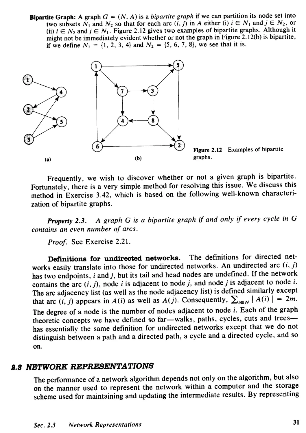
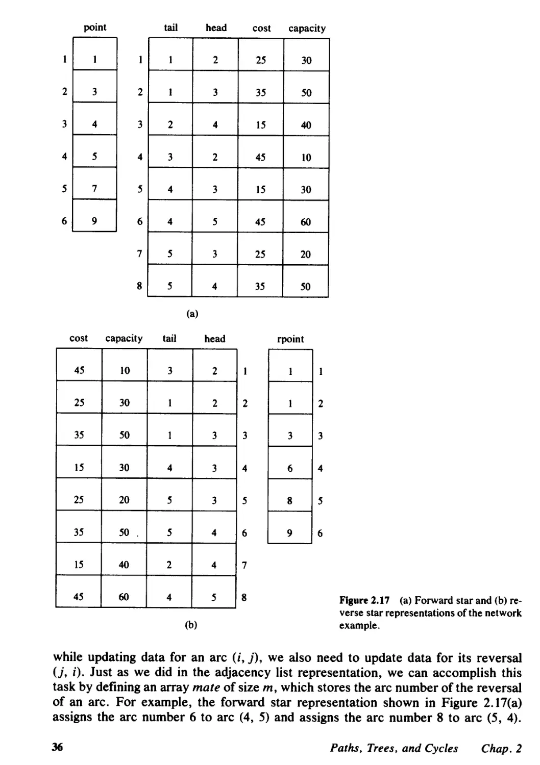
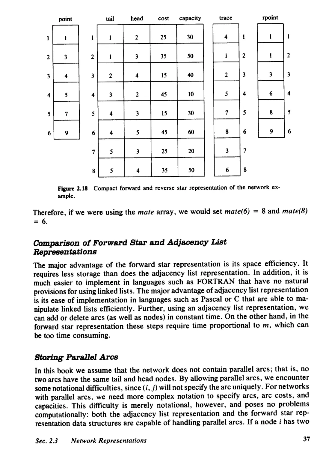
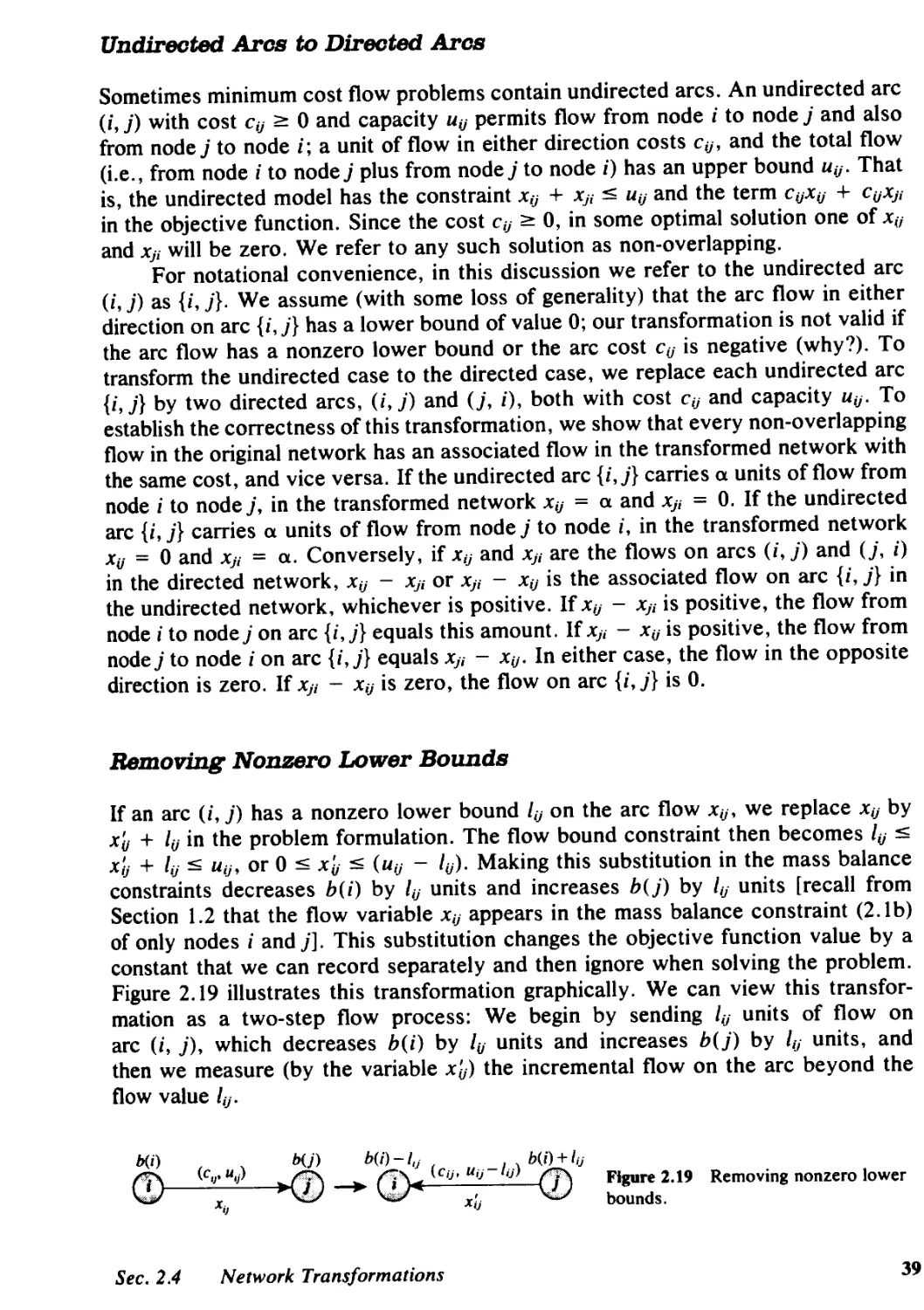
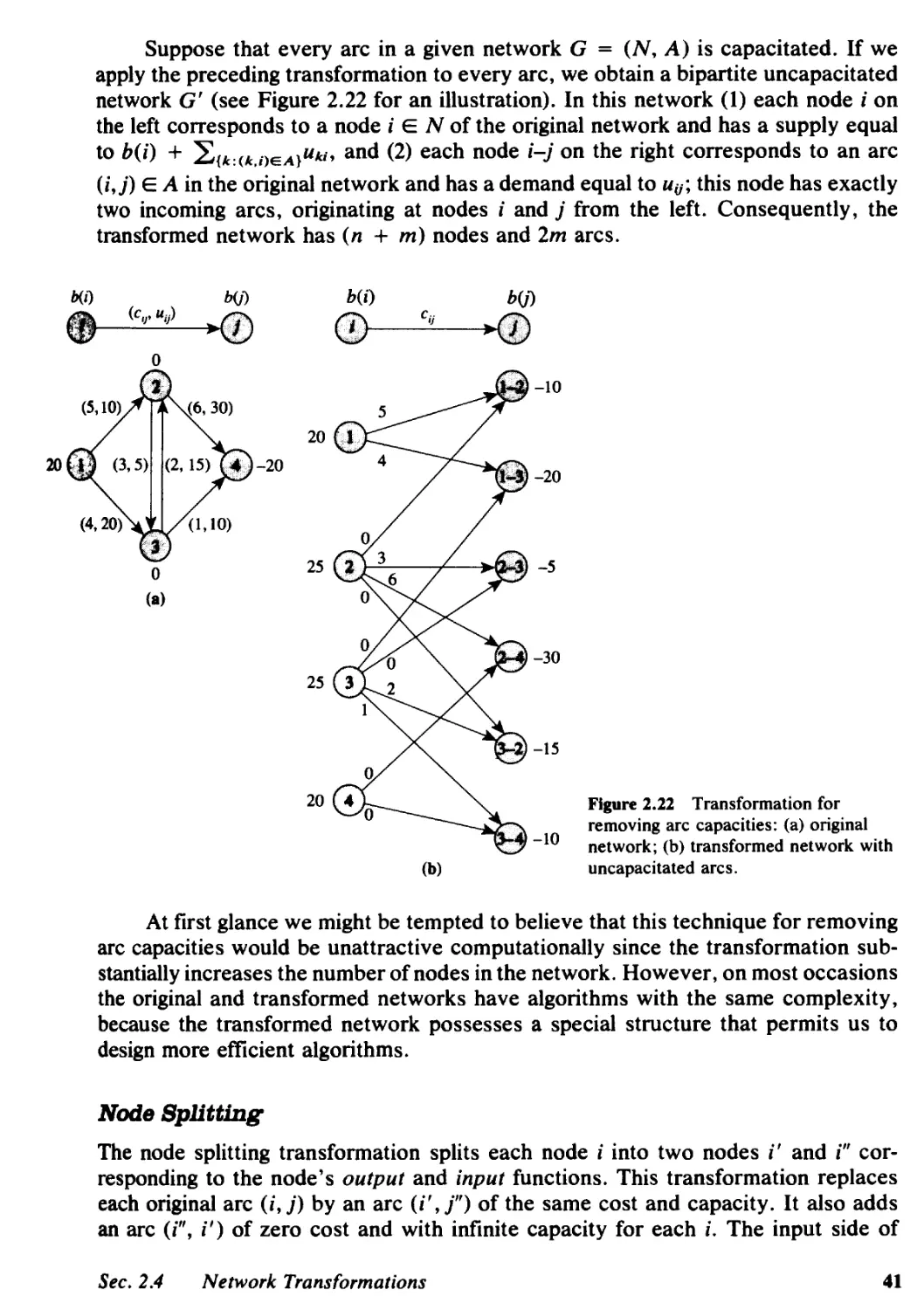
/


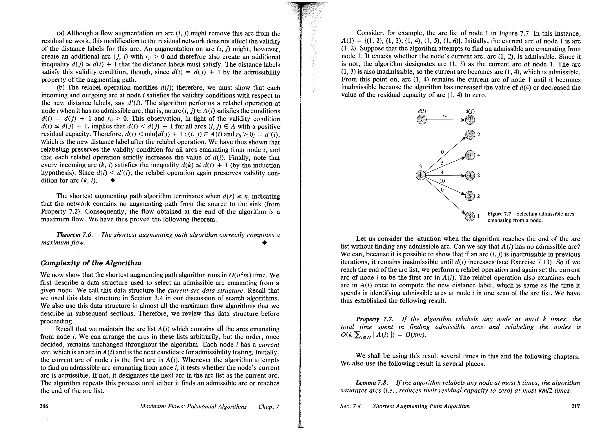


Author: Ahuja I Ravindra K. Magnanll Thomas L. Orlin James B..
Tags: discrete math
ISBN: 0-13-617549-X
Year: 1993


Text
NETWORK FLOWS
Theory, Algorithms,
and Applications
BA VINDBA K. AHUJA
Department of Industrial & Management Engineering
Indian Institute of Technology, Kanpur
THOMAS L. MAGNANT!
Sloan School of Management
Massachusetts Institute of Technology, Cambridge
JAMES B. OBLIN
Sloan School of Management
Massachusetts Institute of Technology, Cambridge
.
PRENTICE HALL, Upper Saddle River, New Jersey 07458
Library of Congress Cataloging-in-Publication Data
Ahuja, Ravindra K. (date)
Network flows: theory, algorithms, and applications I Ravindra K.
Ahuja, Thomas L. Magnanll, James B. Orlin.
p. cm.
Includes bibliographical references and index.
ISBN 0-13-617S49-X
I. Network analysis (Planning) 2. Mathematical optimization.
I. Magnanti, Thomas L. II. Orlin, James B., (date). III. Title.
TS7.8S.A37 1993
6S8.4'032-dc20 92-26702
CIP
Acquisitions editor: Pete Janzow
Production editor: Merrill Peterson
Cover designer: Design Source
Prepress buyer: Linda Behrens
Manufacturing buyer: David Dickey
Editorial assistant: Phyllis Morgan
The author and publisher of this book have used their best efforts in preparing this book. These effort!
include the development, research, and testing of the theories and programs to determine their
effectiveness. The author and publisher make no warranty of any kind, expressed or implied, with
regard to these programs or the documentation contained in this book. The author and publisher shall
not be liable in any event for incidental or consequential damages in connection with, or arising out of
the furnishing, performance, or use of these Drograms.
.
C 1993 by Prentice-Hall, Inc.
Upper Saddle River, New Jeney 074S8
All rights reserved. No part of this book may be
reproduced, in any form or by any means,
without permission in writing from the publisher.
Printed in the United States of America
16 17 18 19
ISBN 0-13-617549-X
PRENTICE-HALL INTERNATIONAL (UK) LIMITED, London
PRENTICE-HALL OF AUSTRALIA PTy. LIMITED, Sydney
PRENTICE-HALL CANADA INC., Toronto
PRENTICE-HALL HISPANOAMERICANA, S.A., Mexico
PRENTICE-HALL OF INDIA PRIVATE LIMITED, New Delhi
PRENTICE-HALL OF JAPAN, INC., Tokyo
EDITORA PRENTICE-HALL DO BRASIL, LTDA., Rio de Janeiro
Ravi dedicates this book to his spiritual master,
Revered Sri Ranaji Saheb.
Tom dedicates this book to his favorite network,
Beverly and Randy.
Jim dedicates this book to Donna,
who inspired him in so many ways.
Collectively, we offer this book as a tribute
to Lester Ford and Ray Fulkerson, whose pioneering research
and seminal text in network flows have been an enduring
inspiration to us and to a generation
of researchers and practitioners.
CONTENTS
PREFACE, xl
1 INTRODUCTION, 1
1.1 Introduction, 1
1.2 Network Flow Problems, 4
1.3 Applications, 9
1.4 Summary, 18
Reference Notes, 19
Exercises, 20
2 PATHS, TREES, AND CYCLES, 23
2.1 Introduction, 23
2.2 Notation and Definitions, 24
2.3 Network Representations, 31
2.4 Network Transformations, 38
2.5 Summary, 46
Reference Notes, 47
Exercises, 47
3 ALGORITHM DESIGN AND ANALYSIS, 3
3.1 Introduction, 53
3.2 Complexity Analysis, 56
3.3 Developing Polynomial-Time Algorithms, 66
3.4 Search Algorithms, 73
3.5 Flow Decomposition Algorithms, 79
3.6 Summary, 84
Reference Notes, 85
Exercises, 86
4 SHORTEST PA THS: LABEL-SE'ITING ALGORITHMS, 93
4.1 Introduction, 93
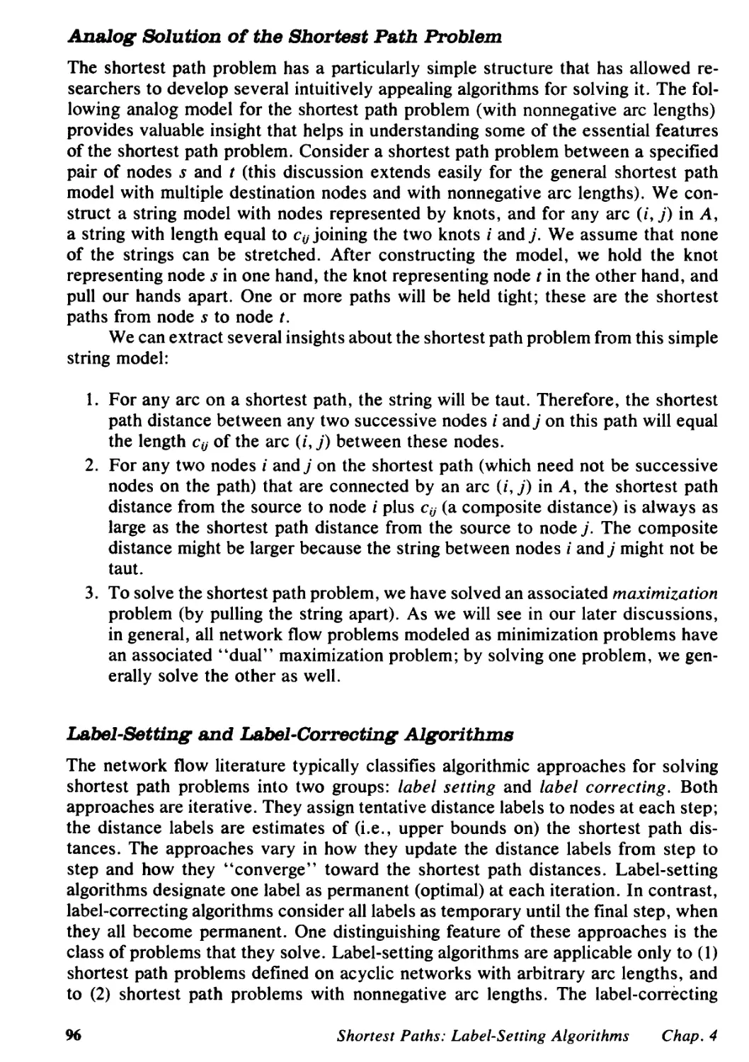
4.2 Applications, 97
4.3 Tree of Shortest Paths, 106
4.4 Shortest Path Problems in Acyclic Networks, 107
4.5 Dijkstra's Algorithm, 108
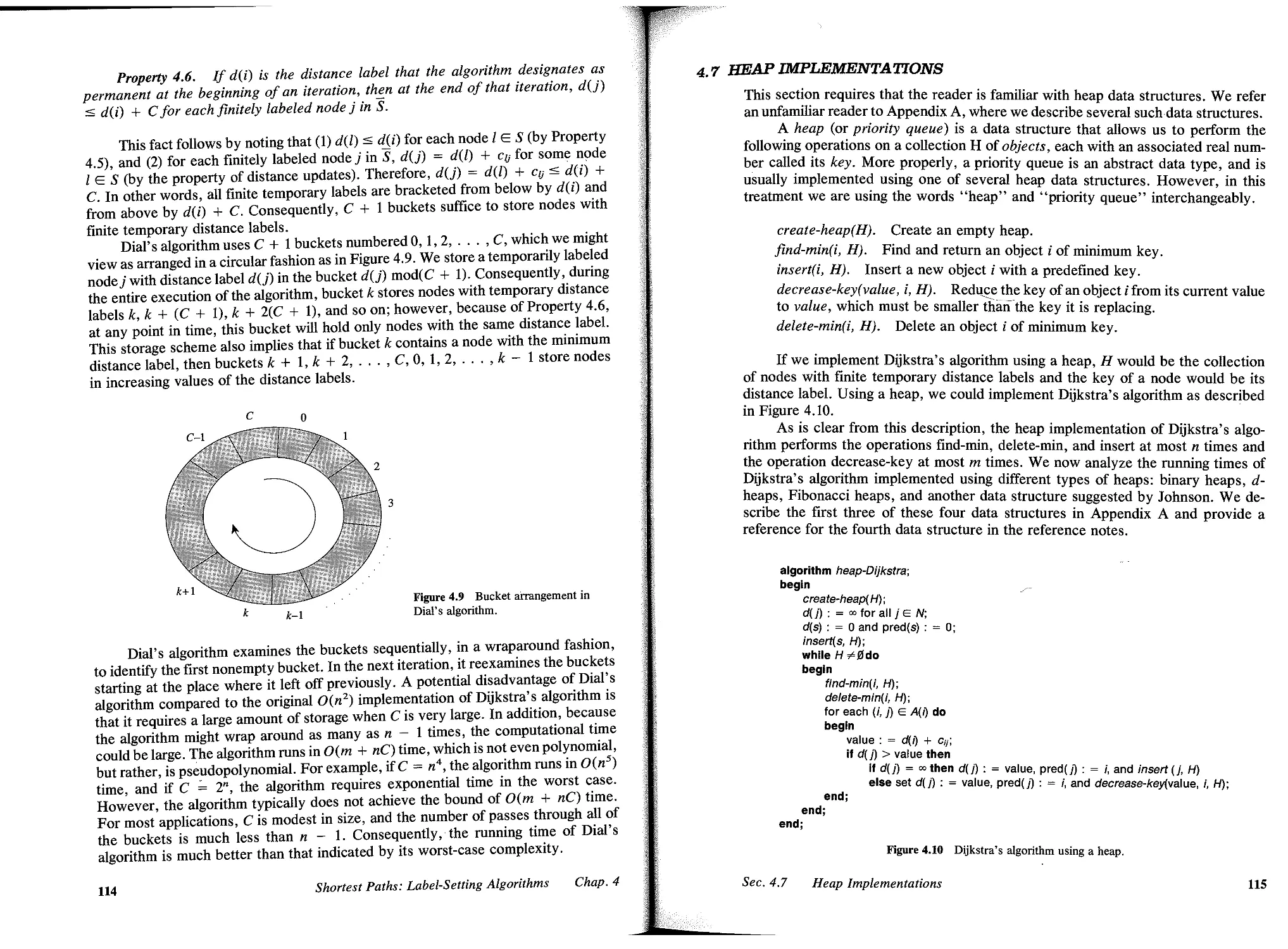
4.6 Dial's Implementation, 113
4.7 Heap Implementations, 115
4.8 Radix Heap Implementation, 116
v
4.9 Summary, 121
Reference Notes, 122
Exercises, 124
15 SHORTEST PATHS: LABEL-CORRECTING ALGOBITHMB, 133
5.1 Introduction, 133
5.2 Optimality Conditions, 135
5.3 Generic Label-Correcting Algorithms, 136
5.4 Special Implementations of the Modified Label-Correcting Algorithm, 141
5.5 Detecting Negative Cycles, 143
5.6 All-Pairs Shortest Path Problem, 144
5.7 Minimum Cost-to-Time Ratio Cycle Problem, 150
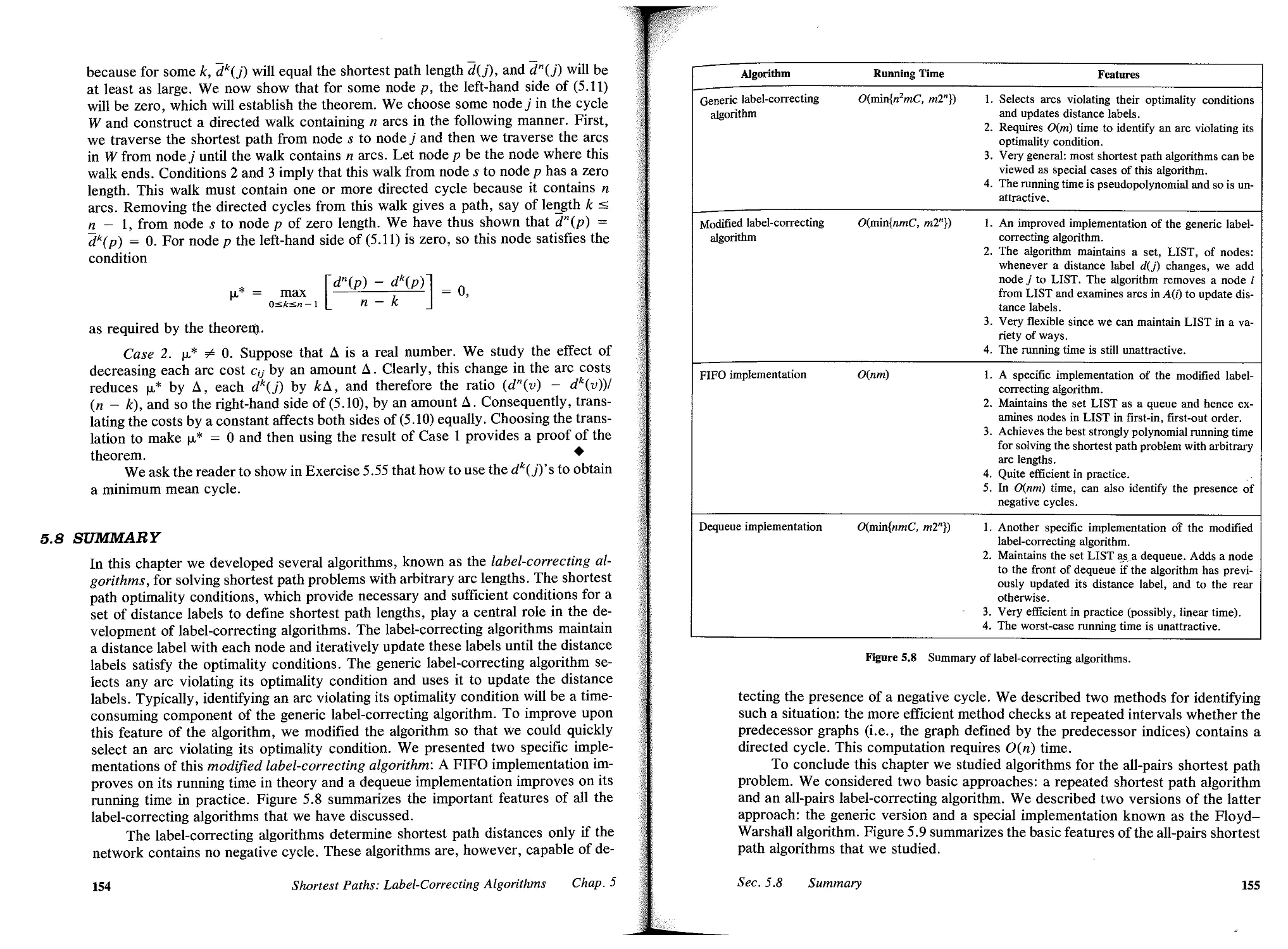
5.8 Summary, 154
Reference Notes, 156
Exercises, 157
8 MAXIMUM FLOWS: BABIC IDEAS, 188
6.1 Introduction, 166
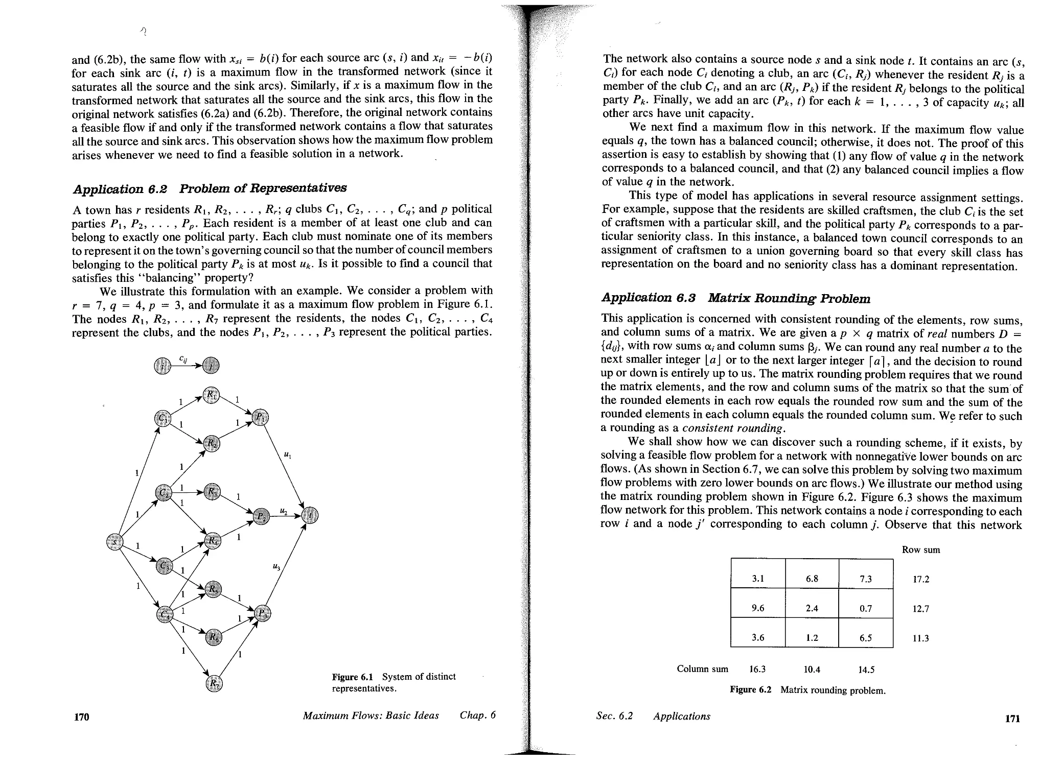
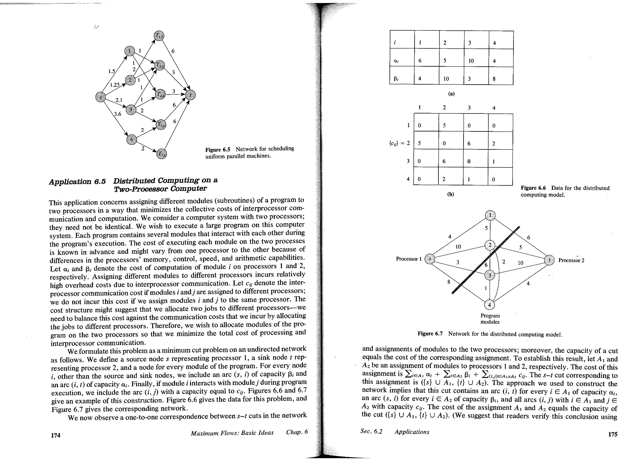
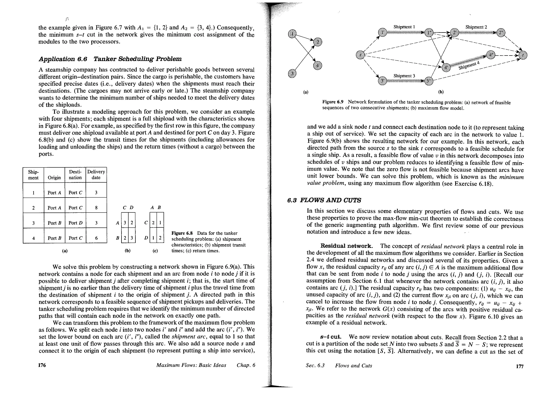
6.2 Applications, 169
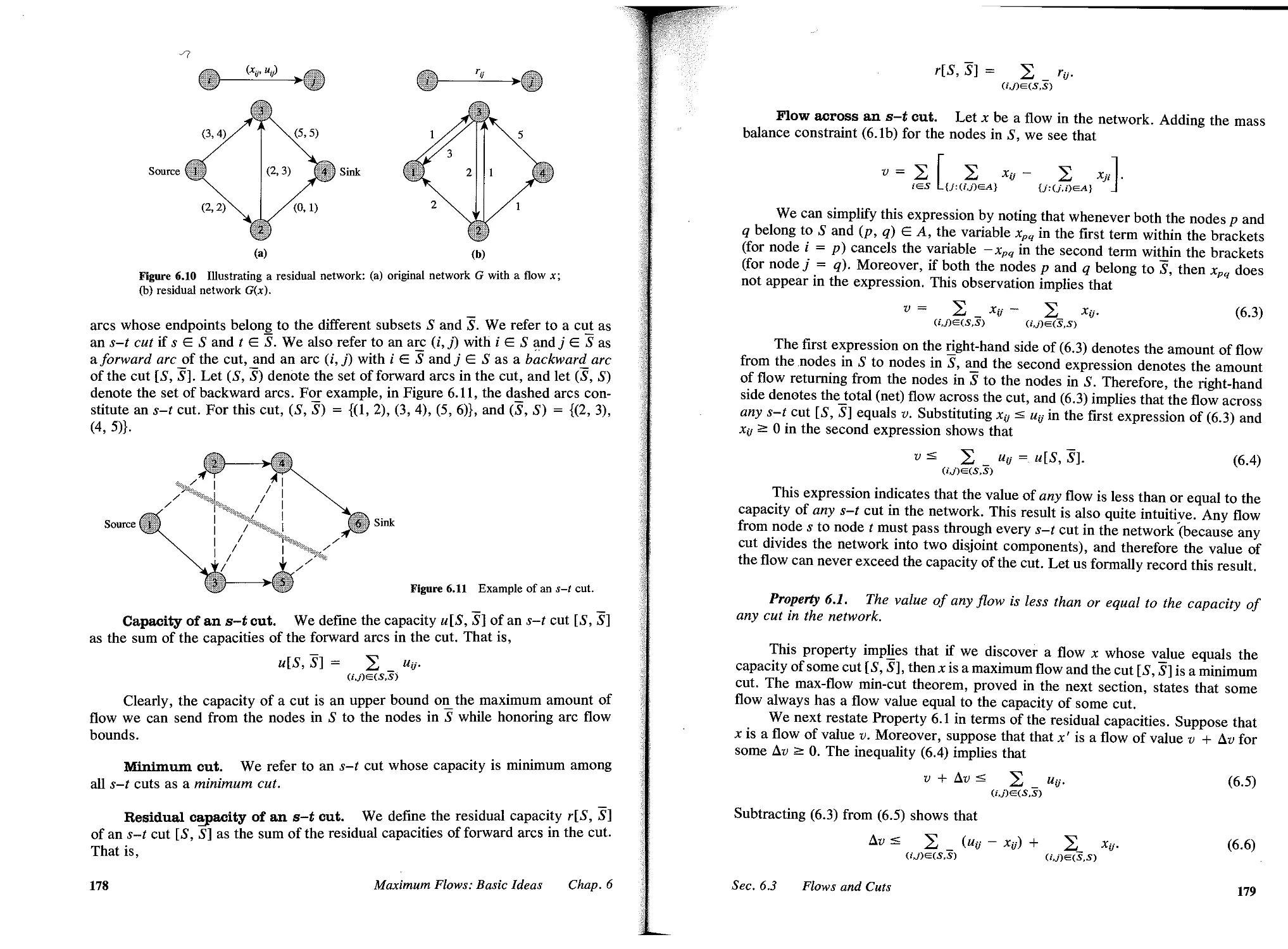
6.3 Flows and Cuts, 177
6.4 Generic Augmenting Path Algorithm, 180
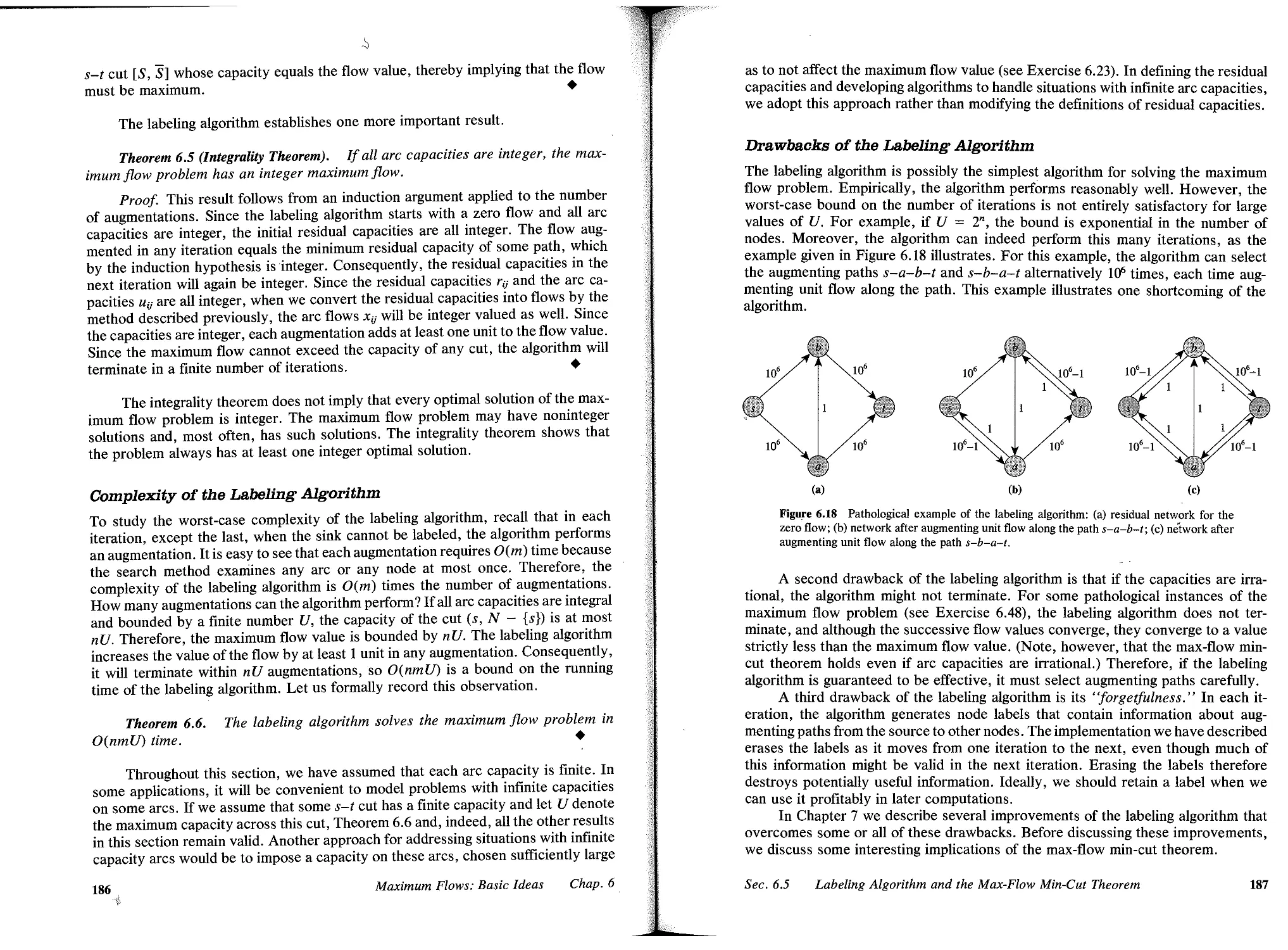
6.5 Labeling Algorithm and the Max-Flow Min-Cut Theorem, 184
6.6 Combinatorial Implications of the Max-Flow Min-Cut Theorem, 188
6.7 Flows with Lower Bounds, 191
6.8 Summary, 196
Reference Notes, 197
Exercises, 198
7 MAXIMUM FLOWS: POLYNOMIAL ALGOBITHMS, 207
7.1 Introduction, 207
7.2 Distance Labels, 209
7.3 Capacity Scaling Algorithm, 210
7.4 Shortest Augmenting Path Algorithm, 213
7.5 Distance Labels and Layered Networks, 221
7.6 Generic Preflow-Push Algorithm, 223
7.7 FIFO Preflow-Push Algorithm, 231
7.8 Highest-Label Preflow-Push Algorithm, 233
7.9 Excess Scaling Algorithm, 237
7.10 Summary , 241
Reference Notes, 241
Exercises, 243
8 MAXIMUM FLOWS: ADDITIONAL TOPICS, 230
8.1 Introduction, 250
8.2 Flows in Unit Capacity Networks, 252
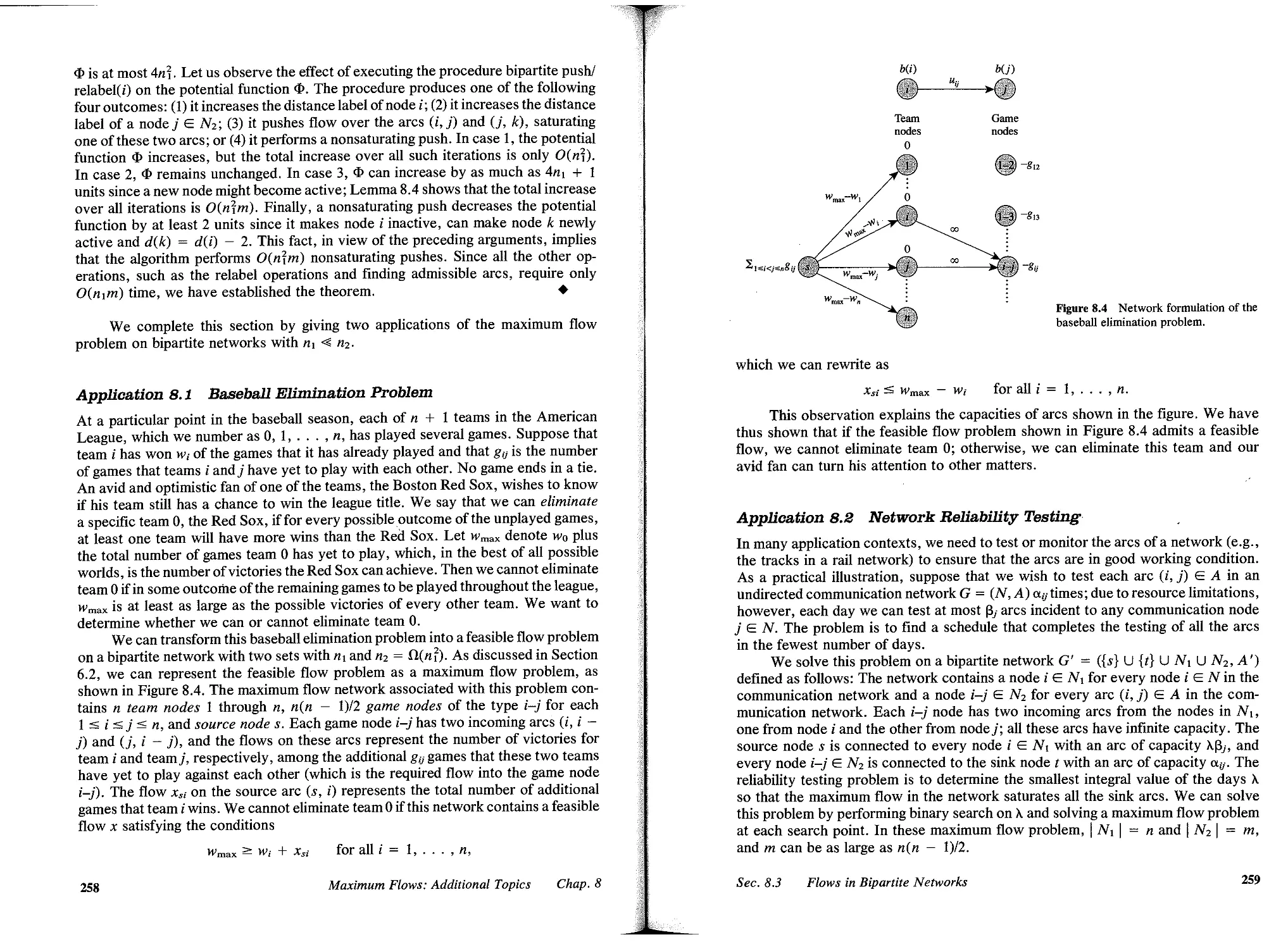
8.3 Flows in Bipartite Networks, 255
8.4 Flows in Planar Undirected Networks, 260
8.5 Dynamic Tree Implementations, 265
vi
Contents
8.6 Network Connectivity, 273
8.7 All-Pairs Minimum Value Cut Problem, 277
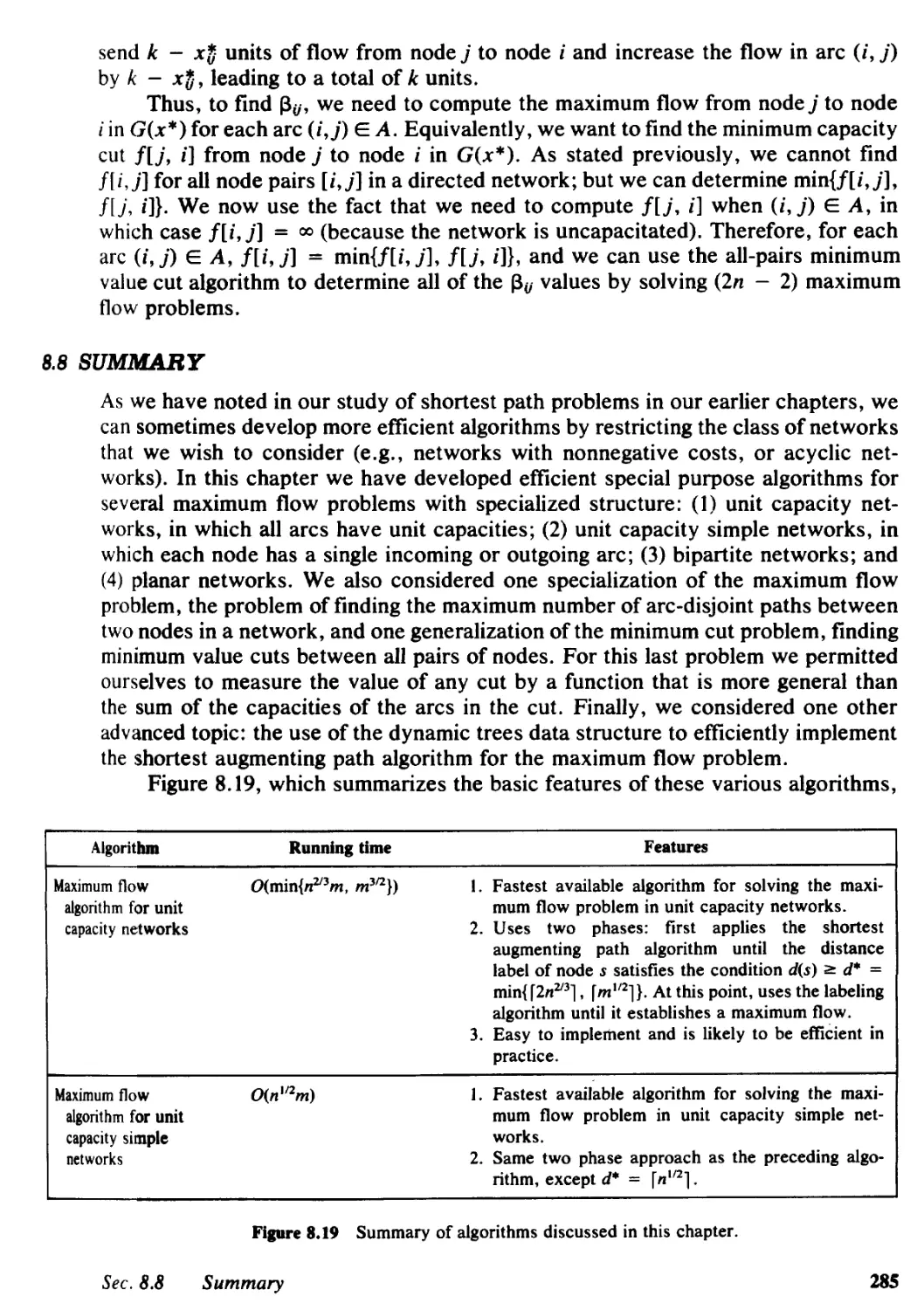
8.8 Summary, 285
Reference Notes, 287
Exercises, 288
9 MINIMUM COST FLOWS: BABIC ALGORITHMS, 294
9.1 Introducti"on, 294
9.2 Applications, 298
9.3 Optimality Conditions, 306
9.4 Minimum Cost Flow Duality, 310
9.5 Relating Optimal Flows to Optimal Node Potentials, 315
9.6 Cycle-Canceling Algorithm and the Integrality Property, 317
9.7 Successive Shortest Path Algorithm, 320
9.8 Primal-Dual Algorithm, 324
9.9 Out-of-Kilter Algorithm, 326
9.10 Relaxation Algorithm, 332
9.11 Sensitivity Analysis, 337
9.12 Summary, 339
Reference Notes, 341
Exercises, 344
10 MINIMUM COST FLOWS: POLYNOMIAL ALGOBITHMS, 3lJ7
10.1 Introduction, 357
10.2 Capacity Scaling Algorithm, 360
10.3 Cost Scaling Algorithm, 362
10,4 Double Scaling Algorithm, 373
10.5 Minimum Mean Cycle-Canceling Algorithm, 376
10.6 Repeated Capacity Scaling Algorithm, 382
10.7 Enhanced Capacity Scaling Algorithm, 387
10.8 Summary, 395
Reference Notes, 396
Exercises, 397
11 MINIMUM COST FLOWS: NETWORK SIMPLEX ALGOlUTHMS, 402
11.1 Introduction, 402
11.2 Cycle Free and Spanning Tree Solutions, 405
11.3 Maintaining a Spanning Tree Structure, 409
11.4 Computing Node Potentials and Flows, 411
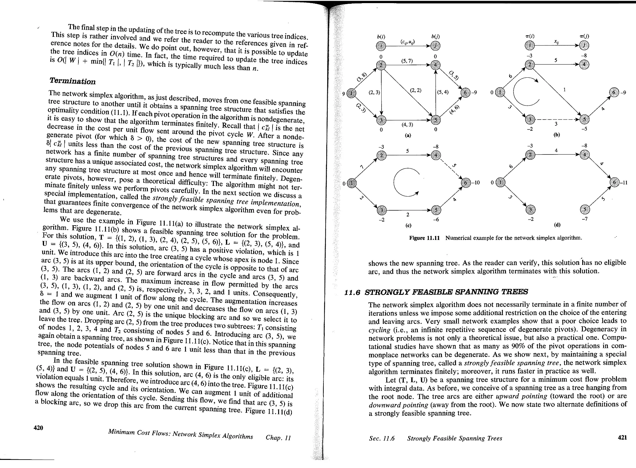
11. 5 Network Simplex Algorithm, 415
11.6 Strongly Feasible Spanning Trees, 421
11.7 Network Simplex Algorithm for the Shortest Path Problem, 425
11.8 Network Simplex Algorithm for the Maximum Flow Problem, 430
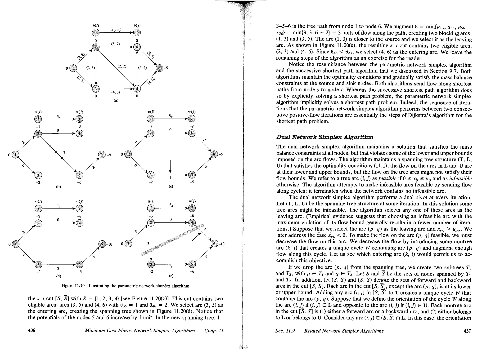
11.9 Related Network Simplex Algorithms, 433
11.10 Sensitivity Analysis, 439
11.11 Relationship to Simplex Method, 441
11.12 U nimodularity Property, 447
11,13 Summary, 450
Reference Notes, 451
Exercises, 453
Contents
vii
12 ASSIGNMENTSANDMATCHlNGS, 481
12.1 Introduction, 461
12.2 Applications, 463
12.3 Bipartite Cardinality Matching Problem, 469
12.4 Bipartite Weighted Matching Problem, 470
12.5 Stable Marriage Problem, 473
12.6 Nonbipartite Cardinality Matching Problem, 475
12.7 Matchings and Paths, 494
12.8 Summary, 498
Reference Notes, 499
Exercises, 501
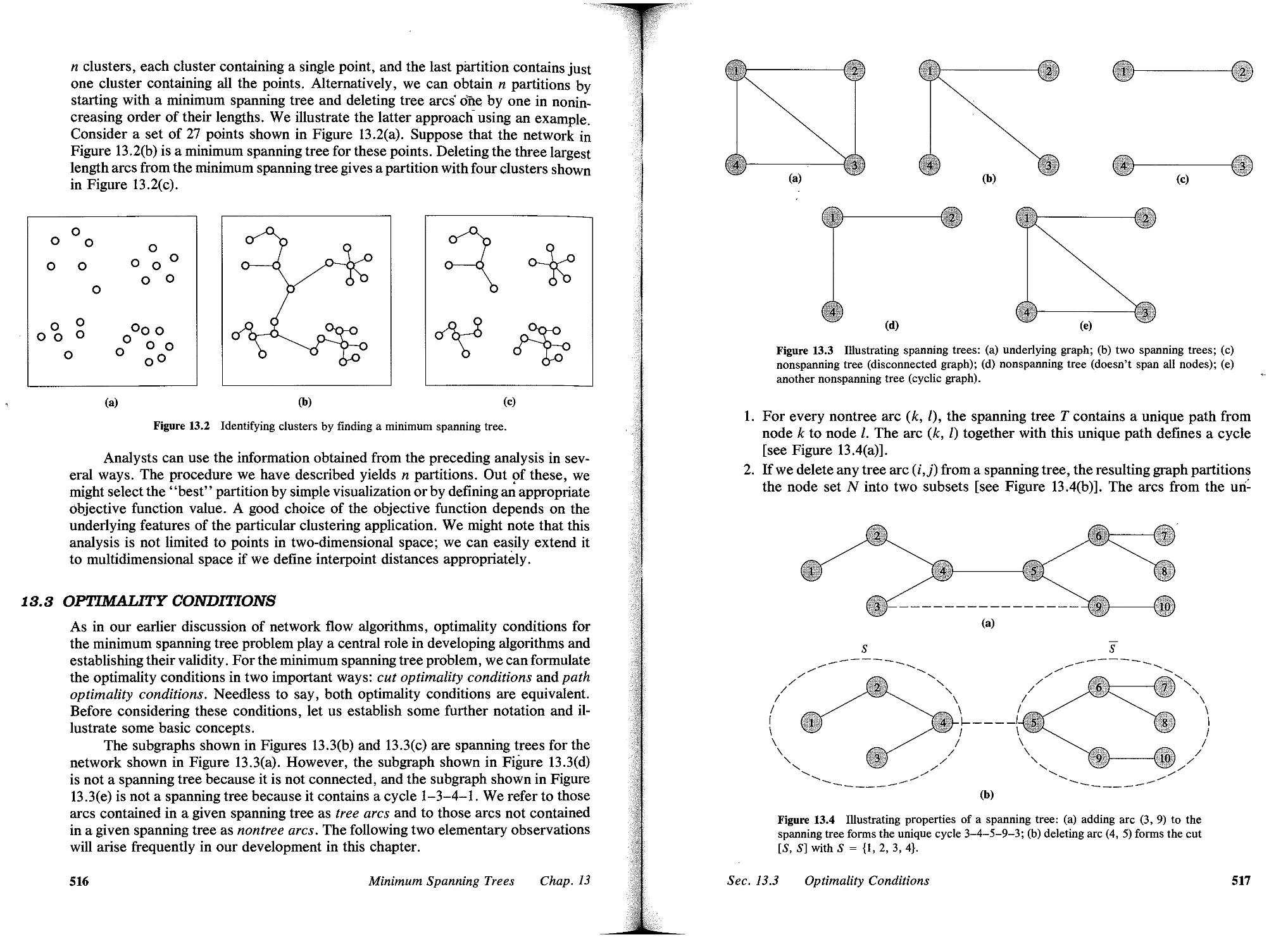
13 MlNIMUM SPANNING TREES, 610
13.1 Introduction, 510
13.2 Applications, 512
13.3 Optimality Conditions, 516
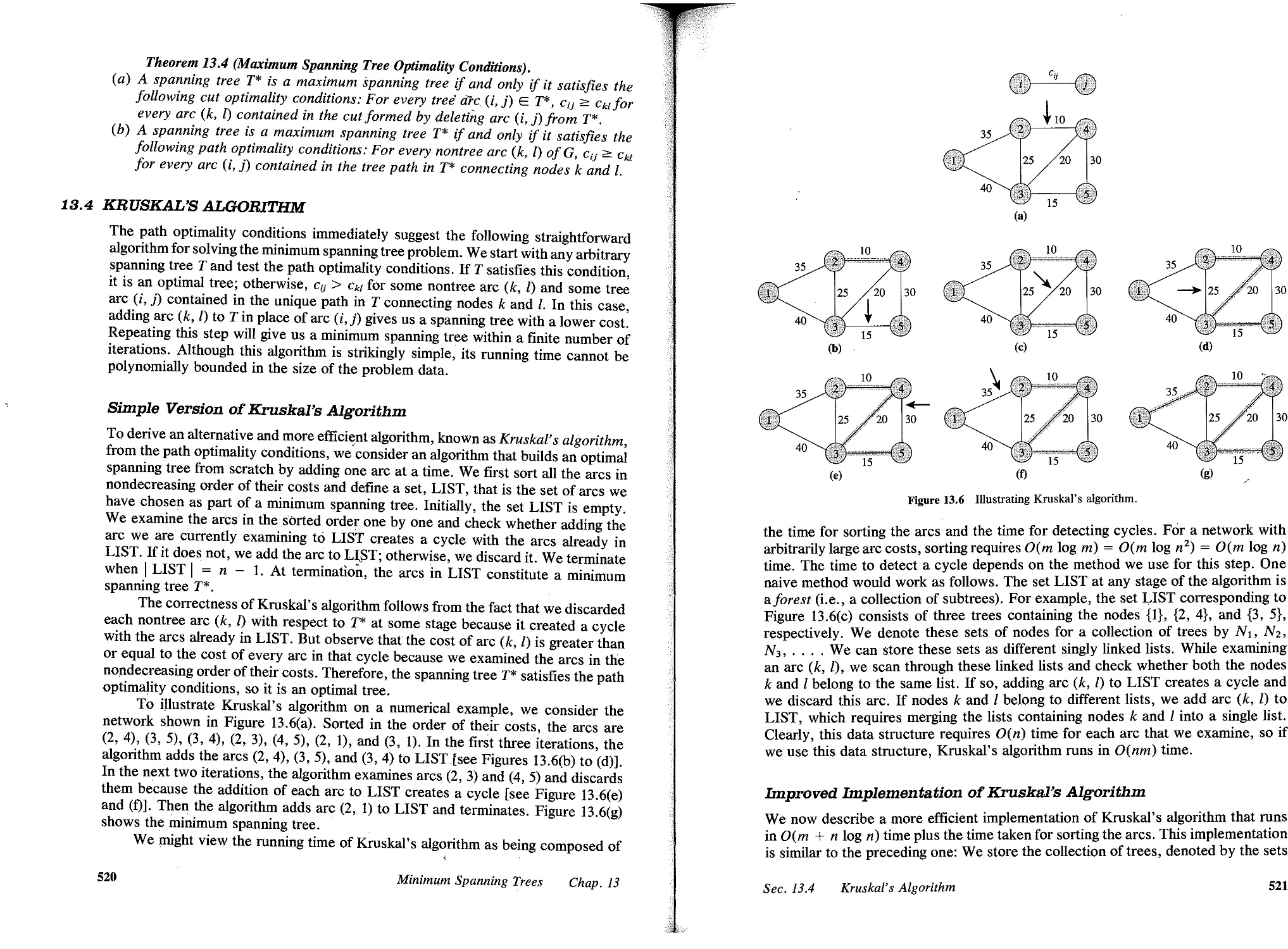
13.4 Kruskal's Algorithm, 520
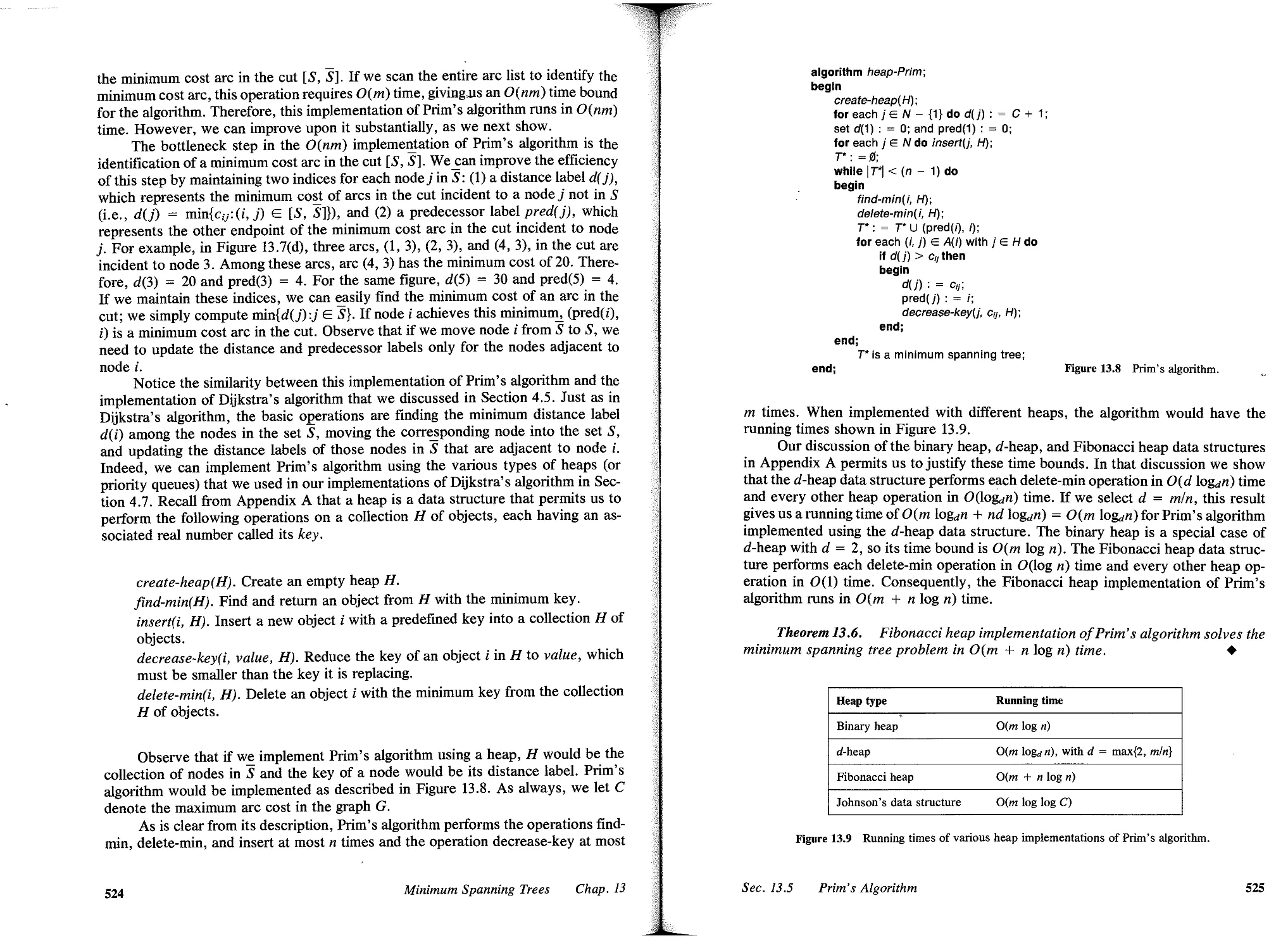
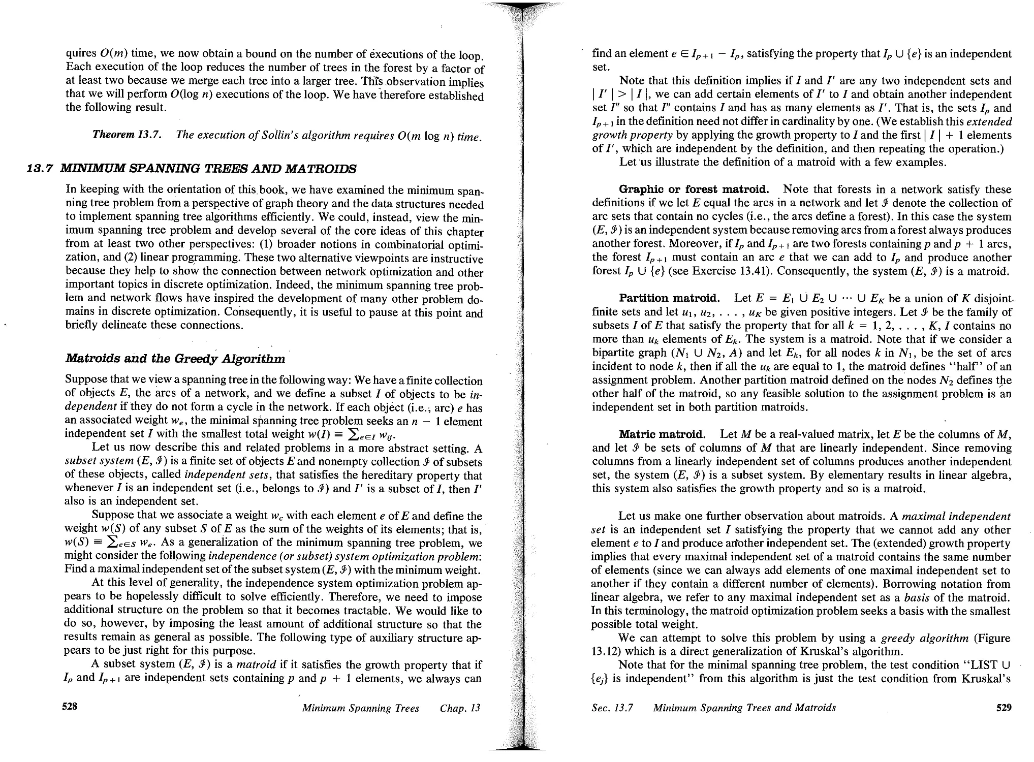
13.5 Prim's Algorithm, 523
13.6 Sollin's Algorithm, 526
13.7 Minimum Spanning Trees and Matroids, 528
13.8 Minimum Spanning Trees and Linear Programming, 530
13.9 Summary, 533
Reference Notes, 535
Exercises, 536
14 CONVEX COST FLOWS, 643
14.1 Introduction, 543
14.2 Applications, 546
14.3 Transformation to a Minimum Cost Flow Problem, 551
14.4 Pseudopolynomial-Time Algorithms, 554
14.5 Polynomial- Time Algorithm, 556
14.6 Summary, 560
Reference Notes, 561
Exercises, 562
15 GENERALIZED FLOWS, 688
15.1 Introduction, 566
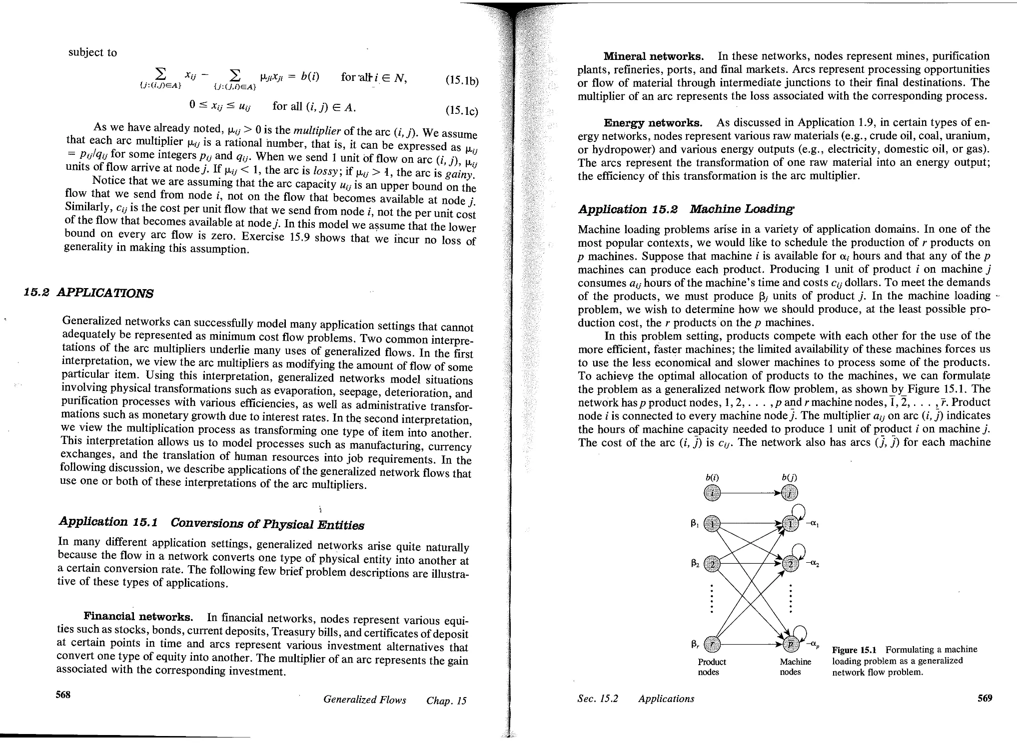
15.2 Applications, 568
15.3 Augmented Forest Structures, 572
15.4 Determining Potentials and Flows for an Augmented Forest Structure, 577
15.5 Good Augmented Forests and Linear Programming Bases, 582
15.6 Generalized Network Simplex Algorithm, 583
15.7 Summary, 591
Reference Notes, 591
Exercises, 593
viii
Contents
18 LAGRANGIAN RELAXATION AND NETWORK OPTIMIZATION, 1J98
16.1 Introduction, 598
16.2 Problem Relaxations and Branch and Bound, 602
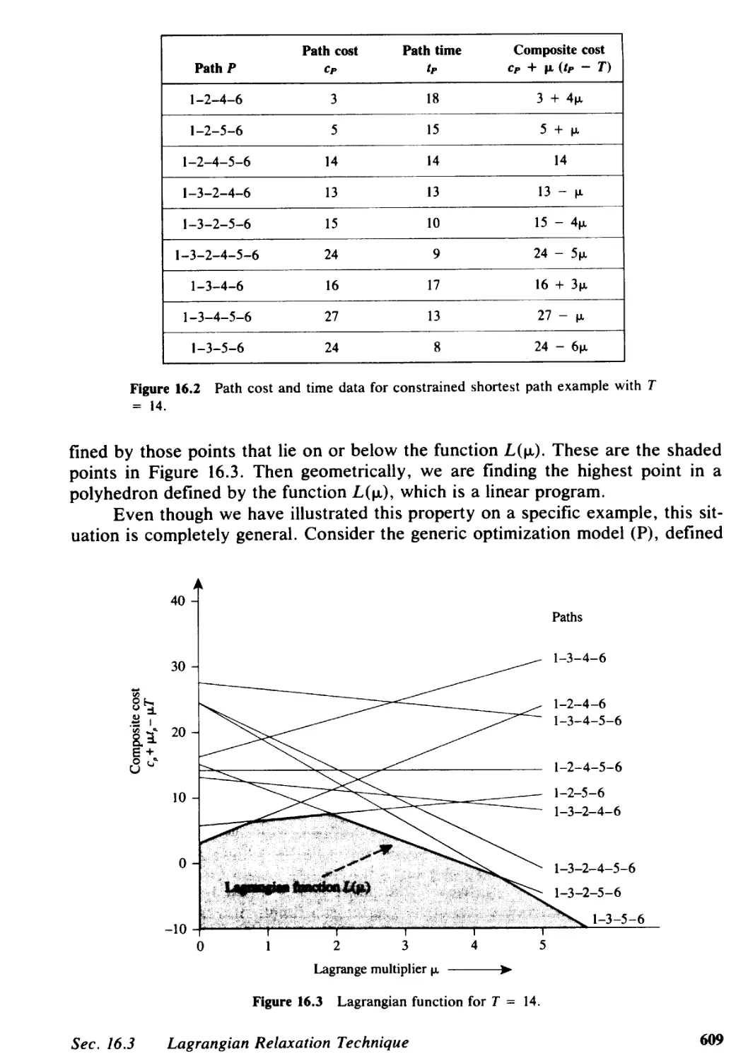
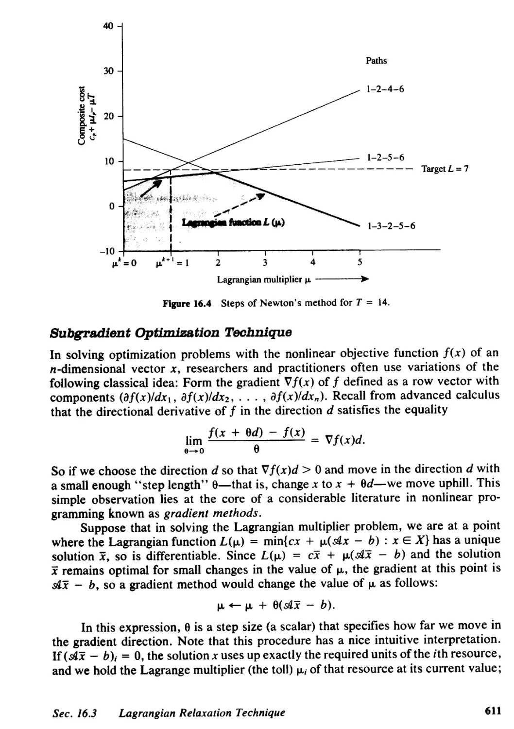
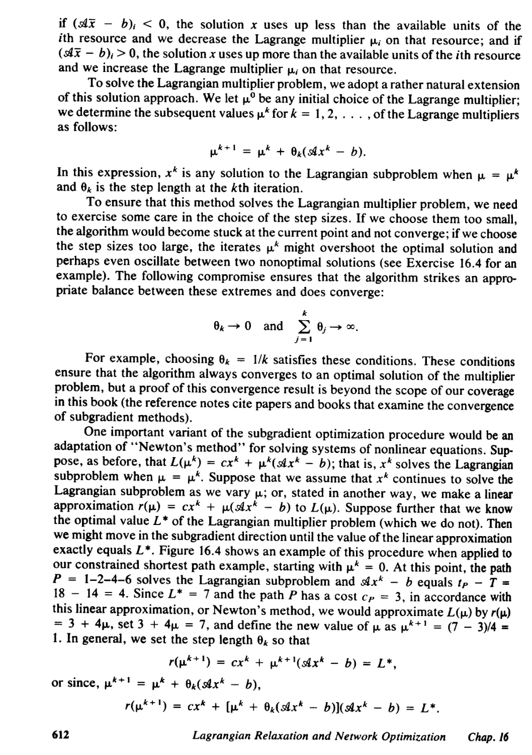
16.3 Lagrangian Relaxation Technique, 605
16.4 Lagrangian Relaxation and Linear Programming, 615
16.5 Applications of Lagrangian Relaxation, 620
16.6 Summary, 635
Reference Notes, 637
Exercises, 638
17 MULTICOMMODITY FLOWS, 849
17.1 Introduction, 649
17.2 Applications, 653
17.3 Optimality Conditions, 657
17.4 Lagrangian Relaxation, 660
17.5 Column Generation Approach, 665
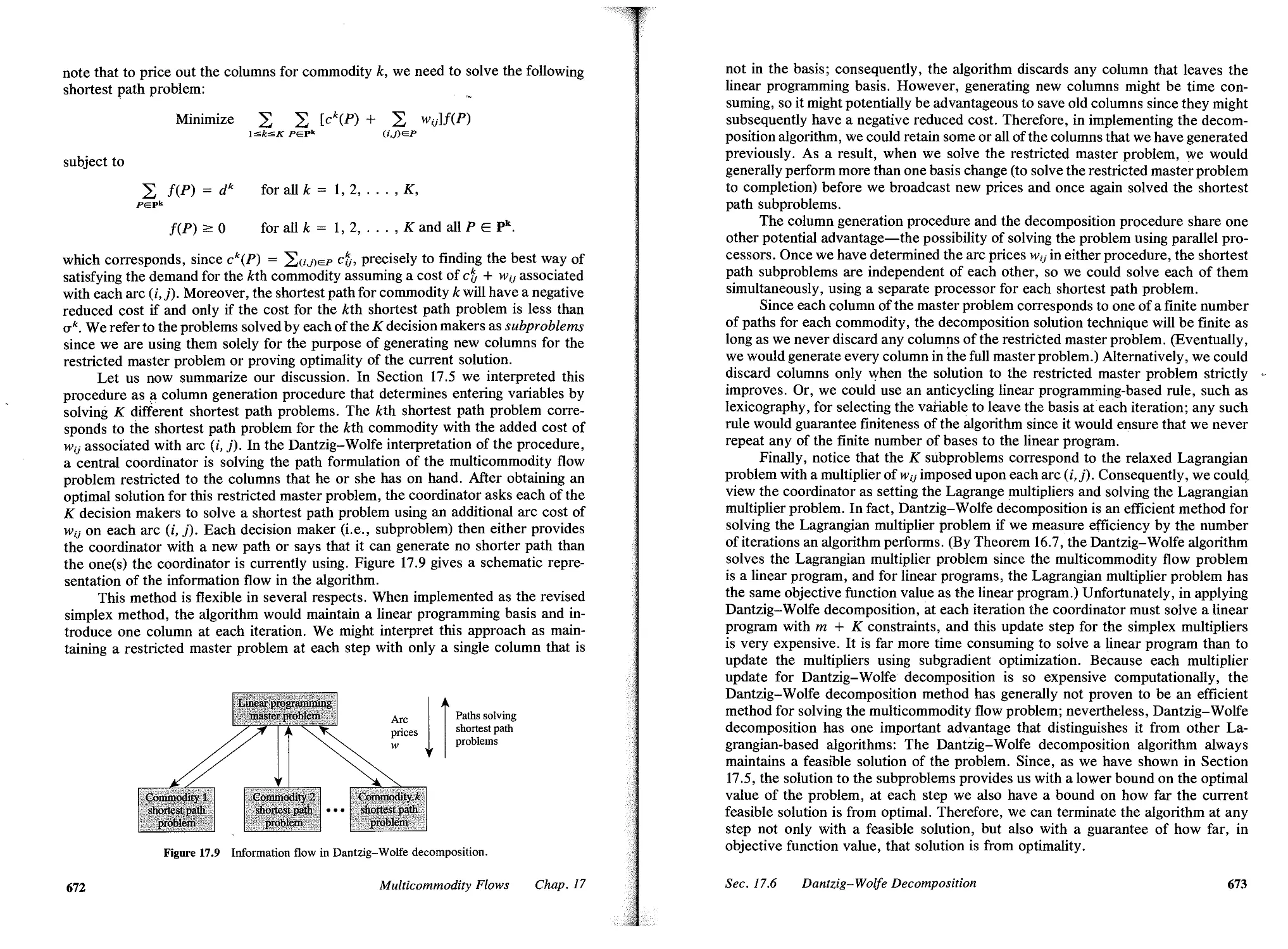
17.6 Dantzig-Wolfe Decomposition, 671
17.7 Resource-Directive Decomposition, 674
17.8 Basis Partitioning, 678
17.9 Summary, 682
Reference Notes, 684
Exercises, 686
18 COMPUTATIONAL TESTING OF ALGORITHMS, 891J
18.1 Introduction, 695
18.2 Representative Operation Counts, 698
18.3 Application to Network Simplex Algorithm, 702
18.4 Summary, 713
Reference Notes, 713
Exercises, 715
19 ADDITIONAL APPLICATIONS, 717
19.1 Introduction, 717
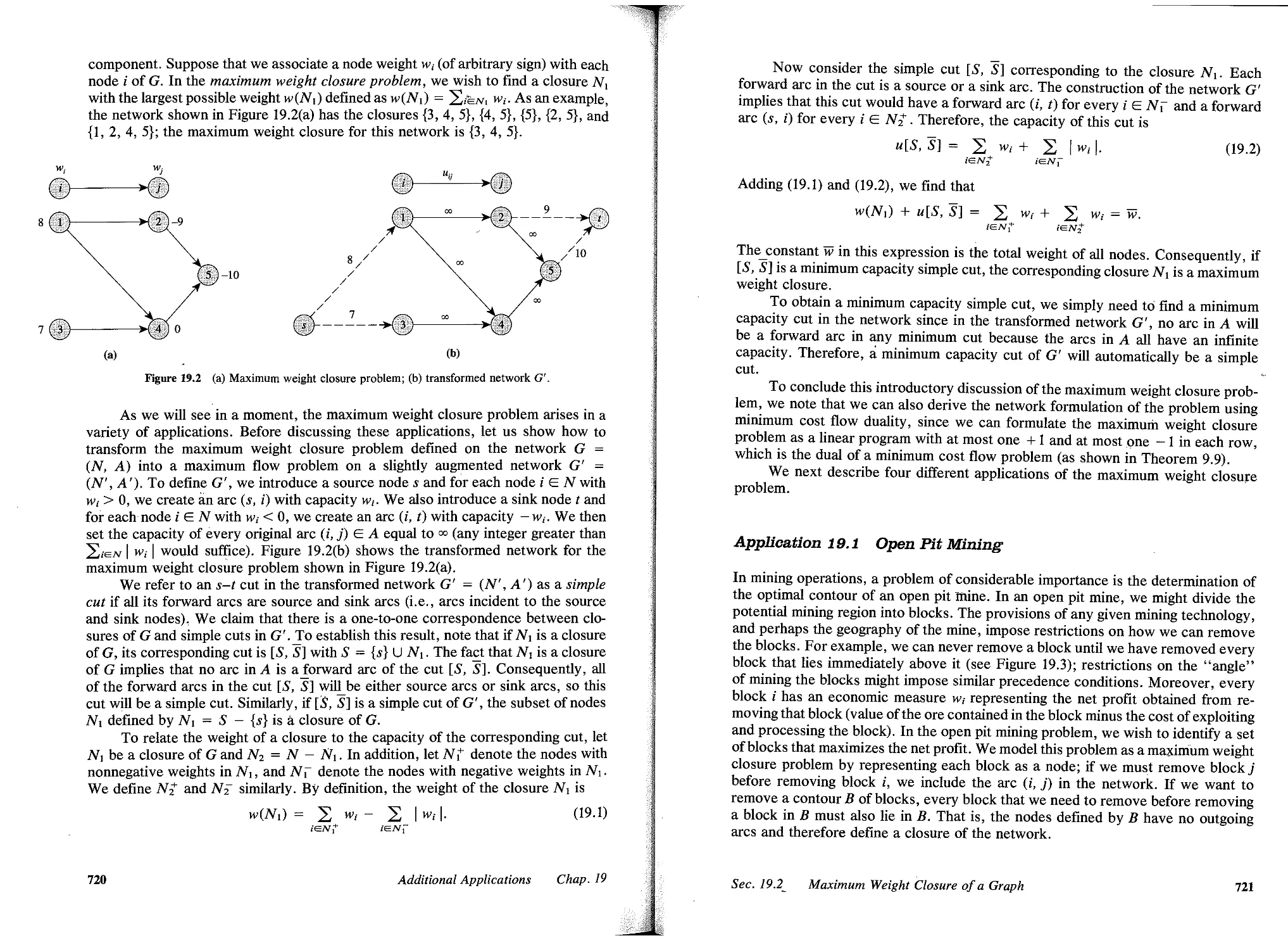
19.2 Maximum Weight Closure of a Graph, 719
19.3 Data Scaling, 725
19.4 Science Applications, 728
19.5 Project Management, 732
19.6 Dynamic Flows, 737
19.7 Arc Routing Problems, 740
19.8 Facility Layout and Location, 744
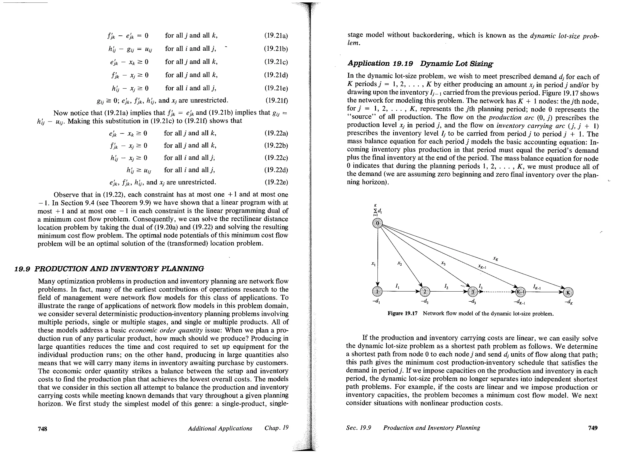
19.9 Production and Inventory Planning, 748
19.10 Summary, 755
Reference Notes, 759
Exercises, 760
Contents
Ix
APPENDIX A DATA STRUCTURES, 78
A.l Introduction, 765
A.2 Elementary Data Structures, 766
A.3 d-Heaps, 773
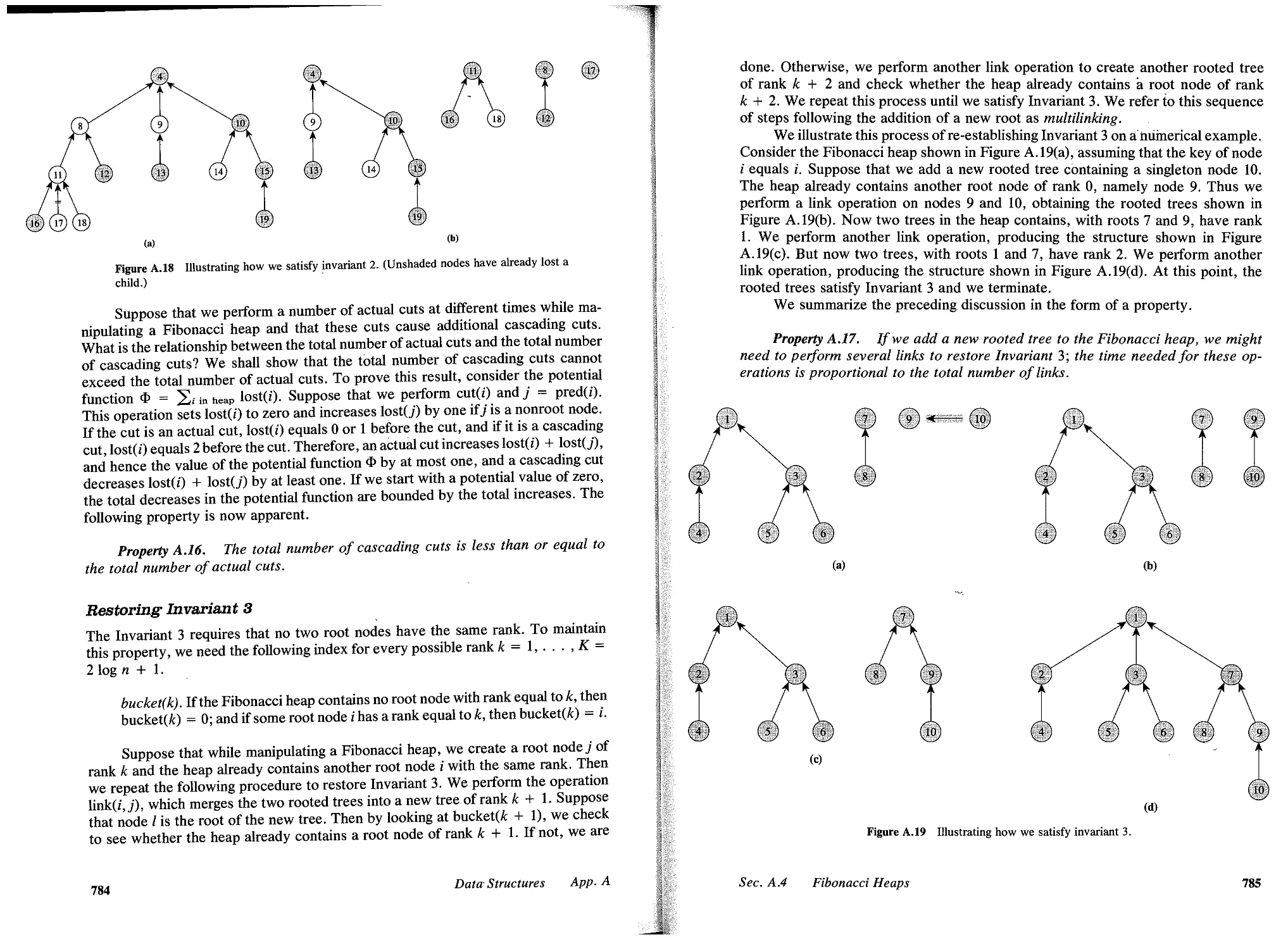
A.4 Fibonacci Heaps, 779
Reference Notes, 787
APPENDIX B Nf/P-COMPLETENESS, 788
B.l Introduction, 788
B.2 Problem Reductions and Transformations, 790
B.3 Problem Classes , .N , .N -Complete, and .N -Hard, 792
B.4 Proving .N -Completeness Results, 796
B.5 Concluding Remarks, 800
Reference Notes, 801
APPENDIX C LINEAR PROGRAMMING, 802
C.l Introduction, 802
C.2 Graphical Solution Procedure, 804
C.3 Basic Feasible Solutions, 805
C.4 Simplex Method, 810
C.5 Bounded Variable Simplex Method, 814
C.6 Linear Programming Duality, 816
Reference Notes, 820
REFERENCES, 821
INDEX,
840
x
Contents
PREFACE
If you would not be forgotten,
As soon as you are dead and rotten,
Either write things worthy reading,
Or do things worth the writing.
-Benjamin Franklin
Network flows is an exciting field that brings together what many students, prac-
titioners, and researchers like best about the mathematical and computational sci-
ences. It couples deep intellectual content with a remarkable range of applicability,
covering literally thousands of applications in such wide-ranging fields as chemistry
and physics, computer networking, most branches of engineering, manufacturing,
public policy and social systems, scheduling and routing, telecommunications, and
transportation. It is classical, dating from the work of Gustav Kirchhoff and other
eminent physical scientists of the last century, and yet vibrant and current, bursting
with new results and new approaches. Its heritage is rooted in the traditional fields
of mechanics, engineering, and applied mathematics as well as the contemporary
fields of computer science and operations research.
In writing this book we have attempted to capture these varied perspectives
and in doing so to fill a need that we perceived for a comprehensive text on network
flows that would bring together the old and the new, and provide an integrative view
of theory, algorithms, and applications. We have attempted to design a book that
could be used either as an introductory or advanced text for upper-level under-
graduate or graduate students or as a reference for researchers and practitioners.
We have also strived to make the coverage of this material as readable, accessible,
and insightful as possible, particularly for readers with a limited background in com-
puter science and optimization.
The book has the following features:
. In-depth and self-contained treatment of shortest path, maximum flow, and
minimum cost flow problems, including descriptions of new and novel poly-
nomial-time algorithms for these core models.
. Emphasis on powerful algorithmic strategies and analysis tools, such as data
scaling, geometric improvement arguments, and potential function arguments.
. An easy-to-understand description of several important data structures, in-
cluding d-heaps, Fibonacci heaps, and dynamic trees.
. Treatment of other important topics in network optimization and of practical
solution techniques such as Lagrangian relaxation.
xi
. Each new topic introduced by a set of applications and an entire chapter de-
voted to applications.
. A special chapter devoted to conducting empirical testing of algorithms.
. Over 150 applications of network flows to a variety of engineering, manage-
ment, and scientific domains.
. Over 800 exercises that vary in difficulty, including many that develop exten-
sions of material covered in the text.
. Approximately 400 figures that illustrate the material presented in the text.
. Extensive reference notes that provide readers with historical contexts and
with guides to the literature.
As indicated by this list, we have not attempted to cover all topics at the same
level of depth, but instead, have treated certain core topics more extensively than
others. Moreover, although we have focused on the design and analysis of efficient
algorithms, we have also placed considerable emphasis on applications.
In attempting to streamline the material in this book and present it in an in-
tegrated fashion, we have devoted considerable time, and in several cases conducted
research, to improve our presentation. As a result, our coverage of some topics
differs from the discussion in the current literature. We hope that this approach will
not lead to any confusion, and that it will, in fact, promote a better understanding
of the material and uncover new connections between topics that might not appear
to be so related in the literature.
TO INSTBUCTORS AND STUDENTS
We have attempted to write this book so that it is accessible to students with many
backgrounds. Although students require some mathematical maturity-for example,
a basic understanding of proof techniques-and some familiarity with computer
programming, they need not be specialists in mathematics, computer science, or
optimization. Some basic knowledge of these topics would undoubtedly prove to be
useful in using this book. In Chapter 3 and Appendices A, B, and C, we have provided
some of this general background.
The book contains far more material than anyone could possibly cover in a
one-semester course. Chapters 1 to 3, 19, selected material from Chapters 5 to 12,
16, and 17, and portions of Chapters 13 to 15 and 18 would serve as a broad-based
course on network flows and network optimization. Because the chapters are gen-
erally modular, instructors might use the introductory material in the first few sec-
tions of each chapter as well as a selection of additional material for chapters that
they would not want to cover in their entirety. An advanced course on algorithms
might focus on Chapter 4 to 12, covering the material in these chapters in their
entirety.
In teaching the algorithms in this book, we feel that it is important to understand
the underlying methods of algorithm design and analysis as well as specific results.
Therefore, we encourage both instructors and students to refer frequently back to
Chapter 3 and its discussion of algorithm design and analysis.
Many of the topics that we have examined in this book are specially structured
xii
Preface
linear programs. Therefore, we could have adopted a linear programming approach
while presenting much of the material. Instead, with the exception of Chapter 17
and parts of Chapters 15 and 16, we have argued almost exclusively from first prin-
ciples and adopted a network or graphical viewpoint. We believe that this approach,
while occasionally imposing a less streamlined development than might be possible
using linear programming, offers several advantages. First, the material is readily
accessible to a wider audience. Second, this approach permits students who are not
optimization specialists to learn many of the ideas of linear programming in a con-
crete setting with easy geometric and algebraic interpretations; it also permits stu-
dents with prior knowledge of linear programming to refine their understanding by
seeing material in a different light. In fact, when the audience for a course has a
background in linear programming, we would encourage instructors and students to
make explicit connections between our coverage and more general results in linear
programming.
Although we have included some numerical exercises that test basic under-
standing of material presented in the text, many of the exercises address applications
or theory. Instructors might like to use this material, with suitable amplification, as
lecture material. Instructors wishing more numerical examples might modify the
ones we have provided.
TO OUB GENERAL READERS
Professionals in applied mathematics, computer science, engineering, and manage-
ment science/operations research as well as practitioners in a variety of application
domains might wish to extract specific information from the text without covering
the book in detail. Since the book is organized primarily by model type (e.g., shortest
path or spanning tree problems), readers have ready access to the material along
these dimensions. For a guide to applications, readers might consult Section 19.10,
which contains a set of tables summarizing the various network flow applications
that we have considered in the text. The end-of-chapter reference notes also contain
references to a number of applications that we have either not discussed or consid-
ered only in the exercises. For the most part, with the exception of applications, we
have been selective in our citations to the literature. Many of the general references
that we have mentioned at the end of Chapter 1 contain more detailed references
to the literature.
We have described many algorithms in this book using a pseudocode that should
be understandable to readers with any passing familiarity with computer program-
ming. This approach provides us with a certain degree of universality in describing
algorithms, but also requires that those wishing to use the algorithms must translate
them into specific programming languages and add material such as input/output and
error handling procedures that will be implementation dependent.
FEEDBACK
Any book of this size and complexity will undoubtedly contain errors; moreover,
in writing this book, we might have inadvertently not given proper credit to everyone
deserving recognition for specific results. We would be pleased to learn about any
Preface
xiii
comments that you might have about this book, including errors that you might find.
Please direct any feedback as follows:
Professor James B. Orlin
Sloan School of Management, MIT
Cambridge, MA 02139, USA
e-mail: jorlin@eagle.mit.edu
fax: 617-258-7579
ACKNOWLEDGMENTS
Many individuals have contributed to this text by enhancing our understanding of
network flows, by advising us in general about the book's content, or by providing
constructive feedback on early drafts.
We owe an intellectual debt to several individuals. From direct collaborations
or through the writings ofE. Dinic, Jack Edmonds, Hal Gabow, Fred Glover, Matsao
Iri, Bruce Golden, Richard Karp, A. Karzanov, Darwin Klingman, Eugene Lawler,
Robert TaIjan, Eva Tardos, Richard Wong, and so many others, we have learned
much about the general topic of networks and network optimization; the pioneering
efforts of George Dantzig, Lester Ford, and Delbert Fulkerson in the 1950s defined
the field of network flows as we know it today. We hope that our treatment of the
subject is true to the spirit of these individuals. Many of our colleagues, too numerous
to mention by name, responded to a questionnaire that we distributed soliciting
advice on the coverage for this book. Their comments were very helpful in refining
our ideas about the book's overall design. Anant Balakrishnan and Janny Leung
read and commented on portions of the manuscript; S. K. Gupta, Leslie Hall, Prak-
ash Mirchandani, and Steffano Pallottino each commented in detail about large seg-
ments of the manuscript. We are especially indebted to Steffano Pallottino for several
careful reviews of the manuscript and for identifying numerous corrections. Bill
Cunningham offered detailed suggestions on an earlier book chapter that served as
the starting point for this book. Each of these individual's advice has greatly im-
proved our final product. Over the years, many of our doctoral students have helped
us to test and refine our ideas. Several recent students-including Murali Kodialam,
Yusin Lee, Tim Magee, S. Raghavan, Rina Schneur, and Jim Walton-have helped
us in developing exercises. These students and many others in our classes have
discovered errors and offered constructive criticisms on the manuscript. In this re-
gard, we are particularly grateful to the Spring 1991 class at MIT in Network Op-
timization. Thanks also to Prentice Hall reviewer Leslie Hall, Princeton University.
Charu Aggarwal and Ajay Mishra also provided us valuable assistance in debugging
the book, proofreading it, and preparing the index; our special thanks go to them.
Ghanshyam Hoshing (LLT., Kanpur) and Karen Martel and Laura Terrell (both
at M.LT., Cambridge) each did a superb job in typing portions of the manuscript.
Ghanshyam Hoshing deserves much credit for typing/drawing and editing most of
the text and figures.
We are indebted to the Industrial and Management Engineering Department
at LLT., Kanpur and to the Sloan School of Management and Operations Research
Center at M.LT. for providing us with an environment conducive to conducting
xiv
Preface
research in network flows and to writing this book. We are also grateful to the
National Science Foundation, the Office of Naval Research, the Department of
Transportation, and GTE Laboratories for supporting our research that underlies
much of this book.
We'd like to acknowledge our parents, Kailash and Ganesh Das Ahuja, Flor-
ence and Lee Magnanti, and Roslyn and Albert Orlin, for their affection and en-
couragement and for instilling in us a love for learning. Finally, we offer our heartfelt
thanks to our wives-Smita Ahuja, Beverly Magnanti, Donna Orlin-and our chil-
dren-Saumya and Shaman Ahuja; Randy Magnanti; and lenna, Ben, and Caroline
Orlin-for their love and understanding as we wrote this book. This book started
as a far less ambitious project and so none of our families could possibly have realized
how much of our time and energies we would be wresting from them as we wrote
it. This work is as much theirs as it is ours!
Kanpur and Cambridge
R. K. Ahuja
T. L. Magnanti
J. B. Orlin
Preface
xv
1
INTRODUCTION
Begin at the beginning . . . and go on till you come to the end:
then stop.
-Lewis Carroll
ClJapter Outline
1.1 Introduction
1.2 Network Flow Problems
1.3 Applications
1.4 Summary
1.1 INTRODUCTION
Everywhere we look in our daily lives, networks are apparent. Electrical and power
networks bring lighting and entertainment into our homes. Telephone networks per-
mit us to communicate with each other almost effortlessly within our local com-
munities and across regional and international borders. National highway systems,
rail networks, and airline service networks provide us with the means to cross great
geographical distances to accomplish our work, to see our loved ones, and to visit
new places and enjoy new experiences. Manufacturing and distribution networks
give us access to life's essential foodstock and to consumer products. And computer
networks, such as airline reservation systems, have changed the way we share in-
formation and conduct our business and personal lives.
In all of these problem domains, and in many more, we wish to move some
entity (electricity, a consumer product, a person or a vehicle, a message) from one
point to another in an underlying network, and to do so as efficiently as possible,
both to provide good service to the users of the network and to use the underlying
(and typically expensive) transmission facilities effectively. In the most general
sense, this objective is what this book is all about. We want to learn how to model
application settings as mathematical objects known as network flow problems and
to study various ways (algorithms) to solve the resulting models.
Network flows is a problem domain that lies at the cusp between several fields
of inquiry, including applied mathematics, computer science, engineering, manage-
ment, and operations research. The field has a rich and long tradition, tracing its
roots back to the work of Gustav Kirchhof and other early pioneers of electrical
engineering and mechanics who first systematically analyzed electrical circuits. This
early work set the foundations of many of the key ideas of network flow theory and
established networks (graphs) as useful mathematical objects for representing many
1
physical systems. Much of this early work was descriptive in nature, answering such
questions as: If we apply a set of voltages to a given network, what will be the
resulting current flow? The set of questions that we address in this book are a bit
different: If we have alternative ways to use a network (i.e., send flow), which
alternative will be most cost-effective? Our intellectual heritage for answering such
questions is much more recent and can be traced to the late 1940s and early 1950s
when the research and practitioner communities simultaneously developed optimi-
zation as an independent field of inquiry and launched the computer revolution,
leading to the powerful instruments we know today for performing scientific and
managerial computations.
For the most part, in this book we wish to address the following basic questions:
1. Shortest path problem. What is the best way to traverse a network to get from
one point to another as cheaply as possible?
2. Maximum flow problem. If a network has capacities on arc flows, how can we
send as much flow as possible between two points in the network while honoring
the arc flow capacities?
3. Minimum cost flow problem. If we incur a cost per unit flow on a network with
arc capacities and we need to send units of a good that reside at one or more
points in the network to one or more other points, how can we send the material
at minimum possible cost?
In the sense of traditional applied and pure mathematics, each of these problems
is trivial to solve. It is not very difficult (but not at all obvious for the later two
problems) to see that we need only consider a finite number of alternatives for each
problem. So a traditional mathematician might say that the problems are well solved:
Simply enumerate the set of possible solutions and choose the one that is best.
Unfortunately, this approach is far from pragmatic, since the number of possible
alternatives can be very large-more than the number of atoms in the universe for
many practical problems! So instead, we would like to devise algorithms that are in
a sense "good," that is, whose computation time is small, or at least reasonable,
for problems met in practice. One way to ensure this objective is to devise algorithms
whose running time is guaranteed not to grow very fast as the underlying network
becomes larger (the computer science, operations research, and applied mathematics
communities refer to the development of algorithms with such performance guar-
antees as worst-case analysis). Developing algorithms that are good in this sense is
another major theme throughout this book, and our development builds heavily on
the theory of computational complexity that began to develop within computer sci-
ence, applied mathematics, and operations research circles in the 1970s, and has
flourished ever since.
The field of computational complexity theory combines both craftsmanship and
theory; it builds on a confluence of mathematical insight, creative algorithm design,
and the careful, and often very clever use of data structures to devise solution meth-
ods that are provably good in the sense that we have just mentioned. In the field of
network flows, researchers devised the first, seminal contributions of this nature in
the 1950s before the field of computational complexity theory even existed as a
separate discipline as we know it today. And throughout the last three decades,
2
Introduction
Chap. 1
researchers have made a steady stream of innovations that have resulted in new
solution methods and in improvements to known methods. In the past few years,
however, researchers have made contributions to the design and analysis of network
flow algorithms with improved worst-case performance guarantees at an explosive,
almost dizzying pace; moreover, these contributions were very surprising: Through-
out the 1950s, 1960s, and 1970s, network flows had evolved into a rather mature
field, so much so that most of the research and practitioner communities believed
that the core models that we study in this book were so very well understood that
further innovations would be hard to come by and would be few and far between.
As it turns out, nothing could have been further from the truth.
Our presentation is intended to reflect these new developments; accordingly,
we place a heavy emphasis on designing and analyzing good algorithms for solving
the core optimization models that arise in the context of network flows. Our intention
is to bring together and synthesize the many new contributions concerning efficient
network flow algorithms with traditional material that has evolved over the past four
decades. We have attempted to distill and highlight some of the essential core ideas
(e.g., scaling and potential function arguments) that underlie many of the recent
innovations and in doing so to give a unified account of the many algorithms that
are now available. We hope that this treatment will provide our readers not only
with an accessible entree to these exciting new developments, but also with an
understanding of the most recent and advanced contributions from the literature.
Although we are bringing together ideas and methodologies from applied mathe-
matics, computer science, and operations research, our approach has a decidedly
computer science orientation as applied to certain types of models that have tra-
ditionally arisen in the context of managing a variety of operational systems (the
foodstuff of operations research).
We feel that a full understanding of network flow algorithms and a full appre-
ciation for their use requires more than an in-depth knowledge of good algorithms
for core models. Consequently, even though this topic is our central thrust, we also
devote considerable attention to describing applications of network flow problems.
Indeed, we feel that our discussion of applications throughout the text, in the ex-
ercises, and in a concluding chapter is one of the major distinguishing features of
our coverage.
We have not adopted a linear programming perspective throughout the book,
however, because we feel there is much to be gained from a more direct approach,
and because we would like the material we cover to be readily accessible to readers
who are not optimization specialists. Moreover, we feel that an understanding of
network flow problems from first principles provides a useful concrete setting from
which to draw considerable insight about more general linear programs.
Similarly, since several important variations of the basic network flow problems
are important in practice, or in placing network flows in the broader context of the
field of combinatorial optimization, we have also included several chapters on ad-
ditional topics: assignments and matchings, minimum spanning trees, models with
convex (instead of linear) costs, networks with losses and gains, and multicommodity
flows. In each of these chapters we have not attempted to be comprehensive, but
rather, have tried to provide an introduction to the essential ideas of the topics.
The Lagrangian relaxation chapter permits us to show how the core network
Sec. 1.1
I ntroduc (ion
3
models arise in broader problem contexts and how the algorithms that we have
developed for the core models can be used in conjunction with other methods to
solve more complex problems that arise frequently in practice. In particular, this
discussion permits us to introduce and describe the basic ideas of decomposition
methods for several important network optimization models-constrained shortest
paths, the traveling salesman problem, vehicle routing problem, multicommodity
flows, and network design.
Since the proof of the pudding is in the eating, we have also included a chapter
on some aspects of computational testing of algorithms. We devote much of our
discussion to devising the best possible algorithms for solving network flow prob-
lems, in the theoretical sense of computational complexity theory. Although the
theoretical model of computation that we are using has proven to be a valuable guide
for modeling and predicting the performance of algorithms in practice, it is not a
perfect model, and therefore algorithms that are not theoretically superior often
perform best in practice. Although empirical testing of algorithms has traditionally
been a valuable means for investigating algorithmic ideas, the applied mathematics,
computer science, and operations research communities have not yet reached a
consensus on how to measure algorithmic performance empirically. So in this chapter
we not only report on computational experience with an algorithm we have pre-
sented, but also offer some thoughts on how to measure computational performance
and compare algorithms.
1.2 NETWORK FLOW PROBLEMS
In this section we introduce the network flow models we study in this book, and in
the next section we present several applications that illustrate the practical impor-
tance of these models. In both the text and exercises throughout the remaining
chapters, we introduce many other applications. In particular, Chapter 19 contains
a more comprehensive summary of applications with illustrations drawn from several
specialties in applied mathematics, engineering, lpgistics, manufacturing, and the
physical sciences.
Minimum Cost Flow Problem
The minimum cost flow model is the most fundamental of all network flow problems.
Indeed, we devote most of this book to the minimum cost flow problem, special
cases of it, and several of its generalizations. The problem is easy to state: We wish
to determine a least cost shipment of a commodity through a network in order to
satisfy demands at certain nodes from available supplies at other nodes. This model
has a number of familiar applications: the distribution of a product from manufac-
turing plants to warehouses, or from warehouses to retailers; the flow of raw material
and intermediate goods through the various machining stations in a production line;
the routing of automobiles through an urban street network; and the routing of calls
through the telephone system. As we will see later in this chapter and in Chapters
9 and 19, the minimum cost flow model also has many less transparent applications.
In this section we present a mathematical programming formulation of the
minimum cost flow problem and then describe several of its specializations and
4
Introduction
Chap. 1
variants as well as other basic models that we consider in later chapters. We assume
our readers are familiar with the basic notation and definitions of graph theory; those
readers without this background might consult Section 2.2 for a brief account of this
material.
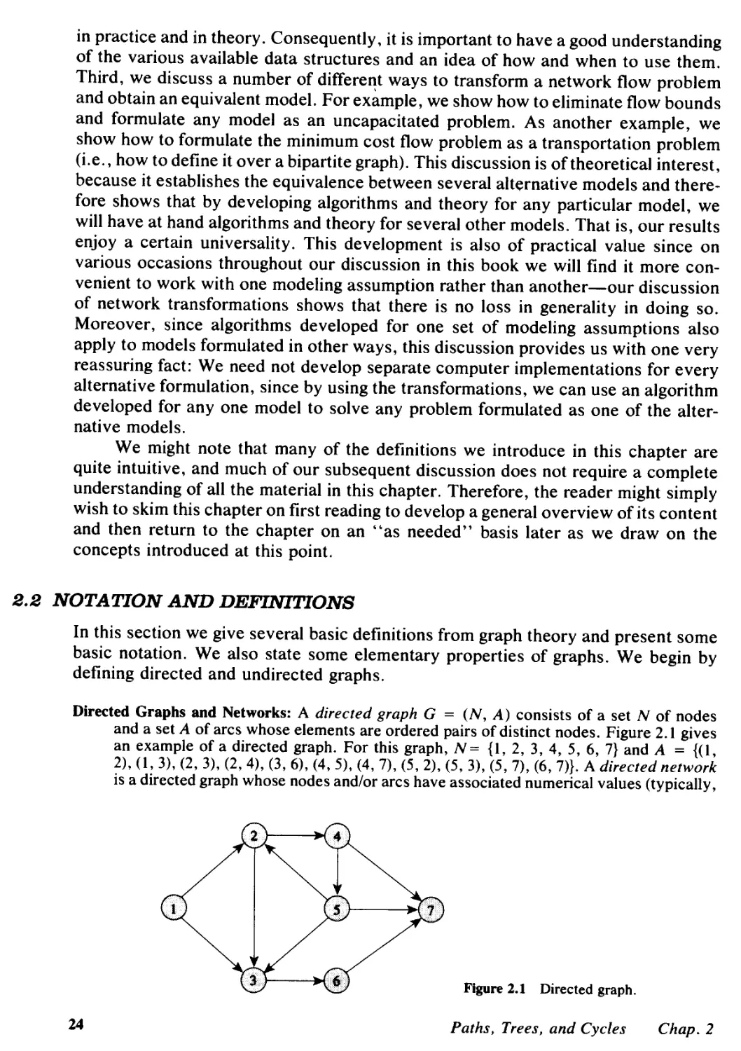
Let G = (N, A) be a directed network defined by a set N of n nodes and a
set A of m directed arcs. Each arc (i, j) E A has an associated cost Cij that denotes
the cost per unit flow on that arc. We assume that the flow cost varies linearly with
the amount of flow. We also associate with each arc (i, j) E A a capacity Uij that
denotes the maximum amount that can flow on the arc and a lower bound lij that
denotes the minimum amount that must flow on the arc. We associate with each
node i E N an integer number b(i) representing its supply/demand. If b(i) > 0, node
i is a supply node; if b(i) < 0, node i is a demand node with a demand of - b(i); and
if b(i) = 0, node i is a transshipment node. The decision variables in the minimum
cost flow problem are arc flows and we represent the flow on an arc (i, j) E A by
Xij. The minimum cost flow problem is an optimization model formulated as follows:
Minimize 2 CijXij
(i,j)EA
(l.1 a)
subject to
2 Xij -
{j: (i.j)EA}
2 Xj; = b(i)
{j:(j,i)EA}
for all i E N,
(l.lb)
lij Xij Uij
for all (i,j) E A,
(l.lc)
where 27= 1 b(i) = O. In matrix form, we represent the minimum cost flow problem
as follows:
Minimize cx
(t .2a)
subject to
Xx = b,
(t .2b)
(t . 2c)
I x u.
In this formulation, X is an n x m matrix, called the node-arc incidence matrix
of the minimum cost flow problem. Each column X ij in the matrix corresponds to
the variable Xij. The column X ij has a + 1 in the ith row, a -1 in the jth row; the
rest of its entries are zero.
We refer to the constraints in (t .lb) as mass balance constraints. The first
term in this constraint for a node represents the total outflow of the node (i.e., the
flow emanating from the node) and the second term represents the total inflow of
the node (i.e., the flow entering the node). The mass balance constraint states that
the outflow minus inflow must equal the supply/demand of the node. If the node is
a supply node, its outflow exceeds its intl"ow; if the node is a demand node, its inflow
exceeds its outflow; and if the node is a transshipment node, its outflow equals its
inflow. The flow must also satisfy the lower bound and capacity constraints (1.1 c),
which we refer to as flow bound constraints. The flow bounds typically model phys-
ical capacities or restrictions imposed on the flows' operating ranges. In most ap-
plications, the lower bounds on arc flows are zero; therefore, if we do not state
lower bounds for any problem, we assume that they have value zero.
Sec. 1.2
Network Flow Problems
5
In most parts of the book we assume that the data are integral (i.e., all arc
capacities, arc costs, and supplies/demands of nodes are integral). We refer to this
assumption as the integrality assumption. The integrality assumption is not restric-
tive for most applications because we can always transform rational data to integer
data by multiplying them by a suitably large number. Moreover, we necessarily need
to convert irrational numbers to rational numbers to represent them on a computer.
The following special versions of the minimum cost flow problem playa central
role in the theory and applications of network flows.
Shortest path problem. The shortest path problem is perhaps the simplest
of all network flow problems. For this problem we wish to find a path of minimum
cost (or length) from a specified source node s to another specified sink node t,
assuming that each arc (i, j) E A has an associated cost (or length) Cij. Some of the
simplest applications of the shortest path problem are to determine a path between
two specified nodes of a network that has minimum length, or a path that takes least
time to traverse, or a path that has the maximum reliability. As we will see in our
later discussions, this basic model has applications in many different problem do-
mains, such as equipment replacement, project scheduling, cash flow management,
message routing in communication systems, and traffic flow through congested cities.
If we set b(s) = 1, b(t) = - 1, and b(i) = 0 for all other nodes in the minimum
cost flow problem, the solution to the problem will send 1 unit of flow from node s
to node t along the shortest path. The shortest path problem also models situations
in which we wish to send flow from a single-source node to a single-sink node in an
uncapacitated network. That is, if we wish to send v units of flow from node s to
node t and the capacity of each arc of the network is at least v, we would send the
flow along a shortest path from node s to node t. If we want to determine shortest
paths from the source node s to every other node in the network, then in the minimum
cost flow problem we set b(s) = (n - 1) and b(i) = - 1 for all other nodes. [We
can set each arc capacity Uij to any number larger than (n - 1).] The minimum cost
flow solution would then send unit flow from node s to every other node i along a
shortest path.
Maximum flow problem. The maximum flow problem is in a sense a com-
plementary model to the shortest path problem. The shortest path problem models
situations in which flow incurs a cost but is not restricted by any capacities; in
contrast, in the maximum flow problem flow incurs no costs but is restricted by flow
bounds. The maximum flow problem seeks a feasible solution that sends the max-
imum amount of flow from a specified source node s to another specified sink node
t. If we interpret uijas the maximum flow rate of arc (i,j), the maximum flow problem
identifies the maximum steady-state flow that the network can send from node s to
node t per unit time. Examples of the maximum flow problem include determining
the maximum steady-state flow of (1) petroleum products in a pipeline network, (2)
cars in a road network, (3) messages in a telecommunication network, and (4) elec-
tricity in an electrical network. We can formulate this problem as a minimum cost
flow problem in the following manner. We set b(i) = 0 for all i E N, Cij = 0 for all
(i, j) E A, and introduce an additional arc (t, s) with cost C ts = - 1 and flow bound
U ts = 00. Then the minimum cost flow solution maximizes the flow on arc (t, s); but
6
Introduction
Chap. 1
since any flow on arc (t, s) must travel from node s to node t through the arcs in A
[since each b(i) = 0], the solution to the minimum cost flow problem will maximize
the flow from node s to node t in the original network.
Assignment problem. The data of the assignment problem consist of two
equally sized sets Nt and N 2 (i.e., I N 1 I = I N 2 1), a collection of pairs A N 1 X
N 2 representing possible assignments, and a cost Cij associated with each element
(i, j) E A. In the assignment problem we wish to pair, at minimum possible cost,
each object in Nt with exactly one object in N 2 . Examples of the assignment problem
include assigning people to projects, jobs to machines, tenants to apartments, swim-
mers to events in a swimming meet, and medical school graduates to available in-
ternships. The assignment problem is a minimum cost flow problem in a network
G = (N 1 U N 2 , A) with b(i) = 1 for all i E Nt, b(i) = -1 for all i E N 2 , and
Uij = 1 for all (i, j) E A.
Transportation problem. The transportation problem is a special case of
the minimum cost flow problem with the property that the node set N is partitioned
into two subsets N 1 and N 2 (of possibly unequal cardinality) so that (1) each node
in N 1 is a supply node, (2) each node N 2 is a demand node, and (3) for each arc
(i,j) in A, i E Nt andj E N 2 . The classical example of this problem is the distribution
of goods from warehouses to customers. In this context the nodes in N 1 represent
the warehouses, the nodes in N 2 represent customers (or, more typically, customer
zones), and an arc (i, j) in A represents a distribution channel from warehouse i to
customer j.
Circulation problem. The circulation problem is a minimum cost flow prob-
lem with only transshipment nodes; that is, b(i) = 0 for all i E N. In this instance
we wish to find a feasible flow that honors the lower and upper bounds lij and Uij
imposed on the arc flows Xij. Since we never introduce any exogenous flow into the
network or extract any flow from it, all the flow circulates around the network. We
wish to find the circulation that has the minimum cost. The design of a routing
schedule of a commercial airline provides one example of a circulation problem. In
this setting, any airplane circulates among the airports of various cities; the lower
bound lij imposed on an arc (i, j) is 1 if the airline needs to provide service between
cities i and j, and so must dispatch an airplane on this arc (actually, the nodes will
represent a combination of both a physical location and a time of day so that an arc
connects, for example, New York City at 8 A.M. with Boston at 9 A.M.).
In this book, we also study the following generalizations of the minimum cost
flow problem.
Convex cost flow problems. In the minimum cost flow problem, we assume
that the cost of the flow on any arc varies linearly with the amount of flow. Convex
cost flow problems have a more general cost structure: The cost is a convex function
of the amount of flow. Flow costs vary in a convex manner in numerous problem
settings, including (1) power losses in an electrical network due to resistance, (2)
congestion costs in a city transportation network, and (3) expansion costs of a com-
munication network.
Sec. 1.2
Network Flow Problems
7
Generalized flow problems. In the minimum cost flow problem, arcs con-
serve flows (Le., the flow entering an arc equals the flow leaving the arc). In gen-
eralized flow problems, arcs might "consume" or "generate" flow. If Xij units of
flow enter an arc (i, j), then jJ.ijXij units arrive at node j; jJ.ij is a positive multiplier
associated with the arc. If 0 < jJ.ij < I, the arc is lossy, and if 1 < jJ.ij < 00, the arc
is gainy. Generalized network flow problems arise in several application contexts:
for example, (1) power transmission through electric lines, with power lost with
distance traveled, (2) flow of water through pipelines or canals that lose water due
to seepage or evaporation, (3) transportation of a perishable commodity, and (4)
cash management scenarios in which arcs represent investment opportunities and
multipliers represent appreciation or depreciation of an investment's value.
Multicommodity flow problems. The minimum cost flow problem models
the flow of a single commodity over a network. Multicommodity flow problems arise
when several commodities use the same underlying network. The commodities may
either be differentiated by their physical characteristics or simply by their origin-
destination pairs. Different commodities have different origins and destinations, and
commodities have separate mass balance constraints at each node. However, the
sharing of the common arc capacities binds the different commodities together. In
fact, the essential issue addressed by the multicommodity flow problem is the al-
location of the capacity of each arc to the individual commodities in a way that
minimizes overall flow costs. Multicommodity flow problems arise in many practical
situations, including (1) the transportation of passengers from different origins to
different destinations within a city; (2) the routing of nonhomogeneous tankers (non-
homogeneous- in terms of speed, carrying capability, and operating costs); (3) the
worldwide shipment of different varieties of grains (such as corn, wheat, rice, and
soybeans) from countries that produce grains to those that consume it; and (4) the
transmission of messages in a communication network between different origin-
destination pairs.
Other Models
In this book we also study two other important network models: the minimum span-
ning tree problem and the matching problem. Although these two models are not
flow problems per se, because of their practical and mathematical significance and
because of their close connection with several flow problems, we have included
them as part of our treatment of network flows.
Minimum spanning tree problem. A spanning tree is a tree (i.e., a con-
nected acyclic graph) that spans (touches) all the nodes of an undirected network.
The cost of a spanning tree is the sum of the costs (or lengths) of its arcs. In the
minimum spanning tree problem, we wish to identify a spanning tree of minimum
cost (or length). The applications of the minimum spanning tree problem are varied
and include (1) constructing highways or railroads spanning several cities; (2) laying
pipelines connecting offshore drilling sites, refineries, and consumer markets; (3)
designing local access networks; and (4) making electric wire connections on a con-
trol panel.
8
Introduction
Chap. 1
Matching problems. A matching in a graph G = (N, A) is a set of arcs
with the property that every node is incident to at most one arc in the set; thus a
matching induces a pairing of (some 00 the nodes in the graph using the arcs in A.
In a matching, each node is matched with at most one other node, and some nodes
might not be matched with any other node. The matching problem seeks a matching
that optimizes some criteria. Matching problems on a bipartite graphs (i.e., those
with two sets of nodes and with arcs that join only nodes between the two sets, as
in the assignment and transportation problems) are called bipartite matching prob-
lems, and those on nonbipartite graphs are called nonbipartite matching problems.
There are two additional ways of categorizing matching problems: cardinality match-
ing problems, which maximize the number of pairs of nodes matched, and weighted
matching problems, which maximize or minimize the weight of the matching. The
weighted matching problem on a bipartite graph is also known as the assignment
problem. Applications of matching problems arise in matching roommates to hostels,
matching pilots to compatible airplanes, scheduling airline crews for available flight
legs, and assigning duties to bus drivers.
1.3 APPLICATIONS
Networks are pervasive. They arise in numerous application settings and in many
forms. Physical networks are perhaps the most common and the most readily iden-
tifiable classes of networks; and among physical networks, transportation networks
are perhaps the most visible in our everyday lives. Often, these networks model
homogeneous facilities such as railbeds or highways. But on other occasions, they
correspond to composite entities that model, for example, complex distribution and
logistics decisions. The traditional operations research "transportation problem" is
illustrative. In the transportation problem, a shipper with inventory of goods at its
warehouses must ship these goods to geographically dispersed retail centers, each
with a given customer demand, and the shipper would like to meet these demands
incurring the minimum possible transportation costs. In this setting, a transportation
link in the underlying network might correspond to a complex distribution channel
with, for example, a trucking shipment from the warehouse to a railhead, a rail
shipment, and another trucking leg from the destination rail yard to the customer's
site.
Physical networks are not limited to transportation settings; they also arise in
several other disciplines of applied science and engineering, such as mathematics,
chemistry, and electrical, communications, mechanical, and civil engineering. When
physical networks occur in these different disciplines, their nodes, arcs, and flows
model many different types of physical entities. For example, in a typical commu-
nication network, nodes will represe'nt telephone exchanges and'transmission facil-
ities, arcs will denote copper cables or fiber optic links, and flow would signify the
transmission of voi e messages or of data. Figure i.l shows some typical associations
for the nodes, arcs, and flows in a variety of physical networks.
Network flow problems also arise in surprising ways for problems that on the
surface might not appear to involve networks at all. Sometimes these applications
are linked to a physical entity, and at other times they are not. Sometimes the nodes
and arcs have a temporal dimension that models activities that take place over time.
Sec. 1.3
Applications
9
Physical analog of
Applications nodes Physical analog of arcs Flow
Communication Telephone exchanges, Cables, fiber optic V oice messages, data,
systems computers, links, microwave video transmissions
transmission relay links
facilities, satellites
Hydraulic systems Pumping stations, Pipelines Water, gas, oil,
reservoirs, lakes hydraulic fluids
Integrated computer Gates, registers, Wires Electrical current
circuits processors
Mechanical systems Joints Rods, beams, springs Heat, energy
Transportation Intersections, airports, Highways, railbeds, Passengers, freight,
systems rail yards airline routes vehicles, operators
Figure 1.1 Ingredients of some common physical networks.
Many scheduling applications have this flavor. In any event, networks model a va-
riety of problems in project, machine, and crew scheduling; location and layout
theory; warehousing and distribution; production planning and control; and social,
medical, and defense contexts. Indeed, these various applications of network flow
problems seem to be more widespread than are the applications of physical networks.
We present many such applications throughout the text and in the exercises; Chapter
19, in particular, brings together and summarizes many applications. In the following
discussion, to set a backdrop for the next few chapters, we describe several sample
applications that are intended to illustrate a range of problem contexts and to be
suggestive of how network flow problems arise in practice. This set of applications
provides at least one example of each of the network models that we introduced in
the preceding section.
Application 1.1 Reallocation of Housing
A housing authority has a number of houses at its disposal that it lets to tenants.
Each house has its own particular attributes. For example, a house might or might
not have a garage, it has a certain number of bedrooms, and its rent falls within a
particular range. These variable attributes permit us to group the house into several
categories, which we index by i = 1, 2, . . . , n.
Over a period of time a number of tenants will surrender their tenancies as
they move or choose to live in alternative accommodations. Furthermore, the re-
quirements of the tenants will change with time (because new families arrive, children
leave home, incomes and jobs change, and other considerations). As these changes
occur, the housing authority would like to relocate each tenant to a house of his or
her choice category. While the authority can often accomplish this objective by
simple exchanges, it will sometimes encounter situations requiring multiple moves:
moving one tenant would replace another tenant from a house in a different category,
who, in turn, would replace a tenant from a house in another category, and so on,
thus creating a cycle of changes. We call such a change a cyclic change. The decision
10
Introduction
Chap. 1
problem is to identify a cyclic change, if it exists, or to show that no such change
exists.
To solve this problem as a network problem, we first create a relocation graph
G whose nodes represent various categories of houses. We include arc (i, j) in the
graph whenever a person living in a house of category i wishes to move to a house
of category j. A directed cycle in G specifies a cycle of changes that will satisfy the
requirements of one person in each of the categories contained in the cycle. Applying
this method iteratively, we can satisfy the requirements of an increasing number of
persons.
This application requires a method for identifying directed cycles in a network,
if they exist. A well-known method, known as topological sorting, will identify such
cycles. We discuss topological sorting in Section 3.4. In general, many tenant reas-
signments might be possible, so the relocation graph G might contain several cycles.
In that case the authority's management would typically want to find a cycle con-
taining as few arcs as possible, since fewer moves are easier to handle administra-
tively. We can solve this problem using a shortest path algorithm (see Exercise 5.38).
Application 1.2 Assortment of Structural Steel Beams
In its various construction projects, a construction company needs structural steel
beams of a uniform cross section but of varying lengths. For each i = 1, . . . , n,
let D i > 0 denote the demand of the steel beam of length L i , and assume that L, <
L 2 < ... < Ln. The company could meet its needs by maintaining and drawing upon
an inventory of stock containing exactly D i units of the steel beam of length L i . It
might not be economical to carryall the demanded lengths in inventory, however,
because of the high cost of setting up the inventory facility to store and handle each
length. In that case, if the company needs a beam oflength L i not carried in inventory,
it can cut a beam of longer length down to the desired length. The cutting operation
will typically produce unusable steel as scrap. Let K i denote the cost for setting up
the inventory facility to handle beams of length L i , and let C; denote the cost of a
beam of length L;. The company wants to determine the lengths of beams to be
carried in inventory so that it will minimize the total cost of (1) setting up the in-
ventory facility, and (2) discarding usable steel lost as scrap.
We formulate this problem as a shortest path problem as follows. We construct
a directed network G on (n + 1) nodes numbered 0, 1, 2, . . . , n; the nodes in this
network correspond to various beam lengths. Node 0 corresponds to a beam of length
zero and node n corresponds to the longest beam. For each node i, the network
contains a directed arc to every node j = i + 1, i + 2, . . . , n. We interpret the
arc (i, j) as representing a storage strategy in which we hold beams of length L j in
inventory and use them to satisfy the demand of all the beams of lengths L i + I ,
L i + 2 , . . . , Lj. The cost Cij of the arc (i, j) is
j
Cij = K j + C j L. D k.
k=i+ I
The cost of arc (i, j) has two components: (1) the fixed cost K j of setting up
the inventory facility to handle beams of length L j , and (2) the cost of using beams
oflength L j to meet the demands of beams of lengths L i + 1, . . . ,L j . A directed path
Sec. 1.3
Applications
11
from node 0 to node n specifies an assortment of beams to carry in inventory and
the cost of the path equals the cost associated with this inventory scheme. For
example, the path 0-4-6-9 corresponds to the situation in which we set up the
inventory facility for handling beams of lengths L 4 , L 6 , and L9. Consequently, the
shortest path from node 0 to node n would prescribe the least cost assortment of
structural steel beams.
Application 1.8 Tournament Problem
Consider a round-robin tournament between n teams, assuming that each team plays
against every other team c times. Assume that no game ends in a draw. A person
claims that a; for 1 :S i :S n denotes the number of victories accrued by the ith team
at the end of the tournament. How can we determine whether the given set of non-
negative integers ai, a2, . . . , an represents a possible winning record for the n
teams?
Define a directed network G = (N, A) with node set N = {I, 2, . . . , n} and
arc set A = {(i, j) E N x N: i < j}. Therefore, each node i is connected to the nodes
i + 1, i + 2, . . . , n. Let Xij for i < j represent the number of times team i defeats
teamj. Observe that the total number of times team i beats teams i + 1, i + 2, . . . ,
n is :L{j:(;,j)EA} Xij. Also observe that the number of times that team i beats a team
j < i is c - Xj;. Consequently, the total number of times that team i beats teams 1,
2, . . . , i-I is (i - l)c - :L{j:(j,i)EA} Xji' The total number of wins of team i must
equal the total number of times it beats the teams 1, 2, . . . , n. The preceding
observations show that
:L Xij-
{j:(i,j)EA}
:L Xj; = cx; - (i - l)c
{j:(j.i)EA}
for all i EN.
(1.3)
In addition, a possible winning record must also satisfy the following lower
and upper bound conditions:
o :S xij :S C
for all (i, j) E A.
(1.4)
This discussion shows that the record a; is a possible winning record if
the constraints defined by (1.3) and (1.4) have a feasible solution x. Let b(i) =
cx; - (i - l)c. Observe that the expressions :L;ENcx; and :L;EN(i - l)c are both
equal to cn(n - 1)/2, which is the total number of games played. Consequently,
:L;E (i) = O. The problem of finding a feasible solution of a network flow system
like (1.3) and (1.4) is called a feasible flow problem and can be solved by solving a
maximum flow problem (see Section 6.2).
Application 1.4 Leveling Mountainous Terrain
This application was inspired by a common problem facing civil engineers when they
are building road networks through hilly or mountainous terrain. The problem con-
cerns the distribution of earth from high points to low points of the terrain to produce
a leveled roadbed. The engineer must determine a plan for leveling the route by
12
Introduction
Chap. 1
specifying the number of truckloads of earth to move between various locations
along the proposed road network.
We first construct a terrain graph: it is an undirected graph whose nodes rep-
resent locations with a demand for earth (low points) or locations with a supply of
earth (high points). An arc of this graph represents an available route for distributing
the earth, and the cost of this arc represents the cost per truckload of moving earth
between the two points. (A truckload is the basic unit for redistributing the earth.)
Figure 1.2 shows a portion of the terrain graph.
5 Figure 1.2 Portion of the terrain graph.
A leveling plan for a terrain graph is a flow (set of truckloads) that meets the
demands at nodes (levels the low points) by the available supplies (by earth obtained
from high points) at the minimum cost (for the truck movements). This model is
clearly a minimum cost flow problem in the terrain graph.
Application 1. ts Rewiring of Typewriters
For several years, a company had been using special electric typewriters to prepare
punched paper tapes to enter data into a digital computer. Because the typewriter
is used to punch a six-hole paper tape, it can prepare 2 6 = 64 binary hole/no-hole
patterns. The typewriters have 46 characters, and each punches one of the 64 pat-
terns. The company acquired a new digital computer that uses a different coding
hole/no-hole patterns to represent characters. For example, using 1 to represent a
hole and 0 to represent a no-hole, the letter A is 111100 in the code for the old
computer and 011010 in the code for the new computer. The typewriter presently
punches the former and must be modified to punch the latter.
Each key in the typewriter is connected to a steel code bar, so changing the
code of that key requires mechanical changes in the steel bar system. The extent of
the changes depends on how close the new and old characters are to each other.
For the letter A, the second, third, and sixth bits are identical in the old and new
codes and no changes need be made for these bits; however, the first, fourth, and
fifth bits are different, so we would need to make three changes in the steel code
bar connected to the A-key. Each change involves removing metal at one place and
Sec. 1.3
Applications
13
adding metal at another place. When a key is pressed, its steel code bar activates
six cross-bars (which are used by all the keys) that are connected electrically to six
hole punches. If we interchange the fourth and fifth wires of the cross-bars to the
hole punches (which is essentially equivalent to interchanging the fourth and fifth
bits of all characters in the old code), we would reduce the number of mechanical
changes needed for the A-key from three to one. However, this change of wires
might increase the number of changes for some of the other 45 keys. The problem,
then, is how to optimally connect the wires from the six cross-bars to the six punches
so that we can minimize the number of mechanical changes on the steel code bars.
We formulate this problem as an assignment problem as follows. Define a
network G = (N) U N 2 , A) with node sets N I = {I, 2, . . . , 6} and N 2 = {I',
2', . . . , 6 ' }, and an arc set A = N I x N 2 ; the cost of the arc (i, j') E A is the
number of keys (out of 46) for which the ith bit in the old code differs from the jth
bit in the new code. Thus if we assign cross-bar i to the punch j, the number of
mechanical changes needed to print the ith bit of each symbol correctly is Cij. Con-
sequently, the minimum cost assignment will minimize the number of mechanical
changes.
Application 1.6 Pairing Stereo Speakers
As a part of its manufacturing process, a manufacturer of stereo speakers must pair
individual speakers before it can sell them as a set. The performance of the two
speakers depends on their frequency response. To measure the quality of the pairs,
the company generates matching coefficients for each possible pair. It calculates
these coefficients by summing the absolute differences between the responses of the
two speakers at 20 discrete frequencies, thus giving a matching coefficient value
between 0 and 30,000. Bad matches yield a large coefficient, and a good pairing
produces a low coefficient.
The manufacturer typically uses two different objectives in pairing the speak-
ers: (1) finding as many pairs as possible whose matching coefficients do not exceed
a specification limit, or (2) pairing speakers within specification limits to minimize
the total sum of the matching coefficients. The first objective minimizes the number
of pairs outside specification, and so the number of speakers that the firm must sell
at a reduced price. This model is an application of the nonbipartite cardinality match-
ing problem on an undirected graph: the nodes of this graph represent speakers and
arcs join two nodes if the matching coefficients of the corresponding speakers are
within the specification limit. The second model is an application of the nonbipartite
weighted matching problem.
Application 1.7 Measuring Homogeneity of Bimetallic
Objects
This application shows how a minimum spanning tree problem can be used to de-
termine the degree to which a bimetallic object is homogeneous in composition. To
use this approach, we measure the composition of the bimetallic object at a set of
sample points. We then construct a network with nodes corresponding to the sample
14
Introduction
Chap. 1
points and with an arc connecting physically adjacent sample points. We assign a
cost with each arc (i, j) equal to the product of the physical (Euclidean) distance
between the sample points i and j and a homogeneity factor between 0 and 1. This
homogeneity factor is 0 if the composition of the corresponding samples is exactly
alike, and is 1 if the composition is very different; otherwise, it is a number between
o and 1. Note that this measure gives greater weight to two points if they are different
and are far apart. The cost of the minimum spanning tree is a measure of the ho-
mogeneity of the bimetallic object. The cost of the tree is 0 if all the sample points
are exactly alike, and high cost values imply that the material is quite nonhomo-
geneous.
Application 1.8 Electrical Networks
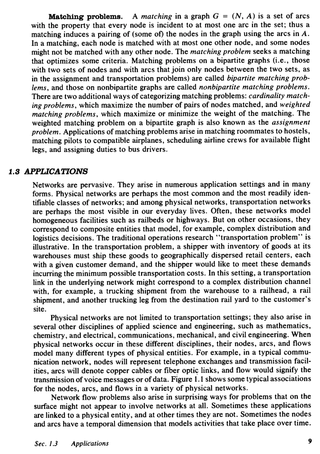
The electrical network shown in Figure 1.3 has eight resistors, two current sources
(at nodes 1 and 6), and one current sink (at node 7). In this network we wish to
determine the equilibrium current flows through the resistors. A popular method for
solving this problem is to introduce a variable Xij representing the current flow on
the arc (i, j) of the electrical network and write a set of equilibrium relationships
for these flows; that is, the voltage-current relationship equations (using Ohm's law)
and the current balance equations (using Kirchhofs law). The solution of these
equations gives the arc currents Xij. An alternative, and possibly more efficient ap-
proach is to formulate this problem as a convex cost flow problem. This formulation
uses the well-known result that the equilibrium currents on resistors are those flows
for which the resistors dissipate the least amount of the total power supplied by the
voltage sources (i.e., the electric current follows the path of least resistance). Ohm's
law shows that a resistor of resistance r;; dissipates r;ixri watts of power. Therefore,
we can obtain the optimal currents by solving the following convex cost flow prob-
lem:
Minimize rijx
(i,j)EA
subject to
Xij-
{j: (i,j)EA}
Xji = b(i)
{j:(j,i)EA}
for each node i EN,
Xij 0
for each arc (i,j) E A.
In this model b(i) represents the supply/demand of a current source or sink.
Figure 1.3 Electrical network.
Sec. 1.3
Applications
15
The formulation of a set of equilibrium conditions as an equivalent optimization
model is a powenul idea in the physical sciences, dating from the last century, which
has become known as so-called variational principles. The term "variational" arises
because the equilibrium conditions are the "optimality conditions" for the equivalent
optimization model that tell us that we cannot improve the optimal solution by vary-
ing (hence the term "variational") the optimal solution to this optimization model.
Application 1.9 Determining an Optimal Energy Policy
As part of their national planning effort, most countries need to decide on an energy
policy (i.e., how to utilize the available raw materials to satisfy their energy needs).
Assume, for simplicity, that a particular country has four basic raw materials: crude
oil, coal, uranium, and hydropower; and it has four basic energy needs: electricity,
domestic oil, petroleum, and gas. The country has the technological base and in-
frastructure to convert each raw material into one or more energy forms. For ex-
ample, it can convert crude oil into domestic oil or petrol, coal into electricity, and
so on. The available technology base specifies the efficiency and the cost of each
conversion. The objective is to satisfy, at the least possible cost of energy conversion,
a certain annual consumption level of various energy needs from a given annual
production of raw materials.
Figure 1.4 shows the formulation of this problem as a generalized network flow
problem. The network has three types of arcs: (1) source arcs (s, i) emanating from
the source node s, (2) sink arcs (j, t) entering the sink node t, and (3) conversion
arcs (i, j). The source arc (s, i) has a capacity equal to the availability a(i) of the
raw material i and a flow multiplier of value 1. The sink arc (j, t) has capacity equal
to the demand (j) of type j energy need and flow multiplier of value 1. Each con-
version arc (i, j) represents the conversion of raw material i into the energy form j;
the multiplier of this arc is the efficiency of the conversion (i.e., units of energy j
obtained from 1 unit of raw material i); and the cost of the arc (i, j) is the cost of
this conversion. In this model, since a(i) is an upper bound on the use of raw material
Crude oil
Electricity
4
aU) --.
;=1
4
--. - (3(i)
1=1
Hydropower
Gas
Figure 1.4 Energy problem as a generalized network flow problem.
16
Introduction
Chap. 1
i, ;= I a(i) is an upper bound on the flow out of node s. Similarly, ; = I J3(i) is a
lower bound on the flow into node t. In Exercise 15.29, we show how to convert
this problem into a standard form without bounds on supplies and demands.
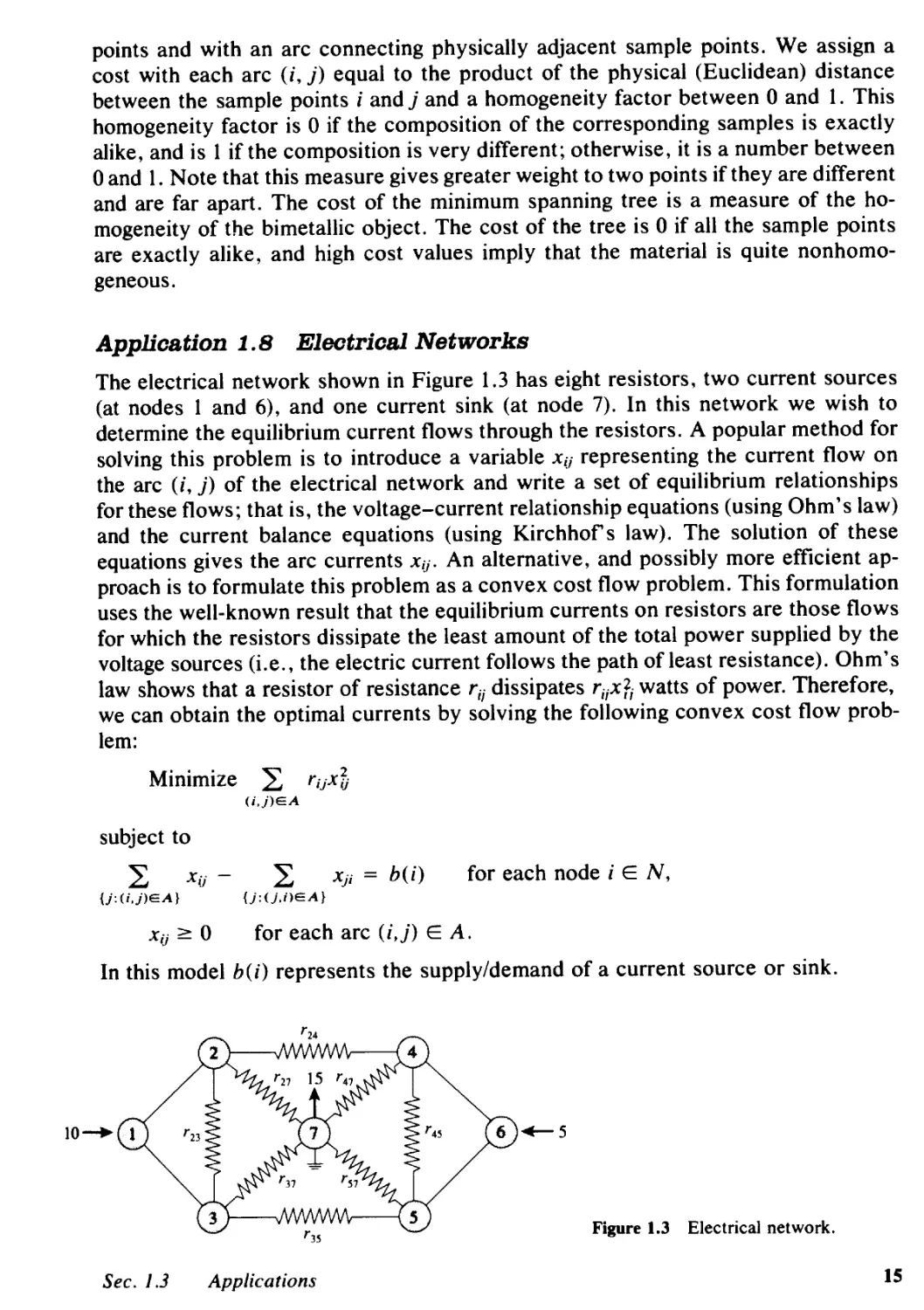
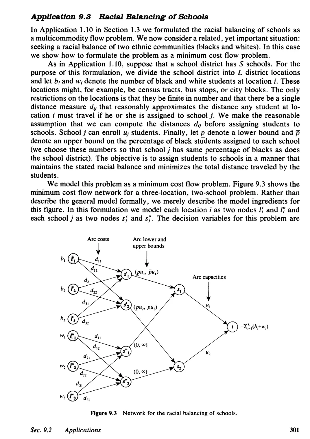
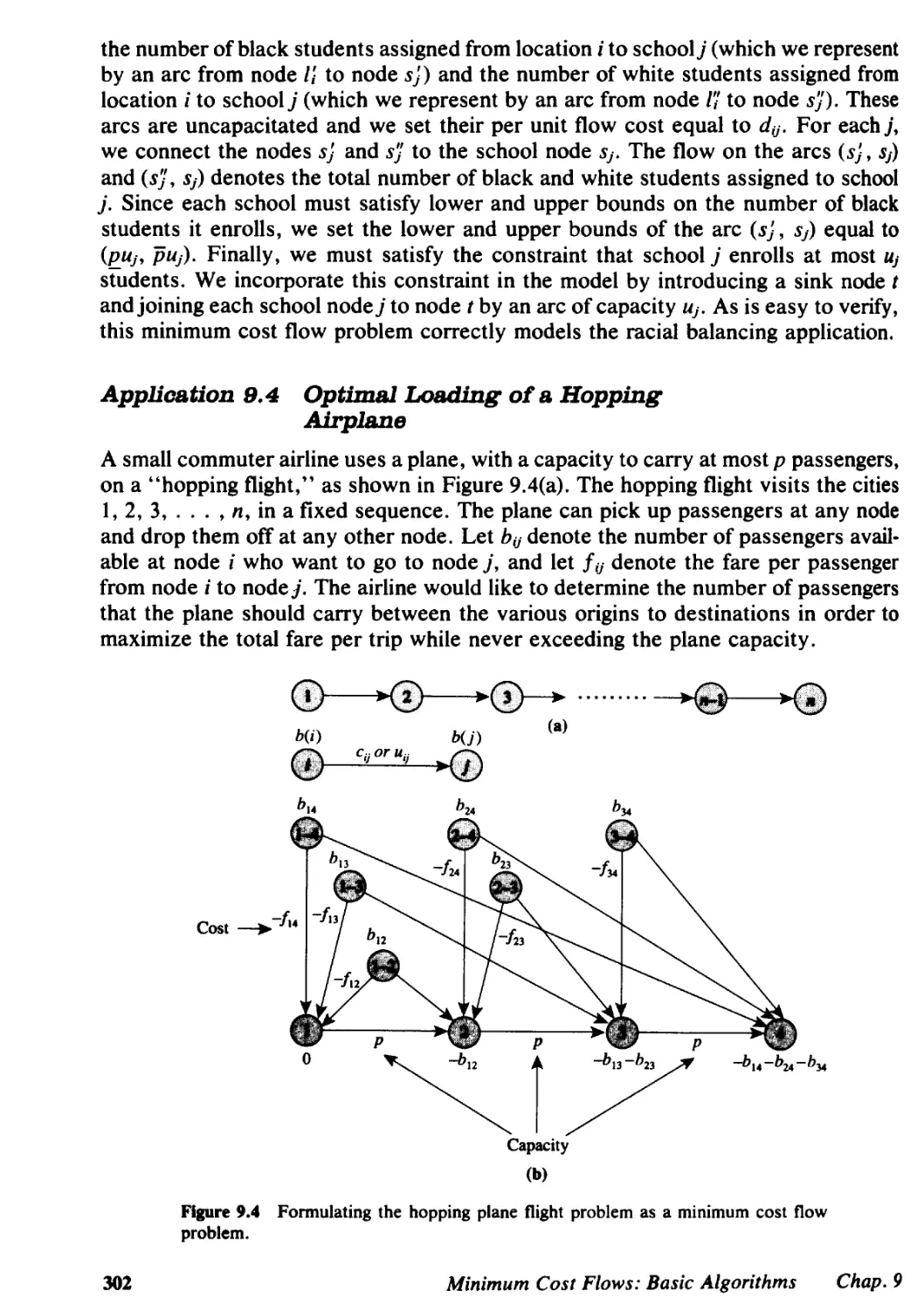
Application 1.10 Racial Balancing of Schools
In 1968, the U.S. Supreme Court ruled that all school systems in the country should
begin admitting students to schools on a nondiscriminatory basis and should employ
faster techniques to promote desegregated schools across the nation. This decision
made it necessary for many school systems to develop radically different procedures
for assigning students to schools. Since the Supreme Court did not specify what
constitutes an acceptable racial balance, the individual school boards used their own
best judgments to arrive at acceptable criteria on which to base their desegregation
plans. This application describes a multicommodity flow model for determining an
optimal assignment of students to schools that minimizes the total distance traveled
by the students, given a specification of lower and upper limits on the required racial
balance in each school.
Suppose that a school district has S schools and school j has capacity Uj. For
the purpose of this formulation, we divide the school district into L population cen-
ters. These locations might, for example, be census tracts, bus stops, or city blocks.
The only restriction on the population centers is that they be finite in number and
that a single distance measure reasonably approximates the distance any student at
center i must travel if he or she is assigned to school j. Let S;k denote the available
number of students of the kth ethnic group at the ith population center. The objective
is to assign students to schools in a way that achieves the desired ethnic composition
for each school and minimizes the total distance traveled by the students. Each
school j has the ethnic requirement that it must enroll at least ljk and no more than
Ujk students from the kth ethnic group.
We can model this problem as a multi commodity flow problem on an appro-
priately defined network. Figure 1.5 shows this network representation for a problem
with three population centers and three schools. This network has one node for each
population center and for each school as well as a "source" and a "sink" node for
each ethnic group. The flow commodities represent the students of different ethnic
groups. The students of the kth ethnic group flow from source ak to sink ek via
population center and school nodes. We set the upper bound on arc (ak, b;) con-
necting the kth ethnic group source node and the ith population center equal to S;k
and the cost of the arc (b;, Cj) connecting the ith population center and jth school
equal to f ij, the distance between that population center and that school. By setting
the capacity of the arc (Cj, d j ) equal to Uj, we ensure that the total number of students
(of all ethnic groups) allocated to thejth school does not exceed the maximum student
population for this school. The students of all ethnic groups must share the capacity
of each school. Finally, we incorporate constraints on the ethnic compositions of
the schools by setting the lower and upper bounds on the arc (d j , ek) equal to ljk and
Ujk. It is fairly easy to verify that the multicommodity flow problem models the racial
balancing problem, so a minimum multicommodity flow will specify an optimal as-
signment of students to the schools.
Sec. 1.3
Applications
17
3
I Sd
3
-, Sd
3
I S'2
3
-' IS'2
Ethnic
groups
(sources)
Population
centers
Schools
(input)
Schools
(output)
Ethnic
groups
(sinks)
Figure I.S Formulating the racial balancing problem as a multicommodity flow prob-
lem.
1.4 SUMMARY
In this chapter we introduced the network flow problems that we study in this book
and described a few scenarios in which these problems arise. We began by giving
a linear programming formulation of the minimum cost flow problem and identifying
several special cases: the shortest path problem, the maximum flow problem, the
assignment problem, the transportation problem, and the circulation problem. We
next described several generalizations of the minimum cost flow problem: the convex
cost flow problem, the generalized network flow problem, and the multicommodity
flow problem. Finally, we described two other important network models: the min-
imum spanning tree problem and the matching problem. Although these two prob-
lems are not network flow problems per se, we have included them in this book
because they are closely related to several network flow problems and because they
arise often in the context of network optimization.
Networks are pervasive and arise in numerous application settings. Physical
networks, which are the most readily identifiable classes of networks, arise in many
applications in many different types of systems: communications, hydraulic, me-
chanical, electronic, and transportation. Network flow problems also arise in sur-
prising ways in optimization problems that on the surface might not appear to involve
networks at all. We described several of these "indirect" applications of network
flow problems, in such problem settings as urban housing, production planning,
electrical networks, racial balancing, leveling mountainous terrain, evaluating tour-
naments, matching stereo speakers, wiring typewriters, assessing the homogeneity
of physical materials, and energy planning. The applications we have considered
offer only a brief glimpse of the wide-ranging practical importance of network flows;
although our discussion of applications in this chapter is limited, it does provide at
least one example of each of the network models that we have introduced in this
chapter.
18
Introduction
Chap. 1
REFERENCE NOTES
The study of network flow models predates the development of linear programming.
The first studies in this problem domain, conducted by Kantorovich [1939], Hitch-
cock [1941], and Koopmans [1947], considered the transportation problem, a special
case of the minimum cost flow problem. These studies provided insight into the
problem structure and yielded algorithmic approaches. Interest in the network flow
problems grew with the advent of the simplex method by Dantzig in 1947, who also
specialized this algorithm for the transportation problem (see Dantzig [1951]).
During the 1950s, researchers began to exhibit increasing interest in the min-
imum cost flow problem and its specializations-the shortest path problem, the
maximum flow problem, and the assignment problem-mainly because of the im-
portance of these models in real-world applications. Soon researchers developed
special algorithms for solving these problems. Dantzig, Ford, and Fulkerson pi-
oneered these efforts. Whereas Dantzig focused on the simplex-based methods, Ford
and Fulkerson developed primal-dual combinatorial algorithms. The landmark
books by Dantzig [1962] and Ford and Fulkerson [1962] present thorough discussions
of these early contributions.
In the years following this groundbreaking work, network flow problems and
their generalizations emerged as major research topics in thousands of papers and
numerous text and reference books. The following books summarize developments
in the field and serve as a guide to the literature:
1. Flows in Networks (Ford and Fulkerson [1962])
2. Programming, Games and Transportation Networks (Berge and Ghouila-Houri
[1962])
3. Finite Graphs and Networks (Busacker and Saaty [1965])
4. Network Flow, Transportation and Scheduling (Iri [1969])
5. Integer Programming and Network Flows (Hu [1969])
6. Communication, Transmission, and Transportation Networks (Frank and
Frisch [1971])
7. Flows in Transportation Networks (Potts and Oliver [1972])
8. Graph Theory: An Algorithmic Approach (Christophides [1975])
9. Flow Algorithms (Adel'son-Vel'ski, Dinics, and Karzanov [1975])
10. Graph Theory with Applications (Bondy and Murty [1976])
11. Combinatorial Optimization: Networks and Matroids (Lawler [1976])
12. Optimization Algorithms for Networks and Graphs (Minieka [1978])
13. Graph Algorithms (Even [1979])
14. Algorithms for Network Programming (Kennington and Helgason [1980])
15. Network Flow Programming (Jensen and Barnes [1980])
16. Fundamentals of Network Analysis (Phillips and Garcia-Diaz [1981])
17. Combinatorial Optimization: Algorithms and Complexity (Papadimitriou and
Steiglitz [1982])
18. Discrete Optimization Algorithms (Syslo, Deo, and Kowalik [1983])
19. Data Structures and Network Algorithms (TaIjan [1983])
Chap. 1
Reference Notes
19
20. Graphs and Algorithms (Gondran and Minoux [1984])
21. Network Flows and Monotropic Optimization (Rockafellar [1984])
22. Linear Programming and Network Models (Gupta [1985])
23. Programming in Networks and Graphs (Derigs [1988])
24. Linear Programming and Network Flows, 2nd ed. (Bazaraa, Jarvis, and Sherali
[1990])
As an additional source of references, the reader might consult the bibliogra-
phies on network optimization prepared by Golden and Magnanti [1977], Ahuja,
Magnanti, and Orlin [1989, 1991], Bazaraa, Jarvis, and Sherali [1990], and the ex-
tensive set of references on integer programming compiled by researchers at the
University of Bonn (Kastning [1976], Hausman [1978], and Yon Randow [1982,
1985]).
Since the applications of network flow models are so pervasive, no single source
provides a comprehensive account of network flow models and their impact on
practice. Several researchers have prepared general surveys of selected application
areas. Notable among these are the papers by Bennington [1974], Glover and Kling-
man [1976], Bodin, Golden, Assad, and Ball [1983], Aronson [1989], and Glover,
Klingman, and Phillips [1990]. The book by Gondran and Minoux [1984] also de-
scribes a variety of applications of network flow problems. In this book we describe
or cite over 150 selected applications of network flow problems. We provide the
references for these problems in the reference notes given at the end of Chapters
4,6,9, 12, 13, 14, 15, 16, 17, and 19. We have adapted many of these applications
from the paper of Ahuja, Magnanti, Orlin, and Reddy [1992].
The applications we present in Section 1.3 are adapted from the following
references:
1. Reallocation of housing (Wright [1975])
2. Assortment of structural steel beams (Frank [1965])
3. Tournament problem (Ford and Johnson [1959])
4. Leveling mountainous terrain (Farley [1980])
5. Rewiring of typewriters (Machol [1961])
6. Pairing stereo speakers (Mason and Philpott [1988])
7. Measuring homogeneity of bimetallic objects (Shier [1982])
8. Electrical networks (Hu [1966])
9. Determining an optimal energy policy (Gondran and Minoux [1984])
10. Racial balancing of schools (Clarke and Surkis [1968])
EXERCISES
1.1. Formulate the following problems as circulation problems: (1) the shortest path prob-
lem; (2) the assignment problem; and (3) the transportation problem.
1.2. Consider a variant of the transportation problem for which (1) the sum of demands
exceeds the sum of supplies, and (2) we incur a penalty Pi for every unit of unfulfilled
demand at demand nodej. Formulate this problem as a standard transportation problem
with total supply equal to total demand.
20
Introduction
Chap. 1
1.3. In this exercise we examine a generalization of Application 1.2, concerning assortment
of structural steel beams. In the discussion of that application, we assumed that if we
must cut a beam of length 5 units to a length of 2 units, we obtain a single beam of
length 2 units; the remaining 3 units have no value. However, in practice, from a beam
of length 5 we can cut two beams of length 2; the remaining length of 1 unit will have
some scrap value. Explain how we might incorporate the possibility of cutting multiple
beam lengths (of the same length) from a single piece and assigning some salvage value
to the scrap. Assume that the scrap has a value of r3 per unit length.
1.4. Large-scale personnel assignment. A recurring problem in the U.S. armed forces is ef-
ficient distribution and utilization of skilled personnel. Each month thousands of in-
dividuals in the U.S. military vacate jobs, and thousands of personnel become available
for assignment. Each job has particular characteristics and skill requirements, while
each person from the pool of available personnel has specific skills and preferences.
Suppose that we use this information to compute the utility (or desirability) dij of each
possible assignment of a person to a job. The decision problem is to assign personnel
to the vacancies in a way that maximizes the total utility of all the assignments. Explain
how to formulate this problem as a network flow problem.
1.5. Dating problem. A dating service receives data from p men and p women. These data
determine what pairs of men and women are mutually compatible. Since the dating
service's commission is proportional to the number of dates it arranges, it would like
to determine the maximum number of compatible couples that can be formed. Formulate
this problem as a matching problem.
1.6. Pruned chessboard problem. A chessboard consists of 64 squares arranged in eight rows
and eight columns. A domino is a wooden or plastic piece consisting of two squares
joined on a side. Show that it is possible to fully cover the chessboard using 32 dominos
(i.e., each domino covers two squares of the board, no two dominos overlap, and some
domino covers each square). A pruned board is a chessboard with some squares re-
moved.
(a) Suppose that we want to know whether it is possible to fully cover a pruned board,
and if not, to find the maximum number of dominos we can place on the pruned
board so that each domino covers two squares and no two dominos overlap. For-
mulate this problem as a bipartite cardinality matching problem.
(b) Suppose that we prune only two diagonally opposite corners of the chessboard.
Show that we cannot cover the resulting board with 31 dominos.
1.7. Paragraph problem. The well-known document processing program Te X uses an op-
timization procedure to decompose a paragraph into several lines so that when lines
are left- and right-adjusted, the appearance of the paragraph will be the most attractive.
Suppose that a paragraph consists of n words and that each word is assigned a sequence
number. Let Cij denote the attractiveness of a line if it begins with the word i and ends
with the word} - 1. The program TeX uses formulas to compute the value of each Cij.
Given the cij's, show how to formulate the problem of decomposing the paragraph into
several lines of text in order to maximize the total attractiveness (of all lines) as a
shortest path problem.
1.8. Seat-sharing problem. Several families are planning a shared car trip on scenic drives
in the White Mountains, New Hampshire. To minimize the possibility of any quarrels,
they want to assign individuals to cars so that no two members of a family are in the
same car. Formulate this problem as a network flow problem.
1.9. Police patrol problem (Khan [1979]). A police department in a small city consists of
three precincts denoted Ph P2, and P3. Each precinct is assigned a number of patrol
cars equipped with two-way radios and first-aid equipment. The department operates
with three shifts. Figure 1.6(a) and (b) shows the minimum and maximum number of
patrol cars needed in each shift. Administrative constraints require that (1) shifts 1, 2,
and 3 have, respectively, at least cars 10, 20, and 18 cars available; and (2) precincts
PI. P2, and P3 are, respectively, allocated at least 10, 14, and 13 cars. The police de-
partment wants to determine an allocation of patrol units that will meet all the require-
Chap. 1
Exercises
21
Shift Shift Shift
I 2 3
Pt 2 4 3
pz 3 6 5
P3 5 7 6
(a)
Shift Shift Shift
1 2 3
PI 3 7 5
pz 5 7 10
P3 8 12 10
(b)
Figure 1.6 Patrol car requirements: (a) minimum required per shift; (b) maximum
required per shift.
ments with the fewest possible units committed to the field. Formulate this problem
as a circulation problem.
1.10. Forest scheduling problem. Paper and wood products companies need to define cutting
schedules that will maximize the total wood yield of their forests over some planning
period. Suppose that a company with control of p forest units wants to identify the
best cutting schedule over a planning horizon of k years. Forest unit i has a total acreage
of aj units, and studies that the company has undertaken predict that this unit will have
wij tons of woods available for harvesting in the jth year. Based on its prediction of
economic conditions, the company believes that it should harvest at least lj tons of
wood in year j. Due to the availability of equipment and personnel, the company can
harvest at most Uj tons of wood in year j. Formulate the problem of determining a
schedule with maximum wood yield as a network flow problem.
22
Introduction
Chap. 1
2
PATHS, TREES, AND CYCLES
I hate definitions.
-Benjamin Disraeli
Cbapter Outl1De
2.1 Introduction
2.2 Notation and Definitions
2.3 Network Representations
2.4 Network Transformations
2.5 Summary
1.1 INTRODUCTION
Because graphs and networks arise everywhere and in a variety of alternative forms,
several professional disciplines have contributed important ideas to the evolution of
network flows. This diversity has yielded numerous benefits, including the infusion
of many rich and varied perspectives. It has also, however, imposed costs: For
example, the literature on networks and graph theory lacks unity and authors have
adopted a wide variety of conventions, customs, and notation. If we so desired, we
could formulate network flow problems in several different standard forms and could
use many alternative sets of definitions and terminology. We have chosen to adopt
a set of common, but not uniformly accepted, definitions: for example, arcs and
nodes instead of edges and vertices (or points). We have also chosen to use models
with capacitated arcs and with exogenous supplies and demands at the nodes. The
circulation problem we introduced in Chapter 1, without exogenous supplies and
demands, is an alternative model and so is the capacitated transportation problem.
Another special case is the uncapacitated network flow problem. In Chapter 1 we
viewed each of these models as special cases of the minimum cost network flow
problem. Perhaps somewhat surprisingly, we could have started with any of these
models and shown that all the others were special cases. In this sense, each of these
models offers another way to capture the mathematical essence of network flows.
In this chapter we have three objectives. First, we bring together many basic
definitions of network flows and graph theory, and in doing so, we set the notation
that we will be using throughout this book. Second, we introduce several different
data structures used to represent networks within a computer and discuss the relative
advantages and disadvantages of each of these structures. In a very real sense, data
structures are the life blood of most network flow algorithms, and choosing among
alternative data structures can greatly influence the efficiency of an algorithm, both
23
in practice and in theory. Consequently, it is important to have a good understanding
of the various available data structures and an idea of how and when to use them.
Third, we discuss a number of different ways to transform a network flow problem
and obtain an equivalent model. For example, we show how to eliminate flow bounds
and formulate any model as an uncapacitated problem. As another example, we
show how to formulate the minimum cost flow problem as a transportation problem
(i.e., how to define it over a bipartite graph). This discussion is of theoretical interest,
because it establishes the equivalence between several alternative models and there-
fore shows that by developing algorithms and theory for any particular model, we
will have at hand algorithms and theory for several other models. That is, our results
enjoy a certain universality. This development is also of practical value since on
various occasions throughout our discussion in this book we will find it more con-
venient to work with one modeling assumption rather than another-our discussion
of network transformations shows that there is no loss in generality in doing so.
Moreover, since algorithms developed for one set of modeling assumptions also
apply to models formulated in other ways, this discussion provides us with one very
reassuring fact: We need not develop separate computer implementations for every
alternative formulation, since by using the transformations, we can use an algorithm
developed for anyone model to solve any problem formulated as one of the alter-
native models.
We might note that many of the definitions we introduce in this chapter are
quite intuitive, and much of our subsequent discussion does not require a complete
understanding of all the material in this chapter. Therefore, the reader might simply
wish to skim this chapter on first reading to develop a general overview of its content
and then return to the chapter on an "as needed" basis later as we draw on the
concepts introduced at this point.
2.2 NOTATION AND DEFINITIONS
In this section we give several basic definitions from graph theory and present some
basic notation. We also state some elementary properties of graphs. We begin by
defining directed and undirected graphs.
Directed Graphs and Networks: A directed graph G = (N, A) consists of a set N of nodes
and a set A of arcs whose elements are ordered pairs of distinct nodes. Figure 2.1 gives
an example of a directed graph. For this graph, N= {l, 2, 3,4,5,6, 7} and A = {(l,
2), (1, 3), (2, 3), (2,4), (3, 6), (4, 5), (4, 7), (5, 2), (5, 3), (5, 7), (6, 7)}. A directed network
is a directed graph whose nodes and/or arcs have associated numerical values (typically,
Figure 2.1 Directed graph.
24
Paths, Trees, and Cycles
Chap. 2
costs, capacities, and/or supplies and demands). In this book we often make no dis-
tinction between graphs and networks, so we use the terms "graph" and "network"
synonymously. As before, we let n denote the number of nodes and m denote the number
of arcs in G.
Undirected Graphs and Networks: We define an undirected graph in the same manner as we
define a directed graph except that arcs are unordered pairs of distinct nodes. Figure
2.2 gives an example of an undirected graph. In an undirected graph, we can refer to
an arc joining the node pair i and j as either (i, j) or (j, n. An undirected arc (i, j) can
be regarded as a two-way street with flow permitted in both directions: either from
node i to nodej or from nodej to node i. On the other hand, a directed arc (i,j) behaves
like a one-way street and permits flow only from node i to node j.
Figure 2.2 Undirected graph.
In most of the material in this book, we assume that the underlying network
is directed. Therefore, we present our subsequent notation and definitions for di-
rected networks. The corresponding definitions for undirected networks should be
transparent to the reader; nevertheless, we comment briefly on some definitions for
undirected networks at the end of this section.
Tails and Heads: A directed arc (i, j) has two endpoints i andj. We refer to node i as the tail
of arc (i, j) and node j as its head. We say that the arc (i, j) emanates from node i and
terminates at nodej. An arc (i,j) is incident to nodes i andj. The arc (i,j) is an outgoing
arc of node i and an incoming arc of node j. Whenever an arc (i, j) E A, we say that
node j is adjacent to node i.
Degrees: The indegree of a node is the number of incoming arcs of that node and its outdegree
is the number of its outgoing arcs. The degree of a node is the sum of its indegree and
outdegree. For example, in Figure 2.1, node 3 has an indegree of 3, an outdegree of 1,
and a degree of 4. It is easy to see that the sum of indegrees of all nodes equals the
sum of outdegrees of all nodes and both are equal to the number of arcs m in the network.
Adjacency List: The arc adjacency list A(i) of a node i is the set of arcs emanating from that
node, that is, A(i) = {(i,j) E A: j EN}. The node adjacency list AU) is the set of nodes
adjacent to that node; in this case, A(i) = {j E N: (i,j) E A}. Often, we shall omit the
terms "arc" and "node" and simply refer to the adjacency list; in all cases it will be
clear from context whether we mean arc adjacency list or node adjacency list. We
assume that arcs in the adjacency list A(i) are arranged so that the head nodes of arcs
are in increasing order. Notice that I AU) I equals the outdegree of node i. Since the
sum of all node outdegrees equals m, we immediately obtain the following property:
Property 2.1. LiEN I AU) I = m.
Multiarcs and Loops: Multiarcs are two or more arcs with the same tail and head nodes. A
loop is an arc whose tail node is the same as its head node. In most of the chapters in
this book, we assume that graphs contain no multiarcs or loops.
Sec. 2.2
Notation and Definitions
2S
Subgraph: A graph G' = (N', A') is a subgraph of G = (N, A) if N' N and A' A. We
say that G' = (N', A') is the subgraph of G induced by N' if A' contains each arc of
A with both endpoints in N'. A graph G' = (N', A') is a spanning subgraph of G =
(N, A) if N' = N and A' A.
Walk: A walk in a directed graph G = (N, A) is a subgraph of G consisting of a sequence
of nodes and arcs i. - at - i 2 - a2 - ... - i r - t - ar-t - i r satisfying the property
that for aliI :5 k :5 r - 1, either ak = (h, h+ d E A or ak = (ik+ t. h) E A. Alternatively,
we shall sometimes refer to a walk as a set of (sequence of) arcs (or of nodes) without
any explicit mention of the nodes (without explicit mention of arcs). We illustrate this
definition using the graph shown in Figure 2.1. Figure 2.3(a) and (b) illustrates two
walks in this graph: 1-2-5-7 and 1-2-4-5-2-3.
3
(a)
(b)
Figure 2.3 Examples of walks.
Directed Walk: A directed walk is an "oriented" version of a walk in the sense that for any
two consecutive nodes hand h+ t on the walk, (h, h+ t> EA. The walk shown in Figure
2.3(a) is not directed; the walk shown in Figure 2.3(b) is directed.
Path: A path is a walk without any repetition of nodes. The walk shown in Figure 2.3(a) is
also a path, but the walk shown in Figure 2.3(b) is not because it repeats node 2 twice.
We can partition the arcs of a path into two groups: forward arcs and backward arcs.
An arc (i, j) in the path is aforward arc if the path visits node i prior to visiting node
j, and is a backward arc otherwise. For example, in the path shown in Figure 2.3(a),
the arcs (1, 2) and (5, 7) are forward arcs and the arc (5, 2) is a backward arc.
Directed Path: A directed path is a directed walk without any repetition of nodes. In other
words, a directed path has no backward arcs. We can store a path (or a directed path)
easily within a computer by defining a predecessor index pred( j) for every node
j in the path. If i and j are two consecutive nodes on the path (along its orientation),
pred(j) = i. For the path 1-2-5-7 shown in Figure 2.3(a), pred(7) = 5, pred(5) = 2,
pred(2) = 1, and pred(l) = O. (Frequently, we shall use the convention of setting the
predecessor index of the initial node of a path equal to zero to indicate the beginning
of the path.) Notice that we cannot use predecessor indices to store a walk since a
walk may visit a node more than once, and a single predecessor index of a node cannot
store the multiple predecessors of any node that a walk visits more than once.
Cycle: A cycle is a path it - i 2 - ... - i r together with the arc (in it> or (it. i r ). We shall
often refer to a cycle using the notation it - i 2 - ... - i r - it. Just as we did for paths,
we can define forward and backward arcs in a cycle. In Figure 2.4(a) the arcs (5, 3)
and (3, 2) are forward arcs and the arc (5, 2) is a backward arc of the cycle 2-5-3.
26
Paths, Trees, and Cycles
Chap. 2
Directed Cycle: A directed cycle is a directed path i) - i 2 - ... - i r together with the arc
(ir, id. The graph shown in Figure 2.4(a) is a cycle, but not a directed cycle; the graph
shown in Figure 2.4(b) is a directed cycle.
? . ... . . . ... . .. . ... . . . ... . :.. . ...... . .... 1 .. . . . .. . .... . ... :. .. . . . ... : .... ! .:. ' :. . ... . ... . . : . . .. . .. . . . .. . . . . . .: . . . . . . . .. . . . . . .. ;I' . . . ... : ... . . . . . . . ...... . .... iI .:. . . ' ... .. .. : . . .... : ... :. ... . : ' ....... . ... . .. . . . ..... . .. .. . . . . :. :
... 1 .....
:.1/. :1'.'
(a)
(b)
Figure 2.4 Examples of cycles.
Acyclic Graph: A graph is a acyclic if it contains no directed cycle.
Connectivity: We will say that two nodes i and j are connected if the graph contains at least
one path from node i to node j. A graph is connected if every pair of its nodes is
connected; otherwise, the graph is disconnected. We refer to the maximal connected
subgraphs of a disconnected network as its components. For instance, the graph shown
in Figure 2.5(a) is connected, and the graph shown in Figure 2.5(b) is disconnected.
The latter graph has two components consisting of the node sets {l, 2, 3, 4} and {5, 6}.
In Section 3.4 we describe a method for determining whether a graph is connected or
not, and in Exercise 3.41 we discuss a method for identifying all components of a graph.
(a)
Figure 2.5 (a) Connected and (b) disconnected graphs.
(b)
Strong Connectivity: A connected graph is strongly connected if it contains at least one directed
path from every node to every other node. In Figure 2.5(a) the component [see Figure
2.5(b)] defined on the node set {l, 2, 3, 4} is strongly connected; the component defined
by the node set {5, 6} is not strongly connected because it contains no directed path
from node 5 to node 6. In Section 3.4 we describe a method for determining whether
or not a graph is strongly connected.
Cut: A cut is a partition of the node set N into two parts, Sand S = N - S. Each cut defines
a set of arcs consisting of those arcs that have one endpoint in S and another endpoint
in S. Therefore, we refer to this set of arcs as a cut and represent it by the notation
[5, S]. Figure 2.6 illustrates a cut with S = {l, 2, 3} and S = {4, 5, 6, 7}. The set of
arcs in this cut are {(2, 4), (5, 2), (5, 3), (3, 6)}.
Sec. 2.2
Notation and Definitions
27
-I-
,,
it"
H "
L
-1/
/i
-L-
t
Figure 2.6 Cut.
s-t Cut: n s-t cut is defined with respect to two disti uished nodes sand t, and is a cut
[S, S] satisfying the property that s E Sand t E S. For instance, if s = 1 and t = 6,
the cut depicted in Figure 2.6 is an s-t cut; but if s = 1 and t = 3, this cut is not an
s-t cut.
c
CD
.0
-0
Figure 2.7 Example of two trees.
Tree. A tree is a connected graph that contains no cycle. Figure 2.7 shows two examples of
trees.
A tree is a very important graph theoretic concept that arises in a variety of
network flow algorithms studied in this book. In our subsequent discussion in later
chapters, we use some of the following elementary properties of trees.
Property 2.2
(a) A tree on n nodes contains exactly n - 1 arcs.
(b) A tree has at least two leaf nodes (i.e., nodes with degree 1).
(c) Every two nodes of a tree are connected by a unique path.
Proof. See Exercise 2.13.
Forest: A graph that contains no cycle is a forest. Alternatively, a forest is a collection of
trees. Figure 2.8 gives an example of a forest.
28
Paths, Trees, and Cycles
Chap. 2
Figure 2.8 Forest.
Subtree: A connected subgraph of a tree is a subtree.
Rooted Tree: A rooted tree is a tree with a specially designated node, called its root; we
regard a rooted tree as though it were hanging from its root. Figure 2.9 gives an instance
of a rooted tree; in this instance, node 1 is the root node.
Figure 2.9 Rooted tree.
We often view the arcs in a rooted tree as defining predecessor-successor (or
parent-child) relationships. For example, in Figure 2.9, node 5 is the predecessor
of nodes 6 and 7, and node 1 is the predecessor of nodes 2, 4, and 5. Each node i
(except the root node) has a unique predecessor, which is the next node on the
unique path in the tree from that node to the root; we store the predecessor of node
i using a predecessor index pred(i). If j = pred(i), we say that node j is the pred-
ecessor of node i and node i is a successor of node j. These predecessor indices
uniquely define a rooted tree and also allow us to trace out the unique path from
any node back to the root. The descendants of a node i consist of the node itself,
its successors, successors of its successors, and so on. For example, in Figure 2.9
the node set {5, 6, 7, 8} is the set of descendants of node 5. We say that a node is
an ancestor of all of its descendants. For example, in the same figure, node 2 is an
ancestor of itself and node 3.
In this book we occasionally use two special type of rooted trees, called a
directed in-tree and a directed out-tree.
Directed-Out- Tree: A tree is a directed out-tree routed at node s if the unique path in the tree
from node s to every other node is a directed path. Figure 2.1O(a) shows an instance
of a directed out-tree rooted at node 1. Observe that every node in the directed out-
tree (except node 1) has indegree 1.
Sec. 2.2
Notation and Definitions
29
(a)
Figure 2.10 Instances of directed out-tree and directed in-tree.
(b)
Directed-In-Tree: A tree is a directed in-tree routed at node s if the unique path in the tree
from any node to node s is a directed path. Figure 2.1O(b) shows an instance of a directed
in-tree rooted at node 1. Observe that every node in the directed in-tree (except node
1) has outdegree 1.
Spanning Tree: A tree T is a spanning tree of G if T is a spanning subgraph of G. Figure 2.11
shows two spanning trees of the graph shown in Figure 2.1. Every spanning tree of a
connected n-node graph G has (n - 1) arcs. We refer to the arcs belonging to a spanning
tree T as tree arcs and arcs not belonging to T as nontree arcs.
(a)
Figure 2.11 Two spanning trees of the network in Figure 2.1.
(b)
Fundamental Cycles: Let T be a spanning tree of the graph G. The addition of any nontree
arc to the spanning tree T creates exactly one cycle. We refer to any such cycle as a
fundamental cycle of G with respect to the tree T. Since the network contains m -
n + 1 nontree arcs, it has m - n + 1 fundamental cycles. Observe that if we delete
any arc in a fundamental cycle, we again obtain a spanning tree.
Fundamental Cuts: Let T be a spanning tree of the graph G. The deletion of any tree arc of
the spanning tree T produces a disconnected graph containing two subtrees T I and T 2 .
Arcs whose endpoints belong to the different subtrees constitute a cut. We refer to any
such cut as a fundamental cut of G with respect to the tree T. Since a spanning tree
contains n - 1 arcs, the network has n - 1 fundamental cuts with respect to any tree.
Observe that when we add any arc in the fundamental cut to the two subtrees T I and
T 2 , we again obtain a spanning tree.
30
Paths, Trees, and Cycles
Chap. 2
Bipartite Graph: A graph G = (N, A) is a bipartite graph if we can partition its node set into
two subsets N) and N 2 so that for each arc (i, j) in A either (i) i E N) and j E N 2 , or
(ii) i E N 2 and j EN,. Figure 2.12 gives two examples of bipartite graphs. Although it
might not be immediately evident whether or not the graph in Figure 2.12(b) is bipartite,
if we define N) = {l, 2, 3, 4} and N 2 = {5, 6, 7, 8}, we see that it is.
(8)
Figure 2.12 Examples of bipartite
graphs.
(b)
Frequently, we wish to discover whether or not a given graph is bipartite.
Fortunately, there is a very simple method for resolving this issue. We discuss this
method in Exercise 3.42, which is based on the following well-known characteri-
zation of bipartite graphs.
Property 2.3. A graph G is a bipartite graph if and only if every cycle in G
contains an even number of arcs.
Proof. See Exercise 2.21.
Definitions for undirected networks. The definitions for directed net-
works easily translate into those for undirected networks. An undirected arc (i, j)
has two endpoints, i andj, but its tail and head nodes are undefined. If the network
contains the arc (i, j), node i is adjacent to node j, and node j is adjacent to node i.
The arc adjacency list (as well as the node adjacency list) is defined similarly except
that arc (i, j) appears in A(i) as well as A(j). Consequently, LiEN I AU) I = 2m.
The degree of a node is the number of nodes adjacent to node i. Each of the graph
theoretic concepts we have defined so far-walks, paths, cycles, cuts and trees-
has essentially the same definition for undirected networks except that we do not
distinguish between a path and a directed path, a cycle and a directed cycle, and so
on.
'.8 NETWORK REPRESENTATIONS
The performance of a network algorithm depends not only on the algorithm, but also
on the manner used to represent the network within a computer and the storage
scheme used for maintaining and updating the intermediate results. By representing
Sec. 2.3
Network Representations
31
a network more cleverly and by using improved data structures, we can often im-
prove the running time of an algorithm. In this section we discuss some popular
ways of representing a network. In representing a network, we typically need to
store two types of information: (1) the network topology, that is, the network's node
and arc structure; and (2) data such as costs, capacities, and supplies/demands as-
sociated with the network's nodes and arcs. As we will see, usually the scheme we
use to store the network's topology will suggest a natural way for storing the as-
sociated node and arc information. In this section we describe in detail represen-
tations for directed graphs. The corresponding representations for undirected net-
works should be apparent to the reader. At the end of the section, however, we
briefly discuss representations for undirected networks.
Node-Arc Incidence Matrix
The node-arc incidence matrix representation, or simply the incidence matrix rep-
resentation, represents a network as the constraint matrix of the minimum cost flow
problem that we discussed in Section 1.2. This representation stores the network as
an n x m matrix .N which contains one row for each node of the network and one
column for each arc. The column corresponding to arc (i,}) has only two nonzero
elements: It has a + 1 in the row corresponding to node i and a-I in the row
corresponding to node}. Figure 2.14 gives this representation for the network shown
in Figure 2.13.
CD
(C lf , u)
. (j)
Figure 2.13 Network example,
(I, 2) 0, 3) (2, 4) (3, 2) (4, 3) (4, 5) (5, 3) (5, 4)
0 0 0 0 0 0
2 -I 0 -) 0 0 0 0
3 0 -) 0 -) 0 -) 0
4 0 0 -) 0 0 -)
5 0 0 0 0 0 -)
Figure 2.14 Node-arc incidence matrix of the network example.
32 Paths, Trees, and Cycles Chap. 2
(35,50)
The node-arc incidence matrix has a very special structure: Only 2m out of
its nm entries are nonzero, all of its nonzero entries are + 1 or - 1, and each column
has exactly one + 1 and one -1. Furthermore, the number of + l's in a row equals
the outdegree of the corresponding node and the number of - 1 's in the row equals
the indegree of the node.
Because the node-arc incidence matrix .N' contains so few nonzero coefficients,
the incidence matrix representation of a network is not space efficient. More efficient
schemes, such as those that we consider later in this section would merely keep
track of the nonzero entries in the matrix. Because of its inefficiency in storing the
underlying network topology, use of the node-arc incidence matrix rarely produces
efficient algorithms. This representation is important, however, because it represents
the constraint matrix of the minimum cost flow problem and because the node-arc
incidence matrix possesses several interesting theoretical properties. We study some
of these properties in Sections 11.11 and 11.12.
Node-Node Adjacenoy Matrix
The node-node adjacency matrix representation, or simply the adjacency matrix
representation, stores the network as an n x n matrix 71f. = {hij}. The matrix has a
row and a column corresponding to every node, and its ijth entry hij equals 1 if
(i, j) E A and equals 0 otherwise. Figure 2.15 specifies this representation for the
network shown in Figure 2.13. If we wish to store arc costs and capacities as well
as the network topology, we can store this information in two additional n x n
matrices, <f6 and OU.
The adjacency matrix has n 2 elements, only m of which are nonzero. Conse-
quently, this representation is space efficient only if the network is sufficiently dense;
for sparse networks this representation wastes considerable space. Nevertheless,
the simplicity of the adjacency representation permits us to use it to implement most
network algorithms rather easily. We can determine the cost or capacity of any arc
(i, j) simply by looking up the ijth element in the matrix <f6 or OU. We can obtain the
arcs emanating from node i by scanning row i: If the jth element in this row has a
nonzero entry, (i, j) is an arc of the network. Similarly, we can obtain the arcs
entering node j by scanning columnj: If the ith element of this column has a nonzero
entry, (i,j) is an arc of the network. These steps permit us to identify all the outgoing
or incoming arcs of a node in time proportional to n. For dense networks we can
usually afford to spend this time to identify the incoming or outgoing arcs, but for
2 3 4 ,
0 0 0
2 0 0 0 0
3 0 0 0 0
4 0 0 0
Figure 2.15 Node-node adjacency
5 0 0 0 matrix of the network example.
Sec. 2.3 Network Representations 33
sparse networks these steps might be the bottleneck operations for an algorithm.
The two representations we discuss next permit us to identify the set of outgoing
arcs A(i) of any node in time proportional to I A(i) I.
Adjacency Lists
Earlier we defined the arc adjacency list A (i) of a node i as the set of arcs emanating
from that node, that is, the set of arcs (i, j) E A obtained as j ranges over the nodes
of the network. Similarly, we defined the node adjacency list of a node i as the set
of nodes j for which (i, j) E A. The adjacency list representation stores the node
adjacency list of each node as a singly linked list (we refer the reader to Appendix
A for a description of singly linked lists). A linked list is a collection of cells each
containing one or more fields. The node adjacency list for node i will be a linked
list having I A (i) I cells and each cell will correspond to an arc (i, j) EA. The cell
corresponding to the arc (i, j) will have as many fields as the amount of information
we wish to store. One data field will store nodej. We might use two other data fields
to store the arc cost Cij and the arc capacity Uij. Each cell will contain one additional
field, called the link, which stores a pointer to the next cell in the adjacency list. If
a cell happens to be the last cell in the adjacency list, by convention we set its link
to value zero.
Since we need to be able to store and access n linked lists, one for each node,
we also need an array of pointers that point to the first cell in each linked list. We
accomplish this objective by defining an n-dimensional array, first, whose element
first(i) stores a pointer to the first cell in the adjacency list of node i. If the adjacency
list of node i is empty, we set first(i) = O. Figure 2.16 specifies the adjacency list
representation of the network shown in Figure 2. 13.
In this book we sometimes assume that whenever arc (i,j) belongs to a network,
so does the reverse arc (j, i). In these situations, while updating some information
about arc (i, j), we typically will also need to update information about arc (j, i).
Since we will store arc (i, j) in the adjacency list of node i and arc (j, i) in the
adjacency list of node j, we can carry out any operation on both arcs efficiently if
we know where to find the reversal (j, i) of each arc (i,j). We can access both arcs
2
3
4
5
Figure 2.16 Adjacency list
representation of the network example.
34
Paths, Trees, and Cycles
Chap. 2
easily if we define an additional field, mate, that contains a pointer to the cell con-
taining data for the reversal of each arc. The mate of arc (i, j) points to the cell of
arc (j, i) and the mate of arc (j, i) points to the cell of arc (i, j).
Forward and Reverse Star Representations
The forward star representation of a network is similar to the adjacency list rep-
resentation in the sense that it also stores the node adjacency list of each node. But
instead of maintaining these lists as linked lists, it stores them in a single array. To
develop this representation, we first associate a unique sequence number with each
arc, thus defining an ordering of the arc list. We number the arcs in a specific order:
first those emanating from node 1, then those emanating from node 2, and so on.
We number the arcs emanating from the same node in an arbitrary fashion. We then
sequentially store information about each arc in the arc list. We store the tails, heads,
costs, and capacities of the arcs in four arrays: tail, head, cost, and capacity. So if
arc (i, j) is arc number 20, we store the tail, head, cost, and capacity data for this
arc in the array positions tail(20), head(20), cost(20), and capacity(20). We also main-
tain a pointer with each node i, denoted by point(i), that indicates the smallest-
numbered arc in the arc list that emanates from node i. [If node i has no outgoing
arcs, we set point(i) equal to point(i + 1).] Therefore, the forward star representation
will store the outgoing arcs of node i at positions point(i) to (point(i + 1) - 1) in
the arc list. Ifpoint(i) > point(i + 1) - 1, node i has no outgoing arc. For consistency,
we set point(1) = 1 and point(n + 1) = m + 1. Figure 2. 17(a) specifies the forward
star representation of the network given in Figure 2.13.
The forward star representation provides us with an efficient means for de-
termining the set of outgoing arcs of any node. To determine, simultaneously, the
set of incoming arcs of any node efficiently, we need an additional data structure
known as the reverse star representation. Starting from a forward star representa-
tion, we can create a reverse star representation as follows. We examine the nodes
i = 1 to n in order and sequentially store the heads, tails, costs, and capacities of
the incoming arcs at node i. We also maintain a reverse pointer with each node i,
denoted by rpoint(i), which denotes the first position in these arrays that contains
information about an incoming arc at node i. [If node i has no incoming arc, we set
rpoint(i) equal to rpoint(i + 1).] For sake of consistency, we set rpoint(1) = 1
and rpoint(n +. 1) = m + 1. As before, we store the incoming arcs at node i at posi-
tions rpoint(i) to (rpoint(i + 1) - 1). This data structure gives us the representation
shown in Figure 2.17(b).
Observe that by storing both the forward and reverse star representations, we
will maintain a significant amount of duplicate information. We can avoid this du-
plication by storing arc numbers in the reverse star instead of the tails, heads, costs,
and capacities of the arcs. As an illustration, for our example, arc (3, 2) has arc
number 4 in the forward star representation and arc (1, 2) has an arc number 1. So
instead of storing the tails, cos s, and capacities of the arcs, we simply store arc
numbers; and once we know the arc numbers, we can always retrieve the associated
information from the forward star representation. We store arc Qumbers in an array
trace of size m. Figure 2.18 gives the complete trace array of our example.
In our discussion of the adjacency list representation, we noted that sometimes
Sec. 2.3
Network Representations
35
point
2
I
3
4
5
7
9
3
4
5
6
I 2 25 30
I 3 35 50
2 4 15 40
3 2 45 10
4 3 15 30
4 5 45 60
5 3 25 20
5 4 35 50
tail
head
2
3
4
5
6
7
8
(a)
cost capacity tail
head
45 10 3 2
25 30 I 2
35 50 I 3
15 30 4 3
25 20 5 3
35 50 5 4
15 40 2 4
45 60 4 5
(b)
cost capacity
rpoint
2
I
I
3
6
8
9
6
2
3
3
4
4
5
5
6
7
8
Figure 2,17 (a) Forward star and (b) re-
verse star representations of the network
example.
while updating data for an arc 0, j), we also need to update data for its reversal
(j, i). Just as we did in the adjacency list representation, we can accomplish this
task by defining an array mate of size m, which stores the arc number of the reversal
of an arc. For example, the forward star representation shown in Figure 2.17(a)
assigns the arc number 6 to arc (4, 5) and assigns the arc number 8 to arc (5, 4).
36
Paths. Trees, and Cycles
Chap. 2
point
2
1
3
4
5
7
9
3
4
5
6
tail
head
cost capacity
trace
4
1
2
5
7
8
3
6
rpoint
2
1
I
3
6
8
9
6
2
1 2 25 30
1 3 35 50
2 4 15 40
3 2 45 10
4 3 15 30
4 5 45 60
5 3 25 20
5 4 35 50
2
3
3
3
4
5
6
7
8
4
4
5
5
6
7
8
Figure 2.18 Compact forward and reverse star representation of the network ex-
ample.
Therefore, if we were using the mate array, we would set mate(6) = 8 and mate(8)
= 6.
Comparison of Forward Star and Adjacenoy List
Bepresentations
The major advantage of the forward star representation is its space efficiency. It
requires less storage than does the adjacency list representation. In addition, it is
much easier to implement in languages such as FORTRAN that have no natural
provisions for using linked lists. The major advantage of adjacency list representation
is its ease of implementation in languages such as Pascal or C that are able to ma-
nipulate linked lists efficiently. Further, using an adjacency list representation, we
can add or delete arcs (as well as nodes) in constant time. On the other hand, in the
forward star representation these steps require time proportional to m, which can
be too time consuming.
Storing Parallel Arcs
In this book we assume that the network does not contain parallel arcs; that is, no
two arcs have the same tail and head nodes. By allowing parallel arcs, we encounter
some notational difficulties, since (i, j) will not specify the arc uniquely. For networks
with parallel arcs, we need more complex notation to specify arcs, arc costs, and
capacities. This difficulty is merely notational, however, and poses no problems
computationally: both the adjacency list representation and the forward star rep-
resentation data structures are capable of handling parallel arcs. If a node i has two
Sec. 2.3
Network Representations
37
outgoing arcs with the same head node but (possibly) different costs and capacities,
the linked list of node i will contain two cells corresponding to these two arcs.
Similarly, the forward star representation allows several entries with the same tail
and head nodes but different costs and capacities.
Representing Undirected Networks
We can represent undirected networks using the same representations we have just
described for directed networks. However, we must remember one fact: Whenever
arc (i, j) belongs to an undirected network, we need to include both of the pairs
(i,j) and (j, i) in the representations we have discussed. Consequently, we will store
each arc (i, j) of an undirected network twice in the adjacency lists, once in the list
for node i and once in the list for node j. Some other obvious modifications are
needed. For example, in the node-arc incidence matrix representation, the column
corresponding to arc (i, j) will have + 1 in both rows i and j. The node-node ad-
jacency matrix will have + 1 in position hij and h ji for every arc (i, j) E A. Since
this matrix will be symmetric, we might as well store half of the matrix. In the
adjacency list representation, the arc (i, j) will be present in the linked lists of both
nodes i andj. Consequently, whenever we update information for one arc, we must
update it for the other arc as well. We can accomplish this task by storing for each
arc the address of its other occurrence in an additional mate array. The forward star
representation requires this additional storage as well. Finally, observe that undi-
rected networks do not require the reverse star representation.
2.4 NETWORK TRANSFORMATIONS
Frequently, we require network transformations to simplify a network, to show
equivalences between different network problems, or to state a network problem in
a standard form required by a computer code. In this section, we describe some of
these important transformations. In describing these transformations, we assume
that the network problem is a minimum cost flow problem as formulated in Section
1.2. Needless to say, these transformations also apply to special cases of the min-
imum cost flow problem, such as the shortest path, maximum flow, and assignment
problems, wherever the transformations are appropriate. We first recall the for-
mulation of the minimum cost flow problem for convenience in discussing the net-
work transformations.
Minimize L CijXij
(i,j)EA
(2.la)
subject to
L Xij-
{}: (i.j)EA}
L Xji = b(i)
{j:(j,i)EA}
for all i E N,
(2.1 b)
lij :s; Xij :s; Uij
for all (i, j) E A.
(2.lc)
38
Paths, Trees, and Cycles
Chap. 2
Undirected Arcs to Directed Arcs
Sometimes minimum cost flow problems contain undirected arcs. An undirected arc
(i, j) with cost Cij 2: 0 and capacity Uij permits flow from node i to node j and also
from node j to node i; a unit of flow in either direction costs C ij, and the total flow
(Le., from node i to nodej plus from nodej to node i) has an upper bound Uij. That
is, the undirected model has the constraint Xij + Xji :5 Uij and the term CijXij + CijXji
in the objective function. Since the cost Cij 2: 0, in some optimal solution one of Xu
and Xji will be zero. We refer to any such solution as non-overlapping.
For notational convenience, in this discussion we refer to the undirected arc
(i, j) as {i, j}. We assume (with some loss of generality) that the arc flow in either
direction on arc {i, j} has a lower bound of value 0; our transformation is not valid if
the arc flow has a nonzero lower bound or the arc cost Cij is negative (why?). To
transform the undirected case to the directed case, we replace each undirected arc
{i, j} by two directed arcs, (i, j) and (j, i), both with cost Cij and capacity Uij. To
establish the correctness of this transformation, we show that every non-overlapping
flow in the original network has an associated flow in the transformed network with
the same cost, and vice versa. If the undirected arc {i, j} carries ex units of flow from
node i to node j, in the transformed network Xij = ex and Xji = O. If the undirected
arc {i, j} carries ex units of flow from node j to node i, in the transformed network
Xij = 0 and Xji = ex. Conversely, if Xij and Xji are the flows on arcs (i, j) and (j, i)
in the directed network, Xij - Xji or Xji - Xij is the associated flow on arc {i, j} in
the undirected network, whichever is positive. If Xij - Xji is positive, the flow from
node i to nodej on arc {i,j} equals this amount. If Xji - Xij is positive, the flow from
nodej to node i on arc {i,j} equals Xji - Xij. In either case, the flow in the opposite
direction is zero. If Xji - Xij is zero, the flow on arc {i, j} is O.
Removing Nonzero Lower Bounds
If an arc (i, j) has a nonzero lower bound Lij on the arc flow Xij, we replace Xij by
xij + lij in the problem formulation. The flow bound constraint then becomes lij :5
xi.; + lij :S Uij, or 0 :5 x . :S (uij - lij). Making this substitution in the mass balance
constraints decreases b(i) by lij units and increases b(j) by lij units [recall from
Section 1.2 that the flow variable Xij appears in the mass balance constraint (2.1b)
of only nodes i and j]. This substitution changes the objective function value by a
constant that we can record separately and then ignore when solving the problem.
Figure 2.19 illustrates this transformation graphically. We can view this transfor-
mation as a two-step flow process: We begin by sending lij units of flow on
arc (i, j), which decreases b(i) by L;j units and increases b(j) by lij units, and
then we measure (by the variable xij) the incremental flow on the arc beyond the
flow value lij.
X j }
b(j) bU) -I/ j b(i) + lij
.(j) -+ (1)_ (Cij, u:j-lij) (j) Figure 2.19 Removing nonzero lower
Xij bounds.
b(i)
,.'
(C , ), U'j)
Sec. 2.4
Network Transformations
39
Arc Reversal
The arc reversal transformation is typically used to remove arcs with negative costs.
Let Uii denote the capacity of the arc (i, j) or an upper bound on the arc's flow if
the arc is uncapacitated. In this transformation we replace the variable Xii by Uii -
Xji. Doing so replaces the arc (i, j), which has an associated cost Cii' by the arc
(j, i) with an associated cost - Cii' As shown in Figure 2.20, the transformation has
the following network interpretation. We first send Uii units of flow on the arc (which
decreases b(i) by Uii units and increases b(j) by Uii units) and then we replace arc
(i, j) by arc (j, i) with cost - Cii' The new flow Xji measures the amount of flow we
"remove" from the "full capacity" flow of Uii'
b(l)
(Cij' u , }
b{j) b(i)-U'l
.....
(-C /l , u i )
b(j)+u jj
X,j
Xji
Figure 2.20 Arc reversal
transformation.
Removing Arc Capacities
If an arc (i, j) has a positive capacity Ui.h we can remove the capacity, making the
arc uncapacitated, by using the following idea: We introduce an additional node so
that the capacity constraint on arc (i, j) becomes the mass balance constraint of the
new node. Suppose that we introduce a slack variable Si; 0, and write the capacity
constraint Xii S Uii in an equality form as Xii + Sii = Uii' Multiplying both sides of
the equality by - 1, we obtain
-Xij - Sii = -Uij
(2.2)
We now treat constraint (2.2) as the mass balance constraint of an additional
node k. Observe that the flow variable Xij now appears in three mass balance con-
straints and Sij in only one. By subtracting (2.2) from the mass balance constraint
of node j (which contains the flow variable Xii with a negative sign), we assure that
each of Xii and sii appears in exactly two constraints-in one with a positive sign
and in the other with a negative sign. These algebraic manipulations correspond to
the network transformation shown in Figure 2.21.
b(i)
(C ij , u i )
b{j) b(i)
.....
(C,j,OO)
X ij
Xij
Figure 2.21 Transformation for removing an arc capacity.
To see the relationships between the flows in the original and transformed
networks, we make the following observations. If Xij is the flow on arc (i, j) in the
original network, the corresponding flow in the transformed network is Xik = Xii and
XJk = Uii - Xii' Notice that both the flows X and x' have the same cost. Similarly,
a flow Xik, XJk in the transformed network yields a flow Xii = Xik of the same cost in
the original network. Furthermore, since Xik + XJk = Uii and Xik and XJk are both
nonnegative, Xii = X:k S Uii' Therefore, the flow Xii satisfies the arc capacity, and
the transformation does correctly model arc capacities.
40
Paths, Trees, and Cycles
Chap. 2
Suppose that every arc in a given network G = (N, A) is capacitated. If we
apply the preceding transformation to every arc, we obtain a bipartite uncapacitated
network G' (see Figure 2.22 for an illustration). In this network (1) each node ion
the left corresponds to a node i E N of the original network and has a supply equal
to b(i) + L{k:(k.i)EA}Uki, and (2) each node i-j on the right corresponds to an arc
(i,j) E A in the original network and has a demand equal to Uij; this node has exactly
two incoming arcs, originating at nodes i and j from the left. Consequently, the
transformed network has (n + m) nodes and 2m arcs.
b(i)
ft ..
A'. . .
(C ,l , U jj )
b(j)
-Q)
o
20
o
(8)
-20
b(i)
b(j)
C ij
20
-10
-10
-20
25
-5
-30
25
-15
20
Figure 2.22 Transformation for
removing arc capacities: (a) original
network; (b) transformed network with
uncapacitated arcs.
(b)
At first glance we might be tempted to believe that this technique for removing
arc capacities would be unattractive computationally since the transformation sub-
stantially increases the number of nodes in the network. However, on most occasions
the original and transformed networks have algorithms with the same complexity,
because the transformed network possesses a special structure that permits us to
design more efficient algorithms.
Node Splitting
The node splitting transformation splits each node i into two nodes i' and i" cor-
responding to the node's output and input functions. This transformation replaces
each original arc (i, j) by an arc (i', j") of the same cost and capacity. It also adds
an arc (i", i') of zero cost and with infinite capacity for each i. The input side of
Sec. 2.4
Network Transformations
41
node i (i.e., node i") receives all the node's inflow, the output side (i.e., node i')
sends all the node's outflow, and the additional arc (i", ;') carries flow from the input
side to the output side. Figure 2.23 illustrates the resulting network when we carry
out the node splitting transformation for all the nodes of a network. We define the
supplies/demands of nodes in the transformed network in accordance with the fol-
lowing three cases:
1. If b(i) > 0, then b(i") = b(i) and b(i') = O.
2. If b(i) < 0, then b(i") = 0 and b(i') = b(i).
3. If b(i) = 0, then b(i') = b(i") = O.
It is easy to show a one-to-one correspondence between a flow in the original
network and the corresponding flow in the transformed network; moreover, the flows
in both networks have the same cost.
The node splitting transformation permits us to model numerous applications
in a variety of practical problem domains, yet maintain the form of the network flow
model that we introduced in Section 1.2. For example, we can use the transformation
to handle situations in which nodes as well as arcs have associated capacities and
costs. In these situatior , each flow unit passing through a node; incurs a cost Ci
and the maximum flow that can pass through the node is Uj. We can reduce this
problem to the standard' 'arc flow" form of the network flow problem by performing
the node splitting transformation and letting Cj and Ui be the cost and capacity of arc
b(i)
(0
e'l
b(j)
. ([)
o
(a)
o 0 6
-80
(b)
Figure 2.23 Node splitting transformation: (a) original network; (b) transformed net-
work.
42
Paths, Trees, and Cycles
Chap. 2
(i", i'). We shall study more applications of the node splitting transformation in
Sections 6.6 and 12.7 and in several exercises.
Working with Reduoed Costs
In many of the network flow algorithms discussed in this book, we measure the cost
of an arc relative to "imputed" costs associated with its incident nodes. These
imputed costs typically are intermediate data that we compute within the context
of an algorithm. Suppose that we associate with each node i E N a number 7f(i),
which we refer to as the potential of that node. With respect to the node potentials
1T = (1T(1), 1T(2), . . . , 1T(n», we define the reduced cost cij of an arc (i, j) as
cij = Cij - 1T(i) + 7f(j). (2.3)
In many algorithms discussed later, we often work with reduced costs cij
instead of the actual costs Cij. Consequently, it is important to understand the
relationship between the objective functions z(7f) = (i.j)EA cijXij and z(O) =
L(i,j)EA CijXij. Suppose, initially, that 7f = 0 and we then increase the node potential
of node k to 7f(k). The definition (2.3) of reduced costs implies that this change
reduces the reduced cost of each unit of flow leaving node k by 7f(k) and increases
the reduced cost of each flow unit entering node k by 7f(k). Thus the total decrease
in the objective function equals 7f(k) times the outflow of node k minus the inflow
of node k. By definition (see Section 1.2), the outflow minus inflow equals the supply/
demand of the node. Consequently, increasing the potential of node k by 7f(k) de-
creases the objective function value by 7f(k)b(k) units. Repeating this argument
iteratively for each node establishes that
z(O) - z(7f) = 7f(i)b(i) = 7fb.
iEN
For a given node potential 7f, 7fb is a constant. Therefore, a flow that minimizes
z(7f) also minimizes z(O). We formalize this result for easy future reference.
Property 2.4. Minimum cost flow problems with arc costs Cij or cij have the
same optimal solutions. Moreover, z( 7f) = z(O) - 7fb.
We next study the effect of working with reduced costs on the cost of cycles
and paths. Let W be a directed cycle in G. Then
cij =
(i.j)E W
(Cij - 7f(i) + 7f(j»,
(i.j)E W
Cij + (7f(j) - 7f(i»,
(i,j)E W (i,j)E W
Cij.
(i.j)E W
The last equality follows from the fact that for any directed cycle W, the expres-
sion L(i.})EW (7f(j) - 7f(i» sums to zero because for each node i in the cycle W,
1T(i) occurs once with a positive sign and once with a negative sign. Similarly, if P
Sec. 2.4
Network Transformations
43
is a directed path from node k to node I, then
L cll =
(i,j)EP
L (cij - 7T(i) + 7T(j»,
(i,j)EP
L cij - L (7T(i) - 7T(j»,
(i.j)EP (i,})EP
L Cij - 7T(k) + 7T(l),
(i,j)E P
because all 7T(') corresponding to the nodes in the path, other than the terminal nodes
k and l, cancel each other in the expression L(i,})EP (7T(i) - 7T(j». We record these
results for future reference.
Property 2.5
(a) For any directed cycle W and for any node potentials 7T, LU.})EW cll =
LU,})E W Cij.
(b) For any directed path P from node k to node I and for any node potentials 7T,
L(i.j)EP cll = L(i,)EP Cij - 7T(k) + 7T(l).
Working with Residual Networks
In designing, developing, and implementing network flow algorithms, it is often
convenient to measure flow not in absolute terms, but rather in terms of incremental
flow about some given feasible solution-typically, the solution at some intermediate
point in an algorithm. Doing so leads us to define a new, ancillary network, known
as the residual network, that functions as a "remaining flow network" for carrying
the incremental flow. We show that formulations of the problem in the original
network and in the residual network are equivalent in the sense that they give a one-
to-one correspondence between feasible solutions to the two problems that preserves
the value of the cost of solutions.
The concept of residual network is based on the following intuitive idea. Sup-
pose that arc (i, j) carries xij units of flow. Then we can send an additional Uij -
xij units of flow from node i to node j along arc (i, j). Also notice that we can send
up to xij units of flow from node j to node i over the arc (i, j), which amounts to
canceling the existing flow on the arc. Whereas sending a unit flow from node i to
node j on arc (i, j) increases the flow cost by Cij units, sending flow from node j to
node i on the same arc decreases the flow cost by Cij units (since we are saving the
cost that we used to incur in sending the flow from node i to node j).
Using these ideas, we define the residual network with respect to a given flow
XO as follows. We replace each arc (i, j) in the original network by two arcs, (i, j)
and (j, i): the arc (i, j) has cost Cij and residual capacity rij = Uij - xij, and the arc
(j, i) has cost - Cij and residual capacity r}i = xij (see Figure 2.24). The residual
network consists of only the arcs with a positive residual capacity. We use the
notation G(XO) to represent the residual network corresponding to the flow XO.
In general, the concept of residual network poses some notational difficulties.
If for some pair i and j of nodes, the network G contains both the arcs (i, j) and
44
Paths, Trees, and Cycles
Chap. 2
(C'j' U ij )
(C ij ' U;rXij)
-
(-C'j' Xii)
Figure 2.24 Constructing the residual
network G(xo).
(j, 0, the residual network may contain two (parallel) arcs from node i to node j
with different costs and residual capacities, and/or two (parallel) arcs from node j
to node i with different costs and residual capacities. In these instances, any ref-
erence to arc (i, j) will be ambiguous and will not define a unique arc cost and
residual capacity. We can overcome this difficulty by assuming that for any pair of
nodes i and j, the graph G does not contain both arc (i, j) and arc (j, i); then the
residual network will contain no parallel arcs. We might note that this assumption
is merely a notational convenience; it does not impose any loss of generality, because
by suitable transformations we can always define a network that is equivalent to
any given network and that will satisfy this assumption (see Exercise 2.47). However,
we need not actually make this transformation in practice, since the network rep-
resentations described in Section 2.3 are capable of handling parallel arcs.
We note further that although the construction and use of the residual network
poses some notational difficulties for the general minimum cost flow problem, the
difficulties might not arise for some special cases. In particular, for the maximum
flow problem, the parallel arcs have the same cost (of zero), so we can merge both
of the parallel arcs into a single arc and set its residual capacity equal to the sum
of the residual capacities of the two arcs. For this reason, in our discussion of the
maximum flow problem, we will permit the underlying network to contain arcs join-
ing any two nodes in both directions.
We now show that every flow x in the network G corresponds to a flow x' in
the residual network G(XO). We define the flow x' 0 as follows:
xij - xi; = Xi} - xij,
(2.4)
and
xijxi; = O.
(2.5)
The condition (2.5) implies that xij and xi; cannot both be positive at the same
time. If Xi} xij, we set xij = (Xi) - xij) and xi; = O. Notice that if Xi} :5 Uij, then
xij :5 Uij - xij = rij. Therefore, the flow xij satisfies the flow bound constraints.
Similarly, if Xij < xij, we set xij = 0 and xi; = xij - Xi}. Observe that 0 :5 xi; :5 xij
= rj;, so the flow xi; also satisfies the flow bound constraints. These observations
show that if x is a feasible flow in G, its corresponding flow x I is a feasible flow in
G(XO).
We next establish a relationship between the cost of a flow x in G and the cost
of the corresponding flow x' in G(XO). Let c ' denote the arc costs in the residual
network. Then for every arc (i, j) E A, cij = cij and ci; = - Cij' For a flow Xij on
arc (i, j) in the original network G, the cost of flow on the pair of arcs (i, j) and
(j, 0 in the residual network G(XO) is cijxij + ci;xi; = cij(xij - xi;) = Ci}Xij -
Ci}xij; the last equality follows from (2.4). We have thus shown that
C'X' = cx - cxo.
Sec. 2.4
Network Transformations
4S
Similarly, we can show the converse result that if x' is a feasible flow in the
residual network G(XO), the solution given by Xij = (xij - xJ;) + xij is a feasible flow
in G. Moreover, the costs of these two flows is related by the equality cx =
c' x' + CXO. We ask the reader to prove these results in Exercise 2.48. We summarize
the preceding discussion as the following property.
Property 2.6. A flow x is a feasible flow in the network G if and only if its
corresponding flow x', defined by xij - x}; = Xij - xij and xijx}; = 0, is feasible in
the residual network G(XO). Furthermore, cx = c ' x' + CXO.
One important consequence of Property 2.6 is the flexibility it provides us.
Instead of working with the original network G, we can work with the residual
network G(XO) for some XC: Once we have determined an optimal solution in the
residual network, we can immediately convert it into an optimal solution in the
original network. Many of the maximum flow and minimum cost flow algorithms
discussed in the subsequent chapters use this result.
2.15 SUMMARY
In this chapter we brought together many basic definitions of network flows and
graph theory and presented basic notation that we will use throughout this book.
We defined several common graph theoretic terms, including adjacency lists, walks,
paths, cycles, cuts, and trees. We also defined acyclic and bipartite networks.
Although networks are often geometric entities, optimization algorithms re-
quire computer representations of them. The following four representations are the
most common: (1) the node-arc incidence matrix, (2) the node-node adjacency
matrix, (3) adjacency lists, and (4) forward and reverse star representations. Figure
2.25 summarizes the basic features of these representations.
Network
representations Storage space Features
N ode-arc incidence nm I. Space inefficient
matrix 2. Too expensive to manipulate
3. Important because it represents the constraint
matrix of the minimum cost flow problem
Node-node kn 2 for some constant k I. Suited for dense networks
adjacency matrix 2. Easy to implement
Adjacency list kin + k 2 m for some I. Space efficient
constants k l and k 2 2. Efficient to manipulate
3. Suited for dense as well as sparse networks
Forward and k3n + k4m for some I. Space efficient
reverse star constants k3 and k4 2. Efficient to manipulate
3. Suited for dense as well as sparse networks
Figure 2.25 Comparison of various network representations.
46
Paths, Trees, and Cycles
Chap. 2
The field of network flows is replete with transformations that allow us to
transform one problem to another, often transforming a problem that appears to
include new complexities into a simplified "standard" format. In this chapter we
described some of the most common transformations: (1) transforming undirected
networks to directed networks, (2) removing nonzero lower flow bounds (which
permits us to assume, without any loss of generality, that flow problems have zero
lower bounds on arc flows), (3) performing arc reversals (which often permits us to
assume, without any loss of generality, that arcs have nonnegative arc costs), (4)
removing arc capacities (which allows us to transform capacitated networks to un-
capacitated networks), (5) splitting nodes (which permits us to transform networks
with constraints and/or cost associated with' 'node flows" into our formulation with
all data and constraints imposed upon arc flows), and (6) replacing costs with reduced
costs (which permits us to alter the cost coefficients, yet retain the same optimal
solutions).
The last transformation we studied in this chapter permits us to work with
residual networks, which is a concept of critical importance in the development of
maximum flow and minimum cost flow algorithms. With respect to an existing flow
x, the residual network G(x) represents the capacity and cost information in the
network for carrying incremental flows on the arcs. As our discussion has shown,
working with residual networks is equivalent to working with the original network.
REFERENCE NOTES
The applied mathematics, computer science, engineering, and operations research
communities have developed no standard notation of graph concepts; different re-
searchers and authors use different names to denote the same object (e.g., some
authors refer to nodes as vertices or points). The notation and definitions we have
discussed in Section 2.2 and adopted throughout this book are among the most
popular in the literature. The network representations and transformation that we
described in Sections 2.3 and 2.4 are part of the folklore; it is difficult to pinpoint
their origins. The books by Aho, Hopcroft, and Ullman [1974], Gondran and Minoux
[1984], and Cormen, Leiserson, and Rivest [1990] contain additional information on
network representations. The classic book by Ford and Fulkerson [1962] discusses
many transformations of network flow problems.
EXERCISES
Note: If any of the following exercises does not state whether a graph is undirected
or directed, assume either option, whichever is more convenient.
2.1 Consider the two graphs shown in Figure 2.26.
(8) List the indegree and outdegree of every node.
(b) Give the node adjacency list of each node. (Arrange each list in the increasing order
of node numbers.)
(c) Specify a directed walk containing six arcs. Also, specify a walk containing eight
arcs.
(d) Specify a cycle containing nine arcs and a directed cycle containing seven arcs.
Chap. 2
Exercises
47
(a)
Figure 2.26 Example networks for Exercises 2.1 to 2.4.
(b)
2.2. Specify a spanning tree of the graph in Figure 2.26(a) with six leaves. Specify a cut of
the graph in Figure 2.26(a) containing six arcs.
2.3. For the graphs shown in Figure 2.26, answer the following questions.
(a) Are the graphs acyclic?
(b) Are the graphs bipartite?
(c) Are the graphs strongly connected?
2.4. Consider the graphs shown in Figure 2.26.
(a) Do the graphs contain a directed in-tree for some root node?
(b) Do the graphs contain a directed out-tree for some root node?
(c) In Figure 2.26(a), list all fundamental cycles with respect to the following spanning
tree T = {(1, 5), (1, 3), (2, 5), (4, 7), (7, 5), (7, 9), (5, 8), (6, 8)}.
(d) For the spanning tree given in part (c), list all fundamental cuts. Which of these
are the s-t cuts when s = 1 and t = 9?
2.5. (a) Construct a directed strongly connected graph with five nodes and five arcs.
(b) Construct a directed bipartite graph with six nodes and nine arcs.
(c) Construct an acyclic directed graph with five nodes and ten arcs.
2.6. Bridges of Konigsberg. The first paper on graph theory was written by Leonhard Euler
in 1736. In this paper, he started with the following mathematical puzzle: The city of
Konigsburg has seven bridges, arranged as shown in Figure 2.27. Is it possible to start
at some place in the city, cross every bridge exactly once, and return to the starting
place? Either specify such a tour or prove that it is impossible to do so.
48
Figure 2.27 Bridges of Konigsberg.
Paths, Trees, and Cycles
Chap. 2
2.7. At the beginning of a dinner party, several participants shake hands with each other.
Show that the participants that shook hands an odd number of times must be even in
number.
2.8. Show that in a directed strongly connected graph containing more than one node, no
node can have a zero indegree or a zero outdegree.
2.9. Suppose that every node in a directed graph has a positive indegree. Show that the
graph must contain a directed cycle.
2.10. Show that a graph G remains connected even after deleting an arc (i, j) if and only if
arc (i, j) belongs to some cycle in G.
2.11. Show that an undirected graph G = (N, A) is connected if and only if for every partition
of N into subsets N 1 and N 2 , some arc has one endpoint in N 1 and the other endpoint
in N 2 .
2.12. Let d min denote the minimum degree of a node in an undirected graph. Show that the
graph contains a path containing at least d min arcs.
2.13. Prove the following properties of trees.
(a) A tree on n nodes contains exactly (n - 1) arcs.
(b) A tree has at least two leaf nodes (Le., nodes with degree 1).
(c) Every two nodes of a tree are connected by a unique path.
2.14. Show that every tree is a bipartite graph.
2.15. Show that a forest consisting of k components has m = n - k arcs.
2.16. Let d max denote the maximum degree of a node in a tree. Show that the tree contains
at least d max nodes of degree 1. (Hint: Use the fact that the sum of the degrees of all
nodes in a tree is 2m = 2n - 2.)
2.17. Let Q be any cut of a connected graph and T be any spanning tree. Show that Q n T
is nonempty.
2.18. Show that a closed directed walk containing an odd number of arcs contains a directed
cycle having an odd number of arcs. Is it true that a closed directed walk containing
an even number of arcs also contains a directed cycle having an even number of arcs?
2.19. Show that any cycle of a graph G contains an even number of arcs (possibly zero) in
common with any cut of G.
2.20. Let d min denote the minimum degree of a node in an undirected graph G. Show that if
d min 2, then G must contain a cycle.
2.21. (a) Show that in a bipartite graph every cycle contains an even number of arcs.
(b) Show that a (connected) graph, in which every cycle contains an even number of
arcs, must be bipartite. Conclude that a graph is bipartite if and only if every cycle
has an even number of arcs.
2.22. The k-color problem on an undirected graph G = (N, A) is defined as follows: Color
all the nodes in N using at most k colors so that for every arc (i, j) E A, nodes i and
j have a different color.
(a) Given a world map, we want to color countries using at most k colors so that the
countries having common boundaries have a different color. Show how to formulate
this problem as a k-color problem.
(b) Show that a graph is bipartite if and only if it is 2-colorable (i.e., can be colored
using at most two colors).
2.23. Two undirected graphs G = (N, A) and G ' = (N', A ') are said to be isomorphic if we
can number the nodes of the graph G so that G becomes identical to G ' . Equivalently,
G is isomorphic to G ' if some one-to-one function f maps N onto N ' so that (i, j) is
an arc in A if and only if (f(i), f(j» is an arc in A'. Give several necessary conditions
for two undirected graphs to be isomorphic. (Hint: For example, they must have the
same number of nodes and arcs.)
2.24. (a) List all nonisomorphic trees having four nodes.
(b) List all nonisomorphic trees having five nodes. (Hint: There are three such trees.)
Chap. 2
Exercises
49
2.25. For any undirected graph G = (N, A), we define its complement G C = (N, A C) as
follows: If (i, j) E A, then (i, j) e A c, and if (i, j) e A, then (i, j) E A c. Show that if
the graph G is disconnected, its complement G C is connected.
2.26. Let G = (N, A) be an undirected graph. We refer to a subset N, N as independent
if no two nodes in N] are adjacent. Let J3(G) denote the maximum cardinality of any
independent set of G. We refer to a subset N z N as a node cover if each arc in A
has at least one of its endpoints in N 2 . Let TJ(G) denote the minimum cardinality of
any node cover G. Show that J3(G) + TJ(G) = n. (Hint: Show that the complement of
an independent set is a node cover.)
2.27. Problem of queens. Consider the problem of determining the maximum number of queens
that can be placed on a chessboard so that none of the queens can be taken by another.
Show how to transform this problem into an independent set problem defined in Ex-
ercise 2.26.
2.28. Consider a directed graph G = (N, A). For any subset S N, let neighbor(S} denote
the set of neighbors of S [i.e., neighbor(S) = {j E N:for some i E S, (i,j) E A andj
e S}]. Show that G is strongly connected if and only if for every proper nonempty
subset S C N, neighbor(S) # 0.
2.29. A subset N, N of nodes in an undirected graph G = (N, A) is said to be a clique if
every pair of nodes in N) is connected by an arc. Show that the set N, is a clique in
G if and only if N. is independent in its complement G C .
2.30. Specify the node-arc incidence matrix and the node-node adjacency matrix for the
graph shown in Figure 2.28.
b(i)
CD
(C ,l , u,)
b(j)
.0
-15
20
(-2, 10)
-10
(2, (0)
5
(10, (0)
a
Figure 2.28 Network example.
2.31. (a) Specify the forward star representation of the graph shown in Figure 2.28.
(b) Specify the forward and reverse star representations of the graph shown in Figure
2.28.
2.32. Let N denote the node-arc incidence matrix of an undirected graph and let NT denote
its transpose. Let "." denote the operation of taking a product of two matrices. Show
how to interpret the diagonal elements of N . NT?
2.33. Let 'M denote the node-node adjacency matrix of a directed network, and let N denote
the node-arc incidence matrix of this network. Can 'M = N . NT?
2.34. Let 'M be the node-node adjacency matrix of a directed graph G = (N, A). Let 'M T be
the transpose of'M, and let G T be the graph corresponding to 'M T . How is the graph
G T related to G?
50
Paths, Trees, and Cycles
Chap. 2
2.35. Let G be a bipartite graph. Show that we can always renumber the nodes of G so that
the node-node adjacency matrix 'M of G has the following form:
o F
E 0
2.36. Show that a directed graph G is acyclic if and only if we can renumber its nodes so
that its node-node adjacency matrix is a lower triangular matrix.
2.37. Let 'M denote the node-node adjacency matrix of a network G. Define 'M k = 'M . 'M k - I
for each k = 2, 3, . . . , n. Show that the ij"th entry of th matrix 'M 2 is the number of
directed paths consisting of two arcs from node i to nodej. Then using induction, show
that the ij"th entry of matrix 'M k is the number of distinct walks from node i to node j
containing exactly k arcs. In making this assessment, assume that two walks are distinct
if their sequences of arcs are different (even if the unordered set of arcs are the same).
2.38. Let 'M denote the node-node adjacency matrix of a network G. Show that G is strongly
connected if and only if the matrix ffi defined by ffi = 'M + 'M 2 + 'M 3 + ... + 'M" has
no zero entry.
2.39. Write a pseudocode that takes as an input the node-node adjacency matrix represen-
tation of a network and produces as an output the forward and reverse star represen-
tations of the network. Your pseudocode should run in O(n 2 ) time.
2.40. Write a pseudocode that accepts as an input the forward star representation ofa network
and produces as an output the network's node-node adjacency matrix representation.
2.41. Write a pseudocode that takes as an input the forward star representation of a network
and produces the reverse star representation. Your pseudocode should run in O(m)
time.
2.42. Consider the minimum cost flow problem shown in Figure 2.28. Suppose that arcs
(1, 2) and (3, 5) have lower bounds equal to 1 12 = 135 = 5. Transform this problem to
one where all arcs have zero lower bounds.
2.43. In the network shown in Figure 2.28, some arcs have finite capacities. Transform this
problem to one where all arcs are uncapacitated.
2.44. Consider the minimum cost flow problem shown in Figure 2.28 (note that some arcs
have negative arc costs). Modify the problem so that all arcs have nonnegative arc
costs.
2.45. Construct the residual network for the minimum cost flow problem shown in Figure
2.28 with respect to the following flow: Xl2 = X\3 = X32 = 10 and X24 = X35 = X54 =
5.
2.46. For the minimum cost flow problem shown in Figure 2.28, specify a vector 11' of node
potentials so that clf 0 for every arc (i,j) EA. Compute cx, c1\'x, and 11'b for the flow
given in Exercise 2.45 and verify that cx = c1\'x + 11'b.
2.47. Suppose that a minimum cost flow problem contains both arcs (i,j) and (j, i) for some
pair of nodes. Transform this problem to one in which the network contains either arc
(i, j) or arc (j, i), but not both.
2.48. Show that if x' is a feasible flow in the residual network G(XO), the solution given by
Xi} = (xij - xi;) + xij is a feasible flow in G and satisfies cx = c ' x' + cxo.
2.49. Suppose that you are given a minimum cost flow code that requires that its input data
be specified so that Ii} = Ui} for no arc (i, j). How would you eliminate such arcs?
Chap. 2
Exercises
51
2.50. Show how to transform a minimum cost flow problem stated in (2.1) into a circulation
problem. Establish a one-to-one correspondence between the feasible solutions of these
two problems. (Hint: Introduce two new nodes and some arcs.)
2.51. Show that by adding an extra node and appropriate arcs, we can formulate any minimum
cost flow problem with one or more inequalities for supplies and demands (Le., the
mass balance constraints are stated as " b(i)" for a supply node i, and/or "';?b(j)"
for a demand node j) into an equivalent problem with all equality constriants (Le.,
" = b(k)" for all nodes k).
52
Paths, Trees, and Cycles
Chap. 2
3
ALGORITHM DESIGN AND ANALYSIS
Numerical precision is the very soul of science.
-Sir D'Arcy Wentworth Thompson
CJJapter OutJme
3.1 Introduction
3.2 Complexity Analysis
3.3 Developing Polynomial-Time Algorithms
3.4 Search Algorithms
3.5 Flow Decomposition Algorithms
3.6 Summary
8.1 INTRODUCTION
Scientific computation is a unifying theme that cuts across many disciplines, in-
cluding computer science, operations research, and many fields within applied math-
ematics and engineering. Within the realm of computational problem solving, we
almost always combine three essential building blocks: (1) a recipe, or algorithm,
for solving a particular class of problems; (2) a means for encoding this procedure
in a computational device (e.g., a calculator, a computer, or even our own minds);
and (3) the application of the method to the data of a specific problem. For example,
to divide one number by another, we might use the iterative algorithm of long di-
vision, which is a systematic procedure for dividing any two numbers. To solve a
specific problem, we could use a calculator that has this algorithm already built into
its circuitry. As a first step, we would enter the data into storage locations on the
calculator; then we would instruct the calculator to apply the algorithm to our data.
Although dividing two numbers is an easy task, the essential steps required to
solve this very simple problem-designing, encoding, and applying an algorithm-
are similar to those that we need to address when solving complex network flow
problems. We need to deveiop an algorithm, or a mathematical prescription, for
solving a class of network flow problems that contains our problem-for example,
to solve a particular shortest path problem, we might use an algorithm that is known
to solve any shortest path problem with nonnegative arc lengths. Since solving a
network flow problem typically requires the solution of an optimization model with
hundreds or thousands of variables, equations, and inequalities, we will invariably
solve the problem on a computer. Doing so requires that we not only express the
mathematical steps of the algorithm as a computer program, but that we also develop
data structures for manipulating the large amounts of information required to rep-
S3
resent the problem. We also need a method for entering the data into the computer
and for performing the necessary operations on it during the course of the solution
procedure.
In Chapter 2 we considered the lower-level steps of the computational problem-
solving hierarchy; that is, we saw how to represent network data and therefore how
to encode and manipulate the data within a computer. In this chapter we consider
the highest level of the solution hierarchy: How do we design algorithms, and how
do we measure their effectiveness? Although the idea of an algorithm is an old one-
Chinese mathematicians in the third century B.C. had already devised algorithms for
solving small systems of simultaneous equations-researchers did not begin to ex-
plore the notion of algorithmic efficiency as discussed in this book in any systematic
and theoretical sense until the early 1970s. This particular subject matter, known as
computational complexity theory, provides a framework and a set of analysis tools
for gauging the work performed by an algorithm as measured by the elementary
operations (e.g., addition, multiplication) it performs. One major stream of research
in computational complexity theory has focused on developing performance guar-
antees or worst-case analyses that address the following basic question: When we
apply an algorithm to a class of problems, can we specify an upper bound on the
amount of computations that the algorithm will require? Typically, the performance
guarantee is measured with respect to the size of the underlying problem: for ex-
ample, for network flow problems, the number n of nodes and the number m of arcs
in the underlying graph. For example, we might state that the complexity of an
algorithm for solving shortest path problems with nonnegative arc lengths is 2n 2 ,
meaning that the number of computations grow no faster than twice the square of
the number of nodes. In this case we say that the algorithm is "good" because its
computations are bounded by a polynomial in the problem size (as measured by the
number of nodes). In contrast, the computational time for a "bad" algorithm would
grow exponentially when applied to a certain class of problems. With the theoretical
worst-case bound in hand, we can now assess the amount of work required to solve
(nonnegative length) shortest path problems as a function of their size. We also have
a tool for comparing any two algorithms: the one with the smaller complexity bound
is preferred from the viewpoint of a worst-case analysis.
Network optimization problems have been the core and influential subject mat-
ter in the evolution of computational complexity theory. Researchers and analysts
have developed many creative ideas for designing efficient network flow algorithms
based on the concepts and results emerging in the study of complexity theory; at
the same time, many ideas originating in the study of network flow problems have
proven to be useful in developing and analyzing a wide variety of algorithms in many
other problem domains. Although network optimization has been a constant subject
of study throughout the years, researchers have developed many new results con-
cerning complexity bounds for network flow algorithms at a remarkable pace in
recent years. Many of these recent innovations draw on a small set of common ideas,
which are simultaneously simple and powerful.
Our intention in this chapter is to bring together some of the most important
of these ideas. We begin by reviewing the essential ingredients of computational
complexity theory, including the definition and computational implications of good
S4
Algorithm Design and Analysis
Chap. 3
algorithms. We then describe several key ideas that appear to be mainstays in the
development and analysis of good network flow algorithms. One idea is an approx-
imation strategy, known as scaling, that solves a sequence of" simple" approximate
versions of a given problem (determined by scaling the problem data) in such a way
that the problems gradually become better approximations of the original problem.
A second idea is a geometric improvement argument that is quite useful in analyzing
algorithms; it shows that whenever we make sufficient (i.e., fixed percentage) im-
provements in the objective function at every iteration, an algorithm is good.
We also describe some important tools that can be used in analyzing or stream-
lining algorithms: (1) a potential function method that provides us with a scalar
integer-valued function that summarizes the progress of an algorithm in such a way
that we can use it to bound the number of steps that the algorithm takes, and (2) a
parameter balancing technique that permits us to devise an algorithm based on some
underlying parameter and then to s.et the parameter so that we minimize the number
of steps required by the algorithm. Next, we introduce the idea of dynamic pro-
gramming, which is a useful algorithmic strategy for developing good algorithms.
The dynamic programming technique decomposes the problem into stages and uses
a recursive relationship to go from one stage to another. Finally, we introduce the
binary search technique, another well-known technique for obtaining efficient al-
gorithms. Binary search performs a search over the feasible values of the objective
function and solves an easier problem at each search point.
In this chapter we also describe important and efficient (i.e., good) algorithms
that we use often within the context of network optimization: search algorithms that
permit us to find all the nodes in a network that satisfy a particular property. Often
in the middle of a network flow algorithm, we need to discover all nodes that share
a particular attribute; for example, in solving a maximum flow problem, we might
want to find all nodes that are reachable from the designated source node along a
directed path in the residual network. Search algorithms provide us with a mechanism
to perform these important computations efficiently. As such, they are essential,
core algorithms used to design other more complex algorithms.
Finally, we study network decomposition algorithms that permit us to decom-
pose a solution to a network flow problem, formulated in terms of arc flows, into a
set of flows on paths and cycles. In our treatment of network flow problems, we
have chosen to use a model with flows defined on arcs. An alternative modeling
approach is to view all flows as being carried along paths and cycles in the network.
In this model, the variables are the amount of flow that we send on any path or
cycle. Although the arc flow formulation suffices for most of the topics that we
consider in this book, on a few occasions such as our discussion of multicommodity
flows in Chapter 17, we will find it more convenient to work with a path and cycle
flow model. Moreover, even if we do not use the path and cycle flow formulation
per se, understanding this model provides additional insight about the nature of
network flow problems. The network decomposition algorithms show that the arc
flow model and the path and cycle flow model are equivalent, so we could use any
of these models for formulating network flow problems; in addition, these algorithms
provide us with an efficient computational procedure for finding a set of path and
cycle flows that is equivalent to any given set of arc flows.
Sec. 3.1
Introduction
ss
8.2 COMPLEXITY ANALYSIS
An algorithm is a step-by-step procedure for solving a problem. By a problem we
mean a generic model such as the shortest path problem or the minimum cost flow
problem. Problems can be subsets of one another: For example, not only does the
set of all shortest path problems define a problem, but so does the class of all shortest
path problems with nonnegative arc costs. An instance is a special case of a problem
with data specified for all the problem parameters. For example, to define an instance
of the shortest path problem we would need to specify the network topology G =
(N, A), the source and destination nodes, and the values of the arc costs. An al-
gorithm is said to solve a problem P if when applied to any instance of P, the algorithm
is guaranteed to produce a solution. Generally, we are interested in finding the most
"efficient" algorithm for solving a problem. In the broadest sense, the notion of
efficiency involves all the various computing resources needed for executing an
algorithm. However, in this book since time is often a dominant computing resource,
we use the time taken by an algorithm as our metric for measuring the "most effi-
cient" algorithm.
Different Complexity Measures
As already stated, an algorithm is a step-by-step procedure for solving a problem.
The different steps an algorithm typically performs are (1) assignment steps (such
as assigning some value to a variable), (2) arithmetic steps (such as addition, sub-
traction, multiplication, and division), and (3) logical steps (such as comparison of
two numbers). The number of steps performed (or taken) by the algorithm is said
to be the sum total of all steps it performs. The number of steps taken by an algorithm,
which to a large extent determines the time it requires, will differ from one instance
of the problem to another. Although an algorithm might solve some "good" instances
of the problem quickly, it might take a long time to solve some "bad" instances.
This range of possible outcomes raises the question of how we should measure the
performance of an algorithm so that we can select the "best" algorithm from among
several competing algorithms for solving a problem. The literature has widely
adopted three basic approaches for measuring the performance of an algorithm:
1. Empirical analysis. The objective of empirical analysis is to estimate how al-
gorithms behave in practice. In this analysis we write a computer program for
the algorithm and test the performance of the program on some classes of
problem instances.
2. A verage-case analysis. The objective of average-case analysis is to estimate
the expected number of steps an algorithm takes. In this analysis we choose
a probability distribution for the problem instances and using statistical analysis
derive asymptotic expected running times for the algorithm.
3. Worst-case analysis. Worst-case analysis provides upper bounds on the number
of steps that a given algorithm can take on any problem instance. In this analysis
we count the largest possible number of steps; consequently, this analysis pro-
vides a "guarantee" on the number of steps an algorithm will take to solve
any problem instance.
56
Algorithm Design and Analysis
Chap. 3
Each of these three performance measures has its relative merits and draw-
backs. Empirical analysis has several major drawbacks: (1) an algorithm's perfor-
mance depends on the programming language, compiler, and computer used for the
computational experiments, as well as the skills of the programmer who wrote the
program; (2) often this analysis is too time consuming and expensive to perform;
and (3) the comparison of algorithms is often inconclusive in the sense that different
algorithms perform better on different classes of problem instances and different
empirical studies report contradictory results.
Average-case analysis has major drawbacks as well: (1) the analysis depends
crucially on the probability distribution chosen to represent the problem instances,
and different choices might lead to different assessments as to the relative merits of
the algorithms under consideration; (2) it is often difficult to determine appropriate
probability distributions for problems met in practice; and (3) the analysis often
requires quite intricate mathematics even for assessing the simplest type of algo-
rithm-the analysis typically is extremely difficult to carry out for more complex
algorithms. Furthermore, the prediction of an algorithm's performance, based on its
average-case analysis, is tailored for situations in which the analyst needs to solve
a large number of problem instances; it does not provide information about the
distribution of outcomes. In particular, although the average-case performance of
an algorithm might be good, we might encounter exceptions with little statistical
significance on which the algorithm performs very badly.
Worst-case analysis avoids many of these drawbacks. The analysis is inde-
pendent of the computing environment, is relatively easier to perform, provides a
guarantee on the steps (and time) taken by an algorithm, and is definitive in the
sense that it provides conclusive proof that an algorithm is superior to another for
the worst possible problem instances that an analyst might encounter. Worst-case
analysis is not perfect, though: One major drawback of worst-case analysis is that
it permits "pathological" instances to determine the performance of an algorithm,
even though they might be exceedingly rare in practice. However, the advantages
of the worst-case analysis have traditionally outweighed its shortcomings, and this
analysis has become the most popular method for measuring algorithmic perfor-
mance in the scientific literature. The emergence of the worst-case analysis as a tool
for assessing algorithms has also had a great impact on the field of network flows,
stimulating considerable research and fostering many algorithmic innovations. In
this book, too, we focus primarily on worst-case analysis. We also try to provide
insight about the empirical performance, particularly in Chapter 18, since we believe
that the empirical behavior of algorithms provides important information for guiding
the use of algorithms in practice.
Problem Size
To express the time requirement of an algorithm, we would like to define some
measure of the "complexity" of the problem instances we encounter. Having a single
performance measure for all problem instances rarely makes sense since as the
problem instances become larger, they typically become more difficult to solve (i.e.,
take more time); often the effort required to solve problem instances varies roughly
Sec. 3.2
Complexity Analysis
57
with their size. Hence to measure the complexity of problem instances, we must
consider the "size" of the problem instance. But what is the size of a problem?
Before we address this question, let us discuss what is the size of a data item
whose value is x. We can make one of the two plausible assumptions: (1) assume
that the size of the data item is x, or (2) assume that the size of the data item is log
x. Of these, for several reasons the second assumption is more common. The primary
reason is that log x reflects the way that computers work. Most modern computers
represent numbers in binary form (i.e., in bits) and store them in memory locations
of fixed bit size. The binary representation of item x requires log x bits, and hence
the space required to store x is proportional to log x.
The size of a network problem is a function of how the problem is stated. For
a network problem, the input might be in the form of one of the representations
discussed in Section 2.3. Suppose that we specify the network in the adjacency list
representation, which is the most space-efficient representation we could use. Then
the size of the problem is the number of bits needed to store its adjacency list
representation. Since the adjacency list representation stores one pointer for each
node and arc, and one data element for each arc cost coefficient and each arc ca-
pacity, it requires approximately n log n + m log m + m log C + m log U bits to
store all of the problem data for a minimum cost network flow problem (recall that
C represents the largest arc cost and U represents the largest arc capacity). Since
m :5 n 2 , log m :5 log n 2 = 2 log n. For this reason, when citing the size of problems
using a "big 0" complexity notation that ignores constants (see the subsection en-
titled "big 0" to follow), we can (and usually do) replace each occurrence of log m
by the term log n.
In principle, we could express the running time of an algorithm as a function
of the problem size; however, that would be unnecessarily awkward. Typically, we
will express the running time more simply and more directly as a function of the
network parameters n, m, log C, and log U.
Worst-Case Complexity
The time taken by an algorithm, which is also called the running time of the algorithm,
depends on both the nature and size of the input. Larger problems require more
solution time, and different problems of the same size typically require different
solution times due to differences in the data. A time complexity function for an
algorithm is a function of the problem size and specifies the largest amount of time
needed by the algorithm to solve any problem instance of a given size. In other
wor s, the time complexity function measures the rate of growth in solution time
as the problem size increases. For example, if the time complexity function of a
network algorithm is cnm for some constant c 0, the running time needed to solve
any network problem with n nodes and m arcs is at most cnm. Notice that the time
complexity function accounts for the dependence of the running time on the problem
size by measuring the largest time needed to solve any problem instance of a given
size; at this level of detail in measuring algorithmic performance, the complexity
function provides a performance guarantee that depends on the appropriate measure
of the problem's input data. Accordingly, we also refer to the time complexity func-
tion as the worst-case complexity (or, simply, the complexity) of the algorithm. We
S8
Algorithm Design and Analysis
Chap. 3
also refer to the worst-case complexity of an algorithm as its worst-case bound, for
it states an upper bound on the time taken by the algorithm.
Big 0 Notation
To define the complexity of an algorithm completely, we need to specify the values
for one or more constants. In most cases the determination of these constants is a
nontrivial task; moreover, the determination might depend heavily on the computer,
and other factors. Consider, for example, the following segment of an algorithm,
which adds two p x q arrays:
for i; = 1 to p do
for j; = 1 to q do
C'j: = ail + b;j;
At first glance, this program segment seems to perform exactly pq additions
and the same number of assignments of values to the computer locations storing the
values of the variables Cij. This accounting, however, ignores many computations
that the computer would actually perform. A computer generally stores a two-
dimensional array of size p x q as a single array of length pq and so would typically
store the element aij at the location (i - l)q + j of the array a. Thus each time we
retrieve the value of aij and bij we would need to perform one subtraction, one
multiplication, and one addition. Further, whenever, the computer would increment
the index i (or j), it would perform a comparison to determine whether i > p (or
j> q). Needless to say, such a detailed analysis of an algorithm is very time con-
suming and not particularly illuminating.
The dependence of the complexity function on the constants poses yet another
problem: How do we compare an algorithm that performs 5n additions and 3n com-
parisons with an algorithm that performs n multiplications and 2n subtractions? Dif-
ferent computers perform mathematical and logical operations at different speeds,
so neither of these algorithms might be universally better.
We can overcome these difficulties by ignoring the constants in the complexity
analysis. We do so by using "big 0" notation, which has become commonplace in
computational mathematics, and replace the lengthy and somewhat awkward expres-
sion ..the algorithm required cnm time for some constant c" by the equivalent
expression ..the algorithm requires O(nm) time." We formalize this definition as
follows:
An algorithm is said to run in O(f(n» time iffor some numbers c and no, the
time taken by the algorithm is at most cf(n) for all n 2: no.
Although we have stated this definition in terms of a single measure n of a
problem-size parameter, we can easily incorporate other size parameters m, C, and
U in the definition.
The big 0 notation has several implications. The complexity of an algorithm
is an upper bound on the running time of the algorithm for sufficiently large values
of n, Therefore, this complexity measure states the asymptotic growth rate of the
running time. We can justify this feature of the complexity measure from practical
Sec. 3.2
Complexity Analysis
S9
considerations since we are more interested about the behavior of the algorithm on
very large inputs, as these inputs determine the limits of applicability of the algo-
rithm. Furthermore, the big 0 notation indicates only the most dominant term in
the running time, because for sufficiently large n, terms with a smaller growth rate
become insignificant as compared to terms with a higher growth rate. For example,
if the running time of an algorithm is lOOn + n 2 + 0.Oooln 3 , then for all n 100,
the second term dominates the first term, and for all n 10,000, the third term
dominates the second term. Therefore, the complexity of the algorithm is O(n 3 ).
Another important implication of ignoring constants in the complexity analysis
is that we can assume that each elementary mathematical operation, such as addition,
subtraction, multiplication, division, assignment, and logical operations, requires an
equal amount of time. A computer typically performs these operations at different
speeds, but the variation in speeds can typically be bounded by a constant (provided
the numbers are not too large), which is insignificant in big 0 notation. For example,
a computer typically multiplies two numbers by repeated additions and the number
of such additions are equal to number of bits in the smaller number. Assuming that
the largest number can have 32 bits, the multiplication can be at most 32 times more
expensive than addition. These observations imply that we can summarize the run-
ning time of an algorithm by recording the number of elementary mathematical op-
erations it performs, viewing every operation as requiring an equivalent amount of
time.
Similarity Assumption
The assumption that each arithmetic operation takes one step might lead us to un-
derestimate the asymptotic running time of arithmetic operations involving very large
numbers on real computers since, in practice, a computer must store such numbers
in several words of its memory. Therefore, to perform each operation on very large
numbers, a computer must access a number of words of data and thus take more
than a constant number of steps. Thus the reader should be forewarned that the
running times are misleading if the numbers are exponentially large. To avoid this
systematic underestimation of the running time, in comparing two running times,
we will sometimes assume that both C (i.e., the largest arc cost) and U (i.e., the
largest arc capacity) are polynomially bounded in n [i.e., C = O(n k ) and U = O(n k ),
for some constant k]. We refer to this assumption as the similarity assumption.
Polynomial- and Exponential-Time Algorithms
We now consider the question of whether or not an algorithm is "good." Ideally,
we would like to say that an algorithm is good if it is sufficiently efficient to be
usable in practice, but this definition is imprecise and has no theoretical grounding.
An idea that has gained wide acceptance in recent years is to consider a network
algorithm "good" if its worst-case complexity is bounded by a polynomial function
of the problem's parameters (Le., it is a polynomial function of n, m, log C, and
log U). Any such algorithm is said to be a polynomial-time algorithm. Some ex-
amples of polynomial-time bounds are O(n 2 ), O(nm), O(m + n log C), O(nm
log(n 21m», and O(nm + n 2 log U). (Note that log n is polynomially bounded because
60
Algorithm Design and Analysis
Chap. 3
its growth rate is slower than n.) A polynomial-time algorithm is said to be a strongly
polynomial-time algorithm if its running time is bounded by a polynomial function
in only nand m, and does not involve log C or log U, and is a weakly polynomial-
time algorithm otherwise. Some strongly polynomial time bounds are 0(n 2 m) and
O(n log n). In principle, strongly polynomial-time algorithms are preferred to weakly
polynomial-time algorithms because they can solve problems with arbitrary large
values for the cost and capacity data.
Note that in this discussion we have said that an algorithm is polynomial time
if its running time is bounded by a polynomial in the network parameters n, m, log C,
and log U. Typically, in computational complexity we say that an algorithm is
polynomial time if its running time is bounded by a polynomial in the problem size,
in this case n log n + m log m + n log C + m log U; however, it is easy to see that
the running time of a network problem is bounded by a polynomial in its problem
size if and only if it is also bounded by a polynomial in the problem parameters. For
example, if the running time is bounded by n 100, it is strictly less than the problem
size to the l00th power. Similarly, if the running time is bounded by the problem
size to the tOOth power, it is less than (n log n + m log m + n log C + m log U)IOO,
which in turn is bounded by (n 2 + m 2 + n log C + m log U)I00, which is a poly-
nomial in n, m, log C, and log U.
An algorithm is said to be an exponential-time algorithm if its worst-case run-
ning time grows as a function that cannot be polynomially bounded by the input
length. Some examples of exponential time bounds are O(nC), 0(2 11 ), O(n!), and
O(n log 11). (Observe that nC cannot be bounded by a polynomial function of nand
log C.) We say that an algorithm is a pseudopolynomial-time algorithm if its running
time is polynomially bounded in n, m, C, and U. The class of pseudopolynomial-
time algorithms is an important subclass of exponential-time algorithms. Some ex-
amples of pseudo polynomial-time bounds are O(m + nC) and O(mC). For problems
that satisfy the similarity assumption, pseudopolynomial-time algorithms become
polynomial-time algorithms, but the algorithms will not be attractive if C and U are
high-degree polynomials in n.
There are several reasons for preferring polynomial-time algorithms to expo-
nential-time algorithms. Any polynomial-time algorithm is asymptotically superior
to any exponential-time algorithm, even in extreme cases. For example, n 4000 is
smaller than nO. 1 log 11 if n is sufficiently large (i.e., n 2100,(00). Figure 3.1 illustrates
the growth rates of several typical complexity functions. The exponential complexity
functions have an explosive growth rate and, in general, they are able to solve only
small problems. Further, much practical experience has shown that the polynomials
encountered in practice typically have a small degree, and generally, polynomial-
time algorithms perform better than exponential-time algorithms.
" log n nO. 5 n 2 n 3 2 n n!
10 3.32 3.16 10 2 10 3 10 3 3.6 x I(f>
100 6.64 10.00 l<r IW 1.27 x 1030 9.33 x 10 m
1000 9.97 31.62 I(f> 10 9 1.07 x 10 301 4.02 X 10 2 ,567
10,000 13.29 100.00 108 10 12 0.99 X 103,010 2.85 X 10 35 ,659
Figure 3.1 Growth rates of some polynomial and exponential functions.
Sec. 3.2
Complexity Analysis
61
A brief examination of the effects of improved computer technology on algo-
rithms is even more revealing in understanding the impact of various complexity
functions. Consider a polynomial-time algorithm whose complexity is 0(n 2 ). Sup-
pose that the algorithm is able to solve a problem of size n 1 in 1 hour on a computer
with speed of Sl instructions per second. If we increase the speed of the computer
to S2, then (n2/n.)2 = S2/S] specifies the size n2 of the problem that the algorithm
can solve in the same time. Consequently, a lOO-fold increase in computer speed
would allow us to solve problems that are 10 times larger. Now consider an expo-
nential-time algorithm with a complexity of 0(2"). As before, let n] and n2 denote
the problem sizes solved on a computer with speeds s] and S2 in 1 hour of computation
time. Then S2/S] = 2"2/2"1. Alternatively, n2 = nl + log(s2/s.), In this case, a 100-
fold increase in computer speed would allow us to solve problems that are only about
7 units larger. This discussion shows that a substantial increase in computer speed
allows us to solve problems by polynomial-time algorithms that are larger by a mul-
tiplicative factor; for exponential-time algorithms we obtain only additive improve-
ments. Consequently, improved hardware capabilities of computers can have only
a marginal impact on the problem-solving ability of exponential-time algorithms.
Let us pause to summarize our discussion of polynomial and exponential-time
algorithms. In the realm of complexity theory, our objective is to obtain polynomial-
time algorithms, and within this domain our objective is to obtain an algorithm with
the smallest possible growth rate, because an algorithm with smaller growth rate is
likely to permit us to solve larger problems in the same amount of computer time
(depending on the associated constants). For example, we prefer O(log n) to O(n k )
for any k > 0, and we prefer 0(n 2 ) to 0(n 3 ). However, running times involving
more than one parameter, such as O(n m log n) and 0(n 3 ), might not be comparable.
If m < n 2 /log n, then O(n m log n) is superior; otherwise, 0(n 3 ) is superior.
Can we say that a polynomial-time algorithm with a smaller growth rate would
run faster in practice, or even that a polynomial-time algorithm would empirically
outperform an exponential-time algorithm? Although this statement is generally true,
there are many exceptions to the rule. A classical exception is provided by the
simplex method and Khachian's "ellipsoid" algorithm for solving linear program-
ming problems. The simplex algorithm is known to be an exponential-time algorithm,
but in practice it runs much faster than Khachian's polynomial-time algorithm. Many
of these exceptions can be explained by the fact that the worst-case complexity is
greatly inferior to the average complexity of some algorithms, while for other al-
gorithms the worst-case complexity and the average complexity might be compa-
rable. As a consequence, considering worst-case complexity as synonymous with
average complexity can lead to incorrect conclusions.
Sometimes, we might not succeed in developing a polynomial-time algorithm
for a problem. Indeed, despite their best efforts spanning several decades, research-
ers have been unable to develop polynomial-time alogorithms for a huge collectin of
important combinatorial problems; all known algorithms for these problems are
exponential-time algorithms. However, the research community has been able to
show that most of these problems belong to a class of problems, called .NCfP-complete
problems, that are equivalent in the sense that if there exists a polynomial-time
algorithm for one problem, there exists a polynomial-time algorithm for every other
.NCfP-complete problem. Needless to say, developing a polynomial-time algorithm
62
Algorithm Design and Analysis
Chap. 3
for some .N -complete problem is one of the most challenging and intriguing is-
sues facing the research community; the available evidence suggests that no such
algorithm exists. We discuss the theory of .N -completeness in greater detail in
Appendix B.
Big n and Big e Notation
The big 0 notation that we introduced earlier in this section is but one of several
convenient notational devices that researchers use in the analysis of algorithms. In
this subsection we introduce two related notational constructs: the big 0, (big omega)
notation and the big 8 (big theta) notation.
Just as the big 0 notation specifies an upper bound on an algorithm's peIfor-
mance, the big 0, notation specifies a lower bound on the running time.
An algorithm is said to be O,(f(n» if for some numbers c / and no and all n
no, the algorithm takes at least c'f(n) time on some problem instance.
The reader should carefully note that the big 0 notation and the big 0, notation
are defined in somewhat different ways. If an algorithm runs in O(f(n» time, every
instance of the problem of size n takes at most cf(n) time for a constant c. On the
other hand, if an algorithm runs in o'(J(n» time, some instance of size n takes at
least c'f(n) time for a constant c/o
The big 8 (big theta) notation provides both a lower and an upper bound on
an algorithm's peIformance.
An algorithm is said to be 8(f(n» if the algorithm is both O(f(n» and O,(f(n».
We generally prove an algorithm to be an O(f(n» algorithm and then try to
see whether it is also an O,(f(n» algorithm. Notice that the proof that the algorithm
requires O(J(n» time does not imply that it would actually take cf(n) time to solve
all classes of problems of the type we are studying. The upper bound of cf(n) could
be "too loose" and might never be achieved. There is always a distinct possibility
that by conducting a more clever analysis of the algorithm we might be able to
improve the upper bound of cf(n), replacing it by a "tighter" bound. However, if
we prove that the algorithm is also O,(f(n», we know that the upper bound of cf(n)
is "tight" and cannot be improved by more than a constant factor. This result would
imply that the algorithm can actually achieve its upper bound and no tighter bound
on the algorithm's running time is possible.
Potential Functions and Amortized Complexity
An algorithm typically performs some basic operations repetitively with each op-
eration peIforming a sequence of steps. To bound the running time of the algorithm
we must bound the running time of each of its basic operations. We typically bound
the total number of steps associated with an operation using the following approach:
We obtain a bound on the number of steps per operation, obtain a bound on the
number of operations, and then take a product of the two bounds. In some of the
Sec. 3.2
Complexity Analysis
63
algorithms that we study in this book, the time required for a certain operation might
vary depending on the problem data and/or the stage the algorithm is in while solving
a problem. Although the operation might be easy to perform most of the time, oc-
casionally it might be quite expensive. When this happens and we consider the time
for the operation corresponding to the worst-case situation, we could greatly
overestimate the running time of the algorithm. In this situation, a more global anal-
ysis is required to obtain a "tighter" bound on the running time of the operation.
Rather than bounding the number of steps per operation and the number of operations
executed in the algorithm, we should try to bound the total number of steps over
all executions of these operations. We often carry out this type of worst-case analysis
using a potential function technique.
We illustrate this concept on a problem of inserting and removing data from a
data structure known as a stack (see Appendix A for a discussion of this data struc-
ture). On a stack S, we perform two operations:
push(x, S). Add element x to the top of the stack S.
popall(S). Pop (i.e., take out) every element of S.
The operation push(x, S) requires 0(1) time and the operation popall(S) re-
quires 0(1 S I) time. Now assume that starting with an empty stack, we perform a
sequence of n operations in which push and popall operations occur in a random
order. What is the worst-case complexity of performing this sequence of n opera-
tions?
A naive worst-case analysis of this problem might proceed as follows. Since
we require at most n push operations, and each push takes 0(1) time, the push
operations require a total of O(n) time. A popall requires 0(1 S I> time and since
1 S 1 n, the complexity of this operation is O(n). Since our algorithm can invoke
at most n popall operations, these operations take a total of 0(n 2 ) time. Conse-
quently, a random sequence of n push and popall operations has a worst-case com-
plexity of 0(n 2 ).
However, if we look closely at the arguments we will find that the bound of
0(n 2 ) is a substantial overestimate of the algorithm's computational requirements.
A popall operation pops I S 1 items from the stack, one by one until the stack becomes
empty. Now notice that any element that is popped from the stack must have been
pushed into the stack at some point, and since the number of push operations is at
most n, the total number of elements popped out of the stack must be at most n.
Consequently, the total time taken by all popall operations is O(n). We can therefore
conclude that a random sequence of n push and popall operations has a worst-case
complexity of O( n ).
Let us provide a formal framework, using potential functions, for conducting
the preceding arguments. Potential function techniques are general-purpose tech-
niques for establishing the complexity of an algorithm by analyzing the effects of
different operations on an appropriately defined function. The use of potential func-
tions enables us to define an "accounting" relationship between the occurrences of
various operations of an algorithm so that we can obtain a bound on the operations
that might be difficult to obtain using other arguments.
Let 4>(k) = I S 1 denote the number of items in the stack at the end of the kth
64
Algorithm Design and Analysis
Chap. 3
step; for the purpose of this argument we define a step as either a push or a popall
operation. We assume that we perform the popall step on a nonempty stack; for
otherwise, it requires 0(1) time. Initially, 4>(0) = O. Each push operation increases
<f>(k) by 1 unit and takes 1 unit of time. Each popall step decreases 4>(k) by at least
1 unit and requires time proportional to 4>(k). Since the total increase in 4> is at
most n (because we invoke at most n push steps), the total decrease in 4> is also at
most n. Consequently, the total time taken by all push and popall steps is O( n).
This argument is fairly representative of the potential function arguments. Our
objective was to bound the time for the popalls. We did so by defining a potential
function that decreases whenever we perform a popall. The potential increases only
when we perform a push. Thus we can bound the total decrease by the total increase
in 4>. In general, we bound the number of steps of one type by using known bounds
on the number of steps of other types.
The analysis we have just discussed is related to the concept known as am-
ortized complexity. An operation is said to be of amortized complexity O(f(n» if
the time to perform a sequence of k operations is O(kf(n» for sufficiently large k.
In our preceding example, the worst-case complexity of performing k popalls for
k n is O(k); hence the amortized complexity of the popall operation is 0(1).
Roughly speaking, the amortized complexity of an operation is the "average" worst-
case complexity of the operation so that the total obtained using this average will
indeed be an upper bound on the number of steps performed by the algorithm.
Parameter Balancing
We frequently use the parameter balancing technique in situations when the running
time of an algorithm is a function of a parameter k and we wish to determine the
value of k that gives the smallest running time. To be more specific, suppose that
the running time of an algorithm is O(f(n, m, k) + g(n, m, k» and we wish to
determine an optimal value of k. We shall assume that f(n, m, k) 0 and g(n, m,
k) 2: 0 for all feasible values of k. The optimization problem is easy to solve if the
functions f(n, m, k) and g(n, m, k) are both either monotonically increasing or
monotonically decreasing in k. In the former case, we set k to the smallest possible
value, and in the latter case, we set k to the largest possible value. Finding the
optimal value of k is more complex if one function is monotonically decreasing and
the other function is monotonically increasing. So let us assume that f(n, m, k) is
monotonically decreasing in k and g(n, m, k) is monotonically increasing in k.
One method for selecting the optimal value of k is to use differential calculus.
That is, we differentiate f(n, m, k) + g(n, m, k) with respect to k, set the resulting
expression equal to zero, and solve for k. A major drawback of this approach is that
finding a value of k that will set the expression to value zero, and so determine the
optimal value of k, is often a difficult task. Consider, for example, a shortest path
algorithm (which we discuss in Section 4.7) that runs in time O(m lo n + nk logk n ).
In this case, choosing the optimal value of k is not trivial. We can restate the al-
gorithm's time bound as OHm log n + nk log n)/log k). The derivative of this expres-
sion with respect to k is
(nk log n log k - m log n - nk log n)/k(log k)2.
Sec. 3.2
Complexity Analysis
6S
Setting this expression to zero, we obtain
m + nk - nk log k = O.
Unfortunately, we cannot solve this equation in closed form.
The parameter balancing technique is an alternative method for determining
the "optimal value" of k and is based on the idea that it is not necessary to select
a value of k that minimizes f(n, m, k) + g(n, m, k). Since we are evaluating the
performance of algorithms in terms of their worst-case complexity, it is sufficient
to select a value of k for which f(n, m, k) + g(n, m, k) is within a constant factor
of the optimal value. The parameter balancing technique determines a value of k so
that f(n, m, k) + g(n, m, k) is at most twice the minimum value.
In the parameter balancing technique, we select k* so that f(n, m, k*) =
g(n, m, k*). Before giving a justification of this approach, we illustrate it on two
examples. We first consider the O(m logkn + nk logkn) time shortest path algorithm
that we mentioned earlier. We first note that m logkn is a decreasing function of k
and nk logkn is an increasing function of k. Therefore, the parameter balancing tech-
nique is appropriate. We set m logk*n = nk* logk*n, which gives k* = min. Con-
sequently, we achieve the best running time of the algorithm, O(m logm/nn), by
setting k = min.
Our second example concerns a maximum flow algorithm whose running time
is O«n 3 Ik)(log k) + nm(log k». We set
n 3
-log k* = nm log k*,
k*
which gives k* = n 2 lm. Therefore, the best running time of this maximum flow
algorithm is O(nm log(n 2 Im». In Exercise 3.13 we discuss more examples of the
parameter balancing technique.
We now justify the parameter balancing technique. Suppose we select k* so
that f(n, m, k*) = g(n, m, k*). Let A. * = f(n, m, k*) + g(n, m, k*). Then for any
k < k*,
f(n, m, k) + g(n, m, k) f(n, m, k) 2:: f(n, m, k*) = A. */2. (3.1)
The second inequality follows from the fact that the function f(n, m, k) is mono-
tonically decreasing in k. Similarly, for any k > k*,
f(n, m, k) + g(n, m, k) 2:: g(n, m, k) 2:: g(n, m, k*) = A. */2. (3.2)
The expressions (3.1) and (3.2) imply that for any k,
f(n, m, k) + g(n, m, k) 2:: A. */2.
This result establishes the fact that A. * = f(n, m, k*) + g(n, m, k*) is within
a factor of 2 of the minimum value of f(n, m, k) + g(n, m, k).
3.3 DEVELOPING POLYNOMIAL-TIME ALGOBITHMS
Researchers frequently employ four important approaches for obtaining polynomial-
time algorithms for network flow problems: (1) a geometric improvement approach,
(2) a scaling approach, (3) a dynamic programming approach, and (4) a binary search
66
Algorithm Design and Analysis
Chap. 3
approach. In this section we briefly outline the basic ideas underlying these four
approaches.
Geometrio Improvement Approach
The geometric improvement approach permits us to show that an algorithm runs in
polynomial time if at every iteration it makes an improvement in the objective func-
tion value proportional to the difference between the objective values of the current
and optimal solutions. Let H be the difference between the maximum and minimum
objective function values of an optimization problem. For most network problems,
H is a function of n, m, C, and V. For example, in the maximum flow problem
H = mV, and in the minimum cost flow problem H = mCV. We also assume that
the optimal objective function value is integer.
Theorem 3.1. Suppose that Zk is the objective function value of some solution
of a minimization problem at the kth iteration of an algorithm and z* is the minimum
objective function value. Furthermore, suppose that the algorithm guarantees that
for every iteration k,
(Zk - Zk+ 1) a(zk - z*)
(3.3)
(i.e., the improvement at iteration k + 1 is at least a times the total possible im-
provement) for some constant a with 0 < a < 1 (which is independent of the problem
data). Then the algorithm terminates in O«(log H)/a) iterations.
Proof. The quantity (Zk - z*) represents the total possible improvement in
the objective function value after the kth iteration. Consider a consecutive sequence
of 2/a iterations starting from iteration k. If each iteration of the algorithm improves
the objective function value by at least a(zk - z*)/2 units, the algorithm would
determine an optimal solution within these 2/a iterations. Suppose, instead, that at
some iteration q + 1, the algorithm improves the objective function value by less
than a(zk - z*)/2 units. In other words,
zq - zq + 1 a(zk - z*)/2. (3.4)
The inequality (3.3) implies that
a(zq - z*) zq - zq+l.
(3.5)
The inequalities (3.4) and (3.5) imply that
(zq - z*) (Zk - z*)/2,
so the algorithm has reduced the total possible improvement (Zk - z*) by a factor
at least 2. We have thus shown that within 2/a consecutive iterations, the algorithm
either obtains an optimal solution or reduces the total possible improvement
by a factor of at least 2. Since H is the maximum possible improvement and
every objective function value is an integer, the algorithm must terminate within
O«log H)/a) iterations. ·
We have stated this result for the minimization version of optimization prob-
lems. A similar result applies to the maximization problems.
Sec. 3.3
Developing Polynomial-Time Algorithms
67
The geometric improvement approach might be summarized by the statement
"network algorithms that have a geometric convergence rate are polynomial-time
algorithms." To develop polynomial-time algorithms using this approach, we look
for local improvement techniques that lead to large (i.e., fixed percentage) improve-
ments in the objective function at every iteration. The maximum augmenting path
algorithm for the maximum flow problem discussed in Section 7.3 and the maximum
improvement algorithm for the minimum cost flow problem discussed in Section 9.6
provide two examples of this approach.
Scaling Approach
Researchers have used scaling methods extensively to derive polynomial-time al-
gorithms for a wide variety of network and combinatorial optimization problems.
Indeed, for problems that satisfy the similarity assumption, the scaling-based al-
gorithms achieve the best worst-case running time for most of the network opti-
mization problems we consider in this book.
We shall describe the simplest form of scaling, which we call bit-scaling. In
the bit-scaling technique, we represent the data as binary numbers and solve a prob-
lem P parametrically as a sequence of problems PI, P 2 , P 3 , . . . , P K : The problem
PI approximates data to the first most significant bit, the problem P 2 approximates
data to the first two most significant bits, and each successive problem is a better
approximation, until P K = P. Moreover, for each k = 2, . . . , K, the optimal solution
of problem P k - I serves as the starting solution for problem P k . The scaling technique
is useful whenever reoptimization from a good starting solution is more efficient
than solving the problem from scratch.
For example, consider a network flow problem whose largest arc capacity has
value U. Let K = rlog Ul and suppose that we represent each arc capacity as a
K-bit binary number, adding leading zeros if necessary to make each capacity K
bits long. Then the problem P k would consider the capacity of each arc as the k
leading bits in its binary representation. Figure 3.2 illustrates an example of this type
of scaling.
The manner of defining arc capacities easily implies the following property.
Property 3.2. The capacity of an arc in P k is twice that in P k - I plus 0 or 1.
The algorithm shown in Figure 3.3 encodes a generic version of the bit-scaling
technique.
This approach is very robust, and variants of it have led to improved algorithms
for both the maximum flow and minimum cost flow problems. This approach works
well for these applications, in part, for the following reasons:
1. The problem PI is generally easy to solve.
2. The optimal solution of problem P k - I is an excellent starting solution for prob-
lem P k since P k - I and P k are quite similar. Therefore, we can easily reoptimize
the problem starting from the optimal solution of P k - I to obtain an optimal
solution of P k.
68
Algorithm Design and Analysis
Chap. 3
4
2
(a)
P 2 :
(d)
(b)
PI:
(c)
Sec. 3.3
Developing Polynomial- Time Algorithms
P 3 :
(e)
Figure 3.2 Examples of a bit-scaling technique: (a) network with arc capacities; (b) network
with binary expansions of arc capacities; (c)-(e) problems PI, P2, and P 3 .
3. The number of reoptimization problems we solve is O(log C) or O(log U). Thus
for this approach to work, reoptimization needs to be only a little more efficient
(i.e., by a factor of log C or log U) than optimization.
Consider, for example, the maximum flow problem. Let Vk denote the maximum
flow value for problem P k and let Xk denote an arc flow corresponding to Vk. In the
problem Pk, the capacity of an arc is twice its capacity in P k - I plus 0 or 1. If we
multiply the optimal flow Xk _ 1 of P k - I by 2, we obtain a feasible flow for P k. More-
over, Vk - 2Vk- 1 s; m because multiplying the flow Xk- I by 2 takes care of the
doubling of the capacities and the additional l's can increase the maximum flow
value by at most m units (if we add 1 to the capacity of any arc, we increase the
algorithm bit-scaling;
begin
obtain an optimal solution of P 1 ;
for Ie = 2 to K do
begin
reoptimize using the optimal solution of P k - 1 to obtain an optimal solution of P k ;
end;
end;
Figure 3.3 Typical bit-scaling algorithm.
69
maximum flow from the source to the sink by at most 1). In general, it is easier to
reoptimize such a maximum flow problem than to solve a general problem from
scratch. For example, the classical labeling algorithm as discussed in Section 6.5
would perform the reoptimization in at most m augmentations, requiring O(m 2 ) time.
Therefore, the scaling version of the labeling algorithm runs in O(m 2 log U) time,
improving on the running time O(nmU) of the nonscaling version. The former time
bound is polynomial and the latter bound is only pseudopolynomial. Thus this simple
bit-scaling algorithm improves the running time dramatically.
An alternative approach to scaling considers a sequence of problems P(1),
P(2), . . . , P(K), each involving the original data, but in this case we do not solve
the problem P(k) optimally, but solve it approximately, with an error of k' Initially,
I is quite large, and it subsequently converges geometrically to O. Usually, we can
interpret an error of k as follows. From the current nearly optimal solution Xk, there
is a way of modifying some or all of the data by at most k units so that the resulting
solution is optimal. Our discussion of the capacity scaling algorithm for the maximum
flow problem in Section 7.3 illustrates this type of scaling.
Dynamic Programming
Researchers originally conceived of dynamic programming as a stagewise optimi-
zation technique. However, for our purposes in this book, we prefer to view it as
a "table-filling" approach in which we complete the entries of a two-dimensional
tableau using a recursive relationship. Perhaps the best way to explain this approach
is through several illustrations.
Computing Binomial Coefficients
In many application of combinatorics, for example in elementary probability, we
frequently wish to determine the number PC q of different combinations of p objects
taken q at a time for some given values of p and q (p 2: q). As is well known, PC q =
p!/«p - q)!q!). Suppose that we wish to make this computation using only the
mathematical operation of addition and using the fact that the combination function
PC q satisfies the following recursive relationship:
iC} = i-I C} + ; - I C} _ I .
(3.6)
To solve this problem, we define a lower triangular table D = {d(i, j)} with p
rows and q columns: Its entries, which we would like to compute, will be d(i, j) =
;C} for i 2: j. We will fill in the entries in the table by scanning the rows in the order
1 through p; when scanning each row i, we scan its columns in the order 1 through
i. Note that we can start the computations by setting the ith entry d(i, 1) = iC 1 in
the first column to value i since there are exactly i ways to select one object from
a collection of i objects. Observe that whenever we scan the element (i, j) in the
table, we have already computed the entries i- IC} and ;- IC}_ I, and their sum yields
d(i, j). So we always have the available information to compute the entries in the
table as we reach them. When we have filled the entire table, the entry d(p, q) gives
us the desired answer to our problem.
70
Algorithm Design and Analysis
Chap. 3
Knapsack Problem
We can also illustrate the dynamic programming approach on another problem,
known as the knapsack problem, which is a classical model in the operations research
literature. A hiker must decide which goods to include in her knapsack on a forth-
coming trip. She must choose from among p objects: Object i has weight Wi (in
pounds) and a utility Ui to the hiker. The objective is to maximize the utility of the
hiker's trip subject to the weight limitation that she can carry no more than W pounds.
This knapsack problem has the following formulation as an integer program:
p
Maximize L UiXi
i= 1
(3.7a)
subject to
p
L Wi X i:5 W,
i= 1
(3. 7b)
Xi = {O, I}
for all i.
(3.7c)
To solve the knapsack problem, we construct a p x W table D whose elements
d(i, j) are defined as follows:
d(i, j): The maximum utility of the selected items if we restrict our selection
to the items 1 through i and impose a weight restriction of j.
Clearly, our objective is to determine d(p, W). We determine this value by
computing d(i, j) for increasing values of i and, for a fixed value of i, for increasing
values ofj. We now develop the recursive relationship that would allow us to compute
d(i,j) from those elements of the tableau that we have already computed. Note that
any solution restricted to the items 1 through i, either (1) does not use item i, or (2)
uses this item. In case (1), d(i, j) = d(i - 1, j). In case (2), d(i, j) = Ui + d(i -
1, j - Wi) for the following reason. The first term in this expression represents the
value of including item i in the knapsack and the second term denotes the optimal
value obtained by allocating the remaining capacity of j - Wi among the items 1
through i-I. W e have thus shown that
d(i, j) = max{d(i - 1, j), Ui + d(i - 1, j - Wi)}'
When carrying out these computations, we also record the decision corre-
sponding to each d(i, j) (i.e., whether Xi = 0 or Xi = 1). These decisions allow us
to construct the solution for any d(i, j), including the desired solution for d(p, W).
In both these illustrations of dynamic programming, we scanned rows of the
table in ascending order and for each fixed row, we scanned columns in ascending
order. In general, we could scan the rows and columns of the table in either ascending
or descending order as long as the recursive relationship permits us to determine
the entries needed in the recursion from those we have already computed.
To conclude this brief discussion, we might note that much of the traditional
literature in dynamic programming views the problem as being composed of' 'stages"
and "states" (or possible outcomes within each state). Frequently, the stages cor-
Sec. 3.3
Developing Polynomial-Time Algorithms
71
respond to points in time (this is the reason that this topic has become known as
dynamic programming). To reconceptualize our tabular approach in this stage and
state framework, we would view each row as a stage and each column within each
row as a possible state at that stage. For both the binomial coefficient and knapsack
applications that we have considered, each stage corresponds to a restricted set of
objects (items): In each case stage i corresponds to a restricted problem containing
only the first i objects. In the binomial coefficient problem, the states are the number
of elements in a subset of the i objects; in the knapsack problem, the states are the
possible weights that we could hold in a knapsack containing only the first i items.
Binary Search
Binary search is another popular technique for obtaining polynomial-time algorithms
for a variety of network problems. Analysts use this search technique to find, from
among a set of feasible solutions, a solution satisfying "desired properties." At every
iteration, binary search eliminates a fixed percentage (as the name binary implies,
typically, 50 percent) of the solution set, until the solution set becomes so small that
each of its feasible solutions is guaranteed to be a solution with the desired properties.
Perhaps the best way to describe the binary search technique is through ex-
amples. We describe two examples. In the first example, we wish to find the tele-
phone number of a person, say James Morris, in a phone book. Suppose that the
phone book contains p pages and we wish to find the page containing James Morris's
phone number. The following "divide and conquer" search strategy is a natural
approach. We open the phone book to the middle page, which we suppose is page
x. By viewing the first and last names on this page, we reach one of the following
three conclusions: (1) page x contains James Morris's telephone number, (2) the
desired page is one of pages 1 through x-I, or (3) the desired page is one of pages
x + 1 to p. In the second case, we would next turn to the middle of the pages 1
through x-I, and in the third case, we would next turn to the middle of the pages
x + 1 through p. In general, at every iteration, we maintain an interval [a, b] of
pages that are guaranteed to contain the desired phone number. Our next trial page
is the middle page of this interval, and based on the information contained on this
page, we eliminate half of the pages from further consideration. Clearly, after
O(log p) iterations, we will be left with just one page and our search would terminate.
If we are fortunate, the search would terminate even earlier.
As another example, suppose that we are given a continuous function f(x)
satisfying the properties that f(O) < 0 and f(1) > O. We want to determine an interval
of size at most E > 0 that contains a zero of the function, that is, a value of x for
which f(x) = 0 (to within the accuracy of the computer we are using). In the first
iteration, the interval [0, 1] contains a zero of the function f(x), and we evaluate
the function at the midpoint of this interval, that is, at the point 0.5. Three outcomes
are possible: (1) f(0.5) = 0, (2) f(0.5) < 0, and (3) f(0.5) > O. In the first case, we
have found a zero x and we terminate the search. In the second case, the continuity
property of the function f(x) implies that the interval [0.5, 1] contains a zero of the
function, and in the third case the interval [0, 0.5] contains a zero. In the second
and third cases, our next trial point is the midpoint of the resulting interval. We
repeat this process, and eventually, when the interval size is less than E, we dis-
72
Algorithm Design and Analysis
Chap. 3
continue the search. As the reader can verify, this method will terminate within
o (log( 1/ e» iterations.
In general, we use the binary search technique to identify a desired value of
a parameter among an interval of possible values. The interval [I, u] is defined by
a lower limit I and an upper limit u. In the phone book example, we wanted to
identify a page that contains a specific name, and in the zero value problem we
wanted to identify a value of x in the range [0, 1] for which f(x) is zero. At every
iteration we perform a test at the midpoint (l + u)/2 of the interval, and determine
whether the desired parameter lies in the range [I, (l + u)/2] or in the range [(I +
u)/2, u]. In the former case, we reset the upper limit to (l + u)/2, and in the latter
case, we reset the lower limit to (l + u)/2. We might note that eliminating one-half
of the interval requires that the problem satisfy certain properties. For instance, in
the phone book example, we used the fact that the names in the book are arranged
alphabetically, and in the zero-value problem we used the fact that the function f(x)
is continuous. We repeat this process with the reduced interval and keep reapplying
the procedure until the interval becomes so small that it contains only points that
are desired solutions. If W max denotes the maximum (i.e., starting) width of the
interval (i.e., u - l) and Wmin denotes the minimum width of the interval, the binary
search technique required o (log( wmax/Wmin» iterations.
In most applications of the binary search technique, we perform a single test
and eliminate half of the feasible interval. The worst-case complexity of the technique
remains the same, however, even if we perform several, but a constant number, of
tests at each step and eliminate a constant portion (not necessarily 50 percent) of
the feasible interval (in Exercise 3.23 we discuss one such application). Although
we typically use the binary search technique to perform a search over a single pa-
rameter, a generalized version of the method would permit us to search over multiple
parameters.
',4 SEARCH ALGOBITHMS
Search algorithms are fundamental graph techniques that attempt to find all the nodes
in a network satisfying a particular property. Different variants of search algorithms
lie at the heart of many maximum flow and minimum cost flow algorithms. The
applications of search algorithms include (1) finding all nodes in a network that are
reachable by directed paths from a specific node, (2) finding all the nodes in a network
that can reach a specific node t along directed paths, (3) identifying all connected
components of a network, and (4) determining whether a given network is bipartite.
To illustrate some of the basic ideas of search algorithms, in this section we discuss
only the first two of these applications Exercises 3.41 and 3.42 consider the other
two applications.
Another important application of search algorithms is to identify a directed
cycle in a network, and if the network is acyclic, to reorder the nodes 1, 2, . . . , n
so that for each arc (i, j) E A, i < j. We refer to any such order as a topological
ordering. Topological orderings prove to be essential constructs in several appli-
cations, such as project scheduling (see Chapter 19). They are also useful in the
design of certain algorithms (see Section 10.5). We discuss topological ordering later
in this section.
Sec. 3.4
Search Algorithms
73
To illustrate the basic ideas of search algorithms, suppose that we wish to find
all the nodes in a network G = (N, A) that are reachable along directed paths from
a distinguished node s, called the source. A search algorithmfans out from the source
and identifies an increasing number of nodes that are reachable from the source. At
every intermediate point in its execution, the search algorithm designates all the
nodes in the network as being in one of the two states: marked or unmarked. The
marked nodes are known to be reachable from the source, and the status of unmarked
nodes has yet to be determined. Note that if node i is marked, node j is unmarked,
and the network contains the arc (i, j), we can mark node j; it is reachable from
source via a directed path to node i plus arc (i,j). Let us refer to arc (i,j) as admissible
if node i is marked and node j is unmarked, and refer to it as inadmissible otherwise.
Initially, we mark only the source node. Subsequently, by examining admissible
arcs, the search algorithm will mark additional nodes. Whenever the procedure
marks a new node j by examining an admissible arc (i, j), we say that node i is a
predecessor of nodej [i.e., pred( j) = i]. The algorithm terminates when the network
contains no admissible arcs.
The search al orithm traverses the marked nodes in a certain order. We recorci
this traversal order in an array order: the entry order(i) is the order of node i in the traversal.
Figure 3.4 gives a formal description of the search algorithm. In the algorithmic
description, LIST represents the set of marked nodes that the algorithm has yet to
examine in the sense that some admissible arcs might emanate from them. When
the algorithm terminates, it has marked all the nodes in G that are reachable from
s via a directed path. The predecessor indices define a tree consisting of marked
nodes. We call this tree a search tree. Figure 3.5(b) and (c), respectively, depict two
search trees for the network shown in Figure 3.5(a).
To identify admissible arcs, we need to be able to access the arcs of the network
and determine whether or not they connect a marked and unmarked node. To do
so we must design a data structure for storing the arcs and assessing the status of
algorithm search;
begin
unmark all nodes in N;
mark node s;
pred(s): = 0;
next: = 1;
order(s): = s;
LIST: = {s}
while LIST :F 0 do
begin
select a node; in LIST;
If node; is incident to an admissible arc (i, j) then
begin
mark node j;
pred( j): = i;
next: = next + 1;
order( j): = next;
add node j to LIST;
end
el.e delete node i from LIST;
end;
end; Figure 3.4 Search algorithm.
74
Algorithm Design and Analysis
Chap. 3
(a)
2
order(i) order(j)
(j)--.(j)
4
6
(b)
3
5
Figure 3.5 Two search trees of a network.
(c)
4
their incident nodes. In later chapters, too, we need the same data structure to
implement maximum flow and minimum cost flow algorithms. We use the current-
arc data structure, defined as follows, for this purpose. We maintain with each node
i the adjacency list A(i) of arcs emanating from it (see Section 2.2 for the definition
of adjacency list). For each node i, we define a current arc (i, j), which is the next
candidate arc that we wish to examine. Initially, the current arc of node i is the first
arc in A(i). The search algorithm examines the list A (i) sequentially: At any stage,
if the current arc is inadmissible, the algorithm designates the next arc in the arc
list as the current arc. When the algorithm reaches the end of the arc list, it declares
that the node has no admissible arc. Note that the order in which the algorithm
examines the nodes depends on how we have arranged the arcs in the arc adjacency
lists A(i). We assume here, as well as elsewhere in this book, that we have ordered
the arcs in A(i) in the increasing order of their head nodes [Le., if (i, j) and (i, k)
are two consecutive arcs in A(i), thenj < k].
It is easy to show that the search algorithm runs in O(m + n) = O(m) time.
Each iteration of the while loop either finds an admissible arc or does not. In the
former case, the algorithm marks a new node and adds it to LIST, and in the latter
case it deletes a marked node from LIST. Since the algorithm marks any node at
most once, it executes the while loop at most 2n times. Now consider the effort
spent in identifying the admissible arcs. For each node i, we scan the arcs in A(i)
at most once. Therefore, the search algorithm examines a total of iEN I AU) I
m arcs, and thus terminates in O(m) time.
Sec. 3.4
Search Algorithms
7S
The algorithm, as described, does not specify the manner for examining the
nodes or for adding the nodes to LIST. Different rules give rise to different search
techniques. Two data structures have proven to be the most popular for maintaining
LIST -a queue and a stack (see Appendix A for a discussion of these data struc-
tures)-and they give rise to two fundamental search strategies: breadth-first search
and depth-first search.
Breadth-First Search
If we maintain the set LIST as a queue, we always select nodes from the front of
LIST and add them to the rear. In this case the search algorithm selects the marked
nodes in a first-in, first-out order. Ifwe define the distance of a node i as the minimum
number of arcs in a directed path from node s to node i, this kind of search first
marks nodes with distance 1, then those with distance 2, and so on. Therefore, this
version of search is called a breadth-first search and the resulting search tree is a
breadth-first search tree. Figure 3.5(b) specifies the breadth-first search tree for the
network shown in Figure 3.5(a). In subsequent chapters we use the following prop-
erty of the breadth-first search tree whose proof is left as an exercise (see Exercise
3.30).
Property 3.3. In the breadth-first search tree, the tree path from the source
node s to any node i is a shortest path (i.e., contains the fewest number of arcs
among all paths joining these two nodes).
Depth-First Search
If we maintain the set LIST as a stack, we always select the nodes from the front
of LIST and also add them to the front. In this case the search algorithm selects the
marked node in a last-in, first-out order.- This algorithm performs a deep probe,
creating a path as long as possible, and backs up one node to initiate a new probe
when it can mark no new node from the tip of the path. Consequently, we call this
version of search a depth-first search and the resulting tree a depth-first search tree.
The depth-first traversal of a network is also called its preorder traversal. Figure
3.5(c) gives the depth-first search tree for the network shown in Figure 3.5(a).
In subsequent chapters we use the following property of the depth-first search
tree, which can be easily proved using induction arguments (see Exercise 3.32).
Property 3.4
(a) If node j is a descendant C!f node i and j =1= i, then order(j) > order(i).
(b) All the descendants of any node are ordered consecutively in sequence.
Reverse Search Algorithm
The search algorithm described in Figure 3.4 allows us to identify all the nodes in
a network that are reachable from a given node s by directed paths. Suppose that
we wish to identify all the nodes in a network from which we can reach a given node
t along directed paths. We can solve this problem by using the algorithm we have
76
Algorithm Design and Analysis
Chap. 3
just described with three slight changes: (1) we initialize LIST as LIST = {t}; (2)
while examining a node, we scan the incoming arcs of the node instead of its outgoing
arcs; and (3) we designate an arc (i,j) as admissible if i is unmarked andj is marked.
We subsequently refer to this algorithm as a reverse search algorithm. Whereas the
(forward) search algorithm gives us a directed out-tree rooted at node s, the reverse
search algorithm gives us a directed in-tree rooted at node t.
Deter minin g Strong Connectivity
Recall from Section 2.2 that a network is strongly connected if for every pair of
nodes i and j, the network contains a directed path from node i to node j. This
definition implies that a network is strongly connected if and only if for any arbitrary
node s, every node in G is reachable from s along a directed path and, conversely,
node s is reachable from every other node in G along a directed path. Clearly, we
can determine the strong connectivity of a network by two applications of the search
algorithm, once applying the (forward) search algorithm and then the reverse search
algorithm.
We next consider the problem of finding a topological ordering of the nodes
of an acyclic network. We will show how to solve this problem by using a minor
modification of the search algorithm.
Topological Ordering
Let us label the nodes of a network G = (N, A) by distinct numbers from 1 through
n and represent the labeling by an array order [i.e., order(i) gives the label of node
i]. We say that this labeling is a topological ordering of nodes if every arc joins
a lower-labeled node to a higher-labeled node. That is, for every arc (i, j) E A,
order(i) < order(j). For example, for the network shown in Figure 3.6(a), the labeling
shown in Figure 3.6(b) is not a topological ordering because (5, 4) is an arc and
order(5) > order(4). However, the labelings shown in Figure 3.6(c) and (d) are to-
pological orderings. As shown in this example, a network might have several to-
pological orderings.
Some networks cannot be topologically ordered. For example, the network
shown in Figure 3.7 has no such ordering. This network is cyclic because it contains
a directed cycle and for any directed cycle W we can never satisfy the condition
order(i) < order(j) for each (i, j) E W. Indeed, acyclic networks and topological
ordering are closely related. A network that contains a directed cycle has no to-
pological ordering, and conversely, we shall show next that a network that does not
contain any negative cycle can be topologically ordered. This observation shows
that a network is acyclic if an only if it possesses a topological ordering of its nodes.
By using a search algorithm, we can either detect the presence of a directed
cycle or produce a topological ordering of the nodes. The algorithm is fairly easy
to describe. In the network G, select any node of zero indegree. Give it a label of
1, and then delete it and all the arcs emanating from it. In the remaining subnetwork
select any node of zero indegree, give it a label of 2, and then delete it and all arcs
emanating from it. Repeat this process until no node has a zero indegree. At this
point, if the remaining subnetwork contains some nodes and arcs, the network G
Sec. 3.4
Search Algorithms
77
(8)
3
2
4
(c)
order(i) order(j)
----.
4
2
3
(b)
2
3
4
Figure 3.6 Topological ordering of nodes.
(d)
Figure 3.7 Network without a
topological ordering of the nodes.
contains a directed cycle (see Exercise 3.38). Otherwise, the network is acyclic and
we have assigned labels to all the nodes. Now notice that whenever we assign a
label to a node at an iteration, the node has only outgoing arcs and they all must
necessarily point to nodes that will be assigned higher labels in subsequent iterations.
Consequently, this labeling gives a topological ordering of nodes.
We now describe an efficient implementation of this algorithm that runs in
O(m) time. Figure 3.8 specifies this implementation. This algorithm first computes
the indegrees of all nodes and forms a set LIST consisting of all nodes with zero
indegrees. At every iteration we select a node i from LIST, for every arc (i, j) E
A(i) we reduce the indegree of node j by 1 unit, and if indegree of node j becomes
zero, we add node j to the set LIST. [Observe that deleting the arc (i, j) from the
78
Algorithm Design and Analysis
Chap. 3
algorithm topological ordering;
begin
for all i E N do indegree(/): = 0;
for all (i, j) E A do indegree( j): = indegree( j) + 1;
LIST: = 0;
next: = 0;
for all i E N do
If indegree(/) = 0 then LIST: = LIST u {I};
while LIST 0do
begin
select a node i from LIST and delete it;
next: = next+ 1;
order(/): = next;
for all (i, j) E A( I) do
begin
indegree( j): = indegree( j) - 1;
If indegree( j) = 0 then LIST: = LIST u {11;
end;
end;
If next < n then the network contains a directed cycle
else the network is acyclic and the array order gives a topological order of nodes;
end;
Figure 3.8 Topological ordering algorithm.
network is equivalent to decreasing the indegree of node j by 1 unit.] Since the
algorithm examines each node and each arc of the network 0(1) times, it runs in
O(m) time.
'.IS FLOW DECOMPOSITION ALGOBITHMS
In formulating network flow problems, we can adopt either of two equivalent mod-
eling approaches: We can define flows on arcs (as discussed in Section 1.2) or define
flows on paths and cycles. For example, the arc flow shown in Figure 3.9(a) sends
7 units of flow from node 1 to node 6. Figure 3.9(b) shows a path and cycle flow
6
4 units
3 units
(b)
Figure 3.9 Two ways to express flows in a network: (a) using arc flows; (b) using path and
cycle flows.
Sec. 3.5
Flow Decomposition Algorithms
79
corresponding to this arc flow: In the path and cycle flow, we send 4 units along
the path 1-2-4-6, 3 units along the path 1-3-5-6, and 2 units along the cycle 2-
4-5-2. Throughout most of this book, we use the arc flow formulation; on a few
occasions, however, we need to use the path and cycle flow formulation or results
that stem from this modeling perspective. In this section we develop several con-
nections between these two alternative formulations.
In this discussion, by an "arc flow" we mean a vector x = {Xij} that satisfies
the following constraints:
Xij-
{j:(i,j)EA}
Xji = -e(i)
{j:(j,i)EA}
for all i E N,
(3.Sa)
o ::5 Xij ::5 Uij for all (i, j) E A. (3.Sb)
where 7= 1 e(i) = O. Notice that in this model we have replaced the supply/demand
b (i) of node i by another term, - e (i); we refer to e (i) as the node's imbalance . We
have chosen this alternative modeling format purposely because some of the max-
imum flow and minimum cost flow algorithms described in this book maintain a
solution that satisfies the flow bound constraints, but not necessarily the supply/
demand constraints. The term e(l) represents the inflow minus outflow of node i. If
the inflow is more than outflow, e(i) > 0 and we say that node i is an excess node.
If inflow is less than the outflow, e(i) < 0 and we say that node i is a deficit node.
If the inflow equals outflow, we say that node i is a balanced node. Observe that if
e = - b, the flow x is feasible for the minimum cost flow problem.
In the arc flow formulation discussed in Section 1.2, the basic decision variables
are flows Xij on the arcs (i, j) EA. The path and cycle flow formulation starts with
an enumeration of all directed paths P between any pair of nodes and all directed
cycles W of the network. We let r;p denote the collection of all paths and OW the
collection of all cycles. The decision variables in the path and cycle flow formulation
are f(P), the flow on path P, and f( W), the flow on cycle W; we define these variables
for every directed path P in C!} and every directed cycle W in OW.
Notice that every set of path and cycle fows uniquely determines arc flows in
a natural way: The flow Xij on arc (i, j) equals the sum of the flows f(P) and f( W)
for all paths P and cycles W that contain this arc. We formalize this observation by
defining some new notation: 8ij(P) equals I if arc (i, j) is contained in the path P,
and is 0 otherwise. Similarly, 8ij( W) equals I if arc (i, j) is contained in the cycle
W, and is 0 otherwise. Then
Xij = 8ij(P)f(P) + 8ij( W)f( W).
PE'!J> WEW
Thus each path and cycle flow determines arc flows uniquely. Can we reverse
this process? That is, can we decompose any arc flow into (i.e., represent it as) path
and cycle flow? The following theorem provides an affirmative answer to this ques-
tion.
Theorem 3.5 (Flow Decomposition Theorem). Every path and cycle flow has a
unique representation as nonnegative arc flows. Conversely, every nonnegative arc
flow x can be represented as a path and cycle flow (though not necessarily uniquely)
with the following two properties:
80
Algorithm Design and Analysis
Chap. 3
(a) Every directed path with positive flow connects a deficit node to an excess node.
(b) At most n + m paths and cycles have nonzero flow; out of these, at most m
cycles have nonzero flow.
Proof In the light of our previous observations, we need to establish only the
converse assertions. We give an algorithmic proof to show how to decompose any
arc flow x into a path and cycle flow. Suppose that io is a deficit node. Then some
arc (io, id carries a positive flow. If i. is an excess node, we stop; otherwise, the
mass balance constraint (3.8a) of node i l implies that some other arc (i., i 2 ) carries
positive flow. We repeat this argument until we encounter an excess node or we
revisit a previously examined node. Note that one of these two cases will occur
within n steps. In the former case we obtain a directed path P from the deficit node
io to some excess node ik, and in the latter case we obtai a a directed cycle W. In
either case the path or the cycle consists solely of arcs with positive flow. If we
obtain a directed path, we let f(P) = min{ - e(io), e(ik), min{xij: (i, j) E PH and
redefine e(io) = e(io) + f(P), e(ik) = e(h) - f(P), and Xij = Xij - f(P) for each
arc (i,j) in P. If we obtain a directed cycle W, we let f(W) = min{xij: (i,j) E W}
and redefine Xij = Xij - f( W) for each (i, j) in W.
We repeat this process with the redefined problem until all node imbalances
are zero. Then we select any node with at least one outgoing arc with a positive
flow as the starting node, and repeat the procedure, which in this case must find a
directed cycle. We terminate when x = 0 for the redefined problem. Clearly, the
original flow is the sum of flows on the paths and cycles identified by this method.
Now observe that each time we identify a directed path, we reduce the excess/deficit
of some node to zero or the flow on some arc to zero; and each time we identify a
directed cycle, we reduce the flow on some arc to zero. Consequently, the path and
cycle representation of the given flow x contains at most n + m directed paths and
cycles, and at most m of these are directed cycles. ·
Let us consider a flow x for which e(i) = 0 for all i E N. Recall from Section
1.2 that we call any such flow a circulation. When we apply the flow decomposition
algorithm to a circulation, each iteration discovers a directed cycle consisting solely
of arcs with positive flow, and subsequently reduces the flow on at least one arc to
zero. Consequently, a circulation decomposes into flows along at most m directed
cycles.
Property 3.6. A circulation x can be represented as cycle flow along at most
m directed cycles.
We illustrate the flow decomposition algorithm on the example shown in Figure
3.1O(a). Initially, nodes 1 and 5 are deficit nodes. Suppose that the algorithm selects
node 5. We would then obtain the directed path 5-3-2-4-6 and the flow on this
path is 3 units. Removing this path flow gives the flow given in Figure 3.10(b). The
algorithm selects node 1 as the starting node and obtains the path flow of 2 units
along the directed path 1-2-4-5-6. In the third iteration, the algorithm identifies a
cycle flow of 4 units along the directed cycle 5-3-4-5. Now the flow becomes zero
and the algorithm terminates.
Sec. 3.5
Flow Decomposition Algorithms
81
-2
eU) e(;)
(J)---4(D
o 0
2 4
Figure 3.10 Illustrating the flow decomposition theorem.
What is the time required for the flow decomposition algorithm described in
the proof of Theorem 3.5? In the algorithm, we first construct a set LIST of deficit
nodes. We maintain LIST as a doubly linked list (see Appendix A for a description
of this data structure) so that selection of an element as well as addition and deletion
of an element require 0(1) time. As the algorithm proceeds, it removes nodes from
LIST. When LIST eventually becomes empty, we initialize it as the set of arcs with
positive flow. Consider now another basic operation in the flow decomposition al-
gorithm: identifying an arc with positive flow emanating from a node. We refer to
such arcs as admissible arcs. We use the current-arc data structure (described in
Section 3.4) to identify an admissible arc emanating from a node. Notice that in any
iteration, the flow decomposition algorithm requires O(n) time plus the time spent
in scanning arcs to identify admissible arcs. Also notice that since arc flows are
nonincreasing, an arc found to be inadmissible in one iteration remains inadmissible
in subsequent iterations. Consequently, we preserve the current arcs of the nodes
in the current-arc data structure when we proceed from one iteration to the next.
Since the current-arc data structure requires a total of Oem) time in arc scanning to
identify admissible arcs and the algorithm performs at most (n + m) iterations, the
flow decomposition algorithm runs in Oem + (n + m)n) = O(nm) time.
The flow decomposition theorem has a number of important consequences. As
one example, it enables us to compare any two solutions of a network flow problem
in a particularly convenient way and to show how we can build one solution from
82
Algorithm Design and Analysis
Chap. 3
another by a sequence of simple operations. The augmenting cycle theorem, to be
discussed next, highlights these ideas.
We begin by introducing the concept of augmenting cycles with respect to a
flow x. A cycle W (not necessarily directed) in G is called an augmenting cycle with
respect to the flow x if by augmenting a positive amount of flow !( W) around the
cycle, the flow remains feasible. The augmentation increases the flow on forward
arcs in the cycle Wand decreases the flow on backward arcs in the cycle. Therefore,
a cycle W is an augmenting cycle in G if Xu < Uu for every forward arc (i, j) and
xu> 0 for every backward arc (i,j). We next extend the notation of 8u( W) for cycles
that are not necessarily directed. We define 8u( W) equal to 1 if arc (i, j) is a forward
arc in the cycle W, 8 u (W) equal to -1 if arc (i,j) is a backward arc in the cycle W,
and equal to 0 otherwise.
Notice that in terms of residual networks (defined in Section 2.4), each aug-
menting cycle W with respect to a flow x corresponds to a directed cycle Win G(x),
and vice versa. We define the cost of an augmenting cycle Was c(W) = (i.j)EW
cu8u(W). The cost of an augmenting cycle represents the change in the cost of a
feasible solution if we augment 1 unit of flow along the cycle. The change in flow
cost for augmenting !(W) units along the cycle W is c(W)!(W).
We next use the flow decomposition theorem to prove an augmenting cycle
theorem formulated in terms of residual networks. Suppose that x and XO are any
two feasible solutions of the minimum cost flow problem. We have seen earlier that
some feasible circulation Xl in G(XO) satisfies the property that x = XO + Xl.
Property 3.6 implies that we can represent the circulation Xl as cycle flows !(W I ),
f(W 2 ), . . . , f( W r ), with r :5 m. Notice that each of the cycles WI, W 2 , . . . , W r
is an augmenting cycle jn G(XO). Furthermore, we see that
CuXu =
(i.j)EA
c..x'!. +
u U
(i.j)EA
c'.x .
u U
(i.j)EG(;xO)
cuxij + c u [ i 8 u (Wk)!(Wk) ]
(i.j)EA (i.j)EG(;xO) k= I
r
cuxij + c(Wk)!(W k ).
(i.j)EA k= I
We have thus established the following result:
Theorem 3.7 (Augmenting Cycle Theorem). Let x and XO be any two feasible
solutions of a network flow problem. Then x equals XO plus the flow on at most m
directed cycles in G(XO). Furthermore, the cost of x equals the cost of XO plus the
cost of flow on these augmenting cycles. ·
In Section 9.3 we see that the augmenting cycle theorem permits us to obtain
the following novel characterization of the optimal solutions of the minimum cost
flow problem.
Theorem 3.8 (Negative Cycle Optimality Theorem). A feasible solution x* of the
minimum cost flow problem is an optimal solution if and only if the residual network
G(x*) contains no negative cost directed cycle.
Sec. 3.5
Flow Decomposition Algorithms
83
8.6 SUMMARY
The design and analysis of algorithms is an expansive topic that has grown in im-
portance over the past 30 years as computers have become more central to scientific
and administrative computing. In this chapter we described several fundamental
techniques that are widely used for this purpose. Having some way to measure the
performance of algorithms is critical for comparing algorithms and for determining
how well they perform. The research community has adopted three basic approaches
for measuring the performance of an algorithm: empirical analysis, average-case
analysis, and worst-case analysis. Each of these three performance measures has
its own merits and drawbacks. Worst-case analysis has become a widely used ap-
proach, due in large part to the simplicity and theoretical appeal of this type of
analysis. A worst-case analysis typically assumes that each arithmetic and logical
operation requires unit time, and it provides an upper bound on the time taken by
an algorithm (correct to within a constant factor) for solving any instance of a prob-
lem. We refer to this bound, which we state in big 0 notation as a function of the
problem's size parameters n, m, log C, and log U, as the worst-case complexity of
the algorithm. This bound gives the growth rate (in the worst case) that the algorithm
requires for solving successively larger problems. If the worst-case complexity of
an algorithm is a polynomial function of n, m, log C, and log U, we say that the
algorithm is a polynomial-time algorithm; otherwise, we say that it is an exponential-
time algorithm. Polynomial-time algorithms are preferred to exponential-time al-
gorithms because polynomial-time algorithms are asymptotically (i.e., for sufficiently
large networks) faster than exponential-time algorithms. Among several polynomial-
time algorithms for the same problem, we prefer an algorithm with the least order
polynomial running time because this algorithm will be asymptotically fastest.
A commonly used approach for obtaining the worst-case complexity of an
iterative algorithm is to obtain a bound on the number of iterations, a bound on the
number of steps per iteration, and take the product of these two bounds. Sometimes
this method overestimates the actual number of steps, especially when an iteration
might be easy most of the time, but expensive occasionally. In these situations,
arguments based on potential functions (see Section 3.3) often allow us to obtain a
tighter bound on an algorithm's required computations.
In this chapter we described four important approaches that researchers fre-
quently use to obtain polynomial-time algorithms for network flow problems: (1)
geometric improvement, (2) scaling, (3) dynamic programming, and (4) binary search.
Researchers have recently found the scaling approach to be particularly useful for
solving network flow problems efficiently, and currently many of the fastest network
flow algorithms use scaling as an algorithmic strategy.
Search algorithms lie at the core of many network flow algorithms . We de-
scribed search algorithms for performing the following tasks: (1) identifying all nodes
that are reachable from a specified source node via directed paths, (2) identifying
all nodes that can reach a specified sink node via directed paths, and (3) identifying
whether a network is strongly connected. Another important application of search
algorithms is to determine whether a given directed network is acyclic and, if so,
to number the nodes in a topological order [i.e., so that i < j for every arc (i, j) E
A]. This algorithm is a core subroutine in methods for project planning (so called
84
Algorithm Design and Analysis
Chap. 3
CPM/PERT models) that practitioners use extensively in many industrial settings.
All of these search algorithms run in O(m) time. Other O(m) search algorithms are
able (1) to identify whether a network is disconnected and if so to identify all of its
components, and (2) to identify whether a network is bipartite. We discuss these
algorithms in the exercises for this chapter.
We concluded this chapter by studying flow decomposition theory. This theory
shows that we can formulate flows in a network in two alternative ways: (1) flows
on arcs, or (2) flows along directed paths and directed cycles. Although we use the
arc flow formulation throughout most of this book, sometimes we need to rely on
the path and cycle flow formulation. Given a path and cycle flow, we can obtain the
corresponding arc flow in a straightforward manner (to obtain the flow on any arc,
add the flow on this arc in each path and cycle); finding path and cycle flows that
corresponds to a set of given arc flows is more difficult. We described an O(nm)
algorithm that permits us to find these path and cycle flows. One important con-
sequence of flow decomposition theory is the fact that we can transform any feasible
flow of the minimum cost flow problem into any other feasible flow by sending flows
along at most m augmenting cycles. We used this result to derive a negative cycle
optimality condition for characterizing optimal solutions for the minimum cost flow
problem. These conditions state that a flow x is optimal if and only if the residual
network G(x) contains no negative cost augmenting cycle.
REFERENCE NOTES
Over the past two decades, worst-case complexity (see Section 3.2) has become a
very popular approach for analyzing algorithms. A number of books provide ex-
cellent treatments of this topic. The book by Garey and Johnson [1979] is an es-
pecially good source of information concerning the topics we have considered. Books
by Aho, Hopcroft, and Ullman [1974], Papadimitriou and Steiglitz [1982], Tarjan
[1983], and Cormen, Leiserson, and Rivest [1990] provide other valuable treatments
of this subject matter.
The techniques used to develop polynomial-time algorithms (see Section 3.3)
fall within the broad domain of algorithm design. Books on algorithms and data
structures offer extensive coverage of this topic. Edmonds and Karp [1972] and Dinic
[1973] independently discovered the scaling technique and its use for obtaining
polynomial-time algorithms for the minimum cost flow problem. Gabow [1985] pop-
ularized the scaling technique by developing scaling-based algorithms for the shortest
path, maximum flow, assignment, and matching problems. This book is the first that
emphasizes scaling as a generic algorithmic tool. The geometric improvement tech-
nique is a combinatorial analog of linear convergence in the domain of nonlinear
programming. For a study of linear convergence, we refer the reader to any book
in nonlinear programming. Dynamic programming, which was first developed by
Richard Bellman, has proven to be a very successful algorithmic tool. Some im-
portant sources of information on dynamic programming are books by Bellman
[1957], Bertsekas [1976], and Denardo [1982]. Binary search is a standard technique
in searching and sorting; Knuth [1973b] and many other books on data structures
and algorithms develop this subject.
Search algorithms are important subroutines for network optimization algo-
Chap. 3
Reference Notes
8S
rithms. The books by Aho, Hopcroft, and Ullman [1974], Even [1979], TaIjan [1983],
and Cormen, Leiserson, and Rivest [1990] present insightful treatments of search
algorithms. Ford and Fulkerson [1962] developed flow decomposition theory; their
book contains additional material on this topic.
EXERCISES
3.1. Write a pseudocode that, for any integer n, computes nn by performing at most 2 log
n multiplications. Assume that multiplying two numbers, no matter how large, requires
one operation.
3.2. Compare the following functions for various values of n and determine the approximate
values of n when the second function becomes larger than the first.
(a) l000n 2 and 2 n /l00.
(b) (log n)3 and no. OOJ .
(c) 1O,OOOn and 0.ln 2 .
3.3. Rank the following functions in increasing order of their growth rates.
(a) 2loilogn, n!, n 2 , 2 n , (1.5)(Iogn)2.
(b) l000(log n)2, 0.OO5no. oool , log log n, (log n)(log log n).
3.4. Rank the following functions in increasing order of their growth rates for two cases:
(1) when a network containing n nodes and m arcs is connected and very sparse [i.e.,
m = O(n)]; and (2) when the network is very dense [i.e., m = O(n 2 )].
(a) n 2 m 1/2, nm + n 2 log n, nm log n, nm log(n 2 /m).
(b) n 2 , m log n, m + n log n, m log log n.
(c) n 3 log n, (m log n)(m + n log n), nm(log log n)log n.
3.5. We say that a function fen) is O(g(n» if for some numbers c and no, fen) s; cg(n) for
all n no. Similarly, we say that a function is O(g( n» if for some numbers c' and no,
fen) c'g(n) for infinitely many n no. Finally, we say that a function fen) is 8(g(n»
if fen) = O(g(n» and fen) = O(g(n». For each of the functions fen) and g(n) specified
below, indicate whether fen) is O(g(n», O(g(n», 8(g(n», or none of these.
f n if n is odd f n if n is even
(a) fen) = n 2 if n is even; g(n) = n 2 if n is odd
( b ) f( ) - n if n is odd. ( ) _ n if n is prim
n - n 2 if n is even' g n - n 2 if n is not prime
(c) fen) = 3 + 1/(log n); g(n) = (n + 4)/(n + 3)
3.6. Are the following statements true or false?
(a) (log n)tOO = O(n E ) for any E > O.
(b) 2 n + J = O(2 n ).
(c) fen) + g(n) = O(max(f(n), g(n»).
(d) If fen) = O(g(n», then g(n) = O(f(n».
3.7. Let g(n, m) = m logdn, where d = r m/n + 21. Show that for any E > 0, g(n, m) =
O(ml+ tE ).
3.8. Show that if fen) = O(g(n» and g(n) = O(h(n», then fen) = O(h(n». Is it true that
if fen) = O(g(n» and g(n) = O(h(n», then fen) = O(h(n»? Prove or disprove this
statement.
3.9. Bubble sort. The bubble sort algorithm is a popular method for sorting n numbers in
nondecreasing order of their magnitudes. The algorithm maintains an ordered set of the
numbers {at, a2, . . . , an} that it rearranges through a sequence of several passes over
the set. In each pass, the algorithm examines every pair of elements (ak, ak + I) for each
k = 1,...,(n_I)' and if the pair is out of order (i.e., ak > ak + 1), it swaps the positions
of these elements. The algorithm terminates when it makes no swap during one entire
pass. Show that the algorithm performs at most n passes and runs in O(n 2 ) time. For
every n, construct a sorting problem (i.e., the initial ordered set of numbers {at.
86
Algorithm Design and Analysis
Chap. 3
a2, . . . , an} SO that the algorithm performs O(n 2 ) operations. Conclude that the bubble
sort is a 8(n 2 ) algorithm.
3.10. Bin packing problem. The bin packing problem requires that we pack n items of lengths
ai, a2, . . . , an (assume that each aj :5 1) into bins of unit length using the minimum
possible number of bins. Several approximate methods, called heuristics, are available
for solving the bin packing problem. The first-fit heuristic is one of the more popular
of these heuristics. It works as follows. Arrange items in an arbitrary order and examine
them one by one in this order. For an item being examined, scan the bins one by one
and put the item in the bin where it fits first. If an items fits in none of the bins that
currently contain an item, we introduce a new bin and place the item in it. Write a
pseudocode for the first-fit heuristic and show that it runs in O(n 2 ) time. For every n,
construct an instance of the bin packing problem for which your first-fit heuristic runs
in O(n 2 ) time. Conclude that the first-fit heuristic runs in 8(n 2 ) time.
3.11. Consider a queue of elements on which we perform two operations: (1) insert(i), which
adds an element i to the rear of the queue; and (2) delete(k), which deletes the k frontmost
elements from the queue. Show that an arbitrary sequence of n insert and delete op-
erations, starting with an empty queue, requires a total of O(n) time.
3.12. An algorithm performs three different operations. The first and second operations are
executed O( nm) and O( n 2) times respectively and the number of executions of the third
operation is yet to be determined. These operations have the following impact on an
appropriately defined potential function <1>: Each execution of operation I increases <I>
by at most n units, each execution of operation 2 increases <I> by 1 unit, and each
execution of operation 3 decreases <I> by at least 1 unit. Suppose we know that I :5 <I>
:5 n 2 . Obtain a bound on the number of executions of the third operation.
3.13. Parameter balancing. For each of the time bounds stated below as a function of the
parameter k, use the parameter balancing technique to determine the value of k that
yields the minimum time bound. Also try to determine the optimal value of k using
differential calculus.
(a) o( n; + knm)
(b) 0 (nk + T)
(c) 0 ( m log n + n k log n )
log k log k
3.14. Generalized parameter balancing. In Section 3.3 we discussed the parameter balancing
technique for situations when the time bound contains two expressions. In this exercise
we generalize the technique to bounds containing three expressions. Suppose that the
running time of an algorithm is O(f(n, k) + g(n, k) + h(n, k» and we wish to determine
the optimal value of k-that is, the value of k producing the smallest possible overall
time. Assume that for all k, f(n, k), g(n, k), and h(n, k) are all nonnegative, f(n, k)
is monotonically increasing, and both g(n, k) and h(n, k) are monotonically decreasing.
Show how to obtain the optimal value of k and prove that your method is valid. Illus-
trate your technique on the following time bounds: (1) kn 2 + n 3 /k + n 4 /k 2 ; (2) nmlk +
kn 2 + n 2 logk U.
3.15. In each of the algorithms described below, use Theorem 3.1 to obtain an upper bound
on the total number of iterations the algorithm performs.
(a) Let v* denote the maximum flow value and v the flow value of the current solution
in a maximum flow algorithm. This algorithm increases the flow value by an amount
(v* - v)lm at each iteration. How many iterations will this algorithm perform?
(b) Let z * and z represent the optimal objective function value and objective function
value of the current solution in an application of the some algorithm for solving the
shortest path problem. Suppose that this algorithm ensures that each iteration decreases
the objective function value by at least (z - z*)/2n 2 . How many iterations will the
algorithm perform?
Chap. 3
Exercises
87
3.16. Consider a function f(n, m), defined inductively as follows:
f(n, 0) = n, f(O, m) = 2m, and
f(n, m) = f(n - 1, m) + f(n, m - 1) - f(n - 1, m - 1).
Derive the values of f(n, m) for all values of n, m :s; 4. Simplify the definition of
f(n, m) and prove your result using inductive arguments.
3.17. In Section 3.3 we described a dynamic programming algorithm for the 0-1 knapsack
problem. Generalize this approach so that it can be used to solve a knapsack problem
in which we can place more than one item of the same type in the knapsack.
3.18. Shortest paths in layered networks. We say that a directed network G = (N, A) with
a specified source node s and a specified sink node t is layered if we can partition its
node set N into k layers N.. N 2 , . . . , N k so that N, = {s}, N k = {t}, and for every
arc (i, j) E A, nodes i and j belong to adjacent layers (i.e., i E N 1 and j E N 1 +, for
some 1 :s; l:s; k - 1). Suggest a dynamic programming algorithm for solving the shortest
path problem in a layered network. What is the running time of your algorithm? (Hint:
Examine nodes in the layers N" N 2 , . . . , Nk, in order and compute shortest path
distances.)
3.19. Let G = (N, A) be a directed network. We want to determine whether G contains an
odd-length directed cycle passing through node i. Show how to solve this problem using
dynamic programming. [Hint: Define dk(j) as equal to 1 if the network contains a walk
from node i to node j with exactly k arcs, and as 0 otherwise. Use recursion on k.]
3.20. Now consider the problem of determining whether a network contains an even-length
directed cycle passing through node i. Explain why the approach described in Exercise
3.19 does not work in this case.
3.21. Consider a network with a length Cij associated with each arc (i, j). Give a dynamic
programming algorithm for finding a shortest walk (i.e., of minimum total length) con-
taining exactly k arcs from a specified node s to every other node j in a network. Does
this algorithm work in the presence of negative cycles? [Hint: Define dk(j) as the length
of the shortest walk from node s to nodej containing exactly k arcs and write a recursive
relationship for dk(j) in terms of d k - I (j) and Cij's.]
3.22. Professor May B. Wright suggests the following sorting method utilizing a binary search
technique. Consider a list of n numbers and suppose that we have already sorted the
first k numbers in the list (i.e., arranged them in the nondecreasing order). At the
(k + 1)th iteration, select the (k + 1)th number in the list, perform binary search over
the first k numbers to identify the position of this number, and then insert it to produce
the sorted list of the first k + 1 elements. Professor Wright claims that this method
runs in O(n log n) time because it performs n iterations and each binary search requires
O(log n) time. Unfortunately, Professor Wright's claim is false and it is not possible
to implement the algorithm in O(n log n) time. Explain why. (Hint: Work out the details
of this implementation including the required data structures.)
3.23. Given a convex function f(x) of the form shown in Figure 3.11, suppose that we want
to find a value of x that minimizes f(x). Since locating the exact minima is a difficult
task, we allow some approximation and wish to determine a value x so that the interval
(x - E, X + E) contains a value that minimizes f(x). Suppose that we know that f(x)
i
f(x)
o
x ----+
u
Figure 3.11 Convex function.
88
Algorithm Design and Analysis
Chap. 3
attains its minimum value in the interval [0, V]. Develop a binary search algorithm for
solving this problem that runs in o (log( Vie» time. (Hint: At any iteration when [a, b]
is the feasible interval, evaluate f(x) at the points (a + b)/4 and 3(a + b)/4, and exclude
the region [a, (a + b)/4] or [3(a + b)/4, b].)
3.24. (a) Determine the breadth-first and depth-first search trees with s = 1 as the source
node for the graph shown in Figure 3.12.
Figure 3.12 Example for Exercise 3.24.
(b) Is the graph shown in Figure 3.12 acyclic? If not, what is the minimum number of
arcs whose deletion will produce an acyclic graph? Determine a topological ordering
of the nodes in the resulting graph. Is the topological ordering unique?
3.25. Knight's tour problem. Consider the chessboard shown in Figure 3.13. Note that some
squares are shaded. We wish to determine a knight's tour, if one exists, that starts at
the square designated by s and, after visiting the minimum number of squares ends at
the square designated by t. The tour must not visit any shaded square. Formulate this
problem as a reachability problem on an appropriately defined graph.
Figure 3.13 Chessboard.
3.26. Maze problem. Show how to formulate a maze problem as a reachability problem in a
directed network. Illustrate your method on the maze problem shown in Figure 3.14.
(Hint: Define rectangular segments in the maze as cords and represent cords by nodes.)
Start
End Figure 3.14 Maze.
Chap. 3
Exercise s
89
3.27. Wine division problem. Two men have an 8-gallon jug full of wine and two empty jugs
with a capacity of 5 and 3 gallons. They want to divide the wine into two equal parts.
Suppose that when shifting the wine from one jug to another, in order to know how
much they have transferred, the men must always empty out the first jug or fill the
second, or both. Formulate this problem as a reachability problem in an appropriately
defined graph. (Hint: Let a, b, and c. respectively, denote a partitioning of the 8 gallons
of wine into the jugs of 8. 5, and 3 gallons capacity. Refer to any such partitioning as
a feasible state of the jugs. Since at least one of the jugs is always empty or full, we
can define 16 possible feasible states. Suppose that we represent these states by nodes
and connect two nodes by an arc when we can permissibly move wine from one jug
to another to move from one state to the other.)
3.28. Give a five-node network for which a breadth-first traversal examines the nodes in the
same order as a depth-first traversal.
3.29. Let T be a depth-first search tree of an undirected graph G. Show that for every nontree
arc (k, /) in G, either node k is an ancestor of node I in T or node I is an ancestor of
node k in T. Show by a counterexample that a breadth-first search tree need not satisfy
this property.
3.30. Show that in a breadth-first search tree. the tree path from the source node to any node
i is a shortest path (i.e., contains the fewest number of arcs among all paths joining
these two nodes). (Hint: Use induction on the number of labeled nodes.)
3.31. In an undirected graph G = (N, A), a set of nodes S c; N defines a clique if for every
pair of nodes i,} in S, (i,}) EA. Show that in the depth-first tree of G, all nodes in
any clique S appear on one path. Do all the nodes in a clique S appear consecutively
on the path?
3.32. Show that a depth-first order of a network satisfies the following properties.
(a) If node} is a descendant of node i, order(j) > order(i).
(b) All the descendants of any node are ordered consecutively in the order sequence.
3.33. Show that a directed network G is either strongly connected or contains a cut r s, S)
having no arc (i,}) with i E Sand} E S.
3.34. We define the diameter of a graph as a longest path (i.e.. one containing the largest
number of arcs) in the graph: The path can start and end at any node. Construct a graph
whose diameter equals the longest path in a depth-first search tree (you can select any
node as the source node). Construct another graph whose diameter is strictly less than
the longest path in some depth-first search tree.
3.35. Transitive closure. A transitive closure of a graph G = (N, A) is a matrix T = {Ti)
defined as follows:
Tij = {6
if the graph G contains a directed path from node i to node}
otherwise.
Give an O(nm) algorithm for constructing the transitive closure of a (possibly cyclic)
graph G.
3.36. Let 'Je = {hij} denote the node-node adjacency matrix of a graph G. Consider the
following set of statements:
for I: = 1 to n - 1 do
for k: = 1 to n do
for j: = 1 to n do
for i: = 1 to n do
h'J; = max{h'J' h'k, h kJ };
Show that at the end of these computations, the matrix 'Je represents the transitive
closure of G.
90
Algorithm Design and Analysis
Chap. 3
3.37. Given the transitive closure of a graph G, describe an O(n 2 ) algorithm for determining
all strongly connected components of the graph.
3.38. Show that in a directed network, if each node has indegree at least one, the network
contains a directed cycle.
3.39. Show through an example that a network might have several topological orderings of
its nodes. Show that the topological ordering of a network is unique if and only if the
network contains a simple directed path passing through all of its nodes.
3.40. Given two n-vectors (a(1), a(2), . . . , a(n» and ( (l), (2), . . . , (n», we say that
a is lexicographically smaller than (i.e., a S; ) if for the first index k for which
a(k) #: (k), a(k) is less than (k). [For example, (2, 4, 8) is lexicographically smaller
than (2, 5, 1).] Modify the algorithm given in Figure 3.8 so that it gives the lexico-
minimum topological ordering of its nodes (i.e., a topological ordering that is lexico-
graphically smaller than every other topological ordering).
3.41. Suggest an O(m) algorithm for identifying all components of a (possibly) disconnected
graph. Design the algorithm so that it will assign a label 1 to all nodes in the first
component, a label 2 to all nodes in the second component, and so on. (Hint: Maintain
a doubly linked list of all unlabeled node.)
3.42. Consider an (arbitrary) spanning tree T of a graph G. Show how to label each node in
T as 0 or 1 so that whenever arc (i,j) is contained in the tree, nodes i andj have different
labels. Using this result, prove that G is bipartite if and only if for every nontree arc
(k, I), nodes k and I have different labels. Using this characterization, describe an O(m)
algorithm for determining whether a graph is bipartite or not.
3.43. In an acyclic network G = (N, A) with a specified source node s, let a(i) denote the
number of distinct paths from node s to node i. Give an O( m) algorithm that determines
a(i) for all i E N. (Hint: Examine nodes in a topological order.)
3.44. For an acyclic network G with a specified source node s, outline an algorithm that
enumerates all distinct directed paths from the source node to every other node in the
network. The running time of your algorithm should be proportional to the total length
of all the paths enumerated (i.e., linear in terms of the output length.) (Hint: Extend
your method developed in Exercise 3.43.)
3.45. In an undirected connected graph G = (N, A), an Euler tour is a walk that starts at
some node, visits each arc exactly once, and returns to the starting node. A graph is
Eulerian if it contains an Euler tour. S ow that in an Eulerian graph, the degree of
every node is even. Next, show that if every node in a connected graph has an even
degree, the graph is Eulerian. Establish the second result by describing an O(m) al-
gorithm for determining whether a graph is Eulerian and, if so, will construct an Euler
tour. (Hint: Describe an algorithm that decomposes any graph with only even-degree
nodes into a collection of arc-disjoint cycles, and then converts the cycles into an Euler
tour. )
3.46. Let T be a depth-first search tree of a graph. Let D(i) denote an ordered set of de-
scendants of the node i E T, arranged in the same order in which the depth-first search
method labeled them. Define last(i) as the last element in the set D(i). Modify the depth-
first search algorithm so that while computing the depth-first traversal of the network
G, it also computes the last index of every node. Your algorithm should run in O(m)
time.
3.47. Longest path-in a tree (Handler, 1973). A longest path in an undirected tree T is a path
containing the maximum number of arcs. The longest path can start and end anywhere.
Show that we can determine a longest path in T as follows: Select any node i and use
a search algorithm to find a node k farthest from node i. Then use a search algorithm
to find a node I farthest from node k. Show that the tree path from node k to node I is
a longest path in T. (Hint: Consider the midmost node or arc on any longest path in
the tree depending on whether the path contains an even or odd number or arcs. Need
the longest path starting from any node j pass through this node or arc?)
Chap. 3
Exercises
91
3.48. Consider the flow given in Figure 3.15(a). Compute the imbalance eO) for each node
i E N and decompose the flow into a path and cycle flow. Is this decomposition unique?
(C jj , Xjj,U;j)
(2, 8, 10)
(3, 12, 15)
(6, 3,4)
(8)
(4, 17,20)
(b)
Figure 3.15 Examples for Exercises 3.48 and 3.49.
3.49. Consider the circulation given in Figure 3.15(b). Decompose this circulation into flows
along directed cycles. Draw the residual network and use Theorem 3.8 to check whether
the flow is an optimal solution of the minimum cost flow problem.
3.50. Consider the circulation shown in Figure 3.16. Show that there are k! distinct flow
decompositions of this circulation.
Figure 3.16 Example for Exercise 3.50.
3.51. Show that a unit flow along directed walk from node i to nodej(i =1= J) containing any arc at most
once can be decomposed into a directed path from node i to node j plus some arc-disjoint direct-
ed cycles. Next, show that a unit flow along a closed directed walk can be decomposed into unit
flows along arc-disjoint directed cycles.
3.52. Show that if an undirected connec.ted graph G = (N, A) contains exactly 2k odd-degree
nodes, the graph contains k arc-disjoint walks Ph P 2 . . . . , P k satisfying the property
that A = PI U P 2 U ... U P k . .
3.53. Let G = (N, A) be a connected network in which every arc (i, j) E A has positive
lower bound lq > 0 and an infinite upper bound Uq = 00. Show that G contains a feasible
circulation (i.e., a flow in which the inflow equals the outflow for every node) if and
only if G is strongly connected.
3.54. Show that a solution x satisfying the flow bound constraints is a circulation if and only
if the net flow across any cut is zero.
92
Algorithm Design and Analysis
Chap. 3
4
SHORTEST PATHS: LABEL-SETI'ING
ALGOBITHMS
A journey of a thousand miles starts with a single step and if
that step is the right step, it becomes the last step.
-Lao Tzu
ClJapter Outlme
4.1 Introduction
4.2 Applications
4.3 Tree of Shortest Paths
4.4 Shortest Path Problems in Acyclic Networks
4.5 Dijkstra's Algorithm
4.6 Dial's Implementation
4.7 Heap Implementations
4.8 Radix Heap Implementation
4.9 Summary
4.1 INTRODUCTION
Shortest path problems lie at the heart of network flows. They are alluring to both
researchers and to practitioners for several reasons: (1) they arise frequently in
practice since in a wide variety of application settings we wish to send some material
(e.g., a computer data packet, a telephone call, a vehicle) between two specified
points in a network as quickly, as cheaply, or as reliably as possible; (2) they are
easy to solve efficiently; (3) as the simplest network models, they capture many of
the most salient core ingredients of network flows and so they provide both a bench-
mark and a point of departure for studying more complex network models; and (4)
they arise frequently as subproblems when solving many combinatorial and network
optimization problems. Even though shortest path problems are relatively easy to
solve, the design and analysis of most efficient algorithms for solving them requires
considerable ingenuity. Consequently, the study of shortest path problems is a nat-
ural starting point for introducing many key ideas from network flows, including the
use of clever data structures and ideas such as data scaling to improve the worst-
case algorithmic performance. Therefore, in this and the next chapter, we begin our
discussion of network flow algorithms by studying shortest path problems.
We first set our notation and describe several assumptions that we will invoke
throughout our discussion.
93
Notation and Assumptions
We consider a directed network G = (N, A) with an arc length (or arc cost) Cij
associated with each arc (i, j) EA. The network has a distinguished node s, called
the source. Let A(i) represent the arc adjacency list of node i and let C = max{cij:
(i, j) E A}. We define the length of a directed path as the sum of the lengths of
arcs in the path. The shortest path problem is to determine for every non source
node i E N a shortest length directed path from node s to node i. Alternatively, we
might view the problem as sending 1 unit of flow as cheaply as possible (with arc
flow costs as cij) from node s to each of the nodes in N - {s} in an uncapacitated
network. This viewpoint gives rise to the following linear programming formulation
of the shortest path problem.
Minimize CijXij
(i,j)EA
(4. 1 a)
subject to
Xi) - Xji = { n - 1
{j:(i,j)EA} {j:(j.i)EA} - 1
for i = s
for all i E N - {s}
(4.1 b)
Xi) 0
for all (i, j) E A.
(4.lc)
In our study of the shortest path problem, we will impose several assumptions.
Assumption 4.1. All arc lengths are integers.
The integrality assumption imposed on arc lengths is necessary for some al-
gorithms and unnecessary for others. That is, for some algorithms we can relax it
and still perform the same analysis. Algorithms whose complexity bound depends
on C assume integrality of the data. Note that we can always transform rational arc
capacities to integer arc capacities by multiplying them by a suitably large number.
Moreover, we necessarily need to convert irrational numbers to rational numbers
to represent them on a computer. Therefore, the integrality assumption is really not
a restrictive assumption in practice.
Assumption 4.2. The network contains a directed path from node s to every
other node in the network.
We can always satisfy this assumption by adding a "fictitious" arc (s, i) of
suitably large cost for each node i that is not connected to node s by a directed path.
Assumption 4.3. The network does not contain a negative cycle (i.e., a di-
rected cycle of negative length).
Observe that for any network containing a negative cycle W, the linear pro-
gramming formulation (4.1) has an unbounded solution because we can send an
infinite amount of flow along W. The shortest path problem with a negative cycle
94
Shortest Paths: Label-Setting Algorithms
Chap. 4
is substantially harder to solve than is the shortest path problem without a negative
cycle. Indeed, because the shortest path problem with a negative cycle is an .NI!P-
complete problem, no polynomial-time algorithm for this problem is likely to exist
(see Appendix B for the definition of .NI!P-complete problems). Negative cycles com-
plicate matters, in part, for the following reason. All algorithms that are capable of
solving shortest path problems with negative length arcs essentially determine short-
est length directed walks from the source to other nodes. If the network contains
no negative cycle, then some shortest length directed walk is a path (i.e., does not
repeat nodes), since we can eliminate directed cycles from this walk without in-
creasing its length. The situation for networks with negative cycles is quite different;
in these situations, the shortest length directed walk might traverse a negative cycle
an infinite number of times since each such repetition reduces the length of the walk.
In these cases we need to prohibit walks that revisit nodes; the addition of this
apparently mild stipulation has significant computational implications: With it, the
shortest path problem becomes substantially more difficult to solve.
Assumption 4.4. The network is directed.
If the network were undirected and all arc lengths were nonnegative, we could
transform this shortest path problem to one on a directed network. We described
this transformation in Section 2.4. If we wish to solve the shortest path problem on
an undirected network and some arc lengths are negative, the transformation de-
scribed in Section 2.4 does not work because each arc with negative length would
produce a negative cycle. We need a more complex transformation to handle this
situation, which we describe in Section 12.7.
Various Types of Shortest Path Problems
Researchers have studied several different types of (directed) shortest path problems:
1. Finding shortest paths from one node to all other nodes when arc lengths are
nonnegative
2. Finding shortest paths from one node to all other nodes for networks with
arbitrary arc lengths
3. Finding shortest paths from every node to every other node
4. Various generalizations of the shortest path problem
In this and the following chapter we discuss the first three of these problem
types. We refer to problem types (1) and (2) as the single-source shortest path prob-
lem (or, simply, the shortest path problem), and the problem type (3) as the all-pairs
shortest path problem. In the exercises of this chapter we consider the following
variations of the shortest path problem: (1) the maximum capacity path problem,
(2) the maximum reliability path problem, (3) shortest paths with turn penalties, (4)
shortest paths with an additional constraint, and (5) the resource-constrained shortest
path problem.
Sec. 4.1
Introduction
95
Analog Solution of the Shortest Path Problem
The shortest path problem has a particularly simple structure that has allowed re-
searchers to develop several intuitively appealing algorithms for solving it. The fol-
lowing analog model for the shortest path problem (with nonnegative arc lengths)
provides valuable insight that helps in understanding some of the essential features
of the shortest path problem. Consider a shortest path problem between a specified
pair of nodes sand t (this discussion extends easily for the general shortest path
model with multiple destination nodes and with nonnegative arc lengths). We con-
struct a string model with nodes represented by knots, and for any arc (i, j) in A,
a string with length equal to Cij joining the two knots i and j. We assume that none
of the strings can be stretched. After constructing the model, we hold the knot
representing node s in one hand, the knot representing node t in the other hand, and
pull our hands apart. One or more paths will be held tight; these are the shortest
paths from node s to node t.
We can extract several insights about the shortest path problem from this simple
string model:
1. For any arc on a shortest path, the string will be taut. Therefore, the shortest
path distance between any two successive nodes i andj on this path will equal
the length Cij of the arc (i, j) between these nodes.
2. For any two nodes i and j on the shortest path (which need not be successive
nodes on the path) that are connected by an arc (i, j) in A, the shortest path
distance from the source to node i plus Cij (a composite distance) is always as
large as the shortest path distance from the source to node j. The composite
distance might be larger because the string between nodes i and j might not be
taut.
3. To solve the shortest path problem, we have solved an associated maximization
problem (by pulling the string apart). As we will see in our later discussions,
in general, all network flow problems modeled as minimization problems have
an associated "dual" maximization problem; by solving one problem, we gen-
erally solve the other as well.
Label-Setting and Label-Correcting Algorithms
The network flow literature typically classifies algorithmic approaches for solving
shortest path problems into two groups: label setting and label correcting. Both
approaches are iterative. They assign tentative distance labels to nodes at each step;
the distance labels are estimates of (i.e., upper bounds on) the shortest path dis-
tances. The approaches vary in how they update the distance labels from step to
step and how they "converge" toward the shortest path distances. Label-setting
algorithms designate one label as permanent (optimal) at each iteration. In contrast,
label-correcting algorithms consider all labels as temporary until the final step, when
they all become permanent. One distinguishing feature of these approaches is the
class of problems that they solve. Label-setting algorithms are applicable only to (1)
shortest path problems defined on acyclic networks with arbitrary arc lengths, and
to (2) shortest path problems with nonnegative arc lengths. The label-correcting
96
Shortest Paths: Label-Setting Algorithms
Chap. 4
algorithms are more general and apply to all classes of problems, including those
with negative arc lengths. The label-setting algorithms are much more efficient, that
is, have much better worst-case complexity bounds; on the other hand, the label-
correcting algorithms not only apply to more general classes of problems, but as we
will see, they also offer more algorithmic flexibility. In fact, we can view the label-
setting algorithms as special cases of the label-correcting algorithms.
In this chapter we study label-setting algorithms; in Chapter 5 we study label-
correcting algorithms. We have divided our discussion in two parts for several rea-
sons. First, we wish to emphasize the difference between these two solution ap-
proaches and the different algorithmic strategies that they employ. The two problem
approaches also differ in the types of data structures that they employ. Moreover,
the analysis of the two types of algorithms is quite different. The convergence proofs
for label-setting algorithms are much simpler and rely on elementary combinatorial
arguments. The proofs for the label-correcting algorithms tend to be much more
subtle and require more careful analysis.
Chapter Overview
The basic label-setting algorithm has become known as Dijkstra' s algorithm because
Dijkstra was one of several people to discover it independently. In this chapter we
study several variants of Dijkstra's algorithm. We first describe a simple imple-
mentation that achieves a time bound of O(n 2 ). Other implementations improve on
this implementation either empirically or theoretically. We describe an implemen-
tation due to Dial that achieves an excellent running time in practice. We also con-
sider several versions of Dijkstra's algorithm that improve upon its worst-case com-
plexity. Each of these implementations uses a heap (or priority queue) data structure.
We consider several such implementations, using data structures known as binary
heaps, d-heaps, Fibonacci heaps, and the recently developed radix heap. Before
examining these various algorithmic approaches, we first describe some applications
of the shortest path problem.
4,' APPLICATIONS
Shortest path problems arise in a wide variety of practical problem settings, both
as stand-alone models and as subproblems in more complex problem settings. For
example, they arise in the telecommunications and transportation industries when-
ever we want to send a message or a vehicle between two geographical locations
as quickly or as cheaply as possible. Urban traffic planning provides another im-
portant example: The models that urban planners use for computing traffic flow
patterns are complex nonlinear optimization problems or complex equilibrium
models; they build, however, on the behavioral assumption that users of the trans-
portation system travel, with respect to prevailing traffic congestion, along shortest
paths from their origins to their destinations. Consequently, most algorithmic ap-
proaches for finding urban traffic patterns solve a large number of shortest path
problems as subproblems (one for each origin-destination pair in the network).
In this book we consider many other applications like this with embedded
shortest path models. These many and varied applications attest to the importance
Sec. 4.2
Applications
97
of shortest path problems in practice. In Chapters 1 and 19 we discuss a number of
stand-alone shortest path models in such problem contexts as urban housing, project
management, inventory planning, and DNA sequencing. In this section and in the
exercises in this chapter, we consider several other applications of shortest paths
that are indicative of the range of applications of this core network flow model.
These applications include generic mathematical applications-approximating func-
tions, solving certain types of difference equations, and solving the so-called knap-
sack problem-as well as direct applications in the domains of production planning,
telephone operator scheduling, and vehicle fleet planning.
Application 4.1 Approximating Piecewise Linear
Functions
Numerous applications encountered within many different scientific fields use piece-
wise linear functions. On several occasions, these functions contain a large number
of breakpoints; hence they are expensive to store and to manipulate (e.g., even to
evaluate). In these situations it might be advantageous to replace the piecewise linear
function by another approximating function that uses fewer breakpoints. By ap-
proximating the function we will generally be able to save on storage space and on
the cost of using the function; we will, however, incur a cost because of the inac-
curacy of the approximating function. In making the approximation, we would like
to make the best possible trade-off between these conflicting costs and benefits.
Let f.(x) be a piecewise linear function of a scalar x. We represent the function
in the two-dimensional plane: It passes through n points al = (XI, Y.), a2 =
(X2, Y2), . . . , an = (x n , Yn). Suppose that we have ordered the points so that XI :S
x 2 :S ... :S Xn. We assume that the function varies linearly between every two consec-
utive points Xi and Xi+.. We consider situations in which n is very large and for
practical reasons we wish to approximate the function f I (x) by another function
f2(X) that passes through only a subset of the points ai, a2, . . . , an (including al
and an)' As an example, consider Figure 4.I(a): In this figure we have approximated
a function fl(x) passing through 10 points by a function f2(X) drawn with dashed
lines) passing through only five of the points.
This approximation results in a savings in storage space and in the use of the
function. For purposes of illustration, assume that we can measure these costs by
a per unit cost a associated with any single interval used in the approximation (which
i
Q9
f{x)
QI
(b)
x -----.
(a)
Figure 4.1 Illustrating Applications 4.1: (a) approximating the function II (x) passing through
10 points by the function f2(x); (b) corresponding shortest path problem.
98
Shortest Paths: Label-Setting Algorithms
Chap. 4
is defined by two points, ai and aj). As we have noted, the approximation also
introduces errors that have an associated penalty. We assume that the error of an
approximation is proportional to the sum of the squared errors between the actual
data points and the estimated points (i.e., the penalty is L7= I [I I (Xi) - I2(xi»)2
for some constant ). Our decision problem is to identify the subset of points to be
used to define the approximation function 12 (x) so that we incur the minimum total
cost as measured by the sum of the cost of storing and using the approximating
function and the cost of the errors imposed by the approximation.
We will formulate this problem as a shortest path problem on a network G with
n nodes, numbered 1 through n, as follows. The network contains an arc (i, j) for
each pair of nodes i and j such that i < j. Figure 4.l(b) gives an example of the
network with n = 5 nodes. The arc (i,j) in this network signifies that we approximate
the linear segments of the function II (X) between the points ai, ai+ I, . . . , aj by
one linear segment joining the points ai and aj. The cost C ij of the arc (i, j) has two
components: the storage cost a and the penalty associated with approximating all
the points between ai and aj by the corresponding points lying on the line joining ai
and aj. In the interval [Xi, Xj], the approximating function is I2(x) = II(xi) + (x -
xi)[II (Xj) - II (Xi»)/(Xj - Xi), so the total cost in this interval is
Cu = a + [ ; (f,(Xk) - J,(Xk»2 J.
Each directed path from node 1 to node n in G corresponds to a function I2(x),
and the cost of this path equals the total cost for storing this function and for using
it to approximate the original function. For example, the path 1-3-5 corresponds
to the function I2(x) passing through the points ai, a3, and as. As a consequence
of these observations, we see that the shortest path from node 1 to node n specifies
the optimal set of points needed to define the approximating function I2(x),
Application 4.2 Anocating Inspection Effort on a
Production Line
A production line consists of an ordered sequence of n production stages, and each
stage has a manufacturing operation followed by a potential inspection. The product
enters stage 1 of the production line in batches of size B ;::: 1. As the items within
a batch move through the manufacturing stages, the operations might introduce
defects. The probability of producing a defect at stage i is ai. We assume that all of
the defects are nonrepairable, so we must scrap any defective item. After each stage,
we can either inspect all of the items or none of them (we do not sample the items);
we assume that the inspection identifies every defective item. The production line
must end with an inspection station so that we do not ship any defective units. Our
decision problem is to find an optimal inspection plan that specifies at which stages
we should inspect the items so that we minimize the total cost of production and
inspection. Using fewer inspection stations might decrease the inspection costs, but
will increase the production costs because we might perform unnecessary manu-
facturing operations on some units that are already defective. The optimal number
of inspection stations will achieve an appropriate trade-off between these two con-
flicting cost considerations.
Sec. 4.2
Applications
99
Suppose that the following cost data are available: (1) Pi, the manufacturing
cost per unit in stage i; (2) fu, the fixed cost of inspecting a batch after stagej, given
that we last inspected the batch after stage i; and (3) gij, the variable per unit cost
for inspecting an item after stagej, given that we last inspected the batch after stage
i. The inspection costs at station j depend on when the batch was inspected last,
say at station i, because the inspector needs to look for defects incurred at any of
the intermediate stages i + 1, i + 2, . . . , j.
We can formulate this inspection problem as a shortest path problem on a
network with (n + 1) nodes, numbered 0, 1, . . . , n. The network contains an arc
(i, j) for each node pair i and j for which i < j. Figure 4.2 shows the network for an
Figure 4.2 Shortest path network
associated with the inspection problem.
inspection problem with four stations. Each path in the network from node 0 to node
4 defines an inspection plan. For example, the path 0-2-4 implies that we inspect
the batches after the second and fourth stages. Letting B(i) = B II = 1 (1 - Uk)
denote the expected number of nondefective units at the end of stage i, we associate
the following cost Cij with any arc (i, j) in the network:
j
Cij = f ij + B(i)gij + B(i) L Pk'
k=i+1
(4.2)
It is easy to see that Cij denotes the total cost incurred in the stages i + 1, i +
2, . . . ,j; the first two terms on the right-hand side of (4.2) are the fixed and variable
inspection costs, and the third term is the production cost incurred in these stages.
This shortest path formulation permits us to solve the inspection application as a
network flow problem.
Application 4.8 Knapsack Problem
In Section 3.3 we introduced the knapsack problem and formulated this classical
operations research model as an integer program. For convenience, let us recall the
underlying motivation for this problem. A hiker must decide which goods to include
in her knapsack on a forthcoming trip. She must choose from among P objects:
Object i has weight Wi (in pounds) and a utility Ui to the hiker. The objective is to
maximize the utility of the hiker's trip subject to the weight limitation that she can
carry no more than W pounds. In Section 3.3 we described a dynamic programming
algorithm for solving this problem. Here we formulate the knapsack problem as a
longest path problem on an acyclic network and then show how to transform the
longest path problem into a shortest path problem. This application illustrates an
intimate connection between dynamic programming and shortest path problems on
acyclic networks. By making the appropriate identification between the stages and
"states" of any dynamic program and the nodes of a network, we can formulate
essentially all deterministic dynamic programming problems as equivalent shortest
100
Shortest Paths: Label-Setting Algorithms
Chap. 4
path problems. For these reasons, the range of applications of shortest path problems
includes most applications of dynamic programming, which is a large and extensive
field in its own right.
We illustrate our formulation using a knapsack problem with four items that
have the weights and utilities indicated in the accompanying table:
j 1 2 3 4
u, 40 15 20 10
J
W' 4 2 3 1
J
Figure 4.3 shows the longest path formulation for this sample knapsack prob-
lem, assuming that the knapsack has a capacity of W = 6. The network in the
formulation has several layers of nodes: It has one layer corresponding to each item
and one layer corresponding to a source node s and another corresponding to a sink
node t. The layer corresponding to an item i has W + 1 nodes, iO, i 1 , . . . , i W . Node
layer 0
layer 1
layer 2
layer 5
layer 3
layer 4
Figure 4.3 Longest path formulation of the knapsack problem.
Sec. 4.2
Applications
101
i k in the network signifies that the items 1, 2, . . . , i have consumed k units of the
knapsack's capacity. The node i k has at most two outgoing arcs, corresponding to
two decisions: (1) do not include item (i + 1) in the knapsack, or (2) include item
i + 1 in the knapsack. [Notice that we can choose the second of these alternatives
only when the knapsack has sufficient spare capacity to accommodate item (i + 1),
i.e., k + Wi+ 1 ::5 W.] The arc corresponding to the first decision is (ik, (i + 1)k) with
zero utility and the arc corresponding to the second decision (provided that k +
Wi+1::5 W) is (ik, (i + l)k+wi+l) with utility Ui+1. The source node has two incident
arcs, (s, 1°) and (s, l W' ), corresponding to the choices of whether or not to include
item 1 in an empty knapsack. Finally, we connect all the nodes in the layer corre-
sponding to the last item to the sink node t with arcs of zero utility.
Every feasible solution of the knapsack problem defines a directed path from
node s to node t; both the feasible solution and the path have the same utility.
Conversely, every path from node s to node t defines a feasible solution to the
knapsack problem with the same utility. For example, the path s-I°-2 2 -3 5 -4 5 -t
implies the solution in which we include items 2 and 3 in the knapsack and exclude
items 1 and 4. This correspondence shows that we can find the maximum utility
selection of items by finding a maximum utility path, that is, a longest path in the
network.
The longest path problem and the shortest path problem are closely related.
We can transform the longest path problem to a shortest path problem by defining
arc costs equal to the negative ofthe arc utilities. If the longest path problem contains
any positive length directed cycle, the resulting shortest path problem contains a
negative cycle and we cannot solve it using any of the techniques discussed in the
book. However, if all directed cycles in the longest path problem have nonpositive
lengths, then in the corresponding shortest path problem all directed cycles have
nonnegative lengths and this problem can be solved efficiently. Notice that in the
longest path formulation of the knapsack problem, the network is acyclic; so the
resulting shortest path problem is efficiently solvable.
To conclude our discussion of this application, we offer a couple of concluding
remarks concerning the relationship between shortest paths and dynamic program-
ming. In Section 3.3 we solved the knapsack problem by using a recursive relation-
ship for computing a quantity d(i, j) that we defined as the maximum utility of
selecting items if we restrict our selection to items 1 through i and impose a weight
restriction of j. Note that d(i, j) can be interpreted as the longest path length from
node s to node i j . Moreover, as we will see, the recursion that we used to solve the
dynamic programming formulation of the knapsack problem is just a special imple-
mentation of one of the standard algorithms for solving shortest path problems on
acyclic networks (we describe this algorithm in Section 4.4). This observation pro-
vides us with a concrete illustration of the meta statement that "(deterministic)
dynamic programming is a special case of the shortest path problem."
Second, as we show in Section 4.4, shortest path problems on acyclic networks
are very easy to solve-by methods that are linear in the number n of nodes and
number m of arcs. Since the nodes of the network representation correspond to the
"stages" and "states" of the dynamic programming formulation, the dynamic pro-
gramming model will be easy to solve if the number of states and stages is not very
large (i.e., do not grow exponentially fast in some underlying problem parameter).
102
Shortest Paths: Label-Setting Algorithms
Chap. 4
Application 4.4 Tramp Steamer Problem
A tramp steamer travels from port to port carrying cargo and passengers. A voyage
of the steamer from port i to port j earns Pij units of profit and requires Tij units of
time. The captain of the steamer would like to know which tour W of the steamer
(i.e., a directed cycle) achieves the largest possible mean daily profit when we define
the daily profit for any tour W by the expression
L pij
(i,j)EW
L Tij
(i,j)EW
!-t(W)
We assume that Tij 2:: 0 for every arc (i, j) E A, and that L(i,j)EW Tij > 0 for every
directed cycle W in the network.
In Section 5.7 we study the tramp steamer problem. In this application we
examine a more restricted version of the tramp steamer problem: The captain of the
steamer wants to know whether some tour W will be able to achieve a mean daily
profit greater than a specified threshold !-to. We will show how to formulate this
problem as a negative cycle detection problem. In this restricted version of the tramp
steamer problem, we wish to determine whether the underlying network G contains
a directed cycle W satisfying the following condition:
L Pij
(i,j)EW
L Tij
(i,j)EW
> !-to.
By writing this inequality as L(i,j)EW (!-tOTij - pij) < 0, we see that G contains
a directed cycle W in G whose mean profit exceeds !-to if and only if the network
contains a negative cycle when the cost of arc (i, j) is (!-tOTij - pij). In Section 5.5
we show that label-correcting algorithms for solving the shortest path problem are
able to detect negative cycles, which implies that we can solve this restricted version
of the tramp steamer problem by applying a shortest path algorithm.
Application 4.5 System of Difference Constraints
In some linear programming applications, with constraints of the form .5flx ::5 b, the
n x m constraint matrix .5fl contains one + 1 and one - 1 in each row; all the other
entries are zero. Suppose that the kth row has a + 1 entry in column jk and a -1
entry in column i k ; the entries in the vector b have arbitrary signs. Then this linear
program defines the following set of m difference constraints in the n variables x ==
(x(1), x(2), . . . , x(n»:
i(jk) - X(ik) ::5 b(k) for each k = 1, . . . , m. (4.3)
We wish to determine whether the system of difference constraints given by
(4.3) has a feasible solution, and if so, we want to identify a feasible solution. This
model arises in a variety of applications; in Application 4.6 we describe the use of
this model in the telephone operator scheduling, and in Application 19.6 we describe
the use of this model in the scaling of data.
Each system of difference constraints has an associated graph G, which we
Sec. 4.2
Applications
103
call a constraint graph. The constraint graph has n nodes corr sponding to th.e n
variables and m arcs corresponding to the m difference constramts. We aSSOCiate
an arc (ik, jk) of length b(k) in G with the constraint x(A) - X(ik) ::5 b( ). As an
example, consider the following system of constraints whose correspondmg graph
is shown in Figure 4.4(a):
x(3) - x(4) ::5 5,
x(4) - x(1) ::5 -10,
x(1) - x(3) ::5 8,
x(2) - x(1) ::5 - 11,
x(3) - x(2) ::5 2.
(4.4a)
(4.4b)
(4.4c)
(4.4d)
(4.4e)
,-
./
./
0/'
/
I //
/ //0
------.........
'-
5
2
-10
\ "-,,- 0
\ "-
\ "-
" "-
"-
o .....
'-
'-
"-
-...-...
-11
./
------,....-
(a)
(b)
Figure 4.4 Graph corresponding to a system of difference constraints.
In Section 5.2 we show that the constraints (4.4) are identical with the optimality
conditions for the shortest path problem in' Figure 4.4(a) and that we can satisfy
these conditions if and only if the network contains no negative (cost) cycle. The
network shown in Figure 4.4(a) contains a negative cycle 1-2-3 oflength -1, and
the corresponding constraints [i.e., x(2) - x(1) ::5 - 11, x( ) - .x(2) ::5 , a d
x(1) - x(3) ::5 8] are inconsistent because summing these constramts yields the mvahd
inequality 0 ::5 - I.> . .,
As noted previously, we can detect the presence of a negative cycle m a netw rk
by using the label-correcting algorithms described in Chapter.5. The label-correctmg
algorithms do require that all the nodes are reachable by a directed path from s me
node which we use as the source node for the shortest path problem. To satisfy
this r quirement, we introduce a new node s andjoin it to all the nodes n the network
with arcs of zero cost. For our example, Figure 4.4(b) shows the modified network.
Since all the arcs incident to node s are directed out of this node, node s is not
contained in any directed cycle, so the modification does not create any new direc ed
cycles and so does not introduce any cycles with ne.gative costs. The abel-correctmg
algorithms either indicate the presence of a negatI e cycle or provi e the shortest
path distances. In the former case the system. of difference. constramts. has no so-
lution, and in the latter case the shortest path distances constitute a solutiOn of (4.4).
104
. Shortest Paths: Label- etting Algorithms
Chap. 4
Application 4.6 Telephone Operator Scheduling
As an application of the system of difference constraints, consider the following
telephone operator scheduling problem. A telephone company needs to schedule
operators around the clock. Let b(i) for i = 0, 1,2, . . . ,23, denote the minimum
number of operators needed for the ith hour of the day [here b(O) denotes number
of operators required between midnight and 1 A.M.]. Each telephone operator works
in a shift of 8 consecutive hours and a shift can begin at any hour of the day. The
telephone company wants to determine a "cyclic schedule" that repeats daily (i.e.,
the number of operators assigned to the shift starting at 6 A.M. and ending at 2 P.M.
is the same for each day). The optimization problem requires that we identify the
fewest operators needed to satisfy the minimum operator requirement for each hour
of the day. Letting Yi denote the number of workers whose shift begins at the ith
hour, we can state the telephone operator scheduling problem as the following op-
timization model:
23
Minimize L Y i
i=O
",
(4.5a)
subject to
Yi-7 + Yi-6 +
+ Yi 2:: b(i) for all i = 8 to 23, (4.5b)
+ Yi 2:: b(i) for all i = 0 to 7, (4.5c)
Yi 2:: 0 for all i = 0 to 23. (4.5d)
Y17+i + ... + Y23 + Yo +
Notice that this linear program has a very special structure because the as-
sociated constraint matrix contains only 0 and 1 elements and the l' s in each row
appear consecutively. In this application we study a restricted version of the tele-
phone operator scheduling problem: We wish to determine whether some feasible
schedule uses p or fewer operators. We convert this restricted problem into a system
of difference constraints by redefining the variables. Let x(O) '::: Yo, x(1) = Yo + Yl,
x(2) = Yo + Yl + Y2, . . . , and x(23) = Yo + Y2 + ... + Y23 = p. Now notice that
we can rewrite each constraint in (4.5b) as
x(i) - x(i - 8) 2:: b(i)
and each constraints in (4.5c) as
x(23) - x(16 + i) + x(i)
= P - x(16 + i) + x(i) 2:: bU)
for all i = 8 to 23,
(4.6a)
for all i = 0 to 7. (4.6b)
Finally, the nonnegativity constraints (4.5d) become
xU) - x(i - 1) 2:: O.
(4.6c)
By virtue of this transformation, we have reduced the restricted version of the
telephone operator scheduling problem into a problem of finding a feasible solution
ofthe system of difference constraints. We discuss a solution method for the general
problem in Exercise 4.12. Exercise 9.9 considers a further generalization that in-
corporates costs associated with various shifts.
In the telephone operator scheduling problem, the rows of the underlying op-
Sec. 4.2
Applications
105
timization model (in the variables y) satisfy a "wraparound consecutive l' s prop-
erty"; that is, the variables in each row have only 0 and 1 coefficients and all of the
variables with 1 coefficients are consecutive (if we consider the first and last variables
to be consecutive). In the telephone operator scheduling problem, each row has
exactly eight variables with coefficients of value 1. In general, as long as any op-
timization model satisfies the wraparound consecutive l's property, even if the rows
have different numbers of variables with coefficients of value 1, the transformation
we have described would permit us to model the problem as a network flow model.
4.8 TREE OF SHORTEST PATHS
In the shortest path problem, we wish to determine a shortest path from the source
node to all other (n - 1) nodes. How much storage would we need to store these
paths? One naive answer would be an upper bound of (n - I? since each path could
contain at most (n - 1) arcs. Fortunately, we need not use this much storage: (n
- 1) storage locations are sufficient to represent all these paths. This result follows
from the fact that we can always find a directed out-tree rooted from the source
with the property that the unique path from the source to any node is a shortest path
to that node. For obvious reasons we refer to such a tree as a shortest path tree.
Each shortest path algorithm discussed in this book is capable of determining this
tree as it computes the shortest path distances. The existence of the shortest path
tree relies on the following property.
Property 4.1. If the path s = it - i 2 - ... - i h = k is a shortest path from
node s to node k, then for every q = 2,3, . . . , h - 1, the subpath s = it - 12 -
- i q is a shortest path from the source node to node iq.
This property is fairly easy to establish. In Figure 4.5 we assume that the
shortest path P t -P 3 from node s to node k passes through some node p, but the
subpath Pt up to node p is not a shortest path to node p; suppose instead that path
P 2 is a shorter path to node p. Notice that P 2 -P 3 is a directed walk whose length is
less than that of path P 1 -P 3 . Also, notice that any directed walk from node s to
node k decomposes into a directed path plus some directed cycles (see Exercise
3.51), and these cycles, by our assumption, must have nonnegative length. As a
result, some directed path from node s to node k is shorter than the path P 1 -P 3 ,
contradicting its optimality.
PI
P 3
.;;
Figure 4.5 Proving Property 4,1.
P 2
Let dO denote the shortest path distances. Property 4.1 implies that if P is a
shortest path from the source node to some node k, then d(j) = d(i) + Cij for every
arc (i, j) E P. The converse of this result is also true; that is, if d(j) = d(i) + Cij
106
Shortest Paths: Label-Setting Algorithms
Chap. 4
for every arc in a directed path P from the source to node k, then P must be a shortest
path. To establish this result, let s = i 1 - iz - ... - i h = k be the node sequence
in P. Then
d(k) = d(ih) = (d(ih) - dUh-l» + (d(ih- d - d(ih-2» + ... + (d(i2) - dUd),
where we use the fact that dUd = O. By assumption, d(j) - d(i) = Cij for every
arc (i, j) E P. Using this equality we see that
d(k) = Cih-lih + Cih-zih-I + ... + Ciliz = L Cij.
(i,j)EP
,:
Consequently, P is a directed path from the source node to node k of length
d(k). Since, by assumption, d(k) is the shortest path distance to node k, P must be
a shortest path to node k. We have thus established the following result.
Property 4.2. Let the vector d represent the shortest path distances. Then a
directed path P from the source node to node k is a shortest path if and only if
d(j) = d(i) + cijfor every arc (i,j) E P.
We are now in a position to prove the existence of a shortest path tree. Since
only a finite number of paths connect the source to every node, the network contains
a shortest path to every node. Property 4.2 implies that we can always find a shortest
path from the source to every other node satisfying the property that for every arc
(i, j) on the path, d(j) = d(i) + Cij. Therefore, if we perform a breadth-first search
of the network using the arcs satisfying the equality d(j) = dU) + Cij, we must be
able to reach every node. The breadth-first search tree contains a unique path from
the source to every other node, which by Property 4.2 must be a shortest path to
that node.
4.4 SHORTEST PATH PROBLEMS IN ACYCLIC NETWORKS
Recall that a network is said to be acyclic if it contains no directed cycle. In this
section we show how to solve the shortest path problem on an acyclic network in
O(m) time even though the arc lengths might be negative. Note that no other al-
gorithm for solving the shortest path problem on acyclic networks could be any
faster (in terms of the worst-case complexity) become any algorithm for solving the
problem must examine every arc, which itself would take O(m) time.
Recall from Section 3.4 that we can always number (or order) nodes in an
acyclic network G = (N, A) in O(m) time so that i <j for every arc U,j) EA. This
ordering of nodes is called a topological ordering. Conceptually, once we have de-
termined the topological ordering, the shortest path problem is quite easy to solve
by a simple dynamic programming algorithm. Suppose that we have determined the
shortest path distances dU) from the source node to nodes i = 1, 2, . . . , k - 1.
Consider node k. The topological ordering implies that all the arcs directed into this
node emanate from one of the nodes 1 through k - 1. By Property 4.1, the shortest
path to node k is composed of a shortest path to one of the nodes i = 1, 2, . . . ,
k - 1 together with the arc U, k). Therefore, to compute the shortest path distance
Sec. 4.4
Shortest Path Problems in Acyclic Networks
107
to node k, we need only select the minimum of d(i) + Cik for all incoming arcs
(i, k). This algorithm is a pulling algorithm in that to find the shortest path distance to
any node, it "pulls" shortest path distances forward from lower-numbered nodes.
Notice that to implement this algorithm, we need to access conveniently all the arcs
directed into each node. Since we frequently store the adjacency list A(i) of each
node i, which gives the arcs emanating out of a node, we might also like to implement
a reaching algorithm that propagates information from each node to higher-indexed
nodes, and so uses the usual adjacency list. We next describe one such algorithm.
We first set d(s) = 0 and the remaining distance labels to a very large number.
Then we examine nodes in the topological order and for each node i being examined,
we scan arcs in A(i). Iffor any arc (i, j) E A(i), we find that d(j) > d(i) + Cij, then
we set d(j) = d(i) + Cij. When the algorithm has examined all the nodes once in
this order, the distance labels are optimal. .
We use induction to show that whenever the algorithm examines a node, its
distance label is optimal. Suppose that the algorithm has examined nodes 1, 2, . . . ,
k and their distance labels are optimal. Consider the point at which the algorithm
examines node k + 1. Let the shortest path from the source to node k + 1 be s =
it - iz - ... - i h - (k + 1). Observe that the path i 1 - i 2 - ... - i h must be a
shortest path from the source to node i h (by Property 4.1). The facts that the nodes
are topologically ordered and that the arc (ih, k + 1) E A imply that i h E {I, 2, . . . ,
k} and, by the inductive hypothesis, the distance label of node i h is equal to the
length of the path it - iz - ... - i h . Consequently, while examining node i h , the
algorithm must have scanned the arc (ih, k + 1) and set the distance label of node
(k + 1) equal to the length of the path i 1 - i 2 - ... - i h - (k + 1). Therefore,
when the algorithm examines the node k + 1, its distance label is optimal. The
following result is now immediate.
Theorem 4.3. The reaching algorithm solves the shortest path problem on
acyclic networks in O(m) time.
In this section we have seen how we can solve the shortest path problem on
acyclic networks very efficiently using the simplest possible algorithm. Unfortu-
nately, we cannot apply this one-pass algorithm, and examine each node a each
arc exactly once, for networks containing cycles; nevertheless, we can utilize the
same basic reaching strategy used in this algorithm and solve any shortest path
problem with nonnegative arc lengths using a modest additional amount of work.
As we will see, we incur additional work because we no longer have a set order for
examining the nodes, so at each step we will need to investigate several nodes in
order to determine which node to reach out from next.
4.5 DIJKSTRA'S ALGORITHM
As noted previously, Dijkstra's algorithm finds shortest paths from the source node
s to all other nodes in a network with nonnegative arc lengths. Dijkstra's algorithm
maintains a distance label d(i) with each node i, which is an upper bound on the
108
Shortest Paths: Label-Setting Algorithms
Chap. 4
shortest path length to node i. At any intermediate step, the algorithm divides the
nodes into two groups: those which it designates as permanently labeled (or per-
manent) and those it designates as temporarily labeled (or temporary). The distance
label to any permanent node represents the shortest distance from the source to that
node. For any temporary node, the distance label is an upper bound on the shortest
path distance to that node. The basic idea of the algorithm is to fan out from node
s and permanently label nodes in the order of their distances from node s. Initially,
we give node s a permanent label of zero, and each other node j a temporary label
equal to 00. At each iteration, the label of a node i is its shortest distance from the
source node along a path whose internal nodes (i.e., nodes other than s or the node
i itself) are all permanently labeled. The algorithm selects a node i with the minimum
temporary label (breaking ties arbitrarily), makes it permanent, and reaches out from
that node-that is, scans arcs in A (i) to update the distance labels of adjacent nodes.
The algorithm terminates when it has designated all nodes as permanent. The cor-
rectness of the algorithm relies on the key observation (which we prove later) that
we can always designate the node with the minimum temporary label as permanent.
Dijkstra's algorithm maintains a directed out-tree T rooted at the source that
spans the nodes with finite distance labels. The algorithm maintains this tree using
predecessor indices [i.e., if (i, j) E T, then pred(j) = i]. The algorithm maintains
the invariant property that every tree arc (i, j) satisfies the condition d(j) = d(i) +
Cij with respect to the current distance labels. At termination, when distance labels
represent shortest path distances, T is a shortest path tree (from Property 4.2).
Figure 4.6 gives a formal algorithmic description of Dijkstra's algorithm.
In Dijkstra's algorithm, we refer to the operation of selecting a minimum tem-
porary distance label as a node selection operation. We also refer to the operation
of checking whether the current labels for nodes i and j satisfy the condition
d(j) > d(i) + Cij and, if so, then setting d(j) = d(i) + Cij as a distance update
operation.
We illustrate Dijkstra's algorithm using the numerical example given in Figure
4.7(a). The algorithm permanently labels the nodes 3, 4, 2, and 5 in the given se-
quence: Figure 4.7(b) to (e) illustrate the operations for these iterations. Figure 4.7(f)
shows the shortest path tree for this example.
algorithm Dijkstra;
begin
8 : = fi1; S: = N;
d(/) : = 00 for each node i E N;
d(s) := 0 and pred(s) : = 0;
while 181 < n do
begin _
let i E 8 be a node for which d(/) = min{d(j) : j E 51;
8 : = 8 U {I};
S: = S - {I};
for each (i, j) E A(1) do
if d(j) > d(1) + cij then d(j) : = d(/) + Clj and pred(j) : = i;
end;
end;
Figure 4.6 Dijkstra's algorithm,
Sec. 4.5
Dijkstra's Algorithm
109
Id(i)1
CD
W+- EJ
Id(J)1
cij . 0)
EJ
ffi1Jifi1 ,. '""'<
-
EJ
. ' . '/('
tu:
. "t'ty
tfJt
w
EJ
(b)
EJ
(a) EJ
r£!ill
w
. 'i''''
mud
EJ
[g]
w
.
(c)
Figure 4.7 Illustrating Dijkstra's algorithm,
Correctness of Dijkstra's Algorithm
We use inductive arguments to establish the validity of Dijkstra's a orithm. At any
iteration, the algorithm has partitioned the nodes into two sets, Sand S. Our induction
hypothesis are (1) that the distance label of each node in S is optimal, and (2) that
the distance label of each node in S is the shortest path length from the source
provided that each internal node in the path lies in S. We perform induction on the
cardinality of the set S.
To prove the first inductive hypothesis, recall that at each iteration the algo-
rithm transfers a node i in the set S with smallest distance label to the set S. We
need to show that the distance label d(i) of node i is optimal. Notice that by our
induction hypothesis, d(i) is the length of a shortest path to node i among all paths
that do not contain any node in S as an internal nod We now show that the length
of any path from s to i that contains some nodes in S as an internal node will be at
least d(i). Consider any path P from the source to node i that contains at least one
node in S as an internal node. The path P can be decomposed into two segments
Pt and P 2 : the path segment Pt does not contain any node in S as an internal node,
but terminates at a node k in S (see Figure 4.8). By the induction hypothesis, the
length of the path PI is at least d(k) and since node i is the smallest distance label
110
Shortest Paths: Label-Setting Algorithms
Chap. 4
s
s
//- "
i
t
(
\
...
......
'''- ...............................'''
/'- \
Pz , i
l ' ./
.'
.'
"
.......... ............ ... .
.. ..h........
Pl pathP
Figure 4.8 Proving Dijkstra's
algorithm.
in S, d( ) 2:: d(i). Therefore, the path segment PI has length at least d(i). Further-
more, si ce all arc lengths are nonnegative, the length of the path segment P 2 is
nonnegative. Consequently, length of the path P is at least d(i). This result establishes
the fact that d(i) is the shortest path length of node i from the source node.
We next how that the algorithm preserves the second induction hypothesis.
Mter the algon!.hm has labeled a new node i permanently, the distance labels of
some nodes in S - {i} might decrease, because node i could become an internal
node. in the te tative shor est paths o these nodes. But recall that after permanently
labelmg ode I, t e algo ithm exammes each arc (i, j) E A(i) and if d(j) > d(i) +
Cij, the.n it sets d(J). = d(/ + cij and pr d(j) = i. Therefore, after the distance update
operatiOn, by the mductiOn hypothesis the path from node j to the source node
defined by the l2!edecessor indices satisfies Property 4.2 and so the distance label
of each node in S - {i} is the length of a shortest path subject to the restriction that
each internal node in the path must belong to S U {i}.
/
Running Time of Dijkstra's Algorithm
We now study the worst-case complexity of Dijkstra's algorithm. We might view
the computational time for Dijkstra's algorithm as allocated to the following two
basic operations:
1. Node selections. The algorithm performs this operation n times and each such
operation requires that it scans each temporarily labeled node. Therefore, the
total node selection time is n + (n - 1)-+ (n - 2) + ... + 1 = 0(n 2 ).
2. I?istance updates. The algorithm performs this operation I A(i) I times for node
I. Ove all, the algorithm performs this operation LiEN I A(i) I = m times. Since
each distance update operation requires 0(1) time, the algorithm requires O(m)
total time for updating all distance labels.
We have established the following result.
Theorem 4.4. Dijkstra's algorithm solves the shortest path problem in 0(n 2 )
time.
Sec. 4.5
Dijkstra's Algorithm
111
The 0(n 2 ) time bound for Dijkstra's algorithm is the best possible for com-
pletely dense networks [i.e., m = O(n 2 )], but can be improved for sparse networks.
Notice that the times required by the node selections and distance updates are not
balanced. The node selections require a total of 0(n 2 ) time, and the distance updates
require only O(m) time. Researchers have attempted to reduce the node selection
time without substantially increasing the time for updating the distances. Conse-
quently, they have, using clever data structures, suggested several implementations
of the lgorithm. These implementations have either dramatically reduced the run-
ning time of the algorithm in practice or improved its worst-case complexity. In
Section 4.6 we describe Dial's algorithm, which is an excellent implementation of
Dijkstra's algorithm in practice. Sections 4.7 and 4.8 describe several implemen-
tations of Dijkstra's algorithm with improved worst-case complexity.
Reverse Dijkstra's Algorithm
In the (forward) Dijkstra's algorithm, we determine a shortest path from node s to
every other node in N - {s}. Suppose that we wish to determine a shortest path
from every node in N - {t} to a sink node t. To solve this problem, we use a slight
modification of Dijkstra's algorithm, which we refer to as the reverse Dijkstra's
algorithm. The reverse Dijkstra's algorithm maintains a distance d'(j) with each
node j, which is an upper bound on the shortest path length from node j to node t.
As before, the algorithm designates a set of nodes, say S', as permanently labeled
and the remaining set of nodes, say 8', as temporarily labeled. At each iteration,
the algorithm designates a node with the minimum temporary distance label, say
d'(j), as permanent. It then examines each incoming arc (i, j) and modifies the
distance label of node i to min{d'(i), Cij + d'(j)}. The algorithm terminates when
all the nodes have become permanently labeled.
Bidirectional Dijkstra's Algorithm
In some applications of the shortest path problem, we need not determine a shortest
path from node s to every other node in the network. Suppose, instead, that we
want to determine a shortest path from node s to a specified node t. To solve this
problem and eliminate some computations, we could terminate Dijkstra's algorithm
as soon as it has selected t from 8 (even though some nodes are still temporarily
labeled). The bidirectional Dijkstra's algorithm, which we describe next, allows us
to solve this problem even faster in practice (though not in the worst case).
In the bidirectional Dijkstra's algorithm, we simultaneously apply the forward
Dijkstra's algorithm from node s and reverse Dijkstra's algorithm from node t. The
algorithm alternatively designates a node in 8 and a node in 8' as permanent until
both the forward and reverse algorithms have permanently labeled the same node,
say node k (i.e., S n s' = {k}). At this point, let P(i) denote the shortest path from
node s to node i E S found by the forward Dijkstra's algorithm, and let P'(j) denote
the shortest path from nodej E S' to node tfound by the reverse Dijkstra's algorithm.
A straightforward argument (see Exercise 4.52) shows that the shortest path from
node s to node t is either the path P(k) U P'(k) or a path P(i) U {(i, j)} U P'(j) for
some arc (i, j), i E Sand j E S'. This algorithm is very efficient because it tends to
112
Shortest Paths: Label-Setting Algorithms
Chap. 4
'..
permanently label few nodes and hence never examines the arcs incident to a large
number of nodes.
4.6 DIAL'S IMPLEMENTATION
The bottleneck operation in Dijkstra's algorithm is node selection. To improve the
algorithm's performance, we need to address the following question. Instead of scan-
ning all temporarily labeled nodes at each iteration to find the one with the minimum
distance label, can we reduce the computation time by maintaining distances in some
sorted fashion? Dial's algorithm tries to accomplish this objective, and reduces the
algorithm's computation time in practice, using the following fact:
Property 4.5. The distance labels that Dijkstra' s algorithm designates as per-
manent are nondecreasing.
This property follows from the fact that the algorithm permanently labels a
node i with a smallest temporary label d(i), and while scanning arcs in A(i) during
the distance update operations, never decreases the distance label of any temporarily
labeled node below d(i) because arc lengths are nonnegative.
Dial's algorithm stores nodes with finite temporary labels in a sorted fashion.
It maintains nC + 1 sets, called buckets, numbered 0,1,2, . . . , nC: Bucket k stores
all nodes with temporary distance label equal to k. Recall that C represents the largest
arc length in the network, and therefore nC is an upper bound on the distance label
of any finitely labeled node . We need not store nodes with infinite temporary distance
labels in any of the buckets-we can add them to a bucket when they first receive
a finite distance label. We represent the content of bucket k by the set content(k).
In the node selection operation, we scan buckets numbered 0, 1,2, . . . , until
we identify the first nonempty bucket. Suppose that bucket k is the first nonempty
bucket. Then each node in content(k) has the minimum distance label. One by one,
we delete these nodes from the bucket, designate them as permanently labeled, and
scan their arc lists to update the distance labels of adjacent nodes. Whenever we
update the distance label of a node i from d t to d2;-w move node i from content( d 1 )
to content(d 2 ). In the next node selection operation, we resume the scanning of
buckets numbered k + 1, k + 2, . . . to select the next nonempty bucket. Property
4.5 implies that the buckets numbered 0, 1, 2, . . . , k will always be empty in the
subsequent iterations and the algorithm need not examine them again.
As a data structure for storing the content of the buckets, we store each set
content(k) as a doubly linked list (see Appendix A). This data structure permits us
to perform each of the following operations in 0(1) time: (1) checking whether a
bucket is empty or nonempty, (2) deleting an element from a bucket, and (3) adding
an element to a bucket. With this data structure, the algorithm requires 0(1) time
for each distance update, and thus a total of O(m) time for all distance updates. The
bottleneck operation in this implementation is scanning nC + 1 buckets during node
selections. Consequently, the running time of Dial's algorithm is O(m + nC).
Since Dial's algorithm uses nC + 1 buckets, its memory requirements can be
prohibitively large. The following fact allows us to reduce the number of buckets to
C+1.
Sec. 4.6
Dial's Implementation
113
Property 4.6. If d(i) is the distance label that the algorithm designates as
permanent at the beginning of an iteration, th!!..n at the end of that iteration, d(j)
::5 d(i) + C for each finitely labeled node j in S.
This fact follows by noting that (1) d(l) ::5 d(i) for each node l E S (by Property
4.5), and (2) for each finitely labeled node j in S, d(j) = d(l) + Clj for some node
l E S (by the property of distance updates). Therefore, d(j) = d(l) + Clj ::5 d(i) +
C. In other words, all finite temporary labels are bracketed from below by d(i) and
from above by d(i) + C. Consequently, C + 1 buckets suffice to store nodes with
finite temporary distance labels.
Dial's algorithm uses C + 1 buckets numbered 0, 1, 2, . . . , C, which we might
view as arranged in a circular fashion as in Figure 4.9. We store a temporarily labeled
nodejwith distance label d(j) in the bucket d(j) mod(C + 1). Consequently, during
the entire execution of the algorithm, bucket k stores nodes with temporary distance
labels k, k + (C + 1), k + 2(C + 1), and so on; however, because of Property 4.6,
at any point in time, this bucket will hold only nodes with the same distance label.
This storage scheme also implies that if bucket k contains a node with the minimum
distance label, then buckets k + 1, k + 2, . . . , C, 0, 1,2, . . . , k - 1 store nodes
in increasing values of the distance labels.
c 0
3
Figure 4.9 Bucket aITangement in
Dial's algorithm.
k
k-l
Dial's algorithm examines the buckets sequentially, in a wraparound fashion,
to identify the first nonempty bucket. In the next iteration, it reexamines the buckets
starting at the place where it left off previously. A potential disadvantage of Dial's
algorithm compared to the original 0(n 2 ) implementation of Dijkstra's algorithm is
that it requires a large amount of storage when C is very large. In addition, because
the algorithm might wrap around as many as n - 1 times, the computational time
could be large. The algorithm runs in O(m + nC) time, which is not even polynomial,
but rather, is pseudopolynomial. For example, ifC = n 4 , the algorithm runs in 0(n 5 )
time, and if C ;, 2 n , the algorithm requires exponential time in the worst case.
However, the algorithm typically does not achieve the bound of O(m + nC) time.
For most applications, C is modest in size, and the number of passes through all of
the buckets is much less than n - 1. Consequently, the running time of Dial's
algorithm is much better than that indicated by its worst-case complexity.
114
Shortest Paths: Label-Setting Algorithms
Chap. 4
4.7 HEAP IMPLEMENTATIONS
This sect n requires that the eader is familiar with heap data structures. We refer
an unfamihar reader .to ppendix , where we describe several such data structures.
heap (o pnonty queue). is a data structure that allows us to perform the
followmg operations on a collectiOn H of objects, each with an associated real num-
ber call d itS key. More properly, a priority queue is an abstract data type and is
usually implemente using one of several heap data structures. However: in this
treatment we are usmg the words "heap" and "priority queue" interchangeably.
create-heap(H). Create an empty heap.
nd-m n(i, H). Find and return an object i of minimum key.
znsert(z, H). Insert a new object i with a predefined key.
decrease-key.(value, i, H). Redu ,the key of an object i from its current value
to value, which must be smaller than the key it is replacing.
delete-min(i, H). Delete an object i of minimum key.
If we mple ent Dijkstra's algorithm using a heap, H would be the collection
o nodes with fim e temporary distance labels and the key of a node would be its
?ist nce label. Usmg a heap, we could implement Dijkstra's algorithm as described
m Figure 4.10.
. As is clear from this description, the heap implementation of Dijkstra's algo-
nthm perf?rms the operations find-min, delete-min, and insert at most n times and
the operatiOn decrease-key at most m times. We now anal yze the runn ' t . f
D"k t ' al . h . mg imes 0
iJ S ra gon m implemented using different types of heaps: binary heaps d-
he ps, Fibonacci heaps, and another data structure suggested by Johnson. We' de-
scnbe the first three of these four data structures in Appendix A and provide a
reference for the fourth data structure in the reference notes.
algorithm heap-Dijkstra;
begin
create-heap( H);
d(j) : = 00 for all j E N;
d(s) : = 0 and pred(s) : = 0;
insert(s, H);
while H ¥0do
begin
find-min(i, H);
delete-min(i, H);
for each (i, j) E A(/) do
begin
value: = d(/) + C;j;
if d(j) > value then
if d(j) = 00 hen d(j) : = value, pred(j) : = i, and insert (j, H)
else set d( J) : = value, pred( j) : = i, and decrease-ke"{value i H) .
.1\ I"
end;
end;
end;
Figure 4.10 Dijkstra's algorithm using a heap,
Sec. 4.7
Heap Implementations
115
Binary heap implementation. As discussed in Appendix A, a binary heap
data structure requires O(log n) time to perform insert, decrease-key, and delete-
min and it requires 0(1) time for the other heap operations. Consequently, the binary
hea version of Dijkstra's algorithm runs in O(m log n) time. Notice that the binary
heap implementation is slower than the original implementation of Dijkstra's algo-
rithm for completely dense networks [i.e., m = O(n 2 )], but is faster when m =
0(n 2 /log n).
d-Heap implementation. For a given parameter d 2:: 2, the d-heap .data
structure requires O(lOgd n) time to perform the insert and decrease-key operatiOns;
it requires O(d logd n) time for delete-min, and it requires 0(1) steps for the other
heap operations. Consequently, the running time of this version of Dijkstra's al-
gorithm is O(m logd n + nd logd n). To obtain an optimal choice of d,. we equ te
the two terms (see Section 3.2), giving d = max{2, r m/n n. The resultmg runmng
time is O(m logd n). Observe that for very sparse networks [i.e., m = O(n)], the un-
ning time of the d-heap implementation is O(n log n). For n nsparse net or s [l.e.,
m = O(n I+€) for some E > 0], the running time of d-heap implementatiOn is O(m
logd n) = O«m log n)/(log d» = O«m log n)/(log n€» = O«m log n)/(E log n». =
O(m/E) = O(m). The last equality is true since E is a constant. Thus the runmng
time is O(m), which is optimal.
Fibonacci heap implementation. The Fibonacci heap data structure per-
forms every heap operation in 0(1) amortized time except delete-min, which requires
O(log n) time. Consequently the running time of this version of Dijkstra' algorithm
is O(m + n log n). This time bound is consistently better than that of bmary heap
and d-heap implementations for all network densities. This implementation is also
currently the best strongly polynomial-time algorithm for solving the shortest path
problem.
Johnson's implementation. Johnson's data structure (see the reference
notes) is applicable only when all arc lengths are integer. This data structure requires
O(log log C) time to perform each heap operation. Consequently, this implemen-
tation of Dijkstra's algorithm runs in O(m log log C) time.
We next discuss one more heap implementation of Dijkstra's algorithm, known
as the radix heap implementation. The radix heap implementation is one ofthe more
recent implementations; its running time is O(m + n 10g(nC».
4.8 RADIX HEAP IMPLEMENTATION
The radix heap implementation of Dijkstra's algorithm is a hybrid of the original
0(n 2 ) implementation and Dial's implementation (the one that s.es nC:: + 1 bucke s).
These two implementations represent two extremes. The ongmalimplementatiOn
considers all the temporarily labeled nodes together (in one large bucket, so to speak)
and searches for a node with the smallest label. Dial's algorithm uses a large number
of buckets and separates nodes by storing any two nodes with different labels in
116
''Shortest Paths: Label-Setting Algorithms
Chap. 4
different buckets. The radix heap implementation improves on these methods by
adopting an intermediate approach: It stores many, but not all, labels in a bucket.
For example, instead of storing only nodes with a temporary label k in the kth bucket,
as in Dial's implementation, we might store temporary labels from 100k to 100k +
99 in bucket k. The different temporary labels that can be stored in a bucket make
up the range of the bucket; the cardinality of the range is called its width. For the
preceding example, the range of bucket k is [100k, 100k + 99] and its width is 100.
Using widths of size k permits us to reduce the number of buckets needed by a
factor of k. But to find the smallest distance label, we need to search all of the
elements in the smallest indexed nonemPty bucket. Indeed, if k is arbitrarily large,
we need only one bucket, and the n!sulting algorithm reduces to Dijkstra's original
implementation.
Using a width of 100, say, for each bucket reduces the number of buckets, but
still requires us to search through the lowest-numbered nonempty bucket to find the
node with minimum temporary label. If we could devise a variable width scheme,
with a width of 1 for the lowest-numbered bucket, we could conceivably retain the
advantages of both the wide'bucket and narrow bucket approaches. The radix heap
algorithm we consider next uses variable widths and changes the ranges dynamically.
In the version of the radix heap that we present:
1. The widths of the buckets are 1, 1, 2, 4, 8, 16, . . . , so that the number of
buckets needed is only O(log(nC».
2. We dynamically modify the ranges of the buckets and we reallocate nodes with
temporary distance labels in a way that stores the minimum distance label in
a bucket whose width is 1.
Property 1 allows us to maintain only O(log(nC» buckets and thereby over-
comes the drawback of Dial's implementation of using too many buckets. Property
2 permits us, as in Dial's algorithm, to avoid the need to search the entire bucket
to find a node with the minimum distance label. When implemented in this way, this
version of the radix heap algorithm has a running time of O(m + n 10g(nC».
To describe the radix heap in more detail, we first set some notation. For a
given shortest path problem, the radix heap consists of 1 + pog(nC)l buckets. The
buckets are numbered 0,1,2, . . . , K = rlog(nC)l. We represent the range of bucket
k by range(k) which is a (possibly empty) closed interval of integers. We store a
temporary node i in bucket k if d(i) E range(k). We do not store permanent nodes.
The set content(k) denotes the nodes in bucket k. The algorithm will change the
ranges of the buckets dynamically, and each time it changes the ranges, it redis-
tributes the nodes in the buckets. Initially, the buckets have the following ranges:
range(O) = [0];
range(1) = [1];
range(2) = [2, 3];
range(3) = [4, 7];
range(4) = [8, 15];
range(K) [2 K - 1 , 2 K - 1].
Sec. 4.8
Radix Heap Implementation
117
These ranges change as the algorithm proceeds; however, the widths of the buckets
never increase beyond their initial widths.
As we have noted the fundamental difficulty associated with using bucket
widths larger than 1, as in the radix heap algorithm, is that we have to examine
every node in the bucket containing a node with the minimum distance label and
this time might be "too large" from a worst-case perspective. The radix heap al-
gorithm overcomes this difficulty in the following manner. Suppose that at some
stage the minimum indexed nonempty bucket is bucket 4, whose range is [8, 15].
The algorithm would examine every node in content(4) to identify a node with the
smallest distance label. Suppose that the smallest distance label of a node in con-
tent(4) is 9. Property 4.5 implies that no temporary distance label will ever again be
less than 9 and, consequently, we will never again need the buckets 0 to 3. Rather
than leaving these buckets idle, the algorithm redistributes the range [9, 15] to
the previous buckets, resulting in the ranges range(O) = [9], range(1) = [10],
range(2) = [11, 12], range(3) = [13,15] and range(4) = 0. Since the range of bucket
4 is now empty, the algorithm shifts (or redistributes) the nodes in content(4) into
the appropriate buckets (0, 1, 2, and 3). Thus each of the nodes in bucket 4 moves
to a lower-indexed bucket and all nodes with the smallest distance label move to
bucket 0, which has width 1.
To summarize, whenever the algorithm finds that nodes with the minimum
distance label are in a bucket with width larger than 1, it examines all nodes in the
bucket to identify a node with minimum distance label. Then the algorithm redis-
tributes the bucket ranges and shifts each node in the bucket to the lower-indexed
bucket. Since the radix heap contains K buckets, a node can shift at most K times,
and consequently, the algorithm will examine any node at most K times. Hence the
total number of node examinations is O(nK), which is not "too large."
We now illustrate the radix heap data structure on the shortest path example
given in Figure 4.11 with s = 1. In the figure, the number besid each arc indic tes
its length. For this problem C = 20 and K = rlog(120)l = 7. Figure 4.12 specifies
the distance labels determined by Dijkstra's algorithm after it has examined node
1; it also shows the corresponding radix heap.
To select the node with the smallest distance label, we scan the buckets 0, 1,
2, . . . , K to find the first nonempty bucket. In our example, bucket 0 is nonempty.
Since bucket 0 has width 1, every node in this bucket has the same (minimum)
distance label. So the algorithm designates node 3 as permanent, deletes node 3 from
the radix heap, and scans the arc (3, 5) to change the distance label of node 5 from
5
Figure 4.11 Shortest path example.
118
Shortest Paths: Label-Setting Algorithms
Chap. 4
node i
2
3
4
6
5
label d(/)
o
13
o
15
00
20
bucket k 0 1 2 3 4 '\ 5 6 7
\
range(k) [0] [1 ] [2,31 [4,7] [8,15] [16,31] [32,63] [64, 1271
content( k) {3} fJ fJ fJ {2,4} {5} fJ
Figure 4.12 Initial radix heap.
20 to 9. We check whether the new distance label of node 5 is contained in the range
of its present bucket, which is bucket 5. It is not. Since its distance label has de-
creased, node 5 should move to a lower-indexed bucket. So we sequentially scan
the buckets from right to left, starting at bucket 5, to identify the first bucket whose
range contains the number 9, which is bucket 4. Node 5 moves from bucket 5 to
bucket 4. Figure 4.13 shows the new radix heap. .
node i
5
6
2
4
label d(/)
9
00
15
13
bucket k 0 1 2 3 4 5 6 7
range(k) [0] [1 ] [2,3] [4,7] [8,15] [16,31] [32,63] [64, 127]
content(k) fJ fJ fJ fJ {2, 4, 5} fJ fJ fJ
Figure 4.13 Radix heap at the end of iteration 1.
We again look for the node with the smallest distance label. Scanning the
buckets sequentially, we find that bucket k = 4 is the first nonempty bucket. Since
the range of this bucket contains more than one integer, the first node in the bucket
need not have the minimum distance label. Since the algorithm will never use the
ranges range(O), . . . , range(k - 1) for storing temporary distance labels we can
redistribute the range of bucket k into the buckets 0, 1, . . . , k - 1, and reinsert
its nodes into the lower-indexed buckets. In our example, the range of bucket 4 is
[8, 15], but the smallest distance label in this bucket is 9. We therefore redistribute
the range [9, 15] over the lower-indexed buckets in the following manner:
Sec. 4.8
Radix Heap Implementation
119
range(O) = [9],
range(1) = [10],
range(2) = [11, 12],
range(3) = [13, 15],
range(4) = 0.
Other ranges do not change. The range of bucket 4 is now empty, and we must
reassign the contents of bucket 4 to buckets 0 through 3. We do so by successively
selecting nodes in bucket 4, sequentially scanning the buckets 3, 2, 1,0 and inserting
the node in the appropriate bucket. The resulting buckets have the following con-
tents:
content(O) = {5},
content(1) = 0,
content(2) = 0,
content(3) = {2, 4},
content(4) = 0.
This redistribution necessarily empties bucket 4 and moves the node with the smallest
distance label to bucket O.
We are now in a position to outline the general algorithm and analyze its com-
plexity. We first consider moving nodes between the buckets. Suppose that j E
content(k) and that we are re-assigning nodej to a lower-numbered bucket (because
either d(j) decreases or we are redistributing the useful range of bucket k and re-
moving the nodes from this bucket). If d(j) E range(k), we sequentially scan lower-
numbered buckets from right to left and add the node to the appropriate bucket.
Overall, this operation requires O(m + nK) time. The term m reflects the number
of distance updates, and the term nK arises because every time a node moves, it
moves to a lower-indexed bucket: Since there are K + 1 buckets, a node can move
at most K times. Therefore, O(nK) is a bound on the total number of node move-
ments.
Next we consider the node selection operation. Node selection begins by scan-
ning the buckets from left to right to identify the first nonempty bucket, say bucket
k. This operation requires O(K) time per iteration and O(nK) time in total. If k =
o or k = 1, any node in the selected bucket has the minimum distance label. If k 2::
2, we redistribute the "useful" range of bucket k into the buckets 0, 1, . . . , k -
1 and reinsert its contents in those buckets. If the range of bucket k is [l, u] and the
smallest distance label of a node in the bucket is d min , the useful range of the bucket
is [dmin, u].
The algorithm redistributes the useful range in the following manner: We assign
the first integer to bucket 0, the next integer to bucket 1, the next two integers to
bucket 2, the next four integers to bucket 3, and so on. Since bucket k has width
less than 2 k -1, and since the widths of the first k buckets can be as large as 1, 1,
2, . . . , 2 k - 2 for a total potential width of2 k - 1 , we can redistribute the useful range
of bucket k over the buckets 0, 1, . . . , k - 1 in the manner described. This redis-
tribution of ranges and the subsequent reinsertions of nodes empties bucket k and
moves the nodes with the smallest distance labels to bucket O. The redistribution of
ranges requires O(K) time per iteration and O(nK) time over all the iterations. As
120
Shortest Paths: Label-Setting Algorithms
Chap. 4
we ha e already s own, th algorithm requires O(nK) time in total to move nodes
and r.emse t them m lower-m?exed buckets. Consequently, the running time of the
algonthm is. O(m + nK). Smce K = flog(nC)l, the algorithm runs in O(m +
n 10g(nC» time. We summarize our discussion as follows.
Theorem 4.7. The radix heap implementation of Dijkstra's algorithm solves
the shortest path problem in O(m + n log(nC» time.
'---...
Thi algorithm requires 1 + flog(nC)l buckets. As in Dial's algorithm, Property
4.6 permi s us to reduce. the num er of buckets to 1 + flog q. This refined im-
plementatiOn of t e .algonthm .runs m ?(m + n log C) time. Using a Fibonacci heap
data structure withm the radix heap implementation, it is possible to reduce this
boun? further to O(m + n Ylog C) , which gives one of the fastest polynomial-time
algonthm to solve the shortest path problem with nonnegative arc lengths.
4.9 SUMMARY
T e s ortest path pr? lem is a core model that lies at the heart of network opti-
miZ tion. Mter descnbmg several applications, we developed several algorithms for
solvmg shortest path problems with nonnegative arc lengths. These algorithms
known as label-setting algorithms, assign tentative distance labels to the nodes and
then iteratively identify a true shortest path distance (a permanent label) to one or
m re no.des at each tep. The shortest path problem with arbitrary arc lengths re-
qUires differe?t solutiOn approaches; we address this problem class in Chapter 5.
The basic shortest path problem that we studied requires that we determine a
shortest (directed) path from a source node s to each node i E N - {s}. We showed
how to store these (n - 1) shortest paths compactly in the form of a directed out-
ree .rooted at node s, called the tree of shortest paths. This result uses the fact that
if P is a shortest path from node s to some nodej, then any subpath of P from node
s to any of its internal nodes is also a shortest path to this node.
.We began o r discussion of shortest path algorithms by describing an O(m)
algonthm for solvmg the hortest path problem in acyclic networks. This algorithm
computes. sh rtest ath. distances to the nodes as it examines them in a topological
or er. This d scussiOn ill strates a fact that we will revisit many times throughout
this book: It is often possible to develop very efficient algorithms when we restrict
the underlying network by imposing special structure on the data or on the network's
topological structure (as in this case).
W next studied Dijkstra's algorithm, whichis a natural and simple algorithm
for so v ng hortest pat problems with nonnegative arc lengths. Mter describing
the ongmalimplementation of Dijkstra's algorithm, we examined several other im-
plementations that either improve on its running time in practice or improve on its
worst-case complexity. We considered the following implementations: Dial's im-
ple entation, d-heap implementation, a Fibonacci heap implementation and a
radix heap implementation. Figure 4.14 summarizes the basic features of th se im-
plementations.
Sec. 4.9
Summary
121
Algorithm Running time Features
Original O(n 2 ) 1, Selects a node with the minimum temporary
implementation distance label, designating it as permanent,
and examines arcs incident to it to modify other
distance labels,
2, Very easy to implement.
3. Achieves the best available running time for
dense networks,
Dial's implementation O(m + nC) 1, Stores the temporary labeled nodes in a sorted
order in unit length buckets and identifies the
minimum temporary distance label by sequen-
tially examining the buckets,
2, Easy to implement and has excellent empirical
behavior,
3, The algorithm's running time is pseudopoly-
nomial and hence is theoretically unattractive,
d-Heap implementation O(m logd n), 1, Uses the d-heap data structure to maintain tem-
where d = m/n porary labeled nodes,
2. Linear running time whenever m = 0'(n 1 +<) for
any positive E > 0,
Fibonacci heap O(m + n log n) 1, Uses the Fibonacci heap data structure to
implementation maintain temporary labeled nodes.
2, Achieves the best available strongly polynom-
ial running time for solving shortest paths
problems,
3. Intricate and difficult to implement.
Radix heap O(m + n 10g(nC)) 1, Uses a radix heap to implement Dijkstra's al-
implementation gorithm,
2, Improves Dial's algorithm by storing tempo-
rarily labeled nodes in buckets with varied
widths.
3, Achieves an excellent running time for prob-
lems that satisfy the similarity assumption,
Figure 4.14 Summary of different implementations of Dijkstra's algorithm,
REFERENCE NOTES
The shortest path problem and its generalizations have a voluminous research lit-
erature. As a guide to these results before 1984, we refer the reader to the extensive
bibliography compiled by Deo and Pang [1984]. In this discussion we present some
selected references; additional references can be found in the survey papers of Ahuja,
Magnanti, and Odin [1989, 1991].
The first label-setting algorithm was suggested by Dijkstra [1959] and, inde-
pendently, by Dantzig [1960], and Whiting and Hillier [1960]. The original imple-
mentation of Dijkstra's algorithm runs in 0(n 2 ) time, which is the optimal running
time for fully dense networks [those with m = O(n 2 )] because any algorithm must
examine every arc. However, the use of heaps permits us to obtain improved running
times for sparse networks. The d-heap implementation of Dijkstra's algorithm with
122
Shortest Paths: Label-Setting Algorithms
Chap. 4
d = max{2, r m/n H runs in O(m logd n) time and is due to Johnson [1977a]. The
Fibonacci heap implementation, due to Fredman and TaIjan [1984], runs in O(m +
n log n) time. Johnson [1982] suggested the O(m log log C) implementation of Dijk-
stra's algorithm, based on earlier work by Boas, Kaas, and Zijlstra [1977]. Gabow's
[1985] scaling algorithm, discussed in Exercise 5.51, is another efficient shortest path
algorithm.
Dial [1969] (and also, independently, Wagner [1976]) suggested the O(m + nC)
implementation of Dijkstra's algorithm that we discussed in Section 4.6. Dial, Glover,
Karney, and Klingman [1979] proposed an improved version of Dial's implemen-
tation that runs better in practice. AlthQugh Dial's implementation is only pseudo-
polynomial time, it has led to algorithms ith better worst-case behavior. Denardo
and Fox [1979] suggested several such improvements. The radix heap implemen-
tation that we described in Section 4.8 is due to Ahuja, Mehlhorn, Odin, and TaIjan
[1990]; we can view it as an improved version of Denardo and Fox's implementations.
Our description of the radix heap implementation runs in O(m + n 10g(nC» time.
Ahuja et al. [1990] also suggested several improved versions of the radix heap im-
plementation that run in O(m + n log C), O(m + (n log C)/(log log C», O(m + n
\flog C) time.
Currently, the best time bound for solving the shortest path probl em with non-
negative arc lengths is O(min{m + n log n, m log log C, m + n \f log C}); this
expression contains three terms because different time bounds are better for different
values of n, m, and C. We refer to the overall time bound as S(n, m, C); Fredman
and TaIjan [1984], Johnson [1982], and Ahuja et al. [1990] have obtained the three
bounds it contains. The best strongly polynomial-time bound for solving the shortest
path problem with nonnegative arc lengths is O(m + n log n), which we subse-
quently refer to as S(n, m).
Researchers have extensively tested label-setting algorithms empirically. Some
ofthe more recent computational results can be found in Gallo and Pallottino [1988],
Hung and Divoky [1988], and Divoky and Hung [1990]. These results suggest that
Dial's implementation is the fastest label-setting algorithm for most classes of net-
works tested. Dial's implementation is, however, slower than some of the label-
correcting algorithms that we discuss in Chapter 5.
The applications of the shortest path problem that we described in Section 4.2
are adapted from the following papers:
1. Approximating piecewise linear functions (Imai and Iri [1986])
2. Allocating inspection effort on a production line (White [1969])
3. Knapsack problem (Fulkerson [1966])
4. Tramp steamer problem (Lawler [1966])
5. System of difference constraints (Bellman [1958])
6. Telephone operator scheduling (Bartholdi, Odin, and Ratliff [1980])
Elsewhere in this book we have described other applications of the shortest
path problem. These applications include (1) reallocation of housing (Application
1.1, Wright [1975]), (2) assortment of steel beams (Application 1.2, Frank [1965]),
(3) the paragraph problem (Exercise 1.7), (4) compact book storage in libraries (Ex-
Chap. 4
Reference Notes
123
ercise 4.3, Ravindran [1971]), (5) the money-changing problem (Exercise 4.5), (6)
cluster analysis (Exercise 4.6), (7) concentrator location on a line (Exercises 4.7 and
4.8, Balakrishnan, Magnanti, and Wong [1989b]), (8) the personnel planning problem
(Exercise 4.9, Clark and Hastings [1977]), (9) single-duty crew scheduling (Exercise
4.13, Veinott and Wagner [1962]), (10) equipment replacement (Application 9.6,
Veinott and Wagner [1962]), (11) asymmetric data scaling with lower and upper
bounds (Application 19.5, Orlin and Rothblum [1985]), (12) DNA sequence alignment
(Application 19.7, Waterman [1988]), (13) determining minimum project duration
(Application 19.9), (14) just-in-time scheduling (Application 19.10, Elmaghraby
[1978], Levner and Nemirovsky [1991]), (15) dynamic lot sizing (Applications 19.19,
Application 19.20, Application 19.21, Veinott and Wagner [1962], Zangwill [1969]),
and (16) dynamic facility location (Exercise 19.22).
The literature considers many other applications of shortest paths that we do
not cover in this book. These applications include (1) assembly line balancing
(Gutjahr and Nemhauser [1964]), (2) optimal improvement of transportation net-
works (Goldman and Nemhauser [1967]), (3) machining process optimization (Szad-
kowski [1970]), (4) capacity expansion (Luss [1979]), (5) routing in computer com-
munication networks (Schwartz and Stern [1980]), (6) scaling of matrices (Golitschek
and Schneider [1984]), (7) city traffic congestion (Zawack and Thompson [1987]),
(8) molecular confirmation (Dress and Havel [1988]), (9) order picking in an isle
(Goetschalckx and Ratliff [1988]), and (10) robot design (Haymond, Thornton, and
Warner [1988]).
Shortest path problems often arise as important subroutines within algorithms
for solving many different types of network optimization problems. These appli-
cations are too numerous to mention. We do describe several such applications in
subsequent chapters, however, when we show that shortest path problems are key
subroutines in algorithms for the minimum cost flow problem (see Chapter 9), the
assignment problem (see Section 12.4), the constrained shortest path problem (see
Section 16.4), and the network design problem (see Application 16.4).
EXERCISES
4.1. Mr. Dow Jones, 50 years old, wishes to place his IRA (Individual Retirement Account)
funds in various investment opportunities so that at the age of 65 years, when he with-
draws the funds, he has accrued maximum possible amount of money. Assume that
Mr. Jones knows the investment alternatives for the next 15 years: their maturity (in
years) and the appreciation they offer. How would you formulate this investment prob-
lem as a shortest path problem, assuming that at any point in time, Mr. Jones invests
all his funds in a single investment alternative.
4.2. Beverly owns a vacation home in Cape Cod that she wishes to rent for the period May
1 to August 31. She has solicited a number of bids, each having the following form:
the day the rental starts (a rental day starts at 3 P.M.), the day the rental ends (checkout
time is noon), and the total amount of the bid (in dollars). Beverly wants to identify a
selection of bids that would maximize her total revenue. Can you help her find the best
bids to accept?
4.3. Compact book storage in libraries (Ravindran [1971]). A library can store books ac-
cording to their subject or author classification, or by their size, or by any other method
that permits an orderly retrieval of the books. This exercise concerns an optimal storage
of books by their size to minimize the storage cost for a given collection of books.
124
Shortest Paths: Label-Setting Algorithms
Chap. 4
#
Suppose that we know the heights and thicknesses of all the books in a collection
(assuming that all widths fit on the same shelving, we consider only a two-dimensional
problem and ignore book widths). Suppose that we have arranged the book heights in
ascending order of their n known heights H), Hz, . . . , Hn; that is, HI < Hz < ... <
Hn. Since we know the thicknesses of the books, we can compute the required length
of shelving for each height class. Let L i denote the length of shelving for books of height
H;. If we order shelves of height Hi for length Xi, we incur cost equal to F i + CiXi; F i
is a fixed ordering cost (and is independent of the length ordered) and C; is the cost of
the shelf per unit length. Notice-thatin order to save the fixed cost of ordering, we
might not order shelves of every possible height because we can use a shelf of height
Hi to store books of smaller heights. We want to determine the length of shelving for
each height class that would minimize the total cost of the shelving. Formulate this
problem as a shortest path problem.
4.4. Consider the compact book storage problem discussed in Exercise 4.3. Show that the
storage problem is trivial if the fixed cost of ordering shelves is zero. Next, solve the
compact book storage problem with the following data.
i 1 2 3 4 5 6
Hi 5 in. 6 in. 7 in. 9 in. 12 in. 14 in.
L i 100 300 200 300 500 100
E i 1000 1200 1100 1600 1800 2000
C i 5 6 7 9 12 14
4.5. Money-changing problem. The money-changing problem requires that we determine
whether we can change a given number p into coins of known denominations ai,
az, . . . , ak. For example, if k = 3, al = 3, az = 5, a3 = ::J; we can change all the
numbers in the set {8, 12, 54}; on the other hand, we cannot change the number 4. In
general, the money-changing problem asks whether p = L7 1 aiXi for some nonnegative
integersxl'xz"" ,Xk'
(a) Describe a method for identifying all numbers in a given range of numbers [I, u]
that we can change.
(b) Describe a method that identifies whether we can change a given number p, and
if so, then identifies a denomination with the least number of coins.
4.6. Cluster analysis. Consider a set of n scalar numbers a), az, . . . , an arranged in non-
decreasing order of their values. We wish to partition these numbers into clusters (or
groups) so that (1) each cluster contains at least p numbers; (2) each cluster contains
consecutive numbers from the list ai, az, . . . , an; and (3) the sum of the squared
deviation of the numbers from their cluster means is as small as possible. Let lieS) =
(LiEs a;)/ISI denote the mean of a set S of numbers defining a cluster. If the number
ak belongs to cluster S, the squared deviation of the number ak from the cluster mean
is (ak - li(S))z. Show how to formulate this problem as a shortest path problem. Il-
lustrate your formulation using the following data: p = 2, n = 6, al = 0.5, az = 0.8,
a3 = 1.1, a4 = 1.5, as = 1.6, and a6 = 2.0.
4.7. Concentrator location on a line (Balakrishnan, Magnanti, and Wong [1989]). In the
telecommunication industry, telephone companies typically connect each customer di-
rectly to a switching center, which is a device that routes calls between the users in
Chap. 4
Exercises
125
the system. Alternatively, to use fewer cables for routing the telephone calls, a company
can combine the calls of several customers in a message compression device known
as a concentrator and then use a single cable to route all of the calls transmitted by
those users to the switching center. Constructing a concentrator at any node in the
telephone network incurs a node-specific cost and assigning each customer to any con-
centrator incurs a "homing cost" that depends on the customer and the concentrator
location. Suppose that all of the customers lie on a path and that we wish to identify
the optimal location of concentrators to service these customers (assume that we must
assign each customer to one of the concentrators). Suppose further that the set of
customers allocated to any concentrator must be contiguous on the path (many tele-
phone companies use this customer grouping policy). How would you find the optimal
location of a single concentrator that serves any contiguous set of customers? Show
how to use the solution of these single-location subproblems (one for each interval of
customers) to solve the concentrator location problem on the path as a shortest path
problem.
4.8. Modified concentrator location problem. Show how to formulate each of the following
variants of the concentrator location problem that we consider in Exercise 4.7 as a
shortest path problem. Assume in each case that all the customer lie on a path.
(a) The cost of connecting each customer to a concentrator is negligible, but each
concentrator can handle at most five customers.
(b) Several types of concentrators are available at each node; each type of concentrator
has its own cost and its own capacity (which is the maximum number of customers
it can accommodate).
(c) In the situations considered in Exercise 4.7 and in parts (a) and (b) of this exercise,
no customer can be assigned to a concentrator more that 1200 meters from the
concentrator (because of line degradation of transmitted signals).
4.9. Personnel planning problem (Clark and Hastings [1977]). A construction company's
work schedule on a certain site requires the following number of skilled personnel,
called steel erectors, in the months of March through August:
Month Mar. Apr. May June July Aug.
Personnel 4 6 7 4 6 2
Personnel work at the site on the monthly basis. Suppose that three steel erectors are
on the site in February and three steel erectors must be on site in September. The
problem is to determine how many workers to have on site in each month in order to
minimize costs, subject to the following conditions:
Transfer costs. Adding a worker to this site costs $100 per worker and redeploying a
worker to another site costs $160.
Transfer rules. The company can transfer no more than three workers at the start of
any month, and under a union agreement, it can redeploy no more than one-third of
the current workers in any trade from a site at the end of any month.
Shortage time and overtime. The company incurs a cost of $200 per worker per month
for having a surplus of steel erectors on site and a cost of $200 per worker per month
for having a shortage of workers at the site (which must be made up in overtime).
Overtime cannot exceed 25 percent of the regular work time.
Formulate this problem as a shortest path problem and solve it. (Hint: Give a dynamic
programming-based formulation and use as many nodes for each month as the maximum
possible number of steel erectors.)
126
Shortest Paths: Label-Setting Algorithms
Chap. 4
4.10. Multiple-knapsack problem. In the shortest path formulation of the knapsack problem
discussed in Application 4.3, an item is either placed in the knapsack or not. Conse-
quently, each Xj E {O, I}. Consider a situation in which the hiker can place multiple
copies of an item in her knapsack (i.e., Xj E {O, 1,2,3, . . .}). How would you formulate
this problem as a shortest path problem? Illustrate your formulation on the example
given in Application 4.3.
4.11. Modified system of difference constraints. In discussing system of difference constraints
in Application 4.5, we assumed that each constraint is of the form X(jk) - X(ik) b(k).
Suppose, instead, that some constraints are of the form X(jk) b(k) or X(ik) b(k).
Describe how you would solve this modified system of constraints using a shortest path
algorithm.
4.12. Telephone operator scheduling. In our discussion of the telephone operator scheduling
problem in Application 4.6, we described a method for solving a restricted problem of
determining whether some feasible schedule uses at most p operators. Describe a
polynomial-time algorithm for determining a schedule with the fewest operators that
uses the restricted problem as a subproblem.
4.13. Single-dnty crew scheduling. The following table illustrates a number of possible duties
for the drivers of a bus company. We wish to ensure, at the lowest possible cost, that
at least one driver is on duty for each hour of the planning period (9 A.M. to 5 P.M.).
Formulate and solve this scheduling problem as a shortest path problem.
Duty hours 9-1 9-11 12-3 12-5 2-5 1-4 4-5
Cost 30 18 21 38 20 22 9
4.14. Solve the shortest path problems shown in Figure 4.15 using the original implementation
of Dijkstra's algorithm. Count the number of distance updates.
.
o4 . W
/f$f.'
G jj
. 0h
)- . . . m . +I .. 9 .. . . ' . ' .. .
4,""'W
",;:"",,
s
(a)
(b)
Figure 4.15 Some shortest path networks.
4.15.
Solve the shortest path problem shown in Figure 4. 15(a) using Dial's implementation
of Dijkstra's algorithm. Show all of the buckets along with their content after the al-
gorithm has examined the most recent permanently labeled node at each step.
Solve the shortest path problem shown in Figure 4. 15(a) using the radix heap algorithm.
4.16.
Chap. 4
Exercises
127
4.17. Consider the network shown in Figure 4.16. Assign integer lengths to the arcs in the
network so that for every k E [0, 2 K - 1], the network contains a directed path of
length k from the source node to sink node.
source
sink
Figure 4.16 Network for Exercise 4,17,
4.18. Suppose that all the arcs in a network G have length 1. Show that Dijkstra's algorithm
examines nodes for this network in the same order as the breadth-first search algorithm
described in Section 3.4. Consequently, show that it is possible to solve the shortest
path problem in this unit length network in Oem) time.
4.19. Construct an example of the shortest path problem with some negative arc lengths, but
no negative cycle, that Dijkstra's algorithm will solve correctly. Construct another
example that Dijkstra's algorithm will solve incorrectly.
4.20. (Malik, Mittal, and Gupta [1989]) Consider a network without any negative cost cycle.
For every node j E N, let dS(j) denote the length of a shortest path from node s to
node j and let d' (j) denote the length of a shortest path from node j to node t.
(a) Show that an arc (i, j) is on a shortest path from node s to node t if and only if
dS(t) = dS(i) + Cij + d'(j).
(b) Show that dS(t) = min{ds(i) + cij + d'(j) : (i, j) E A}.
4.21. Which of the following claims are true and which are false? Justify your answer by
giving a proof or by constructing a counterexample.
(a) If all arcs in a network have different costs, the network has a unique shortest path
tree.
(b) In a directed network with positive arc lengths, if we eliminate the direction on
every arc (i.e., make it undirected), the shortest path distances will not change.
(c) In a shortest path problem, if each arc length increases by k units, shortest path
distances increase by a multiple of k.
(d) In a shortest path problem, if each arc length decreases by k units, shortest path
distances decrease by a multiple of k.
(e) Among all shortest paths in a network, Dijkstra's algorithm always finds a shortest
path with the least number of arcs.
4.22. Suppose that you are given a shortest path problem in which all arc lengths are the
same. How will you solve this problem in the least possible time?
4.23. In our discussion of shortest path algorithms, we often assumed that the underlying
network has no parallel arcs (i.e., at most one arc has the same tail and head nodes).
How would you solve a problem with parallel arcs? (Hint: If the network contains k
parallel arcs directed from node i to node j, show that we can eliminate all but one of
these arcs.)
4.24. Suppose that you want to determine a path of shortest length that can start at either
of the nodes s) or Sz and can terminate at either of the nodes t] and tz. How would you /
solve this problem? l/
4.25. Show that in the shortest path problem if the length of some arc decreases by k units,
the shortest path distance between any pair of nodes decreases by at most k units.
4.26. Most vital arc problem. A vital arc of a network is an arc whose removal from the
network causes the shortest distance between two specified nodes, say node s and node
t, to increase. A most vital arc is a vital arc whose removal yields the greatest increase
128
Shortest Paths: Label-Setting Algorithms
Chap. 4
in the shortest distance from node s to node t. Assume that the network is directed,
arc lengths are positive, and some arc is vital. Prove that the following statements are
true or show through counterexamples that they are false.
(a) A most vital arc is an arc with the maximum value of Cij.
(b) A most vital arc is an arc with the maximum value of cij on some shortest path
from node s to node t.
(c) An arc that does not belong to any shortest path from node s to node t cannot be
a most vital arc.
(d) A network might contain several most vital arcs.
4.27. Describe an algorithm for determining a most vital arc in a directed network. What is
the running time of your algorithm?
4.28. A longest path is a directed path from node s to node t with the maximum length.
Suggest an Oem) algorithm for determining a longest path in an acyclic network with
nonnegative arc lengths. Will your algorithm work if the network contains directed
cycles?
4.29. Dijkstra's algorithm, as stated in Figure 4.6, identifies a shortest directed path from
node s to every node j E N - {s}. Modify this algorithm so that it identifies a shortest
directed path from each node j E N - {t} to node t.
4.30. Show that if we add a constant ex to the length of every arc emanating from the so'urce
node, the shortest path tree remains the same. What is the relationship between the
shortest path distances of the modified problem and those of the original problem?
4.31. Can adding a constant ex to the length of every arc emanating from a nonsource node
produce a change in the shortest path tree? Justify your answer.
4.32. Show that Dijkstra's algorithm runs correctly even when a network contains negative
cost arcs, provided that all such arcs emanate from the source node. (Hint: Use the
result of Exercise 4.30.)
4.33. Improved Dial's implementation (Denardo and Fox [1979]). This problem discusses a
practical speed-up of Dial's implementation. Let Cmin = min{cij: (i, j) E A} and w =
max{l, Cmin}' Consider a version of Dial's implementation in which we use buckets of
width w. Show that the algorithm will never decrease the distance label of any node
in the least index nonempty bucket; consequently, we can permanently label any node
in this bucket. What is the running time of this version of Dial's implementation?
4.34. Suppose that we arrange all directed paths from node s to node t in nondecreasing order
of their lengths, breaking ties arbitrarily. The kth shortes(path problem is to identify
a path that can be at the kth place in this order. Describe an algorithm to find the kth
shortest path for k = 2. (Hint: The second shortest path must differ from the first
shortest path by at least one arc.)
4.35. Suppose that every directed cycle in a graph G has a positive length. Show that a
shortest directed walk from node s to node t is always a path. Construct an example
for which the first shortest directed walk is a path, but the second shortest directed
walk is not a path.
4.36. Describe a method for identifying the first K shortest paths from node s to node t in
an acyclic directed network. The running time of your algorithm should be polynomial
in terms of n, m, and K. (Hint: For each node j, keep track of the first K shortest paths
from node s to node j. Also, use the results in Exercise 4.34.)
4.37. Maximum capacity path problem. Let Cij 2: 0 denote the capacity of an arc in a given
network. Define the capacity of a directed path P as the minimum arc capacity in P.
The maximum capacity path problem is to determine a maximum capacity path from
a specified source node s to every other node in the network. Modify Dijkstra's al-
gorithm so that it solves the maximum capacity path problem. Justify your algorithm.
4.38. Let (ii>jd, (iz,h), . . . , (im,jm) denote the arcs of a network in nondecreasing order
of their arc capacities. Show that the maximum capacity path from node s to any node
j remains unchanged if 'we modify some or all of the arc capacities but maintain the
same (capacity) order for the arcs. Use this result to show that if we already have a
Chap. 4
Exercises
129
sorted list of the arcs, we can solve the maximum capacity path problem in O(m) time.
(Hint: Modify arc capacities so that they are all between I and m. Then use a variation
of Dial's implementation.)
4.39. Maximum reliability path problems. In the network G we associate a reliability 0 <
J.1ij I with every arc (i, j) E A; the reliability measures the probability that the arc
will be operational. We define the reliability of a directed path P as the product of the
reliability of arcs in the path [i.e., J.1(P) = IIu,j)EP J.1ij]. The maximum reliability path
problem is to identify a directed path of maximum reliability from the source node s
to every other node in the network.
(a) Show that if we are allowed to. take logarithms, we can reduce the maximum re-
liability path problem to a shortest path problem.
(b) Suppose that you are not allowed to take logarithms because they yield irrational
data. Specify an O(n z ) algorithm for solving the maximum reliability path problem
and prove the correctness of this algorithm. (Hint: Modify Dijkstra's algorithm.)
(c) Will your algorithms in parts (a) and (b) work if some of the coefficients J.1ij are
strictly greater than I?
4.40. Shortest paths with turn penalties. Figure 4. 15(b) gives a road network in which all road
segments are parallel to either the x-axis or the y-axis. The figure also gives the traversal
costs of arcs. Suppose that we incur an additional cost (or penalty) of a units every
time we make a left turn. Describe an algorithm for solving the shortest path problem
with these turn penalties and apply it to the shortest path example in Figure 4.15(b).
Assume that a = 5. [Hint: Create a new graph G* with a node i - j corresponding to
each arc (i, j) E A and with each pair of nodes i - j andj - kin N joined by an arc.
Assign appropriate arc lengths to the new graph.]
4.41. Max-min result. We develop a max-min type of result for the maximum capacity path
problem that we defined in Exercise 4.37. As in that exercise, suppose that we wish
to find the maximum capacity path from node s to node t. We say that a cut [S, S] is
an s-t cut if s E Sand t E S. Define the bottleneck value of an s-t cut as the largest
arc capacity in the cut. Show that the capacity of the maximum capacity path from
node s to node t equals the minimum bottleneck value of a cut.
4.42. A farmer wishes to transport a truckload of eggs from one city to another city through
a given road network. The truck will incur a certain amount of breakage on each road
segment; let wij denote the fraction of the eggs broken if the truck traverses the road
segment (i, j). How should the truck be routed to minimize the total breakage? How
would you formulate this problem as a shortest path problem.
4.43. A * algorithm. Suppose that we want to identify a shortest path from node s to node t,
and not necessarily from s to any other node, in a network with nonnegative arc lengths.
In this case we can terminate Dijkstra's algorithm whenever we permanently label node
t. This exercise studies a modification of Dijkstra's algorithm that would speed up the
algorithm in practice by designating node t as a permanent labeled node more quickly.
Let h(i) be a lower bound on the length of the shortest path from node i to node
t and suppose that the lower bounds satisfy the conditions h(i) h(j) + cij for all
(i, j) E A. For instance, if nodes are points in a two-dimensional plane with coordi-
nates (Xi, Yi) and arc lengths equal Euclidean distances betwetn points, then h(i) =
[(Xi - x,)z + (Yi - y,)Z]l/Z (i.e., the Euclidean distance from I to t) is a valid lower
bound on the length of the shortest path from node i to node t.
(a) Let ct = cij + h(j) - h(i) for all (i, j) E A. Show that replacing the arc lengths
Cij by ct does not affect the shortest paths between any pair of nodes.
(b) If we apply Dijkstra's algorithm with ct as arc lengths, why should this modification
improve the empirical behavior of the algorithm? [Hint: What is its impact if each
h(i) represents actual shortest path distances from node i to node t?]
4.44. Arc tolerances. Let T be a shortest path tree of a network. Define the tolerances of an
arc (i, j) as the maximum increase, aij, and the maximum decrease, l3ij, that the arc
can tolerate without changing the tree of shortest paths.
130
Shortest Paths: Label-Setting Algorithms
Chap. 4
(a) Show that if the arc (i, j) eo T, then aij = + 00 and l3ij will be a finite number.
Describe an 0(1) method for computing l3ij.
(b) Show that if the arc (i, j) E T, then l3ij = + 00 and aij will be a finite number.
Describe an O(m) method for computing aij.
4.45. (a) Describe an algorithm that will determine a shortest walk from a source node s to
a sink node t subject to the additional condition that the walk must visit a specified
node p. Will this walk always be a path?
(b) Describe an algorithm for determining a shortest walk from node s to node t that
must visit a specified arc (p, q).
4.46. Constrained shortest path problem. Suppose that we associate two integer numbers with
each arc in a network G: the arc's length cij and its traversal time 'fij > 0 (we assume
that the traversal times are integers). The constrained shortest path problem is to de-
termine a shortest length path from a source node s to every other node with the ad-
ditional constraint that the traversal time of the path does not exceed 'fo. In this exercise
we describe a dynamic programming algorithm for solving the constrained shortest path
problem. Let dj('f) denote the length of a shortest path from node s to node j subject
to the condition that the traversal time of the path does not exceed 'f. Suppose that we
set di'f) = 00 for 'f < O. Justify the following equations:
ds(O) = 0,
dj('f) = min[dj('f - 1), minddk('f - 'f,,) + Ckj}]'
Use these equations to design an algorithm for the constrained shortest path problem
and analyze its running time.
4.47. Generalized knapsack problem. In the knapsack problem discussed in Application 4.3,
suppose that each itemj has three associated numbers: value Vj, weight Wj, and volume
rj. We want to maximize the value of the items put in the knapsack subject to the
condition that the total weight of the items is at most Wand the total volume is at most
R. Formulate this problem as a shortest path problem with an additional constraint.
4.48. Consider the generalized knapsack problem studied in Exercise 4.47. Extend the for-
mulation in Application 4.3 in order to transform this problem into a longest path prob-
lem in an acyclic network.
4.49. Suppose that we associate two numbers with each arc (i, j) in a directed network G =
(N, A): the arc's length cij and its reliability rij' We define t'!e reliability of a directed
path P as the product of the reliabilities of arcs in the path. Describe a method for
identifying a shortest length path from node s to node t whose reliability is at least r.
4.50. Resource-constrained shortest path problem. Suppose that the traversal time 'fij of an
arc (i, j) in a ne work is a.functi o!!}ii(4) of the discrete amount .of a esource d that
we consume whIle traversmg the arc. Suppose that we want to Identify the shortest
directed path from node s to node t subject to a budget D on the amount of the resource
we can consume. (For example, we might be able to reduce the traversal time of an
arc by using more fuel, and we want to travel from node s to node t before we run out
of fuel.) Show how to formulate this problem as a shortest path problem. Assume that
d = 3. (Hint: Give a dynamic programming-based formulation.)
4.51. Modified function approximation problem. In the function approximation problem that
we studied in Application 4.1, we approximated a given piecewise linear function fl(X)
by another piecewise linear function fz(x) in order to minimize a weighted function
of the two costs: (1) the cost required to store the data needed to represent the func-
tion fz(x), and (2) the errors introduced by the approximating f 1 (X) by fz(x). Suppose
that, instead, we wish to identify a subset of at most p points so that the function
fz(x) defined by these points minimizes the errors of the approximation (i.e., Lk= 1
[fl (Xk) - fZ(Xk)f). That is, instead of imposing a cost on the use of any breakpoint
in the approximation, we impose a limit on the number of breakpoints we can use. How
would you solve this problem?
Chap. 4
131
Exercises
4.52. Bidirectional Dijkstra's algorithm (Helgason, Kennington, and Stewart [1988]). Show
that the bidirectional shortest path algorithm described in Section 4.5 correctly deter-
mines a shortest path from node s to node t. [Hint: At the termination of the algorithm,
let Sand S' be the sets of nodes that the forward and reverse versions of Dijkstra's
algorithm have designated as permanently labeled. Let k E S n S I. Let p* be some
shortest path from node s to node t; suppose that the fIrst q nodes of p* are in Sand
that the (q + l)st node of p* is not in S. Show fIrst that some shortest path from node
s to node t has the same fIrst q nodes as P* and has its (q + l)st node in S'. Next
show that some shortest path has the same fIrst q nodes as p* and each subsequent
node in S'.]
4.53. Shortest paths in bipartite networks (Orlin [1988]). In this exercise we discuss an im-
proved algorithm for solving shortest path problem in "unbalanced" bipartite networks
G = (N 1 U N z , A), that is, those satisfying the condition that nl = I N 1 I I N z I =
nz. Assume that the degree of any node in N z is at most K for some constant K, and
that all arc costs are nonnegative. Shortest path problems with this structure arise in
the context of solving the minimum cost flow problem (see Section 10.6). Let us defIne
a graph G ' = (N!, A') whose arc set A' is defIned as the following set of arcs: For
every pair of arcs (i, j) and (j, k) in A, A I has an arc (i, k) of cost equal to cij + Cjk.
(a) Show how to solve the shortest path problem in G by solving a shortest path problem
in G ' . What is the resulting running time of solving the shortest path problem in
G in terms of the parameters n, m and K?
(b) A network G is semi-bipartite if we can partition its node set N into the subsets
N 1 and N z so that no arc has both of its endpoints in N z . Assume again that I N 1 I
I Nzi and the degree of any node in N z is at most K. Suggest an improved
algorithm for solving shortest path problems in semi-bipartite networks.
&-
132
Shortest Paths: Label-Setting Algorithms
Chap. 4
5
SHORTEST PATHS: LABEL-CORRECTING
ALGORITHMS
To get to heaven, turn right and keep straight ahead.
-Anonymous
Chapter Outline
5.1 Introduction
5.2 Optimality Conditions
5.3 Generic Label-Correcting Algorithms
5.4 Special Implementations of the ModifIed Label-Correcting Algorithm
5.5 Detecting Negative Cycles
5.6 All-Pairs Shortest Path Problem
5.7 Minimum Cost-to-Time Ratio Cycle Problem
5.8 Summary
5.1 INTRODUCTION
In Chapter 4 we saw how to solve shortest path problems very efficiently when they
have special structure: either a special network topology (acyclic networks) or a
special cost structure (nonnegative arc lengths). When networks have arbitrary costs
and arbitrary topology, the situation becomes more complicated. As we noted in
Chapter 4, for the most general situations-that is, general networks with negative
cycles-finding shortest paths appears to be very difficult. In the parlance of com-
putational complexity theory, these problems are NP-complete, so they are equiv-
alent to solving many of the most noted and elusive problems encountered in the
realm of combinatorial optimization and integer programming. Consequently, we
have little hope of devising polynomial-time algorithms for the most general problem
setting. Instead, we consider a tractable compromise somewhere between the special
case we examined in Chapter 4 and the most general situations: namely, algorithms
that either identify a negative cycle, when one exists, or if the underlying network
contains no negative cycle, solves the shortest path problem.
Essentially, all shortest path algorithms rely on the same important concept:
distance labels. At any point during the execution of an algorithm, we associate a
numerical value, or distance label, with each node. If the label of any node is infinite,
we have yet to find a path joining the source node and that node. If the label is finite,
it is the distance from the source node to that node along some path. The most basic
algorithm that we consider in this chapter, the generic label-correcting algorithm,
reduces the distance label of one node at each iteration by considering only local
133
information, namely the length of the single arc and the current distance labels of
its incident nodes. Since we can bound the sum of the distance labels from above
and below in terms of the problem data, then under the assumption of integral costs,
the distance labels will be integral and so the generic algorithm will always be finite.
As is our penchant in this book, however, we wish to discover algorithms that are
not only finite but that require a number of computations that grow as a (small)
polynomial in the problem's size.
We begin the chapter by describing optimality conditions that permit us to
assess when a set of distance labels are optimal-that is, are the shortest path dis-
tances from the source node. These conditions provide us with a termination cri-
terion, or optimality certificate, for telling when a feasible solution to our problem
is optimal and so we need perform no further computations. The concept of opti-
mality conditions is a central theme in the field of optimization and will be a recurring
theme throughout our treatment of network flows in this book. Typically, optimality
conditions provide us with much more than a termination condition; they often pro-
vide considerable problem insight and also frequently suggest algorithms for solving
optimization problems. When a tentative solution does not satisfy the optimality
conditions, the conditions often suggest how we might modify the current solution
so that it becomes "closer" to an optimal solution, as measured by some underlying
metric. Our use of the shortest path optimality conditions in this chapter for de-
veloping label-correcting algorithms demonstrates the power of optimality conditions
in guiding the design of solution algorithms.
Although the general label-correcting algorithm is finite, it requires 0(n 2 C)u
computations to solve shortest path problems on networks with n nodes and with a
bound of C on the maximum absolute value of any arc length. This bound is not
very satisfactory because it depends linearly on the values of the arc costs. One of
the advantages of the generic label-correcting algorithm is its flexibility: It offers
considerable freedom in the tactics used for choosing arcs that will lead to improve-
ments in the shortest path distances. To develop algorithms that are better in theory
and in practice, we consider specific strategies for examining the arcs. One "bal-
ancing" strategy that considers arcs in a sequential wraparound fashion requires
only O(nm) computations. Another implementation that gives priority to arcs em-
anating from nodes whose labels were changed most recently, the so-called dequeue
implementation, has performed very well in practice even though it has poor worst-
case performance. In Section 5.4 we study both of these modified versions of the
generic label-correcting algorithm.
We next consider networks with negative cycles and show how to make several
types of modifications to the various label-correcting algorithms so that they can
detect the presence of negative cycles, if the underlying network contains any. One
nice feature of these methods is that they do not add to the worst-case computational
complexity of any of the label-correcting algorithms.
We conclude this chapter by considering algorithms for finding shortest paths
between all pairs of nodes in a network. We consider two approaches to this problem.
One approach repeatedly applies the label-setting algorithm that we considered in
Chapter 4, with each node serving as the source node. As the first step in this
procedure, we apply the label-correcting algorithm to find the shortest paths from
one arbitrary node, and use the results of this shortest path computation to redefine
134
Shortest Paths: Label-Correcting Algorithms
Chap. 5
the costs so that they are all nonnegative and so that the subsequent n single-source
problems are all in a form so that we can apply more efficient label-setting algorithms.
The computational requirements for this algorithm is essentially the same as that
required to solve n shortest path problems with nonnegative arc lengths and depends
on which label-setting algorithm we adopt from those that we described in Chapter
4. The second approach is a label-correcting algorithm that simultaneously finds the
shortest path distances between all pairs of nodes. This algorithm is very easy to
implement; it uses a clever dynamic programming recursion and is able to solve the
all-pairs shortest path problem in 0(n 3 ) computations.
5.2 OPTIMALITY CONDITIONS
As noted previously, label-correcting algorithms maintain a distance label d(j) for
every node j E N. At intermediate stages of computation, the distance label d(j) is
an estimate of (an upper bound on) the shOrtest path distance from the source node
s to node j, and at termination it is the shortest path distance. In this section we
develop necessary and sufficient conditions for a set of distance labels to represent
shortest path distances. Let d(j) for j oF s denote the length of a shortest path from
the source node to the nodej [we set d(s) = 0]. If the distance labels are shortest
path distances, they must satisfy the following necessary optimality conditions:
d(j) ::5 d(i) + Cij,
for all (i, j) EA.
(5.1)
These inequalities state that for every arc (i, j) in the network, the length of
the shortest path to node j is no greater than the length of the shortest path to node
i plus the length of the arc (i, j). For, if not, some arc (i, j) E A must satisfy the
condition d(j) > d(i) + Cij; in this case, w could improve the length ofthe shortest
path to node j by passing through node i, thereby contradicting the optimality of
distance labels d(j).
These conditions also are sufficient for optimality, in the ._sense that if each d(j)
represents the length of some directed path from the source node to node j and this
solution satisfies the conditions (5.1), then it must be optimal. To establish this result,
consider any solution d(j) satisfying (5.1). Let s = i 1 - i 2 - . . . - i k = j be any
directed path P from the source to nodej. The conditions (5.1) imply that
d(j) = d(ik) ::5 d(h-l) + Cik-lik,
d(h-l) ::5 d(h-2) + Cik-zik_l,
d(i2) ::5 d(il) + Ciliz = Ciliz.
The last equality follows from the fact that d(il) = d(s) = O. Adding these in-
equalities, we find that
d(j) = d(ik) ::5 Cik-lik + Cik-zik-l + Cik-3ik-z + . . . + Ciliz = L cij.
(i,j)EP
Thus d(j) is a lower bound on the length of any directed path from the source
to node j. Since d(j) is the length of some directed path from the source to node j,
Sec. 5.2
Optimality Conditions
135
it also is an upper bound on the shortest path length. Therefore, d(j) is the shortest
path length, and we have established the following result.
Theorem 5.1 (Shortest Path Optimality Conditions). For every node j E N, let
d(j) denote the length of some directed path from the source node to node j. Then
the numbers d(j) represent shortest path distances if and only if they satisfy the
following shortest path optimality conditions:
d(j) ::5 d(i) + Cij
for all (i, j) EA.
(5.2) .
Let us define the reduced arc length ct of an arc (i, j) with respect to the
distance labels dO as ct = Cij + d(i) - d(j). The following properties about the
reduced arc lengths will prove to be useful in our later development.
Property 5.2
(a) For any directed cycle W, LUJ)EW ct = LUJ)EW Cij.
(b) For any directed path P from node k to node l, LUJ)EP ct = LUJ)EP Cij +
d(k) - d(l).
(c) If d(.) represent shortest path distances, ct 2:: 0 for every arc (i, j) E A.
The proof of the first two results is similar to the proof of Property 2.5 in
Section 2.4. The third result follows directly from Theorem 5.1.
We next note that if the network contains a negative cycle, then no set
of distance labels dO satisfies (5.2). For suppose that W is a directed cycle in
G. Property 5.2(c) implies that LU,j)EW ct 2:: O. Property 5.2(a) implies that
LU,j)EW ct = LU,j)EW Cij 2:: 0, and therefore W cannot be a negative cycle.
Thus if the network were to contain a negative cycle, no distance labels could
satisfy (5.2). We show in the next section that if the network does not contain a
negative cycle, some shortest path distances do satisfy (5.2).
For those familiar with linear programming, we point out that the shortest path
optimality conditions can also be viewed as the linear programming optimality con-
ditions. In the linear programming formulation of the shortest path problem, the
negative of the shortest path distances [i.e., - d(j)] define the optimal dual variables,
and the conditions (5.2) are equivalent to the fact that in the optimal solution, reduced
costs of all primal variables are nonnegative. The presence of a negative cycle implies
the unboundedness of the primal problem and hence the infeasibility of the dual
problem.
5.8 GENERIC LABEL-CORRECTING ALGORITHMS
In this section we study the generic label-correcting algorithm. We shall study several
special implementations of the generic algorithm in the next section. Our discussion
in this and the next section assumes that the network does not contain any negative
cycle; we consider the case of negative cycles in Section 5.5.
The generic label-correcting algorithm maintains a set of distance labels d(.)
at every stage. The label d(j) is either 00, indicating that we have yet to discover a
directed path from the source to node j, or it is the length of some directed path
136
Shortest Paths: Label-Correcting Algorithms
Chap. 5
u
from the source to node j. For each node j we also maintain a predecessor index,
pred(j), which records the node prior to nodej in the current directed path oflength
d(j). At termination, the predecessor indices allow us to trace the shortest path from
the source node back to node j. The generic label-correcting algorithm is a general
procedure for successively updating the distance labels until they satisfy the shortest
path optimality conditions (5.2). Figure 5.1 gives a formal description of the generic
label-correcting algorithm.
algorithm label-correcting;
begin
d(s) : = 0 and pred(s) : = 0;
d(j) : = co for each j E N - {s};
while some arc (i, j) satisfies d(j) > d(/) + cijdo
begin
d(j) : = d(/) + cij;
pred(j) : = i;
end; Figure 5.1 Generic label-correcting
end; algorithm.
By definition of reduced costs, the distance labels dO satisfy the optimality
conditions if ct 2:: 0 for all (i, j) EA. The generic label-correcting algorithm selects
an arc (i, j) violating its optimality condition (i.e., ct < 0) and uses it to update the
distance label of node j. This operation decreases the distance label of node j and
makes the reduced arc length of arc (i, j) equal to zero.
We illustrate the generic label correcting algorithm on the network shown in
Figure 5.2(a). Ifthe algorithm selects the arcs (1, 3), (1, 2), (2,4), (4, 5), (2, 5), and
(3,5) in this sequence, we obtain the distance labels shown in Figure 5.2(b) through
(g). At this point, no arc violates its optimality condition and the algorithm termi-
nates.
The algorithm maintains a predecessor index for every finitely labeled node.
We refer to the collection of arcs (pred(j),j) for every finitely labeled nodej (except
the source node) as the predecessor graph. The predecessor graph is a directed out-
tree T rooted at the source that spans all nodes with finite distance labels. Each
distance update using the arc (i, j) produces a new predecessor graph by deleting
the arc (pred(j),j) and adding the arc (i, j). Consider, for example, the graph shown
in Figure 5.3(a): the arc (6, 5) enters, the arc (3, 5) leaves, and we obtain the graph
shown in Figure 5.3(b).
The label-correcting algorithm satisfies the invariant property that for every
arc (i, j) in the predecessor graph, ct ::5 O. We establish this result by performing
induction on the number of iterations. Notice that the algorithm adds an arc (i, j)
to the predecessor graph during a distance update, which implies that after this update
d(j) = d(i) + Cij, or Cij + d(i) - d(j) = ct = O. In subsequent iterations, d(i)
might decrease and so ct might become negative. Next observe that if d(j) decreases
during the algorithm, then for some arc (i, j) in the predecessor graph ct may become
positive, thereby contradicting the invariant property. But observe that in this case,
we immediately delete arc (i,j) from the graph and so maintain the invariant property.
For an illustration, see Figure 5.3: in this example, adding arc (6, 5) to the graph
decreases d(5), thereby making c'5s < O. This step increases ds, but arc (3, 5) im-
mediately leaves the tree.
Sec. 5.3
Generic Label-Correcting Algorithms
137
Id(i)1 Id(j)1
Ifirn
Ifirn . . . ,.. . ... .. . . 0 . .
(a)
(b)
Ifirn
" 6 A
:: , :i"'<i
, , ",::>
oo
Wiiill . . . ;'tI'I
EMill
(c)
(d)
Wiiill
lli¥MI
' '
; «, - ,"
:: - .,:;::
---"o..1R!ill! ., . . ' , ' . ' . "' . ' , ' . ' , ' . . , ' . '
------'-ma&I
(e)
(0
Wiiill . ' 'j;
IilllM
ITS1ill
.
(g)
138
Figure 5.2 Illustrating the generic label-correcting algorithm.
I:t h iJ dAh
+\5 . . .. .. . ' . " ", . , . 8 . q
%;: ;"":,. ':, :r,'
..
I
I
(a)
(b)
Figure 5.3 Showing that the predecessor graph is a directed out-tree.
We note that the predecessor indices might not necessarily define a tree. To
illustrate this possibility, we use the situation shown in Figure 5.4(a). Suppose that
arc (6, 2) satisfies d(2) > d(6) + C62 (or Cg2 < 0) and we update the distance label
of node 2. This operation modifies the predecessor index of node 2 from 1 to 6 and
the graph defined by the predecessor indices is no longer a tree. Why has this hap-
pened? The predecessor indices do not define a tree because the network contained
a negative cycle. To see that this is the case, notice from Property 5.1 that for the
cycle 2-3-6-2, C23 + C36 + C62 = CQ3 + d6 + Cg2 < 0, because CQ3 ::5 0, C 6 ::5 0,
and d2 < O. Therefore, the cycle 2-3-6-2 is a negative cycle. This discussion shows
that in the absence of negative cycles, we will never encounter a situation shown
in Figure 5.4(b) and the predecessor graph will always be a tree.
The predecessor graph contains a unique directed path from the source node
to every node k and the length of this path is at most d(k). To verify this result, let
P be the path from the source to node k. Since every arc in the predecessor graph
has a nonpositive reduced arc length, LU,j)EP ct ::5 O. Property 5.2(b) implies that
02:: LU,j)EP ct = LU,j)EP Cij + d(s) - d(k) = LU,j)EP Cij - d(k). Alternatively,
LU,j)EPCij ::5 d(k). When the label-correcting algorithm terminates, each arc in the
predecessor graph has a zero reduced arc length (why?), which implies that the length
of the path from the source to every node k equals d(k). Consequently, when the
algorithm terminates, the predecessor graph is a shortest path tree. Recall from
Section 4.3 that a shortest path tree is a directed out-tree rooted at the source with
the property that the unique path from the source to any node is a shortest path to
that node.
(a)
(b)
Figure 5.4 Formation of a cycle in a predecessor graph,
Sec. 5.3
Generic Label-Correcting Algorithms
139
It is easy to show that the algorithm terminates in a finite number of iterations.
We prove this result when the data are integral; Exercise 5.8 discusses situations
when the data are nonintegral. Observe that each d(j) is bounded from above by
nC (because a path contains at most n - 1 arcs, each of length at most C) and is
bounded from below by - nC. Therefore, the algorithm updates any label d(j) at
most 2nC times because each update of d(j) decreases it by at least 1 unit. Con-
sequently, the total number of distance label updates is at most 2n 2 C. Each iteration
updates a distance label, so the algorithm performs 0(n 2 C) iterations. The algorithm
also terminates in 0(2") steps. (See Exercise 5.8.)
Modified Label-Correcting Algorithm
The generic label-correcting algorithm does not specify any method for selecting an
arc violating the optimality condition. One obvious approach is to scan the arc list
sequentially and identify any arc violating this condition. This procedure is very
time consuming because it requires O(m) time per iteration. We shall now describe
an improved approach tlrc}.t reduces the workload to an average of O(m/n) time per
iteration.
Suppose that we maintain a list, LIST, of all arcs that might violate their op-
timality conditions. If LIST is empty, clearly we have an optimal solution. Otherwise,
we examine this list to select an arc, say (i, j), violating its optimality condition. We
remove arc (i, j) from LIST, and if this arc violates its optimality condition we use
it to update the distance label of node j. Notice that any decrease in the distance
label of node j decreases the reduced lengths of all arcs emanating from node j and
some of these arcs might violate the optimality condition. Also notice that decreasing
d(j) maintains the optimality condition for all incoming arcs at node j. Therefore,
if d(j) decreases, we must add arcs in A(j) to the set LIST. Next, observe that
whenever we add arcs to LIST, we add all arcs emanating from a single node (whose
distance label decreases). This suggests that instead of maintaining a list of all arcs
that might violate their optimality conditions, we may maintain a list of nodes with
the property that if an arc (i, j) violates the optimality condition, LIST must contain
node i. Maintaining a node list rather than the arc list requires less work and leads
to faster algorithms in practice. This is the essential idea behind the modified label-
correcting algorithm whose formal description is given in Figure 5.5.
We call this algorithm the modified label-correcting algorithm. The correctness
of the algorithm follows from the property that the set LIST contains every node i
that is incident to an arc (i, j) violating the optimality condition. By performing
induction on the number of iterations, it is easy to establish the fact that this property
remains valid throughout the algorithm. To analyze the complexity of the algorithm,
we make several observations. Notice that whenever the algorithm updates d(j), it
adds node j to LIST. The algorithm selects this node in a later iteration and scans
its arc list A(j). Since the algorithm can update the distance label d(j) at most 2nC
times, we obtain a bound of LiEN (2nC) I A(i) I = O(nmC) on the total number of
arc scannings. Therefore, this version of the generic label-correcting algorithm runs
in O(nmC) time. When C is exponentially large, the running time is 0(2"). (See
Exercise 5.8.)
140
Shortest Paths: Label-Correcting Algorithms
Chap. 5
algorithm modified label-correcting;
begin
d(s) : = 0 and pred(s) : = 0;
d(j) : = 00 for each node j E N - {s};
LIST: = {s};
while LIST ¥' £1 do
begin
remove an element i from LIST;
for each arc (I, j) E A(/) do
if d(j) > d(/) + cij then
begin
d(j) : = d(/) + cij;
pred(j) : = i;
if j E LIST then add node j to LIST;
end;
end;
end;
Figure 5.5 Modified label-correcting
algorithm.
5.4 SPECIAL IMPLEMENTATIONS OF THE MODIFIED
LABEL-CORRECTING ALGORITHM
One nice feature of the generic (or the modified) label-correcting algorithm is its
flexibility: We can select arcs that do not satisfy the optimality condition in any
order and still assure finite convergence of the algorithm. One drawback of this
general algorithmic strategy, however, is that without a further restriction on tli
choice of arcs in the generic label-correcting algorithm (or nodes in the modified
label-correcting algorithm), the algorithm does not necessarily run in polynomial
time. Indeed, if we apply the algorithm to a pathological set of data and make a poor
choice at every iteration, the number of steps can grow exponentially with n. (Since
the algorithm is a pseudopolynomial-time algorithm, these instances must have ex-
ponentially large values of C. See Exercises 5.27 and 5.28 for a family of such
instances.) These examples show that to obtain polynomially bounded label-
correcting algorithms, we must organize the computations carefully. If we apply the
modified label-correcting algorithm to a problem with nonnegative arc lengths and
we always examine a node from LIST with the minimum distance label, the resulting
algorithm is the same as Dijkstra's algorithm discussed in Section 4.5. In this case
our selection rule guarantees that the algorithm examines at most n nodes, and the
algorithm can be implemented to run in 0(n 2 ) time. Similarly, when applying the
modified label-correcting algorithm to acyclic networks, if we examine nodes in LIST
in the topological order, shortest path algorithm becomes the one that we discussed
in Section 4.4, so it is a polynomial-time algorithm.
In this section we study two new implementations of the modified label-
correcting algorithm. The first implementation runs in O(nm) time and is currently
the best strongly polynomial-time implementation for solving the shortest path prob-
lem with negative arc lengths. The second implementation is not a polynomial-time
method, but is very efficient in practice.
Sec. 5.4
Special Implementations of the Modified Label-Correcting Algorithm
141
O(nm) Implementation
We first describe this implementation for the generic label-correcting algorithm. In
this implementation, we arrange arcs in A in some specified (possibly arbitrary)
order. We then make passes through A. In each pass we scan arcs in A, one by one,
and check the condition d(j) > d(i) + Cij. If the arc satisfies this condition, we
update d(j) = d(i) + Cij. We stop when no distance label changes during an entire
pass.
Let us show that this algorithm performs at most n - 1 passes through the arc
list. Since each pass requires 0(1) computations for each arc, this conclusion implies
the O(nm) time bound for the algorithm. We claim that at the end of the kth pass,
the algorithm will compute shortest path distances for all nodes that are connected
to the source node by a shortest path consisting of k or fewer arcs. We prove this
claim by performing induction on the number of passes. Our claim is surely true for
k = 1. Now suppose that the claim is true for the kth pass. Thus d(j) is the shortest
path length to node j provided that some shortest path to node j contains k or fewer
arcs, and is an upper boutW on the shortest path length otherwise.
Consider a node j that is connected to the source node by a shortest path s =
io - i 1 - i 2 - ... - i k - ik+ 1 = j consisting of k + 1 arcs, but has no shortest
path containing fewer than k + 1 arcs. Notice that the path io - i 1 - ... - i k must
be a shortest path from the source to node ik, and by the induction hypothesis, the
distance label of node i k at the end of the kth pass must be equal to the length of
this path. Consequently, when we examine arc (ik, ik+l) in the (k + 1)th pass, we
set the distance label of node ik+ 1 equal to the length of the path io - i 1 - ... -
i k .::.. ik+ 1. This observation establishes that our induction hypothesis will be true
for the (k + 1)th pass as well.
We have shown that the label correcting algorithm requires O(nm) time as long
as at each pass we examine all the arcs. It is not necessary to examine the arcs in
any particular order.
The version of the label-correcting algorithm we have discussed considers
every arc in A during every pass. It need not do so. Suppose that we order the arcs
in the arc list by their tail nodes so that all arcs with the same tail node appear
consecutively on the list. Thus, while scanning arcs, we consider one node at a time,
say node i, scan arcs in A(i), and test the optimality condition. Now suppose that
during one pass through the arc list, the algorithm does not change the distance label
of node i. Then during the next pass, d(j) ::5 d(i) + Cij for every (i, j) E A(i) and
the algorithm need not test these conditions. Consequently, we can store all nodes
whose distance labels change during a pass, and consider (or examine) only those
nodes in the next pass. One plausible way to implement this approach is to store
the nodes in a list whose distance labels change in a pass and examine this list in
the first-in, first-out (FIFO) order in the next pass. If we follow this strategy in every
pass, the resulting implementation is exactly the same as the modified label-
correcting algorithm stated in Figure 5.5 provided that we maintain LIST as a queue
(i.e., select nodes from the front of LIST and add nodes to the rear of LIST). We
call this algorithm the FIFO label-correcting algorithm and summarize the preceding
discussion as the following theorem.
142
Shortest Paths: Label-Correcting Algorithms
Chap. 5
Theorem 5.3. The FIFO label-correcting algorithm solves the shortest path
problem in O(nm) time.
Dequeue Implementation
The modification of the modified label-correcting algorithm we discuss next has a
pseudopolynomial worst-case behavior but is very efficient in practice. Indeed, this
version of the modified label-correcting algorithm has proven in practice to be one
of the fastest algorithms for solving the shortest path problems in sparse networks.
We refer to this implementation of the modified label-correcting algorithm as the
dequeue implementation.
This implementation maintains LIST as a dequeue. A dequeue is a data struc-
ture that permits us to store a list so that we can add or delete elements from the
front as well as the rear of the list. A dequeue can easily be implemented using an
array or a linked list (see Appendix A). The dequeue implementation always selects
nodes from the front of the dequeue, but adds nodes either at the front or at the
rear. If the node has been in the LIST earlier, the algorithm adds it to the front;
otherwise, it adds the node to the rear. This heuristic rule has the following intuitive
justification. If a node i has appeared previously in LIST, some nodes, say ii, i 2 ,
. . . , i k , might have node i as its predecessor. Suppose further that LIST contains
the nodes ii, i 2 , . . . , i k when the algorithm updates d(i) again. It is then advantageous
to update the distance labels of nodes ii, i 2 , . . . , i k from node i as soon as possible
rather than first examining the nodes ii, i 2 , . . . , i k and then reexamine them when
their distance labels eventually decrease due to decrease in d(i). Adding node i to
the front of LIST tends to correct the distance labels of nodes ii, i 2 , . . . , i k quickly
and reduces the need to reexamine nodes. Empirical studies have observed similar
behavior and found that the dequeue implementation examines fewer nodes than do
most other label-correcting algorithms.
5.5 DETECTING NEGATIVE CYCLES
So far we have assumed that the network contains no negative cycle and described
algorithms that solve the shortest path problem. We now describe modifications
required in these algorithms that would permit us to detect the presence of a negative
cycle, if one exists.
We first study the modifications required in the generic label-correcting al-
gorithm. We have observed in Section 5.2 that if the network contains a negative
cycle, no set of distance labels will satisfy the optimality condition. Therefore, the
label-correcting algorithm will keep decreasing distance labels indefinitely and will
never terminate. But notice that - nC is a lower bound on any distance label when-
ever the network contains no negative cycle. Consequently, if we find that the dis-
tance label of some node k has fallen below - nC, we can terminate any further
computation. We can obtain the negative cycle by tracing the predecessor indices
starting at node k.
Let us describe yet another negative cycle detection algorithm. This algorithm
checks at repeated intervals to see whether the predecessor graph contains a directed
Sec. 5.5
Detecting Negative Cycles
143
cycle. Recall from the illustration shown in Figure 5.4 how the predecessor graph
might contain a directed cycle. This algorithm works as follows. We first designate
the source node as marked and all other nodes as unmarked. Then, one by one, We
examine each unmarked node k and perform the following operation: We mark node
k, trace the predecessor indices starting at node k, and mark all the nodes encoun-
tered until we reach the first already marked node, say node l. If k = l, the pre-
decessor graph contains a cycle, which must be a negative cycle (why?). The reader
can verify that this algorithm requires O(n) time to check the presence of a directed
cycle in the predecessor graph. Consequently, if we apply this algorithm after every
an distance updates for some constant a, the computations it performs will not add
to the worst-case complexity of any label-correcting algorithm.
In general, at the time that the algorithm relabels nodej, d(j) = d(i) + Cij for
some node i which is the predecessor ofj. We refer to the arc (i, j) as a predecessor
arc. Subsequently, d(i) might decrease, and the labels will satisfy the condition
d(j) 2:: d(i) + Cij as long as pred(j) = i. Suppose that P is a path of predecessor
arcs from node 1 to node j. The inequalities d(k) 2:: d(l) + Ckl for all arcs (k, l) on
this path imply that J(j) is at least the length of this path. Consequently, no node
j with d(j) ::5 - nC is connected to node 1 on a path consisting only of predecessor
arcs . We conclude that tracing back predecessor arcs from node j must lead to a
cycle, and by Exercise 5.56, any such cycle must be negative.
The FIFO label-correcting algorithm is also capable of easily detecting the
presence of a negative cycle. Recall that we can partition the node examinations in
the FIFO algorithm into several passes and that the algorithm examines any node
at most once within each pass. To implement this algorithm, we record the number
of times that the algorithm examines each node. If the network contains no negative
cycle, it examines any node at most (n - 1) times [because it makes at most (n -
1) passes]. Therefore, if it examines a node more than (n - 1) times, the network
must contain a negative cycle. We can also use the technique described in the pre-
ceding paragraph to identify negative cycles.
The FIFO label-correcting algorithm detects the presence of negative cycles
or obtains shortest path distances in a network in O(nm) time, which is the fastest
available strongly polynomial-time algorithm for networks with nonnegative arc
lengths. However, for problems that satisfy the similarity assumption, other weakly
polynomial-time algorithms run faster than the FIFO algorithm. These approaches
formulate the shortest path problem as an assignment problem (as described in Sec-
tion 12.7) and then use an 0(nI/2 m 10g(nC» time assignment algorithm to solve the
problem (i.e., either finds a shortest path or detects a negative cycle).
5.6 ALL-PAIRS SHORTEST PATH PROBLEM
The all-pairs shortest path problem requires that we determine shortest path dis-
tances between every pair of nodes in a network. In this section we suggest two
approaches for solving this problem. The first approach, called the repeated shortest
path algorithm, is well suited for sparse networks. The second approach is a gen-
eralization of the label-correcting algorithm discussed in previous sections; we refer
to this procedure as the all-pairs label-correcting algorithm. It is especially well
suited for dense networks. In this section we describe the generic all-pairs label-
144
Shortest Paths: Label-Correcting Algorithms
Chap, 5
correcting algorithm and then develop a special implementation of this generic al-
gorithm, known as the Floyd-Warshall algorithm, that runs in 0(n 3 ) time.
In this section we assume that the underlying network is strongly connected
(i.e., it contains a directed path from any node to every other node). We can easily
satisfy this assumption by selecting an arbitrary node, say node s, and adding arcs
(s, i) and (i, s) of sufficiently large cost for all i E N - {s}, if these arcs do not
already exist. For reasons explained earlier, we also assume that the network does
not contain a negative cycle. All the algorithms we discuss, however, are capable
of detecting the presence of a negative cycle. We discuss situations with negative
cycles at the end of this section.
Repeated Shortest Path Algorithm
If the network has nonnegative arc lengths, we can solve the all-pairs shortest path
problem by applying any single-source shortest path algorithm n times, considering
each node as the source node once. If S(n, m, C) denotes the time needed to solve
a shortest path problem with nonnegative arc lengths, this approach solves the all-
pairs shortest path problem in O(n S(n, m, C» time.
If the network contains some negative arcs, we first transform the network to
one with nonnegative arc lengths. We select a node s and use the FIFO label-
correcting algorithm, described in Section 5.4, to compute the shortest distances
from node s to all other nodes. The algorithm either detects the presence of a negative
cycle or terminates with the shortest path distances d(j). In the first case, the all-
pairs shortest path problem has no solution, and in the second case, we consider
the shortest path problem with arc lengths equal to their reduced arc lengths with
respect to the distance labels d(j). Recall from Section 5.2 that the reduced arc
length of an arc (i, j) with respect to the distance labels d(j) is ct = Cij + d(i) -
d(j), and if the distance labels are shortest path distances, then ct 2:: 0 for all arcs
(i, j) in A [see Property 5.2(c)]. Since this transformation produces nonnegative
reduced arc lengths, we can then apply the single-source shortest path algorithm for
problems with nonnegative arc lengths n times (by considering each node as a source
once) to determine shortest path distances between all pairs of nodes in the trans-
formed network. We obtain the shortest path distance between nodes k and l in the
original network by adding d(l) - d(k) to the corresponding shortest path distance
in the transformed network [see Property 5.2(b)]. This approach requires O(nm)
time to solve the first shortest path problem, and if the network contains no negative
cycles, it requires an extra O(n S(n, m, C» time to compute the remaining shortest
path distances. Therefore, this approach determines all pairs shortest path distances
in O(nm + n S(n, m, C» = O(n S(n, m, C» time. We have established the following
result.
Theorem 5.4. The repeated shortest path algorithm solves the all-pairs short-
est path problem in O(n S(n, m, C» time.
In the remainder of this section we study the generic all-pairs label-correcting
algorithm. Just as the generic label-correcting algorithm relies on shortest path op-
timality conditions, the all-pairs label-correcting algorithm relies on all-pairs shortest
path optimality conditions, which we study next.
Sec. 5.6
All-Pairs Shortest Path Problem
145
All-Pairs Shortest Path Optimality Conditions
Let [i, j] denote a pair of nodes i andj in the network. The all-pairs label-correcting
algorithm maintains a distance label d[i, j] for every pair of nodes; this distance
label represents the length of some directed walk from node i to node j and hence
will be an upper bound on the shortest path length from node i to node j. The algorithm
updates the matri of distance labels until they represent shortest path distances. It
uses the following generalization of Theorem 5.1:
Theorem 5.5 (All-Pairs Shortest Path Optimality Conditions). For every pair of
nodes [i, j] E N x N, let d[i, j] represent the length of some directed path from
node i to node j. These distances represent aU-pairs shortest path distances if and
only if they satisfy the foUowing aU-pairs shortest path optimality conditions:
d[i, j] ::5 d[i, k] + d[k, j] for aU nodes i, j, and k. (5.3)
Proof We use a contradiction argument to establish that the shortest path
distances d[i, j] must satisfy the conditions (5.3). Suppose that d[i, k] + d[k, j] <
-J
d[i, j] for nodes i, j, and k. The union of the shortest paths from node i to node k
and node k to node j is a directed walk of length d[i, k] + d[k, j] from node i to
nodej. This directed walk decomposes into a directed path, say P, from node i to
node j and some directed cycles (see Exercise 3.51). Since each direCted cycle in
the network has nonnegative length, the length of the path P is at most d[i, k] +
d[k, j] < d[i, j], contradicting the optimality of d[i, j].
We now show that if the distance labels d[i, j] satisfy the conditions in (5.3),
they represent shortest path distances. We use an argument similar to the one we
used in proving Theorem 5.1. Let P be a directed path of length d[i, j] consisting
of the sequence of nodes i = i 1 - i 2 - i3 - ... - i k = j. The condition (5.3) implies
that
d[i, j] = d[i 1 , i k ] ::5 d[il, i 2 ] + d[i2, i k ] ::5 Ciliz + d[i2, i k ],
d[i2, i k ] ::5 CiziJ + d[i 3 , i k ],
d[ik-l, i k ]::5 Cik-lik'
These inequalities, in turn, imply that
d[i,j]::5 CiIiz + Cizi3 + ... + Cik-lik = L Cij.
U,j)EP
Therefore, d[i, j] is a lower bound on the length of any directed path from node i
to node j. By assumption, d[i, j] is also an upper bound on the shortest path length
from node i to nodej. Consequently, d[i,j] must be the shortest path length between
these nodes which is the derived conclusion of the theorem. .
All-Pairs Generic Label Correcting Algorithm
The all-pairs shortest path optimality conditions (throughout the remainder of this
section we refer to these conditions simply as the optimality conditions) immediately
yield the following generic all-pairs label-correcting algorithm: Start with some dis-
146
Shortest Paths: Label-Correcting Algorithms
Chap. 5
tance labels d[i, j] and successively update these until they satisfy the optimality
conditions. Figure 5.6 gives a formal statement of the algorithm. In the algorithm
we refer to the operation of checking whether d[i, j] > d[i, k] + d[k, j], and if so,
then setting d[i, j] = d[i, k] + d[k, j] as a triple operation.
algorithm all-pairs label-correcting;
begin
set d[1, 11 : = 00 for all [i, 11 E N x N;
set d[i, I] : = 0 for all 1 E N;
for each (I, j) E A do d[1, j] : = Cij;
while the network contains three nodes I, j, and k
satisfying d[1,11 > d[i, k] + d[k,11 do d[i, 11 : = d[i, k] + d[k, j];
end;
Figure 5.6 Generic all-pairs label-correcting algorithm.
To establish the finiteness and correctness of the generic all-pairs label-
correcting algorithm, we assume that the data are integral and that the network
contains no negative cycle. We first consider the correctness of the algorithm. At
every step the algorithm maintains the invariant property that whenever d[i, j] <
00, the network contains a directed walk of length d[i, j] from node i to node j. We
can lise induction on the number of iterations to show that this property holds at
every step. Now consider the directed walk of length d[i, j] from node i to nodej
at the point when the algorithm terminates. This directed walk decomposes into a
directed path, say P, from node i to nodej, and possibly some directed cycles. None
of these cycles could have a positive length, for otherwise we would contradict the
optimality of d[i, j].
Therefore, all of these cycles must have length zero. Conseque!)tly, the path
P must have length d[i, j]. The distance labels d[i, j] also satisfy the optimality
conditions (5.3), for these conditions are the termination criteria of the algorithm.
This conclusion establishes the fact that when the algorithm terminates, the distance
labels represent shortest path distances.
Now consider the finiteness of the algorithm. Since all arc lengths are integer
and C is the largest magnitude of any arc length, the maximum (finite) distance label
is bounded from above by nC and the minimum distance label is bounded from below
by - nC. Each iteration of the generic all-pairs label-correcting algorithm decreases
some d[i, j]. Consequently, the algorithm terminates within 0(n 3 C) iterations. This
bound on the algorithm's running time is pseudopolynomial and is not attractive
from the viewpoint of worst-case complexity. We next describe a specific imple-
mentation of the generic algorithm, known as the Floyd-WarshaU algorithm, that
solves the all-pairs shortest path problem in 0(n 3 ) time.
Floyd- Warshall Algorithm
Notice that given a matrix of distances d[i, j], we need to perform o.(n 3 ) triple
operations in order to test the optimality of this solution. It is therefore surprising
that the Floyd- Warshall algorithm obtains a matrix of shortest path distances within
0(n 3 ) computations. The algorithm achieves this bound by applying the triple op-
Sec. 5.6
All-Pairs Shortest Path Problem
147
erations cleverly. The algorithm is based on inductive arguments developed by an
application of a dynamic programming technique.
Let dk[i, j] represent the length of a shortest path from node i to node j subject
to the condition that this path uses only the nodes 1, 2, . . . , k - 1 as internal nodes.
Clearly, d n + 1 [i, j] represents the actual shortest path distance from node i to node
j. The Floyd-Warshall algorithm first computes d1[i, j] for all node pairs i and j.
Using dl[i, j], it then computes d 2 [i, j] for all node pairs i and j. It repeats this
process until it obtains d n + 1 [i, j] for all node pairs i andj, when it terminates. Given
dk[i, j], the algorithm computes dk+ 1 [i, j] using the following property.
Property 5.6. dk+1[i, j] = min{dk[i, j], dk[i, k] + dk[k, i]}.
This property is valid for the following reason. A shortest path that uses only
the nodes 1,2, . . . , k as internal nodes either (1) does not pass through node k, in
which case d k + 1 [i, j] = dk[i, j], or (2) does pass through node k, in which case
dk+1[i, j] = dk[i, k] +:::ak[k, j]. Therefore, dk+1[i, j] = min{dk[i, j], dk[i, k] +
dk[k, j]}.
Figure 5.7 gives a formal description of the Floyd-Warshall algorithm.
algorithm Floyd-Warshal/;
begin
for all node pairs [i, j] E N x N do
d[i, j] : = 00 and pred[i, j] : = 0;
for all nodes i E N do d[i, /1 : = 0;
for each arc (i, j) E A do d[i, j] : = cij and pred[i, j] : = i;
for each k: = 1 to n do
for each [i, 11 E N x N do
if d[i, j] > d[i, k] + d[k, j] then
begin
d[i,11 : = d[i, kl + d[k, j];
pred[i, j] : = pred[k, J1;
end;
Figure 5.7 Floyd-Warshall algorithm,
end;
The Floyd-Warshall algorithm uses predecessor indices, pred[i, j], for each
node pair [i, j]. The index pred[i, j] denotes the last node prior to node j in the
tentative shortest path from node i to node j. The algorithm maintains the invariant
property that when d[i, j] is finite, the network contains a path from node i to node
j of length d[i, j]. Using the predecessor indices, we can obtain this path, say
P from node k to node l as follows. We backtrack along the path P starting at
n de l. Let g = pred[k, l]. Then g is the node prior to node l in P. Similarly, h =
pred[k, g] is the node prior to node g in P, and so on. We repeat this process until
we reach node k.
The Floyd-Warshall algorithm clearly performs n major iterations, one for each
k, and within each major iteration, it performs 0(1) computations for each node pair.
Consequently, it runs in 0(n 3 ) time. We thus have established the following result.
Theorem 5.7. The Floyd-Warshall algorithm computes shortest path dis-
tances between all pairs of nodes in 0(n 3 ) time. .
148
Shortest Paths: Label-Correcting Algorithms
Chap. 5
Detection of Negative Cycles
We now address the issue of detecting a negative cycle in the network if one exists.
In the generic all-pairs label-correcting algorithm, we incorporate the following two
tests whenever the algorithm updates a distance label d[i, j] during a triple iteration:
1. If i = j, check whether d[i, i] < O.
2. If i ¥' j, check whether d[i, j] < - nC.
If either of these two tests is true, the network contains a negative cycle. To
verify this claim, consider the first time during a triple iteration when d[i, i] < 0 for
some node i. At this time d[i, i] = d[i, k] + d[k, i] for some node k ¥' i. This
condition implies that the network contains a directed walk from node i to node k,
and a directed walk from node k to node i, and that the sum of the lengths of these
two walks is d[i, i], which is negative. The union of these two walks is a closed
walk, which can be decomposed into a set of directed cycles (see Exercise 3.51).
Since d[i, i] < 0, at least one of these directed cycles must be negative.
We next consider the situation in which d[i, j] < - nC for some node pair i
and j. Consider the first time during a triple iteration when d[i, j] < - nC. At this
time the network contains a directed walk from node i to node j of length - nC. As
we observed previously, we can decompose this walk into a directed path P from
node i to node j and some directed cycles. Since the path P must have a length of
at least - (n - 1)C, at least one of these cycles must be a negative cycle.
Finally, we observe that if the network contains a negative cycle, then even-
tually d[i, i] < 0 for some node i or d[i, j] < - nC for some node pair [i, j], because
the distance labels continue to decrease by an integer amount at every iteration.
Therefore, the generic label-correcting algorithm will always determine a negative
cycle if one exists.
In the Floyd-Warshall algorithm, we detect the presence of a negative cycle
simply by checking the condition d[i, i] < 0 whenever we update d[i, i] for some
node i. It is easy to see that whenever d[i, i] < 0, we have detected the presence
of a negative cycle. In Exercise 5.37 we show that whenever the network contains
a negative cycle, then during the computations we will eventually satisfy the con-
dition d[i, i] < 0 for some i.
We can also use an extension of the method described in Section 5.5, using
the predecessor graph, to identify a negative cycle in the Floyd-Warshall algorithm.
The Floyd-Warshall algorithm maintains a predecessor graph for each node k in the
network, which in the absence of a negative cycle is a directed out-tree rooted at
node k (see Section 5.3). If the network contains a negative cycle, eventually the
predecessor graph contains a cycle. For any node k, the predecessor graph consists
of the arcs {(pred[k, i], i) : i E N - {k}}. Using the method described in Section
5.5, we can determine whether or not any predecessor graph contains a cycle. Check-
ing this condition for every node requires 0(n 2 ) time. Consequently, if we use this
method after every an 2 triple operations for some constant a, the computations will
not add to the worst-case complexity of the Floyd- Warshall algorithm.
Sec. 5.6
All-Pairs Shortest Path Problem
149
Comparison of the Two Methods
The generic all-pairs label-correcting algorithm and its specific implementation as
the Floyd-Warshall algorithm are matrix manipulation algorithms. They maintain a
matrix of tentative shortest path distances between all pairs of nodes and perform
repeated updates of this matrix. The major advantages of this approach, compared
to the repeated shortest path algorithm discussed at the beginning of this section,
are its simplicity, intuitive appeal, and ease of implementation. The major drawbacks
of this approach are its significant storage requirements and its poorer worst-case
complexity for all network densities except completely dense networks. The matrix
manipulation algorithms require O(n 2 ) intermediate storage space, which could pro-
hibit its application in some situations. Despite these disadvantages, the matrix ma-
nipulation algorithms have proven to be fairly popular computational methods for
solving all-pairs shortest path problems.
'?
5.7 MINIMUM COST-TO-TIME RATIO CYCLE PROBLEM
The minimum cost-to-time ratio cycle problem is defined on a directed graph G with
both a cost and a travel time associated with each arc: we wish to find a directed
cycle in the graph with the smallest ratio of its cost to its travel time. The minimum
cost-to-time ratio cycle problem arises in an application known as the tramp steamer
problem, which we defined in Application 4.4. A tramp steamer travels from port
to port, carrying cargo and passengers. A voyage of the steamer from port i to port
j earns pij units of profit and requires time Tij. The captain of the steamer wants to
know what ports the steamer should visit, and in which order, in order to maximize
its mean daily profit. We can solve this problem by identifying a directed cycle with
the largest possible ratio of total profit to total travel time. The tramp steamer then
continues to sail indefinitely around this cycle.
In the tramp steamer problem, we wish to identify a directed cycle W of G
with the maximum ratio (LU,j)EW Pij)/(LU,j)EW Tij). We can convert this problem
into a minimization problem by defining the cost Cij of each arc (i, j) as Cij = - Pij.
We then seek a directed cycle W with the minimum value for the ratio
I-L(W) =
L Cij
U,j)EW
L Tij
U,j)EW
We assume in this section that all data are integral, that Tij 2:: 0 for every arc (i, j)
E A, and that LU,j)EW Tij > 0 for every directed cycle Win G.
We can solve the minimum cost-to-time ratio cycle problem (or, simply, the
minimum ratio problem) by repeated applications of the negative cycle detection
algorithm. Let I-L * denote the optimal objective function value of the minimum cost-
to-time ratio cycle problem. For any arbitrary value of I-L, let us define the length
of each arc as lij = Cij - I-LTij. With respect to these arc lengths, we could encounter
three situations:
150
Shortest Paths: Label-Correcting Algorithms
Chap. 5
Case 1. G contains a negative (length) cycle W.
In this case, LU,j)EW (cij - I-LTiJ < O. Alternatively,
L Cij
I-L > U,j)EW 2:: I-L *.
L Tij
U,j)EW
(5.4)
Therefore, I-L is a strict upper bound on I-L *.
Case 2. G contains no negative cycle, but does contain a zero-length cycle W*.
The fact that G contains no negative 'cycle implies that LU,j)EW (cij - I-LTij) 2::
o for every directed cycle W. Alternatively,
L Cij
I-L ::5 U, w
Tij
U,j)EW
for every directed cycle W.
(5.5)
Similarly, the fact that G contains a zero-length cycle W* implies that
L Cij
U,j)EW* (5.6)
I-L= L
Tij
U,j)EW*
The conditions (5.5) and (5.6) imply that I-L = I-L *, so W* is a minimum cost-
to-time ratio cycle.
Case 3. Every directed cycle W in G has a positive length.
In this case LU,j)EW (Cij - I-LTij) > 0 for every directed cycle W. lternatively,
L cij
I-L < U,j)EW
L Tij
U,j)EW
for every directed cycle W.
(5.7)
Consequently, I-L is a strict lower bound on I-L *.
The preceding case analysis suggests the following search procedure for solving
the minimum cost-to-time ratio problem. We guess a value I-L for I-L *, define arc
lengths as (Cij - I-LTij), and apply any shortest path algorithm. If the algorithm iden-
tifies a negative cycle, I-L exceeds I-L * and our next guess should be smaller. If the
algorithm terminates with shortest path distances, we look for a zero-length cycle
(as described in Exercise 5.19). If we do find a zero-length cycle W*, then we stop;
otherwise, I-L is smaller than I-L *, so our next guess should be larger. To implement
this general solution approach, we need to define what we mean by "smaller" and
"larger." The following two search algorithms provide us with two methods for
implementing this approach.
Sequential search algorithm. Let I-L ° be a known upper bound on I-L *. If
we solve the shortest path problem with (Cij - I-L°Tij) as arc lengths, we either find
a zero-length cycle W or find a negative cycle W. In the former case, W is a minimum
Sec. 5.7
Minimum Cost-to-Time Ratio Cycle Problem
151
ratio cycle and we terminate the search. In the latter case, we chose I-L I =
(LU,j)EW Cij)/(L(i,j)EW Ti) as our next guess. Case 1 shows that I-L 0 >. 1-L 1 2:: I-L*.
Repeating this process, we obtain a sequence of values I-L 0 > 1-L 1 > ... > I-L k = I-L*.
In Exercise 5.48 we ask the reader to obtain a pseudopolynomial bound on the
number of iterations performed by this search procedure.
Binary search algorithm. In this algorithm we identify a minimum cost-
to-time ratio cycle using the binary search technique described in Section 3.3. Let
[l!, Ii] be an interval that contains I-L*, that is, l! ::5 I-L* ::5 Ii. If C = max {Cij:
(i, j) E A}, it is easy to verify that [ - C, C] is one such interval. At every iteration
of the binary search algorithm, we consider I-L ° = U! + jJ:)/2, and check whether the
network contains a negative cycle with arc lengths Cij - I-L°Tij. If it does, I-L 0 > I-L*
(from Case 1) and we reset Ii = I-L 0 , otherwise, I-L ° ::5 I-L * (from Case 3) and we reset
l! = I-L 0 . At every iteration, we half the length of the search interval. As shown by
the following result, after a sufficiently large number of iterations, the search interval
becomes so small that it h a unique solution.
Let c(W) and T(W) denote the cost and travel time of any directed cycle Wof
the network G, and let TO = max{Tij: (i, j) E A}. We claim that any intervallli, Ii]
of size at most Ihij contains at most one value from the sef {c( W)h( W) : W is a
directed cycle of the network G}. To establish this result, let WI and W 2 be two
directed cycles with distinct ratios. Then
I C(Wl) - c(W 2 ) I ¥'O
T(W 1 ) T(W 2 ) ,
or
I c(WdT(W2) - c(W 2 )T(Wd I
¥' 0 (5.8)
T(W 1 )T(W 2 ) .
Since the left-hand side of (5.8) is nonzero (and all data are integer), its nu-
merator must be at least 1 in absolute value. The denominator of (5.8) is at most
Tij. Therefore, the smallest value of the left-hand side is Ihij. Consequently, when
(Ii - l!) has become smaller than Ihij, the intervailli, Ii] must contain at most one
ratio of the form c(W)h(W).
Since initially (Ii - l!) = 2C, after 0(10g(2CTij» = 0(10g(T O C» iterations, the
length of the intervailli, Ii] becomes less than Ihij, and we can terminate the binary
search. The network then must contain a zero-length cycle with respect to the arc
lengths (cij - liTij); this cycle is a minimum cost-to-time ratio cycle.
Minimum Mean Cycle Problem
The minimum mean cycle problem is a special case of the minimum cost-to-time
ratio problem obtained by setting the traversal time Tij = 1 for every arc (i, j) EA.
In this case we wish to identify a directed cycle W with the smallest possible mean
cost (LU,j)EW ci)/I W I from among all directed cycles in G. The minimum mean
cycle problem arises in a variety of situations, such as data scaling (see Application
19.6 in Chapter 19) and as a subroutine in certain minimum cost flow algorithms
(see Section 10.5), and its special structure permits us to develop algorithms that
152
Shortest Paths: Label-Correcting Algorithms
Chap. 5
are faster than those available for the general minimum cost-to-time ratio cycle
problem. In this section we describe an O(nm)-time dynamic programming algorithm
for solving the minimum mean cycle problem.
In the subsequent discussion, we assume that the network is strongly connected
(i.e., contains a directed path between every pair of nodes). We can always satisfy
this assumption by adding arcs of sufficiently large cost; the minimum mean cycle
will contain no such arcs unless the network is acyclic.
Let dk(j) denote the length, with respect to the arc lengths Cij, of a shortest
directed walk containing exactly k arcs from a specially designated node s to node
j. We can choose any node s as the specially designated node. We emphasize that
dk(j) is the length of a directed walk to nodej; it might contain directed cycles. We
can compute dk(j) for every node j and for every k = 1, . . . , n, by using the
following recursive relationship:
dk(j) = min {dk-1(i) + cd.
{i:U,j)EA}
(5.9)
We initialize the recursion by setting d°(j) = 00 for each nodej. Given dk-l(j)
for allj, using (5.9) we compute dk(j) for allj, which requires a total of O(m) time.
By repeating this process for all k = 1,2, . . . , n, within O(nm) computations we
determine dk(j) for every node j and for every k. As the next result shows, we are
able to obtain a bound on the cost I-L * of the minimum mean cycle in terms of the
walk lengths dk(j).
Theorem 5.8
*. [ dn(j) - dk(j) ]
I-L = mm max .
jEN Osb<n-l n - k
Proof We prove this theorem for two cases: when I-L * = 0 and'l-L * ¥'. O.
Case 1. I-L * = O. In this case the network does not contain a negative cycle
(for otherwise, I-L * < 0), but does contain a zero cost cycleW. For each node j E
N, let d(j) denote the shortest path distance from node s to nodej. We next replace
each arc cost Cij by its reduced cost ct = Cij + d(i) - d(j). Property 5.2 implies
that as a result of this transformation, the network satisfies the following properties:
(5.10)
1. All arc costs are nonnegative.
2. All arc costs in Ware zero.
3. For each nodej, every arc in the shortest path from node s to nodej has zero
cost.
4. For each node j, the shortest path distances dk(j), for any 1 ::5 k ::5 n, differ
by a constant amount from their values before the transformation.
Let dk(j) denote the length of the shortest walk from node s to node j with
respect to the reduced costs ct. Condition 4 implies that the expression (5.10) re-
mains valid even if we replace dn(j) by dn(j) and dk(j) by dk(j). Next, notice that
for each node j E N,
max [dn(j) - dk(j)] 2:: 0,
ISkSn-l
(5.11)
Sec. 5.7
Minimum Cost-to-Time Ratio Cycle Problem
153
because for some k, (jk(j) will equal the shortest path length (j(j), and (jn(j) will be
at least as large. We now show that for some node p, the left-hand side of (5.11)
will be zero, which will establish the theorem. We choose some node j in the cycle
Wand construct a directed walk containing n arcs in the following manner. First,
we traverse the shortest path from node s to node j and then we traverse the arcs
in W from node j until the walk contains n arcs. Let node p be the node where this
walk ends. Conditions 2 and 3 imply that this walk from node s to node p has a zero
length. This walk must contain one or more directed cycle because it contains n
arcs. Removing the directed cycles from this walk gives a path, say of le gth k ::5
n - 1, from node s to node p of zero length. We have thus shown that dn(p) =
(jk(p) = O. For node p the left-hand side of (5.11) is zero, so this node satisfies the
condition
I-L* = max [ dn(P) - dk(P) J = 0,
Osksn-l n - k
as required by the theorem.
Case 2. I-L* ¥' O. Suppose that Ll is a real number. We study the effect of
decreasing each arc cost Cij by an amount Ll. Clearly, this change in the arc costs
reduces I-L* by Ll, each dk(j) by kLl, and therefore the ratio (dn(v) - dk(v»/
(n - k), and so the right-hand side of (5.10), by an amount Ll. Consequently, trans-
lating the costs by a constant affects both sides of (5.10) equally. Choosing the trans-
lation to make I-L * = 0 and then using the result of Case 1 provides a proof of the
theorem. ·
We ask the reader to show in Exercise 5.55 that how to use the dk(j)'s to obtain
a minimum mean cycle.
5.8 SUMMARY
In this chapter we developed several algorithms, known as the label-correcting al-
gorithms, for solving shortest path problems with arbitrary arc lengths. The shortest
path optimality conditions, which provide necessary and sufficient conditions for a
set of distance labels to define shortest path lengths, playa central role in the de-
velopment of label-correcting algorithms. The label-correcting algorithms maintain
a distance label with each node and iteratively update these labels until the distance
labels satisfy the optimality conditions. The generic label-correcting algorithm se-
lects any arc violating its optimality condition and uses it to update the distance
labels. Typically, identifying an arc violating its optimality condition will be a time-
consuming component of the generic label-correcting algorithm. To improve upon
this feature of the algorithm, we modified the algorithm so that we could quickly
select an arc violating its optimality condition. We presented two specific imple-
mentations of this modified label-correcting algorithm: A FIFO implementation im-
proves on its running time in theory and a dequeue implementation improves on its
running time in practice. Figure 5.8 summarizes the important features of all the
label-correcting algorithms that we have discussed.
The label-correcting algorithms determine shortest path distances only if the
network contains no negative cycle. These algorithms are, however, capable of de-
154
Shortest Paths: Label-Correcting Algorithms
Chap, 5
Algorithm Running Time Features
Generic label-correcting O(min{nZmC, m2 n }) 1, Selects arcs violating their optimality conditions
algorithm and updates distance labels.
2. Requires Oem) time to identify an arc violating its
optimality condition.
3. Very general: most shortest path algorithms can be
viewed as special cases of this algorithm.
4, The running time is pseudopolynomial and so is un-
attractive.
Modified label-correcting O(min{nmC, m2 n }) 1. An improved implementation of the generic label-
algorithm correcting algorithm.
2. The algorithm maintains a set, LIST, of nodes:
whenever a distance label d(j) changes, we add
node j to LIST. The algorithm removes a node i
from LIST and examines arcs in A(i) to update dis-
tance labels.
3. Very flexible since we can maintain LIST in a va-
riety of ways,
4, The running time is still unattractive.
FIFO implementation O(nm) 1. A specific implementation of the modified label-
correcting algorithm.
2. Maintains the set LIST as a queue and hence ex-
amines nodes in LIST in first-in, first-out order.
3. Achieves the best strongly polynomial running time
for solving the shortest path problem with arbitrary
arc lengths.
4. Quite efficient in practice.
5. In O(nm) time, can also identify the presence of
negative cycles.
Dequeue implementation O(min{nmC, m2 n }) I. Another specific implementation of the modified
label-correcting algorithm,
2. Maintains the set LIST 3:sa dequeue. Adds a node
to the front of dequeue if the algorithm has previ-
ously updated its distance label, and to the rear
otherwise.
3. Very efficient in practice (possibly, linear time).
4. The worst-case running time is unattractive.
Figure 5.8 Summary of label-correcting algorithms.
tecting the presence of a negative cycle. We described two methods for identifying
such a situation: the more efficient method checks at repeated intervals whether the
predecessor graphs (i.e., the graph defined by the predecessor indices) contains a
directed cycle. This computation requires O(n) time.
To conclude this chapter we studied algorithms for the all-pairs shortest path
problem. We considered two basic approaches: a repeated shortest path algorithm
and an all-pairs label-correcting algorithm. We described two versions of the latter
approach: the generic version and a special implementation known as the Floyd-
Warshall algorithm. Figure 5.9 summarizes the basic features of the all-pairs shortest
path algorithms that we studied.
Sec. 5.8
Summary
155
Running Time Features
Algorithm
Repeated shortest path O(nS(n,m,C)) 1. Preprocesses the network so that ll (re,?uced? arc
lengths are nonnegative. Then applies DIJkstra s ai-
algorithm gorithm n times with each node i E N as the source
node, , I
2. Flexible in the sense that we can use an Imp emen-
tation of Dijkstra's algorithm.
3, Achieves the best available running time for all net-
work densities,
4. Low intermediate storage,
Floyd- W arshall algorithm O(n 3 ) 1 Corrects distance labels in a systematic way until
, they represent the shortest path distances,
2. Very easy to implement. ,.
3, Achieves the best available runnIng tIme for dense
networks,
4, Requires D.(n Z ) intermediate storage.
::,
Fi e 5.9 Summary of all pairs shortest path algorith s. [S(n, m, C) IS the tIme
re ::red to solve a shortest path problem with nonnegatIve arc lengths.]
REFERENCE NOTES
. . h' th erations research community, have ac-
Researchers, especially th se Wit i.n e op ears' much of this development
tively studied label co:rectmg algor thrr; fO t gorithms. Ford [1956] outlined
has focused on desigmng co putatIona Y e h roblem Subsequently sev-
the first label-corr cting .algonthm for th;] s ;:ta Fulke son [1962], st died
eral researchers, mclu mg Moore [1 5 I 'th Bellman's [1958] dynamic pro-
properties of the genenc label-correctmg h a gon bl ms. n also be viewed as a label-
. I orithm for the shortest pat pro em ca . I
grammi.ng a g . . I mentation of the generic label-correctmg a -
correctI g algonthm. T B he II FIFO [l im 95 P 8] e Althou g h Bellman developed this algorithm
'thm is also due to e man . . . al 'th
e than three decades ago, it is st ll the est strongly polynomial-time gon m
for solving shortest path problems with arbi;rar y : path problem into an
In Section 12.7 we show how to translorm . . ote
assignment problem and then solve it using an en :ta : e :o : in
in the reference notes of Chapter 12, we a Gabow and Tarjan
O(n 112m 10g(nC» ti e u ing leith r h f m h j ;:2 YThese developments
[1989a] or the algont m l eV s :st Y p ath problems with arbitrary arc lengths in
show that we can so ve £ I' th shortest
O(n 112m 10g(nC» time. Thus the best vai1ab e time gund o o I e f rst bound
path problem with arbitrary arclengths is O(mm{ m, n m dO ( )})d Tarjan [1989a]
is due to Bellman [1958], and the second bound is due to a ow an
and Orlin and Ahuja [1992]. . fl .bTt of the generic label-
Researchers have ex.ploited !he mherent : i cient in practice. Pape's
correcting algorithm to design algonthms t at aredv y 'd due tdD'Esopo that
implementation, described in Section 5.4, IS base on an i ea
156
Shortest Paths: Label-Correcting Algorithms
Chap. 5
was later refined and tested by Pape [1974]. Pape [1980] gave a FORTRAN listing
of this algorithm. Pape's algorithm runs in pseudopolynomial time. Gallo and Pal-
lottino [1986] describe a two-queue implementation that retains the computational
efficiency of Pape's algorithm and still runs in polynomial time. The papers by
Glover, Klingman, and Phillips [1985] and Glover, Klingman, Phillips, and Schneider
[1985] have described a variety of specific implementations of the generic label-
correcting algorithm and studied their theoretical and computational behavior. These
two papers, along with those by Hung and Divoky [1988], Divoky and Hung [1990],
and Gallo and Pallottino [1984, 1988], have presented extensive computational results
of label-setting and label-correcting algorithms. These studies conclude that for a
majority of shortest path problems with nonnegative or arbitrary arc lengths, the
label-correcting algorithms, known as Thresh Xl and Thresh X2, suggested by
Glover, Klingman, and Phillips [1985], are the fastest shortest path algorithms. The
reference notes of Chapter 11 provide references for simplex-based approaches for
the shortest path problem.
The generic all-pairs label-correcting algorithm, discussed in Section 5.3, is a
generalization of the single source shortest path problem. The Floyd- Warshall al-
gorithm, which was published in Floyd [1962], was based on Warshall's [1962] al-
gorithm for finding transitive closure of graphs.
Lawler [1966] and Dantzig, Blattner, and Rao [1966] are early and important
references on the minimum cost-to-time ratio cycle problem. The binary search
algorithm described by us in Section 5.7 is due to Lawler [1966]. Dantzig, Blattner,
and Rao [1966] presented a primal simplex approach that uses the linear programming
formulation of the minimum ratio problems; we discuss this approach in Exercise
5.47. Meggido [1979] describes a general approach for solving minimum ratio prob-
lems, which as a special case yields a strongly polynomial-time algorithm for the
minimum cost-to-time ratio cycle problem.
The O(nm)-time minimum mean cycle algorithm, described in Section 5.7, is
due to Karp [1978]. Several other algorithms are available for solving the minimum
mean cycle problem: (1) an O(nm log n) parametric network simplex algorithm
proposed by Karp and Orlin [1981], (2) an O(n 112m 10g(nC» algorithm developed
by Orlin and Ahuja [1992], and (3) an O(nm + n 2 log n) algorithm designed by
Young, Tarjan, and Orlin [1990]. The best available time bound for solving the min-
imum mean cycle problem is O(min{nm, n 112m 10g(nC»: The two bounds contained
in this expression are due to Karp [1978] and Orlin and Ahuja [1992]. However, we
believe that the parametric network simplex algorithm by Karp and Orlin [1981]
would prove to be the most efficient algorithm empirically. We describe an appli-
cation ofthe minimum mean cycle problem in Application 19.6. The minimum mean
cycle problem also arises in solving minimum cost flow problems (see Goldberg and
Tarjan [1987, 1988]).
EXERCISES
5.1. Select a directed cycle in Figure 5.1O(a) and verify that it satisfies Property 5.2(a).
Similarly, select a directed path from node 1 to node 6 and verify that it satisfies Property
5.2(b). Does the network contain a zero-length cycle?
Chap. 5
Exercises
157
d(i)
.
iR . ' . iDi . ' . ., m;
'm:;:;' -.
-5
d(j)
.. .
25
o
6
G ij
s
10
45
o
2
4
Figure 5.10 Examples for Exercises 5.1 to 5.5,
5.2.
Consider the shortest path problems shown in Figure 5.10. Check whether or not the
distance label d(j) given next to each node j represents me length of some path. If your
answer is yes for every node, list all the arcs that do not satisfy the shortest path
optimality conditions.
Apply the modified label-correcting algorithm to the shortest path problem shown in
Figure 5.1O(a). Assume that the adjacency list of each node is arranged in increasing
order of the head node numbers. Always examine a node with the minimum number
in LIST. Specify the predecessor graph after examining each node and count the number
of distance updates.
Apply the FIFO label-correcting algorithm to the example shown in Figure 5.1O(b).
Perform two passes of the arc list and specify the distance labels and the predecessor
graph at the end of the second pass. '
Consider the shortest path problem given in Figure 5.10(a) with the modification that
the length of arc (4, 5) is -15 instead of - 5. Verify that the network contains a negative
cycle. Apply the dequeue implementation of the label-correcting algorithm; after every
three distance updates, check whether the predecessor graph contains a directed cycle.
How many distance updates did you perform before detecting a negative cycle?
Construct a shortest path problem whose shortest path tree contains a largest cost arc
in the network but does not contain the smallest cost arc.
Bellman's equations
(a) Show that the shortest path distances d(-) must satisfy the following equations,
known as Bellman's equations:
5.3.
5.4.
5.5.
5.6.
5.7.
d(j) = min{dU) + cij:U,j) E AU)}
for allj E N.
(b) Show that if a set of\distance labels dU)'s satisfy Bellman's equations and the
network contains no zero-length cycle, these distance labels are shortest path dis-
tances.
(c) Verify that for the shortest path problem shown in Figure 5.11, the distance labels
Figure 5.11 Example for Exercise 5.7.
158
Shortest Paths: Label-Correcting Algorithms
Chap. 5
d = (0, 0, 0, 0) satisfy Bellman's equations but do not represent shortest path
distances. This example shows that in the presence of a zero-length cycle, Bellman's
equations are not sufficient for characterizing the optimality of distance labels.
5.8. Our termination argument of the generic label-correcting algorithm relies on the fact
that the data are integral. Suppose that in the shortest path problem, some arc lengths
are irrational numbers.
(a) Prove that for this case too, the generic label-correcting algorithm will terminate
finitely. (Hint: Use arguments based on the predecessor graph.)
(b) (Gallo and Pallottino [1986]). Assuming that the network has no negative cost cycles,
show the total number of relabels is O(2 n ). (Hint: Show first that if the algorithms uses
the path 1-2-3-4 to label node 4, then it never uses the path 1-3-2-4 to label node 4.
Then generalize this observation.)
(c) Show that the generic label correcting algorithm requires O(2 n ) iterations.
5.9. In Dijkstra's algorithm for the shortest path problem, let S denote the set of permanently
labeled nodes at some stage. Show that for all node pairs [i, j] for which i E S, j E N
and U,j) E A, d(j) :5 dU) + cij. Use this result to give an alternative proof of correctness
for Dijkstra's algorithm.
5.10. We define an in-tree of shortest paths as a directed in-tree rooted at a sink node t for
which the tree path from any node i to node t is a shortest path. State a modification
of the generic label-correcting algorithm that produces an in-tree of shortest paths.
5.11. Let G = (N 1 U N z , A) be a bipartite network. Suppose that nl = I N 1 I, nz = I Nzi
and nl :5 nz. Show that the FIFO label-correcting algorithm solves the shortest path
problem in this network in O(nlm) time.
5.12. Let dk(j) denote the shortest path length from a source node s to nodej subject to the
condition that the path contains at most k arcs. Consider the O(nm) implementation
of the label-correcting algorithm discussed in Section 5.4; let Dk(j) denote the distance
label of node j at the end of the kth pass. Show that Dk(j) :5 dk(j) for every node j E
N. .
5.13. In the shortest path problem with nonnegative arc lengths, suppose that we know that
the shortest path distance of nodes ii, i z , . . . , in are in nondecreasing order. Can we
use this information to help us determine shortest path distances more efficiently than
the algorithms discussed in Chapter 4? If we allow arc lengths to be negative, can you
solve the shortest path problem faster than O(nm) time?
5.14. Show that in the FIFO label-correcting algorithm, if the kth pass of the arc list decreases
the distances of at least n - k + 1 nodes, the network must contain a negative cycle.
(Hint: Use the arguments required in the complexity proof of the FIFO algorithm.)
5.15. Modified FIFO algorithm (Goldfarb and Hao [1988]). This exercise describes a modi-
fication of the FIFO label-correcting algorithm that is very efficient in practice. The
generic label-correcting algorithm described in Figure 5.1 maintains a predecessor
graph. Let f(j) denote the number of arcs in the predecessor graph from the source
node to node j. We can easily maintain these values by using the update formula
f(j) = fU) + 1 whenever we make the distance label update d(j) = dU) + cij. Suppose
that in the algorithm we always examine a node i in LIST with the minimum value of
fU). Show that the algorithm examines the nodes with nondecreasing values of f(-)
and that it examines no node more than n - 1 times. Use this result to specify an
O(nm) implementation of this algorithm.
5.16. Suppose after solving a shortest path problem, you realize that you underestimated
each arc length by k units. Suggest an Oem) algorithm for solving the original problem
with the correct arc lengths. The running time of your algorithm should be independent
of the value of k(Hint: Use Dial's implementation described in Section 4.6 on a modified
problem.)
5.17. Suppose that after solving a shortest path problem, you realize that you underestimated
some arc lengths. The actual arc lengths were Clj cij for all U, j) E A. Let L =
(i,j)EA(Cij - cij). Suggest an Oem + L) algorithm for reoptimizing the solution ob-
Chap. 5
159
Exercises
tained for the shortest path problem with arc lengths cij. (Hint: See the hint for Exercise
5.16.)
5.18. Suppose that after solving a shortest path problem, you realize that you underestimated
some arc lengths and overestimated some other arc lengths, The actual arc lengths are
C;j instead of Cij for all (i, j) E A. Let L = LU,j)EA I cij - C;j I. Suggest an O(mL)
algorithm for reoptimizing the shortest path solution obtained with the arc lengths cij.
(Hint: Apply the label-correcting algorithm on a modified problem.)
5.19. Identifying zero-length cycles. In a directed network G with arc lengths cij, let d(j) denote
the shortest path distance from the source node s to nodej. Define reduced arc lengths
as ct = cij + d(i) - d(j) and define the zero-residual network GO as the subnetwork
of G consisting only of arcs with zero reduced arc lengths. Show that there is a one-
to-one correspondence between zero-length cycles in G and directed cycles in GO.
Explain how you can identify a directed cycle in GO in Oem) time.
5.20. Enumerating all shortest paths. Define the zero-residual network GO as in Exercise 5.19,
and assume that GO is acyclic. Show that a directed path from node s to node t in G
is a shortest path if and only if it is a directed path from node s to node t in GO. Using
this result, describe an algorithm for enumerating all shortest paths in G from node s
to node t. (Hint: Use the algorithm in Exercise 3.44.)
5.21. Professor May B. Wright suggests the following method for solving the shortest path
problem with arbitrary arc lengths. Let Cmin = min{cij :;(i, j) E A}. If Cmin < 0, add
1 Cmin 1 to the length each arc in the network so that they all become nonnegative. Then
use Dijkstra's algorithm to solve the shortest path problem. Professor Wright claims
that the optimal solution of the transformed problem is also an optimal solution of the
original problem. Prove or disprove her claim.
5.22. Describe algorithms for updating the shortest path distances from node s to every other
node if we add a new node (n + 1) and some arcs incident to this node. Consider the
following three cases: (1) all arc lengths are nonnegative and node (n + 1) has only
incoming arcs; (2) all arc lengths are nonnegative and node (n + 1) has incoming as
well as outgoing arcs; and (3) arc lengths are arbitrary, but node (n + 1) has only
incoming arcs. Specify the time required for the reoptimization.
5.23. Maximum multiplier path problem. The maximum multiplier path problem is an exten-
sion of the maximum reliability path problem that we discussed in Exercise 4.39, ob-
tained by permitting the constants fLij to be arbitrary positive numbers. Suppose that
we are not allowed to use logarithms. State optimality conditions for the maximum
multiplier path problem and show that if the network contains a positive multiplier
directed cycle, no path can satisfy the optimality conditions. Specify an O(nm) algo-
rithm for solving the maximum multiplier path problem for networks that contain no
positive multiplier directed cycles.
5.24. Sharp distance labels. The generic label-correcting algorithm maintains a predecessor
graph at every step. We say that a distance label d(i) is sharp if it equals the length of
the unique path from node s to node i in the predecessor graph. We refer to an algorithm
as sharp if every node examined by the algorithm has a sharp distance label. (A sharp
algorithm might have nodes with nonsharp distances, but the algorithm never examines
them.)
(a) Show by an example that the FIFO implementation of the generic label-correcting
algorithm is not a sharp algorithm.
(b) Show that the dequeue implementation of the generic label correcting is a sharp
algorithm. (Hint: Perform induction on the number of nodes the algorithm exam-
ines. Use the fact that the distance label of a node becomes nonsharp only when
the distance label of one of its ancestors in the predecessor graph decreases.)
5.25. Partitioning algorithm (Glover, Klingman, and Phillips [1985]). The partitioning al-
gorithm is a special case of the generic label-correcting algorithm which divides
the set LIST of nodes into two subsets: NOW and NEXT. Initially, NOW = {s} and
NEXT = 0. When examining nodes, the algorithm selects any node i in NOW and
160
Shortest Paths: Label-Correcting Algorithms
Chap. 5
5.26.
adds to NEXT any node whose distance label decreases, provided that the node is not
already in NOW or NEXT. When NOW becomes empty, the algorithm transfers all
the nodes from NEXT to NOW. The algorithm terminates when both NOW and
NEXT become empty.
(a) Show that the FIFO la?el-correcting algo thm is a spec al case of the, partitioning
algorithm. (Hint: SpecIfy rules for selectmg the nodes m NOW, addmg nodes to
NEXT, and transferring nodes from NEXT to NOW.) . .
(b) Show that the partitioning algorithm runs in O(nm) time. (Hint: Call the steps
between two consecutive replenishments of NOW a phase. Extend the proof of
the FIFO label-correcting algorithm to show that at the end of the kth phase, the
algorithm determines optimal distances for all nodes whose shortest paths have no
more than k arcs.)
Threshold algorithm (Glover, Klingman, and Phillips [1985]). The threshold algorithm
is a variation of the partitioning algorithm discussed in Exercise 5.25. When NOW
becomes empty, the threshold algorithm does not transfer all the nodes from NEXT
to NOW; instead, it transfers only those nodes i for which d(i) t for some threshold
value t. At each iteration, the algorithm choses the threshold value t to be at least as
large as the minimum distance label in NEXT (before the transfer), so it transfers all
those nodes with the minimum distance label, and possibly other nodes as well, from
NEXT to NOW. (Note that we have considerable flexibility in choosing t at each step.)
(a) Show that if all arc lengths are nonnegative, the threshold algorithm runs in O(nm)
time. (Hint: Use the proof of Dijkstra's algorithm.)
(b) Show that if all arc lengths are nonnegative and the threshold algorithm transfers
at most five nodes from NEXT to NOW at each step, including a node with the
minimum distance label, then it runs in O(n 2 ) time.
Pathological instances of the label-correcting algorithm (Pa lottino [1991]).. W e not d in
Section 5.4 that the dequeue implementation of the genenc label-correctmg algonthm
has excellent empirical behavior. However, for some problem instances, the algorithm
performs an exponential number of iterations. In this exercise we describe a method
for constructing one such pathological instance for every n. Let G = (N, A) be an
acyclic graph with n nodes and an arc (i, j) for every node pair i :'l d j satisfYi j >
j. Let node n be the source node. We define the cost of each arc (I, J) a Cij = 2 :-
2 j - 1 ;::: O. Assume that the adjacency list of each node i E N - {n} IS arranged m
decreasing order of the head nodes and the adjacency list of the source node n is
arranged in the increasing order of the head nodes.
(a) Verify that for n = 6, the method generates the instance shown n Figure 5.12.
(b) Consider the instance shown in Figure 5.12. Show that e.very tIme the d queue
implementation examines any node (other than node 1), It updates the dIstance
label of node 1. Show that the label of node 1 assumes all values between 15 and
O.
5.27.
Source
Figure 5.12 Pathological example of the label-correcting algorithm.
5.28. Using induction arguments, show that for an instance with n nodes constructed using
the method described in Exercise 5.27, the dequeue implementation of the label-
Chap. 5
161
Exercises
5.29.
correcting algorithm assigns to node 1 all labels between 2 n - 2 - 1 to 0 and therefore
runs in exponential time.
Apply the first three iterations (i.e., k = 1, 2, 3) of the Floyd-Warshall algorithm to
the al -pairs shortest path problems shown in Figure 5.13(a). List four triplets (i, j, k)
that vIolate the all-pairs shortest path optimality conditions at the conclusion of these
iterations.
(a)
(b)
Figure 5.13 Example for Exercises 5.29 to 5.31. \'
5.30.
5.31.
Solve the all-pairs shortest path problem shown in Figure 5.13(b).
Consider the shortest path problem shown in Figure 5. 13 (b) , except with C31 equal to
3. What is the least number of triple operations required in the Floyd-Warshall algo-
rithm before the node pair distances dk[i,j] satisfy one of the negative cycle detection
conditions?
Show that if a network contains a negative cycle, the generic all-pairs label-correcting
algorithm will never terminate.
Suppose that the Floyd-Warshall algorithm terminates after detecting the presence of
a negative cycle. At this time, how would you detect a negative cycle using the pre-
decessor indices?
In an all-pairs shortest path problem, suppose that several shortest paths connect node
i and nodej. If we use the Floyd-Warshall algorithm to solve this problem, which path
will the algorithm choose? Will this path be the one with the least number of arcs?
Consider the maximum capacity path problem defined in Exercise 4.37. Modify the
Floyd-Warshall algorithm so that it finds maximum capacity paths between all pairs
of nodes.
Modify the Floyd- Warshall all-pairs shortest path algorithm so that it determines max-
imum multiplier paths between all pairs of nodes.
Show that if we use the Floyd-Warshall algorithm to solve the all-pairs shortest path
problem in a network containing a negative cycle, then at some stage dk[i, i] < 0 for
some node i. [Hint: Let i be the least indexed node satisfying the property that the
network contains a negative cycle using only nodes 1 through i (not necessarily all of
these nodes).]
Suppose that a network G contains no negative cycle. Let d n + l(i, j) denote the node
pair distances at the end of the Floyd-Warshall algorithm. Show that min{d n + 1 [i, i] :
1 ::s; i::s; n} is the minimum length of a directed cycle in G.
In this exercise we discuss another dynamic programming algorithm for solving the all-
pairs shortest path problem. Let dt denote the length of a shortest path from node i
to nodej subject to the condition that the path contains no more than k arcs. Express
dt in t rms of dt- 1 and the cijs and suggest an all-pairs shortest path algorithm that
uses thIS relationship. Analyze the running time of your algorithm.
5.32.
5.33.
5.34.
5.35.
5.36.
5.37.
5.38.
5.39.
162
Shortest Paths: Label-Correcting Algorithms
Chap. 5
5.40.
Sensitivity analysis. Let dij denote the shortest path distances between the pair [i, j] of
nodes in a directed network G = (N, A) with arc lengths cij. Suppose that the length
of one arc (p, q) changes to value C q < c pqo Show that the following set of statements
finds the modified all-pairs shortest path distances:
if d qp + c pq < 0, then the network has a negative cycle
else
for each pair [i, 11 of nodes do
d 1j : = min {dlj, diP + Cpq + d qj };
5.41.
In Exercise 5.40 we described an O(n 2 ) method for updating shortest path distances
between all-pairs of nodes when we decrease the length of one arc (p, q). Suppose that
we increase the length of the arc (p, q). Can you modify the method so that it reoptimizes
the shortest path distances in O(n 2 ) time? If your answer is yes, specify an algorithm
for performing the reoptimization and provide a justification for it; and if your answer
is no, outline the difficulties encountered.
Arc addition. After solving an all-pairs shortest path problem, you realize that you
omitted five arcs from the network G. Can you reoptimize the shortest path distances
with the addition of these arcs in O(n 2 ) time? (Hint: Reduce this problem to the one
in Exercise 5.40.)
Consider the reallocation of housing problem that we discussed in Application 1.1.
(a) The housing authority prefers to use short cyclic changes since they are easier to
handle administratively. Suggest a method for identifying a cyclic change involving
the least number of changes. (Hint: Use the result of one of the preceding exercises.)
(b) Suppose that the person presently residing in a house of category i desperately
wants to move to his choice category and that the chair of the housing authority
wants to help him. Can the chair identify a cyclic change that allocates the person
to his choice category or prove that no such change is possible? (Hint: Use the
result of one of the preceding exercises.)
Let G = (N, A) denote the road network of the greater Boston area. Four people living
in the suburbs form a car pool. They drive in separate cars to a common meeting point
and drive from there in a van to a common point in downtown Boston. Suggest a method
for identifying the common meeting point that minimizes the total driving time of all
the participants. Also, suggest a method for identifying the common meeting point that
minimizes the maximum travel time of anyone person.
Location problems. In a directed G = (N, A) with arc lengths cij, we define the distance
between a pair of nodes i and j as the length of the shortest path from node i to node
j.
(a) Define the radial distance from node i as the length of the distance from node i to
the node farthest from it. We say that a node p is a center of the graph G if node
p has as small a radial distance as any node in the network. Suggest a straightforward
polynomial-time algorithm for identifying a center of G.
(b) Define the star distance of node i as the total distance from node i to all the nodes
in the network. We refer to a node q as a median of G if node q has as small a star
distance as any node in the network. Suggest a straightforward polynomial-time
algorithm for identifying a median of G.
Suppose that a network G = (N, A) contains no negative cycle. In this network, let
fij denote the maximum amount we can decrease the length of arc (i, j) without creating
any negative cycle, assuming that all other arc lengths remain intact. Design an efficient
algorithm for determining fu for each arc (i, j) EA. (Hint: Use the all-pairs shortest
path distances.)
Consider the following linear programming formulation' of the minimum cost-to-time
ratio cycle problem:
5.42.
5.43.
5.44.
5.45.
5.46.
5.47.
Chap. 5
Exercises
163
Minimize z = 2: CijXij
(i,j)EA
(5. 12a)
subject to
2: Xij-
{j: (i,j)EA)
2: Xji = 0
{j: (j, i)EA)
for all i E N,
(5. 12b)
2: 'rijxij = I,
(i,j)EA
(5. 12c)
5.48.
Xij 2:: 0 for all (i, j) E A. (5. 12d)
Show that each directed cycle in G defines a feasible solution of (5.12) and that each
feasible solution of (5.12) defines a set of one or more directed cycles with the same
ratio. Use this result to show that we can obtain an optimal solution of the minimum
cost-to-time ratio problem from an optimal solution of the linear program (5.12).
Obtain a worst-case bound on the number of iterations performed by the sequential
search algorithm discussed in Section 5.7 to solve the minimum cost-to-time ratio cycle
problem.
In Section 5.7 we saw how to solve the minimum cost-to-time ratio cycle problem
efficiently. This development might lead us to believe that we could also determine
efficiently a minimum ratio directed path between two designate<tnodes sand t (i.e.,
a path P for which (2:(i,j)EP Cij)/(2:(i,j)EP 'rij) is minimum). This assertion is not valid.
Outline the difficulties you would encounter in adapting the algorithm so that it would
solve the minimum ratio path problem.
Use the minimum mean cycle algorithm to identify the minimum mean cycle in Figure
5. 13(b).
Bit-scaling algorithm (Gabow [1985]). The bit-scaling algorithm for solving the shortest
path problem works as follows. Let K = flog Cl. We represent each arc length as a
K-bit binary number, adding leading zeros if necessary to make each arc length K bits
long. The problem P k considers the length of each arc as the k leading bits (see Section
3.3). Let dt denote the shortest path distances in problem P k . The bit-scaling algorithm
solves a sequence of problems Pi> Pz, . . . , Pk> using the solution of problem P k - 1 as
the starting solution of problem P k .
(a) Consider problem P k and define reduced arc lengths with respect to the distances
2dt-l' Show that the network contains a path from the source node to every other
node whose reduced length is at most n. (Hint: Consider the shortest path tree of
problem P k - I .)
(b) Show how to solve each problem P k in O(m) time. Use this result to show that the
bit-scaling algorithm runs in O(m log C) time.
Modified bit-scaling algorithm. Consider Exercise 5.51 but using a base 13 representation
of arc cost Cij in place of the binary representation. In problem P k we use the k leading
base 13 digits of the arc lengths as the lengths of the arcs. Let dt-l denote the shortest
path distances in Problem P k - 1 .
(a) Show that if we define reduced arc lengths in problem P k with respect to the dis-
tances I3dt-l, the network contains a path from the source to every other node
whose reduced length is at most 13 n.
(b) Show how to solve each problem P k in O(m + I3n) time and, consequently, show
that the modified bit-scaling algorithm runs in O«m + I3n) 10g13 C) time. What value
of 13 achieves the least running time?
Parametric shortest path problem. In the parametric shortest path problem, the cost Cij
of each arc (i, j) is a linear function of a parameter A. (i.e., Cij = clj + A.ct) and we
want to obtain a tree of shortest paths for all values of A. from 0 to + 00. Let Th denote
a tree of shortest paths for a specific value of A..
(a) Consider Th for some A.. Show that if d°(j) and d*(j) are the distances in Th with
respect to the arc lengths cij and ct, respectively, then d°(j) + A.d*(j) are the
5.49.
5.50.
5.51.
5.52.
5.53.
164
Shortest Paths: Label-Correcting Algorithms
Chap. 5
5.54.
distances with respect to the arc lengths clj + A.ct in T . Use this result to describe
a method for determiningJhe largest value of. A., say A., for which Th is a shortest
path tree for all A., 1 :5 A. :5 A.. Show that at A. = A., the network contains an alternative
shortest path tree. (Hint: Use the shortest path optimality conditions.)
(b) Describe an algorithm for determining Th for all 0 :5 A. :5 00. Show that 1 is shortest
path tree with the arc lengths as ct.
Consider a special case of the parametric shortest path problem in which each ct = 0
or 1. Show that as we vary A. from 0 to +00, we obtain at most n Z trees of shortest
paths. How many trees of shortest paths do you think we can obtain for the general
case? Is it polynomial or exponential? [Hint: Let f(j) denote the number of arcs with
ct = 1 in the tree of shortest paths from node s to node j. Consider the effect on the
potential function <I> = kEN f(j) of the changes in the tree of shortest paths.]
Let dk(j) denote the length of the shortest path from node s to node j using at most k
arcs in a network G. Suppose that dk(j) are available for all nodes j E N and all k =
1, . . . , n. Show how to determine a minimum mean cycle in G. (Hint: Use some result
contained in Theorem 5.8.)
Show that if the predecessor graph at any point in the execution of the label-correcting
algorithm contains a directed cycle, then the network contains a negative cycle.
5.55.
5.56.
Chap. 5
165
Exercises
6
MAXIMUM FLOWS: BASIC IDEAS
You get the maxxfor the minimum at T. J. Maxx.*
-Advertisement for a clothing store.
Chapter Outline
6.1 Introduction
6.2 Applications
6.3 Flows and Cuts
6.4 Generic Augmenting Path Algorithm
6.5 Labeling Algorithm and the Max-Flow Min-Cut Theorem
6.6 Combinatorial Implications of the Max-Flow Min-Cut Theorem
6.7 Flows with Lower Bounds
6.8 Summary
6.1 INTRODUCTION
The maximum flow problem and the shortest path problem are complementary. They
are similar because they are both pervasive in practice and because they both arise
as subproblems in algorithms for the minimum cost flow problem. The two problems
differ, however, because they capture different aspects of the minimum cost flow
problem: Shortest path problems model arc costs but not arc capacities; maximum
flow problems model capacities but not costs. Taken together, the shortest path
problem and the maximum flow problem combine all the basic ingredients of network
flows. As such, they have become the nuclei of network optimization. Our study of
the shortest path problem in the preceding two chapters has introduced us to some
of the basic building blocks of network optimization, such as distance labels, opti-
mality conditions, and some core strategies for designing iterative solution methods
and for improving the performance of these methods. Our discussion of maximum
flows, which we begin in this chapter, builds on these ideas and introduces several
other key ideas that reoccur often in the study of network flows.
The maximum flow problem is very easy to state: In a capacitated network,
we wish to send as much flow as possible between two special nodes, a source node
s and a sink node t, without exceeding the capacity of any arc. In this and the
following two chapters, we discuss a number of algorithms for solving the maximum
flow problem. These algorithms are of two types:
* @ The TJX Operating Companies, Inc, 1985, Get the Maxx for the Minimum@ and T. J. Maxx
are registered trademarks of the TJX Operating Companies, Inc.
166
1. Augmenting path algorithms that maintain mass balance constraints at every
node of the network other than the source and sink nodes. These algorithms
incrementally augment flow along paths from the source node to the sink node.
2. Preflow-push algorithms that flood the network so that some nodes have ex-
cesses (or buildup of flow). These algorithms incrementally relieve flow from
nodes with excesses by sending flow from the node forward toward the sink
node or backward toward the source node.
We discuss the simplest version of the first type of algorithm in this chapter
and more elaborate algorithms of both types in Chapter 7. To help us to understand
the importance of the maximum flow problem, we begin by describing several ap-
plications. This discussion shows how maximum flow problems arise in settings as
diverse as manufacturing, communication systems, distribution planning, matrix
rounding, and scheduling.
We begin our algorithmic discussion by considering a generic augmenting path
algorithm for solving the maximum flow problem and describing an important special
implementation of the generic approach, known as the labeling algorithm. The la-
beling algorithm is a pseudopolynomial-time algorithm. In Chapter 7 we develop
improved versions of this generic approach with better theoretical behavior. The
correctness of these algorithms rests on the renowned max-flow min-cut theorem of
network flows (recall from Section 2.2 that a cut is a set of arcs whose deletion
disconnects the network into two parts). This central theorem in the study of network
flows (indeed, perhaps the most significant theorem in this problem domain) not only
provides us with an instrument for analyzing algorithms, but also permits us to model
a variety of applications in machine and vehicle scheduling, communication systems
planning, and several other settings, as maximum flow problems, even though on
the surface these problems do not appear to have a network flow structure. In Section
6.6 we describe several such applications.
The max-flow min-cut theorem establishes an important correspondence be-
tween flows and cuts in networks. Indeed, as we will see, by solving a maximum
flow problem, we also solve a complementary minimum cut problem: From among
all cuts in the network that separate the source and sink nodes, find the cut with
the minimum capacity. The relationship between maximum flows and minimum cuts
is important for several reasons. First, it embodies a fundamental duality result that
arises in many problem settings in discrete mathematics and that underlies linear
programming as well as mathematical optimization in general. In fact, the max-flow
min-cut theorem, which shows the equivalence between the maximum flow and
minimum cut problems, is a special case of the well-known strong duality theorem
of linear programming. The fact that maximum flow problems and minimum cut
problems are equivalent has practical implications as well. It means that the theory
and algorithms that we develop for the maximum flow problem are also applicable
to many practical problems that are naturally cast as minimum cut problems. Our
discussion of combinatorial applications in the text and exercises of this chapter and
our discussion of applications in Chapter 19 features several applications of this
nature.
Sec. 6.1
167
Introduction
Notati01l. and Assumptions
We consider a capacitated network G = (N, A) with a nonnegative capacity uij
associated with each arc (i,j) EA. Let V = max{uij:(i,j) E A}. As before, the arc
adjacency list A(i) = {(i, k):(i, k) E A} contains all the arcs emanating from node
i. To define the maximum flow problem, we distinguish two special nodes in the
network G: a source node s and a sink node t. We wish to find the maximum flow
from the source node s to the sink node t that satisfies ,!he arc capacities and mass
balance constraints at all nodes. We can state the problem formally as follows.
Maximize v
(6.1a)
subject to
L Xij -
{j: U,j)EA}
u
(6.1b)
for i = s,
for all i E N - {s and t}
for i = t
L Xji =
{j:(j,i)EA}
0::5 xij::5 Uij for each (i,j) EA. (6.1c)
We refer to a vector x = {Xij} satisfying (6.1b) and (6.1c) as ajlow and the
corresponding value of the scalar variable v as the value of the flow . We consider
the maximum flow problem subject to the following assumptions.
Assumption 6.1. The network is directed.
As explained in Section 2.4, we can always fulfill this assumption by trans-
forming any undirected network into a directed network.
Assumption 6.2. All capacities are nonnegative integers.
Although it is possible to relax the integrality assumption on arc capacities for
some algorithms, this assumption is necessary for others. Algorithms whose com-
plexity bounds involve V assume integrality of the data. In reality, the integrality
assumption is not a restrictive assumption because all modern computers store ca-
pacities as rational numbers and we can always transform rational numbers to integ r
numbers by multiplying them by a suitably large number.
Assumption 6.3. The network does not contain a directed path from node s
to node t composed only of infinite capacity arcs.
Whenever every arc on a directed path P from s to t has infinite capacity, we
can send an infinite amount of flow along this path, and therefore the maximum flow
value is unbounded. Notice that we can detect the presence of an infinite capacity
path using the search algorithm described in Section 3.4.
Assumption 6.4. Whenever an arc (i, j) belongs to A, arc (j, i) also belongs
toA.
This assumption is nonrestrictive because we allow arcs with zero capacity.
168
Maximum Flows: Basic Ideas
Chap. 6
Assumption 6.5. The network does not contain parallel arcs (i.e., two or more
arcs with the same tail and head nodes).
This assumption is essentially a notational convenience. In Exercise 6.24 we
ask the reader to show that this assumption imposes no loss of generality.
Before considering the theory underlying the maximum flow problem and al-
gorithms for solving it, and to provide some background and motivation for studying
the problem, we first describe some applications.
6.2 APPLICATIONS
The maximum flow problem, and the minimum cut problem, arise in a wide variety
of situations and in several forms. For example, sometimes the maximum flow prob-
lem occurs as a subproblem in the solution of more difficult network problems, such
as the minimum cost flow problem or the generalized flow problem. As we will see
in Section 6.6, the maximum flow problem also arises in a number of combinatorial
applications that on the surface might not appear to be maximum flow problems at
all. The problem also arises directly in problems as far reaching as machine sched-
uling, the assignment of computer modules to computer processors, the rounding of
census data to retain the confidentiality of individual households, and tanker sched-
uling. In this section we describe a few such applications; in Chapter 19 we discuss
several other applications.
Application 6.1 Feasible Flow Problem
The feasible flow problem requires that we identify a flow x in a network G
(N, A) satisfying the following constraints:
L Xij - L Xji = b(i) for i E N, (6.2a)
{j:U,j)EA} {j:(j,i)EA}
o ::5 Xij ::5 Uij
for all (i, j) EA.>
(6.2b)
As before, we assume that LiEN b(i) = O. The following distribution scenario il-
lustrates how the feasible flow problem arises in practice. Suppose that merchandise
is available at some seaports and is desired by other ports. We know the stock of
merchandise available at the ports, the amount required at the other ports, and the
maximum quantity of merchandise that can be shipped on a particular sea route.
We wish to know whether we can satisfy all of the demands by using the available
supplies.
We can solve the feasible flow problem by solving a maximum flow problem
defined on an augmented network as follows. We introduce two new nodes, a source
node s and a sink node t. For each node i with b(i) > 0, we add an arc (s, i) with
capacity b(i), and for each node i with b(i) < 0, we add an arc (i, t) with capacity
- b(i). We refer to the new network as the transformed network. Then we solve a
maximum flow problem from node s to node t in the transformed network. If the
maximum flow saturates all the source and sink arcs, problem (6.2) has a feasible
solution; otherwise, it is infeasible. (In Section 6.7 we give necessary and sufficient
conditions for a feasible flow problem to have a feasible solution.)
It is easy to verify why this algorithm works. If x is a flow satisfying (6.2a)
Sec. 6.2
169
Applications
/)
and (6.2b), the same flow with Xsi = b(i) for each source arc (s, i) and Xit = -b(i)
for each sink arc (i, t) is a maximum flow in the transformed network (since it
saturates all the source and the sink arcs). Similarly, if x is a maximum flow in the
transformed network that saturates all the source and the sink arcs, this flow in the
original network satisfies (6.2a) and (6.2b). Therefore, the original network contains
a feasible flow if and only if the transformed network contains a flow that saturates
all the source and sink arcs. This observation shows how the maximum flow problem
arises whenever we need to find a feasible solution in a network.
Application 6.2 Problem of Representatives
A town has r residents R 1 , R 2 , . . . , Rr; q clubs C 1 , C 2 , . . . , C q ; and p political
parties PI, P 2 , . . . , Pp. Each resident is a member of at least one club and can
belong to exactly one political party. Each club must nominate one of its members
to represent it on the town's governing council so that the number of council members
belonging to the political party P k is at most Uk. Is it possible to find a council that
satisfies this "balancing" property?
We illustrate this formulation with an example. We consider a problem with
r = 7, q = 4, p = 3, and formulate it as a maximum flow problem in Figure 6.1.
The nodes R 1 , R 2 , . . . , R7 represent the residents, the nodes C 1 , C 2 , . . . , C 4
represent the clubs, and the nodes PI, P 2 , . . . , P 3 represent the political parties.
Figure 6.1 System of distinct
representatives.
170
Maximum Flows: Basic Ideas
Chap. 6
The network also contains a source node s and a sink node t. It contains an arc (s,
C) for each node C i denoting a club, an arc (C i , R.i) whenever the resident R j is a
member of the club C i , and an arc (R.i, P k ) if the resident R.i belongs to the political
party P k . Finally, we add an arc (P k , t) for each k = 1, . . . , 3 of capacity Uk; all
other arcs have unit capacity.
We next find a maximum flow in this network. If the maximum flow value
equals q, the town has a balanced council; otherwise, it does not. The proof of this
assertion is easy to establish by showing that (1) any flow of value q in the network
corresponds to a balanced council, and that (2) any balanced council implies a flow
of value q in the network.
This type of model has applications in several resource assignment settings.
For example, suppose that the residents are skilled craftsmen, the club C i is the set
of craftsmen with a particular skill, and the political party P k corresponds to a par-
ticular seniori y class. In this instance, a balanced town council corresponds to an
assignment of craftsmen to a union governing board so that every skill class has
representation on the board and no seniority class has a dominant representation.
Application 6.8 Matrix Rounding Problem
This application is concerned with consistent rounding of the elements, row sums,
and column sums of a matrix. We are given a p x q matrix of real numbers D =
{dij}, with row sums ai and column sums I3j. We can round any real number a to the
next smaller integer l a J or to the next larger integer r a 1 , and the decision to round
up or down is entirely up to us. The matrix rounding problem requires that we round
the matrix elements, and the row and column sums of the matrix so that the sum of
the rounded elements in each row equals the rounded row sum and the sum of the
rounded elements in each column equals the rounded column sum. We refer to such
a rounding as a consistent rounding. ..
We shall show how we can discover such a rounding scheme, if it exists, by
solving a feasible flow problem for a network with nonnegatiVe lower bounds on arc
flows. (As shown in Section 6.7, we can solve this problem by solving two maximum
flow problems with zero lower bounds on arc flows.) We illustrate our method using
the matrix rounding problem shown in Figure 6.2. Figure 6.3 shows the maximum
flow network for this problem. This network contains a node i corresponding to each
row i and a node j' corresponding to each column j. Observe that this network
Row sum
3.1 6.8 7.3
9.6 2.4 0.7
3.6 1.2 6,5
17.2
12.7
11.3
Column sum
16.3
10.4
14.5
Figure 6.2 Matrix rounding problem.
Sec. 6.2
Applications
171
5l
(I
"'WJ .. ...,
'tk:4f
(lij' U i )
.
)It 1
'¥dt"'-
Figure 6.3 Network for the matrix
rounding problem.
contains an arc (i, j') for each matrix element dij, an arc (s, i) for each row sum,
and an arc (j', t) for each column sum. The lower and the upper bounds of each
arc (i, j') are ldijJ and r dijl, respectively. It is easy to establish a one-to-one cor-
respondence between the consistent roundings of the matrix and feasible flows in
the corresponding network. Consequently, we can find a consistent rounding by
solving a maximum flow problem on the corresponding network.
This matrix rounding problem arises in several application contexts. For ex-
ample, the U.S. Census Bureau uses census information to construct millions of
tables for a wide variety of purposes. By law, the bureau has an obligation to protect
the source of its information and not disclose statistics that could be attributed to
any particular person. We might disguise the information in a table as follows. We
round off each entry in the table, including the row and column sums, either up or
down to a multiple of a constant k (for some suitable value of k), so that the entries
in the table continue to add to the (rounded) row and column sums, and the overall
sum of the entries in the new table adds to a rounded version of the overall sums
in the original table. This Census Bureau problem is the same as the matrix rounding
problem discussed earlier except that we need to round each element to a multiple
of k 2:: 1 instead of rounding it to a multiple of 1. We solve this problem by defining
the associated network as before, but now defining the lower and upper bounds for
any arc with an associated real number a as the greatest multiple of k less than or
equal to a and the smallest multiple of k greater than or equal to a.
Application 6.4 Scheduling on Uniform Parallel
Machines
In this application we consider the problem of scheduling of a set J of jobs on M
uniform parallel machines. Eachjobj E J has a processing requirement Pj (denoting
the number of machine days required to complete the job), a release date rj (rep-
resenting the beginning of the day whenjobj becomes available for processing), and
a due date d j 2:: rj + pj (representing the beginning of the day by which the job must
be completed). We assume that a machine can work on only one job at a time and
that each job can be processed by at most one machine at a time. However, we
172
Maximum Flows: Basic Ideas
Chap. 6
allow preemptions (i.e., we can interrupt ajob and process it on different machines
on different days). The scheduling problem is to determine a feasible schedule that
completes all jobs before their due dates or to show that no such schedule exists.
Scheduling problems like this arise in batch processing systems involving
batches with a large number of units. The feasible scheduling problem, described
in the preceding paragraph, is a fundamental problem in this situation and can be
used as a subroutine for more general scheduling problems, such as the maximum
lateness problem, the (weighted) minimum completion time problem, and the
(weighted) maximum utilization problem.
Let us formulate the feasible scheduling problem as a maximum flow problem.
We illustrate the formulation using the scheduling problem described in Figure 6.4
with M = 3 machines. First, we rank all the release and due dates, rj and d j for all
j, in ascending order and determine P ::5 2 I J I - 1 mutually disjoint intervals of
dates between consecutive milestones. Let h,/ denote the interval that starts at the
beginning of date k and ends at the beginning of date l + 1. For our example, this
order of release and due dates is 1,3,4,5,7,9. We have five intervals, represented
by T1,2, T 3 . 3 , T 4 ,4, T 5 . 6 , and T7,8. Notice that within each interval T k ,/, the set of
available jobs (i.e., those released but not yet due) does not change: we can process
all jobs j with rj ::5 k and d j 2:: l + 1 in the interval.
Job (j) I 2 3 4
Processing time (Pj) 1.5 1.25 2.1 3.6
Release time (rJ 3 I 3 5
Due date (d j ) 5 4 7 9
Figure 6.4 Scheduling problem.
We formulate the scheduling problem as a maximum flow problem on a bipartite
network G as follows. We introduce a source node s, a sink node t, a node corre-
sponding to eachjobj, and a node corresponding to each interval h,/, as shown in
Figure 6.5 . We connect the source node to every job node j with an arc with capacity
Pj, indicating that we need to assign Pj days of machine time to job j. We connect
each interval node h,/ to the sink node t by an arc with capacity (l - k + I)M,
representing the total number of machine days available on the days from k to l.
Finally, we connect ajob nodej to every interval node h,/ if rj ::5 k and d j 2:: l + 1
by an arc with capacity (l - k + 1) which represents the maximum number of
machines days we can allot to job j on the days from k to l. We next solve a maximum
flow problem on this network: The scheduling problem has a feasible schedule if
and only if the maximum flow value equals kEJ pj [alternatively, the flow on every
arc (s, j) is pj]. The validity of this formulation is easy to establish by showing a
one-to-one correspondence between feasible schedules and flows of value kEJ Pj
from the source to the sink.
Sec. 6.2
Applications
173
if
Figure 6.5 Network for scheduling
uniform parallel machines.
Application 6.5 Distributed Computing on a
Two-Processor Computer
This application concerns assigning different modules (subroutines) of a program to
two processors in a way that minimizes the collective costs of interprocessor com-
munication and computation. We consider a computer system with two processors;
they need not be identical. We wish to execute a large program on this computer
system. Each program contains several modules that interact with each other during
the program's execution. The cost of executing each module on the two processes
is known in advance and might vary from one processor to the other because of
differences in the processors' memory, control, speed, and arithmetic capabilities.
Let ai and l3i denote the cost of computation of module i on processors 1 and 2,
respectively. Assigning different modules to different processors incurs relatively
high overhead costs due to interprocessor communication. Let cij denote the inter-
processor communication cost if modules i andj are assigned to different processors;
we do not incur this cost if we assign modules i and j to the same processor. The
cost structure might suggest that we allocate two jobs to different processors-we
need to balance this cost against the communication costs that we incur by allocating
the jobs to different processors. Therefore, we wish to allocate modules of the pro-
gram on the two processors so that we minimize the total cost of processing and
interprocessor communication.
We formulate this problem as a minimum cut problem on an undirected network
as follows. We define a source node s representing processor 1, a sink node t rep-
resenting processor 2, and a node for every module of the program. For every node
i, other than the source and sink nodes, we include an arc (s, i) of capacity l3i and
an arc (i, t) of capacity ai. Finally, if module i interacts with module j during program
execution, we include the arc (i, j) with a capacity equal to Cij. Figures 6.6 and 6.7
give an example of this construction. Figure 6.6 gives the data for this problem, and
Figure 6.7 gives the corresponding network.
We now observe a one-to-one correspondence between s-t cuts in the network
174
Maximum Flows: Basic Ideas
Chap. 6
i I 2 3 4
Cti 6 5 10 4
J3i 4 10 3 8
(a)
2
3
4
{Cij} = 2
0 5 0 0
5 0 6 2
0 6 0 I
0 2 I 0
Figure 6.6 Data for the distributed
computing model.
3
4
(b)
Processor 1
,
Processor 2
Program
modules
Figure 6.7 Network for the distributed computing model.
and assignments of modules to the two processors; moreover, the capacity of a cut
equals the cost of the corresponding assignment. To establish this result, let Al and
A 2 ?e an ass.ignment of modules to processors 1 and 2, respectively. The cost of this
assignment is LiEAl ai + LiEAz l3i + LU,j)EAIXAz Cij. The s-t cut corresponding to
this assignment is ({s} U At. {t} U A 2 ). The approach we used to construct the
network implies that this cut contains an arc (i, t) for every i E Al of capacity ai,
an ar (s, i) f r every i E A 2 of capacity l3i, and all arcs (i, j) with i E Al and j E
A 2 with capacity cij. The cost of the assignment Al and A 2 equals the capacity of
the cut ({s} U At. {t} U A 2 ). (We suggest that readers verify this conclusion using
Sec. 6.2
Applications
175
f\
the example given in Figure 6.7 with Al = {I, 2} and A 2 = {3, 4}.) Consequently,
the minimum s-t cut in the network gives the minimum cost assignment of the
modules to the two processors.
Application 6.6 Tanker Scheduling Problem
A steamship company has contracted to deliver perishable goods between several
different origin-destination pairs. Since the cargo is perishable, the customers have
specified precise dates (i.e., delivery dates) when the shipments must reach their
destinations. (The cargoes may not arrive early or late.) The steamship company
wants to determine the minimum number of ships needed to meet the delivery dates
of the shiploads.
To illustrate a modeling approach for this problem, we consider an example
with four shipments; each shipment is a full shipload with the characteristics shown
in Figure 6.8(a). For example, as specified by the first row in this figure, the company
must deliver one shipload available at port A and destined for port C on day 3. Figure
6.8(b) and (c) show the transit times for the shipments (including allowances for
loading and unloading the ships) and the return times (without a cargo) between the
ports.
Ship- Desti- Delivery
ment Origin nation date
I Port A Port e 3
2 Port A Port e 8
3 Port B Port D 3
4 Port B Port e 6
e DAB
Am ern
BGLJ DGQ
Figure 6.8 Data for the tanker
scheduling problem: (a) shipment
characteristics; (b) shipment transit
times; (c) return times,
(a)
(b) (c)
We solve this problem by constructing a network shown in Figure 6.9(a). This
network contains a node for each shipment and an arc from node i to node j if it is
possible to deliver shipmentj after completing shipment i; that is, the start time of
shipmentj is no earlier than the delivery time of shipment i plus the travel time from
the destination of shipment i to the origin of shipment j. A directed path in this
network corresponds to a feasible sequence of shipment pickups and deliveries. The
tanker scheduling problem requires that we identify the minimum number of directed
paths that will contain each node in the network on exactly one path.
We can transform this problem to the framework of the maximum flow problem
as follows. We split each node i into two nodes if and i" and add the arc (if, i"). We
set the lower bound on each arc (if, i"), called the shipment arc, equal to 1 so that
at least one unit of flow passes through this arc. We also add a source node sand
connect it to the origin of each shipment (to represent putting a ship into service),
176
Maximum Flows: Basic Ideas
Chap. 6
Shipment 1
Shipment 2
tnn::':"""......
;1( ........
/ -- "-,,-
.{: =- -- -- ---=i.
,,----- tl\
"" ------ S\li.\>f(\c"
" 3
(a)
(b)
Figure 6.9 Network formulation of the tanker scheduling problem: (a) network offeasible
sequences of two consecutive shipments; (b) maximum flow model.
and we add a sink node t and connect each destination node to it (to represent taking
a ship out of service). We set the capacity of each arc in the network to value 1.
Figure 6.9(b) shows the resulting network for our example. In this network, each
directed path from the source s to the sink t corresponds to a feasible schedule for
a single ship. As a result, a feasible flow of value v in this network decomposes into
schedules of v ships and our problem reduces to identifying a feasible flow of min-
imum value. We note that the zero flow is not feasible because shipment arcs have
unit lower bounds. We can solve this problem, which is known as the minimum
value problem, using any maximum flow algorithm (see Exercise 6.18).
6.8 FLOWS AND CUTS
In this section we discuss some elementary properties of flows and cuts. We use
these properties to prove the max-flow min-cut theorem to establish toe correctness
of the generic augmenting path algorithm. We first review some of our previous
notation and introduce a few new ideas.
Residual network. The concept of residual network plays a central role in
the development of all the maximum flow algorithms we consider. Earlier in Section
2.4 we defined residual networks and discussed several of its properties. Given a
flow x, the residual capacity rij of any arc (i, j) E A is the maximum additional flow
that can be sent from node i to node j using the arcs (i, j) and (j, i). [Recall our
assumption from Section 6.1 that whenever the network contains arc (i, j), it also
contains arc (j, i).] The residual capacity rij has two components: (1) Uij - Xij, the
unused capacity of arc (i, j), and (2) the current flow Xji on arc (j, i), which we can
cancel to increase the flow from n()de i to node j. Consequently, rij = Uij - Xij +
Xji. We refer to the network G(x) consisting of the arcs with positive residual ca-
pacities as the residual network (with respect to the flow x). Figure 6.10 gives an
example of a residual network.
s-t cut. We now review notation about cuts. Recall from Section 2.2 that a
cut is a partition of the node set N into two subsets Sand S = N - S; we represent
this cut using the notation [S, S]. Alternatively, we can define a cut as the set of
Sec. 6.3
Flows and Cuts
177
J?
.
(Xij' U;j)
» 8
Tij
» 8
.
Source
Sink
(a)
(b)
Figure 6.10 Illustrating a residual network: (a) original network G with a flow x;
(b) residual network G(x).
arcs whose endpoints belong to the different subsets Sand 8. We refer to a cu..! as
an s-t cut if s E Sand t E 8. We also refer to an arc (i,j) with i E S ndj E S as
a forward arc of the cut, and an arc (i,j) with i E 8 andj E S as a backwarf£arc
of the cut [S, 8]. Let (S, 8) denote the set offorward arcs in the cut, and let (S, S)
denote the set of backward arcs. For example, in Figure 6.11, the dashed arcs con-
stitute an s-t cut. For this cut, (S, 8) = {(1, 2), (3,4), (5, 6)}, and (8, S) = {(2, 3),
(4, 5)}.
Source
Figure 6.11 Example of an s-t cut.
Sink
Capacity of an s-t cut. We define the capacity u [S, 8] of an s-t cut [S, 8]
as the sum of the capacities of the forward arcs in the cut. That is,
u[S,8] = L _ Uij.
(i,j)E(S.S)
Clearly, the capacity of a cut is an upper bound or.!.. the maximum amount of
flow we can send from the nodes in S to the nodes in S while honoring arc flow
bounds.
Minimum cut. We refer to an s-t cut whose capacity is minimum among
all s-t cuts as a minimum cut.
Residual c acity of an s-t cut. We defin.e. the residual capaci.ty r[S, 8]
of an s-t cut [S, S] as the sum of the residual capacities of forward arcs m the cut.
That is,
178
Maximum Flows: Basic Ideas
Chap. 6
r[S, S]
L _ rij.
(iJ)E(S,S)
Flow across an s-t cut. Let x be a flow in the network. Adding the mass
balance constraint (6.1b) for the nodes in S, we see that
v = L [ L Xij-
iES U:(i,j)EA}
L Xji J .
U:(j,i)EA}
We can simplify this expression by noting that whenever both the nodes p and
q belong to Sand (p, q) E A, the variable X pq in the first term within the brackets
(for node i = p) cancels the variable - X pq in the second term within the brackets
(for node j = q). Moreover, if both the nodes p and q belong to 8, then X pq does
not appear in the expression. This observation implies that
v=
L Xij-
(i,j)E(S,S)
(6.3)
L Xij.
(i,j)E(S,S)
The first expression on the right-hand side of (6.3) denotes the amount of flow
from the .nodes in S to nodes in 8, and the second expression denotes the amount
of flow returning from the nodes in 8 to the nodes in S. Therefore, the right-hand
side denotes theJotal (net) flow across the cut, and (6.3) implies that the flow across
any s-t cut [S, S] equals v. Substituting Xij ::5 Uij in the first expression of (6.3) and
Xij 2:: 0 in the second expression shows that
V ::5 L Uij = u[S, 8].
(i,j)E(S,S)
(6.4)
This expression indicates that the value of any flow is less than or equal to the
capacity of any s-t cut in the network. This result is also quite intuitive. Any flow
from node s to node t must pass through every s-t cut in the network '(because any
cut divides the network into two disjoint components), and therefore the value of
the flow can never exceed the capacity of the cut. Let us formally record this result.
Property 6.1. The value of any flow is less than or equal to the capacity of
any cut in the network.
This property implies that if we discover a flow x whose value equals the
capacity of some cut [S, 8], then x is a maximum flow and the cut [S, 8] is a minimum
cut. The max-flow min-cut theorem, proved in the next section, states that some
flow always has a flow value equal to the capacity of some cut.
We next restate Property 6.1 in terms of the residual capacities. Suppose that
x is a flow of value v. Moreover, suppose that that x' is a flow of value v + llv for
some llv 2:: O. The inequality (6.4) implies that
v + llv ::5 L Uij.
(i,j)E(S,S)
(6.5)
Subtracting (6.3) from (6.5) shows that
llv ::5 L (uij - Xij) +
(iJ)E(S,S)
L Xij.
(i,j)E(S,S)
(6.6)
Sec. 6.3
Flows and Cuts
179
':::>
We now use Assumption 6.4 to note that we can rewrite LU,j)E(S,S) Xij as
LU,j)E(S,S) Xji. Consequently,
6.v ::5 L _ (uij - Xij + Xji) = L rij.
U,j)E(S,S) (S,S)
The following property is now immediate.
Property 6.2. For any flow x of value v in a network, the additional flow that
can be sent from the source node s to the sink node t is less than or equal to the
residual capacity of any s-t cut.
6.4 GENERIC AUGMENTING PATH ALGORITHM
In this section, we describe one of the simplest and most intuitive algorithms for
solving the maximum flow problem. This algorithm is known as the augmenting path
algorithm.
We refer to a directed path from the source to the sink in the residual network
as an augmenting path. We define the residual capacity of an augmenting path as
the minimum residual capacity of any arc in the path. For example, the residual
network in Figure 6.10(b), contains exactly one augmenting path 1-3-2-4, and the
residual capacity of this path is 3 = min{r13' r32, r24} = min{l, 2, I} = 1. Observe
that, by definition, the capacity 3 of an augmenting path is always positive. Con-
sequently, whenever the network contains an augmenting path, we can send addi-
tional flow from the source to the sink. The generic augmenting path algorithm is
essentially based on this simple observation. The algorithm proceeds by identifying
augmenting paths and augmenting flows on these paths until the network contains
no such path. Figure 6.12 describes the generic augmenting path algorithm.
algorithm augmenting path;
begin
x: = 0;
while G(x) contains a directed path from node s to node t do
begin
identify an augmenting path P from node s to node t;
1\ : = min{rlj : (i, j) E P};
augment 1\ units of flow along P and update G(x);
end;
end;
Figure 6.12 Generic augmenting path algorithm,
We use the maximum flow problem given in Figure 6.13(a) to illustrate the
algorithm. Suppose that the algorithm selects the path 1-3-4 for augmentation. The
residual capacity of this path is 3 = min{r13' r34} = min{4, 5} = 4. This augmentation
reduces the residual capacity of arc (1, 3) to zero (thus we delete it from the residual
network) and increases the residual capacity of arc (3, 1) to 4 (so we add this arc
to the residual network). The augmentation also decreases the residual capacity of
arc (3, 4) from 5 to 1 and increases the residual capacity of arc (4, 3) from 0 to 4.
Figure 6.13(b) shows the residual network at this stage. In the second iteration,
suppose that the algorithm selects the path 1-2-3-4. The residual capacity of this
180
Maximum Flows: Basic Ideas
Chap. 6
.
r;j
.
Source
Sink
(a)
(b)
(c)
(d)
Figure 6.13 Illustrating the generic augmenting path algorithm: (a) residual network
for the zero flow; (b) network after augmenting four units along the path 1-3-4; (c)
network after augmenting one unit along the path 1-2-3-4; (d) network after aug-
menting one unit along the path 1-2-4,
path is 3 = min{2, 3, I} = 1. Augmenting 1 unit of flow along this path yields the
residual network shown in Figure 6. 13(c). In the third iteration, the algorithm aug-
ments 1 unit of flow along the path 1-2-4. Figure 6. 13(d) shows the corresponding
residual network. Now the residual network contains no augmenting path, so the
algorithm terminates.
Relationship between the Original and Residual
Networks
In implementing any version of the generic augmenting path algorithm, we have the
option of working directly on the original network with the flows Xij, or maintaining
the residual network G(x) and keeping track of the residual capacities rij and, when
the algorithm terminates, recovering the actual flow variables Xij. To see how we
can use either alternative, it is helpful to understand the relationship between arc
flows in the original network and residual capacities in the residual network.
First, let us consider the concept of an augmenting path in the original network.
An augmenting path in the original network G is a path P (not necessarily directed)
from the source to the sink with Xij < Uij on every forward arc (i, j) and xij > 0 on
every backward arc (i, j). It is easy to show that the original network G contains
Sec. 6.4
Generic Augmenting Path Algorithm
181
';:,
an augmenting path with respect to a flow x if and only if the residual network G(x)
contains a directed path from the source to the sink.
Now suppose that we update the residual capacities at some point in the al-
gorithm. What is the effect on the arc flows Xij? The definition ofthe residual capacity
(i.e., rij = Uij - Xij + Xji) implies that an additional flow of 3 units on arc (i, j) in
the residual network corresponds to (1) an increase in Xij by 3 units in the original
network, or (2) a decrease in Xji by 3 units in the original network, or (3) a convex
combination of (1) and (2). We use the example given in Figure 6.14(a) and the
corresponding residual network in Figure 6.14(b) to illustrate these possibilities.
Augmenting 1 unit of flow on the path 1-2-4-3-5-6 in the network produces the
residual network in Figure 6. 14(c) with the corresponding arc flows shown in Figure
6. 14(d). Comparing the solution in Figure 6. 14(d) with that in Figure 6. 14(a), we find
that the flow augmentation increases the flow on arcs (1, 2), (2, 4), (3, 5), (5, 6) and
decreases the flow on arc (3, 4).
Finally, suppose that we are given values for the residual capacities. How
should we determine the flows Xij? Observe that since rij = Uij - Xij + Xji, many
combinations of Xij and Xji correspond to the same value of rij. We can determine
Source
Sink
(b)
Figure 6.14 The effect of augmentation on flow decomposition: (a) original network with
a flow x; (b) residual network for flow x; (c) residual network after augmenting one unit
along the path 1-2-4-3-5-6; (d) flow in the original network after the augmentation.
182
Maximum Flows: Basic Ideas
Chap. 6
one such choice as follows. To highlight this choice, let us rewrite rij = Uij - Xij +
Xji as Xij - Xji = Uij - rij. Now, if uij 2:: rij, we set Xij = uij - rij and Xji = 0; otherwise,
we set Xij = 0 and Xji = rij - Uij.
Effect of Augmentation on Flow Decomposition
To obtain better insight concerning the augmenting path algorithm, let us illustrate
the effect of an augmentation on the flow decomposition on the preceding example.
Figure 6.15(a) gives the decomposition of the initial flow and Figure 6.15(b) gives
the decomposition of the flow after we have augmented 1 unit of flow on the path
1-2-4-3-5-6. Although we augmented 1 unit of flow along the path 1-2-4-3-5-6,
the flow decomposition contains no such path. Why?
(a)
(b)
Figure 6.15 Flow decomposition of the solution in (a) Figure 6.14(a) and (b) Figure 6,14(d).
The path 1-3-4-6 defining the flow in Figure 6. 14(a) contains three segments:
the path up to node 3, arc (3, 4) as a forward arc, and the path up to node 6. We
can view this path as an augmentation on the zero flow. Similarly, the path 1-2-4-
3-5-6 contains three segments: the path up to node 4, arc ( ,4) as a backward arc,
and the path up to node 6. We can view the augmentation on the path 1-2-4-3-5-
6 as linking the initial segment of the path 1-3-4-6 with the last segment of the
augmentation, linking the last segment of the path 1-3-4-6 with the initial segment
of the augmentation, and canceling the flow on arc (3, 4), which then drops from
both the path 1-3-4-6 and the augmentation (see Figure 6.16). In general, we can
s
Figure 6.16 The effect of augmentation on flow decomposition: (a) the two aug-
mentations PI-PZ-P3 and QI-QZ-Q3; (b) net effect of these augmentations.
Sec. 6.4
Generic Augmenting Path Algorithm
183
view each augmentation as "pasting together" segments of the current flow decom-
position to obtain a new flow decomposition.
6.5 LABELING ALGORITHM AND THE MAX-FLOW
MIN-CUT THEOREM
In this section we discuss the augmenting path algorithm in more detail. In Our
discussion of this algorithm in the preceding section, we did not discuss some im-
portant details, such as (1) how to identify an augmenting path or show that the
network contains no such path, and (2) whether the algorithm terminates in finite
number of iterations, and when it terminates, whether it has obtained a maximum
flow. In this section we consider these issues for a specific implementation of the
generic augmenting path algorithm known as the labeling algorithm. The labeling
algorithm is not a polynomial-time algorithm. In Chapter 7, building on the ideas
established in this chapter, we describe two polynomial-time implementations of this
algorithm.
The labeling algorithm uses a search technique (as described in Section 3.4) to
identify a directed path in G(x) from the source to the sink. The algorithm fans out
from the source node to find all nodes that are reachable from the source along a
directed path in the residual network. At any step the algorithm has partitioned the
nodes in the network into two groups: labeled and unlabeled. Labeled nodes are
those nodes that the algorithm has reached in the fanning out process and so the
algorithm has determined a directed path from the source to these nodes in the
residual network; the unlabeled nodes are those nodes that the algorithm has not
reached as yet by the fanning-out process. The algorithm iteratively selects a labeled
node and scans its arc adjacency list (in the residual network) to reach and label
additional nodes. Eventually, the sink becomes labeled and the algorithm sends the
maximum possible flow on the path from node s to node t. It then erases the labels
and repeats this process. The algorithm terminates when it has scanned all the labeled
nodes and the sink remains unlabeled, implying that the source node is not connected
to the sink node in the residual network. Figure 6.17 gives an algorithmic description
of the labeling algorithm.
Correctness of the Labeling Algorithm and Related
Results
To study the correctness of the labeling algorithm, note that in each iteration (i.e.,
an execution of the whole loop), the algorithm either performs an augmentation or
terminates because it cannot label the sink. In the latter case we must show that the
current flow x is a maximum flow. Suppose at this stage that 8 is the set of labeled
nodes and 8 =.N - 8 is the set of unlabeled nodes. Clearly, s E 8 and t E 8. Since
the algorithm cannot label any node in 8 from any node in 8, rij = 0 for each
(i,j) E (8,8). Furthermore, since rij = (Uij - Xij) + Xji, Xij ::5 Uij and Xji 2:: 0, the con-
dition rij = 0 implies that Xij = Uij for every arc (i, j) E (8, 8) and xij = 0 for
every arc (i, j) E (8, 8). [Recall our assumption that for each arc (i, j) E A,
184
Maximum Flows: Basic Ideas
Chap. 6
algorithm labeling;
begin
label node t;
while t is labeled do
begin
unlabel all nodes;
set pred(j) : = 0 for each j E N;
label node s nd set LIST: = {s};
while LIST ¥' 0 or t is unlabeled do
begin
remove a node i from LIST;
for each' arc (i, j) in the residual network emanating from node i do
if rij> 0 and node j is unlabeled then set pred( j): = i, label node j, and
add j to LIST;
end;
if t is labeled then augment
end;
end;
procedure augment;
begin
use the predecessor labels to trace back from the sink to the source to
obtain an augmenting path P from node s to node t;
I) : = min{rij : (i, j) E P};
augment I) units of flow along P and update the residual capacities;
end;
Figure 6.17 Labeling algorithm.
(j, i) E A.] Substituting these flow values in (6.3), we find that
v = L Xij - L_ xij = L _ uij = u[8,8].
(ij)E(S,S) (i,j)E(S,S) (i,j)E(S,S)
This discussion shows that the value of the current flow x equals the capacity
of t!!e cut [8, 8]. But then Property 6.1 implies that x is ,f\. maximum flow and
[8, 8] is a minimum cut. This conclusion establishes the correctness of the labeling
algorithm and, as a by-product, proves the following max-flow min-cut theorem.
Theorem 6.3 (Max-Flow Min-Cut Theorem). The maximum value of the jlow
from a source node s to a sink node t in a capacitated network equals the minimum
capacity among all s-t cuts. .
The proof of the max-flow min-cut theorem shows that when the labeling al-
gorithm terminates, it has also discovered a minimum cut. The labeling algorithm
also proves the following augmenting path theorem.
Theorem 6.4 (Augmenting Path Theorem). Ajlow x* is a maximumjlow if and
only if the residual network G(x*) contains no augmenting path.
Proof If the residual network G(x*) contains an augmenting path, clearly the
flow x* is not a maximum flow. Conversely, if the residual network G(x*) contains
no augmenting path, the set of nodes 8 labeled by the labeling algorithm defines an
Sec. 6.5
Labeling Algorithm and the Max-Flow Min-Cut Theorem
185
s-t cut [8, S] whose capacity equals the flow value, thereby implying that the flow
must be maximum. ·
The labeling algorithm establishes one more important result.
Theorem 6.5 (Integrality Theorem). If all arc capacities are integer, the max-
imum flow problem has an integer maximum flow.
Proof This result follows from an induction argument applied to the number
of augmentations. Since the labeling algorithm starts with a zero flow and all arc
capacities are integer, the initial residual capacities are all integer. The flow aug-
mented in any iteration equals the minimum residual capacity of some path, which
by the induction hypothesis is integer. Consequently, the residual capacities in the
next iteration will again be integer. Since the residual capacities rij and the arc ca-
pacities Uij are all integer, when we convert the residual capacities into flows by the
method described previously, the arc flows Xij will be integer valued as well. Since
the capacities are integer, each augmentation adds at least one unit to the flow value.
Since the maximum flow cannot exceed the capacity of any cut, the algorithm will
terminate in a finite number of iterations. ·
The integrality theorem does not imply that every optimal solution of the max-
imum flow problem is integer. The maximum flow problem may have noninteger
solutions and, most often, has such solutions. The integrality theorem shows that
the problem always has at least one integer optimal solution.
Complexity of the Labeling Algorithm
To study the worst-case complexity of the labeling algorithm, recall that in each
iteration, except the last, when the sink cannot be labeled, the algorithm performs
an augmentation. It is easy to see that each augmentation requires O(m) time because
the search method examines any arc or any node at most once. Therefore, the
complexity of the labeling algorithm is O(m) times the number of augmentations.
How many augmentations can the algorithm perform? If all arc capacities are integral
and bounded by a finite number U, the capacity of the cut (s, N - {s}) is at most
nU. Therefore, the maximum flow value is bounded by nU. The labeling algorithm
increases the value of the flow by at least 1 unit in any augmentation. Consequently,
it will terminate within nU augmentations, so O(nmU) is a bound on the running
time of the labeling algorithm. Let us formally record this observation.
Theorem 6.6.
O(nmU) time.
The labeling algorithm solves the maximum flow problem in
.
Throughout this section, we have assumed that each arc capacity is finite. In
some applications, it will be convenient to model problems with infinite capacities
on some arcs. If we assume that some s-t cut has a finite capacity and let U denote
the maximum capacity across this cut, Theorem 6.6 and, indeed, all the other results
in this section remain valid. Another approach for addressing situations with infinite
capacity arcs would be to impose a capacity on these arcs, chosen sufficiently large
186
Maximum Flows: Basic Ideas
Chap. 6
as to t affect the ma imum fl?w value (see Exercise 6.23). In defining the residual
capacities a d developmg algonthms to handle situations with infinite arc capacities,
we adopt this approach rather than modifying the definitions of residual capacities.
Drawbacks of the Labeling Algorithm
The labeling algorithm is possibly the simplest algorithm for solving the maximum
flow problem. Empirically, the algorithm performs reasonably well. However, the
worst-case bound on the number of iterations is not entirely satisfactory for large
values of U. For example, if U = 2 n , the bound is exponential in the number of
nodes. Moreover, the algorithm can indeed perform this many iterations as the
example giv:n in Figure 6.18 illustrates. For this example, the algorithm c;n select
the a gmen.tmg paths s-a-b-t and s-b-a-t alternatively 106 times, each time aug-
ment ng umt flow along the path. This example illustrates one shortcoming of the
algonthm.
(a)
(b)
(c)
Figure 6.18 Pathological example of the labeling algorithm: (a) residual network for the
zero flow; (b) network after augmenting unit flow along the path s-a-b-t. (c) network after
augmenting unit flow along the path s-b-a-t, '
A second drawback of the labeling algorithm is that if the capacities are irra-
tional, the algorithm might not terminate. For some pathological instances of the
maximum flow problem (see Exercise 6.48), the labeling algorithm does not ter-
minate, and although the successive flow values converge, they converge to a value
strictly less than the maximum flow value. (Note, however, that the max-flow min-
cut theorem holds even if arc capacities are irrational.) Therefore, if the labeling
algorithm is guaranteed to be effective, it must select augmenting paths carefully.
A third drawback of the labeling algorithm is its "forgetfulness." In each it-
erati n, the algorithm generates node labels that contain information about aug-
mentmg paths from the source to other nodes. The implementation we have described
erases the labels as it moves from one iteration to the next, even though much of
this information might be valid in the next iteration. Erasing the labels therefore
destroys potentially useful information. Ideally, we should retain a label when we
can use it profitably in later computations.
In Chapter 7 we describe several improvements of the labeling algorithm that
overcomes some or all of these drawbacks. Before discussing these improvements,
we discuss some interesting implications of the max-flow min-cut theorem.
Sec. 6.5
Labeling Algorithm and the Max-Flow Min-Cut Theorem
187
'::,
6.6 COMBINATORIAL IMPLICATIONS OF THE MAX-FLOW
MIN-CUT THEOREM
As we noted in Section 6.2 when we discussed several applications of the maximum
flow problem, in some applications we wish to find a minimum cut in a network,
which we now know is equivalent to finding a maximum flow in the network. In
fact, the relationship between maximum flows and minimum cuts permits us to view
many problems from either of two dual perspectives: a flow perspective or a cut
perspective. At times this dual perspective provides novel insight about an under-
lying problem. In particular, when applied in various ways, the max-flow min-cut
theorem reduces to a number of min-max duality relationships in combinatorial the-
ory. In this section we illustrate this use of network flow theory by developing several
results in combinatorics. We might note that these results are fairly deep and dem-
onstrate the power of the max-flow min-cut theorem. To appreciate the power of
the max-flow min-cut theorem, we would encourage the reader to try to prove the
following results without using network flow theory.
Network Connectivity
We first study some connectivity issues about networks that arise, for example, in
the design of communication networks. We first define some notation. We refer to
two directed paths from node s to node t as arc disjoint if they do not have any arc
in common. Similarly, we refer to two directed paths from node s to node t as node
disjoint if they do not have any node in common, except the source and the sink
nodes. Given a directed network G = (N, A) and two specified nodes sand t, we
are interested in the following two questions: (1) What is the maximum number of
arc-disjoint (directed) paths from node s to node t; and (2) what is the minimum
number of arcs that we should remove from the network so that it contains no
directed paths from node s to node t? The following theorem shows that these two
questions are really alternative ways to address the same issue.
Theorem 6.7. The maximum number of arc-disjoint paths from node s to node
t equals the minimum number of arcs whose removal from the network disconnects
all paths from node s to node t.
Proof Define the cflpacity of each arc in the network as equal to 1. Consider
any feasible flow x of value v in the resulting unit capacity network. The flow de-
composition theorem (Theorem 3.5) implies that we can decompose the flow x into
flows along paths and cycles. Since flows around cycles do not affect the flow value,
the flows on the paths sum to v. Furthermore, since each arc capacity is 1, these
paths are arc disjoint and each carries 1 unit of flow. Consequently, the network
contains v arc-disjoint paths from s to t.
Now consider any s-t cut [S, S] in the network. Since each arc capacity is 1,
the capacity of this cut is I (S, S) I (i.e., it equals the number of forward arc in the
cut). Since each path from node s to node t contains at least one arc in (S, S), the
removal of the arcs in (S, S) disconnects all the paths from node s to node t. Con-
sequently, the network contains a disconnecting set of arcs of cardinality equal
188
Maximum Flows: Basic Ideas
Chap. 6
to the capacity of any s-t cut [S, S]. The max-flow min-cut theorem immediately im-
plies that the maximum number of arc-disjoint paths from s to t equals the
minimum number of arcs whose removal will disconnect all paths from node s to
node t.
.
We next discuss the node-disjoint version of the preceding theorem.
Theorem 6.8. The maximum number of node-disjoint paths from node s to
node t equals the minimum number of nodes whose removal from the network dis-
connects all paths from nodes s to node t.
Proof Split each node i in G, other than sand t, into two nodes i' and i" and
add a "node-splitting" arc (i', i") of unit capacity. All the arcs in G entering node
i now enter node i' and all the arcs emanating from node i now emanate from node
i". Let G' denote this transformed network. Assign a capacity of 00 to each arc in
the network except the node-splitting arcs, which have unit capacity. It is easy to
see that there is one-to-one correspondence between the arc-disjoint paths in G' and
the node-disjoint paths in G. Therefore, the maximum number of arc-disjoint paths
in G' equals the maximum number of node-disjoint paths in G.
As in the proof of Theorem 6.7, flow decomposition implies that a flow of v
units from node s to node t in G' decomposes into v arc-disjoint paths each carrying
unit flow; and these v arc-disjoint paths in G' correspond to v node-disjoint paths
in G. Moreover, note that any s-t cut with finite capacity contains only node-splitting
arcs since all other arcs have infinite capacity. Therefore, any s-t cut in G' with
capacity k corresponds to a set of k nodes whose removal from G destroys all paths
from node s to node t. Applying the max-flow min-cut theorem to G' and using the
preceding observations establishes that the maximum number of node disjoint paths
in G from node s to node t equals the minimum number of nodes whose removal
from G disconnects nodes sand t. .
Matchings and Covers
We next state some results about matchings and node covers in a bipartite network.
For a directed bipartite network G = (N 1 U N 2 , A) we refer to a subset A' A as
a matching if no two arcs in A' are incident to the same node (i.e., they do not have
any common endpoint). We refer to a subset N' N = N 1 U N 2 as a node cover
if every arc in A is incident to one of the nodes in N'. For illustrations of these
definitions, consider the bipartite network shown in Figure 6.19. In this network the
set of arcs {(1, 1'), (3, 3'), (4, 5'), (5, 2')} is a matching but the set of arcs {(I, 2'),
(3, I'), (3, 4')} is not because the arcs'(3, I') and (3, 4') are incident to the same
node 3. In the same network the set of nodes {I, 2', 3, 5'} is a node cover, but the
set of nodes {2', 3', 4, 5} is not because the arcs (1,1'), (3, 1');-and (3, 4') are not
incident to any node in the set.
Theorem 6.9. In a bipartite network G = (N 1 U N 2 , A), the maximum car-
dinality of any matching equals the minimum cardinality of any node cover of G.
Sec. 6.6
Combinatorial Implications of the Max-Flow Min-Cut Theorem
189
Figure 6.19 Bipartite network.
Proof Augment the network by adding a source node s and an arc (s, i) of
unit capacity for each i E N 1 . Similarly, add a sink node t and an arc (j, t) of unit
capacity for eachj E N 2 . Denote the resulting network by G'. We refer to the arcs
in A as original arcs and the additional arcs as artificial arcs . We set the capacity
of each artificial arc equal to 1 and the capacity of each original arc equal to 00.
Now consider any flow x of value v from node s to node t in the network G'.
We can decompose the flow x into v paths of the form s-i-j-t each carrying 1 unit
of flow. Thus v arcs of the original network have a positive flow. Furthermore, these
arcs constitute a matching, for otherwise the flow on some artificial arc would exceed
1 unit. Consequently, a flow of value v corresponds to a matching of cardinality v.
Similarly, a matching of cardinality v defines a flow of value v.
We next show that any node cover H of G = (N 1 U N 2 , A) defines an s-t cut
of capacity I H I in G'. Given the node cover H, construct a set of arcs Q as follows:
For each i E H, if i E N h add arc (s, i) to Q, and if i E N 2 , add arc (i, t) to Q.
Since H is a node cover, each directed path from node s to node t in G' contains
one arc in Q; therefore, Q is a valid s-t cut of capacity I HI.
We now show the converse result; that is, for a given s-t cut Q of capacity k
in G', the network G contains a node cover of cardinality k. We first note that the
cut Q consists solely of artificial arcs because the original arcs have infinite capacity.
From Q we construct a set H of nodes as follows: if (s, i) E Q and (i, t) E Q, we
add i to H. Now observe that each original arc (i,j) defines a directed path s-i-j-
tin G'. Since Q is an s-t cut, either (s, i) E Q or (j, t) E Q or both. By the preceding
construction, either i E H or j E H or both. Consequently, H must be a node cover.
We have thus established a one-to-one correspondence between node covers in G
and s-t cuts in G'.
The max-flow min-cut theorem implies that the maximum flow value equals
the capacity of a minimum cut. In view of the max-flow min-cut theorem, the
preceding observations imply that the maximum number of independent arcs in
G equals the minimum number of nodes in a node cover of G. The theorem thus
follows. .
190
Maximum Flows: Basic Ideas
Chap. 6
Figure 6.20 gives a further illustration of Theorem 6.9. In this figure, we have
transformed the matching problem of Figure 6.19 into a maximum flow problem,
and we have identified the minimum cut. The minimum cut consists of the arcs
(s, 1), (s, 3), (2', t) and (5', t). Correspondingly, the set {l, 3, 2', 5'} is a mini-
mum cardinality node cover, and a maximum cardinality matching is (1, 1'), (2, 2'),
(3, 3') and (5, 5').
Figure 6.20 Minimum cut for the maximum flow problem defined in Figure 6.19.
As we have seen in the discussion throughout this section, the max-flow min-
cut theorem is a powerful tool for establishing a number of results in the field of
combinatorics. Indeed, the range of applications of the max-flow min-cut theorem
and the ability of this theorem to encapsulate so many subtle duality (i.e., max-min)
results as special cases is quite surprising, given the simplicity. of the labeling al-
gorithm and of the proof of the max-flow min-cut theorem. The wide range of ap-
plications reflects the fact that flows and cuts, and the relationship between them,
embody central combinatorial results in many problem domains within applied math-
ematics.
6.7 FLOWS WITH LOWER BOUNDS
In this section we consider maximum flow problems with nonnegative lower bounds
imposed on the arc flows; that is, the flow on any arc (i, j) E A must be at least
lij 2:: O. The following formulation models this problem: .
Maximize v
subject to
c
{-
for i = s,
for all i E N - {s, t},
for i = t,
L Xij -
{j:(i,J)EA}
L Xji =
{j: (j, i)EA}
"
lij ::5 Xij ::5 Uij
for each (i, j) EA.
Sec. 6.7
Flows with Lower Bounds
191
In previous sections we studied a special case of this problem with only zero
lower bounds. Whereas the maximum flow problem with zero lower bounds always
has a feasible solution (since the zero flow is feasible), the problem with nonnegative
lower bounds could be infeasible. For example, consider the maximum flow problem
given in Figure 6.21. This problem does not have a feasible solution because arc
(1, 2) must carry at least 5 units of flow into node 2 and arc (2, 3) can remove at
most 4 units of flow; therefore, we can never satisfy the mass balance constraint of
node 2.
"
,-:;::r':»,
Source \fu . . .. ' .,. '! . ! . , . i
- ,:i, :,
(5, 10)
.,
\--'.,',+
. \ . 12 . ,. . .. . ".,
::::,,:::;-,:,
(2,4)
. . . . . ! . I} Sink Figure 6.21 Maximum flow problem
., with no feasible solution,
As illustrated by this example, any maximum flow algorithm for problems with
nonnegative lower bounds has two objectives: (1) to determine whether the problem
is feasible, and (2) if so, to establish a maximum flow. It therefore comes as no
surprise that most algorithms use a two-phase approach. The first phase determines
a feasible flow if one exists, and the second phase converts a feasible flow into a
maximum flow. We shall soon see that the problem in each phase essentially reduces
to solving a maximum flow problem with zero lower bounds. Consequently, it is
possible to solve the maximum flow problem with nonnegative lower bounds by
solving two maximum flow problems, each with zero lower bounds. For conve-
nience, we consider the second phase prior to the first phase.
Determining a Maximum Flow
Suppose that we have a feasible flow x in the network. We can then modify any
maximum flow algorithm designed for the zero lower bound case to obtain a max-
imum flow. In these algorithms, we make only one modification: We define the
residual capacity of an arc (i, j) as rij = (uij -, xij) + (Xji - lji); the first term in this
expression denotes the maximum increase in flow from node i to node j using the
remaining capacity of arc (i, j), and the second term denotes the maximum increase
in flow from node i to nodej by canceling the existing flow on arc (j, i). Notice that
since each arc flow is within its lower and upper bounds, each residual capacity is
nonnegative. Recall that the maximum flow algorithm described in this chapter (and
the ones described in Chapter 7) works with only residual capacities and does not
need arc flows, capacities, or lower bounds. Therefore we can use any of these
algorithms to establish a maximum flow in the network. These algorithms terminate
with optimal residual capacities. From these residual capacities we can construct
maximum flow in a large number of ways. For example, through a change of variables
we can reduce the computations to a situation we have considered before. For all
arcs (i, j), let uij = uij - lij, rij = rij, and xij = xij - lij. The residual capacity for
arc (i,j) is rij = (uij - xij) + (Xji - lji)' Equivalently, rij = uij - xij + XJi. Similarly,
r}i = U}i - XJi + xij. If we compute the x' values in terms of r' and u', we obtain
the same expression as before, i.e., xij max(uij - rij, 0) and Xii = max(u}i -
192
Maximum Flows: Basic Ideas
Chap. 6
rij, 0). Converting back into the original variables, we obtain the following formulae:
Xij = lij + max(uij - rij - lij, 0),
Xji = lji + max(Uji - rji - lji, 0).
We now show that the solution determined by this modified procedure solves
the maximum flow problem with nonnegative lower_bounds. Let x denote a feasible
flow in G with value equal to v.:. Moreover, let [S, S] denote an s-t cut. We define
the capacity of an s-t cut [ S, S] as
U[S, S] =
L_ lij.
(i,j)E(S,S)
L _ uij -
(i,j)E(S,S)
(6.7)
The capacity of the cut denotes the maximum amount of "net" flow that can be
sent out of the node set S. We next use equality (6.3), which we restate for con-
venience.
v = L _ Xij -
(i,j)E(S,S)
L_ xij.
(i,j)E(S,S)
(6.8)
Substituting Xij ::5 Uij in the first summation and lij ::5 Xij in the second summation of
this inequality shows that
V ::5 L Uij -
(i,j)E(S,S)
lij = u[S, S].
(iJ)E(S,S)
(6.9)
Inequality (6.9) indicates that the maximum flow value is less than or equal to the
capacity of. any s-t cut. At termination, the ma imum flow algorithm obtains .an
s-t cut [S, S] with rij = 0 for every arc (i,j) E (S, S). Let x denote the correspondmg
flow with value equal to v. Since rij = (uij - xij) + (Xji - 0i), the conditions Xij ::5
Uij and lji ::5 Xji imply that Xij = uij and Xji = lji. COEsequently, xij = Uij for every arc
(i, j) E (S, S) and xij = lij for every arc (i, j) E (S, S). Substituting these values in
(6.8), we find that
v = u[S, S] =
L _ Uij -
(i,j)E(S,S)
L_-Zij .
(i,j)E(S,S)
(6.10)
In view of inequality (6.9), equation (6.10)jmplies that [S, S] is a minimum s-t cut
and x is a maximum flow. As a by-pro<jluct of this result, we. have prove a gener-
alization of the max-flow min-cut theorem for problems with nonnegative lower
bounds.
Theorem 6.10 (Generalized Max-Flow Min-Cut Theorem). If the capacity of an
s-t cut [S, S] in a network with both lower and upper bounds on arc flows is defined
by (6.7), the maximum value of flow from node s to node t equals the minimum
capacity among all s-t cuts. .
Establishing a Feasible Flow
We now address the issue of determining a feasible flow in the network. We first
transform the maximum flow problem into a circulation problem by adding an arc
(t, s) of infinite capacity. This arc carries the flow sent from node s to node t back
to node s. Consequently, in the circulation formulation of the problem, the outflow
Sec. 6.7
Flows with Lower Bounds
193
o
of each node, including nodes sand t, equals its flow. Clearly, the maximum flow
problem admits a feasible flow if and only if the circulation problem admits a feasible
flow. Given the possibility of making this transformation, we now focus our intention
on finding a feasible circulation, and characterizing conditions when an arbitrary
circulation problem, with lower and upper bounds of flows, possesses a feasible
solution.
The feasible circulation problem is to identify a flow x satisfying the following
constraints:
L Xij-
{j: (iJ)EA}
L Xji = 0
{j:(j,i)EA}
for all i E N,
(6.11a)
lij ::5 Xij ::5 Uij
for all (i, j) EA.
(6. 11 b)
By replacing Xij = xij + lij in constraints (6.11a) and (6.11b), we obtain the following
transformed problem:
L xij -
{j:(i,j)EA}
L XJi = b(i)
{j:(j,i)EA}
for all i EN,
(6. 12a)
o ::5 X Ii ::5 uij - lij
for all (i, j) E A,
(6. 12b)
with supplies/demands b(.) at the nodes defined by
b(i) = L 0i -
{j:(j,i)EA}
L lij.
{j:(i,j)EA}
Observe that LiEN b(i) = 0 since each lij occurs twice in this expression, once with
a positive sign and once with a negative sign. The feasible circulation problem is
then equivalent to determining whether the transformed problem has a solution x'
satisfying (6.12). '
Notice that this problem is essentially the same as the feasible flow problem
discussed in Application 6.1. In discussing this application we showed that by solving
a maximum flow problem we either determine a solution satisfying (6.12) or show
that no solution satisfies (6.12). If xij is a feasible solution of (6.12), xij = xij + lij is
a feasible solution of (6.11).
Characterizing a Feasible Flow
We next characterize feasible circulation problems (i.e., derive the necessary and
sufficiency conditions for a circulation problem to possess a feasible solution). Let
8 be any set of nodes in the network. By summing the mass balance constraints of
the nodes in 8, we obtain the expression
L _ Xij -
(i,j)E(S,S)
L_ Xij = O.
(i,j)E(S,S)
(6.13)
U sing the inequalities Xij ::5 Uij in the first term of (6.13) and the inequalities Xij 2:: lij
in the second term, we find that
l ..<
£.J_ lJ -
(iJ)E(S,S)
L_
(i,j)E(S,S)
Uij.
(6.14)
The expression in (6.14), which is a necessary condition for feasibility, states that
194
Maximum Flows: Basic Ideas
Chap. 6
the maximum amount of flow that we can send out from a set 8 of nodes must be
at least as large as the minimum amount of flow that the nodes in 8 must receive.
Clearly, if a set of nodes must receive more than what the other nodes can send
them, the network has no feasible circulation. As we will see, these conditions are
also sufficient for ensuring feasibility [i.e., if the network data satisfies the conditions
(6.14) for every set 8 of nodes, the network has a feasible circulation that satisfies
the flow bounds on all its arcs].
We give an algorithmic proof for the sufficiency of condition (6.14). The al-
gorithm starts with a circulation x that satisfies the mass balance and capacity con-
straints, but might violate some of the lower bound constraints. The algorithm grad-
ually converts this circulation into a feasible flow or identifies a node set 8 that
violates condition (6.14).
With respect to a flow x, we refer to an arc (i, j) as infeasible if Xij < lij and
feasible if lij ::5 Xij' The algorithm selects an infeasible arc (p, q) and attempts to
make it feasible by increasing the flow on this arc. The mass balance constraints
imply that in order to increase the flow on the arc, we must augment flow along one
or more cycles in the residual network that contain arc (p, q) as a forward arc. We
define the residual network G(x) with respect to a flow x the same way we defined
it previously except that we set the residual capacity of any infeasible arc (i, j) to
the value Uij - Xij. Any augmenting cycle containing arc (p, q) as a forward arc
must consist of a directed path in the residual network G(x) from node q to node p
plus the arc (p, q). We can use a labeling algorithm to identify a directed path from
node q to node p.
We apply this procedure to one infeasible arc at a time, at each step decreasing
the infeasibility of the arcs until we either identify a feasible flow or the labeling
algorithm is unable to identify a directed path from node q to node p for some
infeasible arc (p, q). We show that in the latter case, the maximum flow problem
must be infeasible. Let 8 be the set of nodes labeled by the last application of the
labeling algorithm. Clearly, q E 8 and p E 8 == N - 8. Since the labeling algorithm
cannot label any node not in 8, every arc (i, j) from 8 to 8 has-a residual capacity
of value zero. Therefore, Xij = Uij for every arc (i, j) E (8, 8) and Xij ::5 lij for every
arc (i,j) E (8,8). Also observe that (p, q) E (8,8) and X pq < lpq. Substituting these
values in (6.13), we find that (
L_ lij> L _ Uij,
(i,j)E(S,S) (i,j)E(S,S)
contradicting condition (6.14), which we have already shown is necessary for fea-
sibility. We have thus established the following fundamental theorem.
Theorem 6.11 (Circulation Feasibility Conditions). A circulation problem with
nonnegative lower bounds on arc flows is feasible if and only if for every set 8 of
nodes
.4. l ij ::5
(iJ)E(S,S)
L_
(i,j)E(S,S)
Uij.
.
Note that the proof ofthis theorem specifies a one pass algorithm, starting with
the zero flow, for finding a feasible solution to any circulation problem whose arc
Sec. 6.7
Flows with Lower Bounds
195
Lf
upper bounds Uij are all nonnegative. In Exercise 6.7 we ask the reader to specify
a one pass algorithm for any situation (i.e., even when some upper bounds are
negative).
A by.-product o !heorem 6.11 i the following result, which states necessary
and sufficiency conditions for the eXistence of a feasible solution for the feasible
flow. problem st t d in (6.2). (Recall that a feasible flow problem is the feasibility
verSiOn of the mimmum cost flow problem.) We discuss the proof of this result in
Exercise 6.43.
Theorem 6.12. The feasible flow problem stated in (6.2) has a feasible
solution if and only if for every subset S N, b(S) - u[S, S] ::5 0, where b(S) =
LiES b(i). .
6.8 SUMMARY
In this chapter we studied two closely related problems: the maximum flow problem
and the minimum cut problem. Mter illustrating a variety of applications of these
problems, we showed that the maximum flow and the minimum cut problems are
closely related of each other (in fact, they are dual problems) and solving the max-
imum flow problem also solves the minimum cut problem. We began by showing
that the value of any flow is less than or equal to the capacity of any cut in the
network (i.e., this is a "weak duality" result). The fact that the value of some flow
equals the capacity of some cut in the network (i.e., the "strong duality" result) is
a deeper result. This result is known as the max-flow min-cut theorem. We establish
it by specifying a labeling algorithm that maintains a feasible flow x in the network
and sends additional flow along directed paths from the source node to the sink node
in the residual network G(x). Eventually, G(x) contains no directed path from the
source the sink. At this point, the value of the flow x equals the capacity of some
cut [S, in the network. The weak duality result implies that x is a maximum flow
and [S, S] is a minimum cut. Since the labeling algorithm maintains an integer flow
at every step (assuming integral capacity data), the optimal flow that it finds is
integral. This result is a special case of a more general network flow integrality result
that we establish in Chapter 9. The labeling algorithm runs in O(nmU) time. This
time bound is not attractive from the worst-case perspective. In Chapter 7 we develop
two polynomial-time implementations of the labeling algorithm.
The max-flow min-cut theorem has far-reaching implications. It allows us to
prove several important results in combinatorics that appear difficult to prove using
other means. We proved the following results: (1) the maximum number of arc-
disjoint (or node-disjoint) paths connecting two nodes sand t in a network equals
the minimum number of arcs (or nodes) whose removal from the network leaves no
directed path from node s to node t; and (2) in a bipartite network, the maximum
cardinality of any matching equals the minimum cardinality of any node cover. In
the exercises we ask the reader to prove other implications of the max-flow min-cut
theorem.
To conclude this chapter we studied the maximum flow problem with non-
negative lower bounds on arc flows. We can solve this problem using a two-phase
approach. The first phase determines a feasible flow if one exists, and the second
phase converts this flow into a maximum flow; in both phases we solve a maximum
196
Maximum Flows: Basic Ideas
Chap. 6
flow problem with zero lower bounds. We also described a theoretical result for
characterizing when a maximum flow problem with nonnegative lower bounds has
a feasible solution. Roughly speaking, this characterization states that the maximum
flow problem has a feasible solution if and only if the maximum possible outflow of
every cut is at least as large as the minimum required inflow for that cut.
REFERENCE NOTES
The seminal paper of Ford and Fulkerson [1956a] on the maximum flow problem
established the celebrated max-flow min-cut theorem. Fulkerson and Dantzig [1955],
and Elias, Feinstein, and Shannon [1956] independently established this result. Ford
and Fulkerson [1956a] and Elias et al. [1956] solved the maximum flow problem by
augmenting path algorithms, whereas Fulkerson and Dantzig [1955] solved it by
specializing the simplex method for linear programming. The labeling algorithm that
we described in Section 6.5 is due to Ford and Fulkerson [1956a]; their classical
book, Ford and Fulkerson [1962], offers an extensive treatment of this algorithm.
Unfortunately, the labeling algorithm runs in pseudopolynomial time; moreover, as
shown by Ford and Fulkerson [1956a], for networks with arbitrary irrational arc
capacities, the algorithm can perform an infinite sequence of augmentations and
might converge to a value different from the maximum flow value. Several improved
versions of the labeling algorithm overcome this limitation. We provide citations to
these algorithms and to their improvements in the reference notes of Chapter 7. In
Chapter 7 we also discuss computational properties of maximum flow algorithms.
In Section 6.6 we studied the combinatorial implications of the max-flow min-
cut theorem. Theorems 6.7 and 6.8 are known as Menger's theorem. Theorem 6.9
is known as the Konig-Egervary theorem. Ford and Fulkerson [1962] discuss these
and several additional combinatorial results that are provable using the max-flow
min-cut theorem.
In Section 6.7 we studied the fe sibility of a network flow problem with non-
negative lower bounds imposed on tHe arc flows. Theorem 6.11 is due to Hoffman
[1960], and Theorem 6.12 is due to Gale [1957]. The book by Ford and Fulkerson
[1962] discusses these and some additional feasibility results extensively. The al-
gorithm we have presented for identifying a feasible flow in a network with non-
negative lower bounds is adapted from this book.
The applications of the maximum flow problem that we described in Section
6.2 are adapted from the following papers:
1. Feasible flow problem (Berge and Ghouila-Houri [1962])
2. Problem of representatives (Hall [1956])
3. Matrix rounding problem (Bacharach [1966])
4. Scheduling on uniform parallel machines (Federgruen and Groenevelt [1986])
5. Distributed computing on a two-processor model (Stone [1977])
6. Tanker scheduling problem (Dantzig and Fulkerson [1954])
Elsewhere in this book we describe other applications of the maximum flow
problem. These applications include: (1) the tournament problem (Application 1.3,
Ford and Johnson [1959]), (2) the police patrol problem (Exercise 1.9, Khan [1979]),
Chap. 6
Reference Notes
197
(3) nurse staff scheduling (Exercise 6.2, Khan and Lewis [1987]), (4) solving a system
of equations (Exercise 6.4, Lin [1986]), (5) statistical security of data (Exercises 6.5,
Application 8.3, Gusfield [1988], Kelly, Golden, and Assad [1990]), (6) the minimax
transportation problem (Exercise 6.6, Ahuja [1986]), (7) the baseball elimination
problem (Application 8.1, Schwartz [1966]), (8) network reliability testing (Appli-
cation 8.2, Van Slyke and Frank [1972]), (9) open pit mining (Application 19.1,
Johnson [1968]), (10) selecting freight handling terminals (Application 19.2, Rhys
[1970]), (11) optimal destruction of military targets (Application 19.3, Orlin [1987]),
(12) the flyaway kit problem (Application 19.4, Mamer and Smith [1982]), (13) max-
imum dynamic flows (Application 19.12, Ford and Fulkerson [1958a]), and (14)
models for building evacuation (Application 19.13, Chalmet, Francis, and Saunders
[1982]).
Two other interesting applications of the maximum flow problem are preemp-
tive scheduling on machines with different speeds (Martel [1982]), and the multi-
facility rectilinear distance location problem (Picard and Ratliff [1978]). The following
papers describe additional applications or provide additional references: McGinnis
and Nuttle [1978], Picard and Queyranne [1982], Abdallaoui [1987], Gusfield, Martel,
and Fernandez-Baca [1987], Gusfield and Martel [1989], and Gallo, Grigoriadis, and
TaIjan [1989].
EXERCISES
6.1.
Dining problem. Several families go out to dinner together. To increase their social
interaction, they would like to sit at tables so that no two members of the same family
are at the same table. Show how to formulate finding a seating arrangement that meets
this objective as a maximum flow problem. Assume that the dinner contingent has p
families and that the ith family has a(i) members. Also assume that q tables are available
and that the jth table has a seating capacity of b(j).
Nurse staff scheduling (Khan and Lewis [1987]). To provide adequate medical service
to its constituents at a reasonable cost, hospital administrators must constantly seek
ways to hold staff levels as low as possible while maintaining sufficient staffing to
provide satisfactory levels of health care. An urban hospital has three departments: the
emergency room (department 1), the neonatal intensive care nursery (department 2),
and the orthopedics (department 3). The hospital has three work shifts, each with dif-
ferent levels of necessary staffing for nurses. The hospital would like to identify the
minimum number of nurses required to meet the following three constraints: (1) the
hospital must allocate at least 13, 32, and 22 nurses to the three departments (over all
shifts); (2) the hospital must assign at least 26, 24, and 19 nurses to the three shifts
(over all departments); and (3) the minimum and maximum number of nurses allocated
to each department in a specific shift must satisfy the following limits:
Department
6.2.
2 3
Shift 2
(6, 8) (11, 12) (7, 12)
(4,6) (11, 12) (7, 12)
(2, 4) (10, 12) (5, 7)
3
198
Maximum Flows: Basic Ideas
Chap. 6
6.3.
Suggest a method using maximum flows to identify the minimum number of nurses
required to satisfy all the constraints.
A commander is located at one node p in a communication network G and h s sub-
ordinates are located at nodes denoted by the set S. Let uij be the effort reqUIred to
eliminate arc (i, }) from the network. The problem is to determine th minimal. effort
required to block all communicat!ons betwe n t?e commander and his subordinates.
How can you solve this problem In polynomIal tIme?
Solving a system of equations (Lin [1986]). Le F {Iv} be a iven p q matri:, and
consider the following system of p + q equatIOns In the (possibly fractIOnal) vanables
Y:
6.4.
q
IvYij = Ui,
j l
l:5i:5p,
(6. 15a)
p
fijYij = Vj,
i=I
1:5}:5q.
(6. 15b)
In this system Ui 2: 0 and Vj 2: 0 are given constants satisfying the condition f 1 Ui =
D l Vj. .
(a) Define a matrix D = {dij} as follow : dij = 0 if fy = 0, and d V = 1 if Iv ¥' O. Show
that (6.15) has a feasible solution If and only If the following system of p + q
equations has a feasible solution x:
q
dijxij = Ui,
j=1
1 :5 i :5 p,
(6.16a)
p
dijxij= Vj,
;=1
1 :5} :5 q.
(6. 16b)
6.5.
(b) Show how to formulate the problem of identifying a feasible soluti m o.f the system
(6.16) as a feasible circulation problem (i.e., identifying a circulat.IOn In some net-
work with lower and upper boundsjmposed on_ the arc flows). [!lint; The network
has a node i for the ith row in (&16a), a node} for the}th row In (6.16b), and one
extra node s.] (
Statistical security of data (Kelly, Golden, and Assad [1?90], and Gusfield [1988]). Th,e
U S Census Bureau produces a variety of tables from Its census data. Suppose that It
wishes to produce a p x q table D = {dij} of nonnegat,ive integers. Let r(i) denote t e
sum of the matrix elements in the ith row and let c(j) denote the um of t matnx
elements in the}th column. Assume that each sum r(i) and c(j) is stnctly poslt!Ve. The
Census Bureau often wishes to disclose all the row and column sums along with some
matrix elements (denoted by a set Y) and yet suppres the re aining eleme ts to nsure
the confidentiality of privileged informatIon. Unless It exercises care, by disclosing the
elements in Y, the Bureau might permit someone to deduce the exact value of one o.r
more of the suppressed elements. It is possible to deduce a suppressed elem nt dij if
only one value of dij is consistent with the row and colulI!-n sums and the dlsc osed
elements in Y. We say that any such suppressed element IS unprotected. Descnbe. a
polynomial-time algorithm for identifying all the unprotected elements of the matnx
and their values.
Minimax transportation problem (Ahuja [1986] . SUPI?ose that G = (N, A) is an un-
capacitated transportation problem (as defi!1ed In S ctIon 1.2) and t? t we want to find
an integer flow x that minimizes the objectIve functIon max{cijxij:(I,J) E A} among all
feasible integer flows.. "
(a) Consider a relaxed version of the minimax transportatIon problem: GIven a pa m-
eter A, we want to know whether some feasible flow satisfies the. condItIon
max{cijxij:(i, j) E A} :5 A. Show how to solve this problem as a maXImum flow
6.6.
Chap. 6
199
Exercises
problem. [Hint: Use the condition max{cijxij:(i,j) E A} A to formulate the prob-
lem as a feasible flow problem.]
(b) Use the result in part (a) to develqp a polynomial-time algorithm for solving the
minimax transportation problem. What is the running time of your algorithm?
6.7. Consider a generalization of the feasible flow problem discussed in f APplication 6}.
Suppose that the flow bounds constraints are lij xij u in tead 0 0 xij. Uij lor
some nonnegative lij. How would you solve this generalization of the feasIble flow
problem as a single maximum flow problem?
6.8 Consider a generalization of the problem that we discussed in Applicati0';l 6.2. Suppose
that each club must nominate one of its members as a town representative so that the
number of representatives belonging to the political p y P k is b tween lk and Uk.
Formulate this problem as a maximum flow problem wIth nonnegative lower bounds
on arc flows.
6.9. In the example concerning the scheduling of uniform parallel machines (Application
6.4), we assumed that the same number of mac ines are av ilable e ch day. How would
you model a situation when the number of available machines vanes from day to day?
Illustrate your method on the example given in Appli ation 6.4. Assume that three
machines are available on days 1, 2,4, and 5; two machines on days 3 and 6; and four
machines on the rest of the days. .
6.10. Can you solve the police patrol problem described in Exercise 1.9 using a maximum
flow algorithm. If so, how?
6.11. Suppose that we wish to partition an undirected graph into two compone';lts with the
minimum number of arcs between the components. HoW, would you solve thIS problem?
6.12. Consider the network shown in Figure 6.22(a) together with the feasible flow x (8iven
in the figure. . . ,
(a) Specify four s-t cuts in the network, each containing four forward arcs. LISt the
capacity, residual capacity, and the flow acros.s eac? cu . .
(b) Draw the residual network for the network gIven In Figure 6.22(a) and lIst four
augmenting paths from node s to node t.
Source
Sink Source
Figure 6.22 Examples for Exercises 6.12 and 6.13.
6.13.
Solve the maximum flow problem shown in Figure 6.22(b) by the labeling algorithm,
augmenting flow along the longest path in the residual network (i.e., the path contai';ling
maximum number of arcs). Specify the residual network before each augmentatIOn.
After every augmentation, decompose the flow into flows along directed. paths from
node s to node t. Finally, specify the minimum cut in the network obtained by the
labeling algorithm.
200
Maximum Flows: Basic Ideas
Chap. 6
Sink
6.14. Use the labeling algorithm t6 establish a maximum flow in the undirected network shown
in Figure 6.23. Show the residual network at the end of each augmentation and specify
the minimum cut that the algorithm obtains when it terminates.
Source
Figure 6.23 Example for Exercise
6,14.
Sink
6.15. Consider the network given in Figure 6.24; assume that each arc has capacity 1.
(a) Compute the maximum number of arc-disjoint paths from the source node to the
sink node. (You might do so by inspection.)
(b) Enumerate all s-t cuts in the network. For each s-t cut [S, 3t list the node partition
and the sets of forward and backward arcs.
(c) Verify that the maximum number of arc-disjoint paths from node s to node t equals
the minimum number of forward arcs in an s-t cut.
Source
Sink
Figure 6.24 Example for Exercise
6,15.
6.16.
(
Consider the matrix rounding problem given below (see Application 6.3). We want to
round each element in the matrix, and also the row and column sums, to the nearest
multiple of 2 so that the sum of the rounded elements in each row equals the rounded
row sum and the sum of the rounded elements in each column equals the rounded
column sum. Formulate this problem as a maximum flow problem and solve it.
Row sum
7.5 6.3 15.4
3.9 9.1 3.6
15.0 5.5 21.5
29.2
16.6
42.0
Column sum
26.4
20.9
40.5
6.17. Formulate the following example of the scheduling problem on uniform parallel ma-
chines that we discussed in Application 6.4 as a maximum flow problem. Solve the
problem by the labeling algorithm, assuming that two machines are available each day.
Chap. 6
Exercises
201
Job (j) 1 2 3 4
Processing time (p) 2.5 3.1 5.0 1.8
(in days)
Release time (r) 1 5 0 2
Due date (d j ) 3 7 6 5
6.18.
Minimum flow problem. The minimumjlow problem is a close relati,:e .of the maximum
flow problem with nonnegative lower bounds on arc flows. In the mInImUm ow pr b-
lem, we wish to send the minimum amount of flow from the source to the smk, whIle
satisfying given lower and upper bounds on arc flows.. ' .
(a) Show how to solve the minimum flow problem by smg two applicatIOns of any
maximum flow algorithm that applies to problems with zero 100ye bounds, n arc
flows. (Hint: First construct a feasible flow and then convert It mto a mInImUm
flow.) h jl ( 1 b dibn
(b) Prove the following min-jlow max:!:ut theorem. Let t e oo!:. or ower o n .
the cut capacity) of an s-t cut [S, S] be defined as LUJ)E(S,S) lij - LU,j)E(S,S) uij.
Show that the minimum value of all the flows from node s to node t equals the
maximum floor of all s-t cuts. .
Machine setup problem. A job shop needs to perform eight tasks on a partIcular day.
Figure 6.25(a) shows the start and end times of each task. The workers must perform
6.19.
Start End
Task time time
1 1 :00 P.M, 1 :30 P.M,
2 6:00 P.M, 8:00 P.M,
3 10:00 P.M, 11 :00 P,M.
4 4:00 P.M. 5:00 P.M.
5 4:00 P.M. 7:00 P.M,
6 12:00 noon 1 :00 P,M.
7 2:00 P.M, 5:00 P.M.
8 11 :00 P,M. 12:00 midnight
2
3
4
5
6
7
2
- 60 10 25 30 20 15 40
10 - 40 55 40 5 30 35
65 30 - 0 45 30 20 5
0 50 35 - 20 15 10 20
20 24 40 50 - 15 5 23
10 8 9 35 12 - 30 30
15 30 6 18 15 30 - 10
20 35 15 12 75 13 25 -
3
4
5
6
7
8
(a)
(b)
Figure 6.25 Machine setup data: (a) task start and end times; (b) setup times in
transforming between tasks,
202
Maximum Flows: Basic Ideas
Chap. 6
8
these tasks according to this schedule so that exactly one worker performs each task.
A worker cannot work on two jobs at the same time. Figure 6.25(b) shows the setup
time (in minutes) required for a worker to go from one task to another. We wish to
find the minimum number of workers to perform the tasks. Formulate this problem as
a minimum flow problem (see Exercise 6.18).
6.20. Show how to transform a maximum flow problem having several source nodes and
several sink nodes to one with only one source node and one sink node.
6.21. Show that if we add any number of incoming arcs, with any capacities, to the source
node, the maximum flow value remains unchanged. Similarly, show that if we add any
number of outgoing arcs, with any capacities, at the sink node, the maximum flow value
remains unchanged.
6.22. Show that the maximum flow problem with integral data has a finite optimal solution
if and only if the network contains no infinite capacity directed path from the source
node to the sink node.
6.23. Suppose that a network has some infinite capacity arcs but no infinite capacity paths
from the source to the sink. Let A 0 denote the set of arcs with finite capacities. Show
that we can replace the capacity of each infinite capacity arc by a finite number M 2:
LUJ)EAO uij without affecting the maximum flow value.
6.24. Suppose that you want to solve a maximum flow problem containing parallel arcs, but
the maximum flow code you own cannot handle parallel arcs. How would you use the
code to solve your maximum flow problem?
6.25. Networks with node capacities. In some networks, in addition to arc capacities, each
node i, other than the source and the sink, might have an upper bound, say w(i), on
the flow that can pass through it. For example, the nodes might be airports with limited
runway capacity for takeoff and landings, or might be switches in a communication
network with a limited number of ports. In these networks we are interested in deter-
mining the maximum flow satisfying / l50th the arc and node capacities. Transform this
problem to the standard maximum flow problem. From the perspective of worst-case
complexity, is the maximum flow problem with upper bounds on nodes more difficult
to solve than the standard maximum flow problem?
6.26. Suppose that a maximum flow network contains a node, other than theA;ource node,
with no incoming arc. Can we delete this node without affecting the maximum flow
value? Similarly, can we delete a node, other than the sink node, with no outgoing arc?
6.27. Suppose that you are asked to solve a maximum flow problem In a directed network
subject to the absolute value flow bound constraints - Uij Xij uij imposed on some
arcs (i, j). How would you solve this problem?
6.28. Suppose that a maximum flow is available. Show how you would find a minimum cut
in O(m) additional time. Suppose, instead, that a minimum cut is available. Could you
use this cut to obtain a maximum flow faster than applying a maximum flow algorithm?
6.29. Painted network theorem. Let G be a directed network with a distinguished arc (s, t).
Suppose that we paint each arc in the network as green, yellow, or red, with arc
(s, t) painted yellow. Show that the painted network satisfies exactly one of the fol-
lowing two cases: (1) arc (s, 1) is contained in a cycle of yellow and green arcs in which
all yellow arcs have the same direction but green arcs can have arbitrary directions;
(2) arc (s, t) is contained in a cut of yellow and red arcs in which all yellow arcs have
the same direction but red arcs can have arbitrary directions.
6.30. Show that if Xij = Uij for some arc (i, j) in every maximum flow, this arc must be a
forward arc in some minimum cut.
6.31. An engineering department consisting of p faculty members, F 1 , Fz, . . . , Fp, will offer
p courses, C b C z , . . . , C p , in the coming semester and each faculty member will teach
exactly one course. Each faculty member ranks two courses he (or she) would like to
teach, ranking them according to his (or her) preference.
(a) We say that a course assignment is afeasible assignment if every faculty member
Chap. 6
Exercises
203
teaches a course within his (or her) preference list. How would you determine
whether the department can find a feasible assignment? (For a related problem see
Exercise 12.46.)
(b) A feasible assignment is said to be k-feasible if it assigns at most k faculty members
to their second most preferred courses. For a given k, suggest an algorithm for
determining a k-feasible assignment.
(c) We say that a feasible assignment is an optimal assignment if it maximizes the
number of faculty members assigned to their most preferred course. Suggest an
algorithm for determining an optimal assignment and analyze its complexity. [Hint:
Use the algorithm in part (b) as a subroutine.]
6.32. Airline scheduling problem. An airline has p flight legs that it wishes to service by the
fewest possible planes. To do so, it must determine the most efficient way to combine
these legs into flight schedules. The starting time for flight i is ai and the finishing time
is b i . The plane requires rij hours to return from the point of destination of flight i to
the point of origin of flight j. Suggest a method for solving this problem.
6.33. A flow x is even if for every arc (i, j) E A, xij is an even number; it is odd if for every
(i, j) E A, xij is an odd number. Either prove that each of the following claims are true
or give a counterexample for them.
(a) If all arc capacities are even, the network has an even maximum flow.
(b) If all arc capacities are odd, the network has an odd maximum flow.
6.34. Which of the following claims are true and which are false. Justify your answer eith&'r
by giving a proof or by constructing a counterexample.
(a) If Xij is a maximum flow, either Xij = 0 or Xji = 0 for every arc (i, j) EA.
(b) Any network always has a maximum flow x for which, for every arc (i, j) E A,
either Xij = 0 or Xji = O.
(c) If all arcs in a network have different capacities, the network has a unique minimum
cut.
(d) In a directed network, if we replace each directed arc by an undirected arc, the
maximum flow value remains unchanged.
(e) If we multiply each arc capacity by a positive number A, the minimum cut remains
unchanged.
(f) If we add a positive number A to each arc capacity, the minimum cut remains
unchanged.
6.35. (a) Suppose that after solving a maximum flow problem you realize that you have
underestimated the capacity of an arc (p, q) by k units. Show that the labeling
algorithm can reoptimize the problem in O(km) time.
(b) Suppose that instead of underestimating the capacity of the arc (p, q), you had
overestimated its capacity by k units. Can you reoptimize the problem in O(km)
time? .
6.36. (a) Construct a family of networks with the number of s-t cuts growing exponentially
with n.
(b) Construct a family of networks with the number of minimum cuts growing expo-
nentially with n.
6.37. (a) Given a maximum flow in a network, describe an algorithm for determining
the minimum cut [S, S] with the property that for every other minimum cut [R, R],
RC S.
(b) Describe an algorithm for determining the minimum cut [S, S] with the property
that for every other minimum cut [R, R], S R.
(c) Describe an algorithm for determining whether the maximum flow problem has a
unique minimum cut.
6.38. Let [S, S] and [T, T] be two s-t cuts in the directe network_G. Show tha t the cut
capacity function u[. ,.] is submodular, that is, u[S, S] + u[T, T] u[SUT, SUT] +
u[SnT, SnT ]. (Hint: Prove this result by case analysis.)
6.39. Show that if [S, S] and [T, T] are both minimum cuts, so are [SUT, SUT] and [SnT,
snT].
6.40. Suppose that we know a noninteger maximum flow in a directed network with integer
arc capacities. Suggest an algorithm for converting this flow into an integer maximum
flow. What is the running time of your algorithm? (Hint: Send flows along cycles.)
6.41. Optima coverage of porting events. A group of reporters want to cover a set of sporting
eyents In an olympiad. The sports events are held in several stadiums throughout a
city. We known the starting time of each event, its duration, and the stadium where it
is held. We are also given the travel times between different stadiums. We want to
determine the least number of reporters required to cover the sporting events. How
would you solve this problem?
6.42. In Section 6.7 we showed how to solve the maximum flow problem in directed networks
with nonnegative lower bounds by solving two maximum flow problems with zero lower
flow bounds. Try to generalize this approach for undirected networks in which the flow
on any arc (i, j) is permitted in either direction, but whichever direction is chosen the
amount of flow is at least lij. If you succeed in developing an algorithm, state the
algorithm along with a proof that it correctly solves the problem; if you do not succeed
in developing an algorithm state reasons why the generalization does not work.
6.43. Feasibility of the feasible flow problem (Gale [1957]). Show that the feasible flow problem,
discussed in Applici!tion 6.1, has a feasible solution if and only if for every subset
S N, b(S) - u[S, S] O. (Hint: Transform the feasible flow problem into a circulation
problem with nonzero lower bounds and use the result of Theorem 6.11.)
6.44. Prove Theorems 6.7 and 6.8 for undirected networks.
6.45. Let N+ and N- be two nonempty disjoint node sets in G. Describe a method for
determining the maximum number of arc-disjoint paths from N+ to N- (i.e., each path
can start at any node in N+ and can end at any node in N-). What is the implication
of the max-flow min-cut theorem in th;(case? (Hint: Generalize the statement of Theo-
rem 6.7.) \
6.46. Consider a 0-1 matrix H with nl rows and nz columns. We refer to a row or a column
of the matrix H as a line. We say that a set of 1's in the matrix H is independent if no
two of them appear in the same line. We also say that a set of lines in the matrix is a
cover of H if they include (i.e., "cover") all the 1's in the matrix. Show that the max-
imum number of independent l's equals the minimum number oflines in a cover. (Hint:
Use the max-flow min-cut theorem on an appropriately defined network.)
6.47. In a directed acyclic network G, certain arcs are colored blue, while others are colored
red. Consider the problem of covering the blue arcs by directed paths, which can start
and end at any node (these paths can contain arcs of any color). Show that the minimum
number of directed paths needed to cover the blue arcs is equal to the maximum number
of blue arcs that satisfy the property that no two of these arcs belong to the same path.
Will this result be valid if G contains directed cycles? (Hint: Use the min-flow max-
cut theorem stated in Exercise 6.18.)
6.48. Pathological example for the labeling algorithm. In the residual network G(x) corre-
sponding to a flow x, we define an augmenting walk as a directed walk from node s to
node t that visits any arc at most once (it might visit nodes multiple times-in particular,
an augmenting walk might visit nodes s and t multiple times.)
(a) Consider the network shown in Figure 6.26(a) with the arcs labeled a, b, c and d;
note that one arc capacity is irrational. Show that this network contains an infinite
sequence of augmenting walks whose residual capacities sum to the maximum flow
value. (Hint: Each augmenting walk of the sequence contains exactly two arcs from
node s to node t with finite residual capacities.)
(b) Now consider the network shown in Figure 6.26(b). Show that this network contains
an infinite sequence of augmenting walks whose residual capacities sum to a value
different than the maximum flow value.
(c) Next consider the network shown in Figure 6.26(c); in addition to the arcs shown,
the network contain an infinite capacity arc connecting each node pair in the set
204
Maximum Flows: Basic Ideas
Chap. 6
Chap. 6
Exercises
205
. :;t"" . . . . Uii
W,-W
e l ;ffi
)J ;\1
a
d 00
(a)
a
d 00
e
(b)
(c)
Figure 6.26 A subgraph of a pathological instance for labeling algorithm. The fall graph
contains an infinite capacity are connecting each pair of nodes i and j as well as each pair
of nodes i' and j' . c.
{I, 2,3, 4} and each node pair in the set {I', 2 ' ,3', 4'}. Show that each augmenting
walk in the solution of part (b) corresponds to an augmenting path in Figure 6.26(c).
Conclude that the labeling algorithm, when applied to a maximum flow problem
with irrational capacities, might perform an infinite sequence of augmentations and
the terminal flow value might be different than the maximum flow value.
206
Maximum Flows: Basic Ideas
Chap. 6
7
MAXIMUM FLOWS: POLYNOMIAL
ALGORITHMS
Every day, in every way, I am getting better and better.
-Emile Coue
Chapter Outline
7.1 Introduction
7.2 Distance Labels
7.3 Capacity Scaling Algorithm
7.4 Shortest Augmenting Path Algorithm
7.5 Distance Labels and Layered Networks
7.6 Generic Preflow-Push Algorithm
7.7 FIFO Preflow-Push Algoritqm
7.8 Highest Label Preflow-push\ gorithm
7.9 Excess Scaling Algorithm -
7.10 Summary
7.1 INTRODUCTION
The generic augmenting path algorithm that we discussed in Chapter 6 is a powerful
tool for solving maximum flow problems. Not only is it guaranteed to solve any
maximum flow problem with integral capacity data, it also provides us with a con-
structive tool for establishing the fundamental max-flow min-cut theorem and there-
fore for developing many useful combinatorial applications of network flow theory.
As we noted in Chapter 6, however, the generic augmenting path algorithm
has two significant computational limitations: (1) its worst-case computational com-
plexity of O(nmU) is quite unattractive for problems with large capacities; and (2)
from a theoretical perspective, for problems with irrational capacity data, the al-
gorithm might converge to a nonoptimal solution. These limitations suggest that the
algorithm is not entirely satisfactory, in theory. Unfortunately, the algorithm is not
very satisfactory in practice as well: On very large problems, it can require too much
solution time.
Motivated by a desire to develop methods with improved worst-case com-
plexity and empirical behavior, in this chapter we study several refinements of the
generic augmenting path algorithm. We also introduce and study another class of
algorithms, known as prejlow-push algorithms, that have recently emerged as the
most powerful techniques, both theoretically and computationally, for solving max-
imum flow problems.
207
Before describing these algorithms and analyzing them in detail, let us pause
to reflect briefly on the theoretical limits of maximum flow algorithms and to intro-
duce the general solution strategies employed by the refined augmenting path al-
gorithms that we consider in this chapter. Flow decomposition theory shows that,
in principle, we might be able to design augmenting path algorithms that are capable
of finding a maximum flow in no more than m augmentations. For suppose that x
is an optimal flow and XO is any initial flow (possibly the zero flow). By the flow
decomposition property (see Section 3.5), we can obtain x from XO by a sequence
of (1) at most m augmentations on augmenting paths from node s to node t, plus (2)
flows around augmenting cycles. If we define x' as the flow vector obtained from
XO by sending flows along only the augmenting paths, x' is also a maximum flow
(because flows around augmenting cycles do not change the flow value into the sink
node). This observation demonstrates a theoretical possibility of finding a maximum
flow using at most m augmentations. Unfortunately, to apply this flow decomposition
argument, we need to know a. maximum flow. As a consequence, no algorithm
developed in the literature achieves this theoretical bound of m augmentations.
Nevertheless, it is possible to improve considerably on the O(nU) bound on the
number of augmentations required by the generic augmenting path algorithm.
How might we attempt to reduce the number of augmentations or even eliminate
them altogether? In this chapter we consider three basic approaches:
1. Augmenting in "large" increments of flow
2. Using a combinatorial strategy that limits the type of augmenting paths we can
use at each step
3. Relaxing the mass balance constraint at intermediate steps of the algorithm,
and thus not requiring that each flow change must be an augmentation that
starts at the source node and terminates at the sink node
Let us now consider each of these approaches. As we have seen in Chapter
6, the generic augmenting path algorithm could be slow because it might perform a
large number of augmentations, each carrying a small amount of flow. This obser-
vation suggests one natural strategy for improving the augmenting path algorithm:
Augment flow along a path with a large residual capacity so that the number of
augmentations remains relatively small. The maximum capacity augmenting path
algorithm uses this idea: It always augments flow along a path with the maximum
residual capacity. In Section 7.3 we show that this algorithm performs O(m log U)
augmentations. A variation of this algorithm that augments flows along a path with
a sufficiently large, but not necessarily maximum residual capacity also performs
O(m log U) augmentations and is easier to implement. We call this algorithm the
capacity scaling algorithm and describe it in Section 7.3.
Another possible strategy for implementing and improving the augmenting path
algorithm would be to develop an approach whose implementation is entirely in-
dependent of the arc capacity data and relies on a combinatorial argument for its
convergence. One such approach would be somehow to restrict the choice of aug-
menting paths in some way. In one such approach we might always augment flow
along a "shortest path" from the source to the sink, defining a shortest path as a
directed path in the residual network consisting of the fewest number of arcs. If we
208
Maximum Flows: Polynomial Algorithms
Chap. 7
augment flow along a shortest path, the length of any shortest path either stays the
same or increases. Moreover, within m augmentations, the length of the shortest
path is guaranteed to increase. (We prove these assertions in Section 7.4.) Since no
path contains more than n - 1 arcs, this result guarantees that the number of aug-
mentations is at most (n - 1)m. We call this algorithm the shortest augmenting path
algorithm and discuss it in Section 7.4.
The preflow-push algorithms use the third strategy we have identified: They
seek out "shortest paths" as in the shortest augmenting path algorithm, but do not
send flow along paths from the source to the sink. Instead, they send flows on
individual arcs. This "localized" strategy, together with clever rules for imple-
menting this strategy, permits these algorithms to obtain a speed-up not obtained
by any augmenting path algorithm. We study these preflow-push algorithms in Sec-
tions 7.6 through 7.9.
The concept of distance labels is an important construct used to implement the
shortest augmenting path algorithm and the preflow-push algorithms that we consider
in this chapter. So before describing the improved algorithms, we begin by discussing
this topic.
7.2 DISTANCE LABELS
A distance function d: N Z+ U {O} with respect to the residual capacities rij is a
function from the set of nodes to the set of nonnegative integers. We say that a
distance function is valid with respect to a flow x if it satisfies the following two
conditions:
d(t) = 0; (7.1)
d(i) ::5 d(j) + 1 for every arc (i, j) in the residual network G(x). (7.2)
We refer to d(i) as the distance label of node i and conditions (7.1) and (7.2)
as the validity conditions. The following properties show why the distance labels
might be of use in designing network flow algorithms.
Property 7.1. If the distance labels are valid, the distance label d(i) is a lower
bound on the length of the shortest (directed) path from node i to node t in the
residual network.
To establish the validity of this observation, let i i 1 i 2 - ... - i k
h+ I = t be any path of length k from node i to node t in the residual network. The
validity conditions imply that
d(ik) ::5 d(ik+ 1) + 1 = d(t) + 1 = 1,
d(ik-l) ::5 d(ik) + 1 ::5 2,
d(ik-2) ::5 d(ik-l) + 1 ::5 3,
d(i) = d(il) ::5 d(i2) + 1 ::5 k.
Sec. 7.2
Distance Labels
209
Property 7.2. If d(s) 2:: n, the residual network contains no directed path from
the source node to the sink node.
The correctness of this observation follows from the facts that d(s) is a lower
bound on the length of the shortest path from s to t in the residual network, and
therefore no directed path can contain more than (n - 1) arcs. Therefore, if
d(s) 2:: n, the residual network contains no directed path from node s to node t.
We now introduce some additional notation. We say that the distance labels
are exact if for each node i, d(i) equals the length of the shortest path from node i
to node t in the residual network. For example, in Figure 7.1, if node 1 is the source
node and node 4 is the sink node, then d = (0,0,0,0) is a valid vector of distance
label, and d = (3, 1, 2, 0) is a vector of exact distance labels. We can determine
exact distance labels for all nodes in O(m) time by performing a backward breadth-
first search of the network starting at the sink node (see Section 3.4).
"O; 'i'W
',%%W
r ij
» . . I*
mJil\F
Figure 7.1 Residual network.
Admissible Arcs and Admissible Paths
We say that an arc (i, j) in the residual network is admissible if it satisfies the
condition that d(i) = d(j) + 1; we refer to all other arcs as inadmissible. We also
refer to a path from node s to node t consisting entirely of admissible arcs as an
admissible path. Later, we use the following property of admissible paths.
Property 7.3. An admissible path is a shortest augmenting path from the
source to the sink.
Since every arc (i,j) in an admissible path P is admissible, the residual capacity
of this arc and the distance labels of its end nodes satisfy the conditions (1) rij > 0,
and (2) d(i) = d(j) + 1. Condition (1) implies that P is an augmenting path and
condition (2) implies that if P contains k arcs, then d(s) = k. Since d(s) is a lower
bound on the length of any path from the source to the sink in the residual network
(from Property 7.1), the path P must be a shortest augmenting path.
7.8 CAPACITY.SCALING ALGORITHM
We begin by describing the maximum capacity augmenting path algorithm and noting
its computational complexity. This algorithm always augments flow along a path
with the maximum residual capacity. Let x be any flow and let v be its flow value.
210
Maximum Flows: Polynomial Algorithms
Chap. 7
As before, let v* be the maximum flow value. The flow decomposition property (i.e.,
Theorem 3.5), as applied to the residual network G(x), implies that we can find m
or fewer directed paths from the source to the sink whose residual capacities sum
to (v* - v). Thus the maximum capacity augmenting path has residual capacity at
least (v* - v)/m. Now consider a sequence of 2m consecutive maximum capacity
augmentations starting with the flow x. If each of these augmentations augments at
least (v* - v)/2m units of flow, then within 2m or fewer iterations we will establish
a maximum flow. Note, however, that if one of these 2m consecutive augmentations
carries less than (v* - v)/2m units of flow, then from the initial flow vector x, we
have reduced the residual capacity of the maximum capacity augmenting path by a
factor of at least 2. This argument shows that within 2m consecutive iterations, the
algorithm either establishes a maximum flow or reduces the residual capacity of the
maximum capacity augmenting path by a factor of at least 2. Since the residual
capacity of any augmenting path is at most 2U and is at least 1, after O(m log U)
iterations, the flow must be maximum. (Note that we are essentially repeating the
argument used to establish the geometric improvement approach discussed in Sec-
tion 3.3.)
As we have seen, the maximum capacity augmentation algorithm reduces the
number of augmentations in the generic labeling algorithm from O(nU) to
O(m log U). However, the algorithm performs more computations per iteration,
since it needs to identify an augmenting path with the maximum residual capacity,
not just any augmenting path. We now suggest a variation of the maximum capacity
augmentation algorithm that does not perform more computations per iteration and
yet establishes a maximum flow within O(m log U). Since this algorithm scales the
arc capacities implicitly, we refer to it as the capacity scaling algorithm.
The essential idea underlying the capacity scaling algorithm is conceptually
quite simple: We augment flow along a path with a sufficiently large residual ca-
pacity, instead of a path with the maximum augmenting capacity because we can
obtain a path with a sufficiently large residual capacity fairly easily-in O(m) time.
To define the capacity scaling algorithm, let us introduce a parameter and, with
respect to a given flow x, define the -residual network as a network containing arcs
whose residual capacity is at least . Let G(x, ) denote the -residual network.
Note that G(x, 1) = G(x) and G(x, ) is a subgraph of G(x). Figure 7.2 illustrates
this definition. Figure 7.2(a) gives the residual network G(x) and Figure 7.2(b) gives
the -residual network G(x, ) for = 8. Figure 7.3 specifies the capacity scaling
algorithm.
Let us refer to a phase of the algorithm during which remains constant as a
scaling phase and a scaling phase with a specific value of as a -scaling phase.
Observe that in a -scaling phase, each augmentation carries at least units of flow.
The algorithm starts with = 2 l1og UJ and halves its value in every scaling phase
until = 1. Consequently, the algorithm performs 1 + Llog UJ = O(1og U) scaling
phases. In the last scaling phase, = 1, so G(x, ) = G(x). This result shows that
the algorithm terminates with a maximum flow.
The efficiency of the algorithm depends on the fact that it performs at most
2m augmentations per scaling phase. To establish this result, consider the flow at
the end of the -scaling phase. Let x' be this flow and let v' denote its flow value.
Furthermore, let S be the set of nodes reachable from node s in G(x ' , ). Since
Sec. 7.3
Capacity Scaling Algorithm
211
12
4
8
15
6
(a)
(b)
Figure 7.2 Illustrating the -residual network: (a) residual network G(x); (b) -re-
sidual network G(x, ) for = 8.
algorithm capacity scaling;
begin
x: = 0;
: = 2 Llog UJ ;
while 1 do
begin
while G(x, ) contains a path from node s to node t do
begin
identify a path Pin G(x, );
& : = min{rlj : (i. j) E P};
augment & units of flow along P and update G(x, );
end;
: = /)./2;
end;
end;
Figure 7.3 Capacity scaling algorithm,
G(x ' , Ll) contains no augmenting path from the source to the sink, t E 8. Therefore,
[8, 5'] forms an s-t cut. The definition of 8 implies that the residual capacity f
every arc in [8, 5'] is strictly less than Ll, so the residual capacity of the cut [8, 8]
is at most m Ll. Consequently, v* - v' ::5 mLl (from Property 6.2). In the next scaling
phase, each augmentation carries at least Ll/2 units of flow, so this scaling phase
can perform at most 2m such augmentations. The labeling algorithm described in
Section 6.5 requires O(m) time to identify an augmenting path, and updating the Ll-
residual network also requires O(m) time. These arguments establish the following
result.
Theorem 7.4. The capacity scaling algorithm solves the maximumjlow prob-
lem within O(m log U) augmentations and runs in 0(m 2 10g U) time. .
It is possible to reduce the complexity of the capacity scaling algorithm even
further-to O(nm log U)-using ideas of the shortest augmenting path algorithm,
described in the next section.
212
Maximum Flows: Polynomial Algorithms
Chap. 7
7.4 SHORTEST AUGMENTING PATH ALGORITHM
The shortest augmenting path algorithm always augments flow along a shortest path
from the source to the sink in the residual network. A natural approach for imple-
menting this approach would be to look for shortest paths by performing a breadth
first search in the residual network. If the labeling algorithm maintains the set L of
labeled nodes as a queue, then by examining the labeled nodes in a first-in, first-out
order, it would obtain a shortest path in the residual network (see Exercise 3.30).
Each of these iterations would require O(m) steps in the worst case, and (by our
subsequent observations) the resulting computation time would be 0(nm 2 ). Unfor-
tunately, this computation time is excessive. We can improve it by exploiting the
fact that the minimum distance from any node i to the sink node t is monotonically
nondecreasing over all augmentations. By fully exploiting this property, we can
reduce the average time per augmentation to O(n).
The shortest augmenting path algorithm proceeds by augmenting flows along
admissible paths. It constructs an admissible path incrementally by adding one arc
at a time. The algorithm maintains a partial admissible path (i.e., a path from s to
some node i consisting solely of admissible arcs) and iteratively performs advance
or retreat operations from the last node (i.e., the tip) of the partial admissible path,
which we refer to as the current node. If the current node i has (i.e., is incident to)
an admissible arc (i, j), we perform an advance operation and add arc (i, j) to the
partial admissible path; otherwise, we perform a retreat operation and backtrack
one arc. We repeat these operations until the partial admissible path reaches the
sink node at which time we perform an augmentation. We repeat this process until
the flow is maximum. Before presenting a formal description of the algorithm, we
illustrate it on the numerical example given in Figure 7.4(a).
We first compute the initial distance labels by performing Jhe backward
breadth-first search of the residual network starting at the sink node. The numbers
next to the nodes in Figure 7.4(a) specify these values of the distance labels. In this
example we adopt the convention of selecting the arc (i, j) with the smallest value
ofj whenever node i has several admissible arcs. We start at the source node with
a null partial admissible path. The source node has several admissible arcs, so we
perform an advance operation. This operation adds the arc (1, 2) to the partial ad-
missible path. We store this path using predecessor indices, so we set pred(2) = 1.
Now node 2 is the current node and the algorithm performs an advance operation
at node 2. In doing so, it adds arc (2, 7) to the partial admissible path, which now
becomes 1-2-7. We also set pred(7) = 2. In the next iteration, the algorithm adds
arc (7, 12) to the partial admissible path obtaining 1-2-7-12, which is an admissible
path to the sink node. We perform an augmentation of value min{rI2, r27, r7,12} =
min{2, 1, 2} = 1, and thus saturate the arc (2, 7). Figure 7.4(b) specifies the residual
network at this stage.
We again start at the source node with a null partial admissible path. The
algorithm adds the arc (1, 2) and node 2 becomes the new current node. Now we
find that node 2 has no admissible arc. To create new admissible arcs, we must in-
crease the distance label of node 2. We thus increase d(2) to the value min{d(j) +
1 : (i, j) E A(i) and rij > O} = min{d(1) + I} = 4. We refer to this operation as
a relabel operation. We will later show that a relabel operation preserves the validity
Sec. 7.4
Shortest Augmenting Path Algorithm
213
d(i)
d(j)
2
Source
(a)
(b)
Figure 7.4 Illustrating the shortest augmenting path algorithm.
conditions imposed upon the distance labels. Observe that the increase in d(2) causes
arc (1, 2) to become inadmissible. Thus we delete arc (1, 2) from the partial admissible
path which again becomes a null path. In the subsequent operations, the algorithm
identifies the admissible paths 1-3-8-12,1-4-9-12, 1-5-10-12, and 1-6-11-12 and
augments unit flows on these paths. We encourage the reader to carry out the details
of these operations. Figures 7.5 and 7.6 specify the details of the algorithm.
Correctness of the Algorithm
In our analysis of the shortest augmenting path algorithm we first show that it cor-
rectly solves the maximum flow problem.
Lemma 7.5. The shortest augmenting path algorithm maintains valid distance
labels at each step. Moreover, each relabel (or, retreat) operation strictly increases
the distance label of a node.
214
Maximum Flows: Polynomial Algorithms
Chap. 7
algorithm shortest augmenting path;
begin
x: = 0;
obtain the exact distance labels d(/);
i: = s;
while d(s) < n do
begin
if i has an admissible arc then
begin
advance(i);
if i = t then augment and set i = s
end
else retreat(i)
end;
end;
Figure 7.5 Shortest augmenting path algorithm.
procedure advance(i);
begin
let (i, j) be an admissible arc in A(i);
pred(j) : = i and i: = j;
end;
(a)
procedure retreat(i);
begin
d(i) : = min{d(j) + 1 : (i, j) E A(/) and rij> O};
if i ¥- s then i: = pred(/);
end;
(b)
procedure augment;
begin
using the predecessor indices identify an augmenting
path P from the source to the sink;
& : = min{r;i : (i, j) E P};
augment & units of flow along path P;
end;
(c)
Figure 7.6 Procedures of the shortest augmenting path algorithm.
Proof We show that the algorithm maintains valid distance labels at every
step by performing induction on the number of augment and relabel operations. (The
advance operation does not affect the admissibility of any arc because it does not
change any residual capacity or distance label.) Initially, the algorithm constructs
valid distance labels. Assume, inductively, that the distance labels are valid prior
to an operation (i.e., they satisfy the validity conditions). We need to check whether
these conditions remain valid (a) after an augment operation, and (b) after a relabel
operation.
Sec. 7.4
Shortest Augmenting Path Algorithm
215
(a) Although a flow augmentation on arc (i, j) might remove this arc from the
residual network, this modification to the residual network does not affect the validity
of the distance labels for this arc. An augmentation on arc (i, j) might, however,
create an additional arc (j, i) with rji > 0 and therefore also create an additional
inequality d(j) ::5 d(i) + 1 that the distanceJabels must satisfy. The distance labels
satisfy this validity condition, though, since d(i) = d(j) + 1 by the admissibility
property of the augmenting path.
(b) The relabel operation modifies d(i); therefore, we must show that each
incoming and outgoing arc at node i satisfies the validity conditions with respect to
the new distance labels, say d'(i). The algorithm performs a relabel operation at
node i when it has no admissible arc; that is, no arc (i, j) E A(i) satisfies the conditions
d(i) = d(j) + 1 and rij > O. This observation, in light of the validity condition
d(i) ::5 d(j) + 1, implies that d(i) < d(j) + 1 for all arcs (i, j) E A with a positive
residual capacity. Therefore, d(i) < min{d(j) + 1 : (i, j) E A(i) and rij > O} = d'(i),
which is the new distance label after the relabel operation. We have thus shown that
relabeling preserves the validity condition for all arcs emanating from node i, and
that each relabel operation strictly increases the value of d(i). Finally, note that
every incoming arc (k, z) satisfies the inequality d(k) ::5 d(i) + 1 (by the induction
hypothesis). Since d(i) < d'(i), the relabel operation again preserves validity cone
dition for arc (k, i). .
The shortest augmenting path algorithm terminates when d(s) 2:: n, indicating
that the network contains no augmenting path from the source to the sink (from
Property 7.2). Consequently, the flow obtained at the end of the algorithm is a
maximum flow. We have thus proved the following theorem.
Theorem 7.6.
maximum flow.
The shortest augmenting path algorithm correctly computes a
.
Complexity of the Algorithm
We now show that the shortest augmenting path algorithm runs in 0(n 2 m) time. We
first describe a data structure used to select an admissible arc emanating from a
given node. We call this data structure the current-arc data structure. Recall that
we used this data structure in Section 3.4 in our discussion of search algorithms.
We also use this data structure in almost all the maximum flow algorithms that we
describe in subsequent sections. Therefore, we review this data structure before
proceeding.
Recall that we maintain the arc list A (i) which contains ei.t1 the arcs emanating
from node i. We can arrange the arcs in these lists arbitrarily, but the order, once
decided, remains unchanged throughout the algorithm. Each node i has a current
arc, which is an arc in A (i) and is the next candidate for admissibility testing. Initially,
the current arc of node i is the first arc in A(i). Whenever the algorithm attempts
to find an admissible arc emanating from node i, it tests whether the node's current
arc is admissible. If not, it designates the next arc in the arc list as the current arc.
The algorithm repeats this process until either it finds an admissible arc or reaches
the end of the arc list.
216
Maximum Flows: Polynomial Algorithms
Chap. 7
Consider, for example, the arc list of node 1 in Figure 7.7. In this instance,
A(1) = {(1, 2), (1, 3), (1, 4), (1, 5), (1, 6)}. Initially, the current arc of node 1 is arc
(1,2). Suppose that the algorithm attempts to find an admissible arc emanating from
node 1. It checks whether the node's current arc, arc (1, 2), is admissible. Since it
is not, the algorithm designates arc (1, 3) as the current arc of node 1. The arc
(1,3) is also inadmissible, so the current arc becomes arc (1, 4), which is admissible.
From this point on, arc (1, 4) remains the current arc of node 1 until it becomes
inadmissible because the algorithm has increased the value of d(4) or decreased the
value of the residual capacity of arc (1, 4) to zero.
2
4
2
2
Figure 7.7 Selecting admissible arcs
emanating from a node,
Let us consider the situation when the algorithm reaches the €nd of the arc
list without finding any admissible arc. Can we say that A(i) has no admissible arc?
We can, because it is possible to show that if an arc (i,j) is iJ)admissible in previous
iterations, it remains inadmissible until d(i) increases (see Exercise 7.13). So if we
reach the end of the arc list, we perform a relabel operation and again set the current
arc of node i to be the first arc in A(i). The relabel operation also examines each
arc in A(i) once to compute the new distance label, which is same as the time it
spends in identifying admissible arcs at node i in one scan of the arc list. We have
thus established the following result.
Property 7.7. If the algorithm relabels any node at most k times, the
total time spent in finding admissible arcs and relabeling the nodes is
O(k LiEN 1 A(i) I) = O(km).
We shall be using this result several times in this and the following chapters.
We also use the following result in several places.
Lemma 7.8. If the algorithm relabels any node at most k times, the algorithm
saturates arcs (i.e., reduces their residual capacity to zero) at most km/2 times.
Sec. 7.4
Shortest Augmenting Path Algorithm
217
Proof. We show that between two consecutive saturations of an arc (i,j), both
d(i) and d(j) must increase by at least 2 units. Since, by our hypothesis, the algorithm
increases each distance label at most k times, this result would imply that the al-
gorithm could saturate any arc at most k/2 times. Therefore, the total number of arc
saturations would be km/2, which is the assertion of the lemma.
Suppose that an augmentation saturates an arc (i, j). Since the arc (i, j) is
admissible,
d(i) = d(j) + 1.
(7.3)
Before the algorithm saturates this arc again, it must send flow back from node
j to node i. At this time, the distance lfibels d'(i) and d'(j) satisfy the equality
d'(j) = d'(i) + 1.
(7.4)
In the next saturation of arc (i, j), we must have
d"(i) = d"(j) + 1.
Using (7.3) and (7.4) in (7.5), we see that
d"(i) = d"(j) + 1 2:: d'(j) + 1 = d'(i) + 2 2:: d(i) + 2.
The inequalities in this expression follow from Lemma 7.5. Similarly, it is
possible to show that d"(j) 2:: d(j) + 2. As a result, between two consecutive sat-
urations of the arc (i, j), both d(i) and d(j) increase by at least 2 units, which is the
conclusion of the lemma. .
(7.5)
Lemma 7.9.
(a) In the shortest augmenting path algorithm each distance label increases at most
n times. Consequently, the total number of relabel operations is at most n 2 .
(b) The number of augment operations is at most nm/2.
Proof Each relabel operation at node i increases the value of d(i) by at least
1 unit. Mter the algorithm has relabeled node i at most n times, d(i) 2:: n. From this
point on, the algorithm never again selects node i during an advance operation since
for every node k in the partial admissible path, d(k) < d(s) < n. Thus the algorithm
relabels a node at most n times and the total number of relabel operations is bounded
by n 2 . In view of Lemma 7.8, the preceding result implies that the algorithm saturates
at most nm/2 arcs. Since each augmentation saturates at least one arc, we imme-
diately obtain a bound of nm/2 on the number of augmentations. .
Theorem 7.10. The shortest augmenting path algorithm runs in 0(n 2 m) time.
Proof Using Lemmas 7.9 and 7.7 we find that the total effort spent in finding
admissible arcs and in relabeling the nodes is O(nm). Lemma 7.9 implies that the
total number of augmentations is O(nm). Since each augmentation requires O(n)
time, the total effort for the augmentation operations is 0(n 2 m). Each retreat op-
eration relabels a node, so the total number of retreat operations is 0(n 2 ). Each
advance operation adds one arc to the partial admissible path, and each retreat
operation deletes one arc from it. Since each partial admissible path has length at
most n, the algorithm requires at most 0(n 2 + n 2 m) advance operations. The first
218
Maximum Flows: Polynomial Algorithms
Chap. 7
term comes from the number of retreat (relabel) operations, and the second term
from the number of augmentations. The combination of these bounds establishes
the theorem. .
A Practical Improvement
The shortest augmenting path algorithm terminates when d(s) 2:: n. This termination
criteria is satisfactory for the worst-case analysis but might not be efficient in prac-
tice. Empirical investigations have revealed that the algorithm spends too much time
relabeling nodes and that a major portion of this effort is performed after the al-
gorithm has established a maximum flow. This happens because the algorithm does
not know that it has found a maximum flow. We next suggest a technique that is
capable of detecting the presence of a minimum cut and so the existence of a max-
imum flow much before the label of node s satisfies the condition d(s) 2:: n. Incor-
porating this technique in the shortest augmenting path algorithm improves its per-
formance substantially in practice.
We illustrate this technique by applying it to the numerical example we used
earlier to illustrate the shortest augmenting path algorithm. Figure 7.8 gives the
residual network immediately after the last augmentation. Although the flow is now
a maximum flow, since the source is not connected to the sink in the residual net-
work, the termination criteria of d(1) 2:: 12 is far from being satisfied. The reader
can verify that after the last augmentation, the algorithm would increase the distance
labels of nodes 6, 1,2,3,4,5, in the given order, each time by 2 units. Eventually,
d(1) 2:: 12 and the algorithm terminates. Observe that the node set 8 of the minimum
cut [8, S] equals {6, 1, 2, 3,4, 5}, and the algorithm increases the distance labels of
all the nodes in 8 without performing any augmentation. The technique we describe
essentially detects a situation like this one.
To implement this approach, we maintain an n-dimensional aoditional array,
d(i)
-%i"lc!t'
q ;
d(j)
. ."fJ/"
'; d{p
4
Source Sink
Figure 7.8 Bad example for the shortest augmenting path algorithm,
Sec. 7.4
Shortest Augmenting Path Algorithm
219
numb, whose indices vary from 0 to (n - 1). The value numb(k) is the number of
nodes whose distance label equals k. The algorithm initializes this array while com-
puting the initial distance labels using a breadth first search. At this point, the positive
entries in the array numb are consecutive [i.e., the entries numb(O), numb(1), . . . ,
numb(l) will be positive up to some index l and the remaining entries will all be
zero]. For example, the numb array for the distance labels shown in Figure 7.8 is
numb(O) = 1, numb(1) = 5, numb(2) = 1, numb(3) = 1, numb(4) = 4 and the
remaining entries are zero. Subsequently, whenever the algorithm increases the dis-
tance label of a node from k 1 to k 2 , it subtracts 1 from numb(k l ), adds 1 to numb(k 2 )
and checks whether numb(k l ) = O. If numb(kd does equal zero, the algorithm ter-
minates. As seen earlier, the shortest augmenting path algorithm augments unit flow
along the paths 1-2-7-12, 1-3-8-12, 1-4-9-12, 1-5-10-12, and 1-6-11-12. Atthe
end of these augmentations, we obtain the residual network shown in Figure 7.8.
When we continue the shortest augmenting path algorithm from this point, it con-
structs the partial admissible path 1-6. Next it relabels node 6 and its distance label
increases from 2 to 4. The algorithm finds that numb(2) = 0 and it terminates.
To see why this termination criterion works, let 8 = {i E N:d(i) > k l } and
S = {i E N:d(i) < k l }. It is easy to verify that s E 8 and t E S. Now consider the
s-t cut [8, S]. The definitions of the s ts 8 and S imply that d(i) > d(j) + 1 for all
(i,j) E [8, S]. The validity condition (7.2) implies that rij = 0 for each arc (i,j) E
[8, S]. Therefore, [8, S] is a minimum cut and the current flow is a maximum flow.
Application to Capacity Scaling Algorithm
In the preceding section we described an 0(m 2 log U) time capacity scaling algo-
rithm for the maximum flow problem. We can improve the running time of this
algorithm to O(nm log U) by using the shortest augmenting path as a subroutine in
the capacity scaling algorithm. Recall that the capacity scaling algorithm performs
a number of A-scaling phases and in the A-scaling phase sends the maximum possible
flow in the A-residual network G(x, A), using the labeling algorithm as a subroutine.
In the improved implementation, we use the shortest augmenting path algorithm to
send the maximum possible flow from node s to node t. We accomplish this by
defining the distance labels with respect to the network G(x, A) and augmenting
flow along the shortest augmenting path in G(x, A). Recall from the preceding section
that a scaling phase contains O(m) augmentations. The complexity analysis of the
shortest augmenting path algorithm implies that if the algorithm is guaranteed to
perform O(m) augmentations, it would run in O(nm) time because the time for
augmentations reduces from 0(n 2 m) to O(nm) and all other operations, as before,
require O(nm) time. These observations immediately yield a bound of O(nm log U)
on the running time of the capacity scaling algorithm.
Further Worst-Case Improvements
The idea of augmenting flows along shortest paths is intuitively appealing and easy
to implement in practice. The resulting algorithms identify at most O(nm) augmenting
paths and this bound is tight [i.e., on particular examples these algorithms perform
o'(nm) augmentations]. The only way to improve the running time of the shortest
220
Maximum Flows: Polynomial Algorithms
Chap. 7
augmenting path algorithm is to perform fewer computations per augmentation. The
use of a sophisticated data structure, called dynamic trees, reduces the average time
for each augmentation from O(n) to O(log n). This implementation of the shortest
augmenting path algorithm runs in O(nm log n) time, and obtaining further improve-
ments appears quite difficult except in very dense networks. We describe the dy-
namic tree implementation ofthe shortest augmenting path algorithm in Section 8.5.
7.5 DISTANCE LABELS AND LAYERED NETWORKS
Like the shortest augmenting path algorithm, several other maximum flow algorithms
send flow along shortest paths from the source to the sink. Dinic's algorithm is a
popular algorithm in this class. This algorithm constructs shortest path networks,
called layered networks, and establishes blocking flows (to be defined later) in these
networks. In this section we point out the relationship between layered networks
and distance labels. By developing a modification of the shortest augmenting path
algorithm that reduces to Dinic' s algorithm, we show how to use distance labels to
simulate layered networks.
With respect to a given flow x, we define the layered network V as follows.
We determine the exact distance labels din G(x). The layered network consists of
those arcs (i, j) in G(x) satisfying the condition d(i) = d(j) + 1. For example,
consider the residual network G(x) given in Figure 7.9(a). The number beside each
node represents its exact distance label. Figure 7.9(b) shows the layered network
of G(x). Observe that by definition every path from the source to the sink in the
layered network V is a shortest path in G(x). Observe further that some arc in V
might not be contained in any path from the source to the sink. For example, in
Figure 7.9(b), arcs (5, 7) and (6, 7) do not lie on any path in V from the source to
the sink. Since these arcs do not participate in any flow augmentation, we typically
delete them from the layered network; doing so gives us Figure 7. 9( c). In'the resulting
layered network, the nodes are partitioned into layers of nodes Yo, VI, V 2 , . . . ,
VI; layer k contains the nodes whose distance labels equal k. Furthermore, for every
o
I
(a)
V 2
VI
(b)
V o
(c)
Figure 7.9 Forming layered networks: (a) residual network; (b) corresponding layered net-
work; (c) layered network after deleting redundant arcs.
Sec. 7.5
Distance Labels and Layered Networks
221
arc (i, j) in the layered network, i E V k and j E V k - l for some k. Let the source
node have the distance labell.
Dinic's algorithm proceeds by augmenting flows along directed paths from the
source to the sink in the layered network. The augmentation of flow along an arc
(i, j) reduces the residual capacity of arc (i, j) and increases the residual capacity
of the reversal arc (j, i); however, each arc of the layered network is admissible,
and therefore Dink's algorithm does not add reversal arcs to the layered network.
Consequently, the length of every augmenting path is d(s) and in an augmenting
path every arc (i, j) has i E V k and j E V k - 1 for some k. The latter fact allows us
to determine an augmenting path in the layered network, on average, in O(n) time.
(The argument used to establish the O(n) time bound is the same as that used in our
analysis of the shortest augmenting path algorithm.) Each augmentation saturates
at least one arc in the layered network, and after at most m augmentations the layered
network contains no augmenting path. We call the flow at this stage a blocking jlow.
We have shown that we can establish a blocking flow in a layered network in O(nm)
time.
When a blocking flow x has been established in a network, Dinic's algorithm
recomputes the exact distance labels, forms a new layered network, and repeats
these computations. The algorithm terminates when as it is forming the new layered
networks, it finds that the source is not connected to the sink. It is possible to show
that every time Dinic's algorithm forms a new layered network, the distance label
of the source node strictly increases. Consequently, Dinic's algorithm forms at most
n layered networks and runs in 0(n 2 m) time.
We now show how to view Dinic's algorithm as a somewhat modified version
of the shortest augmenting path algorithm. We make the following three modifica-
tions to the shortest augmenting path algorithm.
Modification 1. In operation retreat(i), we do not change the distance label of
node i, but subsequently term node i as blocked. A blocked node has no ad-
missible path to the sink node.
Modification 2. We define an arc (i, j) to be admissible if d(i) = d(j) + 1,
rij> 0, and node j is not blocked.
Modification 3. When the source node is blocked, by performing a backward
breadth-first search we recompute the distance labels of all nodes exactly.
We term the computations within two successive recomputations of distance
labels as occurring within a single phase. We note the following facts about the
modified shortest augmenting path algorithm.-
1. At the beginning of a phase, when the algorithm recomputes the distance labels
dO, the set of admissible arcs defines a layered network.
2. Each arc (i, j) in the admissible path satisfies d(i) = d(j) + 1; therefore, arc
(i, j) joins two successive layers of the layered network. As a result, every
admissible path is an augmenting path in the layered network.
3. Since we do not update distance labels within a phase, every admissible path
has length equal to d(s).
222
Maximum Flows: Polynomial Algorithms
Chap. 7
4. The algorithm performs at most m augmentations within a phase because each
augmentation causes at least one arc to become inadmissible by reduc n its
residual capacity to zero, and the algorithm does not create new admissible
arcs.
5. A phase ends when the network contains no admissible path from nod.e s. to
node t. Hence, when the algorithm recomputes distance labels at the begmnmg
of the next phase, d(s) must increase (why?).
The preceding facts show that the modified shortest augmenti g path algorithm
essentially reduces to Dinic's algorithm. They also show that the distance abels are
sufficiently powerful to simulate layered networks. Further, they are simple: to
understand than layered networks, easier to manipulate, and lead to more efficie t
algorithms in practice. Distance labels are also attracti e because th y are genenc
solution approaches that find applications in several different algonthms; for ex-
ample, the generic preflow-push algorithm described next uses distance labels, as
does many of its variants described lat .
7.6 GENERIC PREFLOW-PUSH ALGORITHM
We now study a class of algorithms, known as prejlow-push algorithms, for solving
the maximum flow problem. These algorithms are more general, more powerfu , and
more flexible than augmenting path algorithms. The best preflow-push algonth s
currently outperform the best augmenting path algorithms in. theory as well as. m
practice. In this section we study the generic preflow-push.algonthm. In he !ollO\ymg
sections we describe special implementations of the genenc approach with improved
worst-case complexity. '"
The inherent drawback of the augmenting path algonthms is the computahon-
ally expensive operation of sending flow along a path, which requires O(n) time in
the worst case. Preflow-push algorithms do not suffer from !his drawback and obtain
dramatic improvements in the worst-case complexity. To understand this point b.et-
ter consider the (artificially extreme) example shown in Figure 7.10. When applied
to his problem, any augmenting path algorithm would discover 10 augmenting paths,
each of length 10, and would augment 1 unit of flow along each of the e paths.
Observe however that although all of these paths share the same first eight arcs,
each au;mentation'traverses all of these arcs. If we could have sent 10 units of flow
from node 1 to node 9, and then sent 1 unit of flow along 1 0 diff rent paths of length
2 we would have saved the repetitive computations in traversmg the common set
of arcs. This is the essential idea underlying the preflow-push algorithms.. .
Augmenting path algorithms send flow by augmenting alon a path. T is basic
operation further decomposes into the more elementary operahon of sendmg flow
along individual arcs. Thus sending a flow of 8 units along a path of k arcs decomposes
into k basic operations of sending a flow of 8 units along each of the arcs of the path.
We shall refer to each of these basic operations as a push. The preflow-push algo-
rithms push flows on individual arcs instead of augmenting pa hs: .
Because the preflow-push algorithms push flows along the i dividual.arcs, these
algorithms do not satisfy the mass balance constraints (6.1b) at mtermedmte stag s.
In fact, these algorithms permit the flow entering a node to exceed the flow leavmg
Sec. 7.6
Generic Prefiow-Push Algorithm
223
. . . . ,
n¥
rij
. A"
)0 wi'
"7 -" '"
Figure 7.10 Drawback of the augmenting path algorithm.
the node. We refer to any such solution as a prejlow. More formally, a prejlow is
a function x: A R that satisfies the flow bound constraint (6.1c) and the following
relaxation of (6.1b).
L Xji -
{j:(j,i)EA}
L Xij 2:: 0
{j:(i,j)EA}
for all i E N - {s, t}.
T e preflow-push algorithms maintain a preflow at each intermediate stage.
For a given preflow x, we define the excess of each node i E N as
e(i) = L Xji-
{j:(j,i)EA}
L Xij.
{j:(i,j)EA}
In a preflow, e(i) 2:: 0 for each i E N - {s, t}. Moreover, because no arc emanates
from node t in the preflow push algorithms, e(t) 2:: 0 as well. Therefore node s is
the only node with negative excess.
We refer to a node with a (strictly) positive excess as an active node and adopt
the convention that the source and sink nodes are never active. The augmenting
path algorithms always maintain feasibility of the solution and strive toward opti-
mality. In contrast, preflow-push algorithms strive to achieve feasibility. In a
preflow-push algorithm, the presence of active nodes indicates that the solution is
infeasible. Consequently, the basic operation in this algorithm is to select an active
node and try to remove its excess by pushing flow to its neighbors. But to which
nodes should the flow be sent? Since ultimately we want to send flow to the sink,
we push flow to the nodes that are closer to sink. As in the shortest augmenting
path algorithm, we measure closeness with respect to the current distance labels,
so sending flow closer to the sink is equivalent to pushing flow on admissible arcs.
Thus we send flow only on admissible arcs. If the active node we are currently
considering has no admissible arc, we increase its distance label so that we create
224
Maximum Flows: Polynomial Algorithms
Chap. 7
Sink
at least one admissible arc. The algorithm terminates when the network contains no
active node. The preflow-push algorithm uses the subroutines shown in Figure 7.11.
procedure preprocess;
begin
x: = 0;
compute the exact distance labels d(i);
Xsj : = Usj for each arc (s, j) E A(s);
d(s) : = n;
end;
(a)
procedure pushlre/abe/(i);
begin
if the network contains an admissible arc (i, J) then
push 1\ : = min{e(i), fJj} units of flow from node i to node j
else replace d(i) by min{d(j) + 1 : (i, J) E A(i) and rlj> O};
end;
(b)
Figure 7.11 Subroutines of the preflow-push algorithm.
A push of 8 units from node i to node j decreases both e(i) and rij by 8 units
and increases both e(j) and rji by 8 units. We say that a push of 8 units of flow on
an arc (i, j) is saturating if 8 = rij and is nonsaturating otherwise. A nonsaturating
push at node i reduces e(i) to zero. We refer to the process of increasing the distance
label of a node as a relabel operation. The purpose of the relabel operation is to
create at least one admissible arc on which the algorithm can perform. further pushes.
The generic version of the preflow-push algorithm (Figure 7.12) combines the
subroutines just described.
algorithm pref/ow-push;
begin
preprocess;
while the network contains an active node do
begin
select an active node i;
push/re/abe/(i):
end;
end;
Figure 7.12 Generic preflow-push
algorithm.
It might be instructive to visualize the generic preflow-push algorithm in terms
of a physical network: Arcs represent flexible water pipes, nodes represent joints,
and the distance function measures how far nodes are above the ground. In this
network we wish to send water from the source to the sink. In addition, we visualize
flow in an admissible arc as water flowing downhill. Initially, we move the source
node upward, and water flows to its neighbors. In general, water flows downhill
towards the sink; however, occasionally flow becomes trapped locally at a node that
has no downhill neighbors. At this point we move the node upward, and again water
Sec. 7.6
Generic Pre flow-Push Algorithm
225
flows downhill toward the sink. Eventually, no more flow can reach the sink. As
we continue to move nodes upward, the remaining excess flow eventually flows back
toward the source. The algorithm terminates when all the water flows either into
the sink or flows back to the source.
The preprocessing operation accomplishes several important tasks. First, it
gives each node adjacent to node s a positive excess, so that the algorithm can begin
by selecting some node with a positive excess. Second, since the preprocessing
operation saturates all the arcs incident to node s, none of these arcs is admissible
and setting d(s) = n will satisfy the validity condition (7.2). Third, since d(s) = n,
Property 7.2 implies that the residual network contains no directed path from node
s to node t. Since distance labels are nondecreasing, we also guarantee that in sub-
sequent iterations the residual network will never contain a directed path from node
s to node t, and so we will never need to push flow from node s again.
To illustrate the generic preflow-push algorithm, consider the example given
in Figure 7. 13 (a). Figure 7. 13 (b) specifies the preflow determined by the preprocess
operation.
Iteration 1. Suppose that the algorithm selects node 2 for the push/relabel
operation. Arc (2, 4) is the only admissible arc and the algorithm performs a
push of value 8 = min{e(2), r24} = min{2, I} = 1. This push is saturating.
Figure 7. 13(c) gives the residual network at this stage.
Iteration 2. Suppose that the algorithm again selects node 2. Since no admissible
arc emanates from node 2, the algorithm performs a relabel operation and gives
node 2 a new distance label d(2) = min{d(3) + 1, d(1) + I} = min{2, 5} =
2. The new residual network is the same as the one shown in Figure 7. 13(c)
except that d(2) = 2 instead of 1.
Iteration 3. Suppose that this time the algorithm selects node 3. Arc (3, 4) is
the only admissible arc emanating from node 3, the algorithm performs a push
of value 8 = min{e(3), r34} = min{4, 5} = 4. This push is nonsaturating. Figure
7. 13 (d) gives the residual network at the end of this iteration.
Iteration 4. The algorithm selects node 2 and performs a nonsaturating push
of value 8 = min{l, 3} = 1, obtaining the residual network given in Figure
7. 13(e).
Iteration 5. The algorithm selects node 3 and performs a saturating push of
value 8 = min{l, I} = 1 on arc (3, 4), obtaining the residual network given in
Figure 7. 13(f).
Now the network contains no active node and the algorithm terminates. The
maximum flow value in the network is e(4) = 6.
Assuming that the generic preflow-push algorithm terminates, we can easily
show that it finds a maximum flow. The algorithm terminates when the excess resides
at the source or at th sink, implying that the current preflow is a flow. Since
d(s) = n, the residual network contains no path from the source to the sink. This
condition is the termination criterion of the augmenting path algorithm, and the
excess residing at the sink is the maximum flow value.
226
Maximum Flows: Polynomial Algorithms
Chap. 7
e(l) = 0
d(l) = 2 ",
e(l) = 0 "
d(1) = 4
e(l) = 0
d(1) = 4
(a)
(c)
(e)
A r ij A . IWh. r'J
e(4) =0 e(1)=O
d(4)=0 d(1)=4
e(4) = 1 e(1) = 0
d(4) =0 d(1)=4
e(4) = 5
d(4) = 0
e(1) = 0
d(1) = 4
(b)
(d)
Figure 7.13 Illustrating the generic preflow-push algorithm,
(f)
e(4) = 0
d(4) = 0
e(4) = 5
d(4) = 0
e(4) = 6
d(4) = 0
Complexity of the Algorithm
To analyze the complexity of the algorithm, we begin by establishing one important
result: distance labels are always valid and do not increase "too many" times. The
first of these conclusions follows from Lemma 7.5, because, as in the shortest aug-
menting path algorithm, the preflow-push algorithm pushes flow only on admissible
arcs and relabels a node only when no admissible arc emanates from it. The second
conclusion follows from the following lemma.
Lemma 7.11. At any stage of the prejlow-push algorithm, each node i with
positive excess is connected to node s by a directed path from node i to node s in
the residual network.
Sec. 7.6
Generic Pre flow-Push Algorithm
227
Proof Notice that for a preflow x, e(s) ::5 0 and e(i) 2:: 0 for all i E N - {s}.
By the flow decomposition theorem (see Theorem 3.5), we can decompose any
preflow x with respect to the original network G into nonnegative flows along (1)
paths from node s to node t, (2) paths from node s to active nodes, and (3) flows
around directed cycles. Let i be an active node relative to the preflow x in G. The
flow decomposition of x must contain a path P from node s to node i, since the paths
from node s to node t and the flows around cycles do not contribute to the excess
at node i. The residual network contains the reversal of P (P with the orientation
of each arc reversed), so a directed path from node i to node s. .
This lemma implies that during a relabel operation, the algorithm does not
minimize over an empty set.
Lemma 7.12. For each node i E N, d(i) < 2n.
Proof The last time the algorithm relabeled node i, the node had a positive
excess, so the residual network contained a path P of length at most n - 2 from
node i to node s. The fact that d(s) = n and that d(k) ::5 d(l) + 1 for every arc
(k, l) in the path P implies that d(i) ::5 d(s) + I P I < 2n. .
Since each time the algorithm relabels node i, d(i) increases by at least 1 unit,
we have established the following result.
Lemma 7.13. Each distance label increases at most 2n times. Consequently,
the total number of relabel operations is at most 2n 2 . .
Lemma 7.14. The algorithm performs at most nm saturating pushes.
Proof This result follows directly from Lemmas 7.12 and 7.8. .
In view of Lemma 7.7, Lemma 7.13 implies that the total time needed to identify
admissible arcs and to perform relabel operations is O(nm). We next count the
number of non saturating pushes performed by the algorithm.
Lemma 7.15. The generic prejlow-push algorithm performs 0(n 2 m) nonsat-
urating pushes.
Proof. We prove the lemma using an argument based on potential functions
(see Section 3.2). Let I denote the set of active nodes. Consider the potential function
<I> = LiEf d(i). Since I I I < n, and d(i) < 2n for all i E I, the initial value of <I>
(after the preprocess operation) is at most 2n 2 . At the termination of the algorithm,
<I> is zero. During the push/relabel(i) operation, one of the following two cases must
apply:
Case 1. The algorithm is unable to find an admissible arc along which it can
push flow. In this case the distance label of node i increases by E 2:: 1 units. This
operation increases <I> by at most E units. Since the total increase in d(i) for each
node i throughout the execution of the algorithm is bounded by 2n, the total increase
in <I> due to increases in distance labels is bounded by 2n 2 .
228
Maximum Flows: Polynomial Algorithms
Chap. 7
Case 2. The algorithm is able to identify an arc on which it can push flow, so
it performs a saturating push or a non saturating push. A saturating push on arc
(i, j) might create a new excess at node j, thereby increasing the number of active
nodes by 1, and increasing <I> by d(j), which could be as much as 2n per saturating
push, and so 2n 2 m over all saturating pushes. Next note that a nonsaturating push
on arc (i, j) does not increase I I I. The nonsaturating push will decrease <I> by d(i)
since i becomes inactive, but it simultaneously increases <I> by d(j) = d(i) - 1 if
the push causes node j to become active, the total decrease in <I> being of value 1.
If node j was active before the push, <I> decreases by an amount d(i). Consequently,
net decrease in <I> is at least 1 unit per non saturating push.
We summarize these facts. The initial value of <I> is at most 2n 2 and the max-
imum possible increase in <I> is 2n 2 + 2n 2 m. Each nonsaturating push decreases <I>
by at least 1 unit and <I> always remains nonnegative. Consequently, the algorithm
can perform at most 2n 2 + 2n 2 + 2n 2 m = 0(n 2 m) non saturating pushes, proving
the lemma. .
Finally, we indicate how the algorithm keeps track of active nodes for the push/
relabel operations. The algorithm maintains a set LIST of active nodes. It adds to
LIST those nodes that become active following a push and are not already in LIST,
and deletes from LIST nodes that become inactive following a nonsaturating push.
Several data structures (e.g., doubly linked lists) are available for storing LIST so
that the algorithm can add, delete, or select elements from it in 0(1) time. Conse-
quently, it is easy to implement the preflow-push algorithm in 0(n 2 m) time. We
have thus established the following theorem.
Theorem 7.16. The generic prejlow-push algorithm runs in 0(n 2 m) time.
.
Several modifications to the generic preflow-push algorithm might improve its
empirical performance. We define a maximum preflow as a preflow with the max-
imum possible flow into the sink. As stated, the generic preflow-push algorithm
performs push/relabel operations at active nodes until all the excess reaches the sink
node or returns to the source node. Typically, the algorithm establishes a maximum
preflow long before it establishes a maximum flow; the subsequent push/relabel
operations increase the distance labels of the active nodes until they are sufficiently
higher than n so they can push their excesses back to the source node (whose distance
label is n). One possible modification in the preflow-push algorithm is to maintain
a set N' of nodes that satisfy the property that the residual network contains no
path from a node in N' to the sink node t. Initially, N' = {s} and, subsequently,
whenever the distance label of a node is greater than or equal to n, we add it to N'.
Further, we do not perform push/relabel operations for nodes in N' and terminate
the algorithm when all nodes in N - Nt are inactive. At termination, the current
preflow x is also an optimal preflow. At this point we convert the maximum preflow
x into a maximum flow using any of the methods described in Exercise 7.11. Em-
pirical tests have found that this two-phase approach often substantially reduces the
running times of preflow push algorithms.
One sufficient condition for adding a nodej to N' is d(j) 2:: n. Unfortunately,
Sec. 7.6
Generic Prefiow-Push Algorithm
229
this simple approach is not very effective and does not substantially reduce the
running time ofthe algorithm. Another approach is to occasionally perform a reverse
breadth-first search of the residual network to obtain exact distance labels and add
all those nodes to N' that do not have any directed path to the sink. Performing this
search occasionally, that is, after an relabel operations for some constant a, does
not effect the worst-case complexity of the preflow-push algorithm (why?) but im-
proves the empirical behavior of the algorithm substantially.
A third approach is to letnumb(k) denote the number of nodes whose distance
label is k. As discussed in Section 7.4, we can update the array numb(.) in 0(1) steps
per relabel operation. Moreover, whenever numb(k') = 0 for some k', any node j
with d(j) > k' is disconnected from the set of nodes i with d(i) < k' in the residual
network. At this point, we can increase the distance labels of each of these nodes
to n and the distance labels will still be valid (why?). Equivalently, we can add any
node j with d(j) > k' to the set N'. The array numb(.) is easy to implement, and
its use is quite effective in practice.
Specific Implementations of Generic Preflow-Push
Algorithm
The running time of the generic preflow-push algorithm is comparable to the bound
of the shortest augmenting path algorithm. However, the preflow-push algorithm
has several nice features: in particular, its flexibility and its potential for further
improvements. By specifying different rules for selecting active nodes for the push/
relabel operations, we can derive many different algorithms, each with different
worst-case complexity than the generic version of the algorithm. The bottleneck
operation in the generic preflow-push algorithm is the number of nonsaturating
pushes and many specific rules for examining active nodes can produce substantial
reductions in the number of nonsaturating pushes. We consider the following three
implementations.
1. FIFO prejlow-push algorithm. This algorithm examines the active nodes in the
first-in, first-out (FIFO) order. We shall show that this algorithm runs in 0(n 3 )
time.
2. Highest-label prejlow-push algorithm. This algorithm always pushes from an
active node with the highest value of the distance label. We shall show that
this algorithm runs in 0(n 2 m 1/2) time. Observe that this time is better than
0(n 3 ) for all problem densities.
3. Excess scaling algorithm. This algorithm pushes flow from a node with suf-
ficiently large excess to a node with sufficiently small excess. We shall show
that the excess scaling algorithm runs in O(nm + n 2 log U) time. For problems
that satisfy the similarity assumption (see Section 3.2), this time bound is better
than that of the two preceding algorithms.
We might note that the time bounds for all these preflow-push algorithms are
tight (except the excess scaling algorithm); that is, for some classes of networks the
generic preflow-push algorithm, the FIFO algorithm, and the highest-label preflow-
push algorithms do perform as many computations as indicated by their worst-case
230
Maximum Flows: Polynomial Algorithms
Chap. 7
time bounds. These examples show that we cannot improve the time bounds of these
algorithms by a more clever analysis.
7.7 FIFO PREFLOW-PUSH ALGORITHM
Before we describe the FIFO implementation of the preflow-push algorithm, we
define the concept of a node examination. In an iteration, the generic preflow-push
algorithm selects a node, say node i, and performs a saturating push or a nonsatu-
rating push, or relabels the node. If the algorithm performs a saturating push, then
node i might still be active, but it is not mandatory for the algorithm to select this
node again in the next iteration. The algorithm might select another node for the
next push/relabel operation. However, it is easy to incorporate the rule that whenever
the algorithm selects an active node, it keeps pushing flow from that node until either
the node's excess becomes zero or the algorithm relabels the node. Consequently,
the algorithm might perform several saturating pushes followed either by a non-
saturating push or a relabel operation. We refer to this sequence of operations as a
node examination. We shall henceforth assume that every preflow-push algorithm
adopts this rule for selecting nodes for the push/relabel operation.
The FIFO preflow-push algorithm examines active nodes in the FIFO order.
The algorithm maintains the set LIST as a queue. It selects a node i from the front
of LIST, performs pushes from this node, and adds newly active nodes to the rear
of LIST. The algorithm examines node i until either it becomes inactive or it is
relabeled. In the latter case, we add node i to the rear of the queue. The algorithm
terminates when the queue of active nodes is empty.
We illustrate the FIFO preflow-push algorithm using the example shown in
Figure 7.14(a). The preprocess operation creates an excess of 10 units at each of
e(1) =-20
d(I)=6
e(1) =-20
d(1) = 3
e(6) = 0
d(6) =0
(a)
(b)
e(1) = -20
d(1)=6
e(6) =0
d(6) =0
Figure 7.14 Illustrating the FIFO preflow-push algorithm,
Sec. 7.7
FIFO Prefiow-Push Algorithm
231
the nodes 2 and 3. Suppose that the queue of active nodes at this stage is LIST =
{2, 3}. The algorithm removes node 2 from the queue and examines it. Suppose that
it performs a saturating push of 5 units on arc (2, 4) and a nonsaturating push of 5
units on arc (2, 5) [see Figure 7.14(b)]. As a result of these pushes, nodes 4 and
5 become active and we add these nodes to the queue in this order, obtaining
LIST = {3, 4, 5}. The algorithm next removes node 3 from the queue. While ex-
amining node 3, the algorithm performs a saturating push of 5 units on arc (3, 5),
followed by a relabel operation of node 3 [see Figure 7. 14(c)]. The algorithm adds
node 3 to the queue, obtaining LIST = {4, 5, 3}. We encourage the r ader to complete
the solution of this example.
To analyze the worst-case complexity of the FIFO preflow-push algorithm, we
partition the total number of node examinations into different phases. The first phase
consists of node examinations for those nodes that become active during the pre-
process operation. The second phase consists of the node examinations of all the
nodes that are in the queue after the algorithm has examined the nodes in the first
phase. Similarly, the third phase consists of the node examinations of all the nodes
that are in the queue after the algorithm has examined the nodes in the second phase,
and so on. For example, in the preceding illustration, the first phase consists of the
node examinations of the set {2, 3}, and the second phase consists of the node
examinations of the set {4, 5, 3}. Observe that the algorithm examines any node at
most once during a phase.
We will now show that the algorithm performs at most 2n 2 + n phases. Each
phase examines any node at most once and each node examination performs at most
one non saturating push. Therefore, a bound of2n 2 + n on the total number of phases
would imply a bound of 0(n 3 ) on the number of non saturating pushes. This result
would also imply that the FIFO preflow-push algorithm runs in 0(n 3 ) time because
the bottleneck operation in the generic preflow-push algorithm is the number of
nonsaturating pushes.
To bound the number of phases in the algorithm, we consider the total change
in the potential function <I> = max{d(i): i is active} over an entire phase. By the "total
change" we mean the difference between the initial and final values of the potential
function during a phase. We consider two cases.
Case 1. The algorithm performs at least one relabel operation during a phase.
Then <I> might increase by as much as the maximum increase in any distance label.
Lemma 7.13 implies that the total increase in <I> over all the phases is at most 2n 2 .
Case 2. The algorithm performs no relabel operation during a phase. In this
case the excess of every node that was active at the beginning of the phase moves
to nodes with smaller distance labels. Consequently, <I> decreases by at least 1 unit.
Combining Cases 1 and 2, we find that the total number of phases is at most
2n 2 + n; the second term corresponds to the initial value of <I>, which could be at
most n. We have thus proved the following theorem.
Theorem 7.17. The FIFO prejlow-push algorithm runs in 0(n 3 ) time. .
232
Maximum Flows: Polynomial Algorithms
Chap. 7
7.8 mGHEST-LABEL PREFLOW-PUSH ALGORITHM
The highest-label preflow-push algorithm always pushes flow from an active node
with the highest distance label. It is easy to develop an 0(n 3 ) bound on the number
of nonsaturating pushes for this algorithm. Let h* = max{d(i): i is active}. The
algorithm first examines nodes with distance labels equal to h * and pushes flow to
nodes with distance labels equal to h* - 1, and these nodes, in turn, push flow to
nodes with distance labels equal to h* - 2, and so on, until either the algorithm
relabels a node or it has exhausted all the active nodes. When it has relabeled a
node, the algorithm repeats the same process. Note that if the algorithm does not
relabel any node during n consecutive node examinations, all the excess reaches the
sink (or the source) and the algorithm terminates. Since the algorithm performs at
most 2n 2 relabel operations (by Lemma 7.13), we immediately obtain a bound of
0(n 3 ) on the number of node examinations. Since each node examination entails at
most one nonsaturating push, the highest-label preflow-push algorithm performs
0(n 3 ) non saturating pushes. (In Exercise 7.20 we consider a potential function ar-
gument that gives the same bound on the number of non saturating pushes.)
The preceding discussion is missing one important detail: How do we select a
node with the highest distance label without expending too much effort? We use the
following data structure. For each k = 1, 2, . . . , 2n - 1, we maintain the list
LIST(k) = {i:i is active and d(i) = k},
in the form of either linked stacks or linked queues (see Appendix A). We define a
variable level that is an upper bound on the highest value of k for which LIST(k) is
nonempty. To determine a node with the highest distance label, we examine the lists
LIST(1evel), LIST(1evel-l), . . . , until we find a nonempty list, say LIST(p). We
set level equal to p and select any node in LIST(p). Moreover, if the distance label
of a node increases while the algorithm is examining it, we set level equal to the
new distance label of the node. Observe that the total increase in level is at most
2 _.
2n (from Lemma 7.13), so the total decrease is at most 2n 2 + n. Consequently,
scanning the lists LISt(1evel), LIST(1evel-1), . . . , in order to find the first nonempty
list is not a bottleneck operation.
The highest-label preflow-push algorithm is currently the most efficient method
for solving the maximum flow problem in practice because it performs the least
number of non saturating pushes. To illustrate intuitively why the algorithm performs
so well in practice, we consider the maximum flow problem given in Figure 7.15(a).
The preprocess operation creates an excess of 1 unit at each node 2,3, . . . , n - 1
[see Figure 7. 15(b)]. The highest-label preflow-push algorithm examines nodes 2,
3, . . . , n - 1, in this order and pushes all the excess to the sink node. In contrast,
the FIFO preflow-push algorithm might perform many more pushes. Suppose that
at the end of the preprocess operation, the queue of active nodes is LIST = {n _
1, n - 2, . . . , 3, 2}. Then the algorithm would examine each of these nodes in the
first phase and would obtain the solution depicted in Figure 7.15(c). At this point,
LIST = {n - 1, n - 2, . . . , 4, 3}. It is easy to show that overall the algorithm
would perform n - 2 phases and use (n - 2) + (n - 3) + . . . + 1 = O(fiZ)
non saturating pushes.
Sec. 7.8
Highest-Label Prefiow-Push Algorithm
233
2
4 0 5
Sink
n-2 n-3 n-4 2 0
(a) Source Sink
-n+2
Figure 7.16 Example of a current-
S 0 0 forest,
o
(c)
Figure 7.15 Bad example for the FIFO
preftow-push algorithm: (a) initial
residual network; (b) network after the
preprocess operation; (c) network after
one phase of the FIFO preflow-push
algorithm.
reader to Section 2.2 for the definition of descendants in a rooted tree). For example,
in Figure 7.16, D(1) = {I}, D(2) = {2}, D(3) = {I, 3, 4}, D(4) = {4}, and D(5) =
{I, 2, 3, 4, 5}. Notice that distance label of the descendants of any node i will be
higher than d(i). We refer to an active node with no active descendants (other than
itself) as a maximal active node. In Figure 7.16 the nodes 2, 4, and 8 are the only
maximal active nodes. Let H denote the set of maximal active nodes. Notice that
two maximal active nodes have distinct descendants. Also notice that the highest-
label preflow-push algorithm always pushes flow from a maximal active node.
We obtain the time bound of 0(n 2 m I/2) for the highest-label preflow-push al-
gorithm using a potential function argument. The argument relies on a parameter K,
whose optimal value we select later. Our potential function is <I> = LiEH <I>(i), with
<I>(i) defined as <I>(i) = max{O, K + 1 - I D(i) I}. Observe that for any node i, <I>(i)
is at most K [because I D(i) I 2:: 1]. Also observe that <I> changes whenever the set
H of maximal active nodes changes or I D(i) I changes for a maximal active node i.
We now study the effect of various operations performed by the preflow-push
algorithm on the potential function <I>. As the algorithm proceeds, it changes the set
of current arcs, performs saturating and non saturating pushes; and relabels nodes.
All these operations have an effect on the value of <I>. By observing the consequence
J of all these operations on <I>, we will obtain a bound on the number of nonsaturating
pushes.
First, consider a nonsaturating push on an arc (i, j) emanating from a maximal
active node i. Notice that a nonsaturating push takes place on a current arc and does
not change the current forest; it simply moves the excess from node i to node j [see
Figure 7. 17(a) for a nonsaturating push on the arc (3, 4)]. As a result of the push,
node i becomes inactive and nodej might become a new maximal active node. Since
I D(j) I > I D(i) I, this push decreases <I>(i) + <I>(j) by at least 1 unit if I D(i) I ::5 K
and does not change <I>(i) + <I>(j) otherwise.
Now consider a saturating push on the arc (i, j) emanating from a maximal
active node i. As a result of the push, arc (i, j) becomes inadmissible and drops out
of the current forest [see Figure 7. 17(b) for a saturating push on the arc (1,3)]. Node
i remains a maximal active node and node j might also become a maximal active
node. Consequently, this operation might increase <I> by upto K units.
Next consider the relabeling of a maximal active node i. We relabel a node
when it has no admissible arc; therefore, no current arc emanates from this node.
(b)
-n+2
o
Although the preceding example is rather extreme, it does illustrate the ad-
vantage in pushing flows from active nodes with the high st distance label. In .our
example the FIFO algorithm selects an excess and pushes it all the way to the smk.
Then it selects another excess and pushes it to the sink, and repeats this process
until no node contains any more excess. On the other hand, the highest-label preflow-
push algorithm starts at the highest level and pushes all he excess. at this level.to
the next lower level and repeats this process. As the algonthm exammes nodes With
lower and lower distance labels, it accumulates the excesses and pushes this ac-
cumulated excess toward the sink. Consequently, the highest-label preflow-push
algorithm avoids repetitive pushes on arcs carrying a small am unt of flow.
This nice feature of the highest-label preflow-push algonthm also translates
into a tighter bound on the number of non saturating pushes. The bound of 0(n 3 ) on
the number of non saturating pushes performed by the algorithm is rather loose and
can be improved by a more clever analysis. We now show that the algorithm in fact
performs 0(n 2 m I/2) nonsaturating pushes. The proof of thi t eorem is somewhat
complex and the reader can skip it without any loss of contmmty. .
At every state of the preflow-push algorithm, each node other than the smk
has at most one current arc which, by definition, must be admissible. We denote
this collection of current arcs by the set F. The set F has at most n - 1 arcs, has
at most one outgoing arc per node, and does not contain any cycle (why?). These
results imply that F defines a forest, which we subsequentl refer to as the c rrent
forest. Figure 7.16 gives an example of a current forest. Notice that each tree m the
forest is a rooted tree, the root being a node with no outgoing arc.
Before continuing, let us introduce some additional notation. For any node
i E N, we let D(i) denote the set of descendants of that node in F (we refer the
234
Maximum Flows: Polynomial Algorithms
Chap. 7
Sec. 7.8
Highest-Label Pre flow-Push Algorithm
235
o
o
2
4
....
o
o
(a)
o
o
(b)
o
o
o
o
o
o
....
4
....
o
o
o
(c)
o
o
o
o
(d)
o
Figure 7.17 (a) Nonsaturating push on arc (d, 4); (b) saturating push on arc (l, 3); (c) relabel
of node 5; (d) addition of the arc (3, 5) to the forest.
As a consequence, node i must be a root node in the current forest. Moreover, since
node i is a maximal active node, none of its proper descendants can be active. Mter
the algorithm has relabeled node i, all incoming arcs at node i become inadmissible;
therefore, all the current arcs entering node i will no longer belong to the current
forest [see Figure 7 .17( c)]. Clearly, this change cannot create any new maximal active
nodes. The relabel operation, however, decreases the number of descendants of
node i to one. Consequently, <P(i) can increase by at most K.
Finally, consider the introduction of new current arcs in the current forest.
The addition of new arcs to the forest does not create any new maximal active nodes.
It might, in fact, remove some maximal active nodes and increase the number of
descendants of some nodes [see Figure 7. 17(d)]. In both cases the potential <P does
not increase. We summarize the preceding discussion in the form of the following
property.
Property 7.18
(a) A nonsaturating push from a maximal active node i does not increase <P; it
decreases <P by at least 1 unit if I D(i) I ::5 K.
(b) A saturating push from a maximal active node i can increase <P by at most K
units.
(c) The relabeling of a maximal active node i can increase <P by at most K units.
(d) Introducing current arcs does not increase <P.
For the purpose of worst-case analysis, we define the concept of phases. A
phase consists of the sequence of pushes between two consecutive relabel opera-
tions. Lemma 7.13 implies that the algorithm contains 0(n 2 ) phases. We call a phase
cheap if it performs at most 2nlK non saturating pushes, and expensive otherwise.
236
Maximum Flows: Polynomial Algorithms
Chap. 7
o
Clearly, the number of non saturating pushes in cheap phases is at most 0(n 2 .
2n1K) = 0(n 3 IK). To obtain a bound on the non saturating pushes in expensive
phases, we use an argument based on the potential function <P.
By definition, an expensive phase performs at least 2nlK nonsaturating pushes.
Since the network can contain at most nlK nodes with K descendants or more, at
least nlK non saturating pushes must be from nodes with fewer than K descendants.
The highest-label preflow-push algorithm always performs push/relabel operation on
a maximal active node; consequently, Property 7.18 applies. Property 7 .18( a) implies
that each of these nonsaturating pushes produces a decrease in <P of at least 1. So
Properties 7. 18(b) and (c) imply that the total increase in <P due to saturating pushes
and relabels is at most O(nmK). Therefore, the algorithm can perform O(nmK)
nonsaturating pushes in expensive phases.
To summarize this discussion, we note that cheap phases perform 0(n 3 IK)
non saturating pushes and expensive phases perform O(nmK) nonsaturating pushes.
We obtain the optimal value of K by balancing both terms (see Section 3.2), that is,
when both the terms are equal: n 3 1K = nmK or K = nlml/ 2 . For this value of K,
the number of nonsaturating pushes is 0(n 2 m 1 / 2 ). We have thus established the
following result.
Theorem 7.19. The highest-label prejlow-push algorithm performs 0(n 2 m 1/2)
nonsaturating pushes and runs in the same time. .
7.9 EXCESS SCALING ALGORITHM
The generic preflow-push algorithm allows flow at each intermediate step to violate'
the mass balance equations. By pushing flows from active nodes, the algorithm
attempts to satisfy the mass balance equations. The function e max = max{ e(i): i is
an active node} provides one measure of the infeasibility of a preflow.'Note that
during the execution of the generic algorithm, we would observe no particular pattern
in the values of e max , except that e max eventually decreases to value O. In this section
we develop an excess scaling technique that systematically reduces the value of e max
to O.
The excess scaling algorithm is similar to the capacity scaling algorithm we
discussed in Section 7.3. Recall that the generic augmenting path algorithm performs
O(nU) augmentations and the capacity scaling algorithm reduces this number to
O(m log U) by assuring that each augmentation carries a "sufficiently large" amount
of flow. Similarly, in the generic preflow-push algorithm, non saturating pushes car-
rying small amount of flow bottleneck the algorithm in theory. The excess scaling
algorithm assures that each non saturating push carries a "sufficiently large" amount
of flow and so the number of non saturating pushes is "sufficiently small."
Let A denote an upper bound on e max ; we refer to this bound as the excess
dominator. We refer to a node with e(i) 2:: A/2 2:: e max /2 as a J?ode with large excess,
and as a node with small excess otherwise. The excess scaling algorithm always
pushes flow from a node with a large excess. This choice assures that during non-
saturating pushes, the algorithm sends relatively large excess closer to the sink.
The excess scaling algorithm also does not allow the maximum excess to in-
crease beyond A. This algorithmic strategy might prove to be useful for the following
Sec. 7.9
Excess Scaling Algorithm
237
reason. Suppose that several nodes send flow to a single nodej, creating a very large
excess. It is likely that node j cannot send the accumulated flow closer to the sink,
and thus the algorithm will need to increase its distance label and return much of
its excess back to the nodes it came from. Thus pushing too much flow to any node
is also likely to be a wasted effort.
The two conditions we have discussed-that each non saturating push must
carry at least A./2 units of flow and that no excess should exceed A.-imply that we
need to select the active nodes for push/relabel operations carefully. The following
selection rule is one that assures that we achieve these objectives.
Node Selection Rule. Among all nodes with a large excess, select a node with
the smallest distance label (breaking ties arbitrarily).
We are now in a position to give, in Figure 7.18, a formal description of the
excess scaling algorithm.
The excess scaling algorithm uses the same push/relabel(i) operation as the
generic preflow-push algorithm, but with one slight difference. Instead of pushing
8 = min{e(i), rij} units of flow, it pushes 8 = min{e(i), rij, A. - e(j)} units. This
change ensures that the algorithm permits no excess to exceed A..
The algorithm performs a number of scaling phases with the value of the excess
dominator A. decreasing from phase to phase. We refer to a specific scaling phase
with a particular value of A. as a A.-scaling phase. Initially, A. = 2 r1og ul. Since the
logarithm is of base 2, V::5 A. ::5 2V. During the A.-scaling phase, A./2 < e max ::5 A.;
the value of e max might increase or decrease during the phase. When e max ::5 A./2,
we begin a new scaling phase. Mter the algorithm has performed flog Vl + 1 scaling
phases, e max decreases to value 0 and we obtain the maximum flow.
Lemma 7.20. The algorithm satisfies the following two conditions:
(a) Each nonsaturating push sends at least A./2 units of flow.
(b) No excess ever exceeds A..
Proof Consider a non saturating push on arc (i,j). Since arc (i,j) is admissible,
d(j) < d(i). Moreover, since node i is a node with the smallest distance label among
all nodes with a large excess, e(i) 2:: A./2 and e(j) < A. 12. Since this push is non-
algorithm excess scaling;
begin
preprocess;
: = 2r109 u 1 ;
while 1 do
begin ( -scaling phase)
while the network contains a node i with a large excess do
begin
among all nodes with a large excess, select a node i with
the smallest distance label;
perform push/relabel (i) while ensuring that no node excess exceeds ;
end;
: = /2;
end;
end;
Figure 7.18 Excess scaling algorithm,
238
Maximum Flows: Polynomial Algorithms
Chap. 7
saturating, it sends min{e(i), A. - e(j)} 2:: A./2 units of flow, proving the first part
of the lemma. This push operation increases the excess of only node j. The new
excess of node j is e(j) + min {e(i), A. - e(j)} ::5 e(j) + {A. - e(j)} ::5 A.. So all
the node excesses remain less than or equal to A.. This proves the second part of
the lemma. .
Lemma 7.21. The excess scaling algorithm performs 0(n 2 ) nonsaturating
pushes per scaling phase and 0(n 2 log V) pushes in total.
Proof Consider the potential function <I> = LiEN e(i)d(i)1 A.. Using this po-
tential function, we will establish the first assertion ofthe lemma. Since the algorithm
performs O(log V) scaling phases, the second assertion is a consequence ofthe first.
The initial value of <I> at the beginning of the A.-scaling phase is bounded by 2n 2
because e(i) is bounded by A. and d(i) is bounded by 2n. During the push/relabel(i)
operation, one of the following two cases must apply:
Case 1. The algorithm is unable to find an admissible arc along which it can
push flow. In this case the distance label of node i increases by E 2:: 1 units. This
relabeling operation increases <I> by at most E units because e(i) ::5 A.. Since for each
i the total increase in d(i) throughout the running of the algorithm is bounded by 2n
(by Lemma 7.13), the total increase in <I> due to the relabeling of nodes is bounded
by 2n 2 in the A.-scaling phase (actually, the increase in <I> due to node relabe1ings is
at most 2n 2 over all scaling phases).
Case 2. The algorithm is able to identify an arc on which it can push flow, so
it performs either a saturating or a nonsaturating push. In either case, <I> decreases.
A nonsaturating push on arc (i, j) sends at least A./2 units of flow from node i to
nodej and since d(j) = d(i) - 1, after this operation decreases <I> by at least 1 unit.
Since the initial value of <I> at the beginning of a A.-scaling phase is at most 2n 2 and
the increases in <I> during this scaling phase sum to at most 2n 2 (from Case 1), the
number of non saturating pushes is bounded by 8n 2 . .
. Thi lemma implies a bound of O(nm + n 2 log V) on the excess scaling al-
gonthm smce we have already seen that all the other operations-such as saturating
p shes: relabel ope:ations, and finding admissible arcs-require O(nm) time. Up to
this pomt we have ignored the method needed to identify a node with the minimum
distance label among nodes with excess more than A./2. Making this identification
is ea y if e use scheme similar to the one used in the highest-label preflow-push
algonthm m Section 7.8 to find a node with the highest distance label. We maintain
the lists LIST(k) = {i E N:e(i) > A./2 and d(i) = k}, and a variable level that is a
lower bound on the smallest index k for which LIST(k) is nonempty. We identify
the lo est-i.ndexed n?nempty list by starting at LIST(level) and sequentially scanning
the higher-mdexed hsts. We leave as an exercise to show that the overall effort
needed to scan the lists is bounded by the number of pushes performed by the
algorithm plus O(n log V), so these computations are not a bottleneck operation.
With this observation we can summarize our discussion as follows.
Theorem 7.22. The excess scaling algorithm runs in O(nm + n 2 log V) time.
.
Sec. 7.9
Excess Scaling Algorithm
239
Algorithm Running time Features
Labeling algorithm O(nmU) I. Maintains a feasible flow and augments flows along
directed paths in the residual network from node s
to node t.
2. Easy to implement and very flexible.
3, Running time is pseudopolynomial: the algorithm is
not very efficient in practice.
Capacity scaling algorithm O(nm log U) I. A special implementation of the labeling algorithm.
2. Augments flows along paths from node s to node t
with sufficiently large residual capacity.
3. Unlikely to be efficient in practice.
Successive shortest path O(nZm) I, Another special implementation of the labeling al-
algorithm gorithm.
2. Augments flows along shortest directed paths from
node s to node t in the residual network.
3. Uses distance labels to identify shortest paths from
node s to node t,
4. Relatively easy to implement and very efficient in
practice.
Generic preflow-push O(n 2 m) I. Maintains a pseudoflow; performs push/relabel op-
algorithm erations at active nodes.
2. Very flexible; can examine active nodes in any
order.
3. Relatively difficult to implement because an effi-
cient implementation requires the use of several
heuristics.
FIFO preflow-push O(n 3 ) I. A special implementation of the generic preflow-
algorithm push algorithm.
2. Examines active nodes in the FIFO order.
3. Very efficient in practice.
Highest-label preflow-push O(n 2 vm) I, Another special implementation of the generic
algorithm preflow-push algorithm.
2. Examines active nodes with the highest distance
label.
3. Possibly the most efficient maximum flow algorithm
in practice.
Excess scaling algorithm O(nm + n 2 log U) I. A special implementation of the generic preflow-
push algorithm.
2. Performs push/relabel operations at nodes with suf-
ficiently large excesses and, among these nodes, se-
lects .a node with the smallest distance label.
3. Achieves an excellent running time without using
sophisticated data structures.
Figure 7.19 Summary of maximum flow algorithms.
240
Maximum Flows: Polynomial Algorithms
Chap. 7
7.10 SUMMARY
Building on the labeling algorithm described in Chapter 6, in this chapter we de-
scribed several polynomial-time algorithms for the maximum flow problem. The
labeling algorithm can perform as many as n U augmentations because each aug-
mentation might carry a small amount of flow. We studied two natural strategies for
reducing the number of augmentations and thus for improving the algorithm's running
time; these strategies lead to the capacity scaling algorithm and the shortest aug-
menting path algorithm. One inherent drawback ofthese augmenting path algorithms
is the computationally expensive operation of sending flows along paths. These al-
gorithms might repeatedly augment flows along common path segments. The
preflow-push algorithms that we described next overcome this drawback; we can
conceive of them as sending flows along several paths simultaneously. In our de-
velopment we considered both a generic implementation and several specific im-
plementations of the preflow-push algorithm. The FIFO and highest-label preflow-
push algorithms choose the nodes for pushing/relabeling in a specific order. The
excess scaling algorithm ensures that the push operations, and subsequent augmen-
tations, do not carry small amounts of flow (with "small" defined dynamically
throughout the algorithm). Figure 7.19 summarizes the running times and basic fea-
tures of these algorithms.
REFERENCE NOTES
The maximum flow problem is distinguished by the long succession of research
contributions that have improved on the worst-case complexity of the best known
algorithms. Indeed, no other network flow problem has witnessed as many incre-
mental improvements. The following discussion provides a brief survey of selective
improvements; Ahuja, Magnanti, and Orlin [1989, 1991] give a more complete survey
of the developments in this field.
The labeling algorithm of Ford and Fulkerson [1956a] runs in pseudopolynomial
time. Edmonds and Karp [1972] suggested two polynomial-time implementations of
this algorithm. The first implementation, which augments flow along paths with the
maximum residual capacity, performs O(m log U) iterations. The second imple-
mentation, which augments flow along shortest paths, performs O(nm) iterations
and runs in 0(nm 2 ) time. Independently, Dinic [1970] introduced a concept of short-
est path networks (in number of arcs), called layered networks, and obtained an
0(n 2 m)-time algorithm. Until this point all maximum flow algorithms were aug-
menting path algorithms. Karzanov [1974] introduced the first preflow-push algo-
rithm on layered networks; he obtained an 0(n 3 ) algorithm. Shiloach and Vishkin
[1982] described another 0(n 3 ) preflow-push algorithm for the maximum flow prob-
lem, which is a precursor of the FIFO preflow-push algorithm that we described in
Section 7.7.
The capacity scaling described in Section 7.3 is due to Ahuja and Orlin [1991];
this algorithm is similar to the bit-scaling algorithm due to Gabow [1985] that we
describe in Exercise 7.19. The shortest augmenting path algorithm described in Sec-
tion 7.4 is also due to Ahuja and Orlin [1991]; this algorithm can be regarded as a
variant of Dinic's [1970] algorithm and uses distance labels instead of layered net-
works.
Chap. 7
Reference Notes
241
Researchers obtained further improvements in the running times of the max-
imum flow algorithms by using distance labels instead oflayered networks. Goldberg
[1985] first introduced distance labels; by incorporating them in the algorithm of
Shiloach and Vishkin [1982], he obtained the 0(n 3 )-time FIFO implementation that
we described in Section 7.7. The generic preflow-push algorithm and its highest-
label preflow-push implementation that we described in Sections 7.8 are due to
Goldberg and Tarjan [1986]. Using a dynamic tree data structure developed by Slea-
tor and Tarjan [1983], Goldberg and Tarjan [1986] improved the running time of the
FIFO implementation to O(nm log(n 2 Im». Using a clever analysis, Cheriyan and
Maheshwari [1989] show that the highest-label preflow-push algorithm in fad runs
in 0(n 2 ) time. Our discussion in Section 7.7 presents a simplified proof of
Cheriyan and Maheshwari approach. Ahuja and Orlin [1989] developed the excess
scaling algorithm described in Section 7.9; this algorithm runs in O(nm + n 2 10g V)
time and obtains dramatic improvements over the FIFO and highest-label preflow-
push algorithms without using sophisticated data structures. Ahuja, Orlin, and Tarjan
[1989] further improved the excess scaling algorithm and obtained several algorithms:
the best time bound of these algorithms is O(nm log(n Ylog Vi m + 2».
Cheriyan and Hagerup [1989] proposed a randomized algorithm for the max-
imum flow problem that has an expected running time of O(nm) for all m 2:: n log 2 n.
Alon [1990] developed a nonrandomized version of this algorithm and obtained a
(deterministic) maximum flow algorithm that runs in (1) O(nm) time for all m =
D.(n 5 / 3 log n), and (2) O(nm log n) time for all other values of nand m. Cheriyan,
Hagerup, and Mehlhorn [1990] obtained an 0(n 3 /10g n) algorithm for the maximum
flow problem. Currently, the best available time bounds for solving the maximum
flow problem are due to Alon [1990], Ahuja, Orlin, and Tarjan [1989], and Cheriyan,
Hagerup, and MeWhorn [1990].
Researchers have also investigated whether the worst-case bounds of the max-
imum flow algorithms are "tight" (i.e., whether algorithms achieve their worst-case
bounds for some families of networks). Galil [1981] constructed a family of networks
and showed that the algorithms of Edmonds and Karp [1972], Dinic [1970], Karzanov
[1974], and a few other maximum flow algorithms achieve their worst-case bounds.
Using this family of networks, it is possible to show that the shortest augmenting
path algorithm also runs in D.(n 2 m) time. Cheriyan and Maheshwari [1989] have
shown that the generic preflow-push algorithm and its FIFO and ...!he highest-label
preflow-push implementations run in D.(n 2 m), D.(n 3 ), and D.(n 2 ym) times, respec-
tively. Thus the worst-case time bounds of these algorithms are tight.
Several computational studies have assessed the empirical behavior of maxi-
mum flow algorithms. Among these, the studies by Imai [1983], Glover, Klingman,
Mote, and Whitman [1984], Derigs and Meier [1989], and Ahuja, Kodialam, Mishra,
and Orlin [1992] are noteworthy. These studies find that preflow-push algorithms
are faster than augmenting path algorithms. Among the augmenting path algorithms,
the shortest augmenting path algorithm is the fastest, and among the preflow-push
algorithms, the performance of the highest-label preflow-push algorithm is the most
attractive.
242
Maximum Flows: Polynomial Algorithms
Chap. 7
EXERCISES
7.1. Consider the network shown in Figure 7.20. The network depicts only those arcs with
a positive capacity. Specify the residual network with respect to the current flow and
compute exact distance labels in the residual network. Next change the arc flows (with-
out changing the flow into the sink) so that the exact distance label of the source node
(1) decreases by 1 unit; (2) increases by 1 unit.
o
(Xij,U i )
0 1) '"
. " '%'
"r{;d1;i'
Source
Figure 7.20 Example for Exercise 7.1.
7.2. Using the capacity scaling algorithm described in Section 7.3, find a maximum flow in
the network given in Figure 7.21(b).
o
",.p
f@j'
U ij
.0
Sink
Source
Sink
Source
(a)
(b)
Figure 7.21 Examples for Exercises 7,2, 7,3, 7,5, and 7.6,
7.3. Using the shortest augmenting path algorithm, solve the maximum flow problem shown
in Figure 7.21(a).
7.4. Solve the maximum flow problem shown in Figure 7.22 using the generic preflow-push
algorithm. Incorporate the following rules to maintain uniformity of your computations:
(1) Select an active node with the smallest index. [For example, if nodes 2 and 3 are
active, select node 2.] (2) Examine the adjacency list of any node in the increasing
order of the head node indices. [For example, if A(1) = {(1, 5), (1, 2), (1, 7)}, then
examine arc (1, 2) first.] Show your computations on the residual networks encountered
during the intermediate iterations of the algorithm.
Chap. 7
Exercises
243
Source
Sink
Figure 7.22 Example for Exercise 7.4,
7.5.
Solve the maximum flow problem shown in Figure 7.21(a) using the FIFO preflow-push
algorithm. Count the number of saturating and non saturating pushes and the number
of relabel operations. Next, solve the same problem using the highest-label preflow-
push algorithm. Compare the number of saturating pushes, nonsaturating pushes, and
relabel operations with those of the FIFO preflow-push algorithm.
Using the excess scaling algorithm, determine a maximum flow in the network given
in Figure 7.21(b).
Most vital arcs. We define a most vital arc of a network as an arc whose deletion causes
the largest decrease in the maximum flow value. Either prove the following claims or
show through counterexample that they are false.
(a) A most vital arc is an arc with the maximum value of uij.
(b) A most vital arc is an arc with the maximum value of Xij.
(c) A most vital arc is an arc with the maximum value of xij among arcs belonging to
some minimum cut.
(d) An arc that does not belong to some minimum cut cannot be a most vital arc.
(e) A network might contain several most vital arcs.
Least vital arcs. A least vital arc in a network is an arc whose deletion causes the least
decrease in the maximum flow value. Either prove the following claims or show that
they are false.
(a) Any arc with xij = 0 in any maximum flow is a least vital arc.
(b) A least vital arc is an arc with the minimum value of xij in a maximum flow.
(c) Any arc in a minimum cut cannot be a least vital arc.
Indicate which of the following claims are true or false. Justify your answer by giving
a proof or by constructing a counterexample.
(a) If the capacity of every arc in a network is a multiple of a, then in every maximum
flow, each arc flow will be a multiple of a.
(b) In a network G, if the capacity of every arc increases by a units, the maximum
flow value will increase by a multiple of a.
(c) Let v* denote the maximum flow value of a given maximum flow problem. Let v'
denote the flow into the sink node t at some stage of the preflow-push algorithm.
Then v* - v' s " t ' e(i).
, I ac lye
(d) By the flow decomposition theory, some sequence of at most m + n augmentations
would always convert any preflow into a maximum flow.
(e) In the excess scaling algorithm, e max = max{e(i): i is active} is a nonincreasing
function of the number of push/relabel steps.
(I) The capacity of the augmenting paths generated by the maximum capacity aug-
menting path algorithm is nonincreasing.
(g) If each distance label d(i) is a lower bound on the length of a shortest path from
node i to node t in the residual network, the distance labels are valid.
7.6.
7.7.
7.8.
7.9.
244
Maximum Flows: Polynomial Algorithms
Chap. 7
7.10. Suppose that the capacity of every arc in a network is a multiple of a and is in the
range [0, aK] for some integer K. Does this information improve the worst-case com-
plexity of the labeling algorithm, FIFO preflow-push algorithm, and the excess scaling
algorithm?
7.11. Converting a maximum preflow to a maximum flow. We define a maximum prejlow X O
as a preflow with the maximum possible flow into the sink.
(a) Show that for a given maximum preflow xo, some maximum flow x* with the same
flow value as xo, satisfies the condition that Xu s x for all arcs (i, j) E A. (Hint:
Use flow decomposition.)
(b) Suggest a labeling algorithm that converts a maximum preflow into a maximum
flow in at most n + m augmentations.
(c) Suggest a variant of the shortest augmenting path algorithm that would convert a
maximum preflow into a maximum flow in O(nm) time. (Hint: Define distance labels
from the source node and show that the algorithm will create at most m arc sat-
urations.)
(d) Suggest a variant of the highest-label preflow-push algorithm that would convert a
maximum preflow into a maximum flow. Show that the running time of this al-
gorithm is O(nm). (Hint: Use the fact that we can delete an arc with zero flow
from the network.)
7.12. (a) An arc is upward critical if increasing the capacity ofthis arc increases the maximum
flow value. Does every network have an upward critical arc? Describe an algorithm
for identifying all upward critical arcs in a network. The worst-case complexity of
your algorithm should be substantially better than that of solving m maximum flow
problems.
(b) An arc is downward critical if decreasing the capacity of this arc decreases the
maximum flow value. Is the set of upward critical arcs the same as the set of
downward critical arcs? If not, describe an algorithm for identifying all downward
critical arcs; analyze your algorithm's worst-case complexity.
7.13. Show that in the shortest augmenting path algorithm or in the preflow-push algorithm,
if an arc (i, j) is inadmissible at some stage, it remains inadmissible until the algorithm
relabels node i.
7.14. Apply the generic preflow-push algorithm to the maximum flow problem shown in
Figure 7.23. Always examine a node with the smallest distance label and break ties in
favor of a node with the smallest node number. How many saturating and nonsaturating
pushes does the algorithm perform?
Figure 7.23 Example for Exercise 7,14.
Chap. 7
Exercises
245
7.15.
Apply the FIFO preflow-push algorithm to the network shown in Figure 7.24. Determine
the number of pushes as a function of the parameters Wand L (correct within a constant
factor). For a given value of n, what values of Wand L produce the largest number of
pushes?
L
o L-1
Figure 7.24 Example for Exercise 7,15,
7.16.
Apply the highest-label preflow-push algorithm on the network shown in Figure 7.24.
Determine the number of pushes as a function of the parameters W and L (correct
within a constant factor). For a given n, what values of Wand L produce the largest
number of pushes?
Describe a more general version of the capacity scaling algorith discussed in Section
7.3, one that scales at each scaling phase by a factor of some Integer number [3 2.
Initially, = [3POg Vl and each scaling phase reduc,es by a actor of [3. Analyze the
worst-case complexity of this algorithm and determIne the optImal value of [3.
Partially capacitated networks (Ahuja and Odin [1991] . Suppose that we wish. to speed
up the capacity scaling algorithm discussed in ExercIse 7.17 for ne work with s0.n: e,
but not all, arcs capacitated. Suppose that the network G. has p rcs with mte capacItIes
and [3 = max{2, f m/p l}. Consider a version of the capacIty scah g algonthm that scales
by a factor of [3 in each scaling phase. Show that the algonthm would I?erform at
most 2m augmentations per scaling phase. [Hint: At the end of the -scahng pha e,
the s-t cut in G( ) contains only arcs with finite capacities.] Conclude that the capacity
scaling algorithm would solve the maximum flow problem in O(m Z 10gJ3 U) time. Fi-
nally, show that this algorithm would run in O(m Z ) time if U = O(n k ) for some k and
m = O(nl+E) for some e > O.
Bit-scaling algorithm (Gabow [1985]). Let K = flog Ul. In the bit-,scaling algo ithI? for
the maximum flow problem works, we represent each arc capacity as a K-blt bInary
number, adding leading zeros if necessary to make each capacity K bits long. The
problem P k considers the capacity of each arc as the k leading bits. Let xt denote a
maximum flow and let vt denote the maximum flow value in the problem P k . The
algorithm solves a sequence of problems PI, Pz, P 3 , . . . , P K , using 2xt-1 as a starting
solution for the problem P k .
(a). Show that 2xt-1 is feasible for P k and that vt - 2vt-l S m.
(b) Show that the shortest augmenting path algorithm for solving problem P k , starting
with 2xt-l as the initial solution, requires O(nm) time. Conclude that the bit-scaling
algorithm solves the maximum flow problem in O(nm log U) time.
Using the potential function <I> = max{d(i): i is active}, show that the highest-label
preflow-push algorithm performs 0(n 3 ) non saturating pushes.
The wave algorithm, which is a hybrid version of the highest-label and FIFO preflow-
push algorithms, performs passes over active nodes. In each pass it examines all the
active nodes in nonincreasing order of the distance labels. While examining a node, it
pushes flow from a node until either its excess becomes zero or the node is relabeled.
If during a pass, the algorithm relabels no node, it terminates; otherwise, in the next
pass, it again examines active nodes in nonincreasing order oftheir new distance labels.
7.17.
7.18.
7.19.
7.20.
7.21.
246
Maximum Flows: Polynomial Algorithms
Chap. 7
7.22.
Discuss the similarities and differences between the wave algorithm with the highest
l bel and FIFO preflow-push algorithms. Show that the wave algorithm runs in 0(n 3 )
tIme.
Several rules listed below are possible options for selecting an active node to perform
the push/relabel operation in the preflow-push algorithm. Describe the data structure
and the implementation details for each rule. Obtain the tightest possible bound on the
numbers of pushes performed by the algorithm and the resulting running time of the
algorithm.
(a) Select an active node with the minimum distance label.
(b) Select an active node with the largest amount of excess.
(c) Select an active node whose excess is at least 50 percent of the maximum excess
at any node.
(d) Select the active node that the algorithm had selected most recently.
(e) Select the active node that the algorithm had selected least recently.
(I) Select an active node randomly. (Assume that for any integer k, you can in 0(1)
steps generate a random integer uniformly in the range [1, k].)
In the excess scaling algorithm, suppose we require that each nonsaturating push pushes
exactly /2 units of flow. Show how to modify the push/relabel step to meet this re-
quirement. Does this modification change the worst-case running time of the algorithm?
In our development in this chapter we showed that the excess scaling algorithm performs
O(n z log U*) nonsaturating pushes if U* is set equal to the largest arc capacity among
the arcs emanating from the source node. However, we can often select smaller values
of U* and still show that the number of non saturating pushes is O(n Z log U*). Prove
that we can also use the following values of U* without affecting the worst-case com-
plexity of the algorithm: (1) U* = L(S,j)EA(S) us) I A(s) I; (2) U* = v ub / 1 A(s) I for any
upper bound v ub on the maximum flow value. (Hint: In the first scaling phase, set
= 2 f1og V*l and forbid nodes except those adjacent to the source from having exces:;
more than .) .
The excess scaling algorithm described in Section 7.9 scales excesses by a factor of 2.
It starts with the value of the excess dominator equal to the smallest p0wer of 2 that
is greater than or equal to U; in every scaling phase, it reduces by a factor of 2. An
alternative is to scale the excesses by a factor of some integer number [3 2. This
algorithm would run as follows. It would start with = [3flOg ([1; it would then reduce
by a factor of [3 in every scaling phase. In the -scaling phase, we refer to a node
with an excess of at least /[3 as a node with a large excess. The algorithm pushes flow
from a node with a large excess and among these nodes it chooses the node with the
smallest distance label. The algorithm also ensures that no excess exceeds . Determine
the number of nonsaturating pushes performed by the algorithm as a function of n, [3,
and U. For what value of [3 would the algorithm perform the least number of non-
saturating pushes?
For any pair [i, j] E N x N, we define a[i, j] in the following manner: (1) if (i, j) E
A, then a[i, j] is the increase in the maximum flow value obtained by setting uij = 00;
and (2) if (i, j) E A, then a[i, j] is the increase in the maximum flow value obtained
by introducing an infinite capacity arc (i, j) in the network.
(a) Show that a[i,j] S a[s,j] and a[i,j] S a[i, t].
(b) Show that a[i, j] = min{a[s, j], a[i, tn.
(c) Show that we can compute a[i,j] for all node pairs by solving O(n) maximum flow
problems.
Minimum cut with the fewest number of arcs. Suppose that we wish to identify from
among all minimum cuts, a minimum cut containing the least number of arcs. Show
that if we replace uij by uij = mUij + I, the minimum cut with respect to the capacities
uij is a minimum cut with respect to the capacities uij containing the fewest number of
arcs.
7.23.
7.24.
7.25.
7.26.
7.27.
Chap. 7
Exercises
247
7.28. Parametric network feasibility problem. In a capacitated network G with arc capacities
Uij, suppose that the supply/demands of nodes are linear functions of time 'T. Let each
bU) = b°(i) + 'Tb*U) and suppose that LiEN bOU) = 0 and LiEN b*U) = O. The
network is currently (i.e., at time 'T = 0) able to fulfill the demands by the existing
supplies but might not be able to do so at some point in future. You want to determine
the largest integral value of'T up to which the network will admit a feasible flow. How
would you solve this problem?
7.29. Source parametric maximum flow problem (Gallo, Grigoriadis, and Tatjan [1989]). In
the source parametric maximum flow problem, the capacity of every source arc (s, j)
is a nondecreasing linear function of a parameter A. (i.e., Usj = U j + A.u't for some
constant u't <=: 0); the capacity of every other arc is fixed, and we wish to determine
a maximum flow for p values 0 = A.J, A.2,' . . , A.p of the parameter A.. Assume that
A.l :::::; A.2 :::::; ... :::::; A.p and p :::::; n. As an application of the source-parametric maximum
flow problem, consider the following variation of Application 6.5. Suppose that pro-
cessor 1 is a shared multiprogrammed system and processor 2 is a graphic processor
dedicated to a single user. Suppose further that we can accurately determine the times
. required for processing modules on processor 2, but the times for processing modules
on processor 1 are affected by a general work load on the processor. As the work load
on processor 1 changes, the optimal distribution of modules between processor 1 and
2 changes. The source-parametric maximum flow problem determines these distribu-
tions for different work loads on processor 1.
Let MF(A.) denote the maximum flow problem for a specific value of A.. Let v(A.)
denote the maximum flow value of MF(A.) and let [S(A.), S(A.)] denote an associated
minimum cut. Clearly, the zero flow is optimal for MF(A.l)' Given an optimal flow X(A.k)
of MF(A.k), we solve MF(A.k+]) as follows: With X(A.k) as the starting flow and the cor-
responding distance labels as the initial distance labels, we perform a preprocess step
by sending additional flow along the source arcs so that they all become saturated.
Then we apply the FIFO preflow-push algorithm until the network contains no more
active nodes. We repeat this process until we have solved MF(A. p ).
(a) Show that the ending distance labels of MF(A.k) are valid distances for MR(A.k+ 1)
in the residual network G(X(A.iC» after the preprocess step. .
(b) Use the result in part (a) to show that overall [i.e., in solving all the problems
MF(A.]), MF(A.2), . . . , MF(A. p )], the algorithm performs O(n 2 ) relabels, O(nm) sat-
urating pushes, and O(n 3 ) non saturating pushes. Conclude that the FIFO preflow-
push algorithm solves the source parametric maximum flow problem in O(n 3 ) time,
which is the same time required to solve a single maximum flow problem.
(c) Show that V(A.l) :::::; V(A.2) :::::; ... :::::; v(A. p ) and some associated minimum cuts satisfy
the nesting condition Sl S2 ... Sp.
7.30. Source-sink parametric maximum flow problem. In the source-sink parametric maxi-
mum flow problem, the capacity of every source arc is a nondecrensing linear function
of a parameter A. and capacity of every sink arc is a nonincreasing linear function of
A., and we want to determine a maximum flow for several values of parameter A.l,
A.2, . . . , A.p, for p :::::; n, that satisfy the condition 0 = A.l < A.2 < '" < A.p. Show how
to solve this problem in a total of O(n 3 ) time. (Hint: The algorithm is same as the one
considered in Exercise 7.29 except that in the preprocess step if some sink arc has flow
greater than its new capacity, we decrease the flow.)
7.31. Ryser's theorem. Let Q be a p x p matrix consisting of 0-1 elements. Let a denote
the vector of row sums of Q and f3 denote the vector of column sums. Suppose that
the rows and columns are ordered so that a] <=: a2 <=: ... <=: a p , and f31 <=: f32 <=: ... <=: f3p.
(a) Show that the vectors a and f3 must satisfy the following conditions: (1) L 1 ai =
L l f3i and (2) L l min(ai' k) :::::; L =] f3i, for all k = 1,..., p. [Hint:
min(ai' k) is an upper bound on the sum of the first k components of row i.]
248
Maximum Flows: Polynomial Algorithms
Chap. 7
(b) Given the nonnegative integer vector a and f3, show how to formulate the problem
of determining whether some 0-1 matrix Q has a row sum vector a and a column
sum vector f3 as a maximum flow problem. Use the max-flow min-cut theorem to
show that the conditions stated in part (a) are sufficient for the existence of such
a matrix Q.
Chap. 7
249
Exercises
8
MAXIMUM FLOWS: ADDITIONAL TOPICS
This was the most unkindest cut of all,
-Shakespeare in Julius Caeser Act III
Chapter Outline
8.1 Introduction
8.2 Flows in Unit Capacity Networks
8.3 Flows in Bipartite Networks
8.4 Flows in Planar Undirected Networks
8.5 Dynamic Tree Implementations
8.6 Network Connectivity
8.7 All-Pairs Minimum Value Cut Problem
8.8 Summary
8.1 INTRODUCTION
In all scientific disciplines, researchers are always making trade-offs between the
generality and the specificity of their results. Network flows embodies these con-
siderations. In studying minimum cost flow problems, we could consider optimi-
zation models with varying degrees of generality: for example, in increasing order
of specialization, (1) general constrained optimization problems, (2) linear programs,
(3) network flows, (4) particular network flow models (e.g., shortest path and max-
imum flow problems), and (5) the same models defined on problems with specific
topologies and/or cost structures. The trade-offs in choosing where to study across
the hierarchy of possible models is apparent. As models become broader, so does
the range of their applications. As the models become more narrow, available results
often become refined and more powerful. For example, as shown by our discussion
in previous chapters, algorithms for shortest path and maximum flow problems have
very attractive worst-case and empirical behavior. In particular, the computational
complexity of these algorithms grows rather slowly in the number of underlying
constraints (i.e., nodes) and decision variables (arcs). For more general linear pro-
grams, or even for more general minimum cost flow problems, the best algorithms
are not nearly as good.
In considering what class of problems to study, we typically prefer models that
are generic enough to be rich, both in applications and in theory. As evidenced by
the coverage in this book, network flows is a topic that meets this criterion. Yet,
through further specialization, we can develop a number of more refined results.
Our study of shortest paths and maximum flow problems in the last four chapters
250
has illustrated this fact. Even within these more particular problem classes, we have
seen the effect of further specialization, which has led to us to discover more efficient
shortest path algorithms for models with nonnegative costs and for models defined
on acyclic graphs. In this chapter we carry out a similar program for maximum flow
problems. We consider maximum flow problems with both (1) specialized data, that
is, networks with unit capacity arcs, and (2) specialized topologies, namely, bipartite
and planar networks.
For general maximum flow problems, the labeling algorithm requires O(nmU)
computations and the shortest augmenting path algorithm requires 0(n 2 m) com-
putations. When applied to unit capacity networks, these algorithms are guaranteed
to perform even better. Both require O(nm) computations. We obtain this improve-
ment simply because of the special nature of unit capacity networks. By designing
specialized algorithms, however, we can improve even further on these results.
Combining features of both the labeling algorithm and the shortest augmenting path
algorithm, the unit capacity maximum flow algorithm that we consider in this chapter
requires only 0(min{n 2/3 m, m 3/2 }) computations.
Network connectivity is an important application context for the unit capacity
maximum flow problem. The arc connectivity between any two nodes of a network
is the maximum number of arc-disjoint paths that connect these nodes; the arc con-
nectivity of the network as a whole is the minimum arc connectivity between any
pair of nodes. To determine this important reliability measure of a network, we could
solve a unit capacity maximum flow problem between every pair of nodes, thus
requiring 0(min{n 2/3 m, m 3/2 }) computations. As we will see in this chapter, by ex-
ploiting the special structure of the arc connectivity problem, we can reduce this
complexity bound considerably-to O(nm).
For networks with specialized bipartite and planar topologies, we can also
obtain more efficient algorithms. Recall that bipartite networks are composed oftwo
node sets, N 1 with nl nodes and N 2 with n2 nodes. Assume that nl :5;: n2. For these
problems we develop a specialization of the generic preflow-push algorithm that
requires O(nI m) instead of O«nl + n2? m) time. Whenever the bipartite network
is unbalanced in the sense that nl (nl + n2) = n, the new implementation has a
much better complexity than the general preflow-push algorithm. Planar networks
are those that we can draw on the plane so that no two arcs intersect each other.
For this class of networks, we develop a specialized maximum flow algorithm that
requires only O(n log n) computations.
In this chapter we also consider two other additional topics: a dynamic tree
implementation and the all-pairs minimum value cut problem. Dynamic trees is a
special type of data structure that permits us to implicitly send flow on paths of
length n in O(1og n) steps on average. By doing so we are able to reduce the com-
putational requirement ofthe shortest augmenting path algorithm for maximum flows
from 0(n 2 m) to O(nm log n).
In some application contexts, we need to find the maximum flow between every
pair of nodes in a network. The max-flow min-cut theorem shows that this problem
is equivalent to finding the minimum cut separating all pairs of nodes. The most
naive way to solve this problem would be to solve the maximum flow problem
n(n - 1) times, once between every pair of nodes. Can we do better? In Section
8.7 we show that how to exploit the relationship of the cut problems between various
Sec. 8.1
Introduction
251
node pairs to reduce the computational complexity of the all-pairs minimum value
cut problem considerably in undirected networks. This algorithm requires solving
only (n - 1) minimum cut problems in undirected networks. Moreover, the tech-
niques used in this development extend to a broader class of problems: they permit
us to solve the all-pairs minimum cut problem for situations when the value of a cut
might be different than the sum of the arc capacities across the cut.
The algorithms we examine in this chapter demonstrate the advantage of ex-
ploiting special structures to improve on the design of algorithms. This theme not
only resurfaces on several other occasions in this book, but also is an important
thread throughout the entire field of large-scale optimization. Indeed, we might view
the field of large-scale optimization, and the field of network flows for that matter,
as the study of theory and algorithms for exploiting special problem structure. In
this sense this chapter is, in its orientation and overall approach, a microcosm of
this entire book and of much of the field of optimization itself.
8.2 FLOWS IN UNIT CAPACITY NETWORKS
Certain combinatorial problems are naturally formulated as zero-one optimization
models. When viewed as flow problems, these models yield networks whose arc
capacities are alii. We will refer to these networks as unit capacity networks.
Frequently, it is possible to solve flow problems on these networks more efficiently
than those defined on general networks. In this section we describe an efficient
algorithm for solving the maximum flow problem on unit capacity networks . We
subsequently refer to this algorithm as the unit capacity maximum flow algorithm.
In a unit capacity network, the maximum flow value is at most n, since the
capacity of the s-t cut [{s}, 8 - {s}] is at most n. The labeling algorithm therefore
determines a maximum flow within n augmentations and requires O(nm) effort. The
shortest augmenting path algorithm also solves this problem in O(nm) time since its
bottleneck operation, which is the augmentation step, requires O(nm) time instead
of 0(n 2 m) time. The unit capacity maximum flow algorithm that we describe is a
hybrid version of these two algorithms. This unit capacity maximum flow algorithm
is noteworthy because by combining features of both algorithms, it requires only
o (min{n 2/3 m, m 3/2 }) time, which is consistently better than the O(nm) bound of either
algorithm by itself.
The unit capacity maximum flow algorithm is a two-phase algorithm. In the
first phase it applies the shortest augmenting path algorithm, although not until com-
pletion: rather, this phase terminates whenever the distance label of the source node
satisfies the condition d(s) 2:: d* = min{ f2n 2/3 1, f mIl21}. Although the algorithm
might terminate with a nonoptimal solution, the solution is probably nearly-optimal
(its value is within d* of the optimal flow value). In its second phase, the algorithm
applies the labeling algorithm to convert this near-optimal flow into a maximum flow.
As we will see, this two-phase approach works well for unit capacity networks
because the shortest augmenting path algorithm obtains a near-optimal flow quickly
(when augmenting paths are "short") but then takes a long time to convert this
solution into a maximum flow (when augmenting paths become "long"). It so hap-
pens that the labeling algorithm converts this near-optimal flow into a maximum
flow far more quickly than the shortest augmenting path algorithm.
252
Maximum Flows: Additional Topics
Chap. 8
Let us examine the behavior of the shortest augmenting path algorithm for
d* = min{ f2n 2/3 1, f m 1/2 1}. Suppose the algorithm terminates with a flow vector x'
with a flow value equal to Vi. What can we say about v* - Vi? (Recall that v* denotes
the maximum flow value.) We shall answer this question in two parts: (1) when
d* = f2n 2/3 1, and (2) when d* = fm Il2 1.
Suppose that d* = f2n 2/3 1. For each k = 0, 1, 2, . . . , d*, let V k denote the
set of nodes with a distance label equal to k [i.e., V k = {i E N:d(i) = k}]. We refer
to V k as the set of nodes in the kth layer of the residual network. Consider the
situation when each of the sets Vb V 2 , . . . , V d . is nonempty. It is possible to show
that each arc (i, j) in the residual network G(X') connects a node in the kth layer
to a node in the (k + l)th layer for some k, for otherwise d(i) > d(j) + 1, which
contradicts the distance label validity conditions (7.2). Therefore, for each k = 1,
2, . . . , d*, the set of arcs joining the node sets V k to V k - 1 form an s-t cut in the
residual network. In case one of the sets, say V k , is empty, our discussion in Section
7.4 implies that the cut [8, S] defined by 8 = V k + 1 U V k + 2 U ... U V d . is a minimum
cut.
Note that I VI I + I V 2 1 + ... + I vd'i ::5 n - 1, because the sink node does
not belong to any of these sets. We claim that the residual network contains at least
two consecutive layers V k and V k - 1 , each with at most n Il3 nodes. For if not, every
alternate layer (say, Vb V 3 , V 5 , . . .) must contain more than n Il3 nodes and the
total number of nodes in these layers would be strictly greater than n Il3 d*/2 2:: n,
leading to a contradiction. Consequently, I V k I ::5 n Il3 and I V k - l I ::5 n Il3 for some
of the two layers V k and V k - 1 . The residual capacity of the s-t cut defined by the
arcs connecting V k to V k - 1 is at most I V k II V k - 1 I ::5 n 2/3 (since at most one arc of
unit residual capacity joins any pair of nodes). Therefore, by Property 6.2, v*
Vi ::5 n 2/3 ::5 d*.
Next consider the situation when d* = f m1l21. The layers of nodes VI,
V 2 , . . . , V d' define d* s-t cuts in the residual network and these cuts are arc disjoint
in G(x). The sum of the residual capacities of these cuts is at most m since each arc
contributes at most one to the residual capacity of any such cut. Thus some s-t cut
must have residual capacity at most f m 112 1. This conclusion proves that v* - Vi ::5
fm1l21 = d*.
In both cases, whenever d* = f2n 2/3 1 or d* = f m 1/2 1, we find that the first
phase obtains a flow whose value differs from the maximum flow value by at most
d* units. The second phase converts this flow into a maximum flow in O(d*m) time
since each augmentation requires O(m) time and carries a unit flow. We now show
that the first phase also requires O( d* m) time.
In the first phase, whenever the distance label of a node k exceeds d*, this
node never occurs as an intermediate node in any subsequent augmenting path since
d(k) < d(s) < d*. So the algorithm relabels any node at most d* times. This ob-
servation gives a bound of O(d*n) on the number of retreat operations and a bound
of O(d*m) on the time to perform the retreat operations. Consider next the aug-
mentation time. Since each arc capacity is 1, flow augmentation over an arc im-
mediately saturates that arc. During two consecutive saturations of any arc (i, j),
the distance labels of both the nodes i andj must increase by at least 2 units. Thus
the algorithm can saturate any arc at most ld*/2J times, giving an O(d*m) bound
on the total time needed for flow augmentations. The total number of advance op-
Sec. 8.2
Flows in Unit Capacity Networks
253
erations is bounded by the augmentation time plus the number of retreat operations
and is again O(d*m). We have established the following result.
Theorem 8.1. The unit capacity maximum jlow algorithm solves a maximum
l . . k . O( . { 2/3 3/2 }) t . .
jlow prob em on unzt capacity networ s zn mzn n m, mIme.
The justification of this two-phase procedure should now be clear. If d*
r2n 2 / 3 1 ::5 m 1/2, the preceding discussion shows that the shortest augmenting path
algorithm requires 0(n 2 / 3 m) computations to obtain a flow within n 2 / 3 of the optimal.
If we allow this algorithm to run until it achieves optimality [i.e., until d(s) 2:: n],
the algorithm could require an additional O«n - n 2 / 3 )m) time to convert this flow
into an optimal flow. For n = 1000, these observations imply that if the algorithm
achieves these bounds, it requires 10 percent of the time to send 90 percent of the
maximum flow and the remaining 90 percent of the time to send 10 percent of the
maximum flow. (Empirical investigations have observed a similar behavior in prac-
tice as well.) On the other hand, the use of labeling algorithm in the second phase
establishes a maximum flow in 0(n 2 / 3 m) time and substantially speeds up the overall
performance of the algorithm.
Another special case of unit capacity networks, called unit capacity simple
networks, also arises in practice and is of interest to researchers. For this class of
unit capacity networks, every node in the network, except the source and sink nodes,
has at most one incoming arc or at most one outgoing arc. The unit capacity maximum
flow algorithm runs even faster for this class of networks. We achieve this improve-
ment by setting d* = r n1/ 2 1 in the algorithm.
Theorem 8.2. The unit capacity maximumjlow algorithm establishes a max-
imumjlow in unit capacity simple networks in 0(n1/2 m ) time.
Proof. Consider the layers of nodes VI, V 2 , . . . , V d . at the end of the first
phase. Note first that d(s) > d* since otherwise we could find yet another aug-
mentation in Phase 1. Suppose that layer V h contains the smallest number of nodes.
Then I V h I ::5 n 1/2, since otherwise the number of nodes in all layers would be strictly
greater than n. Let N' be the nodes in N with at most one outgoing arc. We define
a cut [S, N-S] as follows: S = {j:d(j) 2:: h} U {j:d(j) = hand j EN'}. Since
d(s) > d* 2:: hand d(t) = 0, [S, N-S] is an s-t cut. Each arc with residual capacity
in the cut [S, N-S] is either directed into a node in V h n (N-N') or else it is directed
from a node in V h n N'. Therefore, the residual capacity of the cut Q is at most
I V h I ::5 n1/2. Consequently, at the termination of the .first p.hase, the flow.va!ue
differs from the maximum flow value by at most n1/2 umts. Usmg arguments similar
to those we have just used, we can now easily show that the algorithm would run
in 0(n l / 2 m) time. . .
The proof of the Theorem 8.2 relies on the fact that only 1 unit of flow can
pass through each node in the network (except the source and sink nodes). If we
satisfy this condition but allow some arc capacities to be larger than 1, the unit
capacity maximum flow algorithm would still require only 0(n1/2 m ) time. Networks
with this structure do arise on occasion; for example, we encountered this type of
254
Maximum Flows: Additional Topics
Chap. 8
network when we computed the maximum number of node-disjoint paths from the
source node to the sink node in the proof of Theorem 6.8. Theorem 8.2 has another
by-product: It permits us to solve the maximum bipartite matching problem in
0(n1/2 m ) time since we can formulate this problem as a maximum flow problem on
a unit capacity simple network. We study this transformation in Section 12.3.
8.8 FLOWS IN BIPARTITE NETWORKS
A bipartite network is a network G = (N, A) with a node set N partitioned into two
subsets N 1 and N 2 so that for every arc (i,j) E A, either (1) i E N 1 andj E N 2 , or
(2) i E N 2 and j E N 1 . We often represent a bipartite network using the notation
G = (N 1 U N 2 , A). Let nl = I N 1 I and n2 = I N 2 1. Figure 8.1 gives an example
of a bipartite network; in this case, we can let N 1 = {I, 2, 3, 9} and N 2 = {4, 5, 6,
7,8}.
Figure 8.1 Bipartite network.
In this section we describe a specialization of the preflow-push algorithms that
we considered in Chapter 7, but now adapt it to solve maximum flow problems on
bipartite networks. The worst-case behavior of these special-purpose algorithms is
similar to those of the original algorithms if the node sets N 1 and N 2 are of comparable
size; the new algorithms are considerably faster than the original algorithms, how-
ever, whenever one ofthe sets N 1 or N 2 is substantially larger than the other. Without
any loss of generality, we assume that nl ::5 n2. We also assume that the source node
belongs to N 2 . [If the source node s belonged to NJ, then we could create a new
source node s' E N 2 , and we could add an arc (s' , s) with capacity M for sufficiently
large M.] As one example of the type of results we will obtain, we show that the
specialization ofthe generic preflow-push algorithm solves a maximum flow problem
on bipartite networks in O(nrm) time. If nl (nl + n2) = n, the new implementation
is considerably faster than the original algorithm.
In this section we examine only the generic preflow-push algorithm for bipartite
networks; we refer to this algorithm as the bipartite prejlow-push algorithm. The
ideas we consider also apply in a straightforward manner to the FIFO, highest-label
preflow-push and excess-scaling algorithms and yield algorithms with improved
worst-case complexity. We consider these improvements in the exercises.
We first show that a slightly modified version of the generic preflow-push al-
gorithm requires less than 0(n 2 m) time to solve problems defined on bipartite net-
works. To establish this result, we change the preprocess operation by setting
d(s) = 2nl + 1 instead of d(s) = n. The modification stems from the observation
Sec. 8.3
Flows in Bipartite Networks
255
that any path in the residual network can have at most 2nl arcs since every alternate
node in the path must be in N 1 (because the residual network is also bipartite) and
no path can repeat a node in N 1 . Therefore, if we set d(s) = 2nl + 1, the residual
network will never contain a directed path from node s to node t, and the algorithm
will terminate with a maximum flow.
Lemma 8.3. For each node i E N, d(i) < 4nl + 1.
Proof The proof is similar to that of Lemma 7.12.
.
The following result is a direct consequence of this lemma.
Lemma 8.4.
(a) Each distance label increases at most O(nl) times. Consequently, the total num-
ber of relabel operations is O(nl(nl + n2» = 0(nln2).
(b) The number of saturating pushes is O(nlm).
Proof The proofs are similar to those of Lemmas 7.13 and 7.14. .
It is possible to show that the results of Lemma 8.4 yield a bound of O«nlm)n)
on the number of nonsaturating pushes, as well as on the complexity of the generic
preflow-push algorithm. Instead of considering the details of this approach, we next
develop a modification of the generic algorithm that runs in O(nIm) time.
This modification builds on the following idea. To bound the non saturating
pushes of any preflow-push algorithm, we typically use a potential function defined
in terms of all the active nodes in the network. If every node in the network can be
active, the algorithm will perform a certain number of non saturating pushes. How-
ever, if we permit only the nodes in N 1 to be active, because nl ::5 n we can obtain
a tighter bound on the number of non saturating pushes. Fortunately, the special
structure of bipartite networks permits us to devise an algorithm that always manages
to keep the nodes in N 2 inactive. We accomplish this objective by starting with a
solution whose only active nodes are in N 1 , and by performing pushes of length 2;
that is, we push flow over two consecutive admissible arcs so that any excess always
returns to a node in N 1 and no node in N 2 ever becomes active.
Consider the residual network of a bipartite network given in Figure 8.2(a),
with node excesses and distance labels displayed next to the nodes, and residual
capacities displayed next to the arcs. The bipartite preflow-push algorithm first
pushes flow from node 1 because it is the only active node in the network. The
algorithm then identifies an admissible arc emanating from node 1. Suppose that it
selects the arc (1, 3). Since we want to find a path of length 2, we now look for an
admissible arc emanating from node 3. The arc (3, 2) is one such arc. We perform
a push on this path, pushing 8 = min{e(1), r13, rd = min{6, 5, 4} = 4 units. 'This
push saturates arc (3,2), and completes one iteration of the algorithm. Figure 8:2(b)
gives the solution at this point.
In the second iteration, suppose that the algorithm again selects node 1 as an
active node and arc (1,3) as an admissible arc emanating from this node. We would
also like to find an admissible arc emanating from node 3, but the network has none.
So we relabel node 3. As a result of this relabel operation, arc (1, 3) becomes in-
256
Maximum Flows: Additional Topics
Chap. 8
.
"it &W
',(,m-
r ij
8 illl ':I'h
. ",Mitt
"'o'i ,.,,7.
e(l) = 6
d(l)=2 4
5
e(3) = 0
d(3) = 1
4
3
(a)
. e(4)=0
'i' d(4) = 1
e(1) = 0
d(1) = 2
e(2) = 6
d(2) = 0
e(1) = 2 e(3) = 0
d(1) = 2 4 d(3) = 1
4
e(2) = 4 e( 4) = 0
d(2) = 0 3 d(4) = 1
(b)
e(3) = 0
d(3) = 3
e(4) = 0
d(4) = 1
Figure 8.2 Illustrating the bipartite preflow-flow algorithm,
admissible. This operation completes the second iteration and Figure 8.2(b) gives
the solution at this stage except that d(3) is 3 instead of 1.
Suppose that the algorithm again selects node 1 as an active node in the third
iteration. Then it selects the two consecutive admissible arcs (1, 4) and (4, 2), and
pushes 8 = min{e(1), r14, r42} = min{2, 4, 3} = 2 units of flow over these arcs. This
push is non saturating and eliminates the excess at node 1. Figure 8.2(c) depicts the
solution at this stage.
As we have illustrated in this numerical example, the bipartite'preflow-push
algorithm is a simple generalization of the generic preflow-push algorithm. The bi-
partite algorithm is the same as the generic algorithm given in Figure 7.12 except
that we replace the procedure pushlrelabel(i) by the procedure given in Figure 8.3.
procedure bipartite pushire/abe/(i);
begin
if the residual network contains an admissible arc (i, j) then
If the residual network contains an admissible arc (j, k) then
push 1\ = min{e(i), rij, rjk} units of flow over the path i-j-k
else replace d(j) by min{d(k) + 1 : (j, k) E A(j) and rjk> Q}
el e replace d(i) by min{d(j) + 1 : (i, j) E A(i) and rij> Q};
end;
Figure 8.3 Push/relabel operation for bipartite networks.
Lemma 8.5. The bipartite prejlow-push algorithm performs O(nIm) non-
saturating pushes and runs in O(nIm) time.
Proof. The proof is same as that of Lemma 7.15. We consider the potential
function <I> = LiEf d(i) whose index set I is the set of active nodes. Since we allow
only the nodes in N 1 to be active, and d(i) ::5 4nl for all i E N 1 , the initial value of
Sec. 8.3
Flows in Bipartite Networks
257
<I> is at most 4nI. Let us observe the effect of executing the procedure bipartite push!
relabel(i) on the potential function <1>. The procedure produces one of the following
four outcomes: (1) it increases the distance label of node i; (2) it increases the distance
label of a node j E N 2 ; (3) it pushes flow over the arcs (i, j) and (j, k), saturating
one of these two arcs; or (4) it performs a nonsaturating push. In case 1, the potential
function <I> increases, but the total increase over all such iterations is only O(n1).
In case 2, <I> remains unchanged. In case 3, <I> can increase by as much as 4nl + 1
units since a new node might become active; Lemma 8.4 shows that the total increase
over all iterations is O(nIm). Finally, a non saturating push decreases the potential
function by at least 2 units since it makes node i inactive, can make node k newly
active and d(k) = d(i) - 2. This fact, in view of the preceding arguments, implies
that the algorithm performs O(nIm) non saturating pushes. Since all the other op-
erations, such as the relabel operations and finding admissible arcs, require only
O(nlm) time, we have established the theorem. .
We complete this section by giving two applications of the maximum flow
problem on bipartite networks with nl n2.
Application 8.1 Baseball Elimination Problem
At a particular point in the baseball season, each of n + 1 teams in the American
League, which we number as 0, 1, . . . , n, has played several games. Suppose that
team i has won Wi of the games that it has already played and that gij is the number
of games that teams i andj have yet to play with each other. No game ends in a tie.
An avid and optimistic fan of one of the teams, the Boston Red Sox, wishes to know
if his team still has a chance to win the league title. We say that we can eliminate
a specific team 0, the Red Sox, if for every possible outcome ofthe unplayed games,
at least one team will have more wins than the Red Sox. Let W max denote Wo plus
the total number of games team 0 has yet to play, which, in the best of all possible
worlds, is the number of victories the Red Sox can achieve. Then we cannot eliminate
team 0 if in some outcome of the remaining games to be played throughout the league,
W max is at least as large as the possible victories of every other team. We want to
determine whether we can or cannot eliminate team O.
We can transform this baseball elimination problem into a feasible flow problem
on a bipartite network with two sets with nl and n2 = D.(n?). As discussed in Section
6.2, we can represent the feasible flow problem as a maximum flow problem, as
shown in Figure 8.4. The maximum flow network associated with this problem con-
tains n team nodes 1 through n, n(n - 1)/2 game nodes of the type i-j for each
1 ::5 i ::5 j ::5 n, and source node s. Each game node i-j has two incoming arcs (i, i -
j) and (j, i - j), and the flows on these arcs represent the number of victories for
team i and teamj, respectively, among the additional gij games that these two teams
have yet to play against each other (which is the required flow into the game node
i-j). The flow Xsi on the source arc (s, i) represents the total number of additional
games that team i wins. We cannot eliminate team 0 if this network contains a feasible
flow x satisfying the conditions
W max 2:: Wi + Xsi
for all i = 1, . . . , n,
258
Maximum Flows: Additional Topics
Chap. 8
b(i}
b(j)
Team
nodes
o
Game
nodes
. . g
) ,,: ' - 12
; p
G) 'i¥¥*<
.. -g13
is,,'!''
'It:SO.i<j.s;;ngjj >
-gij
Figure 8.4 Network formulation of the
baseball elimination problem.
which we can rewrite as
X s i::5 W max - Wi for all i = 1, . . . , n.
This observation explains the capacities of arcs shown in the figure. We have
thus shown that if the feasible flow problem shown in Figure 8.4 admits a feasible
flow, we cannot eliminate team 0; otherwise, we can eliminate this team and our
avid fan can turn his attention to other matters.
Application 8.2 Network Reliability Testing
In many application contexts, we need to test or monitor the arcs ofa network (e.g.,
the tracks in a rail network) to ensure that the arcs are in good working condition.
As a practical illustration, suppose that we wish to test each arc (i, j) E A in an
undirected communication network G = (N, A) aijtimes; due to resource limitations,
however, each day we can test at most f3j arcs incident to any communication node
j E N. The problem is to find a schedule that completes the testing of all the arcs
in the fewest number of days.
We solve this problem on a bipartite network G ' = ({s} U {t} U N 1 U N 2 , A')
defined as follows: The network contains a node i E N 1 for every node i E N in the
communication network and a node i-j E N 2 for every arc (i, j) E A in the com-
munication net ork. Each i-j node has two incoming arcs from the nodes in N 1 ,
one from node 1 and the other from node j; all these arcs have infinite capacity. The
source node s is connected to every node i E N 1 with an arc of capacity AI3', and
every node i-j E N 2 is connected to the sink node t with an arc of capacity a . The
reliability testing problem is to determine the smallest integral value of the days A
so that the maximum flow in the network saturates all the sink arcs. We can solve
this problem by performing binary search on A and solving a maximum flow problem
at each search point. In these maximum flow problem, I N 1 I = n and I N 2 1 = m,
and m can be as large as n(n - 1)/2.
Sec. 8.3
Flows in Bipartite Networks
259
8.4 FLOWS IN PLANAR UNDIRECTED NETWORKS
A network is said to be planar if we can draw it in a two-dimensional (Euclidean)
plane so that no two arcs cross (or intersect each other); that is, we allow the arcs
to touch one another only at the nodes. Planar networks are an important special
class of networks that arise in several application contexts. Because of the special
structure of planar networks, network flow algorithms often run faster on these
networks than they do on more general networks. Indeed, several network optim-
ization problems are NP-complete on general networks (e.g., the maximum cut prob-
lem) but can be solved in polynomial time on planar networks. In this section we
study some properties of planar networks and describe an algorithm that solves a
maximum flow problem in planar networks in O(n log n) time. In this section we
restrict our attention to undirected networks. We remind the reader that the undi-
rected networks we consider contain at most one arc between any pair i and j of
nodes. The capacity Uij of arc (i, j) denotes the maximum amount that can flow from
node i to node j or from node j to node i.
Figure 8.5 gives some examples of planar networks. The network shown in
Figure 8.5(a) does not appear to be planar because arcs (1, 3) and (2, 4) cross one
(a)
(b)
(c)
Figure 8.5 Instances of planar networks.
another at the point D, which is not a node. But, in fact, the network is planar
because, as shown in Figure 8.5(b), we can redraw it, maintaining the network struc-
ture (i.e., node, arc structure), so that the arcs do not cross. For some networks,
however, no matter how we draw them, some arcs will always cross. We refer to
such networks as nonplanar. Figure 8.6 gives two instances of nonplanar networks.
In both instances we could draw all but one arc without any arcs intersecting; if we
add the last arc, though, at least one intersection is essential. Needless to say,
determining whether a network is planar or not a straightforward task. However,
Figure 8.6 Instances of two nonplanar
graphs.
(a)
(b)
260
Maximum Flows: Additional Topics
Chap. 8
researchers have developed very efficient algorithms (in fact, linear time algorithms)
for testing the planarity of a network. Several theoretical characterizations of planar
networks are also available.
Let G = (N, A) be a planar network. A face z of G is a region of the (two-
dimensional) plane bounded by arcs that satisfies the condition that any two points
in the region can be connected by a continuous curve that meets no nodes and arcs.
It is possible to draw a planar graph in several ways and each such representation
might have a different set of faces. The boundary of a face z is the set of all arcs
that enclose it. It is convenient to represent the boundary of a face by a cycle.
Observe that each arc in the network belongs to the boundary of at most two faces.
Faces z and z' are said to be adjacent if their boundaries contain a common arc. If
two faces touch each other only at a node, we do not consider them to be adjacent.
The network shown in Figure 8.5(b) illustrates these definitions. This network has
four faces. The boundaries 1-2-3-1, 1-3-4-1, and 2-4-3-2 define the first three
faces of the network. The fourth face is unbounded and consists of the remaining
region; its boundary is 1-2-4-1. In Figure 8.5(b) each face is adjacent to every other
face. The network shown in Figure 8.5(c) is a very special type of planar network.
It has one unbounded face and its boundary includes all the arcs.
Next we discuss two well-known properties of planar networks.
Property 8.6 (Euler's Formula). If a connected planar network has n nodes,
m arcs, and f faces, then f = m - n + 2.
Proof. We prove this property by performing induction on the value of f. For
f = 1, m = n - 1, because a connected graph with just one fa,\e (which is the,'
unbounded face) must be a spanning tree. Now assume, inductively, that Euler's
formula is valid for every graph with k or fewer faces; we prove that the formula is
valid for every graph with k + 1 faces. Consider a graph G with k + 1 faces and n
nodes. We select any arc (i, j) that belongs to two faces, say Zl and Z2 (show that
the network always contains such an arc!). If we delete this arc from G, the two
faces Zl and Z2 merge into a single face. The resulting graph G' has m arcs, k faces,
and n nodes, and by the induction hypothesis, k = m - n + 2. Therefore, if we
reintroduce the arc (i,j) into G', we see that k + 1 = (m + 1) - n + 2, so Euler's
formula remains valid. We have thus completed the inductive step and established
Euler's formula in general. .
Property 8.7. In a planar network, m < 3n.
Proof We prove this property by contradiction. Suppose that m 2:: 3n. Alter-
natively,
n 2:: m/3.
(8.1)
We next obtain a relationship between f and m. Since the network contains
no parallel arcs, the boundary of each face contains at least three arcs. Therefore,
if we traverse the boundaries of all the faces one by one, we traverse at least 3f
arcs. Now notice that we would have traversed each arc in the network at most
twice because it belongs to the boundaries of at most two faces. These observations
Sec. 8.4
Flows in Planar Undirected Networks
261
show that 3f ::5 2m. Alternatively,
f ::5 2m/3.
Using (8.1) and (8.2) in the formula f = m - n + 2, we obtain
2 = n - m + f ::5 m/3 - m + 2m/3 = 0,
which is a contradiction.
(8.3)
.
Property 8.7 shows that every planar graph is very sparse [i.e., m O(n)].
This result, by itself, improves the running times for most network flow algorithms.
For instance, as shown in Section 8.5, the shortest augmenting path algorithm for
the maximum flow problem, implemented using the dynamic tree data structure,
runs in O(nm log n) time. For planar networks, this time bound becomes
0(n 2 10g n). We can, in fact, develop even better algorithms by using the special
properties of planar networks. To illustrate this point, we prove some results that
apply to planar networks, but not to nonplanar networks. We show that we can
obtain a minimum cut and a maximum flow for any planar network in O(n log n)
time by solving a shortest path problem.
Finding Minimum Cuts Using Shortest Paths
Planar networks have many special properties. In particular, every connected planar
network G = (N, A) has an associated "twin" planar network G* = (N*, A *),
which we refer to as the dual of G. We construct the dual G* for a given graph G
as follows. We first place a node f* inside each face f of G. Each arc in G has a
corresponding arc in G*. Every arc (i, j) in G belongs to the boundaries of either
(1) two faces, say fl and f2; or (2) one face, say fl. In case 1, G* contains the arc
(ff, fn; in case 2, G* contains the loop (ff, fn. Figure 8.7, which illustrates this
construction, depicts the dual network by dashed lines.
For notational convenience, we refer to the original network G as the primal
network. The number of nodes in the dual network equals the number of faces in
the primal network, and conversely, the number of faces in the dual network equals
the number of nodes in the primal network. Both the primal and dual networks have
Figure 8.7 Constructing the dual of a
planar network,
262
Maximum Flows: Additional Topics
Chap. 8
(8.2)
the same number of arcs. Furthermore, the dual of the dual network is the primal
network. It is easy to show that a cycle in the dual network defines a cut in the
primal network, and vice versa. For example, the cycle 4*-1*-2*-4* in the dual
network shown in Figure 8.7 [with (4*, 1 *) denoting the arc from 4* to 1 * that also
passes through arc (1, 2)], defines the cut {(2, 1), (2, 3), (2, 4)} in the primal network.
Our subsequent discussion in this section applies to a special class of planar
networks known as s-t planar networks. A planar network with a source node s
and a sink node t is called s-t planar if nodes sand t both lie on the boundary of
the unbounded face. For example, the network shown in Figure 8.8(a) is s-t planar
if s = 1 and t = 8; however, it is not s-t planar if (1) s = 1 and t = 6, or (2) s =
3 and t = 8.
Source
t*
_ . 8 \
, ,'"",:>" - --
/" "'. ..........
/' .....
/ I ,
/ \
I \
I
Sink
Sink Source
(a)
(b)
Figure 8.8 Establishing a relationship between cuts and paths: (a) s-t planar network;
(b) corresponding dual network.
We now show how to transform a minimum cut problem on an s-t planar
network into a shortest path problem. In the given s-t planar network, we first draw
a new arc joining the nodes sand t so that the arc stays within the unbounded face
of the network [see Figure 8.8(b)]; this construction creates a new face of the net-
work, which we call the additional face, but maintains the network's planarity. We
then construct the dual of this network; we designate the node corresponding to the
additional face as the dual source s * and the node corresponding to the unbounded
face as the dual sink t*. We set the cost of an arc in the dual network equal to the
capacity of the corresponding arc in the primal network. The dual network contains
the arc (s*, t*) which we delete from the network. Figure 8.8(b) shows this con-
struction: the dashed lines are the arcs in the dual network. It is easy to establish
a one-to-one correspondence between s-t cuts in the primal network and paths from
node s to node t* in the dual network; moreover, the capacity of the cut equals
Sec. 8.4
Flows in Planar Undirected Networks
263
the cost of the corresponding path. Consequently, we can obtain a minimum s-t cut
in the primal network by determining a shortest path from node s* to node t* in the
dual network.
In the preceding discussion we showed that by solving a shortest path problem
in the dual network, we can identify a minimum cut in a primal s-t planar network.
Since we can solve the shortest path problem in the dual network in O(m log n) =
O(n log n) using the binary heap implementation of Dijkstra's algorithm (see Section
4.7), this development provides us with an O(n log n) algorithm for identifying a
minimum cut in a planar network. Notice that this bound is substantially better than
the one we would obtain for a general network. We now give a generalization of
this result, obtaining a rather surprising result that the shortest path distances in the
dual network provide a maximum flow in the primal network.
Let d(j*) denote the shortest path distance from node s* to nodej* in the dual
network. Recall from Section 5.2 that the shortest path distances satisfy the following
conditions:
d(j*) ::5 d(i*) + Ci*j*
for each (i*, j*) E A *.
(8.4)
Each arc (i, j) in the primal network corresponds to an arc (i*, j*) in the dual
network. Let us define a function Xij for each (i, j) E A in the following manner:
Xij = d(j*) - d(i*).
(8.5)
Note that Xij = -Xji. Now notice that the network G is undirected so that the
arc setA contains both the arc (i,j) and the arc (j, i). Hence we can regard a negative
flow on arc (j, i) as a positive flow on arc (i, j). Consequently, the flow vector x
will always nonnegative.
The expressions (8.5) and (8.4) imply that
Xij = d(j*) - d(i*) ::5 Ci j*. (8.6)
Therefore, the flow x satisfies the arc capacity constraints. We next show that
x also satisfies the mass balance constraints. Each node kin G, except node sand
node t, defines a cut Q = [{k}, N - {k}] consisting of all of the arcs incident to that
node. The arcs in G* corresponding to arcs in Q define a cycle, say W*. For example,
in Figure 8.7, the cycle corresponding to the cut for k = 3 is 1*-2*-3*-4*-1*.
Clearly,
L
(d(j*) - d(i*» = 0,
(8.7)
(i*,j*)EW*
because the terms cancel each other. Using (8.5) in (8.7) shows that
L Xij = 0,
(i,j)EQ
which implies that inflow equals outflow at node k. Finally, we show that the flow
x is a maximum flow. Let p* be a shortest path from node s* to node t* in G*. The
definition of P* implies that
d(j*) - d(i*) = Ci*j*
for each (i*, j*) E P*.
(8.8)
264
Maximum Flows: Additional Topics
Chap. 8
The arcs corresponding to P* define an s-t cut Q in the primal network. Using
(8.5) in expression (8.8) and using the fact that Ci*r = Uij, we get
Xij = Uij
for each (i, j) E Q.
(8.9)
Consequently, the flow saturates all the arcs in an s-t cut and must be a maximum
flow. The following theorem summarizes our discussion.
Theorem 8.8. It is possible to determine a maximum flow in an s-t planar
network in O(n log n) time. .
8.5 DYNAMIC TREE IMPLEMENTATIONS
A dynamic tree is an important data structure that researchers have used extensively
to improve the worst-case complexity of several network algorithms. In this section
we describe the use of this data structure for the shortest augmenting path algorithm.
We do not describe how to actually implement the dynamic tree data structure;
rather, we show how to use this data structure as a "black box" to improve the
computational complexity of certain algorithms. Our objective is to familiarize read-
ers with this important data structure and enable them to use it as a black box module
in the design of network algorithms.
The following observation serves as a motivation for the dynamic tree structure.
The shortest augmenting path algoritl1m repeatedly identifies a path consisting solely
of admissible arcs and augments flows on these paths. Each augmentation saturates
some arcs on this path, and by deleting all the saturated arcs from this path we obtain
a set of path fragments: sets of partial paths of admissible arcs. The path fragments
contain valuable information. If w,e reach a node in any of these path fragments
using any augmenting path, we know that we can immediately extend the augmenting
path along the path fragment. The standard implementation of the s'hortest aug-
menting path algorithm discards this information and possibly regenerates it again
at future steps. The dynamic tree data structure cleverly stores-these path fragments
and uses them later to identify augmenting paths quickly.
The dynamic tree data structure maintains a collection of node-disjoint rooted
trees, each arc with an associated value, called val. See Figure 8.9(a) for an example
of the node-disjoint rooted trees. Each rooted tree is a directed in-tree with a unique
root. We refer to the nodes of the tree by using the terminology of a predecessor-
successor (or parent-child) relationship. For example, node 5 is the predecessor
(parent) of nodes 2 and 3, and nodes 9, 10, and 11 are successors (children) of node
12. Similarly, we define the ancestors and descendants of a node (see Section 2.2
for these definitions). For example, in Figure 8.9(a) node 6 has nodes 1,2,3,4,5,
6 as its descendanfs, and nodes 2,5, and 6 are the ancestors of node 2. Notice that,
according to our definitions, each node is its own ancestor and descendant.
This data structure supports the following six operations:
find-root(i). Find and return the root of the tree containing node i.
find-value(i). Find and return the value of the tree arc leaving node i. If i is a
root node, return the value 00.
Sec. 8.5
Dynamic Tree Implementations
265
<'> <'> 8 :::;
- -
N 8
-
:: 00 ::
N N
-
0\ <'> 0\
00 00 8 00
t- oo t- t-
\CI \CI 8 \CI
V) \CI \CI V)
"" \CI N ""
<'> \CI "" <'>
N \CI \CI V)
- \CI <'> ""
0-
'-'
'-' Q) 0'
'0 :::J
'- 0 <ii Os
.... >
,,:, ,,:, ,,:,
c c c
!,:: !,:: !,::
266
.
B
C<)
:!:
,
'" ....
Q) Q)
Q) 0-
....
- ....
E <IS
g
.... Q)
"-< ....
;
og
t) 0
....
oU-
t) '-'
<IS '" °
'-'C
..0V)
00 ._ ---
E
1= Q) ()
, go
,5 's
c 8 ....
-6'":,,g
c tB
"O
sfi1
0.;j J en
e ::s Q)
.o]
6 tS '0
'g .;- 2
>o
b.l)8
.5.0 ;..::.
eSv:.
ooQ)t-
.a-S
;::; -
0..1<1
en.S
00':;-;
OJ '" C
Os
B
find-min(i). Find and return the ancestor w of i with the minimum value of find-
value(w). In case of a tie, chose the node w closest to the tree root.
Figure 8.9(b) shows the results of the operations find-root(i), find-value(i), and
find-min(i) performed for different nodes i.
change-value(i, val). Add a real number val to the value of every arc along the
path from node i to find-root(i). For example, if we execute change-value(1,
3) for the dynamic tree shown in Figure 8.9(a), we add 3 to the values of arcs
(1,4) and (4, 6) and these values become 6 and 5, respectively.
link(i, j, val). This operation assumes that i is a tree root and that i andj belong
to different trees. The operation combines the trees containing nodes i and j
by making node j the parent of node i and giving arc (i, j) the value val. As an
illustration, if we perform the operation link (6, 7, 5) on our example, we obtain
the trees shown in Figure 8.9(c).
cut(i). Break the tree containing node i into two trees by deleting the arc joining
node i to its parent and returning the value of the deleted arc. We perform this
operation when i is not a tree root. For example, if we execute cut(5) on trees
in Figure 8.9(c), we delete arc (5, 6) and return its value 6. Figure 8.9(d) gives
the new collection of trees.
The following important result, which we state without proof, lies at the heart
of the efficiency of the dynamic tree data structure.
Lemma 8.9. If z is the maximum tree size (i.e., maximum number of nodes
in any tree), a sequence of l tree operations, starting with an initial collection of
singleton trees, requires a total of O(llog(z + l)) time. .
The dynamic tree implementation stores the values of tree arcs only implicitly.
If we were to store these values explicitly, the operation change-value on a tree of
size z might require O(z) time (if this tree happens to be a path), which is compu-
tationally excessive for most applications. Storing the values implicitly allows us to
update the values in only O(log z) time. How the values are actually stored and
manipulated is beyond the scope of this book.
How might we use the dynamic tree data structure to improve the computa-
tional performance of network flow algorithms. Let us use the shortest augmenting
path algorithm as an illustration. The following basic idea underlies the algorithmic
speed-up. In the dynamic tree implementation, each arc in the rooted tree is an
admissible arc [recall that an arc (i, j) is admissible if rij > 0 and d(i) = d(j) + 1].
The value of an arc is its residual capacity. For example, consider the residual
network given in Figure 8.10(a), which shows the distance labels next to the nodes
and residual capacities next to the arcs. Observe that in this network, every arc,
except the arc (12, 13), is admissible; moreover, the residual capacity of every arc
is 2, except for the arc (12, 14) whose residual capacity is 1. Figure 8.10(b) shows
one collection of rooted trees for this example. Notice that although every tree arc
is admissible, every admissible arc need not be in some tree. Consequently, for a
given set of admissible arcs, many collections of rooted trees are possible.
Sec. 8.5
Dynamic Tree Implementations
267
d(i) d(j)
ij ':"'
!h'1i
- "", 4#."
7 6
5
4
3
2
7
6
2
5
4
(a)
3
To
"1""'"''
e)!>1' ,
' BiJ W
" JIi'*"'.6%f,
fill :-< :,";;,:;SZJ\\
1$ ,W( '¥
(b)
Jill;\\,%Zi,'
";' ., ill> ',%U , . ,, *' '
'",'0;;;-;:;">, , w ,
/
./
(c)
.--..
. " . ) . . . i1.,
., ,.-.
Figure 8.10 Finding an augmenting path in the dynamic tree implementations.
Before describing this implementation formally, we first show how the algo-
rithm works on our example. It maintains a rooted tree containing the source node
and progressively expands this tree until it contains the sink node, at which point
the algorithm performs an augmentation. To grow the tree containing the source,
the algorithm repeatedly performs link operations. In our example, the algorithm
starts with the singleton tree To containing only the source node 1 [see Figure 8.to(b)].
It identifies an admissible arc emanating from node 1. Suppose that we select arc
(1, 2). The algorithm performs the operation link(1, 2, 2), which joins two rooted
trees, giving us a larger tree TI containing node 1 [see Figure 8.10(c)]. The algorithm
then identifies the root of T I , by performing the operation find-root(1), which iden-
tifies node 5. The algorithm tries to find an admissible arc emanating from node 5.
Suppose that the algorithm selects the arc (5, 6). The algorithm performs the op-
eration link(5, 6, 2) and obtains a larger tree T 2 containing node 1 [see Figure 8.1,O(d)].
In the next iteration, the algorithm identifies node 8 as the root of T 2 . Suppose that
268
Maximum Flows: Additional Topics
Chap. 8
Sink
" ." /MA
" .,
I
I
Tz /
/
I
"'. I) ""'"
,:t. +:.,;(:>
/r'r 'I11il',
'0::W"_"--- "i j*-
(d)
.--.. '"'11
ili:LJn 'x< '
"" 11 ''''M . ,
\tJ,\ :> h9
(e)
" 'i .... ....
,;;:."
%. /'
, 1'" ,/"1
--
---""- I ' . ' . !I.. . ' . ' . '" -
-
(f)
Figure 8.10 (Continued)
the algorithm selects arc (8, to) as the admissible arc emanating from node 8. The
algorithm performs the operation link(8, 10, 2) and obtains a rooted tree T3 that
contains both the source and sink nodes [see Figure 8.10(e)].
Observe that the unique path from the source to the sink in T3 is an admissible
path since by construction every arc in a rooted tree is admissible. The residual
capacity of this path is the minimum value of the arcs in this path. How can we
determine this value? Recall that the operation find-min(1) would determine an ances-
tor of node 1 with the minimum value of find-value, which is node 12 in our example.
Performing find-value(12) will give us the residual capacity of this path, which is 1
in this case. We have thus discovered the possibility of augmenting 1 unit of flow
along the admissible path and that arc (12, 14) is the blocking arc. We perform the
augmentation by executing change-value(1, -1). This augmentation reduces the re-
sidual capacity of arc (12, 14) to zero. The arc (12, 14) now becomes inadmissible
and we must drop it from the collection of rooted trees. We do so by performing
cut(12). This operation gives us the collection of rooted trees shown in Figure 8.10(f).
To better understand other situations that might occur, let us execute the al-
gorithm for one more iteration. We apply the dynamic tree algorithm starting with
the collection of rooted trees given in Figure 8.10(f). Node 12 is the root of the tree
Sec. 8.5
Dynamic Tree Implementations
269
containing node 1. But node 12 has no outgoing admissible arc; so we relabel node
12. This relabeling increases the distance label of node 12 to 3. Consequently, arcs
(10, 12) and (11, 12) become inadmissible and we must drop them from the collection
of rooted trees. We do so by performing cut(10) and cut(l1), giving us the rooted
trees shown in Figure 8.11(a). The algorithm again executes find-root(1) and finds
node 10 as the root of the tree containing node 1. In the next two operations, the
algorithm adds arcs (10, 13) and (15, 16); Figure 8.1l(b) and 8.11(c) shows the cor-
responding trees.
A "' WifY'"
. \
M;'
ffi
.--. . . ,;.,.'
_ , 'i JM
f"- '<, ;,,;
e i'lMi¥
<%W .---- V
(a)
.
"' ..%. ...
'.
, .
'\ ,
".'"
i;,": i:; ffi:'"",
; ': ; '1"$%
\
\
\
\
\
..
Ll
llif":",,
e
(b)
. ,.
< : . '
.'
'
1\.
.
/
/
.--.
e .,;
,
(c)
Figure 8.11 Another augmentation using dynamic trees.
Figures 8.12 and 8.13 give a formal statement of the algorithm. After offering
explanatory comments, we consider a worst-case analysis of the algorithm. The
algorithm is same as the one we presented in Section 7.4 except that it performs the
procedures advance, retreat, and augment differently using trees. The first two pro-
cedures, tree-advance and tree-retreat, are straightforward, but the tree-augment
procedure requires some explanation. If node p is an ancestor of node s with the
minimum value of find-value(p) and, among such nodes in the path, it is Closest to
the sink, then find-value(p) gives the residual capacity of the augmenting path. The
operation change(s, -8) implicitly updates the residual capacities of all the arcs in
270
Maximum Flows: Additional Topics
Chap. 8
algorithm tree-augmenting-path;
begin
x: = 0;
perform a reverse breadth-first search of the residual network
from node tto obtain the distance labels d(i);
let T be the collection of all singleton nodes;
i: = s;
while d(s) < n do
begin
if i has an admissible arc then tree-advance(i)
else tree-retreat(t);
if i = t then tree-augment;
end;
end;
Figure 8.12 Dynamic tree implementa-
tion of the shortest augmenting path al-
gorithm.
the augmenting path. This augmentation might cause the capacity of more than one
arc in the path to become zero. The while loop identifies all such arcs, one by one,
and deletes them from the collection of rooted trees.
We now consider the worst-case comp!exity of the algorithm. Why is the dy-
namic tree implementation more efficient than the original implementation of the
shortest augmenting path algorithm? The bottleneck operations in the original short-
est augmenting path algorithm are the advance and augment operations, which re-
quire 0(n 2 m) time. Each advance operation in the original algorithm adds one arc;
procedure tree-advance(t);
begin
let (i, j) be an admissible arc in A(i);
Iink(i, j, rij);
i: = find-root(});
end;
(a)
procedure tree-retreat(t);
begin
d(i) : = min{d(j) + 1 : (i, j) E A(i) and (;j> O};
for each tree arc (k, i) do cut(k);
i: = find-root(s);
end;
(b)
procedure tree-augment;
begin
p: = find-min(s);
8 : = find-value(p);
change-value(s, -8);
while find-value(p) = 0 do cut(p) and set p : = find-min(s);
i: = find-root(s);
end;
(c)
Figure 8.13 Procedures of the tree-aug-
menting-path algorithm.
Sec. 8.5
Dynamic Tree Implementations
271
in contrast, the tree implementation adds a collection of arcs using the link operation.
Thus the dynamic tree implementation substantially reduces the number of execu-
tions of the link operation. Similarly, while augmenting flow, the tree implementation
augments flow over a collection of arcs by performing the operation change-value,
thus again substantially reducing the number of required updates.
We now obtain a bound on the number of times the algorithm performs various
tree operations. We will show that the algorithm performs each of the tree operations
O(nm) times. In deriving these bounds, we make use of the results of Lemma 7.9,
proved in Section 7.4.
cut(j). The algorithm performs this operation during the tree-retreat and
tree-augment operations. During the tree-retreat(i) operation, the algorithm might
perform this operation as many times as the number of incoming arcs at node i.
Since this operation relabels node i, and we can relabel a node at most n times, these
operations sum to 0(n 2 ) over all nodes. Furthermore, during the tree-augment op-
eration, we perform the cut operation for each arc saturated during an augmentation.
Since the total number of arc saturations is O(nm), the number of these operations
sums to O(nm).
link(i, j, val). Each link operation adds an arc to the collection of rooted
trees. Observe that if an arc enters a rooted tree, it remains there until a cut operation
deletes it from the tree. Therefore, the number of link operations is at most (n -1)
plus the number of cut operations. The term (n - 1) arises because initially the
collection might contain no arc, and finally, it might contain as many as (n - 1)
arcs. Consequently, the total number of link operations is also O(nm). Since each
tree-advance operation performs a link operation, the previous result also implies
an O(nm) bound on the total number of tree-advance operations.
change-value(i, val). The algorithm performs this operation once per aug-
mentation. Since the number of augmentations is at most nml2, we immediately
obtain a bound of O(nm) on the number of change-value operations.
find-value(i) and find-min(i). The algorithm performs each of these two
operations once per augmentation and once for each arc saturated during the aug-
mentation. These observations imply a bound of O(nm) on the number of executions
of these two operations.
find-root(i). The algorithm performs this operation once during each exe-
cution of the tree-advance, tree-augment, and tree-retreat operations. Since the al-
gorithm executes the first two operations O(nm) times and the third operation 0(n 2 )
times, it executes the find-root operation O(nm) times.
Using simple arguments, we have now shown that the algorithm performs each
of the six tree operations O(nm) times. It performs each tree operation on a tree of
maximum size n. The use of Lemma 8.9 establishes the following important result.
272
Maximum Flows: Additional Topics
Chap. 8
Theorem 8.10. The dynamic tree implementation of the shortest augmenting
path algorithm solves the maximum flow problem in O(nm log n) time. .
Although this result establishes the theoretical utility of the dynamic tree data
structure for improving the worst-case complexity of the shortest augmenting path
algorithm, the practical value of this data structure is doubtful. The dynamic tree
implementation reduces the time for performing advance and augment operations
from 0(n 2 m) to O(nm log n), but simultaneously increases the time of performing
retreat operations from O(nm) to O(nm log n). Empirical experience shows that the
retreat operation is one of the bottleneck operations in practice. Since the dynamic
tree data structure increases the running time of a bottleneck operation, the use of
this data structure actually slows down the algorithm in practice. Furthermore, this
data structure introduces substantial overhead (i.e., a large-constant factor of work
is associated with each tree operation), thus making it of limited practical utility.
8.6 NETWORK CONNECTIVITY
The connectivity of a network is an important measure of the network's reliability
or stability. The arc connectivity of a connected network is the minimum number
of arcs whose removal from the network disconnects it into two or more components.
In this section we suggest algorithms for solving the arc connectivity problem on
undirected networks. The algorithms for solving connectivity problems on directed
networks are different from those we will be discussing; we consider these algorithms
in the exercises for this chapter. To conform with this choice of coverage, in this
section by the term "network" we will invariably mean an undirected (connected)
network.
The node connectivity of a network equals the minimum number of nodes whose
deletion from the network disconnects it into two or more components: We discuss
issues related to node connectivity in Exercise 8.35. We begin by defining several
terms. A disconnecting set is a set of arcs whose deletion from the network dis-
connects it into two or more components. Therefore, the arc connectivity of a net-
work equals the minimum cardinality of any disconnecting set; we refer to this set
of arcs as a minimum disconnecting set.
The arc connectivity of a pair of nodes i and j is the minimum number of arcs
whose removal from the network disconnects these two nodes. We represent the
pair of nodes i andj by [i, j] and the arc connectivity of this pair by a[i, j]. We also
let a(G) denote the arc connectivity of the network G. Consequently,
a(G) = min{a[i, j]: [i, j] EN x N}.
(8.10)
We first bring together some elementary facts concerning the arc connectivity
of a network; we ask the reader to prove these properties in Exercise 8.29.
Property 8.11.
(a) a[i, j] = a[j, i] for every pair of nodes [i, j].
(b) The arc connectivity of a network cannot exceed the minimum degree of nodes
in the network. Therefore, a(G) ::5 lmlnJ.
Sec. 8.6
Network Connectivity
273
(c) Any minimum disconnecting set partitions the network into exactly two com-
ponents.
(d) The arc connectivity of a spanning tree equals 1.
(e) The arc connectivity of a cycle equals 2.
Let 8 denote the minimum degree of a node in the network and let node p be
a node with degree equal to 8. Property 8.11(b) implies that a(G) ::5 8 ::5 lmlnJ.
Since a minimum disconnecting set partitions the node set into exactly two com-
ponents S* C Nand S* = N - S*, we can represent this cut by the notation
[S*, S*]. We assume, without any loss of generality, that node p E S*.
Our development in Chapter 6 provides us with a means for determining the
arc connectivity of a network. Theorem 6.7 states that the minimum number of arcs
in a network whose removal disconnects a specified pair of source and sink nodes
equals the maximum number of arc-disjoint paths from the source to the sink. Fur-
thermore, the proof of this theorem shows that we can obtain the maximum number
of arc-disjoint paths from the source to the sink by solving a maximum flow problem
in a network G whose arcs all have capacity equal to 1. Thus, to determine the arc
connectivity of a network, we need to solve a unit capacity maximum flow problem
between every pair of nodes (by varying the source and sink nodes); the minimum
value among such flows is a( G). Since solving a unit capacity maximum flow problem
requires 0(min{n 2/3 m, m 3/2 }) time (see Section 8.2), this approach produces an al-
gorithm running in time 0(n 2 min{n 2/3 m, m 3/2 }).
We can easily improve on this approach by a factor of n using the following
idea. Consider a node k E S* and recall that node p E S*. Since the cut [S*, S*]
disconnects nodes p and k, the minimum cardinality of a set of arcs that will dis-
connect these two nodes is at most 1 [S*, S*] I. That is, >
a[p, k] ::5 1 [S*, S*] I. (8.11)
Next observe that [S*, S*] is a minimum disconnecting set of the network.
The definition (8.10) of a( G) implies that
a[p, k] 2:: I [S*, S*] I. (8.12)
Using (8.11) and (8.12), we see that
a[p, k] 1 [S*, S*] I. (8.13)
The preceding observations imply that if we compute a[p,j] for allj, the min-
imum among these numbers equals a(G). To summarize the discussion, we can write
a(G) = min{a[p,j]:j EN - {pH.
The preceding approach permits us to determine the arc connectivity of
a network by solving (n - 1) unit capacity maximum flow problems, requiring
0(min{n 513 m, nm 3 /2}) time. We can improve this time bound for sparse networks by
solving these maximum flow problems using the labeling algorithm described in
Section 6.5 instead of the specialized unit capacity algorithms described in Section
8.2. The labeling algorithm will perform at most lmlnJ augmentations to solve each
maximum flow problem (because the degree of node p is 8 ::5 lmlnJ) and would
require 0(m 2 In) time. This approach requires 0(m 2 ) time to solve all the maximum
274
Maximum Flows: Additional Topics
Chap. 8
flow problems. Since nm 3/2 2:: m 2 , we can determine the arc connectivity ofanetwork
in 0(min{n 5/3 m, m 2 }) time. This algorithm is by no means the best algorithm for
determining the arc connectivity of a network. We next describe an algorithm that
computes arc connectivity in only O(nm) time.
Just as the preceding algorithm determines the minimum cardinality of a set
of arcs between pairs of nodes, the improved algorithm determines the minimum
cardinality of a set of arcs that disconnects every node in a set S from some node
k E S; we denote this number by a[S, k]. We can compute a[S, k] using the labeling
algorithm as follows: We allow the augmentation to start at any node in S but end
only at node k. When the labeling algorithm terminates, the network contains no
directed path from any node in S to node k. At this point the set of labeled nodes
defines a cut in the network and the number of forward arcs in the cut is a[S, k].
Our preceding algorithm determines the arc connectivity of a network by com-
puting a[p,j] for each nodej E N - {p} and taking the minimum of these numbers.
The correctness of this approach uses the fact that a( G) equals a[p, j] for some
choice of the nodes p andj. Our improved algorithm determines the arc connectivity
of a network by computing a[S, k] for at most (n - 1) combinations of Sand k and
taking the minimum of these numbers. The algorithm selects the combinations Sand
k quite cleverly so that (1) for at least one combination of Sand k, a[S, k] = a(G);
and (2) the labeling algorithm can compute a[S, k] for every combination in an
average of O(m) time because most augmentations involve only two arcs. Therefore
this algorithm determines the arc connectivity of a network in O(nm) time.
Before describing the algorithm, we first introduce some notation. For any set
S of nodes, we let neighbor(S) denote the set of nodes in S that are adjacent to some
node in S, and nonneighbor(S) as the set of nodes in S that are not adjacent to any
node in S. Consequently, N = S U neighbor(S) U nonneighbor(S). Our improved
arc connectivity algorithm depends on the following crucial result.
Lemma 8.12. Let 8 be the minimum node degree of a network G and let
[S*, S*] denote a minimum disconnecting set of the network... Suppose that a( G) ::5
8 - 1. Then for any set S S*, nonneighbor(S) is nonempty.
_ Pro<.!f. WeJirst notice that the maximum number of arcs emanating from nodes
in * is I S* 1 (I S* 1 - 1) + a(G) because any such arc either has both its endpoints
in S* or belongs to the minimum disconnecting set. Next notice that the minimum
number of arcs emanating from the nodes in S* is 8 1 S* 1 because 8 is the minimum
node degree. Therefore,
1 S* I (I S* I - 1) + a(G) 2:: 1 S* 1 8.
Adding 8 to both the sides of this inequality and simplifying the expression gives
(I S* I - 1)(1 S* 1 - 8) 2:: 8 - a(G) 2:: 1.
The last inequality in this expression follows from the fact a( G) ::5 8 - 1. Notice
that the inequality (I S* I - 1)(1 S* 1 - 8) 2:: 1 implies that both the terms to the left
are at least one. Thus 1 S* 1 2:: 8 + 1; that is, the set S* contains at least 8 + 1
nodes. Since the cut [S*, S*] contains fewer than 8 arcs, at least one of the nodes
in S* is not adjacent to any node in S*. Consequently, the set nonneighbor(S) must
be nonempty, which establishes the lemma. .
Sec. 8.6
Network Connectivity
275
The improved arc connectivity algorithm works as follows. It starts with S =
{p}, selects a node k E nonneighbor(S), and computes a[S, k]. It then adds node k
to S, updates the sets neighbor(S) and nonneighbor(S), selects another node k E
nonneighbor(S) and computes a[S, k]. It repeats this operation until the set non-
neighbor(S) is empty. The minimum value of a[S, k], obtained over all the iterations,
is a( G). Figure 8.14 gives a formal description of this algorithm.
algorithm arc connectivity;
begin
let p be a minimum degree node in the network and 8 be its degree;
set S* : = {p} and ex' : = 8;
set S : = {p};
initialize neighbor( S) and nonneighbor( S);
while nonneighbor(S) is nonempty do
begin
select a node k E nonneighbor(S);
compute ex[S, k] using the labeling algorithm for the maximum flow
problem and let [R, Rj be the corresponding disconnecting cut;
if ex' > ex[S, k] then set ex' : = ex[S, k] and [S*, 81 : = [R, Rj;
add node kto S and update neighbor(S), nonneighbor(S);
end;
end;
Figure 8.14 Arc connectivity algorithm,
To establish the correctness of the arc connectivity algorithm, let [S*, S*]
denote the minimum disconnecting set. We consider two cases: when a(G) = 8 and
when a(G) ::5 8 - 1. If a(G) = 8, the algorithmic description in Figure 8.14 implies
that the algorithm would terminate with [p, N - {p}] as the minimum disconnecting
set. Now suppose a(G)::5 8 - 1. During its execution, the arc connectivity algorithm
determines a[S, k] for different combinations of Sand k; we need to show that at
some iteration, a(S, k) would equal a(G). We establish this result by proving that
at some iteration, S S* and k E S*, in which case a[S, k] = a(G) because the
cut [S*, S*] disconnects every node in S from node k. Notice that initially S* contains
S (because both start with p as their only element), and finally it does not because,
from Lemma 8.9, as long as S* contains S, nonneighbor(S) is nonempty and the
algorithm can add nodes to S. Now consider the last iteration for which S S*.
At this iteration, the algorithm selects a node k that mus be in S* because S U
{k} rI. S*. But then a[S, k] = a(G) because the cut [S*, S*] disconnects S from
node k. This conclusion shows that the arc connectivity algorithm correctly solves
the connectivity problem.
We next analyze the complexity of the arc connectivity algorithm. The algo-
rithm uses the labeling algorithm described in Section 6.5 to compute a[S, k]; sup-
pose that the labeling algorithm examines labeled nodes in the first-in, first-out order
so that it augments flow along shortest paths in the residual network. Each aug-
menting path starts at a node in S, terminates at the node k, and is one of two types:
Its last internal node is in neighbor(S) or it is in nonneighbor(S). All augmenting
paths of the first type are of length 2; within an iteration, we can find any such path
in a total of O(n) time (why?), so augmentations of the first type require a total of
0(n 2 ) time in all iterations. Detecting an augmenting path of the second type requires
276
Maximum Flows: Additional Topics
Chap. 8
O(m) time; it is possible to show, however, that in all the applications of the labeling
algorithm in various iterations, we never encounter more than n such augmenting
paths. To see this, consider an augmenting path of the second type which contains
node l E nonneighbor(S) as the last internal node in the path. At the end of this
iteration, the algorithm will add node k to S; as a result, it adds node l to neighbor(S);
the node will stay there until the algorithm terminates. So each time the algorithm
performs an augmentation of the second type, it moves a node from the set non-
neighbor(S) to neighbor(S). Consequently, the algorithm performs at most n aug-
mentations of the second type and the total time for these augmentations will be
O(nm). The following theorem summarizes this discussion.
Theorem 8.13. In O(nm) time the arc connectivity algorithm correctly de-
termines the arc connectivity of a network. .
8.7 ALL-PAIRS MINIMUM VALUE CUT PROBLEM
In this section we study the all-pairs minimum value cut problem in undirected
network, which is defined in the following manner. For a specific pair of nodes i
and j, we define an [i, j] cut as a set of arcs whose deletion from the network
disconnects the network into two components Sij and Sij so that nodes i andj belong
to different components (i.e., if i E Sij, thenj E Sij; and if i E Sij, thenj E Sij). We
refer to this [i, j] cut as [Sij, Sij] and say that this cut separates nodes i and j. We
associate with a cut [Sij, Sij], a value that is a function of arcs in the cut. A minimum
[i, j] cut is a cut whose value is minimum among all [i, j] cuts. We let [Sa, Sa]
denote a minimum value [i, j] cut and let v[i, j] denote its value. The all-pairs niin-
imum value cut problem requires us to determine for all pairs of nodes i and j, a
minimum value [i, j] cut [S a, S t] and its value !!.[i, j].
The definition of a cut implies that if [Sij, Sij] is an [i, j] cut, it is also a [j, i]
cut. Therefore, v[i,j] = v[j, i] for all pairs i andj of nodes. This observation implies
that we can solve the all-pairs minimum value cut problemoy invoking n(n - 1)/2
applications of any algorithm for the single pair minimum value cut problem. We
can, however, do better. In this section we show that we can solve the all-pairs
minimum value cut problem by invoking only (n - 1) applications of the single-pair
minimum value cut problem.
We first mention some specializations of the all-pairs minimum value cut prob-
lem on undirected networks. If we define the value of a cut as its capacity (i.e., the
sum of capacities of arcs in the cut), the all-pairs minimum value cut problem would
identify minimum cuts (as defined in Chapter 6) between all pairs of nodes. Since
the minimum cut capacity equals the maximum flow value, we also obtain the max-
imum flow values between all pairs of nodes. Several other functions defined on a
cut [Sij, Sij] are plausible, including (1) the number of arcs in the cut, (2) the capacity
of the cut divided by the number of arcs in the cut, and (3) the capacity of the cut
divided by I Sij II Sij I.
We first state and prove an elementary lemma concerning minimum value cuts.
Lemma 8.14. Let iJ, i 2 , . . . , i k be an (arbitrary) sequence of nodes. Then
v[iJ, h] 2:: min{v[il, i 2 ], V[i2, i 3 ], . . . , v[i k - J, i k ]}.
Sec. 8.7
All-Pairs Minimum Value Cut Problem
277
Proof Let i = i1,j = i k , and [st, st] be the minimum value [i,j] cut. Consider
the sequence of nodes iI, i 2 , . . . , i k in order and identify the smallest index r
satisfying the property that i r and i r + 1 are in different components of the cut
[st, st]. Such an index must exist because, by definition, i 1 = i E st and i k =
JESt. Therefore, [st, st] is also an [in ir+d cut, which implies that the value of
the minimum value [in i r + d cut will be no more than the value of the cut
[st, st]. In other words,
v[iI, i k ] 2:: v[ir, i r + d 2:: min{v[iI, i 2 ], V[i2, i 3 ], . . . , V[ik- 1, i k ]}, (8.14)
which is the desired conclusion of the lemma. .
Lemma 8.14 has several interesting implications. Select any three nodes i, j,
and k of the network and consider the minimum cut values v[i, j], v[j, k], and v[k, i]
between them. The inequality (8.14) implies that at least two of the values must be
equal. For if these three values are distinct, then placing the smallest value on
the left-hand side of (8.14) would contradict this inequality. Furthermore, it is pos-
sible to show that one of these values that is not equal to the other two must be the
largest. Since for every three nodes, two of the three minimum cut values must be
equal, it is conceivable that many of the n(n - 1)/2 cut values will be equal. Indeed,
it is possible to show that the number of distinct minimum cut values is at most
(n - 1). This result is the subject of our next lemma. This lemma requires some
background concerning the maximum spanning tree problem that we discuss in
Chapter 13. In an undirected network G, with an associated value (or, profit) for
each arc, the maximum spanning tree problem seeks a spanning tree T*, from among
all spanning trees, with the largest sum of the values of its arcs. In Theorem 13.4
we state the following optimality condition for the maximum spanning tree problem:
A spanning tree T* is a maximum spanning tree if and only if for every nontree arc
(k, l), the value of the arc (k, l) is less than or equal to the value of every arc in the
unique tree path from node k to node l.
Lemma 8.15. In the n(n - 1)/2 minimum cut values between all pairs of nodes,
at most (n - 1) values are distinct.
Proof. We construct a complete undirected graph G ' = (N, A ') with n nodes.
We set the value of each arc (i, j) E A 1 equal to v[i, j] and associate the cut
[st, st] with this arc. Let T* be a maximum spanning tree of G ' . Clearly, I T* I =
n - 1. We shall prove that the value of every nontree arc is equal to the value of
some tree arc in T* and this result would imply the conclusion of the lemma.
Consider a nontree arc (k, l) of value v[k, l]. Let P denote the unique path in
T* between nodes k and l. The fact that T* is a maximum spanning tree implies that
the value of arc (k, l) is less than or equal to the value of every arc (i, j) E P.
Therefore,
v[k, l] ::5 min[v[i, j]: (i, j) E P].
(8.15)
Now consider the sequence of nodes in P that starts at node k and ends at
node l. Lemma 8.14 implies that
v[k, l] 2:: min[v[i, j]: (i, j) E P]. (8.16)
278
Maximum Flows: Additional Topics
Chap. 8
The inequalities (8.15) and (8.16) together imply that
v[k, l] = min[v[i,j]:(i,j) E P].
Consequently, the value of arc (k, l) equals the minimum value of an arc in P,
which completes the proof of the lemma. .
The preceding lemma implies that we can store the n(n - 1)/2 minimum cut
values in the form of a spanning tree T* with a cut value associated with every arc
in the tree. To determine the minimum cut values v[k, l] between a pair k and l of
nodes, we simply traverse the tree path from node k to node l; the cut value v[k, l]
equals the minimum value of any arc encountered in this path. Note that the pre-
ceding lemma only establishes the fact that there are at most (n - 1) distinct minimum
cut values and shows how to store them compactly in the form of a spanning tree.
It does not, however, tell us whether we can determine these distinct cut values by
solving (n - 1) minimum cut problems, because the proof of the lemma requires
the availability of minimum cut values between all node pairs which we do not have.
Now, we ask a related question. Just as we can concisely store the minimum
cut values between all pairs of nodes by storing only (n - 1) values, can we also
store the minimum value cuts between all pairs of nodes concisely by storing only
(n - 1) cuts? Because the network has at most (n - 1) distinct minimum cut values
between n(n - 1)/2 pairs of nodes, does it have at most (n - 1) distinct cuts that
define the minimum cuts between all node pairs? In the following discussion we
provide an affirmative answer to this question. Consider a pair k and l of nodes.
Suppose that arc (i, j) is a minimum value arc in the path from node k to node l in
T*. Our preceding observations imply that v[k, l] = v[i, j]. Also notice that we have
associated a cut [st, st] of value v[i,j] = v[k, l] with the arc (i,j); this cut separates
nodes i and j. Is [st, st] a minimum [k, l] cut? It is if [st, st] sep::j.rates nodes k
and l, and it is not otherwise. If, indeed, [st, st] separates nodes k and l, and if
the same result is true for every pair of nodes in the network, the cuts associated
with arcs in T* concisely store minimum value cuts betweeri"aJl pairs of nodes. We
refer to such a tree T* as a separator tree. In this section we show that every network
G has a separator tree and that we can construct the separator tree by evaluating
(n - 1) single-pair minimum cut values. Before we describe this method, we restate
the definition of the separator tree for easy future reference.
eparator tree. An undirected spanning tree T*, with a minimum [i, j] cut
[st, st] of value v[i,j] associated with each arc (i,j), is a separator tree ifit satisfies
the following property for every nontree arc (k, l): If arc (i, j) is the minimum value
arc f'!}m node k to node l in T* (breaking ties in a manner to be described later),
[st, st] separates nodes k and l.
Our preceding discussion shows that we have reduced the all-pairs minimum
value cut problem to a problem of obtaining a separator tree. Given the separator
tree T*, we determine the minimum [k, l] cut as follows: We traverse the tree path
from node k to node l; the cut corresponding to the minimum value in the path
(breaking ties appropriately) is a minimum [k, l] cut.
We call a subtree of a separator tree a separator subtree. Our algorithm for
Sec. 8.7
All-Pairs Minimum Value Cut Problem
279
constructing a separator tree proceeds by constructing a separator subtree that spans
an expanding set for nodes. It starts with a singleton node, adds one additional node
to the separator subtree at every iteration, and terminates when the separator tree
spans all the nodes. We add nodes to the separator subtree in the order 1, 2, 3, . . . ,
n. Let TP -1 denote the separator subtree for the node set {I, 2;,. . . , p - I} and
TP denote the separator subtree for the node set {I, 2, . . . , p}. We obtain TP from
TP -1 by adding an arc, say (p, k). The essential problem is to locate the node k
incident to node p in TP. Once we have located the node k, we identify a minimum
value cut [S$k, S$k] between nodes p and k, and associate it with the arc (p, k). We
set the value of the arc (p, k) equal to v[p, k]. ,;
As already mentioned, our algorithm for constructing the separator tree adds
arcs to the separator subtree one by one. We associate an index, called an order
index, with every arc in the separator subtree. The first arc added to the separator
subtree has order index 1, the second arc added has order in4ex 2, and so on. We
use the order index to resolve ties while finding a minimum value arc between a
pair of nodes. As a rule, whether we specify so or not in the subsequent discussion,
we always resolve any tie in favor of the arc with the least order index (i.e., the arc
that we added first to the separator subtree).
Figure 8.15 describes the procedure we use to locate the node k E TP -Ion
which the arc (p, k) will be incident in TP.
Note that in every iteration of the locate procedure, Ta N a and T[3 N[3.
This fact follows from the observation that for every k E T and l E T[3, the arc
(a, (3) is the minimum value arc in the path from node k to node l in the separator
subtree T and, by its definition, the cut must separate node k and node l.
We illustrate the procedure locate using a numerical example. Consider a nine-
node network with nodes numbered 1, 2, 3, . . . ,9. Suppose that after five iterations,
the separator subtree TP -I = r is as shown in Figure 8.16(a). The figure also shows
the cut associated with each arc in the separator subtree (here we specify only
S {3, because we can compute S {3 by using S {3 = N - S {3). We next consider
adding node 7 to the subtree. At this point, T = r and the minimum value arc in
Tis (4, 5). Examining S 5 reveals that node 7 is on die same side of the cut as node
procedure locate(TP-1, p, k);
begin
T: = TP-1;
while T is not a singleton node do
begin
let (OL, 13) be the minimum value arc in T (we break ties in favor of the arc with the
smal st order index);
let [ /3' /3] be the cut associated with the arc (ix, 13);
let the arc (OL, 13) partition the tree T into the subtrees Ta
and T so th!!.t OL E Ta and 13 E T ;
let the cut [ /3' S*ap] partition the node set N into the
subsets N a and N so that OL E N a and 13 E N ;
If P E N a then set T: = Ta else set T: = T ;
end;
set k equal to the singleton node in T;
end;
Figure 8.15 Locate procedure,
280
Maximum Flows: Additional Topics
Chap. 8
4; therefore, we updat T to be the subtree containing node 4. Figure 8.16(b) shows
the tree T. Now arc (2, 3) is the minimum value arc in T. Examining S 3 reveals
that node 7 is on the same side of the cut as node 2; so we update T so that it is the
subtree containihg qpde 2. At this point, the tree T is a singleton, node 2. We set
k = 2 and terminate the procedure. We next add arc (2, 7) to the separator subtree,
obtain a minimum value cut between the nodes 7 and 2, and associate this cut with
the arc (2,7). Let v[7, 2] = 5 and S 2 = {7}. Figure 8.16(c) shows the separator
subtree spanning the nodes 1 through 7.
. vfi,j]
.-----.
S 3= {I, 8}
S 3= {2, 7}
S 4= {I, 2, 3,7, 8}
S 5= {5}
S 6= {6, 9}
7
7
(a)
(b)
S 2= {7}
. &t";'
1K t -----
' '1i 5
4
7
(c)
Figure 8.16 Illustrating the procedure locate.
We are now in a position to prove that the subtree TP is a separator subtree
spanning the nodes {I, 2, . . . , p}. Since, by our inductive hypothesis, TP - 1 is a
separator subtree on the nodes {I, 2, . . . , p - I}, our proof amounts to establishing
the following result for every node l E {I, 2, . . . , p - I}: If (i,j) is the minimum
value arc in TP in the path from node p to node l (with ties broken appropriately),
the cut [st, st] separates the nodes p and l. We prove this result in the following
lemma.
Lemma 8.16. For any node l E TP-I, if(i,j) is the minimum value arc in TP
in the path from node p to node l (when we break ties in favor of the arc with the
least order index), [st, st] separates nodes p and l.
Proof. We consider two possipilities for the arc (i, j).
Case 1: (i, j) = (p, k). Let P denote the tree path in TP from node k to node
l. The situation (i,j) = (p, k) can occur only when arc (p, k) is the unique minimum
value arc in TP in P, for otherwise, the tie will be broken in favor of an arc other
than the arc (p, k) (why?). Thus
v[p, k] < v[g, h] for every arc (g, h) E P. (8.17)
Sec. 8.7
All-Pairs Minimum Value Cut Problem
281
Next consider any arc (g, h) E P. We claim that both the nodes g and h must
belong to the same component of the cut [S;k, S;k]; for otherwise, [S;k, S;k] will
also separate nodes g and h, so v[p, k] 2:: v[g, h], contradicting (8.17). Using this
argument inductively for all arcs in P, we see that all the nodes in the path P (that
starts at node k and ends at node l) must belong to the same component of the cut
[S;k> S;k]' Since the cut [S;k, S;k] separates nodes p and k, it also separates nodes
p and l.
Case 2: (i, j) ¥= (p, k). We examine this case using the locate procedure. At
the beginning of the locate procedure, T = TP - 1 , and at every iteration the size of
the tree becomes smaller, until finally, T = {k}. Consider the iteration when T
contains both the nodes k and l, but in the next iteration the tree does not contain
node l. Let P denote the path in T from node k to node l in this iteration. It is easy
to see that the arc (a, (3) selected by the locate procedure in this iteration must belong
to the path P. By definition, (a, (3) is the minimum value arc in T, with ties broken
appropriately. Since T contains the path P, (a, (3) is also a minimum value arc in P.
Now notice from the statement ofthe lemma that arc (i,j) is defined as the minimum
value arc in P, and since we break the tie in precisely the same manner, (i, j) =
(a, (3).
We next show that the cut [S J3' S J3] separates node p and node l. We rec-
ommend that the reader refers to Figure 8.17 while reading the remainder of the
proof. Consider the same iteration of the locate procedure considered in the pre-
ceding paragraph, and let Ta, N a , T[3, N[3 be defined as in Figure 8.15. We have
observed previously that Ta N a and T[3 N[3. We assume that p E N a ; a similar
argument applies when pEN [3' The procedure implies that when pEN a, we
set T = Ta, implying that k E Ta N a . Since the cut [S J3' S J3] separates node k
from node l it also separates node p from node l. The proof of the lemma is
complete. .
-------...,
,
'-
.....
---- .....
-..., "-
..... ,
.....\
'\
'\
\
'\
,.-------
,-
./
./
// ...........------
/ ./
/ /
1/
1/
/
;/
q
I
-...,
'-
.....
.....
.....
,
\
\
\
\
\
N \
\
I
I
/
i
/
I
I
I
/
/
/
/
./
./
,-
,-
./
./
/
/
/
/
I
I
I
I
I
I N"
I
\
\
\
\
\
\
\
,
"-
.....
.....
,
'-...
-...,-
.....
.....
"-
,
\
\
\
\
\
I
I
I
/
I
I
/
/
,"- /
, " /
, '- ./
..... ' ,-
" ------
.....
,
'-...
- - -- -
T
;I
II
/I
/1
//
//
,-./ /
/
./
./
,-
------
Figure 8.17 Proving Lemma 8,16,
282
Maximum Flows: Additional Topics
Chap. 8
Having proved the correctness of the all-pairs minimum cut algorithm, we next
analyze its running time. The algorithm performs (n - 1) iterations. In each iteration
it executes the locate procedure and identifies the arc (p, k) to be added to the
separator subtree. The reader can easily verify that an execution of the locate pro-
cedure requires 0(n 2 ) time. The algorithm then solves a minimum value cut problem
and associates this cut and its value with the arc (p, k). The following theorem is
immediate.
Theorem 8.17. Solving the all-pairs minimum value cut problem requires
0(n 3 ) time plus the time required to solve (n - 1) instances of the single-pair min-
imum value cut problem. .
To summarize, we have shown that the all-pairs minimum cut algorithm finds
the minimum capacity cut separating node i and node j (i.e., with node i on one side
of the cut and nodej on the other side) for every node pair [i,j]. The max-flow min-
cut theorem shows that this algorithm also determines the maximum flow values
between every pair of nodes.
Suppose, instead, that we are given a directed graph. Let f[i, j] denote the
value of the minimum cut from node i to nodej. We cannot use the all-pairs minimum
cut algorithm to determine f[i, j] for all node pairs [i, j] for the following simple
reason: The algorithm would determine the minimum value of a cut separating node
i from node j, and this value is min{f[i, j], f[j, i]} because the minimum cut from
node i to node j separates nodes i and j and so does the minimum cut from node j
to node i. (We did not face this problem for undirected networks because the min-
imum cut from node i to node j is also a minimum cut from node j to node i.) If we
let v[i, j] = min{f[i, j], f[j, i]}, we can use the all-pairs minimum cut algorithm to
determine v[i, j] for each node pair [i, j]. Moreover, this algorithm relies on eval-
uating v[i,j] for only (n - 1) pairs of nodes. Since we can determine v[i,j] by finding
a maximum flow from node i to nodej and from nodej to node i, we can compute
v[i, j] for all node pairs by solving (2n - 2) maximum flow problems.
We complete this section by describing an application of the all-pairs minimum
value cut problem.
Application 8.8 Maximum and Minimum Arc Flows in
a Feasible Flow
Consider the feasible flow problem that we discussed in Application 6.1. Assume
that the network is uncapacitated and that it admits a feasible flow. For each arc
(i, j) E A, let aij denote the minimum arc flow that (i, j) can have in some feasible
flow, and let [3ij denote the maximum arc flow that (i, j) can have in some feasible
flow. We will show that we can determine aij for all node pairs [i, j] by solving at
most n maximum flow problems, and we can determine [3ij for all node pairs [i, j]
by an application of the all-pairs minimum value cut problem.
The problem of determining the maximum and minimum values of the arc flows
in a feasible flow arises in the context of determining the statistical security of data
(e.g., census data). Given a two-dimensional table A of size p x q, suppose that we
want to disclose the row sums ri, the column sums Cj, and a subset of the matrix
Sec. 8.7
All-Pairs Minimum Value Cut Problem
283
elements. For security reasons (or to ensure confidentiality of the data), we would
like to ensure that we have "disguised" the remaining matrix elements (or "hidden"
entries). We wish to address the following question: Once we have disclosed the
row and column sums and some matrix elements, how secure are the hidden entries?
We address a related question: For each hidden element aij, what are the minimum
and maximum values that aij can assume consistent with the data we have disclosed?
If these two bounds are quite close, the element aij is not secure.
We assume that each revealed matrix element has value O. We incur no loss
of generality in making this assumption since we can replace a nonzero element aij
by 0, replace ri by ri - aij, and replace Cj by Cj - aij. To conduct our analysis, we
begin by constructing the bipartite network shown in Figure 8.18; in this network,
each unrevealed matrix element aij corresponds to an arc from node i to node]. It
is easy to see that every feasible flow in this network gives values of the matrix
elements that are consistent with the row and column sums.
How might we compute the aij values? Let x* be any feasible flow in the
network (which we can determine by solving a maximum flow problem). In Section
11.2 we show how to convert each feasible flow into a feasible panning tree solution;
in this solution at most (n - 1) arcs have positive flow. As a consequence, if x* is a
spanning tree solution, at least (m - n + 1) arcs have zero flow; and therefore,
aij = 0 for each of these arcs. So we need to find the aij values for only the remaining
(n - 1) arcs. We claim that we can accomplish this task by solving at most (n -
1) maximum flow problems. Let us consider a specific arc (i, j). To determine the
minimum flow on arc (i,j), we find the maximum flow from node i to nodej in G(x*)
when we have deleted arc (i, j). If the maximum flow from node i to node j has
value k, we can reroute up to k units of flow from node i to node j and reduce the
flow an arc (i, j) by the same amount. As a result, aij = max{O, xU - k}.
To determine the maximum possible flow on arc (i, j), we determine the max-
imum flow from node j to node i in G(x*). If we can send k units from node j to
node i in G(x*), then [3ij = k. To establish this result, suppose that the k units consist
of xij units on arc (j, i) [which is the reversal of arc (i, j)], and k - xij units that
do not use arc (i,j). Then, to determine the maximum flow on the arc (i,j), we can
b(i) b(j)
.'Mh) Un .{Pfu
U':" . :: . :<: lJ ""-"' . "''''x,,,.
f&\) 4W (!I}fi
o
o
p
!r;
i=l
\
Figure 8.18 Feasible flow network for ensuring the statistical security of data,
284
Maximum Flows: Additional Topics
Chap. 8
send k - xU units of flow from node j to node i and increase the flow in arc (i, j)
by k - xU, leading to a total of k units.
Thus, to find [3ij, we need to compute the maximum flow from node j to node
i in G(x*) for each arc (i,j) EA. Equivalently, we want to find the minimum capacity
cut f[j, i] from node j to node i in G(x*). As stated previously, we cannot find
f[i,j] for all node pairs [i,j] in a directed network; but we can determine min{f[i,j],
f[j, i]}. We now use the fact that we need to compute f[j, i] when (i, j) E A, in
which case f[i, j] = 00 (because the network is uncapacitated). Therefore, for each
arc (i, j) E A, f[i, j] = min{f[i, j], f[j, i]}, and we can use the all-pairs minimum
value cut algorithm to determine all of the [3ij values by solving (2n - 2) maximum
flow problems.
8.8 SUMMARY
As we have noted in our study of shortest path problems in our earlier chapters, we
can sometimes develop more efficient algorithms by restricting the class of networks
that we wish to consider (e.g., networks with nonnegative costs, or acyclic net-
works). In this chapter we have developed efficient special purpose algorithms for
several maximum flow problems with specialized structure: (1) unit capacity net-
works, in which all arcs have unit capacities; (2) unit capacity simple networks, in
which each node has a single incoming or outgoing arc; (3) bipartite networks; and
(4) planar networks. We also considered one specialization of the maximum flow
problem, the problem of finding the maximum number of arc-disjoint paths between
two nodes in a network, and one generalization of the minimum cut problem, finding
minimum value cuts between all pairs of nodes. For this last problem we permitted
ourselves to measure the value of any cut by a function that is more general than
the sum of the capacities of the arcs in the cut. Finally, we considered one other
advanced topic: the use of the dynamic trees data structure to efficiently implement
the shortest augmenting path algorithm for the maximum flow problem.
Figure 8.19, which summarizes the basic features of the ,e various algorithms,
Algorithm
Ruuning time
Features
Maximum flow
algorithm for unit
capacity networks
O(min{n Z/3 m, m 3/Z })
I. Fastest available algorithm for solving the maxi-
mum flow problem in unit capacity networks.
2, Uses two phases: first applies the shortest
augmenting path algorithm until the distance
label of node s satisfies the condition d(s) 2: d* =
min{ r2n2l31 , r m 1/2 1 }. At this point, uses the labeling
algorithm until it establishes a maximum flow.
3. Easy to implement and is likely to be efficient in
practice.
Maximum flow
algorithm for unit
capacity simple
networks
O(n llZ m)
I. Fastest available algorithm for solving the maxi-
mum flow problem in unit capacity simple net-
works,
2. Same two phase approach as the preceding algo-
rithm, except d* = r nllz1.
Figure 8.19 Summary of algorithms discussed in this chapter.
Sec. 8.8
285
Summary
send k - xt units of flow from node j to node i and increase the flow in arc (i, j)
by k - xt, leading to a total of k units.
Thus, to find ij, we need to compute the maximum flow from nodej to node
i in G(x*) for each arc (i,j) EA. Equivalently, we want to find the minimum capacity
cut j[j, i] from node j to node i in G(x*). As stated previously, we cannot find
f[i,j] for all node pairs [i,j] in a directed network; but we can determine min{f[i,j],
JU, in. We now use the fact that we need to compute fU, i] when (i, j) E A, in
which case f[i, j] = 00 (because the network is uncapacitated). Therefore, for each
arc (i, j) E A, f[i, j] = min{f[i, j], jU, in, and we can use the all-pairs minimum
value cut algorithm to determine all of the u values by solving (2n - 2) maximum
flow problems.
8.8 SUMMARY
As we have noted in our study of shortest path problems in our earlier chapters, we
can sometimes develop more efficient algorithms by restricting the class of networks
that we wish to consider (e.g., networks with nonnegative costs, or acyclic net-
works). In this chapter we have developed efficient special purpose algorithms for
several maximum flow problems with specialized structure: (1) unit capacity net-
works, in which all arcs have unit capacities; (2) unit capacity simple networks, in
which each node has a single incoming or outgoing arc; (3) bipartite networks; and
(4) planar networks. We also considered one specialization of the maximum flow
problem, the problem of finding the maximum number of arc-disjoint paths between
two nodes in a network, and one generalization of the minimum cut problem, finding
minimum value cuts between all pairs of nodes. For this last problem we permitted
ourselves to measure the value of any cut by a function that is more general than
the sum of the capacities of the arcs in the cut. Finally, we considered one other
advanced topic: the use of the dynamic trees data structure to efficiently implement
the shortest augmenting path algorithm for the maximum flow problem.
Figure 8.19, which summarizes the basic features of these various algorithms,
Algorithm Running time Features
Maximum flow O(min{n2/3 m , m 312 }) I. Fastest available algorithm for solving the maxi-
algorithm for unit mum flow problem in unit capacity networks.
capacity networks 2. Uses two phases: first applies the shortest
augmenting path algorithm until the distance
label of node s satisfies the condition d(s) d* =
minH2n2/ 3 1, rml12l}. At this point, uses the labeling
algorithm until it establishes a maximum flow.
3. Easy to implement and is likely to be effiCient in
practice.
Maximum flow O(n I/2 m) 1. Fastest available algorithm for solving the maxi-
algorithm for unit mum flow problem in unit capacity simple net-
capacity simple works.
networks 2. Same two phase approach as the preceding algo-
rithm, except d* = r nl/21.
Fipre 8.19 Summary of algorithms discussed in this chapter.
Sec. 8.8
Summary
28S
Algorithm Running time Features
Bipartite preflow-push O(nim) 1. Faster approach for solving maximum flow prob-
algorithm lems in bipartite networks satisfying the condition
nl < n2.
2. Improved implementation of the generic preflow-
push algorithm discussed in Section 7.6.
3. Uses "two-arc" push rule in which we always push
flow from an active node over two consecutive ad-
missible arcs.
4. As discussed in the exercises, significant further im-
provements are possible if we examine active nodes
in some specific order.
Planar maximum flow O(n log n) 1. Highly efficient algorithm for solving the maximum
algorithm flow problem in s-t planar networks.
2. Constructs the dual network and solves a shortest
path problem over it. The shortest path in the dual
network yields a minimum cut in the original net-
work and the shortest path distances yield a max-
imum flow.
3. Applicable only to undirected s-t planar networks.
Dynamic tree O(nm log n) 1. Uses the dynamic tree data structure to implement
algorithm the shortest augmenting path algorithm for the max-
imum flow problem.
2. Improves the running time of the shortest augment-
ing path algorithm from O(n 2 m) to O(nm log n).
3. Similar, though not as dramatic, improvements can
be obtained by using this data structure in preflow-
push algorithms.
4. The dynamic tree data structure is quite sophisti-
cated, has substantial overhead and its practical
usefulness has not yet been established.
Arc connectivity O(nm) 1. Fastest available algorithm for obtaining the arc
algorithm connectivity of a network.
2. Uses the labeling algorithm for the maximum flow
problem as a subroutine.
3. Likely to be very efficient in practice.
4. Applicable only to undirected networks.
All-pairs minimum cut O(nM(n. m. U) + n 3 ) 1. Fastest available algorithm for solving the all-pairs
algorithm minimum cut problem. (M(n, m, U) is the time
needed for solving the maximum flow problem on
a network with n nodes, m arcs, and U as the largest
arc capacity.)
2. Determines minimum cuts between all pairs of
nodes in the network by solving (n - 1) maximum
flow problems.
3. Can be used to determine the minimum value cuts
between all pairs of nodes in the case in which we
define the value of a cut differently than the capacity
of the cut.
4. The O(n 3 ) term in the worst-case bound can be re-
duced to O(n 2 ) using different data structures.
5. Applicable to undirected networks only.
Figure 8.19 (Continued)
shows that by exploiting specialized structures or advanced data structures, we can
improve on the running time of maximum flow computations, sometimes dramati-
cally.
REFERENCE NOTES
We present the reference notes in this chapter separately for each of the several
topics related to maximum flows that we have studied in this chapter.
Flows in unit capacity networks. Even and TaIjan [1975] showed that
Dinic's algorithm solves the maximum flow problem in unit capacity and unit ca-
pacity simple networks in O(min{n2/3 m , m 312 }) and O(n l12 m) time, respectively. The
algorithms we presented in Section 8.2 are due to Ahuja and Orlin [1991]; they use
similar ideas and have the same running times. Fernandez-Baca and Martel [1989]
presented and analyzed algorithms for solving more general maximum flow problems
with "small" integer capacities.
Flows in bipartite networks. By improving on the running times of Dinic's
[1970] and Karzanov's [1974] algorithms, Gusfield, Martel, and Fernandez-Baca
[1987] developed the first specializations of maximum flow algorithms for bipartite
networks. Ahuja, Orlin, Stein, and TaIjan [1990] provided further improvements and
showed that it is possible to substitute n) for n in the time bounds of almost all
preflow-push algorithms to obtain new time bounds for bipartite networks (recall
that n) is the number of nodes on the smaller side of the bipartite network). This
result implies that the generic preflow-push algorithm, the FIFO implementation,
the highest-label implementation, and the excess scaling algorithm can solve the
maximum flow problem in bipartite networks in O(nrm), O(n)m + nD, O(n)m +
nrvm), and O(n)m + nr log U) time. Our discussion of the bipartite preflow-push
algorithm in Section 8.3 is adapted from this paper. We have adapted the baseball
elimination application from Schwartz [1966], and the network reliability application
from Van Slyke and Frank [1972]. The paper by Gusfield, Martel, and Fernandez-
Baca [1987] describes additional applications of bipartite maximum flow problems.
Flows in planar networks. In Section 8.4 we discussed the relationship
between minimum s-t cuts in a network and shortest paths in its dual. Given a planar
network G, the algorithm of Hopcroft and TaIjan [1974] constructs a planar repre-
sentation in O(n) time; from this representation, we can construct the dual network
in O(n) time. Berge [1957] showed that augmenting flow along certain paths, called
superior paths, provides an algorithm that finds a maximum flow within n augmen-
tations. Itai and Shiloach [1979] described an O(n log n) implementation of this al-
gorithm. Hassin [1981] showed how to compute a maximum flow from the shortest
path distances in the dual network. We have presented this method in our discussion
in Section 8.4. For faster maximum flow algorithms in planar (but not necessarily
s-1 planar) undirected and directed networks, see Johnson and Venkatesan [1982]
and Hassin and Johnson [1985].
Chap. 8
Reference Notes
287
Dynamic tree implementation. Sleator and TaIjan [1983] developed the
dynamic tree data structure and used it to improve the worst-case complexity of
Dinic's algorithm from O(n 2 m) to O(nm log n). Since then, researchers have used
this data structure on many occasions to improve the performance of a range of
network flow algorithms. Using the dynamic tree data structure, Goldberg and Tarjan
[1986] improved the complexity of the FIFO preflow-push algorithm (described in
Section 7.7) from O(n 3 ) to O(nm log (n 2 Im», and Ahuja, Orlin, and TaIjan [1989]
improved the complexity of the excess scaling algorithm (described in Section 7.9)
and several of its variants.
Network connectivity. Even and TaIjan [1975] offered an early discussion
of arc connectivity of networks. Some of our discussion in Section 8.6 uses their
results. The book by Even [1979] also contains a good discussion on node connec-
tivity of a network. The O(nm) time arc connectivity algorithm (for undirected net-
works) that we presented in Section 8.6 is due to Matula [1987] and is currently the
fastest available algorithm. Mansour and Schieber [1988] presented an O(nm) al-
gorithm for determining the arc connectivity of a directed network.
All-pairs minimum value cut problem. Gomory and Hu [1961] developed
the first algorithm for solving the all-pairs minimum cut problem on undirected net-
works that solves a sequence of (n - 1) maximum flow problems. Gusfield [1990]
presented an alternate all-pairs minimum cut algorithm that is very easy to implement
using a code for the maximum flow problem. Talluri [1991] described yet a third
approach. The algorithm we described in Section 8.7, which is due to Cheng and
Hu [1990], is more general since it can handle cases when the value of a cut is defined
differently than its capacity. Unfortunately, no one yet knows how to solve the all-
pairs minimum value cut problem in directed networks as efficiently. No available
algorithm is more efficient than solving O(n 2 ) maximum flow problems. The appli-
cation of the all-pairs minimum value cut problem that we described at the end of
Section 8.7 is due to Gusfield [1988]. Hu [1974] describes an additional application
of the all-pairs minimum value cut problem that arises in network design.
EXERCISES
8.1 (8) Show that it is always possible to decompose a circulation in a unit capacity network
into unit flows along arc-disjoint directed cycles.
(b) Show that it is always possible to decompose a circulation in a simple network into
unit flows along node-disjoint directed cycles.
8.2. Let G = (N, A) be a directed network. Show that it is possible to decompose the arc
set A into an arc-disjoint union of directed cycles if and only if G has a circulation x
with xij = 1 for every arc (i, j) E A. Moreover, show that we can find such a solution
if and only if the indegree of each node equals its outdegree.
8.3. An undirected network is biconnected if it contains two node disjoint paths between
every pair of nodes (except, of course, at the starting and terminal points). Show that
a biconnected network must satisfy the following three properties: (1) for every two
nodes p and q, and any arc (k, I), some path from p to q contains arc (k, I); (2) for
every three nodes p, q, and r, some path from p to r contains node q; (3) for every
three nodes p, q, and r, some path from p to r does not contain q.
8.4. Suppose that you are given a maximum flow problem in which all arc capacities are
288
Maximum Flows: Additional Topics
Chap. 8
the same. What is the most efficient method (from the worst-case complexity point of
view) to solve this problem?
8.5. Using the unit capacity maximum flow algorithm, establish a maximum flow in the
network shown in Figure 8.20.
Source
Sink
Figure 8.20 Example for Exercise 8.5.
8.6. Adapt the unit capacity maximum flow algorithm for unit capacity simple bipartite networks. In
doing so, try to obtain the best possible running time. Describe your algorithm and analyze its
worst-case complexity.
8.7. Consider a generalization of unit capacity networks in which arcs incident to the source
and the sink nodes can have arbitrary capacities, but the remainder of the arcs have
unit capacities. Will the unit capacity maximum flow algorithm still solve the problem
in O(min{n 2/3 m, m 3/2 }) time, or might the algorithm require more time? Consider a
further generalization of the problem in which arcs incident to the source, the sink,
and one other node have arbitrary capacities. What will be the complexity of the unit
capacity maximum flow algorithm when applied to this problem?
8.8. We define a class of networks to be small-capacity networks if each arc capacity
is between 1 and 4. Describe a generalization of the unit capacity maximum flow al-
gorithm that would solve the maximum flow problems on small-capacity networks in
O(min{n 2/3 m, m 3/2 }) time.
8.9. What is the best possible bound you can obtain on the running time of the generic
preflow-push algorithm applied to unit capacity networks?
8.10. Suppose we apply the preflow-push algorithm on a unit capacity simple network with
the modification that we do not perform push/relabel operations on any node whose
distance label exceeds n 1/2.
(8) Show that the modified preflow-push algorithm terminates within O(n I/2 m) time.
(b) Show that at the termination of the algorithm, the maximum additional flow that
can reach the sink is at most n 1/2.
(c) Can you convert this preflow into a maximum flow in O(n I/2 m) time? If yes, then
how?
8.11. Let x be a flow in a directed network. Assume that x is not a maximum flow. Let P
and P' denote two successive shortest paths (Le., P' is the shortest path after augmenta-
tion on path P) and suppose that p' contains at least one arc whose reversal lies in P.
Show that I p' I I P I + 2.
8.12. This exercise concerns the baseball elimination problem discussed in Application 8.1.
Show that we can eliminate team 0 if and only if some nonempty set S of nodes satisfies
the condition that
Wi + gij - gij
iES ]si<jSn i f£ s andj f£ s
W mu < I S I
(Hint: Use the max-flow min-cut theorem.)
8.13. Given two n-element arrays (X and , we want to know whether we can construct an
n-node directed graph so that node i has outdegree equal to (X(i) and an indegree equal
Chap. 8
Exercises
289
to (i). Show how to solve this problem by solving a maximum flow problem. [Hint:
Transform this problem to a feasible flow problem, as described in Application 6.1, on
a complete bipartite graph G = (N) U N 2 , A) with N) = {I, 2, . . . , n}, N 2 = {I',
2 I, . . . , n'}, and A = N) x N 2,]
8.14. Given an n-node graph G and two n-element arrays (X and , we wish to determine
whether some subgraph G ' of G satisfies the property that for each node i, (X(i) and
(i) are the outdegree and indegree of node i. Formulate this problem as a maximum
flow problem. (Hint: The transformation is similar to the one used in Exercise 8.13.)
8.15. Apply the bipartite preflow-push algorithm to the maximum flow problem given in
Figure 8.21. Among all the active nodes, push flow from a node with the smallest
distance label.
Source
Sink
Fipre 8.21 Example for Exercise 8.15.
8.16. Consider a bipartite network G = (N) U N 2 , A) with n) = I N) I I N 2 1 = n2. Show
that when applied to this network, the shortest augmenting path algorithm peIforms
O(n)(n) + n2» = O(nln2) relabel steps and O(n)m) augmentations, and runs in
O(nrm) time.
8.17. Suppose that we wish to find the maximum flow between two nodes in a bipartite
network G = (N 1 U N 2 , A) with n) = I N) I and n2 = I N 2 1. This exercise considers
the development of faster special implementations of the generic bipartite preflow-push
algorithms.
(8) Show that if the algorithm always pushes flow from an active node with the highest
distance label, it runs in O(n + n)m) time.
(b) Show that if the algorithm examines active nodes in a FIFO order, it runs in
O(n + n)m) time.
(c) Develop an excess scaling version of the generic bipartite flow algorithm and show
that it runs in O(n)m + ni log U) time.
8.18. A semi-bipartite network is defined as a network G = (N, A) whose node set N can
be partitioned into two subsets N) and N 2 so that no arc has both of its endpoints in
N 2 (i. e., we allow arcs with both of their endpoints in N). Let n I = I Nil, n2 = I N 2 1,
and n) n2 . Show how to modify the generic bipartite preflow-push algorithm so that
it solves the maximum flow problem on semi-bipartite networks in O(nrm) time.
8.19. (8) Prove that the graph shown in Figure 8.6(a) cannot be planar. (Hint: Use Euler's
formula.)
(b) Prove that the graph shown in Figure 8.6(b) cannot be planar. (Hint: Use Euler's
formula.)
8.20. Show that an undirected planar network always contains a node with degree at most
5.
8.21. Apply the planar maximum flow algorithm to identify a maximum flow in the network
shown in Figure 8.22.
290
Maximum Flows: Additional Topics
Chap. 8
Source
Sink
Fipre 8.22 Example for Exercise 8.21.
8.22. Duals of directed a-I planar networks. We define the dual graph of a directed s-I planar
network G = (N, A) as follows. We first draw an arc (I, s) of zero capacity, which
divides the unbounded face into two faces: a new unbounded face and a new bounded
face. We then place a node f* inside each face f of the primal network G. Let s * and
1*, respectively, denote the nodes in the dual network corresponding to the new
bounded face and the new unbounded face. Each arc (i, j) E A lies on the boundary
of the two faces f I and f2; corresponding to this arc, the dual graph contains two
oppositely directed arcs (ft. f2) and (J2, fd. If arc (i,j) is a clockwise arc in the face
ft. we define the cost of arc (ft. f2) as Uu and the cost of (f2, fl) as zero. We define
arc costs in the opposite manner if arc (i, j) is a counterclockwise arc in the face fl.
Construct the dual of the s-I planar network shown in Figure 8.20. Next show that
there is a one-to-one correspondence between s-I cuts in the primal network and di-
rected paths from node s. to node t* in the dual network; moreover, show that the
capacity of the cut equals the cost of the corresponding path.
8.23. Show that if G is an s-t planar directed network, the minimum number of arcs in a
directed path from s to t is equal to the maximum number of arc-disjoint s-I cuts. (Hin/:
Apply Theorem 6.7 to the dual of G.)
8.24. Node coloring algorithm. In the node coloring problem, we wish to color the nodes of
a network so that the endpoints of each arc have a different color. In this exercise we
discuss an algorithm for coloring a planar undirected graph using at most six colors.
The algorithm first orders the nodes of the network using the following iterative loop:
It selects a node with degree at most 5 (from Exercise 8.20, we can always find such
a node), deletes this node and its incident arcs from the network, and updates the
degrees of all the nodes affected. The algorithm then examines nodes in the reverse
order and assigns colors to them.
(a) Explain how to assign colors to the nodes to create a valid 6-coloring (Le., the
endpoints of every arc have a different color). Justify your method.
(b) Show how to implement the node coloring algorithm so that it runs in O(m) time.
8.25. Consider the numerical example used in Section 8.5 to illustrate the dynamic tree im-
plementation of the shortest augmenting path algorithm. Perform further iterations of
the algorithm starting from Figure 8.11(c) until you find a maximum flow that has a
value of 3.
8.26. Solve the maximum flow problem given in Figure 8.23 by the dynamic tree implemen-
tation of the shortest augmenting path algorithm.
Chap. 8
Exercises
291
Source
Sink
Fipre 8.23 Example for Exercise 8.26.
8.27. Show how to use the dynamic tree data structure to implement in O(m log n) time the
algorithm described in Exercise 7.11 for converting a maximum preflow into a maximum
flow.
8.28. In Section 3.5 we showed how we can determine the flow decomposition of any flow
in O(nm) time. Show how to use the dynamic tree data structure to determine the flow
decomposition in O(m log n) time.
8.29. Prove Property 8.11.
8.30. Compute the arc connectivity for the networks shown in Figure 8.24. Feel free to
determine the maximum number of arc-disjoint paths between any pairs of nodes by
inspection.
(a)
Flpre 8.24 Example for Exercises 8.30 and 8.36.
(b)
8.31. Construct an undirected network whose nodes all have degree at least 3, but whose
arc connectivity is 2.
8.32. An undirected network is said to be k-connected if every pair of nodes are connected
by at least k arc-disjoint paths. Describe an O(m) algorithm for determining whether
a network is I-connected. Use this algorithm to describe a simple O(knm) algorithm
for determining whether a network is k-connected. This algorithm should be different
than those described in Section 8.6.
8.33. In a directed graph G, we define the arc connectivity, a[i, j), of an ordered pair [i, j)
of nodes as the minimum number of arcs whose deletion from the network eliminates
all the directed path from node i to node}. We define the arc connectivity of a network
Gas a(G) = min{a[i,j):[i,j) EN x N}. Describe an algorithm for determining a(G)
in O(min{n 513 m, m2}) time and prove that this algorithm correctly determines the arc
connectivity of any directed network. (Hint: Let p be a node in G of minimum degree.
Determine a[p, j) and a[j, p) for all}, and take the minimum of these numbers.)
292
Maximum Flows: Additional Topics
Chap. 8
8.34. Arc connectivity of directed networks (Schnorr [1979]). In Exercise 8.33 we showed how
to determine the arc connectivity a( G) of a directed network G by solving at most 2n
maximum flow problems. Prove the following result, which would enable us to deter-
mine the arc connectivity by solving n maximum flow problems. Let 1, 2, . . . , n be
any ordering of the nodes in the network, and let node (n + 1) = l. Show that
a( G) = min{ a[ i, i + 1]: i = 1, . . . , n}.
8.35. Node connectivity of undirected networks. We define the node connectivity, [i, j], of
a pair [i, j] of nodes in an undirected graph G = (N, A) as the minimum number of
nodes whose deletion from the network eliminates all directed paths from node i to
node j.
(8) Show that if (i, j) E A, then [i, j] is not defined.
(b) Let H = ([i,j] EN x N:(i,j) e A} and let (G) = min{ [i,j]:[i,j] E H} denote
the node connectivity of a network G. Show that (G) :S 2lmlnJ.
(c) Show that the node connectivity of a network is no more than its arc connectivity.
(d) A natural strategy for determining the node connectivity of a network would be to
generalize an arc connectivity algorithm described in Section 8.6. We fix a node p
and determine [p, j] for eachj for which (p, j) A. Using Figure 8.25 show that
the minimum of these values will not be equal to r3(G). Explain why this approach
fails for finding node connectivity even though it works for finding arc connectivity.
Fipre 8.25 Example for Exercise 8.35.
8.36. Solve the all-pairs minimum cut problems given in Figure 8.24. Obtain the separator
tree for each problem.
Chap. 8
Exercises
293
9
MINIMUM COST FLOWS: BASIC
ALGORITHMS
. . . men must walk, at least, before they dance.
-Alexander Pope
Chapter OutlbJe
9.1 Introduction
9.2 Applications
9.3 Optimality Conditions
9.4 Minimum Cost Flow Duality
9.5 Relating Optimal Flows to Optimal Node Potentials
9.6 Cycle-Canceling Algorithm and the Integrality Property
9.7 Successive Shortest Path Algorithm
9.8 Primal-Dual Algorithm
9.9 Out -of- Kilter Algorithm
9. 10 Relaxation Algorithm
9.11 Sensitivity Analysis
9.12 Summary
9.1 INTRODUCTION
The minimum cost flow problem is the central object of study in this book. In the
last five chapters, we have considered two special cases of this problem: the shortest
path problem and the maximum flow problem. Our discussion has been multifaceted:
(1) We have seen how these problems arise in application settings as diverse as
equipment replacement, project planning, production scheduling, census rounding,
and analyzing round-robin tournaments; (2) we have developed a number of algo-
rithmic approaches for solving these problems and studied their computational com-
plexity; and (3) we have shown connections between these problems and more gen-
eral problems in combinatorial optimization such as the minimum cut problem and
a variety of min-max duality results. As we have seen, it is easy to understand the
basic nature of shortest path and maximum flow problems and to develop core
algorithms for solving them; nevertheless, designing and analyzing efficient algo-
rithms is a very challenging task, requiring considerable ingenuity and considerable
insight concerning both basic algorithmic strategies and their implementations.
As we begin to study more general minimum cost flow problems, we might ask
ourselves a number of questions.
294
1. How much more difficult is it to solve the minimum cost flow problem than
its shortest path and maximum flow specializations?
2. Can we use some of the same basic algorithmic strategies, such as label-setting
and label-correcting methods, and the many variants of the augmenting path
methods (e.g., shortest augmenting paths, scaling methods) for solving mini-
mum cost flow problems?
3. The shortest path problem and the maximum flow problem address different
components of the overall minimum cost flow problem: Shortest path problems
consider arc flow costs but no flow capacities; maximum flow problems con-
sider capacities but only the simplest cost structure. Since the minimum cost
flow problem combines these problem ingredients, can we somehow combine
the material that we have examined for shortest path and maximum flow prob-
lems to develop optimality conditions, algorithms, and underlying theory for
the minimum cost flow problem?
In this and the next two chapters, we provide (partial) answers to these ques-
tions. We develop a number of algorithms for solving the minimum cost flow prob-
lem. Although these algorithms are not as efficient as those for the shortest path
and maximum flow problems, they still are quite efficient, and indeed, are among
the most efficient algorithms known in applied mathematics, computer science, and
operations research for solving large-scale optimization problems.
We also show that we can develop considerable insight and useful tools and
methods of analysis by drawing on the material that we have developed already.
For example, in order to give us a firm foundation for developing algorithms for
solving minimum cost flow problems, in Section 9.3 we establish optimality con-
ditions for minimum cost flow problems based on the notion of node potentials
associated with the nodes in the underlying network. These node potentials are
generalizations of the concept of distance labels that we used in our study of shortest
path problems. Recall that we were able to use distance labels to characterize optimal
shortest paths; in addition, we used the distance label optimality conditions as a
starting point for developing the basic iterative label-setting and label-correcting
algorithms for solving shortest path problems. We use the node potential in a similar
fashion for minimum cost flow problems. The connection with shortest paths is much
deeper, however, than this simple analogy between node potentials and distance
labels. For example, we show how to interpret and find the optimal node potentials
for a minimum cost flow problem by solving an appropriate shortest path problem:
The optimal node potentials are equal to the negative of the optimal distance labels
from this shortest path problem.
In addition, many algorithms for solving the minimum cost flow problem com-
bine ingredients of both shortest path and maximum flow algorithms. Many of these
algorithms solve a sequence of shortest path problems with respect to maximum
flow-like residual networks and augmenting paths. (Actually, to define the residual
network, we consider both cost and capacity considerations.) We consider four such
algorithms in this chapter. The cycle-canceling algorithm uses shortest path com-
putations to find augmenting cycles with negative flow costs; it then augments flows
along these cycles and iteratively repeats these computations for detecting negative
Sec. 9.1
Introduction
295
cost cycles and augmenting flows. The successive shortest path algorithm incre-
mentally loads flow on the network from some source node to some sink node, each
time selecting an appropriately defined shortest path. The primal-dual and out-of-
kilter algorithms use a similar algorithmic strategy: at every iteration, they solve a
shortest path problem and augment flow along one or more shortest paths. They
vary, however, in their tactics. The primal-dual algorithm uses a maximum flow
computation to augment flow simultaneously along several shortest paths. Unlike
all the other algorithms, the out-of-kilter algorithm permits arc flows to violate their
flow bounds. It uses shortest path computations to find flows that satisfy both the
flow bounds and the cost and capacity based optimality conditions.
The fact that we can implement iterative shortest path algorithms in so many
ways demonstrates the versatility that we have in solving minimum cost flow prob-
lems. Indeed, as we shall see in the next two chapters, we have even more versatility.
Each of the algorithms that we discuss in this chapter is pseudopolynomial for prob-
lems with integer data. As we shall see in Chapter 10, by using ideas such as scaling
of the problem data, we can also develop polynomial-time algorithms.
Since minimum cost flow problems are linear programs, it is not surprising to
discover that we can also use linear programming methodologies to solve minimum
cost flow problems. Indeed, many of the various optimality conditions that we have
introduced in previous chapters and that we consider in this chapter are special cases
of the more general optimality conditions of linear programming. Moreover, we can
interpret many of these results in the context of a general theory of duality for linear
programs. In this chapter we develQp these duality results for minimum cost flow
problems. In Chapter 11 we study the application of the key algorithmic approach
from linear programming, the simplex method, for the minimum cost flow problem.
In this chapter we consider one other algorithm, known as the relaxation algorithm,
for solving the minimum cost flow problem.
To begin our discussion of the minimum cost flow problem, we first consider
some additional applications, which help to show the importance of this problem in
practice. Before doing so, however, let us set our notation and some underlying
definitions that we use throughout our discussion.
Notation and Assumptions
Let G = (N, A) be a directed network with a cost Cij and a capacity Uu associated
with every arc (i, j) E A. We associate with each node i E N a number b(i) which
indicates its supply or demand depending on whether b(i) > 0 or b(i) < O. The
minimum cost flow problem can be stated as follows:
Minimize z(x) L CijXij (9.1a)
(i.j)EA
subject to
L Xij-
{j: (i.j)EA}
L Xji = b(i)
{j:(j.i)EA}
for all i E N,
(9.1b)
o Xu Uij
for all (i, j) E A.
(9.1c)
Let C denote the largest magnitude of any arc cost. Further, let U denote the
296
Minimum Cost Flows: Basic Algorithms
Chap. 9
largest magnitude of any supply/demand or finite arc capacity. We assume that the
lower bounds lij on arc flows are all zero. We further make the following assumptions:
Assumption 9.1. All data (cost, supply/demand, and capacity) are integral.
As noted previously, this assumption is not really restrictive in practice because
computers work with rational numbers which we can convert to integer numbers
by multiplying by a suitably large number.
Assumption 9.2. The network is directed.
We have shown in Section 2.4 that we can always fulfill this assumption by
transforming any undirected network into a directed network.
Assumption 9.3. The supplies/demands at the nodes satisfy the condition
LiEN b(i) = 0 and the minimum cost flow problem has a feasible solution.
We can determine whether the minimum cost flow problem has a feasible so-
lution by solving a maximum flow problem as follows. Introduce a source node s*
and a sink node t*. For each node i with b(i) > 0, add a "source" arc (s *, i) with
capacity b(i), and for each node i with b(i) < 0, add a "sink" arc (i, t*) with capacity
- b(i). Now solve a maximum flow problem from s* to t*. If the maximum flow
saturates all the source arcs, the minimum cost flow problem is feasible; otherwise,
it is infeasible. For the justification of this method, see Application 6.1 in Section
6.2.
Assumption 9.4. We assume that the network G contains an uncapacitated
directed path (i.e., each arc in the path has infinite capacity) between every pair
of nodes.
We impose this condition, if necessary, by adding artificial arcs (1, j) and
(j, 1) for eachj E N and assigning a large cost and infinite capacity to each of these
arcs. No such arc would appear in a minimum cost solution unless the problem
contains no feasible solution without artificial arcs.
Assumption 9.5. All arc costs are nonnegative.
This assumption imposes no loss .of generality since the arc reversal transfor-
mation described in Section 2.4 converts a minimum cost flow problem with negative
arc lengths to those with nonnegative arc lengths. This transformation, however,
requires that all arcs have finite capacities. When some arcs are uncapacitated, we
assume that the network contains no directed negative cost cycle of infinite capacity.
If the network contains any such cycles, the optimal value of the minimum cost flow
problem is unbounded; moreover, we can detect such a situation by using the search
algorithm described in Section 3.4. In the absence of a negative cycle with infinite
capacity, we can make each uncapacitated arc capacitated by setting its capacity
equal to B, where B is the sum of all arc capacities and the supplies of all supply
nodes; we justify this transformation in Exercise 9.36.
Sec. 9.1
Introduction
297
Besidual Network
Our algorithms rely on the concept of residual networks. The residual network G(x)
corresponding to a flow x is defined as follows. We replace each arc (i, j) E A by
two arcs (i, j) and (j, 0. The arc (i, j) has cost Cij and residual capacity rij = Uij -
xu' and the arc (j, i) has cost Cji = - Cu and residual capacity rji = Xij. The residual
network consists only of arcs with positive residual capacity.
9.2 APPLICATIONS
Minimum cost flow problems arise in almost all industries, including agriculture,
communications, defense, education, energy, health care, manufacturing, medicine,
retailing, and transportation. Indeed, minimum cost flow problems are pervasive in
practice. In this section, by considering a few selected applications that arise in
distribution systems planning, medical diagnosis, public policy, transportation, man-
ufacturing, capacity planning, and human resource management, we give a passing
glimpse of these applications. This discussion is intended merely to introduce several
important applications and to illustrate some of the possible uses of minimum cost
flow problems in practice. Taken together, the exercises in this chapter and in Chap-
ter 11 and the problem descriptions in Chapter 19 give a much more complete picture
of the full range of applications of minimum cost flows.
Application 9.1 Distribution Problems
A large class of network flow problems centers around shipping and distribution
applications. One core model might be best described in terms of shipments from
plants to warehouses (or, alternatively, from warehouses to retailers). Suppose that
a firm has p plants with known supplies and q warehouses with known demands. It
wishes to identify a flow that satisfies the demands at the warehouses from the
available supplies at the plants and that minimizes its shipping costs. This problem
is a well-known special case of the minimum cost flow problem, known as the trans-
portation problem. We next describe in more detail a slight generalization of this
model that also incorporates manufacturing costs at the plants.
A car manufacturer has several manufacturing plants and produces several car
models at each plant that it then ships to geographically dispersed retail centers
throughout the country. Each retail center requests a specific number of cars of each
model. The firm must determine the production plan of each model at each plant
and a shipping pattern that satisfies the demands of each retail center and minimizes
the overall cost of production and transportation.
We describe this formulation through an example. Figure 9.1 illustrates a sit-
uation with two manufacturing plants, two retailers, and three car models. This model
has four types of nodes: (1) plant nodes, representing various plants; (2) plant/model
nodes, corresponding to each model made at a plant; (3) retailer/model nodes, cor-
responding to the models required by each retailer; and (4) retailer nodes corre-
sponding to each retailer. The network contains three types of arcs.
1. Production arcs. These arcs connect a plant node to a plant/model node; the
cost of this arc is the cost of producing the model at that plant. We might place
298
Minimum Cost Flows: Basic Algorithms
Chap. 9
p./m l
r,/m.
Plant
lOdes
Plant/model
nodes
Retailer/model
nodes
Retailer Figure 9.1 Production-distribution
nodes model.
lower and upper bounds on these arcs to control for the minimum and maximum
production of each particular car model at the plants.
2. Transportation arcs. These arcs connect plant/model nodes to retailer/model
nodes; the cost of such an arc is the total cost of shipping one car from the
manufacturing plant to the retail center. Any such arc might correspond to a
complex distribution channel with, for example, three legs: (a) a delivery from
a plant (by truck) to a rail system; (b) a delivery from the rail station to another
rail station elsewhere in the system; and (c) a delivery from the rail station to
a retailer (by a local delivery truck). The transportation arcs might have lower
or upper bounds imposed on their flows to model contractual agreements with
shippers or capacities imposed on any distribution channel.
3. Demand arcs. These arcs connect retailer/model nodes to the retailer nodes.
These arcs have zero costs and positive lower bounds which equal the demand
of that model at that retail center.
Clearly, the production and shipping schedules for the automobile company
correspond in a one-to-one fashion with the feasible flows in this network model.
Consequently, a minimum cost flow would yield an optimal production and shipping
schedule.
Application 9.B Reconstruoting the Left Ventriole from
X-ray Projections
This application describes a network flow model for reconstructing the three-
dimensional shape of the left ventricle from biplane angiocardiograms that the medical
profession uses to diagnose heart diseases. To conduct this analysis, we first reduce
the three-dimensional reconstruction problem into several two-dimensional prob-
lems by dividing the ventricle into a stack of parallel cross sections. Each two-
dimensional cross section consists of one connected region of the left ventricle.
SIC. 9.2
Applications
299
During a cardiac catheterization, doctors inject a dye known as Roentgen contrast
agent into the ventricle; by taking x-rays of the dye, they would like to determine
what portion of the left ventricle is functioning properly (Le., permitting the flow of
blood). Conventional biplane x-ray installations do not permit doctors to obtain a
complete picture of the left ventricle; rather, these x-rays provide one-dimensional
projections that record the total intensity of the dye along two axes (see Figure 9.2).
The problem is to determine the distribution of the cloud of dye within the left
ventricle and thus the shape of the functioning portion of the ventricle, assuming
that the dye mixes completely with the blood and fills the portions that are functioning
properly.
X-ray
projection
Observable
intensities
X-ray --.
projection
Cumulative
intensity
0000000000000000
000000 111 0004
00000111111006
000001111111008
0000011111111008
0000011111111008
000001111111008
000 1 1 1 1 1 1 1 1 1 009
001111111 0008
0000000000000000
Observable 0 0 0 0 0 0 0 0 0 0 0 0 0 0 0 0
intensities ---. 0 0 0 2 2 6 7 8 8 8 8 6 4 0 0
Cumulative
intensity
(a)
(b)
Figure 9.2 Using x-ray projections to measure a left ventricle.
We can conceive of a cross section of the ventricle as a p x r binary matrix:
a 1 in a position indicates that the corresponding segment allows blood to flow and
a 0 indicates that it does not permit blood to flow. The angiocardiograms give the
cumulative intensity of the contrast agent in two planes which we can translate into
row and column sums of the binary matrix. The problem is then to construct the
binary matrix given its row and column sums. This problem is a special case of the
feasible flow problem that we discussed in Section 6.2.
Typically, the number of feasible solutions for such problems are quite large;
and these solutions might differ substantially. To constrain the feasible solutions,
we might use certain facts from our experience that indicate that a solution is more
likely to contain certain segments rather than others. Alternatively, we can use a
priori information: for example, after some small time interval, the cross sections
might resemble cross sections determined in a previous examination. Consequently,
we might attach a probability pij that a solution will contain an element (i, j) of the
binary matrix and might want to find a feasible solution with the largest possible
cumulative probability. This problem is equivalent to a minimum cost flow problem.
300
Minimum Cost Flows; Basic Algorithms
Chap. 9
Application 9.3 Racial Balancing of Schools
In Application 1.10 in Section 1.3 we formulated the racial balancing of schools as
a multicommodity flow problem. We now consider a related, yet important situation:
seeking a racial balance of two ethnic communities (blacks and whites). In this case
we show how to formulate the problem as a minimum cost flow problem.
As in Application 1.10, suppose that a school district has S schools. For the
purpose of this formulation, we divide the school district into L district locations
and let hi and Wi denote the number of black and white students at location i. These
locations might, for example, be census tracts, bus stops, or city blocks. The only
restrictions on the locations is that they be finite in number and that there be a single
distance measure d u that reasonably approximates the distance any student at lo-
cation i must travel if he or she is assigned to school j. We make the reasonable
assumption that we can compute the distances d u before assigning students to
schools. School j can enroll Uj students. Finally, let p denote a lower bound and p
denote an upper bound on the percentage of black students assigned to each school
(we choose these numbers so that school j has same percentage of blacks as does
the school district). The objective is to assign students to schools in a manner that
maintains the stated racial balance and minimizes the total distance traveled by the
students.
We model this problem as a minimum cost flow problem. Figure 9.3 shows the
minimum cost flow network for a three-location, two-school problem. Rather than
describe the general model formally, we merely describe the model ingredients for
this figure. In this formulation we model each location i as two nodes Ii and Ii and
each school j as two nodes s; and sJ. }'he decision variables for this problem are
Arc costs
b 3
+
Arc lower and
upper bounds
t -I,:) (b,+w,)
WI
W 2
W 3
Figure 9.3 Network for the racial balancing of schools.
Sec. 9.2
Applications
301
the number of black students assigned from location i to schoolj (which we represent
by an arc from node Ii to node sJ) and the number of white students assigned from
location i to schoolj (which we represent by an arc from node l'/ to node sJ). These
arcs are uncapacitated and we set their per unit flow cost equal to dij. For each j,
we connect the nodes sJ and sJ to the school node Sj. The flow on the arcs (sJ, Sj)
and (sJ, Sj) denotes the total number of black and white students assigned to school
j. Since each school must satisfy lower and upper bounds on the number of black
students it enrolls, we set the lower and upper bounds of the arc (sJ, Sj) equal to
(pub PUj). Finally, we must satisfy the constraint that school j enrolls at most Uj
students. We incorporate this constraint in the model by introducing a sink node t
and joining each school node j to node t by an arc of capacity Uj. As is easy to verify,
this minimum cost flow problem correctly models the racial balancing application.
Application 9.4 Optimal Loading of a Hopping
Airplane
A small commuter airline uses a plane, with a capacity to carry at most p passengers,
on a "hopping flight," as shown in Figure 9.4(a). The hopping flight visits the cities
1, 2, 3, . . . , n, in a fixed sequence. The plane can pick up passengers at any node
and drop them off at any other node. Let bij denote the number of passengers avail-
able at node i who want to go to node j, and let f ij denote the fare per passenger
from node i to nodej. The airline would like to determine the number of passengers
that the plane should carry between the various origins to destinations in order to
maximize the total fare per trip while never exceeding the plane capacity.
b(;)
b(j)
.........
(a)
b l4
b 24
Cost -. -/14
o
P j7
Capacity
(b)
-b 14 -b 24 -b)4
Fipre 9.4 Formulating the hopping plane flight problem as a minimum cost flow
problem.
302
Minimum Cost Flows: Basic Algorithms
Chap. 9
Figure 9.4(b) shows a minimum cost flow formulation of this hopping plane
flight problem. The network contains data for only those arcs with nonzero costs
and with finite capacities: Any arc without an associated cost has a zero cost; any
arc without an associated capacity has an infinite capacity. Consider, for example,
node 1. Three types of passengers are available at node 1, those whose destination
is node 2, node 3, or node 4. We represent these three types of passengers by the
nodes 1-2, 1-3, and 1-4 with supplies b 12 , b 13 , and b 14 . A passenger available at
any such node, say 1-3, either boards the plane at its origin node by flowing through
the arc (1-3, 1), and thus incurring a cost of - fl3 units, or never boards the plane
which we represent by the flow through the arc (1-3, 3). In Exercise 9.13 we ask
the reader to show that this formulation correctly models the hopping plane appli-
cation.
Application 9. Scheduling with Deferral Costs
In some scheduling applications, jobs do not have any fixed completion times, but
instead incur a deferral cost for delaying their completion. Some of these scheduling
problems have the following characteristics: one of q identical processors (machines)
needs to process each of p jobs. Each job j has a fixed processing time o.j that does
not depend on which machine processes the job, or which jobs precede or follow
the job. Job j also has a deferral cost Cj(T) , which we assume is a monotonically
nondecreasing function of T, the completion time of the job. Figure 9.5(a) illustrates
one such deferral cost function. We wish to find a schedule for the jobs, with com-
pletion times denoted by TI, T2, . . . , Tp, that minimizes the total deferral cost
_I Cj(Tj). This scheduling problem is difficult if the jobs have different processing
times, but can be modeled as a minimum cost flow problem for situations with
uniform processing times (i.e., o.j = 0. for each j = 1, . . . ,p).
b(j)
(j)
C I ;
b(i)
.0
Completion time T -..
(a)
-q
i
-q
Deferral
cost c} (T)
-q
Fipre 9.5 Formulating the scheduling problem with deferral costs.
Sec. 9.2
Applications
303
Since the deferral costs are monotonically nondecreasing with time, in some
optimal schedule the machines will process the jobs one immediately after another
(i.e., the machines incur no idle time). As a consequence, in some optimal schedule
the completion of each job will be ko. for some constant k. The first job assigned to
every machine will have a completion time of a units, the second job assigned to
every machine will have a completion time of 20. units, and so on. This observation
allows us to formulate the scheduling as a minimum cost flow problem in the network
shown in Figure 9.5(b).
Assume, for simplicity, that r = p/q is an integer. This assumption implies that
we will assign exactly r jobs to each machine. (There is no loss of generality in
imposing this assumption because we can add dummy jobs so that p/q becomes an
'integer.) The network has p job nodes, 1, 2, . . . , p, each with 1 unit of supply; it
also has r position nodes, T, 2, . . . , r, each with a demand of q units, indicating
that the position has the capability to process q jobs. The flow on each arc (j, i) is
1 or 0, depending on whether the schedule does or does not assign job j to the ith
position of some machine. If we assign job j to the ith position on any machine, its
completion time is io. and its deferral cost is eiio.). Therefore, arc (j, i) has a cost
of eAio.). Feasible schedules' correspond, in a one-to-one fashion, with feasible flows
in the network and both have the same cost. Consequently, a minimum cost flow
will prescribe a schedule with the least possible deferral cost.
Application 9.6 Linear Programs with Consecutive l's
in Columns
Many linear programming problems of the form
Minimize ex
subject to
.:Ax b,
x 0,
have a special structure that permits us to solve the problem more efficiently than
general-purpose linear programs. Suppose that the p x q matrix constraint matrix
.:A is a 0-1 matrix satisfying the property that all of the l' s in each column appear
consecutively (i.e., with no intervening zeros). We show how to transform this prob-
lem into a minimum cost flow problem. We illustrate our transformation using the
following linear programming example:
Minimize ex
(9.2a)
subject to
[;
o 1
o 0
1 0
1 0
i]x [:n
(9.2b)
x O.
(9.2c)
304
Minimum Cost Flows: Basic Algorithms
Chap. 9
We first bring each constraint in (9.2b) into an equality form by introducing a
"surplus" variable Yi for each row i in (9.2b). We then add a redundant row 0 . x +
o . Y = 0 to the set of constraints. These changes produce the following equivalent
formulation of the linear program:
Minimize ex
subject to
[1 1 0 1 1 -1 0 0 - !][: ] [:1]-
1 0 0 1 0 -1 0
1 1 0 0 0 0 -1
1 1 0 0 0 0 0
0 0 0 0 0 0 0
x O.
(9.3a)
(9.3 b)
(9.3c)
We next perform the following elementary row operation for each i = p, p -
1, . . . , 1, in the stated order: We subtract the ith constraint in (9.3b) from the
(i + 1)th constraint. These operations create the following equivalent linear program:
(9.4a)
Minimize ex
subject to
[J 1 0 1 1 -1 0 0 - !][: ] [=1]-
0 0 -1 0 1 -1 0
0 1 0 -1 0 1 -1
0 0 0 0 0 0 1
-1 -1 0 0 0 0 0
x O.
(9.4b)
(9.4c)
Notice that in this form the constraints (9.4b) clearly define the mass balance
constraints of a minimum cost flow problem because each column contains one + 1
and one - 1. Also notice that the entries in the right-hand-side vector sum to zero,
which is a necessary condition for feasibility. Figure 9.6 gives the minimum cost
flow problem corresponding to this linear program.
X 2
Figure 9.6 Formulating a linear
program with consecutive ones as a
minimum cost flow problem.
We have used a specific numerical example to illustrate the transformation of
a linear program with consecutive 1 's into a minimum cost flow problem. It is easy
to show that this transformation is valid in general as well. For a linear program
with p rows and q columns, the corresponding network has p + 1 nodes, one cor-
responding to each row, as well as one extra node that corresponds to an additional
Sec. 9.2
Applications
305
"null row." Each column .st1. k in the linear program that has consecutive l' s in rows
i to j becomes an arc (i, j + 1) of cost Ck. Each surplus variable Yi becomes an arc
(i + 1, i) of zero cost. Finally, the supply/demand of a node i is b(i) - b(i - 1).
Despite the fact that linear programs with consecutive l's might appear to be
very special, and even contrived, this class of problems arises in a surprising number
of applications. We illustrate the range of applications with three practical examples.
We leave the formulations of these applications as minimum cost flow problems as
exercises to the reader.
Optimal capacity scheduling. A vice-president of logistics of a large man-
ufacturing firm must contract for d(i) units of warehousing capacity for the time
periods i = 1, 2, . . . , n. Let Cu denote the cost of acquiring 1 unit of capacity at
the beginning of period i, which is available for possible use throughout periods i,
i + 1,..., j - 1 (assume that we relinquish this warehousing capacity at the
beginning of period j). The vice president wants to know how much capacity to
acquire, at what times, and for how many subsequent periods, to meet the firm's
requirements at the lowest possible cost. This optimization problem arises because
of possible savings that the firm might accrue by undertaking long-term leasing con-
tracts at favorable times, even though these commitments might create excess ca-
pacity during some periods.
Employment scheduling. The vice-president of human resources ofa large
retail company must determine an employment policy that properly balances the
cost of hiring, training, and releasing short-term employees, with the expense of
having idle employees on the payroll for time periods when demand is low. Suppose
that the company knows the minimum labor requirement d j for each period j =
1, . . . , n. Let Cu denote the cost of hiring someone at the beginning of period i and
releasing him at the end of period j - 1. The vice-president would like to identify
an employment policy that meets the labor requirements and minimizes the cost of
hiring, training, and releasing employees.
Equipment replacement. A job shop must periodically replace its capital
equipment because of machine wear. As a machine ages, it breaks down more fre-
quently and so becomes more expensive to operate. Furthermore, as a machine
ages, its salvage value decreases. Let Cu denote the cost of buying a particularly
important machine at the beginning of period i, plus the cost of operating the machine
over the periods i, i + 1, . . . ,j - 1, minus the salvage cost of the machine at the
beginning of period j. The equipment replacement problem attempts to obtain a
replacement plan that minimizes the total cost of buying, selling, and operating the
machine over a planning horizon of n years, assuming that the job shop must have
at least 1 unit of this machine in service at all times.
9.3 OPT1MALITY CONDITIONS
In our discussion of shortest path problems in Section 5.2, we saw that a set of
distance labels d(i) defines shortest path distances from a specified node s to every
other node in the network if and only if they represent distances along some paths
306
Minimum Cost Flows: Basic Algorithms
Chap. 9
from node s and satisfy the following shortest path optimality conditions:
d(j) :S d(i) + Cu
for all (i, j) E A.
(9.5)
These optimality conditions are useful in several respects. First, they give us
a simple validity check to see whether a given set of distance labels does indeed
define shortest paths. Similarly, the optimality conditions provide us with a method
for determining whether or not a given set of paths, one from node s to every other
node in the network, constitutes a set of shortest paths from node s. We simply
compute the lengths of these paths and see if these distances satisfy the optimality
conditions. In both cases, the optimality conditions provide us with a "certificate"
of optimality, that is, an assurance that a set of distance labels or a set of paths is
optimal. One nice feature of the cettificate is its ease of use. We need not invoke
any complex algorithm to certify that a solution is optimal; we simply check the
optimality conditions. The optimality conditions are also valuable for other reasons;
as we saw in Chapter 5, they can suggest algorithms for solving a shortest path
problem: For example, the generic label-correcting algorithm uses the simple idea
of repeatedly replacing d(j) by d(i) + Cu if d(j) > d(i) + Cu for some arc (i, j).
Finally, the optimality conditions provide us with a mechanism for establishing the
validity of algorithms for the shortest path problem. To show that an algorithm
correctly finds the desired shortest paths, we verify that the solutions they generate
satisfy the optimality conditions.
These various uses of the shortest path optimality conditions suggest that sim-
ilar sets of conditions might be valuable for designing and analyzing algorithms for
the minimum cost flow problem. Accordingly, rather than launching immediately
into a discussion of algorithms for solving the minimum cost flow problem, we first
pause to describe a few different optimality conditions for this problem. All the
optimality conditions that we state have an intuitive network interpretation and are
rather direct extensions of their shortest path counterparts. We will consider three
different (but equivalent) optimality conditions: (1) negative cycle optimality con-
ditions, (2) reduced cost optimality conditions, and (3) complementary slackness
optimality conditions.
Negative Cyole Optimality Conditions
The negative cycle optimality conditions stated next are a direct consequence of the
flow decomposition property stated in Theorem 3.5 and our definition of residual
networks given at the end of Section 9.1.
Theorem 9.1 (Negative Cycle Optimality Conditions). A feasible solution x* is
an optimal solution of the minimum cost flow problem if and only if it satisfies the
negative cycle optimality conditions: namely, the residual network G(x*) contains
no negative cost (directed) cycle.
Proof. Suppose that x is a feasible flow and that G(x) contains a negative cycle.
Then x cannot be an optimal flow, since by augmenting positive flow along the cycle
we can improve the objective function value. Therefore, if x* is an optimal flow,
then G(x*) cannot contain a negative cycle. Now suppose that x* is a feasible flow
Sec. 9.3
Optimality Conditions
307
and that G(x*) contains no negative cycle. Let XO be an optimal flow and x* oF- xO.
The augmenting cycle property stated in Theorem 3.7 shows that we can decompose
the difference vector XO - x* into at most m augmenting cycles with respect to the
flow x* and the sum of the costs of flows on these cycles equals CXO - cx*. Since
the lengths of all the cycles in G(x*) are nonnegative, CXO - cx* 2: 0, or CXO 2: cx*.
Moreover, since XO is an optimal flow, CXO ::; cx*. Thus cxo = cx*, and x* is also
an optimal flow. This argument shows that if G(x*) contains no negative cycle, then
x* must be optimal, and this conclusion completes the proof of the theorem..
Reduced Cost Optin:1.ality Conditions
To develop our second and third optimality conditions, let us make one observation.
First, note that we can write the shortest path optimality conditions in the following
equivalent form:
ci = cij + d(i) - d(j) 2: 0 for all arcs (i, j) E A. (9.6)
This expression has the following interpretation: ci is an optimal "reduced cost"
for arc (i, j) in the sense that it measures the cost of this arc relative to the shortest
path distances d(i) and d(j). Notice that with respect to the optimal distances, every
arc in the network has a nonnegative reduced cost. Moreover, since d(j) = d(i) +
Cij, if arc (i, j) is on a shortest path connecting the source node s to any other node,
the shortest path uses only zero reduced cost arcs. Consequently, once we know
the optimal distances, the problem is very easy to solve: We simply find a path from
node s to every other node that uses only arcs with zero reduced costs. This inter-
pretation raises a natural question: Is there a similar set of conditions for more general
minimum cost flow problems?
Suppose that we associate a real number 7T(i), unrestricted in sign, with each
node i E N. We refer to 7T(i) as the potential of node i. We show in Section 9.4 that
7T(i) is the linear programming dual variable corresponding to the mass balance con-
straint of node i. For a given set of node potentials 7T, we define the reduced cost
of an arc (i, j) as clJ = Cij - 7T(i) + 7T(j). These reduced costs are applicable to the
residual network as well as the original network. We define the reduced costs in the
residual network just as we did the costs, but now using clJ in place of cij. The
following properties will prove to be useful in our subsequent developments in this
and later chapters.
Property 9.2
(a) For any directed path P from node k to node I, LU,j)EP clJ = LU,j)EP cij
7T(k) + 7T(l).
(b) For any directed cycle W, LU,j)EW clJ = LU,j)EW Cij.
The proof of this property is similar to that of Property 2.5. Notice that this
property implies that the node potentials do not change the shortest path between
any pair of nodes k and I, since the potentials increase the length of every path by
a constant amount 7T(l) - 7T(k). This property also implies that if W is a negative
cycle with respect to Cij as arc costs, it is also a negative cycle with respect to clJ
308
Minimum Cost Flows: Basic Algorithms
Chap. 9
as arc costs. We can now provide an alternative form of the negative cycle optimality
conditions, stated in terms of the reduced costs of the arcs.
Theorem 9.3 (Reduced Cost Optimality Conditions). A feasible solution x* is an
optimal solution of the minimum cost flow problem if and only if some set of node
potentials 7T satisfy the following reduced cost optimality conditions:
clJ 2: 0 for every arc (i, j) in G(x*). (9.7)
Proof. We shall prove this result using Theorem 9.1. To show that the negative
cycle optimality conditions is equivalent to the reduced cost optimality conditions,
suppose that the. solution x* satisfies the latter conditions. Therefore, LU,j)EW
clJ 2: 0 for every directed cycle W in G(x*). Consequently, by Property 9.2(b),
LU,j)EW clJ = LU,j)EW Cij 2: 0, so G(x*) contains no negative cycle.
To show the converse, assume that for the solution x*, G(x*) contains no
negative cycle. Let dO denote the shortest path distances from node 1 to all other
nodes in G(x*). Recall from Section 5.2 that if the network contains no negative
cycle, the distance labels d(.) are well defined and satisfy the conditions d(j) ::;
d(i) + cij for all (i, j) in G(x*). We can restate these inequalities as Cij - (- d(i)) +
( - d(j)) 2: 0, or clJ 2: 0 if we define 7T = - d. Consequently, the solution x* satisfies
the reduced cost optimality conditions. .
In the preceding theorem we characterized an optimal flow x as a flow that
satisfied the conditions clJ 2: for all (i, j) in G(x) for some set of node potentials 7T.
In the same fashion, we could define "optimal node potentials" as a set of node
potentials 7T that satisfy the conditions clJ 2: 0 for all (i, j) in G(x) for some feasible
flow x.
We might note that the reduced cost optimality conditions have a convenient
economic interpretation. Suppose that we interpret Cij as the cost of transporting 1
unit of a commodity from node i to node j through the arc (i, j), and we interpret
fL(i) = - 7T(i) as the cost of obtaining a unit of this commodity at node i. Then
c ij + fL( i) is the cost of the commodity at node j if we obtain it at node i and transport
it to nodej. The reduced cost optimality condition, Cij - 7T(i) + 7T(j) 2: 0, or equiv-
alently, fL(j) ::; Cij + fL(i), states that the cost of obtaining the commodity at node
j is no more than the cost of the commodity if we obtain it at node i and incur the
transportation cost in sending it from node i toj. The cost at nodej might be smaller
than Cij + fL(i) because there might be a more cost-effective way to transport the
commodity to node j via other nodes.
Complementary Slackness Optimality Conditions
Both Theorems 9.1 and 9.3 provide means for establishing optimality of solutions
to the minimum cost flow problem by formulating conditions imposed on the residual
network; we shall now restate these conditions in terms of the original network.
Theorem 9.4 (Complementary Slackness Optimality Conditions). A feasible so-
lution x* is an optimal solution of the minimum cost flow problem if and only if for
some set of node potentials 7T, the reduced costs andflow values satisfy the following
complementary slackness optimality conditions for every arc (i, j) E A:
Sec. 9.3
Optima/ity Conditions
309
If clJ > 0, then xt = O.
If 0 < Xu < Uij, then clJ = O.
If clJ < 0, then xt = Uij.
(9.8a)
(9. 8b)
(9.8c)
Proof. We show that the reduced cost optimality conditions are equivalent to
(9.8). To establish this result, we first prove that if the node potentials 7T and the
flow vector X satisfy the reduced cost optimality conditions, then they must satisfy
(9.8). Consider three possibilities for any arc (i, j) EA.
Case 1. If clJ > 0, the residual network cannot contain the arc (j, i) because
cX = -cij < 0 for that arc, contradicting (9.7). Therefore, Xu = O.
Case 2. If 0 < xt < Uij, the residual network contains both the arcs (i, j) and
(j, i). The reduced cost optimality conditions imply that clJ 2: 0 and cft 2: O. But
since cX = - cij, these inequalities imply that clJ = cX = O.
Case 3. If clJ < 0, the residual network cannot contain the arc (i, j) because
clJ < 0 for that arc, contradicting (9.7). Therefore, xt = Uij.
We have thus shown that if the node potentials 7T and the flow vector X satisfy
the reduced cost optimality conditions, they also satisfy the complementary slack-
ness optimality conditions. In Exercise 9.28 we ask the reader to prove the converse
result: If the pair (x, 7T) satisfies the complementary slackness optimality conditions,
it also satisfies the reduced cost optimality conditions. . .
Those readers familiar with linear programming might notice that these con-
ditions are the complementary slackness conditions for a linear programming prob-
lem whose variables have upper bounds; this association explains the choice of the
name complementary slackness.
9.4 MINIMUM COST FLOW DUALITY
When we were introducing shortest path problems with nonnegative arc costs in
Chapter 4, we considered a string model with knots representing the nodes of the
network and with a string of length Cij connecting the ith and jth knots. To solve
the shortest path problem between a designated source node s and sink node t, we
hold the string at the knots sand t and pull them as far apart as possible. As we
noted in our previous discussion, if d(i) denotes the distance from the so,urce node
s to node i along the shortest path and nodes i andj are any two nodes on this path,
then d(i) + cij 2: d(j). The shortest path distances might satisfy this inequality as
a strict inequality if the string from node i to node j is not taut. In this string solution,
since we are pulling the string apart as far as possible, we are obtaining the optimal
shortest path distance between nodes sand t by solving a maximization problem.
We could cast this problem formally as the following maximization problem:
Maximize d(t) - d(s)
(9.9a)
subject to
d(j) - d(i) ::; Cij
for all (i, j) EA.
(9.9b)
310
Minimum Cost Flows: Basic Algorithms
Chap. 9
In this formulation, d(s) = O. As we have noted in Chapter 4, if d is any vector
of distance labels satisfying the constraints of this problem and the path P defined
ass - i 1 - i z - ... i k - t is any path from node s to node t, then
d(il) - d(s) ::; Csi)
d(iz) - d(il) ::; Ci,iz
d(t) - d(ik) ::; Cikt,
so by adding these inequalities and using the fact that d(s) = 0, we see that
d(t) ::; CSil + Ciliz + ... + Cik!'
This result shows that if d is any feasible vector to the optimization problem
(9.9), then d(t) is a lower bound on the length of any path from node s to node t
and therefore is a lower bound on the shortest distance between these nodes. As
we see from the string solution, if we choose the distance labels d(.) appropriately
(as the distances obtained from the string solution), d(t) equals the shortest path
distance.
This discussion shows the connection between the shortest path problem and
a related maximization problem (9.9). In our discussion of the maximum flow prob-
lem, we saw a similar relationship, namely, the max-flow min-cut theorem, which
tells us that associated with every maximum flow problem is an associated min-
imization problem. Moreover, since the maximum flow equals the minimum cut, the
optimal value of these two associated problems is the same. These two results'are
special cases of a more general property that applies to any minimum cost flow
problem, and that we now establish.,
For every linear programming problem, which we subsequently refer to as a
primal problem, we can associate another intimately related linear programming
problem, called its dual. For example, the objective function value of any feasible
solution of the dual is less than or equal to the objective function of any feasible
solution of the primal. Furthermore, the maximum objective function value of the
dual equals the minimum objective function of the primaL This duality theory is
fundamental to an understanding of the theory of linear programming. In this section
we state and prove these duality theory results for the minimum cost flow problem.
While forming the dual of a (primal) linear programming problem, we associate
a dual variable with every constraint of the primal except for the nonnegativity
restriction on arc flows. For the minimum cost flow problem stated in (9.1), we
associate the variable 7T(i) with the mass balance constraint of node i and the variable
aij with the capacity constraint of arc (i, j). In terms of these variables, the dual
minimum cost flow problem can be stated as follows:
Maximize
w( 7T, a) = L b(i)7T(i) -
iEN
(9. lOa)
L uijaij
U,j)EA
subject to
7T(i) - 7T(j) - aij ::; c ij
for all (i, j) E A,
(9. lOb)
aij 2: 0
for all (i,j) E A and 7T(j) unrestricted for allj E N. (9.10c)
Sec. 9.4
Minimum Cost Flow Duality
311
Note that the shortest path dual problem (9.9) is a special case ofthis model:
For the shortest path problem, b(s) = 1, b(t) = -1, and b(i) = 0 otherwise. Also,
since the shortest path problem contains no arc capacities, we can eliminate the aij
variables. Therefore, if we let d(i) = - 7T(i), the dual minimum cost flow problem
(9.10) becomes the shortest path dual problem (9.9).
Our first duality result for the general minimum cost flow problem is known
as the wedk duality theorem.
Theorem 9.5 (Weak Duality Theorem). Let z(x) denote the objective function
value of some feasible solution x of the minimum cost flow problem and let w( 7T, a)
denote the objective function value of some feasible solution (7T, a) of its dual. Then
W(7T, a) ::; z(x).
Proof We multiply both sides of (9 . lOb ) by Xij and sum these weighted in-
equalities for all (i, j) E A, obtaining
L (7T(i) - 7T(j))Xij -
(i,j)EA
L aijxij::; L cijxij.
U,j)EA U,j)EA
(9.11)
Notice that cx - c"'x = LU,j)EA (7T(i) - 7T(j))Xij [because clJ = Cij - 7T(i) +
7T(j)]. Next notice that Property 2.4 in Section 2.4 implies that cx - c"'x equals
LiEN b(i)7T(i). Therefore, the first term on the left-hand side of (9.11) equals
LiEN b(i)7T(i). Next notice that replacing Xij in the second term on the left-hand side
of (9.11) by Uij preserves the inequality because Xij ::; Uij and aij 2: O. Consequently,
L b(i)7T(i) - L aijuij::; L cijxij. (9.12)
iEn U,j)EA (i,j)EA
Now notice that the left-hand side of (9.12) is the dual objective W(7T, a)
and the right-hand side is the primal objective, so we have established the
lemma. .
The weak duality theorem implies that the objective function value of any dual
feasible solution is a lower bound on the 6bjectiv function value of any primal
feasible solution. One consequence of this result is immediate: If some dual solution
(7T, a) and a primal solution x have the same objective function value, (7T, a) must
be an optimal solution of the dual problem and x must b an o,ptimal solution of the
primal problem (why?). Can we always find such solutions? The strong duality theo-
rem, to be proved next, answers this question in the affirmative. .
We first eliminate the dual variables aij's from !i dual formation (9.10) using
some properties of the optimal solution. Defining the reduced cost, as before, as
clJ = Cij - 7T(i) + 7T(j), we can rewrite the constraint (9. lOb) as
aij 2: - cij.
(9.13)
The coefficient associated with the variable aij in the dual objective (9. lOa) is
-Uij, and we wish to maximize the objective function value. Consequently, in any
optimal solution we would assign the smallest possible value to aij. This observation,
in view of (9.lOc) and (9.13), implies that
aij = max{O, - cij}.
(9.14)
312
Minimum Cost Flows: Basic Algorithms
Chap. 9
We have thus shown that if we know optimal values for the dual variables 7T(i),
we can compute the optimal values of the variables aij using (9.14). This construction
permits us to eliminate the variables aij from the dual formulation. Substituting (9.14)
in (9. lOa) yields .
Maximize w( 7T) = L b(i)7T(i) - L max{O, - cij}Uij.
iEN U,j)EA
(9.15)
The dual problem reduces to finding a vector 7T that optimizes (9.15). Weare
now in a position to prove the strong duality theorem. (Recall that our blanket
assumption, Assumption 9.3, implies that the minimum cost flow problem always
has a solution.) ,
Theorem 9.6 (Strong Duality Theorem). For any choice of problem data, the
minimum cost flow problem always has a solution x* and the dual minimum cost
flow problem has a solution 7T satisfying the property that z(x*) = W(7T).
Proof. We prove this theorem using the complementary slackness optimality
conditions (9.8). Let x* be an optimal solution of the minimum cost flow problem.
Theorem 9.4 implies that x* together with some vector 7T of node potentials satisfy
the complementary slackness optimality conditions. We claim that this solution sat-
isfies the condition
- clJxij = max{O, - clJ}Uij for every arc (i, j) E A. (9.16)
To establish this result, col1 ider the following three cases: (1) clJ > 0, (2)
cij = 0, and (3) clJ < O. The complementary slackness conditions (9.8) imply that
in the first two cases, both the left -hand side and right -hand side of (9.16) are zero
and in the third case both sides equal - clJUij. '
Next consider the dual objective (9.15). Substituting (9.16) in (9.15) yields
W(7T) = L b(i)7T(i) + L clJxu =
iEN U,j)EA
C .. x :!: = z(x * )
.:::.. IJ 'F .
U,j)EA
The second last inequality follows from Property 2.4. This result is the conclusion
of the theorem. .
The proof of this theorem shows that any optimal solution x* of the minimum
cost flow problem always has an associated dual solution 7T satisfying the condition
z(x*) = W(7T). Needless to say, the solution 7T is an optimal solution of the dual
minimum cost flow problem since any larger value of the dual objective would con-
tradict the weak duality theorem stated in Theorem 9.5.
In Theorem 9.6 we showed that the complementary slackness optimality con-
ditions implies strong duality. We next prove the converse result: namely, that strong
duality implies Jhe complementary slackness optimality conditions.
Theorem 9.7. If x is a feasible flow and 7T is an (arbitrary) vector satisfying
the property t at z(x) = W(7T), then the pair (x, 7T) satisfies the complementary
slackness optimality conditions.
Sec. 9.4
Minimum Cost Flow Duality
313
Proof. Since z(x) = W(7T),
L CijXij = L b(i)7T(i)
(i,j)EA iEN
L max{O, - clJ}Uij.
(i,j)EA
(9. 17)
Substituting the result of Property 2.4 in (9.17) shows that
L max{O, - clJ}Uij = L - cijxij.
(i,j)EA (i,j)EA
(9.18)
Now observe that both the sides have m terms, and each term on the left-hand
side is nonnegative and its value is an upper bound on the corresponding term on
the right-hand side (because max{O, -cij} 2: -cij and Uij 2: xij). Therefore, the two
sides can be equal only when
max{O, - c1J}Uij = - clJXij
for every arc (i, j) EA.
(9.19)
Now we consider three cases.
(a) clJ> O. In this case, the left-hand side of (9.19) is zero, and the right-hand
side can be zero only if Xij = O. This conclusion establishes (9.8a).
(b) 0 < Xij < Uij. In this case, cij = 0; otherwise, the right-hand side of (9.19)
is negative. This conclusion establishes (9.8b).
(c) c; < O. In this case, the left-hand side of (9.19) is - cijUij and therefore,
Xij = uij. This conclusion establishes (9.8c).
These results complete the proof of the theorem.
.
The following result is an easy consequence of Theorems 9.6 and 9.7.
Property 9.8. If x* is an optimal solution of the minimum cost flow problem,
and 7T is an optimal solution of the dual minimum cost flow problem, the pair
(x*, 7T) satisfies the complementary slackness optimality conditions (9.8).
Proof Theorem 9.6 implies that z(x*) W(7T) and Theorem 9.7 implies that
the pair (x*, 7T) satisfies (9.8). .
One important implication of the minimum cost flow duality is that it permits
us to solve linear programs that have at most one + 1 and at most one - 1 in each
row as minimum cost flow problems. Linear programs with this special structure
arise in a variety of situations; Applications 19.10, 19.11, 19.18, and Exlercises 9.9
and 19.18 provide a few examples.
Before examining the situation with at most one + 1 and at most one - 1 in
each row, let us consider a linear program that has at most one + 1 and at most one
- 1 in each column. We assume, without any loss of generality, that each constraint
in the linear program is in equality form, because we can always bring the linear
program into this form by introducing slack or surplus variables. (Observe that col-
umn corresponding the slack or surplus variables will also have one + 1 or one -1.)
If each column has exactly one + 1 and exactly one - 1, clearly the linear program
is a minimum cost flow problem. Otherwise, we can augment this linear program
by adding a redundant equality constraint which is the negative of the sum of all the
314
Minimum Cost Flows: Basic Algorithms
Chap. 9
original constraints. (The new constraint corresponds to a new node that acts as a
repository to deposit any excess supply or a source to fulfill any deficit demand from
the other nodes.) The augmented linear program contains exactly one + 1 and exactly
one -1 in each column and the right-hand side values sum to zero. This model is
clearly an instance of the minimum cost flow problem.
We now return to linear programs (in maximization form) that have at most
one + 1 and at most one - 1 in each row. We allow a constraint in this linear program
to be in any form: equality or inequality. The dual of this linear program contains
at most one + 1 and at most one - 1 in each column, which we have already shown
to be equivalent to a minimum cost flow problem. The variables in the dual problem
will be nonnegative, nonpositive, or unrestricted, depending on whether they cor-
respond to a less than or equal to, a greater than or equal to, or an equality constraint
in the primal. A nonnegative variable xij defines a directed arc (i, j) in the resulting
minimum cost flow formulation. To model any unrestricted variable xij, we replace
it with two nonnegative variables, which is equivalent to introducing two arcs (i, j)
and (j, i) of the same cost and capacity as this variable. The following theorem
summarizes the preceding discussion.
Theorem 9.9. Any linear program that contains (a) at most one + 1 and at
most one -1 in each column, or (b) at most one + 1 and at most one -1 in each
row, can be transformed into a minimum cost flow problem. .
Minimum cost flow duality has several important implications. Since almost
all algorithms for solving the primal problem also generate optimal node potentials
7T(i) and the variables aij, solving the primal problem almost always solves both the
primal and dual problems. Similarly, solving the dual problem typically solves the
primal problem as well. Most algorithms for solving network flow problems explicitly
or implicitly use properties of dual variables (since they are the node potentials that
we have used at every turn) and of the dual linear program. In particular, the dual
problem provides us with a certificate that if we can find a feasible dual solution
that has the same objective function value as a given primal soiution, we know from
the strong duality theorem that the primal solution must be optimal, without making
additional calculations and without considering other potentially optimal primal so-
lutions. This certification procedure is a very powerful idea in network optimization,
and in optimization in general. We have used it at many points in our previous
developments and will see it many times again.
For network flow problems, the primal and dual problems are closely related
via the basic shortest path and maximum flow problems that we have studied in
previous chapters. In fact, these relationships help us to understand the fundamental
importance of these two core problems to network flow theory and algorithms. We
develop these relationships in the next section.
9.5 RELATING OPTIMAL FLOWS TO OPTIMAL NODE
POTENTIALS
We next address the following questions: (1) Given an optimal flow, how might we
obtain optimal node potentials? Conversely, (2) given optimal node potentials, how
might we obtain an optimal flow? We show how to solve these problems by solving
Sec. 9.5
Relating Optimal Flows to Optiinal Node Potentials
315
either a shortest path problem or a maximum flow problem. These results point out
an interesting relationship between the minimum cost flow problem and the maxi-
mum flow and shortest path problems.
Computing Optimal Node Potentials
We show that given an optimal flow x*, we can obtain optimal node potentials by
solving a shortest path problem (with possibly negative arc lengths). Let G(x*)
denote the residual network with respect to the flow x*. Clearly, G(x*) does not
contain any negative cost cycle, for otherwise we would contradict the optimality
of the solution x*. Let dO denote the shortest path distances from node 1 to the
rest of the nodes in the residual network if we use cij as arc lengths. The distances
dO are well defined because the residual network does not contain a negative cycle.
The shortest path optimality conditions (5.2) imply that
d(j) ::; d(i) + Cij
for all (i, j) in G(x*).
(9.20)
Let 7T = - d. Then we can restate (9.20) as
clJ = Cij - 7T(i) + 7T(j) 2: 0 for all (i, j) in G(x*).
Theorem 9.3 shows that 7T constitutes an optimal set of node potentials.
Obtaining Optimal Flows
. We now show that given a set of optimal node potentials 7T, we can obtain an optimal
solution x* by solving a maximum flow problem. First, we compute the reduced
cost clJ of every arc (i, j) E A and then we examine all arcs one by one. We classify
each arc (i, j) in one of the following ways and use these categorizations of the arcs
to define a maximum flow problem.
Case 1: cij > 0
The condition (9.8a) implies that xt must be zero. We enforce this constraint
by setting xt = 0 and deleting arc (i, j) from the network.
Case 2: clJ < 0
The condition (9.8c) implies that Xu = Uij. We enforce this constraint by setting
xt = Uij and deleting arc (i, j) from the network. Since we sent Uij units of flow on
arc (i, j), we must decrease b(i) by Uij and increase b(j) by uij.
Case 3: clJ = 0
In this case we allow the flow on arc (i, j) to assume any value between 0 and
Uij.
Let G' = (N, A') denote the resulting network and let b' denote the modified
supplies/demands of the nodes. Now the problem reduces to finding a feasible flow
in the network G' that meets the modified supplies/demands of the nodes. As noted
in Section 6.2, we can find such a flow by solving a maximum flow problem defined
as follows. We introduce a source node s, and a sink node t. For each node i with
316
Minimum Cost Flows: Basic Algorithms
Chap. 9
b'(i) > 0, we add an arc (s, i) with capacity b'(i) and for each node i with b'(i) <
0, we add an arc (i, t) with capacity - b' (i). We now solve a maximum flow problem
from node s to t in the transformed network obtaining a maximum flow x*. The
solution xt for all (i, j) E A is an optimal flow for the minimum cost flow problem
in G.
9.6 CYCLE-CANCELING ALGORITHM AND THE
INTEGRALITY PROPERTY
The negative cycle optimality conditions suggests one simple algorithmic approach
for solving the minimum cost flow problem, which we call the cycle-canceling al-
gorithm. This algorithm maintains a feasible solution and at every iteration attempts
to improve its objective function value. The algorithm first establishes a feasible
flow X in the network by solving a maximum flow problem (see Section 6.2). Then
it iteratively finds negative cost-directed cycles in the residual network and augments
flows on these cycles. The algorithm terminates when the residual network contains
no negative cost-directed cycle. Theorem 9.1 implies that when the algorithm ter-
minates, it has found a minimum cost flow. Figure 9.7 specifies this generic version
of the cycle-canceling algorithm.
algorithm cycle-canceling;
begin
establish a feasible flow x in the network;
while G(x) contain!> a negative cycle do
begin
use some algorithm to identify a negative cycle W;
1) : = min{rij : (i, j) E W};
augment 1) units of flow in the cycle Wand update G(x);
end;
end; Figure 9.7 Cycle canceling algorithm.
We use the example shown in Figure 9.8(a) to illustrate the cycle-canceling
algorithm. (The reader might notice that our example does not satisfy Assumption
9.4; we violate this assumption so that the network is simpler to analyze.) Figure
9.8(a) depicts a feasible flow in the network and Figure 9.8(b) gives the corresponding
residual network. Suppose that the algorithm first selects the cycle 4-2-3-4 whose
cost is - 1. The residual capacity of this cycle is 2. The algorithm augments 2 units
of flow along this cycle. Figure 9.8(c) shows the modified residual network. In the
next iteration, suppose that the algorithm selects the cycle 4-2-1-3-4 whose cost
is -2. The algorithm sends 1 unit of flow along this cycle. Figure 9.8(d) depicts the
updated residual network. Since this residual network contains no negative cycle,
the algorithm terminates.
In Chapter 5 we discussed several algorithms for identifying a negative cycle
if one exists. One algorithm for identifying a negative cycle is the FIFO label-
correcting algorithm for the shortest path problem described in Section 5.4; this
algorithm requires O(nm) time. We describe other algorithms for detecting negative
cycles in Sections 11.7 and 12.7.
A by-product of the cycle-canceling algorithm is the following important result.
Sec. 9.6
Cycle-Canceling Algorithm and the Integrality Property
317
.
%R'M% . .it
\: $W-
(C ij . U i )
X jj
(C ij . r i )
· f11ra
.
It
. -
..
b(2) = 0
b(l) = 4
b(4) =-4
b(3) = 0
(a)
(b)
(c)
(d)
Figure 9.8 Illustrating the cycle canceling algorithm: (a) network example with a
feasible flow x; (b) residual network G(x); (c) residual network after augmenting 2
units along the cycle 4-2-3-4; (d) residual network after augmenting I unit along the
cycle 4-2-1-3-4.
Theorem 9.10 (Integrality Property). If all arc capacities and supplies/demands
of nodes are integer, the minimum costflow problem always has an integer minimum
cost flow.
Proof. We show this result by performing induction on the number of iterations.
The algorithm first establishes a feasible flow in the network by solving a maximum
flow problem. By Theorem 6.5 the problem has an integer feasible flow and we
assume that the maximum flow algorithm finds an integer solution since all arc
capacities in the network are integer and the initial residual capacities are also in-
teger. The flow augmented by the cycle-canceling algorithm in any iteration equals
the minimum residual capacity in the cycle canceled, which by the inductive hy-
pothesis is integer. Therefore the modified residual capacities in the next iteration
will again be integer. This conclusion implies the assertion of the theorem. .
Let us now consider the number of iterations that the algorithm performs. For
the minimum cost flow problem, mCU is an upper bound on the initial flow cost
318
Minimum Cost Flows: Basic Algorithms
Chap. 9
[since Cij ::; C and Xij ::; U for all (i, j) E A] and - mCU is a lower bound on the
optimal flow cost [since Cij 2: - C and Xij ::; U for all (i, j) E A]. Each iteration of
the cycle-canceling algorithm changes the objective function value by an amount
(LU,j)EW cij)8, which is strictly negative. Since we are assuming that all the data of
the problem are integral, the algorithm terminates within O(mCU) iterations and
runs in O(nm 2 CU) time.
The generic version of the cycle-canceling algorithm does not specify the order
for selecting negative cycles from the network. Different rules for selecting negative
cycles produce different versions of the algorithm, each with different worse-case
and theoretical behavior. The network simplex algorithm, which is widely considered
to be one of the fastest algorithms for solving the minimum cost flow problem in
practice, is a particular version of the cycle-canceling algorithm. The network sim-
plex algorithm maintains information (a spanning tree solution and node potentials)
that enables it to identify a negative cost cycle in O(m) time. However, due to
degeneracy, the algorithm cannot necessarily send a positive amount of flow along
this cycle. We discuss these issues in Chapter 11, where we consider the network
simplex algorithm in more detail. The most general implementation of the network
simplex algorithm does not run in polynomial time. The following two versions of
the cycle-canceling algorithm are, however, polynomial-time implementations.
Augmenting flow in a negative cycle with maximum improvement.
Let x be any feasible flow and let x* be an optimal flow. The improvement in the
objective function value due to an augmentation along a cycle W is
-(LU,j)EW Cij) (min{rij : (i, j) E W}). We observed in the proof of Theorem).7
in Section 3.5 that x* equals x plus the flow on at most m augmenting cycles with
respect to x, and improvements in cost due to flow augmentations on these aug-
menting cycles sum to cx - cx*. Consequently, at least one of these augmenting
cycles with respect to x must decrease the objective function value by at least
(cx - cx*)/m. Consequently, if the algorithm always augments flow along a cycle
giving the maximum possible improvement, then Theorem 3.1 implies that the
method would obtain an optimal flow within O(m 10g(mCU)) iterations. Finding a
maximum improvement cycle is difficult (i.e., it is a XQJ>-complete problem), but a
modest variation of this approach yields a polynomial-time algorithm for the mini-
mum cost flow problem. We provide a reference for this algorithm in the reference
notes.
Augmenting flow along a negative cycle with minimum mean cost.
We define the mean cost of a cycle as its cost divided by the number of arcs it
contains. A minimum mean cycle is a cycle whose mean cost is as small as possible.
It is possible to identify a minimum mean cycle in O(nm) or O(Yn m 10g(nC)) time
(see the reference notes of Chapter 5). Researchers have shown that if the cycle-
canceling algorithm always augments flow along a minimum mean cycle, it performs
O(min{nm 10g(nC), nm 2 log n}) iterations. We describe this algorithm in Section
10.5.
Sec. 9.6
Cycle-Canceling Algorithm and the Integrality Property
319
9.7 SUCCESSIVE SHORTEST PATH ALGORITHM
The cycle-canceling algorithm maintains feasibility of the solution at every step and
attempts to achieve optimality. In contrast, the successive shortest path algorithm
maintains optimality of the solution (as defined in Theorem 9.3) at every step and
strives to attain feasibility. It maintains a solution x that satisfies the nonnegativity
and capacity constraints, but violates the mass balance constraints of the nodes. At
each step, the algorithm selects a node s with excess supply (i.e., supply not yet
sent to some demand node) and a node t with unfulfilled demand and sends flow
from s to t along a shortest path in the residual network. The algorithm terminates
when the current solution satisfies all the mass balance constraints.
To describe this algorithm as well as several later developments, we first in-
troduce the concept of pse udoflow s. A pseudo flow is a function x: A R + satisfying
only the capacity and nonnegativity constraints; it need not satisfy the mass balance
constraints. For any pseudoflow x, we define the imbalance of node i as
e(i) = b(i) + L Xji-
U: (j, i)EA}
L Xij
U: U,j)EA}
for all i E N.
If e(i) > 0 for some node i, we refer to e(i) as the excess of node i; if e(i) <
0, we call - e(i) the node's deficit. We refer to a node i with e(i) = 0 as balanced.
Let E and D denote the sets of excess and deficit nodes in the network. Notice that
LiEN e(i) = LiEN b(i) = 0, and hence LiEE e(i) = -LiED e(i). Consequently,
if the network contains an excess node, it must also contain a deficit node. The
residual network corresponding to a pseudoflow is defined in the same way that we
define the residual network for a flow.
U sing the concept of pseudoflow and the reduced cost optimality conditions
specified in Theorem 9.3, we next prove some results that we will use extensively
in this and the following chapters.
Lemma 9.11. Suppose that a pseudoflow (or a flow) x satisfies the reduced
cost optimality conditions with respect to some node potentials 7T. Let the vector d
represent the shortest path distances from some node s to all other nodes in the
residual network G(x) with clJ as the length of an arc (i, j). Then the following
properties are valid:
(a) The pseudoflow x also satisfies the reduced cost optimality condi ions with re-
spect to the node potentials 7T' = 7T - d.
(b) The reduced costs cij' are zero for all arcs (i, j) in a shortest path from node s
to every other node.
Proof Since x satisfies the reduced cost optimality conditions with respect to
7T, clJ 2: 0 for every arc (i, j) in G(x). Furthermore, since the vector d represents
shortest path distances with clJ as arc lengths, it satisfies the shortest path optimality
conditions, that is,
d(j) ::; d(i) + clJ for all (i, j) in G(x). (9.21)
Substituting cij = Cij - 7T(i) + 7T(j) in (9.21), we obtain d(j) ::; d(i) + Cij
:- 7T(i) + 7T(j). Alternatively, Cij - (7T(i) - d(i)) + (7T(j) - d(j)) 2: 0, or clJ' 2: O.
This conclusion establishes part (a) of the lemma.
320
Minimum Cost Flows: Basic Algorithms
Chap. 9
Consider next a shortest path from node s to some node I. For each arc (i, j)
in this path, d(j) = d(i) + clJ. Substituting cij = Cij - 7T(i) + 7T(j) in this equation,
we obtain clJ' = O. This conclusion establishes part (b) of the lemma. .
The following result is an immediate corollary of the preceding lemma.
Lemma 9.12. Suppose that a pseudoflow (or a flow) x satisfies the reduced
cost optimality conditions and we obtain x' frofYl x by sending flow along a shortest
path from node s to some other node k; then x' also satisfies the reduced cost
optimality conditions.
Proof Define the potentials 7T and 7T' as in Lem a 9.11. The proof of Lemma
9.11 implies that for every arc (i, j) in the shortest path P from node s to the node
k, clJ' = O. Augmenting flow on any such arc might a d its reversal (j, i) to the
residual network. But since clJ' = 0 for each arc (i, j) E P, cX' = 0 and the arc
(j, i) also satisfies the reduced cost optimality conditions. These results establish
the lemma. .
We are now in a position to describe the successive shortest path algorithm.
The node potentials playa very important role in this algorithm. Besides using them
to prove the correctness of the algorithm, we use them to maintain nonnegative arc
lengths so that we can solve the shortest path problem more efficiently. Figure 9.9
gives a formal statement of the successive shortest pa h algorithm. .
We illustrate the successive shortest path algorithm on the same numerical
example we used to illustrate the cycle canceling algorithm. Figure 9.1?(a) shows
the initial residual network. Initially, E = {I} and D = {4}. Therefore, 10 the' first
iteration s = 1 and t = 4. The shortest path distances d (with respect to the reduced
costs) a:e d = (0, 2, 2, 3) and the shortest path from node 1 to npde 4 is 1-:3-4.
Figure 9.10(b) shows the updated node potentials and reduced costs, and FIgure
9.10(c) shows the solution after we have augmented min{e(1),-e(4), r13, r34} =
min{4, 4, 2, 5} = 2 units of flow along the path 1-3-4. In the second iteration, k =
algorithm successive shortest path;
begin
x: = 0 and 'IT : = 0;
e(i) : = b(i) for all i E N;
initialize the sets E: = {i : e(i) > O} and D : = {i : e(i) < O};
while E ¥- fJ do
begin
select a node k E E and a node lED;
determine shortest path distances d(j) from node s to all
other nodes in G(x) with respect to the reduced costs c1J;
let P denote a shortest path from node k to node I;
update 'IT : = 'IT- d;
1) : = min[e(k), - e(l), min{rii : (i, j) E P}I;
augment 1) units of flow along the path P;
update x, G(x) , E, D, and the reduced costs;
end;
end;
Figure 9.9 Successive shortest path algorithm,
Sec. 9.7
Successive Shortest Path Algorithm
321
e(l) = 4
'IT(I) = 0
e(l) = 2
'IT(I) = 0
e
'"' '>""1".
J1Jf!f:'
(cij, r ij )
. . , . .,.: . .
\(19
e(4) =-2
'IT(4) =-3
e(4) = 0
'IT(4) =-4
1, I = 4, d = (0, 0, 1, 1) and the shortest path from node 1 to node 4 is 1-2-3-4.
Figure 9.1O(d) shows the updated node potentials and reduced costs, and Figure
9.IO(e) shows the solution after we have augmented min{e(1), - e(4), r12, r23, r34} =
min{2, 2, 4, 2, 3} = 2 units of flow. At the end of this iteration, all imbalances become
zero and the algorithm terminates.
322
e(2) = 0
'IT(2) = 0
e(l) = 4
'IT(l) = 0
e(2) = 0
'IT(2) =-2
e(4) =-4
'IT(4) = 0
e(2) = 0
'IT(2) = -2
e(3) = 0
'IT(3) = 0
(a)
e(4) =-4
'IT(4) =-3
e(l) = 2
'IT(l) = 0
e(3) = 0
'IT(3) =-2
(b)
e(2) = 0
'IT(2) = -2
e(3) = 0
'IT(3) =-2
(c)
e(2) = 0
'IT(2) = -2
e(l) = 0
'IT(l) = 0
e(4) =-2
'IT(4) = -4
e(3) = 0
'IT(3) = -3
(d)
e(3) = 0
'IT(3) =-3
(e)
Figure 9.10 Illustrating the successive shortest path algorithm: (a) initial residual
network for x = 0 and 'IT = 0; (b) network after updating the potentials 'IT; (c) network
after augmenting 2 units along the path 1-3-4; (d) network after updating the poten-
tials 'IT; (e) network after augmenting 2 units along the path 1-2-3-4.
Minimum Cost Flows: Basic Algorithms
Chap. 9
We now justify the successive shortest path algorithm. To initialize the algo-
rithm, we set x = 0, which is a feasible pseudoflow. For the zero pseudoflow x,
G(x) = G. Note that this solution together with 7T = 0 satisfies the reduced cost
optimality conditions because clJ = Cij 2: 0 for every arc (i,j) in the residual network
G(x) (recall Assumption 9.5, which states that all arc costs are nonnegative). Observe
that as long as any node has a nonzero imbalance, both E and D must be nonempty
since the total sum of excesses equals the total sum of deficits. Thus until all nodes
are balanced, the algorithm always succeeds in identifying an excess node k and a
deficit node I. Assumption 9.4 implies that the residual network contains a directed
path from node k to every other node, including node I. Therefore, the shortest path
distances dO are well defined. Each iteration ofthe algorithm solves a shortest path
problem with nonnegative arc lengths an.d strictly decreases the excess of some node
(and, also, the deficit of some other node). Consequently, if U is an upper bound
on the largest supply of any node, the algorithm would terminate in at most nU
iterations. If S(n, m, C) denotes the time taken to solve a shortest path problem
with nonnegative arc lengths, the overall complexity ofthis algorithm is O(nUS(n,
m, nC)). [Note that we have used nC rather than C in this expression, since the
costs in the residual network are bounded by nC.] We refer the reader to the reference
notes of Chapter 4 for the best available value of S(n, m, C).
The successive shortest path algorithm requires pseudopolynomial time to
solve the minimum cost flow problem since it is polynomial in n, m and the largest
supply U. This algorithm is, however, polynomial time for the assignment problem,
a special case of the minimum cost flow problem, for which U = 1. In Chapter 10,
using scaling techniques, we develop weakly and strongly polynomial-time versions
of the successive shortest path algorithm. In Section 14.5 we generalize this approach
even further, developing a polynomial-time algorithm for the convex cost flow prob-
lem.
We now suggest some practical improvements to the successive'shortest path
algorithm. As stated, this algorithm selects an excess node k, uses Dijkstra's algo-
rithm to identify shortest paths from node k to all other nodes, and augments flow
along a shortest path from node k to some deficit node I. In fact, it is not necessary
to determine a shortest path from node k to all nodes; a shortest path from node k
to one deficit node I is sufficient. Consequently, we could terminate Dijkstra's al-
gorithm whenever it permanently labels the first deficit node I. At this point we might
modify the node potentials in the following manner:
( . ) = { 7T(i) - d(i)
7T I 7T(i) - d(l)
if node i is permanently labeled
if node i is temporarily labeled.
In Exercise 9.47 we ask the reader to show that with this choice of the modified
node potentials, the reduced costs of all the arcs in the residual network remain
nonnegative and the reduced costs of the arcs along the shortest path from node k
to node I are zero. Observe that we can alternatively modify the node potentials in
the following manner:
( . ) = { 7T(i) - d(i) + d(l)
7T I 7T(i)
if node i is permanently labeled
if node i is temporarily labeled.
Sec. 9.7
Successive Shortest Path Algorithm
323
This scheme for updating node potentials is the same as the previous scheme
except that we add d(l) to all of the node potentials (which does not affect the reduced
cost of any arc). An advantage of this scheme is that the algorithm spends no time
updating the potentials of the temporarily labeled nodes.
9.8 PRIMAL-DUAL ALGORITHM
The primal-dual algorithm for the minimum cost flow problem is similar to the
successive shortest path algorithm in the sense that it also maintains a pseudoflow
that satisfies the reduced cost optimality conditions and gradually converts it into
a flow by augmenting flows along shortest paths. In contrast, instead of sending flow
along one shortest path at a time, it solves a maximum flow problem that sends flow
along all shortest paths.
The primal-dual algorithm generally transforms the minimum cost flow prob-
lem into a problem with a single excess node and a single deficit node. We transform
the problem into this form by introducing a source node s and a sink node t. For
each node i with b(i) > 0, we add a zero cost arc (s, i) with capacity b(i), and for
each node i with b(i) < 0, we add a zero cost arc (i, t) with capacity - b(i). Finally,
we set b(s) = L{iEN:b(i»O} b(i), b(t) = -b(s), and b(i) = 0 for all i E N. It is
easy to see that a minimum cost flow in the transformed network gives a minimum
cost flow in the original network. For simplicity of notation, we shall represent the
transformed network as G = (N, A), which is the same representation that we used
for the original network.
The primal-dual algorithm solves a maximum flow problem on a subgraph of
the residual network G(x), called the admissible network, which we represent as
O(x). We define the admissible network GO(x) with respect to a pseudoflow x that
satisfies the reduced cost optimality conditions for some node potentials 7T; the ad-
missible network contains only those arcs in G(x) with a zero reduced cost. The
residual capacity of an arc in GO(x) is the same as that in G(x). Observe that every
directed path from node s to node tin GO(x) is a shortest path in G(x) between the
same pair of nodes (see Exercise 5.20). Figure 9.11 formally describes the primal-
dual algorithm on the transformed network.
algorithm primal-dual;
begin
x: = 0 and 'IT : = 0;
e(s) : = b(s) and e(t) : = b(t);
while e(s) > 0 do
begin
determine shortest path distances dO from node s to all other nodes in G(x) with
respect to the reduced costs c1J;
update 'IT : = 'IT - d;
define the admissible network GO(x);
establish a maximum flow from node s to node tin GO(x);
update e(s) , e(t), and G(x);
end;
end;
Figure 9.11 Primal-dual algorithm.
324
Minimum Cost Flows: Basic Algorithms
Chap. 9
To illustrate the primal-dual algorithm, we consider the numerical example
shown in Figure 9. 12(a). Figure 9. 12(b) shows the transformed network. The shortest
path computation yields the vector d = (0, 0, 0, 1, 2, 1) whose components are in
b( i) b(])
8 C .' (Cij' u i ) 8 rt .
, . .
2
-2
o
o
-4
4
2
-2
o
o
(a)
(b)
8
(CiJ. u i )
8 Wi !&
). w£q
'IT(4) = 1
'IT(2) = 0
e(s) = 4
'IT(s) = 0
e(t) = -4
'IT(t) = 1
'IT(3) = 0
'IT(5) = 2
(c)
8
,0 . :-,,:-,",'<-
f
r ij
8 ,@!i,
. .. . "',""
',;0-"''''
e(s) = 4
e(t) =-4
(d)
Figure 9.12 Illustrating the primal-dual algorithm: (a) example network; (b) trans-
formed network; (c) residual network after updating the node potentials; (d) admis-
sible network.
Sec. 9.8
Primal-Dual Algorithm
325
the order s, 1, 2, 3, 4, t. Figure 9.12(c) shows the modified node potentials and
reduced costs and Figure 9. 12(d) shows the admissible network at this stage in the
computations. When we apply the maximum flow algorithm to the admissible net-
work, it is able to send 2 units of flow from node s to node t. Observe that the
admissible network contained two paths from node s to node t and the maximum
flow computation saturates both the paths. The successive shortest path algorithm
would have taken two iterations to send the 2 units of flow. As the reader can verify,
the second iteration of the primal-dual algorithm also sends 2 units of flow from
node s to node t, at which point it converts the pseudoflow into a flow and terminates.
The primal-dual algorithm guarantees that the excess of node s strictly de-
creases at each iteration, and also assures that the node potential of the sink strictly
decreases from one iteration to the next. The second observation follows from the
fact that once we have established a maximum flow in GO(x), the residual network
G(x) contains no directed path from node s to node t consisting entirely of arcs with
zero reduced costs. Consequently, in the next iteration, when we solve the shortest
path problem, d(t) 2: 1. These observations give a bound of min{nU, nC} on the
number of iterations since initially e(s) ::; nU, and the value of no node potential
can fall below - nC (see Exercise 9.25). This bound on the number of iterations is
better than that of the successive shortest path algorithm, but, of course, the al-
gorithm incurs the additional expense of solving a maximum flow problem at every
iteration. If S(n, m, C) and M(n, m, U) denote the solution times of shortest path
and the maximum flow algorithms, the primal-dual algorithm has an overall com-
plexity of O(min{nU, nC}'{S(n, m, nC) + M(n, m, U)}).
In concluding this discussion, we might comment on why this algorithm is
known as the primal-dual algorithm. This name stems from linear programming
duality theory. In the linear programming literature, the primal-dual algorithm al-
ways maintains a dual feasible solution 7T and a primal solution that might violate
some supply/demand constraints (i.e., is primal infeasible), so that the pair satisfies
the complementary slackness conditions. For a given dual feasible solution, the
algorithm attempts to decrease the degree of primal infeasibility to the minimum
possible level. [Recall that the algorithm solves a maximum flow problem to reduce
e(s) by the maximum amount.] When no further reduction in the primal infeasibility
is possible, the algorithm modifies the dual solution (i.e., node potentials in the
network flow context) and again tries to minimize primal infeasibility. iThis primal-
dual approach is applicable to several combinatorial optimization problems and also
to the general linear programming problem. Indeed, this primal-dual solution strat-
egy is one of the most popular approaches for solving specially structured problems
and has often yielded fairly efficient and intuitively appealing algorithms.
9.9 OUT-OF-KILTER ALGORITHM
The successive shortest path and primal-dual algorithms maintain a solution that
satisfies the reduced cost optimality conditions and the flow bound constraints but
violates the mass balance constraints. These algorithms iteratively modify arc flows
and node potentials so that the flow at each step comes closer to satisfying the mass
balance constraints. However, we could just as well have developed other solution
strategies by violating other constraints at intermediate steps. The out-of-kilter al-
326
Minimum Cost Flows: Basic Algorithms
Chap. 9
gorithm, which we discuss in this section, satisfies only the mass balance constraints,
so intermediate solutions might violate both the optimality conditions and the flow
bound restrictions. The algorithm iteratively modifies flows and potentials in a way
that decreases the infeasibility of the solution (in a way to be specified) and, si-
multaneously, moves it closer to optimality. In essence, the out-of-kilter algorithm
is similar to the successive shortest path and primal-dual algorithms because its
fundamental step at every iteration is solving a shortest path problem and augmenting
flow along a shortest path.
To describe the out-of-kilter algorithm, we refer to the complementary slack-
ness optimality conditions stated in Theorem 9.4. For ease of reference, let us restate
these conditions.
If Xij = 0, then clJ 2: O.
If 0 < xij < Uij, then cif = o.
(9.22a)
(9.22b)
(9.22c)
If xij = Uij, then clJ ::; 0,
The name out-of-kilter algorithm reflects the fact that arcs in the network either
satisfy the complementary slackness optimality conditions (are in-kilter) or do not
(are out-of-kilter). The so-called kilter diagram is a convenient way to represent
these conditions. As shown in Figure 9.13, the kilter diagram of an arc (i, j) is the
collection of all points (Xij, cif) in the two-dimensional plane that satisfy the optimality
conditions (9.22). The condition 9.22(a) implies that cif 2: 0 if Xij = 0; therefore, the
kilter diagram contains all points with zero xij-coordinates and nonnegative
cif-coordinates. Similarly, the condition 9.22(b) yields the horizontal segment of the
diagram, and condition 9.22(c) yields the other vertical segment ofthe diagram. Each
arc has its own kilter diagram.
i
cij
o
U ij
Xij
Figure 9.13 Kilter diagram for arc (i, j).
Notice that for every arc (i, j), the flow Xij and reduced cost clJ define a point
(xij, cl]) in the two-dimensional plane. If the point (Xij, cij) lies on the thick lines in
the kilter diagram, the arc is in-kilter; otherwise, it is out-of-kiIter. For instance, the
points B, D, and E in Figure 9.14 are in-kilter, whereas the points A and Care out-
of-kilter. We define the kilter number kij of each arc (i, j) in A as the magnitude of
the change in Xij required to make the arc an in-kilter arc while keeping cif fixed.
Sec. 9.9
Out-oj-Kilter Algorithm
327
is 1,
c;j
E
0 c1 Uij Xij
D
Figure 9.14 Examples of in-kilter and
out-of-kilter arcs.
Therefore, in accordance with conditions (9.22a) and (9.22c), if clJ > 0, then k =
I Xij I, and if cij < 0, then kij = 1 Uij - Xij I. If cij = 0 and xij > Uij, then kij = Xij -
Uij. If clJ = 0 and xij < 0, then kij = - Xij. The kilter number of any in-kilter arc is
zero. The sum K = LU,j)EA kij of all kilter numbers provides us with a measure of
how far the current solution is from optimality; the smaller the value of K, the closer
the current solution is to being an optimal solution.
In describing the out-of-kilter algorithm, we begin by making a simplifying
assumption that the algorithm starts with a feasible flow. At the end of this section
we show how to extend the algorithm so that it applies to situations when the initial
flow does not satisfy the arc flow bounds (we also consider situations with nonzero
lower bounds on arc flows).
To describe the out-of-kilter algorithm, we will work on the residual network;
in this setting, the algorithm iteratively decreases the kilter number of one or more
arcs in the residual network. To do so, we must be able to define the kilter number
of the arcs in the residual network G(x). We set the kilter number kij of an arc
(i, j) in the following manner:
kij = { 0
rij
if clJ 2: O.
if clJ < o.
(9.23)
This definition of the kilter number of an arc in the residual network is con-
sistent with our previous definition: It is the change in flow (or, equivalently, the
residual capacity) required so that the arc satisfies its optimality condition [which,
in the case of residual networks, is the reduced cost optimality condition (9.7)]. An
arc (i, j) in the residual network with clJ 2: 0 satisfies its optimality condition (9.7),
but an arc (i, j) with clJ < 0 does not. In the latter case, we must send rij units of
flow on the arc (i, j) so that it drops out of the residual network and thus satisfies
its optimality condition. .
The out-of-kilter algorithm maintains a feasible flow x and a set of node po-
tentials 7T. We could obtain a feasible flow by solving a maximum flow problem (as
described in Section 6.2) and start with 7T = O. Subsequently, the algorithm maintains
all of the in-kilter arcs as in-kilter arcs and successively transforms the out-of-kilter
arcs into in-kilter arcs. The algorithm terminates when all arcs in the residual network
become in-kiiter. Figure 9.15 gives a formal description ofthe out-of-kilter algorithm.
328
Minimum Cost Flows: Basic Algorithms
Chap. 9
algorithm out-of-kilter;
begin
'Tr: = 0;
establish a feasible flow x in the network;
define the residual network G(x) and compute the kilter numbers of arcs;
while the network contains an out-of-kilter arc do
begin
select an out-of-kilter arc (p, q) in G(x);
define the length of each arc (i, J) in G(x) as max{O, cJJ};
let dO denote the shortest path distances from node q to all other nodes in
G(x) - {( q, p)} and let P denote a shortest path from node q to node p;
update 'Tr'(i) : = 'Tr(i) - d(i) for all i E N;
if cp < 0 then
begin
W: = P U {(p, q)};
1) : = min{rij : (i, j) E W};
augment 1) units of flow along W;
update x, G(x) , and the reduced costs;
end;
end;
end;
Figure 9.15 Out-of-kilter algorithm,
We now discuss the correctness and complexity of the out-of-kilter algorithm.
The correctness argument of the algorithm uses the fact that kilter numbers of arcs
are nonincreasirig. Two operations in the algorithm affect the kilter numbers of arcs:
updating node potentials and augmenting flow along the cycle W. In the next ,two
lemmas we show that these operations do not increase the kilter number of any arc.
Lemma 9.13. Updating the node potentials does not increas/the kilter num-
ber of any arc in the residual network.
Proof Let 7Tand ,7T' denote the node potentials in the out-of-kilter algorithm
before and after the update. The definition of the kilter numbers from (9.23) implies
that the kilter number of an arc (i, j) can increase only if clJ 2: 0 and clJ' < O. We
show that this cannot ,happen. Consider any arc (i,j) with clJ 2: O. We wish to show
that clJ' 2: O. Since C;q < 0, (i, j) oF- (p, q). Since the distances dO represent the
shortest path distances with max{O, clJ} as the length of arc (i, j), the shortest path
distances satisfy the following shortest path optimality condition (see Section 5.2):
d(j) ::; d(i) + max{O, clJ} = d(i) + clJ.
The equality in this expression is valid because, by assumption, clJ 2: O. The pre-
ceding expression shows that
clJ + d(i) - d(j) clJ' 2: 0,
so each arc in the residual network with a nonnegative reduced cost has a nonnega-
tive reduced cost after the potentials update, which implies the conclusion of the
lemma. .
Sec. 9.9
Out-of-Kilter Algorithm
329
Lemma 9.14. Augmenting flow along the directed cycle W = P U {(p, q)}
does not increase the kilter number of any arc in the residual network and strictly
decreases the kilter number of the arc (p, q).
Proof. Notice that the flow augmentation can change the kilter number of only
the arcs in W = P U {(p, q)} and their reversals. Since P is a shortest path in the
residual network with max{O, clJ} as the length of arc (i, j),
d(j) = d(i) + max{O, cij} 2: d(i) + cij for each arc (i, j) E P,
which, using 7T' = 7T - d and the definition cij = Cij - 7T(i) + 7T(j), implies that
cij' ::; 0
for each arc (i, j) E P.
Since the reduced cost of each arc (i, j) in P with respect to 7T' is nonpositive,
the condition (9.23) shows that sending additional flow does not increase the arc's
kilter number, but might decrease it. The flow augmentation might add the reversals
of arcs in P, but since cij' ::; 0, the reversal of this arc (j, i) has cJ 2: 0, and therefore
arc (j, i) is an in-kilter arc.
Finally, we consider arc (p, q). Recall from the algorithm description in Figure
9.15 that we augment flow along the arc (p, q) only if it is an out-of-kilter arc (i.e.,
c; < 0). Since augmenting flow along the arc (p, q) decreases its residual capacity,
the augmentation decreases this arc's kilter number. Since c;;; > 0, arc (q, p) remains
an in-kilter arc. These conclusions complete the proof of the lemma. .
The preceding two lemmas allow us to obtain a pseudopolynomial bound on
the running time of the out-of-kilter algorithm. Initially, the kilter number of an arc
is at most U; therefore, the sum of the kilter numbers is at most mU. At each
iteration, the algorithm selects an arc, say (p, q), with a positive kilter number and
either makes it an in-kilter arc during the potential update step or decreases its kilter
number by the subsequent flow augmentation. Therefore, the sum of kilter numbers
decreases by at least 1 unit at every iteration. Consequently, the algorithm terminates
within O(mU) iterations. The dominant computation within each iteration is solving
a shortest path problem. Therefore, if S(n, m, C) is the time requireq to solve a
shortest path problem with nonnegative arc lengths, the out-of-kilter algorithm runs
in O(mU S(n, m, nC)) time.
How might we modify the algorithm to handle situations when the arc flows
do not necessarily satisfy their flow bounds? In examining this case we consider the
more general problem setting by allowing the arcs to have nonzero lower bounds.
Let lij denote the lower bound on the flow on arc (i, j) EA. In this case, the com-
plementary slackness optimality conditions become:
If Xij = lij, then clJ 2: O.
If lij < Xij < Uij, then cij = o.
(9. 24a)
(9.24b)
(9.24c)
If Xij = Uij, then clJ ::; o.
The thick lines in Figure 9.16 define the kilter diagram for this case. Consider
arc (i, j). If the point (Xij, clJ) lies on the thick line in Figure 9.16, the arc is an in-
kilter arc; otherwise it is an out-of-kilter arc. As earlier, we define the kilter number
330
Minimum Cost Flows: Basic Algorithms
Chap. 9
i
c;;
.F
A
B
E
Ii]
U i ] Xi]
c
'.D
Figure 9.16 Kilter diagram for an arc
(i, j) with a nonzero lower bound.
of an arc (i, j) in A as the magnitude of the change in Xij required to make the arc
an in-kilter arc while keeping cij fixed. Since arcs might violate their flow bounds,
six types of out-of-kilter arcs are possible, which we depict by points A, B, C, D,
E, and F in Figure 9.16. For example, the kilter numbers of arcs with coordinates
depicted by the points A and D are (II] - Xij) and (Xij - Uij), respectively.
To describe the algorithm for handling these situations, we need to determine
how to form the residual network G(x) for a flow x violating its lower and upper
bounds. We consider each arc (i, j) in A one by one and add arcs to the residual
network G(x) in the following manner:
1. lij::; XI] ::; Uij. If Xij < Uij, we add the arc (i, j) with a residual capacity Uij - xij
and with a cost Cij. If Xij > lij, we add the arc (j, i) with a residual capacity
Xij - lij and with a cost - cij' We call these arcs feasible arcs.
2. xI] < II]. In this case we add the arc (i,j) with a residual capacity t!ij - Xij) and
with a cost cij' We refer to this arc as a lower-infeasible arc.
3. Xij > uij. In this case we add the arc (j, i) with a residual capacity (Xij - uij)
and with a cost -Cij' We refer to this arc as an upper-infeasible arc.
We next define the kilter numbers of arcs in the residual network. For feasible
arcs in the residual network, we define their kilter numbers using (9.23). We define
the kilter number kij of a lower-infeasible or an upper-infeasible arc (i, j) as the
change in its residual capacity required to restore its feasibility as well as its opti-
mality. For instance, for a lower-infeasible arc (i, j) (1) if cij 2: 0, then kl] = (lij -
Xij); and (2) if cij < 0, then kl] = (uij - Xij). Note that
1. Lower-infeasible and upper-infeasible arcs have positive kilter numbers.
2. Sending additional flow on lower-infeasible and upper-infeasible arcs in the
residual network decreases their kilter numbers.
The out-of-kilter algorithm for this case is same as that for the earlier case.
The algorithmic description given in Figure 9.15 applies to this case as well except
that at the beginning of the algorithm we need not establish a feasible flow in the
network. We can initiate the algorithm with X 0 as the starting flow. We leave
Sec. 9.9
Out-of-Kilter Algorithm
331
the justification of the out -of- kilter algorithm for this case as an exercise to the reader
(see Exercise 9.26).
9.10 RELAXATION ALGORITHM
All t e minimum cost fl.ow algorithms we have discussed so far-the cycle-canceling
algonthm, the succeSSIve shortest path algorithm, the primal-dual algorithm, and
the o t-of-kilter algorithm-are classical in the sense that researchers developed
them In the 1950s and 1960s as network flow area was emerging as an independent
field of scientific investigation. These algorithms have several common features: (1)
they repeatedly apply shortest path algorithms, (2) they run in pseudopolynomial
time, and (3) their empirical running times have proven to be inferior to those of the
network simplex algorithm tailored for the minimum cost flow problem (we discuss
this algorithm in Chapter 11). The relaxation algorithm we examine in this section
is a more recent vintage minimum cost flow algorithm; it is competitive or better
than the network simplex algorithm for some classes of networks. Interestingly, the
relaxation algorithm is also a variation of the successive shortest path algorithm.
Even though the algorithm has proven to be efficient in practice for many classes
of problems, its worst-case running time is much poorer than that of every minimum
cost flow algorithm discussed in this chapter.
The relaxation algorithm uses ideas from Lagrangian relaxation, a well-known
technique used for solving integer programming problems. We discuss the Lagran-
gian relaxation technique in more detail in Chapter 16. In the Lagrangian relaxation
technique, we identify a set of constraints to be relaxed, multiply each such constraint
by a scalar, and subtract the product from the objective function. The relaxation
algorithm relaxes the mass balance constraints of the nodes, multiplying the mass
balance constraint for node i by an (unrestricted) variable 7T(i) (called, as usual, a
node potential) and subtracts the resulting product from the objective function. These
operations yield the following relaxed problem:
W(7T) = minimize [ L CijXij +
x (i,j)EA
L 7T(i) { - L Xij + L Xji + b(i) }]
iEN {j:(i,j)EA} {j:(j,i)EA}
subject to
(9.25a)
o ::; Xij ::; uij for all (i, j) EA. (9.25b)
For a specific value of the vector 7T of node potentials, we refer to the relaxed
problem as LR(7T) and denote its objective function value by W(7T). Note that the
optimal solution of LR(7T) is a pseudoflow for the minimum cost flow problem since
it might violate the mass balance constraints. We can restate the objective function
of LR(7T) in the following equivalent way:
" %
W(7T) = minimi e [ L CijXij +
x (i,j)EA
332
L 7T (i)e(i) ] .
iEN
Minimum Cost Flows: Basic Algorithms
(9.26)
Chap. 9
In this expression, as in our earlier discussion, e(i) denotes the imbalance of
node i. Let us restate the objective function (9.25a) of the relaxed problem in another
way. Notice that in the second term of (9.25a), each flow variable Xij appears twice:
once with a coefficient of -7T(i) and the second time with a coefficient of 7T(j).
Therefore, we can write (9.25a) as follows:
W(7T) = minimize [ L (Cij - 7T(i) + 7T(j))Xij + L 7T (i)b(i) ] ,
x (i,j)EA iEN
or, equivalently,
W(7T) = minimize [ L cijxij + I. L EN 7T (Ob(i) ] .
x (i,j)EA
(9.27)
In the subsequent discussion, we refer to the objective function of LR(7T) as
(9.26) or (9.27), whichever is more convenient. For a given vector 7T of node po-
tentials, it is very easy to obtain an optimal solution x of LR(7T): In light of the
formulation (9.27) of the objective function, (1) if clJ > 0, we set Xij = 0; (2) if
cij < 0, we set Xij = uij; and (3) if cij = 0, we can set xij to any value between 0
and Uij. The resulting solution is a pseudoflow for the minimum cost flow problem
and satisfies the reduced cost optimality conditions. We have therefore established
the following result.
Property 9.15. If a pseudo flow x of the minimum cost flow problem satisfies
the reduced cost optimality conditions for some 7T, then x is an optimal solution of
LR(7T).
Let z* denote the optimal objective function value of the minimum cost flow
problem. As shown by the next lemma, the value z* is intimately ,related to the
optimal objective value W(7T) of the relaxed problem LR(7T).
Lemma 9.16
(a) For any node potentials 7T, W(7T) ::; z*.
(b) For some choice of node potentials 7T*, W(7T*) = z*.
Proof Let x* be an optimal solution of the minimum cost flow problem with
objective function value z*. Clearly, for any vector 7T of node potentials, x* is a
feasible solution ofLR(7T) and its objective function value in LR(7T) is also z*. There-
fore, the minimum objective function value of LR(7T) will be less than or equal to
z*. We have thus established the first part of the lemma.
To prove the second part, let 7T* be a vector of node potentials that together
with x* satisfies the complementary slackness optimality conditions (9.8). Property
9.15 implies that x* is an optimal solution of LR(7T*) and w( 7T*) = cx* = z*. This
conclusion completes the proof of the lemma. .
Notice the similarity between this result and the weak duality theorem (i.e.,
Theorem 9.5) for the minimum cost flow problem that we have stated earlier in this
chapter. The similarity is more than incidental, since we can view the Lagrangian
relaxation solution strategy as a dual linear programming approach that combines
Sec. 9.10
Relaxation Algorithm
333
some key features of both the primal and dual linear programs. Moreover, we can
view the dual linear program itself as being generated by applying Lagrangian re-
laxation.
The relaxation algorithm always maintains a vector of node potentials 7T and
a pseudoflow x that is an optimal solution of LR(7T). In other words, the pair (x, 7T)
satisfies the reduced cost optimality conditions. The algorithm repeatedly performs
one of the following two operations:
1. Keeping 7T unchanged, it modifies x to x' so that x' is also an optimal solution
of LR(7T) and the excess of at least one node decreases.
2. It modifies 7T to 7T' and x to x' so that x' is an optimal solution of LR(7T') and
W(7T') > W(7T).
If the algorithm can perform either of the two operations, it gives priority to
the second operation. Consequently, the primary objective in the relaxation algo-
rithm is to increase W(7T) and the secondary objective is to reduce the infeasibility
of the pseudoflow x while keeping W(7T) unchanged. We point out that the excesses
at the nodes might increase when the algorithm performs the second operation. As
we show at the end of this section, these two operations are sufficient to guarantee
finite convergence of the algorithm. For a fixed value of W(7T), the algorithm con-
sistently reduces the excesses of the nodes by at least one unit, and from Lemma
9.16 the number of increases in W(7T), each of which is at least 1 unit, is finite.
We now describe the relaxation algorithm in more detail. The algorithm per-
forms major iterations and, within a major iteration, it performs several minor it-
erations. Within a major iteration, the algorithm selects an excess node s and grows
a tree rooted at node s so that every tree node has a nonnegative imbalance and
every tree arc has zero reduced cost. Each minor iteration adds an additional node
to the tree. A major iteration ends when the algorithm performs either an augmen-
tation or increases W(7T).
Let S denote the set of nodes spanned by the tree some stage.and let S =
N - S. The set S defines a cut which we denote by [S, SJ. As in earlier chapters,
we let (S, S) denote the set of forward arcs in the cut and (S, S) the set of backward
arcs [all in G(x)]. The algorithm maintains two variables e(S) and r(7T, S), defined
as follows:
e(S) = L e(i),
iES
r(7T, S) = L rij.
(i,j)E(S,S) and cij o
Given the set S, the algorithm first checks the condition e(S) > r(7T, S). If the
current solution satisfies this condition, the algorithm can increase W(7T) in the fol-
lowing manner. [We illustrate this method using the example shown in Figure
9.17(a).] The algorithm first increases the flow on zero reduced cost arcs in (S, S)
so that they become saturated (i.e., drop out of the residual network). The flow
change does not alter the value of W(7T) because the change takes place on arcs with
zero reduced costs. However, the flow change decreases the total imbalance of the
334
Minimum Cost Flows: Basic Algorithms
Chap. 9
s
e(i)
, ,',..,
''\''"'", f,';
1;:;\;&;;'
(Cij, rij)
e(j)
A?'r0
. v' cr.,.
;,1 *;F
s
(a)
(3,2)
(b)
(c)
s
-1
o
o
1_,-
o
Figure 9.17 Illustrating the relaxation algorithm: (a) solution at some stage;
(b) solution after modifying the flow; (c) solution after modifying the potentials.
nodes by the amount r(7T, S); but since e(S) > r(7T, S), the remaining imbalance
e(S) - r(7T, S) is still positive [see Figure 9.17(b)].
At this point all the arcs in (S, S) have (strictly) positive redu ed cost. The
algorithm next computes the minimum reduced cost of an arc in (S, S), say a, and
increases the potential of every node i E S by a> 0 units [see Figure 9. 17(c)]. The
Sec. 9.10
Relaxation Algorithm
335
'.:;:
formulation (9.26) of the Lagrangian relaxation objective function implies that this
updating of the node potentials does not change its first term but increases the second
term by (e(S) - r(7T, S))a units. Therefore, this operation increases W(7T) by
(e(S) - r( 7T, S))a units, which is strictly positive. Increasing the potentials of nodes in
S by a decreases the reduced costs of all the arcs in (S, 8) by a units, increases the
reduced costs of all arcs in (8, S) by a units, and does not change the remaining
reduced costs. Although increasing the reduced costs does not change the reduced
cost optimality conditions, decreasing the reduced costs might. Notice, however,
that before we change the node potentials, clJ 2: a for all (i,j) E (S, 8); therefore,
after the change, cij' 2: 0, so the algorithm preserves the optimality conditions. This
completes one major iteration.
We next study situations in which e(S) ::; r(7T, S). Since r(7T, S) 2: e(S) > 0,
at least one arc (i, j) E (S, 8) must have a zero reduced cost. If e(j) 2: 0, the
algorithm adds nodej to S, completes one minor iteration, and repeats this process.
If e(j) < 0, the algorithm augments the maximum possible flow along the tree path
from node s to node j. Notice that since we augment flow along zero residual cost
arcs, we do not change the objective function value of LR(7T). The augmentation
reduces the total excess of the nodes and completes one major iteration of the al-
gorithm.
Figures 9.18 and 9.19 give a formal description of the relaxation algorithm.
It is easy to see that the algorithm terminates with a minimum cost flow. The
algorithm terminates when all of the node imbalances have become zero (i.e., the
solution is a flow). Because the algorithm maintains the reduced cost optimality
conditions at every iteration, the terminal solution is a minimum cost flow.
We now prove that for problems with integral data, the algorithm terminates
in a finite number of iterations. Since each minor iteration adds a node to the set S,
within n minor iterations the algorithm either executes adjust-flow or executes adjust-
potentials. Each call of the procedure adjust-flow decreases the excess of at least
one node by at least 1 unit; therefore, the algorithm can perform a finite number of
executions of the adjust-flow procedure within two consecutive calls of the adjust-
potential procedure. To bound the executions of the adjust-potential procedure, we
notice that (1) initially, W(7T) = 0; (2) each call of this procedure strictly increases
,
algorithm relaxation;
begin
x : = 0 and 'Tr : = 0;
while the network contains a node s with e(s) > 0 do
begin
S : = {s};
if e(S) > r('Tr, S) then adjust-potential;
repeat
select an arc (i, j) E (S, S) in the residual network with cij = 0;
if e( j) ;;;,; 0 then set pred( j) : = i and add node j to S;
until e(j) < 0 or e(S) > r('Tr, S);
if e(S) > r('Tr, S) then adjust-potential
else adjust-flow;
end;
end;
Figure 9.18 Relaxation algorithm,
336
Minimum Cost Flows: Basic Algorithms
Chap, 9
procedure adjust-potential;
begin _
for every arc (i, j) E (S, S) with cij = 0 do send rij units of flow on the arc (i, j);
compute a: = min{cij : (i, j) E (S, S) and rij> O};
for every node i E S do 'Tr(i) : = 'Tr(i) + a;
end;
(a)
procedure adjust-flow;
begin
trace the predecessor indices to identify the directed path P from node s to node j;
1) : = min[e(s), - e(j), min{rij: (i, j) E P}];
augment 1) units of flow along P, update imbalances and residual capacities;
end;
(b)
Figure 9.19 Procedures of the relaxation algorithm.
W(7T) by at least 1 unit; and (3) the maximum possible value of W(7T) is mCV. The
preceding arguments establish that the algorithm performs finite number of itera-
tions. In Exercise 9.27 we ask the reader to obtain a worst-case bound on the total
number of iterations; this time bound is much worse than those of the other minimum
cost flow algorithms discussed in earlier sections.
Notice that the relaxation algorithm is a type of shortest augmenting path al-
gorithm; indeed, it bears some resemblance to the successive shortest path algorithm
that we considered in Section 9.7. Since the reduced cost of every arc in the residual
network is nonnegative, and since every arc in the tree connecting the nodes in S
has a zero reduced cost, the path P that we find in the adjust-flow procedure of the
relaxation algorithm is a shortest path in the residual netwo.rk. Therefore, the se-
quence of flow adjustments that the algorithm makes is a set of flow augmentations
along shortest augmenting paths. The relaxation algorithm differs from the succes-
sive shortest augmenting path algorithm, however, because it uses "intermediate"
information to make changes to the node potentials as it fans out and constructs the
tree containing the nodes S. This use of intermediate information might explain why
the relaxation algorithm has performed much better empirically than the successive
shortest path algorithm.
9.11 SENSITIVITY ANALYSIS
The purpose of sensitivity analysis is to determine changes in the optimal solution
of a minimum cost flow problem resulting from changes in the data (supply/demand
vector or the capacity or cost of any arc). There are two different ways of performing
sensitivity analysis: (1) using combinatorial methods, and (2) using simplex-based
methods from linear programming. Each method has its advantages. For example,
although combinatorial methods obtain better worst-case time bounds for performing
sensitivity analysis, simplex-based methods might be more efficient in practice. In
this section we describe sensitivity analysis using combinatorial methods; in Section
Sec. 9.11
Sensitivity Analysis
337
11.10 we consider a simplex-based approach. For simplicity, we limit our discussion
to a unit change of only a particular type. In a sense, however, this discussion is
quite general: It is possible to reduce more complex changes to a sequence of the
simple changes we consider. We show that sensitivity analysis for the minimum cost
flow problem essentially reduces to applying shortest path or maximum flow algo-
rithms.
Let x* denote an optimal solution of a minimum cost flow problem. Let 7T be
the corresponding node potentials and cij = cij - 7T(i) + 7T(j) denote the reduced
costs. Further, let d(k, I) denote the shortest distance from node k to node I in the
residual network with respect to the original arc lengths Cij. Since for any directed
path P from node k to node I, LU,j)EP cij = LU,j)EP Cij - 7T(k) + 7T(l), d(k, l) equals
the shortest distance from node k to node I with respect to the arc lengths cij plus
[7T(k) - 7T(I)]. At optimality, the reduced costs cij of all arcs in the residual network
are nonnegative. Therefore, we can compute d(k, l) for all pairs of nodes k and I by
solving n single-source shortest path problems with nonnegative arc lengths.
..
Supply/Demand Sensitivity Azialysis
We first study changes in the supply/demand vector. Suppose that the supply/demand
of a node k becomes b(k) + 1 and the supply/demand of another node I becomes
b (I) - 1. [Recall from Section 9.1 that feasibility of the minimum cost flow problem
dictates that LiEN b(i) = 0; therefore, we must change the supply/demand values
of two nodes by equal magnitudes, and must increase one value and decrease the
other.] The vector x* is a pseudoflow for the modified problem; moreover, this vector
satisfies the reduced cost optimality conditions. Augmenting 1 unit of flow from node
k to node I along the shortest path in the residual network G(x*) converts this
pseudoflow into a flow. This augmentation changes the objective function value by
d(k, I) units. Lemma 9.12 implies that this flow is optimal for the modified minimum
cost flow problem. We point out that the residual network G(x*) might not contain
any directed path from node k to node I, in which case the modified minimum cost
flow problem is infeasible.
Arc Capacity Sensitivity Analysis
We next consider a change in an arc capacity. Suppose that the capacity of an arc
(p, q) increases by 1 unit. The flow x* is feasible for the modified problem. In
addition, if C;q 2: 0, it satisfies the reduced cost optimality conditions; therefore, it
is an optimal flow for the modified problem. If C;q < 0, the optimality conditions
dictate that the flow on the arc must equal its capacity . We satisfy this requirement
by increasing the flow on the arc (p, q) by 1 unit, which produces a pseudoflow
with an excess of 1 unit at node q and a deficit of 1 unit at node p. We convert the
pseudoflow into a flow by augmenting 1 unit of flow from node q to node p along
the shortest path in the residual network G(x*), which changes the objective function
value by an amount C pq + d(q, p). This flow is optimal from our observations
concerning supply/demand sensitivity analysis.
When the capacity of the arc (p, q) decreases by 1 unit and the flow on the
arc is strictly less than its capacity, x* remains feasible, and therefore optimal, for
the modified problem. However, if the flow on the arc is at its capacity, we decrease
338
Minimum Cost Flows: Basic Algorithms
Chap. 9
the flow by 1 unit and augment 1 unit of flow from node p to node q along the shortest
path in the residual network. This augmentation changes the objective function value
by an amount -c pq + d(p, q). Observed that the residual network G(x*) might not
contain any directed path from node p to node q, indicating the infeasibility of the
modified problem.
Cost Sensitivity Analysis
Finally, we discuss changes in arc costs, which we assume are integral. We discuss
the case when the cost of an arc (p, q) increases by 1 unit; the case when the cost
of an arc decreases is left as an exercise to the reader (see Exercise 9.50). This
change increases the reduced cost of arc (p, q) by 1 unit as well. If C;q < 0 before
the change, then after the change, the modified reduced cost is nonpositive. Simi-
larly, if C;q > 0 before the change, the modified reduced cost is nonnegative after
the change. In both cases we preserve the optimality conditions. However, if
C;q = 0 before the change and x pq > 0, then after the change the modified reduced
cost is positive and the solution violates the reduced-cost optimality conditions. To
restore the optimality conditions of the arc, we must either reduce the flow on arc
(p, q) to zero or change the potentials so that the reduced cost of arc (p, q) becomes
zero.
We first try to reroute the flow X;q from node p to node q without violating
any of the optimality conditions. We do so by solving a maximum flow problem
defined as follows: (1) set the flow on the arc (p, q) to zero, thus creating an excess
of X;q at node p and a deficit of X;q at node q; (2) designate node p as the source
node and node q as the sink node; and (3) send a maximum of X;q units from the
source to the sink. We permit the maximum flow algorithm, however, to change
flows only on arcs with zero reduced costs since otherwise it would generate a
solution that might violate (9.8). Let V O denote the flow sent from nodep to node q
and X O denote the resulting arc flow. If V O = X;q, then X O denotes a minimum cost
flow of the modified problem. In this case the optimal objective function values of
the original and modified problems are the same.
On the other hand, if V O < X;q, the maximum flow algorithm yields an s-t cut
[S, S] with the properties that pES, q E S, and every forward arc in the cut with
zero reduced cost has flow equal to its capacity and every backward arc in the cut
with zero reduced cost has zero flow . We then decrease the node potential of every
node in S by 1 unit. It is easy to verify by case analysis that this change in node
potentials maintains the complementary slackness optimality conditions and, fur-
thermore, decreases the reduced cost of arc (p, q) to zero. Consequently, we can
set the flow on arc (p, q) equal to X;q - V O and obtain a feasible minimum cost flow.
In this case the objective function value of the modified problem is X;q - V O units
more than that of the original problem.
9.12 SUMMARY
The minimum cost flow problem is the central object of study in this book. In this
chapter we began our study of this important class of problems by showing how
minimum cost flow problem:> arise in several application settings and by considering
Sec. 9.12
Summary
339
Number of
Algorithm iterations Features
Cycle-canceling O(mCU) I. Maintains a feasible flow x at every iteration and augments
algorithm flows along negative cycles in G(x),
2. At each iteration, solves a shortest path problem with ar-
bitrary arc lengths to identify a negative cycle.
3, Very flexible: some rules for selecting negative cycles
leads to polynomial-time algorithms.
Successive shortest O(nU) I, Maintains a pseudoflow x satisfying the optimality con-
path algorithm ditions and augments flow along shortest paths from excess
nodes to deficit nodes in G(x).
2. At each iteration, solves a shortest path problem with non-
negative arc lengths.
3. Very flexible: by selecting augmentations carefully, we can
obtain several polynomial-time algorithms,
Primal-dual O(min{nU, nC}) 1. Maintains a pseudoflow x satisfying the optimality con-
algorithm ditions. Solves a shortest path problem to update node
potentials and attempts to reduce primal infeasibility by
the maximum amount by solving a maximum flow prob-
lem.
2, At each iteration, solves both a shortest path problem with
nonnegative arc lengths and a maximum flow problem.
3, Closely related to the successive shortest path algorithm:
instead of sending flow along one shortest path, sends flow
along all shortest paths,
Out-of-kilter O(nU) 1. Maintains a feasible flow x at each iteration and attempts
algorithm to satisfy the optimality conditions by augmenting flows
along shortest paths.
2. At each iteration, solves a shortest path problem with non-
negative arc lengths.
3. Can be generalized to solve situations in which the flow x
maintained by the algorithm might not satisfy the flow
bounds on the arcs,
Relaxation See Exercise 9.27 I. Somewhat different from other minimum cost flow algo-
algorithm rithms,
2. Maintains a pseudoflow x satisfying the optimality con-
ditions and modifies arc flows and node potentials so that
a Lagrangian objective function does not decrease and oc-
casionally incre ses.
3, With the incorporation of some heuristics, the algorithm
is very efficient in practice and yields the fastest available
algorithm for some classes of minimum cost flow prob-
lems,
Figure 9.20 Summary of pseudopolynomial-time algorithms for the minimum cost
flow problem.
340
Minimum Cost Flows: Basic Algorithms
Chap. 9
the simplest pseudopolynomial-time algorithms for solving these problems. These
pseudopolynomial-time algorithms include classical algorithms that are important
because of both their historical significance and because they provide the essential
building blocks and core ideas used in more efficient algorithms. Our algorithmic
development relies heavily upon optimality conditions for the minimum cost flow
problem that we developed and proved in the following equivalent frameworks:
negative cycle optimality conditions, reduced cost optimality conditions, and com-
plementary slackness optimality conditions. The negative cycle optimality conditions
state that a feasible flow x is an optimal flow if and only if the residual network G(x)
contains no negative cycle. The reduced cost optimality conditions state that a fea-
sible flow x is an optimal flow if and only if the reduced cost of each arc in the
residual network is nonnegative. The complementary slackness optimality conditions
are adaptations of the linear programming optimality conditions for network flows.
As part of this general discussion in this chapter, we also examined minimum cost
flow duality.
We developed several minimum cost flow algorithms: the cycle-canceling, suc-
cessive shortest path, primal-dual, out-of-kilter, and relaxation algorithms. These
algorithms represent a good spectrum of approaches for solving the same problem:
Some of these algorithms maintain primal feasible solutions and strive toward op-
timality; others maintain primal infeasible solutions that satisfy the optimality con-
ditions and strive toward feasibility. These algorithms have some commonalties as
well-they all repeatedly solve shortest path problems. In fact, in Exercises 9.57
and 9.58 we establish a very strong result by showing that the cycle-canceling, suc-
cessive shortest path, primal-dual, and out-of-kilter algorithms are all equivalent in
the sense that if initialized properly, they perform the same sequence of augmen-
tations. Figure 9.20 summarizes the basic features of the algorithms discussed in
this chapter.
Finally, we discussed sensitivity analysis for the minimum cost flow problem.
We showed how to reoptimize the minimum cost flow problem, after we have made
unit changes in the supply/demand vector or the arc capacities-; by solving a shortest
path problem, and how to handle unit changes in the cost vector by solving a max-
imum flow problem. Needless to say, these reoptimization procedures are substan-
tially faster than solving the problem afresh if the changes in the problem data are
sufficiently small.
REFERENCE NOTES
In this chapter and in these reference notes we focus on pseudopolynomial-time
nonsimplex algorithms for solving minimum cost flow problems. In Chapter 10 we
provide references for polynomial-time minimum cost flow algorithms, and in Chap-
ter 11 we give references for simplex-based algorithms.
Ford and Fulkerson [1957] developed the primal-dual algorithms for the ca-
pacitated transportation problem; Ford and Fulkerson [1962] later generalized this
approach for solving the minimum cost flow problem. Jewell [1958], Iri [1960], and
Busaker and Gowen [1961] independently developed the successive shortest path
algorithm. These researchers showed how to solve the minimum cost flow problem
as a sequence of shortest path problems with arbitrary arc lengths. Tomizava [1972]
Chap. 9
Reference Notes
341
and Edmonds and Karp [1972] independently observed that if the computations use
node potentials, it is possible to implement these algorithms so that the shortest path
problems have nonnegative arc lengths.
Minty [1960] and Fulkerson [1961b] independently developed the out-of-kilter
algorithm. Aashtiani and Magnanti [1976] have described an efficient implementation
of this algorithm. The description of the out-of-kilter algorithm presented in Section
9.9 differs substantially from the development found in other textbooks. Our de-
scription is substantially shorter and simpler because it avoids tedious case analyses.
Moreover, our description explicitly highlights the use of Dijkstra's algorithm; be-
cause other descriptions do not focus on the shortest path computations, they find
an accurate worst-case analysis of the algorithm much more difficult to conduct.
The cycle-canceling algorithm is credited to Klein [1967]. Three special im-
plementations of the cycle-canceling algorithms run in polynomial time: the first,
due to Barahona and Tardos [1989] (which, in turn, modifies an algorithm by Wein-
traub [1974]), augments flow along (negative) cycles with the maximum possible
improvement; the second, due to Goldberg and TaJjan [1988], augments flow along
minimum mean cost (negative) cycles; and the third, due to Wallacher and Zim-
merman [1991], augments flow along minimum ratio cycles.
Zadeh [1973a,1973b] described families of minimum cost flow problems on
which each of several algorithms-the cycle-canceling algorithm, successive short-
est path algorithm, primal-dual algorithm, and out-of-kilter algorithm-perform an
exponential number of iterations. The fact that the same families of networks are
bad for many network algorithms suggests an interrelationship among the algorithms.
The insightful paper by Zadeh [1979] points out that each of the algorithms we have
just mentioned are indeed equivalent in the sense that they perform the same se-
quence of augmentations, which they obtained through shortest path computations,
provided that we initialize them properly and break ties using the same rule.
Bertsekas and Tseng [1988b] developed the relaxation algorithm and conducted
extensive computational investigations of it. A FORTRAN code of tpe relaxation
algorithm appears in Bertsekas and Tseng [1988a]. Their study and those conducted
by Grigoriadis [1986] and Kennington and Wang [1990] indicate that the relaxation
algorithm and the network simplex algorithm (described in Chapter 11) are the two
fastest available algorithms for solving the minimum cost flow problem in practice.
When the supplies/demands at nodes are relatively small, the successive shortest
path algorithm is the fastest algorithm. Previous computational studies conducted
by Glover, Karney, and Klingman [1974] and Bradley, Brown, and Graves [1977]
have indicated that the network simplex algorithm is consistently superior to the
primal-dual and out-of-kilter algorithms. Most of these computational testings have
been done on random network flow problems generated by the well-known computer
program NETGEN, suggested by Klingman, Napier, and Stutz [1974].
The applications of the minimum cost flow problem that we discussed Section
9.2 have been adapted from the following papers:
1. Distribution problems (Glover and Klingman [1976])
2. Reconstructing the left ventricle from x-ray projections (Slump and Gerbrands
[1982])
3. Racial balancing of schools (Belford and Ratliff [1972])
342
Minimum Cost Flows: Basic Algorithms
Chap. 9
4. Optimal loading of a hopping airplane (Gupta [1985] and Lawania [1990])
5. Scheduling with deferral costs (Lawler [1964])
6. Linear programming with consecutive l's in columns (Veinott and Wagner
[1962])
Elsewhere in this book we describe other applications of the minimum cost
flow problem. These applications include (1) leveling mountainous terrain (Appli-
cation 1.4, Farley [1980]), (2) the forest scheduling problem (Exercise 1.10), (3) the
entrepreneur's problem (Exercise 9.1, Prager [1957]), (4) vehicle fleet planning (Ex-
ercise 9.2), (5) optimal storage policy for libraries (Exercise 9.3, Evans [1984]), (6)
zoned warehousing (Exercise 9.4, Evans [1984]), (7) allocation of contractors to
public works (Exercise 9.5, Cheshire, McKinnon, and Williams [1984]), (8) phasing
out capital equipment (Exercise 9,6, Daniel [1973]), (9) the terminal assignment prob-
lem (Exercise 9.7, Esau and Williams [1966]), (10) linear programs with consecutive
or circular l's in rows (Exercises 9.8 and 9.9, Bartholdi, Orlin, and Ratliff [1980]),
(11) capacitated maximum spanning trees (Exercise 9.54, Garey and Johnson [1979]),
(12) fractional b-matching (Exercise 9.55), (13) the nurse scheduling problem (Ex-
ercise 11.1), (14) the caterer problem (Exercise 11.2, Jacobs [1954]), (15) project
assignment (Exercise 11.3), (16) passenger routing (Exercise 11.4), (17) allocating
receivers to transmitters (Exercise 11.5, Dantzig [1962]), (18) faculty-course as-
signment (Exercise 11.6, Mulvey [1979]), (19) optimal rounding of a matrix (Exercise
11. 7, Bacharach [1966], Cox and Ernst [1982]), (20) automatic karotyping of chro-
mosomes (Application 19.8, Tso, Kleinschmidt, Mitterreiter, and Graham [1991]),
(21) just-in-time scheduling (Application 19.10, Elmaghraby [1978], Levner and Nem-
irovsky [1991]), (22) time-cost trade-'off in project management (Application 19'.11,
Fulkerson [1961a] and Kelly [1961]), (23) models for building evacuation (Application
19.13, Chalmet, Francis and Saunders [1982]), (24) the directed Cqinese postman
problem (Application 19.14, Edmonds and Johnson [1973]), (25) warehouse layout
(Application 19.17, Francis and White [1976]), (26) rectilinear distance facility lo-
cation (Application 19.18, Cabot, Francis, and Stary [1970]r;(27) dynamic lot sizing
(Application 19.19, Zangwill [1969]), (28) multistage production-inventory planning
(Application 19.23, Evans [1977]), (29) mold allocation (Application 19.24, Love and
Vemuganti [1978]), (30) a parking model (Exercise 19.17, Dirickx and Jennergren
[1975]), (31) the network interdiction problem (Exercise 19.18, Fulkerson and Hard-
ing [1977]), (32) truck scheduling (Exercises 19.19 and 19.20, Gavish and Schweitzer
[1974]), and (33) optimal deployment of firefighting companies (Exercise 19.21, De-
nardo, Rothblum, and Swersey [1988]).
The applications of the minimum cost flow problems are so vast that we have
not been able to describe many other applications in this book. The following list
provides a set of references to some other applications: (1) warehousing and distri-
bution of a seasonal product (Jewell [1957]), (2) economic distribution of coal supplies
in the gas industry (Berrisford [1960]), (3) upsets in round-robin tournaments (Fulk-
erson [1965]), (4) optimal container inventory and routing (Horn [1971]), (5) distri-
bution of empty rail containers (White [1972]), (6) optimal defense of a network
(Picard and Ratliff [1973]), (7) telephone operator scheduling (Segal [1974]), (8) mul-
tifacility minimax location problem with rectilinear distances (Dearing and Francis
[1974]), (9) cash management problems (Srinivasan [1974]), (10) multiproduct mul-
Chap. 9
Reference Notes
343
tifacility production-inventory planning (Dorsey, Hodgson, and Ratliff [1975]), (11)
"hub" and "wheel" scheduling problems (Arisawa and Elmaghraby [1977]), (12)
the warehouse leasing problem (Lowe, Francis, and Reinhardt [1979]), (13) mul-
tiattribute marketing models (Srinivasan [1979]), (14) material handling systems
(Maxwell and Wilson [1981]), (15) microdata file merging (Barr and Turner [1981]),
(16) determining service districts (Larson and Odoni [1981]), (17) control of forest
fires (Kourtz [1984]), (18) allocating blood to hospitals from a central blood bank
(Sapountzis [1984]), (19) market equilibrium problems (Dafetmos and Nagurney
[1984]), (20) automatic chromosome classifications (Tso [1986]), (21) the city traffic
congestion problem (Zawack and Thompson [1987]), (22) satellite scheduling (Servi
[1989]), and (23) determining k disjoint cuts in a network (Wagner [1990]).
EXERCISES
9.1. Enterpreneur's problem (Prager [1957]). An entrepreneur faces the following problem.
In each of T periods, he can buy, sell, or hold for later sale some commodity, subject
to the following constraints. In each period i he can buy at most CXi units of the com-
modity, can holdover at most f3i units of the commodity for the next period, and must
sell at least "Yi units (perhaps due to prior agreements). The enterpreneur cannot sell
the commodity in the same period in which he buys it. Assuming that Pi, Wi, and Si
denote the purchase cost, inventory carrying cost, and selling price per unit in period
i, what buy-sell policy should the entreprenuer adopt to maximize total profit in the
T periods? Formulate this problem as a minimum cost flow problem for T = 4.
9.2. Vehicle fleet planning. The Millersburg Supply Company uses a large fleet of vehicles
which it leases from manufacturers. The company has forecast the following pattern
of vehicle requirements for the next 6 months:
Month Jan. Feb. Mar. ApI. May June
Vehicles 430 410 440 390 425 450
required
Millersburg can lease vehicles from several manufacturers at various costs and for
various lengths of time. Three of the platts appear to be the best available: a 3-month
lease for $1700; a 4-month lease for $2200; and a 5-month lease for $2600. The company
can undertake a lease beginning in any month. On January 1 the company has 200 cars
on lease, all of which go off lease at the end of February. Formulate the problem of
determining the most economical leasing policy as a minimum cost flow problem. (Hint:
Observe that the linear (integer) programming formulation of this problem has consec-
utive l's in each column. Then use the result in Application 9.6.)
9.3. Optimal storage policy for libraries (Evans [1984]). A library facing insufficient primary
storage space for its collection is considering the possibility of using secondary facilities,
such as closed stacks or remote locations, to store portions of its collection. These
options are preferred to an expensive expansion of primary storage. Each secondary
storage facility has limited capacity and a particular access costs for retrieving infor-
mation. Through appropriate data collection, we can determine the usage rates for the
information needs of the users. Let b j denote the capacity of storage facility j and Vj
344
Minimum Cost Flows: Basic Algorithms
Chap. 9
denote the access cost per unit item from this facility. In addition let a. denote the
number of i e s of a particula,r class i requiring storage and let Ui d note the expected
rate (per umt tu e) that we wIll.nee o etrieve books from this class. Our goal is to
store the books m.'a way that wIllll1lmmIZe the expected retrieval cost.
(a) Show .how to formulate t e problem of determining an optimal policy as a trans-
portat o p oble . What IS the special structure of this problem? Transportation
problems WIt,l1 thIS structure have become known as factored transportation prob-
lems.
(b) Show that the simple rule that repeatedly assigns items with the greatest retrievel
rate to the storage facility with lowest access cost specifies an optimal solution of
this library storage problem.
9.4. Zoned warehousing (Evans [1984]). In the storage of multiple, say p, items in a zoned
warehouse, we need to extract (pick) items in large quantities (perhaps by pallet loads).
Suppose that the warehouse is partitioned into q zones, each with a different distance
to the shipping area. Let B j denote the storage capacity of zone j and let d. denote the
average di tance from z ne j to the shipping area. For each item i, we know (1) the
space reqUIrement per umt (ri), (2) the average order size in some common volume unit
(Si), and q) tqe aver ge number of orders per day (fi)' The problem is to determine
th quantIty of each Item to allocate to each zone in order to minimize the average
daily handhng costs. Assume that the handling cost is linearly proportional to the dis-
tance and to the volume moved.
(a) Formulate this problem as a factored transportation problem (as defined in Exercise
9.3).
(b) Specify a simple rule that yields an optimal solution of the zoned warehousing
problem.
9.5.
Allocation of , contractors to publi works (Che i e, McKinnon, and Williams [1984]).
A large !i>u,?hcly owned corporatIon has 12 dIvIsIons in Great Britain. Each division
faces a sImIlar p oblem. Each ear the division subcontracts work to private contrac-
tors. The wo.rk IS of several different types and is done by teams, each of which is
capable of domg all types of work. One of these divisions is divided into several districts'
he jth istrict requires rj teams. The contractors are of two types: eXiperienced and
mexpenenced. Each contractor i quotes a price Cij to have a team conduct the work in
dis ric j. The objecti e is to allocate the work in the districts to the various contractors,
s t s ymg the follo mg conditions: (1) each district j has rrassigned teams; (2) the
dIvIsIon c mtracts wIth contractor i for no more than Ui teams, the maximum number
of eams It an supply; and, (3) each district has at least one experienced contractor
a sIgned to I . F?rmulate th s problem as minimum cost flow problem for a division
wIth three dIstncts, and wIth two expenenced and two inexperienced contractors.
(Hint: Split each district node into two nodes, one of which requires an experienced
contractor. )
9.6.
Phasing out capital equipment (Daniel [1973]). A shipping company wants to phase out
a fleet ?f .(ho ogeneous) general cargo ships over a period of p years. Its objective is
to maJnmIze ItS ,cash ssets at the end of the p years by considering the possibility of
prematurely selhng, ShIpS nd temporary rep acing them by charter ships. The company
faces .a known onmcreasmg demand for ShIpS. Let d(i) denote the demand of ships in
year I. Each ShIP earns a reyenue ?f rk units in p,eriod k. At the beginning of year k,
the company can sell any ship that It owns, accrumg a cash inflow of Sk dollars. If the
c? pany does not, own sufficiently many ships to meet its demand, it must hire ad-
dI lO al charter ShIpS. Let h k denote the cost of hiring a ship for the kth year. The
shIppmg company wants to meet its commitments and at the same time maximize the
cash assets at the end of the pth year. Formulate this problem as a minimum cost flow
problem.
Chap. 9
Exercises
345
9.7.
Terminal assignment problem (Esau and Williams [1966]). Centralized teleprocessing
networks often contain many (as many as tens of thousands) relatively unsophisticated
geographically dispersed terminals. These terminals need to be connected to a central
processor unit (CPU) either by direct lines or though concentrators. Each concentrator
is connected to the CPU through a high-speed, cost-effective line that is capable of
merging data flow streams from different terminals and sending them to the CPU. Sup-
pose that the concentrators are in place and that each concentrator can handle at most
K terminals. For each terminal j, let Coj denote the cost of laying down a direct line
from the CPU to the terminal and let cij denote the line construction cost for connecting
concentrator i to terminal j, The decision problem is to construct the minimum cost
network for connecting the terminals to the CPU, Formulate this problem as a minimum
cost flow problem.
Linear programs with consecutive l's in rows. In Application 9.6 we considered linear
programs with consecutive l's in each column and showed how to transform them into
minimum cost flow problems. In this and the next exercise we study several related
linear programming problems and show how we can solve them by solving minimum
cost flow problems. In this exercise we study linear programs with consecutive l's in
the rows, Consider the following (integer) linear program with consecutive l's in the
rows:
9.8.
Minimize CIXI + C2X2 + C3X3 + C4X4
subject to
X2 + X3 + X4 ? 20
Xl + X2 + X3. + X4 ? 30
X2 + X3 ? 15
X3 + X4 ? 10
9.9.
X], X2, X3, X4 ? 0 and integer.
Transform this problem to a minimum cost flow problem. (Hint: Use the same trans-
formation of variables that we used in Application 4.6.)
Linear programs with circular l's in rows (Bartholdi, Orlin, and Ratliff [l 80]). In this
exercise we consider a generalization of Exercise 9.8 with the l's in each row arranged
consecutively when we view columns in the wraparound fashion (i.e., we consider the
first column as next to the last column). A special case of this problem is the telephone
operator scheduling problem that we discussed in Application 4,6, In this exercise we
focus on the telephone operator scheduling problem; nevertheless, the approach easily
extends to any general linear program with circular l's in the rows. We consider a
version of the telephone operator scheduling in which we incur a cost c; whenever an
operator works in the ith shift, and we wish to satisfy the minimum operator requirement
for each hour of the day at the least possible cost. We can formulate this "cyclic staff
scheduling problem" as the following (integer) linear program.
23
Minimize L Yi
;=0
subject to
Yi-7 + Yi-6 +
+ Yi ? b(i)
+ Yi ? b(i)
for all i = 7 to 23,
for all i = 0 to 6,
for all i = 1 to 23.
YI7+i + ... + Y23 + Yo +
Yi? 0
346
Minimum Cost Flows: Basic Algorithms
Chap. 9
(a) For a parameter p, let !!P(p) denote the cyclic staff scheduling problem when we
impose the additional constraint Lno Yi = p, and let z(p) denote the optimal ob-
jective value of this problem. Show how to transform !!P(p), for a fixed value of p,
into a minimum cost flow problem. (Hint: Use the same transformation of variables
that we used in Application 4.6 and observe that each row has one + 1 and one
-1. Then use the result of Theorem 9.9.)
(b) Show that z(p) is a (piecewise linear) convex function ofp. (Hint: Show that ify'
is an optimal solution of !!P(p') and y" is an optimal solution of !!P(p"), then for any
weighting parameter A, 0 ::; A ::; I, the point AY' + (1 - A)Y" is a feasible solution
of !!P(Ap' + (1 - A)p").)
(c) In the cyclic staff scheduling problem, we wish to determine a value of p, say p*,
satisfying the property that z(p*) ::; z(p) for all feasible p. Show how to solve the
cyclic staff scheduling problem in polynomial time by performing binary search on
the values of p. (Hint: For any integer p, show how to determine whether p ::; p*
by solving problems !!P(p) and !!P(p + 1).)
9.10. Racial balancing of schools. In this exercise we discuss some generalizations of the
problem of racial balancing of schools that we described in Application 9.3. Describe
how would you modify the formulation to include the following additional restrictions
(consider each restriction separately).
(a) We prohibit the assignment of a student from location i to school j if the travel
distance dij between these location exceeds some specified distance D.
(b) We include the distance traveled between location i and schoolj in the objective
function only if dij is greater than some specified distance D' (e.g., we account for
the distance traveled only if a student needs to be bussed).
(c) We impose lower and upper bounds on the number of black students from location
i who are assigned to school j.
9.11. Show how to transform the equipment replacement problem described in Application
9,6 into a shortest path problem. Give the resulting formulation for n = 4.
9.12. This exercise is based on the equipment replacement problem that we discussed in
Application 9.6.
(a) The problem as described allows us to buy and sell the equipment only yearly.
How would you model the situation if you could make decisions every half year?
(b) How sensitive do you think the optimal solution would be to the length T of planning
period? Can you anticipate a situation in which the optimal replacement plan would
change drastically if we were to increase the length of the'planning period to T +
I?
9.13. Justify the minimum cost flow formulation that we described in Application 9.4 for the
problem of optimally loading a hopping airplane. Establish a one-to-one correspondence
between feasible passenger routings and feasible flows in the minimum cost flow for-
mulation of the problem.
9.14. In this exercise we consider one generalization of the tanker scheduling problem dis-
cussed in Application 6.6. Suppose that we can compute the profit associated with each
available shipment (depending on the revenues and the operating cost directly attrib-
utable to that shipment). Let the profits associated with the shipments 1, 2, 3, and 4
be 10, 10, 3, and 4, respectively. In addition to the operating cost, we incur a fixed
charge of 5 units to bring a ship into service. We want to determine the shipments we
should make and the number of ships to use to maximize net profits. (Note that it is
not necessary to honor all possible shipping commitments.) Formulate this problem as
a minimum cost flow problem.
9.15. Consider the following data, with n = 4, for the employment scheduling problem that
we discussed in Application 9.6. Formulate this problem as a minimum cost flow prob-
lem and solve it by the successive shortest path algorithm.
Chap. 9
Exercises
347
2
5
3
4
{Cij} = 2
- 20 35 50 55
- - 15 30 40
- - - 25 35
- - - - 10
i 1 2 3 4
d(i) 20 15 30 25
3
4
9.16. Figure 9.21(b) shows the optimal solution of the minimum cost flow problem shown in
Figure 9.21(a). First, verify that x* is a feasible flow.
(a) Draw the residual network G(x*) and show that it contains no negative cycle.
(b) Specify a set of node potentials 'IT that together with x* satisfy the reduced cost
optimality conditions. List each arc in the residual network and its reduced cost.
"
;.
(C ij , uij)
. .';:4 .,
. ."c1.""
\t!Mt'
20
o
10
-10
-5
-IS
(a)
"
lil W
q*w *'
xij
. 'i&1I'*
. @iI . i .. ' . & . " . i
\ -,.,
(b)
Figure 9.21 Minimum cost flow problem: (a) problem data; (b) optimal solution,
348
Minimum Cost Flows: Basic Algorithms
Chap. 9
(c) Verify that the solution x* satisfies the complementary slackness optimality con-
ditions. To do so, specify a set of optimal node potentials and list the reduced cost
of each arc in A.
9.17. (a) Figure 9.22(a) gives the data and an optimal solution for a minimum cost flow
problem. Assume that all arcs are uncapacitated. Determine optimal node poten-
tials.
(b) Consider the uncapacitated minimum cost flow problem shown in Figure 9.22(b).
For this problem the vector 'IT = (0, -6, -9, -12, -5, -8, -15) is an optimal
set of node potentials. Determine an optimal flow in the network.
bU)
"
(C ij , xij)
b(j)
. .
10
-5
30
(3, 20)
(4,0)
(0,0)
(7,0)
-20
10
(a)
bU)
"
:jp8
i . JI!
"- '.""
C ij
b(j)
A
. .
o
-50
100
-60
-10
20
(b)
Figure 9.22 Example for Exercise 9.17.
9.18. Solve the problem shown in Figure 9.23 by the cycle-canceling algorithm. Use the zero
flow as the starting solution.
Chap. 9
349
Exercises
.
(C ij , U i )
'f.h
. ifY;F'
"1' %W
Figure 9.23 Example for Exercise
9.18.
9.19. Show that if we apply the cycle-canceling algorithm to the minimum cost flow problem
shown in Figure 9.24, some sequence of augmentations requires 2 x 10 6 iterations to
solve the problem.
.
(C ij , Uij)
.
Figure 9.24 Network where cycle
canceling algorithm performs 2 x 10 6
iterations.
(-1,2X10 6 )
9.20. pp y the successive shortest path algorithm to the minimum cost flow problem shown
In Figure 9.25. Show that the algorithm performs eight augmentations, each of unit
flow, and that the cost of these augmentations (Le., sum of the arc costs in the path
bel) = 8
b(8) = -8
Figure 9.25 Example for Exercise 9,20.
350
Minimum Cost Flows: Basic Algorithms
Chap. 9
in the residual network) is 0, 1, 2, 3, 3, 4, 5, and 6. How many iterations does the
primal-dual algorithm require to solve this problem?
9.21. Construct a class of minimum cost flow problems for which the number of iterations
performed by the successive shortest path algorithm might grow exponentially in log U.
(Hint: Consider the example shown in Figure 9.24.)
9.22. Figure 9.26 specifies the data and a feasible solution for a minimum cost flow problem.
With respect to zero node potentials, list the in-kilter and out-of-kilter arcs. Apply the
out-of-kilter algorithm to find an optimal flow in the network.
b(i)
.
o
b(j)
. e
o
(C ij , u ij )
X ij
.
.;,rt.:
. q,
25
o
-25
(a)
(b)
Figure 9.26 Example for Exercises 9.22 and 9,23: (a) problem data; (b) feasible flow.
9.23. Consider the minimum cost flow problem shown in Figure 9.26. Starting with zero
pseudoflow and zero node potentials, apply the relaxation algorithm to establish an
optimal flow.
9.24. Figure 9.21(b) specifies an optimal solution for the minimum cost flow problem shown
in Figure 9.21(a). Reoptimize the solution with respect to the following changes in the
problem data: (1) when CZ3 increases from 0 to 6; (2) when c78 decreases from 9 to 2;
(3) when b(2) decreases to 15 and b(8) increases to -5; and (4) when UZ3 increases to
20. Treat these changes individually.
9.25. Assuming that we set one node potential to value zero, show that nC is an upper bound
and that - nC is a lower bound on the optimal value of any node potential.
9.26. Justify the out-of-kilter algorithm described in Section 9.9 for the case when arcs can
violate their flow bounds. Show that in the execution of the algorithm, the kilter number
of arcs are nonincreasing and at least one kilter number strictly decreases at every
iteration.
9.27. Obtain a worst-case bound on the total number of iterations performed by the relaxation
algorithm. Compare this bound with the number of iterations performed by the cycle-
canceling, successive shortest path, and primal-dual algorithms.
9.28. Show that if the pair (x, 'IT) satisfies the complementary slackness optimality conditions
(9.8), it also satisfies the reduced cost optimality conditions (9.7).
9.29. Prove that if x* is an optimal flow and 'IT is an optimal set of node potentials, the pair
(x*, 'IT) satisfies the complementary slackness optimality conditions. In your proof, do
not use the strong duality theorem. (Hint: Suppose that the pair (x, 'IT) satisfies the
optimality conditions for some flow x. Show that c"'(x* - x) = 0 and use this fact to
prove the desired result.)
Chap. 9
Exercises
351
9.30. With respect to an optimal solution x* of a minimum cost flow problem, suppose that
we redefine arc capacities u' as follows:
u . = { Uij
I) 00
if xt = Uij
if xt < Uij.
Show tha! * is also an optimal solution of the minimum cost flow problem with the
arc capacIties as u'.
9.31. With respect to an optimal solution x* of a minimum cost flow problem, suppose that
we redefine arc capacities u' = x*. Show that x* is also an optimal solution of the
minimum cost flow problem with arc capacities u'.
9.32. In Section 2.4 we showed how to transform a minimum cost flow problem in an un-
irect d network in which all ower bounds are zero into a minimum cost flow problem
In a dIrected network. ExplaIn why this approach does not work when some lower
bounds on arc flows exceed zero.
9.33. In the minimum cost flow problem, suppose that one specified arc (p, q) has no lower
and upper flow bounds. How would you transform this problem into the standard min-
imum cost flow problem?
9.34. As we h v seen in Section 2.4, the ncapacitated transportation problem is equivalent
to the mInImUm cost flow problem In the sense that we can always transform either
problem into a version of another problem. If we can solve the uncapacitated trans-
portation problem in O(g(n, m)) time, can we also solve the minimum cost flow problem
in O(g(n, m)) time?
9.35. In the min-cost ax-flow problem defined on a directed network G = (N, A), we wish
to send the maxImum amount of flow from a node s to a node t at the minimum possible
total cost. That is, among all maximum flows, find the one with the smallest cost.
(a) Show how to formulate any minimum cost flow problem as a min-cost max-flow
problem.
(b) Show how to convert any min-cost max-flow problem into a circulation problem.
9.36. Suppose that in a minimum cost flow problem, some arcs have infinite capacities and
some arc costs are n g.ative. (Assume that the lower bounds on all arc flows are zero.)
(a) how that the .mInImUm cost flow problem has a finite optimal solution if and only
if the uncapacitated arcs do not contain a negative cost-directed cycle.
(b) Let B denote the sum of the finite arc capacities and the supplies b(-) of all the
supp y n?des. .Show that the minimum cost flow problem always has an optimal
solutIo In WhICh each arc flow is at most B. Conclude that without any loss of
generalIty, we can assume that in the minimum cost flow problem (with a bounded
optimal solution value) every arc is capacitated. (Hint: Use the flow decomposition
property. )
9.37. Suppose that in a minim m cost flow problem, some arcs have infinite capacities and
some arc costs are negative. Let B denote the sum of the finite arc capacities and the
right-hand-side coefficients b(i) for all the supply nodes. Let z and z' denote the ob-
jectiv.e fUI?-ction v lues of the minimum cost flow problem when we set the capacity of
each nfinIte capa I y arc to the value Band B + 1, respectively. Show that the objective
functIOn of the lTIlnImum cost flow problem is unbounded if and only if z' < z.
9.38. In a minimum ost flow network, suppose that in addition to arc capacities, nodes have
upper bounds Imposed upon the entering flow. Let w(i) be the maximum flow that can
enter node i E N. How would you solve this generalization of the minimum cost flow
problem?
9.39. Let (k, l) and (p, q) denote a minimum cost arc and a maximum cost arc in a network.
Is it possible.t at no minimum cost flow ve a positive flow on arc (k, l)? Is it possible
that every mInImUm cost flow have a posItive flow on arc (p, q)? Justify your answers.
9.40. Prove or disprove the following claims.
(a) Suppose that all supply/demands and arc capacities in a minimum cost flow problem
352
Minimum Cost Flows: Basic Algorithms
Chap. 9
are all even integers. Then for some optimal flow x*, each arc flow xt is an even
number.
(b) Suppose that all supply/demands and arc capacities in a minimum cost circulation
problem are all even integers. Then for some optimal flow x*, each arc flow xt is
an even number.
9.41. Let x* be an optimal solution of the minimum cost flow problem. Define GO as a
subgraph of the residual network G(x*) consisting of all arcs with zero reduced cost.
Show that the minimum cost flow problem has an alternative optimal solution if and
only if GO contains a directed cycle.
9.42. Suppose that you are given a nonintegral optimal solution to a minimum cost flow
problem with integral data. Suggest a method for converting this solution into an integer
optimal solution. Your method should maintain optimality of the solution at every step.
9.43. Suppose that the pair (x, 'IT), for some pseudoflow x and some node potentials 'IT, satisfies
the reduced cost optimality conditions. Define GO(x) as a subgraph of the residual
network G(x) consisting of only those arcs with zero residual capacity. Define the cost
of an arc (i, j) in GO(x) as Cij if (i, j) E A, and as -Cij otherwise. Show that every
directed path in GO(x) between any pair of nodes is a shortest path in G(x) between
the same pair of nodes with respect to the arc costs cij'
9.44. Let Xl and x 2 be two distinct (alternate) minimum cost flows in a network. Suppose
that for some arc (k, l), xli = p, X I = q, and p < q. Show that for every 0 :5 X, :5 1,
the minimum cost flow problem has an optimal solution x (possibly, noninteger) with
Xkl = (1 - x,)p + x'q.
9.45. Let 'lT 1 and 'lT2 be two distinct (alternate) optimal node potentials of a minimum cost
flow problem. Suppose that for some node k, 'lTl(k) = p, 'lT2(k) = q, and p < q. Show
that for every 0 :5 X, :5 1, the minimum cost flow problem has an optimal set of node
potentials 'IT (possibly, noninteger) with 'IT(k) = (1 - x,)p + x'q.
9.46. (a) In the transportation problem, does adding a constant k to the cost of every outgoing
arc from a specified supply node affect the optimality of a given optimal solution?
Would adding a constant k to the cost of every incoming arc to a specified demand
node affect the optimality of a given optimal solution?
(b) Would your answers to the questions in part (a) be the same if they were posed
for the minimum cost flow problem instead of the transportation pr.oblem?
9.47. In Section 9.7 we described the following practical improvement of the successive
shortest path algorithm: (1) terminate the execution of Dijkstra's algorithm whenever
it permanently labels a deficit node l, and (2) modify the node-potentials by setting 'IT(i)
to 'IT(i) - d(i) if node i is permanently labeled; and by setting 'IT(i) to 'IT(i) - d(l) if
node i is temporarily labeled. Show that after the algorithm has updated the node po-
tentials in this manner, all the arcs in the residual network have nonnegative reduced
costs and all the arcs in the shortest path from node k to node l have zero reduced
costs. (Hint: Use the result in Exercise 5.9.)
9.48. Would multiplying each arc cost in a network by a constant k change the set of optimal
solutions of the minimum cost flow problem? Would adding a constant k to each arc
cost change the set of optimal solutions?
9.49. In Section 9.11 we described a method for performing sensitivity analysis when we
increase the capacity of an arc (p, q) by 1 unit. Modify the method to perform the
analysis when we decrease the capacity of the arc (p, q) by 1 unit.
9.50. In Section 9.11 we described a method for performing sensitivity analysis when we
increase the cost of an arc (p, q) by 1 unit. Modify the method to perform the analysis
when we decrease the cost of the arc (p, q) by 1 unit.
9.51. Suppose that we have to solve a minimum cost flow problem in which the sum of the
supplies exceeds the sum of the demands, so we need to retain some of the supply at
some nodes. We refer to this problem as the minimum cost flow problem with surplus.
Specify a linear programming formulation of this problem Also show how to transform
this problem into an (ordinary) minimum cost flow problem.
Chap. 9
353
Exercises
9.52.
This exercise concerns the minimum cost flow problem with surplus, as defined in
Exercise 9.51. Suppose that we have an optimal solution of a mini um co t flow prob-
lem with surplus and we increase the supply of some node by 1 U llt, holdmg t e o her
data fixed. Show that the optimal objective function value cannot mcrease, but it might
decrease. Show that if we increase the demand of a node by 1 unit, holding the other
data fixed, the optimal objective function value cannot decrease, but it might increase.
More-for-Iess paradox (Charnes and Klingman [1971]). The more-for-less paradox shows
that it is possible to send more flow from the supply nodes to the demand no es of a
minimum cost flow problem at lower cost even if all arc costs are nonnegative. To
establish this more-for-less paradox, consider the minimum cost flow problem shown
in Figure 9.27. Assume that all arc capacities are infinite.
(a) Show that the solution given by X14 = 11, Xl6 = 9, XZ5 = 2, XZ6 = 8, X35 = 11, and
Xn = 14, is an optimal flow for this minimum cost flow problem. What is the total
cost of flow?
(b) Suppose that we increase the supply of node 2 by 2 units, increase the demand of
node 4 by 2 units, and reoptimize the solution using the method described in Section
9.11. Show that the total cost of flow decreases.
9.53.
20
10
25
b(i)
b(j)
-11
-13
-17
-14
Figure 9.27 More-for-less paradox,
9.54. Capacitated minimum spanning tree problem (Garey nd Joh son [1979]). In a complete
undirected network with arc lengths Cij and a specially designated nOde s, called the
central site, we associate an integer requirement r; with every node i E N - {s}. In
the capacitated minimum spanning tree problem, we want to identify a minimum cost
spanning tree so that when we send flow on this tree from the central site to the o!her
nodes to satisfy their flow requirements, no tree arc has a flow of more than a given
arc capacity R, which is the same for all arcs. Show that when each r; is 0 or 1, an.d
R = 1, we can solve this problem as a minimum cost flow problem. (Hint: Model thiS
problem as a minimum cost flow problem with node capacities, as discussed in Exercise
9.38.)
9.55. Fractional b-matching problem. Let G = (N, A) be an undirected graph in w ich each
node i E N has an associated supply b(i) and each arc (i,j) E A has an associated cost
cij and capacity uij. In the b-matching problem, we wish to find a minimum cost subgraph
of G with exactly b arcs incident to every node. The fractional b-match ng p,roblem is
a relaxation of the b-matching problem and can be stated as the followmg Imear pro-
gram:
Minimize L cijxij
(i,j)EA
subject to
L xij = b(i)
jEA(i)
o :5 Xij :5 uij
for all i E N,
for all (i, j) E A.
354
Minimum Cost Flows: Basic Algorithms
Chap. 9
Chap. 9
9.56.
We assume that xij = Xji for every arc (i, j) EA. We can define a related minimum
cost flow problem as follows. Construct a bipartite network G' = (N' UN", A') with
N' = {I', 2', . . . , n'}, N" = {I", 2", . . . , n"}, b(i') = b(i), and b(i") = -b(i). For
each m:c (i, j) E A, the network G' contains two associated arcs (i', j") and (j', i"),
each with cost cij and capacity Uij.
(a) Show how to transform every solution x of the fractional b-matching problem with
cost z into a solution x I of the minimum cost flow problem with cost 2z. Similarly,
show that if x' is a solution of the minimum cost flow problem with cost z', then
xij = (xij + xj;)/2 is a feasible solution of the fractional b-matching problem with
cost z' /2. Use these results to show how to solve the fractional b-matching problem.
(b) Show that the fractional b-matching problem always has an optimal solution in
which each arc flow xij is a multiple of !. Also show that if all the supplies and the
capacities are even integers, the fractional b-matching problem always has an in-
teger optimal solution.
Bottleneck transportation problem. Consider a transportation problem with a traversal
time Tij instead of a cost cij' associated with each arc (i, j). In the bottleneck transpor-
tation problem we wish to satisfy the requirements ofthe demand nodes from the supply
nodes in the least time possible [i.e., we wish to find a flow x that minimizes the quantity
max{Tij: (i, j) E A and xij > OJ].
(a) Suggest an application of the bottleneck transportation problem.
(b) Suppose that we arrange the arc traversal times in the nondecreasing order of their
values. Let Tl < Tz < ... < T[ be the distinct values of the arc traversal times (thus
l:5 m). Let FS(k, found) denote a subroutine that finds whether the transportation
problem has a feasible solution using only those the arcs with traversal times less
than or equal to Tk; assume that the subroutine assigns a value true/false to found.
Suggest a method for implementing the subroutine FS(k, found).
(c) Using the subroutine FS(k, found), write a pseudocode for solving the bottleneck
transportation problem.
Equivalence of minimum cost flow algorithms (Zadeh [1979])
(a) Apply the successive shortest path algorithm to the minimum cost flow problem
shown in Figure 9.28. Show that it performs four augmentations from node 1 to
node 6, each of unit flow.
(b) Add the arc (1, 6) with sufficiently large cost and with Ul6 = 4 to the example in
part (a). Observe that setting X16 = 4 and Xij = 0 for all other arcs gives a feasible
flow in the network. With this flow as the initial flow, apply the cycle-canceling
algorithm and always augment flow along a negative cycle with minimum cost. Show
that this algorithm also performs four unit flow augmentations from node 1 to node
6 along the same paths as in part (a) and in the same order, except that the flow
returns to node 1 through the arc (6, 1) in the residual network.
9.57.
.,
2
(C ij , u i )
G ';'"
)J '!f1mj;:
''i\ qp 0;
b(l) = 4
b(6) =-4
Figure 9.28 Equivalence of minimum cost flow algorithms,
Exercises
355
(c) Using parts (a) and (b) as background, prove the general result that if initialized
properly, the successive shortest path algorithm and the cycle-canceling algorithm
(with augmentation along a most negative cycle) are equivalent in the sense that
they perform the same augmentations and in the same order.
9.58. Modify and initialize the minimum cost flow problem in Figure 9.28 appropriately so
that when we apply the out-of-kilter algorithm to this problem, it also performs four
augmentation in the same order as the successive shortest path algorithm. Then prove
the equivalence ofthe out-of-kilter algorithm with the successive shortest path algorithm
in general.
356
Minimum Cost Flows: Basic Algorithms
Chap. 9
10
MINIMUM COST FLOWS: POLYNOMIAL
ALGORITHMS
Success generally depends upon knowing how long it
takes to succeed.
-Montesquieu
Chapter Outline
10.1 Introduction
10.2 Capacity Scaling Algorithm
10.3 Cost Scaling Algorithm
10.4 Double Scaling Algorithm
10.5 Minimum Mean Cycle-Canceling Algorithm
10.6 Repeated Capacity Scaling Algorithm
10.7 Enhanced Capacity Scaling Algorithm
10.8 Summary
10.1 INTRODUCTION
.'
In Chapter 9 we studied several different algorithms for solving minimum cost prob-
lems. Although these algorithms guarantee finite convergence whenever the problem
data are integral, the computations are not bounded by any-polynomial in the un-
derlying problem specification. In the spirit of computational complexity theory, this
situation is not completely satisfactory: It does not provide us with any good theo-
retical assurance that the algorithms will perform well on all problems that we might
encounter. The circumstances are quite analogous to our previous development of
maximum flow algorithms; we started by first developing straightforward, but not
necessarily polynomial, algorithms for solving those problems, and then enhanced
these algorithms by changing the algorithmic strategy and/or by using clever data
structures and implementations. This situation raises the following natural questions:
(1) Can we devise algorithms that are polynomial in the usual problem parameters:
number n of nodes, number m of arcs, log U (the log of the largest supply/demand
or arc capacity), and log C (the log of the largest cost coefficient), and (2) can we
develop strongly polynomial-time algorithms (i.e., algorithms whose running time
depends upon only on nand m)? A strongly polynomial-time algorithm has one
important theoretical advantage: It will solve problems with irrational data.
In this chapter we provide affirmative answers to these questions. To develop
polynomial-time algorithms, we use ideas that are similar to those we have used
before: namely, scaling of the capacity data and/or of the cost data. We consider
357
three polynomial-time algorithms: (1) a capacity scaling algorithm that is a scaled
version of the successive shortest path algorithm that we discussed in Chapter 9,
(2) a cost scaling algorithm that is a generalization of the preflow-push algorithm for
the maximum flow problem, and (3) a double scaling algorithm that simultaneously
scales both the arc capacities and the costs.
Scaling is a powerful idea that has produced algorithmic improvements to many
problems in combinatorial optimization. We might view scaling algorithms as fol-
lows. We start with the optimality conditions for the network flow problem we are
examining, but instead of enforcing these conditions exactly, we generate an "ap-
proximate" solution that is permitted to violate one (or more) of the conditions by
an amount Ll. Initially, by choosing Ll quite large, for example as Cor U, we will
easily be able to find a starting solution that satisfies the relaxed optimality condi-
tions. We then reset the parameter Ll to Ll/2 and reoptimize so that the approximate
solution now violates the optimality conditions by an amount of at most Ll/2. We
then repeat the procedure, reoptimizing again until the approximate solution violates
the conditions by an amount of at most Ll/4, and so on. This solution strategy is
quite flexible and leads to different algorithms depending on which of the optimality
conditions we relax and how we perform the reoptimizations.
Our discussion of the capacity scaling algorithm for the maximum flow problem
in Section 7.3 provides one example. A feasible flow to the maximum flow problem
is optimal if the residual network contains no augmenting path. In the capacity scaling
algorithm, we relaxed this condition so that after the Ll-scaling phase, the residual
network can contain an augmenting path, but only if its capacity were less than Ll.
The excess scaling algorithm for the maximum flow problem provides us with another
example. In this case the residual network again contains no path from the source
node s to the sink node t; however, at the end of the Ll-scaling phase, we relaxed a
feasibility requirement requiring that the flow into every node other than the source
and sink equals the flow out of that node. Instead, we permitted the excess at each
node to be as large as Ll during the Ll-scaling phase.
In this chapter, by applyip.g a scaling approach to the algorithms that we con-
sidered in Chapter 9, we develop polynomial-time versions of these algorithms. We
begin by developing a modified version of the successive shortest path algorithm in
which we relax two optimality conditions in the Ll-scaling phase: (1) We permit the
solution to violate supply/demand constraints by an amount Ll, and (2) we permit
the residual network to contain negative cost cycles. The resulting algorithm reduces
the number of shortest path computations from nU to m log U.
We next describe a cost-scaling algorithm that uses another concept of ap-
proximate optimality; at the end of each E-scaling phase (E plays the role of Ll) we
obtain a feasible flow that satisfies the property that the reduced cost of each arc
in the residual network is greater than or equal to -E (instead of zero). To find the
optimal solution during the E-scaling phase, this algorithm carries out a sequence of
push and relabel operations that are similar to the preflow-push algorithm for max-
imum flows. The generic cost scaling algorithm runs in O(n 2 m 10g(nC)) time. We
also describe a special "wave implementation" of this algorithm that chooses nodes
for the push/relabel operations in a specific order. This specialization requires O(n 3
10g(nC)) time.
358
Minimum Cost Flows: Polynomial Algorithms
Chap. 10
We then describe a double scaling algorithm that combines the features of both
cost and capacity scaling. This algorithm works with two nested loops. In the outer
loop we scale the costs, and in the inner loop we scale the capacities. Introducing
capacity scaling as an inner loop within a cost scaling approach permits us to find
augmenting paths very efficiently. This resulting double scaling algorithm solves the
minimum cost flow problem in O(nm log U log(nC)) time.
All of these algorithms require polynomial time; they are not, however, strongly
polynomial time because their time bounds depend on log U and/or log C. Developing
strongly polynomial-time algorithms seems to require a somewhat different ap-
proach. Although most strongly polynomial-time algorithms use ideas of data scaling,
they also use another idea: By invoking the optimality conditions, they are able to
show that at intermediate steps of the algorithm, they have already discovered part
of the optimal solution (e.g., optimal flow), so that they are able to reduce the problem
size. In Sections 10.5, 10.6, and 10.7 we consider three different strongly polynomial-
time algorithms whose analysis invokes this "problem reduction argument."
In Section 10.5 we analyze the minimum mean cycle-canceling algorithm that
we described in Section 9.6. Recall that this algorithm augments flow at each step
on a cycle with the smallest average cost, averaged over the number of arcs in the
cycle, until the residual network contains no negative cost cycle; at this point, the
current flow is optimal. As we show in this section, we can view this algorithm as
finding a sequence of improved approximately optimal solutions (in the sense that
the reduced cost of every arc is greater than or equal to - E, with E decreasing
throughout the algorithm). This algorithm has the property that if the magnitude of
the reduced cost of any arc is sufficiently large (as a function of E), the flow on that
arc remains fixed at its upper or lower bound throughout the remainder of the al-
gorithm and so has this value in the optimal solution This property permits us to
show that the algorithm fixes the flow on an arc and does so sufficiently often so
that we obtain an O(n Z m 3 log n) time algorithm for the capacitated minimum cost
flow problem. One interesting characteristic of this algorithm is that it does not
explicitly monitor E or explicitly fix the flow variables. Thes Jeatures of the algo-
rithm are by-products of the analysis.
The strongly polynomial-time algorithm that we consider in Section 10.6 solves
the linear programming dual of the minimum cost flow problem. This repeated ca-
pacity scaling algorithm is a variant of the capacity scaling algorithm that we discuss
in Section 10.2. This algorithm uses a scaling parameter Ll as in the capacity scaling
algorithm, but shows that periodically the flow on some arc (i,j) becomes sufficiently
large (as a function of Ll), at which point we are able to reduce the size of the dual
linear program by one, which is equivalent to contraction in the primal network.
This observation permits us to reduce the size of the problem successively by con-
tracting nodes. The end result is an algorithm requiring O«m 2 log n)(m + n log n))
time for the minimum cost flow problem.
In Section 10.7 we consider an enhanced scaling algorithm that is a hybrid
version of the capacity scaling algorithm and the repeated capacity scaling algorithm.
By choosing a scaling parameter Ll carefully and by permitting a somewhat broader
choice of the augmenting paths at each step, this algorithm is able to fix variables
more quickly than the repeated capacity scaling algorithm. As a consequence, it
See, 10.1
Introduction
359
solves fewer shortest path problems and solves capacitated minimum cost flow prob-
lems in O«m log n)(m + n log n))time, which is currently the best known polynomial-
time bound for solving the capacitated minimum cost flow problem.
10.2 CAPACITY SCALING ALGORITHM
In Chapter 9 we considered the successive shortest path algorithm, one of the fun-
damental algorithms for solving the minimum cost flow problem. An inherent draw-
back of this algorithm is that its augmentations might carry relatively small amounts
of flow, resulting in a fairly large number of augmentations in the worst case. By
incorporating a scaling technique, the capacity algorithm described in this section
guarantees that each augmentation carries sufficiently large flow and thereby reduces
the number of augmentations substantially. This method 'permits us to improve the
worst-case algorithmic performance from O(nU . S(n, m, nC)) to O(m log U . S(n,
m, nC)). [Recall that U is an upper bound on the largest supply/demand and larg-
est capacity in the network, and S(n, m, C) is the time required to solve a shortest
path problem with n nodes, m arcs, and nonnegative costs whose values are no
more than C. The reason that the running time involves S(n, m, nC) rather than
S(n, m, C) is that the costs in the residual network are red ced costs, and the re-
duced cost of an arc could be as large as nC.] .
The capacity scaling algorithm is a variant of the successive shortest path
algorithm. It is related to the successive shortest path algorithm, just as the capacity
scaling algorithm for the maximum flow problem (discussed in Section 7.3) is related
to the labeling. algorithm (discussed in Section 6.5). Recall that the labeling algorithm
performs'O(nU) augmentations; by sending flows along paths with sufficiently large
';'residual capacities, the capacity scaling algorithm reduces the number of augmen-
tations to O(m log U). In a similar fashion, the capacity scaling algorithm for the
minimum cost flow problem ensures that each shortest path augmentation carries a
sufficiently large amount of flow; this modification to the algorithm reduces the
number of successive shortest path iterations from O(nU) to O(m Jog U). This
algorithm not only improves on the algorithmic performance of the successive short-
est path algorithm, but also illustrates how small changes in an algorithm can produce
significant algorithmic improvements (at least in the worst case).
The capacity scaling algorithm applies to the general capacitated minimum cost
flow problem. It uses a pseudoflow x and the imbalances e(i) as defined in Section
9.7. The algorithm maintains a pseudoflow satisfying the reduced cost optimality
condition and gradually converts this pseudoflow into a flow by identifying shortest
paths from nodes with excesses to nodes with deficits and augmenting flows along
these paths. It performs a number of scaling phases for different values of a parameter
Ll. We refer to a scaling phase with a specific value of Ll as the Ll-scaling phase.
Initially, Ll = 2 llog uJ. The algorithm ensures that in the Ll-scaling phase each aug-
mentation carries exactly Ll units of flow. When it is not possible to do so because
no node has an excess of at least Ll, or no node has a deficit of at least Ll, the
algorithm reduces the value of Ll by a factor of2 and repeats the process. Eventually,
Ll = 1 and at the end of this scaling phase, the solution becomes a flow. This flow
must be an optimal flow because it satisfies the reduced cost optimality condition.
360
Minimum Cost Flows: Polynomial Algorithms
Chap. 10
For a given value of Ll, we define two sets S(Ll) and T(Ll) as follows:
S(Ll) = {i : e(i) 2: Ll},
T(Ll) = {i : e(i) ::; - Ll}.
In the Ll scaling phase, each augmentation must start at a node in S(Ll) and
en at a node m T(Ll). oreover, t.he augmentation must take place on a path along
WhICh every arc has resIdual capacIty of at least Ll. Therefore, we introduce another
d.efi.nition: The Ll-residual network G(x, Ll) is defined as the subgraph of G(x) con-
slstmg of those arcs whose residual capacity is at least Ll. In the Ll-scaling phase,
the algorithm augments flow from a node in S (Ll) to a node in T( Ll) along a shortest
path in G(x, Ll). The algorithm satisfies the property that every arc in G(x, Ll) satisfies
th red ced cost optimality condition; however, arcs in G(x) but not in G(x, Ll)
Ight. vIOlate. th,e reduced cost optimality condition. Figure 10.1 presents an algo-
nthmic descnptIOn of the capacity scaling algorithm.
Notice that the capacity scaling algorithm augments exactly Ll units of flow in
the Ll-sc.aling hase, even though it could augment more. For uncapacitated prob-
lems, thIS tactIc leads to the useful property that all arc flows are always an integral
mu ti le of Ll. (Why might capacitated networks not satisfy this property?) Several
vanatIOns of the capacity scaling algorithm discussed in Sections 10.5 and 14.5 adopt
the same tactic.
To establish the correctness of the capacity scaling algorithm observe that the
2Ll-scaling phase ends when S(2Ll) = <I> or T(2Ll) = <1>. At that p int, either e(i) <
2Ll for all i E Nor e(i) > - 2Ll for all i E N. These conditions imply that the sum
of the excesses (whose magnitude equals the sum of deficits) is bounded by 2n Ll >
algorithm capacity scaling;
begin
x: = 0 and 'IT : = 0;
Ll : = 21109 uJ;
while Ll 2: 1
begin {Ll-scaling phase}
for every arc (i, j) in the residual network G(x) do
if fij 2: Ll and cij < 0 then send flj units of flow along arc (i, j),
update x and the imbalances e(.);
S(Ll) : = {i EN: e(i) 2: Ll};
T(Ll) : = {i EN: e(i) s; - Ll};
while S(Ll) ;6.0and T(Ll) ;6.0do
begin
select a node k E S(Ll) and a node IE T(Ll);
determine shortest path distances d(.) from node k to all other nodes in the
Ll-residual network G(x, Ll) with respect to the reduced costs cij;
let P denote shortest path from node k to node I in G(x, Ll);
update 'IT : = 'IT - d;
augment Ll units of flow along the path P;
update x, S(Ll), T(Ll) , and G(x, Ll);
end;
Ll : = Ll/2;
end;
end;
Figure 10.1 Capacity scaling algorithm.
See, 10.2
Capacity Scaling Algorithm
361
At the beginning of the A-scaling phase, the algorithm first checks whether every
arc (i, j) in A-residual network satisfies the reduced cost optimality condition ciJ :::::
O. The arcs introduced in the A-residual network at the beginning of the A-scaling
phase [i.e., those arcs (i, j) for which A ::; rij < 2A] might not satisfy the optimality
condition (since, conceivably, ciJ < 0). Therefore, the algorithm immediately sat-
urates those arcs (i, j) so that they drop out of the residual network; since the reversal
of these arcs (j, i) satisfy the condition cJ'i = - ciJ > 0, they satisfy the optimality
condition. Notice that because rij < 2A, saturating any such arc (i, j) changes the
imbalance of its endpoints by at most 2A. As a result, after we have saturated all
the arcs violating the reduced cost optimality condition, the sum of the excesses is
bounded by 2nA + 2mA = 2(n + m)A.
In the A-scaling phase, each augmentation starts at a node k E S(A), terminates
at a node I E T(A), and carries at least A units of flow. Note that Assumption 9.4
implies that the A-residual network contains a directed path from node k to node I,
so we always succeed in identifying a shortest path from node k to node I. Augmenting
flow along a shortest path in G(x, A) preserves the property that every arc satisfies
the reduced cost optimality condition (see Section 9.3). When either S(A) or T(A)
is empty, the A-scaling phase ends. At this point we divide A by a factor of 2 and
start a new scaling phase. Within O(log U) scaling phases, A = 1, and by the in-
tegrality of data, every node imbalance will be zero at the end of this phase. In this
phase G(x, A) = G(x) and every arc in the residual network satisfies the reduced
cost optimality condition. Consequently, the algorithm will obtain a minimum cost
flow at the end of this scaling phase.
As we have seen, the capacity scaling algorithm is easy to state. Similarly, its
running time is easy to analyze. We have noted previously that in the A-scaling phase
the sum of the excesses is bounded by 2(n + m)A. Since each augmentation in this
phase carries at least A units of flow from a node in S(A) to a node in T(A), each
augmentation reduces the sum of the excesses by at least A units. Therefore, a scaling
phase can perform at most 2(n + m) augmentations. Since we need to solve a shortest
path problem to identify each augmenting path, we have established the following
result.
Theorem 10.1. The capacity scaling algorithm solves the minimum cost flow
problem in O(m log U S(n, m, nC)) time. .
10.8 COST SCALING ALGORITHM
In this section we describe a cost scaling algorithm for the minimum cost flow prob-
lem. This algorithm can be viewed as a generalization of the preflow-push algorithm
for the maximum flow problem; in fact, the algorithm reveals an interesting rela-
tionship between the maximum flow and minimum cost flow problems. This algo-
rithm relies on the concept of approximate optimality.
Approximate Optimality
A flow x or a pseudoflow x is said to be E-optimal for some E > 0 if for some node
potentials 7T, the pair (x, 7T) satisfies the following E-optimality conditions:
362
Minimum Cost Flows: Polynomial Algorithms
Chap. 10
If ciJ > E, then Xij = O. (10.1a)
If -E ::; ciJ::; E, then 0::; xij::; Uij. (10.1b)
IfciJ< -E,thenxij = Uij. (10.1c)
These conditions are relaxations of the (exact) complementary slackness op-
timality conditions (9.8) that we discussed in Section 9.3; note that these conditions
reduce to the complementary slackness optimality conditions when E = O. The exact
optimality conditions (9.8) imply that any combination of (Xij, ciJ) lying on the thick
lines shown in Figure 10.2(a) is optimal. The E-optimality conditions (10.1) imply
that any combination of (Xij, clJ) lying on the thick lines or in the hatched region in
Figure 10.2(b) is E-optimal.
t
t
E
U ij
Xij
cij
eij
o
o
U ij
Xij
-E
(a)
(b)
Figure 10.2 Illustrating the optimality condition for arc (i, j): (a) exact optirt'iality
condition for arc (i, j); (b) E-optimality condition for arc (i, j).
The E-optimality conditions assume the following simpler form when stated in
terms of the residual network G(x): A flow x or a pseudoflow x is said to be E-optimal
for some E > 0 if x, together with some node potential vector 7T, satisfies the following
E-optimality conditions (we leave the proof as an exercise for the reader):
clf 2: -E for every arc (i, j) in the residual network G(x). (10.2)
Lemma 10.2. For a minimum cost flow problem with integer costs, any fea-
sible flow is E-optimal whenever E 2: C. Moreover, if E < 1/n, then any E-optimal
feasible flow is an optimal flow.
Proof. Let x be any feasible flow and let 7T = O. Then ciJ = cij 2: - C for every
arc (i, j) in the residual network G(x). Therefore, x is E-optimal for E = C.
Now consider an E-optimal flow x with E < 1/n. Suppose that x is E-optimal
with respect to the node potentials 7T and that W is a directed cycle in G(x). The con-
dition (10'2) implies that LU,j)EW ciJ 2: -En> -1, because E < 1/n. The integrality
of the costs implies that LU,j)EW ciJ is nonnegative. But notice that LU,j)EW ciJ =
LU,j)EW (cij - 7T(i) + 7T(j)) = LU,j)EW cij. Therefore, W cannot be a negative cost
Sec. 10.3
Cost Scaling Algorithm
363
cycle. Since G(x) cannot contain any negative cycle, x must be optimal (from
Theorem 9.1). .
Algorithm
The cost scaling algorithm treats E as a parameter and iteratively obtains E-optimal
flows for successively smaller values of E. Initially, E = C and any feasible flow is
E-optimal. The algorithm then performs cost scaling phases by repeatedly applying
an improve-approximation procedure that transforms an E-optimal flow into a
4 E-optimal flow. Mter 1 + flog(nC)l cost scaling phases, E < l/n and the algorithm
terminates with an optimal flow. Figure 10.3 provides a more formal statement of
the cost scaling algorithm.
algorithm cost scaling;
begin
'IT : = 0 and E : = c;
let x be any feasible flow;
while E 2: 1/n do
begin
improve-approximation(E, x, 'IT);
E : = El2;
end;
x is an optimal flow for the minimum cost flow problem;
end; Figure 10.3 Cost scaling algorithm.
The improve-approximation procedure transforms an E-optimal flow into a
4 E-optimal flow. It does so by (1) converting the E-optimal flow into arE-optimal
pseudoflow, and (2) then gradually converting the pseudoflow into a flow while
always maintaining 4 E-optimality of the solution. We refer to a node i with e(i) > 0
as active and say that an arc (i, j) in the residual network is admissible if - 4 E ::;
cij < O. The basic operation in the procedure is to select an active node i and perform
pushes on admissible arcs (i, j) emanating from node i. When the network contains
no admissible arc, the algorithm updates the node potential 7T(i). Figure 10.4 sum-
marizes the essential steps of the generic version of the improve-approximation
procedure.
Recall that rij denotes the residual capacity of an arc (i, j) in G(x). As in our
earlier discussion of preflow-push algorithms for the maximum flow problem, if
8 = rij, we refer to the push as saturating; otherwise, it is nonsaturating. We also
refer to the updating of the potential of a node as a relabel operation. The purpose
of a relabel operation at node i is to create new admissible arcs emanating from this
node.
We illustrate the basic operations of the improve-approximation procedure on
a small numerical example. Consider the residual network shown in Figure 10.5(a).
Let E = 8. The current pseudoflow is 4-optimal. Node 2 is the only active node in
the network, so the algorithm selects it for push/relabel. Suppose that arc (2, 4) is
the first admissible arc found. The algorithm pushes min{e(2), r24} = min{30, 5} =
5 units of flow on arc (2, 4); this push saturates the arc. Next the algorithm identifies
arc (2, 3) as admissible and pushes min{e(2), r23} = min{25, 30} = 25 units on this
arc. This push is nonsaturating; after the algorithm has performed this push, node
364
Chap. 10
Minimum Cost Flows: Polynomial Algorithms
procedure improve-approximation(E, x, 'IT);
begin
for every arc (i, j) E A do
if c1J > 0 then Xij : = 0
else if c1J < 0 then Xij : = Uij;
compute node imbalances;
while the network contains an active node do
begin
select an active node i;
push/relabe/( i);
end;
end;
(a)
procedure pushlrelabel(i);
begin
if G(x) contains an admissible arc (i, j) then
push 1) : = min{e(i), rlj} units of flow from node i to node j;
else 'IT(i) : = 'IT(i) + El2;
end;
(b)
Figure 10.4 Procedures of the cost scaling algorithm.
2 is inactive and node 3 is active. Figure 1O.5(b) shows the residual network at this
point.
In the next iteration, the algorithm selects node 3 for push/relabel. Since no
admissible arc emanates from this node, we perform a relabel operation and increase
the node's potential by E/2 = 4 units. This potential change decreases toe reduced
costs of the outgoing arcs, namely, (3, 4) and (3, 2), by 4 units and increases the
reduced costs of the incoming arcs, namely (1, 3) and (2, 3), by-4 units [see Figure
10.5(c)]. The relabel operation creates an admissible arc, namely arc (3, 4), and we
next perform a push of 15 units on this arc [see Figure 10.5(d)]. Since the current
solution is a flow, the improve-approximation procedure terminates.
To identify admissible arcs emanating from node i, we use the same data struc-
ture used in the maximum flow algorithms described in Section 7.4. For each node
i, we maintain a current-arc (i, j) which is the current candidate to test for admis-
sibility. Initially, the current-arc of node i is the first arc in its arc list A(i). To
determine an admissible arc emanating from node i, the algorithm checks whether
the node's current-arc is admissible, and if not, chooses the next arc in the arc list
as the current-arc. Thus the algorithm passes through the arc list starting with the
current-arc until it finds an admissible arc. If the algorithm reaches the end of the
arc list without finding an admissible arc, it declares that the node has no admissible
arc. At this point it relabels node i and again sets its cUrrent-arc to the first arc in
A(i).
We might comment on two practical improvements of the improve-approxi-
mation procedure. The algorithm, as stated, starts with E = C and reduces E by a
factor of 2 in every scaling phase until E = l/n. As a consequence, E could become
Sec. 10.3
Cost Scaling Algorithm
365
e(i)
89
rEtflf'
j."4ijJl
e(j)
(fj , "
)0 '21'.,.,
' 4tS
(cij. r i }
30
o
o
-15
-20
o
-10
(a)
15
(b)
o
o
o
o
o
-15
o
15
(c)
(d)
Figure 10.5 Illustration of push/relabel steps.
nonintegral during the execution of the algorithm. By slightly modifying the algo-
rithm, however, we can ensure that E remains integral. We do so by multiplying all
the arc costs by n, by setting the initial value of E equal to 2 flog (nC)1, and by terminating
the algorithm when E < 1. It is possible t<;> show (see Exercise 10.7) that the modified
algorithm would yield an optimal flow for the minimum cost flow problem in the
same computational time. Furthermore, as stated, the algorithm increases a node
potential by E/2 during a relabel operation. As described in Exercise 10.8, we can
often increase the node potential by an amount larger than E/2.
Analysis of the Algorithm
We show that the cost scaling algorithm correctly solves the minimum cost flow
problem. In the proof, we rely on the fact that the improve-approximation procedure
converts an E-optimal flow into an E/2-optimal flow. We establish this result in the
following lemma.
Lemma 10.3. The improve-approximation procedure always maintains! E-
optimaUty of the pseudoflow, and at termination yields a ! E-optimal flow.
366
Minimum Cost Flows: Polynomial Algorithms
Chap. 10
Proof. We use induction on the number of pushes and relabels. At the beginning
of the procedure, the algorithm sets the flows on arcs with negative reduced costs
to their capacities, sets the flow on arcs with positive reduced costs to zero, and
leaves the flow on arcs with zero reduced costs unchanged. The resulting pseudoflow
satisfies (10.1) for E = 0 and thus is O-optimal. Since a O-optimal pseudoflow is
E-optimal for every E, the resulting flow is also ! E-optimal.
. We next study the effect of a push on the! E-optimality of the solution. Pushing
flow on arc (i, j) might add its reversal (j, i) to the residual network. But since
- E/2 ::; cij < 0 (by the criteria of admissibility), c X = - clf > 0, and so this arc
satisfies the! E-optimality condition (10.2).
What is the effect of a relabel operation? The algorithm relabels a node i when
cij 2: 0 for every arc (i, j) emanating from node i in the residual network. Increasing
the potential of node i by E/2 units decreases the reduced cost of all arcs emanating
from node i by E/2 units. But since clf 2: 0 before the increase in 7T, clf 2: - E/2 after
the increase, and the arc satisfies the ! E-optimality condition. Furthermore, in-
creasing the potential of node i by E/2 units increases the reduced costs of the in-
coming arcs at node i but maintains the! E-optimality condition for these arcs. These
results establish the lemma. .
We next analyze the complexity of the improve-approximation procedure. We
show that the number of relabel operations is O(n Z ), the number of saturating pushes
is O(nm), and the number of non saturating pushes for the generic version is O(nZm).
These time bounds are comparable to those of the preflow-push algorithms for the
maximum flow problem and the proof techniques are also similar. We first prove
the most significant result, which bounds the number of relabel operations.
Lemma 10.4. No node potential increases more than 3n times during an ex-
ecution of the improve-approximation procedure.
Proof. Let x be the current ! E-optimal pseudoflow and x' be the E-optimal
flow at the end of the previous cost scaling phase. Let 7T and 7T' be the node potentials
corresponding to the pseudoflow x and the flow x'. It is possible to show (see Ex-
ercise 10.9) that for every node v with an excess there exists a node w with a deficit
and a sequence of nodes v = Vo, VI, Vz, . . . , VI = w that satisfies the property that
Q1e path P = Vo - VI - Vz - ... - VI is a directed path in G(x) and its reversal
P = VI - VI-I - ... - VI - Vo is a directed path in G(x'). Applying the! E-optimality
condition to the arcs on the path P in G(x), we see that
L cij 2: -1(E/2).
U,j)EP
Substituting clf = Cij - 7T(i) + 7T(j) in this expression gives
L cij - 7T(V) + 7T(W) 2: -1(E/2).
(i,j)EP
Alternatively,
7T(V) ::; 7T(W) + I(E/2) + L Cij.
U,j)EP
(10.3)
Sec. 10.3
Cost Scaling Algorithm
367
Applying the E-optimality conditions to the arcs on the path P in G(x'), we
obtain L(j,i)EP Cft' 2: -IE. Substituting Cft' = Cji - 7T'(j) + 7T'(i) in this expression
gives
L _ Cji - 7T'(W) + 7T'(V) 2: -IE.
(j,i)EP
(10.4)
Notice that L(j,i)EP Cji = - LUJ)EP Cij since P is a reversal of P. In view of this
fact, we can restate (10.4) as
L Cij::; IE - 7T'(W) + 7T'(V). (10.5)
U,j)EP
Substituting (10.5) in (10.3), we see that
(7T(V) - 7T'(V)) ::; (7T(W) - 7T'(W)) + 31E/2.
(10.6)
Now we use the facts that (1) 7T(W) = 7T'(W) (the potential of a node with
negative imbalance does not change because the algorithm never selects it for push!
relabel), (2) I ::; n, and (3) each increase in the potential increases 7T(V) by at least
E/2 units. These facts and expression (10.6) establish the lemma. .
Lemma 10.5. The improve-approximation procedure performs O(nm) satu-
rating pushes.
Proof We show that between two consecutive saturations of an arc (i, j), the
procedure must increase both the potentials 7T(i) and 7T(j) at least once. Consider a
saturating push on arc (i, j). Since arc (i, j) is admissible at the time of the push,
cij < O. Before the algorithm can saturate this arc again, it must send some flow
back from node j to node i. At that time cX < 0 or cij > O. These conditions are
possible only if the algorithm has relabeled node j. In the subsequent saturation of
arc (i, j), cij < 0, which is possible only if the algorithm has relabeled node i. But
by the previous lemma the improve-approximation procedure can relabel any node
O(n) times, so it can saturate any arc O(n) times. Consequently, the number of
saturating pushes is O(nm). .
To bound the number of nonsaturating pushes, we need one more result. We
define the admissible network of a given residual network as the network consisting
solely of admissible arcs. For example, Figure 10.6(b) specifies the admissible net-
work for the residual network given in Figure 10.6(a).
Lemma 10.6. The admissible network is acyclic throughout the improve-
approximation procedure.
Proof We show that the algorithm satisfies this property at every step. The
result is true at the beginning of the improve-approximation procedure because the
initial pseudoflow is O-optimal and the residual network contains no admissible arc.
We show that the result remains valid throughout the procedure. We always push
flow on arc (i, j) with cij < 0; therefore, if the algorithm adds the reversal (j, i) of
this arc to the residual network, then Cft > 0 and so the reversal arc is nonadmissible.
Thus pushes do not create new ad.mi.ssible arcs and the admissible network remains
acyclic. The relabel operation at node i decreases the reduced costs of all outgoing
368
Minimum Cost Flows: Polynomial Algorithms
Chap. 10
(b)
Figure 10.6 Illustration of an admissible network: (a) residual network;
(b) admissible network,
arcs at node i by E/2 units and might create new admissible arcs. This relabel operation
increases the reduced costs of all incoming arcs at node i by E/2 units, so all such
arcs become inadmissible. Consequently, the relabel operation cannot create any
directed cycle passing through node i. Thus neither of the two operations, pushes
and relabels, of the algorithm can create a directed cycle, which establishes the
lemma. . .
Lemma 10.7. The improve-approximation procedure performs O(nZm) non-
saturating pushes.
Proof We use a potential function argument to prove the lemma. Let g(i) be
the number of nodes that are reachable from node i in the admissible network and
let <I> = Li is active g(i) be the potential function. We assume that every node is
reachable from itself. For example, in the admissible network shown in Figure 10.7,
nodes 1 and 4 are the only active nodes. In this network, nodes, 1, 2, 3, 4, and 5 are
reachable from node 1, and nodes 4 and 5 are reachable from node 4. Therefore,
g(1) = 5, g(4) = 2, and <I> = 7.
At the beginning of the procedure, <I> ::; n since the admissible network contains
e(i)
e(j)
-20
o
40
Figure 10.7 Admissible network for
E = 8.
10
Sec. 10.3
Cost Scaling Algorithm
369
no arc and each g(i) = 1. After a saturating push on arc (i, j), nodej might change
its state from inactive to active, which would increase <I> by g(j) ::; n. Therefore,
Lemma 10.5 implies that the total increase due to saturating pushes is O(nZm). A
relabel operation of node i might create new admissible arcs (i, j) and will increase
g(i) by at most n units. But this relabel operation does not increase g(k) for any
other node k because it makes all incoming arcs at node k inadmissible (see the proof
of Lemma 10.6). Thus the total increase due to all relabel operations is 0(n 3 ).
Finally, consider the effect on <I> of a nonsaturating push on arc (i, j). As a
result of the push, node i becomes inactive and node j might change its tatus from
inactive to active. Thus the push decreases <I> by g(i) units and might increase it by
another g(j) units. Now notice that g(i) 2: g(j) + 1 because every node that is
reachable from node j is also reachable from node i but node i is not reachable from
nodej (because the admissible network is acyclic). Therefore, a nonsaturating push
decreases <I> by at least 1 unit. Consequently, the total number of nonsaturating
pushes is bounded by the initial value of <I> plus the total increase in <I> throughout
the algorithm, which is O(n) + O(nZm) + 0(n 3 ) = O(nZm). This result establishes
the lemma. .
Let us summarize our discussion. The improve-approximation procedure re-
quires O(nZm) time to perform nonsaturating pushes and O(nm) time to perform
saturating pushes. The amount of time needed to identify admissible arcs is
O(LiEN I A(i) I n) = O(nm), since between two consecutive potential increases of
a node i, the algorithm will examine I A(i) I arcs for testing admissibility. The al-
gorithm could store all the active nodes in a list. Doing so would permit it to identify
an active node in 0(1) time, so this operation would not be a bottleneck step. Con-
sequently, the improve-approximation procedure runs in O(nZm) time. Since the
cost scaling algorithm calls this procedure 1 + pog(nC)l times, we obtain the fol-
lowing result.
Theorem 10.8.
time.
The generic cost scaling algorithm runs in O(nZm 10g(nC))
.
The cost scaling algorithm illustrates an important connection between
the maximum flow and the minimum cost flow problems. Solving an improve-
approximation problem is very similar to solving a maximum flow problem by the
preflow-push method. Just as in the preflow-push algorithm, the bottleneck opera-
tion in the procedure is the number of nonsaturating pushes. In Chapter 7 we have
seen how to reduce the number of nonsaturating pushes for the preflow-push
algorithm by examining active nodes in some specific order. Similar ideas permit us
to streamline the improve-approximation procedure as well. We describe one such
improvement, called the wave implementation, that reduces the number of nonsat-
urating pushes from O(nZm) to 0(n 3 ).
Wave Implementation
Before we describe the wave implementation, we introduce the concept of node
examination. In an iteration of the improve-approximation procedure, the algorithm
selects a node, say node i, and either performs a saturating push or a nonsaturating
370
Minimum Cost Flows: Polynomial Algorithms
Chap. 10
push from this node, or relabels the node. If the algorithm performs a saturating
push, node i might still be active, but the algorithm might select another node in the
next iteration. We shall henceforth assume that whenever the algorithm selects a
node, it keeps pushing flow from that node until either its excess becomes zero or
the node becomes relabeled. If we adopt this node selection strategy, the algorithm
will perform several saturating pushes from a particular node followed either by a
nonsaturating push or a relabel operation; we refer to this sequence of operations
as a node examination.
The wave implementation is a special implementation of the improve-approx-
imation procedure that selects active nodes for push/relabel steps in a specific order.
The algorithm uses the fact that the admissible network is acyclic. In Section 3.4
we showed that it is always possible to order nodes of an acyclic network so that
for every arc (i, j) in the network, node i occurs prior to node j. Such an ordering
of nodes is called a topological ordering. For example, for the admissible network
shown in Figure 10.6, one possible topological ordering of nodes is 1-2-5-4-3-6.
In Section 3.4 we showed how to arrange the nodes of a network in a topological
order in O(m) time. For a given topological order, we define the rank of a node as
n minus its number in the topological sequence. For example, in the preceding
example, rank(1) = 6, rank(6) = 1 and rank(5) = 4.
Observe that each push carries flow from a node with higher rank to a node
with lower rank. Also observe that pushes do not change the topological ordering
of nodes since they do not create new admissible arcs. The relabel operations, how-
ever, might create new admissible arcs and consequently, might affect the topological
ordering of nodes.
The wave implementation sequentially examines nodes in the topological ord r
and if the node being examined is active, it performs push/relabel steps at the node
until either the node becomes inactive or it becomes relabeled. When examined in
this order, the active nodes push their excesses to nodes with lower rank, which in
turn push their excesses to nodes with even lower rank, and so on. A relabel op-
eration changes the topological order; so after each relabel operation the algorithm
modifies the topological order and again starts to examine nodes according to the
topological order. If within n consecutive node examinations, the algorithm performs
no relabel operation, then at this point all the active nodes have discharged their
excesses and the algorithm has obtained a flow. Since the algorithm performs O(n Z )
relabel operations, we immediately obtain a bound of 0(n 3 ) on the number of node
examinations. Each node examination entails at most one nonsaturating push. Con-
sequently, the wave algorithm performs 0(n 3 ) nonsaturating pushes per execution
of improve-approximation.
To illustrate the wave implementation, we Gonsider the pseudoflow shown in
Figure 10.8. One topological order of nodes is 2-3-4-1-5-6. The algorithm first
examines node 2 and pushes 20 units of flow on arc (2, 1). Then it examines node
3 and pushes 5 units of flow on arc (3,1) and 10 units of flow on arc (3, 4). The push
creates an excess of 10 units at node 4. Next the algorithm examines node 4 and
sends 5 units on the arc (4, 6). Since node 4 has an excess of 5 units but has no
outgoing admissible arc, we need to relabel node 4 and reexamine all nodes in the
topological order starting with the first node in the order.
To complete the description of the algorithm, we need to describe a procedure
Sec. 10.3
Cost Scaling Algorithm
371
e(i)
e(j)
o
-25
20
Figure 10.8 Example to illustrate the
wave implementation.
-5
IO
o
for obtaining a topological order of nodes after each relabel operation. We can use
an O(m) algorithm to determine an initial topological ordering of the nodes (see
Section 3.4). Suppose that while examining node i, the algorithm relabels this node.
At this point, the network contains no incoming admissible arc at node i. We claim
that if we move node i from its present position to the first position in the previous
topological order leaving all other nodes intact, we obtain a topological order of the
new admissible network. For example, for the admissible network given in Figure
10.8, one topological order of the nodes is 2-3-4-1-5-6. If we examine nodes in
this order, the algorithm relabels node 4. Mter the algorithm has performed this
relabel operation, the modified topological order of nodes is 4-2-3-1-5-6. This
method works because (1) after the relabeling, node i has no incoming admissible
arc, so assigning it to the first place in the topological order is justified; (2) the
relabeling of node i might create some new outgoing admissible arcs (i, j) but since
node i is first in the topological order, any such arc satisfies the conditions of a
topological ordering; and (3) the rest of the admissible network does not change, so
the previous order remains valid. Therefore, the algorithm maintains an ordered set
of nodes (possibly as a doubly linked list) and examines nodes in this order. Whenever
it relabels a node i, the algorithm moves this node to the first place in the order and
again examines nodes in order starting from node i.
We have established the following result.
Theorem 10.9. The wave implementation of the cost scaling algorithm solves
the minimum cost flow problem in O(n 3 10g(nC)) time. .
By examining the active nodes carefully and thereby reducing the number of
nonsaturating pushes, the wave implementation improves the running time of the
generic implementation of the improve-approximation procedure from O(nZm) to
O(n 3 ). A complementary approach for improving the running time is to use cleverer
data structure to reduce the time per nonsaturating push. Using the dynamic tree
data structures described in Section 8.5, we can improve the running time of the
generic implementation to O(nm log n) and of the wave implementation to O(nm
log(nz/m)). The references cited at the end ofthe chapter contain the details ofthese
implementations.
372
Minimum Cost Flows: Polynomial Algorithms
Chap, 10
DOUBLE SCALING ALGORITHM
As we have seen in the preceding two sections, by scaling either the arc capacities
or the cost coefficients of a minimum cost flow problem, we can devise algorithms
with improved worst-case performance. This development raises a natural question:
Can we combine ideas from these algorithms to obtain even further improvements
that are not obtained by either technique alone? In this section we provide an af-
firmative answer to this question. The double scaling algorithm we describe solves
the capacitated minimum cost flow problem in O(nm log U 10g(nC)) time. When
implemented using a dynamic tree data structure, this approach produces one of the
best polynomial time algorithms for solving the minimum cost flow problem.
In this discussion we assume that the reader is familiar with the capacity scaling
algorithm and the cost scaling algorithm that we examined in the preceding two
sections. To solve the capacitated minimum cost flow problem, we first transform
it into an uncapacitated transportation problem using the transformation described
in Section 2.4. We assume that every arc in the minimum cost flow problem is
capacitated. Consequently, the transformed network will be a bipartite network
G = (N l U Nz,A) withN I andNzas the sets of supply and demand nodes. Moreover,
I N l I = n and I N z I = m.
The double scaling algorithm is the same as the cost scaling algorithm described
in the preceding section except that it uses a more efficient version of the improve-
approximation procedure. The improve-approximation procedure in the preceding
section relied on a "pseudoflow-push" method to push flow out of active nodes. A
natural alternative would be to try an augmenting path based method. This approach
would send flow from a node with excess to a node with deficit over an admissible
path (Le., a path in which each arc is admissible). A straightforward implementation
of this approach would require O(nm) augmentations since each augmentation would
saturate at least one arc and, by Lemma 10.5, the algorithm requires O(nm) arc
saturations. Since each augmentation requires O(n) time, this approach does not
appear to improve the O(nZm) bound of the generic improve-approximation pro-
cedure.
We can, however, use ideas from the capacity scaling algorithm to reduce the
number of augmentations to O(m log U) by ensuring that each augmentation carries
sufficiently large flow. The resulting algorithm performs cost scaling in an "outer
loop" to obtain E-optimal flows for successively smaller values of E. Within each
cost scaling phase, we start with a pseudoflow and perform a number of capacity
scaling phases, called Ll-scaling phases, for successively smaller values of Ll. In the
Ll-scaling phase, the algorithm identifies admissible paths from a node with an excess
of at least Ll to a node with a deficit and augments Ll units of flow over these paths.
When all node excesses are less than Ll, we reduce Ll by a factor of 2 and initiate
a new Ll-scaling phase. At the end of the I-scaling phase, we obtain a flow.
The algorithmic description of the double scaling algorithm is same as that of
the cost scaling algorithm except that we replace the improve-approximation pro-
cedure by the procedure given in Figure 10.9.
The capacity scaling within the improve-approximation procedure is somewhat
different from the capacity scaling algorithm described in Section 10.2. The new
algorithm differs from the one we considered previously in the following respects:
Sec. 10.4
Double Scaling Algorithm
373
procedure improve-approximation(E, x, 'IT);
begin
set x : = 0 and compute node imbalances;
'IT(j) : = 'IT(j) + E, for all j E N 2 ;
,1, : = 2[109 uJ ;
while the network contains an active node do
begin
5(,1,) : = {i E N 1 U N 2 : e(i) ;0" ,1,};
while 5(,1,) ¥.0do
begin {,1,-scaling phase}
select a node k from 5(,1,);
determine an admissible path P from node k to some node I with e(/) < 0;
augment,1, units of flow on path P and update x and 5(,1,);
end;
,1, : = ,1,/2;
end;
end;
Figure 10.9 Improve-approximation procedure in the double scaling algorithm.
(1) the augmentation terminates at a node I with e(l) < 0 but whose deficit may not
be as large as Ll; (2) each residual capacity is an integral multiple of Ll because each
arc flow is an integral multiple of Ll and each arc capacity is 00; and (3) the algorithm
does not change flow on some arcs at the beginning of the Ll-scaling phase to ensure
that the solution satisfies the optimality conditions. We point out that the algorithm
feature (3) is a consequence of feature (2) because each rij is a multiple of Ll, so
G(x, Ll) = G(x).
The double scaling algorithm improves on the capacity scaling algorithm by
identifying an admissible path in only O(n) time, on average, rather than the time
O(S(n, m, nC)) required to identify an augmentation path in the capacity scaling
algorithm. The savings in identifying augmenting paths more than offsets the extra
requirement of performing O(log(nC)) cost scaling phases in the double scaling al-
gorithm.
We next describe a method for identifying admissible paths efficiently. The
algorithm identifies an admissible path by starting at node k and gradually building
up the path. It maintains a partial admissible path P, which is initially null, and
keeps enlarging it until it includes a node with deficit. We maintain the partial ad-
missible path P using predecessor indices [i.e., if (u, v) E P then pred(v) = u]. At
any point in the algorithm, we perform one of the following two steps, whichever
is applicable, from the tip of P (say, node i):
advance(i). If the residual network contains an admissible arc (i, j), add (i, j)
to P and set pred(j): = i. If e(j) < 0, stop.
retreat(i). If the residual network does not contain an admissible arc (i, j),
update 7T(i) to 7T(i) + E/2. If i oF- k, remove the arc (pred(i), i) from P so that
pred(i) becomes its new tip.
The retreat step relabels (increases the potential of) node i for the purpose of
creating new admissible arcs emanating from this node. However, increasing the
potential of node i increases the reduced costs of all the incoming arcs at the node
374
Minimum Cost Flows: Polynomial Algorithms
Chap. 10
i by E/2. Consequently, the arc (pred(i), i) becomes inadmissible, so we delete this
arc from P (provided that P is nonempty).
We illustrate the method for identifying admissible paths on the example shown
in Figure 10.10. Let E = 4 and Ll = 4. Since node 1 is the only node with an excess
of at least 4, we begin to develop the admissible path starting from this node. We
perform the step advance(1) and add the arc (1, 2) to P. Next, we perform the step
advance(2) and add the arc (2, 4) to P. Now node 4 has no admissible arc. So we
perform a retreat step. We increase the potential of node 4 by E/2 = 2 units, thus
changing the reduced cost of arc (2, 4) to 1; so we eliminate this arc from P. In the
next two steps, the algorithm performs the steps advance(2) and advance(5), adding
arcs (2, 5) and (5, 6) to P. Since the path now contains node 6, which is a node with
a deficit, the method terminates. It has found the admissible path 1-2-5-6.
o
o
4
-1
-3
o
Figure 10.10 Residual network.
(a)
It is easy to show that the double scaling algorithm correctly sol es the min-
imum cost flow problem. At the beginning of the improve-approximation procedure,
we set x = 0 and the corresponding residual network is the-same as the original
network. The E-optimality of the solution at the end of the previous scaling phase
implies that cij 2: - E for all arcs (i, j) E A. Therefore, by adding E to 7T(j) for each
j E N z , we obtain an ! E-optimal pseudoflow (in fact, it is a O-optimal pseudoflow).
Like the improve-approximation procedure described in the preceding section, the
algorithm always augments flow on admissible arcs and relabels a node when it has
no outgoing admissible arc. Consequently, the algorithm preserves! E-optimality of
the pseudoflow and at termination yields a ! E-optimal flow.
We next consider the complexity of the improve-approximation procedure.
Each execution of the procedure performs (1 + llog U J) capacity scaling phases.
At the end of the 2Ll-scaling phase, S(2Ll) = <1>. Therefore, at the beginning of the
Ll-scaling phase, Ll ::; e(i) < 2Ll for each node i E S(Ll). Duringthe Ll-scaling phase,
the algorithm augments Ll units of flow from a node k in S(Ll) to a node I with
e(l) < O. The augmentation reduces the excess of node k to a value less than Ll
and ensures that the imbalance at node I is strictly less than Ll. Consequently, each
augmentation deletes a node from S(Ll) and after at most I N l I + I Nzi = O(m)
augmentations, S(Ll) becomes empty and the algorithm begins a new capacity scaling
phase. The algorithm thus performs a total of O(m log U) augmentations.
Sec. lOA
Double Scaling Algorithm
375
We next focus on the time needed to identify admissible aths. We first count
the number of advance steps. Each advance step adds an arc to the partial admissible
path, and each retreat step deletes an arc from the partial admissible path. Thus we
can distinguish between two types of advance steps: (1) those that add arcs to an
admissible path on which the algorithm later performs an augmentation, and (2) those
that are later canceled by a retreat step. Since the set of admissible arcs is acyclic
(by Lemma 10.6), after at most 2n advance steps of the first type, the algorithm
will discover an admissible path and will perform an augmentation (because the
longest path in the network has 2n nodes). Since the algorithm performs a total of
O(m log U) augmentations, the number of advance steps of the first type is at
most O(nm log U). The algorithm performs O(nm) advance steps of the second
type becaus.e e ch retreat step increases a node potential, and by Lemma 10.4,
node potentIals Increase O(n(n + m)) = O(nm) times. Therefore, the total number
of advance steps is O(nm log U).
The am?unt of time needed to relabel node in N l is O(n LiEN 1 A(i) j) =
O(nm). The tIme needed to relabel nodes in N z is also O(nm) since 1 Nzi = m and
the degree of each node in N z is constant (i.e., it is 2). The same arguments show
that the algorithm requires O(nm) time to identify admissible arcs. We have there-
fore, established the following result. '
Theorem 10.10. The double scaling algorithm solves the minimum cost flow
problem in O(nm log U 10g(nC)) time. .
One nice feature of the double scaling algorithm is that it achieves an excellent
orst-case running time for solving the minimum cost flow problem and yet is fairly
simple, both conceptually and computationally.
10.5 MINIMUM MEAN CYCLE-CANCELING ALGORITHM
The three minimum cost flow algorithms we have discussed in this chapter-the
capacity scaling algorithm, the cost scaling algorithm, and the double scaling al-
gorithm-are weakly polynomial-time algorithms because their running times de-
pend on log U and/or log C. Although these algorithms are capable of solving any
problem with integer or rational data, they are not applicable to problems with ir-
rational data. In contrast, the running times of strongly polynomial-time algorithms
depend only on nand m; consequently, these algorithms are capable of solving
problems with irrational data, assuming that a computer can perform additions and
subtractions on irrational data. In this and the next two sections, we discuss several
strongly polynomial time algorithms for solving any class of minimum cost flow
problems, including those with irrational data.
The alg?rithm discussed in this section is a special case of the cycle-canceling
algorithm that we discussed in Section 9.6. Because this algorithm iteratively cancels
cycles (i.e., augments flows along cycles) with the minimum mean cost in the res-
idential network, it is known as the (minimum) mean cycle-canceling algorithm.
Recall from Section 5.7 that the mean cost of a directed cycle W is (LU,j)EW Cij)/
1 W I, and that the minimum mean cycle is a cycle with the smallest mean cost in
376
Minimum Cost Flows: Polynomial Algorithms
Chap. 10
the network. In Section 5.7 we showed how to use dynamic programming algorithm
to find the minimum mean cycle in O(nm) time.
The minimum mean cycle-canceling algorithm starts with a feasible flow x in
the network. At every iteration, the algorithm identifies a minimum mean cycle W
in G(x). If the mean cost of the cycle W is negative, the algorithm augments the
maximum possible flow along W, updates G(x), and repeats this process. If the mean
cost ofW is nonnegative, G(x) contains no negative cycle and x is a minimum cost
flow, so the algorithm terminates. This algorithm is surprisingly simple to state; even
more surprisingly, the algorithm runs in strongly polynomial time.
To establish the wprst-case complexity of the minimum mean cycle-canceling
algorithm, w recall a few facts. In our subsequent discussion, we often use Property
9.2(b), which states that for any set of node potentials 7T and any directed cycle W,
the sum of the cq Js of the arcs in W equals the sum of the reduced costs of the arcs
in W. We will alsous\hhe following property concerning sequences of real numbers,
which is a variant of the geometric improvement argument (see Section 3.3).
Property 10.11. Let a be a positive integer and let Yl, Yz, Y3, . . . be a sequence
of real numbers satisfying the condition Yk+ 1 ::; (1 - lIa)Yk for every k. Then for
every value of k, Yk+et ::; Yk/2.
Proof We first rewrite the expression Yk+ 1 ::; (1 - lIa)Yk as Yk 2: Yk+ 1 + Yk+ 1/
(a - 1). We now use this last expression repeatedly to replace the first term on the
right-hand side, giving
Yk 2: Yk+ 1 + Yk+ l/(a - 1) 2: Yk+Z + Yk+z/(a + 1) + Yk+ I/(a - 1)
2: Yk+Z + 2Yk+Z/(a - 1) 2: Yk+3 + 3Yk+3/(a - 1)
2: Yk+et + aYk+et/(a - 1) 2: 2Yk+et,
which is the assertion of the property.
.
We divide the worst-case analysis of the minimum mean cycle algorithm into
two parts: First, we show that the algorithm is weakly polynomial-time; then
we establish its strong polynomiality. Although the description of the algorithm
does not use scaling techniques, the worst-cast analysis borrows ideas from the cost
scaling algorithm that we discussed in Section 10.3. In particular, the notion of
E-optimality discussed in that section plays a crucial role in its analysis. We
will show that the flows maintained by the minimum mean cycle-canceling algo-
rithm are 'E-optimal flows satisfying the conditions that (1) between any two
consecutive iterations the value of E either stays the same or decreases; (2) oc-
casionally, the value of E strictly decreases; and (3) eventually, E < lIn and the
algorithm terminates (see Lemma 10.2). As we observed in Section 10.3, the cost
scaling algorithm's explicit strategy is to reduce E from iteration to iteration. Al-
though the minimum mean cycle-canceling algorithm also reduces the value of E
(although periodically, rather than at every iteration), the reduction is very much an
implicit by-product of the algorithm.
We first establish a connection between the E-optimality of a flow x and the
See, 10.5
Minimum Mean Cycle-Canceling Algorithm
377
mean cost of a minimum mean cycle in G(x). Recall that a flow x is E-optimal if for
some set of node potentials, the reduced cost of every arc is at least - E. Notice
that any flow x will be E-optimal for many values of E, because a flow that is
E-optimal is also E'-optimal for all E' 2: E, For any particular set of node potentials 7T,
we let E"'(X) be the negative of the minimum value of any reduced cost [i.e.,
E'IT(X) = -min[cij: (i,j) in G(x)]. Thus cij 2: -E'IT(X) and cij = -E'IT(X) for some
arc (i, j). Thus x is E-optimal for E = E'IT(X) , Potentially, we could find a smaller
value of E by using other values of the node potentials, With this thought in mind,
we let E(X) = min'ITE'IT(x). Note that E(X) is the smallest value of E for which the
flow x is E-optimal. As additional notation, we let f.L(x) denote the mean cost of
the minimum mean cycle in G(x).
Note that since x is E(x)-optimal, conditions (10.2) imply that LU,j)EW Cij =
LU,j)EW cij 2: -E'IT(X) 1 W I. Choosing Was the minimum mean cycle and dividing
this expression by I W I, we see that f.L(x) 2: -E(X). As we have seen, this inequality
is a simple consequence of the definitions of E-optimality and of the minimum mean
cycle cost; it uses the fact that if we can bound the reduced cost of every arc around
a cycle, this same bound applies to the average cost around the cycle. Perhaps
surprisingly, however, we can obtain a converse result: that is, we can always find
a set of node potentials so that every arc around the minimum mean cycle has the
same reduced cost and that this cost equals - E(X). Our next two results establish
this property.
Lemma 10.12. Let x be a nonoptimal flow. Then E(X) = - f.L(x) ,
Proof Since our observation in the preceding paragraph shows that E(X) 2:
- f.L(x), we only need to show that E(X) ::; - f.L(x).
Let W be a minimum mean cycle in the residual network G(x), and let f.L(x)
be the mean cost of this cycle. Suppose that we replace each arc cost Cij by cij =
cij - f.L(x). This transformation reduces the mean cost of every directed cycle in
G(x) by f.L(x) units. Consequently, the minimum mean cost of the cycle W becomes
zero, which implies that the residual network contains no negative cost cycle. Let
d' (.) denote the shortest path distances in G(x) from a specified node s to all other
nodes with cijas the arc lengths. The shortest path optimality conditions imply that
d'(j) ::; d'(i) + cij = d'(i) + Cij - f.L(x)
If we let 7T(j) = d'(j), then (10.7) becomes
cij 2: f.L(x) for each arc (i, j) in G(x), (10.8)
which implies that x is ( - f.L(x))-optimal. Therefore, E(X) ::; - f.L(x), completing the
proof of the lemma. .
for each arc (i, j) in G(x). (10.7)
Lemma 10.13. Let x be any nonoptimalflow. Then for some set of node po-
tentials 7T, cij = f.L(x) = -E(X) for every arc (i,j) in the minimum mean cycle Wof
G(x).
Proof. Let 7T be defined as in the proof of the preceding lemma; with these
set of node potentials, the reduced costs satisfy (10.8). The cost of the cycle W
equals LU,j)EW Cij, which also equals its reduced cost LU,j)EW cij. Con-
378
Minimum Cost Flows: Polynomial Algorithms
Chap. 10
sequently, LU,j)EW cij = f.L(x) I W I. This equation and (10.8) imply that cij =
f.L(x) for each arc (i, j) in W. Lemma 10.12 establishes that cij - E(X) for every
arc in W. .
We next show that during the execution of the minimum mean cycle-canceling
algorithm, E(X) never increases; moreover, within m consecutive iterations E(X) de-
creases by a factor of at least (1 - lIn).
Lemma 10.14. For a nonoptimalflow x, ifwe cancel a minimum mean cycle
in G(x), E(X) cannot increase [alternatively, f.L(x) cannot decrease].
Proof Let W denote the minimum mean cycle in G(x). Lemma 10.13 implies
that for some set of node potentials 7T, cij = -E(X) for each arc (i, j) E W. Let x'
denote the flow obtained after we have canceled the cycle W. This flow augmentation
deletes some arcs in W from the residual network and adds some other arcs, which
are reversals of the arcs in W. Consider any arc (i, j) in G(x'). If (i, j) is in G(x),
then, by hypothesis, cij 2: -E(X). If (i, j) is not in G(x), then (i, j) is a reversal of
some arc (j, i) in G(x) for which cX = -E(X). Therefore, cij = -cft = E(X) > O.
In either case, cij 2: -E(X) for each arc (i, j) in G(x'). Consequently, the minimum
mean cost of any cycle in G(x') will be at least -E(X), since the mean cost around
a cycle, which equals the mean reduced cost, must be at least as large as the minimum
value of the reduced costs. Therefore, in light of Lemma 10.12, as asserted,
E(X') = f.L(x') 2: -E(X) = f.L(x). .
Lemma 10.15. After a sequence ofm minimum mean cycle cancelations start-
ing with a flow x, the value of the optimality parameter E(X) deceases to a value 'at
most (1 - lIn) E(X) [i.e., to at most (1 - lIn) times its original value].
Proof. Let 7T denote a set of node potentials satisfying the cortditions clJ 2:
- E(X) for each arc (i, j) in G(x). For convenience, we designate those arcs in G(x)
with (strictly) negative reduced costs as negative arcs (with respect to the reduced
costs). We now classify the subsequent cycle cancelation into two types: (1) all the
arcs in the canceled cycle are negative (a type 1 cancelation), and (2) at least one
arc in the canceled cycle has a nonnegative reduced cost (a type 2 cancelation). We
claim that the algorithm will perform at most m type 1 cancelations before it either
terminates or performs a type 2 cancelation. This claim follows from the observations
that each type 1 cancelation deletes at least one negative arc from the (current)
residual network and all the arcs that the cancelation adds to the residual network
have positive reduced cost with respect to 7T (as shown in the proof of Lemma 10.14).
Consequently, if within m iterations, the algorithm performs no type 2 cancelations,
all the arcs in the residual network will have nonnegative reduced costs with respect
to 7T and the algorithm will terminate with an optimal flow.
Now consider the first time the algorithm performs a type 2 cancelation. Sup-
pose that the algorithm cancels the cycle W, which contains at least one arc with a
nonnegative reduced cost; let x' and x" denote the flows just before and after the
cancelation. Then cij 2: - E(X') for each arc (i, j) E Wand Crt 2: 0 for some arc
(k, l) E W. As a result, since c(W) = LU,j)EW cij, the cost c(W) of Wwith respect to
the flow x' satisfies the condition c(W) 2: [(I WI - 1)( -E(X'))]. By Lemma 10.14,
See, 10.5
Minimum Mean Cycle-Canceling Algorithm
379
the cancelation cannot increase the minimum mean cost and, therefore, f.L(x") 2:
f.L(x'). But since f.L(x') is the mean cost of W with respect to x', f.L(x") 2: f.L(x') ;:::
(1 - 1/1 W 1)( - E(X')) 2: (1 - 1/n)( - E(X')). This inequality implies that - f.L(x") :s:
(1 - 1/n)E(x'). Using thefactthat f.L(x") = - E(X"), we see that E(X") ::; (1 - 1/n)E(x').
This result establishes the lemma. .
As indicated by the next theorem, the preceding two lemmas imply that the
minimum mean cycle-canceling algorithm performs a polynomial number of itera-
tions.
Theorem 10.16. If all arc costs are integer, the minimum mean cycle-can-
celing algorithm performs O(nm 10g(nC)) iterations and runs in O(nZm Z 10g(nC))
time.
Proof Let x denote the flow at any point during the execution of the algorithm.
Initially, E(X) ::; C because every flow is C-optimal (see Lemma 10.2). In every m
consecutive iterations, the algorithm decreases E(X) by a factor of (1 - 1/n). When
E(X) < 1/n, the algorithm terminates with an optimal flow (see Lemma 10.2). There-
fore, the algorithm needs to decrease E(X) by a factor of nC over all iterations. By
Lemma 10.15, the mean cost of a cycle becomes smaller by a factor of at least
(1 - 1/n) in every m iterations. Property 10.11 implies that the minimum mean cycle
cost decreases by a factor of 2 every nm iterations, so that within nm 10g(nC)
iterations, the minimum mean cycle cost decreases from C to 1/n. At this point the
algorithm terminates with an optimal flow. This conclusion establishes the first part
of the theorem. Since the bottleneck operation in each iteration is identifying a
minimum mean cycle, which requires O(nm) time (see Section 5.7), we also have
established the second part of the theorem.
Having proved that the minimum mean cycle-canceling algorithm runs in
polynomial time, we next obtain a strongly polynomial bound on the number of
iterations the algorithm performs. Our analysis rests upon the following rather useful
result: If the absolute value of the reduced cost of an arc (k, l) is "significantly
greater than" the current value of the parameter E(X), the flow on the arc (k, l) in
any optimal solution is the same as the current flow on this arc. In other words, the
flow on the arc (k, I) becomes "fixed." As we will show, in every O(nm log n)
iterations, the algorithm will fix at least one additional arc at its lower bound or at
its upper bound. As a result, within O(nmZlog n) iterations, the algorithm will have
fixed all the arcs and will terminate with an optimal flow.
We define an arc to be E-fixed if the flow on this arc is the same for all
E'-optimal flows whenever E' ::; E. Since the value of E(X) of the E(x)-optimal flows,
that the minimum mean cycle-canceling algorithm maintains, is nonincreasing, the
flow on an E(X )-fixed arc will not change during the execution of the algorithm and
will be the same in every optimal flow. We next establish a condition that will permit
us to fix an arc.
Lemma 10.17. Suppose that x is an E(x)-optimal flow with respect to the
potentials 7T, and suppose that for some arc (k, l) E A, I cJ:11 2: 2nE(x). Then arc
(k, l) is an E(x)-fixed arc.
380
Minimum Cost Flows: Polynomial Algorithms
Chap. 10
Proof Let E = E(X). We first prove the lemma when CJ:1 2: 2nE. The E-optimality
condition (10.1a) implies that Xkl = O. Suppose that some E(x')-optimal flow x', with
E(X') ::; E(X), satisfies the condition that Xkl > O. The flow decomposition theorem
(i.e., Theorem 3.5) implies that we can express x' as x plus the flow along at most
m augmenting cycles in G(x). Since Xkl = 0 and Xkl > 0, one of these cycles, say
W, must contain the arc (k, l) as a forward arc. Since each arc (i, j) E W is in the
residual network G(x), and so satisfies the condition cij 2: - E, the reduced cost (or,
cost) of the cycle W is at least CJ:1 - E(I W I - 1) 2: 2nE - E(n - 1) > nE.
Now consider the cycle wr obtained by reversing the arcs in W. The cycle wr
must be a directed cycle in the residual network G(x') (see Exercise 10.6). The cost
of the cycle wr is the negative of the cost of the cycle Wand so must be less than
-nE::; -nE(x'). Therefore, the mean cost of wr is less than -E(X'). Lemma 10.12
implies that x' is not E(x')-optimal, which is a contradiction.
We next consider the case when CJ:1 ::; - 2nE. In this case the E-optimality
condition (10.1c) implies that Xkl = Ukl. Using an analysis similar to the one used in
the preceding case, we can show that no E-optimal flow x' can satisfy the condition
Xkl < Ukl. .
We are now in a position to obtain a strongly polynomial bound on the number
of iterations performed by the minimum mean cycle-canceling algorithm.
Theorem 10.18. For arbitrary real-valued arc costs, the minimum mean cycle-
canceling algorithm peiforms O(nm 2 log n) iterations and runs in O(n Z m 3 log n)
time.
Proof Let K = nm( flog n 1 + 1). We divide the iterations performed by the
algorithm into groups of K consecutive iterations. We claim that each group of
iterations fixes the flow on an additional arc (k, l) (i.e., the iterations after those in
the group do not change the value of Xkl). The theorem follows immediately from
this claim, since the algorithm can fix at most m arcs, and each iteration requires
O(nm) time.
Consider any group of iterations. Let x be the flow before the first iteration of
the group and let x' be the flow after the last iteration of the group. Let E = E(X),
E' = E(X'), and let 7T' be the node potentials for which x' satisfies the E'-optimality
conditions. Since every nm iterations reduce E by a factor of at least 2, the nm (flog
n 1 + 1) iterations between x and x' reduce E by a factor of at least 2rlog nl + 1.
Therefore, E'::; (E/2pognl+l)::; E/2n. Alternatively, -E::; -2nE'.
Let W be the cycle canceled when the flow has value x. Lemma 10.12 and the
fact that the sum of the costs and reduced costs around every cycle are the same,
imply that for any values of the node potentials, the average reduced cost around
the cycle Wequals f.L(x) = - E. Therefore, with respect to the potentials 7T', at least
one arc (k, l) in W must have a reduced cost as small as - E, so cJ:; = - E ::; - 2nE'
for some arc (k, I) in W. By Lemma 10.17, the flow on arc (k, l) will not change in
any subsequent iteration. Next notice that in the first iteration in the group, the
algorithm changed the value of Xkl. Thus each group fixes the flow on at least one
additional arc, completing the proof of the theorem. .
Sec. 10.5
Minimum Mean Cycle-Canceling Algorithm
381
We might conclude this section with a few observations. First, note that we
need not formally compute the value of E(X) at each iteration, nor do we need to
identify the E-fixed arcs at any stage in the algorithm. Indeed, we can use any method
to find the minimum mean cost cycle at each step; in principle, we need not maintain
or ever compute any reduced costs. As we noted earlier in this section, the minimum
mean cycle-canceling algorithm implicitly reduces E(X) and fixes some arcs as it
proceeds-we need not keep track of the algorithm's progress concerning these
features.
We also might note that the ideas presented in this section would also permit
us to develop a strongly polynomial-time version of the cost scaling algorithm that
we discussed in Section 10.3. In Exercise 10.12 we consider this modification of the
cost scaling algorithm and analyze its running time.
10.6 REPEATED CAPACITY SCALING ALGORITHM
The minimum cost flow problem described in Section 10.5 uses the idea that when-
ever the reduced cost of an arc is sufficiently large, we can "fix" the flow on the
arc. By incorporating a similar idea in the capacity scaling algorithm, we can develop
another strongly polynomial time algorithm. As we will see, when the flow on an
arc (i, j) is sufficiently large, the potentials of nodes i and j become "fixed" with
respect to each other. In this section we discuss the details of this algorithm, which
we call the repeated capacity scaling algorithm.
The repeated capacity scaling algorithm to be discussed in this section is dif-
ferent from all the other minimum cost flow algorithms discussed in this book. All
ofthe other algorithms solve the primal minimum cost flow problem (9.1) and obtain
an optimal flow; the repeated capacity scaling algorithm solves the dual minimum
cost flow problem (9.10). This algorithm obtains an optimal set of node potentials
for (9.10) and then uses it to determine an optimal flow.
The repeated capacity scaling algorithm is a modified version of the capacity
scaling algorithm discussed in Section 10.2. For simplicity, we describe the algorithm
for the uncapacitated minimum cost flow problem; we could solve the capacitated
problem by converting it to the uncapacitated problem using the transformation
described in Section 2.4. Recall that in the capacity scaling algorithm, each arc flow
is an integral multiple of the scale factor Ll. For uncapacitated networks, each re-
sidual capacity rij is also an integral multiple of Ll, because either rij = Uij = 00, or
rij = Xji = kLl for some integer k. This observation implies that the Ll-residual network
G(x, Ll) is the same as the residual network G(x). As a result, the algorithm for the
uncapacitated problem does not require the preprocessing (i.e., saturating the arcs
violating the optimality conditions) at the beginning of each scaling phase. The fol-
lowing property is an immediate consequence of this result.
Property 10.19. The capacity scaling algorithm for the un capacitated mini-
mum cost flow problem satisfies the following properties: (a) the excesses at the
nodes are monotonically decreasing; (b) the sum of the excesses at the beginning
of the Ll-scaling phase is at most 2n Ll; and (c) the algorithm performs at most 2n
augmentations per scaling phase.
382
Minimum Cost Flows: Polynomial Algorithms
Chap. 10
The repeated capacity scaling algorithm is based on the three simple results
stated in the following lemmas.
Lemma 10.20. Suppose that at the beginning of the Ll-scaling phase, b(k) >
6n Z Ll for some node kEN. Then some arc (k, l) with Xkl > 4nLl emanates from
node k.
Proof. Property 10.19 implies that at the beginning of the Ll-scaling phase, the
sum of the excesses is at most 2nLl. Therefore, e(k)::; 2nLl. Since b(k) > 6n z Ll and
e(k) ::; 2nLl, the net outflow of node k [i.e., b(k) - e(k)] is strictly greater than
(6n Z Ll - 2nLl). Since fewer than n arcs emanate from node k, the flow on at least
one of these arcs must be strictly more than (6n Z Ll - 2nLl)/n 2: (4n Z Ll)/n = 4nLl,
which concludes the lemma. .
Lemma 10.21. If at the beginning of the Ll-scaling phase Xkl > 4n Ll, then for
some optimal solution Xkl > O.
Proof Property 10.19 implies that the algorithm performs at most 2n aug-
mentations in each scaling phase. The fact that the algorithm augments exactly
Ll units of flow in every augmentation in the Ll-scaling phase implies that the total
flow change due to all augmentations in the subsequent scaling phases is at most
2n(Ll + Ll/2 + Ll/4 + ... + 1) < 4nLl. Consequently, if Xkl > 4nLl at the beginning
of the Ll-scaling phase, then Xkl > 0 when the algorithm terminates. .
Lemma 10.22. Suppose that Xkl > 0 in an optimal solution of the minimum
cost flow problem. Then with respect to every set of optimal node potentials, the
reduced cost of arc (k, l) is zero.
Proof. Suppose that x satisfies the complementary slackness optimality con-
dition (9.8) with respect to the node potential 7T. The condition (9.8b) implies that
Crl = O. Property 9.8 implies that if x satisfies the complem mtary slackness opti-
mality condition (9.8b) with respect to some node potential, it satisfies this condition
with respect to every optimal node potential. Consequently, the reduced cost of arc
(k, l) is zero with respect to every set of optimal node potentials. .
We are now in a position to discuss the essential ideas ofthe repeated capacity
scaling algorithm. Let P denote the minimum cost flow problem stated in (9.1). The
algorithm applies the capacity scaling algorithm stated in Figure 10.1 to the problem
P. We will show that within O(1og n) scaling phases, b(k) > 6n z Ll for some node k
and, by Lemma 10.20, some arc (k, l) satisfies the condition Xkl > 4n Ll. Lemmas
10.21 and 10.22 imply that for any set of optimal node potentials, the reduced cost
of arc (k, l) will be zero. This result allows us to show, as described next, that we
can contract the nodes k and I into a single node, thereby. obtaining a new minimum
cost flow problem defined on a network with one fewer node.
Suppose that we are using the capacity scaling algorithm to solve a minimum
cost flow problem P with arc costs Cij and at some stage we realize that for an arc
(k, l), Xkl > 4n Ll. Let 7T denote the node potentials at this point. The optimality
condition (9.8b) implies that
Sec. 10.6
Repeated Capacity Scaling Algorithm
383
Ckl - 7T(k) + 7T(I) = O.
(10.9)
Now consider the same minimum cost flow problem, but with the cost of each
arc (i,j) equal to Clj = clJ = Cij - 7T(i) + 7T(j). Let P' denote the modified minimum
cost flow problem. Condition (10.9) implies that
Ckl = O.
(10.10)
We next observe that the problems P and P' have the same optimal solutions
(see Property 2.4 in Section 2.4). Since Xkl > 4nLl, Lemmas 10.21 and 10.22 imply
that in problem P' the reduced cost of arc (k, I) will be zero. If 7T' denotes an optimal
set of node potentials for P', then
Ckl - 7T'(k) + 7T'(I) = o.
(10.11)
Substituting (10.10) in (10.11) implies that 7T' (k) = 7T' (I).
The preceding discussion shows that if Xkl > 4nLl for some arc (k, I), we can
"fix" one node potential with respect to the other. The discussion also shows that
if we solve the problem P' with the additional constraint that the potentials of nodes
k and I are same, this constraint will not eliminate the optimal solution of P'. But
how can we solve a minimum cost flow problem when two node potentials must be
the same?
Consider the dual minimum cost flow problem stated in (9.10). In this problem
we replace both 7T(k) and 7T(I) by 7T(p). This substitution gives us a linear program-
ming problem with one less dual variable (or, node potential). The reader can easily
verify that the resulting problem is a dual minimum cost flow problem on the network
with nodes k and I contracted into a single node p. The contraction operation consists
of (1) letting b(p) = b(k) + b(l), (2) replacing each arc (i, k) or (i, I) by the arc
(i, p), (3) replacing each arc (k, i) or (I, i) by the arc (p, i), and (4) letting the cost of
an arc in the contracted network equal that of the arc it replaces. We point out that
the contraction might produce multiarcs (i.e., more than one arc with the same tail
and head nodes). The purpose of contraction operations should be clear; since each
contraction operation reduces the size of the network by one node, we can apply
at most n of these operations.
We can now describe th repeated capacity scaling algorithm. We first compute
U = max{b(i) : i E Nand b(i) > O} and initialize Ll = 2 L1og uJ. Let node k be a
node with b(k) = U. We then apply the capacity scaling algorithm as described in
Figure 10.1. Each scaling phase of the capacity scaling algorithm decreases Ll by a
factor of 2; therefore, since the initial value of Ll is b(k), after at most q = log
(6n Z ) = O(1ogn)phases,Ll = b(k)/2 Q ::;b(k)/6n z . The algorithm might obtain a feasible
flow before Ll ::; b(k)/6n z (in which case it terminates); if not, then by Lemma 10.20,
some arc (k, I) will satisfy the condition that Xkl > 4nLl. The algorithm then defines
a new minimum cost flow problem with nodes k and I contracted into a new node
p, and the cost of each arc is the reduced cost of the corresponding arc before the
contraction. We solve the new minimum cost flow problem afresh by redefining U
as the largest supply in the contracted network and reapplying the capacity scaling
algorithm described in Figure 10.1. We repeat these steps until the algorithm ter-
minates. The algorithm terminates in one of the two ways: (1) while applying the
capacity scaling algorithm, it obtains a flow; or (2) it contracts the network into a
384
Minimum Cost Flows: Polynomial Algorithms
Chap, 10
single node p [with b(p) = 0], which is trivially solvable by a zero flow. At this
point we expand the contracted nodes and obtain an optimal flow in the expanded
network. We show how to expand the contracted nodes a little later. The preceding
discussion shows that the algorithm performs O(n log n) scaling phases, and since
each scaling phase solves at most 2n shortest path problems, the running time of
the algorithm is O(n 2 log n S(n, m)). In this expression, S(n, m) is the minimum
time required by a strongly polynomial-time algorithm for solving a shortest path
problem with nonnegative arc lengths. [Recall from Chapter 4 that O(m + n log n)
is currently the best known such bound.]
We illustrate the repeated capacity scaling algorithm on the example shown in
Figure 10.11(a). When applied to this example, the capacity scaling algorithm per-
forms 100 scaling phases with Ll = 2 99 , 2 98 - 1 , . . . , 2°. The strongly polynomial
version, however, terminates within five phases, as shown next.
Phase 1. In this phase, Ll = 2 99 , S(Ll) = {I, 2}, and T(Ll) = {3, 4}. The algorithm
augments Ll units of flow along the two paths 1-3 and 2-1-3-4. Figure 10.11(b)
shows the solution at the end of this phase.
Phase 2. In this phase, Ll = 2 98 . The algorithm augments Ll units of flow along
the path 1-3.
Phase 3. In this phase, Ll = 2 97 . The algorithm augments Ll units of flow along
the path 1-3.
Phase 4. In this phase, Ll = 2 96 . The algorithm finds that the flow on the arc
(1, 3) is 2100 + 2 99 + 2 98 , which is more than 4nLl = 2100. Therefore, the
algorithm contracts the nodes 1 and 3 into a new node 5 and obtains the min-
imum cost flow problem shown in Figure 10.11(c), which it then proceeds to
solve.
Phase 5. In this phase, Ll = 2 95 . The algorithm augments Ll units of.flow along
the path 2-5-4. The solution is a flow now; consequently, the algorithm ter-
minates. The corresponding flow in the original network is XZl = 2 99 , X13 =
2100 - 1, and X34 = 2 99 .
b(i)
b(j)
iOO_l
2 99
_iOO+l
_2 99
(a)
e(i)
e(j)
b(i)
b(j)
2 99
o
o
_2 99 +1
_2 99
o
(b)
(c)
Figure 10.11 Illustrating the repeated capacity scaling algorithm: (a) minimum cost
flow problem; (b) solution after the first phase; (c) minimum cost flow problem after
contracting the nodes 1 and 3 into a new node 5,
Sec. 10.6
Repeated Capacity Scaling Algorithm
385
We now explain how we expand the contracted network, and in the process
we prove that the algorithm determines an optimal solution of the minimum cost
flow problem. The algorithm, in fact, first determines an optimal set of node poten-
tials of the problem, and then by solving a maximum flow problem (as described in
Section 9.5) determines an optimal flow. The algorithm obtains an optimal set of
node potentials for the original problem by repeated use of the following result.
Property 10.23. Let P be a problem with arc costs Cij and P' be the same
problem with arc costs Cij - 7T(i) + 7T(j). If 7T' is an optimal se(of node pote tials
for problem P', then 7T + 7T' is an optimal set of node potentials for P.
Proof This property easily follows from the observation that if a solution x
satisfies the reduced cost optimality condition (9.7) with respect to the arc costs
Cij - 7T(i) + 7T(j) and node potentials 7T', the same solution satisfies these conditions
with arc costs Cij and node potentials 7T + 7T'. .
We expand (or uncontract) the nodes in the reverse order in which we con-
tracted them in the strongly polynomial algorithm and obtain optimal node potentials
of the successive problems. In earlier stages, between two successive problems, we
performed two transformations in the following order: (1) we replaced the arc cost
Cij by its reduced cost Cij - 7T(i) + 7T(j), and (2) we contracted two nodes k and I
into a single new node p. We undo these transformations in the reverse order. To
undo the contracted node p, for case (2) we set the potentials of nodes k and I equal
to that of node p, and for case (1) we add 7T to the existing node potentials. When we
have expanded all the contracted nodes, the resulting node potentials are an optimal
set of node potentials for the minimum cost flow problem. Then, as described in
Section 9.5, we can use these node potentials to obtain an optimal flow by solving
a maximum flow problem. The following theorem summarizes the preceding dis-
cussion.
Theorem 10.24. The repeated capacity scaling algorithm solves the unca-
pacitated minimum cost flow problem in O(nZlog n S(n, m)) time. .
Since the best known strongly polynomial-time algorithm for solving the short-
est path problem with nonnegative arc lengths runs in O(m + n log n) time, the
best current bound for the uncapacitated minimum cost flow problem is O(n log
n(m + n log n)). We can solve the capacitated minimum cost flow problem by the re-
peated capacity scaling algorithm by first transforming it to an uncapacitated problem
(see Section 2.4). The uncapacitated network will have n' = n + m nodes and
m' = 2m arcs. When applied to this network, the repeated capacity scaling algorithm
will perform O(n' log n') = O(m log-n) scaling phases and solve O(m') = O(m)
shortest path problems in each scaling phase. Thus the running time ofthe algorithm
is the time needed to solve O(m Z log n) shortest path problems. Each shortest path
problem in the uncapacitated network requires O(2m + (m + n) log (m + n)) =
O(m + m log n) time, but using a clever approach for solving the resulting shortest
path problem (as discussed in Exercise 4.53) we can obtain a better bound of O(m
+ n log n). Consequently, the repeated capacity scaling algorithm requires O(m Z
log n(m + n log n)) time to solve a capacitated minimum cost flow problem.
386
Minimum Cost Flows: Polynomial Algorithms
Chap. 10
10.7 ENHANCED CAPACITY SCALING ALGORITHM
In this section we discuss yet another strongly polynomial-time algorithm for the
minimum cost flow problem. This algorithm is a variant of the capacity scaling
algorithm that we discussed in Section 10.2 and draws on some ideas from the re-
peated capacity scaling algorithm discussed in Section 10.6. We refer to this algo-
rithm as the enhanced capacity scaling algorithm. This algorithm runs in O«m log
n)(m + log n)) time for the capacitated minimum cost flow problem and is currently
the fastest strongly polynomial-time algorithm for solving the minimum cost flow
problem. In this section we first show how to solve the enhanced capacity scaling
algorithm for the uncapacitated minimum cost flow problem; we can solve the ca-
pacitated problem by transforming it to an uncapacitated problem (see Section 2.4).
Recall from Section 10.6 that the essential idea in the repeated capacity scaling
algorithm is to identify arcs with sufficiently large flow. The repeated capacity scaling
algorithm identifies such an arc (k, l) within O(1og n) scaling phases, contracts the
nodes k and I into a single node, and solves the resulting minimum cost flow problem
afresh. For the uncapacitated minimum cost flow problem, this algorithm performs
a total of O(n log n) scaling phases and O(n 2 log n) shortest path augmentations.
The enhanced capacity scaling algorithm adopts a similar approach but it differs in
the following two ways: (1) the algorithm does not explicitly perform the contraction
operation; and (2) the algorithm does not solve the minimum cost flow problem
afresh, but continues from where it left off in its earlier computations. By avoiding
contractions, the algorithm achieves ease of coding (because contractions change
the network structure and so its computer representation) and maintains a pseu-
doflow satisfying the dual optimality conditions at every step until the end, at which
point it becomes an optimal flow. Moreover, the total number of scaling phases is
O(n log n) and the total number of shortest path augmentations in these scalings
phases is also O(n log n). Consequently, if S(n, m) is the time requited to solve a
shortest path problem with nonnegative arc lengths, the running time of the enhanced
capacity scaling algorithm for uncapacitated problems is Otn log n S(n, m)). For
capacitated minimum cost flow problems, this time bound becomes O(m .log n
S(n, m)). [By Exercise 4.53 the time bound for the shortest path problem 10 the
transformed network is O(S(n, m)) rather than O(S(n + m, 2m)) even though the
transformed network has n + m nodes and 2m arcs.]
The enhanced capacity scaling algorithm proceeds by performing scaling
phases for different values of the scale factor Li. In the Li-scaling phase, we s y that
an arc (i, j) has a sufficiently large flow if Xij 2: 8n Li. [We later show that If xij 2:
8n Li, then arc (i, j) will have positive flow during the entire execution of the al.go-
rithm.] We refer to an arc with sufficiently large flow as an abundant arc; otherwIse,
we call it a nonabundant arc. We refer to the subgraph consisting of the node set
N and abundant arcs as the abundant subgraph. The abundant subgraph typically
contains several components, which we call abundant components. If the network
contains no abundant arc, the abundant subgraph contains n components, each con-
sisting of a singleton node. For simplicity, we will designate an abundant component
by the set S of nodes it spans. We let b(S) = LiES b(i) and e(S) = LiES e(i).
We designate an (arbitrary) node in each abundant component as its root and
refer to all the other nodes as nonroot nodes. By convention we assume that the
Sec. 10.7
Enhanced Capacity Scaling Algorithm
387
minimum index node in an abundant component is its root. For example, if S = {3
5, 9}, hen node 3 is the root node of the abundant component S. Throughout it
executiOn, the enhanced capacity scaling algorithm satisfies the following properties.
Property 10.25 (Flow Property). In the f).-scaling phase, the flow on each non-
abundant arc is an integral multiple off).,. an abundant arc can have any nonnegative
flow value.
Property 10.26 (Imbalance Property). Each nonroot node has a zero imbalance'
a root node can have an excess or a deficit. '
At the beginning of the enhanced capacity scaling algorithm, the network has
no ab ndant arc and the abundant subgraph contains n components, each consisting
of a smgleton node. As the algorithm proceeds, it identifies abundant arcs and adds
them to the abundant subgraph. Suppose that the algorithm adds a new abundant
arc (i,. j at some stage. Let Si and Sj, respectively, denote the abundant components
ontammg the nodes i andj. If Si = Sj [i.e., the arc (i, j) has both of its endpoints
m the s me compo nt], this addition does not create any new abundant component;
otherwIse, the addItIon creates a new abundant component consisting of the union
of Si and Sj. We refer to this operation as a merge operation because it merges the
components Si and Sj into a single abundant component. Notice that since each
merge operation reduces the number of abundant components by one, the algorithm
can perform at most n merge operations. .
Whenever the algorithm merges the components Si and Sj, we need to ensure
that the solution satisfies the imbalance property. Suppose that i r and jr denote the
root nodes of the components Si and Sj before the merge operation. Suppose further
that. i r < jr' If e(jr) = 0, after the merge operation the abundant subgraph satisfies
the Imbalance property. However, if e(jr) is nonzero, we satisfy the imbalance prop-
erty by sending e(jr) units of flow from node jr to node i r using any path in the
merged component. [Notice that if e(jr) < 0, we should view this augmentation as
augmenting 1 e(jr) 1 units of flow from node i r to jr so we eliminate the imbalance at
node jr'] Observe that this augmentation changes the flow on some abundant arcs
bY.1 e(jr) I units: We refer to this augmentation as an imbalance-property augmen-
tatwn. In ExercIse 1?26 we ask the reader to show how to perform merge operations
and the subsequent Imbalance-property augmentations in O(m) time.
. We are n?w in a position to describe the enhanced capacity scaling algorithm.
FIgure 10.12 gIves an algorithmic description of this algorithm.
The enhanced capacity scaling algorithm performs two types of augmentations.
!he rst type of augmentation enforces the imbalance property when the algorithm
IdentIfies new abundant arcs; we have earlier defined these augmentations as the
imbalance-property augmentations. The second type of augmentation takes place
fro excess nodes to deficit nodes along shortest paths. We refer to these augmen-
tatIons as shortest-path augmentations.
As we have already mentioned, the enhanced capacity scaling algorithm is a
variant of the capacity scaling algorithm. These two algorithms differ in the following
respects:
388
Minimum Cost Flows: Polynomial Algorithms
Chap. 10
algorithm enhanced capacity scaling;
begin
set x : = 0, 'IT : = 0, and e: = b;
set D. : = max{le(i)1 : i E N};
while the residual network G(x) contains a node i with e(1) > ° do
begin
if max{e(i) : i E N} s: D./(8n) then D. : = max{e(i) : i E N};
{the D.-scaling phase begins here}
for each nonabundant arc (i, j) do
if xij ;0:: 8nD. then designate arc (i, j) as an abundant arc;
update abundant components and reinstate the imbalance property;
while the residual network G(x) contains a node k with I e(k) I ;0:: (n - 1)D./n do
begin
select a pair of nodes k and I satisfying the property that (i) either e(k) > (n - 1)D./n
and e(l) < -D./n, or (ii) e(k) > D./n and e(l) < -(n - 1)D./n;
considering reduced costs as arc lengths, compute shortest path distance dO in
G(x) from node k to all other nodes;
'IT(i) : = 'IT(i) - d(i) for all i E N;
augment D. units of flow along the shortest path in G(x) from node k to node I;
end;
{the D.-scaling phase ends here}
D. : = D./2;
end;
end;
Figure 10.12 Enhanced capacity scaling algorithm,
1. In the capacity scaling algorithm, we set the initial value of f). = 2 Llog uJ, that
is, the largest power of 2 less than or equal to U = max{1 b(i) I : i EN}. In a
strongly polynomial algorithm, we cannot take logarithms because we cannot
determine log U in 0(1) elementary arithmetic operations. Therefore, in the
enhanced capacity scaling algorithm, we set f). = max{1 b(i) I : i..E N}.
2. The capacity scaling algorithm decreases f). by a factor of 2 in every scaling
phase. In the enhanced capacity scaling algorithm, we .also decrease f). by a
factor of 2, but if max{1 e(i) 1 : i E N} ::; f)./8n, then we reset f). =
max{1 e(i) 1 : i EN}. Consequently, the enhanced capacity scaling algorithm
generally decreases f). by a factor of 2, but sometimes by a larger factor when
imbalances are too small compared to the current scale factor. Without resetting
f). in this way, the capacity scaling algorithm might perform O(log U) scaling
phases, many of which will not perform any augmentations. The resulting
algorithm would contain O(log U) in its running time and would not be strongly
polynomial-time.
3. In the capacity scaling algorithm, each arc flow is an integral multiple of f)..
This property is essential for its correctness because it ensures that each pos-
itive residual capacity is a multiple of f)., and consequently, any augmentation
can carry f). units offlow. In the enhanced capacity scaling algorithm, although
the flows on nonabundant arcs are integral multiples of f)., the flows on the
abundant arcs can be arbitrary. Since the flows on abundant arcs are sufficiently
large, their arbitrary values do not prohibit sending f). units of flow on them.
4. The capacity scaling algorithm sends f). units of flow from a node k with
e(k) 2: f). to a node I with e(l)::; - f).. As a result, the excess nodes do not become
Sec. 10.7
Enhanced Capacity Scaling Algorithm
389
deficit nodes, and vice versa. In the enhanced capacity scaling algorithm au _
mentations carry Ll units f flow and are (a) either from a node k with e(k) ;
(n - 1)Llln to a ode I wIth e(l) < -Llln, (b) or from a node k with e(k) >
Llln to a node l.wIth e(l) < -(n.- 1)Llln. Notice .that due to these choices,
excess nodes mIght become deficIt nodes and deficIt nodes might become ex-
cess nod s. Alth?ugh the.se choices might seem a bit odd when compared to
the capacIty scalIng algonthm, they ensure several nice theoretical properties
that we describe in the following discussion.
We establish the correctness of the enhanced capacity scaling algorithm as
fo ows. In the Ll-scaling phase, we refer to a node i as a large excess node if
e(l) > (n - )Llln and as.a medium excess node if e(i) > Llln. (Observe that a large
exce s node s al o a medIUm excess node.) Similarly, we refer to a node i as a large
deficlt node .If e(l) < -(n - 1)Llln and as a medium deficit node if e(i) < -Llln.
In the Ll-scalIng phase, each shortest path augmentation either starts at a large excess
node k and ends at a medium deficit node I, or starts at a medium excess node k
and ends at a large deficit node I. To establish the correctness of the algorithm, we
need to show that whenever (1) the network contains a large excess node k it must
also co tain a medium de cit node I, or when (2) the network contains a lar e deficit
node I, It must also contam a medium excess node k. We establish this result in the
following lemma.
Lemma 10.27. If the network contains a large excess node k it must also
contain .a medium deficit .node I. Similarly, if the network contains large deficit
node I, It must also contam a medium excess node k.
. . Proof We prove the first part of the lemma; the proof of the second part is
sImilar. Note hat LiEN em. = 0 because the total excess ofthe excess nodes equals
the total deficIt of the deficIt nodes. If e(k) > (n - I)Llln for some excess node k
the to.tal deficit of deficit nodes is also greater than (n - 1)Llln. Since the network
contams at ost (n - 1) deficit nodes, at least one of these nodes, say node I, must
have a deficIt greater than Llln, or equivalently e(l) < - Llln. .
In the proofs, we use the following lemma several times.
Lemm.a 10.28. A.t t e end of the Ll-scaling phase, I e(i) I ::; (n - 1) Llln for
each ode l. At the begmmng of the Ll-scaling phase, I e(i) I::; 2(n - 1) Ll In for each
node l.
Proof Suppose that during some scaling phase the network contains some
large excess node. Then by Lemma 10.27, it also contains some medium deficit
node, so the scaling phase would not yet end. Similarly, if the network contains
som.e large deficit node, it would also contain some medium excess node, and the
scalIng phase would not end. Therefore, at the end of the scaling phase, I e(i) I ::;
(n - I)Llln for each node i.
If at the next scaling ph se the algorithm halves the value of Ll, then I e(i) I ::;
2(n - I)Llln f?r each node l. On the other hand, if the algorithm sets Ll equal to
e max , then I e(l) I ::; Ll for each node i. In either case, the lemma is true. .
390
Minimum Cost Flows: Polynomial Algorithms
Chap. 10
The enhanced capacity scaling algorithm also relies on the fact that in the Ll-
scaling phase, we can send Ll units of flow along the shortest path P from node k to
node I. To prove this result, we need to show that the residual capacity of every
arc in the path P is at least Ll. We establish this property in two parts. First, we
show that the flow on each nonabundant arc is a multiple of Ll; this would imply
that residual capacities of nonabundant arcs and their reversals in the residual net-
work are multiples of Ll (because all the arcs in A are uncapacitated). We next show
that the flow on each abundant arc is always greater than or equal to 4n Ll ; therefore,
we can send Ll units of flow in either direction. These two results would complete
the correctness proof of the enhanced capacity scaling algorithm.
Lemma 10.29. Throughout the execution of the enhanced capacity scaling
algorithm, the solution satisfies the flow and imbalance properties (i.e., Properties
10.25 and 10 .26) .
Proof We prove this lemma by performing induction on the number of flow
augmentations and changes in the scale factor Ll. We first consider the flow property.
Each augmentation sends Ll units of flow and thus preserves the property. The scale
factor Ll changes in one of the two following ways: (1) when we replace Ll by Ll' =
Ll/2, or (2) after replacing Ll' = Ll/2, we reset Ll" = max{1 e(i) I : i EN}. In case (1),
the flows on the nonabundant arcs continue to be multiples of Ll'. In case (2), Ll" =
max{e(i) : i E N} ::; Ll'/8n, or Ll' 2: 8nLl". Since each positive arc flow Xij on a
nonabundant arc is a multiple of Ll', Xij 2: Ll' 2: 8nLl". Consequently, each positive
flow arc becomes an abundant arc (with respect to the new scale factor) and vac-
uously satisfies the flow property.
We next establish the imbalance property by performing induction on the num-
ber of augmentations and the creation of new abundant arcs. Each augmentation
carries flow from a nonroot node to another nonroot node and preserves the property.
Moreover, each time the algorithm creates a new abundant arc, it rriight create a
nonroot node i with nonzero imbalance; however, it immediately performs an
imbalance-property augmentation to reduce its imbalance to -zero. The lemma now
follows. .
Theorem 10.30. In the Ll-scaling phase, the algorithm changes the flow on
any arc by at most 4nLl units.
Proof The flow on an arc changes through either imbalance-property aug-
mentations or shortest path augmentations. We first consider changes caused by
imbalance-property augmentations. At the beginning of the Ll-scaling phase, e(i) ::;
2(n - 1)Llln for each node i (from Lemma 10.28). Consequently, an imbalance-
property augmentation changes the flow on any arc by at most 2(n - 1) Llln. Since
the algorithm can perform at most n imbalance-property augmentations at the be-
ginning of a scaling phase, the change in the flow on an arc due to all imbalance-
property augmentations is at most 2( n - 1) Ll ::; 2n Ll.
Next consider the changes in the flow on an arc caused by shortest path aug-
mentations. At the beginning of the Ll-scaling phase, each root node i satisfies the
condition I e(i) I ::; 2(n - 1) Llln (by Lemma 10.29). Consider the case when the Ll-
scaling phase performs no imbalance-property augmentations. In this case, at most
Sec. 10.7
Enhanced Capacity Scaling Algorithm
391
one shortest path augmentation will begin at a large excess node i, because after
this augmentation, the new excess e' (i) satisfies the inequality e' (i) ::; 2(n _
1)Llln - Ll = (n - 2)Llln ::; (n - . 1) Llln, and node i is no longer a large excess
node. Similarly, at most one shortest path augmentation will end at a large deficit
node. .
Now suppose that the algorithm does perform some imbalance-property aug-
mentations. In this case the algorithm sends e(j) units of flow from each nonroot
node j to the root of its abundant component. The subsequent imbalance-property
augmentation from node j to the root node i can increase I e(i) 1 by at most 2(n _
1) Ll In units, so node i can be the start or end node of at most two additional shortest
path augmentations in the Ll-scaling phase. We "charge" these two augmentations
to node j, which becomes a nonroot node and remains a nonroot node in the sub-
sequent scaling phases. .
To summarize, we have shown that in the Ll-scaling phase, we can charge each
root node at most one shortest path augmentation and each nonroot node at most
two shortest path augmentations. Each such augmentation changes the flow on any
arc by 0 or Ll units. Consequently, the total flow change on any arc due to all shortest
path augmentations is at most 2n Ll. We have earlier shown the total flow change
due to imbalance-property augmentations is at most 2n Ll. These results establish
the theorem. .
The preceding theorem immediately implies the foll wing result.
Lemma 10.31. If the algorithm designates an arc (i, j) as an abundant arc in
the Ll-scaling phase, then in all subsequent Ll'-scaling phas(!s Xu 2: 4nLl'.
Proof. We prove this result by performing induction on the number of scaling
phases. Since the algorithm designates arc (i, j) as an abundant arc at the beginning
of the Ll-scaling phase, the flow on this arc satisfies the condition Xu 2: 8n Ll. The
Lemma 10.31 implies that the flow change on any arc in the Ll-scaling phase is at
most 4n Ll. Therefore, throughout the Ll-scaling phase and, also, at the end of this
scaling phase, the arc (i, j) satisfies the condition Xu 2: 4n Ll. In the next scaling
phase, the scale factor Ll' ::; Ll/2; so at the beginning of the Ll'-scaling phase, Xu 2:
8n Ll'. This conclusion establishes the lemma. .
We next consider the worst-case complexity of the enhanced capacity scaling
algorithm. We show that the algorithm performs O(n log n) scaling phases, requiring
a total of O(n log n) shortest path augmentations. These proofs rely on the result,
stated in Theorem 10.33, that any abundant component whose root node has a me-
dium excess or a medium deficit merges into a larger abundant component within
O(1og n) scaling phases. Theorem 10.33, in turn, depends on the following lemma.
Lemma 10.32. Let S be the set of nodes spanned by an abundant component,
and let e(S) = LiES e(i) and b(S) = LiES b(i). Then b(S) - e(S) is an integral
multiple of Ll.
Proof Summing the mass balance constraints (9.1b) of nodes in S, we see that
b(S) - e(S) = L Xu -
{(i,j)E(S,S)}
L Xu.
{(i,j)E(S,S)}
(10.12)
392
Minimum Cost Flows: Polynomial Algorithms
Chap. 10
In this expression, (S, S) and (S, S) denote the sets of forward and backward arcs
in the cut [S, S]. Since the flow on each arc in the cut is an integral multiple of Ll
(by the flow property), b(S) - e(S) is also an integral multiple of Ll. .
Theorem 10.33. Let S be the set of nodes spanned by an abundant component
and suppose that at the end oft e Ll-scaling phase, 1 e(S) 1 > Llln. Then within O(1og
n) additional scaling phases, the algorithm will merge the abundant component S
into a larger abundant component.
Proof. We first claim that at the end of the Ll-scaling phase, 1 b(S) I 2: /n.
We prove this result by contradiction. Suppose that I b(S) I < Llln. Let node I be
the root node of the component S. Lemma 10.28 implies that at the end of the
Ll-scaling phase, I e(i) I = I e(S) 1 ::; (n - 1) Sin. Therefore, 1 b(S) 1 + J e(S) I. Ll,
which from Lemma 10.32 is possible only if 1 b(S) 1 = 1 e(S) I. This conditIon,
however contradicts the facts that I e(S) 1 > Llln and I b(S) 1 < Llln. Therefore,
1 b(S) I Llln whenever 1 e(S) I > Llln. Consequently, at the end of the Ll-scaling
phase, 1 b(S) 1 2: Llln.
Since the enhanced capacity scaling algorithrri decreases Ll by a factor of at
least 2 in each scaling phase, within log (9n Z m) ::; log (9n 4 ) = O(1og n) scaling
phases, the scale factor will be Ll' ::; Ll/2 Iog (9n Z m) = Ll/(9n z m), or Llln 2: 9nmLl'. Since
1 b(S) 1 2: Llln, 1 b(S) 1 2: 9nmLl'. We consider the situation when b(S) > O. [The
analysis of the situation with b(S) < 0 is sim ar.] Since e(S) ::; Ll' (n. - 1)ln ::; Ll'
(by Lemma 10.28), the flow across the cut [S, S] (i.e., the right-hand side of (10.12))
is at least 9nmLl' - Ll' 2: 8nmLl'. This cut contains at most m arcs; at least one of
these arcs, say arc (i, j), must have a flow at least 8nLl'. Thus the algorithm will
designate the arc (i, j) as an abundant arc and merge the component S into a larger
abundant component. . .
We are now ready to complete the proof of the main result of this section.
Theorem 10.34. The enhanced capacity scaling algorithm solves the unca-
pacitated minimum cost flow problem within O(n log n) scaling phases and performs
a total of O(n log n) shortest path augmentations. If S(n, m) is the time required
to solve a shortest path problem with nonnegative arc lengths, the running time of
the enhanced capacity scaling algorithm is O(n log n S(n, m)).
Proof We first show that the algorithm performs O(n log n) scalin? phas s.
Consider a scaling phase with scale factor equal to Ll. At the end of this scahng
phase, we will encounter one of the following two outcomes:
Case 1. For some node i, 1 e(i) 1 > Ll/16n. Let node i be the root node of an
abundant component S. Clearly, within four scaling phases, either the com-
ponent S merges into a larger component or I e(i) 1 > Llln. In the latter case,
Theorem 10.33 implies that within O(1og n) scaling phases, the component S
merges into a larger component.
Case 2. For every node i,1 e(i) I ::; Ll/16n. At the beginning of the next scaling
phase, the new scale factor Ll' = Ll/2, so 1 e(i) 1 ::; Ll'/8n for each ode . We
then reset Ll' = max{1 e(i) I : i EN}. As a result, for some node I, 1 e(l) 1
Sec. 10.7 Enhanced Capacity Scaling Algorithm
393
Ll' > Ll'/16n and, as in Case 1, within O(1og n) scaling phases, the abundant
component containing node i merges into a larger component.
This discussion shows that within O(1og n) scaling phases the algorithm per-
forms one merge operation. Since each merge operation decreases the number of
abundant components by one, the algorithm can perform at most n merge operations.
Consequently, the number of scaling phases is bounded by O(n log n). The algo-
rithmic description of the enhanced capacity scaling algorithm implies that the al-
gorithm requires O(m) time per scaling phase plus the time required for the aug-
mentations.
We now obtain a bound on the number of augmentations and the time that they
require. The algorithm performs at most n imbalance-property augmentations; it can
easily execute each augmentation in O(m) time; thus these augmentations are not
a bottleneck step in the algorithm. Next consider the shortest path augmentations,
Recall from the proof of Theorem 10.30 that in a scaling phase, we can charge each
shortest path augmentation to a root node (which is a large excess or a large-deficit
node) or to a nonroot node. Since we can charge each nonroot at most two aug-
mentations over the entire execution of the algorithm, we charge at most 2n aug-
mentations to nonroots. Moreover, when we charge an augmentation to a root node
i, this node satisfies the condition I e(i) r 2: (n - 1)Llln. Theorem 10.33 implies that
we will charge at most one augmentation to node i in the following O(1og n) scaling
phases before the algorithm performs a merge operation and the component con-
taining node i merges into a larger component. Since the algorithm encounters at
most 2n different abundant components (n to begin with and n due to merge oper-
ations), the total number of shortest path augmentations we can charge to root nodes
is at most O(n log n). Since each shortest path augmentation requires the solution
of a shortest path problem with nonnegative arc lengths and requires S(n, m) time,
all the shortest path augmentations require a total of O(n log n S(n, m)) time. This
time dominates the time taken by all other operations performed by the algorithm.
Therefore, we have established the assertion of the theorem. .
To solve the capacitated minimum cost flow problem, we transform it to the
uncapacitated version using the transformation described in Section 2.4. The re-
sulting uncapacitated network has n' = n + m nodes and m' = 2m arcs. The
enhanced capacity scaling algorithm will solve the minimum cost flow problem in
the transformed network in O(n' log n') = O(m log m) = O(m log nZ) = O(m
log n) scaling phases and will solve a total of O(n' log n') = O(m log n) shortest
path problems. Each shortest path problem in the uncapacitated network requires
S(n', m') time, but using the ideas described in Exercise 4.53 we can improve this
time bound to S(n, m). Therefore, the enhanced capacity scaling algorithm can solve
the capacitated minimum cost flow problem in O(m log n S(n, m)) time. We state
this important result as a theorem.
Theorem 10.35. The enhanced capacity scaling algorithm solves a capaci-
tated minimum cost flow problem in O(m log n S(n, m)) time. .
394
Minimum Cost Flows: Polynomial Algorithms
Chap. 10
10.8 SUMMARY
In this chapter we continued our study of the minimum cost flow problem by de-
veloping several polynomial-time algorithms. The scaling technique is a central
theme in almost all the algorithms we have discussed. The algorithms discussed use
capacity scaling, cost scaling, or both, or use scaling concepts in their proofs. We
discussed six polynomial-time algorithms: (1) the capacity scaling algorithm, (2) the
cost scaling algorithm, (3) the double scaling algorithm, (4) the minimum mean cycle-
canceling algorithm, (5) the repeated capacity scaling algorithm, and (6) the enhanced
capacity scaling algorithm. The first three of these algorithms are weakly polynomial;
the other three are strongly polynomial. Figure 10.13 specifies the running times of
these algorithms.
The capacity scaling algorithm is possibly the simplest of all the polynomial-
time algorithms we have discussed. This algorithm is an improved version of the
successive shortest path algorithm discussed in Section 9.7; by augmenting flows
along paths with sufficiently large residual capacities, this algorithm is able to de-
crease the number of augmentations from O(nU) to O(m log U).
Whereas the capacity scaling algorithm scales the capacities, the cost scaling
algorithm scales costs. The algorithm maintains E-optimal flows for decreasing values
of E and repeatedly executes an improve-approximation procedure that converts an
E-optimal flow into an E/2-optimal flow. The computations performed by the improve-
approximation procedure are similar to those performed by the preflow-push algo-
rithm for the maximum flow problem. The double scaling algorithm is the same as
the cost scaling algorithm except that it uses a different version of the improve-
approximation procedure. The improve-approximation procedure in the cost scaling
algorithm performs push/relabel steps; in the double scaling algorithm, this procedure
augments flow along paths of sufficiently large residual capacity. Justifying its name,
within a cost scaling phase, the double scaling algorithm performs a number of
capacity scaling phases.
The minimum mean cycle-canceling algorithm for the minimum cost flow prob-
lem is different from all the other algorithms discussed in this chapter. The algorithm
is startlingly simple to describe and does not make explicit use of the scaling tech-
nique; the proof of the algorithm, however, uses arguments from scaling techniques.
Algorithm
Running time
Capacity scaling algorithm
O«m log U)(m + n log n»
O(n 3 log(nC»
O(nm log U log(nC»
Cost scaling algorithm
Double scaling algorithm
Minimum mean cycle-canceling algorithm
O(n 2 m 3 log n)
O«m 2 log n)(m + n log n»
O«m log n)(m + n log n»
Repeated capacity scaling algorithm
Enhanced capacity scaling algorithm
Figure 10.13 Running times of polynomial-time minimum cost flow algorithms.
Sec. 10.8
395
Summary
This lgor thm is .a speci l implementation of the cycle canceling algorithm that we
descn ed m S ctton 9.6; It always aug ents flow along a minimum mean (negative)
cycle m the resIdual network. To establIsh that this algorithm is strongly polynomial,
we show that (1) when the reduced cost of an arc is sufficiently large the flow
the. arc ecomes "fixed" (i.e..' .does not change any more); and (2) within O(nm l :
) IteratIOns, at least one addittonal arc has a sufficiently large reduced cost so that
ItS value becomes fixed.
If we adopt a similar idea in the capacity scaling algorithm it also become
strongly polynomial. We sho,:"ed that whenever the flow on an arc ('i,j) is sufficientl;
large, we can x the .potenttals of nodes i and j with respect to each other. The
repeated cap cIty scalIng .al?orit m applies the capacity scaling algorithm and within
O(lo n) scalIng phases, It Identifies an arc (i, j) with a sufficiently large flow. The
alg nthm then merges the nodes i and j into a single node and starts from scratch
agam. on the mO?ified minimum cost flow problem. The enhanced capacity scaling
algor thm, descnbe next, dramatically improves on the repeated capacity scaling
alg nthm by obser mg that whenever we contract an arc, we need not start all over
agam, .but can cont nue the computations and still contract an additional arc within
ever O(log n) scalIng phases and use only O(m log n) augmentations in total. This
al? nthm does not perform contractions explicitly, but does so implicitly by main-
tammg zero excesses at the contracted nodes (i.e., nonroot nodes).
REFERENCE NOTES
T e following account of olynomial-ti.me minimum cost flow algorithms is fairly
bnef. The surve.ys by AhuJa, agnantt, an Orlin [1989, 1991] and by Goldberg,
Tardos, and TalJan [1989] provIde more detaIls concerning the development of this
field.
. Most of the available (combinatorial) polynomial-time algorithms for the min-
Imum cost flo problems use scaling techniques. Edmonds and Karp [1972] intro-
duced th s alIng approach and obtained the first weakly polynomial-time algorithm
f r the mmimum. cost flow problem. This algorithm used the capacity scaling tech-
mque. Th algon hm w presented in Section 10.2, which is a variant of Edmonds
and Karp s algo Ithm, IS .due to Orlin [1988]. From 1972 to 1984, there was little
research on scal!ng techmques. Since 1985, research employing scaling techniques
has be n extensIve. Researchers now recognize that scaling techniques have great
t eorettcal value as well s potential practical significance. Scaling techniques now
YIe d many of the best (m the worst-case sense) available minimum cost flow al-
gonthms.
. Rock [1:80] and, independently, Bland and Jensen [1985] suggested a cost
sc.al!ng techmque for the minimum cost flow problem. This approach solves the
mimmum cost flo problem.as a sequence of O(n log C) maximum flow problems.
Goldberg an alJan [1987] Improved on the running time of Rock's algorithm and
solved the mimmum cost flow problem by solving "almost" O(log(nC)) maximum
ow problems. This approach is based on the concept of E-optimality, which is,
ndepe dently, due to Bertsekas [1979] and Tardos [1985]. We describe this approach
m SectIOn. 10.3. Gol.dberg and Ta an [ 987] have developed several improved im-
plementatIOns of thIS approach, mcludmg the wave implementation presented in
396
Minimum Cost Flows: Polynomial Algorithms
Chap. 10
Section 10.3. Their best implementation, which runs in O(nm log(nzlm) 10g(nC))
time, uses Fibonacci heaps and finger search trees. Bertsekas and Eckstein [1988],
independently, discovered the wave implementation.
Ahuja, Goldberg, Orlin, and TaIjan [1992] developed the double scaling al-
gorithm described in Section 10.4, which combines capacity and cost scaling. This
paper also describes several improved implementations, the best of which runs in
O(nm log log U 10g(nC)) time and uses the Fibonacci heap data structure.
When Edmonds and Karp [1972] suggested the first (weakly) polynomial-time
algorithm for the minimum cost flow problem, they posed the development of a
strongly polynomial-time algorithm as an open challenging problem. Tardos [1985]
first settled this problem. Subsequently, Orlin [1984], Fujishige [1986], Galil and
Tardos [1986], Goldberg and TaIjan [1987, 1988], Orlin [1988], and Ervolina and
McCormick [1990b] developed other strongly polynomial-time algorithms. Cur-
rently, the best strongly polynomial-time algorithm is due to Orlin [1988]; it runs in
O«m log n)(m + n log n)) time.
Most of the strongly polynomial-time minimum cost flow algorithm use the
ideas of "fixing arc flows" or "fixing node potentials." Tardos [1985] was the first
investigator to propose the use of either of these ideas (her algorithm fixes arc flows).
The minimum mean cycle-canceling algorithm that we presented in Section 10.5
fixes arc flows; it is due to Goldberg and TaIjan [1988]. Goldberg and TaIjan [1988]
also presented several variants of the minimum mean cycle-canceling algorithm with
improved worst-case complexity. Orlin [1984] and Fujishige [1986] independently
developed the idea of fixing node potentials, which is the "dual" of fixing arc flows.
Using this idea, Goldberg, Tardos, and TaIjan [1989] obtained the repeated capacity
scaling algorithm that we examined in Section 10.6. The enhanced capacity scaling
algorithm, which is due to Orlin [1988], achieves the best strongly polynomial-time
for solving the minimum cost flow problem. However, our presentation of the en-
hanced capacity scaling algorithm in Section 10.7 is based on Plotkin and Tardos'
[1990] simplification of Orlin's original algorithm.
Some additional polynomial-time minimum cost flow algorithms include (1) a
triple scaling algorithm due to Gabow and TaIjan [1989a], (2) a special implemen-
tation of the cycle canceling algorithm developed by Barahona and Tardos [1989],
and (3) (its dual approach) a cut canceling algorithm proposed by Ervolina and
McCormick [1990a].
Interior point linear programming algorithms are another source of polynomial-
time algorithms for the minimum cost flow problem. Among these, the fastest avail-
able algorithm, due to Vaidya [1989], solves the minimum cost flow problem in
O(n Z . 5 ym K) time, with K = log n + log C + log U.
Currently, the best available time bound for the minimum cost flow problem
is O(min{nm log(nzlm) 10g(nC)), nm (log log U) 10g(nC), (m log n)(m + n log n)});
the three bounds in this expression are, respectively, due to Goldberg and TaIjan
[1987], Ahuja, Goldberg, Orlin, and TaIjan [1992], and Orlin [1988].
EXERCISES
10.1. Suppose that we want to solve the minimum cost flow problem shown in Figure
1O.14(a) by the capacity scaling algorithm. Show the computations for two scaling
phases. You may identify the shortest path distances by inspection.
Chap. 10
Exercises
397
10.10.
398
15
13
-2
(10,
-7
-5
(a)
(b)
-14
Figure 10.14 Examples for Exercises 10.1 and lOA,
10.2.
In every iteration of the capacity scaling algorithm, we augment flow along a shortest
path from a node k with e(k) ;::: to a node l with e(l) :5 - . Suppose that we modify
the algorithm as follows: We let node l be any deficit node; that is, we do not necessarily
assume that e(l) :5 - . Will this modification affect the worst-case complexity of the
capacity scaling algorithm?
Prove or disprove the following statements.
(a) During the -scaling phase of the capacity scaling algorithm, I e(i) I :5 2 for each
node i E N.
(b) While solving a specific instance of the minimum cost flow problem, the capacity
scaling algorithm might perform more augmentations than the successive shortest
path algorithm.
Consider the minimum cost flow problem given in Figure 1O.14(a) and the feasible
flow x shown in Figure 1O.14(b). Starting with e = 0, apply two phases of the cost
scaling algorithm.
Show that if the cost-scaling algorithm finds that arc (i, j) is inadmissible at some stage,
this arc remains inadmissible until the algorithm relabels node i.
Let x and x' be two distinct (feasible) flows in a network. The flow decomposition
theorem implies that we can always express x' as x plus the flow along at most m
directed cycles WI. W z , . . . , W p in G(x). For every 1 :5 i :5 p, let Wi denote the
directed cycle obtained by reversing each arc in Wi' Show that we can express x as
x' plus the flow along the cycles W'j, W z , . . . , W;.
For the cost scaling algorithm, we showed that whenever e < lIn, any e-optimal flow
is O-optimal. Show that if we multiply all arc costs by n + 1, then any flow that is
e-optimal flow for the modified problem when e :5 1 is O-optimal for the original prob-
lem.
In the cost scaling algorithm, during a relabel operation we increase node potentials
by e/2 units. Show that we can increase node potentials by as much as e/2 +
min{cij : (i, j) in G(x) and rij > O} and still maintain e/2-optimality of the pseudoflow.
Let x' be a feasible flow of the minimum cost flow problem and let x be a pseudoflow.
Show that in the pseudoflow x, for every node v with an excess, there exists a node
w with a deficit and a sequence of nodes v = VO, VI. Vz, . . . , VI = w that satisfies
the property that the path P = Vo - VI - Vz - ... - VI is a directed path in G(x) and
its reversal P = VI - VI-I - ... - Vo is a directed path in G(x ' ). (Hint: This exercise
is similar to Exercise 10.6.)
In this exercise we study the non scaled version of the cost scaling algorithm.
(a) Modify the algorithm described in Section 10.3 so that it starts with a O-optimal
10.3.
10.4.
10.5.
10.6.
10.7.
10.8.
10.9.
Minimum Cost Flows: Polynomial Algorithms
Chap. 10
pseudoflow, maintains an l/(n + i)-optimal pseudoflow at every step, and ter-
minates with an lI(n + i)-optimal flow.
(b) Determine the number of relabel operations, the number of saturating and non-
saturating pushes, and the running time of the algorithm. Compare these numbers
with those of the cost scaling algorithm.
10.11. In the wave implementation of the cost scaling algorithm described in Section 10.3,
we scaled costs by a factor of 2. Suppose, instead, that we scaled costs by a factor
of k ;::: 2. In that case we start with = k l10g CJ and decrease e by a factor of k between
two consecutive scaling phases. Outline the changes required in the algorithm and
determine the number of scaling phases, relabel operations, and saturating and non-
saturating pushes within a scaling phase. For what value of k is the running time
minimum?
10.12. Generalized cost scaling algorithm (Goldberg and Tarjan [1987]), As we noted in the
text, by using some of the ideas of the minimum mean cycle-canceling algorithm (de-
scribed in Section 10.5), we can devise a strongly polynomial-time version of the cost
scaling algorithm that we described in Section 10.3. The modified algorithm, which
we call the generalized cost scaling algorithm, is the same as the cost scaling algorithm
except that it performs the following additional step after it has called the procedure
improve-approximation, but before resetting e : = e/2 (see Figure 10.3).
Additional step: Solve a minimum mean cycle problem to determine the minimum
mean cycle cost /L(x), set e = -/L(x), and then determine a set of potential 'IT so that
the flow x is e-optimal with respect to 'IT (as described in the proof of Lemma 10.12).
Show that the generalized cost scaling fixes a distinct arc after O(log n) scaling
phases. What is the resulting running time of the algorithm?
10.13. In the double scaling algorithm described in Section lOA, we scaled costs by a factor
of 2. Suppose that as described in Exercise 10.2, we scale costs by a factor of k instead
of 2. Show that within a cost scaling phase, the algorithm performs O(knm) retreat
steps. How many advance steps does the algorithm perform within a scaling phase?
How many scaling phases does it require? For what value of k does the algorithm run
in the least time? What is the time bound for this value of k?
10.14. An arc (i, j) in the network G = (N, A) is critical if increasing cij causes the cost of
the optimal flow to increase and decreasing Cij causes the cost of the optimal flow to
decrease. Does a network always contain a critical arc? Show that we can identify all
critical arcs by solving Oem) maximum flow problems. (Hint: Use. the fact that an arc
is critical if it carries a positive flow in every optimal flow.)
10.15. In some minimum cost flow problem, each arc capacity and each supply/demand is a
multiple of a and lies in the range [0, aK] for some constant K. Will the algorithms
discussed in this chapter run any faster when applied to minimum cost flow problems
with this special structure?
10.16. Suppose that in some minimum cost flow problem, e ch rc cos is a multiple of
and lies in the range [0, aK] for some constant K. Will thIS specIal structure permIt
us to solve the minimum cost flow problem any faster by the cost scaling and double
scaling algorithms?
10.17. Minimum cost flows in unit capacity networks. A network is a unit capacity network
if each arc has a capacity of 1.
(a) What is the running time of the capacity scaling algorithm for unit capacity net-
works?
(b) What is the running time of the cost scaling algorithm for unit capacity networks?
(Hint: Will the algorithm make any non saturating pushes?)
10.18. Minimum cost flows in bipartite networks. Let G = (N 1 U N z , A) be a bipartite network.
Let nl = I N 1 I :5 I N z I = nz.
(a) Show that when applied to a bipartite network, the cost scaling algorithm relabels
any node O(nl) times during a scaling phase.
Chap. 10
399
Exercises
(b) Develop an implementation of the generic cost scaling algorithm that runs in
O(nim log(nC)) time for bipartite networks. (Hint: Generalize the bipartite
preflow-push algorithm for the maximum flow problem discussed in Section 8.3.)
10.19. What is the running time of the double scaling algorithm for bipartite networks G ==
(N l U N z , A), assuming that nl == I N 1 I :5 I N z I = nz?
10.20. Two minimum cost flow problems P' and pOI are capacity adjacent if pOI differs from
P' only. in one arc capacity and by 1 unit. Given an optimal solution of P', describe
an efficIent method for solving P". (Hint: Reoptimize by solving a shortest path prob-
lem.)
10.21. Two minimum cost flow problems P' arid pOI are cost adjacent if pOI differs from P'
only in one arc cost, and by I unit. Given an optimal splution of P', describe an efficient
method for solving POI. (Hint: Reoptimize by solving a maximum flow problem.)
10.22. Bit scaling of capacities (Rock [1980]). In this capacity scaling algorithm, we consider
binary representations of the arc capacities (as described in Section 3.3) and define
problem p k to be the minimum cost flow problem with each arc capacity equal to the
k leading bits of the actual capacity. Given an optimal solution of p k , how would you
obtain an optimal solution of pk+ 1 by solving at most m capacity adjacent problems
(as defined in Exercise 10.20). Write a pseudocode for the minimum cost flow problem
assuming the availability of a subroutine for solving capacity adjacent problems (i.e.,
solving one from the solution to the other). What is the running time of your algorithm?
10.23. Bit scaling f costs (Rock [1980]). In this cost scaling algorithm, we consider binary
representatIOns of the arc costs and define problem pk to be the minimum cost flow
problem with each arc cost equal to the k leading bits of the actual cost. Given an
optimal solution f Pk, how would you obtain an optimal solution of pk+ 1 by solving
at most m cost adjacent problems (as defined in Exercise 1O.21)? Write a pseudocode
for the minimum cost flow problem assuming the availability of a subroutine for solving
cost adjaceriLproblems (i.e., solving one from the solution to the other). What is the
running time of your algorithm?
10.24. Suppose that we define the contraction of an arc as in Section 10.5. Let G C denote
the network of G = (N, A) we obtain when we contract the endpoints of an arc
(k, l) E A into a single node p. In addition, let G' = (N, A - {(k, l)}). Show that if
a(G) denotes the number of (distinct) spanning trees of G, then a(G) = a(G C ) +
a(G').
10.25. Constrahwd maximum flow problem. In the constrained maximum flow problem, we
wish to maximize the flow from the source node s to the sink node t subject to an
additional linear constraint. Consider the following linear programming formulation
of this problem:
Maximize v
subject to
L xij-
{j: U,j)EA}
L Xji = {
{j:(j,i)EA} -v
o :5 xij :5 uij,
L cijxij:5 D.
UJ)EA
for i == s
for all i E N - {s,t}
for i == t,
(a) Let v* be any ipteger and let x* be an optimal solution of a minimum cost flow
problem with the objective function LU,j)EA cijxij and with the supply/demand
data b(s) = v*, b(t) = -v*, and b(i) = 0 for all other nodes. Let z* =
LUJ)EA CijXt. Show that x* solves the constrained maximum flow problem when
D = z*. Assume that cij ;:::: 0 for each arc (i, j) E A.
(b) Assume that all of the data in the constrained maximum flow problem are integer.
Use the result in part (a) to develop an algorithm for the constrained maximum
400
Minimum Cost Flows: Polynomial Algorithms
Chap. 10
flow problem that uses a minimum cost flow algorithm as a subroutine. What is
the running time of your algorithm? (Hint: Perform binary search on v.)
10.26. In the enhanced capacity scaling algorithm, suppose we maintain an index with each
arc that stores whether the arc is an abundant or a nonabundant arc. Suppose further
that at some stage the algorithm adds an arc (i, j) to the abundant subgraph. Show
how you would perform each of the following operations in O(m) time: (i) identifying
the root nodes, i r and j" of the abundant components containing the nodes i and j;
(ii) determining whether the nodes i and j belong to the same abundant component;
and (iii) identifying a path from node i to j, or vice versa. Using these operations,
explain how you would perform a merge operation and the subsequent imbalance-
property augmentation in O(m) time. (Hint: Observe that each abundant arc can be
traversed in either direction because it has sufficient residual capacity in both the
directions. Then use the search algorithm described in Section 3.4.)
Chap. 10
401
Exercises
11
MINIMUM COST FLOWS: NETWORK
SIMPLEX ALGORITHMS
. . . seek, and ye shall find.
-The Book of Matthew
Chapter Outline
11.1 Introduction
11.2 Cycle Free and Spanning Tree Solutions
11.3 Maintaining a Spanning Tree Structure
11.4 Computing Node Potentials and Flows
11.5 Network Simplex Algorithm
11.6 Strongly Feasible Spanning Trees
11.7 Network Simplex Algorithm for the Shortest Path Problem
11.8 Network Simplex Algorithm for the Maximum Flow Problem
11.9 Related Network Simplex Algorithms
11.10 Sensitivity Analysis
11 .11 Relationship to Simplex Method
11.12 U nimodularity Property
11.13 Summary
11.1 INTRODUCTION
:. ',
The simplex method for solving linear programming problems is perhaps the most
powerful algorithm ever devised for solving constrained optimization problems. In-
deed, many members of the academic community view the simplex method as not
only one of the principal computational engines of applied mathematic,s, co puter
science, and operations research, but also as one of the landmark contributiOns to
computational mathematics of this century. The algorithm has achieved this lofty
status because of the pervasiveness of its applications throughout many problem
domains, because of its extraordinary efficiency, and because it penp.its u,s to not
only solve problems numerically, but also to gain considerable practical and theo-
retical insight through the use of sensitivity analysis and duality theory. ,'.
Since minimum cost flow problems define a special class of linear programs,
we might expect the simplex method to be an attractive solution procedure for solving
many of the problems that we consider in this text. Then again, because network
flow problems have considerable special structure, we might also ask whether the
simplex method could possibly compete with other "combinatorial" methods, such
as the many variants of the successive shortest path algorithm, that exploit the
underlying network structure. The general simplex method, when implemented in
402
a way that does not exploit underlying network structure, is not a competitive so-
lution procedure for solving minimum cost flow problems. Fortunately, however, if
we interpret the core concepts of the simplex method appropriately as network
operations, we can adapt and streamline the method to exploit the network structure
of the minimum cost flow problem, producing an algorithm that is very efficient.
Our purpose in this chapter is to develop this network-based implementation of the
simplex method and show how to apply it to the minimum cost flow problem, the
shortest path problem, and the maximum flow problem.
We could adopt several different approaches for presenting this material, and
each has its own merits. For example, we could start by describing the simplex
method for general linear programming problems and then show how to adapt the
method for minimum cost flow problems. This approach has the advantage of placing
our development in the broader context of more general linear programs. Alterna-
tively, we could develop the network simplex method directly in the context of
network flow problems as a particular type of augmenting cycle algorithm. This
approach has the advantage of not requiring any background in linear programming
and of building more directly on the concepts that we have developed already . We
discuss both points of view. Throughout most of this chapter we adopt the network
approach and derive the network simplex algorithm from the first principles, avoiding
the use of linear programming in any direct way. Later, in Section 11.11, we show
that the network simplex algorithm is an adaptation of the simplex method.
The central concept underlying the network simplex algorithm is the notion of
spanning tree solutions, which are solutions that we obtain by fixing the flow of
every arc not in a spanning tree either at value zero or at the arc's flow capacity.
As we show in this chapter, we can then solve uniquely for the flow on all the arcs.-
in the spanning tree. We also show that the minimum cost flow problem always has
at least one optimal spanning tree solution and that it is possible to find an optimal
spanning tree solution by "moving" from one such solution to another, at each step
introducing one new non tree arc into the spanning tree in place of one tree arc. This
method is known as the network simplex algorithm because spanning trees corre-
spond to the so-called basic feasible solutions of linear programming, and the move-
ment from one spanning tree solution to another corresponds to a so-called pivot
operation of the general simplex method; In Section 11.11 we make these connec-
tions.
In the first three sections of this chapter we examine several fundamental ideas
that either motivate the network simplex method or underlie its development. In
Section 11.2 we show that the minimum cost flow problem always has at least one
spanning tree solution. We also show how the network optimality conditions that
we have used repeatedly in previous chapters specialize when applied to any span-
ning tree solution. In keeping with our practice in previous chapters, we use these
conditions to assess whether a candidate solution is optimal and, ifnot, how to modify
it to construct a better spanning tree solution.
To implement the network simplex algorithm efficiently we need to develop a
method for representing spanning trees conveniently in a computer so that we can
perform the basic operations of the algorithm efficiently and so that we can efficiently
manipulate the computer representation of a spanning tree structure from step to
step. We describe one such approach in Section 11.3.
Sec. 11.1
Introduction
403
In Section 11.4 we show how to compute the arc flows corresponding to any
spanning tree and associated node potentials so that we can assess whether the
particular spanning tree is optimal. These operations are essential to the network
simplex algorithm, and since we need to make these computations repeatedly as we
move from one spanning tree to another, we need to be able to implement these
operations very efficiently. Section 11.5 brings all these pieces together and describes
the network simplex algorithm.
. In the context of applying the network simplex algorithm and establishing that
the algorithm properly solves any given minimum cost flow problem, we need to
address a technical issue known as degeneracy (which occurs when one of the arcs
in a spanning tree, like the nontree arcs, has a flow value equal to zero or the arc's
flow capacity). In Section 11.6 we describe a very appealing and simple way to
modify the basic network simplex algorithm so that it overcomes the difficulties
associated with degeneracy.
Since the shortest path and maximum flow problems are special cases of the
minimum cost flow problem, the network simplex algorithm applies to these prob-
lems as well. In Sections 11.7 and 11.8 we describe these specialized implementa-
tions. When applied to the shortest path problem, the network simplex algorithm
closely resembles the label-correcting algorithms that we discussed in Chapter 5.
When applied to the maximum flow problem, the algorithm is essentially an aug-
menting path algorithm.
The network simplex algorithm maintains a feasible solution at each step; by
moving from one spanning tree solution to another, it eventually finds a spanning
tree solution that satisfies the network optimality conditions. Are there other span-
ning tree algorithms that iteratively move from one infeasible spanning tree solution
to another and yet eventually find an optimal solution? In Section 11. 9 we describe
two such algorithms: a parametric network simplex algorithm that satisfies all of the
optimality conditions except the mass balance constraints at two nodes, and a dual
network simplex algorithm that satisfies the mass balance constraints at all the nodes
but might violate the arc flow bounds. These algorithms are important because they
provide alternative solution strategies for solving minimum cost flow problems; they
also illustrate the versatility of spanning tree manipulation algorithms for solving
network flow problems.
We next consider a key feature of the optimal spanning tree solutions generated
by the network simplex algorithm. In Section 11.10 we show that it is easy to use
these solutions to conduct sensitivity analysis: that is, to determine a new solution
if we change any cost coefficient or change the capacity of any arc. This type of
information is invaluable in practice because problem data are often only approxi-
mate andlor because we would like to understand how robust a solution is to changes
in the underlying data.
To conclude this chapter we delineate connections between the network sim-
plex algorithm and more general concepts in linear and integer programming. In
Section 11.11 we show that the network simplex algorithm is a special case of the
simplex method for general linear programs, although streamlined to exploit the
special structure of network flow problems. In particular, we show that spanning
trees for the network flow problem correspond in a one-to-one fashion with bases
of the linear programming formulation of the problem. We also show that each of
404
Minimum Cost Flows: Network Simplex Algorithms
Chap. 11
the essential steps of the network simplex algorithm, for example, determining node
potentials or moving from one spanning tree to another, are specializations of the
usual steps of the simplex method for solving linear programs.
As we have noted in Section 9.6, network flow problems satisfy one very
remarkable property: They have optimal integral flows whenever the underlying data
are integral. In Section 11.12 we show that this integrality result is a special case of
a more general result in linear and integer programming. We define a set of linear
programming problems with special constraint matrices, known as unimodular ma-
trices, and show that these linear programs also satisfy the integrality property. That
is, when solved as linear programs with integral data, problems with these specialized
constraint matrices always have integer solutions. Since node-arc incidence ma-
trices satisfy the unimodularity property, this integrality property for linear pro-
gramming is a strict generalization of the integrality property of network flows. This
result provides us with another way to view the integrality property of network flows;
it is also suggestive of more general results in integer programming and shows how
network flow results have stimulated more general investigations in combinatorial
optimization and integer programming.
11.2 CYCLE FREE AND SPANNING TREE SOLUTIONS
Much of our development in previous chapters has relied on a simple but powerful
algorithmic idea: To generate an improving sequence of solutions to the minimum
cost flow problem, we iteratively augment flows along a series of negative cycles
and shortest paths. As one of these variants, the network simplex algorithm uses a
particular strategy for generating negative cycles. In this-section, as a prelude to
our discussion of the method, we introduce some basic background material. We
begin by examining two important concepts known as cycle free solu ions and span-
ning tree solutions.
For any feasible solution, x, we say that an arc (i, j) is afree arc if 0 < Xij <
Uu and is a restricted arc if Xu = 0 or Xu = uu. Note that we can both increase and
decrease flow on a free arc while honoring the bounds on arc flows. However, in a
restricted arc (i, j) at its lower bound (i.e., Xu = 0) we can only increase the flow.
Similarly, for flow on a restricted arc (i, j) at its upper bound (i.e., Xij = Uij) we can
only decrease the flow . We refer to a solution x as a cycle free solution if the network
contains no cycle composed only of free arcs. Note that in a cycle free solution, we
can augment flow on any augmenting cycle in only a single direction since some arc
in any cycle will restrict us from either increasing or decreasing that arc's flow. We
also refer to a feasible solution x and an associated spanning tree of the network as
a spanning tree solution if every nontree arc is a restricted arc. Notice that in a
spanning tree solution, the tree arcs can be free or restricted. Frequently, when we
refer to a spanning tree solution, we do not explicitly identify the associated tree;
rather it will be understood from the context of our discussion.
I this section we establish a fundamental result of network flows: minimum
cost flow problems always have optimal cycle free and spanning tree solutions. The
network simplex algorithm will exploit this result by restricting its search for an
optimal solution to only spanning tree solutions. To illustrate the argument used to
prove these results, we use the network example shown in Figure 11.1.
Sec. 11.2
Cycle Free and Spanning Tree Solutions
405
(3,4)
3-9
:J 2+9
4+9
(b)
(2, 1)
(4,3)
(a)
Figure 11.1 Improving flow around a cycle: (a) feasible solution; (b) solution after aug-
menting 9 amount of flow along a cycle,
For the time being let us assume that all arcs are uncapacitated [i.e., Uu = 00
for each (i,j) E A]. The network shown in Figure 11.1 contains positive flow around
a cycle. We define the orientation of the cycle as the same as that of arc (4, 5). Let
us augment 6 units of flow along the cycle in the direction of its orientation. As
shown in Figure 11.1, this augmentation increases the flow on arcs along the ori-
entation of the cycle (i.e., forward arcs) by 6 units and decreases the flow on arcs
opposite to the orientation of the cycle (i.e., backward arcs) by 6 units. Also note
that the per unit incremental cost for this flow change is the sum of the costs of
. forward arcs minus the sum of the costs of backward arcs in the cycle, that is,
per unit change in cost Ll = 2 + 1 + 3 - 4 - 3 = - 1.
Since augmenting flow in the cycle decreases the cost, we set 6 as large as
possible while preserving nonnegativity of all arc flows. Therefore, we must satisfy
the inequalities 3 - 62: 0 and 4 - 62: 0, and hence we set 6 = 3. Note that in the
new solution (at e = 3), some arc in the cycle has a flow at value zero, and moreover,
the objective function value of this solution is strictly less than the value ofthe initial
solution.
In our example, if we change C12 from 2 to 5, the per unit cost of the cycle is
Ll = 2. Consequently, to improve the cost by the greatest amount, we would decrease
6 as much as possible (i.e., satisfy the restrictions 5 + 6 2: 0, 2 + 6 2: 0, and 4 +
6 2: 0, or e 2: - 2) and again find a lower cost solution with the flow on at least one
arc in the cycle at value zero. We can restate this observation in another way: To
preserve nonnegativity of all the arc flows, we must select e in the interval - 2 ::;
e ::; 3. Since the objective function depends linearly on e, we optimize it by selecting
6 = 3 or 6 = - 2, at which point one arc in the cycle has a flow value of zero.
We can extend this observation in several ways:
1. If the per unit cycle cost Ll = 0, we are indifferent to all solutions in the interval
- 2 ::; e ::; 3 and therefore can again choose a solution as good as the original
one, but with the flow of at least one arc in the cycle at value zero.
2. If we impose upper bounds on the flow (e.g., such as 6 units on all arcs), the
406
Minimum Cost Flows: Network Simplex Algorithms
Chap. 11
range offlow that preserves feasibility (i.e., the mass balance constraints, lower
and upper bounds on flows) is again an interval, in this case - 2 ::; 6 ::; 1, and
we can find a solution as good as the original one by choosing 6 = - 2 or
6 = 1. At these values of e, the solution is cycle free; that is, some arc on the
cycle has a flow either at value zero (at the lower bound) or at its upper bound.
In general, our prior observations apply to any cycle in a network. Therefore,
given any initial flow we can apply our previous argument repeatedly, one cycle at
a time, and establish the following fundamental result.
Theorem 11.1 (Cycle Free Property). If the objective function of a minimum
cost flow problem is bounded from below over the feasible region, the problem
always has an optimal cycle free solution. .
It is easy to convert a cycle free solution into a spanning tree solution. Our
results in Section 2.2 show that the free arcs in a cycle free solution define a forest
(i.e., a collection of node-disjoint trees). If this forest is a spanning tree, the cycle
free solution is already a spanning tree solution. However, if this forest is not a
spanning tree, we can add some restricted arcs and produce a spanning tree.
Figure 11.2 illustrates a spanning tree corresponding to a cycle free solution.
(a)
(b)
(c)
Figure 11.2 Converting a cycle free solution into a spanning tree solution:
(a) example network; (b) set of free arcs; (c) 2 spanning tree solutions.
Sec. 11.2
Cycle Free and Spanning Tree Solutions
407
The solution in Figure 11.2(a) is cycle free. Figure 11.2(b) represents the set offree
arcs, and Figure 11.2(c) shows two spanning tree solutions corresponding to the
cycle free solution. As shown by this example, it might be possible (and often is) to
complete the set of free arcs into a spanning tree in several ways. Adding the arc
(3, 4) instead of the arc (2, 4) or (3, 5) would produce yet another spanning tree
solution. Therefore, a given cycle free solution can correspond to several spanning
trees. Nevertheless, since we assume that the underlying network is connected, we
can always add some restricted arcs to the free arcs of a cycle free solution to produce
a spanning tree, so we have established the following fundamental result:
Theorem 11.2 (Spanning Tree Property). If the objective function of a minimum
cost flow problem is bounded from below over the feasible region, the problem
always has an optimal spanning tree solution. .
A spanning tree solution partitions the arc set A into three subsets: (1) T, the
arcs in the spanning tree; (2) L, the nontree arcs whose flow is restricted to value
zero; and (3) U, the nontree arcs whose flow is restricted in value to the arcs' flow
capacities. We refer to the triple (T, L, U) as a spanning tree structure.
Just as we can associate a spanning tree structure with a spanning tree solution,
we can also obtain a unique spanning tree solution corresponding to a given spanning
tree structure (T, L, U). To do so, we set Xij = 0 for all arcs (i, j) E L, Xij = Uij for
all arcs (i, j) E U, and then solve the mass balance equations to determine the flow
values for arcs in T. In Section 11.4 we show that the flows on the spanning tree
arcs are unique. We say that a spanning tree structure is feasible if its associated
. spanning tree solution satisfies all of the arcs' flow bounds. In the special case in
which every tree arc in a spanning tree solution is a free arc, we say that the spanning
tree is nondegenerate; otherwise, we refer to it as a degenerate spanning tree. We
refer to a spanning tree structure as optimal if its associated spanning tree solution
is an optimal solution of the minimum cost flow problem. The following theorem
states a sufficient condition for a spanning tree structure to be an optimal structure.
As shown by ?ur disc ssion in pr vious chap e.rs, th Fredu ed .costs de n d as
cij = Cij - 7T(Z) + 7T(j) are useful m charactenzmg optimal solutIOns to mImmum
cost flow problems.
Theorem 11.3 (Minimum Cost Flow Optimality Conditions). A spanning tree
structure (T, L, U) is an optimal spanning tree structure of the minimum cost flow
problem if it is feasible and for some choice of node potentials 7T, the arc reduced
costs cij satisfy the following conditions:
(a) cij = 0 for all (i, j) E T. (11.1a)
(b) cij 2: 0 for all (i, j) E L. (11.1b)
(c) cij::; 0 for all (i, j) E U. (11.1c)
Proof Let x* be the solution associated with the spanning tree structure (T,
L, U). We know that some set of node potentials 7T, together with the spanning tree
structure (T, L, U), satisfies (11.1).
We need to show that x* is an optimal solution of the minimum cost flow
408
Minimum Cost Flows: Network Simplex Algorithms
Chap. 11
problem. In Section 2.4 we showed that minimizing LU,j)EA CijXij is equivale t to
minimizing LU,j)EA cijxij. The conditions stated in (11.1) imply that for the gIven
node potential7T, minimizing LU,j)EA cijxij is equivalent to minimizing the following
expreSSIOn:
Minimize
L cijxij-
(i,j)EL
L I cij I Xij.
U,j)EU
(11.2)
The definition of the solution x* implies that for any arbitrary solution x,
Xij 2: xu for all (i, j) ELand xij ::; Xu for all (i, j) E U. The expression (11.2) implies
that the objective function value of the solution X will be greater than or equal to
that of x*. .
These optimality conditions have a nice economic interpretation. As we shall
see later in Section 11.4, if 7T(1) = 0, the equations in (11.1a) imply that -7T(k)
denotes the length of the tree path from node 1 to node k. The reduced cost cij =
Cij - 7T(i) + 7T(j) for a nontree arc (i, j) E L denotes the change in the cost of the
flow that we realize by sending 1 unit of flow through the tree path from node 1 to
node i through the arc (i, j), and then back to node 1 along the tree path from node
j to node 1. The condition ( 11.1 b) implies that this circulation of flow is not profitable
(i.e., does not decrease cost) for any nontree arc in L. The condition (11.1c) has a
similar interpretation.
The network simplex algorithm maintains a feasible spanning tree structure
and moves from one spanning tree structure to another until it finds an optimal
structure. At each iteration, the algorithm adds one arc to the spanning tree in place
of one of its current arcs. The entering arc is a nontree arc violating its optimality
condition. The algorithm (1) adds this arc to the spanning tree, creating a negative
cycle (which might have zero residual capacity), (2) sends the maximum possible
flow in this cycle until the flow on at least one arc in the cycle reaches its lower or
upper bound, and (3) drops a art whose flow has reac ed its l wer ?r upper bo nd,
giving us a new spanning tree structure. Because of ItS rela!IOnshIp to the nmal
simplex algorithm for the linear programming problem (see Appendix C), thIS op-
eration of moving from one spanning tree structure to another is known as a pivot
operation, and the two spiuming trees structures obtained in consecutive iterations
are called adjacent spdhning tree structures. In Section 11.5 we give a detailed
description of this algorithm.
11.8 MAINTAINING A SPANNING TREE STRUCTURE
Since the network simplex algorithm generates a sequence of spanning tree solutions,
to implement the algorithm effectively, we need to be able to represent spanning
trees conveniently in a computer so that the algorithm can perform its basic oper-
ations efficiently and can update the representation quickly when it chan$es the
spanning tree. Over the years, researchers have suggested several procedures for
maintaining and manipulating a spanning tree structure. In this section we describe
one of the more popular representations.
We consider the tree as "hanging" from a specially designated node, called
the root. Throughout this chapter we assume that node 1 is the root node. Figure
Sec. 11.3
Maintaining a Spanning Tree Structure
409
11.3 gives an example of a tree. We associate three indices with each node i in the
tree: a predecessor index, pred(i), a depth index depth(i), and a thread index
thread(i). '
......
......
......
"-
"-
"-
\
\
\
\
\
I
I/o' I / /
I I /
/ \ /
..", I
. . ' .. " #J. . .. ' . . .
T-' "">
s:_;.-)!!
i 1 2 3 4 5 6 7 8 9
pred (i) 0 1 2 3 2 5 5 6 6
depth (i) 0 1 2 3 2 3 3 4 4
thread (i) 2 5 4 1 6 8 3 9 7
------
..-/
(a)
(b)
Figure 11.3 Example of a tree indices: (a) rooted tree; (b) corresponding tree indices,
Predecessor index. Each node i has a unique path connecting it to the root.
The index pred(i) stores the first node in that path (other than node i). For example,
the path 9-6-5-2-1 connects node 9 to the root; therefore, pred(9) = 6. By con-
vention, we set the predecessor node of the root node, node 1, equal to zero. Figure
11.3 specifies these indices for the other nodes. Observe that by iteratively using
the predecessor indices, we can enumerate the path from any node to the root.
A node j is called a successor of node i if pred(j) = i. For example, node 5
has two successors: nodes 6 and 7. A leaf node is a node with no successors. In
Figure 11.3, nodes 4, 7, 8, and 9 are leaf nodes. The descendants of a node i are
the node i itself, its successors, successors of its successors, and so on. For example,
in Figure 11.3, the elements of node set {5, 6, 7, 8, 9} are the descendants of node
5.
Depth index. We observed earlier that each node i has a unique path con-
necting it to the root. The index depth(i) stores the number of arcs in that path. For
example, since the path 9-6-5-2-1 connects node 9 to the root, depth(9) = 4. Figure
11.3 gives depth indices for all of the nodes in the network.
Thread. index. The thread indices define a traversal of a tree that is a
sequence of nodes that walks or threads its way through the nodes of a tr e, starting
at the root node, and visiting nodes in a "top-to-bottom" order, and finally returning
to the root. We can find thread indices by performing a depth-first search of the tree
4'0
Minimum Cost Flows: Network Simplex Algorithms
Chap. 11
as described in Section 3.4 and setting the thread of a node to be the node in the
depth-first search encountered just after the node itself. For our example, the depth-
first traversal would read 1-2-5-6-8-9-7-3-4-1, so thread(1) = 2, thread(2) = 5,
thread(5) = 6, and so on (see the dashed lines in Figure 11.3).
The thread indices provide a particularly convenient means for visiting (or
finding) all descendants of a node i. We simply follow the thread starting at that
node and record the nodes visited, until the depth of the visited node becomes at
least as large as that of node i. For example, starting at node 5, we visit nodes 6,
8, 9, and 7 in order, which are the descendants of node 5 and then visit node 3.
Since the depth of node 3 equals that of node 5, we know that we have left the
"descendant tree" lying below node 5. We shall see later that finding the descendant
tree of a node efficiently is an important step in developing an efficient implemen-
tation of the network simplex algorithm.
In the next section we show how the tree indices permit us to compute the
feasible solution and the set of node potentials associated with a tree.
11.4 COMPUTING NODE POTENTIALS AND FLOWS
As we noted in Section 11.2, as the network simplex algorithm moves from one
spanning tree to the next, it always maintains the condition that the reduced cost of
every arc (i, j) in the current spanning tree is zero (i.e. cij = 0). Given the current
spanning tree structure (T, L, U), the method first determines values for the node
potentials 7T that will satisfy this condition for the tree arcs. In this section we show
how to find these values of the node potentials. "
Note that we can set the value of one node potential arbitrarily because adding
a constant k to each node potential does not alter the reduced cost of any arc; that
is, for any constant k, cij = Cij - 7T(i) + 7T(j) = Cij - [7T(i) + k]:r- [7T(j) + k].
So for convenience, we henceforth assume that 7T(1) = O. We compute the remaining
node potentials using the fact that the reduced cost of every spanning tree arc is
zero; that is,
cij = Cij - 7T(i) + 7T(j) = 0 for every arc (i, j) E T. (11.3)
In equation (11.3), if we know one of the node potentials 7T(i) or 7T(j), we can
easily compute the other one. Consequently, the basic idea in the procedure is to
start at node 1 and fan out along the tree arcs using the thread indices to compute
other node potentials. By traversing the nodes using the thread indices, we ensure
that whenever the procedure visits a node k, it has already evaluated the potential
of its predecessor, so it can compute 7T(k) using (11.3). Figure 11.4 gives a formal
statement of the procedure compute-potentials.
The numerical example shown in Figure 11.5 illustrates the procedure. We first
set 7T(1) = O. The thread of node 1 is 2, so we next examine node 2. Since arc
(1, 2) connects node 2 to its predecessor, using (11.3) we find that 7T(2) = 7T(1) -
C12 = - 5. We next examine node 5, which is connected to its parent by arc (5, 2).
Using (11.3) we obtain 7T(5) = 7T(2) + CS2 = -5 + 2 = -3. In the same fashion
we compute the rest of the node potentials; the numbers shown next to each node
in Figure 11.5 specify these values.
Sec. 11.1
Computing Node Potentials and Flows
411
procedure compute-potentials;
begin
11'(1) : = 0;
j: = thread(1);
while j -F 1 do
begin
i : = pred(j);
if (i, j) E A then 1T(j) : = 1T(i) - Cij;
if (j, i) E A then 11'( j) : = 1T(i) + Cji;
j : = thread(j);
end;
end;
since node potentials are the dual linear programming variables associated with the
minimum cost flow problem.
Theorem 11.4 (Dual Integrality Property). If all arc costs are integer, the min-
imum cost flow problem always has optimal integer node potentials. .
Computing Arc Flows
We next consider the problem of determining the flows on the tree arcs of a given
spanning tree structure. To ease our discussion, for the moment let us first consider
the uncapacitated version of the minimum cost flow problem. We can then assume
that all nontree arcs carry zero flow.
If we delete a tree arc, say arc (i,j), from the spanning tree, the tree decomposes
into two subtrees. Let Tl be the subtree containing node i and let Tz be the subtree
containing node j. Note that LkETI b(k) denotes the cumulative supply/demand
of nodes in Tl [which must be equal to - LkET2 b(k) because LkETI b(k) +
LkET2 b(k) = 0]. In the spanning tree, arc (i, j) is the only arc that connects the
subtree Tl to the subtree Tz, so it must carry LkETI b(k) units of flow, for this is
the only way to satisfy the mass balance constraints. For example, in Figure 11.6,
if we delete arc (1, 2) from the tree, then Tl = {I, 3, 6, 7}, Tz = {2, 4, 5}, and
LkET' b(k) = 10. Consequently, arc (1, 2) carries 10 units of flow.
Figure 11.4 Procedure eompute-
potentials.
-7
Figure 11.5 Computing node
potentials for a spanning tree.
......
......
......
"-
"-
'\
'\
\
\
\
\
-21
I
I
/
1T(i)
elf
1T(j)
15
---/
Let P be the tree path in T from the root node 1 to some node k. Moreover,
let P and r., respectively, denote the sets of forward and backward arcs in P. Now
let us examine arcs in P starting at node 1. The procedure compute-potentials implies
that 7T(j) = 7T(i) - Cij whenever arc (i, j) is a forward arc in the path, and that
7T(j) = 7T(i) + Cji whenever arc (j, i) is a backward arc in the path. This observation
implies that 7T(k) = 7T(k) - 7T(1) = - LU,j)EP Cij + LU,j)E Cij. In other words,
7T(k) is the negative of the cost of sending 1 unit of flow from node 1 to node k along
the tree path. Alternatively, 7T(k) is the cost of sending 1 unit of flow from mode k
to node 1 along the tree path. The procedure compute-potentials requires 0(1) time
per iteration and performs (n - 1) iterations to evaluate the node potential of each
node. Therefore, the procedure runs in O(n) time.
One important consequence of the procedure compute-potentials is that the
minimum cost flow problem always has integer optimal node potentials whenever
all the arc costs are integer. To see this result, recall from Theorem 11.2 that the
minimum cost flow problem always has an optimal spanning tree solution. The po-
tentials associated with this tree constitute optimal node potentials, which we can
determine using the procedure compute-potentials. The description of the procedure
compute-potentials implies that if all arc costs are integer, node potentials are integer
as well (because the procedure performs only additions and subtractions). We refer
to this integrality property of optimal node potentials as the dual integrality property
5
5
10
(a)
15
-15
5
5
10
(b)
-15
Figure 11.6 Computing flows for a spanning tree.
U sing this observation we can devise an efficient method for computing the
flows on all the tree arcs. Suppose that (i, j) is a tree arc and that node j is a leaf
node [the treatment of the case when (i, j) is a tree arc and node i is a leaf node is
similar]. Our observations imply that arc (i, j) must carry - b(j) units of flow. For
our example, arc (3, 7) must carry 15 units of flow to satisfy the demand of node 7.
Setting the flow on this arc to this value has an effect on the mass balance of its
incident nodes: we must subtract 15 units from b(3) and add 15 units to b(7) [which
reduces b(7) to zero]. Having determined X37, we can delete arc (3, 7) from the tree
and repeat the method on the smaller tree. Notice that we can identify a leaf node
in every iteration because every tree has at least two leaf nodes (see Exercise 2.13).
Figure 11.7 gives a formal description of this procedure.
412
Minimum Cost Flows: Network Simplex Algorithms
Chap. 11
Sec. 11.1
Computing Node Potentials and Flows
413
procedure compute-flows;
begin
b'(i) : = b(i), for all i E N;
for each (i, /) E L do set Xij : = 0;
T': = T;
while T' ¥' {1} do
begin
select a leaf node j (other than node 1) in the subtree T"
i: = pred(/); ,
if (i, j) E T' then Xij: = - b'( /)
else Xij : = b'(j);
add b'(j) to b'(i);
delete node j and the arc incident to it from T"
end; ,
end;
Figure 11.7 Procedure compute-flows.
This me hod for c mputing the flow values assumes that the minimum cost
flow probl m IS uncapac tated. For the capacitated version of the problem, we add
the .folloWI?g statement Immediately after the first statement [i.e., b' (i): = b(i) for
allz .E N] In the procedure compute-jlows. We leave the justification of this modi-
ficatIon as an exercise (see Exercise 11.19).
for each (i, j) E U do
set xij: = Uij. subtract Uij from b'(i) and add Utj to b'(j);
. . e :un?ing time of the procedure compute-jlows is easy to determine. Clearly,
the IOltIahzatIon of flows and modification of suppliesldemands b ( i ) and b( . ) C
( . . ) ' U . . J lor
arcs z, J m . req Ires O(.m) tIme. If we set aside the time to select leaf nodes of
T, hen a h IteratIOn req IreS .0(1) time, resulting in a total of O(n) time. One way
?f I.dentifymg leaf.nodes m T IS to select nodes in the reverse order of the thread
IndIces. Note that m the thread traversal, each node appears prior to its descendants
(see Prope ty 3.4). We id ntify the reverse thread traversal of the nodes by examining
the n des m the order dIctated by the thread indices, putting all the nodes into a
stack m the or er of their appearance and then taking them out from the top of the
stack .one at a tIm.e. Therefore, the reverse thread traversal examines each node only
after It has exammed all of the node's descendants. We have thus established that
for t e uncap citated minimum cost flow problem, the procedure compute-flows
runs.m O(m) tI e. For the capacitated version of the problem, the procedure also
reqUires O(m) tIme.
. We. can us the procedure compute-jlows to obtain an alternative proof of the
(pnmal) Integra It!' property that we stated in Theorem 9.10. Recall from Theorem
11..2 that the mInImU cost flow problem always has an optimal spanning tree so-
UtIO? The flow associated with this tree is an optimal flow and we can determine
It uSI g th proce ure comp t -flows. The description of the procedure compute-
flows Imph s that if the capacItIes of all the arcs and the suppliesldemands of all the
nodes ar.e. Integer, arc flo s are integer as well (because the procedure performs
?nly addItIOns and subtractIOns). We state this result again because of its importance
In network flow theory.
414
Minimum Cost Flows: Network Simplex Algorithms
Chap. 11
Theorem 11.5 (Primal Integrality Property). If capacities of all the arcs and
suppliesldemands of all the nodes are integer, the minimum cost flow problem always
has an integer optimalflow. .
In closing this section we observe that every spanning tree structure (T, L, U)
defines a unique flow x. If this flow satisfies the flow bounds 0 ::; Xij ::; Uij for every
arc (i, j) E A, the spanning tree structure is feasible; otherwise, it is infeasible. We
refer to the spanning tree T as degenerate if Xij = 0 or Xij = Uij for some arc (i, j)
E T, and nondegenerate otherwise. In a nondegenerate spanning tree, 0 < Xij < Uij
for every tree arc (i, j).
11.5 NETWORK SIMPLEX ALGORITHM
The network simplex algorithm maintains a feasible spanning tree structure at each
iteration and successively transforms it into an improved spanning tree structure
until it becomes optimal. The algorithmic description in Figure 11.8 specifies the
essential steps of the method.
algorithm network simplex;
begin
determine an initial feasible tree structure (T, L, U);
let x be the flow and 11' be the node potentials associated with this tree structure;
while some nontree arc violates the optimality conditions do
begin
select an entering arc (k, I) violating its optimality condition;
add arc (k, I) to the tree and determine the leaving arc (p, q);
perform a tree update and update the solutions x and 11';
end;
end;
Figure 11.8 Network simplex algorithm.
In the following discussion we describe in greater detail how the network sim-
plex algorithm uses tree indices to perform these various ,steps. This discussion
highlights the value of the tree indices in designing an efficient implementation of
the algorithm.
Obtaining an Initial Sp a,nnin g Tree Structure
Our connectedness assumption (i.e., Assumption 9.4 in Section 9.1) provides one
way of obtaining an initial spanning tree structure. We have assumed that for every
nodej EN - {I}, the network contains arcs (1,j) and (j, 1), with sufficiently large
costs and capacities. We construct the initial tree T as follows. We examine each
node j, other than node 1, one by one. If b(j) 2: 0, we include arc (1, j) in T with
a flow value of b(j). If b(j) < 0, we include arc (j, 1) in T with a flow value of
-b(j). The set L consists of the remaining arcs, and the set U is empty. As shown
in Section 11.4, we can easily compute the node potentials for this tree using the
equations Cij - 7T(i) + 7T(j) = 0 for all (i, j) E T. Recall that we set 7T(1) = O.
If the network does not contain the arcs (1, j) and (j, 1) for each node j E
Sec. 11.5
Network Simplex Algorithm
415
N -:- .{!} (or, w do not wish to add these arcs for some reason), we could construct
an InItIal spanOlng tree structure by first establishing a feasible flow in the network
by solv ng a axim m ow problem (as described in Application 6.1), and then by
convertIng thIS solutIOn Into a spanning tree solution using the method described in
Section 11.2.
Optimality Testing and the Entering Arc
Let (T, L, U) be a feasible spanning tree structure of the minimum cost flow problem
and let 7T be t e co esponding node potentials. To determine whether the spannin
tree structure IS optImal, we check to see whether the spanning tree structure satisfies
the following conditions:
cij 2: 0 for every arc (i, j) E L,
cij ::; 0 for every arc (i, j) E U.
.If the spa?ning tree structure satisfies these conditions, it is optimal and the
alg nth termI tes. Otherwise, the algorithm selects a nontree arc violating the
optImality condItIon to be introduced into the tree. Two types of arcs are eligible
to enter the tree:
1. Any arc (i, j) E L with cij < 0
2. Any arc (i, j) E U with cij > 0
.For any eligible arc ( , ), we refer to I cij I as its violation. The network simplex
al onthm can sel t any elIgIble. arc t enter the tree and still would terminate finitely
(wIth some provIsIOns for dealmg wIth degeneracy, as discussed in Section 11.6).
However, dIfferent rules for selecting the entering arc produce algorithms with dif-
ferent eD?pirical and theoretical behavior. Many different rules, called pivot rules,
are possIble for choosing the entering arc. The following rules are most widely
adopted.
Dan ig's pivot rul . This rule was suggested by George B. Dantzig, the
father of lInear programmmg. At each iteration this rule selects an arc with the
maximum violation to enter the tree. The motivation for this rule is that the arc with
th maximu violation causes the maximum decrease in the objective function per
U It cha ge In the val e of flow on the selected arc, and hence the introduction of
thIS arc I.nto the spanOlng tree would cause the maximum decrease per pivot if the
aver ge Increase In the value of the selected arc were the same for all arcs. Com-
p tatIonal results confirm that this choice of the entering arc tends to produce rel-
atIve y large decreases in the objective function per iteration and, as a result, the
al onthm performs fewer iterations than other choices for the pivot rule. However,
thIS ru e do s have a ma or drawback: The algorithm must consider every nontree
arc o IdentIfy the arc wIth the maximum violation and doing so is very time con-
sumIng. Therefore, even though this algorithm generally performs fewer iterations
than other implementations, the running time of the algorithm is not attractive.
416
Minimum Cost Flows: Network Simplex Algorithms
Chap. 11
First eligible arc pivot rule. To implement this rule, we scan the arc ist
sequentially and select the first eligible arc to enter the tree. In a popular ve sIOn
of this rule we examine the arc list in a wraparound fashion. For example, m an
iteration if e find that the fifth arc in the arc list is the first eligible arc, then in the
next iteration we start scanning the arc list from the sixth arc. If we reach the end
of the arc list while we are performing some iteration, we continue by examining
the arc list from the beginning. One nice feature of this pivot rule is that it quickly
identifies the entering arc. The pivot rule does have a counterbalancing drawback:
with it, the algorithm generally performs more iterations than it would with .other
pivot rules because each pivot operation produc s a.relatively small decr ase.In the
objective function value. The overall effect of thIS piVOt rule on the runOlng tIm of
the algorithm is not very attractive, although the rule does produce a more efficient
implementation than Dantzig's pivot nile. . .
Dantzig's pivot rule and the first pivot rule represent two extreme chOices. of
a pivot rule. The candidate list pivot rule, which we discuss next, strikes an effectIve
compromise between these two extremes and has proven t? be on ? the most
successful pivot rules in practice. This rule also offers sufficient flexIbIlIty for fine
tuning to special circumstances.
Candidate list pivot rule. When implemented with this rule, the algorithm
selects the entering arc using a two-phase pr )Cedure consisting of major iterations
and minor iterations. In a major iteration we construct a candidate list of eligible
arcs. Having constructed this list, we then perform a number of.minor. iter tions;
in each of these iterations, we select an eligible arc from the candIdate lIst wIth the
maximum violation. .-
In a major iteration we construct the candidate list as follows. We first examine
arcs emanating from node 1 and add eligible arcs to the candidate li t. We r peat
this process for nodes 2, 3,. . . , until either the list has rea he ItS .maxIm m
allowable size or we have examined all the nodes. The next major IteratIon begms
with the node where the previous major iteration ended and examines nodes in a
wraparound fashion. . .. .. . .
Once the algorithm has formed the candIdate lIst In a major IteratIon, It performs
a number of minor iterations. In a minor iteration, the algorithm scans all the arcs
in the candidate list and selects an arc with the maximum violation to enter the tree.
As we scan the arcs we update the candidate list by removing those arcs that are
no longer eligible (d e to changes in the node potentials). Once the cand date. list
becomes empty or we have reached a specified limit on the number of. mmo Iter-
ations to be performed within each major iteration, we rebuild the candIdate lIst by
performing another major iteration. .' ..
Notice that the candidate list approach offers considerable flexIbIlIty for fine
tuning to special problem classes. By setting the maximum al.low ble s ze of the
candidate list appropriately and by specifying the number of mInor IteratIOns to be
performed within a major iteration, we can obtain numerous differ nt pivot rules.
In fact, Dantzig's pivot rule and the first eligible pivot rule are specIal cases of the
candidate list pivot rule (see Exercise 11.20).
In the preceding discussion, we described several important pivot les. In the
reference notes, we supply references for other pivot rules. Our next tOpIC of study
Sec. 11.5
Network Simplex Algorithm
417
is deciding how to choose the arc that leaves the spanning tree structure at each
step of the network simplex algorithm.
Leaving Arc
Suppose that we select arc (k, I) as the entering arc. The addition of this arc to the
tree T creates exactly one cycle W, which we refer to as the pivot cycle. The pivot
cycle consists of the unique path in the tree T from node k to node I, together with
arc (k, I). We define the orientation of the cycle Was the same as that of (k, I) if
(k, I) ELand opposite the orientation of (k, I) if (k, I) E U. Let W and W denote
the sets of forward arcs (i.e., those along the orientation of W) and bac kwa rd arcs
(those opposite to the orientation of W) in the pivot cycle. Sending additional flow
around the pivot cycle W in the direction of its orientation strictly decreases the
cost of the current solution at the per unit rate of I Crt I. We augment the flow as
much as po sible until one f the arcs in the pivot cycle reaches its lower or upper
bound. NotIce that augmentmg flow along W increases the flow on forward arcs and
decreases t?e. flow on back ard arcs. Consequently, the maximum flow change 8 ij
on an arc (I, J) E W that satIsfies the flow bound constraints is
8ij = { Uij - Xij
Xij
if (i, j) E W
if (i, j) E W
To maintain feasibility, we can augment 8 = min{8ij : (i, j) E W} units of flow
along W. We refer to any arc (i, j) E W that defines 8 (i.e., for which 8 = 8. -) as a
blocking arc. We then augment 8 units of flow and select an arc (p, q) with 'J 8 =
8 as the leaving arc, breaking ties arbitrarily. We say that a pivot iterationPis a
ond:generate iterati?n i 8> 0 and is a degen rate iteration if 8 = O. A degenerate
IteratIon occurs only If T IS a degenerate spannIng tree. Observe that if two arcs tie
while determining the value of 8, the next spanning tree will be degenerate.
The crucial step in identifying the leaving arc is to identify the pivot cycle. If
P(i) denotes the unique path in the tree from any node i to the root node this cycle
cons sts of the arcs {(k, I)} U P(k) U P(I) - (P(k) n P(l)). In other' words, W
consIsts f t e arc (k, I) an the disjoint portions of P(k) and P(I). Using the pre-
decessor mdices alone permIts us to identify the cycle Was follows. First we des-
ignate all the no es n the network as unmarked. We then start at node k a d, using
the predecessor mdices, trace the path from this node to the root and mark all the
nodes in this path. Next we start at node I and trace the predecessor indices until
we encounter a marked node, say w. The node w is the first common ancestor of
nodes k and I; we refer to it as the apex of cycle W. The cycle W contains the portions
?f th paths P(k) and P(I) up to node w, together with the arc (k, I). This method
Identifies the cycle Win O(n) time and so is efficient. However, it has the drawback
of backtracking along those arcs of P(k) that are not in W. If the pivot cycle lies
"deep in the tree," far frqm its root, then tracing the nodes back to the root will be
inefficient. !deally, we would like to identify the cycle W in time proportional to
I W I. The sImultaneous use of depth and predecessor indices, as indicated in Figure
11.9, permits us to achieve tpis goal.
. Thi.s method scans the arcsin the pivot cycle W twice. During the first scan,
we IdentIfy the apex of the cycle and also identify the maximum possible flow that
418
Minil11:um Cost Flows: Network Simplex Algorithms
Chap. 11
procedure identify-cycle;
begin.
i: = k and j : = I;
while i ¥' j do
begin
if depth (i) > depth( j) then i: = pred(i)
else if depth (j) > depth (i) then j : = pred( j)
else i: = pred(i) and j: = pred(j);
Figure 11.9 Procedure for identifying
the pivot cycle.
end;
end;
can be augmented along W. In the second scan, we augment the flow. The entire
flow change operation requires O(n) time in the worst case, but typically it examines
only a small subset of nodes (and arcs).
Updating the Tree
When the network simplex algorithm has determined a leaving arc (p, q) for a given
entering arc (k, I), it updates the tree structure. If the leaving arc is the same as the
entering arc, which would happen when 8 = 8 kt = Ukt, the tree does not change. In
this instance the arc (k, I) merely moves from the set L to the set U, or vice versa.
If the leaving arc differs from the entering arc, the algorithm must perform more
extensive changes. In this instance the arc (p, q) becomes a non tree arc at its lower
or upper bound, depending on whether (in the updated flow) X pq = 0 or X pq = U Pq ,
Adding arc (k, I) to the current spanning tree and deleting arc (p, q) creates a new
spanning tree.
For the new spanning tree, the node potentials also change; we can update
them as follows. The deletion of the arc (p, q) from the previous tree partitions the
set of nodes into two subtrees, one, TJ, containing the root node, ami the other, Tz,
not containing the root node. Note that the subtree Tz hangs from node p or node
q. The arc (k, I) has one endpoint in Tl and the other inTz. As is easy to verify,
the conditions 7T(1) = 0 and Cij - 7T(i) + 7T(j) = 0 for all arcs in the new tree imply
that the potentials of nodes in the subtree Tl remain unchanged, and the potentials
of nodes in the subtree Tz change by a constant amount. If k E Tl and I E Tz, all
the node potentials in T z increase by - Crt; if I E Tl and k E Tz, they increase by
the amount Crt. Using the thread and depth indices, the method described in Figure
11.10 updates the node potentials quickly.
procedure update-potentials;
begin
If q E T 2 then y: = q else y: = p;
if k E T 1 then change: = - cJ:, else change: = cJ:,;
1T(Y) : = 1T(y) + change;
z: = thread(y);
while depth(z) > depth(y) do
begin
1T(Z) : = 1T(Z) + change;
z: = thread(z);
end;
end;
Figure 11.10 Updating node potentials
in a pivot operation.
Sec. 1J.5
Network Simplex Algorithm
419
The final step in the updating of the tree is to recompute the various tree indices.
This step is rather involved and we refer the reader to the references given in ref-
erence notes for the details. We do point out, however, that it is possible to update
the tree indices in O(n) time. In fact, the time required to update the tree indices
is 0(1 WI + min{1 Tl I, I Tz I}), which is typically much less than n.
Termination
The network simplex algorithm, as just described, moves from one feasible spanning
tree structure to another until it obtains a spanning tree structure that satisfies the
optimality condition (11.1). If each pivot operation in the algorithm is nondegenerate,
it is easy to show that the algorithm terminates finitely. Recall that 1 Crt 1 is the net
decrease in the cost per unit flow sent around the pivot cycle W. Mter a nonde-
generate pivot (for which 8 > 0), the cost of the new spanning tree structure is
8/ cll I units less than the cost of the previous spanning tree structure. Since any
network has a finite number of spanning tree structures and every spanning tree
structure has a unique associated cost, the network simplex algorithm will encounter
any spanning tree structure at most once and hence will terminate finitely. Degen-
erate pivots, however, pose a theoretical difficulty: The algorithm might not ter-
minate finitely unless we perform pivots carefully. In the next section we discuss a
special implementation, called the strongly feasible spanning tree implementation,
that guarantees finite convergence of the network simplex algorithm even for prob-
lems that are degenerate.
We use the example in Figure 11.11(a) to illustrate the network simplex al-
gorithm. Figure 11.11(b) shows a feasible spanning tree solution for the problem.
For this solution, T = {(1, 2), (1, 3), (2, 4), (2, 5), (5, 6)}, L = {(2, 3), (5, 4)}, and
U = {(3, 5), (4, 6)}. In this solution, arc (3, 5) has a positive violation, which is 1
unit. We introduce this arc into the tree creating a cycle whose apex is node 1. Since
arc (3, 5) is at its upper bound, the orientation of the cycle is opposite to that of arc
(3, 5). The arcs (1, 2) and (2, 5) are forward arcs in the cycle and arcs (3, 5) and
(1, 3) are backward arcs. The maximum increase in flow permitted by the arcs
(3, 5), (1, 3), (1, 2), and (2, 5) is, respectively, 3, 3, 2, and 1 units. Consequently,
8 = 1 and we augment 1 unit of flow along the cycle. The augmentation increases
the flow on arcs (1, 2) and (2, 5) by one unit and decreases the flow on arcs (1, 3)
and (3, 5) by one unit. Arc (2, 5) is the unique blocking arc and so we select it to
leave the tre . Dropping arc (2,5) from the tree produces two subtrees: Tl consisting
of nodes 1, 2, 3, 4 and Tz consisting of nodes 5 and 6. Introducing arc (3, 5), we
again obtain a spanning tree, as shown in Figure 11.11 (c). Notice that in this spanning
tree, the node potentials of nodes 5 and 6 are 1 unit less than that in the previous
spanning tree.
In the feasible spanning tree solution shown in Figure 11.11(c), L = {(2, 3),
(5, 4)} and U = {(2, 5), (4, 6)}. In this solution, arc (4, 6) is the only eligible arc: its
violation equals 1 unit. Therefore, we introduce arc (4,6) into the tree. Figure 11.11(c)
shows the resulting cycle and its orientation. We can augment 1 unit of additional
flow along the orientation of this cycle. Sending this flow, we find that arc (3, 5) is
a blocking arc, so we drop this arc from the current spanning tree. Figure 11.11 (d)
420
Minimum Cost Flows: Network Simplex Algorithms
Chap. 11
-rr(j)
b(j)
-3 -8
0 0
-9
0
(a)
-3 5
C
2
-2
o
-8
.
"-
"-,,- J'
"-
"-
10 0
/V-
-6
(c)
o
-9
-2
3
(b)
-5
-3
-8
'XA".C
?;.JttLi
{t't;J'
'il'
/ 'C'
l ; -11
<,x,'/.
" .
jijil"
4
-2
-7
Numen ' c al exam p le for the network simplex algorithm.
Figure 11.11
(d)
.. the reader can verify, this solution-has no eligible
shows the new spanmng tre . A l s al 'thm terminates with this solution.
arc, and thus the network SImp ex gon _.
STRONGLY FEASIBLE SPANNING TREES ..
. necessarily terminate 10 a fimte number of
The network simple algonthm dO::d t I restriction on the choice of the entering
iterations unless we Impose some a lOna I show that a poor choice leads to
and leaving arcs.. Very small ? twor uee:: Po Sdegenerate pivots). Degeneracy in
cycling (i.e., an mfimte repet1t1v seq f cal issue but also a practical one. Compu-
network problems is not only a t eore I 90 of the pivot operations in com-
tational studies have shown that as man A y as h O o w n e xt b y maintaining a special
k b degenerate. s we s, . I
monplace net or scan e stron I feasible spanning tree, the network SImp ex
type of spanmng tree, c lled a g y 't runs faster in practice as well.
algorithm terminates fimtely; IJol°reover, I £ r a minimum cost flow problem
Let (T, L, U) be a spanmng tree t u : :p ning tree as a tree hanging from
with integral data. As before, we CO? eIV d pointing (toward the root) or are
the root node. The tree arcs are elt e; ) u wa ow state two alternate definitions of
downward pointing (awa from the roo. e
a strongly feasible spanmng tree.
11.6
Sec. 11.6
Strongly Feasible Spanning Trees
421
1. Strongly feasible spanning tree. A spanning tree T is strongly feasible if every
tree arc with zero flow is upward pointing and every tree arc whose flow equals
its capacity is downward pointing.
2. Strongly feasible spanning tree. A spanning tree T is strongly feasible if we
can send a positive amount of flow from any node to the root along the tree
path without violating any flow bound.
If a spanning tree T is strongly feasible, we also say that the spanning tree
structure (T, L, U) is strongly feasible.
It is easy to show that the two definitions of the strongly feasible spanning
trees are equivalent (see Exercise 11.24). Figure 11.12(a) gives an example of a
strongly easible spanning tr e, and Figure 11.12(b) illustrates a feasible spanning
tree that IS not strongly feasIble. The spanning tree shown in Figure 11.12(b) fails
to be strongly.feas ble bec use arc (3, 5) carries zero flow and is downward pointing.
Observe that 10 thIS spannIng tree, we cannot send any additional flow from nodes
5 and 7 to the root along the tree path.
To implement the network simplex algorithm so that it always maintains a
strongly feasible spanning tree, we must first find an initial strongly feasible spanning
tree. The method described in Section 11.5 for constructing the initial spanning tree
structure always gives such a spanning tree. Note that a nondegenerate spanning
tree is always strongly feasible; a degenerate spanning tree might or might not be
strongly feasible. The network simplex algorithm creates a degenerate spanning tree
from a nondegenerate spanning tree whenever two or more arcs are qualified as
r "'&'
..''''.1''''
':ffi 3
(xij. uij)
'\i.:h
'."",,,
': &.
(a)
(b)
Figure 11.12 Feasible spanning trees: (a) strongly feasible; (b) nonstrongly feasible.
422
Minimum Cost Flows: Network Simplex Algorithms
Chap. 11
leaving arcs and we drop only one of these. Therefore, the algorithm needs to select
the leaving arc carefully so that the next spanning tree is strongly feasible.
Suppose that we have a strongly feasible spanning tree and, during a pivot
operation, arc (k, I) enters the spanning tree. We first consider the case when (k, I)
is a nontree arc at its lower bound. Suppose that W is the pivot cycle formed by
adding arc (k, I) to the spanning tree and that node w is the apex of the cycle W;
that is, w is the first common ancestor of nodes k and I. We define the orientation
of the cycle Was compatible with that of arc (k, I). After augmenting 8 units of flow
along the pivot cycle, the algorithm identifies the blocking arcs [i.e., those arcs
(i, j) in the cycle that satisfy 8ij = 8]. If the blocking arc is unique, we select it to
leave the spanning tree. If the cycle contains more than one blocking arc, the next
spanning tree will be degenerate (i.e., some tree arcs will be at their lower or upper
bounds). In this case the algorithm selects the leaving arc in accordance with the
following rule.
Leaving Arc Rule. Select the leaving arc as the last blocking arc encountered
in traversing the pivot cycle W along its orientation starting at the apex w.
To illustrate the leaving arc rule, we consider a numerical example. Figure
11.13 shows a strongly feasible spanning tree for this example. Let (9, 10) be the
entering arc. The pivot cycle is 10-8-6-4-2-3-5-7-9-10 and the apex is node 2.
This pivot is degenerate because arcs (2, 3) and (7, 5) block any additional flow in
the pivot cycle. Traversing the pivot cycle starting at node 2, we encounter arc
(7, 5) later than arc (2, 3); so we select arc (7, 5) as the leaving arc.
We show that the leaving arc rule guarantees that in the next spanning tree
every node in the cycle W can send a positive amount of flow to the root node. Let
Uij)
k
Figure 11.13 Selecting the leaving arc.
Sec. 1J.6
Strongly Feasible Spanning Trees
423
(p, q) be the arc selected by the leaving arc rule. Let WI be the segment ofthe cycle
W between the apex wand arc (p, q) when we traverse the cycle along its orientation.
Let W z = W - WI - {(p, q)}. Define the orientation of segments WI and W z as
compatible with the orientation of W. See Figure 11.13 for an illustration of the
segments WI and W z . We use the following property about the nodes in the segment
W z .
Property 11.6. Each node in the segment W z can send a positive amount of
flow to the root in the next spanning tree.
This observation follows from the fact that arc (p, q) is the last blocking arc
in W; consequently, no arc in W z is blocking and every node in this segment can
send a positive amount of flow to the root via node w along the orientation of W z .
Note that if the leaving arc does not satisfy the leaving arc rule, no node in the
segment W z can send a positive amount of flow to the root; therefore, the next
spanning tree will not be strongly feasible.
We next focus on the nodes contained in the segment WI.
Property 11.7. Each node in the segment WI can send a positive amount of
flow to the root in the next spanning tree.
We prove this observation by considering two cases. If the previous pivot was
a nondegenerate pivot, the pivot augmented a positive amount of flow 8 along the
arcs in WI; consequently, after the augmentation, every node in the segment WI can
send a positive amount of flow back to the root opposite to the orientation of WI
via the apex node w (each node can send at least 8 units to the apex and then at
least some of this flow to the root since the previous spanning tree was strongly
feasible). If the previous pivot was a degenerate pivot, WI must be contained in the
segment of W between node w and node k because the property of strong feasibility
implies that every node on the path from node I to node w can send a positive amount
of flow to the root before the pivot, and thus no arc on this path can be a blocking
arc in a degenerate pivot. Now observe that before the pivot, every node in WI
could send a positive amount of flow to the root, and therefore since the pivot does
not change flow values, every node in WI must be able to send a positive amount
of flow to the root after the pivot as well. This conclusion completes the proof that
in the next spanning tree every node in the cycle W can send a positive amount of
flow to the root node.
We next show that in the next spanning tree, nodes not belongingto the cycle
W can also send a positive amount of flow to the root. In the previous spanning tree
(before the augmentation), every nodej could send a positive amount of flow to the
root and if the tree path from node j does not pass through the cycle W, the same
path is available to carry a positive amount of flow in the next spanning tree. If the
tree path from node j does pass through the cycle W, the segment of this tree path
to the cycle W is available to carry a positive amount of flow in the next spanning
tree and once a positive amount of flow reaches the cycle W, then, as shown earlier,
we can send it (or some of it) to the root node. This conclusion completes the proof
that the next spanning tree is strongly feasible.
424
Minimum Cost Flows: Network Simplex Algorithms
Chap. 11
We now establish the finiteness of the network simplex algorithm. Since we
have previously shown that each nondegenerate pivot strictly decreases the objective
function value, the number of nondegenerate pivots is finite. The algorithm can,
however, also perform degenerate pivots. We will show that the number of succes-
sive deg nerate pivots between any two nondegenerate pivots is finitely bounded.
Suppose that arc (k, I) enters the spanning tree at its lower bound and in doing so
it defines a degenerate pivot. In this case, the leaving arc belongs to the tree path
from node k to the apex w. Now observe from Section 11.5 that node k lies in the
subtree Tz and the potentials of all nodes in T z change by an amount Ckt. Since
Ckt < 0, this degenerate pivot strictly decreases the sum of all node potentials (which
by our prior assumption is integral). Since no node potential can fall below - nC,
the number of successive degenerate pivots is finite.
So far we have assumed that the entering arcs are always at their lower bounds.
If the entering arc (k, I) is at its upper bound, we define the orientation of the cycle
Was opposite to the orientation of arc (k, I). The criteria for selecting the leaving
arc remains unchanged-the leaving arc is the last blocking arc encountered in tra-
versing W along its orientation starting at the apex w. In this case node I is contained
in the subtree Tz, and thus after the pivot, the potentials of all the nodes Tz decrease
by the amount Ckt > 0; consequently, the pivot again decreases the sum of the node
potentials.
11.7 NETWORK SIMPLEX ALGORITHM FOR THE
SHORTEST PATH PROBLEM
In this section we see how the network simplex algorithm specializes when applied
to the shortest path problem. The resulting algorithm bears a close resemblance to
the label-correcting algorithms discussed in Chapter 5. In this section we study the
version of the shortest path problem in which we wish to determine shortest paths
from a given source node s to all other nodes in a network. In other wo d , the
problem is to send 1 unit of flow from the source to every other node along mlmmum
cost paths. We can formulate this version of the shortest path problem as the fol-
lowing minimum cost flow model:
Minimize L CijXij
U,j)EA
subject to
L Xij-
{j:(i,j)EA}
{ n - 1
L Xji = - 1
{j:(j,i)EA}
for i = s
for all i E N - {s}
Xij 2: 0
for all (i, j) E A.
If the network contains a negative (cost)-directed cycle, this linear program-
ming formulation would have an unbound d so ution since we cpuld se d an infinite
amount of flow along this cycle without violating any of the constramts (beca se
the arc flows have no upper bounds). The network simplex algorithm we descr be
is capable of detecting the presence of a negative cycle, and if the network contams
no such cycle, it determines the shortest path distances.
Sec. 11.7
Network Simplex Algorithm for the Shortest Path Problem
425
Like other minimum cost flow problems, the shortest path problem has a span-
ning tree solution. Because node s is the only source node and all the other nodes
are demand nodes, the tree path from the source node to every other node is a
directed path. This observation implies that the spanning tree must be a directed
out-tree rooted at node s (see Figure 11.14 and the discussion in Section 4.3). As
before, we store this tree using predecessor, depth, and thread indices. In a directed
out-tree, every node other than the source has exactly one incoming arc but could
have several outgoing arcs. Since each node except node s has unit demand, the
flow of arc (i, j) is I D(j) I. [Recall that D(j) is the set of descendants of node j in
the spanning tree and, by definition, this set includes node j.] Therefore, every tree
of the shortest path problem is nondegenerate, and consequently, the network sim-
plex algorithm will never perform degenerate pivots.
Figure 11.14 Directed out-tree rooted
at the source.
Any spanning tree. for the shortest path problem contains a unique directed
path from node s to every other node. Let P(k) denote the path from node s to node
k. We obtain the node potentials corresponding to the tree T by setting 7T(S) = 0
and then using the equation Cij - 7T(i) + 7T(j) = 0 for each arc (i, j) E T by fanning
out from node s (see Figure 11.15). The directed out-tree property of the spanning
tree implies that 7T(k) = - LU,j)EP(k) Cij. Thus 7T(k) is the negative of the length of
the path P(k).
Since the variables in the minimum cost flow formulation of the shortest path
problem have no upper bounds, every nontree arc is at its lower bound. The algorithm
selects a nontree arc (k, I) with a negative reduced cost to introduce into the spanning
tree. The addition of arc (k, I) to the tree creates a cycle which we orient in the
same direction as arc (k, I). Let w be the apex of this cycle. (See Figure 11.16 for
an illustration.) In this cycle, every arc from node I to node w is a backward arc
and every arc from node w to node k is a forward arc. Consequently, the leaving
arc would lie in the segment from node I to node w. In fact, the leaving arc would
be the arc (pred(l), I) because this arc has the smallest flow value among all arcs in
the segment from node I to node w. The algorithm would then increase the potentials
of nodes in the subtree rooted at the node I by an amount I Crt I, update the tree
426
Minimum Cost Flows: Network Simplex Algorithms
Chap. 11
1T(i) 11'0)
q c.."""
0>.?.t'k IJ :w 4- .
_! %1 fj
s
Figure 11.15 Computing node
potentials.
-19
-23
-10
-9
-15
-24
Figure 11.16 Selecting the leaving arc.
indices, and repeat the computations until all nontree arcs have nonnegative reduced
costs. When the algorithm terminates, the final tree would be a shortest path tree
(i.e., a tree in which the directed path from node s to every other node is a shortest
path).
Recall that in implementing the network simplex algorithm for the minimum
cost flow problem, we maintained flow values for all the arcs because we needed
these values to identify the leaving arc. For the shortest path problem, however,
we can determine the leaving arc without considering the flow values. If (k, I) is the
entering arc, then (pred(l), I) is the leaving arc. Thus the network simplex algorithm
for the shortest path problem need not maintain arc flows. Moreover, updating of
the tree indices is simpler for the shortest path problem.
The network simplex algorithm for the shortest path problem is similar to the
label-correcting algorithms discussed in Section 5.3. Recall that a label-correcting
algorithm maintains distance labels d(i), searches for an arc satisfying the condition
d(j) > d(i) + Cij, and sets the distance label of node j equal to d(i) + cij. In the
Sec. 1J.7
Network Simplex Algorithm for the Shortest Path Problem
427
network simplex algorithm, if we define d(i) = -7T(i), then d(i) are the valid distance
labels (i. ., th y represent the l ngth of som directed path from source to node i).
At each IteratIon the network sImplex algonthm selects an arc (i, j) with cij < O.
Observe that cij = Cij - 7T(i) + 7T(j) = Cij + d(i) - d(j). Therefore, like a label-
correcting algorithm, the network simplex algorithm selects an arc that satisfies the
ondition d(j) > d(i) + Cij. The algorithm then increases the potential of every node
l the subtree rooted at nodej by an amount I cijl which amounts to decreasing the
dlsta ce label of all the nodes in the subtree rooted at node j by an amount I cij I.
In hlS re.gard the networ simplex algorithm differs from the label correcting al-
gonthm: mstead of updatmg one distance label at each step, it updates several of
them.
Ifthe network contains no negative cycle, the network simplex algorithm would
terminat with a shortest path tree. When the network does contain a negative cycle,
the algonthm would eventually encounter a situation like that depicted in Figure
11.17. This type of situation will occur only when the tail of the entering arc (k, I)
belongs to D(l), the set of descendants of node I. The network simplex algorithm
can detect this situation easily without any significant increase in its computational
effort: Mter introducing an arc (k, I), the algorithm updates the potentials of all
nodes in D(l); at that time, it can check to see whether k E D(l), and if so then
terminate. In this case, tracing the predecessor indices would yield a negative Ycle.
Figure 11.17 Detecting a negative
cycle in the network.
The generic version of the network simplex algorithm for the shortest path
problem runs in pseudopolynomial time. This result follows from the facts that (1)
for each node i, - nC ::; 7T(i) ::; nC (because the length of every directed path from
s to node i lies between - nC to nC), and (2) each iteration increases the value of
at least one node potential. We can, however, develop special implementations that
run in polynomial time. In the remainder of this section, in the exercises, and in the
eference n tes at the end of this chapter, we describe several polynomial-time
ImplementatIons of the network simplex algorithm for the shortest path problem.
These algorithms will solve the shortest path problem in O(nzm), O(n 3 ), and O(nm
log c,) time. We obtain these polynomial-time algorithms by carefully selecting the
entermg arcs.
First eligible arc pivot rule. We have described this pivot rule in Section
11:5. The network simplex algorithm with this pivot rule bears a strong resemblance
wIth the FIFO label-correcting algorithm that we described in Section 5.4. Recall
428
Minimum Cost Flows: Network Simplex Algorithms
Chap. 11
that the FIFO label-correcting algorithm examines the arc list in a wraparound fash-
ion: If an arc (i, j) violates its optimality condition (i.e., it is eligible), the algorithm
updates the distance label of nodej. This orderfor examining the arcs ensures that
after the kth pass, the algorithm has computed the shortest path distances to all
those nodes that have a shortest path with k or fewer arcs. The network simplex
algorithm with the first eligible arc pivot rule also examines the arc list in a wrap-
around fashion, and if an arc (i, j) is eligible (i.e., violates its optimality condition),
it updates the distances label of every node in D(j), which also includes j. Conse-
quently, this pivot rule will also, within k passes, determine shortest path distances
to all those nodes that are connected to the source node s by a shortest path with
k or fewer arcs. Consequently, the network simplex algorithm will perform at most
n passes over the arc list. As a result, the algorithm will perform at most nm pivots
and run in O(nzm) time. In Exercise 11.30 we discuss a modification of this algorithm
that runs in O(n 3 ) time.
Dantzig's pivot rule. This pivot rule selects the entering arc as an arc with
the maximum violation. Let C denote the largest arc cost. We will show that the
network simplex algorithm with this pivot rule performs O(n Z 10g(nC)) pivots and
so runs in O(nZm 10g(nC)) time.
Scaled pivot rule. This pivot is a scaled variant of Dantzig's pivot nile. In
this pivot rule we perform a number of scaling phases with varying values of a scaling
parameter Ll. Initially, we let Ll = 2 PogCl (i.e., we set Ll equal to the smallest power
of 2 greater than or equal to C) and pivot in any nontree arc with a violation of at
least Ll/2. When no arc has a violation of at least Ll/2, we replace Ll by Ll/2., and
repeat the steps. We terminate the algorithm when Ll < 1.
We now show that the network simplex algorithm with the scaled pivot rule
solves the shortest path problem in polynomial time. It is easy to verify that Dantzig's
pivot rule is a special case of scaled pivot rule, so this result also shows that when
implemented with Dantzig's pivot rule, the network simplex algorithm requires
polynomial time.
We call the sequence of iterations for which Ll remains unchanged as the
Ll-scaling phase. Let 7T denote the set of node potentials at the beginning of a
Ll-scaling phase. Moreover, let P*(p) denote a shortest path from node s to node
p and let 7T*(p) = - LU,j)EP* Cij denote the optimal node potential of node p. Our
analysis of the scaled pivot rule uses the following lemma:
Lemma 11.8. If 7T denotes the current node potentials at the beginning of the
Ll-scaling phase, then 7T*(p) - 7T(p) ::; 2nLlfor each node p.
Proof In the first scaling phase, Ll 2: C and the lemma follows from the facts
that - nC and nC are the lower and upper bounds on any node potentials (why?).
Consider next any subsequent scaling phase. Property 9.2 implies that
L cij =
(i,j)EP*(k)
L Cij - 7T(S) + 7T(p) = 7T(p) - 7T*(p).
U,j)EP*(k)
(11.4)
Since Ll is an upper bound on the maximum arc violation at the beginning of
the Ll-scaling phase (except the first one), cij 2: - Ll for every arc (i, j) E A. Sub-
Sec. 11.7
Network Simplex Algorithm for the Shortest Path Problem
429
stituting this inequality in (11.4), we obtain
7T(p) - 7T*(p) 2: -ill P*(p) 12: -nil,
which implies the conclusion of the lemma.
Now consider the potential function <I> = L (7T* ( ) .
lemma shows that at the be" f h . pEN P - 7T(p)). The precedmg
. gmnmg 0 eac scalIng phase <I> is at most 2n z il No
r cal: fro: ou.r pre IOus discussion in this section that in ach iteration the n two;k
: t n nt m mcre ses at leas.t one node pot ntial by an amount equal to the
t e entenng arc. Smce the entenng arc has violation at least
t / ast. nes ode potential incre ses by il/2 units, causing <I> to decrease by at
u s. I.nce o n de potentIal ever decreases, the algorithm can erform
em'; te o: :: ;= Ps :;o O raf o:;; t:n:h e::.\'::I p :r
. mce. e gonthm performs O(log C) scaling phases it will erform O ( Z I .
IteratIOns and so require O(nZm log C) time It. h ' p. . n og C)
this al 'th . . . IS, owever, possIble to Implement
result. gon m m O(nm log C) tIme; the reference notes provide a reference for this
11.8 NETWORK SIMPLEX ALGORITHM FOR THE
MAXIMUM FLOW PROBLEM
!t n his tection ,:"e describe nother specialization of the network simplex algorithm'
s Imp e entatIon for solvmg the maximum flow problem. The resultin .'
IS essentIally an augmenting path algorithm so it 'd al . g algonthm
the max-flow min-cut theorem we discussed in Sec ; : . an ternatIve proof of
. As w have noted before, we can view the maximum flow bl
: v:; I tn : ;h :i:num f'fi co t flow problem, obtained by i ; od n s :n P:
.' s coe ICIent Cts = -1 and an upper bound u = d
by settmg Cu = 0 for all the original arcs (i, j) in A. To simplify our n tati: a;
e:eforth assume that A represents the set A U {(t, s)}. The resulting formul tio:
Minimize
-Xts
subject to
L Xu -
U:U,j)EA}
L Xji = 0
U:(j,i)EA}
for all i E lV,
o ::; Xu ::; Uu for all (i, j) E A.
Observe that minimizing - Xts is equivalent to maximi . ".
alent to maximizing the net flow sent from the source to t : :;k' w.hIch .e Iv-
returns to the source via arc (t, s). This observation explains wh th:Ifce IS ow
the outflow for very node. in the network, including the source d the ; eq Ials
of fl N te tha m any feasIble s ann.ing tree solution that carries a positive a o t
ow rom t e source to the smk (I.e., Xts > 0), arc (t, s) must be in the s .
tree. Consequently, the spanning tree for the maximum flow problem CO:S I
430
Minimum Cost Flows: Network Simplex Algorithms
Chap. 11
two subtrees of G joined by the arc (t, s) (see Figure 11.18). Let Ts and Tt denote
the subtrees containing nodes sand t.
Figure 11.18 Spanning tree for the
maximum flow problem,
We obtain node potentials corresponding to a feasible spanning tree of the
maximum flow problem as follows. Since we can set one node potential arbitrarily,
let 7T(t) = O. Furthermore, since the reduced cost of arc (t, s) must be zero, 0 =
cYs = Cts - 7T(t) + 7T(S) = -1 + 7T(S), which implies that 7T(S) = 1. Since (1) the
reduced cost of every arc in Ts and Tt must be zero, and (2) the costs of these arcs
are also zero, the node potentials have the following values: 7T(i) = 1 for every node
i E Ts, and 7T(i) = 0 for every node i E Tt.
Notice that every spanning tree solution of the maximum flow problem defines
an s-t cut [8, S] in the original network obtained by setting 8 =; Ts and S = Tt.
Each arc in this cut is a nontree arc; its flow has value zero or equals the arc's
capacity. For every forward arc (i,j) in the cut, cij = -1, and for every backward
arc (i, j) in the cut, cij = 1. Moreover, for every arc (i,-j) not in the cut, cij = O.
Consequently, if every forward arc in the cut has a flow value equal to the arc's
capacity and every backward arc has zero flow, this spanning tree solution satisfies
the optimality conditions (11.1), and therefore it must be optimal. On the other hand,
if in the current spanning tree solution, some forward arc in the cut has a flow of
value zero or the flow on some backward arc equals the arc's capacity, all these
arcs have a violation of 1 unit. Therefore, we can select any of these arcs to enter
the spanning tree. Suppose that we select arc (k, I). Introducing this arc into the
tree creates a cycle that contains arc (t, s) as a forward arc (see Figure 11.19). The
algorithm augments the maximum possible flow in this cycle and identifies a blocking
arc. Dropping this arc again creates two subtrees joined by the arc (t, s). This new
tree constitutes a spanning tree for the next iteration.
Notice that this algorithm is an augmenting path algorithm: The tree structure
permits us to determine the path from the source to the sink very easily. In this
sense the network simplex algorithm has an advantage over other types of aug-
menting path algorithms for the maximum flow problem. As a compensating factor,
however, due to degeneracy, the network simplex algorithm might not send a positive
amount of flow from the source to the sink in every iteration.
Sec. 11.8
Network Simplex Algorithm for the Maximum Flow Problem
431
/
Figure 11.19 Forming a cycle.
The network simplex algorithm for the maximum flow problem gives another
proof of the max-flow min-cut theorem. The algorithm terminates when every for-
ward arc in the cut is capacitated and every backward arc has a flow of value zero.
This termination condition implies that the current maximum flow value equals the
capacity of the s-t cut defined by the subtrees Ts and Tt, and thus the value of a
maximum flow from node s to node t equals the capacity of the minimum s-t cut.
Just as the mechanics of the network simplex algorithm becomes simpler in
the context of the maximum flow problem, so does the concept of a strongly feasible
spanning tree. If we designate the sink as the root node, the definition of a strongly
feasible spanning tree implies that we can send a positive amount of flow from every
node in Tt to the sink node t without violating any of the flow bounds. Therefore,
eve arc in Tt whose flow value is zero must point toward the sink node t and every
arc 10 Tt whose flow value equals the arc's upper bound must point away from node
t. M reover, the leaving arc criterion reduces to selecting a blocking arc in the pivot
cycle that is farthest from the sink node when we traverse the cycle in the direction
of arc (t, s) starting from node t. Each degenerate pivot selects an entering arc that
is incident to some node in Tt. The preceding observation implies that each blocking
arc must be an arc in Ts. Consequently, each degenerate pivot increases the size of
T t " so the algorithm can perform at most n consecutive degenerate pivots. We might
note that the minimum cost flow problem does not satisfy this property: For the
more general problem, the number of consecutive degenerate pivots can be expo-
nentially large.
The preceding discussion shows that when implemented to maintain a strongly
feasible spanning tree, the network simplex algorithm performs O(n Z U) iterations
for the maximum flow problem. This result follows from the fact that the number
of nondegenerate pivots is at most nU, an upper bound on the maximum flow value.
This bound on the number of iterations is Iionpolynomial, so is not satisfactory from
a theoretical perspective. Developing a polynomial-time network simplex algorithm
for the maximum flow problem remained an open problem for quite some time.
However, researchers have recently suggested an entering arc rule that performs
only O(nm) iterations and can be implemented to run in O(nzm) time. This rule
432
Minimum Cost Flows: Network Simplex Algorithms
Chap. 11
selects entering arcs so that the algorithm augments flow along shortest paths from
the source to the sink. We provide a reference for this result in the reference notes.
11.9 RELATED NETWORK SIMPLEX ALGORITHMS
In this section we study two additional algorithms for the minimum cost flow prob-
lem-the parametric network simplex algorithm and the dual network simplex al-
gorithm-that are close relatives of the network simplex algorithm. In contrast to
the network simplex algorithm, which maintains a feasible solution at each inter-
mediate step, both of these algorithms maintain an infeasible solution that satisfies
the optimality conditions; they iteratively attempt to transform this solution into a
feasible solution. The solution maintained by the parametric network simplex al-
gorithm satisfies all of the problem constraints except the mass balance constraints
at two specially designated nodes, sand t. The solution maintained by the dual
network simplex algorithm satisfies all of the mass balance constraints but might
violate the lower and upper bound constraints on some arc flows. Like the network
simplex algorithm, both algorithms maintain a spanning tree at every step and per-
form all computations using the spanning tree.
Parametric Network Simplex Algorithm
For the sake of simplicity, we assume that the network has one supply node (the
source s) and one demand node (the sink t). We incur no loss of generality in imposing
this assumption because we can always transform a network with several supply
and demand nodes into one with a single supply and a single demand nod .
The parametric network simplex algorithm starts with a solution for which b'(s) =
-b'(t) = 0, and gradually increases b'(s) and -b'(t) until b'(s) = b(s) and b'(t)
= b(t). Let T be a shortest path tree rooted at the source node s in the underlying
network. The parametric network simplex algorithm starts with zero flow and with
(T, L, U) with L = A - T and U = 0 as the initial spanning.tree structure. Since,
by Assumption 9.5, all the arc costs are nonnegative, the zero flow is an optimal
flow provided that b(s) = b(t) = O. Moreover, since T is a shortest path tree, the
shortest path distances dO to the nodes satisfy the condition d(j) = d(i) + Cij for
each (i, j) E T, and d(j) ::; d(i) + Cij for each (i, j) T. By setting 7T(j) = - d(j)
for each node j, these shortest path optimality conditions become the optimality
conditions (11.1) of the initial spanning tree structure (T, L, U).
Thus the parametric network simplex algorithm starts with an optimal solution
of a minimum cost flow problem that violates the mass balance constraints only at
the source and sink nodes. In the subsequent steps, the algorithm maintains opti-
mality of the solution and attempts to satisfy the violated constraints by sending
flow from node s to node t along tree arcs. The algorithm stops when it has sent the
desired amount (b(s) = -b(t)) of flow.
In each iteration the algorithm performs the following computations. Let (T,
L, U) be the spanning tree structure at some iteration. The spanning tree T contains
a unique path P from node s to node t. The algorithm first determines the maximum
amount of flow 3 that can be sent from s to 1 along P while honoring the flow bounds
Sec. 11.9
Related Network Simplex Algorithms
433
on the arcs. Let P and f.. denote the sets offorward and backward arcs in P. Then
3 = min[min{uij - Xij: (i, j) E P}, min{xij: (i, j) E f..}].
The algorithm either sends 3 units of flow along P, or a smaller amount if it
would be sufficient to satisfy the mass balance constraints at nodes sand t. As in
the network simplex algorithm, all the tree arcs have zero reduced costs; therefore,
sending additional flow along the tree path from node s to node t preserves the
optimality of the solution. If the solution becomes feasible after the augmentation,
the algorithm terminates. If the solution is still infeasible, the augmentation creates
at least one blocking arc (i.e., an arc that prohibits us from sending additional flow
from node s to node t). We select one such blocking arc, say (p, q), as the leaving
arc and replace it by some nontree arc (k, I), called the entering arc, so that the
next spanning tree both (1) satisfies the optimality condition, and (2) permits addi-
tional flow to be sent from node s to node t . We accomplish this transition from one
tree to another by performing a dual pivot. Recall from Section 11.5 that a (primal)
pivot first identifies an entering arc and then the leaving arc. In contrast, a dual
pivot first selects the leaving arc and then identifies the entering arc.
We perform a dual pivot in the following manner. We first drop the leaving
arc from the spanning t!,ee. Doing so gives us two subtrees Ts and Tt, with sETs
and t E Tt. Let S aEd S be the subsets of nodes spanned by these two subtrees.
Clearly, the cut [S, S] is an s-t cut and the entering arc (k, I) must belong to [S, 8]
if the next solution is to be a 3Janning tree solution. As earlier, we let (S, 8) denote
the set of forward rcs and (S, S) the set of backward arcs in the cut [S, 8]. Each
arc in the cut [S, S] is at its lower bound or at its upper bound. We define the set
Q of eligible arcs as the set
Q = «S, S) n L) U «8, S) n U),
that is, the set of forward arcs at their lower bound and the set of backward arcs at
their upper bound. Note that if we add a noneligible arc to the subtrees Ts and Tt,
we cannot increase the flow from node s to node t along the new tree path joining
these nodes (since the arc lies on the path and would be a forward arc at its upper
bound or a backward arc at its lower bound). If we introduce an eligible arc, the
new path from node s to node t might be able to carry a positive amount of flow.
Next, notice that if Q = 0, we can send no additional flow from node s to node t.
In fact, the cut [S, 8] has zero residual capacity and the current flow from node s
to node t equals the maximum flow. If b(s) is larger than this flow vahle, the minimum
cost flow problem is infeasible. We now focus on situations in which Q oF- 0. Notice
that we cannot select an arbitrary eligible arc as the entering arc, because the new
spanning tree must also satisfy the optimality condition. For each eligible arc (i, j),
we define a number Su in the following manner:
S.. = { cij
I) - cij
if (i, j) E L,
if(i,j)EU.
Since the spanning tree structure (T, L, U) satisfies the optimality condition
(11.1), Su 2: 0 for every eligible arc (i, j). Suppose that we select some eligible arc
(k, I) as the entering arc. It is asy to see that adding the arc (k, I) to Ts U Tt decreases
the potential of each node in S by Ski units (throughout the computations, we maintain
434
Minimum Cost Flows: Network Simplex Algorithms
Chap. 11
that the node potential of the source node s has value zero). This change in node
potentials decreases the reduced ost of each arc in (S, 8) by Ski units and increases
the reduced cost of each arc in (S, S) by Ski units. We have four cases to consider.
Case 1. (i, j) E (S, S) n L
The reduced cost of the arc (i, j) becomes cij - Ski. The arc will satisfy the
optimality condition (11.1 b) if Ski::; cij = Sij.
Case 2. (i, j) E (S, S) n u
The reduced cost of the arc (i, j) becomes clJ - Ski. The arc will satisfy the
optimality condition (11.1 c) regardless of the value of Ski because c ij::; O.
Case 3. (i, j) E (S, S) n L
The reduced cost of the arc (i, j) becomes clJ + Ski. The arc will satisfy the
optimality condition (11.1b) regardless of the value of Ski because cij 2: O.
Case 4. (i, j) E (S, S) n u
The reduced cost of the arc (i, j) becomes cij + Ski. The arc will satisfy the
optimality condition (11.1c) provided that Ski::; - cij = Sij.
The preceding discussion implies that the new spanning tree structure will
satisfy the optimality conditions provided that
Ski::; Sij for each (i, j) E «S, S) n L) U «S, S) n U) = Q.
Consequently, we select the entering arc (k, I) to be an eligible arc for whi,ch
Ski = min{Sij: (i, j) E Q}. Adding the arc (k, I) to the subtrees Ts and Tt gives us a
new spanning tree structure and completes an iteration. We refer to this dual pivot
as degenerate if Ski = 0, and as nondegenerate otherwise. We repeat this process
until we have sent the desired amount of flow from node s to node t.
It is easy to implement the parametric network simplex algorithm so that it
runs in pseudopolynomial time. In this implementation, if an augmentation creates
several blocking arcs, we select the one closest to the source as the leaving arc.
Using inductive arguments, it is possible to show that in this implementation, the
subtree Ts will permit us to augment a positive amount of flow from node s to every
other node in Ts along the tree path. Moreover, in each iteration, when the algorithm
sends no additional flow from node s to node t, it adds at least one new node to Ts.
Consequently, after at most n iterations, the algorithm will send a positive amount
of flow from node s to node t. Therefore, the parametric network simplex algorithm
will perform O(nb(s)) iterations.
To illustrate the parametric network simplex algorithm, let us consider the same
example we used to illustrate the network simplex algorithm. Figure 11.20(a) gives
the minimum cost flow problem if we choose s = 1 and t = 6. Figure 11.20(b) shows.
the tree of shortest paths. All the nontree arcs are at their lower bounds. In the first
iteration, the algorithm augments the maximum possible flow from node 1 to node
6 along the tree path 1-2-5-6. This path permits us to send a maximum of 3 =
min{u12' U25, U56} = min{8, 2, 6} = 2 units of flow. Augmenting 2 units along the
path creates the unique blocking arc (2, 5). We drop arc (2, 5) from the tree, creating
Sec. 11.9
Related Network Simplex Algorithms
435
o
9
o
7r(i)
7r(j)
-3
-8
o
-2
(b)
7r(i)
-3
0
-5
7r(j)
-8
o
-2
3
(d)
-6
o
o
(a)
-9
o
-9
-3
-8
. fj
."(1)" "
"".?
"
"
:..t . ,.f"" . fi( _ 9
AU,;.",
! / ,",0-
--------.""5','
1 ",lcY
o
-2
-5
(c)
I
@
. ,,: , :, i'
"./
/ " -lO
/
. .5"
+",0'
o
-2
-6
Figure 11.20 Illustrating the parametric network simplex algorithm.
(e)
the s-t cut [8, 8] with 8 = {I, 2, 3, 4} [see Figure 11.20(c)]. This cut contains two
eligible arcs: arcs (3, 5) and (4, 6) with 8 35 = 1 and 8 46 = 2. We select arc (3, 5) as
the entering arc, creating the spanning tree shown in Figure 11.20(d). Notice that
the potentials of the nodes 5 and 6 increase by 1 unit. In the new spanning tree, 1-
436
Minimum Cost Flows: Network Simplex Algorithms
Chap. 11
3-5-6 is the tree path from node 1 to node 6. We augment 3 = min{u13, U35, U56 -
X56} = min{3, 3, 6 - 2} = 3 units of flow along the path, creating two blocking arcs,
(1,3) and (3,5). The arc (1, 3) is closer to the source and we select it as the leaving
arc. As shown in Figure 11.20(e), the resulting s-t cut contains two eligible arcs,
(2,3) and (4, 6). Since 8 46 < 8 23 , we select (4,6) as the entering arc. We leave the
remaining steps of the algorithm as an exercise for the reader.
Notice the resemblance between the parametric network simplex algorithm
and the successive shortest path algorithm that we discussed in Section 9.7. Both
algorithms maintain the optimality conditions and gradually satisfy the mass balance
constraints at the source and sink nodes. Both algorithms send flow along shortest
paths from node s to node t. Whereas the successive shortest path algorithm does
so by explicitly solving a shortest path problem, the parametric network simplex
algorithm implicitly solves a shortest path problem. Indeed, the sequence of itera-
tions that the parametric network simplex algorithm performs between two consec-
utive positive-flow iterations are essentially the steps of Dijkstra's algorithm for the
shortest path problem.
Dual Network Simplex Algorithm
The dual network simplex algorithm maintains a solution that satisfies the mass
balance constraints at all nodes, but that violates some of the lower and upper bounds
imposed on the arc flows. The algorithm maintains a spanning tree structure (T, L,
U) that satisfies the optimality conditions (11.1); the flow on the arcs in Land U are
at their lower and upper bounds, but the flow on the tree arcs might not satisfy their
flow bounds. We refer to a tree arc (i, j) as feasible if 0 ::; Xu ::; Uu and as infeasible
otherwise. The algorithm attempts to make infeasible arcs feasible by sending flow
along cycles; it terminates when the network contains no infeasible arc.
The dual network simplex algorithm performs a dual pivot at every iteration.
Let (T, L, U) be the spanning tree structure at some iteration. In this solution some
tree arcs might be infeasible. The algorithm selects anyone of these arcs as the
leaving arc. (Empirical evidence suggests that choosing an infeasible arc with the
maximum violation of its flow bound generally results in a fewer number of itera-
tions.) Suppose that we select the arc (p, q) as the leaving arc and x pq > u pq . We
later address the casex pq < O. To make the flow on the arc (p, q) feasible, we must
decrease the flow on this arc. We decrease the flow by introducing some nontree
arc (k, l) that creates a unique cycle W containing arc (p, q) and augment enough
flow along this cycle. Let us see which entering arc (k, l) would permit us to ac-
complish this objective.
If we drop the arc (p, q) from the spanning tree, we create two subtrees Tl
and T 2 , with p E TI and q E T 2 . Let 8 and 8 be the sets of nodes spanned by TI
and T 2 . In addition, let (8, 8) and (8, 8) denote the sets of forward and backward
arcs in the cut [8, 8]. Each arc in the cut [8, 8], except the arc (p, q), is at its lower
or upper bound. Adding any arc (i, j) in [8, 8] to T creates a unique cycle W that
contains the arc (p, q). Suppose that we define the orientation of the cycle W along
the arc (i, j) if (i, j) ELand opposite to the arc (i, j) if (i, j) E U. Each nontree arc
in the cut [8, 8] is (1) either a forward arc or a b kward arc, and (2) either belongs
to L or belongs to U. Consider any arc (i, j) E (8, 8) n L. In this case, the orientation
Sec. 11.9
Related Network Simplex Algorithms
437
of the cycle is along arc (i, j); consequently, arc (p, q) will be a backward arc in
the cycle Wand sending additional flow along the orientation of the cycle will de-
crease flow on the arc (p, q) [see Figure 11.21(a)]. Next, consider any arc (i, j) E
(8,8) n U. In this case the orientation of the cycle is opposite to arc (i,j); therefore,
sending additional flow along the orientation of the cycle again decreases flow on
the arc (p, q) [see Figure 11.21(b)]. The reader can easily verify that in the other
two cases when (i, j) E (8, 8) n U or (i, j) E (8, 8) n L, increasing flow along the
orientation of the cycle does not decrease flow on the arc (p, q). Consequently, we
define the set of eligible arcs as
Q = «8, S) n L) U «8, 8) n U).
s
(a)
(a)
Figure 11.21 Identifying eligible arcs in the dual network simplex algorithm.
If Q = 0, we cannot reduce the flow on arc (p, q) and the minimum cost fl?w
problem is infeasible (see Exercise 11.37). If Q oF- 0, we must select as the entenng
arc an eligible arc that would create a new spanning tree structure satisfying the
optimality conditions. This step is similar to the same step in the parametric network
simplex algorithm. We define a number e u for each eligible arc (i, j) in the following
manner:
e.. = { cij
I) - cij
if (i, j) E L,
if (i,j) E U,
and select an arc (k, I) as the entering arc for which ekl = min{eij: (i, j) E Q}. As
before, we say this dual pivot is degenerate if e kl = 0 and is nondegenerate otherwise.
We augment X pq - U pq units of flow along the cycle created by the arc (k, I); doing
so decreases the flow on the arc (p, q) to value u pq ' Note that as a result of the
augmentation, the arc (p, q) becomes feasible; other feasible arcs, however, might
become infeasible. In the next spanning tree structure, the arc (k, I) replaces the
arc (p, q), and (p, q) becomes a nontree arc at its upper bound. Replacing the arc
(p, q) by the arc (k, I) in the spanning tree decreases the potential of each node in
8 by ekl units. (In the dual network simplex algorithm, the potential of node 1 might
not always be zero.) As in our discussion of the parametric network simplex algo-
rithm, it is possible to show that the new spanning tree structure satisfies the op-
timality conditions.
So far we have addressed situations in which the leaving arc (p, q) is infeasible
because X pq > u pq ' We now consider the case when X pq < O. In this instance, to
make this arc feasible, we will increase its flow. The computations in this case are
exactly the same as in the previous case except that we define the subtrees Tl and
438
Minimum Cost Flows: Network Simplex Algorithms
Chap. 11
T 2 so t at p E T 2 and q E Tl' We define the set of eligible arcs as Q = «8, 8) n
L) U «8, 8) n U) and select an eligible arc (k, I) with the minimum value of ekl as
the entering arc. We augment I X pq I units of flow along the cycle created by the arc
(k, I); doing so increases the flow on arc (p, q) to value zero. In the next spanning
tree structure, arc (k, I) becomes a tree arc and (p, q) becomes a nontree arc at its
lower bound.
Proving the finiteness of the dual network simplex algorithm is easy if each
dual pivot is nondegenerate. As before, we assume that X pq > U pq (a similar proof
applies whe X pq < 0). In this case the entering arc (k, I) belongs to (8, 8) n L or
belongs to (8, 8) n U. In the former case, cfl > 0 and the flow on the arc (k, I)
increases by (x pq - u pq ) > 0 units. In the latter case, cfl < 0 and the flow on the
arc decreases by (x pq - u pq ) > 0 units. In either case, the cost of the flow increases
by Ckl(X pq - u pq ) > O. Since mCU is an upper bound on the objective function value
of the minimum cost flow problem and each nondegenerate pivot increases the cost
by at least 1 unit, the dual network simplex algorithm will terminate finitely whenever
every pivot is nondegenerate. In a degenerate pivot, the objective function value
does not change because the entering arc (k, I) satisfies the condition cfl = O. In
Exercise 11.38 we describe a dual perturbation technique that avoids the degenerate
dual pivots altogether and yields a finite dual network simplex algorithm.
11.10 SENSITIVITY ANALYSIS
The purpose of sensitivity analysis is to determine changes in the optimal solution
of the minimum cost flow problem resulting from changes in the data (supply/demand
vector, capacity, or cost of any arc) In Section 9.11 we described methods for
conducting sensitivity analysis llSingnonsimplex algorithms. In this section we de-
scribe network simplex based algorithms for performing sensitivity analysis.
Sensitivity analysis adopts the following basic approach. We first determine
the effect of a given change in the data on the feasibility and optimality of the solution
assuming that the spanning tree structure remains unchanged If the change affects
the optimality of the spanning tree structure, we perform (primal) pivots to achieve
optimality. Whenever the change destroys the feasibility of the spanning tree struc-
ture, we perform dual pivots to achieve feasibility.
Let x* denote an optimal solution of the minimum cost flow problem. Let (T*,
L*, U*) denote the corresponding spanning tree structure and 7T* denote the cor-
responding node potentials. We first consider sensitivity analysis with respect to
changes in the cost coefficients.
Cost Sensitivity Analysis
Suppose that the cost of an arc (p, q) increases by A units. The analysis would be
different when arc (p, q) is a tree or a nontree arc.
Case 1. Arc (p, q) is a nontree arc.
In this case, changing the cost of arc (p, q) does not change the node potentials
of the current spanning tree structure. The modified reduced cost of arc (p,
q) is c;; + A. If the modified reduced cost satisfies condition (11.1b) or (11.1c),
Sec. 11.10
Sensitivity Analysis
439
whichever is appropriate, the current spanning tree structure remains optimal.
Otherwise, we reoptimize the solution using the network simplex algorithm
with (T*, L*, U*) as the starting spanning tree structure.
Case 2. Arc (p, q) is a tree arc.
In this case, changing the cost of arc (p, q) changes some node potentials. If
arc (p, q) is an upward-pointing arc in the current spanning tree, potentials of
all the nodes in D(p) increase by A, and if (p, q) is a downward-pointing arc
potentials of all the nodes in D(q) decrease by A. Note that these changes alte;
the reduced costs of those nontree arcs that belong to the cut [D(q), D (q)]. If
all nontree arcs still satisfy the optimality condition, the current spanning tree
structure remains optimal; otherwise, we reoptimize the solution using the
network simplex algorithm.
Supply/Demand Sensitivity Analysis
To study changes in the supplyldemand vector, suppose that the supplyldemand b(k)
of node k increases by A and the supply/demand b(l) of another node I decreases by
A. [Recall that since LiEN b(i) = 0, the supplies of two nodes must change simul-
taneously, by equal magnitudes and in opposite directions.] The mass balance con-
straints require that we must ship A units of flow from node k to node I. Let P be
the unique tree path from node k to node I. Let P and l!.., respectively, denote the
sets of arcs in P that are along and opposite to the direction ofthe path. The maximum
flow change 3ij on an arc (i, j) E P that preserves the flow bounds is
{ Ui j - Xij
3ij =
Xij
if (i,j) E P,
if (i, j) E l!...
Let
3 = min{3ij:(i,j) E P}.
If A ::; 3, we send A units of flow from node k to node I along the path P. The
modified solution is feasible to the modified problem and since the modification in
b(i) does not affect theoptimality of the solution, the resulting solution must be an
optimal solution of the modified problem.
If A > 3, we cannot send A units of flow from node k to node I along the arcs
of the current spanning tree and preserve feasibility. In this case we send 3 units of
flow along P and reduce A to A - 3. Let x' denote the updated flow . We next perform
a dual pivot (as described in the preceding section) to obtain a new spanning tree
that might allow additional flow to be sent from node k to node I along the tree path.
In a dual pivot, we first decide on the leaving variable and then identify an entering
variable. Let (p, q) be an arcJn P that blocks us from sending additional flow from
node k to node I. If (p, q) E P, then X q = u pq and if (p, q) E l!.., then X q = O. We
drop arc (p, q) from the spanning tree. Doing so partitions the set of nodes into two
subtrees. Let 8 denote the subtree containing node k and S denote the subtree
containing node I. Now consider the cut [8, S]. Since we wish to send additional
flow through the cut [8, S], the arcs eligible to enter the tree would be the forward
arcs in the cut at their lower bound or backward arcs at their upper bounds. If the
440
Minimum Cost Flows: Network Simplex Algorithms
Chap. 11
. network contains no eligible arc, we can send no additional flow from node k to
node I and the modified problem is infeasible. If the network does contain qualified
arcs, then among these arcs, we select an arc, say (g, h), whose reduced cost has
the smallest magnitude. We introduce the arc (g, h) into the spanning tree and update
the node potentials.
We then again try to send A' = A - 3 units of flow from node k to node I on
the tree path. If we succeed, we terminate; otherwise, we send the maximum possible
flow and perform another dual pivot to obtain a new spanning tree structure. We
repeat these computations until either we establish a feasible flow in the network
or discover that the modified problem is infeasible.
Capacity Sensitivity Analysis
Finally, we consider sensitivity analysis with respect to arc capacities. Consider the
analysis when the capacity of an arc (p, q) increases by A units. (Exercise 11.40
considers the situation when an arc capacity decreases by A units.) Whenever we
increase the capacity of any arc, the previous optimal solution always remains fea-
sible; to determine whether this solution remains optimal, we check the optimality
conditions (11.1). If arc (p, q) is a tr..ee...llfC or is a nontree arc at its lower bound,
increasing uPCJ, PY A does not affect the optimality condition for that arc. If, however,
arc (p, q) is a nontree arc at its upper bound and its capacity increases by A units,
the optimality condition (11.1c) dictates that we must increase the flow on the arc
by A units. Doing so creates an excess of A units at node q and a deficit of A units
at node p. To achieve feasibility, we must send A units from node q to node p. We
accomplish'this objective by using the method described earlier in our discussion
of supply/demand sensitivity analysis.
11.11 RELATIONSHIP TO SIMPLEX METHOD
So far in this chapter, we have described the network simplex algorithm as a com-
binatorial algorithm and used combinatorial arguments to show that the algorithm
correctly solves the minimum cost flow problem. This development has the advan-
tage of highlighting the inherent combinatorial structure of the minimum cost flow
problem and of the network simplex algorithm. The approach has the disadvantage,
however, of not placing the network simplex method in the broader context of linear
programming. To help to rectify this shortcoming, in this section we offer a linear
programming interpretation of the network simplex algorithm. We show that the
network simplex algorithm is indeed an adaptation ofthe well-known simplex method
for general linear prQgrams. Because the minimum cost flow problem is a highly
structured linear programming problem, when we apply the simplex method to it,
the resulting computations become considerably streamlined. In fact, we need not
explicitly maib'tiin the matrix representation (known as the simplex tableau) of the
linear program and can perform all the computations directly on the network. As
we will see, the resulting computations are exactly the same as those performed by
the network simplex algorithm. Consequently, the network simplex algorithm is not
a new minimum cost flow algorithm; instead, it is a special implementation of the
Sec. 11.11
Relationship to Simplex Method
441
well-known simplex method that exploits the special structure of the minimum cost
flow problem.
Our discussion in this section requires a basic understanding of the simplex
method; Appendix C provides a brief review of this method. As we have noted
before, the minimum cost flow problem is the following linear program:
Minimize cx
subject to
Xx = b,
o ::; x ::; u.
The bounded variable simplex method for linear programming (or, simply, the
simplex method) maintains a basis structure (B, L, U) at every iteration and moves
from one basis structure to another until it obtains an optimal basis structure. The
set B is the set of basic variables, and the sets Land U are the nonbasic variables
at their lower and upper bounds. Following traditions in linear programming, we
also refer to the variables in B as a basis. Let (%, X, and au denote the sets of columns
in X corresponding to the variables in B, L, and U. We refer to (% as a basis matrix.
Our first result is a graph-theoretic characterization of the basis matrix.
Bases and Spanning Trees
We begin by establishing a one-to-one correspondence between bases of the mini-
mum cost flow problem and spanning trees of G. One implication of this result is
that the basis matrix is always lower triangular. The triangularity of the basis matrix
is a key in achieving the efficiency of the network simplex algorithm.
We define the jth unit vector ej as a column vector of size n consisting of all
zeros except a 1 in thejth row. We let Xij denote the column of X associated with
the arc (i, j). In Section 1.2 we show that Xij = ei - ej. The rows of X are linearly
dependent since summing all the rows yields the redundant constraint
o = L b(i),
iEN
which is our assumption that the suppliesldemands of all the nodes sum to zero. For
convenience we henceforth assume that we have deleted the first row in X (corre-
sponding to node 1, which is treated as the root node). Thus X has at most n - 1
independent rows. Since the number of linearly independent rows of a matrix is the
same as the number of linearly independent columns, X has at most n - 1 linearly
independent columns. We show that the n - 1 columns associated with arcs of any
spanning tree are linearly independent and thus define a basis matrix of the minimum
cost flow problem.
Consider a spanning tree T. Let (% be the (n - 1) x (n - 1) matrix defined
by the arcs in T. As an example, consider the spanning tree shown in Figure 11.22(a)
which corresponds to the matrix (% shown in Figure 11.22(b). The first row in
this matrix corresponds to the redundant row in X and deleting this row yields an
(n - 1) x (n - 1) square matrix. For the sake of clarity, however, we shall some-
times retain the first row . We order the rows and columns of (% in a certain specific
442
Minimum Cost Flows: Network Simplex Algorithms
Chap. 11
(1,2) (3, 1) (3,5) (2,4) (2,4) (1,2) (3,5) (3,1)
......
"- -I 0 0 4 -1 0 0 0
"-
\ -- -----------
\ 2 -1 0 0 2 -1 0 0
\
\ 3 0 0 5 0 0 -1 0
I
I
/ 4 0 0 0 -1 3 0 0
/ -- -----------
5 0 0 -1 0 0 0 -1
(a) (b) (c)
Figure 11.22 (a) Spanning tree and its reverse thread traversal; (b) basis matrix corre-
sponding to the spanning tree; (c) bas rix after rearranging the rows and columns.
manner. Doing so requires the reverse thread traversal of the nodes in the tree.
Recall that a reverse thread traversal visits each node before visiting its predecessor.
We order nodes and arcs in the following manner.
1. We order nodes of the tree in order of the reverse thread traversal. For our
example, this order is 4-2-5-3-1 [see Figure 11.22(a)].
2. We order the tree arcs by visiting the nodes in order of the reverse thread
traversal, and for each node i visited, we select the unique arc incident to it
on the path to the root node. For our example, this order is (2, 4), (1, 2),
(3, 5), and (3, 1).
We now arrange the rows and columns of (% as specified by the preceding node
and arc orderings. Figure 11.22(c) shows the resulting matrix for our example. In
this matrix, if we ignore the row corresponding to node 1, we have a lower triangular
(n - 1) x (n - 1) matrix. The triangularity of the matrix is not specific to our
example: The matrix would be triangular in general. It is easy- to see why. Suppose
that the reverse thread traversal selects node i at some step. Letj = pred(i). Then
either (j, i) E T, or (i, j) E T. Without any loss of generality, we assume that
(i, j) E T. The reverse thread traversal ensures that we have not visited node j so
far. Consequently, the column corresponding to arc (i, j) will contain a +1 entry in
the row r corresponding to node i, will contain all zero entries above this row, and
will contain a-I entry corresponding to node j below row r (because we will visit
node j later). We have thus shown that this rearranged version of (% is a lower
triangular matrix and that all of its diagonal elements are + 1 or - 1. We, therefore,
have established the following result.
Theorem 11.9 (Triangularity Property). The rows and columns of the node-
arc incidence matrix of any spanning tree can be rearranged to be lower triangular.
.
The determinant of a lower triangular matrix is the product of its diagonal
elements. Since each diagonal element in the matrix is :!: 1, the determinant is :!: 1.
We now use the well-known fact from linear algebra that a set of (n -1) column
Sec. 11.11
Relationship to Simplex Method
443
vectors, each of size (n - 1), is linearly independent if and only if the matrix con-
taining these vectors as columns has a nonzero determinant. This result shows that
the columns corresponding to arcs of a spanning tree constitute a basis matrix of H.
We now establish the converse result: Every basis matrix 0'3 of H defines a
spanning tree. The fact that every basis matrix has the same number of columns
implies that every basis matrix 0'3 has (n - 1) columns. These columns correspond
to a subgraph G' of G having (n - 1) arcs. Suppose that G' contains a cycle
W. We assign any orientation to this cycle and consider the ex p ression ( ' . )
':::",,) EW
(:!: 1)Hij = LU,j)EW (:!: l)(ei - ej); the leading coefficient of each term is + 1 for
those arcs aligned along the orientation of the cycle and is - 1 for arcs aligned
oppo ite t the orientation of. the cycle. It is easy to verify that for each node j
contamed m the cycle, the umt vector ej appears twice, once with a + 1 sign and
once with a-I sign. Consequently, the preceding expression sums to zero, indi-
cating that the columns corresponding to arcs of a cycle are linearly dependent.
Since the columns of 0'3 are linearly independent, G' must be an acyclic graph. Any
acyclic graph on n nodes containing (n - 1) arcs must be a spanning tree. So we
have established the following theorem.
Theorem 11.10 (Basis Property). Every spanning tree ofG defines a basis of
the minimum cost flow problem and, conversely, every basis of the minimum cost
flow problem defines a spanning tree of G. .
Implications of Triangularity
In the preceding discussion we showed that we can arrange every basis matrix of
the minimum cost flow problem so that it is lower triangular and has an associated
spanning tree. We now show that the triangularity of the basis matrix allows us to
simplify the computations of the simplex method when applied to the minimum cost
flow problem.
When applied to the minimum cost flow problem, the simplex method maintains
a basis structure (B, L, U) at every step. Our preceding discussion implies that the
arcs in the set B constitute a spanning tree and the arcs in the set L U U are nontree
arcs. Therefore, this basis structure is no different from the spanning tree structure
that the network simplex algorithm maintains. Moreover, the process of moving
from one spanning tree structure to another corresponds to moving from one basis
structure to another in the simplex method.
The simplex method performs the following operations:
1. Given a basis structure (B, L, U), determine the associated basic feasible so-
lution.
2. Given a basis structure (B, L, U), determine the associated simplex multipliers
7T (or, dual variables).
3. Given a basis structure (B, L, U), check whether it is optimal, and if not, then
determine an entering nonbasic variable Xkl.
4. Given a basis structure (B, L, U) and a nonbasic variable Xkl, determine the
representation, H k l, of the column H kl, corresponding to this variable in terms
444
Minimum Cost Flows: Network Simplex Algorithms
Chap. 11
of the basis matrix 0'3. We require this representation to perform the pivot
operation while introducing the variable Xkl into the current basis.
We consider these simplex operations one by one.
Computing the Basic Feasible Solution
Given the basis structure (B, L, U), the sim lex method deter ines the associated
basic feasible solution by solving the follow ng system of equatIOns:
0'3XB = b - Xx - OUx u . (11.5)
In this expression, XB denotes the set of basic variables, and XL and Xu denote
the sets of nonbasic variables at their lower and upper bounds. The simplex method
sets each nonbasic variable in XL to value zero, each nonbasic variable in Xu to its
upper bound, and solves the resulting system of equations. Let Uu be the vector of
upper bounds for variables in U and let b' = b - OUuu. The simplex method solves
the following system of equations:
0'3XB = b'.
(11. 6)
Let us see how can we solve (11.6) for the minimum cost flow problem. For
simplicity of exposition, assume that XB = (X2, X3, . . . , x n ). (Assume that the row
corresponding to node 1 is the redundant row.) Since 0'3 is a lower triangular matrix,
the first row of 0'3 has exactly one nonzero element corresponding to X2. Therefore,
we can uniquely determine the value of X2. Since the coefficient of X2 is :!: 1, the
value of X2 is integral. The second row of 0'3 has at most two nonzero elements
corresponding to the variables X2 and X3. Since we have already determined the value
of X2, we can determine the value of X3 uniquely. Continuing to solve successively
for one variable at a time by this method of forward substitution, we can determine
the entire vector XB. Since the nonzero coefficients in the basis matrix 0'3 all have
the value:!: 1, the only operations we perform are additions ang.subtractions, which
preserve the integrality of the solution.
It is easy to see that the computations required to solve the system of equations
0'3XB = b' are exactly same as those performed by the procedure compute-flows
described in Section 11.4. Recall that the procedure first modifies the supplyldemand
vector b by setting the flows on the arcs in U equal to their upper bounds. The
modified supplyldemand vector b' equals b - OUuu. Then the procedure examines
the nodes in order of the reverse thread traversal and computes the flows on the
arcs incident to these nodes. To put the matrix 0'3 into a lower triangular form, we
ordered its rows using the reverse thread traversal of the nodes. As a result, the
procedure compute-flows computes flows on the arcs exactly in the same order as
solving the system of equation 0'3XB = b' by forward substitution.
Determining the Simplex Multipliers
The simplex algorithm determines the simplex multipliers 7T associated with a basis
structure (B, L, U) by solving the following system of equations:
7T0'3 = CB.
(11. 7)
Sec. 11.11
Relationship to Simplex Method
445
In this expression, CB is the vector consisting of cost coefficients of the variables
in B. Assume, for simplicity of exposition, that 7T = (7T(2), 7T(3), . . . , 7T(n)). Since
0'3 is a lower triangular matrix, the last column of 0'3 has exactly one nonzero element.
Therefore, we can immediately determine 7T(n). The second to last column of 0'3 has
at most two nonzero elements, corresponding to 7T(n - 1) and 7T(n). Since we have
already computed 7T(n), we can easily compute 7T(n - 1), and so on. We can thus
solve (11. 7) by backward substitution and compute all the simplex multipliers by
performing only additions and subtractions. Since we have arranged the rows of 0'3
in the order of the reverse thread traversal of the nodes, and we determine simplex
multipliers in the opposite order, we are, in fact, determining the simplex multipliers
of nodes in the order dictated by the thread traversal. Recall from Section 11.4 that
the procedure compute-potentials also examines nodes and computes the node po-
tentials by visiting the nodes via the thread traversal. Consequently, the procedure
compute-potentials is in fact solving the system of equations 7T0'3 = CB by backward
substitution. Also, notice that the node potentials are the simplex multipliers main-
tained by the simplex method.
optimality Testing
Given a basis structure (B, L, U), the simplex method computes the simplex mul-
tipliers 7T, and then tests whether the basis structure satisfies the optimality con-
ditions (11.1) (see Appendix C). As expressed in terms of the reduced costs cij, the
optimality conditions are
cij = Cij - 7TH ij ,
for each (i, j) E A.
For the minimum cost flow problem, Hij = ei - ej and, therefore, cij = Cij -
7T(i) + 7T(j). Consequently, the reduced costs of the arcs as defined in the network
simplex algorithm are the linear programming reduced costs and the optimality con-
ditions (11.1) for the network simplex algorithm are the same as the linear program-
ming optimality conditions (see Section C.5). The selection of the entering arc
(k, I) in the network simplex algorithm corresponds to selecting the nonbasic variable
Xkl as the entering variable. To simplify our subsequent exposition, we assume that
the entering arc (k, I) is at its lower bound.
Representation of a Nonbasic Column
Once the simplex algorithm has identified a nonbasic variable Xkl to enter the basis
it next obtains the representation H k l of the column corresponding to Xkl with respect
to the current basis matrix. We use this representation to determine the effect on
the basic variables of assigning a value e to Xkl, that is, to solve the system
XB = b' - Hk 1e.
In this expression, b' = 0'3 - 1 b' and H k l = 0'3 - 1 H kl. Observe that - H k l denotes
the change in the values of basic variables as we increase the value of the entering
nonbasic variable Xkl by 1 unit (i.e., set e to value 1) and maintain all other nonbasic
variables at th eir current lower and upper bounds. What is the graph-theoretic sig-
nificance of H kl?
446
Minimum Cost Flows: Network Simplex Algorithms
Chap. 11
The addition of arc (k, I) to the spanning tree T creates exactly one cycle, say
W. Define the orientation of the cycle W to align with the orientation of the arc
(k, I). Let W and W denote the sets of forward and backward arcs in W. Observe
that if we wish to increase the flow on arc (k, I) by 1 unit, keeping the flow on all
other nontree arcs intact, then to satisfy the mass balance constraints we must aug-
ment 1 unit of flow along W. This change would increase the flow on arcs in W by
1 unit and decrease the flow on arcs in W by 1 unit. This discussion shows that the
. fundamental cycle W created by the nontree.arc (k, l) defines the representation Hk l
in the following manner. All the basic Ivar iab les corresponding to the arcs in W have
a coefficient of -1 in the column veqtor H kl , all the basic variables corresponding
to the arcs in W have a coefficient df" + 1, and all other basic variables have a
coefficient of O. This discussion also shows that in the network simplex algorithm,
augmenting flow in the fundamental cycle created by the entering arc (k, I) and
obtaining a new spanning tree solution corresponds to performing a pivot operation
and obtaining a new basis structure in the simplex method.
To summarize, we have shown that the network simplex algorithm is the same
as the simplex method applied to the minimum cost flow problem. The triangularity
of the basis matrix permits us to apply the simplex method directly on the network
without explicitly maintaining the simplex tableau. This possibility permits us to use
the network structure to greatly improve the efficiency of ' the simplex method for
solving the minimum cost flow problem.
In this section we have shown that the network simplex algorithm is an ad-
aptation of the simplex method for solving general linear programs. A similar de-
velopment would permit us to show that the parametric network simplex algorithm
is an adaptation of the right-hand-side parametric algorithm of linear programmi.ng,
and that the dual network simplex algorithm is an adaptation 'of the well-known dual
simplex method for solving linear programs. We leave the details of these results
as exercises (see Exercises 11.35 and 11.36).
11.12 UNIMODULARITY PROPERTY
In Section 11.4, using network flow algorithms, we established one of the funda-
mental results of network flows, the integrality property, stating that every minimum
cost flow problem with integer suppliesldemands and integer capacities has an integer
optimal solution. The type of constructive proof that we used to establish this result
has the obvious advantage of actually permitting us to compute integer optimal so-
lutions. In that sense, constructive proofs have enormous value. However, con-
structive proofs do not always identify underlying structural (mathematical) reasons
for explaining why results are true. These structural insights usually help in under-
standing a subject matter, and often suggest relationships between the subject matter
and other problem domains or help to define potential limitations and generalization
of the subject matter. In this section we briefly examine the structural properties of
the integrality property, by providing an algebraic proof of this result. This discussion
shows relationships between the integrality property and certain integrality results
in linear programming.
Let .sa. be a p x q matrix with integer elements and p linearly independent rows
(the matrix's rank is p). We say that the matrix .sa. is unimodular if the determinant
Sec. 11.12
Unimodularity Property
447
of ever basis matrix of sIi has value + 1 or - 1 [' d _
ppendIx C that ap x p submatrix of sIi is a . I.e.,. e ( ) - :i:: 1]. Recall from
Independent. The following classical result :SIS matnx if It col mns are linearly
modularity and the inte g er solvab I ' II ' ty f I . ows the relatIOnshIp between uni-
o Inear programs.
Theorem 11.11 (Unimodularity Theorem) Let sIi .
early independent rows. Then the foil .'h b.e.an Integer matrix with lin-
(a) sIi is unimodular. oWing tree condltzons are equivalent:
(b) Every b sic feasible solution defined by the constraints sIi _ :>..
for any Integer vector b. x - b, x - 0, lS Integer
(c) Every basis matrix of sIi has an integer inverse - 1
(c) ;[:r!. We prove the theorem by showing that (a) (b), (b) (c), and
(a) (b). Each basic feasible soluti n h .
for which XB = b By Cramer' I 0 XB as an assocIated basic matrix
of the form' s ru e, any component Xj of the solution XB will be
. _ det(integer matrix)
XJ -
det( )
We obtain the integer matrix in thO fi I .
with the vector b. Since by assu f IS I?U a ?y replacmg the jth column of
integer. ' mp lOn, IS ummodular, det( ) is :i:: 1, so Xj is
. . (b) (c). Let be a basis matrix of sIi S'
ItS Inverse -1 exists. Let ej denote the 'th n.Ince ha a nonzero determinant,
the jt position and 0 elsewhere). Let <2lJ l -1 It ector (I.e., a v ctor with a 1 at
We wIll show that the column vector <2lJ." an <2lJ j den.ote the )th column of <2lJ.
holds. Select an integer vector a so th J t I nteger for each) whenever condition (b)
a J + a 2: O. Let x = <2lJ j + a. Notice that
X = (<2lJ. + a ) = ( r1l>-1 )
J va ej + a = ej + a. (11.8)
Multiplying the expression (11 8 ) b y <2lJ = r1l> - 1
e. + r1l> . . t b .' va , we see that x = <2lJ. + S .
J aa IS In eger ( y defimtion), condition (b) i . 'J . . Ince
Recalhng that a is integer, we find that <2lJ. is al . mphes hat <2lJ j +. a IS Integer.
the proof of part (b). 'J so Integer. ThIS conclusIOn completes
(c) (a). Let be a basis matrix of sIi B '"
so det( ) is an integer. By condition (c) _ rassuI?ptIon, IS n Integer matrix,
det( -1) is also an integer. Since '. _ s : Int ger matn.x; c nsequen ly,
det( ) . det( -1) = 1 wh I . ch ' I . h I (I.e., an IdentIty matnx)
, Implest atdet( ) = det( -l) = :i::1. .'
This result shows us when a linear r
to slix = b, x 2: 0, has integer optimal solu o: am of he for minimize CX, subject
b and for all cost vectors c Netwo k fl for all Integer nght-hand-side vectors
of models that satisfy this' integral t o problems are th largest important class
between network flows and the resuftsPem er 'd o es abhsh a formal connection
other noteworthy class of matrices. 0 Ie In thIS theorem, we consider an-
Totally unimodular t' .
, ma nces are an Important special subclass of unimodular
Minimum Cost Flows: Network Simplex Algorithms Chap. 11
448
matrices. We say that a matrix sIi is totally unimodular if each square submatrix of
sIi has determinant 0 or :i:: 1. Every totally unimodular matrix sIi is unimodular because
each basis matrix must have determinant :i:: 1 (because the zero value of the de-
terminant would imply the linear dependence of the columns of ). However, a
unimodular matrix need not be totally unimodular. Totally unimodular matrices are
important, in large part, because the constraint matrices of the minimum cost flow
problems are totally unimodular.
Theorem 11.12. - The node-arc cidence matrix N of a directed network is
totally unimodular.
Proof To prove the theorem, we need to show that every square submatrix
<iF of N of size k has determinant 0, + 1, or -1. We establish this result by performing
induction on k. Since each element of N is 0, + 1, or - 1, the theorem is true for
k = 1. Now suppose that the theorem holds for some k. Let <iF be any (k + 1) x
(k + 1) submatrix of N. The matrix <iF satisfies exactly one of the three following
possibilities: (1) <iF contains a column with no nonzero element; (2) every column of
<iF has exactly two nonzero elements, in which case, one of these must be a + 1 and
the another a -1; and (3) some column <iFt has exactly one nonzero element, in, say,
the ith row. In case (1) the determinant of <iF is zero and the theorem holds. In case
(2) summing all of the rows in <iF yields the zero vector, implying that the rows in
<iF are linearly dependent and, consequently, det(<iF) = O. In case (3) let <iF' denote
the submatrix of <iF obtained by deleting the ith row and the lth column. Then
det(<iF) = :i::l det(<iF'). By the induction hypothesis, det(<iF') is 0, +1, or -1, so
det(<iF) is also 0, + 1, or - 1. This conclusion establishes the theorem. ·
This result, combined with Theorem 11.11, provides us with an algebraic proof
of the integrality property of network flows: Network flow models have integer
optimal solutions because every node-arc incidence matrix is totally unimodular
and therefore unimodular. As we will see in later chapters,-the constraint matrices
for many extensions of the basic network flow problem, for example, generalized
flows and multicommodity flows, are not unimodular. Therefore, we would not ex-
pect the optimal solutions of these models to be integer even when all of the un-
derlying data are integer. Therefore, to find integer solutions to these problems, we
need to rely on methods of integer programming. Although our development of the
minimum cost flow problem has not stressed this point, one of the primary reasons
that we are able to solve this problem so efficiently, and still obtain integer solutions,
is because, as reflected by the integrality property, the basic feasible solutions of
the linear programming formulation of this problem are integer whenever the un-
derlying data are integer.
To close this section, we might note that the unimodularity properties provide
us with a very strong result: any basic feasible solution is guaranteed to be integer-
valued whenever the right-hand-side vector b is integer. It is possible, however, that
basic feasible solutions to a linear program might be integer valued for a particular
right-hand side even though they might be fractional for some other right-hand sides.
We illustrate this possibility in Section 13.8 when we give an integer programming
formulation of the minimal spanning tree problem.
Sec. 11.12
Unimodularity Property
449
11.18 SUMMARY
The network simplex algorithm is one of the most popular algorithms in practice for
solving the minimum cost flow problem. This algorithm is an adaptation for the
minimum cost flow problem of the well-known simplex method of linear program-
ming. The linear programming basis of the minimum cost flow problem is a spanning
tree. This property permits us to simplify the operations of the simplex method
because we can perform all of its operations on the network itself, without main-
taining the simplex tableau. Our development in this chapter does not require linear
programming background because we have developed and proved the validity of the
network simplex algorithm from first principles. Later in the chapter we showed the
connection between the network simplex algorithm and the linear programming sim-
plex method.
The development in this chapter relies on the fact that the minimum cost flow
problem always has an optimal spanning tree solution. This result permits us to
restrict our search for an optimal solution among spanning tree solutions. The net-
work simplex algorithm maintains a spanning tree solution and successively trans-
forms it into an improved spanning tree solution until it becomes optimal. At each
iteration, the algorithm selects a nontree arc, introduces it into the current spanning
tree, augments the maximum possible amount of flow in the resulting cycle, and
drops a blocking arc from the spanning tree, yielding a new spanning tree solution.
The algorithm is flexible in the sense that we can select the entering arc in a variety
of ways and obtain algorithms with different worst-case and empirical attributes.
The network simplex algorithm does not necessarily terminate in a finite num-
ber of iterations unless we impose some additional restrictions on the choice of the
entering and leaving arcs. We described a special type of spanning tree solution,
called the strongly feasible spanning tree solution; when implemented in a way that
maintains strongly feasible spanning tree solutions, the network simplex algorithm
terminates finitely for any choice of the rule used for selecting the entering arc. We
can maintain strongly feasible spanning tree solutions by selecting the leaving arc
appropriately whenever several arcs qualify to be the leaving arc.
We also specialized the network simplex algorithm for the shortest path and
maximum flow problems. When specialized for the shortest path problem, the al-
gorithm maintains a directed out-tree rooted at the source node and iteratively mod-
ifies this tree until it becomes a tree of shortest paths. When we specialize the
network simplex algorithm for the maximum flow problem, the algorithm maintains
an s-t cut and selects an arc in this cut as the entering arc until the associated cut
becomes a minimum cut.
The network simplex algorithm has two close relatives that might be quite useful
in some circumstances: the parametric network simplex algorithm and the dual net-
work simplex algorithm. The parametric network simplex algorithm maintains a
spanning tree solution and parametrically increases the flow from a source node to
a sink node until the algorithm has sent the desired amount of flow between these
nodes. This algorithm is useful in situations in which we want to maximize the amount
of flow to be sent from a source node to a sink node, subject to an upper bound on
the cost of flow (see Exercise 10.25). The dual network simplex algorithm maintains
a spanning tree solution in which spanning tree arcs do not necessarily satisfy the
450
Minimum Cost Flows: Network Simplex Algorithms
Chap. 11
flow bound constraints. The algorithm successively attempts to satisfy the flow
bound constraints. The primary use of the dual network simplex algorithm has been
for reoptimizing the minimum cost flow problem procedures for solving the minimum
cost flow problem after we have changed the supply/demand or capacity data.
We also described methods for usi g the network simplex algorithm to conduct
sensitivity analysis for the minimum cost flow problem with respect to the changes
in costs, supplies/demands, and capacities. The resulting methods maintain a span-
ning tree solution and perform primal or dual pivots. Unlike the methods described
in Section 9.11, these methods for conducting sensitivity analysis do not necessarily
run in polynomial time (without further refinements). However, network simplex-
based sensitivity analysis is excellent in practice.
The minimum cost flow problem always has an integer optimal solution; at the
beginning of the chapter, we gave an algorithmic proof of this integrality property.
We also examined the structural properties of the integrality property by providing
an algebraic proof of this result. We showed that the constraint matrix of the min-
imum cost flow problem is totally unimodular and that, consequently, every basic
feasible solution (or, equivalently, spanning tree solution) is an integer solution.
REFERENCE NOTES
Dantzig [1951] developed the network simplex algorithm for the uncapacitated trans-
portation problem by specializing his linear programming simplex method. He
proved the spanning tree property of the basis and the integrality property of the
optimal solution. Later, his development of the upper bounding technique for linear
programming led to an efficient specialization ofthe simplex method for the minimuD)
cost flow problem. Dantzig's [1962] book discusses these topics.
The network simplex algorithm gained its current popularity in the early 1970s
when the research community began to develop and test algorithms using efficient
tree indices. Johnson [1%6] suggested the ftrst tree indices. Srinivasan and Thomp-
son [1973], and Glover, Karney, Klingman, and Napier [1974] implemented these
ideas' these investigations found the network simplex algorithm to be substantially
faste; than the existing codes that implemented the primal-dual and out-of-kilter
algorithms. Subsequent research has focused on designing improved tree indices and
determining the best pivot rule. The book by Kennington and Helgason [1980] de-
scribes a variety of tree indices and specifies procedures for updating them from
iteration to iteration. The book by Bazaraa, Jarvis, and Sherali [1990] also describes
a method for updating tree indices. The following papers describe a variety of pivot
rules and the computational performance of the resulting algorithms: Glover, Kar-
ney, and Klingman [1974], Mulvey [1978], Bradley, Brown, and Graves [1977], Gri-
goriadis [1986], and Chang and Chen [1989]. The candidate list pivot rule that we
describe in Section 11.5 is due to Mulvey [1978]. The reference notes of Chapter 9
contain information concerning the computational performance of the network sim-
plex algorithm and other minimum cost flow algorithms.
Experience with solving large-scale minimum cost flow problems has shown
that for certain classes of problems, more than 90% of the pivots in the network
simplex algorithm can be degenerate. The strongly feasible spanning tree technique,
proposed by Cunningham [1976] for the minimum cost flow problem, and indepen-
Chap. 11
Reference Notes
451
dently by Barr, Glover, and Klingman [1977] for the assignment problem, helps to
reduce the number of degenerate steps in practice and ensures that the network
simplex algorithm has a finite termination. Although the strongly feasible spanning
tree technique prevents cycling during a sequence of consecutive degenerate pivots,
the number of consecutive degenerate pivots can be exponential. This phenomenon
is known as stalling. Cunningham [1979] and Goldfarb, Hao, and Kai [1990b] describe
several antistalling pivot rules for the network simplex algorithm.
Researchers have attempted, with partial success, to develop polynomial-time
implementations of the network simplex algorithm. Taljan [1991] and Goldfarb and
Hao [1988] have described polynomial-time implementations of a variant of the net-
work simplex algorithm that permits pivots to increase value of the objective func-
tion. A monotone polynomial-time implementation, in which the value of the ob-
jective function is nonincreasing (as it does in any natural implementation), remains
elusive to researchers.
Several FORTRAN codes of the network simplex algorithm are available in
the public domain. These include (1) the RNET code developed by Grigoriadis and
Hsu [1979], (2) the NETFLOW code developed by Kennington and Helgason [1980],
and (3) a recent code by Chang and Chen [1989].
We next give selected references for several specific topics.
Shortest path problem. We have adapted the network simplex algorithm
for the shortest path problem from Dantzig [1962]. Goldfarb, Hao, and Kai [1990a]
and Ahuja and Orlin [1992a] developed the polynomial-time implementations of this
algorithm that we have presented in Section 11.7. Additional polynomial-time im-
plementations can be found in Orlin [1985] and Akgiil [1985a].
Maximum flow problem. Fulkerson and Dantzig [1955] specialized the net-
work simplex algorithm for the maximum flow problem. Goldfarb and Hao [1990]
gave a polynomial-time implementation of this algorithm that performs at most nm
pivots and runs in O(n 2 m) time; Goldberg, Grigoriadis, and Taljan [1988] describe
an O(nm log n) implementation of this algorithm.
Assignment problem. One popular implementation of the network simplex
algorithm for the assignment problem is due to Barr, Glover, and Klingman [1977].
Roohy-Laleh [1980], Hung [1983], Orlin [1985], Akgiil [1985b], and Ahuja and Orlin
[1992a] have presented polynomial-time implementations of the network simplex
algorithm for the assignment problem. Balinski [1986] and Goldfarb [1985] present
polynomial-time dual network simplex algorithms for the assignment problem.
Parametric network simplex algorithm. Schmidt, Jensen, and Barnes
[1982], and Ahuja, Batra, and Gupta [1984] are two sources for additional information
on the parametric network simplex algorithm.
Dual network simplex algorithm. Ali, Padman, and Thiagarajan [1989]
have described implementation details and computational results for the dual net-
work simplex algorithm. Although no one has yet devised a (genuine) polynomial-
time primal network simplex algorithm, Orlin [1984] and Plotkin and Tardos [1990]
452
Minimum Cost Flows: Network Simplex Algorithms
Chap. 11
have developed polynomial-time dual twork. simplex lg?rit.hms. The al.go ithm o
o rn [1984] is more efficient if capacIties satisfy the simIlanty assumption, o her
I t .. h al g orithm of Plotkin and Tardos [1990] is more efficient. The latter algonthm
WIse, e . 3 ) .
performs O(m 2 log n) pivots and runs III O(m log n time.
Sensitivity analysis. Srinivasan and Tho pson [1972] have. des ri e para-
metric and sensitivity analysis for the transportatIOn problem, whIch. IS sImIlar to
that for the minimum cost flow problem. Ali, Allen, Barr, and KennIngton [1986]
also discuss reoptimization procedures for the minimum cost flow problem.
Unimodularity. Hoffman and Kruskal [1956] first proved Theorem 1 : 11;
the proof we have given is due to Veinott and Dantzig [1968]. The book by SchrlJver
[1986] presents an in-depth treatment of the unimodularity property and related
topics.
EXERCISES
11 1 Nurse scheduling problem. A hospital administrator needs to establish sta ng sched-
. . ule for nurses that will meet the minimum daily requireme?ts shown m FIgure 11.?3.
Nurses reporting to the hospital wards for the first five shifts work for 8 consecutIve
hours, except nurses reporting for the last shift (2 ;,-.M. to 6. A:M.), when they work
for only 4 hours. The administrator wants to determme the mm ma1 number of nu s s
to employ to ensure that a sufficient number of nurses are available for each peno .
Formulate this problem as a network flow problem.
1 2 3 4 5 6
Shift
6 A.M. 10 A.M, 2 P,M, 6 P.M. 10 P.M, 2 A.M.
Clock
to to to to to
time to 2 A.M. 6 A.M.
10 A.M. 2 P.M. 6P,M. 10 P.M.
_."
70 80 50 60 40 30
Minimum
nurses
required
Figure 11.23 Nurse scheduling problem,
Caterer problem. As part of its food service, a caterer needs d j napkins for each day
11.2. of the upcoming week. He can buy new napkins at the price of a c.ents each or have
his soiled napkins laundered. Two types of laundry servic are aVailable: regular and
expedited. The regular laundry service re uires two wo kmg days and costs 13 cents
per napkin, and the expedited service reqUl es one worklI g day and costs 'Y c nts per
napkin ('Y > 13). The problem is to determme a purchasmg .and laundry poh.c that
meets the demand at the minimum possible cost. Formulate thIS problem as a mm!mum
costs flow problem. (Hint: Define a network on 15 odes, 7 nodes correspondmg to
soiled napkins, 7 nodes corresponding to fresh na!'kms, and 1 node for the supply of
fresh napkins.) ,
11 3 Project assignment. In a new industry-funded academic program, each maste s d; ree
. . student is required to undertake a 6-month internship project a a comp ny sIte. mce
the projects are such an important component of the student s educatIOnal program
Chap. 11
Exercises
453
and vary considerably by company (e.g., by the problem and industry context) and
by geography, each student would like to undertake a project of his or her liking. To
assure that the project assignments are' 'fair, " the students and program administrators
have decided to use an optimization approach: Each student ranks the available
projects in order of increasing preference (lowest to highest). The objective is to assign
students to projects to achieve the highest sum of total ranking of assigned projects.
The project assignment has several constraints. Each student must work on exactly
one project, and each project has an upper limit on the number of students it can
accept. Each project must have a supervisor, drawn from a known pool of eligible
faculty. Finally, each faculty member has bounds (upper and lower) on the number
of projects that he or she can supervise. Formulate this problem as a minimum cost
flow problem.
11.4. Passenger routing. United Airlines has six daily flights from Chicago to Washington.
From 10 A.M. until 8 P.M., the flights depart every 2 hours. The first three flights have
a capacity of 100 passengers and the last three flights can accommodate 150 passengers
each. If overbooking results in insufficient room for a passenger on a scheduled flight,
United can divert a passenger to a later flight. It compensates any passenger delayed
by more than 2 hours from his or her regularly scheduled departure by paying $200
plus $20 for every hour of delay. United can always accommodate passengers delayed
beyond the 8 P.M. flight on the 11 P.M. flight of another airline that always has a great
deal of spare capacity. Suppose that at the start of a particular day the six United
flights have 110, 160, 103, 149, 175, and 140 confirmed reservations. Show how to
formulate the problem of determining the most economical passenger routing strategy
as a minimum cost flow problem.
11.5. Allocating receivers to transmitters (Dantzig [1962]). An engine testing facility has four
types of instruments: ct. thermocouplers, ct2 pressure gauges, ct3 accelerometers, and
ct4 thrust meters. Each instrument measures one type of engine characteristic and
transmits its measurements over a separate communication channel. A set of receivers
receive and record these data. The testing facility uses four types of receivers, each
capable of recording one channel of information: 131 cameras, 132 oscilloscopes, 133
instruments called "Idiots," and 134 instruments called "Hathaways." The setup time
of each receiver depends on the measurement instruments that are transmitting the
data; let cij denote the setup time needed to prepare a receiver of type i to receive
the information transmitted from any measurement taken by the jth instrument. The
testing facility wants to find an allocation of receivers to transmitters that minimizes
the total setup time. Formulate this problem as a network flow problem.
11.6. Faculty-course assignment (Mulvey [1979]). In 1973, the Graduate School of Manage-
ment at UCLA revamped its M.B.A. curriculum. This change necessitated an in-
creased centralization of the annual scheduling of faculty to courses. The large size
of the problem (100 faculty, 500 courses, and three quarters) suggested that a mathe-
matical model would be useful for determining an initial solution. The administration
knows the courses to be taught in each of the three teaching quarters (fall, winter,
and spring). Some courses can be taught in either of the two specified quarters; this
information is available. A faculty member might not be available in all the quarters
(due to leaves, sabbaticals, or other special circumstances) and when he is available
he might be relieved from teaching some courses by using his project grants for "fac-
ulty offset time." Suppose that the administration knows the quarters when a faculty
member will be available and the total number of courses he will be teaching in those
quarters. The school would like to maximize the preferences of the faculty for teaching
the courses. The administration determines these preferences through an annual fac-
ulty questionnaire. The preference weights range from - 2 to + 2 and the administra-
tion occasionally revises the weights to reflect teaching ability and student inputs.
Suggest a network model for determining a teaching schedule.
11.7. Optimal rounding of a matrix (Bacharach [1966], Cox and Ernst [1982]). In Application
6.3 we studied the problem of rounding the entries of a table to their nearest integers
454
Minimum Cost Flows: Network Simplex Algorithms
Chap. 11
. in the row and column sums of the matrix. We refer to any such rounding
while pre erv t g d'n g Rounding off an element of the matrix introduces some error.
as a conslsten roun I . d b _ l J b.. = f a. . 1 we measure the
If we round off an element aij to bij an u - au or IJ IJ ' ..
r r as (a.. - b;)2. Summing these terms for all the elements of the matnx glV.es us
rror a ociat d with any consistent rounding schem . We. say th t a ,consIstent
d " (mal rounding if the error associated wIth thIS roundmg IS as small
roun mg IS an op I d ' Sh h w to determine an op-
as the error associated with any consistent roun mg. ow 0 k . '1
timal rounding by solving a circulation problem. (Hint: Constru,ct a networ SIml ar
to the one used in Application 6.3. Define the arc o,st ap ropnately.)
Describe an algorithm that either identifies p arc-dIsJ,omt dIrected pat s frohm od h s
11.8. hows that the network does not contam any such set 0 pat s. n e
to node t or s w to determine arc-disjoint paths containing the fewest number
f r:, : wm ifications of thfs algorithm to identify p node-disjoint directed
aths from node s to node t containing the fewest number of arcs. , ,
e is a directed out-tree T rooted at node s if and only If every node m
11.9. Show that a d tre h . d e e 1 State (but do not prove) an equivalent result for a
T except no e s as m egr .
directed in-tree. , , t' .N
that we ermute the rows and columns of the node-ar mCIdence ma nx '?
11.10. Pg h G. Is the modified matrix a node-arc incidence matnx of some graph G .
If so how are G' and G related? . d
' , f G - ( N A) Every nontree arc (k l) has an aSSOCiate
11.11. Let T be a spanmng tree 0 - ,. , {( k l )} 'W'th ect to any
fundamental cycle which is th u?iqu cycle m T .' ';e d fin:et: incidence
arbitrary ordering of the arcs (11, ).), (12, )2), . . . , (1 m , )m), . ( 1 ) 1 'f ( . j) is a
of an c cle Win G as an m-vector whose kth element IS : I , Ik; k
ector d W y . ( 2 ) -1 if Uk A) is a backward arc in W;and(3)0,If(lk,)k)E W.
10rwar arc In, , , I W urn of incidence vectors
Show how to express the incidence vector of any cyc e as a s
of fundamental cycles, .
Fi ure 11 24(b) gives a feasible solution of the minimum cost fl w pr blem shown m
11.12. Fi ure 11 :24(a). Convert this solution into a spanning tree solution wIth the same,or
lower cost.
b(j)
-15
-60
60
(1,35)
25
10
-5
(b)
(a)
Example " or Exercise 11,12: (a) problem data; (b) feasible solution.
Figure 11.24 l'
11.13.
. . trees for the minimum cost flow problem shown
ig;.re II}i ;f( If / : (a), compute the spanning tree solution assum g
m Igure t e cs are at their lower bounds. For Figure 11.25(b), compute e
:i gn r :eSolution assuming that all nontree arcs are at their upper bounds.
Chap. 11
Exercises
455
(a)
Figure 11.25 Two spanning trees of the network in Figure I I ,24.
(b)
11.14. Assume that the spanning trees in Figure 11.25 have node 1 as their root. Specify the
predecessor, depth, thread, and reverse thread indices of the nodes.
11.15. Compute the node potentials associated with the trees shown in Figure 11.25, which
are .the spanning trees of the minimum cost flow problem given in Figure 11.24(a).
Venfy that for each node j, the node potential 'IT(j) equals the length of the tree path
from node j to the root.
11.16. onsider the inil1!-um cost flow problem shown in Figure 11.26. Using the network
sIl1!-plex alg mthm Implemented with the first eligible pivot rule, find an optimal so-
lutIOn of th s p oblem. Assume, as always? that arcs are arranged in the increasing
order of theI tall nodes, and for the same tatl node, they are arranged in the increasing
order of theIr head nodes. Use the following initial spanning tree structure: T =
{(1, 2), (3, 2), (2, 5), (4, 5), (4, 6)}, L = {(3, 5)}, and U = {(l, 3), (2, 4), (5, 6)}.
o
o
20
o
Figure 11.26 Example for Exercises
11.16 and 11.17.
11.17. Using. t e network simplex algorithm implemented with Dantzig's pivot rule, solve
the mInImUm cost flow problem shown in Figure 11.26. Use the same initial spanning
tree structure as used in Exercise 11.16.
11.18. In the procedure compute-potentials, we set 'IT(l) = 0 and then compute other node
potentials. Suppose.' instead, that we set 'IT(l) = a for some a > 0 and then recompute
all the node potenttals. Show that all the node potentials increase by the amount a.
Also show that this change does not affect the reduced cost of any arc.
11.19. Justify the procedure compute-jlows for capacitated etworks.
11.20. In the candidate list pivot rule, let size denote the ma imum allowable size of the
candidate list and iter denote the maximum number of minor iterations to be petformed
within a major iteration. .
456
Minimum Cost Flows: Network Simplex Algorithms
Chap. 11
(a) Specify values of size and iter so that the candidate list pivot rule reduces to
Dantzig's pivot rule.
(b) Specify values of size and iter so that the candidate list pivot rule reduces to the
first eligible arc pivot rule.
11.21. In Section 11.5 we showed how to find the apex of the pivot cycle W in 0(1 Wi) time
using the predecessor and depth indices. Show that by using predecessor indices alone,
you can find the apex of the pivot cycle in O(IWI) time. (Hint: Do so by scanning at
most 21W1 arcs.)
11.22. Given the predecessor indices of a spanning tree, describe an O(n) time method for
computing the thread and depth indices.
11.23. Describe methods for updating the predecessor and depth indices of the nodes when
petforming a pivot operation. Your method should require O(n) time and should run
faster than recomputing these indices from scratch.
11.24. Prove that in a spanning tree we can send a positive amount of flow from any 'node
to the root without violating any flow bound if and only if every tree arc with zero
flow is upward pointing and every tree arc at its upper bound is downward pointing.
11.25. Let G(x) denote the residual network corresponding to a flow x. Show that a spanning
tree T is a strongly feasible spanning tree if and only if for every node i E N - {I},
G(x) contains the arc (i, pred(i)).
11.26. Primal perturbation. In the minimum cost flow problem on a network G, suppose that
we alter the supply/demand vector from value b to value b + E for some vector E.
Let us refer to the modified problem as a perturbed problem. We consider the per-
turbation E defined by E(i) = 1/n for all i = 2,3, . . . , n, and E(l) = -(n - l)/n.
(a) Let T be a spanning tree of G and let D(j) denote the set of descendants of node
j in T. Show that the perturbation decreases the flow on a downward-pointing arc
(i, j) by the amount I D(j) I/n and increases the flow on an upward-pointing arc
(i, j) by the amount I D(i) I/n. Conclude that in a strongly feasible spanning tree
solution, each arc flow is nonzero and is an integral multiple of 1/n.
(b) Use the result in part (a) to show that the network simplex algorithm solves the
perturbed problem in pseudopolynomial time irrespective of the pivot rule used
for selecting entering arcs. .
11.27. Perturbation and strongly feasible solutions. Let (T, L, U) be a feasible spanning tree
structure of the minimum cost flow problem and let E be a perturbation as defined in
Exercise 11.26. Show that (T, L, U) is strongly feasible if and only if (T, L, U) remains
feasible when we replace b by b + E. Use this equivalence to show that when im-
plemented to maintain a strongly feasible basis, the network simplex algorithm runs
in pseudopolynomial time irrespective of the pivot rule used for selecting entering
arcs.
11.28. Apply the network simplex algorithm to the shortest path problem shown in Figure
11.27(a). Use a depth-first search tree with node 1 as the source node in the initial
spanning tree solution and petform three iterations of the algorithm.
11.29. Apply the network simplex algorithm to the maximum flow problem shown in Figure
11.27(b). Use the following spanning tree as the initial spanning tree: a breadth-first
search tree rooted at node 1 and spanning the nodes N - {t} plus the arc (t, s). Show
three iterations of the algorithm.
11.30. Consider the application of the network simplex algorithm, implemented with the fol-
lowing pivot rule, for solving the shortest path problem. We examine all the nodes,
one by one, in a wraparound fashion. Each time we examine a node i, we scan all
incoming arcs at that node, and if the incoming arcs contain an eligible arc, we pivot
in the arc with the maximum violation. We terminate when during an entire pass of
the nodes, we find that no arc is eligible. Show when implemented with this pivot
rule, the network simplex algorithm would petform O(n 2 ) pivot operations and would
run in 0(n 3 ) time. (Hint: The proof is similar to the proof of the fIrst eligible arc pivot
rule that we discussed in Section 11.7.)
Chap. 11
Exercises
457
s 10
(b)
Figure 11.27 Examples for Exercises 11.28 and 11.29.
11.31. The assignme t. problem, as formulated as a linear programming in (12.1), is a special
case of the minImUm cost flow problem. Show that every strongly feasible spanning
tree of the assignment problem satisfies the following properties: (1) every downward-
pointing arc carries unit flow; (2) every upward-pointing arc carries zero flow; and (3)
every downward-pointing arc is the unique arc with flow equal to 1 emanating from
node i.
11.32. In a strongly feasible spanning tree of the assignment problem, a nontree arc (k, l) is
a downward arc if node l is a descendant of node k. Show that when the network
simplex al,gorithm, implemented to maintain strongly feasible spanning trees, is applied
to the assignment problem, a pivot is nondegenerate if and only if the entering arc is
a downward arc.
11.33. Solve the minimum cost flow problem shown in Figure 11.26 by the parametric network
simplex algorithm.
11.34. Show how to solve the constrained maximum flow problem, as defined in Exercise
10.25, by a single application of the parametric network simplex algorithm.
11.35. Show that the parametric network simplex algorithm describedin Section 11.9 is an
adaptation of the right-hand-side parametric simplex method of linear programming.
(Consult any linear programming textbook for a review of the parametric simplex
method of linear programming.)
11.36. Sh?w that the dual etwork simplex al orithm described in Section 11.9 is an adap-
tation ?f the dual simplex ethod of hnear programming. (Consult any linear pro-
grammmg textbook for a reView of the dual simplex method of linear programming).
11.37. At some point during its execution, the dual network simplex algorithm that we dis-
cussed in Section 11.9 might find that the set Q of eligible arcs is empty. In this case
show that the minimum cost flow problem is infeasible. (Hint: Use the result in Ex-
ercise 6.43.)
11.38. Dual perturbation. Suppose that we modify the cost vector c of a minimum cost flow
problem on a network G in the following manner. Mter arranging the arcs in some
order, we add ! to the cost of the first arc, * to the cost of the second arc 1 to the
cost of the third arc, and so on, We refer to the perturbed cost as c', and the inimum
cost flow problem with the cost c' as the perturbed minimum cost flow problem.
(a) Show that if x* is an optimal solution of the perturbed problem, x* is also an
optimal solution of the original problem. (Hint: Show that if G(x*) does not contain
any negative cycle with cost c', it does not contain any negative cycle with cost
c.)
(b) Show that if we apply the dual network simplex algorithm to the perturbed prob-
lem, the reduced cost of each nontree arc is nonzero. Conclude that each dual
458
Minimum Cost Flows: Network Simplex Algorithms
Chap. 11
pivot in the algorithm will be nondegenerate and that the algorithm will terminate
finitely. (Hint: Use the fact that the reduced cost of a nontree arc (k, l) is the cost
of the fundamental cycle created by adding arc (k, l) to the spanning tree.)
11.39. In Exercise 9.24 we considered a numerical example concerning sensitivity analysis
of a minimum cost flow problem. Solve the same problem using the simplex-based
methods described in Section 11.10.
11.40. In Section 11.10 we described simplex-based procedures for reoptimizing a minimum
cost flow solution when some cost coefficient Cij increases or some flow bound Uij
decreases. Modify these procedures so that we can use them to handle situations in
which (1) some cij decreases, or (2) some Uij decreases,
11.41. Let denote the basis matrix associated with the columns of the spanning tree in
Figure 11.25(a), Rearrange the rows and columns of so that it is lower triangular.
11.42. Let G' = (N, A') be a subgraph of G = (N, A) containing 1 A' I = n - 1 arcs. Let
' be the square matrix defined by the columns of arcs in A' (where we delete one
redundant row). Show that A' is a spanning tree of G if and only if the determinant
of I is :t 1.
11.43. Computation of -1. In this exercise we discuss a combinatorial method for computing
the inverse of a basis matrix of the minimum cost flow problem. (We assume that
we have deleted a redundant row from .) By definition, -I = !P, an identity
matrix. Therefore, thejth column j-l of the inverse matrix -I satisfies the condition
j-I = ej. Consequently, j-I is the unique solution x of the system of equations
x = ej' Assuming that we have deleted the row corresponding to node I, x is the
flow vector obtained from sending 1 unit of flow from node j to node 1 on the tree
arcs corresponding to the basis. Use this result to compute -I for the basis defined
by the spanning trees shown in Figure 11.25(a),
11.44. Show that a matrix sIl whose components are 0, + I, or -I is totally unimodular if it
satisfies both of the following conditions: (1) each column of sIl contains at most two
nonzero elements; and (2) the rows of sIl can be partitioned into two subsets sill and
sIl 2 so that the two nonzero entries in any column are in the same set of rows if they
have different signs and are in different set of rows if they have the same sign.
11.45. Let.N be a totally unimodular matrix. Show that .NT and [.N, -.N] ar also totally
unimodular.
11.46. Show that a matrix .N is totally unimodular if and only if the matrix [.N, !P] is uni-
modular.
11.47. Let T be a spanning tree of a directed network G = (N, A) with node 1 as a designated
root node. Let dei, j) denote the number of arcs on the tree path from node i to node
j in T.
(a) For the given tree T, the average depth is (kEN d(1, j»/n, and the average cycle
length is (Lnontree arcs (i,j) dei, j) + 1)/(m - n + I). Show that if G is a complete
graph, the average cycle length is at most twice the average depth. Show that this
relationship is not necessarily valid if the graph is not complete. (Hint: Use the
fact that the length of the cycle created by adding the arc (i, j) to the tree is at
most d(1, i) + d(1, j) + 1.)
(b) For a given tree T, let DU) denote the set of descendants of node j. The average
subtree size of T is (kEN 1 DU) I)/n. Show that the average subtree size is 1 more
than the average depth. (Hint: Let EU) denote the number of ancestors of node
j in the tree T. First show that kEN I EU) I = LjEN I DU) I.)
11.48. Cost parametrization (Srinivasan and Thompson [1972]). Suppose that we wish to solve
a parametric minimum cost flow problem when the cost Cij for each arc (i, j) E A is
given by Cij = c + ct for some constants c and ct and we want to find an optimal
solution for all values of the parameter in a given interval [a, 13].
(a) Let (T, L, U) be an optimal spanning tree structure for the minimum cost flow
problem for some value of the parameter. Let 'IT 0 denote the node potentials for
the tree T when c are the arc costs, and let 'IT* denote node potentials when
Chap. 11
459
Exercises
cv are the arc costs in T (we can compute these potentials using the procedure
compute-potentials). Show that '!To + '!T* are the node potentials for the tree T
when t!!e arc costs are cg + cV. Use this result to identify the largest value of
, say , for whichjT, L, U) satisfies the optimality conditions.
(b) Show that at = , some nontree arc (k, l) satisfies its optimality condition as
an equality and violates the optimality condition when > X:. Show that if we
perform the pivot operation with arc (k, l) as the entering ars the new spanning
tree structure also satisfies the optimality conditions at = .
(c) Use the results in parts (a) and (b) to solve the minimum cost flow problem for
all values of the parameter in a given interval [a, 13].
11.49. Supply/demand parametrization (Srinivasan and Thompson [1972]). Suppose that we
wish to solve a parametric minimum cost flow problem in which the supply/demand
b(i) of each node i E N is given by b(i) = b°(i) + b*(i) for some constants b°(i)
and b*(i) and we want to find an optimal solution for all values of the parameter in
a given interval [a, 13]. We assume that LiEN bO(O = LiEN b*(i) = O.
(a) Let (T, L, U) be an optimal spanning tree structure of the minimum cost flow
problem for some value of the parameter. Let xg. and xV denote the flows on
spanning tree arcs when bO and b* are the supply/demand vectors (we can compute
these flows using the procedure compute-flows). Show that xg + AxV is the flow
on the spanning tree arcs when bO + b* is the supply/demand vector. Use this
result to identify the largest value of A., say X:, for which spanning tree arcs satisfy
the flow bound constraints.
(b) Show that at = X:, some tree arc (p, q) satisfies one of its bounds (lower or
upper bound) as an equality and violate its flow bound for > X:. Show that if we
perform a dual pivot (as described in Section 11.9) with arc (p, q) as the leaving
arc, !!Ie new spanning tree structure also satisfies the optimality conditions at
= .
(c) Use the results in parts (a) and (b) to solve the minimum cost flow problem for
all values of the parameter in a given interval [a, 13].
11.50. Capacity parametrization (Srinivasan and Thompson [1972]). Consider a parametric
minimum cost flow problem when the capacity uij of each arc (i, j) E A is given by
Uij = ug + uV for some constants ug and uv. Describe an algorithm for solving the
minimum cost flow problem for all values of the parameter in an interval [a, 13].
(Hint: Let (T, L, U) be the basic structure at some state. Maintain the flow on each
arc in the set U as the arc's upper flow bound (as a function of ), determine the impact
of this choice on the flows on the arcs in the spanning tree, and identify the maximum
value of for which all the arc flows satisfy their flow bounds.)
11.51. Constrained minimum cost flow problem. The constrained minimum cost flow problem
is a minimum cost flow problem with an additional constraint LU,j)EA dijxij D, called
the budget constraint.
(a) Show that the constrained minimum cost flow problem need not satisfy the in-
tegrality property (i.e., the problem need not have an integer optimal solution,
even when all the data are integer).
(b) For the constrained minimum cost flow problem, we say that a solution x is an
augmented tree solution if some partition of the arc set A into the subsets T U
{(p, q)}, L, and U satisfies the following two properties: (1) T is a spanning tree,
and (2) by setting Xij = 0 for each arc (i, j) ELand xij = Uij for each arc (i, j) E
U, we obtain a unique flow on the arcs in T U {(p, q)} that satisfies the mass
balance constraints and the budget constraint. Show that the constrained minimum
cost flow problem always has an optimal augmented tree solution. Establish this
result in two ways: (1) using a linear programming argument, and (2) using a com-
binatorial argument like the one we used in proving Theorem 11.2.
460
Minimum Cost Flows: Network Simplex Algorithms
Chap. 11
12
AND MATCHINGS
It takes two to tango.
-From a popular American song
Chapter Outline
12.1 Introduction
12.2 Applications
12.3 Bipartite Cardinality Matching Problem
12.4 Bipartite Weighted Matching Problem
12.5 Stable Marriage Problem
12.6 Nonbipartite Cardinality Matching Problem
12.7 Matchings and Paths
12.8 Summary
12.1 INTRODUCTION
To this point in our discussion, we have focused on the three major building blocks.
of network flows: s ths, m lill!.!'!?_ S (or minimum cuts), a m
co st flow s. We have seen how these models arise in numerous application settings,
we n ave studied a number of different solution strategies and specific algorithms for
solving these problems, and we have seen how important data structures can be
used in designing algorithms and in implementing them efficiently. Many of these
same ideas apply more generally to the broader field of combinatorial (or discrete)
optimization and, indeed, many results in this broader field build on those developed
for network flows. This chapter, which considers a particular class of combinatorial
optimization problems known as matching problems, illustrates the flow of ideas
from network flows to other arenas of discrete optimization.
In general, in discrete optimization we are given a finite set of objects and an
objective function defined on these objects, and we wish to choose the object with
the smallest (or largest) objective value. In this most general form, discrete optimi-
zation problems are hopelessly difficult to solve unless we impose some structure
on the finite set and on the objective function. In fact, we might view the field of
combinatorial optimization as the study of those structures that permit us to say
something interesting about the nature of the underlying optimization problem or
permit us to find an optimal solution efficiently.
Network flow problems certainly define one very important class of specially
structured combinatorial optimization problems. With the exception of our treatment
of the combinatorial implications of the max-flow min-cut theorem in Chapter 6, we
have not emphasized this viewpoint very much in our discussion. Nevertheless, all
461
of the problems we have considered fit this description. of discrete optimization
problems. For example, in the context of the shortest path problem, the finite objects
are all the paths joining two nodes in a network and th objectiVe function is additive
over the arcs selected in any path. For the minimum cut problem, the finite set is
the set of cuts separating the source and the sink and the objective function is again
additive over the arcs. For the maximum flow problem with unit arc capacities, the
finite objects are all sets of paths from the source to the sink that are arc-disjoint
and we wish to find the solution with the largest number of paths (by replacing arcs
with integer capacities by parallel arcs with unit capacities, we can interpret all
maximum flow problems in a similar fashion). For minimum cost flow problems with
unit supplies and demands at the nodes, the underlying objects are the set of paths
directed from a supply node to a demand node; the objective function in this case
is the sum of the weight of arcs in the chosen paths. (By duplicating nodes with
integral supplies and demands into sets of nodes with unit supplies and demands,
we can interpret more general minimum cost flow problems in this same way.)
In this and the next chapter, we consider two related combinatorial models
that are defined over graphs with a weight associated with each arc. In Chapter 13
the objects are all the spanning trees in the network and we wish to find the spanning
tree with the smallest overall weight (defined as the sum of the weights of its con-
stituent arcs). This problem is known as the minimum spanning tree problem. In
this chapter the objects are all subgraphs, called matchings, with the property that
every node in the subgraph has degree zero or one. That is, no two arcs in the
subgraph are incident to the same node. We wish to find the matching with the
smallest overall weight, again defined as the sum of the weights of its constituent
arcs.
The matching problem arises in many different problem settings since we often
wish to find the best way to pair objects or people together to achieve some desired
goal. The classical bipartite matching problem is a special case in which objects
separate into two groups, and we wish to pair the objects in the different groups in
some optimal fashion-for example, we wish to assign jobs to machines in the most
cost-effective manner. The general matching problem models situations in which the
objects need not fall into two groups-that is, the underlying network need not be
bipartite.
We begin this chapter by describing several applications of matching problems
in practical contexts as varied as inventory planning, machine scheduling, drilling
oil fields, and personnel assignment. We then describe solution approaches for sev-
eral special cases of the general matching problem. We begin by examining bipartite
matching problems. We consider two versions of these problems: (1) the cardinality
problem in which we wish to find a matching containing the maximum number of
arcs, and (2) the weighted problem in which we have a weight associated with each
arc and we wish to find a matching with the largest overall weight (for the cardinality
problem, the weights are all 1). For the weighted problem, we restrict the matching
to a smaller class of subgraphs, known as perfect matchings, in which every node
is incident to exactly one arc in the matching (i.e., every node has degree exactly
1).
As we will see, bipartite problems are easy to solve because we can model
them as network flow problems and solve them using any of the many algorithms
462
Assignments and Matchings
Chap. 12
that we have already studied. Because the resulting network flow problems have a
special structure, we can refine our analysis of the network flow algorithms and
show that their worst-case complexity is better for the bipartite matching problems
than they are in general. In particular, we show that maximum flow algorithms solve
the cardinality bipartite matching problem in OCViim) time. We also show that if
S(n, m, C) denotes the time required to solve a shortest path problem on an n-node
and m-arc'network with nonnegative arc costs bounded by C, specializations of the
successiye shortest path algorithm and the primal-dual minimum cost flow algo-
rithms solve the weighted bipartite matching problem in O(n S(n, m, C)) time. We
also describe a cost scaling algorithm with an even better time bound.
Nonbipartite matching problems are more difficult to solve because they do
not reduce to standard network flow problems. Therefore, they require specialized
combinatorial algorithms. To demonstrate the flavor of these algorithms but not go
too far afield from the general thrust of this book, we consider only the cardinality
version of the nonbipartite matching problem. We describe a clever O(n 3 ) aug-
menting path algorithm for solving this problem. Even though the details of this
algorithm are quite different from those of the algorithms we have studied for solving
core network flow problems, the algorithm does adopt a common algorithmic strat-
egy that we have seen many times before in previous chapters.
In this chapter we also consider a variant of the matching problem known as
the stable marriage problem. This model differs from other models we have consid-
ered in the text in one important respect: It has no objective function that we wish
to optimize. Instead, it models situations with two groups, such as men and women,
in which each man has a ranking of each woman and each woman has a ranking of
the men. We seek a feasible matching of the members of the two groups, knowJ.?, as
a stable matching, with the property that no pair of man and woman prefer each
other to the partners that they have in the stable matching. We show that for any
set of rankings, this problem always has a stable matching and we show how to
compute such a solution in O(n 2 ) time.
12.2 APPLICATIONS
As we show in this section, matching problems arise in a variety of different problem
contexts. In Chapter 1 we considered two applications, the pairing of stereo speakers
to achieve balanced frequency responses and the rewiring of typewriters. We now
describe several other applications.
Application 12.1 BiPartite Personnel Assignment
In many different problem contexts, we wish to assign people to objects: for example,
to jobs, machines, rooms, or each other. Each assignment has a "value" and we
wish to make the assignments so that we maximize the sum of these values. To
illustrate the range of these contexts, in this and the next application, we consider
six different applications relating to personnel assignment.
1. A firm has hired n graduates to fill n vacant jobs. Based on aptitude tests,
college grades, and letters of recommendation, the firm has assigned a profi-
Sec. 12.2
Applications
463
ciency index Uij for placing candidate i in job j. The objective is to identify an
assignment that maximizes the total proficiency score over all jobs. This prob-
lem is clearly an application of the assignment problem:: _
2. A swimming coach must select from his eight best swimm:-ers a medley relay
team of four, each of whom will then swim one of the four strokes (back, breast,
butterfly, and free-style). The coach knows the time of each swimmer in each
stroke. The problem is to identify the team of the four best swimmers out of
the ei ht that are availab e. Cle rly, the sum of times obtained by optimally
matchmg four out of the eIght SWImmers to the four strokes gives the minimum
feasible relay time and the corresponding team is the best team. We point out
that. in this version of the assignment problem I N l I > I N z I; nevertheless, by
addmg "d mm nodes,"we can easily transform this problem into an equiv-
alent one m whIch both node sets N l and N z have the same size.
3. !n the arme forces, many men and women are qualified to perform specific
Jobs, or postmgs. The armed forces would like to assign the service personnel
to postings in order to minimize moving costs. General rules specify the needed
qualifications of the personnel for the po stings and identify jobs that need to
be filled. Policy rules determine allowable assignments that reflect job quali-
ficati?ns and personnel requir ments. For an allowable assignment, the posting
cost IS the dollar cost of movmg the person, his or her family, and his or her
belongings to the new residence. In this case the assignment problem would
find an allowable assignment that minimizes the total posting cost.
Application 12.2 Nonbipartite Personnel Assignment
1. During World War II, the Royal Air Force (RA.F) of Britain contained many
pilots from foreign countries who spoke different languages and had different
levels of training. The RAF had to assign two pilots to each plane, always
assigning pilots with compatible languages and training to the same plane. The
RAF wanted to fly as many planes as possible. To formulate this problem as
a maximum cardinality matching problem, we define a graph whose nodes
represent pilots; we join two nodes by an arc if the corresponding pilots are
compatible.
2. A hostel manager wants to assign pairs of roommates to rooms of her hostel.
The nationality, religion, cultural background, and hobbies determine com-
patible pairs of roommates. So the problem of finding the maximum number
of compatible pairs is a maximum cardinality matching problem.
3. Suppose that an airline wishes to divide its 2p airplane pilots, linearly ordered
by seniority (with no ties), into m teams each containing a captain and a first
officer. The captain of each team must have. seniority over the first officer.
Each pilot i has a measure, ai, of his effectiveness as a captain and another,
fji, measure of his effectiveness as a first officer. We seek an assignment of
pilots to teams that will maximize the total measure of effectiveness summed
over all the teams. This problem is an instance of the maximum weight matching
problem: We represent each :3:5; a node and define the cost of an arc (i, j)
464
Assignments and Matchings
Chap. 12
as aj .+ ,l3i if pilot j is more senior than pilot i, and as ai + I3j if pilot i is more
senior thaJ;1 pilot j.
Application 12.8 Assigning Medical School Graduates
to Hospitals
Each year medical schools in the United States graduate thousands of doctors who
are eligibleifor residencies at the various hospitals across the country. To give each
of the graduates a chance to find the "best possible" residency and the hospitals
the chance to obtain the "best possible" residents, the American Medical Associ-
ation (AMA) conducts a matching process in which the graduates rank the hospitals
according to their preferences and the hospitals rank the graduates according to their
preferences. It then assigns the graduates to hospitals so that the matching is "stable"
in the following sense. We say that an assignment is unstable if some graduate i is
not assigned a hospitalj, but that graduate prefers hospitalj over his or her current
assignment and, at the same time, hospital j prefers graduate i over one of the
graduates assigned to it. This assignment is unstable because both the graduate i
and the hospital j have an incentive to change their current assignments. We refer
to an assignment that is not unstable as stable. The objective of the AMA is to
identify a stable assignment. This problem is an example of the stable marriage
problem that we discuss in Section 12.5.
Application 12.4 Dual Completion of Oil Wells
An oil company has identified several individual oil traps, called targets, in an off...
shore oil field and wishes to drill wells to extract oil from these traps. Figure 12.1
illustrates a situation with eight targets. The company can extract any target sepa-
rately (so-called single completion) or extract oil from any two targets together by
drilling a single hole (so-called dual completion). It can estimate the cost of drilling
and completing any target as a single completion or any pair of targets as a dual
completion. This cost will depend on the three-dimensional spatial relationships of
targets to the drilling platform and to each other. The decision problem is to deter-
mine which targets (if any) to drill as single completions and which pairs to drill
together as duals, so as to minimize the total drilling and completion costs. If we
restrict the solution to use only dual completions, the decision problem is a non-
bipartite weighted matching problem.
Oil
sand
Oil
sand
Oil
sand
Figure 12.1 Targets and matchings for
the dual completion problem.
Sec. 12.2
Applications
465
Application 12.5 Determining Chemical Bonds
Matching problems arise in the field of chemistry as chemiSts'atlempt to determine
the possible atomic structures of various molecules. Figure 12.2(a) specifies the
partial chemical structure of a molecule of some hydrocarbon compound. The mol-
ecule contains carbon atoms (denoted by nodes with the letter "C" next to them)
and hydrogen atoms (denoted by nodes with the letter "H" next to them). Arcs
denote bonds between atoms. The bonds between the atoms, which can be either
single or double bonds, must satisfy the "valency requirements" of all the nodes.
(The valency of an atom is the sum of its bonds.) Carbon atoms must have a valency
of 4 and hydrogen atoms a valency of 1.
H
H
H
H
H
H
H
H
H
H
H
H
(a)
(b)
Figure 12.2 Determining the chemical structure of a hydrocarbon.
In the partial structure shown in Figure 12.2, each arc depicts a single bond
and, consequently, each hydrogen atom has a valency of 1, but each carbon atom
has a valency of only 3. We would like to determine which pairs of carbon atoms
to connect by a double bond so that each carbon atom has valency 4. We can
formulate this problem of determining some feasible structure of double bonds as
an instance of a perfect matching problem in the network obtained by deleting the
hydrogen atoms and those carbon atoms with valency 4. Figure 12.2(b) gives one
feasible bonding structure of the compound; the bold lines in this network denote
double bonds between the atoms.
Application 12.6 Locating Objects in Space
To identify an object in (three-dimensional) space, we could use two infrared sensors,
located at geographically different sites. Each sensor provides an angle of sight of
the object and hence the line on which the object must lie. The unique intersection
of the two lines provided by the two sensors (provided that the two sensors and the
object are not collinear) determines the unique location of the object in space.
Consider now the situation in which we wish to determine the locations of p
objects using two sensors. The first sensor would provide us with a set of lines Ll ,
L 2 , . . . , L p for the p objects and the second sensor would provide us a different
466
Assignments and Matchings
Chap. 12
set of lines L;, Lz, . . . , L . To identify the location of the objects-using the fact
that if two lines correspond to the same object, the lines intersect one another-we
need to match the lines from the first sensor to the lines from the second sensor. In
practice, two difficulties limit the use of this approach. First, a line from a sensor
might intersect more than one line from the other sensor, so the matching is not
unique. Second, two lines corresponding to the same object might not intersect
because the' sensors make measurement errors in determining the angle of sight. We
can overcpme this difficulty in most situations by formulating this problem as an
assignmerit problem.
In the assignment problem, we wish to match the p lines from the first sensor
with the p lines from the second sensor. We define the cost Cij of the assignment
(i, j) as the minimum Euclidean distance between the lines L i and Lj. We can de-
termine Cij using standard calculations from geometry. If the lines L i and L j corre-
spond to the same object, Cij would be close to zero. An optimal solution of the
assignment problem would provide an excellent matching of the lines. Simulation
studies have found that in most circumstances, the matching produced by the as-
signment problem defines the correct location of the objects.
Application 12.7 Matching Moving Objects
In several different application contexts, we might wish to estimate the speeds and
the directions of movement of a set ofp objects (e.g., enemy fighter planes, missiles)
that are moving in space. Using the method described in the preceding application,
we can determine the location of the objects at any point in time. One plausible way
to estimate the objects' movement directions and speeds is to take two snapshoJs
of the objects at two distinct times and then to match one set of points with the
other set of points. If we match the points correctly, we can assess the speed and
direction of movement of the objects. As an example, consider Figure 12.3 which
denotes the objects at time 1 by squares and the objects at time 2 by circles.
Let (Xi, Yi, Zi) denote the coordinates of object i at time 1 and (xl, yI, zD denote
the coordinates of the same object at time 2. We could match one set of points with
o---e
o-eD--e
o First set of locations
. Second set oflocations
Figure 12.3 Two snapshots of a set of eight objects.
Sec. 12.2
Applications
467
the other set of points in many ways. Minimizing the sum of the squared Euclidean
distances between the matched points is quite appropriate, in this scenario because
it attaches a higher penalty to larger distances. If we take the sna"kshots ofthe objects
at two times that are sufficiently close to each other, the optimal assignment will
often match the points correctly. In this application of the assignment problem, we
let N l = {I, 2, . . . , p} denote the set of objects at time 1, let N 2 = {I', 2', . . . ,
p'} denote the set of objects at time 2, and define the cost of an arc (i, j') as [(Xi -
Xj)2 + (Yi - yj)2 + (Zi - zJf]. The optimal assignment in this graph will specify
the desired matching of the points. From this matching we obtain an estimate of the
movement directions and the velocities of the individual objects.
Application 12.8 Optimal Depletion of Inventory
In many different problem contexts, we need to store items that either deteriorate
or increase in value over time. Suppose that we have a stockpile consisting of p
items of the same type. Item i has a current age ai. A function v(t) specifies the
expected utility (or value) for an item of age t when we withdraw it from the stockpile.
We need to meet a given schedule that specifies the times at which items are required.
The problem is to determine the order for issuing the items that maximizes the total
expected utility summed over all p items. A specific example of this general problem
is the storage of a number of vats of a volatile liquid (e.g., alcohol). Since alcohol
is volatile, we incur an increasing loss due to evaporation with age in storage, so
the value of the vat decreases over time.
Some special instances of this inventory problem are particularly easy to solve;
for example, when the utility function v(t) satisfies convexity or concavity properties
(see Exercise 12.5). When the utility function is arbitrary, we can solve the problem
as an assignment problem. Let tl, t2, . . . , t p denote the time instances when we
need to extract an item from the stockpile. Then since item i has an age ai at time
zero, the expected utility for the issue of ith item at time tj is
Uij = v(ai + tj).
If we compute these utilities for all pairs of i and j, we solve the inventory
problem by solving the p x p assignment problem of maximizing the assignment
utilities.
Application 12.9 Scheduling on Parallel Machines
In many application settings, such as the scheduling of computer programs on pro-
cessors of a computer, we are given a set of w jobs each requiring processing on
one of r machines. Suppose that job i requires a processing time of Pij on machine
j. Our aim is to find an assignment ofthe jobs to the machines and a machine schedule
(i.e., an order for performing the jobs assigned to the same machine) that will min-
imize the total flow time of jobs. The flow time of a job is the time the job spends
in the system before the machines have completed its processing. For example, if
we assign jobs 1, 4, and 5 to machine 2 in the order 4-1-5, the flow time of job 4
is P24, the flow time of job 1 is P24 + P2l, and the flow time of job 5 is P24 + P2t
+ P2S. Consequently, the total flow times of the jobs assigned to machine 2 is l(p2s)
468
Assignments and Matchings
Chap. 12
+ 2(P2d. +: 3(P24). Observe that to determine the total flow time of jobs allocated
to a specific machine, we multiply the processing time of the last job by 1, the
processing time of the second to last job by 2, and so on, and sum these numbers.
Any algorithm for this scheduling problem must accomplish two objectives.
First, it must assign jobs to the various machines. Second, it must sequence the
processing of the jobs assigned to any single machine (i.e., assign one job to the
first place,' one job to the second place, etc.). We would like to make these assign-
ments to ,minimize the total flow time. This viewpoint suggests that we can assign
a job j iIi' one of the wr ways: We can assign it to one of the r machines i (so i can
vary from 1 to r) and to one of the kth to last positions on this machine (so k can
vary from 1 to w). The cost of this specific assignment would be kpij.
This scheduling problem is an assignment problem on a network G = (Nt U
N 2 , A) with nodes N l representing the jobs (so I N l I = w) and with nodes N 2
representing the places on different machines (so I N 2 1 = wr). Each node in N l in
this network is connected to every node in N 2 and the cost of any arc is the cost of
assigning a job to a specific place on any machine. In Exercise 12.6 we provide a
more rigorous set of arguments for establishing the validity of this formulation.
At first glance, the resulting assignment problem might appear to be much larger
than the scheduling problem. However, it is possible to obtain a bound on the max-
imum number of jobs assigned to the machines and thus to reduce the size of the
assignment problem substantially for most instances of the scheduling problem.
12.8 BIPARTITE CARDINALITY MATCHING PROBLEM
As defined earlier, in the bipartite cardinality matching problem (or simply the ,bi-
partite matching problem), we wish to identify a matching of maximum cardinality
in a bipartite undirected network. Several efficient algorithms for solving this prob-
lem achieve a worst-case bound of OeViim). One approach is to transform the
problem into a maximum flow problem in a simple network. In this section we study
this approach. We discuss another approach in Section 12.7 a5 a stepping stone for
developing an algorithm for the nonbipartite cardinality matching problem.
Recall from Section 8.2 that in a simple network, each arc has a unit capacity
and each node has an indegree of at most 1 or an outdegree of at most 1. To transform
a bipartite matching problem defined on an undirected graph G = (N l U N 2 , A)
into a maximum flow problem, we first create a directed version of the underlying
graph G by designating all arcs as pointing from the nodes in N l to the nodes in N 2 .
We then introduce a source node s and a sink node t, with an arc connecting s to
each node in N l and an arc connecting each node in N 2 to t. We set the capacity of
each arc in the network to 1. Figure 12.4 illustrates this transformation. We refer
to the transformed network as G' = (N', A '). Note that the network G' is a simple
network since every node in Nt has one incoming arc and every node in N 2 has one
outgoing arc. We now establish a one-to-one correspondence between a matching
of cardinality k in the original network and an integral flow of value k in the trans-
formed network.
Given a matching {(iI, jd, (i2, h), . . . , Uk> jk)} of cardinality k in the original
network G, we construct a flow in the transformed network G' as follows. We first
set the flow on each of the matched arcs equal to 1. Then to satisfy the mass balance
Sec. 12.3
Bipartite Cardinality Matching Problem
469
(a)
(b)
Figure 12.4 Transforming a bipartite (cardinality) matching problem to a maximum
flow problem: (a) original network; (b) unit capacity maximum flow network.
constraints, we set the flow on the arcs (s, i r ) and (jr, t) equal to 1 for all r =
2, . . . .' . Clearl , this choice gives us a flow of value k from node s to node t. 1,
SimIlarly, given an integral flow of value k from node s to node t in the trans-
formed network, w,e. can spe ify a corresponding matching in the original network:
By flow decomp SihO?, the mtegral flow of cardinality k decomposes into k paths
of the fo m - 11 - JI - t, s - i z - h - t, . . . , s - i k - A - t. Since each of
the arc mCident to nodes sand t have a unit capacity, no two nodes in N l or N 2
a p ar m more than ne of these paths, and so the k arcs WI, jd, (i2, h), . . . ,
(Ik, Jk)} define a matchmg.
We have thus established an equivalence between matchings in the original
netwo k and integral flows in the transformed network. Therefore, to solve the
m tchmg problem, e solve ,a maximum flow problem in the transformed network
usmg the O(:Jiim) hm algonthm described in Section 8.2. Recall that this algorithm
roduces. an mteger ?ph al flow. The matching corresponding to the maximum flows
is a maximum cardmahty matching. We have therefore established the followin g
result.
. Theorem 12 .1. It is possible to solve the maximum cardinality bipartite match-
zng problem in OeViim) time.
12.4 BIPARTITE WEIGHTED MATCHING PROBLEM
In his sect.ion e study the bipartite weighted matching problem; namely, given a
w ighted biparhte networ G = (N.l N z , A) ,with I N l 1 = I Nzi and arc weights
CiJ, nd a perfect. matchmg of 1lllmmum weight. We allow the network G to
b irected .or undirected. If the network is directed, we require that for each arc
(I, J) A, E N l and j E N 2 . If the network is undirected, we make it directed
by designatmg all arcs as pointing from the nodes in Nt to those in N 2 . We shall,
t erefore, henc fort ass me that G is a directed graph. In the operations research
hter ture, the bipartite wei hted matching problem is known as the assignment prob-
lem, . for the sake of brevity and to conform with this convention, we adopt this
termmology.
470
Assignments and Matchings
Chap, 12
Recall that the assignment problem is a special case of the minimum cost flow
problem and can be stated as the following linear program.
Minimize L CijXij
U,j)EA
(12.1a)
subject to
L Xij = 1
{j:U,j)EA}
L Xji = 1
{j:(j,i)EA}
for all i E N j ,
(12.1b)
for all i E N 2 ,
(12.1c)
Xij 2: 0
for all (i, j) E A.
(12.1d)
Since we can formulate the weighted bipartite matching problem as this special
type of flow problem, it is not too surprising to learn that most algorithms for the
assignment problem can be viewed as adaptations of algorithms for the minimum
cost flow problem. However, the special structure of the assignment problem often
permits us to simplify these algorithms and to obtain improved bounds on their
running times.
One popular algorithm for the assignment problem is a specialization of the
network simplex algorithm discussed in Chapter 11. Another popular algorithm is
the successive shortest path algorithm and its many variants. In the following dis-
cussion, we briefly describe some ofthese successive shortest path-based algorithms.
We also describe an adaptation of the cost scaling algorithm.
Successive Shortest Path Algorithm
This algorithm is a direct implementation of the successive shortest path algorithm
for the minimum cost flow problem discussed in Section 9.7. Recall that the suc-
cessive shortest path algorithm obtains shortest path distances from a supply node
to all other nodes in a residual network, uses these distances to update node potentials
and then augments flow from that supply node to a demand node. This algorithm,
when applied to the assignment problem, would augment 1 unit flow in every iter-
ation, which would amount to assigning one additional node in N l . Consequently,
if we let S(n, m, C) denote the time needed to solve a shortest path problem with
nonnegative arc lengths and let nl = 1 N l I, the algorithm would terminate within
nj iterations and would require O(nlS(n, m, C)) time.
Hungarian Algorithm
The Hungarian algorithm is a direct implementation of the primal-dual algorithm
for the minimum cost flow problem that we discussed in Section 9.8. Recall that the
primal-dual algorithm first transforms the minimum cost flow problem into a problem
with a single supply node s* and a single demand node t*. At every iteration, the
primal-dual algorithm computes shortest path distances from s* to all other nodes,
updates node potentials, and then solves a maximum flow problem that sends the
maximum possible flow from node s* to node t* over arcs with zero reduced costs.
When applied to the assignment problem, this algorithm terminates within nj iter-
Sec. 12.1
Bipartite Weighted Matching Problem
471
ations since each iteration sends at least 1 unit of flow, and hence assigns at Ie t
one a ditio al ode in N l . The time required to solve shortest path problems in : l
thes iteratIons is O(nl S(n, .m, C)). Next consider the total time-required to establish
max mum flows. The labelmg algorithm, described in Section 6.5, for solving the
maXimum flow pr blem would require a total of O(nm) time because it would per-
for n augmentatIons and each augmentation requires O(m) time. The dominant
portiOn of these computations is the time required to solve shortest path problems.
Consequently, the overall running time of the algorithm is O(nIS(n, m, C)).
Relaxation Algorithm
The elaxa ion algorithm, which is closely related to the successive shortest path
algor thm, is another popular approach for solving the assignment problem. This
algonthm relaxes the c nstraint (12.1c), thus allowing any node in N 2 to be assigned
to mo e than one node m N l . The relaxed problem is easy to solve: We assign each
node I E N l to any node! E N z with the minimum cost Cij among all arcs in A(i).
As a result, some nodes m N z might be unassigne8 while some other nodes are
overassigned (i.e..' assig ed to more than one node in N l ). The algorithm then grad-
ually converts th..s s lutIon t?a feasible assignment while always maintaining the
reduced cost optImalIty conditIon. At each iteration the algorithm selects an over-
assigned node k in N 2 , obtains shortest path distances from node k to all other nodes
in the residual net ork with reduced costs ,as arc lengths, updates node potentials,
and augments a umt flow from node k to an unassigned node in N 2 along the shortest
pat? Since ea h iteration assigns one more node in N z and never converts any
assi ned node. mto a unassigned node, within nl such iterations, the algorithm
o? ams a feasible assignment. The relaxation algorithm maintains optimality con-
ditIons throughout. Therefore, the shortest path problems have nonnegative arc
lengths, and the overall running time of the algorithm is O(nlS(n, m, C)).
Cost Scaling Algorithm
This algorithm is an adaptation of the cost scaling algorithm for the minimum cost
flow problem discusse in Section 10.3. Recall that the cost scaling algorithm per-
f?rms O(log(nC)) .scalmg phases and the generic implementation requires O(n 2 m)
tIme .for each scalI g phase. The bottleneck operation in each scaling phase is per-
formm nonsat r tmg pushes which require O(n 2 m) time; all other operations, such
as findmg admissible arcs and performing saturating pushes, require O(nm) time.
When w apply the. cost scaling algorithm to the assignment problem, each push is
a s turatmg push smc each arc capacity is 1. Consequently, the cost scaling al-
gonthm solves the assignment problem in O(nm 10g(nC)) time. .
A modified version of the cost scaling algorithm has an improved running time
of C!("0m 10g( C}), hich is the best available time bound for assignment problems
satIsfymg, the imdanty a sumption. This improvement rests on decomposing the
computatiOns m each scalIng phase into two subphases. In the first subphase, we
apply the usual cost scaling algorithm with the difference that whenever we have
elabeled a node more than 2vn times, we set this node aside and do not examine
it further. When we have set aside all (remaining) active nodes, we initiate the second
subphase. It is possible to show that the first subphase requires O( m) time, and
472
Assignments and Matchings
Chap. 12
when it ends, the network will contain at most O( ) active nodes. The second
subphase 'makes these active nodes inactive by identifying "approximate shortest
paths" from nodes with excesses to nodes with deficits and augmenting unit flow
along these paths. The algorithm uses Dial's algorithm (described in Section 4.6) to
identify each such path in O(m) time. Consequently, the second subphase also runs
in O( m 10g(nC)). We provide a reference for this algorithm in the reference
notes.
We summarize the preceding discussion.
Theorem 12.2. The successive shortest path algorithm, Hungarian algorithm,
and the relaxation algorithm solve the assignment problem in O(nlS(n, m, C)) time.
A straightforward implementation of the cost scaling algorithm solves the assign-
ment problem in O(nm 10g(nC») time and a further improvement of this algorithm
runs in O( m 10g(nC)) time. .
12.5 STABLE MARRIAGE PROBLEM
The stable marrittpe problem is a novel application of bipartite matchings. This prob-
lem can be sta:ted asifollows. A certain community consists of n men and n women.
Each person ranks those ofthe opposite sex in accordance with his or her preferences
for a spouse. For a given matching, a man-woman pair is said to be unstable if they
are not married to each other but. prefer each other to their current spouses. A perfect
matching (marriage) of men and women is said to be stable if it contains no unstable
pairs. The stable marriage problem is to identify a stable perfect matching. In this
section W show that for any set of rankings, we can always find a stable matching.
We establish this result constructively, specifying an algorithm that constructs' a
stable matching in O(n 2 ) time.
The input to the stable marriage problem consists of two n x nmatrices; the
first matrix gives each man's ranking of women and the second matrix gives each
woman's ranking of men. A higher rank denotes a more favored person. Without
any loss of generality, we can assume that each rank is an integer between 1 and n.
To implement the stable marriage algorithm efficiently, we use these two matrices
to construct a vector of n elements for each person, called his or her priority list,
that lists the persons of opposite sex in decreasing order of their rankings. Since all
the ranks are between 1 and n, we can construct these priority lists in a total of
O(n 2 ) time using a bucket sort algorithm (see Exercise 12.30).
The algorithm for the stable marriage problem is an iterative greedy algorithm:
Each man proposes to his most preferred woman, and each woman receiving more
than one proposal rejects all except her most preferred man from among those who
have proposed to her. The algorithm maintains a set, LIST, of unassigned men and
for each man it maintains an index, called current-woman, which denotes the woman
in his priority list that he will next offer a proposal. Initially, LIST = N 1, the set
of all men, and the current-woman of each man is the first woman in his priority
list.
The stable marriage algorithm proceeds as follows. At each iteration, the al-
gorithm selects a man from LIST, say Bill, and he proposes to his current-woman,
say Helen. If Helen is still unassigned, she accepts the proposal and Bill and Helen
Sec. 12.5
Stable Marriage Problem
473
are tentatively assigned to each other-they are "engaged."'If Helen is already
engaged to some man, say Frank, she accepts the proposal of Bill or Frank that she
prefers the most and rejects the other. The rejected mandesigfuites the next woman
on his priority list his current-woman. Whenever the algorithm selects a man from
LIST, he is removed from it; and whenever a man is rejected by a woman, he is
added to LIST. The algorithm repeats this iterative step until LIST is empty, at
which point it has assigned all the men and women. We refer to this algorithm as
the propose-and-reject algorithm.
It is easy to show that the matching obtained by this algorithm is stable. Suppose
that Dick prefers Laura to his marriage partner; he must have proposed to Laura
at some earlier stage and she must have rejected his proposal in favor of someone
whom she liked more than Dick. Consequently, since no woman ever switches to
a man that she prefers less, Laura prefers her husband to Dick, so the matching is
stable.
To analyze the complexity of the stable marriage algorithm, we note that at
each iteration each woman receiving a proposal either (1) receives her first proposal
(which occurs exactly once for each woman), or (2) rejects some proposal. Since
each woman rejects any man's proposal at most once, the second outcome occurs
at most (n - 1) times for each woman. Therefore, the algorithm performs O(n) steps
per woman and 0(n 2 ) steps in total. Notice that no algorithm for the stable marriage
problem can have any better complexity bound, since the running time of the
propose-and-reject algorithm is linear in the length of the input data. We have thus
established the following result.
Theorem 12.3. For any matrix of rankings, the stable marriage problem al-
ways has a stable matching. Further, the propose-and-reject algorithm constructs
a stable matching in 0(n 2 ) time. .
Needless to say,_ there could be several stable matchings; the propose-and-
reject algorithm constructs one such stable matching. We refer to a pair (i, j) of a
man i and a womanj as stable partners if some stable matching matches man i with
womanj. The matching constructed by our algorithm possesses an interesting prop-
erty that every man is at least as well off under it as under any stable matching. In
other words, each man obtains his best possible stable partner. For obvious reasons
we refer to such a matching as the man-optimal matching. The fact that the matching
constructed by our algorithm is a man-optimal matching relies on the following result.
Lemma 12.4. In the propose-and-reject algorithm, a woman never rejects a
stable partner.
Proof. Let M* be the matching constructed by the propose-and-reject algo-
rithm. Suppose that the lemma is false and women do reject stable partners. Consider
the first time that a woman, say Joan, rejects a stable partner, say Dave. Let M O be
the stable matching in which Joan and Dave constitute a stable pair of partners.
Suppose that the rejection took place because Joan was engaged to Steve, whom
she prefers to Dave. Now notice that prior to the rejection, no other woman had
rejected a stable partner, which implies that Steve can have no stable partners whom
he prefers to Joan. In M O , let Sue and Steve be the stable pair for Steve. By our
474
Assignments and Matchings
Chap. 12
prior observation, Steve prefers Joan to Sue. We have earlier shown that Sue prefers
Steve to Dave. The preceding two facts contradict the assumption that M O is a stable
matching. This conclusion implies the lemma. .
In the propose-and-reject algorithm, men propose to women in decreasing order
of their preferences, and since no woman ever rejects a stable partner, each man
must be married to the best possible stable partner. Therefore, we have established
the followiQg theorem.
Theorem 12.5.
stable matching.
The propose-and-reject algorithm constructs a man-optimal
.
This theorem is a surprising result. It implies that if each man is independently
given his best stable partner, the result is a stable matching. However, we gain this
optimality from the men's point of view at the expense of the women. In fact, it is
possible to show that in a man-optimal matching, each woman obtains the worst
partner that she can have in any stable matching (see Exercise 12.27).
As a concluding remark, we point out that the stable marriage problem also
has "nonmatrimonial" applications, such as assigning residents to hospitals, or as-
signing graduate students to doctoral programs. These applications are actually
many-to-one matchings, but can be solved by a minor variation of the propose-and-
reject algorithm (see Exercise 12.31).
12.6 NONBIPARTITE CARDINALITY MATCHING
PROBLEM
In this section we study the nonbipartite cardinality matching problem on undirected
graphs, which we subsequently refer to by the abbreviated name the' 'nonbipartite
matching problem." As we shall see, the nonbipartite matching problem is sub-
stantially more difficult to solve than the bipartite problem. To highlight the essential
differences between the nonbipartite and bipartite matching problems, we first con-
sider a very natural approach for the matching problem that closely resembles the
augmenting path algorithm for solving maximum flow problems discussed in Section
6.4. We show that this approach gives an optimal algorithm for the bipartite problem,
but fails for the nonbipartite case. We then identify the reason why the algorithm
fails and modify it so that it works for the nonbipartite case as well.
In this section, as usual, we let A(i) denote the node adjacency list of node i
[i.e., A(i) = {j E N:(i,j) E A}]. We assume that we store each adjacency list as a
singly linked list so that we can insert items into the list in 0(1) time. We begin by
introducing some notation.
"
Matched Arcs and Nodes
A matching M of a graph G = (N, A) is a subset of arcs with the property that no
two arcs of M are incident to the same node. We refer to the arcs in M as matched
arcs, and arcs not in M as unmatched arcs. We also refer to the nodes incident to
matched arcs as matched nodes and refer to the other nodes as unmatched. If (i, j)
Sec. 12.6
Nonbipartite Cardinality Matching Problem
475
belongs to the matching, we say that node i is matched to nodej and nodej is matched
to node i. Figure 12.5 illustrates these definitions. The arcs {(2, 4), (3, 5)} constitute
a matching in this graph; we depict matched arcs using'tHicKer lines. Notice each
node has degree 0 or 1 in the subgraph defined by the matched arcs. Also notice
that a matching can contain at most lnl2J arcs.
Figure 12.5 Matching example.
Alternating Paths and Cycles
We refer to a path P = i l - i 2 - '" - i k in the graph as an alternating path with
respect to a matching M if every consecutive pair of arcs in the path contains one
matched and one unmatched arc. In Figure 12.5, 1-2-4-3-5 and 1-2-4-3-5-6 are
alternating paths. We refer to an alternating path as an even alternating path if it
contains an even number of arcs and an odd alternating path if it contains an odd
number of arcs. In the preceding example, the first alternating path is even, and the
second alternating path is odd. An alternating cycle is an alternating path that starts
and ends at the same node. In Figure 12.5, 3-2-4-5-3 is an alternating cycle.
Augmenting Paths
We refer to an odd alternating path P with respect to a matching M as an augmenting
path if the first and last nodes in the path are unmatched. We use the terminology
augmenting path because by redesignating matched arcs on the path as unmatched
and unmatched arcs as matched, we obtain another matching of cardinality I M I +
1. For example, in Figure 12.5 the path 1-2-4-3-5-6 is an augmenting path with
respect to a matching of cardinality 2, and if we interchange the matched and un-
matched arcs on this path, we obtain the matching of cardinality 3 shown in Figure
12.6.
Figure 12.6 Matching a larger
cardinality than the matching in Figure
12.5.
476
Assignments and Matchings
Chap. 12
Symm t ic Difference
The concept of symmetric difference of sets is quite important in matching theory.
Let Sand S be two sets' the symmetric difference of these sets, denoted S t ED S2,
is the et S 1 S2 = (S 1 u 8 2 ) - (Sin S2). In other words, the symmetric difference
of sets Sl and S2 is the set of elements that are members of one, but not both of St
and S2. For example, if Sl = {4, 5, 7, 8} and S2 = {2, 4, 8, 9}, then Sl ED S2 = {2,
5, 7, 9}. We shall use the following two properties of symmetric differences.
Property 12.6. If M is a matching and P is an augmenting p th with resp ct
to M then M ED P is a matching of cardinality I M I + 1. Moreover, zn the matchzng
M ED' P all the matched nodes in M remain matched and two additional nodes,
, .
namely the first and last nodes of P, are matched.
The symmetric difference of the matching M with the augm nting path P is a
set-theoretic way to interchange the matched and unmatched arcs 10 P, and we have
seen earlier that this operation yields a matching of cardinality M + 1. We refe to
the process of replacing M by M ED P as an augmentation. The second conclusIOn
of Property 12.6 follows from the definitions.
Property 12.7. If M and M* are two matchings, their symmetric difference
defines the subgraph G* = (N, M ED M*) with the property that every component
is one of the six types shown in Figure 12.7. .
(a)
(b)
(c)
(d)
(e)
(I)
"
*
Figure 12.7 Possible types of components formed by a symmetric difference of two
matchings M and M*.
Sec. 12.6
Nonbipartite Cardinality Matching Problem
477
This property follows from the facts that in the subgraph G* each node has
degree 0, 1 or 2, and the only possible components with,these node degrees are
singleton nodes [as shown in Figure 12.7(a)], paths [as shown Tv-Figure 12.7(b) to
(e)], or even-length cycles [as shown in Figure 12.7(t)].
Augmenting Path Theorem
Our algorithm for the matching problem depends crucially on the following aug-
menting path theorem.
Theorem 12.8 (Augmenting Path Theorem). If a node p is unmatched in a
matching M, and this matching contains no augmenting path that starts at node p,
then node p is unmatched in some maximum matching.
Proof. Let M* be a maximum matching. If node p is unmatched in M*, the
theorem is clearly true. Therefore, assume that node p is matched in M*. Consider
the symmetric difference of the matchings M EB M* . We have seen earlier that every
component of the subgraph defined by this symmetric difference is one of the six
types shown in Figure 12.7. The fact that node p is unmatched in M rules out all of
these possibilities except the ones shown in Figure 12.7(d) and (e) with node p as
the starting node. The fact that no augmenting path starts at node p rules out the
possibility shown in Figure 12.7(d). Therefore, the only remaining possibility is the
even alternating path P shown in Figure 12.7(e) with node p as the starting node.
But notice that M' = M* EB P is also a maximum matching in which node p is
unmatched. We have thus shown that given a maximum matching M* in which node
p is matched, we can construct another maximum matching M' in which node pis
unmatched, which establishes the theorem. .
This theorem is an alternative version of a well-known theorem due to Berge,
which states that a matching M* is a maximum matching if and only if the graph G
contains no augmenting path with respect to matching M* . We ask the reader to
prove this theorem in Exercise 12.39.
Bipartite Matching Algorithm
The augmenting path theorem suggests the following algorithm for solving the match-
ing problem. Start with a feasible matching M (which might be a null matching) and
then repeat the following step for every unmatched node pEN. Try to identify an
augmenting path starting at node p. If we find such a path P, replace M with M EB
P; otherwise, delete node p and all the arcs incident to it from the graph.
Using Theorem 12.8, it is easy to show that this algorithm obtains an optimal
matching. At each iteration, the algorithm reduces the number of unmatched nodes
by at least one, either by deleting a node or by matching it. Since matched nodes
remain matched throughout the algorithm (by Property 12.6), when the algorithm
terminates, each node in the remaining subgraph, say G', is matched. Consequently,
the matching M must be a maximum matching for G'. Theorem 12.8 implies that
478
Assignments and Matchings
Chap. 12
the deletion of nodes does not reduce the number of arcs in a maximum cardinality
matching. 'Consequently, M is also a maximum matching in G.
We have therefore reduced the matching algorithm to finding whether or not
the network contains an augmenting path starting at node p. How can we find such
a path if one exists? The most natural approach might be to use a search algorithm
to identify an augmenting path, as we did in the labeling algorithm for the maximum
flow problem as discussed in Section 6.5. We can define a node i in the graph as
reachable from node p if the network contains an alternating path from node p to
node i, and then use a search algorithm to identify all reachable nodes. If the al-
gorithm finds an unmatched node that is reachable from node p, it has discovered
an augmenting path. However, if none of the reachable nodes is unmatched, we can
conclude that the network contains no augmenting path starting at node p.
It is, perhaps, easy to believe that identifying all nodes that are reachable from
a specified node should be a rather straightforward task using a search algorithm.
Unfortunately, the task is complicated. A straightforward version of a search tech-
nique does not work for all matching problems. This approach does work for bipartite
matching problems, but fails for nonbipartite problems. Nevertheless, this approach
gives valuable insight into the matching problem that will help us in solving the
general case. Consequently, we first discuss this straightforward approach and then
<Ievelop a (nontrivial) modification of it that solves the general problem.
A'straightforward approach for solving the matching problem would be to grow
a search tree rooted at node p so that each path in the tree from node p to another
node is an alternating path. For convenience, we refer to node p as the root node
of the search tree. For obvious reasons, we also refer to this search tree as an
alterrtating tree. We say that the nodes in the alternating tree are labeled nodes an,d
that the other nodes are unlabeled. The labeled nodes are of two types: even or odd.
Node i is even or odd depending on whether the number of arcs in the unique path
from the root node to node i in the alternating tree is even or odd. Notice that
whenever.an unmatched node (other than the root) has an odd label, the path joining
the.,root ;p6de to this node is an augmenting path. For convenience, we assign the
label "E" to even nodes and the label "0" to odd nodes.
Recall from Section 3.4 that the search algorithm maintains a set, LIST, of
labeled nodes and examines labeled nodes one by one. While examining an even
node i, the algorithm scans its adjacency list A(i) and assigns an odd label to every
nodej in AU) (provided that nodej is unlabeled). If nodej is unmatched, we have
discovered an augmenting path; otherwise, we add this node to LIST. On the other
hand, while examining an odd node i, the algorithm examines its unique matched
arc (i, j). If node j is unlabeled, the algorithm assigns an even label to this node and
adds it to LIST. The search algorithm terminates when LIST becomes empty, or it
has assigned an odd label to an unmatched node, thus discovering an augmenting
path.
Figure 12.8 illustrates the process of growing the search tree on the graph shown
in Figure 12.8(a). Assuming that we examine the labeled nodes in the first-in, first-
out order, and scan the nodes in any adjacency list in increasing order of the node
numbers, the algorithm will examine the nodes in the order 1-2-4-3-7-6-8-5. The
resulting alternating tree shown in Figure 12.8(b) has an augmenting path 1-4-7-8.
Sec. 12.6
Nonbipartite Cardinality Matching Problem
479
o
E
Root
Root
(a)
o
E
(b)
Figure 12.8 Growing an alternating tree: (a) the graph; (b) its complete alternating tree,
We are now in a position to give a complete algorithmic description of the
matching algorithm. We subsequently refer to this algorithm, as described in Figures
12.9 and 12.10, as the bipartite matching algorithm because, as we explain later, it
will always establish a maximum matching in bipartite networks (it might fail when
applied to nonbipartite networks).
algorithm matching;
begin
M: =0;
for each node pEN do
if node p is unmatched then
begin
search(p, found);
if found equals true then augment
else delete node p and all arcs incident to it from G;
end;
M*= M;
end;
Figure 12.9 Bipartite matching
algorithm.
It is easy to show that the matching algorithm runs in O(nm) time. The algorithm
executes the search and augment procedures at most n times. The augment procedure
clearly requires O(n) time. It is easy to see that the search procedure requires O(m)
time per execution. For each node i, the search procedure performs one of the
following two operations at most once: (1) it executes examine-even(i, found), or
(2) it executes examine-odd(i, found). The latter operation requires 0(1) time
per execution. The former operation requires O(IA(i)i) time, so a total of
O(LiEN IA(i)I) = O(m) time for all the nodes.
Difficulties with the Bipartite Matching Algorithm
Does the search procedure work correctly? It is clear that whenever the algorithm
finds an augmenting path starting at node p, this path is an augmenting path. But
when the algorithm fails to find an augmenting path, can we conclude that the net-
work contains no such path ? We shall show that if the graph possesses a unique
label property (defined next), our conclusion will be correct; otherwise, the conclu-
sion could be incorrect.
480
Assignments and Matchings
Chap. 12
o
procedure .search(p, found);
begin '
found: = false;
unlabel all nodes; }
give an even label to node p and initialize LIST = {p ;
while LIST ¥ 0 do
begin
delete a node i from LIST; . .
if node i has an even label then examme-even(/, found)
el$e examine-odd(i, found);
if found equals true then return;
end;
end;
(a)
procedure examine-even(i, found);
begin
for every node j E A(i) do
begin . d d (q) . - i'
if node j is unmatched then set q : = J an pre . - ,
found: = true and return;
if node j is matched and unlabeled then '.
set pred(j) : = i, give node j an odd label and add node J to LIST,
end;
end;
(b)
"
procedure examine-odd(i,found);
begin .
let j be the node matched to n t ode d / ( ; J ' ) _ i g ive node j an even label and add it to LIST;
if node j is unlabeled then se pre -,
end;
(c)
procedure augment;
begin t ' th P by startin g at node q and traversing the predecessor indices;
trace the augmen Ing pa . ,
update the matching using the operation M: = M EB P,
end;
(d)
Figure 12.10 Procedures for the bipartite matching algorithm.
Uni ue label property. ' A graph is said to possess a unique label prop rty
with resp':ct to a given matching M and a root node p ifth search l!rocedure a ,g s
a unique label to every labeled node (i.e., even or odd) Irrespective of the or er In
which it examines labeled nodes. . 't 'll
It is easy to show that if the graph possesses tpe uOlque label property, I WI
481
Sec. 12.6
Nonbipartite Cardinality Matching Problem
always discover an augmenting path if one such path exists. Suppose that the network
does contain an augmenting path p - i l - jl - i 2 - jz - '" if - jf - q from node
p to node q with respect to the matching M. If we exainineo-the nodes p, ii, jj, i 2 ,
jz, . . . in order, we will assign even labels to nodes P,jl ,jz, .-. . ,jf, and odd labels
to nodes i j, i 2 , . . . , if, q. Since the graph possesses the unique label property, the
algorithm would assign the same labels no matter in which order the search procedure
examines the labeled nodes. Therefore, the search procedure will always assign an
odd label to node q and will discover an augmenting path.
Does any netwprk satisfy the unique label property with respect to any match-
ing and any root node? Yes; in fact, bipartite networks satisfy this property. Recall
from Section 2.2 that in a bipartite network G = (N, A), we can partition the node
set N into two subsets N l and N 2 so that every arc (i, j) E A has its end points in
different subsets. For a bipartite network, if the root node is in N l , every labeled
node in N l will receive an even label and every labeled node in N 2 will receive an
odd label (because the alternating path will begin at a node in N l and then alternate
between nodes in N 2 and N l respectively). Similarly, if the root node is in N 2 , every
labeled node in N l will receive an odd label and every labeled node in N 2 will receive
an even label. Consequently, the matching algorithm will find an optimal matching
in bipartite networks. .
N onbipartite networks might not satisfy the unique label property, and there-
fore the search algorithm might fail to detect an augmenting path even though the
network contains one. Consider, for example, the situation shown in Figure 12.11.
If node 5 receives its label via the path 1-2-3-4-5, it receives the even label. When
we examine node 5, the search algorithm gives node 6 an odd label and discovers
the augmenting path 1-2-3-4-5-6. However, if node 5 receives its label via the
path 1-2-3-7-8-5, its label will be odd. Since node 5 has an odd label, we scan its
unique matched arc (5, 4), attempting to label node 4, but do not scan arc (5, 6).
Thus the algorithm fails to discover an augmenting path.
Root
Figure 12.11 Nonbipartite matching problem.
The preceding situation arises because we can connect node 5 to the root by
both an odd-length and an even-length alternating path. Therefore, depending on the
order in which the search algorithm examines labeled nodes, node 5 might receive
an even or an odd label. But since we assign only one label to any node (either even
or odd), assigning an odd label prevents us from giving the node an even label in
subsequent stages, so we miss the opportunity to give node 6 an odd label.
482
Assignments and Matchings
Chap. 12
On.e plausible way to overcome this difficulty would be to permit n.odes .to have
both even and odd.1abels. When a node i receives an even label, we scan Its adjacency
list A(i) to label further nodes; and when a node i receives an odd label, we sc n
its unique matched arc. But even this modification. does not. work. To se this,
consider the example shown in Figure 12.12. We might examme the nodes m the
following order: 1 (even), 2 (odd), 3 (even), 4 (odd), 5 (even), 8 (?dd), 7 (even), 3
(odd), 2 (even), 6 (odd). At this point, the unmatched node 6 receives an odd label
and the algorithm would declare that it has found an augmenting path, e en.tho?gh
the network contains no such path. To summarize, we find that by asslgmng Just
one label to each node, we might overlook an augmenting path, and by assigning
two labels, we might falsely believe that we have found an augmenting path.
Root
Figure 12.12 Another nonbipartite
matching problem,
Why do we encounter this difficulty? What causes the algorithm to break down?
The root cause of the difficulty in solving a nonbipartite matching problem is .the
presence of certain subgraphs called flowers, composed of particular types of paths
and odd cycles. (Note that since bipartite graphs contain no odd cycles, they never
contain any flowers.)
Flowers and Blossoms
A flower, defined with respect to a matching M and a root node p, is a subgraph
with two components:
1. Stem. A stem is an even (length) alternating path that starts at the root no e
p and terminates at some node w. We permit the possibility that p = w, m
which case we say that the stem is empty.
2. Blossom. A blossom is an odd (length) alternating cycle that starts and ter-
minates at the terminal node w of a stem and has no other node in common
with the stem. We refer to node was the base of the blossom.
Figure 12.13 shows two examples of flowers. The flower shown in Figure
12. 13 (a) has an empty stem, and the flower shown in Figure 12. 13(b) has a nonempty
stem. We denote a blossom by B and define it by its set of arcs or set of nod s,
whichever is convenient. In our subsequent discussion, we use several properties
of flowers, which we record for easy future reference.
Sec. 12.6
Nonbipartite Cardinality Matching Problem
483
(a)
Figure 12.13 Two examples of flowers.
Property 12.9
(a) A stem spans 21 nodes and contains I m h
(b) A blossom spans 2k + 1 d d atc. ed arcs for some integer I 2: O.
k :> 1 Th no es an contazns k matched fi
-. e matched arcs match all nod if h bl arcs or some integer
(c) The base of a blossom is an even noe:e t e ossom except its base.
Property 12.10. Every node i in the bloss .
from the root (or from the base 0+ th bl om (except Its base) is reachable
th h 'J e ossom) through tw d" I
pa s; one as even length and the oth h dd 0 IStznct a ternating
er as 0 length (see, e.g., Figure 12.14).
/----------------
/
/
/
/
/
--
-------
Root
Figure 12.14
som.
..
I
I
I
I
I
I
I
I
I
I
I
, /
-------------_/
Two distinct alternatin g P ath f
s rom the root to every node in the blos-
,
"-
"-
"-
"-
"-
"-
"-
484
Assignments and Matchings
Chap. 12
The even alfernating path to node i terminates with a matched arc, and the odd
alternating path to node i terminates with an unmatched arc.
These properties are relatively straightforward to establish, so we omit their
proofs.
Contracting a Blossom
We now consider the issue we were discussing prior to our definition of blossoms:
Why might the labeling algorithm fail to identify an augmenting path, and how might
we remedy the problem? If the network contains a blossom with respect to the
current matching and the root node p, each node in the blossom is qualified to receive
an even label because the network contains an even alternating path from the root
to that node. But the search algorithm will give even labels to some nodes in the
blossom and odd labels to others. Notice that if we had a choice we would prefer
to give even labels to the nodes for the following reason: When examining even-
labeled nodes, we can label nodes outside the blossom by searching along all un-
matched arcs incident to nodes in the blossom; when examining odd-labeled nodes,
however, we label only the nodes in the blossom.
So, it seems intuitively clear that if we could give all the nodes in the blossom
an even label, whenever we detect a blossom, the search algorithm would always
detect an augmenting path. There are several ways to achieve this objective; one of
the more popular approaches is to contract (or shrink) the blossom into a single
node. This operation replaces the blossom B consisting of the node sequence i l
i 2 - .., - i k - i 1 by a single new node b in the following manner:
1. Introduce a new node b and define its adjacency list A(b) = A(il) U A(i2) U
... U A(ik).
2. Update the adjacency list of every nodej E A(b) by executing A(j) = AU)
U {b}.
3. To be able to recover information about the nodes within the blossom that we
have contracted into the single node b, we form a circular doubly linked list
of nodes ii, i 2 , . . . , ik, and then delete the nodes ii, i 2 , . . . , i k and all arcs
incident to these nodes from the network. (Notice that this operation requires
the updating ofthe adjacency list of all the nodes that are adjacent to the deleted
nodes.)
We refur to the resulting network GC = (N C , A C) as the contracted network.
We let A c(i) denote the adjacency list of a node i in G C and let M C denote the
corresponding matching in the contracted network.
Figure 12.15(a) illustrates a contraction. The flower 1-2-3-4-5-6-7-3 in this
figure contains the blossom 3-4-5-6-7-3. Contracting all these nodes into a new
node, node 11, we obtain the graph shown in Figure 12. 15(b). Each contraction
operation creates a new node. To differentiate this node from the nodes of the original
network, we refer to it as a pseudonode. Notice that a pseudonode is always an
even node because it merges the entire blossom into its base, which is always even
[see Property 12.9(c)]. Since the adjacency list of the pseudonode is the union of
Sec. 12.6
Nonbipartite Cardinality Matching Problem
485
(a)
(b)
Figure 12.15 Contraction: (a) network before the contraction; (b) network after the
contraction.
the adjacency lists of the nodes it contains, scanning the adjacency list of the pseu-
donode allows us to reach out to all the nodes that we would have reached out to
from nodes in the blossom. Consequently, contracting the entire blossom into a single
even pseudonode amounts to assigning even labels to each blossom node in the
original graph.
Nonbipartite Matching Algorithm
We are now in a position to describe the nonbipartite matching algorithm. This
algorithm modifies the search procedure of the bipartite matching algorithm in the
following manner. As the search procedure proceeds, it assigns even or odd labels
to the nodes. Although the algorithm will never relabel an already labeled node, it
will identify the possibility of assigning an odd label to a node with an even label,
or of assigning an even label to a node with an odd label. When we find that we
can, for the first time, assign a node, say node i, a label other than what it already
has, we suspend the search procedure. At this point we have discovered an even
as well as an odd alternating path to node i. If we trace back the predecessor indices
of these paths until we encounter the first common node on these paths, the arcs
we have traced constitute a blossom and the first common node (which has an even
label) is the base of the blossom (see Exercise 12.37). We then contract the blossom
into a pseudonode, update the data structures, and continue the search procedure.
We might note that we could perform several contractions before we either discover
an augmenting path (in the contracted graph) or run out of nodes to examine, which
indicates that the network contains no augmenting path starting from the root node
p. If we succeed in identifying an augmenting path from node p to some unmatched
node q, we check whether this path contains any pseudonodes. If so, we expand
the blossoms represented by these pseudonodes one by one, in an order to be de-
scribed later, until the augmenting path contains no pseudonodes. We point out that
we can contract blossoms containing pseudonodes; so pseudonodes might contain
other pseudonodes.
The algorithmic description of the resulting algorithm, which we subsequently
refer to as the nonbipartite matching algorithm, is the same as the bipartite matching
algorithm with the exception of a change in the search procedure. Figure 12.16 shows
486
Assignments and Matchings
Chap. 12
Sec. 12.6
procedure search(p, found);
begin
. set AC(i) : = A(i) for all nodes i;
found: = false;
unlabel all nodes;
give an even label to node p and initialize LIST: = {p};
while LIST ;60do
begin
delete a node i from LIST;
If node i has even label then examine-evenU, found)
else examine-oddU, found);
if found = true then return;
end;
end;
(a)
procedure examine-evenU, found);
begin
for every node j E AC(i) do
begin
if node j has an even label then contractU, j) and return;
if node j is unmatched then set q : = j,
pred(q) : = i, found: = true and return;
if node j is matched and unlabeled then set pred(j) : = i,
give node j an odd label and add it to LIST;
end;
end;
(b)
procedure examine-oddU, found);
begin
let node i be matched to node j;
If node j has an odd label then contractU, j) and return;
if node j is unmatched and unlabeled
thElnset pred(j) : = i, give node j an even label and add it to LIST;
end;
(c)
procedure contractU, j);
begin
trace the predecessor indices of nodes i and j to identify a blossom B;
create a new node b and define AC(b) = UkEB AC(k);
give an even label to node b and add it to LIST;
update AC(j) = AC(j) U {b} for each j E AC(b);
form a circular doubly linked list of nodes in B;
delete the nodes in B from the network and update the data structure;
end;
(d
Figure 12.16 Procedures for the nonbipartite matching algorithm.
Nonbipartite Cardinality Matching Problem
487
procedure augment;
begin
trace the, augmenting path P' by starting at node lEI afld
traversing the predecessor indices'
if the path P' contain,s pseudonodes'then expand the 'correspondin
U P t:s ;;s an t d h btaln ?n augmenting path P in the original netwo '
. e ma c Ing uSing the operation M = M E9 p. '
end; ,
(e)
Figure 12.16 (Continued)
the .n.ew search procedure and its subroutines. Notice that the algorithm uses
addItIonal proced re ontract that contracts a blossom into a pseudonode. an
In the nonbipartite matching algorithm, each time we execute the procedu
contract, we creat new pseudonode. One particularly simple scheme for kee . re
track of thes addItIonal nodes would be to number them as n + 1 + 2 pIng
3, . . . . I.n thIS scheme, a node i is a pseudonode if and only if i > ' n , n +
We Illustra e th nonbipartite matching algorithm by applying it t 'the numerical
example sho n In Figure 12. 17(a). We assume that the algorithm examines the I
?e ed nod s In the first-in, first-out order, and scans the adjacency list of any no:
In IncreasIng order of the node numbers. Suppose that tbe algorithm selects node 1
Root
Root
(a)
o
E
(b)
Root
--
,
E',
"-
\.
\
\
\
,
I
E
. Root
(c)
(d)
(e)
Figur 12.17 Ide tifying an augmenting path in the contracted network: (a) exam Ie net-
work, (b) alternatmg tree; (c) contracted graph; (d) blossom; (e) contracted graph, p
488
Assignments and Matchings
Chap. 12
I
1
/
I
o
as the root node. Then it would examine the nodes in the following order: 1 (even),
3 (odd), 4 (odd), 5 (even), 6 (even), 7 (odd). Figure 12.17(b) shows the alternating
tree at this point. While examining node 7, the algorithm scans arc (7, 8) and discovers
the blossom 5-7-8-5. Contracting this blossom into the pseudonode numbered 9
gives us the contracted graph shown in Figure 12.17(c). To distinguish a pseudonode
from a node of the original network, in the figure, we depict a pseudonode as a
square instead of a circle. At this point, node 9 is the only unexamined node; while
examining the adjacency list of node 9, we discover another blossom spanning the
nodes 1-3-9-6-4-1 [see Figure 12. 17(d)]. Contracting this blossom into the pseu-
donode numbered 10 gives us the contracted graph shown in Figure 12.17(e). While
examining node 10, we assign an odd label to the unmatched node 2 and discover
an augmenting path 10-2.
We now expand the pseudonodes in the augmenting path so that we can find
an augmenting path in the original network. We first expand node 10, as shown in
Figure 12.18(b). Node 2 is\adjacent to the blossom node 4. To the arc (2, 4), we add
the even alternating path from the root to node 4. Doing so gives us the path 1-3-
9-6-4-2. We next expand node 9,.as shown in Figure 12.18(c), and obtain the aug-
menting path 1-3-5-7-8-6-4-2 in the original network.
(a)
/.......--
/'
/'
/'
/'
/'
/'
I
I
/
I
/
/
/'
/
._----....-----
Root
(b)
(c)
Figure 12.18 Identifying an augmenting path in the original network: (a) contracted graph;
(b) network after expanding node 10; (c) network after expanding node 9.
Correctness of the Nonbipartite Matching Algorithm
To show that the algorithm correctly finds a maximum matching, we need to show
that (1) whenever we find an augmenting path in the contracted graph we can, by
expanding the contracted nodes, also find an augmenting path in the original network;
and (2) by contracting blossoms we do not add or omit augmenting paths. To prove
this result, we assume that we contract only one blossom. If we do contract more
than one blossom, we can use this result iteratively to prove the validity of multiple
contractions. In the proof of the theorem, we assume that we have contracted a
blossom B with respect to a matching M whose base is w, creating the pseudonode
Sec. 12.6
Nonbipartite Cardinality Matching Problem
489
b. We let GC and MC respectively represent the contracted graph and the matching
in the contracted graph.
Lemnia 12.11. If the contracted network GC contains an augmenting path pc
starting at the root node p (or the pseudonode containing p) with respect to the
matching M C , then the original network G contains an augmenting path starting at
the root p with respect to the matching M.
Proof. If the augmenting path pc does not contain node b, it also is an aug-
menting path in G and the conclusion is valid. Next suppose that b is an interior
node of pc (i.e., the blossom B has anonempty stem). In that case the augmenting
path in the contracted network will have the structure shown in Figure 12. 19(a).
Recall from Property 12.9(c) that the pseudonode b is an even node and the alter-
nating path from node p to b ends with a matched arc. We can represent the aug-
menting path in G C as [Ph (i, b), (b, I), P 3 ]. If we expand the contracted node, we
obtain the graph shown in Figure 12.19(b). Notice that node I is incident to some
node in the blossom, say node k. Property 12.10 implies that the network contains
an even alternating path from node w (i.e., the base of the blossom) to node k that
ends with a matched arc. Let P 2 denote this path. Now observe that the path [PI,
(i, w), P 2 , (k, I), P 3 ] is an augmenting path in the graph G. This result establishes
the lemma whenever b is an internal node of the augmenting path. Whenever b is
the first node of the augmenting path, p = wand the path [P 2 , (k, I), P 3 ] is an
augmenting path in the original graph. .
This lemma shows that if we discover an augmenting path iri the contracted
network, we can use this path to identify an augmenting path in the original network.
The lemma also shows that by contracting a blossom we do not add any augmenting
paths beyond those that are contained in the original graph. We now need to prove
the converse result: If G contains an augmenting path in G from node p to some
node q with respect to the matching M, then GC also contains an augmenting path
from node p (or the pseudonode containing p) to node q with respect to the matching
MC. This result will show that by contracting nodes, we do not miss any augmenting
paths from the original network.
(b)
Figure 12.19 Identifying an augmenting path in the original network: (a) augmenting path
in contracted network; (b) augmenting path in original network.
490
Assignments and Matchings
Chap. 12
Lemma 12.12. IfG contains an augmenting path from node p to node q with
respect to -a matching M, then G C contains an augmenting path from node p (or the
pseudonodecontaining p) to node q with respect to the matching MC.
Proof. Suppose that G contains an augmenting path P from node p to node q
with respect to a matching M and that nodes p and q are the only unmatched nodes
in G. We incur no loss of generality in making this assumption since nodes p and q
are the only unmatched nodes that appear in P, so this path remains an augmenting
path even:if we delete the remaining unmatched nodes. If the path P has no node
in common with the nodes in the blossom B, we have nothing to prove because P
is also an augmenting path in the contracted network. When P has some nodes in
common with the blossom B, we consider two cases:
Case 1: The blossom B has an empty stem. In this case, node p is the base of
the blossom and the pseudonode b in the contracted network contains node p. Let
node i be the last node of the path P that lies in the blossom. Path P has the form
[PI, (i,j), P 2 ] for some nodej and some unmatched arc (i,j) [see Figure 12.20(a)].
Note that the path PI might have some arcs in common with the blossom. Now
notice that [(b,j), P 2 ] is an augmenting path in the contracted network and we have
established the desired conClusion [see Figure 12.20(b)].
Case 2: The blossomBhas a nonempty stem. LetP3 denote the even alternating
path from node p to the base w of the blossom and consider the matching M' =
M EB P 3 . In the matching M', node p is matched and node w is unmatched. Moreover,
since the matchings M and M' have the same cardinality, M is not a maximum
matching if and only if M' is not a maximum matching. By assumption, G contains
an augmenting path with respect to M. Therefore, G must also contain an augmenting
path with respect to M'. But with respect to the matching M', nodes wand q are
the only unmatched nodes in G, so the network must contain an augQ1enting path
between these two nodes.
Now let M C ' denote the matching in the contracted graph G C corresponding to
the matching M' in the graph G. Note that M C might be different than M C '. In the
(b)
(a)
P2
Figure 12.20 Proving case I of Lemma 12.12: (a) augmenting path in original network; (b)
augmenting path in contracted network.
Sec. 12.6
Nonbipartite Cardinality Matching Problem
491
matching M', the blossom B has an empty stem and the analysis of Case 1 implies
that the graph contains an augmenting path after we contract the nodes of the blos-
so . Consequently: GC contains an augmenting path with' re pect to the matching
MC . But since MC and MC have the same cardinality, GC must also contain an
augmenting path with respect to the matching MC. This conclusion completes the
proof of the lemma. .
The preceding two lemmas show that the contracted network contains an aug-
menting path starting at node p if and only if the original network contains one.
Therefore, by performing contractions we do not create new augmenting paths con-
taining node p nor do we miss any. As a consequence, the nonbipartite matching
algorithm correctly computes a maximum matching in the network.
Complexity of the Nonbipartite Matching Algorithm
We next show that the nonbipartite matching algorithm has a worst-case complexity
of 0(n 3 ). As a first step in establishing this result, we obtain a bound on the total
number of contractions we can conduct in one execution of the search procedure.
Lemma 12.13. During an execution of the search procedure, the algorithm
performs at most n/2 contractions.
Proof A blossom contains at least three nodes, and contracting it produces
one new node. So each contraction reduces the number of nodes by at least 2. Since
the network initially contains n nodes, we can perform at most n/2 contractions
between two augmentations. .
The nonbipartite matching algorithm is the same as the bipartite matching al-
gorithm except that it contracts and expands blossoms while executing the search
procedure. To perform these steps efficiently, we need to contract blossoms cleverly
so that we can perform future expansions easily. Achieving this objective requires
that we slightly modify our earlier method for contracting a blossom. The modified
method for contracting blossoms is exactly the same as the earlier method except
that we do not delete the nodes ii, i 2 , . . . , i k of the blossom B from the network
since this operation would require that we make many changes to our data structures.
Instead, we formally keep these nodes as part of the network, but declare them as
inactive, so that we avoid examining them in future steps. The advantage of this
modification is that it contracts the network while maintaining information about
the original network that we use later to expand the blossoms. In our subsequent
discussion we refer to those nodes that are not inactive as active nodes. We also
refer to an arc (i, j) as an active arc if nodes i andj are both active; otherwise, we
refer to it as an inactive arc.
By not deleting the nodes that we have contracted into pseudonodes, we need
to exercise some care in carrying out and analyzing the algorithm. First, the algorithm
might attempt to examine inactive nodes. This possibility poses no problem, how-
ever, since we can check the status of a node or arc before examining it and ignore
the node or arc if it is inactive. As a second consideration, we note that keeping
492
Assignments and Matchings
Chap. 12
inactive nodes in the network increases the size of the adjacency list of some nodes,
since wh never we contract a set of nodes into a pseudonode, all the nodes that are
adjacent to the contracted nodes will now also have the pseudonode as a neighbor.
This increase in the size of the adjacency lists might increase the execution time of
certain steps. Since each contraction adds at most one element to any adjacency list
(the pseudonode), and since the algorithm performs at most n/2 contractions, no
adjacency list will ever contain more than 3nl2 elements. Therefore, the increase in
size of the adjacency lists will not add to the computational complexity of the al-
gorithm. '
We have now given sufficient background material for carrying out the worst-
case analysis of the non bipartite matching algorithm. We intend to show that each
execution of the search and augment procedure requires 0(n 2 ) time. Since the non-
bipartite matching algorithm executes these procedures at most n times, the overall
algorithm runs in 0(n 3 ) time.
First, consider the time that the algorithm spends without contracting and ex-
panding blossoms. For each node i, the search procedure performs one of the fol-
lowing operations at most once: (1) it discovers that node i is inactive, in which case
it does nothing; (2) it executes examine-odd(i, found), or (3) it executes examine-
even(i, found). Clearly, the first two cases require 0(1) time; the time for the third-,
step, however, is proportional to I A c(i) I ::; 3n/2. Since the search procedure ex-
amines at most 3n/2 nodes, we obtain a bound of 0(n 2 ) on its running time, ignoring
the time for handling blossoms.
Our next task is to analyze the time for contracting blossoms. The bottleneck
step in contracting a blossom B consisting of the node sequence i l - i 2 - ... -
i k - i l is to form the adjacency list of the resulting pseudonode b, which is defin,ed
as AC(b) = AC(il) U A C (i2) U ... U AC(ik)' To construct the adjacency list AC(b),
we first use a "marking" method for finding the nodes that will be adjacent to the
pseudonode. We first declare all nodes in the network as unmarked. Then we ex-
amine nodes in the blossom one by one, and for each node i being examined, we
mark all the nodes in A c(i). When we have examined all the nodes in the blossom,
we again scan all the nodes in the network and form a set of marked nodes. These
are exactly the nodes that are adjacent to the pseudonode b. We record these nodes
as A C(b) and we also add node b to the adjacency list of all these nodes. Clearly,
this method requires O(n) effort each time we contract a blossom (we do so at most
n/2 times) plus the time spent in scanning nodes in the adjacency list A c(i). The
latter time also sums to 0(n 2 ) over all contractions, because each node is part of a
blossom at most once (since it becomes inactive subsequently), so the algorithm will
examine its adjacency list at most once.
Finally, we analyze the time required for expanding blossoms. The search
procedure needs to expand blossoms during an augmentation in order to obtain an
augmenting path in the original network. Suppose that the procedure discovers an
augmenting path P from node p to node q in the contracted network. We determine
a corresponding augmenting path in the original network using the following repet-
itive process: we start at node q and trace back the predecessor indices until either
(1) we arrive at node p, or (2) we encounter a pseudonode; in the latter case, we
expand the blossom and obtain a corresponding augmenting path in the expanded
network. After at most n/2 such iterations, we obtain an augmenting path in the
Sec. 12.6
Nonbipartite Cardinality Matching Problem
493
original network. Let us show that we can expand each pseuoonode in O(n) time
which would establish a time bound of O(n 2 ) per augmentation. '
Suppose that node j is the first pseudonode encountered ill the path while trac-
ing predecessor indices from node q. Let pred(i) = j. By definItion, node i is not a
pseudonode. Clearly, node i is adjacent to some node in the blossom B contained
in the pseudonodej, and this node must be contained in the adjacency list AC(i). To
locate this node, we again use a marking approach; we first declare all the nodes in
the network as unmarked, mark all nodes in the blossom B, and then scan the nodes
in A c(i) to identify a marked node. Let node k be such a node. Node k is incident
to two arcs in the blossom; one of these arcs is matched and the other is unmatched.
We then trace through the nodes of the blossom in the direction of the matched arc
until we reach the base of the blossom, at which point we trace the predecessor
indices to reach node p. The result is an augmenting path from node p to node q in
the expanded network; as is clear from the preceding discussion, this method requires
O(n) time. We might note that if during the course of expanding a blossom, we
encounter a pseudonode, we expand this pseudonode by the method we have just
described, and once we have finished expanding this node, we continue to expand
the pseudonode that contained it.
We have now shown that all the steps of the search procedure require O(n2)
time per execution. The matching algorithm calls the search procedure at most n
times and therefore runs in O(n 3 ) time. We state this result as a theorem.
Theorem 12.14. The bipartite matching algorithm identifies a maximum
matching in a network in O(n 3 ) time. .
12.7 MATCHINGS AND PATHS
In this section we describe some interesting relationships between matchings and
paths. We show how to solve the shortest path problem in a directed network be-
tween a specific pair of nodes by solving two assignment problems. In fact, this
transformation allows us to obtain the best current time bound for solving the shortest
path problem with arbitrary arc lengths. We also show how to solve a shortest path
problem in an undirected network with arbitrary arc lengths by solving a nonbipartite
weighted matching problem.
Shortest Paths in Directed Networks
Suppose that we want to determine a shortest path from node s to node t in a directed
network that might contain negative arc lengths. We will solve this problem by
invoking two applications of any algorithm for the assignment problem. The first
application determines if the network contains a negative cycle; if it does not, the
second application identifies a shortest path. To solve the assignment problem, we
can use O(n ll2 m 10g(nC)) time approach that we outlined in Section 12.4.
Consider a shortest path problem in the network G = (N, A). We apply the
node-splitting transformation on this network and replace each node i by two nodes
i and i'. Furthermore, we replace each arc (i,j) by an arc (i,j') and add an artificial
zero cost arc (i, i'). As an illustration, consider the shortest path problem from node
494
Assignments and Matchings
Chap. 12
1 to node 5 shown in Figure 12.21(a). Figure 12.21(b) gives the transformed netw.ork
of Figure 12.2'I(a). We first note that the transformed net rk alway h s a feasIble
assignment with cost zero, namely, the assign ent contammg al artIficIal arcs. We
next show that the optimal value of the assIgnment problem m the transformed
network is negative if and only if the original network has a negative cycle.
(a)
(b)
(c)
Figure 12.21 Transforming a shortest path problem to an assignment proble : (a)
original network; (b) network for identifying a negative cycle; (c) network for Iden-
tifying a shortest path from node 1 to node 6.
First suppose that the original network contains a negative cost cycle jl -
jz - ... jk - jl. Then the assignment {(jl, jz), (j2, j3), . . . , (A, jl), (j + 1,
J ., ) (J ' J " ) (J ' J ., )} has a ne g ative cost. Therefore, the costofthe optImal
k+l, k+2,k+2,..', n,n .
assignment must be negative. Conversely, suppose that the cost of an op Im 1 a -
signment {(jl,jZ), (j2,j3), . . . , (j ,jl), (jk+l,jk+l), (jk+2,jk+2), '.' '.,' (j".,J } IS
negative. This solution must contam at least one arc of the form (]l, !2) w th JI oF-
jz.Ifj3 = jl, we stop; otherwise, we consider the arc (h,!4). R peatmg thIS argu-
ment as many times as necessary, we eventually find a partIal assIgnment defined as
{(jl,j2), (j2,j3), . . . , (jk,jD). The cost. of this partial as ignme t is zero r n g-
ative because it can be no more expenSIve than the partIal assIgnment {(JI, Jd,
(j2, jz), . . . , (jk, jO). Since the optimal assignment co t is negative, some partial
assignment must be negative. But then by the constructIon f the tr n.sformed net-
work the cyclejl - jz - ... - jk - jl is a negative cost cycle m the ongmal network.
For o r example, the optimal assignment in Figure 12.21(b) is {(1, 1'), (3, 3' , (2,4'),
(4, 5'), (5, 2')} and has cost equal to -1. This assignme t defines the negatIve cycle
2-4-5-2 of cost -1 in the original network given in Figure 12.21(a).
If the original network contains no negative cost cycle, we can obtain a shortest
path between a specific pair of nodes, say from node 1 to node n, as follows. We
consider the transformed network as described earlier and delete the nodes l' an.d
n and the arcs incident to these nodes. [See Figure 12.21(c) for an example of thIS
transformation; in this figure we have modified the cost of arc (2, 4) to 8 so that the
network contains no negative cost cycle.] Observe that each path from node 1 o
node n in the original network has a corresponding assignment of the same cost m
the transformed network, and the converse is also true. For example, the path
1-2-4 in Figure 12.21(a) corresponds to the assignment {(1, 2'), (2, 4'), (3, 3'),
Sec. 12.7
Matchings and Paths
495
(5, 5')} in Figure 12.21(c), and the assignment {(l, 2'), (2, 4'), (4, 5'), (3, 3')} in Figure
12.21(c) corresponds to the path 1-2-4-5 in Figure 12.21(a). Consequently, an
optimal assignment in the transformed network gives "a '"shortest path in the
original network.
Shortest Paths in Undirected Networks
Having shown how to transform any shortest path problem (with arbitrary arc costs)
in a directed network into an assignment problem, we now study shortest path prob-
lems in undirected networks. As we noted in Section 2.4, solving any shortest path
problem in an undirected network G with nonnegative arc costs is quite easy;
we simply replace each arc (i, j) in the undirected network G with cost Cij by two
directed arcs (i,j) and (j, i), both with the same cost cij, and solve the shortest path
problem in the directed network. If the undirected network G contains some arc (i,
j) with a negative cost Cij, however, this transformation creates a negative cycle i-
j-i. By transforming the undirected problem into a directed problem, we create a
negative cycle even though G itself might not contain any negative cycle. Recall
from Chapters 4 and 5 that the shortest path algorithms for directed networks do
not apply to networks with negative cycles. Consequently, the preceding transfor-
mation does not allow us to solve shortest path problems with arbitrary arc lengths
on undirected networks. Indeed, solving shortest path problems on undirected net-
works with negative arc lengths (but with no negative cycles) is substantially harder
than the corresponding problem with nonnegative arc lengths; nevertheless, the prob-
lem is still solvable in polynomial time. We next describe a transformation that
reduces the problem to a minimum weight nonbipartite perfect matching problem.
We perform this transformation in three stages. First, we transform the shortest
path problem into a minimum weight perfect b-matching problem. For a given non-
negative n-vector b, we say that a subgraph G ' of G is a perfect b-matching if each
node i has exactly b(i) incident arcs in G'. We illustrate the transformation using
the shortest path problem shown in Figure 12.22(a). Suppose that we want to solve
the shortest path problem from the source node s = 1 to the sink node t = 4. As
shown in Figure 12.22(b), we add a loop (i, i) of zero cost for each node i, except
nodes sand t, and consider the perfect b-matching in the resulting network G' with
b(s) = b(t) = 1, and b(i) = :2 for other nodes. If we observe that each loop arc (i,
i) in the matching contributes a degree of 2 units to node i, it is easy to see that any
perfect b-matching in G' corresponds to a path in G from node s to node t, and vice
versa. [The perfect matching contains the loop arc (i, i) whenever the shortest path
from node s to node t does not contain node i.] This observation shows that we can
solve the shortest path problem in G by solving the perfect b-matching problem in
G'.
We might be tempted, at this point, to try to transform the perfect b-matching
problem into a perfect matching problem by splitting those nodes with the degree
condition b(i) = 2 into two nodes. However, in making this transformation, we
encounter one particular difficulty: Mter splitting the nodes, an arc (i, j) in the
original network will correspond to two arcs (i', j) and (i", j) in the new network
that are incident to the copies i' and i" of the split node i; therefore, the perfect
matching in the transformed network might contain both the arcs (i', j) and (i", j)
496
Assignments and Matchings
Chap. 12
(a)
(b)
(c)
Figure 12.22 Formulating a shortest path problem in an undirected network as a
weighted nonbipartite matching problem.
which corresponds to using the original arc (i,j) twice. [We say that we have "used
the arc (i, j) twice" when this situation occurs.] To overcome this difficulty, we
introduce an additional stage in our transformation.
In the second stage of the transformation, we insert two additional nodes, say
nodes k and I, in the middle of each arc (i, j) for which i oF- j and b(i) = b(j) = 2,
and replace the arc (i, j) by the arcs (i, k), (k, I), and (I, j). We set b(k) = b(l) =
1, Cik = Clj = ci)2, and Ckl = O. Let G" denote the graph obtained from this trans-
formation; Figure 12.22(c) shows this graph for our example. To see the equivalence
of b-matchings in G' and G", note that if arc (i, j) is an element of a b-matching M'
in G', the corresponding b-matching Mil in G" would contain the arcs (i, k) and
(I, j). Conversely, if arc (i, j) is not contained in the b-matching M', then (k, I) is
contained in the b-matching M". Also, notice that after we have made this trans-
formation, for each arc (p, q) in G", either b(p) = 1 or b(q) = 1, which ensures
that the matching that we obtain in the subsequent node splitting transformation will
use no arc from the graph G" twice.
Sec. 12.7
Matchings and Paths
497
In the third stage of the transformation, we construct a-third network Gill by
splitting each node i with b(i) = 2 into two nodes i' and i"; for each arc (i,j) in G",
we introduce two arcs (i', j) and (i", j) with the same cost as toe arc (i, j). Because
b (j) = 1, any perfect matching of Gill will contain at most one of the arcs (i' , j) and
(i",j). For our example, Figure 12.22(d) is the resulting network. It is easy to establish
an equivalence between perfect b-matchings in G" and perfect matchings in Gill.
Tracing the steps of these transformations, this result shows that each perfect match-
ing in Gill corresponds to a path from node s to node t in the original graph G;
moreover, because the perfect matching and the path have the same cost, we can
obtain a shortest path in the undirected graph G by solving the minimum cost perfect
matching problem by any polynomial-time algorithm.
12.8 SUMMARY
Matching problems are an important class of optimization models that lie at the
interface between network flows and more general problems in combinatorial op-
timization. The algorithms for certain types of matching problems (those defined on
bipartite networks) are streamlined versions of network flow algorithms that we have
developed in previous chapters. Although the solution methods for other matching
problems (nonbipartite problems) are quite different from those that we have de-
veloped for the,minimum cost flow problem and its variants, these algorithms do
borrow ideas of augmenting paths. Moreover, matching problems are rather inti-
mately related to shortest path problems. In this chapter we studied the following
matching problems: (1) the bipartite cardinality matching problem, (2) the bipartite
weighted matching problem (also known as the assignment problem), (3) the stable
marriage problem, and (4) the non bipartite cardinality matching problem.
As we have seen, since bipartite matching problems are transformable into
network flow problems, we can solve these problems using the algorithms we have
developed in previous chapters: for example, we can solve the bipartite cardinality
matching problem as a maximum flow problem in unit capacity simple networks (as
discussed in Section 8.2). This approach gives an O(vnm) algorithm for solving the
problem. In the saine way we can transform the weighted bipartite matching problem
into a minimum cost flow problem, so we can use the algorithms we have developed
in Chapters 9, 10, and 11. The resulting minimum cost flow problem is, however,
simpler than general versions of this problem (because the supplyldemand vector
has only + 1 or -1 elements), so the minimum cost flow algorithms run faster. By
adapting the three pseudopolynomial-time minimum cost flow algorithms discussed
in Chapter 9, we have been able to solve the assignment problem in O(n S(n, m,
C)) time, where S(n, m, C) denote the time required to solve a shortest path problem
with nonnegative arc lengths. We achieved the best time bound, however, by adapt-
ing the cost scaling algorithm: the resulting algorithm runs in O(vnm 10g(nC)) time.
Nonbipartite matching problems are significantly more difficult to solve. In this
chapter we discussed only the cardinality version of this problem; we did not consider
weighted nonbipartite matching. Although we can solve the bipartite cardinality
matching problem by an augmenting path algorithm, the direct extensions of the
algorithm do not solve nonbipartite matching problems. This approach fails because
the network might contain blossoms. However, if we contract a blossom whenever
498
Assignments and Matchings
Chap. 12
we discover one, we can use an augmenting path algorithm. This approach yields
an O(n 3 ) algorithm for the cardinality matching problem. The proof of the algorithm
and its worst-case analysis are intricate and much more difficult than the corre-
sponding analysis for the bipartite cardinality matching problem.
Matching problems are closely related to shortest path problems. Many al-
gorithms for weighted matching problems-such as the successive shortest path,
Hungarian and relaxation algorithms-use the shortest path algorithm for problems
with nonnegative arcs as a subroutine. Conversely, we can transform shortest path
problems' with arbitrary arc lengths into matching problems, and these transfor-
mations provide some of the best available time bounds for solving shortest path
problems. In this chapter we showed how to transform the shortest path problem
on directed networks into a bipartite weighted matching problem (i.e., the assignment
problem) and how to transform the shortest path problem on undirected networks
into a nonbipartite weighted matching problem.
REFERENCE NOTES
Matching problems have received a great deal of attention in the literature. The book
by Lovasz and Plummer [1986] presents an extensive wealth of information and ,-
references on matching theory. In this discussion we cite several key references to
the literature, placing an emphasis on theoretically efficient algorithms. Ahuja, Mag-
nanti, and Orlin [1989] present more extensive reference notes on the assignment
problem.
Bipartite cardinality matching problems. Hopcroft and Karp [1973] gave
an O(n 5 /2) algorithm for this problem. Using similar ideas, Even and Tarjan [1975]
obtained an O(vnm) algorithm for the maximum flow problem on unit capacity
simple networks. This algorithm, in turn, provides an O(vnm) algorithm for the
bipartite cardinality matching problem, which is still the best available time bound
for solving this problem.
Nonbipartite cardinality matching problem. The backbone of the non-
bipartite matching algorithm is the important characterization result: a matching is
optimal if and only if it contains no augmenting path. This theorem is due to Berge
[1957], who also gave an exponential time algorithm for identifying an augmenting
path. Edmonds [1965a] obtained the first polynomial-time algorithm for this problem,
with a time bound of O(n 4 ). Researchers subsequently developed several improved
implementations of this algorithm. Some notable contributions in chronological order
are (1) an O(n 2 m) algorithm by Witzgall and Zahn [1965], (2) an O(n 3 ) algorithm by
Gabow [1975], (3) an O(n 5 /2) algorithm by Even and Kariv [1975], (4) an O(nm)
algorithm by Kameda and Munro [1974], and finally, (5) an O(nl/ 2 m) algorithm by
Micali and Vazirani [1980]. The algorithm by Micali and Vazirani is still the fastest
available algorithm for solving the nonbipartite cardinality matching problem; its
running time is comparable to the running time of the best bipartite cardinality match-
ing algorithm. Vazirani [1989] offered a complete version of this algorithm and its
proof. Ball and Derigs [1983] described data structures required for implementing
matching algorithms.
Chap. 12
Reference Notes
499
Assignment problem. The assignment problem has been a popular, heavily
studied research topic within the operations research comm,uQjty. The paper by
Ahuja, Magnanti, and Odin [1989] presented a detailed survey of assignment algo-
rithms. Kuhn [1955] developed the first (primal-dual) algorithm for the assignment
problem. Although researchers have developed several different algorithms for the
assignment problem, many of these algorithms share common features. The suc-
cessive shortest path algorithm for the minimum cost flow problem, discussed in
Section 9.7, appears to lie at the heart of many (apparently different) assignment
algorithms. This approach yields an O(n S(n, m, C)) time algorithm for solving the
assignment problem, where S(n, m, C) is the time needed for solving a shortest path
problem with nonnegative arc lengths. Currently, S(n, m, C) = O(min{m + n log
n, m log log C, m + n v'log C }). Therefore, O(nm + n 2 log n) is the best available
strongly polynomial time bound for solving the assignment problem. Gabow and
TaIjan [1989a] developed a cost scaling algorithm for the assignment problem that
runs in O(nI/2 m 10g(nC)) time. Bertsekas [1988] proposed an auction algorithm for
the assignment problem. Incorporating scaling in the auction algorithm, Odin and
Ahuja [1992] also obtained an O(n l / 2 m 10g(nC)) time algorithm; this is the algorithm
that we mentioned in Section 12.4. The reference notes for Chapter 11 provide
references for simplex-based approaches for the assignment problem. Carpento,
Martello, and Toth [1988] presented FORTRAN codes for several algorithms for the
assignment problem. For recent computational studies of assignment algorithms, see
Bertsekas [1988], Zaki [1990], and Kennington and Wang [1990].
Nonbipartite weighted matching problems. Edmonds [1965b] gave the
first algorithm for the nonbipartite weighted matching problem. Gabow [1975] and
Lawler [1976] developed O(n 3 ) implementations of this algorithm. Currently, the
fastest algorithms for this problem are (1 ) an O(nm + n 2 log n) algorithm due to
Gabow [1990], and (2) an O(m 10g(nC) v' na(m, n) log n) algorithm due to Gabow
and TaIjan [1989b]. For information concerning the empirical behavior of nonbi-
partite weighted matching algorithms, see Gr6tschel and Holland [1985].
Stable marriage problem. Our discussion of this problem has presented
the most basic results obtained by Gale and Shapley [1962]. The book by Gusfield
and Irving [1989] on the stable marriage problem contains a wealth of information
on this topic. The paper by Roth, Rothblum, and Vande Vate [1990] studied poly-
hedral aspects of the stable marriage problem and used linear programming theory
to obtain simpler proofs of many fundamental results for the problem.
Paths and assignments. We presented two transformations to reduce
shortest path problems to matching problems. The transformation of the shortest
path problem in directed networks to an assignment problem is due to Hoffman and
Markowitz [1963] and the transformation of the shortest path problem in undirected
networks to the nonbipartite weighted matching problem is due to Edmonds [1967].
The applications of matchings that we gave in Section 12.2 are adapted from
the following papers:
500
Assignments and Matchings
Chap. 12
1. Bipartite personnel assignment (Machol [1970] and Ewashko and Dudding
[1971])
2. Nonbipartite personnel assignment (Meggido and Tamir [1978])
3. Assigning medical graduates to hospitals (Gale and Shapley [1962])
4. Dual completion of oil wells (Devine [1973])
5. Determining chemical bonds (Dewar and Longuet-Higgins [1952])
6. Locat.ing objects in space (Brogan [1989])
7. Matching moving objects (Brogan [1989] and Kolitz [1991])
8. Optimal depletion of inventory (Derman and Klein [1959])
9. Scheduling of parallel machines (Horn [1973])
Elsewhere in the book, we discussed the following applications of matching
problems: (1) rewiring of typewriters (Application 1.5, Machol [1961]), (2) pairing
stereo speakers (Application 1.6, Mason and Philpott [1988]), (3) the dating problem
(Exercise 1.5), (4) the pruned chessboard problem (Exercise 1.6), (5) large-scale
personnel assignment (Exercise 1.4), (6) solving shortest path problems in directed
and undirected networks (Section 12.7), (7) school bus driver assignment (Exercise ,-
12.1, R. B. Potts), (8) the ski instructor's problem (Exercise 12.2), (9) the undirected
Chinese postman problem (Application 19.15, Edmonds and Johnson [1973]), and
(10) discrete location problems (Application 19.16, Francis and White [1976]).
Additional applications of the matching problems arise in (1) two-processor
scheduling (Fujii, Kasami, and Ninomiya [1969]), (2) determining the rank of a matrix
(Anderson [1975]), (3) vehicle and crew scheduling (Carraresi and Gallo [1984]), and
(4) making matrices optimally sparse (Hoffman and McCormick [1984]).
EXERCISES
12.1. School bus driver assignment (R. B. Potts). A bus company has n morning runs and n
afternoon runs that it needs to assign to its n drivers. The runs are of different duration.
If the total duration of the morning and afternoon runs assigned to a driver is more
than a specified number D, the driver receives a premium payment for each hour of
overtime. The company would like to assign the runs to the drivers to minimize the
total number of overtime hours.
(a) Formulate this problem as a matching problem.
(b) Suppose that we arrange the morning runs in the nondecreasing order of their
duration and the afternoon run s in the nonincreasing order of their duration. Show
that if we assign each driver i to the ith morning run and the ith afternoon run,
we obtain the gnment.
12.2. Ski instructor's problem. A ski instructor needs to assign n pairs of skis to n novice
skiers. The skis are available in lengths II ::; lz::; ... ::; In, and the skiers have heights
hi ::; h z ::; .., ::; h n . The lengths of the skis assigned to a skier should be proportional
to his height: Assume that the constant of proportionality is a. The instructor wishes
to assign the skis to skiers so that the total difference between the actual ski lengths
and the ideal ski lengths is as small as possible. Show that if for each i, she assigns
the ith skier to the ith pair of skis, her assignment is optimal.
Chap. 12
501
Exercises
12.3. A budding connoisseur plans to consume one of n bottles of wine in his cellar on
Saturday evening for each of the next n weeks. The age ai of bottle i is known (in
weeks). The utility of bottle i as a function of time t (in weeks) is given by b i t 3 - Ci t ,
for some constants b i and Ci. The connoisseur wants to know how he should consume
his wine to maximize the total utility of wine he consumes. Formulate this problem
as an assignment problem using the following data.
i 1 2 3 4 5 6
ai 10 5 4 20 10 15
b i 2 3 5 3 1 4
Ci 10 15 20 5 25 15
12.4. Show how to solve the bin packing problem described in Exercise 3.10 as a matching
problem if aj > ! for eachj = 1, . . . , n.
12.5. When the utility function for items has a special form, we can solve the optimal in-
ventory depletion problem discussed in Application 12.8 very efficiently.
(a) Show that when the utility function vet) is a concave function, the optimal policy
is to issue the youngest item first.
(b) Show that when the utility function v(t) is a convex function, the optimal policy
is to issue the oldest item first.
12.6. This exercise develops a justification for the assignment formulation of the machine
scheduling problem discussed in Application 12.9. Let us refer to a feasible assignment
as a proper assignment if it assigns the jobs to each machine in consecutive places,
including the last place. For instance, if we assign jobs 1, 4, and 5 to some machine,
assigning job 5 to the last place, job 1 to the second to last place, and job 4 to the
fifth to last place, the resulting assignment is not a proper assignment.
(a) Show that we can always improve a nonproper assignment. Conclude that any
optimal assignment of the assignment problem is a proper assignment.
(b) Establish a one-to-one correspondence, which preserves costs, between feasible
schedules of the scheduling problem and proper assignments of the assignment
problem. Conclude that the solution of the assignment problem will yield an op-
timal schedule for the scheduling problem.
12.7. Determine a maximum cardinality matching in the graph shown in Figure 12.4.
12.8. Let M l and M z be two arbitrary matchings in a bipartite network G = (N l U N z , A).
Show that some matching M matches all the nodes in N] that are matched by M l and
all the nodes of N z that are matched in M z . (Hint: Consider M] ffi M z and modify the
matching M l or M z appropriately.)
12.9. The army would like to transfer five servicemen to five new posts in a way that min-
imizes the total moving cost. The accompanying table specifies allowable assignments
and the moving cost for each possible assignment. Use the relaxation algorithm to
determine an assignment that minimizes the total moving cost.
502
Assignments and Matchings
Chap. 12
1 2 3 4 5
Servicema
1 25 30 - - -
2 20 - 70 35 -
3 80 75 90 65 -
4 - - - 55 40
5 - - - 60 50
12.10. A construction company needs to assign four workers to four jobs. The accompanying
table specifies the workers' proficiency scores for the jobs. A dash "-" in position
(i,j) indicates that worker i is unqualified to performjobj. Use the successive shortest
path algorithm to identify an assignment that maximizes the total proficiency scores
for carrying out the jobs.
1 2 3 4
Worker
1 45 - - 30
2 50 55 15 -
3 - 60 25 75
4 45 - - 35
12.11. Let G = (N l U N z , A) be a bipartite network with 1 N l 1 = I N z I = nl. For any set
S N l , define neighbor(S) as the set of nodes in N z that are adjacent to the nodes
in S.
(a) Show that if G has a perfect matching, then for any subset S N l , I neighbor(S) 1
I SI.
(b) Show that if for every subset S NJ, I neighbor(S) I 1 S I, then G has a perfect
matching. Conclude that G has a perfect matching if and only if for every subset
S N], 1 neighbor(S) I 1 S I. (Hint: Prove that using the bipartite matching
algorithm given in Figure 12.9, we would either find an augmenting path from
every unassigned node in N 1 to a node in N z , or we would contradict the as-
sumption that 1 neighbor(S) 1 I S I.)
Chap. 12
Exercises
503
12.12. Dancing problem. At a high school partY' attended by n boys and n girls, each boy
knows exactly k (1 :5; k :5; n) girls and each girl knows exactly k boys. Assume that
the acquaintanceship is mutual (i.e., if b knows c, then C alsoKnows b).
(a) Show that it is always possible to arrange a dance in which -each boy dances with
a girl he knows. (Hint: Use the result of Exercise 12.11.)
(b) Show that it is possible to arrange k consecutive parties so that at each party each
boy dances with a different girl that he knows.
12.13. A 0-1 matrix of size n x n is a permutation matrix if each row and column contains
a single 1 entry. Let H be a 0-1 matrix of size n x n and suppose that each row and
each column contains exactly k 1 'so Show that it is possible to represent H as the sum
of k permutation matrices of size n x n. (Hint: Use the results in Exercise 12.11 or
12.12.)
12.14. An n x n matrix R is doubly stochastic if all of its elements rij are nonnegative and
if the sum of the elements in each row and each column equals 1. Show that it is
possible to represent a doubly stochastic matrix as a convex combination of the per-
mutation matrices (i.e., R = alP I + azPz + ... + apP p for some set of permutation
matrices PI, Pz, . . . , P p and some positive weights aj satisfying the condition at +
az + ... + a p = 1), Moreover, show that we can choose the permutation matrices
so that p is no more than the number of nonzero elements in the matrix R. (Hint: Let
Q = {qij} be a 0-1 matrix with qij = 1 if rij is positive. Show that Q contains a per-
mutation matrix. Modify R and use this result repeatedly.)
12.15. Suppose that each of 10,000 individuals serves on exactly 13 of 10,000 committees
and each committee has exactly 13 members. Show that we can order the committees
so that for each} = 1, . , . , 10,000, individualj serves on committee}. (Hint: Use
the result of some previous exercise.)
12.16. An arc coloring (or, simply, a coloring) of an undirected graph G = (N, A) is a coloring
of the arcs with several colors so that no two arcs incident to the same node have the
same color. A k-coloring is a coloring of the arcs with k distinct colors.
(a) Show that a k-coloring of the graph G decomposes the arcs in A into k arc-disjoint
matchings.
(b) A graph is k-regular if the degree of each node is exactly k. Show that a k-regular
bipartite graph has a k-coloring.
(c) Let 8( G) denote the maximum degree of any node in the graph G. Show that every
bipartite graph G has a 8(G) coloring. (Hint: Show how to make the graph 8(G)-
regular by adding additional nodes and arcs.)
12.17. A small manufacturing company produces a speciality home security device composed
of p components. The company employs p individuals who have different expertise;
each of them must spend time in the production of each component: the ith worker
must spend aij hours (an integer) on component}. The company wants to determine
the minimum number of hours required to produce the device so that (1) no worker
is working on two different components at the same time, and (2) no more than one
person is working on any component at anyone time.
(a) For each 1 :5; i:5; p, let r; = Lf l aij, and for each 1 :5;}:5; p, let Cj = Lf l aij.
Also let a be the largest value of all the parameters ri and Cj. Show that the company
requires at least a hours to produce the device.
(b) Use the result in part (a) to show that we can increase some of the aij's so that
each ri and each Cj equals a.
(c) Use the results in part (b) and Exercise 12.14 to show that the company can always
produce the device in a hours.
12.18. In this chapter we considered the assignment problem on bipartite networks G =
(N l U N z , A) with I N l I = I Nzi. Consider a modified version of the assignment
problem when I N I I < I Nzi. In this case, in a feasible assignment, we require all the
nodes in N l to be matched, but permit some of the nodes in N z to be unmatched.
504
Assignments and Matchings
Chap. 12
Show that we can transform this modified assignment problem to the (original) as-
signment problem.
12.19. Show how to transform the (uncapacitated) transportation problem into an assignment
problem on an expanded network. Next show how to transform the (capacitated)
minimum cost flow problem into an assignment problem. Justify your transformation.
(Hint: If U denotes the magnitude of the largest supply/demand at a node, transforming
the transportation problem to an assignment problem yields a network with O(nU)
nodes )
12.20. Consider an assignment problem whose arc costs are all 0 or 1. Which assignment
algorithm discussed in this chapter would solve this problem in the least possible time?
12.21. The president's office at a university needs to assign a targeted group of n faculty to
be chairs of n committees. Each person proposes, in decreasing order of preference,
a list of three committees that he or she would like to chair. We want to determine
whether we could possibly find a satisfiable assignment (i.e., one that assigns the
faculty to the committees so that each faculty member obtains ajob on his or her list).
If some satisfiable assignment is possible, we want to find the assignment that max-
imizes the number of faculty with their most preferred committee chair, and further,
among such assignments, the assignment that maximizes the number of faculty with
their second most preferred committee chair. Show how to solve this problem by
solving'a single assignment problem. (Hint: Assign arc costs appropriately.)
12.22. Factored assignment problems
(a) A factored assignment problem is an assignment problem on a complete bipartite -
network G = (N l U N z , A) (i.e., A = N I x N z ) when each arc cost is specified
as cij = aiaj for some set of node numbers a; associated with the nodes in N l U
N z . Assume that we are given the node numbers a;' s sorted in nondecreasing order
for each ofthe sets N I and N z . [Notice that the input size ofthe factored assignment
problem is only O(n).] Describe an O(n) algorithm for solving this specialized
version of the assignment problem. (Hint: First solve the problem when I N l I =
2 and then generalize your result.) ,
(b) Consider the assignment problem on a complete bipartite network G = (N l U N z ,
A) when the cost data Cij is of the form Cij = ai + aj for some node numbers ai
associated with the nodes in Nt U N z . Describe an O(n) algorithm for solving this
assignment problem.
12.23. Bottleneck assignment problem. The bottleneck assignment problem is an important
variation of the classical assignment problem that arises in the following scenario.
Suppose that an assembly line has p jobs to be assigned to p operators. Let cij denote
the number of units per hour that operator i can process if assigned to job}. For a
given assignment, the output rate of the assembly line is given by the minimum Cij in
the assignment, which we would like to maximize over all assignments. In the bot-
tleneck assignment problem we wish to determine an assignment for which the least
costly assignment is as large as possible. This is a maximin version of the bottleneck
assignment problem; similarly, we could define the minimax version in which we want
to determine an"assignment for which the most costly assignment is as small as pos-
sible. In the following exercise, we consider the minimax version of the problem.
Suppose we sort the arc costs cij's: let CI < Cz < .., < Ck denote the sorted list
of distincf'vahH s of these costs (k :5; m). Let FS(l, M) denote a subroutine that for
any input number l 1, determines whether in some assignment every arc cost is no
more than C/. If no such assignment exists, M is a null set.
(a) Describe an O(vn m) algorithm for implementing the subroutine FS(l, M).
(b) Show how to solve the bottleneck assignment problem by calling the subroutine
FS(l, M) O(log k) times.
12.24. Balanced assignment problem (Martello et al. [1984]). The balanced assignment problem
is another variation of the classical assignment problem, which is perhaps best illus-
Chap. 12
Exercises
505
trated by some specific scenarios. Given n people and n tasks, iet cij denote the amount
of work person i requires to perform job}. Suppose that we are interested in choosing
a pairing of workers and jobs that distributes the work load'as evenly as possible. As
another problem setting for the balanced assignment problem, we let Cij be the expected
lifetime of component} produced by a company i; we wish to choose the components
so that we will need to replace all the components at about the same time. In these
settings and in general, in the balanced assignment we wish to determine an assignment
that will minimize the difference between the most costly and the least costly assign-
ment. In this exercise we develop an algorithm for solving this version of the assign-
ment problem.
Suppose that we sort the arc costs cy's and let Cl < Cz < ... < Ck denote the
sorted list of distinct values ofthese costs (k:5; m). Let FS(l, u, M) denote a subroutine
that takes as an input two numbers land u, satisfying the condition 1 :5; l :5; U :5; k,
and determines whether in some assignment M every arc cost is between c[ and ell;
if no such assignment exists, then M is a null set.
(a) Describe an O(Yn m) algorithm for implementing the subroutine FS(l, u, M).
(b) Show how to solve the balanced assignment problem by calling the subroutine
FS(l, u, M) O(k) times.
12.25. Solve the stable marriage problem shown in Figure 12.23 when the matrix M gives
the rankings of men for women and matrix W gives the ranking of women for men.
A higher ranking implies a greater preference.
2
5
5
2
3
3
4
4
M = 2
3 5 2 1 4
4 3 5 1 2
4 I 3 2 5
I 3 2 5 4
4 2 3 1 5
5 4 3 I 2
5 1 3 2 4
5 4 I 3 2
5 3 I 2 4
5 3 2 1 4
W = 2
3
3
4
4
5
5
Figure 12.23 Men and women rankings.
12.26.
Give a 2 x 2 example of the stable marriage problem (i.e., two men and two women)
which has at least two distinct stable matchings.
Show that in a man-optimal matching, each woman has the least preferred partner
that she can have in any stable matching.
Suppose that in the stable marriage problem, men and women might prefer to remain
unmarried if they do not find suitable mates. In this version of the problem, each man
and each woman makes a list of potential mates in order of preference but does not
list anyone whom he/she is unwilling to marry. Now a stable marriage will permit some
men/women to remain unmarried. Show how to modify the stable matching algorithm
given in Section 12.5 to find such a matching. Suppose that a man i is unmarried in
the matching produced by your algorithm. Is it true that he is unmarried in all stable
marriages? Prove your answer.
In Section 12.5 we described an algorithm for constructing a man-optimal matching.
Modify this algorithm so that it constructs a woman-optimal matching. Apply this
algorithm to the example given in Figure 12.23. Is the woman-optimal matching dif-
ferent than the man-optimal matching?
12.27.
12.28.
12.29.
506
Assignments and Matchings
Chap. 12
12.30. Suppose that you are given a matrix denoting men's ranking of women: a higher rank
denotes a more favored woman. Assume that each rank is an integer between 1 and
n. Using this matrix, you wish to prepare the priority list of each man, which lists the
women in nonincreasing order of their rankings. Show how you can construct priority
lists of all men in a total of O(n z ) time.
12.31. Stable nniversity admissions. In the stable marriage algorithm, each man is matched
to one woman and each woman is matched to one man. Generalize this algorithm to
find a stable assignment of medical school graduates to hospitals (see Application 12.3).
In this case each hospital i can hire ai graduates.
12.32. Unstable roommates (Gale and Shapley [1962]). The headmaster of a boarding school
needs to divide an even number of boys into pairs of roommates. In this setting, a set
of pairings is stable if no two boys who are not roommates prefer each other to their
actual roommates. Show that in some situations no stable pairing is possible. (Hint:
There is an example with four boys.)
12.33. Consider the graph shown in Figure 12.24(a) with a matching shown by the bold lines.
In this graph, specify (1) an alternating path of length 10; (2) an alternating cycle of
length 10; (3) an augmenting path of length 5; (4) an augmenting path of length 9; and
(5) an alternating tree rooted at node 2 that spans all the nodes.
(a)
(b)
Figure 12.24 Examples for Exercises 12.33 to 12.35.
12.34.
Consider the graph shown in Figure 12.24(b) with a matching as shown by the bold
lines. Specify a blossom in the graph whose stem contains two arcs. Contract this
blossom and show the contracted graph. List all augmenting paths of length 3 in the
contracted graph and the corresponding paths in the original (uncontracted) graph.
Apply the nonbipartite cardinality matching algorithm to the example shown in Figure
12.24(b). Use the matching shown by bold lines as the starting matching.
Professor May B. Wright has posed the following problem for you to resolve: Consider
the graph shown in Figure 12.25(a) which has an augmenting path 1-2-3-4. The se-
12.35.
12.36.
Figure 12.25 Example for Exercise
12,36,
(a)
(b)
Chap. 12
Exercises
507
quence of nodes 2-3-5-2 defines a blossom in the graph; contracting the nodes, we
obtain the graph shown in Figure 12.25(b). However, the contracted graph does not
have any augmenting path. Professor Wright believes that this, example contradicts
the theorem that the graph has an augmenting path if and only if the contracted graph
has an augmenting path. Is she correct?
12.37. Show that a network is nonbipartite if during the application of the search procedure
of the nonbipartite matching algorithm (described in Section 12.6), it attempts to assign
an odd label to an even-labeled node or an even label to an odd-labeled node. Show
that the "only if" part of the result is not true. (Hint: For the second part, use the
network shown in Figure 12.25.)
12.38. A subset N' N is matchable if each node in N' is matched in some matching. Let
S be a matchable set of nodes. Show that each node in S is matched in some maximum
cardinality matching.
12.39. Berge's theorem (Berge [1957]). Prove the following theorem from first principles: A
matching M* in a graph G is maximum if and only if the graph G contains no augmenting
path with respect to M*.
12.40. A matching M is a maximal matching of G = (N, A) if for every arc (i, j) eo M,
M U {(i, j)} is not a matching.
(a) Show how to construct a maximal matching in O(m) time.
(b) Show that a maximal matching contains at least 50 percent as many arcs as a
maximum matching.
12.41. Let G = (N, A) be a graph. Let I1(G) denote the maximum cardinality of any matching
in G. A subset A' A is an arc cover if for every node i E N, i is an endpoint of at
least one arc in A '. Let a( G) denote the minimum cardinality of any arc cover of G.
Show that I1(G) + a(G) = n, (Hint: Show how to extend any matching of cardinality
k into an arc cover of cardinality n - k.)
12.42. Suppose that an undirected graph G = (N, A) has a perfect matching. An arc (i, j)
in Gis unmatchable if no perfect matching contains the arc (i, j).
(a) Let Gij denote the graph obtained by deleting from G the nodes i and j and the
arcs incident to these nodes. Show that an arc (i, j) is unmatchable if and only if
Gij has no perfect matching. Use this result to develop a polynomial-time algorithm
for identifying all unmatchable arcs.
(b) Specify an 0(n 3 ) algorithm for finding all unmatchable arcs in a graph G, (Hint:
First find a perfect matching. Then show how to find in O(m) time all unmatchable
arcs incident to any node i.)
12.43. Consider a nonbipartite graph G that has a perfect matching, In general, we might
expect that a maximum weight matching of G would be perfect. Show that this is not
always true by constructing an example in which a maximum weight matching is not
a perfect matching. (Hint: Try an example with four nodes.)
Figure 12.26 Policemen's problem.
508
Assignments and Matchings
Chap. 12
12.44. Describe a polynomial-time algorithm for solving the maximum weight matching prob-
lem on a tree.
12.45. Policemen's problem (Gondran and Minoux [1984]). Consider an undirected graph
shown in Figure 12.26, which represents the street map of a town, A policeman stand-
ing in the middle of a street can survey the crossings at the two ends of the street.
What is the smallest number of policemen needed to survey all the crossings in the
network? (Hint: Use the result of a previous exercise.)
Chap. 12
Exercises
509
13
MINIMUM SPANNING TREES
I think I will never see,
A poem as lovely as a tree.
-Joyce Kilmer
Chapter Outline
13.1 Introduction
13.2 Applications
13.3 Optimality Conditions
13.4 Kruskal's Algorithm
13.5 Prim's Algorithm
13.6 Sollin's Algorithm
13.7 Minimum Spanning Trees and Matroids
13.8 Minimum Spanning Trees and Linear Programming
13.9 Summary
18.1 INTRODUCTION
As we have seen repeatedly throughout earlier chapters, spanning trees playa central
role within the field of network flows. In solving the shortest path problem in Chap-
ters 4 and 5, we constructed (shortest path) spanning trees rooted at a source node.
The simplex method for solving minimum cost flow problems that we discussed in
Chapter 11 is a spanning tree manipulation algorithm that iteratively moves from
one spanning tree to another, at each step introducing one arc into the spanning tree
in place of another. As we have also seen in Chapter 11 (Theorem 11.3), minimum
cost flow problems always have spanning tree solutions; therefore, in principle to
solve any minimum cost network flow problem, including shortest path problems
and maximum flow problems, we can always restrict our attention to spanning tree
solutions. Since any network has only a finite number of spanning trees, we can
view any network flow problem as a discrete optimization model and solve it in a
finite number of iterations.
In this chapter we consider another spanning tree model, known as the mini-
mum spanning tree problem. Recall that a spanning tree T of G is a connected acyclic
sub graph that spans all the nodes. Every spanning tree of G has n - 1 arcs (see
Property 2.2). Given an undirected graph G = (N, A) with n = I N I nodes and
m = I A I arcs and with a length or cost cij associated with each arc (i, j) E A, we
wish to find a spanning tree, called a minimum spanning tree, that has the smallest
total cost (or length) of its constituent arcs, measured as the sum of costs of the arcs
510
in the spanning tree. Note that minimal spanning trees differ from the shortest path
tree that we have considered in Chapters 4 and 5 in the following two respects:
1. For the minimum spanning tree problem, the arcs are undirected. [Since the
network is undirected, we refer to the arc between the node pair i and j as
either (i, j) or (j, i).] For the version of the shortest path problems that we
considered previously, the networks were directed. This distinction is unim-
ponant in one sense: We could easily have developed our prior results for
shortest path problems using undirected graphs as well as directed graphs (see
Section 2.4). Viewed in another way, however, this distinction is important:
Finding a minimum spanning tree on a directed network with all paths directed
away from a given root node (this structure is known as a rooted arborescence)
is a much more difficult problem than the undirected minimum spanning tree
problem.
2. Our objective functions for the minimum spanning tree problem and for the
shortest path tree problem are quite different. For the minimal spanning tree
probi m, we count the cost of each arc exactly once; for the shortest path tree
problem, we typically count the cost of some arcs several times: equal to the
number of paths from the root node that pass through that arc (i.e., the number
of shortest paths in the tree that contain that arc).
The minimum spanning tree problem arises in a number of applications, both
as a stand-alone problem and as a subproblem in a more complex problem setting.
We begin this chapter by describing several such applications. We next consider
combinatorially based optimality conditions for assessing whether a given spanQing
tree is a minimum spanning tree. We consider two such optimality conditions. The
first condition is based on comparing the cost of any tree arc with the other arcs
contained in the cut defined by removing that arc from the tree. The other is based
on comparing the cost of a nontree arc with the tree arcs in the path that connects
the endpoints of the nontree arc. These two cut and path optimality conditions are
easy to state and to develop, yet they quite naturally motivate several algorithms
for solving the minimum spanning tree problem.
The resulting algorithms are all very simple, although implementing them ef-
ficiently requires considerable care and ingenuity. The three algorithms we consider
in this chapter-Kruskal's algorithm, Prim's algorithm, and Sollin's algorithm-all
share one characteristic: They are "greedy" algorithms in the sense that at each
step they add an arc of minimum cost from a candidate list, as long as the added
arc does not form a cycle with the arcs already chosen. All three algorithms maintain
a forest containing arcs already chosen and then they add one or more arcs to enlarge
the size ofthe forest. For Kruskal's algorithm, the candidate list is the entire network;
for Prim's algorithm, the forest is a single tree plus a set of isolated nodes and the
candidate list contains all the arcs between the single tree and the nodes not in the
tree; Sollin's algorithm is a hybrid approach that maintains several components in
the forest, as in Kruskal's algorithm, but then adds several arcs at each iteration,
choosing (like Prim's algorithm) the minimum cost arc connecting each component
of the forest to the nodes not in that component.
Since greedy algorithms, such as Kruskal's, Prim's, and Sollin's, arise in many
Sec. I3.1
Introduction
511
other problem contexts in discrete optimization, in Section' 13.7 we show how a
generalization of Kruskal's algorithm will solve a broad class of abstract combi-
natorial optimization problems known as matroid optimizaiio problems. This dis-
cussion not only permits us to show how to solve a new class of combinatorial
optimization problems, but also provides additional insight concerning the combi-
natorial structure of spanning trees that underlies the validity of the greedy solution
approach.
Mathematical programming has another useful way to view the minimal span-
ning tree problem. In Section 13.8 we formulate the minimal spanning tree problem
as an integer programming model and use linear programming arguments to establish
yet another proof of the validity of Kruskal' s algorithm. This discussion serves sev-
eral purposes: (1) it gives another useful view of minimum spanning trees; (2) it
illustrates a proof technique, via linear programming, that has proven to be very
powerful in the field of combinatorial optimization; and (3) it provides a bridge
between the minimum spanning tree problem and an important topic in discrete
optimization, polyhedral combinatorics (i.e., the study of integer polyhedra).
In closing this &ection we might note that we can also define and study the
maximum spanning tree problem, which as its name implies, seeks the spanning tree
with the largest total costs of its constituent arcs. Since we can find a maximum
spanning tree by multiplying all the arc costs by - 1 and then solving a minimum
spanning tree, the algorithms and theory of the maximum spanning tree problem are
essentially the same as those of the minimum spanning tree problem.
18.2 APPLICATIONS
Minimum spanning tree problems generally arise in one of two ways, directly or
indirectly. In some direct applications, we wish to connect a set of points using the
least cost or least length collection of arcs. Frequently, the points represent physical
entities such as components of a computer chip, or users of a system who need to
be connected to each other or to a central service such as a central processor in a
computer system. In indirect applications, we either (1) wish to connect some set
of points using a measure of performance that on the surface bears little resemblance
to the minimum spanning tree objective (sum of arc costs), or (2) the problem itself
bears little resemblance to an "optimal tree" problem-in these instances, we often
need to be creative in modeling the problem so that it becomes a minimum spanning
tree problem. In this section we consider several direct and indirect applications.
Application 18.1 Designing Physical Systems
The design of physical systems can be a complex task involving an interplay between
performance objectives (such as throughput and reliability), design costs and op-
erating economics, and available technology. In many settings, the major criterion
is fairly simple: We need to design a network that will connect geographically dis-
persed system components or that will provide the infrastructure needed for users
to communicate with each other. In many of these settings, the system need not
have any redundancy, so we are interested in the simplest possible connection,
namely, a spanning tree. This type of application arises in the construction (or in-
512
Chap. 13
Minimum Spanning Trees
stallation) of numerous physical systems: highways, computer networks, leased-line
telephone networks, railroads, cable television lines, and high-voltage electrical
power transmission lines. For example, this type of minimum spanning tree problem
arises in the following problem settings:
1. Connect terminals in cabling the panels of electrical equipment. How should
we wire the terminals to use the least possible length of the wire?
2. Constructing a pipeline network to connect a number of towns using the small-
est possible total length of pipeline.
3. Linking isolated villages in a remote region, which are connected by roads but
not yet by telephone service. In this instance we wish to determine along which
stretches of roads we should place telephone lines, using the minimum possible
total miles of the lines, to link every pair of villages. /
4. Constructing a digital computer system, composed of high-frequency circuitry,
when it is important to minimize the length of wires between different com-
ponents to reduce both capacitance and delay line effects. Since all components
must be connected, we obtain a spanning tree problem.
5. Connecting a number of computer sites by high-speed lines. Each line is avail:
able for leasing at a certain monthly cost, and we wish to determine a con-
figuration that connects all the sites at the least possible cost.
Each of these applications is a direct application of the minimum spanning tree
problem. We next describe several indirect applications.
Application 18.2 Optimal Message Passing
An intelligence service has n agents in a nonfriendly country. Each agent knows
some of the other agents and has in place procedures for arranging a rendezvous
with anyone he knows. For each such possible rendezvous, say between agent i and
agent j, any message passed between these agents will fall into hostile hands with
a certain probability Pij. The group leader wants to transmit a confidential message
among all the agents while minimizing the total probability that the message is in-
tercepted.
If we represent the agents by nodes, and each possible rendezvous by an arc,
then in the resulting graph G we would like to identify a spanning tree T that min-
imizes the probability of interception given by the expression {I - IIu,j)ET (1 -
pij)}. Alternatively, we would like to find a tree T that maximizes IIu,j)ET (1 - Pij).
We can identify such a tree by defining the length of an arc (i,j) as 10g(1 - Pij) and
solving a maximum spanning tree problem.
Application 18.8 All-Pairs Minimax Path Problem
The minimax path problem is a variant of the maximum capacity path problem that
we discussed in Exercise 4.37. In a network G = (N, A) with arc costs cij, we define
the value of a path P from node k to node I as the maximum cost arc in P. The all-
pairs minimax path problem requires that we determine, for every pair [k, l] of nodes,
a minimum value path from node k to node I. We show how to solve the all-pairs
Sec. 13.2
Applications
513
'\
minimax path problem on an undirected graph by solving a single minimum spanning
tree problem.
. The minimax path p:oblem arises in a variety of situati?ns. As an example,
consIder a spacecraft that IS about to enter the earth's atmosphere. The craft passes
through different pressure and temperature zones that we can represent by arcs of
a network. It needs to fly along a trajectory that will bring the craft to the surface
of the earth while keeping the maximum temperature to which the surface of the
craft is. exp?s.ed. as low as p ssible. As an alternative, we might wish to select a path
that WIll mInImIZe the maXImum deceleration during the descent. Other examples
of the minimax path problem arise when (1) in traveling through a desert, we want
to minimize the length of the longest stretch between rest areas; and (2) in traveling
in a wheelchair, a person might wish to minimize the maximum ascent along the
path segments.
To transform the all-pairs minimax path problem into a minimum spanning tree
problem, let T* be a minimum spanning tree of G. Let P denote the unique path in
T* between a node pair [p, q] and let (i, j) denote the maximum cost arc in P.
Observe that the value of the pathP is Cij. By deleting arc (i,j) from T*, we partition
the !!.,ode set N into two subsets and therefore define a cut [S, S] with i E Sand
j E S (see Figure 13.1). We later show in Theorem 13.1 that this cut satisfies the
following property:
Cij ::; Ckl for each arc (k, l) E [S, S], (13.1)
for otherwise by replacing the arc (i, j) by an arc (k, I) we can obtain a spanning
tree of sm ller cost. Now, consider any p th P' from node p to node q. This path
must con tam at least one arc (k, l) in [S, S]. Property (13.1) implies that the value
o t?e path P' will be at least Cij. Since cij is the value of the path P, P must be a
mmimum value path from node p to node q. This observation establishes the fact
that the unique path between any pair of nodes in T* is the minimum value path
between that pair of nodes.
Application 18.4 Reducing Data Storage
In several different application contexts, we wish to store data specified in the form
of a two-dimensional array more efficiently than storing all the elements of the array
s
s
Figure 13.1 Cut formed by deleting the arc (i, j) from a spanning tree.
514
Minimum Spanning Trees
Chap. 13
(to save memory space). We assume that the rows of the array have many similar
entries and differ only at a few places. One such situation arises in the sequence of
amino acids in a protein found in the mitochondria of different animals and higher
plants.
Since the entities in the rows are similar, one approach for saving memory is
to store one row, called the reference row, completely, and to store only the dif-
ferences between some of the rows so that we can derive each row from these
differenc s and the reference row. Let cij denote the number of different entries in
rows i atidj; that is, if we are given row i, then by making Cij changes to the entries
in this row we can obtain row j, and viFe versa. Suppose that the array contains
four rows, represented by R I, R 2 , R 3 , and R 4 , and we decide to treat R 1 as a reference
row. Then one plausible solution is to store the differences between R 1 and R 2 , R 2
and R 4 , and RI and R3. Clearly, from this solution, we can obtain rows R 2 and R3
by making C12 and C13 changes to the elements in row R 1. Having obtained row Rz,
we can make C24 changes to the elements of this row to obtain R4'
It is easy to see that it is sufficient to store differences between those rows
that correspond to arcs of a spanning tree. These differences permit us to obtain
each row from the reference row. The total storage requirement for a particular
storage scheme will be the length of the reference row (which we can take as the.
row with the least amount of data) plus the sum of the differences between the rows.
Therefore, a minimum spanning tree would provide the least cost storage scheme.
Application 18.5 Cluster Analysis
The essential issue in cluster analysis is to partition a set of data into "natgral
groups"; the data points within a particular group of data, or a cluster, should be
more "closely related" to each other than the data points not in that cluster. Cluster
analysis is important in a variety of disciplines that rely on empirical investigations.
Consider, for example, an instance of a cluster analysis arising in medicine. Suppose
that we have data on a set of 350 patients, measured with respect to 18 symptoms,
Suppose, further, that a doctor has diagnosed all of these patients as having the
same disease, which is not well understood. The doctor would like to know if he
can develop a better understanding of this disease by categorizing the symptoms
into smaller groupings that can be detected through cluster analysis. Doing so might
permit the doctor to find more natural disease categories to replace or subdivide the
original disease.
In this section we describe the use of spanning tree problems to solve a class
of problems that arise in the context of cluster analysis. Suppose that we are inter-
ested in finding a partition of a set of n points in two-dimensional Euclidean space
into clusters. A popular method for solving this problem is by using Kruskal's al-
gorithm for solving the minimum spanning tree problem (we describe this method
in Section 13.4). As we will show, at each intermediate iteration, Kruskal's algorithm
maintains a forest (i.e., a collection of node-disjoint trees) and adds arcs in non-
decreasing order of their lengths. We can regard the nodes spanned by the trees at
intermediate steps as different clusters. These clusters are often excellent solutions
for the clustering problem, and moreover, we can obtain them very efficiently. Krus-
kal's algorithm can be thought of as providing n partitions: The first partition contains
Sec. 13.2
Applications
515
n clusters, each cluster containing a single point, and the last partition contains just
one cluster containing all the points. Alternatively, we can obtain n partitions by
starting with a minimum spanning tree and deleting tree arcs" dfie by one in nonin-
creasing order of their lengths. We illustrate the latter approach using an example.
Consider a set of 27 points shown in Figure 13.2(a). Suppose that the network in
Figure 13.2(b) is a minimum spanning tree for these points. Deleting the three largest
length arcs from the minimum spanning tree gives a partition with four clusters shown
in Figure 13.2(c).
0
0 0 0
0 0 o 0 0
o 0
0
0 0 000 Ifoo
0 o 0 o 0 0
0 o 00
(a) (b) (c)
Figure 13.2 Identifying clusters by finding a minimum spanning tree.
Analysts can use the information obtained from the preceding analysis in sev-
eral ways. The procedure we have described yields n partitions. Out of these, we
might select the' 'best" partition by simple visualization or by defining a appropriate
objective function value. A good choice of the objective function depends on the
underlying features of the particular clustering application. We might note that this
analysis is not limited to points in two-dimensional space; we can easily extend it
to multidimensional space if we define interpoint distances appropriately.
18.8 OPTIMALITY CONDITIONS
As in our earlier discussion of network flow algorithms, optimality conditions for
the minimum spanning tree problem playa central role in developing algorithms and
establishing their validity. For the minimum spanning tree problem, we can formulate
the optimality conditions in two important ways: cut optimality conditions and path
optimality conditions. Needless to say, both optimality conditions are equivalent.
Before considering these conditions, let us establish some further notation and il-
lustrate some basic concepts.
The subgraphs shown in Figures 13.3(b) and 13.3(c) are spanning trees for the
network shown in Figure 13.3(a). However, the subgraph shown in Figure 13.3(d)
is not a spanning tree because it is not connected, and the subgraph shown in Figure
13.3(e) is not a spanning tree because it contains a cycle 1-3-4-1. We refer to those
arcs contained in a given spanning tree as tree arcs and to those arcs not contained
in a given spanning tree as nontree arcs. The following two elementary observations
will arise frequently in our development in this chapter.
516
Minimum Spanning Trees
Chap. 13
(d)
Figure 13.3 Illustrating spanning trees: (a) underlying graph; (b) two spanning trees; (c)
nonspanning tree (disconnected graph); (d) nonspanning tree (doesn't span all nodes); (e)
another nonspanning tree (cyclic graph).
1. For every nontree arc (k, I), the spanning tree T contains a unique path from
node k to node I. The arc (k, I) together with this unique path defines a cycle
[see Figure 13.4(a)].
2. If we delete any tree arc (i,j) from a spanning tree, the resulting graph partitions
the node set N into two subsets [see Figure 13.4(b)]. The arcs from the uti:
(a)
s
s
-------.........
.....
"-
"-
"-
\
\ I
1--___1
I \
/ \
/ \
./ "-
./ "-
./ .....
.... .....
------ --
....
....
./
./
/
/
I
I
\
\
\
"-
"-
.....
.....
-------.........
.....
"-
"-
"-
\
\
I
I
/
/
./
./
....
....
---
....-
./
./
/
/
(b)
Figure 13.4 Illustrating properties of a spanning tree: (a) adding arc (3, 9) to the
spanning tree forms the unique cycle 3-4-5-9-3; (b) deleting arc (4, 5) forms the cut
[S, S] with S = {I, 2, 3, 4}.
Sec. 13.3
Optimality Conditions
517
derlying graph G whose two endpoints belong to the'different sub ets constitute
a cut.
We next prove the two optimality conditions.
Theorem 13.1 (Cut Optimality Conditions). A spanning tree T* is a minimum
spanning tree if and only if it satisfies the following cut optimality conditions: For
every tree arc (i, j) E T*, c ij ::; Ckl for every arc (k, l) contained in the cut formed
by deleting arc (i, j) from T*.
P,:oof. It is e s to see t at every minimum spanning tree T* must satisfy the
cut optll ahty condItIon. For, If cij > Ckl and arc (k, I) is contained in the cut formed
by deletIng arc (i, j) from T*, then introducing arc (k, l) into T* in place of arc
(i, j) would create a spanning tree with a cost less than T*, contradicting the opti-
mality of T*.
e next show that if any tree T* satisfies the cut optimality conditions, it must
be optImal. Suppose that TO is a minimum spanning tree and TO oF- T*. Then T*
contains an arc (i, j) that is not in TO (the reader might find it helpful to refer to
Figure 13.5 wi!!le reading the rest of the proof). Deleting arc (i, j) from T* creates
a cut, say [S, S]. ow notice that if we add the arc (i, j) to TO, we create a cycle
W that must contaIn an arc (k, l) [other than arc (i, j)] with k E S and I E S. Since
T* sat.isfies the cut optimality conditions, cij ::; Ckl. Moreover, since TO is an optimal
spanOlng tree: c 2: Ckl, for otherwise we could improve on its cost by replacing arc
k, l) by arc (I, J). Therefore, cij = Ckl. Now if we introduce arc (k, l) in the tree T*
In place of arc (i, j), we produce another minimum spanning tree and it has one more
arc in common with r. Repeating this argument several times, we can transform
T* into the minimum spanning tree TO. This construction shows that T* is also a
minimum spanning tree and completes the proof of the theorem. .
. h cut optimality conditions imply that every arc in a minimum spanning tree
IS a mInImUm cost arc across the cut that is defined by removing it from the tree.
In. f ct, the cut optimality conditions also imply that we can always include any
mmImum cost arc in any cut in some minimum spanning tree, which we state in the
following somewhat stronger form.
s
s
-------
..----
..--
./
/
/
/
I
\
\
\
"-
"-
.....
.....--
-------
--.....
.....
"-
"-
"-
\
\
I
I
/
/
./
./
..--
..--
-------
\
\
/ \
----T------- ----
./ "-
------_// "-
Figure 13.5 Proving cut and path optimality conditions.
518
Minimum Spanning Trees
Chap. 13
Property 13.2. Let F be a subset of arcs in some minimum cost spanning tree
and let S be a set of nodes of some component ofF. Suppose that (i, j) is a minimum
cost arc in the cut [S, S]. Then some minimum spanning tree contains all the arcs
in F as well as the arc (i, j).
Proof, Suppose that F is a subset of the minimum cost tree T*. If (i, j) E T*,
we have nothing to prove. So suppose that (i, j) E T*. Adding (i, j) to T* creates
a cycle C, and C contains at least one arc (p, q) oF- (i,j) in [S, S]..By assumption,
Cij ::; c pq . Also, since T* satisfies the cut optimality conditions, cij 2: c pq . Conse-
quently, cij = c pq , so adding arc (i, j) to T* and removing arc (p, q) produces a
minimum spanning tree containing all the arcs in F as well as the arc (i, j). .
The cut optimality conditions provide us with an "external" characterization
of a minimum spanning tree that rests on the relationship between a single arc in
the tree and many arcs outside the tree, that is, those in the cut that we produce by
removing the arc from the tree. The following related path optimality conditions
provide an alternative "internal" characterization that considers the relationship
between a single nontree arc and several arcs in the tree, that is, those in the path
formed by adding the nontree arc to the spanning tree.
Theorem 13.3 (Path Optimality Conditions). A spanning tree T* is a minim'um
spanning tree if and only if it satisfies the following path optimality conditions: For
every nontree arc (k, I) of G, Cij ::; Ckl for every arc (i, j) contained in the path in
T* connecting nodes k and I.
Proof It is easy to show the necessity of the path optimality conditions. Sup-
pose T* is a minimal spanning tree satisfying these conditions and arc (i, j) i con-
tained in the path in T* connecting nodes k and I. If Cij > Ckl, introducing arc (k, l)
into T* in place of arc (i, j) would create a spanning tree with a cost less than T*,
contradicting the optimality of T*.
We establish the sufficiency of the path optimality conditions by using the
sufficiency of the cut optimality conditions. This proof technique highlights the
equivalence between these conditions. We will show that if a tree T* satisfies the
path optimality conditions, it must also satisfy the cut optimality conditions; Theorem
13.1 would then imply that T* is an optimal tree. Let (i, j) be any tree arc in T*,
and let Sand S be the two sets of connected nodes produced by deleting arc (i, j)
from T*. Suppose i E S andj E S. Consider any arc (k, l) E [S, S] (see Figure 13.5).
Since T* contains a unique path joining nodes k and I and since arc (i, j) is the
only arc in T* joining a node in S and a node in S, arc (i, j) must belong to this
path. The path optimality condition implies that Cij Ckl; since this condition
must be valid for every nontree arc (k, l) in the cut [S, S] formed by deleting any
tree arc (i,j), T* satisfies the cut optimality conditions and so it must be a minimum
spanning tree. .
In the preceding discussion we have established two optimality conditions for
the minimum spanning tree problem. The following optimality conditions for the
maximum spanning tree problem are similar. We leave their proofs as an exercise
(see Exercise 13.9).
Sec. 13.3
519
OptimaUty Conditions
Theorem 13.4 (Maximum Spanning Tree Optimality Conditions).
(a) A spanning tree T* is a maximum spanning tree if and only if it satisfies the
following cut optimality conditions: For every tree arc. (i, j) E T*, cij 2: ckzfor
every arc (k, I) contained in the cut formed by deleting arc (i, j) from T*.
(b) A spanning tree is a maximum spanning tree T* if and only if it satisfies the
following path optimality conditions: For every nontree arc (k, I) of G, Cij 2: Ckl
for every arc (i, j) contained in the tree path in T* connecting nodes k and I.
18.4 KRUSKAL'S ALGORITHM
The path optimality conditions immediately suggest the following straightforward
algorithm for solving the minimum spanning tree problem. We start with any arbitrary
spanning tree T and test the path optimality conditions. If T satisfies this condition,
it is an optimal tree; otherwise, cij> Ckl for some nontree arc (k, I) and some tree
arc (i, j) contained in the unique path in T connecting nodes k and I. In this case,
adding arc (k, I) to T in place of arc (i, j) gives us a spanning tree with a lower cost.
Repeating this step will give us a minimum spanning tree within a finite number of
iterations. Although this algorithm is strikingly simple, its running time cannot be
polynomially bounded in the size of the problem data.
Simple Version of Kruskal's Algorithm
To derive an alternative and more efficient algorithm, known as Kruskal's algorithm,
from the path optimality conditions, we"consider an algorithm that builds an optimal
spanning tree from scratch by adding one arc at a time. We first sort all the arcs in
nondecreasing order of their costs and define a set, LIST, that is the set of arcs we
have chosen as part of a minimum spanning tree. Initially, the set LIST is empty.
We examine the arcs in the sorted order one by one and check whether adding the
arc we are currently examining to LIST creates a cycle with the arcs already in
LIST. If it does not, we add the arc to L ST; otherwise, we discard it. We terminate
when I LIST I = n - 1. At termination, the arcs in LIST constitute a minimum
spanning tree T*.
The correctness of Kruskal's algorithm follows from the fact that we discarded
each nontree arc (k, I) with respect to T* at some stage because it created a cycle
with the arcs already in LIST. But observe that the cost of arc (k, I) is greater than
or equal to the cost of every arc in that cycle because we examined the arcs in the
non-decreasing order of their costs. Therefore, the spanning tree T* satisfies the path
optimality conditions, so it is an optimal tree.
To iJIustrate Kruskal's algorithm on a numerical example, we consider the
network shown in Figure 13.6(a). Sorted in the order of their costs, the arcs are
(2, 4), (3, 5), (3, 4), (2, 3), (4, 5), (2, 1), and (3, 1). In the first three iterations, the
algorithm adds the arcs (2, 4), (3, 5), and (3, 4) to LIST [see Figures 13.6(b) to (d)].
In the next two iterations, the algorithm examines arcs (2, 3) and (4, 5) and discards
them because the addition of each arc to LIST creates a cycle [see Figure 13.6(e)
and (t)]. Then the algorithm adds arc (2, 1) to LIST and terminates. Figure 13.6(g)
shows the minimum spanning tree.
We might view the running time of Kruskal's algorithm as being composed of
520
Minimum Spanning Trees
Chap. 13
(b)
(e)
(a)
(c)
(1)
Figure 13.6 Illustrating Kruskal's algorithm.
(d)
(g)
the time for sorting the arcs and the time for detecting cycles. For a network with
arbitrarily large arc costs, sorting requires O(m log m) = O(m log n 2 ) =,O(m log n)
time. The time to detect a cycle depends on the method we use for this ste . O e
naive method would work as follows. The set LIST at any stage of the algont m is
aforest (i.e., a collection of subtrees). For e mple, the set LIST correspondmg to
Figure 13.6(c) consists of three trees contammg the node {I}, {2, 4}, and {3, 5},
respectively. We denote these sets of nodes fo: a co lectio of tree by N l ,. "!2,
N 3 , . . . . We can store these sets as different smgly hnked hsts. Whlle exammmg
an arc (k, I), we scan through these linked lists and check whether both the nodes
k and I belong to the same list. If so, adding arc (k, I) to LIST creates a cycle and
we discard this arc. If nodes k and I belong to different lists, we. add ar (k, I). to
LIST, which requires merging the lists containing nodes k and I mto a si gle hs .
Clearly, this data structure requires O(n) time for e ch arc tha we examme, so if
we use this data structure, Kruskal's algorithm runs m O(nm) time.
Improved Implementation of Kruskal's Algorithm
We now describe a more efficient implementation of Kruskal's algo.rithm that ns
in O(m + n log n) time plus the time taken for sorti g the arcs, This implementation
is similar to the preceding one: We store the collection of trees, denoted by the sets
See, 13.1
Kruskal's Algorithm
521
N l , N z , N 3 , . . . , as different singly linked lists. With each list L, we maintain two
indice : size(L), representi g the umber of elements in th list L; and last(L), rep-
resentmg the last element m the lIst L. For each element i, we associate an index
first(i) that stores t e first element in the list containing node i. For example, if
L = {I, 5, 6}, then slze(L) = 3; last(L) = 6; and first(1) = first(5) = first(6) = 1.
U sing this scheme, we can easily check whether the nodes k and I belong to
the same list. If first(k) = first(l), they do; otherwise, they don't. This step con-
tributes a total of O(m) time to the running time of the algorithm. When we add the
arc (k, I) to. LIST, we need to merge the lists containing the nodes k and I. To merge
these two lIsts, we always put the larger list first, breaking ties arbitrarily. The size
indices allow us to determine the larger list, and last indices allow us to determine
the last element of the larger list where we append the smaller list. As a result of
the merge operation, several indices change. Updating the size and last indices is
easy and requires 0(1) effort. To update the first indices, we need to modify this
index for every node in the smaller list; the time required for this operation is pro-
portional to the number of elements in the list. Suppose that the time required to
merge the two lists Land L' of sizes hand h' (with h ::; h') is ph for some constant
p. We shall show that the total time required in all the mergings is O(n log n).
We prove this result using an induction argument. We claim that the total time
required to obtain a merged list of size n is at most pn log n for some constant p.
This result is clearly true for n = 1, since this case requires no mergings. Let us
assume inductively that th result is true for any number of elements strictly less
than n.
When we carry out the algorithm, we ultimately obtain a single list of n ele-
ments, obtained by appending two smaller lists Land L' containing hand n - h
elements. Let us assume that h ::; n12, so that we place list L after list L' in the
merge operation. By the inductive hypothesis, the time needed to create L is at most
ph log h and the time needed to create L' is at most p(n - h) log(n - h). Since
the time needed for merging the two lists is at most ph, the total time required for
all the merging steps is at most
ph log h + p(n - h) log(n - h) + ph ::; ph log(n/2) + p(n - h)log n + ph
= ph(log n - 1) + p(n - h)log n + ph
= pn log n.
The following theorem summarizes the implication of this result.
Theorem 13.5. The improved implementation of Kruskal's algorithm solves
the minimum spanning tree problem in O(m + n log n) time plus the time for sorting
the arcs.
Kruskal's algorithm requires two basic operations on lists of elements, which
are commonly known as union-find operations. The union operation merges two lists
and the find operation determines the list an element belongs to. Although our im-
plementation of Kruskal's algorithm gives an attractive running time of O(m +
n log n), in addition to the time for sorting, we could improve on this time even
further by using better implementations of the union-find operations. The improved
522
Minimum Spanning Trees
Chap. 13
implementation has a running time of O(m a(n, m)) for a function a(n, m) that grows
so slowly that for all practical purposes it can be viewed as a constant less than 6
(see the reference notes).
PRIM'S ALGORITHM
Just as the path optimality conditions allowed us to develop Kruskal's algorithm,
the cut optimality conditions permit us to develop another simple algorithm for the
minimum spanning tree problem, known as Prim's algorithm. This algorithm builds
a spanning tree from scratch by fanning out from a single node and adding arcs one
at a time. It maintains a tree spanning on a subset S of nodes and adds a nearest
neighbor to S. The algorithm does so by identifying an arc (i, j) of minimum cost
in the cut [S, :st It adds arc (i,j) to the tree, nodej to S, and repeats this basic step
until S = N. The correctness of the algorithm follows directly from Property 13.2
since this result implies that each arc that we add to the tree is contained in some
minimum spanning tree with the arcs that we have selected in the previous steps.
We illustrate Prim's algorithm on the same example, shown in Figure 13.7(a),
that we used earlier to illustrate Kruskal's algorithm. Suppose, initially, that S =
{I}. The cut [S, S] contains two arcs, (1, 2) and (1, 3), and the algorithm J'elects the'
arc (1, 2) [see Figure 13.7(b)]. At this point S = {I, 2} and the cut [S, S] contains
the arcs (1, 3), (2, 3), and (2, 4). The algorithm selects arc (2, 4) since it has the
minimum cost among these three arcs [see Figure 13,7(c)]. In the next two iterations,
the algorithm adds arc (4, 3) and then arc (3, 5); Figure 13.7(d) and (e) show the
details of these iterations. Figure 13. 7(t) shows the minimum spanning tree produced
by the algorithm.
To analyze the running time of Prim's algorithm, we consider each of the
n - 1 iterations that the algorithm performs as it adds one arc at a time to the tree
until it has a spanning tree with n - 1 arcs. In each iteration, the algorithm selects
35\
/
.'c..'P.//
.' 1 .'.
;5 Wi
"t£'; ' .........
'-
'-
40 '-
(a) (b)
(c)
1 /
125 //20 130
'- I / I
'-'-
40 '- 4; A?Bfli)
'pC' 15 .C'ic'
(d) (e)
(1)
Figure 13.7 Illustrating Prim's algorithm.
Sec. 13.5
Prim's Algorithm
523
the minimum cost arc in the cut [S, 8]. If we scan the entire arc list to identify the
minimum cost arc, this operation requires O(m) time, giving.us an O(nm) time bound
for the algorithm. Therefore, this implementation of Prim's algorithm runs in O(nm)
time. However, we can improve upon it substantially, as we next show.
The bottleneck step in the O(nm) implementation of Prim's algorithm is the
identification of a minimum cost arc in the cut [S, 8]. We.£an improve the efficiency
of this step by maintaining two indices for each nodej in S: (1) a distance label d( j),
which represents the minimum cost of arcs in the cut incident to a node j not in S
(i.e., d(j) = min{cij:(i, j) E [S, 8m, and (2) a predecessor label pred(j), which
represents the other endpoint of the minimum cost arc in the cut incident to node
j. For example, in Figure 13.7(d), three arcs, (1, 3), (2, 3), and (4, 3), in the cut are
incident to node 3. Among these arcs, arc (4, 3) has the minimum cost of 20. There-
fore, d(3) = 20 and pred(3) = 4. For the same figure, d(5) = 30 and pred(5) = 4.
If we maintain these indices, we can easily find the minimum cost of an arc in the
cut; we simply compute min{d(j):j E 8}. If node i achieves this minimum....!. (pred(i),
i) is a minimum cost arc in the cut. Observe that if we move node i from S to S, we
need to update the distance and predecessor labels only for the nodes adjacent to
node i.
Notice the similarity between this implementation of Prim's algorithm and the
implementation of Dijkstra's algorithm that we discussed in Section 4.5. Just as in
Dijkstra's algorithm, the basic operations are finding the minimum distance label
d(i) among the nodes in the set 8, moving the corr ponding node into the set S,
and updating the distance labels of those nodes in S that are adjacent to node i.
Indeed, we can implement Prim's algorithm using the various types of heaps (or
priority queues) that we used in our implementations of Dijkstra' s algorithm in Sec-
tion 4.7. Recall from Appendix A that a heap is a data structure that permits us to
perform the following operations on a collection H of objects, each having an as-
sociated real number called its key.
create-heap (H). Create an empty heap H.
find-minCH). Find and return an object from H with the minimum key.
insert(i, H). Insert a new object i with a predefined key into a collection H of
objects.
decrease-key(i, value, H). Reduce the key of an object i in H to value, which
must be smaller than the key it is replacing.
delete-min(i, H). Delete an object i with the minimum key from the collection
H of objects.
Observe that if we implement Prim's algorithm using a heap, H would be the
collection of nodes in 8 and the key of a node would be its distance label. Prim's
algorithm would be implemented as described in Figure 13.8. As always, we let C
denote the maximum arc cost in the graph G.
As is clear from its description, Prim's algorithm performs the operations find-
min, delete-min, and insert at most n times and the operation decrease-key at most
524
Minimum Spanning Trees
Chap. 13
algorithm heap-Prim;
begin
create-heap( H);
for each j E N - {1} do d(j) : = C + 1;
set d(1) : = 0; and pred(1) : = 0;
for each j E N do insert(j, H);
T*: = 0;
while IT*I < (n - 1) do
begin
find-min(i, H);
delete-min(i, H);
T*: = T* U (pred(i), i);
for each (i, j) E A(i) with j E H do
if d( j) > Cij then
begin
d(j) : = Clj;
pred( j) : = i;
decrease-key(j, cij, H);
end;
end;
T* is a minimum spanning tree;
end;
Figure 13.8 Prim's algorithm.
m times. When implemented with different heaps, the algorithm would have the
running times shown in Figure 13.9.
Our discussion of the binary heap, d-heap, and Fibonacci heap data structures
in Appendix A permits us to justify these time bounds. In that discussion we show
that the d-heap data structure performs each delete-min operation in O(d logdn) time
and every other heap operation in 0(10gdn) time. If we select d = m/n, this result
gives us a running time of O(m logdn + nd logdn) = O(m logdn) for Prim's algorithm
implemented using the d-heap data structure. The binary heap is a special case of
d-heap with d = 2, so its time bound is O(m log n). The Fibonacci heap data struc-
ture performs each delete-min operation in O(1og n) time and every other heap op-
eration in 0(1) time. Consequently, the Fibonacci heap implementation of Prim's
algorithm runs in O(m + n log n) time.
Theorem 13.6. Fibonacci heap implementation of Prim's algorithm solves the
minimum spanning tree problem in O(m + n log n) time. .
Heap type Running time
.
Binary heap O(m log n)
d-heap O(m logd n), with d = max{2, m/n}
Fibonacci heap O(m + n log n)
Johnson's data structure O(m log log C)
Figure 13.9 Running times of various heap implementations of Prim's algorithm.
Sec. 13,5
Prim's Algorithm
525
18.6 SOLLIN'S ALGORITHM
We can use the cut optimality conditions to derive another"ng.vel algorithm for the
minimum spanning tree problem, known as Sollin's algorithm. We can view this
algorithm as a hybrid version of Kruskal's and Prim's algorithm. As in Kruskal's
algorithm, Sollin's algorithm maintains a collection of trees spanning the nodes N l ,
N z , N 3 , . . . , and adds arcs to this collection. However, at every iteration, it adds
minimum cost arcs emanating from these trees, an idea borrowed from Prim's al-
gorithm. As a result, we obtain a fairly simple algorithm that uses elementary data
structures and runs in O(m log n) time. As pointed out in the reference notes, a
more clever implementation of this approach runs in O(m log log n) time.
Sollin's algorithm repeatedly performs the following two basic operations:
nearest-neighbor (N k , i k , jk). This operation takes as an input a tree spanning
the nodes N k and determines an arc (h, jk) with the minimum cost among all
arcs emanating from N k [i.e., CiVk = min{cij:(i,j) E A, i E N k andj E N k }].
To perform this operation we need to scan all the arcs in the adjacency lists
of nodes in Nk, and find a minimum cost arc among those arcs that have one
endpoint not belonging to N k.
merge(h, jk). This operation takes as an input two nodes i k andjk, and if the
two nodes belong to two different trees, then merges these two trees into a
single tree.
U sing these two basic operations, we state Sollin' s algorithm as shown in Figure
13.10.
We illustrate Sollin's algorithm on the same numerical example that we have
used to illustrate Kruskal's and Prim's algorithms. As shown in Figure 13. 11 (b),
Sollin's algorithm starts with a forest containing five trees: Each tree is a singleton
node. This figure also shows the least cost arc emanating from each tree. We next
perform mergings, reducing the number of trees to only two [see Figure 13.l1(c)].
The least cost arc emanating from these two trees is (3, 4), and when we add this
arc, we obtain the spanning tree shown in Figure 13.l1(d). The algorithm now ter-
minates.
To analyze the running time of Sollin's algorithm, we need to discuss the data
structure needed to implement it. We will show that the algorithm performs O(1og n)
executions of the while loop, and that we can perform all the nearest-neighbor and
algorithm Bollin;
begin
for each i E N do N i : = {t};
T*: =$1;
while WI < (n - 1) do
begin
for each tree Nkdo nearest-neighbor(N k , i k , M;
for each tree N k do
if nodes i k and jk belong to different trees then
merge(ik, M and update T*: = T* U {(ik, M};
end;
end;
Figure 13.10 SolIin's algorithm.
526
Chap. 13
Minimum Spanning Trees
(a)
35;:J"
. '!$'''/
? -;; . '
$." 's;
., ,'1"'11,,10 IO e '£""
";'12"*'" 'WW'£.\i
kJ1- '1t j:'
. ".\iii f ' -"'- -""- . -
tj . ; . 1i 1 -"'- 5 .....- , ;
."1" 15'W.j. '
(b)
(c)
(d)
Figure 13.11 Illustrating SoUin's algorithm.
merge operations in O(m) time. These results establish a time bound of O(m log n)
for Sollin's algorithm.
We store the nodes of a tree as a circular doubly linked list. The doubly linked
list allows us to visit every node of the tree starting at any tree node. We assign a
numerical label with every node in the network; the label satisfies the following two
properties: (1) nodes of the same tree have the same label, and (2) nodes of differeot
trees have different labels. At the beginning of the algorithm, we assign label i to
each node i E N.
Using this data structure, we can easily check whether an arc (i, j) has both
of its endpoints in the same tree: We answer this question simply by checking the
labels of nodes i and j. This observation implies that we can perform the nearest-
neighbor operation for each tree in the forest in a total time of O(LiEN I A(i) I) =
O(m).
We perform merge operations in a while loop using the following iterative
scheme. In each iteration we select an unexamined tree, say NJ, and consider the
minimum cost arc (it, jl) emanating from N l . (Node i l is in Nt andjt might or might
not be in N l .) Suppose that nodes in N l have the label a. If node jl also has the
label a, the iteration ends. Otherwise, we scan through the nodes of the tree, say
N 2 , containing nodejl and assign them the label a. Next, we consider the minimum
cost arc (i2, jz) emanating from N 2 . If nodejz has label a, the iteration ends; other-
wise, we scan through the nodes ofthe tree, say N 3 , containing nodejz and assign
them the label a. We repeat this process until the iteration ends. Notice that within
an iteration we might assign the nodes of several trees the label of the first tree.
When an iteration ends, we initiate a new iteration by selecting another unexamined
tree. We terminate this iterative process when we have examined all the trees. As
is clear from this description, this method assigns a label to each node once and
hence runs in O(n) time.
Having proved that each execution of the while loop in Sollin's algorithm re-
Sec. 13.6
Sollin's Algorithm
527
quires O(m) time, we now obtain a bound on the number of executions of the loop.
Each execution of the loop reduces the number of trees in the forest by a factor of
at least two because we merge each tree into a larger tree. This observation implies
that we will perform O(log n) executions of the loop. We have therefore established
the following result.
Theorem 13.7. The execution of SoWn's algorithm requires O(m log n) time.
13.7 MINIMUM SPANNING TREES AND MATROIDS
In keeping with the orientation of this. book, we have examined the minimum span-
ning tree problem from a perspective of graph theory and the data structures needed
to implement spanning tree algorithms efficiently. We could, instead, view the min-
imum spanning tree problem and develop several of the core ideas of this chapter
from at least two other perspectives: (1) broader notions in combinatorial optimi-
zation, and (2) linear programming. These two alternative viewpoints are instructive
because they help to show the connection between network optimization and other
important topics in discrete optimization. Indeed, the minimum spanning tree prob-
lem and network flows have inspired the development of many other problem do-
mains in discrete optimization. Consequently, it is useful to pause at this point and
briefly delineate these connections.
Matroids and the Greedy Algorithm
Suppose that we view a spanning tree in the following way: We have a finite collection
of objects E, the arcs of a network, and we define a subset I of objects to be in-
dependent if they do not form a cycle in the network. If each object (i.e.; arc) e has
an associated weight We, the minimal spanning tree problem seeks an n - 1 element
independent set I with the smallest total weight w(I) = LeE! wij.
Let us now describe this and related problems in a more abstract setting. A
subset system (E, !J» is a finite set of objects E and nonempty collection !J> of subsets
of these objects, called independent sets, that satisfies the hereditary property that
whenever I is an independent set (i.e., belongs to !J» and]' is a subset of I, then I'
also is an independent set.
Suppose that we associate a weight We with each element e of E and define the
weight w(S) of any subset S of E as the sum of the weights of its elements; that is, .
w(S) = LeES We. As a generalization of the minimum spanning tree problem, we
might consider the follpwing independence (or subset) system optimization problem:
Find a maximal independent set of the subset system (E, !J» with the minimum weight.
At this level of generality, the independence system optimization problem ap-
pears to be hopelessly difficult to solve efficiently. Therefore, we need to impose
additional structure on the problem so that it becomes tractable. We would like to
do so, however, by imposing the least amount of additional structure so that the
results remain as general as possible. The following type of auxiliary structure ap-
pears to be just right for this purpose.
A subset system (E, !J» is a matroid if it satisfies the growth property that if
I p and Ip + 1 are independent sets containing p and p + 1 elements, we always can
528
Minimum Spanning Trees
Chap. 13
find an element e E Ip + 1 - Ip, satisfying the property that I p U {e} is an independent
set.
Note that this definition implies if I and]' are any two independent sets and
1 I' 1 > 1 I I, we can add certain elements of I' to I and obtain another independent
set I" so that I" contains I and has as many elements as]'. That is, the sets Ip and
I p + I in the definition need not differ in cardinality by one. (We establish this extended
growth property by applying the growth property to I and the first 1 I 1 + 1 elements
of]', which are independent by the definition, and then repeating the operation.)
Let us illustrate the definition of a matroid with a few examples.
Graphic or forest matroid. Note that forests in a network satisfy these
definitions if we let E equal the arcs in a network and let !J> denote the collection of
arc sets that contain no cycles (i.e., the arcs define a forest). In this case the system
(E,!J» is an independent system because removing arcs from a forest always produces
another forest. Moreover, if Ip and Ip + 1 are two forests containing p and p + 1 arcs,
the forest Ip + 1 must contain an arc e that we can add to I p and produce another
forest Ip U {e} (see Exercise 13.41). Consequently, the system (E, !J» is a matroid.
Partition matroid. Let E = El U E 2 U ... U E K be a union of K disjoint.
finite sets and let Ul, U2, . . . , UK be given positive integers. Let !J> be the family of
subsets I of E that satisfy the property that for all k = 1, 2, . . . , K, I contains no
more than Uk elements of Ek. The system is a matroid. Note that if we consider a
bipartite graph (N 1 U N 2 , A) and let E k , for all nodes kin N l , be the set of arcs
incident to node k, then if all the Uk ar equal to 1, the matroid defines "half' of an
assignment problem. Another partition matroid defined on the nodes N 2 defines tJle
other half of the matroid, so any feasible solution to the assignment problem is an
independent set in both partition matroids.
Matric matroid. Let M be a real-valued matrix, let E be the columns of M,
and let !J> be sets of columns of M that are linearly independent. Since removing
columns from a linearly independent set of columns produces another independent
set, the system (E, !J» is a subset system. By elementary results in linear algebra,
this system also satisfies the growth property and so is a matroid.
Let us make one further observation about matroids. A maximal independent
set is an independent set I satisfying the property that we cannot add any other
element e to I and produce aItother independent set. The (extended) growth property
implies that every maximal independent set of a matroid contains the same number
of elements (since we can always add elements of one maximal independent set to
another if they contain a different number of elements). Borrowing notation from
linear algebra, we refer to any maximal independent set as a basis of the matroid.
In this terminology, the matroid optimization problem seeks a basis with the smallest
possible total weight.
We can attempt to solve this problem by using a greedy algorithm (Figure
13 .12) which is a direct generalization of Kruskal's algorithm.
Note that for the minimal spanning tree problem, the test condition "LIST U
{eJ is independent" from this algorithm is just the test condition from Kruskal's
Sec. 13.7
Minimum Spanning Trees and Matroids
529
algorithm greedy;
begin
order the elements of E = {e1, e2, ... , eK} so that W1 s -W2 S ... S WK;
set LIST: = 13;
for j = 1 to K do
if LIST U {ej} is independent then LIST: = LIST U {eJ;
LIST is a minimum weight basis;
end;
Figure 13.12 Greedy algorithm,
algorithm, namely, that the network defined by the arcs in LIST and ej contains no
cycle.
Theorem 13.8. The greedy algorithm solves the matroid optimization prob-
lem.
Proof. Let 1* be any optimal solution to the matroid optimization problem and
let LIST = {ej!, ejzo . . . , ejn} be the solution generated by the greedy algorithm.
We will show that w(LIST) = w(I*) and therefore that LIST is an optimal basis as
well. If LIST = 1*, we have nothing to prove. So assume that LIST oF- 1*. Suppose
that we order the elements of 1* in the order of increasing indices from the set E =
{el, e2, . . . , eK} as ejl' ejzo . . . , ejk' e q , . . . , with e q oF- ejk+' and assume that e q
is the first element of 1* not in LIST. Since the set {ej" ejzo . . . , ejk, e q } is inde-
pendent, the steps of the greedy algorithm imply that q 2: A+ 1 and therefore that
W q 2: Wjk+" Since both the sets 1= {ej" ejzo . . . , ejk> ejk+'} and 1* are independent,
the growth property implies that we can add elements of 1* to I to obtain another
basis I'. Since this basis contains the elements 1* U {ejk+'} - e p for some e p E 1*
and p 2: A+h w(I') ::; w(I*); consequently, I' is also an optimal basis. Note that
this basis has a greater number of lead elements in common with LIST (at least
k + 1). But now if we apply the same argument to the sets I' and LIST, we will
obtain another optimal basis with at least one more lead element in common with
LIST. If we continue in this fashion, eventually I' will equal LIST, therefore es-
tablishing that LIST is a minimum-basis matroid. .
Note that this discussion not only gives an alternative proof of Kruskal's al-
gorithm for the minimum spanning tree problem, but also shows that two underlying
combinatorial properties-independence and the growth property-are the essential
ingredients necessary to ensure that the greedy algorithm solves the minimum span-
ning tree problem. (In Exercise 13.45 we show that the greedy algorithm will solve
the minimum weight independent set problem for any choice of the element weights
if and only if the subset system is a matroid.) Therefore, any other property of a
graph is irrelevant for ensuring that Kruskal's algorithm works correctly. That is,
we have now identified the combinatorial postulates that drive the algorithm.
13.8 MINIMUM SPANNING TREES AND LINEAR
PROGRAMMING
Linear programming provides yet another proof of Kruskal's algorithm. Moreover,
the development of a linear programming-based approach permits us to make some
elementary connections between network optimization and an important topic in
530
Minimum Spanning Trees
Chap. 13
applied mathematics, polyhedral combinatorics, which is the study of integer poly-
hedra (i.e., polyhedra with integer extreme points). As shown in Section 11.12 the
minimum cost flow problem provides another connection between these topic .
LetA(S) denote the set of arcs contained in the subgraph ofG = (N, A) induced
by the node set S [i.e., A (S) is the set of arcs of A with both endpoints in S]. Consider
the following integer programming formulation of the minimum spanning tree prob-
lem:
Minimize L CijXij
U,j)EA
(13.2a)
subject to
L Xij = n - 1,
U,J)EA
(13.2b)
L Xij ::; I S I - 1
(i,j)EA(S)
for any set S of nodes,
(13.2c)
Xij 2: 0 and integer. (13.2d)
In this formulation, the 0-1 variable Xij indicates whether we select arc (i, j)
as part of the chosen spanning tree (note that the second set of constraints with
I S I = 2 implies that each Xij ::; 1). The constraint (13.2b) is a cardinality constraint
implying that we choose exactly n - 1 arcs, and the "packing" constraint (13.2c)
implies that the set of chosen arcs contain no cycles (if the chosen solution contained
a cycle, and S were the set of nodes on a chosen cycle, the solution would violate
this constraint). Note that as a function ofthe number of nodes in the network this
model contains an exponential number of constraints. Nevertheless, as we will show,
we can solve it very efficiently by applying Kruskal's algorithm. We might note that.
any formulation in the variables Xij always requires an exponential number of con-
straints; that is, we cannot replace the given constraints by some polynomial set of
constraints and still have a valid formulation of the problem. Nevertheless, it is
possible to give a polynomial formulation of the problem if we introduce new (mul-
ticommodity flow) variables (see the reference notes).
Suppose that we consider the linear programming relaxation of this integer
programming model. That is, we drop the restriction that the variables be integer.
As we noted in Section 9.4 (also see Appendix C), we can formulate a set of reduced
c st and complementary slackness optimality conditions for every linear program-
mIng problem and use these conditions, as we use the reduced costs and comple-
mentary slackness conditions of network flows, to assess when a given feasible
solution is optimal. Recall that for network flow problems, we used node potentials
to define the reduced costs and the complementary slackness conditions; each node
in a minimum cost flow problem corresponds to one equation of the mass balance
constraints Xx = b, so we can view the potentials as associated with these equations.
Since the minimum spanning tree formulation has one equation or inequality for any
set S of n es (the one equation in the model corresponds to the node set S = N),
for the mlmmum spanning tree problem we associate a potential f.Ls with every set
S of nodes. The potential f.LN is unrestricted in sign and the other potentials f.Ls must
be nonnegative. We then define the reduced cost c!i of any arc as
c!i = Cij + L f.Ls.
A(S) contains arc U,j)
Sec. 13.8
Minimum Spanning Trees and Linear Programming
531
With this definition of the reduced costs, we have the following complementary
slackness optimality conditions.
Minimum spanning tree complementary slackness optimality Con-
ditions. A solution x of the minimum spanning tree problem is an optimal solution
to the linear programming relaxation of the integer programming formulation (13.2)
if and only if we can find node potentials f.Ls defined on node sets S so that the
reduced costs satisfy the following conditions:
cij = 0
if Xij > o.
cij 2: 0 if Xij = O.
We can use this fundamental result to give yet another proof that Kruskal's
algorithm solves the minimum spanning tree problem.
Theorem 13.9. If x is the solution generated by Kruskal's algorithm, x solves
both the integer program (13 .2) and its linear programming relaxation.
Rather than giving a formal proof of this theorem, let us illustrate the proof
technique on the five-node example that we have already considered in Figure 13.6.
For this problem, Kruskal's algorithm chooses the arcs of the minimum spanning
tree in the order (2,4), (3, 5), (3,4), and (1,2). So we set X24 = X35 = X34 = X12 =
1 and Xl3 = X23 = X45 = O. Note that during the course of applying Kruskal's
algorithm, we form several connected node components: first {2, 4}, then {3, 5}, then
{2, 3,4, 5}, and finally, the entire node set {I, 2, 3,4, 5}. We will associate a nonzero
potential with these sets and a zero potential with every other set of nodes. We
define these potentials in the reverse order that Kruskal's algorithm formed the node
components. We first set f.L{1,2,3,4.5} = - 35, the negative of the cost of the final arc
added to the tree. Now we note that each arc (i, j) that we add to the tree defines
a node component S(i, j). For example, S(3, 4) = {2, 3, 4, 5}. Moreover, at some
later stage in the algorithm, we combine the node component S(i, j) with one
or more other nodes to define a large component by adding another arc (p, q) to
the tree. We now set the potential of the node component S(i, j) to be the differ-
ence between the cost of arc (p, q) and the cost of arc (i, j). Therefore, we set
f.L{2,3,4,5} = C12 - C34 = 35 - 20 = 15, f.L{3,5} = C34 - C35 = 20 - 15 = 5, and
f.L{2,4} = C34 - C24 = 20 - 10 = 10.
Now checking the reduced cost of every arc, we find that
C12 = 35 - 35 = 0
C13 = 40 - 35 = 5
C13 = 25 - 35 + 15 = 5
C14 = 10 - 35 + 15 + 10 = 0
C!f4 = 20 - 35 + 15 = 0
C!f5 = 15 - 35 + 15 + 5 = 0
C!t5 = 30 - 35 + 15 = 10.
532
Minimum Spanning Trees
Chap. 13
Note that with these choices of the potentials, the reduced cost of every arc
chosen by Kruskal's algorithm is zero and the cost of every other arc (i, j) is the
difference between the cost of arc (i, j) and the cost of the most expensive arc on
the path formed by adding arc (i, j) to the tree found by Kruskal's algorithm. It is
fairly easy to use an induction argument to extend this proof technique for any
problem and thus to give a formal proof of Theorem 13.9 (see Exercise 13.42).
The proof technique we have just illustrated establishes one of the most im-
portant"core results in combinatorial optimization. Since a linear program always
has an extreme point solution (see Appendix C for this result and for linear pro-
gramming definitions), if we can show that for every choice of the coefficients of
its objective function, a linear programming formulation has at least one integral
solution, then the extreme points of the polyhedron defined by that linear program
are integer valued. Since we have just established this property for the linear pro-
gramming relaxation of the integer program (13.2), we have proven the following
fundamental result.
Theorem 13.10. The polyhedron defined by the linear programming relaxation
of the packing formulation of the minimum spanning tree problem has integer ex-
treme points. <
This theorem is just one example of an important meta rule that seems to lie
at the core of combinatorial optimization; namely, for essentially most optimization
problems that can be solved in polynomial time, it is possible to define a linear
program with integer extreme points that contains the incident vectors of the solution
to the combinatorial optimization problem. The minimum cost flow problem and the
minimal spanning tree problem were two of the first notable examples of this result
discovered in the combinatorial optimization literature; these results have inspired
many streams of investigation within discrete optimization, such as the study of
matroids that we introduced in Section 13.7. For example, it is possible to specify
a linear programming formulation of the matroid optimization problem so that the
extreme points of the linear programming formulation are exactly the set of bases
of the underlying matroid (see Exercise 13.44).
18.9 SUMMARY
The minimum spanning tree problem is perhaps the simplest, and certainly one of
the most central, models in the field of combinatorial optimization. In this chapter,
after describing several applications of minimum spanning trees, we proved two
(equivalent) necessary and sufficient conditions-the cut and path optimality con-
ditions-for characterizing the optimality of minimum spanning trees. The cut op-
timality conditions state that a spanning tree T* is a minimum spanning tree if and
only if the cost of the tree arc (i, j) is less than or equal to the cost of every nontree
arc in the cut formed by deleting arc (i, j) from T*. The path optimality conditions
are closely related to these conditions (in a sense, they are dual conditions); they
state that a spanning tree T* is a minimum spanning tree if and only if the cost of
every nontree arc (k, l) is greater than or equal to the cost of every tree arc in the
path in T* between nodes k and I.
Sec. 13.9
Summary
533
In this chapter we described three algorithms for solving the minimum spanning
tree problem: Kruskal's, Prim's, and Sollin's. All these algQ[ithms are easy to im-
plement, have excellent running times, and are very efficient in practice. Figure
13.13 summarizes the basic features of these algorithms.
The minimum spanning tree problem is important not only because it is a core
model in network optimization, but also because it serves as a valuable prototype
model in combinatorial optimization that has stimulated many lines of inquiry. In
this chapter we have considered two ways in which minimum spanning trees relate
to general issues in combinatorial optimization. If we consider Kruskal's algorithm
as a greedy procedure that chooses the minimum cost feasible arc at each step, we
might ask whether a similar type of greedy algorithm is able to solve other combi-
natorial optimization problems. We have answered this question affirmatively by
showing that the greedy algorithm also solves a broad class of problems known as
matroid optimization problems.
Studying specialized structures, such as matroids, is one very important stream
of inquiry in combinatorial optimization. Another is the use of linear programming
as a tool for understanding and solving combinatorial optimization problems. In
Section 13.8 we showed how to characterize the incidence vectors of spanning trees
as solutions to a linear programming formulation of the problem; we also showed
how to interpret Kruskal's algorithm as a method for solving this linear program.
This development illustrates the use of linear programming in combinatorial optim-
ization and is indicative of the type of investigations that analysts conduct in the
important subspecialty of combinatorial optimization known as polyhedral combi-
natorics (i.e., the study of integer polyhedra).
Algorithm Running time Features
Kruskal's O(m + n log n) 1. Examines arcs in nondecreasing order of their lengths and
algorithm plus time needed to include them in the minimum spanning tree if the added arc
sort m arc lengths does not form a cycle with the arcs already chosen.
2. The proof of the algorithm uses the path optimality
conditions.
3. Attractive algorithm if the arcs are already sorted in
increasing order of their lengths.
Prim's O(m + n log n) 1. Maintains a tree spanning a subs.!Ot S of nodes and adds a
algorithm minimum cost arc in the cut [S, S],
2. The proof of the algorithm uses the cut optimality
conditions.
3. Can be implemented using a variety of heaps structures; the
stated time bound is for the Fibonacci heap data structure.
Sollin's O(m log n) 1. Maintains a collection of node-disjoint trees: in each
algorithm iteration, adds the minimum cost arc emanating from each
such tree.
2. The proof of the algorithm uses the cut optimality
conditions.
Figure 13.13 Summary of minimum spanning tree algorithms.
534
Chap, 13
Minimum Spanning Trees
REFERENCE NOTES .
Algorithms for the minimum spanning tree problem, developed as early as 1926, are
among the earliest network algorithms. The paper by Graham and Hell [1985] pre-
sents an excellent survey of the historical developments of minimum spanning tree
algorithms. Boruvka [1926] and Jarnick [1930] independently formulated and solved
the minimum spanning tree problem. Later, other researchers rediscovered these
algorithms. Kruskal [1956] and Loberman and Weinberger [1957] independently dis-
covered Kruskal's algorithm discussed in Section 13.4. Prim [1957] developed the
algorithm described in Section 13.5. Sollin presented his algorithm, discussed in
Section 13.6, in a seminar in 1961; it was never published. Claude Berge was present
at this seminar and reported this algorithm in his book, Berge and Ghouila-Houri
[1962]. Later, researchers discovered that Sollin's algorithm is similar to
Boruvka's algorithm and that Prim's algorithm is similar to Jarnick's algorithm.
Our description of Kruskal's algorithm runs in the time required to sort m
numbers plus O(m + n log n). The use of improved union-find data structures leads
to a faster implementation of Kruskal's algorithm. This implementation, as devel-
oped by Tarjan [1984], runs in the time required to sort m numbers plus O(m a(n,
m)); a(n, m) is the Ackermann function which, for all practical purposes, is smaller
than 6. In this chapter we reported an O(m + n log n) implementation of Prim's
algorithm; this implementation appears to be new. Gabow, Galil, Spencer, and Tarjan
[1986] presented a variant of this algorithm that runs in O(m log l3(m, n)) time with
the function l3(m, n) defined as l3(m, n) = min{i:log(i)(m/n)::; I}. In this expression,
log(i)x = log log log... log x with the log iterated i times. So l3(m, n) is a very slowly
growing function. For example, if mln = 2 264 ,000 then l3(m, n) = 6. Yao [1975] de-
veloped an improved implementation of Sollin's algorithm running in O(m log log n)
time. Currently, the fastest algorithm for solving the minimum spanning tree algo-
rithm is Tarjan's [1984] implementation of Kruskal's algorithm ifthe arcs are already
sorted, and Gabow et al. [1986] variant of Prim's algorithm, otherwise. Gabow et
al. [1986] also give efficient algorithms that (1) solve the minimum spanning tree
problem in a directed network (i.e., the arborescence problem), and (2) solve the
minimum spanning tree problem with a single degree constraint.
Chin and Houch [1978], Gavish and Srikanth [1979], and Tarjan [1982] have
developed techniques for reoptimizing the minimum spanning tree problem when
we change arc costs. Haymond, Jarvis, and Shier [1980] have described data struc-
tures for implementing Kruskal's, Prim's, and Sollin's algorithm and have presented
computational results for these algorithms. Jarvis and Whited [1983] described the
results of another computational study. These studies indicate that Prim's and Sol-
!in's algorithms are consistently superior to Kruskal's algorithm. They show that
Sollin's algorithm is better than Prim's algorithm for sparse networks, and is worse
for dense networks. These studies find that the best implementation of Prim's al-
gorithm uses a variant of Dial's implementation of Dijkstra's algorithm that we de-
scribed in Section 4.6.
Our presentation of matroids in Section 13.7 and of a linear programming for-
mulation of the minimum spanning tree in Section 13.8 merely touches upon two
very important topics in combinatorial optimization. Although the concept of ma-
troids is quite old, dating from their introduction by Whitney [1935], their use in
Chap. 13
Reference Notes
535
combinatorial optimization is much more recent, stemming from the seminal con-
tributions of Edmonds [1965c, 1971]. The book by L;awler [1976] and the survey
paper by Bixby [1982] highlight connections between matroids and network opti-
mization. The books by Tutte [1971] and Welsh [1976] provide excellent mathe-
matical accounts of this field, and the book by Recski [1988] presents many illu-
minating applications in engineering and the physical sciences.
The description of the polyhedral structure of combinatorial optimization prob-
lems via linear programs has become a very fertile field in combinatorial optimization
that has shed theoretical light on many problems and led to effective algorithms for
solving many important applications. The comprehensive text by Nemhauser and
Wolsey [1988] gives an instructive account of this field, known as polyhedral com-
binatorics. The linear programming description of the minimum spanning tree prob-
lem, and the interpretation of Kruskal's algorithm as a method for solving the linear
programming formulation of the problem, has served as an important stimulus for
developments of this field. As but one example, this approach has proven very fruitful
in developing 'algorithms for solving the nonbipartite matching problems that we
considered in Chapter 12 from a purely combinatorial approach. For a polynomial
formulation of the minimal spanning tree problem using multicommodity flow vari-
ables, see the survey by Magnanti, Wolsey, and Wong [1992].
The applications of the minimum spanning tree problem that we presented in
Section 13.2 are adapted from the following papers:
1. Designing physical systems (Bonlvka [1926], Prim [1957], Loberman and Wein-
berger [1957], and Dijkstra [1959])
2. Optimal message passing (Prim [1957])
3. All pairs minimax path problem (Hu [1961])
4. Reducing data storage (Kang, Lee, Chang, and Chang [1977])
5. Cluster analysis (Gower and Ross [1969], and Zahn [1971])
In Application 1.7 we described another application of the spanning tree prob-
lem that arises in measuring the homogeneity of bimetallic objects (Shier [1982] and
Filliben, Kafadar, and Shier [1983]). Additional applications of the minimum span-
ning tree problem arise in (1) solving a special case of the traveling salesman problem
(Gilmore and Gomory [1964]), (2) chemical physics (Stillinger [1967]), (3) Lagrangian
relaxation techniques (Held and Karp [1970]), (4) network reliability analysis (Van
Slyke and Frank [1972]), (5) pattern classification (Dude and Hart [1973]), (6) picture
processing (Osteen and Un [1974]), and (7) network design (Magnanti and Wong
[1984]). The survey paper of Graham and Hell [1985] provides references for ad-
ditional applications of the minimum spanning tree problem.
EXERCISES
13.1. Suppose that you want to determine a spanning tree T that minimizes the objective
function LLu,j)ET (Cij)2]l/2. How would you solve this problem?
13.2. In the network shown in Figure 13.14, the bold lines represent a minimum spanning
tree.
536
Minimum Spanning Trees
Chap. 13
Figure 13.14 Verifying cut and path
optimality conditions,
13.3.
. (a) By listing each nontree arc (k, l) and the minimum length a c o the tr e, path
from node k to node l, verify that this tree satisfies the path optImahty conditIons.
(b) By listing each tree arc (i, j) and the minimum leng!h a c m the. ut defined by
the arc (i, j), verify that the tree satisfies the cut optImahty conditIons.. .
Using Kruskal's algorithm, find minimum spanning trees of the graphs shown m Figure
13.15.
..
llit'll'.
ilit£t
C jj
I)
"X1t
'p
(b)
Figure 13.15 Examples for Exercises 13.3 to 13.5.
13.4. Using Prim's algorithm, find minimum spanning trees of the graphs shown in Figure
13.15. . ,
13.5. Using Sollin's algorithm, find minimum spanning trees of the graphs shown m Figure
13.15.
13.6. Think of the network shown in Figure 13.16 as a highway map, ,and the umber
. recorded next to each arc as the maximum elevation enco mt red m trav rsmg the
arc. A traveler plans to drive from node 1 to node 12 on this h,ighway. This traveler
dislikes high altitudes and so would like to find a path connectmg node 1 to node 12
Figure 13.16 Highway grid.
Chap. 13
Exercises
537
that minimizes the maximum altitude. Find the best path for this traveler using a
minimum spanning tree algorithm.
13.7. Can you generalize the approach outlined in Application "13:3 to solve the all-pairs
maximum capacity path problem in directed networks? If yes, describe your algorithm'
if not, why not? '
13.8. In Theorem 13.3 we proved the sufficiency of the path optimality conditions using the
cut optimality conditions. Give a direct proof of this sufficiency condition that does
not use the cut optimality conditions.
13.9. Prove the maximum spanning tree optimality conditions stated in Theorem 13.4.
13.10. Let (p, q) be a minimum cost arc in G. Show that (p, q) belongs to some minimum
spanning tree of G. Does every minimum spanning tree of G contain the arc (p, q)?
13.11. Show that a maximum weight acyclic subgraph in an undirected graph G with strictly
positive arc weights Cij must be a spanning tree.
13.12. How would you modify Kruskal's and Prim's algorithms to solve the maximum span-
ning tree problem?
13.13. In an undirected network, we define a tree of shortest paths as a spanning tree in
which the unique path from a specified node s to every other node is a shortest path.
Is a minimum spanning tree of G also a tree of shortest paths? Either prove this result
or construct an example to show that the trees could be different.
13.14. Tree minimax result. Let G = (N, A) be an undirected network with a capacity u..
associated with every arc (i, j) E A. For any spanning tree T of G, we defin
its capacity as min{uij:(i, j) E T}, and for any cut Q of G, we define its value as
max{uij: (i, j) E Q}. Show that the capacity of any spanning tree is a lower bound on
the value of every cut. Next show that the maximum capacity of any spanning tree
equals the minimum value of any cuL
13.15. We say that two spanning trees T' and T" are adjacent if they have all but one arc in
common. Show that for any two spanning trees T' and T", we can find a sequence of
spanning trees T l , T 2 , . . . , T k with T l = T', T k = T' and with T i adjacent to Ti+ 1
for every i = 1 to k - 1.
13.16. Suppose that you are given a graph with each arc colored either red or blue.
(a) Show how to find a spanning tree with the maximum number of red arcs.
(b) Suppose that some spanning tree has k' red arcs and another spanning tree has
k" > k' red arcs. Show that for every k, k' :s k:s k", some spanning tree has k
red arcs.
13.17. Let T be a spanning tree. For any pair [i, j] of nodes, let f3[i, j] denote the least cost
arc among the arcs in the tree path joining node i and node j. Show how to compute
f3[i, j] for every pair of nodes in a total of 0(n 2 ) time.
13.18. In a class of undirected networks, suppose that all arc costs are small (i.e., they lie
in the interval [1, k] for some small integer k, say k = 10). How fast could you im-
plement Kruskal's and Prim's algorithms for solving the minimum spanning tree prob-
lem in this class of networks?
13.19. Consider the following reverse greedy algorithm:
begin
let the arcs (i1, M, (i2, h), ' . , , (irn, jrn) be arranged in
nonincreasing order of their lengths;
G':= G;
for k : = 1 to m do
if G' - {(ik, jk)} is a connected graph then
G': = G' - {(ik, M'};
end;
Show that at the termination of this algorithm, the graph G' is a minimum spanning
tree. '
538
Chap. 13
Minimum Spanning Trees
13.20. Consider the following algorithm. Arrange the arcs in A in any arbitrary order and
start with a null tree T. Examine each arc (i, j) in A, one by one, and perform the
following steps: add arc (i, j) to T and if T contains a cycle W, delete from T an arc
of maximum cost from the cycle W. Show that when this algorithm has examined all
the arcs, the final tree T is a minimum spanning tree. Is it possible to implement this
algorithm as efficiently as Kruskal's algorithm? Why or why not?
13.21. Can you use the data structure of Dial's implementation of Dijkstra's shortest path
algorithm (discussed in Section 4.6) to implement Prim's algorithm? If so, is the running
time of Prim's algorithm better than the running time of the shortest path algorithm?
13.22. In Section 13.5 we observed a striking resemblance between Prim's algorithm and
Dijkstra's algorithm. This observation might lead us to conjecture that we can use a
radix heap data structure (discussed in Section 4.8) to implement Prim's algorithm in
Oem + n 10g(nC» time. However, this conjecture is not valid. What are the difficulties
we would encounter if we attempted to implement Prim's algorithm using radix heaps?
13.23. The first implementation of Kruskal's algorithm that we discussed in Section 13.4
selects a nontree arc (k, l) violating its optimality condition and exchanges this arc
with some tree arc of lower cost. Show that no matter which order we use to select
the nontree arcs violating their optimality conditions, we perform at most nm itera-
tions. (Hint: Let f(i, j) be the number of arcs in the network whose cost is strictly
greater than Cij. Consider the effect on the potential function = LU,j)ET f(i, j) as we
change the spanning tree T.)
13.24. Let T be a minimum spanning tree of an undirected graph G = (N, A) and let Q be-.
a set of nontree arcs (k, l) satisfying the following property: Some arc (i, j) in the tree
path from node k to node l has the same cost as arc (k, l); that is, Cij = Ckl. Professor
May B. Wright claims that every spanning tree in the subgraph G' = (N, T U Q) is
a minimum spanning tree of G. Construct a counterexample to show that Professor
Wright's claim is false.
13.25. Sensitivity analysis. Let T* be a minimum spanning tree of a graph G = (N, A). For
any arc (i, j) E A, we define its cost interval as the set of values of cij for which,T*
continues to be a minimum spanning tree.
(a) Describe an efficient method for determining the cost interval of a given arc
(i,j). (Hint: Consider two cases: When (i,j) E T* and when (i,j) eo T*, and use
the cut and path optimality conditions.)
(b) Describe a method for determining the cost intervals of every arc in A. Your
method must be faster than determining the cost intervals of each arc one by one.
(Hint: Use the result of Exercise 13.17.)
13.26. Suppose that we have in hand a minimum spanning tree T for the undirected graph
G = (N, A). Suppose that we add a new node (n + 1) to Nand p new arcs to A
incident to this node. How fast can you find a minimum spanning tree for the enlarged
network G' from the minimum spanning tree T of G? (Hint: Use the cut optimality
conditions. )
13.27. Arc additions and deletions. Let T* be a minimum spanning tree for the undirected
graph G = (N, A). Describe an algorithm for reoptimizing the minimum spanning tree
when we delete an arc (i, j) E A from the network. Similarly, describe an algorithm
for reoptimizing the problem when we add a new arc (i, j) to A. Prove that your
algorithms correctly find new minimum spanning trees and state their running times.
13.28. Spanning trees containing specific arcs. In an undirected graph G = (N, A), let (p, q)
be a specified arc. Describe a method for identifying a minimum spanning tree T*
subject to the condition that the tree must contain the arc (p, q). Prove that your
method correctly solves this problem. Generalize the method for situations in which
the minimum spanning tree must contain an acyclic set A' of arcs. (Hint: Assign
appropriate costs to the arcs required to be in the optimal tree.)
13.29. Factored minimum spanning tree problem. Let G be a complete undirected graph.
Suppose that we associate a positive real number exi with each node i E N and define
Chap. 13
539
Exercises
the cost of each arc (i,j) as cij = aiaj. This specialized minimum spanning tree problem
is known as the factored minimum spanning tree problem. We wish to develop an
algorithm for solving this class of problems that is more effi€ient than the general
minimum spanning tree algorithms. .
(a) Consider a five-node network with a; = i. Find a minimum spanning tree in this
network.
(b) Use the insight obtained from answering part(a) to develop an O(n) algorithm for
solving the factored minimum spanning tree problem.
13.30. Most vital arcs. In the minimum spanning tree problem, we refer to an arc as a vital
arc if its deletion strictly increases the cost of the minimum spanning tree. A most
vital arc is a vital arc whose deletion increases the cost of the minimum spanning tree
by the maximum amount.
(a) Does a network always contain a vital arc?
(b) Suppose that a network contains a vital arc. Describe an O(nm) algorithm for
identifying a most vital arc. Can you develop an algorithm that runs faster than
O(nm) time? (Hint: Use the cut optimality conditions.)
13.31. Suppose that we arrange all the spanning trees of a graph G in nondecreasing order
of their costs. We refer to a spanning tree T as a kth minimum spanning tree if it is
at the kth position in this order. Describe an 0(n 2 ) algorithm for finding the second
minimum spanning tree. (Hint: Observe that the second minimum spanning tree must
contain at least one arc that is not in the first minimum spanning tree. Then use the
result of Exercise 13.17.)
13.32. Bottleneck spanning trees. A spanning tree T is a bottleneck spanning tree if the max-
imum arc cost in T is as small as possible from among all spanning trees. Show that
a minimum spanning tree of G is also a bottleneck spanning tree of G. Is the converse
result also true (i.e., is a bottleneck spanning tree of G also a minimum spanning tree
of G)? Either prove this result or construct a counterexample.
13.33. Describe an Oem log n) algorithm, using binary search, for solving the bottleneck
spanning tree problem defined in Exercise 13.32.
13.34. Balanced spanning trees. A spanning tree T is a balanced spanning tree if from among
all spanning trees, the difference between the maximum arc cost in T and the minimum
arc cost in T is as small as possible. Describe an 0(m 2 ) algorithm for determining a
balanced spanning tree.
13.35. Parametric analysis of minimum spanning trees. In the parametric minimum spanning
tree problem, each arc length cij = c + Act is a linear function of a parameter A.
Let T A denote a minimum spanning tree with arc lengths chosen as c + Act for a
specific value of A.
(a) Show that for sufficiently large values of the constant k > 0, T- k and T k are the
maximum and minimum spanning trees when the arc lengths are ct.
(b) Show that TA is a minimum spanning tree for all of the values of A in some interval
[A, "X:]. Moreover, show that at the lower and upper limits of this interval, at least
two alternate minimum spanning trees are adjacent in the sense of Exercise 13.15.
(Hint: Use the path optimality conditions.)
(c) Describe an algorithm for determining a minimum spanning tree for all values of
A from -00 to +00.
13.36. (a) Show that in the parametric minimum spanning tree problem, as we vary A from
-00 to +00, we obtain at most m 2 minimum spanning trees and every two con-
secutive minimum spanning trees are adjacent. (Hint: Use the fact that if T' and
Tn are two consecutive minimum spanning trees, we can obtain Tn from T' by
replacing a tree arc (i, j) by a nontree arc (k, l) satisfying the condition ctl ::;
ct.)
(b) Consider a special case of the parametric minimum spanning tree problem in whi h
each ct = 0 or 1. Show that in this case, as we vary A from -00 to +00, we obtam
at most n minimum spanning trees.
540
Minimum Spanning Trees
Chap. 13
13.37.
13.38.
13.39.
13.40.
13.41.
13.42.
13.43.
13.44.
Chap. 13
(c) Consider another special case of the parametric minimum spanning tree problem
in which each C;q = 1 for a specific arc (p, q) and is zero for all other arcs. Show
how to find minimum spanning trees for all values of A in time proportional to
solving a single minimum spanning tree problem.
(d) Consider yet another special case of the minimum spanning tree problem where
all parametric arcs are incident to a common node p (i.e., ct = 1 whenever i =
p or j = q, and is zero for all other arcs). How fast can you find minimum cost
spanning trees for all values of A?
Minimum ratio spanning trees (Chandrasekaran [1977]). In the minimum ratio spanning
tree .problem, we associate two numbers, Cij and 'Tij, with each arc (i, j) in a network
G and wish to determine a spanning tree T* that minimizes ( (i,j)ET Cij)!
( (i,j)ET* 'Tij) from among all spanning trees. We assume that (i, j)ET* 'Tij > 0
for all spanning trees T. Suggest a binary search algorithm for identifying a mini-
mum ratio spanning tree of G that runs in polynomial time.
A I-tree of G is a spanning tree of G plus one arc. Show that the minimum spanning
tree of G plus the least cost nontree arc defines a minimum cost I-tree of G. Suppose
that the additional arc must be adjacent to a particular node s of G. How would you
find a minimum cost I-tree for this version of the problem?
Optimal I-forest. A set of arcs is a I-forest of an undirected graph G if some arc
(k, l) in F satisfies the condition that F - {(k, l)} is a forest.
(a) Show that the collection of all I-forests forms a matroid.
(b) Give a greedy algorithm for identifying a maximum weight I-forest of G.
(c) How would you modify your answers to parts (a) and (b) if we required that the
arc (k, l) be incident to a specific node s of the network?
Optimal k-forest. A set F of arcs is a k-forest of an undirected graph G if some subset
F' F containing k arcs satisfies the condition that F - F' is a forest. Show that the
collection of all k-forests forms a matroid and give a greedy algorithm for identifying
a maximum weight k-forest of G. (Hint: Generalize the result in Exercise 13.39.)
Let Fp and F p + 1 be forests in a graph containing p and p + 1 arcs. Show that we can
always add some arc in F p + 1 to Fp to produce a forest with p + 1 arcs.
U sing the example we have considered in the text as motivation, give a formal proof
of Theorem 13.9.
Linear programming proof of the greedy algorithm. Let (E, !J» be a matroid with an
associated weight We for e E E. Let Xe be a zero-one vector indicating whether or not
the element e is a member of a set I from E; that is, Xe = 1 if eEl and Xe = 0 if
eEl. For any subset S in E, let reS) denote its rank, defined as the number of elements
of the largest independent set in S. For example, the rank of a set S of arcs in a graph
is the size of the largest forest defined by these arcs.
(a) Show that the incidence vectors Xe of a basis of the matroid satisfy the following
conditions:
Xe = r(E),
eEE
(13.3a)
Xe :$ reS)
eES
for all S !J>,
(13.3b)
Xe 2:: O.
(13.3c)
(b) Show that for the minimum spanning tree problem, the constraints in (13.3) contain
all of the constraints in the formulation (13.2).
(c) Mimicking the proof of Theorem 13.9 (see Exercise 13.42), give a linear program-
ming proof that the greedy algorithm solves the matroid optimization problem of
finding a basis of the matroid (E, !J» with the smallest possible weight weB).
Linear programming formulation ofmatroids. In Theorem 13.10 we showed that span-
ning trees of a graph correspond to the extreme points of the linear program (13.2).
Exercises
541
Using the resu t of Exercise 13.43, show that the bases of a matroid correspond to
the extreme pomts of t e polyhedron defined by the constraints given in (13.3). (Hint:
y se the r su1t of xercise 1 .43 and the fact that each extreme point of a linear program
IS the umque optimal solutIOn for some choice of the objective coefficients.)
13.45. In Exercise 13.43 we showed that the greedy algorithm solves the matroid optimization
problem. Show that this property actually characterizes matroids. That is, show that
the reedy algorithm will olve he minimum weight independent set problem for any
choice of the element weIghts If and only if the subset system is a matroid. (Hint:
Any subset system that is not a matroid contains two independent subsets I and I'
sat sfying the property that II' I > I I I and no element in I' can be added to I to obtain
an m ependent set. Define the weight function on E appropriately so that the greedy
algonthm terminates with I, but I' is optimal.)
13.46. (a) The set of minimum spanning trees T 1 , T 2 , . . . , T k - 1 that we determined in
Exercise 13.36(d) as we varied the parameter from C + 1 to -00 satisfy the "mon-
otonicity" property that once an arc (1, j) belongs to any tree TP, it also belongs
to all of the trees Tq for q p. Suppose that the parametric cost of arc (1, j) is
Clj + 'Ad lj for some constant dlj and that the cost of arc (i, j) is Cij for i ¥' 1 and
j ¥' 1. Does the set of optimal spanning trees, as we vary 'A from C + 1 to - 00
satisfy the monotonicity property? '
(b) If possible, describe a polynomial time variant of the procedure discussed in Ex-
. ercise 13.36(d) that will solve the parametric problem defined in part (a). If you
cannot describe any such algorithm, explain the difficulties encountered.
542
Minimum Spanning Trees
Chap. 13
14
CONVEX COST FLOWS
I bend but do not break.
-Jean de La Fontaine
Chapter Outline
14.1 Introduction
14.2 Applications
14.3 Transformation to a Minimum Cost Flow Problem
14.4 Pseudopolynomial-Time Algorithms
14.5 Polynomial-Time Algorithm
14.6 Summary
14.1 INTRODUCTION
Essentially all fields of scientific inquiry evolve into specialized branches of inves-
tigations, each with its own particular traditions and approaches. The field of QP-
timization is no exception; it divides quite naturally into several ways: constrained
versus unconstrained optimization; linear versus nonlinear programming; and dis-
crete versus continuous optimization. By its very nature, network optimization is a
special class of constrained optimization problems. We can, however, distinguish
the various domains of network optimization along the other dimensions. Our de-
velopment has focused exclusively on linear models. Moreover, because the inte-
grality property ensures that linear minimum cost flow problems, even when stated
as continuous optimization models, always have integer solutions (assuming that the
data are integral), with the exception of the matching and spanning tree problems
that we have considered in the preceding two chapters, we have not had to make
any distinction between discrete and continuous models. Yet many of the arguments
and approaches in network optimization have a distinct combinatorial flavor. Indeed,
the optimization community typically views network flows as the starting point for
building much of the theory and algorithmic approaches of discrete optimization.
Suppose that we wish to extend our discussion into the realm of nonlinear
optimization. What type of models should we consider? Perhaps the most natural
approach would be to replace the linear objective function of the minimum cost flow
problem by a general nonlinear function. Although we might like to consider the
most general nonlinear functions possible, doing so would take us far afield from
the mainstream of our investigations. Instead, we might ask the following question:
Is there a class of nonlinear optimization models that arise frequently in practice
and that we can solve by adapting the algorithmic approaches that we have already
543
developed? In this chapter we examine one such set of models, t'hose with separable
convex objective functions. Fortunately, these models provide us with the most
useful set of nonlinear objective functions that arise in the practjce of network op-
timization. Moreover, this particular set of models permits us to remain within the
domain of discrete optimization, since as we will see in this chapter, if we further
restrict these models by requiring the solutions to be integer, we can solve these
problems quite efficiently, in theory as well as in practice.
In all the models we have considered to this point, the objective function was
separable in the sense that the different flow variables Xij appeared in separate terms
cijxij. In the models we consider in this chapter, we retain the separability assump-
tion, but we now permit the separable terms to be nonlinear functions of the form
Cij(Xij). We also impose an additional convexity assumption: Each function Cij(Xij)
is convex: the functions are "bathtub" shaped in the sense that linear interpolations
always lie on or above the functions (mathematically, if e is a parameter satisfying
o ::; e ::; 1 and Xlj and xij are any two points within the flow bounds of Xij, then
Cij(exij + (1 - e)xij) ::; e Cij(xij) + (1 - e)C;ixij)). Figure 14.1 gives two exam-
ples of convex functions.
We consider two different models:
1. Piecewise linear model [see Figure 14.1(a)]. Each arc cost Cij(Xij) has at most
p linear segments: 0 = d < db < dt < ... denote the breakpoints ofthe func-
tion and the cost varies linearly in the interval dt- t to dt. We let ct denote
the linear cost coefficient in the interval [dt- l , dt]. Therefore, to specify a
piecewise linear cost function, we need to specify the breakpoints and the
slopes of the linear segments between successive breakpoints.
2. Concise function model [see Figure 14.1(b)]. The functions Cij(Xij) are specified
in a functional form, such as X&. In this case we often require only 0(1) in-
formation to specify the function. For this model, we assume that we restrict
the feasible solutions to integers. Although we could easily adapt the algorithm
40
I 30
20
Cij(X i )
10
0
-10
0 2 4 6
x ij ---..
(a)
1000
800
600
I 400
Ci/X i ) 200
0
8 10 0 2 4 6
8 10
X ij ---..
(b)
Figure 14.1 Two examples of convex cost flow functions.
544
Convex Cost Flows
Chap. 14
that we examine for this model to solve continuous problems, our computa-
tional complexity results apply only to the integer model.
The integer restriction on the optimal solution does impose some loss of gen-
erality because the integer optimal solution might not be as good as a continuous
optimal solution. But we can always obtain an integer optimal solution as close as
desired to a continuous optimal solution by scaling the data. For example, if we
want a solution more accurate than the integer optimal solution, we could substitute
MYij, for sufficiently large value of M, for each Xij. We would chose M depending
on the accuracy we desired (e.g., M = 1,000 or 10,000). If yt denotes an integer
optimal solution of the transformed problem, xt = ytJM is an optimal solution of
the original problem (to a degree of accuracy of 11M). This technique allows us to
obtain a real-valued optimal solution of the convex cost flow problem to any desired
degree of accuracy.
Note that in view ofthe integrality assumption, we can assume that each convex
cost function is a piecewise linear function since we can allow each integer point to
be a breakpoint of the function and linearize the function between these breakpoints
(see Figure 14.2). However, we differentiate between the two models we have in-
troduced for the following reason:
1. When we specify the function by specifying the breakpoints and the slopes of
the function between successive breakpoints, the length of the input data is
proportional to the number of linear segments in all the cost functions.
2. When we specify the function concisely, we assume the length of the input
data for arc (i, j) is 0(1), but when we linearize it, it will have U segments,.
where U is the largest arc capacity. In this case the length of the input data is
not proportional to the total number of segments.
It is necessary to distinguish between these two cases because an algorithm
that solves breakpoint problems in polynomial time might not solve the concise-
function model in polynomial time.
Before describing algorithms for solving these problems, we discuss several
applications of the convex cost model. First, however, let us formally define the
150
I
100
/i
/i
/i
/i
Ci/X i )
50
4
4
4
o
Figure 14.2 Transforming a function in
concise form to a piecewise linear
5 form. The dashed line shows the
piecewise linear approximation.
o
2 3
xij ---..
4
Sec. 14.1
Introduction
545
convex cost model that we will be considering and introduce several assumptions
that we will be imposing. We formulate the model as the following optimization
problem: . .-
Minimize L Cij(xij)
U,j)EA
(14.1a)
subject to
L Xij-
U:U,j)EA}
L Xji = b(i)
U:(j,i)EA}
for all i E N,
(14.1b)
o ::; Xij ::; Uij
for all (i, j) E A,
(14.1c)
(14.1d)
Xij is integer for all (i, j) EA.
We define this model on a directed network G = (N, A) with a capacity uij
and a convex cost function Cij(Xij) associated with every arc (i, j) EA. As always,
we associate a number b(i) with each node i E N specifying the node's supply or
demand, depending on whether b(i) > 0 or b(i) < O. Let U denote the largest number
among the suppliesldemands of the nodes and the finite arc capacities.
We impose several assumptions that we discussed in some detail in Section
9.1 for the minimum cost flow problem: (1) the network is directed; (2) all the supplyl
demand values b(i) are integers; LiEN b(i) = 0; and the convex cost flow problem
has a feasible solution; (3) the lower bounds on all the arc flows are zero; and (4)
the network contains a directed uncapacitated path between every pair of nodes.
Using arguments similar to those that we have used for the minimum cost flow
problem, we can show that we incur no loss of generality by imposing these as-
sumptions. We also assume that for each arc (i, j), Cij(Xij) = 0 when Xij = O. This
assumption imposes no loss of generality because we can always satisfy it by defining
Cij(Xij) = Cij(Xij) - Cij(O).
14.2 APPLICATIONS
Many of the linear network flow models that we have examined in our previous
discussions have rather natural nonlinear cost generalizations. System congestion
and queuing effects are one source ofthese nonlinearities (since queuing delays vary
nonlinearly with flows). In finance, we often are interested in not only the returns
on various investments, but also in their risks, which analysts often measure by quad-
ratic functions. In some other applications, cost functions assume different forms
over different operating ranges, so the resulting cost function is piecewise linear.
For example, in production applications, the cost of satisfying customers' demand
is different if we meet the demand from current inventory or by backordering items.
To give a flavor of the applications of convex cost network flow models, in
this section we describe four applications. The first one is a direct application of
physical systems' nonlinear cost imposed upon the flows. The second application
is one in which different operating ranges produce different costs. In the last two
applications, even though the underlying problem is not a flow problem, we can
model it as a convex cost network flow model.
546
Convex Cost Flows
Chap. 14
Application 14.1 Urban Traffic Flows
In road networks, as more vehicles use any road segment, the road becomes in-
creasingly congested and so the delay on that road increases. For example.' the delay
on a particular road segment, as a function of th flow x o that road, mIght be I
(u - x). In this expression U denotes a theoretIcal capacIty of the road and a IS
another constant: As the flow increases, so does the delay; moreover, as the flow
x approaches the theoretical capacity of that road segment, the delay on the l nk
becomes arbitrarily large. In many instances, as in this example, the delay funct on
on each road segment is a convex function of the road segment's flow, so findmg
the flow plan that achieves the minimum overall delay, summed over all road seg-
ments is a convex cost network flow model.
Another model of urban traffic flow rests on the behavioral assumption that
users of the system will travel, with respect to any prevailing system flow, from
their origin to their destination by using a path with the minimum delay. So if Cij(Xij)
denotes the delay on arc (i, j) as a function of the arc's flow Xij, each user of the
system will travel along a shortest delay path with respe t to the total del.a ost
Cij(Xij) on the arcs of that path. Note that this problem IS a complex eqUIlIbnum
model because the delay that one user incurs depends on the flow of other users,
and all of the users are simultaneously choosing their shortest paths. In this problem
setting, we can find the equilibrium flow by solving a convex network flow model
with the objective function
L (XU Cij(Y) dy.
U,j)EA Jo
If the delay function is nondecreasing, the function of .each. variable Xij within t.he"
summation is convex, and since the sum of convex functIOns IS convex (see ExercIse
14.1), the overall objective function is convex. Moreover, if we solve the network
optimization problem defined by this objective function and the netw k flow con-
straints, the optimality conditions are exactly the shortes.t path condItIons for the
users. (See the reference notes for the details of these claIms.) . .
This example is a special case of a more general result, known as a vanatLO al
principle, that arises in many settings in the physical and social sciences. The vana-
tional principle says that to find an equilibrium of a system, we can solve an as-
sociated optimization problem: The optimality conditions for the problem are then
equivalent with the equilibrium conditions.
Application 14.2 Area Transfers in Communication
Networks
In communication networks, telephones do not have sufficient "intelligence" to
route calls between each other (historically, equipping every telephone with the
ability to route its own calls has been prohibitively expensive). Inst ad, the system
connects each of the telephones within a collection of customers dIrectly to a so-
phisticated telecommunication device known as a switching center; this center does
all of the routing for the telephones that "home into" it. That is, the switching center
receives and sends all of the calls (1) between its assigned customers, and (2) between
Sec. 14.2
Applications
547
the.se ustomers and every other customer in the system (who home into some other
sWItchmg center). Because the switching centers have limited capacity, as Com-
munication traffic in the system increases, a telephone company must either add
capacity at one or more of its centers or make "area transfers," that is, rehome
traffic from one switching center to another.
Consider a communication network with regions divided into many districts
that are served by several switching centers. Let d(j) denote the current demand
of .dist ict j, as easure.d by numb r of lines, and let b(i) denote the capacity of
sWItchmg center l, that IS, the maXImum number of lines the switching center can
handle. ,!,o eet the current demands of the districts, the company currently uses
Wij workmg lInes between switching center i and districtj. To satisfy future demands
for.lin s at distri t j, he. co pany can use som of the Sij spare lines connecting
sWItchmg center l to dIstnct} at a cost of Aij per lIne. It can also add additional lines
beyond th.e availab.le s ares at a larger per line cost of 3ij > Aij. To avoid exceeding
the capacIty at sWItchmg center i the company can make "area transfers" by dis-
connecting a line connecting switching center i to districtj, at a cost of f.Li' per line
and reconnecting the district to another switching center. The compan/faces th
following pr blem: Given the new demands d(j) + Ll(j) for lines at each districtj,
how. should It assIgn the customers in the districts to the switching centers (with
possIble area transfers) at the least possible total cost?
. Figure 14.3(a) shows a network formulation for this problem. The flow Xi' on
the arc from the switching center i to districtj represents the capacity of the switching
center i allocated to district j. Figure 14.3(b) specifies the cost of the flow on arc
(i, j). Notice that if switching center i supplies wij lines to district j, it incurs no
additional cost; supplying any less of an allocation than Wij incurs the costs of area
transfers, and supplying any more allocation than Wij incurs the cost of adding lines.
ecause of the area tra sfer C?st and the added incremental costs of using spare
lInes, the cost structure IS nonlInear, so the problem is a convex cost network flow
model.
Application 14.8 Matrix Balancing
Statisticians, social scientists, agricultural specialists, and many other practitioners
frequently use experimental data to try to draw inferences about the effects of certain
control parameters at their disposal (e.g., the effects of using different types of
fertilizers). These practitioners often use contingency tables to classify items ac-
cording to several criteria, with each criterion partitioned into a finite number of
categories. As an example, consider classifying r individuals in a population ac-
cording to the criteria of marital status and age, assuming that we have divided these
two criteria into p and q categories, respectively. As categories for marital status,
we might choose single, married, separated, or divorced; as categories for age, we
might choose below 20, 21-25, 26-30, and so on. This categorization gives a table
of pq cells. Dividing the entry in each cell by the number of items r (i.e., the total
population) gives the (empirical) probability of that cell.
In many applications it is important to estimate the current cell probabilities,
which change continually with time. We can estimate these cell probabilities very
accurately using a census, or approximately by using a statistical sampling of the
548
Convex Cost Flows
Chap. 14
b(i)
b(j)
o
q
I(d(j) + il(j»
j=l
-d(q) - il(q)
-d(1) - il(1)
-d(2) - il(2)
Switching centers
(a)
Districts
I
C/X i )
W ij
Wij+Sjj
X ij ---.
(b)
Figure 14.3 (a) Network for the area transfers in communication networks; (b) cost
structure of arcs from switching centers to districts.
population; however, even this sampling procedure is expensive. Typically, we
would calculate the cell probabilities by sampling only occasionally (for some ap-
plications, only once in several years), and at other times revise the most recent
cell probabilities based on partial observations. Suppose that we let aij denote the
most recent cell probabilities. Suppose, further, that we know some aggregate data
in each category with high precision; in particular, suppose that we know the row
sums and column sums. Let Ui denote the number of individuals in the ith marital
category and let Vj denote the number of individuals in the jth age category. Let
r = Lf= 1 Ui. We want to obtain an estimate of the current cell probabilities Xij'S so
that the cumulative sum of the cell probabilities for the ith row equals u;/r, the
cumulative sum of the cell probabilities for thejth column equals v)r, and the matrix
X is, in a certain sense, nearest to the most recent cell probability matrix a. One
popular measure of defining the nearness is to minimize the weighted cumulative
squared deviation of the individual cell probabilities. With this objective, our problem
reduces to the following convex cost flow problem:
p q
Minimize L L wij(Xij - aij)2
i=l j=l
(14.2a)
Sec. 14.2
Applications
549
subject to
q
L xij = u;/r foralli = 1,... ;p .
j=1
(14.2b)
p
- L Xij = - v)r for allj = 1, . . . , q,
i=l
(14.2c)
Xij 2: 0
for all i = 1, . . . , p, and for allj = 1, . . . , q.
(14.2d)
This type of matrix balancing problem arises in many other application settings.
The interregional migration of people provides another important application. In the
United States, using the general census ofthe population, taken once every 10 years,
the federal government produces flow matrices with detailed migration character-
istics. It uses these data for a wide variety of purposes, including the allocation of
federal funds to the states. Between the 10-year census, net migration estimates for
every region become available as by-products of annual population estimates. Using
this information, the federal government updates the migration matrix so that it can
reconcile the out-of-date detailed migration patterns with the more recent net figures.
Application 14.4 Stick Percolation Problem
One method for improving the structural properties of (electrically) insulating ma-
terials is to embed sticks of high strength in the material. The current approach used
in practice is to add, at random, sticks of uniform length to the insulating material.
Because the sticks are generally conductive, if they form a connected path from one
side of the material to the other, the configuration will destroy the material's desired
insulating properties. Material scientists call this phenomenon percolation. Although
longer sticks offer better structural properties, they are more likely to cause per-
colation. Using simulation, analysts would like to know the effectof stick length on
the possibility that a set of sticks causes percolation, and when percolation does
occur, the resulting heat loss due to (electrical) conduction.
Analysts use simulation in the following manner: The computer randomly
places p sticks of a given length L in a square region; see Figure 14.4(a) for an
example. We experience heat loss because of the flow of current through the inter-
section of two sticks. We assume that each such intersection has unit resistance.
We can identify whether percolation occurs and determine the associated power
dissipation by creating an equivalent resistive network as follows. We assign a re-
sistor of 1 unit to every intersection ofthe sticks. We also associate a current source
of 1 unit with one of the boundaries of the insulant and a unit sink with the opposite
boundary. The problem then is to determine the power dissipation of the resistive
network.
Figure 14.4(b) depicts the transformation of the stick percolation problem into
a network model. In this network model, each node represents a resistance and
contributes to the power dissipation. The node splitting transformation described in
Section 2.4 permits us to model the node resistances as arc resistances. Recall from
Ohm's law that a current flow of x amperes across a resistor of r ohms creates a
power dissipation of rx2 watts. Moreover, the current flows in an electrical network
550
Convex Cost Flows
Chap. 14
(a)
(b)
Figure 14.4 Formulating the stick percolator problem: (a) placement of sticks; (b) corre-
sponding network.
in a way that minimizes the rate of power dissipation (i.e., follows the path of least
resistance). Consequently, we can state the stick percolator problem as the follo ing
convex cost flow problem.
Minimize L rijxt
U ,j)EA
(14.3a)
subject to
{ I
L Xji = 0
{j:(j,i)EA} - 1
for i = s
for all i E N - {s, t},
for i = t
L Xji-
{}: U,j)EA}
(14.3b)
for all (i, j) E A.
(14.3c)
Xij 2: 0
In this model, Xij is the current flow on arc (i, j). The solution of this convex
cost flow model indicates whether percolation occurs (i.e., if the problem has a
feasible solution), and if so, the solution specifies the value of the associated power
loss.
14.8 TRANSFORMATION TO A MINIMUM COST FLOW
PROBLEM
In this section we show how to transform a convex cost flow problem with piecewise
linear convex cost functions into a minimum cost flow problem. This transformation
has one significant limitation: it substantially expands the underlying network.
Sec. 14.3
Transformation to a Minimum Cost Flow Problem
551
Recall that we are assuming that each piecewise linear convex function contains
at most p linear segments. To simplify our notation, we assume that each cost func-
tion has exactly p linear segments. We incur no loss of genera11ty in imposing this
assumption because we can always add "trivial" segments of zero length at the end
of the last interval 0 ::; Xu ::; Uu. Moreover, we need not store these trivial segments
explicitly because dt- l = dt = Uu for any such segment.
Consider a flow Xu on arc (i, j), which we will view as decomposed into different
segments, each representing flow between two of the breakpoints dt- l to dt. Let
yt denote the flow along the kth segment, that is, between dt- l and dt. For example,
if we send 6 units of flow along the arc with the cost function depicted in Figure
14.1(a), we send 2 units of flow along segment 1, 3 units along segment 2, and 1 unit
along segment 3. In general, we can compute the segment flows yt from the total
arc flow Xi} using the following formula:
{ o if Xu ::; dt- l
yt = Xu - dt- l if dt- l ::; Xu ::; dt
dt - dt- l if Xu. 2: dt.
By definition, Xu = LJ; 1 yt and CU(Xij) = LJ;= 1 ctyt. Substituting
LJ;= 1 yt for Xu in (14.1) gives us the following problem:
P
Minimiz;e z = L L ctyt
U,j)EA k= 1
(14.4a)
subject to
P
L L yt -
{j:(i,j)EA} k= 1
o ::; yt ::; dt - dt- 1
P
L L yji = b(i)
{j:(j,i)EA} k= 1
for all i EN,
(14.4b)
for all (i, j) E A, for aU k = 1, . . . , p. (14.4c)
It is easy to see that (14.4) is a minimum cost flow problem on an expanded
network G' = (N, A') with at most p nontrivial parallel arcs corresponding to each
arc (i, j) E A. Figure 14.5 shows the costs and capacities corresponding to any arc
(i, j). Let (i, j)l, (i, j)2, . . . , (i, j)P denote these arcs, and let ct and dt - dt- l
denote the cost and capacity of arc (i, j)k. .
We now establish the equivalence between the convex cost flow problem stated
in (14.1) and the minimum cost flow problem stated in (14.4). Given a flow X of
(ct, dt- d8)
l-ij Xij) "'- . );,' Cij(Xi) . iI'
Figure 14.5 Transforming a convex
cost flow problem to a minimum cost
flow problem: (a) original arc; (b)
corresponding arcs in the transformed
networ.k.
(ct, dt- dfi')
(a)
(b)
552
Convex Cost Flows
Chap. 14
(14.1), we obtain the corresponding flow y of (14.4) with the same cost as follows.
For each arc (i, j) E A, we examine the arcs (i, j)l ,(i, j)2, . . . , in order and send
the maximum possible flow along these arcs until we have sent a total of Xi) units
from node ito nodej. We refer to any such solution of (14.4) as a contiguous solution.
The contiguous solution satisfies the property that if the flow on arc (i,j)k is positive,
the flow on each of the arcs (i, j)l, (i, j)2, . . . ;(i, jl-l equals the arc's capacity.
Equivalently, in the contiguous solution, if the flow on arc (i, jl is strictly less than
its upper bound, the flow on each of the arcs (i, jl+ 1 , (i, j)k+ 2, . . . , (i, j)p is zero.
Conversely, if y is a contiguous solution of (14.4), then the flow Xij =
LJ; 1 yt is a solution of (14.1) and both the solutions have the same cost. These
observations establish one-to-one correspondence between solutions of (14.1) and
contiguous solutions of (14.4). A solution Xu of (14.1) defined by a noncontiguOl,ls
solution yt of (14.4) might have a different cost. But we need not worry about
noncontiguous solutions, because an optimal solution of (14.4) will always be a con-
tiguous solution. To see this, consider a noncontiguous solution in which y > 0,
and for some k < I, yt is strictly less than its upper bound. Since ct < c [by the
convexity of the function Cu(xu)], we can improve this solution by adding a small
number e to yt and subtracting e from y j. Therefore, a noncontiguous solution cannot
be an optimal solution to (14.4). '
The preceding discussion shows that we can solve the convex cost flow problem
by solving an associated minimum cost flow problem. If yt is an optimal solution
of the minimum cost flow problem, then Xu = LJ;= 1 yt is an optimal solution of the
convex cost flow problem.
The major drawback of the minimum cost flow transformation is that it expands
the network substantially. Each arc in the convex cost flow network has as many
copies in the minimum cost flow network as the number of linear segments in its
cost function. When we are given the cost function Cu(xu) specified as a piecewise
linear continuous convex function for each arc (i, j) E A, this transformation might
be satisfactory, because the amount of storage space (i.e., input size) required to
specify the convex cost flow problem is proportional to the total number of segments
in all the cost functions, which equals the total number of arcs in the resulting
minimum cost flow problem. In other words, both problems have the same input
size. Consequently, any polynomial-time algorithm for solving the transformed min-
imum cost flow problem would also solve the associated convex cost flow problem
in polynomial time.
On the other hand, if we were to specify the cost C;(xu) for some arc (i, j) as
a concise function, such as xt, and we convert the function into piecewise linear by
introducing segments of unit lengths, the transformation is not satisfactory. In this
case, although stating Cu(xu) might require only 0(1) space, the minimum cost flow
problem will have Uu copies of arc (i, j), and Uu might not be polynomially bounded
by n and m. Consequently, even though we employ a polynomial-time algorithm to
solve the minimum cost flow problem, the resulting algorithm is not a polynomial-
time algorithm for the convex cost flow problem because it is not polynomial in the
problems size. To overcome this drawback, we need to develop new algorithms for
the convex cost flow problem that are polynomial in the problems size. In Section
14.5 we describe one such algorithm, which we call the capacity scaling algorithm
because it is a variant of the capacity scaling algorithm for the minimum cost flow
Sec. 14.3
Transformation to a Minimum Cost Flow Problem
553
problem that we discussed in Section 10.2. As a starting point, however, we first
discuss two pseudopolynomial-time algorithms. . .
14.4 PSEUDOPOLYNOMIAL-TIME ALGORITHMS
In this section we discuss two algorithms for the convex cost flow problem. We
assume that each cost function Cij(xij) is a piecewise linear convex function. The
algorithms we discuss are modifications of the cycle-canceling algorithm and the
successive shortest path algorithm discussed in Sections 9.6 and 9.7. Both algorithms
use the fact that we can convert the integer version of the convex cost flow problem
into a minimum cost flow problem by introducing multiple arcs. The novelty ofthese
algorithms is that rather than introducing the multiple arcs explicitly, they handle
them implicitly. These algorithms use the fact that every optimal solution of the
convex cost flow problem is a contiguous solution.
Both the cycle-canceling and successive shortest path algorithms maintain a
residual network at every step. Because the minimum cost flow transformation of
a convex cost flow problem has multiple arcs between any pair of nodes, so does
the residual network. For example, consider a flow of 3 units on an arc (i, j) of
capacity 5 whose cost function is depicted in Figure 14.2. The resulting flow in the
transformed network will be 1 unit on each of the arcs (i, j)l, (i, j)2, and (i, j)3, and
zero units on each of the arcs (i, j)4 and (i, j)5 [see Figure 14.6(b)]. Our definition
of the residual network as described in Section 2.4 implies that the residual network
will contain the arcs (i, j)4, (i, j)5, (j, i) 1, (j, i)2, and (j, i)3, each of unit capacity
[see Figure 14.6(c)].
The contiguity of the solution implies that if we wish to send additional flow
from node i to node j, we will send it through the arc (i, j)4, and if we wish to send
flow from node j to node i, we will send it through the arc (j, i) 1. This observation
implies that we need not maintain many arcs between this pair of nodes in the residual
network: Maintaining just the two arcs (i, j)4 and (j, i)l is sufficient because those
are the arcs that matter at this point. Eliminating multiple arcs permits us to achieve
substantial savings in the storage requirements, which translates into enhanced speed
of algorithms.
The preceding discussion implies the following method to construct the residual
(a)
(b)
(c)
Figure 14.6 Illustrating the construction of the residual network: (a) flow on the arc
(i, j) ofthe original network; (b) flow on arcs ofthe transformed network; (c) residual
network for flow in the transformed network.
554
Convex Cost Flows
Chap. 14
network G(x). For any arc (i, j) E A, if Xij < Uij, the residual network contains the
arc (i, j) with cost Cij(Xij + 1) - Cij(Xij). Moreover, for any arc (i, j) E A, if Xij >
0, the residual network contains the arc (j, i) with cost Cij(Xij - 1) - CiAxij). For
any arc (i, j) in the residual network, we set its residual capacity equal to the max-
imum flow change for which the unit flow cost remains equal to Cij(Xij + 1) -
Cij(Xij). For instance, if the function shown in Figure 14.7 gives the cost of flow for
an arc (i, j) and Xij = 7, the residual network will contain the arc (i, j) with cost
equal to 3 and residual capacity equal to 5. The residual network will also contain
the arc (j, i) with cost equal to - 2 and residual capacity equal to 2.
25
20
I 15
Ci X i ) 10
5
o
o 1 2 3 4 5 6 7 8 9 10 11 12
Figure 14.7 Illustrating the
construction of the residual network.
Xij
We are now in a position to describe the cycle-canceling algorithm for the
convex cost flow problem. We start the algorithm with a feasible flow x. We construct
the residual network G(x) and use any algorithm to identify a negative cycle. If the
residual network does not contain any negative cycle, x is an optimal integer flow
of the convex cost flow problem. If the residual network contains a negative cycle,
we augment a maximum amount of flow along this cycle, update x and G(x), and
repeat the process. This algorithm is exactly the same as the algorithm we have
discussed in Section 9.6 except that we construct the residual network differently.
To speed up the cycle-canceling algorithm in practice, we might attempt to
augment more flow than would be permitted if we restrict ourselves to just one
segment. At every iteration, the cycle-canceling algorithm identifies a negative cycle
W and augments a maximum amount of flow along this cycle. Mter augmenting the
flow, it updates the residual network (and the costs of arcs in the residual network)
and identifies another negative cycle. At each step we might add some arcs to the
residual network, delete some others, and change the costs of some arcs that remain
in the residual network. However, it is quite possible that the cycle W will still be
a directed cycle in the new residual network (the cost might be different, but the
cycle still might be negative). If so, we augment flow along the same cycle. In fact,
we can keep doing so until either W is no longer a directed cycle in the residual
network or its cost becomes nonnegative. We could identify the amount of flow that
we could send along W before we satisfy one of these two conditions in two ways:
(1) by sending flow repeatedly along W, or (2) by performing binary search in the
Sec. 14.1
Pseudopolynomial- Time Algorithms
555
interval [0, U]. We might choose the methods that would perform better in practice
for the type of applications that we encounter.
The successive shortest path algorithm for the convex cost flow problem is
similar. We maintain a pseudoflow x and the residual network G(x) corresponding
to this pseudoflow. We also maintain a set of node potentials 7T(') so that the reduced
cost of every arc in the residual network is nonnegative. Initially, we set each node
potential 7T(i) = 0 and each arc flow Xij equal to the value at which Cij(xij) attains
its minimum. At every iteration, the algorithm selects a node k with an excess and
obtains shortest path distances dO from node k to every other node in the residual
network. Then it updates the potentials by setting 7T to the value 7T - d and augments
a maximum possible flow along the shortest path from node k to some deficit node
I. The algorithm repeats these steps until the pseudoflow x becomes a flow. Again,
this algorithm is the same as the one that we described in Section 9.7 except that
we construct the residual network differently.
This discussion shows how we can adapt two core pseudopolynomial-time min-
imum cost flow algorithms for the convex cost flow problem. We could also modify
other algorithms for the minimum cost flow problem along similar lines. For example,
in Exercise 14.20, we discuss a modification of the out-of-kilter algorithm for the
convex cost flow problem, and in Exercise 14.21, we consider a modification of the
network simplex algorithm.
2,000 2,000
1,500 1,500
11,000 1 1 ,000
500 Ci/X ij ) 500
0 0
0 8 0 4 8 12
Xij Xij
(a) (b)
2000 2000
1500 1500
I 1000 I 1000
Ci/X i } C ij(x ij )
500 500
0 0
0 2 4 6 8 10 12 0 1 2 3 4 5 6 7 8 9 10 11 12
Xij Xij
(c) (d)
Figure 14.8 Approximations of Ciixij) in several scaling phases.
In this section we describe a polynomial-time algorithm for the convex cost flow
problem. This algorithm is a generalization of the capacity scaling algorithm for the
minimum cost flow problem discussed in Section 10.2 (this development draws heav-
ily upon that discussion). The generalization, however, does not affect the algorithms
worst-case complexity, which remains intact at O«m log U)S(n, m, C)); as before,
S(n, m, C) is the time needed to solve a shortest path problem with nonnegative arc
lengths.
The capacity scaling algorithm for the convex cost flow problem is an im-
provement of the successive shortest path algorithm discussed in Chapter 10. The
major drawback of the successive shortest path algorithm is that it might augment
as little as 1 unit of flow per augmentation, which would be too small compared to
the total imbalances available at the nodes. As a result, the algorithm might perform
too many augmentations. The capacity scaling algorithm ensures that the flow sent
per augmentation is sufficiently large and as a result the total number of augmen-
tations is sufficiently small.
The capacity scaling algorithm uses the following basic idea. The successive
shortest path algorithm linearizes a given functional form by introducing several
linear segments of unit length. The capacity scaling algorithm does not perform this
linearization in a single step, but instead, does it in several scaling phases. Consider,
for example, the function CiAxij) = xt with Uij = 12. In the first scaling phase, the
algorithm linearizes the function into segments of length 8, in the second scaling
phase it linearizes the function into segments of length 4, and so on until the segment
lengths become 1. Figure 14.8 illustrates these linearizations for this function. The
advantage of this scheme is that in the first scaling phase the algorithm can send 8
14.5 POLYNOMIAL-TIME ALGORITHM
units of flow along augmenting paths, in the second scaling phase it can send 4 units
of flow along augmenting paths, and so on. As a result, the algorithm reduces ex-
cesses at nodes at a faster rate, so it terminates more quickly.
The capacity scaling algorithm for the convex cost flow problem performs
a number of scaling phases with varying values of . In the -scaling phase,
the algorithm maintains a -residual network G(x, ) with respect to a pseu-
doflow defined as follows: For any arc (i, j) E A with Xij + ::; Uij, the -residual
network contains the arc (i, j) with a residual capacity of and a cost equal to
(Cij(Xij + ) - Cij(xij))/ . For any arc (i, j) E A with Xij 2: , the -residual
network contains the arc (j, i) with a residual capacity of and a cost equal to
(CiAxij - ) - Cij(Xij))/ .
Initially, = 2 llog U J and we initiate the algorithm with the zero pseudoflow
x and zero node potentials 7T. In the -scaling phase, we first construct the -residual
network G(x, ). We then examine every arc (i, j) in A, and if any of the arcs
556
Convex Cost Flows
Chap. 14
Sec. 14.5
Polynomial-Time Algorithm
557
(i, j) or (j, i), in G(x, ) violates its reduced cost optimality condition (9.7), we
increase or decrease the flow Xu by units, so that both .t arcs satisfy their op-
timality conditions (we later show that it is always possible tQ.do so). The algorithm
next defines S( ) and T( ), respectively, as the set of nodes with excesses and
deficits of at least units. The algorithm then performs the following step iteratively
until either S( ) or T( ) is empty: Identify a shortest path in the -residual network
from a node k E S( ) to a node I E T( ), augment units of flow along this path,
and update G(x, ). At this point the algorithm decreases by a factor of 2 and
starts a new scaling phase. Eventually, = 1 and the solution at the end of this
scaling phase is optimal.
To show that the capacity scaling algorithm correctly solves the convex cost
flow problem, we use the invariant property that the algorithm satisfies the reduced
cost optimality condition for every arc in the -residual network. Assuming that the
algorithm satisfies this invariant at the beginning of each scaling phase, it is easy to
show that the algorithm maintains it subsequently within that phase. The algorithm
augments flow along shortest paths in the -residual network, and Lemma 9.12
implies that the resulting solution satisfies the optimality conditions.
To see that the algorithm satisfies the invariant property at the beginning of
the first scaling phase, notice that in this scaling phase = 2 llog uJ. This definition
of implies that we have linearized each cost function Cu(xu) into at most one linear
segment [as shown in Figure 14.8(a)]. Ifwe setxij == 0, 'the -residual network might
contain the arc (i, j), but not (j, i); let a be the cost of arc (i, j). On the other hand,
if we set Xu = , the -residual network might contain the arc (j, i) with cost - a.
We set the flow on arc (i,j) so that the cost of the corresponding arc in the -residual
network is nonnegative. We repeat this step for all arcs in the network G so that all
arcs in the -residual network have nonnegative costs. Since all node potentials are
zero at this point, the reduced cost of every arc in the residual network is also
nonnegative.
We next show that at the beginning of any general -scaling phase, we can
adjust arc flows by at most units so that the -residual network satisfies the reduced
cost optimality conditions. We initiate the -scaling phase when the 2 -scaling phase
terminates; we assume inductively that the solution X at the end of the 2 -scaling
phase satisfies the optimality conditions. In the 2 -scaling phase, we linearize Cu(xu)
by segments of length 2 , and in the -scaling phase we linearize this cost function
by segments of length . Consequently, when we move from the 2 -scaling phase
to the -scaling phase, the arc costs change. As a result, the reduced costs of the
arcs also change and the new values might become negative. To see this point better,
consider Figure 14.9. In the 2 scaling phase, the cost of the arc (i, j) is the slope
of the line AB and the cost of the arc (j, i) is the negative of the slope of the line
AC. In the -scaling phase, the cost of the arc (i, j) is the slope of the line AD and
the cost of the arc (j, i) is the negative of the slope of the line AE. We claim that
by adjusting flow on an arc (i, j) by at most units, we can make the reduced costs
of both the arcs, (i, j) and (j, i) in the -residual network nonnegative.
Suppose that X denotes the flow at the end of the 2 -scaling phase. At the
beginning of the -scaling phase, we first update the -residual network and the arc
reduced costs. Consider some arc (i, j) in A and assume, for simplicity, that the -
residual network contains both the arcs (i, j) and (j, i). The reduced costs of arcs
558
Convex Cost Flows
Chap. 14
20,000
Arc costs with scale factor 2
15,000
10,000
5,000
o
2
4 6
xij- 2 x ij -
Figure 14.9 Changes in arc costs with
x ij x ij + xij+ 2 changes in .
(i, j) and (j, i) might satisfy four alternatives: (1) clJ 2: 0 and cJI .2: 0, (2) cij < 0 and
c]i 2: 0, (3) cij 2: 0 and cJI < 0, and (4) cij < 0 and c]i O. In case 1, both arcs
(i, j) and (j, i) satisfy the optimality conditions and nothmg needs to e done. II!..
case 2 we increase Xu by units, and in case 3 we decrease Xu by umts. Convex
cost functions cannot .satisfy case 4 (we ask the reader to prove this property in
Exercise 14.17).
j We now show that in case 2, if we increase Xu by units, the reduced costs
of both the arcs (i, j) and (j, i) become nonnegative. The arc (i, j) in G(x, 2 )
satisfies the reduced cost optimality condition at the end of the 2 -scaling pha e.
Therefore,
([CU(Xij + 2 ) - Cu(xij)]!2 ) - 7T(i) + 7T(j) 2: O.
Alternatively,
Cij(Xij + 2 ) - Cij(Xij) - 2 7T(i) + 2 7T(j) 2: O. (14.5)
However, the arc (i, j) in G(x, ) does not satisfy the reduced cost optimality
condition. Consequently,
Cij(Xij + ) - CiAxij) - 7T(i) + 7T(j) < O. (14.6)
We want to show that after we have increased Xij by units, the arc (i, j) in
G(x, ) will satisfy the optimality conditions. In other words, we wish to show the
following result:
Cij(Xij + 2 ) - Cij(xij + ) - 7T(i) + 7T(j) 2: O. (14.7)
We can write the inequality (14.5) as
[Cij(Xij + 2 ) - Cu(Xij + ) - 7T(i) + 7T(j)] (14.8)
+ [Cu(Xij + ) - Cij(Xij) - 7T(i) + 7T(j)] 2: O.
Using the expression (14.6) in (14.8) immediately implies (14.7). We alS? need
to show that after we have increased Xu by units, the arc, (j, i) in G(x, ) w1l1 also
satisfy the optimality condition. To see this result, observe that the reduced cost of
Sec. 14.5
Polynomial-Time Algorithm
559
arc (j, i) is ([Cij(Xij) - CAxij + A)]!A) - 7T(j) + 7T(i), which is clearly positive in
view of (14.6). This observation shows that in case 2, if we increase Xij by A units,
the reduced costs of both the arcs (i, j) and (j, i) are nonnegative. Using similar
arguments, we can show that in case 3, if we decrease xij by 'A units, the reduced
costs of both the arcs (i, j) and (j, i) are nonnegative.
To assess the complexity of the capacity scaling algorithm, note that 2 A-scaling
phase ends when either S(2A) = 0 or T(2A) = 0. Therefore, the sum of the positive
imbalances is at most 2nA. At the beginning of the A-scaling phase, the algorithm
adjusts the flow on any arc by at most A units. Consequently, 2(n + m)A is a bound
on the sum of the positive imbalances. Each augmentation in the A-scaling phase
decreases the sum ofthe positiveimbalances by A units; consequently, the algorithm
can perform at most O(m) augmentations. Overall, the algorithm performs O(m
log U) augmentations and runs in O«m log U)S(n, m, C)) time. We state this result
as the following theorem.
Theorem 14.1. The capacity scaling algorithm obtains an integer optimalflow
for a convex cost flow problem in O«m log U)S(n, m, C)) time.
14.6 SUMMARY
The convex cost flow problem is an efficiently solvable and yet important subcase
of the general nonlinear. network flow problems. Unlike the minimum cost flow
problem, the convex cost flow problem might not have an integer optimal solution.
In this chapter, however, we assume that we wish to determine an integer optimal
solution. We incur no significant loss of generality in making this assumption because
by multiplying the data by a suitably large number, we can use this integer model
to obtain a real-valued optimal solution hat is near integer to any desired level of
accuracy.
We considered two types of mOdels: (1) each arc cost function Cij(xij) is a
piecewise linear convex function of the arc flow Xi;' and (2) each arc cost function
is a concise convex function such as 5x&. By imposing the integrality assumptions
on arc flows, we can transform any concise function into a piecewise linear function
by introducing unit length segments. Throughout most of our discussion, we there-
fore assumed that all of the arc cost functions were piecewise linear.
We first showed how to transform a convex cost flow problem with piecewise
linear cost functions into a minimum cost flow problem. The major drawback of this
transformation is that it expands the network substantially: For each arc of the
convex cost flow network, the transformation introduces one copy of the arc into
the minimum cost flow model for each linear segment in the arc's cost function. We
showed that we need not maintain so many copies of each arc in the residual network
G(x) with respect to any flow x; maintaining at most two copies, corresponding to
those arcs whose flow would change next, is sufficient. We then adapted two min-
imum cost flow algorithms, the cycle-canceling algorithm and the successive shortest
path algorithm, for the convex cost flow problem. These algorithms are the same
as those for the minimum cost flow problem with one exception: they have different
residual networks. The running times of these algorithms are the same as their run-
ning times for the minimum cost flow problem.
560
Convex Cost Flows
Chap. 14
We also discussed a polynomial-time algorithm for the convex cost flow prob-
lem. Polynomial-time algorithms for the minimum cost flow problem do not translate
directly into polynomial-time algorithms for the convex cost flow problem for the
simple reason that the number of arcs in the resulting minimum cost flow formula-
tion might not be polynomially bounded in n, m, and log U. As a result, we need
to make modest changes in the minimum cost flow algorithms so that they retain their
polynomial-time behavior. In this spirit we modified the capacity scaling algo-
rithm for the minimum cost flow problem that we had developed in Section 10.2
to obtain a polynomial-time algorithm for the convex cost flow problem. The run-
ning time ofthis algorithm is O(m log U S(n, m, C)), which is the same as that of
the capacity scaling algorithm for the minimum cost flow problem. [S(n, m, C) is the
time required for solving a shortest path problem on a network with n nodes, m
arcs, and with C as the largest arc cost.]
REFERENCE NOTES
Most of the research devoted to convex cost flows uses nonlinear programming
techniques to obtain a real-valued optimal solution. In this chapter we have adopted
an unconventional approach by examining methods for obtaining an integer optimal.
solution. The transformation of the convex cost flow problem into a minimum cost
flow problem is a specialization of a standard transformation for converting a sep-
arable piecewise linear convex program into a linear program. The adaptations of
the cycle-canceling and successive shortest path algorithms described in Section
14.4 are direct consequences of this transformation.
Minoux [1984] developed a polynomial-time algorithm for obtaining a re l-
valued optimal solution of the quadratic cost flow problem [i.e., the convex cost
flow problem with arc costs of the form Cij(xij) = aijxij + bijx& for some constants
aij and bij]. His approach uses the out-of-kilter algorithm as a subroutine. Subse-
quently, Minoux [1986] observed that this approach can also be used to obtain an
integer optimal solution of the (general) convex cost flow problem. The algorithm
we have presented in Section 14.5 is a variant of Minoux [1986] algorithm; it is in
the framework of a scaling algorithm given by Hochbaum and Shanthikumar [1990].
Our analysis of the correctness and running time of the algorithm is similar to the
analysis presented by Minoux [1986]. Goldberg and Tarjan [1987] generalized their
cost scaling algorithm for the minimum cost flow problem, which we described in
Section 10.3, to obtain an integer optimal solution of the convex cost flow problem
if Cij(Xij) is integer for all integer Xij. Hochbaum and Shanthikumar [1990] developed
scaling based algorithms that would solve separable convex integer programs defined
by totally unimodular constraint matrices. Their algorithm is polynomial time for
finding optimal integer solutions.
Many nonlinear programming techniques are available for solving the convex
cost flow problem. Among these are (1) the Frank-Wolfe method developed by
Braynooghe, Gibert and Sakarovitch [1968] and Collins et al. [1978], (2) the convex
simplex method described by Rosenthal [1981], (3) Newton's method as developed
by Klincewicz [1983], and (4) relaxation methods proposed by Zenios and Mulvey
[1986] and Bertsekas, Hosein, and Tseng [1987]. The paper by Ali, Helgason, and
Kennington [1978] presents a survey of algorithms for the convex cost flow problem
Chap. 14
Reference Notes
561
developed before 1978 and the paper by Florian [1986] describes many recent de-
velopments, focu ing on the use of nonlinear programming algorithms in solving
transportation planning and traffic equilibrium problems. .
In Section 14.2 we described several applications of the convex cost flow prob-
lem. We have adapted these applications from the following papers:
1. Urban traffic flows (Magnanti [1984]).
2. Area transfers in communication networks (Monma and Segal [1982]).
3. Matrix balancing (Schneider and Zenios [1990]).
4. Stick percolation problem (Ahlfeld, Dembo, Mulvey, and Zenios [1987]).
The model arising in electrical networks (Hu [1966]) that we described in Sec-
tion 1.3 is another application of the convex cost flow problem. Some additional
applications of the convex cost flow problem are (1) the target-assignment problem
(Manne [1958]), (2) solution of Laplace's equation (Hu [1967]), (3) production sched-
uling problems (Ratliff [1978]; Barr and Turner [1981]), (4) the pipeline network
analysis problem (Collins et al. [1978]), (5) microdata file merging (Barr and Turner
[1981]), and (6) market equilibrium problems (Barros and Weintraub [1986]). Papers
by Ali, Helgason, and Kennington [1978], Dembo, Mulvey, and Zenios [1989], and
Schneider and Zenios [1990] provide additional references concerning applications
of the convex cost flow problem.
EXERCISES
Note: In the following exercises, interpret an optimal solution of the convex cost
flow problem as an integer optimal solution. Moreover, unless we specifically describe the
form of the cost function Cij(xij), assume that it is a piecewise linear convex function or a
concise function, whichever is more convenient.
14.1. A function f(x) of an n-dimensional vector x is convex if f(AxI + (1 - >..)X2) ::5
>..f(xd + (1 - >..)f(X2) for every two distinct values Xl and X2 of X and for every weighting
parameter >.., 0 ::5 >.. ::5 1. Suppose that f(x) and g(x) are both convex functions of a
scalar x. Which of the following functions h(') are always convex functions? Justify
your answer.
(a) h(x) = f(x) + g(x)
(b) h(x) = f(x) - g(x)
(c) h(x) = (f(X»2
(d) h(x) = yf(x) [Assume that f(x) 2:: 0.]
14.2. Let x and cl, c 2 , . . . , c k be n-dimensional vectors. Show that the function f(x)
max{clx, c 2 x, . . . , ckx} is a convex function of x. Is the function g(x) = min{clx,
c 2 x, . . . , ckx} also convex?
14.3. Consider a minimum cost flow problem whose supply/demand vector b(>") = bO + >..b*
is a function of a scalar parameter >... Let z(>") denote the optimal objective function
value of the problem as a function of this parameter. Show that z(>..) is a convex function
of >...
14.4. Capacity expansion of a network. A network G = (N, A) is used to send flow from one
node s to another node t and does not have sufficient arc capacities to meet anticipated
future demands. Suppose that we wish to increase some of the arc capacities so that
we can send the desired amount of flow from node s to node t. Let aij denote the per
unit cost of increasing the capacity of arc (i, j). Suppose that we wish to determine an
562
, Convex Cost Flows
Chap. 14
expansion plan that increases the maximum flow in the network to VO while incurring
the least possible cost. Formulate this problem as a convex cost flow problem.
14.5. Finding nearly feasible flows. Recall from Section 9.7 that a pseudoflow x of a network
flow problem is a solution that satisfies the arc flow bounds 0 ::5 xij ::5 Uij> but might
violate the mass balance constraints. To determine whether the network flow problem
has a feasible flow, and if not, then to determine a pseudoflow with minimum possible
infeasibility, we could attempt to find a pseudoflow x that minimizes the function
:LiEN [e(i)]2 of the excesses
j
e(i) = b(i) - :L xij +
{j: (i,j)EA}
:L Xji'
{j:(j,i)EA}
(Observe that the minimum value of this problem is zero if and only if the network
flow problem has a feasible solution.) Show how to formulate this excess minimization
problem as a convex cost flow problem. (Hint: Augment the network by adding a node
and some arcs.)
14.6. Racial balancing with penalties. Consider the racial balancing problem described in
Application 9.3. Assume that each schoolj has a targeted enrollment ofb j black students
and Wj white students. The actual number of black and white students enrolled in the
jth school might differ from these targeted values. Suppose that if we miss any of these
targets by y students, we incur an associated penalty of I aj Iy. We would like to allocate
students to the schools in a way that minimizes the sum of the total cost of transpor-
tation and the penalties. Formulate this problem as a convex flow problem.
14.7. Solve the convex cost flow problem shown in Figure 14.IO(a) by the cycle-canceling
algorithm. Assume that arc (i, j) has the flow cost Cijx'fJ for the value of cij specified
in the figure. Start with the following flow: X13 = X34 = 5, and Xij = 0 for all other
arcs. Always augment flow along a negative cycle with the minimum cost. Show the
residual network after each augmentation.
b(i)
.
b(j)
.
» ,, n"
t hW/
>- 'j
( C ij' u ij )
(Uij' f1. ij )
.
#lil
'i !hiW]{
o
5
s
-5
o
(a)
(b)
Figure 14.10 Examples for Exercises 14.7 to 14.9.
14.8. This exercise concerns the capacity expansion problem described in Exercise 14.4.
Consider a numerical example of this capacity expansion problem shown in Figure
14.IO(b) and assume that we wish to send 10 units of flow from the source node to the
sink node. Solve this problem by the successive shortest path algorithm.
14.9. Apply the capacity scaling algorithm to the convex cost flow problem shown in Figure
14.10(a). Show your computations for only the first two scaling phases.
14.10. In a particular class of convex cost flow problems formulated on undirected networks,
the flow cost on any arc (i, j) satisfies the conditions Cij(xij) 2:: 0 for all Xij 2:: 0 and
Chap. 14
Exercises
563
Ci.(O) = O. Show how to convert this type of problem into a convex cost flow problem
o a directed network. Justify your transformation by establishing an equivalence be-
tween the flows in the two networks. What happens if we'rel:ax the assumption that
Cij(O) = O?
14.11. Let x* be an optimal solution of a convex cost flow problem with Cij(Xij) as the flow
cost on arc (i, j) EO A. Suppose that we add a constant k to each arc cost; that is,
C. ( x-. ) = C.. ( x.. ) + k for some constant k. Professor May B. Wright claims that x*
1J IJ IJ IJ .' .
also solves the modified problem. Prove or disprove this claim.
14.12. In Section 11.2 we proved that a minimum cost flow problem always has at least one
optimal spanning tree solution [i.e., a solution with an associated spanning tree that
satisfies the condition that each nontree arc (i, j) has a flow value of Xij = 0 or of
x.. = Ui' and each tree arc (i, j) has flow Xij satisfying the flow bounds 0 ::5 Xij ::5 Uij].
Show that convex cost flow problems do not satisfy this spanning tree property. To
do so construct an instance of the convex cost flow problem (with piecewise linear
conv;x functions or with concise convex functions) that has a unique nonspanning tree
solution.
14.13. We say that a function Cij(Xij) is concave iffor any two points xjj and x'!j and for every
value of the parameter 6 satisfying 0 ::5 6 ::5 1, Cij(6xj) + (1 - 6)x,!) 2: 6 Cij(xlj
+ (1 - 6)Cij(x,!). Consider a capacitated network flow problem in which the cost of
flow Cij(Xij) on each arc (i, j) is a concave function. In this network we want to obtain
a flow that minimizes the total cost of flow. Show that this problem always has an
optimal spanning tree solution. Explain why this result is not true for the convex cost
flow problem. (Hint: Use an approach similar to the one we used in Section 11.2 to
show that we can always obtain a cycle free solution from any given solution without
increasing the cost of the flow.)
14.14. Let x* be an optimal solution of the convex cost flow problem. Describe an Oem)
method that either shows that x* is the unique solution to the problem or that finds
an alternative optimal solution.
14.15. Let x* be a feasible solution of the convex cost flow problem. Consider the residual
network G(x*) as defined in Section 14.4. Show that x* is an optimal solution of the
convex cost flow problem if and only if G(x*) contains no negative cycle.
14.16. In Section 14.4, while describing the cycle-canceling algorithm for the convex cost flow.
problem, we indicated that we can use a binary search technique to determine the
maximum flow 0 that we can augment along the selected cycle W so that it remains a
negative cycle. Work out the details of this method and specify the time needed to
determine o.
14.17. While discussing the capacity scaling algorithm for the convex cost flow problem in
Section 14.5, we claimed that at the beginning of any -scaling phase, we will never
encounter a pair of arcs (i, j) and (j, i) in the residual network satisfying the conditions
cij < 0 and eft < O. Prove this claim.
14.18. Budget-constrained capacity expansion. In this exercise we study a variation of the
capacity expansion problem described in Exercise 14.4. Suppose that we have allocated
D dollars for increasing arc capacities (assume that D is integer). We wish to spend
this money in a way that will permit the maximum possible flow from node s to node
t in the network. Suggest a polynomial-time algorithm for solving this problem. (Hint:
Formulate the problem as a constrained maximum flow problem as in Exercise 10.25
and use the solution technique developed in that exercise.)
14.19. Consider the budget-constrained capacity' expansion problem described in Exercise
14.18. Show how to solve this problem by a single application of the parametric network
simplex algorithm described in Section 11.9.
14.20. Suppose that we wish to develop a generalization of the out-of-kilter algorithm (see
Section 9.9) for solving a convex cost flow problem whose arc costs are all piecewise
linear convex functions. Specify a kilter diagram for an arc (i.e., those combinations
of reduced costs cij and arc flows xij that satisfy the optimality conditions). Next define
564
Convex Cost Flows
Chap. 14
the kilter number of an arc (i, j) as the flow change required to make it an in-kilter
arc. Finally, show that by solving a shortest path problem, we can reduce the kilter
number of some arc by at least 1 unit.
14.21. Adapt the network simplex algorithm for a convex cost flow problem whose arc costs
are each given by a concise function Cij(Xij). Explain how to perform the following
steps: (1) identifying an entering (k, l); (2) determining the maximum flow that we can
augment along the cycle formed by adding arc (k, l) to the spanning tree; and (3)
updating the node potentials.
14.22. Cost scaling algorithm. In this exercise we discuss an adaptation of the cost scaling
algorithm for the minimum cost flow problem discussed in Section 10.3 for solving a
convex cost flow problem when each arc cost is a piecewise linear convex function
containing at most p linear segments. Suppose that we transform this problem into a
minimum cost flow problem and then use the generic version of the cost scaling al-
gorithm described in Section 10.3. For a specific scaling phase, obtain a bound on the
number of times that the algorithm performs each of the following operations: (1) sat-
urating pushes; (2) relabels; and (3) nonsaturating pushes. How much time does the
algorithm require to execute a scaling phase? What is the running time of the entire
algorithm?
14.23. Suppose that we wish to obtain a real-valued optimal flow for a convex cost flow
problem whose arc cost functions Cij(Xi) are all concise functions. Let x be a feasible
flow for the convex cost flow problem and let e be any positive real number. Let G(x)
denote the residual network with respect to the flow x. We define the e-incremental"
costs of arcs in the residual network in the following manner. If (i, j) EO A and Xij <
uij, then G(x) contains the arc (i, j) with an e-incremental cost equal to [Cij(xij +
e) - Cij(xi)]/e. If (i, j) EO A and Xij > 0, then G(x) contains the arc (i, j) with the
e-incremental cost equal to [Cij(xij - e) - Cij(xij)]le. Show that x is a real-valued optimal
solution of the convex cost flow problem if and only if for all e > 0, G(x) contains no
directed cycle with a negative e-incremental cost. Use this result to outline an algorithm
that produces a real-valued optimal solution of the problem to any desired degree. of
accuracy (i.e., produces a solution whose objective function value is sufficiently close
to the optimal objective function value).
Chap. 14
Exercises
565
15
GENERALIZED FLOWS
There are occasions when it is undoubtedly better to incur loss
than to make gain.
-Titus Maccius Plautus
Chapter Outline
15.1 Introduction
15.2 Applications
15.3 Augmented Forest Structures
15.4 Determining Potentials and Flows for an Augmented Forest Structure
15.5 Good Augmented Forests and Linear Programming Bases
15.6 Generalized Network Simplex Algorithm
15.7 Summary
15.1 INTRODUCTION
In each of the models we have considered so far, we have made one very funda-
mental, yet almost invisible, assumption: We conserve flow on every arc. That is,
the amount of flow on any arc that leaves its tail node equals the amount of flow
that. arriv s at i s head node. This assumption is very reasonable in many application
settmgs, mcludIng the numerous applications we have considered in the previous
chapters (and that we consider later in Chapter 19). Other practical contexts how-
ever, violate this conservation assumption. For example, in the transmissio of a
ol tile gas, we might lose flow because of evaporation; or, in the transmission of
lIqUIds such as raw petroleum crude, we might lose flow due to leakage.
In this chapter we consider a basic generalized network flow model for ad-
dressing these situations. In this model we associate a positive multiplier f.Li' with
every arc (i, j) of the network and assume that if we send 1 unit from node i t node
j along the arc (i, j), then f.Lij units arrive at node j. This model is a generalization
?f the minimum cost flow problem that we have been considering in previous chapters
m the sense that if every multiplier has value 1, the generalized network flow model
becomes the minimum cost flow problem.
. The generalized maximum flow problem is another special case of the gener-
alIzed network flow problem. In this model, instead of determining a minimum cost
flow, we determine a maximum flow that can leave the source or that can enter the
sink. The literature on the generalized maximum flow problem is extensive and
includes sev ral r cent1y developed polynomial-time algorithms. In this chapter,
rather than discussmg these algorithms, we concentrate on the generalized minimum
566
cost flow problem because it is more general and includes the generalized maximum
flow problem as a special case. Moreover, rather than attempting to be compre-
hensive in our coverage of algorithms for the generalized minimum cost flow prob-
lem, we will study just one algorithm, an adaptation of the network simplex method,
which we refer to as the generalized network simplex algorithm.
Like our discussion of the network simplex method in Chapter 11, our pre-
sentation of the generalized network simplex algorithm emphasizes the problem's
underlying combinatorial structure. We do, however, require limited background in
linear programming since a linear programming perspective simplifies much of ur
development. The combinatorial and linear programming approaches both provIde
valuable insight into the generalized network simplex method. We stress the com-
binatorial approach because it is similar to the way that we have developed the
network simplex method in Chapter 11 and because it requires only modest back-
ground in linear programming.
Recall from Chapter 11 that the network simplex algorithm maintains a par-
titioning of the arcs of the network as a tri le (T, L, ) called a spanning .tree
structure. The arcs in T correspond to those In a spannIng tree and the arcs m U
and L are nontree arcs with flow at their upper and lower bounds. The rationale for
restricting our search to this type of solution rests on the fundamental spanning t ee
property that implies that any minimum cost flow problem always has a spann!ng
tree solution. The generalized network simplex algorithm will be conceptually SIm-
ilar. We again restrict our attention to a particular type of solution (F, L, U), called
an augmented forest structure; in this case, the arcs in F constitu e what w,e call n
augmented forest. As in the network simplex method, the generalIzed algonthm wIll
be an iterative procedure, moving from one augmented.forest structure to anoth.er,
at each step producing an augmented forest structure wIth a smaller cost (a summg
nondegeneracy). To guide the algorithmic steps, we aga n define nod potentIaI.s a d
use them to determine optimality conditions for assessIng when a gIven SolutIon IS
optimal.
We have organized this chapter in a modular fashion. Mter describing a number
of applications of the generalized flow problem, we begin to develop th eneralized
network simplex algorithm by defining augmented forests and by descnbmg several
of their properties, including optimality conditions for assessing when an .augm n ed
forest structure defines an optimal solution. We then develop the two major bUIldIng
blocks of the generalized network simplex algorithm: procedures for finding the node
potentials and the arc flows associated with any augmented forest structure. Not
coincidentally, these procedures are also the major building blocks of the simplex
method for general linear programs. To highlight the connection between our de-
velopment in this chapter and linear programming in general, we next sho that n
augmented forest is a graph-theoretic interpretation of a linear programmIng basIs
of the linear programming formulation of the generalized network flow problem. In
Section 15.6 we bring all of these algorithm ingredients together to produce the
generalized network simplex algor thm. . . .
To set notation, let us first Introduce the followmg lInear programmmg for-
mulation of the generalized flow problem:
Minimize L CijXij
U,j)EA
(IS.1a)
Sec. 15.1
Introduction
567
subject to
L Xu -
{j:U,j)EA}
L f.LjiXji = b(i)
{j: (j,i)EA}
for'altiE N,
(15.1b)
o ::; Xu ::; Uu for all (i, j) EA. (15. Ie)
As we have already noted, f.Lu> 0 is the multiplier of the arc (i J ' ) . We assu
that each If r . . ,me
arc mu p Ier f.Lu IS a ratIOnal 'number, that is, it can be expressed as i'
= Pu/qu for some mtegers Pu and qu. When we send 1 unit of flow on arc ( i . ) f.L)
unit of fl . t d . If ' ,J , f.Lu
s .ow arnve a no eJ. . f.Lu < 1, the arc IS lossy; if f.Lu > 1, the arc is gainy.
NotIce that we are assummg that the arc capacity Uu is an upper bound on the
fl? that we .send from node .i, not on the flow that becomes available at node j.
SImIlarly, Cu IS the cost per mt flow that we send from node i, not the per unit cost
of the flow that becomes aVailable at node j. In this model we assume that the 10
bound on fl . . wer
. .every rc ?W IS zero. Exercise 15.9 shows that we incur no loss of
generahty m makmg thIS assumption.
15.2 APPLICATI01iS
Generalized networks can successfully model many application settings that cann t
ad quately be represen.te as minim m cost flow problems. Two common interpr -
atIOns of he arc ultIphers underhe many uses of generalized flows. In the first
mte retat on, we v ew the arc multipliers as modifying the amount of flow of some
artIc lar Ite . U smg this interpretation, generalized networks model situations
mv?lvm phYSICal transf?rmations such as evaporation, seepage, deterioration, and
pun?catIOn processes wIth various efficiencies, as well as administrative transfor-
matI ns such as o eta y growth due to interest rates. In the second interpretation,
we. v ew the m ltIphcatIOn process as transforming one type of item into another.
ThIS mterpretatIOn allows u to model processes such as manufacturing, currency
excha ges,. and t.he translatIOn of human resources into job requirements. In the
followmg dIScussIon, we describe applications of the generalized network flows that
use one or both of these interpretations of the arc multipliers.
Application 15.1 Conversions of Physical Entities
In many different. application settings, generalized networks arise quite naturally
becaus the flow.m a network converts one type of physical entity into another at
certam converSIOn rate. The following few brief problem descriptions are illustra-
tIve of these types of applications.
. Financial networks. In financial networks, nodes represent various equi-
tIes suc as st?cks; bo ds, current deposits, Treasury bills, and certificates of deposit
at certam pomts m tIme and arcs represent various investment alternativ s that
conv rt one ype of equity into another. The multiplier of an arc represents the gain
assocIated wIth the corresponding investment.
568
Generalized Flows
Chap. 15
Mineral networks. In these networks, nodes represent mines, purification
plants, refineries, ports, and final markets. Arcs represent processing opportunities
or flow of material through intermediate junctions to their final destinations. The
multiplier of an arc represents the loss associated with the corresponding process.
Energy networks. As discussed in Application 1.9, in certain types of en-
ergy networks, nodes represent various raw materials (e.g., crude oil, coal, uranium,
or hydropower) and various energy outputs (e.g., electricity, domestic oil, or gas).
The arcs represent the transformation of one raw material into an energy output;
the efficiency of this transformation is the arc multiplier.
Application 15.2 Machine Loading
Machine loading problems arise in a variety of application domains. In one of the
most popular contexts, we would like to schedule the production of r products on
p machines. Suppose that machine i is available for cti hours and that any of the p
machines can produce each product. Producing 1 unit of product i on machine j
consumes au hours of the machine's time and costs Cu dollars. To meet the demands
of the products, we must produce j units of product j. In the machine loading.
problem, we wish to determine how we should produce, at the least possible pro-
duction cost, the r products on the p machines.
In this problem setting, products compete with each other for the use of the
more efficient, faster machines; the limited availability of these machines forces us
to use the less economical and slower machines to process some of the products.
To achiev the optimal allocation of products to the machines, we can formulate
the problem as a generalized network flow problem, as shown by Figure 15.1. The
network hasp product nodes, 1,2, . . . ,p and rmachinenodes, T, 2, . . . , r. Product
node i is connected to every machine node]. The multiplier au on arc (i,]) indicates
the hours of machine capacity needed to produce 1 unit of product i on machine j.
The cost of the arc (i,]) is Cu. The network also has arcs (],]) for each machine
b(i)
b(j)
13,
Figure 15.1 Formulating a machine
loading problem as a generalized
network flow problem.
132
13,
Product
nodes
Machine
nodes
See, 15.2
Applications
569
node j; the multiplier of each of these arcs is 2 and the cost is zero. The purpose of
these arcs is to account for the unfulfilled capacities of the machines: as described
in Section 15.3, we can send additional flow along these arcs. to generate enough
flow (or items) to exactly consume the available machine capacity.
As stated, this machine loading problem is fairly generic. Consequently, it
arises naturally in many different problem settings. The following example illustrates
one such application context. We leave the detailed formulation of this problem as
an exercise (see Exercise 15.3).
Aircraft assignment. An airline needs to assign its fleet of various aircrafts
to its flight routes. The airline fleet has l3i aircraft of type i; it wishes to use this
fleet to meet its demand of ctj passengers on each of its j routes. By operating an
aircraft of type i on route j, the airline incurs a cost of Cij and can accommodate aij
passengers. The airline would like to assign aircrafts to the routes to satisfy the
customer demand at the least possible operating costs. Note that the generalized
network flow formulation of the aircraft assignment problem does not assure that
the number of aircrafts assigned to a route will be integral. The optimal solution
might be fractional. In some cases, rounding up this fractional solution to an integer
solution might provide a good solution of the problem. In other cases, the solution
to the generalized flow problem would serve as a good starting point, and as a
valuable bounding mechanism, for initiating an implicit enumeration procedure.
Application 15.8 Managing Warehousing Goods and
Funds Flows
An entrepreneur owns a warehouse of fi:x,ed capacity H that she uses to store a price-
volatile product. Knowing the price of this product over the next K time periods,
she needs to manage her purchases, sales, and storage patterns. Suppose that she
holds 10 units of the good and Co dollars as her initial assets. In each period she can
either buy more goods or sell the goods in the warehouse to generate additional
cash. The price of the product varies from period to period and ultimately all goods
must be sold. The problem is to identify a buy-sell strategy that maximizes the
amount of cash C K available at the end of the Kth period.
Figure 15.2 gives a generalized network flow formulation of this warehousing
Inventory carrying arcs
/0
...... . > *'c,
Co
Cash flow arcs
Figure 15.2 Formulating the warehouse funds flow model.
570
Generalized Flows
Chap, 15
goods and funds flow problem. This formulation has the following three types of
arcs:
1. Inventory carrying arcs. The cost of this type of arc is the inventory carrying
cost per unit; its capacity is H. The multiplier on this arc is less than 1 or equal
to 1, depending on whether carrying inventory incurs any loss.
2, Cashflow arcs. These arcs are uncapacitated and have zero cost. The multiplier
of this type of arc is the bank interest rate for that period.
3. Buy and sell arcs. These arcs also are uncapacitated and have zero cost. If Pi
is the purchase cost of the product in period i, a buy arc has a multiplier of
value lIpi and a sell arc has a multiplier of value Pi.
It is easy to establish a one-to-one correspondence between buy-sell strategies
of the entrepreneur and flows in the underlying network. To enrich this model, we
could easily incorporate various additional features, such as policy limits on the
maximum and minimum amount of cash held or goods flow in each period or intro-
duce alternative investments such as certificates of deposits that extend beyond a
single period.
Application 15.4 Land Management
The U.S. Bureau of Land Management (BLM) manages 173 million acres of public
rangelands. It uses a significant part of this land to grow vegetation consumed by
animals (both wild and domestic). The BLM must devise- a resource manageme, t
plan for determining the optimal number of animals of different ty es that the land
can support, given the vegetation inventory and the dietary reqUIrements for the
different animal types. We present a simplified version of this problem. .
The BLM needs to support several animal types, say AI, A 2 , . . . , Aa, usmg
several types of vegetation, say VI, V 2 , . . . , V v , while satisfying the following
constraints:
1. The total animal consumption cannot exceed an upper limit I3j (in pounds) on
the production of vegetation V j . This upper limit prescribes the maximum
amount of the annual vegetation production that the animals can remove by
grazing without reducing the vigor of this type of veget tion. The .B reau uses
historical records and professional judgment to determme these lImIts.
2. Each animal type i consumes cti units of vegetation. Animal typeA i ca consume
at most "{ij pounds of vegetation type V j . This bound defines a fractiOn of he
total annual vegetation production that a given animal type can consume wIth-
out destroying the surrounding vegetation community (different animals might
have a different effect on the vegetation).
3. Each animal type must receive a "balanced diet" that will satisfy. certain d.ietary
requirements. These requirements are stated as follows: The ratIo of the mtake
of vegetation of type V j (in pounds) to the total intake of all ve etation for a h
animal type Ai must lie between fij and gij. The Bureau determmes these lImIts
from the scientific literature.
Sec. 15.2
571
Applications
Figure 15.3 shows a generalized network flow model for a situation with two
animal types and three vegetation types, but restricted to only the first two of the
three listed constraints. In the figure any arc other than the source arc has a multiplier
of value 1. The flow on a source arc (s, i) indicates the number of animals of type
Ai supported. Since the multiplier of this arc is ai, when this flow reaches node i
it is converted into the total food requirement of the animal type Ai. The network
distributes this food requirement among different vegetation types while honoring
the imposed lower and upper limits. If we set the cost of each source arc to be - 1
this model will determine the maximum number of animal types that the land ca
support.
Figure 15.3 Generalized network flow
formulation of the land management
problem.
Vegetation
nodes
Incorporating the third constraint in the model formulation adds additional
complications. This constraint states that fij(aixSi) ::; Xij ::; gij(aixs;) for each animal
type Ai and vegetation type V j . Unfortunately, these constraints destroy the network
structure of the model. However, we can still use network flow techniques to solve
the problem because it has significant embedded network flow structure. By using
a technique known as the Lagrangian relaxation (which we discuss in Chapter 16),
we can relax-that is, remove-these "nonnetwork" constraints and solve the orig-
inal problem by repeatedly solving a sequence of generalized network flow problems.
15.8 AUGMENTED FOREST STRUCTURES
In this section we present background material needed for developing the generalized
network simplex algorithm for the generalized network flow problem. This algorithm
maintains a topological structure that we call an augmentedforest structure. In this
section we define the augmented forest structure and derive associated optimality
conditions for it. In Section 15.5 we show that an augmented forest structure defines
a linear programming basis structure for the generalized network flow problem.
572
Generalized Flows
Chap. 15
Flows along Paths
Let P be a path (not necessarily, directed) from node s to node t. Let P and f.. denote
the sets of forward and backward arcs in P. We define the path multiplier f.L(P) of
the path P as follows:
f.L(P) = IIu,j)EPf.Lij
IIu,j)E f.Lij
(15.2)
We first address the following question: If we send a unit amount of flow from
node s to node t along P, how does the arc flow change? Consider, for example,
the path shown in Figure 15.4(a); suppose that we wish to send 2 units offl?w from
node 1 to node 5. To send 2 units from node 1 to node 5 means that 2 umts leave
node 1, a certain amount, say a, reaches node 5, and inflow equals ou flow at all
the internal nodes of the path. If we send 2 units on the arc (1, 2), 6 umts become
available at node 2 because the multiplier of this arc is 3. The arc (2, 3) has multiplier
0.5, so when we send 6 units on it, only 3 units reach node 3. If w,e c rry the flow
further then 12 units reach node 4 as well as node 5. To summanze, if we send 2
units along the path 1-2-3-4-5, then 12 units reach node 5. The ratio of n ts
reaching node 5 to the units sent from node 1 is 12/2 = 6, which equals the multlpher
of the path.
(a)
Figure 15.4 Flows along paths in a
generalized network: (a) path with all
forward arcs, path multiplier is 6; (b)
path with both forward and backward
arcs, path multiplier is .
(b)
Next, suppose that we send 1 unit along the path 1-2- -4 shown in Figure
15.4(b). If we send 1 unit on the arc (1,2),2 units become aVailable at node 2. The
next arc on the path, arc (3, 2), is a backward arc. We need to send enough flow
on this arc to cancel the 2 units at node 2. If we send - of a unit on the arc ( , 2),
- 2 units become available at node 2, thus satisfying the mass balance constramt at
node 2. But sending _1 of a unit on arc (3, 2) creates an excess of of a unit at
node 3. We next send 3 o a unit on arc \3, 4) and of a unit becomes a ailable t
node 4. We thus find that if we send 1 umt along the path 1-2-3-4, then '3 of a umt
reaches node 4 which again equals the multiplier of the path. .
As illustr ted by these two examples, (1) if we send Y units of flow on a forward
arc (i, j), the flow creates f.LijY units at nodej; and (2) if w send Y units rom node
j on a backward arc (j, i), the flow on the arc is - /f.Lji u.mts an.d Y/f.Lji umts of flow
become available at node i. The following property is an immediate consequence of
the preceding discussion.
See, 15.3
Augmented Forest Structures
573
Property 15.1. Ifwe send 1 unit of flow from node s to another node t along
a path P, then f.L(P) units become available at node t. .
Flows along Cycles
Let W be a cycle (not necessarily directed) from a specified node s to itself whose
orientation has already been defined. Let W and W denote the sets of forward and
backward arcs in this cycle. With respect to the cycle's orientation, we define its
cycle multiplier f.L(W) as follows:
f.L(W) = IIu,j)Ewf.Lij .
IIu,j)Elrf.Lij
(15.3)
Sending flow along a cycle is the same as sending flow along a path except
that the flow comes back to itself. Property 15.1 implies that if we send 1 unit of
flow along the cycle W starting from node s, then f.L( W) units return to this node. If
f.L(W) > 1, we create an excess at node s; in this case we refer to the cycle Was a
gainy cycle. If f.L(W) < 1, we create a deficit at node s; in this case we refer to the
cycle Was a lossy cycle. If f.L(W) = 1, the flow around this cycle conserves mass
balance at all its nodes; we refer to any such cycle Was a breakeven cycle.
Notic!..,that if we reverse the orientation of the cycle, we exchange the roles
of the sets Wand W and as a result, the numerator in the expression (15.3) becomes
the denominator, and the denominator becomes the numerator. The following result
formalizes this observation:
Property 15.2. If f.L(W) is the multiplier of a cycle W with a particular ori-
entation, then 1/f.L(W) is the multiplier of the same cycle with the opposite orientation.
Note that unless the cycle is a breakeven cycle, we can make it either a gainy
cycle or a lossy cycle by defining its orientation appropriately. We next state some
additional properties of cycles that are immediate consequences of the preceding
discussion. The proofs of these properties are straightforward and left to the reader.
Property 15.3. By sending (i.e., augmenting) 6 units along a nonbreakeven
cycle W starting at node s, we create an imbalance of6(f.L(W) - 1) units at node s.
Property 15.4. Let s be a node in a nonbreakeven cycle W. Then to uniquely
create an imbalance of a units at node s (while satisfying the mass balance con-
straints at all other nodes), we must send a/(f.L(W) - 1) flow along the cycle W
starting at node s.
Augmented Tree and Augmented Forest
Property 15.4 implies that in a feasible solution of the generalized network flow
problem, the set of arcs A' with positive flow will not, in general, be a spanning
tree. To ensure feasibility, the arcs in A' might contain a cycle. For example, if the
network itself is a cycle W with a gain f.L(W), one node t has a positive demand and
each node other than node t has a zero demand, the problem has a unique solution
574
Generalized Flows
Chap. 15
and the set A' of arcs with positive flow will be the entire cycle. Therefore, for the
generalized network flow problem, each component of A' might contain a cycle. As
we show later in this chapter, the generalized network flow problem always has an
optimal solution for which each component of A' contains exactly one cycle (as-
suming nondegeneracy). These types of solutions play the same central ro e in g n-
eralized flows that spanning tree solutions play in minimum cost flows. In thIS sectIOn
we describe these special types of solutions and develop optimality conditions for
them.
Let Ga = (Na, T a ) be a subgraph of G = (N, A) so that Na Nand T a A.
We refer to G a as an augmented tree if Ta is a spanning tree of the node set N a
together with an additional arc (a, ) which we call the extra arc. An augmented
tree has a specially designated node, called its root. We consider any augmented
tree as hanging from its root. Figure 15.5(b) and (c) show two augmented trees of
the graph shown in Figure 15.5(a). In the e figures we depict the extra arcs by dashed
lines.
An augmented tree contains exactly one cycle which is formed by adding the
extra arc (a, ) to the tree T a - {(a, )}; we refer to this cycle as the extra cycle.
Note that we can consider any arc in the extra cycle as the extra arc. For reasons
that will become clear later, we refer to an augmented tree as a good augmented
tree if its extra cycle is lossy or gainy (Le., not a breakeven cycle).
We define an augmented forest Gf = (N, F) with F A as a collection of
node-disjoint augmented trees that span all the nodes of the graph. We refer to an
augmented forest as a good augmented forest if each of its components is a go d
augmented tree. Figure 15.5(d) shows an augmented forest of the graph shown 10
Figure 15.5(a). We refer to those arcs in an augmented forest as the augfn; mted-
forest arcs and the remaining arcs as nonaugmented-forest arcs.
f'
\ »-
(a)
(b)
f'
\ »-
(c)
(d)
Figure 15.5 Examples of augmented trees and augmented forest: (a) original graph;
(b) and (c) two augmented trees; (d) augmented forest.
Sec. 15.3
Augmented Forest Structures
575
We store an augmented forest in a computer as a collection of augmented trees
Each ug ente tree is a tree l s the extra arc. We can store.a !ree by associatin
hree mdices .wIth each node. 1 m the tree: a predecessor index, pred(i), a depth
mdex, dep,th(I),. and thread mdex, thread(i). We refer the reader to Section 11.3
for a detailed dIscussIOn of these indices. These indices allow us to perform oper-
ations on trees very efficiently.
Augmented Forest Structures and Optimality Conditions
Suppose that the sets F, L, and U define a partition of the arc set A and that F is a
good augmented forest. As before, we refer to the arcs in F as AF-arcs. We refer
to the arcs in L as nonaugmented-forest arcs at their lower bounds, and the arcs in
U as nonaugmented-forest arcs at their upper bounds. We also refer to the triple (F,
L, U) as an augmented forest structure.
An augmented forest structure (F, L, U) is either feasible or infeasible. If we
set Xij = 0 for all (i, j) ELand xij = uij for all (i, j) E U, then a unique flow on the
arcs of the augmented forest will satisfy the system of equations (15.1b) (in Section
15.4 we show how to compute this flow). If this flow satisfies the lower and upper
bound constraints imposed on all the arcs of the augmented forest, we say that the
structure (F, L, U) is feasible; otherwise, it is infeasible. We will say that a feasible
gmented forest struc.ture is nondegenerate if 0 < Xij < Uij for every arc (i, j) E F;
It IS degenerate otherwIse. We will also say that a feasible augmented forest structure
(F, L, U) is an optimal augmented forest structure if its associated flow Xij is an
optimal solution of (15.1).
We associate with each node i a number 7T(i), which we refer to as its node
potential. With respect to a set of node potentials, we define the reduced cost of an
arc (i, j) as cij = Cij - 7T(i) + f.Lij7T(j). In the following theorem, we state and prove
a sufficiency condition for a flow to be optimal.
Theorem 15.5 (Generalized Flow Optimality Conditions). Aflow x* is an optimal
solution of the generalized networkflow problem ifit isfeasible andfor some vector
7T of node potentials, the pair (x*, 7T) satisfies the following optimality conditions:
(a) If 0 < xt < Uij, then cij = o. (15.4a)
(b) If xu = 0, then cij 2: O. (15.4b)
(c) If xt = Uij, then cij ::; o. (15.4c)
Proof We first claim that minimizing LU.j)EA CijXij is equivalent to minimizing
LU,j)EA cijxij. The proof of this claim is similar to that of Property 2.4 and is left
as an exercise (see Exercise 15.12). Let 7T be a vector that together with the flow
x* satisfies the conditions (15.4), and let x be any arbitrary flow. Consider the fol-
lowing summation:
L cij(xij - xU).
(i,j)EA
(15.5)
We claim that each term in (15.5) is nonnegative. We establish this claim by
considering three cases.
576
Generalized Flows
Chap. 15
Case 1: 0 < xu < Uij. In this case (15.4a) implies that cij = 0, so the term
cij(Xij - xu) is zero.
Case 2: xt = O. In this case Xij 2: xU = 0, and by (15.4b), cij 2: 0, so the term
cij(Xij - xt) is nonnegative.
Case 3: xt = Uij. In this case, Xij ::; Xu = uij, and by (15.4c), cij ::; 0, so the
term cij(Xij - xu) is again nonnegative.
We have shown that c'IT(x - x*) = c'ITx - c'ITx* 2: 0, or c'ITx* ::; c'IT x , which
concludes the proof of the theorem. .
The following property is an immediate consequence of this optimality con-
dition.
Property 15.6 (Augmented Forest Structure Optimality Conditions). A feasible
augmented forest structure (F, L, U) with the associated flow x* is an optimal aug-
mented forest structure if for some vector 7T of node potentials, the pair (x*, 7T)
satisfies the following optimality conditions:
(a) cij = 0 for all (i, j) E F. (15.6a)
(b) cij 2: 0 for all (i, j) E L. (15,6b)
(c) cij ::; 0 for all (i, j) E U, (15.6c)
15.4 DETERMINING POTENTIALS AND FLOWS FOR AN
AUGMENTED FOREST STRUCTURE
Associated with each augmented forest structure are unique arc flows and a unique
set of node potentials; in this section we describe efficient methods for determining
these quantities. These methods are the major subroutines of the generalized network
simplex algorithm that we describe in Section 15.6. We begin by considering the
computation of node potentials.
Determining Node Potentials for an Augmented Forest
Structure
Let (F, L, U) be an augmented forest structure of the generalized network flow
problem. The augmented forest F contains several augmented trees. We describe a
method for determining node potentials for the nodes in an augmented tree. Applying
this method iteratively for every augmented tree, we can obtain potentials for every
node in the network. Let T U {(a, )} be the augmented tree under consideration
and let node h be its root. We wish to determine node potentials that satisfy the
condition cij = 0 for every arc (i, j)in the augmented tree T U {(a, )}, We first set
the potential of node h equal to a parameter e whose numerical value we will compute
later. We then fan out along the tree arcs (i, j) using the thread indices and compute
the other node potentials by using the equation cij =Cij - 7T(i) + f.Lij7T(j) = O. The
thread traversal ensures (see Section 11.3) that we have already evaluated one of
the potentials, 7T(i) or 7T(j), so we can compute the other from the equation Cij -
Sec. 15.1
Determining Potentials and Flows for an Augmented Forest Structure
577
7T(i) + f.Lij7T(j) = O. We note that all the node potentials determined in this way
will be (linear) functions of e. We next use the equation for the extra arc, c"'l3 _
7T(a) + f.L"'I37T( ) = 0, to compute a numerical value of e. This' numerical value of e
allows us to compute the numerical values of all the node potentials. Figure 15.6
gives an algorithmic description of this method.
procedure compute-potentials;
begin
'IT(h): = 9;
j: = thread(h);
while j ¥' h do
begin
i: = pred(j);
if (i, j) E A then 'IT(j) : = ('IT(i) - Cij)/fJ.-ij;
if (j, i) E A then 'IT(j) : = fJ.-jl'IT(i) + Cjl;
j : = thread(i)
end;
for each node i, let the potential 'IT(i), as a function of 9, be represented
by f(i) + g(i)9 for some constants f(i) and g(i);
compute 9 : = (C"'13 - f(Ct) + fJ.-",d(l3)) / (g(Ct) - fJ.-"'13 g(I3));
supstitute this value of 9 in the expression 'IT(i) = f(i) + 9g(i) to
compute the potentials for each node i;
end;
Figure 15.6 Computing node potentials of an augmented tree.
Let us illustrate this procedure on a numerical example. Figure 15.7(a) shows
an augmented tree and Figure 15.7(b) shows the node potentials in terms of the
parameter e. Using the extra arc (2, 3), we compute e = -17. Substituting for this
value of e permits us to determine the numerical values of all node potentials, as
shown in Figure 15.7(c). We suggest that the reader verify that all the arcs in the
augmented tree have zero reduced costs.
The correctness of this procedure follows from the definition of the node po-
tentials [i.e., the vector 7T must satisfy the condition cij = 0 for every arc (i, j) in
the augmented tree T U {(a, 13))]. To show that we can carry out the steps of these
computations, we need to show that while computing the numerical value of e in
the procedure compute-potentials (see Figure 15.6), the denominator (g(a) -
f.L"'l3g(I3)) is never zero. We ask the reader to establish this result in Exercise 15.20.
The procedure compute-potentials has a complexity of O(n).
Determining Flow for an Augmented Forest Structure
Let (F, L, U) be an augmented forest structure of the generalized network flow
problem. Assume for the time being that the network is uncapacitated, and conse-
quently, U = 0. As before, we describe a method for determining the flow for an
augmented tree; applying this method for every augmenting tree individually, we
can determine flows on all the arcs of the augmented forest. The method for com-
puting the arc flows proceeds in the reverse fashion of the method we have used
for computing the node potentials: Instead of starting at the root node and fanning
out along the tree arcs, we start at the leaf nodes and move in toward the root.
578
Generalized Flows
Chap. 15
Root
9
I " (Cij' fJ.-,)
11
+ g(j) 9
-2.5 + 0.59
-6.25 + 0.259
(a)
(b)
I 40t'h .
. :
(c)
Figure 15.7 Illustrating the computation of node potentials.
Our method for determining the flow for an augmenting tree T U {(a, 13)} with.
root h works as follows. We first define the imbalance e(i) of each node i as equal
to b(i) and set the flow on each arc equal to zero. We then set the flow on the extra
arc (a, 13) equal to e. This amounts to decreasing the imbalance at node a by e units
and increasing the imbalance at node 13 by f.L"'13 e units. We next determine all of the
arc flows as a function of e; then we determine the numerical value of e, and sub-
stituting this value for the arc flows, we determine the numerical values of all the
arc flows.
Let us consider a leaf node j in the tree T. Exactly one tree arc (i.e., an arc
in 1) is incident to node j: It is either (j, i) or (i, j). Therefore, we have only one
way to discharge the imbalance of node j, through the arc (j, i) or (i, j). If arc
(j, i) is incident to node j, we send e(j) units of flow from node j to node i, which
reduces the imbalance of node j to zero, sets the flow on arc (j, i) equal to e(j),
and changes the imbalance of node i to e(i) + e(j)f.Lji [because e(j)f.Lji additional
units of flow arrive at node i]. We illustrate this case in Figure 15.8(a). If arc (i, j)
is incident to node j, we need to send - e (j)/ f.Lij units of flow from node i over the
arc (i, j) in order to make - e(j) units available at node j, thus canceling its excess.
We illustrate this possibility in Figure 15.8(b). In this case we change the imbalance
of node i to e(i) - e(j)/f.Lij and set the flow on arc (i, j) to - e(j)/f.Lij. Once we have
determined the flow value on the arc (i, j) or (j, i), whichever is present in the
network, we delete this arc and repeat the procedure on the remaining tree. Even-
tually, we are left with only the root node h with an imbalance e(h).
At this point, the flow on each arc in the augmented tree T U {(a, 13)} is a linear
Sec. 15.1
Determining Potentials and Flows for an Augmented Forest Structure
579
Root
Ic,. ,)
(a)
8
-2.5 + 0.58
f(i) + g(i)41
ftj) + g(j)O
-22+30l
-6.25 + 0.258
(b)
.. 'Tr(i)
"UJ
-73 -10.5
Figure 15.7 Illustrating the computation of node potentials.
(c)
Our method for determining the flow for an augmenting tree T U {(ex, )} with
root h works as follows. We first define the imbalance e(i) of each node i as equal
to b(i) and set the flow on each arc equal to zero. We then set the flow on the extra
arc (ex, ) equal to e. This amounts to decreasing the imbalance at node ex by e units
and increasing the imbalance at node by J.La e units . We next determine all of the
arc flows as a function of e; then we determine the numerical value of e, and sub-
stituting this value for the arc flows, we determine the numerical values of all the
arc flows.
Let us consider a leaf node j in the tree T. Exactly one tree arc (i.e., an arc
in T) is incident to node j: It is either (j, i) or (i, j). Therefore, we have only one
way to discharge the imbalance of node j, through the arc (j, i) or 0, j). If arc
(j, i) is incident to node j, we send e(j) units of flow from node j to node i, which
reduces the imbalance of node j to zero, sets the flow on arc (j, i) equal to e(j),
and changes the imbalance of node i to e(i) + e(j)J.Lji [because e(j)J.Lji additional
units of flow arrive at node i]. We illustrate this case in Figure 15.8(a). If arc (i, j)
is incident to node j, we need to send - e(j)/J.LiJ units of flow from node i over the
arc (i, j) in order to make - e(j) units available at node j, thus canceling its excess.
We illustrate this possibility in Figure 15.8(b). In this case we change the imbalance
of node i to e(i) + e(j)/J.Lij and set the flow on arc (i, j) to - e(j)/J.Lij. Once we have
determined the flow value on the arc (i, j) or (j, i), whichever is present in the
network, we delete this arc and repeat the procedure on the remaining tree. Even-
tually, we are left with only the root node h with an imbalance e(h).
At this point, the flow on each arc in the augmented tree T U {(ex, )} is a linear
Sec. 15.4
Determining Potentials and Flows for an Augmented Forest Structure
579
e(i) + j;e(j)
e(i)
e(i) + e{j)
fJ.')
e(i)
Q)
-+
£)
o
e0)
e(j)
o
Figure 15.8 Computing flows on tree
arcs.
(a)
(b)
function of e and the flow satisfies the mass balance constraints of all the nodes
except node h, which has an imbalance of e(h) (which again is a linear function of
e). By setting e(h) = 0, we compute e and determine the numerical values of flows
on the arcs in the augmented tree. Figure 15.9 summarizes our discussion in the
form of an algorithmic description of the procedure. We apply the procedure shown
in Figure 15.9 for every augmented tree, starting from the following global initiali-
zation: e(i) = b(i) for all i E N and Xi} = 0 for all (i, j) E A.
procedure compute-flows;
begin
set Xap : = 8, e(a) : = e(a) - 8, and e( ) : = e( ) + fJ. ap 8;
T': = T;
while T' {h} do
begin
select a leaf node j in T';
i: = pred( j);
If (j, i) E T' then set X}I : = e( j) and add e( j)fJ.ji to e(i);
If (i, j) E T' then set Xi} : = - e( j)/fJ.lj and add e( j)/fJ.I} to e(i);
delete node j and the arc incident to it from T';
end;
for each arc (i, j) in the augmented tree, let XII be represented by fU, j) + 8g(i, j);
let e(h) be represented by f(h) + 8g(h);
compute 8 : = - f(h)/g(h) and use this value of 8 to compute numerical values of all the arc
flows;
end;
Figure 15.9 Determining arc flows for an augmented tree.
It is easy to verify that this procedure uniquely determines the flow on arcs of
the augmented tree since by scanning tree arcs we determine the arc flows uniquely
as a function of 9, and the mass balance constraints of the root node h imply a unique
numerical value of 9.
We illustrate this procedure using the numerical example shown in Figure
15.10(a). The figure shows the node imbalances after we have sent an amount of
flow 9 on the extra arc (2, 3). We examine nodes of the trees in the order 4, 5, 2,
3, and compute the flows on the arcs incident to these nodes. Figure 15.10(b) shows
the arc flows and node imbalances at this point. Now, node 1 has an imbalance of
25 - 0.59, and equating this quantity to zero, we find that e = 50. Using this value
of 9, we compute the numerical values for all the arc flows, as shown in Figure
15.10(c).
580
Generalized Flows
Chap. 15
Root
5
e(1) = 25 - 0.58
-6
0.58
j.,
(j)
I ',
c' > x"
J
I ..... . .. . ;,. . . . : . . . e(i)
,
. e(j)
10 -20
(8)
(b)
(c)
Figure 15.10 Illustrating the computation of flow for an augmented tree.
To complete our discussion showing that the procedure compute-flows cor-
rectly finds the arc flows, we need to show that g(h) is never zero; otherwise, we
cannot compute e using the equation e = - f(h)/g(h). It is easy to see that 9g(h)
is the imbalance at node h resulting from setting the flow on the extra arc (a, ) to
value 9. Setting the flow on the arc (a, ) to value 9 creates a deficit of - e units at
node a and an excess of J.La e units at node . Let P a denote the tree path from node
h to node a and P denote the tree path from node to node h; also, let J.L(P a)
denote the multiplier of the path P a' We can cancel the deficit at node a by sending
e/J.L(p a) units from node h to node a. Similarly, when we send the excess of J.La
units from node to node h on the path P , J.La 9J.L(P ) units arrive at node h. These
observations show that
g(h) = J.La J.L(P ) - 1/J.L(P a)'
Therefore, g(h) is zero if and only if J.L(P a)J.La J.L(P ) = 1. Since J.L(P a)J.La J.L(P )
is the multiplier of the extra cycle, we have shown that g(h) is zero if and only if
the extra cycle is a breakeven cycle. Since the augmented tree is good, the extra
cycle is not a breakeven cycle and g(h) is nonzero.
So far we have considered uncapacitated networks, that is, we have assumed
that fl.ij = 00 for all (i, j) E A. As a result, the set U is empty. If the network is
capacitated and the set U is non empty , we need to slightly modify the procedure
compute-flows. In the uncapacitated case, we start with Xi} = 0 for all (i, j) E A and
e(i) = b(i) for all i E N. In the capacitated case we start with the same values of
Xij and e(i) and then execute the following statements:
for every (i, j) E U do
begin
XI} : = Ulj;
e(i) : = e(i) - UI I ;
e( j) : = e( j) + fJ.ijUij;
end;
The purpose of these statements is to set the flow on each arc (i, j) E U to its
upper bound, which creates an additional deficit of Uij units at node i and an additional
Sec. 15.4
Determining Potentials and Flows for an Augmented Forest Structure
581
excess of J.Li}Ui} units at node j. After invoking this initialization, we execute the
procedure compute-flows as described in Figure 15.9.
The procedure compute-flows provides us with a method for determining a flow
that satisfies the supply/demand constraints of all the nodes in an augmented tree.
Applying this procedure repeatedly for each augmented tree, we obtain a flow that
satisfies the supply/demand constraints of all the nodes. Note that we have computed
the arc flows by applying the procedure update-flows and using the fact that the flow
satisfies the mass balance constraints. We have observed earlier that the flows on
the arcs in the augmented forest that satisfy the mass balance constraints are unique
and the procedure compute-flows determines this unique solution. This flow might
or might not satisfy the flow bounds on the arc flows. If it does, the augmented
forest structure is feasible; otherwise, it is infeasible. Clearly, the running time of
the procedure compute-flows is Oem).
115.15 GOOD AUGMENTED FORESTS AND LINEAR
PROGRAMMING BASES
In this section we establish a connection between the good augmented forests of G
and bases of the generalized network flow problem. The graph-theoretic structure
of the basis allows us to specialize the linear programming simplex method so that
we can perform all of the computations on the network itself. As a result, the gen-
eralized network simplex algorithm is substantially faster than the general-purpose
simplex method. Our main result in this section uses a well-known property of linear
programs.
In stating this result, we consider a linear program formulated as
Minimize ex
subject to
stlx = b ,
o x u.
In this formulation, :A is a p x q matrix whose rows are linearly independent
(i.e., the matrix has rank equal to p). We let :Ai denote the column in :A associated
with the variable Xi, let B denote an index set of p variables, XB = {Xi: i E B}, and
el3 = {:Ai: i E B}. We use the following well-known result:
Property 15.7. The variables XB define a basis of the linear programming
problem if and only if the system of equations el3XB = b has a unique solution.
When translated into the framework of the generalized network flow problem,
this property implies that a subset B of arcs defines a basis of the generalized network
flow problem if and only if for every supply/demand vector b, the arcs in B have a
unique flow (not necessarily honoring the flow bounds) that satisfies the mass balance
constraints. We will show that arcs in B have a unique flow if and only if B is a good
augmented forest.
Recall from the last section that if B is a good augmented forest, the flow on
each augmented forest arc is unique. Therefore each augmented forest defines a
582
Generalized Flows
Chap. 15
basis of the generalized network flow problem. We next establish the converse result:
If B is not a good augmented forest, it cannot be a basis. To do so, we use another
well-known result stating that each basis of a linear program contains the same
number of variables. Since each good augmented forest contains n arcs and defines
a basis, each basis B of the generalized network flow problem must contain narcs.
Now consider a set B of n arcs that does not define a good augmented forest. Let
us consider those components (i.e., connected subgraphs) of B that are not good
augmented trees. Since some component is not a good augmented tree, either some
component is a spanning tree (Case 1), or some component is an augmented tree
whose extra cycle is breakeven (Case 2). (As a third possibility, some component
might have two or more extra arcs; but notice that in this case some other component
must satisfy Case 1; therefore, it is sufficient to consider Case 1 and Case 2.) We
consider these two cases separately.
Case 1.
Let B be a component of B that is a tree. Designate an arbitrary node, say
node h, as the root of B. Set b(h) = 1 and b(i) = 0, for each node i E N -
{h}. As is easy to verify, we can never consume the supply at node h if we
restrict the flow to only tree arcs. This conclusion violates the basis property
that for every vector b, some flow must satisfy the mass balance constraints.
Case 2.
Let B be a component of B that is an augmented tree whose extra cycle W is
breakeven. Notice that sending additional flow around a breakeven cycle main-
tains the mass balance constraints at all the nodes of the cycle. Therefore, if
B has a feasible flow, it has infinitely many feasible flows. This conclusion
violates the basis property that for every vector b, a unique flow satisfies the
mass balance constraints.
The preceding observations establish the following result.
Theorem 15.8. A set B of arcs defines a basis of the generalized network flow
problem if and only ifB is a good augmented forest.
Since each good augmented forest constitutes a basis of the generalized network
flow problem, each good augmented forest structure defines a basis structure of the
generalized network flow problem.
1 .8 GENERALIZED NETWORK SIMPLEX ALGORITHM
The generalized network simplex algorithm is similar to the network simplex al-
gorithm that we discussed in Chapter 11. The algorithm maintains a (good) feasible
augmented forest structure at every iteration (which, in linear programming termi-
nology, is a feasible basis structure) and by performing a pivot operation transforms
this solution into an improved (good) augmented forest structure. The algorithm
repeats this process until the augmented forest structure satisfies the optimality
conditions (15.6). Figure 15.11 gives an algorithmic description of the generalized
network simplex algorithm.
Sec. 15.6
Generalized Network Simplex Algorithm
583
algorithm generalized network simplex;
begin
determine an initial feasible augmented forest structure (F, L, U);
let x be the flow and 'IT be the node potentials associated
with the initial augmented forest structure;
while some nonaugmented forest arc violates its optimality condition do
begin
select an entering arc (k, I) violating its optimality condition;
add arc (k, I) to the augmented forest and determine the leaving arc (p, q);
update the the solutions x and 'IT and the augmented forest structure;
end;
end;
Figure 15.11 Generalized network simplex algorithm.
In the following discussion we describe in greater detail various steps of this
algorithm.
Obtaining an Initial Augmented Forest Structure
It is easy to obtain an initial (all-artificial) augmented forest structure. For every
node i E N we first introduce an artificial arc 0, i) of sufficiently large cost M and
infinite capacity. We set the multiplier of the arc (i, i) equal to 0.5 if node i is a
supply node [i.e., b(i) > 0], and equal to 2 if node i is a demand or a transshipment
node [i.e., b(i) :s 0]. Notice that for a supply node i, because the cycle consisting
of the arc (i, i) is a lossy cycle, we can consume the supply of node i by sending
flow along this cycle. Similarly, for a demand node i, the cycle (i, i) is a gainy cycle
and by augmenting flow along the cycle we can generate sufficient flow to satisfy
the demand of node i. Property 15.4 implies that by setting Xii = e(i)/(l - J.Lii), we
can satisfy the supply/demand of the node i. Moreover, notice that since each ar-
tificial arc (i, i) has sufficiently large cost M, no solution with a positive flow on
any artificial arc will be optimal unless the generalized network flow problem is
infeasible. We determine the initial node potentials from the fact that the reduced
cost of each arc in F must be zero. Using cll = Cii - 'iT(i) + J.Lii'iT(i) for each node
i E N yields 'iT(i) = M/(l - J.Lii).
Optimality Testing and Entering Arc
Let (F, L, U) denote a feasible augmented forest structure of the generalized network
flow problem and let 'iT be the corresponding node potentials. To determine whether
the augmented forest structure (F, L, U) is optimal, we check to see whether it
satisfies the following optimality conditions:
clJ 2: 0
for every arc (i, j) E L,
for every arc (i, j) E U.
clJ :s 0
If the current augmented forest structure satisfies these conditions, it is optimal
and the algorithm terminates. Otherwise, the algorithm selects a non augmented for-
est arc violating its optimality condition and introduces this arc into the augmented
forest. Two types of arcs are eligible to enter the augmented forest:
S84
Generalized Flows
Chap. 15
1. Any arc (i, j) E L with cij < 0
2. Any arc (i, j) E U with cij > 0
For any eligible arc (i, j), we refer to I cij I as its violation. The generalized
network simplex algorithm can select any eligible arc as the entering arc. However,
different rules, known as pivot rules, for selecting the entering arc produce algorithms
with different empirical behavior. In Chapter 11 we discussed several popular pivot
rules for the network simplex algorithm. These were (1) Dantzig's pivot rule, which
selects the arc with maximum violation as the entering arc; (2) the first eligible arc
pivot rule, which selects, in a wraparound fashion, the first arc with positive violation
encountered in examining the arc list; and (3) the candidate list pivot rule, which
maintains a candidate list of arcs with positive violation and selects the arc with the
maximum violation from the candidate list as the entering arc. We can use these
same rules for the generalized network simplex algorithm.
Identifying the Leaving Arc
To describe a procedure for determining the leaving arc, suppose that we select arc
(k, l) as the entering arc. The arc (k, I) belongs to the set L or the set U. Throughout
the discussion in this section, we examine the situation in which (k, l) is at its lower
bound; we leave the case when (k, l) is at its upper bound as an exercise for the
reader (see Exercise 15.22). The approach first determines the rate by which the
flow on any arc (i, j) of F changes per unit increase of flow on the entering arc
(k, I). Let Yij denote this rate. It is easy to verify that the flow on the augmented
forest arcs change linearly with the flow on the entering arc (k, l) [i.e., if the entering
arc (k, l) carries 8 units of flow, the flow change on arc (i, j) is 8Yij. Therefore, if
we know the Yi} values, we can easily compute the maximum value of 8 for which
all the arc flows remain within their lower and upper bounds. At this value of 8, at
least one arc in F reaches its lower or upper bound and we select one such arc as
the leaving arc.
We now address the problem of determining the Yij values, which represent
the flow changes produced on the arcs when we send 1 unit of flow on the entering
arc (k, l) (Le., set YkJ = 1). We can compute the other Yij values by setting the flow
on arc (k, l) equal to 1 and then determining flows on the other arcs so that every
node satisfies the mass balance constraint. Setting the flow on arc (k, l) to value 1
creates a deficit (or, demand) of 1 unit at node k and an excess (or, supply) of J.LkJ
units at node l. To determine the effect of sending a unit flow on arc (k, I), we apply
the procedure compute-flows on the augmented trees containing nodes k and I, start-
ing with zero flow and the following imbalance vector:
{ -I
e(i) = kJ
for i = k,
for i = l,
for all i ¥= k and l.
If the nodes k and l belong to different augmented trees, we need to execute
the procedure compute-flows twice; otherwise, one execution is sufficient. The arc
flows we obtain are the Yij values. Having determined the Yij values, we can easily
Sec. 15.6
Generalized Network Simplex Algorithm
585
compute the maximum additional flow 0 on the entering arc (k, I). Let Xi} denote
the flow corresponding to the current augmented forest structure (F, L, U). The flow
bound constraints require that
o :S Xi} + 0Yij :S Ui}
for all (i, j) E F U {(k, l)}.
If for some arc (i, j), Yij > 0, the flow on the arc increases with 0 and will
eventually reach the arc's upper bound. Similarly, if Yi} < 0, the flow on the arc
decreases with 0 and will eventually reach its lower bound. Therefore, if oij denotes
the maximum possible increase in 0 allowed by arc (i, j), then
{ (Uij - xu}/Yij if Yij > 0,
oi) = Xi)( - Yi}) if Yij < 0,
00 if Y ij = O.
The largest value of 0 for which X + oY is feasible is
o = min[oij : (i, j) E F U {(k, l)}].
We next augment 0 units of flow on the arc (k, l) and change the flow on the
augmented forest arcs to xij + oYij. We refer to any arc (i, j) that defines 0, that is,
for which 0 = Oi}, as a blocking arc. We select any blocking arc, say (p, q), as the
leaving arc. Observe that for the leaving arc (p, q), Ypq ;:j:; O. We say that the iteration
is nondegenerate if 0 > 0, and degenerate if 0 = O. A degenerate iteration occurs
only if F is a degenerate augmented forest.
We illustrate the procedure of determining the leaving arc on a numerical ex-
ample. Figure 15.12(a) shows an augmented tree along with the arc multipliers.
Figure 15.12(b) gives the arc capacities and the current arc flows. Assume that
(5, 6) is the entering arc. We first determine the values Yi} of the flow changes. To
determine these values, we set the flow on the entering arc to value 1 and the flow
on the extra arc (2, 3) to value 9. Then, as described in the procedure compute-
flows, we examine the leaf nodes of the tree, one by one, and determine the flows
on the unique arcs incident to them. Figure 15.12(c) gives the arc flows as a function
of 9. The excess at the root node 1 is 0.5 - 0.59 and setting this quantity equal to
o gives 9 = 1. Figure 15.12(b) shows the resulting numerical value for each Yi}' This
figure also specifies the values of each oij; using these values, we find that 0 = 2.
Clearly, (1, 3) is the leaving arc and dropping it gives the augmented tree shown in
Figure 15.12(d) with arc (5, 6) as the extra arc.
Updating the Augmented Forest
When the generalized network simplex algorithm has determined a leaving arc
(p, q) for a given entering arc (k, I), it updates the augmented forest structure. If
the leaving arc is the same as the entering arc, which would happen when 0 = 8kl
= Ukl, the augmented forest does not change. In this instance, the arc (k, l) merely
moves from the set L to the set U, or vice versa. If the leaving arc differs from the
entering arc, the augmented forest changes and we need to update the sets F, L,
and U. In this case we need to show that the modified set of arcs in F constitutes
an augmented forest and is good. To do so, we use the fact that the simplex method
moves from one basis to another. Since each basis in the generalized network flow
586
Generalized Flows
Chap. 15
(a)
e( I) = 0.5 - 0.58
1
(c)
(i,j) (1,2) 0,3) (2,3) (3,5) (4,2) (5,6) (6,3)
fJ.') 0.5 I 1.5 2 3 4 0.25
u'J 10 00 8 00 5 7 00
x,) 5 4 3 2 0 2 5
Y,) 2 -2 I 0.5 0 I 4
8,) 2.5 2 5 00 00 5 00
(b)
Figure 15.12 Illustrating the selection of a leaving arc.
(d)
problem is a good augmented forest, the generalized network simplex algorithm
moves from one good augmented forest to another good augmented forest.
Updating Potentials and Tree Indices
After we have updated the flows and obtained a new augmented forest structure,
the next step is to update the node potentials. Clearly, we need to update the node
potentials for only those nodes that belong to the augmented tree(s) involved in the
pivot operation. In fact, for the generalized network flow problem, updating the node
potentials appears to be almost as difficult as recomputing them from scratch. We
can recompute the node potentials of the augmented tree(s) using the procedure
compute-potentials described in Figure 15.6. The final step in the pivot operation is
to update various tree indices. This step is rather involved and for details we refer
the reader to the references given in the reference notes. Alternatively, we could
compute the tree indices from scratch, which would also require D(n) time.
Flows in Bicycles
As we have seen in Chapter 11, in the process of moving from one spanning tree
solution to another, the network simplex algorithm sends flows along cycles. Since
this interpretation helped us to understand the network simplex algorithm, we might
Sec. 15.6
Generalized Network Simplex Algorithm
587
naturally ask the following question: What is the counterpart of a cycle in the gen-
eralized network flow problem? Alternatively, we might pose this question as fol-
lows. Let Yij be the changes in the flows on the arcs that we defined previously, and
let Y denote the set of arcs with strictly positive values of Yi}. Then, what is the
graph-theoretic structure of Y?
To answer this question, consider several possibilities for the entering arc
(k, l) as shown in Figure 15.13. Figure 15. 13 (a) shows a case when the entering arc
has both of its endpoints in different augmented trees and Figure 15.13(b) to (d) show
three cases when the entering arc has both of its endpoints in the same augmented
WI
--1//
J!\
j /)])
(a)
(b)
(c)
(d)
Figure 15.13 Several possibilities for the entering arc.
S88
Generalized Flows
Chap. 15
tree. Consider Figure 15. 13(a) first. To increase the flow on the entering arc (5, 8),
we first circulate some flow along WI starting at some node, say node 3, in a direction
defined so that WI is a gainy cycle. This flow change creates some excess at node
3. We send this excess to node 5 by the unique tree path, and then to node 8 through
the arc (5, 8). Finally, we send a sufficient amount of flow along the cycle W 2 (whose
direction is defined so that it is a lossy cycle), so that the excess available at node
8 is consumed. Clearly, Yu will be positive for any arc in the cycles WI and W 2 and
in the unique path connecting these two cycles. The flow changes in the cases shown
in Figure 15. 13(b) to (d) have similar interpretations. In each case we have two cycles:
one is gainy and the other is lossy. We create an excess by sending flow along one
cycle and consume it by circulating flow along the second cycle. As a result, we
increase the flow on the entering arc and satisfy the mass balance constraints at all
the nodes.
The preceding observations imply that the subgraph defined by the arcs in the
set Y is one of the two types shown in Figure 15.14. We refer to the subgraph shown
in Figure 15.14(a) as a type 1 bicycle and the subgraph shown in Figure 15.14(b) as
a type 2 bicycle. Figure 15.13 illustrates these bicycles. The cases shown in Figure
15. 13 (a) and (b) have type 1 bicycles and the cases shown in Figure 15. 13(c) and (d)
have type 2 bicycles. Therefore, bicycles play the same role in the generalized net-
work simplex algorithm as cycles play in the network simplex algorithm.
PI
(a)
(b)
Figure 15.14 Two types of bicycles.
Finally, we note that in the generalized network simplex algorithm, the number
of augmented trees in F might change from one iteration to the next. For example,
consider the situations shown in Figure 15.13(a). If arc (7,8) is the leaving arc, the
pivot creates one fewer augmented tree. On the other hand, if (5, 3) is the leaving
arc, the pivot does not change the number of augmented trees. Consider the situation
shown in Figure 15.13(b). In this case, if (7, 3) is the leaving arc, the pivot creates
an additional augmented tree; for every other leaving arc, the number of augmented
trees remain unchanged.
Termination
The generalized network simplex algorithm moves from one feasible augmented
forest structure to another until it obtains a structure that satisfies the optimality
conditions. In a pivot operation, the objective function value decreases by the
Sec. 15.6
Generalized Network Simplex Algorithm
589
amount & I Crl I. If each pivot operation in the algorithm is nondegenerate (i.e., & >
0), each subsequent augmented forest structure has a smaller cost. Since any network
has a finite number of augmented forest structures and each augmented forest struc-
ture has a unique associated cost, the generalized network simplex algorithm ter-
minates finitely. Degenerate pivots, however, pose some difficulties: The algorithm
might not terminate finitely unless we perform pivots carefully. In the following
discussion we describe a perturbation technique that ensures that the generalized
network simplex algorithm always terminates finitely.
Complexity
The worst-case complexity of the generalized network simplex algorithm is the prod-
uct of the number of iterations and the complexity per iteration. Although in the
worst case we cannot bound the number of iterations by any polynomial function
of nand m, in practice the number of iterations an algorithm performs is generally
a low-order polynomial in nand m. And what is the running time per iteration? The
algorithm requires O( m) time to identify the entering arc. Each of the other oper-
ations, such as computing the Yij values, updating the flows, the potentials, and the
tree indices, requires Oem) time. Therefore, in practice, the running time of the
generalized network simplex algorithm is a low-order polynomial of nand m. Em-
pirical investigations have found that the generalized network simplex algorithm is
only two to three times slower than the network simplex algorithm for the minimum
cost flow problem.
Perturbation
To ensure finite termination of the algorithm for problems that are degenerate, we
use the well-known perturbation technique of linear programming, which we dis-
cussed for the minimum cost flow problem in Exercise 11.26. For the generalized
network flow problem, we define E as an n-vector whose elements are (a, a, a, . . . ,
a) for a sufficiently small real number a. We then replace the supply/demand vector
b by b + E and apply the generalized network simplex algorithm to the perturbed
problem. It is possible to show that for the perturbed problem, the augmented forest
structure maintained by the generalized simplex algorithm at every iteration is non-
degenerate. Consequently, every pivot is nondegenerate and the algorithm will ter-
minate finitely. Moreover, it is possible to show that an optimal augmented forest
structure of the perturbed problem is also an optimal augmented forest structure of
the original problem. Thus the perturbation does not affect optimality of the solution.
For the sake of brevity, we do not specify the details of these results (see the ref-
erence notes for a citation to the literature). We do note, however, that we do not
need to actually carry out the perturbation. Just as the perturbation for the network
simplex algorithm is equivalent to maintaining strongly feasible spanning tree struc-
tures, similarly, perturbation in the generalized network simplex algorithm reduces
to maintaining certain special types of augmented forest structures which are called
strongly feasible augmented forest structures (see the reference notes for citations
to the literature concerning this issue as well).
590
Generalized Flows
Chap. 15
1 .7 SUMMARY
The generalized network flow problem is a generalization of the minimum cost flow
problem in the sense that arcs do not conserve flow. The generalized network flow
problem is significantly more difficult to solve than the minimum cost flow problem
and, in only a few instances, can we generalize algorithms for the minimum cost
flow algorithm so that they would be suitable for solving the generalized network
flow problem. The network simplex algorithm discussed in Chapter 11 is one such
instance and the resulting algorithm, called the generalized network simplex algo-
rithm, is the fastest available algorithm for solving the generalized network flow
problem in practice. This chapter has developed the details of the generalized net-
work simplex algorithm.
The generalized network simplex algorithm is an adaptation of the linear pro-
gramming simplex method (see Appendix C) for the generalized network flow prob-
lem. This adaptation is possible because of the special topological structure of the
basis. The basis of the generalized network flow problem is a good augmented forest;
this fact permits us to perform the steps of the simplex method without maintaining
the simplex tableau. Good augmented forests play the same role in the generalized
network simplex algorithm as do spanning trees in the network simplex algorithm.
The optimality conditions for a good augmented forest are the same as those for the
minimum cost flow problem, but with a slightly different definition of the reduced
cost clJ of an arc (i, j); in this context, it is clJ = Cij - 7T(i) + J.Lij7T(j).
The generalized network simplex algorithm performs two fundamental oper-
ations at every iteration: determining the node potentials and arc flows associated
with a good augmented forest structure. We showed how to implement both oper-
ations very efficiently, in Oem) time, using methods that generalize their counterparts
in the network simplex algorithm.
The generalized network simplex algorithm maintains a feasible (good) aug-
mented forest structure at every iteration and successively transforms it into an
improved augmented forest structure until it becomes optimal. To implement the
generalized network simplex algorithm, we can use the tree indices that we described
in Chapter 11 in our discussion of the implementation of the network simplex al-
gorithm. U sing these indices permits us to select the leaving variable and to update
the flows and potentials in O(n) time. The time to select an entering arc is Oem).
The generalized network simplex algorithm terminates finitely, even though the num-
ber of iterations it performs cannot be bounded by a polynomial or pseudopolynomial
function of the input size parameters. In practice, however, because the algorithm
rarely performs more than 5m iterations for moderately sized problems and because
the average time per pivot is much less than n, its computational time grows slower
than O(nm), even though its worst-case running time is exponential. Empirical tests
have found the generalized network simplex algorithm to be about two to three times
slower than the network simplex algorithm.
REFERENCE NOTES
The generalized network simplex algorithm, presented in this chapter, is an adap-
tation of the linear programming simplex method and is due to Dantzig [1963]. Ken-
nington and Helgason [1980] and Jensen and Barnes [1980] have given other textbook
Chap. 15
Reference Notes
591
treatments of the generalized network simplex algorithm. Our presentation of the
generalized network simplex algorithm differs from these presentations; it is more
combinatorial than algebraic. The approach we have adopted appears for the first
time in this book. Elam, Glover, and Klingman [1979] describe the generalized net-
work simplex algorithm, which maintains a strongly feasible basis at every step.
Orlin [1985] discusses pertubation techniques for the generalized network simplex
algorithm. Elam, Glover, and Klingman [1979] and Brown and McBride [1984] have
presented implementation details of the generalized network simplex algorithm and
have examined the computational performances of the resulting algorithms. These
investigations have found that the generalized network simplex algorithm is about
two to three times slower than the network simplex algorithm for the minimum cost
flow problem, but substantially faster than a general-purpose linear programming
code.
Researchers have also studied nonsimplex approaches for the generalized net-
work flow problem. These approaches include (1) a primal-dual algorithm developed
by Jewell [1962], (2) a dual algorithm proposed by Jensen and Bhaumik [1977], and
(3) a relaxation algorithm developed by Bertsekas and Tseng [1988b]. Balachandran
and Thompson [1975] describe procedures for performing sensitivity and parametric
analyses for the generalized network flow problem.
Researchers have also actively studied the generalized maximum flow problem,
which is a special case of the generalized network flow problem. These studies have
produced simpler algorithms for this problem. The survey paper by Truemper [1977]
described these approaches and showed that the generalized maximum flow problem
is, in several ways, related to the (ordinary) minimum cost flow problem. None of
these algorithms are pseudopolynomial-time algorithms, partly because the optimal
arc flows and node potentials might be fractional. Goldberg, Plotkin, and Tardos
[1991] presented the first polynomial-time combinatorial algorithm for the general-
ized maximum flow problem.
In Section 15.2 we described several applications of the generalized network
flow problem. Our discussion of these applications has been adapted from the fol-
lowing papers:
1. Conversion of physical entities (Golden, Liberatore, and Lieberman [1979],
Glover, Glover, and Shields [1988], and Farina and Glover [1983])
2. Machine loading (Dantzig [1962])
3. Managing warehousing goods and funds flow (Cahn [1948])
4. Land management (Glover, Glover, and Martinson [1984])
In Section 1.3 we described another application of generalized networks arising
in energy modeling. Additional applications of the generalized network flow problem
arise in (1) resort development (Glover and Rogozinski [1982]), (2) airline seat al-
location problems (Dror, Trudeau, and Ladany [1988]), (3) personnel planning (Gor-
ham [1963]), (4) a consensus ranking model (Barzilai, Cook, and Kress [1986]), and
(5) cash flow management in an insurance company (Crum and Nye [1981]). The
survey papers of Glover, Hultz, Klingman, and Stutz [1978] and Glover, Klingman,
and Phillips [1990] contain additional references concerning applications of gener-
alized network flow problems.
592
Generalized Flows
Chap. 15
EXERCISES
15.1. Generalized caterer problem. In Exercise 11.2 we studied a particular version of the
caterer problem; here we consider a generalization of this problem. Suppose that two
types of laundry service are available, slow and fast. Suppose, in addition, that each
type of service incurs a loss: the slow service loses 5 percent of the napkins it is given
to clean and a fast service loses 10 percent of the napkins it is given. The objective,
as earlier, is to provide the desired number of napkins on each week day at the lowest
possible total cost. Show how to model this extension of the caterer problem as a
generalized network flow problem.
15.2. Production scheduling problem. A steel fabricator has several manufacturing plants.
Plant i has a manufacturing capacity of S; tons per month. The company produces n
distinct products and for a given month the total customer demand for product j is Dj
tons. The plants differ in their fabricating facilities and production efficiencies. A ton
of capacity at plant i can produce au tons of product j. The fabricator incurs a cost
of Cij dollars for each ton of product j produced at plant i and would like to allocate
its customer demands to its plants at the least possible cost. Formulate this problem
as a generalized network flow problem.
15.3. Formulate the aircraft assignment problem described in Application 15.2 as a gener-
alized network flow problem.
15.4. Optimal currency conversion. Each day an exchange control bureau permits people to
exchange a limited amount of money from one currency to another. On a particular
day, suppose that the "table shown in Figure 15.15 specifies these limits as well as the
exchange rates of various currencies that the exchange control department handles.
Suppose that you have $1000 and you want to determine the maximum number of
francs you can obtain on that day through a sequence of currency transactions. For-
mulate this problem as a generalized maximum flow problem.
Currency Currency Exchange rate, r Limit
given, x received, y (y = rx) (on x)
Dollars Pounds 0.56 1,000
Dollars Lira 1,241 500
Pounds Lira 2,200 160
Lira Pounds 0.00045 200,000
Guilders Pounds 3.37 400
Lira Yen 0.11 950,000
Yen Guilders 0.014 15,000
Guilders Yen 70.5 500
Guilders Francs 3.0 1,600
Yen Francs 0.042 80,000
Figure 15.15 Currency exchange rates on a particular day.
15.5. In Exercise 11.3 we studied a project assignment problem in which each project had
exactly one supervisor. Suppose that we permit each project to have a group of su-
pervisors and we know this group for each project. Show that it is difficult to model
Chap. 15
Exercises
593
the modified problem as a minimum cost flow problem but that we can model it as
an integer generalized network flow problem.
15.6. In this exercise we study a few generalizations of the warehouse funds and goods flows
problem that we discussed in Application 15.3. Give network flow formulations for
situations with K = 4 time periods when we impose the following additional problem
features.
(8) At the beginning of each period, the entrepreneur can lend cash for 2 or 3 years,
accruing an interest of 20 percent and 35 percent.
(b) At the beginning of each period, the entrepreneur can borrow cash for 2 years.
She pays an interest in the amount of 25 percent for the 2-year period.
(c) The entrepreneur must satisfy a demand of d(k) units for the product in each time
period k.
15.7. In the warehouse funds and goods flows model that we discussed in Application 15.3,
suppose that the warehouse can store two products: In every period the entrepreneur
can convert portions of each product into cash or into each other. The conversion
ratios for each period are known in advance. Can you formulate this model as a gen-
eralized network flow problem? Ifso, give the formulation; if no, outline the difficulties
encountered.
15.8. Give two real-life situations, not described in this chapter, of networks that have flow
gains and/or losses on their arcs.
15.9. Explain how you would model each of the following extensions of the generalized
network flow problems: (1) the flow on arc (i, j) has a nonnegative lower flow bound
Ii); (2) the multiplier of an arc (i, j) is zero; (3) a supply node i is permitted to keep
some of its supply b(i); and (4) at most u(i) units can enter node i. Consider each of
these generalizations separately.
15.10. (8) Consider a linear programming problem in which each column has exactly two
nonzero entries: one positive and the other negative. Transform this linear pro-
gramming problem into a generalized network flow problem.
(b) Consider a linear programming problem satisfying two properties: (1) each column
has at most two nonzero entries, and (2) if any column has exactly two nonzero
entries, one of these is positive and the other is negative. Transform this linear
programming problem into a generalized network flow problem.
15.11. Prove Properties 15.3 and 15.4.
15.12. Show that the generalized network flow problem satisfies c""x = ex - 7rb for any 'IT.
Conclude that any solution that minimizes ex also minimizes c""x. (Hint: The proof
is similar to that of property 2.4.)
15.13. In the generalized network simplex algorithm, we obtain an initial augmented forest
structure by introducing an artificial arc (i, i), with a sufficiently large cost M, for
every node i E N. Specify a finite value of M, as a function of the problem data, that
would ensure that these artificial arcs carry zero flow if the generalized network flow
problem has a feasible solution. (Hint: Determine an upper bound a on the objective
function value of any feasible flow without using artificial arcs. Next, determine a
lower bound on the flow on any artificial arc (i, i) if that arc carries a positive flow
in any augmented forest. Select M so that M > a.)
15.14. Professor May B. Wright announced a novel algorithm for solving the generalized
network flow problem when all the arcs are lossy. Can you transform a generalized
network flow problem with arbitrary positive arc multipliers to a problem in which all
arcs are lossy? Assume that all arcs have finite capacities.
15.15. Suppose that we associate a positive real number a(i) with each node i E N in a graph
G. With respect to the vector a, we define the reduced multiplier of an arc (i, j) as
....ij = a(i)....i)/a(j).
(8) Show that .... Q( W) = ....( W) for any cycle W.
(b) Let T be a spanning tree of G. Define a vector a so that ....ij = 1 for every arc
(i, j) E T. Let W(k, l) be the fundamental cycle defined by a nontree arc (k, I).
594
Generalized Flows
Chap. 15
Show that if W(k, I) is a breakeven cycle, IJ.kl = 1. Conclude that if every fun-
damental cycle of G with respect to T is a breakeven cycle, then lJ.ij = 1 for all
(i, j) E A.
(c) Prove that all cycles in G are breakeven if and only if all fundamental cycles with
respect to any spanning tree Tare breakeven. Use this result to show that we can
determine in O(m) time whether all cycles in G are breakeven.
15.16. Consider the linear programming formulation of the generalized network flow problem
given in (15.1). Suppose that we associate a positive real number aU) with each node
i E N and define the new set of variables y as Yu = xij/a(i). Suppose that we then
make the substitution Xij = Yija(i) for every (i, j) in (15.1). Show that the resulting
formulation is also a generalized network flow problem, but with different supplies/
demands, arc costs, capacities, and multipliers. We refer to the resulting problem as
the a-transformed problem.
(8) What are the supplies/demands, arc costs, capacities, and multipliers of the
a-transformed problem in terms of a and the original problem data?
(b) Show that if all the cycles in G are breakeven, then for some choice of the vector
a, the a-transformed problem becomes a minimum cost flow problem. (Hint: Use
the result of Exercise 15.15.)
15.17. Using the procedure compute-potentials, determine node potentials for the augmented
trees shown in Figure 15.16.
40
-2
10
-5
b{J)
-9
12
o
22
-15
b(i)
(8)
Figure 15.16 Two augmented trees.
15.18. Using the procedure compute-flows, determine arc flows for the augmented trees
shown in Figure 15.16. Assume that all arcs are uncapacitated. Are the flows feasible?
15.19. Apply two iterations of the generalized network simplex algorithm to the generalized
network flow problem shown in Figure 15.17. Assume that all arcs are uncapacitated.
b(i)
bU)
-10
-30
15
10
-10
Figure 15.17 Generalized network
example for Exercise 15.19.
Chap. 15
Exercises
595
15.20. Let T U {(ex, (3)} be an augmented tree of G. Suppose that we defin.e the multiplier of
a path P as j.L(P) = ( (i.j)EP j.Lij)/( (i.j)EP j.Lij); in this expression, P and f.. denote the
sets of forward and backward arcs in the path P.
(a) Let Pi denote the unique path from any node i to the root node h in T [i.e., the
augmenting tree minus the extra arc (ex, (3)]. Show that at the termination of the
procedure compute-potentials described in Figure 15.6, each g(i) equals j.L(P;).
(b) Show that the expression (g(ex) - j.Laj3g(J3)) is nonzero if and only if the augmented
tree T U {(ex, (3)} is good (i.e., contains no breakeven cycle).
15.21. Show that if an augmented forest is not good, node potentials determined by the
procedure compute-potentials might not be unique. Next argue that if an augmented
forest is good, node potentials determined by the procedure compute-potentials are
unique. Conclude that the procedure compute-potentials gives a unique set of node
potentials if and only if the augmented forest is good.
15.22. In the description of the generalized network simplex algorithm, we have assumed
that the entering arc (k, l) belongs to L. If arc (k, l) E U, what steps of the algorithm
would we need to modify, and how?
15.23. When we add the entering arc (k, l) to an augmented forest, we create a bicycle. Write
separate pseudocodes to accomplish the following tasks: (I) determine whether the
bicycle is a type 1 bicycle or a type 2 bicycle; (2) if the bicycle is a type 1 bicycle,
determine the cycles W" W 2 and the path segment P; (3) if the bicycle is a type 2
bicycle, determine the three path segments PI, P 2 , and P 3 ; (4) if the bicycle is a type
2 bicycle and contains a breakeven cycle, determine the breakeven cycle. Your pseu-
docodes should use only predecessor and depth indices and run in O(n) time.
15.24. For a given feasible flow x of the generalized network flow problem, we define a
residual network G(x) as follows. We replace each arc (i, j) by two arcs (i, j) and
(j, i). Arc (i, j) has cost cij, a residual capacity rij = Uij - xij, and a multiplier J.Lij;
arc (j, i) has cost - Ci)j.Lij, a residual capacity Xi)j.Lij, and a multiplier 1/j.Lij. The residual
network consists of only those arcs with a positive residual capacity.
(a) Define the length of each arc (i, j) in G(x) as -log(j.Lij). Show that a directed cycle
W is a gainy cycle if and only if its length is a negative cycle. Using this result,
describe a polynomial-time algorithm for identifying whether G(x) contains a di-
rected cycle that is gainy.
(b) Describe a polynomial-time algorithm for identifying whether G(x) contains a di-
rected cycle that is lossy.
15.25. Generalized maximum flow problem. In the generalized maximum flow problem, we
wish to obtain a feasible flow that maximizes one of two objectives: (I) the flow into
a sink node t, or (2) the flow out of the source node s. Formulate the generalized
maximum flow problem as a generalized minimum cost flow problem. (Hint: Trans-
form the problem into one in which all the nodes have zero supplies/demands.)
15.26. Generalized maximum flow algorithm. In this exercise we discuss an algorithm for
maximizing the flow into the sink node t. Suppose that we define the residual network
G(x) with respect to a flow x as in Exercise 15.24. In the residual network, we define
a generalized augmenting path as either (1) a directed path from node s to node t,
or (2) a directed cycle W that is gainy, plus a directed path from some node in W to
node t.
(a) Show that if G(x) contains a generalized augmenting path, we can increase the
flow into the sink. Use this result to describe an algorithm for the generalized
maximum flow problem.
(b) Describe a polynomial-time algorithm for identifying a generalized augmenting
path. (Hint: To identify the second type of augmenting path, let G' be the subgraph
of G consisting of those nodes that have directed paths to node t. Then look for
a gainy cycle in G'.)
15.27. Generalized flow decomposition property. We refer to a generalized network flow prob-
lem as a generalized circulation problem if b( i) = 0 for every node i E N (Le., for
each node the inflow equals its outflow). In a generalized circulation problem, we refer
596
Generalized Flows
Chap. 15
to any flow Xu satisfying the mass balance and flow bound constraints as a generalized
circulation. Two types of generalized circulation are of special interest: cycle flow and
bicycle flow. A cycle flow is a generalized circulation for which Xu > 0 only along
arcs of a breakeven cycle; a bicycle circulation is a generalized flow for which
Xij> 0 only along arcs of a bic le (of either type 1 or type 2). We refer to a cycle or
bicycle flow X as negative if (i.j)EA CUXij is negative. Show that it is possible to
decompose any generalized circulation into flows along at most m cycle or bicycle
flows. Hint: Use the generalized simplex method to find a breakeven cycle or a bicycle.
15.28. Generalized ftow optimality conditions. Show that a generalized circulation x* is an
optimal solution of the generalized circulation problem if and only if the network
contains no negative cycle or bicycle flow with respect to x* .
15.29. Show that by adding a loop arc (i, i) of zero cost with a multiplier of! to every node
with S b(i) constraint and a loop arc (j, j) of zero cost with a multiplier of 2 to every
node j with b(j) constraint, we can formulate any generalized flow problem with
one or more inequalities for supplies and demands, (i.e., the mass balance constraints
are stated as "sb(i)" for a supply node i, and/or " b(j)" for a demand node j) into
an equivalent problem with all equality constraints (Le., "= b(k)" for all nodes k).
Chap. 15
Exercises
597
16
LAGRANGIAN RELAXATION AND
NETWORK OPTIMIZATION
I never missed the opportunity to remove obstacles in the way
of unity.
-Mohandas Gandhi
Chapter OutlIne
16.1 Introduction
16.2 Problem Relaxations and Branch and Bound
16.3 Lagrangian Relaxation Technique
16.4 Lagrangian Relaxation and Linear Programming
16.5 Applications of Lagrangian Relaxation
16.6 Summary
16.1 INTRODUCTION
As we have noted throughout our discussion in this book, the basic network flow
models that we have been studying-shortest paths, maximum flows, minimum cost
flows, minimum spanning trees, matchings, and generalized and convex flows-
arise in numerous applications. These core network models are also building blocks
for many other models and applications, in the sense that many models met in prac-
tice have embedded network structure: that is, the broader models are network
problems with additional variables and/or constraints.
In this chapter we consider ways to solve these models using a solution strategy
known as decomposition which permits us to draw upon the many algorithms that
we have developed in previous chapters to exploit the underlying network structure.
In a sense this chapter serves a dual purpose. First, it permits us to introduce a
broader set of network optimization models than we have been considering in our
earlier discussion. As such, this chapter provides a glimpse of how network flow
models arise in a wide range of applied problem settings that cannot be modeled as
pure network flow problems. Second, the chapter introduces a solution method,
known as Lagrangian relaxation, that has become one of the very few solution
methods in optimization that cuts across the domains of linear and integer program-
ming, combinatorial optimization, and nonlinear programming.
Perhaps the best way to understand the basic idea of Lagrangian relaxation is
via an example.
598
Constralned Shortest Paths
Consider the network shown in Figure 16.1(a) which has two attributes associated
with each arc (i, j): a cost Cij and a traversal time tij. Suppose that we wish to find
the shortest path from the source node 1 to the sink node 6, but we wish to restrict
our choice of paths to those that require no more than T = 10 time units to traverse.
This type of constrained shortest path application arises frequently in practice since
in many contexts a company (e.g., a package delivery firm) wants to provide its
services at the lowest possible cost and yet ensure a certain level of service to its
customers (as embodied in the time restriction). In general, the constrained shortest
path problem from node 1 to node n can be stated as the following integer program-
ming problem:
Minimize
subject to
:L CijXij
(iJ)EA
(16.1a)
:L Xij-
{j: (i.j)EA}
{ I
:L Xji = 0
{j:(j,i)EA} -1
(16.1b)
for i = 1
for i E N - {l, n},
for i = n
:L tijxij:5; T,
(i,j)EA
Xij = 0 or 1
(16.1c)
for all (i, j) E A.
(16.1d)
The problem is not a shortest path problem because of the timing restriction.
Rather, it is a shortest path problem with an additional side constraint (16.1c). Instead
of solving this problem directly, suppose that we adopt an indirect approach by
combining time and cost into a single modified cost; that is, we place a dollar equiv-
alent on time. So instead of setting a limit on the total time we can take on the chosen
path, we set a "toll charge" on each arc proportional to the time that it takes to
(0
(C'J' t,)
0
(0 (c') + fJ.t,) (f)
(b)
Figure 16.1 Time-constrained shortest path problem: (a) constrained shortest path problem
(bold lines denote the shortest path for fJ. = 0); (b) modified cost c + fJ.t with Lagrange
multiplier fJ. = 2 (bold lines denote the shortest path).
Sec. 16.1
Introduction
S99
traverse that arc. For example, we might charge $2 for each hour that it takes to
traverse any arc. Note that if the toll charge is zero, we are ignoring time altogether
and the problem becomes a usual shortest path problem with respect to the given
costs. On the other hand, if the toll charge is very large, these charges become the
dominant cost and we will be seeking the quickest path from the source to the sink.
Can we find a toll charge somewhere in between these values so that by solving the
shortest path problem with the combined costs (the toll charges and the original
costs), we solve the constrained shortest path problem as a single shortest path
problem?
For any choice J.L of the toll charge, we solve a shortest path problem with
respect to the modified costs Cij + J.Ltij. For the sample data shown in Figure 16.1(a),
if J.L = 0, the modified problem becomes the shortest path problem with respect to
the original costs Cij and the shortest path 1-2-4-6 has length 3. This value is an
obvious lower bound on the length of the constrained shortest path since it ignores
the timing constraint. Now suppose that we set J.L = 2 and solve the modified prob-
lem. Figure 16.1(b) shows the modified costs Cij + 2tij. The shortest path 1-3-2-
5-6 has length 35. In this case, the path 1-3-2-5-6 that solves the modified problem
happens to require 10 units to traverse, so it is a feasible constrained shortest path.
Is it an optimal constrained shortest path?
To answer this question, let us make an important observation (which we will
prove formally in the next section). Let P, with cost Cp = LU,j)EP Cij and traversal
time tp = LU.j)EP tij, be any feasible path to the constrained shortest path problem,
and let l(J.L) denote the optimal length of the shortest path with the modified costs
when we impose a toll of J.L units. Since the path P is feasible for the constrained
shortest path problem, the time tp required to traverse this path is at most T = 10
units. With respect to the modified costs Cij + J.Ltij, the cost Cp + J.Ltp of the path P
is the path's true cost Cp plus J.Ltp :5; J.LT units. Therefore, if we subtract J.LT from the
modified cost Cp + J.Ltp of this path, we obtain a lower bound Cp + J.Ltp - J.LT =
Cp + J.L(tp - T):5; Cp on the cost Cp of this path. Since the shortest path with respect
to the modified arc costs is less than or equal to the modified cost of any particular
path, l(J.L) :5; Cp + J.Ltp and so 1(J.L) - J.LT is a common lower bound on the length of
any feasible path P and thus on the length of the constrained shortest path. Because
this argument is completely general and applies to any value J.L 2: 0 of the toll charges,
if we subtract J.LTfrom the optimal length of the shortest path of the modified problem,
we obtain a lower bound on the optimal cost of the constrained shortest path problem.
Bounding Principle. For any nonnegative value of the toll J.L, the length l(fL)
of the modified shortest path with costs Cij + J.Ltij minus J.LT is a lower bound on the
length of the constrained shortest path.
Note that for our numerical example, for J.L = 2, the cost of the modified shortest
path problem is 35 units and so 35 - 2( T) = 35 - 2( 10) = 15 is a lower bound on
the length of the optimal constrained shortest path. But since the path 1-3-2-5-6
is a feasible solution to the constrained shortest path problem and its cost equals
the lower bound of 15 units, we can be assured that it is an optimal constrained
shortest path.
Observe that in this example we have been able to solve a difficult optimization
600
Lagrangian Relaxation and Network Optimization
Chap. 16
model (the constrained shortest path problem is an ,N'g:>-complete problem) by re-
moving one or more problem constraints-in this case the single timing constraint-
that makes the problem much more difficult to solve. Rather than solving the difficult
optimization problem directly, we combined the complicating timing constraint with
the original objective function, via the toll J.L, so that we could then solve a resulting
embedded shortest path problem. The motivation for adopting this approach was
our observation that the original constrained shortest path problem had an attractive
substructure, the shortest path problem, that we would like to exploit algorithmically.
Whenever we can identify such attractive substructure, we could adopt a similar
approach. For reasons that will become clearer in the next section, this general
solution approach has become known as Lagrangian relaxation.
In our example we have been fortunate to find a constrained shortest path by
solving the Lagrangian subproblem for a particular choice of the toll J.L. We will not
always be so lucky; nevertheless, as we will see, the lower bounding mechanism of
Lagrangian relaxation frequently provides valuable information that we can exploit
algorithmically.
Lagrangian relaxation is a general solution strategy for solving mathematical
programs that permits us to decompose problems to exploit their special structure.
As such, this solution approach is perfectly tailored for solving many models with
embedded network structure. The Lagrangian solution strategy has a number of
significant advantages:
1. Since it is often possible to decompose models in several ways and apply La-
grangian relaxation to each different decomposition, Lagrangian relaxation is
a very flexible solution approach. Indeed, because of its flexibility, Lagrangian
relaxation is more of a general problem solving strategy and solution framework
than any single solution technique.
2. In decomposing problems, Lagrangian relaxation solves core subproblems as
stand-alone models. Consequently, the solution approach permits us to exploit
any known methodology or algorithm for solving the subproblems. In partic-
ular, when the subproblems are network models, the Lagrangian solution ap-
proach can take advantage of the various algorithms that we have developed
previously in this book.
3. As we have already noted, Lagrangian relaxation permits us to develop bounds
on the value of the optimal objective function and, frequently, to quickly gen-
erate good, though not necessarily optimal solutions with associated perfor-
mance guarantees-that is, a bound on how far the solution could possibly be
from optimality (in objective function value). In many instances in the context
of integer programming, the bounds provided by Lagrangian relaxation meth-
ods are much better than those generated by solving the linear programming
relaxation of the problems, and as a consequence, Lagrangian relaxation is
often an attractive alternative to linear programming as a bounding mechanism
in branch-and-bound methods for solving integer programs.
4. In many instances we can use Lagrangian relaxation methods to devise effective
heuristic solution methods for solving complex combinatorial optimization
problems and integer programs.
Sec. 16.1
Introduction
601
In the remainaer of this chapter we describe the Lagrangian relaxation solution
approach in more detail and demonstrate its use in solving several important network
optimization models. Our purpose is not to present a comprehensive treatment of
Lagrangian relaxation or of its applications to the field of network optimization, but
rather to introduce this general solution strategy and to illustrate its applications in
a way that would lay the essential foundations for applying the method in many other
problem contexts. As a by-product of this discussion, in the text and in the exercises
at the end of this chapter we introduce several noteworthy network optimization
models that we do not treat elsewhere in the book.
Since one of the principal uses of Lagrangian relaxation is within implicit enu-
meration procedures for solving integer programs, before describing Lagrangian re-
laxation in more detail, we first discuss its use within classical branch-and-bound
algorithms for solving integer programs. The reader can skip this section without
loss of continuity.
16.2 PROBLEM RELAXATIONS AND BRANCH AND
BOUND
In the last section we observed that Lagrangian relaxation permits us to develop a
lower bound on the optimal length of a constrained shortest path. In Section 16.3
we develop a generalization of this result, showing that we can obtain a lower bound
on the optimal objective function value of any minimization problem. These lower
bounds can be of considerable value: for example, for our constrained shortest path
example, we were able to use a lower bound to demonstrate that a particular solution
that we generated by solving a shortest path subproblem, with modified costs, was
optimal for the overall constrained problem. In general, we will not always be as
fortunate in being able to use a lower bound to guarantee that the solution to a single
subproblem solves the original problem. Nevertheless, as we show briefly in the
section, we might still be able to use lower bounds as an algorithmic tool in reducing
the number of computations required to solve combinatorial optimization problems
formulated as integer programs.
Consider the following integer programming model:
Minimize cx
subject to
xE F.
In this formulation, the set F represents the set of feasible solutions to an integer
program, that is, the set of solutions x = (XI, X2, . . . , xJ) to the system
sflx = b,
Xj = 0 or 1 for j = 1, 2, . . . , J.
In a certain conceptual sense, this integer program is trivial to solve: We simply
enumerate every combination of the decision variables, that is, all zero-one vectors
(XI, X2, . . . , xJ) obtained by setting each variable Xj to value zero or 1; from among
602
Lagrangian Relaxation and Network Optimization
Chap. 16
all those vectors that satisfy the given equality constraint sflx = b, we choose the
combination with the smallest value of the objective function ex. Of course, because
of its combinatorial explosiveness, this total enumeration procedure is limited to
very small problems; for a problem with 100 decision variables, even if we could
compute one solution every nanosecond (10 -9 se ond), enumerating all 2 100 solutions
would take us over a million million years-that is, a million different million years!
Can we avoid any of these computations? Suppose that F = F I U F 2 . For
example, we might obtain F' from F by adding the constraint XI = 0 and F 2 by
adding the constraint XI = 1. Note that the optimal solution over the feasible set F
is the best of the optimal solutions over F I and F 2 . Suppose that we already have
found an optimal solution x to min{cx : x E F2} and that its objective function value
is z(x) = 100. The number of potential integer solutions in F' is still 2 J - I, so it will
be prohibitively expensive to enumerate all these possibilities, except when J is
small.
Rather than attempt to solve the integer program over the feasible region F ' ,
suppose that we solve a relaxed version of the problem, possibly by relaxing the
integrality constraints, and/or possibly by performing a Lagrangian relaxation of the
problem. In general, we obtain a relaxation by removing some constraints from the
model: for example, by replacing the restrictions Xj 2: 0 and integer, by the restriction
Xj 2: 0, or by deleting one or more constraints of the form (XX = . We could use
many different types of relaxation-in Lagrangian relaxation, for example, we not
only delete some problem constraints, but we also change the objective function of
the problem. For the purpose of this discussion, we merely require that we relax
some of the problem constraints and that the objective function value of the relax-
ation is a lower bound on the objective function value of the original problem.
Let x' denote an optimal solution to the relaxation, and let z(x') denote the
objective function value of this solution. We consider four possibilities:
1. The solution x' does not exist because the relaxed problem has no feasible
solution.
2. The solution x' happens to lie in F ' (even though we relaxed some of the
constraints).
3. The solution x' does not lie in F ' and its objective function value z(x') satisfies
the inequality z(x') 2: z(x) = 100.
4. The solution x' does not lie in F' and its objective function value z(x') of x'
satisfies the inequality z(x') < z(x) = 100.
Note that these four alternatives exhaust all possible outcomes and are mutually
exclusive. Therefore, exactly one of them must occur.
We now make an important observation. In cases 1 to 3, we can terminate our
computations: we have solved the original problem over the set F, even though we
have not explicitly solved any integer program (assuming that we obtained the so-
lution over the set F 2 without solving an integer program). In case 1, since the
relaxation of the set F I is empty, the set F' is also empty, so the solution x solves
the original (overall) integer program. In case 2, since we have found the optimal
solution in the relaxation (and so a superset) of the set F ' , and this solution lies in
Sec. 16.2
Problem Relaxations and Branch and Bound
603
F I , we have also found the best solution in FI; therefore, either x or x' is the solution
to the original problem (whichever solution has the smaller objective function value).
Note that in this case we have implicitly considered (enumerated) all of the solutions
in F I in the sense that we know that no solution in this set is better than x. In case
3, the solution x has as good an objective function value as the best solution in a
relaxation of F I , so it has an objective function value that is as good as any solution
in Fl. Therefore, x solves the original problem. Note that in case 3 we have used
bounding information on the objective function value to eliminate the solutions in
the set F I from further consideration.
In case 4, we have not yet solved the original problem. We can either try to
solve the problem minimize {cx : x E FI} by some direct method of integer pro-
gramming or, we can partition F I into two sets F 3 and F 4 . For example, we might
obtain F 3 from F by constraining XI = 0 and X2 = 0 and obtain F 4 by setting XI = 0
and X2 = 1. We could then apply any relaxation or direct approach for the problems
defined over the sets F 3 and F 4 .
In a general branch-and-bound procedure, we would systematically partition
the feasible region F into subregions F" F 2 , F 3 , . . . , F K . Let x denote the best
feasible solution (in objective function value) we have obtained in prior computa-
tions. Suppose that for each k = 1, 2, . . . , K, either F k is empty or Xk is a solution
of a relaxation of the set F k and cx :S cx k . Then no point in any of the regions F I ,
p2, F 3 , . . . , F k could have a better objective function value than x, so x solves the
original optimization problem. If cx > cx k , though, for any region F k , we would
need to subdivide this region by "branching" on some of the variables (i.e., dividing
a subregion in two by setting Xj = 0 or Xj = 1 for some variable j to define two new
subregions). Whenever we have satisfied the test cx :S CXk for all of the subregions
(or we know they are empty), we have solved the original problem.
The intent of the branch-and-bound method is to find an optimal solution by
solving only a small number of relaxations. To do so, we would need to obtain good
solutions quickly and obtain good relaxations so that the objective function value
Z(Xk) of the solution Xk to the relaxation of the set F k is close in objective function
value to the optimal solution over F k itself.
In practice, in implementing the branch-and-bound procedure, we need to make
many design decisions concerning the order for choosing the subregions, the vari-
ables to branch on for each subregion, and mechanisms (e.g., heuristic procedures)
that we might use to find "good" feasible solutions. The literature contains many
clever approaches for resolving these issues and for designing branch-and-bound
procedures that are quite effective in practice. We also need to develop good re-
laxations that would permit us to obtain effective (tight) lower bounds: if the lower
bounds are weak, cases 2 and 3 will rarely occur and the branch-and-bound procedure
will degenerate into complete -enumeration. On the other hand, if the bounds are
very tight, the relaxations will permit us to eliminate much of the enumeration and
develop very effective solution procedures. Since our purpose in this chapter is to
introduce one relaxation procedure that has proven to be very effective in practice
and discuss its applications, we will not consider the detailed design choices for
implementing the branch-and-bound procedure.
We next summarize the basic underlying ideas of the Lagrangian relaxation
technique.
604
Lagrangian Relaxation and Network Optimization
Chap. 16
16.3 LAGRANGIAN RELAXATION TECHNIQUE
To describe the general form of the Lagrangian relaxation procedure, suppose that
we consider the following generic optimization model formulated in terms of a vector
x of decision variables:
z * = min cx
subject to
.silx = b,
xEX.
This model (P) has a linear objective function cx and a set .silx = b of explicit
linear constraints. The decision variables x are also constrained to lie in a given
constraint set X which, as we will see, often models embedded network flow struc-
ture. For example, the constraint set X = {x : Xx = q, 0 x u} might be all the
feasible solutions to a network flow problem with a supply/demand vector q. Or,
the set X might contain the incidence vectors of all spanning trees or matchings of
a given graph. Unless we state otherwise, we assume that the set X is finite (e.g.,
for network flow problems, we will let it be the finite set of spanning tree solutions).
As its name suggests, the Lagrangian relaxation procedure uses the idea of
relaxing the explicit linear constraints by bringing them into the objective function
with associated Lagrange multipliers J.L (this old idea might be a familiar one from
advanced calculus in the context of solving nonlinear optimization problems). We
refer to the resulting problem
Minimize cx + J.L(.silx - b)
(P)
subject to
x E X,
as a Lagrangian relaxation or Lagrangian subproblem of the original problem, and
refer to the function
L(J.L) = min{cx + J.L(.silx - b) : x EX},
as the Lagrangian function. Note that since in forming the Lagrangian relaxation,
we have eliminated the constraints .silx = b from the problem formulation, the so-
lution of the Lagrangian subproblem need not be feasible for the original problem
(P). Can we obtain any useful information about the original problem even when the
solution to the Lagrangian subproblem is not feasible in the original problem (P)?
The following elementary observation is a key result that helps to answer this ques-
tion and that motivates the use of the Lagrangian relaxation technique in general.
Lemma 16.1 (Lagrangian Bounding Principle). For any vector J.L of the La-
grangian multipliers, the value L(J.L) of the Lagrangian function is a lower bound
on the optimal objective function value z* of the original optimization problem (P).
Proof. Since.silx = b for every feasible solution to (P), for any vector J.L of
Lagrangian multipliers, z * = min{ cx : .silx = b, x E X} = min{ cx + J.L(.silx - b) :
.silx = b, x E X}. Since removing the constraints.silx = b from the second formulation
Sec. 16.3
Lagrangian Relaxation Technique
605
cannot lead to an increase in the value of the objective function (the value might
decrease), z* min{cx + J.L(3lx - b) : x E X} = L(J.L). .
As we have seen, for any value of the Lagrangian multiplier J.L, L(J.L) is a lower
bound on the optimal objective function value of the original problem. To obtain the
sharpest possible lower bound, we would need to solve the following optimization
problem
L * = maxf-LL(J.L)
which we refer to as the Lagrangian multiplier problem associated with the original
optimization problem (P). The Lagrangian bounding principle has the following im-
mediate implication.
Property 16.2 (Weak Duality). The optimal objective function value L * of the
Lagrangian multiplier problem is always a lower bound on the optimal objective
function value of the problem (P) (i.e., L * :5; z*).
Our preceding discussion provides us with valid bounds for comparing objective
function values of the Lagrange multiplier problem and optimization (P) for any
choices of the Lagrange multipliers J.L and any feasible solution x of (P):
L(J.L) :5; L * :5; z* :5; cx.
These inequalities furnish us with a guarantee when a Lagrange multiplier J.L to the
Lagrange multiplier problem or a feasible solution x to the original problem (P) are
optimal.
Property 16.3 (Optimality Test)
(a) Suppose that J.L is a vector of Lagrangian multipliers and x is a feasible solution
to the optimization problem (P) satisfying the condition L(J.L) = cx. Then L(J.L)
is an optimal solution of the Lagrangian multiplier problem [i.e., L * = L(J.L)]
and x is an optimal solution to the optimization problem (P).
( b) If for some choice of the Lagrangian multiplier vector J.L, the solution x* of the
Lagrangian relaxation is feasible in the optimization problem (P), then x* is an
optimal solution to the optimization problem (P) and J.L is an optimal solution to
the Lagrangian multiplier problem.
Note that by assumption in part (b) of this property, L(J.L) = cx* + J.L(3lx* -
b) and 3lx* = b. Therefore, L(J.L) = cx* and part (a) implies that x* solves problem
(P) and J.L solves the Lagrangian multiplier problem.
As indicated by Property 16.3, the bounding principle immediately implies one
advantage of the Lagrangian relaxation approach-the method can give us a certif-
icate [in the form of the equality L(J.L) = cx for some Lagrange multiplier J.L] for
guaranteeing that a given feasible solution x to the optimization problem (P) is an
optimal solution. Even if L(J.L) < cx, having the lower bound permits us to state a
bound on how far a given solution is from optimality: If [cx - L(J.L)]/L(J.L) :5; 0.05,
for example, we know that the objective function value of the feasible solution x is
no more than 5% from optimality. This type of bound is very useful in practice-it
606
Lagrangian Relaxation and Network Optimization
Chap. 16
permits us to assess the degree of suboptimality of given solutions and it permits us
to terminate our search for an optimal solution when we have a solution that we
know is close enough to optimality (in objective function value) for our purposes.
Lagrangian Relaxation and Inequality Constraints
In the optimization model (P), the constraints .:Ax = b are all equality constraints.
In practice, we often encounter models, such as the constrained shortest path prob-
lem, that are formulated more naturally in inequality form .:Ax :s b. The Lagrangian
multiplier problem for these problems is a slight variant of the one we have just
introduced: The Lagrangian multiplier problem becomes
L * = max L(J.L).
2:0
That is, the only change in the Lagrangian multiplier problem is that the La-
grangian multipliers now are restricted to be nonnegative. In Exercise 16.1, by in-
troducing "slack variables" to formulate the inequality problem as an equivalent
equality problem, we show how to obtain this optimal multiplier problem from the
one we have considered for the equality problem. This development implies that the
bounding property, the weak duality property, and the optimality test 16.3(a) are
valid when we apply Lagrangian relaxation to any combination of equality and in-
equality constraints.
There is, however, one substantial difference between relaxing equality con-
straints and inequality constraints. When we relax inequality constraints .:Ax :s b, if
the solution x* of the Lagrangian subproblem happens to satisfy these constraints,
it need not be optimal (see Exercise 16.2). In addition to being feasible, this solution
needs to satisfy the complementary slackness condition J.L( .:Ax * - b) = 0, which is
familiar to us from much of our previous discussion of network flows in section 9.4.
Property 16.4. Suppose that we apply Lagrangian relaxation to the optimi-
zation problem (P S ) defined as minimize {cx : .:Ax :s b and x E X} by relaxing the
inequalities .:Ax :s b. Suppose, further, that for some choice of the Lagrangian mul-
tiplier vector J.L, the solution x* of the Lagrangian relaxation (1) is feasible in the
optimization problem (P S ), and (2) satisfies the complementary slackness condition
J.L(.:Ax* - b) = O. Then x* is an optimal solution to the optimization problem (P S ).
Proof. By assumption, L(J.L) = cx* + J.L(.:Ax* - b). Since J.L(.:Ax* - b) = 0,
L(J.L) = cx*. Moreover, since .:Ax* :s b, x* is feasible, and so by Property 16.3(a)
x* solves problem (P S ). .
Are solutions to the Lagrangian subproblem of use in solving the original prob-
lem? Properties 16.3 and 16.4 show that certain solutions of the Lagrangian sub-
problem provably solve the original problem. We might distinguish two other cases:
(1) when solutions obtained by relaxing inequality constraints are feasible but are
not provably optimal for the original problem (since they do not satisfy the com-
plementary slackness condition), and (2) when solutions to the Lagrangian relaxation
are not feasible in the original problem.
In the first case, the solutions are candidate optimal solutions (possibly for use
Sec. 16.3
Lagrangian Relaxation Technique
607
in a branch-and-bound procedure). In the second case, for many applications, re-
searchers have been able to devise methods to modify "modestly" infeasible so-
lutions so that they become feasible with only a slightly degradation in the objective
function value. These observations suggest that we might be able to use the solutions
obtained from the Lagrangian subproblem as "approximate" solutions to the original
problem, even when they are not provably optimal; in these instances, we can use
Lagrangian relaxation as a heuristic method for generating provably good solutions
in practice (the solutions might be provably good because of the Lagrangian lower
bound information). The development of these heuristic methods depends heavily
on the problem context we are studying, so we will not attempt to provide any further
details.
Solving the Lagrangian Multiplier Problem
How might we solve the Lagrangian multiplier problem? To develop an understand-
ing of possible solution techniques, let us consider the constrained shortest path
problem that we defined in Section 16.1. Suppose that now we have a time limitation
of T = 14 instead of T = 10. When we relax the time constraint, the Lagrangian
multiplier function L(J.L) for the constrained shortest path problem becomes
L(J.L) = min{cp + J.L(tp - T) : P E g>}.
In this formulation, g> is the collection of all directed paths from the source node 1
to the sink node n. For convenience, we refer to the quantity Cp + J.L(tp - T) as
the composite cost of the path P. For a specific value of the Lagrangian multiplier
J.L, we can solve L(J.L) by enumerating all the directed paths in Cl} and choosing the
path with the smallest composite cost. Consequently, we can solve the Lagrangian
multiplier problem by determining L(J.L) for all nonnegative values of the Lagrangian
multiplier J.L and choosing the value that achieves max....2:0 L(J.L).
Let us illustrate this brute force approach geometrically. Figure 16.2 records
the cost and time data for every path for our numerical example. Note that the
composite cost Cp + J.L(tp - T) for any path P is a linear function of J.L with an
intercept of Cp and a slope of (tp - T). In Figure 16.3 we have plotted each of these
path composite cost functions. Note that for any specific value of the Lagrange
multiplier J.L, we can find L(J.L) by evaluating each composite cost function (line) and
identifying the one with the least cost. This observation implies that the Lagrangian
multiplier function L(J.L) is the lower envelope of the composite cost lines and that
the highest point on this envelope corresponds to the optimal solution of the La-
grangian multiplier problem.
In practice, we would never attempt to solve the problem in this way because
the number of directed paths from the source node to the sink node typically grows
exponentially in the number of nodes in the underlying network, so any such enu-
meration procedure would be prohibitively expensive. Nevertheless, this problem
geometry helps us to understand the nature of the Lagrangian multiplier problem
and suggests methods for solving the problem.
As we noted in the preceding paragraph, to find the optimal multiplier value
J.L * of the Lagrangian multiplier problem, we need to find the highest point of the
Lagrangian multiplier function L(J.L). Suppose that we consider the polyhedron de-
608
Lagrangian Relaxation ana Network Optimization
Chap. 16
Path cost Path time Composite cost
Path P Cp tp Cp + J1. (tp - T)
1-2-4-6 3 18 3 + 4fJ.
1-2-5-6 5 15 5+fJ.
1-2-4-5-6 14 14 14
1-3-2-4-6 13 13 13-fJ.
1-3-2-5-6 15 10 15 - 4fJ.
1-3-2-4-5-6 24 9 24 - 5fJ.
1-3-4-6 16 17 16 + 3fJ.
1-3-4-5-6 27 13 27 - fJ.
1-3-5-6 24 8 24 - 6fJ.
Figure 16.2 Path cost and time data for constrained shortest path example with T
= 14.
fined by those points that lie on or below the function L(J.L). These are the shaded
points in Figure 16.3. Then geometrically, we are finding the highest point in a
polyhedron defined by the function L(J.L), which is a linear program.
Even though we have illustrated this property on a specific example, this sit-
uation is completely general. Consider the generic optimization model (P), defined
40
Paths
30 1-3-4-6
-
<I}
OE--, 1-2-4-6
:1.
.':: I 1-3-4-5-6
['£ 20
s+
8 ..... 1-2-4-5-6
10 1-2-5-6
1-3-2-4-6
o
1-3-5-6
-10
o
2
3
4
5
Lagrange multiplier fJ. ..
Figure 16.3 Lagrangian function for T = 14.
Sec. 16.3
Lagrangian Relaxation Technique
609
as min{ cx : Stlx = b, x E X} and suppose that the set X = {x I , x 2 , . . . , XK} is finite.
By relaxing the constraints Stlx = b, we obtain the Lagrangian multiplier function
L(jJ.) = min{cx + jJ.(Stlx - b) : x E X}. By definition,
L(J.L) :s: cx k + J.L(Stlx k - b)
for all k = 1, 2, . . . , K.
In the space of composite costs and Lagrange multipliers J.L (as in Figure 16.3),
each function cx k + J.L( Stlx k - b) is a multidimensional "line" called a hyperplane
(if J.L is two-dimensional, it is a plane). The Lagrangian multiplier function L(J.L) is
the lower envelope of the hyperplanes cx k + J.L(Stlx k - b) for k = 1, 2, . . . , K. In
the Lagrangian multiplier problem, we wish to determine the highest point on this
envelope: We can find this point by solving the optimization problem
Maximize w
subject to
W :s: cx k + J.L( Stlx k - b)
for all k = 1, 2, . . . , K,
J.L unrestricted,
which is clearly a linear program. We state this result as a theorem.
Theorem 16.5. The Lagrangian multiplier problem L * = max L(J.L) with
L(J.L) = min{cx k + J.L(Stlx - b) : x E X} is equivalent to the linear programming
problem L* = max{w : w :s: cx k + J.L(Stlx k - b) for k = 1,2, . . . , K}. .
Since, as shown by the preceding theorem, the Lagrangian multiplier problem
is a linear program, we could solve this problem by applying the linear programming
methodology. One resulting algorithm, which is known as Dantzig- Wolfe decom-
position or generalized linear programming, is an important solution methodology
that we discuss in some depth in Chapter 17 in the context of solving the multicom-
modity flow problem. One of the disadvantages of this approach is that it requires
the solution of a series of linear programs that are rather expensive computationally.
Another approach might be to apply some type of gradient method to the Lagrangian
function L(J.L). As shown by the constrained shortest path example, the added com-
plication of this approach is that the Lagrangian function L(J.L) is not differentiable.
It is differentiable whenever the optimal solution of the Lagrangian subproblem is
unique; but when the subproblem has two or more solutions, the Lagrangian function
generally is not differentiable. For example, in Figure 16.4, at J.L = 0, the path
1-2-4-6 is the unique shortest path solution to the subproblem and the function
L(J.L) is differentiable. At this point, for the path P = 1-2-4-6, L(J.L) = Cp +
J.L(tp - T); since tp = 18 and T = 14, L(J.L) has a slope (tp - T) = (18 - 14) = 4.
At the point J.L = 2, however, the paths 1-2-5-6 and 1-3-2-5-6 both solve the
Lagrangian subproblem and the Lagrangian function is not differentiable. To ac-
commodate these situations, we next describe a technique, known as the sub gradient
optimization technique, for solving the (nondifferentiable) Lagrangian multiplier
problem.
610
Lagrangian Relaxation and Network Optimization
Chap. 16
40
Paths
30
.B
... I... 20
['3.
8 +...
u"
10
o
1-2-4-6
1-2-5-6
Target L = 7
1-3-2-5-6
-10
fJ.k = 0 fJ.k+ I = 1
2
3
4
5
Lagrangian multiplier fJ. ..
Figure 16.4 Steps of Newton's method for T = 14.
Bubgradient Op timiv.a tion Technique
In solving optimization problems with the nonlinear objective function f(x) of an
n-dimensional vector x, researchers and practitioners often use variations of the
following classical idea: Form the gradient V f(x) of f defined as a row vector with
components (iJf(x)/dxl, af(x)/dx2, . . . , af(x)/dx n ). Recall from advanced calculus
that the directional derivative of f in the direction d satisfies the equality
lim f(x + 9d) - f(x) = Vf(x)d.
8-0 9
So if we choose the direction d so that Vf(x)d > 0 and move in the direction d with
a small enough "step length" 9-that is, change x to x + 9d-we move uphill. This
simple observation lies at the core of a considerable literature in nonlinear pro-
gramming known as gradient methods.
Suppose that in solving the Lagrangian multiplier problem, we are at a point
where the Lagrangian function L(J.L) = min{cx + J.L(slx - b) : x E X} has a unique
solution X, so is differentiable. Since L(J.L) = cx + p,(slx - b) and the solution
x remains optimal for small changes in the value of J.L, the gradient at this point is
.sl!x - b, so a gradient method would change the value of J.L as follows:
JL +- JL + 9(slx - b).
In this expression, 9 is a step size (a scalar) that specifies how far we move in
the gradient direction. Note that this procedure has a nice intuitive interpretation.
If (slx - b)i = 0, the solution x uses up exactly the required units of the ith resource,
and we hold the Lagrange multiplier (the toll) J.Li of that resource at its current value;
Sec. 16.3
Lagrangian Relaxation Technique
611
if (Stlx - b); < 0, the solution x uses up less than the available units of the
ith resource and we decrease the Lagrange multiplier J.Li on that resource; and if
(Stlx - b); > 0, the solution x uses up more than the available units of the ith resource
and we increase the Lagrange multiplier J.Li on that resource.
To solve the Lagrangian multiplier problem, we adopt a rather natural extension
of this solution approach. We let J.L 0 be any initial choice of the Lagrange multiplier;
we determine the subsequent values J.L k for k = 1, 2, . . . ,of the Lagrange multipliers
as follows:
J.Lk+1 = J.Lk + 9k(StlX k - b).
In this expression, Xk is any solution to the Lagrangian subproblem when J.L = k
and 9k is the step length at the kth iteration.
To ensure that this method solves the Lagrangian multiplier problem, we need
to exercise some care in the choice of the step sizes. If we choose them too small,
the algorithm would become stuck at the current point and not converge; if we choose
the step sizes too large, the iterates J.Lk might overshoot the optimal solution and
perhaps even oscillate between two nonoptimal solutions (see Exercise 16.4 for an
example). The following compromise ensures that the algorithm strikes an appro-
priate balance between these extremes and does converge:
k
9k 0 and L 9j 00.
j=1
For example, choosing 9k = 1/k satisfies these conditions. These conditions
ensure that the algorithm always converges to an optimal solution of the multiplier
problem, but a proof of this convergence result is beyond the scope of our coverage
in this book (the reference notes cite papers and books that examine the convergence
of subgradient methods).
One important variant of the subgradient optimization procedure would be an
adaptation of "Newton's method" for solving systems of nonlinear equations. Sup-
pose, as before, that L(J.Lk) = cx k + J.Lk(Stlxk - b); that is, Xk solves the Lagrangian
subproblem when J.L = J.L k. Suppose that we assume that Xk continues to solve the
Lagrangian subproblem as we vary J.L; or, stated in another way, we make a linear
approximation r(J.L) = cx k + J.L(Stlx k - b) to L(J.L). Suppose further that we know
the optimal value L * of the Lagrangian multiplier problem (which we do not). Then
we might move in the subgradient direction until the value of the linear approximation
exactly equals L *. Figure 16.4 shows an example of this procedure when applied to
our constrained shortest path example, starting with J.L k = O. At this point, the path
P = 1-2-4-6 solves the Lagrangian subproblem and Stlx k - b equals tp - T =
18 - 14 = 4. Since L * = 7 and the path P has a cost Cp = 3, in accordance with
this linear approximation, or Newton's method, we would approximate L(J.L) by r(....>
= 3 + 4,"", set 3 + 4J.L = 7, and define the new value of J.L as J.L k + I = (7 - 3)/4 =
1. In general, we set the step length 9k so that
r(J.Lk+l) = cx k + J.Lk+I(Stlxk - b) = L*,
or since, J.Lk+ I = J.Lk + 9k(StlX k - b),
r(J.Lk+l) = cx k + [J.Lk + 9k(StlX k - b)](Stlx k - b) = L*.
612
Lagrangian Relaxation and Network Optimization
Chap. 16
Collecting terms, recalling that L(J.Lk) = cx k + J.L(slx k - b), and letting /I y /I =
(L.; yJ)1/2 denote the Euclidean norm of the vector y, we can solve for the step length
and find that
L* - L(J.Lk)
e k = II slx k - b 11 2 '
Since we do not know the optimal objective function value L * of the Lagrangian
multiplier problem (after all, that's what we are trying to find), practitioners of La-
grangian relaxation often use the following popular heuristic for selecting the step
length:
9 _ AdUB - L(J.L k)]
k - II slx k - b 11 2 .
In this expression, VB is an upper bound on the optimal objective function
value z* of the problem (P), and so an upper bound on L* as well, and Ak is a scalar
chosen (strictly) between 0 and 2. Initially, the upper bound is the objective function
value of any known feasible solution to the problem (P). As the algorithm proceeds,
if it generates a better (i.e., lower cost) feasible solution, it uses the objective function
value of this solution in place of the upper bound UB. Usually, practitioners choose
the scalars Ak by starting with Ak = 2 and then reducing Ak by a factor of 2 whenever
the best Lagrangian objective function value found so far has failed to increase in
a specified number of iterations. Since this version of the algorithm has no convenient
stopping criteria, practitioners usually terminate it after it has penormed a specified
number of iterations.
The rationale for these choices of the step size and the convergence proof of
the subgradient method would take us beyond the scope of our coverage. In passing,
we might note that the subgradient optimization procedure is not the only way to
solve the Lagrangian multiplier problem: practitioners have used a number of other
heuristics, including methods known as multiplier ascent methods that are tailored
for special problems. Since we merely wish to introduce some of the basic concepts
of Lagrangian relaxation and to indicate some of the essential methods used to solve
the Lagrangian multiplier problem, we will not discuss these alternative methods.
Subgradient Optimization and Inequality Constraints
As we noted earlier in this section, if we apply Lagrangian relaxation to a problem
with constraints slx b stated in inequality form instead of the equality constraints,
the Lagrange multipliers J.L are constrained to be nonnegative. The update formula
J.L k + I = J.L k + 9 k ( slx k - b) might cause one or more of the components J.Li of J.L to
become negative. To avoid this possibility, we modify the update formula as follows:
J.Lk+1 = [IJ-k + ek(slx k - b)]+.
In this expression, the notation [y] + denotes the "positive part" of the vector y;
that is, the ith component of [y] + equals the maximum of 0 and Yi. Stated in another
way, if the update formula J.L k + I = J.L k + 9 k ( slx k - b) would cause the ith component
of J.Li to be negative, then we simply set the value of this component to be zero. We
then implement all the other steps of the subgradient procedure (i.e., the choice of
Sec. 16.3
Lagrangian Relaxation Technique
613
the step size 9 at each step and the solution of the Lagrangian subproblems) exactly
the same as for problems with equality constraints. For problems with both equality
and inequality constraints, we use a straightforward mixture of the equality and
inequality versions of the algorithm: whenever the update formula for the Lagrange
multipliers would cause any component J.Li of J.L corresponding to an inequality con-
straint to become negative, we set the value of that multiplier to be zero.
Let us illustrate the subgradient method for inequality constraints on our con-
strained shortest path example. Suppose that we start to solve our constrained short-
est path problem at J.L 0 = 0 with A 0 = 0.8 and with UB = 24, the cost corresponding
to the shortest path 1-3-5-6joining nodes 1 and 6. Suppose that we choose to reduce
the scalar Ak by a factor of 2 whenever three successive iterations at a giveri\value
of Ak have not improved on the best Lagrangian objective function value L(J.L). As
we have already noted, the solution X O to the Lagrangian subproblem with J.L = 0
corresponds to the path P = 1-2-4-6, the Lagrangian subproblem has an objective
function value of L(O) = 3, and the subgradient Stlx u - b at J.L = 0 is (tp - 14) =
18 - 14 = 4. So at the first step, we choose
9 0 = 0.8(24 - 3)/16 = 1.05,
J.L 1 = [0 + 1.05(4)] + = 4.2.
For this value of the Lagrange multiplier, from Figure 16.3, we see that the path
P = 1-3-2-5-6 solves the Lagrangian subproblem; therefore, L(4.2) = 15 +
4.2(10) - 4.2(14) = 15 - 16.8 = -1.8, and Stlx l - b equals (tp - 14) = 10 -
14 = - 4. Since the path 1-3-2-5-6 is feasible, and its cost of 15 is less than VB,
we change UB to value 15. Therefore,
9 1 = 0.8(15 + 1.8)/16 = 0.84,
J.L 2 = [4.2 + 0.84( - 4)] + = 0.84.
From iterations 2 through 5, the shortest paths alternate between the paths 1-2-4-
6 and 1-3-2-5-6. At the end of the fifth iteration, the algorithm has not improved
upon (increased) the best Lagrangian objective function value of 6.36 for three it-
erations, so we reduce Ak by a factor of 2. In the next 7 iterations the shortest paths
are the paths 1-2-5-6, 1-3-5-6, 1-3-2-5-6, 1-3-2-5-6, 1-2-5-6, 1-3-5-6, and
1-3-2-5-6. Once again for three consecutive iterations, the algorithm has not im-
proved the best Lagrangian objective function value, so we decrease Ak by a factor
of 2 to value 0.2. From this point on, the algorithm chooses either path 1-3-2-5-
6 or path 1-2-5-6 as the shortest path at each step. Figure 16.5 shows the first 33
iterations of the subgradient algorithm. As we see, the Lagrangian objective function
value is converging to the optimal value L * = 7 and the Lagrange multiplier is
converging to its optimal value of J.L * = 2.
Note that for this example, the optimal multiplier objective function value of
L * = 7 is strictly less than the length of the shortest constrained path, which has
value 13. In these instances, we say that the Lagrangian relaxation has a duality
(relaxation) gap. To solve problems with a duality gap to completion (i.e., to find
an optimal solution and a guarantee that it is optimal), we would apply some form
of enumeration procedure, such as branch and bound, using the Lagrangian lower
bound to help reduce the amount of concentration required.
614
Lagrangian Relaxation and Network Optimization
Chap. 16
k ....k t p - T L(....k) A. k Ok
0 O. ()()()() 4 3.0000 0.80000 1.0500
I 4.2000 -4 -1.8000 0.80000 0.8400
2 0.8400 4 6.3600 0.80000 0.4320
3 2.5680 -4 4.7280 0.80000 0.5136
4 0.5136 4 5.0544 0.80000 0.4973
5 2.5027 -4 4.9891 0.40000 0.2503
6 1.5016 I 6.5016 0.40000 3.3993
7 4.9010 -6 - 5.4059 0.40000 0.2267
8 3.5406 -4 0.8376 0.40000 0.3541
9 2.1244 -4 6.5026 0.40000 0.2124
10 1.2746 I 6.2746 0.40000 3.4902
II 4.7648 -6 - 4.5886 0.40000 0.2177
12 3.4589 -4 1.1646 0.20000 0.1729
13 2.7671 -4 3.9316 0.20000 0.1384
14 2.2137 -4 6.1453 0.20000 0.1107
15 1.7709 I 6.7709 0.20000 1.6458
16 3.4167 -4 1.3330 0.20000 0.1708
17 2.7334 -4 4.0664 0.20000 0.1367
18 2.1867 -4 6.2531 0.10000 0.0547
19 I. 9680 I 6.9680 0.10000 0.8032
20 2.7712 -4 3.9150 0.10000 0.0693
21 2.4941 -4 5.0235 0.10000 0.0624
22 2.2447 -4 6.0212 0.05000 0.0281
23 2.1325 -4 6.4701 0.05000 0.0267
24 2.0258 -4 6.8966 0.05000 0.0253
25 1.9246 I 6.9246 0.00250 0.0202
26 1.9447 I 6.9447 0.00250 0.0201
27 1.9649 I 6.9649 0.00250 0.0201
28 1.9850 I 6.9850 0.00250 0.0200
29 2.0050 -4 6.9800 0.00250 0.0013
30 2.0000 -4 7.0000 0.00250 0.0012
31 1.9950 1 6.9950 0.00250 0.0200
32 2.0150 -4 6.9400 0.00250 0.0013
33 2.0100 -4 6.9601 0.00125 0.0006
Figure 16.5 Subgradient optimization for a constrained shortest path problem.
18.4 LAGRANGIAN RELAXATION AND LINEAR
PROGRAMMING
In this section we discuss several theoretical properties of the Lagrangian relaxation
technique. As we have noted earlier in Section 16.2, the primary use of the La-
grangian relaxation technique is to obtain lower bounds on the objective function
values of (discrete) optimization problems. By relaxing the integrality constraints in
the integer programming formulation of a discrete optimization problem, thereby
Sec. 16.4
Lagrangian Relaxation and Linear Programming
615
creating a linear programming relaxation, we obtain an alternative method for gen-
erating a lower bound. Which of these lower bounds is sharper (i.e., larger in value)?
In this section we answer this question by showing that the lower bound obtained
by the Lagrangian relaxation technique is at least as sharp as that obtained by using
a linear programming relaxation. As a result, and because the Lagrangian relaxation
bound is often easier to obtain than the linear programming relaxation bound, La-
grangian relaxation has become a very useful lower bounding technique in practice.
The content in this section requires some background in linear algebra and
linear programming. We refer the reader to Appendix C for a review of this material.
Our first result in this section concerns the application of Lagrangian relaxation
to a linear programming problem.
Theorem 16.6. Suppose that we apply the Lagrangian relaxation technique
to a linear programming problem (P') defined as min{cx : s4x = b, qj;x ::; q, x O}
by relaxing the constraints s4x = b. Then the optimal value L * of the Lagrangian
multiplier problem equals the optimal objective function value of (P').
Proof We use linear programming optimality conditions to prove the theorem.
Suppose that x* is an optimal solution of the linear programming problem (P') and
that 'TT* and 'Y* denote vectors of optimal dual variables associated with the con-
straints s4x = band qj;x ::; q. By linear programming theory, x*, 'TT*, and 'Y* satisfy
the following dual feasibility and complementary slackness conditions:
c + 'TT*s4 + 'Y*qj; 0, [c + 'TT*s4 + 'Y*qj;]x* = 0, and 'Y*[qj;x - q] = O.
Consider the Lagrangian subproblem L(J.L) at IJ. = 'TT*, which is L('TT*) =
min{cx + 'TT*(s4x - b) : qj;x ::; q, x O}. Notice that x* is feasible for this problem
because it is feasible to (P'). Moreover, for the fixed value J.L = 'TT*, the previous
dual feasibility and complementary slackness conditions are exactly those for the
Lagrangian subproblem; therefore, x* also solves the Lagrangian subproblem at
= 'TT*. But since 'TT*(s4x* - b) = 0, L( 'TT*) = cx*. Consequently, Property 16.3
implies that L* = L('TT*) = cx*, the optimal objective function value of (P').
.
The preceding theorem shows that the Lagrangian relaxation technique pro-
vides an alternative method for solving a linear programming problem. Instead of
solving the linear programming problem directly using any linear programming al-
gorithm, we can relax a subset of the constraints and solve the Lagrangian multiplier
problem by using subgradient optimization and solving a sequence of relaxed prob-
lems. In some situations the relaxed problem is easy to solve, but the original problem
is not; in these situations, a Lagrangian relaxation-based algorithm is an attractive
solution approach.
Suppose next that we apply Lagrangian relaxation to a discrete optimization
problem (P) defined as min{cx : s4x = b, x E X}. We assume that the discrete set
X is specified as X = {x : qj;x ::; q, x 0 and integer} for an integer matrix Cfn and
an integer vector q. Consequently, the problem (P) becomes
z* = min{cx : s4x = b, Cfnx ::; q, x 0 and integer}.
(P)
616
Lagrangian Relaxation and Network Optimization
Chap. 16
We incur essentially no loss of generality by specifying the set X in this manner
because we can formulate almost all real-life discrete optimization problems as in-
teger programming problems. Let (LP) denote the linear programming relaxation of
the problem (P) and let ZO denote its optimal objective function value. That is,
ZO = min{cx : silx = b, CZlJx ::; q, x O}.
(LP)
Clearly, ZO ::; z * because the set of feasible solutions of (P) lies within the set
of feasible solutions of (LP). Therefore, the linear programming relaxation provides
a valid lower bound on the optimal objective function value of (P). We have earlier
shown in Property 16.2 that the Lagrangian multiplier problem also gives a lower
bound L * on the optimal objective function value of (P). We now show that ZO ::;
L *; that is, Lagrangian relaxation yields a lower bound that is at least as good as
that obtained from the linear programming relaxation. We establish this result by
showing that the Lagrangian multiplier problem also solves a linear programming
problem but that the solution space for this problem is contained within the solution
space of the problem (LP). The linear programming problem that the Lagrangian
multiplier problem solves uses "convexification" of the solution space X = {x : CZlJx
::; q, x 0 and integer}.
We assume that X = {x I, x 2 , . . . , XK} is a finite set. We say that a solution
x is a convex combination of the solutions x I, x 2 , . . . , x K if x = :Lf = I AkXk for
some nonnegative weights AI, A2, . . . , AK satisfying the condition :Lf= I Ak = 1.
Let (X) denote the convex hull of X (i.e., the set of all convex combinations of
X). In the subsequent discussion we use the following properties of (X).
Property 16.7
(a) The set (X) is a polyhedron, that is, it can be expressed as a solution space
defined by a finite number of linear inequalities.
(b) Each extreme point solution of the polyhedron (X) lies in X, and if we optimize
a linear objective function over (X), some solution in X will be an optimal
solution.
(c) The set (X) is contained in the set of solutions {x : CZlJx ::; q, x O}.
Proof. Part (a) is a well-known result in linear algebra which we do not prove.
The first statement in part (b) follows from the fact that every point of (X) not in
X is a convex combination, with positive weights, of two or more points in X and
so is not an extreme point (see Appendix C). The second statement in part (b) is a
consequence of the fact that linear programs always have at least one extreme point
solution (see Appendix C). Part (c) follows from the fact that every solution in
X also belongs to the convex set {x : CZlJx ::; q, x O}, and consequently, every
convex combination of solutions in X, which defines (X), also belongs to the set
{x : 2LJx ::; q, x O}. .
We now prove the main result of this section.
Theorem 16.8. The optimal objective function value L * of the Lagrangian
multiplier problem equals the optimal objective function value of the linear program
min{cx : Stlx = b, x E (X)}.
Sec. 16.4
Lagrangian Relaxation and Linear Programming
617
Proof. Consider the Lagrangian subproblem
L(J.L) = min{cx + J.L(Stlx - b) : x EX},
for some choice J.L of the Lagrange multipliers. This problem is equivalent to the
problem
L(J.L) = min{ cx + J.L(Stlx - b) : x E (X)},
(16.2)
because by Property 16.7(b), some extreme point solution of (X) solves this prob-
lem and each extreme point solution of (X) belongs to X. Now, notice that the
Lagrangian subproblem defined by (16.2) is a linear programming problem because
by Property 16.7(a), we can formulate the set (X) as the set of solutions of a finite
number of linear inequalities. Therefore, we can conceive of the Lagrangian sub-
problem (16.2) as a relaxation of the following linear programming problem:
min{cx : Stlx = b, x E (X)}.
Finally, we use Theorem 16.6 to observe that the optimal value L * of the
Lagrangian multiplier problem equals the optimal objective function value of the
linear program min{cx : Stlx = b, x E (X)}. .
We subsequently refer to the problem min{cx : Stlx = b, x E (X)} as the
convexified version of problem (P) and refer to it as (CP). The preceding theorem
shows that L * equals the optimal objective function value of the convexified problem.
What is the relationship between the set of feasible solutions of the convexified
problem (CP) and the linear programming relaxation (LP)? We illustrate this rela-
tionship using a numerical example.
For simplicity, in our example we assume that the relaxed constraints are of
the form Stlx b instead of Stlx = b. We consider a two-variable problem with the
constraints Stlx band 2lJx q as shown in Figure 16.6(a). This figure also specifies
the set of solutions of the integer programming problem (P), denoted by the circled
points. Figure 16.6(b) shows the solution space of the linear programming relaxation
(LP) of the problem. Figure 16.6(c) shows the convex hull (X) and Figure 16.6(d)
depicts the solution space of the convexified problem (CP). Note that the solution
space of (CP) is a subset of the solution space of (LP).
The preceding result is also easy to establish in general. Notice from Property
16.7(c) that since (X) is contained in the set {x : 2lJx q, x O}, the set of solutions
of problem (CP) given by {x : Stlx = b, x E (X)} is contained in the set of solutions
of (LP) given by {x : Stlx = b, 2LJx q, x O}. Since optimizing the same objective
function over a smaller solution space cannot improve the objective function value,
we see that ZO L *. We state this important result as a theorem.
Theorem 16.9. When applied to an integer program stated in minimization
form, the lower bound obtained by the Lagrangian relaxation technique is always
as large (or, sharp) as the bound obtained by the linear programming relaxation of
the problem; that is, ZO L * .
Under what situations will the Lagrangian bound equal the linear programming
618
Lagrangian Relaxation and Network Optimization
Chap. 16
The set Ix: .stx S b, x S q. x 0 and integer) The set Ix: .stx S b. x S q, x 0)
t 2 t
o 1
XI -----.
The convex hull '3e(X)
t 2
x 2 1
.
o
(c)
(b)
The set I x: .stx S b, x E '3e(X))
t 2
x 2 1
o 1
x I -----.
(d)
Figure 16.6 Illustrating the relationship between the problem (LP) and (CP): (a)
solution space of the integer program (P); (b) solution space of the linear programming
relaxation (LP); (c) convex hull '3e(x); (d) solution space of the convexified problem
(CP).
bound ? We show that if the Lagrangian subproblem satisfies a property, known as
the integrality property, the Lagrangian bound will equal the linear programming
bound. We say that the Lagrangian subproblem min{dx : x q, x 0 and integer}
satisfies the integrality property if it has an integer optimal solution for every choice
of objective function coefficients even if we relax the integrality restrictions on the
variables x. Note that this condition implies that the problems min{cx + f.L(.six -
b) : x :5 q, X 0 and integer} and min{cx + f.L(.six - b) : x :5 q, X O} have
the same optimal objective function values for every choice of the Lagrange mul-
tiplier f.L. For example, if Jhe constraints x :5 q are the mass balance constraints
of a minimum cost flow problem (or any of its special cases, such as the maximum
flow, shortest path, and assignment problems), the problem min{cx + f.L(.six - b)
: 2'bx :5 q, X O} will always have an integer optimal solution and imposing integrality
constraints on the variables will not increase the optimal objective function value.
Sec. 16.4
Lagrangian Relaxation and Linear Programming
619
Theorem 16.10. If the Lagrangian subproblem of the optimization problem
(P) satisfies the integrality property, then ZO = L *.
Proof. Observe that the problem min{dx : qj)x :::; q, x O} will have an integer
optimal solution for every choice of d only if every extreme point solution of the
constraints qj)x :::; q, x 0, is integer; for otherwise, we can select d so that a
noninteger extreme point solution becomes an optimal solution. This observation
implies that the set {x : qj)x :::; q, x O} equals the convex hull of X = {x : qj)x :::;
q, x 0 and integer}, which we have denoted by ::1e(X). This result further implies
that the sets {x : 9'lx = b, qj)x :::; q, x O} and {x : 9'lx = b, x E ::1e(X)} are the
same. The first of these sets is the set of feasible solutions of the linear programming
relaxation (LP) and the latter set is the set of feasible solutions of the convexified
problem (CP). Since both the problems (LP) and (CP) have the same set of feasible
solutions, they will have the same optimal objective function value, which is the
desired conclusion of the theorem. .
This result shows that for problems satisfying the integrality property, solving
the Lagrangian multiplier problem is equivalent to solving the linear programming
relaxation of the problem. In these situations the Lagrangian relaxation technique
provides no bettcr a bound than the linear programming relaxation. Nevertheless,
the Lagrangian relaxation technique might still be of considerable value, because
solving the Lagrangian multiplier problem might be more efficient than solving the
linear programming relaxation directly. Network optimization problems perhaps pro-
vide the most useful problem domain for exploiting this result because the Lagrangian
subproblem in these cases often happens to be a minimum cost flow problem or one
of its specializations.
As we have noted previously, in many (in fact, most) problem instances, the
optimal objective function value L * of the Lagrangian multiplier problem will be
strictly less than the optimal objective function value z* of problem (P); that is, the
problem has a duality gap. As an example, consider the constrained shortest path
example that we discussed in Section 16.3. For this example, L * = 7 and z* = 13.
The duality gap occurs because the Lagrangian multiplier problem solves an optim-
ization problem over a larger solution space (its convexification) than that of the
original problem (P), and consequently, its optimal objective function value might
be smaller.
16.5 APPLICATIONS OF LAGRANGIAN RELAXATION
As we noted earlier in the chapter, Lagrangian relaxation has many applications in
network optimization. In this section we illustrate the breadth of these applications.
The selected applications are both important in practice and illustrate how many of
the network models we have considered in earlier chapters arise as Lagrangian
subproblems. We consider the following models with embedded network structure.
620
Lagrangian Relaxation and Network Optimization
Chap. 16
Topic
Emhedded network structure
Networks with side constraints
· Minimum cost flows
. Shortest paths
· Assignment problem
· Minimum cost flows
· Assignment problem
· A variant of minimum spanning tree
. Shortest paths
. Shortest paths
· Minimum cost flows
· Minimum spanning tree
· Shortest paths
. Minimum cost flows
. Dynamic programs
Traveling salesman problem
Vehicle routing
Network design
Two-duty operator scheduling
Degree-constrained minimum spanning trees
Multi-item production planning
Application 16.1 Networks with Side Constraints
The constrained shortest path problem is a special case of a broader set of optim-
ization models known as network flow problems with side constraints. We can for-
mulate a generic version of this problem as follows:
Minimize ex
subject to
.s.4.x b,
.Nx = q,
l x u, and Xij integer
for all (i, j) E I.
In this formulation, as in the usual minimum cost flow problem, x is a vector
of arc flows, .N is a node-arc incidence matrix, q is a vector of node supplies and
demands, and land u are lower and upper bounds imposed on the arc flows. The
set I is an index set of variables that must be integer. The flow vector x might be
constrained to be integer or not, depending on the application being modeled. The
added complication in this model are the side constraints .s.4.x b that further restrict
the arc flows.
For example, in the constrained shortest path problem, the network constraints
model a shortest path problem [i.e., q(s) = 1 and q(t) = -1 for the source node
s and destination node t, and q(j) = 0 for every other node j; also, every lower
bound lij = 0 and every upper bound Uij = 00]. In this case the side constraint
LCi,j)EA tijxij T is a single inequality constraint modeling the timing restriction.
The network flow model with side constraints arises in many application con-
texts in which the arc flows consume scarce resources (e.g., labor) or we wish to
impose service constraints on the flows (e.g., maximum delay times in a commu-
nication and transportation network). The model also arises when the network flow
model has multiple commodities, each governed by their own flow constraints, that
Sec. 16.5
Applications of Lagrangian Relaxation
621
share common resources such as arc capacities. In Chapter 17 we consider one such
model, the classical multicommodity flow problem, in some detail.
We might note that the network flow model with side constraints also arises
in other, perhaps more surprising ways. As an illustration, consider a standard work
force scheduling problem. Suppose that we wish to schedule employees (e.g., tele-
phone operators, production workers, or nurses) in a way that ensures that a(j)
employees are available for work on the jth day of the week; suppose, further, that
we wish to schedule the employees so that each has two consecutive days off each
week. That is, each of them works 5 consecutive days and then has 2 days off. We
incur a cost Cj for each employee that is scheduled to work on day j. Figure 16.7
shows a network flow model with side constraints for this problem. The network
contains three types of arcs.
1. A "work arc" for each day of the week: The flow on this arc is the number
of employees scheduled to work on that day; the arc has an associated cost
(e.g., weekends might have a pay premium and so a higher cost) and a lower
flow bound equaling the number of employees required to work on that day.
2. A "total work force arc" that introduces the work force at the beginning of
the planning cycle (which we arbitrarily take to be Sunday) and removes it at
the end of the planning cycle (Saturday): the flow y on this arc is the total
number of employees employed during the week.
3. "Days-off arcs" with the flows X sun , X mon , . . . , Xsat, each representing a sched-
ule with 2 days off beginning with the day indicated by the subscript: The flow
on arc X sun , for example, bypasses the Sunday and Monday work arcs, indi-
cating that the employees working in this schedule are not available for work
on Sunday and Monday.
A complicating feature of this network flow model is a single additional con-
straint indicating that every employee must be assigned to at least one schedule;
that is,
y = X sun + X mon + ... + Xsat.
Total workforce arc
Total workforce y = x,un + x mon + x tue + x wed + x thu + x fn + xsat
Figure 16.7 Network model of the cyclic scheduling problem. Lower bound on day
arcs = demand for the day.
622
Lagrangian Relaxation and Network Optimization
Chap. 16
This side constraint specifies a flow relationship between several of the arcs
in the network flow model. Relaxing this constraint and using Lagrangian relaxation
provides us with one algorithmic approach for solving this problem. The algorithmic
procedure for applying Lagrangian relaxation to the general network flow model
with side constraints is essentially the same as the procedure we have discussed for
the constrained shortest path problem: we associate nonnegative Lagrange multi-
pliers J.L with the side constraints 9'lx b and bring them into the objective function
to produce the network flow subproblem
minimize{cx + J.t.(9'lx - b) : Xx = q, l x u},
and then solve a sequence of these problems with different values of the Lagrange
multipliers J.L which we update using the subgradient optimization technique. For
each choice of the Lagrangian multiplier on this constraint, the Lagrangian sub-
problem is a network flow problem. In Exercise 9.9 we show that we can actually
solve this special case of network flows with side constraints much more efficiently
by solving a polynomial sequence of network flow problems.
Application 16.2 Traveling Salesman Problem
The traveling salesman problem is perhaps the most famous problem in all of network
and combinatorial optimization: Its simplicity and yet its difficulty have made it an
alluring problem that has attracted the attention of many noted researchers over a
period of several decades. The problem is deceptively easy to state: Starting from
his home base, node 1, a salesman wishes to visit each of several cities, represented
by nodes 2, . . . , n, exactly once and return home, doing so at the lowest possible
travel cost. We will refer to any feasible solution to this problem as a tour (of the
cities).
The traveling salesman problem is a generic core model that captures the com-
binatorial essence of most routing problems and, indeed, most other routing problems
are extensions of it. For example, in the classical vehicle routing problem, a set of
vehicles, each with a fixed capacity, must visit a set of customers (e.g., grocery
stores) to deliver (or pick up) a set of goods. We wish to determine the best possible
set of delivery routes. Once we have assigned a set of customers to a vehicle, that
vehicle should take the minimum cost tour through the set of customers assigned to
it; that is, it should visit these customers along an optimal traveling salesman tour.
The traveling salesman problem also arises in problems that on the surface
have no connection with routing. For example, suppose that we wish to find a se-
quence for loading jobs on a machine (e.g., items to be painted), and that whenever
the machine processes job i after job j, we must reset the machine (e.g., clear the
dies of the colors of the previous job), incurring a setup time Cij. Then in order to
find the processing sequence that minimizes the total setup time, we need to solve
a traveling salesman problem-the machine, which functions as the "salesman,"
needs to "visit" the jobs in the most cost-effective manner.
There are many ways to formulate the traveling salesman problem as an op-
timization model. We present a model with an embedded (directed) network flow
structure. Exercises 16.21 and 16.23 consider other modeling approaches. Let Cij
Sec. 16.5
Applications of Lagrangian Relaxation
623
denote the cost of traveling from city i to city j and let Yij be a zero-one variable,
indicating whether or not the salesman travels from city i to city j. Moreover,
let us define flow variables Xij on each arc (i, j) and assume that the salesman has
n - 1 units available at node 1, which we arbitrarily select as a .. source node," and
that he must deliver 1 unit to each of the other nodes. Then the model is
Minimize CijYij
(i,j)EA
(16.3a)
subject to
Yij = 1
I S;jS;n
for all i = 1, 2, . . . , n,
(16.3b)
YiJ = 1
I s;iS;n
for all j = 1, 2, . . . , n,
(16.3c)
.N' x = b, (16.3d)
xij :5 (n I)YiJ for all (i, j) E A, (16.3e)
xij 0 for all (i, j) E A, (16.30
Yij = 0 or 1 for all (i, j) E A. (16.3g)
To interpret this formulation, let A' = {(i, j) : YiJ = I} and let A" {(i, j) :
xij > O}. The constraints (16.3b) and (16.3c) imply that exactly one arc of A I leaves
and enters any node i; therefore, A I is the union of node disjoint cycles containing
all of the nodes of N. In general, any integer solution satisfying (16.3b) and (16.3c)
will be the union of disjoint cycles; if any such solution contains more than one
cycle, we refer to each of the cycles as subtours, since they pass through only a
subset of the nodes. Figure 16.8 gives an example of a subtour solution to the con-
straints (16.3b) and (l6.3c).
Home base
vv
Figure 16.8 Infeasible solution for the
traveling salesman problem containing
subtours.
Constraint (16.3d) ensures that A" is connected since we need to send 1 unit
of flow from node 1 to every other node via arcs in A ". The "forcing" constraints
(16.3e) imply that A" is a subset of A'. [Notice that since no arc need ever carry
more than (n - I) units of flow, the forcing constraint for arc (i, j) is redundant if
Yij = 1.] These conditions imply that the arc set A' is connected and so cannot
contain any subtours. We conclude that the formulation (16.3) is a valid formulation
for the traveling salesman problem.
One of the nice features of this formulation is that we can apply Lagrangian
relaxation to it in several ways. For example, suppose that we attach Lagrange
multipliers J.Lij 0 with the forcing constraints (16.3e) and bring them into the ob-
jective function, giving the Lagrangian objective function
624
Lagrangian Relaxation and Network Optimization
Chap. 16
Minimize
[cu' - (n - l)J.Lij]Yij + J.t.ijxij,
(i,j)EA
(i,j)EA
and leaving (16.3b)-(16.3d), (16.30, and (16.3g) as constraints in the Lagrangian
subproblem. Note that nothing in this Lagrangian subproblem couples the variables
Yij and Xij. Therefore, the subproblem decomposes into two separate subproblems:
(1) an assignment problem in the variables Yij, and (2) a minimum cost flow problem
in the variables Xij. So for any choice of the Lagrangian multipliers J.L, we solve two
network flow subproblems; by using subgradient optimization we can find the best
lower bound and optimal values of the multipliers. By relaxing other constraints in
this model, or by applying Lagrangian relaxation to other formulations of the trav-
eling salesman problem, we could define other network flow subproblems (see Ex-
ercise 16.19).
Application 16.3 Vehicle Routing
The vehicle routing problem is a generic model that practitioners encounter in many
problem settings including the delivery of consumer products to grocery stores, the
collection of money from vending machines and telephone coin boxes, and the de-
livery of heating oil to households. As we have noted earlier in this section, the
vehicle routing problem is a generalization of the traveling salesman problem.
The vehicle routing problem is easy to state: Given (1) a fleet of K capacitated
vehicles domiciled at a common depot, say node 1, (2) a set of customer sites j =
2, 3, . . . , n, each with a prescribed demand d j , and (3) a cost Cij of traveling from
location i to locationj, what is the minimum cost set of routes for delivering (picking
up) the goods to the customer sites? We assume that the vehicle fleet is homogeneous
and that each vehicle has a capacity of u units.
There are many different variants on this core vehicle routing problem. For
example, the vehicle fleet might be nonhomogeneous, each vehicle route might have
a total travel time restriction, or deliveries for each customer might have time window
restrictions (earliest and latest delivery times). We illustrate the use of Lagrangian
relaxation by considering only the basic model, which we formulate with decision
variables xt indicating whether (xt = 1) or not (xt = 0) we dispatch vehicle k on
arc (i, j) and Yij indicating whether some vehicle travels on arc (i, j):
Minimize
c,-x ,
IJ IJ
I $k$K (i,j)EA
(16.4a)
subject to
xt = Yij,
I $k$K
(16.4b)
Yij = 1
l$j$1I
for i = 2,3, . . . ,n,
(16.4c)
Yij = 1
1$;$11
forj = 2,3,.. . ,n,
(16.4d)
YJj=K,
l$j$1I
(16.4e)
Yil = K,
(16.40
1$;$11
Sec. 16.5
Applications of Lagrangian Relaxation
625
d i xt:5 U
2,s;i,s;n l,s;j,s;n
for all k = 1, 2, . . . , K,
(16.4g)
Yu:51 Q I - 1
iEQ jEQ
for all subsets Qof{2, 3, . . . ,n},
(16.4h)
Yu = 0 or 1
xt = 0 or 1
for all (i,j) E A,
forall(i,j)EAandallk= 1,2,... ,K.
(16.4i)
( 16.4j)
Let A' = {(i, j) : Yu. = I}. As in our discussion of the traveling salesman
problem, constraints (16.4c) and (16.4d) ensure that A' is the union of node disjoint
cycles containing all of the nodes in N. Constraint (16.4h) ensures that the solution
must contain no cycle using the nodes 2, 3, . . . , n (i.e., not contain any subtours
on these nodes); otherwise, the arcs A' would contain some cycle passing through
a set Q of nodes and the solution would violate constraint (16.4h) since the left-hand
side of the constraint (16.4h) would be at least I Q I. For this reason, we refer to the
constraints (16.4h) as subtour breaking constraints.
We might note that if K = 1, and u is so large that the constraint (16.4g) is
redundant, this model becomes an "assignment-based" formulation of the traveling
salesman problem, which is an alternative formulation to the "flow-based" model
that we introduced previously as (16.3). In Exercise 16.24 we study the relationships
between these formulations as well as a third model, a multicommodity flow-based
formulation.
Note that this formulation has several embedded structures that we might ex-
ploit in a Lagrangian relaxation solution approach. By relaxing some of the con-
straints, we are also able to decompose the problem into independent subproblems.
For example, if we relax only constraints (16.4b), no constraint connects the x vari-
ables and y variables, so the problem decomposes into separate subproblems in each
of these variables. By relaxing different combinations of the constraints, we create
several different types of subproblems:
1. If we relax the constraints (16.4b), (16.4g) , and (16.4h), the resulting formulation
is an assignment problem.
2. If we relax the constraints (16.4b) to (16.40, and (16.4h), the resulting problem
decomposes into independent "knapsack problems," one for each vehicle k.
3. If we relax constraint (16.4b), the problem decomposes into separate sub-
problems, one in the y variables and one in the Xk variables for each vehicle
k. The first of these problems is a so-called K-traveling salesman problem (see
Exercise 16.25) and each problem in the variables Xk is a knapsack problem.
4. If we relax the assignment constraints (16.4c) to (16.40, the constraint (16.4b)
defining y, and the capacity constraint (16.4g), the resulting problem is a min-
imum forest problem on the nodes 2, 3, . . . , n. This problem is easy to solve
by a simple variant of any minimum spanning tree algorithm. We could
strengthen this approach by adding other (redundant) constraints to the problem
formulation (see Exercise 16.28).
5. If we relax constraints (16.4b), (16.4c), and (16.4e) to (16.4g), the subproblem
with the constraints (16.4d), (16.4h), and (16.4i) becomes a directed minimum
spanning tree problem-any feasible solution will be a directed spanning tree
626
Lagrangian Relaxation and Network Optimization
Chap. 16
with exactly one arc directed into each node (except for the root node 1).
Although we do not consider this problem in this book, it is polynomially solv-
able.
6. If we relax the constraint (16.4g), the problem becomes a variant of the
K -traveling salesman problem.
These various possibilities illustrate the remarkable flexibility of the Lagrangian
relaxation solution approach.
Application 16.4 Network Design
Suppose that we have the flexibility of designing a network as well as determining
its optimal flow (routing). That is, we have a directed network G = (N, A) and can
introduce an arc or not into the design of the network: If we use (introduce) an arc
(i, j), we incur a design (construction) cost f ij' Our problem is to find the design
that minimizes the total systems cost-that is, the sum of the design cost and the
routing cost. This type of model arises in many application contexts, for example,
the design of telecommunication or computer networks, load planning in the trucking
industry (i.e., the design of a routing plan for trucks), and the design of production
schedules.
Many alternative modeling assumptions arise in practice. We consider one
version of the problem, the uncapacitated network design problem. In this model
we need to route multiple commodities on the network; each commodity k has a
single source node Sk and a single destination node d k . Once we introduce an arc
(i, j) into the network, we have sufficient capacity to route all of the flow by all
commodities on this arc.
To formulate this problem as an optimization model, let Xk denote the vector
of flows of commodity k on the network. Rather than letting xi model the total flow
of commodity k on arc (i, j), however, we let xi. denote the fraction of the required
flow of commodity k to be routed from the source Sk to the destination d k that flows
on arc (i,j). Let c k denote the cost vector for commodity k, which we scale to reflect
the way that we have defined xi [i.e., ci is the per unit cost for commodity k on arc
(i, j) times the flow requirement of that c mmodity]. Also, let YiJ be a zero-one
vector indicating whether or not we select arc (i, j) as part of the network design.
Using this notation, we can formulate the network design problem as follows:
Minimize
CkXk + fy
1 s;ks;K
(16.5a)
subject to
xi-
{j:(j.j)EA}
xt
{j:(j,i)EA}
= {-i
if i = s k
if i = d k for all i E N, k = 1, 2, . . . , K, (16.5b)
otherwise
xi Yij
for all (i, j) E A, k = 1, 2, . . . , K,
(16.5c)
Sec. 16.5
Applications of Lagrangian Relaxation
627
xt 0
for all (i, j) E A and all k = 1, 2, . . . , K,
(16.5d)
Yij = 0 or 1
for all (i, j) E A.
(16.5e)
In this formulation, the "forcing constraints" (16.5c) state that if we do not select
arc (i,j) as part of the design, we cannot flow any fraction of commodity k's demand
on this arc, and if we do select arc (i, j) as part of the design, we can flow as much
of the demand of commodity k as we like on this arc.
Note that if we remove the forcing constraints from this model, the resulting
model in the flow variables Xk decomposes into a set of independent shortest path
problems, one for each commodity k. Consequently, the model is another attractive
candidate for the application of Lagrangian relaxation. To see why this type of
solution approach might be attractive, consider a typically sized problem with, say,
50 nodes and 500 candidate arcs. Suppose that we have a separate commodity for
each pair of nodes (as is typical in communication settings in which each node is
sending messages to every other node). Then we have 50(49) = 2450 commodities.
Since each commodity can flow on each arc, the model has 2450(500) = 1,225,000
flow variables, and since (1) each flow variable defines a forcing constraint, and (2)
each commodity has a flow balance constraint at each node, the model has 1,225,000
+ 2450(50) = 1,347,500 constraints. In addition, it has 500 zero-one variables. So
even as a linear program, this model far exceeds the capabilities of current state of
the art software systems. By decomposing the problem, however, for each choice
of the vector of Lagrange multipliers, we will solve 2450 small shortest path prob-
lems.
Application 16.lS Two-Duty Operator Scheduling
In many different problem contexts in work force planning, a private firm or public-
sector organization must schedule its employees-for example, nurses, airline
crews, telephone operators-to provide needed services. Typically, the problems
are complicated by complex work rules, for example, airline crews have limits on
the number of hours that they can fly in any week or month. Moreover, frequently,
the demand for the services of these employees varies considerably by time of the
day or week, or across geography (as in the case of airline crew scheduling). Con-
sequently, finding a minimum cost schedule requires that we balance the prevailing
work rules with the demand patterns. Figure 16.9 shows one example of a work
force planning problem, which we will view as a driver schedule for a single bus
line.
Every column in this table corresponds to a possible schedule. For example,
in schedule 1, a driver operates the bus line in two shifts, from 8 to 11 and then
from 1 to 3; in schedule 2 the driver works a single shift, from 11 to 1, and in schedule
3, he/she drives from 3 to 6. As indicated by the column entitled demand in the
table, we wish to find a set of schedules satisfying the property that at least one
driver is assigned to the bus at every hour of the day from 8 A.M. until 6 P.M. (if two
drivers are assigned to the same bus at the same time, one drives and the other is
a rider). One possibility is to choose schedules 1, 2, and 3; another is schedules 4
and 5; and still another is schedules 3, 5, and 6. Each schedulej has an associated
628
Lagrangian Relaxation and Network Optimization
Chap. 16
Schedule
Time
period 1 2 3 4 5 6 7 8 Demand
8-9 1 0 0 1 0 1 0 1 1
9-10 1 0 0 1 0 1 0 1 1
10-11 1 0 0 0 1 0 0 1 1
11-12 0 1 0 0 1 0 0 1 1
12-1 0 1 0 0 1 0 0 1 1
1-2 1 0 0 I 0 1 1 0 I
2-3 1 0 0 I 0 1 1 0 1
3-4 0 0 1 1 0 0 1 0 1
4-5 0 0 1 I 0 0 1 0 1
5-6 0 0 1 I 0 0 I 0 1
Cost CI C2 C3 C4 C5 C6 C7 Cs
Figure 16.9 Two-duty operator schedule.
cost Cj and we wish to choose the set of schedules that meets the scheduling re-
quirement at the lowest possible cost. To formulate this problem formally as an
optimization model, let Xj be a binary (i.e., zero-one) variable indicating whether
(Xj = 1) or not (Xj = 0), we choose schedulej, and let 31 denote the zero-one matrix
of coefficients of the scheduling table (i.e., the ijth element is 1 if schedule j has a
driver on duty during the ith hour of the day). Also, let e denote a column of 1 's.
Then the model is
Minimize cx
(16.6a)
subject to
3lx e, (16.6b)
Xj = 0 or 1 for j = 1, 2, . . . , n. (16.6c)
The choice of the available schedules in the problem depends on the governing
work rules; as an illustration, in our example, no operator works in any shift of less
than 2 hours. Moreover, note that the schedules permit split shifts, that is, time on,
time off, and then time on again as in schedule 1. Note, however, that no schedule
has more than two shifts . We refer to this special version of the general operator
scheduling problem as the two-duty operator scheduling problem.
In Exercise 4.13 we showed how to solve the single-duty scheduling problem
as a shortest path problem: The shortest path model contains a node for each time
period 1, 2, . . . , T to be covered, plus an artificial end node T + 1, and an arc
from node i to node j whenever a schedule starts at the beginning of time period i
and ends at the beginning of time period j. We interpret arc (i, j) as H covering" the
time periods i, i + 1, . . . , j - 1. The network also contains Hbackward" arcs of
the form (j + 1, j) that permits us to "back up" from time period j + 1 to time
period j so that we can cover any node more than once and model the possibility
that a schedule might assign more than one driver to any time period. Can we use
Sec. 16.5
Applications of Lagrangian Relaxation
629
Lagrangian relaxation to exploit the fact that the single-duty problem is a shortest
path problem? To do so, we will use an idea known as variable splitting.
Consider any column j of the matrix 31 that contains two sequences of l' s-
that is, corresponds to a schedule with two shifts. Let us make two columns 31; and
31J out of this column; each of these columns contains one of the duties (sequence
of 1 's) from 31 j , so 31 j = 31; + 31J. Let us also replace the variable Xj in our model
with two variables x; and xJ. We form a new model with these variables as
Minimize e ' x' + e"x"
(16.7a)
subject to
31'x ' + 31"x" e,
x; and xJ
o or 1
for j = 1, 2, . . . , n.
(16.7b)
(16.7c)
(16.7d)
X I - x"
0,
For convenience, in formulating this model we have assumed that we have split
every column of the matrix 31. If not, we can simply assume that some columns of
31" are columns of zeros. Moreover, we can split the cost of each variable Xj arbitrarily
between e; and eJ. For example, we could let each of these costs be half of Cj. This
model and the original model (16.6) are clearly equivalent. Note, however, that the
new model reveals embedded network structure; as shown in Figure 16.10, which
is the network model associated with the data in Figure 16.9, the model is a shortest
path problem with the complicating constraints that we need to choose arcs in pairs:
We choose either both or none of the arcs corresponding to the variables xj and
xJ. If we eliminate the "complicating" constraint x' - x" = 0, the problem becomes
an easily solvable single duty scheduling problem, which as we have seen before,
we can solve via a shortest path computation. This observation suggests that we
adopt a Lagrangian relaxation approach, relaxing the constraints with a Lagrange
multiplier J.L so that the Lagrangian subproblem has the objective function
L(J.L) = min(e ' + J.L)x' + (e" - J.L)x".
(16.8)
Now, as usual to solve the Lagrangian multiplier problem, we apply subgradient
Paired arcs
"-
" "-
" "-
"- "-
"- --- --"-- ---- --- - -
Paired arcs
/
./
./
...-///
--
--- --
Figure 16.10 Shortest path subproblem for the two duty scheduling problem.
630
Lagrangian Relaxation and Network Optimization
Chap. 16
optimization, or some other solution technique, to maximize L(J.L) over all possible
choices of the Lagrange multipliers J.L.
When we split a column A j into two columns Ai and Ai, it does not matter
how we split the cost Cj between c} and cJ, as long as Cj = C i + cJ. Since x} =
xi in any feasible solution, the cost of any feasible solution will be the same no matter
how we allocate the cost. However, cost splitting does make a significant difference
in the relaxed problem obtained by dropping the constraint xi = xi. If we were to
make c; large and ci small, then in the solution to the relaxed problem we would
probably find that xi would be 0 and xi would be 1. Similarly, if we made c; small
and cJ large, in the solution to the relaxed problem we would likely find that xi
would be 1 and xi would be O. Ideally, we should allocate the costs between c; and
ci, so that either x} = xJ = 0 or xi = xJ = 1 in the relaxed problem.
As it turns out, we need not worry about the cost allocation at all if we use
Lagrangian relaxation since the Lagrange multiplier J.Lj for the constraint x; - xJ =
o does the cost allocation. Suppose, for example, that c; = Cj and cJ = O. Then,
since we are relaxing the constraint x} - xi = 0, the coefficient of x} in the relaxed
problem is Cj + J.Lj, and the coefficient of xi is - J.Lj. As J.Lj ranges over the real
numbers, we obtain all possible ways of splitting the cost Cj between c; and cJ.
The operator scheduling problem we have considered permits us to find an
optimal schedule of drivers for a single bus line. If we wish to schedule several bus
lines simultaneously, the right-hand-side coefficients in the constraints (16.6) will be
arbitrary positive integers, indicating the number of required operators for each time
period during the day. In this instance, the variable splitting device still permits us
to use Lagrangian relaxation and network optimization to solve the problem. In this
instance, the Lagrangian subproblems will be minimum cost flow problems rather
than shortest path problems.
As this application shows, embedded network flow structure is not always so
apparent and, consequently, the use of Lagrangian relaxation often requires con-
siderable ingenuity in model formulation. Indeed, the application of Lagrangian re-
laxation typically requires considerable skill in modeling. Moreover, as several of
our examples have shown, we often can formulate network optimization problems
in several different ways, and by doing so we might be able to recognize and exploit
different network substructures. The models we have proposed for the traveling
salesman problem, both in the discussion of this problem and in the discussion of
the vehicle routing problem, illustrate these possibilities. As a result, the design and
implementation of Lagrangian relaxation algorithms often require careful choices
concerning the "best" models to use and the "best" constraints to relax. The lit-
erature that we cite in the reference notes gives some guidance concerning these
issues; successful prior applications, such as those that we have discussed in this
section and in the exercises at the end of this chapter, provide additional guides.
Application 18.8 Degree-Constrained Minimum
Spanning Trees
Suppose that we wish to find a minimum spanning tree of a network, but with the
added provision that the tree contain exactly k arcs incident to a given root node,
say node 1 (in some settings, the degree of the root node should be at most k). This
Sec. 16.5
Applications of Lagrangian Relaxation
631
degree-constrained minimum spanning tree problem arises in several applications.
For example, in computer networking, the root node might be a central processor
with a fixed number of ports and the other nodes might be terminals that we need
to connect to the processor. In the communication literature, this problem has be-
come known as the teleprocessing design problem or as the multidrop terminal layout
problem. The vehicle routing problem, described in Application 16.3, provides an-
other application setting. If we are routing k vehicles and we delete the last arc from
every route, every solution is a spanning tree with k arcs incident to the depot (the
tree has additional structure: each subtree off the root is a single path). Therefore,
the degree constrained minimum spanning tree problem is a relaxation of the vehicle
routing problem. Note that this relaxation is stronger than the minimum spanning
tree relaxation that we discussed in Application 16.3.
We might formulate the degree-constrained minimum spanning tree problem
as follows.
Minimize cx
subject to
n
Xlj = k,
j=2
xEX.
In this formulation, x = (xij) is a vector of decision variables and each Xij is a zero-
one variable indicating whether (Xij = 1) or not (Xij = 0), arc (i, j) belongs to the
spanning tree. The number Cij denotes the fixed cost of installing arc (i, j) and the
set X denotes the set of incidence vectors of spanning trees. The additional constraint
states that the degree of node 1 must be k. Let C = max{cij : (i, j) E A}.
To solve this problem, we might use Lagrangian relaxation. If we associate a
Lagrange multiplier J.L with the degree constraint and relax it, the objective function
of the Lagrangian subproblem becomes cx + J.L L7 = 2 X Ij - J.Lk and the remaining
(implicit) constraint, x E X, states that the vector x defines a spanning tree. Note
that if we ignore the last term, J.Lk, which is a constant for any fixed value of J.L, this
problem is a parametric minimum spanning tree problem: for eachj, the cost of arc
(1, j) is clj + J.L, and whenever i =1= 1 and j =1= 1, the cost of arc (i, j) is Cij' We will
use this observation to solve the degree constrained problem. That is, rather than
using subgradient optimization, we will use a combinatorial algorithm to solve the
Lagrangian multiplier problem.
We first solve the minimum spanning tree problem for J.L = O. If the degree of
node 1 in the optimal tree equals k, this tree is optimal for the degree-constrained
minimum spanning tree problem. So suppose that the degree of node 1 is different
than k. We first consider the case when the degree of node 1 is strictly less than k.
Notice that since J.L affects the lengths of only those arcs incident to node 1, changing
the value J.L affects the ranking of these arcs relative to the arcs not incident to node
1. Consequently, as we decrease the value of J.L, the arcs incident to node 1 become
more attractive relative to the other arcs, so we would insert these arcs into the
spanning tree in place of the other arcs. The algorithm uses this observation: It starts
with a minimum spanning tree T I for J.L = 0 and by decreasing the value of f.L, it
632
Lagrangian Relaxation and Network Optimization
Chap. 16
generates a sequence of spanning trees T I , . . . , Tq - I, terminating with a minimum
spanning tree Tq for J.L = - C - 1. Each tree T ' , . . . , Tq - I is a minimum spanning
tree for some value of J.L. The algorithm creates TJ from Tj - I by adding one arc
(1, i) to Tj-l and deleting one arc (p, q) with p =F 1 and q =F 1 from Tj-l. That is,
at each step it increases the degree of node 1 by one. Finally, Tq includes all the
arcs incident to node 1. (For a discussion of parametric minimum spanning trees,
see Exercises 13.35 and 13.36.)
Let T k denote the tree containing exactly k arcs incident to node 1 and let J.L k
denote the value of J.L for which T k is a minimum spanning tree for the parametric
problem. Further, let Xk denote the incidence vector associated with the span-
ning tree T k . By definition, Xk solves the Lagrangian multiplier problem L(J.L) =
ex + J.L L7 = 2 Xi} - J.Lk, X EX, for J.L = J.L k because J.Lk is a constant. Now notice
that L(J.Lk) = ex k + J.Lk L7=2 Xlj - J.Lkk = ex k + J.Lkk - J.Lkk = ex k , which implies
that for J.L = J.L k, the optimal objective function value of the Lagrangian subproblem
equals the value of a feasible solution Xk of the degree-constrained minimum
spanning tree problem. Property 16.3 shows that Xk is an optimal solution of the
degree-constrained minimum spanning tree problem.
When the optimal tree for J.L = 0 contains more than k arcs, we parametrically
increase the value of J.L until J.L = C + 1. As we increase the value of J.L, the arcs
incident on node 1 become less attractive, and they leave the optimal tree one by
one. Eventually, node 1 will have degree exactly equal to k, and the tree at this
point will be a minimum degree-constrained spanning tree.
Note that this application of Lagrangian relaxation is different than the others
that we have considered in this chapter. In this case we have used Lagrangian re-
laxation to define a parametric problem that is related to the constrained model we
are considering. We have then used a combinatorial algorithm rather than a general-
purpose Lagrangian relaxation algorithm to solve the parametric problem. In this
case the Lagrangian relaxation has proven to be valuable not only in formulating
the parametric problem, but also in validating that the solution generated by the
parametric problem is optimal for the constrained model.
Applioation 18.7 Multi-item Produotion Planning
In production planning we would like to find the best use of scarce resources (people,
machinery, space) in order to meet customer demand at the least possible cost. As
we show in Chapter 19, the research community has developed a number of different
models for addressing various planning issues in this application domain. Some of
these models are shortest path problems and some are minimum cost flow problems;
still others are multicommodity flow problems or more general models with embed-
ded network flow structure. In this section, to show how we might use Lagrangian
relaxation to solve more general models, we consider two applications of production
planning: multi-item production planning and production planning with changeover
costs.
Suppose that we are producing K items over a planning horizon containing T
periods (e.g., production shifts). Suppose, further, that we produce the items on the
same machine and that we can produce at most one item in each period. We would
Sec. 16.5
Applications of Lagrangian Relaxation
633
like to find the least cost production plan that will satisfy a demand d kt for every
item k in each period t.
Let Xkt denote the amount of item k that we produce in period t and let ht
denote the amount of inventory of item k that we carry from period t to period
t + 1. Let Zkt be a zero-one variable indicating whether or not we produce item
k in period t. With this notation, we can model the multi-item production planning
problem as follows:
K T K T K T
Minimize L L CktXkt + L L hktht + L L FktZ kt
(16.9a)
k=1 t=1
k=1 t=1
k=1 t=1
subject to
K
L Zkt:5 1
k=1
fort = 1,2,... ,T,
(16.9b)
Xkt + h,t-l - ht = d kt fork = 1,2, . . . ,Kandt = 1,2, . . . , T,
Xkt:5P kt Z kt fork = 1,2, . . . ,Kandt = 1,2, . . . , T,
Xkt 0, ht 0 for k = 1,2, . . . , K and t = 1,2, . . . , T,
Zkt = Oor 1 fork = 1,2, . . . ,Kandt = 1,2, . . . ,T.
(16.9c)
(16.9d)
(16.ge)
(16.90
In this model Ckt is the per unit production cost and h kt is the per unit inventory
carrying cost for item k in period t. Fkt is a fixed cost that we incur if we produce
item k in period t and P kt is the production capacity for item k in period t. The
constraint (16.9a) ensures that we produce at most one item in each period. Con-
straint (16.9c) states that we allocate the amount we have on hand of item k in period
t (i.e., the production plus incoming inventory of that item) either to demand in that
period or to inventory at the end of the period. The "forcing" constraint (16.9d)
ensures that the quantity Xkt of item k produced in period t is zero if we do not select
that item for production in that period, that is, if Zkt = 0; this constraint also ensures
that the production of item k in period t never exceeds the production capacity of
that item.
Note that constraints in (16.9b) are the only constraints in this model that link
various items. Therefore, these constraints would be attractive candidates to relax
via Lagrange multipliers At. Doing so creates the following objective function
K T K T K T T
Minimize L L CktXkt + L L hktht + L L [F kt + At]Zkt - LAt.
k=lt=1 k=lt=1 k=lt=l t=1
For a fixed value of the Lagrange multipliers, the last term is a constant, so the
problem separates into a single-item production planning problem for each item k;
the production and inventory carrying costs in the relaxation are the same as those
in the original model, and in each period the fixed cost for each item in the relaxation
is At units more than in the original model.
The subproblems assume different forms, depending on the nature of the pro-
duction capacities. In Chapter 19 we show that whenever each single-item sub-
problem is uncapacitated (i.e., P kt is as large as the sum of the demands d kt in periods
t + 1, t + 2, . . . , T), we can solve each single-item subproblem as a shortest path
problem. If we impose production capacities, the subproblems are NP-complete. In
634
Lagrangian Relaxation and fVetwork Optimization
Chap. 16
these instances, since the number of time periods is often very small, we might use
a dynamic programming approach for solving the subproblems.
To conclude this discussion, we might note that we can enrich this basic multi-
item production planning model in a variety of ways. For example, as shown in
Chapter 19, we can model multiple stages of production or the backlogging of de-
mand. As another example, we can model situations in which we incur a startup
cost whenever we initiate the production of a new item. To model this situation, we
let Ykt be a zero-one variable, indicating whether or not the production system
switches from not producing item k in period t - 1 to producing the item in period
t. We then add the following constraints to the basic model (16.9):
Zkt - Zk,t- I $ Ykt
for k = 1, 2, . . . , K and t = 1, 2, . . . , T,
and for each "turn on" variable Ykt, we add a cost term aktYkt to the objective function
(akt is the cost for turning on the machine to produce item k in period t). By relaxing
these constraints as well as the item choice constraints (16.9b), we again obtain
separate production planning problems for each item. Or, by relaxing only the item
choice constraints, we obtain a single-item production planning problem in which
we incur three types of production costs: (1) a cost for turning the machine on, (2)
a cost for setting up the machine in any period to produce any amount of the item,
and (3) a per unit production cost.
This startup cost problem is important in many practical production settings.
Moreover, this model is illustrative of the enhancements that we can make to the
basic production planning problem and once again demonstrates the algorithmic
flexibility of Lagrangian relaxation.
16.8 SUMMABY
Lagrangian relaxation is a flexible solution strategy that permits modelers to exploit
the underlying structure in any optimization problem by relaxing (i.e., removing)
complicating constraints. This approach permits us to "pull apart" models by re-
moving constraints and instead place them in the objective function with associated
Lagrange multipliers. In this chapter we have developed the core theory of La-
grangian relaxation, described popular solution approaches, and examined several
application contexts in which Lagrangian relaxation effectively exploits network
substructure.
The starting point for the application and theory of Lagrangian relaxation (as
applied to a model specified as a minimization problem) is a key bounding principle
stating that for any value of the Lagrange multiplier, the optimal value of the relaxed
problem, called the Lagrangian subproblem, is always a lower bound on the objective
function value of the problem. To obtain the best lower bound, we need to choose
the Lagrangian multiplier so that the optimal value of the Lagrangian subproblem
is as large as possible. We call this problem the Lagrangian multiplier problem. We
can solve the Lagrangian multiplier problem in a variety of ways. The subgradient
optimization technique is possibly the most popular technique for solving the La-
grangian multiplier problem and we have described this technique in some detail.
The subgradient optimization technique solves a sequence of Lagrangian subprob-
lems.
Sec. 16.6
Summary
635
Usually, we choose the constraints to relax so that the Lagrangian subproblem
is much easier to solve than the original problem. Consequently, when applying
Lagrangian relaxation, we solve many "simple" problems instead of one single
"complicated" problem. Frequently, the complicating constraints that we relax are
the only constraints that couple otherwise independent subsystems (e.g., shortest
path problems); in these instances, Lagrangian relaxation permits us to decompose
a problem into smaller, more tractable subproblems. For this reason, the research
community often refers to Lagrangian relaxation as a decomposition technique.
In discussing the theory of Lagrangian relaxation, we showed how to formulate
the Lagrangian multiplier problem as an associated linear program with a large num-
ber of constraints; we also showed how to interpret the Lagrangian multiplier prob-
lem as a convexification of the original optimization model. That is, instead of re-
stricting our choices to a discrete set of possible alternatives (e.g., spanning tree
solutions), the multiplier problem produces the same objective function value that
we would obtain if we solved the original problem, but permitted the use of convex
combinations of the alternatives. We also showed that when applied to integer pro-
grams, the Lagrangian relaxation always gives at least as large a lower bound as
does the linear programming relaxation of the problem. Finally, we showed that
whenever the Lagrangian subproblem satisfies the integrality property (so it has an
integer solution for all values of the Lagrange multiplier), solving the Lagrange mul-
tiplier problem is equivalent to solving the linear programming relaxation of the
original optimization model. In these instances, even though the Lagrangian ap-
proach provides the same lower bound as the linear programming relaxation, it does
have the ability to solve network (or other) subproblems quickly, which is often
greatly preferred to solving the original problem by general-purpose linear program-
ming codes.
Our discussion of applications has introduced several important network op-
timization models: networks with side constraints, the traveling salesman problem,
vehicle routing, network design, personnel scheduling, degree-constrained minimum
spanning trees, and production planning. As we have seen, these optimization models
have applications in such diverse settings as machine scheduling, communication
system design, delivery of consumer goods, telephone coin box collection, telephone
operator scheduling, logistics, and production. Consequently, our discussion has
illustrated the broad applicability of Lagrangian relaxation across many practical
problem contexts. It has also illustrated the versatility of Lagrangian relaxation and
its ability to exploit the core network substructures-shortest paths, minimum cost
flows, the assignment problem, and minimum spanning tree problems-that we have
studied in previous chapters. Our discussion of applications has also highlighted
several other points:
1. Need for creative modeling. Formulating Lagrangian relaxations can require
considerable ingenuity in modeling (as in the variable splitting device that we
used to study the two-duty operator scheduling problem).
2. Flexibility of Lagrangian relaxation. In many models, such as the vehicle rout-
ing problem, we can obtain a variety of different Lagrangian subproblems by
relaxing different constraints. This variety of potential subproblems permits us
to develop different algorithms for solving the same problem.
63«»
Lagrangian Relaxation and Network Optimization
Chap. 16
3. Use of Lagrangian relaxation as a conceptual as well as algorithmic tool. On
some occasions, as in our discussion of the degree-constrained minimum span-
ning tree problem, we can use the bounding information provided by Lagran-
gian relaxation as a stand-alone tool that is unrelated to any iterative method
for solving the Lagrangian multiplier problem. For example, we can use the
bounds to analyze the solutions generated by combinatorial or heuristic al-
gorithms for solving a problem.
REFERENCE NOTES
The Lagrange multiplier technique of nonlinear optimization dates to the eighteenth
century and was suggested by the famous mathematician Lagrange, for whom the
technique is named. The use of this technique in integer programming and discrete
optimization is much more recent, originating in the seminal papers by Held and
Karp [1970, 1971], who studied the traveling salesman problem. Everett's [1963]
development of Lagrangian multiplier methods for general mathematical program-
ming problems was a precursor to this development. Held and Karp's application
of the Lagrange multiplier method was not only an eye-opening successful appli-
cation, but also set out many key ideas in applying the method to integer program-
ming problems. Fisher [1981, 1985], Geoffrion [1974], and Shapiro [1979] provide
insightful surveys of Lagrangian relaxation and its uses in integer programming. The
papers by Fisher contain many citations to successful applications in a wide variety
of problem settings. For a discussion of the branch-and-bound algorithm, see Win-
ston [1991].
Most of the key results of Lagrangian relaxation (e.g., the bounding properties
and optimality conditions) are special cases of more general results in mathematical
programming duality theory. Rockafellar [1970] and Stoer and Witzgall [1970] pro-
vide comprehensive treatments of this subject. Magnanti, Shapiro, and Wagner
[1976] establish the equivalence of the Lagrangian multiplier problem and generalized
linear programming, whose development by Dantzig and Wolfe [1961] predates the
formal development of Lagrangian relaxation in integer programming. The integrality
property is due to Geoffrion [1974]. The subgradient method is an outgrowth of so-
called relaxation methods for solving systems of linear inequalities. Bertsimas and
Orlin [1991] have developed the most efficient algorithms (in the worst-case sense)
for solving many classes of Lagrangian relaxation problems.
Several of the application contexts that we have discussed in Section 16.5 and
in the exercises have very extensive literatures. The following books and survey
articles, which contain many references to the literature, serve as good sources of
information on these topics.
Traveling salesman problem: the book edited by Lawler, Lenstra, Rinnooy
Kan, and Shmoys [1985]
Vehicle routing: surveys by Bodin, Golden, Assad, and Ball [1983], Laporte
and N obert [1987], and Magnanti [1981]
Network design: surveys by Magnanti and Wong [1984], Magnanti, Wolsey,
and Wong [1992], and Minoux [1989]
Chap. 16
Reference Notes
637
Production planning: the survey paper by Shapiro [1992], the book by Hax
and Candea [1984], and the paper by Graves [1982]
Several other of the applications discussed in this chapter are adapted from
research papers from the literature. For a Lagrangian relaxation-based branch-and-
bound approach to the constrained shortest path problem, see Handler and Zang
[1980]. Shepardson and Marsten [1980] have used the variable splitting device and
Lagrangian relaxation for solving the two-duty operator scheduling problem and
applied this approach to bus operator scheduling. For an algorithmic approach to
the network design problem, see Balakrishnan, Magnanti, and Wong [1989a]. Vol-
genant [1989] considers the degree-constrained minimum spanning tree problem.
EXERCISES
16.1. Lagrangian relaxation and inequality constraints. To develop the Lagrangian multiplier
problem for an inequality constraint problem stated as min{ ex : s.1x b, x E X},
suppose that we add nonnegative "slack" variables s to model the problem in the
following equivalent equality form: min{cx : .s4.x + s = b, x E X and s OJ.
(a) State the Lagrangian multiplier problem for the equality formulation.
(b) Show that if some J.1.i < 0, then L(J.1.) = -00. Further, show that if some J.1.i> 0,
then in the optimal solution of the Lagrangian subproblem L(J.1.), the slack variable
Si = O.
(c) Conclude from part (b) that the Lagrangian multiplier problem of the inequality
constrained problem is maxIJ.20 L(J.1.) with L(J.1.) = min{cx + J.1.(.s4.x - b) : x EX}.
16.2. Consider the problem
Minimize - 2x - 3y
subject to
x + 4y 5,
x, y E {O, I},
and the corresponding relaxed problem
Minimize - 2.x - 3y + (x + 4y - 5)
subject to
x, Y E {O, l}.
Show that x = I, y = 0 solves the relaxed problem, is feasible for the original problem,
and yet does not solve the original problem. (Reconcile this example with Property
16.4.)
16.3. Lagrangian relaxation applied to linear programs. Suppose that we apply Lagrangian
relaxation to the linear program q} defined as min{ ex : s.1x = b, x O} by relaxing
the equality constraints .s4.x = b. The Lagrangian function is L(J.1.) = min x2 0 {ex -
J.1.(s.1x - b)} = min x2 0 {( c - J.1.s.1)x + J.1.b}. (Since the constraints .s4.x = b are equalities,
the Lagrange multipliers J.1. are unconstrained in sign. For the purpose of this exercise,
we have chosen a different sign convention than usual, that is, used - J.1. in place of
J.1..) Now, consider the Lagrangian multiplier problem maxIJ.L(J.1.).
(a) Suppose we choose a value of J.1. so that for some}, (c - J.1..s4.)j < O. Show that
L(J.1.) = - 00.
(b) Suppose we choose a value of J.1. so that for some}, (c - J.1..s4.)j> O. Show that in
the optimal solution of the Lagrangian subproblem, Xj = o.
(c) Conclude from parts (a) and (b) that the Lagrangian multiplier problem is equiv-
638
Lagrangian Relaxation and Network Optimization
Chap. 16
alent to the linear programming dual of W>, that is, the problem max JJ.b, subject
to JJ..si S c.
16.4. Oscillation in Lagrangian relaxation. Suppose that we apply Lagrangian relaxation to
the constrained shortest path example shown in Figure 16.1 with the time constraint
of T = 14, starting with value JJ. 0 = 0 for the Lagrange multiplier JJ.. Show that if we
choose the step size Ok = 1 at each iteration, the subgradient algorithm JJ. k + I = JJ. k +
Ok(.siX k - b) oscillates between the values JJ. = 0 and JJ. = 4 and the Lagrangian
subproblem solutions alternate between the paths 1-2-4-6 and 1-3-2-5-6.
16.5. In Section 16.4 we showed that when T = 14, our constrained shortest path example
had an optimal objective function value z* = 13 while the Lagrange multiplier problem
had a value L * = 7. Show that L * equals the optimal objective function value of the
linear programming relaxation of the problem. Interpret the solution of the linear pro-
gram as the convex hull of shortest path solutions. That is, find a set of paths whose
convex combination satisfies the timing constraint and whose weighted (i.e., convex
combination) cost equals L * .
16.6. Suppose that X is a finite set and that when we solve the Lagrangian multiplier problem
corresponding to the optimization problem min{cx : .six = b, x E X} for any value
of c, we find that the problem has no duality gap, that is, if x* solves the given optimi-
zation problem and JJ. * is an optimal solution to the Lagrangian multiplier problem,
then cx* = L(JJ. *). Show that the polyhedron {x : .six = b and x E 'af(X)} has integer
extreme points. (Hint: Use the results given in the proofs of Theorems 16.9 and 16.10.)
16.7. Lagrangian relaxation interpretation of successive shortest paths. Recall from Section
9.7 that each intermediate stage of the successive shortest path algorithm for solving
the minimum cost flow problem maintains a pseudoflow x satisfying the flow bound
constraints and a vector 'TI' of node potentials satisfying the conditions cij = cij - 'TI'(i)
+ 'TI'(j) 0 for all arcs (i, j) E G(x).
(a) Show that the pseudoflow x is optimal for the problem obtained by relaxing the
mass balance constraints and replacing the objective function ex with the La-
grangian function
Minimize (cij - 'TI'(i) + 'TI'(j»xi}'
(i,j)EA
(b) Interpret the successive shortest path algorithm as a method that proceeds by
adjusting the Lagrangian multipliers. At each stage the method adjusts the mul-
tipliers 'TI' so that (1) the current pseudoflow x is optimal for the Lagrangian sub-
problem, and (2) some alternate optimal pseudoflow x' for the Lagrangian relax-
ation is "less infeasible" than x. Finally, when the optimal pseudoflow becomes
a flow, we obtain an optimal solution of the Lagrangian subproblem that is also
feasible for the original problem; therefore, it must be an optimal solution of the
original problem.
16.8. Generalized assignment problem (Ross and Soland [1975]). The generalized assignment
problem is the optimization model
Minimize ci}xij
iEI jEJ
(16. lOa)
subject to
Xi} = 1
jEJ
for all i E I,
(16. lOb)
aijxij d j
iEI
for all j E J,
(16.lOc)
Xij 0 and integer
for all (i, j) E A.
(16.lOd)
In this problem we wish to assign III "objects" to I J I "boxes." The variable
xij = 1 if we assign object i to box j and Xij = 0 otherwise. We wish to assign each
Chap. 16
Exercises
639
object to exactly 1 box; if assigned to box j, object i consumes aij units of a given
"resource" in that box. The total amount of resource available in the jth box is d j .
This generic model arises in a variety of problem contexts. For example, in machine
scheduling, the objects are jobs, the boxes are machines; aij is the processing time for
job i on machine j and d j is the total amount of time available on machine j.
(a) Outline the steps required for solving the Lagrangian subproblem obtained by (1)
relaxing the constraint (16. lOb), and (2) by relaxing the constraint (16.lOc).
(b) Compare the lower bounds obtained by the two relaxations suggested in part (a).
Which provides the sharper lower bound? Why? (Hint: Use Theorems 16.9 and
16.10.)
(c) Compare the optimal objective function value of the Lagrangian multiplier problem
for each relaxation suggested in part (a) with the bound obtained by the linear
programming relaxation of the generalized assignment model.
16.9. FacUity location (Erlenkotter [1978]). Consider the following facility location model:
Minimize cijxij + FjYj (16. 11 a)
iEl jEJ jEJ
subject to
xij = 1
jEJ
for all i = I, 2, . . . , I,
(16.1Ib)
d . x .. <: K. y .
'v- ))
;El
for all j = I, 2, . . . , J,
(16. 11 c)
Os xij S 1 for all i E I andj E J, (16. 11 d)
Yj = 0 or 1 for all j E J. (16. 11 e)
In this model, I denotes a set of customers and J denotes a set of potential facility
(e.g., warehouse) locations used to supply to the customers. The zero-one variable
Yj indicates whether or not we choose to locate a facility at location j and Xij is the
fraction of the demand of customer i that we satisfy from facility j. The constant d i
is the demand of customer i. The cost coefficient Cij is the cost (e.g., the transportation
cost) of satisfying all of the ith customer's demand from facility j, and the cost coef-
ficient Fj is the fixed cost of opening (e.g., leasing) a facility of size Kj at location j.
The constraints (16. 11 b) state that we need to satisfy all of the demand for each cus-
tomer, and the constraints (16.11c) state that (1) we cannot meet any of the demand
of any customer if we do not locate a facility at locationj (i.e., Xij = 0 if Yj = 0), and
(2) if we do locate a facility at location j (Le., Yj = 1), the total demand met by the
facility cannot exceed the facility's capacity K j .
(a) Show how you would solve the Lagrangian subproblem obtained by relaxing the
constraints (16.llb). (Hint: Note that the Lagrangian subproblem decomposes into
a separate subproblem for each location.)
(b) Show next how you would solve the Lagrangian subproblem if we relax the con-
straints (16.llc). (Hint: Note that the Lagrangian subproblem decomposes into a
separate subproblem for each customer.)
(c) Show that if III = I J I = I, K, = 10, d, = 5, and C'I = 0, the relaxation suggested
in part (a) gives a sharper lower bound than the relaxation in part (b). Next prove
the general result that the relaxation in part (a) gives at least as good a bound as
given by the relaxation in part (b).
16.10. Modified facUity location. Suppose that in the model considered in Exercise 16.9, we
impose the additional constraint that the demand for each customer should be "sole
sourced"; that is, each variable xij has value zero or I.
(a) Show how to use the solution of a single knapsack problem for each facility j to
solve the Lagrangian relaxation obtained by relaxing the constraints (16.llb).
(b) Show that the bound obtained from the Lagrangian multiplier problem by relaxing
640
Lagrangian Relaxation and Network Optimization
Chap. 16
the constraints (16.11b) is always at least as strong as the bound obtained by
relaxing the constraints (16.11c).
16.11 Tightening the facility location relaxation. Suppose that we add the redundant con-
straints Xij s min{Yb Kj} to the facility location model described in Exercise 16.9 and
then we apply Lagrangian relaxation by relaxing the constraints (16.11b) or (16.11c).
(a) Show that the bound obtained from the Lagrangian multiplier problem is always
as strong or stronger than the bound obtained by relaxing the corresponding con-
straints in the original model without the additional constraints Xij s; min{yj, K)d i }.
(b) How would you solve the Lagrangian subproblem with the added constraints
Xi) s min{yj, K)d i }?
(c) How would your answers to parts (a) and (b) change if we considered the sole-
sourcing-facility location model described in Exercise 16.1O?
16.12. Local access capacity expansion (Balakrishnan, Magnanti, and Wong [1991]). The lowest
level of national telephone networks are trees that connect individual customers to
the rest of the national network through special nodes known as switching centers,
which route telephone calls to their final destination. Each local access network (tree)
T has its own switching center. As demand for service increases, telephone companies
have two basic options for increasing the capacity of a local access network: (1) they
can install more copper cables on the arcs of the networks; or (2) they can install
devices, called multiplexers (or concentrators), at the nodes. The multiplexers com-
press calls so that they use less downstream cable capacity. We assume that once a
call reaches a multiplexer, it requires negligible cable capacity to send it to the switch-
ing center. Every call must be routed through the tree T either to the switching center
or to one of the multiplexers. Suppose that the existing capacity of arc (i, j) is Uij and
increasing the capacity by Yij units incurs an arc-dependent cost Ci.JYij. Let d i denote
the numbers of calls originating at node i that must be routed to the switching center
or to a multiplexer. Each multiplexer has two associated costs: (1) a fixed cost F, and
(2) a variable throughput cost a incurred for each unit of call compressed by that
multiplexer. The optimization problem is to meet the demand for service by incurring
minimum total cost.
(a) Let Zi be a zero-one variable indicating whether or not we place a multiplexer at
node i. Further, let Xij be a zero-one variable indicating whether or not we assign
node i to the multiplexer j. In the local access network T, for any pair [i, j] of
nodes, we let Pi) denote the unique path between these two nodes, and for any
arc (k, I) in T, we let Qkl be the set of all node pairs [i, j] from which Pij contains
the arc (k, I). We assume that node 1 is the switching center. Let node S denote
the remaining nodes in the network. Using this notation, give an integer program-
ming formulation of the local access network design problem.
(b) Suggest two relaxations of the formulation in part (a) that produce a relaxed prob-
lem with a structure that we have treated in this book.
16.13. Contiguous local access capacity expansion problem (Balakrishnan, Magnanti, and Wong
[1991]). In most practical settings of the local access capacity expansion problems,
the set of nodes assigned to the switching center or to any multiplexer must be con-
tiguous. That is, if we assign node i to a multiplexer at node j and node k lies on the
path in T from node i to node j, we must also assign node k to the multiplexer at node
j. Therefore, the final configuration of the local access network will be a subdivision
of the tree T into subtrees, with each subtree containing either the switching center
or one multiplexer and the nodes it serves.
(a) Show that we can incorporate the contiguity condition in the formulation of Ex-
ercise 16.12 by adding the following constraints for every pair [i, j] of nodes: if
the path Pi) contains node k, then Xkj 2: xij.
(b) Consider the integer programming formulation of the contiguous local access ca-
pacity expansion problem from part (a). Suppose that we relax the capacity con-
straints imposed on the arcs. Show that we can solve the Lagrangian subproblem
in polynomial time using a dynamic programming technique.
Chap. 16
Exercises
641
16.14. Design of telecommunication networks (Leung, Magnanti, and Singhal [1990] and Mag-
nanti, Mirchandani, and Vachani [1991]). In designing telecommunications networks,
we would like to install sufficient capacity to carry required traffic (telephone calls,
data transmissions) simultaneously between various source-sink locations. Suppose
that (Sk, t k ) for 1 s k s K denote K pairs of source-sink locations, and r k denotes
the number of messages sent from the source Sk to the sink t k . We can install either
of two different types of facilities on each link of the transmission network, so-called
TO lines and Tl lines. Each TO line can carry 1 unit of message and each Tl line can
carry 24 units of messages; installing a TO line on arc (i, j) incurs a cost of aij and
installing a Tl line on arc (i, j) incurs a cost of bij. Once we have installed the lines,
we incur no additional costs in sending flow on them. This problem arises in practice
because companies with large telecommunication requirements might be able to lease
lines more cost-effectively than paying public tariffs. The same type of problem arises
in trucking of freight; in this setting, the facilities to be "installed" on any arc are the
trucks of a particular type (e.g., 36-foot trailers or 48-foot trailers) to be dispatched
on that arc.
(a) Show how to formulate this telecommunication network design problem with two
types of constraints: (1) a set of network flow constraints modeling the required
flow between every pair of source-sink locations, and (2) capacity constraints
restricting the total flow on each arc to be no more than the capacity that we install
on that arc. (Hint: Use the following integer decision variables: (1) Yu : the number
of TO lines for arc (i, j), (2) Zij : the number of Tl lines for arc (i, j), and (3) the
number of messages xi sent from the source Sk to the sink t k that pass through
the arc (i, j).)
(b) How would you solve the linear programming relaxation of this model? (Hint:
Consider two cases: when 24 aij < bij and when 24 au bu.)
(c) Show how to solve the Lagrangian subproblem obtained by relaxing constraints
of type 1 in the model formulation. (Hint: Consider the two cases as in part (b).)
(d) Show how to solve the Lagrangian subproblem obtained by relaxing constraints
of type 2 in the model formulation.
16.15. Steiner tree problem. The Steiner tree problem is an .N -hard variant of the minimum
spanning tree problem. In this problem we are given a subset S N of nodes, called
customer nodes, and we wish to determine a minimum cost tree (not necessarily a
spanning tree) that must contain all the nodes in S and, optionally, some nodes in
N - S. This problem arises in many application settings, such as the design of rural
road networks, pipeline networks, or communication networks. Formulate this prob-
lem as a special case of the network design problem discussed in Application 16.4 and
show how to apply Lagrangian relaxation to the resulting formulation. (Hint: Designate
any customer node as a source node and send 1 unit of flow to every other customer
node.)
16.16. In this exercise we show how to formulate a directed traveling salesman problem as
a network design problem. Consider a network design problem with the following data:
(1) unit commodity flow requirements between every pair of nodes, (2) the cost of
flow on every arc is zero, and (3) the fixed cost of the arc (i, j) is Ci} + M for some
sufficiently large number M. Show that the optimal network will be an optimal traveling
salesman tour with c.; as arc lengths. (Hint: The optimal network must be strongly
connected and must contain the fewest possible number of arcs.)
16.17. Uncapacitated undirected network design problem. In the formulation of the directed
uncapacitated network design problem in Application 16.4, the zero-one vector Yij
indicated whether we would include the directed arc (i, j) in the underlying network.
Suppose, instead, that the arcs are undirected, so if we introduce arc (i, j) in the
network, we can send flow in either direction on the arc.
(a) How would you formulate this problem and apply Lagrangian relaxation to obtain
lower bounds?
642
Lagrangian Relaxation and Network Optimization
Chap. 16
(b) Show that in the uncapacitated undirected network design problem, if all flow
costs ct are zero, all the fixed costs f ij are nonnegative and the problem has a
commodity for each pair of nodes, the problem reduces to the minimum spanning
tree problem.
16.18. (a) Show that if the un capacitated network design problem has a single commodity
(i.e. K = 1), we can solve the problem by solving a single shortest path problem.
(b) Show how to formulate the production planning problems that we described in
Application 16.7 as capacitated or uncapacitated network design problems.
16.19. (a) Suppose that we relax the mass balance constraint Xx = b in the formulation
(16.3) of the traveling salesman problem described in Application 16.2. Show how
to solve the Lagrangian subproblem as an assignment problem. (Hint: Show that
some optimal solution of the Lagrangian subproblem satisfies the conditions
Xij = 0 or Xii = (n - I)Yii for each arc (i j) E A. Use this fact to eliminate the
variables xii from the subproblem.)
(b) Suppose that we relax the assignment constraints (16.3b) and (16.3c) in the for-
mulation (16.3) of the traveling salesman problem. Show how to solve the La-
grangian subproblem as an uncapacitated network design problem.
(c) What is the relationship between the optimal solutions of the Lagrangian multiplier
problems obtained by the relaxations considered in parts (a) and (b), the relaxation
described in the text (obtained by relaxing the forcing constraints Xij S (n - 1)Yii)
and the optimal objective function value of the linear programming relaxation of
the problem?
16.20. Assignment-based formulation of the traveling salesman problem
(a) Consider the integer program (16.3) with the constraints (16.3d) and (16.3e) re-
placed by the subtour breaking constraints (16.4h). Show that the resulting model
is an integer programming formulation of the traveling salesman problem.
(b) Show that the solution of the Lagrangian subproblem formed by relaxing the sub.
tour breaking constraints will be a set of directed cycles satisfying the property
that each node is contained in exactly one cycle. Describe a heuristic method for
modifying the Lagrangian subproblem solution so that it becomes a feasible trav-
eling salesman tour.
16.21. Undirected traveling salesman problem. In the undirected (or symmetric) traveling
salesman problem, we can traverse any arc (i, j) in either direction at the same cost
cij' Let Yij indicate whether or not we include arc (i, j) in a feasible tour.
(a) Give a formulation of this problem as an integer program containing three sets of
constraints: (1) degree 2 constraints, indicating that each node should have degree
at most 2 in any feasible tour; (2) sub tour breaking constraints on the nodes
2, 3, . . . , n; and (3) a cardinality constraint indicating that the tour contains
exactly n arcs. (Hint: Modify the assignment based formulation of the directed
traveling salesman problem described in Exercise 16.20.)
(b) Show how to apply Lagrangian relaxation in two ways: (1) by relaxing the degree
2 constraints; and (2) by relaxing the subtour breaking constraints and the car-
dinality constraint. In case 1 show how to solve the Lagrangian subproblem as a
I-tree (see Exercise 13.38). In case 2 show how to solve the Lagrangian subproblem
as a matching problem. (Hint: In case 2, first show that any network with narcs
and degree at most 2 on each node must have a degree of exactly 2 at each node.)
16.22. Multicommodity now-based formulation of the traveling salesman problem. In Appli-
cation 16.2 we examined a single-commodity flow-based formulation of the traveling
salesman problem with n - 1 units available at a source node (which we arbitrarily
took to be node 1) and 1 unit of demand required at each other node. Suppose that
instead, we formulated a multicommodity flow model with 2(n - 1) commodities with
two commodities k defined for each node k :F 1, an "outgoing" commodity and an
"incoming" commodity. The incoming commodity for node k has 1 unit of supply at
node 1 and 1 unit of demand at node k and the outgoing commodity for node k has
Chap. 16
Exercises
643
1 unit of supply at node k and 1 unit of demand at node 1 (i.e., we wish to send I unit
from node I to node k and 1 unit from node k to node 1). We can state this formulation
of the traveling salesman problem as the following integer program:
Minimize L cijYij,
(i,j)EA
subject to
L Yij = 1 for all i = 1,2, . . . , n,
Isjsn
L Yij = 1 for all j = 1,2, . . . , n,
Isisn
Nx k = b k for all k = 2, . . . , n,
Nz k = d k for all k = 2, . . . , n,
xt :5 Yij and zt :5 Yij for all (i, j) and all k,
Yij and xt = 0 or 1 for all (i, j) and all k.
Note that the supply/demand vectors b k and d k in this formulation have a special
form: d k = - b k and b7 is 1 if i = 1, is - 1 if i = k, and is 0 if i =1= 1 and i =1= k.
(a) Suppose that we apply Lagrangian relaxation to the multicommodity flow-based
model by relaxing the forcing constraints [Le., the constraints xt :5 Yij and
zt :5 Yij, for all (i,j) and all k]. How would you solve the Lagrangian subproblem?
(b) Show that the lower bound L * determined by the Lagrangian multiplier problem
for the Lagrangian relaxation in part (a) is always as strong or stronger than the
lower bound determined by relaxing the forcing constraints in the single-com-
modity flow-based formulation. (Hint: Compare the set of feasible solutions of
both problems.)
(c) What is the relationship between the optimal objective function values ofthe linear
programming relaxations of the single and multicommodity flow-based formula-
tions? (Hint: Same as that in part (b).)
16.23. Alternate formulations of the traveling salesman problem (Wong [1980]). In this chapter
we have considered three different formulations of the traveling salesman problem:
(1) a single-commodity flow-based formulation in Application 16.2, (2) an assignment-
based formulation discussed in Exercise 16.20, and (3) a multicommodity flow-based
formulation in Exercise 16.22, where we showed that from the perspective of linear
programming or Lagrangian relaxations, the multicommodity flow-based formulation
is stronger than the single commodity flow-based formulation.
(a) Show that we can replace the subtour breaking constraints in the assignment-
based formulation, or in its linear programming relaxation, by the constraints LiES
L.;EN-S Yij 2: 1 for all sets S of nodes satisfying the cardinality condition 1 :S
I S I :5 n - 1, and in both cases obtain an equivalent model (i.e., one with the
same feasible solutions).
(b) Using the max-flow min-cut theorem and part (a), show that the linear program-
ming relaxation of the assignment-based formulation of the traveling salesman
problem and the linear programming relaxation of the multicommodity flow-based
formulation are equivalent in the sense that Y is feasible in the linear programming
relaxation of the assignment-based formulations if and only if for some flow vector
x, (x, y) is feasible in the multicommodity flow-based formulation. (Note that the
number of subtour breaking constraints in the assignment-based formulation is
exponential in n. The number of constraints in the multicommodity flow-based
formulation is polynomial in n, so this formulation is a so-called compact for-
mulation.)
16.24. Consider the undirected traveling salesman problem shown in Figure 16.11.
(a) What is the optimal tour length for this problem?
644
Lagrangian Relaxation and Network Optimization
Chap. 16
CD C'J 0 CD Y'j 0
(a)
(b)
Figure 16.11 Traveling salesman problem: (a) network data; (b) solution to the linear pro-
gramming relaxation.
(b) Show that the arc weights shown in Figure 16.11(b) solve the linear programming
relaxation of the formulation developed in Exercise 16.21. Interpret this solution
as the convex hull of I-tree solutions to the Lagrangian subproblem that we obtain
by relaxing the degree two constraints in this formulation. That is, show how to
represent this solution as a convex combination of I-tree solutions.
(c) Show the network corresponding to the equivalent directed traveling salesman
problem and specify the optimal solution to the linear programming relaxation of
the assignment-based formulation and both the single and multicommodity flow-
based formulations.
(d) Interpret the solution to each linear programming relaxation as the convex hull of
solutions to Lagrangian subproblems.
16.25. X-traveling salesman problem. Suppose that we wish to find a set of K a c-disjoint
directed cycles in a directed graph satisfying the property that node I is contained in
exactly K cycles and every other node is contained in exactly one cycle. In this model
each arc has an associated cost cij and we wish to find a feasible solution with the
smallest possible sum of arc costs. We refer to this problem as the K -traveling salesman
problem since it corresponds to a situation in which K salesmen, all domiciled at the
same node I, need to visit all the other nodes of a graph.
(a) Formulate this problem as an optimization model and show how to apply La-
grangian relaxation to the formulation. (Hint: Modify the single-commodity flow-
based formulation given in Application 16.2 or the assignment-based formulation
given in Exercise 16.20.)
(b) By forming K copies of node I and assigning a large cost with all of the arcs joining
the copies of node 1, show how to formulate the problem as an equivalent (single)
traveling salesman problem.
16.26. Consider the K-traveling salesman problem described in Exercise 16.25. Show how
to formulate this problem as a special case of the vehicle routing problem described
in Application 16.3. The resulting formulation will be considerably simpler than the
general vehicle routing problem. (Hint: First show that we can eliminate the con-
straints (16.4g). Next show how to use the constraints (l6.4b) to eliminate the variables
xt.)
16.27. Vehicle routing with nonhomogeneous Deets and with time restrictions. This exercise
studies a generalization of the vehicle routing problem discussed in Application 16.3.
Show how to formulate a vehicle routing problem with each of the following problem
ingredients: (1) each vehicle k in a fleet of K vehicles can have different capacity Uk,
Chap. 16
Exercises
645
16.28.
or (2) each vehicle must make its deliveries within T hours, given that it takes tii hours
to traverse any arc (i, j).
Suppose that we add the redundant constraint (i,j)EA Yii = n +" K'to the formulation
(16.4) of the vehicle routing problem. Consider the additional set of constraints
kES Ylj + iES jES Yii :s I S I for all subsets S of {2, 3, . . . , n}.
(a) Are these constraints valid?
(b) Are these constraints implied by the other constraints in the integer programming
formulation of the problem? Are they implied by the other constraints in the linear
programming relaxation of the problem?
(c) Suppose that we add the additional constraints to the formulation of the vehicle
routing problem. Show that by relaxing the capacity constraints (16.4g) and the
assignment constraints (16.2c) and (16.2d) for nodes 2, 3, . . . , n, the resulting
Lagrangian subproblem decomposes into two subproblems: (i) a degree-con-
strained minimum spanning tree problem with degree K imposed on node 1, and
(ii) a problem of choosing the K cheapest (with respect to the Lagrangian sub-
problem coefficients) arcs of the form Yjl. (Hint: First eliminate the variables
xt and then note that the Lagrangian subproblem decomposes into two subprob-
lems, one containing the variables Yjl and one containing all the other variables.)
Solve the degree-constrained minimum spanning tree problem shown in Figure 16.12
assuming that the degree of node 1 must be 8. Solve it if the degree of node 1 must
be 5.
16.29.
Length = 0.8
Length = 1
"\iff$i, ii11t'1t,
%5.1i1'1i,f. i)iA\l
/"'0ffi" tW
Length = 2.5
Figure 16.12 Constrained minimum spanning tree problem.
16.30.
Suppose that X is a finite set and that when we solve the Lagrangian multiplier problem
corresponding to the optimization problem min{cx : sIlx = b, x E X} for any value of
c, we find that the problem has no relaxation gap; that is, if x* solves the given
optimization problem and f.I. * is an optimal solution to the Lagrangian multiplier prob-
lem, then cx* = L(f.I. *). Show that the polyhedron {x E (X) : sIlx = b} has integer
extreme points. (Hint: Use the equivalence between convexification and Lagrangian
relaxation (Theorem 16.10) and the fact that every extreme point to a polyhedron CfP
is the unique optimal solution to the linear program min{cx : x E CfP} for some choice
of the objective coefficients c.)
Let X denote the set of incidence vectors of spanning trees of a given network.
16.31.
646
Lagrangian Relaxation and Network Optimization
Chap. 16
16.32.
16.33.
16.34.
16.35.
16.36.
Chap. 16
(a) Using Exercise 16.30 and the results in Section 16.4, show that for any value of
k, the polyhedron {x : x E (X) and j#1 Xii = k} has integer extreme points.
Note that if we view the set of solutions to x E (X) and j#l Xlj = k as we
vary k as "parallel slices" through the polyhedron x E (X), this result says that
extreme points of every slice are integer valued.
(b) For any subset S of nodes, let A(S) = {(i, j) E A : i E S andj E S}. Using the
result of part (a) and the development in Section 13.8, show that for any value of
k, the following polyhedron has integer extreme points:
xlj = k,
j#1
Xii = n - 1,
(i,j)EA
xii :s I S I - 1
(i,j)EA(S)
for any set S of nodes,
xii O.
(Hint: In Section 13.8 we showed that without the cardinality constraint
k#1 Xlj = k, the extreme points in the polyhedron defined by the remaining con-
straints are incident vectors of spanning tree solutions (and so are integer valued).)
Suppose that we wish to find a minimum spanning tree of an undirected graph G
satisfying the additional conditions that the degree of node 1 is k and the degree of
node n is I. Suggest a Lagrangian relaxation bounding procedure for this problem.
(Hint: Consider relaxing just one of the two degree constraints.)
Capacitated minimum spanning tree problem (Gavish [1985]). In some applications of
the minimum spanning tree problem, we want to construct a capacitated tree T rooted
at a specially designated node, say node 1. In this problem we wish to identify a
minimum cost spanning tree subject to the additional condition that no subtree of T
formed by eliminating all the arcs incident to node 1 contains more than a prescribed "
number u of nodes. This model arises, for example, in computer networking when
node 1 is a central processor and for reasons of reliability we wish to limit the number
of nodes (terminals) attached to this node through any of its ports (incident arcs). Let
Yii be a zero-one variable, indicating whether or not we include arc (i,j) in the optimal
capacitated tree.
(a) Explain how the capacitated minimum spanning tree problem differs from the
degree-constrained minimum spanning tree problem.
(b) By introducing additional constraints in the integer programming formulation
(13.2) of the minimum spanning tree problem, obtain an integer programming for-
mulation of the capacitated minimum spanning tree problem.
(c) Suggest a Lagrangian-based method for obtaining a lower bound on the optimal
solution by solving a sequence of minimum spanning tree problems.
Identical customer vehicle routing problem. In the identical customer vehicle routing
problem, each customer has the same demand. Formulate this problem as a capacitated
minimum spanning tree problem with additional constraints. Show how to obtain
bounds on the objective values by applying Lagrangian relaxation to this problem
using the capacitated minimum spanning tree problem as a subproblem.
Note that every solution to a vehicle routing problem is a degree constrained minimum
spanning tree (with degree K for node 1) together with K additional arcs incident to
node 1 as well as another set of constraints modeling vehicle capacities. Use this
observation to give a formulation of the vehicle routing problem and an associated
Lagrangian relaxation that contains the degree-constrained minimum spanning tree
problem as a subproblem.
Lagrangian decomposition (Guignard and Kim [1987a,b]). Consider the optimization
problem PI defined as min{cx : sIlx = b, qnx = d, x 0 and integer}. Suppose th t
by using a variable splitting technique described in Application 16.5, we restate thIS
Exercises
647
problem in the following equivalent form P2: minHcx + icy : sIlx = b, qny = d, x _
Y = 0, x, Y 0 and integer}. We might form three different Lagrangian relaxations
for this problem, one by relaxing the constraint sIlx = b "in'-J>2, one by relaxing the
constraint qnx = d in P2, and one by relaxing the constraint x - Y in P2. Let L I , L 2
and L 3 denote the optimal values of the Lagrangian multiplier problems for each of
these relaxations. The approach via problem L 3 is known as a Lagrangian decom-
position since it permits us to decompose the problem into two separate subproblems
one corresponding to each set of equality constraints. Using Theorems 16.8 and Theo
rem 16.9, show that L 3 L I and L 3 L 2 . (Hint: Let HI and H 2 , respectively, denote
the convex hulls of the sets {qnx = d, x 0 and integer} and {sIlx = b x 0 and
integer}. Consider the sets HI n {x : sIlx = b}, H 2 n {x : qnx = d}, and HI n fl2
and consider the minimization of the objective function ex over each of these sets'
Which of these problems has the smallest objective function value? What is the re
lationship between these optimal objective function values and the values L I L 2 and
L3 ' ,
16.37. Example of Lagrangian decomposition. Suppose that we apply the Lagrangian decom-
position procedure to the following integer programming example:
Minimize -2x 1 - 3X2
subject to
9xI + IOx 2 :s 63,
4xI + 9x 2 :s 36,
XI, X2 0 and integer.
In this case, the reformulated problem is:
Minimize - Xl - X2 - YI - Y2
subject to
9xI + lOx 2 :s 63,
4YI + 9y2 :S 36,
XI - Yl = 0,
X2 - Y2 = 0,
Xl, X2, YI, Y2 0 and integer.
Give a geometrical interpretation of the Lagrangian relaxation obtained by relaxing
each of the following constraints: (1) 4xI + 9X2 :S 36; (2) 4YI + 9Y2 :S 36; and (3)
XI - Yl = 0 and X2 - Y2 = O. From these geometrical considerations, interpret the
fact that in the notation of Exercise 16.36, L 3, L I and that L 3 L 2 .
648
Lagrangian Relaxation and Network Optimization
Chap. 16
17
MULTICOMMODITY FLOWS
You cannot conceive the many without the one.
-Plato
Chapter Outline
17 .1 Introduction
17.2 Applications
17.3 Optimality Conditions
17.4 Lagrangian Relaxation
17 .5 Column Generation Approach
17.6 Dantzig-Wolfe Decomposition
17.7 Resource-Directive Decomposition
17.8 Basis Partitioning
17.9 Summary
17.1 INTRODUCTION
Throughout most of our discussion to this pOInt, we have considered network models
composed of a single commodity-one that we wish to send from its source(s) to
its sink(s) in some optimal fashion, for example, along.a shortest path or via a min-
imum cost flow. In many application contexts, several physical commodities, ve-
hicles, or messages, each governed by their own network flow constraints, share
the same network. For example, in telecommunications applications, telephone calls
between specific node pairs in an underlying telephone network each define a sep-
arate commodity. If the commodities do not interact in any way, then to solve
problems with several commodities, we would solve each single-commodity problem
separately using the techniques that we have developed in prior chapters. In other
situations, however, because the commodities do share common facilities, the in-
dividual single commodity problems are not independent, so to find an optimal flow,
we need to solve the problems in concert with each other. In this chapter we study
one such model, known as the multicommodity flow problem, in which the individual
commodities share common arc capacities. That is, each arc has a capacity Uij that
restricts the total flow of all commodities on that arc.
Let xt denote the flow of commodity k on arc (i, j), and let Xk and c k denote
the flow vector and per unit cost vector for commodity k. Using this notation we
Can formulate the multicommodity flow problem as follows:
Minimize CkXk (17.1a)
I s;kS;K
subject to
649
xt:::; Uij
1 s;kS;K
for all (i, j) E A,
(17.1b)
.Nx k = b k
(17.1c)
(17.1d)
for k = 1,2, . . . , K,
o :::; xt :::; ut
for all (i, j) E A and all k = 1, 2, . . . , K.
This formulation has a collection of K ordinary mass balance constraints
(17.1c), modeling the flow of each commodity k = 1,2, . . . , K. The "bundle"
constraints (17.1b) tie together the commodities by restricting the total flow
1S;kS;K xt of all the commodities on each arc (i, j) to at most uu. Note that we also
impose individual flow bounds ut on the flow of commodity k on arc (i, j). Many
applications do not impose these bounds, so for these applications we set each bound
to + 00. Although we might formulate a variety of alternative multi commodity models
with different assumptions, we will refer to this model as the multicommodity flow
problem.
At times in our discussion, it will be more convenient to state the bundle con-
straints (17 .1 b) as equalities instead of inequalities. In these instances we introduce
nonnegative "slack" variables Su and write the bundle constraints as
xt + Sij = Uij
1 s;kS;K
for all (i, j) E A.
(17.1b')
The slack variable Sij for the arc (i, j) measures the unused bundle capacity on that
arc.
Assumptions
Note that the model (17.1) imposes capacities on the arcs but not on the nodes. This
modeling assumption imposes no loss of generality, since by using the node splitting
techniques described in Section 2.4, we can use this formulation to model situations
with node capacities as well. Three other features of the model are worth noting.
Homogeneous goods assumption. Weare assuming that every unit flow
of each commodity uses 1 unit of capacity of each arc. A more general model would
permit the unit flow of each commodity k to consume a given amount pt of
the capacity (or some other resource) associated with each arc (i, j), and replace
the bundle constraint with a more general resource availability constraint
1S;kS;K ptxt :::; Uij. With minor modificatIons, the solution techniques that we
will be discussing in this chapter apply to this more general model as well (see
Exercise 17.10).
No congestion assumption. We are assuming that we have a hard (i.e.,
fixed) capacity on each arc and that the cost on each arc is linear in the flow on that
arc. In some applications encountered in communication, transportation, and other
problem domains, the commodities interact in a more complicated fashion in the
sense that as the flow of any commodity increases on an arc, we incur an increasing
and nonlinear cost on that arc. This type of model arises frequently, for example,
in traffic networks where the objective function is to find the flow pattern of all the
commodities that minimizes overall system delay. In this setting, because of queuing
650
Multicommodity Flows
Chap. 17
effects, the greater the flow on an arc, the greater is the queuing delay on that arc.
For example, a "congestion" model for multicommodity flows might contain the
individual flow constraints (17.1b) and (17.1c), no bundle constraint, but a nonlinear
objective function of the form
Minimize
xij
(i,j)EA Uij - Xu
In this model Uu is the "nominal" capacity of the arc (i, j); as the total flow
Xij = (i,j)EA xt on any arc approaches the arc's nominal capacity, the delay ap-
proaches + 00 (this form of the objective function is derived from basic results in
queuing theory). Practitioners often use this type of model in the context of "per-
formance modeling" to see how overall system delay, or performance, varies as a
function of various system designs (e.g., in response to changes in the network
topology). In Chapter 14 we show how to solve these nonlinear models for a single
commodity as a generalization of the minimum cost flow problem. In Exercise 17.11
we show how to solve a class of nonlinear multicommodity flow problems.
Indivisible goods assumption. The model (17.1) assumes that the flow
variables can be fractional. In some applications encountered in practice, this as-'
sumption is appropriate; in other contexts, however, the variables must be integer
valued. In these instances the model that we are considering might still prove to be
useful, since the linear programming model might either be a good approximation
of the integer programming model, or we can use the linear programming model as
a linear programming relaxation of the integer program and embed it within branch-
and-bound or some other type of enumeration approach.
We note that the integrality of solutions is one very important distinguishing
feature between single and multicommodity flow problems. As we have seen several
times in our previous development, one very nice feature of single-commodity net-
work flow problems is that they always have integer solutions whenever the supply/
demand and capacity data are integer valued. Multicommodity flow problems do
not satisfy this integrality property. For example, consider a multicommodity max-
imum flow problem with three noctes 1, 2, 3, and three commodities as shown in
Figure 17.1. Each arc has a capacity of 1 unit. We wish to find a solution that
maximizes the total flow between the source and sink nodes of all three commodities.
Figure 17.1 Multicommodity
maximum flow problem with a
fractional solution. Maximum total flow
from all sources to all sinks is 1.5 units.
Sec. 17.1
Introduction
651
The optimal solution is to send 0.5 units between the source and sink of all three
commodities for a total flow of 1.5 units. The optimal integral solution to this problem
would send 1 unit between just one of the three commodities for a total flow of 1
unit. In Exercise 17.25 we ask the reader to formulate this multicommodity maximum
flow problem as a special case of the multicommodity flow problem stated in (17.1)
and so to show that this model does not always have integral solutions even when
the problem data are integral.
Solution Approaches
Researchers have developed several approaches for solving the multicommodity flow
problem, including:
1. Price-directive decomposition
2. Resource-directive decomposition
3. Partitioning methods
Price-directive decomposition methods place Lagrangian multipliers (or prices)
on the bundle constraints and bring them into the objective function so that the
resulting problem decomposes into a separate minimum cost flow problem for each
commodity k. That is, these methods remove the capacity constraints and instead
"charge" each commodity for the use of the capacity of each arc. These methods
attempt to find appropriate prices so that some optimal solution to the resulting
"pricing problem" or Lagrangian subproblem also solves the overall multicom-
modity flow problem. Several methods are available for finding appropriate prices.
Building on our discussion of Lagrangian relaxation methods in Chapter 16, we
describe the application of Lagrangian relaxation to find the correct prices in Section
17.4.
Dantzig-Wolfe decomposition is another approach for finding the correct
prices; this method is a general-purpose approach for decomposing problems that
have a set of "easy" constraints and also a set of "hard" constraints (that is, con-
straints that make the problem much more difficult to solve). For multicommodity
flow problems, the network flow constraints are the easy constraints and the bundle
constraints are the hard constraints. The approach begins, like Lagrangian relaxa-
tion, by ignoring or imposing prices on the bundle constraints and solving Lagrangian
subproblems with only the single-commodity network flow constraints. The resulting
solutions need not satisfy the bundle constraints, and the method uses linear pro-
gramming to update the prices so that the solutions generated from the subproblems
satisfy the bundle constraints. The method iteratively solves two different problems:
a Lagrangian subproblem and a price-setting linear program. This method has played
an important role in the field of optimization both because the algorithm itself has
proven to be very useful, and also because it has stimulated many other approaches
to problem decomposition. Moreover, the algorithm and its associated underlying
theory have had a significant influence on the field of economics since this type of
price decomposition formalizes ideas of transfer pricing and coordination that lie at
the heart f planned economies. In Sections 17.5 and 17.6 we describe the use of
652
Multicommodity Flows
Chap. 17
Dantzig-Wolfe decomposition, and the related technique of column generation, for
solving the multicommodity flow problem.
An alternative way of viewing the multicommodity flow problem is as a capacity
allocation problem. All the commodities are competing for the fixed capacity Uij of
every arc (i, j) of the network. Any optimal solution to the multicommodity flow
problem will prescribe a specific flow on each arc (i, j) for each commodity which
is the appropriate capacity to allocate to that commodity. If we started by allocating
these capacities to the commodities and then solved the resulting (independent)
single-commodity flow problems, we would be able to solve the problem quite easily
as a set of independent single-commodity flow problems. Resource-directive meth-
ods provide a general solution approach for implementing this idea. They begin by
allocating the capacities to the commodities and then use information gleaned from
the solution to the resulting single-commodity problems to reallocate the capacities
in a way that improves the overall system cost. In Section 17.7 we show how to
solve the multicommodity flow problem using this resource-directive approach.
Partitioning methods exploit the fact that the multicommodity flow problem is
a specially structured linear program with embedded network flow problems. As we
have seen in Chapter 11, to solve any single-commodity flow problem, we can use
the network simplex method, which works by generating a sequence of improving-
spanning tree solutions. In Section 11.11 we showed how to interpret the network
simplex method as a special implementation of the simplex method for general linear
programs and showed that spanning trees solutions correspond to basic feasible
solutions of the minimum cost flow problem. This observation raises the following
questions: (1) Can we adopt a similar approach for solving the multicommodity flow
problem? (2) Can we somehow use spanning tree solutions for the embedded network
flow constraints .Nx k = b k ? The partitioning method is a linear programming ap-
proach that permits us to answer both of these questions affirmatively. It maintains
a linear programming basis that is composed of bases (spanning trees) of the indi-
vidual single-commodity flow problems as well as additional arcs that are required
to "tie" these solutions together to accommodate the bundle constraints. In Section
17.8 we describe the essential features of this approach.
The various solution techniques we describe in this chapter require linear pro-
gramming background. We refer the reader to Appendix C for a review of this ma-
terial. Before discussing the solution techniques, we describe several applications
of the multicommodity flow problem.
17.2 APPLICATIONS
Multicommodity flow problems arise in a wide variety of application contexts. In
this section we consider several instances of one very general type of application
as well as a production planning and warehousing example and a vehicle fleet plan-
ning example.
Application 17.1 Routing of Multiple Commodities
In many applications of the multicommodity flow problem, we distinguish com-
modities because they are different physical goods, and/or because they have dif-
ferent points of origin and destination; that is, either (1) several physically distinct
Sec. 17.2
Applications
653
commodities (e.g., different manufactured goods) share a common network, or (2)
a single physical good (e.g., messages or products) flows on a network, but the good
has multiple points of origin and destination defined by different pairs of nodes in
the network that need to send the good to each other. This second type of application
arises frequently in problem contexts such as communication systems or distribution!
transportation systems. In this section we introduce several application domains of
both types.
Communication networks. In a communication network, nodes represent
origin and destination stations for messages, and arcs represent transmission lines.
Messages between different pairs of nodes define distinct commodities; the supply
and demand for each commodity is the number of messages to be sent between the
origin and destination nodes of that commodity. Each transmission line has a fixed
capacity (in some applications the capacity of each arc is fixed; in others, we might
be able to increase the capacity at a certain cost per unit). In this network, the
problem of determining the minimum cost routing of messages is a multicommodity
flow problem.
Computer networks. In a computer communication network, the nodes
represent storage devices, terminals, or computer systems. The supplies and de-
mands correspond to the data transmission rates between the computer, terminals,
and storage devices, and the transmission line capacities define the bundle con-
straints.
Railroad transportation networks. In a rail network, nodes represent yard
and junction points, and arcs represent track sections between the yards. The de-
mand is measured by the number of cars (or any other equivalent measure of tonnage)
to be loaded on any train. Since the system incurs different costs for different goods,
we divide traffic demand into different classes. Each commodity in this network
corresponds to a particular class of demand between a particular origin-destination
pair. The bundle capacity of each arc is the number of cars that we can load on the
trains that are scheduled to be dispatched on that arc (over some period of time).
The decision problem in this network is to meet the demands of cars at the minimum
possible operating cost.
Distribution networks. In distribution systems planning, we wish to dis-
tribute multiple (nonhomogeneous) products from plants to retailers using a fleet of
trucks or railcars and using a variety of railheads and warehouses. The products
define the commodities of the multi commodity flow problem, and the joint capacities
of the plants, warehouses, railyards, and the shipping lanes define the bundle con-
straints. Note that in this application the nodes (plants, warehouses) as well as the
arcs have bundle constraints.
Foodgrain export-import network. The nodes in this network correspond
to geographically dispersed locations in different countries, and the arcs correspond
to shipments by rail, truck, and ocean freighter. Between these locations, the com-
654
Multicommodity Flows
Chap. 17
modities are various foodgrains, such as corn, wheat, rice, and soybeans. The ca-
pacities at the ports define the bundle constraints.
Application 17.2 Warehousing of Seasonal Products
A company manufactures multiple products. The products are seasonal, with de-
mands varying weekly, monthly, or quarterly. To use its work force and capital
equipment efficiently, the company wishes to "smooth" production, storing pre-
season production to supplement peak-season production. The company has a ware-
house with fixed capacity R that it uses to store all the products it produces. Its
decision problem is to identify the production levels of all the products for every
week, month, or quarter of the year that will permit it to satisfy the demands incurring
the minimum possible production and storage costs.
We can view this warehousing problem as a multicommodity flow problem
defined on an appropriate network. For simplicity, consider a situation in which the
company makes two products and the company needs to schedule its production for
each of the next four quarters of the year. Let dJ and dJ denote the demand for
products 1 and 2 in quarter j. Suppose that the production capacity for thejth quarter
is uJ and uJ, and that the per unit cost of production for this quarter is
cJ and cJ. Let hJ and hJ denote the storage (holding) costs of the two products from
quarter j to quarter j + 1.
Figure 17.2 shows the network corresponding to the warehousing problem. The
network contains one node for each time period (quarter) as well as a source and
sink node for each commodity. The supply and demand of the source and sink nodes
is the total demand for the commodity over all four quarters. Each source nod <f. Sk
has four outgoing arcs, one corresponding to each quarter. Only one commodity
flows on each of these arcs. We associate a cost cJ and capacity uJ with arc (sk,j).
Similarly, the sink node t k has four incoming arcs; sink arc (j, t k ) has a zero cost
and capacity dJ. The remaining arcs are of the form (j, j + 1) for j = 1, 2, 3; the
flow on these arcs represents the units stored from period j to period j + 1. Each
of these storage arcs has a capacity R, a per unit flow of hJ for commodity 1 and a
per unit flow cost of hJ for commedity 2. The two commodities share the capacity
of this arc.
Source
nodes for
commodities k
Time
periods
Sink
nodes for
commodities k
"i.j ld]
Figure 17.2 Optimal warehousing of
seasonal products.
"i.;'t d ]
"i.j A2
"i.;ld}
Sec. 17.2
Applications
655
It is easy to see that each feasible multicommodity flow x in the network spec-
ifies a feasible production and inventory schedule for the two products with the same
cost as the flow x. By optimizing the multicommodity flow,-we find the optimal
production and inventory plan. ....
The warehousing problem we have considered IS a relatively simple model; we
can augment it to include more realistic complexities: for example, transportation
expenses incurred between plant-warehouse, warehouse-retailer, and plant-
retailer combinations. It is relatively straightforward to incorporate these features
in our model (see Exercise 17.2).
Application 17.3 Multivehicle Tanker Scheduling
Suppose that we wish to determine the optimal routing f fuel. oil ta kers req ired
to achieve a prescribed schedule of deliveries: Each dehvery IS a shIpment with a
given delivery date of some commodity from a oint of supply to a po nt. of dema d.
In the simplest form this problem considers a smgle product (e.g., aViatIOn gasohne
or crude oil) to be delivered by a single type of tanker. We discussed this simple
version of the problem in Application 6.6 and showed how to determine the minimum
tanker fleet to meet the delivery schedule by solving a maximum flow problem. The
multivehicle tanker scheduling problem, studied in this application, considers the
scheduling and routing of a fixed fleet of nonhomogeneous tankers to meet a pre-
specified set of shipments of multiple products. The tankers differ in their speeds,
carrying capabilities, and operating costs.
To formulate the multivehicle tanker scheduling problem as a multicommodity
flow problem, we let the different commodities correspond to different tanker types.
The network corresponding to the multivehicle tanker scheduling problem is similar
to that of the single vehicle type, shown in Figure 6.9, except that each distinct type
of tanker originates at a unique source node Sk. This network has four types of arcs
(see Figure 17.3 for a partial example with two tanker types): in-service arcs, out-
of-service arcs, delivery arcs, and return arcs. An in-service arc corresponds to the
initial employment of a tanker type; the cost of this arc is the cost of deploying the
tanker at the origin of the shipment. Similarly, an out-of-service arc corresponds to
the removal of the tanker from service. A delivery arc (i, j) represents a shipment
from origin i to destination j; the cost ct of this arc is the operating cost of carrying
the shipment by a tanker of type k. A return arc (j, k) denotes the movement ("back-
Tanker
origin
nodes
Delivery arc
Delivery arc
--
O _-;;-f:e ke-ar:jj{i
'C I)S
_'i> <:;: ./ ./
./ /
fIr- - - c;- -/.:. - _ _ _ ervice arc
/ -----
.&/ ---
"/
/ ------
'$'/ -----
__ _ _ _ - - - -In_service arc
-----_ OUt-of_servo
---__ earc
--
--
---
Figure 17.3 Multivehicle tanker scheduling problem as a multicommodity flow problem.
656
Multicommodity Flows
Chap. 17
haul") of an empty tanker, with an appropriate cost, between two consecutive ship-
ments (i, j) and (k, I).
Each arc in the network has a capacity of 1. The shipment arcs have a bundle
capacity ensuring that at most one tanker type services that arc. Each shipment arc
also has a lower flow bound of 1 unit, which ensures that the chosen schedule does
indeed deliver the shipment. Some arcs might also have commodity-based capacities
ut. For instance, if tanker type 2 is not capable of handling the shipment on arc
(i, j), we set u& = O. Moreover, if tanker type 2 can use the return arc (j, k), but
tanker type 1 cannot (because it is too slow to make the connection between ship-
ments), we set uA = O.
Airline scheduling is another important application domain for this type of
model. In this problem context, the vehicles are different types of airplanes in an
airline's fleet (e.g., Boeing 727s or 747s or McDonald Douglas DC 10s). The delivery
arcs in this problem context are the flight legs that the airline wishes to cover.
We might note that in this formulation of the multivehicle tanker scheduling
problem, we are interested in integer solutions ofthe multicommodity flow problem.
The solutions obtained by the multicommodity flow algorithms described in this
chapter need not be integral. Nevertheless, the fractional solution might be useful
in several ways. For example, we might be able to convert the nonintegral solution
into a (possibly, suboptimal) integral solution by minor tinkering, or as we noted
earlier, we might use the nonintegral solution as a bound in solving the integer-
valued problem by a branch-and-bound enumeration procedure.
17.3 OPTIMALITY CONDITIONS
Throughout our previous development, as we introduced each new problem, we
usually began by stating optimality conditions for characterizing when a given fea-
sible solution was optimal. Doing so permitted us to assess whether or not we have
found an optimal solution to the problem. It also permitted us to interpret various
algorithms as particular methods for solving the optimality conditions, and in several
instances even suggested novel algorithmic approaches for solving the problem we
were studying. Optimality conditions for the multicommodity flow problem serve
these same purposes; so before discussing algorithms for solving the problem, we
describe these conditions. For this discussion we assume that the flow variables
xt have no individual flow bounds; that is, each ut = + 00 in the formulation (17.1).
Since the multicommodity flow problem is a linear program, we can use linear
programming optimality conditions to characterize optimal solutions to the problem.
These conditions assume a particularly simple, and familiar, form for the multicom-
modity flow problem. Since the linear programming formulation (17.1) of the problem
has one bundle constraint for every arc (i, j) of the network and one mass balance
constraint for each node-commodity combination, the dual linear program has two
types of dual variables: a price Wij on each arc (i, j) and a node potential 'JTk(i) for
each combination of commodity k and node i. Using these dual variables, we define
the reduced cost cij,k of arc (i, j) with respect to commodity k as follows:
cij,k = ct + Wij - 'JTk(i) + 'JTk(j).
In matrix notation, this definition is c'IT,k = c k + W - 'JTk.N.
Sec. 17.3
Optimality Conditions
657
Note that if we consider a fixed commodity k, this reduced cost is similar to
the reduced cost that we have used previously for the minimum cost flow problem;
" , k
the difference is that we now add the arc price w ij to the arc cost c ij. Note that just
as the bundle constraints provided a linkage between the otherwise independent
commodity flow variables xt, the arc prices Wij provide a linkage between the other-
wise independent commodity reduced costs.
To use linear programming duality theory to characterize optimal solutions to
the multicommodity flow problem, we first write the dual of the multicommodity
flow problem (17.1):
K
Maximize - UijWij + b k 7r k
(i,j)EA k= I
subject to
cij,k = ct + Wij - 7r k (i) + 7r k (j) ;::: 0
for all (i, j) E A and all k = 1, . . . , K,
for all (i, j) EA.
Wij ;::: 0
The optimality conditions for a linear programming, called the complementary
slackness (optimality) conditions, state that a primal feasible solution x and a dual
feasible solution (w, 7r k ) are optimal to the respective problems if and only if the
product of each primal (dual) variable and the slack in the corresponding dual (primal)
constraint is zero. The complementary slackness conditions for the primal-dual pair
of the multicommodity flow problem assume the following special form. (In this
statement, we use yt to denote a specific value of the flow variable xt.)
Multicommodity flow complementary slackness conditions. The com-
modity flows yt are optimal in the multicommodity flow problem (17.1) with each
ut = +00 if and only if they are feasible andfor some choice of (nonnegative) arc
prices Wij and (unrestricted in sign) node potentials 7r k (i), the reduced costs and
arc flows satisfy the following complementary slackness conditions:
(a) Wij ( yt - Uij) = {j for all arcs (i, j) EA. (17.2a)
I s; ks;K
(b) cij,k ;::: 0 for all arcs (i, j) E A and
all commodities k = 1, 2, . . . , K.
(17.2b)
(c) cij,kyt = 0 for all arcs (i, j) E A and
all commodities k = 1, 2, . . . , K. (17.2c)
We refer to any set of arc prices and node potentials that satisfy the comple-
mentary slackness conditions as optimal arc prices and optimal node potentials. The
following theorem shows the connection between the multicommodity and single-
commodity flow problems.
Theorem 17.1 (Partial Dualization). Let yt be optimal flows and let Wij be
optimal arc prices for the multicommodity flow problem (17.1). Thenfor each com-
modity k, the flow variables yt for (i, j) E A solve the following (uncapacitated)
minimum cost flow problem:
658
Multicommodity Flows
Chap. 17
min{ (ct + Wij)xt : .Nx k = b, xt ;::: Ofor all (i, j) E A}.
(i,j)EA
(17.3)
Proof. Since yt are optimal flows and Wij are optimal arc prices for the mul-
ticommodity flow problem (17.1), these variables together with some set of node
potentials 7r k (i) satisfy the complementary slackness condition (17.2). Now notice
that conditions (17.2b) and (17.2c) are the optimality conditions for the uncapacitated
minimum cost flow problem for commodity k with arc costs (ct + wij) [see condition
(9.8) in Section 9.3 with Uij = 00]. This observation implies that the flows yt solve
the corresponding minimum cost flow problems. .
This property shows that we can use a sequential approach for obtaining optimal
arc prices and node potentials: We first find optimal arc prices and then attempt to
find the optimal node potentials and flows by solving the single-commodity minimum
cost flow problems (17.3). In the next few sections we use this observation to develop
and assess algorithms for solving the multicommodity flow problem.
To illustrate the partial dualization result, we consider a numerical example.
The multicommodity flow problem shown in Figure 17.4 has two commodities and
two arcs with bundle capacities: arc (s I, t l ) with a capacity of 5 units and arc (1, 2).
CiJ = cij for all arcs (i, j) and
for all commodities k = I, 2
10 units
20 units
0,5)
10 units
20 units
(5, (0)
(a)
10 units
Flow = 5
10 units
20 units
20 units
Flow = 15
(b)
Figure 17.4 Multicommodity flow example: (a) problem data; (b) optimal solution.
Sec. 17.3
Optimality Conditions
659
with a capacity of 10 units. For this example, since each commodity has a single
source and sink, for any choice of the arc prices Wij, the networ flow problem (17.3)
is a shortest path problem. As shown in Figure 17 A(b), the optimal solution of this
bl h I I - I - I - 2 - 2 - 2 - 5 2 - 15 and II
pro em as Yslt l = Ysll - Yl2 - Y2t l - Ys21 - Yl2 - Y2t 2 - , Ys2t 2 - , a
other Yt = O. Note that the total flow on arc (SI, t l ) and on arc (1, 2) equals its
bundle capacity. Suppose that we set Wl2 = 2 and Wsltl = 12. Then with respect to
the arc costs ct + Wij, the shortest path distances for commodity 1 are dl(sl) =
0, d l (1) = 5, d l (2) = 8, dl(t l ) = 13, d l (t2) = 9, d l (s2) = +00 and the shortest
path distances for commodity 2 are d 2 (s2) = 0, d 2 (1) = 1, d 2 (2) = 4, d 2 (t 2 ) = 5,
d 2 (t1) = 9, d 2 (sl) = +00. If we set, '1Tk(i) = -dk(i) for all nodes i and for both
commodities k = 1, 2, the node potentials '1T k (i), arc prices Wij, and arc flows Yt
given earlier satisfy the optimality conditions (17.2). Therefore, we have verified
that Y is an optimal solution to the problem and that w, '1T 1 , '1T 2 are optimal arc prices
and node potentials.
17.4 LAGRANGIAN RELAXATION
To apply Lagrangian relaxation to the multicommodity flow problem, we associate
nonnegative Lagrange multipliers Wij with the bundle constraints (17 .1 b), creating
the following Lagrangian subproblem:
L(w) = min CkXk + Wij ( xt - UiJ (17Aa)
I s;kS;K (i,j)EA I s;kS;K
or, equivalently,
L(w) = mtn (ct + WiJXt -
I s;ks;K (i,j)EA
WijUij
(i,j)EA
(17Ab)
subject to
.Nx k = b k
(17Ac)
(17 Ad)
xt 2:: 0
for all k = 1, . . . , K,
for all (i, j) E A and all k = 1, 2, . . . , K.
Note that since the term - (i,j)EA WijUij in the objective function of the La-
grangian subproblem is a constant for any given choice of the Lagrange multipliers,
for any fixed value of these multipliers, this term is a constant and therefore we can
ignore it. The resulting objective function for the Lagrangian subproblem has a cost
of ct + W ij associated with every flow variable xt. Since none of the constraints in
this problem contains the flow variables for more than one of the commodities, the
problem decomposes into separate minimum cost flow problems, one for each c m-
modity. Consequently, to apply the subgradient optimization procedure from SectIOn
16. to this problem, we would alternately (1) solve a set of minimum cost flow
pr blems (for a fixed value of the Lagrange multipliers w) with the cost coefficients
ct' + Wij, and (2) update the multipliers by the algorithmic procedures described in
Section 16.3. In this case, if Yt denotes the optimal solution to the minimum cost
floiT subproblems when the Lagrange multipliers have the value wlj at the qth it-
eration, the subgradient update formula becomes
wlj+1 [wlj + 6 q ( Yt - UiJ] + .
I s;ks;K
660
Multicommodity Flows
Chap. 17
In this expression, the notation [a] + denotes the positive part of a, that is, max(a,
0). The scalar 6q is a step size specifying how far we move from the current solution
wlj. Note that this update formula increases the multiplier wlj on arc (i, j) by the
amount ( IS;kS;K Yt - Uij) if the subproblem solutions Yt use more than the available
capacity Uij of that arc, or reduces the Lagrange multiplier of arc (i, j) by the amount
(uij - 1S;kS;K Yt) if the subproblem solutions Yt use less than the available capacity
of that arc. If, however, the decrease would cause the multiplier wij+ I to become
negative, we reduce the multiplier to value zero. We choose the step sizes 6 q for
iterations q = 1, 2, . . . , in accordance with the procedures described in Chapter
16.
It is instructive to view the subgradient method for the multicommodity flow
problem as a solution procedure for solving the linear program (17.1) that is able to
exploit the special structure of the unrelaxed mass balance constraints. In Theorem
16.6 we noted that whenever we apply Lagrangian relaxation to any linear program,
such as the multicommodity flow problem, the optimal value L * = maxw,,=o L( w)
of the Lagrangian multiplier problem equals the optimal objective function value z*
of the linear program. We illustrate this technique with a numerical example.
Consider again the two-commodity example shown in Figure 1704. As we noted
in our discussion in Section 17.3, for any choice of the Lagrange multipliers Wl2 and
Wsltl for the two capacitated arcs (Sl, t l ) and (1,2), the problem decomposes into
two shortest path problems. If we start with the Lagrange multipliers WY2
W ltl = 0, then in the subproblem solutions, the shortest path s I_t l carries 10 units
of flow at a cost of 1(10) = 10 and the path s2-1-2-t 2 carries 20 units of flow at a
cost of 3(20) = 60. Therefore, L(O) = 10 + 60 = 70 is a lower bound on the optimal
objective function value for the problem. Since y11tl + Y ltl - Us1t I = 5 and yh +
YI2 - Ul2 = 10, the update formulas become
w1 1 t l = [0 + 6 0 .5]+ and wh = [0 + 6 0 .10]+.
If we choose 6 0 = 1, then w11tl = 5 and wh = 10. The new shortest path
solutions send 10 units on the path s I_t l at a cost of (1 + 5) (10) = 60 and 20 units
on the path s2_t 2 at a cost of 5(20) ;;;, 100. The new lower bound obtained through
(17Ab) is 60 + 100 - whul2 - W11tlUsltl = 160 - 10(10) - 5(5) = 35. (Note that
the value of the lower bound has decreased.) At this point, y11tl + Y ltl - Usltl =
5 and yh + YI2 - UI2 = 0, so the update formulas become
w11t1 = [5 + 6 0 .5]+ and wh = [10 - 6 0 .10]+.
Choosing the step size 6 1 = 1 again, we find that wh = 0 and w11t1 = 10 and that
the new shortest path solutions send 10 units on the path s I_t l at a cost of (1 + 10)
(10) = 110 and 20 units on the path s2-1-2-t 2 at a cost of 3(20) = 60. If we continue
by choosing the step sizes for the kth iteration as 6k = 1/k, in accordance with the
theory of subgradient optimization as discussed in Section 1604, we obtain the set
of iterates shown in Figure 17.5. From iteration 14 on, the values of the Lagrange
multipliers oscillate about, and converge to, their optimal values WI2 = 2 and
Wsltl = 12 and the optimal lower bound oscillates about its optimal value 150, which
equals the optimal objective function value of the multicommodity flow problem.
Sec. 17.4
Lagrangian Relaxation
661
Iteration Shortest Shortest path 10wf2 Lower bound
number q Wf2 w1 1 t 1 paths costs + 5w1'I,I. L(w q ) 9 q
0 0 0 sl_t l 10(1) 0 70 I
s2_1_2_t 2 20(1 + I + I)
1 10 5 sl_il 10(1 + 5) 125 35 I
s2_t 2 20(5)
2 0 10 sl-t l 10(1 + 10) 50 120 0.5
s2_1_2_t 2 20(1 + I + 1)
3 5 12.5 sl_t l 10(1 + 12.5) 112.5 122.5 0.333
s2_t 2 20(5)
4 1.67 14.17 sl-1-2-t l 10(5 + 2.67 + 5) 87.55 132.5 0.25
s2_1_2_t 2 20(1 + 2.67 + 1)
5 6.67 12.92 sl-t l 10(1 + 12.92) 131.3 107.9 0.2
s2_t 2 20(5)
6 4.67 13.92 sl-t l 10(1 + 13.92) 116.3 132.9 0.167
s2_t 2 20(5)
7 3 14.75 sl-I-2-t l 10(5 + 4 + 5) 103.8 136.3 0.143
s2_t 2 20(5)
8 3 14.04 sl-I-2-t l 10(5 + 4 + 5) 100.2 139.8 0.125
s2_t 2 20(5)
9 3 13.41 sl-1-2-t l 10(5 + 4 + 5) 97.05 143.0 0.111
s2_t 2 20(5)
10 3 12.86 sl-t l 10(1 + 12.86) 94.3 144.3 0.1
s2_t 2 20(5)
11 2 13.36 sl-1-2-t l 10(5 + 3 + 5) 86.8 143.2 0.091
s2_f 20(5)
12 2 12.9 sl-1-2-t l 10(5 + 3 + 5) 84.5 145.5 0.083
s2_t 2 20(5)
13 2 12.48 sl-I-2-t l 10(5 + 3 + 5) 82.2 147.6 0.077
s2_t 2 20(5)
14 2 12.09 sl-1-2-t l 10(5 + 3 + 5) 80.25 149.5 0.071
s2-f 20(5)
Figure 17.5 Application of subgradient optimization to a multicommodity flow problem.
Figures 17.6 and 17.7 show how the values of the Lagrange multipliers and
Lagrangian lower bounds vary during the execution of the algorithm. Note that
neither the multiplier values nor the lower bounds converge monotonically to their
optimal values. In this example, as in the application of Lagrangian relaxation in
general, these values tend to oscillate, sometimes considerably, before settling down
to their optimal values.
662
Multicommodity Flows
Chap. 17
20
19
18 --<>-- W 12
17 --a-- W s l t 2
I 16
15
14
13
12 --\
'" 11
Q} 10
'"
«! 9
>
... 8
. 7 Optimal values
6 nl
"3 5
;:;s 4
3
2
I
0
0 5 10 15 20
Iteration .
Figure 17.6 Multiplier values for the numerical example.
The use of subgradient optimization for solving the Lagrangian multiplier prob-
lem is attractive for several reasons. First, as we have just noted, this sohJtion
approach permits us to exploit the underlying network flow structure. Second, the
formulas for updating the Lagrange multipliers Wij are rather trivial computationally
and very easy to encode in a computer program. This solution approach, however,
also has some limitations. To ensure convergence we need to take small step sizes;
as a result, the method does not converge very fast. Second, the method is dual-
based, and so even though it is converging to the optimal dual variables Wij, the
optimal solutions yt of the subproblems need not converge to the optimal solution
to the multicommodity flow problem. Indeed, even though we have shown that if
we set the Lagrangian multipliers to their optimal values [i.e., as the optimal dual
160
150
I 140
130
120
110
'" 100
I':
'"
0 90
.!:1
... 80
Q}
..8 70
a 60
.Eb
50
40
'"" 30
20
0
20
-'\-
Best possible lower bound
5
10
15
Iteration .
Figure 17.7 Lagrangian lower bound for the numerical example.
Sec. 17.4
Lagrangian Relaxation
663
variables for the bundle constraints in the dual to the linear program (17.1)], the
optimal flows yt solve the Lagrangian subproblem.(17A), theBe subproble s might
also have other optimal solutions that do not satisfy the bundle constramts. For
example for the problem we have just solved, with the optimal Lagrange multipliers
W12 = 2 nd Wsltl = 12, the shortest paths subproblems have solutions with 10 units
on the path sl-t l and 20 units on the path s2_t 2 . This solution violates the capacity
of the arc (s I, t l ). In general, to obtain optimal flows, even after we ave solved
the Lagrangian multiplier problem, requires additional work (see ExerCIse 17.18).
To conclude this discussion of Lagrangian relaxation, we might note that we
can also combine Lagrangian relaxation with linear programming by using Lagran-
gian relaxation to develop an "advance basis" start for the linear programming
formulation (17.1). Suppose that we solve the Lagrangian subproblem for any choice
of the Lagrange multipliers by the network simplex algorithm (see Chapter 11). By
doing so we obtain an optimal spanning tree solution for each commodity, which
corresponds to a basis rzAk of the network flow constraints .Nx k = b k . We c n e tend
these bases into an overall basis rzA of the linear program (17 .1) . as shown m Figure
17.8.
The identity matrix in the topmost row in this matrix corresponds to the slack
variables Sij in the equality formulation (17.1b') of the bttndle constraints. Note that
in the solution corresponding to the basis rzA, (1) each flow variable Xk for k = 1,
2, . . . , K equals the solution yk to the Lagrangian subproblem, and (2) the alues
of the slack variables are given by Sij = Uij - 1S;kS;K yt. If all the slack vanables
are nonnegative, this basis is feasible. If any of them are negative,. the basis is
infeasible. In either case we can apply standard linear programming methods (either
the primal simplex method or the dual simplex method) using this basis as a starting
solution for solving the problem to completion.
This advanced basis defines an attractive starting solution for the simplex
method because it permits us to exploit the underlying network structure and flow
costs to generate a "smart" starting solution for the algorithm. For proble ns t at
are "modestly capacitated," the advanced basis can be a very good approximation
Bundle
Constraint .'J
Coefficients
Coefficients of the flow variables
in the bundle constraints
Commodity 1 I
=
Commodity 2
2
Commodity 3
3
Commodity K
G;]
Figure 17.8 Initial basis formed from bases of individual commodity subproblems.
664
Multicommodity Flows
Chap. 17
of the optimal solution of the problem and so can greatly improve the performance
of the simplex method.
We next consider an alternative solution approach, known as Dantzig-Wolje
decomposition, for solving the Lagrangian multiplier problem. This approach re-
quires considerably more work at each iteration for updating the Lagrange multipliers
(the solution of a linear program) but has proved to converge faster than the subgra-
dient optimization procedure for several classes of problems. Rather than describing
the Dantzig- Wolfe decomposition procedure as a variation of Lagrangian relaxation,
we will first develop it from an alternate large-scale linear programming viewpoint
that provides a somewhat different perspective on the approach.
17.5 COLUMN GENERATION APPROACH
To simplify our discussion in this section, we consider a special case of the multi-
commodity flow problem: We assume that each commodity k has a single source
node Sk and a single sink node t k and a flow requirement of d k units between these
source and sink nodes. We also assume that we >impose no flow bounds on the
individual commodities other than the bundle constraints. Therefore, for each com-
modity k, the subproblem constraints .Nx k = b\ Xk 2:: 0 define a shortest path prob.:
lem: For this model, for any choice Wij of the Lagrange multipliers for the bundle
constraints, the Lagrangian relaxation requires the solution of a series of shortest
path problems, one for each commodity.
Reformulation with Path Flows
To begin our discussion in this section, let us first reformulate the multicommodity
flow problem using path and cycle flows instead of arc flows. Recall from Section
3.5 that we can formulate any network flow problem using path and cycle flows. To
simplify our discussion even further, let us assume that for every commodity the
cost of every cycle W in the underlying network is nonnegative (in Exercise 17.8
we relax this assumption). The problem satisfies this condition, for example, if the
arc flow costs are all nonnegative. If-we impose this nonnegative cycle cost condition,
then in some optimal solution to the problem, the flow on every cycle is zero, so
we can eliminate the cycle flow variables. Therefore, throughout this section we
assume that we can represent any potentially optimal solution as the sum of flows
on directed paths. Let us recall our notation from Section 3.5 concerning path and
cycle decompositions, tailored a bit for the multicommodity flow problem.
For each commodity k, let pk denote the collection of all directed paths from
the source node Sk to the sink node t k in the underlying network G = (N, A). In
the path flow formulation, each decision variable f(P) is the flow on some path P
and for the kth commodity, we define this variable for every directed path Pin pk.
As in Section 3.5, let 8ij(P) be an arc-path indicator variable, that is, 8ij(P)
equals 1 if arc(i, j) is contained ip the path P, and is 0 otherwise. The flow decom-
position theorem of network flows states that we can always decompose some op-
timal arc flow xt into path flows f(P) as follows:
f(P) = xt 8ij(P)f(P).
PEpk
Sec. 17.5
Column Generation Approach
665
Let ck(P) = (i.j)EA ct3ij(P) = (i,j)EP ct denote the per unit cost of flow
on the path P E pk with respect to the commodity k. Note that for each commodity
k, if we substitute for the arc flow variables in the objective''function, interchange
the order of the summations, and collect terms, we find that
ctxt =
(i,j)EA
ct [ 3ij(P)f(P)] = ck(P)f(P).
(i,j)EA PEpk PEpk
This observation shows that we can express the cost of any solution as either the
cost of arc flows or the cost of path flows.
By substituting the path variables in the multicommodity flow formulation, we
obtain the following equivalent path flow formulation of the problem:
Minimize ck(P)f(P)
ls;ks;K PEpk
(17.5a)
subject to
3ij(P)f(P):::; Uij
I s;kS;K PEpk
for all (i, j) E A,
(17.5b)
f(P) = d k
PEpk
for all k = 1, 2, . . . , K,
(17.5c)
f(P) ;:::: 0
for all k = 1, 2, . . . , K and all P E pk.
(17.5d)
In formulating this problem we have invoked the flow decomposition theorem stating
that we can decompose any feasible arc flow of the system .Nx k = b k into a set of
path and cycle flows in such a way that the path flows satisfy the mass balance
condition (17.5c).
Note that the path flow formulation of the multicommodity flow problem has
a very simple constraint structure. The problem has a single constraint for each arc
(i, j) which states that the sum of the path flows passing through the arc is at most
Uij, the capacity of the arc. Moreover, the problem has a single constraint (17.5c)
for each commodity k which states that the total flow on all the paths connecting
the source node Sk and sink node t k of commodity k must equal the demand d k for
this commodity. For a network with n nodes, m arcs, and K commodities, the path
flow formulation contains m + K constraints (in addition to the nonnegativity re-
strictions imposed on the path flow values). In contrast, the arc formulation (17.1)
contains m + nK constraints since it contains one mass balance constraint for every
node and commodity combination. For example, a network with n = 1000 nodes
and m = 5000 arcs and with a commodity between every pair of nodes has ap-
proximately K = n 2 = 1,000,000 commodities. Therefore, the path flow formulation
contains about 1,005,000 constraints. In contrast, the arc flow formulation contains
about 1,000,005,000 constraints. But the difference is even more pronounced: Be-
cause no path appears in more than one of the constraints (17.5c), we can apply a
specialized version of the simplex method, known as the generalized upper bounding
simplex method, to solve the path flow formulation very efficiently. Even though
the linear programming basis for our example has size 1,005,000 by 1,005,000, the
generalized upper bounding simplex method is able to perform all of its matrix com-
putations on a much smaller basis of size 5000 by 5000. This method essentially
solves the problem as though it contained only m bundle constraints, which, for this
666
Multicommodity Flows
Chap. 17
. "
. sample data, means that we can essentially solve a linear program with only 5000
constraints instead of over 1 billion constraints in the arc formulation.
This savings in the number of constraints does come at a cost, however, since
the path flow formulation has a variable for every path connecting a source and sink
node for each of the commodities. The number of variables will typically be enor-
mous, growing exponentially in the size of the network. All hope is not lost, though,
since we might expect that only very few of the paths will carry flow in the optimal
solution to the problem. In fact, linear programming theory permits us to show that
at most K + m paths carry positive flow in some optimal solution to the problem
(see Exercise 17.6). Therefore, for a problem with 1,000,000 commodities and 5,000
arcs as in our previous example, we could, in principle, solve the path flow for-
mulation using 1,005,000 paths. Since the problem contains 1,000,000 commodities,
this solution would use two or more paths for at most 5,000 commodities and one
path for at least the 995,000 remaining commodities. If we knew the optimal set of
paths, or a very good set of paths, we could obtain an optimal solution (i.e., values
for the path flows) by solving a linear program containing just the commodities with
two or more sets of paths. The generalized upper bounding linear programming
procedure for solving linear programs permits us to exploit this observation.
OptimaJity Conditions
Recall that the revised simplex method of linear programming maintains a basis at
every step, and using this basis determines a vector of simplex multipliers for the
constraints. Since the path flow formulation (17.5) contains one bundle constraint
for each arc and one demand constraint (17.5c) for every commodity, the duallin ar
program has a dual variable wij for each arc (this is the same arc price that we have
introduced before) and another dual variable Uk for each commodity k = 1, 2, . . . ,
K. With respect to these dual variables, the reduced cost c'f,'w for each path flow
variable f(P) is
c'f,'W = ck(P) + Wij - Uk.
(i,j)EP
-,
and the complementary slackness conditions (17.2) for the arc formulation of the
original problem assume the following form:
Path flow complementary slackness conditions. The commodity path
flows f(P) are optimal in the path flow formulation (17.5) of the multicommodity
flow problem if and only if for some arc prices wij and commodity prices Uk, the
reduced costs and arc flows satisfy the following complementary slackness condi-
tions:
(a) wij [ 3ij(P)f(P) - uij] = 0 for all (i, j) E A.
ls;ks;K PEpk
(17.00)
(b) c'f,'w;:::: 0 for all k = 1, 2, . . . , K and all P E pk.
(c) c'f"Wf(P) = 0 for all k = 1, 2, . . . , K and all P E pk.
(17.6b)
(17.6c)
We leave the proof of these conditions as an exercise for the reader. These
optimality conditions have a very appealing and intuitive interpretation. Condition
Sec. 17.5
Column Generation Approach
667
(a) states that the price Wij of arc (i, j) is zero if the optimal solution f(P) does not
use all of the capacity Uij of the arc. That is, if the optimal solution does not fully
use the capacity of that arc, we could ignore the constraint (place no price on it).
Since the cost ck(P) of path P is just the sum of the cost of the arcs contained
in that path, that is, ck(P) = (i,j)EP ct, we can write the reduced cost of path P
as
cp,W = (ct + wij) - Uk.
(i,j)EP
That is, the reduced cost of path P is just the cost of that path with respect to the
modified costs ct + Wij minus the commodity cost Uk. The complementary slackness
condition (17.6b) states that the modified path cost (i,j)EP (ct + wij) for each path
connecting the source node Sk and the sink node t k of commodity k must be at least
as large as the commodity cost Uk. The condition (17.6c) implies that reduced cost
cp'w must be zero for any path P that carries flow in the optimal solution [i.e., for
which the flow f(P) is positive]; that is, the modified cost (i,j)EP (ct + wij) of this
path must equal the commodity cost Uk. Therefore, conditions (17.6b) and (17.6c)
imply that
Uk is the shortest path distance from node Sk to node t k with respect to the modified
costs ct + Wij and in the optimal solution every path from node Sk to node t k that
carries a positive flow must be a shortest path with respect to the modified costs.
This result shows that the arc costs Wij permit us to decompose the multicom-
modity flow problem into a set of independent "modified" cost shortest path prob-
lems.
Column Generation Solution Procedure
To this point we have restated the multicommodity flow problem as a large-scale
linear program with an enormous number of columns-with one flow variable for
each path connecting the source and sink of any commodity. We have also shown
how to characterize any optimal solution to this formulation in terms of the linear
programming dual variables Wij and Uk, interpreting these conditions as shortest path
conditions with respect to the modified arc costs ct + Wij. We next show how to
solve the problem by using a solution procedure known as column generation.
The key idea in column generation is never to list explicitly all of the columns
of the problem formulation, but rather to generate them only "as needed." The
revised simplex method of linear programming is perfectly suited for carrying out
this algorithmic strategy. Recall from Appendix C that the revised simplex method
maintains a basis at each iteration. It uses this basis to define a set of simplex
multipliers 1T via the matrix computation 1T = CB (in our application, the multipliers
are wand u). That is, the method defines the simplex multipliers so that the reduced
costs CB of the basic variables are zero; that is, CB = Coo - 1T = O. To find the
simplex multipliers, the method requires no information about columns (variables)
not in the basis. It then uses the multipliers to price-out the nonbasic columns, that
is, compute their reduced costs. If any reduced cost is negative (assuming a min-
668
Multicommodity Flows
Chap. 17
imization formulation), the method will introduce one nonbasic variable into the
basis in place of one of the current basic variables, recompute the simplex multipliers
1T, and then repeat these computations. To use the column generation approach, the
columns should have structural properties that permit us to perform the pricing out
operations without explicitly examining every column.
When applied to the path flow formulation of the multicommodity flow problem,
with respect to the current basis at any step (which is composed of a set of columns,
or path variables, for the problem), the revised simplex method defines the simplex
multipliers Wij and Uk so that the reduced cost of every variable in the basis is zero.
Therefore, if a path P connecting the source Sk and sink t k for commodity k is one
of the basic variables, then cp'w = 0, or equivalently, (i,j)EP (ct + wij) = Uk.
Therefore, the revised simplex method determines the simplex multipliers Wij and
Uk so that they satisfy the following equations:
(ct + wij) = Uk for every path P in the basis.
(i,j)EP
Notice that since each basis consists of K + m paths, each basis gives rise to
K + m of these equations. Moreover, the equations contain K + m variables (i.e.,
m arc prices Wij and K shortest path distances Uk). The revised simplex method uses .
matrix computations to solve the K + m equations and determines the unique values
of the simplex multipliers.
The complementary slackness condition (17.6c) dictates that cp,Wf(P) = 0 for
every path P in the network. Since each path P in the basis satisfies the condition
cp'w = 0, we can send any amount of flow on it and still satisfy the condition (17.6c).
To satisfy this condition for a path P not in the basis, we set f(P) = O. Next consider;.
the complementary slackness condition (17.6a). If the slack variable Sij =
[ lS;kS;K (i,j)EPk3ij(P)f(P) - uij] is not in the basis, Sij = 0, so the solution sat-
isfies (17.6a). On the other hand, if the slack variable Sij is in the basis, its reduced
cost, which equals 0 - Wij, is zero, implying that Wij = 0 and the solution satisfies
(17.6a). We have thus shown that the solution defined by the current basis satisfies
conditions (17.6a) and (17.6c); it is optimal if it satisfies condition (17.6b) (i.e., the
reduced cost of every path flow variable is nonnegative). How could we check this
condition? That is, how can we check to see if for each commodity k,
cp'w = (ct + wij) - Uk ;::: 0 for all P E Pk,
(i,j)EP
or, equivalently,
min (ct + wij) ;::: Uk.
PEpk (i,j)EP
As we have noted, the left-hand side of this inequality isjust the length of the shortest
path connecting the source and sink nodes, Sk and t k , of commodity k with respect
to the modified costs ct + Wij. Thus, to see whether the arc prices Wij together with
current path distances Uk satisfy the complementary slackness conditions, we solve
a shortest path problem for each commodity k. If for all commodities k, the length
of the shortest path for that commodity is at least as large as Uk, we satisfy the
complementary slackness condition (17.6b).
Otherwise, if for some commodity k, Q denotes the shortest path with respect
Sec. 17.5
Column Generation Approach
669
to the current modified costs ct + Wij and the reduced cost of path Q is less than
the length Uk of the minimum cost path from the set pk, then ,
cQ'w = (ct + Wi) - Uk < o.
(i,j)EQ
In terms of the linear program (17.5), the path Q has a negative reduce? cost, so we
can profitably use it in the linear program in place of one of the paths P m the current
basis . That is using the usual steps of the simplex method, we would perform a
basis change int oducing the path Q into the current bas.is. Doing so would permit
us to determine a new set of arc prices Wij and a new modIfied shortest path dIstance
k between the source and sink nodes of commodity k. We choose the values of
hese variables so that the reduced cost of every basic variable is zero. That is, using
matrix operations, we would once again solve the system c'f,'w = (i,j)EP (ct +
Wij) - Uk = 0 in the variables Wij and Uk. We would then, as before, solve a shortest
path problem for each commodity k. and se whether ny path h s a shorter length
than Uk. If so, we would introduce thIS path mto the baSIS and contmue by ternatelY
(1) finding new values for the arc pnces Wij and for the path lengths u , and (2)
solving shortest path problems. ..,
This discussion shows us how we would determme the vanable to mtroduce
into the basis at each step. The rest of the steps for implementing the simplex method
(e.g., determining the variable to remove from the basis t each step) are th same
as those of the usual implementation, so we do not specify any further details.
Determining Lower Bounds
Let z* denote the optimal objective function value of the multicommodity ow pr b-
lem (17.5) and let Zip denote the optimal objective function value at any step m solvmg
the path flow formulation of the problem (17.5) by the simplex method. Sin e Zip
corresponds to a feasible solution to the problem, z* :::; ZIp. As we have noted I.n our
discussion of the Lagrangian relaxation technique in Section 1704, for any chOice of
the arc prices w, the optimal value L(w) of the Lagrangian subproblem is a I. ower
bound on z*. Therefore, suppose that at any point during the course oft e algonthm,
we solve the Lagrangian subproblem with respect to the current arc pnces Wij. That
is we solve for the shortest path lengths lk(w) for all the commodities k with respect
t the modified costs ct +wij. (Notice that this is the same computation that we
perform in pricing out columns for the simplex method.) Then from (1704) the value
L(w) of the Lagrangian subproblem is
K
L(w) = [k(W) -
k=l
wijuij,
(i,j)EA
and by the theory of Lagrangian relaxation,
L(w) :::; z* :::; ZiP.
Therefore, as a by-product of finding the shortest path distances lk(w) as ",:,e
are pricing out columns in implementing the colum generation procedure, we o.btam
a lower bound on the objective function value. ThIS lower bound allows us to Judge
the quality of the current solution in the column generation technique and often
670,
"
Multicommodity Flows
Chap. 17
terminate the procedure without further computations if the difference between the
solution value Zip and lower bound L(w) is sufficiently small. We might note that
since at each step of the simplex method, the objective value Zip of the problem
stays the same or decreases, the upper bound is monotonically nonincreasing from
step to step. On the other hand, the objective value L(w) of the Lagrangian sub-
problem need not decrease from step to step, so at any point in the algorithm we
would use the largest of the values L( w) generated in all previous steps as the best
lower bound.
17.6 DANTZIG- WOLFE DECOMPOSITION
In Section 17.5 we showed how to use a column generation procedure to solve the
multicommodity flow problem formulated in the space of path flows. In this section
we interpret this solution approach in another framework, known as Dantzig- Wolfe
decomposition. Imagine that K different decision makers as well as one "coordi-
nator!' are solving the K-commodity flow problem. Each person plays a special role
in solving the problem. The coordinator's job is to solve the path formulation (17.5)
of the problem, which we refer to as the "master" or "coordinating" problem. In"
solving the problem the coordinator does not, however, generate the columns of the
master problem; instead, the K decision makers, with guidance from the coordinator
in th fotpl of arc prices, generate these columns, with the kth decision maker gen-
erating the columns of the master problem corresponding to the kth commodity.
In general, the coordinator has on hand only a subset of the columns of the
master problem. Since the coordinator can, at best, solve the linear program ;;is
restricted to this subset of columns, we refer to this smaller linear program as the
restricted master problem.
The path formulation of the multicommodity flow problem has m + K con-
straints: (1) one for each commodity k, specifying that the flow of commodity k is
d k ; and (2) one for each arc (i, j), specifying that the total flow on that arc is at most
Uij. The coordinator solves the restricted master problem to optimality using any
linear programming technique, such> as the simplex algorithm, and then needs to
determine whether the solution to the restricted master problem is optimal for the
original problem or if some other column has a negative reduced cost. To this end
the coordinator broadcasts the optimal set of simplex multipliers (or prices) of the
restricted master problem, that is, broadcasts an arc price Wij associated with arc
(i, j) and a path length Uk associated with each commodity k.
Mter the coordinator has broadcast the prices, the decision maker for com-
modity k determines the least cost way of shipping d k units from the source node
Sk to the sink t k of commodity k, assuming that each arc (i, j) has an associated toll
of Wij in addition to its arc cost ct. If the cost of this shortest path is less than uk,
the kth decision maker will report this solution to the coordinator as an improving
solution. If the cost of this path equals Uk, the kth decision maker need not report
anything to the coordinator. (The cost will never be greater than Uk because, as
shown by our discussion of optimality conditions in Section 17.5, the coordinator
is already using some path of cost Uk for the kth commodity in his or her optimal
solution.) To see that this interpretation is consistent with the preceding section,
Sec. 17.6
Dantzig- Wolfe Decomposition
671
Arc 1 r Paths solving
prices shortest path
w problems
not in the basis; consequently, the algorithm discards any column that leaves the
linear programming basis. However, generating new columns might be time con-
suming, so it might potentially be advantageous to save old columns since they might
subsequently have a negative reduced cost. Therefore, in implementing the decom-
position algorithm, we could retain some or all of the columns that we have generated
previously. As a result, when we solve the restricted master problem, we would
generally perform more than one basis change (to solve the restricted master problem
to completion) before we broadcast new prices and once again solved the shortest
path subproblems.
The column generation procedure and the decomposition procedure share one
other potential advantage-the possibility of solving the problem using parallel pro-
cessors. Once we have determined the arc prices Wij in either procedure, the shortest
path subproblems are independent of each other, so we could solve each of them
simultaneously, using a separate processor for each shortest path problem.
Since each column of the master problem corresponds to one of a finite number
of paths for each commodity, the decomposition solution technique will be finite as
long as we never discard any colum!1s of the restricted master problem. (Eventually,
we would generate every column in the full master problem ) Alternatively, we could
discard columns only vyhen the solution to the restricted master problem strictly "
improves. Or, we could use an anticycling linear programming-based rule, such as
lexicography, for selecting the vafiable to leave the basis at each iteration; any such
rule would guarantee finiteness of the algorithm since it would ensure that we never
repeat any of the finite number of bases to the linear program. .
Finally, notice that the K subproblems correspond to the relaxed Lagrangian
problem with a multiplier of Wij imposed upon each arc (i,j). Consequently, we coulq.
view the coordinator as setting the Lagrange multipliers and solving the Lagrangian
multiplier problem. In fact, Dantzig-Wolfe decomposition is an efficient method for
solving the Lagrangian multiplier problem if we measure efficiency by the number
of iterations an algorithm performs. (By Theorem 16.7, the Dantzig-Wolfe algorithm
solves the Lagrangian multiplier problem since the multicommodity flow problem
is a linear program, and for linear programs, the Lagrangian multiplier problem has
the same objective function value as the linear program.) Unfortunately, in applying
Dantzig-Wolfe decomposition, at each iteration the coordinator must solve a linear
program with m + K constraints, and this update step for the simplex multipliers
is very expensive. It is far more time consuming to solve a linear program than to
update the multipliers using subgradient optimization. Because each multiplier
update for Dantzig-Wolfe decomposition is so expensive computationally, the
Dantzig-Wolfe decomposition method has generally not proven to be an efficient
method for solving the multicommodity flow problem; nevertheless, Dantzig-Wolfe
decomposition has one important advantage that distinguishes it from other La-
grangian-based algorithms: The Dantzig- Wolfe decomposition algorithm always
maintains a feasible solution of the problem. Since, as we have shown in Section
17.5, the solution to the subproblems provides us with a lower bound on the optimal
value of the problem, at each step we also have a bound on how far the current
feasible solution is from optimal. Therefore, we can terminate the algorithm at any
step not only with a feasible solution, but also with a guarantee of how far, in
objective function value, that solution is from optimality.
note that to price out the columns for commodity k, we need to solve the following
shortest :path problem:
Minimize
[ck(P) +
I s;kS;K PEpk
wiJf(P)
(i,j)EP
subject to
f(P) = d k
PEpk
for all k = 1, 2, . . . , K,
f(P) 0
for all k = 1, 2, . . . , K and all P E pk.
which corresponds, since ck(P) = (i,j)EP ct, precisely to finding the best way of
satisfying the demand for the kth commodity assuming a cost of ct + Wij associated
with each arc (i, j). Moreover, the shortest path for commodity k will have a negative
reduced cost if and only if the cost for the kth shortest path problem is less than
Uk. We refer to the problems solved by each of the K decision makers as subproblems
since we are using them solely for the purpose of generating new columns for the
restricted master problem or proving optimality of the current solution.
Let us now summarize our discussion. In Section 17.5 we interpreted this
procedure as 11 column generation procedure that determines entering variables by
solving K different shortest path problems. The kth shortest path problem corre-
sponds to the shortest path problem for the kth commodity with the added cost of
Wij associated with arc (i, j). In the Dantzig-Wolfe interpretation of the procedure,
a central coordinator is solving the path formulation of the multicommodity flow
problem restricted to the columns that he or she has on hand. Mter obtaining an
optimal solution for this restricted master problem, the coordinator asks each of the
K decision makers to solve a shortest path problem using an additional arc cost of
Wij on each arc (i, j). Each decision maker (i.e., subproblem) then either provides
the coordinator with a new path or says that it can generate no shorter path than
the one(s) the coordinator is currently using. Figure 17.9 gives a schematic repre-
sentation of the information flow in the algorithm.
This method is flexible in several respects. When implemented as the revised
simplex method, the algorithm would maintain a linear programming basis and in-
troduce one column at each iteration. We might interpret this approach as main-
taining a restricted master problem at each step with only a single column that is
Figure 17.9 Information flow in Dantzig-Wolfe decomposition.
672
Multicommodity Flows
Chap. 17
Sec. 17.6
Dantzig- Wolfe Decomposition
673
17.7 RESOURCE-DIRECTIVE DECOMPOSITION
Lagrangian relaxation and Dantzig-Wolfe decomposition are price-directive meth-
ods that decompose the multicommodity flow problem into single-commodity net-
work flow problems (or shortest path problems) by placing tolls or prices on the
complicating bundle constraints. The resource-directive method that we consider in
this section takes a different algorithmic approach. Instead of using prices to de-
compose the problem, it allocates the joint bundle capacity of each arc to the in-
dividual commodities. When applied to the problem formulation (17.1), the resource-
directive approach allocates rt :::; ut units of the bundle capacity Uij of arc (i, j) to
commodity k, producing the following resource-directive problem:
z = min CkXk (17.7a)
I s;ks;K
subject to
rt:::; Uij
1 s;kS;K
for all (i, j) E A,
(17.7b)
.Nx k = b k
for k = 1,2, . . . , K,
for all (i, j) E A and all k = 1, 2, . . . , K.
(17.7c)
(17.7d)
o :::; xt :::; rt
Note that the constraint (17.7b) ensures that the total resource allocation for
arc (i, j) does not exceed that arc's bundle capacity. Let r = (rt) denote the vector
of resource allocations.
We now make a few elementary observations about this problem.
Property 17.2. The resource-directive problem (17.7) is equivalent to the orig-
inal multicommodity flow problem (17.1) in the sense that (1) if(x, r) is feasible in
the resource-directive problem, then x is feasible and has the same objective function
value in the original problem, and (2) if x is feasible in the original problem and we
set r = x, then (x, r) is feasible and has the same objective function value in the
resource-directive problem.
Now consider the following sequential approach for solving the resource-
directive problem (17.7). Instead of solving the problem by choosing the vectors r
and x simultaneously, let us choose them sequentially. We first fix the resource
allocations rt and then choose the flow xt. That is, let z(r) denote the optimal value
of the resource-directive problem for a fixed value of the resource allocation rand
consider the following derived resource-allocation problem:
Minimize z(r)
(17.8a)
subject to
rt:::; Uij
I s;kS;K
(17.8b)
for all (i, j) E A,
0:::; rt:::; ut for all (i,j) E A and all k = 1,2, . . . , K. (17.8c)
The objective function z(r) for this problem is complicated. We know its value
only implicitly as the solution of an optimization problem in the flow variables xt.
674
Multicommodity Flows
Chap. 17
Moreover, note that for any fixed value of the resource variables rt, the resource-
directive problem decomposes into a separate network flow subproblem for each
commodity. That is, z(r) = kEK zk(r k ) with the value zk(r k ) of the kth subproblem
given by
zk(r k ) = min CkXk
1 s; kS;K
(17.9a)
subject to
.Nx k = b k
(17.9b)
(17.9c)
forallk = 1,... ,K,
o :::; xt :::; rt
for all (i, j) E A and for all k = 1,2, . . . , K.
Property 17.3. The resource-directive problem (17.7) is equivalent to the re-
source-allocation problem (17.8) in the sense that (1) if (x, r) is feasible in the re-
source-directive problem, then r is feasible in the resource-allocation problem and
z(r) :::; cx, and (2) if r is feasible in the resource-allocation problem, then for some
vector x, (x, r) is feasible in the original problem and ex = z(r).
Proof. If (x, r) = (xl, x 2 , . . . , x K , r 1 , r 2 , . . . , r K ) is feasible in the resource-
directive problem, then r is feasible in the resource-allocation problem. Moreover"
Xk is feasible in the kth commodity subproblem (17.9), so zk(r k ) :::; CkXk. Therefore,
z(r) = 1S;kS;K zk(r k ) :::; 1S;kS;K CkXk = ex. Conversely, if r is feasible in the
resource-allocation problem, then by definition of zk(r k ), zk(r k ) = CkXk for some
vector Xk, so x = (Xl, x 2 , . . . , x K ) satisfies the condition cx = z(r). .
Let us pause to consider the implication of Properties 17.2 and 17.3. They
imply that rather than solving the multicommodity flow problem directly, we can
decompose it into a resource-allocation problem with a very simple constraint struc-
ture with a single inequality constraint but with a complex objective function z(r).
Although the overall structure of the objective function is complicated, it is easy to
evaluate: To find its value for any choice of the resource-allocation vector r, we
need merely solve K single-commodity flow problems.
Another way to view the objective function z(r) is as the cost of the linear
program (17.7) as a function of the right-hand-side parameters r. That is, any value
r for the allocation vector defines the values of right-hand-side parameters for this
linear program. A well-known result in linear program shows us that the function
has a special form. We state this result for a general linear programming problem
that contains the multicommodity flow problem as a special case.
Property 17.4. Let R denote the set of allocationsfor which the linear program
minimize {cx : .ilx = b, 0 :::; x :::; r} is feasible. Let z(r) denote the value of this
linear program as a function of the right-hand-side parameter r. On the set R, the
objective function z(r) is a piecewise linear convex function ofr.
Proof To establish convexity of z(r), we need to show that if? and f are any
two values of the parameter r for which the given linear program is feasible and 6
is any scalar, 0 :::; 6 :::; 1, then z(6r + (1 - 6)f) :::; 6z(r) + (1 - 6)z(f). Let y and y
be optimal solutions to the linear program for the parameter choices r = rand r =
Sec. 17.7
Resource-Directive Decomposition
675
f. Note that .ily = b, .ily = b, y :::; r, and y :::; f. But then .il(Oy + (1 - O)y) == b
and Oy + (1 - O)y :::; Or + (1 - O)f. Therefore, the vector Oy + (1 - O)y is feasible
for the linear program with parameter vector r = Or + (1 - O)f, so the optimal
objective function value for this problem is at most c(Oy + (1 - O)y). Moreover
by our choice of y and y, z(r) = cy and z(f) = cy; therefore, ,
z(Or + (1 - O)f) :::; Oc)i + (1 - O)cy = Oz(r) + (1 - O)z(f),
so z(r) is a convex function.
The piecewise linearity of z(r) follows from the optimal basis property of linear
programs. That is, for any choice of the parameter r, the problem has a basic feasible
optimal solution, and this basic feasible solution remains optimal for all values of r
for which it remains feasible. Moreover, the objective function value of the linear
program is linear in r for any given (optimal) basis. .
Solving the Resource-Directive Models
A number of algorithmic approaches are available for solving the resource-directive
models that we have introduced in this section. In the discussion to follow, we outline
a few basic approaches. The references cited in the reference notes contain further
details about these methods.
Since the function z(r) is nondifferentiable (because it is piecewise linear), we
cannot use gradient methods from nonlinear programming to solve the resource-
allocation problem. We could, instead, use several other approaches. For example,
we could search for local improvement in z(r) using a heuristic method. As one such
possibility, we could use an "arc-at-a-time approach" by adding 1 to r and sub-
tracting 1 from r for some arc (p, q) for two commodities k' and k", choosing the
arc and commodities at each step using some criterion (e.g., the choices that give
the greatest decrease in the objective function value at each step). This approach is
easy to implement but does not ensure convergence to an optimal solution. Note
that we can view this approach as changing the resource allocation at each step using
the formula
r (,- r + O"{,
with a step length of 0 = 1 and a movement direction "{ = ("{t) given by "{k' =
k" k . .. pq.
1, "{pq = -1, and "{U = 0 for all other arc-commodity combmatlOns. Borrowmg
ideas from subgradient optimization, however, we could use an optimization ap-
proach by choosing the movement direction "{ as a subgradient corresponding to the
resource allocation r (see Figure 17.10). A natural approach would be to search for
a subgradient, or movement direction "{, and a step length 0 that simultaneously
maintain feasibility and ensure convergence to an optimal solution r of the resource-
allocation problem (17.8). We will adopt a two-step approach. First we determine
a subgradient direction and step length that would ensure convergence, provided
that we had no constraints imposed on the allocations. If moving to r + O"{ gives
us an infeasible solution, we transform r to a point r' that would maintain feasibility,
yet ensure convergence. To apply this approach, we need to be able to answer two
basic questions: (1) How can we find a subgradient "{ of z(r) at any given point r?
(2) How could we transform any nonfeasible resource allocation r + O"{ so that it
676
Multicommodity Flows
Chap. 17
becomes feasible for the resource-choice problem, that is, it satisfies the constraints
ls;ks;K rt :::; Uij for all (i, j) E A, and 0 :::; rt :::; ut for all (i, j) E A and all k = 1,
2, . . . , K? (Notice that when we applied subgradient optimization to the Lagrangian
multiplier problem in Chapter 15, the Lagrange multipliers were either unconstrained
or constrained to be nonnegative, so we either used the update formula r (,- r + O"{
directly or used a modest modification of it to ensure that the Lagrange multipliers
remained nonnegative. Therefore, in the context of Lagrangian relaxation, feasibility
was easy to ensure.)
To answer 1, recall that as shown in Figure 17.10, a subgradient "{ of z(r) at
the point r = r is any vector satisfying the condition
z(r) ;::: z(r) + "{(r - r) for all r = (r l , r 2 , . . . , r K ) with r k E R k .
In this expression, R k is the set of resource allocations for commodity k for which
the subproblem (17.8) is feasible. The following property shows that to find any such
subgradient, we can work with each of the constituent functions zk(r k ) indepen-
dently.
Property 17.5.
point r K . Then "{
r K ).
Let "{k for k = 1, 2, . . . , K be a subgradient of zk(r k ) at the
I 2 k ) . b d . .1' ( ) - - ( -1 -2
("{ , "{ , . . . , "{ IS a su gra lent oJ Z r at r - r, r , . . . ,
Proof Since "{k is a subgradient of zk(r k ),
z(r k ) ;::: z(r k ) + "{k(rk - rk) for all r k E R k .
Adding these expressions for k = 1, 2, . . . , K and using the fact that z(r)
kEK zk(r k ) and "{(r - r) = kEK "{k(rk - rk) gives us the desired result. .
This result shows us that to obtain a subgradient of z(r), we can find a subgra-
dient of each function zk(r k ), which requires information about the sensitivity of the
solution of a network flow problem (17.9) to changes in the upper bounds rt on the
arc flows. Fortunately, as shown by the following result, this information will be a
by-product of almost any solution PfQcedure for solving the subproblem (17.9). Since
this result is general and applies to broader application contexts, we state it for a
general network flow problem (i.e., we subsume the index k).
I
z(r)
Subgradient
Resource allocation r
Figure 17.10 Subgradient for the
function z(r).
Sec. 17.7
Resource-Directive Decomposition
677
To apply Property 17.6, we solve each. subproblem (17.9). Mter we solve the
subproblem for the kth commodity with q = r k , we set ",k equal to the vector f..L.
We then use Property 17.6 and set", = (",I, ",2, . . . , ",K). These results show us
how to use any minimum cost flow algorithm that produces reduced costs c'" as well
as an optimal flow vector to find a subgradient.
Once we have obtained a subgradient '" of z(r), we could use the subgradient
formula r (,- r + 6", to find the new resource allocation r. If the resulting resource-
allocation vector r is feasible (i.e., satisfies the constraints lS;kS;K rt :::; uij), we
move to this point. If the new resource allocation r is not feasible, however, we
need to modify it to ensure feasibility, moving instead to some other point r. One
approach that ensures that the algorithm converges with the appropriate choice of
step sizes (as discussed in Chapter 16) is to choose r as the feasible point that is
as close as possible to r in the sense of minimizing the quantity 1S;kS;K
(i,j)EA (rt - rtF. The references cited at the end of this chapter show how to
carry out this computation efficiently and show that with this choice off the algorithm
still converges.
combines network methodology together with more generic ideas from linear pro-
gramming.
This discussion is intended as an introduction to the basis partitioning method,
not as a detailed account of the method, which is rather involved; instead, we present
just the essential underlying ideas with the aim of showing how we can exploit the
underlying network structure. This discussion assumes familiarity with the network
simplex method (described in Chapter 11) and with the basic concepts of linear
programming (described in Appendix C).
Consider any basis of the linear programming formulation (17.1) of the mul-
ticommodity flow problem. Since each column of corresponds to the flow on an
arc of some commodity, the columns in the basis define a set of subgraphs, one for
each commodity. Let At k denote the submatrix of corresponding to commodity
k. We note that each matrix At k must contain a basis k of the node-arc incidence
matrix.N k (see Exercise 17.19). Our results in Section 11.11 show that each such
basis corresponds to a spanning tree T k for the corresponding commodity k. There-
fore, the subgraphs corresponding to any basis are spanning trees together with some
additional arcs. Moreover, since the constraints of the multicommodity flow problem
have a block angular form, so does the basis . Figure 17. 11 (a) shows the structure
of the basis .
Rather than working directly with the basis matrix , through a change in
variables, we will transform this matrix into another matrix ' so that we can perform
the steps of the simplex method much more efficiently using the underlying network
structure of the problem. Suppose that we state the bundle constraints as equality
constraints [see (17.1b')] by adding the nonnegative slack variable Sij to the bundle
constraint for arc (i,j). The variable Sij denotes the amount of unused bundle capacity
on arc (i, j). Consider the system of mass balance and bundle constraints for a basts
of the multicommodity flow problem, which we write as XB = b. In this expression,
b = (u, b 1, b 2 , . . . , b K ) is the vector of right- hand-side coefficients for the equations
and XB is the set of variables corresponding to the basic variables. These variables
include both flow variables xt and slack variables Sij for the bundle constraints.
To simplify the system XB = b, suppose that we make a change in variables
by letting 2lJYB = XB for some appropriately selected nonsingular matrix 2lJ. If we
Property 17.6. Consider the network flow problem z(q) = min{cx : .Nx = b,
o :::; x :::; q}, with a parametric vector q of nonnegative upper bounds on the arc
flows. Suppose that x* is an optimal solution to this problem when q = q*, and
that x* together with the reduced cost vector c'" satisfy the minimum cost flow
optimality conditions (9.8). Define the vectors f..L = (f..Lij) by setting f..Lij = 0 if
xt < qt and f..Lij = cij if xt = qt. Then for any nonnegative vector q' for which the
problem is feasible, z(q') ;::: z( q*) + f..L(q' - q*). That is, f..L is a subgradient of the
parametric objective function z(f..L) at f..L = f..L *.
Proof. Recall that the definition of c'" implies that for any feasible flow vector
x, cx = c"'x - 'ITb. Therefore, z(q*) = cx* = c"'x* - 'ITb = f..Lq* - 'ITb. The last
equality in this expression follows from the optimality conditions (e.g., cij =
o if 0 < xt < qt) and the definition of f..L. Let x' solve the parametric problem when
q = q' and note that z(q') = ex' = c"'x' - 'ITb ;::: f..Lq' - 'ITb. (The inequality in this
expression follows from the fact that c'" :::; f..L and 0 :::; x :::; q'. Further, cij > f..Lij is
possible when xt = 0.) By combining the expressions for z(q*) and z(q'), we see
that z(q') ;::: z(q*) + f..L(q' - q*). ·
Commodity I
Commodity 2
Commodity 3
Commodity 4
Bundle
constraints
B'
17.8 BASIS PARTITIONING
Bundle
constraints
Our development in Chapter 11 built on a principal advantage of the simplex method
for the (single-commodity) minimum cost flow problem; namely, the algorithm can
use the spanning tree structure of the linear programming basis to accelerate the
required matrix computations. The multicommodity flow problem is a linear program
that combines two sets of constraints: (1) independent mass conservation constraints
.Nx k = b k for each commodity k = 1, 2, . . . , K, and (2) bundle constraints that
link the commodities through shared arc capacities. Because of this underlying net-
work substructure, we might ask whether we could also use some form of spanning
tree structure to implement the simplex method for the multicommodity flow prob-
lem. The basis partitioning algorithm that we consider in this section provides at
least a partially affirmative answer to this question. As we will see, the method
Commodity 1
Commodity 2
Commodity 3
Commodity 4
B
Commodity K
i /gH'
Commodity K
Basic (spanning tree) for each commodity
Basic (spanning tree) for each commodity
(a)
(b)
Figure 17.11 Partitioning a linear programming basis of the multicommodity flow problem:
(a) original basis; (b) basis after change in variables and rearrangement of columns.
678
Multicommodity Flows
Chap. 17
Sec. 17.8
Basis Partitioning
679
substitute 2bYB for XB in the system XB = b, and let ' = 2b, the system becomes
(2bYB) = ( 2b)YB = 'YB = b. Suppose that we can make this change in variables
so that the matrix I has the special structure shown in Figure 17.11 (b); in this
special structure, only the Y variables that appear in the mass balance constraints
for commodity k are those corresponding to the basis k. Later in this section we
show how to use the underlying network structure of the problem to make this change
in variables. For the moment, so that we can obtain a broad view of the basic
approach without the complicating details, let us assume that we can easily make
this transformation of variables.
In the transformed system, let"W denote the matrix from the bundle constraints
that do not correspond to any of the columns in the bases k for k = 1, 2, . . . , K.
We refer to "W as the working basis. In the pictorial representation of the basis '
in Figure 17. l1(b), we have rearranged the columns of the basis so that those in the
working basis appear first.
We now make two further observations:
1. Since a change in variables, which corresponds to column operations on the
matrix , does not change the nonsingularity of this matrix, the matrix ' is
also nonsingular. This fact implies that the working basis "W is nonsingular.
2. Since column operations on the matrix do not change the solution of the
system 1T = CB, the vector of the simplex multipliers determined by the system
1T ' = CB' is the same as those determined by the original system 1T = CB.
(When we perform the column operations, we change both and CB; CB' de-
notes the result of the column operations on the costs CB.)
These two observations and our change in variables gives us all the necessary
ingredients for implementing the basis partitioning simplex method for the multi-
commodity flow problem. Recall that the simplex method requires that we make
two types of matrix computations:
1. Solving a system of the form XB = b or XB = .iJ-j for some column .il j of
the coefficient matrix .il of the linear programming model (we make this com-
putation at each step before we introduce column .il j into the basis).
2. Solving a system of the form 1T = CB to find the vector 1T of simplex multipliers.
Rather than making these computations of the matrix directly, we will use
the matrix '. As we have already noted, the systems 1T == CB and 1T ' = CB' have
the same solutions. Suppose that we partition the vector of simplex multipliers as
1T = (1T O , 1T 1 , . . . , 1T K ). The vector 1T O contains the simplex multipliers for the bundle
constraints and the vector 1T k contains the simplex multipliers corresponding to the
mass balance constraints .Nxk = b k for commodity k. Let Cw denote the subvector
of CB corresponding to the columns in "W. We solve the system 1T ' = CB' efficiently
by the following forward substitution procedure. We first solve the subsystem
1T 0 "W = Cw by solving a system of linear equations. If we substitute these values
into the system 1T ' = CB', the system decomposes into separate subsystems for
each commodity k with modified coefficients CB' for CB" Moreover, the computations
for each subsystem are exactly those required to find the simplex multipliers for a
single-commodity network flow problem. Therefore, we can use the very efficient
680
Multicommodity Flows
Chap. 17
procedure for computing the simplex multipliers that we developed in Chapter 11.
Recall that these computations are very efficient because they use the tree structure
of the basis.
To solve a system of the form XB = b, we first solve the related system
'YB = b using forward substitution. That is, ifwe partition the vector YB as YB =
(yO, yl, y2, . . . , yK) corresponding to the columns "W, I, 2, . . . , K of ', we
first solve the independent subsystems kyk = b k . Notice that we can perform these
computations by using the efficient procedure for computing the arc flows that we
developed in Chapter 11. Recall that this procedure also used the spanning tree
structure corresponding to the basis k. We then substitute the values of the vari-
ables yl, y2, . . . , yK into the system 'y = b, leaving a reduced system of the form
"WyO = u'. (Here u I denotes the modified arc capacities we obtain after substituting
the values of the flow variables y 1, y2, . . . , yK in the transformed bundle con-
straints.) Mter solv,ng this system of linear equations, we use the transformation
between XB and YB (i.e.; XB = 2bYB) to find the values for the variables XB.
Notice what this pproach has accomplished. Suppose that we apply the pro-
cedure to a problem with p bundle constraints (p might equal the number m of arcs
if they all have bundle capacities, or it could be much less thanm). Rather than
solving systems of the form x = b on the full matrix which has dimension p +'
K by p + K, we make K tree computations and solve one smaller p x p system
"WyO = u'. Similarly, rather than solving a large (p + K) x (p + K) system of the
form 1T = CD solve a single p x p syst m 1T 0 "W = Cw and make K tree computations.
The resulting speed up in computations can be very substantial.
The rest of the steps of the simplex method (e.g., pricing out columns to find
the. entering variable at each step o performing the ratio test to find the outgoing
vanable) are exactly those of the method in. general. Since our purpose in this dis-
cussion is n?t to describe the simplex method, but rather to show how we can exploit
the underlymg network structure to accelerate the computations we do not describe
these details. There is one other important feature of the algorithm that we do not
discuss, namely how to recompute the matrix ' when we exchange one column in
the basis for another. The referenc s cited at the end of this chapter show how to
perform these computations. .
To complete this brief description of the basis partitioning method, let us show
how to make the change in variables XB = 2bYB needed to eliminate any column
Att that belongs to At k but not to k from the mass balance equations for commodity
k so that the only remaining variables in these equations will be those corresponding
to the basis k.
Consider the following example, which corresponds to the system Atkxk = b k
(for simplicity, we subsume the commodity index k and use Xij in place of xt):
Node
1 +1 +1 X12 4
2 -1 X13 2
3 -1 +1 +1 X34 1
4 -1 +1 X35 2
5 -1 -1 X65 4
6 +1 -1 X46 3
Sec. 17.8 Basis Partitioning 681
Let.Mij denote the column of this system corresponding to the variable Xij. The
columns .M 12 , .M 13 , .M 34 , .M 35 , and .M65 form a basis for this s)lstem and .M46 is the
nonbasic column that we would like to eliminate. Notice that .M46 = -.M 34 +
.M35 - .A45, which in terms of the underlying network (see Figure 17.12) gives the
representation of arc (4, 6) in terms of the spanning tree defined by the arcs
(1, 2), (1, 3), (3, 4), (3, 5), and (6, 5). Now suppose that we make the change in
variables X34 = Y34 - Y46, X35 = Y35 + Y46, X65 = Y65 - Y46, XI2 = YI2, X13 = Y13,
and X46 = Y46. Then we find that
.M 12 XI2 + .M 13 X13 + .M 34 X34 + .M 35 X35 + .M 65 X65 + .M 46 X46
= .M 12 YI2 + .M 13 YI3 + .M 34 (Y34 - Y46) + .M 35 (Y35 + Y46)
+ .M 65 (Y65 - Y46) + .M 46 Y46
= .M 12 Y12 + .M 13 Y13 + .M 34 Y34 + .M 35 Y35 + .M 65 Y65.
That is, we have eliminated the column .M46 from the system. Notice that the new
variables Yij have a natural interpretation. The new variables Y34, Y35, and Y65 measure
both flows Xij on these arcs as well as the flow X46 "diverted" from the arc (4, 6) to
these arcs on the path 4-3-5-6.
Figure 17.12 Representing nontree
(nonbasic) arc for variable
transformation.
In general, if we have several columns .Mij that we want to eliminate from the
system, and in the underlying graph the arc (i, j) forms a unique cycle when added
to the spanning tree T corresponding to the basis of the system, we let "Iff be either
:t 1 or 0, depending on whether or not the arc (p, q) of the tree belongs to this cycle
(the sign of each :t 1 depends upon the orientation of the tree arc (p, q) relative to
the arc (i, j». To transform the variables, we then set x pq = Ypq - "IffYpq with
the sum taken over the indices (i, j) for all the columns .Mij that we wish to eliminate.
We also set Xij = Yij for all arcs (i, j) not in the tree T.
To implement this procedure for the multicommodity flow problem, we apply
these network computations and change of variables for each of the matrices .M k.
These computations give us the matrix QJj' and then we apply the operations discussed
previously in this section.
17.9 SUMMARY
Multicommodity flow problems arise whenever several network flow problems share
the same underlying network. This chapter has focused on a generic multicommodity
flow problem with fixed bundle capacities imposed on the total flow on any arc by
682
Multicommodity Flows
Chap. 17
all the commodities. As we have seen in this chapter, in Chapter 1, and as we show
further in Chapter 19, this model arises in a wide variety of application settings in
communications, logistics, manufacturing, and transportation as well as in such prob-
lem domains as urban housing and foodgrain export-import. The solution methods
for solving the multicommodity flow problem generally attempt to exploit the net-
work flow structure of the individual-constitutent single-commodity flow problems.
Lagrangian relaxation removes the complicating bundle constraints by applying La-
grangian multipliers to them and bringing them into the objective function. The
resulting Lagrangian subproblem separates into independent flow problems for each
commodity. This method is price directive in that rather than considering the bundle
constraints directly, it places tolls, or Lagrange multipliers on them. By the theory
of Lagrangian relaxation, for any choice of the tolls, the Lagrangian subproblems
give us a lower bound on the optimal objective function value of the problem. More-
over, because the multicommodity flow problem is a linear program, the best possible
(i.e., largest) lower bound equals the optimal objective function value for the prob-
lem. Therefore, by solving the Lagrangian multiplier problem of finding the best
Lagrangian lower bound, we find the optimal objective function value for the mul-
ticommodity flow problem.
The column generation procedure solves the multicommodity flow problem
formulated in the space of path (and cycle) flows. This formulation is a large-scale
linear program with an enormous number of variables (columns) but a rather simple
constraint structure. The column generation procedure solves the problem by ex-
plicitly maintaining a relatively small number of these variables as part of a linear
programming basis and then pricing-out the remaining columns to determine a col-
umn(s) that we could profitably add to the basis. The key to this procedure is the
observation that to price-out the columns and to find the most profitable column to
add to the basis (in terms of reduced cost for each commodity), we need not consider
each column explicitly but can instead solve a shortest path problem for each com-
modity. Since this procedure is just a special (and efficient) implementation of the
simplex method of linear programming, it inherits the finite convergence properties
of the simplex method (with provisions for handling linear programming degeneracy).
Moreover, since we can view the pricing-out operation as solving a Lagrangian
relaxation of the problem, at each step we have not only a feasible solution, but also
a lower bound providing a guarantee how far the solution is from optimality in the
objective function value.
We might also interpret the column generation procedure as a price-setting
algorithm with the basis for the linear program determining prices on the bundle
capacities, and broadcasting these prices to shortest path subproblems, one for each
commodity. When interpreted in this way, this so-called Dantzig-Wolfe decom-
position procedure is an alternative solution procedure for solving the Lagrangian
relaxation of the problem. In this approach we use a linear program, rather than
simply move in a subgradient direction, to update the values of the Lagrangian
multipliers at each step.
In our discussion of column generation and Dantzig-Wolfe decomposition, we
have assumed that each commodity in the multicommodity flow problem has a single
source and single sink. These algorithms apply to multicommodity flow problems
with multiple sources and sinks for each commodity (see Exercise 17.14) and to more
Sec. 17.9
Summary
683
general problems with otherwise independent subproblems coupled by joint resource
constraints (see Exercises 17.37 and 17.38). "
Resource-directive decomposition is an alternative conceptual approach for
solving the multicommodity flow problem. Rather than removing the complicating
bundle capacities by charging tolls for them, this approach decomposes the problem
into a separate single commodity flow problem for each commodity by allocating
the scarce bundle capacities to the various commodities. Finding the optimal allo-
cation (i.e., the one that gives the overall lowest cost) is an optimization problem
with a simple constraint structure and with a (complicated) convex cost objective
function. Using sensitivity information about the single-commodity subproblems,
however, we can generate subgradient information about the resource-allocation cost
function and therefore we can solve the allocation problem by a version of the
subgradient optimization technique.
One approach for solving the minimum cost flow problem is the simplex method
implemented to exploit the underlying network flow structure, particularly the span-
ning tree interpretation of any linear programming basis. The basis partitioning
method for solving the multicommodity flow problem is a generalization of this
approach. It uses the fact that any linear programming basis for the multicommodity
flow problem contains a basis for each commodity. Consequently, through a change
of variables, we can transform any basis of the problem into a basis for each com-
modity as well as a small working basis for the bundle constraints that contains
information about the interactions between the individual commodities. This ap-
proach permits us to solve the multicommodity flow problem by combining the
special network simplex approach for each commodity together with more general
linear programming matrix computations as applied to the working basis.
REFERENCE NOTES
Researchers have proposed a number of basic approaches for solving the multicom-
modity flow problem. The three basic approaches, all based on exploiting network
flow substructure, that we have considered in this chapter and selected references
are (1) price-directive decomposition algorithm (Cremeans, Smith, and Tyndall
[1970], Swoveland [1971], Chen and Dewald [1974], and Assad [1980b]), (2) resource-
directive decomposition algorithm (Geoffrion and Graves [1974], Kennington and
Shalaby [1977], and Assad [1980a]), and (3) basis partitioning (Graves and McBride
[1976] and Kennington and Helgason [1980]). Ford and Fulkerson [1958b] and Tomlin
[1966] first suggested the column generation approach. The first of these papers was
the forerunner of the general Dantzig-Wolfe [1960] decomposition procedure of
mathematical programming. The excellent survey papers by Assad [1978] and by
Kennington [1978] describe all of these algorithms and several standard properties
of multicommodity flow problems. The book by Kennington and Helgason [1980]
and the doctoral dissertation by Schneur [1991] are other valuable references on this
topic.
Most of the material discussed in this chapter is classical and dates from the
1960s and 1970s. Many of the standard properties of multicommodity flows (e.g.,
nonintegrality of optimal flows), including several of the examples we have used in
684
Multicommodity Flows
Chap. 17
the text and exercises to illustrate these properties, are due to Fulkerson [1963], Hu
[1963], and Sakarovitch [1973].
The column generation and decomposition methods that we have considered
in this chapter extend to other situations as long as we can represent any solution
to a problem as a convex combination of other particularly "simple solutions"; in
the text we have used shortest paths as the simple solutions. For some applications
we might use solutions to knapsack problems as the simple solutions, and in other
cases, such as the general multicommodity flow problem with multiple sources and
destinations for each commodity, the simple solutions might be spanning tree so-
lutions (see Exercise 17.14).
Researchers have developed and tested several codes for multicommodity flow
problems. Kennington [1978] and Ali et al. [1984] have described the results of some
of these computational experiments. These results have suggested that price-direc-
tive and partitioning algorithms are the fastest algorithms for solving multicommodity
flow problems. The best multicommodity flow codes are two to five times faster
than a general-purpose linear programming code. Recent computational experience
by Bixby [1991] in solving large-scale network flow problems with side constraints
has shown that the simplex method with an advanced starting basis technique can
be very effective computationally. The approach that we have suggested at the end '
of our discussion of Lagrangian relaxation in Section 1704 is a variant of this ap-
proach.
Interior point algorithms provide another approach for solving multicommodity
flow problems. Although these algorithms yield the only known polynomial-time
bounds for these problems, an efficient and practical implementation of these al-
gorithms is the subject of future research. The best time bound for the multicom-
modity flow problem is due to Vaidya [1989]. Tardos's [1986] algorithm can solve
the multicommodity flow problem in strongly polynomial time.
Several researchers have recently suggested new algorithms for the multicom-
modity flow problem: Gersht and Shulman [1987], Barnhart [1988], Pinar and Zenios
[1990], and Farvolden and Powell [1990]. Schneur [1991] studied scaling techniques
for the multicommodity flow problem. Matsumoto, Nishizeki, and Saito [1986] gave
a polynomial-time combinatorial algorithm for solving a multicommodity flow prob-
lem in s-t planar networks.
In this chapter we have presented several applications of multicommodity flow
problems, adapted from the following papers:
1. Routing of multiple commodities (Golden [1975] and Crainic, Ferland, and
Rousseau [1984])
2. Warehousing of seasonal products (Jewell [1957])
3. Multivehicle tanker scheduling problem (Bellmore, Bennington, and Lubore
[1971])
We have presented three additional applications elsewhere in this book: (1)
racial balancing of schools in Application 1.10 (Clarke and Surkis [1968]), (2) optimal
deployment of resources in Exercise 17.1 (Kaplan [1973]), and (3) multiproduct mul-
tistage production-inventory planning in Application 19.23 (Evans [1977]). Other
applications of multicommodity flows arise in (1) multicommodity distribution sys-
Chap. 17
Reference Notes
685
tem design (Geoffrion and Graves [1974]), (2) rail freight planning (Bodin, Golden,
Schuster, and Rowing [1980] and Assad [1980a]), and (3) V!--SI chip design (Korte
[1988]).
EXERCISES
686
17.1.
Optimal deployment of resources (Kaplan [1973]). Suppose that an organization requires
varying levels of resources at q geographical locations. Suppose, further, that changes
in economic, political, social, or environmental conditions have brought about a sud-
den demand for the resources. For example, natural disasters such as floods might
create a need for various types of rescue equipment at various flood locations. Or,
the resources might be relief supplies such as food or medicines. This exercise studies
a model that minimizes the combined cost of transportation and unfulfilled demands.
Let dj denote the demand of resource k (in tons) at location j. The resources are
available in limited quantities at p different locations; let af denote the amount of
resource k available at location i. The cost of transporting 1 unit of the resource k
from location i to locationj is ct. Due to technological constraints, at most Ui tons of
all resources can be transported from location i. As a result, it might not be possible
to completely satisfy the demands for the resource. Let ctj denote the cost of unfulfilled
demand of resource k at location j. Our objective is to identify the shipment of re-
sources that minimizes the total of the transportation costs and the costs arising due
to unfulfilled demands. Formulate this problem as a multicommodity flow problem.
Show how to incorporate transportation expenses incurred between plant-warehouse,
warehouse-retailer, and plant-retailer combinations in the warehousing of seasonal
products model that we considered in Application 17.2.
Show that the optimal solution ofthe multicommodity flow problem in Figure 17.4(a),
as shown in Figure 17.4(b), satisfies both the arc optimality conditions (17.2) and the
path optimality conditions (17.6).
State a generalization of the arc optimality conditions (17.2) for the multicommodity
flow problem with upper bounds ut imposed on arc flows xt.
Write the dual of the path flow formulation of the multicommodity flow problem given
in (17.5). Show that (17.6) represents the complementary slackness conditions ofthis
primal-dual pair for the multicommodity flow problem.
The path formulation (17.5) of a multicommodity flow problem with p :S m bundle
constraints and K commodities contains p + K constraints, and therefore any linear
programming basis for the problem will contain p + K basic variables.
(a) Show that at least one basic variable must appear in each of the K demand con-
straints PEPk f(P) = d k ; that is, in any basis at least one path must carry a
positive flow for each commodity.
(b) Show that in any feasible basis, at most p commodities will send flow on two or
more paths, so at least K - p commodities will send flow on a single path.
The numerical example shown in Figure 17.13 has four commodities: these commod-
ities have nodes 1 and 4, 5 and 8, 9 and 12, and 13 and 16 as their source and sink
nodes. We wish to send 10 units from the source node to the sink node of each com-
modity. The arcs (2, 3), (6, 7), (10, 11), and (14, 15) all have a bundle capacity of 15
units. All the other arcs are uncapacitated. The per unit flow costs shown next to each
arc are the same for each commodity. Starting with the Lagrange multiplier values
1.1.23 = 1.1.67 = 1.1.10,11 = 1.1.13,16 = 0, and assuming step lengths of 6 0 = 1 and 6k = 1/k
for k 1, perform the first five steps of the Lagrangian relaxation algorithm for this
problem.
17.2.
17.3.
17.4.
17.5.
17.6.
17.7.
Multicommodity Flows
Chap. 17
17.10.
17.11.
17.12.
Chap. 17
All arcs across this cut
have bundle capacity of 15
10 units
10 units
10 units
10 units
10 units
10 units --
..... 10 units
10 units
Figure 17.13 Multicommodity flow example with four commodities and with four
arcs with bundle capacities.
17.8.
ind n op imal oluti0I?- of the problem introduced in Exercise 17.7 by any method,
mcludmg VISUal mspectlOn, and use the multicommodity flow optimality conditions
to prove that your solution is optimal.
Since the multicommodity flow example shown in Figure l7.4(a) has two arcs with
bundle capacities, the working basis in applying the basis partitioning algorithm to this
problem will be a 2 x 2 matrix. Specify the optimal linear programming basis (JJ.j
corresponding to the optimal solution shown in Figure 17.4(b). Restricting your choice
of variables to those in (13, specify a basis (spanning tree) for each commodity and the
resulting working basis for (13. Show how to use the working basis and spanning tree
to ompute the simplex multipliers corresponding to the optimal linear programming
basIs.
N?nhomogeneous goods. Consider a!l extension of the multicommodity flow problem
wIth nonhomogeneous goods. In thIs model, each unit xt of flow of commodity k on
arc (i, j) consumes a given aII).ount pt of the capacity (or some other resource) as-
sociated with the arc (i, j), and we replace the bundle constraint with a more general
il b ' l o . "" k k
resource ava a IIty constramt 1s;ks;K pijXij :S Uij.
(a) Show how to convert this model into the bundle constraint model (17.1) that we
have considered in this chapter if each commodity consumes the same amount of
resource on each arc, that is, for every arc (i, j), P& = P = ... = pff = Pij.
(b) Show how to solve the general version of this problem by using a modification of
the following methods that we have considered in this chapter: (1) Lagrangian
relaxation, and (2) column generation.
Modeling piecewise linear convex costs. Suppose that a multicommodity flow problem
has no bundle constraints, but instead the cost of flow on each arc is a piecewise
linear function of the total flow xij = 1S;kS;K xt of all the commodities on that arc.
Show how to model this problem as a (linear) multicommodity flow problem with
bundle constraints. (Hint: See Section 14.3.)
Multicommodity circulation problem. Suppose that the flow of each commodity in a
multicommodity flow problem must be a circulation (Le., each supply/demand vector
b k is the zero vector). Also, assume that some of the arc costs might be negative.
Show how to modify the column generation algorithm to solve this circulation variant
17.9.
Exercises
687
of the multicommodity flow problem. (Hint: It is always possible to express any cir-
culation as the union of cycle flows. Also, recall that we can use the label correcting
shortest path algorithm to detect a negative cost cycle.) '"
17.13. Show how to extend the column generation algorithm to handle situations with negative
costs. In these situations, some potentially optimal feasible flows could be a weighted
combination of both cycle and path flows, and the output of any shortest path sub-
problem might be a negative cost cycle.
17.14. Show how to apply column generation and Dantzig-Wolfe decomposition to multi-
commodity flow problems in which each commodity can have several sources and
destinations. Assume that the cost vector for each commodity is nonnegative. For
each commodity k, let xk,q for q = I, 2, . . . , Qk denote the flow vector corresponding
to the qth of Qk feasible spanning tree solution for the system .Nx k = b k , 0 :s Xk :s
Uk. Use the fact that we can write any potentially optimal feasible solution Xk to this
system as Xk = I ""k""K A k,q xk,q for some nonnegative weighting vectors A k,q satisfying
the condition 1""q""Qk A k,q = 1. (Note that the nonnegativity ofthe costs implies that
we need not consider cycles in the optimal solution.)
17.15. Multisink maximum flow problem (Rothfarb; Shein, and Frisch [1968])
(a) Consider a multicommodity maximum flow problem with a source node s and with
two different sink nodes, t 1 and t 2 . Suppose that every unit shipped from node s
into node t l yields a profit of $3, and that every unit shipped from node s into
node t 2 yields a profit of $2. Show how to find the maximum profit flow by solving
two maximum flow problems. (Hint: First ship as much flow as possible from
node s to node t I , obtaining a maximum s-t I flow x'. Subsequently, ship as much
flow as possible from s to t 2 in the residual network G(x') while keeping the flow
from node s to node t 2 constant. Show that the resulting flow x" is optimal for the
two-sink problem by showing that the residual network G(x") contains no aug-
menting path from node s to node t l and no augmenting path from node s to node
t 2 .)
(b) Generalize the results of part (a) to the following situation. A network
G = (N, A) has one source node sand K sink nodes t l , t 2 , . . . , t K , one for each
of K commodities. For k = 1 to K, let Ck be the value of shipping each unit of
commodity k to sink t k . Assume that Cl ... CK. Show how to find the optimal-
valued multicommodity flow. Justify your solution procedure. (Hint: Extending
the results of part (a), solve the problem as a sequence of K maximum flow prob-
lems.)
17.16. Common-source or common-sink multicommodity flow problem
(a) The common-source multicommodity flow problem is a special case of the mul-
ticommodity flow problem (17.1) in which all commodities have a common source
but (possibly) distinct sinks. Show how to solve the common-source multicom-
modity flow problem by solving one single-commodity minimum cost flow prob-
lem. (Hint: First solve a minimum cost flow problem and then use flow decom-
position.)
(b) In the common-sink multicommodity flow problem, all commodities have a com-
mon sink but (possibly) distinct sources. Show how to solve the common-sink
multicommodity flow problem by solving one single-commodity minimum cost
flow problem.
17.17. Funnel problem. Let G = (N, A) be a network with K source nodes Sl, . . . , SK and
J sink nodes t l , . . . , rI. Suppose, further, that the network contains a cut node v
whose deletion disconnects each source from each sink. That is, G - v has two
components, one containing all the source nodes and the other containing all the sink
nodes. Each source node Si and each sink node t j defines a commodity and has an
associated demand of dij; therefore, we must send dij units of flow from node Si to
node t j . Suppose that each arc (p, q) has an associated per unit arc flow cost C pq
(which is the same for all the commodities) and an associated flow capacity U pq ' Show
that by solving two single-commodity minimum cost flow problems, we can either
688
Multicommodity Flows
Chap. 17
determine a I!linimu cost m ltico modity flow in the network G or prove that none
such flow eXists. (Hint: Use Ideas Introduced in Exercise 17.16.)
17.18. Suppose that you had an algorithm that could find a feasible multicommodity flow for
the problem (17.1). Further, suppose that you also had the optimal set of prices (tolls)
for bundle constraints for the arcs. How might you use these prices and the solution
algorithm to find an optimal flow for the multicommodity flow problem?
17.19. Let.M,k denote the submatrix of a basis matrix W3 for the multicommodity flow model
(17.1) corresponding to the flow equations .Nx k = b k . Show that.M,k must contain a
basis W3 k of the node-arc incident matrix .N. (Hint: Show that the arcs corresponding
to th col.umn in :M k mu t contain a spanning tree of the underlying network by recalling
that if W3 IS a basIs matnx, we can solve the system of equations W3x = d for any vector
d.)
17.20. Cutting stock problem. The production of paper or cloth often uses ihe following pro-
cess. We first produce the paper on long rolls which we then cut to meet specific
de and req i ements. The cutting stock problem is to meet the specified demand by
us ng the mInImum number of rolls. The cutting stock problem also arises in other
gUises as well. For example, it arises when we wish to store information with bit length
L i onto tracks in a computer disk, assuming that each track can hold L bits. Suppose
that the rolls all have length L and that we have a demand of d. for smaller rolls of
size L i . There might be many ways to cut any roll into smaller r lls. For example, if
L = 50 and the L i have lengths 10, 15, 25, 30, we could cut the rolls into several,
diff rent patterns: for e ample, (1) 5 rolls of size 10; (2) 3 rolls of size 15; (3) 2 rolls
o! size 10 a.nd 1 roll of size 25. Note that in the fIrst pattern, we use the entire roll of
size L, but In the other two patterns we incur a waste of 5. Let CfP denote the collection
of all patterns, and for any pattern P E CfP, let ni p denote the number of small rolls
of size L i in pattern P. '
(a) Letting Xp be a nonnegative integer variable indicating how many rolls we cut into
pattern P, show how to formulate the cutting stock problem of finding the fewest
number oflarge rolls to meet the specified demands as an optimization model with
a variable for each cutting pattern.
(b) Suppose that we wish to cut a single roll of size L into subrolls and that we receive
a profit of 1Ti for every subroll of size L i that we use in the solution. Show how
to formulate this problem as an integer knapsack problem.
(c) Show how to use the column generation technique described in Section 17.5 to
so!ve the linear programming relaxation of the cutting stock problem in part (a),
USIng knapsack problems of _ e form stated in part (b) to price out columns.
17.21. Undirected multicommodity flow problem. In an undirected multicommodity flow prob-
l m, the u.ndle constraint of .any arc (i, j) is f= I I xt I :S uij. The flows xi can be
either posItIve, zero, or negatIve. Assume that all flow costs ct are nonnegative.
(a) Show that using the transformation given in Figure 17.14 we can replace an un-
directed arc by a set of directed arcs.
(b) Explain how you would transform an undirected multicommodity flow problem
into a directed multicommodity flow problem. What are the number of nodes and
arcs in the transformed network?
Figure 17.14 Converting an undirected
arc with nonnegative cost into directed
arcs.
Chap. 17
Exercises
689
17.22.
Two-commodity undirected multicommodity flows (Hu [1963], Sakarovitch [1973]). Let
.N be the node-arc incidence matrix for a given undirected network and consider a
two-commodity flow problem with the flow vectors Xl and 2:
Minimize CIXI + C 2 X 2 (17. lOa)
subject to
17.23.
.Nx l = bl, (l7.lOb)
.Nx 2 = b 2 , (17.lOc)
I Xl I + I x 2 1 :S u. (17.10d)
In this formulation u = (Ui) is a vector of upper bounds imposed on the total flow
on the arcs. Assume that u is an integer vector. This model is a two-commodity version
of the undirected multicommodity flow problem that we introduced in Exercise 17.21.
(a) Introducing vectors yl and y2 and making the substitution Xl :if yl'+ y2 - u.and
x 2 = y I - y2, show that the upper bound constraints (17.lOd) are equivalent to
the following constraints: 0 :s yl :s u, 0 :s y2 :S u. Show that after we have made
this substitution, the problem decomposes into two single commodity flow prob-
lems, one with flows yl and the other with flows y2. (Hint: After substituting the
y variables for the X variables, add and subtract (17.lOb) and (17.lOc).)
(b) Use the transformation introduced in part (a) to show that the two-comQ.1odity
undirected multicommodity flow problem has an optimal solution in which each
arc flow x ij is a multiple of!. In addition, show that if (1) the sum ?f the capacities
of the arcs incident to each node is an even integer, and (2) all supphes and demands
are even integers, the problem has an optimal solution with every xij and x in-
teger.
Multicommodity maximum flow problem. In the multiple commodity maximum .flow
problem, each commodity k = 1,2, . . . , K has a source node Sk and a sin node t k ,
and we wish to send the maximum total flow from the source nodes to the smk nodes
while honoring a given bundle capacity Uij on each arc (i, j). That is, we wish to
maximize the sum of the flows over all the commodities. We refer to the largest possible
sum of flows as the maximum flow. We say that a cut [S, N - S] is a source-sink
cut if the set S contains all of the source nodes Sk and the set N - S contains all of
the sink nodes t k . The capacity of any source-sink cut is the sum of the bundle ca-
pacities across the cut. We can define the multiple commodity maximum flow problem
for either directed or undirected problems. For undirected problems, we define the
bundle constraints as in Exercise 17.21.
(a) Show that for either the directed or undirected versions of the problem, the max-
imum flow is always less than or equal to the capacity of any source-sink cut.
(b) Using the network shown in Figure 17.15, show that the maximum flow of the
17.26.
17.25.
All arcs have a
capacity of one unit
Figure 17.15 Two-commodity
undirected maximum flow problem with
value of the maximum flow strictly less
than the value of the minimum cut.
17.27.
690
Multicommodity Flows
Chap. 17
Chap. 17
17.24.
undirected two-commodity flow problem can be strictly less than the minimum
capacity of all source-sink cuts.
(c) Using the network shown in Figure 17.15 and the transformation of the undirected
multicommodity flow problem into a directed problem in Exercise 17.21, show
that the maximum flow of the directed two-commodity flow problem can be strictly
less than the minimum capacity of all source-sink cuts.
Nonintegrality of solutions to the multicommodity maximum flow problem. U sing the
network shown in Figure 17.16, show that the maximum flow in an undirected two-
commodity maximum flow problem can be noninteger. Give an example of a directed
two-commodity flow problem with a noninteger optimal solution.
Figure 17.16 Two-commodity
undirected maximum flow problem with
a fractional solution.
Show how to formulate the multicommodity maximum flow problem as a version of
the multicommodity flow problem (17.1).
Concurrent flow problem. Consider a multicommodity flow problem in which, for each
commodity k = 1, 2, . . . , K, we wish to send Dk units from the commodity's source
node Sk to its destination node t k . Suppose that the problem has no feasible solution;
so instead of finding a feasible flow, we wish to find a flow that for some parameter
6 :S 1 satisfies all the bundle constraints as well as sends 6Dk units from the source
to destination of each commodity k. We refer to the maximum value 6* of the parameter
6 for which the problem has a feasible solution as the feasibility index or the optimal
throughput for the problem. We refer to the problem itself as the concurrent flow
problem since its objective is to satisfy all demands by the same proportional amount
6.
(a) Formulate the concurrent flow problem as a multicommodity flow problem with
one additional variable.
(b) The feasibility index for each commodity k is the maximum value 6t of a parameter
6k satisfying the property that the network has a feasible flow satisfying the demand
6k D k for commodity k (with no demand requirement for any other commodity).
Show how to find 6t for each commodity k.
(c) Let 6* be the optimal throughput defined in part (a), let 6t be as defined in part
(b), and let 8 = minlS;ks;K 6t. Show that 8/K:s 6* :S 8.
(d) Suppose that you had an algorithm for finding a feasible flow, assuming that one
exists, for a multicommodity flow problem. Show how to use this algorithm as a
subroutine to determine the optimal throughput 6* to within a factor of e. That
is, the objective is to determine a value 6' satisfying the inequalities (1 e)6* :S
6' :S (1 + e)6*. How many times do you need to call the subroutine for determining
a feasible multicommodity flow? (Hint: Use the results of part (c) to limit the
search.)
Show that for the concurrent flow problem described in Exercise 17.26, the optimal
throughput 6* satisfies the following inequalities: 6* :S CAP(S, N - S)/DEMAND(S)
for every set S of nodes. In this expression, DEMAND(S) denotes the sum of the
demands Dk of all the commodities whose origin nodes lie in S, and CAP(S, N - S)
denotes the total bundle capacity of the arcs in the cut [S, N - S].
Exercises
691
17.28. Suppose that we associate a certain positive cost Cij and a capacity Uij with each arc
(i, j) of the concurrent flow problem. For a given path P, let s(P) denote the sum of
the costs of the arcs in P. Also, let d k denote the cost of the shortest path from the
source node Sk to the sink node t k of commodity k using the arc costs Cr. Show that
the maximum throughput 6* satisfies the following inequality: 6* :s (f(i,j)EA CijUi)/
( IS;kS;K dkD k ). (Hint: Show that 6* ISkS;K dkDk is a lower bound on the cost of any
feasible flow that satisfies all the demands, and that (i,j)EA cijuij is an upper bound
on the cost of any feasible flow.)
17.29. Dynamic throughput in computer networks. Suppose that in a computer system, for
each pair [i, j] of nodes, we would like to send dij units of information from node i to
node j in the least amount of time. Sending any message on arc (i, j) requires tij units
of time and each arc (i, j) has a bundle capacity of uij at each instant in time (i.e., it
can carry at most uij messages at each instant in time). How would you approximate
this dynamic throughput problem as a maximum concurrent flow problem?
17.30. Show that the multicommodity flow problem always has K redundant constraints by
viewing it as follows. Each commodity flows on a separate, but identical network and
the bundle constraints tie together the flows on the separate network. In this "layered
representation" of the problem, letf denote the copy of node j on the network (layer)
corresponding to commodity k. Next show that it is possible to replace the nodes 1 k
for k = 1 to K by a single node 1 *, and that the resulting formulation corresponds to
a connected network.
17.31. Single bundle constraint as a single-commodity flow problem. Suppose that a multi-
commodity flow problem has a bundle constraint imposed upon only one arc (i, j).
Show that the resulting problem is a minimum cost flow problem. (Hint: Use the result
of Exercise 17.30.)
17.32. Penalty approach for the multicommodity flow problem (Schneur [1991]). Consider the
following penalty approach for solving the multicommodity flow problem:
Minimize F(x) = CkXk + p/2 (fij)2 (17. 11 a)
I skS;K (iol)EA
subject to
"" x . - f .. <: U..
,£..i IJ 'i - 'i
l ksK
for all arcs (i, j) E A,
(17. 11 b)
.Nx k = b k
fu 0
(17. 11 c)
(17. 11 d)
(17. 11 e)
o :s xt :s ut
for all k = 1, . . . , K,
for all arcs (i, j) E A,
for all arcs (i,j) E A and all k = 1,2, . . . , K.
Note that in any optimal solution, fu is the excess flow in arc (i, j) [i.e., fu = max(O,
k=I....,K xt - Uij)]. Therefore, this model replaces the hard (i.e., fixed) bundle ca-
pacity uij on any arc (i, j) by a quadratic penalty for exceeding the arc's capacity. In
this formulation p is a parameter specifying how much we penalize excess flows.
(a) Let z denote the optimal objective function value for the linear multicommodity
flow problem and let G(p) denote the optimal objective function value of the pen-
alty problem for a fixed value of p. Show that G(p) :S Z for all p. Show also that
limp->ooG(p) = z.
(b) Let y denote 1 unit flow of commodity k around the cycle W (i.e., a flow of + 1
in each forward arc of W for commodity k and a flow of - 1 in each backward
arc of W for commodity k). We refer to the cycle W as a negative cycle with
respect to a flow x' if F(x' + 6y) - F(x') is negative for some scalar 6> O. Show
that a feasible flow x' of (17.11) is an optimal flow if and only if it contains no
I , negative cost cycle. (Hint: The proof is similar to that of Theorem 3.8.)
'k.'W.
692
Multicommodity Flows
Chap. 17
17.33.
Penalty method for the multicommodity flow problem. In this exercise we discuss an
alg?rithl!l for th: multicommodity flow problem that uses the penalty approach de-
scnbed m ExercIse 17.32. Let W be a cycle in the network and c(W) be its cost (i.e.,
the sum of the costs of the forward arcs in W minus the costs of the backward arcs
in W). Moreover, let f(W) denote the excess flow of W (i.e., the sum of the excess
fl?wS of the forward arcs minus the sum of the excess flows of the backward arcs).
Fmally, let y denote a unit flow of the commodity k around the cycle W (as defined
in Exercise 17.32(b).
(a) Express F(x' + 6y) - F(x') in terms of 6,1 wi, c(W), and f(w), and observe
that F(x' + 6y) - F(x') is a convex function of 6. Use this observation to suggest
a polynomial-time algorithm for finding a negative cycle in the network.
(b) Use your answer in part (a) to describe an algorithm for solving the penalty version
of the multicommodity flow problem.
Suppose that we apply Lagrangian relaxation to the resource-allocation problem (17.7)
by associating Lagrange multipliers Wij with the resource-allocation constraints
lsksK rt :S uij, to produce the following Lagrangian subproblem:
_ . "" k k "" "" k
Z - mm C x + wij ( rij - Ui)
ls;ks;K (iol)EA ls;ksK
17.34.
subject to
17.35.
.Nx k = b k for k = 1, . . . , K,
o :S xt :S rt for all (i, j) E A and all k = 1, 2, . . . , K.
Show. that this problem is equivalent to the Lagrangian subproblem determined by
applymg Lagrangian relaxation to the original formulation (17.1) obtained by relaxing
the bundle constraints 1S;kS;K xt :S uij.
Consider a linear program of the form
Minimize
CkXk
lsksK
(17.12a)
subject to
sIlkxk:s b,
lsk:s.K
(17. 12b)
qnkxk = d k for all k = 1,2, . . . , K, (17. 12c)
Xk 0 for all k = '1, 2, . . . , K. (17. 12d)
In this formulation, each Xk is a vector of decision variables. The constraints (17.12c)
are separate constraints imposed on each vector x\ and the constraint (17.12b) models
the limited availability of joint resources shared by these decision vectors. Note that
each qnk and silk is a matrix.
(a) Suppose that we introduce new "resource-allocation" variables r k and replace the
constraint (17. 12b) by the constraints 1S;kS;K rk:s band sIlkxk:s r k for each k =
1, 2, . . . , K. Show that the formulation in the variables r k is equivalent to the
given formulation.
(b) Using the model with the resource-allocation variables r k , show how to adapt the
resource-directive decomposition technique described in Section 17.7 to solve
(17.12).
17.36. Show how to apply the basis partitioning algorithm to solve the optimization model
specified in the last exercise.
(a) First show that any basis W3 for the problem must contain a basis W3 k for each
matrix qn k.
(b) Next show how to make a change in variables so that the only variables appearing
Chap. 17
Exercises
693
17.37.
in the basis in the equations qnkxk = d k are those in the basis @,k. (Hint: If'Y is
any column of qnk, it is always possible to solve the e9uatio (J3ky = 'Y).
(c) Define the working basis W as those columns of the constralllts 1S;kS;K kXk :S
b that are in the basis (J3 but not in any (J3k. Show that the columns ofW are lInearly
independent. . I 2
(d) Show how to use the working basis W and the basis matnces (J3 , (J3 , . . . , (J3K
to implement the simplex method for solving the problem.
Show how to apply Dantzig-Wolfe decomposition to the optimization model (17.12)
with the constraints (l7.12c) and (17. 12d) defining the subproblems.
Consider the optimization model
18
COMPUTATIONAL TESTING OF
ALGORITHMS
17.38.
Minimize ex
subject to
Ax = b,
xEX,
defined over a finite set X. Show how to apply column generation and Dantzig-Wolfe
decomposition to solve the following convexified version of this problem:
Minimize ex
The purpose of mathematical programming is insight,
not numbers.
-A. M Geoffrion
Chapter Outline
18.1 Introduction
18.2 Representative Operation Counts
18.3 Application to Network Simplex Algorithm
18.4 Summary
subject to
Ax = b
(17.13)
x E (x)
defined over the convex hull (x) of x. Recall that any point x E (x) has the rep-
resentation x = I A kXk for some set of nonnegative weights satisfying the weight-
ing condition f= I A k = l. (Hint: Make the replacement x = f= I A kXk to form llate
problem (17.13) in terms the weighting variables A I, A 2 , . . . , A and form a restncted
version of the reformulated model by eliminating all but a small number of the A b S .)
18.1 INTRODUCTION
In this book we have focused on developing the most "efficient" algorithms for
solving network optimization problems. The notion of efficiency involves all the
various computing resources needed for executing an algorithm. However, since
time is often a dominant computing resource in practice, we have used computational
time as the primary measure for assessing algorithmic efficiency . We have measured
the computational time of an algorithm through its worst-case analysis. Worst-case
analysis provides upper bounds on the number of steps that a given algorithm can
take on any problem instance. As we have noted in Chapter 3, for a variety of reasons,
the worst-case analysis of algorithms is a very popular criterion for judging algo-
rithmic efficiency, and this approach has stimulated considerable research. How-
ever, worst-case analysis can be overly pessimistic since it permits "pathological"
instances to determine the performance of an algorithm, even though they might be
exceedingly rare in practice. Often, the empirical behavior of an algorithm is much
better than suggested by its worst-case analysis. Consequently, the research com-
munity typically relies on the empirical testing of an algorithm to assess its perfor-
mance in practice. .
In the operations research literature, researchers have conducted a large num-
ber of empirical investigations of various network flow algorithms to determine the
"best" algorithms in practice. A typical study tests more than one algorithm for a
specific network flow problem and generally consists of the following steps: (1) write
a computer program (often in FORTRAN) for each algorithm to be tested; (2) use
pseudorandom network generators to generate random problem instances with se-
lected combinations of input size parameters (e.g., nodes and arcs); (3) run computer
694
Multicommodity Flows
Chap. 17
695
programs and note the CPU (central processing unit) times for the different algo-
rithms on the data obtained by the network generators; ang (4) declare the algorithm
that takes the least amount of CPU time as the "winner" (if different algorithms are
faster for different input size parameters, then report this fact as well).
The existing literature on computational testing has a tendency to overrely on
CPU time as the primary measure of performance. CPU time depends greatly on
subtle details of the computational environment and the test problems such as (1)
the chosen programming language, compiler, and computer; (2) the implementation
style and skill ofthe programmer; (3) network generators used to generate the random
test problems; (4) combinations of input size parameters; and (5) the particular pro-
gramming environment (e.g., the use of the computer system by other users). Be-
cause of the multiple sources of variabilities, CPU times are often difficult to rep-
licate, which is contrary to the spirit of scientific investigation. Another drawback
of the use of CPU time is that it is an aggregate measure of empirical performance
and does not provide much insight about an algorithm's behavior. For example, an
algorithm generally performs some fundamental operations repeatedly, and a typical
CPU time analysis does not help us to identify these "bottleneck" operations. Iden-
tifying the bottleneck operations of an algorithm can provide useful guidelines for
where to direct future efforts to understand and subsequently improve an algorithm.
The spirit of worst-case analysis is to identify theoretiCal bottlenecks in the
performance of any algorithm and to provide upper bounds on the computation
counts of these bottleneck operations as a measure of the algorithm's overall be-
havior. Borrowing this point of view for computational testing, we might attempt to
measure the empirical performance of an algorithm (or its computer implementation)
by counting the number of times the algorithm executes each of these bottleneck
operations while solving each instance of the problem. That is, we would conduct
computer experiments to obtain an actual count of bottleneck operations in tead of
providing a theoretical upper bound on this number. This approach suggests that in
analyzing the empirical behavior of an algorithm, we need not count the number of
times it executes each line (of possibly thousands of lines) of code, but instead can
focus on a relatively small number of lines that are "summary measures" of the
algorithm's empirical behavior. Even for the most complex algorithms described in
this book, we need to keep track of the computation counts of at most three or four
operations or lines of code.
For example, in the FIFO preflow-push algorithm for the maximum flow prob-
lem that we presented in Section 7.7, each push operation first selects an active
node i, next selects an admissible arc (i, j), and then pushes min{e(i), rij} units of
flow on the arc. If no admissible arc emanates from node i, we scan all of the arcs
emanating from this node, and we relabel the distance label of node i, giving it the
value d(i) = 1 + min{d(j) : rij > O}. We claim that for the generic preflow-push
algorithm, we need to keep track of only two operations: (1) the number of pushes,
and (2) the number of arcs scanned in the relabel operations.
These two operations dominate every other operation of the generic preflow-
push algorithm. To establish this statement, note that to select a node requires 0(1)
operations per push, so the algorithm spends O(number of pushes) operations in
selecting nodes. In selecting admissible arcs, we check if the current arc is admis-
sible, and if not, we modify the current arc. The algorithm modifies the current arc
696
Chap. 18
Computational Testing of Algorithms
for node i 0(1 A(i) I) times, which is the number of arcs scanned in relabeling node
i between successive relabels of node i. Thus the algorithm modifies the current arcs
O(n mber of arcs scanned in relabels) times. We leave it to the reader to verify that
these two operations also bound each of the other operations performed in the FIFO
preflow-push algorithm. To summarize, even though an implementation of the FIFO
prefl w-push algorithm might contain hundreds of lines of code, we need to keep
track of only two fundamental operations in order to identify the bottleneck oper-
ations,as well as to estimate the running time to within a constant factor.
We will soon formalize this notion of "representative operation counts" in
computational testing; however, let us first summarize some of the advantages of
this approa h as compared to the more common approach of analyzing only CPU
time. "
1. ReprestPt!!Jive operation counts allow us to identify the asymptotiC bottleneck
operations of an algorithm-i.e., the operations that progressively consume a
larger share of the computational time as the problem size increases. (For
sufficiently large problem sizes, improving the asymptotic bottleneck operation
has the maximum possible impact on the running time of the algorithm.)
2. Representative operation counts provide more guidance and insight about com-
paring two algorithms that are run on different computers and permits us even
to compare algorithms implemented with different computer languages.
3. Representative operation counts permit us to determine lower and upper
bounds on the asymptotic growth rate in computation time as a function of the
problem size.
4. We can use statistical methodologies to estimate the CPU time on a computer
as a linear function of the representative operation counts. We refer to this
estimate of the CPU times as the virtual CPU time. Virtual CPU time permits
researchers to carry out experiments on different computers, but estimate the
running times as if all the experiments had been carried out on the same com-
puter.
This type of asymptotic emPirical analysis complements the worst-case analysis
that we have examined in many other chapters. The empirical analysis using rep-
resentative operation counts allows us to identify the actual empirical behavior of
the algorithm for sufficiently large problem sizes. Just as the worst-case analysis
ignores constant factors in the running time, empirical analysis using representative
operation counts ignores constant factors in the running time, and instead focuses
on the dominant term in the computations.
Bef<;>re continuing we might note that the field of computational testing is very
broad, and we cannot do justice to it in a short chapter. Rather than treat the wide
range of topics of importance in computational testing (such as how to select test
problems, how to conduct an experimental design, what type of statistical tests are
most appropriate, and what data needs to be reported), we focus on the use of
representative operation counts as an aid in the analysis of computational experi-
ments. We believe that it is quite easy to count representative operations while
conducting any computational testing and that generating this added information has
considerable potential payback.
Sec. 18.1
Introduction
697
18.2 REPRESENTATIVE OPERATION COUNTS
In order to formalize our notion of counting operations perforined by an algorithm,
let us first stand back and consider what a computer does in executing a computer
program. Suppose that .sfJ. is a computer program for solving s.ome proble and that
I is an instance of the problem. The computer program consIsts of a fimte number
of lines of computer code, say aI, az, . . . , aK. Each line of code gives either one
or a small number of instructions to the computer. The instruction might tell the
computer to carry out an arithmetic operation on a regist r or to. m ve dat from
one memory location to another; or it might be a control mstructlOn mformmg the
computer which line of code it should execute next. For onvenien e, we ssume
that the program is written so that each line of the code gIves 0(1) mstructlons to
the computer and that each instruction requires 0(1) units of time. We assume that
the fastest computer operation requires 1 time unit. (Although these assumptions
are reasonable, they do imply some restrictions; for example, we do not permit lines
of code that tell the computer to add two vectors, as would be allowed in some high-
level languages such as APL. Rather, we would require that adding vectors be carried
out as a loop that sums the two vectors one component at a time.) The assumption
that each operation executed by the computer requires a comparable amount of time
seems reasonable in practice with the notable exceptions of input-output, caching
(moving data to and from storage), and paging (memory management of the sec-
ondary storage space).
The preceding discussion implies that executing any line of code requires 0(1)
time units, and at least 1 time unit. Therefore, each line of code requires e(l) time
units since its execution time is bounded from both above and below by a constant
number of units. Suppose that the computer code we are investigating has K lines
of code. For a given instance I of the problem, let CXk(I), for k = 1 to K, be the
number of times that the computer executes line k of this computer program. Let
CPU(I) denote the CPU time of the computer program on instance I. The preceding
discussion implies the following lemma.
Lemma 18.1. CPU(l) = e( f= I CXk(l)).
.
Lemma 18.1 states that we can estimate the running time of an algorithm to
within a constant factor by counting the number of times it executes each line of
code. However, counting each line of code is unnecessarily burdensome. As we
shall soon see, it really suffices to count a relatively small number of lines of code.
For example, consider the following fragment of code.
for i: = 1 to 3 do
begin
A(i) : = A(i) + 1;
B(i) : = B(i) + 2;
C(i) : = C(i) + 3;
end;
We need not count the number of times the algorithm executes the statement
"B(i) : = B(i) + 2," since it executes this statement whenever it executes the
698
Computational Testing of Algorithms
Chap. 18
statement "A(i) : = A(i) + 1." Similarly, we need not count the number of times
the algorithm executes the statement "C(i) : = C(i) + 3." Moreover, it appears
that regardless of the size of the problem we are solving, the algorithm modifies nine
elements of the vectors A, B, and C during the execution of the "for loop. " So in
this case it would suffice to keep track of just the number of times that the algorithm
executes the "for loop."
Note that we have treated the number of iterations of the do loop as a constant.
Suppose, instead, that the first line of the do loop were "for i: = 1 to 10 do." Should
we also treat the 10 as a constant? What if the first line of the do loop were "for
i: = 1 to 10,000 do." Should we continue to treat the 10,000 as a constant? In
answering these questions, we might invoke two rules of thumb. First, we should
determine the representative operation counts after expressing the algorithm as a
pseudocode with all the problem parameters treated explicitly as parameters and
not as constants. For example, although in many practical situations log V will be
less than 16, in a pseudocode we should use the term "log V" rather than the
constant 16. We would not treat log Vas a constant. Second, as a rule, we should
not treat the number of iterations of a "do loop" or a "while loop" or any other
loop as a constant since frequently the number of times that the program will call
the loop depends on a problem parameter rather than a constant.
We now formalize the notion we have been suggesting; that is, keeping track
of a small number of lines of code, which we call the representative operation counts.
Let S denote a subset of {I, . . . , K}, and let as denote the set {ai: i E S}. We say
that as is a representative set of lines of code of a program if for some constant c,
CXi(I) :::; c ( CXk(I»,
kES
for every instance I of the problem and for every line ai of code. In other words,
he time spent in executing line ai is dominated (up to a constant) by the time spent
m executmg the lines of code in as. With this definition, we have the following
corollary to Lemma 18.1. .
Property 18.2. Let S be a rep,: sentative set of lines of code. Then CPU(l) =
e( kES CXk(l)).
Proof. By Lemma 18.1, CPU(I) = e( f l CXk(l)). Moreover, for each line CXi
of code not in S, CXi(l) :::; C( kES CXk(l)), so f l CXk(l) = e( kES CXk(l)). .
This methodology identifies a set of representative lines of code, and during
empirical investigations keeps track of the representative operation counts for each
instance solved. Sometimes, the selected representatives will not refer specifically
to one line of code. For example, we might keep track of the number of pushes in
the preflow-push algorithms, and each push might be described over several lines
of code. Rather than use the expression "the computation counts for a set of rep-
resentative lines of code" we will refer to "the computation counts for a set of
representative operations" or more briefly as representative operation counts.
In the next section we discuss various uses of representative operation counts.
In addition to noting representative operation counts for various problem instances
we have solved, we might record some other counts that might be helpful in assessing
Sec. 18.2
Representative Operation Counts
699
an algorithm's behavior. For example, for each instance solved, we might note the
number of major iterations that the algorithm performs, such as the number of pivots
of the network simplex algorithm.
At first glance we might suspect that determining a representative set of op-
erations could be difficult and that the set might be quite large. In fact, our experience
suggests that it is generally quite easy to determine represent tive sets, and ?ften
we have several possible choices. In addition, the representative sets are typically
quite small. For the algorithms presented in this book, the. number of repre entative
operation counts typically range from 1 to 4, even for qUite complex algonthms.
We now give examples of representative sets for several network flow algo-
rithms we have discussed in this book. The representative sets we indicate are not
unique. In some cases we suggest additional operation counts that might be of value
in empirical investigations.
Dial's implementation of Dijkstra's algorithm (see Section 4.6). A set
of representative operations for this algorithm are (1) the numb r ofbuc ets scanned
while identifying the first nonempty bucket (as part of a findmm operatIOn), and (2)
the number of arcs scanned to update distance labels. Since we know that the im-
plementation scans 8(m) arcs, we need not actually count the number of arc scans.
Thus we need to keep track of only one operation in our representative set. In
addition to these representative operation counts, we might keep track of other
operations. For example, we might record the number of decreases in the distance
labels during the distance update operations since this set of operation counts would
also allow us to bound the running time of the binary heap implementation of Dijk-
stra's algorithm.
Original implementation of Dijkstra's algorithm (see Section 4.5).. The
running time of this algorithm is 8(n Z ) since the number of nodes scanned m the
findmin operation is (n - 1) + (n - 2) + ... + 2 + 1 = n(n - 1)/2 = O(n Z ) time.
Therefore, we need not keep track of any counts in executing the algorithm.
FIFO label-correcting algorithm for the shortest path problem (see Sec-
tion 5.4). The representative operation for this algorithm is the arcs scanned while
examining nodes in the set LIST.
Labeling algorithm for the maximum flow problem (see ection . ).
A representative operation for this algorithm is the arcs canned while ex mmg
labeled nodes. This operation dominates all other operatIOns that the labeling al-
gorithm performs. In addition to this representative operation, we would robably
want to count the number of augmentations. This additional information might pro-
vide insight for comparing the labeling algorithm to other maximum flow algorithms.
For example, we could check whether the labeling algorithm requires more aug-
mentations than other augmenting path algorithms.
Preflow-push algorithm for the maximum flow problem (see Section
7.7). A set of representative operations for this algorithm are (1) the number of
nonsaturating pushes, and (2) the arcs scanned while updating distance labels of
700
Computational Testing of Algorithms
nodes. (Operation 2 dominates the number of operations the algorithm performs in
updating the current arc and in making saturating pushes.) We do not need to keep
track of saturating pushes because the tiflle spent in saturating pushes is bounded
by the time spent in scanning arcs to determine a current arc, and this time, in turn,
is bounded by the time spent updating the distance labels of nodes. Even though we
know that saturating pushes will not be a bottleneck operation, we might want to
keep track of them for a different reason. In practice, it appears that nonsaturating
pushes are not a bottleneck operation, even though they are the theoretical bottle-
neck. An easy way to show that nonsaturating pushes are not a bottleneck operation
is to show, for example, that the number of nonsaturating pushes are, in practice,
at most a small constant times the number of saturating pushes. Keeping track of
saturating pushes would permit us to make this assessment empirically. We might
also want to record the number of saturating pushes because they might be a bot-
tleneck operation if we use the dynamic trees data structure, and by keeping track
of the two operations (1) and (2) we can estimate whether the use of dynamic trees
might lead to an asymptotic improvement in the running time.
Successive shortest path algorithm for the minimum cost flow problem-
(see Section 9.7). The successive shortest path algorithm determines shortest
paths from excess nodes to deficit nodes. Suppose that we use Dial's implementation
to solve shortest path problems. Then the representative operations for this algorithm
are: (1) the buckets scanned while the algorithm identifies nonempty buckets in Dial's
algorithm, and (2) the number of arcs that the algorithm scans while it updates
distance labels. In addition, we would want to keep track of the number of shorte.st
path problems that the algorithm solves.
Network simplex algorithm (see Section 11.5). The network simplex
algorithm has the following set of representative operations: (1) the number of arcs
whose reduced cost the algorithm calculates while it is identifying the entering arc,
(2) the number of arcs in the pivot cycles that the algorithm creates when it adds
the entering arc to the current spanning tree, and (3) the number of nodes in the
subtree Tz (i.e., nodes whose potentials the algorithm changes during a pivot op-
eration). The network simplex algorithm performs many other operations. We do
not need to keep track of these operations because the three operation counts we
have identified dominate them. For example, to update flows in a pivot cycle W
requires 8(1 W I) time. (Even for degenerate pivots, the time spent by most algo-
rithms is at least I WI, since most algorithms identify the pivot cycle before deter-
mining the flow to send around the cycle.) To update the multipliers in a subtree Tz
of nodes whose potential changes require 8(1 Tz I) time. Similarly, to update the tree
indices requires 8(1 WI + 1 Tzl) time. This set of representative operations is strik-
ingly compact considering the fact that implementations of the network simplex
algorithm are typically quite intricate.
In addition to these representative operations, we might keep track of other
operations. For example, we would most likely want to count the number of pivots.
Moreover, if we were concerned about the effects of degeneracy, we would also
record the number of degenerate pivots that the algorithm performs.
Sec. 18.2
Representative Operation Counts
701
18.8 APPLICATION TO NETWORK SIMPLEX ALGORITHM
In this section we illustrate the use of representative operation counts using the
network simplex algorithm for the minimum cost flow problem. We provide exper-
iments based on the network simplex algorithm, as implemented with the first eligible
arc pivot rule. As described in Section 11.5, this pivot rule selects the first arc with
positive violation as the entering arc while scanning the arcs in the wraparound
fashion.
The computational time that the network simplex algorithm requires to solve
a minimum cost flow problem depends on a number of different parameters, including
the number of nodes, the number of arcs, the network generator, the size of the cost
and capacity data, and the number of supply nodes. To illustrate the approach dis-
cussed in this chapter, of these factors, we have chosen to focus on the number of
nodes and the number of arcs. We conducted experiments on networks with 1000,
2000,4000,6000, and 8000 nodes. For each choice of n nodes, we created networks
with 2n, 4n, 6n, 8n, and IOn arcs. Setting d = m/n, we have considered networks
with d = 2, 4, 6, 8, or 10. Thus the largest network size we considered had 8000
nodes and 80,000 arcs.
We used the well-known network generator NETGEN to generate minimum
cost flow problems with specified values of nand m. For each specific setting of n
and m, we solved five different problems generated from NETGEN and computed
the average of these five problem instances. (The averages have a lower variability
of outcomes than the individual tests, so the resulting graphs and charts reveal
patterns more clearly.) For each problem that we solved, we noted the following
values:
<XE: number of arcs scanned in selecting an entering arc (summed over all pivots)
<xw: number of arcs in the pivot cycles (summed over all pivots)
<Xp: number of node potentials modified (summed over all pivots)
p: number of pivots, further decomposed into the number of degenerate pivots
and the number of nondegenerate pivots
T: CPU time to execute the algorithm (times noted on a HP9000/850 computer
under a multiprogramming and multi sharing environment).
We computed the averages ofthese values over five problem instances for each
parameter setting. Figure 18.1 gives these averages for the network simplex algorithm
with the first eligible arc pivot rule.
Identifying Asymptotic Bottleneck Operations
We consider an operation to be a "bottleneck operation" for an algorithm if the
operation cQp.sumes a significant percentage of the execution time on at least some
fraction of the problems tested. We refer to an operation as an asymptotic nonbot-
tleneck operation if its share in the computational time becomes smaller and ap-
proaches zero as the problem size increases. Otherwise, we refer to an operation
as an asymptotic bottleneck operation. The asymptotic bottleneck operations are
702
Computational Testing of Algorithms
Chap. 18
ClE + Clw CPU
No. n m d ClE ClW e Clp p + Cl p time
1 1,000 2,000 2 41,590 183,540 237,599 4,721 462,729 4.46
2 2,000 4,000 2 129,125 831,593 1,356,773 ]5,358 2,317,49] 21.62
3 4,000 8,000 2 406,115 3,989,374 8,3]9,325 5],936 ]2,7]4,8]4 119.7
4 6,000 12,000 2 863,573 10,770,317 25,045,320 116,303 36,679,210 345.64
5 8,000 16,000 2 ] ,453,942 21,438,864 54,392,393 ]97,005 77,285,199 699.88
6 1,000 4,000 4 87,883 284,830 403,699 10,275 776,412 7.31
7 2,000 8,000 4 248,760 1,101,807 2,090,021 29,879 3,440,588 31.26
8 4,000 16,000 4 765,758 5,171,901 ]2,341,060 99,858 18,278,719 160.7
9 6,000 24,000 4 1,475,9]9 12,277,824 33,993,925 ]97,858 47,747,668 420.96
10 8,000 32,000 4 2,4]9,]20 24,614,630 77,921,501 335,296 104,955,25] 853.21
11 1,000 6,000 6 141,475 351,763 518,265 14,372 1,011 ,503 9.33
]2 2,000 12,000 6 379,171 1,253,222 2,353,123 38,837 3,985,516 35.42
13 4,000 24,000 6 1,]52,766 5,655,431 ]5,215,392 ]24,249 22,023,589 188.55
]4 6,000 36,000 6 2,329,115 14,249,457 42,84],133 259,742 59,419,705 505.79
]5 8,000 48,000 6 3,639,711 26,157,289 90,280,080 4]6,123 120,077 ,080 978.57
]6 1,000 8,000 8 207,114 380,015 598,636 16,586 1,185,765 10.7
]7 2,000 16,000 8 529,747 1,452,365 3,012,]90 47,116 4,994,302 42.6]
18 4,000 32,000 8 1,534,355 5,919,861 13,833,227 139,434 2],287,443 200.67
19 6,000 48,000 8 2,918,853 13,917,221 48,13],763 273,089 64,967,837 518.08
20 8,000 64,000 8 4,532,492 25,791,836 99,057,203 437,558 129,381,531 1,033.05
21 ],000 10,000 IO 266,54] 410,304 739,070 18,634 1,415,915 ]2.39'.
22 2,000 20,000 10 710,258 1,555,660 3,305,765 53,425 5,571,683 48.08
23 4,000 40,000 ]0 1,975,386 5,844,629 ]7,922,439 145,303 25,742,454 208.30
24 6,000 60,000 10 3,902,416 ]5,193,494 48,615,853 312,355 67,711,763 584.34
25 8,000 80,000 10 5,942,548 26,724,636 103,238,910 487,624 135,906,094 ] ,064.45
Figure 18.1 Table of computation counts for the network simplex algorithm with
the first entering pivot rule. ,
important because they determine the rupning times of the algorithm for sufficiently
large problem sizes.
We have earlier shown that the representative operation counts provide both
upper and lower bounds on the number of operations an algorithm performs; there-
fore, the set of representative operations must contain at least one asymptotic bot-
tleneck operation. There is no formal method for determining asymptotic bottleneck
operations using computational testing unless we are willing to impose further as-
sumptions on the behavior of an algorithm on large problems. Mter all, it is theo-
retically possible that an algorithm behaves one way for problems of sufficiently
large size and it behaves totally differently for small problems. Nevertheless, some
procedures seem quite effective in practice for determining asymptotic bottlenecks,
even if we cannot completely justify their use.
We illustrate how to find an asymptotic bottleneck operation for the network
simplex algorithm. Let <Xs(I) = <XE(I) + <Xw(I) + <xp(I). Then we simply plot
Sec. 18.3
Application to Network Simplex Algorithm
703
o.E(1) /o. s(1), o.w(1)/ o. s(1), o.p(1) /o. s(1) for increasingly larger problem instances I and
look for a trend. Figure 18.2 gives these plots for the network simplex algorithm
with the first eligible arc pivot rule. In these plots we use th.e number of nodes as
a surrogate for the problem size and provide a plot for each different density d =
min. This choice helps us to visualize the effect of nand m on the growth in rep-
resentative operation counts. These plots suggest that updating node potentials is
an asymptotic bottleneck operation in the algorithm.
Estimating Growth Rates of Bottleneck Operations
How should we estimate the growth in the computational time (i.e., CPU time) as
the problem size increases? Instead of directly estimating the growth in the Com-
putational time, we estimate the growth in the asymptotic bottleneck operations. By
focusing only on the asymptotic bottleneck operations, we eliminate the contribution
of the nonbottleneck operations, and therefore the estimates should be superior. In
the notation of the preceding section, the asymptotic running time is proportional
to limlll oo max(o.l(1), 0.2(1),'. . . , o.K(1». In the manner that we have selected the
representative operations, the asymptotic running time is also proportional to
limlll oo max( 0.;(1) : i E S). We need not consider the nonbottleneck operations in
estimating the asymptotic running time. The CPU time is a linear function of the
terms 0.;(1) for i = 1 to K, and thus includes information from many of the non-
bottleneck operations. For this reason, the CPU time is a much "noisier" estimator
of the asymptotic running time.
We describe a simple approach for estimating the growth rates of a bottleneck
operation, which in our illustration is o. p , the number of potential updates. Our
approach consists of the following steps:
1. Determine an appropriate functional form for estimating the counts for the
operation o. p . In our example, we choose the functional form to be n"Y for some
choice of a growth parameter 'Y. (A more common approach would be to choose
a function of both nand m; however, we will consider each network density
separately, and for each network density d = mln, the ratio of m to n is fixed.
Therefore, a function of m and n reduces to a function of n.)
2. Select a candidate lower bound n L and a candidate upper bound n U on the growth
rate using one of the several possible methods.
3. Evaluate (using some methodology) whether n L and n U are really the lower and
upper bounds on o. p . If not, return to step 2 and repeat the process.
For our illustration, suppose that we wished to consider a candidate lower
bound of n 2 . 2 on the growth rate ofthe number of potential updates o. p and a candidate
upper bound of n 2 . S (we might simply have guessed to determine these bounds).
Figure 18.3 gives a plot of o. p ln 2 . 2 and o. p ln 2 . S . In Figure 18.3(a) we find that the
function o. p ln 2 . 2 has an increasing trend with the problem size, suggesting that n 2 . 2
is indeed a lower bound on the number of potential updates. Further, we find in
Figure 18.3(b) that the function o. p ln 2 . S has a decreasing trend, suggesting that n 2 . S
is an upper bound on the number of potential updates. If we want more refined lower
and upper bounds, we carry out the technique further to see if n 2 .4 is a valid lower
704
Computational Testing of Algorithms
Chap. 18
800\O N
II II II II II
'<;'<;'<;'<;'<;
I
I
I
I
I
d
r-
'"
o
r-
'"
o
0(
I
?j rj'"
I'
I:
I:
I:
I:
I:
II:
I I :
II:
II:
I I :
I I :
I I
I I
I I
I J
/ I
/ I
/ I
/ I
/ I
/ I
/ /
/ I
/ /
// /
/ /
/ /
/ /
/ /
o
OO\O.q-N
II II II II II
'<;'<;'<;'<;'<;
N
o
0(
o
:;:,. 1 :;:,.
(j'<l d"
o
o
o
00
o
\0
qe
'"
'"
o
s:;
o
o
o
o
00
o
\0
d
'"
8.
'"
o
o
o
$
o
,.....(OO\O-q-N
II II II II II
'<;'<;'<;'<;'<;
t-
o
'"
o
'"
o
0(
I
?j" ?j'"
....
o
8
00
o
8
'fS
L
8
'"
o
'"
"'.....
= 0
.9 .
.D
& g .g
o = E!
= - Q)
o:s o:s Co
U'o 0
"' .....
-g
o:s o:s Q)
..... '.D
a
' .9 a
o:s
'- E! ,.:c<!
Q)
$ go B
.. Q)
'" Q).c
S ....,
. 'R -g
=:s CI:S
Co
000
t;: .
..... 0 E!
= Q)
'..9 go
o Cd 2
.D '- o:s
. :D 'R
......o
o ._
c..rJ'.I"a
a =.-
o
>"- =
gp&Co
.- 0 r.a
g"O 0
.-
E Cd
"=I.D'-
-aU'
0......
<'1 = '"
. '"
00-=
... o:s 0
'0 '.;j
... o:s
5iJ"=I !:s
. = Co
"'" o:s 0
705
0.3
0.2
<>'p(/)/.2.2 0.1
-
---
---
--
/' ---
/// ------
/' ---
--
---
--
r
--
./
./
-d=IO
-d=8
----- d=6
----- d=4
h____h_ d=2
0.0
o
2,000
4.000
6,000
8,000
n .
(a)
0.003
-d=IO
-d=8
----- d=6
----. d=4
h_____h d=2
0.002
\
\
\
\
.... \
.... \
" '-----
'-----
----
---
-----------
r
<>.p(/)/.2.8 0.001
o
o
2.000
4.000
6,000
8.000
n .
(b)
Figure 18.3 Determining asymptotic growth rates of the bottleneck step: (a) plot of
o.p(I)/n 2 . 2 has an increasing trend; (b) plot of o.p(I)/n 2 . 8 has a decreasing trend.
bound or if n 2 . 6 is a valid upper bound. The polynomial estimates for the lower and
upper bounds are significantly different because our method for estimating lower
and upper bounds typically is quite conservative and underestimates the lower bound
and overestimates the upper bound.
We might emphasize that our approach is intended primarily for gathering in-
sight into the upper and lower bounds on function growth and is not rigorous. For
example, to determine the upper bound on the growth, the methodology must rec-
ognize that a certain function has an increasing trend. However, we have not rig-
orously d fined what we mean by "increasing trend"; it depends, to an extent, on
a judgment call by the user.
706
Computational Testing of Algorithms
Chap. 18
In addition to its lack of rigor, the methodology, as we have used it, is perhaps
too conservative, and can be strengthened through careful statistical analysis. To
illustrate, in the previous example, we estimated the growth in the number of po-
tential updates as being between n 2 . 2 and n 2 . 8 . The gap between these bounds is very
large, and careful statistical analysis should be able to narrow the gap considerably.
Comparing Two Algorithms
Suppose that we want to compare two different algorithms sIl:£1 and sIl:£2 for solving
the same problem and are interested in knowing which algorithm performs better
asymptotically. We can apply the same methodology for assessing asymptotic bot-
tleneck operations to compare different algorithms. Let cx}(k) and cx (k) be the total
expected number of representative operations performed by the algorithms sIl:£1 and
sIl:£2 on instances of size k. We say that algorithm sIl:£1 is asymptotically superior
to algorithm sIl:£2 if
. cx}(k)
hm 2 (k) = O.
k_oo CXs
Virtual Running Times
In Section 18.1 we have already mentioned some difficulties that arise when we use
CPU times as an empirical measure for computational investigations. We might note
yet one more disadvantage: CPU times force unnecessary rigidity in the testing of
an algorithm. To collect the CPU times for an algorithm, we should conduct all of
our tests on the same machine using the same compiler. Moreover, if the mach!pe
is a time-sharing machine, we should ideally solve all the test problems when the
machine has a similar work load. As an additional complication, for large instances,
paging might dominate CPU times.
We can overcome some of these drawbacks by using virtual times instead of
CPU times. (We point out that the virtual time is not directly related to "virtual
memory. ") The virtual running time of an algorithm is a linear estimate of its CPU
time obtained by using its represent.ative operation counts. For example, the virtual
running time V(I) of the network simplex algorithm to solve instance I is given by
V(I) = csCXE(I) + C6 CX W(I) + C7CXp(I),
for a set of constants Cs, C6, and C7 selected so that V(I) is the best possible estimate
of the algorithm's actual running time CPU(I) on the problem instance I. One plau-
sible way to determine the constants Cs, C6, and C7 is to use (multiple) regression
analysis. To do so, we consider the points (CPU(I), CXE(I), cxw(I), cxp(I» generated
by solving various individual instances and use regression analysis to determine the
constants Cs, C6, and C7 that minimizes the expression I (CPU(I) - V(I))2.
In our regression analysis we generated each of the points (CPU(I), CXE(I),
cxw(I), cxp(I) by taking an average of five problem instances; we used the averages
reported in Figure 18.1, so we found the best linear fit to the 5-point averages. We
found that for the network simplex algorithm with the first eligible pivot rule, we
could estimate the virtual running time of an instance I as follows:
V(I) = (CXE(I) + 2cxw(I) + CXp (I»/69, 000.
Sec. 18.3
Application to Network Simplex Algorithm
707
To obtain an idea of the goodness of this fit, in Figure 1804 we plot the ratio
V(I)/CPU(I) for all the data points. We find that in 15 of 25 cases, the error is less
than 3%. In each case the error is at most 7%. So for this "example, we can Use the
virtual running time instead of the CPU time with remarkably little loss of accuracy.
1.5
1.4
1.3
r 1.2
1.1
1.0
V(l)/CPU (l)
0.9
0.8
0.7
0.6
0.5 I
0
-d=10
-d=8
----- d=6
----- d=4
--------- d=2
--
- ---::-- -==--= ----
--- --
I
2,000
I
4,000
6,000
.
8,000
10,000
n
Figure 18.4 Determining how well the virtual running time estimates CPU time.
Using virtual running times has several advantages. First, the virtual running
time helps us to assess the proportion of time that an algorithm spends on different
representative operations. As an immediate consequence, it helps us to identify not
only the asymptotic bottleneck operation, but also the bottleneck operations for
different sizes of problem instances. For example, we estimated the virtual running
time of the network simplex algorithm as V(I) = (a.E(I) + 2a.w(I) + a.p(I))/69,000.
To estimate the proportion of time spent on potential updates, in Figure 18.5 we plot
a.P(I)/(a.E(I) + 2a.w(/) + a.p(I». As we can see, for small problems, the percentage
of time spent in updating node potential is less than 50 percent; however, as n
increases the percentage of the time spent in updating node potential also increases,
and it seems that as n approaches 00, the percentage of time spent updating node
potentials approaches 100 percent.
A second advantage of virtual running time is that it is particularly well suited
for situations in which the testing is carried out on more than one computer. This
situation might arise for several reasons: For example, several users might be con-
ducting computational experiments at different sites; or the same user might wish
to conduct additional tests after upgrading from an old computer. This situation is
very co mon in the research literature because authors often conduct additional
experiments at the suggestion of a referee or editor. When we move from one com-
puter system to another, the representative operation counts remain unchanged.
Using the representative operation counts of the previous study and the
ofthe new computer system (obtained through the regression estimate for the
running time), we can obtain the virtual running times for all problems of the
study measured in terms of the new computer system.
708
Computational Testing of Algorithms
0.7
0.6
r
0.5
,,-/l)/V(l)
p// ,/",
/ ,,'
/ ",
Y "
/':/
d= 10
d=8
----- d=6
----- d=4
---------- d=2
0.4
0.3
o
6,000
I
8,000
2,000
4,000
n .
Figure 18.5 Identifying the percentage of the virtual running time accounted for by
potential updates.
A third advantage of virtual running time is that it permits us to eliminate the
effect of "paging" and "caching" in determining the running times. When a com-
puter program executes a large program whose data do not fully fit into the com-
puter's primary memory (e.g., RAM), it stores part of the data in the secondary
memory (e.g., disk) with higher retrieval times. As a result, large programs run m6re
slowly. In the virtual running time analysis, if we evaluate the constants using small
problems (that fully execute in primary memory), the virtual running times for large
problems would provide running time information as though the program were en-
tirely run in primary memory. Thus we can use virtual running times to estimate
the running time of an algorithm on a computer with sufficiently large primary mem-
ory.
A natural question is whether the constants used in the virtual running time
are robust (i.e., do they give an accurate estimate of the CPU times for all possible
problem inputs). Again, our use of virtual CPU times is not fully rigorous, but our
limited experience so far has suggested that they do appear to be robust. In practice,
we can also measure the robustness of the constants using statistical analysis.
Additional Insight into Algorithms
Computation counts have the potential to provide additional insight concerning an
algorithm. For example, we can use the preceding analysis to estimate the number
of pivots performed by the network simplex algorithm. Consider the following widely
held belief in the linear programming literature: for most pivoting rules, the number
of pivots is typically proportional to the number of constraints and rarely more than
3 times the number of constraints. In our case, the number of constraints is n + m
since we assume that each variable has an associated upper bound. Let us try to
verify whether this assertion is valid for the first eligible pivot rule as applied to our
Sec. 18.3
Application to Network Simplex Algorithm
709
randomly generated problems. Notice that this rule would imply that if we plot the
ratio of (number of pivots)/n versus n for any specific network density d, we should
obtain nonincreasing functions. The plots given in Figure 18.6(a) indicate that this
conjecture is not true: the number of pivots, for a fixed value of d, is not bounded
by a linear function of n. However, if we plot (number of pivots)/n 2 for different
network densities, then, as indicated by Figure 18.6(b), we do obtain nondecreasing
functions. Therefore, the growth rate of the number of pivots is bounded from above
by n 2 and bounded from below by n.
70
60
50
r 40
30
p/n
20
10
0
0
0.02
r 001
p/n 2
0.00
d= 10
d=8
----- d=6
----- d=4
_hh_____ d=2
--
........------...----
----
/'
/'
/'
/'
/'
/'
/'
/'
/'
/'
/'
/'
/'
/'
/'
/'
/'
--
--
/'--
--............
----
............
--
----
----
------
......--
......--
--
--
--
--
--
----
-----
2000
4000
6000
8000
n
.
(a)
d= 10
d=8
----- d=6
----- d=4
h__hhU d=2
\
"\
"\
"\
"\
"\
\..
"
"
"
"
'--
--
---
----
---
---
----------
----------------------
o
2000
4000
6000
8000
n
.
(b)
Figure 18.6 Determining lower and upper bounds on the growth rate of the number
of pivots.
710
Computational Testing of Algorithms
Chap. 18
We might also be interested in determining what percentages of pivots are
degenerate as the network size grows. The plots in Figure 18.7, which show the ratio
of the number of degenerate pivots to the total number of pivots as a function of n,
indicate that the ratio of degenerate pivots to total pivots varies between 70 and 90
percent.
0.90
'" 0.88
'0
>
.s..
-;;;
B 0.86
....
0
'"
'0
> 0.84
.s..
B
'"
...
.,
c:
., 0.82
"0
'S
'*"
0.80
0.78
0
............
......
......
......
......
......
......
--
--
"
d= 10
d=8
----- d=6
----- d=4
__h___h_ d=2
2,000
4,000
6,000
8,000
n
.
"
Figure 18.7 Occurance of degenerate pivots.
We might plot a few more graphs to gain additional insight about the network
simplex algorithm. For example, we might plot the average size of the tree whose
node potentials change during the pivot operation [i.e., <xp(I)/p]. This plot would
give us a good estimate of the running time per pivot since the potential update is
the bottleneck operation, at least for the first entering pivot rule.
In addition, we might be interested in c.onvergence results for the network
simplex algorithm, i.e., how quickly does the network algorithm converge to the
optimal objective function value? Does the algorithm quickly obtain a solution with
a near-optimal objective function value and then slows down, or does it slowly
approach the optimal objective function value and then converges rapidly? We could,
in principle, provide a partial answer to this question by selecting a few sufficiently
large instances and plotting the objective function values as a function of the number
of pivots.
Limitations
We emphasize that the methodology we have described is suggestive and provides
both insight and guidance, but it does not provide guarantees. In certain circum-
stances it can lead to incorrect conclusions. Let us illustrate a situation in which
Sec. 18.3
Application to Network Simplex Algorithm
711
this approach would underestimate the asymptotic growth rate of the bottleneck
operation. S ppose that the actual growth rate of a bottlen_eck operation is (n) =
n 2 + 1000n and we have data only 'for instances n :::; 2000. Suppose we conjecture
that the growth rate of the function is n 1.7. When we plot the ratio (n 2 + 1000n)/
n 1.7 for various values of n, we obtainHthe plot shown in Figure 18.8, which is a
decreasing function of n. Therefore, using the methodology suggested earlier, we
would incorrectly reach the conclusion that n I. 7 has an upper bound on h (n).
50
40
,
,
,
,
,
,
,
,
,
,
,
,
,
,
,
,
,
,
30
n 2 / n1. 7
20
(n 2 + lOoon) / n1. 7
10
1000n / n1. 7
o
o 1,000
2,000
n .
Figure 18.8 Limitation of the analysis using representative operation counts.
What went wrong in the previous example that would lead us to make such a
significant mistake in estimating the running time? In our illustration, the growth
rate had two components with very dissimilar constant terms and our test problems
weren't sufficiently large so that the effect of the constant terms became insignificant.
Had the growth function been n 2 + IOn or had we solved problems of size n =
100,000, we would not have assessed the running time incorrectly, except possibly
by a minimal amount. We anticipate that errors of this type would occur rather
infrequently in practice.
We have suggested that we can determine an expression for the virtual running
time using regression analysis. In general, regression analysis will misestimate the
constant terms in the expression if the representative operation counts are highly
correlated. In this case we might prefer to use more sophisticated methods of es-
timating the constants, possibly including computer timings of the basic operations.
We further point out that the methodology we have described is not useful for
identifying improvements that affect only the constant factors. The use of compu-
tational counts will not identify improvements in coding or in data structures that
improve the running time by a constant factor; the analysis of CPU times would be
able to identify the effects of these improvements.
712
Computational Testing of Algorithms
Chap. 18
18.4 SUMMARY
Most iterative algorithms for solving network flow problems repetitively perform
some basic operations. For almost all algorithms, we can decompose these basic
operations into fundamental operations so that the algorithm executes each operation
in 8(1) time. An algorithm typically performs a large number of fundamental op-
erations. We refer to a subset of fundamental operations as a set of representative
operations if for every possible problem instance, the sum of representative oper-
ations provides an upper bound (to within a multiplicative constant) on the sum of
all operations that an algorithm performs. We have shown that these representative
operation counts might provide valuable information about an algorithm's behavior
that is not captured by CPU time. For example, the representative operation counts
allow us (1) to determine the asymptotic growth rate of the running time of an al-
gorithm independent of its computing environment, (2) to assess the time an algo-
rithm spends on different basic operations, (3) to compare two algorithms executed
on different computers, and (4) to estimate the running time of an algorithm on a
computer different from the one carrying out the experiments.
The simple methodologies that we have presented for conducting empirical
analysis of an algorithm using representative operation counts do not provide rig:
orous guarantees; nevertheless, they often provide considerable insight about an
algorithm's behavior, and they typically yield far more insight than is obtainable by
analyzing only CPU times. The ideas we have outlined in this chapter apply to most
network algorithms and should, as well, apply to optimization algorithms for prob-
lems arising in several other application domains.
REFERENCE NOTES
This chapter has been largely excerpted from the paper of Ahuja and Orlin [1992b].
We illustrated our ideas on computational testing of algorithms using a network
simplex code developed by these authors. Researchers have tested several other
codes of the network simplex algQrithm; some notable computational studies are
due to Glover, Karney, and Klingman [1974], Mulvey [1978], Bradley, Brown, and
Graves [1977], Grigoriadis [1986], and Chang and Chen [1989]. In the computational
results reported in this chapter, we used NETGEN to generate random. network
flow problems; Klingman, Napier, and Stutz [1974] developed this network gener-
ator.
In our discussion we have emphasized the value of operation counts in com-
putational testing. The idea of using operation counts is quite old and probably dates
back to the origins of computational experiments. Nevertheless, the literature on
computational testing for mathematical programming has historically used CfU time
as its primary measure of computational effort and has used operation counts in a
rather limited way. (For example, most computational experiments on the network
simplex algorithm have counted the number of pivots, but have not kept track in
any systematic way of the work per pivot.) The thesis of McGeoch [1986] is an
excellent reference that deemphasizes CPU time in favor of other measures of per-
formance. The computational studies by Johnson [1990] and Bentley [1990] provide
excellent illustrations of how to use both CPU times and representative operation
Chap. 18
Reference Notes
713
counts to analyze empirical behavior of algorithms. The term "virtual time" appears
in the thesis of Brown [1988] and is used in a similar way in this chapter.
Although we have focused on the use of operation counts in this chapter, the
following references offer insight about other very important aspects of computa-
tional testing.
Performai1.ce measures. In this chapter we have focused on empirical run-
ning time as measured both by representative operation counts and by CPU times.
Other important measures of performance for an algorithm include (1) ease of im-
plementation, (2) robustness, (3) reliability, and (4) accuracy of the solutions. The
papers by Crowder and Saunders [1980], Hoffman and Jackson [1982], and Green-
berg [1990] discuss these measures of performance.
Reporting computational experiments. The most comprehensive refer-
ences on the reporting of computational experiments in mathematical programming
is Crowder, Dembo, and Mulvey [1978, 1979]. The authors provide guidelines for
what should be reported in a research paper and offer advice on how to conduct
appropriate computational experiments. Jackson and Mulvey [1978] have summa-
rized the reporting of computational experiments within the mathematical program-
ming literature, largely detailing how poor the reporting had been up to that time.
More recently, Jackson, Boggs, Nash, and Powell [1989] have provided updated
guidelines for conducting computational experiments.
Analysis and evaluation of test results. As emphasized in this chapter,
a large part of data analysis can be carried out without the formal use of statistical
methodology. Graphs, charts, and elementary statistics such as the computation of
means and standard deviations often provide significant insights into the performance
of algorithms. McGeoch [1986], Bentley [1990], and Johnson [1990] present several
case studies to show the power of these basic analytical tools.
Statistical methodologies. Often, statistical methodologies can provide
analysis and insight that is unavailable through other means. "For some papers on
computational testing that provide details on the use of statistical methodologies,
see Bland and Jensen [1985] and Golden, Assad, Wasil, and Baker [1986]. Moreover,
statistical methodologies such as variance reduction can often increase the power
of the analysis and reduce the number of experiments needed to obtain conclusive
results. We refer the reader to McGeoch [1992] for excellent illustrations of variance
as well as for pointers to the literature.
Algorithm animation. Algorithm animation is another technique for gain-
ing insight about an algorithm. In his dissertation, Brown [1988] provides an excellent
treatment of this topic. Algorithm animation techniques view the progress of an
algorithm on a single instance as a sequence of snapshots. For example, consider
the greedy algorithm for finding the minimum spanning tree joining n points in the
plane. This algorithm creates the minimum spanning tree one arc at a time, main-
taining a forest at each intermediate stage until it ultimately creates the minimum
714
Computational Testing of Algorithms
Chap. 18
cost spanning tree. Using animation, we could construct a sequence of figures show-
ing the forest at intermediate stages. Viewing a motion picture consisting of a series
of these snapshots might reveal additional insight about an algorithm. Alternatively,
we could see how the total length of the forest increases as a function of computer
time, or we could see how the size of the components decreases as a function of
computer time. The papers by Bentley and Kernighan [1990] and Bentley [1990]
discuss a simple language that facilitates the construction of these animations.
EXERCISES
18.1. An algorithm is said to have a predictable running time if its empirical running time
is guaranteed to be within a constant factor of its worst-case running time. State which
of the following algorithms have a predictable running time: (1) the breadth-fIrst search
algorithm discussed in Section 3.4; (2) the original implementation of Dijkstra's al-
gorithm discussed in Section 4.5; (3) Dial's implementation of Dijkstra's algorithm
discussed in Section 4.6; (4) the radix heap implementation of Dijkstra's algorithm
discussed in Section 4.8; (5) the O(nm)-time cycle detection algorithm discussed in
Section 5.5; and (6) the minimum mean cycle algorithm discussed in Section 5.7. Justify
your answers by theoretical arguments without doing the computational testing.
18.2. Specify a set of representative operations for each of the following algorithms: (1) the
topological sorting algorithm discussed in Section 3.4; (2) the binary heap implemen-
tation of Dijkstra's algorithm discussed in Section 4.7; and (3) the radix heap algorithm
described in Section 4.8. Justify your answers.
18.3. Give a set of representative operations for the following maximum flow algorithms
discussed in Chapter 7: (1) the shortest augmenting path algorithm; (2) the highest-
label preflow-push algorithm; and (3) the excess scaling algorithm. For each algorithm,
obtain a set of representative operations with the fewest possible number of operations
and justify your answer.
18.4. Specify a set of representative operations for the following minimum cost flow al-
gorithms: (1) the relaxation algorithm described in Section 9.10; (2) the cost scaling
algorithm described in Section 10.3; and (3) the double scaling algorithm described in
Section 10.4.
18.5. Give a set of representative operations for the following minimum spanning tree al-
gorithms: (1) the O(m + n log n) time implementation of Kruskal's algorithm (assume
that arcs are already sorted); and (2) the O(m log n) time implementation of Sollin's
algorithm. Justify your answers.
18.6. What are a set of representative operations for the generalized network simplex al-
gorithm discussed in Chapter 15 and for the Dantzig-Wolfe decomposition algorithm
discussed in Chapter 17?
18.7. Let operation i and operationj be two operations that require 8(1) time in a particular
algorithm. Suppose that when this algorithm is applied to an instance I, it executes
operation i a.;(I) times and operationj a.AI) times. We say that operationj dominates
operation i if for every possible instance I, a.;(I) :S Cl a.j(I) for some know!) constant
CI' For each of the algorithms mentioned in Exercises 18.1 and 18.2, specify repre-
sentative operations as well as a nonrepresentative operation that it dominates.
18.8. Design a computational experiment for comparing the following implementations of
the shortest path problem discussed in Chapter 4: (1) the original implementation; (2)
Dial's implementation; and (3) the radix heap implementation. Which set of repre-
sentative operations would you collect for each algorithm? Write a computer code for
each ofthese algorithms and test them using the methodology described in this chapter.
Chap. 18
Exercises
715
18.9.
Write computer programs for the following maximum flow algorit ms and ompare
them using the methodology described in this chapter..: (1) t e labelIng al onthm; (2)
the capacity scaling algorithm; and (3) the shortest augmentmg path algonthm.
Write computer programs for the following minimum cost flow algorithms and ompare
them using the methodology described in this chapter: (1) the cycl:-cancelI g algo-
rithm; (2) the successive shortest path algorithm; and (3) the relaxatIOn algonthm.
18.10.
716
Computational Testing of Algorithms
Chap. 18
19
ADDITIONAL APPLICATIONS
Mens et Manus (Mind and Hand)
-The MIT Motto
Chapter Outline
19.1 Introduction
19.2 Maximum Weight Closure of a Graph
19.3 Data Scaling
19.4 Science Applications
19.5 Project Management
19.6 Dynamic Flows
19.7 Arc Routing Problems
19.8 Facility Layout and Location
19.9 Production and Inventory Planning
19.10 Summary
19.1 INTRODUCTION
As we have noted throughout this book, network flows is a topic that has evolved
in the best tradition of applied mathematics: It is a subject matter that poses con-
siderable challenges for modeling and algorithm development and it has a core of
substantial theory and scholarly content. It unites ideas from the abstract world of
mathematics and concrete world of computation, and so draws its intellectual her-
itage from several disciplines, including applied mathematics, computer science,
engineering, management science, and operations research. But perhaps as impor-
tant, it is a subject that has had numerous applications in a wide variety of practical
problem settings.
As indicated by the title of this book, our coverage has attempted to emphasize
three critical ingredients of network flows: theory, algorithms, and applications.
Although we have organized most of our discussion in the previous chapters around
core network models and algorithmic approaches, as a key element of our discussion,
we have described approximately 150 applications and mentioned dozens more. We
have introduced these applications in the context of core network flow models-
shortest path problems, maximum flow problems, minimum cost flows-and other
network optimization models such as minimal spanning trees. In this chapter we
adopt a somewhat different approach. We discuss 24 applications, organized around
application type. Therefore, within most ofthe topics that we introduce, we consider
717
several different network optimization models. Adopting this approach permits Us
to see a number of important applications in a somewhat different light: at times,
building from simple to more complex models all within the same application context.
At the end of Chapters 4, 6, 9, and 12 to 17 we have listed, with references
a great many applications, including both those that we have considered in the tex
and in the exercises and others from the literature. At the end of this chapter, We
offer another view of these applications, including those that we have considered in
this chapter, organized in the following categories:
Applied mathematics
Computer science and communication systems
Defense
Distribution systems and transportation
Engineering
Management science
Manufacturing, production, and inventory planning
Physical and medical sciences
Scheduling
Social sciences and public policy
Although we could have adopted many alternative ways to categorize these
various applications, this topography provides one useful view of network flows in
practice. Some of the categories, such as manufacturing and transportation, refer
to specific industries; in these categories, the applications typically are models of
direct relevance to practitioners. Applied mathematics represents another type of
category; the applications in this case are mathematical problems of some interest
to the applied mathematics community (e.g., finding solutions to certain systems of
equations and inequalities) and which often are generic models with rich end ap-
plications of their own. When viewed in its entirety, this list of applications attests
to the remarkable robustness of network flows as a practical modeling tool; it sug-
gests that we might revise the opening sentence in this book and state: "Everywhere
we look, not only in our daily lives, but also in the worlds of commerce, science,
social systems, and technology, networks are apparent."
Figure 19.1 summarizes the applications that we consider in this chapter as
well as the network problems used to model these applications. As indicated by this
table, just the applications in this chapter attest to the richness of network flows in
practice. As shown by this table, this collection of applications uses many of the
network models that we have developed in previous chapters, including the core
shortest path, maximum flow, and minimum cost flow models, as well as minimum
spanning trees, matchings, and multicommodity flows. The applications also use
more specialized models that are transformable into network flow models (duals of
minimum cost flow models).
718
Additional Applications
Chap. 19
Application
Problem type
19.1 Open pit mining
19.2 Selecting freight handling terminals
19.3 Optimal destruction of military targets
19.4 Flyaway kit problem
19.5 Asymmetric data scaling with lower and
upper bounds
19.6 Minimum ratio asymmetric data scaling
19.7 DNA sequence alignment
19.8 Automatic karyotyping of chromosomes
19.9 Determining minimum project duration
19.10 Just -in-time scheduling
19.11 Time-cost trade-off in project management
19.12 Maximum dynamic flows
19.13 Models for building evacuation
19.14 Directed Chinese postman problem
19.15 Undirected Chinese postman problem
19.16 Discrete location problems
19.17 Warehouse layout
19.18 Rectilinear distance facility location
19.19 Dynamic lot sizing
19.20 Dynamic lot sizing with concave costs
19.21 Dynamic lot sizing with backorders
19.22 Multistage production-inventory planning
19.23 Multiproduct multistage production-inven-
tory planning
19.24 Mold allocation
Minimum cut problem
Minimum cut problem
Minimum cut problem
Minimum cut problem
Shortest path problem
Minimum mean cycle problem
Shortest path problem
Transportation problem
Longest path problem
Longest path problem, minimum cost flow problem
Dual of minimum cost flow problem
Maximum flow problem
Minimum cost flow problem
Minimum cost flow problem
Shortest path problem and nonbipartite matching
problem
Assignment problem
Transportation problem
Dual of minimum cost flow problem
Shortest path problem, minimum cost flow
problem
Shortest path problem
Shortest path problem
Minimum cost flow problem, mixed integer
programs
Integer multicommodity flow problem
Minimum cost flow problem
.....1\
Figure 19.1 Applications considered in this chapter.
19.2 MAXIMUM WEIGHT CLOSURE OF A GRAPH
One of the primary purposes of scientific investigation is to structure the world
around us, discovering patterns that cut across and therefore help to unify varied
applied contexts. To begin our discussion of applications, in this section we examine
one such generic model that has applications as varied as designing mining opera-
tions, scheduling freight handling terminals, developing a strategy for destroying
military targets, and designing optimal kits of parts and tools for field repair crews.
A closure of a directed network G = (N; A) is a subset of nodes without any
outgoing arcs, that is, a subset N I N satisfying the property that if i belongs to
Nt and (i, j) E A, then j also belongs to N I . A closure might have more than one
Sec. 19.2
Maximum Weight Closure of a Graph
719
component. Suppose that we associate a node weight Wi (of a!bitrary sign) with each
node i of G. In the maximum weight closure problem, we WIsh to find a closure N 1
with the largest possible weight w(N I ) defined as w(Nd = LiEN' Wi. As an example,
the network shown in Figure 19.2(a) has the closures {3, 4, 5}, {4, 5}, {5}, {2, 5}, and
{I, 2, 4, 5}; the maximum weight closure for this network is {3, 4, 5}.
8
-- --
00 /
//10
8
-10
7
7
(a)
(b)
Figure 19.2 (a) Maximum weight closure problem; (b) transformed network G'.
As we will see in a moment, the maximum weight closure problem arises in a
variety of applications. Before discussing these applications, let us show how to
transform the maximum weight closure problem defined on the network G =
(N, A) into a maximum flow problem on a slightly augmented netw?rk G' . =
(N', A '). To define G', we introduce a source node s an? for each n de I E N wIth
Wi> 0, we create an arc (s, i) with capacity Wi. We also l troduce.a smk node t and
for each node i E N with Wi < 0, we create an arc (i, t) wIth capacIty - Wi. We then
set the capacity of every original arc (i, j) E A equal to 00 (any integer greater than
iEN 1 Wi 1 would suffice). Figure 19.2(b) shows the transformed network for the
maximum weight closure problem shown in Figure 19.2(a).
We refer to an s-t cut in the transformed network G' = (N', A') as a simple
cut if all its forward arcs are source and sink arcs (i.e., arcs incident to the source
and sink nodes), We claim that there is a one-to-one corresponde ce b tween clo-
sures of G and simple cuts in G' .1'0 establish this result, note that If N I s a closure
of G, its corresponding cut is [S, S] with S = {s} U N I . The fa .t that NIlS a closure
of G implies that no arc in A is a .forward arc of the cut [S, S]. C?nsequently, l
of the forward arcs in the cut [S, S] will be either source arcs or smk arcs, so thIS
cut will be a simple cut. Similarly, if [5', S] is a simple cut of G', the subset of nodes
N I defined by N I = S - {s} is it closure of G. .
To relate the weight of a closure to the capacity of the correspondmg cut, et
N be a closure of G and N 2 = N - N I . In addition, let Nt denote the nodes wIth
n nnegative weights in N I , and Ni denote the nodes ith negative weights i N l .
We define Nt and N z similarly. By definition, the weIght of the closure N I IS
w(N I ) = Wi - 1 Wi I. (19.1)
iEN"( iEN,
720
Additional Applications
Chap. 19
Now consider the simple cut [S, S] corresponding to the closure N I . Each
forward arc in the cut is a source or a sink arc. The construction of the network G'
implies that this cut would have a forward arc (i, t) for every i E Ni and a forward
arc (s, i) for every i E Nt. Therefore, the capacity of this cut is
u[S, S] = Wi + I Wi I.
iEN; iEN,
(19.2)
Adding (19.1) and (19.2), we find that
w(Nd + u[S, S] = Wi + Wi = w.
lENt lENt
The constant w in this expression is the total weight of all nodes. Consequently, if
[S, S] is a minimum capacity simple cut, the corresponding closure N I is a maximum
weight closure.
To obtain a minimum capacity simple cut, we simply need t6 find a minimum
capacity cut in the network since in the transformed network G', no arc in A will
be a forward arc in any minimum cut because the arcs in A all have an infinite
capacity. Therefore, a minimum capacity cut of G' will automatically be a simple
cut.
To conclude this introductory discussion of the maximum weight closure prob-
lem, we note that we can also derive the network formulation of the problem using
minimum cost flow duality, since we can formulate the maximum weight closure
problem as a linear program with at most one + 1 and at most .one - 1 in each row,
which is the dual of a minimum cost flow problem (as shown in Theorem 9.9).
We next describe four different applications of the maximum weight closure
problem.
Application 19.1 Open Pit Mining
In mining operations, a problem of considerable importance is the determination of
the optimal contour of an open pit mine. In an open pit mine, we might divide the
potential mining region into blocks. The provisions of any given mining technology,
and perhaps the geography of the mine, impose restrictions on how we can remove
the blocks. For example, we can never remove a block until we have removed every
block that lies immediately above it (see Figure 19.3); restrictions on the "angle"
of mining the blocks might impose similar precedence conditions. Moreover, every
block i has an economic measure Wi representing the net profit obtained from re-
moving that block (value of the ore contained in the block minus the cost of exploiting
and processing the block). In the open pit mining problem, we wish to identify a set
of blocks that maximizes the net profit. We model this problem as a maximum weight
closure problem by representing each block as a node; if we must remove block j
before removing block i, we include the arc (i, j) in the network. If we want to
remove a contour B of blocks, every block that we need to remove before removing
a block in B must also lie in B. That is, the nodes defined by B have no outgoing
arcs and therefore define a closure of the network.
Sec. 19.2 Maximum Weight Closure of a Graph
721
Possible
mining
profile
Figure 19.3 Open pit mine; we must remove blocksj and k before removing block i.
Application 19.2 Selecting Freight Handling Terminals
A transport company is considering the installation of a number of freight ha dling
t . al It wants to choose from a set S of possible locations for the term1Oals.
erm10 s. . h .. f
The company has the potential to attract market share (W?IC IS a gIven amount 0
demand) between some of the pairs of terminals. To satIsfy the demand bet,:"een
I t . . nd ' the compa n y must locate terminals at both of these locatIOns.
oca IOns 1 a J, ..'
Suppose that Cj is the cost of installing a terminal at 10.catIO? J an? that Pij IS the
profit obtained by satisfying the demand between locat ons I. and J. The tran.sp?rt
company would like to determine where to ins all erm1Oals 10 order o maXImIze
its net profit (i.e., the revenue obtained from satIsfY10g the demands m10US the cost
of installing the terminals). . . . .
Consider, for example, the network shown 10 FIgure 19A(a). Each node 10 thIS
4
10
5
-4
-2
6
-4
3
-8
(a) (b)
Figure 19.4 (a) Selection problem; (b) corresponding maximum closure problem.
722
Additional Applicatiqns
network represents a potential terminal; the number next to it represents the negative
of the cost of installing that terminal. Each arc (i, j) represents a service that can
be operated only if both the terminals i andj are operating; the number next to the
arc represents the profit obtained by operating that service. For example, if we decide
to operate terminals 1, 2, and 3, we can operate services only between the following
pairs of terminals: (1, 2), (1, 3), and (2, 3). The net profit for this selection is 4, which
is the difference of the total revenues (of value 20) and the total installation cost
(which is 16).
To reduce the selection problem to the maximum weight closure problem, we
define a bipartite network G = (N I U N z , A) with a node in N I for every service
and a node in N z for every terminal. The service node representing the service
between nodes i andj has two outgoing arcs entering the nodes representing terminals
i andj, implying that whenever we decide to provide the service between the nodes
i and j and accrue the profit Pij, we must install the terminals at these two nodes
and incur the installation cost Ci and Cj. Figure 19.4(b) shows the resulting maximum
weight closure problem for our example.
Application 19.8 Optimal Destruction
of Military Targets
A military commander has identified a set S of military targets that he wants to
destroy. These targets are heavily defended by four different layers of defense. The
first layer consists of forward air defense sites (FADS), the second layer consi ts
of band surface to air missiles (BSAM), the third layer consists of airborne inter-
ceptors (AI), and the fourth layer consists of terminal surface to air missiles (TSAM);
a fifth layer contains the military targets themselves. Let S denote the set of all
defense sites. Each military target is protected by some, but not necessarily all, of
these defense sites. A defense site might also provide protection to other defense
sites in lower-numbered layers. LetP(i) denote the set of defense sites that protect
the target or defense site i E S U S.
Based on his past experience, the military commander feels that while it might
be possible for missiles to pass through all the defenses to reach the military targets,
the probability of such a "leakage" is quite small. Instead, he believes that to destroy
a target, he must first destroy all the defense sites that protect it. Therefore, he must
destroy defense sites as well as targets. Destroying the ith target or defense site has
a certain military benefit but also incurs some loss. Let Wi denote the benefit minus
the loss, which is the (net) value, of destroying the ith target or defense site. The
military commander wants to identify a set of targets and defense sites with the
largest possible total value.
To formulate this problem as a maximum weight closure problem, we associate
a node i with a weight of Wi with the ith target or defense site. For each i E S U S,
we introduce an arc (i, j) for every j E D(i). Figure 19.5 gives an example of the
resulting network. As is easy to see, every feasible destruction oftargets and defense
sites corresponds to a closure of the network. Therefore, the military commander's
problem is a maximum weight closure problem. .
Sec. 19.2
Maximum Weight Closure of a Graph
723
Layer I Layer 2 Layer 3 Layer 4 Layer 5 the total expected cost of broken jobs per kit per year for policy M would be
U:Bjq;M} V)j. Therefore, policy M incurs a total expected yearly cost per kit of
z(M) = H i + Lj.
iEM u:B4 M }
In this expression, Lj = V)j. The optimal policy would, of course, be a set M C {I,
Missiles 2, . . . , r} that minimizes z(M). Notice that minimizing z(M) is equivalent to max-
» imizing - z(M), which we can restate as
» - z(M) = H; - L,
L-
»
U:Bj<;;;'M} iEM
»
by letting L = j= 1 Lj, a constant. Consequently, our objective is to identify a
policy M that maximizes U:Bj<;;;'M}Lj - iEM Hi. This problem is a special case
of the maximum weight closure problem on the bipartite network shown in Figure
19.6. This network contains two types of nodes: those representing parts and those
representing jobs. It also contains an arc from a node representing job type J j to
each part node in Bj. Notice that a node J j can be in the maximum weight closure
FADS BSAM AI TSAM Military only if the closure also contains each part (and tool) in Bj.
targets
Figure 19.5 Formulation for the optimal destruction of military targets.
LI
-HI
Application 19.4 Flyaway Kit Problem
Many companies (e.g., computer companies or telephone ompanies) own, l ase,
or warrantee a wide range of equipment that they must mamt m at geographIca ly
dispersed field locations. In performing a given job, the repair crew often reqUire
various types of parts (and tools). In many case the cre s carry some re lacement
parts in a kit rather than storing them at t.he eqUlp ent sIte. If ll the reqUired parts
are in the kit the crew member can repaIr the eqUipment. But If any of these Items
is not availabie the service call is incomplete and the job is a "broken job. " Broken
jobs are costly' for several reasons: (1) they increase equi ment do ntime, .(2) the
repair crew must make an extra trip for parts, and (3) partially repa red eqUI ment
might be unsafe or vulnerable to damage. On the other hand, carry ng more Items
in the kit increases handling and inventory costs. In the flyaway kit problem, we
need to obtain the optimal kit of parts (and tools) that minimizes the sum of the
handling and inventory costs and the costs of broken jo s: .
Suppose that we number the parts required for servIc.mg the Job as 1, 2, . . . ,
r. We assume that the repairman restocks the kit between Jobs, but wIth a fixed and
specified content. For our purposes we define a job by. the s:t of parts (and tools)
that it requires. Making this association defines a collectIOn f Job ty es J I, lz, . . . ,
J I , that encompasses all the known possibilities that a. repairman mght encounter.
The job type J j is defined by the set Bj of he arts reqUired by that Job. Let lj denote
the expected number of job types J j servIced m one year, and V j denote the penalty
cost we incur whenever job j is a broken job.
A stocking policy of a kit consists of a fixed set of parts M C {I, 2, . . . , r}
that a crew would carry. Let Hi denote the yearly handling and inventory cost for
carrying part i in the kit. Then the total handling cost is iEM Hi. Moreover,
Lz
-Hz
Lf
Job type
-H,
Figure 19.6 Network for the flyaway
kit problem.
Part type
19.8 DATA SCALING
724
Additional Applications
Chap. 19
In many applied problem contexts, we wish to modify matrix data to achieve some
desired objective. In Application 6.3 we examined one instance of this generic prob-
lem: the rounding of entries in census tables to preserve the basic nature of the
tabular entries and yet disguise confidential information. In this section we consider
two variations of a model of data scaling: We would now like to scale the rows and
columns of a matrix so that the resulting entries of the matrix are "close" to each
other; one variant of this model requires that we solve a shortest path problem and
the other requires that we solve a minimum mean cycle problem. Before discussing
these generic models, we first consider one important application context for data
scaling.
When we solve a linear programming problem of the form minimize ex, subject
to .s!lx = b and x 2:: 0 by the simplex method, we incur round-off errors because
computers perform arithmetic operations in floating-point arithmetic. The magnitude
of these errors depends on the relative sizes of the numbers. If the numbers being
Sec. 19.3
Data Scaling
725
manipulated are comparable, the round-off errors are relatively small; otherwise,
they are larger. Thus, given a linear program, it is often d sirable to transform it
into an equivalent linear program whose constraint matrix A = {aij} has elements
that are as close as possible to each other. We can achieve this objective by data
scaling: that is, multiplying each row i by a positive constant ai and dividing each
column j by a positive constant f3j. Notice that multiplying the equality (row) i by
the constant ai does not affect the feasibility of any solution, and dividing a column
j by a constant f3j is equivalent to replacing the variable Xj by the variable xi = Xjf3j.
Consequently, other than rescaling the variables, this transformation does not affect
the optimal solutions of the linear program.
We now study two data scaling problems and, in each case, reduce the problem
to a network flow model.
Application 19.5 Asymmetric Data Scaling with Lower
and Upper Bounds
In the asymmetric data scaling problem with lower and upper bounds, we want to
determine whether we can find row multipliers ai and column divisors f3j so that
every scaled entry of a matrix has a value between the prescribed lower and upper
bounds I and u, that is,
I:::; ai 1 au 1/f3j :::; u for each i = 1, . . . , p and eachj = 1, . . . , q. (19.3)
If we take the logarithms of both sides of the inequalities in (19.3), they become
log I :::; log ai + log I au I - log f3j :::; log u
(1904)
for each i = 1, . . . , p, and each j = 1, . . . , q.
For notational convenience, let us index the rows from 1 to p and index the
columns from p + 1 to p + q. Because of this numbering convention, we subse-
quently refer to f3j by f3p+j and to a matrix element au by ai,p+j. Let
7r(i) = log ai for each i = 1, . . . , p,
7r(j) = log f3j foreachj = p + 1,...,p + q.
Also, let I' = log I, u' = log u, and au = log I aij I. Then we can rewrite the two
inequalities in (1904) as
7r(i) - 7r(j) :::; u' - a!j for each i = 1, . . . , p and j = p + 1, . . . , p + q, (19.5a)
-7r(i) + 7r(j):::; au - I' for each i = 1, . . . , p and j = p + 1, . . . , p + q. (19.5b)
We have thus reduced the data scaling problem into the problem of identifying
whether some vector 7r satisfies the inequalities in (19.5). This problem is known as
a system of difference constraints and, as described in Application 4.5, we can solve
it as a shortest path problem on the network shown in Figure 19.7. This network is
a complete bipartite network G = (N I U N 2 , A) with node sets N I = {I, . . . , p}
and N 2 = {p + 1, . . . , p + q}. The network contains an arc (i, j) of cost Cij =
u' - alj for every node pair [i, j] E N I X N 2 , and an arc (j, i) of cost Cji = alj - I'
726
Chap. 19
Additional Applications
.
. .
( ptj
. .
N 1
Figure 19.7 Network for data scaling
problems. The network contains an arc
for each [i, j] E N 1 X N 2 and an arc
for each [j, i] E N 2 X N 1 .
N 2
for every node pair [j, i] E N 2 X N I . If we set d(j) = -7r(j) for eachj, then the
inequalities (19.5) reduce to
d(j) :::; d(i) + Cu for each arc (i, j) E A, (19.6)
which are the optimality conditions of a shortest path problem (see Section 5.2). We
have shown in Section 5.2 that (19.6) has a feasible solution [i.e., a set of shortest
path distances d(.)] if and only if the network contains no negative cycle. We can
resolve this question in O(nm) time by using the negative cycle detection algorithl)1
described in Section 5.5. .
Application 19.6 Minimum Ratio Asymmetric
Data Scaling
In the minimum ratio asymmetric data scaling problem, we want to identify bounds
I and u, row multipliers ai, and coly.mn divisors f3j so that
I:::; ai 1 au 1/f3j:::; u for each i = 1, . . . , p andj = 1, . . . , q, (19.7)
with the smallest possible ratio u/l. We will show how to solve this data scaling
problem by solving a minimum mean cycle problem.
We first observe that without any loss of generality we can fix I = 1 and identify
the minimum value of u that, together with some row and column multipliers, satisfies
the inequalities (19.7) (because we can transform any solution with I different than
1 to a solution with I equal to 1 by multiplying u and each ai by I). Our discussion
of the preceding application shows that the following linear program is an alternative
formulation of the minimum ratio asymmetric data scaling problem:
Minimize u'
(19.8a)
subject to
7r(i) - 7r(j) - u':::; -au for every i = 1,. . . ,p, andj = p + 1,. . . ,p + q, (19.8b)
- 7r(i) + 7r(j) :::; a lj
for every i = 1,. . . ,p andj = p + 1,. . . ,p + q. (19.8c)
Sec. 19.3
Data Scaling
727
In this model the variables 7I"(i) and constants u' and aij are defined as in Application
19.5. Notice that I' = log2 1 = O. To simplify (19.8), we ag n redefine the variables.
Let 6 = - u' /2, 71"' (i) = 7I"(i) - u/2 for each i= 1, . . . , p, and 71"' (j) = 7I"(j)for each
j = p + 1, . . . , p + q. Moreover, for each i = 1, . . . , p andj = p + 1, . . . ,
p + q, define Cij = -aij and Cji = aij. In this notation, the problem (19.8) becomes
the following linear program:
Minimize 6
(19.9a)
subject to
7I"'(i) - 7I"'(j) + 6:::; cij for every i = 1,. . . ,p andj = p + 1,. . . ,p + q, (19.9b)
-7I"'(i) + 7I"'(j) + 6 :::;cjdoreveryi = 1,. . . ,pandj = p + 1,. . . ,p + q. (19.9c)
This problem is similar to the one addressed in the preceding application; in
this case we want to find the minimum value of 6 for which the system of difference
constraints (19.9b) and (19.9c) has a feasible solution. Our discussion in the last
application implies that the system of inequalities (19.9b) and (19.9c) has a feasible
solution if and only if the network shown in Figure 19.7, with Cij -.6 as the length
of each arc (i, j), does not contain a negative cycle. The latter statement is equivalent
to saying that the network does not contain a negative cycle with mean 6. Therefore,
determining the minimum value of 6 for which the network contains no negative
cycle corresponds to determining the minimum mean cycle of the graph in Figure
19.7. In Section 5.7, we showed how to use dynamic programming to solve the
problem efficiently. If u * denotes the minimum cycle mean and d(.) represents short-
est path distances with Cij - 6 as arc lengths, then 71"' (i) = -d(i) solves (19.9). We
can use these 71"' (i) values to obtain row multipliers and column divisors.
19.4 SCIENCE APPLICATIONS
In previous chapters we have considered several applications in the physical and
medical sciences, for example, reconstructing the left ventricle from x-ray projec-
tions and determining chemical bonds. To illustrate other possibilities in the science
arena, we next consider two applications in the field of biology: DNA sequencing
and automatic karyotyping of chromosomes. We solve the first I of these problems
as a shortest path problem and the second one as a transportation problem.
Application 19.7 DNA Sequence Alignment
Scientists model strands of DNA as a sequence of letters drawn from the alphabet
{A, C, G, T}. Given two sequences of letters, say B = blb z ... b p and D = dld z ...
d q of possibly different lengths, molecular biologists are interested in determining
how similar or dissimilar these sequences are to each other. (These sequences are
subsequences of a genome and typically contain several thousand letters.) A natural
way of measuring the dissimilarity between the two sequences Band D is to deter-
mine the minimum "cost" required to transform sequence B into sequence D. To
transform B into D, we can perform the following operations: (1) insert an element
, in B (at any place in the sequence) at a "cost" of a units; (2) delete an element from
728
Chap. 19
Additional Applications
B (at any place in the sequence) at a "cost" of 13 units; and (3) mutate an element
b i into an element d j at a "cost" of g(b i , d j ) units. Needless to say, it is possible to
ransform the sequence B into the sequence D in many ways, so identifying a min-
Imum cost transformation is a nontrivial task. We show how we can solve this
problem using dynamic programming, which we can also view as solving a shortest
path problem on an appropriately defined network.
Suppose that we conceive of the process of transforming the sequence B into
the sequence D as follows. Add or delete elements from the sequence B so that the
modified sequence, say B', has the same number of elements as D. Next "align"
the sequences B' and D to create a one-to-one alignment between their elements.
Finally, mutate the elements in the sequence B' so that this sequence becomes
identical with the sequence D. As an example, suppose that we wish to transform
the sequence B = AGTT into the sequence D = CTAGC. One possible transfor-
mation is to elete one T from B and add two new elements at the beginning, giving
the sequence B' = EBEBAGT (we denote the new element by the placeholder EB and
later assign a letter to this placeholder). We then align B' with D, as shown in Figure
19.8, and mutate the element T into C so that the sequences become identical. Notice
hat because we are free to assign values to the newly added elements, they do not
mcur any mutation cost. The cost of this transformation is 13 + 2a + g(T, C).<'
B' = EBE9AGT::;> CTAGC Figure 19.8 Transforming the sequence
D = CTAGC CTAGC B into the sequence D.
. . We now desc:i?e a dynamic programming formulation of this problem. ,Let
f(z, J) denote the mlmmum cost of transforming the subsequence blb z ... b i into the
subsequence d 1 d 2 ... d j . We are interested in the value f(p, q), which is the minimum
ost 'of transforming B into D. To determine f(p, q), we determine f(i, j) for all
z = 0, 1, . . . , p,and for allj = 0, 1, . . . , q. We can determine these intermediate
quantities f(i, j) using the following recursive relationships:
f(i, 0) = l3i
for all),
(19. lOa)
(19. lOb)
f(O,j) = aj for allj,
f(i, j) = min{f(i - 1, j - 1) + g(b i , d j ), f(i, j - 1) + a,
f(i - 1,j) + (3}.
(19.10c)
We now justify this recursion. The cost f(i, 0) of transforming a sequence of
i elements into a null sequence is the cost of deleting i elements. The cost f(O, j) of
transforming a null sequence into a sequence of j elements is the cost of adding j
lements. Next consider f(i, j). Let B' denote the optimal aligned. sequence of B
(I.e., he s quen,ce e create just before the mutation of B' to transform it into D).
At thIS pomt, B satisfies exactly one of the following three cases:
Case 1. B' contains the letter b i , which is aligned with the letter d. of D [as
shown in Figure 19.9(a)]. j
In this case, f(i, j) equals the optimal cost of transforming the subsequence b l b 2 ...
Sec. 19.4
Science Applications
729
B' = []IIQ B' = UI]
D=
(a)
D = GIJIGJ
(b)
Figure 19.9 Explaining the dynamic
programming recursion.
b i - I into d l d 2 .., d j _ 1 and the cost of transforming the element b i into d j . Therefore,
f(i, j) = f(i - 1, j - 1) + g(b i , d j ).
Case 2. B' contains the letter b i , which is not aligned with the d j [as shown
in Figure 19.9(b)].
In this case, b i is to the left of dj, so a newly added element must be aligned with
b j . In this case f(i, j) equals the optimal cost of transforming the subsequence b l b 2
... b i into d 1 d z ... d j - I plus the cost of adding a new element to B. Therefore,
f(i, j) = f(i, j - 1) + a.
Case 3. B' does not contain the letter b i .
In this case we must have deleted b i from B, so the optimal cost of the transformation
equals the cost of deleting this element and transforming the remaining sequence
intoD. Therefore, f(i,j) = f(i -l,j) + .
The preceding discussion justifies the recursive relationships specified in
(19.10). We can use these relationships to compute f(i, j) for increasing values of i
and, for a fixed value of i, for increasing values ofj. This method allows us to compute
f(p, q) in O(pq) time.
We can alternatively formulate the DNA sequence alignment problem as a
shortest path problem. In Figure 19.10 we show the shortest path network for this
Figure 19.10 Sequence alignment
problem as a shortest path problem.
730
Additional Applications
Chap. 19
formulation for a situation with p = 3 and q = 3. For simplicity, in this network
we denote g(b i , d) by gij. We can establish the correctness of this formulation by
applying an induction argument based on the induction hypothesis that the shortest
path length from node 0° to node i j equals f(i, j). The shortest path from node 0°
to node i j must contain one of the following arcs as the last arc in the path: (1) arc
(i - Ii-I, i j ), (2) arc (ii-I, i j ), or (3) arc (i - Ii, i j ). In these three cases, the lengths
of these paths will be f(i - 1, j - 1) + g(b i , d j ), f(i, j - 1) + a, and f(i - 1, j)
+ . Clearly, the shortest path length f(i, j) will equal the minimum of these three
numbers, which is consistent with the dynamic programming relationships stated in
(19.10).
Application 19.8 Automatic Karyotyping
of Chromosomes
A normal human cell has 46 chromosomes, usually subdivided into 23 groups with
two identical (homologous) chromosomes per group, except for one male chromo-
some. For males, the group with the sex chromosomes has one X chromosome and
one Y chromosome; these two chromosomes are not homologous. Each of these 23
groups of chromosomes has its own characteristic features and serves different bi-
ological functions. In certain clinical tests, such as amniocentesis, it is necessary to
identify each of the 46 chromosomes of the cell. The medical community refers to
the process of identifying which chromosomes belong to which of the 23 chromosome
classes as karyotyping.
We consider the process of karyotyping a female cell. In this case each of the
23 chromosome classes consists of two homologous chromosomes. (Karyotyping of
male cells is identical except for the treatment of the sex chromosomes.) The chro-
mosomes of a suitably stained cell, when viewed under a microscope, exhibit a series
of characteristic bands along the length of the cell. For each chromosome i of a cell
and for each chromosome classj, we can assign a measure Pij which is the probability
that chromosome i is a member of classj. In some settings, a clinician measures the
characteristic bands used to determi!1e the Pij's. In other settings, a commercially
available imaging machine, such as the Cytoscan system, uses a mechanical scanning
device (known as a linear CCD array) to measure the bands.
The assignment of chromosomes to classes is easy if Pu is nearly 1 for all correct
assignments; however, in practice, the values of Pij'S might be far from 1 for some
correct assignments. An important task in karyotyping is to assign the chromosomes
to classes in order to maximize the expected number of correct assignments, or,
equivalently, to minimize the number of incorrect assignments.
We let Xij = 1 if we assign chromosome i to class j, and Xij = 0 otherwise.
U sing this notation we can formulate the problem of minimizing the expect d number
of incorrect assignments of chromosomes to chromosome classes as {he following
transportation problem:
46 23
Minimize (1 - Pi)Xij
i=l j=1
subject to
Sec. 19.4
Science Applications
731
23
.L Xij =
j=1
for i = 1 to 46,
46
.L Xij = 2
i 1
for j = 1 to 23,
Xij ;::: 0 and integer.
19.5 PROJECT MANAGEMENT
An important class of network problems centers around the planning and scheduling
oflarge projects, such as constructing a building or a highway, planning and launch-
ing a new product, installing and debugging a computer system, or developing and
implementing a space exploration program. This application context was among the
earliest successes of network optimization, and the network flow models of project
management continue to be an important management tool used in numerous in-
dustries every day. In this section we consider three basic models of project man-
agement: a shortest path technique for scheduling projects to achieve the earliest
possible completion and two network flow models for (1) just-in-time scheduling of
jobs in a project and (2) deciding where to allocate additional resources to reduce
a project's overall duration.
Application 19.9 Determining Minimum Project
Duration
For the purpose of modeling, we envision a project as a set of jobs and a set A of
precedence relations between the jobs. If (i, j) E A, we need to complete job i before
beginning job j. In addition, each job j has a known duration 'Tj. The problem is to
identify the project schedule (i.e., the start time of each job) that will satisfy the
precedence relations between the jobs and complete the project in the least possible
amount of time (alternatively, that gives the least possible project duration). Con-
sider, for example, the project planning problem given in Figure 19.11.
We can formulate this project planning problem as a shortest path problem; in
Job Duration Immediate predecessors
a 14 -
b 3 -
c 3 a, b
d 7 a
e 4 d
f 10 C, e
Figure 19.11 Project planning problem.
732
Additional Applications
Chap. 19
fact, there are two alternative methods for doing so. In the first method we represent
jobs by arcs, and in the second method we represent jobs by nodes. Although the
first of these approaches is more popular in the literature, we adopt the latter ap-
proach in this discussion because it is conceptually simpler.
To formulate the project planning problem as a shortest path problem, we define
a project network by associating a node j with each job j, and by including arc
(i, j) whenever job i is an immediate predecessor of job j. We set the length Cij of
arc (i,j) equal to 'Ti, the duration of job i. We also introduce a source node s, denoting
the beginning of the project, and connect it to every node that has no incoming arc
(corresponding to jobs without any predecessors) by zero-length arcs. Similarly, we
introduce a sink node t, denoting the end of the project, and connect every node i
with no outgoing arc to this sink node by an arc (i, t) whose length equals the duration
of job i. Figure 19.12 gives the network corresponding to the project planning ex-
ample shown in Figure 19.12. Note that the network corresponding to any project
planning model must be acyclic because we could never complete a network con-
taining a cycle (why?).
Figure 19.12 Shortest path formulation of the project planning problem.
Let u(j) denote the earliest possible start time of job j in a project planning
schedule that satisfies the precedence constraints. Notice that with respect to quan-
tities u(j), the project duration is u(t) - u(s). We can state the project planning
problem as the following optimization model:
Minimize u(t) - u(s), (19.11a)
subject to
u(j) - u(i);:::cij,forall(i,j)EA, (19.11b)
u(j) unrestricted. (19.11c)
The inequalities (19.11b) model the precedence constraints by stating that if job i is
an immediate predecessor of job j, then job j can start only after Cij =Ui u!lits of
time have elapsed since the start of job i.
To bring (19.11) into a familiar network flow form, we take its dual. If we
associate the dual variables Xij with the constraints (19.11b), the dual linear program
is
Maximize cijxij
U: (i,j)EA}
Sec. 19.5
Project Management
733
subject to
Xji-
U: (j,i)EA}
{ -I
Xij = 0
U: (i,j)EA} 1
for i = s,
for all i E N - {s, t},
for i = t,
Xi} 0
for all (i, j) E A.
Clearly, this is a longest path problem with Cij as the length of arc (i, j); we
wish to send 1 unit of flow from node s to node t along the longest path. To solve
the problem we multiply each arc length by - 1 and then solve a shortest path
problem. Note that since the project planning network is acyclic, by multiplying the
arc lengths by - 1, we do not create any negative cycle. Let dO denote the vector
of shortest path distances for this problem. Then by setting u( i) = - d( i) for each
i E N, we obtain an optimal solution of (19.11).
Application 19.10 Just-in-Time Scheduling
The just-in-time scheduling problem is an extension of the project planning problem
that we discussed in the last application. In the just-in-time scheduling problem, we
determine the minimum project duration subject to both the precedence constraints
and some additional "just-in-time constraints." In this problem we are given a subset
S A and a number aij for each (i, j) E S. The just-in-time constraints state that
for each (i, j) E S, job j must start within ai} units of time from the start of job i.
Notice that if aij = Cij, the just-in-time scheduling constraint for arc (i, j) says that
job i must start exactly Cij units before the start of job j, which is the latest possible
start time for this job. Just-in-time is a management philosophy that has become
very popular in recent years; it attempts to eliminate waste by reducing slack times
and buffers, such as inventory between distribution, production, and scheduling
activities.
If u(.) denotes the earliest start times of the jobs, the just-in-time constraints
require that
u(j) :::; u(i) + aij
for all (i, j) E S,
or, equivalently,
u(i) - u(j) -aij for all (i, j) E S.
The start times must also satisfy the usual precedence constraints:
u(j) - u(i) Cij for all (i, j) EA. (19.13)
In the just-in-time scheduling problem, we wish to minimize [u(t) - u(s)]
subject to the inequalities (19.12) and (19.13). Just as we noted in our discussion in
the last application, we can solve this problem as a longest path problem, in this
case on an augmented network G' = (N, A') whose arc set A' includes an arc
(i, j) of cost Cij for each (i, j) E A and an arc (j, i) of cost - aij for each (i, j) E S.
To transform this longest path problem into a shortest path problem, we multiply
each arc cost by -1. Notice that in this case the augmented network G' might not
(19.12)
734
Chap. 19
Additional Applications
be acyclic, and the resulting shortest path problem might contain a negative cycle.
The presence of a negative cycle indicates that the just-in-time scheduling problem
has no feasible solution (why?). When the resulting shortest path problem has no
negative cycle, the negative of the shortest path distances provide optimal start times
for the jobs.
As a variant of the just-in-time scheduling problem, suppose that instead of
imposing an upper bound on when job j should start after the start of job i, we
penalize the time difference between the completion of job i and the start of job j
using a penalty factor of dij. We wish to determine start times of jobs that will
minimize this penalty and yet satisfy the restriction that the project duration is at
most 'A (a specified constant). The following linear program models this problem:
Minimize (u(j) - u(i) - cij)dij, (19. 14a)
(i,j)EA
subject to
-u(t) + u(s) -'A, (19. 14b)
u(j) - u(i) cij for all (i, j)E A, (19. 14c)
u(j) unrestricted for allj EN. (19. 14d)
Let D i = U: (j,i)EA} d ji - {j:(i,j)EA} dij. The following linear program is the dual
of this model.
Maximize cijxij - Axts
U: (i,j)EA}
subject to
Xjs-
{j: (j,s)EA}
Xsj + X ts = Ds,
U:(s,j)EA}
Xji-
U: (j,i)EA}
Xij = D i
U:(i,j)EA}
for all i ¥- s or t,
Xjt-
U: U,t)EA}
- .Xtj - X ts = Dt,
U: {tJ)EA}
Xij 0
for all (i, j) E A.
Note that this problem is a minimum cost network flow problem with an arc (t, s)
from the end node t to the start node s.
Application 19.11 Time-Cost Trade-off
in Project Management
Project scheduling problems provide celebrated applications of minimum cost flow
duality theory. In the basic project scheduling problem that we examined in the
preceding applications, we showed how we could represent an interrelated set of
jobs as a network. As we noted in that discussion, whenever the time to perform
each job is fixed, we can determine the minimum project duration by solving a
shortest path problem. Many project managers would argue that they could reduce
Sec. 19.5
Project Management
735
the duration of most jobs by allocating extra resources (people, machines, or money)
to them. Although the use of the added resources typically ill( .reases the cost of
carrying out any particular job, expediting or crashing the job might permit the
project team to complete the entire project more quickly. There might, however, be
no reason to shorten the length of some jobs if they have a generous amount of slack
(i.e., the time between the earli st and latest possible start times for the job that
would not delay the project); the project team should perform this job at its normal
pace, without any added resources. Thus we need not crash all jobs to complete a
project faster; only certain "critical" jobs that have no slack need to be crashed.
As we will see, we can formulate the problem of identifying which jobs to expedite,
and by what amount, to complete the project within a specified time x., as a minimum
cost flow problem.
With job (i) in the network we associate a time-cost trade-off curve, which
represents the cost of performing the job as a function of its duration. We assuxe
that the time-cost trade-off curve is linear, as shown in Figure 19.13. We use three
numbers to specify the trade-off curve for any job (0: Its "normal" completion time
ai, its "crash" completion time b i , and the cost d i of shortening the job duration by
1 unit. To assess the overall project cost, we would also need to know the normal
cost of performing a job. But since we must perform every job, the normal cost
contributes a constant to the objective function value; therefore, we ignore it from
the analysis.
Cost
hi
Figure 19.13 Time-cost trade-off
curve of job i.
Qi
Time
»
We would like to determine the optimal reduction, if any, in each job time that
would permit us to reduce the project duration to a given value X. while incurring
the least possible cost in reducing one or more of the job durations. To formulate
this problem as a network flow model, we introduce some notation. As in the last
application, we let node s designate the beginning of the project and node t designate
its completion. The formulation uses two decision variables for each job: (1) u(i),
which denotes the start time of job i (i.e., the start time of all the jobs emanating
from node i) and (2) i' which represents the reduction in time required to complete
job i. Mter we reduce the duration of the jobs, the time required to complete job i
will be ai - i' Using this notation, we state the project scheduling problem mathe-
matically as follows:
Minimize di i
iEN
(19. 15a)
736
Additional Applications
Chap. 19
subject to
u(t) - u(s) :::; x.,
u(j) u(i) + (ai - i)
for all (i, j) E A,
(19. 15b)
(19. 15c)
(19. 15d)
(19. 15e)
o :::; i :::; ai - b i for all i E N,
u(i) unrestricted for all i E N.
In this formulation, the constraint (19. 15a) assures that the project duration is
at most x., constraint (19.15b) ensures that the jobs satisfy their precedence con-
straints, and (19. 15c) imposes lower and upper bounds on the reductions injob times.
We next make a substitution of variables to simplify (19.15). Let i = u(i) - ;for
all i E N. Substituting i in (19.15) in the place of i, we obtain the following modified
formulation:
Minimize diu(i) - di i
iEN iEN
(19. 16a)
subject to
u(t) - u(s) :::; x.,
u(j) i ai
for all (i, j) E A,
for all i E N,
for all i EN,
(19. 16b)
(19. 16c)
(19. 16d)
(19. 16e)
(19.161) "
u(i)
u(i)
i 0
i :::; ai - b i
u(i) and i are unrestricted for all i E N.
In this formulation, each row has at most one + 1 and at most one - 1; con-
sequently, our discussion in Section 904 shows that this model is the dual of a min-
imum cost flow problem. Consequently, we can obtain an optimal solution of (19.16)
using any minimum cost flow algorithm.
19.6 DYNAMIC FLOWS
'"',.
Much of our discussion in this book has focused on static models, that is, problems
that have no underlying temporal dimensions. As we have seen, static network
models provide good mathematical representations of a great many applications. In
some other applications, however, such as scheduling of people, jobs, or projects,
or the carryover of inventory of a product from one time period to another, time is
an essential ingredient. In these instances, to account properly for the evolution of
the underlying system over time, we need to use dynamic network flow models. We
might view these models as being composed of multiple copies of an underlying
network, one at each point in time: arcs that link these static "snapsQ,ots" of the
underlying network describe temporal linkages in the system. Since each node in
the network now has an associated time, we refer to the dynamic networks as time-
expanded networks. Dynamic network models arise in many problem settings, in-
cluding production-distribution systems, economic planning, energy systems, traffic
systems, and building evacuation systems. In the following discussion we describe
two applications of dynamic network flow models.
Sec. 19.6
Dynamic Flows
737
Application 19.12 Maximum Dynamic Flows
The maximum dynamic flow problem is a variant of the maximum flow problem that
arises, for example, in the following scenario. In a war between two countries, A
and B, suppose that the generals of army A have decided to launch a major offensive
in the next 24 hours using their major infantry units based at location s against enemy
troops at location t. The generals would like to send a maximum number of units
from location s to location t within 24 hours while honoring the arc capacities and
traversal times of the arcs.
In the maximum flow problem, we maximize the number of flow units that can
pass through the network from node s to node t per unit time while satisfying the
arc capacities Uij. In the dynamic flow problem, we maximize the total number of
flow units that can be sent from node s to node t in p time periods while satisfying
arc capacities Uij and the arc traversal times 'Tij. In other words, the maximum flow
problem determines the maximum steady state flow per unit time between two nodes
so we might refer to this problem as the static flow problem. On the other hand, th
maximum dynamic flow problem maximizes the total (transient) flow that we can
send between two nodes within a given period. We will show how to transform the
maximum dynamic flow problem into a maximum flow problem on a new network
GP = (NP, AP), called the time-expanded replica of G. We illustrate our transfor-
mation on the example shown in Figure 19. 14(a) with the time-expanded replica for
p = 6 shown in Figure 19.14(b).
For a given network G = (N, A), we form the network GP as follows. We
make p copies iI, i 2 , . . . , ip of each node i. Node i k in the time-expanded network
represents node i of the original network at time k. We include arc (ik,jt) of capacity
Uij in the time-expanded network whenever (i, j) E A and I - k = 'Ti'; the arc
(ik. jt) in the time-expanded network represents the potential movement f a com-
modity from node i to node j in time 'Tij. It is easy to see that any static flow in GP
from the source nodes Sl, S2, . . . , Sp to the sink nodes tl, t2, . . . , t p is equivalent
to a dynamic flow in G, and vice versa. We can further reduce the multiple-source,
multiple-sink problem in the time-expanded network to the single-source, single-sink
problem by introducing a super-source node s* and a super-sink node t*. Conse-
quently, we can solve the maximum dynamic flow problem in G by solving an (or-
dinary) maximum flow problem in GP.
Application 19.13 Models for Building Evacuation
In .large metropolitan areas, among the criteria used to design large buildings, ar-
chItects must ensure sufficient capabilities to evacuate buildings quickly: to respond,
for example, to a fire, an earthquake, a toxic or natural gas leak, a power blackout,
a bomb threat, or a civil defense emergency. As an aid to their design efforts the
architects would like to be able to develop an evacuation plan and assess the ;vac-
uation time for any particular design. We show how to model this building evacuation
problem as a dynamic flow problem and solve it using a minimum cost flow algorithm.
In our description we present a highly simplified version of the building evacuation
problem. The references cited at the end of this chapter provide a more realistic
description of the problem.
738
Additional Applications
Chap. 19
(a)
@
\
\
\
\
\
\
\
\
" \
" \
" \
"" \
-"'-..._<.<
t*
------ 1f
------ //
// /
/ /
/ /
/ /
// /
t s /
..... /
/
/
/
/
(b)
Figure 19.14 (a) Network G; (b) time-expanded replica of G. All capacities equal 2
in both the networks.
We first construct a static network for the building. The nodes of this network
represent locations of the building such as work centers, offices, hallways, elevator
stops, staircases, and building exits; the arcs represent passages between locations.
Those locations of the building that house a significant number of people are source
nodes in the network, and the building exits are the sink nodes. The supply of a
source node equals an estimate of the number of people in the location that the node
represents. The capacity of an arc is the number of people that can pass through
the associated passage way per unit time. For example, if we anticipate that at most
60 people per minute can pass by every point in a stairwell, and the length of the
time period in our model is 10 seconds, the capacity of the stairwell is (60)(i) = 10
Sec. 19.6
Dynamic Flows
739
units. We estimate the travel time of an arc and represent it as an integral number
of time periods. For example, specifying two time periods for descending one floor
in a stairwell means that we allow 20 seconds.
Although the static model might have multiple sources and multiple sinks
(exits), we can transform it into a model with single source and single sink by using
the standard technique of introducing a super-source node and a super-sink node.
Therefore, we assume that the network contains a single source s with a given supply,
say B, and a single sink t.
We construct the time-expanded replica of the static model as described in the
last application. The time-expanded replica of the network contains p nodes iI, i 2 ,
i 3 , . . . , i P for each node i in the static network; we choose p to be suitably large
to ensure that we can evacuate the building within p time periods. The minimum
time required to evacuate the building is the smallest index r satisfying the property
that the maximum flow from the nodes s I, S2, . . . , sr to the nodes t 1, t 2 , . . . , r
is at least B people (B is given data). As shown in Exercise 19.11, we can solve this
problem by a single application of any minimum cost flow algorithm or repeated
application of any maximum flow algorithm.
19.7 ARC ROUTING PROBLEMS
Leaving from his or her home post office, a postal carrier needs to visit the house-
holds on each block in the carrier's route, delivering and collecting letters, and then
returning to the post office. The carrier would like to cover this route by traveling
the minimum possible distance. Mathematically, this problem has the following form:
Given a network G = (N, A) whose arcs (i, j) have an associated nonnegative length
cij, we wish to identify a walk of minimum length that starts at some node (the post
office), visits each arc of the network at least once, and returns to the starting node.
This problem has become known as the Chinese postman problem because it was
first discussed by a Chinese mathematician, K. Mei-Ko. The Chinese postman prob-
lem arises in other application settings as well; for instance, in patrolling streets by
police, routing of street sweepers and household refuse collection vehicles, fuel oil
delivery to households, and the spraying of roads with sand during snowstorms.
We discuss the Chinese postman problem on directed and undirected networks
separately. We will show how to reduce the Chinese postman problem on a directed
network to a minimum cost flow problem and how to solve the Chinese postman
problem on an undirected network as a nonbipartite weighted matching problem.
Interestingly, the Chinese postman problem on a mixed network (i.e., some arcs are
directed and the others are undirected) is .N'2J>-complete.
Application 19.14 Directed Chinese Postman Problem
In the Chinese postman problem on directed networks, we are interested in a closed
(directed) walk that traverses each arc of the network at least once. The network
need not contain any such walk! Figure 19.15 shows an example. The network con-
tains the desired walk if and only if every node in the network is reachable from
every other node; that is, it is strongly connected. In Section 304 we showed how
740
Additional Applications
Chap. 19
Figure 19.15 Network with no feasible
solution for the Chinese postman
problem.
to determine whether or not the graph is strongly connected within O(m) time. In
the remainder of our discussion we assume that the network G is strongly connected.
In an optimal walk, a postal carrier might traverse arcs more than once. The
minimum length walk minimizes the sum of lengths of the repeated arc traversals.
Let Xij denote the number of times the postal carrier traverses arc (i, j) in a walk.
Any carrier walk must satisfy the following conditions:
Xij - Xji = 0 for all i E N, (19. 17a)
{j: (i,j)EA} {j:(j,i)EA}
Xij 1
for all (i, j) E A.
(19. 17b)
The constraints (19.17a) state that the carrier enters a node the same number
of times that he or she leaves it. The constraints (19. 17b) state that the carrier must
visit each arc at least once. Any solution x satisfying (19. 17a) and (19. 17b) defines
a carrier's walk. We can construct such a walk in the following manner. We replace
each arc (i, j) with flow Xij with Xij copies of the arc, each carrying a unit flo,",,:, Let
A' denote the resulting arc set. Since the outflow equals inflow for each node 10 the,.
flow x, once we have transformed the network, the outdegree of each node will equal
its indegree. The flow decomposition theorem (i.e., Theorem 3.5) implies that we
can decompose the arc set A into a set of at most m directed cycles. We can connect
these cycles together to form a closed walk as follows. The carrier starts at some
node in one of the cycles, say WI, and visits the nodes (and arcs) of WI in order
until returning to his or her starting node, or encountering a node that also lies in a
directed cycle not yet visited, say W 2 :-In the former case, the walk is complete; and
in the latter case the carrier visits cycle W 2 first before resuming his or her visit of
the nodes in WI: While visiting nodes in W 2 , the carrier follows the same policy,
i.e., if he/she encounters a node lying on another directed cycle W 3 not yet visited,
he/she visits W 3 first before visiting the remaining nodes in W 2 , and so on. We
illustrate this method on a numerical example. Let A I be as indicated in Figure
19. 16(a). This solution decomposes into three directed cycles, WI, W 2 , and W 3 . As
shown in Figure 19.16(b), the carrier starts at node a and visits the nodes in the
following order: a-b-d-g-h-c-d-e-b-c-f-a.
This discussion shows that the solution x defined by a feasible \Valk for the
carrier satisfies (19.17), and, conversely, every feasible solution of (19.17) defines
a walk of the postman. The length of a walk equals (i.j)EA CijXij. Therefore, the
Chinese postman problem seeks a solution x that minimizes (i.j)EA cijxij, subject
to the set of constraints (19.17). This problem is clearly an instance of the minimum
cost flow problem.
One particular instance of the directed Chinese postman problem deserves
Sec. 19.7
Arc Routing Problems
741
(b)
Euler's theorem is very easy to establish. Note that since any closed walk in
an undirected network enters and leaves any node the same number of times, the
subgraph composed of the arcs in any closed walk is even. Therefore, if the network
contains a closed walk visiting each arc exactly once, the graph must be even. The
converse statement-that is, if the graph is even, then it contains an Eulerian tour-
is an easy consequence of a simple probing algorithm that we discussed in the pre-
vious application. Since all Eulerian tours have the same cost (the sum of the arc
costs), solving the Chinese postman problem on an even graph does not involve any
optimization. We simply need to find any Eulerian tour.
If the graph is not even, a closed walk on a graph must repeat some arcs.
Consequently, identifying a minimum length closed walk requires an optimization
technique; we must determine which arcs to repeat. Suppose that a feasible carrier
tour is a closed walk W that traverses arc (i, j), Xij times. Suppose that we replace
each arc (i, j) by Xij copies of the same arc and refer to the resulting graph as the
traversal graph. Notice that since the degree of each node in the traversal graph is
even, it contains a closed walk visiting each arc exactly once. We now delete one
copy of each arc (i, j) in the traversal graph and refer to the remaining graph as the
repetition graph, which we represent as G" = (N, A"). Observe that the arc set
A U A" defines the traversal graph.
We now focus on the optimal repetition graph G" = (N, A"). A node i in
G" = (N, A") has an odd degree if and only if i has an odd degree in G = (N, A),
because A U A" defines even degrees for all nodes. We claim that the repetition
graph can be decomposed into an arc-disjoint union of cycles and paths satisfying
the following properties: (1) each path starts and ends at odd-degree nodes in G",
and (2) each odd-degree node in G" is the start node or the end node of exactly 0ge
path. We can establish this claim by using an argument similar to the one we used
in the proof of the flow decomposition theorem (i.e., Theorem 3.5).
Consider now the optimal repetition graph G* (i.e., the repetition graph cor-
responding to an optimal solution of the Chinese postman problem). We can assume
without any loss of generality that G* does not contain any cycle because each such
cycle must have zero length (because arc lengths are nonnegative, any cycle length
is nonnegative; hence, G* would not be optimal if it contained a positive length
cycle). We can eliminate any zero length cycle without affecting the objective func-
tion value. Therefore, we can assume that the optimal repetition graph G* consists
of arc-disjoint paths between odd-degree nodes. Each odd-degree node is paired to
another odd-degree node by a path, and collectively these paths contain all the arcs
in G*. Notice that for a given pairing of odd-degree nodes, the path between them
must be a shortest path; otherwise, we could improve the solution.
The preceding discussion implies the following procedure for solving the
Chinese postman problem. We first solve an all-pairs shortest path problem in G =
(N, A) to compute shortest path distances dij between all pairs of n,?des. We then
construct a graph G' = (N', A') whose node set consists of all odd-degree nodes
in N and whose arc set contains arcs between every pair of nodes in Nt. We set the
cost of the arc (i, j) E A' to the shortest path distance dij. The network G' is
nonbipartite. Next we identify a minimum weight (nonbipartite) matching M of G'
to identify an optimal pairing of the nodes. For each arc (i, j) E M in the optimal
(a)
Figure 19.16 Constructing a closed walk for the postal carrier.
special mention. Suppose that the indegree of each node in G equals its outdegree.
In that case, by setting Xij = 1 for each arc (i, j) E A, we define a feasible solution
of (19.17) that is also a minimum cost solution (why?). Consequently, whenever the
indegree of each node in a network equals its outdegree, the network contains a
walk that traverses each arc exactly once (i.e., the walk has no arc repetitions). If
the network contains a node whose indegree differs from its outdegree, the walk
must necessarily repeat some arcs (why?). This result is the directed version of the
well-known Euler's theorem for undirected graphs that we discussed in Exercise
3.45.
Application 19.15 Undirected Chinese
Postman Problem
The undirected version of the Chinese postman problem is more complicated than
the directed version; as we will see, rather than solving this problem as a minimum
cost flow problem, we will solve it by using both an all-pairs shortest path algorithm
and a nonbipartite weighted matching algorithm.
As we observed in the directed case, a network contains a directed walk visiting
each arc exactly once if and only if the indegree of each node equals its outdegree.
For the undirected case, we have an analogous result, which is known as Euler's
theorem. This theorem states that a graph contains a closed walk that visits each
arc exactly once if and only if every node in the graph has an even degree (i.e.,
the graph is even). In Euler's honor, the research community often refers to even
graphs as Eulerian graphs and to closed walks that visit each arc exactly once as
Eulerian tours.
742
Additional Applications
Chap. 19
Sec. 19.7
Arc Routing Problems
743
matching, we add one copy of every arc in the shortest path from node i to node j
to A. We can then decompose the resulting even graph into the carrier's closed walk
by the procedure described in the previous application. -
f i ( Wik dkjXU ) ,
i=1 k=1 J=I
or, equivalently,
19.8 FACILITY LAYOUT AND LOCATION
Facility layout and location problems offer two perspectives on a similar set of issues.
In facility layout problems we would like to determine the best internal configuration
of an office building, plant, or warehouse. Where should we put offices, equipment,
storage locations, and any support facilities, such as material handling equipment,
heating and ventilation, a mailroom, dining rooms, and rest rooms? In answering
this question, we would like to configure the facility for maximum benefit (e.g., most
efficient interactions between the occupants) at the least possible cost, while rec-
ognizing building codes and other externally imposed regulations (e.g., evacuation
codes). Facility location models typically are more macroscopic and consider the
interactions between, rather than within, facilities: for example, between plants,
warehouses, and retail outlets; or between libraries, fire houses, service facilities
(e.g., drugstores, fast-food restaurants), and the populations that they serve. Many
facility layout and facility location problems are integer programming models with
embedded network flow structure since we either locate a facility at a particular
location or not (a zero-one variable) and once we have decided on the location of
the facilities, we wish to route people or goods between them at the least possible
cost. Some facility location and layout problems, however, such as the two that we
consider in this section, are pure network flow models.
pq ( r ) pq
i 1 j 1 k 1 wikd kj Xu = i 1 j l CijXij.
In this expression Cij = k I Wikdkj is the cost of locating the new facility i at site
j. This model is an instance of the assignment problem.
Notice that in this model, the new facilities are independent of each other in
the sense that the transportation cost (as measured by number of trips) between new
facility i and old facility k does not depend upon the location of other new facilities.
When the demand (and the transportation cost) between facilities depends on the
location of other facilities (e.g., when the new facilities provide the same service
and any old facility will travel to the least cost or closest facility), the models become
more complicated, and typically are integer programming models.
Application 19.16 Discrete Location Problems
This application is concerned with the optimal location of p new, facilities to be
selected from an available set of q ;?: P sites. The new facilities interact with the r
existing facilities. The objective is to locate the facilities to minimize the total trans-
portation cost between the new and existing facilities. One example of this problem
is the location of hospitals, fire station's, or libraries in a metropolitan area; in this
setting we can treat population concentrations as the existing facilities. Other ex-
amples' of this problem are the locations of new airfields used to provide supplies
for a number of military bases, new components on a control panel, and water
fountains iri an office building.
The data of this problem consist of (1) d kj , the distance between existing facility
k and site j; and (2) Wik. the total transportation cost per unit distance (for some
given time period) incurred between the new facility i and the existing facility k. If
we use the same medium of transportation between all the facilities, we can let Wik
be the n mber of trips per unit time (day, week, month) made between the new
facility i and the existing facility k. The objective is to assign each new facility i to
an available site j, denoted by a binary variable Xu' to minimize the total cost of
transportation between new and existing facilities. For a given assignment x,
Wik J= 1 dkjxij is the cost of transportation between the new facility i and the existing
facility k. Thus the total transportation cost is given by
Application 19.17 Warehouse Layout
A warehouse typically is configured with docks for loading and unloading goods and
with open areas (or bins) for storing the goods. Trucks that deliver or pick up goods
arrive at anyone of the loading docks (typically, at random). The warehouse op-
erators must collect or deliver the required items from their storage locations. In
managing the warehouse, the operating staff must decide where to locate each of
the goods-the closer a good is to any dock, the lower is the cost of (1) accessing
that good and transferring it to the dock for loading, or (2) unloading the good from
the dock and transporting it to its storage area. Consequently, the items "compete"
for the storage areas that are closest to the docks. .suppose that a company is using
a warehouse to store p items. The warehouse has r loading and unloading docks.
Let Wik be a known total cost per foot incurred in transporting item i between dock
k and its storage region (this cost might be just the cost of the time of a forklift
operator-the transport time migh(oepend on the item being moved, because some
items are heavier or bulkier than others). Typically, the warehouse will store items
on pallets (small wooden platforms) and Wik is directly proportional to the number
of pallet loads of item i moving between dock k and the storage region of the item.
The warehouse layout problem is to determine the region(s) for storing each of the
p items that will minimize the total transportation cost between the items and the
docks.
We first discretize this problem by subdividing the floor area into q square
grids of equal size, numbered in any convenient manner from 1 to q. Since we
represent the distance between each grid and each dock by a single (average) number,
we will be approximating the travel distances and associated loading and unloading
costs; the accuracy of the approximation depends on the size of the grids. Choosing
a smaller grid size improves the accuracy of the approximation but increases the
problem size; therefore, we must make a trade-off between accuracy and solution
cost. Let F i be the total number of grids required to store item i. For simplicity, we
744
Additional Applications
Chap. 19
Sec. 19.8
Facility Layout and Location
745
assume that f I F i = q. Let d kj denote the distance between dock k and the center
of grid j. Multiplying this quantity by Wik, we obtain the transp..ortation cost Wikdkj
for item i between grid locationj and dock k. Since we are assuming that each item
is equally likely to be loaded and unloaded from each dock, the average cost for
locating item i in grid j is
In our location problem, we want to determine the coordinates (Xi> Yj) for all
j = 1, . . . , r that optimize the following objective function:
p p
Minimize ajk(1 Xj - Xk 1 + I Yj - Yk I)
j=1 k= 1
1 r
Cij = F . Wikdkj.
l k= I
(19.18)
We convert the warehousing problem to a standard transportation problem by de-
fining the variables Xij, for all i = 1, . . . , p andj = 1,2, . . . , q, as follows:
Xij = {0 1 if we store item i in grid square j,
if we do not store item i in grid square j.
p
+ dij(1 Xj - Ui 1 + 1 Yj - Vi I).
i=1 j=1
q
Xij = F i
j 1
for i = 1, . . . , p,
In this expression, ajk and d ij are constants that represent the cost (per unit
time) per unit distance traveled between the two facilities. It might be useful to think
of d ij as the number of trips made between the existing facility i and the new facility
j. With this interpretation, the term ajk (as well as akj) would represent half of the
number of trips made between the new facilities j and k (because the summation
counts the interaction between the new facilities j and k twice). In the first term,
we should, in fact, be summing over all indices j and k with j ¥- k; since 1 Xj - Xj 1
= 1 Yj - Yj 1 = 0, for eachj we can set ajj to any value, e.g., ajj = 0 for allj.
First, we notice that the objective function (19.18) consists of two parts; the
first part contains the x-coordinates of the new facilities and the second part contains
the y-coordinates. Since these two parts are independent of each other, we can
optimize them separately. In view of this observation, we assume that our location
problem has the following form:
In terms of the variables Xii> the warehouse layout problem becomes
p q
Minimize CijXij
i=1 j=1
subject to
p
Xij =
i=1
for j = 1, . . . , q,
p p p
Minimize ajk 1 Xj - Xk 1 + dij I Xj - Ui I.
j=1 k=1 i=1 j=1
(19.19)
Xij 2':: 0,
for all i = 1, . . . , p, j = 1, . . . , q,
We have a similar problem for the Y variables. To solve the location problem,
we first convert it into a linear program. To do so, we use a standard technique for
converting a function with absolute value functions to a linear programming problem
[i.e., we replace the term "minimize 1 a - I" by the term "minimize (c + d),
subject to the constraints a - = c - d, c 2':: 0, and d 2':: 0"] (we discuss this
transformation in Exercise 19.1). Using this technique, we convert (19.19) into the
following equivalent problem, which we state in the form of a maximization problem:
which is clearly an instance of the transportation problem.
Application 19.18 Rectilinear Distance
Facility Location
In this application we model a rectilinear distance facility location as the dual of a
minimum cost flow problem. Suppose that r existing facilities (e.g., hospitals that
offer different medical expertise) are located at distinct points in a two-dimensional
plane: The ith facility has the coordinates (Ui, Vi). We wish to locate p new facilities.
Let (Xi> Yj), which are the decision variables, denote the coordinates of thejth new
facility. For each set of locations of the new facilities, we incur transportation costs
that are proportional to the rectilinear distances between the new facilities and be-
tween the new and existing facilities. The rectilinear distance between any two points
in the xy-plane is the shortest distance between the points if we restrict travel to be
parallel to the two axes (i.e., x-axis and y-axis). Therefore, the rectilinear distance
between the two points (XI, Yd and (xz, yz) is (I XI - xzl + 1 Y1 - Yzl). Because
rectilinear distances model distances on many urban street networks, they are some-
times also called manhattan distances.
p p r p
Maximize (-ajk)(ejk + fjk) + (-di)(gij + h ij ) (19.20a)
j=1 k=1 i 1 j=1
subject to
Xj - Xk - ejk + fjk = 0
Xj - gij + h ij = Ui
for all j and all k,
for all i and all j,
(19.20b)
(19.20c)
(19.20d)
ejk 2':: 0, fjk 2':: 0, gij 2':: 0, hij 2':: 0, and Xj unrestricted. .
We next make a transformation of variables to simplify (19.20). Let elk =
ejk + Xk, flk = fjk + Xj, and hij = hij + Xj. Substituting these variables in (19.20)
gIves
746
Additional Applications
Chap. 19
Sec. 19.8
Facility Layout and Location
747
ilk - elk = 0
for all j and all k,
for all i and all j,
for all j and all k,
for all j and all k,
for all i and all j,
(19.21a)
(19.21b)
(19.21c)
(19.21d)
(19.21e)
(19.21f)
hij - gij = Uij
elk - Xk 2':: 0
ilk - Xj 2':: 0
h;j - Xj 2':: 0
gij 2':: 0; elk. ilk, h!j, and Xj are unrestricted.
Now notice that (19.21a) implies that ilk = elk and (19.21b) implies that gij =
h!j - Uij. Making this substitution in (19.21c) to (19.21f) shows that
elk - Xk 2':: 0 for all j and all k,
ilk - Xj 2':: 0 for all j and all k,
h!j - Xj 2':: 0
for all i and all j;
for all i and all j,
(19. 22a)
(19.22b)
(19.22c)
(19.22d)
(19.22e)
hij 2':: Uij
elk, ilk. hj j , and Xj are unrestricted.
Observe that in (19.22), each constraint has at most one + 1 and at most one
-1. In Section 904 (see Theorem 9.9) we have shown that a linear program with at
most + 1 and at most one - 1 in each constraint is the linear programming dual of
a minimum cost flow problem. Consequently, we can solve the rectilinear distance
location problem by taking the dual of (19.20a) and (19.22) and solving the resulting
minimum cost flow problem. The optimal node potentials of this minimum cost flow
problem will be an optimal solution of the (transformed) location problem.
19.9 PRODUCTION AND INVENTORY PLANNING
Many optimization problems in production and inventory planning are network flow
problems. In fact, many of the earliest contributions of operations research to the
field of management were network flow models for this class of applications. To
illustrate the range of applications of network flow models in this problem domain,
we consider several deterministic production-inventory planning problems involving
multiple periods, single or multiple stages, and single or multiple products. All of
these models address a basic economic order quantity issue: When we plan a pro-
duction run of any particular product, how much should we produce? Producing in
large quantities reduces the time and cost required to set up equipment for the
individual production runs; on the other hand, producing in large quantities also
means that we will carry many items in inventory awaiting purchase by customers.
The economic order quantity strikes a balance between the setup and inventory
costs to find the production plan that achieves the lowest overall costs. The models
that we consider in this section all attempt to balance the production and inventory
carrying costs while meeting known demands that vary throughout a given planning
horizon. We first study the simplest model of this genre: a single-product, single-
748
Additional Applications
Chap. 19
stage model without backordering, which is known as the dynamic lot-size prob-
lem.
Application 19.19 Dynamic Lot Sizing
In the dynamic lot-size problem, we wish to meet prescribed demand d j for each of
K periods j = 1, 2, . . . , K by either producing an amount Xj in period j and/or by
drawing upon the inventory I j - 1 carried from the previous period. Figure 19.17 shows
the network for modeling this problem. The network has K + 1 nodes: thejth node,
for j = 1, 2, . . . , K, represents the jth planning period; node 0 represents the
"source" of all production. The flow on the production arc (0, j) prescribes the
production level Xj in period j, and the flow on inventory carrying arc (j, j + 1)
prescribes the inventory levell.i to be carried from period j to period j + 1. The
mass balance equation for each period j models the basic accounting equation: In-
coming inventory plus production in that period must equal the period's demand
plus the final inventory at the end of the period. The mass balance equation for node
o indicates that during the planning periods 1, 2, . . . , K, we must produce all of
the demand (we are assuming zero beginning and zero final inventory over the plan-
ning horizon).
K
ldi
X K
-d 1
-d z
-d 3
-d K _ 1
-d K
Figure 19.17 Network flow model of the dynamic lot-size problem.
If the production and inventory carrying costs are linear, we can easily solve
the dynamic lot-size problem as a shortest path problem as follows. We determine
a shortest path from node 0 to each node j and send d j units of flow along that path;
this path gives the minimum cost production-inventory schedule that satisfies'the
demand in periodj. If we impose capacities on the production and inventory in each
period, the dynamic lot-size problem no longer separates into independent shortest
path problems. For example, if the costs are linear and we impose production or
inventory capacities, the problem becomes a minimum cost flow model. We next
consider situations with nonlinear production costs.
Sec. 19.9
Production and Inventory Planning
749
Application 19.20 Dynamic Lot Sizing
with Concave Costs
In practice, the production Xj in the jth period frequently incurs a fixed cost Pj
(independent of the level of production) and a per unit production cost Cj. Therefore,
for each period j, the flow cost on the production arc (0, j) is 0 if Xj = 0 and Pj +
Cj Xj if Xj > 0, which is a concave function ofthe production level Xj. (The production
cost might also be concave, due to other economies of scale in production.) We
assume that the inventory carrying cost is linear and that we have no capacity im-
posed upon production and inventory. So this problem is an instance of the concave
cost flow problem.
In Exercise 14.13 we showed that any concave cost flow problem always has
an optimal spanning tree solution (i.e., for some spanning tree, the tree arcs may
carry nonzero flows and nontree arcs have zero flow). As we saw in Chapter 11,
the fact that the spanning tree arcs must carry nonnegative flows, restricts our choice
of spanning trees: Only some of them define a feasible solution of the dynamic lot-
size problem. Any such feasible spanning tree decomposes into disjoint directed
paths from the source node 0; the first arc on each path is a production arc and
every other arc is an inventory carrying arc (see Figure 19.18). This observation
implies the following production property: In the solution, each time we produce,
we produce enough to meet the demand for an integral number of contiguous periods.
Moreover, in no period do we both carry inventory from the previous period and
produce.
Application 19.21 Dynamic Lot Sizing with Backorders
In the preceding model we obtained the optimal production-inventory schedule as-
suming that we must satisfy the demands exactly in each period. In a more general
ve sion of this model, we permit backordering, which implies that we might not fully
satIsfy the demand of any period from the production in that period or from current
inventory, but could fulfill the demand from production in future periods. In this
model we assume that we do not lose any customer whose demand is not satisfied
on time and who must wait until his or her order materializes. Instead, we assume
that we incur a penalty cost for backordering any item. Figure 19.19 shows the
network flow model for this situation. This model is the same as that of the dynamic
lot-size model, except that we have additional backorder carrying arcs (j, j - 1)
for eachj = 2, 3, . . . , K, which represent the flow of backorders.
As in the preceding model, we assume that production costs are concave and
inventory carrying costs are linear, as are the costs of backordering. (Backord ring
does not affect the demand but incurs intangible cost in the form of lost goodwill of
the customer.) We also assume that production, inventory, and backordering (and
so the corresponding arcs) have no capacity limitations. This problem, again, is a
K
'6 di
"
X K
-d l
BI
-d 2
B 2
-d J BJ
-d K _ 1
B K
-d K
(a)
Figure 19.18 Illustrating the production property.
The production property permits us to solve the problem very efficiently as a
shortest path problem on an auxiliary network G' defined as follows. The network
G' consists of nodes 1 through K + 1 and contains an arc (i, j) for every pair of
nodes i andj satisfying i <j. We set the cost of each arc (i, j) equal to the production
and inventory carrying costs incurred in satisfying the demands of periods i, i + 1,
. . . ,j - 1 by the production in period i. Observe that for every production schedule
satisfying the production property, G' contains a directed path from node 1 to node
K + 1 with the same objective function value, and vice versa. Therefore, we can
obtain the optimal production schedule by solving a shortest path problem.
(b)
Figure 19.19 Dynamic lot-size problem with backorders: (a) network for the dynamic
lot-size problem; (b) graphical structure of a spanning tree solution.
750
Additional Applications
Chap. 19
Sec. 19.9
Production and Inventory Planning
751
con ave cost flow problem and has an optimal spanning tree solution. A feasible
spanning tree solution in this case could, however, be different from the no-backorder
case that we discussed in the last application. Although tlie optimal solution still
satisfies the production property, we can use the production in period j to satisfy
previous as well as future demands. Figure 19.19(b) shows an instance ofthe spanning
tree solution.
The shortest patl network G' for this problem is the same as the case without
backorders except'ihat we define the cost of arc (i, j) differently. In the case with
backorders, we set the cost of arc (i, j) equal to the sum of the production, inventory
carrying, and backorder carrying costs incurred in satisfying the demands of periods
i, i + 1, . . . ,j.- 1 by producing in some period k between i andj - 1; we select
the period k that gives the least possible cost. In other words, we vary k from i to
j - 1, and for each k, we compute the CiJst incurred in sa isfying the demands of
periods i throughj - 1 by the production in period k; the minimum of these values
defiries the cost of arc (i, j) in the auxiliary network G'. (Recall that in the situation
without backordering, we always chose period i as the production perjod for meeting
the demand in the periods between i and j - 1.)
Figure 19.20 Network model for the multistage production-inventory planning problem.
Application 19.22 Multistage Production-Inventory
Planning
In the dynamic lot-size model, we considered a simple produCtion process with a
single stage of production. Often to produce a product, we must perform a sequence
of operations, possibly performed on different machines at different times. If these
machines have different production capaCities that possibly vary from period to
period, a multistage model would be a better approximation of this planning situation.
In this case we treat each production operation as a separate stage and require that
the product pass through each of the stages before its production is complete. We
will use the following notation:
correspondence between feasible flows in the network and production schedules.
Consequently, we can obtain a minimum cost production-inventory schedule by
finding a minimum cost flow in the network.
The model we have considered assumes that the production cost in each period
is linear in the production quantity. If these costs are concave (e.g., because of fixed
production costs for producing any quantity in any period), the model becomes a
more complex (NP-hard) mixed integer programming model.
d j : demand of the product in periodj
Xkj: amount of the product produced at stage k in period j
hj: inventory of the product carried from period j to j + 1 at stage k
P kj: production capacity at stage k in period j
Ukj: upper limit on inventory holding from period j to j + 1 at stage k
Ckj: unit production cost at stage k in period j
h kj : inventory carrying cost from period j to j + 1 at stage k
Application 19.23 Multiproduct Multistage Production-
Inventory Planning
The multistage model that we just -discussed modeled the production and inventory
operations of only a single item. In more general situations we would need to consider
not only multiple stages but also multiple products. Suppose that r different products
share the common manufacturing facilities in p stages, and we want to meet the
prescribed demands of the products in each period. The underlying network model
is the same as that shown in Figure 19.20 with the exception that H distinct com-
modities flow on each arc. Consequently, the resulting model is an integer minimum
cost multicommodity flow model. Clearly, the multiproduct multistage model is sig-
nificantly more difficult than the single-product multistage model. Accordingly, to
solve the model, we might use heuristic procedures that exploit the underlying net-
work structure, or we might use general-purpose solution methods from integer
programming and combinatorial iJptimization. For example, as shown in Chapter
16, where we examine a multiproduct, single-stage version ofthis problem, we might
use Lagrangian relaxation and solve a sequence of single-product subproblems as
shortest path problems.
Figure 19.20 shows a minimum cost flow model of this problem. The network
has KT + 1 nodes: For each k = 1, . . . , K, and for eachj = 1, . . . , T, the node
jk represents the kth stage in period j. The decision variable next to each arc in the
network models the flow on that arc; Ckj and P kj are the cost and capacity for the
arc representing the production Xkj at stage kin periodj; h kj and Ukj are the cost and
capacity for the arc representing the inventory hj carried from period j to j + 1 at
stage k. As is evident from the construction of the network, there is one-to-one
752
Additional Applications
Chap. 19
Sec. 19.9
Production and Inventory Planning
753
Application 19.24 Mold Allocation
This application concerns a mold allocation problem that arises in the tire industry.
A manufacturing plant in this industry consists of w cavities (or presses). At the
beginning of eacl;1 scheduling period, the manufacturing plant will insert different
mold types (assume that the plant has p different mold types, one for each type of
tire) into the cavities and subsequently use each mold to produce a fixed number of
tires in that scheduling period. In the next scheduling period, depending on the
demand requirements and cost structure, the plant might change some mold types
in the cavities. In the mold allocation problem, we would like to assign molds to
cavities over a scheduling horizon of T scheduling periods in order to satisfy the
following conditions:
1. Changeover restrictions. We incur a setup cost whenever we place a mold in
a cavity. This cost includes the cost of setting the mold in the cavity and
performing quality control testing of the initial output of the mold. Highly skilled
personnel perform these operations using specialized equipment; the limited
availability of these personnel and of the specialized equipment normally re-
stricts the number of setups that we can perform at the beginning of any sched-
uling period. Let R j denote the maximum number of setups that we can perform
at the beginning of thejth scheduling period. Let Ci denote the cost of placing
a mold of type i in a cavity. In the mold allocation problem, our objective is
to assign molds to cavities in a way that minimizes the total cost of placing the
molds in the cavities.
2. Minimum tire requirements. The number of molds of a given type in place in
the cavities during each scheduling period must meet a management-specified
minimum. These limits originate from agreements assuring independent dis-
tributors with minimum production quantities in each period. Let rij denote the
minimum number of molds of type i required in the jth scheduling period.
3. Mold availability constraints. The number of molds of a given type in place in
the cavities during a given scheduling period is limited by the number of molds
of that type available during that scheduling period. Mold availability might
vary from period to period because of the planned arrival of new molds and
the "reworking" of molds to convert them from one type to another. Let aij
denote the molds of type i available in the jth scheduling period.
4. Plant capacity /imitations. The total number of molds in place in the cavities
during any scheduling period cannot exceed the number w of available cavities.
Figure 19.21 shows the minimum cost flow formulation of the mold allocation
problem for p = 2 and T = 2. Next to each arc, we give the cost, lower bound, and
capacity for the arc; for those arcs without any accompanying data, (cij, lij, Uij) =
(0, 0, 00). This formulation has T layers of nodes, one for each scheduling period.
In our example, the first layer has nodes Ie, 11, 1 2 , 1*, and the second layer has
nodes 2°, 2 1 , 2 2 , 2*. In general, the layer i has p + 2 nodes numbered i O , iI, i 2 , i 3 ,
. . . , i P , i*. The network essentially represents the flow of cavities. Initially, assume
that Vi cavities contain mold i, and V o of the cavities are empty. Notice that V o +
VI + ... + V p = w. We represent this relationship by introducing for each mold
754
Additional Applications
Chap. 19
c../..u,, )
Alko" 1)' IJ' I, 4"g""
;'1101 ' ' {3'
Figure 19.21 Minimum cost flow formulation of the mold allocation problem.
type i, arcs (s, 1 i) whose lower and upper bounds are equal to Vi; node s has a
throughput capacity of w. At the beginning of the first scheduling period, we might
change molds in the existing cavities. We accomplish this by using the node 1 *, which
collects all such cavities (including the empty ones) through the arcs (0°, 1 *),
W, 1 *), and (0 2 , 1 *), retains some of these cavities as empty [by sending flow on
arc (1 *, 1°»), and changes the molds in the remaining cavities [by sending flow. on
arcs (1 *, 11) and (1 *, 12)] . We allow a maximum of R 1 changes in the first scheduling
period. We impose this restriction by setting the capacity of the node 1* equal to
R I. The arc (1 *, 11) carries the cavities in which we place mold 1; therefore, this
arc has cost Cl. Similarly, the arc (1 *, 12) carries the cavities in which we place
mold 2, and so has cost C2. Since the flow on the arc (11, 2 1 ) is the total number of
cavities that contain mold 1 in the first scheduling period, we impose a lower bound
of rll and an upper bound of all on this arc. Similarly, the flow on the arc (12, 22)
represents the number of cavities that contain mold 2, and flow on the arc (10, 2°)
represents the number of empty cavities. This network has capacities on some nodes;
we can transform node capacities into arc capacities by performing the node splitting
transformation described in Section 204.
This discussion shows that there is one-to-one correspondence between feasible
flows in the network and feasible mold allocations. Consequently, a minimum cost
flow would prescribe a minimum cost mold allocation plan.
19.10 SUMMARY
This chapter complements our discussion in previous chapters by introducing a num-
ber of additional applications of network flows. The applications are of two types:
(1) broad generic problem types (the maximum weight closure of a graph, data scal-
ing, dynamic flows, and arc routing), and (2) contextual applications (DNA sequenc-
ing, automatic karyotyping of chromosomes, facility layout and location, project
Sec. 19.10
Summary
755
management, and production and inventory planning): Within the generic problem
types, we have considered a number of more specific applica!ions: open pit mining,
selecting freight handling terminals, optimal destruction of military targets, the fly-
away kit problem, scaling linear programming constraint matrices; in addition, build-
ing evacuations, patrolling streets by police cars, routing of street sweepers and
household refuse collection vehicles, fuel oil delivery, and spraying roads during
snowstorms. As part of this discussion we have also examined some classical net-
work optimization models, including the directed and undirected Chinese postman
problems, critical path scheduling, and various dynamic models of economic lot
sizing.
As shown by the following tables, these applications, when combined with
those that we have examined in previous chapters, demonstrate the ability of network
flows to model an extraordinarily wide range of problems met in practice. Our choice
of the categories in these tables is somewhat arbitrary, yet does provide at least one
Engineering
1. Leveling mountainous terrain (Application 1.4)
2. Rewiring of typewriters (Application 1.5)
3. Measuring homogeneity of bimetallic objects
(Application 1.7)
4. Electrical networks (Application 1.8)
5. The paragraph problem (Exercise 1.7)
6. Network reliability testing (Application 8.2)
7. Equipment replacement (Application 9.6)
8. Phasing out capital equipment (Exercise 9.6)
9. Terminal assignment problem (Exercise 9.7)
10. Capacity expansion of a network (Exercise
14.4)
11. Dual completion of oil wells (Application 12.4)
12. Cabling electrical panels (Application 13.1)
13. Constructing pipeline networks (Application
13.1)
14. Managing energy or mineral networks (Appli-
cation 15.1)
15. Stick percolation problem (Application 14.4)
16. Machine loading (Application 15.2)
17. Network design (Application 16.4)
18. Open pit mining (Application 19.1)
19. Flyaway kit problem (Application 19.4)
756
Manufacturing, production, and inventory planning
1. Assortment of structural steel beams (Applica-
tion 1.2)
2. Allocating inspection effort on a production
line (Application 4.2)
3. Machine setup problem (Exercise 6.19)
4. Entrepreneur's problem (Exercise 9.1)
5. Caterer problem (Exercises 11.2 and 15.1)
6. Optimal depletion of inventory (Application
12.8)
7. Two-duty operator scheduling (Application
16.5)
8. Multi-item production planning (Application
16.7)
9. Warehousing of seasonal products (Application
17.2)
10. Warehouse layout (Application 19.17)
11. Determining minimum project duration (Appli-
cation 19.9)
12. Just-in-time scheduling (Application 19.10)
13. Time-cost trade-off in project management
(Application 19.11)
14. Dynamic lot sizing (Application 19.19)
15. Dynamic lot sizing with concave costs (Appli-
cation 19.20)
16. Dynamic lot sizing with backorders (Applica-
tion 19.21)
17. Multistage production-inventory planning (Ap-
plication 19.22)
18. Multiproduct multistage production-inventory
planning (Application 19.23)
19. Mold allocation (Application 19.24)
Additional Applications
Chap. 19
Scheduling
1. Police patrol problem (Exercise 1.9)
2. Telephone operator scheduling (Application
4.6)
3. Single-duty crew scheduling (Exercise 4.13)
4. Scheduling on uniform parallel machines (Ap-
plication 6.4)
5. Tanker scheduling problem (Application 6.6)
6. Nurse scheduling problem (Exercises 6.2 and
11.1)
7. Airline scheduling problem (Exercise 6.32)
8. Scheduling with deferral costs (Application 9.5)
9. Optimal capacity scheduling (Application 9.6)
10. Employment scheduling (Application 9.6)
11. Scheduling on parallel machines (Application
12.9)
12. School bus driver assignment (Exercise 12.1)
13. Multivehicle tanker scheduling (Application
17.3)
Physical and medical sciences
1. Disease categorization (Exercise 4.6 and Appli-
cation 13 .5)
2. Reconstructing the left ventricle from X-ray
projections (Application 9.2)
3. Determining chemical bonds (Application 12.5)
4. Storing sequences of amino acids in proteins
(Application 13.4)
5. DNA sequence alignment (Application 19.7)
6. Automatic karyotyping of chromosomes (Appli-
cation 19.8)
Defense
1. Locating objects in space (Application 12.6)
2. Matching moving objects (Application 12.7)
3. Optimal destruction of military targets (Applica-
tion 19.3)
4. Network interdiction problem (Exercise 19.18)
Sec. 19.10
Summary
Management science
1. Compact book storage in libraries (Exercise
4.3)
2. Personnel planning (Exercise 4.9)
3. Optimal storage policy for libraries (Exercise
9.3)
4. Zoned warehousing (Exercise 9.4)
5. Project assignment (Exercise 11.3)
6. Faculty-course assignment (Exercise 11.6)
7. Bipartite personnel assignment (Application
12.1)
8. Nonbipartite personnel assignment (Applica-
tion 12.2)
9. Managing financial investments (Application
15.1)
10. Managing warehousing goods and funds flows
(Application 15.3)
11. Managing foodgrain imports-exports (Applica-
tion 17.1)
Computer science and communication systems
1. Concentrator location on a line (Exercises 4.7
and 4.8)
2. Distributed computing on a two-processor com-
puter (Application 6.5)
3. Allocating receivers to transmitters (Exercise
11.5)
4. Constructing digital computer systems (Applica-
tion 13.1)
5. Designing computer networks (Application 13.1)
6. Area transfers in communication. networks (Ap-
plication 14.2)
7. Message routing in computer and communica-
tion networks (Application 17.1)
8. Reducing data storage (Application 13.4)
757
Social sciences and public policy
1. Reallocation of housing (Application 1.1)
2. Determining an optimal energy policy (Applica-
tion 1.9)
3. Racial balancing of schools (Applications 1.10
and 9.3)
4. Police patrol problem (Exercise 1.9)
5. Forest scheduling problem (Exercise 1.10)
6. Large-scale personnel assignment (Exercise
1.4)
7. Problem of representatives (Application 6.2)
8. Matrix rounding problem (Application 6.3)
9. Statistical security of data (Exercise 6.5 and
Application 8.3)
10. Allocation of contractors to public works (Ex-
ercise 9.5)
11. Assigning medical school graduates to hospi-
tals (Application 12.3)
12. Optimal message passing (Application 13.2)
13. Designing physical systems (Application 13.1)
14. Matrix balancing problems (Application 14.3)
15. Land management (Application 15.4)
16. Optimal deployment of resources (Exercise
17.1)
17. Models for building evacuation (Application
19.13)
18. Parking model (Exercise 19.17)
19. Optimal deployment of firefighting companies
(Exercise 19.21)
Applied mathematics
1. Approximating piecewise linear functions (Ap-
plication 4.1)
2. Knapsack problem (Application 4.3)
3. Cluster analysis (Exercise 4.6 and Application
13.5)
4. System of difference constraints (Application
4.5)
5. Finding feasible network flows (Application
6.1)
6. Matrix rounding problem (Application 6.3)
7. Solving a system of equations (Exercise 6.4)
8. Linear programs with consecutive ones in col-
umns (Application 9.6)
9. Capacitated minimum spanning tree problem
(Exercise 9.54)
10. Fractional b-matching problem (Exercise 9.55)
11. Bottleneck transportation problem (Exercise
9.56)
12. Linear programs with consecutive l's in rows
(Exercise 9.8)
13. Linear programs with circular l's in rows (Ex-
ercise 9.9)
14. Optimal rounding of a matrix (Exercise 11.7)
15. All pairs minimax path problem (Application
13.3)
16. Traveling salesman problem (Application 16.2)
17. Degree-constrained minimum spanning trees
(Application 16.6)
18. Asymmetric data scaling with lower and upper
bounds (Application 19.5)
19. Minimum ratio asymmetric data scaling (Appli-
cation 19.6)
20. Symmetric data scaling problems (Exercise
19.6)
21. Maximum dynamic flows (Application 19.12)
plausible way to group the various applications. Several of t e applications in these
tables fit into several of the categories; rather than attemptmg to capture all such
overlaps, with only a few exceptions we have placed ea h pplication into a single
table, usually reflecting the application's primary apphcatIOn context. .(In a few
cases, an application combines several problems context ; t? help us obtam a better
picture of the application contexts, we have included CItatIOns to several of these
applications more than once.) We encourage readers t scan all of th se tables to
obtain a broad picture of the applications we have consIdered and to dIscover con-
nections between the various categories.
We note that these tables underestimate the full range of applications that we
have considered in our discussion throughout the text. For example, the tables con-
758
Additional Applications
Chap. 19
Distribution and transportation
1. Tramp steamer problem (Application 4.4)
2. Minimax transportation problem (Exercise 6.6)
3. Optimal loading of a hopping airplane (Applica-
tion 9.4)
4. Distribution problems (Application 9.1)
5. Vehicle fleet planning (Exercise 9.2)
6. Passenger routing (Exercise 11.4)
7. Pilot assignments (Application 12.2)
8. Designing rural road networks (Application
13.1)
9. Aircraft assignment (Application 15.2)
10. Vehicle routing problem (Application 16.3)
11. Routing of railcars (Application 17.1)
12. Distribution systems planning for multiple
products (Application 17.1)
13. Selecting freight handling terminals (Applica-
tion 19.2)
14. Directed Chinese postman problem (Applica-
tion 19.14)
15. Undirected Chinese postman problem (Appli-
cation 19.15)
16. Discrete location problems (Application 19.16)
17. Rectilinear distance facility location (Applica-
tion 19.18)
18. Truck scheduling problem (Exercises 19.19 and
19.20)
19. Dynamic facility location (Exercise 19.22)
Miscellaneous
1. Pruned chessboard problem (Exercise 1.6)
2. Dating problem (Exercise 1.5)
3. Seat-sharing problem (Exercise 1.8)
4. Bridges of Konigsberg (Exercise 2.6)
5. Knight's .tour problem (Exercise 3.25)
6. Maze problem (Exercise 3.26)
7. Wine division problem (Exercise 3.27)
8. Money-changing problem (Exercise 4.5)
9. Dining problem (Exercise 6.1)
10. Ski instructor's problem (Exercise 12.2)
11. Dancing problem (Exercise 12.12)
12. Tournament problem (Application 1.3)
13. Optimal coverage of sports events (Exercise
6.41)
14. Baseball elimination problem (Application 8.1)
15. Balanced assignment problem (Exercise 12.24)
16. Optimal message passing (Application 13.2)
17. Urban traffic flows (Application 14.1)
tain a single entry for discrete location problems, even though, as pointed out in
this chapter, this application class applies to problem contexts in (1) the public and
service sectors such as hospitals, fife stations, libraries, and air field locations, (2)
technical arenas such as the layout of the component of a control panel, and (3)
architectural design, such as the location of water fountains in an office building.
We also note that the coverage of applications in this book, as broad as it is,
is not intended to be exhaustive. The applications we have discussed typically are
classical, are easy to describe, or are representative of a broad class of probleins.
The literature contains many other applications, some that amplify on the themes
we have presented and some that treat new problem domains. We hope that when
viewed in its entirety, our coverage in this book gives an appreciation for the power
of network flows as a field that not only has substantial intellectual content, but also
has an important impact on practice.
REFERENCE NOTES
In this chapter we described many applications of network flow problems. We have
adapted these applications from the following papers:
Chap. 19
Reference Notes
759
EXERCISES
19.1. Show that minimizing I Ct - 13 I is equivalent to minimizing (c + d), subject to the
conditions Ct - 13 = c - d, c 0, and d O. (Hint: Consider the cases when Ct
13 and Ct :S 13.)
19.2. Write a linear programming formulation of the maximum weight closure problem.
Show that the dual of this linear program is a minimum cost flow problem.
19.3. This exercise concerns the least cost interdiction of a physical transportation network
for carrying supplies, troops, or arms during a large-scale conventional war. Let
G = (N, A) denote a transportation network with two distinguished nodes sand t
and let cij denote the cost of destroying arc (i, j) in this network.
(a) Suggest a method for identifying the cheapest way to destroy a subset of arcs that
will disconnect nodes s and t.
(b) Suppose that besides destroying arcs of the transportation network, we could also
destroy nodes of the network. Destroying a node in the network is equivalent to
destroying all the arcs incident to that node. Let c; denote the cost of destroying
a node i in N. Identify the cheapest way to disconnect node s from node t.
19.4. This exercise concern the flyaway kit problem that we discussed in Application 19.4.
(a) Suppose that the penalty cost for all jobs is the same; that is, for all j, Lj = Ct for
some constant Ct. Then what is the optimal policy when Ct = 0 or when Ct = oo?
(b) Our formulation assumes that each job requires at most one item of each part type.
Modify the formulation so that it allows multiple parts of the same type. Justify
your modification.
19.5. This exercise concerns the asymmetric data scaling problem with lower and upper
flow bounds that we discussed in Application 19.5. Suppose that you want to find the
row multipliers Cti and the column multipliers I3j so that I :S Cti I au 1 / I3j :S U for all
matrix elements and, moreover, among all such multipliers, you want the ones withe
the smallest possible product fIW,j):aijT'O} Ct; I au 1 / I3j. How would you solve this prob-
lem as a network flow problem?
19.6. In'this exercise we study a restriction of the asymmetric data scaling problem (dis-
cussed in Section 19.3) known as the symmetric data scaling problem. In this problem
the matrix A is a p x p square matrix and we want to scale the data so that the diagonal
elements of the matrix do not change. This implies that if the multiplier of row i is Cti,
the multiplier of column i is 1/Ct;. .
(a) Describe how you would solve the symmetric data scaling problem with lower
and upper flow bounds.
(b) Describe how you would solve the minimum ratio symmetric data scaling problem.
19.7. In the project scheduling problem that we discussed in Application 19.11, we assumed
that the cost of each job (i, j) is a linear function of its duration. Suppose, instead,
that the cost of job (i; j) is a piecewise linear convex function of its duration, with
breakpoints at the job durations 0 = d :S d ij :S ... :S dlij; assume that the cost function
has a slope of ct in the interval--[dt- 1 , dt]. Specify a linear programming formulation
of this problem and show that its dual is a convex cost flow problem.
19.8. Battle of the Marne (Berge and Ghouila-Houri [1962]). From the different towns ai,
a2, . . . , an, buses leave to go to a single destination b. For any direct road joining
town ai and town aj, we are given the number Cu of buses that can leave town ai for
aj in a unit of time; we also know the time tu required to make this journey. Given
the number Si of buses available at town ai at the start of our planning horizon and
the number c; of buses that can be parked at town a;, we want to organize traffic
routes so that in a given interval of time T, the number of buses arriving at b will be
as large as possible. Formulate this problem as a network flow problem.
19.9. This exercise is related to the maximum dynamic flow problem discussed in Appli-
cation 19.12.
(a) Can the time-expanded replica of a network contain a directed cycle?
(b) Can you solve the maximum dynamic flow problem if arc capacities change from
one time period to another? If yes, how?
(c) Show that the maximum dynamic flow problem can have multiple optimal solu-
tions. .
(d) For any optimal solution of the maximum dynamic flow problem, let v be a
p-element vector whose kth element denotes the flow reaching the sink node at
1. Open pit mining (Johnson [1968])
2. Selecting freight handling terminals (Rhys [1970])
3. Optimal destruction of military targets (Odin [1987])
4. Flyaway kit problem (Mamer and Smith [1982])
5. Asymmetric data scaling with lower and upper bounds (Odin and Rothblum
[ 1985])
6. Minimum ratio asymmetric data scaling (Odin and Rothblum [1985])
7. DNA sequence alignment (Waterman [1988])
8. Automatic karyotyping of chromosomes (Tso, Kleinschmidt, Mitterreiter, and
Graham [1991])
9. Determining minimum project duration (Elmaghraby [1978])
10. Just-in-time scheduling (Elmaghraby [1978], Levner and Nemirovsky [1991])
11. Time-cost trade-off in project management (Fulkerson [1961a], Kelley [1961])
12. Maximum dynamic flows (Ford and Fulkerson [1958a])
13. Models for building evacuation (Chalmet, Francis, and Saunders [1982])
.:...
14. Directed Chinese postman problem (Edmonds and Johnson [1973])
15. Undirected Chinese postman problem (Edmonds and Johnson [1973])
16. Discrete location problem (Francis and White [1976])
17. Warehouse layout (Francis and White [1976])
18. Rectilinear distance facility location (Cabot, Francis, and Stary [1970])
19. Dynamic lot sizing (Veinott and Wagner [1962])
20. Dynamic lot sizing with concave costs (Zangwill [1969])
21. Dynamic lot sizing with backorders (Zangwill [1969])
22. Multistage production-inventory planning (Zangwill [1969])
23. Multiproduct multistage production-inventory planning (Evans [1977])
24. Mold allocation (Love and Vemuganti [1978])
Additional applications of network flow problems can be found throughout this
book, in the text and in the exercises. We provide numerous citations to the literature
in the reference notes of Chapters 1, 4, 6, 9, 12, 13, 14, 15, 16, and 17. We have
adapted many applications in this book from the paper of Ahuja, Magnanti, Odin,
and Reddy [1992]. Since the applications of network flow models are so pervasive,
no single source provides a comprehensive account of network flow models and their
impact on practice. Several researchers have prepared general surveys of selected
application areas. Notable among these are the papers ,by Bennington [1974], Glover
and Klingman [1976], Bodin, Golden, Assad, and Ball [1983], Aronson [1989],
Bazaraa, Jarvis, and Sherali [1990], and Glover, Klingman, and Phillips [1990].
The book by Gondran and Minoux [1984] also describes a variety of applications of
network flow problems.
760
Additional Applications
Chap. 19
Chap. 19
Exercises
761
time k. Suggest a method for identifying a solution with the lexicographically max-
imum vector v from among all solutions.
19.10. In a maximum dynamic flow x, let v(k), for every k = 1,2, . .'. , p, denote the amount
of flow reaching the sink up to time period k. Clearly, v(1) :s v(2) :s ... :s v(p). Show
that if p is sufficiently large, then for some index I, vU) - v(i - 1) = a for every
I :S i :S p. What is a?
19.11. Consider the time-expanded replica GP of a network G. Let st, S2, . . . , sP denote
the sources and t l , t 2 , . . . , t P denote the sinks in different time periods 1, 2, . . . ,
p. In this expanded network GP, we wish to determine the smallest index r so that
the maximum flow from the nodes in s I, S2, . . . , sP to the nodes in t l , t 2 , . . . , t P is
at least B.
(a) Show how you can solve this problem in polynomial time using any maximum
flow algorithm.
(b) Show how you can solve this problem by a single application of any minimum
cost flow algorithm.
19.12. In our study of the dynamic maximum flow problem in Application 19.12, we assumed
that capacities do not change over time. Explain how to model situations when the
capacities are functions of time and change from period to period.
19.13. In a transportation network, let Cij represent the time required to traverse arc U, j)
and assume, therefore, that Cij 0 for all arcs (i, j) E A. In this network we wish to
identify a directed path with the least possible traversal time from node s to node t.
In the shortest path algorithms studied in Chapter 4, we assumed that all arc traversal
times are fixed and do not change with time. But often in practice traversal times are
functions of time: They are higher during rush hours and lower at other times. Explain
how you could model the situation in which the traversal times vary with the time of
the day. Assume that you want to obtain a shortest directed walk from node s to node
t (the walk might sometimes be shorter than the directed path). State your assumptions.
19.14. Constrained shortest path problem. In a network G we associate two numbers with
each arc: its length Cij and its traversal time 'Tij. We would like to determine a shortest-
length path from the source node s to the sink node t with the additional constraint
that the traversal time of the path does not exceed 'T. Formulate this problem as a
shortest path problem in a time-expanded network.
19.15. Consider an undirected graph G = (N, A) with arc costs cij. For any given subset
S k N, we want to find a minimum cost subgraph of G that has an odd number of
arcs incident to the nodes in S and an even number (possibly, zero) of arcs incident
to the nodes in N - S. Describe a method for solving this problem. (Hint: Use the
results in Application 19.15.) .
19.16. As we discussed in Application 19.14, the optimal Chinese postman tour for directed
network might traverse some arcs several times. Suppose that we can traverse no arc
more than k times for some fixed k 2. How would you solve this problem? Will this
problem always have a feasible carrier tour?
19.17. Parking model (Dirickx and Jennergren [1975]). Develop a network model to solve the
following parking problem that arises in the downtown area of a busy district. You
are given a city district consisting of I blocks. Every block i has a daily demand Dik
for parking places of class k = 1, . . . , K and each class k has its own time length
(0-1 hours, 1-2 hours, etc.). We measure the demand Dik in physical parking places,
which should be understood to mean that somewhere we must reserve D ik parking
places for vehicles whose drivers and passengers have their final destination in block
i. Drivers might have to park in some other block and then walk by foot to block i.
Suppose that the downtown area contains several public parking facilities (offstreet
parking, garages, etc.). Let Sj denote the capacity of the jth parking facility. Our
objective is to assign users to the parking facilities in order to minimize the total societal
cost. The societal cost has two elements: walking costs, and the cost of maintaining
762
Additional Applications
Chap. 19
the. parking facili ies. Formulate this problem as a minimum cost flow problem. De-
scnbe your notatiOn and state your assumptions.
19.18. Network interdiction roblem (Fulkerson. nd Harding [1977]). Let G = (N, A) rep-
resent the transportatiOn network of a mIlItary opponent. Suppose that node s is our
opponent's supply point, that node t is his demand point, and the length of arc
(i, j) E A is cij. We can increase the length of any arc (i, j) E A by any positive amount
Yij 0 units by spending dijYij units of resources. Our task is to increase the difficulty
of our opponent's supply task by increasing the length of the shortest path from node
s to node t.
(a) Suppose that our objective is to increase the length of the shortest path from node
s to node t to a value of at least 'At while spending the least possible amount of
resources. Show that we can solve this problem by solving a minimum cost flow
problem. (Hint: Write the linear programming formulation and take its dual.)
(b) Suppose that our task requires that we design the network so that the length of
the shortest path from node s to node i be 'Ai, for all i E N - {s}. How could we
achieve this objective while spending the least amount of resources?
19.19. Truck sc ed ling problem (Gavish and. Schweitzer [1974]). In this exercise we study
a generalIzatiOn of the tanker schedulmg problem that we discussed in Application
6.6. A large trucking company must decide on a weekly basis how best to meet the
demands for truck trips from its customers during the next week. Each customer
demand is specified by the following information: (1) a quantity of cargo (in terms of
the numbers of trucks), (2) a starting place and time for the job, and (3) the terminating
place and time for completing the job. The company has a truck depot within its area
?f opera ion and a fleet of trucks adequate to meet the demands. The decision problem
IS to assIgn trucks from the depot to meet the demand at minimum cost. Explain how
you would formulate this problem as a minimum cost flow problem. Use the following
data in your ormulation: (1) job j begi s . at time tj, ends at time tJ, and requires rj
trucks; (2) Cj IS the cost of (one-way) dnvmg between the depot and the origin of job
j; (3) d j is the cost of performing job j; and (4) fu is the cost of driving from the
destination of job i to the origin of job j; this trip requires 'Tij time. Assume that all
trucks start at the depot and return to it after completing their jobs.
19.20. This exercise studies some generalizations of the truck scheduling problem that we
c?l!sidered in xer ise 19.19. Explain ?ow you would incorporate the following ad-
dItiOnal constramts m the model. ConsIder each of these constraints independently.
(a) The trucking company has several, say k, depots for the supply of trucks. Let Sk
denote the number of trucks available at the kth depot at the beginning of the
week. You can assume thaLtpe trucks need not return to their own depot.
(b) Allow a "safety margin" of hij time for the direct driving time from the destination
of job i to the origin of job j.
(c) The same truck cannot perform jobs i andj if doing so would mean that the truck
would arrive too early at job j. We forbid any truck to wait more than L units of
time to prevent the drivers from becoming accustomed to too much idle time.
(d) Certain jobs cannot be combined. For example, we cannot carry food directly
after we have transported garbage.
19.21. Optimal deployment of firefighting companies (Denardo, Rothblum, and Swersey
P988]). This exercise studies an application of the transportation problem that arises
m the deployment of firefighting companies. Its special nature results from the fact
that the benefit obtained from the firefighting companies depends on their order of
arrival. The company arriving at the scene first offers the greatest benefit, and as
further companies arrive their benefits decrease.
We assume that q incidents are in hand and we want to assign firefighting com-
panies located at p company locations to them. Let Ui denote the number of companies
available at location i and Vj denote the number of companies required at incident j.
We assume that f I Ui J I Vj. Let 'Tij denote the travel time from company
Chap. 19
Exercises
763
location i to incidentj. Furthermore, let aJk denote the cost per unit time delay in the
arrival of the kth company at incidentj; assume that ajl> ajr for I < r. If, for instance,
the first two arrivals at incident j have identical travel times, one is given a cost of
a"1 and the other is given a cost of aj2. The objective is to assign frrefighting companies
t fire incidents to minimize the total cost. Formulate this problem as a minimum cost
flow problem. Justify your formulation.
19.22. Dynamic facility location problem. A manufacturing facility supplies K consumer re-
gions. The demand of each consumer region changes from period to period and is
known in advance for each period in a planning horizon consisting of T periods. The
company transports goods produced at its manufacturing facility to the consumer re-
gions. The manufacturing facility is always located at one of the consumer regions,
and due to fluctuating demands, the company might profitably relocate this facility
occasionally. We wish to determine where to locate the manufacturing facility in each
period of the planning horizon to minimize the total cost of transporting the goods
and relocating the facility. Formulate this problem as a shortest path problem in a
time-expanded network for the data shown in Figure 19.22 for which T = 4 and K =
4. Figure 19.22(a) gives the demand of the product in the next four periods, and Figure
19.22(b) gives the cost of transporting 1 unit of the product between consumerregions.
Assume that the cost of relocating the facility is 300 times the cost of transporting 1
unit of the product. Moreover, assume that at the beginning of period 1, the facility
is located in region 1.
Time period
1
2
3
1
100 50 50 80
200 300 250 150
100 50 200 250
75 125 125 200
Consumer 2
region
3
4
4
Consumer 2
region
Consumer region
1
2
3
3
- 5 2 3
5 - 1 6
2 1 - 4
3 6 4 -
4
(a) (b)
Figure 19.22 Dynamic facility location problem.
764
Additional Applications
4
Chap. 19
Appendix A
DATA STRUCTURES
Knowledge is of two kinds. We know a subject ourselves or we
know where we can find information on it.
-Samuel Johnson
Chapter Outline
A.1 Introduction
A.2 Elementary Data Structures
A.3 d-Heaps
A.4 Fibonacci Heaps
A.l INTRODUCTION
Most network algorithms require the manipulation of data, particularly sets repre-
senting arc and node information, or representing trees or other network structur s.
Over the years, analysts have studied many different ways to store and manipulate
data within computer memory; these investigations have shown, both empirically
and in theory, that the choice of storage schemes often has a considerable effect on
algorithmic performance. Indeed, by storing and manipulating sets more cleverly,
we can often improve the worst-case complexity of an algorithm. In this appendix
we describe some of the more common ways of storing and manipulating sets.
Often, elements of a set are -()rdered; following customary practice, we refer
to such sets as lists. We typically perform several basic operations on lists: for
example, inserting elements, deleting elements, determining whether a list contains
a certain element. In Section A.2 we describe some of the more popular ways for
storing lists and for performing these operations on them. The discussion focuses
on data structures known as arrays, singly linked lists, doubly linked lists, queues,
and stacks.
Sometimes we associate a number, or key, with each element of a set. We
often need to perform some of the following operations on a set and its associated
keys: finding an element in the set with the minimum key, inserting an element in
the set, deleting an element, decreasing the key of an element. A -heap is a data
structure for sets that allows us to perform these operations efficiently. In Section
A.3 we discuss binary and d-heaps. In Section A.4 we describe a more efficient
(and, also, more sophisticated) heap known as the Fibonacci heap.
765
A.2 ELEMENTARY DATA STRUCTURES
In this section we discuss some of the most popular ways of storing lists (i.e., ordered
sets).
Arrays
An array is the simplest data structure used to store an ordered set. This represen-
tation uses an array of size n, called list; the ith position- (or index) of the array
contains the ith element of the set, which we denote by list[i]. Figure A.1 shows an
array representation of the ordered set {10, 5, 8, 9, 7}. To keep track of the size of
the array that contains data elements, we also use a variable last which we set equal
to the number of elements in the list. For our example, last = 5, indicating that list
contains no data elements in the positions 6, 7, . . . , n.
list
1
2
3
4
last 5
6
Figure A.l Storing a set as an array.
n
Some operations are very convenient to perform using the array representation
of a list. To determine the kth element of the list, we simply access the data element
list(k). To establish whether list contains a given element a, we vary the index i
from 1 to last and check whether list(i) = a. This operation requires time proportional
to the number of elements in the set. In fact, all the storage methods described in
this section require time proportional to the number of elements in a list to check
for membership of any element. If we wish to insert an element at the end of the
list, we increment last by one and store the new element as list(1ast).
An array is not very well suited for performing some other set operations. For
example, suppose that we wish to delete the kth element of the set and k < last.
Deleting the kth element from the list changes the position of the elements stored
at indices k + 1, k + 2, . . . , last; we must shift each element back by one position.
In the worst case, deleting the element and revising the list requires as many op-
erations as the number of elements in the list, which is quite unattractive. Inserting
an element in the middle of the list requires a similar amount of work. The linked
list representations, discussed next, perform these operations much more efficiently
but at the expense of using more storage.
766
Data Structures
App.A
Singly Linked Lists
Rather than store the elements of an ordered set sequentially as in an array, a singly
linked list may store elements in an arbitrary order; however, it then requires ad-
ditional information that permits us to access the data in the order specified in the
ordered set.
A cell is the basic building block of linked lists. We can picture a cell as a box
that is capable of holding several values, called fields. A singly linked list, then, is
a collection of cells that are linked together. Each cell in the singly linked list has
two fields: a data field and a link field. The data field holds the element of the list
and the link field stores a pointer to the location of the next element in the list.
Figure A.2(a) shows a geometric representation of a linked list for the set LIST =
{5, 8, 9, 10}. The computer science community uses two popular methods for im-
plementing linked lists: a pointer-based implementation and an array-based imple-
mentation. In this section we describe array-based implementations; in several ref-
erences the reference notes of this appendix describe pointer-based implementations.
We can store a singly linked list by defining two arrays of size n, data and link.
These two arrays define 11 cells, indexed from 1 through n: the kth cell consists of
the fields data(k) and link(k). The data field of a cell contains an element of the set
LIST and the link field contains the index of the cell containing the next element of
the set. We also maintain a scalar called first that stores the index of the cell con-
taining the first element of LIST. We set first to zero if the set is empty. Figure
A.2(b) shows the array form of the linked list, LIST = {5, 8, 9, 10}. Because the
list contains the element 9 in position 4 and next element 10 in position 2, data(4) =
9, link(4) = 2, and data(1ink(4» = data(2) = 10. .
It is fairly easy to manipulate singly linked lists. Suppose that we wish to scan
all the elements of a set to determine membership of an element. We define a variable
next = first. If next = 0, the set is empty and we stop. Otherwise, the first element
of the set is data(next). Notice that link(next) gives the index of the following element
in the set. Therefore, we update next = link(next) and check whether next equals
fIrst
data link
(a)
1
2
fIrst 3
4
5
6
7
8
(b)
Figure A.2 Example of a singly linked list: (a) pointer representation; (b) array represen-
tation.
Sec. A.2 Elementary Data Structures
767
zero. If so, we stop; otherwise, the second element of the set is data(next). We
repeat this process until next becomes zero. We suggest that the reader use this
method to scan through the elements of the linked list shown in Figure A.2(b).
Now consider the insertion of an element into a linked list. Suppose, for ex-
ample, that we wish to insert the element 6 into the linked list shown in Figure
A.3(a). We first identify an unused cell with index new, and set data(new) = 6. If
we wish to insert the element at the beginning of the list, we set link(new) = first
and set first = new [as depicted in Figure A.3(a)]. If we wish to insert the element
after the cell with index prey, we set link(new) = link(prev), link(prev) = new [as
depicted in Figure A.3(b)]. This discussion shows that we can add an element to a
linked list in 0(1) time.
fIrst
new
(a)
new
(b)
Figure A.3 Inserting an element in a linked list: (a) insertion at the beginning of the
jist; (b) insertion in the middle of the list.
Now consider the deletion of an element from the linked list; let us illustrate
the process using the same example. As shown in Figure AA(a), the deletion of the
first element in the list is rather easy: We simply set next = first, and redefine first =
fIrst
'-
'-
'-
'-
'-
'-
'-
fIrst
(a)
(b)
Figure A.4 Deleting an element from a linked list: (a) deletion from the beginning
of the list; (b) deletion from the middle of the list.
768
Data Structures
App,A
link(next); therefore, first now points to the position of the second element of the
original list. The deletion of an element from the middle of the list is more difficult.
As shown in Figure AA(b), to delete the element 8, we must modify the link field
of the preceding cell so that its link array now points to the index of the cell following
the element 8. So if we knew the preceding cell of the element to be deleted, we
could easily perform the deletion in 0(1) time; otherwise, we will need to scan the
linked list starting at the first element until we reach the element preceding the one
to be deleted. The later operation in the worst case would require O(n) time. To
make deletion more efficient, we need to represent LIST as a doubly linked list, a
data structure that we will discuss in the next subsection.
Some algorithms described in this book require the storage of sets LIST(1),
LIST(2), . . . , LIST(n) of disjoint elements, each with a value between 1 and n.
For example, for n = 6, we might have LIST(1) = {5, 4}, L ST(3) = {I, 2, 3},
LIST(4) = {6}, and LIST(2) = LIST(5) = LIST(6) = 0. In these situations we will
always add or delete elements from the front of any list. One plausible way to store
this information would be by maintaining n different singly linked lists or n different
arrays, but this method is not space efficient. In fact, we can store these n different
sets using two n-dimensional arrays: first and link. Figure A.5 illustrates this storage
scheme on this example data.
fIrst link
1
2
3
4
5
6
Figure A.S Storing multiple singly
linked lists of disjoint elements.
In this storage scheme, first(k) stores the first element in the set LIST(k). If
first(k) = 0; then LIST(k) is empty; otherwise, LIST(k) contains one or more ele-
ments. For example, first(1) = 5. Therefore, the first element in LIST(1) is 5. We
then look at link(5), which is 4. --Consequently, the second element in LIST(1)
is 4. We then look at link(4), which is 0, indicating the end of the list. Therefore,
LIST(1) = {5, 4}.
Suppose that we wish to insert an elementp into LIST(k). Observe that because
these lists are mutually disjoint, none of them can contain p. We insert element
p to the beginning of LIST(k) by executing the statements link(p) = first(k) and
first (k) = p. To delete the first element from LIST(k), we execute the statement
first (k) = first(1ink(k». .
Doubly Linked Lists
A doubly linked list is the same as a singly linked list except that each cell has two
links, one to the preceding cell and the other to the succeeding cell. Maintaining
two links allows us to traverse the list easily in both directions and perform an
arbitrary deletion of an element in 0(1) time.
Sec. A.2
Elementary Data Structures
769
A cell of the doubly linked list consists of three fields: data, !link (denoting left
link), and rlink (denoting right link), which store the data element, the index of the
preceding cell, and the index of the succeeding cell. For the -set LIST = {5, 8, 9,
10}, Figure A.6(a) and (b) shows the pointer form and array form representations of
the doubly linked lists.
fIrst----"
(a)
index data Ilink rlink
1
2
fIrst ----.. 3
4
5
6
7
8
(b)
Figure A.6 Example of a doubly linked list: (a) geometric representation; (b) array rep-
resentation.
We manipulate a doubly linked list in almost the same way in which we ma-
nipulate a singly linked list. We scan elements of the list in the same fashion, except
that we can traverse the list in two directions: forward as well as backward. Using
rlinks, we traverse the list in the forward direction (i.e., from left to right), and using
llinks, we traverse the list in the backward direction (i.e., from right to left). Inser-
tions and deletions from the doubly linked lists are easy to perform. Figure A.7
fIrst----..
(a)
fIrst ----..
(b)
Figure A.7 Addition and deletion from a doubly linked list: (a) adding an element in the
middle of the list; (b) deleting an element from the middle of the list.
770
Data Structures
App.A
shows how to apply these operations to the middle of a linked list. We ask the reader
to show how to perform insertions and deletions from the beginning of the list. In
each case, an insertion or deletion requires 0(1) time.
The doubly linked list allows us to traverse the list in either direction. Starting
at some element i, by traversing rlinks, we can identify all the subsequent elements
in the set. Traversing llinks allows us to identify all the elements preceding any
element i. However, in some applications of doubly linked lists, we need to examine
all the elements of the set starting at some arbitrary element i. We can do so by
storing the elements in wraparound fashion (i.e., we set the rlink of the last element
of the set equal to the index of the cell storing the first element and we set the llink
of the first element of the set equal to the index of the cell storing the last element).
We refer to this modification of the doubly linked list as a circular doubly linked
list.
Finally, consider the storage of multiple doubly linked lists of disjoint elements,
namely LIST(1), LIST(2), . . . , LIST(n). As in our earlier discussion, the value of
each element lies between 1 and n. We can store these n different sets using three
n-dimensional arrays: first, rlink, and llink. Figure A.8 illustrates this storage scheme
for the previous example for which n = 6, LIST(1) = {5, 4}, LIST(3) = {I, 2, 3},
LIST(4) = {6}, and LIST(2) = LIST(5) = LIST(6) = 0.
index fIrst Ilink rlink
1
2
3
4
5
6
Figure A.S Storing multiple doubly
linked list of disjoint elements.
Stacks
A stack is a special kind of ordered list (or set) in which all insertions and deletions
take place at one end, called the top. The intuitive model of a stack is a pile of poker
chips or a pile of dishes on a table; accordingly, we can conveniently remove only
the top object on the pile or add a new one to the top. We can store a stack as an
array or as a linked list. We shall discuss the array implementation of a stack.
A stack is represented by an n-dimensional array, list, that stores the element
of a set, and a scalar top that denotes the index of the last entry to the array list. If
the stack is empty, then top = O. For example, suppose that we start with an empty
list, and insert elements in the order 5, 4, 8, 7, 10; then at the end of the last step,
the stack will appear as shown in Figure A.9. Since we have inserted. five elements,
when we have completed these operations, top = 5.
The most frequent operations performed on a stack are insertions and deletions.
To insert a new element i on the stack, we increment top by 1 and set list(top) =
i. To delete the topmost element i from the stack, we set i = list(top) and decrease
top by 1. Clearly, both of these steps require 0(1) time. Notice that in a stack, we
always remove the element that we added last. Consequently, if we store elements
Sec. A.2
Elementary Data Structures
771
6
top 5
4
3
2
1
list
n
Figure A.9 Example of a stack.
using a stack and examine them one by one, we inspect the elements in a last-in,
first-out (LIFO) order. Therefore, whenever we need to examine the elements of a
dynamically changing set in the UFO order, it is very natural to store the set as a
stack.
Queues
A queue is another special kind of list, with elements inserted at one end (the rear)
and deleted from the other end (the front). The operations for a queue are similar
to those for a stack, the substantial difference being that insertions take place at the
end of the list rather than the beginning. We see physical examples of queues every-
where since they are an integral part of contemporary society. Examples include
lines at banks and at grocery stores, or items in a manufacturing plant waiting to be
processed by a machine. A less apparent example is telephone calls waiting in a
buffer for a telephone trunk to become available.
We represent a queue by an array list of size n that contains elements of the
set. Figure A.10(a) gives an example of the queue. As shown in this example, we
maintain a pointer called front, which is the index of the first position of the array
front
+
2 3
4
rear
+
5 6 7
(a)
n
n-I
o
(b)
Figure A.I0 Example of a queue: (a) sequential representation; (b) circular representation.
App.A
772
Data Structures
3
minus one, and maintain another pointer called rear, which is the index of the last
position of the array.
We perform operations on a queue as follows. To check if the queue is empty,
we simply check whether front equals rear. If so, the queue is empty; otherwise, it
is nonempty. The frontmost element in the queue is list(front+ 1). To insert a new
element i in the queue, we increment rear by 1 and set list(rear) = i. To delete an
element i from the queue, we set front = front + 1 and set i = list(front). Clearly,
both the steps require 0(1) time. Notice that in a queue, the first element we remove
is the one we added first. Consequently, if we store elements using a queue and
examine the elements one by one, then we inspect the elements in a first-in, first-
out (FIFO) order. Consequently, whenever we want to examine the elements of a
dynamically changing set in the FIFO order, it is very natural to store the set as a
queue.
Notice that if we keep adding elements to the rear of the queue and keep deleting
elements from the front, eventually rear becomes equal to n and we cannot add any
more elements to the queue. The queue at this point might not be "full" because
the earlier part of the queue might be empty. We can overcome this difficulty by
representing the elements of the list in the wraparound fashion, as shown in Figure
A.10(a). In this representation, we perform the operations in exactly the same way.
as earlier except that while adding an element to the list we increment rear as
(rear + 1)mod n, and while deleting an element from the list we increment front as
(front + 1)mod n.
Summary
In this appendix we studied three important ways to store and manipulate sets:
arrays, singly linked lists, and doubly linked lists. Figure A.11 summarizes the time
complexity for performing various set operations on these data structures. Stacks
and queues are special types of sets that perform operations either at the beginning
or at the end of a list. To implement stacks and queues, we can use either arrays
or linked lists; we have described only the array implementation.
-., Singly Doubly
linked linked
Array list list
1. Inserting element at the end
2. Inserting element at an arbitrary place
3. Deleting element from the end
4. Deleting element from an arbitrary place
5. Determining kth element of the list
6. Determining membership of an
element in the set
0(1) 0(1) 0(1)
O(n) 0(1) 0(1)
0(1) 0(1) 0(1)
O(n) O(n) 0(1)
0(1) O(k) O(k)
O(n) O(n) O(n)
Figure A.ll Time complexity of
various set operations for arrays and
linked lists.
A.a d-HEAPS
A heap (or, a priority queue) is a data structure for efficiently storing and manip-
ulating a collection H of elements (or objects) when each element i E H has an
associated real number, denoted by key(i). We want to perform the following op-
erations on the elements in the heap H:
Sec. A.3
d-Heaps
773
create(H). Create an empty heap H.
insert(i, H). Insert an element i in the heap. _
find-min(i, H). Find an element i with the minimum key in the heap.
delete-min(i, H). Delete the element i with the minimum key from the heap.
delete(i, H). Delete an arbitrary element i from the heap.
decrease-key(i, value, H). Decrease the key of element i to a smaller value,
denoted by value.
increase-key(i, value, H). Increase the key of element i to a larger value, de-
noted by value.
Root
In this section we discuss the d-heap and binary heap data structures (the binary
heap is a well-known special case of the d-heap with d = 2). In the next section we
describe a more efficient (and also more complex) heap known as the Fibonacci
heap.
In most applications of heaps to network flow algorithms, the elements are
nodes and their keys are node labels. Therefore, in our discussion of heaps, we shall
use the word "element" and "node" interchangeably. Moreover, to be consistent
with the conventions we have adopted for networks, we shall assume that the heap
stores a maximum of n nodes.
Heaps find a variety of applications in network flow algorithms. Two such
applications are Dijkstra's algorithm for the shortest path problem discussed in Sec-
tion 4.7, and Prim's algorithm for the minimum spanning tree problem described in
Section 13.5. Another important application of heaps is the sorting of n numbers in
a nondecreasing order. We can sort n numbers using a heap as follows. First, we
create an empty heap. Then, one by one, we add n numbers to the heap by performing
n insert operations, letting the key for the ith entry be one of the numbers we wish
to sort. Next, we repeat the following step iteratively: Select an element i with the
minimum key using the operation find-min and then delete it from the heap using
the operation delete-min. We terminate this procedure when the heap is empty. It
is easy to see that we delete the elements from the heap in a nondecreasing order
of their values.
Figure A.12 Example of a d-heap for d = 3.
Each node in the d-heap has at most d successors, which we assume to be
ordered from left to right. We refer to the successors of a node as siblings (of each
other). The d-heap always satisfies the following property that we maintain induc-
tively. We add nodes to the heap in an increasing order of depth values, and for the
same depth value we add nodes from left to right. We refer to this property as the
contiguity property. Figure A.12 gives an example of the d-heap for d = 3. In this
example, we assume for convenience that key(i) = i for each i = 1 to n (in this
case n = 50). In this particular example, we have stored only a subset of the nodes
in the heap. Note that nodes 12, 29, and 15 have the predecessors 9, 8, and 5,
respectively.
The contiguity property implies the following results:
Property A.I
(a) At most d k nodes have depth k.
(b) At most (d k + I - 1)/(d - 1) nodes have depth between 0 and k.
( c) The depth of a d-heap containing n nodes is at most llogd n J .
We leave the proof of this property as an exercise to the reader.
Definition and Properties of ad-Heap
In a d-heap, we store the nodes of the heap as a rooted tree whose arcs represent
a predecessor-successor (or parent-child) relationship. We store the rooted tree
using predecessor indices and sets of successors, as follows:
Storing ad-Heap
pred(i): the predecessor (or the parent) of node i in the d-heap. The root node
has no predecessor, so we set its predecessor equal to zero.
SUCC(i).' the set of successors (or children) of node i in the d-heap.
The structure of a d-heap permits us to store it as an array and manipulate it quite
efficiently. We order the nodes in the increasing values of their depths, and we order
the nodes with the same depth from left to right. We then store the nodes, in order,
in an array DHEAP. For example, if we apply this method to the d-heap shown in
Figure A.12, then DHEAP = {5, 9, 8, 15,21, 12, 16, 18,29, 10,31,22,27,28,36,
32, 14, 13, 20, 38, 17, 41, 52, 42, 48, 39}. We also maintain an array position that
contains the position of each node. For this example, position(9) = 2 and
position(15) = 4. We maintain an additional parameter last that specifies the number
of nodes stored in the array DHEAP. For this example, last = 26. This storage
In the d-heap we define the depth of a node i as the number of arcs in the
unique path from node i to the root. For example, in the d-heap shown in Figure
A.12, node 5 has a depth of 0 and nodes 9, 8, and 15 have a depth of 1.
774
Data Structures
App.A
Sec. A.3
d-Heaps
775
scheme has one rather nice property that permits us to easily access the predecessors
and successors of any node:
Property A.2
(a) The predecessor of the node in position i is contained in position r(i - 1)/d1.
(b) The successors of the node in position i are contained in positions id - d + 2,
. . . , id + 1.
We leave the proof of this property as an exercise to the reader; it is instructive
to verify this result on our numerical example. For example, node 18 is in position
8, so its predecessor is in position r(8 - 1)/31 = 3 and its successors are in positions
3(8) - 3 + 2 = 23 to 3(8) + 1 = 25. This property implies that if we maintain the
array DHEAP, we need not explicitly maintain the predecessor index and the set
of successor indices of a node. We can compute these when required during the
course of an algorithm. For the sake of exposition, we continue using predecessors
and successors, but ignore the time required to update these data structures when-
ever the d-heap changes.
Heap Order Property
A heap always satisfies the following invariant, which we subsequently refer to as
the heap order property.
Property A.3 (Invariant 1). The key of node i in the heap is less than or equal
to the key of each of its successors. That is, for each node i, key (i) :::; key(j) for
every j E SUCC(i).
We note that we might violate Invariant 1 while performing a heap operation
but will always satisfy it at the end of any heap operation. The reader can verify
that the example shown in Figure A.12 satisfies the heap order property if for every
node in the heap we assume that key(i) = i.
The following result is an immediate consequence of the heap order property.
Property A.4. The root node of the d-heap has the smallest key.
Swapping
In the d-heap data structure, we reduce each heap operation into a sequence of a
fundamental operation, each called swap(i, j). The operation swap(i, j) swaps (or
interchanges) nodes i and j. Figure A. 13 gives an example of a swap. In terms of
the array used to store a d-heap, as a result of applying swap(i, j), we store node i
at the position where nodej was stored, and store nodej at the position where node
i was stored. For example, if we perform swap(4,6) in the DHEAP = {5, 6, 7, 4, 8,
11, 12, 9}, as shown in Figure A. 13, then the new array representation of the d-heap
becomes DHEAP = {5, 4, 7, 6, 8, 11, 12, 9}. Clearly, the swap operation requires
0(1) time.
776
Data Structures
App.A
(a)
(b)
Figure A.13 Example of swap (4, 6): (a) heap before the swap; (b) heap after the
swap.
Restoring the Heap Order Property
In the course of applying an algorithm, we wiil frequently change the value of some'
key and so temporarily violate the heap order property. How can we restore this
property? Suppose that we decrease the key of some node i. Letj = pred(i). If after
the change in the value of key(i), key (j) :::; key(i), the heap still satisfies the heap
order property and we are done. However, if key(j) > key(i), we need to restore
the heap order property. The procedure siftup(i) described in Figure A.14 accom-
plishes this task. .
procedure siftup(i);
begin
while i is not a root node and key(i) < key(pred(i» do swap(i, pred(i));
end;
Figure 14 Procedure siftup(i).
Inductive arguments show that at the tennination of the siftup procedure, the
heap satisfies the heap order property. The procedure siftup requires o (10gdn ) time
because each execution of the while loop decreases the depth of node i by one unit
and, by Property A.1, its original depth is 0(10gdn).
Suppose next that we increase the key of some node i. If after the change in
the value of key(i), key(i) :::; key(j) for allj E SDCC(i), the heap still satisfies the
heap order property and we are done; otherwise, we need to restore the heap order
property. The procedure siftdown(i) described in Figure A.15 accomplishes this task.
In the description we let minchild(i) denote the node with smallest key in SUCC(i).
procedure siftdown(i);
begin
while i is not a leaf node and key(i) > key(minchild(i» do swap(i, minchild(i));
end;
Sec. A.3
Figure A.IS Procedure siftdown(i).
d-Heaps
777
An inductive argument will again show that at the termination of the siftdown
procedure, the heap satisfies the heap order property. The procedure requires
O(d logdn) time because each execution of the while loop increases the depth of
node i by one unit and each execution requires O(d) time to compute minchild(i).
Performing Heap Operations
Weare now in a position to describe how we can perform various operations in the
d-heap.
find-min(i, H). The root node of the heap is the node with the minimum key
and it is located at the first position of the array DHEAP. Therefore, this
operation requires 0(1) time.
insert(i, H). We increment last by one and store the new node i at the last
position of the array DHEAP. Then we execute the procedure siftup(i) to re-
store the heap order property. Clearly, this operation requires O(lOgdn) time.
decrease-key(i, value, H). We decrease the key of node i and execute the
procedure siftup(i) to restore the heap order property. This operation requires
O(lOgdn) time.
delete-min(i, H). Clearly, node i is the root node of the heap. Let node j be
the node stored at the last position of the array DHEAP. We first perform
swap(i,j) and then decrease last by 1. Next, we perform siftdown(j) to restore
the heap order property. Clearly, this heap operation requires O(d logdn) time.
We ask the reader to show as an exercise how to perform the remaining two
heap operations, delete(i, H) and increase-key(i, value, H), in O(d logdn) time. We
summarize our discussion as follows:
Theorem A.S. The d-heap data structure requires 0(1) time to perform the
operation find-min, O(lOgdn) time to perform the operations insert and decrease-
key, and O(d logdn) time to perform the operations delete-min, delete, and increase-
. .
Recall that a binary heap is a d-heap with d = 2. For binary heaps, this theorem
assumes the following special form.
Theorem A.6. The binary heap data structure requires 0(1) time to perform
the operationfind-min, and O(log n) time to perform each of the operations insert,
delete, delete-min, decrease-key, and increase-key. .
As an example of applying heaps, consider a sorting algorithm. Recall from
our prior discussion that while sorting n numbers, we perform n inserts, n find-mins,
and n delete-mins. Consequently, the running time of the sorting algorithm using
d-heaps is O(nd logdn), which is O(n log n) for any fixed value of d.
778
Data Structures
App.A
"""H"' ,
AA FIBONACCI HEAPS
The Fibonacci heap is a novel data structure that allows the heap operations to be
performed more efficiently than d-heaps. This data structure performs the operations
insert, find-min, and decrease-key in 0(1) amortized time and the operations delete-
min, delete, and increase-key in O(log n) amortized time. Recall from Section 3.2
that the amortized complexity of an operation is the average worst-case complexity
of performing that operation. In other words, the amortized complexity of an op-
eration is O(g(n» iffor a sequence of k (sufficiently large) operations, the total time
required by these operations is O(kg(n». For our purpose, k;;:: n is sufficiently large.
Properties of Fibonacci Numbers
Researchers have given the Fibonacci heap data structure its name because the proof
of its time bounds uses properties of the well-known Fibonacci numbers. Before
discussing the data structure, we first discuss these properties. The Fibonacci num-
bers are defined recursively as F(1) = 1, F(2) = 1, and F(k) = F(k - 1) +
F(k - 2), for all k ;;:: 3. These numbers satisfy the following properties:
Property A.7
(a) For k ;;:: 3, F(k) ;;:: 2(k-I)12.
(b) F(k) = 1 + F(1) + F(2) + '.' + F(k - 2).
Proof. The facts that F(k) = F(k -1) + F(k - 2) and F(k - 1) ;;:: F(k - 2)
imply that F(k) ;;:: 2F(k - 2). Consequently, if k is odd, F(k) ;;:: 2F(k - 2) ;;:: 22
F(k - 4) ;;:: 2 3 F(k - 6) ;;:: 2(k-1)/2 F(1) = 2(k-I)/2. If k is even, we argue by induction.
The claim is true if k = 4. Suppose it is true for even numbers less than k. The
F(k) ;;:: F(k - 1) + F(k - 2) ;;:: 2(k-2)/2 + 2(k-3)/2 by the result for k odd and the
induction hypothesis. But thenF(k);;:: 2(k-3)12 [21/2 + 1];;:: 2(k-1)/2 and so by induction
the conclusion is true for all k ;;:: 3.
To prove part (b), let us define ;"series of numbers G'O as G'(1) = 1, G'(2) =
1, and G'(k) = 1 + G'(1) + G'(2) + ... + G'(k - 2) for all k;;:: 3. Then G'(k _
1) = 1 + G'(1) + G'(2) + ... + G'(k - 3) and G'(k) - G'(k - 1) = G'(k - 2).
Alternatively, G'(k) = G'(k - 1) + G'(k - 2), which is the same manner in which
Fibonacci numbers are defined. Therefore, G' (k) = F(k) for all k. .
Property A.8. Suppose that a series of numbers GO satisfies the properties
that G(1) = 1, G(2) = 1, and G(k) ;;:: 1 + G(1) + G(2) + ... + G(k - 2) for all
k ;;:: 3. Then G(k) ;;:: F(k).
Proof. We prove inductively that G(k) ;;:: F(k) for all k. This claim cer-
tainly is true for k = 1 and k = 2. Let us assume that it is true for all values of k
from 1 through q - 1. Then G(q) ;;:: 1 + G(1) + G(2) + . . + G(q - 2) ;;:: 1 +
F(1) + F(2) + ... + F(q - 2) = F(q), the equality following from Property
A.7(b). .
Sec. A.4
Fibonacci Heaps
779
so on. For example, in Figure A.16, the subtree hanging at node 5 contains the nodes
5, 6, and 9, and the subtree hanging at node 7 contains the nodes 7 and 10.
Linking and Cutting
In using the Fibonacci heap data structure, we reduce each heap operation into a
sequence of two fundamental operations: link(i,j) and cut(i). We apply the operation
link(i, j) to two (distinct) root nodes i and j of equal rank; it merges the two trees
rooted at these nodes into a single tree. The operation cut(i) cuts node i from its
predecessor and makes i a root node.
link(i, j). If key(j) :::; key(i), then add arc (i, j) to the Fibonacci heap (thus
making node i the predecessor of node j). If key(j) > key(i), then add arc
(j, i) to the heap.
cut(i). Delete arc (i, pred(i» from the heap (thus making node i a root node).
Defining and Storing a Fibonacci Heap
As we noted earlier, a heap stores a set of elements, each with a real-valued key.
A Fibonacci heap is a collection of directed rooted in-trees: each node i in the tree
represents an element i and each arc (i, j) represents a predecessor-successor
(parent-child) relationship: node j is the predecessor (parent) of node i. Figure A.16
gives an example of a Fibonacci heap.
(a)
We illustrate these two operations on the examples shown in Figure A.17. For
simplicity, we assume that for every node i, key(i) = i. Notice that the link operation
increases the rank of node i or of node j by 1. Moreover, each of these operations-
i 1 2 3 4 5 6 7 8 9 10 11 12 13
pred(i) 0 0 2 2 0 5 0 2 5 7 4 3 3
SUCC(i) 0 {3,8,4} {B,12} {ll} {6,9} 0 {1O} 0 0 0 0 0 0
rank(i) 0 3 2 1 2 0 1 0 0 0 0 0 0
(b)
Figure A.16 Fibonacci heap: (a) rooted trees; (b) corresponding data structure.
To represent a Fibonacci heap numerically (i.e., in a computer) and to manip-
ulate it effectively, we need the following data structure:
pred(i): the predecessor (or the parent) of node i in the Fibonacci heap.
We refer to a node with no parent as a root node and we set its predecessor
to zero. This convention permits us to determine whether a node is a root node or
a nonroot node by looking at the node's predecessors index. We also need the
following data structures:
SUCC(i): the set of successors (or children) of node i. We maintain this set as
a doubly linked list.
rank(i): the number of successors of node i [i.e., rank(i) = I SUCC(i) IJ.
minkey: the node with the minimum key.
Figure A.16(b) shows this data structure for the rooted trees given in Figure
A.16(a). We need additional data structures to support various heap operations; we
will introduce these data structures later, when we require them.
We need one additional piece of notation. A subtree hanging at any node i of
any rooted tree contains the node i, its successors, successors of its successors, and
(c)
(a)
(b)
Figure A.17 Illustrating link and cut operations: (a) original heap; (b) heap after the
operation link (3, 6); (c) heap after the operation cut(lO).
780
Data Structures
App.A
Sec. A.4
Fibonacci Heaps
781
While manipulating the Fibonacci heap data structure, we perform a sequence
of links and cuts. There is a close relationship between the number of links and cuts.
To observe this relationship, consider a potential function <I> defined as the number
of rooted trees. Each link operation decreases <I> by 1 and each cut operation in-
creases <I> by 1. The total decrease in <I> is bounded by its initial value (which is n)
plus the total increase in <I>. The following result is now evident.
Property A.I0. The number of links is at most n plus the number of cuts.
i-I successors. (It might have had more than i-I successors at that time some
having been cut since then.) Since at the time of this link operation, nodes /and w
both have the same rank, node y had at least i-I successors just before we per-
formed this link operation. Furthermore, notice that since that time node y has lost
at most one successor (from Invariant 2). Therefore, node y (which is the ith suc-
cessor of node w) has rank at least i - 2. As a result, the subtree hanging at node
w contained at least 1 + G(1) + G(2) + '" + G(k - 2) nodes. To summarize, we
have shown that G(k) ;;:: 1 + G(1) + G(2) + ... + G(k - 2), which in view of
Property A8 implies that G(k) ;;:: F(k). From our prior observation, this conclusion
establishes the lemma. .
changes the pred and SUCC and rank information for at most two nodes; conse-
quently, we can perform them in 0(1) time. Later in this se tion we describe the
additional data structures that we maintain to manipulate the Fibonacci heap effec-
tively; we can also modify them in constant time as we perform a link and a cut
operation. We record this result formally for ease of future reference.
Property A.9. The operations link(i,j) and cut(i) require 0(1) time to execute.
The following property follows directly from Invariant 3 and Lemma A.B.
Property A.14. A Fibonacci heap contains at most 1 + 2 log n rooted trees.
We next discuss how we restore Invariants 2 and 3 if they become violated at
intermediate steps of a heap operation.
Invariants in Fibonacci Heaps
The Fibonacci heap data structure maintains a set of rooted trees that change dy-
namically as we perform various linking and cutting operations. These rooted trees
satisfy certain invariants that are essential for deriving the claimed time bounds for
the heap operations. The nodes of the Fibonacci heap always satisfy the heap order
property (i.e., Invariant 1), which states that the key of a node is less than or equal
to the keys of its successors. The Fibonacci heap also satisfies the following two
invariants:
Restoring Invariant 2
To restore Invariant 2, we maintain an additional index lost(i) for every node i,
defined as follows.
lost(i): For a nonroot i, lost(i) represents the number of successors the node
has lost after it became a nonroot node. For a root node i, lost(i) = O.
As before, although we might violate these invariants at intermediate steps of
some heap operations, the heap will satisfy them at the conclusion of each heap
operation. One important consequence of Invariants 2 and 3 is that the maximum
possible rank of any node is 2 log n + 1. We establish this result next.
Lemma A.13. Any node in the Fibonacci heap has rank at most 2 log n + 1.
Proof Let G(k) denote the minimum number of nodes contained in a subtree
hanging at a node of rank k in a Fibonacci heap. We shall prove that G(k) ;;:: F(k).
Since no subtree can contain more than n nodes, Properties A7 and A8 imply that
n ;;:: G(k) ;;:: F(k) ;;:: 2(k-l)l2, which implies that k :::; 2 log n + 1.
Let w be a node in a Fibonacci heap with rank k. Arrange the successors of
node w in the same order in which the previous operations linked them to w, from
the earliest to the latest. We claim that the rank of the ith successor of w is at least
i - 2. To establish this result, let y be the ith successor of node wand consider
the moment when y was linked to w. Just before this link operation, w had at least
Suppose that while manipulating a Fibonacci heap, we perform the operation
cut(i). We refer to this cut as the actual cut. Letj = pred(i). In this operation, node
j loses a successor. If node j is a nonroot node, we increment lost(j) by 1. If lost(j)
becomes two, Invariant 2 requires that we make nodej a root node. In that case we
perform cut(j) and make j a root node. Let k = pred(j). This cut increases lost(k)
by 1. If k is a nonroot node and lCY t(k) = 2, we must make it a root node as well,
and so on. Thus an actual cut might lead to several cuts due to a cascading effect:
We keep performing these cuts until we reach a node that has not lost any successor
so far or is a root node. We refer to these additional cuts that are triggered by an
actual cut as cascading cuts, and the entire sequence of steps following an actual
cut as multicascading.
We illustrate this process on the Fibonacci heap shown in Figure A.18(a). In
this figure we represent nonroot nodes with lost(i) = 1 by shaded circles. Suppose
that we cut node 17 from its predecessor. This operation also requires that we also
cut nodes 11 and 8 from their predecessors. Figure A.18(b) shows the resulting
Fibonacci heap that satisfies Invariant 2. We now summarize the preceding discus-
sion.
Property A.ll (Invariant 2). Each nonroot node has lost at most one successor
after becoming a nonroot node.
Property A.12 (Invariant 3). No two root nodes have the same rank.
Property A.IS. If we perform an actual cut, we might also need to perform
several cascading cuts so that the heap again satisfies Invariant 2; the time needed
for these operations is proportional to the total number of cuts performed.
782
Data Structures
App.A
Sec. A.4
Fibonacci Heaps
783
1\ . . ' . ' .1. . . . . . . . . ... . . . .
,
!!f j 18
(a)
(b)
Figure A.IS Illustrating how we satisfy invariant 2. (Unshaded nodes have already lost a
child.)
Suppose that we perform a number of actual cuts at different times while ma-
nipulating a Fibonacci heap and that these cuts cause additional cascading cuts.
What is the relationship between the total number of actual cuts and the total number
of cascading cuts? We shall show that the total number of cascading cuts cannot
exceed the total number of actual cuts. To prove this result, consider the potential
function <I> = i in heap lost(i). Suppose that we perform cut(i) and j = pred(i).
This operation sets lost(i) to zero and increases lost(j) by one ifj is a nonroot node.
If the cut is an actual cut, lost(i) equals 0 or 1 before the cut, and if it is a cascading
cut, lost(i) equals 2 before the cut. Therefore, an actual cut increases lost(i) + lost(j),
and hence the value of the potential function <I> by at most one, and a cascading cut
decreases lost(i) + lost(j) by at least one. If we start with a potential value of zero,
the total decreases in the potential function are bounded by the total increases. The
following property is now apparent.
Property A.16. The total number of cascading cuts is less than or equal to
the total number of actual cuts.
Restoring Invariant 8
The Invariant 3 requires that no two root nodes have the same rank. To maintain
this property, we need the following index for every possible rank k = 1, . . . , K =
2 log n + 1.
bucket(k). If the Fibonacci heap contains no root node with rank equal to k, then
bucket(k) = 0; and if some root node i has a rank equal to k, then bucket(k) = i.
Suppose that while manipulating a Fibonacci heap, we create a root nodej of
rank k and the heap already contains another root node i with the same rank. Then
we repeat the following procedure to restore Invariant 3. We perform the operation
link(i,j), which merges the two rooted trees into a new tree ofrank k + 1. Suppose
that node I is the root of the new tree. Then by looking at bucket(k + 1), we check
to see whether the heap already contains a root node of rank k + 1. If not, we are
784
Data' Structures
App.A
done. Otherwise, we perform another link operation to create another rooted tree
of rank k + 2 and check whether the heap already contains it root node of rank
k + 2. We repeat this process until we satisfy Invariant 3. We refer to this sequence
of steps following the addition of a new root as multilinking.
.We illustrate this process ofre-establishing Invariant 3 on ahuinerical example.
onsider.the Fibonacci heap shown in Figure A.19(a), assuming that the key of node
/ equals /. Suppose that we add a new rooted tree containing a singleton node 10.
The heap already contains another root node of rank 0, namely node 9. Thus we
perform a link operation on nodes 9 and 10, obtaining the rooted trees shown in
Figure A. 19(b). Now two trees in the heap contains, with roots 7 and 9, have rank
1. We perform another link operation, producing the structure shown in Figure
A.19(c). But now two trees, with roots 1 and 7, have rank 2. We perform another
link operation, producing the structure shown in Figure A.19(d). At this point, the
rooted trees satisfy Invariant 3 and we terminate.
We summarize the preceding discussion in the form of a property.
Property A.17. If we add a new rooted tree to the Fibonacci heap, we might
need to perform several links to restore Invariant 3; the time needed for these op-
erations is proportional to the total number of links.
(c)
Sec. A.4
:1( .. .:'
(a)
(b)
(d)
Figure A.19 Illustrating how we satisfy invariant 3.
Fibonacci Heaps
785
Heap Operations
Finally, we show how we perform various eap operations using the Fibonacci heap
data structure and indicate the amount of time they take.
find-min(i, H). We simply return i = minkey, since the variable minkey contains
the node with the minimum key.
insert(i, H). We create a new singleton root. node.i and add i to H. ter ,!,e
have performed this operation, the heap m ght lOlate Invanant 3, m whICh
case we perform multilinking to restore the mvanant.
decrease-key(i, value, H). We first decrease the key of node i a d set it equal \
to value. After we have decreased the key of node i, every node m the subtree
hanging at node i still satisfi s the heap order .property;. the prede e or of node
i might, however, violate this property. Let] = pre.d(z). Ifkey(]).- value, we
are done. Otherwise, we perform an actual cut, cut(z), make node z root ?ode,
and update minkey. After we have performed the cut, th eap l11ght vlOlate
Invariant 2, so we perform multi cascading to restore this mvanant. .The .re-
suiting cascading cuts generate new rooted trees whose roots we store:n a hst,
LIST. Then one by one, we remove a root node from LIST, a d It to the
previous set of roots, and perform multilinking to satisfy Invanant 3. We
terminate when LIST becomes empty.
delete-min(i, H). We first set i = minkey. Then one by one, w.e scan each node
I E SUCC(i), perform an ctual cut, cut(l), and update mmkey. We apply
multilinking after performing each such actual cut. When we have cut each
node in SUCC(i), we scan through all root nodes [which are st?red n .bucket(k),
for k = 0, 1, . . . , 2 log n + 1], identify the root node h with mlmmum key,
and set minkey = h. Recall that I SUCC(i) I :::; 2 log n + 1, because Lemma
A.13 implie$ that each node has at most 2 log n + 1 successors. Therefore,
the delete-min operation performs O(log n) actual cuts, followed by a number
of cascading cuts and links. Then we scan through O(log n) root nodes to
identify the root with the minimum key.
Figure A.20, which lists the sequence of st ps d the.assoc ated running time
for each heap operation, summarizes .the pre edmg dISCU lO . Smce we. do, ' as
yet, know the time required for multIcascadmg and multllmkmg, we wnte . for
the times of these steps. .,. .
We now consider the time required for multicascadmg and mu tIhn mg. yve
claim that we can ignore the time taken by these two steps. To estabhsh this claim,
we use the following facts: (1) Property A.16, which states that the number of c s-
cading cuts is no more than the number of actual cuts; and (2) Property A.to, whICh
states that the number of links is'no more than n plus the number of actual.and
cascading cuts. Consequently, if we perform a sufficiently large number of o eratIons
(i.e., more than n), the number of actual cuts will count he number .of lInks nd
cascading cuts within a constant factor; therefore, we can Ignore the time reqUIred
for the latter operations. .
We illustrate this idea further by considering Dijkstra's algonthm for the short-
786
Data Structures
App.A
''0'
Heap operation Sequence of steps Time taken
find-min(i, H) (a) Return i = minkey. 0(1)
insert(i, H) (a) Add a new singleton node i. 0(1)
(b) Perform multilinking. ?
decrease-key(i, value, H) (a) Decrease the key of node i. 0(1)
(b) If node i violates Invariant I then
(b. I) Perform cut(i) and update minkey. 0(1)
(b.2) Perform multicascading. ?
(b.3) Perform multilinking. ?
delete-min(i, H) (a) For each node I E SUCC(i) do
(a. I) Perform cut(/). O(log n)
(a.2) Perform multilinking. ?
(b) Compute minkey by scanning all root nodes. O(log n)
Figure A.20 Summary of heap operations in a Fibonacci heap.
est path problem as described in Section 4.7. In that discussion we showed that
Dijkstra's algorithm performs n inserts, n find-mins, n delete-mins, and at most m
decrease-key operations. The time requirements of the heap operations listed in
Figure A.20 imply that the algorithm requires O(m + n log n) time, plus the time
for O(n log n) actual cuts, plus the time for multicascading and multilinking. Using
the facts that the number of cascading cuts and links are no more than twice the
number of actual cuts, and that each actual cut requires 0(1) time, we immediately
see that the shortest path algorithm runs in O(m + n log n) time.
So, if we ignore the time for multicascading and multilinking, it is clear from
Figure A.20 that the operations find-min, insert, and decrease-key require 0(1) am-
ortized time, and the operation delete-min requires O(log n) amortized time. We ask
the reader to prove that the operatiQn delete and increase-key also require O(log n)
amortized time. We summarize the discussion in this section as follows:
Theorem A.18. The Fibonacci heap data structure requires 0(1) amortized
time to perform each of the operations insert,find-min, and decrease-key, and O(log
n) amortized time to perform each of the operations delete-min, delete, and increase-
. .
REFERENCE NOTES
The role of data structure is critical in designing efficient algorithms and in writing
computer programs for implementing algorithms. In this appendix we have presented
some of the most elementary data structures and the ones that we use frequently in
network flow algorithms. The following books provide much additional information
on data structures: Knuth [1973a, 1973b], Aho, Hopcroft, and Ullman [1983], Mehl-
horn [1984], and Cormen, Leiserson, and Rivest [1990].
App.A
Reference Notes
787
Appendix B
Xlja.COMPLETENESS
Seek not out the things that are too hard for thee. neither
search the things that are above thy strength.
-The Apocrypha (The Hidden Books)
Chapter Outline
B.l Introduction
B.2 Problem Reductions and Transformations
B.3 Problem Classes 'lJ', .N'lJ', .N'lJ'-Complete, and .N'lJ'-Hard
BA Proving .N'lJ'-Completeness Results
B.5 Concluding Remarks
B.l INTRODUCTION
One of the primary purposes of scientific inquiry is to help structure the world around
us so that we can better understand it. For example, in physics and chemistry, the
periodic chart of the elements helps us to understand and categorize the r lationship
between the basic elements of the universe; in biology, the genus/specIes nomen-
clature helps us to understand the commonalties and differences among animals and
plants. Computer science, mathematics, and operations research a e no ifferent;
we often classify these fields in a variety of ways-for example, simply mto sub-
specialties such as discrete and continuous mathematics-that helps us t.o .discern
their underlying structure. This idea of using classification as an orgamzmg tool
prompts the following basic question: Is there a way to develop a structural under-
standing of algorithms or for the problems to which we wish to apply them? Perh ps
surprisingly, the research community had not proposed an approach for resolvi g
this question until the early 1970s, when the field began in earnest to develop a tOpIC
known as computational complexity theory which attempts to categorize the com-
putational requiremerits of both algorithms and important classe of problems met
in practice. In this appendix, we discuss one cornerstone of this development, a
topic known as .N -completeness. . .
We call a class of optimization problems easy if we can develop an algonthm
to solve every instance of the problem class in polynomial time (Le., by an algorithm
that requires a number of operations that is polynomial in the size of the input data
for the problem). We also refer to a polynomial-time algorithm as an efficient al-
gorithm. A majority of the network flow problems studied in this book-the shortest
path problem, the maximum flow problem, the minimum cost flow problem, to name
a few-are easy. Despite the best efforts of thousands of researchers across the
788
globe spanning several decades, the research community has been unable to show
that many other network and combinatorial optimization problems (e.g., the knap-
sack problem and the traveling salesman problem) are easy because no one has been
able to develop any efficient algorithm for solving these problems. These unsuc-
cessful attempts have led some researchers to question whether these problems are
inherently hard in the sense that no efficient algorithm could possibly ever solve
these problems. The theory of .N -completeness is an outgrowth of these inquiries.
Although this theory has been unable to prove that these difficult problems admit
no efficient algorithms, the theory has shown that the majority of these problems
are equivalent to each other in the sense that if we could develop an efficient al-
gorithm for one problem in this class, we would then be able to develop an efficient
algorithm for every other problem in this class. We refer to this broad class of
"computationally equivalent" problems as .N -complete problems (later in this ap-
pendix we give a formal definition of this class of problems). This class now includes
thousands of problems and possesses the remarkable property (which is somewhat
difficult to believe initially) that each problem in this class can be transformed to
every other problem in polynomial time; as a consequence, each problem is "just
as hard" as every other problem. This relationship suggests that .N -complete prob-
lems share some generic difficulty that is beyond the reach of polynomial-time al-
gorithms. Indeed, the research community widely believes that .N -complete prob-
lems cannot be solved efficiently. This is the bad news about difficult problems.
The theory of .N -completeness also has its positive aspects. To capture its
usefulness, consider the following story. Suppose that your boss asks you to develop
an algorithm for a complex design problem. Despite weeks of sincere efforts y Jl
do not succeed in developing an efficient algorithm for solving this problem. Every
algorithm that you are able to construct is substantially no better than searching
through all possible designs: There are so many of them that this enumeration would
require several years of computer time on the fastest computers owned by your
company. Surely, you are intelligent enough not to return to your boss's office and
report, HI can't find an efficient algorithm, I guess I am just too dumb."
Although you did not succeed.Jn developing an efficient algorithm, you were
convinced that the design problem is inherently difficult and that no one, no matter
how smart and creative, could possibly develop an efficient algorithm for this design
problem. However, you cannot prove your conjecture, because proving it could be
as difficult as finding an efficient algorithm. Therefore, you cannot walk into your
boss's office and declare, HI can't find an efficient algorithm because no such al-
gorithm is possible!"
The theory of .N -completeness provides many tecbniques for proving that a
given problem is just as hard as a large number of other problems that have defied
solution by an efficient algorithm despite decades of efforts of the brighte.st re-
searchers. Using these techniques, you might be able to show that' your design
problem is .N -complete. Then you can confidently march into your boss's office
and announce, HI can't find an efficient algorithm, but neither can these famous
people." This statement might be sufficient to save your job.
As illustrated by this story, the theory of .N -completeness has the following
utility in practice. Whenever we encounter a new problem of some practical or
theoretical interest, we try to develop an efficient algorithm for solving it. If we do
Sec. B.l
Introduction
789
succeed, clearly the problem is easy and we and others might make further attempts
to develop an even more efficient algorithm. However, if we do not succeed in
developing an efficient algorithm for the problem, we might begin to wonder whether
our problem is an .N -complete problem. The theory of .N -completeness provides
us with several tools for establishing that a problem is .N -complete. If we do succeed
in showing the problem is .N -complete, we have sufficient reason to believe that
the problem is hard and no efficient algorithm can ever be developed to solve it.
We should thus abandon our quest for an efficient algorithm and direct our efforts
at developing efficient heuristics (i.e., algorithms that give solutions that are not
guaranteed to be optimal), or at developing various types of enumeration algorithms
or other algorithms that will generally run in exponential time. If we cannot prove
that our problem is .N -complete, the status of the problem is inconclusive and
remains so until someone settles it either way. Indeed, many interesting problems
live in this never-never land: for example, the important problem of recognizing
whether two graphs are isomorphic.
This appendix provides the basic tools for carrying out this program and is
organized as follows. In Section B.2 we describe problem reductions and transfor-
mations, an important construct in the theory of .N -completeness. In Section B.3
we describe several problem classes, such as , .N , and .N -complete. In Section
BA we study a method for showing that a problem is .N -complete and illustrate
this approach on a variety of simple optimization problems. Needless to say, our
discussion of the theory of .N -completeness is intended to be very elementary. For
a deeper study of this topic, we refer the reader to the literature discussed in the
reference notes.
B.2 PROBLEM REDUCTIONS AND TRANSFORMATIONS
The theory of .N -completeness helps us to classify a given problem into two broad
classes: (1) easy problems that can be solved by polynomial-time algorithms, and
(2) hard problems that are not likely to be solved in polynomial time and for which
all known algorithms require exponential running time. Notice that in this classifi-
cation we want to determine only whether a problem can or cannot be solved in
polynomial time; the order of the polynomial is irrelevant. We should keep this point
in mind throughout our subsequent discussion.
In almost all the problems studied in this book, we have been concerned with
determining some type of an optimal solution. The theory of .N -completeness re-
quires that problems be stated so that we can answer them with a yes or no; we
refer to this yes-no version of a problem as a recognition version of it. We illustrate
this notion using the traveling salesman problem (TSP).
TSP-optimization. Given a directed graph G = (N, A) and an integer arc length
Cij associated with every arc (i, j) E A, determine a tour W (i.e., a directed
cycle that visits each node in the network exactly once) with the smallest
possible value of the tour length (i.j)EW cij.
TSP-recognition-I. Given a directed graph G = (N, A), an integer arc length
Cij associated with every arc (i, j) E A, and an integer k*, does the network
contain a tour W satisfying the condition (i.j)EW Cij :::; k*?
790
.N'lJ'-Completeness
App.B
It is easy to see that if we have a polynomial-time algorithm for TSP-optimi-
zation, we can use it to solve TSP-recognition-I. To do so, we use an algorithm for
the TSP-optimization to determine an optimal tour W*, and then we check to see
whether (i.j)EW* Cij is less than or equal to k*. The answer to this question is an
answer of TSP-recognition-I. Interestingly, the converse is also true: If we have a
polynomial-time algorithm for TSP-recognition-I, we can use it, although applied
several times, to solve TSP-optimization in polynomial time. First, we perform bi-
nary search (see Section 3.3 for details of binary search methods) on the possible
tour lengths and solve TSP-recognition-I at each search point to identify the optimal
tour length, say k*, of TSP-optimization. If C denotes the largest arc length in the
network, then using the binary search, we require O(log(nC» executions of TSP-
recognition-I to identify the optimal tour length k*. Next we determine the optimal
tour, again by executing the TSP-recognition-I algorithm repeatedly. We consider
every arc (i, j) E A, and one by one, apply the TSP-recognition-I algorithm to find
whether the network G(N, A - {(i,j)}) contains a tour with length less than or equal
to k*. Ifthe answer is yes, we delete the arc. After we have considered all the arcs,
the remaining graph is an optimal tour of TSP-optimization.
The preceding discussion showed that we could solve TSP-optimization in poly-
nomial time if we could solve TSP-recognition-I in polynomial time. Thus the op-
timization and recognition versions are equivalent in terms of whether or not they
can be solved in polynomial time. Alternatively, we say that these two problems
are polynomially equivalent. We point out that recognition problems are not always
polynomially equivalent to the corresponding optimization problems. To illustrate
this point, consider the following two alternative recognition problems for the trav-
eling salesman problem:
TSP-recognition-II. Given a directed graph G = (N, A), an integer k*, and an
integer arc length Cij associated with every arc (i, j) E A, does the network
contain a tour W for which (i.j)EW Cij 2: k*?
TSP-recognition-III. Given a directed graph G = (N, A), an integer k*, and
an integer arc length Cij assQ,fiated with every arc (i, j) E A, does every tour
Win G satisfy the condition (i.j)EW cij 2: k*?
Note that TSP-recognition-III has a no instance if and only TSP-recognition-I
has a yes instance, so we can use TSP-recognition-III, like TSP-recognition-I, to
solve TSP-optimization. Can we solve the TSP-optimization by solving a polynomial
number of instances ofTSP-recognition-II? Perhaps. But the problem has no obvious
solution. In general, each optimization problem has several associated recognition
problems and we want to select a recognition problem that is polynomially equivalent
to the optimization problem. For all optimization problems considered in this book,
and for most problems that ever arise, some recognition version is polynomially
equivalent to the optimization version. For this reason the theory of .N -complete-
ness, even though it applies formally only to recognition problems, is also suitable
for assessing the complexity of optimization problems.
The preceding discussion also illustrates an important technique known as prob-
lem reduction. We say that a problem PI reduces to problem P 2 if we can solve
problem PI using an algorithm for P 2 as a subroutine. We have shown in the preceding
Sec. B.2
Problem Reductions and Transformations
791
discussion that the TSP-optimization reduces to TSP-recognition. We say that the
problem PI polynomially reduces to problem P 2 if some polynomial-time algorithm
that solves PI uses the algorithm for solving P 2 at unit cost. A point of central
importance in this definition is the unit cost clause, which implies that the algorithm
for P 2 requires unit time to execute. Naturally, in almost all cases, this assumption
will be very unrealistic. Its usefulness, however, is apparent because of the following
property, whose proof is left to the reader.
Property B.l. If a problem PI polynomially reduces to problem P 2 and some
polynomial-time algorithm solves P 2 , some polynomial-time algorithm solves PI.
We refer to an instance of the recognition problem as a yes instance if the
answer to this problem instance is yes, and a no instance otherwise. A special type
of problem reduction is of significant interest, which we call problem transformation.
We say that a problem PI polynomially transforms to another problem P 2 iffor every
instance II of problem PI we can construct in polynomial time (e.g., polynomial in
terms of the size of II) an instance 1 2 of problem P 2 so that II is a yes instance of
PI if and only if h is a yes instance of P 2 . In the subsequent discussion, we consider
several examples of polynomial-time transformations.
Polynomial reductions and polynomial transformations are useful in the fol-
lowing sense. If problem PI polynomially transforms to problem P 2 , problem P 2 is
at least as hard as PI: Given an algorithm for problem P 2 , we can always use it to
solve problem PI with comparable (i.e., polynomial or not) running times. If the
algorithm for P 2 is polynomial-time, then by using it (and the polynomial transfor-
mation), we can also solve PI in polynomial time. If PI is polynomially transformable
to P 2 , then P 2 is at least as hard as PI. The possibility of making this transformation
does not imply that PI is as hard as P 2 . In fact, PI might be easy, while P 2 is hard.
As an example, we can transform the minimum cost flow problem PI to an integer
linear programming problem P 2 . Although no known algorithm will solve the integer
linear programming problem in polynomial time, as we have seen in the text, several
algorithms will solve the minimum cost flow problem in polynomial time. As shown
by this example, even though we might be able to polynomially reduce (or transform)
an easy problem to a more difficult problem, this transformation does not imply that
the easy problem is difficult. Whenever we can polynomially reduce a given problem
to an easy problem, though, we can be assured that the given problem is easy.
B.a PROBLEM CLASSES r;JI, .J(r;JI, .J(r;JI-COMPLETE, AND
.J(r;JI -HARD
In this section we study the problem classes CfP, .NCfP, and .NCfP-complete and discuss
relationships among these classes.
Class r;JI
We say that a recognition problem PI belongs to class CfP if some polynomial-time
algorithm solves problem PI. In this book we have seen several examples of problems
that belong to class CfP; the recognition versions of the following problems belong to
792
.N'lJ'-Completeness
App.B
¥- -' ,,*m ! '1b;;:;& 1;;'i 'iL;0Hi0W
class CfP: the shortest path problem the maximum flow problem th "
fl bl" , e mimmum cost
ow pro em, assIgnment and matching problems, and the minimum spannin g tree
problem.
Class .J(r;JI
Roughly s eaking, we say that a recognition problem PI is in the class.NCfP 'f fi
eve y yes ms.tance I f PI, there is a short (Le., polynomial length) verificati th
the mstance IS a yes mstance.
Thro ghout this book, our standard measure of complexity of a problem has
been the dIfficulty o solving the problem. However, the class .NCfP deals with another
measure of complexIty that is more closely related to the idea of a proof Consider
for example, the TSP-recognition-I. If someone hands you a yes instance' and a tou;
."' of length at most k* and a ks ou to verify whether the problem instance is a yes
mstance,. you can do sp rapIdly m O(n) time by examining the tour and checking
; ether It passes through every node exactly once and has a length of no more than
Next, suppose that you are handed a no instance of TSP-recognition-I and
ou are a ked to prove that it is no instance; then you are in serious trouble. There
IS no ObVIOUS pr of other than (1) enumerating all possible tours and verifying that
each tour .length IS g eater than k*, or (2) using any algorithm for TSP-optimization
to determme the optimal tour length L and verif y in g that L > k * U -" rt t I
th r' . . 1110 una e y,
. e Ime to Implement eIther of these approaches is not polynomial in the size of the
mstance !. Indeed, a pr?of of a no instance might (in the worst case) require an
exp? entIal amount of tI e. We herefore see a peculiar asymmetry in TSP-rec
og ItIon I. Altho gh we Ight reqUire the same amount of time to determine whether
a gIven mstance IS a yes msta ce or a o instance, and need only polynomial time
to prove the corr ctness o.f a gIven yes mstance, we might require exponential time
to prove that an mstance IS a no instance.
This sit ation is som what akin to proving theorems. When we ask a student
to prove or. dISpr?Ve a con ecture, s focuses on how long it takes to find a proof.
Thus ,:"e mIght VIew a conjecture to be quite difficult if the student requires a very
long tI e t? settle it either way. In contrast, suppose that we hand her a theorem
ong wIth ItS. proof a d ask her to verify the proof. Here the student's task is easy
If she can qUickly venfy the proof. Thus the student's measure of difficulty of the
theo em is how long it takes to verify the correctness of the given proof, not how
long It takes. her to develop t e proof o her own. Needless to say, verifying a given
proof of a dIfficult theorem IS substantially easier than developing its proof
W now make these notions more formal. Let PI be a recognition p oblem.
F.o an m tance I of PI, let I I I denote the size of the instance (i.e., the nJImber of
dIgItS or b ts needed to represent I; see Section 3.2 for a discussion of how to measure
problem sIzes) . We refer to a p o f t at an instance is a yes instance as its certificate.
For example, fo the TSP-optImizatIOn-I, the certificate of a yes instance is a tour
W whose length IS at m st k.*. Let CR(I) denote the certificate of a yes instance I,
and let ICR(I).I denote. ItS sIze. W refer to an algorithm that can verify the cor-
rectne s of a gIven certificate, that IS, that the certificate establishes the instance as
a ye mstance,as a certificate checking algorithm. For example, for TSP-optimi-
Sec. B.3
Problem Classes P, .N'lJ', .N'lJ'-Complete, and .N'lJ'-Hard
793
zation-I, the certificate checking algorithm might be an algorithm that scans the nodes
in a given certificate and verifies that each node is visited exactly once and that the
length of the tour is at most k*. We can now give a formal definition of the class
.N .
We say that a recognition problem PI is in the class .N if some certificate
checking algorithm .sIl:£ and polynomial p(.) satisfy the following properties:
1. Every yes instance I of PI has a certificate CR(I).
2. The algorithm .sIl:£ can verify the correctness of CR(I) in at most p(1 I I) steps.
We say that a certificate is succinct if it, together with some polynomial p(.),
satisfies these conditions. Note that since the time to verify the correctness of the
certificate CR(I) must be polynomial in I I I, ICR(I) I must also be polynomial in I I I.
Observe that the definition of the class .N implies that every problem in
the class is also in .N . Let PI be a problem in the class .N and let .sIl:£1 be a
polynomial-time algorithm for solving PI. In this case we could choose the null set
as the certificate and choose the algorithm .sIl:£1 itself as the certificate checking
algorithm. Then for any given yes instance I of PI, the algorithm .sIl:£1 can verify
the correctness of I in polynomial time.
We next introduce some additional problems that are in the class .N .
1. Hamiltonian cycle problem. Does a given directed network G = (N, A) contain
a directed cycle that visits each node in the network exactly once?
2. Partition problem. Given a finite set N of elements with element values
w(.), does some subset S S; N satisfy the property that iES w(i) =
iEN-S w(i)?
3. 3-cover problem. Given a collection of m (possibly overlapping) sets S I,
S2, . . . , Sm, each with three elements in a ground set {I, 2, . . . , n}, do n/3
pairwise disjoint sets from this collection span the entire ground set (i.e., the
union of the sets is {I, 2, . . . , n})?
4. Integer programming feasibility problem. Given a p x q constraint matrix .sIl
and a p-vector b, does some nonnegative integer q-vector x satisfy the equations
.sIlx = b?
We now prove that some of these problems are in the class .N .
TSP-recognition-II. In this case the certificate of a yes instance is a tour
W of length at least k*. The certificate checking algorithm can easily verify the
correctness of W in O(n) steps. Consequently, TSP-recognition-II is in the class
.N .
TSP-recognition-ID. In this case there is no obvious succinct certificate of
a yes instance (enumerating all the tours of the network G requires an exponential
amount of space and time), although there is a succinct certificate for a no instance.
Therefore, we cannot conclude that TSP-recognition- III is in the class .N . (It prob-
ably is not in the class .N , although no one has yet been able to prove this fact.)
794
.N'lJ'-Completeness
App.B
Integer programming feasibility problem. At first glance this problem
appears to be in the class .N . If the integer programming problem has a feasible
solution x, then x is a certificate and we can easily verify the correctness of this
c rtificate i.n time that is polynomial in I I I and x. The potential difficulty is that the
SIze of x mIght not be polynomial in I I I and the definition of the class .N requires
that th certifi a be polyno i lly bounded in I I I. Nevertheless, the integer pro-
grammmg feasIbIlIty problem IS m the class .N , because a deep theorem of integer
programming states that if an instance I is feasible, some feasible solution has a size
that is polynomially bounded in the size of I I I.
We ask the reader to prove that the remaining problems we have introduced
in this appendix are in the class .N .
Class .N' -Complete
A recognition problem P I is said to be .N -complete if (1) PIE .N , and (2) all other
problems in the class .N polynomially transform to PI.
Property B.1 implies that if there is an efficient algorithm for some .N -complete
problem PI, there is an efficient algorithm for every problem in the class .N . As a
result, an .N -complete problem is (in a certain technical sense) at least as hard as
very other problem in the class .N . The class .N is a broad class of problems that
mcludes all the "hard nuts" of combinatorial optimization such as the TSP, the
3-cover problem, and the Hamiltonian cycle problem. At first glance, the definition
of .N -complete problems might appear to be so restrictive that we might be tempted
to thmk that very few problems are .N -complete, and that proving a problem to be
.N -complete would be a remarkable feat. Nevertheless, researchers have shown
that many problems are .N -complete, including all three problems in .N that we
listed earlier: the Hamiltonian cycle problem, the partition problem, and the 3-cover
p oble . Since we will be using these .N -completeness results in our subsequent
dIScussIon, we state these results as a theorem (which we do not prove).
Theorem B.2. Each of the f llowing problems is .N -complete:
(a) The Hamiltonian cycle problem
(b) The partition problem
(c) The 3-cover problem ·
Consider two .N -complete problems PI and P 2 . By definition, PI polynomially
transforms to P 2 and P 2 polynomially transforms to PI. This observation implies
that each .N -complete problem polynomially transforms to every other .N -
complete problem. Therefore, all .N -complete problems are in some sense com-
parable in their computational difficulty. If we succeed in developing an efficient
algorithm for one .N -complete problem, we know that every problem in tl)e class
.N is polynomially solvable, and = .N . Most researchers today conjecture that
no polynomial-time algorithm could possibly solve any .N -complete problem.
Equivalently, most researchers believe that ¥- .N , but the issue remains unre-
solved.
Figure B.1 gives a schematic representation of relationships between different
problem classes studied in the section.
Sec. B.3
Problem Classes P, .N'lJ', .N'lJ'-Complete, and .N'lJ'-Hard
795
Figure B.l Relationship between
various problem classes.
Class .N' -Hard
A recognition problem PI is said to be .N -hard if all other problems in the class
.N polynomially reduce to PI.
The class .N -hard is broader than the class .N -complete because it includes
the class .N as well as problems that are not in class .N .
B.4 PROVING .N' -COMPLETENESS RESULTS
Proving the existence ofthe first .N -complete problem was indeed quite challenging,
but once researchers discovered one (or a few) .N -complete problems, showing
that some other problems are .N -complete was much easier. To prove that a problem
P 2 is .N -complete, we must establish two facts:
1. P 2 is in .N .
2. All other problems in .N polynomially transform to P 2 .
In practice we establish part (b) by showing that a known .N -complete prob-
lem, say PI, polynomially transforms to P 2 . Since PI is a .N -complete problem,
every other problem in.N polynomially transforms to PI. Moreover, since PI poly-
nomially transforms to P 2 , every problem in the class .N polynomially transforms
to P 2 .
For most problems encountered in practice, we can find recognition versions
that are in .N . Showing that problem P 2 is in .N is generally (but not always)
straightforward. However, identifying a known .N -complete problem PI that would
polynomially transform to P 2 frequently is more challenging. The selection of the
problem P t , for which this transformation is simple and direct, requires some skill,
experience, and insight. Indeed, proving .N -completeness results is more of an art
than a science. In the following discussion we illustrate briefly how to establish .N -
completeness results by selecting a few problems and proving that they are .N -
complete. We have selected problems related to the network flow problems dis-
cussed in this book and for which the resulting transformations are direct. In this
discussion, we use the fact that the Hamiltonian cycle, partition, and 3-cover prob-
796
.N'lJ'-Completeness
App.B
lems that we have discussed earlier in this appendix are .N -complete. We do not
prove that these problems are in .N , because doing so is straightforward in each
case.
Traveling salesman problem. We show that the Hamiltonian cycle prob-
lem polynomially transforms to the TSP. Suppose that we wish to solve the Ham-
iltonian cycle problem in the graph G = (N, A). We construct a complete directed
graph G' = (N, A') with arc lengths defined as follows: cij = 1 if (i, j) E A and
Cij = 2 otherwise. We define k* = n. With this definition of arc lengths, the tour
constraint (i.j)EW Cij :::; k* is satisfied if and only if W belongs to A and thus W is
a Hamiltonian cycle of the original problem. Consequently, TSP has a yes instance
if and only if G contains some tour of length n, and this occurs if and only if G has
a Hamiltonian cycle. Notice that for every triple i, j, k, Cik :::; Cij + Cjk, and thus the
arc costs satisfy the triangle inequality. We have therefore shown that the traveling
salesman problem is .N -complete even if arc costs satisfy the triangle inequality.
Hamiltonian path problem. Does a given directed network G = (N, A)
contain a directed path that visits every node exactly once (the path can start at any
node and can end at any other node)?
We transform the Hamiltonian cycle problem to the Hamiltonian path problem.
Suppose that we want to determine whether the graph G contains a Hamiltonian
cycle. From G we construct a new graph G' as follows. We add a new node n + 1
and redirect every incoming arc at node 1 to node n + 1 (i.e., we replace arc (i, 1)
by the arc (i, n + 1). We prove that G contains a Hamiltonian cycle if and only if
G' contains a Hamiltonian path. Consider a Hamiltonian cycle 1 = i l - i 2 - .;. -
in - it in G; this cycle corresponds to a Hamiltonian path 1 = it - i 2 - ... - in -
(n + 1) in G'. To see the converse, notice that every Hamiltonian path in G' must
begin at node 1 (because this node has no incoming arc) and must end at node n +
1 (because this node has no outgoing arc). Moreover, every Hamiltonian path of the
form 1 = jl - j2 - ... - jn - (n + 1) in G' corresponds to the Hamiltonian cycle
1 = jl - j2 - '" - jn - jl in G._This conclusion establishes that we can solve the
Hamiltonian cycle problem in G by solving a Hamiltonian path problem in G'.
Longest path problem. Does a given network G = (N,A) contain a (simple)
path from node s to node t with at least L arcs?
If L = n - 1, a path of length L from node s to node t is a Hamiltonian path.
We have already seen that this problem is .N -complete.
Knapsack problem. Given a finite set N of elements, the integers v* and
w*, and a value v(i) and a weight w(i) associated with every element i E N, does
some subset S k N satisfy the property that iES v(i);::: v* and iES w(i):::; w*?
We show that the knapsack problem is .N -complete using a transformation
from the partition problem. Given a partition problem on a set N with element values
s(.), we construct a knapsack problem on the same set as follows. We define
v(i) = w(i) = s(i) for every element i E N, and v* = w* = K = ( iES s(i»/2. The
knapsack problem then finds a set S for which iES s(i) :::; K and iES s(i) ;::: K,
Proving .NCfP-Completeness Results
797
Sec. B.4
SO iES s(i) = K. Now notice that iEN-S s(i) = iEN s(i) - iES s(i) = 2K -
K = K. Therefore, the set S is a partition.
,v;,I:.n
"'%iP7A'
(l1ij' u i )
.
Constrained shortest path problem. Given a graph G = (N, A), integers
C and 'T, and an arc length Cij and a traversal time 'Tij associated with every arc
(i,j) E A, does the graph contain a directed path from node s to node t whose length
is at most C and whose traversal time is at most 'T?
We show that the constrained shortest path problem is .N -complete by trans-
forming the knapsack problem to it. For a given knapsack problem, consider the
constrained shortest path problem shown in Figure B.2 with C = -v and 'T = w.
As is easy to verify, the knapsack problem has a feasible solution if and only if the
graph in Figure B.2 contains a path whose length is at most -v = C and whose
traversal time is at most w. Therefore, we can solve the knapsack problem by solving
a constrained shortest path problem.
(1, 1)
Figure B.3 Transforming a 3-cover
problem into an integer generalized flow
problem.
.
.
0-1 integer programming problem. Given an p x q matrix .s/l and an
integer p-vector b, does some integer q-vector x, whose components are all 0 or 1,
satisfy the inequality system .s/lx :::; b?
The fact that the 0-1 integer programming problem is .N -complete is fairly
straightforward to establish because we can formulate most of the problems dis
cussed'previously as 0-1 integer programs. Consider, for instance, the knapsack
problem which can be formulated as determining binary variables x/ s satisfying the
following constraints:
I)
""ill"
,,* 4
(C ij , T ij )
.,."fll.
. '<11""
\
.
.
n
Vj Xj :::; - v*
j=1
and
Figure B.2 Transforming the knapsack problem into the constrained shortest path
problems. (Arcs without any data have zero cost and zero traversal time.)
n
WjXj:::; w*,
j=!
which is a 0-1 integer programming problem.
Integer generalized flow problem. Given a network G = (N, A), a number
v* and an arc multiplier fLij and an arc capacity Uij associated with every arc
(i,'j) E A (the network has no associated arc costs), does the network contain an
integer generalized flow with a total flow of value of at least v* into the sink?
We will show that 3-cover problem reduces to an integer generalized flow
problem in an appropriately defined network. For a given 3-cover problem, we con-
sider the integer generalized flow problem shown in Figure B.3. In this network a
node representing the set Si has three outgoing arcs directed toward the nodes rep-
resenting the three elements of the set Si; these arcs have unit multipliers and unit
capacities. Now notice that if we send a uni,t flow on the arc (s, Si) from node s, 3
units arrive at node Si, which in turn sends 1 unit along each of the outgoing arcs.
U sing this observation, we can easily establish a one-to-one correspondence between
3-covers and integer generalized flows. This correspondence implies that the 3-cover
problem has a yes instance if and only if the integer generalized flow problem has
a yes instance.
Weak and Strong .N' -Completeness and the Similarity
Assumption
Throughout much of this book, we have emphasized that data for network flow
problems typically satisfies the similarity assumption in practice, i.e., for some fixed
integer k, C = O(n k ) and U = O(n k ). We have also pointed out that algorithms
with running times involving C or U rather than log C or log U should be considered
pseudo-polynomial and not polynomial. For example, Dial's algorithm for the short-
est path problem requires time O(m + nC) and is thus a pseudo-polynomial algo-
rithm. However, if the data is known to satisfy the similarity assumption, any pseudo-
polynomial time algorithm becomes a polynomial time algorithm. For example, if C
= O(n k ) then the running time for Dial's algorithm would become O(m + nk+I).
If a problem is .N -complete even when the similarity assumption is satisfied,
we say that the problem is strongly .N -complete. If a problem is .N -complete but
798
.N'lJ'-Completeness
App.B
Sec. B.4
Proving .N'lJ'-Completeness Results
799
it fails to be .N -complete when the similarity assumption is satisfied, then we call
it weakly .N -complete. For example, the knapsack problem. and the constrained
shortest path problem are both weakly .N -complete. The traveling salesman prob-
lem, the Hamiltonian path problem, the longest path problem, the integer generalized
flow problem, and 0-1 integer programming are all strongly .N -complete.
An an aside, we showed that integer programming is .N -complete by showing
that the knapsack problem is a special case. While this proof is very simple, it has
the disadvantage of showing only weak .N -completeness of integer programming
(why?). In fact, we could also have showed that the traveling salesman problem is
a special case of 0-1 integer programming, and this transformation would show the
strong .N -completeness of integer programming (assuming that we had already es-
tablished the strong .N -completeness of the traveling salesman problem).
B.5 CONCLUDING REMARKS
In this book we have discussed a variety of network flow problems and developed
many polynomial-time algorithms for solving these problems. It is interesting to
observe that simple generalizations of these problems often are .N -complete. The
shortest path problem is polynomially solvable, but the constrained shortest path
problem is .N -complete. The maximum flow problem in directed networks with
nonnegative lower bounds is polynomially solvable (see Section 6.5), but the max-
imum flow problem in undirected networks with nonnegative lower bounds on arc
flows is .N -complete. We have seen how to find a minimum cut in a network ef-
ficiently, but the maximum cut problem is .N -complete. Several efficient algorithms
will solve the two-dimensional matching problem (i.e., the matching of objects two
at a time), but a three-dimensional version of the problem is .N -hard. In Chapter
19 we have shown how to solve the Chinese postman problem efficiently in directed
as well as undirected networks; in mixed networks (i.e., those whose arcs can both
be directed and undirected) this problem is .N -complete. The generalized network
flow problem and the multicommodity flow problem are polynomially solvable, since
they are special cases of the linear programming problem, which has several po-
lynomial-time algorithms. Unfortunately, integer versions of both the problems are
.N -complete. The literature cited in the reference notes contains proof of some of
these results. We do not intend to imply that every single generalization of network
flow problems studied in this book is .N -complete. Nevertheless, most generali-
zations are .N -complete, except some generalizations that happen to be linear pro-
gramming problems.
Like worst-case complexity theory, the theory of .N -completeness is pessi-
mistic: It always focuses on what happens in the worst case. The worst-case behavior
of an algorithm might be markedly different than its behavior in practice. For ex-
ample, from a worst-case perspective a problem whose best available algorithm runs
in time O(n IOO ) is an easy problem, despite the fact that the O(n IOO ) time is terrible
running time in practice. Similarly, the theory will regard an .N -complete problem
with an O(nO.O I log n) time bound as a hard problem, even though for n :::; 21<JO, the
running time is better than linear. Indeed, several .N -complete problems can be
solved very efficiently in practice, possibly faster than some problems in class of
comparable size. However, we can safely say that .N -complete problems "some-
800
.N'lJ'-Completeness
App.B
times" do not have algorithms that can solve large practical instances in reasonable
time, whereas problems in class "often" have.
In concluding this discussion of .N -completeness proofs, we might note that
we have considered just one set of issues within the very broad field of computational
complexity. Many other issues and refinements arise when we try to understand the
structure of algorithms and of computers and the computations they perform. In
particular, it is possible to classify algorithms in terms of the space they require and
it is possible to distinguish algorithms and problems by imposing more structure on
the underlying data.
REFERENCE NOTES
The field of .N -completeness is vast and replete with deep results. In this appendix
we have discussed only some of the most elementary results. Cobham [1964] and,
independently, Edmonds [1965a] introduced the class . Cook [1971] introduced the
notion of .N -completeness and proved that the satisfiability problem is .N -
complete. Independently, Leyin [1973] developed this notioQ. Karp [1972] showed
that a rich class of problems, including the traveling salesman problem and the
knapsack problem, is .N -complete. The set of problems known to be in the class
.N -complete grew at a phenomenal pace; this set now contains thousands of prob-
lems. The book by Garey and Johnson [1979] is still the best guide to .N -complete-
ness results. The story given in Section B.1 has also been adapted from this book.
Books by Papadimitriou and Steiglitz [1982] and by Cormen, Leiserson, and Rivest
[1990] are good additional references on this topic. '
App.B
Reference Notes
801
Appendix C
we have needed to rely on several central ideas oflinear programming. This appendix
serves to make our coverage as complete as possible; it functions both (1) as an
introduction to linear programming for those who have only passing familiarity with
this topic, and(2) as a review oflinear programming for those readers who are already
conversant with this topic.
A linear program is an optimization problem with a linear objective function,
a set of linear constraints, and a set of nonnegativity restrictions imposed upon the
underlying decision variables; that is, it is an optimization model of the form
LINEAR PROGRAMMING
Inequality is the cause of all local movements.
-Leonardo da Vinci
Minimize
q
'" c. x-
£.JJJ
j=1
(C.1a)
subject to
Chapter Outline
q
aij Xj = b(i)
j=1
for all i = 1, . . . , p,
(C.1b)
C.1 Introduction
C.2 Graphical Solution Procedure
C.3 Basic Feasible Solutions
C.4 Simplex Method
C.5 Bounded Variable Simplex Method
C.6 Linear Programming Duality
Linear programming is perhaps the core model of constrained optimization; and the
simplex method for solving linear programming has been one of the most significant
algorithmic discoveries of this century. Developed in 1947, the simplex method has
stood the test of time, having been applied to thousands of applications in fields as
diverse as agriculture, communications, computer science, engineering design, fi-
nance, industrial and military logistics, manufacturing, transportation, and urban
planning. Moreover, methods and concepts developed for linear programming-such
as duality theory, decomposition methods, and sensitivity analysis-have served as
important base methodologies for stimulating discoveries in many other fields within
the sphere of optimization. For these reasons, linear programming rightly deserves
its position as one of the basic cornerstones of applied mathematics, computer sci-
ence, and operations research.
In this appendix we summarize some of the basic ideas of linear programming
and the simplex method. We do so for at least two reasons. First, a great majority
of the models that we have developed in this book, and indeed most of the models
encountered in the field of network optimization, are either linear programs or integer
programming extensions of linear programs. Therefore, a firm understanding of lin-
ear programming is valuable for understanding the structure of the models we have
been studying. Second, although we have attempted to d velop much of network
flows from first principles and to use basic combinatorial ideas rather than more
general methodologies and concepts of linear programming, we have, by necessity,
needed to invoke ideas from linear programming on many occasions, sometimes as
a basic tool in our development and at other times to make appropriate connections
between the ideas we have been developing and more general concepts. Therefore,
Xj 2: 0 for al1j = 1, . . . , q. (C.1c)
This problem has q nonnegative decision variables Xj and p equality constraints
(C.1b). (In many texts, m denotes the number of equality constraints and n denotes
the number of decision variables. This notation, unfortunately, is the reverse of the
convention in network flows, since network flow systems contain one constraint per
node and one variable per arc. For this reason we do not use the notation of m and
n to denote the number of constraints and variables of a linear program.)
We assume, by multiplying the ith equation by - 1, if necessary, that the right-
hand-side coefficient b(i) of each constraint i = 1, . . . , p is nonnegative. We might
note that we could formulate a linear program in several alternative ways; for ex-
ample, the objective function could be stated in maximization form, or the constraints
could be in a less than or equal to or greater than or equal to form. The linear
programming literature frequently refers to the formulation (C. l)-a model with
equality constraints, nonnegative variables, and a minimization form of the objective
function-as the standard form of a linear program.
In economic planning, each decision variable models one particqlar production
activity (Xj is the level of that activity), each constraint corresponds to a scarce
resource, and the coefficient aij indicates the amount of the ith resource consumed
per unit of the jth production activity. In this instance the model seeks the "best"
use of the scarce resources, that is, the production plan that uses the available
resources to produce the maximum possible revenue (assuming a maximization form
of the objective function).
In matrix notation, the linear programming model has the following form:
Minimize ex (C.2a)
C.l INTRODUCTION
subject to
.s/lx = b,
(C.2b)
(C.2c)
X 2: O.
In this formulation the matrix.s/l = (aij) has p rows and q columns, the vector
c = (cJ is a q-dimensional row vector, the vectors x = (xJ and b = (b(i» are q-
802
Sec. G.l
Introduction
803
and p-dimensional column vectors, respectively. We let.91 j denote the column of 91.
corresponding to the variable Xj. We assume that the rows of the f!1atrix are linearly
independent; thus the system.91x = b contains no redundant equations. In terms of
linear and matrix algebra (we assume modest background concerning these topics),
this assumption states that the rows of the matrix 91. are linearly independent; that
is, the matrix 91. has full row rank.
For the special case of the minimum cost network flow problem, each com-
ponent of the decision variable x corresponds to the flow on an arc and the matrix
91. has one row for each node of the underlying network. In this case the matrix 91.
is the node-arc incident matrix .N that we introduced in Chapter 1.
In the following sections we describe the rudiments of linear programming
theory. We begin by illustrating the underlying geometry of linear programs and by
introducing the fundamental concepts of extreme points and basic feasible solutions.
Then we describe the key features of the simplex method and of a variant that permits
us to efficiently handle upper bounds on the decision variables. We conclude this
appendix by introducing the basic features and key results of linear programming
duality theory.
C.2 GRAPHICAL SOLUTION PROCEDURE
Linear programs involving only two or three variables have a convenient graphical
representation that helps in understanding the nature of linear programming and of
the simplex method. We illustrate this procedure using the following example, stated
in inequality form with a maximization objective:
Maximize Z = XI + X2
(C.3a)
subject to
2xI + 3X2 :::; 12,
(C.3b)
(C.3c)
. (C.3d)
(C.3e)
XI:::; 4,
X2 :::; 3,
XI, X2 ;::: O.
The shaded region in Figure C.1 is the set of feasible solutions for this problem.
The set of feasible solutions for the linear programming problem is generally referred
to as a polyhedron. The points A, B, C, D, and E are the extreme points of the
polyhedron; these points are formed by the intersection of the lines corresponding
to various constraints. Note that extreme points do not lie on any line segment joining
two other points in the polyhedron. More formally, a vector X is a strict convex
combination of distinct vectors X I , X2, . . . , Xk if X = a I X I + a 2 X2 + ... + a k Xk for
a set of weights a i > 0 satisfying the condition f= I a i = 1. A vector X is an extreme
point of a polyhedron if it is not a strict convex combination of two distinct points
in the polyhedron, that is, cannot be represented as x = axl + (1 - a)x 2 for some
weight 0 < a < 1 and two distinct points Xl and x 2 of the polyhedron. It is an easy
exercise to show that if x is a strict convex combination of k > 2 distinct points in
the polyhedron, it is not an extreme point.
804
Linear Programming
App. C
5
4
6
Figure C.l Set of feasible solutions
for a linear program.
The linear programming problem seeks a point (XI, X2) in the polyhedron
ABCDEA that achieves the maximum possible value of XI + X2. Equivalently, we
wish to determine the largest value of w for which the line XI + X2 = z has at
least one point in common with the polyhedron ABCDEA. The lines obtained for
different values of z are parallel to each other. Since these lines move farther away
from the origin as z becomes larger, to maximize XI + X2 we need to slide the
line XI + X2 = Z away from the origin as far as possible so that it has some point
in common with the polyhedron ABCDEA. We can do so until we reach some extreme.
point, point D in our case, at which point the line has only one point in common
with the polyhedron; at this point, for any further translation of the line away from
the origin, no matter how small, the line has no point in common with the polyhedron.
Thus point D is an optimal solution of our linear programming problem; its objective
function value equals 16/3.
This graphical solution procedure illustrates an important property of linear
programs, namely that every linear program always has an extreme point solution
as one of its optimal solutions. Therefore, to solve a linear programming problem,
we can focus only on the extreme point solutions. Consequently, we need to consider
only a finite number of solutions. The simplex method, described in the next section,
makes use of this extreme point property. It starts at some feasible extreme point
and visits "adjacent" extreme points, improving the objective function values of
the solution at each step, until it reaches an optimal extreme point. For instance,
in our example, if the simplex method starts at point A, it might visit the points B
and C before reaching the optimal extreme point D. Alternatively, it might follow
the path A, E, D.
C.8 BASIC FEASIBLE SOLUTIONS
Our description of the simplex method requires that the linear program to be solved
be stated in the standard form (C.1); that is, the objective function is in the min-
imization form; each constraint, except for the nonnegative condition imposed on
Sec. C.3
Basic Feasible Solutions
805
the decision variables, is an equality; and each right-hand-side coefficient b(i) is
nonnegative. Any linear program not in the standard form can be brought into stan-
dare form through simple transformations. For example, maximizing 2:/ I CjXj
is equivalent to minimizing - 2:/= I CjXj. To model an inequality constraint
2:/= I aijxj :::; b(i) as an equality constraint, we could add a new nonnegative "slack
variable" Yi, with zero cost, and writing the inequality as 2:/=1 aijXj + Yi = b(i).
During its execution, the simplex method modifies the original linear program
stated in the standard form by performing a series of one or more of the following
elementary row operations:
1. Multiplying a row (i.e., constraint) by a constant, or
2. Adding one row to another row or to the objective function.
Since we have stated all the constraints in the equality form, row operations
do not affect the set of feasible solutions of the linear program. As an illustration,
consider the following linear program:
Canonical Property. The formulation has one decision variable isolated in
each constraint; the variable isolated in a given constraint has a coefficient of + 1
in that constraint and does not appear in any other constraint, nor does it appear
in the objective function.
Minimize z(x) = Xl + X2 - 8X3 + 6X4
(CAa)
The previous formulation satisfies the canonical property because XI is isolated
in constraint (C.6b) and X2 in constraint (C.6c).
A linear program typically has a large number of canonical forms since there
are many ways to isolate decision variables in the constraints. The canonical form
in (C.6) has the following attractive feature. Assigning any values to X3 and X4
uniquely determines the values of XI and X2. In fact, setting X3 = X4 = 0 immediately
gives the solution XI = 6 and X2 = 4. Solutions such as these, known as basic feasible
solutions, playa central role in the simplex method. In general, given a canonical
form for any linear program, we obtain a basic solution by setting the variable isolated
in constraint i, called the ith basic variable, equal to the right-hand side of the ith
constraint, and by setting the remaining variables, called nonbasic, all to value zero.
Collectively, the basic variables are known as a basis.
In general, we obtllin a basic feasible solution as follows. We isolate a variable
in each constraint. For simplicity, assume that we have isolated the variable Xi in
the ith constraint. Let B = {I, 2, . . . , p} denote the index set of basic variables
and let L = {p + 1, p + 2, . . . , q} denote the index set of non basic variables (we
choose the mnemonic L for the index set of nonbasic variables because we set the
value of the corresponding variables to their lower bound-that is, value O-in the
basic solution defined by this index set). We refer to the pair (B, L) as a basis structure
of the linear problem. For a given basis structure (B,L), we can compatibly partition
the columns of the constraint matrix.sa. Let (% = [.sa I , .sa 2 , . . . , .sap] and = [.sap + I,
.sa p + 2 , . . . , .sa q ]. We refer to the p x p matrix (% as a basis matrix. We also let
XB = [Xi: i E B] and XL = [Xj : j E L] be a partitioning of the variables into subvectors
corresponding to the index sets Band L. With this notation, we can rewrite the
constraint matrix .sax = b as
subject to
(CAb)
(CAc)
(CAd)
Subtracting (CAc) from (CAa) and (CAb) gives the following equivalent linear pro-
gram:
2xI + X2 - 14 x 3 + lOx4 = 16,
XI + X2 - 11x3 + 7X4 = 10,
XI, X2 , X3, X4 2:: O.
Minimize z(x) = OXI + OX2 + 3X3 - X4 + 10
, (C.5a)
subject to
(C.5b)
(C.5c)
(C.5d)
Subtracting (C.5b) from (C.5c) gives another equivalent formulation of this linear
program:
XI - 3X3 + 3X4 = 6,
XI + X2 -11x3 + 7X4 = 10,
XI, X2, X3, X4 2:: O.
(% B + XL = b.
(C.7)
Minimize z(x) = OXI + OX2 - 3X3 + X4 + 10
(C.6a)
We can convert (C.?) to the canonical form by premultiplying each term by
(%-1, the inverse of the basis matrix, giving
XB + (%-1 XL = (%-1 b. (C.8)
We obtain a basic solution from (C.8) by setting each nonbasic variable to value
zero. The resulting solution is
XB = (%-Ib and XL = O.
We refer to this solution as a basic feasible solution if the value of ea h basic
variable is nonnegative (i.e., XB 2:: 0). We also say that the basis structure (B, L) is
feasible if its associated basic solution is feasible. For some choices of the basis
matrix, the corresponding basic solution will be feasible, and for some other choices
it will not be feasible.
Converting a linear program to a canonical form requires that we invert the
basis matrix, which is possible only if the columns associated with the basic variables
subject to
XI
-3X3 + 3X4 = 6,
(C.6b)
(C.6c)
(C.6d)
X2 -8X3 + 4X4 = 4,
X), X2, X3, X4 2:: O.
Since the linear program (C.6) is equivalent to (CA), both have the same optimal
solutions. A linear program like (C.6) is said to be in the canonicalform if it satisfies
the following canonical property. .
806
Linear Programming
App. C
Sec. C.3
Basic Feasible Solutions
807
are linearly independent. If the associated columns are linearly dependent, the basis
matrix is singular (Le., its determinant is zero) and we cannot invert it. We shall
therefore henceforth refer to a basis as a subset of p variables whose corresponding
columns are linearly independent.
During its execution, the simplex method requires information abo ut (%-1 S'1-j,
the updated column corresponding to the nonbasic variable Xj. We let dl j = (%-1 dl j
and call this vector the representation of dl j with respect to the basis matrix (%-1 (or,
alternatively, basis B). We refer to this column vector as a representation because
by premultiplying both sides of the equations dl j = (%-1 dl j by (%, we obtain (% dl j =
dlj, which implies that we can interpret the elements in the vector dl j as weights that
we use to multiply the columns of the basis matrix (% in order to obtain the column
dl j . For notational convenience, we let dl L denote the matri (%-I3! containing the
column representations of all the nonbasic variables and let b = (%-1 b; we refer to
the vector b as the modified right-hand side. Finally, let CB = (c), C2, . . . , c p ) and
CL = (Cp+l, C p +2, . . . , c q ) denote the cost vectors associated with the basic and
nonbasic variables, respectively.
In a canonical form of a linear program, each basic variable has a zero coef-
ficient in the objective function. We can obtain this special form of the objective
function by performing a sequence of elementary row operations (i.e., multiplying
constraints by some multipliers and subtracting them from the objective function).
Any sequence of elementary row operations is equivalent to the following: Multi-
ply each constraint i by a number 'IT(i) and subtract it from the objective func-
tion. This operation gives the equivalent objective function 2:1= I CjXj -
f=I'IT(i)L t=1 aijXj - b(i)], or, collecting terms and letting Zo = f=1 'IT(i)b(i),
p p q
z(x) = [Cj - 'IT(i)aij]xj +
j=1 i=l j=p+1
p
[Cj - 'IT(i)aij]xj + zoo
i=1
(C.9)
To obtain a canonical form, we select the vector 'IT so that
p
Cj - 'IT(i)aij = 0
i=1
for each j E B.
(C.IO)
In matrix notation we select 'IT so that
'IT(% = CB.
In this expression, CB = (cl, C2, . . . , c p ) is the cost vector associated with the basic
variables. We refer to
'IT = CB(%-I
as the simplex multipliers associated with the basis B and refer to c} =
. - f I 'IT(i)aij as the reduced cost of the variable Xj. Note that Zo = 'ITb =
:B(%-I b = CBXB, which since (XL = 0) is the value of the objective function corre-
sponding to the basis B. '
In Section C.2 we observed that linear programs always have extreme-point
solutions and in this section we have focused on basic solutions. Are these concepts
related? Indeed, they are. To conclude this section we show that extreme points
and basic solutions are geometric and algebraic manifestations of the same concept.
808
Linear Programming
App. C
- . ,-" ----- ,---- "" _. = w "" "'-"-.='_wi
Therefore, by finding an optimal basic solution, we are obtaining an optimal extreme
point solution, and vice versa. Recall that columns of the constraint matrix dl cor-
responding to the basis B are linearly independent.
Theorem C.] (Extreme Points and Basic Feasible Solutions). Afeasible solution
x to a linear program (C.1) is an extreme point if and only if the columns {dl j : Xj >
O} of the constraint matrix corresponding to the strictly positive variables are linearly
independent.
Proof To simplify our notation, suppose that XI > 0, X2 > 0, . . . , Xk > 0 and
Xk+ I = Xk+2 == ... = X q = O. Suppose that the columns dl l , dl 2 , . . ., dl k are linearly
dependent. Then there exist constants WI, W2, . . . , Wk (not all zero), satisfying the
condition
dllwl + dl 2 W 2 + ... + dlkWk = O.
Let us define Wk+1 = Wk+2 ... = W q = 0 and let W denote the vector (WI,
W2, . . . , w q ). Then since each of the first k components of the solution x are positive,
for some sufficiently small value of the scalar e,
x + ew 2:: 0 and x - ew 2:: o.
Also, since dlw = 0, dl(x + ew) = dl(x - ew) = dlx = b. Therefore, both
x + ew and x - ew are feasible for the linear program. But then x = l(x + ew) +
l(x - ew), which implies that x is not an extreme point (because it lies on the line
joining the points x + ew and x - ew). Therefore, we have shown that if x is an
extreme point, the columns dl l , dl 2 , . . . , dl k must be linearly independent.'
To establish the converse, suppose that x = exl + (1 - e)x 2 for some scalar
o < e < 1 and two feasible points Xl and x 2 to the linear program (C.1). Since
Xj = ex) + (1 - e)x] for any j 2:: k + 1, and both x) and x] are nonnegative, both
x) and x] must have value zero. Therefore, since both these points are feasible
solutions to the linear program, they satisfy
dllxl + dl"zx! + ... + dlkxk = b,
and
dllxy + dl2X + '.' + dlkX = b.
Subtracting these equations from each other shows that
dll(xl - xI) + dl 2 (x! - x ) + ... + dlk(Xk - xD = O.
But since the columns dl l , dl 2 , . . . , dl k are linearly independent, each component
of Xl and x 2 must be the same. But then we cannot represent x = ex l + (1 ::- e)x 2
in terms of two distinct feasible points of the linear program and th refore x is an
extreme point. .
Although we have not stated this theorem as "x is a basic feasible solution if
and only if it is an extreme point," the theorem easily implies this statement. Notice
that if k = p in this proof, the columns dl 1 , dl 2 , . . . , dl k form a basis of the linear
program, so x is a basic feasible solution. On the other hand, if k < p, we can add
Sec. C.3
Basic Feasible Solutions
809
-
p _ k other linearly independent columns to si l , si 2 , . . . , si k to form a basis .
In this case x still is a basic feasible solution, but with some basic variables at value
zero (those corresponding to the columns we have added). Therefore, these obser-
vations and Theorem C.1 imply that basic feasible solutions and extreme points are
identical.
C.4 SIMPLEX METHOD
The simplex method maintains a basic feasible solution at every step. Given a basic
feasible solution, the method first applies the optimality criteria to test the optimality
of the current solution. If the current solution does not fulfill this condition, the
algorithm performs an operation, known as a pivot operation, to obtain another basis
structure with a lower or identical cost. The simplex method repeats this process
until the current basic feasible solution satisfies the optimality criteria. Before de-
scribing the details of these steps, we consider some preliminary issues.
Obtaining an Initial Basis Structure
Recall from our preceding discussion that a basic solution might not be feasible.
Therefore, identifying a basic feasible solution requires specifying a set of basic
variables so that the columns associated with these variables are linearly independent
and the solution XB, XL obtained by setting XB = -lb and XL = 0 is nonnegative.
Unfortunately, there is no simple method for identifying any such colkction of basic
variables. In fact, finding a feasible solution of a linear program (or a basic feasible
solution) is almost as difficult as finding an optimal solution. Nevertheless, using a
simple technique, we can find a basic feasible solution of a related linear program
and use it to initiate the simplex method. This technique consists of introducing an
artificial variable Xq+i with a sufficiently large cost M for each constraint i and
defining an augmented linear program as:
q q+p
Minimize CjXj + MXj
j=l j=q+1
(C. 11 a)
subject to
q
aijXj + Xq+i = b(i)
j=1
(C.llb)
for all i = 1, . . ., p,
Xj;::: 0 for allj = 1, . . . , q. (C.llc)
It is easy to show that the original linear program (C.1) has a feasible solution
if and only if each artificial variable has value zero in every optimal solution of the
augmented linear program (C.11). (The large cost coefficient associated with each
artificial variable ensures that it has value zero in an optimal solution if the original
problem has a feasible solution.) As a consequence, solving the augmented linear
program solves the original linear program. For the augmented linear program, t e
set of all artificial variables constitutes an initial basis and the value of the ith baSIC
variable is b(i) ;::: o.
Linear Programming
App. C
810
Optimality Criteria
L t.(B, L) denote a feasible basis structure of the linear program Assume £ .
plICIty that B - { I 2 } C . d ., or SIm-
.' -, ,..., p. onSI er the canonical form associated with this
baSIS structure. In this canonical form the objective function is
q
Minimize z(x) = Zo + cJ'Xj. (C.12)
j=p+1
The coefficient c'" = c. - It.' ( . ) . h d
. J J ,= I 'IT 1 aij IS t e re uced cost of the nonbasic variable
Xj wIth espe t to the current simplex multipliers 'IT. We claim that if cJ' ;::: 0 for each
n nb.asIc van abies Xj, the cun:ent basic feasible solution X is an optimal solution of
t e lInear pr gram. To ee thIS, observe that in any feasible solution of the linear
progra , Xj - 0 for all J E L. Therefore, if cJ' ;::: 0 for each nonbasic variables x.
then. Zo IS a lower bound on the optimal objective value. As we noted in the precedi;
sectIOn, the current s lution x, which sets Xj = 0 for all j E L, achieves this lower
bound and, therefore It must be optimal.
Pivot Operation
If cJ' < 0 or some nonbasi variable j, the current basic feasible solution might
no be. optimal.. The expreSSIOn (C.12) Implies that cJ' is the rate of decrease in the
objective function value per unit increase in the value of x'. The simplex method
elects o e such nonbasic ariable, say Xs, as the enterin variable and tries to
Increas ItS va ue. As e wIll see, when the simplex method increases Xs as much
as ossible while keepIng all the other nonbasic variable at value zero, some basic
vanable, say x:-' reaches val e zero. The simplex method replaces the basic vailable
X r by Xs, definIng a new basIs structure. It then updates the inverse of the basis and
repeats the computations.
If.we in rease the value of the entering variable Xs to value a and keep all other
nonbasIc v nables at z ro value, expression (C.8) implies that the basic variables
XB change In the folloWIng manner:
XB + asi s = b. (C.B)
In this _ expr _ ession b = -I b ;::: 0, si s = -I si s , and X B [
..II [ XI, X2, . . . , x p ]. Let
s = al s , az s , . . . , aps]. We can restate (C. B) as
Xi = b(i) - aais for all i = 1, . . . , p. (C.14)
_ If ais :::; 0 a d we increase a, then Xi either remains unchanged or increases. If
ais > 0 and we Incre se , then X,i decreases and eventually it will become zero.
C.o?sequ n!!y.' . 4) ImplIes that Ifais >: 0, then th scalar a must satisfy the con-
dItion a _ b(l)/ ais In order for Xi to remaIn nonnegative. As a result,
a = min {b(i)/aiS: ais > O}
l:==i:sp ,
the largest val?e of a that we can assign to Xs while remaining feasible. What if
ais :::; .0 for e ch 1 = 1, . . . , p? Then we can assign an arbitrarily large value to the
entenng vanabl.e Xs and the solution remains feasible. Since c-: < 0, by setting Xs
as large as we lIke, we can make the objective function arbitrarily small, and make
Sec. CA
Simplex Method
811
it approach - 00. In this instance we say that the linear program has an unbounded
solution.
We next focus on situations in which e is finite. If we set Xs = e, one of the
basic variables, say X n becomes zero. Note that b(r)/a rs = e. We refer to X r as the
leaving variable and refer to the rule we have described for identifying e and the
corresponding leaving variable as the minimum ratio rule. Next, we designate Xs a
basic variable, X r a nonbasic variable, and update the canonical form of the linear
program so that it satisfies the canonical property with respect to the new basis. We
do so by performing a sequence of elementary row operations.
XI - x2+3x3=3,
X4 + t X2 - 2X3 = 1,
XI, X2, X3, X4 2:: O.
Updating the Simplex Tableau
Recall from Section C.3 that in the canonical form with respect to the basis B, the
equations of the linear program assume the form
XB + (%-1 :£XL = (%-1 b. (C.15)
In the new basis, the entering variable Xs becomes the basic variable for the
rth row, which requires that in the new canonical form the variable Xs should have
a coefficient + 1 in the rth row, and a coefficient 0 in all other rows. We achieve
this new canonical form by first dividing the rth row by a rs ; the variable Xs then has
a + 1 coefficient in this row. Then, for each 1 :::; i.:::; p, i ¥= r, we multiply the rth
row by the constant - ais and add it to the ith row so that the updated value of ais
becomes zero. We also multiply the rth row by a constant - c-: and add it to the
objective function so that the objective function coefficient of Xs becomes zero. We
refer to this set of computations as a pivot operation.
To illustrate these steps of the simplex method, consider the linear program-
ming example given in (C.6). For convenience, we state the example again.
Minimize z(x) = OXI + OX2 + 3X3 - X4 + 10 (C.16a)
In this canonical form, the reduced costs of both nonbasic variables X2 and
X3 are nonnegative, so the current basic feasible solution, XI = 3, X4 = 1, and
X2 = X3 = 0, is optimal. This solution has an objective function value of 9.
. One way to perform the pivot operation is by updating the full matrix dl , that
IS, by performing the explicit set of pivot computations iteratively on the matrix dl.
This set of computations can be very expensive for linear programs that contain
many variables (as is typical in practice). The revised simplex method is a particular
implementation of the simplex method that permits us to avoid many of these com-
putations. To describe the basic approach of the revised simplex method, suppose
that we (conceptually) append a set of fictitious variables y to the original linear
program and form a new linear program with the constraints:
X), X2, X3, X4 2:: O.
(C.16b)
(C.16c)
(C.16d)
dlx + !Jy = b,
X 2:: 0, Y 2:: O.
In this formulation, !J is an identity matrix; that is, its diagonal elements all
have value 1 and its elements off the diagonal all have value zero. Then to obtain
the canonical form (C. B) with respect to the basis (%, we premultiply this system
by the basis inverse (%-1. With the fictitious variables y, the system becomes
XB + (%-I:£XL + (%-Iy = (%-Ib.
. As sh?wn by this expression, if we were to perform the pivot operation on the
entire at Ix dl from tep to step, the coefficients of fictitious variables y would be
the ba.sIs mverse. T IS obse vation shows that we need not carry out the pivot
operatIOns on the entIre matnx dl. Instead, we can perform these operations on the
column.s associate with the initial_!,dentity matrix !J (we do not formally introduce
the vanables y). Smce the resulting computations give us the basis inverse (%-1 we
can use this matrix to compute the simplex multipliers 1T = CB(%-I and then use them
to compute the reduced cost of each variable. Once we have determined the variable
Xs to i?t oduce into the basis, we compute its representation dl s = (%-I.sfls and then
use. thIs mformation to perform the ratio test to identify the variable X r to leave the
basIs. We next perform the row elementary operations on the current (%-1 matrix
and obtain the updated basis inverse.
The advantage of this approach is that we use only the original data dl in
com uting the reduced c ost s [using the formula cJ = Cj - f=I1T(i)aij] and de-
termm the modified data dl for only one column s of dl and perform row elementary
oper tIons only on the basis inverse matrix. This apparently modest change in the
algonthm often has dramatic effects on its efficiency because the original data dl for
most pro?lems me in practice is very sparse in the sense that most (90 percent or
more) of ItS coefficIents are zero. On the other hand, the modified matrix dl typically
bec.omes .very dense as we perform the iterations of the simplex algorithm. In the
revIsed sImplex method, by using appropriate data structures, we can avoid all the
subject to
XI -3X3 + 3 X 4 = 6,
X2 - 8X3 + 4X4 = 4,
The nonbasic variable X4 has a negative reduced cost, and we select it as the en-
tering variable. Applying the minimum ratio rule, we find that e = min{6/3, 4/4} = 1,
the minimum being achieved in the second row, which contains the basic variable
X2' The variable X2 is the leaving variable. In the next basis, XI and X4 are the basic
variables, so we need to modify the canonical form. Since X4 is the new basic variable
for the constraint (C.16c), we divide this constraint by 4 so that X4 has a + 1 coef-
ficient. We then multiply the modified constraint by - 3 and add it to (C.16b), and
multiply it by + 1 and add it to (C.16a). These operations produce the following
(equivalent) formulation of the linear program:
Minimize z(x) = OXI + OX4 + t X2 + X3 + 9
subject to
812
Linear Programming
App. C
Sec. CA
Simplex Method
813
computations corresponding to the zero elements. A a consequence, ?y mple-
menting the revised simplex method, we usually achIeve great economIes m our
computations. The vast linear programming literature and man7 standard texts ec-
ify more details about this approach and about other ways to Improve the empmcal
efficiency of the simplex method.
Finite Termina.tion
The simplex method moves from one basic feasible solutio to another by performing
a pivot operation. In each iteration, the solution value Impr?Ves by the am?unt
c e. If e > 0, we say that the pivot is nondegenerate; otherwIse, we efe to It as
degenerate. A nondegenerate pivot strictly decreases the v.alue.ofthe objective func-
tion associated with the basic feasible solution. If every PIvot IS nondegenerate, the
simplex method will terminate finitely because a linear program has at .most Cp
distinct basic feasible solutions and the algorithm can never repeat any basIc feasIble
solution (since the objective function valu is strictly ecreasing). How ver, }he
simplex method might perform degenerate PIvots, and wIthout fu ther mO?IficatIons
it might repeat a basic feasible solution and therefore not termmate fimtely. For-
tunately, researchers have developed several ways for implem.enting the simp ex
method so that it converges finitely. We refer the reader to lInear programmmg
textbooks for a discussion of these techniques.
The simplex method terminates with one of the following three outcomes:
Case 1. The method terminates with an unbounded solution. In this case the
linear program has no optimal solution with a finite solution value.
Case 2. The method terminates with a finite solution in which some artificial
variable has a positive value. In this case the original linear program has no feasible
solution.
Case 3. The method terminates with a finite solution in which all the artificial
variables have zero value. This solution is an optimal solution of the original linear
program.
C.5 BOUNDED VARIABLE SIMPLEX METHOD
Often linear programming problems have upper as well as lower bounds imposed
on the variables. Network flow problems with arc capacities on the arc flows belong
to this class. We refer to this class of linear programs, formulated as follows, as
bounded variable linear programs.
q
Minimize CjXj
j=1
(C.17a)
subject to
q
aijXj = b(i)
j=1
for all i = 1, . . . , p,
(C.17b)
814
Linear Programming
App. C
Xj:::; Uj for allj = 1, . . . , q, (C.17c)
Xj 2:: 0 for allj = 1, . . . , q. (C.17d)
The simplest way to handle the upper bound constraints (C.17c) i to treat them
like the. other constraints (by adding slack variables to convert them into equality
cons ramts). However, doing so increases the size of the linear program substantially
and IS therefore undesirable. In this section we describe a generalization of the
simplex method, called the bounded variable simplex method, that treats these upper
bound constraints implicitly, very much like the lower bound constraints (C.17d).
In our previous discussion we defined a basic feasible solution in the simplex
method by a pair (B, L), consisting of a set B of basic variables and a set L of
nonbasic variables at their lower bounds. We define a basic feasible solution in the
bo nded variable simplex method by a triplet (B, L, U), consisting of a set B of basic
vanables, a set L of non basic variables at their lower bounds, and a set U of non basic
variables at t eir upp r bounds. Let (%, 3!, and UU denote a compatible partitioning
of the constramt matnx A corresponding to the sets B, L, and U. Then
(%XB + 3!XL + UUxu = b.
In a basic feasible solution we set the value of each nonbasic variable to its
appropriate bound, depending on whether the variable is contained in L or U. Let
Uu denote the vector of upper bounds for variables in U. Then, setting XL = 0 and
Xu = Uu, we find that
(%XB = b - UUuu,
or
XB = (%-1 b - (%-1 [UUuuJ.
As before, (%-1 is the inverse of the basis (%. For the bounded variable simplex
ethod, we defi e he simplex multipliers 1T in the same way as in the simplex method
(l.e., as the multiplIers to apply to the constraints to create the reduced cost of zero
for each basic ariable). We now discuss, one by one, various steps of the simplex
method and pomt out any changes-required in the bounded variable simplex method.
Optimality Criteria.
In a canonical form of the linear program with espect to the basis B, we can write
the objective function as
z(X) = cJ'Xj + cJ'Xj + Zoo
jEL jEU
U sing arguments similar to those used earlier for the case without upper
bounds, we can easily show that if cJ' 2:: 0 for eachj ELand cJ' :::; 0 for eachj E
U, th.en Zo + kEu cJ'Uj is a lower bound on the optimal value of the objective
functIOn. We refer to these conditions as the optimality conditions for bounded
variable linear programs. If the basic feasible solution sat sfies these optimality con-
diti?ns, the objective function achieves this lower bound, and hence it must be
optimal. Observe that the optimality conditions imply that it is not cost-effective to
Sec. C.5
815
Bounded Variable Simplex Method
"...'.-."'-.....-......"...c..'i'"""""=""'."'.:.i;;;:c.
-" ., _ ..i""".c..'''-,'';''''''''.".,, ,''''; '''"="".c...c.."";,,'.c..c.;C:i.;;,;:;,,,,,,''C'''Cc,.
increase the value of any non basic variable at its lower bound or decrease the value
of any non basic variable at its upper bound.
hile discuss ng duality theory, we assume that the linear program has been
stated m the followmg form:
Entering Arc Criteria
The bourided variable simplex method selects any non basic variable violating its
optimality condition as the entering arc. In other words, a non basic variable Xj is
eligible to be an entering arc if (1) j ELand cJ < 0, or (2) j E U and cJ> O.
q
Minimize CjXj
j=1
(C. 18a)
subject to
Leaving Arc Criteria
If the entering variable Xs is a nonbasic variable at its lower bound, the method
attempts to increase the value of Xs by the largest possible amount, and if the entering
variable Xs is at its upper bound, the method atteinpts to decrease its value by the
largest possible amount. The maximum change is determined by the requirement
that the value of every basic variable and of the nonbasic variable Xs remains between
(or at) its lower and upper bounds. The expression (C.14) implies that if ai; < 0,
then by increasing e, we increase the value of the basic variable Xi. In this cas the
maximum change allowed by the upper bound constraint of Xi is e i = (Ui - b(i»/
( - ais)' If ais > 0, then by increasing e, we decrease the value of the basic variable
Xi. In this case the maximum change allowed by the lower bound constraint of Xi is
e i = b(i)/aiS' We let e i = +00 ifais = O. Finally, the maximum change allowed by
the upper and lower bound constraints of Xs is lusl. The maximum value of e that
we can assign to Xs will be the minimum of lusl and min{e i : 1 :::; i :::; p}. In the former
case the basis remains unchanged; Xs simply moves from the set L to U or from the
set U to L. In the latter case the basis changes and so does the canonical form. The
method of updating the canonical form is same as for the case without upper bounds.
Conceivably, we might find that e = 00, in which case the linear programming prob-
lem has an unbounded solution. The case, when the entering variable Xs is a nonbasic
variable at its upper bound, is left as an exercise to the reader.
q
aijxj 2:: b(i)
j=1
for all i = 1, . . . , p,
(C.18b)
Xj 2:: 0 for allj = 1, . . . , q. (C.18c)
In this formulation, we permit b(i) to have an arbitrary sign. We refer to this form
as th symmetric fo m of a linear program. It is possible to show that we can convert
any lInear program m a nonsymmetric form into the symmetric form. To define the
du.al problem, we associ te a dual variable 'IT(i) with the ith constraint in (C.18b).
WIth respect to these vanables, the dual problem is:
p
Maximize b(i)'IT(i)
i=1
(C. 19a}
subject to
p
aij'IT(i) :::; Cj
i=1
for all j = 1, . . . , q,
(C.l9b)
Termination of the Method
Under the nondegeneracy assumption, the bounded variable simplex method ter-
minates finitely because it strictly decreases the objective function value of the basic
feasible solution at each step and any linear program has a finite number of basic
feasible solutions. Without the nondegeneracy assumption, we need some additional
technique to ensure finite termination of the method. For a discussion of these tech-
niques, we refer the reader to linear programming textbooks.
'IT(i) 2:: 0 for all i = 1, . . . , p. (C. 19c)
Notice t at each co straint in the primal has an associated variable in the dual
and t at the r ght-hand sIde of this constraint becomes the cost coefficient of the
ass cIa ed vanable. Moreover, each variable in the primal has an associated con-
s ramt m the du l and the co t coefficient of this variable becomes the right-hand
sI e of the associated constramt. It is easy to verify that the dual of the dual is the
pnmal.
In. the linear programming p blem, whose dual we want to form if some
const:amt J,,: I aijxj = b(i) is in the equality form, we form the dual e act1y as
d s nbed arlIer, xcep that the .dual variable 'IT(i) becomes unrestricted in sign.
SImIlarly, m the nmal, If some. pnmal variable Xi is unrestricted in sign, then in the
dual th constramt correspondmg to Xi is an equality constraint. Our first result
concernIng the primal-dual pair is known as the weak duality theorem.
Theorem C. (WeakDu.ality Theorem). ffx is any feasible solution of the primal
pr blem and 'IT IS any feasible solution of the dual problem, then f= 1 b(ihr(i) :::;
j= I CjXj.
C.6 LINEAR PROGRAMMING DUALITY
Each linear programming problem, which for the purposes of this discussion we call
the primal problem, has a closely related associated linear programming problem,
called the dual problem, and together these two problems define a duality theory
that lies at the heart of linear programming and many other areas in the field of
constrained optimization. In this section we review briefly some of the most salient
features of duality theory.
Proof Multiplying the ith constraint in (C. 18b) by 'IT(i) and adding yields
i 1 b(i)'IT(i) :::; i 1 'IT(i) l 1 aijXjJ ' (C.20)
while multiplying the jth constraint in (C. 19b) by Xj and adding yields
816
Linear Programming
App. C
Sec. C.6
Linear Programming Duality
817
q [ p ] q
Xj . aij'IT(i) :::; CjXj.
j=1 .=1 J=I
(C.21)
of the primal solution x. Property C.3(d) implies that 'IT is an optimal dual solution
completing the proof of the theorem. . '
Since the right-hand side of (C.20) equals the left-hand side of (C.21), together these
two constraints imply that
p q
b(i)'IT(i) :::; CjXj,
i=1 j=1
The weak and strong duality theorems imply several fundamental results con-
cerning relationships between the primal and dual problems. The following comple-
mentary slackness prope y, w ich is another way of relating the two problems,
makes some of these relatIOnshIps more explicit.
which is the conclusion of the lemma. ·
Property C.3
(a) The objective function value of any feasible dual solution is a lower bound on
the objective function value of every feasible primal solution.
(b) If the primal problem has an unbounded solution, the dual problem is infeasible.
(c) If the dual problem has an unbounded solution, the primal problem is infeasible.
(d) If the primal problem has a feasible solution x and the dual problem has a
feasible solution 'IT and f= 1 b(i)'IT(i) = J= 1 CjXj, then x is an optimal solution
of the primal problem and 'IT is an optimal solution of the dual problem.
Complementary Slackness Property. A pair (x, 'IT) of the primal and dualfeasible
solutions is said to satisfy the complementary slackness property if
'IT(i) L I aijXj - b(i) ] = 0 for each i = 1, . . . , p, (C.23a)
The weak duality theorem has a number of immediate consequences, which
we state next.
and
Xj [c j - i 1 aij'IT(i) ] = 0
foreachj = 1,..., q.
(C.23b)
Theorem CA (Strong Duality Theorem). If anyone of the pair of primal and
dual problems has a finite optimal solution, so does the other one and both have
the same objective function values.
Proof. Assume without any loss of generality that the primal problem has a
finite optimal solution. We can convert the primal problem into standard form (in
which all constraints have equalities instead of inequalities) by adding slack vari-
ables. Suppose that we apply the simplex method to this standard form and let
(B, L) be the optimal basis structure. Let x be the optimal solution and 'IT be the
simplex multipliers associated with the optimal basis structure. Recall from our pre-
vious discussion that the simplex multipliers 'IT are the multipliers associated with
the constraints (C.1b), which when subtracted from the original form of the objective
function yield the objective function in the final canonical form. Therefore,
. ?bserve from the form.ulatio (C.1 ) of the primal problem that [ J= I aijXj -
b(I)] IS the amount of slack In the Ith pnmal constraint and 'IT(i) is the dual variable
ssoci ted with this constraint. Similarly, [Cj - f=1 aij'IT(i)] is the amount of slack
In the Jth dual constraint and Xj is the primal variable associated with this constraint.
The. complementary slackness property states that for every primal and dual con-
str Int, t e product of the slack in the constraint and its associated primal or dual
vanable IS zero. In other words, if a constraint has a positive slack the associated
pril lal or dual var ble must have value zero, and alternatively, if primal or dual
van ble has a posI.tlve value, the dual solution must satisfy the corresponding con-
straInt as an qUality.
p
z(x*) = cJ'Xj + cJ'Xj + b(i)'IT(i),
jEB jEL i= I
. Theo em C.5 (Complementary Slackness Optimality Conditions). A primal fea-
sible solutIOn x and a dual feasil7le solution 'IT are optimal solutions of the primal
and dual problems if and only if they satisfy the complementary slackness property.
Proof We first prove that if x and 'IT are optimal primal and dual solutions
they. must satisfy the complementary slackness property. While proving the weak
duahty theorem, we observed that
and
P P q q
b(i)'IT(i) :::; aij'IT(i)Xj:::; CjXj.
i=1 i=lj 1 j=1
(C.24)
p
cJ' = Cj - aij'IT(i).
i 1
(C.22)
. . Since x and 'IT are optimal primal and dual solutions, the strong duality theorem
Impl es that both of the inequalities in (C.24) must be satisfied as equalities. We can
rewnte the first equality in (C.23) as
i 1 'IT(i) L I aijXj - b(i) ] = O. (C.25)
Since x and 'IT are feasible in the primal and dual problems, each term in (C.25)
Since x is a basic feasible solution, cJ' = 0 for al1j E B, and Xj = 0 for all j
E L. Consequently, z(x*) = f I b(i)'IT(i). Moreover, since the basis structure
(B, L) satisfies the optimality criteria (i.e., cJ' ;;::= 0 for allj E B U L), the expressions
(C.22) and (C.19b) imply that 'IT is a feasible solution to the dual problem. The ob-
jective function value ofthis dual solution is f= I b(i)'IT(i), which is same as that
818
Linear Programming
App. C
Sec. C.6
Linear Programming Duality
819
is nonnegative. Consequently, the sum of these terms can ?e zero. only if each t rm
is individually zero. This observation shows that the solu IOns sa IsfY (C.23a). SIm-
ilarly the second equality in (C.24) implies that the solutIOns satisfy (C.23b!.
We next prove the converse result: namely, if the solutions x an 1T satisfy the
complementary slackness prope y,. they must be optimal in the prImal and dual
problems. Adding (C.23a) for alII YIelds
q p
aij1T(i)Xj
j=1 i=1
p
b(i)1T(i).
i=1
Similarly, adding (C.23b) for allj yields
q p
aij1T(i)xj
j=1 i=1
q
CjXj.
j=1
Therefore, f= 1 b(i)1T(i)
primal solution and 1T is
theorem.
= 2:1= 1 CjXj, and by Property C.3(c), x is an optimal
an optimal dual solution, concluding the proof of the
.
REFERENCE NOTES
Dantzig who conducted the pioneering work in line r programming, deve o ed he
. plex'method in 1947 to solve several military plannIng problems. The optimIzatIOn
munity introduced a steady stream of developments since then and now t e
theory of linear programming includes a vast body of knowledge. ?oks by Dantzig
[1962], Bradley, Hax, and Magnanti [1977], Chvatal [1983]: S hr1Jver [1986], a
Winston [1991] are excellent references on the history, applIcatIOns, and theory f
this topic.
820
Linear Programming
App. C
REFERENCES
AASHT1AN1, H. A., and T. L. MAGNANT!. 1976. Implementing primal-dual network flow algorithms. Tech-
nical Report OR 055-76, Operations Research Center, MIT, Cambridge, MA.
ABDALLAOUl, G. 1987. Maintainability of a grade structure as a transportation problem. Journal of the
Operational Research Society 38, 367-369.
ADEL'SON-VEL'SK1, G. M., E. A. D1N1C, and E. V. KARZANOV. 1975. Flow Algorithms. Science, Moscow.
(In Russian.)
AHLFELD, D. P., R. S. DEMBO, J. M. MULVEY, and S. A. ZENIOS. 1987. Nonlinear programming on
generalized networks. ACM Transactions on Mathematical Software 13, 350-367.
AHO, A. V., J. E. HOPCROFT, and J. D. ULLMAN. 1974. The Design and Analysis of Computer Algorithms.
Addison-Wesley, Reading, MA.
AHO, A. V., J. E. HOPCROFT, and J. D. ULLMAN. 1983. Data Structures and Algorithms. Addison-Wesley,
Reading, MA.
AHUJA, R. K. 1986. Algorithms for the minimax transportation problem. Naval Research Logistics Quar-
terly 33, 725-740.
AHUJA, R. K., and J. B. ORLIN. 1989. A fast and simple algorithm for the maximum flow problem.
Operations Research 37, 748-759.
AHUJA, R. K., and J. B. ORLIN. 1991. Distance-directed augmenting path algorithms for maximum flow
and parametric maximum flow problems. Naval Research Logistics Quarterly 38, 413-430.
AHUJA, R. K., and J. B. ORLIN. 1992a. The scaling network simplex algorithm. Operations Research 40,
Supplement 1, S5-S13.
AHUJA, R. K., and J. B. ORLIN. 1992b. Use of representative counts in computational testings of algo-
rithms. Sloan Working Paper, Sloan School of Management, MIT, Cambridge, MA.
AHUJA, R. K., J. L. BATRA, and S. K. GUPTA. 1984. A parametric algorithm for the convex cost network
flow and related problems. European Journal of Operational Research 16, 222-235.
AHUJA, R. K., A. V. GOLDBERG, J. B. ORLfN, and R. E. TARJAN. 1992. Finding minimum-cost flows by
double scaling. Mathematical Programming 53, 243-266.
AHUJA, R. K., M. KODIALAM, A. K. M1SHRA, and J. B. ORLIN. 1992. Computational testing of maximum
flow algorithms. Sloan Working Paper, Sloan School of Management, MIT, Cambridge, MA.
AHUJA, R. K., T. L. MAGNANT1, and J. B. ORLIN. 1989. Network flows. In Handbooks in Operations
Research and Management Science. Vol. 1: Optimization, edited by G. L. Nemhauser, A. H. G.
Rinnooy Kan, and M. J. Todd. North-Holland, Amsterdam, pp. 211-369.
AHUJA, R. K., T. L. MAGNANT1, and J. B. ORLIN. 1991. Some recent advances in network flows. SIAM
Review 33, 175-219.
AHUJA, R. K., T. L. MAGNANT!, J. B. ORLlN, and M. R. REDDY. 1992. Applications of network optim-
ization. Sloan Working Paper, Sloan School of Management, MIT, Cambridge, MA.
AHUJA, R. K., K. MEHLHORN, J. B. ORLlN, and R. E. TARJAN. 1990. Faster algorithms for the "shortest
path problem. Journal of ACM 37,213-223.
AHUJA, R. K., J. B. ORLlN, C. STEIN, and R. E. TARJAN. 1990. Improved algorithms for bipartite network
flow problems. Technical Report, Sloan School of Management, MIT, Cambridge, MA. Submitted
to SIAM Journal on Computing.
AHUJA, R. K., J. B. ORLlN, andR. E. TARJAN. 1989. Improved time bounds for the maximum flow problem.
SIAM Journal on Computing 18, 939-954.
AKGUL, M. 1985a. Shortest path and simplex method. Research Report, Department of Computer Science
and Operations Research, North Carolina State University, Raleigh, NC.
821
. .' I' I al orithm for the assignment problem. Resea ch
AKGUL, M. 1985b. A genumely polynom s l 1 pnma ; p e io S Research, North Carolina State University,
Report, Department of Computer C1ence an per ,
Raleigh, NC. K 1986 Reoptimization procedures for bounded
ALl, A. 1., E. P..ALLE , R. S. BARR, a k nd l J. \h E NN p O: n Jo rnal of Operational Research 23, 256-
variable pnmal SImplex networ a gon ms.
263. L KENNINGTON B. PATTY, B. SHETTY, B. MCCARL, and
ALl, A. 1., D. BARNETT, 1.<. FARH d ":NGlAN t , J. k . oblems' A pp 'lications and computations. llE Transac-
P. WONG. 1984. Multtcommo Ity ne wor pr .
tions 16, 127-134. 1978 The convex cost network flow problem: A
ALl, A. I., R. V. HELGASON, and .J. R KE%Nb 78001 . Southern Methodist University, Dallas, TX.
state-of-the-art survey. T H ec lca epo 1989 Dual lgorithms for pure network problems. Oper-
ALl, A. 1., R. PADMAN, and . HIAGARAJAN. .
ations Research 37, 159-171. t . d maximum flow algorithms. Information
A N 199 0 Generating pseudo-random permuta IOns an
LON,. .
Processing Letters 35, 201-204. . d h k f matrix SIAM Journal on Applied Math-
ANDERSON, W. N. 1975. Maximum matchmg an t e ran 0 a .
ematics 28,114-123.. 19 77 Th "hub" and "wheel" scheduling problems. Transportation
ARISAwA,S.,andS.E.ELMAGHRABY. . e
Science 11, 124-146. I -"0 erations Research 20, 1-66.
J E 1989 A survey of dynamic network flows. Anna s OJ P
ARONSON, .' . N k 8 37-91
A A A 1978. Multicommodity network flows: A survey. etwor s, . 0
SSAD, . . '1 t ns ortation Transportation Research 14A, 205-22 .
ASSAD, A. A. 1980a. Mo els .for ral l p d't y flow P roblems. Proceedings of the IEEE International
ASSAD, A. A. 1980b. Solvmg hnear mu tlcommo I .
Conference on Circuits and Computers, pp. 157-161. . 2 742
. ndin roblems Management SCience 9, 73 - .
BACHARACH, M. 1966. Matnx rou g p 1975 'An operator theory of parametric programming for the
BALACHANDRAN, V., and G.. L. THOM I PSONpart i IV Naval Research Logistics Quarterly 22, 79-125,
generalized transportatton prob ems. s - .
297-340. d R T WONG. 1989. A dual-ascent procedure for large scale
BALAKRISHNAN, A., T. L. MA NANT1, an. . R . h 37 71 6-740
. d t k desIgn OperatIOns esearc,' .
uncapacltate ne wor. d R T WONG 1991. Models for capacity expansIOn
A T L MAGNANTI A. SHULMAN, an ..' 239 284
BALAKRISHNAN, ., ., ..' t k Annals of Operations Research 33, - .
in local access telecommumcatlOn n ;o s 1991 A decomposition algorithm for local access
BALAKRISHNAN, A., T. L. MAGNANT!, an. . I' .oNGWorki gPaper Operations Research Center, MIT,
telecommunications network expansIOn p anmng. ,
cambn M 'dge L , M 19 A 8 A com p etitive (dual) simplex method for the assignment problem. Mathematical
BALINSKI, .' .
progra o mming d 3 u 4, 1 : . 1983 An analysis of alternative strategies for implementing matching
BALL, M. ., an. . .
algorithms. Netw E ,or T ks 13, 517 1 - 9 :9'Note on Weintraub's minimum cost circulation algorithm. SIAM
BARAHONA, F., and . ARDOS. .
Journal on Computing 18, 579-583. . for the multicommodity network
BARNHART, C. 1988p et i : P ; : : f ilm; f:; , MIT, Cambridge, MA..
flow problem. ., K ' 19 7 7 The alternating path basis algorithm for the assignment
BARR R S F GLOVER and D. LlNGMAN. .
, . ., . '. . 13 1-13
pro R ble s m. M t :::g;; fcro ata fi;e merging through large scale network technology.
BARR, . ., an . 1 22
Math o emati d ca P;:;:= : :;;: S :tia m rket equilibrium problems as network models. Discrete
BARROS, . ., an '. -130 .
Applzed Mathematlc o s 13, 109 d H' D RATLIFF. 1980. Cyclic scheduling via integer programs with
BARTHOLDI, J. J., J. B. LlN, an . . 074-1085
circular ones. OperatIOns Research 28, 1 A . eneralized network formulation of the pairwise
BARZ1LA1, J., W. D. COOK, an M. KRESS. 1986'eme t Science 32, 1007-1014.
comparison consensus rankmg model. Manag . d Network Flows 2nd
M S J J JARVIS and H. D. SHERALI. 1990. Linear Programmzng an '
BAZARAA, . ., . . ,
ed. Wiley, New York.
BELFORD, P. C., and H. D. RATLIFF. 1972. A network-flow model for racially balancing schools. Operations
Research 20, 619-628.
BELLMAN, R. E. 1957. Dynamic Programming. Princeton University Press, Princeton, NJ.
BELLMAN, R. 1958. On a routing problem. Quarterly of Applied Mathematics 16, 87-90.
BELLMORE, M., G. BENNINGTON, and S. LUBORE. 1971. A multivehicle tanker scheduling problem. Trans-
portation Science 5, 36-47.
BENNINGTON, G. E. 1974. Applying network analysis. Industrial Engineering 6, 17-25.
BENTLEY, J. L. 1990. Experiments on geometric traveling salesman heuristics. Computing Science Tech-
nical Report 151, AT&T Bell Laboratories, Holmdel, NY.
BENTLEY, J. L., and B. W. KERNIGHAN. 1990. A system for algorithm animation: Tutorial and algorithm
animation. Unix Research System Paper, 10th ed., Vol. II. Saunders College Publishing, Philadelphia,
pp. 451-475.
BERGE, C. 1957. Two theorems in graph theory. Proceedings of the National Academy of Sciences USA
43, 842-844.
BERGE, C., and A. GHOUlLA-HoURI. 1962. Programming, Games and Transportation Networks. Wiley,
New York.
BERRISFORD, H. G. 1960. The economic distribution of coal supplies in the gas industry: An application
of the linear programming transport theory. Operations Research Quarterly 11, 139-150.
BERTSEKAS, D. P. 1976. Dynamic Programming and Stochastic Control. Academic Press, New York.
BERTSEKAS, D. P. 1979. A distributed algorithm for the assignment problem. Working Paper, Laboratory
for Information and Decision Systems, MIT, Cambridge, MA.
BERTSEKAS, D. P. 1988. The auction algorithm: A distributed relaxation method for the assignment prob-
lem. Annals of Operations Research 14, 105-123.
BERTSEKAS, D. P., and D. E. BAZ. 1987. Distributed asynchronous relaxation methods for convex network
flow problems. SIAM Journal on Control and Optimization 25, 74-85.
BERTSEKAS, D. P., and J. ECKSTEIN. 1988. Dual coordinate step methods for linear network flow problems.
Mathematical Programming B 42, 203-243.
BERTSEKAS, D. P., P. A. HOSE1N, and P. TSENG. 1987. Relaxation methods for network flow problems
with convex arc costs. SIAM Journal on Control and Optimization 25, 1219-1243.
BERTSEKAS, D. P., and P. TSENG. 1988a. The relax codes for linear minimum cost network flow problems.
In FORTRAN Codes for Network Optimization, edited by B. Simeone, P. Toth, G. Gallo, F. Maffioli,
and S. Pallottino. Annals of Operations Research 13, 125-190.
BERTSEKAS, D. P., and P. TSENG. 1988b. Relaxation methods for minimum cost ordinary and generalized
network flow problems. Operations Research 36, 93-114.
BERTS1MAS, D., and J. B. ORLIN. 1991. A technique for speeding up the solution of the Lagrangian dual.
Working Paper OR 248-91, Operations Research Center, MIT, Cambridge, MA.
BIXBY, R. E. 1982. Matroids and operatioQs research. In Advanced Techniques in the Practice of Op-
erations Research, edited by H. J. Greenberg, F. H. Murphy, and S. H. Shaw. North-Holland,
Amsterdam, pp. 433-458.
BIXBY, R. E. 1991. The simplex method: It keeps getting better. Presented at the 14th International
Symposium on Mathematical Programming, Amsterdam" The Netherlands.
BLAND, R. G., and D. L. JENSEN. 1992. On the computational behavior of a polynomial-time network
flow algorithm. Mathematical Programming 54, 1-39.
BOAS, P. V. E., R. KAAS, and E. ZIJLSTRA. 1977. Design and implementation of an efficient priority queue.
Mathematical Systems Theory 10, 99-127.
BODIN, L. D., B. L. GOLDEN, A. D. SCHUSTER, and W. ROWING. 1980. A model for the bloc kings of
trains. Transportation Research 14B, 115-120.
BODIN, L. D., B. L. GOLDEN, A. A. ASSAD, and M. O. BALL. 1983. Routing and scheduling of vehicles
and crews: The state of the art. Computers and Operations Research 10, 69-211.
BONDY, J. A., and U. S. R. MURTY. 1976. Graph Theory with Applications. American Elsevier, New
York.
BORUVKA, O. 1926, Pi'ispevek k i'eseni otazky ekonomicke stavby elektrovodnfch sitf. Elektrotechnicky
Obzor 15, 153-154.
BRADLEY, G., G. BROWN, and G. GRAVES. 1977. Design and implementation of large scale primal trans-
shipment algorithms. Management Science 21, 1-38.
References
References
823
822
BRADLEY, S. P., A. C. HAX, and T. L. MAGNANT!. 1977. Applied Mathematical Programming. Addison-
Wesley, Reading, MA.
BROGAN, W. L. 1989. Algorithm for ranked assignments with application to multiobject tracking. Journal
of Guidance, 357-364.
BROWN, M. H. 1988. Algorithm Animation. MIT Press, Cambridge, MA.
BROWN, G. G., and R. D. McBRIDE. 1984. Solving generalized networks. Management Science 30,1497-
1523.
BRUYNOOGHE, M., A. GIBERT, and M. SAKAROVITCH. 1968. Une methode d'affection du traffic. In: Fourth
International Symposium on the Theory of Traffic Flow, Karlsruhe, 1968, W. Lentzb ck and P.
Barons (eds.), Beitrage Theorie des Verkehrsflusses Strassenbau und Strassenkehrstechmk Heft 86,
Herausgeben von Bunderesminister fur Verkehr, Abteilung Strassenbau, Bonn, Germany.
BUSAKER, R. G., and P. J. GOWEN. 1961. A procedure for determining mini':llal-co t ne work fI w patterns.
ORO Technical Report 15, Operational Research Office, Johns Hopkms Umverslty, Baltimore, MD.
BUSACKER, R. G., and T. L. SAATY. 1965. Finite Graphs and Networks. McGraw-Hill, New York.
CABOT, A. V., R. L. FRANCIS, and M. A. STARY. 1970. A network flow solution to a rectilinear distance
facility location problem. AIlE Transactions 2, 132-141.
CAHN, A. S. 1948. The warehouse problem (Abstract). Bulletin of the American Mathematical Society
54, 1073.
CARPENTO, G., S. MARTELLO, and P. TOTH. 1988. Algorithms and codes for the assignment problem. In
FORTRAN Codes for Network Optimization, edited by B. Simeone, P. Toth, G. Gallo, F. Maffioli,
and S. Pallottino. Annals of Operations Research 13, 193-224.
CARRARESI, P., and G. GALLO. 1984. Network models for vehicle and crew scheduling. European Journal
of Operational Research 16, 139-151.
CHALMET, L.G., R. L. FRANCIS, and P. B. SAUNDERS. 1982. Network models for building evacuation.
Management Science 28, 86-105.
CHANDRASEKARAN, R. 1977. Minimum ratio spanning trees. Networks 7,335-342.
CHANG, M. D., and C. J. CHEN. 1989. An improved primal simplex variant for pure processing networks.
ACM Transactions on Mathematical Software 15, 64-78.
CHARNES, A., and D. KLINGMAN. 1971. The "more for less" paradox in the distribution model. Cahiers
du Centre D' Etudes de Recherche Operationnelle 13, 11-22.
CHEN, H., and C. G. DEWALD. 1974. A generalized chain labeling algorithm for solving multicommodity
flow problems. Computers and Operations Research 1, 437-465.
CHENG, C. K., and T. C. Hu: 1990. Ancestor tree for arbitrary multi-terminal cut functions. Proceedings
of a Conference on "Integer Programming and Combinatorial Optimization," edited by R. Kannan
and W. R. Pulleyblank. University of Waterloo, Waterloo, Canada.
CHERIYAN, J., and T. HAGERUP. 1989. A randomized maximum-flow algorithm. Proceedings of the 30th
IEEE Conference on the Foundations of Computer Science, pp. 118-123.
CHER1YAN, J., T. HAGERUP, and K. MEHLHORN. 1990. Can a maximum flow be computed in O(nm) time?
Proceedings of the 17th International Colloquium on Automata, Languages and Programming, pp.
235-248.
CHER1YAN, 1., and S. N. MAHESHWAR1. 1989. Analysis of preflow push algorithms for maximum network
flow. SIAM Journal on Computing 18, 1057-1086.
CHESHIRE, M., K. 1. M. McKINNON, and H. P. WILLIAMS. 1984. The efficient allocation of private con-
tractors to public works. Journal of the Operational Research Quarterly 35, 705-709.
CHIN, F., and D. HOUCH. 1978. Algorithms for updating spanning trees. Journal of Computer and System
Sciences 16, 333-344.
CHR1STOPHIDES, N. 1975. Graph Theory: An Algorithmic Approach. Academic Press, New York.
CHvATAL, V. 1983. Linear Programming. W. H. Freeman, New York.
CLARK, J. A., and N. A. J. HASTINGS. 1977. Decision networks. Operational Research Quarterly 20,51-
68.
CLARKE, S., and J. SURK1S. 1968. An operations research approach to racial desegregation of school
systems. Socio-Economic Planning Sciences 1, 259-272.
COBHAM, A. 1964. The intrinsic computational difficulty offunctions. Proceedings of the 1964 Congress
for Logic, Methodology, and the Philosophy of Science, North-Holland, Amsterdam, pp. 24-30.
COLLINS, M., L. COOPER, R. HELGASON, J. KENNINGTON, and L. LEBLANC. 1978. Solving the pipe network
analysis problem using optimization techniques. Management Science 24, 747-760.
COOK, S. 19:1. The complexity of theorem proving procedures. Proceedings of the 3rd Annual ACM
Symposium on Theory of Computing, pp. 151-158.
CORMEN, T. H.,. C. L. LE1SERSON, and R. L. RIVEST. 1990. Introduction to Algorithms. MIT Press and
McGraw-HIll, New York.
Cox, L. H., and L. R. ERNST. 1982. Controlled rounding. INFOR 20, 423-432.
CRA1N1C, ., J. A. FERLAND, and J. M. ROUSSEAU. 1984. A tactical planning model for rail freight trans-
portatIOn. Transportation Science 18, 165-184.
CREMEANS, J. E., R.. A. SM1T?I' and G. R. TYNDALL. 1970. Optimal multicommodity network flows with
resource allocation. Naval Research Logistics Quarterly 17, 269-280.
CROWDE , H. P., R. S. PEMBO, and J. M. MULVEY. 1978. Reporting computational experiments in mathe-
matical programmmg. Mathematical Programming 15, 316-329.
CROWDER, H. ., R. S. DEMBO, and J. M. ULVEY. 1979. On reporting computational experiments with
mathematical software. ACM TransactIOns on Mathematical Software 5, 193-203.
CROWDER, H. P., and P. B. SAUNDERS. 1980. Results of a survey on MP performance indicators COAL
Newsletter, January, pp. 2-6. .
CRUM, R. L., and D. J. NYE: 1981. A network model of insurance company cash flow management
Mathematical Programming 15, 86-101. .
CUNNINGHAM, W. H. 1976. A network simplex method. Mathematical Programming 11, 105-116.
CUNN1N HAM, W. H. 1979. Theoretical properties of the network simplex method. Mathematics of Op-
eratIOns Research 4, 196-208.
DAFER OS.' S., .and A.. AGURNEY. 1984. A network formulation of market equilibrium problems and
vanatIOnal mequahtIes. Operations Research Letters 5, 247-250.
DANIEL, R. C. 1973. Phasing out capital equipment. Operations Research Quarterly 24, 113-116.
DANTZ1G, G. B. 1?51. Applicatio of the. simplex method to a transportation problem. In Activity Analysis
and ProductIOn and AllocatIOn, edited by T. C. Koopmans. Wiley, New York, pp. 359-373.
DANTZ1G, G. B. 1960. On the shortest route through a network. Management Science 6, 187-190.
DANTZ1G, G. B. 1962. Linear Programming and Extensions. Princeton University Press, Princeton, NJ.
DANT.ZIG, G.. B.,. W. BLATTNER, and M. R. RAo. 1966. Finding a cycle in a graph with minimum cost to
time ratio w.lth application to a ship routing problem. In Theory of Graphs. International Symposium
Dunod, Pans, and Gordon and Breach, New York, pp. 209-213. ." .
DANTZ1G, G. B., and D. R. FULKERSON. 1954. Minimizing the number of tankers to meet a fixed schedule
Naval Research Logistics Quarterly 1, 217-222. .
DAN lfo1 i i.' and P. WOLFE. 1960. Decomposition principle for linear programs. Operations Research
DANTZIG, G. B., and P. WOLFE. 1961. The decomposition method for linear programming Econometrica
29, 767-778. .
DEARING, P. ., an.d R. L.. RANCI . 1974. network flow solution to a multifacility minimax location
problem mvolvmg rectIlmear dIstances. Transportation Science 8 126-141
DEMBO, . .., J. M. MULVEY, and S. A. ZEN10S. 1989. Large-scale n nlinear n twork models and their
apphcatIOns. Operations Research 37, 353-372.
DEN fO' E. V. 1982. Dynamic Programming: Models and Applications. Prentice Hall, Englewood Cliffs,
DENARD , E. V., and B. L. Fox. 1979. Shortest-route methods: 1. Reaching, pruning and buckets. Op-
erations Research 27, 161-186.
DENARDO, E. V., U. G. ROTHB uM, and A. J. SWERSEY. 1988. A transportation problem in which costs
depend on the order of arnval. Management Science 34, 774-783.
DE03 :' and C. PANG. 1984. Shortest path algorithms: Taxonomy and annotation. Networks 14, 275-
DERIG"S, U. 1988. Programming in Networks and Graphs. Lecture Notes in Economics and Mathematical
Systems, Vol. 300. Springer-Verlag, New York.
DER1GS, .U". and W. MEIER. 1989. Implementing Goldberg's max-flow algorithm: A computational in-
vestigatIOn. Zeitschriji fur Operations Research 33, 383-403.
DERMAN, C., and M. KLEIN. 1959. A note on the optimal depletion of inventory. Management Science
5, 210-214.
DEV1Nr;, M. V. 1973. A model for minimizing the cost of drilling dual completion oil wells. Management
SCience 20, 532-535.
References
References
825
824
DEWAR, M. S. J., and H. C. LONGUET-HIGGINS. 1952. The correspondence between the resonance and
molecular orbital theories. Proceedings of the Royal Society of London A214, 482-493.
DIAL, R. 1969. Algorithm 360: Shortest path forest with topological ordering. Communications of ACM
12, 632-633.
DIAL, R., F. GLOVER, D. KARNEY, and D. KLINGMAN. 1979. A computational analysis of alternative
algorithms and labeling techniques for finding shortest path trees. Networks 9, 215-248.
DIJKSTRA, E. 1959. A note on two problems in connexion with graphs. Numeriche Mathematics 1, 269-
271.
DINIC, E. A. 1970. Algorithm for solution of a problem of maximum flow in networks with power esti-
mation. Soviet Mathematics Doklady 11, 1277-1280.
D1N1C, E. A. 1973. The method of scaling and transportation problems. Issled. Diskret. Mat. Science,
Moscow. (In Russian.)
DIR1CKX, Y. M.' I., and L. P. JENNERGREN. 1975. An analysis of the parking situation in the downtown
area of West Berlin. Transportation Research 9, 1-11.
D1VOKY, J. J., and M. S. HUNG. 1990. Performance of shortest path algorithms in network flow problems.
Management Science 36, 661-673.
DORSEY, R. C., T. J. HODGSON, and H. D. RATLIFF. 1974. A production scheduling problem with batch
processing. Operations Research 22, 1271-1279.
DORSEY, R. C., T. J. HODGSON, and H. D. RATLIFF. 1975. A network approach to a multi-facility, multi-
product production scheduling problem without backordering. Management Science 21, 813-822.
DRESS, A. W. M., and T. F. HAVEL. 1988. Shortest path problems and molecular conformation. Discrete
Applied Mathematics 19, 129-144.
DROR, M., P. TRUDEAU, and S. P. LADANY. 1988. Network models for seat allocation on flights. Trans-
portation Research 22B, 239-250.
DUDE, R. 0., and P. E. HART. 1973. Pattern Classification and Science Analysis. Wiley, New York.
EDMONDS, J. 1965a. Paths, trees, and flowers. Canadian Journal of Mathematics 17, 449-467.
EDMONDS, J. 1965b. Maximum matchings and a polyhedran with 0, I vertices. Journal of Research of
the National Bureau of Standards 69B, 125-130.
EDMONDS, J. 1965c. Minimum partition of a matroid into independent subsets. Journal of Research of
the National Bureau of Standards 69B, 67-72.
EDMONDS, J. 1967. An introduction to matching. Mimeographed notes, Engineering Summer Conference,
The University of Michigan, Ann Arbor, MI.
EDMONDS, J. 1971. Matroids and the greedy algorithm. Mathematical Programming 1, 127-136.
EDMONDS, J., and E. L. JOHNSON. 1973. Matching, Euler tours and the Chinese postman. Mathematical
Programming 5, 88-124.
EDMONDS, J., and R. M. KARP. 1972. Theoretical improvements in algorithmic efficiency for network
flow problems. Journal of ACM 19, 248-264.
ELAM, J., F. GLOVER, and D. KLINGMAN. 1979. A strongly convergent primal simplex algorithm for
generalized networks. Mathematics of Operations Research 4, 39-59.
ELIAS, P., A. FEINSTEIN, and C. E. SHANNON. 1956. Note on maximum flow through a network. IRE
Transactions on Information Theory IT-2, 117-119.
ELMAGHRABY, S. E. 1978. Activity Networks: Project Planning and Control by Network Models. Wiley-
Interscience, New York.
ERLENKOTTER, D. 1978. A dual-based procedure for uncapacitated facility location. Operations Research
26, 992-1009.
ERVOLlNA, T. R., and S. T. MCCORMICK. 1990a. Cancelling most helpful cuts for minimum cost network
flow. Faculty of Commerce Working Paper 90- MSC-O 18, University of British Columbia, Vancouver,
Canada.
ERVOLlNA, T. R., and S. T. MCCORMICK. 199Ob. Two strongly polynomial cut cancelling algorithms for
minimum cost network flow. Technical Report, Faculty of Commerce and Business Administration,
University of British Columbia, Vancouver, Canada.
ESAu, L. R., and K. C. WILLIAMS. 1966. On teleprocessing system design II. IBM Systems Journal 5,
142-147.
EVANS, J. R. 1977. Some network flow models and heuristics for multiproduct production and inventory
planning. AIlE Transactions 9, 75-81.
EVANS, J. R. 1984. The factored transportation problem. Management Science 30, 1021-1024.
EVEN, S. 1979. Graph Algorithms. Computer Science Press, Rockville, MD.
EVEN, S., and O. KAR1V. 1975. A O(n 2 - 5 ) algorit m for maximum matching in general graphs. Proceedings
of the 16th Annual Symposium on FoundatIOns of Computer Science, pp. 100-112.
EVEN, S., a d R. E. TARJAN. 1975. Network flow and testing graph connectivity. SIAM Journal on
Computing 4, 507-518.
EVERETT, H., III. 1963. Generalized Lagrange multiplier method for solving problems of optimal allocation
of resources. Operations Research 11, 399-417.
EWASHK?, T. A.: and R. C. DUDDING. 1971. Application of Kuhn's Hungarian assignment algorithm to
postmg serVIcemen. Operations Research 19, 991.
FARINA, R. F., and F. W. GLO:'ER. 1983. The application of generalized networks to choice of raw materials
for fuels and petrochemIcals. In Energy Models and Studies, edited by B. Lev. North-Holland
Amsterdam. '
FARLEY, A. R. 1980. Levelling terrain trees: A transshipment problem. Information Processing Letters
10, 189-192.
FARVOLDEN, J. M., and W: B. POWELL. 1990. A primal partitioning solution for multicommodity network
flow problems. Working Paper 90-04, Department of Industrial Engineering, University of Toronto
Toronto, Canada. '
FEDERGRUEN, A., and . GROENEVELT. 1986. Preemptive scheduling of uniform machines by ordinary
network flow techmques. Management Science 32, 341-349.
FERNANDEZ- ACA, D.,.and C. U. "':RTEL. 1989. On the efficiency of maximum flow algorithms on net-
works wIth small mteger capaclttes. Algorithmica 4, 173-189.
F1LLlBEN, J. J.,.K. KAF ADA.R, and D. R. SHIER. 1983. Testing for homogeneity of two-dimensional surfaces.
Mathematical Modelling 4, 167-189. --
FISHER, M. L. 1 81. The Lagrangian relaxation methods for solving integer programming problems. Man-
agement SCience 27, 1-18.
FISHER, M. L. 1985. An applications oriented guide to Lagrangian relaxation. Interfaces 15, 10-21.
FLORIAN, M. 1986. Nonlinear cost network models in transportation analysis. Mathematical Programming
Study 26, 167-196.
FLOYD, R. W. 1962. Algorithm 97: Shortest path. Communications of ACM 5,345.
FORD, L. R. 1956. Network flow theory. Report P-923, Rand Corp., Santa Monica, CA.
FORD, L. R., nd D. R. FULKERSON. 1956a. Maximal flow through a network. Canadian Journal of
Mathematics 8, 399-404.
FORD, L. R., and D. R. FULKERSON. 1956b. Solving the transportation problem. Management Science
3, 24-32.
FORD, L. R., and D. R. FULKERSON. 1957. A primal-dual algorithm for the capacitated Hitchcock problem
Naval Research Logistics Quarterly 4, 47-54. .
FORD, L. R:, and D. R. FULKERSON. 1958a. Constructing maximum dynamic flows from static flows.
OperatIOns Research 6, 419-433. .. ,
FORD, L. R., and D. R. FULKERSON. 1958b. A suggested computation for maximal multicommodity net-
work flows. Management Science 5, 97-101.
FORD, L. R., and D. R. FULKERSON. 1962. Flows in Networks. Princeton Universit y Press Pri n cet o n
NJ. ' ,
FORD, L. R., and S. M. JOHNSON. 1959. A tournament problem. The American Mathematical Monthly
66, 387-389.
FRA ; , R. L., and J. A. WHrrE. 1976. Facility Layout and Location. Prentice Hall, Englewood Cliffs,
FRANK, C. R. 1965. A note on the assortment problem. Management Science 11, 724-726.
FRAN , H., and I. T. FRISCH. 1971. Communication, Transmission, and Transportation Networks Ad-
dIson-Wesley, Reading, MA. ' .
FRE MA , M. L.: and R. E. TA AN. 1984. Fibonacci heaps and their uses in improved network optim-
1za.tlOn algonthms. Proceedings of the 25th Annual IEEE Symposium on Foundations of Computer
SCience, pp. 338-346. Full paper in Journal of ACM 34(1987), 596-615.
FUJII, M., T. KASAM1.' and K. N1NOM1YA. 1969. Optimal sequencing of two equivalent processors. SIAM
Journal on Applzed Mathematics 17, 784-789. Erratum, same journal 18, 141.
FUJlSHlGE, S. 1986. A capacity-.rounding algorithm for the minimum cost circulation problem: A dual
framework of Tardos algonthm. Mathematical Programming 35, 298-308.
826
References
References
827
FULKERSON, D. R. 1961a. A network flow computation for project cost curve. Management Science 7,
167-178.
FULKERSON, D. R. 1961b. An out-of-kilter method for minimal cost flow problems. SIAM Journal on
Applied Mathematics 9, 18-27.
FULKERSON, D. R. 1963. Flows in networks. In Recent Advances in Mathematical Programming, edited
by R. L. Graves and P. Wolfe. McGraw-Hill, New York, pp. 319-332.
FULKERSON, D. R. 1965. Upsets in a round robin tournament. Canadian Journal of Mathematics 17,957-
969.
FULKERSON, D. R. 1966. Flow networks and combinatorial operations research. American Mathematical
Monthly 73, 115-138.
FULKERSON, D. R., and G. B. DANTZ1G. 1955. Computation of maximum flow in networks. Naval Research
Logistics Quarterly 2, 277-283.
FULKERSON, D. R., and G. C. HARDING. 1977. Maximizing the minimum source-sink path subject to a
budget constraint. Mathematical Programming 13, 116-118.
GABOW, H. N. 1975. An efficient implementation of Edmond's algorithm for maximum matchings on
graphs. Journal of ACM 23,221-234.
GABOW, H. N. 1985. Scaling algorithms for network problems. Journal of Computer and System Sciences
31, 148-168.
GABOW, H. N. 1990. Data structures for weighted matching and nearest common ancestors with li king.
Proceedings of the First Annual ACM-SIAM Symposium on Discrete Algorithms. SIAM, Philadel-
phia, pp. 434-443.
GABOW, H. N., Z. GALlL, T. SPENCER, and R. E. TARJAN. 1986. Efficient algorithms for finding minimum
spanning trees in undirected and directed graphs. Combinatorica 6, 109-122.
GABOW, H. N., and R. E. TARJAN. 1989a. Faster scaling algorithms for network problems. SIAM Journal
on Computing 18, 1013-1036.
GABOW, H. N., and R. E. TARJAN. 1989b. Faster scaling algorithms for general graph matching problems.
Technical Report CU-CS-432-89, Department of Computer Science, University of Colorado, Boulder,
CO.
GALE, D. 1957. A theorem on flows in networks. Pacific Journal of Mathematics 7, 1073-1082.
GALE, D., and L. S. SHAPLEY. 1962. College admissions and the stability of marriage. American Mathe-
matical Monthly 69, 9-14.
GALlL, Z. 1981. On the theoretical efficiency of various network flow algorithms. Theoretical Computer
Science 14, 103-111.
GALlL, Z., and E. TARDOS. 1986. An O(n 2 (m + n log n) log n) min-cost flow algorithm. Proceedings ?f
the 27th Annual Symposium on the Foundations of Computer Science, pp. 136-146. Full paper In
Journal of ACM 35(1987),374-386.
GALLO, G., M. D. GR1GOR1ADlS, and R. E. T ARJAN. 1989. A fast parametric maximum flow algorithm and
applications. SIAM Journal on Computing 18, 30-55.
GALLO, G., and S. PALLOTI1NO. 1984. Shortest path methods in transportation models. In Transportation
Planning Models, edited by M. Florian. Elsevier/North-Holland, Amsterdam.
GALLO, G., and S. PALLOTI1NO. 1986. Shortest path methods: A unifying approach. Mathematical Pro-
gramming Study 26, 38-64.
GALLO, G., and S. PALLOTIINO. 1988. Shortest path algorithm . In Fortran C?des for Network Opt mi-
zation, edited by B. Simeone, P. Toth, G. Gallo, F. Maffiolt, and S. Pallottlno. Annals of OperatIOns
Research 13, 3-79.
GAREY, M. S., and D. S. JOHNSON. 1979. Computers and Intractability: A Guide to the Theory of NP-
Completeness. W. H. Freeman, New York.
GAV1SH, B. 1985. Augmented Lagrangian based algorithms for centralized network design. IEEE Trans-
actions on Communications COM-33, 1247-1257.
GAV1SH, B., and P. SCHWEITZER. 1974. An algorithm for combining truck trips. Transportation Science
8, 13-23.
GAV1SH, B., and K. N. SR1KANTH. 1979. O(n 2 ) algorithms for sensitivity analysis of minima spa ning
trees and related subgraphs. Working Paper 8003, Graduate School of Management, UniversIty of
Rochester, Rochester, NY.
GEOFFRION, A. 1974. Lagrangian relaxations for integer programming. Mathematical Programming Study
2, 82-114.
GEOFFRION, A: ., and G. W. GRAVES. 1974. Multicommodity distribution system design by Benders
decomposltton. Management Science 20, 822-844.
GERSHT, .A., and A. SHULMAN. 1987. A new algorithm for the solution of the minimum cost multicom-
modity flow problem. Proceedings of the IEEE Conference on Decision and Control 26, 748-758.
GILMORE, P. C., and R. E. GOMORY. 1964. Sequencing a one state-variable machine: A solvable case of
the travelling salesman problem. Operations Research 12, 655-679.
GLOVER, F., R. GLOVER, and F. K. MARTINSON. 1984. A netform system for resource p"lanning in the
U.S. Bureau of Land Management. Journal of the Operational Research Society 35,605-616.
GLOVER, F., R. GLOVER, and D. J. SHIELDS. 1988. Microcomputer-based model of international mineral
market. In Operational Research '87, edited by G. K. Rand. Elsevier, Amsterdam.
GLOVER, F., J. H.UL TZ, D. KLINGMAN, and J. STUTZ. 1978. Generalized networks: A fundamental computer
based planning tool. Management Science 24, 1209-1220.
GLOVE , F., D. KARNEY, and D. KLINGMAN. 1974. Implementation and computational comparisons of
pnmal, dual and primal-dual computer codes for minimum cost network flow problem. Networks 4
191-212. '
GLOVER, F., D. KAR:'E":' D. KLlNG AN, and . NAPIER. 1974. A computational study on start procedures,
basIs change cntena, and solutton algonthms for transportation problem. Management Science 20
793-813. '
GLOVER, F., and D. KLINGMAN. 1977. Network applications in industry and government. AIlE Trans-
actions 9, 363-376.
GLOVER, F., D. KLINGMAN, J. MOTE, and D. WHITMAN. 1984. A primal simplex variant for the maximum
flow problem. Naval Research Logistics Quarterly 31, 41-61.
GLOVER, F.: D. KLINGMAN, and N. PHILLIPS. 1985. A new polynomially bounded shortest path algorithm.
OperatIons Research 33, 65-73.
GLOVER, F., D. KLINGMAN, and N. PHILLIPS. 1990. Netform modeling and applications. Inter'aces 20
n. J' ,
GLOVER, F., D. KLINGMAN, N. PHILLIPS, and R. F. SCHNEIDER. 1985. New polynomial shortest path
algorithms and their computational attributes. Management Science 31, 1106-1128.
GLOVER, .: and J. ROGOZINSKI. 1982. Resort development: A network-related model for optimizing sites
and VISItS. Journal of Leisure Research, 235-247. ,"
GOETSCHALCKX, M., and H. D. RATLIFF. 1988. Order picking in an aisle. lIE Transactions 20, 53-62.
GOLDBERG, A. V. 1985. A new max-flow algorithm. Technical Report MIT/LCS/TM-291 Laboratory for
Computer Science, MIT, Cambridge, MA. '
GOLDBE.RG, A. V., M. D: GR1GOR1AD1S, and R. E. TARJAN. 1988. Efficiency of the network simplex al-
gonthm for the maxImum flow problem. Technical Report, Department of Computer Science Stan-
ford University, Stanford, CA. '
GOLD ERG, ('>.. V., S. A. PLOTKIN, and E. TARDOS. 1991. Combinatorial algorithms for the generalized
cIrculatIOn problem. Mathematics of Operations Research 16, 351-381.
GOLDBERG, A. V., E. !ARDOS, and R. E. TARJA . 1989. Network flow algorithms. Technical Report 860,
School of OperatIOns Research and Industnal Engineering, Cornell University, Ithaca, NY.
GOLDBERG, A. V., and R. E. T:-RJAN. 1986. A new approach to the maximum flow problem. Proceedings
of the 18th ACM SymposIum on the Theory of Computing, pp. 136-146. Full paper in Journal of
ACM 35(1988), 921-940.
GOLl?BER.G, A. V., an R. E. TARJAN. 1987. Solving minimum cost flow problem by successive approx-
matton. Proceedmgs of the 19thACM Symposium on the Theory of Computing, pp. 7-18. Full paper
In Mathematics of Operations Research 15(1990), 430-466.
GOLDBERG, A. V., a d R. E. TARJAN. 1988. Finding minimum-cost circulations by cancelling negative
cycles: Proceedmgs of the 20th ACM Symposium on the Theory of Computing, pp. 388-397. Full
paper In Journal of ACM 36(1989),873-886.
GOLDEN, B. L. 1975. A minimum cost multicommodity net ork flow problem concerning imports and
exports. Networks 5, 331-356.
GOLDEN, B. L., A. A. ASSAD, E. A. WASIL, and E. BAKER. 1986. Experiments in optimization. Working
Paper Series MS/S 86-004, University of Maryland, College Park, MD.
GOLDEN, B. L., M. LIBERATORE, and C. LIEBERMAN. 1979. Models and solution techniques for cash flow
management. Computers and Operations Research 6, 13-20.
GOLDEN, B. L., and T. L. MAGNANT1. 1977. Deterministic network optimization: A bibliography. Networks
7, 149-183.
828
References
References
829
GOLDFARB, D. 1985. Efficient dual simplex algorithms for the assignment problem. Mathematical Pro-
gramming 33, 187-203.
GOLDFARB, D., and J. HAO. 1988. Polynomial-time primal simplex algorithms for the minimum cost net-
work flow problem. Technical Report, Department of Industrial Engineering and Operations Re-
search, Columbia University, New York.
GOLDFARB, D., and J. HAO. 1990. A primal simplex algorithm that solves the maximum flow problem in
at most nm pivots and O(n 2 m) time. Mathematical Programming 47,353-365.
GOLDFARB, D., J. HAO, and S. KAt. 1990a. Efficient shortest path simplex algorithms. Operations Research
38, 624-628.
GOLDFARB, D., J. HAO, and S. KAt. 199Ob. Anti-stalling pivot rules for the network simplex algorithm.
Networks 20, 79-91.
GOLDMAN, A. J., and G. L. NEMHAUSER. 1967. A transport improvement problem transformable to a
best-path problem. Transportation Science 1, 295-307.
GOLITSCHEK, M. V., and H. SCHNEIDER. 1984. Applications of shortest path algorithms to matrix scalings.
Numerische Mathematik 44, 111-126.
GOMORY, R. E., and T. C. Hu. 1961. Multi-terminal network flows. Journal of SIAM 9,551-570.
GONDRAN, M., and M. M1NOUX. 1984. Graphs and Algorithms. Wiley-Interscience, New York.
GORHAM, W. 1963. An application of a network flow model to personnel planning. IEEE Transactions
on Engineering Management 10, 113-123.
GOWER, J. C., and G. J. S. Ross. 1969. Minimum spanning trees and single linkage cluster analysis.
Applied Statistics 18, 54-64.
GRAHAM, R. L., anti P. HELL. 1985. On the history of minimum spanning tree problem. Annals of the
History of Computing 7, 43-57.
GRAVES, S. C. 1982. Using Lagrangian techniques to solve hierarchical production planning problems.
Management Science 28, 260-275.
GRAVES, G. W., and R. D. McBRIDE. 1976. The factorization approach to large scale linear programming.
Mathematical Programming 10, 91-110.
GREENBERG, H. 1990. Computational testing: Why, how, and how much. ORSA Journal of Computing
2, 94-97.
GRIGOR1AD1S, M. D. 1986. An efficient implementation of the network simplex method. Mathematical
Programming Study 26, 83-111.
GR1GOR1ADIS, M. D., and Y. Hsu. 1979. The Rutgers minimum cost network flow subroutines. SIGMAP
Bulletin of the ACM 26, 17-18.
GROTSCHEL, M., and O. HOLLAND. 1985. Solving matching problems with linear programming. Mathe-
matical Programming 33, 243-259.
GUiGNARD, M., and S. KIM. 1987a. Lagrangian decomposition: A model yielding stronger Lagrangian
bounds. Mathematical Programming 39, 215-228.
GUiGNARD, M., and S. KIM. 1987b. Lagrangian decomposition for integer programming: Theory and
applications. Technical Report 93, Department of Statistics, The Wharton School, University of
Pennsylvania, Philadelphia, PA.
GUPTA, S. K. 1985. Linear Programming and Network Models. Affiliated East-West Press, New Delhi,
India.
GUSFIELD, D. 1988. A graph theoretic approach to statistical data security. SIAM Journal on Computing
17, 552-571.
GUSFIELD, D. 1990. Very simple methods for all pairs network flow analysis. SIAM Journal on Computing
19, 143-155.
GUSFIELD, D., and R. W. IRVING. 1989. The Stable Marriage Problem: Structure and Algorithms. MIT
Press, Cambridge, MA.
GUSFIELD, D., and C. MARTEL. 1989. A fast algorithm for the generalized parametric minimum cut problem
and applications. Technical Report CSE-89-21, Computer Science Division, University of California,
Davis, CA.
Gus FIELD, D., C. MARTEL, and D. FERNANDEZ-BACA. 1987. Fast algorithms for bipartite network flow.
SIAM Journal on Computing 16, 237-251.
GUTJAHR, A. L., and G. L. NEMHAUSER. 1964. An algorithm for the line balancing problem. Management
Science 11, 308-315.
HALL, M. 1956. An algorithm for distinct representatives. American Mathematical Monthly 63, 716-717.
HAMACHER: H. W., and S. TUFEKCI. 1987. On the use of lexicographic min cost flows in evacuation
modelling. Naval Research Logistics Quarterly 34, 487-504.
HANDLER, G. Y. 1973. Minimax location of a facility in an undirected graph Transportation Science 7
287-293. .,
HANDLER, G., and I. ZANG. 1980. A dual algorithm for the constrained shortest path problem Networks
10, 293-309. .
HASS1N, R. 1981. Maximum flow in (s, t)-planar networks. Information Processing Letters 13, 107.
HASS1N, R., and D. B. JOHNSON. 1985. An O(n log2 n) algorithm for maximum flow in undirected planar
networks. SIAM Journal on Computing 14, 612-624.
HAU MAN, H. 1?78. Integer Prog amming and Related Areas: A Classified Bibliography. Lecture Notes
m EconomIcs and Mathematical Systems, Vol. 160. Springer-Verlag, Berlin.
HAXc 2N: d C. CANDEA. 1984. Production and Inventory Management. Prentice Hall, Englewood
HAYMOND, R. E., J. P. J VIS, and D. R. SHIER. 1980. Computational methods for minimum spanning
tree problems. Techmcal Report 354, Department of Mathematical Sciences Clemson University
Clemson, SC. "
HAY 'lO D, R. E., J.. R. THORNTON, and D. D. WARNER. 1988. A shortest path algorithm in robotics and
ItS ImplementatIOn on the FPS T-20 hypercube. Annals of Operations Research 14, 305-320.
HELD, M., and R. KARP. 1970. The traveling salesman problem and minimum spanning trees. Operations
Research 18, 1138-1162.
HELD, M., and R. KARP. 1971. The traveling salesman problem and minimum spanning trees Part II
Mathemqtical Programming 6, 62-88. ' .
HELGAS?N, 'R. V., !. L. KENNINGTON, and B. D. S-:EWART. 1988. Dijkstra's two-tree shortest path al-
gonthm. Te hmca Rep.ort, Department of OperatIOns Research and Engineering Management, South-
ern MethodIst UmvefSlty, Dallas, TX.
HITCHCOCK, F. L. 1941. The distribution of a product from several sources to numerous facilities Journal
of Mathematical Physics 20, 224-230. .
HOCHBAU , D. S., .a d J: G. SHANTHIKUMAR. 1990. Convex separable optimization is not much harder
than lmear optimizatIOn. Journal of ACM 37, 843-862..
HOFFMAN: A. J. 19.60. Some recent applications of the theory of linear inequalities to extremal combi-
nat nal ana!ysls. In C.0mbinatorial Analysis, edited by R. Bellman and M. Hall. American Mathe-
matical SocIety, ProVIdence, RI, pp. 113-128.
HOFFMAN, K. .L., and R. H. F. JACKSON. 1982. In pursuit of a methodology for testing mathematical
program lIng software. In. Evaluating Mathematical Programming Techniques, Lecture Notes in
EconomIcs and Mathematical Systems, Vol. 199, edited by J. M. Mulvey et al. S p rin g er-Verla g
New York. , ,
HOFFMAN, '. J., and J. B. KRUSKAL. 19?6. !l1tegral boundary points of convex polyhedra. In Linear
Inequallt es and Related Systems, edIted by H. W. Kuhn and A. W. Tucker. Princeton University
Press, Pnnceton, NJ, pp. 233-246.
HOFFMAN, A. J., and H. M. MARKOWITZ. 1963. A note on shortest path, assignment and transportation
problems. Naval Research Logistics Quarterly 10, 375-379.
HOFFMAN, A. !., and S. T. MCCORMICK. 1984. A fast algorithm that makes matrices optimally sparse. In
Progress In Combinatorial Optimization. Academic Press Canada, Don Mills, Ontario, Canada.
HOPCROFT, J. E., and R. M. KARP. 1973. A n 5 / 2 algorithm for maximum matchings in bipartite graphs
SIAM Journal on Computing 2, 225-231. .
HOPCROFT, J. E., and R. E. TARJAN. 1974. Efficient planarity testing. Journal of ACM 21,549-568.
HORN, W. A. 1971. Determining optimal container inventory and routing. Trans p ortation Science 5 2 2 5
231. , -
HORN, W. A. 1973. Minimizing average flow time with parallel machines. O p erations Research 21 846
W. , -
Hu, T. C. 1961. The maximum capacity route problem. Operations Research 9, 898-900.
Hu, T. C. 1963. Multi-commodity network flows. Operations Research 11, 344-360.
Hu, L9 ' 1966. Minimum cost flows in convex cost networks. Naval Research Logistics Quarterly 13,
Hu, T. C. 1967. Laplace's equation and network flows. Operations Research 15, 348-354.
Hu, T. C. 1969. Integer Programming and Network Flows. Addison-Wesley, Reading, MA.
830
References
References
831
Hu, T. C. 1974. Optimum communication spanning trees. SIAM Journal on Computing 3, 188-195.
HUNG, M. S. 1983. A polynomial simplex method for the assignment problem. Operations Research 31,
595-600.
HUNG, M. S., and J. J. D1VOKY. 1988. A computational study of efficient shortest path algorithms. Com-
puters and Operations Research 15, 567-576.
IMA1, H. 1983. On the practical efficiency of various maximum flow algorithms. Journal of the Operations
Research Society of Japan 26, 61-82.
IMA1, H., and M. IRI. 1986. Computational-geometric methods for polygonal approximations of a curve.
Computer Vision, Graphics and Image Processing 36, 31-41.
IR1, M. 1960. A new method of solving transportation-network problems. Journal of the Operations
Research Society of Japan 3, 27-87.
IR1, M. 1969. Network Flow, Transportation and Scheduling. Academic Press, New York.
ITA1, A., and Y. SHILOACH. 1979. Maximum flow in planar networks. SIAM Journal on Computing 8,
135-150.
JACKSON, R. H. B., P. T. BOGGs, S. G. NASH, and S. POWELL. 1989. Report of the ad hoc committee to
revise the guidelines for reporting computational experiments in mathematical programming. COAL
Newsletter 18, 3-14. '
JACKSON, R. H. B., and J. M. MULVEY. 1978. A critical review of comparisons of mathematical pro-
gramming algorithms and software (1953-1977). Journal of Research of the National Bureau of
Standards 83, 563-584.
JACOBS, W. W. 1954. The caterer problem. Naval Research Logistics Quarterly 1, 154-165.
JARNicK, V. 1930. 0 jistem problemu minimalnfm. Acta Societatis Scientiarum Natur. Moravicae 6,57-
63.
JARVIS, J. P., and D. E. WHITE. 1983. Computational experience with minimum spanning tree algorithms.
Operations Research Letters 2, 36-41.
JENSEN, P. A., and W. BARNES. 1980. Network Flow Programming. Wiley, New York.
JENSEN, P., and G. BHAUM1K. 1977. A flow augmentation approach to the network with gains minimum
cost flew problem. Management Science 23, 631-643.
JEWELL, W. S. 1957. Warehousing and distribution of a seasonal product. Naval Research Logistics
Quarterly 4, 29-34.
JEWELL, W. S. 1958. Optimal flow through networks. Interim Technical Report 8, Operations Research
Center, MIT, Cambridge, MA.
JEWELL, W. S. 1962. Optimal flow through networks with gains. Operations Research 10, 476-499.
JOHNSON, E. L. 1966. Networks and basic solutions. Operations Research 14, 619-624.
JOHNSON, T. B. 1968. Optimum pit mine production scheduling. Technical Report, University of Cali-
fornia, Berkeley, CA.
JOHNSON, D. B. 1982. A priority queue in which initialization and queue operations take O(log log D)
time. Mathematical Systems Theory 15, 295-309.
JOHNSON,D. S. 1990. Local optimization and the traveling salesman problem. Proceedings of the 17th
Colloquium on Automata, Languages, and Programming. Springer-Verlag, New York, pp. 446-461.
JOHNSON, D. B., and S. VENKATESAN. 1982. Using divide and conquer to find flows in directed planar
networks in 0(n 3 / 2 log n) time. Proceedings of the 20th Annual Allerton Conference on Communi-
cation, Control, and Computing, University of Illinois, Urbana-Champaign, IL, pp. 898-905.
KAMEDA, T., and 1. MUNRO. 1974. A 0(1 VI. I E I) algorithm for maximum matching of graphs. Computing
12,91-98.
KANG, A. N. C., R. C. T. LEE, C. L. CHANG, and S. K. CHANG. 1977. Storage reduction through minimal
spanning trees and spanning forests. IEEE Transactions on Computers C-26, 425-434.
KANTOROVICH, L. V. 1939. Mathematical methods in the organization and planning of production. Pub-
lication House of the Leningrad University. Translated in Management Science 6(1960), 366-422.
KAPLAN, S. 1973. Readiness and the optimal redeployment of resources. Naval Research Logistics Quar-
terly 20, 625-638.
KARP, R. M. 1972. Reducibility among combinatorial problems. In Complexity of Computer Computations,
edited by R. E. Miller and J. W. Thacher. Plenum Press, New York, pp. 83-103.
KARP, R. M. 1978. A characterization of the minimum cycle mean in a diagraph. Discrete Mathematics
23, 309-311.
KARP, R. M., nd J. B. O LlN. 1981. Parametric shortest path algorithms with an application to cyclic
staffing. DIscrete Applzed Mathematics 3, 37-45.
KARZANOV, A. y. 1974. Determining the maximal flow in a network by the method of preflows. Soviet
MathematIcs Doklady 15, 434-437.
KAS:N1NG, C. 1?76. Integer Prog amming and Related Areas: A Classified Bibliography. Lecture Notes
m EconomIcs and Mathemattcal Systems, Vol. 128, Springer-Verlag, Berlin.
KELLY, J. R. 1961. Critical path planning and scheduling: Mathematical basis O p erations Resea rc h 9
296-320. .,
KELLY, J. P., B. L. GOLDEN, and A. A. ASSAD. 1992. Cell suppression: Disclosure protection for sensitive
tabular data. Networks 22, 397-412.
KENNINGTON, J. L. 1978. A survey of linear cost multi commodity network flows Operations Research
26, 209-236. .
KENNINGTON, J. L., and R. V. HELGASON. 1980. Algorithms for Network Programming. Wiley-Intersci-
ence, New York.
KEN INGTON, !. L., and M. SHALABY. 1977. An effective subgradient procedure for minimal cost mul-
ttcommodlty flow problems. Management Science 23, 994-1004.
KENNINGTON, J. L., .and Z. WANG. 1990. The shortest augmenting path algorithm for the transportation
problem. Techmcal Report 90-CSE-10, Southern Methodist University, Dallas, TX.
KHAN, M. R. 1979. A capacitated network formulation for manpower scheduling. Industrial Management
21, 24-28.
KHAN, M. ., and D. A. LEWIS. 1987. A network model for nursing staff scheduling. Zeitschrift fur
OperatIOns Research 31, B161-BI71.
KLEIN, M.. 1967. A primal method for minimal cost flows with application to the assignment and tran -
portatlOn problems. Management Science 14, 205-220.
KLINCEWICZ, J. G. 1983. A Newton method for convex separable network flow P roblems Netwo rk s 1 3
427-442. . ,
KLI GMAN, D:, A. NAPIER, and J. STUTZ. 1974. NETGEN: A program for generating large scale capac-
Itated assIgnment, transportation, and minimum cost flow network problems Management Science
20, 814-821. .
KNUTH, ? E. 1973a. The :4rt of Computer Programming. Vol. 1: Fundamental Algorithms, 2nd' ed.
AddIson-Wesley, Readmg, MA.
KNUTH, D. E. 19 3b. The Art of Computer Programming. Vol. III: Sorting and Searching. Addison-
Wesley, Reading, MA.
KOLlTZ, S. 1991. Personal communication.
KOOPMA S,. T. C. 1947. Optimum u.tilization of the transportation system. Proceedings of the International
StatistIcal Conference, Washmgton, DC. Also in Econometrica 17(1949).
KORTE, B. 1988: Application of combin torial optimization. Technical Report 88541-0R, Institute fUr
Okonometne und Operattons Research, Bonn, Germany.
KOURTZ, P. 1984. A network approach to least cost daily transfers of forest fire control resources INFOR
22, 283-290. .
KRUSKAL? J. B. 1956. On he shortest spanning tree of graph and the traveling salesman problem. Pro-
ceedzngs of the Amencan Mathematical Society 7, 48-50.
KUHN, H. W. 1955. The Hungarian method for the assignment problem. Naval Research Logistics Quar-
terly 2, 83-97.
LAPORTE, ?, a d Y. O ER:. 198 . Exact algorithms for the vehicle routing problem. In Surveys in
Combznatonal OptimIzatIOn, edIted by S. Martello, G. Laporte, M. Minoux, and C. Ribeiro. North-
Holland, Amsterdam. .
LAR r.' R. C., and A. R. ODONI. 1981. Urban Operations Research. Prentice Hall, Englewood Cliffs,
LAWANIA, A. K. 1990. Personal communication.
LAWLER, E. L. 1964. On scheduling problems with deferral costs. Management Science 11, 280-287.
LAWLER, E. . 1966. Optimal.cYcles in doubly weighted linear graphs. In Theory of Graphs: International
SymposIum, Dunod, Pans, and Gordon and Breach, New York, pp. 209-213.
LAWLER, E. L. 1976. Combinatorial Optimization: Networks and Matroids. Holt, Rinehart and Winston
New York. '
832
References
References
833
LAWLER, E. L., J. K. LENSTRA, A. H. G. R1NNOOY KAN, and D. B. SHMOYS (eds.). 1985. The Traveling
Salesman Problem: A Guided Tour of Combinatorial Optimization. Wiley, ;New York.
LEUNG, J., T. L. MAGNANT1, and V. SINGHAL. 1990. Routing in point to point delivery systems. Trans-
portation Science 24, 245-260.
LEVIN, L. A. 1973. Universal sorting problems. Problemy Peredachi Informatsii 9,265-266. (In Russian.)
LEVNER, E. V., and A. S. NEM1ROVSKY. 1991. A network flow algorithm for just-in-time project scheduling.
Memorandum COSOR 91-21, Department of Mathematics and Computing Science, Eindhoven Uni-
versity of Technology, Eindhoven, The Netherlands.
L1N, T. F. 1986. A system of linear equations related to the transportation problem with application to
probability theory. Discrete Applied Mathematics 14,47-56.
LOBERMAN, H., and A. WEINBERGER. 1957. Formal procedures for connecting terminals with a minimum
total wire length. Journal of ACM 4,428-437.
LovAsz, L., and M. D. PLUMMER. 1986. Matching Theory. North-Holland, Amsterdam.
LOVE, R. R., and R. R. VEMUGANTI. 1978. The single-plant mold allocation problem with capacity and
changeover restriction. Operations Research 26, 159-165.
LOWE, T. J., R. L. FRANCIS, andE. W. REINHARDT. 1979. A greedy network flow algorithm for a warehouse
leasing problem. AIlE Transactions 11, 170-182.
Luss, H. 1979. A capacity expansion model for two facilities. Naval Research Logistics Quarterly 26,
291-303.
MACHOL, R. E. 1961. An application of the assignment problem. Operations Research 9, 585-586.
MACHOL, R. E. 1970. An application of the assignment problem. Operations Research 18,745-746.
MAGNANTI, T. L. 1981. Combinatorial optimization and vehicle fleet planning: Perspectives and prospects.
Networks 11, 179-214.
MAGNANT1, T. L. 1984. Models and algorithms for predicting urban traffic equilibria. In Transportation
Planning Models, edited by M. Florian. North-Holland, Amsterdam, pp. 153-186.
MAGNANT1, T. L., P. M1RCHANDANI, and R. V ACHANI. 1991. Modeling and solving the capacitated network
loading problem. Working Paper, Operations Research Center, MIT, Cambridge, MA.
MAGNANTI, T. L., J. SHAPIRO, and M. WAGNER. 1976. Generalized linear programming solves the dual.
Management Science 22, 1195-1203.
MAGNANT1, T. L., L. A. WOLSEY, and R. T. WONG. 1992. Optimal Trees. To appear in Handbooks in
Operations Research and Management Science. Vol. 6: Networks, edited by M. Ball, T. L. Magnanti,
C. L. Monma, and G. L. Nemhauser. North-Holland, Amsterdam.
MAGNANTI, T. L., L. A. WOLSEY, and R. T. WONG. 1992. Network design. To appear in Handbooks in
Operations Research and Management Science, Vol. 6: Networks, edited by M. Ball, T. L. Magnanti,
C. L. Monma, and G. L. Nemhauser. North-Holland, Amsterdam.
MAGNANT1, T. L., and R. T. WONG. 1984. Network design and transportation planning: Models and
algorithms. Transportation Science 18, 1-55.
MALIK, K., A. K. MITrAL, and S. K. GUPTA. 1989. The k most vital arcs in the shortest path problem.
Operations Research Letters 8, 223-227. Erratum: Same journal 9(1990) 283.
MAMER, J. W., and S. A. SMITH. 1982. Optimizing field repair kits based on job completion rate. Man-
agement Science 28, 1328-1334.
MANNE, A. S. 1958. A target-assignment problem. Operations Research 6, 346-351.
MANSOUR, Y., and B. SCHIEBER. 1988. Finding the edge connectivity of directed graphs. Research Report
RC 13556, IBM Thomas J. Watson Research Center, Yorktown Heights, NY.
MARTEL, C. 1982. Preemptive scheduling with release times, deadlines, and due times. Journal of ACM
29, 812-829.
MARTELLO, S., W. R. PULLEYBLANK, P. TOTH, and D. DE WERRA. 1984. Balanced optimization problems.
Operations Research Letters 3, 275-278.
MASON, A. J., and A. B. PHILPOTT. 1988. Pairing stereo speakers using matching algorithms. Asia-Pacific
Journal of Operational Research 5, 101-116.
MATSUMOTO, K., T. N1SHlZEK1, and N. SAITO. 1985. An efficient algorithm for finding multicommodity
flows in planar networks. SIAM Journal on Computing 14, 289-302.
MATULA, D. W. 1987. Determining edge connectivity in O(nm). Proceedings of the 28th Symposium on
Foundations of Computer Science, pp. 249-251.
MAXWELL, W. L., and R. C. WILSON. 1981. Dynamic network flow modelling of fixed path material
handling systems. AIlE Transactions 13, 12-21.
MCGEOCH, C. C. 1986. Experimental Analysis of Algorithms. Unpublished Ph.D. dissertation, Department
of Computer Science, Carnegie Mellon University, Pittsburgh, PA.
MCGEOCH, C. C. 1992. Analysis of algorithms by simulation: Variance reduction techniques and simulation
speedups. Computing Surveys 24, June issue.
MCGINNIS, L. F., and H. L. W. NUTrLE. 1978. The project coordinators P roblem. OMEGA 6 325-
330. '
MEGGIDO, N. 1979. Combinatorial optimization with rational objective functions. Mathematics of Op-
erations Research 4, 414-424.
MEGGIDo, N., and A. TAM1R. 1978. An O(n log n) algorithm for a class of matching problems. SIAM
Journal on Computing 7, 154-157.
MEHLHORN, K. 1984. Data Structures and Algorithms, Vol. I: Searching and Sorting. Springer-Verlag,
New York.
M1CALI, S., and V. V. V AZ1 ANI. 1980. An O(vTVl . lEi) algorithm for finding maximum matching in
general graphs. Proceedmgs of the 21 st Annual Symposium on the Foundations of Computer Science,
pp. 17-27.
M1NIEKA, E. 1978. Optimization Algorithms for Networks and Graphs. Marcel Dekker, New York.
M1NOUX, M. 1984. A polynomial algorithm for minimum quadratic cost flow problems. European Journal
of Operational Research 18, 377-387.
MINOUX, M. 1986. Solving integer minimum cost flows with separable convex cost objective polynomially.
Mathematical Programming Study 26, 237-239.
M1NOUX, M. 1989. Network synthesis and optimal network design problems: Models solution methods
and applications. Networks 19, 313-360. "
MINTY, G. J. 1960. Monotone networks. Proceedings of the Royal Society of London 257A, 194-212.
MONMA, C. L., nd M. .SE AL. 1982. A primal algorithm for finding minimum-cost flows in capacitated
networks wIth apphcatJons. Bell System Technical Journal 61, 449-468.
MOORE, E. F. 1957. The shortest path through a maze. In Proceedings of the International Symposium
on the Theory of Switching, Part II; The Annals ofthe Computation Laboratory of Harvard University
30, Harvard University Press, pp. 285-292.
MULVEY, J. 1978. Pivot strategies for primal-simplex network codes. Journal of ACM 25,266-270.
MULVEY, J. M. 1979. Strategies in modeling: A personal scheduling example. Interfaces 9,66-76. ,.
NEMHAUSER, G. L., and L. A. WOLSEY. 1988. Integer and Combinatorial Optimization. Wiley, New
York.
ORL1N, D. 1987. Optimal weapons allocation against layered defenses. Naval Research Logistics Quarterly
34, 605-617.
ORLlN, J. B. 1984. Genuinely polynomial simplex and non-simplex algorithms for the minimum cost flow
problem. Technical Report 1615-84, Sloan School of Management, MIT, Cambridge, MA.
ORLlN, J. B. 1985. On the simplex algorithm for networks and generalized networks. Mathematical Pro-
gramming Study 24, 166-178. "'"
ORLlN, J. B. 1988. A faster strongly polynomial minimum cost flow algorithm. Proceedings of the 20th
ACM Symposium on the Theory of Computing, pp. 377-387. Full paper to appear in Operations
Research.
ORLlN, J. B., and R. K. AHUJA. 1992. New scaling algorithms for the assignment and minimum cycle
mean problems. Mathematical Programming 54,41-56.
ORLlN, J. B., and U. G. ROTHBLUM. 1985. Computing optimal scalings by parametric network algorithms.
Mathematical Programming 32, 1-10.
OSTEEN, R. E., and P. P. L1N. 1974. Picture skeletons based on eccentricities of points of minimum
spanning trees. SIAM Journal on Computing 3, 23-40.
PALLOTrINO, S. 1991. Personal communications.
PAPAD1MITRIOU, C. H., and K. STE1GLlTZ. 1982. Combinatorial Optimization: Algorithms and Complexity.
Prentice Hall, Englewood Cliffs, NJ.
PAPE, U. 1974. Implementation and efficiency of Moore-algorithms for the shortest route problem. Mathe-
matical Programming 7,212-222.
PAPE, U. 1980. Algorithm 562: Shortest path lengths. ACM Transactions on Mathematical Software 6
m. '
PHILLIPS, D. T., and A. GARCIA-DIAZ. 1981. Fundamentals of Network Analysis. Prentice Hall, Englewood
Cliffs, NJ.
834
References
References
835
P J C and M Q UEYRANNE. 1982. Selected applications of minimum cuts in networks. INFOR
ICARD, .", .
20, 394-422. "
PICARD, J. C., and H. D. RATLIFF. 1973. Minimal cost cut equivalent networks. Management Science
19, 1087-1092.
P J C and H D RATLIFF. 1978. A cut a pp roach to the rectilinear distance facility location problem.
ICARD, .", ..
Operations Research 26, 422-433. ..
P1NAR, M. C., and S. A. ZENIOS. 1990. Parallel decomposition of multicommo l y net ork flows usmg
smooth penalty functions. Technical Report 90-12-06, Department of DecIsIon SCIences, Wharton
School, University of Pennsylvania, Philadelphia, PA.
PINTO, Y., and R. SHAM1R. 1990. Efficient algorithms for minimum. cost ow roblems w th convex costs.
Technical Report, Department of Computer Science, Tel AVIV Umverslty, Tel AVIV, Israel.
PLOTKIN, S., and E. TARDos. 1990. Improved dual network simplex. Proceedings of the First ACM-
SIAM Symposium on Discrete Algorithms, pp. 367-376.
POITS, R. B., and R. M. OLIVER. 1972. Flows in Transportation Networks. Academic Press, New York.
PRAGER, W. 1957. On warehousing problems. Operations Research 5, 504-512.
PRIM, R. C. 1957. Shortest connection networks and some generalizations. Bell System Technical Journal
36, 1389-1401.
RATLIFF, H. D. 1978. Network models for production scheduling problems with convex cost and batch
processing. AIlE Transactions 10, 104-108.
RAVINDRAN, A. 1971. On compact book storage in libraries. Opsearch 8, 245-252.
RECSKI, A. 1988. Matroid Theory and Its Applications. Springer-Verlag, New York.
RHYS, J. M. W. 1970. A selection problem of shared fixed costs and network flows. Management Science
17, 200-207.
ROCK, H. 1980. Scaling techniques for minimal cost network flows. In Discrete Structures and Algorithms.
Edited by V. Page. Carl Hanser, Munich, pp. 181-191.
ROCKAFELLAR, R. T. 1970. Convex Analysis. Princeton University Press, Princeton, NJ.
ROCKAFELLAR, R. T. 1984. Network Flows and Monotropic Optimization. John Wiley & Sons, New York.
ROOHy-LALEH, E. 1980. Improvements to the Theoretical Efficiency of the Network Simplex Method.
Unpublished Ph.D. dissertation, Carleton University, Ottawa, Canada. .
ROSENTHAL, R. E. 1981. A nonlinear network flow algorithm for maximization of benefits in a hydroelectnc
power system. Operations Research 29, 763-786. . .
Ross, G. T., and R. M. SOLAND. 1975. A branch and bound algorithm for the generahzed assIgnment
problem. Mathematical Programming 8, 91-103.
ROTH, A. E., U. G. ROTHBLUM, and J. H. VANDE VATE. 1990. Stable atc ings, optimal assignments
and linear programming. Rutcor Research Report 23-90, The State U mverslty of New Jersey, Rutgers,
NJ.
ROTHFARB, B., N. P. SHEIN, and I. T. FRISCH. 1968. Common terminal multicommodity flow. Operations
Research 16, 202-205.
SAKAROV1TCH, M. 1973. Two commodity network flows and linear programming. Mathematical Pro-
gramming 4, 1-20.
SAPOUNTZ1S, C. 1984. Allocating blood to hospitals from a central blood bank. European Journal of
Operational Research 16, 157-162. .
SCHMIDT, S. R., P. A. JENSEN, andJ. W. BARNES. 1982. An advanced dual incremental network algonthm.
Networks 12, 475-492.
SCHNEIDER, M. H., and S. A. ZENIOS. 1990. A comparative study of algorithms for matrix balancing.
Operations Research 38, 439-455.
SCHNEUR, R. 1991. Scaling algorithms for multicommodity fl0:-V'prob1 ms nd network flo,",: problems
with side constraints. Ph.D. dissertation, Department of CIVIl Engmeenng, MIT, Cambndge, MA.
SCHNORR, C. P. 1979. Bottlenecks and edge connectivity in unsymmetrical networks. SIAM Journal on
Computing 8, 265-274.
SCHRIJVER, A. 1986. Theory of Linear and Integer Programming. Wiley, New York.
SCHWARTZ, B. L. 1966. Possible winners in partially completed tournaments. SIAM Review 8, 302-308.
SCHWARTZ, M., and T. E. STERN. 1980. Routing techniques used in computer communication networks.
IEEE Transactions on Communications COM-28, 539-552.
SEGAL, M. 1974. The operator-scheduling problem: A network flow approach. Operations Research 22,
808-823.
SERV1, L. D. 1989. A network flow approach to a satellite scheduling problem. Research Report, GTE
Laboratories, Waltham, MA.
SHAPIRO, J. F. 1979. Mathematical Programming: Structures and Algorithms. Wiley, New York.
SHAPIRO, J. F. 1992. Mathematical programming models and methods for production planning and sched-
uling. To appear in Handbooks in Operations Research and Management Science, Vol. 4: Logistics
of Production and Inventory, edited by S. C. Graves, A. H. G. Rinnooy Kan, and P. Zipkin. North-
Holland, Amsterdam.
SHEPARDSON, F., and R. E. MARSTEN. 1980. A Lagrangian relaxation algorithm for the two-duty scheduling
problem. Management Science 26, 274-281.
SHIER, D. R. 1982. Testing for homogeneity using minimum spanning trees. The UMAP Journal 3, 273-
283.
SHILOACH, Y., and U. VISHKIN. 1982. An O(n 2 log n) parallel max-flow algorithm. Journal of Algorithms
, 3, 128-146.
SLEATOR, D. D., and R. E. TARJAN. 1983. A data structure for dynamic trees. Journal of Computer and
System Sciences 24, 362-391.
SLUMP, C. H., and J. J. GERBRANDS. 1982. A network flow approach to reconstruction of the left ventricle
from two projections. Computer Graphics and Image Processing 18, 18-36.
SRINIVASAN, V. 1974. A transshipment model for cash management decisions. Management Science 20,
1350-1363.
SRINIVASAN, V. 1979. Network models for estimating brand-specific effects in multiattribute marketing
models. Management Science 25, 11-21.
SRINIVASAN, V., and G. L. THOMPSON. 1972. An operator theory of parametric programming for the
transportation problem. Naval Research Logistics Quarterly 19, 205-252.
SRINIVASAN, V., and G. L. THOMPSON. 1973. Benefit-cost analysis of coding techniques for primal trans-
portation algorithm. Journal of ACM 20, 194-213.
STILLINGER, F. H. 1967. Physical clusters, surface tension, and critical phenomenon. Journal of Chemical
Physics 47, 2513-2533.
STOER, J., and C. W1TZGALL. 1970. Convexity and Optimization in Finite Dimensions. Springer-Verlag,
New York.
STONE, H. S. 1977. Multiprocessor scheduling with the aid of network flow algorithms. IEEE Transactions
on Software Engineering 3, 85-93.
SWOVELAND, C. 1971. Decomposition algorithms for the multi-commodity distribution problem. Working
Paper 184, Western Management Science Institute, University of California, Los Angeles, CA.
SYSLO, M. M., N. DEO, and J. S. KOWALIK. 1983. Discrete Optimization Algorithms. Prentice Hall,
Englewood Cliffs, NJ.
SZADKOWSK1, S. 1970. An approach to machining process optimization. International Journal of Pro-
duction Research 9, 371-376.
T ALLUR1, K. T. 1991. Issues in the design of survivable networks. Ph.D. dissertation, Operations Research
Center, MIT, Cambridge, MA.
TARDos, E. 1985. A strongly polynomial minimum cost circulation algorithm. Combinatorica 5, 247-255.
TARDos, E. 1986. A strongly polynomial algorithm to solve combinatorial linear programs. Operations
Research 34, 250-256.
TARJAN, R. E. 1982. Sensitivity analysis of minimum spanning trees and shortest path trees. Information
Processing Letters 14, 30-33.
TARJAN, R. E. 1983. Data Structures and Network Algorithms. SIAM, Philadelphia, PA.
T ARJAN, R. E. 1984. A simple version of Karzanov' s blocking flow algorithm. Operations Research Letters
2, 265-268.
TARJAN, R. E. 1991. Efficiency of the primal network simplex algorithm for the minimum-cost circulation
problem. Mathematics of Operations Research 16, 272-291.
TOM1ZA VA, N. 1972. On some techniques usefulfor solution oftransportation network problems. Networks
1, 173-194.
TOMLIN, J. A. 1966. A linear programming model for the assignment of traffic. Proceedings of the 3rd
Conference of the Australian Road Research Board 3, 263-271.
836
References
References
837
TRUEMPER, K. 1977. On max flow with gains and pure min-cost flows. SIAM Journal on Applied Math-
ematics 32, 450-456. '
Tso, M. 1986. Network flow models in image processing. Journal of the Operational Research Society
37, 31-34.
Tso, M., P. KLEINSCHMIDT, I. M1ITERREITER, and J. GRAHAM. 1991. An efficient transportation algorithm
for automatic chromosome karotyping. Pattern Recognition Letters 12, 117-126.
TUITE, W. T. 1971. Introduction to the Theory of Matroids. American Elsevier, New York.
VAIDYA, P. M. 1989. Speeding up linear programming using fast matrix multiplication. Proceedings of
the 30th Annual Symposium on the Foundations of Computer Science, pp. 332-337.
VAN SLYKE, R., and H. FRANK. 1972. Network reliability analysis: Part I. Networks 1,279-290.
V AZ1RAN1, V. V. 1989. A theory of alternating paths and blossoms for proving correctness of the
0(nl/2m) general graph matching algorithm. Technical Report 89-1035, Department of Computer
Science, Cornell University, Ithaca, NY.
VE1NOTI, A. F., and G. B. DANTZIG. 1968. Integer extreme points. SIAM Review 10, 371-372.
VE1NOIT, A. F., and H. M. WAGNER. 1962. Optimal capacity scheduling: Parts I and II. Operations
Research 10, 518-547.
VOLGENANT, A. 1989. A Lagrangian approach to the degree-constrained minimum spanning tree problem.
European Journal of Operational Research 39, 325-331.
VON RANDOW, R. 1982. Integer Programming and Related Areas: A Classified Bibliography 1978-1981.
Lecture Notes in Economics and Mathematical Systems, Vol. 197. Springer-Verlag, Berlin.
VON RANDOW, R. 1985. Integer Programming and Related Areas: A Classified Bibliography 1981-1984.
Lecture Notes in Economics and Mathematical Systems, Vol. 243. Springer-Verlag, Berlin.
WAGNER, R. A. 1976. A shortest path algorithm for edge-sparse graphs. Journal of ACM 23, 50-57.
WAGNER, D. K. 1990. Disjoint (s, t)-cuts in a network. Networks 20, 361-371.
WALLACHER, C., and U. T. ZIMMERMANN. 1991. A combinatorial interior point method for network flow
problems. Presented at the 14th International Symposium on Mathematical Programming, Amster-
dam, The Netherlands.
WARSHALL, S. 1962. A theorem on boolean matrices. Journal of ACM 9,11-12.
WATERMAN, M. S. 1988. Mathematical Methods for DNA Sequences. CRC Press, Boca Raton, FL.
WEINTRAUB, A. 1974. A primal algorithm to solve network flow problems with convex costs. Management
Science 21, 87-97.
WELSH, D. J. A. 1976. Matroid Theory. Academic Press, New York.
WHITE, L. S. 1969. Shortest route models for the allocation of inspection effort on a production line.
Management Science 15, 249-259.
WHITE, W. W. 1972. Dynamic transshipment networks: An algorithm and its application to the distribution
of empty containers. Networks 2, 211-230.
WHITING, P. D., and J. A. HILLIER. 1960. A method for finding the shortest route through a road network.
Operations Research Quarterly 11, 37-40.
WHITNEY, H. 1935. On the abstract properties of linear dependence. American Journal of Mathematics
57,509-533.
WINSTON, W. L. 1991. Operations Research: Applications and Algorithms. PWS-Kent, Boston, MA.
WITZGALL, C., and C. T. ZAHN. 1965. Modification of Edmonds maximum matching algorithm. Journal
of Research of the National Bureau of Standards 69B, 91-98.
WONG, R. T. 1980. Integer programming formulations of the traveling salesman problem. Proceedings of
the 1980 IEEE International Conference on Circuits and Computers, pp. 149-152.
WRIGHT, J. W. 1975. Reallocation of housing by use of network analysis. Operational Research Quarterly
26, 253-258.
Y AO, A. 1975. An 0(1 E I log log I V I) algorithm for finding minimum spanning trees. Information Pro-
cessing Letters 4, 21-23.
YOUNG, N. E., R. E. TARJAN, and J. B. ORLIN. 1990. Faster parametric shortest path and minimum
balance algorithms. Working Paper 3112-90-MS, Sloan School of Management, MIT, Cambridge,
MA.
ZADEH, N. 1973a. A bad network problem for the simplex method and other minimum cost flow algorithms.
Mathematical Programming 5, 255-266.
ZADEH, N. 1973b. More pathological examples for network flow problems. Mathematical Programming
5, 217-224.
ZADEH, N. .1979. Near equivalence of network flow algorithms. Technical Report 26 Department of
Operations Research, Stanford University, Stanford, CA. '
ZAHN, . T. 1971. Graph-theoretical methods for detecting and describing gestalt clusters. IEEE Trans-
actIOns on Computing C20, 68-86.
ZAK1, H. 1990. A comparison of t o algorithms fo the as.signment problem. Technical Report ORL
90-002, epartment of Mechamcal and Industnal Engmeering, University of Illinois at Urbana-
ChampaIgn, Urbana, IL.
ZANGW1LL, V!. I. 1969. A backlogging model and a multi-echelon model of a dynamic economic lot size
productIOn system: A network approach. Management Science 15, 506-527.
ZAWACK, D.. J., and G. L. THOMPSON. 1987. A dynamic space-time network flow model for city traffic
congestIOn. Transportation Science 21, 153-162.
ZENIOS, S. A., and J. .M. MULVEY. 1986. Relaxation techniques for strictly convex network problems.
Annals of OperatIOns Research 5, 517-538.
838
References
References
839
INDEX
I-forest, 541
I-tree, 541
3-cover problem, 794-95
-residual network, 211-12,
557-58
-scaling phase, 211, 238, 360,
373, 557-60
E-optimality conditions, 363
A * algorithm, 130
Active node, 224
Acyclic networks, 51
applications of, 368-69, 444
definition, 27
determination of, 77-79
properties, 51
Adjacency lists, 25, 34-35,46
Adjacency matrix representations,
33-34,46
Admissible arcs, 74, 210, 364
Admissible networks, 324, 368
Admissible paths, 210
Aircraft assignment, 570
Airline scheduling problem, 204
Algorithms
animation, 714-15
bad, 54
easy, 788
efficient, 54, 788
good, 54
All pairs label correcting
algorithms, 146-50
All-pairs minimum value cut
problem, 277-86
All-pairs shortest path problem,
144-50, 155-56
Allocating contractors to public
works, 345
Allocating receivers to
transmitters, 454
Alternating paths, 476
Alternating tree, 479-80
Amortized complexity, 63-65
Analog solution of shortest paths,
96
840
Applications
of convex cost flows, 562
of generalized flow problems,
592
of maximum flow problem,
197-98
of matchings and assignments,
501
of minimum cost flow problem,
342-44
of minimum cut problem,
197-98
of minimum spanning trees, 536
of multi commodity flow
problems, 685-86
of shortest path problem,
123-24
Applications of network models
in computer science and
communication systems, 757
in defense, 757
in distribution and
transportation, 759
in engineering, 756
in management science, 757
in manufacturing, production
and inventory planning, 756
in physical and medical
sciences, 757
in scheduling, 757
in social sciences and public
policy, 758
Approximate optimality, 362-63
Approximating piecewise linear
functions, 98-99, 131
Arborescence, 511
Arc adjacency list, 25, 34
Arc coloring problem, 504
Arc connectivity, 273-74, 292-93
Arc reversal transformation, 40
Arc routing problems, 740-44
Arc tolerances, 130-31
Assigning medical school
graduates to hospitals, 465
Assignment problem, 7, 470-73
Assortment of structural steel
beams, 11,21
Asymptotic bottleneck operations,
702-07
Augmented forest structures,
572-90
Augmented tree, 575
Augmenting cycle theorem, 83
Augmenting path algorithm,
180-84, 223
Augmenting path theorem, 185,
478
Average-case analysis, 56-57
Bipartite matching algorithm,
469-73,478-81
Bipartite networks, 49, 51, 288
applications, 41
-definition, 31
in matching algorithms, 189-91
in maximum flow algorithms,
255-59, 286
in minimum cost flow
algorithms, 373, 399-400
in shortest path algorithms, 159
properties, 31, 49, 51
Bit-scaling algorithms
basic approach, 68-70
for maximum flow problem, 246
for minimum cost flow
problem, 400
for shortest path problem, 164
Blocking arc, 418
Blocking flows, 221-22
Blossoms, 483-94
Book storage in libraries, 124-25
Bottleneck assignment problem,
505
Bottleneck operations, 704-07
Bottleneck spanning tree problem,
540
Bottleneck transportation
problem, 355
Branch and bound technique,
602-04
Breadth-first search, 76, 90, 107
Breakeven cycle, 574
Bridges of Konigsberg, 48
Bubble sort algorithm, 86
Buckets, 113-14, 116-21
Building evacuation models,
738-39
Backward arc, 26
Balanced assignment problem,
505-06
Balanced nodes, 80, 320
Balanced spanning tree problem,
540
Baseball elimination problem,
258-59, 289
Basic feasible solutions
for generalized flows, 582-83
for linear programs, 805-10
for minimum cost flows, 445
for multicom'modity flows,
679-82
Basis property
for generalized flows, 582-83
for minimum cost flows, 442-46
Bellman's equations, 158
Berge's theorem, 508
Bicycles, 587-89
Big !l notation, 59-60
Big 0 notation, 63
Bin packing problem, 87
Binary heaps
applications, 116, 525
data structure, 778
Binary search
applications, 88. 152, 791
technique, 72-73
Binomial coefficients, 70
Candidate list pivot rule, 417
Capacitated minimum spanning
tree problem, 354, 647
Capacity expansion problems,
562-64, 641
Capacity of a cut, 178
Capacity scaling algorithms
for convex cost flows, 555-60
for maximum flows, 210-12,
220, 240, 246
for minimum cost flows,
360-62, 373-76, 382-95, 400
Caterer problem, 453, 593
Certificate checking algorithm,
793-94
Chinese postman problems
undirected version, 742-44
Index
Circulation problem, 7, 20, 81, 92
feasibility conditions, 195
for multicommodity flows,
687-88
Class N'2J>, 793-96
Class N'2J>-complete, 795-801
strong N'2J>-completeness,
799-800
Class N'2J>-hard, 796
Class '2J>, 792-95
Clique, 50
Cluster analysis, 125,515-16
Coloring problems, 49, 504
Column generation approach,
665-70
Comparison of algorithms, 707
Complementary slackness
conditions
for generalized flows, 576-77
for Lagrangian relaxation, 607
for linear programs, 819-20
for minimum cost flows,
309-14, 330
for minimum spanning trees,
531-32
for multicommodity flows, 658,
667-68
Complexity analysis, 56-66
Components of a graph, 27
Computational testing of
algorithms, 695-716
Concentrator location problem,
125-26
Concurrent flow problem, 691
Connectivity
algorithms, 273-77, 286, 292-93
arc, 273-74, 292-93
biconnectiVity, 288
definition, 27
node, 273, 293
Constrained maximum flows,
400-01
Constrained minimum cost flows,
460, 621-22
Constrained minimum spanning
trees, 631-33
Constrained shortest paths,
599-600, 762, 798
Contractions, 384-85, 492
Conversion of physical entities,
568-69
Convex cost flow problem, 7,
543-65
Convexification, 618, 646
Cost scaling algorithms
for assignment problem, 472-73
for convex cost flows, 565
for minimum cost flows,
362-72, 399
Coverage of sporting events, 205
Crew scheduling, 127
Currency conversion problem,
593
Current-arc data structure, 75, 82,
216-17, 365-72
Current forest, 234
Cuts, 27
s-t cuts, 28
Cycle-canceling algorithms
for convex cost flows, 555-56
for minimum cost flows,
317-19,340,376-82
specific implementations, 319,
376-82
Cycle free solutions, 405-09
Cycles, 26
Cyclic scheduling problem, 622
Cyclic staff scheduling problem,
346-47
d-heaps
applications, 116, 525
data structure, 773-78
Dancing problem, 504
Dantzig- Wolfe decomposition,
652-53,671-73 "
Data scaling, 725-28
Data structures
arrays, 766
binary heaps, 778
current-arc, 75
d-heaps, 773-78
Fibonacci heaps, 779-87
linked lists, 767-71
Dating problem, 21
Deficit of a node, 80, 320
Degrees, 25
Degeneracy
in dual network simplex
method, 438-39
in network simplex method,
418, 420-25
in simplex method, 814
Deployment of firefighting
companies, 763-64'
Deployment of resources, 686
Depth-first search
applications, 410
technique, 76, 90
Depth index, 410
Dequeue, 143
Descendants, 29
841
-
Designing physical systems,
512-13
Destruction of military targets,
723
Determining an optimal energy
policy, 16
Determining chemical bonds, 466
Dial's implementation
algorithm, 113-14, 129
applications, 122, 700
Dijkstra's algorithm, 108-22
bidirectional implementation,
112-13, 132
Dial's implementation, 113-14,
122, 129, 700
Johnson's implementation, 116
original implementation,
108-12, 122
radix heap implementation,
116-22
reiationship to label correcting
algorithms, 141
reverse implementation, 112
Dinic's algorithm, 221-23
Dining problem, 198
Directed cycles, 27
Directed in-trees, 30
Directed networks
defmitions,24-31
representation, 31-38
Directed out-trees, 29
Directed path, 26
Directed walk, 26
Distance labels, 209-10, 221-23
Distribution problems, 298-99,
654
DNA sequence alignment, 728-31
Double scaling algorithm, 373-76,
399
Doubly linked lists
applications, 113,229,372,527
data structure, 769-71, 773
Doubly stochastic matrix, 504
Distributed computing on
computers, 174-75
Dual completion of oil wells, 465
Dual integrality property, 413
Dual networks, 262-65, 291
Duality gap, 614, 620
Duality theory
for linear programming, 816-20
for minimum cost flows,
310-15, 384
for multicommodity flows,
657-58
Dynamic flow problems, 737-40
842
Dynamic lot sizing, 749-52
Dynamic programming
applications, 88, 102, 107, 148,
153, 162, 729-31
technique, 70-72
Dynamic trees
applications, 372
data structure, 265-73,286
Economic order quantity, 748
Electrical networks, 15
Eligible arcs, 416, 585-86
in dual network simplex, 438
in network simplex, 416
in parametric network simplex,
434
Empirical analysis of algorithms,
56-57, 695-716
Employment scheduling, 306
Endpoints, 25
Equipment replacement problem,
306, 347
Euler's formula, 261
Euler's theorem, 742-43
Euler's tour, 91
Excess dominator, 237
Excess of a node, 80, 224, 320
Exponential-time algorithms,
60-62
Extreme point solutions, 533
Extreme points, 804-05, 809-10
Factored assignment problems,
505
Factored minimum spanning tree
problem, 539-40
Factored transportation problem,
345
Faculty-course assignment, 454
Feasible flow problem
algorithm, 169-70
applications, 170-74, 194,
258-59, 563
feasibility conditions, 196, 205
max and min arc flows, 283-85
Feasibility of perfect matchings,
503
Fibonacci heaps
applications, 116, 122, 525
data structure, 779-87
Fibonacci numbers, 779
FIFO label correcting algorithm,
142-44, 155, 159, 429, 700
FIFO preflow-push algorithm,
231-32, 696
Flow across a cut, 179
Flow bound constraints, 5
Flow decomposition,
applications of, 92, 183-84,
188-90, 228, 308, 398, 470,
596-97, 666, 741, 743
theory, 79-83
Flow property, 388
Flowers, 483
Floyd-Warshall algorithm,
147-50, 156, 162
Flyaway kit problem, 724-25
Forest, 28-29, 49
Forest scheduling problem, 22
Forward arc, 26
Forward star representation,
35-37, 46
Fractional b-matching problem,
354
Fundamental cuts, 30
Fundamental cycles, 30
Integrality assumption, 6
Integrality property
for Lagrangian relaxation
619-20 '
for maximum flows, 186
for minimum cost flows, 318,
413, 415, 447-49
Isomorphic graphs, 49, 790
Just-in-time scheduling, 734-35
Karyotyping of chromosomes 731
Kilter diagram, 327 '
Kilter number, 327-31
Knapsack problem, 71-72, 88,
100-02, 127, 131,697
Knight's tour problem, 89
Kruskal's algorithm, 520-23,
530-34
Gainy arc, 8, 568, 574
Gainy cycle, 574
Generalized assignment problem,
639-40
Generalized flow problems, 8,
566-97,800,596
Generalized upper bounding
simplex method, 666-67
Geometric improvement approach
applications, 211, 377
basic ideas, 67-68
Good algorithm, 54
Greedy algorithm, 528-30, 541
Label correcting algorithms,
136-65
and network simplex algorithm,
427-28
dequeue implementation, 143,
155, 161
FIFO implementation, 142-44,
155, 159, 317
for finding negative cycles,
143-44, 159
generic implementation,
136-41, 155, 159, 161
Labeling algorithm, 70, 184-87
240, 252-55, 274, 700 '
pathological example, 205-06
Lagrangian decomposition,
647 -48
Lagrangian multiplier problem,
607-15
Lagrangian relaxation, 598-648
for minimum cost flows, 332
for multicommodity flows,
660-65
Land management, 571-72
Layered networks, 88, 221-23
Leaving arc rule, 423
Leveling mountainous terrain 12
Linear programming, 802-20 '
and assignment problem, 471
and convex cost flows, 552-53
and generalized flow, 567-68,
582-83 ,
and greedy algorithm, 541
and Lagrangian relaxation,
615-20, 638-39
and m:atroids, 541-42
Hamiltonian cycle problem,
794-95
Hamiltonian path problem, 797
Hard problems, 789
Head nodes, 25
Heaps, 773-87
Hungarian algorithm, 471-72
Imbalance of a node, 80, 320
Imbalance property, 388
Incidence matrix, 5, 32-33, 46
Incoming arc, 25
Indegree, 25
Independent arcs, 190, 205
Independent nodes, 50
Insights into 1llgorithms, 709-11
Inspection of a production line,
99-100
Instance of a problem, 56
Integer programming, 531-33,
598-648, 794-95, 799
Index
Index
and maximum flows, 168
and minimum cost flows 296
304-06, 310-15 "
and minimum ratio cycle
problem, 163-64
and multicommodity flows,
649-50, 666
and primal-dual algorithm, 326
and shortest paths, 94, 136
and spanning trees, 530-33
Linear programs
canocial form, 806
standard form, 803
symmetric form, 817
with consecutive 1 's in
columns, 304-06, 314-15 344
with consecutive l's in row
314-15, 346-47, 737, 748 '
Linked lists
applications, 34-35, 233, 239,
521, 527
data structure, 767-69, 773
Loading of a hopping airplane,
302
Locating objects in space, 466
Location and layout problems,
163, 640-41, 744-48, 764
Longest path problem, 91, 102,
129, 797
Loops, 25
Lossy arc, 8, 568
Lossy cycle, 574
Machine loading problem, 569-70
Machine scheduling, 172-74,
303-04, 468-69
Mass balanc constraints 5
Matching problems, 9, 461-509
and Chinese Postman, 743-44
and maximum flows, 189-191
and shortest paths, 494-98
three-dimensional, 800
Matrix balancing, 548-49
Matrix manipulation algorithms,
150
Matrix rounding problems,
171-72, 454-55
Matroids, 528-30, 533, 541-42
Max-flow min-cut theorem
184-85 '
combinatorial implications,
188-191
for nonzero lower bounds, 193
linear programming proof, 432
Maximum capacity augmenting
path algorithm, 210-11
Maximum capacity path problem
129 '
Maximum cut problem, 800
Maximum dynamic flow problem
738 '
Maximum flow problem, 6,
69-70, 166-293
Maximum flows
and minimum cost flows
324-26, 339 '
and primal-dual algorithm,
324-26
in bipartite networks, 255-59
in planar networks, 260-65
in unit capacity networks
252-55 '
with nonzero lower bounds
191-96 '
Maximum preflow, 245
Maximum spanning tree problem,
278, 519-20
Maximum weight closure, 719-25
Maze problem, 89
Measuring homogeneity of
. bimetallic objects, 14
Mm-cost max-flow problem 352
Min-value max-cut theorem' 202
Minimax path problem, 513 14
Minimax transportation problem
199 .' '
Minimum cost flow problem, 4-5,
52, 83, 294-460
Minimum cost flows
and assignment problem,
470-73
and convex cost flow problem
552-53 '
and maximum flow problem,
324-26, 339
and shortest path problem, 316,
320-32, 360-62, 382-94
Minimum cut problem 167 178
184-85, 204 ' , ,
all-pairs, 277-86
applications, 174-76,283-85
in. planar networks, 262-63
wIth fewest arcs, 247
Minimum disconnecting set,
273-77
Minimum flow problem
algorithm, 202
min-value max-cut theorem 202
Minimum mean cycle proble ,
152-54
application to data scaling, 728
application to minimum cost
flow algorithms, 319, 376-82
843
Minimum ratio cycle problem,
150-54, 163-64
Minimum ratio rule, 812
Minimumratio spanning trees,
541
Minimum spanning trees, 8,
510-42
and all-pairs min cut problem,
278
applications, 536
Minimum value problem. See
Minimum flow problem
Mold allocation, 754
Money-changing problem, 125
More-for-less paradox, 354
Multiarcs, 25
Multicommodity flows, 8, 649-94
funnel problem, 688-89
in two-commodity networks,
690
in undirected networks, 689-90
maximum flow version, 690-91
multisink problem, 688
multisource problem, 688
Multidrop terminal layout
problem, 632
Multipliers of arcs, 568
Multipliers of paths and cycles,
573-74
Negative cycle detection
algorithms, 136, 143-44, 149,
162, 428, 495
applications, 103-04, 151-52,
317,727
Negative cycle optimality
conditions, 307-08
Negative cycle optimality
theorem, 83
Network connectivity, 188-91,
273-77
Network decomposition
algorithms, 79-83
Network design problems,
627-28, 642
Network flow books, 19-20
Network interdiction problem,
763
Network reliability testing, 259
Network representations, 31-38,
46
Network simplex algorithms,
402-60
degeneracy in, 421
empirical analysis, 702-12
Network transformations, 38-46
844
Network types
communication, 10, 654
computer, 10, 654
energy, 569
financial, 568
hydraulic, 10
mechanical, 10
transportation, 10
Node-arc incidence matrix, 5, 32,
46, 50, 449
N ode adjacency list, 25, 34
Node capacities, 42, 203
Node coloring, 49
Node connectivity, 273, 279
Node cover, 50, 189-91
Node-node adjacency matrix, 33,
46, 50, 51
Node potentials, 308
N ode splitting transformation
applications, 189,497-98
technique, 41
Nonbipartite matching problem,
475-494, 498
Nonsaturating push, 225, 364
Nontree arcs, 30
NP-completeness, 788-801
Nurse scheduling problem, 453
Nurse staff scheduling, 198
Open pit mining, 721-23
Operator scheduling, 628-31
Optimal capacity scheduling, 306
Optimal depletion of inventory,
468
Optimal message passing, 513
Optimality conditions
for all-pairs shortest paths, 146
for generalized flows, 576-77,
597
for Lagrangian relaxation, 606
for minimum cost flows,
306-10,408-09
for minimum spanning trees,
516-19, 531-32
for multicommodity flows,
657-58, 667-68
for shortest paths, 135-36,
306-07
Out-of-kilter algorithm, 326-31,
340
Outdegree, 25
Outgoing arc, 25
Painted network theorem, 203
Pairing stereo speakers, 14
Paragraph problem, 21
Parallel arcs, 25, 37-38, 128, 203
representation, 37-38
Parameter balancing
applications, 87, 116, 525
technique, 65-66, 87
Parametric analysis
for maximum flows, 248
for minimum cost flows, 459-60
for minimum spanning trees,
540
for shortest paths, 164-65,
433-37
Parking model, 762-63
Partition problem, 794-95
Partitioning algorithm
for shortest paths, 160-61
Partitioning methods
for multicommodity flows, 653,
678-88
Passenger routing, 454
Path and cycle flow, 80-83
Path flow formulation, 665-66
Path optimality conditions, 519
Path problems
maximum capacity, 129, 162
maximum multiplier, 160, 162
maximum reliability, 130
minimax, 513-14
with additional constraints, 131
with resource constraints, 131
with turn penalties, 130
Pathological examples, 161,
205-06
Paths, 26
Penalty approach, 692-93
Perfect b-matching, 496-97
Performance measures, 714
Permanently labeled node, 109
Permutation matrix, 504
Personnel assignment, 21, 463-64
bipartite, 463-64
nonbipartite, 464-65
Personnel planning problem, 126
Perturbation
and strongly feasible solutions,
457
for generalized flows, 590
for minimum cost flows, 457-59
Phasing out capital equipment,
345
Physical networks, 9-10
Pivot operations
for dual network simplex
method, 434-35
for linear programming, 811-13
for network simplex method,
418-20, 711
Pivot rules
for generalized flows, 585
for minimum cost flows, 416-17
for shortest paths, 428-29
Planar networks, 260-65, 286-87
Police patrol problem, 21-22
Policemen's problem, 509
Polyhedron, 804=-05
Polynomial reductions, 790-92
Polynomial-time algorithms,
60-62
pseudopolynomial, 61
strongly polynomial, 61
Polynomial-time algorithms for
all-pairs shortest paths, 147-48
assignment problem, 470-73
bipartite matchings, 469-70
478-80 '
convex cost flows, 556-60
maximum flows, 210-40
minimum cost flows, 360-95
non bipartite matchings, 475-94
shortest paths, 108-112
115-22, 141-43, 429-30
spanning trees, 520-28
Polynomial transformations
792-801 '
Polynomially equivalent, 791
Potential functions
applications, 165, 228-29, 232,
235-37, 239, 257-58, 369-70
430, 782, 784 '
technique, 63-65
Potential of a node, 43
Practical improvements
for cost scaling algorithms,
365-66
for Dial's implementation, 129
for preflow-push algorithms
229-30 '
for shortest augmenting path
algorithm, 219-20
for successive shortest path
algorithm, 323-24
Predecessor graph, 137-39
Predecessor index, 26, 29, 410
Preflow, 224
Preflow push' algorithms
empirical testing, 700
excess scaling implementation,
237-40, 247
FIFO implementation, 230-34
240, 246 '
for bipartite networks 255-5 8
2W "
generic version, 223-31 240
255-58 "
Index
Index
highest label implementation,
233-36, 240, 246
Pre order traversal, 76
Price-directive decomposition 652
Prim's algorithm, 523-26, 534'
Primal-dual algorithm, 324-26
340 '
Priority queue, 773-87
Problem of queens, 50
Problem of representatives
170-71 '
Problem size, 57-58
Production-inventory planning
models, 748-53
Production planning, 633-35
Production property, 750
Production scheduling problem
593 '
Project assignment, 453-54
Project management, 732-37
Pseudoflow, 320
Pseudo polynomial-time
algorithms, 113-14, 140, 143,
136, 317-37, 554-56
Pushes, 223
Queues
applications, 142, 231
data structure, 772-73
Racial balancing of schools 17
301-02,347,563 "
Radix heaps, 116-21
Reallocation of housing, 10, 163
Recognition problems, 790-91
Reconstructing left ventricle from
X-ray projections, 299-300
Reduced cost optimality
conditions, 308-09
Reduced costs, 43-44, 308, 808
Reducing data storage, 514
Relabel operation, 213, 225, 364
Relaxation algorithm, 332-37
340, 472 '
Repeated shortest path algorithm
144-45, 156 '
Reporting computational
experiments, 714
Representative operation counts
698-716 '
Residual capacity, 44
Residual capacity of a cut 178
Residual networks, 44-46: 51,83,
177, 298, 554-55
Resource-directive
decomposition, 652, 674-78
Reverse search algorithm, 76
Reverse star representation
35-37 '
Revised simplex method, 813-14
Rewiring of typewriters 13
Rooted trees, 29 '
Routing multiple commodities
653 '
Running time of algorithms, 58-66
Ryser's theorem, 248-49
s-t cut, 177-78
s-t planar networks, 263-65
Saturating push, 225, 364
Scaling algorithms
basic ideas, 68-70
for convex cost flows, 556-61
for maximum flows, 210-12
237-39, 246 '
for minimum cost flows,
360-94, 400
for shortest paths, 164
Scheduling problems, 172-74,
303-04, 468-69 '
School bus driver assignment, 501
Search algorithms
basic approaches, 73-79
Search trees, 74, 76, 90, 107, 479
Seat-sharing problem, 21
Selecting freight terminals 722
Semi-bipartite networks, 1'32 290
Sensitivity analysis '
for maximum flows, 204
for minimum cost flows
337-39, 353, 439-40 '
for minimum spanning trees
539 '
for shortest paths, 159-60, 163
Separable functions, 544
Separator tree, 279-83
Sequencial search algorithm
151-52 '
Sharp distance labels, 160
Shortest augmenting path
algorithm, 213-23 240
252-55,265-73' ,
Shortest path tree, 106-07, 139
Shortest paths, 6, 93-165
application to min cost flows
262-63, 320-56, 360-62 '
382-94 '
numerating all paths, 160
In acyclic networks, 107-08
n bipartite networks, 132, 159
In layered networks 88
Similarity assumption' 60
799-800 "
845
Simplex method,
for bounded variables, 814-15
for generalized flows, 583-89
for linear programming, 810-19
for maximum flows, 430-33
for minimum cost flows, 415-21
for shortest paths, 425-30
generalized upper bounding,
666-67
revised, 813-14
Simplex multipliers
for linear programs, 808
for minimum cost flows, 445-46
Ski instructor's problem, 501
Small-capacity networks, 289
Sollin's algorithm, 526-28, 534
Solving systems of equations, 199
Sorting, 86, 521, 774, 778
Spanning subgraph, 26
Spanning tree, 30
Spanning tree solutions, 405-09
Spanning tree structures, 408-09
Stable marriage problem, 473-75
Stable matchings, 475
Stable university admissions, 507
Stacks
applications, 64-65
Statistical security of data, 199,
283-85
Steiner tree problem, 642
Stick percolation problem, 550-51
Storage policy for libraries,
344-45
Strong connectivity
algorithm, 77
definition, 27
Strong duality theorem
for linear programs, 818-19
for minimum cost flows, 312-13
Strongly feasible solutions,
421-25,432,457,590
and perturbation, 457
Subgradient optimization
application to multicommodity
flows, 663-65
technique, 611-15
Subgraph, 26
Subset systems, 528-30
Subtour breaking constraints, 626
846
Successive shortest path
algorithm
applications, 360, 437, 471, 556,
639, 701
basic approach, 320-24, 340
Succint certificate, 794
Symmetric difference, 477
System of difference constraints,
103-05, 127,726-28
Tail nodes, 25
Tanker scheduling problems,
176-77,347,656
Telephone operator scheduling,
105-06, 127
Teleprocessing design problem,
632
Temporarily labeled nodes, 109
Terminal assignment problem, 346
Thread index, 410-14, 443-46
Threshold algorithm, 161
Time complexity function, 58
Time-cost trade-off problem,
735-37
Time-expanded networks, 737-40
Topological ordering
algorithm, 77-79
applications, 11, 107-08,
371-72
Totally unimodular matrices,
,448-49
Tournament problem, 12
Traffic flows, 547
Tramp steamer problem, 103, 150
Transfers in communication
networks, 547-48
Transformations
for removing arc capacities, 40
for removing nonzero lower
bounds, 39
for removing undirected arcs,
39
node splitting, 41-43
Transitive closure, 90, 91
Transportation problem, 7, 9, 20,
294
Travelling salesman problem. See
TSP
Tree arcs, 30
Tree indices, 410-14, 419, 576
Tree of shortest paths, 106, 139
Trees, 28-30
Triangularity property, 443-47
Triple operation, 147
Truck scheduling problem, 763
TSP, 623-25, 643-44, 790-91,
794,797
Uncapacitated networks, 40-41
Undirected networks
definitions, 25, 31
representations, 38
transformation, 39
Unimodular matrices, 447-49
Unimodularity property, 447-49
Union-find operation, 522
Unique label property, 481-82
U nit capacity networks
and bipartite matchings, 469-70
and minimum cost flows, 399
and network connectivity,
188-91, 274
maximum flows in, 252-55,
285, 289
Unstable roommates, 507
Validity conditions, 209
Variable splitting, 630
Variational principle, 16, 547
Vehicle fleet planning, 344
Vehicle routing, 625-27, 645-47
Virtual running times, 707-09
Vital arcs, 128-29, 244
Walk, 26
Warehousing problem, 570, 655
Wave algorithm, 246
Weak duality theorem
for Lagrangian relaxation, 606
for linear programs, 817-18
for minimum cost flow, 312
Wine division problem, 90
Worst-case complexity, 56-66
Zero length cycle, 151, 160
Zoned warehousing, 345
Index