/


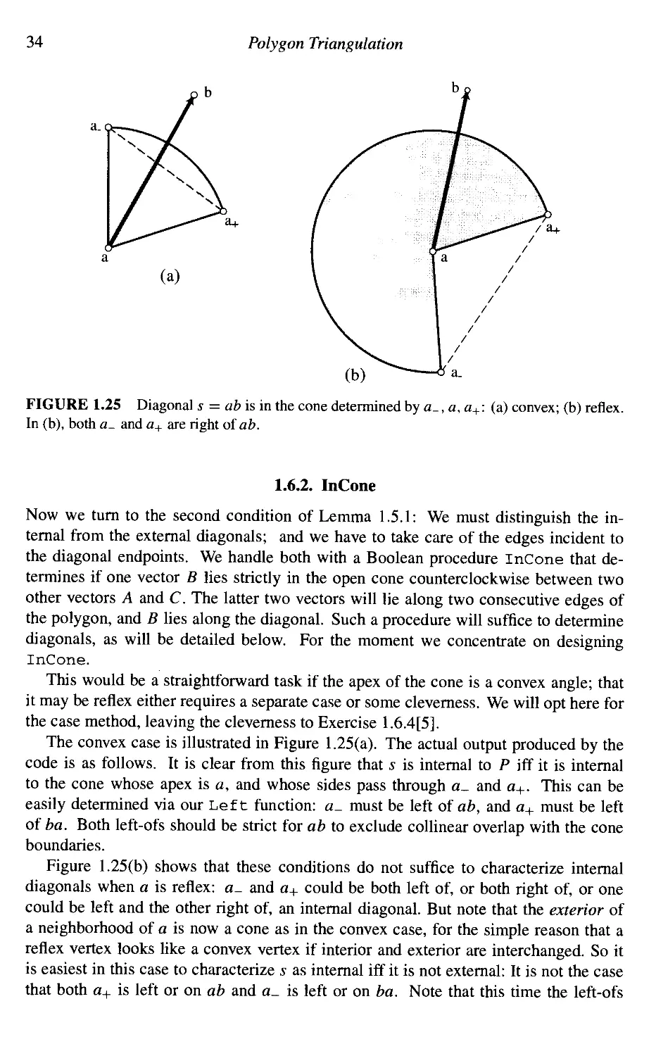


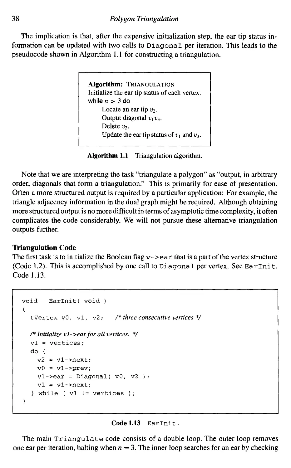


Author: O'Rourke J.
Tags: mathematics geometry programming higher mathematics computer science cambridge university press math computational geometry
Year: 1998


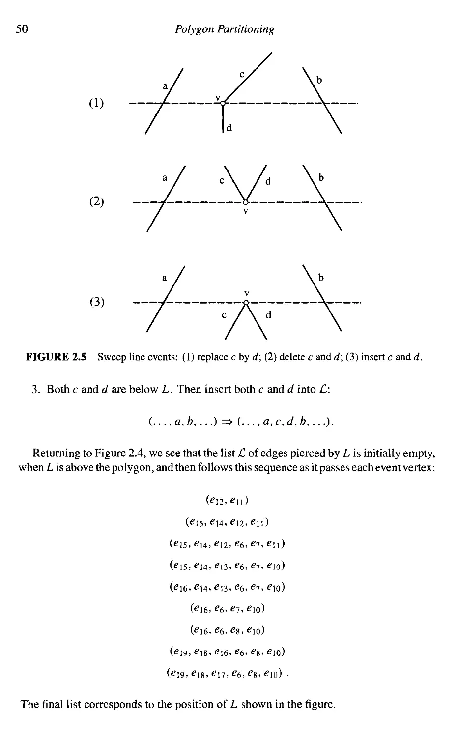
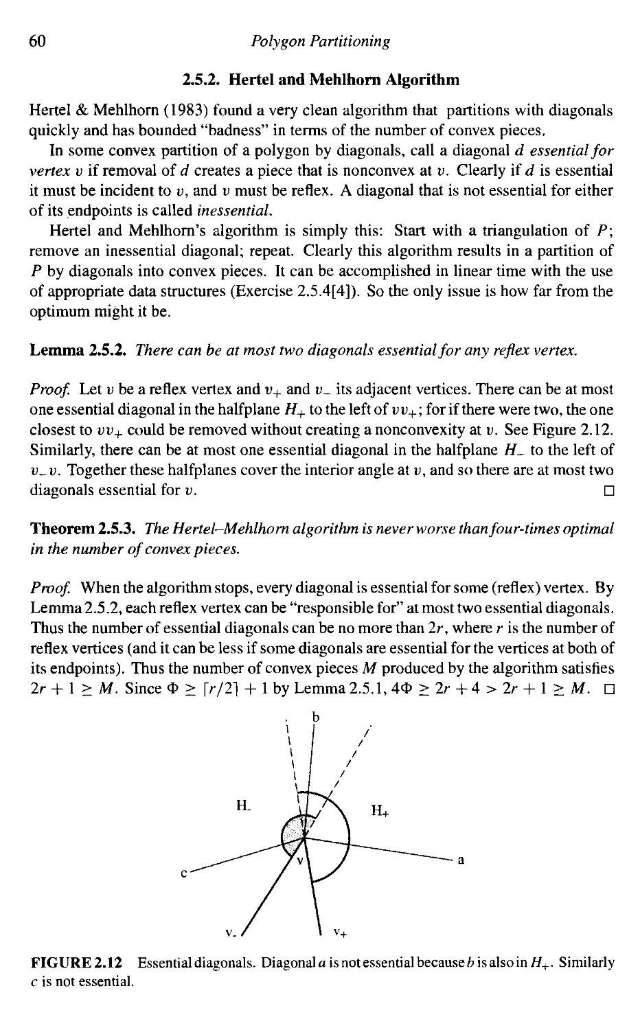
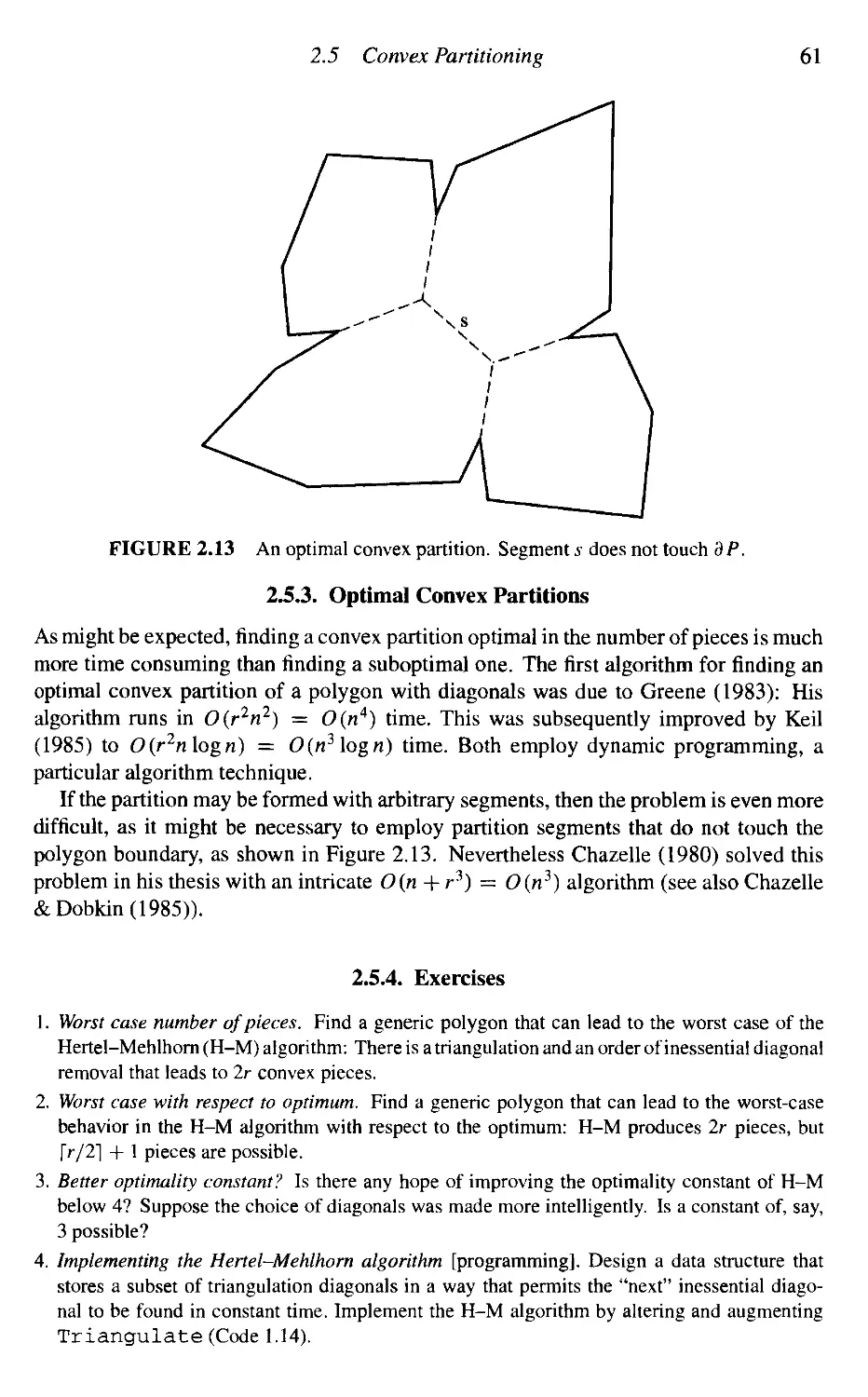
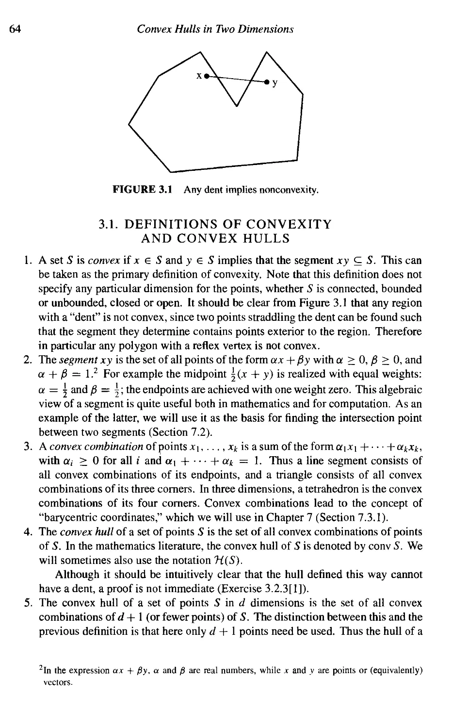
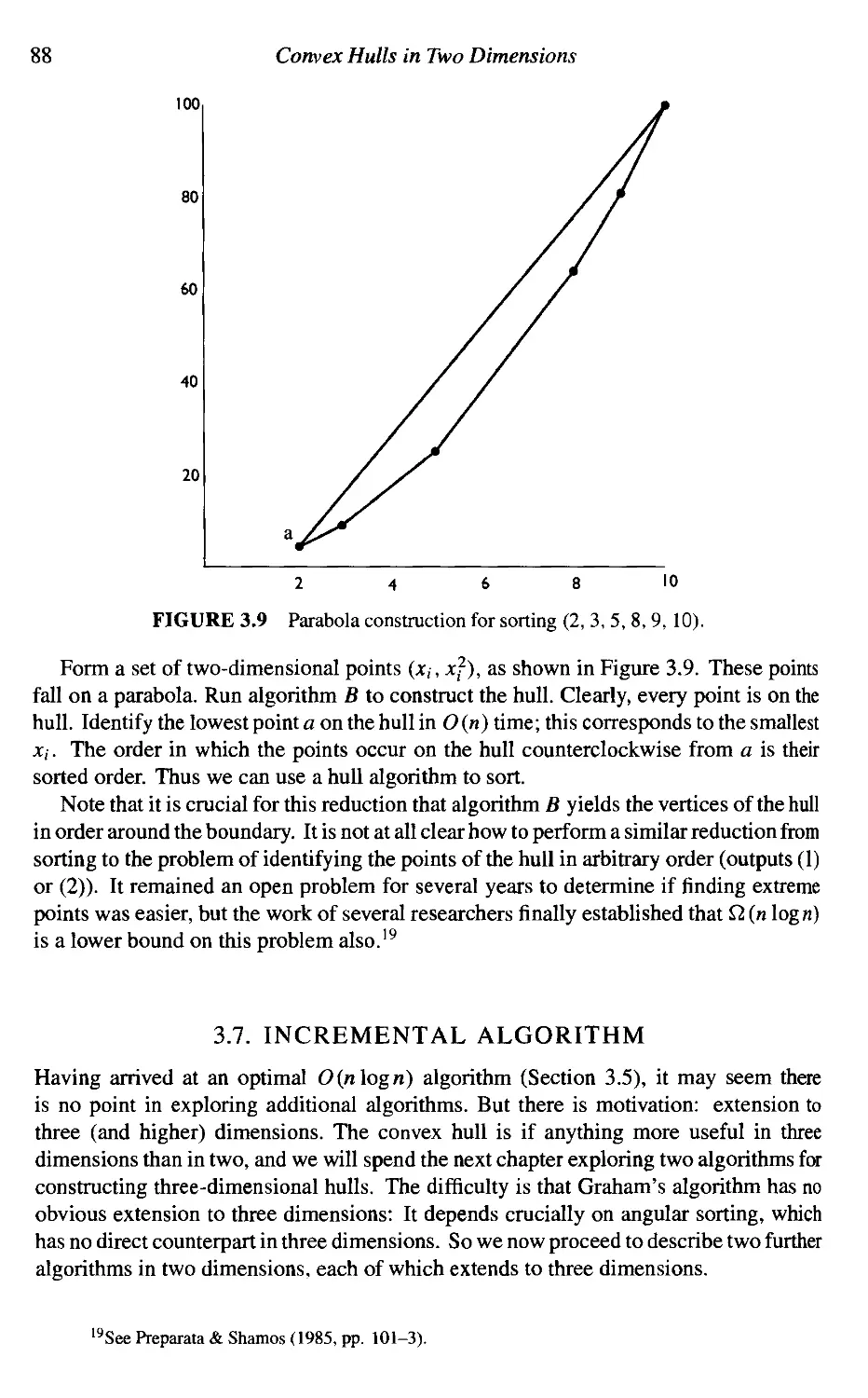
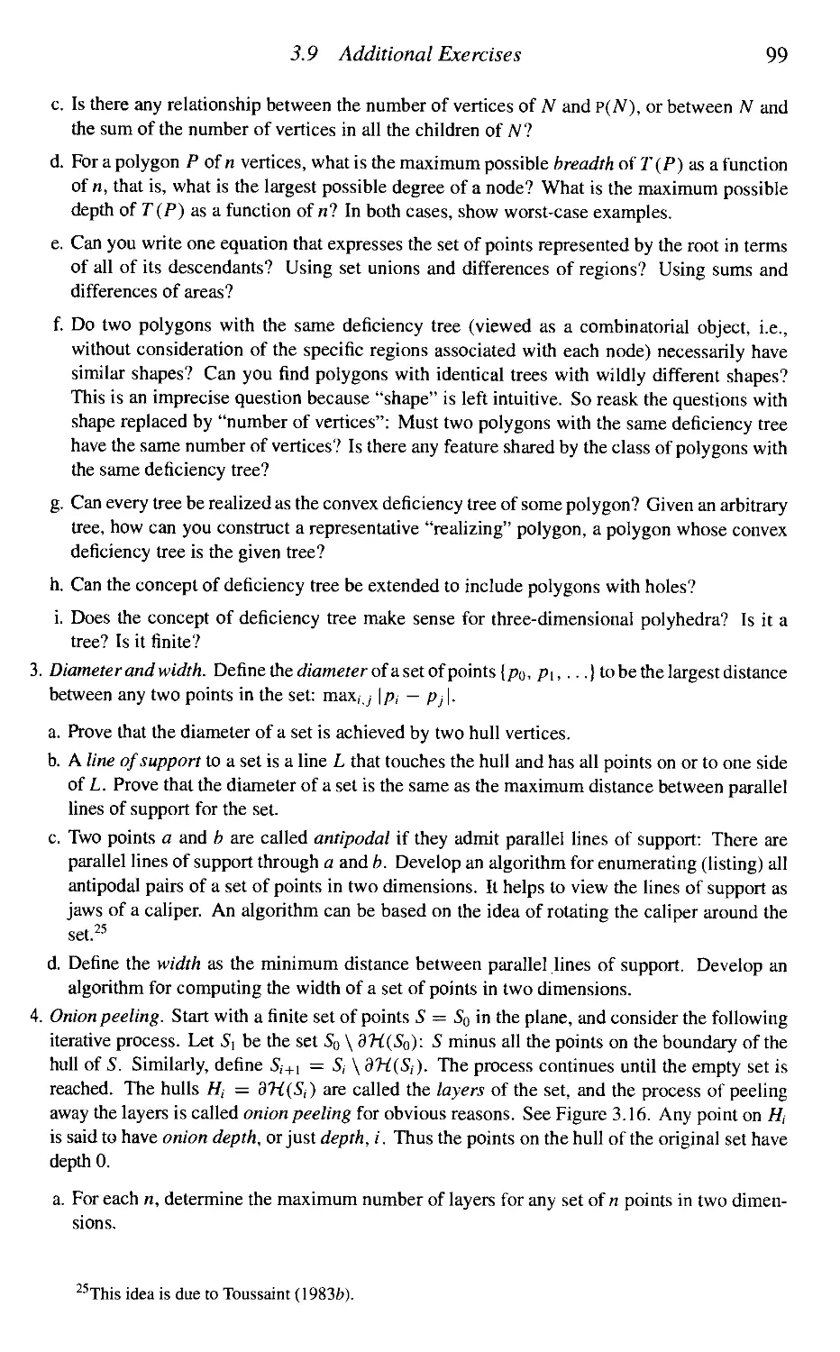
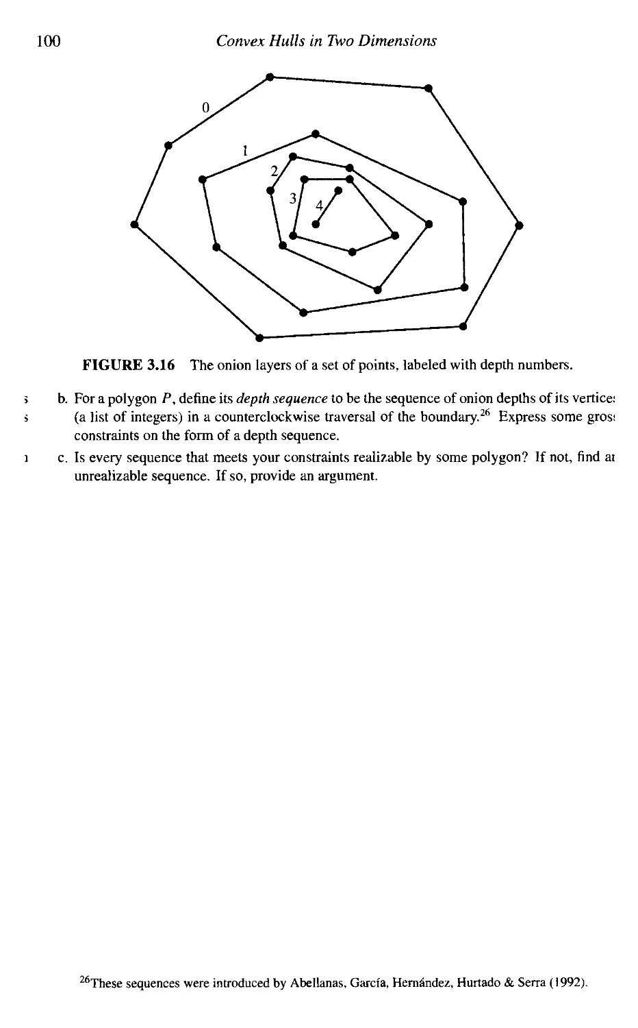
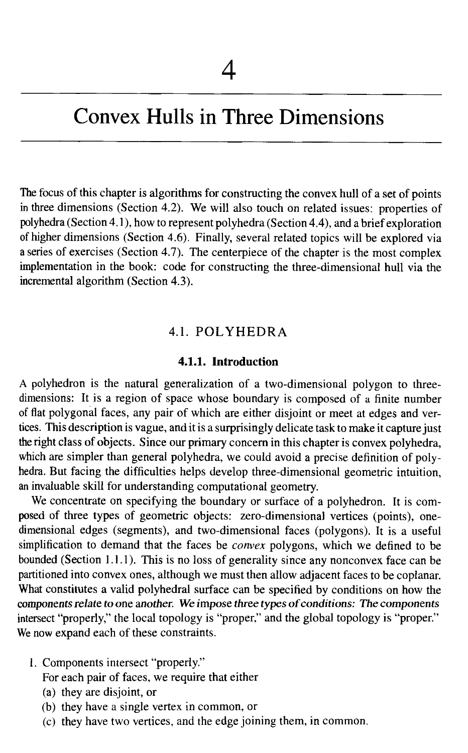
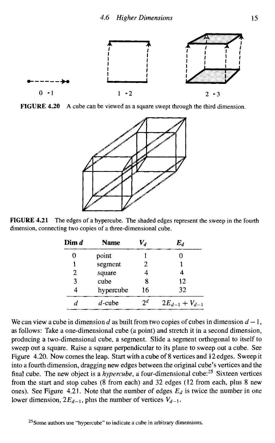
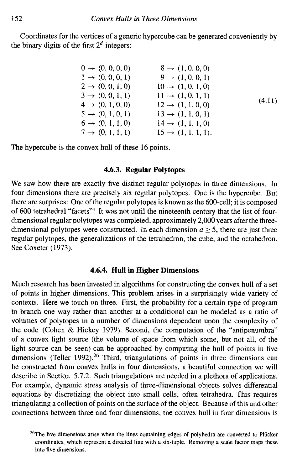
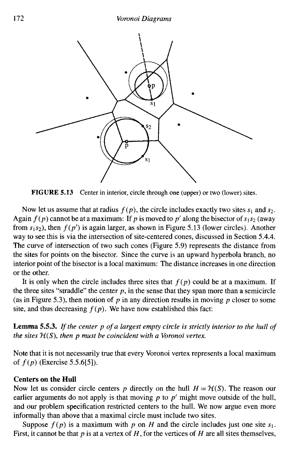
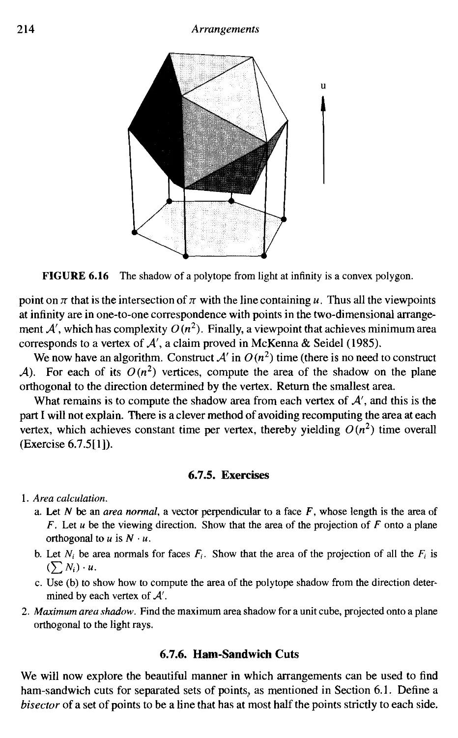
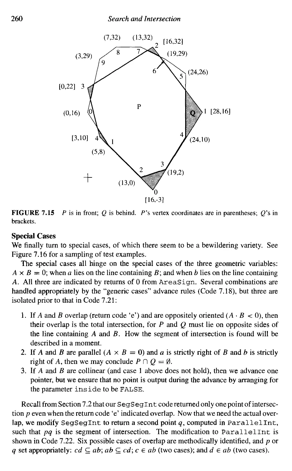
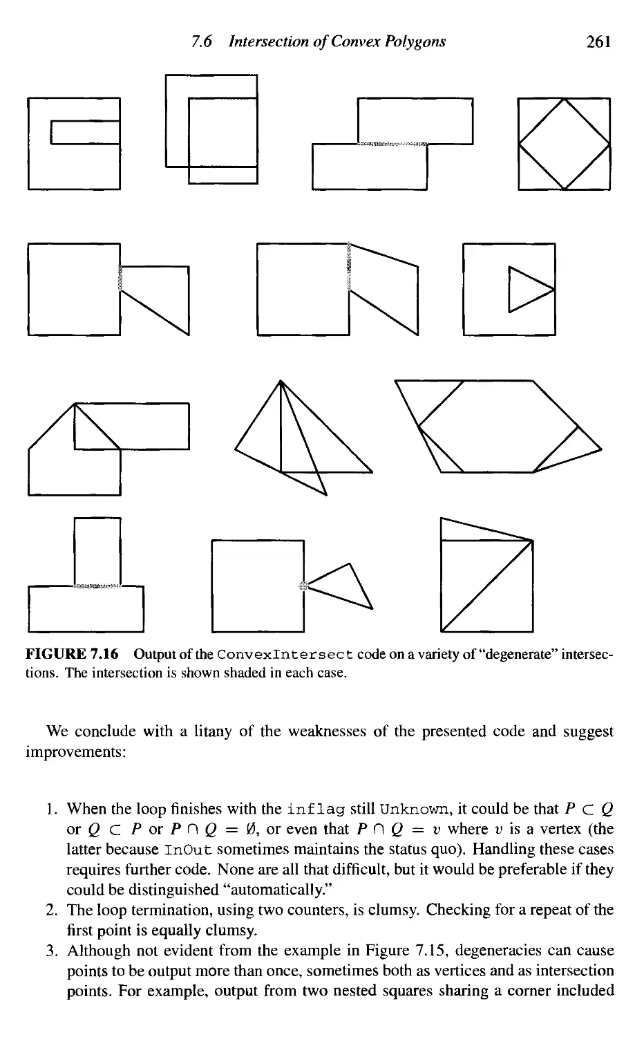
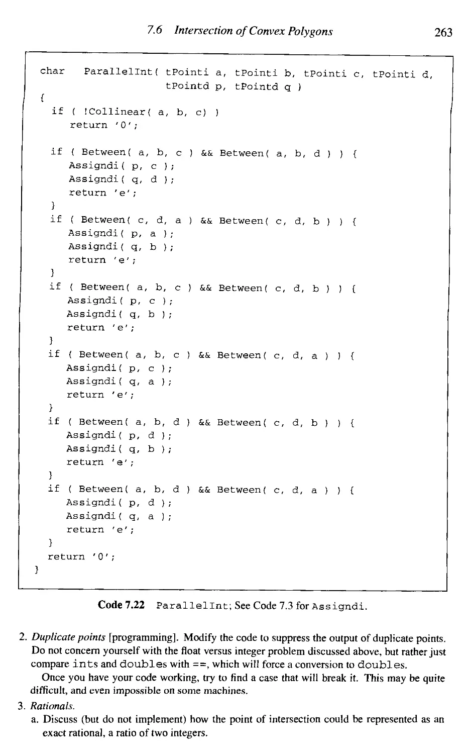
Text
COMPUTATIONAL
GEOMETRY IN С
SECOND EDITION
JOSEPH O'ROURKE
Cambridg
UNIVERSITY PRESS
Contents
t. Polygon Triangulation
1.1
1.2
1.3
1.4
1.5
1.6
Art Gallery Theorems
Triangulation: Theory
Area of Polygon
Implementation Issues
Segment Intersection
Triangulation: Implementation
Preface page x
11
16
24
27
32
2. Polygon Partitioning 44
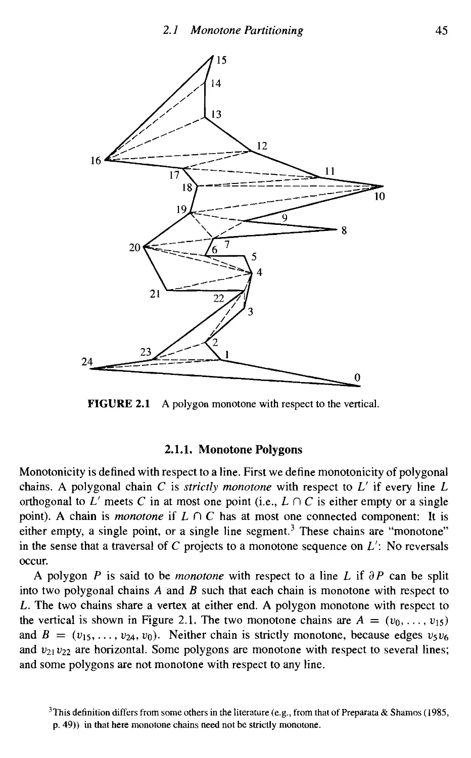
2.1 Monotone Partitioning 44
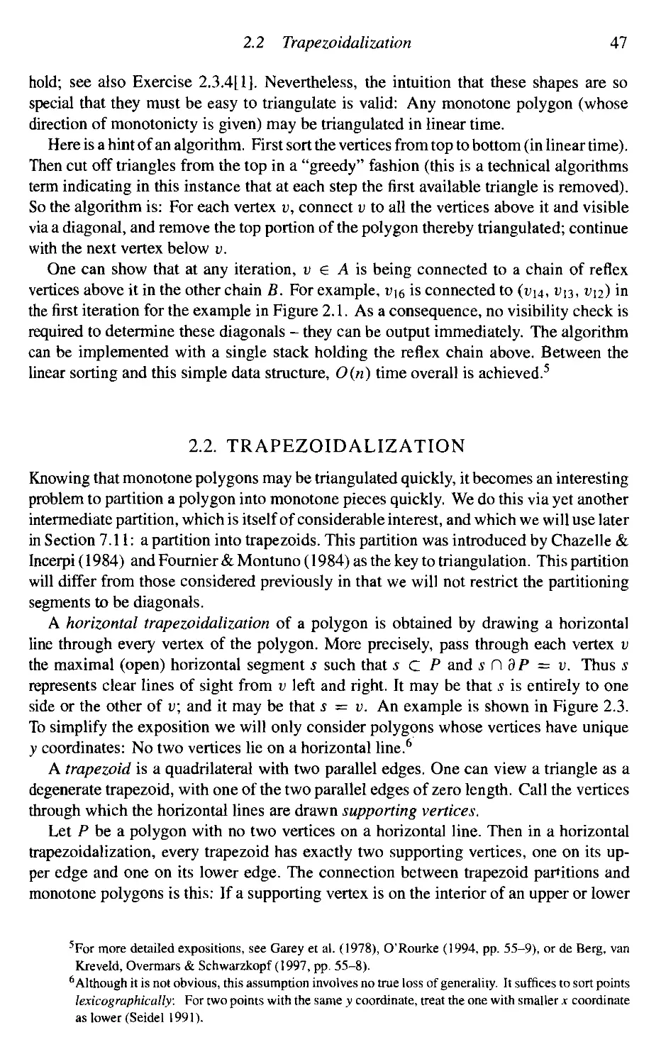
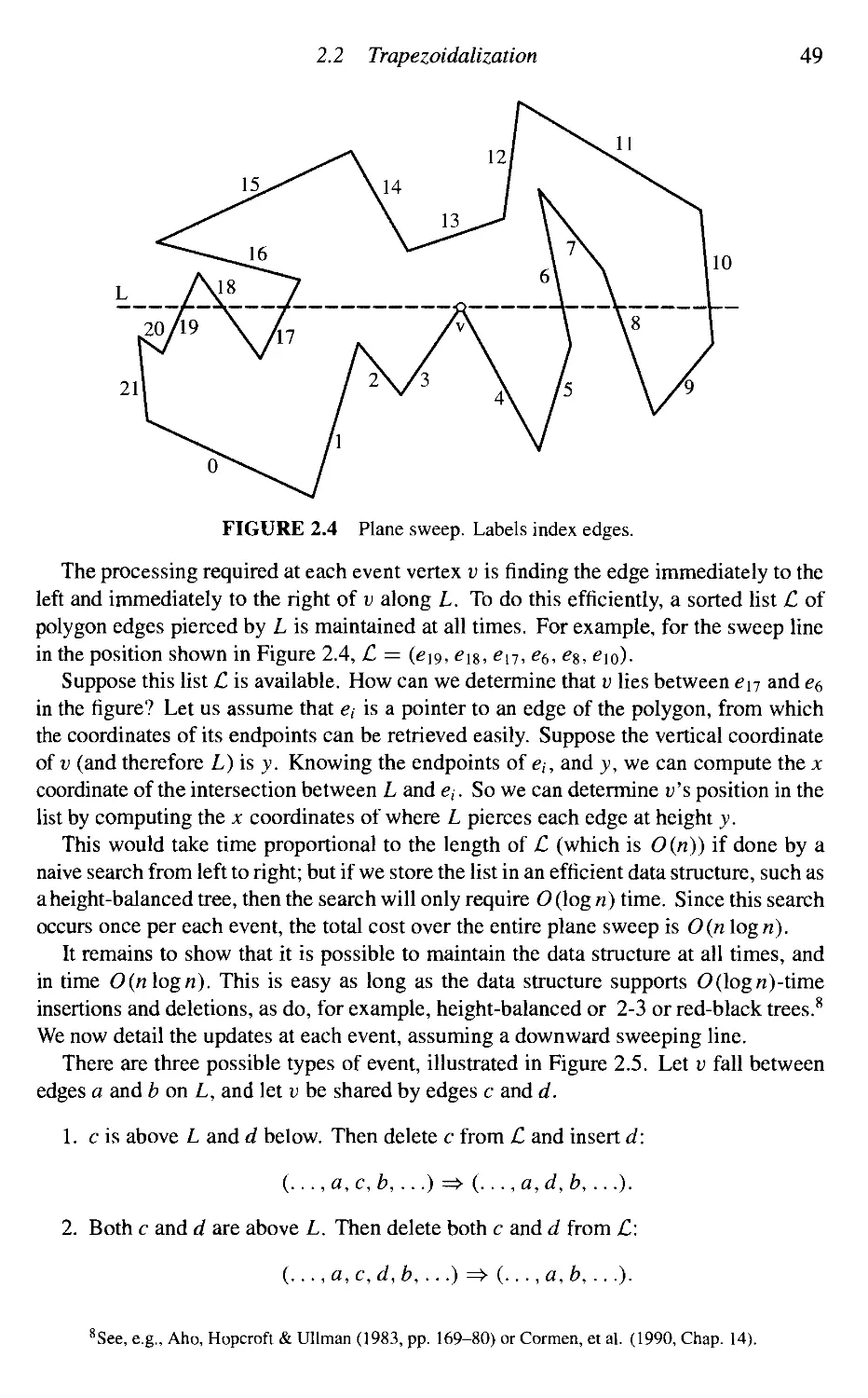
2.2 Trapezoidalization 47
2.3 Partition into Monotone Mountains 51
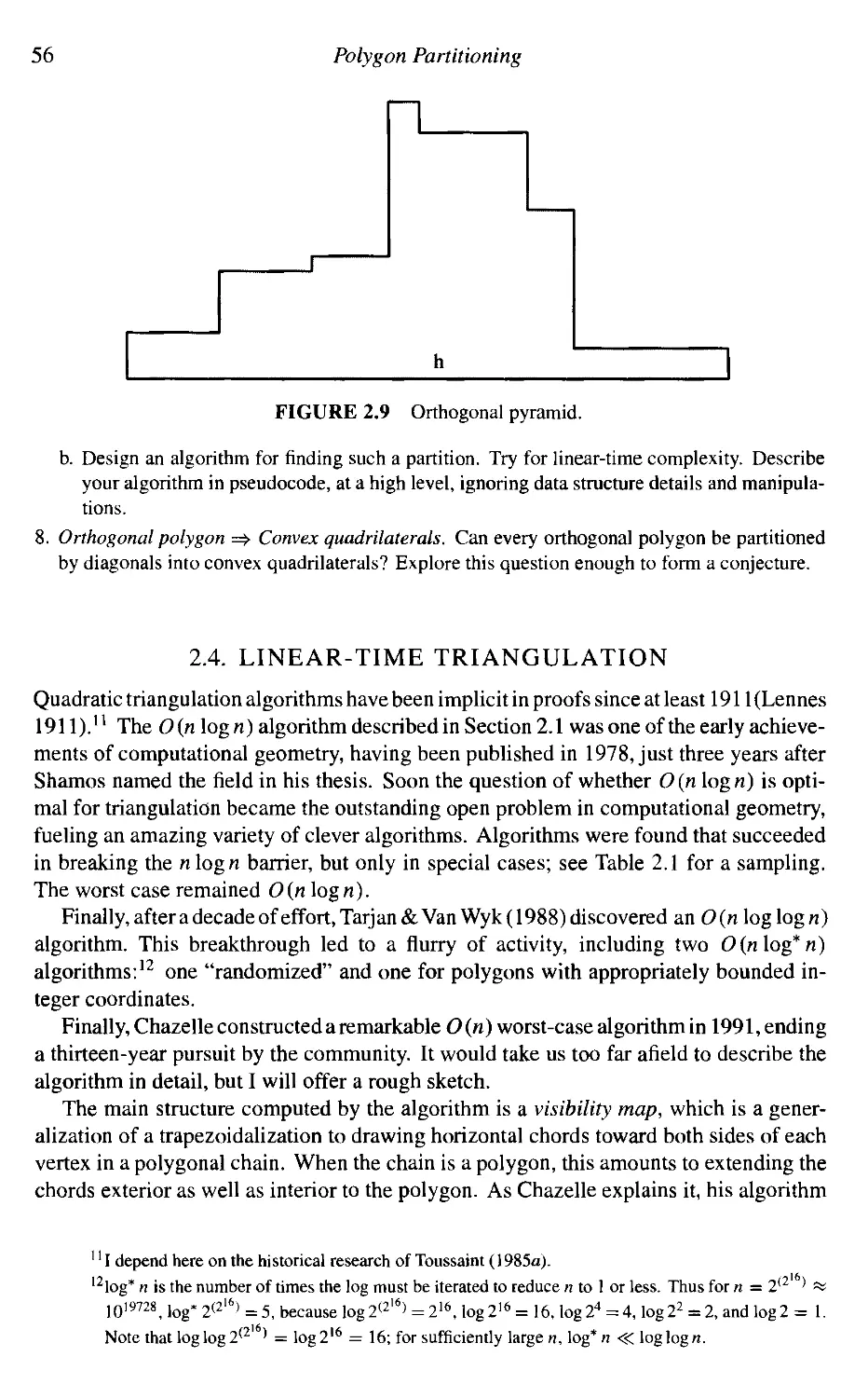
2.4 Linear-Time Triangulation 56
2.5 Convex Partitioning 58
3. Convex Hulls in Two Dimensions 63
3.1 Definitions of Convexity and Convex Hulls 64
3.2 Naive Algorithms for Extreme Points 66
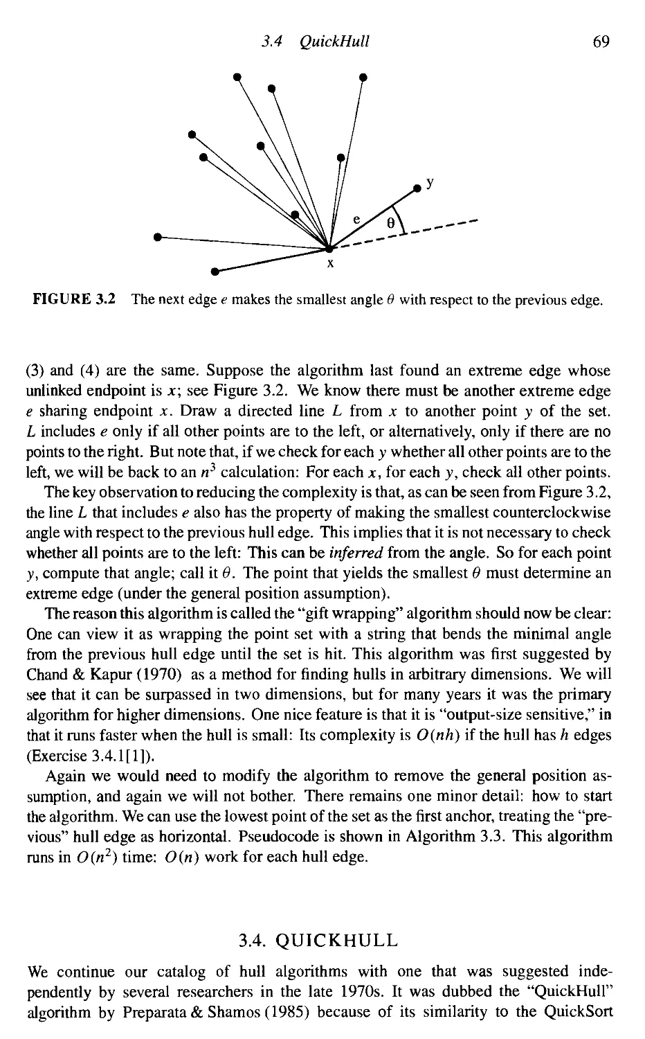
3.3 Gift Wrapping 68
3.4 QuickHull 69
3.5 Graham's Algorithm 72
3.6 Lower Bound 87
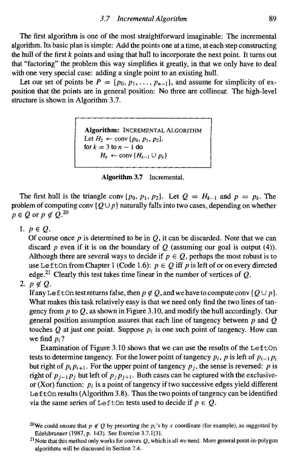
3.7 Incremental Algorithm 88
3.8 Divide and Conquer 91
3.9 Additional Exercises 96
4. Convex Hulls in Three Dimensions 101
4.1 Polyhedra 101
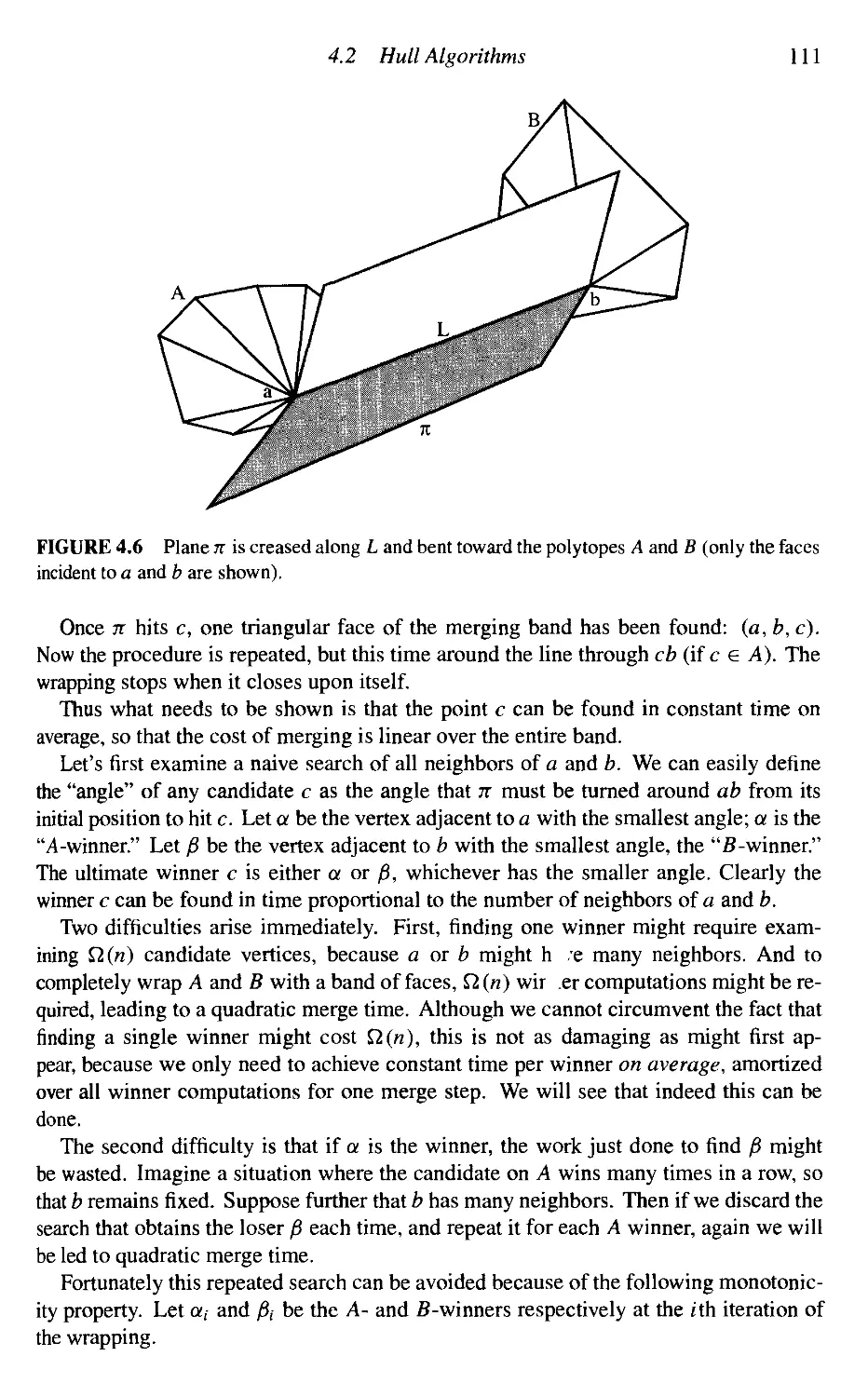
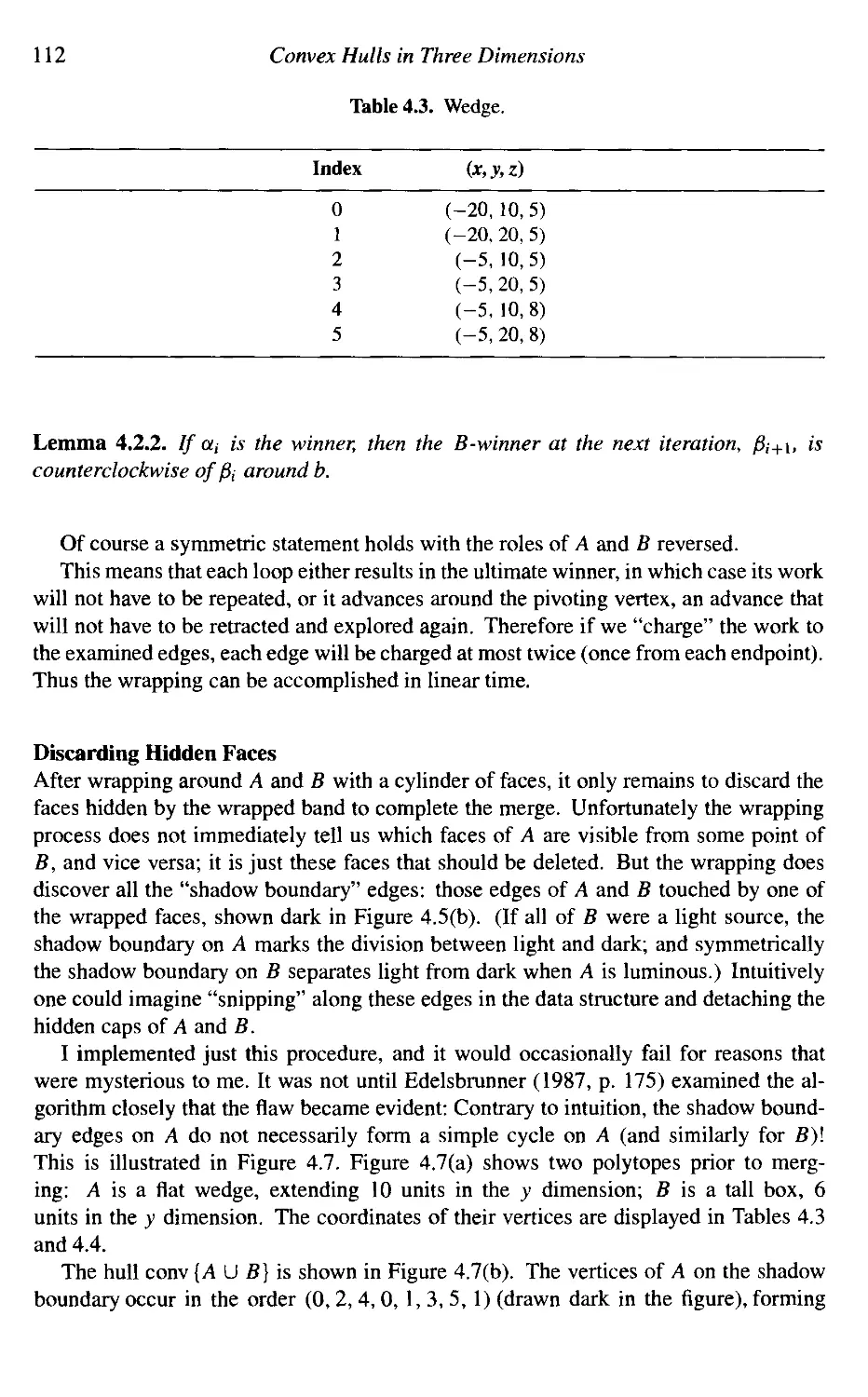
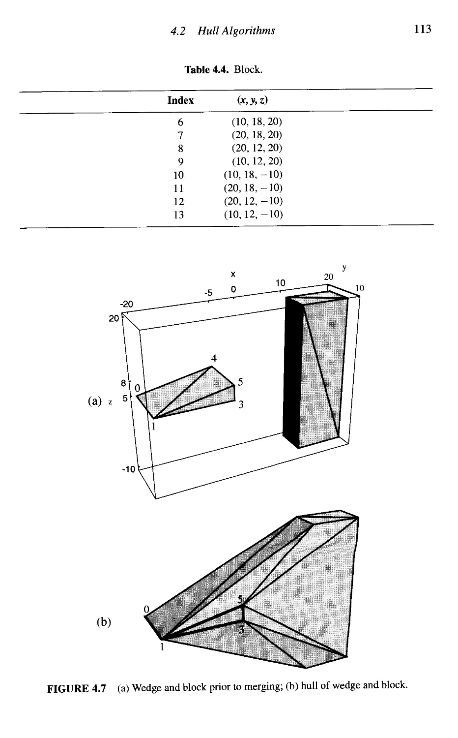
4.2 Hull Algorithms 109
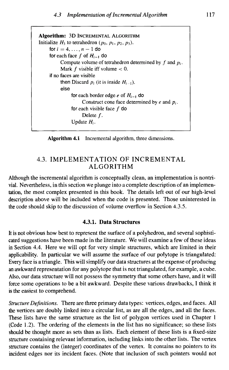
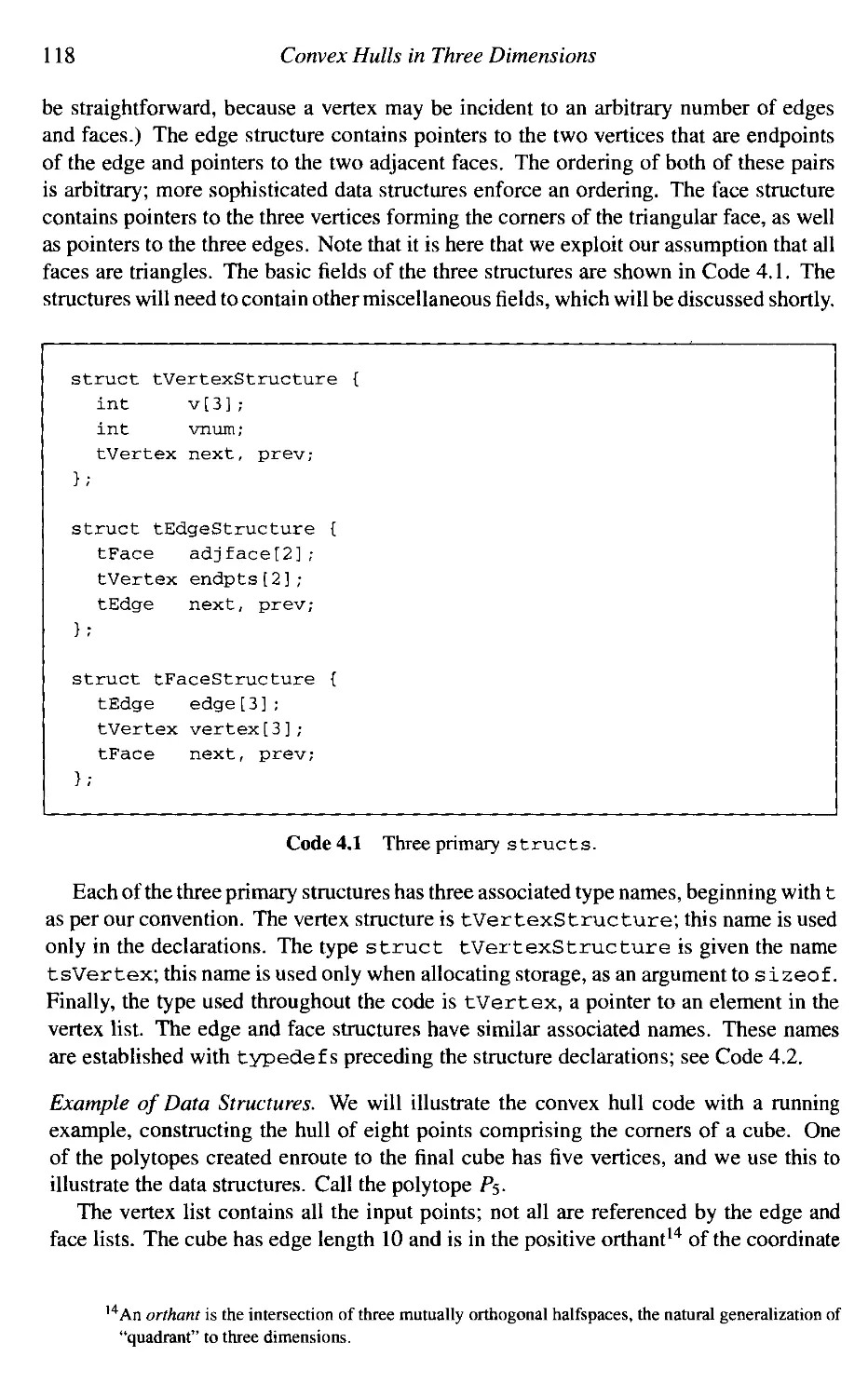
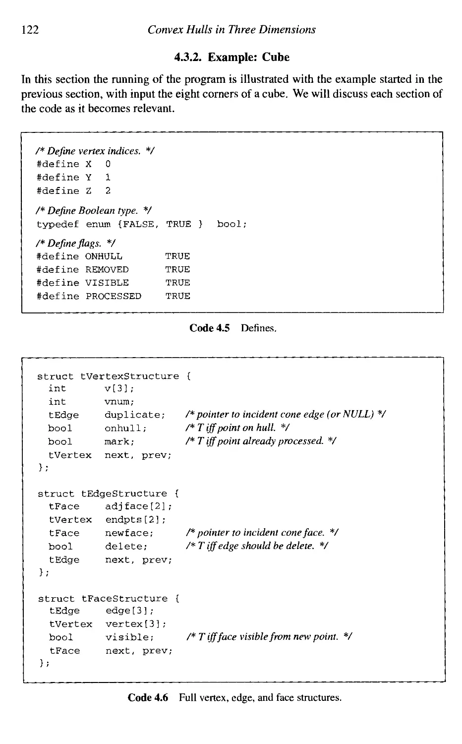
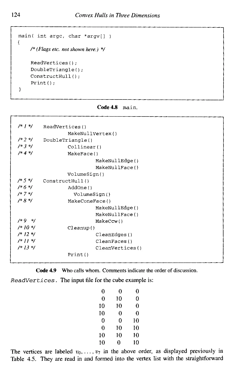
4.3 Implementation of Incremental Algorithm 117
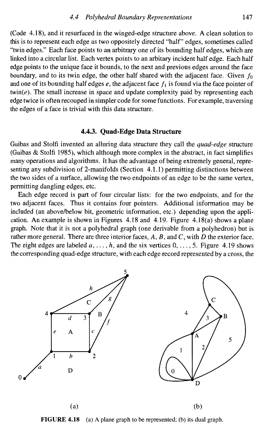
4.4 Polyhedral Boundary Representations 146
4.5 Randomized Incremental Algorithm 149
4.6 Higher Dimensions 150
4.7 Additional Exercises 153
Vm Contents
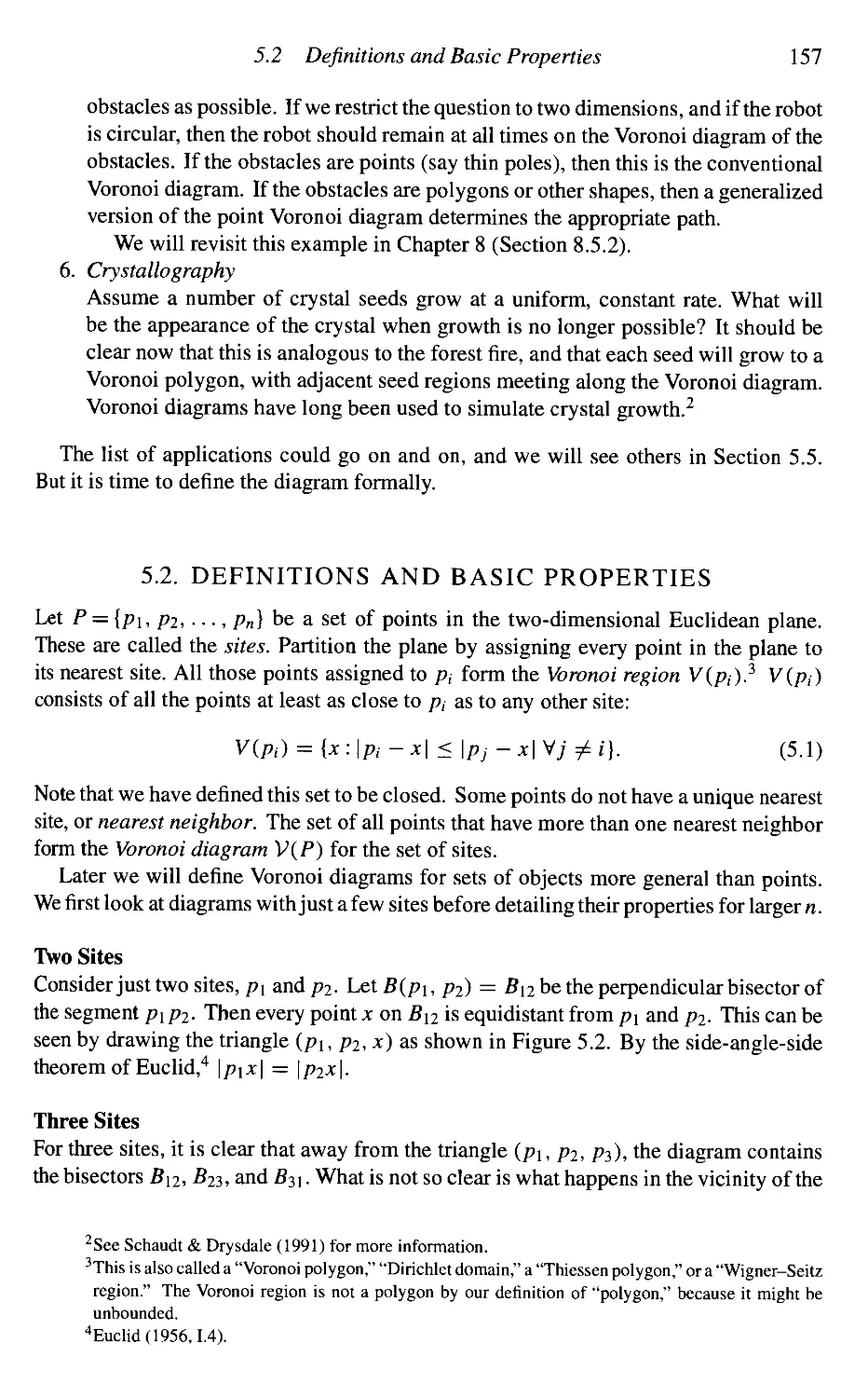
5. Voronoi Diagrams 155
5.1 Applications: Preview 155
5.2 Definitions and Basic Properties 157
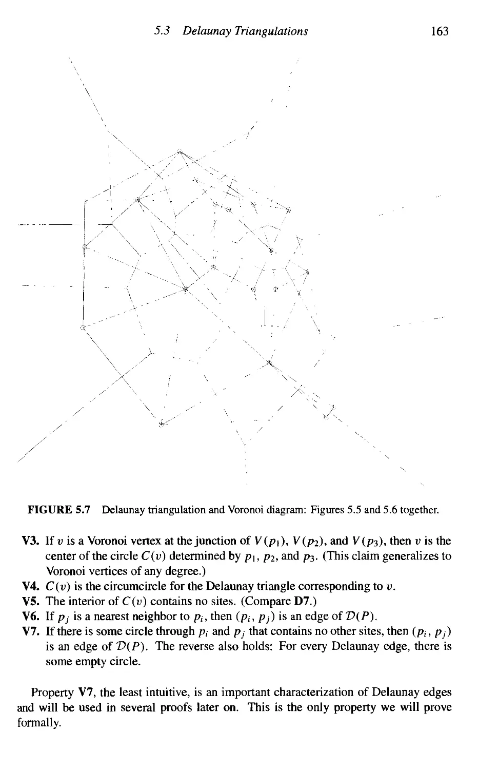
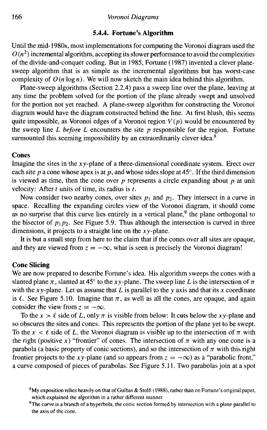
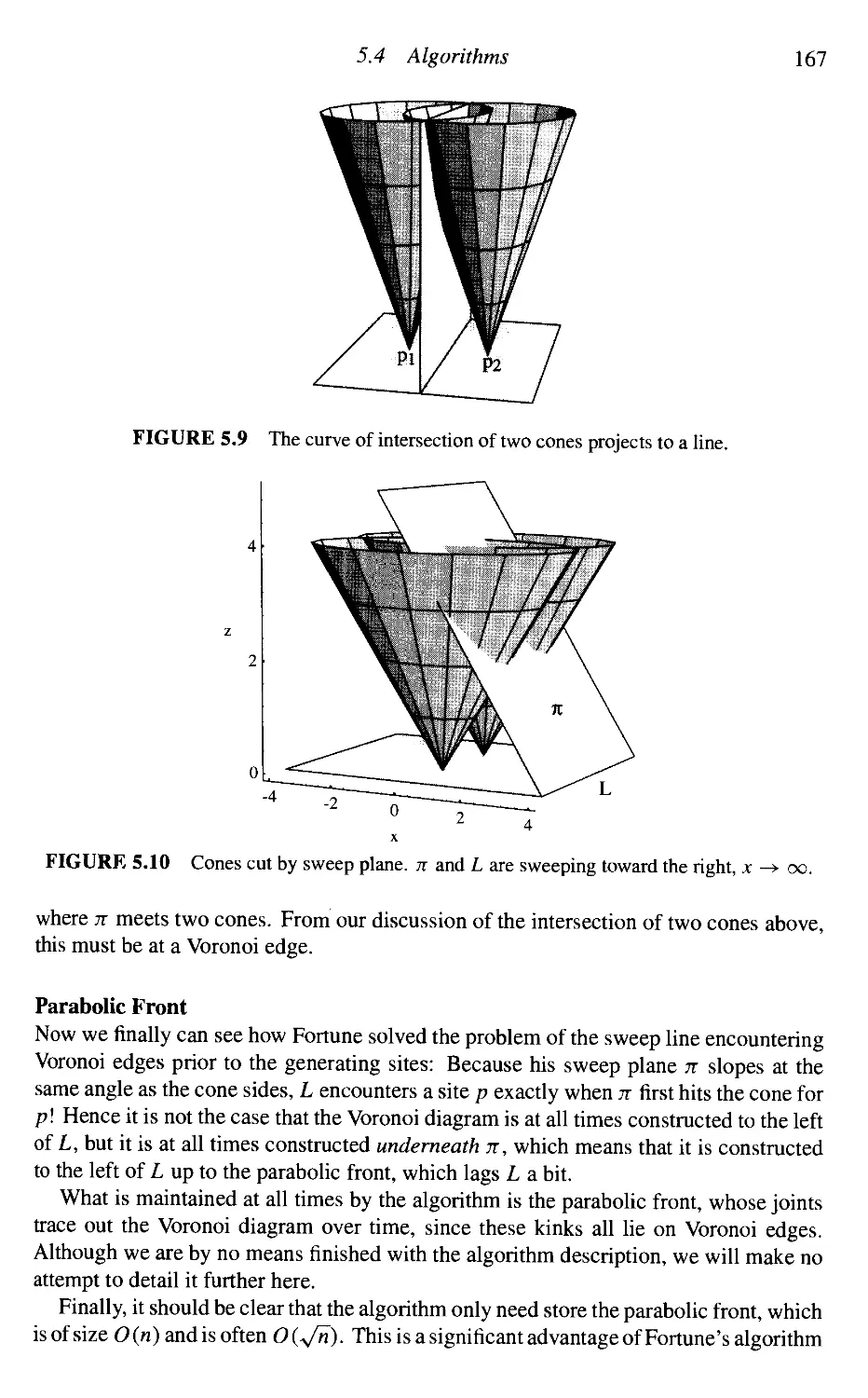
5.3 Delaunay Triangulations 161
5.4 Algorithms 165
5.5 Applications in Detail 169
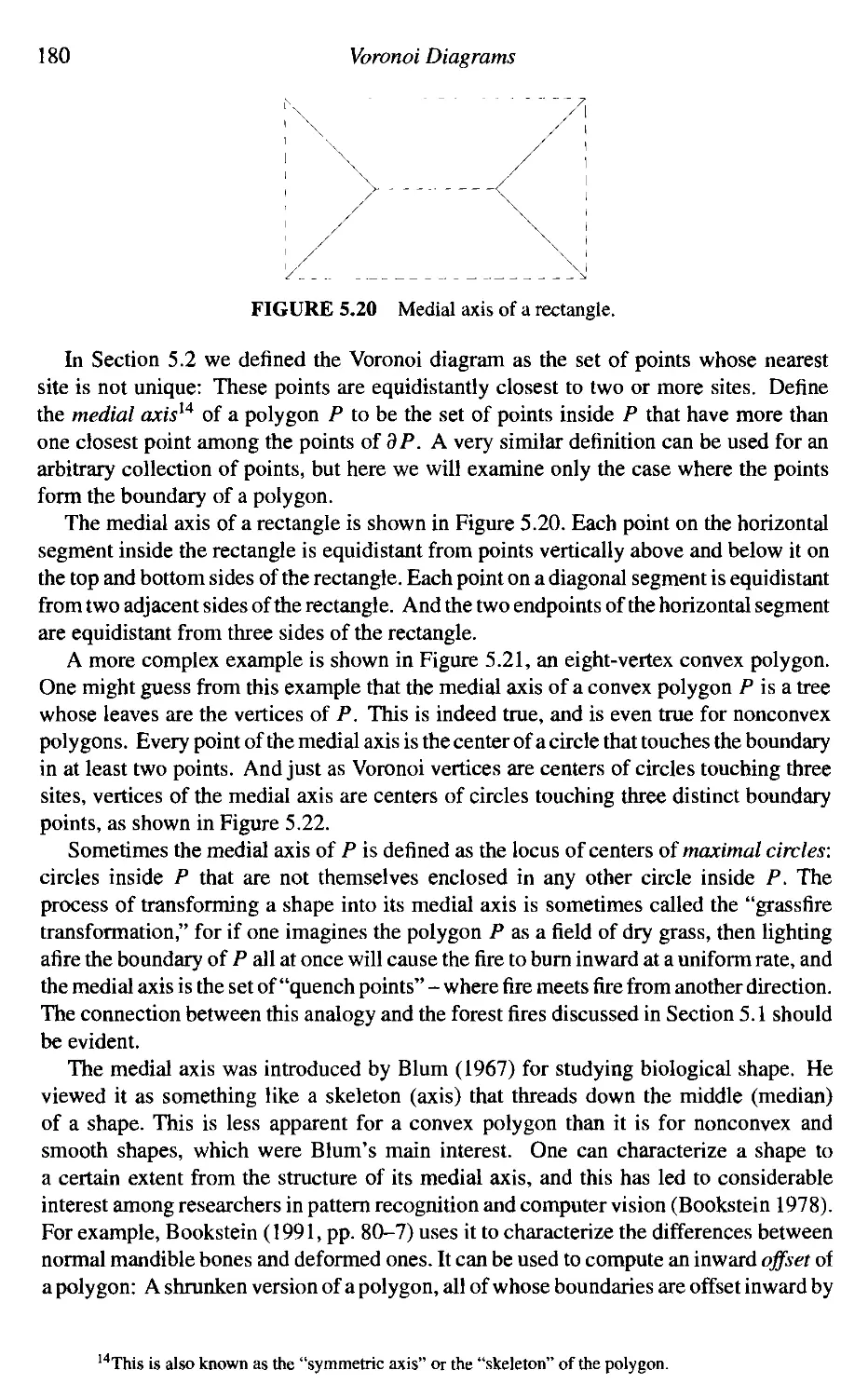
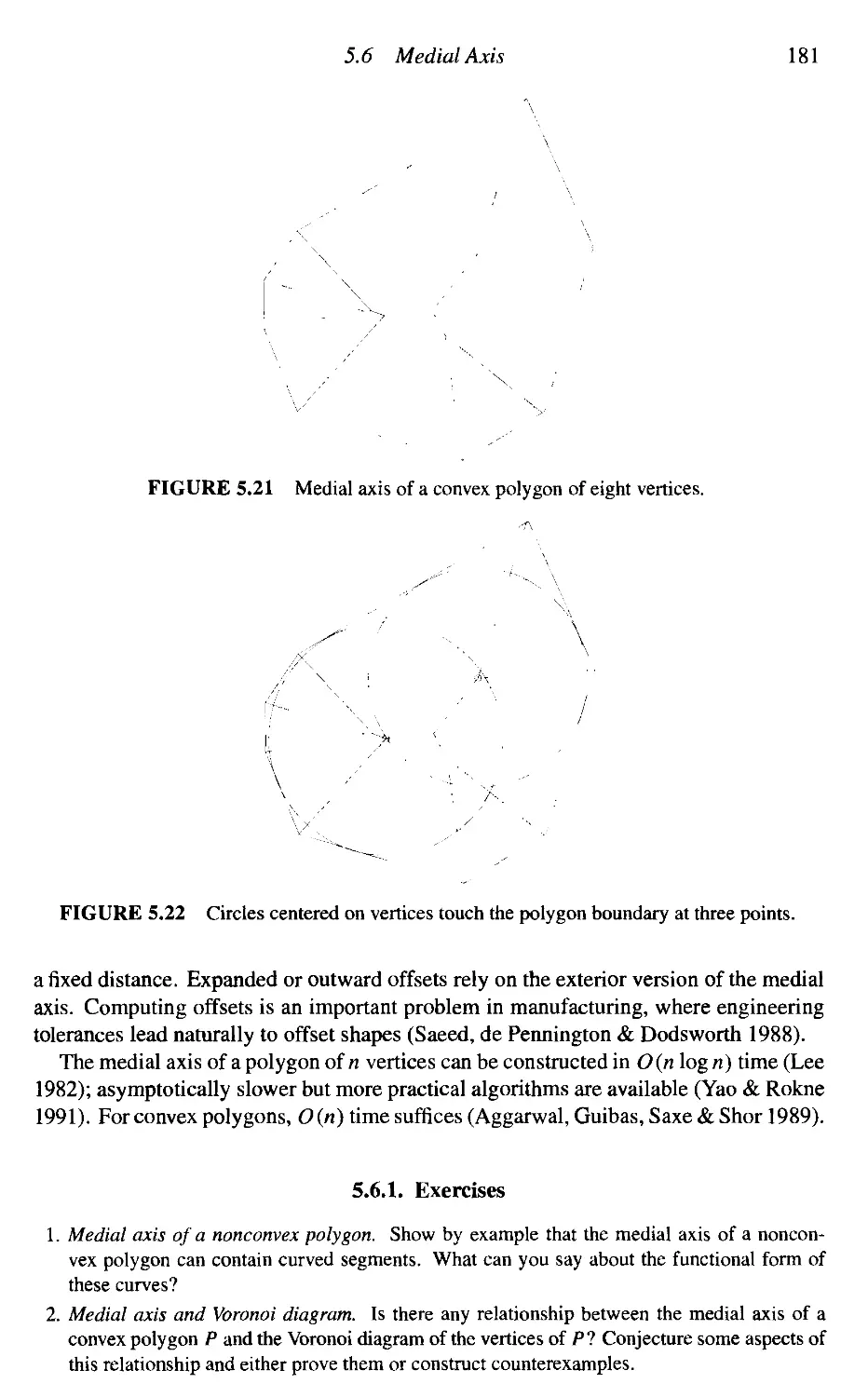
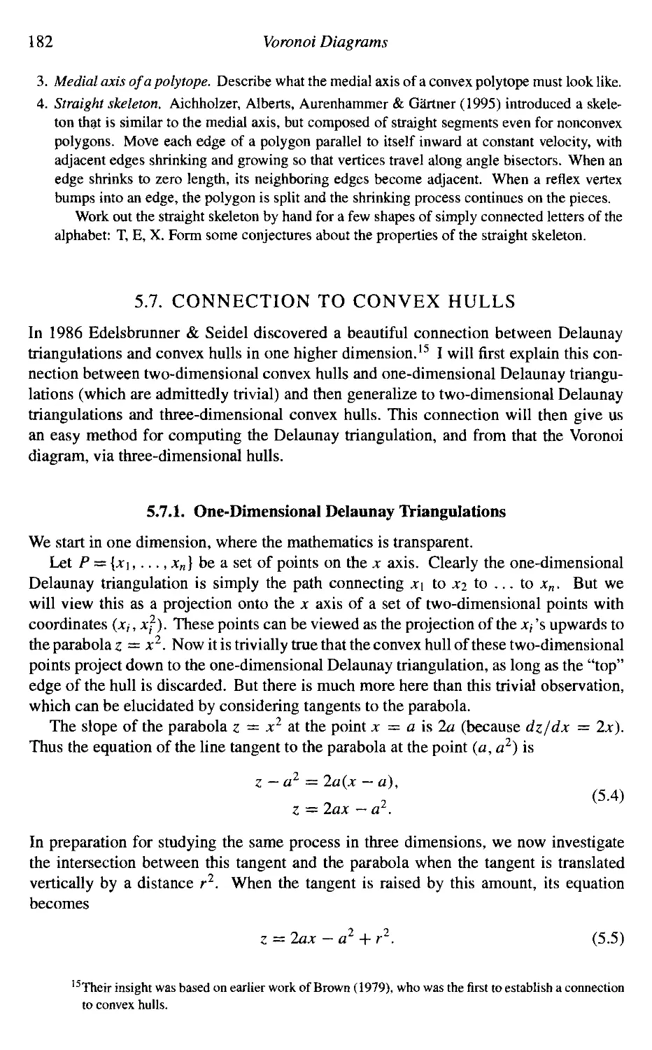
5.6 Medial Axis 179
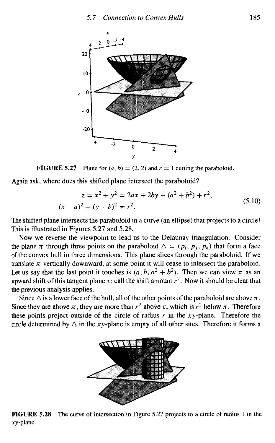
5.7 Connection to Convex Hulls 182
5.8 Connection to Arrangements 191
6. Arrangements 193
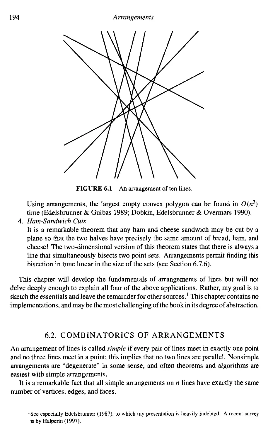
6.1 Introduction 193
6.2 Combinatorics of Arrangements 194
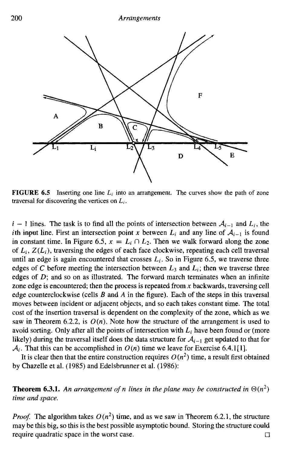
6.3 Incremental Algorithm 199
201
201
205
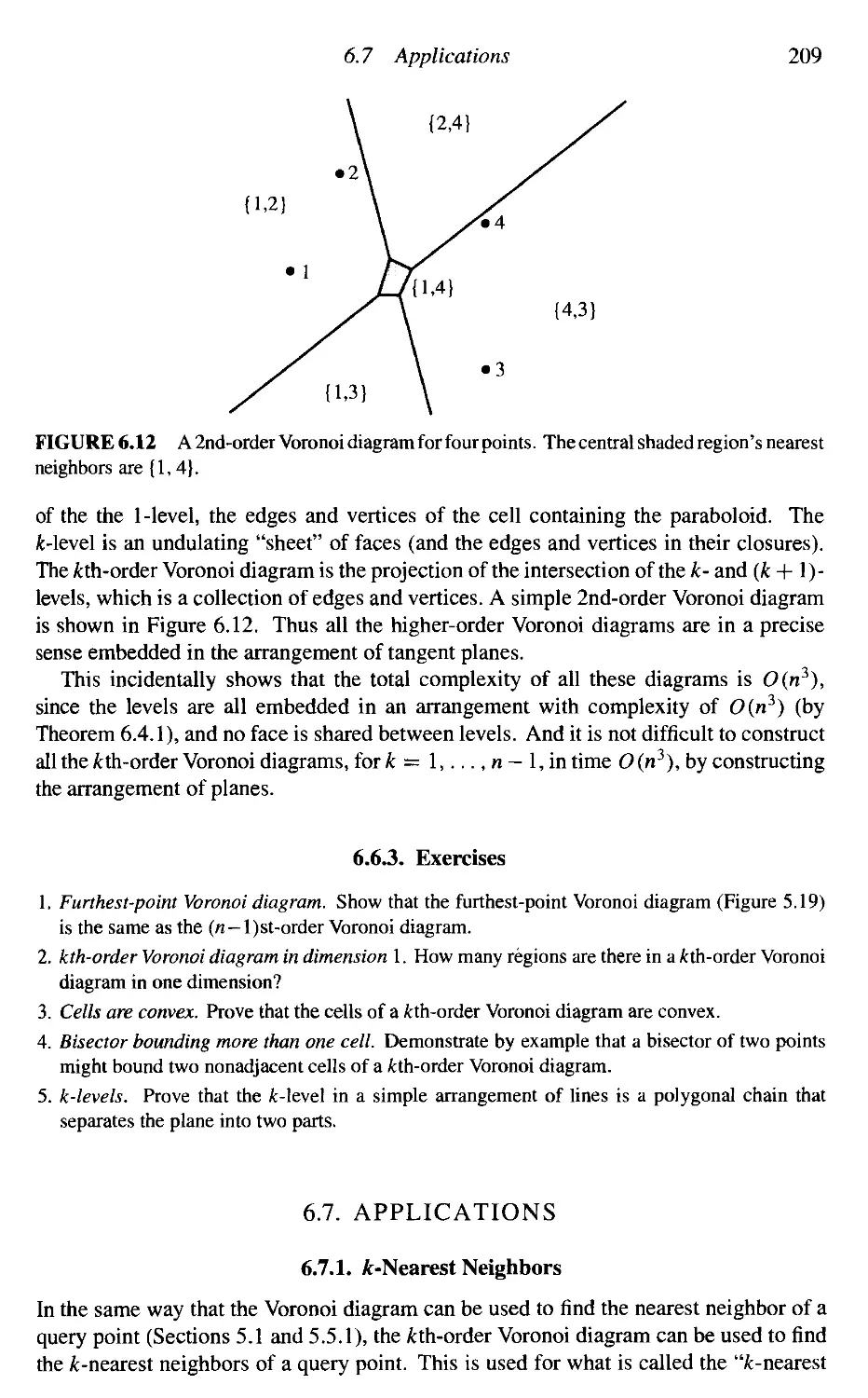
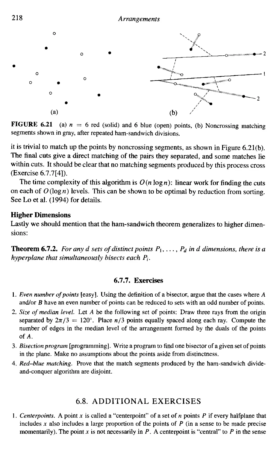
209
218
220
220
220
226
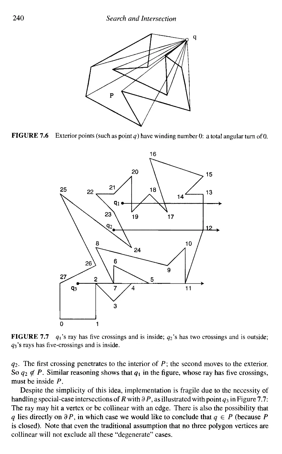
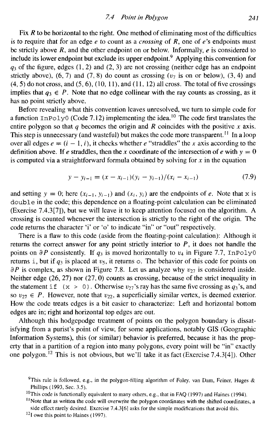
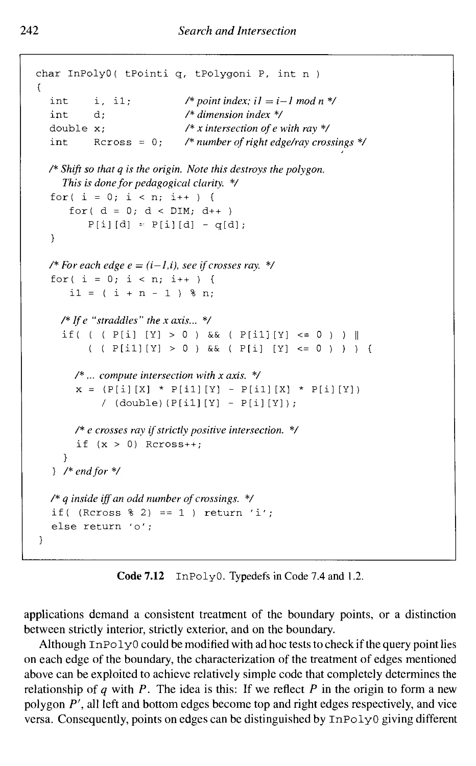
239
245
252
263
266
269
272
285
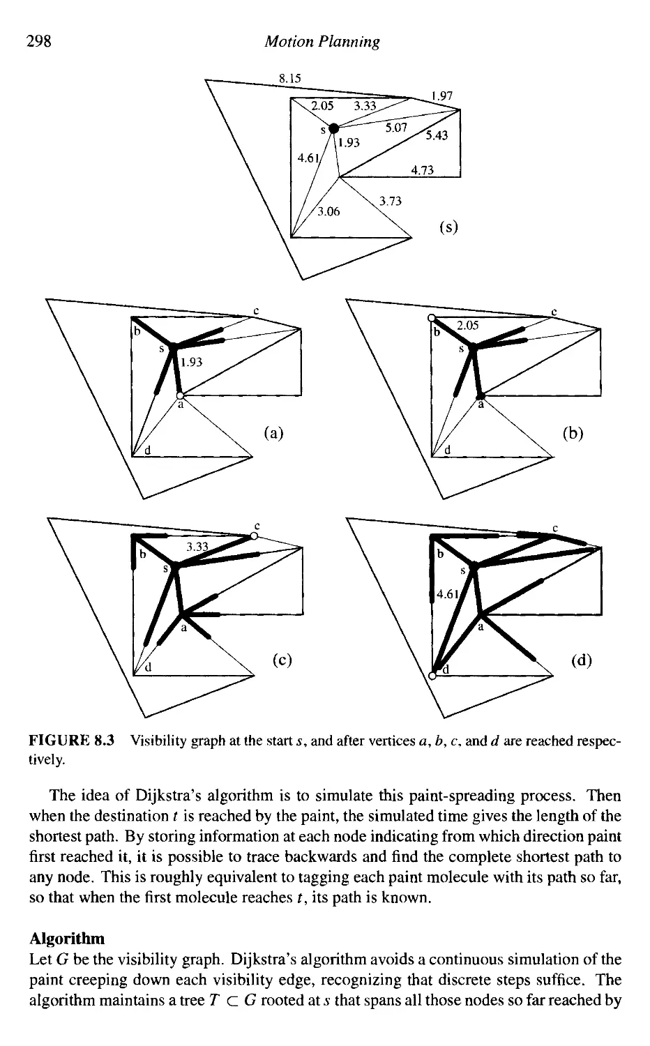
294
294
295
300
302
313
322
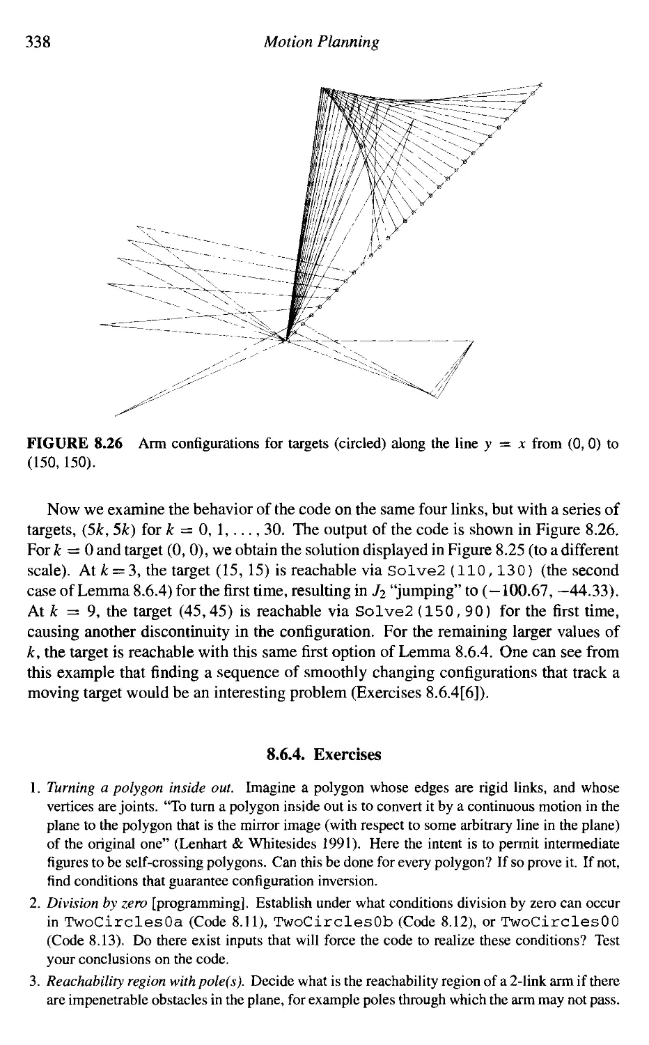
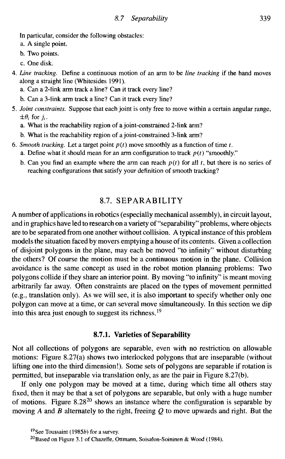
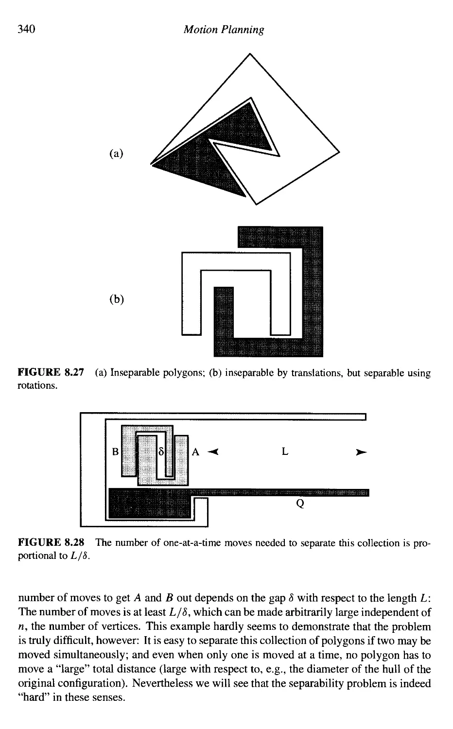
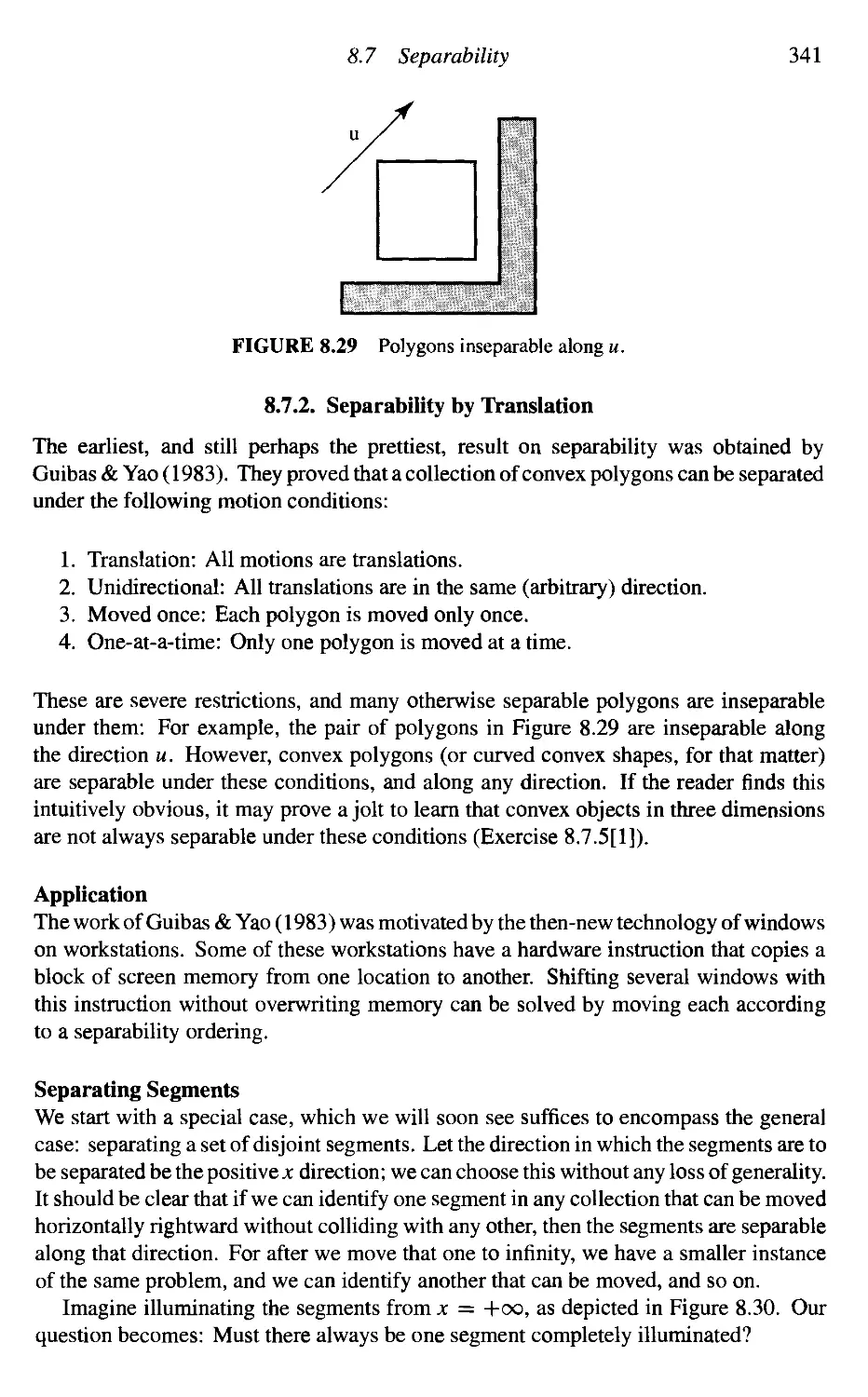
339
9. Sources 347
9.1 Bibliographies and FAQs 347
9.2 Textbooks 347
9.3 Book Collections 348
6.4
6.5
6.6
6.7
6.8
Three and Higher Dimensions
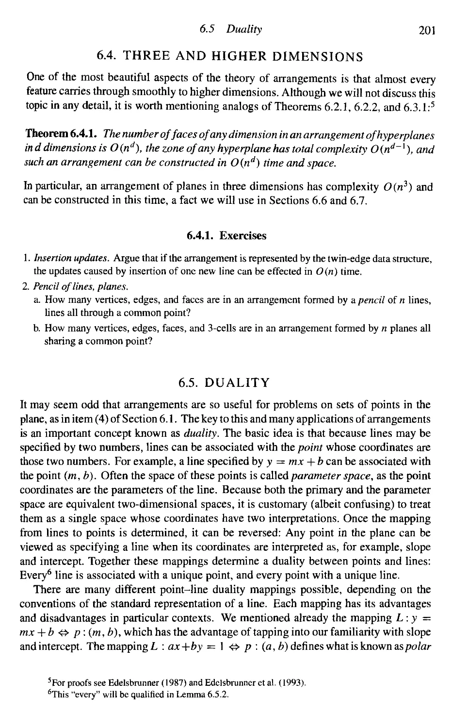
Duality
Higher-Order Voronoi Diagrams
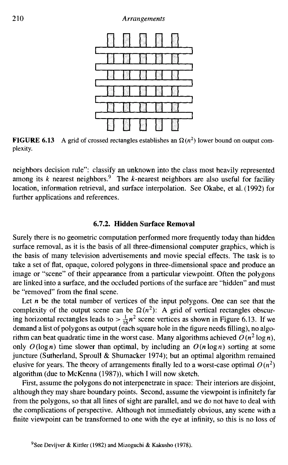
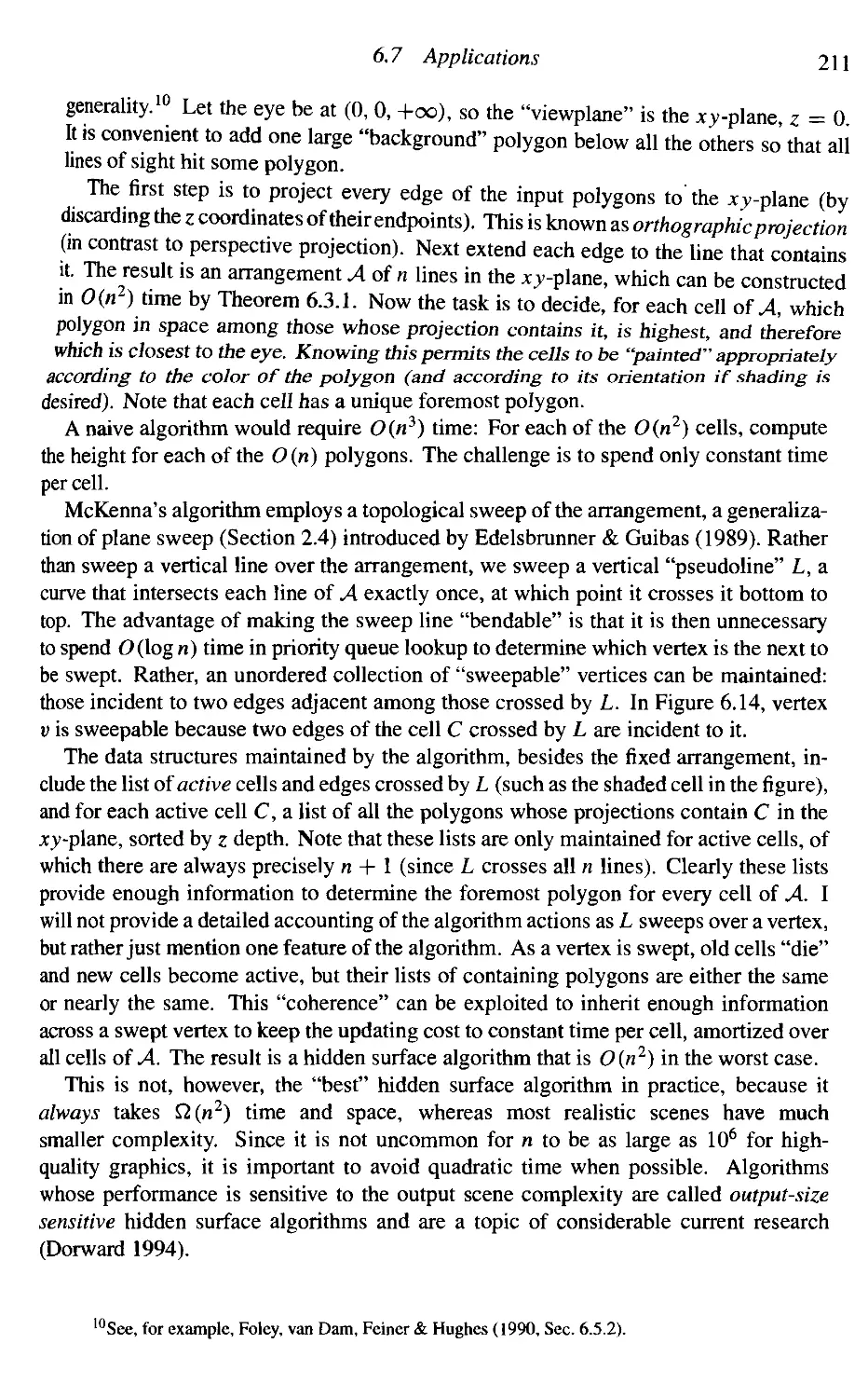
Applications
Additional Exercises
7. Search and Intersection
7.1
7.2
7.3
7.4
7.5
7.6
7.7
7.8
7.9
7.10
7.11
Introduction
Segment-Segment Intersection
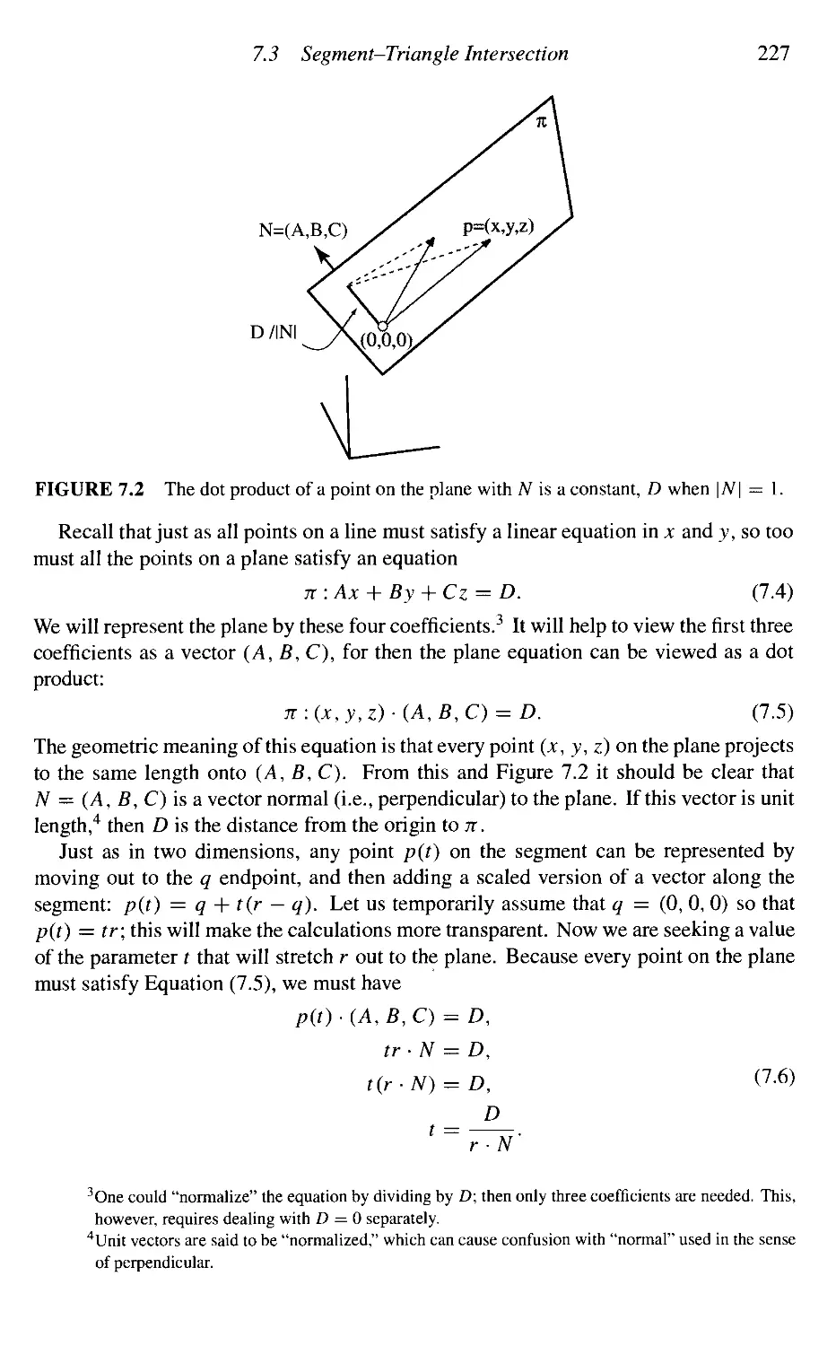
Segment-Triangle Intersection
Point in Polygon
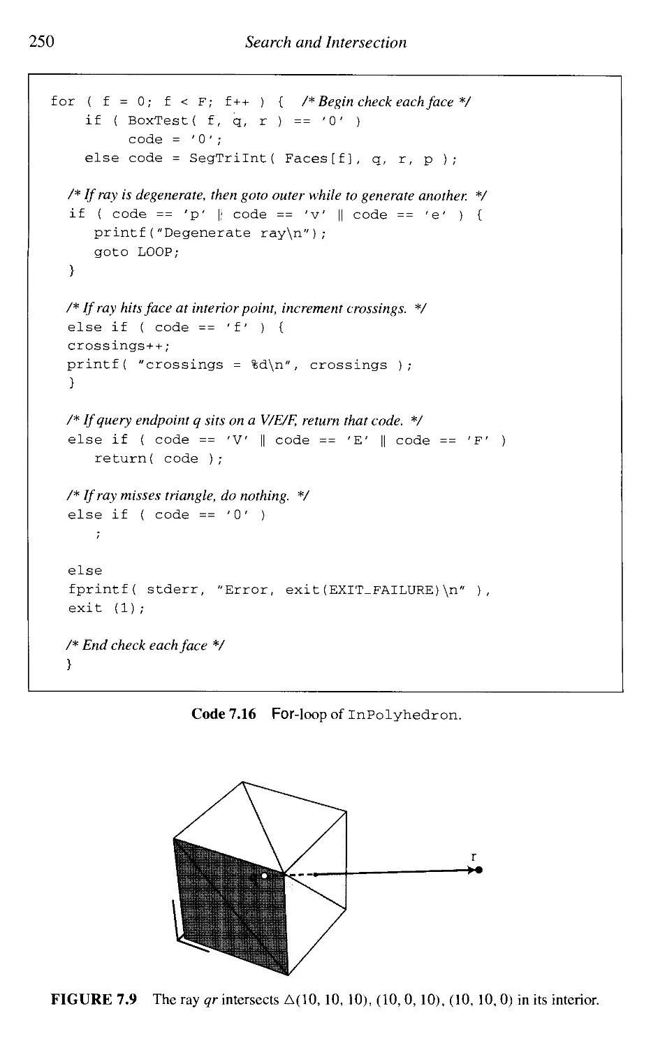
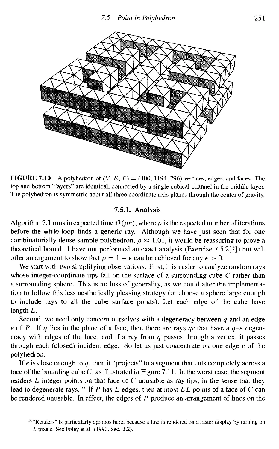
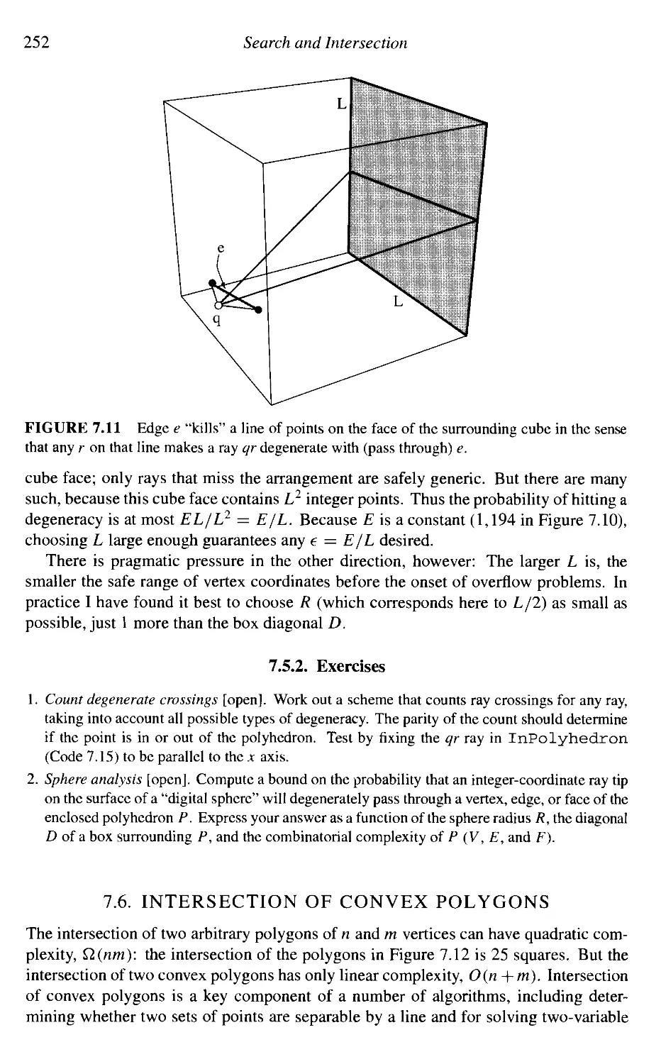
Point in Polyhedron
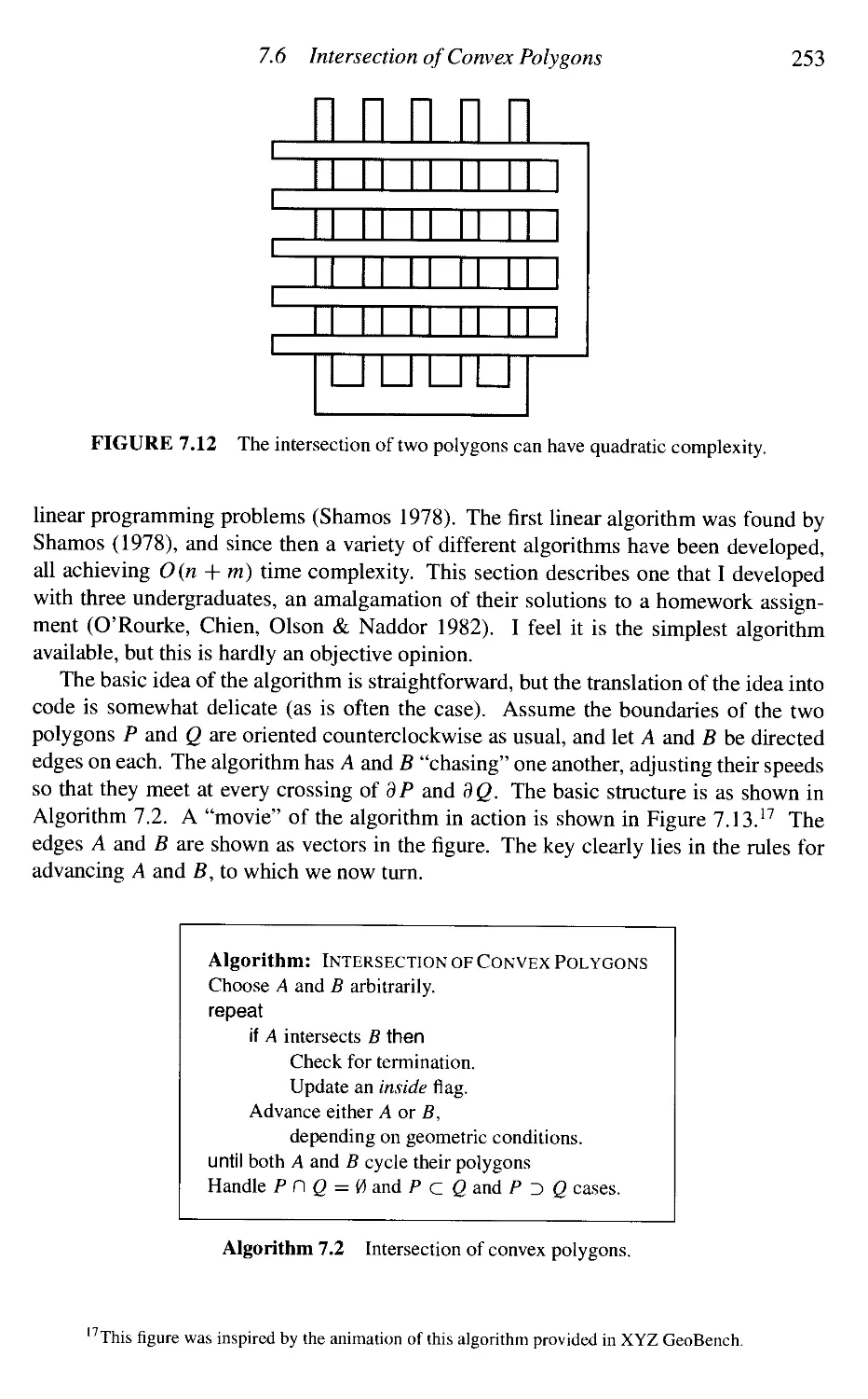
Intersection of Convex Polygons
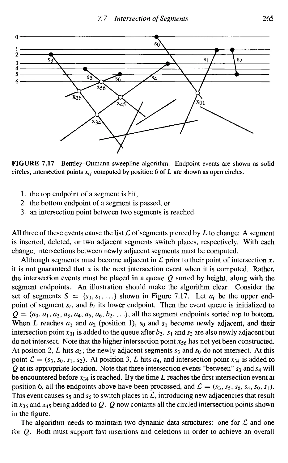
Intersection of Segments
Intersection of Nonconvex Polygons
Extreme Point of Convex Polygon
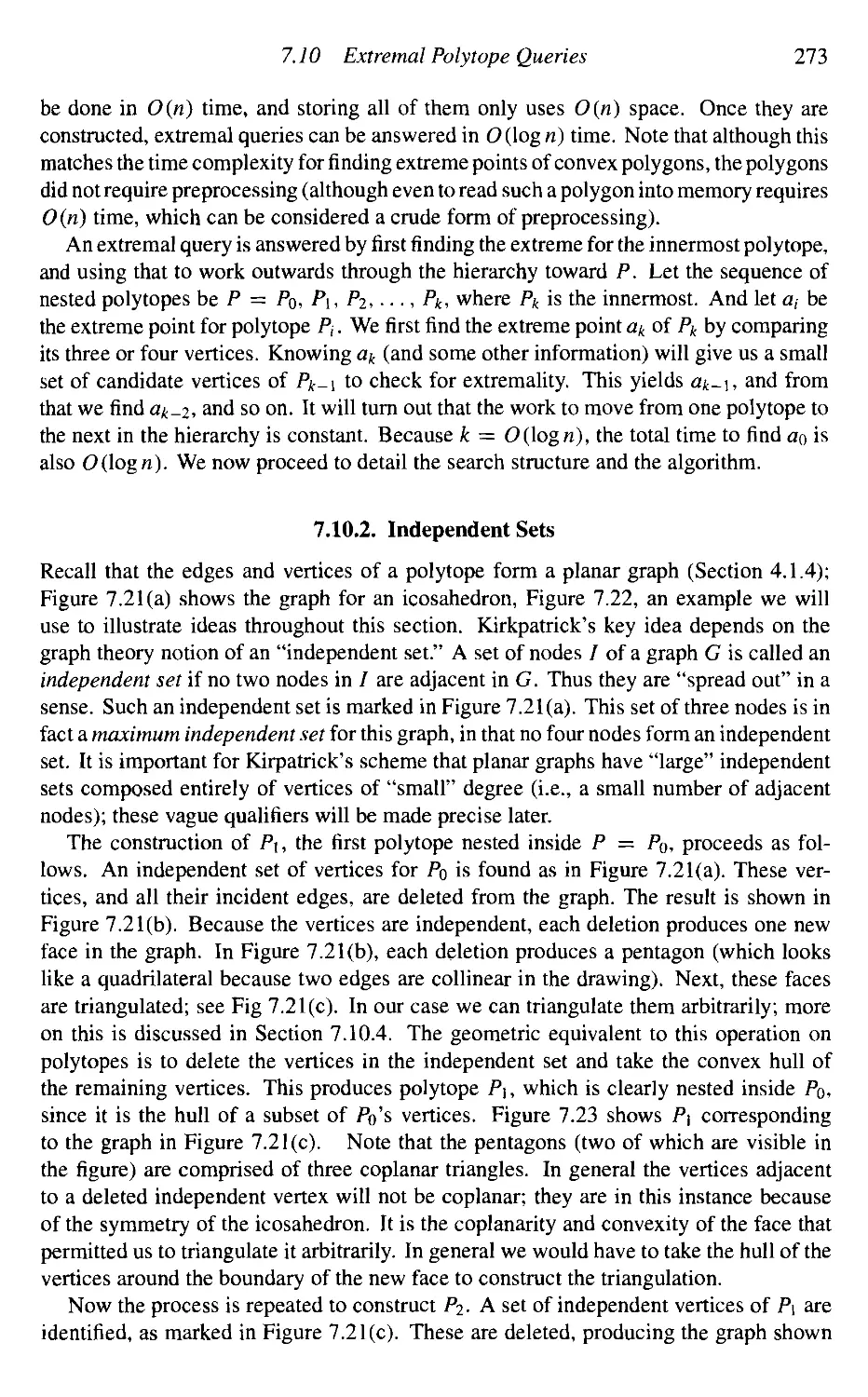
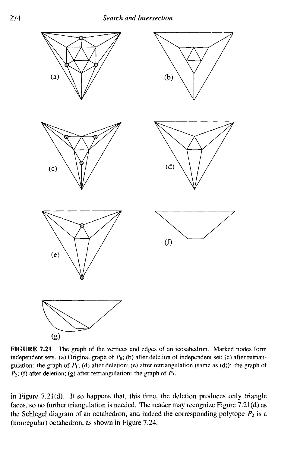
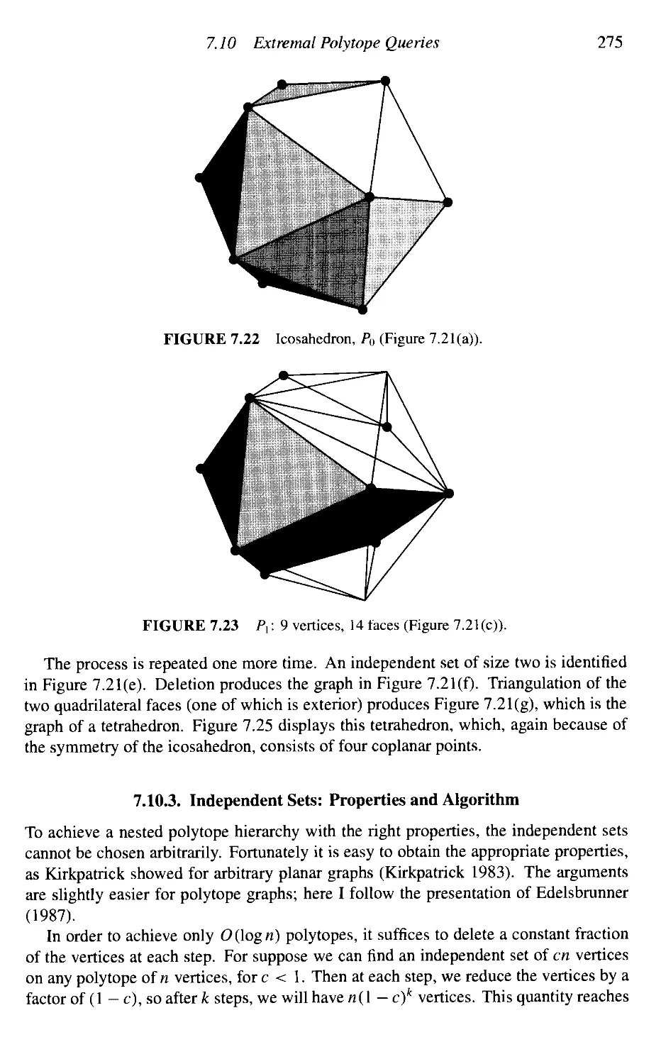
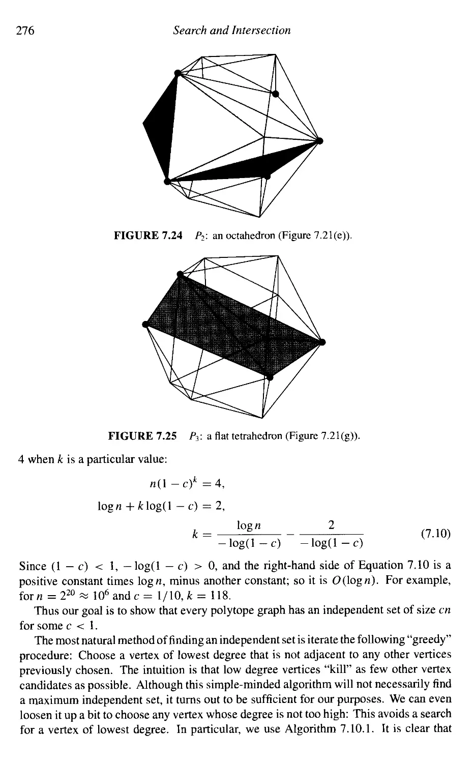
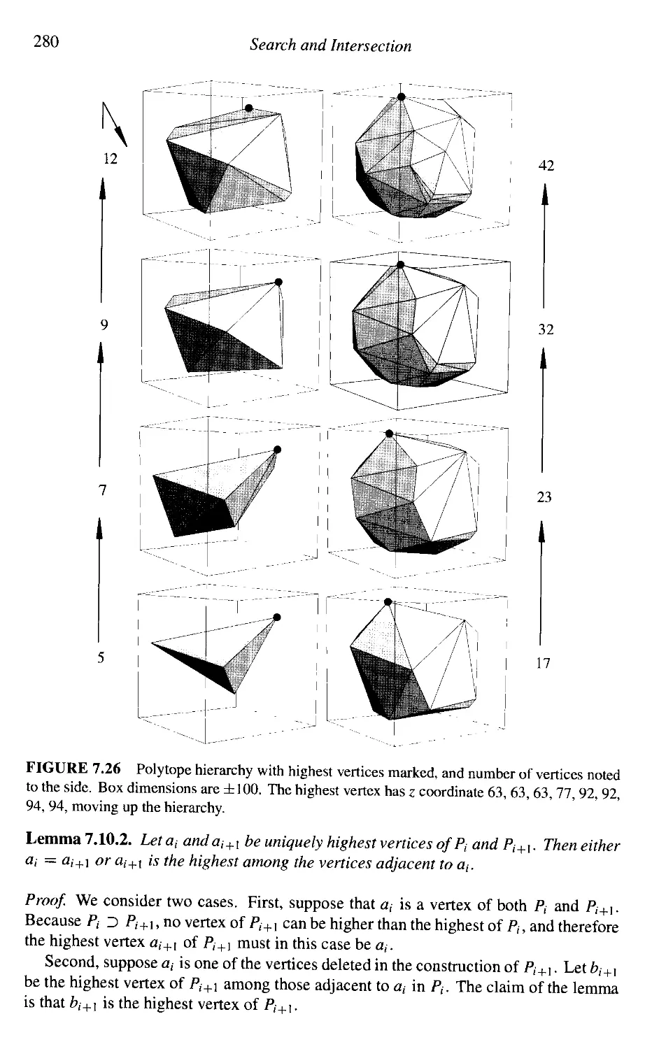
Extremal Polytope Queries
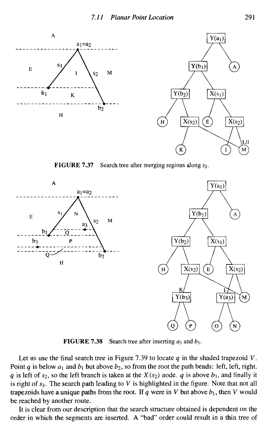
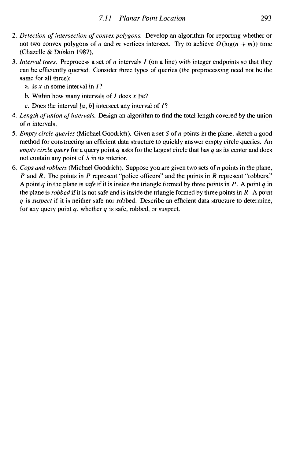
Planar Point Location
8. Motion Planning
8.1
8.2
8.3
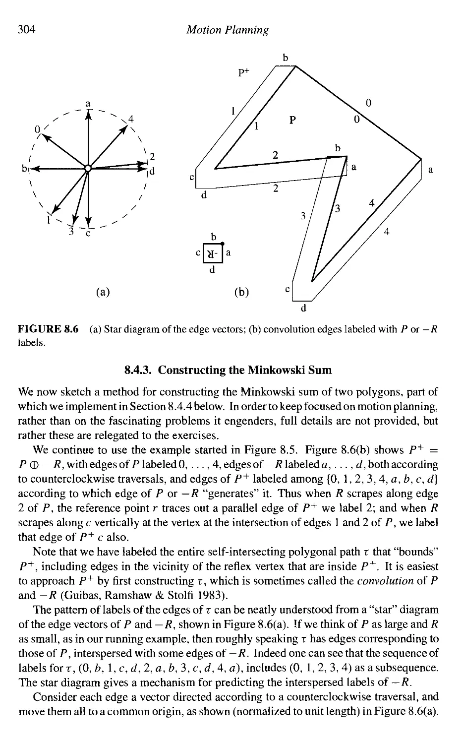
8.4
8.5
8.6
8.7
Introduction
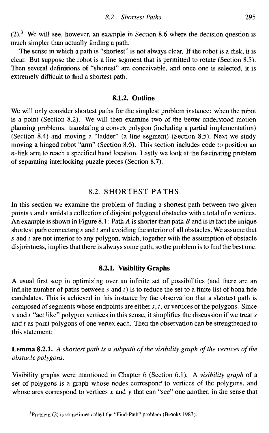
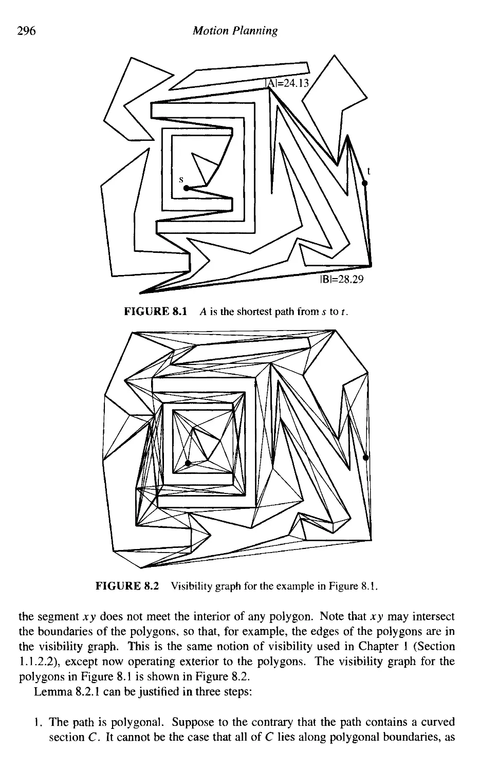
Shortest Paths
Moving a Disk
Translating a Convex Polygon
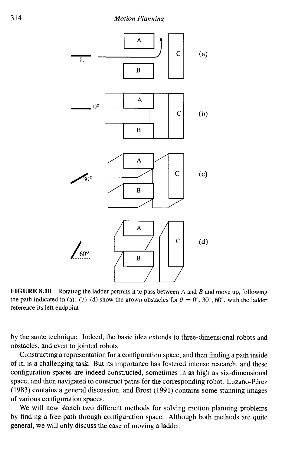
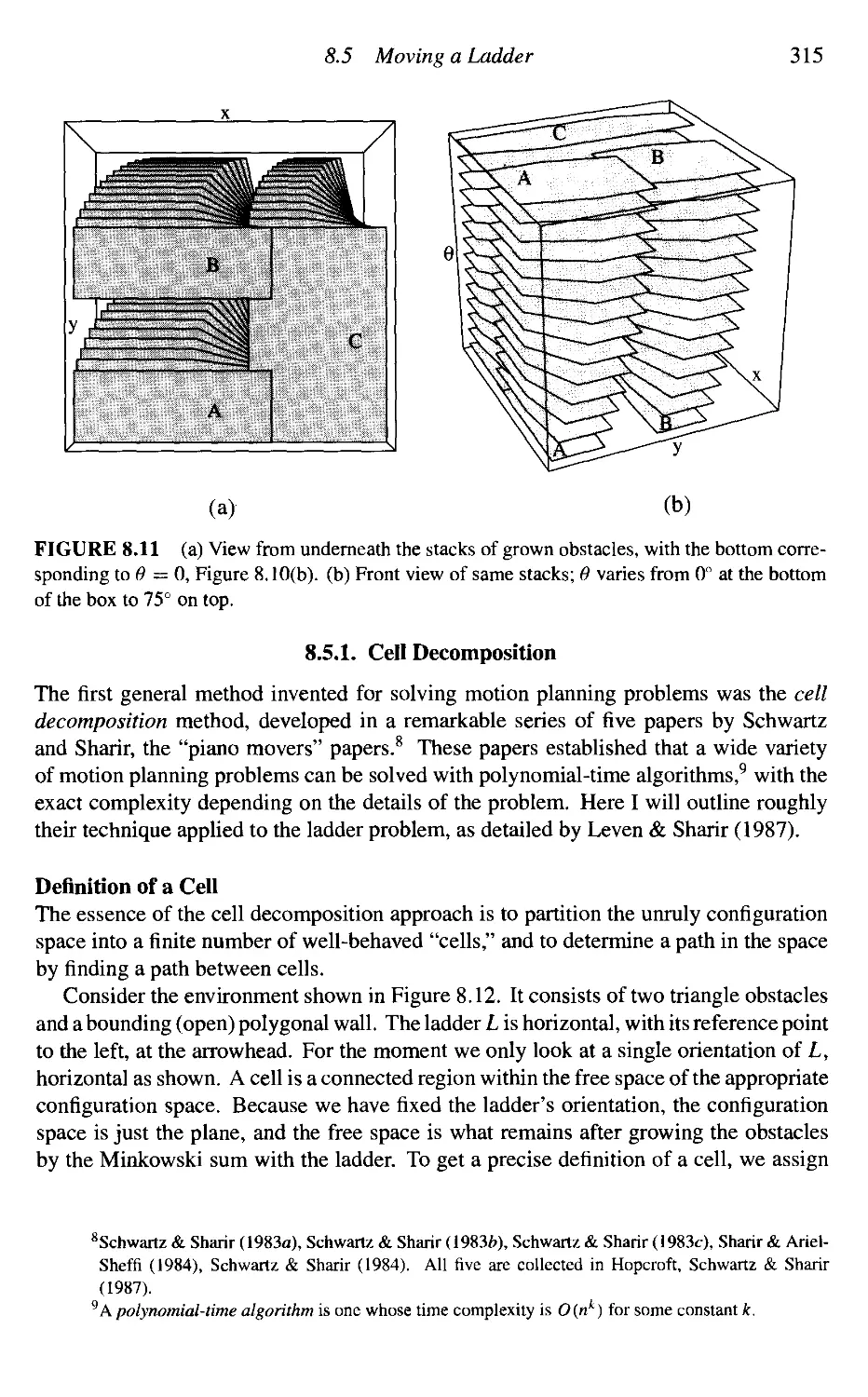
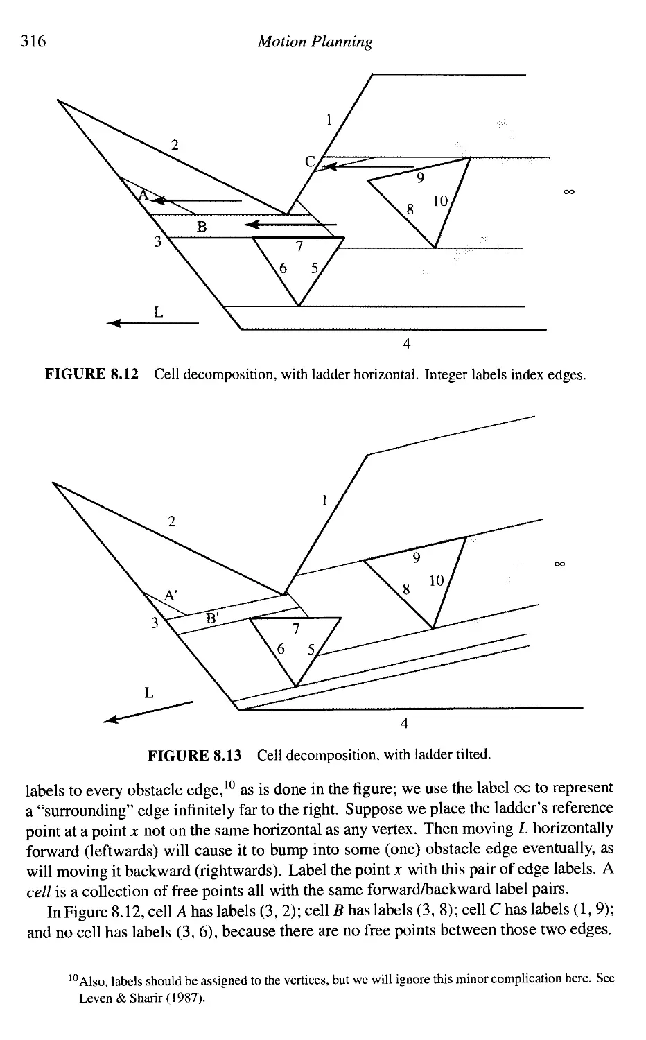
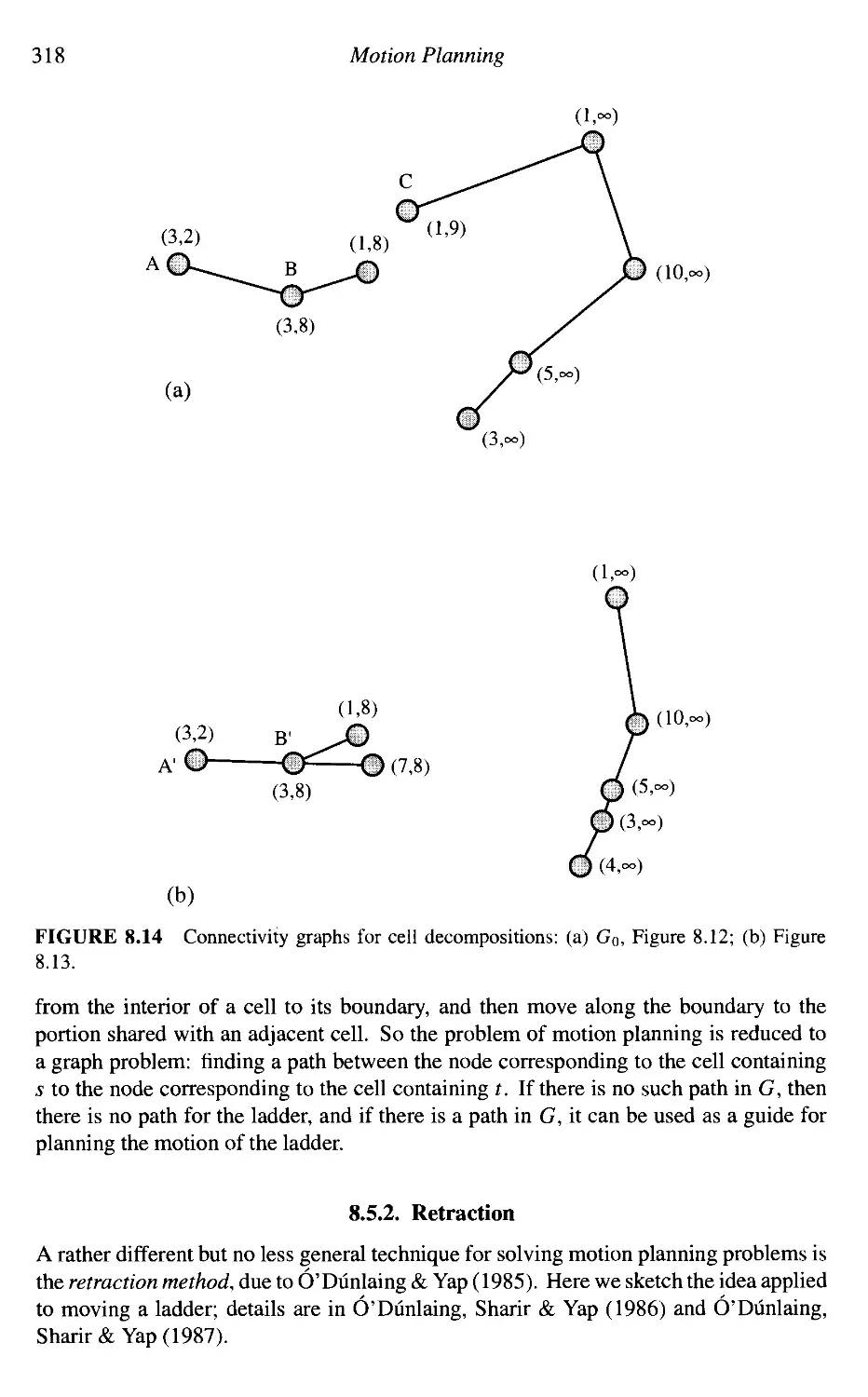
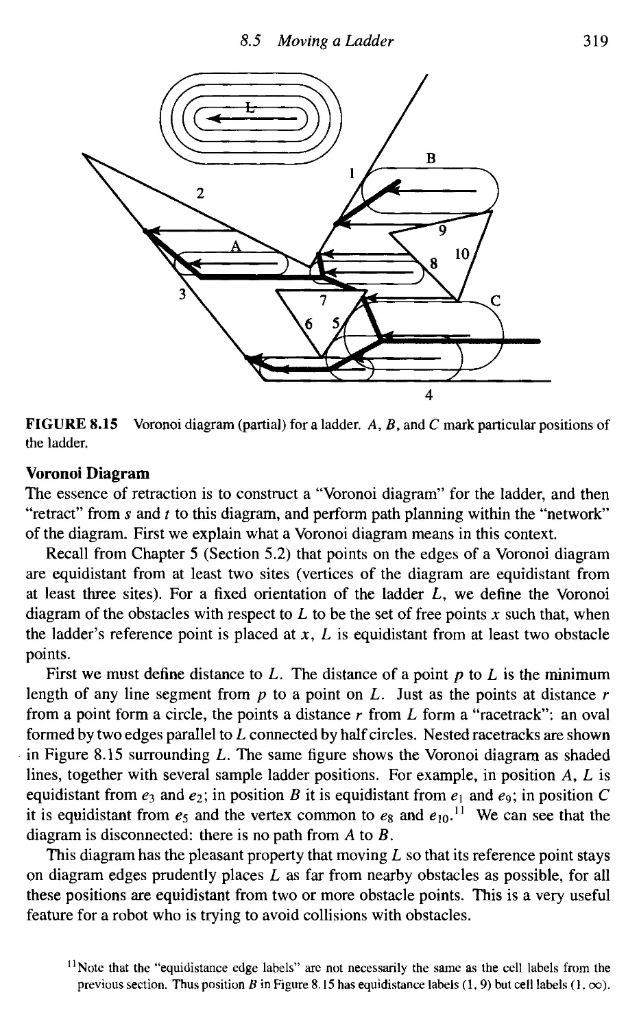
Moving a Ladder
Robot Arm Motion
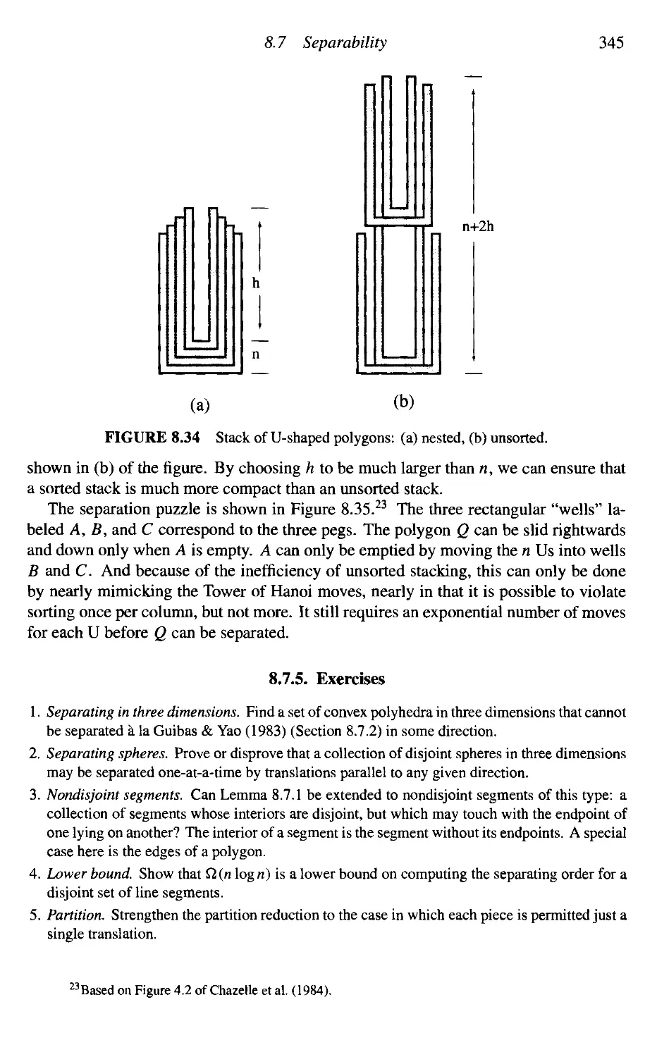
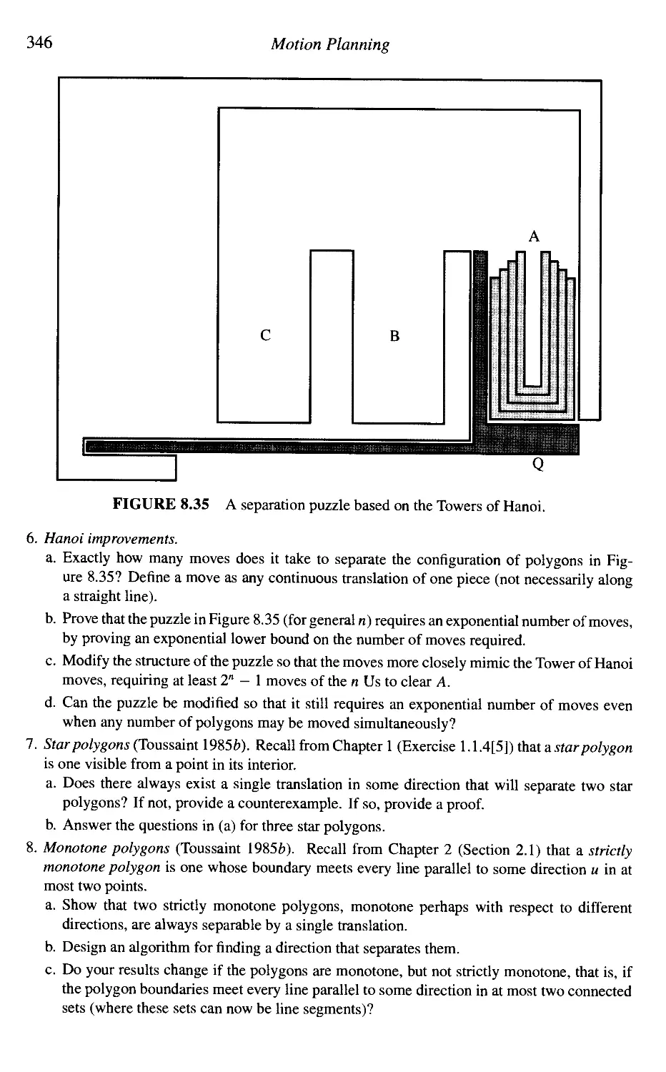
Separability
Contents
9.4 Monographs
9.5 Journals
9.6 Conference Proceedings
9.7 Software
Bibliography
Index
IX
349
349
350
350
351
361
Preface
Computational geometry broadly construed is the study of algorithms for solving geo-
geometric problems on a computer. The emphasis in this text is on the design of such
algorithms, with somewhat less attention paid to analysis of performance. I have in
several cases carried out the design to the level of working С programs, which are
discussed in detail.
There are many brands of geometry, and what has become known as "computational
geometry," covered in this book, is primarily discrete and combinatorial geometry. Thus
polygons play a much larger role in this book than do regions with curved boundaries.
Much of the work on continuous curves and surfaces falls under the rubrics of "geometric
modeling" or "solid modeling," a field with its own conferences and texts,' distinct
from computational geometry. Of course there is substantial overlap, and there is no
fundamental reason for the fields to be partitioned this way; indeed they seem to be
merging to some extent.
The field of computational geometry is a mere twenty years old as of this writing, if
one takes M. I. Shamos's thesis (Shamos 1978) as its inception. Now there are annual
conferences, journals, texts, and a thriving community of researchers with common
interests.
Topics Covered
I consider the "core" concerns of computational geometry to be polygon partitioning
(including triangulation), convex hulls, Voronoi diagrams, arrangements of lines, geo-
geometric searching, and motion planning. These topics from the chapters of this book. The
field is not so settled that this list can be considered a consensus; other researchers would
define the core differently.
Many textbooks include far more material than can be covered in one semester. This
is not such a text. I usually cover about 80% of the text with undergraduates in one
40 class-hour semester and all of the text with graduate students. In order to touch on
each of the core topics, I find it necessary to oscillate the level of detail, only sketching
some algorithms while detailing others. Which ones are sketched and which detailed is
a personal choice that I can only justify by my classroom experiences.
Prerequisites
The material in this text should be accessible to students with only minimal preparation.
Discrete mathematics, calculus, and linear algebra suffice for mathematics. In fact very
1 E.g., Hoffmann A989) and Mortenson A990).
Preface xi
little calculus or linear algebra is used in the text, and the enterprising student can learn
the little needed on the fly. In computer science, a course in programming and exposure
to data structures is enough (Computer Science I and II at many schools). I do not
presume a course in algorithms, only familiarity with the "big-0" notation. I teach
this material to college juniors and seniors, mostly computer science and mathematics
majors.
I hasten to add that the book can be fruitfully studied by those who have no program-
programming experience at all, simply by skipping all the implementation sections. Those who
know some programming language, but not C, can easily appreciate the implementation
discussions even if they cannot read the code. All code is available in Java as well as C,
although only С is discussed in the body of the text.
When teaching this material to both computer science and mathematics majors, I offer
them a choice of projects that permits those with programming skills to write code and
those with theoretical inclinations to avoid programming.
Although written to be accessible to undergraduates, my experience is that the ma-
material can form the basis of a challenging graduate course as well. I have tried to mix
elementary explanations with references to the latest literature. Footnotes provide tech-
technical details and citations. A number of the exercises pose open problems. It is not
difficult to supplement the text with research articles drawn from the 300 bibliographic
references, effectively upgrading the material to the graduate level.
Implementations
Not all algorithms discussed in the book are provided with implementations. Full code
for twelve algorithms is included:2
• Area of a polygon.
• Triangulating a polygon.
• Convex hull in two dimensions.
• Convex hull in three dimensions.
• Delaunay triangulation.
• Segment/ray-segment intersection.
• Segment/ray-triangle intersection.
• Point in polygon.
• Point in polyhedron.
• Intersecting convex polygons.
• Minkowski convolution with a convex polygon.
• Multilink robot arm reachability.
Researchers in industry coming to this book for working code for their favorite algorithms
may be disappointed: They may seek an algorithm to find the minimum spanning circle
for a set of points and find it as an exercise.3 The presented code should be viewed as
samples of geometry programs. I hope I have chosen a representative set of algorithms
to implement; much room is left for student projects.
2The distribution also includes code to generate random points in a cube (Figure 4.14), random points
on a sphere (Figure 4.15), and uniformly distributed points on a sphere (the book cover image).
3Exercise5.5.6fl2].
xii Preface
All the С code in the book is available by anonymous ftp from cs . smith, edu
A31.229.222.23), in the directory /pub/compgeom.4 I regularly update the files in this
directory to correct errors and incorporate improvements. The Java versions of all pro-
programs are in the same directory.
Exercises
There are approximately 250 exercises sprinkled throughout the text. They range from
easy extensions of the text to quite difficult problems to "open" problems. These latter
are an exciting feature of such a fresh field; students can reach the frontier of knowledge
so quickly that even undergraduates can hope to solve problems that no one has managed
to crack yet. Indeed I have written several papers with undergraduates as a result of their
work on homework problems I posed.5 Not all open problems are necessarily difficult;
some are simply awaiting the requisite attention.
Exercises are sporadically marked "[easy]" or "[difficult]," but the lack of these
notations should not be read to imply that neither apply. Those marked "[programming]"
require programming skills, and those marked "[open]" are unsolved problems as far
as I know at this writing. I have tried to credit authors of individual problems where
appropriate. Instructors may contact me for a partial solutions manual.
Second Edition Improvements
It is a law of nature that second editions are longer than first editions, and this book is
no exception: It is about fifty pages longer, with fifty new exercises, thirty new figures,
and eighty additional bibliographic references. All the code from the first edition is
significantly improved: All programs now produce Postscript output, all have been
translated to Java, many are simpler and/or logically cleaner, most are more robust in the
face of degeneracies and numerical error, and most run (sometimes) significantly faster.
Both the polygon triangulation code and the Delaunay triangulation code are now О (п2).
Four new programs have been included: for computing Delaunay triangulation from
the three-dimensional convex hull (Section 5.7.4), for intersecting a ray with a triangle
in 3-space (Section 7.3), for deciding if a point is inside a polyhedron (Section 7.5), for
computing the convolution (Minkowski sum) of a convex polygon with a general polygon
(Section 8.4.4), as well as the point generation code that produced the cover image.
New sections are included on partitioning into monotone mountains (Section 2.3),
randomized triangulation (Section 2.4.1), the ultimate(?) planar convex hull algorithm
(Section 3.8.4), randomized convex hull in three dimensions (Section 4.5), the twin edge
data structure (Section 4.4), intersection of a segment and triangle (Section 7.3), the
point-in-polyhedron problem (Section 7.5), the Bentley-Ottmann algorithm for inter-
intersecting segments (Section 7.7), computing Boolean operations between two polygons
(Section 7.8), randomized trapezoidal decomposition for point location (Section 7.11.4),
Minkowski convolution computation (Section 8.4.4), and a list of sources for further
reading (Chapter 9).
4Connect with ftp cs.smith.edu and use the name anonymous. Or access the files via
http://cs.smith.edu/~orourke.
5The material from one paper is incorporated into Section 7.6.
Preface xiii
Other sections are greatly improved, including those on QuickHull (Section 3.4),
Graham's algorithm (Section 3.5.5), volume overflow (Section 4.3.5), Delaunay trian-
gulation via the paraboloid transformation (Section 5.7.4), the point-in-polygon problem
(Section 7.4), intersecting two segments (Section 7.2), and the implementation of convex
polygon intersection (Section 7.6.1).
Acknowledgments
I have received over six hundred e-mail messages from readers of the first edition of this
book, and I despair of accurately apportioning credit to their many specific contributions
to this edition. I deeply appreciate the suggestions of the following people, many of whom
are my professional colleagues, twenty-nine whom are my former students, but most of
whom I have met only electronically: Pankaj Agarwal, Kristy Anderson, Bill Baldwin,
Michael Baldwin, Pierre Beauchemin, Ed Bolson, Helen Cameron, Joanne Cannon, Roy
Chien, Satyan Coorg, Glenn Davis, Adlai DePano, Matthew Diaz, Tamala Dirlam, David
Dobkin, Susan Dorward, Scot Drysdale, Herbert Edelsbrunner, John Ellis, William
Flis, Steve Fortune, Robert Fraczkiewicz, Reinaldo Garcia, Sharmilli Ghosh, Carole
Gitlin, Jacob E. Goodman, Michael Goodrich, Horst Greiner, Suleyman Guleyupoglu,
Eric Haines, Daniel Halperin, Eszter Hargittai, Paul Heckbert, Claudio Heckler, Paul
Heffernan, Kevin Hemsteter, Christoph Hoffmann, Rob Hoffmann, Chun-Hsiung Huang,
Knut Hunstad, Ferran Hurtado, Joan Hutchinson, Andrei Iones, Chris Johnston,
Martin Jones, Amy Josefczyk, Martin Kerscher, Ed Knorr, Nick Korneenko, John
Kutcher, Eugene Lee, David Lubinsky, Joe Malkevitch, Michelle Maurer, Michael
McKenna, Thomas Meier, Walter Meyer, Simon Michael, Jessica Miller, Andy
Mirzaian, Joseph Mitchell, Adelene Ng, Seongbin Park, Irena Pashchenko, Octavia
Petrovici, Madhav Ponamgi, Ari Rappoport, Jennifer Rippel, Christopher Saunders,
Catherine Schevon, Peter Schorn, Vadim Shapiro, Thomas Shermer, Paul Short, Saul
Simhon, Steve Skiena, Kenneth Sloan, Stephen Smeulders, Evan Smyth, Sharon Solms,
Ted Stern, Ileana Streinu, Vinita Subramanian, J.W.H. Tangelder, Yi Tao, Seth Teller,
Godfried Toussaint, Christopher Van Wyk, Gert Vetger, Jim Ward, Susan Weller, Wendy
Welsh, Rephael Wenger, Gerry Wiener, Bob Williamson, Stacia Wyman, Min Xu,
Dianna Xu, Chee Yap, Amy Yee, Wei Yinong, Lilla Zollei, and the Faculty Advancement
in Mathematics 1992 Workshop participants. My apologies for the inevitable omissions.
Lauren Cowles at Cambridge has been the ideal editor. I have received generous sup-
support from the National Science Foundation for my research in computational geometry,
most recently under grant CCR-9421670.
Joseph O'Rourke
orourke@cs. smith, edu
http://cs.smith.edu/~orourke
Smith College, Massachusetts
December 23, 1997
Note on the Cover:
The cover image shows the convex hull of 5,000 points distributed on a spiral curve on
the surface of a sphere. It was generated by running the sp i ra 1. с and chu 11. с code
distributed with this book: spiral 5000 -rlOOO | chull.
1
Polygon Triangulation
1.1. ART GALLERY THEOREMS
/././. Polygons
Much of computational geometry performs its computations on geometrical objects
known as polygons. Polygons are a convenient representation for many real-world ob-
objects; convenient both in that an abstract polygon is often an accurate model of real
objects and in that it is easily manipulated computationally. Examples of their use in-
include representing shapes of individual letters for automatic character recognition, of
an obstacle to be avoided in a robot's environment, or of a piece of a solid object to
be displayed on a graphics screen. But polygons can be rather complicated objects, and
often a need arises to view them as composed of simpler pieces. This leads to the topic
of this and the next chapter: partitioning polygons.
Definition of a Polygon
A polygon is the region of a plane bounded by a finite collection of line segments1
forming a simple closed curve. Pinning down a precise meaning for the phrase "simple
closed curve" is unfortunately a bit difficult. A topologist would say that it is the home-
omorphic image of a circle,2 meaning that it is a certain deformation of a circle. We
will avoid topology for now and approach a definition in a more pedestrian manner, as
follows.
Let Do, v\, i>2, • • •, vn-\ be n points in the plane. Here and throughout the book, all
index arithmetic will be mod n, implying a cyclic ordering of the points, with do following
«„_!, since (n- 1) + 1 sn = 0(modn). Leteo = "o"bei =diD2, ..., <?,¦ = d,d,+i, ...,
en_x = Dn_iDo be n segments connecting the points. Then these segments bound a
polygon iff3
1. The intersection of each pair of segments adjacent in the cyclic ordering is the
single point shared between them: e, П e,-+i = d,+i, for all i = 0, ..., n — 1.
2. Nonadjacent segments do not intersect: e, П ej = 0, for all j' ф i + 1.
1A line segment ab is a closed subset of a line contained between two points a and b, which are called
its endpoints. The subset is closed in the sense that it includes the endpoints. (Many authors use ab
to indicate this segment.)
2A circle is a one-dimensional set of points. We reserve the term disk to mean the two-dimensional
region bounded by a circle.
3"Iff" means "if and only if," a convenient abbreviation popularized by Halmos A985, p. 403).
Polygon Triangulation
(a) ' (b)
FIGURE 1.1 Nonsimple polygons.
The reason these segments define a curve is that they are connected end to end; the
reason the curve is closed is that they form a cycle; the reason the closed curve is simple
is that nonadjacent segments do not intersect.
The points u, are called the vertices of the polygon, and the segments e, are called its
edges. Note that a polygon of n vertices has n edges.
An important theorem of topology is the Jordan Curve Theorem:
Theorem 1.1.1 (Jordan Curve Theorem). Every simple closed plane curve divides the
plane into two components.
This strikes most as so obvious as not to require a proof; but in fact a precise proof is
quite difficult.4 We will take it as given. The two parts of the plane are called the interior
and exterior of the curve. The exterior is unbounded, whereas the interior is bounded.
This justifies our definition of a polygon as the region bounded by the collection of
segments. Note that we define a polygon P as a closed region of the plane. Often a
polygon is considered to be just the segments bounding the region, and not the region
itself. We will use the notation ЭР to mean the boundary of P; this is notation borrowed
from topology.5 By our definition, ЭР с Р.
Figure 1.1 illustrates two nonsimple polygons. For both objects in the figure, the
segments satisfy condition A) above (adjacent segments share a common point), but not
condition B): nonadjacent segments intersect. Such objects are often called polygons,
with those polygons satisfying B) called simple polygons. As we will have little use for
nonsimple polygons in this book, we will drop the redundant modifier.
We will follow the convention of listing the vertices of a polygon in counterclockwise
order, so that if you walked along the boundary visiting the vertices in that order (a
boundary traversal), the interior of the polygon would be always to your left.
4See, e.g., Henle A979, pp. 100-3). The theorem dates back to 1877.
5There is a sense in which the boundary of a region is like a derivative, so it makes sense to use the
partial derivative symbol 3.
1.1 Art Gallery Theorems
FIGURE 1.2 Grazing contact of line of sight.
1.1.2. The Art Gallery Theorem
Problem Definition
We will study a fascinating problem posed by Klee6 that will lead us naturally into the
issue of triangulation, the most important polygon partitioning. Imagine an art gallery
room whose floor plan can be modeled by a polygon of n vertices. Klee asked: How
many stationary guards are needed to guard the room? Each guard is considered a fixed
point that can see in every direction, that is, has a 2n range of visibility.7 Of course a
guard cannot see through a wall of the room. An equivalent formulation is to ask how
many point lights are needed to fully illuminate the room. We will make Klee's problem
rigorous before attempting an answer.
Visibility
To make the notion of visibility precise, we say that point x can see point у (or у is visible
to x) iff the closed segment xy is nowhere exterior to the polygon P: xy с Р. Note that
this definition permits the line-of-sight to have grazing contact with a vertex, as shown
in Figure 1.2. An alternative, equally reasonable definition would say that a vertex can
block vision; say that x has clear visibility to у if xy с P and xy П ЭР с {х, у]. We
will occasionally use this alternative definition in exercises (Exercises 1.1.4[2] and [3]).
A guard is a point. A set of guards is said to cover a polygon if every point in the
polygon is visible to some guard. Guards themselves do not block each other's visibility.
Note that we could require the guards to see only points of ЭР, for presumably that is
where the paintings are! This is an interesting variant, explored in Exercise 1.1.4[1].
Max over Min Formulation
We have now made most of Klee's problem precise, except for the phrase "How many."
Succinctly put, the problem is to find the maximum over all polygons of n vertices,
of the minimum number of guards needed to cover the polygon. This max-over-min
formulation is confusing to novices, but it is used quite frequently in mathematics, so
we will take time to explain it carefully.
6Posed in 1973, as reported by Honsberger A976). The material in this section (and more on the topic)
may be found in O'Rourke A987).
7We will use radians throughout to represent angles, ж radians = 180°.
Polygon Triangulation
(a)
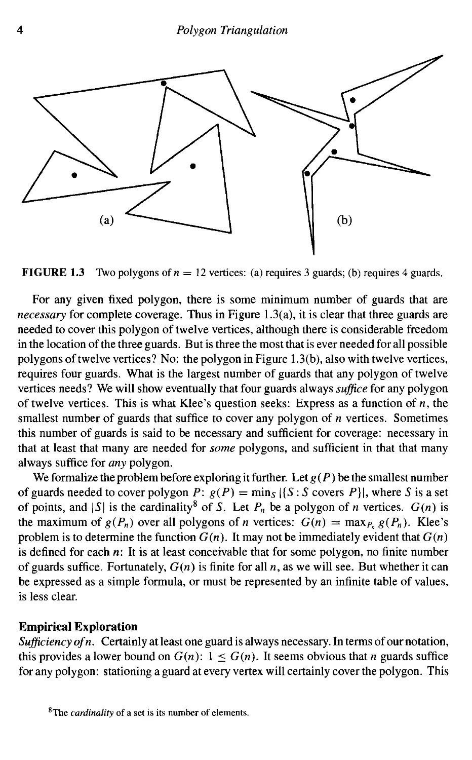
FIGURE 1.3 Two polygons of n = 12 vertices: (a) requires 3 guards; (b) requires 4 guards.
For any given fixed polygon, there is some minimum number of guards that are
necessary for complete coverage. Thus in Figure 1.3(a), it is clear that three guards are
needed to cover this polygon of twelve vertices, although there is considerable freedom
in the location of the three guards. But is three the most that is ever needed for all possible
polygons of twelve vertices? No: the polygon in Figure 1.3(b), also with twelve vertices,
requires four guards. What is the largest number of guards that any polygon of twelve
vertices needs? We will show eventually that four guards always suffice for any polygon
of twelve vertices. This is what Klee's question seeks: Express as a function of n, the
smallest number of guards that suffice to cover any polygon of n vertices. Sometimes
this number of guards is said to be necessary and sufficient for coverage: necessary in
that at least that many are needed for some polygons, and sufficient in that that many
always suffice for any polygon.
We formalize the problem before exploring it further. Let g(P) be the smallest number
of guards needed to cover polygon P: g(P) = minx \{S: S covers P}\, where S is a set
of points, and \S\ is the cardinality8 of S. Let Pn be a polygon of n vertices. G(n) is
the maximum of g(Pn) over all polygons of n vertices: G(n) = max/>n g(Pn)- Klee's
problem is to determine the function G(n). It may not be immediately evident that G(n)
is defined for each n: It is at least conceivable that for some polygon, no finite number
of guards suffice. Fortunately, G(n) is finite for all n, as we will see. But whether it can
be expressed as a simple formula, or must be represented by an infinite table of values,
is less clear.
Empirical Exploration
Sufficiency ofn. Certainly at least one guard is always necessary. In terms of our notation,
this provides a lower bound on G(n): 1 < G(n). It seems obvious that n guards suffice
for any polygon: stationing a guard at every vertex will certainly cover the polygon. This
8The cardinality of a set is its number of elements.
1.1 Art Gallery Theorems 5
provides an upper bound: G(n) < n. But it is not even so clear that n guards suffice. At
the least it demands a proof. It turns out to be true, justifying intuition, but this success of
intuition is tempered by the fact that the same intuition fails in three dimensions: Guards
placed at every vertex of a polyhedron do not necessarily cover the polyhedron! (See
Exercise 1.1.4[6].)
There are many art-gallery-like problems, and for most it is easiest to first establish a
lower bound on G(n) by finding generic examples showing that a large number of guards
are sometimes necessary. When it seems that no amount of ingenuity can increase the
number necessary, then it is time to turn to proving that that number is also sufficient.
This is how we will proceed.
Necessity for Small n. For small values of n, it is possible to guess the value of G(n)
with a little exploration. Clearly every triangle requires just one guard, so GC) = 1.
Quadrilaterals may be divided into two groups: convex quadrilaterals and quadri-
quadrilaterals with a reflex vertex. Intuitively a polygon is convex if it has no dents. This
important concept will be explored in detail in Chapter 3. A vertex is called reflex9 if its
internal angle is strictly greater than n\ otherwise a vertex is called convex}0 A convex
quadrilateral has four convex vertices. A quadrilateral can have at most one reflex vertex,
for reasons that will become apparent in Section 1.2. As Figure 1.4(a) makes evident,
even quadrilaterals with a reflex vertex can be covered by a single guard placed near that
vertex. Thus GD) = 1.
For pentagons the situation is less clear. Certainly a convex pentagon needs just one
guard, and a pentagon with one reflex vertex needs only one guard for the same reason as
in a quadrilateral. A pentagon can have two reflex vertices. They may be either adjacent
or separated by a convex vertex, as in Figures 1.4(c) and (d); in each case one guard
suffices. Therefore GE) = 1.
Hexagons may require two guards, as shown in Figure 1.4(e) and (f). A little ex-
experimentation can lead to a conviction that no more than two are ever needed, so that
GF) = 2.
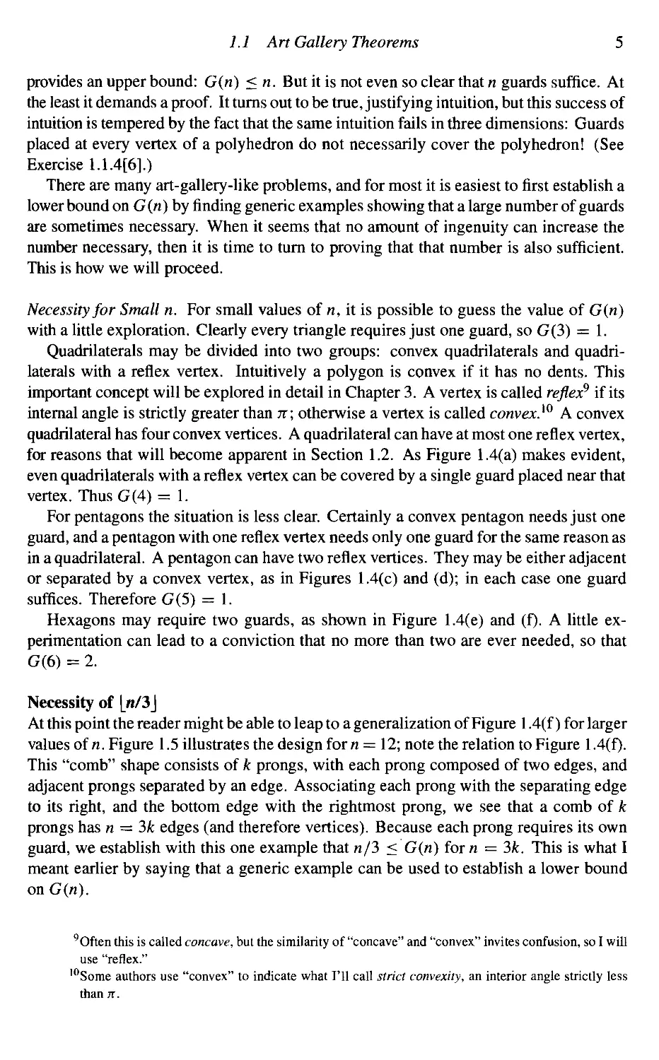
Necessity of \п/Ъ\
At this point the reader might be able to leap to a generalization of Figure 1.4(f) for larger
values of n. Figure 1.5 illustrates the design for n~\1\ note the relation to Figure 1.4(f).
This "comb" shape consists of k prongs, with each prong composed of two edges, and
adjacent prongs separated by an edge. Associating each prong with the separating edge
to its right, and the bottom edge with the rightmost prong, we see that a comb of k
prongs has n = 3k edges (and therefore vertices). Because each prong requires its own
guard, we establish with this one example that n/3 < G(n) for n = Ък. This is what I
meant earlier by saying that a generic example can be used to establish a lower bound
on G(n).
9Often this is called concave, but the similarity of "concave" and "convex" invites confusion, so I will
use "reflex."
l0Some authors use "convex" to indicate what I'll call strict convexity, an interior angle strictly less
than jt.
Polygon Triangulation
(с)
(e) (f)
FIGURE 1.4 Polygons of n = 4, 5, 6 vertices.
FIGURE 1.5 Chvdtal's comb for n = 12.
Noticing that GC) = GD) = GE) might lead one to conjecture that G{n) = Ln/3J,"
and in fact this conjecture turns out to be true. This is the usual way that such mathemat-
mathematical questions are answered: First the answer is conjectured after empirical exploration,
11 [xj is the floor of л: the largest integer less than or equal to x. The floor function has the effect of
discarding the fractional portion of a positive real number.
1.1 Art Gallery Theorems 1
and only then, with a definite goal in mind, is the result proven. We now turn to a
proof.
1.1.3. Fisk's Proof of Sufficiency
The first proof that G(n) = \п/Ъ\ was due toChvatalA975). His proof is by induction:
Assuming that \п/Ъ\ guards are needed for all n < N, he proves the same formula
for n = N by carefully removing part of the polygon so that its number of vertices is
reduced, applying the induction hypothesis, and then reattaching the removed portion.
The proof splinters into a number of cases and is quite delicate.
Three years later Fisk found a very simple proof, occupying just a single journal
page (Fisk 1978). We will present Fisk's proof here.
Diagonals and Triangulation
Fisk's proof depends crucially on partitioning a polygon into triangles with diagonals.
A diagonal of a polygon P is a line segment between two of its vertices a and b that
are clearly visible to one another. Recall that this means the intersection of the closed
segment ab with ЭР is exactly the set {a, b]. Another way to say this is that the open
segment from a to b does not intersect 3 P; thus a diagonal cannot make grazing contact
with the boundary.
Let us call two diagonals noncrossing if their intersection is a subset of their end-
points: They share no interior points. If we add as many noncrossing diagonals to a
polygon as possible, the interior is partitioned into triangles. Such a partition is called
a triangulation of a polygon. The diagonals may be added in arbitrary order, as long as
they are legal diagonals and noncrossing. In general there are many ways to triangulate
a given polygon. Figure 1.6 shows two triangulations of a polygon of n = 14 vertices.
We will defer a proof that every polygon can be triangulated to Section 1.2, and for
now we just assume the existence of a triangulation.
Three Coloring
To prove sufficiency of [n/3J guards for any polygon, the proof must work for an arbi-
arbitrary polygon. So assume an arbitrary polygon P of n vertices is given. The first step of
Fisk's proof is to triangulate P. The second step is to "recall" that the resulting graph
may be 3-colored. We need to explain what this graph is, and what 3-coloring means.
Let G be a graph associated with a triangulation, whose arcs are the edges of the poly-
polygon and the diagonals of the triangulation, and whose nodes are the vertices of the poly-
polygon. This is the graph used by Fisk. A k-coloring of a graph is an assignment of к colors to
the nodes of the graph, such that no two nodes connected by an arc are assigned the same
color. Fisk claims that every triangulation graph may be 3-colored. We will again defer a
proof of this claim, but a little experimentation should make it plausible. Three-colorings
of the triangulations in Figure 1.6 are shown in Figure 1.7. Starting at, say, the vertex in-
indicated by the arrow, and coloring its triangle arbitrarily with three colors, the remainder
of the coloring is completely forced: There are no other free choices. Roughly, the reason
this always works is that the forced choices never double back on an earlier choice; and
the reason this never happens is that the underlying figure is a polygon (with no holes, by
definition).
Polygon Tnangulation
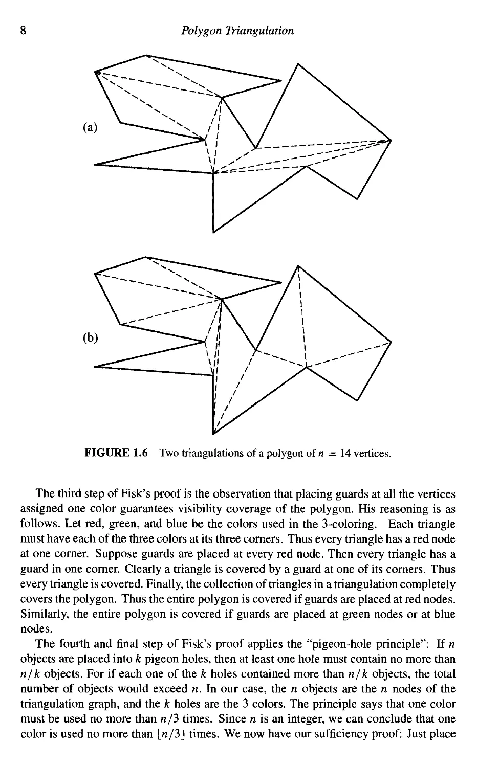
FIGURE 1.6 Two triangulations of a polygon of n = 14 vertices.
The third step of Fisk's proof is the observation that placing guards at all the vertices
assigned one color guarantees visibility coverage of the polygon. His reasoning is as
follows. Let red, green, and blue be the colors used in the 3-coloring. Each triangle
must have each of the three colors at its three corners. Thus every triangle has a red node
at one corner. Suppose guards are placed at every red node. Then every triangle has a
guard in one corner. Clearly a triangle is covered by a guard at one of its corners. Thus
every triangle is covered. Finally, the collection of triangles in a triangulation completely
covers the polygon. Thus the entire polygon is covered if guards are placed at red nodes.
Similarly, the entire polygon is covered if guards are placed at green nodes or at blue
nodes.
The fourth and final step of Fisk's proof applies the "pigeon-hole principle": If n
objects are placed into к pigeon holes, then at least one hole must contain no more than
n/k objects. For if each one of the k holes contained more than n/k objects, the total
number of objects would exceed n. In our case, the n objects are the n nodes of the
triangulation graph, and the k holes are the 3 colors. The principle says that one color
must be used no more than n/3 times. Since n is an integer, we can conclude that one
color is used no more than [n/3] times. We now have our sufficiency proof: Just place
1.1 Art Gallery Theorems
(b)
\
FIGURE 1.7 Two 3-colorings of a polygon of n = 14 vertices, based on the triangulations
shown in Figure 1.6.
guards at nodes colored with the least-frequently used color in the 3-coloring. We are
guaranteed that this will cover the polygon with no more than G(n) = [n/3\ colors.
If you don't find this argument beautiful (or at least charming), then you will not
enjoy much in this book!
In Figure 1.7, n = 14, so [n/3\ = 4. In (a) of the figure color 2 is used four times;
in (b), the same color is used only three times. Note that the 3-coloring argument does
not always lead to the most efficient use of guards.
1.1.4. Exercises
1. Guarding the walls. Construct a polygon P and a placement of guards such that the guards see
every point of 9 P, but there is at least one point interior to P not seen by any guard.
2. Clear visibility, point guards. What is the answer to Klee's question for clear visibility
(Section 1.1.2)? More specifically, let G'(n) be the smallest number of point guards that suffice
to clearly see every point in any polygon of n vertices. Point guards are guards who may stand at
any point of P; these are distinguished from vertex guards who may be stationed only at vertices.
10
Polygon Triangulation
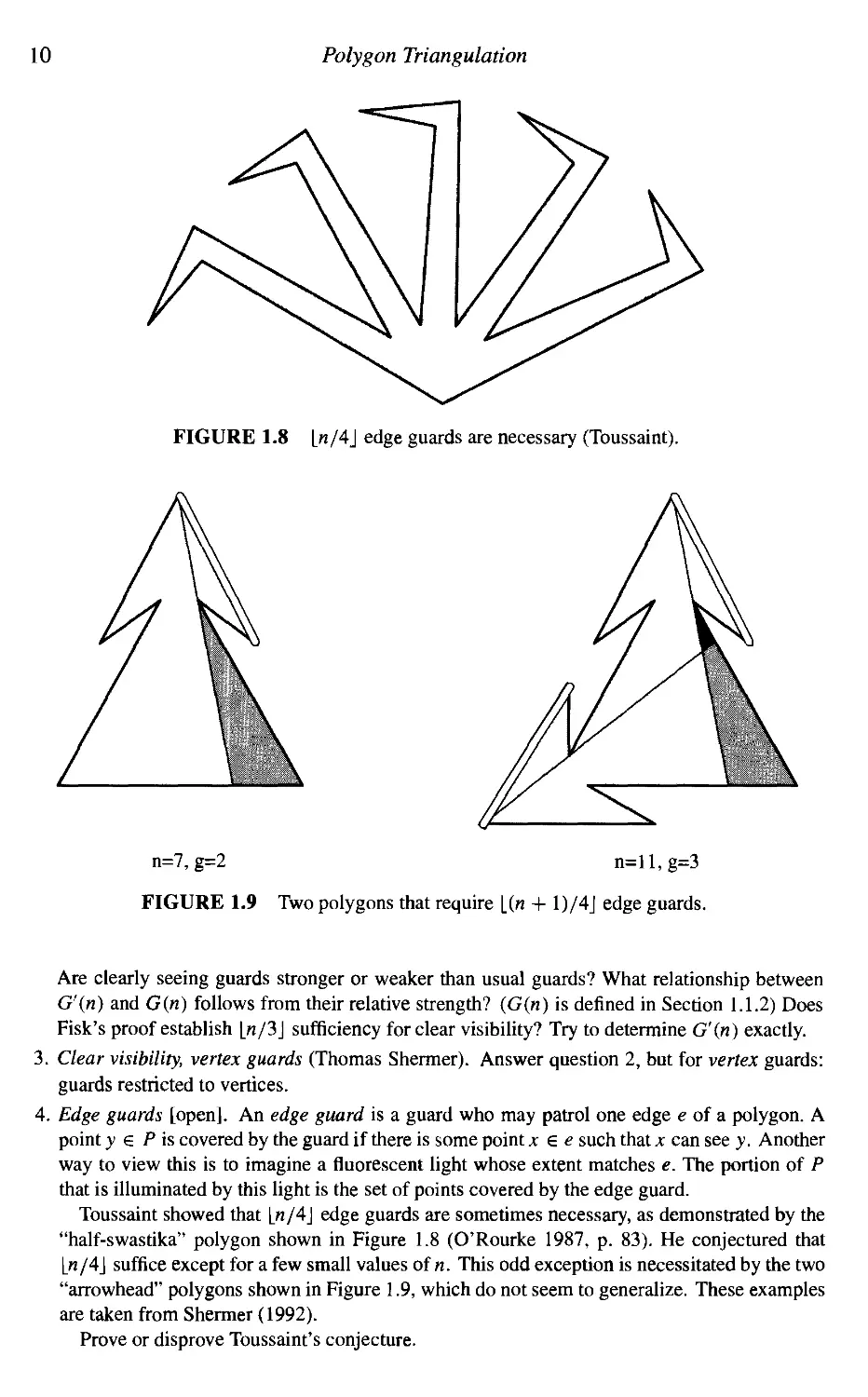
FIGURE 1.8 L«/4J edge guards are necessary (Toussaint).
n=7, g=2 n=ll,g=3
FIGURE 1.9 Two polygons that require [(n + 1)/4J edge guards.
Are clearly seeing guards stronger or weaker than usual guards? What relationship between
G'(n) and G(n) follows from their relative strength? (G(n) is defined in Section 1.1.2) Does
Fisk's proof establish [n/3] sufficiency for clear visibility? Try to determine G'(n) exactly.
3. Clear visibility, vertex guards (Thomas Shermer). Answer question 2, but for vertex guards:
guards restricted to vertices.
4. Edge guards [open]. An edge guard is a guard who may patrol one edge e of a polygon. A
point у € P is covered by the guard if there is some point x € e such that x can see y. Another
way to view this is to imagine a fluorescent light whose extent matches e. The portion of P
that is illuminated by this light is the set of points covered by the edge guard.
Toussaint showed that In/4] edge guards are sometimes necessary, as demonstrated by the
"half-swastika" polygon shown in Figure 1.8 (O'Rourke 1987, p. 83). He conjectured that
\_n/4\ suffice except for a few small values of n. This odd exception is necessitated by the two
"arrowhead" polygons shown in Figure 1.9, which do not seem to generalize. These examples
are taken from Shermer A992).
Prove or disprove Toussaint's conjecture.
1.2 Triangulation: Theory 11
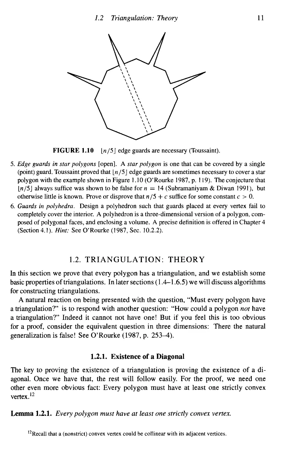
FIGURE 1.10 L«/5J edge guards are necessary (Toussaint).
5. Edge guards in star polygons [open]. A star polygon is one that can be covered by a single
(point) guard. Toussaint proved that L«/5J edge guards are sometimes necessary to cover a star
polygon with the example shown in Figure 1.10 (O'Rourke 1987, p. 119). The conjecture that
[n/5J always suffice was shown to be false for n = 14 (Subramaniyam & Diwan 1991), but
otherwise little is known. Prove or disprove that n/5 + с suffice for some constant с > 0.
6. Guards in polyhedra. Design a polyhedron such that guards placed at every vertex fail to
completely cover the interior. A polyhedron is a three-dimensional version of a polygon, com-
composed of polygonal faces, and enclosing a volume. A precise definition is offered in Chapter 4
(Section 4.1). Hint: See O'Rourke A987, Sec. 10.2.2).
1.2. TRIANGULATION: THEORY
In this section we prove that every polygon has a triangulation, and we establish some
basic properties of triangulations. In later sections A.4—1.6.5) we will discuss algorithms
for constructing triangulations.
A natural reaction on being presented with the question, "Must every polygon have
a triangulation?" is to respond with another question: "How could a polygon not have
a triangulation?" Indeed it cannot not have one! But if you feel this is too obvious
for a proof, consider the equivalent question in three dimensions: There the natural
generalization is false! See O'Rourke A987, p. 253^).
1.2.1. Existence of a Diagonal
The key to proving the existence of a triangulation is proving the existence of a di-
diagonal. Once we have that, the rest will follow easily. For the proof, we need one
other even more obvious fact: Every polygon must have at least one strictly convex
vertex.12
Lemma 1.2.1. Every polygon must have at least one strictly convex vertex.
l2Recall that a (nonstrict) convex vertex could be collinear with its adjacent vertices.
12 Polygon Triangulation
v
FIGURE 1.11 The rightmost lowest vertex must be strictly convex.
Proof. If the edges of a polygon are oriented so that their direction indicates a coun-
counterclockwise traversal, then a strictly convex vertex is a left turn for someone walking
around the boundary, and a reflex vertex is a right turn. The interior of the polygon is
always to the left of this hypothetical walker. Let L be a line through a lowest vertex i;
of P, lowest in having minimum у coordinate with respect to a coordinate system; if
there are several lowest vertices, let v be the rightmost. The interior of P must be above
L. The edge following i; must lie above L. See Figure 1.11. Together these conditions
imply that the walker makes a left turn at i; and therefore that и is a strictly convex vertex.
?
This proof can be used to construct an efficient test for the orientation of a polygon
(Exercise 1.3.9[3]).
Lemma 1.2.2 (Meisters). Every polygon ofn > 4 vertices has a diagonal.
Proof. Let i; be a strictly convex vertex, whose existence is guaranteed by Lemma 1.2.1.
Let a and b the vertices adjacent to v. If ab is a diagonal, we are finished. So suppose ab
is not a diagonal. Then either ab is exterior to P, or it intersects 3 P. In either case, since
n > 3, the closed triangle Aavb contains at least one vertex of P other than a, v,b. Let
x be the vertex of P in Aavb that is closest to v, where distance is measured orthogonal
to the line through ab. Thus x is the first vertex in Aavb hit by a line L parallel to ab
moving from i; to ab. See Figure 1.12.
Now we claim that vx is a diagonal of P. For it is clear that the interior of Aavb
intersected with the halfplane bounded by L that includes и (the shaded region in the
figure) is empty of points of ЭР. Therefore vx cannot intersect ЭР except at i; and x,
and so it is a diagonal. ?
Theorem 1.2.3 (Triangulation). Every polygon P ofn vertices may be partitioned into
triangles by the addition of (zero or more) diagonals.
Proof. The proof is by induction. If n = 3, the polygon is a triangle, and the theorem
holds trivially.
Let n > 4. Let d = ab be a diagonal of P, as guaranteed by Lemma 1.2.2. Because
d by definition only intersects ЭР at its endpoints, it partitions P into two polygons,
1.2 Triangulation: Theory
13
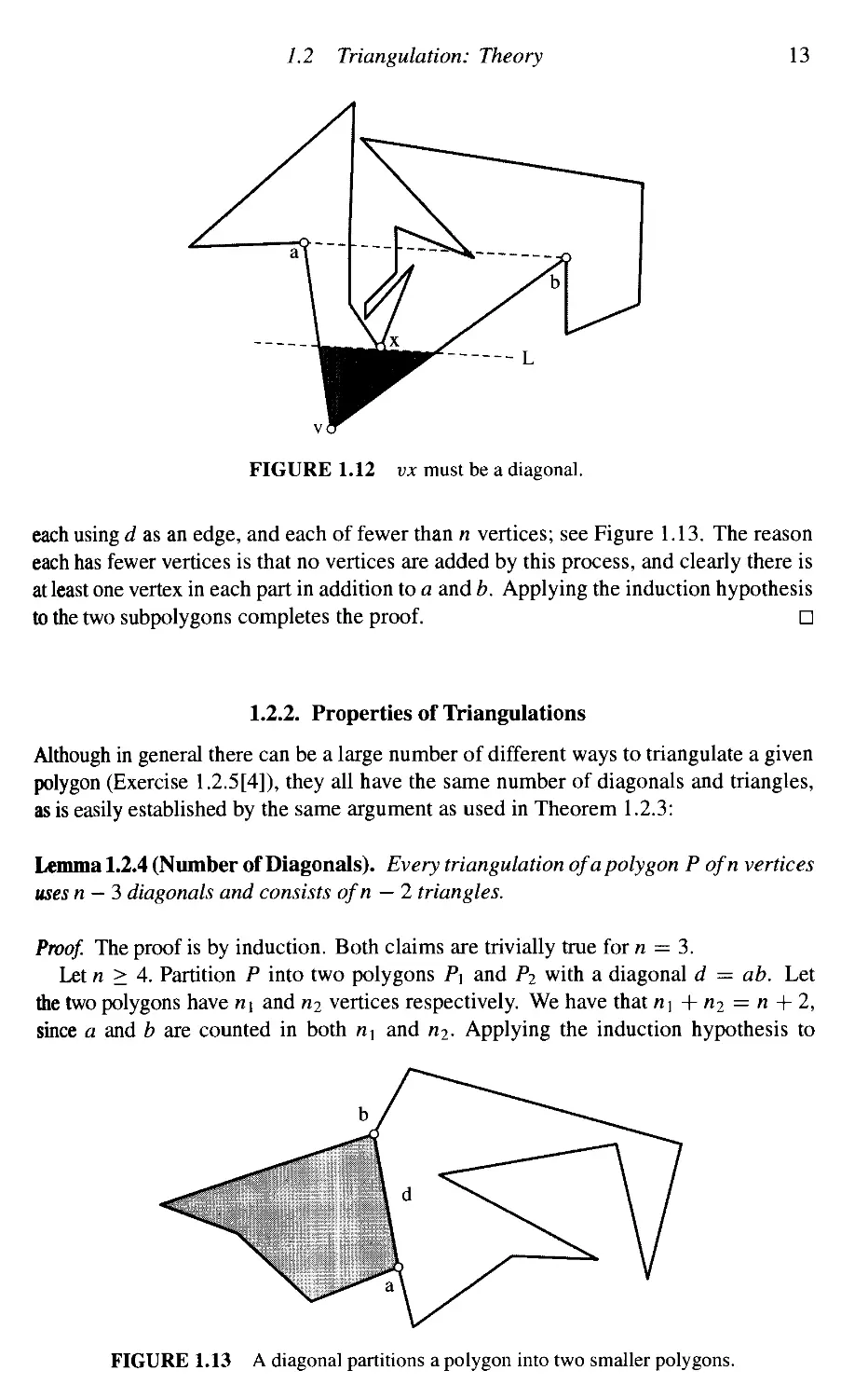
FIGURE 1.12 vx must be a diagonal.
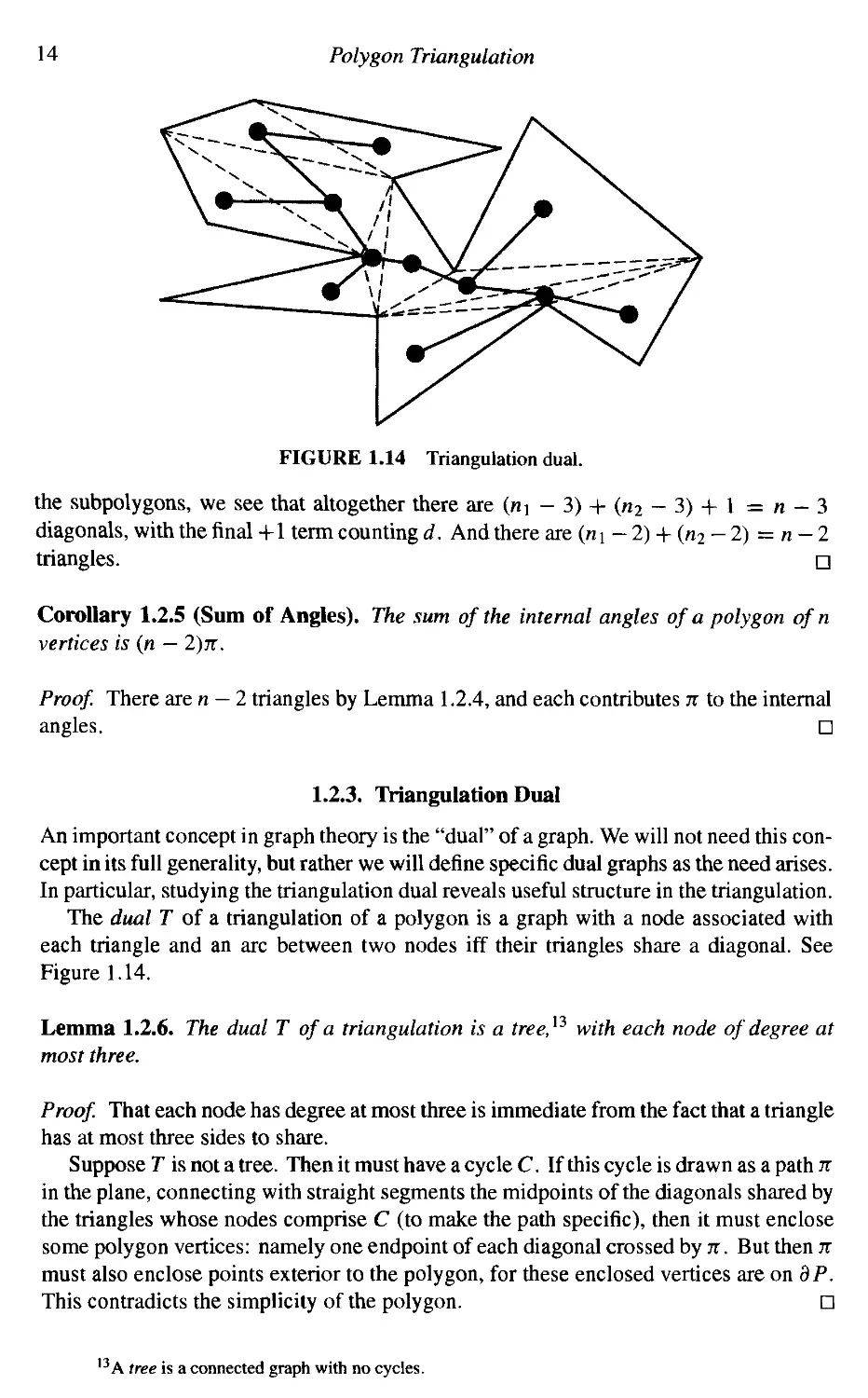
each using d as an edge, and each of fewer than n vertices; see Figure 1.13. The reason
each has fewer vertices is that no vertices are added by this process, and clearly there is
at least one vertex in each part in addition to a and b. Applying the induction hypothesis
to the two subpolygons completes the proof. ?
1.2.2. Properties of Triangulations
Although in general there can be a large number of different ways to triangulate a given
polygon (Exercise 1.2.5[4]), they all have the same number of diagonals and triangles,
as is easily established by the same argument as used in Theorem 1.2.3:
Lemma 1.2.4 (Number of Diagonals). Every triangulation of a polygon P ofn vertices
uses n — 3 diagonals and consists ofn — 2 triangles.
Proof. The proof is by induction. Both claims are trivially true for n — 3.
Let n > 4. Partition P into two polygons P\ and Рг with a diagonal d = ab. Let
the two polygons have n\ and n2 vertices respectively. We have that n\ + n2 = n + 2,
since a and b are counted in both П] and n2. Applying the induction hypothesis to
FIGURE 1.13 A diagonal partitions a polygon into two smaller polygons.
14 Polygon Triangulation
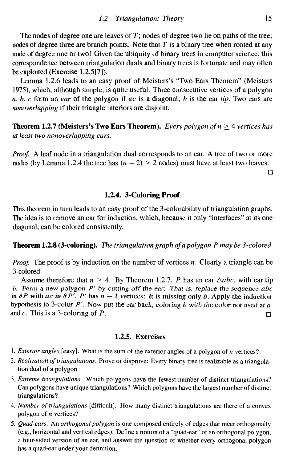
FIGURE 1.14 Triangulation dual.
the subpolygons, we see that altogether there are (m - 3) + (n2 - 3) + 1 = n - 3
diagonals, with the final +1 term counting d. And there are (n i - 2) + (n2 - 2) = n - 2
triangles. ?
Corollary 1.2.5 (Sum of Angles). The sum of the internal angles of a polygon of n
vertices is (n — 2)n.
Proof. There are n — 2 triangles by Lemma 1.2.4, and each contributes ж to the internal
angles. ?
1.2.3. Triangulation Dual
An important concept in graph theory is the "dual" of a graph. We will not need this con-
concept in its full generality, but rather we will define specific dual graphs as the need arises.
In particular, studying the triangulation dual reveals useful structure in the triangulation.
The dual Г of a triangulation of a polygon is a graph with a node associated with
each triangle and an arc between two nodes iff their triangles share a diagonal. See
Figure 1.14.
Lemma 1.2.6. The dual T of a triangulation is a tree,13 with each node of degree at
most three.
Proof. That each node has degree at most three is immediate from the fact that a triangle
has at most three sides to share.
Suppose T is not a tree. Then it must have a cycle C. If this cycle is drawn as a path n
in the plane, connecting with straight segments the midpoints of the diagonals shared by
the triangles whose nodes comprise С (to make the path specific), then it must enclose
some polygon vertices: namely one endpoint of each diagonal crossed by n. But then n
must also enclose points exterior to the polygon, for these enclosed vertices are on дP.
This contradicts the simplicity of the polygon. ?
13A tree is a connected graph with no cycles.
1.2 Triangulation: Theory 15
The nodes of degree one are leaves of Г; nodes of degree two lie on paths of the tree;
nodes of degree three are branch points. Note that Г is a binary tree when rooted at any
node of degree one or two! Given the ubiquity of binary trees in computer science, this
correspondence between triangulation duals and binary trees is fortunate and may often
be exploited (Exercise 1.2.5[7]).
Lemma 1.2.6 leads to an easy proof of Meisters's "Two Ears Theorem" (Meisters
1975), which, although simple, is quite useful. Three consecutive vertices of a polygon
a, b, с form an ear of the polygon if ac is a diagonal; b is the ear tip. Two ears are
nonoverlapping if their triangle interiors are disjoint.
Theorem 1.2.7 (Meisters's Two Ears Theorem). Every polygon ofn > 4 vertices has
at least two nonoverlapping ears.
Proof. A leaf node in a triangulation dual corresponds to an ear. A tree of two or more
nodes (by Lemma 1.2.4 the tree has (n — 2) > 2 nodes) must have at least two leaves.
?
1.2.4. 3-Coloring Proof
This theorem in turn leads to an easy proof of the 3-colorability of triangulation graphs.
The idea is to remove an ear for induction, which, because it only "interfaces" at its one
diagonal, can be colored consistently.
Theorem 1.2.8 C-coloring). The triangulation graph of a polygon P may be 3-colored.
Proof. The proof is by induction on the number of vertices n. Clearly a triangle can be
3-colored.
Assume therefore that n > 4. By Theorem 1.2.7, P has an ear Aabc, with ear tip
b. Form a new polygon P' by cutting off the ear: That is, replace the sequence abc
in dP with ac in dP'. P' has n — 1 vertices: It is missing only b. Apply the induction
hypothesis to 3-coIor P'. Now put the ear back, coloring b with the color not used at a
and c. This is a 3-coloring of P. О
1.2.5. Exercises
1. Exterior angles [easy]. What is the sum of the exterior angles of a polygon of n vertices?
2. Realization of triangulations. Prove or disprove: Every binary tree is realizable as a triangula-
triangulation dual of a polygon.
3. Extreme triangulations. Which polygons have the fewest number of distinct triangulations?
Can polygons have unique triangulations? Which polygons have the largest number of distinct
triangulations?
4. Number of triangulations [difficult]. How many distinct triangulations are there of a convex
polygon of n vertices?
5. Quad-ears. An orthogonal polygon is one composed entirely of edges that meet orthogonally
(e.g., horizontal and vertical edges). Define a notion of a "quad-ear" of an orthogonal polygon,
a four-sided version of an ear, and answer the question of whether every orthogonal polygon
has a quad-ear under your definition.
16 Polygon Triangulation
7
/
I
I
I
A
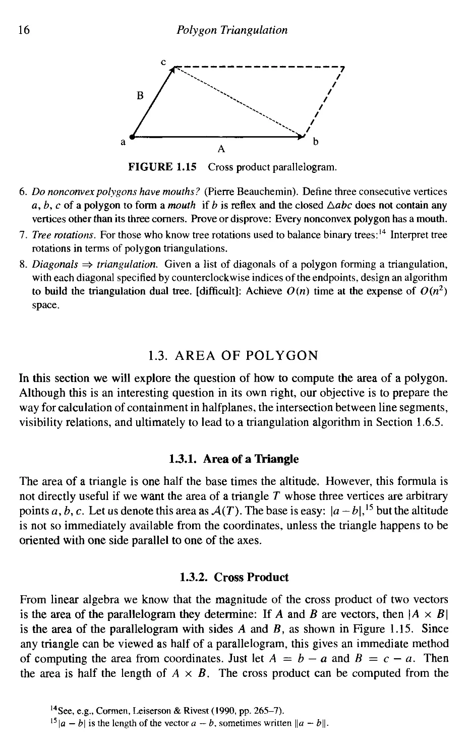
FIGURE 1.15 Cross product parallelogram.
6. Do nonconvex polygons have mouths? (Pierre Beauchemin). Define three consecutive vertices
a, b, с of a polygon to form a mouth if b is reflex and the closed Aabc does not contain any
vertices other than its three corners. Prove or disprove: Every nonconvex polygon has a mouth.
7. Tree rotations. For those who know tree rotations used to balance binary trees:14 Interpret tree
rotations in terms of polygon triangulations.
8. Diagonals =>• triangulation. Given a list of diagonals of a polygon forming a triangulation,
with each diagonal specified by counterclockwise indices of the endpoints, design an algorithm
to build the triangulation dual tree, [difficult]: Achieve O(n) time at the expense of O(n2)
space.
1.3. AREA OF POLYGON
In this section we will explore the question of how to compute the area of a polygon.
Although this is an interesting question in its own right, our objective is to prepare the
way for calculation of containment in halfplanes, the intersection between line segments,
visibility relations, and ultimately to lead to a triangulation algorithm in Section 1.6.5.
1.3.1. Area of a Triangle
The area of a triangle is one half the base times the altitude. However, this formula is
not directly useful if we want the area of a triangle T whose three vertices are arbitrary
points a, b, с Let us denote this area as A(T). The base is easy: \a -b\,15 but the altitude
is not so immediately available from the coordinates, unless the triangle happens to be
oriented with one side parallel to one of the axes.
1.3.2. Cross Product
From linear algebra we know that the magnitude of the cross product of two vectors
is the area of the parallelogram they determine: If A and В are vectors, then \A x B\
is the area of the parallelogram with sides A and B, as shown in Figure 1.15. Since
any triangle can be viewed as half of a parallelogram, this gives an immediate method
of computing the area from coordinates. Just let A = b — a and В = с — a. Then
the area is half the length of A x B. The cross product can be computed from the
14See, e.g., Cormen, Leiserson & Rivest A990, pp. 265-7).
15 \a — b\ is the length of the vector a — b, sometimes written \\a — b\\.
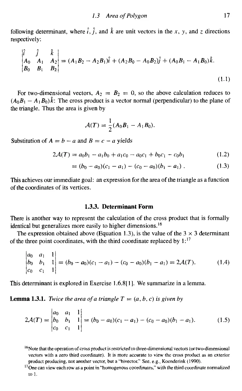
1.3 Area of Polygon 17
following determinant, where i,j, and к are unit vectors in the x, y, and z directions
respectively:
i j к
Ao A\ A2
Bo By B2
= (A}B2 - A2Bx)i + (A2B0 - A0B2)j + (A0B, -
A.1)
For two-dimensional vectors, A2 = B2 = 0, so the above calculation reduces to
— A\Bf))k: The cross product is a vector normal (perpendicular) to the plane of
the triangle. Thus the area is given by
A(T) = -(A0Bl~AlB0).
Substitution of A = b — a and В — с — a yields
2A(T) = аф\ - афо + a\c0 - aoc\ + boc{ - cob\ A.2)
= {b0 - ao)(ci - aO - (c0 - ao)(b{ - a,) . A.3)
This achieves our immediate goal: an expression for the area of the triangle as a function
of the coordinates of its vertices.
1.3.3. Determinant Form
There is another way to represent the calculation of the cross product that is formally
identical but generalizes more easily to higher dimensions.16
The expression obtained above (Equation 1.3), is the value of the 3x3 determinant
of the three point coordinates, with the third coordinate replaced by I:17
= (b0 - ooXc! - ai) - (c0 - aoX&i - oi) = 2A(T). A.4)
This determinant is explored in Exercise 1.6.8[1]. We summarize in a lemma.
Lemma 1.3.1. Twice the area of a triangle T = (a,b,c) is given by
ao a\ 1
2A(T)= b0 b{ 1 = (bo - ao)(cx - ax) - (со - ao)(b\ -a,). A.5)
a0
bo
CO
ax
b\
C\
1
1
1
a0
bo
CO
a\
bi
C\
1
1
1
16Note that the operation of cross product is restricted to three-dimensional vectors (or two-dimensional
vectors with a zero third coordinate). It is more accurate to view the cross product as an exterior
product producing, not another vector, but a "bivector." See, e.g., Koenderink A990).
17One can view each row as a point in "homogenous coordinates," with the third coordinate normalized
to 1.
18
Polygon Triangulation
5
FIGURE 1.16 Triangulation of a convex polygon. The fan center is at 0.
1.3.4. Area of a Convex Polygon
Now that we have an expression for the area of a triangle, it is easy to find the area of
any polygon by first triangulating it, and then summing the triangle areas. But it would
be pleasing to avoid the rather complex step of triangulation, and indeed this is possible.
Before turning to that issue, we consider convex polygons, where triangulation is trivial.
Every convex polygon may be triangulated as a "fan," with all diagonals incident
to a common vertex; and this may be done with any vertex serving as the fan "center."
See Figure 1.16. Therefore the area of a polygon with vertices u0, v\,..., i>n_i labeled
counterclockwise can be calculated as
A(P) =
A(v0, v2,v3)-\ \- A(v0, vn_2
A.6)
Here D0 is the fan center.
We will warm up to the result we will prove in Theorem 1.3.3 below by examining
convex and nonconvex quadrilaterals, where the relevant relationships are obvious.
1.3.5. Area of a Convex Quadrilateral
The area of a convex quadrilateral Q = (a,b,c,d) may be written in two ways, depend-
depending on the two different triangulations (see Figure 1.17):
A(Q) = A(a, b, c) + A(a, c, d) = A(d, a, b) + A(d, b, c).
A.7)
Writing out the expressions for the areas using Equation A.2) for the two terms of the
first triangulation, we get
A.8)
Note that the terms a\Co — a$c\ appear in A(a, b, c) and in A{a, c, d) with opposite
signs, and so they cancel. Thus the terms "corresponding" to the diagonal ac cancel;
1.3 Area of Polygon
19
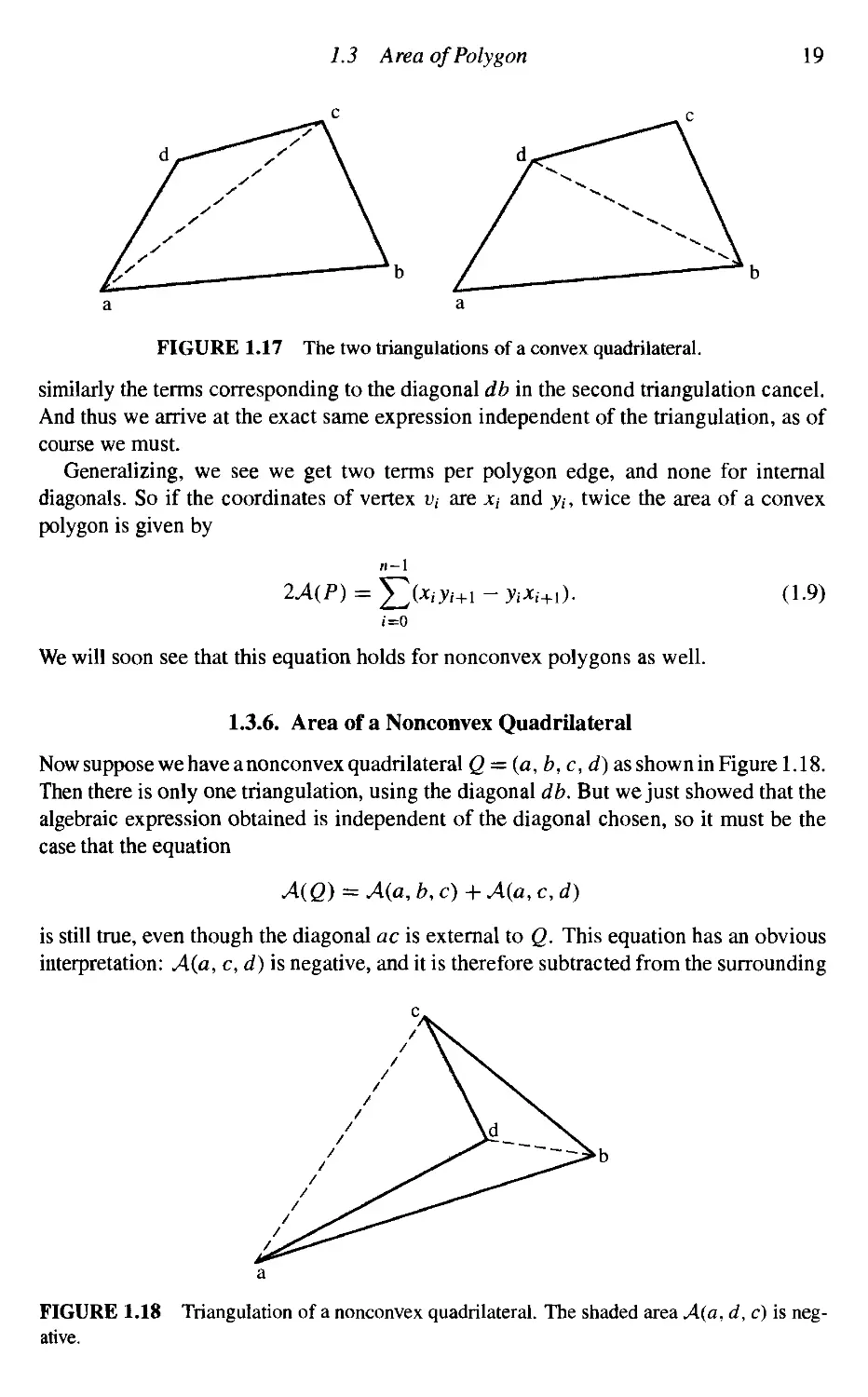
FIGURE 1.17 The two triangulations of a convex quadrilateral.
similarly the terms corresponding to the diagonal db in the second triangulation cancel.
And thus we arrive at the exact same expression independent of the triangulation, as of
course we must.
Generalizing, we see we get two terms per polygon edge, and none for internal
diagonals. So if the coordinates of vertex i>, are xt and yt, twice the area of a convex
polygon is given by
Л-1
2A(P) =
A.9)
i=0
We will soon see that this equation holds for nonconvex polygons as well.
1.3.6. Area of a Nonconvex Quadrilateral
Now suppose we have a nonconvex quadrilateral Q = (a, b, c, d) as shown in Figure 1.18.
Then there is only one triangulation, using the diagonal db. But we just showed that the
algebraic expression obtained is independent of the diagonal chosen, so it must be the
case that the equation
is still true, even though the diagonal ac is external to Q. This equation has an obvious
interpretation: A(a, c, d) is negative, and it is therefore subtracted from the surrounding
FIGURE 1.18 Triangulation of a nonconvex quadrilateral. The shaded area A(a, d, c) is neg-
negative.
20 Polygon Triangulation
triangle Aabc. And indeed, note that (a, c, d) is a clockwise path, so the cross product
formulation shows that the area will be negative.
The phenomenon observed with a nonconvex quadrilateral is general, as we now
proceed to demonstrate.
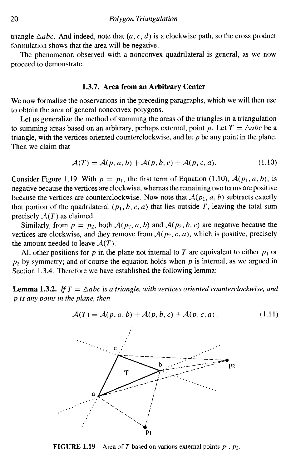
1.3.7. Area from an Arbitrary Center
We now formalize the observations in the preceding paragraphs, which we will then use
to obtain the area of general nonconvex polygons.
Let us generalize the method of summing the areas of the triangles in a triangulation
to summing areas based on an arbitrary, perhaps external, point p. Let T = Aabc be a
triangle, with the vertices oriented counterclockwise, and let p be any point in the plane.
Then we claim that
A(T) = A(p, a, b) + A{p, b, c) + A{p, c, a). A.10)
Consider Figure 1.19. With p = p\, the first term of Equation A.10), A{p\, a, b), is
negative because the vertices are clockwise, whereas the remaining two terms are positive
because the vertices are counterclockwise. Now note that A(pi, a, b) subtracts exactly
that portion of the quadrilateral (p\, b, c, a) that lies outside T, leaving the total sum
precisely A(T) as claimed.
Similarly, from p = рг, both А(рг, a, b) and A(P2, b, c) are negative because the
vertices are clockwise, and they remove from А{рг, с, a), which is positive, precisely
the amount needed to leave A(T).
All other positions for p in the plane not internal to T are equivalent to either p\ or
Pi by symmetry; and of course the equation holds when p is internal, as we argued in
Section 1.3.4. Therefore we have established the following lemma:
Lemma 1.3.2. IfT = Aabc is a triangle, with vertices oriented counterclockwise, and
p is any point in the plane, then
,a) . A.11)
P2
FIGURE 1.19 Area of T based on various external points p\, рг-
1.3 Area of Polygon 21
We may now generalize the preceding lemma to establish the same equation (gener-
(generalized) for arbitrary polygons.
Theorem 1.3.3 (Area of Polygon).18 Let a polygon (convex or nonconvex) P have
vertices vo, V\,..., vn-\ labeled counterclockwise, and let p be any point in the plane.
Then
A{P) = A(p, vo, Vi) + A(p, vi, v2) + A(p, v2, u3) н
+ A(p, vn-2, vn-i) + A(p, и„_ь vo). A-12)
Ifvi = (Xi, yi), this expression is equivalent to the equations
Л-1
2A(P) = ^(Xiyi+i - yiXi+l) A.13)
i=0
я-1
[xi +xi+i)(yi+i -yt). A.14)
Proof. We prove the area sum equation by induction on the number of vertices n of P.
The base case, n = 3, is established by Lemma 1.3.2.
Suppose then that Equation A.12) is true for all polygons with n — 1 vertices, and
let P be a polygon of n vertices. By Theorem 1.2.7, P has an "ear." Renumber the
vertices of P so that E ~ (vn-2, vn-\, i>o) is an ear. Let Pn^\ be the polygon obtained
by removing E. By the induction hypothesis,
A(Pn-i) = A(p, vo, vi)-\ h A(p, и„_з, vn-2) + A(p, vn-2, v0).
By Lemma 1.3.2,
A(E) = A(p, vn-2,vn-i) + A(p, vn-i, v0) + A(p,vo,vn-2)-
Since A(P) = A(Pn-\) + A(E), we have
A(P) = A(p, vo,vi)-\ h A{p, и„_з, и„_2) + A(p, и„_2, v0)
+ A(p, vn-2, vn-i) + A(p, и„_ь vo) + A(p, vo, vn^2)-
But note that A(p, v0, vn-2) = —A{p, vn-2, vq). Canceling these terms leads to the
claimed equation.
Equation A.13) is obtained by expansion of the determinants and canceling terms,
as explained in Section 1.3.5. Equation A.14) can be seen as equivalent by multiplying
out and again canceling terms. Q
18This theorem can be viewed as a discrete version of Green's theorem, which relates an integral around
the boundary of a region with an integral over the interior of the region: J w = JJp dw, where w
is a -form" (see, e.g., Buck & Buck A965, p. 406) or Koenderink A990, p. 99)).
22
Polygon Triangulation
FIGURE 1.20 Computation of the area of a nonconvex polygon from point p. The darker
triangles are oriented clockwise, and thus they have negative area.
Equation A.14) can be computed with one multiplication and two additions per term,
whereas Equation A.13) uses two multiplications and one addition. The second form is
therefore more efficient in most implementations.
In Figure 1.20, the triangles Др12, Ар67, and Др70 are oriented clockwise, and
the remainder are counterclockwise. One can think of the counterclockwise triangles as
attaching to each point they cover a +1 charge, whereas the clockwise triangles attach
a —1 charge. Then the points R of Др12 that falls inside the polygon (labeled in the
figure) are given a — 1 charge by this clockwise triangle; but R is also covered by two
counterclockwise triangles, ApOl and Др23. So R has net +1 charge. Similarly every
point inside P is assigned a net +1 charge, and every point outside is assigned a net 0
charge.
1.3.8. Volume in Three and Higher Dimensions
One of the benefits of the determinant formulation of the area of a triangle in Lemma 1.3.1
is that it extends directly into higher dimensions. In three dimensions, the volume of a
tetrahedron T with vertices a, b, c, d is
6V(T) =
do CL\ CL2 1
b0 b\ b2 1
Co C\ C2 1
d0 d\ d2 1
A.15)
= -(fl2 - d2)(bi - di)(c0 - d0) + (fli - dx){b2 - d2)(c0 - do)
+ (a2 - d2)(b0 - 4>)(c, - dx) - (a0 - do)(b2 - d2){cx - dx)
- (a, - di)(b0 - do)(c2 - d2) + (ao - do)(bi - dx){c2 - d2).
A.16)
1.3 Area of Polygon
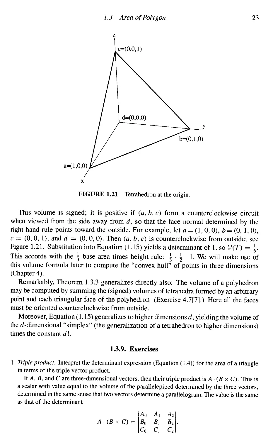
23
a=( 1,0,0)
b=@,l,0)
FIGURE 1.21 Tetrahedron at the origin.
This volume is signed; it is positive if (a, b, c) form a counterclockwise circuit
when viewed from the side away from d, so that the face normal determined by the
right-hand rule points toward the outside. For example, let a = A, 0, 0), b = @, 1,0),
с = @, 0, 1), and d = @, 0, 0). Then (a, b, c) is counterclockwise from outside; see
Figure 1.21. Substitution into Equation A.15) yields a determinant of 1, so V(T) = ±.
This accords with the | base area times height rule: | ¦ \ ¦ 1. We will make use of
this volume formula later to compute the "convex hull" of points in three dimensions
(Chapter 4).
Remarkably, Theorem 1.3.3 generalizes directly also: The volume of a polyhedron
may be computed by summing the (signed) volumes of tetrahedra formed by an arbitrary
point and each triangular face of the polyhedron (Exercise 4.7[7].) Here all the faces
must be oriented counterclockwise from outside.
Moreover, Equation A.15) generalizes to higher dimensions d, yielding the volume of
the ^-dimensional "simplex" (the generalization of a tetrahedron to higher dimensions)
times the constant d\.
1.3.9. Exercises
1. Triple product. Interpret the determinant expression (Equation A.4)) for the area of a triangle
in terms of the triple vector product.
If A, B, and С are three-dimensional vectors, then their triple product is A ¦ (В x C). This is
a scalar with value equal to the volume of the parallelepiped determined by the three vectors,
determined in the same sense that two vectors determine a parallelogram. The value is the same
as that of the determinant
A(B x C) =
Ao
Co
24 Polygon Triangulation
Assuming this determinant is the parallelepiped volume, argue that Equation A.4) is twice the
area of the indicated triangle.
2. Orientation of a polygon: from area [easy]. Given a list of vertices of a simple polygon
in boundary traversal order, how can its orientation (clockwise versus counterclockwise) be
determined using Theorem 1.3.3?
3. Orientation of a polygon. Use the proof of Lemma 1.2.1 to design a more efficient algorithm
for determining the orientation of a polygon.
4. Volume of a cube. Compute the volume of a unit cube (side length 1) with the analog of
Equation A.12), using one vertex as p.
1.4. IMPLEMENTATION ISSUES
The remainder of the chapter takes a rather long "digression" into implementation is-
issues. The goal is to present code to compute a triangulation. This hinges on detecting
intersection between two segments, a seemingly trivial task that often is implemented
incorrectly. We will approach segment intersection using the computation of areas from
Section 1.3. We start with a few representation issues.
1.4.1. Representation of a Point
Arrays versus Records
All points will be represented by arrays of the appropriate number of coordinates. It is
common practice to represent a point by a record with fields named x and y, but this
precludes the use of for-loops to iterate over the coordinates.19 There may seem little
need to write a for-loop to iterate over only two indices, but I find it easier to understand,
and it certainly generalizes to higher dimensions more easily.
Integers versus Reals
We will represent the coordinates with integers rather than with floating-point numbers
wherever possible. This will permit us to avoid the issue of floating-point round-off error
and allow us to write code that is verifiably correct within a range of coordinate values.
Numerical error is an important topic and will be discussed at various points throughout
the book (e.g., Sections 4.3.5 and 7.2). Obviously this habit of using integers will have
to be relaxed when we compute, for example, the point of intersection between two line
segments. The type definitions will be isolated so that modification of the code to handle
different varieties of coordinate datatypes can be made in one location.
Point Type Definition
All type identifiers will begin with lowercase t. All defined constants will appear entirely
in uppercase. The suffixes i and d indicate integer and double types respectively.
See Code 1.1. In mathematical expressions, we will write po and p\ for p [ 0 ] and p [ 1 ].
9That is, precludes it in most programming languages.
1.4 Implementation Issues 25
#define
#define
typedef
#define
typedef
X 0
Y 1
enum
DIM
int
{FALSE
2
tPointi
, TRUE
IDIM];
} bool;
/*
/*
Dimension of points */
Type integer point */
Code 1.1 Point type.
1.4.2. Representation of a Polygon
The main options here are whether to use an array or a list, and if the latter, whether
singly or doubly linked, and whether linear or circular.
Arrays are attractive for code clarity: The structure of loops and index increments are
somewhat clearer with arrays than with lists. However, insertion and deletion of points
is clumsy with arrays. As the triangulation code we develop will clip off ears, we will
sacrifice simplicity to gain ease of deletion. In any case, we will need to use identical
structures for the convex hull code in Chapters 3 and 4, so the investment here will reward
us later. With an eye toward that generality, we opt to use a doubly linked circular list
to represent a polygon. The basic cell of the data structure represents a single vertex,
tVertexStructure, whose primary data field is tPoint. Pointers next andprev
are provided to link each vertex to its adjacent vertices. See Code 1.2. An integer index
vnum is included for printout, and other fields (such as bool ear) will be added as
necessary.
typedef struct tVertexStructure
typedef tsVertex *tVertex;
struct tVertexStructure {
int vnum;
tPointi v;
bool ear;
tVertex next,prev;
tVertex vertices = NULL;
tsVertex; /* Used only in NEW(). */
/* Index */
/* Coordinates */
/* TRUE iff an ear */
/* "Head" of circular list. */
Code 1.2 Vertex structure.
At all times, a global variable vertices is maintained that points to some vertex
cell. This will serve as the "head" of the list during iterative processing. Loops over all
vertices will take the form shown in Code 1.3. Care must be exercised if the processing
in the loop deletes the cell to which vertex points.
26 Polygon Triangulation
tVertex v;
v = vertices;
do {
/* Process vertex v */
v = v->next;
} while ( v != vertices );
Code 1.3 Loop to process all vertices.
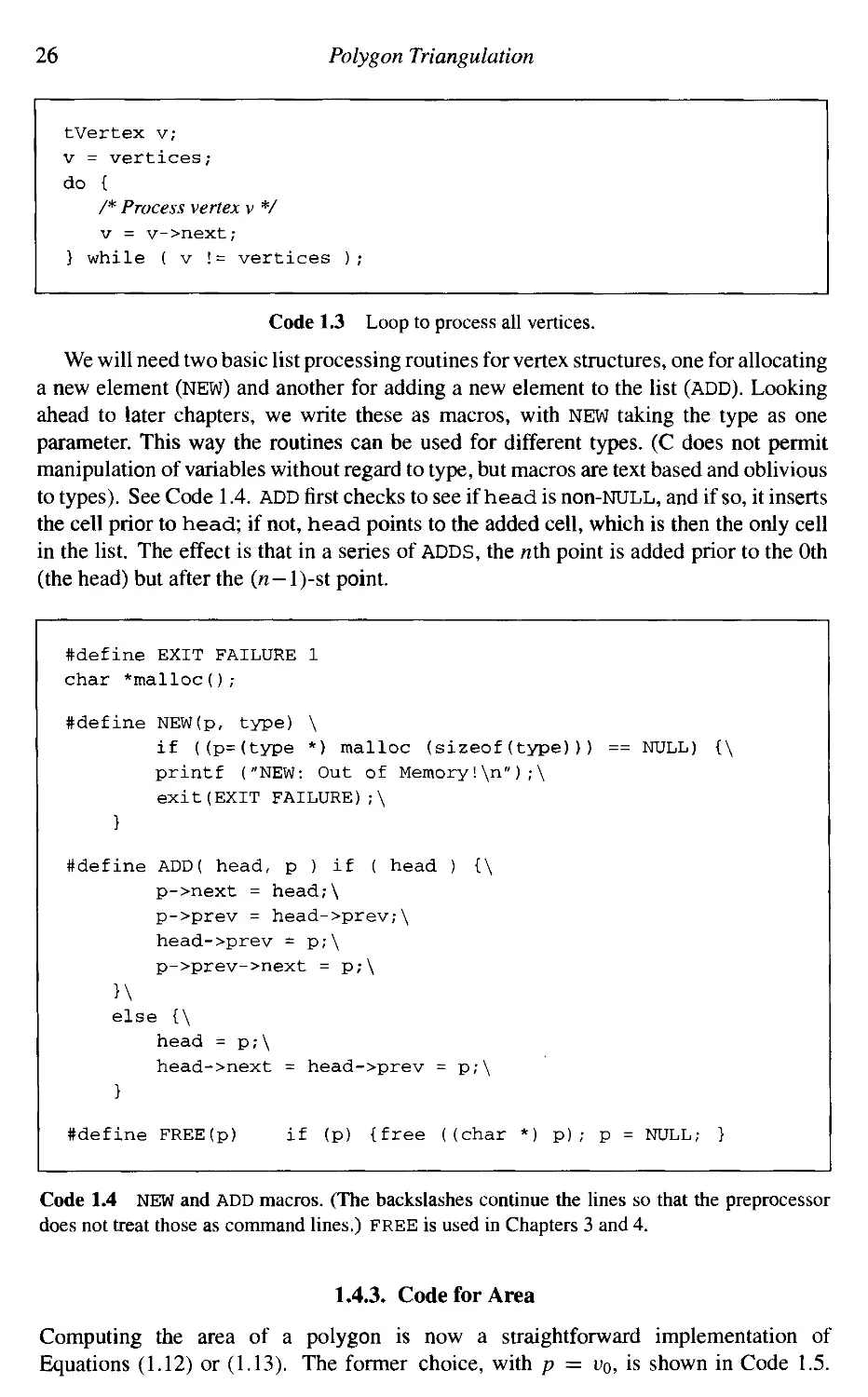
We will need two basic list processing routines for vertex structures, one for allocating
a new element (NEW) and another for adding a new element to the list (ADD). Looking
ahead to later chapters, we write these as macros, with NEW taking the type as one
parameter. This way the routines can be used for different types. (C does not permit
manipulation of variables without regard to type, but macros are text based and oblivious
to types). See Code 1.4. ADD first checks to see if head is non-NULL, and if so, it inserts
the cell prior to head; if not, head points to the added cell, which is then the only cell
in the list. The effect is that in a series of ADDS, the nth point is added prior to the Oth
(the head) but after the (n—l)-st point.
#define EXIT FAILURE 1
char *malloc () ,-
#define NEW(p, type) \
if ((p=(type *) malloc (sizeof(type))) == NULL) {\
printf ("NEW: Out of Memory!\n");\
exit(EXIT FAILURE);\
}
#define ADD( head, p ) if ( head ) {\
p->next = head,-\
p->prev = head->prev;\
head->prev = p;\
p->prev->next = p;\
}\
else {\
head = p;\
head->next = head->prev = p;\
}
#define FREE(p) if (p) {free ((char *) p); p = NULL; }
Code 1.4 NEW and ADD macros. (The backslashes continue the lines so that the preprocessor
does not treat those as command lines.) FREE is used in Chapters 3 and 4.
1.4.3. Code for Area
Computing the area of a polygon is now a straightforward implementation of
Equations A.12) or A.13). The former choice, with p = v0, is shown in Code 1.5.
1.5 Segment Intersection 27
The data structures and conventions established in the previous section are employed.
int Area2( tPointi a, tPointi
1
1
return
<b[X] -
(c[X] -
int AreaPoly2
t
int sum = 0
tVertex p, a;
p = vertices;
a = p->next;
do {
sum += Area2
a = a->next;
a[X]) * (c[Y] -
a[X]) * (b[Y] -
void )
/* Fixed. V
/* Moving. */
( p->v, a->v, a-
} while ( a->next != vertices )
return sum;
b, tPointi с )
a[Y]) -
a[Y]);
>next->v ) ;
Code 1.5 Area2 and AreaPoly2.
There is an interesting potential problem with Ar ea2: If the coordinates are large, the
multiplications of coordinates could cause integer word overflow, which is unfortunately
not reported by most С implementations. For Area2 we have followed the expression
given by Equation A.3) rather than that in A.2), as the former both uses fewer multipli-
multiplications and multiplies coordinate differences. Nevertheless, the issue remains, and we
will revisit this point in Section 4.3.5. See Exercise 1.6.4[1].
1.5. SEGMENT INTERSECTION
1.5.1. Diagonals
Our goal is to develop code to triangulate a polygon. The key step will be rinding a
diagonal of the polygon, a direct line of sight between two vertices u, and vj. The segment
VjVj will not be a diagonal if it is blocked by a portion of the polygon's boundary. To
be blocked, u, Vj must intersect an edge of the polygon. Note that if v,- vj only intersects
an edge e at its endpoint, perhaps only a grazing contact with the boundary, it is still
effectively blocked, because diagonals must have clear visibility.
The following is an immediate consequence of the definition of a diagonal (Sec-
(Section 1.5.1):
Lemma 1.5.1. The segment s = u, vj is a diagonal of P iff
28 Polygon Triangulation
1. for all edges e of P that are not incident to either u, or Vj, s and e do not intersect:
2. s is internal to P in a neighborhood ofvj and Vj.
Condition A) of this lemma has been phrased so that the "diagonalhood" of a segment
can be determined without finding the actual point of intersection between s and each e:
Only a Boolean segment intersection predicate is required. Note that this would not be
the case with the more direct implementation of the definition: A diagonal only intersects
polygon edges at the diagonal endpoints. This phrasing would require computation of
the intersection points and subsequent comparison to the endpoints. The purpose of
condition B) is to distinguish internal from external diagonals, as well as to rule out
collinear overlap with an incident edge. We will revisit this condition in Section 1.6.2.
We now turn our attention to developing code to check the nonintersection condition.
1.5.2. Problems with Slopes
Let VjVj — ab and e = cd. A common first inclination when faced with the task of
deciding whether ab and cd intersect is to find the point of intersection between the
lines L\ and Ьг containing the segments by solving the two linear equations in slope-
intercept form, and then checking that the point falls on the segments. This method
will clearly work, and it is not all that difficult to code. But the code is messy and error
prone; it takes a surprising amount of diligence to get it exactly right. There are two
special cases to handle: a vertical segment, whose containing line's slope is infinite, and
parallel segments, whose containing lines do not intersect. Both cases lead to division
by zero in the computations, which must be avoided by special-case code. Even beyond
this, checking that the point of intersection falls on the segments can lead to numerical
precision problems.
To circumvent these problems, we avoid slopes altogether.
1.5.3. Left
Whether two segments intersect can be decided by using a Left predicate, which
determines whether or not a point is to the left of a directed line. How Left is used
to decide intersection will be shown in the next section. Here we concentrate on Left
itself.
A directed line is determined by two points given in a particular order (a, b). If a
point с is to the left of the line determined by (a, b), then the triple (a, b, c) forms a
counterclockwise circuit: This is what it means to be to the left of a line. See Figure 1.22.
Now the connection to signed area is finally clear: с is to the left of {a, b) iff the area
of the counterclockwise triangle, A(a, b, c), is positive. Therefore we may implement
the Left predicate by a single call to Area2 (Code 1.6).
Note that Left could be implemented by finding the equation of the line through a
and b, and substituting the coordinates of point с into the equation. This method would
be straightforward but subject to the special case objections raised earlier. The area code
in contrast has no special cases.
1.5 Segment Intersection 29
FIGURE 1.22 с is left of ab iff Aabc has positive area; Aabc' also has positive area.
bool Left( tPointi a,
return Area2( a, b, с
bool LeftOn( tPointi
return Area2( a, b, с
tPointi b, tPointi с )
)
a,
)
bool Collinear( tPointi
return Area2( a, b, с
)
> 0;
tPointi b, tPointi с )
>= 0,-
a, tPointi b, tPointi с )
= = 0;
Code 1.6 Left.
What happens when с is collinear with ab! Then the determined triangle has zero
area. Thus we have the happy circumstance that the exceptional geometric situation cor-
corresponds to the exceptional numerical result. As it will sometimes be useful to distinguish
collinearity, we write a separate Collinear predicate20 for this, as well as Lef tOn,
giving us the equivalent of =, <, and <; see again Code 1.6.
Note that we are comparing twice the area against zero in these routines: We are not
comparing the area itself. The reason is that the area might not be an integer, and we
would prefer not to leave the comfortable domain of the integers.
1.5.4. Boolean Intersection
If the two segments ab and cd intersect in their interiors, then с and d are split by the
line L\ containing ab: с is to one side and d to the other. And likewise, a and b are
20If floating-point coordinates are demanded by a particular application, this predicate would need
modification, as it depends on exact equality with zero.
30 Polygon Triangulation
(a)
(b)
FIGURE 1.23 Two segments intersect (a) iff their endpoints are split by their determined lines;
both pair of endpoints must be split (b).
split by L2, the line containing cd. See Figure 1.23(a). Neither one of these conditions
is alone sufficient to guarantee intersection, as Figure 1.23(b) shows, but it is clear that
both together are sufficient. This leads to straightforward code to determine proper
intersection, when two segments intersect at a point interior to both, if it is known that
no three of the four endpoints are collinear. We can enforce this noncollinearity condition
by explicit check; see Code 1.7.
bool IntersectProp( tPointi a, tPointi b, tPointi c, tPointi d)
{
/* Eliminate improper cases. */
if (
Collinear (a, b, c) ||
Collinear (a, b,d) ||
Collinear (c,d, a) ||
Collinear(c,d,b)
)
return FALSE;
return
Xor( Left(a,b,c), Left(a,b,d) )
&& Xor( Left(c,d,a), Left(c,d,b) );
}
/* Exclusive or: T iff exactly one argument is true. */
bool Xor( bool x, bool у )
{
/* The arguments are negated to ensure that they are 0/1 values. */
return !x !y;
Code 1.7 IntersectProp.
/.5 Segment Intersection 31
There is unfortunate redundancy in this code, in that the four relevant triangle areas
are being computed twice each. This redundancy could be removed by computing the
areas and storing them in local variables, or by designing other primitives that fit the
problem better. I would argue against storing the areas, as then the code would not
be transparent. But it may be that the code can be designed around other primitives
more naturally. It turns out that the first if-statement may be removed entirely for the
purposes of triangulation, although then the routine no longer computes proper intersec-
intersection (nor does it compute improper intersection). This is explored in Exercise 1.6.4[2].
I prefer to sacrifice efficiency for clarity and leave IntersectProp as is, for it is
useful to look beyond the immediate programming task to possible other uses. In this
instance, IntersectProp is precisely the function needed to compute clear visibility
(Section 1.1.2).
One subtlety occurs here: It might be tempting to implement the exclusive-or by
requiring that the products of the relevant areas be strictly negative, thus assuring that
they are of opposite sign and that neither is zero:
Area2(a,b,c)* Area2(a,b,d) < 0
&& Area2(c,d,a) *Area2(c,d,b) < 0;
The weakness in this formulation is that the product of the areas might cause integer
word overflow! Thus a clever coding trick to save a few lines could hide a pernicious
bug. This overflow problem can be avoided by having Area2 return +1, 0, or —1
rather than the true area (Sedgewick 1992, p. 350). I prefer to return the area for now,
as this is useful in other contexts - for example, to compute the area of a polygon! In
Chapter 4 we will revise this decision when we discuss overflow as a generic problem
(Code 4.23).
Improper Intersection
Finally we must deal with the "special case" of improper intersection between the two
segments, as Lemma 1.5.1 requires that the intersection be completely empty for a
segment to be a diagonal. Improper intersection occurs precisely when an endpoint of
one segment (say c) lies somewhere on the other (closed) segment ab. See Figure 1.24(a).
This can only happen if a, b, с are collinear. But collinearity is not a sufficient condition
(b)
FIGURE 1.24 Improper intersection between two segments (a); collinearity is not sufficient (b).
32 Polygon Triangulation
for intersection, as Figure 1.24(b) makes clear. What we need to decide is if с is between
a and b.
Betweenness
We would like to compute this "betweenness" predicate without resorting to slopes,
which would require special-case handling. Because we will only check betweenness of
с when we know it lies on the line containing ab, we may exploit this knowledge. If ab
is not vertical, then с lies on ab iff the x coordinate of с falls in the interval determined
by the x coordinates of a and b. If ab is vertical, then a similar check on у coordinates
determines betweenness. See Code 1.8.
bool Between( tPointi a, tPointi b, tPointi с
{
tPointi ba, ca;
if ( ! Collinear( a, b, с ) )
return FALSE;
/* If ab not vertical, check betweenness on x; else on y. */
if ( a[X] != b[X] )
return ((a[X] <= с [X] ) && (c[X] <= b[X])) ||
<(a[X] >= c[X]) && (c[X] >= b[X]));
else
return ((a[Y] <= с [Y] ) && (c[Y] <= b[Y])) ||
((a[Y] >= c[Y]) && (c[Y] >=
Code 1.8 Between.
1.5.5. Segment Intersection Code
We finally can present code for computing segment intersection. Two segments intersect
iff they intersect properly or one endpoint of one segment lies between the two endpoints
of the other segment. The check for improper intersection is therefore implemented by
four calls to Between; see Code 1.9. Exercise 1.6.4[3] asks for an analysis of the
inefficiencies of this routine.
1.6. TRIANGULATION: IMPLEMENTATION
1.6.1. Diagonals, Internal or External
Having developed segment intersection code, we are nearly prepared to write code for
triangulating a polygon. Our first goal is to find a diagonal of the polygon.
1.6 Triangulation: Implementation 33
bool Intersect( tPointi a
r
1
if
return
else if
return
else ]
IntersectProp( a
TRUE ;
Between; a, b,
|| Between ( a, b,
|| Between( c, d,
|| Between; c, d,
TRUE ;
return FALSE;
tPointi b, tPointi c, tPointi d )
, b, c, d ) )
с )
d )
a )
b )
Code 1.9 Intersect.
Recall that Lemma 1.5.1 characterized diagonals by two conditions: nonintersection
with polygon edges and being interior. If we ignore the distinction between internal
and external diagonals, finding diagonals is a straightforward repeated application of
Intersect: For every edge e of the polygon not incident to either end of the potential
diagonal s, see if e intersects s. As soon as an intersection is detected, it is known that s
is not a diagonal. If no such edge intersects s, then s might be a diagonal. The reason we
cannot reach a positive conclusion immediately is that it is possible that one of the edges
incident to an endpoint of s might be collinear with s, and this would not be detected. We
will deal with this possibility shortly. The straightforward code for intersection detection
is shown in Code 1.10.
bool Diagonalie; tVertex a, tVertex b )
{
tVertex c, cl;
/* For each edge (c,cl) ofP V
с = vertices;
do {
cl = c->next;
/* Skip edges incident to a orb */
if ( ( с != a ) && ( cl != a )
&& ( с != b ) && ( cl != b )
&& Intersect; a->v, b->v, c->v, cl->v
return FALSE;
с = c->next;
} while ( с != vertices );
return TRUE;
Code 1.10 Diagonalie.
34
Polygon Triangulation
a.
FIGURE 1.25 Diagonal * = ab is in the cone determined by a_, a, a+: (a) convex; (b) reflex.
In (b), both a- and a+ are right of ab.
1.6.2. InCone
Now we turn to the second condition of Lemma 1.5.1: We must distinguish the in-
internal from the external diagonals; and we have to take care of the edges incident to
the diagonal endpoints. We handle both with a Boolean procedure InCone that de-
determines if one vector В lies strictly in the open cone counterclockwise between two
other vectors A and C. The latter two vectors will lie along two consecutive edges of
the polygon, and В lies along the diagonal. Such a procedure will suffice to determine
diagonals, as will be detailed below. For the moment we concentrate on designing
InCone.
This would be a straightforward task if the apex of the cone is a convex angle; that
it may be reflex either requires a separate case or some cleverness. We will opt here for
the case method, leaving the cleverness to Exercise 1.6.4[5].
The convex case is illustrated in Figure 1.25(a). The actual output produced by the
code is as follows. It is clear from this figure that s is internal to P iff it is internal
to the cone whose apex is a, and whose sides pass through a_ and a+. This can be
easily determined via our Left function: a_ must be left of ab, and a+ must be left
of ba. Both left-ofs should be strict for ab to exclude collinear overlap with the cone
boundaries.
Figure 1.25(b) shows that these conditions do not suffice to characterize internal
diagonals when a is reflex: a_ and a+ could be both left of, or both right of, or one
could be left and the other right of, an internal diagonal. But note that the exterior of
a neighborhood of a is now a cone as in the convex case, for the simple reason that a
reflex vertex looks like a convex vertex if interior and exterior are interchanged. So it
is easiest in this case to characterize s as internal iff it is not external: It is not the case
that both a+ is left or on ab and a_ is left or on ba. Note that this time the left-ofs
1.6 Triangulation: Implementation 35
must be improper, permitting collineanty, as we are rejecting diagonals that satisfy these
conditions.
Finally, distinguishing between the convex and reflex cases is easily accomplished
with one invocation of Left: a is convex iff a_ is left or on aa+. Note that if
(a-,a,a+) are collinear, the internal angle at a is n, which we defined as convex
(Section 1.1.2).
The code in Code 1.11 implements the above ideas in a straightforward manner.
bool InCone(
tVertex aO,al
al = a->next;
aO = a->prev;
/* If a is a convex
tVertex a, tVertex b )
/* aO,a,al
vertex ...*/
if( LeftOn( a->v, al->v,
return
/* Else a is reflex:
return !
>
Left( a->v,
Left( b->v,
*/
LeftOn(
&& LeftOn(
are consecutive
aO->v
b->v,
a->v,
a->v,
b->v,
) )
aO->v
al->v
b->v,
a->v,
vertices. */
)
al->v )
aO->v ) );
Code 1.11 InCone.
Although this InCone test is simple, there are many opportunities to implement
it incorrectly. Note that the entire function consists of five signed-area calculations,
illustrating the utility of that calculation.
1.6.3. Diagonal
We now have developed code to determine if a fc is a diagonal: iff Diagonalie (a,b),
InCone (a, b), and InCone (b, a) are true. The InCone calls serve both to ensure
that ab is internal and to cover the edges incident to the endpoints not examined in
Diagonalie. There would seem to be little more to say on this topic, but in fact
there is a choice of how to order the function calls. Once the question is asked, the
answer is immediate: The inCones should be first, because they are each constant-time
calculations, performed in the neighborhood of a and b without regard to the remainder
of the polygon, whereas Diagonalie includes a loop over all n polygon edges. If
either InCone call returns FALSE, the (potentially) expensive Diagonalie check
will not be executed. See Code 1.12.
36 Polygon Triangulation
bool Diagonal( tVertex a, tVertex b )
{
return InCone( a, b ) && InCone( b, a ) && Diagonalie( a, b )
Code 1.12 Diagonal.
1.6.4. Exercises
1. Integer overflow. On a machine that restricts ints to ±231, how large can the coordinates of
a, b, and с be to avoid integer overflow in the computation of Area2 (Code 1.5)?
2. IntersectProp. Detail exactly what IntersectProp (Code 1.7) computes if the
if-statement is deleted. Argue that after this deletion, Intersect (Code 1.9) still works
properly.
3. Inefficiencies in Intersect. Trace out (by hand) Intersect (Code 1.9) and determine
the largest number of calls to Area2 (Code 1.5) it might induce. Design a new version that
avoids duplicate calls.
4. Saving intersection information. Work out a scheme to avoid testing the same two segments
for intersection twice. Analyze the time and space complexity of the new algorithm.
5. InCone improvement (Andy Mirzian). Prove that ab is in the cone at a iff at most one of
these three Lefts are false: Left(a, a+, b), Left(a, b, a_), Left(a, a_, a+).
6. Diagonal improvement. Prove that either one of the two calls to InCone in Diagonal
can be removed without changing the result.
1.6.5. Triangulation by Ear Removal
We are now prepared to develop code for finding a triangulation of a polygon. One
method is to mimic the proof of the triangulation theorem (Theorem 1.2.3): Find a
diagonal, cut the polygon into two pieces, and recurse on each. We will see that this
method results in rather inefficient code, and we will eventually chose a method based
on Meisters's two ears theorem (Theorem 1.2.7). But first we analyze the speed of the
recursive method. We will use the so-called big-О notation, which we assume to be
familiar to the reader.21
Diagonal-Based Algorithm
The method suggested by Theorem 1.2.3 is an О (n4) algorithm: There are (n2) = O(n2)
diagonal candidates, and testing each for diagonalhood costs O(n). Repeating this 0(n3)
computation for each of the n — 3 diagonals yields O(nA).
We can speed this up by a factor of n by exploiting the two ears theorem: not only do
we know there must be an internal diagonal, we know there must be an internal diagonal
210(f(n)) means that a constant times f(n) is an upper bound for large n\ ?2(g(n)) means that a
constant times g(n) is a lower bound for infinitely many n; ©(/(«)) means both O(f(n)) and
Sl(f(n)) hold. See, e.g., Cormen et al. A990, Chapter 2), Albertson & Hutchinson A988, Sec. 2.8),
orRawlinsA992, Sec. 1.4).
1.6 Triangulation: Implementation
37
E2
VO
FIGURE 1.26 Clipping an ear E2 = A(t>i, v2, щ). Here the ear status of vx changes from
TRUE to FALSE.
that separates off an ear. There are only O(n) "ear diagonal" candidates: (u,-, w,+2) for
i = 0,..., n — 1. This also makes the recursion simpler, as there is only one piece on
which to recurse: the other is the ear, a triangle, which is of course already triangulated.
Thus we can achieve a worst-case complexity of O(n3) this way.
Ear Removal
We now improve the above algorithm to O(n2). Because one call to Diagonal costs
O(n), to achieve O(n2), Diagonal may only be called 0{n) times. The key idea
that permits improvement here is that removal of one ear does not change the polygon
very much, and in particular, it does not change whether or not many of its vertices
are potential ear tips. This suggests first determining for each vertex w,, whether it is a
potential ear tip in the sense that w,_i, u,+i is a diagonal. This already uses O(n2), but
this expensive step need not be repeated.
Let (vo, t>i, V2, t>3, v4) be five consecutive vertices of P, and suppose v2 is an ear tip
and the ear E2 = A(wi, vi, из) is deleted; see Figure 1.26. Which vertices' status as
ear tips might change? Only v\ and ч3. Consider u4, for example. Whether it is an ear
tip depends on whether U3U5 is a diagonal. The removal of E2 leaves the endpoints of
segment V3 v$ unchanged. Certainly this removal can not block the previous line of sight
between these endpoints if they could see one another. It is perhaps less clear that if
they couldn't see one another, they still don't after removal of E2. But as in the proof
of Lemma 1.2.2, there are only two cases to consider. If U3U5 is external, then clearly
removal of E% cannot render it internal. Otherwise Д(из, W4,1M) must contain a vertex,
and in fact a reflex vertex (x in Figure 1.12). But removal of ?2 only removes one vertex,
and that is convex. Therefore, the status of 114 is unchanged by the removal of E2, as
is that of every vertex but v\ and 113, whose ear diagonals are incident to the removed
vertex V2-
38 Polygon Triangulation
The implication is that, after the expensive initialization step, the ear tip status in-
information can be updated with two calls to Diagonal per iteration. This leads to the
pseudocode shown in Algorithm 1.1 for constructing a triangulation.
Algorithm
Initialize the
while и > 3
Locate
Output
Delete
Triangulation
ear tip status of each vertex.
do
an ear tip V2-
diagonal V\v3.
V2-
Update the ear tip status of Vi and u3.
Algorithm 1.1 Triangulation algorithm.
Note that we are interpreting the task "triangulate a polygon" as "output, in arbitrary
order, diagonals that form a triangulation." This is primarily for ease of presentation.
Often a more structured output is required by a particular application: For example, the
triangle adjacency information in the dual graph might be required. Although obtaining
more structured output is no more difficult in terms of asymptotic time complexity, it often
complicates the code considerably. We will not pursue these alternative triangulation
outputs further.
Triangulation Code
The first task is to initialize the Boolean flag v->ear that is a part of the vertex structure
(Code 1.2). This is accomplished by one call to Diagonal per vertex. See Earinit,
Code 1.13.
void Earinit( void )
{
tVertex vO , vl, v2 ; /* three consecutive vertices */
/* Initialize vl->earfor all vertices. */
vl = vertices;
do {
v2 = vl->next;
vO = vl->prev;
vl->ear = Diagonal; vO, v2 );
vl = vl->next;
} while ( vl != vertices );
Code 1.13 Earinit.
The main Triangulate code consists of a double loop. The outer loop removes
one ear per iteration, halting when n = 3. The inner loop searches for an ear by checking
1.6 Triangulation: Implementation 39
the precomputed v2->ear flag, where «2 is the potential ear tip. Once an ear tip is
found, the ear status of v\ and из are updated by calls to Diagonal, the diagonal
representing the base of the ear is printed, and the ear is removed from the polygon.
This removal is accomplished by rewiring the next and prev pointers for v\ and из.
(At this point the cell for vi could be freed if it is not used in a surrounding appli-
application.) Care must be exercised lest v^ is the "head" of the vertex list, the point of
access into the circular list. This head pointer, vertices, is moved to point to из for
that reason. See Code 1.14. We step through an example before analyzing the time
complexity.
void Triangulate( void )
{
tVertex vO, vl, v2 , v3 , v4; /* five consecutive vertices */
int n = nvertices; /* number of vertices; shrinks to 3. */
Earlnit();
/* Each step of outer loop removes one ear. */
while ( n > 3 ) {
/* Inner loop searches for an ear. */
v2 = vertices;
do {
if (v2->ear) {
/* Ear found. Fill variables. */
v3 = v2->next; v4 = v3->next;
vl = v2->prev; vO = vl->prev;
/* (vl,v3) is a diagonal */
PrintDiagonal( vl, v3 ) ;
/* Update earity of diagonal endpoints */
vl->ear = Diagonal; vO, v3 );
v3->ear = Diagonal( vl, v4 );
/* Cut off the ear v2 У
vl->next = v3 ;
v3->prev = vl;
vertices = v3 ; /* In case the head was v2. */
n--;
break; /* out of inner loop; resume outer loop */
}/* end if ear found */
v2 = v2->next;
} while ( v2 != vertices );
} /* end outer while loop */
Code 1.14 Triangulate.
40
Polygon Triangulation
13
16
r0
FIGURE 1.27 A polygon of 18 vertices and the triangulation produced by Triangulate.
The dark subpolygon is the remainder after the 9th diagonal A5, 3) is output. Vertex coordinates
are displayed in Table 1.1.
1.6.6. Example
Figure 1.27 shows a polygon and the triangulation produced by the simple main program
(Code 1.15). The code for reading and printing is straightforward and will not be shown
here.22
main()
ReadVertices(
PrintVertices
Triangulate()
);
0 ;
Code 1.15 main.
We now walk through the output of the diagonals for this example, displayed in
Table 1.2. v0 is an ear tip, so the first diagonal output is A7, 1). vi is not an ear tip, so
the v2 pointer moves to vi, which is a tip, printing the diagonal A,3) next. Neither vj,
22See the Preface for how to obtain the full code.
1.6 Triangulation: Implementation 41
Table 1.1. Vertex coordinates for the polygon shown in Figure 1.27.
i (x,y) i (x,y)
0
1
2
3
4
5
6
7
8
@,0)
A0,7)
A2,3)
B0, 8)
A3,17)
A0, 12)
A2, 14)
A4,9)
(8, 10)
9
10
11
12
13
14
15
16
17
F, 14)
A0, 15)
G, 10)
@, 16)
0,13)
C, 15)
E,8)
(-2, 9)
E,5)
nor V4 is an ear tip, so it is not until w5 is reached that the next diagonal, D, 6), is output.
The segment изи8 is collinear with u7, so the next ear detected is not until ищ. The
dark-shaded subpolygon in Figure 1.27 shows the remaining polygon after the A5, 3)
diagonal (the 9th) is output. Another collinearity, vg with (V]]Vi5), prevents w9 from
being an ear after the A5, 9) diagonal is cut.
1.6.7. Analysis
We now analyze the time complexity of the algorithm. Earlnit costs O(n2), as
previously mentioned. The outer loop of Triangulate iterates as many times as there
are diagonals, n — 3 = O(n). The inner search-for-an-ear loop is also O(n), potentially
checking every vertex. The work inside the inner loop is O(n): Each of the two calls
to Diagonal could, in the worst case, loop over the entire polygon to verify that the
diagonal is not blocked. Naively we have then a time complexity of O(n3), falling short
of the promised O(n2). A closer analysis will show that O(n2) is the correct bound for
Triangulate after all.
Consider the example in Figure 1.28. After w0 is deleted, the inner loop searches past
vi,..., V(, before reaching the next ear tip v7. Then it must search past ug, ..., U12 before
finding the ear tip u]3. This example shows that indeed the inner loop might iterate ?2 (n)
times before finding an ear. But notice that the two O(n) Diagonal calls within the
loop are only invoked once an ear is found - they are not called in each iteration. Thus
although the superficial structure of the code suggests a complexity of nxnxn = О (n3),
it is actually n x (n + n) = O(n2).
Although further slight improvements are possible (Exercise 1.6.8[4]), lowering the
asymptotic time complexity below quadratic requires rather different approaches, which
are discussed in the next chapter.
1.6.8. Exercises
1. Repeated intersection tests [programming]. Triangulate (Code 1.14) often checks for the
same segment/segment intersections. Modify the code so that you can determine how many
unnecessary segment/segment intersection tests are made. Test it on Figure 1.27.
42
Polygon Triangulatwn
Table 1.2. The columns show the order in which the diagonals, specified as pairs of endpoint
indices, are output.
Order
1
2
3
4
5
6
7
8
9
Diagonal Indices
A7, 1)
0.3)
D,6)
D,7)
(9,11)
A2, 14)
A5,17)
A5,1)
A5,3)
Order
10
11
12
13
14
15
Diagonal Indices
C,7)
A1,14)
A5,7)
A5,8)
A5,9)
(9, 14)
FIGURE 1.28 An example that forces the inner ear loop to search extensively for the next ear.
2. Convex polygons [easy]. Analyze the performance of Triangulate when run on aconvex
polygon.
3. Spiral. Continue the analysis of Figure 1.28: Does Triangulate continue to traverse the
boundary in search of an ear? More specifically, if the polygon has n vertices, how many
complete circulations of the boundary will the pointer v2 execute before completion?
4. Ear list [programming]. The inner loop search of Triangulate can be avoided by link-
linking the ear tips into their own (circular) list, linking together those vertices v for which
v->ear == TRUE with pointers nextear and prevear in the vertex structure. Then
the ear for the next iteration can be found by moving to the next ear on this list beyond the one
just clipped. Implement this improvement, and see if its speedup is discernible on an example
(perhaps one akin to Figure 1.28).
1.6 Triangulation: Implementation 43
5. Center of gravity. Design an algorithm to compute the center of gravity of a polygon, assuming
that it is cut from a material of uniform density. The center of gravity is a point, which can
be treated as a vector. The center of gravity of a triangle is at its centroid, whose coordinates
happen to be at the average of the coordinates of the triangle's vertices. The center of gravity
у (S) of any set S that is the disjoint union of sets A and В is the weighted sum of the centers
of gravity of the two pieces. Let w(S) = w(A) + w(B) be the weight of S. Then
w(A)y(A) + w(B)y(B)
Here the weight of each triangle is its area under the uniform density assumption.
Polygon Partitioning
In this short chapter we explore other types of polygon partitions: partitions into mono-
monotone polygons (Section 2.1), into trapezoids (Section 2.2), into "monotone mountains"
(Section 2.3), and into convex polygons (Section 2.5). Our primary motivation is to
speed up the triangulation algorithm presented in the previous chapter, but these parti-
partitions have many applications and are of interest in their own right. One application of
convex partitions is character recognition: Optically scanned characters can be repre-
represented as polygons (sometimes with polygonal holes) and partitioned into convex pieces,
and the resulting structures can be matched against a database of shapes to identify the
characters (Feng & Pavlidis 1975). In addition, because so many computations are easier
on convex polygons (intersection with obstacles or with light rays, finding the distance
to a line, determining if a point is inside), it often pays to first partition a complex shape
into convex pieces.
This chapter contains no implementations (but suggests some as exercises).
2.1. MONOTONE PARTITIONING
We presented an O(n2) triangulation algorithm in Section 1.4. Further improvements
will require organizing the computation more intelligently, so that each diagonal can
be found in sublinear time.' There are now many algorithms that achieve O{n\ogn)
time, averaging O(\ogn) work per diagonal.2 The first was due to Garey, Johnson,
Preparata & Tarjan A978). Although one might expect an O(n logn) algorithm to find
each diagonal by an О (logn) binary search, that is not in fact the way their algorithm
works. Rather they first partition the polygon into simpler pieces, in O(n log я) time, and
then triangulate the pieces in linear time. The pieces are called "monotone," a concept
first introduced and exploited by Lee & Preparata A977). It will develop that partitions
into monotone polygons will have several other uses aside from triangulation, so their
exploration is a worthwhile pursuit.
We will only sketch the O(n logn) algorithm based on monotone partitioning, but re-
return in Section 2.3 to detail a closely related algorithm based on partitions into "monotone
mountains."
We first define monotonicity, then show how to triangulate monotone polygons in
linear time, and finally describe how to partition a polygon into monotone pieces.
'The technical notation for sublinear time is o(n) time.
throughout the text, all logarithms are to the base 2. But since the big-O notation absorbs constants,
the base of the logarithm is irrelevant when inside an O( )-expression.
2.1 Monotone Partitioning
45
FIGURE 2.1 A polygon monotone with respect to the vertical.
2.1.1. Monotone Polygons
Monotonicity is defined with respect to a line. First we define monotonicity of polygonal
chains. A polygonal chain С is strictly monotone with respect to L' if every line L
orthogonal to L' meets С in at most one point (i.e., L Л С is either empty or a single
point). A chain is monotone if L П С has at most one connected component: It is
either empty, a single point, or a single line segment.3 These chains are "monotone"
in the sense that a traversal of С projects to a monotone sequence on L'\ No reversals
occur.
A polygon P is said to be monotone with respect to a line L if dP can be split
into two polygonal chains A and В such that each chain is monotone with respect to
L. The two chains share a vertex at either end. A polygon monotone with respect to
the vertical is shown in Figure 2.1. The two monotone chains are A = (vo,..., U15)
and В = (ui5,..., U24, vo)- Neither chain is strictly monotone, because edges v5ve
and v2\ U22 are horizontal. Some polygons are monotone with respect to several lines;
and some polygons are not monotone with respect to any line.
3This definition differs from some others in the literature (e.g., from that of Preparata & Shamos A985,
p. 49)) in that here monotone chains need not be strictly monotone.
46 Polygon Partitioning
(b)
FIGURE 2.2 Interior cusps: (a) d+ and i>_ are both above d; (b) a, c, and e are interior cusps;
b and d are not.
Properties of Monotone Polygons
Many algorithms that are difficult for general polygons are easy for monotone polygons,
primarily because of this key property: The vertices in each chain of a monotone polygon
are sorted with respect to the line of monotonicity. Let us fix the line of monotonicity
to be the vertical у axis. Then the vertices can be sorted by у coordinate in linear time:
Find a highest vertex, find a lowest, and partition the boundary into two chains. The
vertices in each chain are sorted with respect to y. Two sorted lists of vertices can be
merged in linear time to produce one list sorted by y.
There is a simple local structural feature that characterizes monotonicity. Essentially
it says that a polygon is monotone if it is monotone in the neighborhood of every vertex.
This can form the basis of an algorithm to partition a polygon into monotone pieces, by
cutting at the local nonmonotonicities.
Define an interior cusp of a polygon as a reflex vertex v whose adjacent vertices
u_ and v+ are either both at or above, or both at or below, v. See Figure 2.2. Recall
that a reflex vertex has internal angle strictly greater than я, so it is not possible for an
interior cusp to have both adjacent vertices with the same у coordinate as v. Thus d in
Figure 2.2(b) is not an interior cusp. The characterization is this simple lemma:
Lemma 2.1.1. If a polygon P has no interior cusps, then it is monotone.
Despite the naturalness of this lemma, a proof requires care.4 It is perhaps not obvious
that it cannot be strengthened to the claim that the lack of interior cusps implies strict
monotonicity (Exercise 2.2.3[2]). We will not pause to prove this lemma, but rather
continue with the high-level sketch. We will use the lemma in Section 2.2 to partition a
polygon into monotone pieces.
2.1.2. Triangulating a Monotone Polygon
Because monotone polygons are so restricted, one might hope that their triangulations
are similarly special - that the triangulation dual is always a path, or every diagonal
connects the two monotone chains. Figure 2.1 shows that neither of these hypotheses
4See Lee & Preparata A977) or O'Rourke A994, pp. 54-5).
2.2 Trapezoidalization 47
hold; see also Exercise 2.3.4[1]. Nevertheless, the intuition that these shapes are so
special that they must be easy to triangulate is valid: Any monotone polygon (whose
direction of monotonicty is given) may be triangulated in linear time.
Here is a hint of an algorithm. First sort the vertices from top to bottom (in linear time).
Then cut off triangles from the top in a "greedy" fashion (this is a technical algorithms
term indicating in this instance that at each step the first available triangle is removed).
So the algorithm is: For each vertex v, connect v to all the vertices above it and visible
via a diagonal, and remove the top portion of the polygon thereby triangulated; continue
with the next vertex below v.
One can show that at any iteration, v e A is being connected to a chain of reflex
vertices above it in the other chain B. For example, v\e is connected to (v\4, U13, v^) in
the first iteration for the example in Figure 2.1. As a consequence, no visibility check is
required to determine these diagonals - they can be output immediately. The algorithm
can be implemented with a single stack holding the reflex chain above. Between the
linear sorting and this simple data structure, O(n) time overall is achieved.5
2.2. TRAPEZOIDALIZATION
Knowing that monotone polygons may be triangulated quickly, it becomes an interesting
problem to partition a polygon into monotone pieces quickly. We do this via yet another
intermediate partition, which is itself of considerable interest, and which we will use later
in Section 7.11: a partition into trapezoids. This partition was introduced by Chazelle &
Incerpi A984) and Fournier & Montuno A984) as the key to triangulation. This partition
will differ from those considered previously in that we will not restrict the partitioning
segments to be diagonals.
A horizontal trapezoidalization of a polygon is obtained by drawing a horizontal
line through every vertex of the polygon. More precisely, pass through each vertex v
the maximal (open) horizontal segment s such that s С P and s П ЭР = v. Thus s
represents clear lines of sight from v left and right. It may be that s is entirely to one
side or the other of v\ and it may be that s = v. An example is shown in Figure 2.3.
To simplify the exposition we will only consider polygons whose vertices have unique
у coordinates: No two vertices lie on a horizontal line.6
A trapezoid is a quadrilateral with two parallel edges. One can view a triangle as a
degenerate trapezoid, with one of the two parallel edges of zero length. Call the vertices
through which the horizontal lines are drawn supporting vertices.
Let P be a polygon with no two vertices on a horizontal line. Then in a horizontal
trapezoidalization, every trapezoid has exactly two supporting vertices, one on its up-
upper edge and one on its lower edge. The connection between trapezoid partitions and
monotone polygons is this: If a supporting vertex is on the interior of an upper or lower
5For more detailed expositions, see Garey et al. A978), O'Rourke A994, pp. 55-9), or de Berg, van
Kreveld, Overmars & Schwarzkopf A997, pp. 55-8).
6 Although it is not obvious, this assumption involves no true loss of generality. It suffices to sort points
lexicographically: For two points with the same у coordinate, treat the one with smaller x coordinate
as lower (Seidel 1991).
48
Polygon Partitioning
14
FIGURE 2.3 Trapezoidalization. Dashed lines show trapezoid partition lines; dotted diagonals
resolve interior cusps (circled). The shaded polygon is one of the resulting monotone pieces.
trapezoid edge, then it is an interior cusp. If every interior supporting vertex v is con-
connected to the opposing supporting vertex of the trapezoid v supports, downward for a
"downward" cusp and upward for an "upward" cusp, then these diagonals partition P
into pieces monotone with respect to the vertical. This follows from Lemma 2.1.1, since
every interior cusp is removed by these diagonals. For example, the downward cusp
Vf, in Figure 2.3 is resolved with the diagonal i^tu; the upward cusp vi5 is resolved by
connecting to vi2 (which happens to be a downward cusp); and so on.
Now that we see that a trapezoidalization yields a monotone partition directly, we
concentrate on drawing horizontal chords through every vertex of a polygon.
2.2.1. Plane Sweep
The algorithm we use to construct a trapezoidalization depends on a technique called
a "plane sweep" (or "sweep line"), which is useful in many geometric algorithms
(Nievergelt & Preparata 1982). The main idea is to "sweep" a line over the plane,
maintaining some type of data structure along the line. The sweep stops at discrete
"events" where processing occurs and the data structure is updated. For our particu-
particular problem, we sweep a horizontal line L over the polygon, stopping at each vertex.
This requires sorting the vertices by у coordinate, and since the polygon is general, this
requires O(nlogn) time.7
7Sorting has time complexity 0(n log/i): It can be accomplished in O(rclogn) time, but no faster. See
KnuthA973).
2.2 Trapezoidalization
49
11
15
21
FIGURE 2.4 Plane sweep. Labels index edges.
The processing required at each event vertex v is finding the edge immediately to the
left and immediately to the right of v along L. To do this efficiently, a sorted list С of
polygon edges pierced by L is maintained at all times. For example, for the sweep line
in the position shown in Figure 2.4, С = (е\д, ejg, en, e6, eg, ею).
Suppose this list С is available. How can we determine that v lies between en and e$
in the figure? Let us assume that e,- is a pointer to an edge of the polygon, from which
the coordinates of its endpoints can be retrieved easily. Suppose the vertical coordinate
of v (and therefore L) is y. Knowing the endpoints of e,-, and y, we can compute the x
coordinate of the intersection between L and e,. So we can determine v's position in the
list by computing the x coordinates of where L pierces each edge at height y.
This would take time proportional to the length of С (which is O(n)) if done by a
naive search from left to right; but if we store the list in an efficient data structure, such as
a height-balanced tree, then the search will only require О (log n) time. Since this search
occurs once per each event, the total cost over the entire plane sweep is O(n logn).
It remains to show that it is possible to maintain the data structure at all times, and
in time O(n\ogn). This is easy as long as the data structure supports O(logn)-time
insertions and deletions, as do, for example, height-balanced or 2-3 or red-black trees.8
We now detail the updates at each event, assuming a downward sweeping line.
There are three possible types of event, illustrated in Figure 2.5. Let v fall between
edges a and b on L, and let v be shared by edges с and d.
1. с is above L and d below. Then delete с from С and insert d:
(..., a, c,b, ...)=>¦ (...,a,d,b,...).
2. Both с and d are above L. Then delete both с and d from C:
(...,a,c,d,b,...)=> (...,a,b,...).
8See, e.g., Aho, Hopcroft & Ullman A983, pp. 169-80) or Cormen, et al. A990, Chap. 14).
50
A)
Polygon Partitioning
B)
C)
FIGURE 2.5 Sweep line events: A) replace с by d; B) delete с and d; C) insert с and d.
3. Both с and d are below L. Then insert both с and J into C:
(..., a, b, ...)=>(..., a, c,d,b,.. .)•
Returning to Figure 2.4, we see that the list С of edges pierced by L is initially empty,
when L is above the polygon, and then follows this sequence as it passes each event vertex:
ei4, en, «6, <?v, ею)
(ei6, «м.еп, бб,е7, ею)
(«16, «6, «7, ею)
(«16, «6, в8,«10)
(«19, «18, «16.^6, eg, ею)
18, «п. «6, «8, ею) ¦
The final list corresponds to the position of L shown in the figure.
2.3 Partition into Monotone Mountains 51
2.2.2. Triangulation in 0(n log и)
Leaving out the remaining (mainly data structure) details, we summarize the О (п log n)
algorithm for triangulating a polygon in Algorithm 2.1.
Algorithm: Polygon Triangulation: Monotone Partition
Sort vertices by у coordinate.
Perform plane sweep to construct trapezoidalization.
Partition into monotone polygons by connecting from interior cusps.
Triangulate each monotone polygon in linear time.
Algorithm 2.1 О(n log n) polygon triangulation.
2.2.3. Exercises
1. Monotone with respect to a unique direction. Can a polygon be monotone with respect to
precisely one direction?
2. Interior cusps. Construct a monotone but not strictly monotone polygon that has no interior
cusps, thereby showing that Lemma 2.1.1 cannot be strengthened to the claim that the lack of
interior cusps implies strict monotonicity.
3. Several vertices on a horizontal. Extend the trapezoid partition algorithm to polygons that may
have several vertices on a horizontal line.
4. Sweeping a polygon with holes. Sketch an algorithm for triangulating a polygon with holes (one
outer polygon P containing several polygonal holes) via plane sweep. The diagonals should
partition the interior of P outside each hole. Express the complexity as a function of the total
number of vertices n.
2.3. PARTITION INTO MONOTONE MOUNTAINS
A minor variation of the algorithm just described is simpler. The idea is to again start with
a trapezoidalization of P, but add more than just cusp-to-cusp diagonals, partitioning P
into pieces we will call monotone mountains. These shapes are even easier to triangulate.
2.3.1. Monotone Mountains
A monotone mountain is a monotone polygon with one of its two monotone chains a
single segment, the base. If the direction of monotonicity is horizontal, such a polygon
resembles a mountain range; see Figure 2.6.9 Note that both endpoints of the base must
be convex, as otherwise one of the chains would contain more than one segment.
The following lemma makes triangulation of such polygons easy.
Lemma 23.1. Every strictly convex vertex of a monotone mountain M, with the possible
exception of the base endpoints, is an ear tip.
9Fourmer & Montuno A984) call these shapes unimonotone polygons.
52
Polygon Partitioning
FIGURE 2.6 A monotone mountain with base B; b is an ear tip.
Proof. Let a, b, с be three consecutive vertices of M, with b a strictly convex vertex not
an endpoint of the base B. Let the direction of monotonicity be horizontal. We aim to
prove that ac is a diagonal, by contradiction.
Assume that ac is not a diagonal. Then by Lemma 1.5.1, either it is exterior in the
neighborhood of an endpoint or it intersects dM.
1. Suppose first that ac is locally exterior in the neighborhood of endpoint a in
Figure 2.6 (endpoint с is symmetrical and need not be considered separately). If
a is not also an endpoint of В (as illustrated), then the two incident edges are left
and right of a, with M below. To be exterior, ac must be locally above ab, which
is inconsistent with the assumption that b is convex. If a is the right endpoint of
B, then either ac is locally above ab, leading to the same contradiction, or it is
locally below B. In the latter case, it could not connect to c, which must lie above
B. We may conclude that ac is locally interior to M at each endpoint.
2. Assume therefore that ac intersects 3M. This would require a reflex vertex x to
be interior to Aabc (cf. Figure 1.12). Because x is interior, it cannot lie on the
chain С = (a, b,c); and it cannot lie on B, which is a single segment with convex
endpoints. Thus a vertical line L through x meets dM in at least three points:
С П L, В П L, and x. This contradicts the definition of a monotone polygon. ?
This lemma does not hold for monotone polygons; for example, из in Figure 2.1 is
convex but not an ear tip. Note that the exclusion of fi's endpoints cannot be removed
from the preconditions of the lemma: Neither endpoint in Figure 2.6 is an ear tip.
2.3.2. Triangulating a Monotone Mountain
Lemma 2.3.1 yields a nearly trivial linear algorithm for triangulating a monotone moun-
mountain: Find a convex vertex not on the base, clip off the associated ear, and repeat.
To ensure that this algorithm runs in linear time requires only that (a) the base be
identified in linear time and (b) that the "next" convex vertex be found without a search, in
constant time. The former is easy: The base endpoints are extreme along the direction of
2.3 Partition into Monotone Mountains
53
monotonicity. If this direction is horizontal, simply search for the leftmost and rightmost
vertices.10 Once the base is identified, its endpoints can be avoided in the ear-clipping
phase.
Achieving (b) is similar to the task faced in Section 1.4 when the ear tip status of a and
с needed updating after clipping ear Aabc. Here instead we need to update the convexity
status, which by Lemma 2.3.1 implies the ear tip status. This is easily accomplished
by storing with each vertex its internal angle, and subtracting from a and c's angles
appropriately upon removal of Aabc. One issue remains, however. The Triangulate
code (Code 1.14) tolerated a linear inner-loop search for the next ear, for there we only
sought O(n2) behavior. But now our goal is O(n). To find the next convex vertex with-
without a search requires following Exercise 1.6.8[4] in linking the convex vertices into a
(circular) list and updating the list with each ear clip appropriately. Then as long as this
list is nonempty, its "first" element can be chosen immediately for each clipping.
The algorithm is summarized in the pseudocode displayed as Algorithm 2.2.
Algorithm: Triangulation of Monotone Mountain
Identify the base edge.
Initialize internal angles at each nonbase vertex.
Link nonbase strictly convex vertices into a list.
while list nonempty do
For convex vertex b, remove Aabc.
Output diagonal ac.
Update angles and list.
Algorithm 2.2 Linear-time triangulation of a monotone mountain.
2.3.3. Adding Diagonals to Trapezoidalization
Now we address how to convert a trapezoidalization to a partition into monotone moun-
mountains. The monotone mountains will be turned on their sides, with a vertical direction of
monotonicity. We first motivate the key idea, and then we prove that it works.
Consider building a monotone mountain from trapezoids abutting on a particular base
edge, for example В = Unui2 in Figure 2.7. Use the notation T(i, j) to represent the
trapezoid with support vertices u,- and vj, below and above respectively. ГA2, 2) is
based on В but must be cut by the diagonal U12U2 to ensure that the v\2 endpoint is
convex. 7B, 3) and ГC, 4) may be included in their entirety. 7D, 6) must be cut by
the diagonal v4V(, to separate off the nonmonotonicity at V(,, and similarly 7F, 8) must
be cut by ueug. Finally, 7(8, 11) must be cut by ugUn to ensure convexity at v\\. The
resulting union (shown shaded in the figure) is a monotone mountain.
Note that we have cut a trapezoid by a diagonal between its supporting vertices in
exactly those cases where those vertices do not lie on the same side of the trapezoid.
This suggests the following lemma:
l0We will see in Chapter 7 (Section 7.9) that these extremes can be found in O(logn) time, but we do
not need such sophistication here.
54
Polygon Partitioning
14
FIGURE 2.7 A partition into monotone mountains.
Lemma 2.3.2. Inatrapezoidalizationofapolygon P, connecting every pair of trapezoid-
supporting vertices that do not lie on the same (left/right) side of their trapezoid partitions
P into monotone mountains.
Proof. We may observe at once that the pieces must be monotone, because an interior
cusp does not lie on either the left or the right side of the trapezoid it supports, so it is
always the endpoint of a diagonal that resolves it. Thus Lemma 2.1.1 guarantees that the
pieces of the partition are monotone. It only remains to prove that each piece has one
chain that is a single segment.
Suppose to the contrary that both monotone chains A and В of one piece Q of the
partition each contain at least two edges. Let z be the topmost vertex of Q, adjacent on
bQ = A U В to vertices a e A and b e B, with b below a. See Figure 2.8. In order for
В to contain more than just the edge zb, b cannot be the endpoint of a partition diagonal
from above. But consider the trapezoid T(b, c) supported from below by b. Its upper
supporting vertex с cannot lie on zb, for с must lie at or below a (it could be that a — c).
Thus с is not on the same side of T(b, c) as b, and the diagonal cb is included in the
partition, contradicting the assumption that В extends below b. ?
Figure 2.7 shows the result of applying this lemma to the example used previously in
Figure 2.3. Three more diagonals are needed to achieve this finer partition, resulting in
eight monotone mountains compared to five monotone pieces.
We now have an outline of a second О («log и) triangulation algorithm: After
trapezoidalization, add diagonals per Lemma 2.3.2, and triangulate each piece with
Algorithm 2.2.
2.3 Partition into Monotone Mountains 55
FIGURE 2.8 Proof of Lemma 2.3.2: Diagonal cb must be present.
We leave designing data structures to permit the efficient extraction of the monotone
mountain pieces to Exercise 2.3.4[4].
2.3.4. Exercises
1. Monotone duals. Prove that every binary tree can be realized as the triangulation dual of a
monotone mountain. (Cf. Exercise 1.2.5[2].)
2. Random monotone mountains [programming]. Develop code to generate "random" monotone
mountains. Generating random polygons, under natural definitions of "random," is an open
problem, but monotone mountains are special enough to make it easy in this case.
3. Triangulating monotone mountains [programming]. Implement Algorithm 2.2.
4. Trapezoid data structure. Design a data structure for a trapezoidalization of a polygon P
augmented by a set of diagonals that permits extraction of the subpolygons of the resulting
partition in time proportional to their size.
5. Polygon => Convex quadrilaterals. Prove or disprove: Every polygon with an even number of
vertices may be partitioned by diagonals into convex quadrilaterals.
6. Polygon => Quadrilaterals. Prove or disprove: Every polygon with an even number of vertices
may be partitioned by diagonals into quadrilaterals.
7. Orthogonal pyramid => Convex quadrilaterals. An orthogonal polygon is a polygon in which
each pair of adjacent edges meets orthogonally (Exercise 1.2.5[5]). Without loss of generality,
one may assume that the edges alternate between horizontal and vertical.
An orthogonal pyramid P is an orthogonal polygon monotone with respect to the vertical,
that contains one horizontal edge h whose length is the sum of the lengths of all the other
horizontal edges. Thus P is monotone with respect to both the vertical and the horizontal; in
fact it is a monotone mountain with respect to the horizontal. P consists of two "staircases"
connected to h, as shown in Figure 2.9.
a. Prove that an orthogonal pyramid may be partitioned by diagonals into convex quadri-
quadrilaterals.
56
Polygon Partitioning
П
FIGURE 2.9 Orthogonal pyramid.
b. Design an algorithm for finding such a partition. Try for linear-time complexity. Describe
your algorithm in pseudocode, at a high level, ignoring data structure details and manipula-
manipulations.
Orthogonal polygon => Convex quadrilaterals. Can every orthogonal polygon be partitioned
by diagonals into convex quadrilaterals? Explore this question enough to form a conjecture.
2.4. LINEAR-TIME TRIANGULATION
Quadratic triangulation algorithms have been implicit in proofs since at least 1911 (Lennes
1911).ll The О (n log n) algorithm described in Section 2.1 was one of the early achieve-
achievements of computational geometry, having been published in 1978, just three years after
Shamos named the field in his thesis. Soon the question of whether O(n logn) is opti-
optimal for triangulation became the outstanding open problem in computational geometry,
fueling an amazing variety of clever algorithms. Algorithms were found that succeeded
in breaking the n logn barrier, but only in special cases; see Table 2.1 for a sampling.
The worst case remained 0{n logn).
Finally, after a decade of effort, Tarjan & Van Wyk A988) discovered an О (n log log n)
algorithm. This breakthrough led to a flurry of activity, including two O(nlog*n)
algorithms:12 one "randomized" and one for polygons with appropriately bounded in-
integer coordinates.
Finally, Chazelle constructed a remarkable О (и) worst-case algorithm in 1991, ending
a thirteen-year pursuit by the community. It would take us too far afield to describe the
algorithm in detail, but I will offer a rough sketch.
The main structure computed by the algorithm is a visibility map, which is a gener-
generalization of a trapezoidalization to drawing horizontal chords toward both sides of each
vertex in a polygonal chain. When the chain is a polygon, this amounts to extending the
chords exterior as well as interior to the polygon. As Chazelle explains it, his algorithm
1' I depend here on the historical research of Toussaint A985a).
12log* n is the number of times the log must be iterated to reduce n to 1 or less. Thus for n — 2<2 ' «
1019728, log* 2B'6) =5, because Iog2B'6> =216, Iog216= 16, Iog24 =4, Iog22 = 2, and Iog2 = 1.
Note that log log 2<2 ' = log 216 = 16; for sufficiently large n, log* n <SC log log n.
2.4 Linear-Time Triangulation 57
Table 2.1. History of triangulation algorithms.
Year
1911
1978
1983
1984
1988
1986
1989
1990
1990
1991
Complexity
O(n2)
O(n log и)
O(nlogr), r reflex
O(n log.?), * sinuosity
O(n + nto), to int. triangs.
O(n log log n)
O(n log* n), randomized
O(n log* n), bnded. ints.
O(n)
O(n log* n), randomized
Reference
LennesA911)
Gareyetal. A978)
Hertel&MehlhornA983)
Chazelle&IncerpiA984)
Toussaint A990)
Tarjan& Van Wyk A988)
Clarkson, Tarjan & Van Wyk A989)
Kirkpatrick, Klawe & Tarjan A990)
ChazelleA991)
Seidel A991)
mimics merge sort, a common technique for sorting by divide-and-conquer. The polygon
of n vertices is partitioned into chains with и/2 vertices, and these into chains of и/4
vertices, and so on. The visibility map of a chain is found by merging the maps of its
subchains. This leads to an O(n logn) time complexity.
Chazelle improves on this by dividing the process into two phases. In the first phase,
only coarse approximations of the visibility maps are computed, coarse enough so
that the merging can be accomplished in linear time. These maps are coarse in the
sense that they are missing some chords. A second phase then refines the coarse map
into a complete visibility map, again in linear time. A triangulation is then produced
from the trapezoidalization defined by the visibility map as before. The details are
formidable.
Although this closed the longstanding open problem, it remained open to find a simple,
fast, practical algorithm for triangulating a polygon. Several candidates soon emerged,
including Seidel's randomized O(n log* n) algorithm, which we will sketch here (Seidel
1991).13
2.4.1. Randomized Triangulation
Seidel's algorithm follows the trapezoidalization —>• monotone mountains —> triangula-
triangulation path described in Section 2.3. His improvement is in building the trapezoidalization
quickly. He builds the visibility map for a collection of segments into a "query structure"
Q, a data structure that permits location of a point in its containing trapezoid in time
proportional to the depth of the structure. We will describe this structure in detail in
Chapter 7 (Section 7.11); for now an impressionistic view will suffice.
The depth of the structure could be ?2 (n) for n segments, but if the structure is built
incrementally by adding the segments in random order, then the expected cost of locating
apointin Qis O(logn). This is the sense in which the algorithm is "randomized": It uses
a coin flip to make decisions on which segment to add next. No assumptions are made
that the segments themselves are randomly distributed in any sense. Such assumptions
13For another randomized algorithm with the same complexity, see Devillers A992).
58 Polygon Partitioning
lead to algorithms that work well on "average-case" inputs but could perform poorly on
unusual inputs. Randomized algorithms (sometimes called "Las Vegas" algorithms), in
contrast, can be expected to work well on all inputs, but through an unluckly series of
coin flips might perform poorly. Fortunately the probability of such an unlucky streak
is often so minuscule as to be practically irrelevant.14 The use of random sampling tech-
techniques in geometric algorithms has developed in the past decade into a key technique for
creating algorithms that are both efficient and simple (Mulmuley & Schwarzkopf 1997).
We will revisit this topic in Chapters 4 and 7 (Sections 4.5, 7.5, and 7.11.4).
Returning to Seidel's algorithm, we can construct the visibility map by inserting the
segments in random order in O(nlogn) time and O(n) space, using the structure so
far built to locate the endpoints of each new segment added. This results in another
О (п log n) triangulation algorithm. But we have not yet used the fact that the segments
form the edges of a simple polygon. This can be exploited by running the algorithm in
log* n phases. In phase i, a subset of the segments is added in random order, producing
a query structure Qi. Then the entire polygon is traced through 2,, locating each vertex
in a trapezoid of the current visibility map. In phase i + 1, more segments are added,
but the knowledge of where they were in 2, helps locate their endpoints more quickly.
This process is repeated until the entire visibility map is constructed, after which we fall
back to earlier techniques to complete the triangulation. Analysis of the expected time
for this algorithm, expected over all possible n! segment insertion orders, shows it to be
O(n log* n). Moreover, the algorithm is relatively simple to implement.15
2.5. CONVEX PARTITIONING
A partition into triangles can be viewed as a special case of a partition into convex
polygons. Because there is an optimal-time triangulation algorithm, there is an optimal-
time convex partitioning algorithm. But triangulation is by no means optimal in the
number of convex pieces.
There are two goals of partitions into convex pieces: A) partition a polygon into as
few convex pieces as possible and B) do so as quickly as possible. The goals conflict
of course. There are two main approaches. First, compromise on the number of pieces:
Find a quick algorithm whose inefficiency in terms of the number of pieces is bounded
with respect to the optimum. Second, compromise on the time complexity: Find an
algorithm that produces an optimal partition, as quickly as possible. Although we will
only discuss the first approach in any detail, we will mention results on the second
approach.
Two types of partition of a polygon P may be distinguished: a partition by diagonals
or a partition by segments. The distinction is that diagonal endpoints must be vertices,
whereas segment endpoints need only lie on ЭР. Partitions by segments are in general
14The probability that the algorithm takes many steps can be made arbitrarily small by halting long
runs and restarting with a new seed to the random number generator. See Alt, Guibas, Mehlhorn,
Karp & Widgerson A998).
15See Amenta A997) for pointers to triangulation code.
2.5 Convex Partitioning
59
FIGURE 2.10 r + 1 convex pieces: r = 4; 5 pieces.
more complicated in that their endpoints must be computed somehow, but the freedom
to look beyond the set of vertices often results in more efficient partitions.
2.5.1. Optimum Partition
To evaluate the efficiency of partitions, it is useful to have bounds on the best possible
partition.
Theorem 2.5.1 (Chazelle). Let Ф be the fewest number of convex pieces into which a
polygon may be partitioned. For a polygon ofr reflex vertices, \r/2] + 1<Ф<г+1.
Proof. Drawing a segment that bisects each reflex angle removes all reflex angles and
therefore results in a convex partition. The number of pieces is r + 1. See Figure 2.10.
All reflex angles must be resolved to produce a convex partition. At most two reflex
angles can be resolved by a single partition segment. This results in \r/2~\ + 1 convex
pieces. See Figure 2.11. ?
FIGURE 2.11 \r/2] + 1 convex pieces: r = 7; 5 pieces.
60
Polygon Partitioning
2.5.2. Hertel and Mehlhorn Algorithm
Hertel & Mehlhorn A983) found a very clean algorithm that partitions with diagonals
quickly and has bounded "badness" in terms of the number of convex pieces.
In some convex partition of a polygon by diagonals, call a diagonal d essential for
vertex v if removal of d creates a piece that is nonconvex at v. Clearly if d is essential
it must be incident to v, and v must be reflex. A diagonal that is not essential for either
of its endpoints is called inessential.
Hertel and Mehlhorn's algorithm is simply this: Start with a triangulation of P;
remove an inessential diagonal; repeat. Clearly this algorithm results in a partition of
P by diagonals into convex pieces. It can be accomplished in linear time with the use
of appropriate data structures (Exercise 2.5.4[4]). So the only issue is how far from the
optimum might it be.
Lemma 2.5.2. There can be at most two diagonals essential for any reflex vertex.
Proof. Let v be a reflex vertex and v+ and v_ its adjacent vertices. There can be at most
one essential diagonal in the halfplane H+ to the left of vv+; for if there were two, the one
closest to vv+ could be removed without creating a nonconvexity at v. See Figure 2.12.
Similarly, there can be at most one essential diagonal in the halfplane #_ to the left of
u_u. Together these halfplanes cover the interior angle at v, and so there are at most two
diagonals essential for v. ?
Theorem 2.5.3. The Hertel-Mehlhorn algorithm is never worse than four-times optimal
in the number of convex pieces.
Proof. When the algorithm stops, every diagonal is essential for some (reflex) vertex. By
Lemma2.5.2, each reflex vertex can be "responsible for" at most two essential diagonals.
Thus the number of essential diagonals can be no more than 2r, where r is the number of
reflex vertices (and it can be less if some diagonals are essential for the vertices at both of
its endpoints). Thus the number of convex pieces M produced by the algorithm satisfies
2r + 1 > M. Since Ф > \r/2~\ + 1 by Lemma 2.5.1, 4Ф > 2r + 4 > 2r + 1 > M. ?
FIGURE2.12 Essential diagonals. Diagonal a is not essential because b is also in H+. Similarly
с is not essential.
2.5 Convex Partitioning
61
FIGURE 2.13 An optimal convex partition. Segment s does not touch ЭР.
2.5.3. Optimal Convex Partitions
As might be expected, finding a convex partition optimal in the number of pieces is much
more time consuming than finding a suboptimal one. The first algorithm for finding an
optimal convex partition of a polygon with diagonals was due to Greene A983): His
algorithm runs in O(r2n2) — 0{пл) time. This was subsequently improved by Keil
A985) to O(r2n\ogn) = O(n3\ogn) time. Both employ dynamic programming, a
particular algorithm technique.
If the partition may be formed with arbitrary segments, then the problem is even more
difficult, as it might be necessary to employ partition segments that do not touch the
polygon boundary, as shown in Figure 2.13. Nevertheless Chazelle A980) solved this
problem in his thesis with an intricate 0{n + r3) = O(n3) algorithm (see also Chazelle
&DobkinA985)).
2.5.4. Exercises
1. Worst case number of pieces. Find a generic polygon that can lead to the worst case of the
Hertel-Mehlhorn (H-M) algorithm: There is a triangulation and an order of inessential diagonal
removal that leads to 2r convex pieces.
2. Worst case with respect to optimum. Find a generic polygon that can lead to the worst-case
behavior in the H-M algorithm with respect to the optimum: H-M produces 2r pieces, but
fr/2] + 1 pieces are possible.
3. Better optimality constant? Is there any hope of improving the optimality constant of H-M
below 4? Suppose the choice of diagonals was made more intelligently. Is a constant of, say,
3 possible?
4. Implementing the Hertel-Mehlhorn algorithm [programming]. Design a data structure that
stores a subset of triangulation diagonals in a way that permits the "next" inessential diago-
diagonal to be found in constant time. Implement the H-M algorithm by altering and augmenting
Triangulate (Code 1.14).
62 Polygon Partitioning
5. Better approximate algorithm (diagonals) [open]. Find a "fast" algorithm that achieves an opti-
mality constant less than 4. By fast I mean O(npolylogn), where polylogn is some polynomial
in log и, such as log3 n.
6. Better approximate algorithm (segments) [open]. Find a fast approximation algorithm using
segments rather than diagonals.
7. Partition into rectangles. Design an algorithm to partition an orthogonal polygon (Exercise
2.3.4[7]) into rectangles. Use only horizontal and vertical partition segments that are collinear
with some polygon edge. Try to achieve as few pieces as possible, as quickly as possible.
8. Cover with rectangles. Design an algorithm to cover an orthogonal polygon P with rectangles
whose sides are horizontal and vertical. Each rectangle should fall inside P, and their union
should be exactly P. In a partition the rectangle interiors are pairwise disjoint, but in a cover
they may overlap. Try to achieve as few pieces as possible, as quickly as possible.
Convex Hulls in Two Dimensions
The most ubiquitous structure in computational geometry is the convex hull (sometimes
shortened to just "the hull"). It is useful in its own right and useful as a tool for constructing
other structures in a wide variety of circumstances. Finally, it is an austerely beautiful
object playing a central role in pure mathematics.
It also represents something of a success story in computational geometry. One of the
first papers identifiably in the area of computational geometry concerned the computation
of the convex hull, as will be discussed in Section 3.5. Since then there has been an
amazing variety of research on hulls, ultimately leading to optimal algorithms for most
natural problems. We will necessarily select a small thread through this work for this
chapter, partially compensating with a series of exercises on related topics (Section 3.9).
Before plunging into the geometry, we briefly mention a few applications.
1. Collision avoidance. If the convex hull of a robot avoids collision with obstacles,
then so does the robot. Since the computation of paths that avoid collision is much
easier with a convex robot than with a nonconvex one, this is often used to plan
paths. This will be discussed in Chapter 8 (Section 8.4).
2. Fitting ranges with a line. Finding a straight line that fits between a collection of
data ranges maps1 to finding the convex region common to a collection of half-
planes (O'Rourke 1981).
3. Smallest box. The smallest area rectangle that encloses a polygon has at least
one side flush with the convex hull of the polygon, and so the hull is computed
at the first step of minimum rectangle algorithms (Toussaint 19834"). Similarly,
finding the smallest three-dimensional box surrounding an object in space depends
crucially on the convex hull of the object (O'Rourke 1985a).
4. Shape analysis. Shapes may be classified for the purposes of matching by their
"convex deficiency trees," structures that depend for their computation on convex
hulls. This will be explored in Exercise 3.2.3[2].
The importance of the topic demands not only formal definition of a convex hull,
but a thorough intuitive appreciation. The convex hull of a set of points in the plane is
the shape taken by a rubber band stretched around nails pounded into the plane at each
point. The boundary of the convex hull of points in three dimensions is the shape taken
by plastic wrap stretched tightly around the points.
We now examine a series of more formal definitions and approaches to convexity
concepts. The remainder of the chapter is devoted to algorithms for constructing the hull.
'Maps via a duality relation to be studied in Chapter 6 (Section 6.5).
64 Convex Hulls in Two Dimensions
FIGURE 3.1 Any dent implies nonconvexity.
3.1. DEFINITIONS OF CONVEXITY
AND CONVEX HULLS
1. A set S is convex if x e S and у e S implies that the segment xy с S. This can
be taken as the primary definition of convexity. Note that this definition does not
specify any particular dimension for the points, whether S is connected, bounded
or unbounded, closed or open. It should be clear from Figure 3.1 that any region
with a "dent" is not convex, since two points straddling the dent can be found such
that the segment they determine contains points exterior to the region. Therefore
in particular any polygon with a reflex vertex is not convex.
2. The segment xy is the set of all points of the form ax + f}y with a > 0, /3 > 0, and
a + /3 = I.2 For example the midpoint |(x + y) is realized with equal weights:
a = j and f} = |; the endpoints are achieved with one weight zero. This algebraic
view of a segment is quite useful both in mathematics and for computation. As an
example of the latter, we will use it as the basis for finding the intersection point
between two segments (Section 7.2).
3. A convex combination of points x\,..., x^ is a sum of the form a\X\+- • ¦ + a^xk,
with a, > 0 for all i and <x\ + ¦ ¦ ¦ + а к — 1. Thus a line segment consists of
all convex combinations of its endpoints, and a triangle consists of all convex
combinations of its three corners. In three dimensions, a tetrahedron is the convex
combinations of its four corners. Convex combinations lead to the concept of
"barycentric coordinates," which we will use in Chapter 7 (Section 7.3.1).
4. The convex hull of a set of points S is the set of all convex combinations of points
of S. In the mathematics literature, the convex hull of S is denoted by conv S. We
will sometimes also use the notation H(S).
Although it should be intuitively clear that the hull defined this way cannot
have a dent, a proof is not immediate (Exercise 3.2.3[1]).
5. The convex hull of a set of points S in d dimensions is the set of all convex
combinations of d + 1 (or fewer points) of S. The distinction between this and the
previous definition is that here only d + 1 points need be used. Thus the hull of a
2In the expression ax + fiy, a and fi are real numbers, while x and у are points or (equivalently)
vectors.
3.1 Definitions of Convexity and Convex Hulls 65
two-dimensional set is the convex combinations of its subsets of three points, each
of which, as we saw in C) above, determine a triangle. That the (d + l)-points
definition is equivalent to the all-points definition D) is known as Caratheodory's
Theorem (Lay 1982, p. 17).
6. The convex hull of a set of points S is the intersection of all convex sets that
contain S. This definition is perhaps clearer than the previous two because it does
not depend on the notion of convex combination. However, the notion of "all
convex sets" is not easily grasped.
7. The convex hull of a set of points S is the intersection of all halfspaces that contain
S. This is perhaps the clearest definition, equivalent (though not trivially) to all
the others. A halfspace in two dimensions is a halfplane: It is the set of points on
or to one side of a line. This notion generalizes to higher dimensions: A halfspace
is the set of points on or to one side of a plane, and so on.
Note that the convex hull of a set is a closed "solid" region, including all the
points inside. Often the term is used more loosely in computational geometry to
mean the boundary of this region, since it is the boundary we compute, and that
implies the region. We will use the phrase "on the hull" to mean "on the boundary
of the convex hull."
8. The convex hull of a finite set of points S in the plane is the smallest convex
polygon P that encloses S, smallest in the sense that there is no other polygon P'
such that P d P' 2 S.
9. The convex hull of a finite set of points S in the plane is the enclosing convex
polygon P with smallest area.
10. The convex hull of a finite set of points S in the plane is the enclosing convex
polygon P with smallest perimeter.
The equivalence of these last two definitions (9 and 10), with smallest in terms of
subset nesting (8), is intuitively but not mathematically obvious (Exercise 3.2.3[6]).
But none of these three definitions of the boundary suggest an easy algorithm.
11. The convex hull of a set of points S in the plane is the union of all the triangles
determined by points in S. This is just a restatement of E) above, but in a form
that hints at a method of computation.
The remainder of this chapter will concentrate on algorithms for constructing the
boundary of the convex hull of a finite set of points in two dimensions. We will start with
rather inefficient algorithms (Sections 3.2, 3.3, and 3.4), gradually working toward an
optimal algorithm (Section 3.5), and finally examining algorithms that extend to three
(and higher) dimensions (Sections 3.7 and 3.8). The only algorithm we exhibit in full
detail, and for which code is provided, is Graham's (Section 3.5).
3.1.1. Extreme points
Before studying algorithms, we must first address the question of what output we desire
from the algorithms, in particular, what constitutes constructing the boundary. Let us
keep attention fixed to two dimensions until Chapter 4, with S a finite set of n points.
Four outputs can be distinguished:
66 Convex Hulls in Two Dimensions
1. all the points on the hull, in arbitrary order;
2. the extreme points, in arbitrary order;
3. all the points on the hull, in boundary traversal order; and
4. the extreme points, in boundary traversal order.
The extreme points of a set S of points in the plane are the vertices of the convex hull at
which the interior angle is strictly convex, less than я. Thus we only want to count "real"
vertices as extreme: Points in the interior of a segment of the hull are not considered
extreme.3 Not only might different applications require different of the above outputs,
but it is conceivable that, for example, it is easier to output hull points unordered (A)
and B)) than to order them. We will see in Section 3.6 that in fact it is no easier (under
the big-О measure).
Let us first concentrate on output B): identifying the extreme points. First, note that
the highest point of S, the one with the largest у coordinate, is extreme if it is unique,
or even if there are exactly two equally highest vertices (both are then extreme). The
same is of course true of the lowest points, the rightmost points, and the leftmost points.
It should be clear that a point is extreme iff there exists a line through that point that
otherwise does not touch the convex hull. Such "there exists" formulations, however, do
not immediately suggest a method of computation.
Let us therefore look at the other side of the coin, the nonextreme points.
3.2. NAIVE ALGORITHMS FOR EXTREME POINTS
This section will be a bit of a digression, in that it will lead only to rather slow algorithms,
but they will serve as useful foils for the faster algorithms to follow.
3.2.1. Nonextreme Points
Clearly, identifying the nonextreme points is enough to identify the extreme points.
Lemma 3.2.1. A point is nonextreme iff it is inside some (closed) triangle whose vertices
are points of the set and is not itself a corner of that triangle.
Proof The basis of this lemma is the final characterization of the hull, A1) in the list
in Section 3.1. Assuming that, it is clear that if a point is interior to a triangle, it is
nonextreme, and it is also evident that corners of a triangle might be extreme. A point
that lies on the boundary of a triangle but not at a corner is not extreme. This accounts
for all possibilities. ?
Let S = [po, P\, ••¦, Pn-i), with all points distinct. Based on this lemma,
Algorithm 3.1 is immediate. The in-triangle test can be implemented with three Le f tons.
3A more mathematical definition is that "a point x in S is extreme if there is no nondegenerate line
segment in S that contains x in its relative interior" (Lay 1982, p. 42).
3.2 Naive Algorithms for Extreme Points
67
Algorithm:
for each i do
for each j ф i
for each к ф i
for each
\\pi
Interior Points
do
Ф) do
\ф1ф
6 A(p,
then p,
j ф к do
Pj-Pk)
is nonextreme
Algorithm 3.1 Interior points.
Note that it is unnecessary to check the second clause of the lemma, that pt not be
a comer of the triangle: By our assumption that the points of S are distinct, and our
exclusion of i, j, and к as indices in the I loop, this condition is guaranteed.
This algorithm clearly runs in O(n4) time because there are four nested loops, each
О (и): For each of the и3 triangles, the test for extremeness costs n. It would be a challenge
to find a slower algorithm!
3.2.2. Extreme Edges
It is somewhat easier to identify extreme edges, edges of the convex hull. An edge is
extreme if every point of S is on or to one side of the line determined by the edge.
It seems easiest to detect this by treating the edge as directed, and specifying one of
the two possible directions as determining the "side." Let the left side of a directed
edge be the inside. Phrased negatively, a directed edge is not extreme if there is some
point that is not left of it or on it. This is the formulation we use in the pseudocode
below.
Unfortunately this algorithm computes output A) above rather than B). For suppose
xy is an extreme edge, and z lies on the interior of the segment xy. Then xz and zy will
both have the property that there is no point strictly to their rights - no point that is not
left of or on. But it makes sense to say that neither of these counts as an extreme edge
and to demand that both endpoints of an extreme edge, be extreme vertices.
We opt not to check this precise condition below (since we are only sketching this
algorithm in order to improve upon it); therefore Algorithm 3.2 only produces output B)
for point sets "in general position," with no three points collinear.
Algorithm: Extreme Edges
for each i do
for each j ф i do
for each к ф i ф j do
if pk is not left or on (p,, pj)
then (pi, pj) is not extreme
Algorithm 3.2 Extreme edges.
68 Convex Hulls in Two Dimensions
This algorithm clearly runs in О (и3) time because there are three nested loops, each
O(n): For each of the n2 pairs of points, the test for extremeness costs n. Which vertices
are extreme can be found easily now (under the general position assumption), since an
extreme point is an endpoint of two extreme edges.
3.2.3. Exercises
1. Convexity of the convex hull. Starting from the definition of the convex hull of S as the set of
all convex combinations of points from 5D), prove that conv S is in fact convex, in that the
segment connecting any two points is in conv S(\).
2. Extreme point implementation [programming]. Write code to take a list of points as input and
to print the extreme points in arbitrary order. Try to write the shortest, simplest code you can
think of, without regard to running time. Make use of the functions in the triangulation code
from Chapter 1: ReadPoints to read in the points (that they do not necessarily form a
polygon is irrelevant), Left and Lef tOn (Code 1.6), and so on.
3. Min supporting line (Modayur 1991). Design an algorithm to find a line L that
a. has all the points of a given set to one side,
b. minimizes the sum of the perpendicular distances of the points to L.
Assume a hull algorithm is available.
4. Affine hulls. An affine combination of points x,,..., xk is a sum of the form U\X\ -\ 1- a^xk,
with ai + ¦ • ¦ + a* = 1. Note that this differs from the definition of a convex combination C) in
that the condition a, > 0 is dropped. In two dimensions, what is the affine hull of two points?
Three points? n > 3 points? In three dimensions, what is the affine hull of two points? Three
points? Four points? n > 4 points?
5. Extreme edges. Modify Algorithm 3.2 so that it works correctly without the general position
assumption.
6. Minimum area, convex. Prove characterization (9) of Section 3.1: The minimum area convex
polygon enclosing a set of points is the convex hull of the points.
7. Minimum area, nonconvex [easy]. Show by explicit example that the minimum area polygon
(perhaps nonconvex) enclosing a set of points might not be the convex hull of the points.
8. Shortest path below. Let a set of points S and two additional points a and b be given, with a
left of S and b right of S. Develop an algorithm to find the shortest path from a to b that avoids
the interior of S. Assume a convex hull algorithm is available.
3.3. GIFT WRAPPING
We now move to more realistic hull algorithms. A minor variation on the Extreme Edge
algorithm (Algorithm 3.2) will both accelerate it by a factor of n and at the same time
output the points in the order in which they occur around the hull boundary. The idea is
to use one extreme edge as an anchor for finding the next. This works because we know
that the extreme edges are linked into a convex polygon. Since the most vertices this
polygon can have is n, the number of extreme edges is O(n). The anchored search will
only explore O(n) candidates, rather than the O(n2) candidates in Algorithm 3.2. This
saves a factor of и and reduces the complexity to O(n2).
Now let's examine how this anchored search can be accomplished. Assume general
position of the points for clarity: no three points in S are collinear, so that outputs
3.4 QuickHull 69
FIGURE 3.2 The next edge e makes the smallest angle в with respect to the previous edge.
C) and D) are the same. Suppose the algorithm last found an extreme edge whose
unlinked endpoint is x; see Figure 3.2. We know there must be another extreme edge
e sharing endpoint x. Draw a directed line L from x to another point у of the set.
L includes e only if all other points are to the left, or alternatively, only if there are no
points to the right. But note that, if we check for each у whether all other points are to the
left, we will be back to an и3 calculation: For each x, for each y, check all other points.
The key observation to reducing the complexity is that, as can be seen from Figure 3.2,
the line L that includes e also has the property of making the smallest counterclockwise
angle with respect to the previous hull edge. This implies that it is not necessary to check
whether all points are to the left: This can be inferred from the angle. So for each point
y, compute that angle; call it в. The point that yields the smallest в must determine an
extreme edge (under the general position assumption).
The reason this algorithm is called the "gift wrapping" algorithm should now be clear:
One can view it as wrapping the point set with a string that bends the minimal angle
from the previous hull edge until the set is hit. This algorithm was first suggested by
Chand & Kapur A970) as a method for finding hulls in arbitrary dimensions. We will
see that it can be surpassed in two dimensions, but for many years it was the primary
algorithm for higher dimensions. One nice feature is that it is "output-size sensitive," in
that it runs faster when the hull is small: Its complexity is O{nh) if the hull has h edges
(Exercise 3.4.1[1]).
Again we would need to modify the algorithm to remove the general position as-
assumption, and again we will not bother. There remains one minor detail: how to start
the algorithm. We can use the lowest point of the set as the first anchor, treating the "pre-
"previous" hull edge as horizontal. Pseudocode is shown in Algorithm 3.3. This algorithm
runs in 0{n2) time: O(n) work for each hull edge.
3.4. QUICKHULL
We continue our catalog of hull algorithms with one that was suggested inde-
independently by several researchers in the late 1970s. It was dubbed the "QuickHull"
algorithm by Preparata& Shamos A985) because of its similarity to the Quicksort
70
Convex Hulls in Two Dimensions
Algorithm: Gift Wrapping
Find the lowest point (smallest у coordinate).
Let ;'o be its index, and set i «— iQ.
repeat
for each j ф i do
Compute counterclockwise angle 9 from previous hull edge.
Let к be the index of the point with the smallest в.
Output (pi, pk) as a hull edge.
i <r-k
until i = i0
Algorithm 3.3 Gift wrapping.
algorithm (Knuth 1973).4 The basic intuition is as simple as it is sound: For "most"
sets of points, it is easy to discard many points as definitely interior to the hull, and then
concentrate on those closer to the hull boundary. The first step of the QuickHull algorithm
is to find two distinct extreme points; we will use the rightmost lowest and leftmost
highest points x and y, which are guaranteed extreme and distinct (cf. Lemma 1.2.1 and
Figure 1.11); see Figure 3.3. The full hull is composed of an "upper hull" above xy
and a "lower hull" below xy. QuickHull finds these through a procedure that starts with
extreme points (a, b), finds a third extreme point с strictly right of ab, discards all points
inside Aabc, and operates recursively on (a, c) and (c, b).
Let S be the set of points strictly right of ab (S may be empty). The key idea is that
a point с e S that is furthest away from ab must be on the hull: It is extreme in the
direction orthogonal to ab. Therefore we can discard all points on or in Aabc (except
for a, b, and с themselves) and repeat the same procedure on the points A right of ac
and the points В right of cb; again see Figure 3.3.
The pseudocode shown in Algorithm 3.4 assumes the procedure returns a list of points
and uses'+' to represent list concatenation. The final hull is (x) + QuickHull (x, у, S\ )+
(y) + QuickHull (y, x, S2), where S\ and S2 are the points strictly above and below xy
respectively. The successive triangles Aabc generated by the recursive calls are shown
in Figure 3.3. We leave further details to Exercise 3.4.1 [3].
Algorithm: QuickHull
function QuickHull (a, b, S)
if S = 0 then return ()
else
с •<— index of point with max distance from ab.
A <— points strictly right of (a,
В -е- points strictly right of (c.
return QuickHull{a, с A) + (c)
c).
b).
+ QuickHull(c.b. B)
Algorithm 3.4 QuickHull.
4The presentation here is based upon that in Preparata & Shamos A985, pp. 112-14).
3.4 QuickHull
71
FIGURE 3.3 QuickHull discards the points in Aabc (shaded) and recurses on A and B. Here
Д = 0and|fi| = 2.
We turn now to an analysis of the time complexity of QuickHull. Finding the initial
extremes x and y, and partitioning S into S\ and S2, can be accomplished in O(n) time.
For the recursive function, suppose }S\ = n. Then it takes n steps to determine the
extreme point c, but the cost of the recursive calls depends on the sizes of A and B. Let
\A\ = a and |B| = /3 witha + /? < n — 1 = 0{n). (The sum is at most n — 1 because с is
not included in either A orB.) If the time complexity for calling QuickHull with \S\ = n
is T(n), we can express T recursively in terms of itself: T{n) = 0{n) + T(a) + Тф).
It is not possible to solve this equation without expressing a and ft in terms of n.
Consider the best possible case, when each division is as balanced as possible:
a = /3 = и/2 (it is safe to ignore the minor discrepancy that a + fi should sum to
n - 1 in this rough analysis). Then we have T(n) = 27* (и/2) + О (и). This is a familiar
recurrence relation, whose solution is T (и) = O(nlogn). Therefore Г (и) = O(nlogn)
in the "best" case, which would occur with randomly distributed point sets.
The worst case occurs when each division is as skewed as possible: a = 0 and
/8 = n — 1. Then we arrive at the recurrence relation Г (и) = T(n — 1) + O(n) =
T(n — 1) + en. Repeated expansion shows this to be O(n2). Thus although QuickHull
is indeed generally quick (Exercise 3.4.1 [7]), it is still quadratic in the worst case.
In the next section we culminate our progression of ever-faster algorithms with a
worst-case optimal 0{n log и) algorithm.
3.4.1. Exercises
1. Bestcase? Find the best case for the gift wrapping algorithm (Algorithm 3.3): sets of л points
such that the algorithm's asymptotic time complexity is as small as possible as a function of n.
What is this time complexity?
72 Convex Hulls in Two Dimensions
2. Improving gift wrapping. During the course of gift wrapping (Algorithm 3.3), it is sometimes
possible to identify points that cannot be on the convex hull and to eliminate them from the set
"on the fly." Work out rules to accomplish this. What is a worst-case set of points for your
improved algorithm?
3. QuickHull details. Provide more details for the QuickHull algorithm. In particular, specify how
the point с with maximum distance from ab can be found. Also detail what strategy should be
pursued in case с is not unique, in order to achieve output D): only the extreme points. Finally,
check that the algorithm works for an input consisting of n collinear points.
4. QuickHull worst case. Construct a generic point set that forces QuickHull to its worst-case
quadratic behavior. By "generic" is meant a construction that works for arbitrarily large values
of n (i.e., "general" n).
5. Analysis of worst case. Argue that QuickHull, like gift wrapping, has output-size sensitive
complexity 0{nh) for a set of n points, h of which are on the hull.
6. Implementation of QuickHull [programming]. Implement QuickHull, and measure its perfor-
performance on points uniformly distributed within a square.
7. Average time complexity of QuickHull (Scot Drysdale). Argue that QuickHull's average time
complexity on points uniformly distributed within a square is О (и). Hint: The area of a triangle
is half the area of a surrounding parallelogram with the same base.
3.5. GRAHAM'S ALGORITHM
Perhaps the honor of the first paper published in the field of computational geometry
should be accorded to Graham's algorithm for finding the hull of points in two dimensions
in 0{n log и) time (Graham 1972).5 In the late 1960s an application at Bell Laboratories
required the hull of n % Ю, 000 points, and they found the O(n2) algorithm in use too
slow. Graham developed his simple algorithm in response to this need (personal comm.,
1992).
3.5.1. Top Level Description
The basic idea of Graham's algorithm is simple. We will first explain it with an example,
making several assumptions that will be removed later. Assume we are given a point x
interior to the hull, and further assume that no three points of the given set (including x)
are collinear. Now sort the points by angle, counterclockwise about x. For the example
shown in Figure 3.4, the sorted points are labeled a, b, ..., j. The points are now
processed in their sorted order, and the hull grown incrementally around the set. At
any step, the hull will be correct for the points examined so far, but of course points
encountered later will cause earlier decisions to be reevaluated.
The hull-so-far is maintained in a stack S of points. Initially the stack contains the first
twopoints,S = {b, a) in our example, with b on top. We will use the convention of listing
the stack top to bottom, left to right, anticipating its implementation in Section 3.5.5.
Point с is added because (a, b, c) forms a left turn at b, the previous stack top. Note that
5I say "perhaps" because Toussaint A985a) found an earlier paper that contained many ideas that
appeared in later hull algorithms. See Bass & Schubert A967).
3.5 Graham's Algorithm
73
FIGURE 3.4 Example for Graham's algorithm: x = B, 1); S = {G, 4), F, 5), C, 3), @, 5),
(-2, 3), (-2, 2), (-5, 1), @, 0), (-3, -2), C, -2)}.
S = (c, b, a) is a convex chain, a condition that will be maintained throughout. Next
point d is considered, but since {b, c, d) forms a right turn at the stack top c, the chain
is not extended, but rather the last decision, to add c, is revoked by poping с from the
stack, which then becomes 5 = (b, a) again. Now d is added, because (a, b, d) forms
a left turn at b.
Continuing in this manner, e and / are added, after which the stack is S — (f,e,d,b, a).
Point g causes / and then e to be deleted, since both (e, f, g) and (d, e, g) are right
turns. Then g can be added, and the stack is 5 = (g, d, b, a). And so on.
If we are as fortunate as in the considered example and our first point a is on the hull,
the convex chain will close naturally, resulting in the final hull 5 = (j, i, g, d, b, a).
Note that from stack top to bottom represents a clockwise traversal, as we built it up via
counterclockwise scan. If a were not on the hull, the head of the chain would start to
consume the tail (so to speak), and the algorithm analysis would be more difficult. We
will see that this can be avoided.
3.5.2. Pseudocode, Version A
Before proceeding to a more careful presentation, we summarize the rough algorithm
in pseudocode in Algorithm 3.5. We assume stack primitives Push(p, S) and Pop(S),
which push p onto the top of the stack S, and pop the top off, respectively. We use
t to index the stack top and i for the angularly sorted points. Many issues remain to
be examined (start and termination in particular), but at this coarse level, it should be
apparent that the while loop iterates O(n) times: Each stack pop permanently removes
one point, so the number of backups cannot exceed n. Together with n forward steps,
the loop iterates at most 2n times. So the algorithm runs in linear time after the sorting
step, which takes O(n logn) time. We will see in Section 3.6 that this is the best that
can be hoped for: Its time complexity is "worst-case optimal."
74
Convex Hulls in Two Dimensions
Algorithm: Gra^m Scan, Version A
Find interior point x; label it po-
Sort all other points angularly about x\ label p\,..
Stack S = (p2, pi) = (pt, Pi-&, t indexes tcp.
/ -c-3
while i < n do
if pi is left of (pt-\, Pi)
then Push (pi, S) and set i <- i + 1.
else Pop(S).
-,Pn-\-
Algorithm 3.5 Graham Scan, Version A.
3.5.3. Details: Boundary Conditions
A number of details have been ignored in our presentation so far. We will rectify this in
two stages. First, various "boundary" conditions are examined in this section. Second,
implementation issues are explored in the sections following.
Start and Stop of Loop
Even a simple loop can be difficult to start and stop properly: The algorithm so far
presented might have trouble at either end.6 We already mentioned the termination
difficulties that would arise if a, the stack bottom, were not on the hull. Startup difficulties
occur when b, the second point pushed on the stack, is not on the hull. For suppose that
(a, b, c) is a right turn. Then b would be popped from the stack, and the stack reduced
to 5 = (a). But at least two points are needed to determine if a third forms a left turn
with the stack top.
Clearly both startup and stopping problems are avoided if both a and b are on the
hull. How this can be arranged will be shown in the next subsection.
Sorting Origin
We assumed that the point x, about which all others are sorted, is interior to the
hull. Graham provided a careful linear algorithm for computing such an interior point.7
However, not only is this calculation unnecessary, it may force the use of floating-point
numbers even when the input coordinates are all integers. We would like to avoid all
floating-point calculations to guarantee a correct answer on integer input.
A simplification is to sort with respect to a point of the set, and in particular, with
respect to a point on the hull.8 We will use the lowest point, which is clearly on the
6SeveraI early published versions were in error over these difficulties. A short history is presented by
Gries & Stojmenovic A987).
7His method may be of interest in its own right (Graham 1972): "... this can be done ... by testing
3 element subsets ... for collinearity, discarding middle points of collinear sets, and stopping when
the first noncollinear set (if there is one), say x, y, and z, is found. [The point] can be chosen to be
the centroid of the triangle formed by x, y, and z" It is notable that he did not assume that the given
points are in general position.
8This useful idea occurred to several researchers independently, including Akl & Toussaint A978)
and Anderson A978).
3.5 Graham's Algorithm
75
0
FIGURE 3.5 New sorting origin for the points in Figure 3.4.
hull. In case there are several with the same minimum у coordinate, we will use the
rightmost of the lowest as the sorting origin. This is point j in Figure 3.4. Now the
sorting appears as in Figure 3.5. Note all points in the figure have been relabeled
with numbers; this is how they will be indexed in the implementation. We will call the
points po, pi,. ¦ ¦, pn-\, with po the sorting origin and pn-\ the most counterclockwise
point.
Now we are prepared to solve the startup and termination problems discussed above.
If we sort points with respect to their counterclockwise angle from the horizontal ray
emanating from our sorting origin po, then p\ must be on the hull, as it forms an
extreme angle with po. However, it may not be an extreme point (in the sense defined in
Section 3.1.9), an issue we will address below. If we initialize the stack to S — (po, p\),
the stack will always contain at least two points, avoiding startup difficulties, and will
never be consumed when the chain wraps around to po again, avoiding termination
difficulties.
Collinearities
The final "boundary condition" we consider is the possibility that three or more points
are collinear, until now a situation conveniently assumed not to occur. This issue affects
several aspects of the algorithm. First we focus on defining precisely what we seek as
output.
Hull Collinearities. We insist here on the most useful output D): the extreme vertices
only, ordered around the hull. Thus if the input consists of the corners of a square,
together with points sprinkled around its boundary, the output should consist of just
the four corners of the square. Avoiding nonextreme hull points is easily achieved by
requiring a strict left turn (pt-\, Pt, Pi) to push pi onto the stack, where p, and pt-\
are the top two points on the stack. Then if p, is collinear with pt-\ and pt, it will be
deleted.
76
Convex Hulls in Two Dimensions
10
FIGURE 3.6 Sorting points with collinearities. Indices indicate sorting rank. Points to be deleted
are shown as open circles.
Sorting Collinearities. Collinearities raise another issue: How should we break ties in
the angular sorting if both points a and b form the same angle with pqI One's first
inclination is to assume (or hope) it does not matter, but alas the situation is more
delicate. There are at least two options. First, use a consistent sorting rale, and then
ensure start and stop and hull collinearities are managed appropriately. A reasonable
rale is that if angle(a) = angle(b), then define a < b if \a — po\ < \b — po\: Closer
points are treated as earlier in the sorting sequence. With this rale we obtain the sorting
indicated by the indices in the example shown in Figure 3.6.
Note, however, that p\ is not extreme in the figure, which makes starting with S =
(P\, Po) problematic. Although this can be circumvented by starting instead with 5 =
(Pn-i, Po) (note that pn-\ = p\% is extreme), we choose here a second option.9 It is
based on this simple observation: If angle(a) = angle(fo) and a < b according to the
above sorting rale, then a is not an extreme point of the hull and may therefore be deleted.
In Figure 3.6, points p\, p$, p<), p\2, and p\i may be deleted for this reason.
Coincident Points. Often code that works on distinct points crashes for sets that may
include multiple copies of the same point. We will see that we can treat this issue as a
special case of a sorting collinearity, deleting all but one copy of each point.
3.5.4. Pseudocode, Version В
Before proceeding with implementation details, we summarize the preceding discussion
with pseudocode in Algorithm 3.6 that incorporates the changes.
9See O'Rourke A994, 87ff.) for the first option. I owe the idea for the second option to Chee K. Yap.
3.5 Graham's Algorithm
77
Algorithm: Graham Scan, Version В
Find rightmost lowest point; label it p0.
Sort all other points angularly about p0.
In case of tie, delete the point closer to p0
(or all but one copy for multiple points).
Stack 5= (p\, po) = {p,, pt-\)J indexes top.
while i < n do
if pi is strictly left of p,-\p,
then Push(p,-, S) and set /
else Pop(S).
i + 1
Algorithm 3.6 Graham Scan, Version B.
We have not discussed yet the details of loop termination. Is the condition i < n
correct, even when there are collinearities? Or should it be г < n, or i < n — 1? Note
from the pseudocode that by the time the while loop is entered, the sorting collinearities
have been removed. So once pn-1 is pushed on the stack, we are assured of being finished:
pn in Figure 3.6 is gone. Thus the loop stopping condition is indeed i < n.
3.5.5. Implementation of Graham's Algorithm
We now describe an implementation of Algorithm 3.6. We assume the input points are
given with integer coordinates, and we insist upon avoiding all floating-point calculations
so that a correct output can be guaranteed. We will see that this can only be guaranteed
if the coordinates are not too large, but with that caveat aside, the implementation yields
the correct hull.
We start with data structures, then tackle the sorting step, and finally present the code.
Data Representation
As usual, we have a choice between storing the points in an array or a list. We choose in
this instance to use an array, anticipating using a sorting routine that expects its data in a
contiguous section of memory. Each point will be represented by a structure paralleling
that used for vertices in Chapter 1 (Code 1.2). The points are stored in a global array P,10
with P: P [ 0 ],..., P [n-1 ] corresponding to p0,..., pn-\- Each P [ i ] is a structure
with fields for its coordinates, a unique identifying number, and a flag to mark deletion.
See Code 3.1.
The stack is most naturally represented by a singly linked list of cells, each of which
"contains" a point (i.e., contains a pointer to a point record). See Code 3.2. With these
definitions, the stack top can be declared as tStack top, and the element under the
top is top->next.
10The static declaration limits the scope to the use of functions in this file (e.g., Compare).
78 Convex Hulls in Two Dimensions
typedef
typedef
struct
int
struct tPointStructure tsPoint;
tsPoint *tPoint;
tPointStructure {
vnum;
tPointi v;
bool
};
#define
typedef
static
int n =
delete;
PMAX 1000
tsPoint tPointArray[PMAX];
tPointArray P;
0;
/* Max # of points */
/* Actual # of points */
Code 3.1 Point(s) structure. (See Code 1.1 for tPointi and bool and other defines.
typedef struct tStackCell tsStack; /* Used only in NEW()*/
typedef tsStack *tstack;
struct tStackCell {
tPoint p;
tStack next;
Code 3.2 Stack structure.
We need three stack manipulationroutines (Code 3.3): Pop, Push, and Print Stack.
The stack top is always the head (leftmost) element of the list. Pop frees the top cell
and returns a pointer to the next cell. Push (p, t) allocates new storage, fills it up with
p, and makes it the new stack top. Note in PrintStack that t->p->v reaches the
coordinates of the point: t is type tStack, p is type tPoint, v is type tPointi, the
latter being the type used in Code 1.1 for the coordinates of a point.
Sorting
FindLowest. We first dispense with the easiest aspect of the sorting step: finding the
rightmost lowest point in the set. The function FindLowest (Code 3.4) accomplishes
this and swaps the point into P [ 0 ]. The straightforward Swap is not shown.
Avoiding Floats. The sorting step seems straightforward, but there are hidden pitfalls
if we want to guarantee an accurate sort. First we introduce a bit of notation. Let r, =
Pi — />o> the vector from po to pt. Our goal is to give a precise calculation to determine
when pi < pj, where "<" represents the sorting relation.
3.5 Graham's Algorithm 79
tStack Pop( tStack s )
tStack top;
top = s->next;
FREE( s );
return top;
tStack Push( tPoint p, tStack top )
tStack s;
/* Get new cell and fill it with point. */
NEW( s, tsStack );
s->p = p;
s->next = top;
return s;
void PrintStack( tStack t )
while (t) {
printf("vnum=%d\tx=%d\ty=%d\n" ,
t->p->vnum,t->p->v[X],t->p->v[Y]);
t = t->next;
Code 3.3 Stack routines. (See Code 1.4 for FREE and NEW.)
void FindLowest( void )
int i ;
int m =
for ( .
if (
(d
m =
Swap@
= 0; /* Index of lowest so far. */
l = 1; i < n; i++ )
(P[i] .v[Y] < P[m] ,v[Y] ) ||
D[i].v[Y] == P[m].v[Y]) && (P
= i;
m) ; /* Swap P[0] and P[m] */
i].v[X] > P[m].v[X])) )
Code 3.4 FindLowest.
80 Convex Hulls in Two Dimensions
P0
FIGURE 3.7 Notation for sorting angle.
Atan2. The obvious choice is to define pi < pj if angle(r,) < angle (r,-), where
angle(r) is the counterclockwise angle of r from the positive x axis. See Figure 3.7.
(We will discuss tie breaking later.) Since p0 is lowest, all these angles are in the range
@, n], which is convenient because sorting positive and negative angles can be tricky
(as we will see in Section 8.4.4). С provides precisely the desired function: angle(r) =
atan2 ( r [Y] , r [X] ). There are at least two reasons not to use this:
• Although the conversion from ints to doubles (required by atan2) should be
accurate, there is no guarantee that the arctangent computation is itself accurate.
• The arctangent is a complicated, expensive function - slopes are simpler and serve
the same purpose.
Slopes. For r in the first quadrant (i.e., both coordinates positive), the slope r [ Y ] / r [ X]
can substitute for the arctangent, and in the second quadrant, we could use (-r [X] /
r [ Y ] ). Although invoking a simpler calculation than atan2, this approach suffers from
several of the same weaknesses. An example should suffice to illustrate the point.
Clearly if r, = crj, where с is some positive number, then we want to conclude that
angle(r,) = angle(ry), and then fall into our tie-breaking code. If we are using slopes,
this amounts to requiring that a/b = (ca)/(cb), which is of course true mathematically.
But it may come as a shock to realize that this equality is not guaranteed to hold for
floating-point division in С It depends on the machine. In particular, on a Cray Y-
MP/4, the following evaluates to FALSE: 1.0/1.0 == 3.0/3.0. The reason is that
the Cray performs division by reciprocating and multiplying, and the two operations
sometimes lead to small errors. Here 3 . 0/3 . 0 == 0 . 999999999999996.n
The lesson is clear: Any floating-point calculation might be in error on some machine
whose С compiler and libraries fully meet specifications. This is why we opt for integer
computation whenever possible.
Left. The impatient reader will have realized long ago that the solution is already in
hand: Left, the function to determine whether a point is left of a line determined by two
other points, is precisely what we need to compare r, and rj. And we implemented this
entirely with integer computations in Chapter 1. Recall that Left was itself a simple
test on the value of Area 2, which computes the signed area of the triangle determined
1' I thank Dik T. Winter for this example (personal comm., 1991).
3.5 Graham's Algorithm 81
by three points. We will use this area function rather than Left, as it is then easier to
distinguish ties.
As we mentioned before (Section 1.4.3), Area2 itself is "flawed" in that standard С
gives no error upon integer overflow, which could occur in the calculation if the input
coordinates are large with respect to the machine word size. This point will be revisited in
Chapter 4 (Code 4.23), but it is worth noting the dilemma faced by most existent С code12
that performs geometric computations: If the code uses floating-point calculations, it
may rely on machine-dependent features, whereas if the code uses integer calculations
only, it is not guaranteed to work correctly unless the size of the integers is severely
restricted. This situation is fortunately starting to change now with the availability of
packages with robust computation options, such as LEDA (see Chapter 9).
We will first discuss the overall sorting method before showing how Area2 is em-
employed for comparisons.
Qsort. The standard С library includes a sorting routine qsort ("quicker sort") that
is at least as good as most programmers could develop on their own, and it makes sense
to use it. Because it is general, however, it takes a bit of effort to set it up properly. The
routine requires information on the shape and location of the data and a comparison
function to compare keys. It then uses the provided comparison function to sort the data
in place, from smallest to largest. Its four arguments are:
1. A pointer to the base of the data, in our case &P [ 1 ], the address of the first point.
(Remember that P [ 0 ] is fixed as our lexicographic minimum.)
2. The number of elements to be sorted: n-1.
3. The width of an element in bytes: sizeof ( tsPoint ).
4. The name of the two-argument comparison routine: Compare.
Compare. The routine qsort expects the comparison function to "return an integer
less than, equal to, or greater than 0 according as the first argument is to be considered
less than, equal to, or greater than the second." Moreover, it will be called "with two
arguments which are pointers to the elements being compared.3 This latter requirement
presents a slight technical problem, because we need three inputs: p$, pi, and pj. One
way around this difficulty is to compute a separate array filled with the r,'s. Here we
choose another solution: Make P global, so that p0 can be referenced inside the body of
Compare without passing it as a parameter.
Finally we can specify the heart of Compare (Code 3.5): If pj is left of the directed
line through poPi, then pt < pj. In other words, pt < pj if Area2 (p0, pt, pj) > 0,
in which case qsort expects a return of -1 to indicate "less than." See Figure 3.7.
When the area is zero, we fall into a sorting collinearity, which requires action as
discussed previously (Section 3.5.3). First we need to decide which point is closer to
Pq. We can avoid computing the distance by noting that if pi is closer, then r, = pt — po
projects to a shorter length than does r,- = pj — p0. The code computes these projections
12This is true of many other languages as well, including any language that uses a fixed word size to
represent either integers or floating-point numbers.
13The quotes are from man qsort, the manual page on the routine.
82 Convex Hulls in Two Dimensions
x and у and bases further decisions on them. If pt is closer, mark it for later deletion; if
pj is closer, mark it instead. If x = у = 0, then pi = pj and we mark the one with lower
index for later deletion. (Which one we choose to delete doesn't matter, but consistency
is required by qsort.) In all cases, one member of {—1, 0, +1} is returned according
to the angular sorting rule detailed earlier.
The peculiar casting from const void *tpitopi = (tPoint) tpi satisfies
the demands of qsort but permits natural use in the body of Compare.
int Compare( const void *tpi, const void *tpj )
{
int a; /* area */
int x, y; /* projs. of ri & rj in 1st quadrant */
tPoint pi, pj;
pi = (tPoint)tpi;
pj = (tPoint)tpj;
a = Area2( P[0].v, pi->v, pj->v ) ;
if (a > 0)
return -1;
else if (a < 0)
return 1;
else {/* Collinear with P[0] */
x = abs( pi->v[X] - P[0].v[X] )-abs( pj->v[X] - P[0].v[X]
у = abs( pi->v[Y] - P[0].v[Y] )-abs( pj->v[Y] - P[0].v[Y]
if ( (x < 0) || (Y < 0) ) {
pi->delete = TRUE;
return -1;
}
else if ( (x > 0) || (y > 0) ) {
pj->delete = TRUE;
return 1;
}
else {/* points are coincident */
if (pi->vnum > pj->vnum)
pj->delete = TRUE;
else
pi->delete = TRUE;
return 0;
}
ndelete++;
Code 3.5 Compare.
3.5 Graham's Algorithm 83
Main
Having worked out the sorting details, let us move to the top level and discuss main
(Code 3.6). The points are read in, the rightmost lowest is swapped with P [ 0 ] in
FindLowest, and P[l],..., P[n-1] are sorted by angle with qsort. The repeated
calls to Compare mark a number of points for deletion by setting the Boolean delete
field. The next (easy) task is to delete those points, which we accomplish with a simple
routine Squash (Code 3.7). This maintains two indices i and j into the points array P,
copying P [ i ] on top of P [ j ] for all undeleted points i. After this the most problem-
problematic cases are gone,14 and we can proceed with the Graham scan, with the call top =
Graham().
main()
{
tStack top;
n = ReadPoints();
FindLowest();
qsort(
&P [ 1 ] , /* pointer to 1st elem */
n-1, /* number ofelems */
sizeof( tsPoint ), /* size of each elem */
Compare /* —l,0,+l compare function */
);
Squash();
top = Graham ();
PrintStackf top );
Code 3.6 main.
Code for the Graham Scan
The code for the Graham scan is a nearly direct translation of the while loop in the
pseudocode presented earlier (Algorithm 3.6); see Code 3.8. We have the all too common
situation where the majority of the coding effort is on the periphery, with relatively little
needed for the heart of the geometric algorithm.
Example
The example in Figure 3.8 (a repeat of the points in Figure 3.6) was designed to be a
stringent test of the code, as it includes collinearities of all types. The points after angular
sorting, with marks for those to be deleted, are shown in Table 3.1. (The vnum indices
shown accord with the labels in Figure 3.8.) After deleting five points in Squash,
n — 14 points remain.
14Quite literally: If this code is embedding in another application, it may be necessary to avoid
corrupting the original input by copying into another array.
84 Convex Hulls in Two Dimensions
void Squash( void )
{
int i, j;
i = 0; j = 0;
while ( i < n ) {
if ( !P[i].delete ) {/* ifnot marked for deletion */
Copy ( i, j ) ; /* Copy P[i] to P[j]. */
/* else do nothing: delete by skipping. */
n = j;
Code 3.7 squash. (The code for Copy is not shown.)
tStack Graham()
tStack top;
int i ;
tPoint pi, p2; /* Top two points on stack. */
/* Initialize stack. */
top = NULL;
top = Push ( &P[0], top );
top = Push ( &P[1], top );
/* Bottom two elements will never be removed. */
i = 2;
while ( i < n ) {
pi = top->next->p;
p2 = top->p;
if ( Left( pl->v , p2->v,
top = Push ( &P[i], top
}else
top = Pop ( top ) ;
}
return top;
Code 3.8 Graham.
3.5 Graham's Algorithm
85
Table 3.1. Points in Figure 3.8 after sorting.
vnum
(x,y)
delete
15
13
18
6
12
0
1
3
16
2
7
4
17
5
8
14
9
10
11
C, -2)
E,1)
G,4)
F,5)
D,2)
C,3)
C,5)
B,5)
@,5)
@,1)
(-3, 4)
(-2, 2)
@,0)
(-3,2)
(-5, 2)
(-5, 1)
(-5,-1)
A,-2)
(-3, -2)
11
FIGURE 3.8 Graham Scan for Figure 3.6. Indices correspond to the coordinates in Table 3.1.
86
Convex Hulls in Two Dimensions
Below is shown the stack (point vnums only) and the value of i at the top of the
while loop:
1
i
i
i
i
i
i
i
i
i
i
i
i
i
i
i
i
i
i
= 2
= 4
= 4
= 5
= 5
= 6
= 6
= 7
= 8
= 9
= 9
= 10
= 10
= 11
= 12
= 12
= 13
= 14
18,
6,
12,
6,
1,
6,
3,
6,
16,
7,
4,
7,
5,
7,
8,
14,
8,
9,
• 11,
15
18,
6,
18,
6,
18,
6,
18,
6,
16,
7,
16,
7,
16,
7,
8,
7,
8,
9,
15
18
15
18,
15
18,
15
18
6,
16,
6,
16,
6,
16,
7,
16,
7,
8,
, 15
15
15
, 15
18,
6,
18,
6,
18,
6,
16,
6,
16,
7,
15
18,
15
18,
15
18,
6,
18,
6,
16,
15
15
15
18, 15
15
18, 15
6, 18, 15
The stack is initialized to (р\%, pis). Point p(, and pn are added to form (pn, Рь, Pi%,
pis), but then p\ causes р\г to be deleted. After p\ is pushed onto the stack, p^ causes p\
to be popped, because (p6, p\, ръ) is not a strict left turn (the three points are collinear).
Then рз is removed by pl6. And so on. For this example, the total number of iterations
is 19 < 2 • n — 2 ¦ 14 = 28. The final result is (pu, pg, p%, pj, р\в, Рь, Pis, Pis), the
extreme points in clockwise order.
3.5.6. Conclusion
We summarize in a theorem.
Theorem 3.5.1. The convex hull of n points in the plane can be found by Graham's
algorithm in О (n log n) time: О (n log n)for sorting and no more than In iterations for
the scan. His algorithm can be implemented entirely with integer arithmetic.
3.5.7. Exercises
1. All points collinear. What will the code output if all input points are collinear?
2. Best case. How many iterations of the scan's while loop (in Algorithm 3.6) occur if the input
points are all already on the hull?
3. Worst case. Construct a set of points for each n that causes the largest number of iterations of
the while loop of the scan (in Algorithm 3.6).
3.6 Lower Bound 87
4. Random hulls [programming]. Write code to generate random points in a square. Modify
graham. с to output just the number of points read in and the number on the hull. Run this
on sufficiently many random trials with large enough n to confirm the known theorem that the
expected number is О (log n). '5
3.6. LOWER BOUND
Having presented an О (п log n) algorithm to construct the convex hull, the next question
is: Can we do better? It seems at least feasible that O(n) might be possible. We show in
this section that this is in fact not possible: n log n is a "lower bound" on the complexity
of any algorithm that finds the hull. In technical language, the time complexity of any
algorithm that constructs the convex hull is in the set Q (n log n);16 this often is abbrevia-
abbreviated by saying that hull construction has a lower bound of Q (n log n).
Researchers in computer science have found it fiendishly difficult to establish non-
trivial lower bounds for problems. The difficulty is that the lower bound must hold
for any conceivable algorithm, and it is hard to capture all algorithms in a proof.
Nevertheless, this has been accomplished for a few key problems, notably sorting:
п(п log n) is a lower bound for sorting n elements.17 Once a lower bound for one prob-
problem has been established, lower bounds for other problems can be proved via "problem
reduction."
Suppose problem A is known to have some particular lower bound. One can view
this as knowing that problem A is "hard" to the degree exhibited by the lower bound.
So if A has a lower bound of ?2 (и4), it is a rather hard problem. Now suppose problem
A can be reduced to problem B, in the sense that an algorithm for solving problem В
can be used to solve problem Л (with little additional work). A has been reduced to В
in the sense that if we can solve В quickly, we can solve A quickly.18 This often leads
to a lower bound on B, since if we could solve В too quickly, the known lower bound
on A would be violated.
This is how we will establish a lower bound on constructing the hull: We will show
that if we had a fast algorithm for the hull, we could sort faster than О (п log n); but this
is known to be impossible.
The original method of sorting using the hull is due to Shamos A978), and is quite
simple. Suppose we are given an unsorted list of numbers to be sorted, {x\,xj, ...,xn),
Xi > 0 Vi; this is problem A. Second, suppose we have an algorithm В that constructs
the convex hull as a convex polygon (say, output D), Section 3.1.1) of n points in T(n)
time. Now our task is to use В to solve A in time T(n) + O(n), where the additional
0(n) represents the time to convert the solution of В to a solution of A.
15The theorem is due to Renyi-Sulanke, quoted in Preparata & Shamos A985, Thm. 4.1). A more
precise estimate is (8/3)(y + Inn), where у R» 0.57721566 is the Euler-Mascheroni constant.
16In even more technical language, this set is defined for any function f(n) as all those functions g(n)
that satisfy ?l(f(n)) = [g{n) : 3c such that \g(n)\ > cf(n) infinitely often}.
17This statement is imprecise as it stands, and it would take us too far afield to make it airtight. Suffice
it to say that the model of computation only permits comparisons between the input numbers, and
the lower bound is on the number of such comparisons necessary.
18It is a frequent confusion of algorithm novices to assimilate this definition backwards, and to say
mistakenly that В is reduced to A.
88
Convex Hulls in Two Dimensions
100
80
60
40
20
2 4 6 8 Ю
FIGURE 3.9 Parabola construction for sorting B, 3, 5, 8, 9, 10).
Form a set of two-dimensional points (*,, xf), as shown in Figure 3.9. These points
fall on a parabola. Run algorithm В to construct the hull. Clearly, every point is on the
hull. Identify the lowest point a on the hull in О (n) time; this corresponds to the smallest
xi. The order in which the points occur on the hull counterclockwise from a is their
sorted order. Thus we can use a hull algorithm to sort.
Note that it is crucial for this reduction that algorithm В yields the vertices of the hull
in order around the boundary. It is not at all clear how to perform a similar reduction from
sorting to the problem of identifying the points of the hull in arbitrary order (outputs A)
or B)). It remained an open problem for several years to determine if finding extreme
points was easier, but the work of several researchers finally established that Q (n logn)
is a lower bound on this problem also.19
3.7. INCREMENTAL ALGORITHM
Having arrived at an optimal О(пlogn) algorithm (Section 3.5), it may seem there
is no point in exploring additional algorithms. But there is motivation: extension to
three (and higher) dimensions. The convex hull is if anything more useful in three
dimensions than in two, and we will spend the next chapter exploring two algorithms for
constructing three-dimensional hulls. The difficulty is that Graham's algorithm has no
obvious extension to three dimensions: It depends crucially on angular sorting, which
has no direct counterpart in three dimensions. So we now proceed to describe two further
algorithms in two dimensions, each of which extends to three dimensions.
19See Preparata & Shamos A985, pp. 101-3).
3.7 Incremental Algorithm 89
The first algorithm is one of the most straightforward imaginable: The incremental
algorithm. Its basic plan is simple: Add the points one at a time, at each step constructing
the hull of the first к points and using that hull to incorporate the next point. It turns out
that "factoring" the problem this way simplifies it greatly, in that we only have to deal
with one very special case: adding a single point to an existing hull.
Let our set of points be P = [po, p\, ¦.., pn-\), and assume for simplicity of ex-
exposition that the points are in general position: No three are collinear. The high-level
structure is shown in Algorithm 3.7.
Algorithm: Incremental Algorithm
Let #2 <- conv {p0, plt p2}.
for к = 3 to n - 1 do
Hk <— conv {Hk-i U Pk)
Algorithm 3.7 Incremental.
The first hull is the triangle conv{/?o, P\, Рг\- Let Q = Hk-\ and p = pk. The
problem of computing conv {Q U p} naturally falls into two cases, depending on whether
peQorpgQ.20
1. peQ.
Of course once p is determined to be in Q, it can be discarded. Note that we can
discard p even if it is on the boundary of Q (assuming our goal is output D)).
Although there are several ways to decide if p e Q, perhaps the most robust is to
use Lef ton from Chapter 1 (Code 1.6): p e Q iff p is left of or on every directed
edge.21 Clearly this test takes time linear in the number of vertices of Q.
2. piQ.
If any Lef tOn test returns false, then p$Q, and we have to compute conv {Q U p}.
What makes this task relatively easy is that we need only find the two lines of tan-
gency from p to Q, as shown in Figure 3.10, and modify the hull accordingly. Our
general position assumption assures that each line of tangency between p and Q
touches Q at just one point. Suppose pt is one such point of tangency. How can
we find pi ?
Examination of Figure 3.10 shows that we can use the results of the Lef tOn
tests to determine tangency. For the lower point of tangency pt, p is left of /?,-_ i /?,
but right of pi Pi+i. For the upper point of tangency pj, the sense is reversed: p is
right of pj _ i Pj but left of pj Pj+\. В oth cases can be captured with the exclusive-
or (Xor) function: pt is a point of tangency if two successive edges yield different
Lef ton results (Algorithm 3.8). Thus the two points of tangency can be identified
via the same series of Lef ton tests used to decide if p e Q.
20We could ensure that p ? Q by presorting the p,'s by x coordinate (for example), as suggested by
Edelsbrunner A987, p. 143). See Exercise 3.7.1 [3].
21 Note that this method only works for convex Q, which is all we need. More general point-in-polygon
algorithms will be discussed in Section 7.4.
90
Convex Hulls in Two Dimensions
'left
left
left
FIGURE 3.10 Tangent lines from p to Q; "left" means that p is left of the indicated directed
line, and "!left" means "not left."
It only remains to form the new hull. In Figure 3.10, the new hull is
(PO,PU ...,Pi-\,Pi, p, Pj,pj + l, ..., pn-l).
If the hulls are represented by linked lists, this update can be accomplished by a
simple sequence of insertions and deletions.
Algorithm: Tangent Points
for i = 0 to n - 1 do
if Xor (p left or on (p,-_i, p,-), p left or on (/?,-, p,-+
then pi is point of tangency
Algorithm 3.8 Tangent points.
We leave as an exercise (Exercise 3.7.1 [1]) exploring how to proceed when a
line of tangency from p is flush with an edge of Q.
The complexity analysis of this algorithm is simple: The work at each step is O(n);
more precisely, it is proportional to the number of vertices of the ifcth hull. In the worst
case we would have p g Q at each step, resulting in total work proportional to 3 + 4 +
• •¦+n = O(n2).
It turns out that with only a little more effort, the time complexity can be reduced to
O(nlogn) (Exercise 3.7.1[3]).
3.7.1. Exercises
1. Degenerate tangents. Modify the incremental algorithm as presented to output the correct hull
when a tangent line from p includes an edge of Q. The "correct" hull should not have three
collinear vertices.
2. Collinearities. Modify the incremental algorithm to work with sets of points that may include
three or more collinear points, extending [1] above.
3.8 Divide and Conquer 91
3. Optimal incremental algorithm. Presort the points by their x coordinate, so that p g Q at each
step. Now try to arrange the search for tangent lines in such a manner that the total work over
the life of the algorithm is O(n). This then provides an O(n logn) algorithm.22
3.8. DIVIDE AND CONQUER
The final two-dimensional hull algorithm we consider achieves optimal О (п log n) time
by a method completely different than Graham's algorithm: divide and conquer. This is
the only technique known to extend to three dimensions and achieve the same asymp-
asymptotically optimal O(n logn) time complexity. It is therefore well worth studying, even
though in two dimensions it is relatively complicated.
3.8.1. Divide-and-Conquer Recurrence Relation
"Divide and conquer" is a general paradigm for solving problems that has proved very
effective in computer science. The essence is to partition the problem into two (nearly)
equal halves, solve each half recursively, and create a full solution by "merging" the
two half solutions. When the recursion reduces the original problem down to very small
subproblems, they are usually quite easy to solve. All the work therefore lies in the merge
step.
Let T(n) be the time complexity of a divide-and-conquer hull algorithm for n points.
If the merge step can be accomplished in linear time, then we have the recurrence relation
T(n) = 2T(n/2) + O(n): The two problems of half size take 2T(n/2) time, and the
merge takes O(n) time. As we mentioned before, this has solution O(n logn).
Exercises 3.8.5[1] and [2] ask for exploration of the recurrence relation when the
merge step is less efficient; the conclusion is that the merge must be O(n) to achieve
optimality.
3.8.2. Algorithm Description
The divide-and-conquer technique was first applied to the convex hull problem by
Preparata & Hong A977), whose goal was to create an efficient algorithm for three
dimensions.
To keep the explanation simple, we assume two types of nondegeneracy: No three
points are collinear, and no two points lie on a vertical line. The outline of their algorithm
is as follows:
1. Sort the points by x coordinate.
2. Divide the points into two sets Л and В, Л containing the left [n/2] points, and
В the right \n/2\ points.
3. Compute the convex hulls A = H(A) and В — H(B) recursively.
4. Merge A and B: Compute conv {AU B}.
22This idea is due to Edelsbrunner A987, p. 144).
92
Convex Hulls in Two Dimensions
The sorting step A) guarantees the sets Л and В will be separated by a vertical line (by
our assumption that no two points lie on a vertical), which in turn guarantees that A
and В will not overlap. This simplifies the merge step. Steps 2, 3, and 4 are repeated at
each level of the recursion, stopping when n < 3; if n = 3 the hull is a triangle by our
assumption of noncollinearity.
All of the work in this divide-and-conquer algorithm resides in the merge step. For
this algorithm it is tricky to merge in linear time: The most naive algorithm would only
achieve O(n2), which as we mentioned is not sufficient to yield O(n logn) performance
overall.
We will use a and b as indices of vertices of A and В respectively, with the vertices of
each ordered counterclockwise and numbered from 0. All index arithmetic is modulo the
number of vertices in the relevant polygon, so that expressions like a +1 and a — 1 can be
interpreted as the next and previous vertices around A's boundary, respectively. The goal
is to find two tangent lines, one supporting the two hulls from below, and one supporting
from above. From these tangents, conv {A U B} is easily constructed in O(n) time. We
will only discuss finding the lower tangent; the upper tangent can be found analogously.
Let the lower tangent be T = ab. The difficulty is that neither endpoint of T is known
ahead of time, so a search has to move on both A and B. Note that the task in the
incremental algorithm was considerably easier because only one end of the tangent was
unknown; the other was a single, fixed point. Now a naive search for all possible a
endpoints and all possible b endpoints would result in a worst-case quadratic merge
step, which is inadequate. So the search must be more delicate.
The idea of Preparata and Hong is to start Г connecting the rightmost point of A
to the leftmost point of B, and then to "walk" it downwards, first advancing on one
hull, then on the other, alternating until the lower tangent is reached. See Figure 3.11.
Pseudocode is displayed in Algorithm 3.9. Note that a — 1 is clockwise on A, and b + 1
is counterclockwise on B, both representing downward movements. T = ab is a lower
tangent at a if both a — 1 and a + 1 lie above Г; this is equivalent to saying that both of
these points are left or on ab. A similar definition holds for lower tangency to B. And
again we assume for simplicity of exposition that lines are always tangent at a point,
rather than along an edge.
Algorithm: Lower Tangent
a -t— rightmost point of A.
b -t— leftmost point of B.
while T = ab not lower tangent to both A and В do
while T not lower tangent to A do
a *— a — 1
while T not lower tangent to В do
b <-b+\
Algorithm 3.9 Lower tangent.
An example is shown in Figure 3.11. Initially, T = D, 7); note that T is tangent to
both A and B, but it is only a lower tangent for A. The A loop does not execute, but the
3.8 Divide and Conquer
93
10
FIGURE 3.11 Finding the lower tangent: from D, 7) to @, 12).
В loop increments b to 11, at which time T = D, 11) is a lower tangent for B. But now
T is no longer a lower tangent for A, so the A loop decrements a to 0; now T = @, 11)
is a lower tangent for A. This is not a lower tangent for B, so & is incremented to 12.
Now Г = @, 12) is a lower tangent for both A and B, and the algorithm stops. Note
that b = 12 is not the lowest vertex of B: 0 is slightly lower.
3.8.3. Analysis
Neither the time complexity nor the correctness of the hull-merging algorithm are evident.
Certainly when the outermost while loop terminates, T is tangent to both A and B. But
two issues remain:
1. The outer loop must terminate: It is conceivable that establishing tangency at a
always breaks tangency at b and vice versa.
2. There are four mutual tangents (see Figure 3.12), and the algorithm as written
should only find one, the one that supports both A and В to its left.
Lemma 3.8.1. The lower tangent T = ab touches both A and В on their lower halves:
Both a and b lie on the closed chain from the leftmost vertex counterclockwise to the
rightmost vertex, of A and В respectively.
94
Convex Hulls in Two Dimensions
FIGURE 3.12 Four mutual tangents.
Proof. This is a consequence of the horizontal separation of A and В. Let L be a vertical
line separating them. Then if В is very high above A, T approaches being parallel to
L, and a approaches the rightmost vertex of A. Similarly if В is very low below A, a
approaches the leftmost vertex of A. Between these extremes, a lies on the lower half
of A. D
Since a starts at the rightmost vertex, and is only decremented (i.e., moved clockwise),
the inner A loop could only iterate infinitely if a could pass the leftmost vertex. However,
the next lemma will show this is not possible.
Lemma 3.8.2. Throughout the life of Algorithm 3.9, ab does not meet the interior of A
or of В.
Proof. The proof is by induction. The statement is true at the start of the algorithm.
Suppose it is true after some step, and suppose that a is about to be decremented,
which only happens when T is not a lower tangent to A. The new tangent T' = (a — l,b)
could only intersect the interior of Л if b is left of (a — I, a); see Figure 3.13. But b could
not also be left of (a, a + 1), for then T would have intersected A, which we assumed
FIGURE 3.13 If T' intersects A, then T must be a lower tangent at a.
3.8 Divide and Conquer 95
by induction was not the case. So if the next step would cause intersection, T must be
tangent at a, and the next step would not be taken. ?
Now because T does not meet the interior of A, and because b is right of L (the line
separating A and B), a cannot advance (clockwise) beyond the leftmost vertex of A.
Similar reasoning applies to B. Therefore both loops must terminate eventually, since
they each move the indices in one direction only, and there is a limit to how far the indices
can move. Now everything we need for correctness follows. Because the loops terminate,
they must terminate with double tangency, which clearly must be the lower tangent.
The loops can only take linear time, since they only advance, never back up, and the
number of steps is therefore limited by the number of vertices of A and B. Therefore
the merge step is linear, which implies that the entire algorithm is O(n log n).
3.8.4. Output-Size Sensitive Optimal Algorithm
As a function of n, this asymptotic time complexity cannot be improved, in view of the
lower bound (Section 3.6). But recall that the gift wrapping and QuickHull algorithms are
output-size sensitive, running in time O{nh) for hulls of size h. Examining the lower
bound proof more closely shows it to establish &(nlogh). The divide-and-conquer
algorithm does not match this more refined bound, which opened the possibility that
it was not "the ultimate planar convex hull algorithm." Kirkpatrick & Seidel A986)
published a paper with this title (suffixed by '?'), seven years after the Preparata and
Hong algorithm. They introduced a novel variation of the divide-and-conquer paradigm
they called "marriage-before-conquest" that leads to an O(n log h) time complexity. The
algorithm constructs the upper and lower hulls separately. Rather than conquering the
subproblems after dividing, it finds an upper tangent of the two sets prior to finding their
hulls recursively. Finding this "bridge" in linear time is tricky, but knowing it permits
all the points vertically underneath the bridge and between its endpoints to be discarded
before recursing. This partial discard is the key to achieving the lower asymptotic time
complexity. However, it is questionable whether this theoretical improvement is worth
the additional programming complexity in practical situations.
3.8.5. Exercises
1. Recurrence relation with O(n2)merge. Solve the recurrence relation T(n) = 2T(n/2) + O(n2).
2. Recurrence relation with O(n logn) merge. Solve the recurrence relation T(n) = 2T(n/2) +
O(nlogn).
3. Degeneracies. Remove all assumptions of nondegeneracy from the divide-and-conquer algo-
algorithm by considering the following possibilities:
a. Several points lie on the same vertical line.
b. A tangent line T is collinear with an edge of A and/or B.
c. The recursion bottoms out with three collinear points.
4. Merge without sorting (Toussaint 1986). If the sorting step of the divide-and-conquer algorithm
is skipped, the hulls to be merged might intersect. Design an algorithm that can merge two
arbitrarily located hulls of n and m vertices in O(n + m) time. This then provides an alternative
O(n logn) divide-and-conquer algorithm.
96 Convex Hulls in Two Dimensions
3.9. ADDITIONAL EXERCISES
3.9.1. Polygon Hull
1. Hull of monotone polygon. Develop an algorithm to find the convex hull of a monotone polygon
in linear time.
2. Hull of polygon [difficult]. Develop an algorithm to find the convex hull of an arbitrary polygon
in linear time. (Note that the lower bound in Section 3.6 holds for sets of unorganized points,
not for the vertices of a polygon.) This is quite tricky, and several published algorithms for this
problem were later discovered to be flawed.
3.9.2. Orthogonal Polygons
1. Orthogonally convex polygons: characterization. The standard definition of a convex polygon
is a polygon P for which the line segment connecting any two points in P lies entirely within
P (Section 3.1A)). This definition is equivalent to: The intersection of P with any (infinite)
line L has at most one connected component - it is either empty, a line segment, or a point.
The only truly convex orthogonal polygon is a rectangle. But we can generalize the second
definition of convexity in a natural way to define "orthogonally convex" to include more than
just the rectangle.
Define an orthogonal polygon to be orthogonally convex if its intersection with any vertical
or horizontal line has at most one connected component. Characterize the shape of orthogonal
convex polygons. By "characterize the shape" I mean state and prove something like "an
orthogonal polygon is orthogonally convex if and only if every two convex vertices have at
least one reflex vertex between them, and there is one vertical edge whose length is the square
root of the sum of the lengths of the horizontal edges." This is manifestly false but indicative
of what constitutes a characterization. Of course, the definition of orthogonal convexity itself
provides a characterization: "Its intersection with any vertical or horizontal line is either empty
or a line segment." But there are other ways to characterize the shape, some of which will help
in the next exercise.
2. Orthogonal convex polygons: test algorithm. Design an algorithm to test whether a given
orthogonal polygon is orthogonally convex, based on your characterization above. Argue for
its correctness (perhaps invoking your characterization) and analyze its time complexity as a
function of n.
3. Orthogonal convex hull. Let P be an orthogonal polygon. Define the orthogonal convex hull
H(P) of an orthogonal polygon P as the smallest orthogonally convex polygon that encloses
P. (See [1] above for a definition of orthogonally convex.) If P is already orthogonally convex,
then Ti-(P) = P. Otherwise, Ti(P) encloses P. In the example in Figure 3.14, P is shown in
dark lines, and Ti(P) is shown shaded.
Design an algorithm to compute Ti(P). Assume as input a list of the coordinates of the
vertices of P, given in counterclockwise order around the boundary of P. Produce as output a
similar list for H{P). Do not assume that no two edges occur on the same vertical or horizontal
line; in fact most applications that produce orthogonal polygons select their vertices from an
integer grid, and it is quite likely that several lie on the same grid line (as in Figure 3.14).
Hand-execute your algorithm on at least one nontrivial example.
4. Orthogonal star polygons: characterization. A polygon P is star if there exists a point x 6 P
that can see every point in the polygon (Exercise 1.1.4[5]). (The line of sight does not have to
be vertical or horizontal; it may be at any angle.) Characterize (state and prove) the shape of
orthogonal star polygons, star polygons composed of horizontal and vertical edges.
3.9 Additional Exercises
97
L
FIGURE 3.14 The orthogonal convex hull of an orthogonal polygon.
5. Orthogonal star kernels: algorithm. The kernel of a star polygon is the set of all points that can
see every point in the polygon. Design an algorithm for constructing the kernel of an orthogonal
star polygon. Argue for its correctness (perhaps invoking your characterization) and analyze
its time complexity as a function of n.
6. Krasnosselsky's theorem.21" Characterize (state and prove) the shape of an orthogonal polygon
P for which the following holds: For every two points a and b on the boundary of P, there
exists a point x e P that can see both a and b. (Note that x is (or may be) dependent on a and
b.)
3.9.3. Miscellaneous Hull-Related
1. Distance between convex polygons. Let A and В be two convex polygons. Define two distance
concepts as follows:
S = min \x — y\,
xeA,yeB
A = max \x — y\,
xeA.yeB
where |дг — y\ is the Euclidean distance between the points x and y. Design algorithms to
compute both S and A. You may assume that А П В = 0.
First establish a few geometric lemmas that characterize the type of points that can achieve
the minimum or maximum distance. Can the points be interior to A or B, or must they be on
the boundary? If the latter, must one or both be vertices, that is, can either or both lie on the
interior of an edge? The answers to these questions are not necessarily the same for both types
of distance measures.
Try to achieve O(n) for computing A and O(logn) for computing S. The former is not
that difficult, but the latter is rather tricky (Edelsbrunner 1985), depending on the fact that the
median of n numbers can be found in linear time. It is somewhat surprising that S can be
computed in less than linear time.
23Krasnosselsky's theorem states that for any compact set 5 in d dimensions containing at least d + 1
points if each d + 1 point of 5 are visible to one point, then 5 is star-shaped (Lay 1982, p. 53).
98
Convex Hulls in Two Dimensions
(a)
(b)
(c)
<\
(d)
FIGURE 3.15 (a) P and H(P)\ (b) D(P) and hulls; (c) deficiencies of polygons from (b); (d)
deficiency of the one nonconvex piece from (c).
2. Convex deficiency tree. Let P be a polygon (with no holes) and H(P) its convex hull, where as
usual both are considered closed regions in the plane. Define the convex deficiency of P, D(P),
to be the set of points H(P) \ P, that is, the set difference between the hull and the polygon.24
In general this set will have several disconnected components, which I will call pockets. Each
of these pockets has the shape of a polygon, as shown in Figure 3.15(b). Technically these are
partially "open" sets, because portions of their boundaries were subtracted away. To clean up
this minor blemish, redefine D to fill in the boundaries by taking the closure. Let Q be the
closure of Q. Then
D(P) = H(P)\P.
Define the deficiency tree T(P) for a polygon P as follows. The root of Г is a node associated
with P. The children of the root are nodes associated with the distinct connected components
of D(P). And in general, if P' is the set of points corresponding to a node of T, the children
of the node correspond to the distinct connected components of D(P'). Define P(W) to be the
parent of a node N. Define the depth of a node of T in the usual manner: The depth of the root
is 0, and the depth of any node N is 1 greater than the depth of P(N).
These exercises ask you to explore the properties of the convex deficiency tree.
a. Is T(P) a tree in fact? Is it always finite for a polygon P? What if P were permitted to
have curved edges?
b. Let us identify a node and its associated region, so that phrases such as "the area of a node"
make sense. Is the area of a node N always less than or equal to the area of v(N)l Is the
sum of the areas of all the children of N less than or equal to the area of N1
24This concept was introduced by Batchelor A980). The "\" symbol is used for set subtraction.
3.9 Additional Exercises 99
c. Is there any relationship between the number of vertices of N and P(N), or between N and
the sum of the number of vertices in all the children of /V?
d. For a polygon P of n vertices, what is the maximum possible breadth of T(P) as a function
of n, that is, what is the largest possible degree of a node? What is the maximum possible
depth of T(P) as a function of n? In both cases, show worst-case examples.
e. Can you write one equation that expresses the set of points represented by the root in terms
of all of its descendants? Using set unions and differences of regions? Using sums and
differences of areas?
f. Do two polygons with the same deficiency tree (viewed as a combinatorial object, i.e.,
without consideration of the specific regions associated with each node) necessarily have
similar shapes? Can you find polygons with identical trees with wildly different shapes?
This is an imprecise question because "shape" is left intuitive. So reask the questions with
shape replaced by "number of vertices": Must two polygons with the same deficiency tree
have the same number of vertices? Is there any feature shared by the class of polygons with
the same deficiency tree?
g. Can every tree be realized as the convex deficiency tree of some polygon? Given an arbitrary
tree, how can you construct a representative "realizing" polygon, a polygon whose convex
deficiency tree is the given tree?
h. Can the concept of deficiency tree be extended to include polygons with holes?
i. Does the concept of deficiency tree make sense for three-dimensional polyhedra? Is it a
tree? Is it finite?
3. Diameter and width. Define the diameter of a set of points {po, p\, ...} to be the largest distance
between any two points in the set: max,-,; |p, — Pj\.
a. Prove that the diameter of a set is achieved by two hull vertices.
b. A line of support to a set is a line L that touches the hull and has all points on or to one side
of L. Prove that the diameter of a set is the same as the maximum distance between parallel
lines of support for the set.
с Two points a and b are called antipodal if they admit parallel lines of support: There are
parallel lines of support through a and b. Develop an algorithm for enumerating (listing) all
antipodal pairs of a set of points in two dimensions. It helps to view the lines of support as
jaws of a caliper. An algorithm can be based on the idea of rotating the caliper around the
set.25
d. Define the width as the minimum distance between parallel lines of support. Develop an
algorithm for computing the width of a set of points in two dimensions.
4. Onion peeling. Start with a finite set of points S = SQ in the plane, and consider the following
iterative process. Let St be the set SQ \ dH(So): S minus all the points on the boundary of the
hull of S. Similarly, define S,+1 = S, \ 97iE,). The process continues until the empty set is
reached. The hulls //,• = 97iE;) are called the layers of the set, and the process of peeling
away the layers is called onion peeling for obvious reasons. See Figure 3.16. Any point on #,
is said to have onion depth, or just depth, i. Thus the points on the hull of the original set have
depth 0.
a. For each n, determine the maximum number of layers for any set of n points in two dimen-
dimensions.
25This idea is due to Toussaint A983b).
100
Convex Hulls in Two Dimensions
FIGURE 3.16 The onion layers of a set of points, labeled with depth numbers.
b. For a polygon P, define its depth sequence to be the sequence of onion depths of its vertice:
(a list of integers) in a counterclockwise traversal of the boundary.26 Express some grosi
constraints on the form of a depth sequence.
с Is every sequence that meets your constraints realizable by some polygon? If not, find at
unrealizable sequence. If so, provide an argument.
26These sequences were introduced by Abellanas, Garcia, Hernandez, Hurtado & Serra A992).
Convex Hulls in Three Dimensions
The focus of this chapter is algorithms for constructing the convex hull of a set of points
in three dimensions (Section 4.2). We will also touch on related issues: properties of
polyhedra (Section 4.1), how to represent polyhedra (Section 4.4), and a brief exploration
of higher dimensions (Section 4.6). Finally, several related topics will be explored via
a series of exercises (Section 4.7). The centerpiece of the chapter is the most complex
implementation in the book: code for constructing the three-dimensional hull via the
incremental algorithm (Section 4.3).
4.1. POLYHEDRA
4.1.1. Introduction
A polyhedron is the natural generalization of a two-dimensional polygon to three-
dimensions: It is a region of space whose boundary is composed of a finite number
of flat polygonal faces, any pair of which are either disjoint or meet at edges and ver-
vertices. This description is vague, and it is a surprisingly delicate task to make it capture just
the right class of objects. Since our primary concern in this chapter is convex polyhedra,
which are simpler than general polyhedra, we could avoid a precise definition of poly-
polyhedra. But facing the difficulties helps develop three-dimensional geometric intuition,
an invaluable skill for understanding computational geometry.
We concentrate on specifying the boundary or surface of a polyhedron. It is com-
composed of three types of geometric objects: zero-dimensional vertices (points), one-
dimensional edges (segments), and two-dimensional faces (polygons). It is a useful
simplification to demand that the faces be convex polygons, which we defined to be
bounded (Section 1.1.1). This is no loss of generality since any nonconvex face can be
partitioned into convex ones, although we must then allow adjacent faces to be coplanar.
What constitutes a valid polyhedral surface can be specified by conditions on how the
components relate to one another. We impose three types of conditions: The components
intersect "properly," the local topology is "proper," and the global topology is "proper."
We now expand each of these constraints.
1. Components intersect "properly."
For each pair of faces, we require that either
(a) they are disjoint, or
(b) they have a single vertex in common, or
(c) they have two vertices, and the edge joining them, in common.
102
Convex Hulls in Three Dimensions
FIGURE 4.1 Faces A and В meet С improperly even though they do not penetrate C.
This is where the assumption that faces are convex simplifies the conditions. Im-
Improper intersections include not only penetrating faces, but also faces touching
in the "wrong" way; see Figure 4.1. There is no need to specify conditions on
the intersection of edges and vertices, as the condition on faces covers them also.
Thus an improper intersection of a pair of edges implies an improper intersection
of faces.
2. Local topology is "proper."
The local topology is what the surface looks like in the vicinity of a point. This
notion has been made precise via the notion of neighborhoods: arbitrarily small
portions (open regions) of the surface surrounding a point. We seek to exclude the
three objects shown in Figure 4.2. In all three examples in that figure, there are
points that have neighborhoods that are not topological two-dimensional disks.
The technical way to capture the constraint is to require the neighborhoods of
every point on the surface to be "homeomorphic" to a disk. A homeomorphism
between two regions permits stretching and bending, but no tearing.1 A fly on the
surface would find the neighborhood of every point to be topologically like a disk.
A surface for which this is true for every point is called a 2-manifold, a class more
general than the boundaries of polyhedra.
We have expressed the condition geometrically, but it is useful to view it combi-
natorially also. Suppose we triangulate the polygonal faces. Then every vertex is
the apex of a number of triangles. Define the link of a vertex v to be the collection
of edges opposite v in all the triangles incident to v.2 Thus the link is in a sense the
combinatorial neighborhood of v. For a legal triangulated polyhedron, we require
that the link of every vertex be a simple, closed polygonal path. The link for the
circled vertex in Figure 4.2(b), for example, is not such a path.
1 Two sets are homeomorphic if there is a mapping between them that is one-to-one and continuous, and
whose inverse is also continuous. See, e.g., Mendelson A990, pp. 90-1). This concept is different
from a homomorphism.
2My discussion here is indebted to that of Giblin A977, pp. 51-3).
4.1 Polyhedra
103
(с)
FIGURE 4.2 Three objects that are not polyhedra. In all three cases, a neighborhood of the
circled point is not homeomorphic to an open disk. In (a) the point lies both on the top surface
shown and on a similar surface underneath. Object (c) is not closed, so the indicated point's
neighborhood is a half-disk.
One consequence of this condition is that every edge is shared by exactly two
faces.
3. Global topology is "proper."
We would like the surface to be connected, closed, and bounded. So we re-
require that the surface be connected in the sense that from any point, one may
walk to any other on the surface. This can be stated combinatorially by requir-
requiring that the I-skeleton, the graph of edges and vertices, be connected. Note that
this excludes, for instance, a cube with a "floating" internal cubical cavity. Together
with stipulating a finite number of faces, our previous conditions already imply
closed and bounded, although this is perhaps not self-evident (Exercise 4.1.6[1]).
One might be inclined to rale out "holes" in the definition of polyhedron, holes
in the sense of "channels" from one side of the surface to the other that do not
disconnect the exterior (unlike cavities). Should a torus (a shape like a doughnut)
be a polyhedron? We adopt the usual terminology and permit polyhedra to have
an arbitrary number of such holes. The number of holes is called the genus of
the surface. Normally we will only consider polyhedra with genus zero: those
topologically equivalent to the surface of a sphere.
104 Convex Hulls in Three Dimensions
In summary, the boundary of a polyhedron is a finite collection of planar, bounded
convex polygonal faces such that
1. the faces intersect properly (as in A) above);
2. the neighborhood of every point is topologically an open disk, or (equivalently)
the link of every vertex is a simple polygonal chain; and
3. the surface is connected, or (equivalently) the 1-skeleton is connected.
The boundary is closed and encloses a bounded region of space. Every edge is shared
by exactly two faces; these faces are called adjacent.
Convex polyhedra are called polytopes, or sometimes 3-polytopes to emphasize their
three-dimensionality.3 A polytope is a polyhedron that is convex in that the segment
connecting any two of its points is inside. Just as convex polygons can be characterized
by the local requirement that each vertex be convex, polytopes can be specified locally
by requiring that all dihedral angles be convex (< n). Dihedral angles are the internal
angles in space at an edge between the planes containing its two incident faces. For any
polytope, the sum of the face angles around each vertex are at most 2n, but this condition
does not alone imply convexity (Exercise 4.1.6[5]).
It is important for building intuition and testing out ideas to become intimately familiar
with a few polyhedra. We therefore take time to discuss the five Platonic solids.
4.1.2. Regular Polytopes
A regular polygon is one with equal sides and equal angles: equilateral triangle, square,
regular pentagon, regular hexagon, and so on. Clearly there are an infinite variety of
regular polygons, one for each n. It is natural to examine regular polyhedra; they are
convex, so they are often called regular polytopes. The greatest regularity one can impose
is that all faces are congruent regular polygons, and the number of faces incident to each
vertex is the same for all vertices. It turns out that these conditions imply equal dihedral
angles, so that need not be included in the definition.
The surprising implication of these regularity conditions is that there are only five
distinct types of regular polytopes! These are known as the Platonic solids, since they
are discussed in Plato's Timaeus.4
We now prove that there are exactly five regular polytopes. The proof is pleasingly
elementary. The intuition is that the internal angles of a regular polygon grow large with
the number of vertices of the polygon, but there is only so much room to pack these
angles around each vertex.
Let p be the number of vertices per face; so each face is a regular p-gon. The sum
of the faces angles for one p-gon is n(p — 2) (Corollary 1.2.5), so each face angle is
1/p-thofthis, n{\ -2/p).
Let v be the number of faces meeting at a vertex. The key constraint is that the sum
of the face angles meeting at a vertex is less than 2n, in order for the polyhedron to be
3The notation in the literature is unfortunately not standardized. I define a polytope to be convex and
bounded, and a polyhedron to be bounded. Some define a polytope to be bounded but permit a
polyhedron to be unbounded. Some do not require a polytope to be convex. Often polytopes have
arbitrary dimensions.
4It seems that the constructions in Plato may originate with the Pythagoreans (Heath 1956, Vol. 2,
p. 98). See Malkevitch A988) and Cromwell A997) for the history of polyhedra.
4.1 Polyhedra 105
Table 4.1. Legal p/v values.
p v (p — 2)(v — 2) Name Description
3 3 1 Tetrahedron 3 triangles at each vertex
4 3 2 Cube 3 squares at each vertex
3 4 2 Octahedron 4 triangles at each vertex
5 3 3 Dodecahedron 3 pentagons at each vertex
3 5 3 Icosahedron 5 triangles at each vertex
convex.5 This can be seen intuitively by noticing that if the polyhedron surface is flat in
the vicinity of a vertex, the sum of the angles is exactly 2n; and the sum of angles at a
needle-sharp vertex is quite small. So the angle sum is in the range @, 2n). Thus we have
v angles, each 7гA — 2/p), which must sum to less than 2n. We transform this inequality
with a series of algebraic manipulations to reach a particularly convenient form:
-2/p) < 2л, D.1)
\-2/p<2/v,
pv < 2v + 2p,
pv — 2v — 2p + 4 < 4,
(p - 2){v - 2) < 4. D.2)
Both p and v are of course integers. Because a polygon must have at least three sides,
p > 3. It is perhaps less obvious that v > 3: At least three faces must meet at each
vertex, for no "solid angle" could be formed at v with only two faces. These constraints
suffice to limit the possibilities to those listed in Table 4.1. For example, p = 4 and
v = 4 leads to (p — 2)(v — 2) = 4, violating the inequality. And indeed if four squares
are pasted at a vertex, they must be coplanar, and this case cannot lead to a poly-
polyhedron.
It is not immediately evident why the listed p and v values lead to the objects claimed:
These numbers provide local information, from which the global structure must be in-
inferred. We will not take the time to perform this deduction; examining the five polytopes
in Figure 4.36 quickly reveals they realize the {p, v} numbers.7 Counting vertices, edges,
and faces leads to the numbers in Table 4.2.
The Greek prefixes in the names refer to the number of faces: tetra = 4, octa = 8,
dodeca = 12, icosa = 20. Sometimes a cube is called a "hexahedron"!
4.1.3. Euler's Formula
In 1758 Leonard Euler noticed a remarkable regularity in the numbers of vertices, edges,
and faces of a polyhedron of genus zero: The number of vertices and faces together
5We only consider "real" vertices, at which the face angles sum to strictly less than 2л.
6This figure and most of the three-dimensional illustrations in the book were generated using Mathe-
matica.
7This pair of numbers is called the Schldfi symbol for the polyhedron (Coxeter 1973, p. 14).
106 Convex Hulls in Three Dimensions
Table 4.2. Number of Vertices, Edges, and Faces of the five regular polytopes.
Name
Tetrahedron
Cube
Octahedron
Dodecahedron
Icosahedron
{ftv}
{3,3}
{4,3}
{3,4}
{3,5}
{5,3}
V
4
8
6
20
12
E
6
12
12
30
30
F
4
6
8
12
20
FIGURE 4.3 The five Platonic solids (left to right): tetrahedron, cube, octahedron, dodecahe-
dodecahedron, and icosahedron.
is always two more than the number of edges; and this is true for all polyhedra. So a
cube has 8 vertices and 6 faces, and 8 + 6 = 14 is two more than its 12 edges. And the
remaining regular polytopes can be seen to satisfy the same relationship. If we let V,
E, and F be the number of vertices, edges, and faces respectively of a polyhedron, then
what is now known as Euler's formula is:
V - E + F = 2 . D.3)
One might think that recognizing this regularity is no great achievement, but Euler had to
first "invent" the notions of vertex and edge to formulate his conjecture. It was many years
before mathematicians developed a rigorous proof,8 although with modern methods it is
not too difficult. We now turn to a proof.
4.1.4. Proof of Euler's Formula
Our proof comprises three parts:
1. Converting the polyhedron surface to a plane graph.
2. The theorem for trees.
3. Proof by induction.
8 See Lakatos A976) for the fascinating history of this theorem.
4.1 Polyhedra 107
FIGURE 4.4 The 1-skeleton of a cube, obtained by flattening to a plane.
We first "flatten" the polyhedron surface P onto a plane, perhaps with considerable
distortion, by the following procedure. Imagine the surface is made of a pliable material.
Choose an arbitrary face f of P and remove it, leaving a hole in the surface. Now stretch
the hole wider and wider until it becomes much larger than the original size of P. It should
be intuitively plausible that one can then flatten the surface onto the plane, resulting in a
plane graph G (the 1-skeleton of the polytope):9 a graph embedded in the plane without
edge crossings, whose nodes derive from vertices of P, and whose arcs derive from
edges of P. The edges of / become the outer boundary of G. Each face of P except
for / becomes a bounded face of G; / becomes the exterior, unbounded face of G.
Figure 4.4 illustrates the graph that results from flattening a cube. Thus if we count this
exterior face of G as a true face (which is the usual convention), then the vertices, edges,
and faces of P are in one-to-one correspondence with those of G. This permits us to
concentrate on proving Euler's formula for plane graphs.
The second step is to prove the formula in the highly restricted case where G is a
tree. Of course a tree could never result from stretching a polyhedron, but this is a useful
tool for the final step of the proof. So suppose G is a tree of V vertices and E edges.
It is a property of trees that V = E + 1, a fact we assume for the proof. A tree bounds
or delimits only one face, the exterior face, so F = 1. Now Euler's formula is
immediate:
V-E + F = (E+\)-E+l=2.
The third and final step of the proof is by induction on the number of edges. Suppose
Euler's formula is true for all connected graphs with no more than E — 1 edges, and let
G be a graph of V, E, and F vertices, edges, and faces. If G is a tree, we are done by
the previous argument without even using induction. So suppose G has a cycle, and let
e be an edge of G in some cycle. The graph G' = G \ e is connected,10 with V vertices,
E - 1 edges, and (here is the crux) F — 1 faces: Removal of e must join two faces into
one. By the induction hypothesis,
V - (E - 1) + (F - I) = 2= V - E + F,
and we are finished.
9Note that this flattening would not work for genus greater than zero.
IOG \ e is the graph G with edge e removed.
108 Convex Hulls in Three Dimensions
4.1.5. Consequence: Linearity
We now show that Euler's formula implies that the number of vertices, edges, and faces
of a polytope are linearly related: If У = n, then E = O(n) and F = O(n). This will
permit us to use "и" rather loosely in complexity analyses involving polyhedra.
Because we seek to establish an upper bound on E and F as a function of V = n,
it is safe to triangulate every face of the polytope, for this will only increase E and F
without affecting V. So for the remainder of this argument we assume the polytope
is simplicial: All of its faces are triangles." If we count the edges face by face, then
because each face has three edges, we get 3F. But since each edge is shared by two
faces, this double-counts the edges. So3F = 2E. Now substitution into Euler's formula
establishes the linear bounds:
V - E + F = 2,
V -E + 2E/3 = 2,
V -2= E/3,
E = ЗУ - 6 < ЗУ = Ъп = O(n), D.4)
F = 2E/3 = 2У-4 < 2V = 2n = O(n) . D.5)
We summarize in a theorem for later reference:
Theorem 4.1.1. For a polyhedron with V = n, E, and F vertices, edges, and faces
respectively, V — E + F = 2, and both E and F are O(n).
Cromwell A997) is a good source for further information on polyhedra.
4.1.6. Exercises
1. Closed and bounded. Argue that the definition of a polyhedron in the text guarantees that it is
closed and bounded.
2. Flawed definition 1. Here is a "flawed" definition of polyhedron; call the objects so defined
polyhedral • Find objects that are polyhedral but are not polyhedra according to the definition
in the text.
A polyhedron^ is a region of space bounded by a finite set of polygons such that every
polygon shares at least one edge with some other polygon, and every edge is shared by exactly
two polygons.
3. Flawed definition 2. Do the same as the previous exercise, but with this definition:
A polyhedroni is a region of space bounded by a finite set of polygons such that every edge
of a polygon is shared by exactly one other polygon, and no subset of these polygons has the
same property.
4. Cuboctahedron [easy]. Verify Euler's formula for the cuboctahedron: a polytope formed by
slicing off each corner of a unit cube in such a fashion that each corner is sliced down to an
equilateral triangle of side length V2/2, and each face of the cube becomes a diamond: a
square again of side length -У2/2. Make a rough sketch of the polytope first.
1' A triangle is a two-dimensional simplex, and thus the name "simplicial."
4.2 Hull Algorithms 109
5. Milk canon (Saul Simhon). Find an example of a nonconvex polyhedron such that the sum
of the face angles around each vertex is no more than 2л.
6. Euler's formula for nonzero genus. There is a version of Euler's Formula for polyhedra of any
genus. Guess the formula based on empirical evidence for genus 1: polyhedra topologically
equivalent to a torus.
7. No 1-edge polyhedron [easy]. Prove that there is no polyhedron with exactly seven edges.
8. Polyhedra in FV-space. Show that to every integer pair (F, V) satisfying
~F + 2< V <2F -4
there exists a simple polyhedron of F faces and V vertices.
9. Polyhedral torus [difficult]. What is the fewest number of triangles needed to build a polyhedral
torus? (Certainly four triangles are not enough.) What is the fewest number of vertices? Design
a polyhedral torus, attempting to minimize the combinatorial size of the surface measured in
these two ways.
10. Gauss-Bonnet theorem. Compute the total sum of the face angles at all the vertices of a few
polyhedra (of genus 0), and formulate a conjecture.
4.2. HULL ALGORITHMS
Algorithms for constructing the hull in three dimensions are much more complex than
two-dimensional algorithms, and the coverage here will be necessarily uneven. We will
only mention gift wrapping, and talk through divide and conquer at a high level. The
bulk of this chapter plunges into the incremental algorithm in full detail. Section 4.5
will sketch a randomized version of the incremental algorithm.
4.2.1. Gift Wrapping
As mentioned previously, the gift-wrapping algorithm was invented to work in arbitrary
dimensions (Chand & Kapur 1970). The three-dimensional version is a direct general-
generalization of the two-dimensional algorithm. At any step, a connected portion of the hull is
constructed. A face F on the boundary of this partial hull is selected, and an edge e of
this face whose second adjacent face remains to be found is also selected. The plane л
containing F is "bent" over e toward the set until the first point p is encountered. Then
Conv {p, e} is a new triangular face of the hull, and the wrapping can continue. As in two
dimensions, p can be characterized by the minimum turning angle from n. A careful
implementation can achieve O(n2) time complexity: O(n) work per face, and as we
just saw in Theorem 4.1.1, the number of faces is О (n). And as in two dimensions, this
algorithm has the advantage of being output-size sensitive: О (n F) for a hull of F faces.
4.2.2. Divide and Conquer
The only lower bound for constructing the hull in three dimensions is the same as
for two dimensions: Q(n logn) (Section 3.6). The question then naturally arises if this
complexity is achievable in three dimensions, as it is in two dimensions. We mentioned in
110 Convex Hulls in Three Dimensions
FIGURE 4.5 (a) Polytopes prior to merge. In this example, Л and В are congruent, although
that will not be true in general, (b) conv {A U B). The dark edges show the "shadow boundary":
the boundary of the newly added faces.
the previous chapter that although several of the two-dimensional algorithms extend (with
complications) to three dimensions, the only one to achieve optimal O(n logn) time is
the divide-and-conquer algorithm of Preparata & Hong A977).'2 This algorithm is both
theoretically important and quite beautiful. It is, however, rather difficult to implement,
and it is not used as frequently in practice as other asymptotically slower algorithms, such
as the incremental algorithm (Section 4.2.4), or those that "only" guarantee expected
O(n logn) performance (Section 4.5). In this section I will describe the algorithm at a
level one step above implementation details. Greater detail may be found in Preparata
& Shamos A985), Edelsbranner A987), and Day A990).
The paradigm is the same as in two dimensions: Sort the points by their x coordinate,
divide into two sets, recursively construct the hull of each half, and merge. The merge
must be accomplished in O(n) time to achieve the desired O(n logn) bound. All the
work is in the merge, and we concentrate solely on this.
Let A and В be the two hulls to be merged. The hull of A U В will add a single
"band" of faces with the topology of a cylinder without endcaps. See Figure 4.5(b). The
number of these faces will be linear in the size of the two polytopes: Each face uses at
least one edge of either A or В, so the number of faces is no more than the total number
of edges. Thus it is feasible to perform the merge in linear time, as long as each face can
be added in constant time (on average).
Let n be a plane that supports A and В from below, touching A at the vertex a and В
at the vertex b. To make the exposition simpler, assume that a and b are the only points of
contact. Then n contains the line L determined by ab. Now "crease" the plane along L
and rotate half of it about L until it bumps into one of the two polytopes. See Figure 4.6.
A crucial observation is that if it first bumps into point с on polytope A (say), then ac
must be an edge of A. In other words, the first point с hit by n must be a neighbor of
either a or b. This limits the vertices that need to be examined to determine the next to
be bumped. We highlight this important fact as a lemma, but we do not prove it.
Lemma 4.2.1. When plane n is rotated about the line through ab as described above,
the first point с to be hit is a vertex adjacent to either a or b.
l2Preparata & Shamos A985) contains important corrections to the original paper.
4.2 Hull Algorithms 111
FIGURE 4.6 Plane n is creased along L and bent toward the polytopes A and В (only the faces
incident to a and b are shown).
Once n hits c, one triangular face of the merging band has been found: (a, b, c).
Now the procedure is repeated, but this time around the line through cb (if с е A). The
wrapping stops when it closes upon itself.
Thus what needs to be shown is that the point с can be found in constant time on
average, so that the cost of merging is linear over the entire band.
Let's first examine a naive search of all neighbors of a and b. We can easily define
the "angle" of any candidate с as the angle that n must be turned around ab from its
initial position to hit с Let a be the vertex adjacent to a with the smallest angle; a is the
"A-winner." Let $ be the vertex adjacent to b with the smallest angle, the -winner."
The ultimate winner с is either a or /3, whichever has the smaller angle. Clearly the
winner с can be found in time proportional to the number of neighbors of a and b.
Two difficulties arise immediately. First, finding one winner might require exam-
examining Q(n) candidate vertices, because a or b might h /e many neighbors. And to
completely wrap A and В with a band of faces, Q (n) wir er computations might be re-
required, leading to a quadratic merge time. Although we cannot circumvent the fact that
finding a single winner might cost Q(n), this is not as damaging as might first ap-
appear, because we only need to achieve constant time per winner on average, amortized
over all winner computations for one merge step. We will see that indeed this can be
done.
The second difficulty is that if a is the winner, the work just done to find /6 might
be wasted. Imagine a situation where the candidate on A wins many times in a row, so
that b remains fixed. Suppose further that b has many neighbors. Then if we discard the
search that obtains the loser /6 each time, and repeat it for each A winner, again we will
be led to quadratic merge time.
Fortunately this repeated search can be avoided because of the following monotonic-
ity property. Let a,- and Д be the A- and 5-winners respectively at the ;th iteration of
the wrapping.
112 Convex Hulls in Three Dimensions
Table 4.3. Wedge.
Index (x, y, z)
0
1
2
3
4
5
(-20, 10, 5)
(-20, 20, 5)
(-5,10,5)
(-5, 20, 5)
(-5,10,8)
(-5, 20, 8)
Lemma 4.2.2. If a, is the winner, then the B-winner at the next iteration, Д+ь is
counterclockwise of Д around b.
Of course a symmetric statement holds with the roles of A and В reversed.
This means that each loop either results in the ultimate winner, in which case its work
will not have to be repeated, or it advances around the pivoting vertex, an advance that
will not have to be retracted and explored again. Therefore if we "charge" the work to
the examined edges, each edge will be charged at most twice (once from each endpoint).
Thus the wrapping can be accomplished in linear time.
Discarding Hidden Faces
After wrapping around A and В with a cylinder of faces, it only remains to discard the
faces hidden by the wrapped band to complete the merge. Unfortunately the wrapping
process does not immediately tell us which faces of A are visible from some point of
B, and vice versa; it is just these faces that should be deleted. But the wrapping does
discover all the "shadow boundary" edges: those edges of A and В touched by one of
the wrapped faces, shown dark in Figure 4.5(b). (If all of В were a light source, the
shadow boundary on A marks the division between light and dark; and symmetrically
the shadow boundary on В separates light from dark when A is luminous.) Intuitively
one could imagine "snipping" along these edges in the data structure and detaching the
hidden caps of A and B.
I implemented just this procedure, and it would occasionally fail for reasons that
were mysterious to me. It was not until Edelsbrunner A987, p. 175) examined the al-
algorithm closely that the flaw became evident: Contrary to intuition, the shadow bound-
boundary edges on A do not necessarily form a simple cycle on A (and similarly for 5)!
This is illustrated in Figure 4.7. Figure 4.7(a) shows two polytopes prior to merg-
merging: Л is a flat wedge, extending 10 units in the у dimension; В is a tall box, 6
units in the у dimension. The coordinates of their vertices are displayed in Tables 4.3
and 4.4.
The hull conv {A U B} is shown in Figure 4.7(b). The vertices of A on the shadow
boundary occur in the order @, 2, 4, 0, 1, 3, 5, 1) (drawn dark in the figure), forming
4.2 Hull Algorithms
113
Table 4.4. Block.
Index
(x,y,z)
6
7
8
9
10
11
12
13
A0, 18,20)
B0, 18, 20)
B0, 12, 20)
A0, 12, 20)
A0,18,-10)
B0,18,-10)
B0,12,-10)
A0,12,-10)
FIGURE 4.7 (a) Wedge and block prior to merging; (b) hull of wedge and block.
114
Convex Hulls in Three Dimensions
2 3
FIGURE 4.8 Topology of shadow boundary edges for Figure 4.7(b).
the topological "barbell" shown in Figure 4.8. Note that this sequence touches po and
P\ twice, and so is not simple.
Despite this unexpected complication, the hidden faces form a connected cap
(Exercise 4.2.3[3]) and can be found by a search from the shadow boundary, for ex-
example by depth-first search.
My discussion has been somewhat meandering, but I hope it conveys something of
both the delicacy and the beauty of the algorithm. Given the complexity of the task of
constructing the three-dimensional hull, I find it delightfully surprising that an О (п log n)
algorithm exists.
4.2.3. Exercises
1. Winning angle. Detail the computation of the A-winner. Assume you know a and b,
and you have accessible all of a's neighbors on A sorted counterclockwise about a.
2. Degeneracies. Discuss some difficulties that might arise for the divide-and-conquer algorithm
with points that are not in general position: more than two collinear and/or more than three
coplanar.
3. Deleted faces. Prove that the faces deleted from A during the merge step form a connected
set.
4. Topology of shadow boundary (Michael Goodrich). Construct an example of two polytopes
A and В such that the shadow boundary on A in conv {A U B) has the topology shown in
Figure 4.9.
FIGURE 4.9 Can this graph be realized as a shadow boundary?
4.2 Hull Algorithms
115
FIGURE 4.10 Viewpoint one: (a) H, t before adding point in corner; (b) after: //,-.
4.2.4. Incremental Algorithm
The overall structure of the three-dimensional incremental algorithm13 is identical to
that of the two-dimensional version (Section 3.7): At the ith iteration, compute #, «-
conv (Я,_1 U р,). And again the problem of computing the new hull naturally divides
into two cases. Let p = pt and Q = Hi^\. Decide if p e Q. If so, discard p\ if not,
compute the cone tangent to Q whose apex is p, and construct the new hull.
The test p e Q can be made in the same fashion as in two dimensions: p is inside Q
Шр is to the positive side of every plane determined by a face of Q. The left-of-triangle
test is based on the volume of the determined tetrahedron, just as the left-of-segment test
is based on the area of the triangle. If all faces are oriented consistently, the volumes
must all have the same sign (positive under our conventions). This test clearly can be
accomplished in time proportional to the number of faces of Q, which as we saw in the
previous section, is O(n).
When p is outside Q, the problem becomes more difficult, as the hull will be altered.
Recall that in the two-dimensional incremental algorithm, the alteration required finding
two tangents from p to Q (Figure 3.10). In three dimensions, there are tangent planes
rather than tangent lines. These planes bound a cone of triangle faces, each of whose
apex is p, and whose base is an edge e of Q. An example is shown in Figures 4.10
and 4.11. Figure 4.10 shows H,_i and H, from one point of view, and Figure 4.11 shows
the same example from a different viewpoint. We now discuss how these cone faces can
be constructed.
Imagine standing at p and looking toward Q. Assuming for the moment that no faces
are viewed edge-on, the interior of each face of Q is either visible or not visible from
l3This algorithm is sometimes called the "beneath-beyond" method when used to construct the hull in
arbitrary dimensions. It seems to have been first discussed in print around 1981, by Seidel A986)
and Kallay A984) (as cited in Preparata & Shamos A985)).
116
Convex Hulls in Three Dimensions
FIGURE 4.11 Viewpoint two: (a) #,_, before adding point in comer; (b) after: #,.
p. It should be clear that the visible faces are precisely those that are to be discarded in
moving from Q = Я,_! to Я,. Moreover, the edges on the border of the visible region
are precisely those that become the bases of cone faces apexed at p. For suppose e is an
edge of Q such that the plane determined by e and p is tangent to Q. Edge e is adjacent
to two faces, one of which is visible from p, and one of which is not. Therefore, e
is on the border of the visible region. An equivalent way to view this is to think of a
light source placed at p. Then the visible region is that portion of Q illuminated, and
the border edges are those between the light and dark regions, analogous to the shadow
boundary edges in Section 4.2.2.
From this discussion, it is evident that if we can determine which faces of Q are
visible from p and which are not, then we will know enough to find the border edges and
therefore construct the cone, and we will know which faces to discard. We now need a
precise definition of visibility.
Define a face to be visible from p iff some point x interior to / is visible from p, that
is, px does not intersect Q except at x: px П Q = {x}. Note that under this definition,
seeing only an edge of a face does not render the face visible, and faces seen edge-on
are also considered invisible. Whether a triangle face (a, b, c) is visible from p can be
determined from the signed volume of the tetrahedron (a, b, c, p): It is visible iff the
volume is strictly negative. (This sign convention will be discussed in Section 4.3.2
below.)
We can now outline the algorithm based on the visibility calculation; see Algo-
Algorithm 4.1. Of course many details remain to be explained, but the basics of the algorithm
should be clear.
Complexity Analysis
Recall by Theorem 4.1.1 that F = O(n) and E = O(n), where и is the number of vertices
of the polytope, so the loops over faces and edges are linear. Since these loops are
embedded inside a loop that iterates n times, the total complexity is quadratic: О (и2).
4.3 Implementation of Incremental Algorithm
117
Algorithm: 3D Incremental Algorithm
Initialize #3 to tetrahedron (p0, рь p2, рз).
for / = 4,..., и - 1 do
for each face / of //,_, do
Compute volume of tetrahedron determined by / and p,.
Mark / visible iff volume < 0.
if no faces are visible
then Discard p, (it is inside #,_i).
else
for each border edge e of #,_, do
Construct cone face determined by e and p,.
for each visible face / do
Delete /.
Update Hi.
Algorithm 4.1 Incremental algorithm, three dimensions.
4.3. IMPLEMENTATION OF INCREMENTAL
ALGORITHM
Although the incremental algorithm is conceptually clean, an implementation is nontri-
vial. Nevertheless, in this section we plunge into a complete description of an implemen-
implementation, the most complex presented in this book. The details left out of our high-level
description above will be included when the code is presented. Those uninterested in
the code should skip to the discussion of volume overflow in Section 4.3.5.
4.3.1. Data Structures
It is not obvious how best to represent the surface of a polyhedron, and several sophisti-
sophisticated suggestions have been made in the literature. We will examine a few of these ideas
in Section 4.4. Here we will opt for very simple structures, which are limited in their
applicability. In particular we will assume the surface of our polytope is triangulated:
Every face is a triangle. This will simplify our data structures at the expense of producing
an awkward representation for any polytope that is not triangulated, for example, a cube.
Also, our data structure will not possess the symmetry that some others have, and it will
force some operations to be a bit awkward. Despite these various drawbacks, I think it
is the easiest to comprehend.
Structure Definitions. There are three primary data types: vertices, edges, and faces. All
the vertices are doubly linked into a circular list, as are all the edges, and all the faces.
These lists have the same structure as the list of polygon vertices used in Chapter 1
(Code 1.2). The ordering of the elements in the list has no significance; so these lists
should be thought more as sets than as lists. Each element of these lists is a fixed-size
structure containing relevant information, including links into the other lists. The vertex
structure contains the (integer) coordinates of the vertex. It contains no pointers to its
incident edges nor its incident faces. (Note that inclusion of such pointers would not
118 Convex Hulls in Three Dimensions
be straightforward, because a vertex may be incident to an arbitrary number of edges
and faces.) The edge structure contains pointers to the two vertices that are endpoints
of the edge and pointers to the two adjacent faces. The ordering of both of these pairs
is arbitrary; more sophisticated data structures enforce an ordering. The face structure
contains pointers to the three vertices forming the corners of the triangular face, as well
as pointers to the three edges. Note that it is here that we exploit our assumption that all
faces are triangles. The basic fields of the three structures are shown in Code 4.1. The
structures will need to contain other miscellaneous fields, which will be discussed shortly.
struct tVertexStructure {
int
int
tVertex
v[3];
vnum;
next, prev;
struct tEdgeStructure {
tFace
tVertex
tEdge
adjface[2] ;
endpts[2];
next, prev;
struct tFaceStructure {
tEdge
tVertex
tFace
edge[3] ;
vertex[3];
next, prev;
Code 4.1 Three primary s t rue t s.
Each of the three primary structures has three associated type names, beginning with t
as per our convention. The vertex structure is tVertexStructure; this name is used
only in the declarations. The type struct tVertexStructure is given the name
tsVertex; this name is used only when allocating storage, as an argument to sizeof.
Finally, the type used throughout the code is tVertex, a pointer to an element in the
vertex list. The edge and face structures have similar associated names. These names
are established with typedef s preceding the structure declarations; see Code 4.2.
Example of Data Structures. We will illustrate the convex hull code with a running
example, constructing the hull of eight points comprising the corners of a cube. One
of the polytopes created enroute to the final cube has five vertices, and we use this to
illustrate the data structures. Call the poly tope P$.
The vertex list contains all the input points; not all are referenced by the edge and
face lists. The cube has edge length 10 and is in the positive orthant14 of the coordinate
14An orthant is the intersection of three mutually orthogonal halfspaces, the natural generalization of
"quadrant" to three dimensions.
4.3 Implementation of Incremental Algorithm 119
Table 4.5. Vertex list.
Vertex Coordinates
V\
v2
Щ
u4
V6
Vl
@, 0, 0)
@,10,0)
A0, 10,0)
A0,0,0)
@, 0, 10)
@,10,10)
A0, 10, 10)
A0,0, 10)
system. The indices assigned here to the vertices (and edges and faces) play no role in
the code, as all references are conducted via pointers.
typedef
typedef
typedef
typedef
typedef
typedef
struct
struct
struct
tsEdge
struct
tsFace
tVertexStructure tsVertex;
tVertexStructure tsVertex;
tEdgeStructure tsEdge;
*tEdge;
tFaceStructure tsFace;
*tFace;
Code 4.2 Structure typedefs.
The polytope P5 consists of 9 edges and 6 faces. The three lists in Tables 4.5-4.7 are
shown exactly as they are constructed by the code. The indices on the v, e, and / labels
indicate the order in which the records were created. Note that the face list contains
no /1 or /4; both were created and deleted before the illustrated snapshot of the data
structures.
A view of the polytope is shown in Figure 4.12. Faces /2, /5, and /6 are visible; /0
is on the ;tv-plane. The two "back" faces, /3 and /7, are coplanar, forming a square face
of the cube, (vq, V\, v5, u4).
An important property of the face data structure that is maintained at all times is that the
vertices in field vertex are ordered counterclockwise, so that the right-hand rule yields
a vector normal to the face pointing exterior to the polytope. Thus /g's vertices occur in
the order (u4, u2, Vs)- The same counterclockwise ordering is maintained for the edge
field. Thus the ordering of fy's edges is (e4, e^, eg). The code often exploits the coun-
counterclockwise ordering of the vertices, but by happenstance never needs to use the coun-
counterclockwise ordering of the edges. The edge ordering is maintained by judicious swaps
nevertheless, for aesthetics, and for potential uses beyond those presented here.
120 Convex Hulls in Three Dimensions
Table 4.6. Edge list.
Edge Endpoints Adjacent faces
eo (u0, v2) (fi, /o)
e\ («i,«o) (/з./о)
e4
e?
0>2,l>i)
(. Щ)
(V2, VA)
(V], D4)
(V2, V5)
(Vu V$)
(u4, 115)
Table 4.7. Face list.
(/5, /0)
(/2, /з)
(/2, /б)
(/з, fi)
(/5, /б)
(/5. /7)
(/б, /7)
Face Vertices Edges
/0 (uo, Ui, U2) (?(ъ еь ег)
/г (uo, i^2, ^4) («о. «4. «з)
/з (^Ь ^(>7 ^4) (^Ь^3»^5)
/5 («2>«b«s) (е2,еб.еб)
fl (v,,v4,v5) (e5,eg,e7)
Head Pointers. At all times a global "head" pointer is maintained to each of the three
lists, initialized to NULL, just as in Chapter 1 (Code 1.2). See Code 4.3.
tVertex vertices = NULL;
tEdge edges = NULL;
tFace faces = NULL;
Code 4.3 Head Pointers.
Loops over all vertices, edges, or faces all have the same basic structure, previously
shown in Code 1.3. This looping structure assumes that the lists are nonempty, which is
indeed the case immediately after the initial polytope is built.
Basic List Processing. Four basic list processing routines are needed for each of the
three data structures: allocation of a new element (NEW), freeing an element's memory
(FREE), adding a new element to the list (ADD), and deleting an old element (DELETE).
4.3 Implementation of Incremental Algorithm 121
vi
v2
FIGURE 4.12 A view of P5, with labels.
The first three were used in Chapters 1-3; see Code 1.4. Note that the NEW macro works
for all three structures: The type, which will be one of tsVertex, tsEdge, or tsFace,
is passed as an argument. The fourth macro DELETE is shown in Code 4.4. DELETE
must manage the head pointer in case the cell p to which it points is the one deleted.
In that case, it advances it to head->next.
#define DELETE( head, p )
if ( head == head->next
head = NULL; \
else if ( p == head ) \
head = head->next;
p->next->prev = p->prev
p->prev->next = p->next
FREE( p ); \
}
if ( head ) {\
) \
\
; \
; \
Code 4.4 DELETE macro.
structs: Full Detail. The fields of the basic data structures are augmented by
several flags and auxiliary pointers, presented in Code 4.5 and 4.6 with the full structure
definitions. The additional fields are all commented, and each will be explained further
when first used. Each data structure has a corresponding MakeNull routine, which
creates a new cell, initializes it, and adds it to the appropriate list. See Code 4.7.
122
Convex Hulls in Three Dimensions
4.3.2. Example: Cube
In this section the running of the program is illustrated with the example started in the
previous section, with input the eight corners of a cube. We will discuss each section of
the code as it becomes relevant.
/* Define vertex indices. */
fdefine X 0
fdefine Y 1
fdefine Z 2
/* Define Boolean type. */
typedef enum {FALSE,
/* Define flags. */
fdefine ONHULL
#define REMOVED
#define VISIBLE
fdefine PROCESSED
TRUE } bool;
TRUE
TRUE
TRUE
TRUE
Code 4.5 Defines.
struct
int
int
tEdge
bool
bool
tVertexStructure
v[3];
vnum;
duplicate;
onhull;
mark ;
tVertex next, prev;
struct
tFace
tEdgeStructure {
adjface[2];
tVertex endpts[2];
tFace
bool
tEdge
struct
tEdge
newface;
delete;
next, prev;
tFaceStructure {
edge[3];
tVertex vertex[3];
bool
tFace
visible;
next, prev;
{
/* pointer to incident cone edge (or NULL) */
/* T iff point on hull. */
/* T iff point already processed. */
/* pointer to incident cone face. */
/* T iff edge should be delete. */
/* T iff face visible from new point. */
Code 4.6 Full vertex, edge, and face structures.
4.3 Implementation of Incremental Algorithm 123
tVertex MakeNullVertex( void )
tVertex v;
NEW( v, tsVertex );
v->duplicate = NULL;
v->onhull = 1ONHULL;
v->mark = !PROCESSED;
ADD( vertices, v );
return v;
tEdge MakeNullEdge( void )
tEdge e;
NEW( e, tsEdge );
e->adjface[0] = e->adjface[1] = e->newface = NULL;
e->endpts[0] = e->endpts[l] = NULL;
e->delete = !REMOVED;
ADD( edges, e );
return e;
tFace MakeNullFace( void )
tFace f;
int i ;
NEW( f, tsFace);
for ( i=0; i < 3; ++i ) {
f->edge[i] = NULL;
f->vertex[i] = NULL;
f->visible = 1VISIBLE;
ADD( faces, f );
return f;
}
Code 4.7 Full vertex, edge, and face structures.
Main. The work is separated into four sections at the top level (Code 4.8): read, create
initial polytope, construct the hull, and print.
The code will be discussed in as linear an order as is possible. Code 4.9 shows a list
of which routine calls which, with a comment number indicating the order in which they
are discussed.
124 Convex Hulls in Three Dimensions
main( int argc, char *argv[]
{
/* (Flags etc. not shown here.) */
ReadVertices();
DoubleTriangle();
ConstruetHull();
Print();
Code 4.8 main.
/* 1 */
/*2V
/*4 У
/*5*/
/*6*/
/*7V
/*8*/
/*9 */
/* 70 */
/* 72 */
/* 11 */
/* 13 */
ReadVertices()
MakeNullVertex()
DoubleTriangle()
Collinear()
MakeFace()
MakeNullEdge()
MakeNullFaceO
VolumeSign()
ConstructHull()
AddOne()
VolumeSign()
MakeConeFace()
MakeNullEdge()
MakeNullFace()
MakeCcw()
Cleanup()
CleanEdges()
CleanFaces ()
CleanVertices ()
Print!)
Code 4.9 Who calls whom. Comments indicate the order of discussion.
ReadVertices. The input file for the cube example is:
0
0
10
10
0
0
10
10
0
10
10
0
0
10
10
0
0
0
0
0
10
10
10
10
The vertices are labeled vo, ¦¦¦ ,v^ in the above order, as displayed previously in
Table 4.5. They are read in and formed into the vertex list with the straightforward
4.3 Implementation of Incremental Algorithm 125
procedures ReadVertices (Code 4.10) and MakeNullVertex (Code 4.7). The
meaning of the various fields of each vertex record will be explained later.
void ReadVertices (, void
tVertex
int
int
v;
x, y,
vnum
z;
= 0;
while ( scanf ("%d %d %d", &x, &y, &z ) != EOF ) {
v = MakeNullVertex();
v->v[X] = x;
v->v[Y] = y;
v->v[Z] = z;
v->vnum = vnum++;
Code 4.10 ReadVertices.
DoubleTriangle. The next and first substantial step is to create the initial poly-
tope. It is natural to start with a tetrahedron, as in Algorithm 4.1, but I have found it a bit
easier to start with a doubly covered triangle (a d-triangle henceforth15), a polyhedron
with three vertices and two faces identical except in the order of their vertices. Although
this is not a polyhedron according to the definition in Section 4.1, it has the same local
incidence structure as a polyhedron, which suffices for the code's immediate purposes.
Given that the goal is construction of a d-triangle, one might think this task is trivial;
but in fact the code is complicated and messy, for several reasons. First, it is not adequate
to use simply the first three points in the vertex list, as those points might be collinear.
Although we can tolerate the degeneracy of double coverage, a face with zero area will
form zero-volume tetrahedra with subsequent points, something we cannot tolerate. So
we must first find three noncollinear points. Of course, an assumption of general position
would permit us to avoid this unpleasantness, but even the vertices of a cube are not in gen-
general position. Second, the data structures need to be constructed to have the appropriate
properties. In particular, the counterclockwise ordering of the vertices in each face record
must be ensured. This also seems unavoidable. Third, the data structures are somewhat
unwieldy. I have no doubt this is avoidable with more sophisticated data structures.
The d-triangle is constructed in three stages:
1. Three noncollinear points (uo, v\, 1*2) are found.
2. The two triangle faces /0 and f\ are created and linked.
3. A fourth point из not coplanar with (u0, v\, V2) is found.
15 Technically, a "bihedron."
126 Convex Hulls in Three Dimensions
void DoubleTriangle( void )
tVertex
tFace
tEdge
int
vO,
fO,
eO,
vol
vl,
fl
el,
v2, v3,
= NULL;
e2, s;
t;
/* Find 3 noncollinear points. */
vO = vertices;
while ( Collinear( vO, vO->next, vO->next->next ) )
if ( ( vO = vO->next ) == vertices )
printf("DoubleTriangle: All points are Collinear!\n")
exit@);
vl = vO->next; v2 = vl->next;
/* Mark the vertices as processed. */
v0->mark=PROCESSED; vl->mark=PROCESSED; v2->mark=PROCESSED;
/* Create the two "twin" faces. */
?0 = MakeFace( vO, vl, v2, fl );
fl = MakeFace( v2, vl, vO, fO );
/* Link adjacent face fields. */
fO->edge[O]->adjface[l] = fl;
fO->edge[l]->adjface[l] = fl;
fO->edge[2]->adjface[l] = fl;
fl->edge[0]->adjface[l] = fO;
fl->edge[l]->adjface[l] = fO;
fl->edge[2]->adjface[l] = fO;
/* Find a fourth, noncoplanar point to form tetrahedmn. */
v3 = v2->next;
vol = VolumeSign( fO, v3 );
while ( !vol ) {
if ( ( v3 = v3->next ) == vO )
printf("DoubleTriangle: All points are coplanar!\n")
exit@) ;
vol = VolumeSign( fO, v3 );
/* Insure that v3 will be the first added. */
vertices = v3;
Code 4.11 DoubleTriangle.
4.3 Implementation of Incremental Algorithm 127
We now discuss each stage of DoubleTriangle (Code 4.11) in more detail.
1. Three noncollinear points. It suffices to check all triples of three consecutive points
in the vertex list. For if not all points are collinear, at least one of these triples must
be noncollinear. Collinearity is checked by the same method used in Chapter 1,
but now because the points are in three dimensions, we cannot rely solely on the z
coordinate of the cross product. The area of the triangle determined by the three
points is zero iff each component of the cross product in Equation A.1) is zero.
This is implemented in Code 4.12.
bool Collinear(
{ return
( c->v[Z]
( b->v[Z]
&&( b->v[Z]
( b->v[X]
&&( b->v[X]
( b->v[Y]
tVertex a.
- a->v[Z]
- a->v[Z]
- a->v[Z]
- a->v[X]
- a->v[X]
- a->v[Y]
tVertex b.
)*( b->v[Y]
)*( c->v[Y]
)*( c->v[X]
)*( c->v[Z]
)*( c->v[Y]
)*( c->v[X]
tVertex с
- a->v[Y]
- a->v[Y]
- a->v[X]
- a->v[Z]
- a->v[Y]
- a->v[X]
) -
)= =
) -
)= =
) -
)=-
0
0
0 ;
Code 4.12 Collinear.
2. Face construction. Each face is created by an ad hoc routine MakeFace, which
takes three vertex pointers as input and one face pointer fold (Code 4.13). It
constructs a face pointing to those three vertices. If the face pointer fold is not
NULL, it uses it to access the edge pointers. This is tricky but not deep: The goal
is to fill the face record with three vertex pointers in the order passed, and with
three edge pointers, either constructed de novo (for the first triangle) or copied
from fold (for the second triangle), and finally to link the adj face fields of
each edge. Note that achieving an initially correct orientation for each face is easy:
One face uses (vq, vl, i>2) and the other (u2, ui, uo).
3. Fourth noncoplanar point. A noncoplanar point is found by searching for а из such
that the volume of the tetrahedron (i>o, i>i, i>2, из) is nonzero. Once this is found,
the head pointer is repositioned to v3 so that this will be the first point added. This
strategy is used so that we can be assured of reaching a legitimate nonzero-volume
polyhedron on the next step. To permit it to grow in a plane would make orientation
computations difficult.
When DoubleTriangle is run on our cube example, the first three vertices tried
are noncollinear: i>o, v\, i>2 (in fact, no three points of the input are collinear). Faces
/o and /i are then constructed; f\ will be deleted later in the processing. The first
candidate tried for v3 is v3 (Table 4.5), which is in fact coplanar with (v0, v}, v2). (We
will discuss VolumeSign shortly.) The head pointer vertices is set to u4, which
is not coplanar, and the stage is set for the first point to be added by the incremental
algorithm.
128 Convex Hulls in Three Dimensions
tFace MakeFace( tVertex vO, tVertex vl, tVertex v2, tFace fold
{
tFace f;
tEdge eO, el, e2;
/* Create edges of the initial triangle. */
if( !fold ) {
eO = MakeNullEdgeO;
el = MakeNullEdgeO;
e2 = MakeNullEdgeO;
}
else { /* Copy from fold, in reverse order. */
eO = fold->edge[2];
el = fold->edge[l];
e2 = fold->edge[0];
}
eO->endpts[0] = vO; eO->endpts[1] = vl;
el->endpts[0] = vl; el->endpts[1] = v2;
e2->endpts[0] = v2; e2->endpts[1] = vO;
/* Create face for triangle. */
f = MakeNullFaceO ;
f->edge[0] =e0; f->edge[l] =el; f->edge[2] = e2 ;
f->vertex[0] =v0; f->vertex[l] = vl; f->vertex[2] = v2 ;
/* Link edges to face. */
eO->adjface[O] = el->adjface[0] = e2->adjface[0] = f;
return f;
Code 4.13 MakeFace.
ConstructHull. We now come to the heart of the algorithm. It is instructive to note
how much "peripheral" code is needed to reach this point. The routine Cons t rue tHu 11
(Code 4.14) is called by main after the initial polytope is constructed, and it simply
adds each point one at a time with the function AddOne. One minor feature to note:
The entire list of vertices is processed using the field v->mark to avoid points already
processed. It would not be possible to simply pick up in the vertex list where the initial
DoubleTri angle procedure left off, because the vertices comprising that d-triangle
might be spread out in the list.
After each point is added to the previous hull, an important routine Cleanup is
called. This deletes superfluous parts of the data structure and prepares for the next
iteration. We discuss this in detail below.
AddOne. The primary work of the algorithm is accomplished in the procedure AddOne
(Code 4.15), which adds a single point p to the hull, constructing the new cone of faces
4.3 Implementation of Incremental Algorithm 129
void ConstructHull( void )
tvertex v, vnext;
int vol;
v = vertices;
do {
vnext = v->next;
if ( !v->mark ) {
v->mark = PROCESSED;
AddOne( v );
Cleanup();
v = vnext;
} while ( v != vertices );
}
Code 4.14 ConstructHull.
if p is exterior. There are two steps to this procedure:
1. Determine which faces of the previously constructed hull are "visible" to p. Recall
that face / is visible to p iff p lies strictly in the positive halfspace determined
by /, where, as usual, the positive side is determined by the counterclockwise
orientation of /. The strictness condition is a crucial subtlety: We do not consider
a face visible if p illuminates it edge-on.
The visibility condition is determined by a volume calculation (discussed be-
below): / is visible from p iff the volume of the tetrahedron determined by / and
p is negative.
If no face is visible from p, then p must lie inside the hull, and it is marked for
subsequent deletion.
2. Add a cone of faces to p. The portion of the polytope visible from p forms a
connected region on the surface. The interior of this region must be deleted, and
the cone connected to its boundary. Each edge of the hull is examined in turn.16
Those edges whose two adjacent faces are both marked visible are known to be
interior to the visible region. They are marked for subsequent deletion (but are
not deleted yet). Edges with just one adjacent visible face are known to be on the
border of the visible region. These are precisely the ones that form the base of a
new triangle face apexed at p. The (considerable) work of constructing this new
face is handled by MakeConeFace..
One tricky aspect of this code is that we are looping over all edges at the same
time as new edges are being added to the list by MakeConeFace (as we will see).
Recall that all edges are inserted immediately prior to the head of the list, edges.
Thus the newly created edges are reprocessed by the loop. But both halves of the
16One could imagine representing this region when it is marked, and then only looping over the
appropriate edges. See Exercise 4.3.6[6].
130 Convex Hulls in Three Dimensions
bool AddOne( tVertex p
tFace
tEdge
bool
f;
e.
vis
temp;
= FALSE;
/* Mark faces visible from p. */
f = faces;
do {
if ( VolumeSign( f, p ) < 0 ) j
f->visible = VISIBLE;
vis = TRUE;
}
f = f->next;
} while ( f != faces );
/* If no faces are visible from p, then p is inside the hull. */
if ( !vis ) {
p->onhull = 1ONHULL;
return FALSE;
/* Mark edges in interior of visible region for deletion.
Erect a newface based on each border edge. */
e = edges;
do {
temp = e->next;
if ( e->adjface[0]->visible && e->adjface[1]->visible )
/* e interior: mark for deletion. */
e->delete = REMOVED;
else if ( e->adjface[0]->visible || e->adjface[1]->visible
/* e border: make a newface. */
e->newface = MakeConeFace( e, p );
e = temp,-
} while ( e != edges );
return TRUE;
Code 4.15 Addone.
if-statement fail for these edges, because their adjacent faces are created with their
visible flag set to FALSE.
AddOne is written to return TRUE or FALSE depending on whether the hull is modified
or not, but the version of the code shown does not use this Boolean value.
4.3 Implementation of Incremental Algorithm
131
VolumeSign. Recall from Section 1.3.8 that the volume of the tetrahedron whose
vertices are (a, b, c, d) is 1/6-th of the determinant
ay az 1
bx by bz 1
Cx Cy Cz 1
dx dy dz 1
D.6)
The volume can be computed by a straightforward expansion of this determinant into an
algebraic expression. We choose to express the computation differently from the expan-
expansion in Equation A.16) as that used in Vo lumeS ign (Code 4.16) is algebraically equiv-
equivalent but uses fewer multiplications. It derives from translating the tetrahedron so that
the p-corner is placed at the origin. The individual coordinates are tediously assigned to
many distinct variables to make it easier to transcribe the volume equation without error.
The reader will note that the code does something strange: It takes integer coordi-
coordinates as input, converts to floating point for the computation, and finally returns an
integer in {—1, 0, +1}. We defer discussion of the reason for this circumlocution to
Section 4.3.5.
int VolumeSign( tFace
r
I
double vol;
double ax, ay, az, bx
ax =
ay =
az =
bx =
by =
bz =
cx =
cy =
cz =
vol
/*The
if
else
else
f->vertex[0]->v[
f->vertex[0]->v[
f->vertex[0]->v[
f->vertex[l]->v[
f->vertex[l]->v[
f->vertex[l]->v[
f->vertex[2]->v[
f->vertex[2]->v[
f->vertex[2]->v[
= ax * (by*cz -
+ ay * (bz*cx -
+ az * (bx*cy -
f, tVertex p )
, by
- bz*
- bx*
- by*
volume should be an integer.
( vol > 0.5 )
if ( vol < -0.5
)
, bz, cx, cy, cz;
p->v[X]
p->v[Y]
P->V[Z]
p->v[X]
¦p->v[Y]
p->v[Z]
p->v[X]
p->v[Y]
p->v[Z]
cy)
cz)
CX) ;
*/
return 1;
return -1;
return 0;
Code 4.16 VolumeSign.
132 Convex Hulls in Three Dimensions
Recall that the volume is positive when p is on the negative side of /, with the positive
side determined by the right-hand rale. Consider adding the point v^ = A0, 10, 10) to
the polytope P$ in Figure 4.12. It can see face /6, whose vertices in counterclockwise
order "from the outside" are (U4, V2, vs). The determinant of /e and V(, is.
0 0 10 1
10 10 0 1
0 10 10 1
10 10 10 1
=-1,000 <0. D.7)
This negative volume is interpreted in AddOne as indicating that Vf, can see /б.
AddOne: Cube Example. Before discussing the routines employed by AddOne, we
illustrate its functioning with the cube example. The first three vertices in the vertex
list were marked by DoubleTriangle: vq, v\, i>2- As discussed previously, the head
pointer is moved to v4 because u3 is coplanar with those first three vertices. The vertices
are then added in the order u4, v5, v6, vj, u3. Let P, be the polytope after adding vertex
vt. The poly topes are then produced in the order Рг, Ра, Рь, Рб, Pi, and P3. They are
shown in Figure 4.13(a)-(f).
Let us look at the P5 to P6 transition, caused by the addition of Vf,- As is evident from
Figure 4.13(c) (see also Figure 4.12), v& can only see the face: /6 = (i>4, i>2. V5). The
visibility calculation computes the volume of the tetrahedra formed by V(, with all the
faces of Р(„ returning —1 for /6 (as we just detailed), +1 for faces /0, /3, and /7, and
0 for /2 and /5. Note that the code does not mark the two coplanar faces /2 and /5 as
visible, per our definition of visibility.
The second part of AddOne finds no edges in the interior of the visible region, since
it consists solely of /e- And it finds that each of /6's edges, (e4, e^, eg), are border edges,
and so constructs three new faces with those as bases: /8, /9, and /10. Initially these
faces are linked into the field e->newface, permitting the old hull data structure to
maintain its integrity as the cone is being added. This permits the old structure to be
interrogated by MakeConeFace while the new is being built. Only after the entire cone
is attached are the data structures cleaned up with Cleanup.
Coplanarity Revisited. To return to the issue of coplanarity, note that if we considered
/2 visible from i>6, then two of /2's edges (e0 and e3) would become boundary edges,
and e4 would be interior to the visible region. The cone would then be based on four
edges rather than three. So our decision to treat coplanar faces as invisible makes the
visible region, and therefore the new cone, as small as possible.
There are two reasons for treating vol==0 faces as invisible:
1. The changes to the data structure are minimized, since, as just explained, the visible
region is minimized.
2. Points that fall on a face of the old hull are discarded.
Note that if we treated zero-volume faces as visible, a point in the interior of a face would
see that face and thus would end up needlessly fracturing it into new faces.
V5
134 Convex Hulls in Three Dimensions
Although this treatment of visibility avoids inserting new points in the interior of old
faces, it does not avoid all unnecessary coplanar points: If the interior point is encountered
in the construction first, it will never be deleted later. An unfortunate consequence is
that, unlike our code for Graham's two-dimensional hull algorithm in Section 3.5, the
three-dimensional hull code can produce different outputs for different permutations of
the same input points. Invariance with respect to permutations could be achieved by
postprocessing to delete unnecessary coplanar points (Exercise 4.3.6[11]).
Two major pieces of the code remain to be explained, both managing the data struc-
structures: MakeConeFace and Cleanup.
MakeConeFace. The routine MakeConeFace (Code 4.17) takes an edge e and a
point p as input and creates a new face spanned by e and p and two new edges between
tFace MakeConeFace( tEdge e, tVertex p
tEdge
tFace
int
new_edge[2];
new_ face;
i, 3 ;
/* Make two new edges (if they don't already exist). */
for ( i=0; i < 2; ++i )
/* If the edge exists, copy it into new-edge. */
if ( !( new_edge[i] = e->endpts[i]->duplicate) ) {
/* Otherwise (duplicate is NULL), MakeNullEdge. */
new_edge[i] = MakeNullEdge();
new_edge[i]->endpts[0] = e->endpts[i];
new-edge[i]->endpts[1] = p;
e->endpts[i]->duplicate = new_edge[i];
/* Make the new face. */
new.face = MakeNullFace() ;
new_face->edge[0] = e;
new_face->edge[1] = new_edge[0];
new_face->edge[2] = new_edge[1];
MakeCcw( new_face, e, p );
/* Set the adjacent face pointers. */
for ( i=0; i < 2; ++i )
for ( j=0; j < 2; ++j )
/* Only one NULL link should be set to new-face. */
if ( !new_edge[i]->adjface[j] ) {
new_edge[i]->adjface[j] = new_face;
break;
}
return new_face;
Code 4.17 MakeConeFace.
4.3 Implementation of Incremental Algorithm 135
p and the endpoints of e. A pointer to the face is returned, and the created structures are
linked together properly.
This is mostly straightforward, but there are two complications. First, the creation of
duplicate edges must be avoided. Because we have opted not to structure the border of
the visible region, the faces of the cone are constructed in an arbitrary order. Once one
face of the cone and its edges have been created, subsequent faces might share two, one,
or no edges with previously created faces.
The mechanism we use to detect this is as follows. Each time an edge e, is created
with one end at p and the other at a vertex v on the old hull, a field of v's record,
v->duplicate, points to e,. For any vertex not incident to a constructed cone edge,
the duplicate field is NULL. Note that each vertex is incident to at most one cone
edge.
For every edge e on the border of the visible region, a new face / is always created.
But a new edge e for / is only created if the dupl icate field of the u-endpoint of e is
NULL. If one is not NULL, then the already-created cone edge pointed to by that field is
used to fill the appropriate edge field of /.
The second complication in MakeConeFace is the need to arrange the array elements
in the vertex field of / in counterclockwise order. This is handled by the somewhat
tricky routine MakeCcw. The basic idea is simple: Assuming that the old hull has
its faces oriented properly, make the new faces consistent with the old orientation. In
particular, a cone face / can inherit the same orientation as the visible face adjacent to
the edge e of the old hull that forms its base. This follows because the new face hides the
old and is in a sense a replacement for it; so it naturally assumes the same orientation.
It is here that the most awkward aspect of our choice of data structure makes itself
evident. Because e is oriented arbitrarily, we have to figure out how e is directed with
respect to the orientation of the visible face, that is, which vertex pointer / of the visible
face points to the "base" [ 0 ] -end of e. We can then anchor decisions from this index /.
Although not needed in the code as displayed, we also swap the edges of the new face /
to follow the same orientation. Because e was set to be edge [ 0 ] in MakeConeFace,
we swap edge [ 1 ] with edge [ 2 ] when they run against the orientation of the visible
face. See Code 4.18.
Cleanup. Just prior to calling Cleanup after AddOne, the new hull has been con-
constructed: All the faces and edges and one new vertex are linked to each other and to the
old structures properly. However, the cone is "glued on" to the old structures via the
newface fields of edges on the border of the visible region. Moreover, the portion of
the old hull that is now inside the cone needs to be deleted. The purpose of Cleanup is
to "clean up" the three data structures to represent the new hull exactly and only, thereby
preparing the structures for the next iteration.
This task is less straightforward than one might expect. We partition the work into
three natural groups (Code 4.19): cleaning up the vertex, the edge, and the face lists. But
the order in which the three are processed is important. It easiest to decide which faces
are to be deleted: those marked f->visible. Edges to delete require an inference,
made earlier and recorded in e->delete: Both adjacent faces are visible. Vertices to
delete require the most work: These vertices have no incident edges on the new hull.
We first describe CleanFaces (Code 4.20), which is a straight deletion of all
faces marked visible, meaning visible from the new point just added, and therefore
136 Convex Hulls in Three Dimensions
tFace
int
tEdge
fv;
i ;
s;
void MakeCcw( tFace f, tEdge e, tVertex p )
/* The visible face adjacent to e */
/* Index of e->endpoint[0] infv. */
/* Temporary, for swapping */
if ( e->adjface[0]->visible )
fv = e->adjface[0];
else fv = e->adjface[1];
/* Set vertexlO] & [1] off to have the same orientation
as do the corresponding vertices offv. */
for ( i = 0; fv->vertex[i] != e->endpts [0] ,- + + i )
/* Orient f the same as fv. */
if ( fv->vertex[ (i+1) % 3 ] != e->endpts[1] ) {
f->vertex[0] = e->endpts[1];
f->vertex[1] = e->endpts[0];
else {
f->vertex[0] = e->endpts[0];
f->vertex[l] = e->endpts[l];
SWAP( s, f->edge[l], f->edge[2] );
f->vertex[2] = p;
}
¦define SWAP(t,x,y) { t = x; x = у; у = t; }
Code 4.18 MakeCcw.
void Cleanup( void
CleanEdges();
CleanFaces();
CleanVertices();
Code 4.19 Cleanup.
inside the new hull. There is one minor coding feature to note. Normally our loops
over all elements of a list start with the head and stop the do-while when the head is
encountered again. But suppose, for example, that the first two elements A and В of the
faces list are both visible, and so should be deleted. Starting with f = faces, the
element f = A is deleted, f is set to B, and the DELETE macro revises faces to point
4.3 Implementation of Incremental Algorithm 137
to В also. Now if we used the standard loop termination while ( f != faces ), it
would appear that we are finished when in fact we are not.
This problem is skirted by repeatedly deleting the head of the list (if appropriate) and
only starting the general loop when we are assured that reencountering the head of the
list really does indicate proper loop termination. The same strategy is used for deletion
in CleanEdges and CleanVertices.
void CleanFaces( void )
{
tFace f; /* Primary pointer into face list. */
tFace t,- /* Temporary pointer, for deleting. */
while ( faces && faces->visible ) {
f = faces;
DELETE( faces, f );
}
f = faces->next;
do {
if ( f->visible ) {
t = f;
f = f->next;
DELETE( faces, t ) ;
}
else f = f->next;
} while ( f != faces ) ;
Code 4.20 CleanFaces.
Recall that it is the border edges of the visible region to which the newly added cone is
attached. For each of these border edges, CleanEdges (Code 4.21) copies newface
into the appropriate adj face field. The reason that CleanEdges is called prior to
CleanFaces is that we need to access the visible field of the adjacent faces to
decide which to overwrite. So the old faces must be around to properly integrate the
new.
Second, С1 eanEdges deletes all edges that were previously marked for deletion (by
the routine AddOne).
The vertices to delete are not flagged by any routine invoked earlier. But we have
called CleanEdges first so that we can infer that a vertex is strictly in the interior of the
visible region if it has no incident edges: Those interior edges have all been deleted by
now. Hence in CleanVertices (Code 4.22) we run through the edge list, marking
each vertex that is an endpoint as on the hull in the v->onhull field. And then a vertex
loop deletes all those points already processed but not on the hull. Finally, the various
flags in the vertex record are reset.
This completes the description of the code. As should be evident, there is a signif-
significant gap between the relatively straightforward algorithm and the reality of an actual
138 Convex Hulls in Three Dimensions
implementation. We continue discussing a few more "real" implementation issues in the
next three subsections.
void CleanEdges( void )
tEdge e; /* Primary index into edge list. */
tEdge t; /* Temporary edge pointer. */
/* Integrate the newfaces into the data structure. */
/* Check every edge. */
e = edges;
do {
if ( e->newface ) {
if ( e->adjface[O]->visible )
e->adjface[O] = e->newface;
else e->adjface[1] = e->newface;
e->newface = NULL;
e = e->next;
} while ( e != edges );
/* Delete any edges marked for deletion. */
while ( edges && edges->delete ) {
e = edges;
DELETE( edges, e );
e = edges->next;
do {
if ( e->delete ) {
t = e;
e = e->next;
DELETE( edges, t );
else e = e->next;
} while ( e != edges );
}
Code 4.21 CleanEdges.
4.3.3. Checks
It is not feasible to hope that a program as complex as the foregoing will work correctly
upon first implementation. I have spared the reader the debugging printout statements,
which are turned on by a command-line flag. Another part of the code not shown is
perhaps more worthy of discussion: consistency checks. Again via a command-line
flag, we can invoke functions that comb through the data structures checking for various
properties known to hold if all is copacetic. The current set of checks used are:
4.3 Implementation of Incremental Algorithm 139
1. Face orientations: Check that the endpoints of each edge occur in opposite orders
in the two faces adjacent to that edge.
2. Convexity: Check that each face of the hull forms a nonnegative volume with each
vertex of the hull.
3. Euler's relations: Check that F = 2V - 4 (Equation 4.5)) and IE = 3V.
These tests are run after each iteration. They are very slow, but receiving a clean bill of
health from these gives some confidence in the program.
void CleanVertices( void )
{
tEdge e ;
tVertex v, t;
/* Mark all vertices incident to some undeleted edge as on the hull. */
e = edges,-
do {
e->endpts[0]->onhull = e->endpts[1]->onhull = ONHULL;
e = e->next;
} while (e != edges);
/* Delete all vertices that have been pmcessed but are not on the hull. */
while ( vertices && vertices->mark && !vertices->onhull ) {
v = vertices;
DELETE( vertices, v ) ;
}
v = vertices->next;
do {
if ( v->mark && !v->onhull ) {
t = v;
v = v->next;
DELETE( vertices, t )
}
else v = v->next;
} while ( v != vertices );
/* Reset flags. */
v = vertices;
do {
v->duplicate = NULL;
v->onhull = !ONHULL;
v = v->next;
} while ( v != vertices );
Code 4.22 CleanVertices.
140
Convex Hulls in Three Dimensions
FIGURE 4.14 Hull of 10,000 points in a cube.
4.3.4. Performance
The program is fundamentally quadratic, but its performance varies greatly depending
on the data. We present data here for two extreme cases: random points uniformly
distributed inside a cube and random points uniformly distributed near the surface of
a sphere. Figures 4.14 and 4.15 show examples for n = 10,000. Most of the points
in a cube do not end up on the hull, whereas a large portion of the points near the
sphere surface are part of the hull. In Figure 4.14, the hull has 124 vertices, so 9,876
FIGURE 4.15 Hull of 10,000 points near the surface of a sphere.
4.3 Implementation of Incremental Algorithm
141
Seconds
500
400
300
200
100
f, f' , „ .
4
1
"¦
_——
Sphere
Cube
— ' '""
2000
4000 6000
Number of points
8000
10000
FIGURE 4.16 Runtimes for random points in a cube and near a sphere surface.
points of the 10,000 were interior. The hull in Figure 4.15 has 2,356 vertices; the other
7,644 points were within 2% of the sphere radius of the surface. The sphere points
were generated from random vectors of length r = 100, whose tips were then rounded to
integer coordinates; about three quarters of the lengths of these truncated vectors exceed
99.17
Figure 4.16 shows the computation time for the two cases for various n up to 10,000.
The times are in seconds on an Silicon Graphics 133 MHz Indy workstation. The
superlinear growth is evident in the sphere curve and barely discernible in the cube
curve.
4.3.5. Volume Overflow
All the geometry in the code just presented is concentrated in one spot: the volume
computation. We have insisted on integer coordinates for the points so that we can be
sure this computation is correct. But now we have to face an unpleasant reality: Even
computing the volume with integer arithmetic is not guaranteed to give the correct result,
due to the possibility of overflow! On most current machines,18 signed integers use 32
bits and can represent numbers from -231 = -2147483648 to 231 - 1 = 2147483647:
about two billion, ±2.1 x 10⁹. When a computation (e.g., addition or multiplication)
exceeds these bounds, the С program proceeds without a complaint (unlike division by
zero, integer overflow is not detected and reported back to the С program). Rather the
32 bits are just interpreted as a normal signed integer, which usually means that numbers
that exceed 231 — 1 slightly "wrap around" to negative integers.
17The code for generating random points, sphere, с and cube.c, is included in the software
distribution for this book (see the Preface).
l8Some machines (e.g., Silicon Graphics workstations) have hardware for 64-bit integer computations.
142 Convex Hulls in Three Dimensions
This does not affect many programs, because the numbers used never become very
large. But our critical volume computation multiplies three coordinates together. To
make this evident, the fully expanded determinant in Equation 4.6 is:
—bxcydz + axcydz + bycxdz - aycxdz — axbydz D.8)
+aybxdz + bxczdy — axczdy — bzcxdy + azcxdy
+axbzdy — azbxdy — byczdx + ayczdx + bzcydx
—azcydx — aybzdx + azbydx + axbycz — aybxcz
-axbzcy + azbxcy + aybzcx - azbycx.
The generic term of the computation is abc, where a, b, and с are each one of the three
coordinates of various points.
Let us explore the "safe range" of this computation. Because of the many terms,
the freedom of compilers to reorganize the computation, and the possible cancellations
of even incorrect calculations, this is not an easy question to answer. The smallest
example on which I could make the computation err uses coordinates of only ±512.
The idea behind this example is that a regular tetrahedron maximizes its volume among
all tetrahedra with fixed maximum edge length. So start with the regular tetrahedron
Г defined by A, 1, 1), A,-1,-1), (-1, 1,-1), and (-1,-1, 1), which is formed by
four vertices of a cube centered on the origin. Scaled by a constant c, the volume of this
tetrahedron is 16c3. With с = 29 = 512, the volume is 23(9)+4 = 231. Thus,
512 512 512 1
512 -512 -512 1 _23i _ 21474S3648 (А ЧЛ
-512 512 -512 1 ~Z -^14/483048. 14.У)
-512 -512 512 1
However, evaluating Equation D.8) results in the value -2147483648 = -231.19
To have the computation in error with such small coordinate values severely limits
the usefulness of the code. Fortunately there is a way to extend the safe range of the
computation on contemporary machines without much additional effort. It is based
on the fact that most machines allocate doubles 64 bits, over 50 of which are used
for the mantissa (i.e., not the exponent).20 So curiously, integer calculations can be
performed more accurately with floating-point numbers! In particular, the example
above that failed in integer arithmetic is correctly computed when the computations use
floating-point arithmetic.
Using doubles, however, only shifts the precision problem elsewhere. For example,
the four points C, 0, 0), @, 3, 0), @, 0, 3), and A, 1, 1) are coplanar; the fourth is the
l9The precise value of the incorrect result is machine dependent.
20The IEEE 754 standard is followed by many machines; it requires at least 53 bits for the mantissa.
4.3 Implementation of Incremental Algorithm 143
centroid of the triangle determined by the first three. Scaling these points by с produces
this determinant for the volume:
3c 0 0 1
0 0° 3°c 1
с с с 1
D10>
With с = 200001 % 2 x 10⁵, evaluation of Equation D.8) with all variables doubles
results in a volume of 16!21 The reason is that some intermediate terms in the calculation
are as large as
CcK = 6000033 = 2i6O03240O1620O027 % 2.2 x 10¹⁷,
which cannot be represented exactly in the 54 bits available on my machine, because
254 = 18014398509481984 % 1.8 x 10¹⁶.
Code 4.16 does not compute the volume following Equation D.8), but rather it
uses a more efficient factoring, even more efficient than that presented in Chapter 1
(Equation A.15)). Here efficiency is measured in terms of the number of multiplications,
which are more time consuming on most machines than addition or subtraction. The
Volume Sign code in fact computes the above determinant correctly, as cancellations
prevent any terms from needing more than 54 bits.
But again, this reorganization only pushes off the "crash horizon" a bit more; terms
are still composed of three coordinate differences multiplied. With с = 800000001 »
8x 10⁸, the computation, in doubles, yields a volume of — 1.16453 x 1027 rather than
0. Some intermediate computations run as high as A09K = 1027, which exceeds the
1016 that can be precisely represented with a 54-bit mantissa. I do not know the exact
safe range of Code 4.16, but coordinate values to about 106 should give exact results on
most machines (Exercise 4.3.6[12]).
One final point about the Volume Sign code needs to be made: It returns only the
sign of the volume, not the volume itself. This is all that is needed for the visibility
tests;22 more importantly, converting a correct double volume to an int for return
might cause the result to be garbled by the type conversion.
There is no easy solution to the fundamental problem faced here, an instance of what
has become known as robust computation. Here are several coping strategies:
1. Report arithmetic overflows. C++ permits defining a class of numbers so that
overflow will be reported. Other languages also report overflows. This does not
extend the range of the code, but at least the user will know when it fails.
21 This is again machine dependent; in this case, the number was calculated on a Sun Sparcstation.
22Exercise 4.7[7] requires the volume itself.
144 Convex Hulls in Three Dimensions
2. Use higher precision arithmetic. Machines are now offering 64-bit integer com-
computations, which extend the range of the volume computation to more comfortable
levels.
3. Use bignums. Some languages, such as LISP and Mathematica, use arbitrary
precision arithmetic, often called "bignums." The problem disappears in these lan-
languages, although they are often not the most convenient to mesh with other applica-
applications. Recently a number of arbitrary-precision expression packages have become
available (Yap 1997), some specifically targeted toward geometric computations.
The LEDA library is perhaps the most ambitious and widely used (Mehlhorn &
Naher 1995).
4. Incorporate special determinant code. The critical need for accurate determinant
evaluations has led to considerable research on this topic. An example of a recent
achievement is a method of Clarkson A992) that permits the sign of a determinant
to be evaluated with just a few more bits than are used for the coordinates. The
idea is to focus on getting the sign right, while making no attempt to find the
exact value of the determinant (in our case, the volume). This permits avoiding
the coordinate multiplications that forced our computation to need roughly three
times as many bits as the coordinates.23
All of the issues faced with the volume computation occur in the area computation used
in Chapter 1, except in more muted form because coordinates are only squared rather
than cubed. Nevertheless it make sense to use an AreaSign function paralleling the
VolumeSign function just discussed, and for the very same reasons. Consequently,
the function shown in Code 4.23 is used throughout the code distributed with this book
wherever only the sign of the area is needed (e.g., this would not suffice for the centroid
computation in Exercise 1.6.8[5]). Note how integers are forced to doubles so that
the multiplication has more bits available to it. We'll return to this point in Section 7.2.
int AreaSign( tPointi a
double area2;
area2=( b[0] - a[0] ) y
( c[0] - a[0] ) "
/* The area should be an integer.
if ( area2 > 0.5
else if ( area2 < -0.5
else
, tPointi b,
1 (double)(
1 (double) (
V
) return
) return
return
tPointi с )
=[1] - a[l] ) -
о [ 1 ] - a [ 1 ] ) ;
1;
-1;
0;
Code 4.23 AreaSign.
23See Bronnimann & Yvinec A997) for further details and Shewchuk A996) and Avnaim, Boissonnat.
Devillers, Preparata & Yvinec A997) for similar results.
4.3 Implementation of Incremental Algorithm 145
4.3.6. Exercises
1. Explore chull. с [programming]. Learn how to use chu 11. с and related routines. There
are three main programs: chull, sphere, and cube, sphere n outputs n random
points near the surface of a sphere, cube n outputs n random points inside a cube, chul 1
reads points from standard input and outputs their convex hull. The output of sphere or
cube may be piped directly intochull: sphere 100 | chull. See the lead comment for
details of input and output formatting conventions and other relevant information. Although
chull produces Postscript output, it can be modified easily for other graphics displays.
2. Measure time complexity [programming]. Measure the time complexity of chul 1 by timing
its execution on random data produced by sphere and cube. You may use the Unix
function time; see man time. Make sure you don't time the point generation routines -
only time chul 1. Compare the times on your machine with those shown in Figure 4.16.
3. Profile [programming]. Analyze where chull is spending most of its time with the Unix
"profiling" tools. Compile with a -p flag and then run the utility prof. See the manual
pages.
4. Speed up chul 1 [programming]. David Dobkin sped up my code by a factor of five in some
cases with various improvements. Suggest some improvements and implement them.
5. Distributed volume computation [programming]. If the volume computation is viewed as area
times height, some savings can be achieved by computing the area normal a for each face /,
and then calculating the height of the tetrahedron by dotting a vector from the face to p with
a (where p is the point being added to the hull). Implement this change and see how much it
speeds up the code.
6. Visibility region. Prove that the visibility region (the region of Q visible from p) is connected
(compare Exercise 4.2.3[3]). Prove that the boundary edges of the visibility region form a
simple cycle (in contrast to the situation in Figure 4.7). Suggest code improvements based
on this property.
7. Criticize data structures. Point out as many weaknesses of the data structures that you can
think of. In each case, suggest alternatives.
8. Consistency checks. Think of a way the data structure could be incorrect that would not be
detected by the consistency checks discussed in Section 4.3.3. Design a check that would
catch this.
9. Faces with many vertices. Design a data structure that allows faces to have an arbitrary number
of vertices.
10. Distinct points. Does the code work when not all input points are distinct?
11. Deleting coplanarpoints [programming]. Postprocess the hull data structure to delete unnec-
unnecessary coplanar points.
12. Volume range [open]. For a machine that allocates L bits to its floating-point mantissas,
determine an integer m such that if all vertex coordinates are within the range [—m, +m], then
the result of VolumeSign is correct.
13. Volume and doubles [programming]. Find an example for which the double computation
of VolumeSign is incorrect on your machine, and which uses coordinates whose absolute
value is as small as possible.
14. Break the code [programming]. Find an example set of (noncoplanar) points for which the
output of chull. с is incorrect, but where all volume computations are correct. Notify the
author.
146 Convex Hulls in Three Dimensions
4.4. POLYHEDRAL BOUNDARY REPRESENTATIONS
Representing the boundaries of polyhedra and more general objects has developed into
an important subspecialty within computer graphics, geometric modeling, and computa-
computational geometry. In this section I will sketch three representations more sophisticated than
that used in Section 4.3.1. In particular, these representations do not require faces to be
triangles. This immediately raises the issue of how to represent faces: Can fixed-length
records be used, or must we resort to variable-length lists?
Our goal in this section is merely to indicate a few issues; no attempt will be made at
comprehensive coverage.
4.4.1. Winged-Edge Data Structure
One of the first representations developed, and still popular, is Baumgart's winged-edge
representation (Baumgart 1975). The focus of this data structure is the edge. Each
vertex points to an arbitrary one of its incident edges, and each face points to an arbitrary
one of its bounding edges. An edge record for e consists of eight pointers: to the
two endpoints of e, vq and vi\ to the two faces adjacent to e, /o and /j, left and right
respectively of v$V\; and to four edges (the "wings" of e): e$ and ej, edges incident to
vq, clockwise and counterclockwise of e respectively; and e\ and ej1", edges incident to
v\. See Figure 4.17. Note that all three structures are constant size, a useful feature.
As an example of the use of the data structure, the edges bounding a face / may be
found by retrieving the sole edge e stored in /'s record, and then following the e+ edges
around / until e is again encountered. However, because e is oriented arbitrarily, it is
necessary to check if / is left or right of e to decide whether the e* or e$ edge should
be followed.
4.4.2. Twin-Edge Data Structure
Data structures in which the orientation of an edge is arbitrary force extra effort to
determine its local orientation for certain operations. We saw this with the code MakeCcw
FIGURE 4.17 The winged-edge data structure.
4.4 Polyhedral Boundary Representations
147
(Code 4.18), and it resurfaced in the winged-edge stracture above. A clean solution to
this is to represent each edge as two oppositely directed "half" edges, sometimes called
"twin edges." Each face points to an arbitrary one of its bounding half edges, which are
linked into a circular list. Each vertex points to an arbitary incident half edge. Each half
edge points to the unique face it bounds, to the next and previous edges around the face
boundary, and to its twin edge, the other half shared with the adjacent face. Given /o
and one of its bounding half edges e, the adjacent face /i is found via the face pointer of
twin(e). The small increase in space and update complexity paid by representing each
edge twice is often recouped in simpler code for some functions. For example, traversing
the edges of a face is trivial with this data stracture.
4.4.3. Quad-Edge Data Structure
Guibas and Stolfi invented an alluring data stracture they call the quad-edge stracture
(Guibas & Stolfi 1985), which although more complex in the abstract, in fact simplifies
many operations and algorithms. It has the advantage of being extremely general, repre-
representing any subdivision of 2-manifolds (Section 4.1.1) permitting distinctions between
the two sides of a surface, allowing the two endpoints of an edge to be the same vertex,
permitting dangling edges, etc.
Each edge record is part of four circular lists: for the two endpoints, and for the
two adjacent faces. Thus it contains four pointers. Additional information may be
included (an above/below bit, geometric information, etc.) depending upon the appli-
application. An example is shown in Figures 4.18 and 4.19. Figure 4.18(a) shows a plane
graph. Note that it is not a polyhedral graph (one derivable from a polyhedron) but is
rather more general. There are three interior faces, A, B, and C, with D the exterior face.
The eight edges are labeled a,... ,h, and the six vertices 0,..., 5. Figure 4.19 shows
the corresponding quad-edge structure, with each edge record represented by a cross, the
(a) (b)
FIGURE 4.18 (a) A plane graph to be represented; (b) its dual graph.
148
Convex Hulls in Three Dimensions
D
FIGURE 4.19 The quad-edge data structure for the graph in Figure 4.18. Dark cycles represent
faces, and light cycles vertices.
four arms corresponding to the four pointers. The face cycles are drawn with dark lines;
the vertex cycles are drawn with light lines. For example, face Л is the ring of edges
{b, c, d, e), and vertex 3 is the ring (c, g, d). Note that the dangling edge a is modeled
in a pleasingly consistent way, appearing twice on the cycle for the exterior face D.
As with the winged-edge data structure, vertices and faces have minimal representa-
representations: Each is assigned to an arbitrary edge on their ring. The true representation of a
vertex or face is this ring; the edge pointer just gives access to the ring.
One of the most beautiful aspects of this structure is that it encodes the dual subdivision
automatically. We discussed triangulation duals in Chapter 1 (Section 1.2.3). The dual
of a general plane graph G assigns a node to each face and an arc for each edge between
adjacent faces. The "exterior face" is also assigned a node, and it connects to every face
with an exterior boundary edge. This has the consequence that every vertex in G is
surrounded by a cycle of face nodes in the dual, as shown in Figure 4.18(b). The dual
subdivision is achieved in a quad-edge structure simply by interpreting the light cycles
as faces and the dark cycles as vertices in Figure 4.19: No computation is necessary!
We will encounter dual graphs again in the next chapter (Section 5.2.2).
4.5 Randomized Incremental Algorithm 149
4.4.4. Exercises
1. Winged-edge: edges incident to vertex. Given a vertex v and a winged-edge data structure,
describe how to create a sorted list of all edges incident to v.
2. Quad-edge: enumeration of edges. Given one edge and a quad-edge data structure, describe
a method of enumerating all edges in the subdivision.
3. Twin-edge: implementation [programming]. Modify the chull. с data structures (Code
4.1) so that each edge is a half edge, and each half edge points to its twin edge.
4.5. RANDOMIZED INCREMENTAL ALGORITHM
We have described an optimal O(n log и) algorithm and a practical O(n2) algorithm.
The question naturally arises: Is there a practical O(nlogn) algorithm? This is not
merely an academic question. There are applications that require repeated computations
of hulls of many points, for example, collision detection in environments consisting
of complex polyhedral models. Fortunately, there is a randomized algorithm, due to
Clarkson & Shor A989), that achieves О (и log и) expected time. Recall from
Section 2.4.1 that this means that the algorithm achieves this time complexity with
high probability on any input.
We sketch the algorithm here. It is a variant of the incremental algorithm, a vari-
variant that on first blush seems like it might be inferior to that algorithm. Recall from
Algorithm 4.1 that the faces of H,_i visible from the next point pi to be added are
found by computing the volume of the tetrahedron determined by pt and each face /.
This O(n) check is performed O(n) times, yielding the overall O(n2) complexity. The
Clarkson—Shor algorithm avoids the brute-force search of all faces to determine which
are visible. It does this by maintaining in a data structure (called the conflict graph)
two complementary sets of information: one for each face / of H,-_i, which of the
yet-to-be-added points /?,-, pi+\,..., pn can see it; and another for each such point /?*,
the collection of faces it can see.24 Although this seems to destroy the simplicity of
the incremental algorithm, which only deals with one point at a time, this extra infor-
information makes finding the visible faces easy. For when pt is added, the set of faces it
can see (i.e., with which it is "in conflict") is immediately available from the conflict
graph.
Of course now the conflict graph mustbe updated in each iteration. Removing infor-
information about deleted faces is easy. The only difficult part is adding information about
the new "cone" faces incident to /?,-. Let / = conv {e, pi) be one such new face, based
on a polytope edge e on the border between the faces visible and invisible from pi. The
key observation is that if p^ sees /, then it must have been able to see either (or both) of
the two faces adjacent to e on H,_i (see Figure 4.10 and 4.11).
Although this gives a hint of how to update the conflict graph at each iteration, it
is not at all clear that the overall complexity is improved. It requires a subtle analysis
to establish O(nlogn) expected complexity (see, e.g., Mulmuley A994, Sec. 3.2) or
de Berg, et al. A997, Sec. 11.2)). Fortunately the subtlety of the analysis does not make
the algorithm itself any more complicated.
24Thus the conflict graph is bipartite: All arcs are between face nodes and point nodes.
150 Convex Hulls in Three Dimensions
4.5.1. Exercises
1. Conflict updates. Prove the claim above: that if pk sees / = conv {<?, p,}, then it must have
been able to see either (or both) of the two faces adjacent to e. Use this to detail an efficient
update procedure.
2. Implementation [programming]. Modify chull. с to maintain a conflict graph. Test it and
see if the graph update overhead is compensated by the search reduction for n =» 105.
4.6. HIGHER DIMENSIONS
Although we will not cover computational geometry in dimensions beyond three in
this book, it would be remiss not even to mention this fertile and important area. This
section (together with brief mentions elsewhere) will constitute our nod in this direc-
direction.
It is an intellectual challenge to appreciate higher-dimensional geometry, and the
reader will only get a taste here. Banchoff A990) and Rucker A984) are good sources
for more thorough explications.
It is best to approach higher dimensions by analogy with lower dimensions, preferably
attaining a running start for your intuition by examining zero-, one-, two-, and three-
dimensional examples before leaping into hyperspace.
4.6.1. Coordinates
A point on a number line can be represented by a single number: its value, or location.
This can be viewed as a one-dimensional point, since the space in which it is located, the
line, is one dimensional. A point in two dimensions can be specified by two coordinates
{x, y), and in three dimensions by three coordinates (x, y, z). The leap here is easy: A
point in four dimensions requires four coordinates for specification, say (x, y, z, t).
If we think of (x, y, z) as space coordinates and t as time, then the four numbers
specify an event in both space and time. . Besides the use of four dimensions for
space-time, there are many other possible spaces of higher dimensions. Just to con-
contrive one example, we could represent the key sartorial characteristics of a person by
height, sleeve length, inseam length, and neck and waist circumferences. Then each
person could be viewed as a point in a five-dimensional space: (height, arm, leg, neck,
waist).
Unfortunately the bare consideration of coordinates yields little insight into higher-
dimensional geometry. For that we turn to the hypercube.
4.6.2. Hypercube
A zero-dimensional cube is a point. A one-dimensional cube is a line segment. A
two-dimensional cube is a square. A three-dimensional cube is a normal cube. Before
leaping into four dimensions, let's gather some statistics:
4.6 Higher Dimensions
15
\7
0-1 1-2 2-3
FIGURE 4.20 A cube can be viewed as a square swept through the third dimension.
FIGURE 4.21 The edges of a hypercube. The shaded edges represent the sweep in the fourth
dimension, connecting two copies of a three-dimensional cube.
Dimrf
Name
Vd
Ed
0
1
2
3
4
d
point
segment
square
cube
hypercube
J-cube
1
2
4
8
16
2d :
0
1
4
12
32
!?,,_, + Vd-.i
We can view a cube in dimension d as built from two copies of cubes in dimension d — 1,
as follows: Take a one-dimensional cube (a point) and stretch it in a second dimension,
producing a two-dimensional cube, a segment. Slide a segment orthogonal to itself to
sweep out a square. Raise a square perpendicular to its plane to sweep out a cube. See
Figure 4.20. Now comes the leap. Start with a cube of 8 vertices and 12 edges. Sweep it
into a fourth dimension, dragging new edges between the original cube's vertices and the
final cube. The new object is a hypercube, a four-dimensional cube:25 Sixteen vertices
from the start and stop cubes (8 from each) and 32 edges A2 from each, plus 8 new
ones). See Figure 4.21. Note that the number of edges Ed is twice the number in one
lower dimension, 2Ed_1, plus the number of vertices Vd-\.
25Some authors use "hypercube" to indicate a cube in arbitrary dimensions.
152 Convex Hulls in Three Dimensions
Coordinates for the vertices of a generic hypercube can be generated conveniently by
the binary digits of the first 2d integers:
0->-
1 -*
2-»-
3 -*
4-+
5 -*
6-»-
7-»-
@, 0, 0, 0)
@,0,0,1)
@,0,1,0)
@,0,1,1)
@, 1,0,0)
@,1,0,1)
@,1,1,0)
@,1,1,1)
8-
9 -
lO-
ll -
12-
13 -
14-
15 -
> A,0,0,0)
> A,0,0,1)
> A,0, 1,0)
> A,0,1,1)
> A,1,0,0)
> A,1,0,1)
> A,1,1,0)
> A,1, 1,1)
D.11)
The hypercube is the convex hull of these 16 points.
4.6.3. Regular Polytopes
We saw how there are exactly five distinct regular polytopes in three dimensions. In
four dimensions there are precisely six regular polytopes. One is the hypercube. But
there are surprises: One of the regular polytopes is known as the 600-cell; it is composed
of 600 tetrahedral "facets"! It was not until the nineteenth century that the list of four-
dimensional regular polytopes was completed, approximately 2,000 years after the three-
dimensional polytopes were constructed. In each dimension d > 5, there are just three
regular polytopes, the generalizations of the tetrahedron, the cube, and the octahedron.
See Coxeter A973).
4.6.4. Hull in Higher Dimensions
Much research has been invested in algorithms for constructing the convex hull of a set
of points in higher dimensions. This problem arises in a surprisingly wide variety of
contexts. Here we touch on three. First, the probability for a certain type of program
to branch one way rather than another at a conditional can be modeled as a ratio of
volumes of polytopes in a number of dimensions dependent upon the complexity of
the code (Cohen & Hickey 1979). Second, the computation of the "antipenumbra"
of a convex light source (the volume of space from which some, but not all, of the
light source can be seen) can be approached by computing the hull of points in five
dimensions (Teller 1992).26 Third, triangulations of points in three dimensions can
be constructed from convex hulls in four dimensions, a beautiful connection we will
describe in Section 5.7.2. Such triangulations are needed in a plethora of applications.
For example, dynamic stress analysis of three-dimensional objects solves differential
equations by discretizing the object into small cells, often tetrahedra. This requires
triangulating a collection of points on the surface of the object. Because of this and other
connections between three and four dimensions, the convex hull in four dimensions is
26The five dimensions arise when the lines containing edges of polyhedra are converted to Pliicker
coordinates, which represent a directed line with a six-tuple. Removing a scale factor maps these
into five dimensions.
4.7 Additional Exercises 153
in considerable demand, and a number of high-quality software packages have been
developed (Amenta 1997).
There is, unfortunately, a fundamental obstruction to obtaining efficient algo-
algorithms: The structure of the hull is so complicated that just printing it out sets a stiff
lower bound on algorithms. Klee A980) proved that the hull of n points in d dimen-
dimensions can have ?2(nLd/2J) facets. Hence in particular, the hull in d = A dimensions can
have quadratic size, and no О (п log n) algorithm is possible. Nevertheless, algorithms
have been developed that are as efficient as possible under the circumstances: worst-
case О(n logn+nLd/2J). Moreover, output-size sensitive algorithms are available: One
achieves O(ndF) time to produce the F facets (Avis & Fukuda 1992).
4.6.5. Exercises
1. Simplicies. A simplex is the generalization of a triangle and tetrahedron to arbitrary dimen-
dimensions. Guess how many vertices, (d—l)-dimensional facets, and (d—2)-dimensional "ridges"
a simplex in d dimensions has. A ridge is the higher-dimensional analog of an edge in three
dimensions.
2. Volume ofhypersphere. What is the volume of a unit-radius sphere in four dimensions? Try to
generalize to d dimensions. What is the limit of the volume as d —> oo?
4.7. ADDITIONAL EXERCISES
1. Diameter and width. This is a generalization of Exercise 3.9.3[3].
(a) Construct a polytope of и vertices whose diameter (largest distance between any two points)
is realized by as many distinct pairs of points as possible.
(b) Construct a polytope of n vertices that has as many distinct antipodal pairs of points as
possible. Antipodal points are points that admit parallel planes of support: planes that
touch at the points and have the hull to one side.
(c) Characterize the contacts that may realize the width of a polytope, where the width is the
smallest distance between parallel planes of support. Each plane of support may touch a
face (/), an edge (e) (but not a face), or a vertex (v) (but not an edge). Which of the six
possible combinations, (v, v), (v, e), (v, /), (e, e), (e, /), (/, /), can realize the width?
2. GEB. The cover of Godel, Escher, Bach (Hofstadter 1979) shows a solid piece of carved wood,
which casts the letters "G," "E," and "B" as shadows in three orthogonal directions.
(a) Can all triples of letters be achieved as shadows of a solid, connected object? Make any
reasonable assumptions on the shapes of the letters. If so, supply an argument. If not,
exhibit triples that cannot be mutually realized.
(b) Given three orthogonal polygons, design an algorithm for computing a shape that will
have those polygons as shadows (see Figure 4.22), or report that no such shape exists.
Keep your algorithm description at a high level, focusing on the method, not the de-
details of implementation. Analyze your algorithm's time complexity as a function of the
number of vertices и of the polygons (assume they all have about the same number of
vertices).
Discuss whether your algorithm might be modified to handle nonorthogonal polygons;
it may be that it cannot.
154
Convex Hulls in Three Dimensions
FIGURE 4.22 An orthogonal polyhedron whose shadow in each of the three labeled directions
is an orthogonally polygonal letter of the alphabet.
3. Polytope to tetrahedra. For a polytope of V, E, and F vertices, edges, and faces, how many
tetrahedra T result when it is partitioned into tetrahedra, partitioned in such a way that all edges
of the tetrahedra have polytope vertices as endpoints? Is T determined by V, E, and F1 If so,
provide a formula; if not, provide upper and lower bounds on T.
4. Stable polytopes. Design an algorithm to decide if a polytope resting on a given face is stable
or will fall over (cf. Exercise 1.6.8[5]).
5. Shortest path on a cube's surface. Design a method for finding the shortest path between two
points x and у on the surface of a cube, where the path lies on the surface. This is the shortest
path for a fly walking between x and y.
6. Triangle П cube. When a triangle in three dimensions is intersected with the closed region
bound by a cube, the result is a polygon P. This is a common computation in graphics,
"clipping" a triangle to a cubical viewing space. What is the largest number of vertices P can
have for any triangle?
7. Volume of a polyhedron [programming]. Compute the volume of a polyhedron in a manner
analogous to that used in Chapter 1 to compute the area of a polygon: Choose an arbitrary
point p (e.g., the Oth vertex), and compute the signed volume of the tetrahedron formed by p
and each triangle t. The sum of the tetrahedra volumes is the volume of the polyhedron.
Input the polyhedron as follows: Read in V, the number of vertices, and then the coordi-
coordinates of the vertices. Read in F, the number of (triangular) faces, and then three vertex indices
for each face.
Voronoi Diagrams
In this chapter we study the Voronoi diagram, a geometric structure second in importance
only to the convex hull. In a sense a Voronoi diagram records everything one would ever
want to know about proximity to a set of points (or more general objects). And often one
does want to know detail about proximity: Who is closest to whom? who is furthest?
and so on. The concept is more than a century old, discussed in 1850 by Dirichlet and
in a 1908 paper of Voronoi.1
We will start with a series of examples to motivate the discussion and then plunge
into the details of the rich structure of the Voronoi diagram (in Sections 5.2 and 5.3).
It is necessary to become intimately familiar with these details before algorithms can
be appreciated (in Section 5.4). Finally we will reveal the beautiful connection between
Voronoi diagrams and convex hulls in Section 5.7. This chapter includes only two short
pieces of code, to construct the dual of the Voronoi diagram (the Delaunay triangulation),
in Section 5.7.4.
5.1. APPLICATIONS: PREVIEW
1. Fire Observation Towers
Imagine a vast forest containing a number of fire observation towers. Each ranger
is responsible for extinguishing any fire closer to her tower than to any other
tower. The set of all trees for which a particular ranger is responsible constitutes
the "Voronoi polygon" associated with her tower. The Voronoi diagram maps
out the lines between these areas of responsibility: the spots in the forest that
are equidistant from two or more towers. (A look ahead to Figure 5.5 may aid
intuition.)
2. Towers on Fire
Imagine now the perverse situation where all the rangers ignite their towers si-
simultaneously, and the forest burns at a uniform rate. The fire will spread in circles
centered on each tower. The points at which the fire quenches because it reaches
previously consumed trees are those points equidistant from two or more towers,
which are exactly the points on the Voronoi diagram.
3. Nearest Neighbor Clustering
A technique frequently employed in the field of pattern recognition is to map a
set of target objects into a feature space by reducing the objects to points whose
coordinates are feature measurements. The example of five tailor's measurements
'See Aurenhammer A991) for a history.
156
Voronoi Diagrams
Outer radius
4
В
a'
1 1
?
X
i
3
2
1
0
0 12 3 4
Inner radius
FIGURE 5.1 x is closer to В than to A.
from Section 4.6.1 can be viewed as defining such a feature space. The identity of
an object of unknown affiliation then can be assigned the nearest target object in
feature space.
An example will make this clearer. Suppose a parts bin includes two types of
nuts A and B, A with inner and outer diameters of 2 and 3 centimeters respectively,
and В with diameters 3 and 4 cm. Feature space is the positive quadrant of the
two-dimensional Euclidean plane, positive because neither radius can be negative.
A maps to the point B, 3), and В to the point C, 4).
Suppose a vision system focuses on a nut x in the bin and measures its inner and
outer radii to be 2.8 and 3.7 cm. Knowing that there are measurement inaccuracies,
and that only nuts of type A and В are in the bin, which type of nut is jc? It is most
likely to be а В nut, because its distance to В in feature space is 0.36, whereas its
distance to A is 1.06. See Figure 5.1. In other words, the nearest neighbor of x is
B, because x is in B's Voronoi polygon.
If there are many types of nuts, the identification task is to locate the unknown
nut x in the Voronoi diagram of the target nuts. How this can be done efficiently
will be discussed in Section 5.5.1.
4. Facility Location
Suppose you would like to locate a new grocery store in an area with several
existing, competing grocery stores. Assuming uniform population density, where
should the new store be located to optimize its sales? One natural method of
satisfying this vague constraint is to locate the new store as far away from the old
ones as possible. Even this is a bit vague; more precisely we could choose a location
whose distance to the nearest store is as large as possible. This is equivalent to
locating the new store at the center of the largest empty circle, the largest circle
whose interior contains no other stores. The distance to the nearest store is then
the radius of this circle.
We will show in Section 5.5.3 that the center of the largest empty circle must
lie on the Voronoi diagram.
5. Path Planning
Imagine a cluttered environment through which a robot must plan a path. In order
to minimize the risk of collision, the robot would like to stay as far away from all
5.2 Definitions and Basic Properties 157
obstacles as possible. If we restrict the question to two dimensions, and if the robot
is circular, then the robot should remain at all times on the Voronoi diagram of the
obstacles. If the obstacles are points (say thin poles), then this is the conventional
Voronoi diagram. If the obstacles are polygons or other shapes, then a generalized
version of the point Voronoi diagram determines the appropriate path.
We will revisit this example in Chapter 8 (Section 8.5.2).
6. Crystallography
Assume a number of crystal seeds grow at a uniform, constant rate. What will
be the appearance of the crystal when growth is no longer possible? It should be
clear now that this is analogous to the forest fire, and that each seed will grow to a
Voronoi polygon, with adjacent seed regions meeting along the Voronoi diagram.
Voronoi diagrams have long been used to simulate crystal growth.2
The list of applications could go on and on, and we will see others in Section 5.5.
But it is time to define the diagram formally.
5.2. DEFINITIONS AND BASIC PROPERTIES
Let P — {p\, p2, . -., Pn) be a set of points in the two-dimensional Euclidean plane.
These are called the sites. Partition the plane by assigning every point in the plane to
its nearest site. All those points assigned to pt form the Voronoi region V{pt)? V{pi)
consists of all the points at least as close to pt as to any other site:
V(Pi) = {x : \Pi -x\< \Pj - x\ V; ф i]. E.1)
Note that we have defined this set to be closed. Some points do not have a unique nearest
site, or nearest neighbor. The set of all points that have more than one nearest neighbor
form the Voronoi diagram V(P) for the set of sites.
Later we will define Voronoi diagrams for sets of objects more general than points.
We first look at diagrams with just a few sites before detailing their properties for larger n.
Two Sites
Consider just two sites, p\ and p2. Let B{p\, pi) = B12 be the perpendicular bisector of
the segment p\ p2. Then every point x on B\2 is equidistant from p\ and p2. This can be
seen by drawing the triangle {p\, p2, x) as shown in Figure 5.2. By the side-angle-side
theorem of Euclid,4 \p\x\ — \p2x\.
Three Sites
For three sites, it is clear that away from the triangle {p\, p2, p3), the diagram contains
the bisectors B\2, В2ъ, and B31. What is not so clear is what happens in the vicinity of the
2See Schaudt & Drysdale A991) for more information.
3This is also called a "Voronoi polygon," "Dirichlet domain," a "Thiessen polygon," or a "Wigner-Seitz
region." The Voronoi region is not a polygon by our definition of "polygon," because it might be
unbounded.
4Euclid A956,1.4).
158
Voronoi Diagrams
В, 2/
FIGURE 5.2 Two sites: |p,x| = \p2x\.
B12
FIGURE 5.3 Three sites: bisectors meet at circumcenter.
triangle. Again from Euclid5 the perpendicular bisectors of the three sides of a triangle
all pass through one point, the circumcenter, the center of the unique circle that passes
through the triangle's vertices. Thus the Voronoi diagram for three points must appear as
in Figure 5.3. (However, the circumcenter of a triangle is not always inside the triangle
as shown.)
5.2.1. Halfplanes
The generalization beyond three points is perhaps not yet clear, but it is certainly clear that
the bisectors Bij will play a role. Let H(pt, pj) be the closed halfplane with boundary
Bij and containing pt. Then H{pt, pf) can be viewed as all the points that are closer to
Pi than they are to pj. Now recall that V (p,) is the set of all points closer to pt than to any
other site: in other words, the points closer to pi than to pi, and closer to pt than to рг,
5EuclidA956,
5.2 Definitions and Basic Properties
159
(a)
(b)
FIGURE 5.4 (a) Voronoi diagram of four cocircular points; (b) the diagram after moving the
upper left point.
and closer to pt than to p3, and so on. This shows we can write this equation for V (p,0:
Pj), E-2)
where the notation implies that the intersection is to be taken over all i and j such that
i ф j. Note that the English conjunction "and" has been translated to set intersection.
Equation E.2) immediately gives us an important property of Voronoi diagrams: The
Voronoi regions are convex, for the intersection of any number of halfplanes is a convex
set. When the regions are bounded, they are convex polygons. The edges of the Voronoi
regions are called Voronoi edges, and the vertices are called Voronoi vertices. Note that
a point on the interior of a Voronoi edge has two nearest sites, and a Voronoi vertex has
at least three nearest sites.
Four Sites
The diagram of four points forming the corners of a rectangle is shown in Figure 5.4(a).6
Note that the Voronoi vertex is of degree four. Now suppose one site is moved slightly,
6This and several similar figures in this chapter were produced by the XYZ GeoBench software (Schorn
1991).
160 Voronoi Diagrams
FIGURE 5.5 Voronoi diagram of и = 20 sites.
as in Figure 5.4(b). There is a sense in which this diagram is normal, and the one
in Figure 5.4(a) is abnormal, or "degenerate." It is degenerate in that there are four
cocircular points. We often will find it useful to exclude this type of degeneracy.
Many Sites
A typical diagram with many sites is shown in Figure 5.5. One Voronoi vertex is not
shown in this figure: The two nearly horizontal rays leaving the diagram to the left
are not quite parallel and intersect at a Voronoi vertex about 70 centimeters left of the
figure.
5.2.2. Size of Diagram
Although there are exactly n Voronoi regions for n sites, the total combinatorial size of
the diagram conceivably could be quadratic in n, for any particular Voronoi region can
5.3 Delaunay Triangulations 161
have Q(n) Voronoi edges (Exercise 5.3.3[4]). However, we now show that this is in fact
not the case, that the total size of the diagram is O(n).
Let us assume for simplicity that no four points are cocircular, and therefore every
Voronoi vertex is of degree three. Construct the dual graph G (Section 4.4) for a
Voronoi diagram V{P) as follows: The nodes of G are the sites of V(P), and two nodes
are connected by an arc if their corresponding Voronoi polygons share a Voronoi edge
(share a positive length edge).
Now observe that this is a planar graph: We can embed each node at its site, and
all the arcs incident to the node can be angularly sorted the same as the polygon edges.
Moreover, all the faces of G are triangles, corresponding to the degree-three Voronoi
vertices. This claim will be made clearer in a moment (Figure 5.6).
But we previously showed that Euler's formula implies that a triangulated planar graph
with n vertices has Ъп — 6 edges and In — 4 faces; see Section 4.1.5, Theorem 4.1.1.
Because the faces of G correspond to Voronoi vertices, and because the edges of G
correspond to Voronoi edges (since each arc of G crosses a Voronoi edge), we have
shown that the number of Voronoi vertices, edges, and faces are O(n).
If we now remove the assumption that no four points are cocircular, the graph is still
planar, but not necessarily triangulated. For example, the dual of the diagram shown
in Fig 5.4(a) is a quadrilateral. But such nontriangulated graphs have fewer edges and
faces, so the O(n) bounds continue to hold.
One consequence of the Ъп — 6 edge bound is that the average number of edges of a
Voronoi polygon can be no more than six (Exercise 5.3.3[5]).
5.3. DELAUNAY TRIANGULATIONS
In 1934 Delaunay proved that when the dual graph is drawn with straight lines, it produces
a planar triangulation of the Voronoi sites P (if no four sites are cocircular), now called
the Delaunay triangulation V(P). Figure 5.6 shows the Delaunay triangulation for
the Voronoi diagram in Figure 5.5, and Figure 5.7 shows the Delaunay triangulation
superimposed on the corresponding Voronoi diagram. Note that it is not immediately
obvious that using straight lines in the dual would avoid crossings in the dual; the dual
segment between two sites does not necessarily cross the Voronoi edge shared between
their Voronoi regions, as is evident in Figure 5.7. We will not prove Delaunay's theorem
now, but rather we will wait until we have gathered more properties of Voronoi diagrams
and Delaunay triangulations, when the proof will be easy.
5.3.1. Properties of Delaunay Triangulations
Because the Delaunay triangulation and Voronoi diagram are dual structures, each con-
contains the same "information" in some sense, but represented in a rather different form.
To gain a grasp on these complex structures, it is important to have a thorough under-
understanding of the relationships between a Delaunay triangulation and its corresponding
Voronoi diagram. We list without proof several Delaunay properties and follow with a
162 Voronoi Diagrams
FIGURE 5.6 Delaunay triangulation for the sites in Figure 5.5.
more substantive list of Voronoi properties.7 Only the properties D6 and D7 have not
been mentioned before. Fix a set of sites P.
Dl. V(P) is the straight-line dual of V(P). This is by definition.
D2. T>(P) is a triangulation if no four points of P are cocircular: Every face is a
triangle. This is Delaunay's theorem. The faces of V(P) are called Delaunay
triangles.
D3. Each face (triangle) ofD(P) corresponds to a vertex of V(P).
D4. Each edge of V(P) corresponds to an edge of V(P).
D5. Each node of V(P) corresponds to a region of V(P).
D6. The boundary of V(P) is the convex hull of the sites.
D7. The interior of each (triangle) face of V{P) contains no sites. (Compare V5.)
Properties D6 and D7 here are the most interesting; they can be verified in Figures 5.6
and 5.7.
5.3.2. Properties of Voronoi Diagrams
VI. Each Voronoi region V(pi) is convex.
V2. V(pi) is unbounded iff pt is on the convex hull of the point set. (Compare D6.)
7Here I am following the pedagogic lead of Preparata & Shamos A985, Section 5.5.1). Also, some
notation is borrowed from Okabe, Boots & Sugihara A992).
5.3 Delaunay Triangulations
163
I---
FIGURE 5.7 Delaunay triangulation and Voronoi diagram: Figures 5.5 and 5.6 together.
V3. If v is a Voronoi vertex at the junction of V(p\), У(рг), and У(ръ), then v is the
center of the circle C(i>) determined by p\, рг, and рз. (This claim generalizes to
Voronoi vertices of any degree.)
V4. C(v) is the circumcircle for the Delaunay triangle corresponding to v.
V5. The interior of C(v) contains no sites. (Compare D7.)
V6. If pj is a nearest neighbor to p,, then (pt, pj) is an edge of T>(P).
V7. If there is some circle through pt and Pj that contains no other sites, then (p,, pj)
is an edge of V{P). The reverse also holds: For every Delaunay edge, there is
some empty circle.
Property V7, the least intuitive, is an important characterization of Delaunay edges
and will be used in several proofs later on. This is the only property we will prove
formally.
164 Voronoi Diagrams
FIGURE 5.8 C(x) is the shaded circle. Its center x can move along Bab while remaining empty
and still through a and b.
Theorem 5.3.1. ab e T>(P) iff there is an empty circle through a and b: The closed
disk bounded by the circle contains no sites of P other than a and b.
Proof. One direction is easy: If ab is a Delaunay edge, then V(a) and V(b) share a
positive-length edge e e V(P). Put a circle C(x) with center* on the interior of e, with
radius equal to the distance to a or b. This circle is obviously empty of other sites, for
if it were not, if, say, site с were on or in the circle, x would be in V(c) as well, but we
know that x is only in V(a) and V(b).
The reverse implication is more subtle. Suppose there is an empty circle С (х) through
a and b, with center x. We aim to prove that ab e T>(P). Because x is equidistant
from a and b, x is in the Voronoi regions of both a and b as long as no other point
interferes with "nearest-neighborliness." But none does, because the circle is empty.
Therefore, x e V(a) П V(b) (recall we defined Voronoi regions to be closed sets). Be-
Because no points are on the boundary of C{x) other than a and b (by hypothesis), there
must be freedom to wiggle x a bit and maintain emptiness of С (ж). In particular, we can
move x along Ваь, the bisector between a and b, and maintain emptiness while keeping
the circle through a and b. See Figure 5.8. Therefore x is on a positive-length Voronoi
edge (a subset of Ваъ) shared between V(a) and V(b). And therefore ab e V{P). ?
We leave the proof of the other properties to intuition, exercises, and to Section 5.7.2.
5.3.3. Exercises
1. Regular polygon [easy]. Describe the Voronoi diagram and Delaunay triangulation for the
vertices of a regular polygon.
2. Unbounded regions. Prove property V2: V{pi) is unbounded iff p,is on the convex hull of the
point set. Do not assume the corresponding Delaunay property D6, but otherwise any Delaunay
or Voronoi property may be employed in the proof.
3. Nearest neighbors. Prove property V6: If Pj is a nearest neighbor to pt, then (p,-, Pj) is an
edge of T>{P). Any Delaunay or Voronoi property may be employed in the proof.
4. High-degree Delaunay vertex. Design a set of n points, with n arbitrary, and with no four
cocircular, such that one vertex of the Delaunay triangulation has degree n — 1.
5. Average number of Voronoi polygon edges. Prove that the number of edges in a Voronoi
polygon, averaged over all Voronoi regions for any set of n points, does not exceed 6 (Preparata
&Shamosl985,p. 211).
5.4 Algorithms 165
6. Pitteway triangulations. A triangulation of a set of points P is called a Pitteway triangulation
(Okabe et al. 1992, p. 90) if, for each triangle T = (a, b, c), every point in T has one of a, b,
or с as its nearest neighbor among the points of P.
a. Show by example that not every Delaunay triangulation is a Pitteway triangulation.
b. Characterize those Delaunay triangulations that are Pitteway triangulations.
5.4. ALGORITHMS
The many applications of the Voronoi diagram and its inherent beauty have spurred
researchers to invent a variety of algorithms to compute it. In this section we will examine
four algorithms, each rather superficially, for we will see in Section 5.7.2 that the Voronoi
diagram can be computed using our convex hull code.
5.4.1. Intersection of Halfplanes
We could construct each Voronoi region separately, by intersecting n — 1 halfplanes
according to Equation E.2). Constructing the intersection of n halfplanes is dual to
the task of constructing the convex hull of n points in two dimensions and can be
accomplished with similar algorithms in О (п log n) time (Exercise 6.5.3[5]). Doing this
for each site would cost 0(n2logn).
5.4.2. Incremental Construction
Suppose the Voronoi diagram V for к points is already constructed, and now we would
like to construct the diagram V after adding one more point p. Suppose p falls inside
the circles associated with several Voronoi vertices, say C(v\), ..., C(vm). Then these
vertices of V cannot be vertices of V, for they violate the condition that Voronoi vertex
circles must be empty of sites (V5, Section 5.3.2). It turns out that these are the only
vertices of V that are not carried over to V. It also turns out that these vertices are all
localized to one area of the diagram. These vague observations can be made precise, and
they form one of the cleanest algorithms for constructing the Voronoi diagram (Green &
Sibson 1977). The algorithm spends 0{n) time per point insertion, for a total complexity
of O(n2). Despite this quadratic complexity, this has been the most popular method of
constructing the diagram; see Field A986) for implementation details.
The incremental algorithm has been revitalized recently with randomization, which
we will touch upon in Section 5.7.4.
5.4.3. Divide and Conquer
The Voronoi diagram can be constructed with a complex divide-and-conquer algorithm
in O(n log n) time, first detailed by Shamos & Hoey A975). It was this paper that intro-
introduced the Voronoi diagram to the computer science community. This time complexity
is asymptotically optimal, but the algorithm is rather difficult to implement. However,
it can be done with careful attention to data structures; see (Guibas & Stolfi 1985).
We will pass over this historically important algorithm in order to focus on some
exciting recent developments.
166 Voronoi Diagrams
5.4.4. Fortune's Algorithm
Until the mid-1980s, most implementations for computing the Voronoi diagram used the
О (п1) incremental algorithm, accepting its slower performance to avoid the complexities
of the divide-and-conquer coding. But in 1985, Fortune A987) invented a clever plane-
sweep algorithm that is as simple as the incremental algorithms but has worst-case
complexity of O(n logn). We will now sketch the main idea behind this algorithm.
Plane-sweep algorithms (Section 2.2.4) pass a sweep line over the plane, leaving at
any time the problem solved for the portion of the plane already swept and unsolved
for the portion not yet reached. A plane-sweep algorithm for constructing the Voronoi
diagram would have the diagram constructed behind the line. At first blush, this seems
quite impossible, as Voronoi edges of a Voronoi region V (p) would be encountered by
the sweep line L before L encounters the site p responsible for the region. Fortune
surmounted this seeming impossibility by an extraordinarily clever idea.8
Cones
Imagine the sites in the .xv-plane of a three-dimensional coordinate system. Erect over
each site p a cone whose apex is at p, and whose sides slope at 45°. If the third dimension
is viewed as time, then the cone over p represents a circle expanding about p at unit
velocity: After t units of time, its radius is t.
Now consider two nearby cones, over sites p\ and p2- They intersect in a curve in
space. Recalling the expanding circles view of the Voronoi diagram, it should come
as no surprise that this curve lies entirely in a vertical plane,9 the plane orthogonal to
the bisector of piP2- See Figure 5.9. Thus although the intersection is curved in three
dimensions, it projects to a straight line on the jcy-plane.
It is but a small step from here to the claim that if the cones over all sites are opaque,
and they are viewed from z = — oo, what is seen is precisely the Voronoi diagram!
Cone Slicing
We are now prepared to describe Fortune's idea. His algorithm sweeps the cones with a
slanted plane л, slanted at 45° to the жу-plane. The sweep line L is the intersection of л
with the жу-plane. Let us assume that L is parallel to the у axis and that its x coordinate
is I. See Figure 5.10. Imagine that л, as well as all the cones, are opaque, and again
consider the view from z = —oo.
To the x > I side of L, only л is visible from below: It cuts below the jcy-plane and
so obscures the sites and cones. This represents the portion of the plane yet to be swept.
To the x < t side of L, the Voronoi diagram is visible up to the intersection of л with
the right (positive x) "frontier" of cones. The intersection of л with any one cone is a
parabola (a basic property of conic sections), and so the intersection of л with this right
frontier projects to the .xv-plane (and so appears from z = — oo) as a "parabolic front,"
a curve composed of pieces of parabolas. See Figure 5.11. Two parabolas join at a spot
8My exposition relies heavily on that of Guibas & Stolfi A988), rather than on Fortune's original paper,
which explained the algorithm in a rather different manner.
9The curve is a branch of a hyperbola, the conic section formed by intersection with a plane parallel to
the axis of the cone.
5.4 Algorithms
167
FIGURE 5.9 The curve of intersection of two cones projects to a line.
FIGURE 5.10 Cones cut by sweep plane, n and L are sweeping toward the right, x
oo.
where л meets two cones. From our discussion of the intersection of two cones above,
this must be at a Voronoi edge.
Parabolic Front
Now we finally can see how Fortune solved the problem of the sweep line encountering
Voronoi edges prior to the generating sites: Because his sweep plane л slopes at the
same angle as the cone sides, L encounters a site p exactly when л first hits the cone for
p\ Hence it is not the case that the Voronoi diagram is at all times constructed to the left
of L, but it is at all times constructed underneath л, which means that it is constructed
to the left of L up to the parabolic front, which lags L a bit.
What is maintained at all times by the algorithm is the parabolic front, whose joints
trace out the Voronoi diagram over time, since these kinks all lie on Voronoi edges.
Although we are by no means finished with the algorithm description, we will make no
attempt to detail it further here.
Finally, it should be clear that the algorithm only need store the parabolic front, which
is of size О (и) and is often О (y/n). This is a significant advantage of Fortune's algorithm
168
Voronoi Diagrams
FIGURE 5.11 Figure 5.10 viewed from z « —oo. The heavy curve is the parabolic front.
when n is large: The storage needed at any one time is often much smaller than the size
of the diagram. And n is often large, perhaps 106 (Sugihara & Iri 1992), for diagrams
based on data gathered by, for example, geographic information systems.
5.4.5. Exercises
1. T>(P) => V(P). Design an algorithm for computing the Voronoi diagram, given the Delaunay
triangulation. Try to achieve O(n) time complexity.
2. One-dimensional Voronoi diagrams. A one-dimensional Voronoi diagram for a set of points
P = {pi,..., pn] on a line (say the x axis) is a set of points V(P) = [x\,..., х„_|) such that
xt is the midpoint of /?, pi+\.
Suppose you are given a set X = {xb ... ,*„_,}. Design criteria that will permit you to
determine whether or not X is a one-dimensional Voronoi diagram of a set of points, and if so,
determine P. How fast is the implied algorithm?
3. Dynamic Voronoi diagrams. Imagine a set of points moving on the plane, each with a fixed
velocity and direction. Let V (t) be the Voronoi diagram of the points at time t. It is an unsolved
problem to obtain tight bounds on the number of combinatorially distinct diagrams that can
result over all time. Here I ask you to establish the best-known lower bound: Q.(n2). In other
words, find a set of n moving points such that V(t) changes its combinatorial structure en2
times for some constant c.
No one has been able to find an example in which there are more than n2 changes, but the
best upper bound is about O(n3) (Fu & Lee 1991), Guibas, Mitchell & Roos A991).
5.5 Applications in Detail 169
4. Arbitrary triangulation. Design an algorithm to find an arbitrary triangulation of a point set P:
a collection of diagonals incident to every point of P that partitions l-L(P) into triangles. The
absence of the requirement that the triangulation be Delaunay permits considerable freedom in
the design.
5. Flipping algorithm. Investigate the following proposed algorithm for constructing T>(P): Start
with an arbitrary triangulation of P. Then repeat the following procedure until V{P) is attained.
Identify two adjacent triangles abc and cbd sharing diagonal be, such that the quadrilateral
abed is convex. If d is inside the circumcircle of abc, then delete cb and add ad. Will this
work?
5.5. APPLICATIONS IN DETAIL
We will now discuss five applications of the Voronoi diagram, in uneven detail: near-
nearest neighbors, "fat" triangulations, largest empty circles, minimum spanning trees, and
traveling salesperson paths.
5.5.1. Nearest Neighbors
An application of the Voronoi diagram for nearest-neighbor clustering was mentioned
in Section 5.1. That problem can be viewed as a query problem: Which is the nearest
neighbor to a query point? Another version is the all nearest neighbors problem: Find
the nearest neighbor to each point in a given set. This has a number of applications in a
variety of fields, including biology, ecology, geography, and physics.10
Define the nearest neighbor relation among a set of points P as follows: b is a nearest
neighbor of a iff \a — b\ < minc^a \a — c\, where с е P. We can write this relation
a ->¦ b: A nearest neighbor of a is b. Note that the definition is not symmetric with
respect to the roles that a and b play, suggesting that the relation is not itself symmetric.
And in fact this is indeed the case: If a -*¦ b, it is not necessary that b ->¦ a; see
Figure 5.12. Also note that a point can have several equally nearest neighbors (e.g.,
point d in the figure).
Nearest Neighbor Queries
Given a fixed set of points P, construct the Voronoi diagram in O(n logn) time. Now
for a query point q, finding a nearest neighbor of q reduces to finding in which Voronoi
region(s) it falls, for the sites of those Voronoi regions are precisely its nearest neighbors.
The problem of locating a point inside a partition is called point location. The problem
has been studied heavily and will be discussed in Chapter 7 (Section 7.11). We will see
there that in this instance, О (logn) time suffices for each query.
All Nearest Neighbors
Define the Nearest Neighbor Graph (NNG) to have a node associated with each point
of P and an arc between them if one point is a nearest neighbor of the other. We have
defined this to be an undirected graph, although because the relation is not symmetric,
'"Citations in Preparata & Shamos A985, p. 186) and Okabe et al. A992, p. 422).
170 Voronoi Diagrams
b
FIGURE 5.12 a ->• b, but b -» c; also tff -> e and rf ->• /.
it could well be defined to be directed. But we will not need the directed version
here.
A succinct way to capture the essence of efficient nearest neighbor algorithms is
through the following lemma.
Lemma 5.5.1. NNG с V(P).
I leave the proof to Exercises 5.5.6[2] and [3].
A brute-force algorithm for finding the nearest neighbors for each point in a set
would require О {n2) time, but the above lemma lets us search only the 0{n) edges of
the Delaunay triangulation and therefore achieve O(n logn).
5.5.2. Triangulation Maximizing the Minimum Angle
Analyzing the structural properties of complex shapes is often accomplished by a tech-
technique called "finite element analysis." This is used, for example, by automobile manu-
manufacturers to model car bodies (Field 1986). The domain to be studied is partitioned into
a mesh of "finite elements," and then the relevant differential equations modeling the
structural dynamics are solved by discretizing over the partition. The stability of the
numerical procedures used depends on the quality of the partition, and it so happens that
Delaunay triangulations are especially good partitions. We will now discuss the sense
in which Delaunay triangulations are good.
A triangulation of a point set S is the generalization of the object of which the
Delaunay triangulation is a particular instance: a set of segments whose endpoints are
in 5, which only intersect each other at endpoints, and which partition the convex hull
of S into triangles. For the purposes of finite element analysis, triangulations with "fat"
triangles are best. One way to make this more precise is to avoid triangles with small
angles. Thus it is natural to seek a triangulation that has the largest smallest angle, that
is, to maximize the smallest angle over all triangulations. This happens to be precisely
the Delaunay triangulation! In fact, a somewhat stronger statement can be made, which
we now describe after introducing some notation.
5.5 Applications in Detail 171
Let Г be a triangulation of a point set 5, and let its angle sequence (ct\, c*2,..., a3l),
be a list of the angles of the triangles, sorted from smallest to largest, with t the number
of triangles in T. The number t is a constant for each 5 (Exercise 5.5.6[4]). We can
define a relation between two triangulations of the same point set, T and 7", that attempts
to capture the "fatness" of the triangles. Say that T > T' (T is fatter than 7") if the
angle sequence of T is lexicographically greater than the angle sequence of 7": either
a\ > a\, or ot\ = a\ and «2 > a2, or aj = a\ and аг = a'2 and «з > a'3, and so on.
Edelsbrunner A987, p. 302) proved this pleasing theorem:
Theorem 5.5.2. The Delaunay triangulation T = V{P) is maximal with respect to the
angle-fatness relation: T > T' for any other triangulation T' of P.
In particular this says that the Delaunay triangulation maximizes the smallest angle.
5.5.3. Largest Empty Circle
We mentioned in Section 5.1 the problem of finding the largest empty circle among a
set 5 of sites: The center of such a circle is a good location for a new store. Another
application is mentioned by Toussaint A983a): Locate a nuclear reactor as far away
from a collection of city-sites as possible. We now examine the largest empty circle
problem in some detail.
The problem makes little sense unless some restriction is placed on the location of
the circle center, for there are always arbitrarily large empty circles outside any finite set
of points. So we phrase the problem this way:
Largest Empty Circle. Find a largest empty circle whose center is in the (closed) convex
hull of a set ofn sites S, empty in that it contains no sites in its interior, and largest in
that there is no other such circle with strictly larger radius.
Let f(p) be the radius of the largest empty circle centered on point p. Then we are
looking for a maximum of this function over all p in the hull of 5, H = H(S). But there
are a seemingly infinite number of candidate points for these maxima. A common theme
in computational geometry is to reduce an infinite candidate set to a small finite list, and
then to find these efficiently. We follow this scenario in this section, starting by arguing
informally that only certain points p are true candidates for maxima of /.
Centers Inside the Hull
Imagine inflating a circle from a point pin H. The radius at which this circle first bumps
into and therefore includes some site of S = {su ..., sn] is the value of f(p). Let us
temporarily assume throughout this subsection that p is strictly interior to H. If at radius
f(p), the circle includes just one site s\, then it should be clear that f(p) cannot be a
maximum of the radius function. For if p is moved to p' along the ray s\ p (the ray from
s\ through p) away from s\, then f(p') is larger, as shown in Figure 5.13 (upper circles).
Therefore p could not have been a local maximum of /, for there is a point p' in any
neighborhood of p where / is larger. Note that the assumption that p is strictly interior
to the hull guarantees that there is a p' as above that is also in H.
172
Voronoi Diagrams
FIGURE 5.13 Center in interior, circle through one (upper) or two (lower) sites.
Now let us assume that at radius f{p), the circle includes exactly two sites s\ and $2-
Again/(p) cannot be at a maximum: If p is moved to p' along the bisector of s \S2 (away
from s\S2), then f(p') is again larger, as shown in Figure 5.13 (lower circles). Another
way to see this is via the intersection of site-centered cones, discussed in Section 5.4.4.
The curve of intersection of two such cones (Figure 5.9) represents the distance from
the sites for points on the bisector. Since the curve is an upward hyperbola branch, no
interior point of the bisector is a local maximum: The distance increases in one direction
or the other.
It is only when the circle includes three sites that f(p) could be at a maximum. If
the three sites "straddle" the center p, in the sense that they span more than a semicircle
(as in Figure 5.3), then motion of p in any direction results in moving p closer to some
site, and thus decreasing f(p). We have now established this fact:
Lemma 5.5.3. If the center p of a largest empty circle is strictly interior to the hull of
the sites H(S), then p must be coincident with a Voronoi vertex.
Note that it is not necessarily true that every Voronoi vertex represents a local maximum
of f(p) (Exercise 5.5.6[5]).
Centers on the Hull
Now let us consider circle centers p directly on the hull H = H(S). The reason our
earlier arguments do not apply is that moving p to p' might move outside of the hull,
and our problem specification restricted centers to the hull. We now argue even more
informally than above that a maximal circle must include two sites.
Suppose f(p) is a maximum with p on H and the circle includes just one site s\.
First, it cannot be that p is at a vertex of H, for the vertices of H are all sites themselves,
5.5 Applications in Detail
173
FIGURE 5.14 Center on hull edge h, circle through one site.
and this would imply that f(p) = 0. So p is on the interior of an edge h of H. Then
moving p one way or the other along h must increase its distance from S], as shown
in Figure 5.14. One can again see this intuitively by thinking of the cone apexed at s\,
sliced by a vertical plane (Figure 5.9).
If, however, the circle centered on p contains two sites si and S2, then it is possible
that the direction along the bisector of the sites that increases distance is the direction
that goes outside the hull. Thus it could well be that f(p) is at a local maximum. We
have shown this fact:
Lemma 5.5.4. If the center p of a largest empty circle lies on the hull of the sites H(S),
then p must lie on a Voronoi edge.
Algorithm
We have now established our goal: we have found a finite set of points that are potential
centers of largest empty circles: The Voronoi vertices and the intersections between
Voronoi edges and the hull of the sites. This suggests the algorithm in Algorithm 5.1,
due to Toussaint A983a).11
Note that not every Voronoi vertex is necessarily inside the hull (Figure 5.14), which
necessitates the v e H check in the algorithm. A naive implementation of this al-
algorithm would require quadratic time in n, but locating a Voronoi vertex in H and
intersecting a Voronoi edge with e can both be accomplished in О (log л) time, and
these efficiencies lead to an O(n log я) algorithm overall. We leave details to Exercise
5.5.6[6].
"The main ideas go back to Shamos A978).
174
Voronoi Diagrams
Algorithm: Largest Empty Circle
Compute the Voronoi diagram V(S) of the sites S.
Compute the convex hull H = H(S).
for each Voronoi vertex v do
if v is inside H. v € H then
Compute radius of circle centered on v and update max.
for each Voronoi edge e do
Compute p = e П 3 H, the intersection of e with the hull boundary.
Compute radius of circle centered on p and update max.
Return max.
Algorithm 5.1 Largest empty circle.
FIGURE 5.15 A Euclidean Minimum Spanning Tree.
5.5.4. Minimum Spanning Tree
A minimum spanning tree (MST) of a set of points is a minimum length tree that spans
all the points: a shortest tree whose nodes are precisely those in the set. When the
length of an edge is measured by the usual Euclidean length of the segment connecting
its endpoints, the tree is often called the Euclidean minimum spanning tree, abbreviated
EMST. Here we will only consider Euclidean lengths and so will drop the redundant
modifier. An example is shown in Figure 5.15. MSTs have many applications. For
example, many local area networks take the form of a tree spanning the host nodes. The
MST is the network topology that minimizes total wire length, which usually minimizes
both cost and time delays.
Kruskal's Algorithm
Here we will consider the problem of computing the MST of a set of points in the plane.
Let us first look at the more general problem of computing the MST for a graph G.
Although it is by no means obvious, a mindless greedy strategy finds the MST, based
on the simple intuition that a shortest tree should be composed of the shortest edges.
This suggests that such a tree can be built up incrementally by adding the shortest edge
not yet explored, which also maintains treeness (acyclicity). This algorithm is known as
Kruskal's algorithm and dates back to 1956.12
12My presentation is based on that of Albertson & Hutchinson A988, pp. 264-8).
5.5 Applications in Detail 175
Let T be the tree incrementally constructed, and let the notation T + e mean the tree
T union the edge e. Kruskal's algorithm is shown in Algorithm 5.2. We will not stop to
prove this algorithm correct but only claim that its complexity is dominated by the first
sorting step. This requires О (E log E) time, where E is the number of edges in the graph.
Algorithm: Kruskal's Algorithm
Sort all edges of G by length: eue2,
Initialize T to be empty,
while T is not spanning do
if T + ei is acyclic
then T «- T + e,
i <- i + 1
Algorithm 5.2 Kruskal's algorithm.
MST С Т>(Р)
For the MST of points in the plane, there are Q) edges, so the complexity of the sorting
step is О (п2 log n) if carried out on the complete graph. But recalling that the Delaunay
triangulation edges record proximity information in some sense, it is reasonable to hope
that only Delaunay edges ever need be used to construct an MST. And fortunately this
is true, as shown by the following theorem.
Theorem 5.5.5. A minimum spanning tree is a subset of the Delaunay triangulation:
MST С V(P).
Proof. We want to show that if ab e MST, then ab e V. Assume that ab e MST and
suppose to the contrary that ab $ T>. Then we seek to derive a contradiction by showing
that the supposed MST is not minimal.
Recall that if ab e V, then there is an empty circle through a and b (Property V7 and
Theorem 5.3.1). So if ab g V, no circle through a and b can be empty. In particular,
the circle with diameter ab must have a site on or in it.
So suppose с is on or in this circle, as shown in Figure 5.16. Then \ac\ < \ab\, and
\bc\ < \ab\; these inequalities hold even if с is on the circle, since с is distinct from a
FIGURE 5.16 Ta + be + Tb is shorter than Ta + ab + Tb.
176 Voronoi Diagrams
and b. Removal of ab will disconnect the tree into two trees, with a in one part, Ta, and
b in the other, Tb. Suppose without loss of generality that с is in Ta. Remove ab and add
edge be to make a new tree, T = Ta + be + Ть. This tree is shorter, so the one using ab
could not have been minimal. We have reached a contradiction by denying that ab is in
V, so it must be that ab eT>. ?
This then yields an improvement on the first step of Kruskal's algorithm: First find
the Delaunay triangulation in O(n logn) time, and then sort only those O(n) edges, in
O(n logn) time. It turns out that the remainder of Kruskal's algorithm can be imple-
implemented to run in O(n logn), so that the total complexity for finding the MST for a set
of n points in the plane is O(n logn).
5.5.5. Traveling Salesperson Problem
One of the most-studied problems in computer science is the Traveling Salesperson
problem: Find the shortest closed path that visits every point in a given set. Such a path
is called a traveling salesperson path (TSP); imagine the points as cities that the sales-
salesperson must visit in arbitrary order before returning home. This problem has tremendous
practical significance, not only for that application, but because many other problems can
be reduced to it. Unfortunately, the problem has been proven to be NP-hard, a technical
term that means that no polynomial algorithm is known to solve it (Garey & Johnson
1979); nor does it seem likely at this writing that one will be found. The combination of
practical significance and intractability have led to a search for effective heuristics and
approximation algorithms. One of the simplest approximation algorithms is based on
the Delaunay triangulation, via the Minimum Spanning Tree.
The idea is rather simple-minded, but nevertheless it does a reasonable job: Find
the MST for the set of points, and simply follow that out and back in the manner illus-
illustrated in Figure 5.17. It should be clear that the tour constructed this way has exactly
twice the length of the MST, since each edge of the tree is traversed once in each
direction.
We now obtain a bound on how bad this doubled-MST tour can be. Let M be the
length of a minimum spanning tree and M2 the length of a doubled-MST; of course
Mi = 1M. Let T be the length of a traveling salesperson path and T\ the length of a
TSP with one edge removed. Note that T{ is a spanning tree.
t
FIGURE 5.17 A tour formed by following the MST.
5.5 Applications in Detail 177
t
FIGURE 5.18 Shortcutting the doubled-MST tour in Figure 5.17.
The following inequalities are immediate:
Г] < T,
M <ТЪ
M < T,
M2 < 2T.
This then achieves a constant upper bound on the quality of the tour: The doubled-MST
is no worse than twice the optimal TSP length.
This result can be improved with various heuristics. I will sketch only the simplest
such heuristic, which is based on the understandable resolve not to revisit a site twice.
Traverse the doubled-MST path from the start site, with the modification that if the next
site has already been visited by the path so far, skip that site and consider connecting to the
next one along the doubled-MST tour. This has the effect of taking a more direct route to
some sites. If we index the sites by the order in which they are visited along the doubled-
MST tour, some site s,- might connect to sj by a straight line segment in the shortcut
tour, whereas in the doubled-MST tour it follows a crooked path s,•, s,-+i,..., Sj-\, Sj.
A straight path is always shorter than a crooked path (by the triangle inequality), so this
heuristic can only shorten the path. An example is shown in Figure 5.18. Note that the
shortened path might self-intersect.
Unfortunately this heuristic does not guarantee an improved performance, but a slight
variation known as the "Christofides heuristic" does. It uses a set of segments called
a "minimum Euclidean matching" as a guide to shortcutting and can guarantee a path
length no more than C/2) T, that is, no more than 50% longer than the optimum. More
sophisticated heuristics generally find a path within a few percent of optimal (Bentley
1992), although this performance is not guaranteed as it is for the algorithm above. A
recent exciting theoretical breakthrough is a "polynomial-time approximation scheme"
for the TSP, about the best one can hope for an NP-complete problem. This is a method
of getting within A + e) of optimal for any e > 0, in time О (n p), where p is proportional
to 1/e. See Arora A996) and Mitchell A996).
5.5.6. Exercises
1. Degree of NNG. What is the maximum out-degree of a node of a directed Nearest Neigh-
Neighbor Graph (NNG) (Section 5.5.1) of и points in two dimensions? What is the maximum
178 Voronoi Diagrams
in-degree of a node? Demonstrate examples that achieve your answers, and try to prove they
are maximum.
2. NNG and T> [easy]. Find an example that shows that NNG can be a proper subset of V(P).
3. NNG С D. Prove Lemma 5.5.1: If b is a nearest neighbor of a, then ah e T>(P).
4. Number of triangles in a triangulation. Prove that the number of triangles t in any triangulation
of some fixed point set S is a constant: All triangulations of S have the same t.
5. Voronoi vertex not a local max. Construct a set of points that has a Voronoi vertex p strictly
inside the hull, such that f{p) is not a local maximum, where / is the radius function defined
in Section 5.5.3.
6. Empty circle algorithm. Detail (in pseudocode) how to implement the empty circle algorithm
(Algorithm 5.1) so that its time complexity is O{n log n).
7. Relative Neighborhood Graph. The Relative Neighborhood Graph (RNG) of a set of points
P\,..., pn is a graph whose nodes correspond to the points, and with two nodes /?, and Pj
connected by an arc iff they are at least as close to each other as to any other point, that is, if
I Pi - Pj\ < max{|/?,- - pm\, \pj - pm\). E.3)
тфи}
(See Jaromczyk & Toussaint A992).) This equation determines a "forbidden" region within
which no point pm may lie if p; and pj are adjacent in the RNG, not unlike Theorem 5.3.1.
This region, called Lune{pi, pj), is the intersection of two open disks centered on p> and Pj,
both of radius |p, — pj\.
a. Design a "brute-force" algorithm to construct the RNG. Do not worry about efficiency.
What is its time complexity?
b. Prove that RNG c.T>(P): Every edge of the RNG is also an edge of the Delaunay triangu-
triangulation. (Compare with Theorem 5.5.5.)
с Use (b) to design a faster algorithm.
8. Size of Delaunay triangulation in three dimensions. We have shown that the size of the De-
Delaunay triangulation in two dimensions is linear, 0{n). Show that this does not hold in three
dimensions: The size of T>(P) can be quadratic. Define V(P) in three dimensions exactly
analogously to the two-dimensional version: It is the dual of V(P), which is the locus of points
that do not have a unique nearest neighbor.
Let P be a point set consisting of two parts:13
a. n/2 points uniformly distributed around a circle in the x^-plane centered on the origin, and
b. n/2 points uniformly distributed on the z axis symmetrical about the origin.
Argue that the size of V(P) is U(n2).
9. Size of Relative Neighborhood Graph in three dimensions. Exercise [7] above established that
RNG с Т>(Р) in two dimensions, and this relationship holds in arbitrary dimensions. It has
been proved that the size of the RNG in three dimensions is O(n4/3) (Jaromczyk & Toussaint
1992), so it is smaller than the Delaunay triangulation. But it appears that this upper bound
is weak: Jaromczyk & Kowaluk A991) conjecture that the size is O(n). Confirming this
conjecture is an open problem.
Try to determine what the RNG is for the example in Exercise [8] above, which established
that T>(P) can be quadratic.
10. MST С RNG. Prove that every edge of an MST is an edge of the RNG. (Compare with
Theorem 5.5.5.)
13This example is from Preparata & Shamos A985, Fig. 4.3).
5.6 Medial Axis
179
FIGURE 5.19 A furthest-point Voronoi diagram for n =9 points. There are six regions, whose
site indices are circled; the region for site 3 is offscreen. Sites {0, 5, 7} are not the furthest neighbor
of any point in the plane.
11. Furthest-point Voronoi diagram. Define the furthest-point Voronoi diagram JF( P) to associate
each point of the plane to the site that is its "furthest neighbor," the site that is furthest away.
Points with one furthest neighbor form a furthest-neighbor Voronoi region; points with two
furthest neighbors form the edges of JF(P). See Figure 5.19.
a. What is T{P) for two sites?
b. What is F(P) for three sites?
с Derive some structural properties of furthest-point Voronoi diagrams, similar to the De-
launay and Voronoi properties in Sections 5.3.1 and 5.3.2. Use Figure 5.19 to help form
hypotheses.
12. Minimum spanning circle. Show how the furthest-point Voronoi diagram can be used to
compute the smallest-radius circle that surrounds a given point set. Assume JF(P) is available.
5.6. MEDIAL AXIS
The Voronoi diagram may be generalized in several directions, and some of these gen-
generalizations have considerable practical significance. In this section we touch on just
one generalization, one of the simplest: allowing the set of sites to be an infinite set of
points, in particular the continuous boundary of a polygon.
180 Voronoi Diagrams
FIGURE 5.20 Medial axis of a rectangle.
In Section 5.2 we defined the Voronoi diagram as the set of points whose nearest
site is not unique: These points are equidistantly closest to two or more sites. Define
the medial axis14 of a polygon P to be the set of points inside P that have more than
one closest point among the points of ЭР. A very similar definition can be used for an
arbitrary collection of points, but here we will examine only the case where the points
form the boundary of a polygon.
The medial axis of a rectangle is shown in Figure 5.20. Each point on the horizontal
segment inside the rectangle is equidistant from points vertically above and below it on
the top and bottom sides of the rectangle. Each point on a diagonal segment is equidistant
from two adjacent sides of the rectangle. And the two endpoints of the horizontal segment
are equidistant from three sides of the rectangle.
A more complex example is shown in Figure 5.21, an eight-vertex convex polygon.
One might guess from this example that the medial axis of a convex polygon Pisa tree
whose leaves are the vertices of P. This is indeed true, and is even true for nonconvex
polygons. Every point of the medial axis is the center of a circle that touches the boundary
in at least two points. And just as Voronoi vertices are centers of circles touching three
sites, vertices of the medial axis are centers of circles touching three distinct boundary
points, as shown in Figure 5.22.
Sometimes the medial axis of P is defined as the locus of centers of maximal circles:
circles inside P that are not themselves enclosed in any other circle inside P. The
process of transforming a shape into its medial axis is sometimes called the "grassfire
transformation," for if one imagines the polygon P as a field of dry grass, then lighting
afire the boundary of P all at once will cause the fire to burn inward at a uniform rate, and
the medial axis is the set of "quench points" - where fire meets fire from another direction.
The connection between this analogy and the forest fires discussed in Section 5.1 should
be evident.
The medial axis was introduced by Blum A967) for studying biological shape. He
viewed it as something like a skeleton (axis) that threads down the middle (median)
of a shape. This is less apparent for a convex polygon than it is for nonconvex and
smooth shapes, which were Blum's main interest. One can characterize a shape to
a certain extent from the structure of its medial axis, and this has led to considerable
interest among researchers in pattern recognition and computer vision (Bookstein 1978).
For example, Bookstein A991, pp. 80-7) uses it to characterize the differences between
normal mandible bones and deformed ones. It can be used to compute an inward offset of
a polygon: A shrunken version of a polygon, all of whose boundaries are offset inward by
14This is also known as the "symmetric axis" or the "skeleton" of the polygon.
5.6 Medial Axis 181
FIGURE 5.21 Medial axis of a convex polygon of eight vertices.
\
FIGURE 5.22 Circles centered on vertices touch the polygon boundary at three points.
a fixed distance. Expanded or outward offsets rely on the exterior version of the medial
axis. Computing offsets is an important problem in manufacturing, where engineering
tolerances lead naturally to offset shapes (Saeed, de Pennington & Dodsworth 1988).
The medial axis of a polygon of n vertices can be constructed in O(n logn) time (Lee
1982); asymptotically slower but more practical algorithms are available (Yao & Rokne
1991). For convex polygons, O(n) time suffices (Aggarwal, Guibas, Saxe & Shor 1989).
5.6.1. Exercises
1. Medial axis of a nonconvex polygon. Show by example that the medial axis of a noncon-
vex polygon can contain curved segments. What can you say about the functional form of
these curves?
2. Medial axis and Voronoi diagram. Is there any relationship between the medial axis of a
convex polygon P and the Voronoi diagram of the vertices of P? Conjecture some aspects of
this relationship and either prove them or construct counterexamples.
182 Voronoi Diagrams
3. Medial axis of a polytope. Describe what the medial axis of a convex polytope must look like.
4. Straight skeleton. Aichholzer, Alberts, Aurenhammer & Gartner A995) introduced a skele-
skeleton that is similar to the medial axis, but composed of straight segments even for nonconvex
polygons. Move each edge of a polygon parallel to itself inward at constant velocity, with
adjacent edges shrinking and growing so that vertices travel along angle bisectors. When an
edge shrinks to zero length, its neighboring edges become adjacent. When a reflex vertex
bumps into an edge, the polygon is split and the shrinking process continues on the pieces.
Work out the straight skeleton by hand for a few shapes of simply connected letters of the
alphabet: T, E, X. Form some conjectures about the properties of the straight skeleton.
5.7. CONNECTION TO CONVEX HULLS
In 1986 Edelsbrunner & Seidel discovered a beautiful connection between Delaunay
triangulations and convex hulls in one higher dimension.15 I will first explain this con-
connection between two-dimensional convex hulls and one-dimensional Delaunay triangu-
triangulations (which are admittedly trivial) and then generalize to two-dimensional Delaunay
triangulations and three-dimensional convex hulls. This connection will then give us
an easy method for computing the Delaunay triangulation, and from that the Voronoi
diagram, via three-dimensional hulls.
5.7.1. One-Dimensional Delaunay Triangulations
We start in one dimension, where the mathematics is transparent.
Let P = {xi,..., xn) be a set of points on the x axis. Clearly the one-dimensional
Delaunay triangulation is simply the path connecting x\ to хг to ... to xn. But we
will view this as a projection onto the x axis of a set of two-dimensional points with
coordinates (xj,xf). These points can be viewed as the projection of the jc,-*s upwards to
the parabola z = x2. Now it is trivially true that the convex hull of these two-dimensional
points project down to the one-dimensional Delaunay triangulation, as long as the "top"
edge of the hull is discarded. But there is much more here than this trivial observation,
which can be elucidated by considering tangents to the parabola.
The slope of the parabola z — x1 at the point x = a is la (because dz/dx = 2x).
Thus the equation of the line tangent to the parabola at the point (a, a2) is
z — a2 = 2a(x — a),
z = 2ax — a .
In preparation for studying the same process in three dimensions, we now investigate
the intersection between this tangent and the parabola when the tangent is translated
vertically by a distance r2. When the tangent is raised by this amount, its equation
becomes
z = 2ax - a2 + r2. E.5)
I5Their insight was based on earlier work of Brown A979), who was the first to establish a connection
to convex hulls.
5.7 Connection to Convex Hulls
183
10
-20
FIGURE 5.23 For a = 5, the tangent is z = \Qx - 25.
Where does this line intersect the parabola? Whenever
z = x = 2ax — a + r2,
(x - aJ = Л
x = a ± r.
E.6)
So the raised tangent intersects the parabola ±r away from a, the original point of
tangency. Note that x = a ± r can be thought of as the equation of a one-dimensional
circle of radius r centered on a. This is illustrated in Figure 5.23, with a = 5 and r — 3,
so that the "disk" is the segment [2, 8].
5.7.2. Two-Dimensional Delaunay Triangulations
Now we repeat the same analysis in two dimensions.
The paraboloid is z — x2 + y2, see Figure 5.24. Take the given sites/points in the
plane, and project them upwards until they hit the paraboloid, that is, map every point
as follows:
yf).
E.7)
Take the convex hull of this set of three-dimensional points; see Figure 5.25. Now
discard the "top" faces of this hull: all those faces whose outward pointing normal
points upward, in the sense of having a positive dot product with the z axis vector. The
result is a bottom "shell." Project this to the xy-plam. The claim is that this is the
Delaunay triangulation! See Figure 5.26. We now establish this stunning connection
formally.
The equation of the tangent plane above the point (a, b) is
z = 2ax +2by - (a2
b2).
E.8)
(This is a direct analogy to the equation z = 2ax — a2: dz/дх = 2x and dz/ду = 2y.)
Now shift this plane upwards by r2, just as we shifted the tangent line upward in the
previous subsection:
E.9)
184
Voronoi Diagrams
z = x2 + у2
FIGURE 5.24 The paraboloid up to which the sites are projected.
FIGURE 5.25 The convex hull of 65 points projected up to the paraboloid
1
щ
/
FIGURE 5.26 The paraboloid hull viewed from z « -oo.
5.7 Connection to Convex Hulls
185
.2-4
-10
-20
FIGURE 5.27 Plane for (a,b) = B, 2) and r = 1 cutting the paraboloid.
Again ask, where does this shifted plane intersect the paraboloid?
z = x2 + y2 = lax + 2by - (a2 + b2) + r2,
E.10)
The shifted plane intersects the paraboloid in a curve (an ellipse) that projects to a circle!
This is illustrated in Figures 5.27 and 5.28.
Now we reverse the viewpoint to lead us to the Delaunay triangulation. Consider
the plane ж through three points on the paraboloid Д = (/?,-, pj, pk) that form a face
of the convex hull in three dimensions. This plane slices through the paraboloid. If we
translate ж vertically downward, at some point it will cease to intersect the paraboloid.
Let us say that the last point it touches is (a, b, a2 + b2). Then we can view ж as an
upward shift of this tangent plane т; call the shift amount r2. Now it should be clear that
the previous analysis applies.
Since Д is a lower face of the hull, all of the other points of the paraboloid are above ж.
Since they are above ж, they are more than r2 above x, which is r2 below ж. Therefore
these points project outside of the circle of radius r in the xy-plane. Therefore the
circle determined by Д in the *)>-plane is empty of all other sites. Therefore it forms a
FIGURE 5.28
xy-plane.
The curve of intersection in Figure 5.27 projects to a circle of radius 1 in the
186 Voronoi Diagrams
Delaunay triangle. Therefore every lower triangular face of the convex hull corresponds
to a Delaunay triangle. Therefore the projection of the "bottom" of the convex hull
projects to the Delaunay triangulation! Again consult Figure 5.26.
Let me explain this important insight again in another way. Start with the plane г
tangent to the paraboloid above p = (a, b). Its point of contact projects downward to
p. Now move т upwards. The projection of its intersection with the paraboloid is an
expanding circle centered on p. When т hits a point q on the paraboloid that is above
a site, the expanding circle bumps into the site on the plane that is the projection of q.
Thus the circle is empty until г reaches n, when it passes through the three sites whose
projection forms the triangle hull face Д supported by n.
A useful corollary to the above discussion is this:16
Corollary 5.7.1. Four points (xt, yt), i — 1, 2, 3, 4, lie on a circle iff(Xi, yt,x} + yf)
lie on a plane.
The coplanarity of these points can be checked by seeing if the volume of the tetrahedron
they determine (Equations 1.15 and 4.6) is zero.
5.7.3. Implications
Theorem 5.7.2. The Delaunay triangulation of a set of points in two dimensions is
precisely the projection to the xy-plane of the lower convex hull of the transformed points
in three dimensions, transformed by mapping upwards to the paraboloid z = x2 + y2.
Since the convex hull in three dimensions can be computed in O(nlogn) time
(Section 4.2.2), this implies that the Delaunay triangulation can be computed in the
same time bound. Once the Delaunay triangulation is in hand, it is relatively easy to
compute the Voronoi diagram (Exercise 5.7.5[2]). This leads to another O(nlogn)
algorithm for constructing the Voronoi diagram.
As one might hope, this relationship between Voronoi diagrams and convex hulls in
one higher dimension holds in arbitrary dimensions. Thus both the Voronoi diagram and
the Delaunay triangulation in three dimensions can be constructed from a convex hull
in four dimensions. In fact, it may be that the most common use of 4D hull code is for
constructing solid meshes of Delaunay tetrahedra. In general, the Voronoi diagram dual
for a set of d-dimensional points is the projection of the "lower" hull of points in d + 1
dimensions.
5.7.4. Implementation of Delaunay Triangulation: O(n4) Code
Theorem 5.7.2 allows amazingly concise code to compute the Delaunay triangulation,
if one is unconcerned about time complexity. In particular, if O(n4) is acceptable (and
it rarely is), the Delaunay triangulation can be computed with less than thirty lines of
16See Pedoe A970, p. 146) for a proof.
5.7 Connection to Convex Hulls 187
С code! This is presented in Code 5.1 partly as a curiosity, but also to emphasize how
deep understanding of geometry can lead to clean code.
main()
int x[NMAX],y[NMAX],z[NMAX];
int n ;
int i, j , k, m;
int xn, yn, zn;
int flag;
/* Input points and compute z = x + y~2. *
scanf("%d," &n);
for ( i = 0; i < n; i++ ) {
scanf ("%d %d, " &x[i], &y[i]),-
z[i] = x[i] * x[i] + y[i] * у
/* For each triple (i,j,k) */
for ( i = 0; i < n - 2; i++ )
for ( j = i + 1; j < n; j++ )
for ( к = i + 1; к < n; k++ )
if ( j != к ) {
/* Compute normal to triangle (i,j,k). */
xn = (y[j]-y[i])*(z[k]-z[i])
yn = (x[k]-x[i])*(z[j]-z[i])
zn = (x[j]-x[i])*(y[k]-y[i])
/* input points xy,z=x'2+y */
/* number of input points */
/* indices of four points */
/* outward normal to (i,j,k) */
/* t ifm above of(i,j,k) */
V
[i] ;
- (y[k]-y[i])*(z[j]-z[i] ) ;
- (x[j]-x[i])*(z[k]-z[i]);
- (x[k]-x[i])*(y[j]-y[i]);
/* Only examine faces on bottom of paraboloid: zn < 0. */
if ( flag = (zn < 0) )
/* For each other point m */
for (m = 0; m < n; m++)
/* Check ifm above (i,j,k). */
flag = flag &&
((x[m]-x[i])*xn +
(y [m] -y [i] ) *yn +
(z[m]-z[i])*zn <= 0);
if (flag)
printf("%d\t%d\t%d\n, " i,j
,k);
Code 5.1 O(n4) Delaunay triangulation algorithm: dt4 . с
The O(n4) structure of the code is evident in the four nested for-loops. For each
triple of points (i, j, k), the program checks to see if all other points m are on or above
the plane containing i, j, and k. If so, («, j, k) are output as a Delaunay triangle. (The
similarity to the two-dimensional hull algorithm in Algorithm 3.2 should be evident.)
188 Voronoi Diagrams
The above-plane test is performed by dotting the outward-pointing normal to the triangle,
(xn, Уп, zn), with a vector from point i to point m.
Although it is interesting to see such concise code compute an object like the Delaunay
triangulation, it is impractical for several reasons:
1. The code outputs all triangles inside a Delaunay face whose boundary consists of
four or more cocircular points. Thus a square face results in four triangles output,
representing the two triangulations of the square. Obtaining more useful output
would require postprocessing.
2. There are obvious inefficiencies in the code (for example, the m-loop could break
when one point is discovered below the ijk plane). These could be easily repaired
at the cost of lengthening it a bit, but...
3. The n4 time dependence is unacceptable. For two test runs with n = 100 and
n = 200 points, the computation time was 12 and 239 seconds respectively,17
exhibiting a more than 24 = 16-fold increase for twice the number of points. This
indicates that n = 1,000 would take several days.
3D Hull to Delaunay Triangulation: O(n2) Code
It is an easy task to convert the quadratic code developed in Chapter 4 for construct-
constructing the 3D hull into quadratic code for constructing the Delaunay triangulation. All
the complexity is in the hull code (about 1,000 lines of code) and the reasoning that
went into Theorem 5.7.2. The additional modifications are relatively minor. First, the
ReadVertices routine (Code 4.10) should read in x and у and compute z = x2 + y2.
Second, after the entire hull is constructed, a procedure LowerFaces is called to loop
over all faces and identify which are on the lower hull (Code 5.2). As in Code 5.1, this
is accomplished by computing the z coordinate of a vector normal to each face /. This
computation, embodied in Normz, is just a slight change to Collinear (Code 4.12).
If Normz ( f ) < 0, then the face is on the lower hull, and its projection onto the
x v-plane is a Delaunay triangle.
We illustrate with an example of n = 10 points whose coordinates are displayed in
Table 5.1. Note that the z coordinates are pumped up in magnitude by the squaring. This
small example stays well within the safe range of the volume computation discussed
in Section 4.3.5, but the squaring does reduce the range of applicability of this code in
comparison to the 3D hull code. The Postscript output of the code is shown in Figure 5.29.
As expected, this O(n2) implementation is much faster than the O(n4) code: On the
same n = 100 and n = 200 examples that the slower code used 12 and 239 seconds, the
faster code used 0.2 and 1.4 seconds respectively. Moreover, the randomized speedup
discussed in Section 4.5 turns this into an O(n log n) expected-time algorithm.
5.7.5. Exercises
1. Range of dt2 . с [programming]. Find a point set whose coordinates are as small as possible,
and for which the dt2 . с code (Code 5.2) returns an incorrect result due to overflow of the
volume calculation (cf. Exercise 4.3.6[12]).
17
On an 80 MHz Sun workstation.
5.7 Connection to Convex Hulls 189
void LowerFaces( void )
{
tFace f = faces;
int Flower = 0; /* Total number of lower faces. */
do {
if ( Normz( f ) < 0 ) {
Flower++;
printf("lower face indices: %d, %d, %d\n, "
f->vertex[0]->vnum,
f->vertex[l]->vnum,
f->vertex[2]->vnum );
}
f = f->next;
}while ( f != faces );
printf("%d lower faces identified. \n, " Flower)
int Normz( tFace f )
{
tVertex a, b, c;
a = f->vertex[0];
b = f->vertex[l];
с = f->vertex[2] ;
return
( b->v[X] - a->v[X] ) * ( c->v[Y] - a->v[Y]
( b->v[Y] - a->v[Y] ) * ( c->v[X] - a->v[X]
Code 5.2 Lowerf aces and Normz: additions to chull. с to form dt2 . с
2. V(P) =>¦ V(P) [programming]. Modify the dt2 . с code to compute the Voronoi diagram
from the Delaunay triangulation. (See Exercise 5.5.6[1 ].) It will be necessary to repeatedly
construct circles through three given points a, b, c. The coordinates of the center p = (po, p\)
of this circle can be computed as follows:
A = b0 - a0,
В = b\ -a\,
С = c0- я0,
D = c\ -a,,
E = A(a0 + b0) + B(a, +fc,)> E.11)
F = C(a0 + c0) + D(a, +<?,),
po = (DE-BF)/G,
P] ={AF-CE)/G.
190 Voronoi Diagrams
Table 5.1. Coordinates of Delaunay sites, including z = x1 + y1.
x2 +y2
0
1
2
3
4
5
6
7
8
9
31
-13
-63
-5
87
40
23
64
0
-14
-76
21
-83
-66
-94
71
-46
-80
-57
2
6737
610
10858
4381
16405
6641
2645
10496
3249
200
FIGURE 5.29 Delaunay triangulation of the points displayed in Table 5.1. The origin is marked
with '+.'
(The somewhat awkward form of these equations reduces the number of multications to reach
the final coordinates.) If G = 0 then the three points are collinear and no finite-radius circle
through them exists. Otherwise, the radius of the circle is
r2 = (a0 - poJ + (a, - PlJ.
Output coordinates for all the Voronoi vertices. For each finite-length Voronoi edge, output
its two endpoints (either their coordinates or an index into your Voronoi vertex list). For each
unbounded Voronoi edge-ray, output its endpoint and a vector (of arbitrary length) along the
ray, oriented toward infinity.
3. Furthest-point Voronoi diagram. Argue that the "top" of the convex hull of the transformed
points is the dual of the furthest-point Voronoi diagram. See Exercise 5.5.6[11] for a defi-
definition of this diagram. The "top" faces are those whose outward normals have a positive z
5.8 Connection to Arrangements
191
FIGURE 5.30 View of the hull in Figure 5.25 seen from z » +oo.
component. Thus the view of the paraboloid hull from z = +oo shows the dual of T{P)! See
Figure 5.30.
4. Circular separability. Given two sets of planar points A and B, design an algorithm for finding
(if it exists) a closed disk that encloses every point of A but excludes every point of B.
5.8. CONNECTION TO ARRANGEMENTS
We have shown how the Delauany triangulation can be derived from the paraboloid
transformation and indicated that it is then easy to obtain the Voronoi diagram. It is
also possible to obtain the Voronoi diagram directly from the paraboloid transformation.
Although a full understanding of this will have to await the next chapter (Section 6.6),
we will sketch the connection now while the relevant equations are nearby.
5.8.1. One-Dimensional Voronoi Diagrams
Consider two tangents to the parabola examined in Section 5.7.1 (Equation 5.4), one
above x = a and the other above x = b:
z = lax — a2,
z = 2bx- b2.
Where do they intersect? Solving these equations simultaneously yields
lax -a2 = 2bx - b2,
xBa - 2b) = a2 - b2,
(a + b)(a-b)
E.12)
x =
x =
2{a - b) '
a + b
E.13)
Therefore, the intersections of adjacent tangents projects to the one-dimensional Voronoi
diagram of the point set.
192
Voronoi Diagrams
4-
2
-4-2 2 4 6 8 10
FIGURE 5.31 Bisectorof(l,2)andD,7)is*(-6) + y(-10) = -60, or у = (-6/10)*+6.
5.8.2. Two-Dimensional Voronoi Diagrams
Consider two tangent planes to the paraboloid analyzed in Section E.7.2) (Equation 5.8),
one above (a, b) and the other above (c, d):
z = 2ax+2by-(a2 + b2),
z = 2cx + 2dy - (c2 + d2).
Where do they intersect? Solving these equations simultaneously yields
2ax + 2by - (a2 + b2) = 2cx + 2dy - (c2 + d2),
xBa - 2c) + yBb - Id) = (a2 - c2) + {b2 - d2).
E.14)
E.15)
E.16)
This equation is precisely the perpendicular bisector of the segment from (a, b) to (c, d).
See Figure 5.31.
If we view the (opaque) tangent planes from z = +oo (with the paraboloid transpar-
transparent), then they would only be visible up to their first intersection. Their first intersection
is the bisector between the sites that generate the tangent planes. The projection of these
first intersections is precisely the Voronoi diagram!
So we have the remarkable situation that viewing the points projected onto the
paraboloid from z = — oo one sees the Delaunay triangulation, and viewing the planes
tangent to the paraboloid at those points from z = +oo, one sees the Voronoi diagram.
Further Reading
Several surveys cover algorithms for constructing Voronoi diagrams: Aurenhammer
A991), Fortune A992), and Fortune A997). The book by Okabe et al. A992) covers
applications as well as algorithms.
Arrangements
6.1. INTRODUCTION
Arrangements of lines (and planes) form the third important structure used in com-
computational geometry, as important as convex hulls and Voronoi diagrams. And as we
glimpsed at the end of the previous chapter, and will see more clearly in Section 6.6, all
three structures are intimately related. An arrangement of lines is shown in Figure 6.1.
It is a collection of (infinite) lines "arranged" in the plane. These lines induce a partition
of the plane into convex regions (called cells, or faces), segments or edges (between
line crossings), and vertices (where lines meet). The example in the figure has V = 45
vertices, E = 100 edges, and F = 56 faces; not all of these are visible within the limited
window of the figure. It is this partition that is known as the arrangement. It is convenient
to view the faces as open sets (not including their edges) and the edges as open segments
(not including their bounding vertices), so that the dissection is a true partition: Its pieces
cover the plane, but the pieces are disjoint from one another, "pairwise disjoint" in the
idiom preferred by mathematicians.
Arrangements may seem too abstract to have much utility, but in fact they arise in a
wide variety of contexts. Here are four; more will be discussed in Section 6.7.
1. Visibility Graphs
Let S be a set of n disjoint segments with no three endpoints collinear. The endpoint
visibility graph has a node for each endpoint and an arc between endpoints x and
у if the open segment (x, y) does not touch any segment in S: So x and у can
see one another clearly. Usually arcs corresponding to the segments themselves
are also included in the graph. This graph has application in robotics, as we will
see in Chapter 8 (Section 8.2). A naive algorithm for constructing this graph has
complexity O(n3), for each x and y, spend O{n) time checking (x, y) against all
segments. Employing arrangements leads to an O(n2) algorithm (O'Rourke 1987,
pp. 211-17).
2. Hidden Surface Removal
Hidden surface removal is the process of computing which surfaces in a three-
dimensional scene are hidden from the viewpoint, and using this to construct a
two-dimensional graphics image. The first worst-case optimal &(n2) algorithm
found depends on arrangements (McKenna 1987) (see Section 6.7.2).
3. Empty Convex Polygons
Given a set of n points in the plane, find the largest empty convex polygon whose
vertices are drawn from S. Here "largest" means the most vertices. This problem is
inspired by an unresolved question posed by Erdos: It is unknown whether every
sufficiently large set of points must contain an empty hexagon (Horton 1983).
194 A rrangements
FIGURE 6.1 An arrangement of ten lines.
Using arrangements, the largest empty convex polygon can be found in O(n3)
time (Edelsbrunner & Guibas 1989; Dobkin, Edelsbrunner & Overmars 1990).
4. Ham-Sandwich Cuts
It is a remarkable theorem that any ham and cheese sandwich may be cut by a
plane so that the two halves have precisely the same amount of bread, ham, and
cheese! The two-dimensional version of this theorem states that there is always a
line that simultaneously bisects two point sets. Arrangements permit finding this
bisection in time linear in the size of the sets (see Section 6.7.6).
This chapter will develop the fundamentals of arrangements of lines but will not
delve deeply enough to explain all four of the above applications. Rather, my goal is to
sketch the essentials and leave the remainder for other sources.1 This chapter contains no
implementations, and may be the most challenging of the book in its degree of abstraction.
6.2. COMBINATORICS OF ARRANGEMENTS
An arrangement of lines is called simple if every pair of lines meet in exactly one point
and no three lines meet in a point; this implies that no two lines are parallel. Nonsimple
arrangements are "degenerate" in some sense, and often theorems and algorithms are
easiest with simple arrangements.
It is a remarkable fact that all simple arrangements on n lines have exactly the same
number of vertices, edges, and faces.
'See especially Edelsbrunner A987), to which my presentation is heavily indebted. A recent survey
isbyHalperinA997).
6.2 Combinatorics of Arrangements 195
Theorem 6.2.1. In a simple arrangement of n lines, the number of vertices, edges,
and faces is V - (n2), E -n2, and F = {]) + n + 1, respectively, and no nonsimple
arrangement exceeds these quantities.
Proof. That the number of vertices is () follows directly from the fact that in a simple
arrangement, each pair of lines generates exactly one vertex. The formula for E can be
proven by an easy induction. Assume any simple arrangement Л of n—\ lines has (n-1J
edges. Insert a new line L into Л. It splits one edge on each of the n - 1 lines of Л in
two, and L itself is partitioned by Л into n new edges. Thus E = (n - IJ + (n- 1) + n,
which simple algebra reveals to be n2.
We can now derive F from Euler's formula (Theorem 4.1.1): V — E + F = 2.
We cannot apply this directly, as it counts these quantities for plane graphs, and an
arrangement Л is not a plane graph under the usual interpretation. There are at least
two ways to proceed here: Convert Л into a graph by joining the lines to a new vertex,
or reexamine the proof of Euler's theorem. Here we choose the latter route. Recall
that we proved Euler's theorem by puncturing a face of a polytope with a point in its
interior and flattening to the plane. If we instead puncture at a vertex v, we lose one
vertex so that the formula is now V — E + F = 1, and the flattening stretches all edges
incident to v to extend to infinity. This flattening could be achieved, for example, by
stereographic projection from v as the north pole of a surrounding sphere, with any other
point p of the skeleton mapped to the spot where the line through v and p hits the plane
supporting the south pole. The result is an unbounded object topologically equivalent to
an arrangement. Thus V — E + F = 1 holds for arrangements. Now substituting in the
known values of V and E yields F = 1 + n2 + n(n - l)/2 = (n2 + n + 2)/2, which is
the same as the claimed formula.
Finally, we argue informally that simple arrangements are the worst case for these
combinatorial quantities. If it > 2 lines meet at a vertex, we can "perturb" the lines
slightly to break the coincidence, as shown in Figure 6.2(a). This increases each of V,
E, and F, as is evident from examining just the contributions of the shaded region in
(a) of the figure. If two lines are parallel, then again perturbation, as in Figure 6.2(b),
increases V by 1, E by 2, and F by 1. Thus breaking degeneracies only increases the
combinatorial complexity of an arrangement, and so a nonsimple arrangement cannot
be a worst case.
What hasn't been demonstrated, but what should accord with intuition, is that all the
degeneracies in an arrangement can be broken simultaneously. Establishing this formally
would take us too far afield.2 D
The important consequence of this theorem for algorithm design is that arrangements
in the plane are fundamentally quadratic: V, E, and F are all &{n2).
The key combinatorial property of arrangements that permits efficient construction
is that no one line of an arrangement pierces cells with too many edges. The reason this
is key will be made clear after we make this notion of a "zone" precise. Following that
we will prove the "Zone Theorem."
2See Edelsbrunner & Mucke A990).
196
Arrangements
(b)
FIGURE 6.2 Perturbing the lines in a nonsimple arrangement only increases the number of
vertices, edges, and faces: (а) к > 3 lines through a point; (b) parallel lines.
6.2.1. Zone Theorem
Fix an arrangement Л of n lines, and let L be any other line (usually not in A). We
assume for clarity that the arrangement A U {L} is simple. The zone of L in A, Za(L)
(or just Z(L) when the arrangement is clear from the context), is the set of cells (faces)
intersected by L. For example, in Figure 6.3, Z(h) = {A, B, C, D, E, F\. The Zone
Theorem bounds the total number of edges of these cells. Let | С | be the number of edges
bounding a cell/face C. In that figure, \A\ = 2, \B\ = 4, |C| = 3, \D\ = 4, \E\ = 2,
and \F\ = 4. The total number of edges of the cells in the zone Z(L) we denote by
z(L); thus z(h) = 19 in Figure 6.3. Note that edges adjacent to two cells in the zone are
counted twice in z(L)? Lastly we let zn be the maximum value of z(L) over all possible
lines L in all arrangements of n lines: The largest z(L) could ever be as a function of n.
To look ahead to Section 6.3 quickly, we will construct an arrangement of lines
incrementally, by inserting each line one after another into a growing arrangement. The
complexity of this insertion will be bound above by zn, as the edges of the zone of the
inserted line will be traversed by the algorithm.
We now focus on the Zone Theorem, which claims that zn = O(n). This was first
proved by Chazelle, Guibas & Lee A985) and Edelsbrunner, O'Rourke & Seidel A986L
and since then many alternative proofs have been found. Here I expand on a proof of
Edelsbrunner et al. A993). My proof is a bit long-winded, so the reader should take a
deep breath.
Theorem 6.2.2. The total number of edges in all the cells that intersect one line in an
arrangement of n lines is O(n): Specifically, zn < 6л.
3In other words, we are counting the half-edges in the corresponding twin-edge data structure
(Section 4.4).
4Unfortunately the proof for dimensions >3 in this paper (and in Edelsbrunner A987)) is incorrect,
although the theorem is true. A correct proof appears in Edelsbrunner, Seidel & Sharir A993).
6.2 Combinatorics of Arrangements 197
Proof. We will make three assumptions to simplify the exposition: The arrangement
with the new line is simple, the line h whose zone we seek is horizontal, and no line is
vertical. I will not take the time to justify these assumptions, since the proof is difficult
enough without dealing with "special" cases. Suffice it to say that the worst case is again
achieved by simple arrangements, so it is no loss of generality to assume this for an
upper bound.
Because no line is vertical, it makes sense to partition the lines of each cell of Z(h)
into left-bounding and right-bounding edges; we will simplify these to "left" and "right"
edges. Points on a left edge of a cell С have interior cell points immediately to their right;
thus they form the left boundary of C. Right edges are those that are not left edges. Note
that, by our assumption of simplicity, no line is parallel to h, and therefore the highest
and lowest vertices of bounded cells С are unique, providing a clean separation between
left and right edges. In Figure 6.3, the left edges of the zone cells are highlighted with
dotted lines.
Since left and right edges play a symmetrical role, we need only prove that the number
of left edges contributing to zn, call this /„, is < 3n. In Figure 6.3, there are 9 left edges,
and n = 5.
The proof is by induction. The basis of the induction is the obvious /o < 0: An
empty arrangement has no left edges. Suppose it is true that /„_i < 3n — 3. Let A be
an arrangement of n lines satisfying our assumptions. The plan is to remove one line
from A, apply induction, and put it back. The line we choose to remove is the one whose
intersection with h is rightmost: L5 in Figure 6.3. (Note that, by the assumption of
simplicity, no two lines are parallel, and thus every line intersects h.) Call this rightmost
line r. Let A' be the arrangement A \ {r}\ A with r removed. It has n — 1 lines, and
so the induction hypothesis holds. Now our goal is to show that inserting r back into A'
can increase /„_i by at most 3. The remainder of the proof establishes this, by showing
that r introduces one new left edge and splits at most two old left edges. Here "old"
refers to A', before reinsertion of r, and "new" refers to A, after insertion of r.
Figure 6.4 shows A' corresponding to A in Figure 6.3. We label all the cells with
primes, using the same letter for obvious correspondents. Inserting r = L5 splits cell
С of A' into cells F and E in A, and it clips cells A', B'', C", and D' to form А, В, С,
and D respectively. The total effect of this insertion is complicated: For example, the
number of left edges of B' and В are the same, С has one less left edge than C", and
F has one more left edge than G. What makes the situation simpler than it might first
appear is that (a) we only need an upper bound on the increase, not an exact accounting,
and (b) the effect on the left edges is simpler than the changes to the right edges. This
latter claim results from our choice^oLthe rightmost line to obtain a bound on the left
edges, as we will see.
Because r was chosen to have the rightmost intersection with h in A, this intersection
(call it x = rDh) must lie in the rightmost cell intersected by h in A' (C in Figure 6.4).
The rightmost line r will bound the rightmost cell of A (F in Figure 6.3) from the left,
for r contains x and the ray from x to the right must be in the rightmost cell. So r will
contain at least one new left edge. Now the key observation is that r does not contain
any other left edges in A (note that it does contain several new right edges in Figure 6.3),
for any line a of A (such as L3 in Figure 6.3) that contains more than one left edge must
be cut by a line /S (such as L4) that separates the cells a supports to the right; but then
198 Arrangements
Li
FIGURE 6.3 The zone of h is Z(h) = {A,B, C, D, E, F); z(h) = 2 + 4 + 3 + 4 + 2 + 4=19.
The lines of .4 are numbered Lit..., L5.
ft would intersect h to the right of a. Thus a could not have the rightmost intersection
with h. This explains the choice of r.
Having concluded that r contains exactly one new left edge, we need only limit the
number of old left edges that r splits in two. For example, the left edge of G' in Figure 6.4
that crosses h (contained in L4) is split by r = L5 in Figure 6.3 into a left edge for E
and one for F. This splitting can only happen in the rightmost cell on h in A', for r
"clips" rather than splits all other cells that it intersects. The reason is similar to that just
used above: If r splits a left edge, then the two cells supported to the right by these left
edges must straddle r on h, implying that one is rightmost (since r has the rightmost
intersection with h)\ this in turn implies that the old edge split must have been part of
the rightmost cell.
So we have established that r can split only edges of the rightmost zone cell. Because
this cell is convex, r can cross it at most twice (r only intersects the boundary of
G' = E U F once in Figure 6.3). Therefore r can split at most two old left edges.
We now have our theorem: r adds one new left edge and can split at most two old
left edges, increasing ln^\ by at most 3, to /„ < 3n. ?
6.2.2. Exercises
1. Biggest zone [difficult]. Construct a generic example that achieves the largest value of zn that
you can manage. Theorem 6.2.2 guarantees that zn < 6n, but this is not in fact achievable
(Bern, Eppstein, Plassman & Yao 1991).
2. Space partitions. Derive formulas for the number of vertices, edges, faces, and cells of a simple
arrangement of n planes in three-dimensional space.
6.3 Incremental Algorithm
199
G'
A'
L2\ /* L3
D'
FIGURE 6.4 The arrangement A' = А \ \r).
6.3. INCREMENTAL ALGORITHM
We now have in place the machinery to discuss an algorithm for constructing an ar-
arrangement of lines. First we must decide on the input and output. Input is easy: Any
representation of the lines, such as slope and intercept, will do. Output is less clear. But
I hope that after our discussion of data structures for polytope surfaces (Section 4.4)
it should be evident that any of those could be used to represent an arrangement, with
slight modification to account for unbounded edges. In particular, the quad-edge data
structure can be used as is, since it can represent any subdivision. And the twin-edge
structure's emphasis on half-edges melds well with the combinatorics of arrangements.
We will not explore representation issues but just assume that the representation permits
easy traversal of the edges bounding a face and movement between adjacent faces.
The incremental algorithm for constructing an arrangement (Algorithm 6.1) is pleas-
pleasingly simple. At any given stage, we have an arrangement A,: _ i constructed for the first
Algorithm: Arrangement Construction
Construct Ao, a data structure for an empty arrangement,
for each i = 1,..., n do
Insert line L, into A,_i as follows:
Find an intersection point x between L,
and some line of A_i.
Walk forward from x along cells in Z(Li).
Walk backward from x along cells in Z(Lj).
Update Ai-i to Д.
Algorithm 6.1 Incremental construction of an arrangement.
200
Arrangements
FIGURE 6.5 Inserting one line L, into an arrangement. The curves show the path of zone
traversal for discovering the vertices on L,.
i — 1 lines. The task is to find all the points of intersection between A{-\ and L,, the
ith input line. First an intersection point x between L, and any line of Av-\ is found
in constant time. In Figure 6.5, x = L, П Li. Then we walk forward along the zone
of Lt, Z{Li), traversing the edges of each face clockwise, repeating each cell traversal
until an edge is again encountered that crosses L,. So in Figure 6.5, we traverse three
edges of С before meeting the intersection between L3 and L,; then we traverse three
edges of D; and so on as illustrated. The forward march terminates when an infinite
zone edge is encountered; then the process is repeated from x backwards, traversing cell
edge counterclockwise (cells В and A in the figure). Each of the steps in this traversal
moves between incident or adjacent objects, and so each takes constant time. The total
cost of the insertion traversal is dependent on the complexity of the zone, which as we
saw in Theorem 6.2.2, is O{n). Note how the structure of the arrangement is used to
avoid sorting. Only after all the points of intersection with L, have been found or (more
likely) during the traversal itself does the data structure for Ai-\ get updated to that for
Aj. That this can be accomplished in O(n) time we leave for Exercise 6.4.1[1].
It is clear then that the entire construction requires O(n2) time, a result first obtained
by Chazelle et al. A985) and Edelsbrunner et al. A986):
Theorem 6.3.1. An arrangement of n lines in the plane may be constructed in @(n2)
time and space.
Proof. The algorithm takes O(n2) time, and as we saw in Theorem 6.2.1, the structure
may be this big, so this is the best possible asymptotic bound. Storing the structure could
require quadratic space in the worst case. ?
6.5 Duality 201
6.4. THREE AND HIGHER DIMENSIONS
One of the most beautiful aspects of the theory of arrangements is that almost every
feature carries through smoothly to higher dimensions. Although we will not discuss this
topic in any detail, it is worth mentioning analogs of Theorems 6.2.1, 6.2.2, and 6.3.1:5
Theorem 6.4.1. The number effaces of any dimension in an arrangement ofhyperplanes
ind dimensions is O(nd), the zone of any hyperplane has total complexity O{nd~l), and
such an arrangement can be constructed in O{nd) time and space.
In particular, an arrangement of planes in three dimensions has complexity O(n3) and
can be constructed in this time, a fact we will use in Sections 6.6 and 6.7.
6.4.1. Exercises
1. Insertion updates. Argue that if the arrangement is represented by the twin-edge data structure,
the updates caused by insertion of one new line can be effected in O(n) time.
2. Pencil of lines, planes.
a. How many vertices, edges, and faces are in an arrangement formed by a pencil of n lines,
lines all through a common point?
b. How many vertices, edges, faces, and 3-cells are in an arrangement formed by n planes all
sharing a common point?
6.5. DUALITY
It may seem odd that arrangements are so useful for problems on sets of points in the
plane, as in item D) of Section 6.1. The key to this and many applications of arrangements
is an important concept known as duality. The basic idea is that because lines may be
specified by two numbers, lines can be associated with the point whose coordinates are
those two numbers. For example, a line specified by у = mx + b can be associated with
the point (m,b). Often the space of these points is called parameter space, as the point
coordinates are the parameters of the line. Because both the primary and the parameter
space are equivalent two-dimensional spaces, it is customary (albeit confusing) to treat
them as a single space whose coordinates have two interpretations. Once the mapping
from lines to points is determined, it can be reversed: Any point in the plane can be
viewed as specifying a line when its coordinates are interpreted as, for example, slope
and intercept. Together these mappings determine a duality between points and lines:
Every6 line is associated with a unique point, and every point with a unique line.
There are many different point-line duality mappings possible, depending on the
conventions of the standard representation of a line. Each mapping has its advantages
and disadvantages in particular contexts. We mentioned already the mapping L : у =
mx + b •&¦ p:(m,b), which has the advantage of tapping into our familiarity with slope
and intercept. ThemappingL : ax+by = 1 4> p : (a, b) defines what is known as polar
5For proofs see Edelsbrunner A987) and Edelsbrunner et al. A993).
6This "every" will be qualified in Lemma 6.5.2.
202
Arrangements
--20
FIGURE 6.6 D(a) = A, E>(b) = B, D(c) = C.
duality (Coxeter & Greitzer 1967).7 This mapping has pleasing geometric properties,
some of which are explored in exercises (Exercise 6.5.3[3] and [4]). But the mapping
we will use throughout this chapter is
L : у — lax -b 4> p : (a, b).
F.1)
We use the symbol D to indicate this mapping: D(L) = p and D(p) = L. Although
this may seem like an odd choice for a mapping, it is often the most convenient in
computational geometry, largely because of its intimate connection to the paraboloid
transformation (Section 5.7.2). We now examine this connection, first informally, and
then via a series of lemmas (Section 6.5.2).
6.5.1. Duality Mapping
The relationship between the point p = (a,b) and the line L: у = 2ax — b is not
immediately evident. However, the similarity of L to Equation E.12) in Section 5.8.1
should indicate a relationship to the parabola у = x2. Recall that у = lax — a2 is the
tangent to this parabola at the point (a, a2). Thus Ю(р) for p = (a, b) with b = a2
maps to this tangent. If b < a2, then D(p) maps to a line parallel to this tangent but
raised vertically by (a2 — b) (as we saw in Figure 5.7.1). lib > a2, then D(p) maps
to a parallel line shifted (b — a2) below the tangent. This is illustrated in Figure 6.6 for
three points with a —2 and b 6 {0,4, 8). Here and throughout we display the points
and their duals in the same space.
7The mapping L : ax + by = — 1 о р : (a, b) is often given the same name (Chazelle et al. 1985).
203
FIGURE 6.7 The duals
40
30
V
20
10
•
-10 -5
• HO
So
-30
-40
of the lines in Figure 6.1.
• 5 10
•
*
FIGURE 6.8 The points from Figure 6.7: {(-7, 25) (-7, 0), (-4, -10), (-2, 5), (-1,-18),
A, 2), B, -3), E, 16), G, -36), (9, -10)}.
With this duality transformation, we can convert any set of points into an arrange-
arrangement of lines and vice versa. One reason this is often so useful is that the relation-
relationships between points are revealed more explicitly in the dual arrangement of lines.8
8This observation is due to Edelsbranner A987, p. 4).
204 Arrangements
Figure 6.7 shows the constraction of the points dual to the ten lines shown in Figure 6.1,
and Figure 6.8 displays the points alone. This example will be employed later, in
Section 6.7.6.
6.5.2. Duality Properties
In this section we develop some basic properties of the duality transform, which will
then be employed in later sections.
Lemma 6.5.1. D is its own inverse: D(D(x)) = x, where x is either a point or a line.
Proof. The mapping was defined to be symmetric. ?
Lemma 6.5.2. Ю is a one-to-one correspondence between all nonvertical lines and all
points in the plane.
Proof. Vertical lines cannot be represented in the form у = 2ax — b, and these are the
only lines that cannot be so represented. ?
The special cases involving vertical lines can be skirted in any given problem by rotating
the lines slightly so that none is vertical. We will simply exclude vertical lines from
consideration.
Duality preserves point-line incidence:
Lemma 6.5.3. Point p lies on line L iff point D(L) lies on line T>(p).
Proof Let L be the line у = lax — b, and let p = (c, d). Then since p lies on L,
d — lac - b. D(L) is {a, b), and D(p) is the line у = lex — d. Substituting the
coordinates of D(L) into D(/?)'s equation results in b = lea — d, which holds since
this is just a rearrangement of d = lac — b. Therefore D(L) lies on D(p).
The reverse implication follows from Lemma 6.5.1. ?
The fact that two points determine a line dualizes to two lines determining a point of
intersection:
Lemma 6.5.4. Lines L\ and Li intersect at point p iff the line Ю(р) passes through the
two points D(Li) andT)(L2).
Proof. This follows by applying Lemma 6.5.3 twice: Since p lies on L\ and on L2, both
D(L j) and D(L2) lie on D(p). Again the reverse implication follows from Lemma 6.5.1.
D
When vertical lines are excluded from consideration, points and lines can be related
unambiguously as above, on, or below. The duality mapping can be seen to reverse
vertical ordering, in the following sense:
6.6 Higher-Order Voronoi Diagrams 205
Lemma 6.5.5. If point p lies above line L, then line D(p) lies below point D(L); and
symmetrically if p lies below L, Ю(р) lies above D(L).
Proof We only prove the first claim. So assume p lies above L. Let L be the line
у = lax - b, and let p = (c, d). Because p lies above L, the у coordinate of p is
larger than L evaluated at jc = c: d > lac — b. Ю(р) is the line у = lex - d, and
D(L) = (a, b). Substituting x = a into D(p) yields a j coordinate of 2ca — d, which
is smaller than b because b > lea — d is just a rearrangement of d > lac — b. Thus
line D(p) lies below point D(L). ?
This can be seen clearly in Figure 6.6. For example, point с is above line B, and line С
is below point b.
6.5.3. Exercises
1. Collinearpoints [easy]. What is the dual D of k collinear points?
2. Dual of regular polygons. Find the dual D of the vertices, and of the lines containing the edges,
of a regular polygon centered on the origin, oriented so that no edge is vertical. Hint: An-
Analyze what happens when the number of vertices n —>¦ oo by studying the unit origin-
centered circle.
3. Polar dual properties. Recall that the polar dual is defined by the mapping L : ax + by = 1 <Ф-
P ¦ (a, b).
a. Relate polar dual points and lines geometrically to the unit circle centered on the origin.
b. Prove that the polar dual of a line that intersects this unit circle at points a and b is the point
p that is the intersection of the tangents to the circle at a and b.
4. Polar dual of regular polygons. Redo Exercise [2] above under polar duality: Find the polar
dual of the vertices, and of the lines containing the edges, of a regular polygon centered on the
origin.
5. Intersection of halfplanes.
a. Let Я be a set of n halfplanes, each of which contains a portion of the negative у axis
(i.e., they are all facing downwards). Let Q = Г\Н, the intersection of all the halfplanes.
Let S be D(#): the set of points dual to the lines bounding the halfplanes. Finally, let
p = Ti(S), the convex hull of S. Explain the relationship between the structures of P and
of Q.
b. Suggest an algorithm for computing the intersection of halfplanes based on your observa-
observations.
6.6. HIGHER-ORDER VORONOI DIAGRAMS
In this section we will explore the intimate connection between arrangements and Voronoi
diagrams, a connection foreshadowed in Section 5.8. We will detail the relationship only
for one-dimensional Voronoi diagrams, leaving the more interesting two-dimensional
case largely to analogy. The focus of the connection is on objects called "higher-order
Voronoi diagrams," which we will explain after developing the requisite machinery.
206
Arrangements
-400-
---400
FIGURE 6.9 The parabola arrangement for P = {-15, -3, 1, 10,20). Cell С vertically
projects to the Voronoi diagram of P, {-9, —1, 5j, 15).
6.6.1. One-Dimensional Diagrams
Recall from Sections 5.8.1 that a set of points P = {x\,..., xn} on the jc axis are
mapped to a set of lines tangent to the parabola у = x2. The points of tangency are
(Xi, xf), directly above jc;. The equations of the tangent lines are T,;: у = 2xtx — jc?
(Equation 5.12). Note that this tangent is precisely D((jc,,xf)). Let us choose the
indices of the points so that they are sorted: jc, < jc,+i . We showed that the x coordinate
of the intersection point between two adjacent tangents is the midpoint between their
generating points: The tangents for X[ andjc,+i intersect at i(jc, +jc,+i) (Equation 5.13).
These intersections vertically project, therefore, to the one-dimensional Voronoi diagram
of P, the set of midpoints for P.
Now we consider the entire arrangement of lines formed by the n parabola tangents, as
illustrated in Figure 6.9 for P = {-15, -3, 1, 10, 20}. Note that the parabola is entirely
contained within one cell С of this arrangement, and it is the projection of the boundary
of this cell that gives the Voronoi diagram of P: at jc = {—9, — 1, 5|, 15} in Figure 6.9.
It will be useful to view this in another manner, as follows. Imagine dropping down the
vertical line jc = b. The first edge of С encountered maps to the Voronoi cell (a segment
on the jc axis) in which b lies.
We give yet another interpretation of this observation, already implicit in Section 5.7.1,
before introducing the new connections. Let Г be a line tangent to the parabola above
jc = a, so T is у = lax — a1. We claim that the vertical distance d between the parabola
and T above jc = b is the square of the distance between a and b. See Figure 6.10. This
can be verified by a simple calculation: d — b1 — Bab — a2) = (b — aJ. The relation
between this observation and the preceding one should now be clear: If, when dropping
down jc = b, 7} is encountered prior to 7}, then 7} is closer to the parabola above b than
is Tj, and therefore b is closer to х, than it is to jc^.
6.6 Higher-Order Voronoi Diagrams 207
y = x2
a b
FIGURE 6.10 d = (b - aJ. Here (b - a) < 1 so that d < (b - a).
From this discussion we can conclude the following generalization:
Lemma 6.6.1. The order in which the tangents are encountered moving down the vertical
x = b is the same as the order of closeness ofb to the jc, 's that generate the tangents.
In other words, vertical sorting of the tangents corresponds to nearest-neighbor sorting.
Finally we come to the punchline. Define the 2nd-order Voronoi diagram to par-
partition the relevant space (in the case we are discussing, the x axis) into regions that
have the same first two nearest neighbors. Which of these neighbors is first and which
second is irrelevant for this definition. Thus if a's closest neighbor is jc, and its second
closest is Xj, it is in the same 2nd-order Voronoi region as a point b whose nearest
neighbor is Xj and second closest is jc,. The 2nd-order diagram is implicit in those
edges of the parabola arrangement composed of points that have exactly one line strictly
above them vertically (and therefore two lines at or above them, since each edge is
on a line). These edges comprise what is known as the 2-level of the arrangement.
The 2-level for the arrangement from Figure 6.9 is highlighted with dashes in Fig-
Figure 6.11. The projection of the vertices of the 2-level partition the x axis into cells whose
points have the same first two nearest neighbors in the same order. Thus in Figure 6.11,
all jc > 15 have B0, 10) as their two nearest neighbors; all 10^ < jc < 15 have A0, 20)
as nearest neighbors; all 5^<x < 10^ have A0, 1) as nearest neighbors; and so on.
This partition of the line induced by the projection of the 2-level is finer than the
2nd-order Voronoi diagram, since in that diagram the order of the neighbors does
not matter. So in Figure 6.11, all points x > 10| have {10, 20} as their set of two
nearest neighbors. We now argue that the transition points for the 2nd-order Voronoi
diagram are the projections of the points of intersection between the 2-level and the
3-level of the arrangement.
Define the &-level of an arrangement as the set of edges whose points have exactly к — 1
lines strictly above them, together with the endpoints of these edges. (Recall that arrange-
arrangement edges are open segments.) We do not demand any certain number of lines above the
vertices, as they might not have k — l. The 3-level is highlighted with dots in Figure 6.11.
Let a be the projection of a vertex at the intersection between the 2-level and the 3-level.
(These three vertices are circled in the figure.) Let the first three tangents met by the
208
Arrangements
400
-400
FIGURE 6.11 Dashed 2-level; dotted 3-level. Open circles indicate points of intersection be-
between these levels. The projection of these points, x = {—7, 3^, 101), forms the 2nd-orderVoronoi
diagram.
vertical line jc = a + e be (A, B, C) from top to bottom, where e > 0 is small. В is on the
2-level and С on the 3-level at this jc value. Then just to the other side of a, the line jc =
a—€ meets those tangents in the order (A, C, B), for here С is on the 2-level and В on the
3-level, with В and С intersecting at x = a. Therefore x = a represents a change in first-
two nearest neighbors from {A, В} to {A, С}. This shows that the vertices common to the
2-level and 3-level do indeed represent 2nd-order Voronoi region transitions. It is equally
clear that the other vertices of the 2-level (those not also on the 3-level) represent a switch-
switching of the order of the two nearest neighbors, without changing the set of these neighbors.
What we just argued informally holds for arbitrary k:
Theorem 6.6.2. The points of intersection of the k- and (k+ \)-levels in the para-
parabola arrangement project to the kth-order Voronoi diagram (Edelsbrunner 1987,
p. 317).
Note that this theorem even "works" for к = 1: The points of intersection between the
1-level and the 2-level are precisely the vertices of the 1-level, which are the vertices of
the parabola-containing cell, which project to the ordinary Voronoi diagram, which can
be viewed as the 1 st-order Voronoi diagram.
6.6.2. Two-Dimensional Diagrams
We will not derive any results in two dimensions, but as the reader should expect,
all definitions and results from one dimension generalize exactly as one might hope.
Given a set of points in the plane, construct an arrangement of planes tangent to the
paraboloid above the points, as in Section 5.8.2. The Voronoi diagram is the projection
6.7 Applications 209
D,3)
FIGURE 6.12 A 2nd-order Voronoi diagram forfour points. The central shaded region's nearest
neighbors are {1,4}.
of the the 1 -level, the edges and vertices of the cell containing the paraboloid. The
fc-level is an undulating "sheet" of faces (and the edges and vertices in their closures).
The &th-order Voronoi diagram is the projection of the intersection of the k- and (k + 1)-
levels, which is a collection of edges and vertices. A simple 2nd-order Voronoi diagram
is shown in Figure 6.12. Thus all the higher-order Voronoi diagrams are in a precise
sense embedded in the arrangement of tangent planes.
This incidentally shows that the total complexity of all these diagrams is 0{пг),
since the levels are all embedded in an arrangement with complexity of 0{пъ) (by
Theorem 6.4.1), and no face is shared between levels. And it is not difficult to construct
all the &th-order Voronoi diagrams, for к = 1,..., n — 1, in time О (n3), by constructing
the arrangement of planes.
6.6.3. Exercises
1. Furthest-point Voronoi diagram. Show that the furthest-point Voronoi diagram (Figure 5.19)
is the same as the in—l)st-order Voronoi diagram.
2. kth-order Voronoi diagram in dimension 1. How many regions are there in a &th-order Voronoi
diagram in one dimension?
3. Cells are convex. Prove that the cells of a /tth-order Voronoi diagram are convex.
4. Bisector bounding more than one cell. Demonstrate by example that a bisector of two points
might bound two nonadjacent cells of a fcth-order Voronoi diagram.
5. k-levels. Prove that the fc-level in a simple arrangement of lines is a polygonal chain that
separates the plane into two parts.
6.7. APPLICATIONS
6.7.1. ^-Nearest Neighbors
In the same way that the Voronoi diagram can be used to find the nearest neighbor of a
query point (Sections 5.1 and 5.5.1), the ?th-order Voronoi diagram can be used to find
the /t-nearest neighbors of a query point. This is used for what is called the "^-nearest
210 Arrangements
п п п п п
UUUUU
FIGURE 6.13 A grid of crossed rectangles establishes an Q(n2) lower bound on output com-
complexity.
neighbors decision rule": classify an unknown into the class most heavily represented
among its к nearest neighbors.9 The A:-nearest neighbors are also useful for facility
location, information retrieval, and surface interpolation. See Okabe, et al. A992) for
further applications and references.
6.7.2. Hidden Surface Removal
Surely there is no geometric computation performed more frequently today than hidden
surface removal, as it is the basis of all three-dimensional computer graphics, which is
the basis of many television advertisements and movie special effects. The task is to
take a set of flat, opaque, colored polygons in three-dimensional space and produce an
image or "scene" of their appearance from a particular viewpoint. Often the polygons
are linked into a surface, and the occluded portions of the surface are "hidden" and must
be "removed" from the final scene.
Let n be the total number of vertices of the input polygons. One can see that the
complexity of the output scene can be Q(n2): A grid of vertical rectangles obscur-
obscuring horizontal rectangles leads to > -f^n2 scene vertices as shown in Figure 6.13. If we
demand a list of polygons as output (each square hole in the figure needs filling), no algo-
algorithm can beat quadratic time in the worst case. Many algorithms achieved О (п2 log n),
only O(logn) time slower than optimal, by including an O(nlogn) sorting at some
juncture (Sutherland, Sproull & Shumacker 1974); but an optimal algorithm remained
elusive for years. The theory of arrangements finally led to a worst-case optimal O(n2)
algorithm (due to McKenna A987)), which I will now sketch.
First, assume the polygons do not interpenetrate in space: Their interiors are disjoint,
although they may share boundary points. Second, assume the viewpoint is infinitely far
from the polygons, so that all lines of sight are parallel, and we do not have to deal with
the complications of perspective. Although not immediately obvious, any scene with a
finite viewpoint can be transformed to one with the eye at infinity, so this is no loss of
9See Devijver & Kittler A982) and Mizoguchi & Kakusho A978).
6.7 Applications 211
generality.10 Let the eye be at @, 0, +oo), so the "viewplane" is the *y-plane, z = 0.
It is convenient to add one large "background" polygon below all the others so that all
lines of sight hit some polygon.
The first step is to project every edge of the input polygons to'the xj-plane (by
discarding the z coordinates of their endpoints). This is known as orthographic projection
(in contrast to perspective projection). Next extend each edge to the line that contains
it. The result is an arrangement Л of и lines in the xj-plane, which can be constructed
in O(n ) time by Theorem 6.3.1. Now the task is to decide, for each cell of A, which
polygon in space among those whose projection contains it, is highest, and therefore
which is closest to the eye. Knowing this permits the cells to be "painted" appropriately
according to the color of the polygon (and according to its orientation if shading is
desired). Note that each cell has a unique foremost polygon.
A naive algorithm would require О (я3) time: For each of the O(n2) cells, compute
the height for each of the О (n) polygons. The challenge is to spend only constant time
per cell.
McKenna's algorithm employs a topological sweep of the arrangement, a generaliza-
generalization of plane sweep (Section 2.4) introduced by Edelsbrunner & Guibas A989). Rather
than sweep a vertical line over the arrangement, we sweep a vertical "pseudoline" L, a
curve that intersects each line of A exactly once, at which point it crosses it bottom to
top. The advantage of making the sweep line "bendable" is that it is then unnecessary
to spend О (log n) time in priority queue lookup to determine which vertex is the next to
be swept. Rather, an unordered collection of "sweepable" vertices can be maintained:
those incident to two edges adjacent among those crossed by L. In Figure 6.14, vertex
v is sweepable because two edges of the cell С crossed by L are incident to it.
The data structures maintained by the algorithm, besides the fixed arrangement, in-
include the list of active cells and edges crossed by L (such as the shaded cell in the figure),
and for each active cell C, a list of all the polygons whose projections contain С in the
лу-plane, sorted by z depth. Note that these lists are only maintained for active cells, of
which there are always precisely n + 1 (since L crosses all n lines). Clearly these lists
provide enough information to determine the foremost polygon for every cell of A. I
will not provide a detailed accounting of the algorithm actions as L sweeps over a vertex,
but rather just mention one feature of the algorithm. As a vertex is swept, old cells "die"
and new cells become active, but their lists of containing polygons are either the same
or nearly the same. This "coherence" can be exploited to inherit enough information
across a swept vertex to keep the updating cost to constant time per cell, amortized over
all cells of A. The result is a hidden surface algorithm that is 0{n2) in the worst case.
This is not, however, the "best" hidden surface algorithm in practice, because it
always takes Q(n2) time and space, whereas most realistic scenes have much
smaller complexity. Since it is not uncommon for n to be as large as 106 for high-
quality graphics, it is important to avoid quadratic time when possible. Algorithms
whose performance is sensitive to the output scene complexity are called output-size
sensitive hidden surface algorithms and are a topic of considerable current research
(Dorward 1994).
10See, for example, Foley, van Dam, Feiner & Hughes A990, Sec. 6.5.2).
212 Arrangements
L
FIGURE 6.14 Vertex v is sweepable.
6.7.3. Aspect Graphs
In the late 1970s, researchers in computer vision introduced the notion of an "as-
"aspect graph" to aid image recognition (Koenderink & van Doom 1976, 1979). The
idea is to store all the "characteristic views" an object can present to a viewer, and
compare these against what is actually seen. For a polyhedral object, a characteris-
characteristic view is determined by combinatorial equivalence: Two viewpoints see the same
aspect of the polyhedron if the image has the same combinatorial structure, that is,
the (labeled) plane graph induced by the projection of the visible faces of the polyhe-
polyhedron on the viewplane is the same. The visual space partition (VSP) is a partition of
all space exterior to an object into connected regions or cells of constant aspect. Fi-
Finally, the aspect graph is the dual of the VSP (dual in the sense used in Sections 1.2.3
and 4.4), with a node for every region and an arc connecting regions that share a
face.
Arrangements provide a clean framework for understanding VSPs (and therefore as-
aspect graphs) for convex polyhedra, an important special case. For a polytope P, the
VSP is precisely the arrangement formed by planes containing the faces of P (Plantinga
& Dyer 1990). For example, consider a cube that partitions space into twenty six un-
unbounded regions, as shown in Figure 6.15. There are six rectangular cylinders based
on the cube faces, eight octants, one incident to each vertex, and twelve "wedges,"
one incident to each edge of the cube. Consider the view of the cube from a point p
that moves from one cell A, across a face / of the arrangement, to an adjacent cell B,
as illustrated in the figure. Suppose from cell A the cube face F, in whose plane the
arrangement face / lies, is visible. Then when p is on /, it views F edge-on, and
when p is in cell B, F is no longer visible. So / indeed represents a transition in the
aspect.
From Theorem 6.4.1 we obtain immediately that the VSP of a convex polytope of n
vertices has size 0{пг) and can be constructed in 0{n3) time. The aspect graph is then
available by traversing the representation of the VSP.
The aspect graph may be defined for general, nonconvex polyhedra as well, where
its combinatorial complexity shoots up to @(n9) (under perspective projection)! See
Gigus, Canny & Seidel A991).
6.7 Applications 213
FIGURE 6.15 The arrangement of planes containing the faces of a cube, p can see F from
cell A but not from cell B.
6.7.4. Smallest Polytope Shadow
Consider the problem of finding the smallest area shadow a given polytope P can cast
orthogonally on a plane from a light source at infinity. This problem was first investigated
by McKenna & Seidel A985) and McKenna A989), who gave a solution based on
arrangements. I will sketch their employment of arrangements, without explaining their
solution in full.
The primary insight is the same as the basis of aspect graphs: The combinatorial
structure of the shadow projection changes when the viewpoint crosses a plane containing
a face of P. What makes this problem different from the VSP construction is that
the viewpoint/lightsource is at infinity, so the projection is orthographic rather than
perspective. From a viewpoint infinitely far away, P in effect shrinks to a point, and all
the face planes include that point. This intuition suggests the following approach.
Let TTf be the plane parallel to face f of P that passes through the origin. Let A be
the arrangement of planes formed by ж/ for all / of P. A cuts up space into unbounded
cones apexed at the origin. Any vector и representing the direction of light rays falls
inside some cone. The cone determines the combinatorial equivalence class of the view
from infinity in the direction и and therefore the combinatorial structure of the shadow
on a plane orthogonal to u. See Figure 6.16.
Although the combinatorial structure of the shadow is constant for any direction vector
within one cone, the area of the shadow is not constant throughout the cone. McKenna
and Seidel proved, however, that the minimum area is achieved along some edge of A,
that is, along a direction determined by the intersection of two face planes.
Although A is an arrangement of planes, and therefore has size O(n3) by
Theorem 6.4.1, it is highly degenerate since all planes include the origin. In fact, it
only has size O(n2), as the following argument shows.
Intersect A with a plane ж parallel to the лгу-plane, say ж : z = 1. It should be clear
that А П jr = A' is itself an arrangement of lines. Any direction vector и maps to the
214
Arrangements
FIGURE 6.16 The shadow of a polytope from light at infinity is a convex polygon.
point on 7Г that is the intersection of ж with the line containing u. Thus all the viewpoints
at infinity are in one-to-one correspondence with points in the two-dimensional arrange-
arrangement A', which has complexity О (п2). Finally, a viewpoint that achieves minimum area
corresponds to a vertex of A', a claim proved in McKenna & Seidel A985).
We now have an algorithm. Construct A' in О (п2) time (there is no need to construct
A). For each of its O(n2) vertices, compute the area of the shadow on the plane
orthogonal to the direction determined by the vertex. Return the smallest area.
What remains is to compute the shadow area from each vertex of A', and this is the
part I will not explain. There is a clever method of avoiding recomputing the area at each
vertex, which achieves constant time per vertex, thereby yielding O(n2) time overall
(Exercise 6.7.5[1]).
6.7.5. Exercises
1. Area calculation.
a. Let N be an area normal, a vector perpendicular to a face F, whose length is the area of
F. Let и be the viewing direction. Show that the area of the projection of F onto a plane
orthogonal to и is N ¦ u.
b. Let Nj be area normals for faces Ft. Show that the area of the projection of all the F, is
(X>,).«.
с Use (b) to show how to compute the area of the polytope shadow from the direction deter-
determined by each vertex of A'.
2. Maximum area shadow. Find the maximum area shadow for a unit cube, projected onto a plane
orthogonal to the light rays.
6.7.6. Ham-Sandwich Cuts
We will now explore the beautiful manner in which arrangements can be used to find
ham-sandwich cuts for separated sets of points, as mentioned in Section 6.1. Define a
bisector of a set of points to be a line that has at most half the points strictly to each side.
6.7 Applications
40
215
В
-10
-40
FIGURE 6.17 Two sets of five points each (from Figure 6.8): A right of the у axis, and В left.
The line shown is a ham-sandwich cut: It bisects both A and B.
We will restrict our attention for simplicity to points in general position (no three on a
line). In addition, we will assume our sets each have an odd number of points; thus a
bisector of a set passes through (at least) one point (Exercise 6.7.7[1] asks for a removal
of this restriction).
Consider first bisectors of a single set A of n points. Under our assumptions above,
a set will never have only vertical bisectors, so we can safely ignore them. Dualize the
points of A by the mapping D discussed in Section 6.5, producing an arrangement A
of n lines. We now argue that all the bisectors of A dualize precisely to the median
level Ma of A. The median level is the collection of edges of A (and their connecting
vertices) whose points have exactly (n — l)/2 lines strictly above them vertically (and
the same number below). For by Lemma 6.5.5, a point p e Л/д dualizes to a line D(p)
that has the same number of points below it as p has lines above it. Since p has (n — l)/2
lines above it by definition of the median level, D(p) has (n — l)/2 points of A below
it: That is, D(p) bisects Л. Thus D(p) is a bisector iff p e
Lemma 6.7.1. The bisectors of a set of points dualize to the median level of the dual
arrangement of lines.
By this lemma, a line that is a ham-sandwich cut for A and В must dualize to a
point that lies on both Л/д and Mb (where Б is the arrangement dual to B). Thus all
ham-sandwich cuts can be found by intersecting the median levels of the two sets.
These two levels can intersect in a complicated way, but the situation is simpler if
the two sets are separable by a line (as they often are in applications). Let A' and B'
be two sets separable by a line. Then by a suitable translation and rotation, they can be
transformed to sets A and В separated by the у axis (A right and В left). See Figure 6.17
216
ю
FIGURE 6.18 The duals of the points with x > 0 (set A in Figure 6.17) all have positive slope.
-10
FIGURE 6.19 The duals of the points with x < 0 (set В in Figure 6.17) all have negative slope.
for an example. Now apply the dual mapping D to both. The lines in arrangement Л
all have positive slope, as shown in Figure 6.18, whereas the lines in В all have negative
slope, as shown in Figure 6.19.
Because Мд is composed of subsegments of positively sloped lines, it is strictly
monotonically increasing; similarly, Mg is strictly monotonically decreasing. (Both are
drawn shaded in Figures 6.18 and 6.19.) Therefore they intersect in a single point: The
6.7 Applications
111
FIGURE 6.20 Л and Б together. The intersection of their median levels is at (-±, 2|).
ham-sandwich cut is unique. Figure 6.20 shows they intersect at (—\, 2|), and indeed
the line у = 2(—i)jc — ^ is the ham-sandwich cut for those two point sets shown in
Figure 6.17.
It turns out that this intersection point can be found without constructing the entirety
of either arrangement, in only O(n + m) time for sets of n and m points! The algorithm is
rather intricate, and I will not explain it here (Edelsbrunner 1987, pp. 336-45). Moreover,
the same linear time complexity can be achieved for point sets that are not separated
(Lo, Matousek & Steiger 1994). This provides an optimal algorithm for an interesting
matching problem first studied by Atallah A985), which we describe next.
Red-Blue Matching
Given n red and n blue points in the plane, the task is to match them in red-blue
pairs with noncrossing segments. The points might be features of an object that has
translated between successive ("red" and "blue") frames of a computer vision system;
the matching then recovers the translation. This is a specialized instance of the problem
where all matching segments are not only noncrossing, but translates of one another.
Other applications have no such length restriction.
The general red-blue matching problem can be solved by a divide-and-conquer al-
algorithm that uses ham-sandwich cuts at each level. Consider the set of n = 6 red and 6
blue points shown in Figure 6.21 (a). First ham-sandwich the set into two sets of three
red and three blue points each (cut 1 in (b) of the figure). Each of these sets is next cut
into one red point, one blue, and one red and blue on the cut (cuts labeled 2). Note
the necessity to have these cuts pass through points to achieve a bisection, because the
number of each color is odd (three in this case); otherwise we'd be left with an imbalance.
Finally, each of the remaining sets of two points are separated again (dashed cuts). Now
218 Arrangements
о
о
(а)
FIGURE 6.21 (а) и = 6 red (solid) and 6 blue (open) points, (b) Noncrossing matching
segments shown in gray, after repeated ham-sandwich divisions.
it is trivial to match up the points by noncrossing segments, as shown in Figure 6.21(b).
The final cuts give a direct matching of the pairs they separated, and some matches lie
within cuts. It should be clear that no matching segments produced by this process cross
(Exercise 6.7.7[4]).
The time complexity of this algorithm is О (п log n): linear work for finding the cuts
on each of O(logn) levels. This can be shown to be optimal by reduction from sorting.
See Lo et al. A994) for details.
Higher Dimensions
Lastly we should mention that the ham-sandwich theorem generalizes to higher dimen-
dimensions:
Theorem 6.7.2. For any d sets of distinct points P\,..., Рд in d dimensions, there is a
hyperplane that simultaneously bisects each Pi.
6.7.7. Exercises
1. Even number of points [easy]. Using the definition of a bisector, argue that the cases where A
and/or В have an even number of points can be reduced to sets with an odd number of points.
2. Size of median level. Let A be the following set of points: Draw three rays from the origin
separated by 2я/3 = 120°. Place и/3 points equally spaced along each ray. Compute the
number of edges in the median level of the arrangement formed by the duals of the points
of A.
3. Bisection program [programming]. Write a program to find one bisector of a given set of points
in the plane. Make no assumptions about the points aside from distinctness.
4. Red-blue matching. Prove that the match segments produced by the ham-sandwich divide-
and-conquer algorithm are disjoint.
6.8. ADDITIONAL EXERCISES
1. Centerpoints. A point x is called a "centerpoint" of a set of n points P if every halfplane that
includes x also includes a large proportion of the points of P (in a sense to be made precise
momentarily). The point x is not necessarily in P. A centerpoint is "central" to P in the sense
6.8 Additional Exercises 219
that capturing it with a halfplane necessarily captures a large portion of P. The technical
definition is that x is a centerpoint if no open halfplane that avoids x includes more than \n
points of P (Edelsbrunner 1987, p. 64).
a. Verify that every set of n = 4 points has a centerpoint by exploring "all" configurations of
four points.
b. Interpret the claim that every finite set of points has a centerpoint in terms of levels in
arrangements.
с Suggest an algorithm for finding a centerpoint based on (b).
2. Minimum area triangle.
a. Prove that if points {a, b, c] achieve a minimum area triangle among the points in a given
finite point set P, then с is a closest point among P \ {a, b} to the line Lab containing ab,
where distance is measured orthogonal to Lab.
b. Interpret this relationship in the dual arrangement of lines A(P).
c. Use this relationship to design an algorithm for finding a minimum area triangle whose
vertices are selected from a set of и points P in the plane. Try to beat the brute-force O(n3)
algorithm.
3. Voracious circle points. Given a set of n points P = {p{,..., /?„}, define At(/?,-, Pj) as the
fewest points of P contained in any closed disk that contains both pt and pj. Call a pair of
points voracious circle points (Diaz 1990) if they maximize /j. over all pairs of points in P.
Call this maximum M(P) = ma\PifPj€p /Lt(p,, Pj).
a. Determine M(P) for all sets P of n = 3 points.
b. Determine M(P) for all sets P of n = 4 points.
c. Prove that, if there is a disk D that includes p, and pj and к other points of P, there is a
disk D' с D whose boundary includes p, and Pj, and which encloses <k points of P.
d. Use (c) to design an algorithm to compute ц. (р,, pf) for a fixed p, and pj.
e. Use (d) to design an algorithm to find a pair of voracious circle points.
4. Four-section. A four-section of a point set Я is a pair of lines such that the number of points
in each of the open wedges formed by these lines is no more than \n/4~\.
a. Argue that every finite point set has a four-section.
b. Design an algorithm to find a four-section.
5. Orthogonal four-section. Design an algorithm to find a four-section of a point set such that the
two sectioning lines are orthogonal (Diaz 1990).
7
Search and Intersection
7.1. INTRODUCTION
In this (long) chapter we examine several problems that can be loosely classified as
involving search or intersection (or both). This is a vast, well-developed topic, and I
will make no attempt at systematic coverage.' The chapter starts with two constant-time
computations that are generally below the level considered in the computational geometry
literature: intersecting two segments (Section 7.2) and intersecting a segment with a
triangle (Section 7.3). Implementations are presented for both tasks. Next we employ
these algorithms for two more difficult problems: determining whether a point is in a
polygon - the "point-in-polygon problem" (Section 7.4), and the "point-in-polyhedron
problem" (Section 7.5). The former is a heavily studied problem; the latter has seen less
scrutiny. Again implementations are presented for both. We next turn to intersecting two
convex polygons (Section 7.6), again with an implementation (the last in the chapter).
Intersecting a collection of segments (Section 7.7) leads to intersection of nonconvex
polygons (Section 7.8).
The theoretical jewel in this chapter is an algorithm to find extreme points of a
polytope in any given query direction (Section 7.10). This leads naturally to planar
point location (Section 7.11), which allows us to complete the explanation of the ran-
randomized triangulation algorithm from Chapter 2 (Section 2.4.1) with a presentation of
a randomized algorithm to construct a search structure for a trapezoid decomposition
(Section 7.11.4).
7.2. SEGMENT-SEGMENT INTERSECTION
In Chapter 1 (Section 1.5) we spent some time developing code that detects intersection
between two segments for use in triangulation (Intersect, Code 1.9), but we never
bothered to compute the point of intersection. It was not needed in the triangulation algo-
algorithm, and it would have forced us to leave the comfortable world of integer coordinates.
For many applications, however, the floating-point coordinates of the point of inter-
intersection are needed. We will need this to compute the intersections between two poly-
polygons in Sections 7.6 and 7.8. Fortunately, it is not too difficult to compute the intersection
point (although there are potential pitfalls), and the necessary floating-point calculations
are not as problematical here as they sometimes are. In this section we develop code for
this task.
'See, e.g., de Berg et al. A997).
7.2 Segment—Segment Intersection 221
FIGURE 7.1 p(s) = a + sA; рф = a + \A is shown.
Although the computation could be simplified a bit by employing the Boolean
Intersect from Chapter 1, we opt here for an independent calculation. Let the
two segments have endpoints a and b and с and d, and let Lab and Lcd be the lines
containing the two segments. A common method of computing the point of intersection
is to solve slope-intercept equations for Lab and LC(i simultaneously:2 two equations in
two unknowns (the x and у coordinates of the point of intersection). Instead we will use
a parametric representation of the two segments, as the meaning of the variables seems
more intuitive. We will see in Section 7.3 that the parametric approach generalizes nicely
to more complex intersection computations.
Let A = b — a and С = d — c; these vectors point along the segments. Any point
on the line Lah can be represented as the vector sum p(s) = a + sA, which takes us to
a point a on Lab, and then moves some distance along the line by scaling A by s. See
Figure 7.1. The variable s is called the parameter of this equation. Consider the values
obtained for s = 0, s = 1, and s = j\ p@) = a, p(\) = a + A — a + b — a — b, and
рф) = (a + b)/2. These examples demonstrate that p(s) for s e [0, 1] represents all
the points on the segment ab, with the value of s representing the fraction of the distance
between the endpoints; in particular, the extremes of s yield the endpoints.
We can similarly represent the points on the second segment by q{t) = с + tC,
t e [0, 1]. A point of intersection between the segments is then specified by values of
s and t that make p(s) equal to q{t): a + sA = с + tC. This vector equation also
comprises two equations in two unknowns: the x and у equations, both with * and
t as unknowns. With our usual convention of subscripts 0 and 1 indicating x and у
coordinates, its solution is
s
t
D
= [ao(d
= [flo(C!
= ao(d\
i -cO-
-ciL
f co(a\ - с
f^o(«, -«
-foo(ci -d
*i) + <*b(ci
"i) + co(b,
-fl|)]/D,
-fl,)]/D,
-ai) + co(ai
-61)
G.1)
G.2)
G.3)
Division by zero is a possibility in these equations. The denominator D happens to be
zero iff the two lines are parallel, a claim left to Exercise 7.3.2[1]. Some parallel seg-
segments involve intersection, and some do not, as we detailed in Chapter 1 (Section 1.5.4).
Temporarily, we will treat parallel segments as nonintersecting. The above equations
lead to the rough code shown in Code 7.1. We will first describe this code, then criticize
it, and finally revise it.
2E.g., see Berger A986, pp. 332-5).
222 Search and Intersection
#define X 0
#define Y 1
typedef enum {FALSE, TRUE }bool;
#define DIM 2 /* Dimension of points */
typedef int tPointi [DIM] ,- /* Type integer point */
typedef double tPointd [DIM] ; /* Type double point */
bool SegSeglnt( tPointi a, tPointi b, tPointi c, tPointi d,
tPointd p )
/* Parameters of the parametric eqns. */
/* Numerator and denominator ofeqns. */
double
double
denom
s, t;
num,
= a[X]
b[X]
d[X]
c[X]
denom
* (
* (
* (
* (
/*.
/*.
d[Y] -
c[Y] -
b[Y] -
a[Y] -
faram
Numet
C[Y]
d[Y]
a[Y]
b[Y]
/* If denom is zero, then segments are parallel. */
if (denom == 0.0)
return FALSE;
num = a[X] * ( d[Y] - c[Y] ) +
c[X] * ( a[Y] - d[Y] ) +
d[X] * ( c[Y] - a[Y] );
s = num / denom;
num = -( a[X] * ( c[Y] - b[Y] ) +
b[X] * ( a[Y] - c[Y] ) +
c[X] * ( b[Y] - a[Y] ) ) ;
t = num / denom;
p[X] = a[X] + s * ( b[X] - a[X] );
p[Y] = a[Y] + s * ( b[Y] - a[Y] );
if ( @.0 <= s) && (s <= 1.0) &&
@.0 <= t) && (t <= 1.0) )
return TRUE;
else return FALSE;
Code 7.1 Segment-segment intersection code: rough attempt.
7.2 Segment-Segment Intersection 223
The code takes the four integer-coordinate endpoints as input and produces two types
of output: It returns a Boolean indicating whether or not the segments intersect, and it
returns in the point p the double coordinates of the point of intersection; note that p is of
type double tPointd. The computations of the numerators and denominators paral-
parallel Equations G.1 )-G.3) exactly, and the test for intersection is 0 < s < 1 andO < / < 1.
There are at least three weaknesses to this code:
1. The code does not handle parallel segments. Most applications will need to know
whether the segments overlap or not.
2. Many applications need to distinguish proper from improper intersections, just as
we did for triangulation in Chapter 1. It would be useful to distinguish these in
the output.
3. Although floating-point variables are used, the multiplications are still performed
with integer arithmetic before the results are converted to doubles. Here is a
simple example of how this code can fail due to overflow. Let the four endpoints
be
a = (-r, -r),
с = (+r, -r),
d = (-r, +r).
The segments form an 'X' shape intersecting at p = @, 0). Calculation shows
that the numerators from Equations G.1) and G.2) are both — Ar2. For r = 105,
this is —4 x 10¹⁰, which exceeds what can be represented in 32 bits. In this case
my machine returns p = (—267702.8, —267702.8) as the point of intersection!
We now address each of these three problems. First, we change the function from
bool to char and have it return a "code" that indicates the type of intersection found.
Applications that need to base decisions on whether or not the intersection is proper
can use this code. Although the exact codes used should depend on the application, the
following capture most needs:
'e': The segments collinearly overlap, sharing a point; 'e' stands for 'edge.'
V: An endpoint of one segment is on the other segment, but 'e' doesn't hold; V
stands for 'vertex.'
'Г: The segments intersect properly (i.e., they share a point and neither V nor 'e'
holds); ' 1' stands for TRUE.
'0': The segments do not intersect (i.e., they share no points); '0' stands for FALSE.
Note that the case where two collinear segments share just one point, an endpoint of
each, is classified as 'e' in this scheme, although V might be more appropriate in some
contexts.
Second, we increase the range of applicability of the code by forcing the multiplica-
multiplications to floating-point by casting with (double). This leads us to the code shown in
Code 7.2. Before moving to the parallel segment case, let us point out a few features
224 Search and Intersection
char SegSeglnt( tPointi a, tPointi b, tPointi c, tPointi d,
tPointd p )
double s, t; /* The two parameters of the parametric eqns. */
double num, denom; /* Numerator and denominator of equations. */
char code = ' ? ' ; /* Return char characterizing intersection. */
denom = a[X] * (double)( d[Y] - с[Y] ) +
b[X] * (double)( c[Y] - d[Y] ) +
d[X] * (double)( b[Y] - a[Y] ) +
c[X] * (double)( a[Y] - b[Y] );
/* If denom is zero, then segments are parallel: handle separately. */
if (denom == 0.0)
return Parallellnt(a, b, c, d, p);
num = a[X] * (double)( d[Y] - c[Y] ) +
c[X] * (double)( a[Y] - d[Y] ) +
d[X] * (double)( c[Y] - a[Y] );
if ( (num == 0.0) || (num == denom) ) code = 'v';
s = num / denom;
num = -( a[X] * (double)( c[Y] - b[Y] ) +
b[X] * (double) ( a[Y] - с [Y] ) +
c[X] * (double)( b[Y] - a[Y] ) );
if ( (num == 0.0) || (num == denom) ) code = 'v' ;
t = num / denom;
&&
if
code :
else if
code :
p[X] =
p[Y] =
return
( @
@
= '1'
( @
@
= '0'
a[X]
a[Y]
code;
.0 <
.0 <
;
.0 >
.0 >
+ s
+ s
s)
t)
s)
t)
* (
* (
&& (s
&& (t
II (s
II (t
b[X]
b[Y]
< 1.0)
< 1.0)
> 1.0)
> 1.0)
- a[X]
- a[Y]
Code 7.2 SegSeglnt.
7.2 Segment-Segment Intersection 225
char Parallelint(
if ( !Collinear(
return '0';
if ( Between( a,
Assigndi( p,
if ( Between( a,
Assigndi( p,
if ( Between( c,
Assigndi( p,
if ( Between( c,
Assigndi( p,
return '0';
tPointi a, tPointi b, tPointi c, tPointi d,
tPointd p )
a, b, c) )
b, с ) ) {
с ); return 'e';
b, d ) ) {
d ); return 'e' ;
d, a ) ) {
a ); return 'e';
d, b ) ) {
b ); return 'e';
void Assigndi( tPointd p, tPointi a )
int i ;
for ( i = 0; i <
p [ i ] = a [ i ] ,-
DIM; i++ )
bool Between( tPointi a, tPointi b, tPointi с )
tPointi ba
, ca;
/* If ab not vertical, check betweenness on x; else on y. */
if ( a[X] != b[X] )
return ((a[X] <= c[X]) && (c[X] <= b[X] ) ) ||
((a[X] >= c[X]) && (c[X] >= b[X]));
else
return ((a[Y] <= c[Y]) && (c[Y] <= b[Y] ) ) ||
<(a[Y] >= C[Y]) && (c[Y] >= b[Y]));
}
Code 7.3 Parallelint.
226 Search and Intersection
of this code. Checking the 'v' case is done with num rather than with s and t after
division; this skirts possible floating-point inaccuracy in the division. The check for
proper intersection is 0 < s < 1 and 0 < t < 1; the reverse inequalities yield no
intersection.
With the computations forced to doubles, the range is greatly extended. I could
only make it fail for coordinates each over a billion: r = 1234567809 ~ 109 in the
previous overflow example. It is not surprising that it fails here, as —4r2 is now over
1018, which requires 60 bits, exceeding the accuracy of double mantissas on most
machines.
Finally we come to parallel segments, handled by a separate procedure Paralleling
Collinear overlap was dealt with in Chapter 1 with the function Between (Code 1.8),
which is exactly what we need here: The segments overlap iff an endpoint of one lies
between the endpoints of the other. There is one small simplification. In the triangu-
lation code, we had Between check collinearity, but here we can make one check: If
с is not collinear with ab, then the parallel segments ab and cd do not intersect. The
straightforward code is shown in Code 7.3. Note that an endpoint is returned as the
point of intersection p. It is conceivable that some application might prefer to have
the midpoint of overlap returned; in Section 7.6 we will need the entire segment of
overlap.
It should be clear that minor modification of this intersection code can find ray-
segment, ray-ray, ray-line, or line-ray intersection, by altering the acceptable s and t
ranges. For example, accepting any nonnegative s corresponding to a positive stretch of
the first segment yields ray-segment intersection.
7.3. SEGMENT-TRIANGLE INTERSECTION
We now turn to the more difficult, but still ultimately straightforward, computation of
the point of intersection between a segment and a triangle in three dimensions. We
will use this code in Section 7.5 to detect whether a point is in a polyhedron, but
it has many other uses. In fact this is one of the most prevalent geometric compu-
computations performed today, because it is a key step in "ray tracing" used in computer
graphics: finding the intersection between a light ray and a collection of polygons in
space.
We will again use a parametric representation to derive the equations. Through-
Throughout we will let T = Aabc be the triangle and qr the segment, where q is viewed
as the originating ("query") endpoint in case qr represents a ray and r is the "ray"
endpoint. We will assume throughout that г ф q, so the input segment has nonzero
length.
7.3.1. Segment-Plane Intersection
The first step is to determine if qr intersects the plane n containing T. We will pursue
this halfway goal throughout this subsection before turing to determining if the point of
intersection lies in the triangle.
7.3 Segment-Triangle Intersection 227
N=(A,B,C)
D/INI
FIGURE 7.2 The dot product of a point on the plane with TV is a constant, D when \N\ = 1.
Recall that just as all points on a line must satisfy a linear equation in x and y, so too
must all the points on a plane satisfy an equation
rt: Ax + By + Cz = D. G.4)
We will represent the plane by these four coefficients.3 It will help to view the first three
coefficients as a vector (А, В, С), for then the plane equation can be viewed as a dot
product:
n:(x,y,z)(A,B,C) = D. G.5)
The geometric meaning of this equation is that every point (x, y, z) on the plane projects
to the same length onto (А, В, С). From this and Figure 7.2 it should be clear that
N = (A, В, C) is a vector normal (i.e., perpendicular) to the plane. If this vector is unit
length,4 then D is the distance from the origin to n.
Just as in two dimensions, any point p(t) on the segment can be represented by
moving out to the q endpoint, and then adding a scaled version of a vector along the
segment: p(t) = q + t(r — q). Let us temporarily assume that q = @, 0, 0) so that
p(t) = tr; this will make the calculations more transparent. Now we are seeking a value
of the parameter t that will stretch r out to the plane. Because every point on the plane
must satisfy Equation G.5), we must have
p(t)-(A,B,C) = D,
tr-N = D,
t(r ¦ N) = D, G-6)
_ D
1 ~ r ¦ N'
3One could "normalize" the equation by dividing by D\ then only three coefficients are needed. This,
however, requires dealing with D = 0 separately.
4Unit vectors are said to be "normalized," which can cause confusion with "normal" used in the sense
of perpendicular.
228 Search and Intersection
For example, consider the plane containing the three points A,0,0), @, 1,0), and
@, 0, 1). Its plane equation is x + у + z = 1, so N = A, 1, 1). Let r = A,2, 3).
Equation G.6) yields
_ 1 I
A, 2, 3) - A, 1, 1) ~ 6'
And indeed tr= ?A,2,3) = (?, |, \) lies on the plane because ? + 5 + 5 = 1-
Generalizing Equation G.6) for arbitrary q is not difficult:
[q + t(r-q)]N = D,
q-N +t(r-q)-N = D,
D-q-N
* (r-q)-N'
The reader may wonder why this more complex situation yields an equation in only
one unknown, whereas the simpler segment-segment intersection led to two equations
in two unknown parameters (Equations G.1) and G.2)). The reason is that we have not
pinpointed the intersection with respect to the triangle yet; that will involve other un-
unknowns. We could have followed this same strategy in two dimensions, first intersecting
a segment with a line, but the situation there was simple enough to permit jumping right
to simultaneous determination of the parameters.
One more step remains before we develop code: obtaining the plane coefficients.
Usually, and in our case, we start with three points determining a triangle in space,
not with the coefficients. The coefficients may be found using the observation above
that three of them define a vector normal to the triangle. We can use the cross product
from Chapter 1 (Equation A.1)) to determine N, just as it was used in Chapter 5 to find
the lower hull (Section 5.7.4). With N in hand, we can find the fourth coefficient D
by substituting any point on the plane, for example, one of the triangle vertices, into
Equation G.5).
Segment-Plane Implementation
We now proceed to code. Looking ahead to how we will employ this code, we use
the following simple data structure: Input points will be of type tPointi, stored in
an array tPointi Vertices [ PMAX]. Triangles are represented as three integer in-
indices into this array. With some possibility of confusion, we will use type tPointi
for these three indices. Eventually we will have a collection of triangles, which are
stored in an array tPointi Faces [PMAX]. Thus Face[i] is a particular trian-
triangle, and if T is a triangle, Vertices [T[j ] ], j = 0, 1,2 are its three vertices.
The data will be read in with straightforward read routines we will not show. See
Code 7.4.
We partition the work into two procedures. The first, PlaneCoef f, computes N
and D as just detailed. We choose to return the coefficients in two pieces, as they are
employed in Equation G.7) separately. For reasons that will become apparent later,
we also record and return the index m of the largest component of N. See Code 7.5. The
7.3 Segment-Triangle Intersection
229
#define X 0
#define Y 1
#define Z 2
#define DIM 3
typedef int tPointi[DIM];
typedef double tPointd[DIM];
#define PMAX 10000
tPointi Vertices[PMAX];
tPointi Faces[PMAX];
main()
t
X
int V, F;
V = ReadVertices();
F = ReadFaces();
/* Processing */
}
/* Dimension of points */
/* Type integer point */
/* Type double point */
/* Max # ofpts */
/* All the points */
/* Each triangle face is 3 indices */
Code 7.4 Type definitions for triangles in space.
int
PlaneCoeff( tPointi T, tPointd N, double *D
int i ;
double t; /* Temp storage V
double biggest = 0.0,- /* Largest component ofnormal vector. */
int m = 0; /* Index of largest component. */
NormalVec( Vertices[T[0]], Vertices[T[l]], Vertices[T[2]], N )
*D = Dot( Vertices[T[0]], N ) ;
/* Find the largest component ofN. */
for ( i = 0; i < DIM; i++ ) {
t = fabs( N[i] );
if ( t > biggest ) {
biggest = t;
m = i ;
return m;
Code 7.5 PlaneCoeff.
230 Search and Intersection
void NormalVecf tPointi a,
N[X]=(
(
N[Y]=(
(
N[Z]=(
}
c[Z] -
b[Z] -
b[z] -
b[X] -
b[X] -
b[Y] -
a[Z] ) *
a[Z] ) *
a[Z] ) *
a[X] ) *
a[X] ) *
a[Y] ) *
double Dot( tPointi a,
int i ;
double
fort i
sum
return
sum =
= 0;
0.0;
i < DIM;
+= a[i] * b[i]
sum;
void SubVec
int i ;
/*a- b
for( i
=>c. */
= 0;
( tPointi
i < DIM;
i] - b[i]
b[Y] -
C[Y] -
c[X] -
c[Z] -
c[Y] -
c[X] -
tPointi b, tPointi c, tPointd N )
a[Y] ) -
a[Y] ) ;
a[X] ) -
a[Z] );
a[Y] ) -
a[X] );
tPointd b )
i + + )
a, tPointi b, tPointi с )
i + + )
Code 7.6 Vector utility functions.
code forNormalVec (Code 7.6) follows Code 4.12, returning N = (b — a) x (c — a).
Note that we represent TV with doubles even though its coordinates are integers, for
the familiar reason: to stave off overflow.
We will follow the convention established in Section 7.2 in having the intersection
procedure return a code to classify the intersection:
'p': The segment lies wholly within the plane.
'q': The (first) q endpoint is on the plane (but not 'p').
'r': The (second) r endpoint is on the plane (but not 'p').
'0': The segment lies strictly to one side or the other of the plane.
'Г: The segment intersects the plane, and none of {p, q, r} hold.
We now discuss how to determine when the code 'p' applies. When the denominator
of Equation G.7) is zero, then qr is parallel to the plane n. This can perhaps best be
seen in the simpler version, Equation G.6), where it is clear that the denominator is
zero iff r is orthogonal to N (i.e., if r is parallel to the plane ж to which N is orthogo-
orthogonal). It is also clear from that equation that if, in addition, the numerator D is zero, then
7.3 Segment—Triangle Intersection 231
char SegPlanelnt( tPointi
int *m)
s
tPointd N; double D;
tPointi rq;
double num, denom, t;
int i ;
*m = PlaneCoeff( T, N,
num = D - Dot( q, N );
SubVec( r, q, rq );
denom = Dot( rq, N );
if ( denom ==0.0) {
if ( num == 0.0 )
return 'p';
else
return '0';
else
t = num / denom;
for ( i = 0; i < DIM; 14
p[i] = q[i] + t * (
if ( @.0 < t) && (t <
return '1';
else if ( num == 0.0 )
return 'q';
else if ( num == denom
return 'r';
else return '0';
T, tPointi q, tPointi r, tPointd p,
&D ) ;
/* Segment is parallel to plane. */
/* q is on plane. */
r[i] - q[i] );
1.0) )
/*t==0*/
) /*t==l*/
Code 7.7 SegPlanelnt.
r lies in the plane. Generalizing to qr, we see in Equation G.7) that the numerator is zero
whenever q ¦ N = D, which is precisely the plane equation (G.5)) with q substituted.
So the numerator is zero iff q lies on ж. Thus the code 'p' should be returned iff both
the numerator and denominator are zero. The codes 'q' and 'r' are determined by t — 0
and t = 1 respectively, which may be tested on the numerator and denominator to avoid
reliance on the floating-point division.
See Code 7.7.
Segment-Triangle Classification
Now that we have the point p of intersection between the segment qr and the plane л
containing the triangle T, it only remains to classify the relationship between p and T:
Is it inside or out, on the boundary, at a vertex? Although this may seem a simple task,
232 Search and Intersection
there are some subtleties. We first describe an elegant mathematical approach that we
will ultimately choose not to implement.
Barycentric Coordinates. The barycenter of an object is its center of gravity.5 The
barycentric coordinates of a point p with respect to a triangle T = Aabc (in two
or three or any dimensions) are the unique real numbers (a, /3, y) that sum to 1 such
that
aa + fib + у с = р. G.8)
From the discussion of convex combinations and affine combinations in Chapter 3
(Section 3.1 and Exercise 3.2.3[4]), it should be clear that Equation G.8) describes a point
on the plane n. The point is in T iff each of the three barycentric coordinates is in [0, 1].
The coordinates can be viewed as masses placed at the vertices whose center of gravity is
p. For example, let a = @, 0), b = A, 0), and с — C, 2). The barycentric coordinates
(a,P,y) = (i,0, \) specify the point p = @,0)/2+ 0A,0) + C,2)/2 = (§, 1), the
midpoint of the ac edge.
This example illustrates that all the classes we might want to distinguish are encoded
in the barycentric coordinates: p is on an edge interior iff exactly one coordinate is
zero, p coincides with a vertex iff one coordinate is one, and of course the inside/outside
distinction is determined by whether the coordinates are in [0, 1].
The barycentric coordinates can be calculated by solving the Equation G.8) together
with a + p + y = 1. This gives four equations in three unknowns for three-dimensional
triangles. Because the triangle lies in plane, we have redundant information, and the
problem can be reduced to solving three equations in three unknowns.
Although it is quite possible to perform this computation, we choose another tack,
partly to connect with techniques we used in Chapter 4, and partly because the com-
computation slides into needing considerable precision. Let us make a crude estimate
of this precision, assuming no attempt at optimizing. If our input coordinates use L
bits of precision, then the normal vector N uses 2L, and q ¦ N consumes 3L. Thus
the numerator and, similarly, the denominator of Equation G.7) are each 3L, so t
needs potentially 6L bits. Next t is multiplied by r — q, raising the count to 1L for
p. And we have not even started solving the barycentric coordinate equations. We
conclude that it will be delicate to classify p based on the floating-point representa-
representation of p. Nevertheless, we will in any case need to classify p when it is an end-
point of the query segment (which has precision only L), and we proceed to this task
next.
Projection to Two Dimensions. The situation is that we have a point p known to lie
on the plane n containing triangle T, and we would like to classify p's relationship
to T. Because p lies in n, the problem is fundamentally two dimensional, not three
dimensional. However, it would take a bit of work to translate and rotate ж so that it
coincides with, say, the xy-plane. But two observations allow us to solve the problem
5"Bary" means "heavy" in Greek.
7.3 Segment-Triangle Intersection
233
FIGURE 7.3 psT iff p' e T.
in two dimensions without this realignment of the plane. First, p is in T iff it is in
a projection of T, say to the xy-p\ane. This is evident from Figure 7.3. Let p' and
V be the projections of p and T respectively. The complete classification of p with
respect to T can be made with these projections: p is in the interior of an edge of T
iff p' is in the interior of an edge of T', and so on. But there is a worry: What if n is
vertical, when the claim just made fails? This can be avoided by a second observation:
Projecting out the coordinate corresponding to the largest component of the vector N
normal to л guarantees nondegeneracy. Thus a nearly horizontal plane has a large z
component, and projection to the ху-рЫпе is called for. A vertical plane's N will have
zero z component and so will be projected to either the xz- or уг-plane, depending on
which one is closer to being parallel to ж. This is why Code 7.5 computed the index m
of the largest component.
We are now prepared to write a procedure InTri3D that classifies a point p on a
triangle T using the following classification scheme:
'V: p coincides with a Vertex of T.
'E': p is in the relative interior of an Edge of T.
'F': p is in the relative interior of a Face of T.
'0': p does not intersect T.
The top-level code, shown in Code 7.8, does very little: It projects out coordinate m,
and passes p' and T' to a procedure InTri2D that operates on the two-dimensional
projection. Note that we fill up the x and у coordinate slots of pp and Tp regardless of
the coordinate of projection.
Now that the problem is in the xy-plane, it is easy to solve. We can classify p' by
computing signed areas as in Chapter 1. The only complication is that we do not know
the orientation of the three vertices. But because there are only three, the given order
234 Search and Intersection
char InTri3D( tPointi T, int m, tPointi p )
{
int i; /* Index for X,Y,Z */
int j; /* Index for X,Y*/
int k; /* Index for triangle vertex */
tPointi pp; /*projectedp У
tPointi Tp [ 3 ] ; /* projected T: three new vertices */
/* Project out coordinate m in both p and the triangular face */
3 = 0;
for ( i = 0; i < DIM; i++ ) {
if ( i ! = m } { /* skip largest coordinate У
PP t j] = P[i1;
for ( к = 0; к < 3; k++ )
Tp[k][j] = Vertices[T[k]][i];
return) InTri2D( Tp, pp
Code 7.8 InTri3D.
must be either counterclockwise or clockwise. The code must handle both orientations.
lnTri2D first computes the three areas determined by p' with each of the three edges
of T. The classification is based on these areas. See Figure 7.4 (and compare with
Figure 1.19). If all three are positive, or all three negative, p' is strictly interior to T'.
If two are zero, then p' lies on the lines containing two edges (i.e., at a vertex). If all
three are zero, then p' must be collinear with all three edges, which can only happen
when T lies in a line. This case should never occur, so we exit with an error message.
That leaves only the case when a single area is zero and the other two are nonzero. Only
when the other two have the same sign does p' lie on the interior of an edge of 7". This
leads to the code shown in Code 7.9.
Segment in Plane. It should be clear now that the case where the segment qr lies in the
plane n can be handled by the same projection method: Project to two dimensions, check
if either q' or r' lies in T (in which case the corresponding endpoint may be returned as
p), and if not, check if q'r' intersects each edge of 7"', using SegSeglnt (Code 7.2).
As we have all these pieces of code assembled, we will not pursue this further, but rather
leave the implementation details to Exercise 7.3.2[4].
Classification by Volumes. We are finally prepared to tackle the "usual" case, where qr
crosses plane jr, and therefore q is on one side and r is on the other. We can classify
how qr meets Г in a manner similar to how we classified p' in InTri2D, except now
we compute volumes rather than areas. In particular, we compute the signed volumes of
7.3 Segment—Triangle Intersection 235
FIGURE 7.4 Assuming the edges of T' are counterclockwise, the sign pattern of the areas
determined by p' and each edge are as shown. The boundary line between each + and — has
"sign" 0.
the three tetrahedra determined by qr and each edge of T.6 Let T = (v0, v\, v2). Then
the volumes we use are V, = Volume(g, v,-, vi+\, r). As with the two-dimensional case,
we can only assume the vertices are ordered counterclockwise or clockwise, but this is
enough information. We will employ this classification scheme:
V: The open segment includes a vertex of T.
'e': The open segment includes a point in the relative interior of an edge of T.
'f: The open segment includes a point in the relative interior of a face of T.
'0': The open segment does not intersect triangle T.
If all three Vi are positive, or all three negative, then qr goes through a point strictly
interior to T\ see Figure 7.5(f). If two of the V,- are of opposite sign, then qr misses
T. If one is zero, then qr passes through a point interior to some edge. For example,
in Figure 7.5(e), V\ = 0. If two are zero, qr passes through a vertex. In Figure 7.5(v),
V\ = V2 = 0. If all three V, are zero this implies that qrlies in the plane of T, a situation
handled earlier. All these conditions are easily seen to be necessary and sufficient for
the corresponding characterization. The straightforward implementation of these rules
is embodied in the procedure SegTriCross, Code 7.10. VolumeSign is the same
6An elegant formulation of the same computation can be based on "Pliicker coordinates" (Erickson
1997).
236
Search and Intersection
char InTri2D( tPointi Tp[3], tPointi pp )
{
int areaO, areal, area2;
areaO = AreaSign( pp, Tp[0], Tp[l] );
areal = AreaSign( pp, Tp[l], Tp[2] );
area2 = AreaSign( pp, Tp[2], Tp[0] );
if
if
( areaO =
( areal =
( area2 =
return 'E
( areaO =
( areal =
( area2 =
return 'E';
:= 0 ) && ( areal > 0 ) && ( area2 > 0 ) |
= 0 ) && ( areaO > 0 ) && ( area2 > 0 ) |
= 0 ) && ( areaO > 0 ) && ( areal > 0 )
= 0 ) && ( areal < 0 ) && ( area2 > 0
= 0 ) && ( areaO < 0 ) && ( area2 > 0
= 0 ) && ( areaO < 0 ) && ( areal > 0
if ( ( areaO > 0 ) && ( areal > 0 ) && ( area2 > 0 ) ||
( areal < 0 ) && ( areal < 0 ) && ( area2 < 0 ))
return 'F';
if ( ( areaO == 0 ) && ( areal == 0 ) &&
fprintf( stderr, "Error in InTriD\n" ),
exit (EXIT_FAILURE);
area2 == 0 ) )
if ( ( areaO =
( areaO =
( areal =
return 'V ;
else
return ' 0' ;
= 0 ) && ( areal == 0 ) ||
= 0 ) && ( area2 == 0 ) ||
= 0 ) && ( area2 == 0 ) )
Code 7.9 InTri2D. See Code 4.23 for AreaSign.
q- (f) ^ (e) •" (v)
FIGURE 7.5 The segment qr intersects T in the face (f), on an edge (e), or through a vertex (v).
7.3 Segment-Triangle Intersection
237
char SegTriCross( tPointi T, tPointi q, tPointi r )
{
int volO, voll, vol2;
volO = VolujneSign( q, Vertices! T[0] ], Vertices! T[l] ], r )
voll = VolumeSign( q, Vertices! T[l] ], Vertices! T[2] ], r )
vol2 = VolumeSign( q, Vertices! T[2] ], Vertices! T[0] ], r )
/* Same sign: segment intersects interior of triangle. */
if ( ( ( volO > 0 ) && ( voll > 0 ) && ( vol2 > 0 )
( ( volO < 0 ) && ( voll < 0 ) && ( vol2 < 0 )
return 'f';
/* Opposite sign: no intersection between segment and triangle. */
if ( ( ( volO > 0 ) || ( voll > 0 ) || ( vol2 > 0 ) ) &&
( ( volO < 0 ) || ( voll < 0 ) || ( vol2 < 0 ) ) )
return ' 0 ' ;
else if ( ( volO == 0 ) && ( voll == 0 ) && ( vol2
fprintf( stderr, "Error 1 in SegTriCross\n" ),
exit (EXIT-FAILURE);
= = 0 ) )
/* Two zeros: segment intersects vertex. */
else if
return 'v';
volO == 0 ) && ( voll
volO == 0 ) && ( vol2
voll == 0 ) && ( vol2
== 0
= = 0
== 0
/* One zero: segment intersects edge. */
else if ( ( volO == 0 ) || ( voll == 0 )
return 'e';
else
fprintf( stderr, "Error 2 in SegTriCross\n"
exit (EXIT.FAILURE);
vol2 == 0 ) )
Code 7.10 SegTriCross. See Code 4.16 for VolumeSign.
as Code 4.16 used in Chapter 4, with accomodation for the slightly different input data
structures.
This completes our development of code to intersect a segment with a triangle. The
simple top-level procedure is shown in Code 7.11. With InPlane unimplemented and
simply returning 'p', the code returns a character in {0, p, V, E, F, v, e, f}, with the
following mutually exclusive meanings:
'0': The closed segment does not intersect T.
'p': The segment lies wholly within the plane of T. All the remaining categories
assume that 'p' does not hold.
238 Search and Intersection
'V: An endpoint of the segment coincides with a Vertex of T.
'E': An endpoint of the segment is in the relative interior of an Edge of T.
'F': An endpoint of the segment is in the relative interior of a Face of T.
V: The open segment includes a vertex of T.
'e': The open segment includes a point in the relative interior of an edge of T.
'f: The open segment includes a point in the relative interior of a face of T.
The return codes may be viewed as a refinement on the usual Boolean 0/1, expanding
1 into seven types of degenerate intersection. As mentioned earlier, it is easy to modify
this to permit intersection of a ray or line with a triangle, by permitting the range of the
parameter t to vary outside of [0, 1]. We will delay illustrating the use of this code until
Section 7.5.
char
int
int
code
if
else
else
else
SegTriInt( tPointi T
code;
m;
= SegPlanelnt( T,
( code == ' q')
return InTri3D( T,
if ( code == 'r')
return InTri3D( T,
if ( code == 'p' )
return InPlane( T,
return SegTriCross(
q.
m,
m,
m.
T,
r
q
r
q
tPointi q, tPointi r, tPointd p )
- P,
) ;
) ;
q. r
&m ) ;
P ) ;
) ;
Code 7.11 SegTrilnt.
7.3.2. Exercises
1. Denominator zero. Prove that the denominator in the segment-segment intersection equations
(Equations G.1)—G.3)) is zero iff the segments are parallel.
2. Ray-segment intersection [programming]. Modify the SegSeglnt code to RaySeglnt,
interpreting a as a ray origin and b as a point on the ray, so that it returns a character code
indicating the variety of possible intersections between the ray and the segment cd.
3. Barycentric coordinates. Let p be a point in the triangle T = (t>i, t>2, u3) with barycentric
coordinates (t\, h, h). Join p to the three vertices, partitioning T into three triangles. Call
them Г], 72, 7з, with 7) not incident to t>,. Prove that the areas of these triangles 7} are
proportional to the barycentric coordinates f, of p (Coxeter 1961, p. 217).
4. Segment in plane [programming]. Extend the SegTri Int code to handle the case where qr
lies entirely in the plane of T, by implementing an appropriate procedure InPlane.
7.4 Point in Polygon 239
7.4. POINT IN POLYGON
Every time a mouse is clicked inside a shape on a workstation screen, an instance of the
point-in-polygon problem is solved: Given a fixed polygon P and a query point q, is
q e PI Although the hardware of a particular machine may permit solutions that avoid
geometry, we consider the problem here from the computational geometry viewpoint.
If P is convex, the obvious method is to perform a Lef tOn test (Code 1.6) for each
edge of the polygon. Indeed, we used precisely this technique in the two-dimensional
incremental hull algorithm in Chapter 3 (Section 3.7). This can be improved to О (log n),
but we leave this to Exercise 7.4.3[1].
The more interesting case is when P is nonconvex. Two rather different methods
for solving this problem have become popular: counting ray crossings and computing
"winding" numbers.7 Both are O(n), but one is significantly faster than the other. These
algorithms are the topics of the next two subsections.
7.4.1. Winding Number
We start with a mathematically pleasing method that, alas, has been shown to be greatly
inferior in practice. It is based on the notion of the "winding number" of a polygon.
Imagine you are standing at point q. While watching a point p completely traverse ЭР
counterclockwise, pivot so that you always face toward p. If q e P, you would turn a
full circle, 2n radians, whereas if q g P, your total angular turn would be exactly zero
(with the usual convention: counterclockwise turns are positive, and clockwise turns
negative). This is easy to see if P is convex, and I hope at least intuitively believable
when P is arbitrary: After all, you return to your starting orientation, so the total turn
must be a whole number of revolutions. See Figure 7.6. We will not pause to prove this
claim. The winding number* of q with respect to P is the number of revolutions 9 P
makes about q: the total signed angular turn (call it со) divided by 2n. We will leave
details of the computation to Exercise 7.4.3[8].
Although the winding-number algorithm is appealing, its dependence on floating-
floatingpoint computations, and trigonometric computations in particular, makes it significantly
slower (on standard hardware) than the ray-crossing algorithm which we discuss next:
An implementation comparison showed it to be more than twenty times slower (Haines
1994)! This incidentally demonstrates the danger of thoughtlessly absorbing constants
in the big-О notation.
7.4.2. Ray Crossings
Draw a ray R from q in an arbitrary direction (say, in the +x direction), and count the
number of intersections of R with dP. The point q is in or out of P if the number of
crossings is odd or even, respectively. For example, suppose there are two crossings, as
with point q2 in Figure 7.7, and imagine traveling backwards along R from infinity to
7See Haines A994) for other methods.
8See Chinn & Steenrod A966, pp. 84-6); the winding number is also used in Foley et al. A990,
p. 965).
240
Search and Intersection
FIGURE 7.6 Exterior points (such as point q) have winding number 0: a total angular turn of 0.
16
25
22,
21
17
19
27,
\
Яз
\
8
r-
2Л \
2
\
X
6
NT
3
24
/4
/
^y
9
10 /
11
о
1
FIGURE 7.7 <ji's ray has five crossings and is inside; g2's has two crossings and is outside;
<?3!s rays has five-crossings and is inside.
qi. The first crossing penetrates to the interior of P\ the second moves to the exterior.
So qi g P. Similar reasoning shows that q\ in the figure, whose ray has five crossings,
must be inside P.
Despite the simplicity of this idea, implementation is fragile due to the necessity of
handling special-case intersections of R with 3 P, as illustrated with point qj, in Figure 7.7:
The ray may hit a vertex or be collinear with an edge. There is also the possibility that
q lies directly on ЭР, in which case we would like to conclude that q e P (because P
is closed). Note that even the traditional assumption that no three polygon vertices are
collinear will not exclude all these "degenerate" cases.
7.4 Point in Polygon 241
Fix R to be horizontal to the right. One method of eliminating most of the difficulties
is to require that for an edge e to count as a crossing of R, one of e's endpoints must
be strictly above R, and the other endpoint on or below. Informally, e is considered to
include its lower endpoint but exclude its upper endpoint.9 Applying this convention for
q3 of the figure, edges A,2) and B, 3) are not crossing (neither edge has an endpoint
strictly above), F, 7) and G, 8) do count as crossing (w7 is on or below), C, 4) and
D, 5) do not cross, and E, 6), A0, 11), and A1, 12) all cross. The total of five crossings
implies that q^ € P. Note that no edge collinear with the ray counts as crossing, as it
has no point strictly above.
Before revealing what this convention leaves unresolved, we turn to simple code for
a function inPolyO (Code 7.12) implementing the idea.10 The code first translates the
entire polygon so that q becomes the origin and R coincides with the positive x axis.
This step is unnecessary (and wasteful) but makes the code more transparent.'' In a loop
over all edges e = (i — 1, /'), it checks whether e "straddles" the x axis according to the
definition above, lie straddles, then the x coordinate of the intersection of г with у — 0
is computed via a straightforward formula obtained by solving for x in the equation
У - y,_! = (X - Xj-l)(yi - yi-l)/(Xi ~ Xi-x) G.9)
and setting у = 0; here (jc,-_i, yt-\) and (xi, y,) are the endpoints of e. Note that x is
double in the code; this dependence on a floating-point calculation can be eliminated
(Exercise 7.4.3[7]), but we will leave it to keep attention focused on the algorithm. A
crossing is counted whenever the intersection is strictly to the right of the origin. The
code returns the character T or 'o' to indicate "in" or "out" respectively.
There is a flaw to this code (aside from the floating-point calculation): Although it
returns the correct answer for any point strictly interior to P, it does not handle the
points on dP consistently. If g3 is moved horizontally to 14 in Figure 7.7, InPolyO
returns i, but if qi is placed at v5, it returns o. The behavior of this code for points on
dP is complex, as shown in Figure 7.8. Let us analyze why D27 is considered inside.
Neither edge B6, 27) nor B7, 0) counts as crossing, because of the strict inequality in
the statement if (x > 0). Otherwise v2i's ray has the same five crossing as^'s, and
so U27 € P. However, note that U22, a superficially similar vertex, is deemed exterior.
How the code treats edges is a bit easier to characterize: Left and horizontal bottom
edges are in; right and horizontal top edges are out.
Although this hodgepodge treatment of points on the polygon boundary is dissat-
dissatisfying from a purist's point of view, for some applications, notably GIS (Geographic
Information Systems), this (or similar) behavior is preferred, because it has the prop-
property that in a partition of a region into many polygons, every point will be "in" exactly
one polygon.12 This is not obvious, but we'll take it as fact (Exercise 7.4.3[4]). Other
9This rule is followed, e.g., in the polygon-filling algorithm of Foley, van Dam, Feiner, Huges &
Phillips A993, Sec. 3.5).
10This code is functionally equivalent to many others, e.g., that in FAQ A997) and Haines A994).
"Note that as written the code will overwrite the polygon coordinates with the shifted coordinates, a
side effect rarely desired. Exercise 7.4.3[6] asks for the simple modifications that avoid this.
12I owe this point to Haines A997).
242 Search and Intersection
char InPolyO ( tPointi q, tPolygoni P, int n )
{
int i, il; /*point index; il = i—1 mod n */
int d; /* dimension index */
double x; /*x intersection of e with ray */
int Rcross = 0; /* number of right edge/ray crossings */
/* Shift so that q is the origin. Note this destroys the polygon.
This is done for pedagogical clarity. */
for( i = 0; i < n; i++ ) {
for( d = 0; d < DIM; d++ )
P[i] [d] = P[i] [d] - q[d] ;
/* For each edge e = (i—l,i), see if crosses ray. */
for( i = 0; i < n; i++ ) {
/* If e "straddles" the x axis... */
if( ( ( P[i] [Y] > 0 ) && ( P[il][Y] <= 0 ) ) ||
( ( P[il][Y] > 0 ) && ( P[i] [Y] <= 0 ) ) ) {
/* ... compute intersection with x axis. */
x = (P[i] [X] * P[il] [Y] - P[il] [X] * P[i] [Y] )
/ (double) (P[il] [Y] - P[i][Y]);
/* e crosses ray if strictly positive intersection. */
if (x > 0) Rcross++;
}
} /* end for V
/* q inside iff an odd number of crossings. */
if( (Rcross % 2) ==1 ) return 'i';
else return 'о';
Code 7.12 InPolyO. Typedefs in Code 7.4 and 1.2.
applications demand a consistent treatment of the boundary points, or a distinction
between strictly interior, strictly exterior, and on the boundary.
Although InPo 1 у 0 could be modified with ad hoc tests to check if the query point lies
on each edge of the boundary, the characterization of the treatment of edges mentioned
above can be exploited to achieve relatively simple code that completely determines the
relationship of q with P. The idea is this: If we reflect P in the origin to form a new
polygon P', all left and bottom edges become top and right edges respectively, and vice
versa. Consequently, points on edges can be distinguished by InPolyO giving different
7.4 Point in Polygon
16
243
о о'
,12
FIGURE 7.8 According to InPolyO, dark edges and solid vertices are i; other edges and
open circles are o.
results for the same q in P and in P'. There is no need to actually perform the reflection:
Using a leftward ray, with a "straddles" test biased below rather than the above bias used
with rightward rays, achieves the same effect.
This method handles points on the relative interior of the edges but does not work for
vertices (e.g., both of fie's rays have zero crossings, due to the x > 0 test). An explicit
easy check for q being a vertex handles this case. This leads to InPolyl, Code 7.13,
which returns one of four chars: {i, o, e, v}, representing these mutually exclusive
cases:
'i': q is strictly interior.
'o': q is strictly exterior (outside).
'e': q is on an edge, but not an endpoint.
'v': q is a vertex.
A few comments on this code need to be made. The straddles test from InPolyO,
( ( P[i] [Y] > 0 ) && ( P[il][Y] <= 0 ) ) ||
( ( P[il][Y] > 0 ) && ( P[i] [Y] <= 0 ) )
has been replaced in InPolyl with an assignment of this expression to the Boolean
variable Rstrad:
( P[i][Y] > 0 ) != ( P[il][Y] > 0 )
244 Search and Intersection
char InPolyl( tPointi q, tPolygoni P, int n )
{
/* Declarations of i, il, d, x same as in InPolyO; DELETED here. */
int Rcross = 0; /* number of right edge/ray crossings */
int Lcross = 0; /* number of left edge/ray crossings */
bool Rstrad, Lstrad; /*flags indicating the edge strads the x axis. */
/* Shift so that q is the origin, same as in InPolyO; DELETED here. */
/* For each edge e = (i—l,i), see if crosses rays. */
for ( i = 0; i < n; i + + ) {
/* First check ifq = @, 0) is a vertex. */
if ( P[i][X]==0 && P[i][Y]==0 ) return 'v';
il = ( i+n-1 ) % n;
/* Check if e straddles x axis, with bias above/below. */
Rstrad = ( P[i][Y] > 0 ) != ( P[il][Y] > 0 );
Lstrad = ( P[i][Y] < 0 ) != ( P[il][Y] < 0 );
iff Rstrad || Lstrad ) {
/* Compute intersection of e with x axis. */
x = (P[i][X] * p[il][Y] - P[il][X] * p[i][Y])
/ (double)(P[il][Y] - P[i][Y]);
if (Rstrad && x > 0) Rcross++;
if (Lstrad ScSc x < 0) Lcross + +;
} /* end straddle computation */
} /* end for*/
/* q on an edge ifL/Rcross counts are not the same parity. */
iff ( Rcross % 2 ) != (Lcross % 2 ) ) return 'e';
/* q inside iff an odd number of crossings. */
iff (Rcross % 2) ==1 ) return 'i';
else return 'o';
Code 7.13 InPolyl. (Some portions shared with InPolyO are deleted above.)
Although it may not be obvious, these two expressions are logically equivalent: Rstrad
is TRUE iff one endpoint of e is strictly above the x axis and the other is not (i.e., the
other is on or below). This more concise form makes it easier to see the proper definition
for Lstrad: Just reverse the inequalities to bias below. Now the computation of x is
needed whenever either of these straddle variables is TRUE, which only excludes edges
passing through q = @, 0) (and incidentally protects against division by 0). Finally, the
7.5 Point in Polyhedron 245
key determination of when to return e reduces to seeing if the two ray-crossing counts
have different parity.
7.4.3. Exercises
1. Point in convex polygon. Design an algorithm to determine in O(logn) time if a point is inside
a convex polygon.
2. Worst ray crossings. Could the ray crossing algorithm be made to run in О (log n) time for
arbitrary query points?
3. Division vs. multiplication [programming]. On some machines (e.g., PCs), floating-point
division can be as much as twenty times slower than multiplication. Modify the InPolyl
code to avoid the division in Equation G.9), and time it on examples to see if there is a significant
difference on your machine.
4. Tessellation by polygons. Argue that in a partition of a region of the plane into polygons,
InPolyO classifies a point q "in" at most one polygon.
5. Speed-up [programming]. Speed up InPolyO (Code 7.12) by avoiding the computation of
x whenever the straddling segment is on the negative side of the ray.
6. Avoid translation [programming; easy]. Develop a new version of InPolyl (Code 7.13) that
avoids the unnecessary translation of P and q.
7. Integer ray crossing [programming].
a. Modify InPolyO (Code7.12)toavoidthesolefloating-pointcalculation. UseAreaSign
(Code 4.23).
b. Use the AreaSign results to decide if q lies on an edge, thereby achieving the functionality
of InPolyl without shooting rays in both directions.
8. Winding number [programming]. Implement the winding number algorithm. The basic routine
required is the angle subtended by a polygon edge e, from the point q. The angle #, can be
found from the cross product: u, x i),+, = |i>,||i>/+i| sin#/. Recall that Area2 ( q, P[i] ,
P [ i +1 ] ) from Chapter 1 (Code 1.5) is the magnitude of this cross product. The lengths
of the vectors must then be divided out, the arcsine computed, and the angles summed over
all/.
Develop code for computing this angle sum. Pay particular attention to the range of an-
angles returned by the as in library function, remembering that all counterclockwise turns must
be positive angles, and clockwise turns negative angles. Decide what should be done when
|u;|=0or|u,-+i|=0.
7.5. POINT IN POLYHEDRON
Determining whether a point is inside a polyhedron has many applications, including
collision detection: Determining if a moving point (e.g., the tip of a tool) has penetrated
an object in its environment is an instance. As in two dimensions, the problem is easy if
the polyhedron is convex; in fact, the convex hull code in Chapter 4 solves this problem
as the first step in AddOne (Code 4.15). The nonconvex case admits the same two
solutions as in two dimensions: the generalization of the winding number computation
and counting ray crossings.
246 Search and Intersection
Solid Angles
It is perhaps surprising that the winding number idea works in three dimensions as well as
in two. It depends on a notion of signed solid angle, a measure of the fraction of a sphere
surface consumed by a cone apexed at a point. It is measured in "steradians," which
assigns 4n to the full-sphere angle. The solid angle of a tetrahedron with apex q and base
T is the surface area of the unit sphere S falling within the tetrahedron when q is placed
at the center of S, and the faces incident to q are extended (if necessary) to cut through
S. The sign of the angle depends on the orientation of T. If the solid angles formed by
q and every face of a polyhedron P are summed, the result is An if q e P and zero of
q ? P. This provides an elegant algorithm for point in polyhedron, which, alas, suffers
the same pragmatic flaws as its two-dimensional counterpart: It is subject to numerical
errors, and it is slow. A timing comparison between the ray-crossing code to be presented
below and an implementation of the solid angle approach (Carvalho & Cavalcanti 1995)
showed the latter to be twenty-five times slower. Their code is, however, much shorter.
Ray Crossings
The logic behind the ray-crossing algorithm in three dimensions is identical to that for the
two-dimensional version: q is inside iff a ray from q to infinity crosses the boundary of P
an odd number of times. A ray to infinity can be effectively simulated by a long segment
qr, long enough so that r is definitely outside P. As we have worked out segment-
triangle intersection in Section 7.3, it would seem easy to count ray crossings. The
problematic aspect of this approach is to develop a scheme to count crossings accurately
in the presence of the wide variety of possible degeneracies that could occur: qr could
lie in a face of P, could hit a vertex, could collinearly overlap with an edge, hit an edge
transversely, etc. It seems a proper accounting could be made, but I am not aware of any
attempt in this direction. I leave this as an open problem (Exercise 7.5.2[1]).
Here we proceed on the basis of two observations. First, the crossings of a ray without
degeneracies, which, for each face / of P, either misses / entirely or passes through a
point in its relative interior, are easily counted. Second, "most" rays are nondegenerate
in this sense, so a random ray is likely to be nondegenerate. Our plan is then to generate
a random ray and check for degeneracies. If there are none, the crossing count answers
the query. If a degeneracy is found, the ray is discarded and another random one chosen.
Degeneracies can be detected with the SegTrilnt code developed in Section 7.3
(Code 7.11). This leads to the pseudocode shown in Algorithm 7.1.
We now discuss the generation of the random ray. Let D be the the length of the
diagonal of the smallest coordinate-aligned13 "bounding box" В surrounding P. D is
easily computed from the maximum and minimum coordinates of the vertices of P. Let
R — ("?)] + l. If a query point q is outside B, then it is outside P. For any query
point inside B, a ray of length R from q must reach outside В (because D is the largest
separation between any two points within B) and therefore outside P. We will use this
value of R to guarantee that our query ray/segment qr reaches strictly outside P.
Generation of random rays of length R can be viewed as generating random points
on the surface of a sphere of radius R. This is a well-studied problem, which we
will not explore here.14 The code sphere. с distributed with this book, and used to
"A coordinate-aligned object is often called isothetic.
l4See O'Rourke A997). Shoemake A992), Arvo A991), and Knuth A969, p. 116. 485).
7.5 Point in Polyhedron
247
produce the 10,000 points in Figure 4.15, implements one method of generating such
points. We will employ that as part of our point-in-polyhedron code without detailing it
further.
Algorithm: Point in Polyhedron
Compute bounding radius R.
loop forever
r0 = random ray of length R.
r = q + r0.
crossings = 0.
for each triangle T of polyhedron P do
SegTriInter, q, r).
if degenerate intersection
then Go back to loop,
else Increment crossings appropriately,
if crossings odd
then q is inside P.
elseg is outside P.
Exit.
Algorithm 7.1 Point in Polyhedron.
We make one last point before proceeding to code for the entire algorithm. The
for-loop of Algorithm 7.1 calls SegTrilnt for each face of P. Not only does the
ray miss most faces of P, it misses them by a wide margin. This is a situation that
calls for a quick miss-test, one that does not do all the (considerable) computation of
SegTrilnt. We will include in our implementation a very simple bounding-box test,
as follows: As each face is read in (by ReadFaces, a simple routine not shown), a
bounding box is computed and stored as two minimum and maximum corner points
tPointi Box [PMAX] [2 ]. Before committing to the full intersection test with face
/, we first see if the query ray qr lies entirely to one side of one of the six faces of the
box bounding / with a call to BoxTest (f, q, r) (Code 7.14). This returns '0' when
nonintersection is guaranteed for this reason, and '?' otherwise. My testing shows that
this simple rejection handles more than half of the intersection checks, well worth the
slight overhead on the remaining half.
We now present InPolyhedron, code for testing if a query point q is in a polyhe-
polyhedron. We design it to return a code as follows:
'V: q coincides with a Vertex of P.
'E': q is in the relative interior of an Edge of P.
'F': q is in the relative interior of a Face of P.
T : q is strictly interior to P.
'o': q is strictly exterior (outside) to P.
The codes {V, E, F} are inherited from the same codes returned by SegTrilnt: Because
we have ensured that r is strictly outside P, if qr has an endpoint on a vertex, edge, or
face of P, then it must be the q endpoint. Thus we distinguish the on-boundary cases for
248 Search and Intersection
q without further effort. The codes {i, o} are distinguished by the parity of the crossings
counter.
char BoxTest (
int
int
for
i;
w;
(
w
if
w
if
1
return
int n,
tPointi
/* Coordinate index
i = 0; i
= Box[
( (a[
= Box[
( (a[
< DIM;
n ] [0]
l] < w)
n ] [1]
l] > w)
i + +
[i] ;
&&
[i];
&&
*/
, {
/*
(b[i
/*
a,
min:
] <
max:
] >
tPointi b )
lower left */
w) ) return
upper right */
w) ) return
'0' ;
'0' ;
Code 7.14 BoxTest.
The overall structure of the main procedure InPolyhedron is shown in Code 7.15.
First, query points outside the bounding box for P lead to an immediate return after the
InBox ( q, bmin, bmax ) test; the simple code for InBox is not shown. Then
a near-infinite loop adds a random ray to q to get r. (An upper limit is placed on the
number of repetitions just as a matter of programming practice.) Next, qr is tested against
every face of P, with a for-loop whose body is displayed separately (Code 7.16). If the
for-loop runs to completion, then we are certain that the ray is generic, and the parity of
crossings determines the result.
The for-loop (Code 7.16) first uses BoxTest hoping for a quick conclusion that the
ray misses /, as discussed above. Otherwise SegTrilnt is called and its return code
used for subsequent decisions. Only if the code is 'f (qr intersects the face in its relative
interior) is the crossings counter incremented. The three codes {p, v, e) all indicate
degeneracies: The ray lies in the plane of / or passes through a vertex or edge of /.
We do not need further distinctions within the in-plane case 'p': Even if the ray misses
/ entirely, we are still safe in rejecting this as a degenerate case and awaiting a "better"
ray. For all these degeneracies, the for-loop is abandoned, with control returning back
to the infinite while-loop for another random ray. The codes {V, E, F) allow immediate
exit, as discussed before.
Example: Cube. A simple example is shown in Figure 7.9. Here q = E, 5, 5) is at the
center of a 10 x 10 x 10 cube of 12 triangular faces. With D = V300, the ray radius
is R — 19. The call to RandomRay results (in one particular trial) to r = B3, 6, 11),
which is well outside of P. The test against each of the 12 faces leads to 8 decided
by BoxTest and 4 calls to SegTrilnt, only one of which returns 'Г. Thus there is
exactly one ray crossing, and q is determined to be inside.
7.5 Point in Polyhedron 249
char InPolyhedron( int F, tPointi q,
tPointi bmin, tPointi bmax, int radius )
{
tPointi r; /* Ray endpoint. */
tPointd p; /* Intersection point; not used. */
int f, к = 0, crossings = 0;
char code = '?';
/* If query point is outside bounding box, finished. */
if ( !InBox( q, bmin, bmax ) )
return 'o';
LOOP:
while( k++ < F ) {
crossings = 0;
RandomRayf r, radius ) ;
AddVec( q, r, r );
for ( f = 0; f < F; f++ ) { /* Begin check each face */
/* Intersect ray with face f and increment crossings: see BELOW. */
} /* End check each face */
/* No degeneracies encountered: ray is generic, so finished. */
break;
} /* End while loop */
/* q strictly interior to polyhedron iff an odd number of crossings. */
iff ( crossings % 2 ) == 1 )
return ' i' ;
else return 'o';
Code 7.15 InPolyhedron. (AddVec is similar to SubVec in Code 7.6.)
Example: Nonconvex Polyhedron. A more stringent test is provided by the polyhedron
P of V = 400 vertices and F = 796 (triangle) faces shown in Figure 7.10. Performance
of the code was tested by generating random query points within the bounding box of
P.]5 Out of 1,000,000 random rays generated, 8,121 @.8%) were degenerate and caused
the while-loop to try again. In 110 cases @.01%) the loop again failed, and in only one
instance of the one million trials did the loop generate three random rays before finding
a generic one. Although the polyhedron can hardly be said to be "typical" (whatever
that might mean), I do not expect performance to be significantly worse than this 99%
"hit rate."
15The code cube. с that produced Figure 4.14 was used to generate the query points.
250
Search and Intersection
for ( f = 0; f < F; f++ ) { /* Begin check each face */
if ( BoxTest( f, q, r ) == '0' )
code = '0';
else code = SegTrilnt( Faces[f], q, r, p );
/* If'ray is degenerate, then goto outer while to generate another. */
if ( code == 'p' || code == 'v' || code == 'e' ) {
printf("Degenerate ray\n") ;
goto LOOP;
/* If ray hits face at interior point, increment crossings. */
else if ( code == 'f' ) {
crossings++;
printf( "crossings = %d\n", crossings );
/* If query endpoint q sits on a V/E/F, return that code. */
else if ( code == 'V || code == 'E' || code
return( code );
== 'F'
/* If ray misses triangle, do nothing. */
else if ( code == '0' )
else
fprintf( stderr, "Error, exit(EXIT-FAILURE)\n"
exit A);
/* End check each face */
Code 7.16 For-loopof InPolyhedron.
FIGURE 7.9 The ray qr intersects ЛA0, 10, 10), A0, 0, 10), A0, 10, 0) in its interior.
7.5 Point in Polyhedron 251
FIGURE 7.10 A polyhedron of (V, E, F) = D00, 1194, 796) vertices, edges, and faces. The
top and bottom "layers" are identical, connected by a single cubical channel in the middle layer.
The polyhedron is symmetric about all three coordinate axis planes through the center of gravity.
7.5.1. Analysis
Algorithm 7.1 runs in expected time О (pn), where p is the expected number of iterations
before the while-loop finds a generic ray. Although we have just seen that for one
combinatorially dense sample polyhedron, p ~ 1.01, it would be reassuring to prove a
theoretical bound. I have not performed an exact analysis (Exercise 7.5.2[2]) but will
offer an argument to show that p = 1 + e can be achieved for any e > 0.
We start with two simplifying observations. First, it is easier to analyze random rays
whose integer-coordinate tips fall on the surface of a surrounding cube С rather than
a surrounding sphere. This is no loss of generality, as we could alter the implementa-
implementation to follow this less aesthetically pleasing strategy (or choose a sphere large enough
to include rays to all the cube surface points). Let each edge of the cube have
length L.
Second, we need only concern ourselves with a degeneracy between q and an edge
e of P. If q lies in the plane of a face, then there are rays qr that have a q-e degen-
degeneracy with edges of the face; and if a ray from q passes through a vertex, it passes
through each (closed) incident edge. So let us just concentrate on one edge e of the
polyhedron.
If e is close enough to q, then it "projects" to a segment that cuts completely across a
face of the bounding cube C, as illustrated in Figure 7.11. In the worst case, the segment
renders L integer points on that face of С unusable as ray tips, in the sense that they
lead to degenerate rays.16 If P has E edges, then at most EL points of a face of С can
be rendered unusable. In effect, the edges of P produce an arrangement of lines on the
16"Renders" is particularly apropos here, because a line is rendered on a raster display by turning on
L pixels. See Foley et al. A990, Sec. 3.2).
252
Search and Intersection
FIGURE 7.11 Edge e "kills" a line of points on the face of the surrounding cube in the sense
that any r on that line makes a ray qr degenerate with (pass through) e.
cube face; only rays that miss the arrangement are safely generic. But there are many
such, because this cube face contains L2 integer points. Thus the probability of hitting a
degeneracy is at most EL/L2 = E/L. Because ? is a constant A,194 in Figure 7.10),
choosing L large enough guarantees any e = E/L desired.
There is pragmatic pressure in the other direction, however: The larger L is, the
smaller the safe range of vertex coordinates before the onset of overflow problems. In
practice I have found it best to choose R (which corresponds here to L/2) as small as
possible, just 1 more than the box diagonal D.
7.5.2. Exercises
1. Count degenerate crossings [open]. Work out a scheme that counts ray crossings for any ray,
taking into account all possible types of degeneracy. The parity of the count should determine
if the point is in or out of the polyhedron. Test by fixing the qr ray in InPolyhedron
(Code 7.15) to be parallel to the x axis.
2. Sphere analysis [open]. Compute a bound on the probability that an integer-coordinate ray tip
on the surface of a "digital sphere" will degenerately pass through a vertex, edge, or face of the
enclosed polyhedron P. Express your answer as a function of the sphere radius R, the diagonal
D of a box surrounding P, and the combinatorial complexity of P (V, E, and F).
7.6. INTERSECTION OF CONVEX POLYGONS
The intersection of two arbitrary polygons of n and m vertices can have quadratic com-
complexity, ?l(nm): the intersection of the polygons in Figure 7.12 is 25 squares. But the
intersection of two convex polygons has only linear complexity, 0(n + m). Intersection
of convex polygons is a key component of a number of algorithms, including deter-
determining whether two sets of points are separable by a line and for solving two-variable
7.6 Intersection of Convex Polygons
253
П П П П П
1
1 1
1 1
1 1
II 1
II 1
II 1
1
1
1
1
uuuu
FIGURE 7.12 The intersection of two polygons can have quadratic complexity.
linear programming problems (Shamos 1978). The first linear algorithm was found by
Shamos A978), and since then a variety of different algorithms have been developed,
all achieving O(n + m) time complexity. This section describes one that I developed
with three undergraduates, an amalgamation of their solutions to a homework assign-
assignment (O'Rourke, Chien, Olson & Naddor 1982). I feel it is the simplest algorithm
available, but this is hardly an objective opinion.
The basic idea of the algorithm is straightforward, but the translation of the idea into
code is somewhat delicate (as is often the case). Assume the boundaries of the two
polygons P and Q are oriented counterclockwise as usual, and let A and В be directed
edges on each. The algorithm has A and В "chasing" one another, adjusting their speeds
so that they meet at every crossing of dP and dQ. The basic structure is as shown in
Algorithm 7.2. A "movie" of the algorithm in action is shown in Figure 7.13.17 The
edges A and В are shown as vectors in the figure. The key clearly lies in the rules for
advancing A and B, to which we now turn.
Algorithm: Intersection of Convex Polygons
Choose A and В arbitrarily.
repeat
if A intersects В then
Check for termination.
Update an inside flag.
Advance either A or B,
depending on geometric conditions,
until both A and В cycle their polygons
Handle P П Q = 0 and P с Q and P D Q cases.
Algorithm 7.2 Intersection of convex polygons.
17This figure was inspired by the animation of this algorithm provided in XYZ GeoBench.
254
Search and Intersection
FIGURE 7.13 Snapshots of polygon intersection algorithm, sequenced left to right, top to
bottom. This example is explored in more detail in Section 7.6.1.
Let a be the index of the head of A, and b the head of B. If В "aims toward" the line
containing A, but does not cross it (as do all the solid vectors in Figure 7.14), then we
want to advance В in order to "close in" on a possible intersection with A. This is the
essence of the advance rules. The situations in the figure can be captured as follows:
Let H{A) be the open halfplane to the left of A. I will use the notation "A x В > О"
to mean that the z coordinate of the cross product is > 0 (recall that this means that the
shortest turn of A into В is counterclockwise):
ifAxB>0 and b#H(A), or
if A x В < 0 and be H(A),
then advance B.
(Let us ignore for the moment collinearities of P[a] with В or P[b] with A.) A similar
7.6 Intersection of Convex Polygons
255
H(A)
FIGURE 7.14 All the solid В vectors "aim" toward A; none of the dotted vectors do.
rule applies with the roles of A and В reversed (recall that В x A = —A x B):
ifAxB<0 and a <? H(B), or
ifAxB>0 and asH(B),
then advance A.
If both vectors aim toward each other, either may be advanced. When neither A nor В
aim toward the other, we advance whichever is outside the halfplane of the other or either
one if they are both outside. It takes some thought to realize that if both a e H(B) and
b e H{A), then one must aim toward the other; so the above rules cover all cases. The
cases may be organized in the following table:
Ax В a € ЩВ) b E ЩА) Advance Rule
>0
>0
>0
>0
<0
<0
<0
<0
T
T
F
F
T
T
F
F
T
F
T
F
T
F
T
F
A
A or В
A
В
В
В
A or В
A
These rules are realized by the following condensation, which exploits the freedom
in the entries that are arbitrary.
A x В Halfplane Condition Advance Rule
>0
>0
b e H(A)
b # H(A)
A
В
<0
<0
a e H(B)
a # H(B)
В
A
These are the advance rules we use below.
256 Search and Intersection
7.6.1. Implementation
The core of the implementation is a do-while loop that implements the advance rules in
the above table. Although the translation of the table is straightforward, I have not found
a concise way to handle all the peripheral issues surrounding this core, which threaten to
overwhelm the heart of the algorithm. We will discuss the generic cases before turning
to special cases.
The polygon vertices are stored in two arrays P and Q, indexed by a and b, with
n and m vertices, respectively. The three main geometric variables on which de-
decisions are based are all computed with AreaSign (the sign-version of Area2):
Л x В is provided by AreaSign ( О, А, В ), where 0 is the origin; a e H(B)
is AreaSign( Q[bl], Q[b],P[a] ), with b\ — (b - l)modn; b e H(A) is a
similar expression.
Code 7.17 shows the local variables, initialization, and overall structure. The central
do-while is shown in Code 7.18, for generic cases only (corresponding to the above
table). The special case Code 7.21 will be discussed later.
In Code 7.17, the variable inf lag is an enumerated type that keeps track of which
polygon is currently "inside"; it takes on one of the three values {Pin, Qin, Un-
Unknown}. Before the first intersection, its value is Unknown. After a crossing is
detected between A and B, inf lag remembers which one is locally inside just be-
beyond the intersection point. This flag is used to output appropriate polygon vertices
as the edge vectors are advanced. If inf lag remains Unknown throughout a
cycling of the counters, we know dP and dQ do not (properly) cross, and either
they do not intersect, or they intersect only at a point, or one contains the
other.
Termination of the loop is conceptually simple but tricky in practice. One could
await the return of the first output point (Exercise 7.6.2[1]), but the version shown bases
termination on the edge vector indices: When both a and b have cycled around their
polygons, we are finished. In some cases of degenerate intersection, one of the indices
does not cycle; so the while-statement also terminates when either has cycled twice after
the first intersection, when the counters aa and ba (the suffix a stands for "advances")
are reset.
Aside from the initialization details, the basic operations within the loop (Code 7.18)
are: Intersect the A and В edge vectors with SegSeglnt, print the intersection point
p and toggle the inf lag if they do intersect by a call to InOut, and finally, advance
either a or b according to the advance rules, and perhaps print a vertex, by a call to
Advance.
An intersection is considered to have occurred when SegSeglnt returns a code of
either 'Г or V; the code 'e,' indicating collinear overlap, will not toggle the flag, nor
produce any output, except in a special case considered later. InOut (Code 7.19) prints
the point of intersection and then bases its decision on how to set inf lag according to
which edge vector's head is inside the other vector's half plane. If the situation is not
determined, the flag is not toggled.
The Advance routine (Code 7.20) advances the counters (a by return, aa by side
effect) and prints out the vertex just passed if it was inside. Note that when inf lag
7.6 Intersection of Convex Polygons
257
void
Convexlntersect{
int a, b;
int al, Ы;
tPointi A, B;
int cross;
int bHA, aHB;
tPointi Origin = {0,0}
tPointd p;
tPointd q;
tlnFlag inflag;
int aa, ba;
bool FirstPoint;
tPointd pO;
int code;
tPolygoni P, tPolygoni Q,
int n, int m )
/* P has n vertices, Q has m vertices. */
/* indices on P and Q (resp.) */
/*a-l,b-l (resp.) */
/* directed edges on P and Q (resp.) */
/* sign of z-component of A x В */
/* b in H(A); a in H(b). */
: /* @, 0) */
/* double point of intersection */
/* second point of intersection (for 'e') */
/* /Pin, Qin, Unknown}: which inside */
/* # advs. on a & b indices (after 1st inter.)
/* Is this first point? (used to initialize). */
/* The first point. */
/* SegSeglnt return code. */
/* Initialize variables. */
a = 0; b = 0; aa = 0; ba = 0;
inflag = Unknown; FirstPoint = TRUE;
do {
/* BODY of do-while: see part (b) below. */
/* Quit when both adv. indices have cycled, or one has cycled twice. */
} while ( ( (aa < n) || (ba < m) ) && (aa < 2*n) && (ba < 2*m)
if ( !FirstPoint ) /* If at least one point output, close up. */
LineTo( pO );
/* Deal with remaining special cases: not implemented. */
if ( inflag == Unknown)
printf("The boundaries of P and Q do not cross.\n");
Code 7.17 Convexlntersect, part (a): top-level structure.
is set to, for example, Pin, it is not known that a is actually inside; only that just beyond
the point of intersection, A is inside (except in a special case). But by the time Advance
increments a, it is known that a is truly in the intersection.
Before proceeding to a discussion of special cases, we show the output of the code
on a relatively generic example, shown in Figure 7.15. The code produces the following
258 Search and Intersection
do {
/* Computations of key variables. */
al = (a + n - 1) % n;
bl = (b + m - 1) % m;
SubVec( P[a], P[al], A ) ;
SubVec( Q[b], Q[bl], В );
cross = AreaSign( Origin, А, В
aHB = AreaSign( Q[bl], Q[b],
bHA = AreaSign( P[al], P[a],
/* If A & В intersect, update inflag. */
code = SegSegInt( P[al], P[a],
if ( code == '1' || code == 'v'
) ;
P[a] ),
Q[b] )
Q[bl],
) {
Q[b], p
if ( inflag == Unknown && FirstPoint ) {
aa = ba = 0;
FirstPoint = FALSE;
pO[X] = p[X]; pO[Y] = p[Y];
MoveTo_d( pO );
inflag = InOut( p, inflag, aHB, bHA
/* Advance rules */
/* SPECIAL CASES: see part (c) below */
/* Generic cases. */
else if ( cross >= 0 ) {
if ( bHA > 0)
a = Advance( a, &aa, n,
else
b = Advance( b, &ba, m,
else /* if ( cross < 0 ) */ {
if ( aHB > 0)
b = Advance( b, &ba, m,
else
a = Advance( a, &aa, n,
} while ( ( (aa < n) || (ba < m) )
inflag
inflag
inflag
inflag
&& (aa <
) ;
== Pin,
== Qin,
== Qin,
== Pin,
2*n) &&
) ;
P[a] );
Q[b] );
Q[b] );
P[a] );
(ba < 2*m) );
Code 7.18 Convexlntersect, part (b): do-while loop. MoveTo^d prints a Postscript
"moveto" command for double coordinates.
7.6 Intersection of Convex Polygons 259
tlnFlag InOut( tPointd tp, tlnFlag inflag, int aHB, int bHA )
{
LineTo_d( p );
/* Update inflag. */
if ( aHB > 0)
return Pin;
else if ( bHA > 0)
return Qin;
else /* Keep status quo. */
return inflag;
Code 7.19 InOut. LineTo_d prints a Postscript "lineto" command.
int
if
(*
Advance
( inside
LineTo_i(
aa)+ +;
return (a+1)
int a, int *aa, int n, bool inside, tPointi v )
v ) ;
% n;
Code 7.20 Advance. LineTo_ i prints a "lineto" command for ints.
Postscript output for these polygons:
5.00
5.00
13.00
19
24
24.00
17.80
14.67
1.62
0.72
2.50
5.00
8.00
8.00
0.00
2
10
21.33
29.60
31.17
23.01
19.12
12 .00
8.00
moveto
lineto
lineto
lineto
lineto
lineto
lineto
lineto
lineto
lineto
lineto
lineto
The "movie" in Figure 7.13 shows the progression of A and В for this example. The ex-
example is not entirely generic, in that edge A, 2) of P collinearly overlaps with D, 0) of Q.
The alternation between integers and reals in the output reflects whether the point
is a vertex (and printed in Advance) or a computed intersection point (and printed in
InOut). The repeats of the point E, 8) at the beginning and end of the list are an artifact
of Postscript initialization and closure and could be removed easily. Below we will see
more pernicious duplication of points.
260
Search and Intersection
G,32) A3,32)
C,29)
[0,22] 3
@,16)
[3,10]
B4,26)
Q)l [28,16]
B4,10)
FIGURE 7.15 P is in front; Q is behind. P's vertex coordinates are in parentheses; Q's in
brackets.
Special Cases
We finally turn to special cases, of which there seem to be a bewildering variety. See
Figure 7.16 for a sampling of test examples.
The special cases all hinge on the special cases of the three geometric variables:
A x В = 0; when a lies on the line containing B; and when b lies on the line containing
A. All three are indicated by returns of 0 from AreaSign. Several combinations are
handled appropriately by the "generic cases" advance rules (Code 7.18), but three are
isolated prior to that in Code 7.21:
1. If Л and В overlap (return code 'e') and are oppositely oriented (A ¦ В < 0), then
their overlap is the total intersection, for P and Q must lie on opposite sides of
the line containing A and B. How the segment of intersection is found will be
described in a moment.
2. If A and В are parallel (A x В = 0) and a is strictly right of В and b is strictly
right of A, then we may conclude P П Q = 0.
3. If A and В are collinear (and case 1 above does not hold), then we advance one
pointer, but we ensure that no point is output during the advance by arranging for
the parameter inside to be FALSE.
Recall from Section 7.2 that our SegSegInt code returned only one point of intersec-
intersection p even when the return code 'e' indicated overlap. Now that we need the actual over-
overlap, we modify SegSegInt to return a second point q, computed in Paralleling
such that pq is the segment of intersection. The modification to Parallellnt is
shown in Code 7.22. Six possible cases of overlap are methodically identified, and p or
q set appropriately: cd с ab; ab с cd; с е ab (two cases); and d e ab (two cases).
7.6 Intersection of Convex Polygons
261
FIGURE 7.16 Output of the Convexlntersect code on a variety of "degenerate" intersec-
intersections. The intersection is shown shaded in each case.
We conclude with a litany of the weaknesses of the presented code and suggest
improvements:
1. When the loop finishes with the inf lag still Unknown, it could be that P С Q
or б С P or P П Q = 0, or even that P П Q = v where v is a vertex (the
latter because InOut sometimes maintains the status quo). Handling these cases
requires further code. None are all that difficult, but it would be preferable if they
could be distinguished "automatically."
2. The loop termination, using two counters, is clumsy. Checking for a repeat of the
first point is equally clumsy.
3. Although not evident from the example in Figure 7.15, degeneracies can cause
points to be output more than once, sometimes both as vertices and as intersection
points. For example, output from two nested squares sharing a corner included
262 Search and Intersection
/* Advance rules (continued from part (a)) */
/* Special case: A & В overlap and oppositely oriented. */
if ( ( code == 'e' ) && (Dot( А, В ) < 0) )
PrintSharedSeg( p, q ), exit(EXIT_SUCCESS);
/* Special case: A & В parallel and separated. */
if ( (cross ==0) && ( aHB < 0) && ( bHA < 0 ) )
printf("%%P and Q are disjoint.\n"), exit(EXIT_SUCCESS);
/* Special case: A & В collinear. */
else if ( (cross == 0) && ( aHB == 0) && ( bHA == 0 ) ) {
/* Advance but do not output point. */
if ( inflag == Pin )
b = Advance( b, &ba, m, inflag == Qin, Q[b] );
else
a = Advance( a, &aa, n, inflag == Pin, P[a] );
/* Generic cases (continued in part (b) above) */
Code 7.21 Convexlntersect, part (c): special cases.
this sequence:
0.00 50.00 lineto
0 50 lineto
0.00 50.00 lineto
Such duplicate points could wreak havoc with another program that expects all
polygon vertices to be distinct. Although it is not difficult to suppress output of
duplicates (Exercise 7.6.2[2]), this raises the integer versus float problem directly,
for it will be necessary to decide, for example, if the integer 50 is equal to the
floating-point number 50.00 where this latter number is computed with doubles
in SegSeglnt. An inexact calculation might result in identical points being con-
considered distinct; use of a "fuzz" factor will inevitably enable acceptance of some
distinct points as equal.
4. The biggest weakness is the need to handle many cases specially, often with delicate
logic. It would be more satisfying to have the generic code specialize naturally. I
leave this as an open problem (Exercise 7.6.2[4]).
7.6.2. Exercises
1. Loop termination (Peter Schorn) [programming]. Modify the code so that loop termination
depends on cycling past the first output vertex, rather than on the loop counters aa and ba.
Test your code on the two triangles C, 4), F, 4), D, 7) and D, 7), B, 5), F, 2).
7.6 Intersection of Convex Polygons 263
char Paralleling tPointi a, tPointi b, tPointi c, tPointi d,
tPointd p, tPointd g )
{
if ( !Collinear( a, b, c) )
return ' 0 ' ;
if ( Between( a, b, с ) && Between( a, b, d ) ) {
Assigndi( p, с );
Assigndi( q, d );
return 'e';
}
if ( Between( c, d, a ) && Between) c, d, b ) ) {
Assigndi( p, a )•
Assigndi( q, b );
return ' e' ;
}
if ( Between( a, b, с ) && Between( c, d, b ) ) {
Assigndi( p, с );
Assigndi( q, b ) ;
return 'e';
}
if ( Between( a, b, с ) && Between) c, d, a ) ) {
Assigndi( p, с );
Assigndi( q, a );
return 'e';
}
if ( Between( a, b, d ) && Between( c, d, b ) ) {
Assigndi( p, d );
Assigndi( q, b );
return 'e';
}
if ( Between( a, b, d ) && Between( c, d, a ) ) {
Assigndi( p, d );
Assigndi( q, a );
return 'e';
}
return '0';
Code 7.22 Paralleling See Code 7.3 for Assigndi.
2. Duplicate points [programming]. Modify the code to suppress the output of duplicate points.
Do not concern yourself with the float versus integer problem discussed above, but rather just
compare ints and doubles with ==, which will force a conversion to doubles.
Once you have your code working, try to find a case that will break it. This may be quite
difficult, and even impossible on some machines.
3. Rationals.
a. Discuss (but do not implement) how the point of intersection could be represented as an
exact rational, a ratio of two integers.
264 Search and Intersection
b. Design a Boolean function that determines if two such rationale are equal. Note that, e.g.,
2/6 = 127131/381393.
c. [programming] Implement the rational equal function.
4. Clean code [open]. Design a set of advance rules that handle the special cases more cleanly
than does the presented code. Ideally all the cases in Figure 7.16, as well as P С Q, Q С Р,
and P П Q = 0, would be handled naturally.
7.7. INTERSECTION OF SEGMENTS
Although we have seen that Q(n2) is a lower bound on intersecting two polygons of n
edges each, in many applications the worst case is rare. This suggests a goal of devel-
developing an output-size sensitive algorithm, one whose complexity depends on k, the size
of (the number of vertices in) the output.18 It turns out that the hard part of this task is
a more general problem: finding the intersections among a collection of n segments in
the plane. This is more general in that no assumption is made that the segments connect
to form polygons. We will now pursue the segment intersection problem, presenting an
elegant algorithm due to Bentley & Ottmann A979), one of the first output-size sensi-
sensitive algorithms in computational geometry, and return in Section 7.8 to the problem of
intersecting polygons.
A brute-force intersection algorithm takes Q(n2) time: Check each segment against
every other (using, e.g., SegSegint from Section 7.2). To achieve output sensitivity,
we want to compute intersections between only those pairs of segments that actually in-
intersect. This goal sounds circular, but even this formulation carries a hint of a solution, for
segments that intersect are close to one another- not throughout their length, but certainly
at their point of intersection! If we could somehow "travel down" the lengths of a pair of
segments until they become close to one another before deciding to intersect, we could
achieve output sensitivity. Plane sweep provides the needed "travel down" mechanism.
Recall from Section 2.4 that a trapezoidalization could be computed efficiently by
sweeping a horizontal line L over a collection of polygon edges, and only searching for
chord intersections in the local neighborhood of a vertex hit by L. It is just this sort of
local focus we need for the segment intersection problem.
Imagine sweeping the line L over a collection of segments S = {sq, si, ..., sn-i}.
Let x = s,: П Sj be an intersection point between two segments. Just before L reaches x,
L pierces both s, and sj, and they are adjacent along L: No other segment is between
them on L. Thus, at some time prior to every intersection "event" (when L crosses
an intersection point), the intersecting segments are adjacent on L. This gives us the
sought-for locality: Computing intersections between segments adjacent on L suffices
to capture all intersection points. Some of these adjacent segments do not in fact intersect,
but we will see that the "wasted effort" is small.
Let us make several simplifying assumptions to keep focused on the main idea:
Assume no segment is horizontal and no three segments pass through one point. The
plan is to sweep L over the segments, stopping at events of three types, when
l8See Sections 3.3, 4.6.4, and 6.7.2 for other output-size sensitive algorithms.
7.7 Intersection of Segments 265
\ f—f
•\ у \
\ / i
FIGURE 7.17 Bentley-Ottmann sweepline algorithm. Endpoint events are shown as solid
circles; intersection points x,j computed by position 6 of L are shown as open circles.
1. the top endpoint of a segment is hit,
2. the bottom endpoint of a segment is passed, or
3. an intersection point between two segments is reached.
All three of these events cause the list С of segments pierced by L to change: A segment
is inserted, deleted, or two adjacent segments switch places, respectively. With each
change, intersections between newly adjacent segments must be computed.
Although segments must become adjacent in С prior to their point of intersection x,
it is not guaranteed that x is the next intersection event when it is computed. Rather,
the intersection events must be placed in a queue Q sorted by height, along with the
segment endpoints. An illustration should make the algorithm clear. Consider the
set of segments S = [so, si,...} shown in Figure 7.17. Let a, be the upper end-
point of segment s,, and fr, its lower endpoint. Then the event queue is initialized to
Q = (ao, a\, «2, яз, я4, tf5, #6, Ъг, ...), all the segment endpoints sorted top to bottom.
When L reaches a\ and a-i (position 1), so and s\ become newly adjacent, and their
intersection point jcoi is added to the queue after bi- s\ and S2 are also newly adjacent but
do not intersect. Note that the higher intersection point x^ has not yet been constructed.
At position 2, L hits ay, the newly adjacent segments s3 and sq do not intersect. At this
point С = (s?,, so, s\, S2). At position 3, L hits a^, and intersection point X34 is added to
Q at its appropriate location. Note that three intersection events "between" s3 and S4 will
be encountered before JC34 is reached. By the time L reaches the first intersection event at
position 6, all the endpoints above have been processed, and С = (s3,ss,S6,S4,so,s\).
This event causes S5 and ^6 to switch places in C, introducing new adjacencies that result
in JC36 and JC45 being added to Q. Q now contains all the circled intersection points shown
in the figure.
The algorithm needs to maintain two dynamic data structures: one for С and one
for Q. Both must support fast insertions and deletions in order to achieve an overall
266 Search and Intersection
low time complexity. We will not pursue the data structure details19 but only claim that
balanced binary trees suffice to permit both С and Q to be stored in space proportional to
their number of elements m, with all needed operations performable in O(logw) time.
We now argue that such structures lead to a time complexity for intersecting n segments
of O((n + k) log n), where к is the number of intersection points between the segments.
We will continue to assume that no three segments meet in one point.
The total number of events is 2n + к = O(n + к): the 2n segment endpoints and
the к intersection points. Thus the length of Q is never more than this. Because each
event is inserted once and deleted once from Q, the total cost of maintaining Q is
O((n + k)log(n + k)). Because к = O(n2), O(log(n + k)) = O(logn + 21ogrc) =
О (logn). Thus maintaining Q costs O((n + k) log и).
The total cost of maintaining ? is O(n logn): n segments inserted and deleted at
О (log n) each. It only remains to bound the number of intersection computations (each
of which can be performed in constant time, by a call to SegSeglnt, Code 7.2). Recall
the earlier worry about "wasted effort." However, the number of intersection calls is at
most twice the number of events, because each event results in at most two new segment
adjacencies: an inserted segment with its new neighbors, two new neighbors when the
segment between is deleted, and new left and right neighbors created by a switch at an
intersection event. Thus the total number of intersection calls is O(n + k).
The overall time complexity of the algorithm is therefore O((n+k) log n), sensitive to
the output size k. We have seen that the space requirements are О (n + k) because this is
how long Q can grow. It turns out that this can be reduced to O(n) (Exercise 7.8.1 [2]).
Moreover, both of these desirable complexities can be achieved without any of our
simplifying assumptions (Exercise 7.8.1 [1]).
These results were achieved by 1981 (Bentley & Ottmann 1979; Brown 1981), but
more than a decade of further work was needed to reach an optimal algorithm in both
time and space:
Theorem 7.7.1. The intersection of n segments in the plane may be constructed in
O(n logn + k) time (Chazelle & Edelsbrunner 1992) and O(n) space (Balaban 1995),
where к is the number of intersection points between the segments.
Here к is not multiplied by log n as in the original Bentley-Ottmann algorithm. The
practical difference may be slight, but closing the theoretical gap required the develop-
development of new techniques.
7.8. INTERSECTION OF NONCONVEX POLYGONS
It is not difficult to alter the Bently-Ottmann sweepline algorithm to compute the inter-
intersection of two polygons. Let the two polygons be Л and B, with vertices labeled a, and
bj respectively. The main idea is similar to that used by scan-line algorithms for filling
(painting) a polygonal region on a graphics screen20 and is related to our ray-crossing
19See de Berg, van Kreveld, Overmars & Schwarzkopf A997, Sec. 2.1), Preparata & Shamos A985,
Sec. 7.2.3), orMehlhorn A984, Sec. VIII. 4.1).
20See, e.g., Foley, van Dam, Feiner, Hughes & Phillips A993, Sec. 3.5).
7.8 Intersection of Nonconvex Polygons
267
FIGURE 7.18 Intersection of two polygons: А П В is shaded darkest.
analysis in Section 7.4. One maintains along the length of the sweep line L a "status"
indicator, which has the following value:
0: exterior to both polygons;
Л: inside Л, but outside B;
B: inside B, but outside A; or
AB: inside both A and B.
The status is recorded for the span between each two adjacent segments pierced by
L; clearly it is constant throughout each span.
Consider the example shown in Figure 7.18. When L is at position 2 (event b\), the
left-to-right status list is @, Л, AB, B, 0). This information can be easily stored in the
same data structure representing L. We will not delve into the data structure details, but
rather sketch how the status information can be updated in the same sweep that processes
the segment intersection events, using the example in Figure 7.18.
268 Search and Intersection
At position 0, when L hits uq, the fact that both A-edges are below a0 indicates that
we are inserting an A-span. At position 1, a fi-span is inserted. Just slightly below
bo, an intersection event opens up an Afi-span, easily recognized as such because the
intersecting segments each bound A and В from opposite sides, with A and В below.
At position 3, intersection event x, the opposite occurs: The intersecting segments each
bound A and В above them. Thus an Afi-span disappears, replaced by an 0-span between
the switched segments. At a2 (position 4), the inverse of the a0 situation is encountered:
The A-edges are above, and an A-span is engulfed by the surrounding fi-spans. Although
we have not provided precise rules (Exercise 7.8.1 [5]), it should be clear that the span
status information may be maintained by the sweepline algorithm without altering the
asymptotic time or space complexity.
Although this enables us to "paint" the intersection А П В on a raster display, there
is a further step or two to obtain lists of edges for each "polygonal" piece of А П B. The
reason for the scare quotes around "polygonal" is that the intersection may include pieces
that are degerate polygons: segments, points, etc. - what are sometimes collectively
called "hair." Whether this is desired as part of the output depends on the application.
This issue aside, there is still further work. For example, at position 3 in Figure 7.18, an
Afi-span disappears at x, but the polygonal piece that disappears locally at x continues
on to lower sweepline positions elsewhere. Two AB-spans may merge, revealing that
what appeared to be two separate pieces above L are actually joined below.
This aspect of the algorithm may be handled by growing polygonal chain boundaries
for the pieces of the intersection as the sweepline progresses and then joining these
pieces at certain events. Thus position 3 in the figure is an event that initiates joining a
left-bounding Afi-chain with a right-bounding Afi-chain. Keeping track of the number
of "dangling endpoints" of a chain permits detection of when a complete piece of the
output has been passed: For example, at position 4 of the figure, ai closes up the chain
and an entire piece can be printed, whereas at position 3, the chain joined at x remains
open at its rightmost piercing with L. Again we will not present details.
Finally, it is easy to see that we could just have easily computed A U B, or A \ B,
or В \ А — the status indicator is all we need to distinguish these. Thus all "Boolean
operations" between polygons may be constructed with variants of the Bentley-Ottmann
sweepline algorithm, in the same time complexity. These Boolean operations are the
heart of many CAD/CAM software systems, which, for example, construct complex parts
for numerically controlled machining by subtracting one shape from another, joining
shapes, slicing away part of a shape, etc., all of which are Boolean operations.
Theorem 7.8.1. The intersection, union, or difference of two polygons with a total ofn
vertices, whose edges intersect in к points, may be constructed in O(n log и + к) time
and O(n) space.
7.8.1. Exercises
1. Handling degeneracies.
(a) [easy] Show that horizontal segments can be accommodated within the presented algorithm
without increasing time or space complexity.
7.9 Extreme Point of Convex Polygon 269
(b) [more difficult] Show that permitting many segments to pass through one intersection point
does not lead to greater time or space complexity.
2. Reducing the space requirements. Show that the following strategy of Pach & Sharir A991)
(see also de Berg et al. A997, p. 29)) reduces the space requirements of the Bentley-Ottmann
algorithm to O(n) without increasing its time complexity. Delete an intersection point, such
as X34 in Figure 7.17, from Q whenever its generating segments cease being adjacent because
another segment (s5 in this example) is encountered between them. The same intersection point
is recomputed and reinserted into Q later.
3. Intersection of segments: implementation [programming]. Using SegSeglnt (Code 7.2) as
a subroutine, implement the Bentley-Ottmann algorithm with naive data structures.
4. Degenerate intersections.
(a) [easy] Show by example that А П В can be a path of segments (i.e., a polygonal chain).
(b) Prove that no connected component of the intersection of two simple polygons can be
topologically equivalent to the union of three segments forming a "Y"-shape.
5. Span status rules. Detail the rules for updating the span status information (Section 7.8) for
the various events that could occur during a sweep of two polygons.
6. Polygon simplicity [easy]. Prove that the Bentley-Ottmann algorithm may be used to detect
whether a given list of n points form a simple polygon in time O(n log и).
7.9. EXTREME POINT OF CONVEX POLYGON
It is frequently necessary to find a boundary point of a convex polygon extreme in a
certain direction. For example, the smallest box enclosing a polygon, where the box
sides are aligned with the coordinate axes, can be constructed from extreme points in
the four compass directions. Although often this computation is performed by a simple
O(n) scan of all vertices, it is not surprising that a minor variant of binary search will
accomplish the same goal in О (log n) time. In this section we will sketch such a search
algorithm to find a highest point and then generalize to an extreme in a particular, arbitrary
direction.
Let the n polygon vertices be P [0],..., P [n — 1 ], labeled counterclockwise. Suppose
at some point of the search we know a highest vertex is counterclockwise between indices
a and b. We will represent the collection of these indices, our search interval, by [a, b].
So if a < b, one of P[a], P[a + l],..., P[b—\], P [b] is a highest vertex. For this initial
sketch, we will not worry about wraparound through index 0, nor will we be concerned
with the possibility that two vertices are equally highest, although both of these issues
complicate implementations.
The main idea is to use the directed edges of the polygon to decide how to halve
the search interval. Let с be an index strictly between a and b. If the edge A after
P[a] points upward, then a is on the right chain of P. If in addition the edge С
after P[c] points downward, then с is on the left chain, and we have the situation
illustrated in Figure 7.19(a): The highest point is between. In this case we may shorten
the original search interval [a, b] to [a, c]. A similar shortening occurs if A points
downward and С upward ((b) of the figure), or if A and С both point upward ((c)
and (d) of the figure), or if A and С both point downward (not shown). This halving
process is repeated until the edge after с points down and the edge before it points up,
270
Search and Intersection
(c)
(d)
FIGURE 7.19 Four cases for finding a highest point. The [a, b] interval is shortened to the
shaded chain in each case.
indicating that с is highest. The pseudocode in Algorithm 7.3 shows the details of the
decisions.
Algorithm: Highest Point of Convex Polygon
Initialize a and b.
repeat forever
с •«- index midway from a to b.
if P[c] is locally highest then return с
if A points up and С points down
then [a, b] 4- [a, c]
else if A points down and С points up
then [a, b] <- [c, b]
else if A points up and С points up
if P[a] is above P[c]
then [a, b] <г- [а, с]
else [a, b] <- [c, b]
else if A points down and С points down
if P[a] is below P[c]
then [a, b] <- [a, c]
else [a, b] <- [c, b]
Algorithm 7.3 Highest point of convex polygon.
Three points require further clarification:
1. How is the midway index с computed?
2. How can the loop termination be implemented?
3. How does the possibility that two vertices are equally highest affect the algorithm?
7.9 Extreme Point of Convex Polygon 271
Let us tackle the first problem: how to find an index midway between a and b. If
a < b, then {a + b)/2 is midway. Note that if b = a + 1, then (a + b)/2 = a, due to
truncation. If a > b, the interval [a, b] includes 0, and the formula (a + b)/2 no longer
works. For example, let n = 10, a = 7, and b = 3. Here [7, 3] = G, 8, 9, 0, 1, 2, 3),
and the midpoint is 0. This can be computed by shifting b by n so that it is again
larger than a, and taking the result modn: ((a + b + n)/2) modn. In our example,
(G + 3 + 10)/2) mod 10 = 0. Note that if a > b and b = (a + 1) modn, then again
the computation yields a, which is the same behavior as when a < b: When a and b are
adjacent, the midpoint is a.
This gives us a midway function that could be implemented as shown in Code 7.23.
Note what this function yields for the midpoint of [a, a], which should represent
the entire boundary of P: {a + и/2) modn, halfway around from a, exactly as de-
desired.
Loop termination is easy if there is a uniquely highest vertex: Then the vertices
adjacent to с are both strictly lower. Capturing the situation where a horizontal edge is
int
if (a
else
Midway( int
< b) return
return
a.
(
(
int b,
a + b )
( a + b
int
/ 2
+ n
n ',
;
)
i 2
)
Ь n;
Code 7.23 Midway.
highest (or several collinear horizontal edges if the input permits this) is not much more
difficult: Neither vertex adjacent to с is higher.
Unfortunately, we cannot be guaranteed that с will ever hit an extreme vertex, due to
the truncation in Midway when b = a + 1. This always truncates clockwise, which can
block a last needed counterclockwise step. Termination can be ensured by capturing the
с = a case specially. We leave a full implementation to Exercise 7.9.2[2] and turn now
to a generalization and an application.
It is easy to alter the algorithm to find an extreme in an arbitrary direction w. Each
test that a vector V points downward is replaced by the test и ¦ V < 0, each test that P[a]
is above P[c] is replaced by the test that и • (P[a] — P[c]) > 0, and so on. This permits
using the extreme-finding algorithm for more than just bounding box calculations.
7.9.1. Stabbing a Convex Polygon
The problem of finding the intersection of a geometric object with a line is often called
the "stabbing" problem. Here we show how the extreme-finding algorithm can be used
to stab a convex polygon in (9(logn) time.
Let P be the polygon and L the given line, and let и be a vector orthogonal to L.
Find two vertices of P extreme in the +u and —u directions; call these a and b. See
Figure 7.20. If both a and b are to one side of L, L П P = 0. Otherwise a and b split 9 P
into two chains whose intersections with L can be found by straightforward binary search:
Chain P[a, b] will yield intersection point x in the figure, and P[b, a] will yield y.
272 Search and Intersection
b
FIGURE 7.20 Stabbing a convex polygon.
7.9.2. Exercises
1. Collinear points. Suppose the input polygon contains three or more consecutive collinear
vertices. Does this present a problem for Algorithm 7.3?
2. Implement extremes algorithm [programming]. Implement Algorithm 7.3, generalized to arbi-
arbitrary directions u. Test on examples that have an extreme edge.
3. Line-polygon distance. Design an algorithm to determine the distance between an arbitrary
polygon Pofn vertices and a query line L. Define the distance to be
min{|x -y\ : x e P , у e L],
JC, V
where x and у are points. Try to achieve О (log n) per query after preprocessing.
7.10. EXTREMAL POLYTOPE QUERIES
The problem of finding an extreme point of a polytope is much more difficult than the
two-dimensional version covered in the previous section. There is no direct counterpart
to the one-dimensional search we used on the boundary chain of the convex polygon:
The two-dimensional surface of a polytope provides too much freedom in the search
direction. Nevertheless, Kirkpatrick A983) invented a breathtakingly beautiful search
structure that permits the problem to be solved in (9(logn) query time, asymptotically
the same as in two dimensions (although we will see that the constant of proportionality
is larger).
7.10.1. Sketch of Idea
The key idea is to form a sequence of simpler and simpler polytopes nested within the
original given polytope P.21 The innermost polytope is a tetrahedron or triangle, and
there are (9 (log я) polytopes altogether. Construction of the hierarchy of polytopes can
21 This sequence is often called the Dobkin-Kirkpatrick hierarchy; see Dobkin & Kirkpatrick A990).
7.10 Extremal Polytope Queries 273
be done in 0{n) time, and storing all of them only uses 0{n) space. Once they are
constructed, extremal queries can be answered in О (log n) time. Note that although this
matches the time complexity for finding extreme points of convex polygons, the polygons
did not require preprocessing (although even to read such a polygon into memory requires
O(n) time, which can be considered a crude form of preprocessing).
An extremal query is answered by first finding the extreme for the innermost polytope,
and using that to work outwards through the hierarchy toward P. Let the sequence of
nested polytopes be P = Po, P\, P%,..., /\, where Pk is the innermost. And let at be
the extreme point for polytope P,. We first find the extreme point ak of Pk by comparing
its three or four vertices. Knowing ak (and some other information) will give us a small
set of candidate vertices of Pk-\ to check for extremality. This yields at-\, and from
that we find a*_2, and so on. It will turn out that the work to move from one polytope to
the next in the hierarchy is constant. Because к = О (log и), the total time to find ao is
also O(logn). We now proceed to detail the search structure and the algorithm.
7.10.2. Independent Sets
Recall that the edges and vertices of a polytope form a planar graph (Section 4.1.4);
Figure 7.21(a) shows the graph for an icosahedron, Figure 7.22, an example we will
use to illustrate ideas throughout this section. Kirkpatrick's key idea depends on the
graph theory notion of an "independent set." A set of nodes / of a graph G is called an
independent set if no two nodes in / are adjacent in G. Thus they are "spread out" in a
sense. Such an independent set is marked in Figure 7.21(a). This set of three nodes is in
fact a maximum independent set for this graph, in that no four nodes form an independent
set. It is important for Kirpatrick's scheme that planar graphs have "large" independent
sets composed entirely of vertices of "small" degree (i.e., a small number of adjacent
nodes); these vague qualifiers will be made precise later.
The construction of Pi, the first polytope nested inside P = Po, proceeds as fol-
follows. An independent set of vertices for Po is found as in Figure 7.21(a). These ver-
vertices, and all their incident edges, are deleted from the graph. The result is shown in
Figure 7.21(b). Because the vertices are independent, each deletion produces one new
face in the graph. In Figure 7.2l(b), each deletion produces a pentagon (which looks
like a quadrilateral because two edges are collinear in the drawing). Next, these faces
are triangulated; see Fig 7.21(c). In our case we can triangulate them arbitrarily; more
on this is discussed in Section 7.10.4. The geometric equivalent to this operation on
polytopes is to delete the vertices in the independent set and take the convex hull of
the remaining vertices. This produces polytope P\, which is clearly nested inside Po,
since it is the hull of a subset of Po's vertices. Figure 7.23 shows P\ corresponding
to the graph in Figure 7.2 l(c). Note that the pentagons (two of which are visible in
the figure) are comprised of three coplanar triangles. In general the vertices adjacent
to a deleted independent vertex will not be coplanar; they are in this instance because
of the symmetry of the icosahedron. It is the coplanarity and convexity of the face that
permitted us to triangulate it arbitrarily. In general we would have to take the hull of the
vertices around the boundary of the new face to construct the triangulation.
Now the process is repeated to construct Pi. A set of independent vertices of Pi are
identified, as marked in Figure 7.2l(c). These are deleted, producing the graph shown
274
Search and Intersection
(a)
(b)
(c)
(d)
(e)
FIGURE 7.21 The graph of the vertices and edges of an icosahedron. Marked nodes form
independent sets, (a) Original graph of Po\ (b) after deletion of independent set; (c) after retrian-
gulation: the graph of P\\ (d) after deletion; (e) after retriangulation (same as (d)): the graph of
P2\ (f) after deletion; (g) after retriangulation: the graph of P3.
in Figure 7.2l(d). It so happens that, this time, the deletion produces only triangle
faces, so no further triangulation is needed. The reader may recognize Figure 7.2l(d) as
the Schlegel diagram of an octahedron, and indeed the corresponding polytope P2 is a
(nonregular) octahedron, as shown in Figure 7.24.
7.10 Extremal Poly tope Queries
275
FIGURE 7.22 Icosahedron, Po (Figure 7.21 (a)).
FIGURE 7.23 P,: 9 vertices, 14 faces (Figure 7.21(c)).
The process is repeated one more time. An independent set of size two is identified
in Figure 7.2l(e). Deletion produces the graph in Figure 7.2l(f). Triangulation of the
two quadrilateral faces (one of which is exterior) produces Figure 7.21(g), which is the
graph of a tetrahedron. Figure 7.25 displays this tetrahedron, which, again because of
the symmetry of the icosahedron, consists of four coplanar points.
7.10.3. Independent Sets: Properties and Algorithm
To achieve a nested polytope hierarchy with the right properties, the independent sets
cannot be chosen arbitrarily. Fortunately it is easy to obtain the appropriate properties,
as Kirkpatrick showed for arbitrary planar graphs (Kirkpatrick 1983). The arguments
are slightly easier for polytope graphs; here I follow the presentation of Edelsbrunner
A987).
In order to achieve only О (log и) polytopes, it suffices to delete a constant fraction
of the vertices at each step. For suppose we can find an independent set of en vertices
on any polytope of и vertices, for с < 1. Then at each step, we reduce the vertices by a
factor of A - c), so after к steps, we will have n(\ - c)k vertices. This quantity reaches
276
Search and Intersection
FIGURE 7.24 P2: an octahedron (Figure 7.21(e)).
FIGURE 7.25 Py. a flat tetrahedron (Figure 7.21(g)).
4 when к is a particular value:
„A -cf = 4,
logrc + Hog(l - c) = 2,
к =
log и
-log(l-c) -log(l-c)
G.10)
Since A-е) < 1, -log(l - c) > 0, and the right-hand side of Equation 7.10 is a
positive constant times log и, minus another constant; so it is О (log и). For example,
forrc = 220% 106andc= 1/10,* = 118.
Thus our goal is to show that every polytope graph has an independent set of size en
for some с < 1.
The most natural method of finding an independent set is iterate the following "greedy"
procedure: Choose a vertex of lowest degree that is not adjacent to any other vertices
previously chosen. The intuition is that low degree vertices "kill" as few other vertex
candidates as possible. Although this simple-minded algorithm will not necessarily find
a maximum independent set, it turns out to be sufficient for our purposes. We can even
loosen it up a bit to choose any vertex whose degree is not too high: This avoids a search
for a vertex of lowest degree. In particular, we use Algorithm 7.10.1. It is clear that
7.70 Extremal Polytope Queries 111
this algorithm produces an independent set and runs in O(n) time on a planar graph
of n nodes. What is not so clear is that it produces a "large" independent set. This is
established in the following theorem of Edelsbrunner A987, Theorem 9.8).
Algorithm: Independent Set
Input: a graph G.
Output: an independent set /.
/ ^0
Mark all nodes of G of degree > 9.
while some nodes remain unmarked do
Choose an unmarked node v.
Mark v and all the neighbors of v.
I <-/U(u}.
Algorithm 7.4 Independent set.
Theorem 7.10.1. An independent set I of a polytope graph G ofn vertices produced by
Algorithm 7.10.1 has size at least n/18.
In terms of our previous notation, the theorem claims the constant с = 1/18 is achieved
by Algorithm 7.10.1.
Proof. The key to the proof is Euler's formula, V — E + F = 2. We established in
Chapter 4 (Section 4.1.5, Equation D.4)) that this formula implies that the number of
edges of a polytope graph is bounded above by 3 V — 6: E < Ъп — 6. We now use this
to obtain an upper bound on the sum E of the degrees of all the nodes of G. This sum
double counts every edge of G, since each edge has two endpoints. Thus S < 6и — 12.
This bound on the sum of degrees immediately implies that there must be numerous
nodes with small degrees. For if all nodes had high degree, the sum of their degrees
would exceed this bound. Quantitatively, there must be at least и/2 vertices of degree
<8. For suppose the contrary: There are more than и/2 nodes of degree >9. The sum
of the degrees of just these nodes is >9и/2. The other nodes must each have degree
>3. Let us assume that n is even, to simplify the calculations. The smallest value of
E would occur when only half the nodes have high degree and the other half have the
lowest degree possible. Therefore
E > 9и/2 + Зи/2 = 6и. G.11)
This contradicts the upper bound of 6и — 12 we established above. For и odd, a similar
contradiction is obtained (Exercise 7.10.6[2]). Therefore we have established that at
least half the nodes of G have degree <8 and so are candidates for the independent set
constructed by Algorithm 7.10.1. It remains to show that the algorithm selects a "large"
number of these candidates.
Every time the algorithm chooses a node v, it marks v and all of v's neighbors. The
worst that could happen is that (a) all of these nodes it marks were previously unmarked
and (b) v has the highest degree possible, 8. Let m be the number of unmarked nodes
278 Search and Intersection
of G of degree <8. An example may make the relationships clearer. Suppose m = 90.
A node v is chosen, and in the worst case, 8 unmarked nodes are marked. This reduces
m by 9, to 81. Again a node is chosen among these 81, and again in the worst case, m
is reduced by 9. It should be clear that at least 1 /9-th of m nodes will be added to the
independent set /; so with m — 90, |/| > 10.
Now since we showed above that m > и/2, it follows that |/| > n/18. And thus
we have established that Algorithm 7.10.1 always produces an independent set at least
1 /18-th the size of the original graph. ?
With с =1/18, the number of nested poly topes is (by Equation 7.10) less than
12.13 log n. This constant of proportionality leaves much to be desired, but always
choosing the unmarked node of smallest degree improves с to 1/7 (Edelsbrunner 1987,
Problem 9.9(d)) and the log constant to 4.50.
7.10.4. Construction of Nested Polytope Hierarchy
We now detail the construction of the hierarchy. In the pseudocode shown in Algorithm
7.5, N(v) is the set of neighbors of v: all the vertices adjacent to v.
Algorithm: Nested Polytope Hierarchy
Input: a polytope P.
Output: an O(logn) hierarchy of nested polytopes, P =
i «- 0; Po «- P.
while |P,| >4do
Apply Algorithm 7.10.1 to
Initialize P,+i to P,.
for each vertex ue/do
Delete v from P,+).
Retriangulate the hole
Link each new face of
Link unchanged faces of P,
identify an independent
by constructing the hull
P,+1 to d.
+i toP,.
Po,Pu...,Pt
set/ of Pj.
ofN(v).
Algorithm 7.5 Nested polytope hierarchy.
Space Requirements
We have already established that the polytope hierarchy has height О (log и). At first
it might seem that the time and space required to construct the hierarchy would be
О (п log n), linear per level, but in fact the total is linear because of the constant fractional
reduction between levels of the hierarchy. In particular, with с = 1/18, each polytope
has at most 17/18-ths as many vertices as its "parent." So the total size is no more
than
n [A7/18) + A7/18J + A7/18K + ¦••].
7.70 Extremal Poly tope Queries 279
Although the sum of powers of A — c) has only к terms, it is easier to obtain an upper
bound by letting it run to infinity. Then it is the familiar geometric series, with sum
' =1-18.
l-(l-c) с
Therefore the total storage required is at most 18n = O(n). And similarly the construc-
construction time is O(n), although this needs some argument, not provided here.
Retriangulating Holes
We mentioned earlier that when a vertex v is deleted from />,-, the resulting hole must be
triangulated appropriately to produce P,+i- Let N(v) be the neighbors of v. In general
they will not be coplanar, and so an arbitrary triangulation will not suffice. We need to
compute the convex hull of N(v) and use the "outer faces" of this hull to provide the
triangulation. In practice we might recompute the entire hull at each step to construct
from Pi, but this would lead to О (и log и) time complexity. But observe that
<8, because и had degree <8. This means that each hole can be patched with
triangles in constant time. And the total number of hole patches necessary for the entire
hierarchy construction is no more than a constant times the number of vertices deleted,
which is O(n).
Linking Polytopes
It is necessary to connect the polytopes in adjacent positions of the hierarchy with data
structure links to aid the search. Because the vertices removed at each step of the
hierarchy construction form an independent set, the relationships among vertices, edges,
and faces of two adjacent polytopes are unambiguous. We will not go into details here
(see Edelsbrunner A987, pp. 199-200)) but rather will just assume that any reasonable
link we need is available.
7.10.5. Extreme Point Algorithm
Now we apply the hierarchy to answer extreme point queries. We will explain the
algorithm as if we are seeking the highest point of the polytope, a vertex with largest
z coordinate, but the process works for an extreme in any direction и in an analogous
fashion. The algorithm was first detailed by Edelsbrunner & Maurer A985); see also
Edelsbrunner A987, Section 9.5.3).
Let a, be a highest point of polytope P,. To keep the presentation simple, we will
assume that a, is unique for each i. The essence of the algorithm is to find the highest
point ak of Pk, the innermost polytope, by brute-force search, and then use ak to help
find ak-\, use this to find ак-г, and so on until a0 is found, which is the highest point
of Pq = P, the original polytope. This process can be viewed as raising a plane л
orthogonal to the z axis from ak, to ak-\, and so on to a0. Because the polytopes are
nested, this plane only moves upwards. An example is shown in Figure 7.26. Here the
innermost polytope, a triangle, is not shown.
The key to the algorithm is the relationship between ai+l and a,-. We condense this
relationship into two lemmas, Lemmas 7.10.2 and 7.10.3 below. The first is perhaps
easiest to see if we imagine n moving downwards, from a, to ai+\.
280
Search and Intersection
\
12
42
32
23
17
FIGURE 7.26 Polytope hierarchy with highest vertices marked, and number of vertices noted
to the side. Box dimensions are ±100. The highest vertex has z coordinate 63, 63, 63, 77, 92, 92,
94, 94, moving up the hierarchy.
Lemma 7.10.2. Letat andaj+\ be uniquely highest vertices ofPi and P,+I. Theneither
at = ai+\ or ai+x is the highest among the vertices adjacent to at.
Proof. We consider two cases. First, suppose that a, is a vertex of both P, and Pi+\.
Because Pt D Pt+\, no vertex of Pi+\ can be higher than the highest of P,, and therefore
the highest vertex a,+I of Pi+\ must in this case be a,-.
Second, suppose a, is one of the vertices deleted in the construction of Pi+\. Let bi+\
be the highest vertex of Pi+\ among those adjacent to a, in Pt. The claim of the lemma
is that bi+\ is the highest vertex of P,+i.
7.10 Extremal Polytope Queries
281
bi+i
FIGURE 7.27 Highest point a, of P,.
FIGURE 7.28 Highest point bi+\ = ai+l of Pi+l.
Consider the cone of faces incident to щ in P(; see Figure 7.27. Call the infinite ex-
extension of this cone С By the convexity of P,, С D P,, and by nesting, С D P, D P,+i.
Thus ai+\ € С But now no vertex of P,+1 can be located in the umbrella-shaped re-
region under ai, U = C - Pi+\. So ai+\ must lie in the other part of С, С - U, which
is necessarily below the height of bi+\, as Figure 7.28 makes clear. Therefore bi+\
П
An immediate corollary of this lemma is that щ is either identical to ai+\, or is adjacent
to it. It might seem this gives us the "hook" we need to move from ai+\ to a,-, but in
fact this is not enough, because we have no bound on the number of vertices adjacent to
ai+\\ so if we search them all for a, the algorithm will work correctly, but it will have
time complexity O(n) rather than the O(logn) we desire. We need a more specific hook
fromal+i to a;.
Extreme Edges
If one projects Pi+\ onto a plane orthogonal to n, say the xz-plane, then n becomes
a line and Pi+\ becomes a convex polygon Р/+!, as shown in Figure 7.29. Let primes
denote objects projected to the xz-plane. Define Li+\ and Rj+\ as the two edges of P,+i
that project to the two edges of P{+1 incident to a'i+i, as illustrated.
Now define the "umbrella parents," or just parents, of an edge e of Pi+\ to be the
vertices of P, from which it derives, in the following sense: If e is an edge of Pi+l but
not of Pi, then it sits "under" some vertex v of P, whose umbrella of incident faces
was deleted to produce P,-+i; this v is the (sole) parent of e. (This is most evident in
Figure 7.23, where the two diagonals of the upper pentagonal face sit under a vertex of
degree five.) If e is an edge of both Pi+\ and P,, then its parents are the two vertices of
282 Search and Intersection
FIGURE 7.29 Definition of extreme edges Li+\ and Ri+\\ The z axis is vertical.
P, at the tips of the two triangle faces adjacent to e (which may or may not be vertices
OfPi + l).
The key lemma is:
Lemma 7.10.3. Let ai and a, + i be uniquely highest vertices ofPt and Pi+\. Then either
a, = ai+\ or a, is the highest among the parents of the extreme edges L,+I and /?,•+[.
Before discussing why this might be true, let us explore its consequences. If we have
both the extreme vertex ai+\ of P,-+,, and the extreme edges L,-+, and Ri+\, we can find
the extreme vertex a, of P, by examining the (at most) five candidates provided by the
lemma. If we can then find the new extreme edges L, and /?, of P, in constant time,
we have achieved one full step up the hierarchy in constant time, which will result in
О (log n) overall.
How can the extreme edges be computed once a, is known? There are two cases to
consider:
1. а, Ф a,-+i. Here, surprisingly, we can use a brute-force search for the extreme
edges. The reason is that such a search will have time complexity dependent on the
degree of a,, which, when we first encounter it in the hierarchy of poly topes, is an
independent vertex chosen for deletion in the hierarchy construction and therefore
has degree <8.
2. a, = al+\. Here a brute-force search is not appropriate, because if we move
through a series of levels of the hierarchy without the extreme vertex changing, its
degree can grow larger and larger by "accretion" of edges: We are only guaranteed
a degree <8 upon first encounter. This accretion is evident in the three innermost
poly topes of the hierarchy in Figure 7.26. Fortunately, the new extreme edges are
"close" to the old: L, is either Li+\ or is adjacent to a parent of Li+\; and similarly
for /?,-. I will not justify this claim (Exercise 7.10.6[3]).
So in both cases the new extreme edges can be found in constant time. Now we justify
Lemma 7.10.3.
7.10 Extremal Poly tope Queries
283
FIGURE 7.30 Potential locations for a\ and tangents shown dotted.
Proof. Suppose щ ф щ+\. Then a, is above n. Of course the projection of P, onto the
*?-plane is a convex polygon P[ that encloses the projection P(+i. (Recall that primes
indicate projected objects.) If possible locations for a\ are considered, as in Figure 7.30,
it becomes clear that a, must "sit over" one or both of the extreme edges L,+i and /?,+i.
This is the intuition behind the lemma.
Why are the dotted connections from a\ in the figure reasonable possibilities? First,
recall that all the vertices adjacent to a, in Pt are also vertices of Pi+i. So the edges in
the projection emanate from a- and terminate in P/+1 below n. Second, P, D conv {a, U
Pi+\}, so the two tangents through a\ supporting P'i+X are in P[. Third, there can be no
edges from a[ "outside of these tangents, because such edges could not terminate in
P'i+x- Thus the boundary of P/ includes the a\ tangents, and Figure 7.30 is an accurate
depiction.
Since it is clear that the a[ tangents must encompass at least one of the extreme edge
of P'i+X and that a, is a parent of this edge, we have established the lemma. ?
We can summarize the algorithm in the pseudocode shown in Algorithm 7.6. From
Lemmas 7.10.2 and 7.10.3, and from Exercise 7.10.6[3], this algorithm will work cor-
correctly, so the only issue remaining is its time complexity. But we have ensured that the
work done at each level of the algorithm is constant. This then establishes the query
time of the algorithm: O(logn) levels of the hierarchy are searched, and the work at
each level is a constant. Modulo the details we have ignored, we have established the
following theorem:
Theorem 7.10.4. After O(n) time and space preprocessing, polytope extreme-point
queries can be answered in O(logn) time each.
One important application of this theorem arises in collision detection: detecting
whether two convex polyhedra of и and m vertices intersect. Representing each polytope
284
Search and Intersection
Algorithm: Extreme Point of a Polytope
Input: a polytope P, and a direction vector u.
Output: the vertex a of P extreme in the и direction.
Construct the hierarchy of nested polytopes, P = Pq,
by running Algorithm 7.5.
ak <- the vertex of P* extreme in the и direction.
Compute Lk and Л*.
for/ = A — 1Д-2, ...,1,0do
щ <—the extreme vertex among a,+i
and the parents of L,+i and i?,+i.
if a, / a,+i then
for all edges incident to a, do
Save extreme edges L, and Л,.
else (a, = ai+\) Compute L, from Li+i etc.
• ¦, Pk
Algorithm 7.6 Extreme point of a polytope.
in a hierarchy, and using Exercise 7.10.6[8], it is possible to compute efficiently the
separation between the polytopes at a common level of the hierarchy from the separation
between the polytopes at the level below. This leads to an О (log n log m) intersection
detection algorithm (Dobkin & Kirkpatrick 1983).
7.10.6. Exercises
1. Innermost polytope [easy]. Why cannot the innermost polytope of the hierarchy have >5
vertices?
2. n odd. In the proof of Theorem 7.10.1, we only covered then even case. Follow the argument
for n odd, and show the conclusion still holds.
3. a, = ai+]. Argue that if a, = ai+i in Algorithm 7.6, L, is either L,+1 or it is adjacent to a
parent of Li+\. Show how these facts permit Li+1 to be found in constant time in this case.
4. Nested polygon hierarchy. Develop a method of constructing a hierarchy of O(logn) convex
polygons nested inside a given convex polygon of n vertices. Use this to design an extreme-
point algorithm that achieves О (log n) query time.
5. The constant с [easy]. Compute the average constant с for the example in Figure 7.26, and
using this, calculate к from Equation 7.10.
6. Implementation of independent set algorithm [programming]. Write a program to find an
independent set in a given graph using Algorithm 7.10.1.
7. Nested polytope implementation [programming]. Use the convex hull code from Chapter 4 and
the independent set code from the previous exercise to find a polytope nested inside the hull of
n points. Test it on randomly generated hulls, and compute the average fractional size of the
independent sets. Compare this against the с = 1/18 constant established in Theorem 7.10.1,
and try to explain any difference.
8. Plane-polyhedron distance. Design an algorithm to determine the distance between an arbi-
arbitrary polyhedron P of n vertices and a query plane n. Define the distance to be
min{|x - y\ :x € P , у € n\ ,
X. V
7.11 Planar Point Location 285
where x and у are points. Try to achieve O(logn) per query after preprocessing. Compare
with Exercise 7.9.2[3].
9. Finger probing a polytope (Skiena 1992). Develop an algorithm for "probing" a polytope P
that contains the origin, with a directed line L through the origin. Each probe is to return
the first face of P hit by L moving in from infinity. Try to achieve O(logn) query time, by
dualizing P and L with the polar dual discussed in Chapter 6 (Exercise 6.5.3[3]).
10. Circumscribed hierarchies.
a. Define an О (log и) hierarchy of polygons surrounding a convex polygon, with properties
similar to the inscribed hierarchy.
b. Define an О (log n) hierarchy of polytopes surrounding a given polytope.
с Suggest applications for these circumscribed hierarchies.
7.11. PLANAR POINT LOCATION
7.11.1. Applications
One of the most fundamental of geometric searches involves locating a point in a sub-
subdivision of the plane, known as the planar point location problem. We have already
encountered needs for this search for constructing a trapezoidalization (Section 2.4.1),
for searching Voronoi diagrams to find nearest neighbors (Section 5.5.1), and for search-
searching the /fcih-order Voronoi diagram to find the ^-nearest neighbors (Section 6.6).
Another common application of planar point location is determining if a query point
is inside a given polytope. Although we already mentioned a method for solving the
point-in-polytope problem in Section 7.5, that method is "single-shot" and not efficient
for the situation where the polytope is fixed and must be repeatedly queried for different
points. The connection between this problem, and planar point location can be seen via
the same type of three-to-two dimensions projection used in Section 7.3.1.22 Suppose
the given polytope P sits on the x>>-plane, and let P+ be the set of all faces of P whose
outward normal has a nonnegative upward component (i.e., whose г component is > 0).
These are the faces visible from z = +oo. Let P~ be the set of all the other faces, whose
normals point down. Project P~ onto the z = 0 plane, and project P+ onto the z = h
plane, where h is the height of P. This results in two subdivisions on these two planes;
call them S+ and S~. Now, given any query point q, project it up and down and locate
it in both subdivisions. Suppose it projects into face /+ of S+. Then this selects out a
vertical "prism" as shown in Figure 7.31. It is then easy to decide if q is above or below
/ in this prism. If it is above f,q#P. If below, then the process is repeated on the
lower subdivision, q e P iff it is below the face of P provided by the search in S+ and
above the face of P provided by the search in S~.
7.11.2. Independent Set Algorithm
The reader may have realized already that Kirkpatrick's search structure, presented in
Section 7.10, provides a solution to the planar point location problem. Indeed this was his
original motivation (Kirkpatrick 1983). The only complication is that a general planar
Suggested in Edelsbrunner A987, Ex. 11.5).
286 Search and Intersection
FIGURE 7.31 Face / of the polytope projects up to face /+ of the upper planar subdivision.
Cf. Figure 7.3.
subdivision may have general polygonal faces, which need to be triangulated by a polygon
triangulation algorithm. After that step, we can proceed as with the polytope hierarchy,
except that each hole produced by a vertex deletion should be retriangulated by a polygon
triangulation algorithm. As with the polytope case, however, this retriangulation only
takes constant time per hole, since the holes have at most eight vertices.
Theorem 7.11.1. A polygonal planar subdivision of n vertices can be preprocessed in
O(n) time and space so that point location queries can be answered in О (log n) time.
7.11.3. Monotone Subdivisions
Although Kirkpatrick's search structure in some sense settles the planar point location
problem, it was neither the first algorithm to achieve those bounds nor the most recent.
An early algorithm by Dobkin & Lipton A976) uses quadratic space, but is very simple,
and achieves a much better query constant: Queries can be performed with 2 log n
comparisons. Lipton & Tarjan A980) were the first to achieve O(n) preprocessing
with О (log и) query time, but their algorithm is impractically complex. Kirkpatrick's
algorithm is elegant and ideal for polytope problems, but its high query constant make
it unattractive for general planar subdivision search.
One popular method of performing planar point location depends on monotone sub-
subdivisions. A subdivision is monotone if every face is monotone, say with respect to
the horizontal. A face is monotone if it meets every vertical line in a connected set:
either a point or a segment (see Section 2.1). Many commonly encountered subdivisions
are monotone: triangulations and any convex subdivision such as a Voronoi diagram or
a &th-order Voronoi diagram or an arrangement of lines. Those subdivisions that are
not monotone can be further partitioned (by, e.g., triangulating each face) to produce
a monotone subdivision. The utility of these subdivisions was recognized by Lee &
Preparata A977), and they have been studied intensively ever since.
We will now sketch roughly some of the main ideas behind monotone subdivision
search. Define a separator in a monotone subdivision as a connected collection of edges
of the subdivision that meet every vertical line exactly once. These are monotone chains
that separate the subdivision into two parts, above and below.
The main idea is to find a collection of separators that partition the subdivision into
"horizontal" strips. Then a double binary search is performed: a vertical search on these
7.11 Plana r Point Location
287
FIGURE 7.32 Separators in a monotone subdivision: Si < S2 < S3 < S4.
strips to locate the query point between two separators and a horizontal search to locate
it within one strip.
An example is shown in Figure 7.32. The subdivision is a Voronoi diagram, which is
of course monotone. Four separators are shown. S\ is the lowest, having only the Voronoi
cell C\ for point 1 below it. Si is the next highest, having Сг and C\ below it. Note that
S2 is above S\ throughout their lengths. Similarly S3 is above C3, and S4 is above C4.
This process could be continued, finding a collection of separators S\, S2, ¦.., Sm that
can be considered sorted vertically, with each pair of adjacent separators having one cell
of the subdivision sandwiched between them.
Consider the problem of deciding whether a query point q is above or below some
particular separator 5,. This can be accomplished via a horizontal binary search on the
x coordinates of the vertices of 5, and the x coordinate of q, because 5,- is monotone
with respect to the x axis. Once the projection of q on the x axis is located between
two endpoints of an edge e of 5,, it can be tested for above or below e. Since any 5, has
0{n) edges, the query "Is q above or below 5,-?" can be answered in О (log и) time.
Now this query can be used repeatedly to perform a binary search on the collection of
separators. First ask if q is above or below Sm/2- If it is below, query its relation to Sm/A\
if above, query S^m/*', and so on. This binary search will take O(logm) steps, each of
which costs O(log n). Since m = O(n), the total query time is O(log2 и).
288
Search and Intersection
Of course this is asymptotically worse than what is achieved in Theorem 7.11.1.
Moreover, it could require quadratic space to store the separators, due to the high
degree of shared edges, as is evident in Figure 7.32. However, the algorithm is at-
attractively simple, and it can be improved in both query time and space requirements
to achieve the same asymptotic complexities as claimed in Theorem 7.11.1. These
improvements are by no means straightforward and awaited the inventions of topolog-
ical sorting and fractional cascading (Chazelle & Guibas 1986a; Chazelle & Guibas
1986fe) among other ideas. See Edelsbrunner A987, Chapter 11) for a thorough pre-
presentation.
7.11.4. Randomized Trapezoidal Decomposition
Randomized algorithms present a relatively recent, attractive alternative for point lo-
location. Here we present one such algorithm due to Seidel A991), foreshadowed in
Chapter 2. In Section 2.4.1, we used trapezoidalization to triangulate a polygon. The
same general technique applies to more general objects than polygons. In particular, it
works for collections of noncrossing segments: no two segments share a point interior
to either, but they may share endpoints. Note that the edges of a polygon satisfy this
definition. Let S = {s\,..., sn] be a collection of noncrossing segments. The goal
is to extend horizontal chords left and right from each segment endpoint, partitioning
the plane into "trapezoids." These are faces of two horizontal sides each, one of which
may be degenerate, of zero length. Faces may be unbounded (although sometimes it is
convenient to surround S with a large axis-aligned rectangle to ensure that all trapezoids
are bounded). See Figure 7.33. There are O(n) trapezoids; Exercise 7.11.5[1] asks for
a proof that 3n + 1 is a tight upper bound.
To simplify the details, we will assume that no two endpoints lie on a horizontal line
(see Section 2.2). This limits the neighboring relations:
Lemma 7.11.2. Each trapezoid has at most two trapezoids neighboring above, and two
below, where neighboring trapezoids share a nonzero-length portion of a horizontal
chord.
FIGURE 7.33 The trapezoid decomposition induced by n = 10 segments.
7.11 Planar Point Location 289
FIGURE 7.34 Search tree after inserting s\ = аф\.
Proof. Suppose a trapezoid had, for example, three neighbors above. The three sections
of horizontal chord that form its top side cannot derive from a single endpoint, because
each endpoint generates at most two: a left and right chord. Thus this upper side must
contain at least two vertices, violating the assumption that no two endpoints lie on a
horizontal line. ?
This lemma allows us to represent the trapezoid locations with a binary search tree,
binary because there are at most two neighbors. This clever search structure was devel-
developed in the late 1970s and was explicitly used by Preparata A981). The version detailed
here follows Seidel A991), with the trapezoid decomposition algorithm growing out of
work of Mulmuley A990).
The search tree has three types of nodes:
1. internal X nodes, which branch left or right of a segment s,-;
2. internal Y nodes, which branch above or below a segment endpoint; and
3. leaf trapezoid nodes.
The search tree is constructed incrementally. Let s = ab be a new segment to be added
to an existing structure. The update of the structure can be partitioned into several steps:
1. Add endpoints a and b. For each endpoint, find the trapezoid that contains it by
searching in the tree. Split this trapezoid with a Y node.
2. Add segments.
(a) "Thread" s through the partition, identifying each trapezoid cut by s.
(b) On each side of s, merge trapezoids whose left and right bounding segments
are the same.
(c) Create X nodes for all trapezoids separated by s.
We now run through the construction of the search tree for three particular segments
{si, S2, ?3}. Although the details are somewhat tedious, patience will be rewarded by
better appreciation of the beauty of the resulting data structure. Throughout the figures
G.34—7.39), below arcs are drawn left of above arcs, and left arcs drawn left of right
arcs.
Search and Intersection
a,=a2
d/
Y(b2)
/
Y(bi)
/ \
Y(ai)
/ \
\
X(si)
b2
н
H) (G) ( E
FIGURE 7.35 Search tree after inserting a2 and b2.
/
Y(b2)
/
Y(b,)
/ \
/V
h) X(s2) (]
Y(ai)
У \
\
X(si)
Л
\
VV
\f
X(S2)
FIGURE 7.36 Search tree after threading s2.
1. Add a\. Split the original region (the whole plane) into A and B, above and below
respectively. Create aF(ai) node as their parent.
2. Add b\. Locate b\ e B. Split В into С and D with a Y{b\) parent node.
3. Thread $i. Split С into E and F, left and right respectively, with anX(i]) parent
node. The search tree is now as shown in Figure 7.34.
4. Add иг — a\. No change to the structure occurs.
5. Add b2. Locate b2 e D. Split D into G and Я with a K(fc2) node. See Figure 7.35.
6. Thread 52. Split F into / and J, and split G into К and L, both with separate
X(s2) parents. See Figure 7.36.
7. Merge along s2. Merge / and L one region M, because they share the same left and
right bounding segments (^2 and +00). Rewire tree accordingly. See Figure 7.37.
8. Add a3. Locate аз e /, and split into N and О with a Y(a^) node.
9. Addfe3. Located e K, and split into P and Q with а У (b3) node. See Figure 7.38.
10. Thread 53. Split О into R and 5, and split P into Г and U, both with X E3) parents.
11. Merge along 53. Merge S and f/ into one trapezoid V. See Figure 7.39.
7.11 Planar Point Location
291
H X(s2) E X(s2)
FIGURE 7.37 Search tree after merging regions along 52.
b2
H X(s2) E X(s2)
FIGURE 7.38 Search tree after inserting a3 and b}.
Let us use the final search tree in Figure 7.39 to locate q in the shaded trapezoid V.
Point q is below a\ and b\ but above hi, so from the root the path bends: left, left, right.
q is left of 52, so the left branch is taken at the XO2) node, q is above bj, and finally it
is right of S3. The search path leading to V is highlighted in the figure. Note that not all
trapezoids have a unique paths from the root. If q were in V but above b\, then V would
be reached by another route.
It is clear from our description that the search structure obtained is dependent on the
order in which the segments are inserted. A "bad" order could result in a thin tree of
292
Search and Intersection
H X(s2) E X(s2)
Q X(s3) X(s3) N
FIGURE 7.39 Search tree after inserting s3. The search path for^ e V is highlighted.
height ?2 (и); a "good" order will yield a bushy tree of height О (log и). And the query
time is proportional to this height. As mentioned in Section 2.4.1, if the segments are
added in random order (i.e., each of the n! orders is equally likely), then it can be proven
that the expected height is O(logn); moreover, the expected time to build the entire
structure is О (и log и). Although it is conceivable that these expectations are weak
in the sense that they are broad averages masking nasty performance, in fact it can be
further proved that the probability that the tree height significantly exceeds О (log n) is
small.23 Thus this clean and practical algorithm achieves expected О (log n) query time
with expected O(n log и) preprocessing.
Planar point location remains an active area of research. Not only does there remain
room for improvement on the basic problem discussed here, but two important related
problems are very much in flux at this writing: "dynamic" planar point location, where
the subdivision changes, for example, by insertions or deletions of Voronoi sites, and
point location in subdivisions of three-dimensional and higher spaces.
7.11.5. Exercises
1. Number of trapezoids. Prove that the number of trapezoids produced by the trapezoidal decom-
decomposition algorithm is at most Ъп + 1 for n segments (de Berg et al. 1997, Lem. 6.2). Include
in your count a trapezoid above all segments and one below; or equivalently, surround the
segments by a large rectangle and count all trapezoids in the rectangle.
23See, e.g., de Berg et al. A997, Lem. 6.7).
7.11 Planar Point Location 293
2. Detection of intersection of convex polygons. Develop an algorithm for reporting whether or
not two convex polygons of n and m vertices intersect. Try to achieve O(log(n + m)) time
(Chazelle & Dobkin 1987).
3. Interval trees. Preprocess a set of n intervals / (on a line) with integer endpoints so that they
can be efficiently queried. Consider three types of queries (the preprocessing need not be the
same for all three):
a. Is x in some interval in /?
b. Within how many intervals of / does x lie?
с Does the interval [a, b] intersect any interval of /?
4. Length of union of intervals. Design an algorithm to find the total length covered by the union
of n intervals.
5. Empty circle queries (Michael Goodrich). Given a set S of n points in the plane, sketch a good
method for constructing an efficient data structure to quickly answer empty circle queries. An
empty circle query for a query point q asks for the largest circle that has q as its center and does
not contain any point of S in its interior.
6. Cops and robbers (Michael Goodrich). Suppose you are given two sets of n points in the plane,
P and R. The points in P represent "police officers" and the points in R represent "robbers."
A point q in the plane is safe if it is inside the triangle formed by three points in P. A point q in
the plane is robbed if it is not safe and is inside the triangle formed by three points in R. A point
q is suspect if it is neither safe nor robbed. Describe an efficient data structure to determine,
for any query point q, whether q is safe, robbed, or suspect.
8
Motion Planning
8.1. INTRODUCTION
The burgeoning field of robotics has inspired the exploration of a collection of problems in
computational geometry loosely called "motion planning" problems, or more specifically
"algorithmic motion planning" problems. As usual, details are abstracted away from
a real-life application to produce mathematically "cleaner" versions of the problem.
If the abstraction is performed intelligently, the theoretical explorations have practical
import. This happily has been the case with motion planning, which applies not only to
traditional robotics, but also to planning tool paths for numerically controlled machines,
to wire routing on chips, to planning paths in geographic information systems (GIS),
and to virtual navigation in computer graphics.
8.1.1. Problem Specification
The primary paradigm we examine in this chapter assumes a fixed environment of
impenetrable obstacles, usually polygons and polyhedra in two and three dimensions
respectively. Within this environment is the "robot" R, a movable object1 with some pre-
specified geometric characteristics: It may be a point, a line segment, a convex polygon,
a hinged object, etc. The robot is at some initial position s (start), and the task is to plan
motions that will move it to some specified final position t (terminus), such that through-
throughout the motion, collision between the robot and all obstacles is avoided. A collision
occurs when a point of the robot coincides with an interior point of an obstacle. Note
that sliding contact with the boundary of the obstacles does not constitute a collision. A
collision-avoiding path is called a free path? Often there are restrictions on the type of
motions permitted.
Within this general class of problems, we consider three specific questions, each
asking for more information than the preceding:
1. Decision question: Does there exist a free path for R from s to tl
2. Path construction: Find a free path for R from slot.
3. Shortest path: Find the shortest free path for R from s to /.
A solution to C) solves B), which in turn solves A). So the decision question is the
easiest, although in practice it is usually answered by finding some path, thereby solving
1 There is no assumption of autonomous capability.
2Most authors follow Schwartz & Sharir A983й) in calling this a semifree path, using "free path" to
imply no boundary contact (e.g., Latombe A991, p. 10)). We will not require the distinction.
8.2 Shortest Paths 295
B).3 We will see, however, an example in Section 8.6 where the decision question is
much simpler than actually finding a path.
The sense in which a path is "shortest" is not always clear. If the robot is a disk, it is
clear. But suppose the robot is a line segment that is permitted to rotate (Section 8.5).
Then several definitions of "shortest" are conceivable, and once one is selected, it is
extremely difficult to find a shortest path.
8.1.2. Outline
We will only consider shortest paths for the simplest problem instance: when the robot
is a point (Section 8.2). We will then examine two of the better-understood motion
planning problems: translating a convex polygon (including a partial implementation)
(Section 8.4) and moving a "ladder" (a line segment) (Section 8.5). Next we study
moving a hinged robot "arm" (Section 8.6). This section includes code to position an
n-link arm to reach a specified hand location. Lastly we look at the fascinating problem
of separating interlocking puzzle pieces (Section 8.7).
8.2. SHORTEST PATHS
In this section we examine the problem of finding a shortest path between two given
points s and t amidst a collection of disjoint polygonal obstacles with a total of и vertices.
An example is shown in Figure 8.1: Path A is shorter than path В and is in fact the unique
shortest path connecting s and t and avoiding the interior of all obstacles. We assume that
s and t are not interior to any polygon, which, together with the assumption of obstacle
disjointness, implies that there is always some path; so the problem is to find the best one.
8.2.1. Visibility Graphs
A usual first step in optimizing over an infinite set of possibilities (and there are an
infinite number of paths between s and t) is to reduce the set to a finite list of bona fide
candidates. This is achieved in this instance by the observation that a shortest path is
composed of segments whose endpoints are either s, t, or vertices of the polygons. Since
s and t "act like" polygon vertices in this sense, it simplifies the discussion if we treat s
and t as point polygons of one vertex each. Then the observation can be strengthened to
this statement:
Lemma 8.2.1. A shortest path is a subpath of the visibility graph of the vertices of the
obstacle polygons.
Visibility graphs were mentioned in Chapter 6 (Section 6.1). A visibility graph of a
set of polygons is a graph whose nodes correspond to vertices of the polygons, and
whose arcs correspond to vertices x and у that can "see" one another, in the sense that
3Problem B) is sometimes called the "Find-Path" problem (Brooks 1983).
296
Motion Planning
IBN28.29
FIGURE 8.1 A is the shortest path from stot.
FIGURE 8.2 Visibility graph for the example in Figure 8.1.
the segment xy does not meet the interior of any polygon. Note that xy may intersect
the boundaries of the polygons, so that, for example, the edges of the polygons are in
the visibility graph. This is the same notion of visibility used in Chapter 1 (Section
1.1.2.2), except now operating exterior to the polygons. The visibility graph for the
polygons in Figure 8.1 is shown in Figure 8.2.
Lemma 8.2.1 can be justified in three steps:
1. The path is polygonal. Suppose to the contrary that the path contains a curved
section C. It cannot be the case that all of С lies along polygonal boundaries, as
8.2 Shortest Paths 297
these boundaries are not curved. Then there must be a convex subsection of С
that does not touch any polygon and that can be shortcut by a straight segment,
contradicting the assumption that the path is shortest.
2. The turning points of the path are at polygon vertices: Any turn in "free space"
can be shortcut.
3. The segments of the path are visibility edges. This follows from the definition of
visibility and the definition of what constitutes a free path.
Since the visibility graph is finite, this lemma establishes that there are only a finite
number of candidate paths from s to t to search. However, the number of paths in the
graph might be exponential in n, and we will need further analysis before we have a
practical algorithm. First we briefly consider constructing the visibility graph.
8.2.2. Constructing the Visibility Graph
Constructing the visibility graph for a set of polygons is a fascinating problem with many
applications, and it has been studied extensively. It would be a distraction from our main
focus on motion planning to explain this, however, so we will make just a few remarks.
Finding visibility graph edges is nearly identical to finding polygon diagonals; the
only differences are inessential: We have several polygons instead of just one, and
consider exterior instead of interior visibility. An О (и3) algorithm is immediate: For
each vertex x and for each vertex y, check xy against every edge. The graph can have a
quadratic number of edges, so ?2 (n2) is a lower bound on any algorithm. We mentioned
in Section 6.1 that use of arrangements leads to an optimal O(n2) algorithm (O'Rourke
1987, Chapter 8). After a long pursuit, an output-size sensitive algorithm was found by
Ghosh & Mount A991): О (n log n + E) for a graph with ? edges. Of course E = O(n2),
but often (as in Figure 8.2), E is much smaller than (!J).
8.2.3. Dijkstra's Algorithm
Assuming we have the visibility graph constructed and stored in some convenient data
structure, the next question, and one on which we will concentrate, is how to find a
shortest path in this graph. This is an instance of a problem studied in graph theory:
finding a shortest path in a weighted graph. In our case, the "weights" on the edges of
the graph are the lengths of those edges, the Euclidean distances between the endpoints.
A gem of an algorithm for this problem was found by Dijkstra A959). I will start
explaining the key idea on a small example before turning to implementation details.
Spreading Paint
Consider the portion of a visibility graph shown in Figure 8.3; not all visibility edges are
included to reduce clutter. Imagine pouring paint on the source node s, and suppose the
visibility edges are thin pipes of the same diameter, so that the paint spreads evenly along
all visibility edges at a uniform rate, one unit of length per unit of time. The first vertex
of the visibility graph to be hit by paint is a, shown in Figure 8.3(a): Its distance of 1.93
to s is the shortest length of all visibility edges incident to s. After just another 0.12 time
units, vertex b is hit (part (b) of the figure), and the paint has crept a bit further along all
other paths. At time 3.33, vertex с is hit; at time 4.61, vertex d is reached", and so on.
298
Motion Planning
8.15
1.97
FIGURE 8.3
tively.
(d)
Visibility graph at the start s, and after vertices a, b, c, and d are reached respec-
The idea of Dijkstra's algorithm is to simulate this paint-spreading process. Then
when the destination t is reached by the paint, the simulated time gives the length of the
shortest path. By storing information at each node indicating from which direction paint
first reached it, it is possible to trace backwards and find the complete shortest path to
any node. This is roughly equivalent to tagging each paint molecule with its path so far,
so that when the first molecule reaches t, its path is known.
Algorithm
Let G be the visibility graph. Dijkstra's algorithm avoids a continuous simulation of the
paint creeping down each visibility edge, recognizing that discrete steps suffice. The
algorithm maintains a tree T с G rooted at s that spans all those nodes so far reached by
8.2 Shortest Paths 299
paint: the discrete paint frontier. At each step, the edges incident to every node of T are
examined, and one edge is added to T that (a) reaches a node x outside of T: x e G\T,
and (b) such that the distance to x from s is shortest among all nodes satisfying (a). The
point of (b) is to ensure that x is the next node to be reached by paint.
Consider the step of the algorithm after Figure 8.3(b). Nodes s, a, and b have been
reached by paint, so T = {sa, sb]. Now all edges incident to these three nodes are
examined, and their lengths added to the shortest distance to the nodes. So the edge ad
has length 3.06, yielding a distance 1.93 + 3.06 = 4.99 from s. Edge sc has length 3.33,
yielding a distance 0 + 3.33 = 3.33 from s. One can see that sc is the appropriate edge
to add to T.
We can state Dijkstra's algorithm succinctly (see Algorithm 8.1).
Algorithm: Dijkstra's Algorithm
T <- {s}
while t $ T do
Find an edge e e G\T that augments T to reach a node x
whose distance from 5 is minimum
T *-T + {e)
Algorithm 8.1 Dijkstra's shortest path algorithm.
Time Complexity
Analyzing the time complexity of Dijkstra's algorithm is an interesting exercise in the
analysis of algorithms,4 but tangent to our interests here. So we will just sketch some
issues and leave a full analysis as an exercise.
The while loop cannot execute more than n times, as each edge added to T reaches a
new node, and there are n nodes total. But the number of candidate edges to examine for
each step of the loop is potentially O(n2), since a visibility graph can have a quadratic
number of edges. This gives a crude bound of О(и3). One can see, however, that it
is wasteful to examine these edges afresh at each iteration, and in fact the algorithm
can be implemented to ran in O(n2) time (Exercise 8.2.4[2]). Together with the O(n2)
construction of the visibility graph, this gives the following theorem.
Theorem 8.2.2. A shortest path for a point moving among polygon obstacles with a
total ofn vertices can be found in O(n2) time and space.
8.2.4. Exercises
1. Strengthen visibility graph lemma? Can Lemma 8.2.1 be strengthened to say that a shortest
path never includes a reflex vertex of a polygon?
2. Complexity of Dijkstra's algorithm. Show that Dijkstra's algorithm can be implemented to ran
in O(n2) time.
4See, e.g., Albertson & Hutchinson A988, pp. 390-4) or Chartrand & Oellermann A993, p. 106).
300 Motion Planning
3. Disk obstacles. Design and analyze an algorithm for finding a shortest path for a point amidst
n disjoint disk obstacles.
4. Visibility graph [programming]. Write a program to construct the visibility graph for a set of
polygons. Just implement the brute-force О(пъ) algorithm. Use as much of the triangulation
code from Chapter 1 as possible.
5. Number of shortest paths. For polygon obstacles with a total of n vertices (not counting s and
t), what is the largest number of equal-length shortest paths possible?
6. Unit disks.
a. Suppose that all obstacles are unit disks, disjoint as usual. Must a shortest path between s
and t be monotonic with respect to the segment stl
b. [open] Design a subquadratic algorithm for finding a shortest path in the presence of unit
disks.
7. Shortest path in a polygon (Guibas, Hershberger, Leven, Sharir & Tarjan 1987). Design an
algorithm to find a shortest path between two points inside a polygon. Try to beat O(n2).
8.3. MOVING A DISK
We now commence our study of motion planning algorithms where the goal is to find
any path (if one exists), rather than a shortest path. We proceed in three increasingly
complex stages: moving a disk, translating a convex polygon (Section 8.4), and moving
a segment with rotation (Section 8.5). Only in this latter section will we consider a variety
of approaches.
Suppose the robot R is a disk centered on s, and the goal is to move it so that it
becomes centered on t, never penetrating an obstacle during its motion. As before, the
obstacles are disjoint polygons. The path shown in Figure 8.4(a) is not a free path, as
the robot is too wide to fit through the indicated channel. There is a useful way to view
the problem that makes it obvious that this path is not free; and this view extends nicely
to more complicated situations. Let r be a reference point on the moving disk R, say
its center. Then r cannot get too close to any particular polygon P - in fact r cannot
move closer than the disk radius p to P. This suggests that we consider an "expanded"
obstacle P+ for the purposes of moving the point r, expanded by p. Effectively we
shrink the robot to a point, and grow the obstacles by p, thereby reducing the problem
to moving a point among obstacles.
What does the enlarged P+ look like for any given PI Its boundary can be obtained
by tracing out what happens to r when the disk is moved around the boundary of P,
tracking dP. This is illustrated in Figure 8.4(b). It should be clear that if r stays outside
of P+, R will not intersect P; and if r is inside P+ then R must intersect P. Figure 8.4(b)
now makes it quite clear that the path in (a) is not possible, as the grown obstacles overlap
in the channel.
Our description of P+ is somewhat vague. We can be more precise by using the notion
of the "Minkowski sum" of two point sets.
8.3.1. Minkowski Sum
Let A and В be two sets of points in the plane. If we establish a coordinate system,
then the points can be viewed as vectors in that coordinate system. Define the sum of A
8.3 Moving a Disk
301
(a)
FIGURE 8.4 Enlarging a polygon by a disk: (a) a nonfree path; (b) expanded obstacles.
and В in the most natural manner possible: A®B = {x+y\xeA, у е В], where
x + у is the vector sum of the two points. This is known as the Minkowski sum of A
and B.5
It will be a little easier to grasp the meaning of this abstract idea by considering
the Minkowski sum of a point x and a set В: х ф В = {* + у \ у е В]. This is
just a copy of В translated by the vector x, for each point у of В is moved by x. So
Афй = Ux?a(x © ^) *s l^e uni°n °f copies of B, one for each x e A. Now suppose
Л is a polygon P and В is a disk /? centered on the origin. Then P ф R can be viewed
as many copies of R, translated by x for all x e P. Since R is centered on the origin,
x ф R will be centered on x. So P © /? amounts to placing a copy of R centered on
top of every point of P. Now it should be clear that P ф R is precisely the expanded
region P+.
Let us examine the expansion of the triangle obstacle in Figure 8.4(b). A copy of R is
placed at each vertex of the triangle when x is a vertex, and when x lies on an edge, the
5 It is also known as the pointwise sum of A and B.
302 Motion Planning
tangents between these vertex disks are generated. For x interior to the triangle, x ф R
lies inside P+
8.3.2. Conceptual Algorithm
We return now to the problem of moving a disk among polygonal obstacles. We will
sketch a conceptual algorithm but will not provide details.
First, grow every obstacle by the disk R by constructing the Minkowski sum with
R. We have not described how the grown obstacles can be constructed algorithmically;
this issue we defer to the next section. Second, form the union of the grown obstacles.
Again, we will not discuss how this can be done; it is not trivial. If t, the destination, is
in a different "component" of the plane than is s, then there is no free path from s to t. If
they are in the same component, then there is a path, and the shortest path can be found
by modifying the visibility graph to include the appropriate arcs of the circles. We will
not describe this algorithm any further, but it can be accomplished all in О (п2 log n)
time (Chew 1985).
8.4. TRANSLATING A CONVEX POLYGON
When the robot is a convex polygon, we come to a serious complication: Rotation
of the robot might be necessary to move from one location to another. We will defer
consideration of rotation until Section 8.5. Here we restrict the motion to translations
only.
The task is still more complicated than moving a disk, but fortunately the idea of
growing obstacles by Minkowski sums still works. We explain the basic idea with an
example before discussing algorithmic details.
8.4.1. Minkowski Sum Example
Let the robot R be a square, and choose the reference point r to be its lower left corner.
Consider a polygon P such as the pentagon shown in Figure 8.5. As R moves around
дР, г traces out the boundary of P+, an expanded obstacle that defines the region of the
plane where r cannot penetrate. Note that the situation is somewhat different from that
with a disk, since we chose the reference point at a corner of R: P grows by a different
amount along each edge. For example, along edge e0, P and P+ match, since it is
possible for r to touch e0. And the offset of P+ from edges e\ and e4 of P is different:
the width of R horizontally from e\, and the height of R vertically from e4. Also note
what happens near the reflex vertex: If we trace the complete lengths of the two edges
incident to it, r traces out a self-crossing path, whose "outside" nevertheless precisely
represents the physical limits of /?'s approach to P.
8.4.2. Minkowski Addition
With R a disk, we argued that P+ = P © R. But that clearly will not work in Figure 8.5:
For example, P © R will "stick out" beyond edge e0 of P, but P+ does not. The
8.4 Translating a Convex Polygon
303
FIGURE 8.5
are shown.
Growing P by R produces P+. Critical placements of R near the vertices of P
appropriate computation is rather to take the Minkowski sum of P with a reflection of
R through the reference point r. Since r is the origin for the purposes of the Minkowski
sum formulation, this reflected version of R is simply —R, where every point of R is
negated. The intuitive reason for the need for reflection is that each point p e R (say
the upper right corner of R) has the effect of holding r away from ЭР by —p. Now
we can see that P+ in Figure 8.5 is P ® —R. Note that because a disk is centrally
symmetric about its center, /? = —/?, and so this new formulation is consistent with
our presentation in the previous section. Because the term "Minkowski subtraction" is
sometimes used for another concept (Guggenheimer 1977), we will continue to call it
Minkowski addition.
We formalize our discussion with a slightly more general claim.6
Theorem 8.4.1. Let R be a region (the robot) and re. R be a reference point. Let P be
an obstacle. Then the region P+ = P ® —R is the set of points forbidden to r in the
sense that:
1. If R is translated so that r is strictly interior to P+, then R penetrates P.
2. If R is translated so that r lies ondP+, then 3 R touches 3 P.
3. If R is translated so that r is strictly exterior to P+, then R Г) Р = 0.
This is slightly more general in that neither R nor P need be convex, nor must they even
be polygons. But we continue to assume in this section that both are polygons and that
R is convex. For convenience we'll take r to be the origin.
6This seems to have been used first by Jarvis A983).
304
Motion Planning
P+
(a)
(b)
FIGURE 8.6 (a) Star diagram of the edge vectors; (b) convolution edges labeled with P or — R
labels.
8.4.3. Constructing the Minkowski Sum
We now sketch a method for constructing the Minkowski sum of two polygons, part of
which we implement in Section 8.4.4 below. In order to keep focused on motion planning,
rather than on the fascinating problems it engenders, full details are not provided, but
rather these are relegated to the exercises.
We continue to use the example started in Figure 8.5. Figure 8.6(b) shows P+ =
P © — /?, with edges of P labeled 0, ..., 4, edges of — R labeled a, ..., d, both according
to counterclockwise traversals, and edges of P+ labeled among {0, 1, 2, 3, 4, a, b, c, d)
according to which edge of P or — R "generates" it. Thus when R scrapes along edge
2 of P, the reference point r traces out a parallel edge of P+ we label 2; and when R
scrapes along с vertically at the vertex at the intersection of edges 1 and 2 of P, we label
that edge of P+ с also.
Note that we have labeled the entire self-intersecting polygonal path г that "bounds"
P+, including edges in the vicinity of the reflex vertex that are inside P+. It is easiest
to approach P+ by first constructing r, which is sometimes called the convolution of P
and -R (Guibas, Ramshaw & Stolfi 1983).
The pattern of labels of the edges of г can be neatly understood from a "star" diagram
of the edge vectors of P and—/?, shown in Figure 8.6(a). If we think of P as large and R
as small, as in our running example, then roughly speaking г has edges corresponding to
those of P, interspersed with some edges of — R. Indeed one can see that the sequence of
labels for т, @, b, 1, c, d, 2, a, b, 3, c, d, 4, a), includes @, 1, 2, 3, 4) as a subsequence.
The star diagram gives a mechanism for predicting the interspersed labels of — R.
Consider each edge a vector directed according to a counterclockwise traversal, and
move them all to a common origin, as shown (normalized to unit length) in Figure 8.6(a).
8.4 Translating a Convex Polygon 305
Call this arrangement of edge vectors the star diagram. Now starting with 0, circle
around the star counterclockwise. Between the indices i and i + 1 of P edges, write
down all the indices of — R encountered. Thus between 0 and 1, b is encountered,
yielding the subsequence @, b, 1). Between 1 and 2, с and d are encountered, yielding
the subsequence A, c, d, 2). Continuing in this manner we generate the entire sequence
for т by the time 0 is reached again. We will discuss an implementation in a moment.
To obtain the Minkowski sum P+ from r, there remains work to find the self-
intersections of the convolution, another interesting problem we will not explore (Guibas
et al. A983); Ramkumar A996)). Although the details are not clear, it at least should be
clear that a determinant procedure exists for constructing P+ from P and R. We jump
now to a statement of the complexity of computing P®—R under a variety of convexity
assumptions:
Theorem 8.4.2. If P has n vertices, and R has a fixed (constant) number of vertices,
then the Minkowski sum P © —R can be constructed in these time complexities:
R P Size of Sum Time Complexity
convex convex O(n) O(n)
convex nonconvex O(n) O(n2\ogn)
nonconvex nonconvex O(n2) О(n2log n)
These results were obtained by Guibas et al. A983), Toussaint A983b), Sharir A987),
and Kaul, O'Connor & Srinivasan A991). Note that we view the size of the robot to
be some fixed constant number of vertices and only report complexities with respect
to n, the number of vertices of the obstacle polygon. Exercises 8.4.6[4]-[6] explore
complexities as a function of the number of robot vertices.
8.4.4. Implementation of Minkowski Convolution
Although constructing the convolution tracing is only halfway to constructing its outer
boundary, the Minkowski sum, the star diagram approach is elegant enough to warrant
an implementation. Most of the effort required is in constructing the star diagram; with
that in hand, tracing the convolution is easily accomplished by repeated addition of the
corresponding edge vectors. Constructing the star diagram is essentially angular sorting
of vectors, a task we already faced in Section 3.5.5 with Graham's convex hull algorithm.
We will follow most of the implementation conventions we established for that algorithm.
In particular, we will store the edge vectors in an array of structures and then sort with
qsort. These structures and the top-level main procedure are shown in Code 8.1. The
point structure tPoint differs from that used in Section 3.5.5 only in having a Boolean
field primary which indicates whether the point belongs to the primary (nonconvex)
polygon P (TRUE) or the secondary (convex) polygon R (FALSE). This field is set by
ReadPoints (not shown), which also numbers the points in two separate series in the
field vnum. Thus we have enough information to uncover a point's identity after qsort
shuffles them all together in the array P [ ]. The number of vertices of the primary
polygon is n, in the secondary is s, and in total m = n +s. The secondary polygon R is
reflected as it is read in, so that only — R is stored and used henceforth.
306 Motion Planning
typedef struct tPointStructure tsPoint;
typedef tsPoint *tPoint;
struct tPointStructure {
int vnum;
tPointi v;
bool primary;
# define PMAX 100 0 /* Max # of points*/
typedef tsPoint tPointArray[PMAX];
static tPointArray P;
int m; /*Total number ofpoints in both polygons*/
int n; /* Number of points in primary polygon */
int s; /* Number of points in secondary polygon */
main()
{
tPointi pO = {0,0};
int j 0 ; /* index of start point */
jO = ReadPoints( pO );
Vectorize();
qsort(
&P [ 0 ] , /* pointer to 1st elem */
m, /* number of elems */
sizeof ( tsPoint ), /* size of each elem */
Compare /* —],0,+l compare function */
) ;
Convolve) jO, pO );
Code 8.1 Data structures and main program for Minkowski convolution. Cf. Code 3.6.
Although we read in polygon vertices, all computations are performed on the edge
vectors. So the first substantive step of the main procedure is to compute these edge
vectors with a call to Vectorize (Code 8.2). There is no need to normalize to unit
length as in Figure 8.6(a); in fact the vectors are more useful as is. We choose to store
these vectors in the same array P [ ] that held the points. Aside from a little care needed
to avoid using a newly overwritten vector instead of the original point (the reason for the
temporary storage last), this computation is straightforward.
The call to qsort parallels its invocation in Code 3.6 and will not be discussed
further. As with Graham's algorithm, coding the comparison function Compare is
the delicate task. We cannot follow our previous model (Code 3.5) exactly, as there all
vectors fell in the upper halfplane with respect to the origin. Here the edge vectors spray
in all directions. We choose the following angular sorting convention. A vector aiming
along the x axis toward the left (e.g., (—1, 0)) is at the minimum possible angle, — n
8.4 Translating a Convex Polygon 307
counterclockwise from the positive x axis (the usual convention for measuring angles).
Angles increase with the counterclockwise angle from there, through the halfplane below
the x axis, through the positive x axis, and finally through the halfplane above. This
convention matches our earlier one but extends over the full 2лг range. The left-of
computation is still the key to deciding which vector precedes which. In the case of
ties, we again choose the shorter vector as earlier in the sequence.
void Vectorize( void )
{
int i;
tPointi last; /* Holds the last vector difference. */
SubVec( P[0].v, P[n-l].v, last );
for( i = 0; i < n-1; i++ )
SubVec( P[i+1].v, P[i].v, P[i].v );
P[n-1].v[X] = last[X];
].v[Y] = last[Y];
SubVec( P[n].v, P[n+s-l].v, last );
for( i = 0; i < s-1; i++ )
SubVec( P[n+i+l].v, P[n+i].v, P[n+i].v
P[n+s-l].v[X] = last[X];
P[n+s-l]-v[Y] = last[Y];
Code 8.2 Vectorize. See Code 7.6 for Subveс.
Although the left-of computation is the heart of Compare (Code 8.3 and 8.4), most
of the code is devoted to managing the special cases.7 Vectors in the lower halfplane are
before those in the upper halfplane; this can be decided by comparison of v [Y] for each
vector. Vectors on the x axis require special handling. Otherwise we fall into the left-of
calculation and tie resolution, which is handled the same as we used in the Chapter 3
version.
After the call to qsort, the edge vectors, with their identifying tags, sit in P[]
in angularly sorted order. The remaining task is to cycle around the star diagram in
the manner described earlier, adding up the edge vectors. One tricky issue is where to
start - what should be the initial point pol This in turn depends on where we start
processing the angles. We choose to start with the minimum angle, corresponding to a
vector (—1, 0), even though it is likely there is no such vector among the polygon edge
vectors. (An alternative is to start at some specific edge vector of the primary polygon.)
Although this is by no means self-evident, this choice implies we should start at the
upper-rightmost point of the primary polygon P, shifted by the upper-rightmost point of
7I am not confident I found the optimal structure for this code.
308 Motion Planning
the secondary polygon — R. We will notjustify this claim. This start point po is computed
in ReadPoints and passed to the convolution procedure Convolve, which "moveto"s
this point as its first action. The output of points is shown as Postscript commands in
Code 8.5.
Convolve then cycles around the star diagram by incrementing an index i over
P [ i ], wrapping around as necessary with the statement i = (i+1) %m. This is the
outer do-while-loop in the code. At each iteration it is seeking the next edge vector
of the primary polygon, indexed by j. This index j is initialized to j0, the index of
the primary edge vector based on po. During its search for primary vector j, it outputs
int Compare! const void *tpi, const void *tpj )
{
int a; /* AreaSign result */
int x, y; /*projections in Jst quadrant */
tPoint pi, pj ; /* Recasted points */
tPointi Origin = {0,0};
pi = (tPoint)tpi;
pj = (tPoint)tpj;
/* A vector in the open upper halfplane is after
a vector in the closed lower halfplane. */
if ( ( pi->v[Y] > 0 ) && (pj->v[Y] <= 0 ) )
return 1;
else if ( ( pi->v[Y] <= 0 ) && (pj->v[Y] > 0 ) )
return -1;
/* A vector on the x axis and one in the lower
halfplane are handled by the Left computation below. */
/* Both vectors on the x axis require special handling. */
else if ( ( pi->v[Y] == 0 ) && (pj->v[Y] == 0 ) ) {
if ( ( pi->v[X] < 0 ) && ( pj->v[X] > 0 ) )
return -1;
if ( ( pi->v[X] > 0 ) && ( pj->v[X] < 0 ) )
return 1;
else if ( abs(pi->v[X]) < abs(pj->v[X]) )
return -1;
else if ( abs(pi->v[X]) > abs(pj->v[X]) )
return 1;
else
return 0;
}
/* Continued... */
Code 8.3 Compare, Part a. Cf. Code 3.5.
8.4 Translating a Convex Polygon 309
/* ... Continued */
/* Otherwise, both in open upper halfplane, or
both in closed lower halfplane, but not both on x axis. */
else {
a = AreaSign( Origin, pi->v, pj->v );
if (a > 0)
return -1;
else if (a < 0)
return 1;
else { /* Begin collinear */
x = abs( pi->v[X] ) - abs( pj->v[X] )
у = abs( pi->v[Y] ) - abs( pj->v[Y] )
if ( (x < 0) || (y < 0) )
return -1;
else if ( (x > 0) || (y > 0) )
return 1;
else /*points are coincident */
return 0;
} /* End collinear */
Code 8.4 Compare, Part b.
every secondary vector it encounters (this corresponds to the interspersed labels of — R
in Figure 8.6(a)). This is accomplished in the inner while-loop. When this inner loop
ends, the next j has been found, and a primary edge vector is output and j incremented.
The process repeats until j wraps around back to jo again.
An example of the code's output is shown in Figure 8.7. The corresponding star
diagram is displayed in Figure 8.8. The angularly minimum vector is (—20, 0), corre-
corresponding to the horizontal base of R, reflected in — R to pointing leftward. The first step
taken from p^ (the uppermost point of P, circled in the figure) is this leftward horizontal
"lineto." The index i then cycles through all m = n + s = 22 + 8 = 30 points of P [ ]
ten times before returning back to j0. The ten cycles are evident in the ten loops of the
final figure. This figure makes manifest the further considerable effort needed to move
from the convolution to the Minkowski sum, the outer boundary of Figure 8.7.
8.4.5. Conceptual Motion Planning Algorithm
We now return to planning a motion for a convex polygon R. Again we will only provide
a rough sketch of an algorithm. Let the obstacles be P\, Pj, ¦.., Pm with a total of n
vertices. The algorithm consists of four steps:
1. Grow all obstacles: F(+ = P,¦& -R.
2. Form their union P+ = Ц P,+ .
310
Motion Planning
FIGURE 8.7 The convolution of a 22-vertex nonconvex polygon P (shaded) with a cor
octagon R, shown unreflected at the lower left with its reference point circled.
FIGURE 8.8 The edge vectors for P (longer) and -R (shorter) from Figure 8.7.
8.4 Translating a Convex Polygon 311
void
int
int
Convolve( int jO, tPointi p )
i; /* Index into sorted edge vectors P */
j ; /* Primary polygon index */
MoveTo_i ( p );
i —
j =
do
0 ; /* Start at angle -pi, rightward vector. */
j 0 ; /* Start searching for jO. */
{
/* Advance around secondary edges until next} reached. */
while ( !(P[i].primary && P[i].vnum == j) ) {
if ( !P[i].primary ) {
AddVec( p, P[i].v, p ) ;
LineTo_i( p );
i = (i+l)%m;
/* Advance one primary edge. */
AddVec( p, P[i].v, p );
LineTo_i( p );
j = (j+l)%n;
} while ( j != jO);
Code 8.5 Convolve. Subsidiary Postscript output commands are not shown.
3. Find the component containing s and t.
4. Find a path between s and t in that component.
Figure 8.9 illustrates the process with a quadrilateral robot R and eight obstacles (dark
shading).
Note that, in this example, the free space has three connected components, containing
the points a, b, and с From the initial robot position shown, a is reachable, but neither
b nor с is. Thus deciding whether or not a goal position t is reachable from 5 is reduced
to determining whether 5 are / are in the same connected component of the free space.
And planning a path for the robot reduces to finding a path for the reference point within
this component.
All four of the above steps present interesting algorithmic issues, none of which we
will explore here. In light of the intricacy of the whole scheme, it is a testimony to the
many researchers who worked on aspects of this problem that Kedem & Shark A990)
were able to achieve the remarkable complexity of O(n log n):
312
Motion Planning
FIGURE 8.9 Robot R with reference point and origin r shown in lower left corner. Dark
polygons are obstacles. The grown obstacles, each the Minkowski sum with —R, are shown
lightly shaded.
Theorem 8.4.3. Finding a series of translations that move a convex polygonal robot
between given start and termination positions, avoiding polygonal obstacles with a total
ofn vertices, can be accomplished in O(n log я) time. More precisely, if the robot has
к vertices, the complexity is O(kn log(kn)).
Even more remarkably, roughly the same complexity has been established for moving
a convex polytope robot in 3-space, avoiding polyhedral obstacles (Aronov & Shark
1997).
8.4.6. Exercises
1. Sum of square and triangle [easy]. What is the largest number of edges the Minkowski sum of
a square and a triangle can have?
2. Convolution cycles. Develop a way to predict the number of times Convolve (Code 8.5)
will cycle around the star diagram, based on the structure of P. Test out your theory on
Figures 8.6(b) and 8.7.
3. Star diagram: nonconvex. Explore the convolution for nonconvex R. Does the star diagram
approach still find r?
4. Convex-convex [easy]. Prove that the Minkowski sum of two convex polygons R and P of к
and n vertices, respectively, can have Q(Jt + n) vertices.
5. Convex-nonconvex. Prove that the Minkowski sum of a convex polygon R and a (perhaps
nonconvex) polygon P of к and n vertices, respectively, can have Si(kn) vertices.
8.5 Moving a Ladder 313
6. Nonconvex-nonconvex. Prove that the Minkowski sum of two (perhaps nonconvex) polygons
R and P of к and n vertices, respectively, can have ?l(k2n2) vertices.
7. Union of convex regions [difficult]. What is the largest possible number of vertices of the union
of m convex polygons with a total of n vertices? Express your answer as a function of и and m.
a. First guess an upper bound, supported with examples.
b. Prove your bound (Kedem, Livne, Pach & Sharir 1986).
8.5. MOVING A LADDER
The most complicated rigid-robot motion planning problem we consider is moving a
line segment robot among polygonal obstacles. The segment is often called a ladder
(or sometimes a rod). What makes this complicated is that, in contrast to the previous
sections, here we allow rotation.
Rotation gives the ladder three "degrees of freedom" in its motion: two of translation
(e.g., horizontal and vertical) and one of rotation. This means that it is not possible to
transform a general instance of this problem to that of a point moving in two dimensions
(as we did in the previous two sections), since such a point has two degrees of freedom.
However, it is possible to reduce any ladder problem to a motion planning problem
of a point robot moving in a three-dimensional obstacle space. The beautiful idea that
permits this transformation was first annunciated by Lozano-Perez & Wesley A979).
We will explain it with the simple example shown in Figure 8.10(a). The ladder L is
initially horizontal; we would like it to follow the path indicated in (a). But it can only
do so by rotating. Figure 8.10(b) grows the obstacles by the Minkowski sum of the
objects with the horizontal ladder, as described in the previous section. That С grows to
overlap A and В clearly shows that L cannot pass through the channel without rotating.
Part (c) of the figure shows the grown obstacles when the ladder is rotated by 30°, and
in part (d) the ladder is rotated 60°. In (d) the vertical channel between A and С has
opened up, while the horizontal channel between A and В has closed. These figures
show that the ladder can follow a path indicated in (a), by moving between A and В with
little or no rotation, and then by rotating counterclockwise 60° or more before moving
vertically.
Now imagine stacking all the grown obstacles for all possible rotation values 0, all in
parallel planes, as depicted in Figure 8.11. Each point (x, y, 9) in this space represents
a position of the reference point of the ladder; the plane on which it lies represents the
rotation 9. Thus we have achieved what was claimed above: We have transformed the
problem of moving a ladder in two dimensions to an equivalent problem of moving a
point in three dimensions. This three-dimensional space is known as the configuration
space for the robot/ladder.
Although perhaps not evident from Figure 8.11, the obstacles are not polyhedral. In
each 9 plane they are polygonal, but they twist along the 9 direction, producing complex
shapes. The space in which the reference point is free to move is called the. free space.
Were you standing at the start position s in this space, you would see a cavernous chamber
with twisted walls. There is a path for the ladder iff t is in the same connected component
of the free space as is s.
It should be evident that there is nothing special about a ladder: We could as well
obtain a configuration space for an arbitrary polygonal robot among polygonal obstacles,
314
Motion Planning
, 0°
А
В
А
В
А
1 //
г"
В
|
С
с
с
(а)
(b)
(с)
Д60°
(d)
FIGURE 8.10 Rotating the ladder permits it to pass between A and В and move up, following
the path indicated in (a), (b)-(d) show the grown obstacles for 0 = 0°, 30°, 60°, with the ladder
reference its left endpoint
by the same technique. Indeed, the basic idea extends to three-dimensional robots and
obstacles, and even to jointed robots.
Constructing a representation for a configuration space, and then finding a path inside
of it, is a challenging task. But its importance has fostered intense research, and these
configuration spaces are indeed constructed, sometimes in as high as six-dimensional
space, and then navigated to construct paths for the corresponding robot. Lozano-Perez
A983) contains a general discussion, and Brost A991) contains some stunning images
of various configuration spaces.
We will now sketch two different methods for solving motion planning problems
by finding a free path through configuration space. Although both methods are quite
general, we will only discuss the case of moving a ladder.
8.5 Moving a Ladder
315
\
В
^ ^
I1 ~::::=
A
Щ
c
/
(а)
(Ь)
FIGURE 8.11 (a) View from underneath the stacks of grown obstacles, with the bottom corre-
corresponding to в — 0, Figure 8.10(b). (b) Front view of same stacks; в varies from 0° at the bottom
of the box to 75° on top.
8.5.1. Cell Decomposition
The first general method invented for solving motion planning problems was the cell
decomposition method, developed in a remarkable series of five papers by Schwartz
and Sharir, the "piano movers" papers.8 These papers established that a wide variety
of motion planning problems can be solved with polynomial-time algorithms,9 with the
exact complexity depending on the details of the problem. Here I will outline roughly
their technique applied to the ladder problem, as detailed by Leven & Sharir A987).
Definition of a Cell
The essence of the cell decomposition approach is to partition the unruly configuration
space into a finite number of well-behaved "cells," and to determine a path in the space
by finding a path between cells.
Consider the environment shown in Figure 8.12. It consists of two triangle obstacles
and a bounding (open) polygonal wall. The ladder L is horizontal, with its reference point
to the left, at the arrowhead. For the moment we only look at a single orientation of L,
horizontal as shown. A cell is a connected region within the free space of the appropriate
configuration space. Because we have fixed the ladder's orientation, the configuration
space is just the plane, and the free space is what remains after growing the obstacles
by the Minkowski sum with the ladder. To get a precise definition of a cell, we assign
8Schwartz & Sharir A983a), Schwartz & Sharir A983?), Schwartz & Sharir A983c), Sharir & Ariel-
Sheffi A984), Schwartz & Sharir A984). All five are collected in Hopcroft, Schwartz & Sharir
A987).
9A polynomial-time algorithm is one whose time complexity is O(nk) for some constant k.
316
Motion Planning
FIGURE 8.12 Cell decomposition, with ladder horizontal. Integer labels index edges.
FIGURE 8.13 Cell decomposition, with ladder tilted.
labels to every obstacle edge,10 as is done in the figure; we use the label oo to represent
a "surrounding" edge infinitely far to the right. Suppose we place the ladder's reference
point at a point x not on the same horizontal as any vertex. Then moving L horizontally
forward (leftwards) will cause it to bump into some (one) obstacle edge eventually, as
will moving it backward (rightwards). Label the point x with this pair of edge labels. A
cell is a collection of free points all with the same forward/backward label pairs.
In Figure 8.12, cell A has labels C, 2); cell В has labels C, 8); cell С has labels A, 9);
and no cell has labels C,6), because there are no free points between those two edges.
10Also, labels should be assigned to the vertices, but we will ignore this minor complication here. See
Leven&SharirA987).
8.5 Moving a Ladder 317
Connectivity Graph Ge
In the cell decomposition approach, the cell structure is represented with a graph, the
connectivity graph Gg. The subscript indicates that this graph captures the structure for
a particular orientation of the ladder 9. The nodes of Ge are the cells, and two nodes
are connected by an arc if the cells touch, or more precisely, if their boundaries share
a nonzero-length segment. So Ge is something like the duals considered in Chapter 1
(Section 1.2.3) and Chapter 4 (Section 4.4). Go corresponding to the cells in Figure 8.12
is shown in Figure 8.14(a). Note that Go is disconnected: There is no path in Go between
cells A and C.
The importance of this graph is that motion planning within a cell is trivial, so that a
path in the graph can be easily converted into a path for the ladder. Moreover, the ladder
can onJy move from one cell to another if there exists a path in the graph between these
cells.
Critical Orientations
Now we incorporate rotation in a manner similar to the plane-stacking idea used pre-
previously. If we rotate the ladder slightly, the connectivity graph for the obstacles in
Figure 8.12 normally will not change: All the cells will change shape, but they will re-
remain and will maintain their cell adjacencies. But when the rotation exceeds some critical
orientation в*, the combinatorial structure of Gg* will be different from that of Go.
The 9 = 0 orientation shown in Figure 8.12 is critical, because there are obstacle
edges parallel to L. Thus a slight rotation of L counterclockwise about its reference point
will create a G, 8) cell and a D, oo) cell. Further rotation to the orientation of obstacle
edge ?9 causes cell С to disappear, as no points any longer have label A,9). The cell
decomposition at this orientation is shown in Figure 8.13; its corresponding connectivity
graph is shown in Figure 8.14(b).
As the reader might guess, critical orientations all involve the alignment of the ladder
with either edges of obstacles or two obstacle vertices. Thus there are at most O(n2)
critical orientations.
Connectivity Graph G
Now the idea is to form one grand connectivity graph G that incorporates the information
in all the Gg graphs. We extend the definition of a cell to represent regions of the three-
dimensional configuration space, all of whose points have the same forward/backward
label pairs. This amounts to stacking the cells for fixed orientations on top of one another
in the 9 direction. Thus the points in cell A in Figure 8.12 are in the same three-
dimensional cell as the points in cell A' in Figure 8.13. Each distinct three-dimensional
cell is a node of G, and again two nodes are connected by an arc if their cells touch,
which now means that they share a nonzero-area boundary section.
The graph G may be constructed by building Go, initializing G <r- Go, and then
moving through all critical orientations in sorted order, modifying Gg along the way,
and incorporating the changes into G. We will not present any details (see Leven &
Sharir A987)), but the reader should see that construction of G is possible.
Again motion planning within a single cell represented by a node of G is not difficult,
and moving between touching cells is also not difficult. For example, one could move
318
Motion Planning
A,°°)
C,2)
A0,°°)
C,°°)
A.8)
C,2)
B'
G,8)
C,8)
(b)
A,°°)
A0,°°)
i D,°°)
FIGURE 8.14 Connectivity graphs for cell decompositions: (a) Go, Figure 8.12; (b) Figure
8.13.
from the interior of a cell to its boundary, and then move along the boundary to the
portion shared with an adjacent cell. So the problem of motion planning is reduced to
a graph problem: finding a path between the node corresponding to the cell containing
s to the node corresponding to the cell containing t. If there is no such path in G, then
there is no path for the ladder, and if there is a path in G, it can be used as a guide for
planning the motion of the ladder.
8.5.2. Retraction
A rather different but no less general technique for solving motion planning problems is
the retraction method, due to 6'Dunlaing & Yap A985). Here we sketch the idea applied
to moving a ladder; details are in 6'Dunlaing, Sharir & Yap A986) and 6'Dunlaing,
Shark & Yap A987).
8.5 Moving a Ladder
319
FIGURE 8.15 Voronoi diagram (partial) for a ladder. A, B, and С mark particular positions of
the ladder.
Voronoi Diagram
The essence of retraction is to construct a "Voronoi diagram" for the ladder, and then
"retract" from s and t to this diagram, and perform path planning within the "network"
of the diagram. First we explain what a Voronoi diagram means in this context.
Recall from Chapter 5 (Section 5.2) that points on the edges of a Voronoi diagram
are equidistant from at least two sites (vertices of the diagram are equidistant from
at least three sites). For a fixed orientation of the ladder L, we define the Voronoi
diagram of the obstacles with respect to L to be the set of free points x such that, when
the ladder's reference point is placed at jc, L is equidistant from at least two obstacle
points.
First we must define distance to L. The distance of a point p to L is the minimum
length of any line segment from p to a point on L. Just as the points at distance r
from a point form a circle, the points a distance r from L form a "racetrack": an oval
formed by two edges parallel to L connected by half circles. Nested racetracks are shown
in Figure 8.15 surrounding L. The same figure shows the Voronoi diagram as shaded
lines, together with several sample ladder positions. For example, in position A, L is
equidistant from e3 and e2; in position В it is equidistant from e\ and e9; in position С
it is equidistant from es and the vertex common to e% and ею-11 We can see that the
diagram is disconnected: there is no path from A to B.
This diagram has the pleasant property that moving L so that its reference point stays
on diagram edges prudently places L as far from nearby obstacles as possible, for all
these positions are equidistant from two or more obstacle points. This is a very useful
feature for a robot who is trying to avoid collisions with obstacles.
"Note that the "equidistance edge labels" are not necessarily the same as the cell labels from the
previous section. Thus position В in Figure 8.15 has equidistance labels A, 9) but cell labels A, oo).
320 Motion Planning
From here the strategy should sound familiar. We imagine stacking Voronoi diagrams
for each value of 9 orthogonal to the 9 axis, thereby forming a Voronoi diagram for all of
configuration space. One can see that the diagram consists of twisted "sheets," formed
by the stacking of edges, and "ribs" where two sheets meet, formed by the stacking of
vertices.
Retraction
Again the problem will be reduced to a graph search, but in a rather different manner than
in the cell decomposition approach. The ribs between Voronoi sheets form a network
of curves on the Voronoi diagram in configuration space. These curves form a graph N
in the natural manner: Interpret each curve as an arc, and the point where two or more
curves meet as a node.
The final step involves two retractions of the start and termination points s and t: The
first retraction maps these points to the Voronoi surface, and the second maps from there
to the network. Let s' and t' be these retracted points on the network. Then there is a
path for the ladder from s to t iff there is a path in the network from s' to t', which can be
determined by searching the graph N. The resulting "high-clearance" path is appropriate
in many contexts, for example, controlling the motion of a cutting tool.
8.5.3. Complexity
So far we have said little about the complexity of planning motion for a ladder. Rather
than attempt to analyze the complexity of the above incompletely specified algorithms,
we will sketch a short history of the complexities obtained for moving a ladder in two and
in three dimensions, which illustrates if nothing else the doggedness of the community's
pursuit.
The two-dimensional problem, which we have been discussing in this section, has
received considerable attention, serving as something of a test bed for algorithmic ideas.
The first solution was obtained in the first piano movers paper, and subsequently a
variety of improvements were made (not all of which are reflected in the asymptotic
time complexity). I showed that there are configurations of obstacles that force any
solution path to have a quadratic number of distinct "moves," establishing a lower bound
on any algorithm that prints them out. This lower bound was finally reached in 1990.
The time complexities are shown in the table below.
Authors Time Complexity
(Schwartz & Sharir 1983a) O(n5)
F'Dunlaing et al. 1987) O(n2 log и log* n)
(Leven & Sharir 1987) 0{n2 log и)
(Sifrony & Sharir 1987) O(n2 log и)
(Vegter 1990) O(n2)
(O'Rourke 19856) Q.{n2)
We have not discussed the problem of moving a ladder in three dimensions among po-
polyhedral obstacles. It is of course much more complicated, leading to a five-dimensional
8.5 Moving a Ladder 321
configuration space. Again the first algorithm was achieved by cell decomposition, with
a formidable time complexity. The fastest algorithm to date employs Canny's "roadmap"
algorithm, which is another general technique for solving motion planning problems, a
generalization of retraction. In this instance, there remains a gap with the best lower
bound.
Authors Time Complexity
(Schwartz & Sharir 1984) O(nli)
(Ke & O'Rourke 1987) О (п6 log n)
(Canny 1987) O(n5logn)
(Ke & O'Rourke 1988)
The strongest general result on motion planning is due to Canny A987):
Theorem 8.5.1. Any motion planning problem in which the robot has d degrees of
motion freedom can be solved in О (nd log n) time.
Although this is the best general result, specific problem instances have asymptotically
faster algorithms. For example, a ladder in two dimensions has three degrees of freedom,
and Canny's result implies there is an О(п? log и) algorithm; but we have already seen
that this has been improved by a factor of n log и.
8.5.4. Exercises
1. Shape of cells. For moving a ladder in two dimensions via the cell decomposition approach
(Section 8.5.1), prove or disprove:
a. Every cell represented by a node of Ge is convex.
b. Every cell represented by a node of G is convex.
2. Ladder Vomnoi diagrams. Prove or disprove that the ladder Voronoi diagram for a fixed
orientation of the ladder consists of straight segments only.
3. ft(n2) connected components. Construct an example that establishes that the connectivity
graph G for moving a ladder can have Q (n2) distinct components.
4. Worst chair through a doorway [open]. Let a doorway be a vertical line, say coinciding with
the у axis, with the open segment from у = 0 to у = 1 removed. A polygon is said to fit
through the doorway if there is a continuous motion that moves it from the left of the doorway
to the right without the interior of the polygon ever intersecting the rays above and below the
doorway: from у — 1 upwards and from у = 0 downwards. In this problem you are to concoct
a class of polygons of n vertices that all fit through the doorway but require a large number of
distinct moves to pass through the doorway. For this to make sense, we need to define what
constitutes a "move."
Fix a reference point r in the polygon. Then any continuous motion of the polygon can be
viewed as a continuous translation of and rotation about r, continuous with respect to a time
parameter t. Thus a motion of the polygon can be represented by three functions, x(t), y(t),
and 9(t), specifying the translation of r and the rotation about r.
Imagine plotting these functions with respect to time; see Figure 8.16. We consider a move
to encompass a maximal interval of time during which all three functions are monotonic, either
increasing or decreasing. The task is to find polygons that require the most moves under this
322
Motion Planning
12 3 4 5
FIGURE 8.16 Motion functions of time. This motion counts as five "moves."
definition, with respect to the number of polygon vertices. These are the shapes that are the
most difficult in some sense to move through a doorway.
The "worst" polygons I know of require n/2 moves (Jones & O'Rourke 1990). But the only
upper bound is O(n2) (Yap 1987). Either find a generic example that forces more than a linear
number of moves or prove a smaller upper bound. Even improving on the fraction A would be
interesting.
5. Shortest ladder path. There are many different possible measures of the length of a ladder path,
the movement of a segment (with rotation). Here we explore three. Let the segment/ladder
be unit length, and let there be no obstacles. For the segment in some initial position, say
[@, 0), A, 0)], the task is to find the length of a shortest path to turn the segment around to
[A, 0), @, 0)], returning it to its original position but oriented backwards. Find this length
under three measures:
a. The length of the ladder path is the length of the path the midpoint of the segment follows
during the motion.
b. The length of the ladder path is the length of the path followed by one endpoint of the
segment.
с The length of the ladder path is measured by the sum of the lengths of the paths followed
by the two endpoints of the segment (Icking, Rote, Welzl & Yap 1993).
8.6. ROBOT ARM MOTION
Problem Definition
A subfield of motion planning of considerable practical interest is planning the motion
of an anchored "robot arm." In this section we will examine a particularly simple
instance, the planar multilink arm. This is a chain of fixed-length segments, the links
8.6 Robot Arm Motion 323
FIGURE 8.17 Notation for a multilink arm.
Li,i = 1,..., n, connected at joints Jt, i = 0,..., n. Joint Jo is anchored to the origin,
sometimes called the "shoulder" of the arm. 7, for 0 < i < n is the joint between L,
and Lj+i. Jn is the tip of Ln, sometimes called the "hand." See Figure 8.17.
We will need notation for various quantities associated with a given robot arm. We
let ?, be the length of link L,, and y, be the angle at joint /,, measured counterclockwise
between L, and Li+\, treated as vectors from /,_i to 7, and from J, to Ji+l respectively.
The angle jo is measured from the positive x axis; jn is undefined. An arm A is specified
by its list of link lengths: (l\,..., tn).
We will explore a particularly simple version of the general problem, simple in two
respects:
1. We place no restriction on the joint angles. In particular, the arm may self-intersect.
2. We consider the plane to be empty: There are no obstacles.
With these restrictions, we study the reachability problem: Given n link lengths ?,
defining an arm A, and a point in the plane p, determine if A can reach p, and if so,
find a set of joint angles that establish Jn — p. It will turn out that deciding whether
p is reachable (the decision question) is easy, but computing joint angles that realize a
solution is more challenging.
History
The algorithmic issues for robot arm motion were first explored in a paper by Hopcroft,
Joseph & Whitesides A985). They established that the problem with no obstacles (the
one studied in this section) is easy, the problem with arbitrary obstacles is hard (the
technical term is "NP-hard"), but the problem with the arm confined inside a circle
is tractable (polynomial). Since then a number of other researchers have improved
on their circle-confined algorithm or obtained similar algorithms for different obstacle
environments.12 See Whitesides A991) for a general discussion.
I2See Kantabutra & Kosaraju A986), Kantabutra A992), Kutcher A992), and Suzuki & Yamashita
A996).
324
Motion Planning
(a)
(b)
FIGURE 8.18 Reachable region for a 2-link arm: (a) lt > l2; (b) lx < i2-
8.6.1. Reachability: Decision
What is the set of points reachable by a multilink arm? The answer is surprisingly easy:
It is always an origin-centered annulus, the closed set of points between two concentric
circles. We establish this in Lemma 8.6.1 below and then proceed to determine in
Theorem 8.6.3 the inner and outer radii r, and ro of the annulus as a function of the link
lengths.
Reachability Region
The region reachable by a 1 -link arm is a circle centered on the origin, which is an
annulus with equal inner and outer radii.
Let A = (t\, lj) be a 2-link arm. If l\ > t2, then the reachability region is clearly an
annulus with outer radius r0 = I \ + I2 and inner radius r, —l\— l2- See Figure 8.18(a).
If l\ = l2, rt =0 and the annulus is a disk of radius ro.
When l\ < ?2, the situation is perhaps not so clear. But, as Figure 8.18(b) shows,
the result is again an annulus with ro = l\ + 12> but with r, = I2 — i\ (or, as it will
sometimes be convenient to write it, r, = \l\ — 12\)-
It is revealing to view the 2-link reachability region as the Minkowski sum of two
circles (see Section 8.3.1): On each point on the circle C\ of radius I \, center a circle of
radius I2. Thus the sum of two origin-centered circles is an origin-centered annulus.
8.6 Robot Arm Motion 325
L2/
(a) (b)
FIGURE 8.19 Parallelograms for (a) two links and (b) three links show that the order of the
links does not affect reachability.
Moreover, it should now be clear that the sum of an annulus and a circle, both origin-
centered, is again an origin-centered annulus. Thus we have:
Lemma 8.6.1. The reachability region for an n-link arm is an annulus centered on the
origin (shoulder).
Annulus Radii
Although it is clear that the outer radius of the annulus in Lemma 8.6.1 is obtained by
stretching all the links out straight, ro = Ym=\ U, the inner radius is not so obvious. We
now turn to computing r,-.
Whether or not r, > 0 depends on the relation between the length of the longest link
and the lengths of the other links. In particular, r,- > 0 iff the longest link is longer than
all the other link lengths combined. This is perhaps easiest to see if the longest link is
the first link in the arm. We will now show how to view matters this way without loss
of generality.
Lemma 8.6.2. The region of reachability for an arm is independent of the order in which
the links are arranged.
Proof. This follows from the commutativity of vector addition. Consider, for example, a
configuration of a particular 2-link arm, as shown in Figure 8.19(a). Following the other
two sides of the parallelogram clearly reaches the same endpoint.13 The same holds true
for a 3-link arm, as shown in (b) of the figure, and indeed for an n-link arm. ?
We therefore concentrate, without loss of generality, on arms whose first link L \ is
longest. For these arms, it should be clear from Figure 8.20 that r,- = l\ - YTt=i U, as
long as this sum is positive, and r, = 0 otherwise. We can now summarize our findings,
first stated by Hopcroft et al. A985).14
13This proof idea is from Dettmers, Doraiswamy, Gorini & Toy A992).
I4They offer no proof in their paper. They remark, incidentally, that the theorem clearly holds in three
dimensions as well.
326 Motion Planning
I r; I L4 L3 L2
О ~ ' ¦
Li
FIGURE 8.20 rt = ix - (?2 + h + U)-
Theorem 8.6.3. The reachability region for an n-link arm is an origin-centered annulus
with outer radius ro = Yll=i ^< and inner radius rt ~ 0 if the longest link length lM is
less than or equal to half the total length of the links, and r, = lM — ^2i:±M l\ otherwise.
It is an immediate corollary of this theorem that we can decide reachability in О (п)
time: Find^M and compute ro and r,; then pis reachable iff r,- < \p\ < ro. The theorem,
however, gives no hint how to find a configuration that reaches a given point. We now
turn to this question.
8.6.2. Reachability: Construction
At first blush, it is not evident how to find a configuration for an n-link arm to reach
a point within its reachability region. In some sense there are too many solutions, and
methods that attempt to explore methodically all potential solutions can become mired
in exponentially many possibilities. For example, trying to delimit the angle ranges at
each joint within which solutions lie quickly fractures into an exponential number of
ranges.
Fortunately, much more efficient algorithms can be achieved by exploiting the weak
requirement that just some one solution is desired. We examine the 2- and 3-link problems
before jumping to the n-link case.
2-Link Reachability
Determining the shoulder angle j0 for a 1-link arm to reach a point on its circle is trivial.
Solving a 2-link problem is not much more difficult. Let p be the point to be reached.
Simply intersect the circle C\ of radius t\ centered on the origin (/0) with the circle
Сг of radius I2 centered on p. In general there will be two solutions, but there could
be zero, one, two, or an infinite number, depending on how the circles intersect, as
shown in Figure 8.21. We will discuss implementing this intersection computation in
Section 8.6.3
3-Link Reachability
Our general approach will be to reduce multilink problems to 2-link problems. Let
A3 = {l\, l2, h)- We know from Lemma 8.6.1 that the reachability region for Aj =
(l\, li) is an annulus; call it R. Note that all points of the boundary 97? of R represent
configurations of A 2 that are extreme in that either the arms are aligned or antialigned:
jl = 0 or j\ = n. In these positions, A2 acts like a single link of length ly + l2 or
}l\ —12\ respectively.
Now examine how the circle С of radius €3, centered onp = J3, intersects R. Our
goal is to reduce 3-link solutions to alignments of two links, so that they may be viewed
as 2-link solutions. We distinguish two cases, depending on whether or not 37? П С = 0.
8.6 Robot Arm Motion
0 1
327
FIGURE 8.21 2-Link reachability: number of solutions shown.
FIGURE 8.22 3-Link reachability. The shaded annulus is R; the other circle is С
1. Case 1: dR П С ф 0 (Figure 8.22(a,b)).
In this case, the problem can be reduced to a 2-link problem by aligning (a) or
antialigning (b) L\ and L2. Of course there are in general infinitely many other
solutions, but we restrict ourselves to seeking just one. It will be convenient to
avoid antialignment of links, so we analyze Figure 8.22(b) a bit closer.
Let dR = IU О, where / is the inner and О the outer boundary of the annulus.
If О П С = 0 and / П С Ф 0 as in Figure 8.22(b), we can choose a circle C2 of
328 Motion Planning
FIGURE 8.23 Aligning links L2 and L3 when С П / ф 0.
radius I2 tangent to C, which permits reaching p by alignment of L2 and L3 rather
than antialignment of L\ and Li- See Figure 8.23.
2. Case 2: ЭЯ П С = 0.
Two further cases can be distinguished here, depending on whether or not С
encloses the origin Jq.
(a) С does not enclose Jo (Figure 8.22(c)).
We claim that again it is possible to find a solution with two links aligned.
Let Сг be a circle of radius ?2 in the annulus R and tangent to С Then L2 and
L3 can be aligned (in a manner similar to Figure 8.23), which again reduces
the problem to two links.
(b) С does enclose /0 (Figure 8.22(d)).
Here there is no solution in which two links align (or antialign), dashing
hopes that every 3-link problem can be solved by such alignments. Nonethe-
Nonetheless, there is another feature of this situation that makes it easy to solve: There
is a solution for every value of jo!
To see this, choose jo arbitrarily, and draw a circle C2 centered on J\.
Because С is in the annulus R and encloses the origin, it must enclose /, the
inner boundary of R. Since Ci connects the inner to the outer boundary of R, it
must cross С somewhere. That crossing provides a solution for an arbitrary jq.
Thus we can reduce this case to 2 links after all: Choose 70 arbitrarily, say
jo = 0, and then solve the resulting 2-link problem.
We summarize in a lemma:
Lemma 8.6.4. Every 3-link problem may be solved by one of the following 2-link
problems:
A) (*i+*2,*3).
B) (*i,?2 + *3).
C) jo = 0 and (e2, t3).
Proof Figure 8.22(a) corresponds to A), Figure 8.22(b) (and Figure 8.23) and
Figure 8.22(c) correspond to B), and Figure 8.22(d) corresponds to C). ?
8.6 Robot Arm Motion 329
n-Link Reachability
Linear Algorithm for n-Link Reachability. Reexamine Figure 8.22, but now imagining
the annulus R representing n — 1 links of an n-link arm A, with the circle С of radius ln,
centered on p. Since we are assuming A can reach the target point, we know R П С is
nonempty. Indeed the possibilities for intersection are just those illustrated in Figure 8.22.
This suggests the following recursive procedure15 for determining a configuration for an
n-link arm to reach a given reachable point p:
1. Case 1: dR П С ф 0 (Figure 8.22(a,b)).
Choose one of the (in general) two points of intersection t.
2. Case 2: R э С (Figure 8.22(c,d)).
Choose any point t on C, say the point furthest from Jo-
Join either case, recursively find a configuration for An_i = (€j,..., ln-i) to reach t.
Append the last link Ln to this solution to connect t to p (recall С is centered on p).
The base of the recursion can be our previously outlined solution to the 3-link problem.
Because the cases in Figure 8.22 are exhaustive, this procedure is guaranteed to find
a solution (if one exists). That it requires only O(n) time follows from the fact that
reducing n by 1 is accomplished in constant time, by intersecting С with О and with /,
where dR = /U O.
This then achieves our goal: Given a point p to reach, and a list of link lengths
specifying the arm, first determine if p is reachable with Theorem 8.6.3, and if it is, find
a configuration via this recursive procedure.
Two Kinks. Although it is not possible to improve on the asymptotic time complexity
of О {n), for it takes that long just to sum the link lengths, there is in fact a significant
conceptual simplification possible. One hint is provided by the simplicity of the solution
obtained in Case 1 of the above algorithm: The first n — 1 links are straightened out if
p e O, and they are "kinked" only at the joints on either end of the longest link if p e I.
This latter claim follows from the formula for r,: All links "oppose" LM (the longest
link) to reach a point on the inner annulus radius. Thus the arm need not have many
kinks in Case 1. And in Case 2 p could lie anywhere on C, suggesting that this freedom
might be exploited to avoid kinks.
In fact, it is a remarkable theorem that if an n-link arm can reach a point, it can do
so with only two kinked joints!16 Moreover, which two joints can be easily determined.
The implication of this is that any n-link problem can be directly reduced to one 3-link
problem! We now proceed to prove this.
Theorem 8.6.5 (Two Kinks). If an n-link arm A can reach a point, it can reach it with
at most two joints "kinked": Only two joints among J\,..., /„_i have nonzero angles.
The two joints may be chosen to be those at either end of the "median link": The link Lm
such that Y1?J\ ^i " less tnan or equal to half the total length of the links, but Y17=\ ^
is more than half
''Suggested by Carl Lee.
I6This result is implicit in the work of Kutcher A992, pp. 191-3) and that of Lenhart & Whitesides
A992). Both works prove stronger results.
330 Motion Planning
(a) A J_-
A' _
(b)
FIGURE 8.24 2-Kinks theorem, with links shown staggered for clarity: (a) ?/2 — 5|, r, =
1 > 0, longest link is the median link; (b) 1/2 = 85, r,- =0, median link is not the longest link.
Proof. The strategy of the proof is to modify the arm A by "freezing" all but the two
indicated joints, and showing that the resulting new arm A' has the same reachability
region. A joint is "frozen" by fixing its angle to 0. Note that since r0 depends only on
the sum of the link lengths (Theorem 8.6.3), such freezing leaves ro fixed. So the onus
of the proof is to show that r, is also unaltered.
Let I be the total length of the links. We partition the work into two cases, depending
on whether or not r, = 0.
1. Case r, > 0 (Figure 8.24(a)).
Recall from Theorem 8.6.3 that r, is nonzero only when the longest link Lm exceeds
the length of the remaining links. Then it must be that lM > 1/2. Therefore
LM = Lm regardless of where it appears in the sequence of links: Because LM is
so long, it covers the midpoint of the lengths under any shift in the sequence.
Now because Lm = LM and lM > 5Zi=tM ^<> if we freeze all joints except those
at the endpoints of LM to form a new arm A', we do not change the fact that LM
is the longest link. (In Figure 8.24(a), the longest link length is 6 in both A and
A'.) Since r, depends only on I and ?M by Theorem 8.6.3 again, A' has the same
reachability region as A.
2. Case r, = 0 (Figure 8.24(b)).
In this case we know from Theorem 8.6.3 that the longest link LM is < 1/2, since
t-M < Х^?ш ^i- Let Lm be the median link, and freeze all joints before and after
Lm, forming arm A'. This might change which link is longest; in Figure 8.24(b),
the longest link length is 6 in Л and 8 in A'. But note that the new longest link
L'M cannot exceed 1/2 in length: Since Lm straddles the midpoint of the lengths,
both what precedes it and what follows it must be < 1/2. Since r, is only nonzero
when the longest link exceeds 1/2, we are assured that r, is still zero. Therefore
the reachability region of A' is the same as that of A. ?
Algorithm. The two-kinks theorem gives us an alternative O(n) algorithm, where the
only part that depends on n is summing the lengths of the n links: After that the algorithm
is constant-time. So if we count the number of circle-intersection tests performed, the
recursive algorithm requires О (п) of these, whereas the two-kinks algorithm only needs
О (I). For after identifying Lm, the problem is reduced to a single 3-link problem,
8.6 Robot Arm Motion 331
which is reduced by Lemma 8.6.4 to three 2-link problems, each of which performs one
circle-intersection test.
8.6.3. Implementation of Link Configuration
The implementation of the just-described algorithm is relatively straightforward, al-
although intersecting two circles requires some care. We first describe the top-level pro-
procedures before plunging into the circle-intersection detail.
The link lengths are stored in an integer array. Throughout the code we stick to integers
until we are forced to use doubles, as of course we will be (for circle intersection).
This isolates problems that might arise from floating-point calculations. The main
routine and data structures are as shown in Code 8.6. After reading the link lengths
with ReadLinks, main enters a loop that reads in a target and solves the reachability
problem for that target with a call to Solven. This routine initiates a cascade of function
calls, each reducing the problem to a simpler problem: Solven—> Solve3 —> Solve2
—> TwoCircles —> TwoCirclesOa —>¦ TwoCirclesOb—>¦ TwoCirclesOO. The
three Sol vex routines are Boolean functions, returning TRUE iff the target is reachable.
The four TwoCircles routines compute the number of circle intersections and one
point of intersection p. This point is passed back up as J to Solve3, which prints out
the solution. We now describe each of the main functions.
/* Global variables. */
int linklen[NLINKS] ; /* link lengths */
int nlinks; /* number of links */
tPointi target; /* target point */
main()
{
tPointi origin = {0,0};
nlinks = ReadLinks();
whi 1 e (TRUE) { /* loop broken by EOF in ReadTarget V
ReadTarget( target );
MoveTo_i( origin );
if ( (Solvent nlinks ) )
printf("Solven: no solutions !\ n");
LineTo_i( target );
Code 8.6 main.
The Solven procedure (Code 8.7) identifies the median link and calls Solve3
with the joints fore and aft of it frozen. Throughout the code, Ll, L2, ... are used to
represent the lengths l\, ?2,..., to avoid the awkward typography of 1." Solve3
(Code 8.8) follows Lemma 8.6.4, calling Solve2 as many as three times. Only the last
332 Motion Planning
call results in two kinked joints. Solve2 (Code 8.9) simply arranges the arguments for
TwoCircles, which intersects two circles.
bool Solvent int nlinks )
{
int i ;
int m; /* index of median link */
int LI, L2 , L3 ; /* length of links between kinks */
int totlength; /* total length of all links */
int halflength; /* floor of half of total */
/* Compute total and halflength. */
totlength = 0;
for ( i = 0; i < nlinks; i++ )
totlength += linklen[i];
halflength = totlength / 2 ;
/* Find median link. */
LI = 0;
for ( m = 0; m < nlinks; m++ ) {
if ( (LI + linklen[m]) > halflength)
break;
LI += linklen[m];
L2 = linklen[m];
L3 = totlength - Ll - L2;
if ( Solve3( Ll, L2, L3, target ) )
return TRUE;
else return FALSE;
Code 8.7 Solven.
Intersection of Two Circles
Two circles can clearly be intersected in constant time, so the only issues are practical.
We develop code general enough to be used in other applications.
Let the two circles C\ and Сг have centers c,- = (a,-, bi) and radii r,-, / = 1,2.
Because the equation of a circle is a quadratic equation, on the basis of general al-
algebraic principles,17 we can expect there to be no more than four intersections. But
in fact there can be no more than two intersections because of the special form of the
equations. Of course there can also be zero, one, or an infinite number of intersections,
as previously shown in Figure 8.21. The first task is to distinguish these cases; the second
is to solve the generic two-intersection case.
17Bezout's Theorem: The number of proper intersections between two plane curves of algebraic degree
m and n is at most mn.
8.6 Robot Arm Motion
333
bool Solve3( int Ll, int L2, int L3, tPointi target )
tPointd Jk;
tPointi Jl;
tPointi Ttarget;
/* coords of kinked joint returned by Solve2 */
/* Jointl on x axis */
/* translated target */
if ( Solve2( Ll + L2, L3, target, Jk
LineTo_d( Jk );
return TRUE;
else if ( Solve2( Ll, L2 + L3,
LineTo_d( Jk );
return TRUE;
target, Jk ) ) {
else { /*pinJOtoO. */
/* Shift so Jl is origin. */
J1[X] = Ll; J1[Y] = 0;
SubVec( target, Jl, Ttarget );
if ( Solve2( L2, L3, Ttarget, Jk
/* Shift solution back to origin. */
Jk[X] + = Ll;
LineTo_i( Jl );
LineTo_d( Jk );
return TRUE;
}
else
return FALSE;
) ) {
Code 8.8 Solve3.
bool
{
Solve2( int Ll, int L2, tPointi target, tPointd J )
tPointi cl = {0,0};
int nsoln,-
nsoln = TwoCircles(
return nsoln != 0;
/* center of circle 1 */
/*#ofsolns: 0,l,2,3(infinite) */
cl, Ll, target, L2, J );
Code 8.9 Solve2 .
It will simplify matters considerably to arrange the circles conveniently with respect
to the coordinate system. It will be no loss of generality to assume that c\ — @, 0) and
c2 = (п2, 0). The sole function of TwoCircles (Code 8.10) is to ensure half of this
by translating so that c\ = @, 0) and calling TwoCirclesOa.
334 Motion Planning
/* TwoCircles finds an intersection point between two circles.
General routine: no assumptions. Returns # of intersections; point in p. */
int TwoCircles( tPointi cl, int rl, tPointi c2, int r2,
tPointd p)
{
tPointi C;
tPointd q;
int nsoln = -1;
/* Translate so that cl = {0,0}. */
SubVec( c2, cl, с );
nsoln = TwoCirclesOa( rl, c, r2, q )¦
/* Translate back. */
p[X] = q[X] + cl[X];
p[Y] = q[Y] + cl[Y];
return nsoln;
Code 8.10 TwoCircles . SubVec is in Code 7.6.
TwoCirclesOa (Code 8.11) handles all the special cases. Continuing our resolve
to stick with integers until forced to floating-point numbers, we detect all special cases
prior to floating-point division. This is possible because we assumed the target point
has integer coordinates. Computing (r\ + r^J and (r\ — riJ and comparing against the
square of the distance to ci permits detection of the zero-, one-, and infinite-intersections
cases. We convert to doubles to gain precision and thereby protect against integer
overflow in the squaring, as we did earlier in Section 7.2, but the comparisons remain
between integers. (Without this protection, radii of 105 lead to overflow.) In the one-
intersection cases, we know the point of intersection is at distance rx from the origin,
a fraction of the way to сг. For example, if r\ = 10, r2 = 15, and сг = (—3, —4),
then (r\ — ггJ — 25 = |C2|2, and the fraction / = ^3 = —2 is used to compute the
intersection point p = f ¦ сг = F, 8).
If no special case holds, then TwoCirclesOa calls TwoCirclesOb (Code 8.12).
This routine ensures the second half of convenient arrangement within a coordinate
system by placing C2 on the x axis. It rotates C2 so that it lies on the x axis, calls
TwoC irclesOOto solve the problem in this rotated coordinate system, and rotates back.
Rotation is performed by the standard method, well-known in graphics:18 multiplying
the point q by the rotation matrix R:
-sin^l
cosflj
Note that sin# and cos# can be computed by simple ratios; no calls to trigonometric
library functions are needed.
8See, e.g., Rogers & Adams A990, Sec. 2-9).
8.6 Robot Arm Motion 335
/* TwoCirclesOa assumes that the first circle is centered on the origin.
Returns # of intersections: 0, 1, 2, 3 (inf); point in p. */
int TwoCirclesOa( int rl, tPointi c2, int r2, tPointd p
double dc2; /* dist to center 2 squared */
double rplus2, rminus2; /* (rl +/- r2f */
double f; /* fraction along c2 for nsoln = 1 */
/* Handle special cases. */
dc2 = Length2( c2 );
rplus2 = (rl + r2) * (rl + r2);
rminus2 = (rl - r2) * (rl - r2) ;
/* No solution if c2 out of reach + or —. */
if ( ( dc2 > rplus2 ) || ( dc2 < rminus2 ) )
return 0;
/* One solution if c2 just reached. */
/* Then solution is rl-of-the-way (f) to c2. */
if ( dc2 == rplus2 ) {
f = rl / (double)(rl + r2);
p[X] = f * c2[X]; p[Y] = f * c2[Y];
return 1;
if ( dc2 == rminus2 ) {
if ( rminus2 == 0 ) { /* Circles coincide. */
p[X] = rl; p[Y] = 0;
return 3;
f = rl / (double)(rl - r2);
p[X] = f * C2[X]; p[Y] = f * c2[Y];
return 1;
/* Two intersections. */
return TwoCirclesOb( rl, c2, r2, p ) ;
}
Code8.11 TwoCirclesOa; Length2 not shown.
Finally, TwoCirclesOO (Code 8.13) performs the generic two-intersections com-
computation. The task is to solve these two equations simultaneously:
(x - a2f + y2 = r\.
Solving the first equation for y2 and substituting into the second yields (jc — aiI + r\ —
336 Motion Planning
x2 — r\, which can be solved for x:
x=-[a2
2 V «2
/* TwoCirclesOb also assumes that the 1st circle is origin-centered. */
int TwoCirclesOb( int
double a2;
tPointd q;
double cost, sint;
/* Rotate c2 to a2 on x axis.
a2 = sqrt( Length2(
cost = c2[X] / a2;
sint = c2[Y] / a2;
TwoCirclesOO( rl, a2
/* Rotate back */
p[X] = cost * q[X] +
p[Y] = sint * q[X] +
return 2;
rl, tPointi c2, int r2, tPointd p )
/* center of 2nd circle when rotated to x axis */
/* one solution when c2 on x axis */
/* sine and cosine of angle ofc2 */
*/
) ) ;
, r2, q ) ;
-Sint * q[Y];
cost * q[Y];
Code 8.12 TwoCirclesOb.
/*
TwoCirclesOO assumes circle centers are @,0)
void TwoCirclesOO( int rl, double
r
1
double
rlsq =
r2sq =
/* Return
p[X] =
p[Y] =
rlsq, r2sq;
rl*rl;
r2*r2;
only positive-y soln in p. */
( a2 + ( rlsq - r2sq ) /
sqrt( rlsq - p[X]*p[X] )
and(a2,0). */
a2, int r2, tPointd p )
a2 ) / 2;
Code 8.13 TwoCirclesOO.
Note that a2 ф 0 because we have already eliminated the no-solutions and infinite-
solutions cases. From x we solve for у by substituting back into one of the circle
8.6 Robot Arm Motion
337
equations. The two solutions have the same x coordinate, and with one у coordinate the
negative of the other. This is the advantage of working in a convenient coordinate system.
The remaining utility routines necessary to make working code are straightforward and
not shown.
It is unfortunately typical of computational geometry code that a large portion of the
effort is spent dispensing of the special cases. In this case, the actual circle intersection
is performed in two lines of code, but these are preceded by many other lines arranging
that those two lines work correctly.
Example
Consider a 4-link arm, with link lengths 100, 10, 40, and 90 respectively. We first
examine one particular target in detail and then look at the output for a series of tar-
targets. Start with the goal to reach back to the shoulder as target, @, 0). Solven
computes the total length to be 240 and identifies the third link as the median link. It
thencallsSolve3A10,40,90). This in turn calls Solve2 A50,90) andSolve2
A10,130), both of which fail: the former because the hand can't reach back to
@, 0), the latter because the hand necessarily overshoots @, 0). We then fall into the
third case of the 3-link lemma (Lemma 8.6.4): The first joint is fixed at y'o = 0 and
Solve2 D0, 90) is called, this time trying to reach (-110,0) (because the first
two links are frozen at 0° and length l\ — 100 + 10). This succeeds, finding the
intersection point p — B5.45, 30.86) in TwoCirclesOO, which, after reversing the
transformations, is returned as p = (—25.45, —30.86) from Solve2, and finally
p = (84.55, —30.86) from Solve3. It is this point that is printed as the coordinate of
/j. The corresponding arm configuration is shown in Figure 8.25.
10
400
40
90
FIGURE 8.25 A 4-link example: A = A00, 10,40,90). Jo = @,0); 7, = A00,0); J2
A10, 0); h = (84.55, -30.86); and 74 = Ль
338 Motion Planning
FIGURE 8.26 Arm configurations for targets (circled) along the line у = х from @, 0) to
A50,150).
Now we examine the behavior of the code on the same four links, but with a series of
targets, Ek, 5k) for к = 0, 1,..., 30. The output of the code is shown in Figure 8.26.
For к = 0 and target @, 0), we obtain the solution displayed in Figure 8.25 (to a different
scale). At k = 3, the target A5, 15) is reachable via Solve2 A10,130) (the second
case of Lemma 8.6.4) for the first time, resulting in Ji "jumping" to (—100.67, —44.33).
At к = 9, the target D5,45) is reachable via Solve2 A50, 90) for the first time,
causing another discontinuity in the configuration. For the remaining larger values of
k, the target is reachable with this same first option of Lemma 8.6.4. One can see from
this example that finding a sequence of smoothly changing configurations that track a
moving target would be an interesting problem (Exercises 8.6.4[6]).
8.6.4. Exercises
1. Turning a polygon inside out. Imagine a polygon whose edges are rigid links, and whose
vertices are joints. "To turn a polygon inside out is to convert it by a continuous motion in the
plane to the polygon that is the mirror image (with respect to some arbitrary line in the plane)
of the original one" (Lenhart & Whitesides 1991). Here the intent is to permit intermediate
figures to be self-crossing polygons. Can this be done for every polygon? If so prove it. If not,
find conditions that guarantee configuration inversion.
2. Division by zero [programming]. Establish under what conditions division by zero can occur
in TwoCirclesOa (Code 8.11), TwoCirclesOb (Code 8.12), or TwoCirclesOO
(Code 8.13). Do there exist inputs that will force the code to realize these conditions? Test
your conclusions on the code.
3. Reachability region with pole(s). Decide what is the reachability region of a 2-link arm if there
are impenetrable obstacles in the plane, for example poles through which the arm may not pass.
8.7 Separability 339
In particular, consider the following obstacles:
a. A single point.
b. Two points,
с One disk.
4. Line tracking. Define a continuous motion of an arm to be line tracking if the hand moves
along a straight line (Whitesides 1991).
a. Can a 2-link arm track a line? Can it track every line?
b. Can a 3-link arm track a line? Can it track every line?
5. Joint constraints. Suppose that each joint is only free to move within a certain angular range,
±6», for;,.
a. What is the reachability region of a joint-constrained 2-link arm?
b. What is the reachability region of a joint-constrained 3-link arm?
6. Smooth tracking. Let a target point p(t) move smoothly as a function of time t.
a. Define what it should mean for an arm configuration to track p(t) "smoothly."
b. Can you find an example where the arm can reach p(t) for all t, but there is no series of
reaching configurations that satisfy your definition of smooth tracking?
8.7. SEPARABILITY
A number of applications in robotics (especially mechanical assembly), in circuit layout,
and in graphics have led to research on a variety of "separability" problems, where objects
are to be separated from one another without collision. A typical instance of this problem
models the situation faced by movers emptying a house of its contents. Given a collection
of disjoint polygons in the plane, may each be moved "to infinity" without disturbing
the others? Of course the motion must be a continuous motion in the plane. Collision
avoidance is the same concept as used in the robot motion planning problems: Two
polygons collide if they share an interior point. By moving "to infinity" is meant moving
arbitrarily far away. Often constraints are placed on the types of movement permitted
(e.g., translation only). As we will see, it is also important to specify whether only one
polygon can move at a time, or can several move simultaneously. In this section we dip
into this area just enough to suggest its richness.19
8.7.1. Varieties of Separability
Not all collections of polygons are separable, even with no restriction on allowable
motions: Figure 8.27(a) shows two interlocked polygons that are inseparable (without
lifting one into the third dimension!). Some sets of polygons are separable if rotation is
permitted, but inseparable via translation only, as are the pair in Figure 8.27(b).
If only one polygon may be moved at a time, during which time all others stay
fixed, then it may be that a set of polygons are separable, but only with a huge number
of motions. Figure 8.2820 shows an instance where the configuration is separable by
moving A and В alternately to the right, freeing Q to move upwards and right. But the
l9See Toussaint A985b) for a survey.
20Based on Figure 3.1 of Chazelle, Ottmann, Soisalon-Soininen & Wood A984).
340
Motion Planning
(a)
(b)
FIGURE 8.27 (a) Inseparable polygons; (b) inseparable by translations, but separable using
rotations.
В
m
FIGURE 8.28 The number of one-at-a-time moves needed to separate this collection is pro-
proportional to L/S.
number of moves to get A and В out depends on the gap <5 with respect to the length L:
The number of moves is at least L/8, which can be made arbitrarily large independent of
n, the number of vertices. This example hardly seems to demonstrate that the problem
is truly difficult, however: It is easy to separate this collection of polygons if two may be
moved simultaneously; and even when only one is moved at a time, no polygon has to
move a "large" total distance (large with respect to, e.g., the diameter of the hull of the
original configuration). Nevertheless we will see that the separability problem is indeed
"hard" in these senses.
8.7 Separability
341
FIGURE 8.29 Polygons inseparable along u.
8.7.2. Separability by Translation
The earliest, and still perhaps the prettiest, result on separability was obtained by
Guibas & Yao A983). They proved that a collection of convex polygons can be separated
under the following motion conditions:
1. Translation: All motions are translations.
2. Unidirectional: All translations are in the same (arbitrary) direction.
3. Moved once: Each polygon is moved only once.
4. One-at-a-time: Only one polygon is moved at a time.
These are severe restrictions, and many otherwise separable polygons are inseparable
under them: For example, the pair of polygons in Figure 8.29 are inseparable along
the direction u. However, convex polygons (or curved convex shapes, for that matter)
are separable under these conditions, and along any direction. If the reader finds this
intuitively obvious, it may prove a jolt to learn that convex objects in three dimensions
are not always separable under these conditions (Exercise 8.7.5[1]).
Application
The work of Guibas & Yao A983) was motivated by the then-new technology of windows
on workstations. Some of these workstations have a hardware instruction that copies a
block of screen memory from one location to another. Shifting several windows with
this instruction without overwriting memory can be solved by moving each according
to a separability ordering.
Separating Segments
We start with a special case, which we will soon see suffices to encompass the general
case: separating a set of disjoint segments. Let the direction in which the segments are to
be separated be the positive x direction; we can choose this without any loss of generality.
It should be clear that if we can identify one segment in any collection that can be moved
horizontally rightward without colliding with any other, then the segments are separable
along that direction. For after we move that one to infinity, we have a smaller instance
of the same problem, and we can identify another that can be moved, and so on.
Imagine illuminating the segments from x = +oo, as depicted in Figure 8.30. Our
question becomes: Must there always be one segment completely illuminated?
342
Motion Planning
FIGURE 8.30 One segment b is always illuminated from x = +00.
Lemma 8.7.1. In any collection of disjoint line segments, there is always at least one
that is completely illuminated from x = +00.
Proof. We first examine the subset U of segments whose upper endpoint is illuminated,
that is, a horizontal rightward ray from their upper endpoint does not hit any segment.
Certainly U is not empty: Consider the segments whose upper endpoint is highest. If
there is just one, then it is in U. If there are several tied for highest, then the one with
the rightmost upper endpoint is in U (segment a in Figure 8.30).
As the figure shows, this rightmost highest segment is not necessarily completely
illuminated: a is blocked from below. But our claim is that the segment b in U with
the lowest upper endpoint is completely illuminated. Let 5 be the infinite strip to the
right of b. Because the upper endpoint of b is visible from x — +00, if any portion of
5 is blocked by a segment c, the upper endpoint of с must lie in 5. Then the highest
upper endpoint of all the segments blocking S must be illuminated, contradicting our
assumption that b has the lowest illuminated upper endpoint. ?
Separating Convex Polygons
The problem for convex polygons is now solved by the simple observation that the region
swept by the right boundary of a convex shape С moving horizontally is a subset of the
region swept by a line segment s between the leftmost highest and lowest points of С
(see Figure 8.31). Therefore a schedule for separating such vertically spanning segments
for a set of convex shapes will suffice to separate the shapes themselves.
Complexity
Computing a separating order for a set of convex shapes is similar to sorting them along
the direction of separation, so it should not be surprising that it can be accomplished in
O(n log n) time. We will not prove this result of Guibas & Yao A983).
8.7 Separability 343
FIGURE 8.31 The region swept by С is a subset of the region swept by s.
Theorem 8.7.2. Any set ofn convex shapes in the plane may be separated via translations
all parallel to any given fixed direction, with each shape moving once only. An ordering
for moving them can be computed in О (п log n) time.
8.7.3. Reduction from Partition
Having considered an "easy" instance of separability, we now demonstrate in this and
the next subsection that general separability problems are "hard" in some sense. Proving
hardness can be done by proving a lower bound on the problem, as we did in Chapter 3
(Section 3.9) by reduction from a known hard problem. Recall that the idea is to show
that, if we could solve our problem В quickly, then we could solve some problem A
quickly, where A is known to be difficult. This then establishes that В is at least as
difficult as A: A has been reduced to B.
The separation problem В we examine allows only translation and movement of
polygons one-at-a-time. But each translation can be in a different direction, and each
polygon can be moved several times. The known difficult problem A is the partition
problem: Given a collection S of integers, decide whether or not it may be partitioned
into two parts whose sums are equal. For example, if S = {1, 3, 3, 5, 6}, the answer to
the partition question is YES since 1 + 3 + 5 = 3 + 6, but for the set {1, 3, 3, 5, 10}, the
answer is NO. Although this may not seem like a very difficult problem, no one has been
able to think of a way to solve it that is significantly better than examining every possible
partition of 5. Because there are 2" possible partitions for a set of n elements, this is a
very slow algorithm: It requires time exponential in n and so is effectively useless for
e.g., n > 100. Moreover, the partition problem has been shown to be "NP-complete,"
which means that it is among a large class of apparently intractable problems.21
Given any instance of the partition problem, we construct a separability problem that
can be solved iff the partition problem can. The construction is illustrated in Figure 8.32
for the set {1, 3, 3, 5, 6}.22 It consists of blocks of height 1 and widths corresponding to
each element of 5. Let ? be the sum of all the numbers in 5. The piece Q in the figure
21 As of this writing, however, it has not been proven that even the NP-complete problems are truly
hard. This is the famous P = NP question. See Garey & Johnson A979).
22Based on Figure 4.1 of Chazelle et al. A984).
344
Motion Planning
3 I 3
FIGURE 8.32 Q can be moved to infinity iff the partition problem can be solved.
can be moved down and right iff the blocks can be packed to the left within the (? /2) x 2
rectangle of empty "storage" space. And this can be done iff S can be partitioned into
two equal parts.
This proves that this version of the separation is at least as difficult as the partition
problem—in the technical argot, separation is "NP-hard."
8.7.4. Mimicking the Towers of Hanoi
Although we have shown that separation is hard, note that separating the partition con-
configuration does not require many moves: It may take considerable off-line thought, but
the actual moves, once known, are easily accomplished. Separation can be effected by
moving each block just once. We conclude with an example whose solution is not diffi-
difficult to find, but which requires some pieces to be moved an exponential number of times.
Again we restrict motions to be translations, and allow polygons to be moved more than
once, but always one-at-a-time.
It is based on the well-known "Towers of Hanoi" puzzle. In this puzzle, disks of
various radii are stacked on one of three pegs, sorted with largest on bottom and smallest
on top; see Figure 8.33. The task is to move the disks one by one from peg A to peg B,
using peg С whenever convenient, such that at all times not more than one disk is "in
the air" (not on a peg) and no disk is ever placed on top of one of smaller radius. This
"sorted at all times" condition forces many moves: 2" — 1 moves are required to move
n disks from A to В (Rawlins 1992, p. 14-26).
A clever separation instance that mimics the Towers of Hanoi puzzle was suggested
by Chazelle et al. A984). The disks are simulated by n U-shaped polygons each of
height h and thickness 1, which may nest snugly inside one another to form a stack n + h
tall; see Figure 8.34(a). Any stack not sorted by size must be at least n + 2h tall, as
г
1
1
i
в
J
FIGURE 8.33 Towers of Hanoi, side view. A total of 63 moves are needed to transfer the stack
to peg C.
8.7 Separability
345
h
n
n+2h
(a)
(b)
FIGURE 8.34 Stack of U-shaped polygons: (a) nested, (b) unsorted.
shown in (b) of the figure. By choosing h to be much larger than n, we can ensure that
a sorted stack is much more compact than an unsorted stack.
The separation puzzle is shown in Figure 8.35.23 The three rectangular "wells" la-
labeled A, B, and С correspond to the three pegs. The polygon Q can be slid rightwards
and down only when A is empty. A can only be emptied by moving the n Us into wells
В and C. And because of the inefficiency of unsorted stacking, this can only be done
by nearly mimicking the Tower of Hanoi moves, nearly in that it is possible to violate
sorting once per column, but not more. It still requires an exponential number of moves
for each U before Q can be separated.
8.7.5. Exercises
1. Separating in three dimensions. Find a set of convex polyhedra in three dimensions that cannot
be separated a la Guibas & Yao A983) (Section 8.7.2) in some direction.
2. Separating spheres. Prove or disprove that a collection of disjoint spheres in three dimensions
may be separated one-at-a-time by translations parallel to any given direction.
3. Nondisjoint segments. Can Lemma 8.7.1 be extended to nondisjoint segments of this type: a
collection of segments whose interiors are disjoint, but which may touch with the endpoint of
one lying on another? The interior of a segment is the segment without its endpoints. A special
case here is the edges of a polygon.
4. Lower bound. Show that ?2 (n log n) is a lower bound on computing the separating order for a
disjoint set of line segments.
5. Partition. Strengthen the partition reduction to the case in which each piece is permitted just a
single translation.
23
Based on Figure 4.2 of Chazelle et al. A984).
346
Motion Planning
В
FIGURE 8.35 A separation puzzle based on the Towers of Hanoi.
6. Hanoi improvements.
a. Exactly how many moves does it take to separate the configuration of polygons in Fig-
Figure 8.35? Define a move as any continuous translation of one piece (not necessarily along
a straight line).
b. Prove that the puzzle in Figure 8.35 (for general n) requires an exponential number of moves,
by proving an exponential lower bound on the number of moves required.
с Modify the structure of the puzzle so that the moves more closely mimic the Tower of Hanoi
moves, requiring at least 2" — 1 moves of the n Us to clear A.
d. Can the puzzle be modified so that it still requires an exponential number of moves even
when any number of polygons may be moved simultaneously?
7. Star polygons (Toussaint 1985b). Recall from Chapter 1 (Exercise 1.1.4[5]) thai a star polygon
is one visible from a point in its interior.
a. Does there always exist a single translation in some direction that will separate two star
polygons? If not, provide a counterexample. If so, provide a proof.
b. Answer the questions in (a) for three star polygons.
8. Monotone polygons (Toussaint 1985b). Recall from Chapter 2 (Section 2.1) that a strictly
monotone polygon is one whose boundary meets every line parallel to some direction и in at
most two points.
a. Show that two strictly monotone polygons, monotone perhaps with respect to different
directions, are always separable by a single translation.
b. Design an algorithm for finding a direction that separates them.
с Do your results change if the polygons are monotone, but not strictly monotone, that is, if
the polygon boundaries meet every line parallel to some direction in at most two connected
sets (where these sets can now be line segments)?
Sources
This book has only scratched the surface of a large and evolving topic. This chapter
lists various sources for those seeking further information. Although the lists may seem
overwhelming, three sources may suffice for most purposes:
1. the Handbook of Discrete and Computational Geometry for short surveys,
2. the Computational Geometry Community Bibliography for bibliographic informa-
information, and
3. the Directory of Computational Geometry Software for software.
Each of these and many other sources are mentioned below.
9.1. BIBLIOGRAPHIES AND FAQs
Because computational geometry is a relatively young field, much of its literature is
only available in primary sources: conference proceeding papers and journal articles.
Fortunately, the community has developed a nearly comprehensive bibliography, freely
available via ftp, complete with searching software. At this writing the bibliogra-
bibliography contains 10,000 entries; fewer than 500 are books. I describe the Computational
Geometry Community Bibliography in O'Rourke A993). Its URL is f tp: / / f tp. cs .
usask.ca/pub/geometry/.
Other bibliographies that include papers in computational geometry are available,
most notably the ACM SIGGRAPH Online Bibliography at f tp: / / s iggraph. org /
publications/bibliography/.
Each Usenet newsgroup maintains a "FAQ," a file of answers to "frequently asked
questions." There is no newsgroup specifically devoted to computational geometry, but
a good portion of the traffic in comp. graphics . algorithms concerns geomet-
geometric algorithms. Their FAQ is available from ftp://rtfm.mit. edu/pub/f aqs/
graphics / algorithins-faq/ . It contains pointers to other relevant FAQs.
9.2. TEXTBOOKS
As the field matures, more textbooks are available, listed below. The three published in
the 1980s remain useful:
Mehlhorn A984): Multi-Dimensional Searching and Computational Geometry.
Preparata & Shamos A985): Computational Geometry: An Introduction.
Edelsbrunner A987): Algorithms in Combinatorial Geometry.
348 Sources
Mehlhorn's is especially clear on search data structures, and Preparata and Shamos's
classic text, which greatly influenced the field, remains unsurpassed on many of the topics
it covers. Edelsbranner's text remains the best source on arrangements and computational
geometry in arbitrary dimensions.
Two texts have emphasized particular aspects of computational geometry: random-
randomized algorithms and parallel algorithms. These are:
Mulmuley A994): Computational Geometry: An Introduction through Randomized
Algorithms.
Akl & Lyons A993): Parallel Computational Geometry.
The most recent textbook published is especially strong on data structures:
de Berg et al. A997): Computational Geometry: Algorithms and Applications.
Aside from these, there are a number of texts on algorithms that include sections on
computational geometry:
Cormen et al. A990): Introduction to Algorithms.
Sedgewick A992): Algorithms in C++.
Rawlins A992): Compared to What? An Introduction to the Analysis of Algorithms.
Textbook in other fields, most notably computer graphics, also cover aspects of com-
computational geometry. The Graphics Gems series below is especially noteworthy, as it
contains working С code.
Laszlo A996): Computational Geometry and Computer Graphics in C++.
Rogers & Adams A990): Mathematical Elements for Computer Graphics.
Foley et al. A993): Introduction to Computer Graphics.
Hill A990): Computer Graphics.
Glassner (I), Arvo (II), Kirk (III), Heckbert (IV) & Paeth (V) A990-1995): Graphics
Gems: I-V.
Mortenson A990): Computer Graphics Handbook: Geometry and Mathematics.
Samet A990): The Design and Analysis of Spatial Data Structures.
Farin A993): Curves and Surfaces for Computer Aided Geometric Design: A Prac-
Practical Guide.
Faugeras A993): Three-Dimensional Computer Vision: A Geometric Viewpoint.
Kanatani A993): Geometric Computation for Machine Vision.
9.3. BOOK COLLECTIONS
Two collections of surveys are now available, with a third on the way:
Du & Hwang A992): Computing in Euclidean Geometry (World-Scientific).
Goodman & O'Rourke A997): Handbook of Discrete and Computational Geometry
(CRC Press LLC).
Sack & Urrutia A998): Handbook on Computational Geometry (North-Holland).
The CRC Handbook contains fifty-two chapters covering a broad range of topics. The
North-Holland Handbook has a narrower focus but its surveys are more in-depth.
9.5 Journals 349
Motion planning (Chapter 8) papers are collected in several volumes:
Hopcroft et al. A987): Planning, Geometry, and Complexity of Robot Motion.
Schwartz & Yap A987): Advances in Robotics I: Algorithmic and Geometric Aspects
of Robotics.
Goldberg, Halperin, Latombe & Wilson A995): Algorithmic Foundations of Robotics.
The following two collections pay special attention to shape and pattern recognition:
Toussaint A985c): Computational Geometry.
Toussaint A988): Computational Morphology.
The rich connection between discrete geometry and computational geometry is evident
in several collections:
Goodman, Pollack & Steiger A991): Discrete and Computational Geometry: Papers
from the DIMACS Special Year.
Pach A993): New Trends in Discrete and Computational Geometry.
Chazelle, Goodman & Pollack A998): Advances in Discrete and Computational
Geometry.
9.4. MONOGRAPHS
There are many monographs devoted to more specialized topics, either directly in com-
computational geometry (such as my own book on art gallery theorems) or on related topics
(such as Stofli's book on projective geometry). A sampling follows:
Chvatal A983): Linear Programming.
O'Rourke A987): Art Gallery Theorems and Algorithms.
Latombe A991): Robot Motion Planning.
Stolfi A991): Oriented Projective Geometry: A Framework for Geometric Compu-
Computations.
Okabe et al. A992): Spatial Tessellations: Concepts and Applications ofVoronoi
Diagrams.
Sharir & Agarwal A995): Davenport—Schinzel Sequences and Their Geometric Ap-
Applications.
Pach & Agarwal A995): Combinatorial Geometry.
9.5. JOURNALS
Two journals are devoted exclusively to computational geometry, and one to discrete and
computational geometry:
Computational Geometry: Theory and Applications (Elsevier).
Computational Geometry & Applications (World Scientific).
Discrete & Computational Geometry (Springer-Verlag).
350 Sources
Other journals regularly publish papers on computational geometry:
SIAM Journal on Computing.
Information Processing Letters.
Journal of Algorithms.
Algorithmica.
Journal of the ACM.
About half of the 4,000 journal articles in the community bibliography are drawn from
those listed above.
9.6. CONFERENCE PROCEEDINGS
Three annual conferences specialize in computational geometry. The ACM Symposium
started in 1984, the Canadian Conference in 1989, and the Applied Workshop in 1996:
Proceedings of the ACM Symposium on Computational Geometry.
Proceedings of the Canadian Conference on Computational Geometry.
Proceedings of the ACM Workshop on Applied Computational Geometry.
Other conference proceedings regularly include papers in computational geometry:
Proceedings of the ACM SIGGRAPH Conference.
Proceedings of the Graph Drawing Conference.
Proceedings of the ACM-SIAM Symposium on Discrete Algorithms.
Proceedings of the IEEE Symposium on the Foundations of Computer Science.
Proceedings of the ACM Symposium on the Theory of Computing.
Proceedings of the Symposium on Theoretical Aspects of Computer Science.
Proceedings of the Workshop on Algorithms and Data Structures.
9.7. SOFTWARE
The best sources for software links are the Directory of Computational Geometry Soft-
Software and the Stonybrook Algorithms Repository. The former is described in Amenta
A997); its URL is http: //www. geom.umn.edu/software/cglist/ . The
latter is described in Skiena A998); its URL is http: / /www. cs . sunysb.edu/
algorith/ . The code from this book is accessible through either site, as well as my
own site: http: //cs . smith. edu/~orourke.
Two pieces of software deserve special mention. Qhull is high-quality, robust, user-
friendly code for computing the convex hull in any dimension, recently extended to
construction of Voronoi diagrams via the paroboloid transformation of Section 5.7. LEDA
(Mehlhorn & Naher 1998) is a full C++ library of computational geometry software,
including an extensive class library and robust primitives.
Enjoy!